Smoothed Particle Dynamics Methods for the Simulation of ... · Smoothed Particle Dynamics Methods...
152
Smoothed Particle Dynamics Methods for the Simulation of Viscoelastic Fluids vorgelegt von Diplom-Physiker Marco Ellero aus Triest Von der Fakult¨ at II - Mathematik und Naturwissenschaften der Technischen Universit¨ at Berlin zur Erlangung des akademischen Grades Doktor der Naturwissenschaften – Dr. rer. nat – genehmigte Dissertation Promotionsausschuss: Vorsitzender: Prof. Dr. rer. nat. Erwin Sedlmayr Berichter: Prof. Dr. Siegfried Hess Berichter: PD Dr. Martin Kr¨ oger Tag der wissenschaftlichen Aussprache: 22. Juni 2004 Berlin 2004 D 83
Transcript of Smoothed Particle Dynamics Methods for the Simulation of ... · Smoothed Particle Dynamics Methods...
Smoothed Particle Dynamics Methods for the
Simulation of Viscoelastic Fluids
vorgelegt vonDiplom-Physiker
Marco Elleroaus Triest
Von der Fakultat II - Mathematik und Naturwissenschaftender Technischen Universitat Berlin
zur Erlangung des akademischen Grades
Doktor der Naturwissenschaften– Dr. rer. nat –
genehmigte Dissertation
Promotionsausschuss:
Vorsitzender: Prof. Dr. rer. nat. Erwin SedlmayrBerichter: Prof. Dr. Siegfried HessBerichter: PD Dr. Martin Kroger
Tag der wissenschaftlichen Aussprache: 22. Juni 2004
Berlin 2004D 83

ii
1
Acknowledgments
First of all, I am deeply indebted to Prof. Dr. Siegfried Hess, who supervised thiswork and gave me the opportunity to study this fascinating subject with the freedomto choose research directions.I am very grateful to PD Dr. Martin Kroger for having been my co-advisor. Withoutits fruitful hints and suggestions this work would have been difficult to complete.Thanks are also due to Prof. Dr. Erwin Sedlmayr for having the kindness to head theexamination committee.
In addition, I would like to thank Prof. Dr. Pep Espanol which gave me the possi-bility to join his group in Madrid and for having introduced me to the field of complexmesoscopic fluid dynamics. The time spent there has been for me an invaluable profes-sional and human experience.I am also very grateful to Dr. Patrick Ilg and Dr. Jose Cifre Hernandez for the stimu-lating conversations and discussions which we had in the last years. Of course, the sameacknowledgment goes to all the people in my group: Igor Stankovic, Haiko Steuer andNana Sadowsky.
I would like to thank specially Eloisa for her appreciable interest in listening toabstruse problems of fluid mechanics and of course for her love support.Another thank goes also to all the friends of ’Kinzo’. My remember of Berlin could notbe separated from them.
Finally, the most particular acknowledgment goes to my father Ennio and my motherBruna. Without their constant love, presence and encourage I would not simply be here.

2
3
Abstract
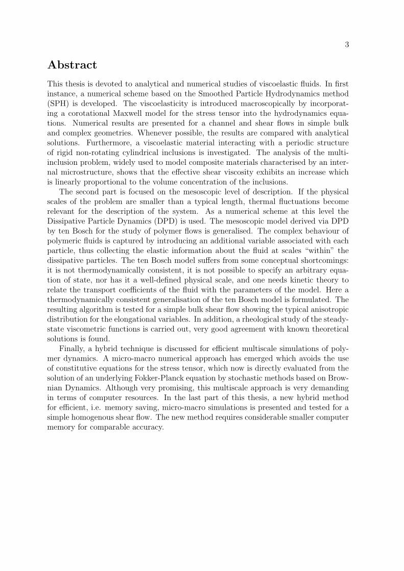
This thesis is devoted to analytical and numerical studies of viscoelastic fluids. In firstinstance, a numerical scheme based on the Smoothed Particle Hydrodynamics method(SPH) is developed. The viscoelasticity is introduced macroscopically by incorporat-ing a corotational Maxwell model for the stress tensor into the hydrodynamics equa-tions. Numerical results are presented for a channel and shear flows in simple bulkand complex geometries. Whenever possible, the results are compared with analyticalsolutions. Furthermore, a viscoelastic material interacting with a periodic structureof rigid non-rotating cylindrical inclusions is investigated. The analysis of the multi-inclusion problem, widely used to model composite materials characterised by an inter-nal microstructure, shows that the effective shear viscosity exhibits an increase whichis linearly proportional to the volume concentration of the inclusions.
The second part is focused on the mesoscopic level of description. If the physicalscales of the problem are smaller than a typical length, thermal fluctuations becomerelevant for the description of the system. As a numerical scheme at this level theDissipative Particle Dynamics (DPD) is used. The mesoscopic model derived via DPDby ten Bosch for the study of polymer flows is generalised. The complex behaviour ofpolymeric fluids is captured by introducing an additional variable associated with eachparticle, thus collecting the elastic information about the fluid at scales “within” thedissipative particles. The ten Bosch model suffers from some conceptual shortcomings:it is not thermodynamically consistent, it is not possible to specify an arbitrary equa-tion of state, nor has it a well-defined physical scale, and one needs kinetic theory torelate the transport coefficients of the fluid with the parameters of the model. Here athermodynamically consistent generalisation of the ten Bosch model is formulated. Theresulting algorithm is tested for a simple bulk shear flow showing the typical anisotropicdistribution for the elongational variables. In addition, a rheological study of the steady-state viscometric functions is carried out, very good agreement with known theoreticalsolutions is found.
Finally, a hybrid technique is discussed for efficient multiscale simulations of poly-mer dynamics. A micro-macro numerical approach has emerged which avoids the useof constitutive equations for the stress tensor, which now is directly evaluated from thesolution of an underlying Fokker-Planck equation by stochastic methods based on Brow-nian Dynamics. Although very promising, this multiscale approach is very demandingin terms of computer resources. In the last part of this thesis, a new hybrid methodfor efficient, i.e. memory saving, micro-macro simulations is presented and tested for asimple homogenous shear flow. The new method requires considerable smaller computermemory for comparable accuracy.

4
5
Zusammenfassung
Diese Dissertation ist analytischen und numerischen Studien viskoelastischer Fluidegewidmet. Zunachst wird ein numerisches Verfahren auf Basis der Smoothed-Particle-Hydrodynamics-Methode (SPH) entwickelt. Die Viskoelastizitat wird hierbei makro-skopisch eingefuhrt, indem die hydrodynamische Gleichungen um ein korotationalesMaxwell-Modell fur den Spannungstensor erweitert werden. Numerische Ergebnissefur Kanal- und Scherstromungen, sowohl im einfachen bulk, als auch in komplexen Ge-ometrien werden angegeben. Wenn dies moglich ist, wird mit theoretischen Losungenverglichen. Ausserdem wird ein viskoelastisches Material in Wechselwirkung mit einerperiodischen Struktur starrer, nicht rotierender zylinderformiger Einschlusse untersucht.Die multi-inclusion Problem wird ferner benutzt, um Kompositmaterialien mit innererMikrostruktur zu modellieren. Die effektive Scherviskositat zeigt einen effektiven Anstieg,der linear proportional zur Volumenkonzentration der Einschlusse ist.
Die zweite Teil dieser Arbeit konzentriert sich auf die mesoskopische Ebene derBeschreibung. Sobald die fuer das Stroemungsproblem relevanten Laengen und Abmes-sungen kleiner als eine materialabhaengige, intrinsische, Laengenskala sind, werdendie thermische Fluktuationen wichtig fuer die Beschreibung des Systems. Eines dermeistverwendeten Verfahren auf dieser Ebene ist die Dissipative-Particle-Dynamics-Methode (DPD). Das mesoskopische Modell zum Studium von Polymerstromungen,mithilfe der DPD entwickelt, wird verallgemeinert. Hierbei wird das komplexe Ver-halten der Polymer-Fluessigkeiten durch eine zusatzliche Variable fur jedes Teilchenbeschrieben. Im vorliegenden Fall repraesentiert die Variable die Konformation einesPolymers. Diese sammelt die Information uber die Elastizitat der Flussigkeit auf einerSkala von der Grossenordnung der dissipativen Polymer-Teilchen. Das ten Bosch-Modellzeigt einige konzeptionelle Unzulanglichkeiten: Es ist thermodynamisch nicht konsistent,es besitzt keine wohldefinierte physikalische Langenskala, und es benotigt die kinetis-che Theorie, um den Zusammenhang zwischen Transportkoeffizienten und Modellpa-rametern herzustellen. Eine thermodynamisch konsistente Verallgemeinerung des tenBosch-Modells wird in diesem Teil der vorliegenden Arbeit formuliert. Zusatzlich wirdeine rheometrische Studie der stationaren viskometrischen Funktionen durchgefuhrt, diewiederum sehr gute Ubereinstimmung mit den bekannten theoretischen Losungen zeigt.
Zuletzt wird eine Hybridmethode zur effizienten Durchfuhrung mehrskaliger Polymer-dynamik-Simulationen diskutiert. Ein ’Micro-Macro’ numerischer Ansatz wurde kurzlichentwickelt, um die Verwendung von konstitutiven Gleichungen fur den Spannungstensorzu vermeiden. Bei dieser Methode extrahiert man mithilfe stochastischer Methoden,basierend auf Brownscher Dynamik, den polymerischen Beitrag zum Spannungsten-sor direkt aus der Losung der zugrundeliegenden Fokker-Planck-Gleichung. Obwohldieser Multiskalenansatz sehr vielversprechend ist, benotigt er doch erhebliche Rechner-essourcen. Im letzten Teil der vorliegenden Arbeit wird eine neue Hybridmethode fureffiziente (das heisst, Arbeitsspeicher sparende) Micro-Macro-Simulationen prasentiertund fur eine einfachen, homogenen Scherstromung auch getestet. Die neue Methodebenotigt fur vergleichbare Genauigkeit weniger Arbeitsspeicher.

6
Contents
1 Introduction 91.1 Numerical methods for viscoelastic flows . . . . . . . . . . . . . . . . . . 10
1.1.1 Traditional macroscopic approaches . . . . . . . . . . . . . . . . . 101.1.2 Micro-macro approaches . . . . . . . . . . . . . . . . . . . . . . . 111.1.3 Lagrangian concepts in computational rheology . . . . . . . . . . 13
1.2 The Smoothed Particle Hydrodynamics method . . . . . . . . . . . . . . 141.3 Motivation of the present work . . . . . . . . . . . . . . . . . . . . . . . 141.4 Outline of the thesis . . . . . . . . . . . . . . . . . . . . . . . . . . . . . 15
2 The Smoothed Particle Hydrodynamics method 192.1 Basic SPH formalism . . . . . . . . . . . . . . . . . . . . . . . . . . . . . 192.2 Hydrodynamics equations . . . . . . . . . . . . . . . . . . . . . . . . . . 21
2.2.1 Momentum equation . . . . . . . . . . . . . . . . . . . . . . . . . 212.2.2 Energy equation . . . . . . . . . . . . . . . . . . . . . . . . . . . . 232.2.3 Continuity equation . . . . . . . . . . . . . . . . . . . . . . . . . . 24
2.3 Particle motion . . . . . . . . . . . . . . . . . . . . . . . . . . . . . . . . 252.4 Constitutive relations . . . . . . . . . . . . . . . . . . . . . . . . . . . . . 26
2.4.1 Equation of state . . . . . . . . . . . . . . . . . . . . . . . . . . . 262.4.2 Dissipation . . . . . . . . . . . . . . . . . . . . . . . . . . . . . . 28
2.5 The kernel function . . . . . . . . . . . . . . . . . . . . . . . . . . . . . . 302.6 Boundary conditions . . . . . . . . . . . . . . . . . . . . . . . . . . . . . 32
2.6.1 Periodic boundary conditions . . . . . . . . . . . . . . . . . . . . 322.6.2 Rigid boundary conditions . . . . . . . . . . . . . . . . . . . . . . 34
2.7 Time integration . . . . . . . . . . . . . . . . . . . . . . . . . . . . . . . 372.8 Numerical tests: the incompressible Newtonian flow . . . . . . . . . . . 38
2.8.1 Couette flow . . . . . . . . . . . . . . . . . . . . . . . . . . . . . . 392.8.2 Poiseuille flow . . . . . . . . . . . . . . . . . . . . . . . . . . . . . 41
3 Smoothed Particle Dynamics for viscoelastic flows 453.1 The constitutive equation . . . . . . . . . . . . . . . . . . . . . . . . . . 46
3.1.1 The corotational Maxwell model . . . . . . . . . . . . . . . . . . . 463.1.2 The limiting case of vanishing elasticity . . . . . . . . . . . . . . . 483.1.3 Non-dimensional formulation . . . . . . . . . . . . . . . . . . . . . 48
3.2 Velocity profile relaxation in a 2D channel . . . . . . . . . . . . . . . . . 493.3 Viscoelastic fluid under a steady shear flow . . . . . . . . . . . . . . . . . 53
7
8 CONTENTS
3.4 Viscoelastic matrix with solid inclusions . . . . . . . . . . . . . . . . . . 573.4.1 SPH implementation for the inclusion problem . . . . . . . . . . . 583.4.2 Flow analysis: Newtonian matrix . . . . . . . . . . . . . . . . . . 593.4.3 Rheological analysis: non-Newtonian matrix . . . . . . . . . . . . 663.4.4 Flow analysis: non-Newtonian matrix . . . . . . . . . . . . . . . . 69
4 Smoothed Particle Dynamics for mesoscopic problems 754.1 Modelling mesoscopic flow problems . . . . . . . . . . . . . . . . . . . . . 754.2 Mesoscopic simulations of complex fluids . . . . . . . . . . . . . . . . . . 774.3 TC fluid particle model of polymer solutions . . . . . . . . . . . . . . . . 784.4 generic formulation . . . . . . . . . . . . . . . . . . . . . . . . . . . . . 814.5 Reversible part of the dynamics . . . . . . . . . . . . . . . . . . . . . . . 824.6 Irreversible part of the dynamics . . . . . . . . . . . . . . . . . . . . . . . 854.7 Polymer diffusivity . . . . . . . . . . . . . . . . . . . . . . . . . . . . . . 914.8 Simulation results . . . . . . . . . . . . . . . . . . . . . . . . . . . . . . . 96
4.8.1 Theoretical results for Hookean dumbbells . . . . . . . . . . . . . 974.8.2 Setup of the numerical simulations . . . . . . . . . . . . . . . . . 984.8.3 Numerical results . . . . . . . . . . . . . . . . . . . . . . . . . . . 99
4.9 Final remarks . . . . . . . . . . . . . . . . . . . . . . . . . . . . . . . . . 103
5 Multiscale simulations of viscoelastic flows 1055.1 Micro-macro methods for complex fluids . . . . . . . . . . . . . . . . . . 1065.2 Microscopic kinetic model and standard CT approach . . . . . . . . . . . 1085.3 The hybrid BDDFS method . . . . . . . . . . . . . . . . . . . . . . . . . 1115.4 Numerical results . . . . . . . . . . . . . . . . . . . . . . . . . . . . . . . 1165.5 Final remarks . . . . . . . . . . . . . . . . . . . . . . . . . . . . . . . . . 122
6 Conclusions 125
A Review of generic 129
B Microscopic calculation of entropy 131
C Advection of a vector 135
D Diffusion of dumbbells 137
E SPH discretisation of the advection diffusion equation 139
Chapter 1
Introduction
It is known from the experience that whether a system behaves like a ’solid’ or a ’fluid’is a matter of observation times. Fluids like water responds like a solid under very rapiddeformations, while a glacier, usually considered quite hard, will flow like a fluid whenobserved on a sufficiently large time. If we assume that a solid is generally charac-terised by an elastic behaviour and a fluid by a viscous one, then a viscoelastic material,mathematically speaking, is a model in which these effects become comparable or, inother terms, where shear stresses are sustained for an appreciable time before flowing.Even if in principle, under specific circumstances, also the water can be described bya viscoelastic model, in practice this is of little interest, indeed the times at which itselastic behaviour has a considerable effect are so small (typically 10−10s) that phenom-ena of practical interest take place widely behind this scale and are very well describedby its viscous dynamics, i.e Navier-Stokes equations. Nevertheless, a variety of fluids,whose behaviour differs from the Newtonian one, are usually encountered in real life.Indeed, it is easy comprehensible that materials like polymers solutions, polymers melts,foods and rubbers cannot be described within the classical formalism of the Newtonianfluid mechanics. At the same time, the interest into model their dynamics and predicttheir mechanical, thermal and rheological properties is of essential importance in manyindustrial and manufacturing sectors.
Materials like those mentioned above are characterised by a typical relaxation timefor their internal microstructure which becomes comparable with the macroscopic scales,for example with the viscous diffusion time. The mathematical viscoelastic models aretherefore required to describe the complex interactions between such phenomena, whichmanifest themselves in the governing equations usually as strong memory effects andfunctional dependence of the stress tensor upon its strain history. It is therefore expectedthat this complex interplay of effects is much more difficult to describe theoretically thanin a Newtonian fluid and it reflects the complexity of the correspondent model equa-tions. Although analytical solutions are available in simple cases, it is obvious thatproceed by ’pencil and paper’ is a quite hard challenge while, at the same time, the newfrontiers opened by the increasing power and speed of digital computers allows for fastand accurate numerical solutions of the equation discussed above.
The main subject of this thesis is the numerical modelling of viscoelastic fluids, i.e.
9
10 CHAPTER 1. INTRODUCTION
polymer solutions, by using Lagrangian techniques derived by the Smoothed ParticleHydrodynamics method. In the present work, different approaches depending on thephysical length and time scales are studied. Indeed, we will consider first a purely macro-scopic approach based on the solution of a constitutive model equations combined withthe usual hydrodynamics conservation laws; secondly, we will focus on the mesoscopiclevel of description, constructing a model for polymer solutions which is thermodynam-ically consistent, that is, equipped with fluctuations properly introduced in the fluidvariables. Finally, we will investigate the interplay between such scales and attemptto develop efficient numerical techniques which can contribute to make the multiscaleapproach computationally feasible.We start in the next section by giving a general overview of the numerical methodsmostly used in the simulations of viscoelastic flows.
1.1 Numerical methods for viscoelastic flows
1.1.1 Traditional macroscopic approaches
Until recently, numerical simulations of viscoelastic flows in complex geometries havebeen often based on a purely macroscopic approach where one solves numerically theconservation laws together with a suitable rheological constitutive equation. In this areamany numerical schemes have been proposed, generally based on finite difference (FDM),finite element (FEM), finite volume (FVM) or boundary element methods (BEM) tomention but a few [1,2,3]. One of the problems that emerges when trying to describe anon-Newtonian flow in this way is purely mathematical and is related to the correctnessof the model constitutive equation adopted. Indeed, it is well-known that a rigorousderivation of the evolution equation for the macroscopic stress tensor starting from an“exact” kinetic theory is to date not available. In order to obtain a closed form relatingthe stress to the other macroscopic variables, many more or less physically motivated,approximations must be performed, which can alter, if not completely destroy, theviscoelastic properties of the original microscopic system [4, 5]. Although progresses inthe derivation of suitable constitutive equations for complex fluids, as polymer melts,foods, rubbers, has been very impressive, the subject, however, is by no means resolvedand further developments are still called for. On the validity of macroscopic constitutiveequations, the reader is referred for example to the monography by Tanner [6] or Larson[7].
Once the validity of a suitable model equation has been assumed, the second mainproblem, which the computational rheologists must face, is its numerical discretisation.Indeed, the constitutive equations can be cast into an integral or differential form andparticular techniques must be developed in order to solve them accurately and in areasonable time. It is beyond the scope of this introduction to review in detail all thenumerical methods developed in this direction, nevertheless it has been widely recog-nised that one of the major challenges for the traditional schemes based on the solutionof the constitutive equations cast in differential form, is the presence of the advectiveterm which, whenever its contribution becomes dominant, can highly affect the stabil-
1.1. NUMERICAL METHODS FOR VISCOELASTIC FLOWS 11
ity and the accuracy of the resulting algorithm. This is similar to the problem alreadyencountered in advective-dominated Newtonian flows where special techniques must beimplemented in order to ensure a safe, stable integration of the correspondent flow fields.A complete state-of-the-art review of the methods used in computational rheology canbe found in [1, 2, 3, 8].
1.1.2 Micro-macro approaches
The classical numerical schemes presented above are based on the assumption of validityof a suitable constitutive equation describing a complex fluid. As already pointed out,the derivation of a consistent macroscopic model is an hard theoretical challenge andoften, inaccurate approximations must be made in order to obtain a final manageableequation. Only very recently, a new class of methods, denoted as micro-macro, haveappeared in the literature, which try to combine the macroscopic hydrodynamics (con-servation laws) with un-approximated dynamics coming from a kinetic description ofthe microstructural model [9]. The basic idea is to split the dynamics of the system intwo parts: at the macroscopic level, the usual conservation laws for mass, momentumand energy are solved by using traditional discretisation techniques, while the micro-scopic properties of the system are obtained by solving a kinetic theory model. Thisapproach provides a consistent way to extract the evolution of the stress tensor for com-plex fluids, bypassing the need to use potentially inaccurate closure approximations.On the other hand, it should be pointed out that the solution of a kinetic theory modelmust be performed, in principle, on a very high-dimensional configurational space and,as a consequence, the technique can be very demanding in term of computer require-ments. Although the approach can be considered in many complex situations, to datethe method has been applied successfully only in relatively simple cases, characterisedby low-dimensional configurational spaces, such as dilute suspensions of polymers de-scribed by quite coarse-grained models (dumbbells or ’small’ chains). The starting pointcommon to all the micro-macro approaches is the solution of a Fokker-Planck equationsin the configurational space. Although, very recently some works have appeared in theliterature showing that reasonably fast numerical solutions can be obtained by a crudedirect discretisation of the Fokker-Planck equation based on a spectral method [10], itis generally acknowledged that even for low-dimensional configurational spaces (poly-mer chains characterised by N > 3 beads) the relative simulations require unacceptableCPU-time and memory.
For the sake of clarity, we next sketch the basic ideas of the micro-macro approaches,based on the standard method developed in the early 90’s by Laso and Ottinger [11].Here, instead of solving the deterministic Fokker-Planck equation, one solves an associ-ated isomorphic set of stochastic differential equations for a large number of realizations.This is the so-called CONNFFESSIT method (Calculation Of Non-Newtonian Flowsusing Finite Elements and Stochastic Simulation Techniques) which combines a FiniteElement discretisation of the conservation laws with a stochastic evaluation of the stresstensor. A large number of polymer-models (i.e. dumbbells) are dispersed over all thephysical domain and the stochastic differential equations must be integrated along thecorrespondent trajectories. The macroscopic stress is finally evaluated as an ensemble
12 CHAPTER 1. INTRODUCTION
average over many microscopic configurations. It is not the scope of this section to givean exact description of this method, which will be discussed in great details in Chapt. 5of this work. Nevertheless, it is useful to outline here some of the drawbacks sufferedby this approach. Maybe the most difficult problem is inherent to the stochastic na-ture of the methods and it is related to the determination of the macroscopic stressbased on ensemble averages. If the number of realizations is not sufficiently large, largefluctuations can affect the macroscopic variables, eventually making the averaged sig-nal indistinguishable. The reduction of such undesirable noise is a big challenge andis often referred to as variance reduction problem. We will come back to this point inthe next section. Here we would like to focus on another drawback suffered by thestandard micro-macro approaches. As it has been recognised by Keunings in its recentreview [3], one difficulty is associated with the fact that the dumbbells are allowed toflow through the domain and, in order to evaluate their local contribution to the stress,one has to know at every time step in which spatial element they are contained. Theconsequent searching algorithm can cause a numerical bottleneck whenever the numberof simulated dumbbells becomes quite large. On the other hand, a large number ofdumbbells is often required in order to have a sufficiently large number of stochasticrealizations for permitting accurate, noise-free averages. This problem is by nature dueto the Lagrangian character of the dumbbells dynamics which contrast with the fixedEulerian discretisation for the macroscopic flow fields.
The method of the Brownian Configuration Fields (BCF), recently introduced byvan den Brule [12], partially solves the problem, by considering a continuous, totallycorrelated (in space) configurational field instead of a discrete set of uncorrelated dumb-bells. In this way, one bypass the need to consider dumbbells advection through theEulerian grid, but one solves directly a partial differential stochastic equation for theconfigurational field. One of the problems of this approach lies in the fact that com-pletely artificial correlations over the physical domain are assumed in order to deal witha continuous field. Of course, this hypothesis becomes questionable whenever dealingwith problems characterised by physical fluctuations.A semi-Lagrangian numerical scheme, Lagrangian Particle method (LPM), has now beenintroduced by Keunings in the attempt to solve such difficulties [13] . This method com-bines, in a decoupled fashion, the Eulerian solution of the conservation laws (using aGalerkin finite elements technique) with a Lagrangian computation of the extra-stressat a number of discrete particles that are convected by the flow. The extra-stress is com-puted by integrating along the particle paths either the relevant differential constitutiveequation (macroscopic approach), or the stochastic differential equation associated tothe kinetic theory model (micro-macro approach). In the micro-macro LPM simula-tions, each Lagrangian particle convected by the flow carries an ensemble of particleswith internal degrees of freedom, which can be statistically uncorrelated or correlated.Keeping track of the motion of this ’small’ set of Lagrangian particle is not an expensivetask and, at the same time, it permits the avoidance of the problem of using disperseddumbbells and the consequent time-consuming searching algorithm. The time-historyfor the flow variables is here directly accessible in every Lagrangian particle and wecan regard the microscopic dumbbells as a constant set of stochastic realizations of
1.1. NUMERICAL METHODS FOR VISCOELASTIC FLOWS 13
the same process. The technique seems to be very useful and it has been applied suc-cessfully to a variety of viscoelastic problems. Nevertheless, the Eulerian-Lagrangianformalism requires to have at least three particles in every element of the Eulerian gridin order to perform an interpolation for the stress tensor. Modification of the originalLPM method have been developed in the last years which corrects this drawback andimproves its efficiency. In the opinion of the author, the LPM method seems to be themost promising, and surely the most flexible, micro-macro method presently available.Its strength is mainly due to the natural way in which it takes into account the typicaladvective character of the stochastic differential equations presented above. Neverthe-less, as it has been recognised by Keunings, some problems still exist which are relatedto the exchange of information between the Eulerian grid and the Lagrangian particles.Smoothing effects due to this transfer, have been shown to affect the accuracy and thestability of the resulting algorithm. In this context, a fully Lagrangian description couldpermit to avoid such numerical artifacts.
1.1.3 Lagrangian concepts in computational rheology
From the discussions presented above, it emerges quite clearly that one of the main dif-ficulties in the numerical simulation of viscoelastic fluids, is often related to the intrinsicadvective character of the governing equations. This happens, both in the macroscopicand in the micro-macro approaches. In the first case, the hyperbolic nature of the dif-ferential constitutive equation seems to affect strongly the stability and the accuracy ofthe Eulerian based algorithm used for the numerical solution. As already mentioned,many of these problems can be partially remedied by using the large staff of numeri-cal results available for the analogous problem of advective-dominated Newtonian flows(high Reynolds number). For these simulations, many specific techniques have been de-veloped to deal with the hyperbolic character of the resulting equations as for examplethe well-known “upwind” scheme, which, in the case of viscoelastic flows simulations,consists of considering a further artificial diffusivity tensor in the constitutive equationacting in the streamline direction. Although the method has been able to successfullyreproduce many viscoelastic flows, some doubts still remain on its final resulting accu-racy which seems to be limited to first order [3].As mentioned above, the problem also presents itself in the context of micro-macro ap-proaches. Here, it is related to the advective flow of the model dumbbells dispersed overthe flow domain, for which time-consuming searching algorithms are required. It seemstherefore natural to apply ideas from a Lagrangian framework to such kind of fluids,trying to avoid directly all the problems related to the complicate treatment of advec-tive terms, which now disappear, automatically absorbed by the material derivative. Inaddition to these theoretical argumentations, the Lagrangian picture can represent thebest framework to deal with general flow problems represented by complex boundaryconditions, free-surface flows or flows characterised by large deformations, where theclassical Eulerian schemes encounter many difficulties. In this work, a numerical meth-ods based on a fully Lagrangian formalism will be presented and applied specifically toviscoelastic flow problems. In the next section, a brief historical review with a list ofthe most relevant applications of the method will be given.
14 CHAPTER 1. INTRODUCTION
1.2 The Smoothed Particle Hydrodynamics method
Smoothed Particle Hydrodynamics (SPH) is a Lagrangian ‘macro’ method developedtwenty-five years ago for astrophysical problems by Lucy [14], Gingold and Monaghan[15]. SPH is a fully Lagrangian scheme permitting to dicretize a prescribed set ofmacroscopic equations by interpolating the flow properties directly at a discrete set ofpoints, i.e. pseudo-particles, distributed randomly over the domain of solution, withoutthe need to define a spatial mesh. Its Lagrangian nature, associated to the absence ofa fixed grid, is its main strength allowing to remove difficulties associated to convectiveterm and to tackle fluid and solid flow problems involving large deformations and freesurfaces in a relatively natural way. In the last ten years many SPH simulations havebeen applied to different physical situations including compressible Newtonian flows [16],incompressible free surface flows [17], high strain mechanics, ultrarelativistic shocks [18],impact and sliding friction problems between elasto-plastic materials [19, 20, 21, 22],numerical fluid [23] and gas dynamics in astrophysics [24]. The SPH method has beenalso applied to problems in kinetic theory, such as the dynamics of homogeneous liquidcrystals [25] based on a Fokker-Planck approach while implementations of standard SPHfor parallel architectures have become recently available [26]. In addition, a detailedmathematical study showing the numerical convergence of the methodology has beencarried out by Pulvirenti et al. [27]
The method has received substantial theoretical support in order to make it consis-tent from a statistical point of view, that is correct treatments of thermal fluctuationsand consistent fluctuating hydrodynamics [28]. In Ref. [29], a close connection is madebetween SPH and Dissipative Particle Dynamics (DPD), a fully Lagrangian methodin which the force between the particles are modelled on the mesoscale, following thephilosophy of Lattice Boltzmann or Lattice Gas Automata schemes but with the advan-tage of the flexibility being gridless. Recently, application of DPD to viscoelastic flowhas been proposed consisting in assigning to every DPD particle one or more internalstructural variables [30].
The increasing literature that has appeared in recent years on SPH shows that themethod has been improved, correcting many of its original shortcoming and applyingit to a variety of physical problems involving fluid and solid-mechanics. Nevertheless,although its success for numerical modelling in the areas above mentioned, it is clearthat this method has not yet achieved its mature stadium but many theoretical andcomputational improvements are still called for in order to compare it with the well-established field of the Eulerian grid-based techniques.
1.3 Motivation of the present work
The goal of the present work is to investigate the applications of the Smoothed Parti-cle Hydrodynamics methods in the context of viscoelastic flows modelling. The SPHliterature that has appeared in this area, seems to be a rarity in contrast with thepotential contribution that such Lagrangian technique could offer. To our knowledge,the only paper published on this argument, except ours, has appeared last year and
1.4. OUTLINE OF THE THESIS 15
involves a numerical study of a Non-Newtonian free-surface flow [31]. Unfortunately,the constitutive equation used was based on a generalised Newtonian fluid while it iscommonly believed that such a model have only a limited range of applicability and it istoo ’simple’ to describe complex flows where the elastic effects play a crucial role. Theintroduction of viscoelasticity in the SPH method through a macroscopic constitutiveMaxwell model and the consequent application to many different flow problems, i.e.channel-flows, bulk-shear flows or flows in complex geometries, is the main issue of thefirst part of this work. The results demonstrates that, accurate and stable solutions canalso be obtained in unsteady situations.
Particular attention is also paid to the modelling of mesoscopic flow problems viathe SPH method. It is obvious that at such ’small’ level of description, the fluctuationsemerging in the system dynamics represent a crucial physical ingredient and they shouldbe carefully introduced in the numerical model. Indeed, if one is interested in resolvingsubmicronic scales, it is of fundamental importance to have a fluid particle whose vari-ables are equipped with thermal fluctuations consistent with the first and second lawsof thermodynamics. The construction of a thermodynamically consistent viscoelasticfluid model suitable for mesoscale simulations is another goal of the present thesis.
Finally, as already mentioned in the previous section, a big issue concerning micro-macro simulations of viscoelastic flows is the one related to the variance reduction. Inparticular flows of interest, a large number of stochastic realizations must be taken intoaccount in order to extract reliable averaged quantities. Indeed, it is well-known that inthe limit of small elasticity, whenever the variance reduction techniques, such as BCF,are numerically not applicable or physically not motivated, averaged results extractedby the stochastic runs are affected by unacceptable noise. The way to reduce it is ofcourse to increase the dimensions of the stochastic ensemble with the obvious associ-ated numerical difficulties in term of CPU-time and mainly memory requirements forthe correspondent algorithm. It is the last scope of this work, to study possible hybridalgorithms based on standard Brownian Dynamics methods, able to obtain accurate re-sults at lower memory price. The hybrid BDDFS (Brownian Dynamics and DistributionFunction) method presented in the last chapter of this thesis, could offer an alternativefor those particular viscoelastic flows (i.e turbulent) where a large number of freedomdegrees are necessary for accurate stochastic estimates of the flow variables.
1.4 Outline of the thesis
The present work is organised as follows.Chapt. 2 describes the basic ideas of the Smoothed Particle Hydrodynamics (SPH)
method. In particular, a weak formulation for the discretized equations based on therigorous derivation of Benz [32], is presented for the conservation equations of mass,momentum and energy. The accuracy of the resulting discretized equations is alsodiscussed, demonstrating that, under suitable choice of the interpolation functions, anumerical method which is second order accurate in space can be obtained. Particular
16 CHAPTER 1. INTRODUCTION
attention is devoted also to the problem of closure for the hydrodynamics equations forthe well-established case of a Newtonian compressible fluid, providing at the same timesome technical details regarding treatment of boundary conditions and time integrationof the flow fields. Finally, some numerical results are shown proving the correctness ofthe numerical scheme to simulate a Newtonian fluid in simple flow geometries.
Chapt. 3 is devoted to the generalisation of the SPH method previously intro-duced for the description of more complex viscoelastic fluids. The formalism describingviscoelasticity is introduced in the ordinary conservation laws by providing a furtherindependent partial differential constitutive equations for the stress tensor based onthe corotational Maxwell model. In order to test the validity of this description fornon-Newtonian fluids, the numerical method is applied to non-stationary relaxationprocesses in a 2D channel geometry and simple bulk shear flows, for which analyticalcomparisons are available. Finally, once the accuracy of the method in simple situa-tions is proven, the model is applied to the specific problem of a viscoelastic bulk matrixcontaminated with non-rotating rigid circular inclusions and underlying a steady-shearflow. The so called ’multi-inclusion’ problem is widely adopted in literature to modelcomposite materials characterised by a microstructure. A study of interplay between itsmacroscopic rheological properties and the microstructure is carried out giving evidencethat some few microscopic parameters have a major influence on the effective transportproperties of the material.
Chapt. 4 deals with the simulations of viscoelastic flow at a mesoscopic level. Itis obvious that whenever the length scale characterising a specific problem becomesquite small, fluctuations in the physical quantities represent a crucial ingredient for thedynamics. On the other hand, it is important to introduce such fluctuations into thedescription in a consistent way. This chapter is focused on a particular viscoelasticDissipative Particle Dynamics model, recently proposed by ten Bosch in [30], and it isput into a thermodynamically consistent form that allows for non-isothermal situations.This model consists of fluid particles that have an additional elastic vector characterisingthe state of elongation of the molecules within the fluid particle. Very simple physicalmechanisms are proposed for the dynamics of the elastic vector that, with the help ofthe GENERIC formalism, allows us to derive the full set of dynamic equations for themodel. The model is further generalised to include polymer diffusion. The connection ofthe present model with the CONNFFESSIT approach and the Brownian ConfigurationFields approach is finally discussed.
Chapt. 5 proposes and test the ‘Brownian Dynamics and Distribution FunctionStoring’ (BDDFS) strategy for performing numerical calculations of viscoelastic com-plex flows based on the unapproximated CONNFFESSIT-type approach. Hardwarelimits this established approach for highly complex flows due to fluctuations whichcome together with the stochastic determination of the macroscopic extra stress tensor.As soon as the number of cells in the flow domain becomes large an even much largernumber of freedom degrees must be used to extract accurate results. Usually, vari-ance reduction techniques are used to suppress noise, lower the memory requirements,produce correlated dynamics, and obtain approximate, and ‘good’ results. BDDFS isa numerical method for the still approximate, but ‘uncorrelated’ solution of the same
1.4. OUTLINE OF THE THESIS 17
problem with limited memory needs. It relies on a discrete storage of the configurationaldistribution function (D-CDF) for dumbbells, or polymers. Configurational variablessubject to standard BD are sampled consistently with the D-CDF. Compared with theoriginal approach, the memory requirement is reduced by the ratio between the num-ber of D-CDF grid points and the number of molecules. The strategy has been testedagainst a homogeneous shear flow of dumbbells. Results reveal that the BDDFS conceptmay offer advantages upon alternative approaches which must become larger with thecomplexity of the system under study and whenever molecular correlations on lengthscales larger than the grid size contain information relevant to interpret experiments.

18 CHAPTER 1. INTRODUCTION
Chapter 2
The Smoothed ParticleHydrodynamics method
In this chapter we review the basic formalism of the Smoothed Particle Hydrodynam-ics (SPH) method which will be used in the following of the thesis in the attempt togeneralise it for the description of more complex viscoelastic fluids. After recalling inthe first section the basic SPH ideas based on interpolation theory, we derive rigorously,in section 2.2, a weak SPH formulation for the discretized hydrodynamics equation.Section 2.3 describes briefly the Lagrangian evolution of the adaptative grid constitutedby the SPH particles, while section 2.4 is devoted to the problem of physical closure forthe hydrodynamics equations, that is, the choice of suitable constitutive relations forpressure and friction stress. In particular, in Sec. 2.4.1 we review many forms of equa-tions of state usually adopted in the literature discussing positive and negative aspectsin relation with their numerical implementation. The description of a mechanism ofviscous dissipation is the subject of section 2.4.2, where we discuss firstly the historicalapproach consisting in the introduction of a completely artificial viscosity and, secondly,the consistent approach followed in our work and based on a direct discretisation of theNavier-Stokes friction stress tensor. Section 2.5 deals with the accuracy of the schemewhich, translated in the SPH formalism, corresponds to the choice of a suitable inter-polating kernel. Sections 2.6 and 2.7 are devoted to the description of technical aspectsof the numerical implementation, respectively boundary conditions and time integra-tion. Finally, in section 2.8 we present some numerical results and comparison withknown theoretical solution in the cases of a Couette and Poiseulle flows of a Newtonianincompressible fluid.
2.1 Basic SPH formalism
It has been shown that SPH can be derived in the context of interpolation theory [14,15].Any function f , defined over a domain of interest and representing some physical variableor density, can be expressed in terms of its values at a discrete set of disordered points(SPH particle positions) by suitable definition of an interpolation kernel. Let us startwith some basic definitions: given a function f defined over all the domain Ω, we can
19
20 CHAPTER 2. THE SMOOTHED PARTICLE HYDRODYNAMICS METHOD
always write it as
f(x) =
∫
Ω
f(x′)δ(x − x′) dx′, (2.1)
where δ(x) is the Dirac delta function centred at the position x. Eq. (2.1) is an identityand it is referred as integral representation of a function f(x).
Let us introduce now the concept of the integral estimate 〈f〉 at the point x. If wereplace the Dirac delta function in (2.1) with an interpolating kernel W (x − x′, h), weobtain
〈f(x)〉 =
∫
Ω
f(x′)W (x − x′, h) dx′, (2.2)
which represents evidently an approximation of f(x) so far as the kernel function is notexactly equal to the Dirac delta. Here, h represents the range of the interpolating kernelif it is supposed to have compact support, or, for example in the case of Gaussian kernel,its width at half height. In order to obtain a correct integral estimate 〈f〉, usually thefollowing two assumptions are made
∫
Ω
W (x − x′, h)dx′ = 1, (2.3)
and
limh→0
W (x − x′, h) = δ(x − x′). (2.4)
These features assure proper normalisation and consistency in the continuum limit.Concerning accuracy, the approximation corresponding to Eq. (5.1) is known to besecond order in space. This can be easily shown [32], considering the fact that W (x −x, h) is a strongly peaked function at x = x′ and therefore we can expand f(x′) in aTaylor series around x. IfW (x, h) is an even function, particularly in the caseW (x, h) =W (|x|, h), the term of order O(h) vanishes automatically and Eq. (5.1) becomes
〈f(x)〉 = f(x) + C∇2f(x)h2 +O(h3), (2.5)
where C is a coefficient independent of h. Provided that f varies quite smoothly ona length scale of the dimensions h, this relation gives a leading error term which isproportional to h2 with a resulting accuracy for the SPH discretisation of the secondorder in space.
In addition, a further approximation is introduced at this point which is purelynumerical and it corresponds to an estimate of the integral in (5.1) as a sum over pointsof the domain. To this end, let us introduce the concept of number density which definesthe positions of a disordered set of points where the physical properties of the systemare considered known,
n(x) =∑
j
δ(x − xj). (2.6)
2.2. HYDRODYNAMICS EQUATIONS 21
We can therefore associate the infinitesimal integration volume dx′ with the quantityφj (volume occupied by the j-th particle), which is defined through the replacement rule
dx′ → φj ≡mj
ρj
, (2.7)
where we introduced the concepts of mass mj and density ρj = mj 〈n(xj)〉 associatedwith the j-th particle. The final SPH approximation for a function f defined in somepoint x reads
〈f(x)〉 '∑
j
mj
ρj
fj W (|x − xj|, h), (2.8)
and fj ≡ f(xj). By substituting the function mass density f(x) = ρ(x) into (5.5) weobtain the following expression
〈ρ(x)〉 '∑
j
mjW (|x − xj|, h). (2.9)
This is a direct way to evaluate the density explicitly as a sum over the particlesand justifies the original denomination “SPH” in the sense that the particles are notintended like points but their masses are smoothed out over a distance of order h. Agood overview of the mathematical basis of SPH can be found for example in Benz [32]or Monaghan [33,34].
2.2 Hydrodynamics equations
Keeping in mind the definitions and the approximations introduced in the previoussection, we will present here the derivation of a weak SPH form for the continuity,momentum and energy equations. This will be obtained following the rigorous approachof Benz [32]. The basic step consists actually in an integration over all the domain of thepartial differential equations describing the conservation laws of continuum mechanics.An integration by parts removes therefore a surface term permitting to differentiatedirectly the interpolating kernel which is analytic. We postpone the section dealingwith the evaluation of the mass density which requires a particular discussion.
2.2.1 Momentum equation
Let us consider the equation for the conservation of momentum which describes thebalance of momentum fluxes on a macroscopic (continuum assumption) volume of fluid.Written in the Eulerian form, it reads
∂V α
∂t+ (V β∇β)V α =
1
ρ∇βP αβ, (2.10)
where tensorial notation with Greek indices indicating spatial coordinates and the sum-mation convention for repeated indices is used. As usual, V α denotes the velocity field
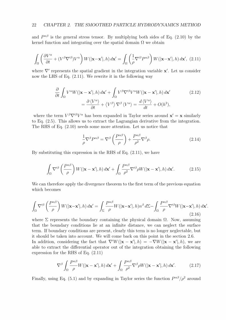
22 CHAPTER 2. THE SMOOTHED PARTICLE HYDRODYNAMICS METHOD
and P αβ is the general stress tensor. By multiplying both sides of Eq. (2.10) by thekernel function and integrating over the spatial domain Ω we obtain
∫
Ω
(
∂V α
∂t+ (V β∇′β)V α
)
W (|x−x′|, h) dx′ =
∫
Ω
(
1
ρ∇′βP αβ
)
W (|x−x′|, h) dx′, (2.11)
where ∇′ represents the spatial gradient in the integration variable x′. Let us considernow the LHS of Eq. (2.11). We rewrite it in the following way
∂
∂t
∫
Ω
V αW (|x − x′|, h) dx′ +
∫
Ω
V β∇′βV αW (|x − x′|, h) dx′ (2.12)
=∂ 〈V α〉∂t
+⟨
V β⟩
∇β 〈V α〉 =d 〈V α〉dt
+O(h2),
where the term V β∇′βV α has been expanded in Taylor series around x′ = x similarlyto Eq. (2.5). This allows us to extract the Lagrangian derivative from the integration.The RHS of Eq. (2.10) needs some more attention. Let us notice that
1
ρ∇βP αβ = ∇β
(
P αβ
ρ
)
+P αβ
ρ2∇βρ. (2.14)
By substituting this expression in the RHS of Eq. (2.11), we have
∫
Ω
∇′β
(
P αβ
ρ
)
W (|x − x′|, h) dx′ +
∫
Ω
P αβ
ρ2∇′βρW (|x − x′|, h) dx′. (2.15)
We can therefore apply the divergence theorem to the first term of the previous equationwhich becomes
∫
Ω
∇′β
(
P αβ
ρ
)
W (|x−x′|, h) dx′ =
∫
Σ
P αβ
ρW (|x−x′|, h)nβ dΣ−
∫
Ω
P αβ
ρ∇′βW (|x−x′|, h) dx′.
(2.16)where Σ represents the boundary containing the physical domain Ω. Now, assumingthat the boundary conditions lie at an infinite distance, we can neglect the surfaceterm. If boundary conditions are present, clearly this term is no longer neglectable, butit should be taken into account. We will come back on this point in the section 2.6.In addition, considering the fact that ∇′W (|x − x′|, h) = −∇W (|x − x′|, h), we areable to extract the differential operator out of the integration obtaining the followingexpression for the RHS of Eq. (2.11)
∇β
∫
Ω
P αβ
ρW (|x − x′|, h) dx′ +
∫
Ω
P αβ
ρ2∇βρW (|x − x′|, h) dx′. (2.17)
Finally, using Eq. (5.1) and by expanding in Taylor series the function P αβ/ρ2 around

2.2. HYDRODYNAMICS EQUATIONS 23
x′ = x (neglecting terms of order h2), we obtain the integral Lagrangian form ofEq. (2.10)
d
dt〈V α〉 = ∇β
⟨
P αβ
ρ
⟩
+P αβ
ρ2∇β 〈ρ〉 +O(h2). (2.18)
where we substituted ρ = 〈ρ〉. By using the particle approximation corresponding toEq. (5.5), Eq. (2.18) becomes
d
dt〈V α〉 = ∇β
(
∑
j
mj
P αβj
ρ2j
W (|x − xj|, h))
+P αβ(x)
ρ2(x)∇β
(
∑
j
mjW (|x − xj|, h))
.
(2.19)Finally, evaluating the previous equation on the particle location xi and by reorderingthe terms, we obtain the final SPH discretized equation for the momentum
dV αi
dt=∑
j
mj
(
P αβi
ρ2i
+P αβ
j
ρ2j
)
∇αi Wij, (2.20)
where Roman indices indicate particles and V αi is the smooth velocity corresponding to
the i-th particle. Here we used also the abbreviation Wij ≡ W (|xi − xj|, h). Because of∇iWij = −∇jWij, we have, that the contribution to the force acting on the i-th particledue to the j-th particle Fij = −Fji and the momentum is automatically and exactlyconserved from the bulk particles. This is a property of this particular set of equations,in fact it must be pointed out that there is not a unique derivation of them. A largenumber of different sets of SPH equations, all describing the same physics to the secondorder accuracy, can be in principle found using other approximations. The equation(5.7) is, on the other hand, preferable because it conserves exactly the momentum.Many different forms of SPH have been discussed by Monaghan [33].
2.2.2 Energy equation
Let us consider now the equation for the conservation of energy. In the adiabatic case,we can neglect the heat flux and the equation reflects the first law of thermodynamics.Written in Eulerian form, it reads
∂U
∂t+ (V β∇β)U =
P αβ
ρ∇αV α, (2.21)
where U represents the specific (for unit of mass) internal energy of the fluid. Byrepeating the same steps described for the derivation of the momentum equation, thatis integrating by parts and neglecting surface terms, we obtain the following secondorder accurate SPH discretisation of Eq. (2.21)
dUi
dt= −P
αβi
ρi
∑
j
mj
(
V αi − V α
j
)
∇βi Wij, (2.22)
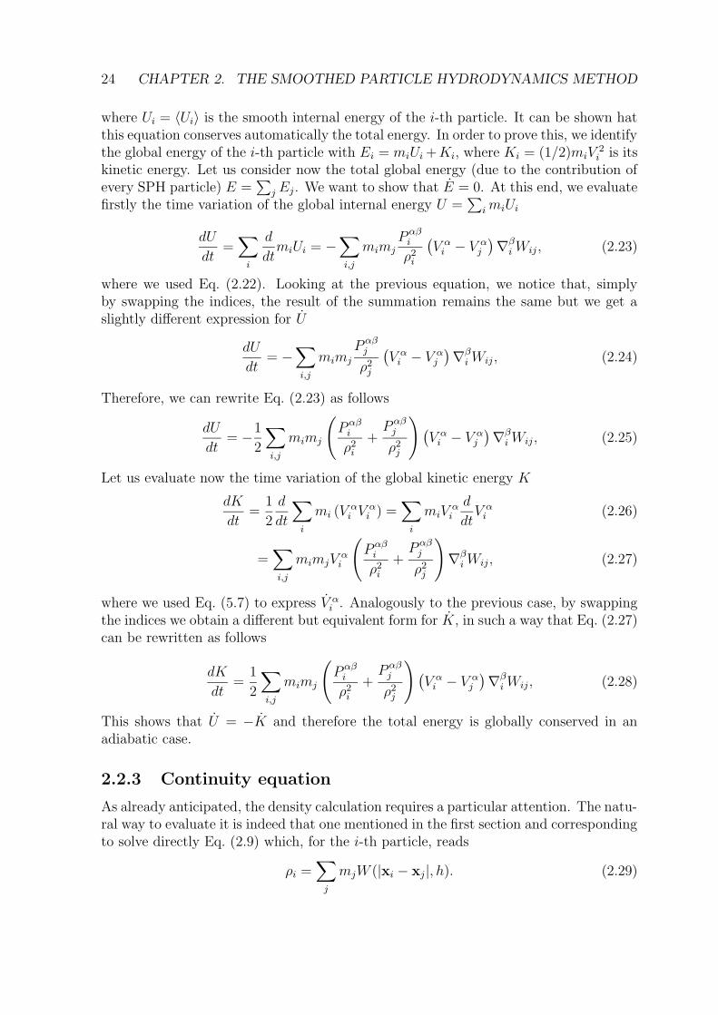
24 CHAPTER 2. THE SMOOTHED PARTICLE HYDRODYNAMICS METHOD
where Ui = 〈Ui〉 is the smooth internal energy of the i-th particle. It can be shown hatthis equation conserves automatically the total energy. In order to prove this, we identifythe global energy of the i-th particle with Ei = miUi +Ki, where Ki = (1/2)miV
2i is its
kinetic energy. Let us consider now the total global energy (due to the contribution ofevery SPH particle) E =
∑
j Ej. We want to show that E = 0. At this end, we evaluatefirstly the time variation of the global internal energy U =
∑
imiUi
dU
dt=∑
i
d
dtmiUi = −
∑
i,j
mimjP αβ
i
ρ2i
(
V αi − V α
j
)
∇βi Wij, (2.23)
where we used Eq. (2.22). Looking at the previous equation, we notice that, simplyby swapping the indices, the result of the summation remains the same but we get aslightly different expression for U
dU
dt= −
∑
i,j
mimj
P αβj
ρ2j
(
V αi − V α
j
)
∇βi Wij, (2.24)
Therefore, we can rewrite Eq. (2.23) as follows
dU
dt= −1
2
∑
i,j
mimj
(
P αβi
ρ2i
+P αβ
j
ρ2j
)
(
V αi − V α
j
)
∇βi Wij, (2.25)
Let us evaluate now the time variation of the global kinetic energy K
dK
dt=
1
2
d
dt
∑
i
mi (Vαi V
αi ) =
∑
i
miVαi
d
dtV α
i (2.26)
=∑
i,j
mimjVαi
(
P αβi
ρ2i
+P αβ
j
ρ2j
)
∇βi Wij, (2.27)
where we used Eq. (5.7) to express V αi . Analogously to the previous case, by swapping
the indices we obtain a different but equivalent form for K, in such a way that Eq. (2.27)can be rewritten as follows
dK
dt=
1
2
∑
i,j
mimj
(
P αβi
ρ2i
+P αβ
j
ρ2j
)
(
V αi − V α
j
)
∇βi Wij, (2.28)
This shows that U = −K and therefore the total energy is globally conserved in anadiabatic case.
2.2.3 Continuity equation
As already anticipated, the density calculation requires a particular attention. The natu-ral way to evaluate it is indeed that one mentioned in the first section and correspondingto solve directly Eq. (2.9) which, for the i-th particle, reads
ρi =∑
j
mjW (|xi − xj|, h). (2.29)
2.3. PARTICLE MOTION 25
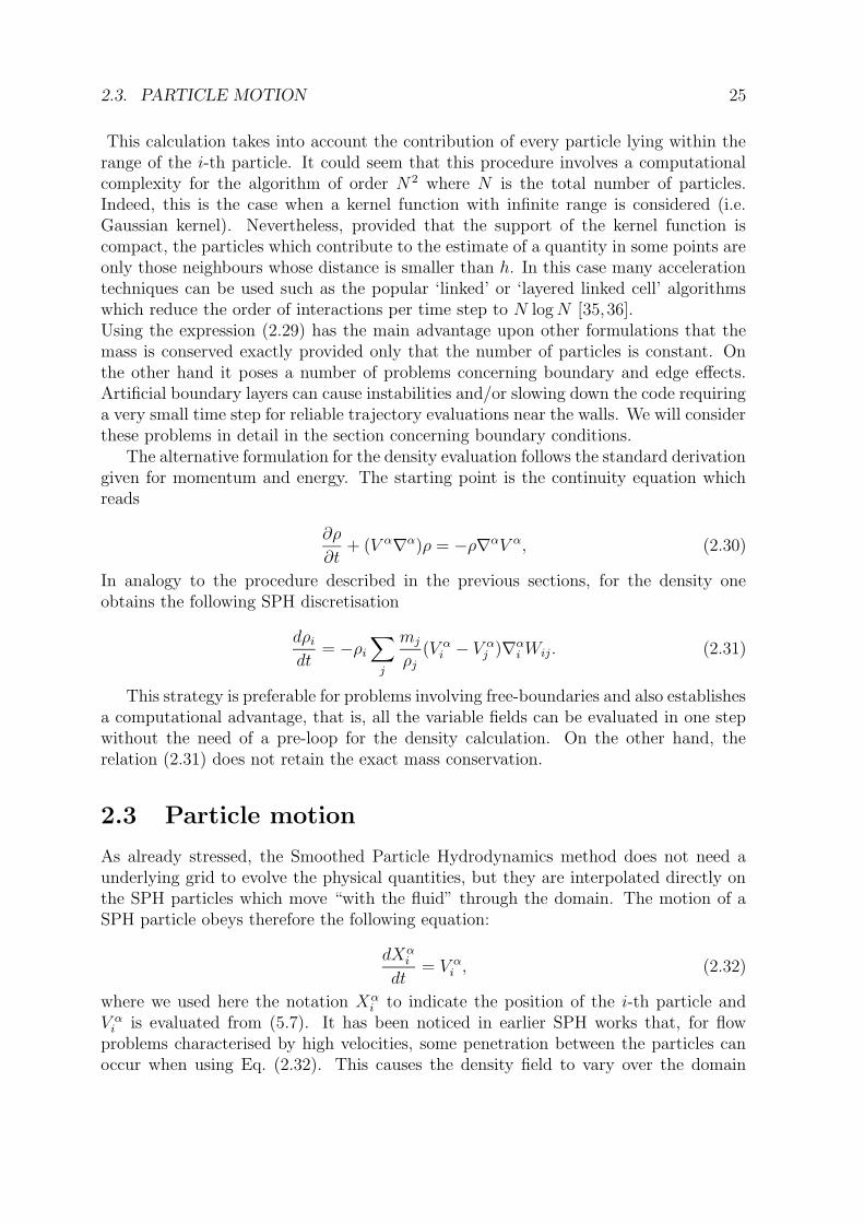
This calculation takes into account the contribution of every particle lying within therange of the i-th particle. It could seem that this procedure involves a computationalcomplexity for the algorithm of order N 2 where N is the total number of particles.Indeed, this is the case when a kernel function with infinite range is considered (i.e.Gaussian kernel). Nevertheless, provided that the support of the kernel function iscompact, the particles which contribute to the estimate of a quantity in some points areonly those neighbours whose distance is smaller than h. In this case many accelerationtechniques can be used such as the popular ‘linked’ or ‘layered linked cell’ algorithmswhich reduce the order of interactions per time step to N logN [35, 36].Using the expression (2.29) has the main advantage upon other formulations that themass is conserved exactly provided only that the number of particles is constant. Onthe other hand it poses a number of problems concerning boundary and edge effects.Artificial boundary layers can cause instabilities and/or slowing down the code requiringa very small time step for reliable trajectory evaluations near the walls. We will considerthese problems in detail in the section concerning boundary conditions.
The alternative formulation for the density evaluation follows the standard derivationgiven for momentum and energy. The starting point is the continuity equation whichreads
∂ρ
∂t+ (V α∇α)ρ = −ρ∇αV α, (2.30)
In analogy to the procedure described in the previous sections, for the density oneobtains the following SPH discretisation
dρi
dt= −ρi
∑
j
mj
ρj
(V αi − V α
j )∇αi Wij. (2.31)
This strategy is preferable for problems involving free-boundaries and also establishesa computational advantage, that is, all the variable fields can be evaluated in one stepwithout the need of a pre-loop for the density calculation. On the other hand, therelation (2.31) does not retain the exact mass conservation.
2.3 Particle motion
As already stressed, the Smoothed Particle Hydrodynamics method does not need aunderlying grid to evolve the physical quantities, but they are interpolated directly onthe SPH particles which move “with the fluid” through the domain. The motion of aSPH particle obeys therefore the following equation:
dXαi
dt= V α
i , (2.32)
where we used here the notation Xαi to indicate the position of the i-th particle and
V αi is evaluated from (5.7). It has been noticed in earlier SPH works that, for flow
problems characterised by high velocities, some penetration between the particles canoccur when using Eq. (2.32). This causes the density field to vary over the domain
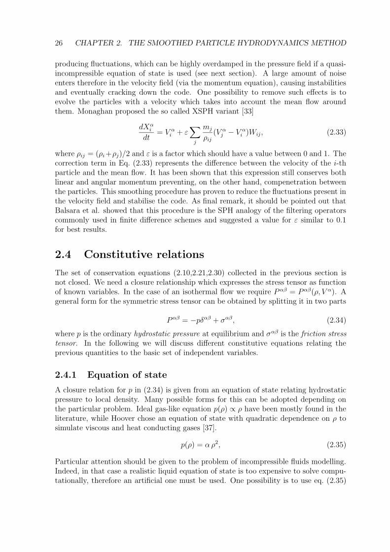
26 CHAPTER 2. THE SMOOTHED PARTICLE HYDRODYNAMICS METHOD
producing fluctuations, which can be highly overdamped in the pressure field if a quasi-incompressible equation of state is used (see next section). A large amount of noiseenters therefore in the velocity field (via the momentum equation), causing instabilitiesand eventually cracking down the code. One possibility to remove such effects is toevolve the particles with a velocity which takes into account the mean flow aroundthem. Monaghan proposed the so called XSPH variant [33]
dXαi
dt= V α
i + ε∑
j
mj
ρij
(V αj − V α
i )Wij, (2.33)
where ρij = (ρi +ρj)/2 and ε is a factor which should have a value between 0 and 1. Thecorrection term in Eq. (2.33) represents the difference between the velocity of the i-thparticle and the mean flow. It has been shown that this expression still conserves bothlinear and angular momentum preventing, on the other hand, compenetration betweenthe particles. This smoothing procedure has proven to reduce the fluctuations present inthe velocity field and stabilise the code. As final remark, it should be pointed out thatBalsara et al. showed that this procedure is the SPH analogy of the filtering operatorscommonly used in finite difference schemes and suggested a value for ε similar to 0.1for best results.
2.4 Constitutive relations
The set of conservation equations (2.10,2.21,2.30) collected in the previous section isnot closed. We need a closure relationship which expresses the stress tensor as functionof known variables. In the case of an isothermal flow we require P αβ = P αβ(ρ, V α). Ageneral form for the symmetric stress tensor can be obtained by splitting it in two parts
P αβ = −pδαβ + σαβ, (2.34)
where p is the ordinary hydrostatic pressure at equilibrium and σαβ is the friction stress
tensor. In the following we will discuss different constitutive equations relating theprevious quantities to the basic set of independent variables.
2.4.1 Equation of state
A closure relation for p in (2.34) is given from an equation of state relating hydrostaticpressure to local density. Many possible forms for this can be adopted depending onthe particular problem. Ideal gas-like equation p(ρ) ∝ ρ have been mostly found in theliterature, while Hoover chose an equation of state with quadratic dependence on ρ tosimulate viscous and heat conducting gases [37].
p(ρ) = α ρ2, (2.35)
Particular attention should be given to the problem of incompressible fluids modelling.Indeed, in that case a realistic liquid equation of state is too expensive to solve compu-tationally, therefore an artificial one must be used. One possibility is to use eq. (2.35)
2.4. CONSTITUTIVE RELATIONS 27
with a choice of the parameter α such that the resulting speed of sound c0
c(ρ) ≡√
∂p(ρ)
∂ρ'√
2αρ0, (2.36)
is suitably larger then a typical flow velocity V characterising the model. It has beenargued by Monaghan that a choice of c0 being ten times larger than this typical velocityV should diminish density fluctuations under a level comparable with the squared Machnumber M 2 (M ≡ V/c0) which in this case corresponds to 1%. This condition ofquasi incompressibility introduces of course small errors due to density fluctuations butthese are consistent with the global accuracy of SPH which comes together with theinterpolation process.One problem of this equation is that it can introduce a large amount of noise in thesimulation when used to simulate flow characterised by high speeds of sound. In orderto clarify this point, let us consider the SPH discretisation of the momentum equationfor an inviscid fluid (where P αβ has been neglected) equipped with the equation of stategiven in (2.35). The SPH form of the momentum equation (5.7) becomes
dV αi
dt= 2αm0
∑
j
∇αi Wij, (2.37)
where we assumed a constant mass m0 for every SPH particle. Now, looking at themomentum equation (2.10), one can easily notice that the pressure term appears underdifferential operator. That is, only variations of the pressure field are important, whileits reference value is left out of the dynamics. Therefore, the presence of a constantdensity field ρ0 produces a constant pressure field which should give no contributions tothe particle accelerations, independently on its absolute value.If we use eq. (2.29), the constant-density contribution to the acceleration of the i-thparticle due to the j-th particle is 2αm0 ∇α
i Wij, which is in principle different fromzero. Now, assuming to be in the continuum limit (number of particle N → ∞), wewill have a very large number of particle randomly distributed in the neighbourhood ofthe i-th particle and therefore, all the contributions appearing in eq. (2.37) will deleteexactly by symmetry.Nevertheless, from a numerical point of view the picture is quite different. Indeed therewill be always a finite number of SPH particles distributed inhomogeneously in theneighbourhood of a particular location xi and, consequently, the summation in (2.37)will introduce spurious fluctuating terms proportional to c20. Therefore, for incompress-ible flow problems, modelled by large values of the speed of sound, this spurious termcan introduce a big amount of numerical noise in the simulations.
Another equation widely used, mainly in the case of free-surface flows, is the followone
p(ρ) = p0
((
ρ
ρ0
)γ
− 1
)
. (2.38)
proposed initially by Batchelor [39] with γ = 7 for the description of water. A property ofthis equation of state is that it introduces an equilibrium pressure reference equal to zero.
28 CHAPTER 2. THE SMOOTHED PARTICLE HYDRODYNAMICS METHOD
This can be sometimes seen as an advantage because it reduces the random fluctuationscoming from the SPH discretisation of the term ∇p/ρ appearing in the momentumequation. On the other hand it must be noticed that, although the advantages abovementioned, the equation of state (4.66) exhibits numerical instabilities in particular flowsituations where the mass density decreases under the equilibrium value ρ0 (specially forregions characterised by a very low pressure). In this case, the pressure contributionsbecome negative, resulting in attractive force between the particle and causing the codeto cracking down.Finally, let us notice that an exact treatment of the incompressibility should take intoaccount a further kinematic constraint on the velocity field which ensures its divergence-freeness [38].
2.4.2 Dissipation
It has often been observed that numerical solutions usually present large unphysicaloscillations and are unstable if a dissipative term is not introduced in the equations.This is because shocks are always present – mostly in the first stages when initialconditions must relax – and if they are not well enough smeared out on a length scalelarger than the discretisation step h, strong instabilities can occur.
In order to introduce a mechanism of dissipation in our model, let us consider thefriction stress tensor appearing in Eq. (2.34). This symmetric stress tensor can berewritten as the sum of an isotropic plus a symmetric traceless (anisotropic) part
σαβ = σδαβ + σαβ, (2.39)
where σ is a dynamic pressure responsible of volumetric changes and σαβ
is the devi-atoric traceless tensor related to shape deformations preserving volumes.The formalism introduced above is purely mathematical and does not provide still anyphysical information about the friction stress tensor. Let us restrict now our analysisto the simple case of Newtonian fluids. In that case, it can be show that, on the basisof physical considerations, we can motivate the following two constitutive relations forthe Newtonian friction stress tensor, [40]
σ = ζ∇αV α, σαβ
= 2η ∇αV β = η
(
∇αV β + ∇βV α − 2
dδαβ∇αV α
)
(2.40)
where η and ζ are, respectively, the shear and bulk viscosities. This corresponds to thewell-known stress tensor appearing in the Navier-Stokes equations for viscous compress-ible Newtonian fluids.The natural way to proceed should be to dicretize, in the SPH formalism, the contribu-tion of the friction stress σαβ and to add it to the hydrostatic pressure term. As it canbe seen in Eq. (2.40), σαβ is proportional to gradients of the velocity field, i.e. termslike ∇βV α. It should be also noticed that the stress tensor enters into the momentumequation under divergence operation, therefore, we should perform SPH dicretizationsof terms containing second derivatives of the velocity field, i.e. ∇α∇βV α.Now, there are basically two ways to perform this discretisation. One possibility is to
2.4. CONSTITUTIVE RELATIONS 29
consider a double differentiation of the interpolating kernel. Although this procedurecan be shown to produce quite accurate results in simple cases, it introduces large scat-tering in the results when the particle are spatially disordered. As we will see in thenext chapter, this problem becomes evident when dealing with simulations in complexgeometries which involve complicated particle-paths.The other possibility is to consider a preliminary SPH discretisation for the first deriva-tives of the velocity field (producing the following tensor field (∇αV β)i defined for theevery particle) and therefore, in a second loop, a further derivation of the previouslyestimated field. As for the previous case, also this approach does not solve completelythe problem of the large fluctuations present in the evaluated quantities and, on theother hand, introduces nested sums over the particles causing the code to slow down.Nevertheless, it should be pointed out that one way to improve the accuracy and reducethe scatter is by employing higher-order kernel functions (i.e. quintic spline), which,although involving a little extra CPU-time, permit to reduce the noise and stabilise thesimulation.In conclusion, in spite of the numerical problems above mentioned, we are convincedthat this approach is the most physically consistent one because based on a direct SPHdiscretisation of the exact Navier-Stokes friction stress tensor (without introducing arti-ficial terms) and therefore we will adopt it in the following when dealing with Newtonianflows.
At this point, it is instructive to present the most commonly adopted solution, his-torically suggested by Gingold and Monaghan [15] and consisting in the introductionof a completely artificial viscosity term in the momentum equation acting only whenshocks are present and smearing out the discontinuities, mimicking in some way a phys-ical mechanism. The artificial viscosity is actually build up by two contributions: onelinearly proportional to the divergence of velocity and another one substantially analo-gous to the Von Neumann-Richtmeyer viscosity [41] able to handle high Mach numberflows. This artificial viscosity Πij, which creates a force on particle i in the presence ofparticle j as explicitly stated by Eq. 2.48 below, reads
Πij =
(−αcijµij + βµ2ij)/ρij , V α
ij xαij < 0
0 , V αij x
αij ≥ 0
, (2.41)
where the abbreviations
ρij ≡ (ρi + ρj)/2, cij ≡ (ci + cj)/2,
V αij ≡ V α
i − V αj , xα
ij ≡ xαi − xα
j , (2.42)
and
µij ≡hV α
ij xαij
V αij V
αij + 0.01h2
, (2.43)
were used. Here ci represents the speed of sound associated with the i-th particle.The parameters α and β are arbitrary, but Monaghan suggested to choose their values
30 CHAPTER 2. THE SMOOTHED PARTICLE HYDRODYNAMICS METHOD
approximately equal to 1 for best results. The term 0.01h2 is introduced in order toprevent singularities when two particles come too close. This viscosity is incorporatedin the momentum equation in the following way
dV αi
dt=∑
j
mj
(
pi
ρ2i
+pj
ρ2j
+ Πij
)
∇αi Wij, (2.44)
Although numerical results have been obtained which are in good agreement with exper-imental observations of flows with complex topologies [17], it has also been noted thatfor simple test cases, where analytical solutions and/or previous exact calculations areavailable, this term produces inaccuracies in the velocity profiles. These are actuallydue to an excessive shear viscosity giving a too large vorticity decay and unphysicaltransfer of momentum. Several ways to escape this difficulty have been proposed as,for example, another form of the viscosity term which takes into account also the vor-ticity associated with every particle, thus assuring the artificial viscosity to vanish inpure shear flows [42]. Other switches are based on the definition of a further viscosityparameter associated to a source-decay equation causing increasing and decaying of thisparameter respectively in an entering and outgoing shock [43].Finally, it should be also pointed out that this formulation for the dissipation does notallow to know a priori the exact viscosity of the simulated fluid, while for the directdiscretisation of the friction stress tensor it represents a simple input parameter. In thefollowing, if not explicitly remarked, the above mentioned discretisation of stress tensorbased on the nested summation approach will be used for the Newtonian case.
2.5 The kernel function
Until now, we did not specify the kernel function but only discussed the main propertieswhich it should possess. In this section we want to discuss different forms for it allsatisfying the previous requirements. One of the simplest choice is that one adopted byTakeda et al. [16], in the simulation of viscous compressible flows, and correspondingto use a simple Gaussian function which has best stability properties, and is infinitelydifferentiable:
W (r, h) = w0 exp−(r/h)2 , (2.45)
where w0 = 1/(2πh2) in 2D. The main problem of this kernel is that it has no compactsupport. This is a severe deficiency because it is not possible to use acceleration tech-niques like linked lists [35] and the contribution of every particles must be taken intoaccount in the evaluation of the force and not only that one of few first neighbours. Theresulting algorithmic complexity is of the order N 2, where N is the number of particles.
It seems therefore reasonable to take a kernel which unifies a computational efficiencywith good smoothing properties. The most frequently used kernel is the cubic spline
kernel with
2.5. THE KERNEL FUNCTION 31
0
0.2
0.4
0.6
0.8
1
1.2
1.4
1.6
0 0.5 1 1.5 2 2.5 3
r/h
Lucy kernelquintic spline kernel
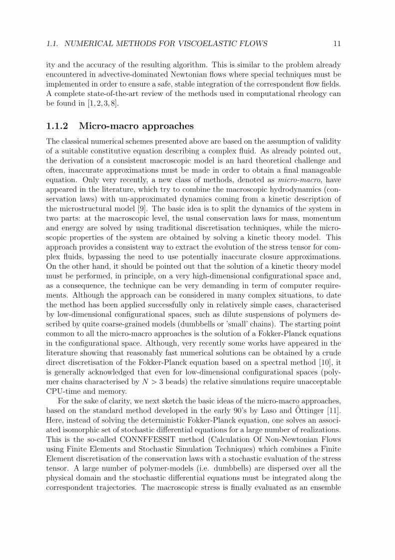
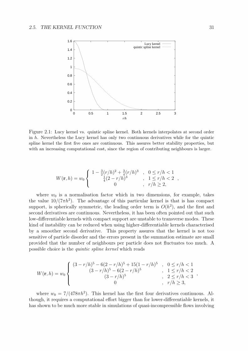
Figure 2.1: Lucy kernel vs. quintic spline kernel. Both kernels interpolates at second orderin h. Nevertheless the Lucy kernel has only two continuous derivatives while for the quinticspline kernel the first five ones are continuous. This assures better stability properties, butwith an increasing computational cost, since the region of contributing neighbours is larger.
W (r, h) = w0
1 − 32(r/h)2 + 3
4(r/h)3 , 0 ≤ r/h < 1
14(2 − r/h)3 , 1 ≤ r/h < 2
0 , r/h ≥ 2,,
where w0 is a normalisation factor which in two dimensions, for example, takesthe value 10/(7πh2). The advantage of this particular kernel is that is has compactsupport, is spherically symmetric, the leading order term is O(h2), and the first andsecond derivatives are continuous. Nevertheless, it has been often pointed out that suchlow-differentiable kernels with compact support are unstable to transverse modes. Thesekind of instability can be reduced when using higher-differentiable kernels characterisedby a smoother second derivative. This property assures that the kernel is not toosensitive of particle disorder and the errors present in the summation estimate are smallprovided that the number of neighbours per particle does not fluctuates too much. Apossible choice is the quintic spline kernel which reads
W (r, h) = w0
(3 − r/h)5 − 6(2 − r/h)5 + 15(1 − r/h)5 , 0 ≤ r/h < 1(3 − r/h)5 − 6(2 − r/h)5 , 1 ≤ r/h < 2
(3 − r/h)5 , 2 ≤ r/h < 30 , r/h ≥ 3,
,
where w0 = 7/(478πh2). This kernel has the first four derivatives continuous. Al-though, it requires a computational effort bigger than for lower-differentiable kernels, ithas shown to be much more stable in simulations of quasi-incompressible flows involving
32 CHAPTER 2. THE SMOOTHED PARTICLE HYDRODYNAMICS METHOD
very low Reynolds number. In that case, the cubic spline kernel produces very noisyhydrodynamics fields.Higher-order kernels have been also proposed which interpolate more accurately in space,for example the super-Gaussian kernel (dominant error O(h4)), but they possess disad-vantages such as expensive computational performance, or they become locally negativein some parts of the domain. This introduces conceptual difficulties in order to describepositive-definite hydrodynamics field, i.e. mass density. A detailed discussion can befound in [44].
In most of the present work, we choose for the kernel the Lucy weighting function
originally introduced by Lucy and Monaghan in the first SPH papers [15] and morerecently used in problems dealing with ideal gases [45, 46], i.e., we employ
W (r, h) = w0
(1 + 3r/h)(1 − r/h)3 , r/h < 10 , r/h ≥ 1
, (2.46)
where w0 = 5/(πh2) in 2D. It interpolates at second order in h, has a compact supportand its first and second derivatives are continuous, cf. Fig. 2.1.
2.6 Boundary conditions
Until now we discussed the SPH equations which must be solved in a bulk fluid disre-garding what happens at the boundaries. From a numerical point of view, boundariesmust be always specified, not only for problems defined on bounded domains, but alsofor bulk fluids. In the last case, the finite availability of memory and CPU-time limitsthe size of the simulated systems and force us to use a finite number of elements (i.e.SPH particles) to dicretize the physical problem. As a consequence, suitably boundaryconditions must be imposed which eliminate unwanted surface effects.In this section we will present the common implementation of boundary conditions firstfor a bulk fluid (unbounded domain) and, secondly, for fluids in confined geometries.
2.6.1 Periodic boundary conditions
The first question which arises when performing numerical simulations of bulk fluids is:“How to deal with boundary conditions for systems defined on an unbounded domain ?”. If we simply allow the system to terminate, the particles near the surfaces will expe-rience quite different forces from the particles in the bulk. Unless we want to describesmall system (i.e. clusters, drops of liquid), where the finite size play a crucial physicalrole, this situation is not satisfactory. For simulations of bulk fluids, we must removethe surface effects, if we want to have a consistent homogeneous description of a systemextending indefinitely.
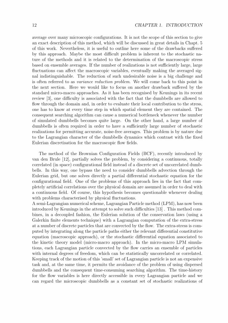
This problem can be solved by using the so called periodic boundary conditions
(PBC) [36]. This approach describes the system via a “primary box”, representing afixed control volume, which is replicated to infinity by rigid translations in all Cartesiandirections. The replicas are called “image boxes” and contain the same sets of particles
2.6. BOUNDARY CONDITIONS 33
1 3
4
2
5
1a 3a
4a
2a
5a
1b 3b
4b
2b
5b
1c 3c
4c
2c
5c
1e 3e
4e
2e
5e
1d 3d
4d
2d
5d
1f 3f
4f
2f
5f
1g 3g
4g
2g
5g
1h 3h
4h
2h
5h
h
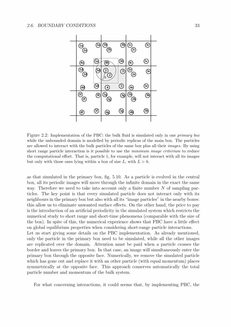
Figure 2.2: Implementation of the PBC: the bulk fluid is simulated only in one primary box
while the unbounded domain is modelled by periodic replicas of the main box. The particlesare allowed to interact with the bulk particles of the same box plus all their images. By usingshort range particle interaction is it possible to use the minimum image criterium to reducethe computational effort. That is, particle 1, for example, will not interact with all its imagesbut only with those ones lying within a box of size L, with L > h.
as that simulated in the primary box, fig. 5.10. As a particle is evolved in the centralbox, all its periodic images will move through the infinite domain in the exact the sameway. Therefore we need to take into account only a finite number N of sampling par-ticles. The key point is that every simulated particle does not interact only with itsneighbours in the primary box but also with all its “image particles” in the nearby boxes:this allow us to eliminate unwanted surface effects. On the other hand, the price to payis the introduction of an artificial periodicity in the simulated system which restricts thenumerical study to short range and short-time phenomena (comparable with the size ofthe box). In spite of this, the numerical experience shows that PBC have a little effecton global equilibrium properties when considering short-range particle interactions.Let us start giving some details on the PBC implementation. As already mentioned,only the particle in the primary box need to be simulated, while all the other imagesare replicated over the domain. Attention must be paid when a particle crosses theborder and leaves the primary box. In that case, an image will simultaneously enter theprimary box through the opposite face. Numerically, we remove the simulated particlewhich has gone out and replace it with an other particle (with equal momentum) placessymmetrically at the opposite face. This approach conserves automatically the totalparticle number and momentum of the bulk system.
For what concerning interactions, it could seems that, by implementing PBC, the
34 CHAPTER 2. THE SMOOTHED PARTICLE HYDRODYNAMICS METHOD
number of interacting pairs should increase enormously. In practice, if we deal withshort-range forces, we can optimise the algorithm by using the so called periodic image
criterium and no additional complexity is introduced in the code. The main idea isthe following one: assumed that the interaction range h is less than the size of the boxL, the particle in the primary box does not interact with all its possible images butonly with those ones whose centre lies within a box of edge L centred on the particlelocation. As shown in fig. 5.10, the SPH particle labelled with i = 1 in the primary box,will interact only with the particle 2 in the same box and with the image particles 4band 3d in the remaining domain.This permits to reduce the computational effort to (1/2)N(N−1) whereN is the numberof simulated particles in the main box. This squared dependence over N represents stilla potential bottleneck for the program, but it can be easily removed considering linkedcell algorithms as those described in [36]
2.6.2 Rigid boundary conditions
Solid boundary conditions represent a crucial point in SPH. Many possible approacheshave been addressed in the last years. One may consider fixed boundary particles ly-ing at the wall surfaces and interacting with the SPH bulk particles via an artificialrepulsive force which prevents penetration. Problems arise if particle density has to beevaluated near the wall: as already mentioned in the previous section, if we considerjust one layer of equispaced boundary particles, the density of those particles approach-ing the surface will decrease rapidly to an approximatively half value of that one intothe domain. This is because, for a particle just on the surface, only the half sphereintersecting the inner domain is taken into account in the average process, while theremaining particle-volume lying outside does not contribute. This causes a gradient ofdensity and consequently, via Eq. 2.35, a strongly deeper gradient of pressure in themomentum equation which forces the particle to accelerate towards the wall producingloss of homogeneity in the dynamical grid and artificial layers parallel to the surface.One possible way to escape this difficulty is to evaluate the density via the continuityequation and not like a summation over neighbouring particles. In this calculation, onlyone layer of boundary particles is involved, which does not contribute to the quantitiesestimated in the inner domain, see fig. 2.3. This permit to eliminate the artificial pres-sure force due to the gradient of density near the wall [17]. Nevertheless, it introducesother problems related to a consistent evaluation of other hydrodynamics field in theboundary layers, i.e. velocity field evaluation for moving boundary conditions.Some other alternatives have been proposed in the literature: one possibility is to evalu-ate the contribute of a gas of imaginary particles supposed existing outside the domain.As already mentioned in section 2.1, the derivation of the integral SPH equations isexact until a distance of order h/2 apart from the walls. In the vicinity of the solidboundaries, the surface terms present in Eq. (2.16) must be taken into account. Inthe Takeda’s approach [16], such surface terms are evaluated analytically assuming ahomogeneous continuum distribution of SPH particles outside the domain. This is ac-tually the best approach, because it is exact SPH in the continuum limit (no artificialassumption are considered but only SPH interaction are used) and does not involve ex-
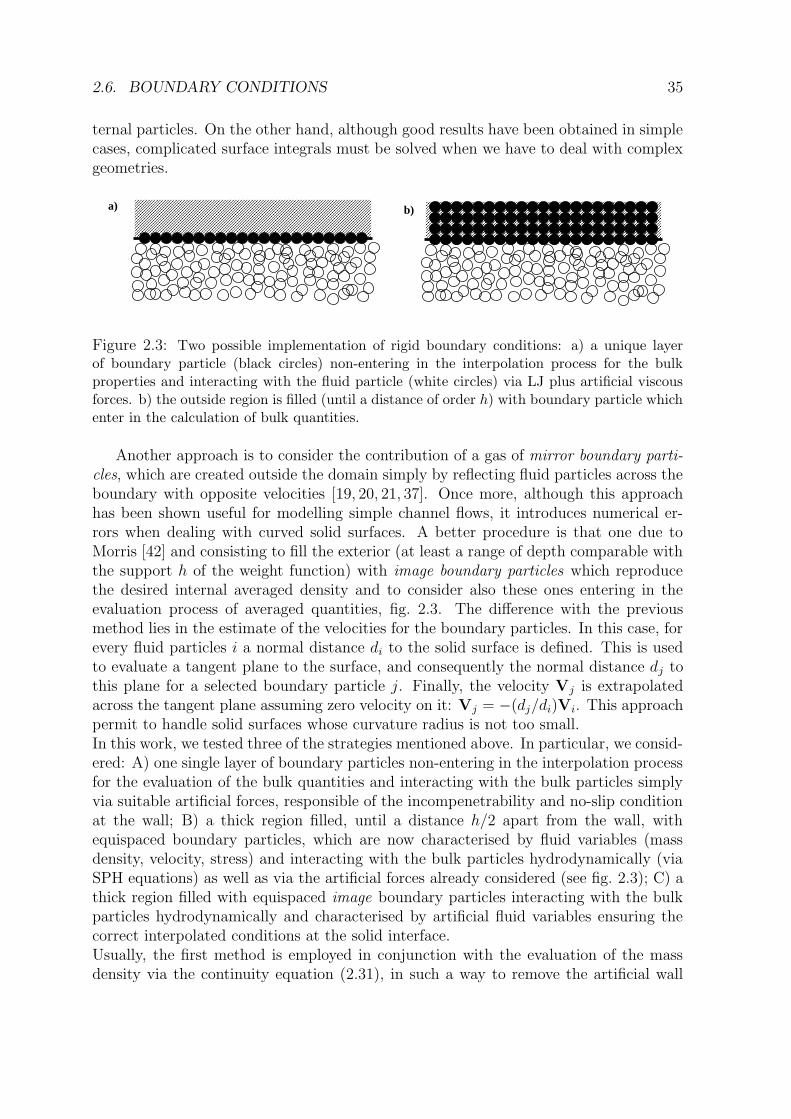
2.6. BOUNDARY CONDITIONS 35
ternal particles. On the other hand, although good results have been obtained in simplecases, complicated surface integrals must be solved when we have to deal with complexgeometries.
a) b)
Figure 2.3: Two possible implementation of rigid boundary conditions: a) a unique layerof boundary particle (black circles) non-entering in the interpolation process for the bulkproperties and interacting with the fluid particle (white circles) via LJ plus artificial viscousforces. b) the outside region is filled (until a distance of order h) with boundary particle whichenter in the calculation of bulk quantities.
Another approach is to consider the contribution of a gas of mirror boundary parti-
cles, which are created outside the domain simply by reflecting fluid particles across theboundary with opposite velocities [19, 20, 21, 37]. Once more, although this approachhas been shown useful for modelling simple channel flows, it introduces numerical er-rors when dealing with curved solid surfaces. A better procedure is that one due toMorris [42] and consisting to fill the exterior (at least a range of depth comparable withthe support h of the weight function) with image boundary particles which reproducethe desired internal averaged density and to consider also these ones entering in theevaluation process of averaged quantities, fig. 2.3. The difference with the previousmethod lies in the estimate of the velocities for the boundary particles. In this case, forevery fluid particles i a normal distance di to the solid surface is defined. This is usedto evaluate a tangent plane to the surface, and consequently the normal distance dj tothis plane for a selected boundary particle j. Finally, the velocity Vj is extrapolatedacross the tangent plane assuming zero velocity on it: Vj = −(dj/di)Vi. This approachpermit to handle solid surfaces whose curvature radius is not too small.In this work, we tested three of the strategies mentioned above. In particular, we consid-ered: A) one single layer of boundary particles non-entering in the interpolation processfor the evaluation of the bulk quantities and interacting with the bulk particles simplyvia suitable artificial forces, responsible of the incompenetrability and no-slip conditionat the wall; B) a thick region filled, until a distance h/2 apart from the wall, withequispaced boundary particles, which are now characterised by fluid variables (massdensity, velocity, stress) and interacting with the bulk particles hydrodynamically (viaSPH equations) as well as via the artificial forces already considered (see fig. 2.3); C) athick region filled with equispaced image boundary particles interacting with the bulkparticles hydrodynamically and characterised by artificial fluid variables ensuring thecorrect interpolated conditions at the solid interface.Usually, the first method is employed in conjunction with the evaluation of the massdensity via the continuity equation (2.31), in such a way to remove the artificial wall
36 CHAPTER 2. THE SMOOTHED PARTICLE HYDRODYNAMICS METHOD
effects described at the beginning of this section. Inversely, the second approach can beimplemented with the usual evaluation of density based on eq. (2.29), provided that thedistribution of boundary particles reproduce the correct bulk density.As already mentioned, in order to enforce incompenetrability and no-slip at the wallspecial forces are considered in both cases. In particular the following repulsive Lennard-Jones like force vector is adopted
fαwall(r) ∝
[(r0/r)4 − (r0/r)
2] r−2 rα , r ≤ r00α , r > r0
, (2.47)
which prevents particles to cross the border via adjustment of a (in any other respectunimportant) proportionality factor in (2.47). In order to consider no-slip boundaryconditions, just for particles approaching the wall (whose distance from the boundaryis less than the cutoff radius in the Lucy function) we take into account a viscous forcebased on the artificial viscosity already introduced. This term introduce a repulsiveinteraction which push the bulk particles forcing them to assume the same velocity ofthe boundary ones. With an appropriate choice of the parameters α and β appearingin Eq. (2.41), we can obtain an exact zero velocity at the wall or, alternatively, suitableslips as experimentally observed in several microscopic flows. Therefore, the final formfor the boundary contribute to the force, which should be added to eq. (5.7), reads
F αext,i = −
∑
j
(
mjΠij∇αi Wij + fα
wall,ij
)
, (2.48)
with Π from (2.41), and where the term appearing in the sum represents now the effectof the j-th boundary particle to the i-th bulk particle. As already pointed out, thisapproach is consistent with the fact that we are going to solve the physical conservationequations in the inner domain as far as a distance of order h/2 (h: smooth cutoffradius) apart from the boundary. In this thin area artificial terms are included in theexact discretized SPH bulk equations in order to take into account wall effects.A brief discussion on the two forms of boundary conditions presented above is in order.Although both of them solve the problem of density evaluation near the walls, noneenable to dicretize the gradients of velocity field in a satisfactory way. Indeed, theabsence of boundary particles in the first case, or the impositions of an arbitrary velocityfield on the external domain in the second one, introduce inconsistencies or inaccurateinterpolations at the border. This problem can be however remedied by suitable choice ofthe parameters α and β entering in (2.41), and forcing the system, in some sense “againstits will”, to assume the correct behaviour. Concerning advantage of one formulationupon the other one, the second approach was found to be numerically more stable andaccurate, specially for problems involving moving boundaries therefore, if not explictlystated, we will adopt it in the following.
As last remark, we should point out that this treatment of the boundary conditionsshould be replaced with other approaches, i.e. image particles [42] or, whenever feasible,the Takeda’s one [16], if accurate estimate of the hydrodynamics fields are needed in thevicinity of the walls, i.e. high Reynolds number problems involving very thin boundarylayers.
2.7. TIME INTEGRATION 37
2.7 Time integration
We adopt a simple two-step predictor-corrector (P-C) scheme with 2nd order accuracyin time to calculate the evolution of the independent variables. It should be replacedif higher precision is essential. In the following, the superscript indicates the discretetime step. Actually, the P-C scheme consists in an Eulerian explicit first evaluation ofall quantities (predictor step):
xn+1α = xn
α + V nα
4t2
V n+1α = V n
α + F nα
4t2
ρn+1 = ρn +Gn4t2
(2.49)
where F and G are the sources evaluated as follows Gn = G(ρn, V nα ), F n
α = Fα(ρn, V nα )
and we are considering the density ρ as an independent variable evolved via the continu-ity equation (2.31). Alternatively, if eq. (2.29) is used, a pre-loop over all the particlesis necessary to determine the density before to calculate the source terms: this ap-proach requires extra CPU-time but has the remarkable advantage to conserve exactlythe mass.
Once we obtained the predicted values of all the independent variables (for everyparticle) we evaluate the source over these states in order to calculate the final correctedvariables. This step involves the calculation of the following quantities as summationover all the particles: Gn+1 ≡ G(ρn+1, V n+1
α ) and F n+1α ≡ Fα(ρn+1, V n+1
α ). It mustpointed out that this part of the algorithm is the most CPU-time requiring if fastsearching neighbours routines (described in the previous section) are not employed.The final corrected quantities read therefore
Xn+1α = Xn
α + (V nα + V n+1
α )4t2,
V n+1α = V n
α + (F nα + F n+1
α )4t2,
ρn+1α = ρn
α + (Gn + Gn+1)4t2, (2.50)
where the source terms appearing in the previous integration equations are obtained bya summation of contributions over the SPH particles. For example, the term F n
α (xi) –evaluated on the position of the particle i – is obtained by a summation process like theone given by Eq. 2.48. This form is valid only in the bulk part of the fluid, while forparticles approaching the boundaries the previous source term (2.48) is supplementedby an expression involving the L-J like force (2.47) and the contribution due to theartificial pressure, Eqs. 2.41-2.43, in order to enforce the incompenetrability and no-slipcondition at the wall. For the stability condition, it should be sufficient to accommodatea Courant-Friedrichs-Lewy [47] condition which actually makes sure that there is nonumerical propagation of signals faster than the speed of sound c0, i.e., for the time stepwe require 4t ≤ h/c0. In addition, we consider also a condition on the forces acting on
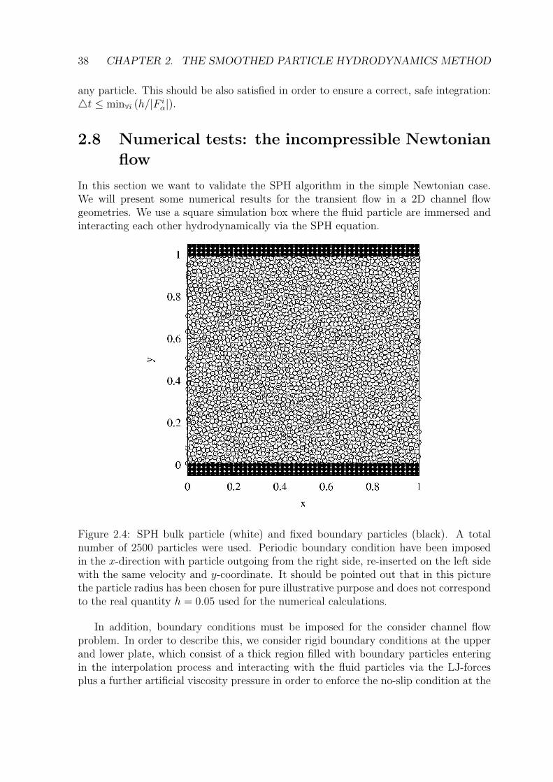
38 CHAPTER 2. THE SMOOTHED PARTICLE HYDRODYNAMICS METHOD
any particle. This should be also satisfied in order to ensure a correct, safe integration:4t ≤ min∀i (h/|F i
α|).
2.8 Numerical tests: the incompressible Newtonian
flow
In this section we want to validate the SPH algorithm in the simple Newtonian case.We will present some numerical results for the transient flow in a 2D channel flowgeometries. We use a square simulation box where the fluid particle are immersed andinteracting each other hydrodynamically via the SPH equation.
Figure 2.4: SPH bulk particle (white) and fixed boundary particles (black). A totalnumber of 2500 particles were used. Periodic boundary condition have been imposedin the x-direction with particle outgoing from the right side, re-inserted on the left sidewith the same velocity and y-coordinate. It should be pointed out that in this picturethe particle radius has been chosen for pure illustrative purpose and does not correspondto the real quantity h = 0.05 used for the numerical calculations.
In addition, boundary conditions must be imposed for the consider channel flowproblem. In order to describe this, we consider rigid boundary conditions at the upperand lower plate, which consist of a thick region filled with boundary particles enteringin the interpolation process and interacting with the fluid particles via the LJ-forcesplus a further artificial viscosity pressure in order to enforce the no-slip condition at the
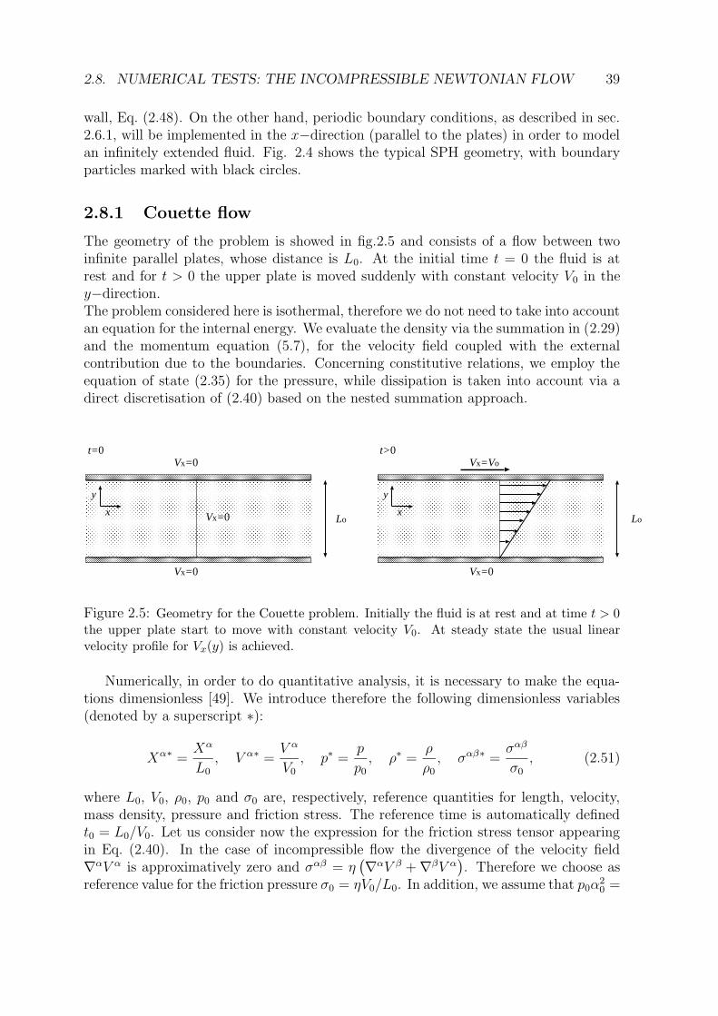
2.8. NUMERICAL TESTS: THE INCOMPRESSIBLE NEWTONIAN FLOW 39
wall, Eq. (2.48). On the other hand, periodic boundary conditions, as described in sec.2.6.1, will be implemented in the x−direction (parallel to the plates) in order to modelan infinitely extended fluid. Fig. 2.4 shows the typical SPH geometry, with boundaryparticles marked with black circles.
2.8.1 Couette flow
The geometry of the problem is showed in fig.2.5 and consists of a flow between twoinfinite parallel plates, whose distance is L0. At the initial time t = 0 the fluid is atrest and for t > 0 the upper plate is moved suddenly with constant velocity V0 in they−direction.The problem considered here is isothermal, therefore we do not need to take into accountan equation for the internal energy. We evaluate the density via the summation in (2.29)and the momentum equation (5.7), for the velocity field coupled with the externalcontribution due to the boundaries. Concerning constitutive relations, we employ theequation of state (2.35) for the pressure, while dissipation is taken into account via adirect discretisation of (2.40) based on the nested summation approach.
Lo
Vx=0
Vx=0
x
y
Lo
Vx=Vo
Vx=0
x
y
Vx=0
t=0 t>0
Figure 2.5: Geometry for the Couette problem. Initially the fluid is at rest and at time t > 0the upper plate start to move with constant velocity V0. At steady state the usual linearvelocity profile for Vx(y) is achieved.
Numerically, in order to do quantitative analysis, it is necessary to make the equa-tions dimensionless [49]. We introduce therefore the following dimensionless variables(denoted by a superscript ∗):
Xα∗ =Xα
L0
, V α∗ =V α
V0
, p∗ =p
p0
, ρ∗ =ρ
ρ0
, σαβ∗ =σαβ
σ0
, (2.51)
where L0, V0, ρ0, p0 and σ0 are, respectively, reference quantities for length, velocity,mass density, pressure and friction stress. The reference time is automatically definedt0 = L0/V0. Let us consider now the expression for the friction stress tensor appearingin Eq. (2.40). In the case of incompressible flow the divergence of the velocity field∇αV α is approximatively zero and σαβ = η
(
∇αV β + ∇βV α)
. Therefore we choose asreference value for the friction pressure σ0 = ηV0/L0. In addition, we assume that p0α
20 =
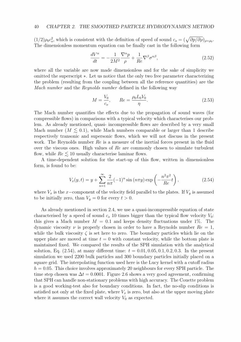
40 CHAPTER 2. THE SMOOTHED PARTICLE HYDRODYNAMICS METHOD
(1/2)ρ0c2o, which is consistent with the definition of speed of sound co = (
√
∂p/∂ρ)ρ=ρ0 .The dimensionless momentum equation can be finally cast in the following form
dV α
dt= − 1
2M2
∇αp
ρ+
1
Re∇βσαβ, (2.52)
where all the variable are now made dimensionless and for the sake of simplicity weomitted the superscript ∗. Let us notice that the only two free parameter characterizingthe problem (resulting from the coupling between all the reference quantities) are theMach number and the Reynolds number defined in the following way
M =V0
co, Re =
ρ0L0V0
η. (2.53)
The Mach number quantifies the effects due to the propagation of sound waves (forcompressible flows) in comparisons with a typical velocity which characterises our prob-lem. As already mentioned, quasi- incompressible flows are described by a very smallMach number (M . 0.1), while Mach numbers comparable or larger than 1 describerespectively transonic and supersonic flows, which we will not discuss in the presentwork. The Reynolds number Re is a measure of the inertial forces present in the fluidover the viscous ones. High values of Re are commonly chosen to simulate turbulentflow, while Re . 10 usually characterise laminar flows.
A time-dependent solution for the start-up of this flow, written in dimensionlessform, is found to be:
Vx(y, t) = y +∞∑
n=1
2
nπ(−1)n sin (nπy) exp
(
−n2π2
Ret
)
, (2.54)
where Vx is the x−component of the velocity field parallel to the plates. If Vy is assumedto be initially zero, than Vy = 0 for every t > 0.
As already mentioned in section 2.4, we use a quasi-incompressible equation of statecharacterised by a speed of sound co 10 times bigger than the typical flow velocity V0:this gives a Mach number M = 0.1 and keeps density fluctuations under 1%. Thedynamic viscosity ν is properly chosen in order to have a Reynolds number Re = 1,while the bulk viscosity ζ is set here to zero. The boundary particles which lie on theupper plate are moved at time t = 0 with constant velocity, while the bottom plate ismaintained fixed. We compared the results of the SPH simulation with the analyticalsolution, Eq. (2.54), at many different time: t = 0.01, 0.05, 0.1, 0.2, 0.3. In the presentsimulation we used 2200 bulk particles and 300 boundary particles initially placed on asquare grid. The interpolating function used here is the Lucy kernel with a cutoff radiush = 0.05. This choice involves approximately 20 neighbours for every SPH particle. Thetime step chosen was ∆t = 0.0001. Figure 2.6 shows a very good agreement, confirmingthat SPH can handle non-stationary problems with high accuracy. The Couette problemis a good working-test also for boundary conditions. In fact, the no-slip conditions issatisfied not only at the fixed plate, where Vx is zero, but also at the upper moving platewhere it assumes the correct wall velocity V0 as expected.
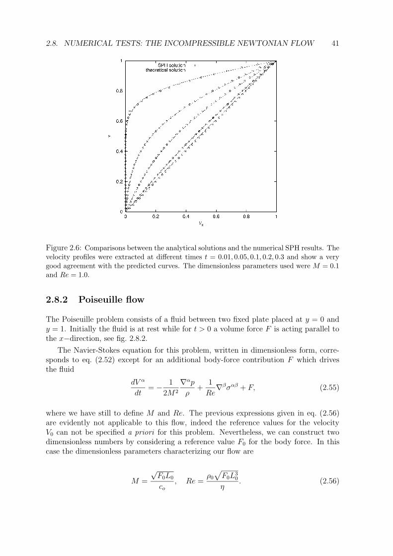
2.8. NUMERICAL TESTS: THE INCOMPRESSIBLE NEWTONIAN FLOW 41
Figure 2.6: Comparisons between the analytical solutions and the numerical SPH results. Thevelocity profiles were extracted at different times t = 0.01, 0.05, 0.1, 0.2, 0.3 and show a verygood agreement with the predicted curves. The dimensionless parameters used were M = 0.1and Re = 1.0.
2.8.2 Poiseuille flow
The Poiseuille problem consists of a fluid between two fixed plate placed at y = 0 andy = 1. Initially the fluid is at rest while for t > 0 a volume force F is acting parallel tothe x−direction, see fig. 2.8.2.
The Navier-Stokes equation for this problem, written in dimensionless form, corre-sponds to eq. (2.52) except for an additional body-force contribution F which drivesthe fluid
dV α
dt= − 1
2M2
∇αp
ρ+
1
Re∇βσαβ + F, (2.55)
where we have still to define M and Re. The previous expressions given in eq. (2.56)are evidently not applicable to this flow, indeed the reference values for the velocityV0 can not be specified a priori for this problem. Nevertheless, we can construct twodimensionless numbers by considering a reference value F0 for the body force. In thiscase the dimensionless parameters characterizing our flow are
M =
√F0L0
co, Re =
ρ0
√
F0L30
η. (2.56)
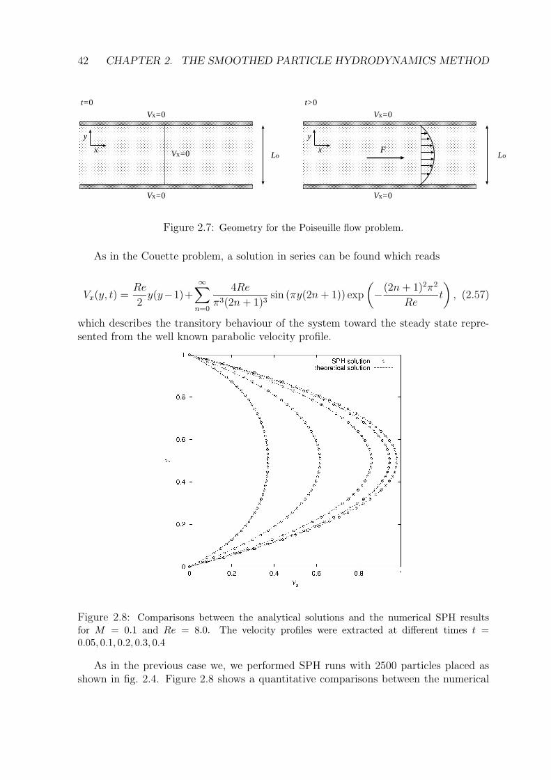
42 CHAPTER 2. THE SMOOTHED PARTICLE HYDRODYNAMICS METHOD
Lo
Vx=0
Vx=0
x
y
Lo
Vx=0
Vx=0
Fx
y
Vx=0
t=0 t>0
Figure 2.7: Geometry for the Poiseuille flow problem.
As in the Couette problem, a solution in series can be found which reads
Vx(y, t) =Re
2y(y−1)+
∞∑
n=0
4Re
π3(2n+ 1)3sin (πy(2n+ 1)) exp
(
−(2n+ 1)2π2
Ret
)
, (2.57)
which describes the transitory behaviour of the system toward the steady state repre-sented from the well known parabolic velocity profile.
Figure 2.8: Comparisons between the analytical solutions and the numerical SPH resultsfor M = 0.1 and Re = 8.0. The velocity profiles were extracted at different times t =0.05, 0.1, 0.2, 0.3, 0.4
As in the previous case we, we performed SPH runs with 2500 particles placed asshown in fig. 2.4. Figure 2.8 shows a quantitative comparisons between the numerical
2.8. NUMERICAL TESTS: THE INCOMPRESSIBLE NEWTONIAN FLOW 43
solution and the theoretical one, eq. (2.57), at five different times: t = 0.05, 0.1, 0.2,0.3, 0.4. The free parameters chosen here were M = 0.1 and Re = 8.0.

44 CHAPTER 2. THE SMOOTHED PARTICLE HYDRODYNAMICS METHOD
Chapter 3
Smoothed Particle Dynamics forviscoelastic flows
In this chapter a viscoelastic numerical scheme based on Smoothed Particle Dynamics,which goes a step beyond the Smoothed Particle Hydrodynamics method (SPH) dis-cussed in the previous chapter, is presented. The formalism describing viscoelasticity isintroduced in the ordinary conservation laws by a differential constitutive equation forthe anisotropic part of the stress tensor [50]. For illustrative purpose we choose the non-linear Jaumann-Maxwell (i.e. corotational Maxwell) model, which in turn is obtainedby replacing the partial derivative appearing in the linear Maxwell model with a Jau-mann derivative which contains a nonlinear advective term plus a term which takes intoaccount solid-body rotations. Some remarks should be done on this particular choice. Itis widely acknowledged that such a model, although exhibiting typical non-Newtonianeffects like shear-dependent viscosity and presence of normal stress differences, it doesnot represent an adequate approach for quantitative comparisons with real viscoelasticflows [7, 6]. In particular, some anomalies in the behaviour of the shear stress coupledwith an excessive shear thinning at large shear rates are not consistent with experimen-tal observations in polymeric fluids. Nevertheless, the same properties above mentioned,showing very complex non-linear behaviours, test severely the resulting numerical imple-mentation of the model. It is not the goal of the present investigation to study whetheror not our choice of the constitutive equation give realistic results, rather, assumed thevalidity of the model, to developed a stable, accurate and consistent numerical algo-rithm for it. As it will be clear later, more realistic constitutive equations can be usedwith only minor modifications in the coding.
The scheme of the chapter is the following one: in Sec. 3.1 we present rigorously theJaumann-Maxwell model used in this work, discussing the way to dicretize it numericallyin the SPH formalism, its consistency and proper dimensional analysis. After that, inSec. 3.2, some numerical results are discussed for unsteady relaxation processes of aninitial sinusoidal velocity profile, since an analytic reference solution is readily availablein that particular non-equilibrium problem. Sec. 3.4 deals with the problem of bulksteady shear-flow: here a rheological study in the elastic parameter will be presented andcompared with theoretical results. Finally, in Sec. 3.5 we apply the method described
45
46 CHAPTER 3. SMOOTHED PARTICLE FOR VISCOELASTIC FLOWS
above to the specific problem of shear flow of a viscoelastic matrix contaminated withrigid non-rotating inclusions. Since this is a severe test for the numerical algorithm, wecompare first our results in the case of a Newtonian matrix where analytical solutionsare recoverable, secondly we focus on the J-M viscoelastic model, showing the effectof the presence of such inclusions on global material properties and discussing localfeatures of its resulting flow dynamics.
3.1 The constitutive equation
In this section we will describe in details the constitutive model which we chose for theimplementation in the SPH algorithm. As already discussed, the set of hydrodynamicsconservation equations given in sec. 2.2, (2.10,2.21,2.30), must be suitably closed. Thishas been done in the previous chapter dealing with simple Newtonian flows. In thatcase a standard Newtonian constitutive relation has been adopted to model the frictionstress tensor.
In analogy with the formalism already introduced, it is possible describe the generalsymmetric stress tensor P αβ by splitting it into an isotropic plus an anisotropic part,cf. eq.(2.39). For the sake of clarity we rewrite it here again
P αβ = −(p− σ)δαβ + σαβ. (3.1)
where p−σ is the total pressure (hydrostatic and friction term) responsible of volumetric
changes, while σαβ
is the deviatoric traceless tensor related to shape deformationspreserving volumes.A closure relation for p in (4.65) is given from an equation of state relating hydrostaticpressure to local density. We will adopt the equations of state defined in (2.34) and(4.66), depending on the particular application. In any case, both of them will becharacterised by large values of the speed of sound in order to simulate incompressibleflows: this was the already mentioned hypothesis of quasi-incompressibility. Concerningthe dynamic pressure σ, we will neglect it in the following by assuming a zero bulkviscosity.
3.1.1 The corotational Maxwell model
In order to describe shear and extensional deformations we propose tentatively a non-linear corotational Maxwell model for the components of the anisotropic stress tensorσ [4]. As already mentioned in the previous section, Maxwell-like models does notexhibit theoretical behaviours which can be useful for a realistic modelling of practicalproblems. Despite their inability to describe quantitatively real complex fluids, theyhave been widely used in numerical calculations because their relative simplicity whichmake them understandable but at the same time able to reproduce, at least quali-tatively, many macroscopic viscoelastic phenomena. The model used in this work ischosen for purely illustrative purpose, and have been used in a limited number of appli-cations [19, 20, 21]. Nevertheless, as it will be clear at the end of the section, the SPH
3.1. THE CONSTITUTIVE EQUATION 47
discretisation of this equation assumes a very general form, which allows for changesand adaptations to more ’realistic’ constitutive equations with only minor modificationsof the algorithm.
Let us start by defining the symmetric strain rate tensor as follows
εαβ =1
2
(
∂V β
∂xα+∂V α
∂xβ
)
. (3.2)
This tensor characterises the local total deformation (shape and volume) of the material.On the other hand, changes in volume are controlled in our scheme uniquely fromthe equation of state, while the constitutive Maxwell equation describes separately thedeviatoric strain rate tensor which is by definition the traceless part of symmetric strainrate tensor, i.e.,
εαβ
≡ εαβ − 1
dδαβ εγγ = εαβ − 1
d
∂V γ
∂xγδαβ, (3.3)
where d is the dimensionality of the problem. The corotational Maxwell model [4] relatesat this point locally the deviatoric stress to deviatoric strain rate in the following way
d
dtσ
αβ+ σ
αγωγβ + σ
γβωαγ =
2η
λε
αβ
− 1
λσ
αβ, (3.4)
where λ is the viscoelastic relaxation time, η is the viscosity of the specimen and the lhsof (4.70) is the so called Jaumann temporal derivative of σ which describes the timeevolution of a fixed volume in a Lagrangian way and subjected to rotations, and ωαβ isthe vorticity tensor defined as
ωαβ ≡ 1
2
(
∂Vβ
∂xα
− ∂Vα
∂xβ
)
. (3.5)
Finally, the SPH model equations for the stress tensor are obtained, from (4.70), inthe same way as those ones for momentum or mass conservation giving
d
dtσ
αβ
i = σαγ
i (kγβi − kβγ
i ) + σγβ
i (kαγi − kγα
i ) − 1
λσ
αβ
i
+2η
λ(kαβ
i + kβαi − 2
dkγγ
i δαβ) (3.6)
where the SPH discretisation of the transposed velocity gradient appearing throughstrain (4.69) and rotation rate (vorticity) tensors, explicitly appearing in (4.72) reads
kµνi ≡ 1
2
(
∂V µ
∂xν
)
i
' 1
2
∑
j
mj
ρj
(V µj − V µ
i )∂Wij
∂xν. (3.7)
There are comparable approaches using differential constitutive equations adaptedto simulate elasto-plastic materials [19, 20, 21, 22]. In these works, the term due toelasticity in (4.70) remains the same but a further relation, e.g. based on the von Misescriterion, is used to recognise the plastic regime where the stress stays constant.
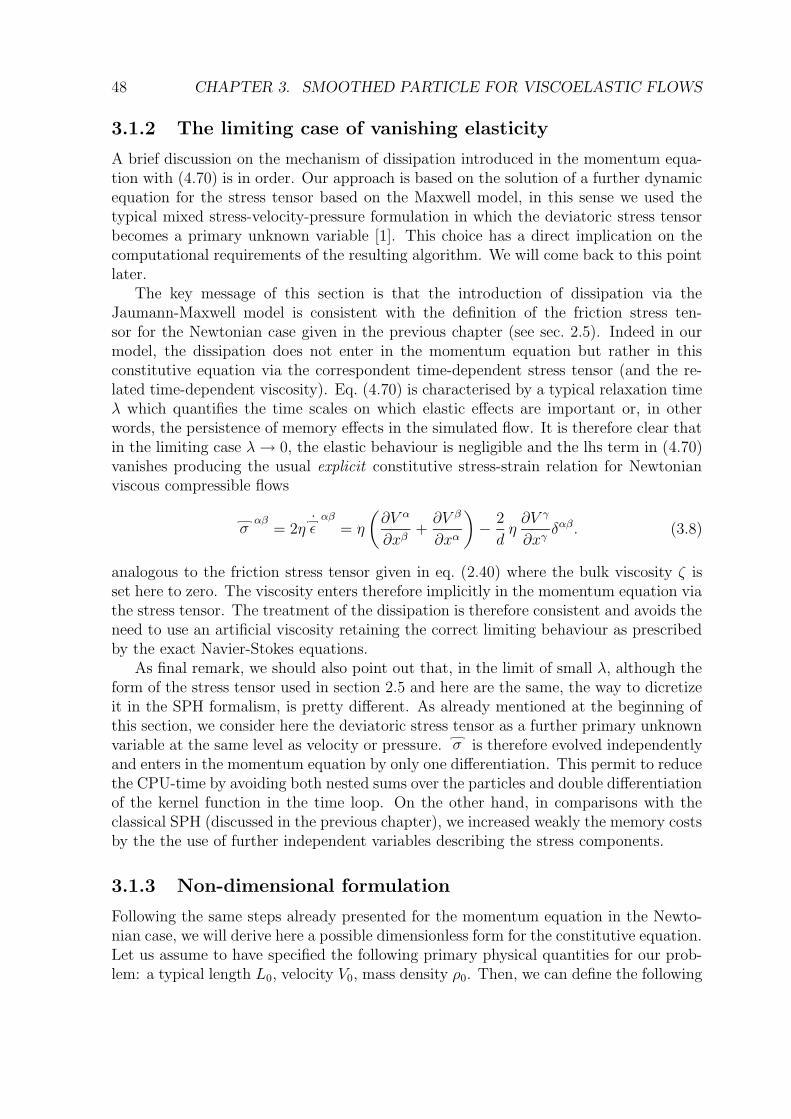
48 CHAPTER 3. SMOOTHED PARTICLE FOR VISCOELASTIC FLOWS
3.1.2 The limiting case of vanishing elasticity
A brief discussion on the mechanism of dissipation introduced in the momentum equa-tion with (4.70) is in order. Our approach is based on the solution of a further dynamicequation for the stress tensor based on the Maxwell model, in this sense we used thetypical mixed stress-velocity-pressure formulation in which the deviatoric stress tensorbecomes a primary unknown variable [1]. This choice has a direct implication on thecomputational requirements of the resulting algorithm. We will come back to this pointlater.
The key message of this section is that the introduction of dissipation via theJaumann-Maxwell model is consistent with the definition of the friction stress ten-sor for the Newtonian case given in the previous chapter (see sec. 2.5). Indeed in ourmodel, the dissipation does not enter in the momentum equation but rather in thisconstitutive equation via the correspondent time-dependent stress tensor (and the re-lated time-dependent viscosity). Eq. (4.70) is characterised by a typical relaxation timeλ which quantifies the time scales on which elastic effects are important or, in otherwords, the persistence of memory effects in the simulated flow. It is therefore clear thatin the limiting case λ→ 0, the elastic behaviour is negligible and the lhs term in (4.70)vanishes producing the usual explicit constitutive stress-strain relation for Newtonianviscous compressible flows
σαβ
= 2η εαβ
= η
(
∂V α
∂xβ+∂V β
∂xα
)
− 2
dη∂V γ
∂xγδαβ. (3.8)
analogous to the friction stress tensor given in eq. (2.40) where the bulk viscosity ζ isset here to zero. The viscosity enters therefore implicitly in the momentum equation viathe stress tensor. The treatment of the dissipation is therefore consistent and avoids theneed to use an artificial viscosity retaining the correct limiting behaviour as prescribedby the exact Navier-Stokes equations.
As final remark, we should also point out that, in the limit of small λ, although theform of the stress tensor used in section 2.5 and here are the same, the way to dicretizeit in the SPH formalism, is pretty different. As already mentioned at the beginning ofthis section, we consider here the deviatoric stress tensor as a further primary unknownvariable at the same level as velocity or pressure. σ is therefore evolved independentlyand enters in the momentum equation by only one differentiation. This permit to reducethe CPU-time by avoiding both nested sums over the particles and double differentiationof the kernel function in the time loop. On the other hand, in comparisons with theclassical SPH (discussed in the previous chapter), we increased weakly the memory costsby the the use of further independent variables describing the stress components.
3.1.3 Non-dimensional formulation
Following the same steps already presented for the momentum equation in the Newto-nian case, we will derive here a possible dimensionless form for the constitutive equation.Let us assume to have specified the following primary physical quantities for our prob-lem: a typical length L0, velocity V0, mass density ρ0. Then, we can define the following
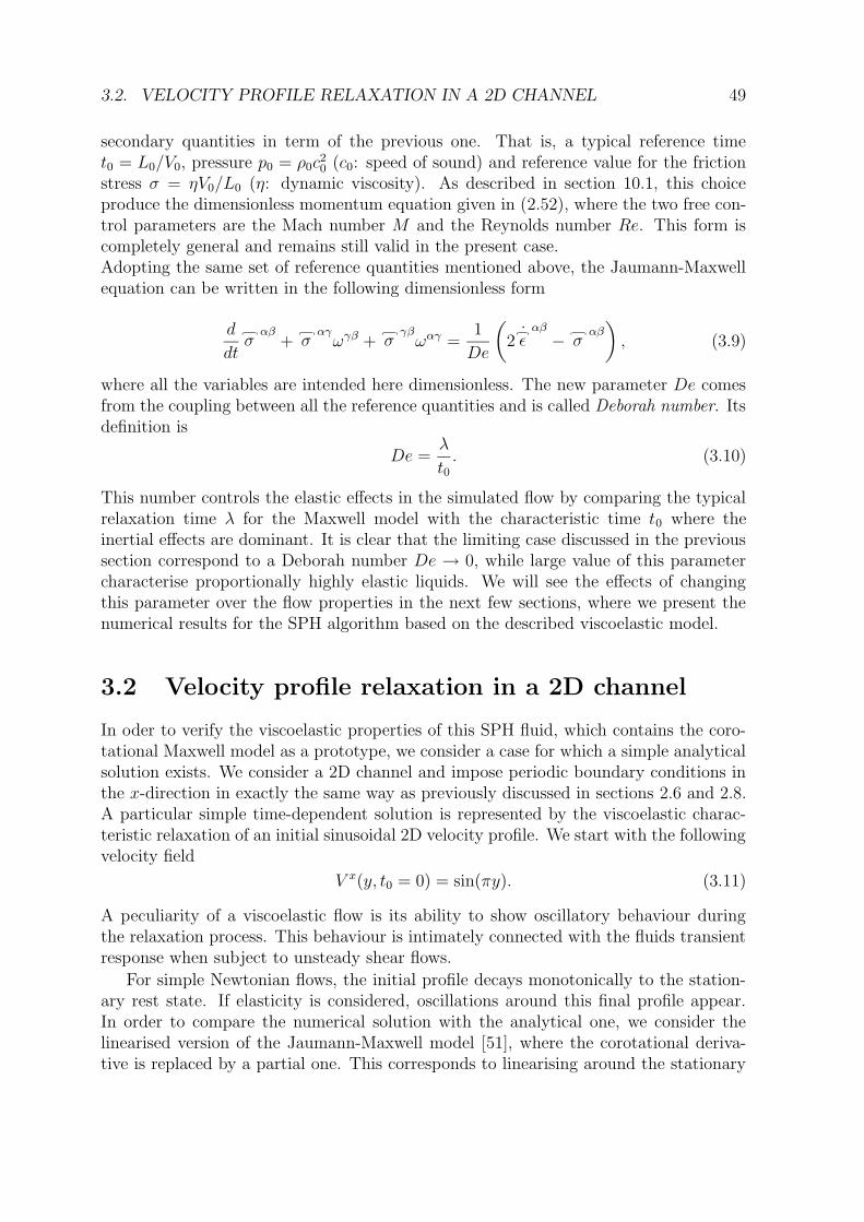
3.2. VELOCITY PROFILE RELAXATION IN A 2D CHANNEL 49
secondary quantities in term of the previous one. That is, a typical reference timet0 = L0/V0, pressure p0 = ρ0c
20 (c0: speed of sound) and reference value for the friction
stress σ = ηV0/L0 (η: dynamic viscosity). As described in section 10.1, this choiceproduce the dimensionless momentum equation given in (2.52), where the two free con-trol parameters are the Mach number M and the Reynolds number Re. This form iscompletely general and remains still valid in the present case.Adopting the same set of reference quantities mentioned above, the Jaumann-Maxwellequation can be written in the following dimensionless form
d
dtσ
αβ+ σ
αγωγβ + σ
γβωαγ =
1
De
(
2 εαβ
− σαβ)
, (3.9)
where all the variables are intended here dimensionless. The new parameter De comesfrom the coupling between all the reference quantities and is called Deborah number. Itsdefinition is
De =λ
t0. (3.10)
This number controls the elastic effects in the simulated flow by comparing the typicalrelaxation time λ for the Maxwell model with the characteristic time t0 where theinertial effects are dominant. It is clear that the limiting case discussed in the previoussection correspond to a Deborah number De → 0, while large value of this parametercharacterise proportionally highly elastic liquids. We will see the effects of changingthis parameter over the flow properties in the next few sections, where we present thenumerical results for the SPH algorithm based on the described viscoelastic model.
3.2 Velocity profile relaxation in a 2D channel
In oder to verify the viscoelastic properties of this SPH fluid, which contains the coro-tational Maxwell model as a prototype, we consider a case for which a simple analyticalsolution exists. We consider a 2D channel and impose periodic boundary conditions inthe x-direction in exactly the same way as previously discussed in sections 2.6 and 2.8.A particular simple time-dependent solution is represented by the viscoelastic charac-teristic relaxation of an initial sinusoidal 2D velocity profile. We start with the followingvelocity field
V x(y, t0 = 0) = sin(πy). (3.11)
A peculiarity of a viscoelastic flow is its ability to show oscillatory behaviour duringthe relaxation process. This behaviour is intimately connected with the fluids transientresponse when subject to unsteady shear flows.
For simple Newtonian flows, the initial profile decays monotonically to the station-ary rest state. If elasticity is considered, oscillations around this final profile appear.In order to compare the numerical solution with the analytical one, we consider thelinearised version of the Jaumann-Maxwell model [51], where the corotational deriva-tive is replaced by a partial one. This corresponds to linearising around the stationary
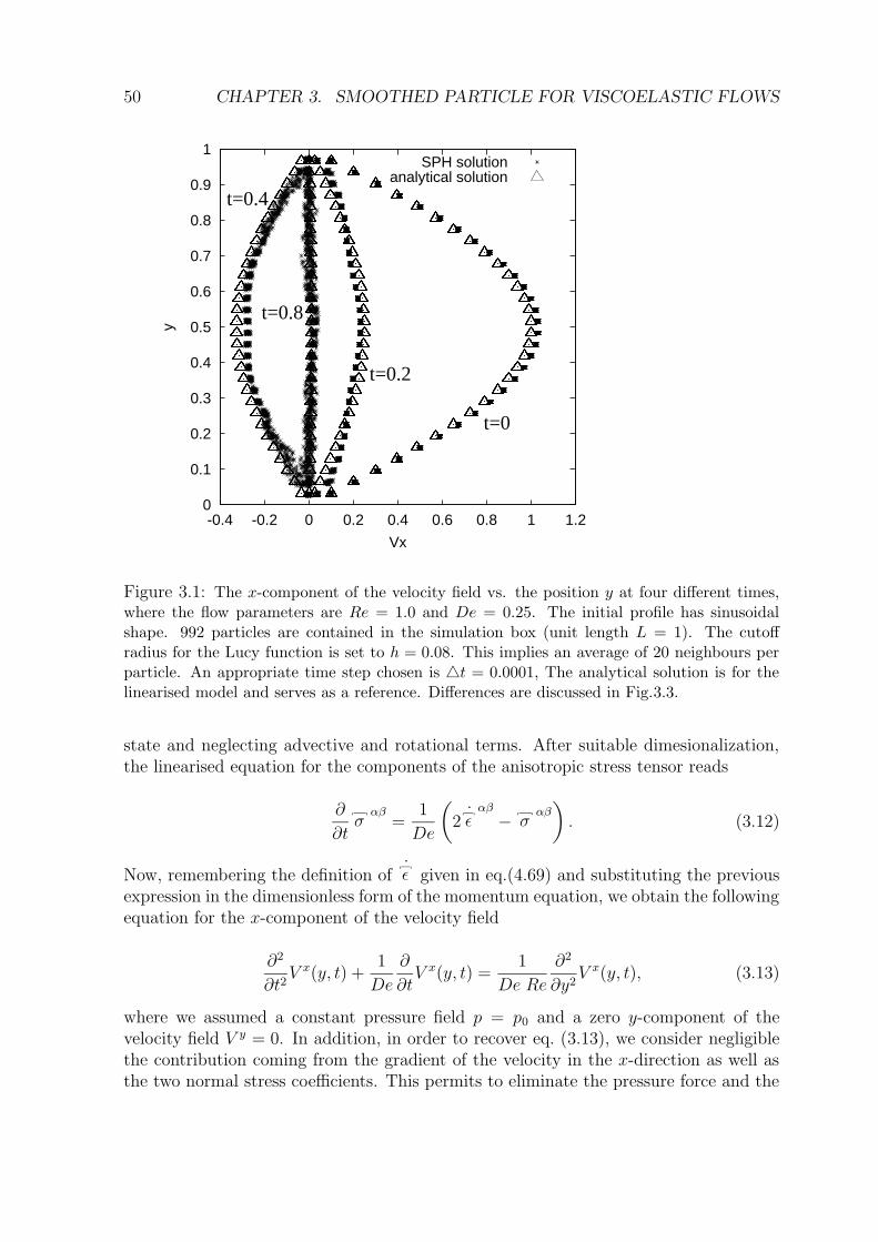
50 CHAPTER 3. SMOOTHED PARTICLE FOR VISCOELASTIC FLOWS
0
0.1
0.2
0.3
0.4
0.5
0.6
0.7
0.8
0.9
1
-0.4 -0.2 0 0.2 0.4 0.6 0.8 1 1.2
y
Vx
SPH solutionanalytical solution
t=0
t=0.2
t=0.4
t=0.8
Figure 3.1: The x-component of the velocity field vs. the position y at four different times,where the flow parameters are Re = 1.0 and De = 0.25. The initial profile has sinusoidalshape. 992 particles are contained in the simulation box (unit length L = 1). The cutoffradius for the Lucy function is set to h = 0.08. This implies an average of 20 neighbours perparticle. An appropriate time step chosen is 4t = 0.0001, The analytical solution is for thelinearised model and serves as a reference. Differences are discussed in Fig.3.3.
state and neglecting advective and rotational terms. After suitable dimesionalization,the linearised equation for the components of the anisotropic stress tensor reads
∂
∂tσ
αβ=
1
De
(
2 εαβ
− σαβ)
. (3.12)
Now, remembering the definition of ε given in eq.(4.69) and substituting the previousexpression in the dimensionless form of the momentum equation, we obtain the followingequation for the x-component of the velocity field
∂2
∂t2V x(y, t) +
1
De
∂
∂tV x(y, t) =
1
De Re
∂2
∂y2V x(y, t), (3.13)
where we assumed a constant pressure field p = p0 and a zero y-component of thevelocity field V y = 0. In addition, in order to recover eq. (3.13), we consider negligiblethe contribution coming from the gradient of the velocity in the x-direction as well asthe two normal stress coefficients. This permits to eliminate the pressure force and the
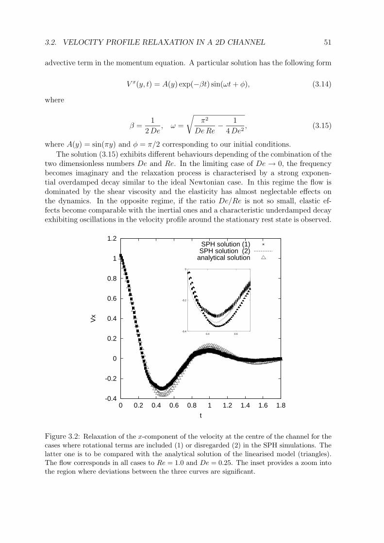
3.2. VELOCITY PROFILE RELAXATION IN A 2D CHANNEL 51
advective term in the momentum equation. A particular solution has the following form
V x(y, t) = A(y) exp(−βt) sin(ωt+ φ), (3.14)
where
β =1
2De, ω =
√
π2
DeRe− 1
4De2, (3.15)
where A(y) = sin(πy) and φ = π/2 corresponding to our initial conditions.
The solution (3.15) exhibits different behaviours depending of the combination of thetwo dimensionless numbers De and Re. In the limiting case of De → 0, the frequencybecomes imaginary and the relaxation process is characterised by a strong exponen-tial overdamped decay similar to the ideal Newtonian case. In this regime the flow isdominated by the shear viscosity and the elasticity has almost neglectable effects onthe dynamics. In the opposite regime, if the ratio De/Re is not so small, elastic ef-fects become comparable with the inertial ones and a characteristic underdamped decayexhibiting oscillations in the velocity profile around the stationary rest state is observed.
-0.4
-0.2
0
0.2
0.4
0.6
0.8
1
1.2
0 0.2 0.4 0.6 0.8 1 1.2 1.4 1.6 1.8
Vx
t
SPH solution (1)SPH solution (2)
analytical solution
-0.4
-0.2
0
0.4 0.6
Figure 3.2: Relaxation of the x-component of the velocity at the centre of the channel for thecases where rotational terms are included (1) or disregarded (2) in the SPH simulations. Thelatter one is to be compared with the analytical solution of the linearised model (triangles).The flow corresponds in all cases to Re = 1.0 and De = 0.25. The inset provides a zoom intothe region where deviations between the three curves are significant.
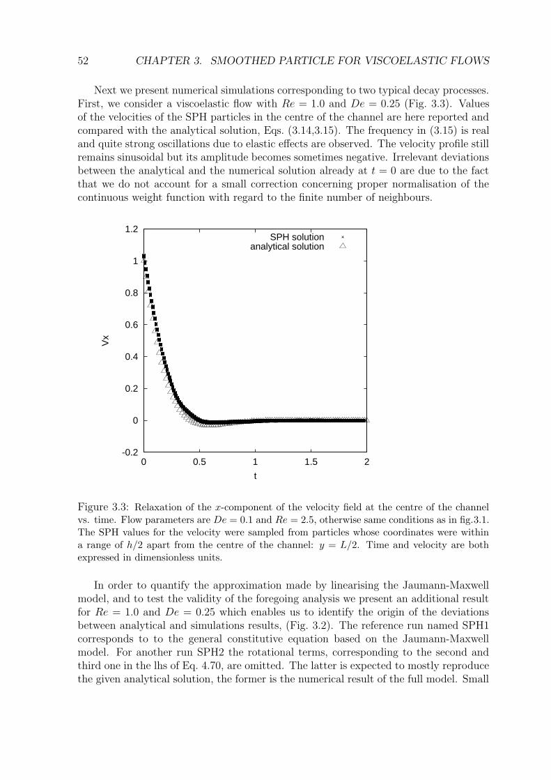
52 CHAPTER 3. SMOOTHED PARTICLE FOR VISCOELASTIC FLOWS
Next we present numerical simulations corresponding to two typical decay processes.First, we consider a viscoelastic flow with Re = 1.0 and De = 0.25 (Fig. 3.3). Valuesof the velocities of the SPH particles in the centre of the channel are here reported andcompared with the analytical solution, Eqs. (3.14,3.15). The frequency in (3.15) is realand quite strong oscillations due to elastic effects are observed. The velocity profile stillremains sinusoidal but its amplitude becomes sometimes negative. Irrelevant deviationsbetween the analytical and the numerical solution already at t = 0 are due to the factthat we do not account for a small correction concerning proper normalisation of thecontinuous weight function with regard to the finite number of neighbours.
-0.2
0
0.2
0.4
0.6
0.8
1
1.2
0 0.5 1 1.5 2
Vx
t
SPH solutionanalytical solution
Figure 3.3: Relaxation of the x-component of the velocity field at the centre of the channelvs. time. Flow parameters are De = 0.1 and Re = 2.5, otherwise same conditions as in fig.3.1.The SPH values for the velocity were sampled from particles whose coordinates were withina range of h/2 apart from the centre of the channel: y = L/2. Time and velocity are bothexpressed in dimensionless units.
In order to quantify the approximation made by linearising the Jaumann-Maxwellmodel, and to test the validity of the foregoing analysis we present an additional resultfor Re = 1.0 and De = 0.25 which enables us to identify the origin of the deviationsbetween analytical and simulations results, (Fig. 3.2). The reference run named SPH1corresponds to to the general constitutive equation based on the Jaumann-Maxwellmodel. For another run SPH2 the rotational terms, corresponding to the second andthird one in the lhs of Eq. 4.70, are omitted. The latter is expected to mostly reproducethe given analytical solution, the former is the numerical result of the full model. Small
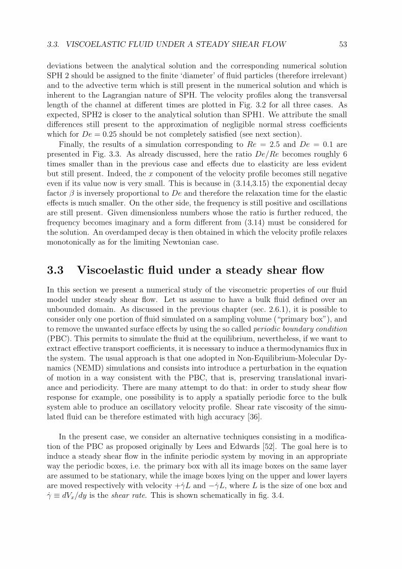
3.3. VISCOELASTIC FLUID UNDER A STEADY SHEAR FLOW 53
deviations between the analytical solution and the corresponding numerical solutionSPH 2 should be assigned to the finite ‘diameter’ of fluid particles (therefore irrelevant)and to the advective term which is still present in the numerical solution and which isinherent to the Lagrangian nature of SPH. The velocity profiles along the transversallength of the channel at different times are plotted in Fig. 3.2 for all three cases. Asexpected, SPH2 is closer to the analytical solution than SPH1. We attribute the smalldifferences still present to the approximation of negligible normal stress coefficientswhich for De = 0.25 should be not completely satisfied (see next section).
Finally, the results of a simulation corresponding to Re = 2.5 and De = 0.1 arepresented in Fig. 3.3. As already discussed, here the ratio De/Re becomes roughly 6times smaller than in the previous case and effects due to elasticity are less evidentbut still present. Indeed, the x component of the velocity profile becomes still negativeeven if its value now is very small. This is because in (3.14,3.15) the exponential decayfactor β is inversely proportional to De and therefore the relaxation time for the elasticeffects is much smaller. On the other side, the frequency is still positive and oscillationsare still present. Given dimensionless numbers whose the ratio is further reduced, thefrequency becomes imaginary and a form different from (3.14) must be considered forthe solution. An overdamped decay is then obtained in which the velocity profile relaxesmonotonically as for the limiting Newtonian case.
3.3 Viscoelastic fluid under a steady shear flow
In this section we present a numerical study of the viscometric properties of our fluidmodel under steady shear flow. Let us assume to have a bulk fluid defined over anunbounded domain. As discussed in the previous chapter (sec. 2.6.1), it is possible toconsider only one portion of fluid simulated on a sampling volume (“primary box”), andto remove the unwanted surface effects by using the so called periodic boundary condition
(PBC). This permits to simulate the fluid at the equilibrium, nevertheless, if we want toextract effective transport coefficients, it is necessary to induce a thermodynamics flux inthe system. The usual approach is that one adopted in Non-Equilibrium-Molecular Dy-namics (NEMD) simulations and consists into introduce a perturbation in the equationof motion in a way consistent with the PBC, that is, preserving translational invari-ance and periodicity. There are many attempt to do that: in order to study shear flowresponse for example, one possibility is to apply a spatially periodic force to the bulksystem able to produce an oscillatory velocity profile. Shear rate viscosity of the simu-lated fluid can be therefore estimated with high accuracy [36].
In the present case, we consider an alternative techniques consisting in a modifica-tion of the PBC as proposed originally by Lees and Edwards [52]. The goal here is toinduce a steady shear flow in the infinite periodic system by moving in an appropriateway the periodic boxes, i.e. the primary box with all its image boxes on the same layerare assumed to be stationary, while the image boxes lying on the upper and lower layersare moved respectively with velocity +γL and −γL, where L is the size of one box andγ ≡ dVx/dy is the shear rate. This is shown schematically in fig. 3.4.
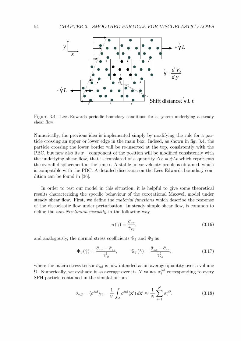
54 CHAPTER 3. SMOOTHED PARTICLE FOR VISCOELASTIC FLOWS
+ γ L
- γ L
Shift distance: γ L t
γ = .
.
d Vx
d y
.
.
xy
Figure 3.4: Lees-Edwards periodic boundary conditions for a system underlying a steadyshear flow.
Numerically, the previous idea is implemented simply by modifying the rule for a par-ticle crossing an upper or lower edge in the main box. Indeed, as shown in fig. 3.4, theparticle crossing the lower border will be re-inserted at the top, consistently with thePBC, but now also its x− component of the position will be modified consistently withthe underlying shear flow, that is translated of a quantity ∆x = γLt which representsthe overall displacement at the time t. A stable linear velocity profile is obtained, whichis compatible with the PBC. A detailed discussion on the Lees-Edwards boundary con-dition can be found in [36].
In order to test our model in this situation, it is helpful to give some theoreticalresults characterizing the specific behaviour of the corotational Maxwell model understeady shear flow. First, we define the material functions which describe the responseof the viscoelastic flow under perturbation. In steady simple shear flow, is common todefine the non-Newtonian viscosity in the following way
η (γ) =σxy
γxy
, (3.16)
and analogously, the normal stress coefficients Ψ1 and Ψ2 as
Ψ1 (γ) =σxx − σyy
γ2xy
, Ψ2 (γ) =σyy − σzz
γ2xy
, (3.17)
where the macro stress tensor σαβ is now intended as an average quantity over a volume
Ω. Numerically, we evaluate it as average over its N values σαβi corresponding to every
SPH particle contained in the simulation box
σαβ = 〈σαβ〉Ω =1
V
∫
Ω
σαβ(x′) dx′ ≈ 1
N
N∑
i=1
σαβi . (3.18)
3.3. VISCOELASTIC FLUID UNDER A STEADY SHEAR FLOW 55
0
0.2
0.4
0.6
0.8
1
1.2
0.01 0.1 1 10
η/ η
0
De
SPH resultstheoretical results
Figure 3.5: Comparisons between the analytical and the numerical non-Newtonian viscosityη versus Deborah number for the corotational Maxwell model in steady-state shearing.
Let us point out that one peculiarity characterizing a viscoelastic fluid, differently tothe Newtonian one, is to exhibit a γ-dependent viscosity and non-zero first normalstress coefficients. In this sense the corotational Maxwell equation (4.70), showing shearthinning, is a “good” model to describe complex rheological behaviours.
An analytical solution for the dependence of the material functions upon the shearrate γ and elastic relaxation time λ is found to be [7]
η (γ, λ) =η0
1 + λ2γ2(3.19)
for the non-Newtonian viscosity, and
Ψ1 (γ, λ) =2λη0
1 + λ2γ2, (3.20)
for the first normal stress coefficient, where λ is the relaxation time and η0 is the viscosityconstant appearing in equation (4.70).
For the simulations presented in this chapter, we considered the same dimensionalformulation presented in sec. 3.2.3, where now L0 represents the size of the simulationbox and V0 is velocity difference between two layers of periodic boxes. This correspondsto choose the reference time t0 ≡ L0/V0 = 1/γ, with the shear rate γ kept constant.We should point out that in this problem neither L0 nor V0 are physically specified: theonly parameter uniquely determined is given by their ratio γ. Assuming this, we canrewrite the Reynolds and Mach numbers as Re = τvγ and M = τsγ, where τv and τs are,respectively, two typical times characterizing viscous relaxation and sound propagation.Next, we will choose Re = 0.1 and M = 0.1 (very viscous incompressible fluid) andkeep them constant, while we will study the effect of variation of the elastic parameterDe on the results.
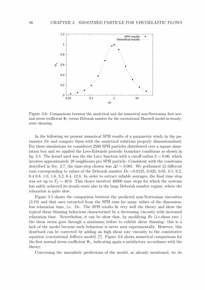
56 CHAPTER 3. SMOOTHED PARTICLE FOR VISCOELASTIC FLOWS
0
0.2
0.4
0.6
0.8
1
1.2
0.01 0.1 1 10
Ψ1
De
SPH resultstheoretical results
Figure 3.6: Comparisons between the analytical and the numerical non-Newtonian first nor-mal stress coefficient Ψ1 versus Deborah number for the corotational Maxwell model in steady-state shearing.
In the following we present numerical SPH results of a parametric study in the pa-rameter De and compare them with the analytical solutions properly dimensionalised.For these simulations we considered 2500 SPH particles distributed over a square simu-lation box and we applied the Lees-Edwards periodic boundary conditions as shown infig. 3.4. The kernel used was the the Lucy function with a cutoff radius h = 0.06, whichinvolves approximately 28 neighbours pro SPH particle. Consistent with the constrainsdescribed in Sec. 2.7, the time-step chosen was ∆t = 0.001. We performed 12 differentruns corresponding to values of the Deborah number De =0.0125, 0.025, 0.05, 0.1, 0.2,0.4 0.8, 1.0, 1.6, 3.2, 6.4, 12.8. In order to extract reliable averages, the final time stepwas set up to Tf = 40.0. This choice involved 40000 time steps for which the systemshas safely achieved its steady-state also in the large Deborah number regime, where therelaxation is quite slow.
Figure 3.5 shows the comparison between the predicted non-Newtonian viscosities(3.19) and that ones extracted from the SPH runs for many values of the dimension-less relaxation time, i.e. De. The SPH results fit very well the theory and show thetypical shear thinning behaviour characterised by a decreasing viscosity with increasedrelaxation time. Nevertheless, it can be show that, by modifying Re (i.e.shear rate )the shear stress goes through a maximum before to exhibit shear thinning: this is alack of the model because such behaviour is never seen experimentally. However, thisdrawback can be corrected by adding an high shear rate viscosity to the constitutiveequation (corotational Jeffreys model) [7]. Figure 3.6 shows numerical comparisons forthe first normal stress coefficient Ψ1, indicating again a satisfactory accordance with thetheory.
Concerning the unrealistic predictions of the model, as already mentioned, we do
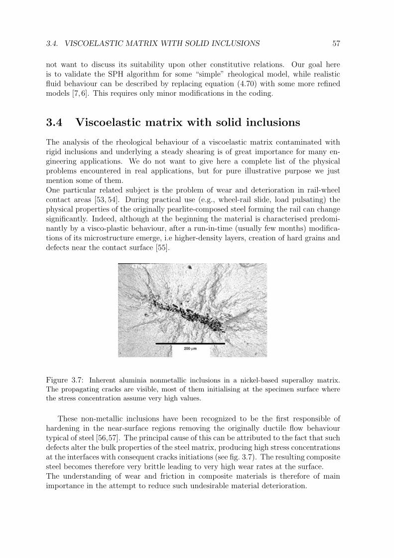
3.4. VISCOELASTIC MATRIX WITH SOLID INCLUSIONS 57
not want to discuss its suitability upon other constitutive relations. Our goal hereis to validate the SPH algorithm for some “simple” rheological model, while realisticfluid behaviour can be described by replacing equation (4.70) with some more refinedmodels [7, 6]. This requires only minor modifications in the coding.
3.4 Viscoelastic matrix with solid inclusions
The analysis of the rheological behaviour of a viscoelastic matrix contaminated withrigid inclusions and underlying a steady shearing is of great importance for many en-gineering applications. We do not want to give here a complete list of the physicalproblems encountered in real applications, but for pure illustrative purpose we justmention some of them.One particular related subject is the problem of wear and deterioration in rail-wheelcontact areas [53, 54]. During practical use (e.g., wheel-rail slide, load pulsating) thephysical properties of the originally pearlite-composed steel forming the rail can changesignificantly. Indeed, although at the beginning the material is characterised predomi-nantly by a visco-plastic behaviour, after a run-in-time (usually few months) modifica-tions of its microstructure emerge, i.e higher-density layers, creation of hard grains anddefects near the contact surface [55].
Figure 3.7: Inherent aluminia nonmetallic inclusions in a nickel-based superalloy matrix.The propagating cracks are visible, most of them initialising at the specimen surface wherethe stress concentration assume very high values.
These non-metallic inclusions have been recognized to be the first responsible ofhardening in the near-surface regions removing the originally ductile flow behaviourtypical of steel [56,57]. The principal cause of this can be attributed to the fact that suchdefects alter the bulk properties of the steel matrix, producing high stress concentrationsat the interfaces with consequent cracks initiations (see fig. 3.7). The resulting compositesteel becomes therefore very brittle leading to very high wear rates at the surface.The understanding of wear and friction in composite materials is therefore of mainimportance in the attempt to reduce such undesirable material deterioration.
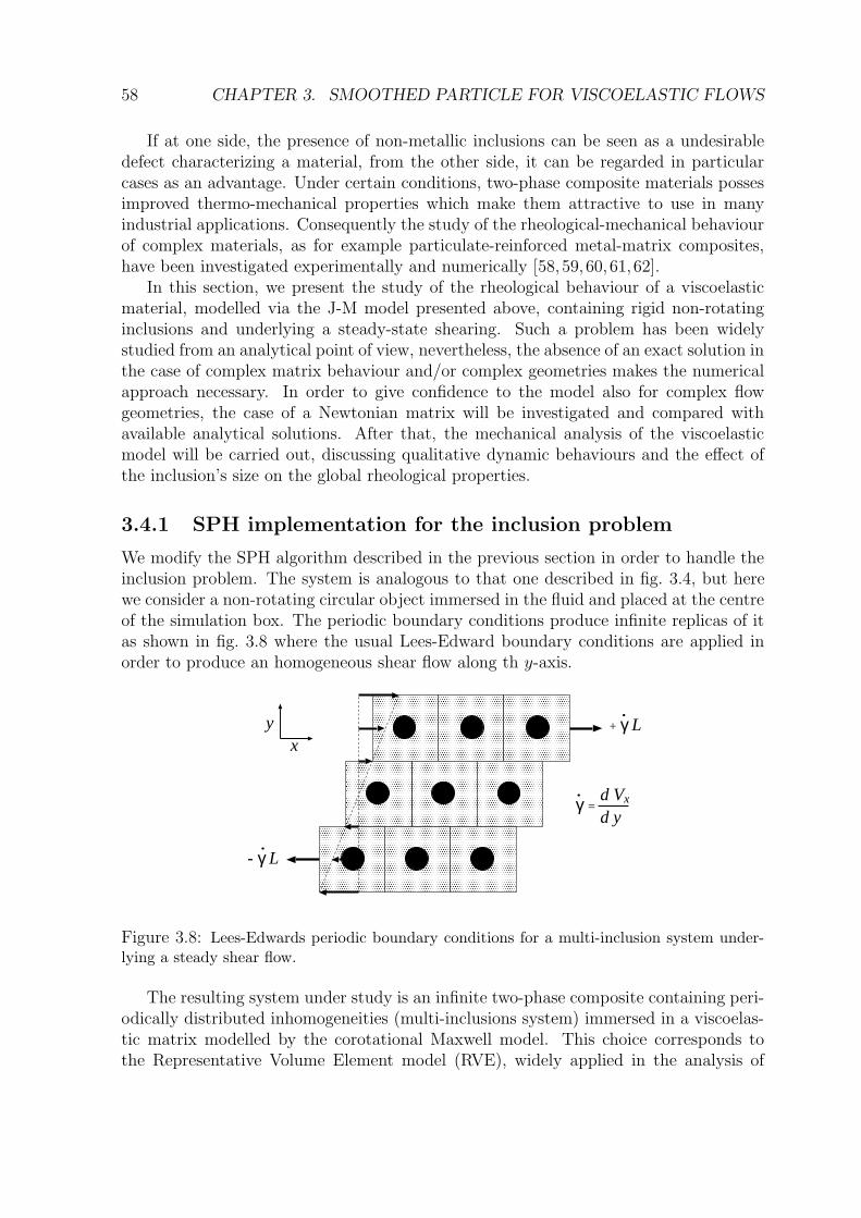
58 CHAPTER 3. SMOOTHED PARTICLE FOR VISCOELASTIC FLOWS
If at one side, the presence of non-metallic inclusions can be seen as a undesirabledefect characterizing a material, from the other side, it can be regarded in particularcases as an advantage. Under certain conditions, two-phase composite materials possesimproved thermo-mechanical properties which make them attractive to use in manyindustrial applications. Consequently the study of the rheological-mechanical behaviourof complex materials, as for example particulate-reinforced metal-matrix composites,have been investigated experimentally and numerically [58, 59, 60,61,62].
In this section, we present the study of the rheological behaviour of a viscoelasticmaterial, modelled via the J-M model presented above, containing rigid non-rotatinginclusions and underlying a steady-state shearing. Such a problem has been widelystudied from an analytical point of view, nevertheless, the absence of an exact solution inthe case of complex matrix behaviour and/or complex geometries makes the numericalapproach necessary. In order to give confidence to the model also for complex flowgeometries, the case of a Newtonian matrix will be investigated and compared withavailable analytical solutions. After that, the mechanical analysis of the viscoelasticmodel will be carried out, discussing qualitative dynamic behaviours and the effect ofthe inclusion’s size on the global rheological properties.
3.4.1 SPH implementation for the inclusion problem
We modify the SPH algorithm described in the previous section in order to handle theinclusion problem. The system is analogous to that one described in fig. 3.4, but herewe consider a non-rotating circular object immersed in the fluid and placed at the centreof the simulation box. The periodic boundary conditions produce infinite replicas of itas shown in fig. 3.8 where the usual Lees-Edward boundary conditions are applied inorder to produce an homogeneous shear flow along th y-axis.
+ γ L
- γ L
γ = .
.
d Vx
d y
.
xy
Figure 3.8: Lees-Edwards periodic boundary conditions for a multi-inclusion system under-lying a steady shear flow.
The resulting system under study is an infinite two-phase composite containing peri-odically distributed inhomogeneities (multi-inclusions system) immersed in a viscoelas-tic matrix modelled by the corotational Maxwell model. This choice corresponds tothe Representative Volume Element model (RVE), widely applied in the analysis of
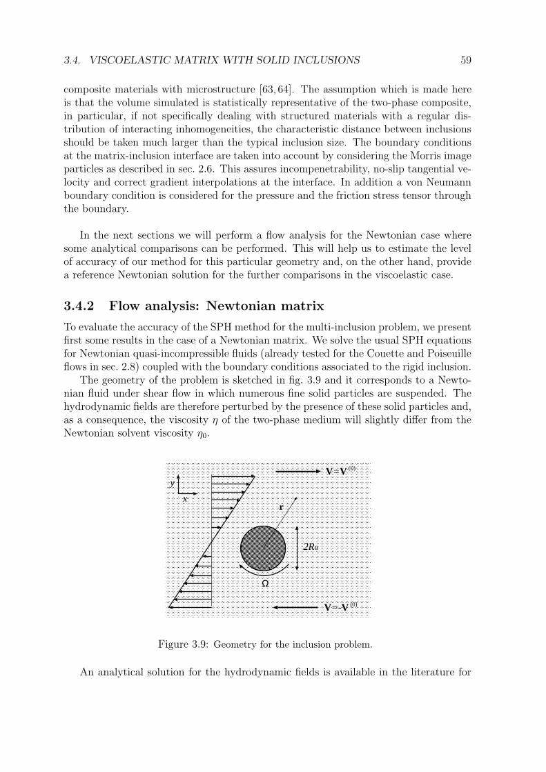
3.4. VISCOELASTIC MATRIX WITH SOLID INCLUSIONS 59
composite materials with microstructure [63, 64]. The assumption which is made hereis that the volume simulated is statistically representative of the two-phase composite,in particular, if not specifically dealing with structured materials with a regular dis-tribution of interacting inhomogeneities, the characteristic distance between inclusionsshould be taken much larger than the typical inclusion size. The boundary conditionsat the matrix-inclusion interface are taken into account by considering the Morris imageparticles as described in sec. 2.6. This assures incompenetrability, no-slip tangential ve-locity and correct gradient interpolations at the interface. In addition a von Neumannboundary condition is considered for the pressure and the friction stress tensor throughthe boundary.
In the next sections we will perform a flow analysis for the Newtonian case wheresome analytical comparisons can be performed. This will help us to estimate the levelof accuracy of our method for this particular geometry and, on the other hand, providea reference Newtonian solution for the further comparisons in the viscoelastic case.
3.4.2 Flow analysis: Newtonian matrix
To evaluate the accuracy of the SPH method for the multi-inclusion problem, we presentfirst some results in the case of a Newtonian matrix. We solve the usual SPH equationsfor Newtonian quasi-incompressible fluids (already tested for the Couette and Poiseuilleflows in sec. 2.8) coupled with the boundary conditions associated to the rigid inclusion.
The geometry of the problem is sketched in fig. 3.9 and it corresponds to a Newto-nian fluid under shear flow in which numerous fine solid particles are suspended. Thehydrodynamic fields are therefore perturbed by the presence of these solid particles and,as a consequence, the viscosity η of the two-phase medium will slightly differ from theNewtonian solvent viscosity η0.
V=V (0)
x
y
V=-V (0)
2Ro
r
Ω
Figure 3.9: Geometry for the inclusion problem.
An analytical solution for the hydrodynamic fields is available in the literature for
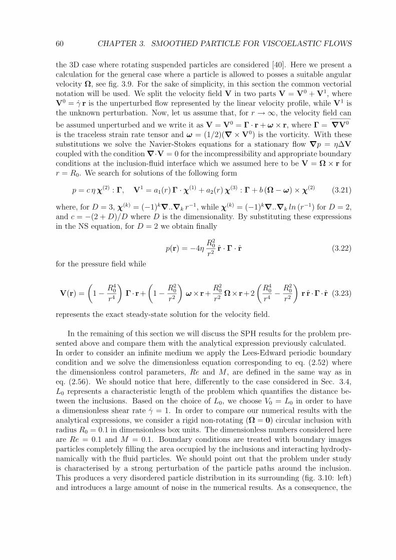
60 CHAPTER 3. SMOOTHED PARTICLE FOR VISCOELASTIC FLOWS
the 3D case where rotating suspended particles are considered [40]. Here we present acalculation for the general case where a particle is allowed to posses a suitable angularvelocity Ω, see fig. 3.9. For the sake of simplicity, in this section the common vectorialnotation will be used. We split the velocity field V in two parts V = V0 + V1, whereV0 = γ r is the unperturbed flow represented by the linear velocity profile, while V1 isthe unknown perturbation. Now, let us assume that, for r → ∞, the velocity field can
be assumed unperturbed and we write it as V = V0 = Γ · r + ω × r, where Γ = ∇V0
is the traceless strain rate tensor and ω = (1/2)(∇ × V0) is the vorticity. With thesesubstitutions we solve the Navier-Stokes equations for a stationary flow ∇p = η∆Vcoupled with the condition ∇·V = 0 for the incompressibility and appropriate boundaryconditions at the inclusion-fluid interface which we assumed here to be V = Ω × r forr = R0. We search for solutions of the following form
p = c ηχ(2) : Γ, V1 = a1(r)Γ · χ(1) + a2(r) χ(3) : Γ + b (Ω − ω) × χ(2) (3.21)
where, for D = 3, χ(k) = (−1)k∇..∇k r
−1, while χ(k) = (−1)k∇..∇k ln (r−1) for D = 2,
and c = −(2 +D)/D where D is the dimensionality. By substituting these expressionsin the NS equation, for D = 2 we obtain finally
p(r) = −4ηR2
0
r2r · Γ · r (3.22)
for the pressure field while
V(r) =
(
1 − R40
r4
)
Γ ·r+
(
1 − R20
r2
)
ω×r+R2
0
r2Ω×r+2
(
R40
r4− R2
0
r2
)
r r ·Γ · r (3.23)
represents the exact steady-state solution for the velocity field.
In the remaining of this section we will discuss the SPH results for the problem pre-sented above and compare them with the analytical expression previously calculated.In order to consider an infinite medium we apply the Lees-Edward periodic boundarycondition and we solve the dimensionless equation corresponding to eq. (2.52) wherethe dimensionless control parameters, Re and M , are defined in the same way as ineq. (2.56). We should notice that here, differently to the case considered in Sec. 3.4,L0 represents a characteristic length of the problem which quantifies the distance be-tween the inclusions. Based on the choice of L0, we choose V0 = L0 in order to havea dimensionless shear rate γ = 1. In order to compare our numerical results with theanalytical expressions, we consider a rigid non-rotating (Ω = 0) circular inclusion withradius R0 = 0.1 in dimensionless box units. The dimensionless numbers considered hereare Re = 0.1 and M = 0.1. Boundary conditions are treated with boundary imagesparticles completely filling the area occupied by the inclusions and interacting hydrody-namically with the fluid particles. We should point out that the problem under studyis characterised by a strong perturbation of the particle paths around the inclusion.This produces a very disordered particle distribution in its surrounding (fig. 3.10: left)and introduces a large amount of noise in the numerical results. As a consequence, the
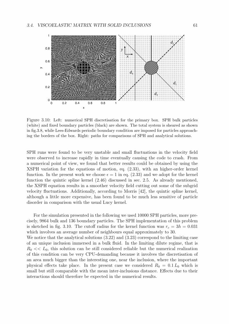
3.4. VISCOELASTIC MATRIX WITH SOLID INCLUSIONS 61
d2
d1
d3
d4
x
y
Figure 3.10: Left: numerical SPH discretisation for the primary box. SPH bulk particles(white) and fixed boundary particles (black) are shown. The total system is sheared as shownin fig.3.8, while Lees-Edwards periodic boundary condition are imposed for particles approach-ing the borders of the box. Right: paths for comparisons of SPH and analytical solutions.
SPH runs were found to be very unstable and small fluctuations in the velocity fieldwere observed to increase rapidly in time eventually causing the code to crash. Froma numerical point of view, we found that better results could be obtained by using theXSPH variation for the equations of motion, eq. (2.33), with an higher-order kernelfunction. In the present work we choose ε = 1 in eq. (2.33) and we adopt for the kernelfunction the quintic spline kernel (2.46) discussed in sec. 2.5. As already mentioned,the XSPH equation results in a smoother velocity field cutting out some of the subgridvelocity fluctuations. Additionally, according to Morris [42], the quintic spline kernel,although a little more expensive, has been found to be much less sensitive of particledisorder in comparison with the usual Lucy kernel.
For the simulation presented in the following we used 10000 SPH particles, more pre-cisely, 9864 bulk and 136 boundary particles. The SPH implementation of this problemis sketched in fig. 3.10. The cutoff radius for the kernel function was rc = 3h = 0.031which involves an average number of neighbours equal approximately to 30.We notice that the analytical solutions (3.22) and (3.23) correspond to the limiting caseof an unique inclusion immersed in a bulk fluid. In the limiting dilute regime, that isR0 << L0, this solution can be still considered reliable but the numerical realizationof this condition can be very CPU-demanding because it involves the discretisation ofan area much bigger than the interesting one, near the inclusion, where the importantphysical effects take place. In the present case we considered R0 = 0.1L0 which issmall but still comparable with the mean inter-inclusions distance. Effects due to theirinteractions should therefore be expected in the numerical results.
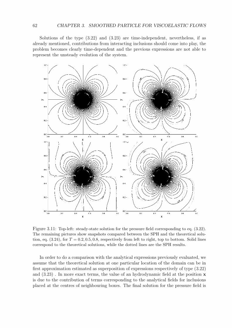
62 CHAPTER 3. SMOOTHED PARTICLE FOR VISCOELASTIC FLOWS
Solutions of the type (3.22) and (3.23) are time-independent, nevertheless, if asalready mentioned, contributions from interacting inclusions should come into play, theproblem becomes clearly time-dependent and the previous expressions are not able torepresent the unsteady evolution of the system.
Figure 3.11: Top-left: steady-state solution for the pressure field corresponding to eq. (3.22).The remaining pictures show snapshots compared between the SPH and the theoretical solu-tion, eq. (3.24), for T = 0.2, 0.5, 0.8, respectively from left to right, top to bottom. Solid linescorrespond to the theoretical solutions, while the dotted lines are the SPH results.
In order to do a comparison with the analytical expressions previously evaluated, weassume that the theoretical solution at one particular location of the domain can be infirst approximation estimated as superposition of expressions respectively of type (3.22)and (3.23) . In more exact terms, the value of an hydrodynamic field at the position xis due to the contribution of terms corresponding to the analytical fields for inclusionsplaced at the centres of neighbouring boxes. The final solution for the pressure field is
3.4. VISCOELASTIC MATRIX WITH SOLID INCLUSIONS 63
evaluated asp(x) =
∑
i
pi(x) (3.24)
where pi(x) are the theoretical solutions evaluated at the positions (x0 − L0, y0), (x0 +L0, y0), (x0 − γL0∆t, y0 − L0), .., (x0 + γL0∆t, y0 + L0) and (x0, y0) is the position ofthe inclusion in the main box. It should be also noticed that, due to the Lees-Edwardsboundary conditions, the positions of the inclusions corresponding to the higher andlower boxes change in time. As a consequence, the problem can no longer achieve astationary configuration but time periodic contributions of the images boxes will beadded to the hydrodynamic fields.
Figure 3.12: Comparisons between the pressure evaluated by SPH (•), by eq. (3.22) () andby superposition (3.24)() .
Let us start considering the pressure field p(x). Fig. 3.11 shows four different config-urations. The first figure, top-left corner, shows the steady state solution correspondingto equation (3.22) while the remaining pictures illustrate the comparison between theSPH results and the superposed analytical solutions previously discussed. The compar-isons are made for three different configurations corresponding to time T = 0.2, 0.5, 0.8.The theoretical solutions are obtained by the superposition (3.24) for the 8 first imageboxes. It is clear that the first steady-state solution is not able to represent the pressurefield, while a time-dependent superposition of them, at least qualitatively, captures itsunsteady evolution.
The previous arguments shows that a choice of R0 = 0.1 is not appropriate toconsider the two-phase system as a dilute suspension of rigid particles, but interactionsbetween them are relevant. In order to quantify the deviations of our results, let usconsider the two paths corresponding to the diagonals d1 and d2 plotted in fig. 3.10 andcompare quantitatively the respective numerical and analytical pressure field sectionsalong them. They are shown in fig. 3.12 where the constant equilibrium pressure wassubtracted from the numerical one for comparisons.
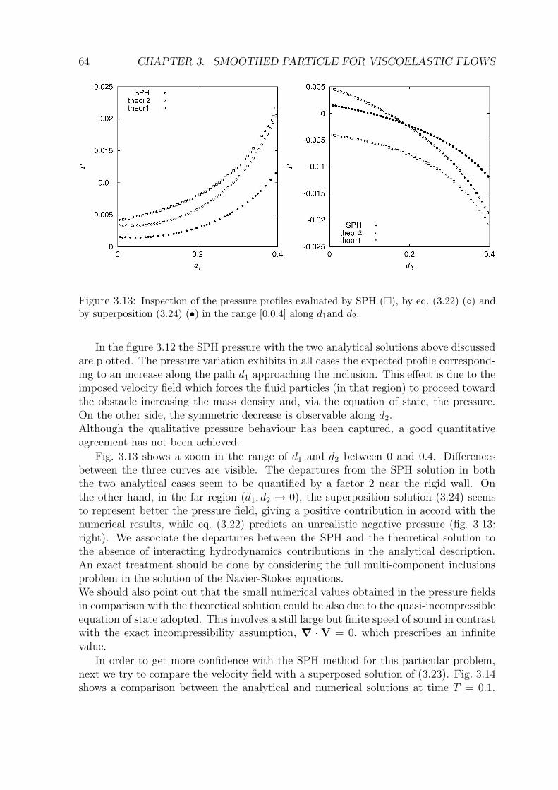
64 CHAPTER 3. SMOOTHED PARTICLE FOR VISCOELASTIC FLOWS
Figure 3.13: Inspection of the pressure profiles evaluated by SPH (), by eq. (3.22) () andby superposition (3.24) (•) in the range [0:0.4] along d1and d2.
In the figure 3.12 the SPH pressure with the two analytical solutions above discussedare plotted. The pressure variation exhibits in all cases the expected profile correspond-ing to an increase along the path d1 approaching the inclusion. This effect is due to theimposed velocity field which forces the fluid particles (in that region) to proceed towardthe obstacle increasing the mass density and, via the equation of state, the pressure.On the other side, the symmetric decrease is observable along d2.Although the qualitative pressure behaviour has been captured, a good quantitativeagreement has not been achieved.
Fig. 3.13 shows a zoom in the range of d1 and d2 between 0 and 0.4. Differencesbetween the three curves are visible. The departures from the SPH solution in boththe two analytical cases seem to be quantified by a factor 2 near the rigid wall. Onthe other hand, in the far region (d1, d2 → 0), the superposition solution (3.24) seemsto represent better the pressure field, giving a positive contribution in accord with thenumerical results, while eq. (3.22) predicts an unrealistic negative pressure (fig. 3.13:right). We associate the departures between the SPH and the theoretical solution tothe absence of interacting hydrodynamics contributions in the analytical description.An exact treatment should be done by considering the full multi-component inclusionsproblem in the solution of the Navier-Stokes equations.We should also point out that the small numerical values obtained in the pressure fieldsin comparison with the theoretical solution could be also due to the quasi-incompressibleequation of state adopted. This involves a still large but finite speed of sound in contrastwith the exact incompressibility assumption, ∇ · V = 0, which prescribes an infinitevalue.
In order to get more confidence with the SPH method for this particular problem,next we try to compare the velocity field with a superposed solution of (3.23). Fig. 3.14shows a comparison between the analytical and numerical solutions at time T = 0.1.
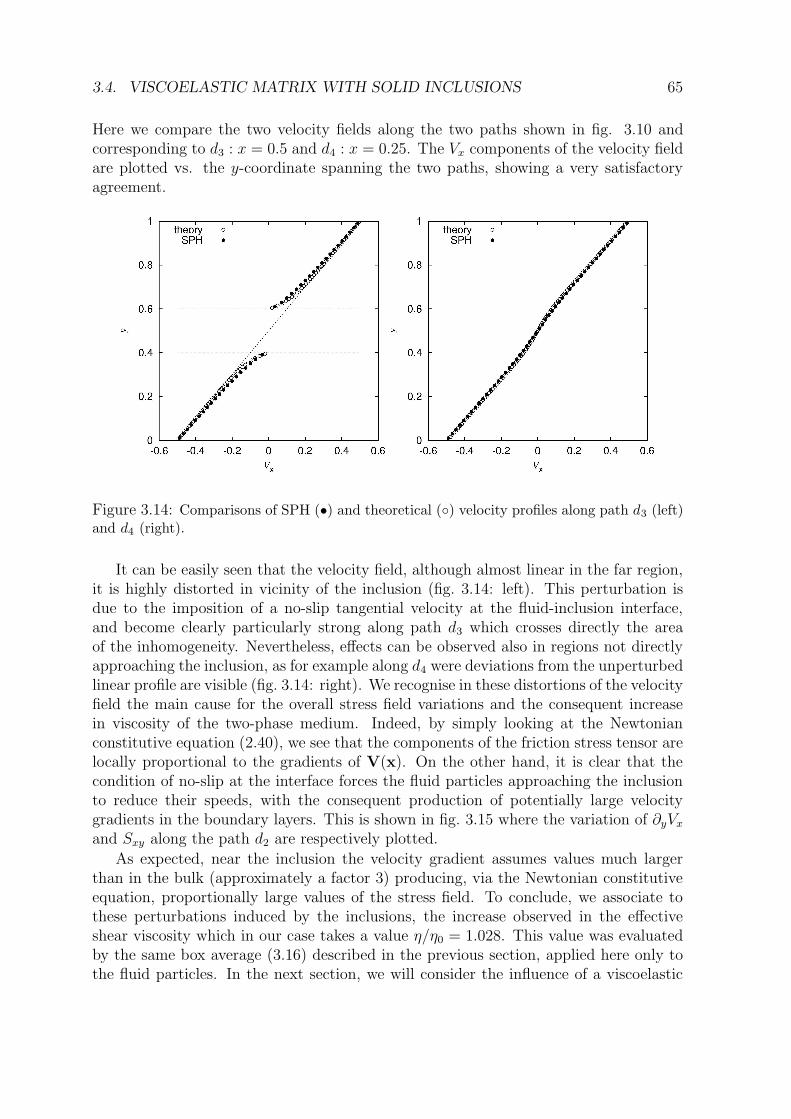
3.4. VISCOELASTIC MATRIX WITH SOLID INCLUSIONS 65
Here we compare the two velocity fields along the two paths shown in fig. 3.10 andcorresponding to d3 : x = 0.5 and d4 : x = 0.25. The Vx components of the velocity fieldare plotted vs. the y-coordinate spanning the two paths, showing a very satisfactoryagreement.
Figure 3.14: Comparisons of SPH (•) and theoretical () velocity profiles along path d3 (left)and d4 (right).
It can be easily seen that the velocity field, although almost linear in the far region,it is highly distorted in vicinity of the inclusion (fig. 3.14: left). This perturbation isdue to the imposition of a no-slip tangential velocity at the fluid-inclusion interface,and become clearly particularly strong along path d3 which crosses directly the areaof the inhomogeneity. Nevertheless, effects can be observed also in regions not directlyapproaching the inclusion, as for example along d4 were deviations from the unperturbedlinear profile are visible (fig. 3.14: right). We recognise in these distortions of the velocityfield the main cause for the overall stress field variations and the consequent increasein viscosity of the two-phase medium. Indeed, by simply looking at the Newtonianconstitutive equation (2.40), we see that the components of the friction stress tensor arelocally proportional to the gradients of V(x). On the other hand, it is clear that thecondition of no-slip at the interface forces the fluid particles approaching the inclusionto reduce their speeds, with the consequent production of potentially large velocitygradients in the boundary layers. This is shown in fig. 3.15 where the variation of ∂yVx
and Sxy along the path d2 are respectively plotted.
As expected, near the inclusion the velocity gradient assumes values much largerthan in the bulk (approximately a factor 3) producing, via the Newtonian constitutiveequation, proportionally large values of the stress field. To conclude, we associate tothese perturbations induced by the inclusions, the increase observed in the effectiveshear viscosity which in our case takes a value η/η0 = 1.028. This value was evaluatedby the same box average (3.16) described in the previous section, applied here only tothe fluid particles. In the next section, we will consider the influence of a viscoelastic
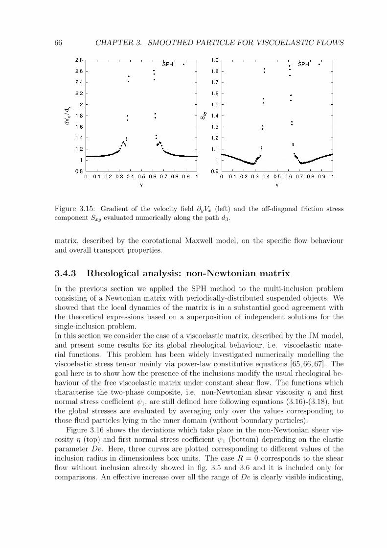
66 CHAPTER 3. SMOOTHED PARTICLE FOR VISCOELASTIC FLOWS
Figure 3.15: Gradient of the velocity field ∂yVx (left) and the off-diagonal friction stresscomponent Sxy evaluated numerically along the path d3.
matrix, described by the corotational Maxwell model, on the specific flow behaviourand overall transport properties.
3.4.3 Rheological analysis: non-Newtonian matrix
In the previous section we applied the SPH method to the multi-inclusion problemconsisting of a Newtonian matrix with periodically-distributed suspended objects. Weshowed that the local dynamics of the matrix is in a substantial good agreement withthe theoretical expressions based on a superposition of independent solutions for thesingle-inclusion problem.In this section we consider the case of a viscoelastic matrix, described by the JM model,and present some results for its global rheological behaviour, i.e. viscoelastic mate-rial functions. This problem has been widely investigated numerically modelling theviscoelastic stress tensor mainly via power-law constitutive equations [65, 66, 67]. Thegoal here is to show how the presence of the inclusions modify the usual rheological be-haviour of the free viscoelastic matrix under constant shear flow. The functions whichcharacterise the two-phase composite, i.e. non-Newtonian shear viscosity η and firstnormal stress coefficient ψ1, are still defined here following equations (3.16)-(3.18), butthe global stresses are evaluated by averaging only over the values corresponding tothose fluid particles lying in the inner domain (without boundary particles).
Figure 3.16 shows the deviations which take place in the non-Newtonian shear vis-cosity η (top) and first normal stress coefficient ψ1 (bottom) depending on the elasticparameter De. Here, three curves are plotted corresponding to different values of theinclusion radius in dimensionless box units. The case R = 0 corresponds to the shearflow without inclusion already showed in fig. 3.5 and 3.6 and it is included only forcomparisons. An effective increase over all the range of De is clearly visible indicating,
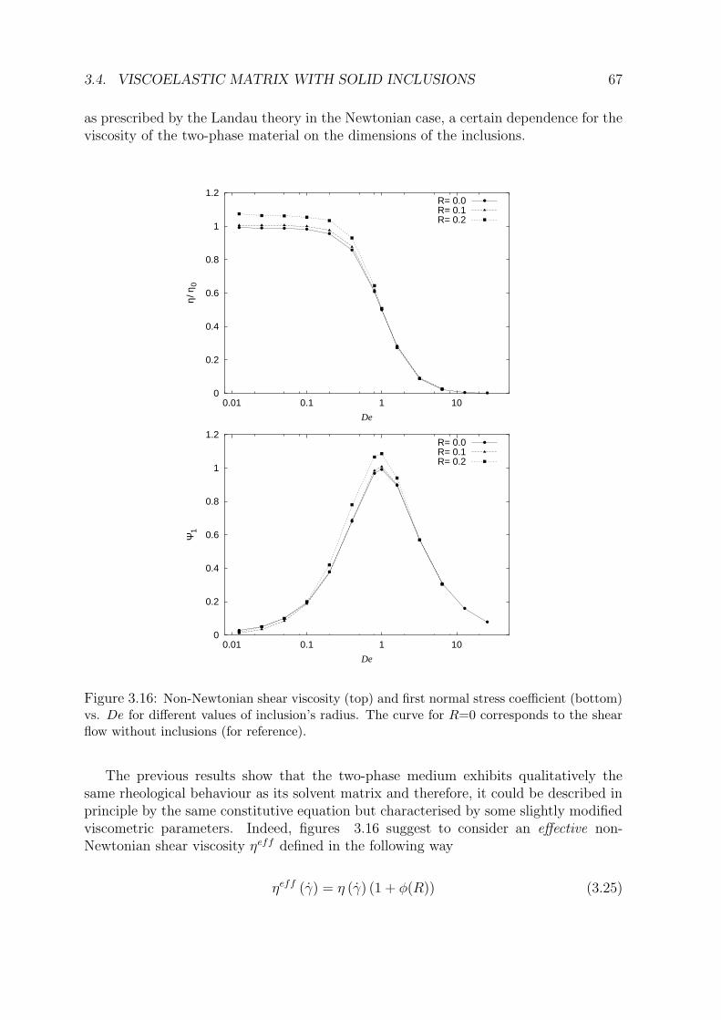
3.4. VISCOELASTIC MATRIX WITH SOLID INCLUSIONS 67
as prescribed by the Landau theory in the Newtonian case, a certain dependence for theviscosity of the two-phase material on the dimensions of the inclusions.
0
0.2
0.4
0.6
0.8
1
1.2
0.01 0.1 1 10
η/ η
0
De
R= 0.0R= 0.1R= 0.2
0
0.2
0.4
0.6
0.8
1
1.2
0.01 0.1 1 10
Ψ1
De
R= 0.0R= 0.1R= 0.2
Figure 3.16: Non-Newtonian shear viscosity (top) and first normal stress coefficient (bottom)vs. De for different values of inclusion’s radius. The curve for R=0 corresponds to the shearflow without inclusions (for reference).
The previous results show that the two-phase medium exhibits qualitatively thesame rheological behaviour as its solvent matrix and therefore, it could be described inprinciple by the same constitutive equation but characterised by some slightly modifiedviscometric parameters. Indeed, figures 3.16 suggest to consider an effective non-Newtonian shear viscosity ηeff defined in the following way
ηeff (γ) = η (γ) (1 + φ(R)) (3.25)
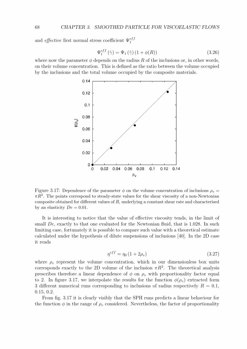
68 CHAPTER 3. SMOOTHED PARTICLE FOR VISCOELASTIC FLOWS
and effective first normal stress coefficient Ψeff1
Ψeff1 (γ) = Ψ1 (γ) (1 + φ(R)) (3.26)
where now the parameter φ depends on the radius R of the inclusions or, in other words,on their volume concentration. This is defined as the ratio between the volume occupiedby the inclusions and the total volume occupied by the composite materials.
Figure 3.17: Dependence of the parameter φ on the volume concentration of inclusions ρv =πR2. The points correspond to steady-state values for the shear viscosity of a non-Newtoniancomposite obtained for different values of R, underlying a constant shear rate and characterisedby an elasticity De = 0.01.
It is interesting to notice that the value of effective viscosity tends, in the limit ofsmall De, exactly to that one evaluated for the Newtonian fluid, that is 1.028. In suchlimiting case, fortunately it is possible to compare such value with a theoretical estimatecalculated under the hypothesis of dilute suspensions of inclusions [40]. In the 2D caseit reads
ηeff = η0 (1 + 2ρv) (3.27)
where ρv represent the volume concentration, which in our dimensionless box unitscorresponds exactly to the 2D volume of the inclusion πR2. The theoretical analysisprescribes therefore a linear dependence of φ on ρv with proportionality factor equalto 2. In figure 3.17, we interpolate the results for the function φ(ρv) extracted form3 different numerical runs corresponding to inclusions of radius respectively R = 0.1,0.15, 0.2.
From fig. 3.17 it is clearly visibly that the SPH runs predicts a linear behaviour forthe function φ in the range of ρv considered. Nevertheless, the factor of proportionality
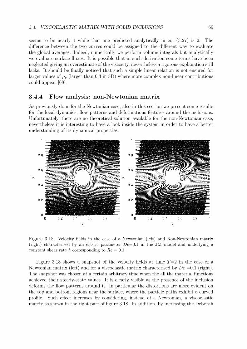
3.4. VISCOELASTIC MATRIX WITH SOLID INCLUSIONS 69
seems to be nearly 1 while that one predicted analytically in eq. (3.27) is 2. Thedifference between the two curves could be assigned to the different way to evaluatethe global averages. Indeed, numerically we perform volume integrals but analyticallywe evaluate surface fluxes. It is possible that in such derivation some terms have beenneglected giving an overestimate of the viscosity, nevertheless a rigorous explanation stilllacks. It should be finally noticed that such a simple linear relation is not ensured forlarger values of ρv (larger than 0.3 in 3D) where more complex non-linear contributionscould appear [68].
3.4.4 Flow analysis: non-Newtonian matrix
As previously done for the Newtonian case, also in this section we present some resultsfor the local dynamics, flow patterns and deformations features around the inclusions.Unfortunately, there are no theoretical solution available for the non-Newtonian case,nevertheless it is interesting to have a look inside the system in order to have a betterunderstanding of its dynamical properties.
Figure 3.18: Velocity fields in the case of a Newtonian (left) and Non-Newtonian matrix(right) characterised by an elastic parameter De=0.1 in the JM model and underlying aconstant shear rate γ corresponding to Re = 0.1.
Figure 3.18 shows a snapshot of the velocity fields at time T=2 in the case of aNewtonian matrix (left) and for a viscoelastic matrix characterised by De =0.1 (right).The snapshot was chosen at a certain arbitrary time when the all the material functionsachieved their steady-state values. It is clearly visible as the presence of the inclusiondeforms the flow patterns around it. In particular the distortions are more evident onthe top and bottom regions near the surface, where the particle paths exhibit a curvedprofile. Such effect increases by considering, instead of a Newtonian, a viscoelasticmatrix as shown in the right part of figure 3.18. In addition, by increasing the Deborah
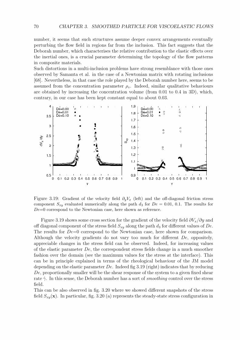
70 CHAPTER 3. SMOOTHED PARTICLE FOR VISCOELASTIC FLOWS
number, it seems that such structures assume deeper convex arrangements eventuallyperturbing the flow field in regions far from the inclusion. This fact suggests that theDeborah number, which characterises the relative contribution to the elastic effects overthe inertial ones, is a crucial parameter determining the topology of the flow patternsin composite materials.Such distortions in a multi-inclusion problems have strong resemblance with those onesobserved by Samanta et al. in the case of a Newtonian matrix with rotating inclusions[68]. Nevertheless, in that case the role played by the Deborah number here, seems to beassumed from the concentration parameter ρv. Indeed, similar qualitative behavioursare obtained by increasing the concentration volume (from 0.01 to 0.4 in 3D), which,contrary, in our case has been kept constant equal to about 0.03.
Figure 3.19: Gradient of the velocity field ∂yVx (left) and the off-diagonal friction stresscomponent Sxy evaluated numerically along the path d3 for De = 0.01, 0.1. The results forDe=0 correspond to the Newtonian case, here shown as reference.
Figure 3.19 shows some cross section for the gradient of the velocity field ∂Vx/∂y andoff diagonal component of the stress field Sxy along the path d3 for different values of De.The results for De=0 correspond to the Newtonian case, here shown for comparison.Although the velocity gradients do not vary too much for different De, oppositely,appreciable changes in the stress field can be observed. Indeed, for increasing valuesof the elastic parameter De, the correspondent stress fields change in a much smootherfashion over the domain (see the maximum values for the stress at the interface). Thiscan be in principle explained in terms of the rheological behaviour of the JM modeldepending on the elastic parameterDe. Indeed fig 3.19 (right) indicates that by reducingDe, proportionally smaller will be the shear response of the system to a given fixed shearrate γ. In this sense, the Deborah number has a sort of smoothing control over the stressfield.This can be also observed in fig. 3.20 where we showed different snapshots of the stressfield Sxy(x). In particular, fig. 3.20 (a) represents the steady-state stress configuration in
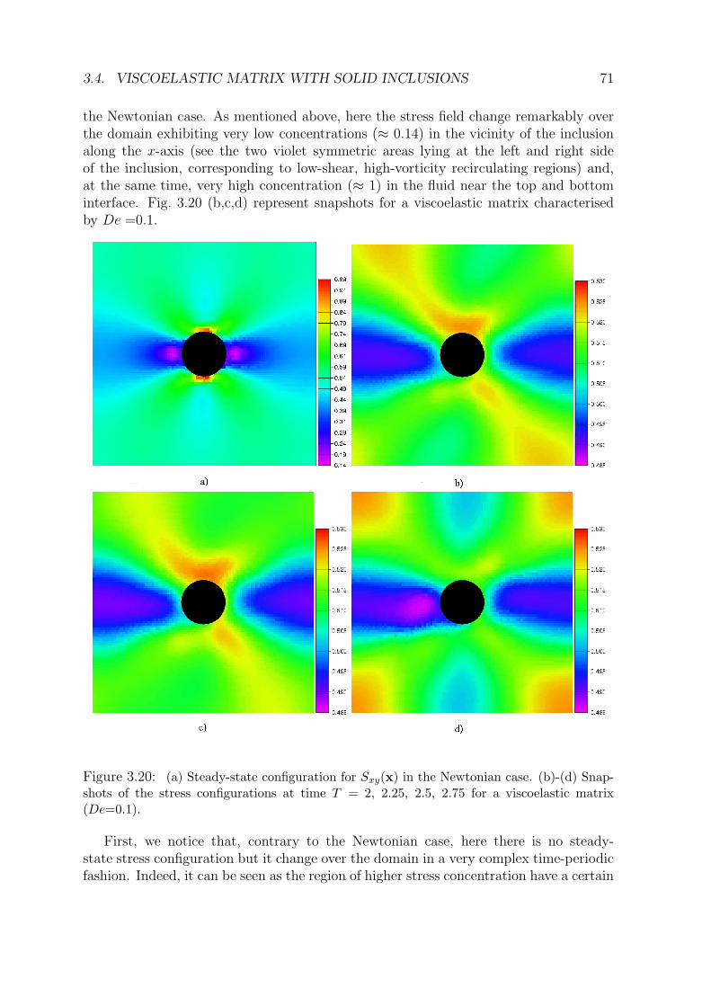
3.4. VISCOELASTIC MATRIX WITH SOLID INCLUSIONS 71
the Newtonian case. As mentioned above, here the stress field change remarkably overthe domain exhibiting very low concentrations (≈ 0.14) in the vicinity of the inclusionalong the x-axis (see the two violet symmetric areas lying at the left and right sideof the inclusion, corresponding to low-shear, high-vorticity recirculating regions) and,at the same time, very high concentration (≈ 1) in the fluid near the top and bottominterface. Fig. 3.20 (b,c,d) represent snapshots for a viscoelastic matrix characterisedby De =0.1.
Figure 3.20: (a) Steady-state configuration for Sxy(x) in the Newtonian case. (b)-(d) Snap-shots of the stress configurations at time T = 2, 2.25, 2.5, 2.75 for a viscoelastic matrix(De=0.1).
First, we notice that, contrary to the Newtonian case, here there is no steady-state stress configuration but it change over the domain in a very complex time-periodicfashion. Indeed, it can be seen as the region of higher stress concentration have a certain
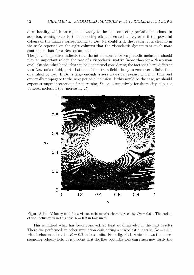
72 CHAPTER 3. SMOOTHED PARTICLE FOR VISCOELASTIC FLOWS
directionality, which corresponds exactly to the line connecting periodic inclusions. Inaddition, coming back to the smoothing effect discussed above, even if the powerfulcolours of the images corresponding to De=0.1 could trick the reader, it is clear formthe scale reported on the right columns that the viscoelastic dynamics is much morecontinuous than for a Newtonian matrix.The previous pictures indicate that the interactions between periodic inclusions shouldplay an important role in the case of a viscoelastic matrix (more than for a Newtonianone). On the other hand, this can be understood considering the fact that here, differentto a Newtonian fluid, perturbations of the stress fields decay to zero over a finite timequantified by De. If De is large enough, stress waves can persist longer in time andeventually propagate to the next periodic inclusion. If this would be the case, we shouldexpect stronger interactions for increasing De or, alternatively for decreasing distancebetween inclusion (i.e. increasing R).
Figure 3.21: Velocity field for a viscoelastic matrix characterised by De = 0.01. The radiusof the inclusion is in this case R = 0.2 in box units.
This is indeed what has been observed, at least qualitatively, in the next resultsThere, we performed an other simulation considering a viscoelastic matrix, De = 0.01,with inclusions of radius R = 0.2 in box units. From fig. 3.21, which shows the corre-sponding velocity field, it is evident that the flow perturbations can reach now easily the
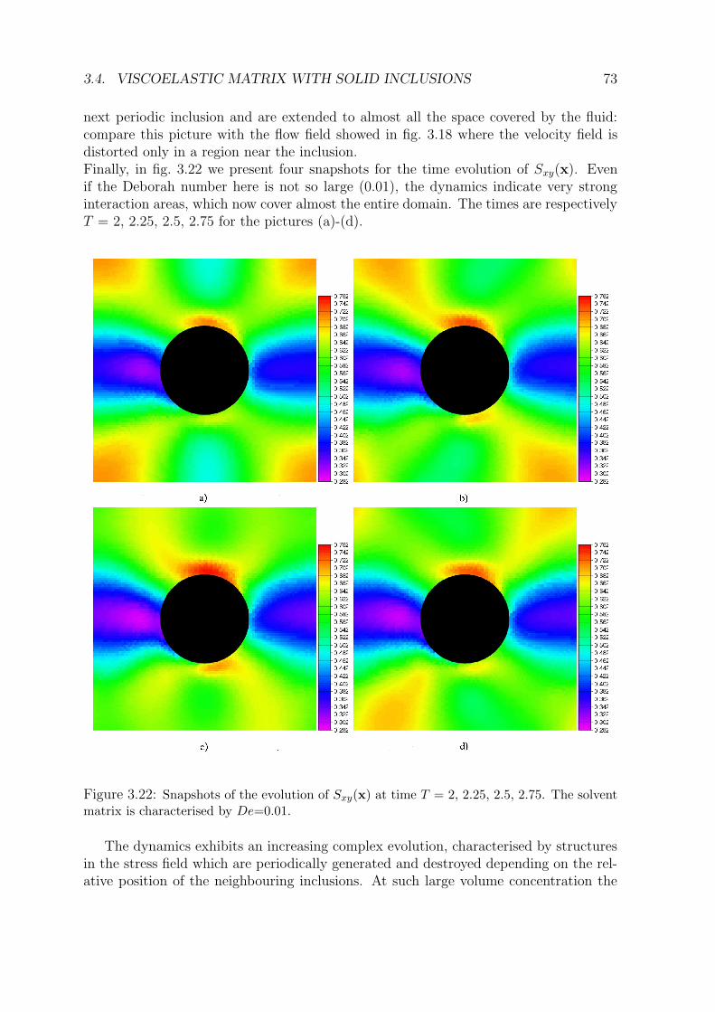
3.4. VISCOELASTIC MATRIX WITH SOLID INCLUSIONS 73
next periodic inclusion and are extended to almost all the space covered by the fluid:compare this picture with the flow field showed in fig. 3.18 where the velocity field isdistorted only in a region near the inclusion.Finally, in fig. 3.22 we present four snapshots for the time evolution of Sxy(x). Evenif the Deborah number here is not so large (0.01), the dynamics indicate very stronginteraction areas, which now cover almost the entire domain. The times are respectivelyT = 2, 2.25, 2.5, 2.75 for the pictures (a)-(d).
Figure 3.22: Snapshots of the evolution of Sxy(x) at time T = 2, 2.25, 2.5, 2.75. The solventmatrix is characterised by De=0.01.
The dynamics exhibits an increasing complex evolution, characterised by structuresin the stress field which are periodically generated and destroyed depending on the rel-ative position of the neighbouring inclusions. At such large volume concentration the
74 CHAPTER 3. SMOOTHED PARTICLE FOR VISCOELASTIC FLOWS
dynamics of the system is definitely influenced by the mutual interactions between therigid objects defining the microstructured network. At such level, the isotropy of thesystem, assumed valid in the limiting case of dilute concentration, is clearly not satisfiedbut very complex directional-preferred macroscopic properties could be showed by theresulting composite material. Further investigations in this direction are a must.
To conclude, we would like to point out that, even if not rigorous, the qualitativelyanalysis carried out in this section has been useful to explain some global propertiesexhibited by the material functions characterizing two-phase composite. The dynamicsof the flow fields showed very exotic behaviours which can be partially understood as aninterplay between two crucial parameters: the Deborah number De, which controls themagnitude of the elastic effects in the matrix, and the volume concentration ρv whichestimates the relative space occupied by the inclusions in the systems. The problemstudied here is not at all closed, inversely, there are still many open questions related tothe connection between macroscopic material properties and microstructural dynamics.In this sense, the results presented in this section should be intended not as definitive,rather as a starting point for new stimulating theoretical and numerical explorations.
Chapter 4
Smoothed Particle Dynamics formesoscopic problems
The modelling of a fluid by a direct discretisation of a deterministic set of partial differ-ential equations is valid, basically, under two ansatz: the continuum hypothesis and theassumptions that thermal fluctuations can be neglected. The first one tells us that thelength and time scales of variation for the variables, which we choose to describe theproblem, are much larger than the typical atomistic scales characterizing the underlyingphysics: that is, the system can be seen as a “continuum”.The second assumption is much more strict than the first one. Indeed, a coarse-grainedsystem where fluctuations can be neglected represents a subclass of a continuous system.In that case, the only effect coming from the elimination of freedom degrees show up asdissipation which can be described deterministically. Systems which satisfy the previoustwo requirements will be called macroscopic. On the other hand, systems which can bestill described continuously but in which fluctuations play a crucial role will be referredlater on as mesoscopic.In this chapter we focus on the description of a complex fluid at the mesoscopic scale.After a brief overview in section 4.1 on the existing numerical techniques, we recall insec. 4.2 the so-called Dissipative Particle Dynamics method for the description of com-plex fluids. Sec. 4.3, 4.4 and 4.5 are devoted to the formulation of a thermodynamicallyconsistent fluid particle model for non-isothermal polymeric solutions. Its structure fol-lows the rigid prescriptions of the generic formalism for the construction of physicalmodels consistent with the First and Second Law of Thermodynamics. In sec. 4.6 thepolymeric diffusivity is considered and introduced in the previous formalism. Finally,numerical results for the isothermal case are presented in sec. 4.8, while in sec. 4.9 wediscuss good aspects and drawbacks of this model.
4.1 Modelling mesoscopic flow problems
The Smoothed Particle methods presented in the first two chapters make the implicitassumption that the macroscopic equations of motion are known on theoretical or phe-nomenological grounds and that they model at a certain level of accuracy the physical
75
76 CHAPTER 4. SMOOTHED PARTICLE FOR MESOSCOPIC PROBLEMS
problem under investigation. This is the case of a simple Newtonian fluid, where theNavier-Stokes equations are an established tool of description. Indeed, for this particularproblem, a consistent derivation from the microscopic “atomistic” picture can be ob-tained using a kinetic theory [69]. On the other hand, exact coarse-graining proceduresapplied to fluids characterised by a complex microstructure are usually not availableand approximated constitutive equations must be used. The problem of deriving “con-sistent” (microscopically) macroscopic constitutive equations for complex fluids will bediscussed in great details in the next chapter.Here, we would like to focus the attention on the mesoscopic level of description of aparticular fluid. In fact, it is well-known that, if the physical scales of the problembecome smaller than a typical length, thermal fluctuations arise naturally in the sys-tem. Evidently, physical problems for which such fluctuations are important can notbe described on the basis of the traditional numerical methods based on a simple dis-cretisation of macroscopic equations. At the same time such problems, involving scalesmuch larger than typical atomistic size, can be numerically very demanding when mod-elled by microscopic techniques, i.e. Molecular Dynamics methods. The presence ofa extraordinary variety of complex phenomena at the mesoscopic scales, ranging fromcolloidal fluids, polymer dynamics to porous systems to mention but a few, creates agreat demand of adequate numerical methods able to capture the physics occurring insuch systems. It is not the goal of this section to give a complete list of the methodswhich have been developed in the last fifty years, however a very schematic overviewof the most popular ones is in order. We can distinguish two basic directions in whichsuch methodologies have been carried on: grid-based techniques and grid-off particlemethods. In the first group enter the well-known Cellular Automata (CA), Lattice Gas(LG) and Lattice Boltzmann (LB) methods. These techniques gained popularity inthe computational community due to their very simple structure which allows for veryefficient numerical algorithms. An overview on the basis of such approaches can befound for example in [70]. On the other hand the presence of some difficulties in thegrid-based methods, mostly associated to lattice artifacts due to the lack of rotationalinvariance, has carried to the development of a large number of off-grid methods whichinvolve the basic, and maybe more physical, concept of “particle” against that one ofgrid node. In this class, maybe the most popular is the so called Dissipative ParticleDynamics method (DPD) and therefore we will spend here some words about. DPD,as originally invented by Hoogerbrugge and Koelman, is a stochastic particle model forthe simulation of Newtonian fluids at mesoscopic scales [71], [72]. In DPD, a Newtonianfluid is represented by a collection of points whose interactions can be defined as a sumof conservative, dissipative and stochastic forces that conserve momentum and producehydrodynamic behaviour. The Brownian stochastic term introduces fluctuations in thesystem, mimicking the statistical behaviour of the unresolved scales averaged out inthe coarse graining process. The way to introduce it is determined by the fluctuation-dissipation theorem relating the amplitude of the noise to a viscous parameter presentin the dissipative force. This condition ensures the correct fluctuating hydrodynamics asprescribed by the Landau and Lifshitz theory [40]. However, there are many problemsconnecting to this DPD formulation. As it has been recognized by Espanol [73], the
4.2. MESOSCOPIC SIMULATIONS OF COMPLEX FLUIDS 77
original DPD model cannot specify an arbitrary thermodynamic behaviour (i.e the formof equation of state is dictated by the kinetic theory derivation), it has not a well-definedphysical scale and one needs to use kinetic theory to relate the transport coefficients ofthe fluid with model parameters. Nevertheless, it has been shown that by including inthe original DPD model two extra state variables, the internal energy and the volumeof the particles, one can solve its conceptual shortcoming, exhuming a thermodynami-
cally consistent (TC) version of DPD which has a strong resemblance in the structurewith the Smoothed Particle Hydrodynamics method except for the presence of thermalfluctuations. The new method extracts, so to say, the best of the two techniques abovementioned, thermal fluctuations from DPD and connection to Navier-Stokes from SPH:the resulting formulation can be also seen as a TC version of SPH which should beuse in place of the usual SPH equations as far as the length scale characterizing theproblem is so small that the fluid feels effects of its microstructure. The connectionbetween DPD and SPH with its relative TC version has been deeply investigate in [73]in the case of simple Newtonian fluids. The generalisation of this model for the studyof more complex viscoelastic fluids will be the subject of this chapter [74].
4.2 Mesoscopic simulations of complex fluids
The primary objective of DPD research has been to use this stochastic fluid solver for thestudy of Non-Newtonian fluids displaying interesting and complex rheological behaviourlike, for example, colloidal suspensions and polymeric solutions. The simple Newtonianfluid of DPD has been made “complex” by introducing additional interactions betweenthe dissipative particles. For example, the complex rheological behaviour of colloidalsuspensions has been simulated by freezing spheres (i.e. introducing a rigid interactionbetween particles) of DPD particles that behave like solid suspended objects [75], [76],[77]. Polymer solutions have been simulated by connecting some of the dissipativeparticles with springs [78], [79]. Binary mixtures have been also modelled by consideringtwo types of particles that interact with different interaction parameters [80], [81], [82].In this respect, DPD turns out to be a versatile method for the simulation of complexfluids. A couple of recent reviews on applications of DPD to the simulation of complexfluids can be found in Refs. [83], [84].
A very interesting generalisation of the Dissipative Particle Dynamics model hasbeen recently introduced by ten Bosch in order to study polymer flows [30]. The ideais to capture the complex behaviour of polymeric fluids by introducing an additionalvariable Q associated to each particle [30]. The vector Q collects the elastic informa-tion about the fluid at scales “within” the dissipative particles. The introduction ofthe additional internal variable Q is a radically different way of introducing complex-ity in the DPD model. It actually changes the scale of the technique with respect tothose DPD simulations in which elasticity is modelled through springs connecting dis-sipative particles. A particle in the ten Bosch model would represent large portions ofparticles in previous DPD simulations of polymers. It represents, therefore, a seriouscomputational advantage. Of course, the price to pay for this advantage is the requireddeep knowledge of the physics of the mesoscopic viscoelasticity in order to formulate
78 CHAPTER 4. SMOOTHED PARTICLE FOR MESOSCOPIC PROBLEMS
the suitable equations of motion for Q. Because the ten Bosch model is a more coarsegrained model than the usual DPD models for polymers, molecular details are hiddenin the phenomenological parameters of the model. However, from the point of viewof applications and computer time saving, this might be regarded in some cases as abenefit.
The ten Bosch model suffers from the same conceptual shortcomings of the originalDPD model: it is not thermodynamically consistent, it is not possible to specify arbi-trary thermodynamic behaviour, has not a well-defined physical scale, and one needs touse kinetic theory to relate the transport coefficients of the fluid with the parameters ofthe model. The aim of this chapter is to formulate in a thermodynamically consistentway a generalisation of the ten Bosch model to non-isothermal situations. To this endwe first formulate a model in which each fluid particle contains a fixed number of dumb-bells. This model can be understood as a Lagrangian SPH version of the connffessit
approach [11], [85]. Inspired by this model, in a second step we consider only one elon-gation variable per fluid particle, as in the ten Bosch model. This second model is muchfaster to simulate because of the large reduction of dumbbell variables in the system.In addition, this second model incorporates the number of dumbbells in the cell as anadditional variable and allows one to study polymer diffusivity problems. The modelis essentially a version of the smoothed particle hydrodynamic model like the one pre-sented in Ref. [73], with additional elastic variables. As a final remark, we note that thisapproach is radically different to that one presented in the previous chapter. Indeed,here the viscoelasticity is introduced by modelling mechanically the behaviour of modelsprings, without assuming the validity of suitable macroscopic constitutive equations.As it will be clear later, as far as this model will be used at macroscopic scale, the priceto pay will be memory and CPU-time requirements for the numerical algorithm.
4.3 TC fluid particle model of polymer solutions
A very convenient way to construct new discrete models for fluid dynamics which areconsistent with Thermodynamics is by using the generic framework [86] which wesummarise in Appendix A. This framework, introduced by Ottinger and Grmela, cap-tures in a very synthetic way all the required constraints that a model should satisfyin order to comply with the First and Second Law. It also describes how to introducethermal fluctuations in a consistent way through the Fluctuation-Dissipation theorem.No additional physics is introduced in generic further than the First and Second Lawsand the Fluctuation-Dissipation theorem. However, it facilitates enormously the task ofconstructing new models which are compatible with these physical laws. This approachhas been successfully used in Refs. [73], [28], [87], where mesoscale fluid particle modelsfor Newtonian fluids have been constructed.
Here we model a polymeric solution through a collection of M fluid particles withpositions ri and velocities vi which are understood as representing real portions of thematerial. They are regarded actually as small thermodynamic subsystems that movefollowing the flow. Each thermodynamic subsystem is composed by N s
i molecules of thesolvent plus the N d
i polymer molecules. We will assume initially that the numbers N si ,
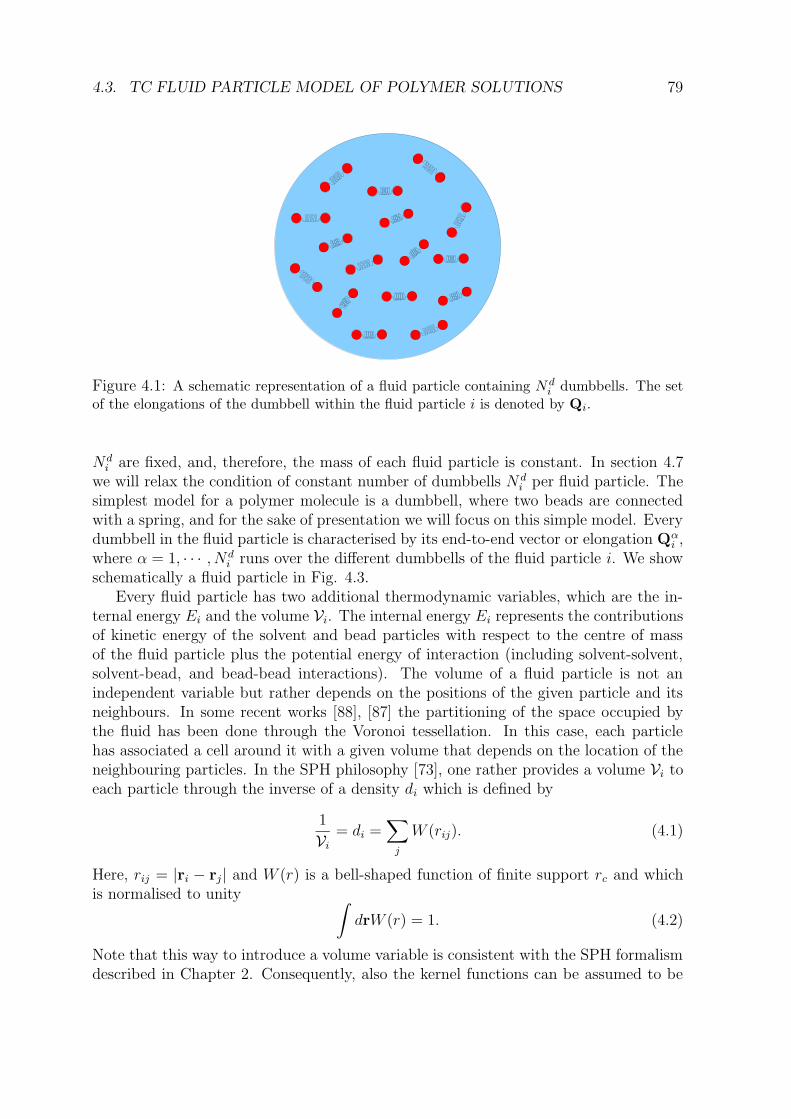
4.3. TC FLUID PARTICLE MODEL OF POLYMER SOLUTIONS 79
Figure 4.1: A schematic representation of a fluid particle containing N di dumbbells. The set
of the elongations of the dumbbell within the fluid particle i is denoted by Qi.
Ndi are fixed, and, therefore, the mass of each fluid particle is constant. In section 4.7
we will relax the condition of constant number of dumbbells N di per fluid particle. The
simplest model for a polymer molecule is a dumbbell, where two beads are connectedwith a spring, and for the sake of presentation we will focus on this simple model. Everydumbbell in the fluid particle is characterised by its end-to-end vector or elongation Qα
i ,where α = 1, · · · , N d
i runs over the different dumbbells of the fluid particle i. We showschematically a fluid particle in Fig. 4.3.
Every fluid particle has two additional thermodynamic variables, which are the in-ternal energy Ei and the volume Vi. The internal energy Ei represents the contributionsof kinetic energy of the solvent and bead particles with respect to the centre of massof the fluid particle plus the potential energy of interaction (including solvent-solvent,solvent-bead, and bead-bead interactions). The volume of a fluid particle is not anindependent variable but rather depends on the positions of the given particle and itsneighbours. In some recent works [88], [87] the partitioning of the space occupied bythe fluid has been done through the Voronoi tessellation. In this case, each particlehas associated a cell around it with a given volume that depends on the location of theneighbouring particles. In the SPH philosophy [73], one rather provides a volume Vi toeach particle through the inverse of a density di which is defined by
1
Vi
= di =∑
j
W (rij). (4.1)
Here, rij = |ri − rj| and W (r) is a bell-shaped function of finite support rc and whichis normalised to unity
∫
drW (r) = 1. (4.2)
Note that this way to introduce a volume variable is consistent with the SPH formalismdescribed in Chapter 2. Consequently, also the kernel functions can be assumed to be
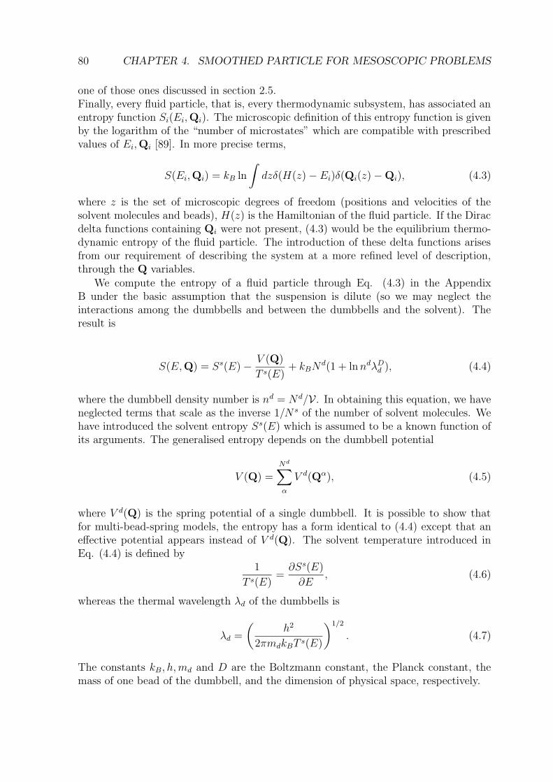
80 CHAPTER 4. SMOOTHED PARTICLE FOR MESOSCOPIC PROBLEMS
one of those ones discussed in section 2.5.Finally, every fluid particle, that is, every thermodynamic subsystem, has associated anentropy function Si(Ei,Qi). The microscopic definition of this entropy function is givenby the logarithm of the “number of microstates” which are compatible with prescribedvalues of Ei,Qi [89]. In more precise terms,
S(Ei,Qi) = kB ln
∫
dzδ(H(z) − Ei)δ(Qi(z) − Qi), (4.3)
where z is the set of microscopic degrees of freedom (positions and velocities of thesolvent molecules and beads), H(z) is the Hamiltonian of the fluid particle. If the Diracdelta functions containing Qi were not present, (4.3) would be the equilibrium thermo-dynamic entropy of the fluid particle. The introduction of these delta functions arisesfrom our requirement of describing the system at a more refined level of description,through the Q variables.
We compute the entropy of a fluid particle through Eq. (4.3) in the AppendixB under the basic assumption that the suspension is dilute (so we may neglect theinteractions among the dumbbells and between the dumbbells and the solvent). Theresult is
S(E,Q) = Ss(E) − V (Q)
T s(E)+ kBN
d(1 + lnndλDd ), (4.4)
where the dumbbell density number is nd = Nd/V . In obtaining this equation, we haveneglected terms that scale as the inverse 1/N s of the number of solvent molecules. Wehave introduced the solvent entropy Ss(E) which is assumed to be a known function ofits arguments. The generalised entropy depends on the dumbbell potential
V (Q) =Nd∑
α
V d(Qα), (4.5)
where V d(Q) is the spring potential of a single dumbbell. It is possible to show thatfor multi-bead-spring models, the entropy has a form identical to (4.4) except that aneffective potential appears instead of V d(Q). The solvent temperature introduced inEq. (4.4) is defined by
1
T s(E)=∂Ss(E)
∂E, (4.6)
whereas the thermal wavelength λd of the dumbbells is
λd =
(
h2
2πmdkBT s(E)
)1/2
. (4.7)
The constants kB, h,md and D are the Boltzmann constant, the Planck constant, themass of one bead of the dumbbell, and the dimension of physical space, respectively.
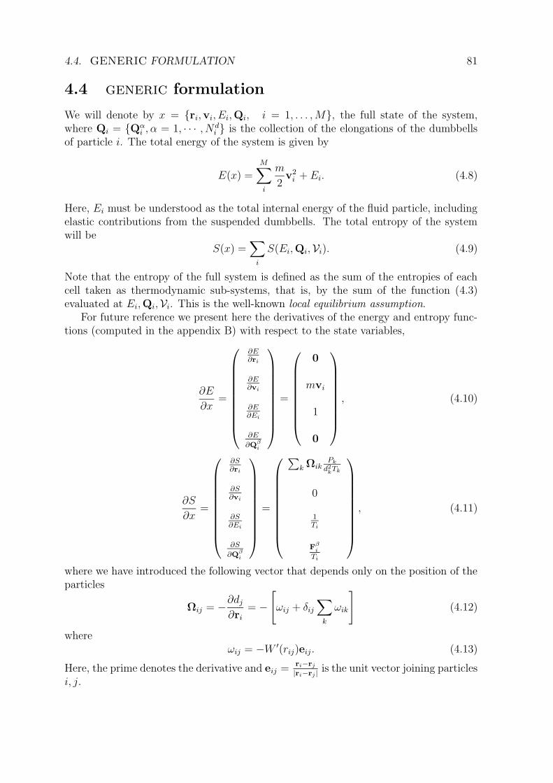
4.4. GENERIC FORMULATION 81
4.4 generic formulation
We will denote by x = ri,vi, Ei,Qi, i = 1, . . . ,M, the full state of the system,where Qi = Qα
i , α = 1, · · · , N di is the collection of the elongations of the dumbbells
of particle i. The total energy of the system is given by
E(x) =M∑
i
m
2v2
i + Ei. (4.8)
Here, Ei must be understood as the total internal energy of the fluid particle, includingelastic contributions from the suspended dumbbells. The total entropy of the systemwill be
S(x) =∑
i
S(Ei,Qi,Vi). (4.9)
Note that the entropy of the full system is defined as the sum of the entropies of eachcell taken as thermodynamic sub-systems, that is, by the sum of the function (4.3)evaluated at Ei,Qi,Vi. This is the well-known local equilibrium assumption.
For future reference we present here the derivatives of the energy and entropy func-tions (computed in the appendix B) with respect to the state variables,
∂E
∂x=
∂E∂ri
∂E∂vi
∂E∂Ei
∂E
∂Qβi
=
0
mvi
1
0
, (4.10)
∂S
∂x=
∂S∂ri
∂S∂vi
∂S∂Ei
∂S
∂Qβi
=
∑
k ΩikPk
d2kTk
0
1Ti
Fβi
Ti
, (4.11)
where we have introduced the following vector that depends only on the position of theparticles
Ωij = −∂dj
∂ri
= −[
ωij + δij∑
k
ωik
]
(4.12)
whereωij = −W ′(rij)eij. (4.13)
Here, the prime denotes the derivative and eij =ri−rj
|ri−rj |is the unit vector joining particles
i, j.
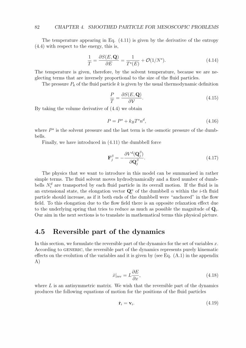
82 CHAPTER 4. SMOOTHED PARTICLE FOR MESOSCOPIC PROBLEMS
The temperature appearing in Eq. (4.11) is given by the derivative of the entropy(4.4) with respect to the energy, this is,
1
T=∂S(E,Q)
∂E=
1
T s(E)+ O(1/N s). (4.14)
The temperature is given, therefore, by the solvent temperature, because we are ne-glecting terms that are inversely proportional to the size of the fluid particles.
The pressure Pk of the fluid particle k is given by the usual thermodynamic definition
P
T=∂S(E,Q)
∂V . (4.15)
By taking the volume derivative of (4.4) we obtain
P = P s + kBTsnd, (4.16)
where P s is the solvent pressure and the last term is the osmotic pressure of the dumb-bells.
Finally, we have introduced in (4.11) the dumbbell force
Fβj = −
∂V d(Qβj )
∂Qβj
. (4.17)
The physics that we want to introduce in this model can be summarised in rathersimple terms. The fluid solvent moves hydrodynamically and a fixed number of dumb-bells Nd
i are transported by each fluid particle in its overall motion. If the fluid is inan extensional state, the elongation vector Qα
i of the dumbbell α within the i-th fluidparticle should increase, as if it both ends of the dumbbell were “anchored” in the flowfield. To this elongation due to the flow field there is an opposite relaxation effect dueto the underlying spring that tries to reduce as much as possible the magnitude of Qi.Our aim in the next sections is to translate in mathematical terms this physical picture.
4.5 Reversible part of the dynamics
In this section, we formulate the reversible part of the dynamics for the set of variables x.According to generic, the reversible part of the dynamics represents purely kinematiceffects on the evolution of the variables and it is given by (see Eq. (A.1) in the appendixA)
x|rev = L∂E
∂x, (4.18)
where L is an antisymmetric matrix. We wish that the reversible part of the dynamicsproduces the following equations of motion for the positions of the fluid particles
ri = vi. (4.19)
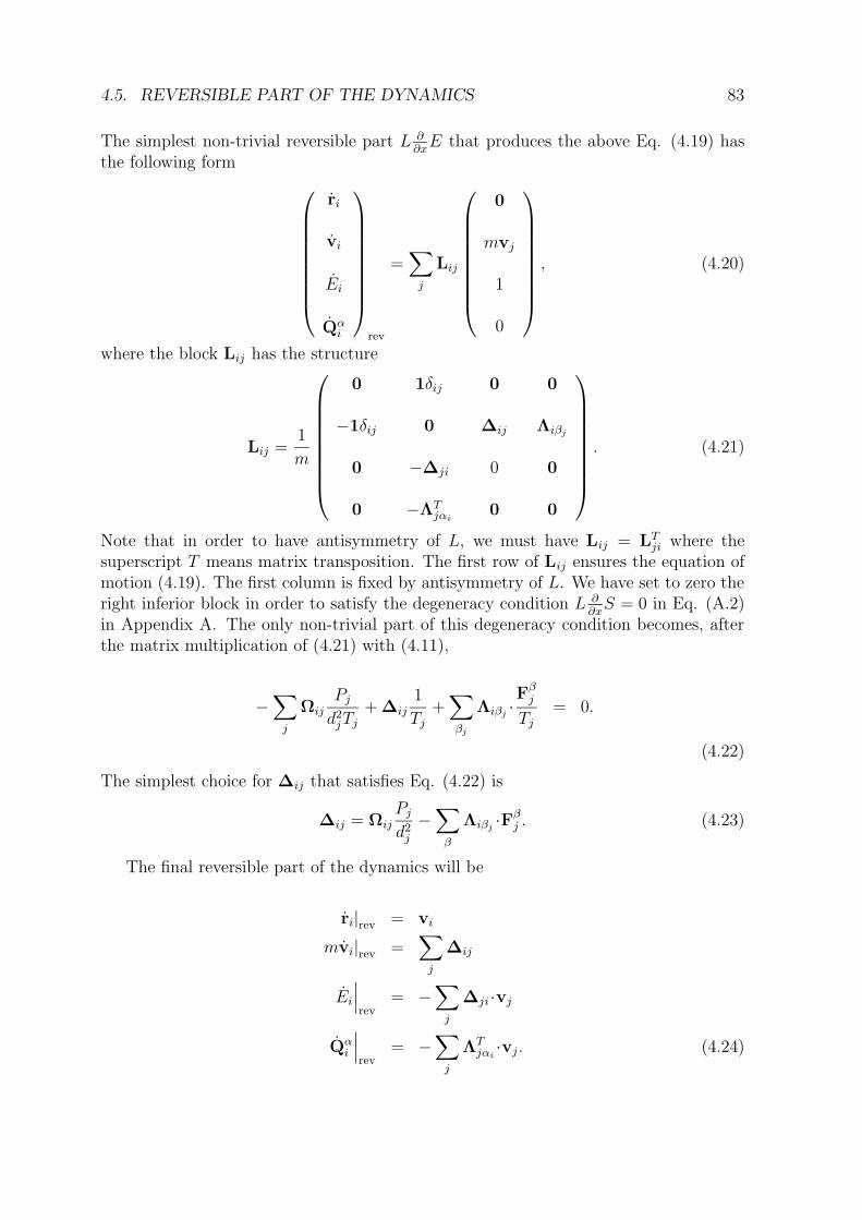
4.5. REVERSIBLE PART OF THE DYNAMICS 83
The simplest non-trivial reversible part L ∂∂xE that produces the above Eq. (4.19) has
the following form
ri
vi
Ei
Qαi
rev
=∑
j
Lij
0
mvj
1
0
, (4.20)
where the block Lij has the structure
Lij =1
m
0 1δij 0 0
−1δij 0 ∆ij Λiβj
0 −∆ji 0 0
0 −ΛTjαi
0 0
. (4.21)
Note that in order to have antisymmetry of L, we must have Lij = LTji where the
superscript T means matrix transposition. The first row of Lij ensures the equation ofmotion (4.19). The first column is fixed by antisymmetry of L. We have set to zero theright inferior block in order to satisfy the degeneracy condition L ∂
∂xS = 0 in Eq. (A.2)
in Appendix A. The only non-trivial part of this degeneracy condition becomes, afterthe matrix multiplication of (4.21) with (4.11),
−∑
j
ΩijPj
d2jTj
+ ∆ij1
Tj
+∑
βj
Λiβj·Fβ
j
Tj
= 0.
(4.22)
The simplest choice for ∆ij that satisfies Eq. (4.22) is
∆ij = ΩijPj
d2j
−∑
β
Λiβj·Fβ
j . (4.23)
The final reversible part of the dynamics will be
ri|rev = vi
mvi|rev =∑
j
∆ij
Ei
∣
∣
∣
rev= −
∑
j
∆ji ·vj
Qαi
∣
∣
∣
rev= −
∑
j
ΛTjαi
·vj. (4.24)

84 CHAPTER 4. SMOOTHED PARTICLE FOR MESOSCOPIC PROBLEMS
Let us turn, now, to the specification of Λij by requiring a particular motion for thevector Qi due to the advection of the fluid. From a continuum point of view, an arbitraryvector A is advected under a velocity field v(r) according to
A = A·∇v(r), (4.25)
where the dot stands for the substantial derivative (Eq. (E.3) in Appendix E). Thephysical picture is that the vector A has its both ends “anchored” in the fluid, as shownheuristically in Appendix C. We want that the elastic vector Qα
i evolves in a similarway. We need, therefore, the gradient of the velocity field at the point where particle iis. Following the SPH philosophy, we interpolate the velocity field according to
v(r) =
∑
j W (r − rj)vj∑
j W (r − rj). (4.26)
By taking the gradient of this expression we obtain
∇v(r) =
∑
j ∇W (r − rj)vj∑
j W (r − rj)− v(r)
∑
j ∇W (r − rj)∑
j W (r − rj). (4.27)
Therefore, at particle i we have the approximate expression for the gradient of thevelocity field
∇v(ri) =
∑
j ∇W (ri − rj)vj
di
− v(ri)
∑
j ∇W (ri − rj)
di
≈ 1
di
∑
j
ωijvij, (4.28)
where vij = vi−vj and ωij is defined in Eq. (4.13). Therefore, the continuum advectionequation (4.25) becomes the discrete equation for the kinematic motion of Qα
i
Qαi =
Qαi
di
·∑
j
ωijvij. (4.29)
By comparing Eq. (4.29) with the last equation in (4.24) we obtain the explicit formfor the matrix −ΛT
ji, i.e.
− ΛTjαi
=Qα
i
di
·[
−ωij + δij∑
k
ωik
]
1
Λiβj= −
Qβj
dj
·[
ωij + δij∑
k
ωik
]
1
= −Qβ
j
dj
·Ωij1. (4.30)
4.6. IRREVERSIBLE PART OF THE DYNAMICS 85
With this particular form of the matrix Λij we can write the vector ∆ij in Eq. (4.23)as
∆ij =1
d2j
Ωij ·[
Pj1 + dj
∑
β
Fβj Q
βj
]
. (4.31)
The term in brackets can be understood as the reversible part of the stress tensor ofparticle j, i.e,
Πj = Pj1 + dj
∑
β
Fβj Q
βj . (4.32)
This stress tensor includes an isotropic component given by pressure in Eq. (4.16) anda non-diagonal part. Substitution of (4.12) and (4.32) into Eqs. (4.24) leads to the finalreversible part of the dynamics for the viscoelastic model
ri|rev = vi
mvi|rev =∑
j
[
Πi
d2i
+Πj
d2j
]
·ωij
Ei
∣
∣
∣
rev= −Πi
d2i
:∑
j
ωijvij
Qαi
∣
∣
∣
rev=
Qαi
di
·∑
j
ωijvij. (4.33)
These equations (4.33) conserve total energy (due to the antisymmetry of L) and leavethe entropy unchanged (due to the degeneracy L ∂S
∂x= 0). They also conserve total
momentum P(x) =∑
imvi due to the symmetries under exchange of the indices i, j inthe momentum equation.
Let us summarise now the line of reasoning followed in this section. We have assumeda particular equation of motion for Qα
i in which this vector is “anchored” in the solvent.This implies a particular form for the matrix Λiβj
in Eq. (4.30). The conservationof energy implied by the antisymmetry of the matrix L imposes that this matrix Λiβj
should appear in an additional term in the momentum equation. The particular formof this term is dictated by the degeneracy condition L ∂S
∂x= 0, Eq. (4.23) which ensures
that there is no entropy production due to the reversible part of the dynamics. As aresult, we have been able to identify a reversible part of the stress tensor, which dependson the configuration Qα
i of the dumbbells. It is quite remarkable that the small physicalinput given by the “anchoring” of Qα
i translates, through the generic formalism, intoa very specific form for the stress tensor. Finally, the energy equation in (4.33) describeshow the mechanical work is transformed into internal energy in a reversible way.
4.6 Irreversible part of the dynamics
As shown in Appendix A, in order to derive the irreversible part of the dynamics ofthe viscoelastic non-isothermal particle model, a very useful route is to first postulate
86 CHAPTER 4. SMOOTHED PARTICLE FOR MESOSCOPIC PROBLEMS
the thermal noises dx and afterwards compute the dissipative matrix M through thefluctuation-dissipation theorem,
M =dxdxT
2kBdt. (4.34)
This procedure ensures that M defined through Eq. (4.34) is automatically symmetricand positive semi-definite.We postulate the following form for the thermal noises dx = 0, dvi, dEi, dQ
αi . Note
that we do not assume any thermal noise for the position of the fluid particles, as wewant to respect the equation of motion ri = vi. In Ref. [73] it has discussed how tointroduce the thermal noises dvi, dEi in order to recover a matrix M which producesan irreversible part of the dynamics that can be understood as a smoothed particlehydrodynamics discretisation of the irreversible terms of the Navier-Stokes equations.We only have to postulate now the noise terms dQα
i . We discuss in the Appendix Dthat a reasonable assumption for the stochastic force on Qα
i is given by
dQαi =
(
4kBTi
6πηa
)1/2
dUαi, (4.35)
where dUαiis an independent increment of the Wiener process, satisfying
dUαidUβj
= δαiβj1dt. (4.36)
We recognise in the prefactor of (4.35) the diffusion coefficient of the beads of radius agiven by the Stokes-Einstein relation. We will assume that the noise dQα
i are statisticallyindependent of dvi, dEi.
According to Eq. (4.34), the matrix M → Mij is given by
0 0 0 0
0dvidv
Tj
2kBdt
dvidEj
2kBdt0
0dEidv
Tj
2kBdt
dEidEj
2kBdt0
0 0 0dQα
i dQβj
2kBdt
. (4.37)
The central diagonal block has been computed in Ref. [73] and we have to compute onlythe last diagonal element, which is
dQαi dQ
βj
2kBdt=
2Ti
ζδαβδij1. (4.38)
Now we are in position to write the deterministic irreversible part of the dynamics
4.6. IRREVERSIBLE PART OF THE DYNAMICS 87
x|irr = M · ∂S∂x
which, after use of Eq. (4.11) for the derivative of the entropy, becomes
ri
vi
Ei
Qαi
|irr
=∑
j
Mij
∑
k ΩjkPk
d2kTk
0
1Tj
Fβj
Tj
, (4.39)
By collecting the results of [73] (once we neglect, for simplicity, the bulk viscosity) forthe diagonal blocks of Mij together with (4.38) we obtain the following irreversible partof the dynamics
ri|irr = 0
mvi|irr = −5η
3
∑
j
Fij
didj
(vij + (eij ·vij)eij)
Ei|irr =1
2
5η
3
∑
j
Fij
didj
(
v2ij + (vij ·eij)
2)
− 2κ∑
j
Fij
didj
Tij
Qαi |irr =
2
ζFα
i , (4.40)
where η is the shear viscosity of the solvent and κ the thermal conductivity. Thegeometrical factor Fij is given by
Fij = −W′(rij)
rij
. (4.41)
Note that concerning the irreversible part of the dynamics, the solvent and dumbbellsare completely uncoupled and, therefore, the solvent irreversible dynamics is identicalto that in Ref. [73].
By collecting the reversible part of the dynamics Eqs. (4.33) and the irreversiblepart of the dynamics Eqs. (4.40) we obtain the following set of deterministic equations,corresponding to Eq. (A.1)
88 CHAPTER 4. SMOOTHED PARTICLE FOR MESOSCOPIC PROBLEMS
ri = vi
mvi =∑
j
[
Πi
d2i
+Πj
d2j
]
·ωij
− 5η
3
∑
j
Fij
didj
(vij + (eij ·vij)eij)
Ei = −Πi
d2i
:∑
j
ωijvij
+1
2
5η
3
∑
j
Fij
didj
(
v2ij + (vij ·eij)
2)
− 2κ∑
j
Fij
didj
Tij
Qαi =
Qαi
di
·∑
j
ωijvij +2
ζFα
i . (4.42)
This set of equations have the very appealing features of conserving energy and totalmomentum P =
∑
imvi, and leading to a positive production of entropy S(x) ≥ 0.The evolution of ri,vi, Ei is identical to that of a simple fluid without dumbbells, as givenin Ref. [73], except for the additional dumbbell contribution to the stress tensor in Eq.(4.32). Apart from that, we recognise in these equations the different physical processesinvolved. In the momentum equation, viscous forces proportional to the viscosity tryto reduce velocity differences between fluid particles. In the energy equation, a viscousheating term proportional to the shear viscosity describes how the kinetic energy whichis dissipated by the friction forces leads to an increase of internal energy of the particles.Also in this energy equation, the heat conduction term, with overall magnitude given bythe thermal conductivity of the solvent, tries to reduce temperature differences betweenfluid particles.Finally, the last set of equations governs the dynamics of the elongation of every singledumbbell in the solution. Let us discuss with some detail this set of equations for thesimplest case of Hooke an dumbbells. For Hooke an dumbbells Fα
i = −HQαi , where
H is the spring constant, and the last irreversible term describes an exponential decaygoverned by a time scale given by ζ/2H. Given an initial elongation of every dumbbellin each fluid particle, this terms relaxes it towards a zero elongation. The advectiveterm cannot do anything against this relaxation and, actually, Qα
i = 0 is the finalsolution of the equations for the dumbbell elongation. Apparently, we have deriveda very stupid model in which the dumbbells just relax towards zero elongations, thedumbbell contribution to the stress tensor vanish, and we are back to the model for aNewtonian fluid.Of course, an essential element is lacking in the above set of equations, which is thepresence of thermal fluctuations. Thermal fluctuations are the crucial bit that rendersthe present model sensible and useful for the simulation of polymer solutions. The way
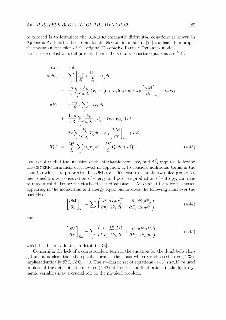
4.6. IRREVERSIBLE PART OF THE DYNAMICS 89
to proceed is to formulate the generic stochastic differential equations as shown inAppendix A. This has been done for the Newtonian model in [73] and leads to a properthermodynamic version of the original Dissipative Particle Dynamics model.For the viscoelastic model presented here, the set of stochastic equations are [74].
dri = vidt
mdvi =∑
j
[
Πi
d2i
+Πj
d2j
]
·ωijdt
− 5η
3
∑
j
Fij
didj
(vij + (eij ·vij)eij) dt+ kB
[
∂M
∂x
]
v,i
+mdvi
dEi = −Πi
d2i
:∑
j
ωijvijdt
+1
2
5η
3
∑
j
Fij
didj
(
v2ij + (vij ·eij)
2)
dt
− 2κ∑
j
Fij
didj
Tijdt+ kB
[
∂M
∂x
]
E,i
+ dEi
dQαi =
Qαi
di
·∑
j
ωijvijdt−2H
ζQα
i dt+ dQαi . (4.43)
Let us notice that the inclusion of the stochastic terms dvi and dEi requires, followingthe generic formalism overviewed in appendix 1, to consider additional terms in theequation which are proportional to ∂M/∂x. This ensures that the two nice propertiesmentioned above, conservation of energy and positive production of entropy, continueto remain valid also for the stochastic set of equations. An explicit form for the termsappearing in the momentum and energy equations involves the following sums over theparticles
[
∂M
∂x
]
v,i
=∑
j
(
∂
∂vj
dvidvTj
2kBdt+
∂
∂Ej
dvidEj
2kBdt
)
(4.44)
and
[
∂M
∂x
]
E,i
=∑
j
(
∂
∂vj
dEidvTj
2kBdt+
∂
∂Ej
dEidEj
2kBdt
)
(4.45)
which has been evaluated in detail in [73].Concerning the lack of a correspondent term in the equation for the dumbbells elon-
gation, it is clear that the specific form of the noise which we choosed in eq.(4.38),implies identically ∂Mij/∂Qi = 0. The stochastic set of equations (4.43) should be usedin place of the deterministic ones, eq.(4.42), if the thermal fluctuations in the hydrody-namic variables play a crucial role in the physical problem.
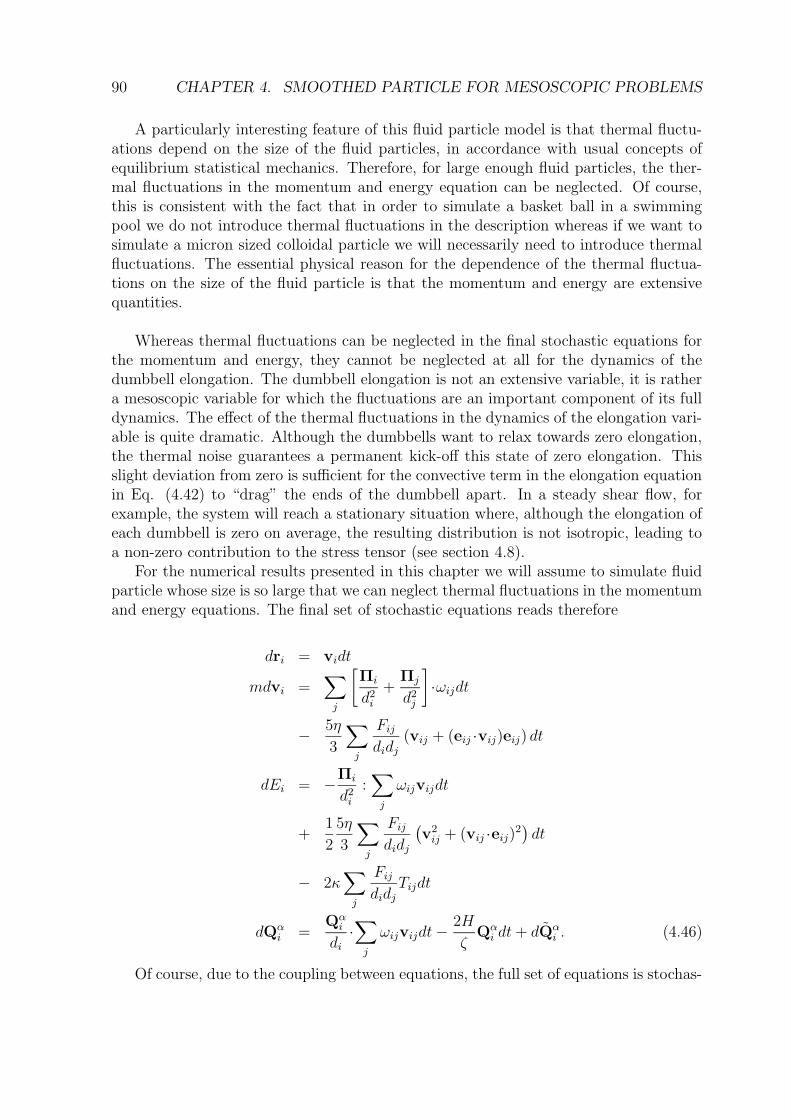
90 CHAPTER 4. SMOOTHED PARTICLE FOR MESOSCOPIC PROBLEMS
A particularly interesting feature of this fluid particle model is that thermal fluctu-ations depend on the size of the fluid particles, in accordance with usual concepts ofequilibrium statistical mechanics. Therefore, for large enough fluid particles, the ther-mal fluctuations in the momentum and energy equation can be neglected. Of course,this is consistent with the fact that in order to simulate a basket ball in a swimmingpool we do not introduce thermal fluctuations in the description whereas if we want tosimulate a micron sized colloidal particle we will necessarily need to introduce thermalfluctuations. The essential physical reason for the dependence of the thermal fluctua-tions on the size of the fluid particle is that the momentum and energy are extensivequantities.
Whereas thermal fluctuations can be neglected in the final stochastic equations forthe momentum and energy, they cannot be neglected at all for the dynamics of thedumbbell elongation. The dumbbell elongation is not an extensive variable, it is rathera mesoscopic variable for which the fluctuations are an important component of its fulldynamics. The effect of the thermal fluctuations in the dynamics of the elongation vari-able is quite dramatic. Although the dumbbells want to relax towards zero elongation,the thermal noise guarantees a permanent kick-off this state of zero elongation. Thisslight deviation from zero is sufficient for the convective term in the elongation equationin Eq. (4.42) to “drag” the ends of the dumbbell apart. In a steady shear flow, forexample, the system will reach a stationary situation where, although the elongation ofeach dumbbell is zero on average, the resulting distribution is not isotropic, leading toa non-zero contribution to the stress tensor (see section 4.8).
For the numerical results presented in this chapter we will assume to simulate fluidparticle whose size is so large that we can neglect thermal fluctuations in the momentumand energy equations. The final set of stochastic equations reads therefore
dri = vidt
mdvi =∑
j
[
Πi
d2i
+Πj
d2j
]
·ωijdt
− 5η
3
∑
j
Fij
didj
(vij + (eij ·vij)eij) dt
dEi = −Πi
d2i
:∑
j
ωijvijdt
+1
2
5η
3
∑
j
Fij
didj
(
v2ij + (vij ·eij)
2)
dt
− 2κ∑
j
Fij
didj
Tijdt
dQαi =
Qαi
di
·∑
j
ωijvijdt−2H
ζQα
i dt+ dQαi . (4.46)
Of course, due to the coupling between equations, the full set of equations is stochas-
4.7. POLYMER DIFFUSIVITY 91
tic even though there is only one noise source dQαi . It may appear odd that having
neglected thermal fluctuations in the momentum and energy equations, the equationsfor these variables still retain a stochastic character. However, we should remark thatwhat we have neglected are spontaneous thermal fluctuations as they appear in theLandau-Lifshitz theory of fluctuating hydrodynamics. Its physical origin is the ran-dom interchange of solvent molecules between fluid particles, and these fluctuations aresmall as compared with the total amount of momentum or energy in the fluid particle.However, the fluctuations in the Qα
i variables have an indirect effect on the momentumand energy variables through the coupling via the stress tensor. The importance of thisindirect coupling depends, of course, on the concentration of polymer molecules and thestrength of the springs, and can make a crucial contribution to the dynamic behaviourof the fluid.
4.7 Polymer diffusivity
The model governed by Eqs. (4.46) describes the dynamics of every single dumbbell inthe system. This approach is a similar to connffessit [11], [85], where a stochasticsimulation of the dumbbells is coupled with a numerical solution of the fluid flows. Ofcourse, having to keep track of the evolution of every single dumbbell in each fluidparticle is an expensive task. Note that, according to the last equation in (4.46), all thedumbbells of a given fluid particle will display essentially the same behaviour, at leastin a statistical sense. The dynamics of different dumbbells of the same fluid particlediffers only by the initial conditions and the actual sequence of random numbers usedfor the stochastic term. For this reason, we could focus on a given tagged dumbbellwithin each fluid particle and assume that the rest of dumbbells of that fluid particle“is doing the same thing”.
In addition, the model presented above has a constant number of dumbbells in everyfluid particle. This does not seem to be a very reasonable assumption. After all, if thebeads of each dumbbell are subject to thermal fluctuations, then the centre of massof the dumbbell will suffer also from thermal fluctuations, leading to a diffusion of thecentre of mass of the dumbbells within the region of a fluid particle until they cross thefluid particle’s “boundary”. This, eventually, should lead to an interchange of dumbbellsbetween fluid particles. The model in Eqs. (4.46) does not allow for a change in timeof the number of dumbbells in a fluid particle.
In order to encompass the possibility of describing polymer diffusion and, at thesame time, reduce the number of variables to simulate, we present in this section a newmodel that differs from the one presented in the previous sections in the variables usedto describe the state of the system. Now, each fluid particle will be characterised byits position ri, its velocity vi, its internal energy Ei, a unique vector Qi describing theelongation of a statistical representative of the dumbbells, and the number of dumb-bells Nd
i within the fluid particle. By selecting a single elongation vector for every fluidparticle we return to a version of the ten Bosch model which, in turn, is analogous to aLagrangian version of the Brownian Configuration Field Approach [12]. The BrownianConfiguration Field Approach is similar to the connffessit approach except that only
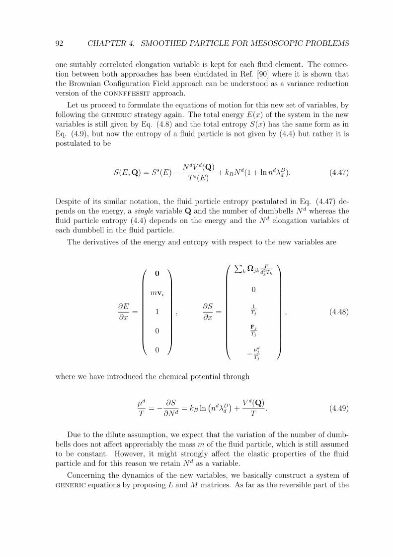
92 CHAPTER 4. SMOOTHED PARTICLE FOR MESOSCOPIC PROBLEMS
one suitably correlated elongation variable is kept for each fluid element. The connec-tion between both approaches has been elucidated in Ref. [90] where it is shown thatthe Brownian Configuration Field approach can be understood as a variance reductionversion of the connffessit approach.
Let us proceed to formulate the equations of motion for this new set of variables, byfollowing the generic strategy again. The total energy E(x) of the system in the newvariables is still given by Eq. (4.8) and the total entropy S(x) has the same form as inEq. (4.9), but now the entropy of a fluid particle is not given by (4.4) but rather it ispostulated to be
S(E,Q) = Ss(E) − NdV d(Q)
T s(E)+ kBN
d(1 + lnndλDd ). (4.47)
Despite of its similar notation, the fluid particle entropy postulated in Eq. (4.47) de-pends on the energy, a single variable Q and the number of dumbbells N d whereas thefluid particle entropy (4.4) depends on the energy and the N d elongation variables ofeach dumbbell in the fluid particle.
The derivatives of the energy and entropy with respect to the new variables are
∂E
∂x=
0
mvi
1
0
0
,∂S
∂x=
∑
k ΩjkP
d2kTk
0
1Tj
Fj
Tj
−µdj
Tj
, (4.48)
where we have introduced the chemical potential through
µd
T= − ∂S
∂Nd= kB ln
(
ndλDd
)
+V d(Q)
T. (4.49)
Due to the dilute assumption, we expect that the variation of the number of dumb-bells does not affect appreciably the mass m of the fluid particle, which is still assumedto be constant. However, it might strongly affect the elastic properties of the fluidparticle and for this reason we retain N d as a variable.
Concerning the dynamics of the new variables, we basically construct a system ofgeneric equations by proposing L and M matrices. As far as the reversible part of the
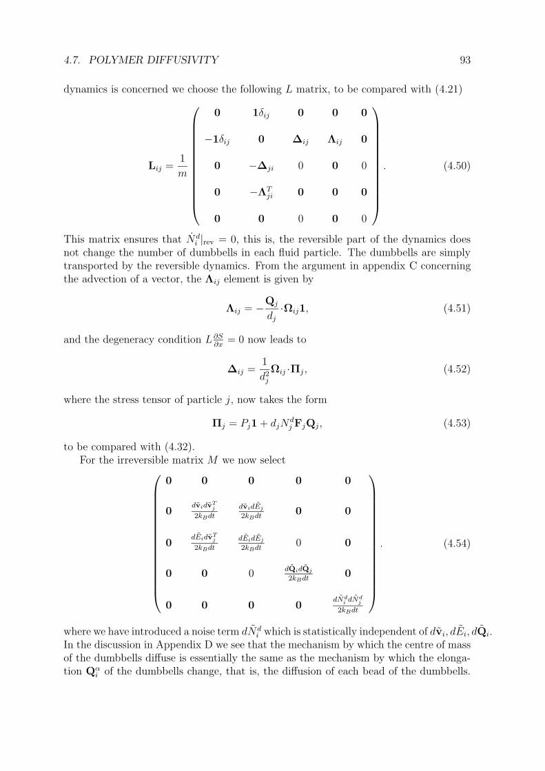
4.7. POLYMER DIFFUSIVITY 93
dynamics is concerned we choose the following L matrix, to be compared with (4.21)
Lij =1
m
0 1δij 0 0 0
−1δij 0 ∆ij Λij 0
0 −∆ji 0 0 0
0 −ΛTji 0 0 0
0 0 0 0 0
. (4.50)
This matrix ensures that Ndi |rev = 0, this is, the reversible part of the dynamics does
not change the number of dumbbells in each fluid particle. The dumbbells are simplytransported by the reversible dynamics. From the argument in appendix C concerningthe advection of a vector, the Λij element is given by
Λij = −Qj
dj
·Ωij1, (4.51)
and the degeneracy condition L∂S∂x
= 0 now leads to
∆ij =1
d2j
Ωij ·Πj, (4.52)
where the stress tensor of particle j, now takes the form
Πj = Pj1 + djNdj FjQj, (4.53)
to be compared with (4.32).For the irreversible matrix M we now select
0 0 0 0 0
0dvidv
Tj
2kBdt
dvidEj
2kBdt0 0
0dEidv
Tj
2kBdt
dEidEj
2kBdt0 0
0 0 0dQidQj
2kBdt0
0 0 0 0dNd
i dNdj
2kBdt
. (4.54)
where we have introduced a noise term dNdi which is statistically independent of dvi, dEi, dQi.
In the discussion in Appendix D we see that the mechanism by which the centre of massof the dumbbells diffuse is essentially the same as the mechanism by which the elonga-tion Qα
i of the dumbbells change, that is, the diffusion of each bead of the dumbbells.
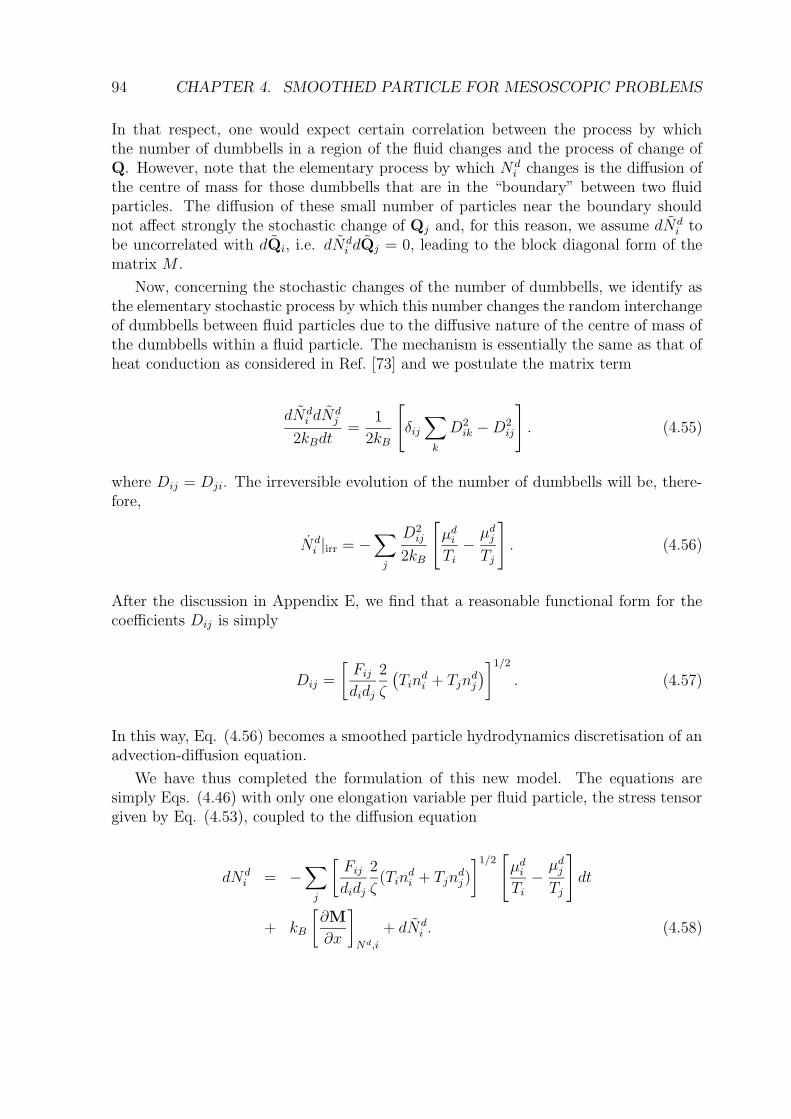
94 CHAPTER 4. SMOOTHED PARTICLE FOR MESOSCOPIC PROBLEMS
In that respect, one would expect certain correlation between the process by whichthe number of dumbbells in a region of the fluid changes and the process of change ofQ. However, note that the elementary process by which N d
i changes is the diffusion ofthe centre of mass for those dumbbells that are in the “boundary” between two fluidparticles. The diffusion of these small number of particles near the boundary shouldnot affect strongly the stochastic change of Qj and, for this reason, we assume dNd
i tobe uncorrelated with dQi, i.e. dNd
i dQj = 0, leading to the block diagonal form of thematrix M .
Now, concerning the stochastic changes of the number of dumbbells, we identify asthe elementary stochastic process by which this number changes the random interchangeof dumbbells between fluid particles due to the diffusive nature of the centre of mass ofthe dumbbells within a fluid particle. The mechanism is essentially the same as that ofheat conduction as considered in Ref. [73] and we postulate the matrix term
dNdi dN
dj
2kBdt=
1
2kB
[
δij∑
k
D2ik −D2
ij
]
. (4.55)
where Dij = Dji. The irreversible evolution of the number of dumbbells will be, there-fore,
Ndi |irr = −
∑
j
D2ij
2kB
[
µdi
Ti
−µd
j
Tj
]
. (4.56)
After the discussion in Appendix E, we find that a reasonable functional form for thecoefficients Dij is simply
Dij =
[
Fij
didj
2
ζ
(
Tindi + Tjn
dj
)
]1/2
. (4.57)
In this way, Eq. (4.56) becomes a smoothed particle hydrodynamics discretisation of anadvection-diffusion equation.
We have thus completed the formulation of this new model. The equations aresimply Eqs. (4.46) with only one elongation variable per fluid particle, the stress tensorgiven by Eq. (4.53), coupled to the diffusion equation
dNdi = −
∑
j
[
Fij
didj
2
ζ(Tin
di + Tjn
dj )
]1/2[
µdi
Ti
−µd
j
Tj
]
dt
+ kB
[
∂M
∂x
]
Nd,i
+ dNdi . (4.58)
4.7. POLYMER DIFFUSIVITY 95
where
[
∂M
∂x
]
Nd,i
=∑
j
(
∂
∂Ndj
dNdi dN
dj
2kBdt
)
=1
2Tidi
∑
j
[
∑
k
(
2Fik
didkζ
)2
− 2
(
2Fij
d2i ζ
)2]
+∑
j
(
2Fij
didjζ
)
Tjdj. (4.59)
This equation conserves the total number of dumbbells∑
i Ndi = 0. The evolution of
the number of dumbbells in each fluid particle is governed by the unbalance of dumbbellchemical potentials between neighbouring fluid particles that will produce an exchangeof dumbbells between fluid particles. This equation couples with the momentum andenergy equations through the stress tensor. Note that the variable N d
i is extensive andwe could neglect the additional stochastic forces in Eq. (4.58) so far as we consider fluidparticle whose size is quite large. In this way, we are assuming that even though thesuspension is dilute, every fluid particle contains a sufficiently large number of dumbbellsfor the fluctuations on the number of dumbbells to be negligible. It is of course possibleto validate this assumption by explicitly including the thermal noise and assess its effect.For the sake of simplicity, we neglect here the stochastic forces (the last two terms Eq.(4.58)), in on the number of dumbbells.
96 CHAPTER 4. SMOOTHED PARTICLE FOR MESOSCOPIC PROBLEMS
4.8 Simulation results
In this section, we present simulation results in order to check and validate the presentmodel. As a first step, we will assume that the number of dumbbells within each fluidparticle is a constant equal to N d
0 , thus neglecting dumbbell diffusion between fluidparticles. We will also assume that the thermal conductivity is very large in such a waythat the temperature is already equilibrated to the same T0 in all the fluid particles. AHookean dumbbell spring will be assumed here. Although the model permits to studymore general situations, the isothermal and constant dumbbell density case allows fora comparison with analytically known predictions for Hookean dumbbells.
The simulated isothermal equations are
dri = vidt
dρi = −ρi
∑
j
m
ρj
vij ·ωijdt
mdvi =∑
j
[
Πi
d2i
+Πj
d2j
]
·ωijdt
− 5ηs
3
∑
j
Fij
didj
(vij + (eij ·vij)eij) dt
dQi =Qi
di
·∑
j
ωijvijdt−2H
ζQidt+ dQi, (4.60)
with
Πi = (Pis + kBT0n
d0)1 −Hnd
0QiQi, (4.61)
where ρi = mdi is the solvent mass density and nd0 = Nd/V is the constant dumbbells
number density. Note that we evaluate here the density by solving a discretized versionof the continuity equation and not like in the simulations presented in chapter 1, byusing a summation over the particle (4.1). We select an ideal gas equation of state forthe solvent pressure P s
i = cpρiT0 where cp is the specific heat at constant pressure. Forthe weight function, we have chosen the Lucy function
W (r) = cW (1 + 3r/rc)(1 − r/rc)3, (4.62)
where cW = 5/πr2c in two dimensions and cW = 105/16πr3
c in three dimension.
In order to make the previous equations dimensionless, we consider the followingbasic units: unit of mass ms (mass of a solvent molecule), unit of length L0 (boxdimension), unit of time λH = ξ/4H (viscoelastic decay time for Hookean dumbbellmodel), unit of temperature T0. We define a reference velocity in terms of the primaryvariables as v0 = L0/λH . By using these units, we can make the above equationsdimensionless (variables with an overline are dimensionless)
4.8. SIMULATION RESULTS 97
dri = vidt
dρi = −ρi
∑
j
m
ρj
vij ·ωijdt
dvi =∑
j
m
[
Πi
ρ2i
+Πj
ρ2j
]
·ωijdt
− C1
∑
j
mF ij
ρiρj
(vij + (eij ·vij)eij) dt
dQi =Qi
ρi
·∑
j
mωijvijdt−1
2Qidt+ dQi, (4.63)
with
dQi = C2dUi
Πi = (Ps
i + C3)1 − C4QiQi
Ps
i = C5ρi. (4.64)
Five non-dimensional constants appear in Eqs. (4.63)-(4.64),
C1 =5ηs
3ρ0L0v0
C2 =
√
kBT0
HL20
(4.65)
C3 =NdkBT0
ρ0v50λ
3H
C4 =NdH
ρ0v30λH
C5 =cpT0
v20
(4.66)
The reference density is ρ0 = msNs/L3
0. Here ms represents the mass of a single solventmolecule and N s the total number of solvent molecules contained in the box. Note thatwe have the usual dimensions for density, pressure, viscosity, etc. corresponding to 3Dsystems. On the other hand, we are performing 2D simulations, under the assumptionof translationally invariant behaviour in the z-direction.
4.8.1 Theoretical results for Hookean dumbbells
Analytical results for an isothermal Couette flow for Hookean dumbbells are availablein the literature [4], and give exact prescriptions for the dependence of the materialfunctions and the stretching of the dumbbells 〈Q2〉 as a function of the shear rate in asteady shear flow. Let us assume a 2D steady shear flow. The Cartesian components ofthe velocity field are by definition
vx = γy vy = 0, (4.67)
98 CHAPTER 4. SMOOTHED PARTICLE FOR MESOSCOPIC PROBLEMS
where γ = ∂vx/∂y is the shear rate. Let us consider now only the polymeric contributionto the pressure tensor. It can be written in tensorial notation:
τ pαβ = kBT0n
d0δαβ −Hnd
0QαQβ, (4.68)
where the Greek indices indicate the spatial coordinates. For Hookean dumbbells, it canbe shown that the stress components and material functions in the final steady stateconfiguration are [4]:
τ pxy = −nd
0kBT0λH γ, (4.69)
τ pyy − τ p
xx = 2nd0kBT0λ
2H γ
2. (4.70)
From Eq. (4.69) and Eq. (4.70), we obtain the polymer contribution to the shearviscosity ηp and the first normal stress difference Ψ1,
ηp = −τ pxy
γ,= nd
0kBT0λH (4.71)
Ψ1 =τ pyy − τ p
xx
γ2= 2nd
0kBT0λ2H . (4.72)
In this Hookean model, all material functions are constant, independent of the shearrate. It is also found that the global dumbbell stretching takes the form (2D):
〈Q2〉〈Q2
eq〉= 1 + (λH γ)
2. (4.73)
This shows that the Hookean dumbbells continue to stretch indefinitely as the shearrate is increased. This characteristic of the dynamics based on the Hookean model isinadequate for the description of realistic polymeric solutions. In fact, it is well-knownthat the viscosity and first normal stress coefficient should decrease for increasing shearrate instead of remaining constant. The failure of the model is related to the infiniteextensibility which is shown in Eq. (4.73). Nevertheless, although this model does notprovide an accurate description of a polymeric solution, it allows for exact comparisonswith numerical results. More complex models like the FENE model, can be easily takeninto account.
4.8.2 Setup of the numerical simulations
In order to produce a uniform stable shear flow, we apply the well-known Lees-Edwardsboundary conditions [36]. The periodic image criterion is applied in both spatial di-rections in order to simulate an infinite periodic medium. In addition, a shear is im-posed along the y-axis simply by moving in opposite directions the periodic boxes atthe top and the bottom of the central simulation box. Their respective velocities are±vbox = γL0, where γ is the desired shear rate. Particles crossing the edge at the topof the simulation box are re-inserted at the bottom with the same y-component of the
4.8. SIMULATION RESULTS 99
velocity vy but with opposite vx. A linear stable velocity profile corresponding to theequation (4.67) is therefore produced.
The numerical parameters of our simulations are: the reference temperature, chosento be the typical room temperature T0 = 300 K, the reference time λH = 1.0 × 10⁻⁶sand the reference length L0 = 1.0 × 10⁻⁵m which corresponds to the length of the box.The reference velocity is therefore v0 = L0/λH = 10 m s−1. We choose a value for ms
corresponding to the mass of a water molecule (ms = 2.98× 10⁻²⁶kg) and total numberof solvent molecules N s = 3.35 × 10¹³. This gives a solvent density ρ0 = 103 kg m−3
corresponding to typical values for water under standard conditions.There are other input parameters which influence the dynamics. The solvent shear
viscosity ηs = 10−3kg m−1s−1. The reference dumbbell number density is defined asnd
0 = Nd/L30, where Nd is an arbitrary number corresponding to the total number of
dumbbells contained in the simulation box. The viscoelastic behaviour is due to the lastterm in the stress tensor in Eq. (4.61). This term is proportional to N d and controlsthe magnitude of the deviatoric non-Newtonian effects. Indeed, for N d = 0 we recoverthe Newtonian fluid dynamics. The value of N d is determined accordingly with all theother parameters in order to obtain a suitable polymeric viscosity consistent with Eq.(4.71). Here we assumed N d = 108. With these parameters and by using the formulas(4.71)-(4.72), we obtain the polymeric contribution to the viscosity ηp = 4.142× 10⁻⁴kgm−1s−1 and the first normal stress coefficient Ψ1 = 8.284 × 10⁻¹⁰kg m−1 in S.I. units.Therefore, in our numerical framework, their dimensionless values are ηp = 4.142×10⁻³
and Ψ1 = 8.284 × 10⁻³. As already noticed, these viscometric functions for a Hookeanspring model should be independent on the shear rate. The spring constant H can bedetermined using the the Stokes-Einstein relation, so that H = 6πηsa/4λH , where a isthe radius of a bead and λH the reference time. Here we chose a = 4.0× 10⁻¹⁰m whichgives a value of H = 1.88 × 10⁻⁶kg s−2. In addition, the equilibrium value for 〈Q2
eq〉 inEq. (4.73) (averaged over all the box domain) for zero shear rate should be equal to〈Q2
x,eq〉 + 〈Q2y,eq〉 = 2C2 = 2kBT0/HL
20 = 4.4 × 10⁻⁵ in dimensionless units.
In the equation of state cp is chosen equal to 462 J kg−1K−1. As the speed of sound is
defined as cs =√
∂p/∂ρ =√
cpT0, we obtain a value equal to 372.3 m s−1. Its valuein reduced units is 37.2 which is almost 10 times bigger than the typical box velocitywhose maximum value is 5 (corresponding to the highest shear rate simulated γ = 10).This choice of cs prevents compressibility effects and retains the divergence-free velocityconditions according to Monaghan [91].
The cutoff radius rc for the “smoothed particle” is chosen 0.08 in reduced units.From a computational point of view, such a choice of rc involves nearly 50 neighboursfor each ‘smoothed particle’ which is a quite large but necessary number for an accurateestimate of the viscometric functions. Finally, the total number M of simulated fluidparticle is 2500.
4.8.3 Numerical results
In this section we present the results of a Couette shear flow experiment. The polymericviscosity ηp, first normal stress coefficient Ψ1 and global stretching 〈Q2〉 are extractedfrom 7 different runs corresponding to different values of the shear rate γ. Finally, we
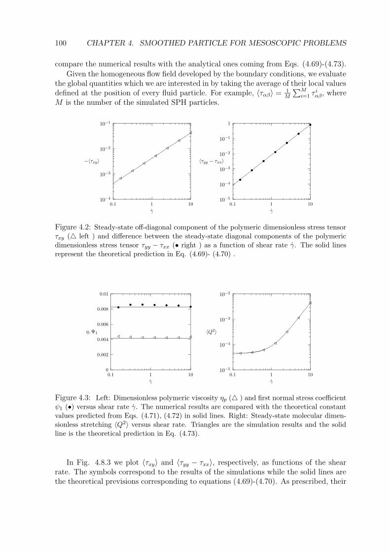
100 CHAPTER 4. SMOOTHED PARTICLE FOR MESOSCOPIC PROBLEMS
compare the numerical results with the analytical ones coming from Eqs. (4.69)-(4.73).
Given the homogeneous flow field developed by the boundary conditions, we evaluatethe global quantities which we are interested in by taking the average of their local valuesdefined at the position of every fluid particle. For example, 〈ταβ〉 = 1
M
∑Mi=1 τ
iαβ, where
M is the number of the simulated SPH particles.
10−4
10−3
10−2
10−1
0.1 1 10
−〈τxy〉
γ
/
/
/
/
/
/
/
10−5
10−4
10−3
10−2
10−1
1
0.1 1 10
〈τyy − τxx〉
γ
•
•
•
•
•
•
•
Figure 4.2: Steady-state off-diagonal component of the polymeric dimensionless stress tensorτxy (4 left ) and difference between the steady-state diagonal components of the polymericdimensionless stress tensor τyy − τxx (• right ) as a function of shear rate γ. The solid linesrepresent the theoretical prediction in Eq. (4.69)- (4.70) .
0
0.002
0.004
0.006
0.008
0.01
0.1 1 10
η,Ψ1
γ
///////
•••••••
10−5
10−4
10−3
10−2
0.1 1 10
〈Q2〉
γ
/
/
/
/
///
Figure 4.3: Left: Dimensionless polymeric viscosity ηp (4 ) and first normal stress coefficientψ1 (•) versus shear rate γ. The numerical results are compared with the theoretical constantvalues predicted from Eqs. (4.71), (4.72) in solid lines. Right: Steady-state molecular dimen-sionless stretching 〈Q2〉 versus shear rate. Triangles are the simulation results and the solidline is the theoretical prediction in Eq. (4.73).
In Fig. 4.8.3 we plot 〈τxy〉 and 〈τyy − τxx〉, respectively, as functions of the shearrate. The symbols correspond to the results of the simulations while the solid lines arethe theoretical previsions corresponding to equations (4.69)-(4.70). As prescribed, their
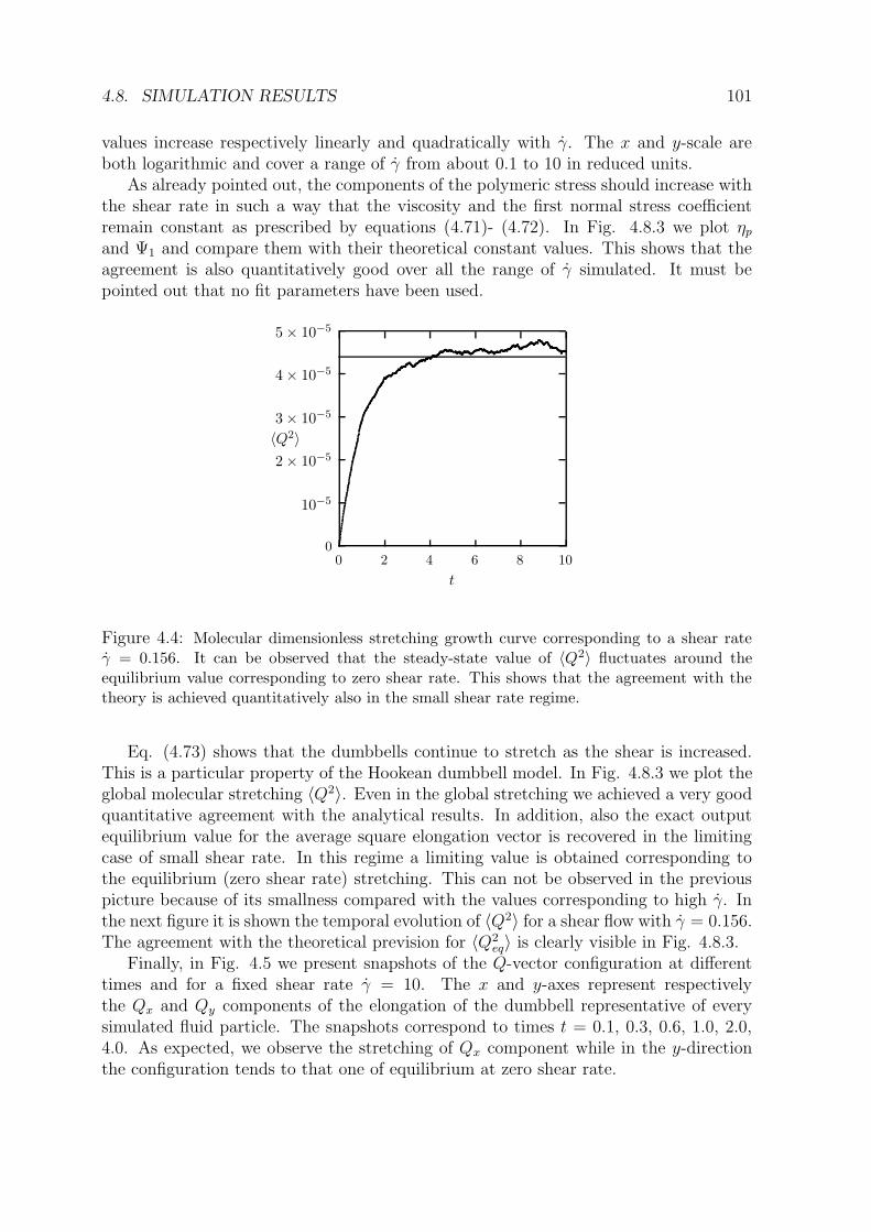
4.8. SIMULATION RESULTS 101
values increase respectively linearly and quadratically with γ. The x and y-scale areboth logarithmic and cover a range of γ from about 0.1 to 10 in reduced units.
As already pointed out, the components of the polymeric stress should increase withthe shear rate in such a way that the viscosity and the first normal stress coefficientremain constant as prescribed by equations (4.71)- (4.72). In Fig. 4.8.3 we plot ηp
and Ψ1 and compare them with their theoretical constant values. This shows that theagreement is also quantitatively good over all the range of γ simulated. It must bepointed out that no fit parameters have been used.
0
10−5
2 × 10⁻⁵
3 × 10⁻⁵
4 × 10⁻⁵
5 × 10⁻⁵
0 2 4 6 8 10
〈Q2〉
t
Figure 4.4: Molecular dimensionless stretching growth curve corresponding to a shear rateγ = 0.156. It can be observed that the steady-state value of 〈Q2〉 fluctuates around theequilibrium value corresponding to zero shear rate. This shows that the agreement with thetheory is achieved quantitatively also in the small shear rate regime.
Eq. (4.73) shows that the dumbbells continue to stretch as the shear is increased.This is a particular property of the Hookean dumbbell model. In Fig. 4.8.3 we plot theglobal molecular stretching 〈Q2〉. Even in the global stretching we achieved a very goodquantitative agreement with the analytical results. In addition, also the exact outputequilibrium value for the average square elongation vector is recovered in the limitingcase of small shear rate. In this regime a limiting value is obtained corresponding tothe equilibrium (zero shear rate) stretching. This can not be observed in the previouspicture because of its smallness compared with the values corresponding to high γ. Inthe next figure it is shown the temporal evolution of 〈Q2〉 for a shear flow with γ = 0.156.The agreement with the theoretical prevision for 〈Q2
eq〉 is clearly visible in Fig. 4.8.3.Finally, in Fig. 4.5 we present snapshots of the Q-vector configuration at different
times and for a fixed shear rate γ = 10. The x and y-axes represent respectivelythe Qx and Qy components of the elongation of the dumbbell representative of everysimulated fluid particle. The snapshots correspond to times t = 0.1, 0.3, 0.6, 1.0, 2.0,4.0. As expected, we observe the stretching of Qx component while in the y-directionthe configuration tends to that one of equilibrium at zero shear rate.
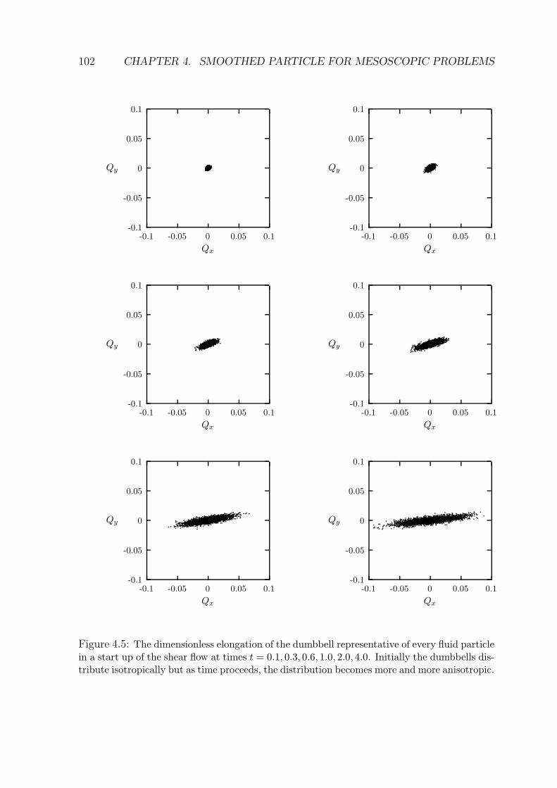
102 CHAPTER 4. SMOOTHED PARTICLE FOR MESOSCOPIC PROBLEMS
-0.1
-0.05
0
0.05
0.1
-0.1 -0.05 0 0.05 0.1
Qy
Qx
-0.1
-0.05
0
0.05
0.1
-0.1 -0.05 0 0.05 0.1
Qy
Qx
-0.1
-0.05
0
0.05
0.1
-0.1 -0.05 0 0.05 0.1
Qy
Qx
-0.1
-0.05
0
0.05
0.1
-0.1 -0.05 0 0.05 0.1
Qy
Qx
-0.1
-0.05
0
0.05
0.1
-0.1 -0.05 0 0.05 0.1
Qy
Qx
-0.1
-0.05
0
0.05
0.1
-0.1 -0.05 0 0.05 0.1
Qy
Qx
Figure 4.5: The dimensionless elongation of the dumbbell representative of every fluid particlein a start up of the shear flow at times t = 0.1, 0.3, 0.6, 1.0, 2.0, 4.0. Initially the dumbbells dis-tribute isotropically but as time proceeds, the distribution becomes more and more anisotropic.
4.9. FINAL REMARKS 103
We notice also that at every time the stretching in the x-direction increases, butalways preserving the symmetry of the particle distribution around the origin in theQ-plane, that is, on average over all the box the components of the Q-vector are zero.
4.9 Final remarks
Inspired by a Dissipative Particle Dynamics model formulated by ten Bosch [30], we haveproposed a fluid particle model for the simulation of dilute polymeric solutions. Specialattention has been paid to the thermodynamic consistency of the model, by writing itwithin the generic framework. Actually, several basic differences between the modelpresented and that of ten Bosch [30] arise from the thermodynamic consistency of ourmodel. First, our model includes a fluid particle volume variable and, therefore, theconservative forces in the momentum equation are replaced by actual pressure forces.As we have shown in Ref. [73], the conservative forces in the original classic DPD modelare not very physical and do not allow to study arbitrary equations of state. Second,our model includes an internal energy variable and it allows to study non-isothermalprocesses. Again, this can be regarded as an improvement over the classic DPD model.Finally, we have introduced the number of dumbbells as an additional variable, whichallows to study diffusive processes of dumbbells which are absent in the ten Bosch model.
From a more technical point of view, we observe that our model has a smaller numberof parameters and functions than the ten Bosch model. For example, the antisymmetryof L forces the α and β parameters of ten Bosch model to be exactly the same. Also, thesolvent parameters are the physical transport coefficients, which are directly given asan input. There is no need to perform a kinetic theory of the model in order to obtainthe transport coefficients in terms of the model parameters, as it is done in Ref. [30].
Our approach also puts the ten Bosch model in a conceptual framework that high-lights the validity and limitations of the model as a tool for simulating viscoelasticmaterials. From the microscopic calculation of the entropy and the physical argumentsused to derive the equations of motion, it is apparent that this model should providea good description for dilute polymeric solutions. Semi-dilute solutions could perhapsbe treated by including excluded volume effects of the dumbbells and mean field in-teractions between dumbbells using similar ideas as those of van der Waals for simplefluids. Polymer melts cannot be described by our model. A continuum theory for poly-mer melts in non-isothermal situations has been presented in Ref. [92], which makesuse of a conformation tensor for describing the microstructure of the melt. The con-tinuum equations for polymer melts in Ref. [92] could also be discretized in terms offluid particles with a well-defined underlying physical picture that respects the laws ofthermodynamics.
In this chapter, we have presented numerical simulations for isothermal homogeneousshear flow without polymer diffusivity. For reasons of simplicity, we have modelledthe polymer molecules with Hookean dumbbells, although more realistic models forpolymer molecules can also be considered. Finite extensibility and more complex bead-spring models [4] are easily implemented. The simulation results are preliminary but,nevertheless, reproduce the known theoretical predictions without fitting parameters.

104 CHAPTER 4. SMOOTHED PARTICLE FOR MESOSCOPIC PROBLEMS
Of course, the potential of the method lies in the possibility of exploring more complexnon-isothermal, non-homogeneous, and non-Hookean situations.
A final comment on the connection between our model and the Brownian Configura-tion Fields (BCF) method is in order. In BCF, there is also only one elastic variable per(Eulerian) computational cell, and the goal is to reduce the noise inherent in the methodby using the same sequence of random kicks for all the position over the domain. Thenone has one realization of the vector field Q (and consequently one realization of thepolymeric pressure tensor), which are completely correlated over all the space. Whenthe divergence of the stress tensor is evaluated in the momentum equation, it is usu-ally done by a two-points difference discretisation, and, because of the total correlationbetween tensor fields in different points, the noise is dramatically reduced. In the SPHdiscretisation of the momentum equation, the gradients are represented by a sum (inorder to have an antisymmetric force in the particle index) and not by a difference.Therefore, our method is intrinsically noisy and the level of fluctuations cannot be re-duced by the trick in BCF (or we would loose exact momentum conservation). In orderto study non-homogeneous flows, the two options are either to use a sufficiently largenumber of fluid particles in such a way that we can perform spatial averages over manyparticles underlying the same shear flow or to use a very big number of dumbbells perfluid particle as in the connffessit approach. The last option represents, from a nu-merical point of view, a very difficult task because the correspondent algorithm couldbe potentially very demanding in terms of CPU-time and memory requirements. Thistopic will be the subject of the next chapter where we will present also a new methodable to avoid, at least partially, the computational bottleneck mentioned above.
Chapter 5
Multiscale simulations ofviscoelastic flows
In this chapter we consider the problem of a consistent description of complex flows basedon a multiscale formulation. As already mentioned in Chapter 2, traditional numericalmethods based on the solution of suitable macroscopic constitutive equations, relatingviscoelastic stress to history deformation (i.e. Jaumann-Maxwell model), represent anestablished tool in computational rheology. However, these approaches present somedifficulties mostly related to the correctness and accuracy of the model constitutiveequation used. Indeed, it is well-known that their derivations from kinetic theory involvea number of unphysical closure approximations which can have a major influence on thefinal results. In the attempt to solve this problem, new techniques emerged in the lastyears which couple the macroscopic hydrodynamic scales of the flow with a microscopicconsistent evaluation of the viscoelastic stress tensor based on coarse-grained kineticmodels. These micro-macro methods allow to describe a complex fluid by a multiscalemodelling using directly microscopic results. In spite of their physical appealing, it hasbeen early recognized that the correspondent numerical implementations can be verydemanding in term of memory and CPU-time resources. The goal of this chapter isto give a general overview of the micro-macro methods recently used in computationalrheology, discussing the drawbacks and finally to present a new hybrid technique ableto correct some of them at least in some specific case.The scheme of the chapter is the following: Sec. 5.1 overviews briefly the micro-macromethods, while in sec. 5.2 it is described rigorously the multiscale formalism for thestudy of dilute polymeric solutions: this is generally based on the solution of a Fokker-Planck equation by using stochastic methods. At this point it will be clear that one ofthe main issue in micro-macro simulations is represented by the reduction of the memoryrequirements. This is achieved in a new hybrid method, presented in Sec. 5.3, whichsplits the stochastic dynamics and the storage of the relevant variables at every time stepin such a way to optimise the computer resources. Finally, in Sec. 5.4 numerical resultsare presented and compared with the traditional methods based on Brownian Dynamicssimulations while in Sec. 5.5 possible improvements and applications are discussed.
105
106 CHAPTER 5. MULTISCALE SIMULATIONS OF VISCOELASTIC FLOWS
5.1 Micro-macro methods for complex fluids
Computational fluid dynamics for non-Newtonian flows is to date a well-established fieldof research which has experienced in the last decades several improvements from boththe conceptual and numerical point of view. Finite element methods, finite volumes,boundary elements, smoothed particle dynamics, as that presented in Chapter 3, havebeen developed able to produce accurate and stable solutions for a wide range of flowfields [3, 95, 96, 50].These methods, however, rely on the knowledge of an exact constitutive relationshipbetween stress and deformation, which is not available for non-trivial, ‘realistic’ mod-els. Although promising results have been obtained using different closures, the rangeof their applicability is still unresolved, or severely limited. Focusing on this prob-lem, ten years ago emerged the idea of the CONNFFESSIT micro-macro approach(Calculation of Non-Newtonian Flows using Finite Elements and Stochastic Simula-tion Techniques) [11, 97], further abbreviated as CT in the following. It combines afinite element calculation of the macroscopic flow fields with a microscopic evaluationof the viscoelastic extra stress tensor based on Brownian Dynamics (BD) simulationsof polymer molecules. This approach obviously bypasses the need of closed constitutiveequations and avoids all problems related to their validity and degree of approxima-tion. Viscoelasticity is introduced in the scheme in an elegant and physically motivatedway just by evolving all the polymer variables and then extracting stresses from theirmicro-configurations. However, in spite of its undoubtedly physical appeal, it has beennoticed early that a fully CT simulation is enormously memory and time consuming.In fact, this stochastic technique is intrinsically noisy and, in order to achieve accurateevaluations of the stress tensor in one position over the domain, the level of fluctuationsmust be drastically reduced by using a very large number of dumbbells. This drawbackinvolves a big amount of memory requirements for every discretizing element, posingmany problems in order to make simulations in situations of practical interest, where avery large number of grid points is necessary to dicretize all the computational domainand to capture all the relevant length scales of the problem. 3D and/or turbulencesimulations coupled with complex boundary conditions are up to now completely farfrom the numerical capabilities of the present generation of workstations. On the otherhand, very recently have been performed fully-developed turbulence simulations in sim-ple channel geometries by using order of million cells discretizing the physical domainand thousands of dumbbells pro cell in order to evaluate the extra stress via BD. To ourknowledge, this represents the state-of-the-art large scale parallel stochastic simulationsof CT type [98].
In order to avoid this problem modifications have been proposed, such as ‘variancereduced CONNFFESSIT’ (VRCT), and ‘Brownian Configuration Fields’ (BCF), bothusing a manageable number of freedom degrees. They rely on the idea of using suitablefully correlated ensembles of dumbbells. The key point of the VRCT method is theconcept of control variables which should have the same fluctuations as the randomvariable of interest and vanishing averages. When, during a run, the control variable issubtracted from the variable of interest, the average of the latter should not be affectedfrom this operation, but its fluctuation should be considerably reduced. The way by
5.1. MICRO-MACRO METHODS FOR COMPLEX FLUIDS 107
which such control variables are constructed, i.e. parallel process simulations, has beendiscussed in [99].
The second approach, Brownian configuration Fields (BCF) [12] relies on the ideaof replacing the collection of individual polymer molecules with an ensemble of config-uration fields. On every element on the spatial domain is therefore defined only onedumbbell connector. All of them have the same initial conditions and are subjectedto same sequence of random kicks during the flow dynamics. This corresponds to oneparticular realization of the flow field which is completely correlated over all the space.At this point, one should notice that the extra stress tensor appears in the momentumequation under divergence operation. Stresses are calculated from two-points differencesbetween nearby elements. When performing the usual divergence operation a large noisesuppression takes place (provided that adjacent elements have very similar flow histo-ries). The connection between the two approaches has been recently clarified furtherin [90]. A variation of BCF, where time steps are splitted into a BD step followed by aconvective step, where the distribution is projected onto an orthogonal polynomial basishas been presented in [114]. We should also mention the Lagrangian Particle Method(LPM) [13, 100, 101], which combines an Eulerian finite element solution of the conser-vation equations with a Lagrangian computation of the extra-stress tensor by using acertain number of discrete particles convected by the flow. Due to its Lagrangian natureit is not required to keep track of the motion of every dumbbells, as in the first-generationCT, and, at the same time, the intrinsic convective term contained in the Ito-stochasticequations is naturally taken into account. LPM simulations have been performed withcorrelated and uncorrelated ensembles of dumbbells in order to study the effect of thevariance reduction on the results. It has been pointed out that the polymer stress resultsextracted from one particular run with correlated ensembles are much smoother thanfor fully uncorrelated systems but, by performing many independent runs, they varya lot from one to the other. These deviations in the results are due to an incompleterealization of the initial configurational distribution when using a finite number of corre-lated dumbbells. This finding constitutes a major problem emerging when introducingunrealistic correlations in simulations while effectively reducing the number of freedomdegrees. Upon increasing the number of simulated dumbbells in each of the ensemblesdiscussed above, the results tend to exhibit the same statistical properties, no matterif correlated or uncorrelated ensembles have been used. In other words, as the numberof internal freedom degrees becomes larger, variance reduction is no longer achieved. Adetailed review of micro-macro methods for multiscale simulations of viscoelastic flowscan be found in [9].
The hybrid BDDFS method (Brownian Dynamics and Distribution Function Stor-ing) presented in this chapter, avoids the storage problem by using a smaller quantityof information compressed in a discretized configurational distribution function (D-CDF) [102]. All physical quantities of interest in the flow calculation are completelydescribed by this function, which itself can be accurately obtained by using suitablegrids in the configuration space with an economically small resolution. We use a rep-resentative set of dumbbells to evolve the D-CDF. They are created (consistently withthe D-CDF at the previous time step) and overwritten at every time step. We do not
108 CHAPTER 5. MULTISCALE SIMULATIONS OF VISCOELASTIC FLOWS
need to store them. The only memorised quantities will be the values of the D-CDFdiscretized on a grid, while on the other hand, the extra stress tensor will be evaluatedas average over a large number of dumbbells (without memory costs) in order to achievean accuracy comparable with a conventional BD routine.
To summarise: With CT you need large memory and large CPU time. With BCF,LPM and VRCT you need few memory and small CPU time, but the results could benot so accurate because of the ’poor’ sample over initial configurations using few cor-related stochastic representations. For BDDFS you need small memory but large CPUtime (comparable with CT ), however you do not have to do any assumption of similarflow histories to obtain variance reduction. In addition, the results of BDDFS are soaccurate as the standard uncorrelated CT approach. Finally, for spectral methods youneed small memory and small CPU time.Concerning chain length, for CT, BCF, LPM, and VRCT the required resources increase‘normally’ with chain length, for ‘Brownian Dynamics and Distribution Function Stor-ing’ (BDDFS) the memory costs increase fast, and spectral methods become unfeasiblealready for short chains. Concerning numerical accuracy the use of a fully uncorrelatedensembles of dumbbells (CT or BDDFS) should be preferred. In fact, the hypothesisof similar flow histories (which is assumed in order to have noise reduction) is quitequestionable in particular situations of interest as for instance in turbulence flows wherethe velocity field changes remarkably in nearby points. For flows near boundaries where– even for moderate Reynolds numbers – the velocity ’jumps’ from a finite value rapidlyto zero at the wall, the resolution of the BDDFS lattice – and therefore its memory costs– does not necessarily increase. It should however increase, if the distribution functionbecomes peaked around a preferred aligned state, i.e., at large Reynolds numbers wherespectral methods (if applicable) offer advantages.
5.2 Microscopic kinetic model and standard CT ap-
proach
The main task of a microscopic description of the polymeric fluid is to motivate suitableexpressions relating the macroscopic stress tensor, which appears in the Navier-Stokesequations, to the additional structural variables. Additional equations of change havethen to couple the macroscopic flow field to the additional variables. In order to illustratethis approach in some detail, let us consider the general Navier-Stokes equation writtenin Lagrangian form and equipped with the usual extra stress tensor introducing elasticeffects
dv
dt= −1
ρ∇p+
ηs
ρ∆v +
1
ρ∇ · τ p, (5.1)
where ηs is the solvent viscosity and τ p is the polymeric contribution to the totalstress tensor. We assumed here that we are dealing with a perfect incompressible flowso that ∇ · v = 0 and all corresponding terms are removed in the momentum equation(5.1). Challenging is the evaluation of the components of τ p at (x, t). Microscopically,
5.2. MICROSCOPIC KINETIC MODEL AND STANDARD CT APPROACH 109
a dilute polymer solution (polymers dissolved in Newtonian solvent) is typically mod-elled by non-interacting dumbbells consisting of two beads connected with a spring andsubjected to a dissipative force with friction coefficient ζ plus a stochastic contribution.Each dumbbell is described in terms of its orientation and length, i.e., by a vector Q
connecting two beads. The evolution equation for the CDF ψ(x,Q, t) for dumbbells indilute solution follows from standard kinetic theory for this problem and reads [4]
dψ
dt= − ∂
∂Q·(
κ · Q − 2
ζF (Q)
)
ψ − 2kBT
ζ
∂2
∂Q2ψ , (5.2)
where kB is Boltzmann’s constant, T is the kinetic temperature and ψ(x,Q, t)dQrepresents the probability of having a dumbbell located in x with a connector vectorin the range [Q − dQ,Q + dQ]. Equation (5.2) describes convection and diffusion ofthe CDF ψ(x,Q, t) subjected to the (transposed) macroscopic deformation rate tensorκ(x, t) = (∇v(x, t))T and F (Q) represents the spring force acting between bondedbeads. At this point, we should be able to recover the extra stress tensor τ p directlyfrom the knowledge of the CDF at the corresponding location. We can use Kramer’sexpression for the stress tensor
τ p = −nkBT 1 + nH〈F (Q)Q〉, (5.3)
where n is the number density of dumbbells, and 1 the unit tensor. The averageof a quantity f(Q) is defined via 〈f〉 =
∫
ψf(Q)dQ. The problem, Eq. (5.1), sup-plemented with Eqs. (5.2)-(5.3), is therefore well-defined. Once the initial conditionsfor the macroscopic velocity field v(x, t0) and for the microscopic CDF ψ(x,Q, t0) areknown, the strategy is to integrate Eq. (5.1) using a suitable evolution scheme (i.e., Eu-ler, Predictor-Corrector, etc.), then to evaluate the macroscopic gradient κ(x, t) (fromthe new velocity field) and to insert it into Eq. (5.2). By integrating Eq. (5.2) we obtaina new CDF ψ, when introduced in Eq. (5.3), produces a new extra stress tensor fieldτ p(x, t) for the momentum equation, thus closing the loop. Despite of its apparentsimplicity, the described way to proceed poses many computational problems. In fact,Eq. (5.2) is a second-order partial differential equation with derivatives in both con-figurational and physical space. Consequently, it should be integrated on a high-orderdimensional space. This approach is generally considered quite uneconomic and onlyfew numerical works appeared in the literature based on this strategy [103, 104, 105].Using spectral methods, however, is an alternative for low-dimensional problems suchas the dumbbell dynamics considered in this work, see, e.g. [10, 106, 107, 4, 108, 109].For more complex kinetic models (e.g. multibead chains with more than two beads) theintegration of the Fokker-Planck equation on the respective higher-order configurationalspace via spectral methods looses its efficiency, and becomes conceptually cumbersome,while the structure of stochastic techniques remains unchanged, independent of chainlength, as long as hydrodynamic interactions between beads are disregarded.
An approximate treatment of this problem, probably the one mostly adopted, andwhich we would therefore like to mention, is to motivate a closed equation for the ex-tra stress tensor starting from the microscopic equations (5.2)-(5.3). Exact closuresare derivable only in a few simple, technologically irrelevant, cases. An exact solution
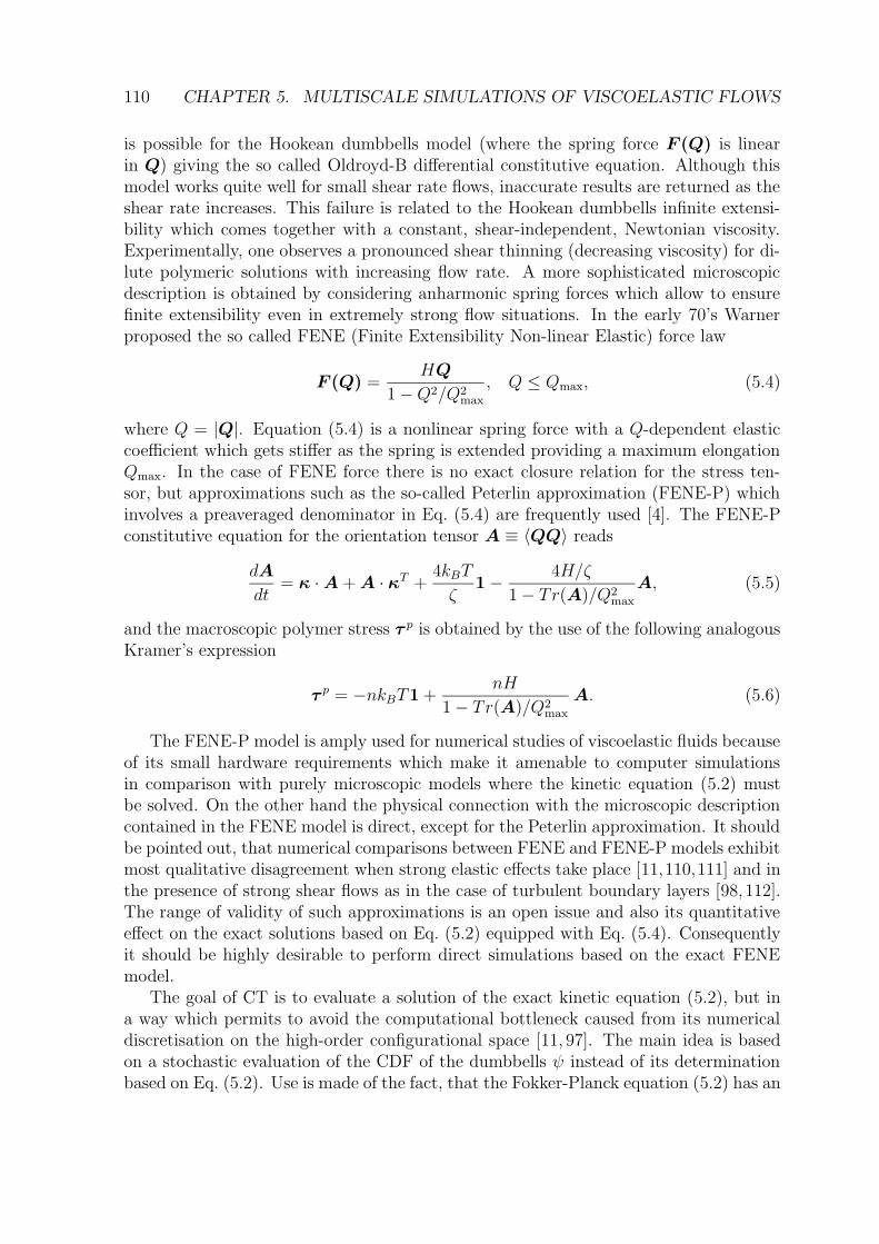
110 CHAPTER 5. MULTISCALE SIMULATIONS OF VISCOELASTIC FLOWS
is possible for the Hookean dumbbells model (where the spring force F (Q) is linearin Q) giving the so called Oldroyd-B differential constitutive equation. Although thismodel works quite well for small shear rate flows, inaccurate results are returned as theshear rate increases. This failure is related to the Hookean dumbbells infinite extensi-bility which comes together with a constant, shear-independent, Newtonian viscosity.Experimentally, one observes a pronounced shear thinning (decreasing viscosity) for di-lute polymeric solutions with increasing flow rate. A more sophisticated microscopicdescription is obtained by considering anharmonic spring forces which allow to ensurefinite extensibility even in extremely strong flow situations. In the early 70’s Warnerproposed the so called FENE (Finite Extensibility Non-linear Elastic) force law
F (Q) =HQ
1 −Q2/Q2max
, Q ≤ Qmax, (5.4)
where Q = |Q|. Equation (5.4) is a nonlinear spring force with a Q-dependent elasticcoefficient which gets stiffer as the spring is extended providing a maximum elongationQmax. In the case of FENE force there is no exact closure relation for the stress ten-sor, but approximations such as the so-called Peterlin approximation (FENE-P) whichinvolves a preaveraged denominator in Eq. (5.4) are frequently used [4]. The FENE-Pconstitutive equation for the orientation tensor A ≡ 〈QQ〉 reads
dA
dt= κ · A + A · κT +
4kBT
ζ1 − 4H/ζ
1 − Tr(A)/Q2max
A, (5.5)
and the macroscopic polymer stress τ p is obtained by the use of the following analogousKramer’s expression
τ p = −nkBT1 +nH
1 − Tr(A)/Q2max
A. (5.6)
The FENE-P model is amply used for numerical studies of viscoelastic fluids becauseof its small hardware requirements which make it amenable to computer simulationsin comparison with purely microscopic models where the kinetic equation (5.2) mustbe solved. On the other hand the physical connection with the microscopic descriptioncontained in the FENE model is direct, except for the Peterlin approximation. It shouldbe pointed out, that numerical comparisons between FENE and FENE-P models exhibitmost qualitative disagreement when strong elastic effects take place [11,110,111] and inthe presence of strong shear flows as in the case of turbulent boundary layers [98, 112].The range of validity of such approximations is an open issue and also its quantitativeeffect on the exact solutions based on Eq. (5.2) equipped with Eq. (5.4). Consequentlyit should be highly desirable to perform direct simulations based on the exact FENEmodel.
The goal of CT is to evaluate a solution of the exact kinetic equation (5.2), but ina way which permits to avoid the computational bottleneck caused from its numericaldiscretisation on the high-order configurational space [11, 97]. The main idea is basedon a stochastic evaluation of the CDF of the dumbbells ψ instead of its determinationbased on Eq. (5.2). Use is made of the fact, that the Fokker-Planck equation (5.2) has an
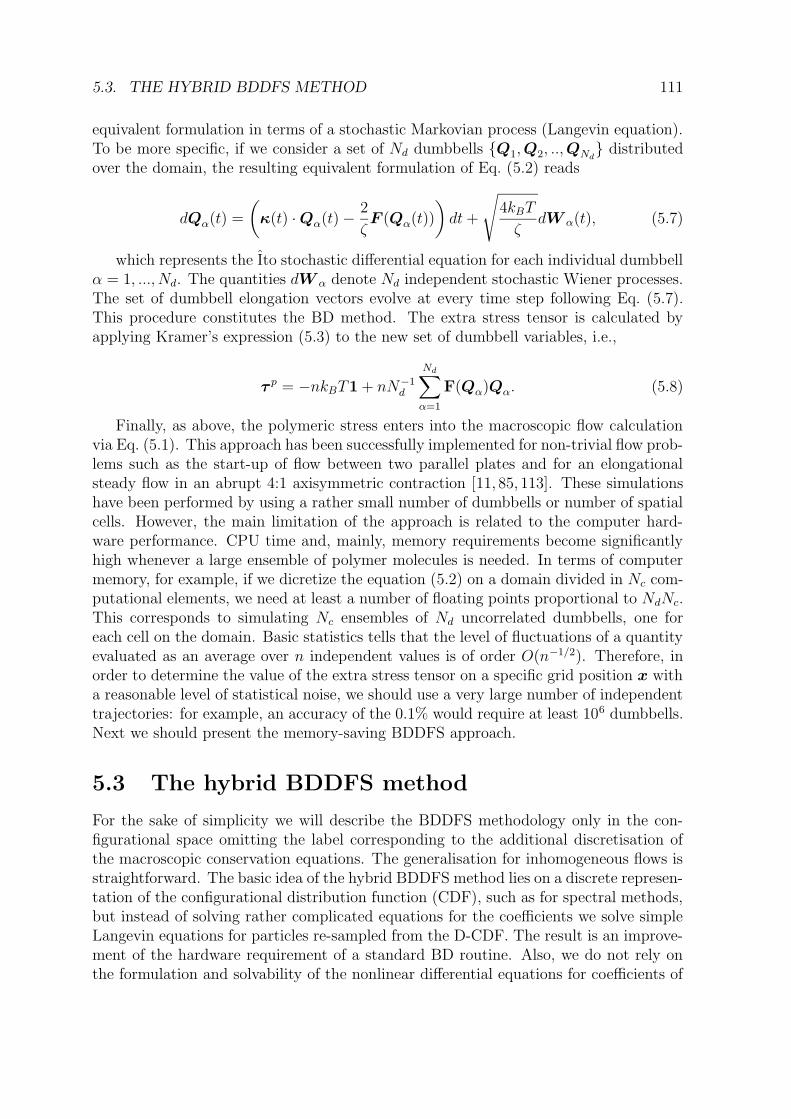
5.3. THE HYBRID BDDFS METHOD 111
equivalent formulation in terms of a stochastic Markovian process (Langevin equation).To be more specific, if we consider a set of Nd dumbbells Q1,Q2, ..,QNd
distributedover the domain, the resulting equivalent formulation of Eq. (5.2) reads
dQα(t) =
(
κ(t) · Qα(t) − 2
ζF (Qα(t))
)
dt+
√
4kBT
ζdW α(t), (5.7)
which represents the Ito stochastic differential equation for each individual dumbbellα = 1, ..., Nd. The quantities dW α denote Nd independent stochastic Wiener processes.The set of dumbbell elongation vectors evolve at every time step following Eq. (5.7).This procedure constitutes the BD method. The extra stress tensor is calculated byapplying Kramer’s expression (5.3) to the new set of dumbbell variables, i.e.,
τ p = −nkBT1 + nN−1d
Nd∑
α=1
F(Qα)Qα. (5.8)
Finally, as above, the polymeric stress enters into the macroscopic flow calculationvia Eq. (5.1). This approach has been successfully implemented for non-trivial flow prob-lems such as the start-up of flow between two parallel plates and for an elongationalsteady flow in an abrupt 4:1 axisymmetric contraction [11, 85, 113]. These simulationshave been performed by using a rather small number of dumbbells or number of spatialcells. However, the main limitation of the approach is related to the computer hard-ware performance. CPU time and, mainly, memory requirements become significantlyhigh whenever a large ensemble of polymer molecules is needed. In terms of computermemory, for example, if we dicretize the equation (5.2) on a domain divided in Nc com-putational elements, we need at least a number of floating points proportional to NdNc.This corresponds to simulating Nc ensembles of Nd uncorrelated dumbbells, one foreach cell on the domain. Basic statistics tells that the level of fluctuations of a quantityevaluated as an average over n independent values is of order O(n−1/2). Therefore, inorder to determine the value of the extra stress tensor on a specific grid position x witha reasonable level of statistical noise, we should use a very large number of independenttrajectories: for example, an accuracy of the 0.1% would require at least 106 dumbbells.Next we should present the memory-saving BDDFS approach.
5.3 The hybrid BDDFS method
For the sake of simplicity we will describe the BDDFS methodology only in the con-figurational space omitting the label corresponding to the additional discretisation ofthe macroscopic conservation equations. The generalisation for inhomogeneous flows isstraightforward. The basic idea of the hybrid BDDFS method lies on a discrete represen-tation of the configurational distribution function (CDF), such as for spectral methods,but instead of solving rather complicated equations for the coefficients we solve simpleLangevin equations for particles re-sampled from the D-CDF. The result is an improve-ment of the hardware requirement of a standard BD routine. Also, we do not rely onthe formulation and solvability of the nonlinear differential equations for coefficients of
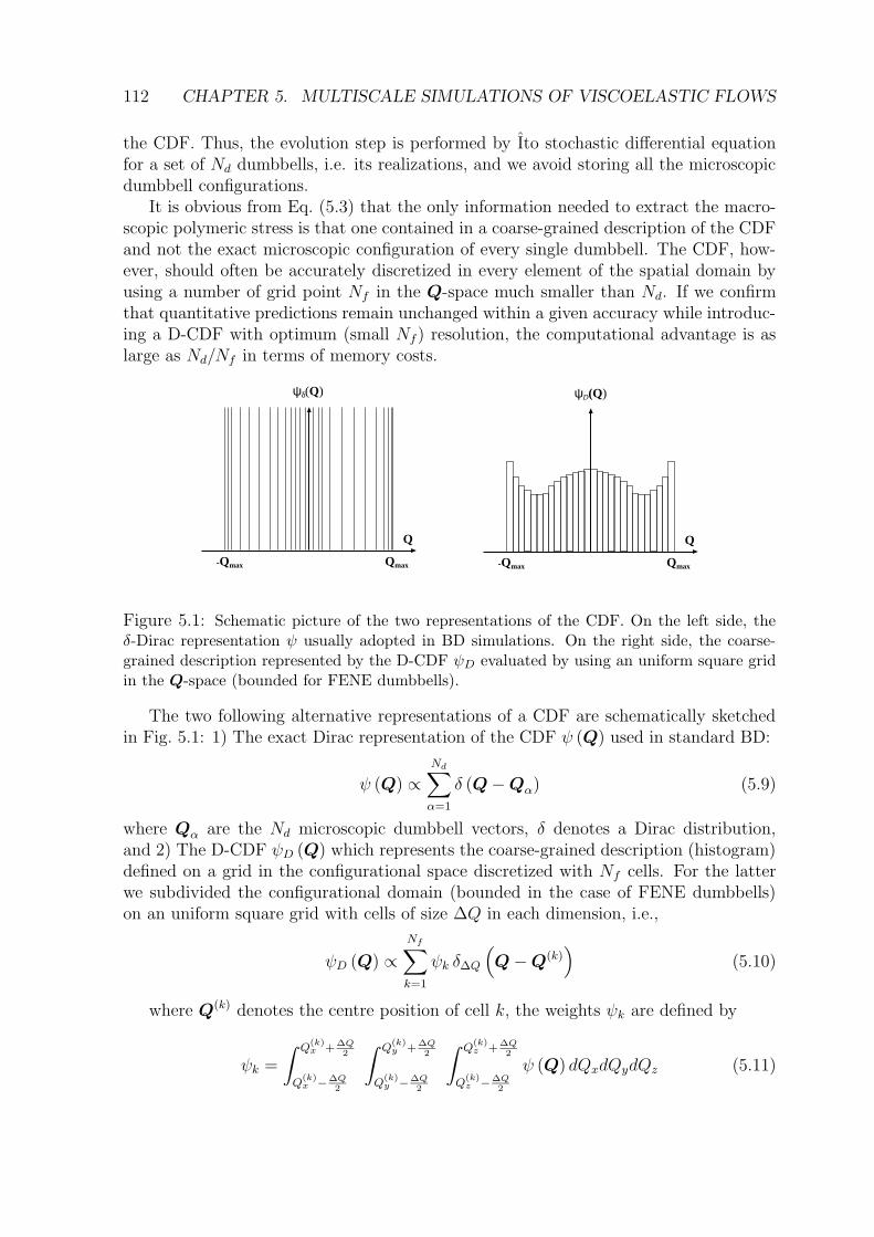
112 CHAPTER 5. MULTISCALE SIMULATIONS OF VISCOELASTIC FLOWS
the CDF. Thus, the evolution step is performed by Ito stochastic differential equationfor a set of Nd dumbbells, i.e. its realizations, and we avoid storing all the microscopicdumbbell configurations.
It is obvious from Eq. (5.3) that the only information needed to extract the macro-scopic polymeric stress is that one contained in a coarse-grained description of the CDFand not the exact microscopic configuration of every single dumbbell. The CDF, how-ever, should often be accurately discretized in every element of the spatial domain byusing a number of grid point Nf in the Q-space much smaller than Nd. If we confirmthat quantitative predictions remain unchanged within a given accuracy while introduc-ing a D-CDF with optimum (small Nf ) resolution, the computational advantage is aslarge as Nd/Nf in terms of memory costs.
Q
ψD(Q)
Qmax-Qmax
Q
Qmax-Qmax
ψδ(Q)
Figure 5.1: Schematic picture of the two representations of the CDF. On the left side, theδ-Dirac representation ψ usually adopted in BD simulations. On the right side, the coarse-grained description represented by the D-CDF ψD evaluated by using an uniform square gridin the Q-space (bounded for FENE dumbbells).
The two following alternative representations of a CDF are schematically sketchedin Fig. 5.1: 1) The exact Dirac representation of the CDF ψ (Q) used in standard BD:
ψ (Q) ∝Nd∑
α=1
δ (Q − Qα) (5.9)
where Qα are the Nd microscopic dumbbell vectors, δ denotes a Dirac distribution,and 2) The D-CDF ψD (Q) which represents the coarse-grained description (histogram)defined on a grid in the configurational space discretized with Nf cells. For the latterwe subdivided the configurational domain (bounded in the case of FENE dumbbells)on an uniform square grid with cells of size ∆Q in each dimension, i.e.,
ψD (Q) ∝Nf∑
k=1
ψk δ∆Q
(
Q − Q(k))
(5.10)
where Q(k) denotes the centre position of cell k, the weights ψk are defined by
ψk =
∫ Q(k)x +∆Q
2
Q(k)x −∆Q
2
∫ Q(k)y +∆Q
2
Q(k)y −∆Q
2
∫ Q(k)z +∆Q
2
Q(k)z −∆Q
2
ψ (Q) dQxdQydQz (5.11)
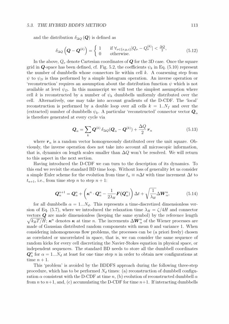
5.3. THE HYBRID BDDFS METHOD 113
and the distribution δ∆Q (Q) is defined as
δ∆Q
(
Q − Q(k))
=
1 if ∀ν∈x,y,z|Qν −Q(k)ν | < ∆Q
2,
0 otherwise.(5.12)
In the above, Qν denote Cartesian coordinates of Q for the 3D case. Once the squaregrid in Q-space has been defined, cf. Fig. 5.2, the coefficients ψk in Eq. (5.10) representthe number of dumbbells whose connectors lie within cell k. A coarsening step fromψ to ψD is thus performed by a simple histogram operation. An inverse operation or‘reconstruction’ requires an assumption about the distribution function ψ which is notavailable at level ψD. In this manuscript we will test the simplest assumption wherecell k is reconstructed by a number of ψk dumbbells uniformly distributed over thecell. Alternatively, one may take into account gradients of the D-CDF. The ‘local’reconstruction is performed by a double loop over all cells k = 1..Nf and over the(extracted) number of dumbbells ψk. A particular ‘reconstructed’ connector vector Qα
is therefore generated at every cycle via
Qα =∑
k
Q(k) δ∆Q(Qα − Q(k)) +∆Q
2rα (5.13)
where rα is a random vector homogeneously distributed over the unit square. Ob-viously, the inverse operation does not take into account all microscopic information,that is, dynamics on length scales smaller than ∆Q won’t be resolved. We will returnto this aspect in the next section.
Having introduced the D-CDF we can turn to the description of its dynamics. Tothis end we revisit the standard BD time loop. Without loss of generality let us considera simple Euler scheme for the evolution from time tn ≡ n∆t with time increment ∆t totn+1, i.e., from time step n to step n+ 1:
Qn+1α = Qn
α +
(
κn · Qnα − 1
2λH
F (Qnα)
)
∆t+
√
1
λH
∆W nα, (5.14)
for all dumbbells α = 1...Nd. This represents a time-discretized dimensionless ver-sion of Eq. (5.7), where we introduced the relaxation time λH = ζ/4H and connectorvectors Q are made dimensionless (keeping the same symbol) by the reference length√
kBT/H; κn denotes κ at time n. The increments ∆W nα of the Wiener processes are
made of Gaussian distributed random components with mean 0 and variance 1. Whenconsidering inhomogeneous flow problems, the processes can be (a priori freely) chosenas correlated or uncorrelated in space, that is, we can consider the same sequence ofrandom kicks for every cell discretizing the Navier-Stokes equation in physical space, orindependent sequences. The standard BD needs to store all the dumbbell coordinatesQn
α for α = 1...Nd at least for one time step n in order to obtain new configurations attime n+ 1.
This ‘problem’ is avoided by the BDDFS approach during the following three-stepprocedure, which has to be performed Nd times: (a) reconstruction of dumbbell configu-ration α consistent with the D-CDF at time n, (b) evolution of reconstructed dumbbell αfrom n to n+1, and, (c) accumulating the D-CDF for time n+1. If interacting dumbbells
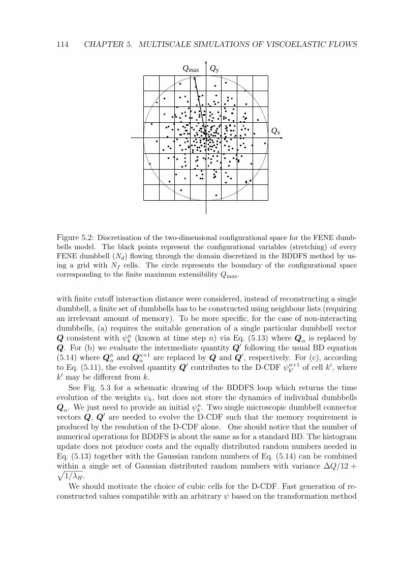
114 CHAPTER 5. MULTISCALE SIMULATIONS OF VISCOELASTIC FLOWS
Qmax Qy
Qx
Figure 5.2: Discretisation of the two-dimensional configurational space for the FENE dumb-bells model. The black points represent the configurational variables (stretching) of everyFENE dumbbell (Nd) flowing through the domain discretized in the BDDFS method by us-ing a grid with Nf cells. The circle represents the boundary of the configurational spacecorresponding to the finite maximum extensibility Qmax.
with finite cutoff interaction distance were considered, instead of reconstructing a singledumbbell, a finite set of dumbbells has to be constructed using neighbour lists (requiringan irrelevant amount of memory). To be more specific, for the case of non-interactingdumbbells, (a) requires the suitable generation of a single particular dumbbell vectorQ consistent with ψn
k (known at time step n) via Eq. (5.13) where Qα is replaced byQ. For (b) we evaluate the intermediate quantity Q′ following the usual BD equation(5.14) where Qn
α and Qn+1α are replaced by Q and Q′, respectively. For (c), according
to Eq. (5.11), the evolved quantity Q′ contributes to the D-CDF ψn+1k′ of cell k′, where
k′ may be different from k.
See Fig. 5.3 for a schematic drawing of the BDDFS loop which returns the timeevolution of the weights ψk, but does not store the dynamics of individual dumbbellsQα. We just need to provide an initial ψn
k . Two single microscopic dumbbell connectorvectors Q, Q′ are needed to evolve the D-CDF such that the memory requirement isproduced by the resolution of the D-CDF alone. One should notice that the number ofnumerical operations for BDDFS is about the same as for a standard BD. The histogramupdate does not produce costs and the equally distributed random numbers needed inEq. (5.13) together with the Gaussian random numbers of Eq. (5.14) can be combinedwithin a single set of Gaussian distributed random numbers with variance ∆Q/12 +√
1/λH .
We should motivate the choice of cubic cells for the D-CDF. Fast generation of re-constructed values compatible with an arbitrary ψ based on the transformation method
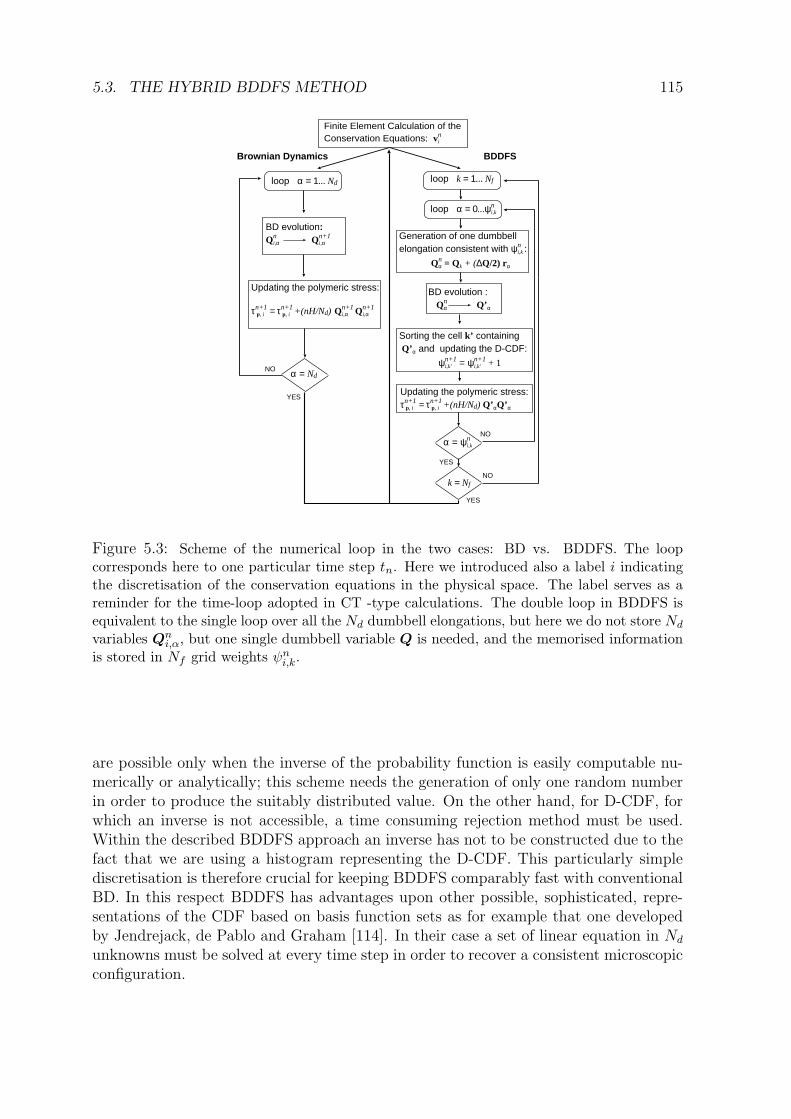
5.3. THE HYBRID BDDFS METHOD 115
Finite Element Calculation of theConservation Equations: vn
i
loop k = 1... Nf
loop α = 0...ψni,k
Generation of one dumbbellelongation consistent with ψn
i,k :
Qnα = Qk + (∆Q/2) rα
BD evolution : Qn
α Q’α
BD evolution: Qn
i,α Qn+1i,α
Updating the polymeric stress:
τn+1 p, i = τn+1
p, i +(nH/Nd) Qn+1i,α Qn+1
i,α
Sorting the cell k’ containing Q’α and updating the D-CDF:
ψn+1i,k’ = ψn+1
i,k’ + 1 α = Nd
loop α = 1... Nd
Updating the polymeric stress:τn+1
p, i = τn+1 p, i +(nH/Nd) Q’αQ’α
α = ψni,k
Brownian Dynamics BDDFS
YES
YES
YES
NO
NO
NO k = Nf
Figure 5.3: Scheme of the numerical loop in the two cases: BD vs. BDDFS. The loopcorresponds here to one particular time step tn. Here we introduced also a label i indicatingthe discretisation of the conservation equations in the physical space. The label serves as areminder for the time-loop adopted in CT -type calculations. The double loop in BDDFS isequivalent to the single loop over all the Nd dumbbell elongations, but here we do not store Nd
variables Qni,α, but one single dumbbell variable Q is needed, and the memorised information
is stored in Nf grid weights ψni,k.
are possible only when the inverse of the probability function is easily computable nu-merically or analytically; this scheme needs the generation of only one random numberin order to produce the suitably distributed value. On the other hand, for D-CDF, forwhich an inverse is not accessible, a time consuming rejection method must be used.Within the described BDDFS approach an inverse has not to be constructed due to thefact that we are using a histogram representing the D-CDF. This particularly simplediscretisation is therefore crucial for keeping BDDFS comparably fast with conventionalBD. In this respect BDDFS has advantages upon other possible, sophisticated, repre-sentations of the CDF based on basis function sets as for example that one developedby Jendrejack, de Pablo and Graham [114]. In their case a set of linear equation in Nd
unknowns must be solved at every time step in order to recover a consistent microscopicconfiguration.
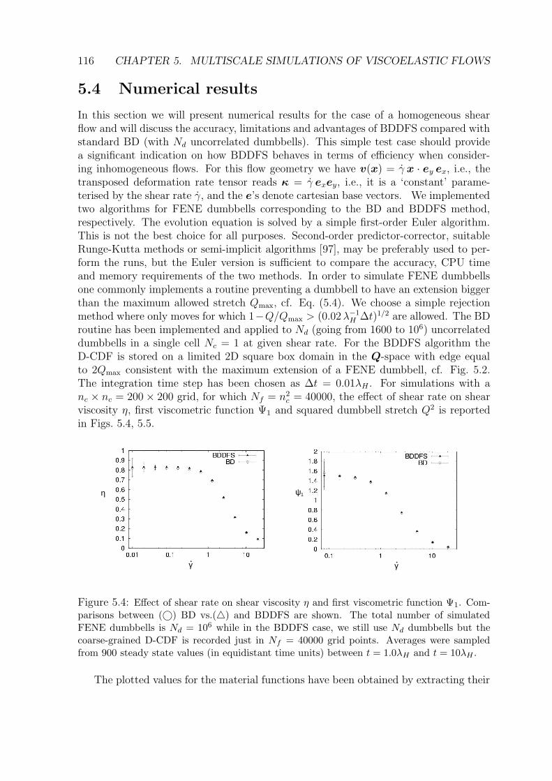
116 CHAPTER 5. MULTISCALE SIMULATIONS OF VISCOELASTIC FLOWS
5.4 Numerical results
In this section we will present numerical results for the case of a homogeneous shearflow and will discuss the accuracy, limitations and advantages of BDDFS compared withstandard BD (with Nd uncorrelated dumbbells). This simple test case should providea significant indication on how BDDFS behaves in terms of efficiency when consider-ing inhomogeneous flows. For this flow geometry we have v(x) = γ x · ey ex, i.e., thetransposed deformation rate tensor reads κ = γ exey, i.e., it is a ‘constant’ parame-terised by the shear rate γ, and the e’s denote cartesian base vectors. We implementedtwo algorithms for FENE dumbbells corresponding to the BD and BDDFS method,respectively. The evolution equation is solved by a simple first-order Euler algorithm.This is not the best choice for all purposes. Second-order predictor-corrector, suitableRunge-Kutta methods or semi-implicit algorithms [97], may be preferably used to per-form the runs, but the Euler version is sufficient to compare the accuracy, CPU timeand memory requirements of the two methods. In order to simulate FENE dumbbellsone commonly implements a routine preventing a dumbbell to have an extension biggerthan the maximum allowed stretch Qmax, cf. Eq. (5.4). We choose a simple rejectionmethod where only moves for which 1−Q/Qmax > (0.02λ−1
H ∆t)1/2 are allowed. The BDroutine has been implemented and applied to Nd (going from 1600 to 106) uncorrelateddumbbells in a single cell Nc = 1 at given shear rate. For the BDDFS algorithm theD-CDF is stored on a limited 2D square box domain in the Q-space with edge equalto 2Qmax consistent with the maximum extension of a FENE dumbbell, cf. Fig. 5.2.The integration time step has been chosen as ∆t = 0.01λH . For simulations with anc × nc = 200 × 200 grid, for which Nf = n2
c = 40000, the effect of shear rate on shearviscosity η, first viscometric function Ψ1 and squared dumbbell stretch Q2 is reportedin Figs. 5.4, 5.5.
η ψ1
γ.
γ.
Figure 5.4: Effect of shear rate on shear viscosity η and first viscometric function Ψ1. Com-parisons between (©) BD vs.(4) and BDDFS are shown. The total number of simulatedFENE dumbbells is Nd = 106 while in the BDDFS case, we still use Nd dumbbells but thecoarse-grained D-CDF is recorded just in Nf = 40000 grid points. Averages were sampledfrom 900 steady state values (in equidistant time units) between t = 1.0λH and t = 10λH .
The plotted values for the material functions have been obtained by extracting their
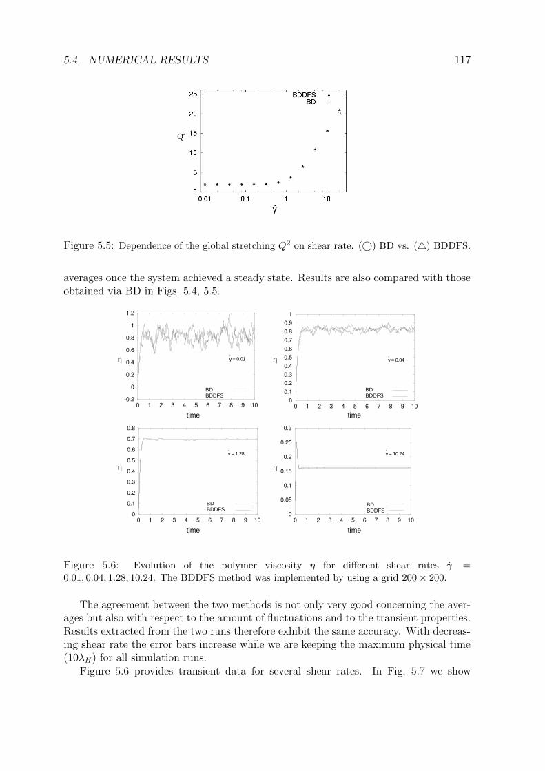
5.4. NUMERICAL RESULTS 117
Q2
γ.
Figure 5.5: Dependence of the global stretching Q2 on shear rate. (©) BD vs. (4) BDDFS.
averages once the system achieved a steady state. Results are also compared with thoseobtained via BD in Figs. 5.4, 5.5.
time time
time time
η η
η ηγ = 0.01.
γ = 0.04.
γ = 1.28.
γ = 10.24.
BDBDDFS
BDBDDFS
BDBDDFS
BDBDDFS
Figure 5.6: Evolution of the polymer viscosity η for different shear rates γ =0.01, 0.04, 1.28, 10.24. The BDDFS method was implemented by using a grid 200 × 200.
The agreement between the two methods is not only very good concerning the aver-ages but also with respect to the amount of fluctuations and to the transient properties.Results extracted from the two runs therefore exhibit the same accuracy. With decreas-ing shear rate the error bars increase while we are keeping the maximum physical time(10λH) for all simulation runs.
Figure 5.6 provides transient data for several shear rates. In Fig. 5.7 we show
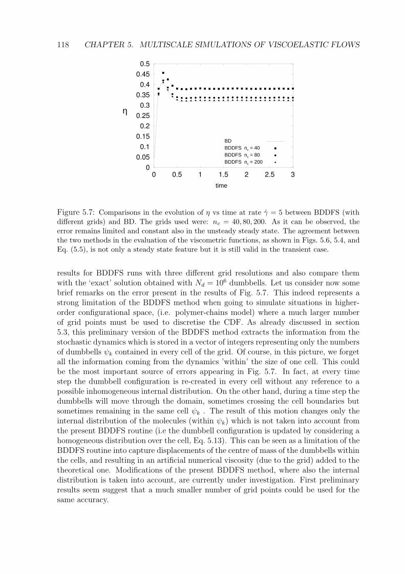
118 CHAPTER 5. MULTISCALE SIMULATIONS OF VISCOELASTIC FLOWS
time
η
BDBDDFS nc = 40BDDFS nc = 80BDDFS nc = 200
Figure 5.7: Comparisons in the evolution of η vs time at rate γ = 5 between BDDFS (withdifferent grids) and BD. The grids used were: nc = 40, 80, 200. As it can be observed, theerror remains limited and constant also in the unsteady steady state. The agreement betweenthe two methods in the evaluation of the viscometric functions, as shown in Figs. 5.6, 5.4, andEq. (5.5), is not only a steady state feature but it is still valid in the transient case.
results for BDDFS runs with three different grid resolutions and also compare themwith the ‘exact’ solution obtained with Nd = 106 dumbbells. Let us consider now somebrief remarks on the error present in the results of Fig. 5.7. This indeed represents astrong limitation of the BDDFS method when going to simulate situations in higher-order configurational space, (i.e. polymer-chains model) where a much larger numberof grid points must be used to discretise the CDF. As already discussed in section5.3, this preliminary version of the BDDFS method extracts the information from thestochastic dynamics which is stored in a vector of integers representing only the numbersof dumbbells ψk contained in every cell of the grid. Of course, in this picture, we forgetall the information coming from the dynamics ’within’ the size of one cell. This couldbe the most important source of errors appearing in Fig. 5.7. In fact, at every timestep the dumbbell configuration is re-created in every cell without any reference to apossible inhomogeneous internal distribution. On the other hand, during a time step thedumbbells will move through the domain, sometimes crossing the cell boundaries butsometimes remaining in the same cell ψk . The result of this motion changes only theinternal distribution of the molecules (within ψk) which is not taken into account fromthe present BDDFS routine (i.e the dumbbell configuration is updated by considering ahomogeneous distribution over the cell, Eq. 5.13). This can be seen as a limitation of theBDDFS routine into capture displacements of the centre of mass of the dumbbells withinthe cells, and resulting in an artificial numerical viscosity (due to the grid) added to thetheoretical one. Modifications of the present BDDFS method, where also the internaldistribution is taken into account, are currently under investigation. First preliminaryresults seem suggest that a much smaller number of grid points could be used for thesame accuracy.
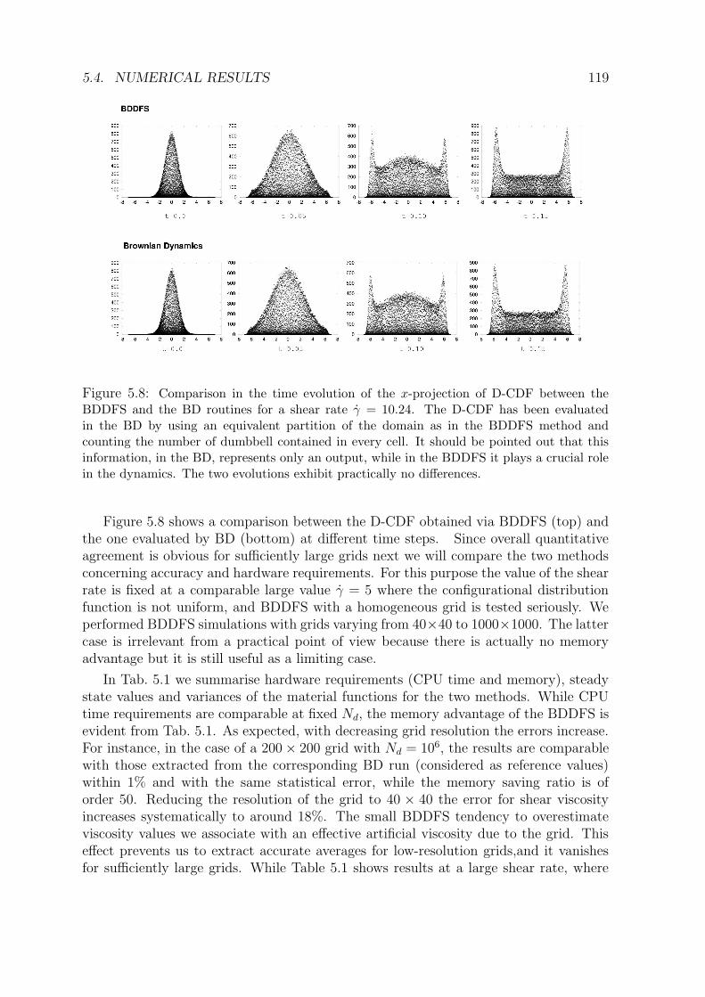
5.4. NUMERICAL RESULTS 119
Figure 5.8: Comparison in the time evolution of the x-projection of D-CDF between theBDDFS and the BD routines for a shear rate γ = 10.24. The D-CDF has been evaluatedin the BD by using an equivalent partition of the domain as in the BDDFS method andcounting the number of dumbbell contained in every cell. It should be pointed out that thisinformation, in the BD, represents only an output, while in the BDDFS it plays a crucial rolein the dynamics. The two evolutions exhibit practically no differences.
Figure 5.8 shows a comparison between the D-CDF obtained via BDDFS (top) andthe one evaluated by BD (bottom) at different time steps. Since overall quantitativeagreement is obvious for sufficiently large grids next we will compare the two methodsconcerning accuracy and hardware requirements. For this purpose the value of the shearrate is fixed at a comparable large value γ = 5 where the configurational distributionfunction is not uniform, and BDDFS with a homogeneous grid is tested seriously. Weperformed BDDFS simulations with grids varying from 40×40 to 1000×1000. The lattercase is irrelevant from a practical point of view because there is actually no memoryadvantage but it is still useful as a limiting case.
In Tab. 5.1 we summarise hardware requirements (CPU time and memory), steadystate values and variances of the material functions for the two methods. While CPUtime requirements are comparable at fixed Nd, the memory advantage of the BDDFS isevident from Tab. 5.1. As expected, with decreasing grid resolution the errors increase.For instance, in the case of a 200 × 200 grid with Nd = 106, the results are comparablewith those extracted from the corresponding BD run (considered as reference values)within 1% and with the same statistical error, while the memory saving ratio is oforder 50. Reducing the resolution of the grid to 40 × 40 the error for shear viscosityincreases systematically to around 18%. The small BDDFS tendency to overestimateviscosity values we associate with an effective artificial viscosity due to the grid. Thiseffect prevents us to extract accurate averages for low-resolution grids,and it vanishesfor sufficiently large grids. While Table 5.1 shows results at a large shear rate, where
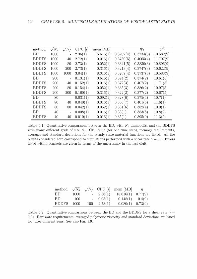
120 CHAPTER 5. MULTISCALE SIMULATIONS OF VISCOELASTIC FLOWS
method√Nd
√
Nf CPU [s] mem [MB] η Ψ1 Q2
BD 1000 - 2.36(1) 15.616(1) 0.3202(4) 0.3734(3) 10.582(9)BDDFS 1000 40 2.72(1) 0.016(1) 0.3730(5) 0.4065(4) 11.707(9)BDDFS 1000 80 2.73(1) 0.052(1) 0.3341(5) 0.3830(3) 10.896(9)BDDFS 1000 200 2.73(1) 0.316(1) 0.3213(4) 0.3747(3) 10.622(9)BDDFS 1000 1000 3.04(1) 8.316(1) 0.3207(4) 0.3737(3) 10.588(9)BD 200 - 0.131(1) 0.616(1) 0.324(2) 0.374(2) 10.61(5)BDDFS 200 40 0.152(1) 0.016(1) 0.372(3) 0.407(2) 11.71(5)BDDFS 200 80 0.154(1) 0.052(1) 0.335(3) 0.386(2) 10.97(5)BDDFS 200 200 0.160(1) 0.316(1) 0.322(2) 0.377(2) 10.67(5)BD 80 - 0.031(1) 0.092(1) 0.328(6) 0.375(4) 10.7(1)BDDFS 80 40 0.040(1) 0.016(1) 0.366(7) 0.401(5) 11.6(1)BDDFS 80 80 0.042(1) 0.052(1) 0.331(6) 0.382(4) 10.9(1)BD 40 - 0.008(1) 0.016(1) 0.33(1) 0.383(8) 10.8(2)BDDFS 40 40 0.010(1) 0.016(1) 0.35(1) 0.395(9) 11.3(2)
Table 5.1: Quantitative comparisons between the BD, with Nd dumbbells, and the BDDFSwith many different grids of size Nf . CPU time (for one time step), memory requirements,averages and standard deviations for the steady-state material functions are listed. All theresults considered here correspond to simulations performed with a shear rate γ = 5.0. Errorslisted within brackets are given in terms of the uncertainty in the last digit.
method√Nd
√
Nf CPU [s] mem [MB] ηBD 1000 - 2.36(1) 15.616(1) 0.77(9)BD 100 - 0.05(1) 0.148(1) 0.4(9)BDDFS 1000 100 2.73(1) 0.080(1) 0.73(9)
Table 5.2: Quantitative comparisons between the BD and the BDDFS for a shear rate γ =0.01. Hardware requirements, averaged polymeric viscosity and standard deviations are listedfor three different runs. See also Fig. 5.9.
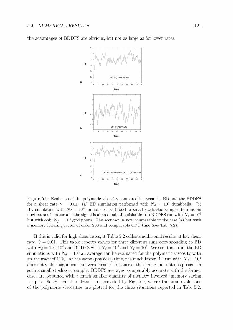
5.4. NUMERICAL RESULTS 121
the advantages of BDDFS are obvious, but not as large as for lower rates.
0
0.2
0.4
0.6
0.8
1
1.2
0 5 10 15 20 25 30 35 40 45 50
time
η
BD Nd=1000x1000
-1
-0.5
0
0.5
1
1.5
2
2.5
0 5 10 15 20 25 30 35 40 45 50
0
0.2
0.4
0.6
0.8
1
1.2
0 5 10 15 20 25 30 35 40 45 50
time
η
BD Nd=100x100
time
η
BDDFS Nd=1000x1000 N
f=100x100
a)
b)
c)
Figure 5.9: Evolution of the polymeric viscosity compared between the BD and the BDDFSfor a shear rate γ = 0.01. (a) BD simulation performed with Nd = 106 dumbbells. (b)BD simulation with Nd = 104 dumbbells: with such a small stochastic sample the randomfluctuations increase and the signal is almost indistinguishable. (c) BDDFS run with Nd = 106
but with only Nf = 104 grid points. The accuracy is now comparable to the case (a) but witha memory lowering factor of order 200 and comparable CPU time (see Tab. 5.2).
If this is valid for high shear rates, it Table 5.2 collects additional results at low shearrate, γ = 0.01. This table reports values for three different runs corresponding to BDwith Nd = 106, 104 and BDDFS with Nd = 106 and Nf = 104. We see, that from the BDsimulations with Nd = 106 an average can be evaluated for the polymeric viscosity withan accuracy of 11%. At the same (physical) time, the much faster BD run with Nd = 104
does not yield a significant nonzero measure because of the strong fluctuations present insuch a small stochastic sample. BBDFS averages, comparably accurate with the formercase, are obtained with a much smaller quantity of memory involved; memory savingis up to 95.5%. Further details are provided by Fig. 5.9, where the time evolutionsof the polymeric viscosities are plotted for the three situations reported in Tab. 5.2.
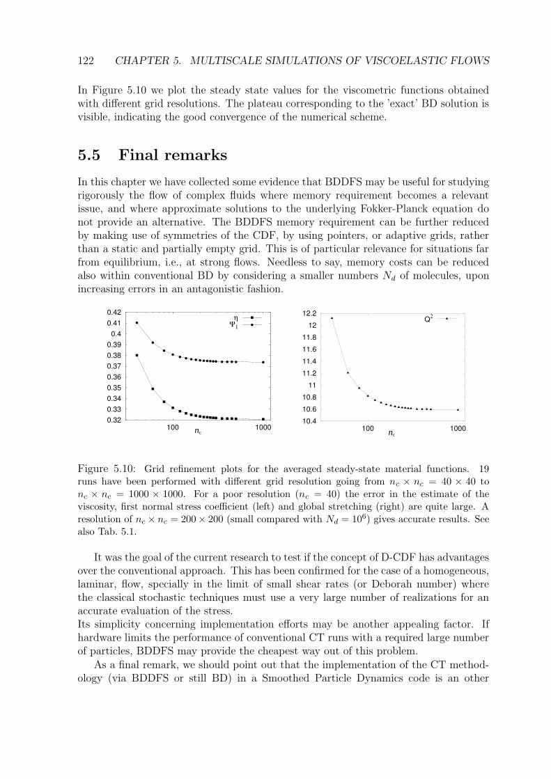
122 CHAPTER 5. MULTISCALE SIMULATIONS OF VISCOELASTIC FLOWS
In Figure 5.10 we plot the steady state values for the viscometric functions obtainedwith different grid resolutions. The plateau corresponding to the ’exact’ BD solution isvisible, indicating the good convergence of the numerical scheme.
5.5 Final remarks
In this chapter we have collected some evidence that BDDFS may be useful for studyingrigorously the flow of complex fluids where memory requirement becomes a relevantissue, and where approximate solutions to the underlying Fokker-Planck equation donot provide an alternative. The BDDFS memory requirement can be further reducedby making use of symmetries of the CDF, by using pointers, or adaptive grids, ratherthan a static and partially empty grid. This is of particular relevance for situations farfrom equilibrium, i.e., at strong flows. Needless to say, memory costs can be reducedalso within conventional BD by considering a smaller numbers Nd of molecules, uponincreasing errors in an antagonistic fashion.
nc nc
Figure 5.10: Grid refinement plots for the averaged steady-state material functions. 19runs have been performed with different grid resolution going from nc × nc = 40 × 40 tonc × nc = 1000 × 1000. For a poor resolution (nc = 40) the error in the estimate of theviscosity, first normal stress coefficient (left) and global stretching (right) are quite large. Aresolution of nc × nc = 200× 200 (small compared with Nd = 106) gives accurate results. Seealso Tab. 5.1.
It was the goal of the current research to test if the concept of D-CDF has advantagesover the conventional approach. This has been confirmed for the case of a homogeneous,laminar, flow, specially in the limit of small shear rates (or Deborah number) wherethe classical stochastic techniques must use a very large number of realizations for anaccurate evaluation of the stress.Its simplicity concerning implementation efforts may be another appealing factor. Ifhardware limits the performance of conventional CT runs with a required large numberof particles, BDDFS may provide the cheapest way out of this problem.
As a final remark, we should point out that the implementation of the CT method-ology (via BDDFS or still BD) in a Smoothed Particle Dynamics code is an other
5.5. FINAL REMARKS 123
interesting computational issue. Indeed, as we have already mentioned in the first sec-tion, the ’state-of-the-art’ micro-macro methods suffer of some difficulties related tothe fact that they do not describe the flow in a fully Lagrangian fashion. This is forexample the case of the traditional CT, where molecules are dispersed through the flowdomain: the consequent algorithmic complexity due to their search and track can beresult in serious computational drawbacks. In addition, it is not generally ensured thata sufficient number of molecules (for an accurate estimate of the stress tensor via (5.8))will be present in every finite elements at every time step. This makes very difficult, ifnot impossible, an accurate control of the statistical error in the stress evaluation. Thisdrawbacks are partially solved by the BCF and LPM methods, which, by consideringrespectively a correlated configuration field and a set of Lagrangian particles, can avoidthe problems mentioned above. Nevertheless, these approaches are not exempt fromdifficulties: BCF can not be applied to an uncorrelated field, therefore problems char-acterised by physical fluctuations (i.e. turbulence) can not be described, while LPM,as recognized by Keunings in [13], can suffer of unphysical (over-smoothed) transfer ofmomentum between the Lagrangian evaluation of the stress and the Eulerian solutionof the hydrodynamic fields. From this point of view, the Smoothed Particle Dynamicsmethod, being fully Lagrangian, could in principle bypass all these problems, indeed1) dumbbells tracking is not necessary as long as we consider element (’smooth parti-cle’) moving with the flow (only dumbbells diffusion should consider as we discussedin Chapter 4); 2) we do not have any problem related to unphysical coupling betweengrids. To our knowledge, if implemented, this would be the first every fully LagrangianCT method in the literature. Needless to say, it could be very useful for a wide rangeof problems, i.e. free surface viscoelastic flows. We reserve to do this work in the nextfuture.

124 CHAPTER 5. MULTISCALE SIMULATIONS OF VISCOELASTIC FLOWS
Chapter 6
Conclusions
In this work, a general study on the applicability of the Lagrangian Smoothed ParticleHydrodynamics method for the solution of viscoelastic flow problems was carried out.The pursued research directions were developed along three different paths which wecan denote as follows: macroscopic, mesoscopic and multiscale approach for viscoelasticfluids. In the first part of this thesis, a generalisation of SPH, i.e. Smoothed Particle Dy-namics method, was presented, which is able to study complex viscoelastic phenomenaby previous incorporation of a macroscopic constitutive equation for the stress tensorbased on the corotational Maxwell model. The accuracy of the method was proven firstin simple Newtonian cases and then tested in a variety of viscoelastic situations, includ-ing velocity profile relaxations in channel geometries, steady bulk shear flows, unsteadyshear flows of a viscoelastic matrix in a periodic array of non-rotating rigid inclusions.The results obtained showed that the methodology is able to reproduce accurately, alsoquantitatively basis, many theoretical solutions recoverable in simple cases. In addi-tion the strength of the scheme lies on its flexibility, which make it suitable to studymore complex physical situations. The Lagrangian nature of the Smoothed ParticleDynamics method takes into account in the most natural way the hyperbolic characterof the rheological constitutive equation, bypassing the need to consider special stabil-ity treatment, as “upwind” schemes, and allowing to simulate general unsteady flowproblems. In addition, the absence of an underlying grid and the adaptivity of the par-ticle system, avoids the problem of using complicate mesh, rezoning procedures or othergrid-dependent drawbacks. Such peculiarity suggests that the method should representan ideal alternative for problems dealing with irregular/complicate geometries (wherean Eulerian scheme should use time-consuming preprocessing mesh-generation proce-dures) or even for free-surface flow problems, which we did not discuss in the presentwork, but which represent a natural field of application for future research. However,some problems stll persist that are connected with an accurate treatment of boundaryconditions which, although very easy to implement, do not achieve, in the opinion ofthe author, the performance obtained in well-established Eulerian techniques, where anaccumulated numerical experience is available.
As often pointed out in the course of this work, the method for macroscopic flowproblems becomes inapplicable to physical situations in which the length scales char-
125
126 CHAPTER 6. CONCLUSIONS
acterizing the problem are quite ’small’. The word ’small’ in this context is related tothe presence of fluctuations in the thermodynamic subsystem considered. Indeed, itis well-known that as far as we are studying problems involving colloidal suspensions,microphase separation, polymer mixtures or any other kind of system where a crucialrole is played by thermal diffusion, it is essential to use a description consistent witha fluctuating hydrodynamic theory. Fluctuations in the fluid variables must thereforebe introduced in a way which respects the fundamental laws of physics, that is, Firstand Second Laws of Thermodynamics. The main result of the second part of this thesiswas the construction of a thermodynamically consistent model for viscoelastic fluids inthe sense given above. This was done using the GENERIC formalism which permits tobuild, in an easy and elegant way, physical models consistent with the previous laws.The elastic dynamics were introduced in the hydrodynamic formalism by consideringa further variable associated to every particle and representing its elongational state.Very simple physical argumentations brought to the definition of an evolution rule whichfollows an Ito stochastic differential equation. A particularly interesting feature of theresulting set of equations is that the thermal fluctuations depend on the size of the fluidparticles. This means that for large enough fluid particles, the thermal fluctuations inthe energy and momentum equations can be neglected in accordance with the extensivenature of such variables. Contrary to the previous cases, the thermal fluctuations cannotbe neglected at all in the stochastic equations for the dumbbell elongations and indeedthey do not depend on the size of the particles. The reason for this is related to thefact that the dumbbell elongations are purely mesoscopic variables (we cannot extendtheir definitions to a macroscopic level) and for them the stochastic term is an essentialpart of the dynamics. The main conclusion is therefore that this model, as it has beendeveloped, should have an applicability only for mesoscopic problems and not for a localdescription of a macroscopic flow. Nevertheless, one could argue that a connection tothe micro-macro approaches is still possible by considering these elongational variablesas one possible realization of the configurational field (in the sense given in BCF) evenif here, as it has been stressed at the end of Chapt. 4, the advantages of variance reduc-tion present in BCF, are less evident. The generalisation of this methodology for thestudy of macroscopic field, following the CONNFFESSIT philosophy, should resort tothe CPU-time consuming and memory requiring procedure of averaging over a large setof stochastic realizations of the same hydrodynamic flow.
In the context of micro-macro simulations and after the considerations presentedabove, we attempted in Chapt. 5, an investigation on possible efficient algorithms formultiscale CONNFFESSIT-type simulations of polymer solutions. From the model pre-viously developed, it is clear that, whenever interested in applying it to macroscopicflows, the problem of variance reduction for the stochastic estimate of the stress tensorshould be addressed. As discussed in detail in Chapt. 5, there exists a huge variety offlow situations in which the standard variance reduction algorithms can not be applied.In such problems, a brute averaging routine involving very large ensembles of stochas-tic realizations is necessary so far. In the last part of this work, we presented a newhybrid method, i.e. Brownian Dynamics and Distribution Function Storing (BDDFS),which offers numerical advantages over traditional stochastic integrators like Brownian
127
Dynamics (BD). The method is based on a dual representation of the configurationaldistribution function: a Dirac-delta representation (commonly used in BD), and a dis-cretized configurational distribution function (D-CDF) defined on square coarse-grainedgrid in the configurational space. The dynamics are split in two steps: the evolutionbased on a typical BD step and a further part consisting in the storage and recovery ofa smaller set of relevant variables, i.e. the values of the D-CDF on the grid. As far asthe number of grid points used is smaller than the number of dumbbells, for the samelevel of accuracy, the BDDFS method offers memory advantage over classical BD rou-tines. This was tested in a homogeneous shear flow for different values of the shear rate.Although the memory advantage resulted to be quite modest in the range of high shearrates (where a small stochastic ensemble already gives accurate estimates for the stresstensor), a large memory reduction was obtained in the limit of small shear rates, wherethe difficulties of the stochastic techniques are well-known. For the same accuracy andcomparable CPU-time, the BDDFS method offers a lowering memory factor of order200 over a standard BD routine. This peculiarity of the BDDFS method could turn outto be very useful in simulations of viscoelastic flows where a large number of freedomdegrees must be take into account to discretize finely the physical domain or to produceaccurate local ensemble averages (i.e viscoelastic turbulent flows). Although the methodappears to be very promising for simple dumbbell models, it seems to become cumber-some for higher dimensional spaces describing for example polymer-chain models. Insuch situations, the algorithmic complexity of the BDDFS method, being based on thefully discretisation of the configurational space, should increase much faster than forstandard stochastic BD routines. Nevertheless, further investigations in this directionare still called for in order to compare the two methods for increasing numerical reso-lution and higher dimensional spaces where the accuracy of the BD method, dependingon the underlying distribution function, can not be specified ’a priori’.

128 CHAPTER 6. CONCLUSIONS
Appendix A
Review of generic
In this appendix, we present a brief summary of the generic framework [86]. Thestate of a system at a given level of description is described by a set of variables thatform a vector x. The energy and the entropy are two of the basic building blocks of thegeneric formalism and they should be expressed as functions of the state variables atthe given level of description. The generic dynamic equations are given then by
dx
dt= L· ∂E
∂x+M · ∂S
∂x. (A.1)
The first term in the right hand side is named the reversible part of the dynamics andthe second term is named the irreversible part. The predictive power of generic reliesin the fact that very strong requirements exists on the matrices L,M leaving relativelysmall room for the physical input about the system. First, L is antisymmetric whereasM is symmetric and positive semidefinite. Most important, the following degeneracy
conditions should hold
L· ∂S∂x
= 0, M · ∂E∂x
= 0. (A.2)
These properties ensure that the energy is a dynamical invariant, E = 0, and thatthe entropy is a non-decreasing function of time, S ≥ 0, as can be proved by a sim-ple application of the chain rule and the equations of motion (A.1). In the case thatother dynamical invariants I(x) exist in the system (as, for example, linear or angularmomentum), then further conditions must be satisfied by L,M . In particular,
∂I
∂x·L· ∂E
∂x= 0,
∂I
∂x·M · ∂S
∂x= 0, (A.3)
which ensure that I = 0.The deterministic equations (A.1) are, actually, an approximation in which thermal
fluctuations are neglected. If thermal fluctuations are not neglected, the dynamics isdescribed by the following stochastic differential equations [89]
dx =
[
L· ∂E∂x
+M · ∂S∂x
+ kB∂
∂x·M]
dt+ dx, (A.4)
129
130 APPENDIX A. REVIEW OF GENERIC
to be compared with the deterministic equations (A.1). The deterministic additionalterm involving the Boltzmann constant kB appears due to the stochastic interpretationof the equation which is taken to be the Ito interpretation. The stochastic term dx inEq. (A.4) is a linear combination of independent increments of the Wiener process. Itsatisfies the mnemotechnical Ito rule
dxdxT = 2kBMdt, (A.5)
which means that dx is an infinitesimal of order 1/2 [93]. Eq. (A.5) is a compact andformal statement of the Fluctuation-Dissipation theorem.
In order to guarantee that the total energy and dynamical invariants do not changein time, a strong requirement on the form of dx holds,
∂E
∂x·dx = 0,
∂I
∂x·dx = 0, (A.6)
implying the last equations in (A.2) and (A.3). The geometrical meaning of (A.6) isclear. The random kicks produced by dx on the state x are orthogonal to the gradientsof E, I. These gradients are perpendicular vectors (strictly speaking they are one forms)to the hypersurface E(x) = E0, I(x) = I0. Therefore, the kicks let the state x alwayswithin the hypersurface of dynamical invariants.
Appendix B
Microscopic calculation of entropy
In this appendix we compute the entropy of a thermodynamic system composed ofa set of N s solvent molecules and N d dumbbells. We understand this system as theportion of fluid that constitutes a fluid particle. The dumbbells are a highly simplifiedmodel of a real polymer molecule. The purpose of this calculation is to provide specificanalytical expressions for the entropy which may have some resemblance with the actualentropy of a dilute polymer system. We denote by z the set of microscopic degrees offreedom of the system, which are ri,pi for the position and momentum of the solventmolecules, Ri,Qi for the centre of mass and relative position of the dumbbells, andPi for the bead momentum. We will denote schematically r = ri, i = 1, · · · , N s,R = Ri, i = 1, · · · , N d, Q = Qi, i = 1, · · · , N d. The Hamiltonian is given by
H(z) =Ns∑
i
p2i
2ms
+2Nd∑
i
P2i
2md
+ V s(r) + V sd(r,R,Q) + V d(Q). (B.1)
Here we have introduced the potential energy of the solvent molecules V s(r) whichdepends only on the coordinates of the solvent molecules, the potential energy of in-teraction between solvent and beads V sd(r,R,Q) of the dumbbells, and finally, thepotential energy of interaction of the dumbbells V d(R,Q). In order to be able to obtainanalytical expressions, we will assume that the suspension is dilute in such a way thatthe potential energy of interaction between solvent and dumbbells can be neglected infront of the solvent potential energy, this is, V sd(r,R,Q) = 0. Also, we will assumethat the interaction between different dumbbells is negligible and, therefore, the po-tential energy of the dumbbells does not depend on the centre of mass variables, i.e.,V d(R,Q) = V d(Q).
The entropy, defined as the logarithm of the “number of microstates” compatiblewith a given macrostate E,Q is given by the classic Boltzmann definition
S(E,Q) = kB ln
∫
dzδ(H(z) − E)δ(Q(z) − Q). (B.2)
131
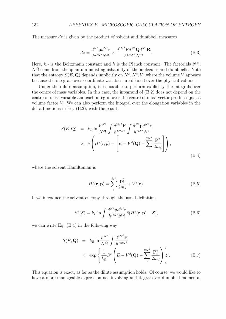
132 APPENDIX B. MICROSCOPIC CALCULATION OF ENTROPY
The measure dz is given by the product of solvent and dumbbell measures
dz =dNs
pdNs
r
hDNsN s!× d2Nd
PdNd
QdNd
R
hD2NdNd!. (B.3)
Here, kB is the Boltzmann constant and h is the Planck constant. The factorials N s!,Nd! come from the quantum indistinguishability of the molecules and dumbbells. Notethat the entropy S(E,Q) depends implicitly on N s, Nd, V , where the volume V appearsbecause the integrals over coordinate variables are defined over the physical volume.
Under the dilute assumption, it is possible to perform explicitly the integrals overthe centre of mass variables. In this case, the integrand of (B.2) does not depend on thecentre of mass variable and each integral over the centre of mass vector produces just avolume factor V . We can also perform the integral over the elongation variables in thedelta functions in Eq. (B.2), with the result
S(E,Q) = kB lnV Nd
Nd!
∫
d2Nd
P
hD2Nd
∫
dNs
pdNs
r
hDNsN s!
× δ
Hs(r, p) −
E − V d(Q) −2Nd∑
i
P2i
2md
,
(B.4)
where the solvent Hamiltonian is
Hs(r,p) =Ns∑
i
p2i
2ms
+ V s(r). (B.5)
If we introduce the solvent entropy through the usual definition
Ss(E) = kB ln
∫
dNs
pdNs
r
hDNsN s!δ(Hs(r,p) − E), (B.6)
we can write Eq. (B.4) in the following way
S(E,Q) = kB lnV Nd
Nd!
∫
d2Nd
P
hD2Nd
× exp
1
kB
Ss
E − V d(Q) −2Nd∑
i
P2i
2md
. (B.7)
This equation is exact, as far as the dilute assumption holds. Of course, we would like tohave a more manageable expression not involving an integral over dumbbell momenta.
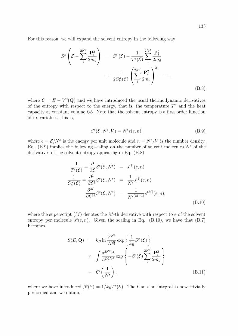
133
For this reason, we will expand the solvent entropy in the following way
Ss
E −2Nd∑
i
P2i
2md
= Ss (E) − 1
T s(E)
2Nd∑
i
P2i
2md
+1
2CsV (E)
2Nd∑
i
P2i
2md
2
− · · · ,
(B.8)
where E = E − V d(Q) and we have introduced the usual thermodynamic derivativesof the entropy with respect to the energy, that is, the temperature T s and the heatcapacity at constant volume Cs
V . Note that the solvent entropy is a first order functionof its variables, this is,
Ss(E , N s, V ) = N ss(e, n), (B.9)
where e = E/N s is the energy per unit molecule and n = N s/V is the number density.Eq. (B.9) implies the following scaling on the number of solvent molecules N s of thederivatives of the solvent entropy appearing in Eq. (B.8)
1
T s(E)=
∂
∂E Ss(E , N s) = s(1)(e, n)
1
CsV (E)
=∂2
∂E2Ss(E , N s) =
1
N ss(2)(e, n)
∂M
∂EMSs(E , N s) =
1
N s(M−1)s(M)(e, n),
(B.10)
where the superscript (M) denotes the M -th derivative with respect to e of the solvententropy per molecule ss(e, n). Given the scaling in Eq. (B.10), we have that (B.7)becomes
S(E,Q) = kB lnV Nd
Nd!exp
1
kB
Ss (E)
×∫
d2Nd
P
hD2Ndexp
−βs(E)2Nd∑
i
P2i
2md
+ O(
1
N s
)
, (B.11)
where we have introduced βs(E) = 1/kBTs(E). The Gaussian integral is now trivially
performed and we obtain,

134 APPENDIX B. MICROSCOPIC CALCULATION OF ENTROPY
S(E,Q) = Ss (E − V (Q)) + kB lnV Nd
Nd!
(
2πmd
h2βs
)DNd
+ O(
1
N s
)
. (B.12)
Of course, within the same approximation of neglecting terms that scale as the inverseof the number of solvent molecules, we can also write
S(E,Q) = Ss(E) − V (Q)
T s(E)+ kB ln
V Nd
Nd!
(
2πmd
h2βs
)DNd
+ O(
1
N s
)
. (B.13)
The last term corresponding to the integration over the centre of mass of the dumb-bells has the form of an ideal gas contribution. By using Stirling’s approximation(lnN ! ≈ N lnN −N), this ideal gas term has the usual form
lnV Nd
Nd!λDNd
d
= Nd(1 + lnndλDd ), (B.14)
where nd = Nd/V is the dumbbell density and we have introduced the thermal wave-length of the beads by
λd =
(
h2
2πmdkBT s(E)
)1/2
, (B.15)
and our final result is
S(E,Q) = Ss(E) − V (Q)
T s(E)+ kBN
d(1 + lnndλDd )
+ O(
1
N s
)
. (B.16)
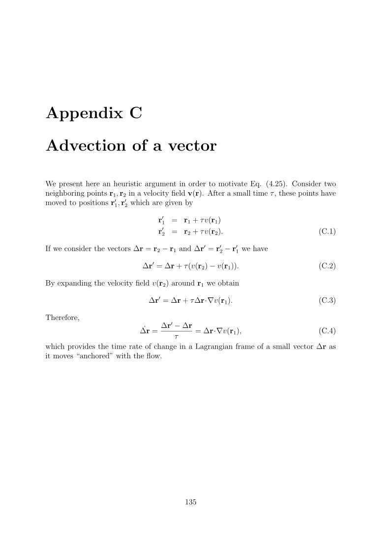
Appendix C
Advection of a vector
We present here an heuristic argument in order to motivate Eq. (4.25). Consider twoneighboring points r1, r2 in a velocity field v(r). After a small time τ , these points havemoved to positions r′1, r
′2 which are given by
r′1 = r1 + τv(r1)
r′2 = r2 + τv(r2). (C.1)
If we consider the vectors ∆r = r2 − r1 and ∆r′ = r′2 − r′1 we have
∆r′ = ∆r + τ(v(r2) − v(r1)). (C.2)
By expanding the velocity field v(r2) around r1 we obtain
∆r′ = ∆r + τ∆r·∇v(r1). (C.3)
Therefore,
∆r =∆r′ − ∆r
τ= ∆r·∇v(r1), (C.4)
which provides the time rate of change in a Lagrangian frame of a small vector ∆r asit moves “anchored” with the flow.
135

136 APPENDIX C. ADVECTION OF A VECTOR
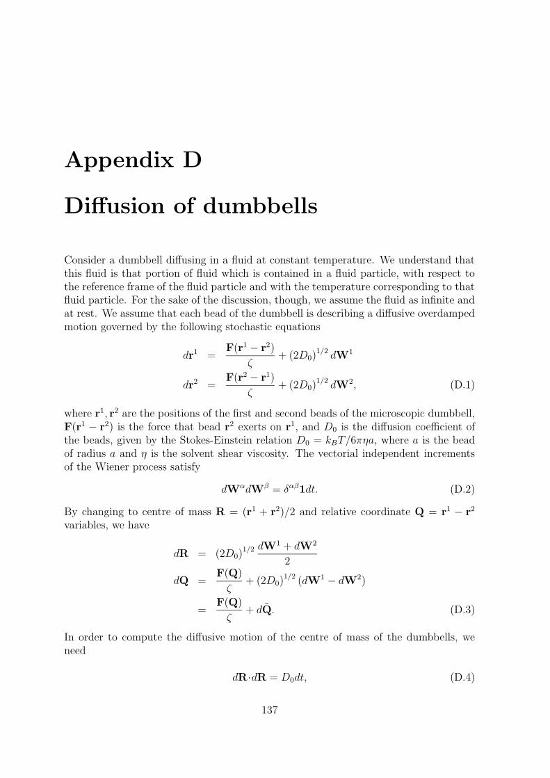
Appendix D
Diffusion of dumbbells
Consider a dumbbell diffusing in a fluid at constant temperature. We understand thatthis fluid is that portion of fluid which is contained in a fluid particle, with respect tothe reference frame of the fluid particle and with the temperature corresponding to thatfluid particle. For the sake of the discussion, though, we assume the fluid as infinite andat rest. We assume that each bead of the dumbbell is describing a diffusive overdampedmotion governed by the following stochastic equations
dr1 =F(r1 − r2)
ζ+ (2D0)
1/2 dW1
dr2 =F(r2 − r1)
ζ+ (2D0)
1/2 dW2, (D.1)
where r1, r2 are the positions of the first and second beads of the microscopic dumbbell,F(r1 − r2) is the force that bead r2 exerts on r1, and D0 is the diffusion coefficient ofthe beads, given by the Stokes-Einstein relation D0 = kBT/6πηa, where a is the beadof radius a and η is the solvent shear viscosity. The vectorial independent incrementsof the Wiener process satisfy
dWαdWβ = δαβ1dt. (D.2)
By changing to centre of mass R = (r1 + r2)/2 and relative coordinate Q = r1 − r2
variables, we have
dR = (2D0)1/2 dW
1 + dW2
2
dQ =F(Q)
ζ+ (2D0)
1/2 (dW1 − dW2)
=F(Q)
ζ+ dQ. (D.3)
In order to compute the diffusive motion of the centre of mass of the dumbbells, weneed
dR·dR = D0dt, (D.4)
137
138 APPENDIX D. DIFFUSION OF DUMBBELLS
which corresponds to a diffusion coefficient D0/2. The physical meaning of this is thatthe dumbbell is subject to two friction forces (one for each bead), and therefore thecentre of mass diffuses with half the diffusion coefficient of each bead. We also need tocompute
dQ·dQ = 4D0dt. (D.5)
This means that the average dumbbell elongation Q is subject to a random walk witha diffusion coefficient given by 2D0.
Appendix E
SPH discretisation of the advectiondiffusion equation
Consider the advection diffusion equation for the concentration of a passive densityn(r, t) in a velocity field v(r, t),
∂n
∂t= −∇·nv + ∇·Tn
ζ∇µ
T, (E.1)
where µ = µ(n(r, t)) is the chemical potential field and T = T (r) is the temperaturefield. For a very dilute system, one can use the ideal gas form for the chemical potentialkBT lnn. If we further assume an isothermal system, the above equation becomes
∂n
∂t= −∇·nv +D∇2n, (E.2)
where D = kBT/ζ is the diffusion coefficient and ζ = 6πηa is the friction coefficient ofthe beads of radius a with the solvent of shear viscosity η.
We write Eq. (E.1) in Lagrangian form by using the usual substantial derivative
d
dt=
∂
∂t+ v·∇, (E.3)
so we obtaindn
dt= −n(∇·v) + ∇·Tn
ζ∇µ
T, (E.4)
which expresses the time rate of change of the concentration field as we move with theflow field.
Our aim is to discretize (E.4) on the fluid particles following the smoothed particlehydrodynamics philosophy. a discrete version of (E.4) would read
ni = −ndi (∇·v)i +
(
∇·Tnζ∇µ
T
)
i
. (E.5)
Instead of working with the density ndi we prefer to work with Ni = ni/di the actual
number of suspended particles in the fluid particle of volume d−1i . This variable evolves
139
140 APPENDIX E. ADVECTION DIFFUSION EQUATION
according to
Ni = −Nidi
di
− ni
di
(∇·v)i +1
di
(
∇·Tnζ∇µ
T
)
i
. (E.6)
This equation is still a meaningless collection of symbols until we specify how the deriva-tives in the parenthesis are computed. The divergence of the velocity field (∇·v)i at thelocation of the i-th fluid particle can be computed from Eq. (4.28). The final result canbe written as
(∇·v)i =Vi
Vi
= − di
di
. (E.7)
The physical meaning of this equation is clear, the divergence of the velocity field isassociated to the relative rate of change of the volume of the fluid particles, as expected.After substitution of Eq. (E.7) into (E.6) one obtains
Ni =1
di
(
∇·Tnζ∇µ
T
)
i
, (E.8)
and we observe that if the dynamics is given by the advection diffusion equation (E.1)then the rate of change of the number of suspended particles as we follow the fluid isentirely due to irreversible processes (governed by the transport coefficient ζ). This isconsistent with our requirement that the reversible part of the dynamics for Ni is zero,as expressed in Eqs. (4.33).
We still have to provide an expression for the derivatives appearing in Eq. (E.8).We follow here the interpolant method first proposed by Cleary and Monaghan [94]. Asa preliminary, we introduce the isotropic function F (r) through
∇W (r) = −rF (r), (E.9)
which satisfies∫
drr · · · rF (r) = 0, (E.10)
if the number of r’s is odd, by isotropy. It also satisfies
∫
drrrF (r) = 1, (E.11)
as can be proved from
∫
drr∇W (r) = −1. (E.12)
This equation is obtained from a partial integration and the normalisation of the weightfunction W (r).
Now, consider the following integral
∫
dr(B(r′) +B(r))(A(r′) − A(r))F (|r − r′|), (E.13)
141
where A(r), B(r) are arbitrary functions that change slowly on the scale of the range ofW (r) and F (r). By Taylor expanding A(r′), B(r′) around r, neglecting terms of orderhigher than the second, and using Eqs. (E.10), (E.11) we obtain that the above integralis given by ∇·(B(r)∇A(r)), up to terms involving higher order derivatives. The nextstep in SPH is to discretize the integral on the locations of the particles
∫
dr(B(ri) +B(r))(A(ri) − A(r))F (|r − ri|)
≈∑
j
1
dj
(B(ri) +B(rj))(A(ri) − A(rj))F (|rj − ri|).
(E.14)
So finally, we obtain the following interpolant for computing the second derivatives ata particle location, i.e.
(∇·(B(r)∇A(r)))i ≈∑
j
1
dj
(Bi +Bj)AijFij, (E.15)
where Bi = B(ri), Aij = A(ri) − A(rj) and Fij = F (|rj − ri|).With this result (E.15) inserted into (E.8), we can readily obtain a discretized version
of Eq. (E.1) on the Lagrangian grid of moving fluid particles in the form
Ni =1
di
(
∇·Tnζ∇µ
T
)
i
=∑
j
Fij
djdi
(
Tini
ζ+Tjnj
ζ
)(
µi
Ti
− µj
Tj
)
. (E.16)
Note that this equation conserves the total number of suspended particles,∑
i Ni = 0.

142 APPENDIX E. ADVECTION DIFFUSION EQUATION
Bibliography
[1] M. J. Crochet, A. R. Davies, and K. Walters, Numerical Simulation of Non-
Newtonian Flow (Elsevier, Amsterdam, 1984)
[2] R. Keunings, Simulation of viscoelastic fluid flow, in: C.L. Tucker III, (Ed.), Fun-
damentals of Computer Modeling for Polymer Processing (Hanser, Munich, 1989)pp. 402.
[3] F. P. T. Baaijens, Mixed finite element methods for viscoelastic flow analysis: areview, J. Non-Newt. Fluid Mech. 79, 361 (1998).
[4] R. B. Bird, R. C. Armstrong. O. Hassager Dynamics of Polymeric Liquids, Vol. 1(John Wiley, NY, 1976).
[5] P. Ilg, Reduced Description of Kinetic Models of Polymer Dynamics, Ph.D. Thesis,Wissenschaft und Technik Verlag, Berlin, 2002.
[6] R. I. Tanner, Engineering Rheology (Clarendon Press, Oxford, 1988).
[7] R. G. Larson, Constitutive Equations of Polymer Melts and Solutions (Butter-worths, Boston, 1987).
[8] R. G. Owens and T. N. Phillips, Computational rheology (Imperial College Press,London, 2002).
[9] R. Keunings, Micro-Macro methods for the multiscale simulations of viscoelasticflow using molecular models of kinetic theory , to appear in Rheology Rewiews 2004,D.M. Bindings and K. Walters (2003).
[10] A. Lozinski, C. Chauviere, J. Fang and R. G. Owens, Fokker-Planck simulations offast flows of melts and concentrated polymer solutions in complex geometries, J.Rheol. 47(2), 535 (2002).
[11] M. Laso and H.C. Ottinger, Calculation of viscoelastic flow using molecular models:the CONNFFESSIT approach. J. Non-Newt. Fluid Mech. 47, 1 (1993).
[12] M. A. Hulsen, A. P. G. van Heel, and B. H. A. A. van den Brule, Simulation ofviscoelastic flows using Brownian configuration fields, J. Non-Newt. Fluid Mech.70, 79 (1997).
143
144 BIBLIOGRAPHY
[13] P. Halin, G. Lielens, R. Keunings, and V. Legat, The Lagrangian Particle Methodfor Macroscopic Micro-Macro Viscoelastic Flow Computations, J. Non-Newt. FluidMech. 79, 387 (1998).
[14] L. B. Lucy, A numerical approach to the testing of the fission hypothesis, Astron.J. 83, 1013 (1977).
[15] R. A. Gingold and J. J. Monaghan, Smoothed particle hydrodynamics theory andapplication to non-spherical stars, Mon. Not. R. Astron. Soc. 181, 375 (1977).
[16] H. Takeda, S. M. Miyama and M. Sekiya, Numerical Simulation of Viscous Flowby Smoothed Particle Hydrodynamics, Prog. Theor. Phys. 92(5), 939 (1994).
[17] J. J. Monaghan, Simulating Free Surface Flows with SPH, J. Comput. Phys. 110,399 (1994).
[18] S. Siegler, and H. Riffert, Smoothed Particle Hydrodynamics Simulations of Ultra-relativistic Shocks with Artificial Viscosity. Astrophys. J. 531, 1053 (2000).
[19] L. D. Libersky, A. G. Petschek, T. C. Carney, J. R. Hipp, and F. A. Allahdadi,High Strain Lagrangian Hydrodynamics, J. Comput. Phys. 109, 67 (1993).
[20] A. G. Petschek and L. D. Libersky, Cylindrical Smoothed Particle Hydrodynamics,J. Comput. Phys. 109, 76 (1993).
[21] L. D. Libersky and A. G. Petschek, Smooth Particle Hydrodynamics With Strength
of Materials, in: Advances in the Free-Lagrange Method, Moran, WY, USA, June
1990, edited by H. E. Trease, M. J. Fritts and W. P. Crowley, Lect. Notes in Phys.(Springer-Verlag, New York/Berlin, 1991), Vol. 395, p. 248.
[22] C. Maveyraud, W. Benz, A. Sornette, and D. Sornette, Solid friction at high slid-ing velocities: An explicit three-dimensional dynamical smoothed particle hydro-dynamics approach, J. Geophys. Res. 104, 28769 (1999).
[23] R. Speith, H. Riffert, and H. Ruder, Numerical Fluid Dynamics in Astrophysics
with Smoothed Particle Hydrodynamics, in: Bungartz H.-J., Durst F., Zenger C.(eds.): High Performance Scientific and Engineering Computing, Lecture Notes in
Computational Science and Engineering (1999) pp. 417.
[24] O. Flebbe, S. Munzel, H. Herold, H. Riffert, H. Ruder, Smoothed Particle Hydro-dynamics: Physical Viscosity and the simulation of accretion disk, Astroph. J. 431,754 (1994).
[25] C.V. Chaubal, A. Srinivasan, O. Egecioglu, and L.G. Leal, SPH techniques for thesolution of kinetic theory problems J. Non-Newt. Fluid Mech. 70, 125 (1997).
[26] T. Bubeck, M. Hipp, S. Httemann, S. Kunze, M. Ritt, W. Rosenstiel, H. Ruder,and R. Speith, Parallel SPH on Cray T3E and NEC SX-4 using DTS, in: KrauseE., Jger W. (eds.): Proc. High Performance Computing in Science and Engineering1998 (1999) pp. 396.
BIBLIOGRAPHY 145
[27] R. Di Lisio, E. Grenier, and M. Pulvirenti, The convergence of the SPH method,Computer Math. Applic. 35, 95 (1998).
[28] P. Espanol, M. Serrano, and H. C. Ottinger, Thermodynamically admissible formfor discrete hydrodynamics, Phys. Rev. Lett. 83, 4552 (1999).
[29] P. Espanol, Europhys. Lett. 39, 606 (1997); Phys. Rev. E 57, 2930 (1998).
[30] B.I.M. ten Bosch, On a extension of Dissipative Particle Dynamics for viscoelasticflow modelling, J. Non-Newt. Fluid Mech. 83, 231 (1999).
[31] S. Shao, E. Y. M. Lo, Incompressible SPH method for simulating Newtonian andnon-Newtonian flows with a free surface, Advances in Water Resources 26 (7), 787(2003).
[32] W. Benz, Smoothed Particle Hydrodynamics: A Review, in: The Numerical Mod-
elling of Nonlinear Stellar Pulsation: Problems and Prospects, Les Arcs, France,
March 1989, edited by J. R. Buchler, Nato ASI Series (Kluwer Academic, Boston,MA, 1990), Vol. 302, p. 269.
[33] J. Monaghan, Smoothed Particle Hydrodynamics, Annu. Rev. Astron. Astrophys.30, 543 (1992).
[34] J. J. Monaghan, An Introduction to SPH, Comp. Phys. Commun. 48, 89 (1988).
[35] R. W. Hockney and J. W. Eastwood, Computer Simulation Using Particles
(McGraw-Hill, New York, 1981)
[36] M. P. Allen and D. J. Tildesley, Computer Simulation of Liquids (Clarendon Press,Oxford, 1987).
[37] O. Kum, W. G. Hoover, Viscous conducting flows with smooth-particle appliedmechanics, Phys. Rev. E 52, 4889 (1995).
[38] S. J. Cummins, M. Rudman, An SPH Projection Method, J. Comp. Phys. 152,584 (1999).
[39] G. K. Batchelor, An Introduction to Fluid Dynamics (Cambridge University Press,Cambridge, 1967).
[40] L. D. Landau and E. M. Lifshitz, Fluid Mechanics (Pergamon Press, London, 1959).
[41] J. Von Neumann and R. D. Richtmeyer, A Method for the Numerical Calculationof Hydrodynamic Shocks, J. Appl. Phys. 21, 232 (1950).
[42] J. P. Morris, P. J. Fox, and Y. Zhu, Modeling Low Reynolds Number IncompressibleFlows Using SPH, J. Comput. Phys. 136, 214 (1997).
[43] J. P. Morris and J. J. Monaghan, A Switch to Reduce SPH Viscosity, J. Comput.Phys. 136, 41 (1997).
146 BIBLIOGRAPHY
[44] J. P. Morris, Analysis of Smoothed Particle Hydrodynamics with Applications,Ph.D. Thesis, Monash University, Melbourne, Australia, 1996.
[45] W. G. Hoover and S. Hess, Equilibrium and nonequilibrium thermomechanics foran effective pair potential used in smooth particle applied mechanics, Physica A231, 425 (1996).
[46] H. A. Posch, W. G. Hoover and O. Kum, Steady-state shear flows via nonequilib-rium molecular dynamics and smooth-particle applied mechanics, Phys. Rev. E 52,1711 (1995).
[47] W. H. Press, S. A. Teukolsky, W. T. Vetterling, and B. P. Flannery, Numerical
Recipes in C: The Art of Scientific Computing (Cambridge University Press, Cam-bridge, 1992), p. 847.
[48] J. H. Ferziger, M. Peric, Computational Methods for Fluid Dynamics (Springer-Verlag Berlin, 1997).
[49] R. L. Panton, Incompressible Flow (John Wiley, NY, 1984).
[50] M. Ellero, M. Kroger and S. Hess, Viscoelastic flows studied by Smoothed ParticleDynamics. J. Non-Newtonian Fluid Mech. 105, 35 (2002).
[51] D. D. Joseph, Fluid Dynamics of Viscoelastic Liquids (Springer-VerlagBerlin,Applied mathematical sciences, v.84, 1990).
[52] A. W. Lees and S. F. Edwards, The computer study of transport process underextreme conditions, J. Phys. C5, 1921 (1972).
[53] A. Bomer and T. Klimpel, Plastic deformation of corrugated rails - a numericalapproach using data of rail steel, Wear 253, 150 (2002).
[54] K. Sugino, H, Kageyama and C. Urashima, Metallurgical improvement of rail forthe reduction of rail-wheel contact fatigue failures, Wear 144, 319 (1991).
[55] B. N. J. Perrson, Sliding Friction (Springer-Verlag, Berlin, 1998).
[56] J. Ahlstrom and B. Karlsson, Microstructural evaluation and interpretation of themechanically and thermally affected zone under railway wheel flats, Wear 232, 1(1999).
[57] H. Krause and C. Schroelkamp, Influence of non-metallic inclusions on the wearbehaviour of ferrous materials in nominally dry friction systems, Wear 120, 353(1987).
[58] H. T. Zhu and H. M. Zbib, A macroscopic model for plastic flow in metal-matrixcomposites, Int. J. of Plasticity 11 (4), 471 (1995).
BIBLIOGRAPHY 147
[59] S. Piazolo, P. D. Bons and C. W. Passchier, The influence of matric rheology andvorticity on fabric development of populations of rigid objects during plane straindeformation, Tectonophysics 351, 315 (2002).
[60] Stankovic, M. Kroger, and S. Hess, Recognition and analysis of local structure inpolycrystalline configurations, Comput. Phys. Commun. 145, 371 (2002).
[61] M. Kroger, I. Stankovic, and S. Hess, Towards multiscale modeling of metals viaembedded particle computer simulations, Multiscale Model. Simul. 1, 25 (2003).
[62] Stankovic, S. Hess, and M. Kroger, Structural changes and viscoplastic behaviorof a generic embedded atom model metal in steady shear flow, Phys. Rev. E 69,021509 (2004).
[63] R. M. Christensen, Mechanics of composite materials (Wiley, New York, 1979).
[64] Q. S. Yang and Q. H. Qin, Micro-mechanical analysis of composite materials byBEM, to appear in Eng. Analys. with Bound. Elem.(2004).
[65] P. Gilormini and J. C. Michel, Finite element solutions of the problem of a sphericalinhomogeneity in an infinite power-law viscous matrix, Eur. J. Mech. A/Solids 17,725 (1998).
[66] G. Pennacchioni, L. Fasolo, M. M. Checchi and L. Salasnich, Finite-element mod-elling of simple shear flow in Newtonian and non-Newtonian fluids around a circularrigid particle, J. Struct. Geol. 22, 683 (2000).
[67] T. Masuda and N. Mizuno, Deflection of non-Newtonian simple shear flow arounda rigid cylindrical body by the Finite Element Method, J. Struct. Geol. 18 (8),1089 (1996).
[68] S. K. Samanta, N. Mandal and C. Chakraborty, Flow pattern around rigid inclu-sions in a multiple inclusion system undergoing bulk simple shear deformations, J.Struct. Geol. 25, 209 (2003).
[69] S. Chapman and T. G. Cowling, The Mathematical Theory of Non-Uniform Gases,(Cambridge University Press Cambridge, 1970).
[70] D. Doolen, Lattice Gas Methods for partial differential equations, (Addison-Wesley,1987).
[71] P. J. Hoogerbrugge and J. M. V. A. Koelman, Simulating Microscopic Hydrody-namics Phenomena with Dissipative Particle Dynamics, Europhys. Lett. 19, 155(1992).
[72] P. Espanol and P. Warren, Statistical mechanics of Dissipative Particle Dynamics,Europhys. Lett.30, 191 (1995).
[73] P. Espanol and M. Revenga, Smoothed Dissipative Particle Dynamics, Phys. Rev.E 67, 026705 (2003).
148 BIBLIOGRAPHY
[74] M. Ellero, P. Espanol and E. G. Flekkoy, Thermodynamically consistent fluid par-ticle model for viscoelastic flows, Phys. Rev. E 68, 041504 (2003).
[75] J. M. V. A. Koelman and P. J. Hoogerbrugge, Dynamic simulations of hard-spheresuspensions under steady state shear, Europhys. Lett. 21, 363 (1993).
[76] E. S. Boek, P. V. Coveney, H. N. W. Lekkerkerker, and P. van der Schoot, Simulat-ing the rheology of dense colloidal suspensions using dissipative particle dynamics,Phys. Rev. E 55, 3124 (1997).
[77] M. Whittle and E. Dickinson, On simulating colloids by dissipative particle dy-namics: Issues and complications, Journal of Colloid and Interface Science 242,106 (2001).
[78] A. G. Schlijper, P. J. Hoogerbrugge and C. W. Manke, Computer simulation ofdilute polymer solutions with the dissipative particle dynamics method, J. Rheol.39, 567 (1995).
[79] N. A. Spenley, Scaling laws for polymers in dissipative particle dynamics, Europhys.Lett. 49, 534 (2000).
[80] P. V. Coveney and K. Novik, Erratum: Computer simulations of domain growthand phase separation in two-dimensional binary immiscible fluids using dissipativeparticle dynamics, Phys. Rev. E 55, 4831 (1997).
[81] S. I. Jury, P. Bladon, S. Krishna, and M. E. Cates, Test of dynamical scaling inthree-dimensional spinodal decomposition, Phys. Rev. E 59, R2535 (1999).
[82] C. M. Wijmans, B. Smit, and R. D. Groot, Phase behavior of monomeric mixturesand polymer solutions with soft interaction potentials, J. Chem. Phys. 114, 7644(2001).
[83] P. B Warren, Dissipative particle dynamics, Curr. Opinion Colloid Interface Sci. 3,620 (1998).
[84] P. Espanol, Dissipative Particle Dynamics, in: Trends in Nanoscale Mechanics:
Analysis of Nanostructured Materials and Multi-Scale Modeling, edited by V. M.Harik and M. D. Salas editors (Kluwer 2003).
[85] K. Feigl, M. Laso, and H. C. Ottinger, The CONNFFESSIT approach for solvinga two-dimensional viscoelastic fluid problem, Macromolecules 28, 3261 (1995).
[86] H. C. Ottinger and M. Grmela, Dynamics and Thermodynamics of complex fluids.II. Illustrations of a general formalism, Phys. Rev. E 56, 6633 (1997).
[87] M. Serrano and P. Espanol, Thermodynamically consistent mesoscopic fluid particlemodel, Phys. Rev. E 64, 46115, (2001).
[88] E. G. Flekkoy, P. V. Coveney, and G. D. Fabritiis, Foundations of dissipative par-ticle dynamics, Phys. Rev. E 62, 2140 (2000).
BIBLIOGRAPHY 149
[89] H. C. Ottinger, General projection operator formalism for the dynamics and ther-modynamics of complex fluids, Phys. Rev. E 57, 1416, (1998).
[90] H. C. Ottinger, B. H. A. A. van den Brule and M. A. Hulsen, Brownian configu-ration fields and variance reduced CONNFFESSIT, J. Non-Newt. Fluid Mech. 70,255 (1997).
[91] J. J. Monaghan, New Developments in Smoothed Particle Hydrodynamics, in:Meshfree Methods for Partial Differential Equations, Lecture notes in computa-tional science and engineering, Vol. 26 edited by M. Griebel and M. A. Schweitzer(Springer-Verlag, Berlin, 2002).
[92] M. Dressler, B. J. Edwards and H. C. Ottinger, Rheol. Acta 38, 117 (1999).
[93] C. Gardiner, Handbook of Stochastic Methods (Springer-Verlag, Berlin, 1983).
[94] P. W. Cleary and J. J. Monaghan, Conduction Modelling using Smoothed ParticleHydrodynamics, J. Comp. Phys. 148, 227 (1999).
[95] M. Rappaz, M. Bellet and M. Deville, Numerical Modeling in Material Science and
Engineering (Springer-Verlag, Berlin Heidelberg, 2003)
[96] A. Chandra and S. Mukherjee, Boundary Element Methods in Manufacturing (Ox-ford University Press, 1997)
[97] H.C. Ottinger, Stochastic Processes in Polymeric Fluids (Springer, Berlin Heidel-berg New York, 1996)
[98] Q. Zhou and R. Akhavan, A comparison of FENE and FENE-P dumbbells andchain models in turbulent flow, J. Non-Newtonian Fluid Mech. 109, 115 (2003).
[99] M. Melchior and H. C. Ottinger, Variance reduced simulations of polymer dynamics,J. Chem. Phys. 105(8), 3316 (1996).
[100] X. Gallez, P. Halin, G. Lielens, R. Keunings and V. Legat, The adaptative La-grangian particle method for macroscopic and micro-macro computations of time-dependent viscoelastic flows, Comput. Methods Appl. Mech. Engrg. 180, 345(1999).
[101] P. Wapperom, R. Keunings and V. Legat, The backward-tracking Lagrangianparticle method for transient viscoelastic flows, J. Non-Newtonian Fluid Mech. 91,273 (2000).
[102] M. Ellero and M. Kroger, The hybrid BDDFS method: memory saving approachfor CONNFFESSIT-typer simulations , J. Non-Newtonian Fluid Mech. (2004) inpress.
[103] X.-J. Fan, Viscosity, first normal stress-coefficients, and molecular stretching indilute polymer solutions, J. Non-Newtonian Fluid Mech. 17, 125 (1985).
150 BIBLIOGRAPHY
[104] X.-J. Fan, Viscosity, first normal stress-coefficient and molecular stretching inconcentrated solutions and melts, J. Non-Newtonian Fluid Mech. 17, 251 (1985).
[105] J. K. Suen, Y. L. Joo and R. C. Armstrong, Molecular orientation effects inviscoelasticity, Annu. Rev. Fluid Mech. 134, 417 (2002).
[106] A. Lozinski and C. Chauviere, A fast solver for Fokker-Planck equation appliedto viscoelastic flow calculations, submitted to Elsevier Science, (2003).
[107] C. Chauviere, J. Fang, A. Lozinski and R. G. Owens, On the numerical simulationof flows of polymer solutions using high-order methods based on the Fokker-Planckequation, Int. J. Mod. Phys. B 17, 9 (2003).
[108] M. Kroger, Flow-alignment and rheology of polymer melts. Computation ofthe single-link orientational distribution function. Makromol. Chem. – Macromol.Symp. 81 (1994) 83.
[109] M. Kroger, Simple models for complex nonequilibrium fluids, Phys. Rep.390, 453(2004).
[110] M. Herrchen and H. C. Ottinger, A detailed comparison of various FENE dumbbellmodels J. Non-Newtonian Fluid Mech. 68, 17 (1997).
[111] R. Keunings, On the Peterlin approximation for finite extensible dumbbells, J.Non-Newtonian Fluid Mech. 68, 85 (1997).
[112] P. Ilg, E. De Angelis, I. V. Karlin, C. M. Casciola and S. Succi, Polymer dynamicsin wall turbulent flow, Europhys. Lett. 58 (4), 616 (2002).
[113] M. Laso, M. Picasso, and H. C. Ottinger, 2D time-dependent viscoelastic flowcalculations using CONNFFESSIT, AIChE J. 43, 877 (1997).
[114] R. M. Jendrejack, J. J. de Pablo and M. D. Graham, A method for multiscalesimulations of flowing complex fluids, J. Non-Newtonian Fluid Mech. 108, 123(2002).
[115] J. Bonvin and M. Picasso, Variance reduction methods for CONNFFESSIT-likesimulations, J. Non-Newtonian Fluid Mech. 84, 191 (1999).
[116] T. W. Bell, G. H. Nyland, J. J. de Pablo, and M.D. Graham, Combined Browniandynamics and spectral simulation of the recovery of polymeric fluids after shearflow, Macromolecules 30, 1806 (1997).