Soil erosion and sediment transport measurement and assessment · Soil erosion and sediment...

Soil erosion and sediment transport measurement and assessment

Andreas Klik, Tomas Dostal, Josef Krasa

and Stefan Strohmeier

CTU Prague November 21 – November 25, 2010

Universität für Bodenkultur WienDepartment für Wasser-Atmosphäre-UmweltInstitut für Hydraulik undlandeskulturelle Wasserwirtschaft

Department of Irrigation, Drainage and Landscape Engineering Faculty of Civil Engineering, CTU Prague

Soil erosion and sediment transport

1. Introduction .................................................................................................. 1 1.1 Soil erosion models ...................................................................................................... 1 1.2 Structured approach to soil erosion modeling.............................................................. 4 2. GIS application in soil erosion modelling .................................................. 5 2.1 Basics and structure of IDRISI Kilimanjaro ................................................................ 5

2.1.1 Raster format ...................................................................................................... 5 2.1.2 Vector format ..................................................................................................... 5

2.2 Estimation of sediment amount in a reservoir.............................................................. 6 2.2.1 Reservoir Trapping Efficiency ........................................................................... 6

2.2.1.1 Introduction .................................................................................................... 6 2.2.1.2 Trap Efficiency Methods................................................................................ 7

a) Capacity-Watershed Method (Brown’s Curve).................................................. 7 b) Capacity-Inflow Method (Brune’s Curve) ......................................................... 7 c) Sediment Index Method (Churchill’s Curve)..................................................... 8 d) Reservoir Trapping Efficiency (TE) .................................................................. 9

2.2.2 Sediment amount measurement and calculation – reservoir ............................ 10 2.3 Soil loss and Sediment Transport from a watershed using USLE ............................. 21

2.3.1 DEM preparation.............................................................................................. 21 2.3.2 C factor = Vegetation factor and land use map................................................ 23 2.3.3 K factor............................................................................................................. 25 2.3.4 R factor = Rainfall erosivity factor .................................................................. 28 2.3.5 P factor ............................................................................................................. 29 2.3.6 LS factor = Slope length and steepness factor ................................................. 29 2.3.7 Soil loss - model RUSLE ................................................................................. 30

3. Sedimentation - the sediment transport ................................................... 32 3.1 Runoff and Sedimentation.......................................................................................... 32 3.2 Reservoir trapping efficiency (Brune, Dendy)........................................................... 34 3.3 Further analyses ......................................................................................................... 34

1. Introduction

1.1 Soil erosion models Evaluation of soil erosion hazard: field measurement

• simulation models Can be divided into different groups based on:

• process description • space scale

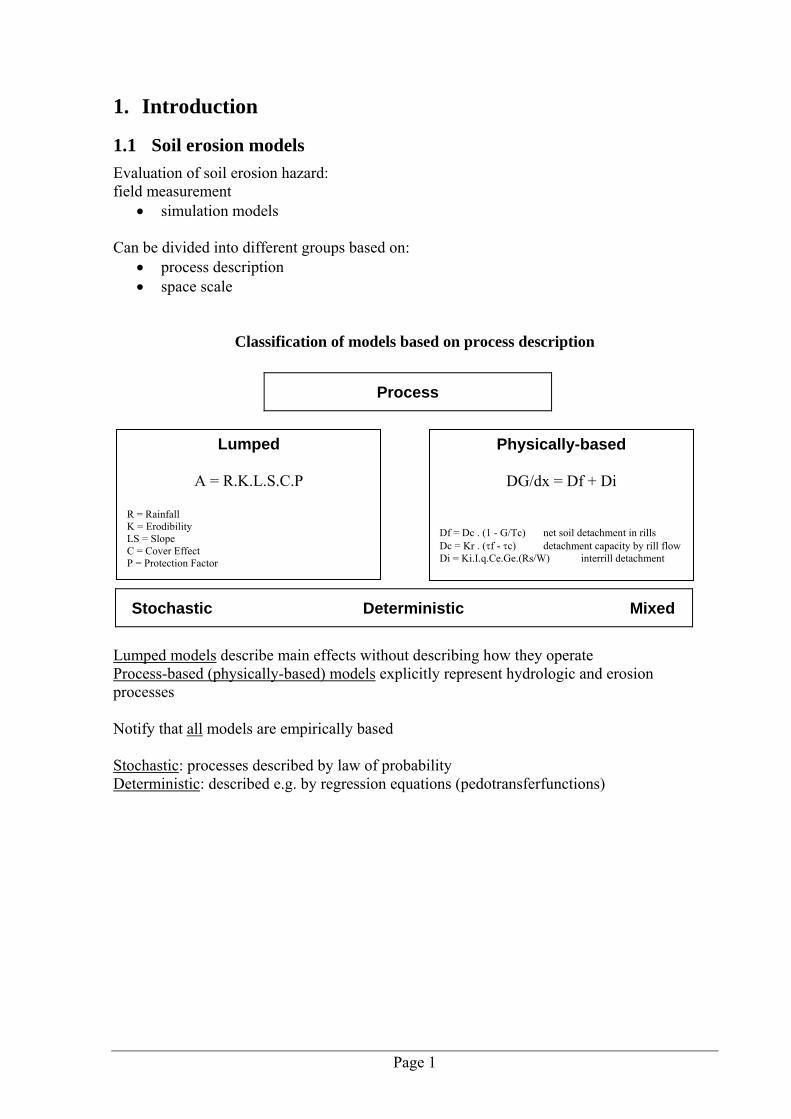
Classification of models based on process description

Lumped models describe main effects without describing how they operate Process-based (physically-based) models explicitly represent hydrologic and erosion processes Notify that all models are empirically based Stochastic: processes described by law of probability Deterministic: described e.g. by regression equations (pedotransferfunctions)

Process

Stochastic Deterministic Mixed

Lumped

A = R.K.L.S.C.P

R = Rainfall K = Erodibility LS = Slope C = Cover Effect P = Protection Factor

Physically-based

DG/dx = Df + Di Df = Dc . (1 - G/Tc) net soil detachment in rills Dc = Kr . (τf - τc) detachment capacity by rill flow Di = Ki.I.q.Ce.Ge.(Rs/W) interrill detachment


Page 2

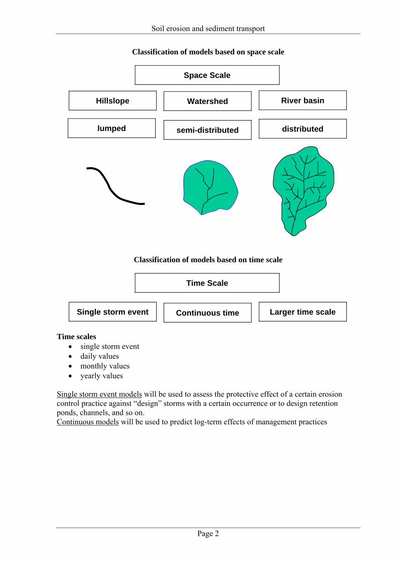
Classification of models based on space scale

Classification of models based on time scale

Time scales

• single storm event • daily values • monthly values • yearly values

Single storm event models will be used to assess the protective effect of a certain erosion control practice against “design” storms with a certain occurrence or to design retention ponds, channels, and so on. Continuous models will be used to predict log-term effects of management practices

Watershed

distributed lumped

River basin

semi-distributed

Hillslope

Space Scale

Time Scale

Continuous time Single storm event Larger time scale


Page 3

Result of simulation • Soil loss • Runoff and soil loss • Runoff, soil erosion and deposition • Transport of nutrients and pesticides

Requirements of a model

• Applicable to the problem • consistent and repeatable results • cover full range of conditions (climate, soils, vegetation, management,....) • can be used with available resources • can easily be used • quality of results adequate and comparable • transferability to other regions

Data needs, calibration and verification (Singh, 1995)

• type of model dictated by availability of data • different models have different needs:

distributed models require more data than lumped • models need calibration, verification and assessment of reliability

available data split in calibration and verification set calibration set should encompass full range of data variability expected in verification parameter estimation techniques are available

• error analysis of calibration should be performed errors in data, parameters or model

• model verification


Page 4

1.2 Structured approach to soil erosion modeling Whenever modeling any problem in a landscape, always use structured approach. To define:

• Goal (what should be the output) • Scale • Accuracy • Time available for calculation • Input data available

3 basic approaches: global ⇒ regional ⇒ local or scales: large ⇒ medium ⇒ small Global (Large regions, strategic studies) • Areas (watersheds) between 100 and 1000 km2 • Input data – in GIS layers, digital format, standard data, field survey excluded • Methods – robust empirical simple models with limited number of input parameters,

continuous models • Outputs – general maps, to compare individual areas, to define the most risky (source,

key) areas Regional (Medium scale, decision making support studies) • Area (watersheds) between 10 and 100 km2 • Input data – in GIS layers, digital format, rough field survey possible and recommended • Methods – more comprehensive empirical methods, physically based simulation models,

continuous or event based models • Outputs – to define “hot spots” in a watershed, to identify critical profiles, source areas, to

compare individual land-use scenarios,… Local (detailed studies and projects) • Area (watersheds) in 1 km2 or hectares • Input data – possible also analog records or maps, detailed field survey, measurement and

sampling necessary • Methods – physically based mathematical simulation models, usually event based • Outputs – detailed and precise values for protection measures design (discharges, runoff

volume, sediment transport). Situation in the Czech Republic – often solved consequences, instead of reasons – i.e. Erosion problems – sediment excavation instead of soil erosion measures Flood protection – larger channels instead of land-use changes, polders, inundation areas Landscape revitalization – small watersheds are selected more or less randomly


Page 5

2. GIS application in soil erosion modelling

Objectives The main objective of this course is to calculate soil loss within a certain watershed and compare it with the real sedimentary deposition in a near reservoir. Therefore a GIS-application named IDRISI Kilimanjaro is used. 2.1 Basics and structure of IDRISI Kilimanjaro IDRISI Kilimanjaro is a GIS (Geographic Information System) and Image Processing software solution that includes over 200 modules for the analysis and display of digital spatial information (http://www.clarklabs.org). IDRISI - like other GIS-applications - uses different layers to process and view data. A layer is either based on raster- or vector format. 2.1.1 Raster format Equal squares with the same dimension build a raster. Every pixel has a value, cells with the same value are called grids.

1 Residential 2 Water 3 Farmland

2.1.2 Vector format defined by coordinates: Lines (City, watershed)

Points (single points) Polygons (City, watershed)

1 Residential 2 Water 3 Farmland


Page 6

2.2 Estimation of sediment amount in a reservoir 2.2.1 Reservoir Trapping Efficiency 2.2.1.1 Introduction Even after hundreds of years of designing and constructing dams and reservoirs, man docs not completely understand the sedimentation processes in reservoirs. For example, we still need to know more about why or how the sediment is deposited where it is. We also need to improve our accuracy in estimating the long-term sediment trap efficiency for proposed small reservoirs under a variety of environmental conditions. This improved technology is necessary because good reservoir sites are scarce and constitute a valuable natural resource that must be protected and used wisely. Because of limited sites and increasing construction costs, we must carefully design and build each reservoir to best accomplish its specific objectives - for soil and water conservation, irrigation, domestic or animal watering, fish farming, recreation, or protecting and enhancing our environment. To optimize the effectiveness of each reservoir, we must be able to predict the rate of reservoir sedimentation processes, especially reservoir-sediment trap efficiency. Reservoir-sediment trap efficiency is the fraction of the sediment transported into a reservoir that is deposited in that reservoir, usually expressed as a percentage OR the percentage of the total inflowing sediment that is retained in the reservoir

E-[Ys (in)-Ys (Out)]/Ys (In) Where: E = Trap efficiency expressed as decimal Ys = Sediment yield in weight units In = inflow Out= outflow Trap efficiency is of particular importance when determining the annual sedimentation rate or capacity loss as expressed by the equation

C1=EYs/C (F-2) Where: C1 = annual sedimentation rate E = trap efficiency, in percent Ys = annual net sediment yield from the drainage area C = original reservoir storage capacity in same units as Ys As sediment is trapped, the reservoir storage capacity is decreased and in turn, the trap efficiency decreases. For practical purposes, the initial trap efficiency can be used as a constant up to 50% Depletion; however, if storage depletion is rapid, the trap efficiency should be updated at time increment with an adjustment of C to reflect the sediment retained. Knowledge of this process is needed to control the sediment accumulation and thereby the life of the reservoir, and to assure its proper operation.


Page 7

2.2.1.2 Trap Efficiency Methods

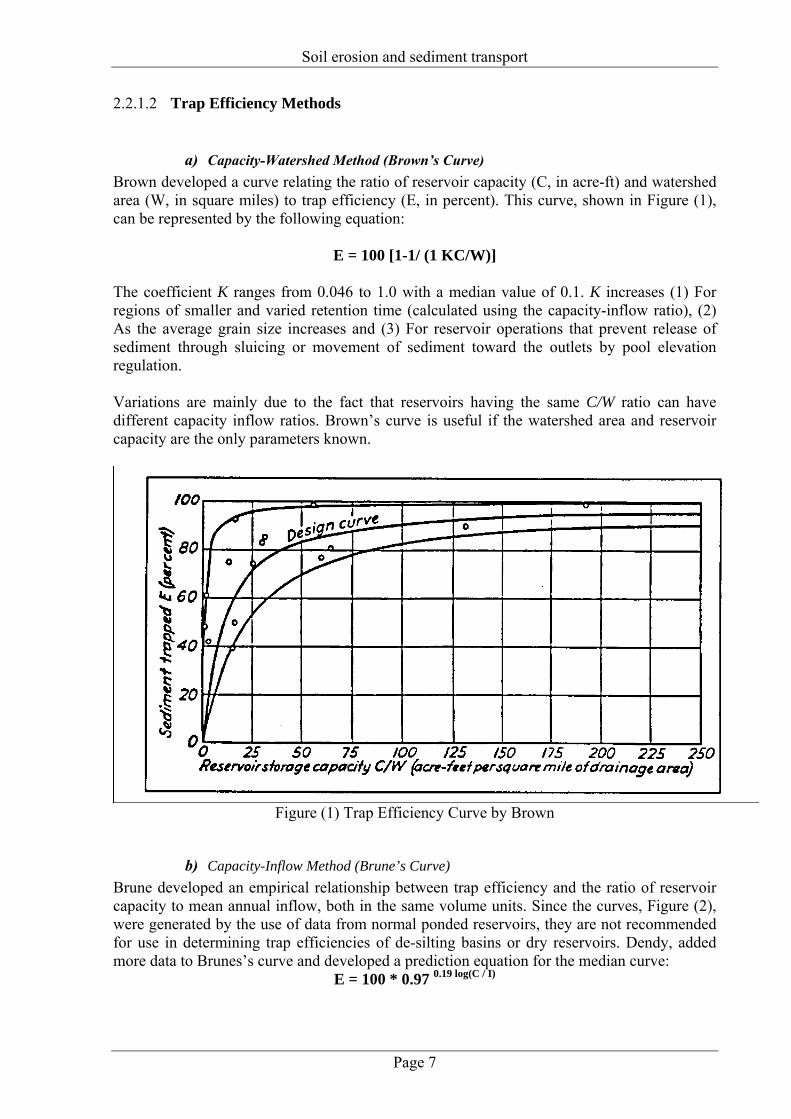
a) Capacity-Watershed Method (Brown’s Curve) Brown developed a curve relating the ratio of reservoir capacity (C, in acre-ft) and watershed area (W, in square miles) to trap efficiency (E, in percent). This curve, shown in Figure (1), can be represented by the following equation:

E = 100 [1-1/ (1 KC/W)] The coefficient K ranges from 0.046 to 1.0 with a median value of 0.1. K increases (1) For regions of smaller and varied retention time (calculated using the capacity-inflow ratio), (2) As the average grain size increases and (3) For reservoir operations that prevent release of sediment through sluicing or movement of sediment toward the outlets by pool elevation regulation. Variations are mainly due to the fact that reservoirs having the same C/W ratio can have different capacity inflow ratios. Brown’s curve is useful if the watershed area and reservoir capacity are the only parameters known.

Figure (1) Trap Efficiency Curve by Brown

b) Capacity-Inflow Method (Brune’s Curve) Brune developed an empirical relationship between trap efficiency and the ratio of reservoir capacity to mean annual inflow, both in the same volume units. Since the curves, Figure (2), were generated by the use of data from normal ponded reservoirs, they are not recommended for use in determining trap efficiencies of de-silting basins or dry reservoirs. Dendy, added more data to Brunes’s curve and developed a prediction equation for the median curve:

E = 100 * 0.97 0.19 log(C / I)


Page 8

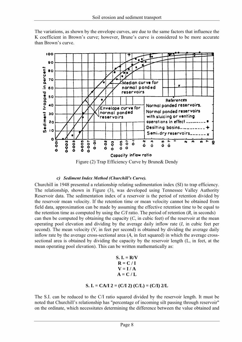
The variations, as shown by the envelope curves, are due to the same factors that influence the K coefficient in Brown’s curve; however, Brune’s curve is considered to be more accurate than Brown’s curve.

Figure (2) Trap Efficiency Curve by Brune& Dendy

c) Sediment Index Method (Churchill’s Curve). Churchill in 1948 presented a relationship relating sedimentation index (SI) to trap efficiency. The relationship, shown in Figure (3), was developed using Tennessee Valley Authority Reservoir data. The sedimentation index of a reservoir is the period of retention divided by the reservoir mean velocity. If the retention time or mean velocity cannot be obtained from field data, approximation can be made by assuming the effective retention time to be equal to the retention time as computed by using the C/I ratio. The period of retention (R, in seconds) can then be computed by obtaining the capacity (C, in cubic feet) of the reservoir at the mean operating pool elevation and dividing by the average daily inflow rate (I, in cubic feet per second). The mean velocity (V, in feet per second) is obtained by dividing the average daily inflow rate by the average cross-sectional area (A, in feet squared) in which the average cross-sectional area is obtained by dividing the capacity by the reservoir length (L, in feet, at the mean operating pool elevation). This can be written mathematically as:

S. I. = R/V R = C / I V = I / A A = C / L

S. I. = CA/I 2 = (C/I 2) (C/L) = (C/I) 2/L

The S.I. can be reduced to the C/I ratio squared divided by the reservoir length. It must be noted that Churchill’s relationship has "percentage of incoming silt passing through reservoir" on the ordinate, which necessitates determining the difference between the value obtained and


Page 9

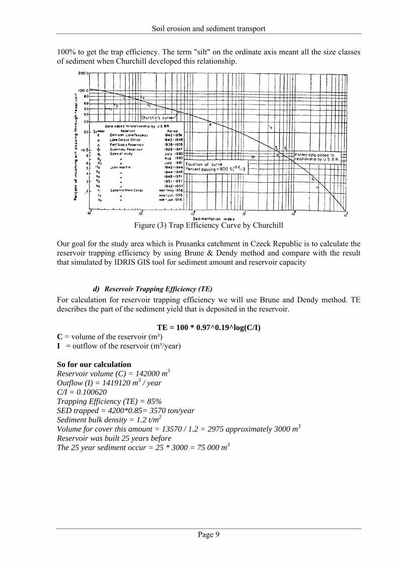
100% to get the trap efficiency. The term "silt" on the ordinate axis meant all the size classes of sediment when Churchill developed this relationship.

Figure (3) Trap Efficiency Curve by Churchill

Our goal for the study area which is Prusanka catchment in Czeck Republic is to calculate the reservoir trapping efficiency by using Brune & Dendy method and compare with the result that simulated by IDRIS GIS tool for sediment amount and reservoir capacity

d) Reservoir Trapping Efficiency (TE) For calculation for reservoir trapping efficiency we will use Brune and Dendy method. TE describes the part of the sediment yield that is deposited in the reservoir.

TE = 100 * 0.97^0.19^log(C/I) C = volume of the reservoir (m³) I = outflow of the reservoir (m³/year) So for our calculation Reservoir volume (C) = 142000 m3 Outflow (I) = 1419120 m3 / year C/I = 0.100620 Trapping Efficiency (TE) = 85% SED trapped = 4200*0.85= 3570 ton/year Sediment bulk density = 1.2 t/m2 Volume for cover this amount = 13570 / 1.2 = 2975 approximately 3000 m3 Reservoir was built 25 years before The 25 year sediment occur = 25 * 3000 = 75 000 m3


Page 10

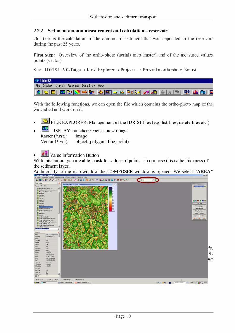
2.2.2 Sediment amount measurement and calculation – reservoir Our task is the calculation of the amount of sediment that was deposited in the reservoir during the past 25 years. First step: Overview of the ortho-photo (aerial) map (raster) and of the measured values points (vector).

Start IDRISI 16.0-Taiga→ Idrisi Explorer→ Projects → Prusanka orthophoto_3m.rst

With the following functions, we can open the file which contains the ortho-photo map of the watershed and work on it. • FILE EXPLORER: Management of the IDRISI-files (e.g. list files, delete files etc.)

• DISPLAY launcher: Opens a new image Raster (*.rst): image Vector (*.vct): object (polygon, line, point)

• Value information Button With this button, you are able to ask for values of points - in our case this is the thickness of the sediment layer. Additionally to the map-window the COMPOSER-window is opened. We select “AREA” Watershed Module. After that we did the following functions in the COMPOSER window: LAYER PROPERTIES → Display parameters →Autoscaling Options → Equal intervals, number of classes → 256, Palette File → Grey → ADVANCED PALETTE/SYMBOL SELECTION → Data relationship → Quantitative, Color logic → Unipolar [ramp from white], Current Selection → UnipolarWred → OK


Page 11

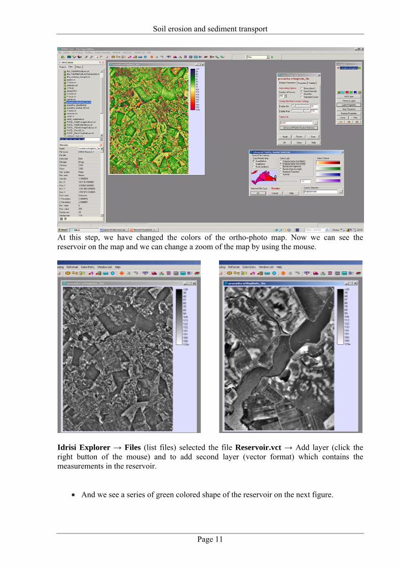
At this step, we have changed the colors of the ortho-photo map. Now we can see the reservoir on the map and we can change a zoom of the map by using the mouse.

Idrisi Explorer → Files (list files) selected the file Reservoir.vct → Add layer (click the right button of the mouse) and to add second layer (vector format) which contains the measurements in the reservoir.

• And we see a series of green colored shape of the reservoir on the next figure.


Page 12

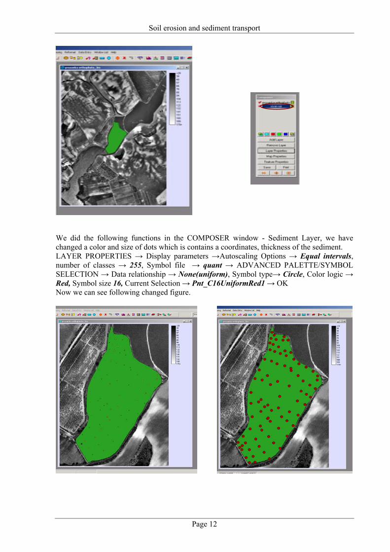
We did the following functions in the COMPOSER window - Sediment Layer, we have changed a color and size of dots which is contains a coordinates, thickness of the sediment. LAYER PROPERTIES → Display parameters →Autoscaling Options → Equal intervals, number of classes → 255, Symbol file → quant → ADVANCED PALETTE/SYMBOL SELECTION → Data relationship → None(uniform), Symbol type→ Circle, Color logic → Red, Symbol size 16, Current Selection → Pnt_C16UniformRed1 → OK Now we can see following changed figure.


Page 13

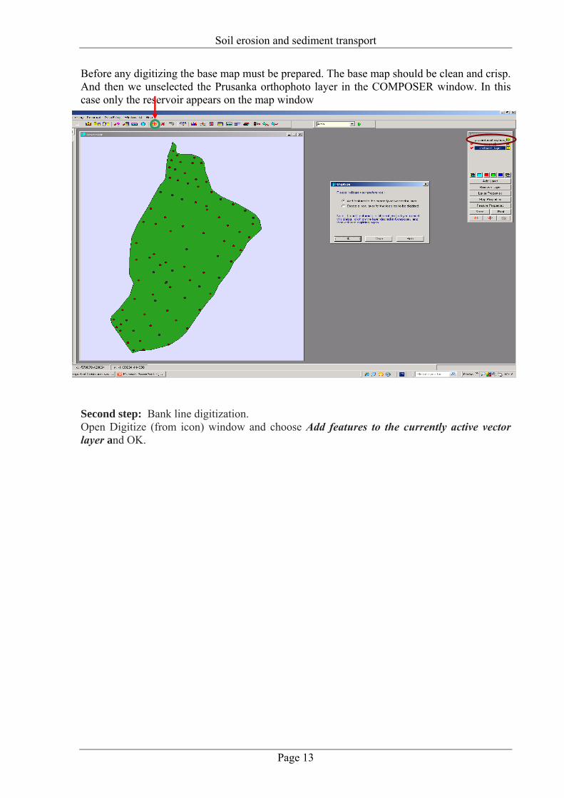
Before any digitizing the base map must be prepared. The base map should be clean and crisp. And then we unselected the Prusanka orthophoto layer in the COMPOSER window. In this case only the reservoir appears on the map window Second step: Bank line digitization. Open Digitize (from icon) window and choose Add features to the currently active vector layer and OK.


Page 14

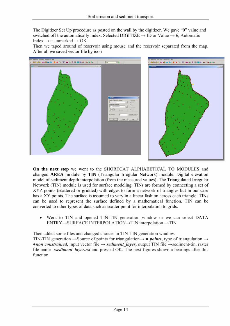
The Digitizer Set Up procedure as posted on the wall by the digitizer. We gave “0” value and switched off the automatically index. Selected DIGITIZE → ID or Value → 0, Automatic Index → □ unmarked → OK. Then we taped around of reservoir using mouse and the reservoir separated from the map. After all we saved vector file by icon

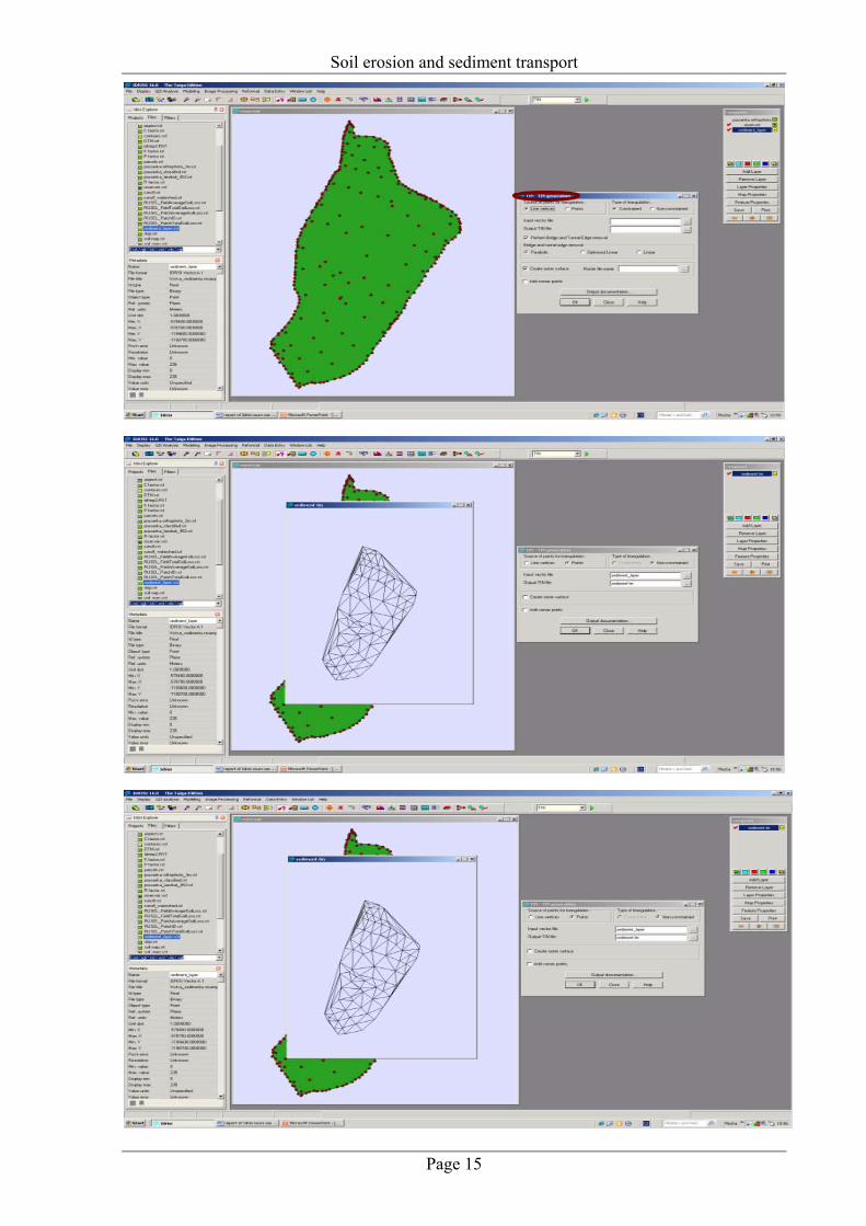
On the next step we went to the SHORTCAT ALPHABETICAL TO MODULES and changed AREA module by TIN (Triangular Irregular Network) module. Digital elevation model of sediment depth interpolation (from the measured values). The Triangulated Irregular Network (TIN) module is used for surface modeling. TINs are formed by connecting a set of XYZ points (scattered or gridded) with edges to form a network of triangles but in our case has a XY points. The surface is assumed to vary in a linear fashion across each triangle. TINs can be used to represent the surface defined by a mathematical function. TIN can be converted to other types of data such as scatter point for interpolation to grids.

• Went to TIN and opened TIN-TIN generation window or we can select DATA ENTRY→SURFACE INTERPOLATION→TIN interpolation →TIN

Then added some files and changed choices in TIN-TIN generation window. TIN-TIN generation →Source of points for triangulation→ ● points, type of triangulation → ●non constrained, input vector file → sediment_layer, output TIN file →sediment-tin, raster file name→sediment_layer.rst and pressed OK. The next figures shown a bearings after this function


Page 15


Page 16

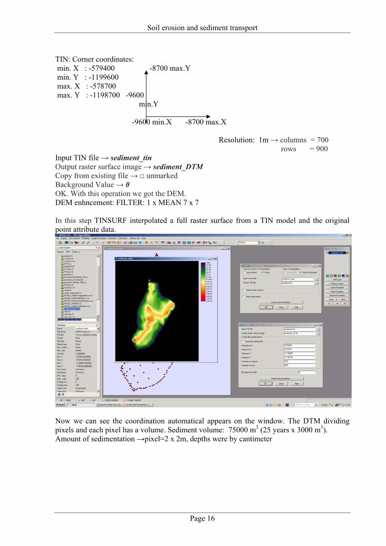
TIN: Corner coordinates: min. X : -579400 -8700 max.Y min. Y : -1199600 max. X : -578700 max. Y : -1198700 -9600

min.Y -9600 min.X -8700 max.X

Resolution: 1m → columns = 700 rows = 900

Input TIN file → sediment_tin Output raster surface image → sediment_DTM Copy from existing file → □ unmarked Background Value → 0 OK. With this operation we got the DEM. DEM enhncement: FILTER: 1 x MEAN 7 x 7 In this step TINSURF interpolated a full raster surface from a TIN model and the original point attribute data.

Now we can see the coordination automatical appears on the window. The DTM dividing pixels and each pixel has a volume. Sediment volume: 75000 m3 (25 years x 3000 m3). Amount of sedimentation →pixel=2 x 2m, depths were by cantimeter


Page 17

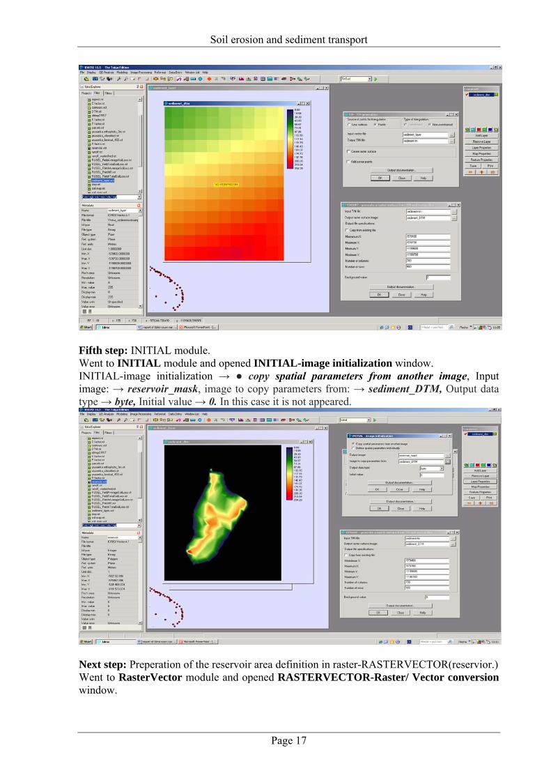
Fifth step: INITIAL module. Went to INITIAL module and opened INITIAL-image initialization window. INITIAL-image initialization → ● copy spatial parameters from another image, Input image: → reservoir_mask, image to copy parameters from: → sediment_DTM, Output data type → byte, Initial value → 0. In this case it is not appeared.

Next step: Preperation of the reservoir area definition in raster-RASTERVECTOR(reservior.) Went to RasterVector module and opened RASTERVECTOR-Raster/ Vector conversion window.


Page 18

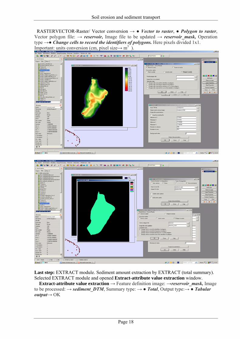
RASTERVECTOR-Raster/ Vector conversion → ● Vector to raster, ● Polygon to raster, Vector polygon file: → reservoir, Image file to be updated → reservoir_mask, Operation type →● Change cells to record the identifiers of polygons. Here pixels divided 1x1. Important: units conversion (cm, pixel size→ m3 ).

Last step: EXTRACT module. Sediment amount extraction by EXTRACT (total summary). Selected EXTRACT module and opened Extract-attribute value extraction window. Extract-attribute value extraction → Feature definition image: →reservoir_mask, Image to be processed: → sediment_DTM, Summary type: → ● Total, Output type:→ ● Tabular output→ OK


Page 19

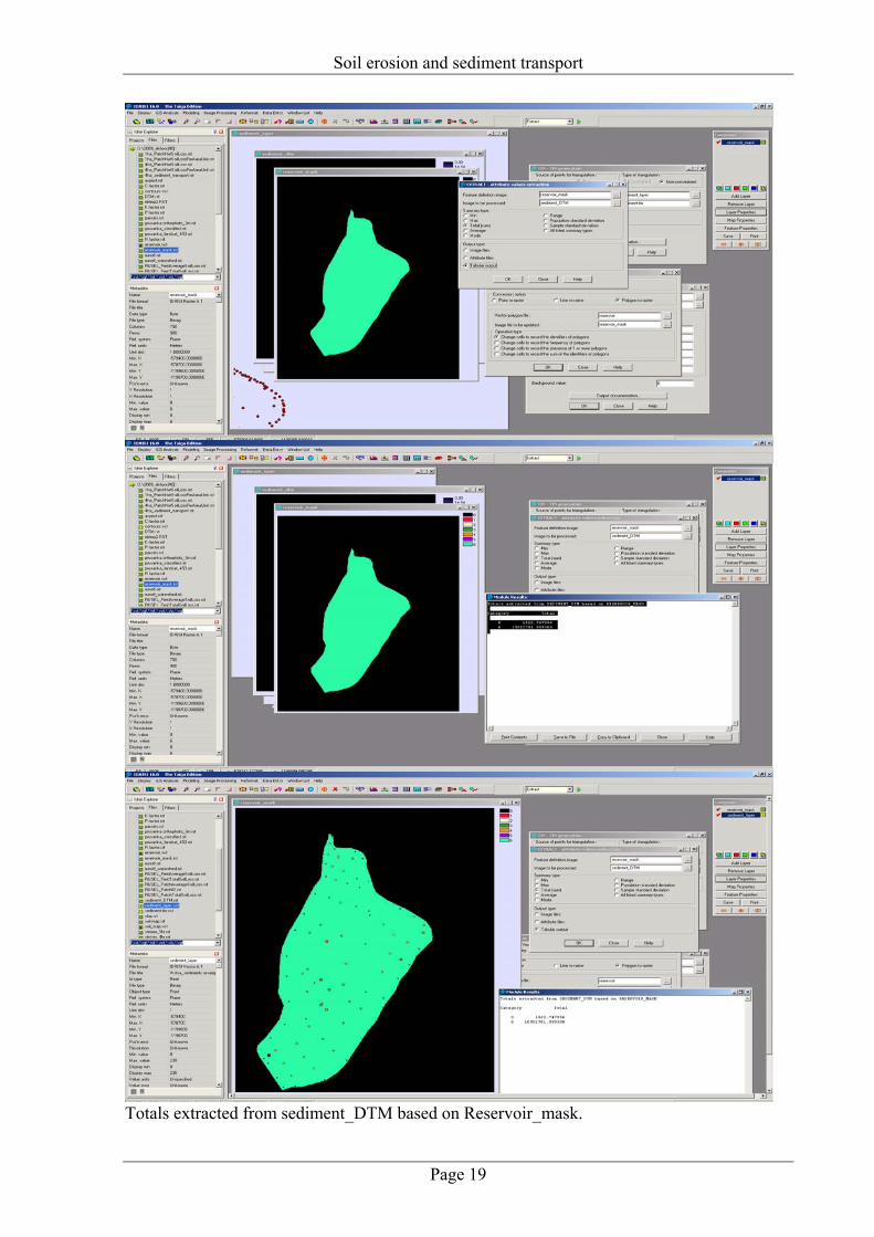
Totals extracted from sediment_DTM based on Reservoir_mask.


Page 20

Original volume → 145 000 m3 Estimated volume→ 145 000 m3 Comparison-measured vs. computed by RUSLE&SEDIMENTATION Conclusions: The sediment yield estimated by SDR was almost the same with measured amount. Therefore, the methodology is quite efficient and reasonable for computing sediment yield in other similar catchments.


Page 21

2.3 Soil loss and Sediment Transport from a watershed using USLE

USLE: A = R.K.L.S.C.P

A … Average annual soil loss (t ha-1 year-1) R … rainfall erosivity factor (MJ cm ha-1 h-1 y-1) K … soil erodibility factor (t h MJ-1 cm-1) L … slope length factor (-) S … slope steepness factor (-) C … crop management factor (-) P … rates erosion control practices (-)

After having the pure soil loss, the sediment delivery ratio must be applied to estimate the deposition within catchment area. By using a GIS software, we will use one layer for each factor: one layer = one raster map. Important: At the beginning of the work, always make sure that you selected the right working „project“ Source layers overview: “Prusanka_Landsat_453” – Landsat image in false colors (Landsat has seven color layers from red to green. Red means no vegetation, green means vegetation.) “Prusanka_Ortofoto_3m” – contracted orthophoto (3m resolution)

ADD layer – “watershed_big” ADD layer – “contours.rst“

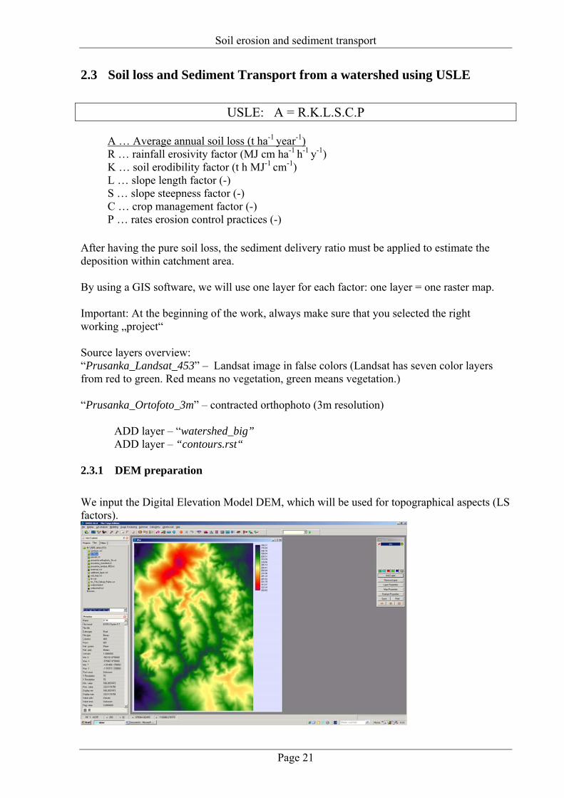
2.3.1 DEM preparation We input the Digital Elevation Model DEM, which will be used for topographical aspects (LS factors).


Page 22

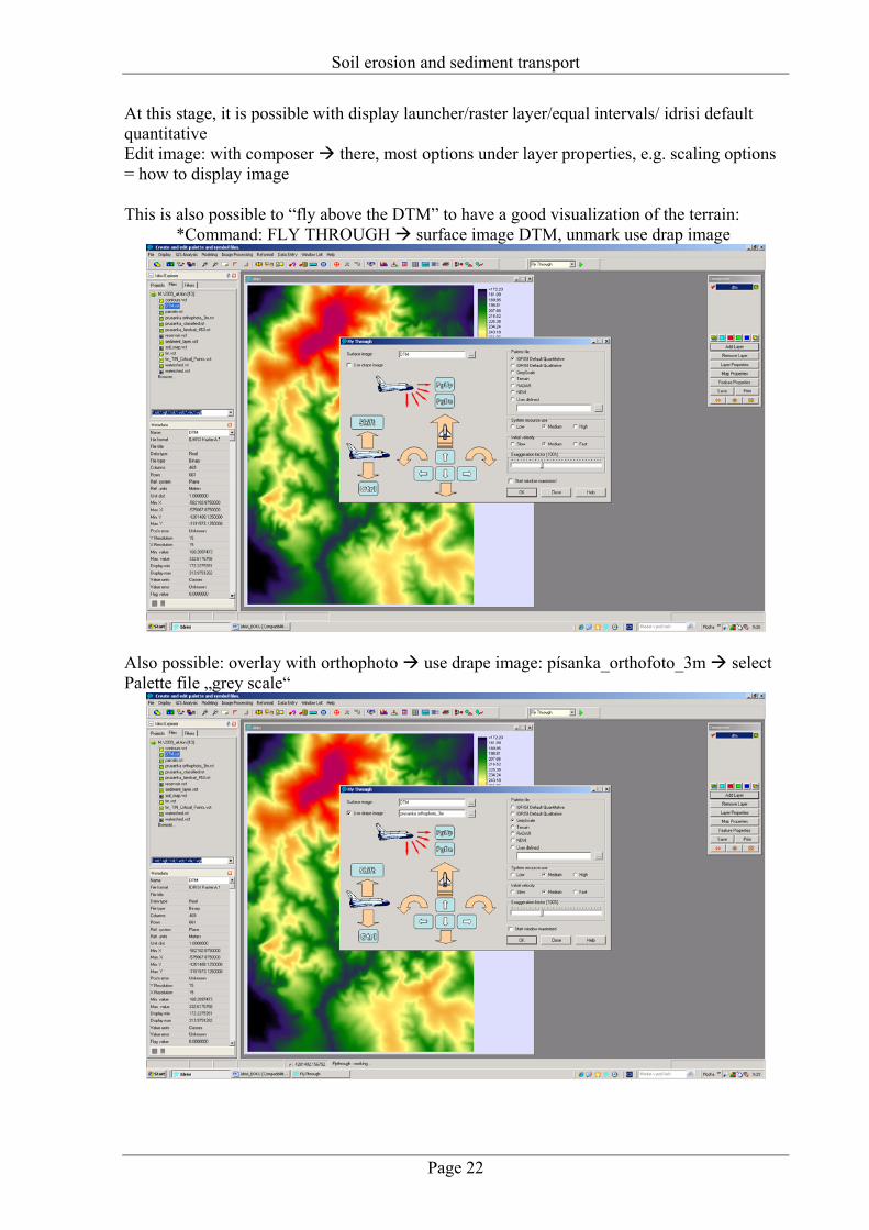
At this stage, it is possible with display launcher/raster layer/equal intervals/ idrisi default quantitative Edit image: with composer there, most options under layer properties, e.g. scaling options = how to display image This is also possible to “fly above the DTM” to have a good visualization of the terrain:

*Command: FLY THROUGH surface image DTM, unmark use drap image

Also possible: overlay with orthophoto use drape image: písanka_orthofoto_3m select Palette file „grey scale“


Page 23

2.3.2 C factor = Vegetation factor and land use map The C factor varies from 0 to 1: 1 means no cover so no protection at all, 0 means no erosion How can we know the C-Factors?

ask farmer about the crop rotation and the land use along the year because A = average annual soil loss

use the existing tables: Orchards C = 0,22 Vineyards C = 0,35

Arable land Area C factor corn 40 % 0,50 winter wheat 30 % 0,12 alfalfa 15 % 0,02 spring barley 15 % 0,15

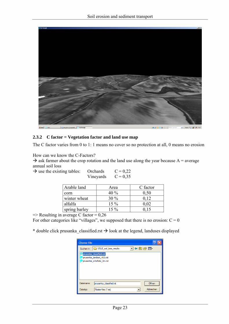
=> Resulting in average C factor = 0,26 For other categories like “villages”, we supposed that there is no erosion: C = 0 * double click prusanka_classified.rst look at the legend, landuses displayed


Page 24

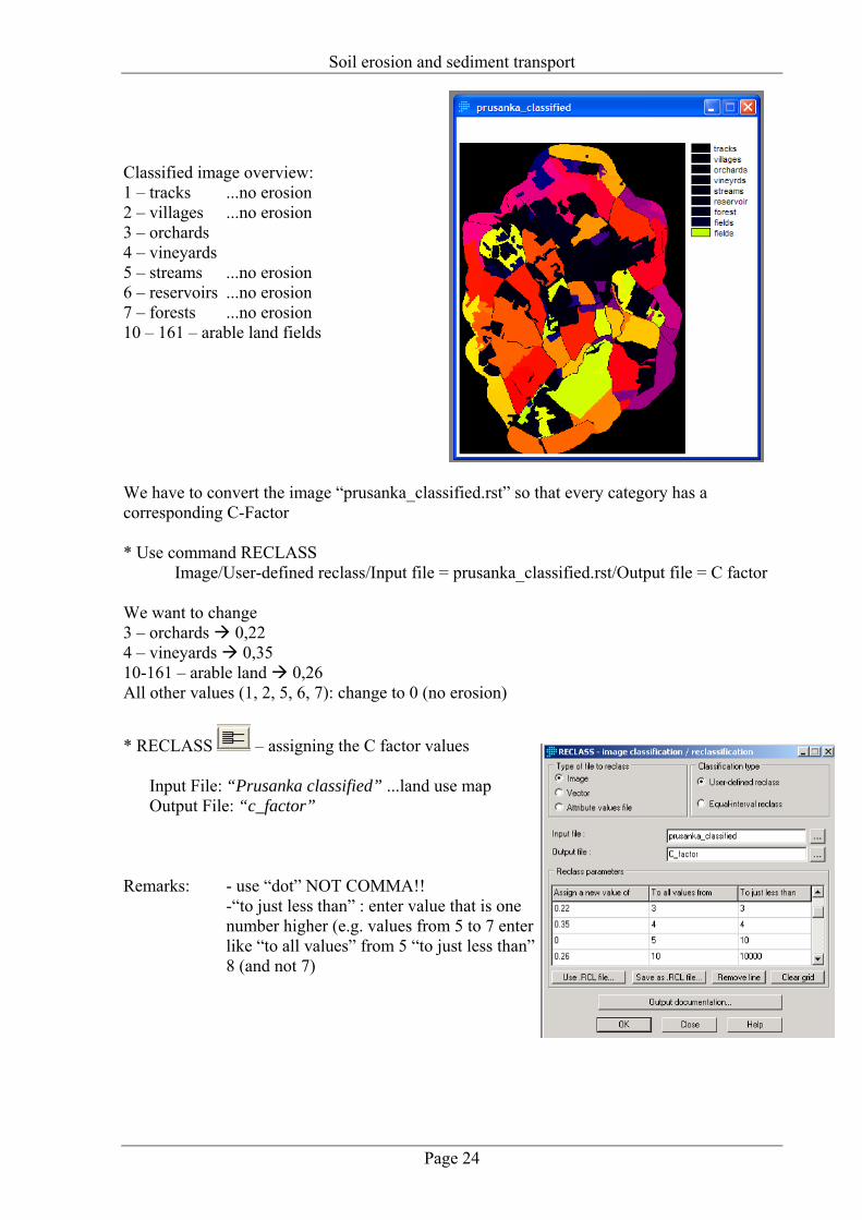
Classified image overview: 1 – tracks ...no erosion 2 – villages ...no erosion 3 – orchards 4 – vineyards 5 – streams ...no erosion 6 – reservoirs ...no erosion 7 – forests ...no erosion 10 – 161 – arable land fields We have to convert the image “prusanka_classified.rst” so that every category has a corresponding C-Factor * Use command RECLASS Image/User-defined reclass/Input file = prusanka_classified.rst/Output file = C factor We want to change 3 – orchards 0,22 4 – vineyards 0,35 10-161 – arable land 0,26 All other values (1, 2, 5, 6, 7): change to 0 (no erosion)

* RECLASS – assigning the C factor values

Input File: “Prusanka classified” ...land use map Output File: “c_factor”

Remarks: - use “dot” NOT COMMA!!

-“to just less than” : enter value that is one number higher (e.g. values from 5 to 7 enter like “to all values” from 5 “to just less than” 8 (and not 7)


Page 25

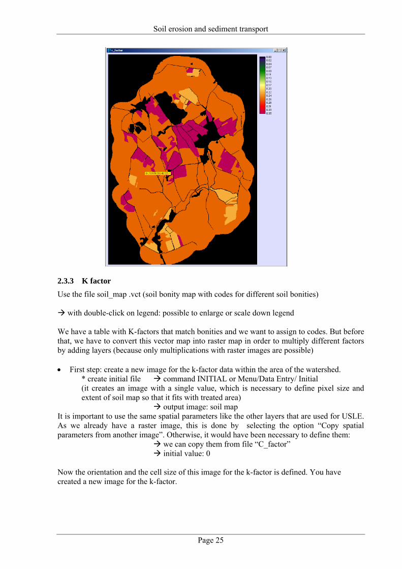
2.3.3 K factor Use the file soil_map .vct (soil bonity map with codes for different soil bonities)

with double-click on legend: possible to enlarge or scale down legend We have a table with K-factors that match bonities and we want to assign to codes. But before that, we have to convert this vector map into raster map in order to multiply different factors by adding layers (because only multiplications with raster images are possible) • First step: create a new image for the k-factor data within the area of the watershed.

* create initial file command INITIAL or Menu/Data Entry/ Initial (it creates an image with a single value, which is necessary to define pixel size and extent of soil map so that it fits with treated area)

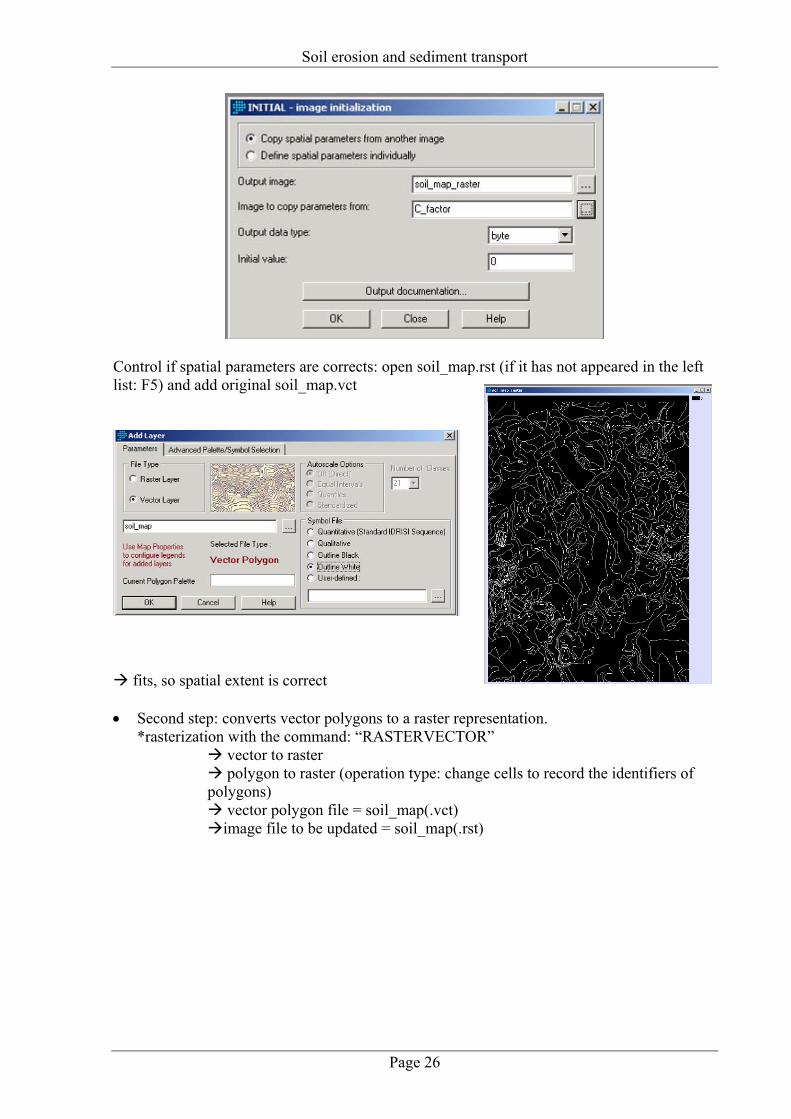
output image: soil map It is important to use the same spatial parameters like the other layers that are used for USLE. As we already have a raster image, this is done by selecting the option “Copy spatial parameters from another image”. Otherwise, it would have been necessary to define them:

we can copy them from file “C_factor” initial value: 0 Now the orientation and the cell size of this image for the k-factor is defined. You have created a new image for the k-factor.


Page 26

Control if spatial parameters are corrects: open soil_map.rst (if it has not appeared in the left list: F5) and add original soil_map.vct

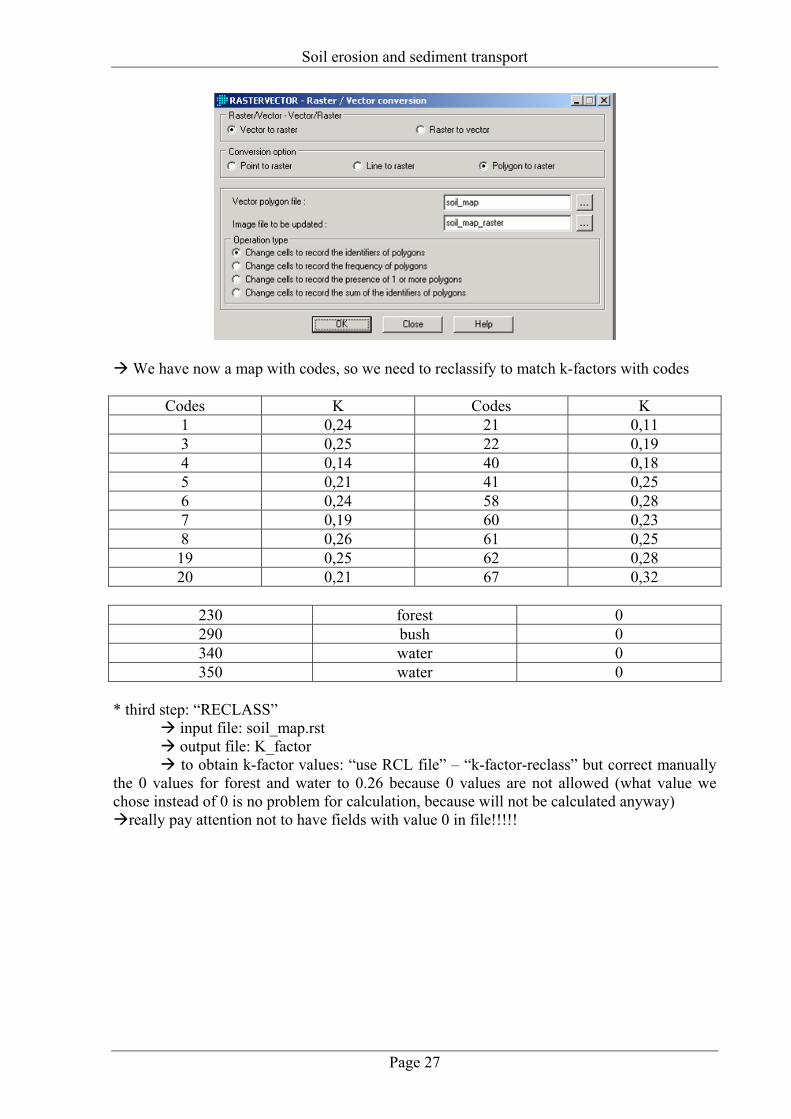
fits, so spatial extent is correct • Second step: converts vector polygons to a raster representation.

*rasterization with the command: “RASTERVECTOR” vector to raster polygon to raster (operation type: change cells to record the identifiers of polygons) vector polygon file = soil_map(.vct) image file to be updated = soil_map(.rst)


Page 27

We have now a map with codes, so we need to reclassify to match k-factors with codes

Codes K Codes K 1 0,24 21 0,11 3 0,25 22 0,19 4 0,14 40 0,18 5 0,21 41 0,25 6 0,24 58 0,28 7 0,19 60 0,23 8 0,26 61 0,25 19 0,25 62 0,28 20 0,21 67 0,32

230 forest 0 290 bush 0 340 water 0 350 water 0

* third step: “RECLASS” input file: soil_map.rst output file: K_factor to obtain k-factor values: “use RCL file” – “k-factor-reclass” but correct manually the 0 values for forest and water to 0.26 because 0 values are not allowed (what value we chose instead of 0 is no problem for calculation, because will not be calculated anyway)

really pay attention not to have fields with value 0 in file!!!!!


Page 28

Excurs: We had to repare our k-factor.rst file because there were fields with value 0 in it * step 1: rename K_factor.rst in K-factor_0.rst *command “RECLASS” assign a new value of 0.26 to all values from 0 to just less than 0 now K_factor.rst-file without any 0-values in it

now we have the new K_factor.rst without 0-values delete K_factor_0.rst 2.3.4 R factor = Rainfall erosivity factor

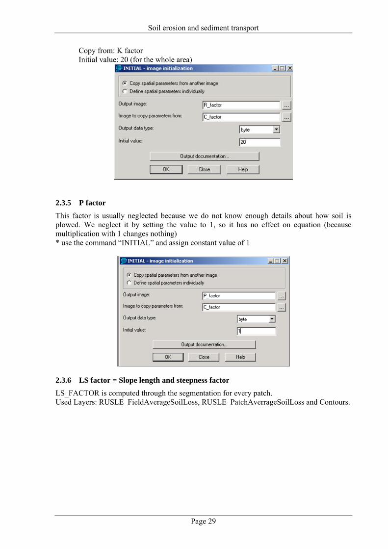
As the area of study is only of around 50m², we consider that the climate remains the same and we take the same value of R for the whole area: R=20 MJ cm ha-1 h-1 y-1 * use command “INITIAL” Output: R factor


Page 29

Copy from: K factor Initial value: 20 (for the whole area)

2.3.5 P factor This factor is usually neglected because we do not know enough details about how soil is plowed. We neglect it by setting the value to 1, so it has no effect on equation (because multiplication with 1 changes nothing) * use the command “INITIAL” and assign constant value of 1

2.3.6 LS factor = Slope length and steepness factor LS_FACTOR is computed through the segmentation for every patch. Used Layers: RUSLE_FieldAverageSoilLoss, RUSLE_PatchAverrageSoilLoss and Contours.


Page 30

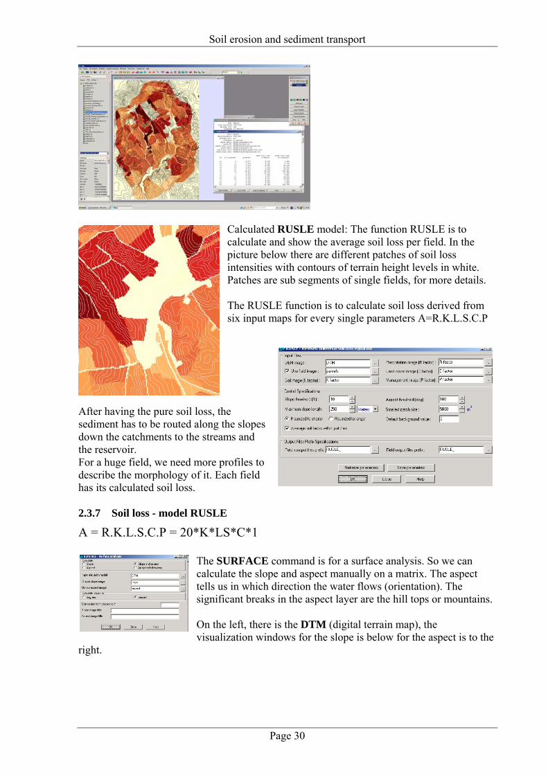
Calculated RUSLE model: The function RUSLE is to calculate and show the average soil loss per field. In the picture below there are different patches of soil loss intensities with contours of terrain height levels in white. Patches are sub segments of single fields, for more details. The RUSLE function is to calculate soil loss derived from six input maps for every single parameters A=R.K.L.S.C.P

After having the pure soil loss, the sediment has to be routed along the slopes down the catchments to the streams and the reservoir. For a huge field, we need more profiles to describe the morphology of it. Each field has its calculated soil loss. 2.3.7 Soil loss - model RUSLE

A = R.K.L.S.C.P = 20*K*LS*C*1

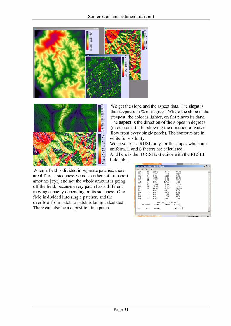
The SURFACE command is for a surface analysis. So we can calculate the slope and aspect manually on a matrix. The aspect tells us in which direction the water flows (orientation). The significant breaks in the aspect layer are the hill tops or mountains. On the left, there is the DTM (digital terrain map), the visualization windows for the slope is below for the aspect is to the

right.


Page 31

We get the slope and the aspect data. The slope is the steepness in % or degrees. Where the slope is the steepest, the color is lighter, on flat places its dark. The aspect is the direction of the slopes in degrees (in our case it’s for showing the direction of water flow from every single patch). The contours are in white for visibility. We have to use RUSL only for the slopes which are uniform. L and S factors are calculated. And here is the IDRISI text editor with the RUSLE field table.

When a field is divided in separate patches, there are different steepnesses and so other soil transport amounts [t/yr] and not the whole amount is going off the field, because every patch has a different moving capacity depending on its steepness. One field is divided into single patches, and the overflow from patch to patch is being calculated. There can also be a deposition in a patch.


Page 32

3. Sedimentation - the sediment transport

3.1 Runoff and Sedimentation

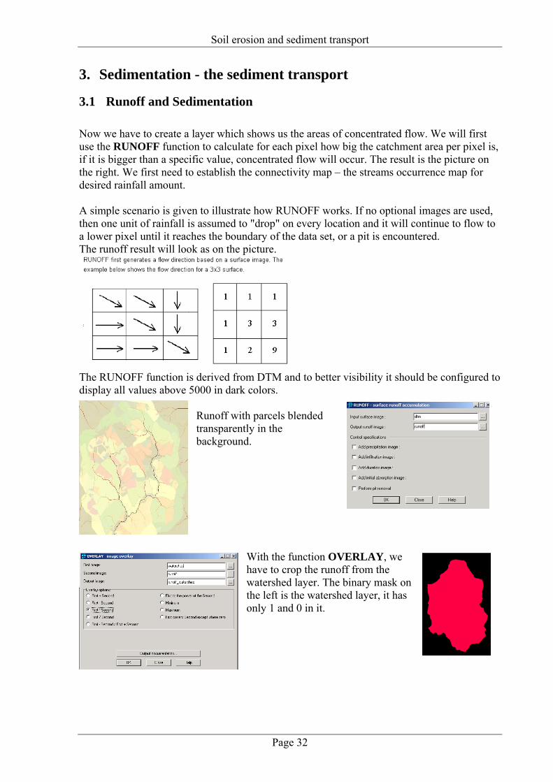
Now we have to create a layer which shows us the areas of concentrated flow. We will first use the RUNOFF function to calculate for each pixel how big the catchment area per pixel is, if it is bigger than a specific value, concentrated flow will occur. The result is the picture on the right. We first need to establish the connectivity map – the streams occurrence map for desired rainfall amount. A simple scenario is given to illustrate how RUNOFF works. If no optional images are used, then one unit of rainfall is assumed to "drop" on every location and it will continue to flow to a lower pixel until it reaches the boundary of the data set, or a pit is encountered. The runoff result will look as on the picture.

The RUNOFF function is derived from DTM and to better visibility it should be configured to display all values above 5000 in dark colors.

Runoff with parcels blended transparently in the background.

With the function OVERLAY, we have to crop the runoff from the watershed layer. The binary mask on the left is the watershed layer, it has only 1 and 0 in it.


Page 33

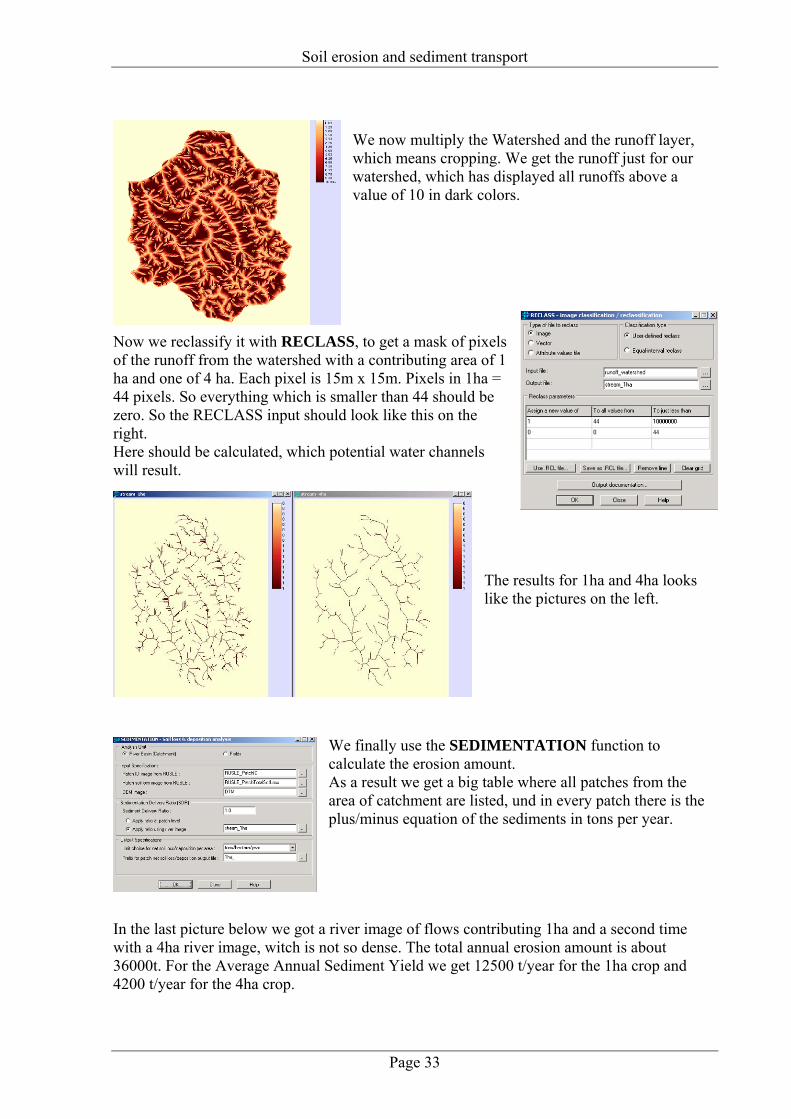
We now multiply the Watershed and the runoff layer, which means cropping. We get the runoff just for our watershed, which has displayed all runoffs above a value of 10 in dark colors.

Now we reclassify it with RECLASS, to get a mask of pixels of the runoff from the watershed with a contributing area of 1 ha and one of 4 ha. Each pixel is 15m x 15m. Pixels in 1ha = 44 pixels. So everything which is smaller than 44 should be zero. So the RECLASS input should look like this on the right. Here should be calculated, which potential water channels will result.

The results for 1ha and 4ha looks like the pictures on the left.

We finally use the SEDIMENTATION function to calculate the erosion amount. As a result we get a big table where all patches from the area of catchment are listed, und in every patch there is the plus/minus equation of the sediments in tons per year.

In the last picture below we got a river image of flows contributing 1ha and a second time with a 4ha river image, witch is not so dense. The total annual erosion amount is about 36000t. For the Average Annual Sediment Yield we get 12500 t/year for the 1ha crop and 4200 t/year for the 4ha crop.


Page 34

The difference between the amounts of soil loss from the higher patch to the lower patch represents the net soil loss or deposition in the lower patch. For example if in the initial state the proportional soil loss in Patch A (the higher patch) delivered to the lower patch B is 1 t/yr, and Patch B’s initial soil loss is 3 t/yr (RUSLE soil loss value), SEDIMENTATION then determines the difference between the amount of sediment coming into the patch and the patch’s RUSLE soil loss value. In our example, 3 (Patch B) -1 (moved from Patch A) = net soil loss for Patch B of 2 t/yr. If soil loss from Patch A was 5 t/yr and Patch B initial soil loss was 2 t/ yr, the difference is 2 -5 = -3 which is interpreted as 3 t/yr net deposition in patch B. (Total sediment yield for 4 ha streams approx. 4190 t/year)

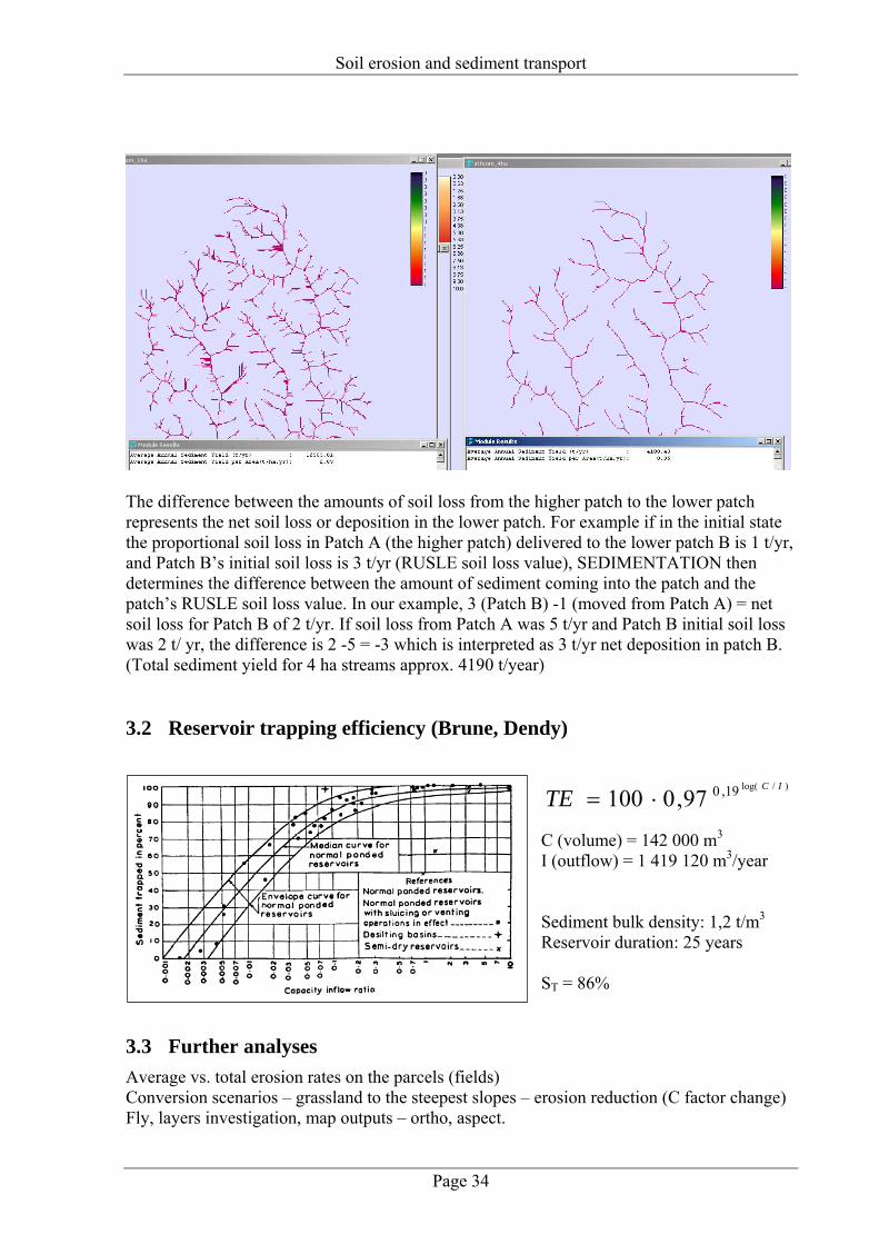
3.2 Reservoir trapping efficiency (Brune, Dendy)

C (volume) = 142 000 m3 I (outflow) = 1 419 120 m3/year Sediment bulk density: 1,2 t/m3 Reservoir duration: 25 years ST = 86%

3.3 Further analyses Average vs. total erosion rates on the parcels (fields) Conversion scenarios – grassland to the steepest slopes – erosion reduction (C factor change) Fly, layers investigation, map outputs – ortho, aspect.

)/log(19,097,0100IC

TE ⋅=

Soil erosion and sediment transport measurement and assessment · Soil erosion and sediment...

Documents

Transcript of Soil erosion and sediment transport measurement and assessment · Soil erosion and sediment...