SPE-1216-G

8/10/2019 SPE-1216-G

http://slidepdf.com/reader/full/spe-1216-g 1/7

T.

P.8081

Calculation of the Stabilized Performance Coefficient of

Low Permeability Natural Gas Wells

FRED H. POETTMANN

ROBERT

E.

SCHILSON

MEMBERS AIME

B S T R C T

The direct determination

oj

the stabilized perjorm

ance behavior oj low capacity, slowly stabilizing gas

wells is extremely time-consuming and wastejul oj gas.

From

both field experience

and

theoretical considera

tions, a test procedure has been evolved by which the

stabilized back pressure behavior

oj

such gas wells can

be predicted without having to revert to long time flow

tests.

The

method

consists oj using the isochronal test pro

cedure to establish the slope oj the back pressure curve,

n , and the short time variation oj the perjormance

coefficient, C , with time.

From this short time transient flow data and theore

tical considerations, the value oj

C

at large times can

he established.

By

assuming the radius

oj

drainage

oj

a well to be halj the distance between wells, one can

calculate the stabilization time jor various well spacing

patterns. Once the stabilization time jor a given spacing

has been determined, the value

oj C

can be calculated

and the stabilized back-pressure curve can be estab

lished.

The calculated perjormance coefficient as a junction

oj

time was compared to the experimentally measured

values

jor

a number oj gas wells. The deviation oj the

calculated

jrom

the experimental results vary depending

on

the set oj short time experimental points used to

evaluate the parameters oj the equation. The longer the

time jor the flow test data used in the calculations, the

better was the agreement with the experimental results.

The time necessary to obtain this data jrom well tests

varies considerably, depending on the physical nature

of

the reservoir under consideration.

I N T R O D U C T I O N

For

many years, the U. S. Bureau of Mines Mono

graph 7 has served as a guide for testing and evaluating

the performance of gas wells by means of the back-pres

sure method.

The

back-pressure performance of a gas

well is expressed by the following equation:

Q

=

C(P/ - Ps') . 1)

where the characteristics

of

the back-pressure equation

are determined by C, the performance coefficient, and

Original

manuscript

received

in

Society of Petroleum Engineers

office

Feb.

16. 1959. Revised

manuscript

received

June

13. 1959.

Paper

presented

at

Fifth

Annual

Meeting of

Rocky

Mountain Pe

,troleum Sections in Casper. Wyo

•

April 2-3. 1959.

References

given

at end

of paper.

SPE 1216-G

PETROLEUM TRANSACTIONS, AIME

THE

O IO OIL CO.

LITTLETON

COLO

n the exponent which corresponds to the slope of the

straight line when

Q

and

(P/ - Ps')

are plotted on

logarithmic paper.

Q

is gas flow rate at standard oondi

tions, and

Pi

and P

B

are equalized and flowing bottom

hole pressures, respectively.

Prior to the development of the back-pressure test,

the open flow capacity method

of

testing a well was

common. By this method, the wells were flowed wide

open to the air and the flow rate measured. Such pro

cedure was wasteful of gas and did not provide informa

tion on the deliverability of the gas to the pipe line.

MONOGRAPH 7 PROCEDURE

The back-pressure method of testing wells was de

veloped to overcome these shortcomi·ngs.

Although

much has been learned regarding the laws of the flow

of gas through porous formations, the original develop

ment of the back-pressure relationship was based en

tirely on empirical methods. The

back-pressure

be

havior provides the engineer with information essential

in predicting the future development of a field.

It

per

mits him to calculate the deliver ability

of

gas into a

pipe line at predetermined line pressures, to design and

analyze gas gathering lines, to determine the spacing

and number of wells to be drilled during the develop

me'nt of a field to meet gas purchasers' requirements,

and to solve many other technical and economic prob

lems.

As described in Monograph 7, the flow-after-flow

method of back-pressure testing, when applied to fast

stabilizing and usually high capacity wells,

correctly

characterized the behavior of the well. However, as

the value of the gas at the wellhead increased, small

capacity gas wells having slow rates of stabilization be

came economically operable.

The

flow-after-flow method

of testing could not be used to describe the behavior

of

these slowly stabilizing wells.

The procedure of Rawlins and Shellhardt for estab

lishing the back-pressure behavior

of

a gas well was

based on the requirement that the data be obtained un

der stabilized flow conditions; that is, that C is constant

and does not vary with time. C depends on the physical

properties of the reservoir, the location, extent and ge

ometry of the drainage radius, and the properties of

the flowing fluid.

In

a highly permeable formation, only

a very short period

of

time is required for the well to

reach a stabilized condition, and, consequently, the re

quirements for the test procedure described in Mono

graph 7 are met.

For

a given well,

n

is also constant

240

8/10/2019 SPE-1216-G


and will have values ranging between the limits of 0.5

and 1.0.

In

the case

of

low permeability reservoirs, the direct

determination

of

stabilized performance behavior

of

gas wells becomes extremely time-consuming and waste

ful

of

gas.

For

example, some of the Mesa Verde wells

in the San

Juan

gas field' take weeks and months to

reach stabilized flow conditions.

Thus, it

is

desirable to have a procedure which will

predict the stabilized back-pressure behavior and elim

inate the ·necessity for using the long flow tests outlined

in Monograph 7. Such a test procedure has been evolved

from both field experience and theoretical considera

tions '.

CULLENDER

METHOD

In 1955, Cullender' published a paper in which he

described the isochronal (constant time) performance

method

of

determining the flow characteristics of a gas

well. Cullender found from experience that the steady

state flow conditions are not ne.cessary to establish n

for the back-pressure curve. However, as long as tran

sient conditions exist, C will vary with time. When C

becomes constant, the flow will have stabilized. This

behavior

is

illustrated by the shifting of the back-pres

sure curves to the left, at increasing time, with the slope

remaining constant.

The

theory on which isochronal

performance is based assumes that the flow at a given

time, starting from a shut-in condition, is from the same

radius

of

drainage, regardless

of

the pressure level

of

the reservoir

or

the flow rate. This means that the ra

dius of drainage moving away from the well bore is de

pendent only on the formation and gas properties. Once

the radius

of

drainage has reached the boundaries

of

the reservoir

or

the point of interference with an off

set well, the performance coefficient becomes constant

and the back-pressure curve becomes stabilized.

The

slope of the isochronal back-pressure curves is

the same as that of the stabilized curve.

In

fact, the

stabilized curve represents the limiting value

of

the

isochronal curves. The method employed to obtain the

isochronal performance curves of a gas well is to open

the well from a closed-in condition and obtain rate of

flow and pressures at fixed time intervals without dis

turbing the flow rate.

The

well is then shut in and al

lowed to return to a pressure comparable to that exist

ing at the time the well was first opened to flow.

The

well is reopened at a different rate of flow and data ob

tained at the same time intervals as before. The pro

cedure

is

repeated as often as desired.

A plot of Q vs (P/ P, ) on logarithmic paper at

constant time establishes

n.

From

the transient tests establishing the isochronal

curves and theoretical considerations, ' procedures

have been evolved by which the stabilized back-pressure

behavior

of

low permeabili ty gas wells can be calculated.

In

addition, the buildup curves permit the calculation

of

the interwell permeability

of

the formation. This in

terwell permeability is used in the calculation of the

stabilized performance curve of a well for various

spacing patterns.

The purpose of this report is to describe a procedure

for calculating the variation

of

C with time from the

short term isochronal tests. This curve, along with other

reservoir data, is used to obtain the stabilized back-pres

sure performance curves of a well for various spacing

patterns. Calculated results are compared with actual

performance data.

241

C A L C U L A T I O N P R O C E D U R E

As stated in the introduction, the results of tests over

a period of years established the fact that the gas flow

rate for a single-phase gas well was related empirically

to the formation shut-in pressure and the bottom-hole

pressure by the equation:

Q

=

C(P,

p,')n

.

1)

In

1953, Houpeurt' derived from theoretical studies

an equation relating the gas production rate and the

over-all pressure drop between the reservoir boundary

and the well bore radius. This equation was converted

for use with English units by Tek, Grove and Poett

mann', with the following results.

where

Q

=

2.49 ~ 6 5 9 ) · n y (7T.hk b

R

) (P/

_

P,')

fl n

a

2)

Thk

=

the Test-Index which

is

obtained from

pressure build-up analysis;

k

is the permeability, darcies;

h is the formation thickness, cm;

JL

is the viscosity of

the gas, centipoises.

Comparing Eqs. 1 and 2, it may be seen that:

C

=

2.49 (4.659)"Y( "hk

_ ~ )

G L

InR

a

(3)

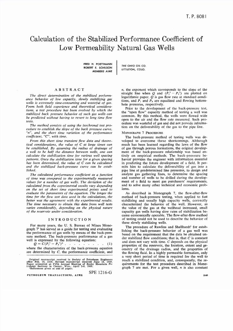
The radius of drainage, R, for an unstabilized gas

well, is shown by Tek, Grove and Poettmann' to be:

R

=

0.0704

( ~ )

~ , f l f 3

(4)

From

the time a gas well begins flowing from an

equalized shut-in condition, the radius

of

drainage

R

changes according to Eq. 4 until either the reservoir

boundary or the point of interference with an off-set

well is reached, at which time the well is stabilized.

From

Eqs. 3 and 4, it can be seen that C is a function

of time, decreasing in magnitude until the well is

stabilized. When this condition

is

attained, C becomes

the stabilized performance coefficient, and the stabilized

performance of the well is as described in Eq.

1.

K Permeability, Darcies

> F r a c t H . J n ~ PorDSity

J

- VIscosity

C c n t i p o i ~ e <

f

Compressibility

(Vol.l/(Vol.j(Atm)

WEll

SPACING.

ACRES

FIG.

l - S T A ~ I L I Z A T l O N TIME OF GAS WELLS.

IVOL. 2 1 6 1.959

8/10/2019 SPE-1216-G


The isochronal performance

method of

determining

the flow characteristics of gas wells has been shown

to be

the

proper

method of

testing gas wells. This

method is particularly applicable to low permeability

formations' .

From

such a series

of

short term flow

tests,

n is

determined.

The

variation

of

C is determined

experimentally as a function

of

time from these flow

tests. Using

the

experimental

data of the

variation

of

C

with time, a procedure has been developed

for

predict

ing C for long time periods, utilizing Eqs. 3 and 4.

For a particular gas well, all terms

of

Eq. 3 can be

considered constant with the exception

of

R.

Taking

the

ratio

of

Eq.

3 for

fixed values

of C, the

following

expression results:

= n .

(

1

R, n

-

a

(5)

Now, by defining

the

parameter,

a:

a

=

0.0704

( ~ )

cpp.f3 .

(6)

Eq.

4 may

be written as:

R =

at'

.

Theoretically,

a

is a constant for a particular reser

voir. Hence, R is a function

of

time only and is inde

pendent of the rate of

flow.

Making use

of

Eq.

7

in Eq. 5:

(7)

C,

a

(

In

a

t? n

C, = In

a;

(8)

Solving

for ala,

[

Ciln

]

t, 2( C,'ln _ Ciln)

[

C

/n

]

t, 2 (C,' ' ~ Ciln)

a

(9)

Therefore,

ala

may be evaluated from any two

C

values and the corresponding times,

t

as determined

from short-term flow tests. Once this is done,

C

may

be expressed as a function

of

time by the following

equation:

_

, l n ~ r

C -

( In

aatl)

10)

The final objective

of

the above analysis is the pre

diction

of the

stabilized back-pressure curve

for the

well

for various spacing patterns. By assuming

the

radius

of

drainage as half the distance between wells, the stabili

zation times for various spacing patterns

can

be cal

culated by

the

use

of

Eq. 4, as shown graphically on

Fig.

1.

The

effective interwell permeability

k

used in

Eq. 4 is

obtained from

the

pressure-buildup curves

taken during

the

course

of the

isochronal testing

of the

well.

The

fractional porosity is

the

weighted average

value taken

over the net

effective

sand

thickness from

core analysis data.

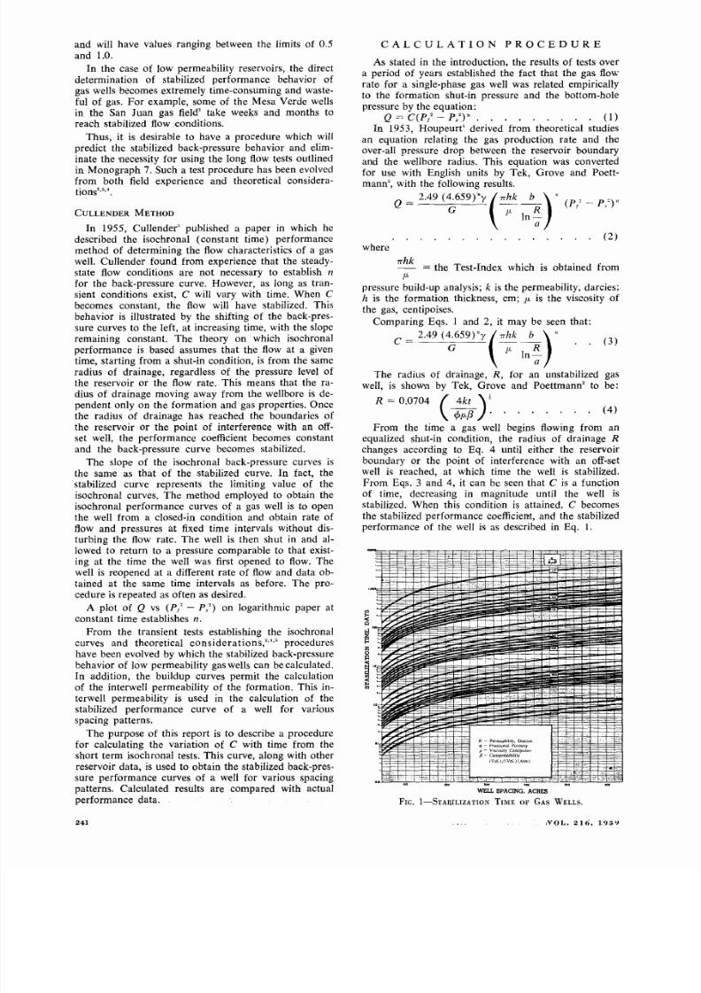
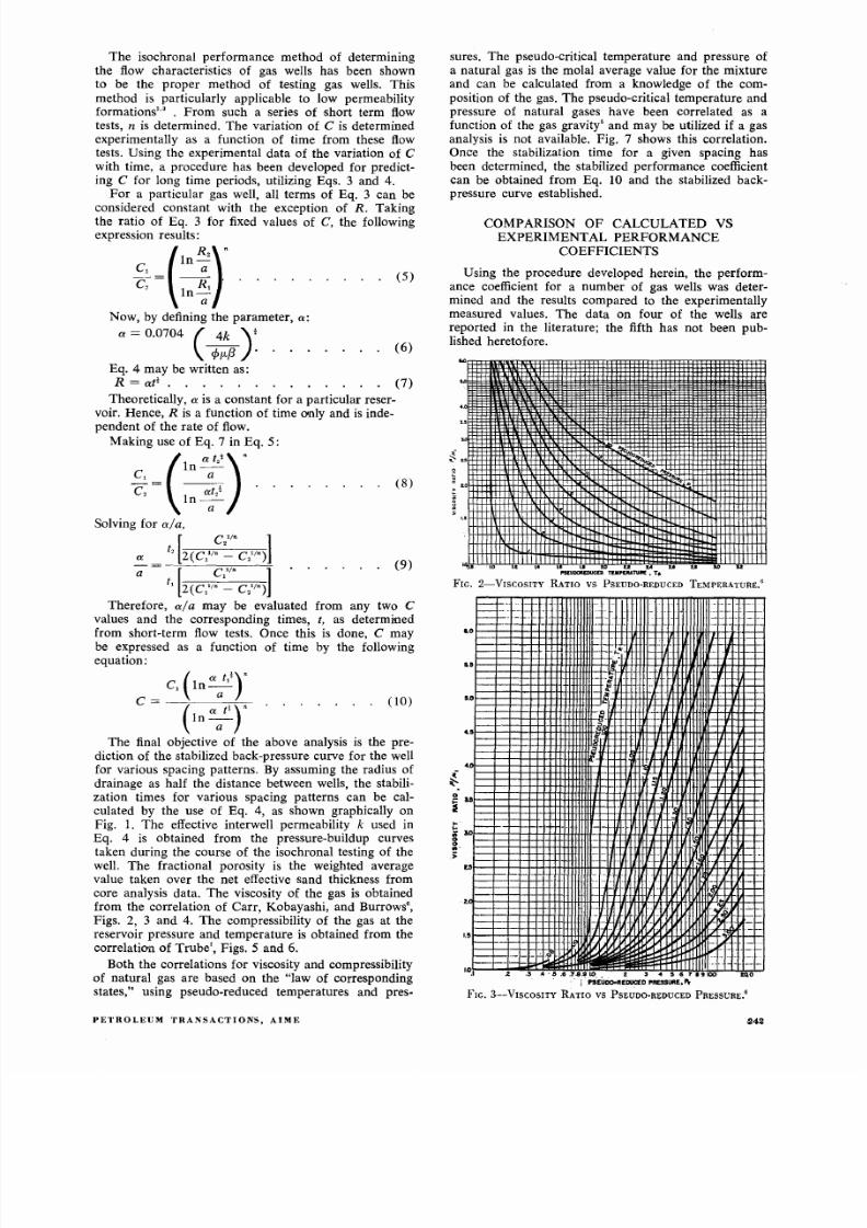
The

viscosity

of

the gas is obtained

from the correlation

of

Carr, Kobayashi, and Burrows',

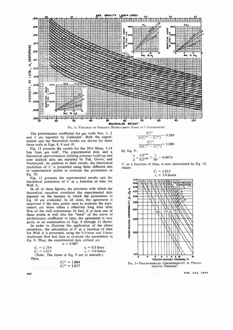
Figs. 2, 3 and 4. The compressibility

of the

gas

at

the

reservoir pressure

and temperature is

obtained from the

correlation

of

Trube , Figs. 5 and 6.

Both the correlations for viscosity and compressibility

of natural

gas

are

based

on

the law

of

corresponding

states, using pseudo-reduced temperatures and pres-

PETROLEUM TRANSACTIONS, AI ME

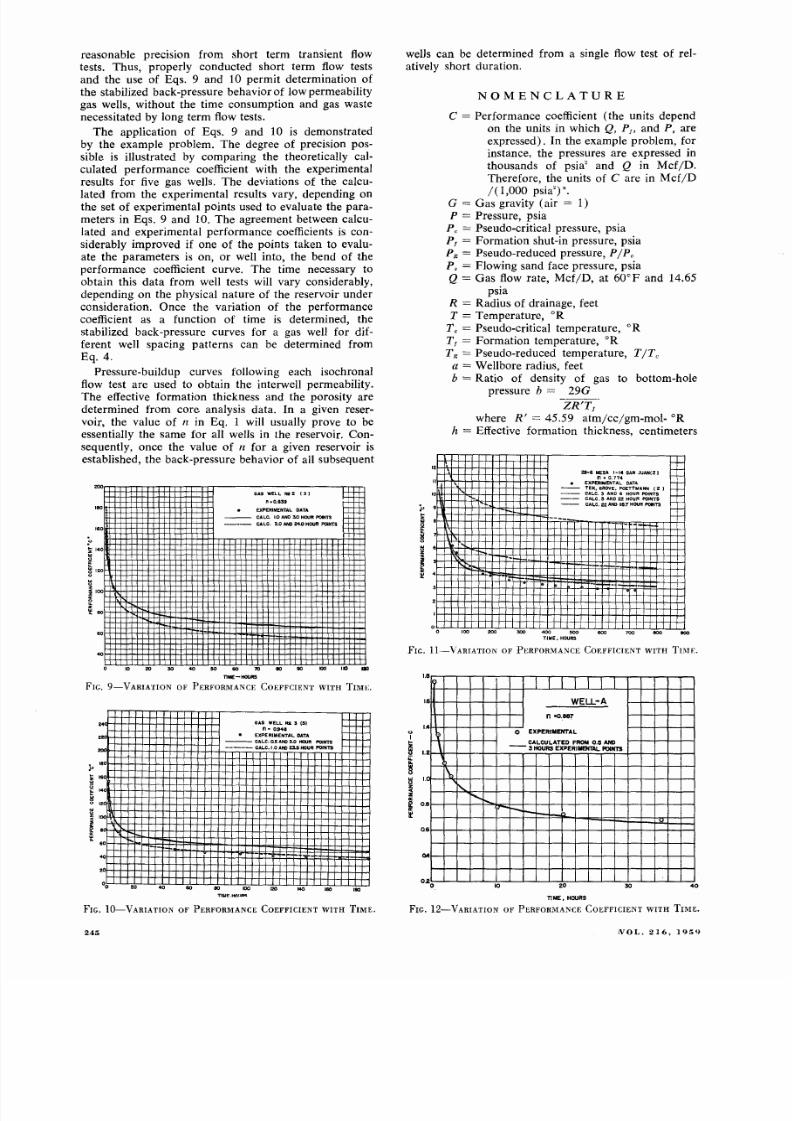
sures. The pseudo-critical temperature and pressure of

a natural gas

is the

molal average value for

the

mixture

and can

be calculated from a knowledge

of

the com

position

of the

gas. The pseudo-critical temperature and

pressure

of

natural gases have been correlated as a

function of the gas gravity'

and

may be utilized if a gas

analysis

is

not available. Fig.

7

shows this correlation.

Once the stabilization time

for

a given spacing has

been determined, the stabilized performance coefficient

can be obtained from Eq.

10

and

the

stabilized back

pressure curve established.

COMPARISON OF CALCULATED VS

EXPERIMENTAL PERFORMANCE

COEFFICIENTS

Using the procedure developed herein, the perform

ance coefficient for a number

of

gas wells was deter

mined and the results compared to the experimentally

measured values. The data on

four

of

the wells are

reported in the literature; the fifth has not been pub

lished heretofore.

- -

1111

I"SEUDOREDUeD

Tf.. .

1ATUM

• Til

FIG. 2-VISCOSITY

RATIO VS PSEUDO-REDUCED TEMPERATURE:

f---f--

f----,,-.

-- - - - -

f - - -- f- -

--

1.0

-

-,-

0,0

f tfH-I-t-IH-t1

I

4.0

.

1.11

i

~ a o

g

WI'

;:

-

~ ~ . - ~

1 5 - I I

~

- , -

: ; ~ = = _ ~

•

~ ~ ~ : ~ ~

ID.I . 2 .3 .4 . 5 .8 .7 .8 .9 1 0 5671 00

ZQO

, .

I'

pSEUDO REDUCED

PRESSURE. '

z

FIG. 3-VISCOSITY RATIO VS PSEUDO-REDUCED PRESSURE.

8/10/2019 SPE-1216-G


8/10/2019 SPE-1216-G


I.

O

0

9

8

o.

cit 0.

7

.

<Q. 0.6

,:

I-

O

::;

iii

G

e

0.4

0:

::E

8 0.3

o

...

o

"...

f 0.2

o

o

"

..

( I )

o.1

1 . 2 - -

~

1 3

1 4

-r-J.5

/1 .6

\ ~

1.7

/ Ilc

\

~

\ 1\

I.

\

\

\ \

\

\\

\

1\

\ \

\

\

\

\ \

1 . 0 ~ 1 . \

PSEUDO-REDUCED

TEMPERATURE

Tr

\ \ ~

2D

\1\

~ ~ V

1.8

1.7

1\

1 6

1 5

\ \ \

. \ ~

1 4

\

1 2 34567891

PSEUDO

- REDUCED

PRESSURE.

Pr

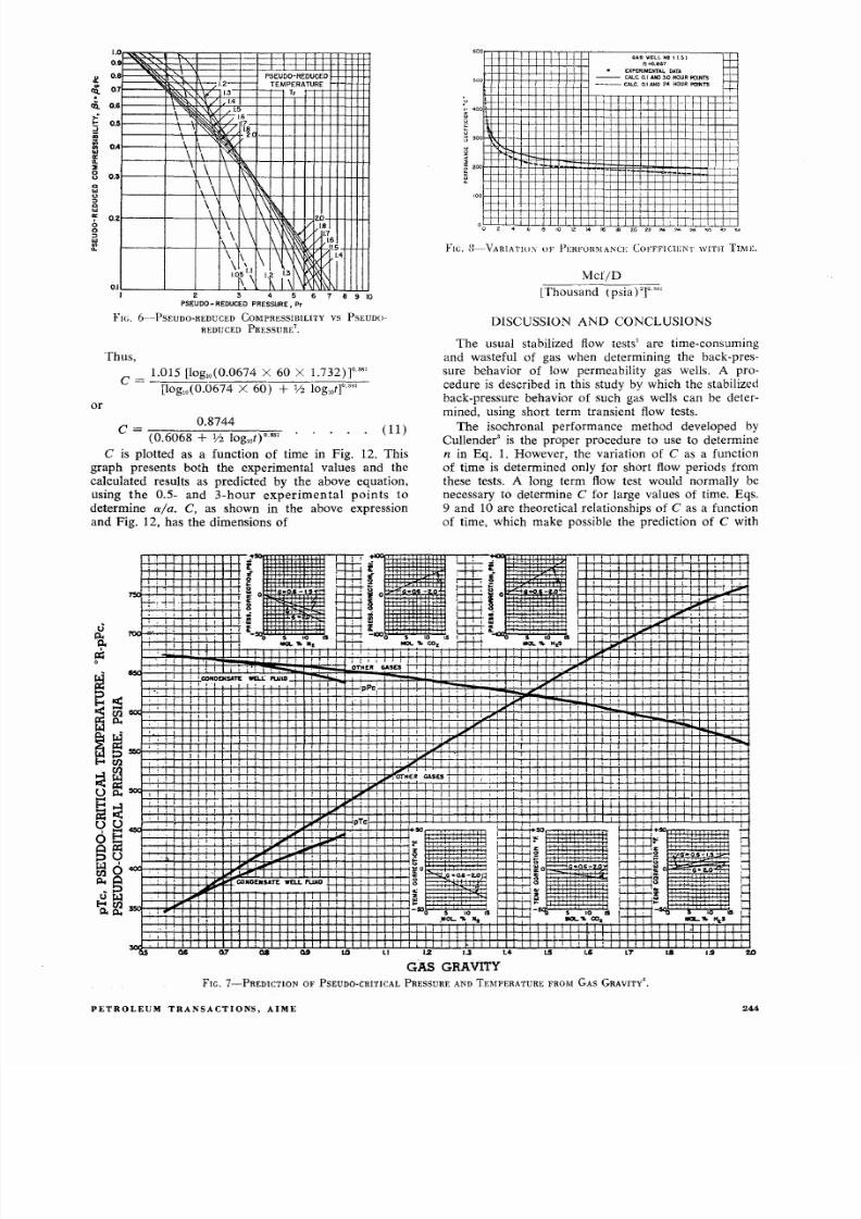
FIG. 6-PSEUDO-REDUCED COMPRESSIBILITY VS PSEUDO

REDUCED PRESSURE'.

Thus,

or

1.015 [log,o(0.0674 X 60 X 1.732)]°'

c=

[loglO(0.0674 X 60)

+

1/2 log,ot]"'"

c

= 0.8744 (11)

(0.6068 +

V2

10g,ot)0.,,,

C is plotted as a function of time in Fig. 12.

This

graph presents both

the

experimental values

and

the

calculated results as predicted by the above equation,

using the 0.5-

and

3-hour experimental points

to

determine a/a C, as

shown

in

the

above expression

and Fig. 12,

has the

dimensions

of

U

I l.

a

I

I

I

-o.S -L

o

° ° f t m W f f i ± ~ ~ l E

AS WELL Ni I z,)

n -0.867

EXPERIMENTAL

DATA

CALC 0.1

AHO 3.0

HOUR POINTS

----

CAL. :.

al ANO 2:4

HOUR POINTS

FIG.

H-VARIA1 W:\

OF

P E R F O H ~ l A N c r ;

COEFFICIENT WITH TIME.

Mcf/D

[Thousand (psia) ']"'"

DiSCUSSION AND CONCLUSIONS

The usual stabilized flow tests

'

are time-consuming

and wasteful of gas when determining the back-pres

sure behavior of low permeability gas wells. A pro

cedure is described in this study by which the stabilized

back-pressure behavior

of

such gas wells can be deter

mined, using

short term

transient flow tests.

The

isochronal

performance method

developed by

Cullender' is the proper procedure

to

use to determine

n in Eq. 1 However, the variation

of

C as a function

of time is determined only for short flow periods from

these tests. A long term flow test would normally be

necessary

to

determine C for large values of time. Eqs.

9 and 10 are theoretical relationships of C as a function

of time, which make possible

the

prediction of C with

, .

.. .

.,.;-- -

'

' . . . -

I I

I'

5

10

S

,

,

MOL

tS

, ,

I%:

o

~ o t

. I

I'

I

~ ; ~ R ; +-i--++--I.-+' ..

-f-.c....,--;-+--+-f-'-+-f-t-+, -':-.,-;.1 :

9-t-+-f-t-+-f-t-+--+--t-+-f-t-+-f-t-+.-+-;--i

....

ffi-

, I

j CONOENS TE WELL FWIO I ,

I

I

I I

I

.I

i

Q7

Q8 LO LI

i'

I I

, .Yo

,

'

I

L

.Yo

1 i

1.2

, ,

I

GAS GRAVITY

I

J ; f

I '

i I

,

• I

I

l4

LT

FIG. 7-PREDICTION OF PSEUDO-CRITICAL PRESSURE AND TEMPERATURE FROM GAS GRAVITY'.

PETROLEUM

TRANSACTIONS, AIME

, i

, 1 I

1.9 2D

244

8/10/2019 SPE-1216-G


reasonable precIsiOn from short term transient flow

tests. Thus, properly conducted short term flow tests

and the use of Eqs. 9 and 10 permit determination of

the stabilized back-pressure behavior of low permeability

gas wells, without the time consumption and gas waste

necessitated by long term flow tests.

The application

of

Eqs. 9 and 10 is demonstrated

by the example problem. The degree of precision pos

sible is illustrated by comparing the theoretically cal

culated performance coefficient with the experimental

results for five gas wells. The deviations of the calcu

lated from the experimental results vary, depending on

the set of experimental points used to evaluate the para

meters in Eqs. 9 and 10. The agreement between calcu

lated and experimental performance coefficients is con

siderably improved if one

of

the points taken to evalu

ate the parameters is on, or well into, the bend of the

performance coefficient curve. The time necessary to

obtain this data from well tests will vary considerably,

depending on the physical nature of the reservoir under

consideration. Once the variation of the performance

coefficient as a function

of

time is determined, the

stabilized back-pressure curves for a gas well for dif

ferent well spacing patterns can be determined from

Eq.4.

Pressure-buildup curves following each isochronal

flow test are used to obtain the interwell permeability.

The effective formation thickness and the porosity are

determined from core analysis data. In a given reser

voir, the value

of n

in Eq. 1 will usually prove to be

essentially the same for all wells in the reservoir. Con

sequently, once the value of n for a given reservoir is

established, the back-pressure behavior of all subsequent

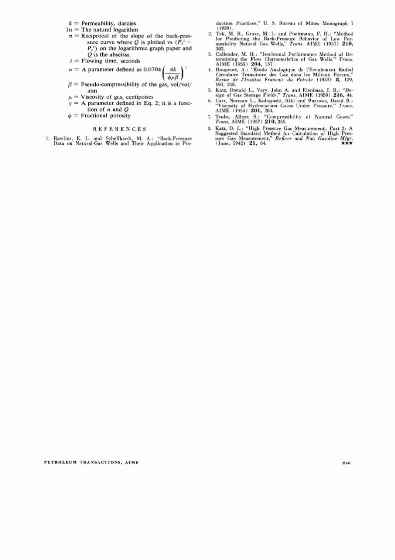
100

160

60

GAS WELL N$l2

51

n 0 839

EXPERIMENTAL DATA

CALC.

1.0

AND : O HOUR POM S

CALC. 3.0

AND 4D HOUR POINTS

10 20

30 40 50

60 10 eo 90 XX

nO

lID

nME-HOURS

FIG.

9-VARIATION

OF PERFORMANCE COEFFClENT WITH TIME.

24

P

180

180

z

140

i

120

100

I

60

40

20

00

20

40

60

80

100

GAS WELL NI. 3

5)

n · 0 9 4

EXPERIMENTAL

DATA

CALC. 0 15 AND 3.0 HOUR POINTS

CALC

1.0 Af«)

23.5

HOUR

POINTS

120

140

160

180

FIG. lO-VARIATION

OF PERFORMANCE COEFFICIENT WITH

TIME.

245

wells can be determined from a single flow test of rel

atively short duration.

NOMENCLATURE

C

=

Performance coefficient (the units depend

on the units in which Q Pi and P, are

expressed). In the example problem, for

instance, the pressures are expressed in

thousands of psia and Q in Mcf/D.

Therefore, the units of C are in

Mcf/D

/(1,000

psia )n.

G

=

Gas gravity (air

=

1)

P

=

Pressure, psia

P

= Pseudo-critical pressure, psia

P =

Formation shut-in pressure, psia

P

R

= Pseudo-reduced pressure,

PIP,

P,

=

Flowing sand face pressure, psia

Q

= Gas flow rate, Mcf/D, at 60°F and 14.65

psia

R =

Radius of drainage, feet

T

=

Temperature,

OR

T c =

Pseudo-critical temperature, ° R

T =

Formation temperature,

OR

T

R

=

Pseudo-reduced temperature,

T

/T,

a

=

Well bore radius, feet

b

=

Ratio

of

density of gas to bottom-hole

pressure

b

= 29G

ZR T,

where

R

= 45.59 atm/cc/gm-mol-

OR

h

=

Effective formation thickness, centimeters

1 2 w m f f i H i ~ ~

2&--6 MESA

1-14

SAN

JUAN(2 )

10

o

o

100 200

'

400 000

TIME. HOURS

n_ O .7 7 4

EXPERIMENTAL

DATA

TEte, GROVE. POfTTMANN

{2 I

CALC. 3 AND 6 HOUR

POINTS

CALC. 5 AND 22 HOUR

POINTS

CALC. 22 AND 118.7 HOUR POINTS

600

100

800

FIG.

l l -VARIATION

OF PERFORMANCE COEFFICIENT WITH TI,\ E.

1 8

1 6

WELL A

n 00.887

1 4

e

EXPERIMENTAL

.2 \

- g ~ t ' l . ; l i : E : ~ :rm

1\

1 -..

.8

r--..

r- Io-

Q

6

.2

0

o

1

20

30

40

TIME, HOURS

FIG. 12 -VARIATION OF PERFOR:\IANCE

COEFFICIENT WITH

TIME.

,VOL. 2 1 6 . 1 9 5 9

8/10/2019 SPE-1216-G


k Permeability, darcies

In The natural logarithm

n

=

Reciprocal

of

the slope

of

the back-pres

sure curve where

Q

is plotted vs P/

P:) on the logarithmic graph paper and

Q is the abscissa

t =

Flowing time, seconds

a =

A parameter defined as 0.0704 ~ )

j

cf> p..f3

f =

Pseudo-compressibility

of

the gas,

vol/vol

atm

IL

Viscosity of gas, centipoises

y

=

A parameter defined in Eq.

2;

it

is

a func

tion of nand Q

cf = Fractional porosity

R E F E R E N C E S

1

Rawlins, E.

L.

and Schellhar dt, M. A.: Back-Press ure

Data

on Natural-Gas Wells

and Their

Application to Pro-

PE T R O L E U M T R A N S A C T I O N S A I M E

duction Practices, U. S.

Bureau

of Mines Monograph 7

(1939) .

2

Tek, M.

R.,

Grove, M.

L. and

Poettmann, F. H.:

"Method

for

Predicting

the Back-Pr,essure Behavior of Low Per_

meability

Natural

Gas Wells, Trans. AI ME (1957)

210,

302.

3

Cullender, M.

H.:

Isochronal Performance Method of De

termining the Flow Characteristics of Gas Wells, Trans.

AIME (1955) 204, 137.

.t.

Houpeurt, A.:

"Etude

Analogique de I'Ecoulement Radial

Circulaire Transitoire des Gaz dans les Milieux

Poreux,"

Revue e l ]nstitu t Francais du Petrole (1953) 8, 129,

193,

248

5

Katz, Donald

L.,

Vary,

John

A.

and

Elenbaas, J. R.: De

sign of Gas Storage Fields,

Trans.

AIME

(1959)

216,

44

6

Carr, Norman

L.,

Kobayashi, Riki

and

Burrows, David B.:

Viscosity of Hydrocarbon Gases

Under

Pr,essure, Trans.

AIME (1954)

201,

264

7

Trube,

Albert S.: Compressibility of

Natural

Gases,

Trans.

AIME (1957) 210,355.

S Katz, D. L.: "High Pressure Gas Measurement; Part 2: A

Suggested

Standard

Method for Calculation of

High

Pres

sure Gas Measurement, Refiner and Nat. Gasoline Mlgr.

(June,

1942)

21,

64

1246

SPE-1216-G

Documents

Transcript of SPE-1216-G