Spe 166395

SPE 166395

Streamline-Based Time Lapse Seismic Data Integration Incorporating Pressure and Saturation Effects Shingo Watanabe, SPE, Jichao Han, SPE, Akhil Datta-Gupta, SPE, and Michael J. King, SPE, Texas A&M University

Copyright 2013, Society of Petroleum Engineers This paper was prepared for presentation at the SPE Annual Technical Conference and Exhibition held in New Orleans, Louisiana, USA, 30 September–2 October 2013. This paper was selected for presentation by an SPE program committee following review of information contained in an abstract submitted by the author(s). Contents of the paper have not been reviewed by the Society of Petroleum Engineers and are subject to correction by the author(s). The material does not necessarily reflect any position of the Society of Petroleum Engineers, its officers, or members. Electronic reproduction, distribution, or storage of any part of this paper without the written consent of the Society of Petroleum Engineers is prohibited. Permission to reproduce in print is restricted to an abstract of not more than 300 words; illustrations may not be copied. The abstract must contain conspicuous acknowledgment of SPE copyright.

Abstract We present an efficient history matching approach that simultaneously integrates 4-D repeat seismic surveys with well production data. This approach is particularly well-suited for the calibration of the reservoir properties of high-resolution geologic models because the seismic data is areally dense but sparse in time, while the production data is continuous in time but averaged over interwell spacing. The joint history matching is performed using streamline-based sensitivities derived from either finite-difference or streamline-based flow simulation. Previous approaches to seismic data integration have mostly incorporated saturation effects but the pressure effects have largely been ignored. We propose, for the first time, streamline-based analytic approaches to compute parameter sensitivities that relate the seismic data to reservoir properties while accounting for both pressure and saturation effects via appropriate rock physics models. The inverted seismic data (e.g., changes in acoustic impedance or fluid saturations), is distributed as a 3-D high-resolution grid cell property or as a vertically integrated two-dimensional map. We derive pressure drop sensitivities along streamlines in addition to our previous work of water saturation sensitivity computation. The novelty of the method lies in the analytic sensitivity computations which make it computationally efficient for high resolution geologic models. We demonstrate the versatility of our approach by implementing it in a finite difference simulator which incorporates detailed physical processes, while the streamline trajectories provide for rapid evaluation of the sensitivities. The efficacy of our proposed approach is demonstrated with both synthetic and field applications. The synthetic example is the SPE benchmark Brugge field case. The field example involves waterflooding of a North Sea reservoir with multiple seismic surveys. For both the synthetic and the field cases, the advantages of incorporating the time-lapse variations are clearly demonstrated through improved estimation of the permeability distribution, pressure profile, and fluid saturation evolution and swept volumes. Introduction Three-dimensional (3-D) reservoir simulation models play an essential role in the oil and gas industry. They are routinely utilized to plan the development strategy, calculate hydrocarbon reserves and predict future production estimates. Due to sparse well observation data coverage, reservoir models are often poorly constrained away from well locations. A key challenge for reservoir engineers and geoscientists is therefore the quantitative data integration of 3-D, and where available 4-D, seismic data to obtain a more accurate representation of reservoir properties between wells.

Geostatiscal techniques have been widely adapted in the petroleum industry to construct reservoir models and commercial and research geomodeling software packages are widespread and available (e.g., GSLIB, Deutsch and Journel, 1992). For example, geostatistical techniques for constraining 3-D reservoir models with seismic information utilize co-kriging and co-simulation. There are several problems associated with integrating seismic and well data for both 3-D and 4-D reservoir characterization. First, the seismic data must be converted from time to depth, while the velocity model is only calibrated at the wells. Second, seismic data is band-limited, whereas well data has both high and low frequency components. The seismic response must be calibrated to the well data, but loses the high frequency information. The limited vertical resolution of inverted seismic data has been a major obstacle to the widespread use of seismic information in 3-D property modeling (Doyen et al., 1997). Behrens et al (1998) introduced a geostatistical method to incorporate seismic attribute maps into a 3-D reservoir model. The method, called sequential Gaussian simulation with block kriging (SGSBK) accounts for the volume support differences between the seismic interval-average rock properties and the well log point-rock properties.

2 SPE 166395

More recently, the concept of time-lapse seismic data as the dynamic observation data has emerged. Time-lapse seismic reservoir monitoring is the process of acquiring and analyzing multiple seismic surveys, repeated at the same site over months or years, in order to image fluid flow effects in a producing reservoir. If each survey is “3-D seismic,” then the resulting set of time-lapse data is often termed “4-D seismic,” where the extra fourth dimension is time.

The first quantitative time-lapse seismic data found in rock physics studies in mid 1980s. The laboratory measurement on heavy oil saturated core samples showed large decreases in seismic rock velocity when the viscous oil was heated (Nur et al., 1984; Wang and Nur, 1988; Nur, 1989). These rock physics observations have now been validated by many 4-D seismic field data with steam injection projects (Pullin et al., 1987; Eastwood et al., 1994; Jenkins et al., 1997). Early lab measurement of Domenico (1976) showed the presence of free gas in a reservoir without an associated temperature change can also significantly decrease the rock’s seismic impedance and this leads to the possibility of monitoring gas-fluid contact movement and injected gases such as CO2 injection projects (Harris et al., 1996).

Monitoring oil-water system is more technically challenging because the seismic impedance contrast between oil and water-saturated rock is often much smaller than the free-gas or heated oil effects (Wang et al., 1991). Recent developments in seismic processing that improve time-lapse repeatability with noise filtering algorithms facilitated the use of 4-D seismic for monitoring reservoir waterflood performance (Burkhart et al., 2000; O’Donovan et al., 2000; Behrens et al., 2002).

Lumley et al. (1997) and Lumley and Behrens (1998) discussed the practical issues relevant to the successful monitoring of oil-water and other reservoir fluid-flow systems, and the general technical challenges associated with time-lapse seismic reservoir monitoring were thoroughly reviewed (Lumley 2001). With these proposed guidelines, the field applications of time-lapse seismic data has evolved (Fanchi, 2001; Clifford et al., 2003) and 4-D seismic is now recognized as a reservoir management tool with a number of successful field applications (Landro et al., 1999; Behrens et al., 2002; Toinet, 2004; Foster, 2007).

The next logical step of this technology is to use the time-lapse seismic data to infer reservoir permeability and porosity heterogeneity through the reservoir model calibration process, also known as history matching. The traditional history matching process mainly involves production data and the solution is highly non-unique, as production data provides limited information about permeability and porosity variations away from the well locations. The possibility of incorporating 4-D seismic information into history matching as additional dynamic data is therefore attractive as it provides images of fluid movements between wells, albeit at a vertically average scale compared to the layers in the flow simulation model. Time-lapse seismic images can identify the bypassed oil regions to be targeted for infill drilling, and add major reserves to production to extend a field’s economic life. Also, 4-D seismic can map the reservoir compartmentalization and identify the fluid flow properties of faults (sealing versus leaking), which can be extremely useful for the optimal design of well trajectories in complex reservoir flow systems.

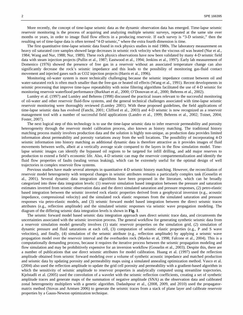
Previous studies have made several attempts in quantitative 4-D seismic history matching. However, the reconciliation of reservoir model heterogeneity with temporal changes in seismic attributes remains a particularly complex task (Gosselin et al., 2001). Several dynamic data integration algorithms have been proposed in the literature, which can be broadly categorized into three data integration levels: (1) reservoir simulation based integration between the pressure and saturation estimates inverted from seismic observation data and the direct simulated saturation and pressure responses, (2) petro-elastic based integration between the seismic inverted rock elastic properties derived from a geophysical inversion (e.g., acoustic impedance, compressional velocity) and the simulated rock elastic responses from the simulated saturation and pressure responses via petro-elastic models, and (3) seismic forward model based integration between the direct seismic traces attributes (e.g., reflection amplitude) and the simulated seismic responses via seismic wave propagation modeling. The diagram of the differing seismic data integration levels is shown in Fig. 1.

The seismic forward model based seismic data integration approach uses direct seismic trace data, and circumvents the uncertainties associated with the seismic inversion process. The general workflow for generating synthetic seismic data from a reservoir simulation model generally involves (1) static reservoir properties on the simulation grid, (2) simulation of dynamic pressure and fluid saturations at each cell, (3) computation of seismic elastic properties (e.g., P and S wave velocities), and finally, (4) simulation of the seismic attribute (e.g., reflection amplitude) by applying a seismic wave propagation model over the reservoir interval and the overburden rock (Mavko et al, 1998; Falcone et al., 2004). This is a computationally demanding process, because it requires the iterative process between the seismic propagation modeling and flow simulation and may be prohibitively expensive for an inversion workflow (Gosselin et al., 2003). Despite this, there are a number of publications that use direct seismic attributes for model calibration. Huang et al. (1997) used the reflection amplitude obtained from seismic forward modeling over a volume of synthetic acoustic impedance and matched production and seismic data by updating porosity and permeability maps using a simulated annealing optimization method. Vasco et al. (2004) also used the reflection amplitude to update the grid cell porosity and permeability with a gradient-based algorithm in which the sensitivity of seismic amplitude to reservoir properties is analytically computed using streamline trajectories. Kjelstadli et al. (2005) used the convolution of a wavelet with the seismic reflection coefficients, creating a set of synthetic amplitude traces and generate maps of the summation of negative amplitude (SNA) as the observation data and calibrated zonal heterogeneity multipliers with a genetic algorithm. Dadashpour et al., (2008, 2009, and 2010) used the propagator-matrix method (Stovas and Arntsen 2006) to generate the seismic traces from a stack of plane layer and calibrate reservoir properties by a Gauss-Newton optimization technique.

SPE 166395 3

The inclusion of the seismic inversion within the first workflow makes this an expensive approach. The petro-elastic and the reservoir simulation based approaches to seismic data integration are workflows that evaluate the seismic match quality in terms of the inverted seismic responses. The type of time-lapse seismic data considered to be observation data varies among different researchers. The inverted responses can be derived from traditional post-stack data inversion techniques such as the sparse spike inversion (e.g., seismic volumes of acoustic impedance), or from the direct saturation and pressure front detection using an amplitude versus offset (AVO) inversion of pre-stack seismic data (Tura and Lumley 2000; Landro et al, 2001). From a computational standpoint, these methods are more efficient, because they perform the geophysical inversion of the seismic volumes as a separate process from the model calibration workflow. Gosselin et al. (2003) emphasized the need to maintain consistency between the geophysical inversion and the calibration workflow when the data misfit is expressed in terms of rock elastic properties. There are a significant number of publications that apply seismic inverted responses for the reservoir model calibration compared with those that apply the direct seismic attributes. For example, Landa and Horne (1997) used saturation changes data obtained directly from inverted time-lapse seismic data. Gosselin et al. (2001) applied synthetic acoustic impedance maps generated with a rock physics model, and calibrate model with a heterogeneity parameterization based on the grad zone analysis. Arenas et al. (2001) used the compressional velocity to calibrate the permeability field at a set of pilot points used as conditioning data by kriging in a gradient-based optimization loop. Dong and Oliver (2005) assumed the availability of differences in acoustic impedance from a geophysical seismic inversion and calibrated the grid cell porosity and permeability using a quasi-Newton method with the objective function gradient calculated by an adjoint method. In stochastic approaches, Skjervheim et al. (2007) used the ensemble Kalman smoother to assimilate the time-lapse seismic data of changes in acoustic impedance and compressional velocity. Fahimuddin et al. (2010) similarly used the seismic derived impedance data with the ensemble Kalman filter with a covariance localization method. Feng and Mannseth (2010) applied a pseudo seismic data in the form of maps of saturation changes and investigated the impact of the seismic data in the presence of noise on permeability estimation. Finally, Rey et al. (2012) applied a streamline based sensitivity calculation to integrate the seismic derived water saturation changes and the acoustic impedance differences and demonstrated field-scale applications.

Our current study examines both reservoir simulation based calibration and rock physics based calibration. In the first instance we calibrate against both time lapse changes in pressure and in saturation. In the second instance we calibrate against the time lapse change in acoustic impedance. In both cases, the inversion will provide local updates to the reservoir model using analytic streamline-based sensitivity calculations. This is the major new result of our study. As with most previous studies, we will calibrate against changes in properties over the interval of the time lapse survey, instead of the properties themselves. This minimizes systematic biases introduced by lack of calibration of the initial model. In addition, we will also integrate this approach in a sequential fashion with other forms of data calibration. In both cases we will follow the seismic data integration with a fairly conventional streamline based integration of water-cut field performance. This data is high resolution in time, but only available at the production wells. When calibrating the model against acoustic impedance we will perform a global model calibration first, which ensures that we have a good starting point for the local calibrations.

The outline of this paper is as follows. First, we start with the mathematical background to determine the streamline-based analytic sensitivities for fluid saturation and pressure data integration. These sensitivity results are validated by numerical experiments. Second, we illustrate the history matching applications of time-lapse pressure and saturation changes by using a synthetic model and the SPE benchmark Brugge field model. Finally, using the petro-elastic modeling level of seismic data integration, we apply the proposed approach to a field example, the Norne field, in terms of time-lapse acoustic impedance change derived from the post-stack seismic amplitude data. This combination of examples demonstrates the utility and the effectiveness of our approach.

Fig. 1―Seismic data integration levels, (1) reservoir simulation level of data integration, (2) petro-elastic modeling level of data integration, and (3) seismic forward modeling level of data integration.

4 SPE 166395

Background and Methodology Our approach relies on the use of streamlines to relate the reservoir properties to the dynamic reservoir response:

production, pressure and time lapse seismic response. Establishing these relations, also called sensitivities, is crucial to the data integration process. We make extensive use of streamlines to describe the flow field and to calculate the fluid tracer time of flight along each streamline. The time of flight acts as a spatial coordinate along the lines. However, our proposed approach does not rely on the use of a streamline simulator, and is well-suited for both conventional finite difference reservoir simulators and streamline simulators. In fact, most of the examples presented in this paper utilize a commercial finite difference simulator for flow simulation. For streamline simulators, the streamline trajectories and time of flight are readily available. However, for finite difference simulator the streamline and time of flight are obtained via a post processing of the finite difference velocity field.

In this section, we first discuss the mathematical details related to sensitivity computations in streamline-based seismic data integration. The derivations of sensitivity formulation include time of flight sensitivity, saturation front arrival time sensitivity, water saturation sensitivity and pressure drop sensitivity. Also, we discuss the objective function for data misfit quantification and its minimization. Time of Flight Sensitivity Calculation We start with the definition of the streamline time of flight which is the travel time of a neutral tracer along a streamline (Datta-Gupta and King, 2007),

(1)

Here the integral is along the streamline trajectory , r is distance along the streamline, and is the slowness defined by the reciprocal of the interstitial velocity

| |. (2)

Using Darcy’s law, the slowness can be written as

| | (3)

Here is the total relative mobility, and | | is the pressure gradient along the streamline. Because slowness is a composite quantity involving reservoir properties, its first order variation, assuming a fixed pressure gradient, will be given by

, (4)

From Eq. 3 the partial derivatives are

| |, (5)

| |. (6)

The approximation in Eq. 5 and Eq. 6 is that the local perturbations in permeability or porosity generate negligible pressure changes. This approximation implies that to leading order streamlines do not shift because of these small perturbations. Now we can relate the change in time of flight to the change in slowness by integrating along each streamline trajectory as

= . (7)

Thus, the tracer travel time sensitivity along a single streamline, with respect to permeability and porosity at location follows Eq. 7 by integrating from the inlet to the outlet of the streamline within the gridblock,

, (8)

. (9)

Here Δ is the time-of-flight across the gridblock at location . Saturation Front Arrival Time Sensitivity In the previous section we developed expressions for sensitivity of the streamline time of flight to reservoir porosity and permeability. We now relate the time of flight sensitivity to the travel time sensitivity of the water saturation. For two phase flow, this sensitivity is used after water breakthrough at a producing well to calibrate the reservoir properties to water cut response, and can be generalized to three phase flow. First, we consider two phase incompressible flow of oil and water

SPE 166395 5

described by the Buckley-Leverett equation written using the streamline time of flight as the spatial coordinate (Datta-Gupta and King, 2007),

0. (10)

The velocity of a given saturation along a streamline is given by the slope of the fractional flow curve,

. (11)

This equation relates the travel time of a saturation, , ; to the time of flight , . We can now compute the

sensitivity of the saturation arrival time using that of the streamline time of flight as follows

, ;/ , (12)

, ;/ . (13)

After water breakthrough on a streamline, these arrival times are evaluated at the total time of flight, , for the streamline.

Water Saturation Sensitivity Calculation We now derive expressions for the sensitivity of water saturation with respect to variations in permeability. For two phase flow, water saturation is a function of the streamline time of flight, and time, . First consider self-similar solutions to Eq. 10, as have just been derived. Along a streamline the saturation is a function of the dimensionless ratio /t. This allows us to relate the derivative of saturation with respect to time to the derivative with respect to as follows:

⁄

⁄ (14)

⁄

⁄ (15)

Hence:

(16)

From this we have the water saturation sensitivity:

, (17)

The partial derivative of water saturation with respect to time in Eq. 16 can be calculated numerically by a backward time difference as

, , , (18)

Here Δ is the timestep size. This requires saving the saturation information for the time step immediately prior to the time lapse survey time. Therefore, the saturation sensitivity at location at a given time can be calculated by:

, , , (19)

where the last partial derivative of travel time with respect to permeability can be obtained from Eq. 8. The derivation in Eq. 19 assumes that the streamline trajectories do not change with time. This is an incorrect assumption

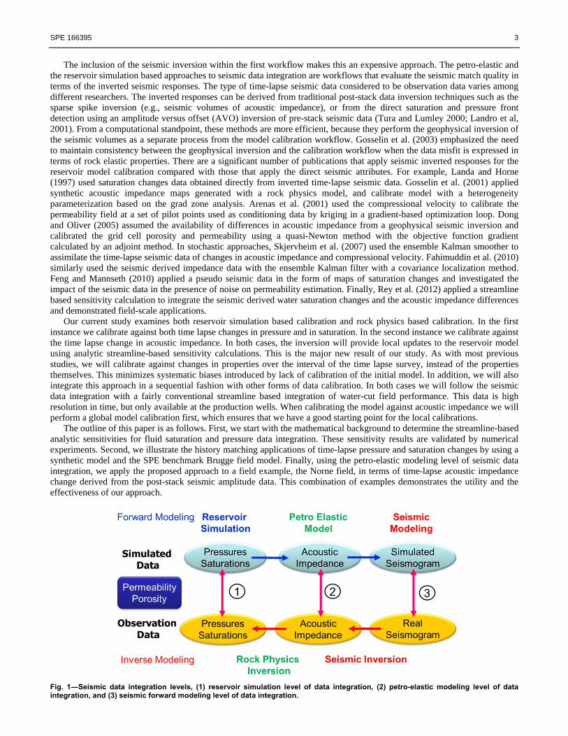
considering the large time intervals typically used in time lapse seismic surveys. Also, most often we are calibrating against the changes in saturation, rather than the saturation itself. The generalization of the sensitivity calculation to account for these effects is discussed in the Appendix. Pressure Data Integration Pressure data integration is performed by converting the spatial distribution of pressure to a spatial distribution of the viscous pressure drop along a streamline from each location, to the producing well where that streamline terminates. Specifically, for a particular location i, and pressure then the pressure drop, ∆ | along the streamline passing through the location i and leading to well w with bottom hole pressure (Fig. 2) is:,

∆ | . (20)

This utilizes the (known) bottom hole flowing pressure at the time at which the spatial distribution of pressure data was obtained. If distributed time lapse pressure data and well bottom hole pressure are available, we can compute the pressure drop from Eq. 20 and use it as our observation data,

6 SPE 166395

∆ | , , , . (21)

Now, the data misfit between the simulation response and observation can be written as

∆ | , ∆ | ,

, , , ,

, , , , . (22)

The first term is the pressure difference at location i, and the second term is the bottom hole pressure difference at well w. Pressure Drop Sensitivity Calculation The pressure drop along a streamline can be expressed as

∆ ∆ . (23)

This can be computed by simply summing up the pressure drop across the grid blocks that intersect the streamline as shown in Fig. 2. Further, we can express the local pressure drop along a streamline using Darcy’s law as

∆∆

(24)

where is the cross sectional area, is the flow rate along a streamline, is the total relative mobility, and ∆ is the arc length of the streamline within the gridblock. The pressure drop is a composite quantity involving reservoir properties. We assume that the streamline trajectories, flow rate along streamline and the total mobility do not change because of small perturbations in permeability. We can now relate the change in local pressure drop to a small change in permeability as

∆∆

, (25)

where the partial derivatives are

∆ ∆ ∆. (26)

The pressure drop to a location i, ∆ | will be given by integration along the streamline trajectory passing through i to well w,

∆ | ∆ =∆

(27)

and the pressure drop sensitivity for a particular gridblock at location follows from Eq. 27,

∆ | ∆ ∆. (28)

Fig. 2―A streamline between well pairs connecting gridblocks.

Objective Function Minimization Formulation After we compute the sensitivities of the seismic derived data and/or the production data with respect to the grid block permeability, we perform the data integration by minimizing a penalized misfit function consisting of the following three terms (He et al., 2002):

m ‖ d S m‖ ‖ m‖ ‖L m‖. (29)

In the above expression, d is the data misfit between the observation and simulated response, and S is the sensitivity matrix containing the sensitivities of model responses with respect to reservoir parameters. Also m corresponds to the reservoir parameter change vector and L is a second spatial difference operator matrix. The first term ensures the difference between

Streamline=1D Grids

Producer

Injector

SPE 166395 7

the observed and calculated model response is minimized. The second term, called a “norm constraint”, penalizes deviations from the prior model. This prevents large changes and helps preserve geologic realism by preserving major features of the prior model during the model calibration process. Finally, the third term, a “roughness constraint”, constrains the model changes to be spatially smooth. The weights and determine the relative strengths of the norm and smoothness constraints; guidelines exist in the literature for their selection. An iterative sparse matrix solver, LSQR (Paige and Saunders 1982), is used for solving the augmented linear system efficiently.

In this paper, we carry out the data integration in a sequential manner starting with pressure data first followed by the saturation changes and then the well production information. The sequential framework is analogous to the structured approach used in the industry (Williams et al., 1998; Cheng et al., 2008) and accounts for the different length scales associated with different data types. The sequential framework also facilitates convergence of the inversion algorithm. The norm constraint in Eq. 29 maintains consistency between different steps in the sequential process by limiting the changes and thus, preserves the calibration results from the previous step. Sensitivity Calculation Validations In this section, numerical experiments are conducted to verify the proposed water saturation and pressure drop sensitivity calculations. Water Saturation Sensitivity Validation

We set up a simple model which is a 1-D homogeneous model with one injector and one producer at the two ends as shown in Fig. 3. It is similar to a core flood experiment. The system is two phase oil and water. Rock and fluid properties are summarized in Table 1 and relative permeability curves are shown in Fig. 4. Wells are controlled by bottom hole pressure constraints. We conduct the simulation for 50 days with 10 timesteps of 5 days. Simulation specification is summarized in Table 2.

Fig. 3―A 1-D simulation model.

*PVT values are at the reference pressure of 5000 psi

P1I1

0.00 0.25 0.50 0.75 1.00SWAT

TABLE 1―ROCK AND FLUID PROPERTIES.

Porosity 0.15

Permeability, mD 200

Rock compressibility, 1/psi 8.0 x 10‐6

Oil density, lb/cf 52.1

Water density, lb/cf 63.3

Oil viscosity, lb/cf 0.29

Water viscosity, cp 0.31

Oil formation volume factor 1.305

Water formation volume factor 1.04

TABLE 2―SIMULATION SPECIFICATIONS OF SATURATION SENSITIVITY VALIDATION CASE.

Grid number 50 x 1 x 1

Grid size, ft 20 x 20 x 20

Initial pressure, psi 5000

Injector location (1,1,1)

Injector bottom hole pressure, psi 5200

Producer location (50,1,1)

Producer bottom hole pressure, psi 5000

Total simulation time, days 50

Timestep size, days 5

8 SPE 166395

Fig. 4―Relative permeability curves.

We compare the proposed sensitivity calculation with a numerical perturbation method. The numerical perturbation method calculates the sensitivity as

, (30)

. (31)

Here d is the observed quantity, g( ) is the non-linear function of reservoir simulation and m is the perturbed reservoir property. Therefore the total computation requires Ng+1 simulations, where Ng is the number of grid blocks, while the proposed analytic sensitivity calculation requires only a single simulation. For the following experiment, the perturbation value is 10% of the original parameter value for numerical sensitivity calculations.

Water saturation sensitivities with respect to reservoir permeability are shown in Fig. 5. The proposed streamline based sensitivity calculation shows very good agreement with the numerical perturbation values. The peak value of the sensitivity profile corresponds to the water saturation front location where a sharp saturation change occurs. Behind the water saturation front location, the sensitivity profile decays because the saturation changes diminish.

(a) (b)

(c) (d) Fig. 5―Water saturation sensitivity with respect to reservoir permeability comparisons. (a) Sensitivity values with respect to the permeability of grid block no. 15 at a time of 25 days. Red line is the analytic streamline based calculation, green line is the numerical perturbation. (b) Water saturation profile at a time of 25 days. (c) Sensitivity values with respect to permeability of grid block no. 15 at a time of 50 days. (d) Water saturation profile at a time of 50 days.

0.0

0.1

0.2

0.3

0.4

0.5

0.6

0.7

0.8

0.9

1.0

0.0 0.2 0.4 0.6 0.8 1.0

Relative permeab

ility

Normalized water saturation

Krw

Kro

SPE 166395 9

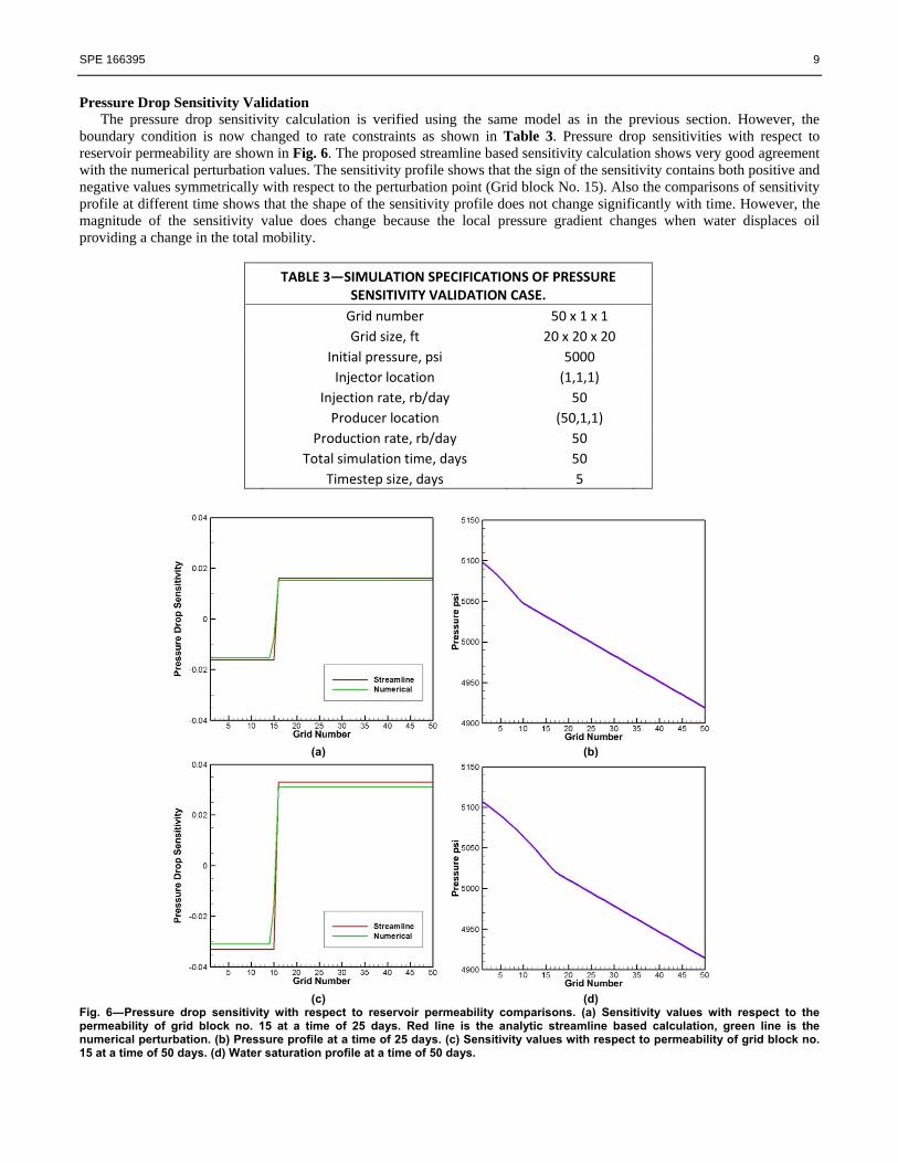
Pressure Drop Sensitivity Validation The pressure drop sensitivity calculation is verified using the same model as in the previous section. However, the

boundary condition is now changed to rate constraints as shown in Table 3. Pressure drop sensitivities with respect to reservoir permeability are shown in Fig. 6. The proposed streamline based sensitivity calculation shows very good agreement with the numerical perturbation values. The sensitivity profile shows that the sign of the sensitivity contains both positive and negative values symmetrically with respect to the perturbation point (Grid block No. 15). Also the comparisons of sensitivity profile at different time shows that the shape of the sensitivity profile does not change significantly with time. However, the magnitude of the sensitivity value does change because the local pressure gradient changes when water displaces oil providing a change in the total mobility.

(a) (b)

(c) (d) Fig. 6―Pressure drop sensitivity with respect to reservoir permeability comparisons. (a) Sensitivity values with respect to the permeability of grid block no. 15 at a time of 25 days. Red line is the analytic streamline based calculation, green line is the numerical perturbation. (b) Pressure profile at a time of 25 days. (c) Sensitivity values with respect to permeability of grid block no. 15 at a time of 50 days. (d) Water saturation profile at a time of 50 days.

TABLE 3―SIMULATION SPECIFICATIONS OF PRESSURE SENSITIVITY VALIDATION CASE.


Grid size, ft 20 x 20 x 20

Initial pressure, psi 5000


Injection rate, rb/day 50

Producer location (50,1,1)

Production rate, rb/day 50



10 SPE 166395

History Matching Applications Five-Spot Synthetic Case

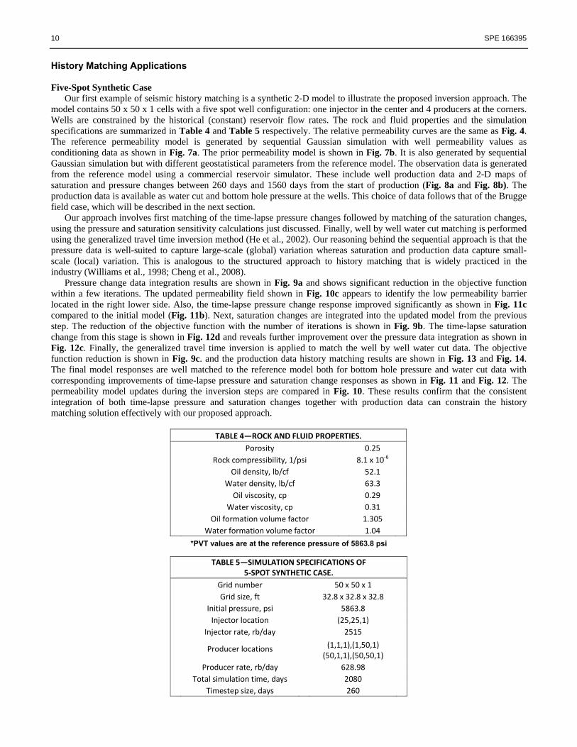
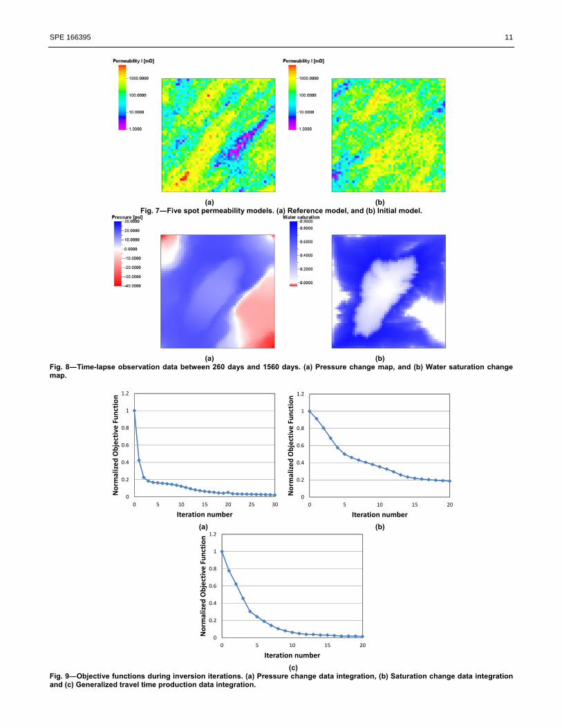
Our first example of seismic history matching is a synthetic 2-D model to illustrate the proposed inversion approach. The model contains 50 x 50 x 1 cells with a five spot well configuration: one injector in the center and 4 producers at the corners. Wells are constrained by the historical (constant) reservoir flow rates. The rock and fluid properties and the simulation specifications are summarized in Table 4 and Table 5 respectively. The relative permeability curves are the same as Fig. 4. The reference permeability model is generated by sequential Gaussian simulation with well permeability values as conditioning data as shown in Fig. 7a. The prior permeability model is shown in Fig. 7b. It is also generated by sequential Gaussian simulation but with different geostatistical parameters from the reference model. The observation data is generated from the reference model using a commercial reservoir simulator. These include well production data and 2-D maps of saturation and pressure changes between 260 days and 1560 days from the start of production (Fig. 8a and Fig. 8b). The production data is available as water cut and bottom hole pressure at the wells. This choice of data follows that of the Brugge field case, which will be described in the next section.

Our approach involves first matching of the time-lapse pressure changes followed by matching of the saturation changes, using the pressure and saturation sensitivity calculations just discussed. Finally, well by well water cut matching is performed using the generalized travel time inversion method (He et al., 2002). Our reasoning behind the sequential approach is that the pressure data is well-suited to capture large-scale (global) variation whereas saturation and production data capture small-scale (local) variation. This is analogous to the structured approach to history matching that is widely practiced in the industry (Williams et al., 1998; Cheng et al., 2008).

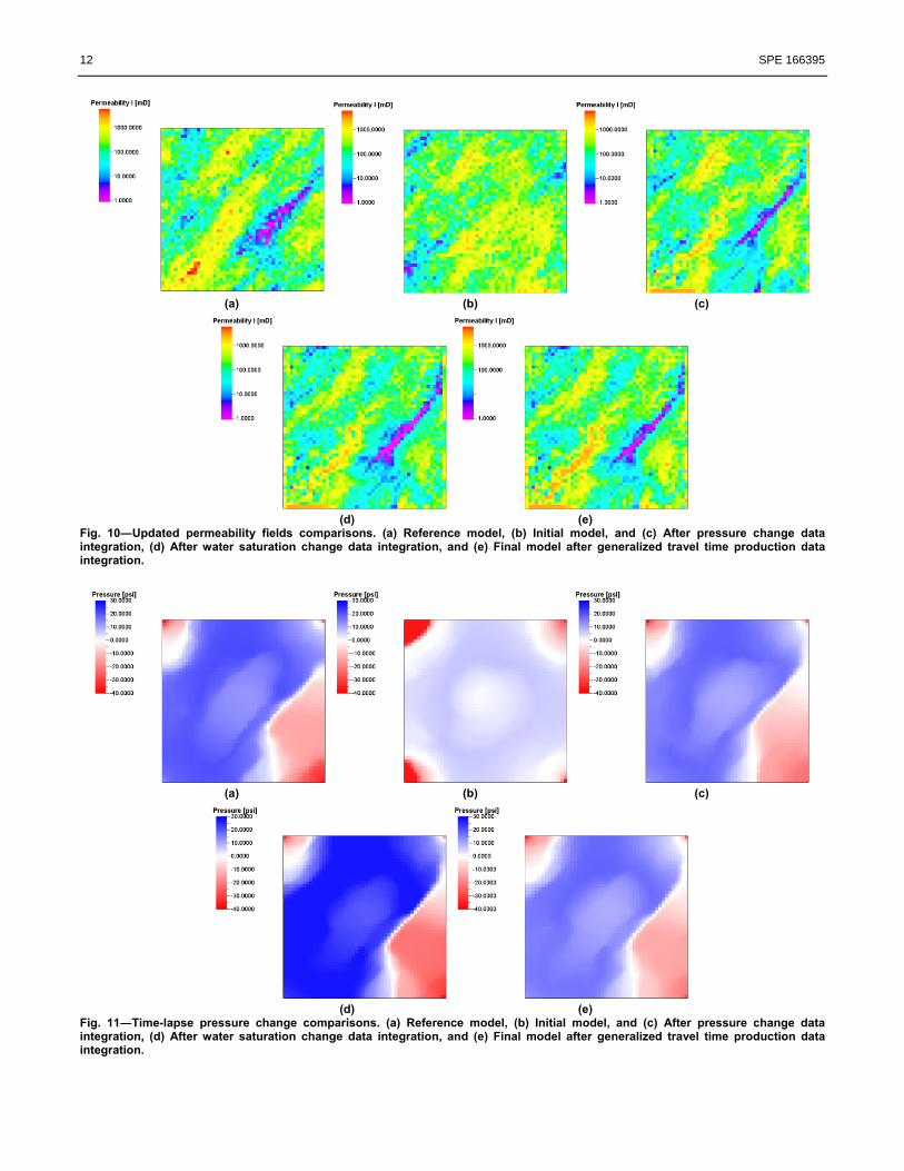
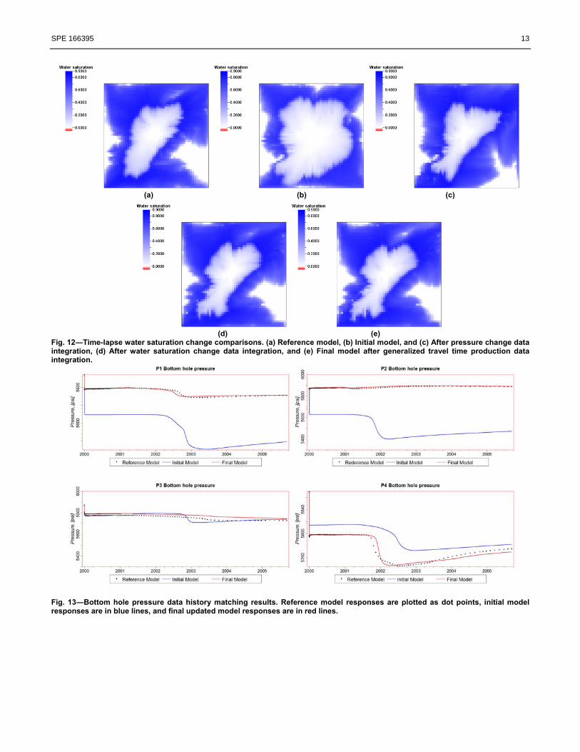
Pressure change data integration results are shown in Fig. 9a and shows significant reduction in the objective function within a few iterations. The updated permeability field shown in Fig. 10c appears to identify the low permeability barrier located in the right lower side. Also, the time-lapse pressure change response improved significantly as shown in Fig. 11c compared to the initial model (Fig. 11b). Next, saturation changes are integrated into the updated model from the previous step. The reduction of the objective function with the number of iterations is shown in Fig. 9b. The time-lapse saturation change from this stage is shown in Fig. 12d and reveals further improvement over the pressure data integration as shown in Fig. 12c. Finally, the generalized travel time inversion is applied to match the well by well water cut data. The objective function reduction is shown in Fig. 9c. and the production data history matching results are shown in Fig. 13 and Fig. 14. The final model responses are well matched to the reference model both for bottom hole pressure and water cut data with corresponding improvements of time-lapse pressure and saturation change responses as shown in Fig. 11 and Fig. 12. The permeability model updates during the inversion steps are compared in Fig. 10. These results confirm that the consistent integration of both time-lapse pressure and saturation changes together with production data can constrain the history matching solution effectively with our proposed approach.

*PVT values are at the reference pressure of 5863.8 psi

TABLE 4―ROCK AND FLUID PROPERTIES.

Porosity 0.25

Rock compressibility, 1/psi 8.1 x 10‐6

Oil density, lb/cf 52.1

Water density, lb/cf 63.3

Oil viscosity, cp 0.29

Water viscosity, cp 0.31

Oil formation volume factor 1.305

Water formation volume factor 1.04

TABLE 5―SIMULATION SPECIFICATIONS OF 5‐SPOT SYNTHETIC CASE.


Grid size, ft 32.8 x 32.8 x 32.8

Initial pressure, psi 5863.8


Injector rate, rb/day 2515

Producer locations (1,1,1),(1,50,1)

(50,1,1),(50,50,1)

Producer rate, rb/day 628.98



SPE 166395 11

(a) (b)

Fig. 7―Five spot permeability models. (a) Reference model, and (b) Initial model.

(a) (b) Fig. 8―Time-lapse observation data between 260 days and 1560 days. (a) Pressure change map, and (b) Water saturation change map.

(a) (b)

(c) Fig. 9―Objective functions during inversion iterations. (a) Pressure change data integration, (b) Saturation change data integration and (c) Generalized travel time production data integration.

0

0.2

0.4

0.6

0.8

1

1.2

0 5 10 15 20 25 30

Norm

alized Objective Function

Iteration number

0

0.2

0.4

0.6

0.8

1

1.2

0 5 10 15 20

Norm


Iteration number

0

0.2

0.4

0.6

0.8

1

1.2

0 5 10 15 20

Norm


Iteration number

12 SPE 166395

(a) (b) (c)

(d) (e) Fig. 10―Updated permeability fields comparisons. (a) Reference model, (b) Initial model, and (c) After pressure change data integration, (d) After water saturation change data integration, and (e) Final model after generalized travel time production data integration.

(a) (b) (c)

(d) (e) Fig. 11―Time-lapse pressure change comparisons. (a) Reference model, (b) Initial model, and (c) After pressure change data integration, (d) After water saturation change data integration, and (e) Final model after generalized travel time production data integration.

SPE 166395 13

(a) (b) (c)

(d) (e) Fig. 12―Time-lapse water saturation change comparisons. (a) Reference model, (b) Initial model, and (c) After pressure change data integration, (d) After water saturation change data integration, and (e) Final model after generalized travel time production data integration.

Fig. 13―Bottom hole pressure data history matching results. Reference model responses are plotted as dot points, initial model responses are in blue lines, and final updated model responses are in red lines.

14 SPE 166395

Fig. 14―Water cut data history matching results. Reference model responses are plotted as dot points, initial model responses are in blue lines, and final updated model responses are in red lines. The Brugge Field Case

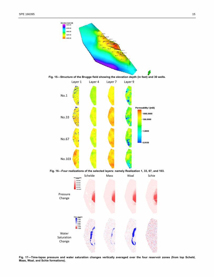
The Brugge field case was designed for a SPE benchmark project to test the combined use of history matching and waterflooding optimization methods in a closed-loop workflow (Peters et al., 2010). The structure of the Brugge field consists of an east/west elongated half-dome with a large boundary fault at its northern edge and one internal fault with a modest throw as shown in Fig. 15. The dimensions of the field are roughly 10 km x 3 km. The reservoir model contains more than 40,000 active grid cells, 20 producers located in the center of the dome and 10 infill water injectors located in the surrounding aquifer to provide additional pressure support. A total of 104 realizations were generated by four different classes of control parameters: (1) facies association, (2) facies modeling, (3) porosity, and (4) permeability. The detailed descriptions of the realization construction can be found in Peters et al. (2010). In order to account for the uncertainty of the prior models in history matching, we test the proposed inversion method for four distinct realizations, namely realization 1, 33, 67 and 103 as shown in Fig. 16. Production data are given in the form of water and oil rates, and also bottom-hole pressure at each of the 20 producers for the 10 years of production. The reservoir is an under saturated oil reservoir (i.e., no solution gas). Inverted 4-D seismic data in terms of pressure and saturation changes between time-lapse of 10 years are also provided. Pressure and saturation changes were calculated as vertically averaged values over the four reservoir zones in total 9 layers (i.e., the Scheld, Maas, Wall, and Schie), representative for the seismic resolution with added noise (Fig. 17). We use these data sets as observation data to calibrate reservoir permeability to minimize the differences of the observed and simulated time-lapse pressure and saturation changes as well as the production data. One of the challenging aspects of this application is the long gap of the time-lapse data. During the 10 years of production, the reservoir drive mechanism has evolved from primary depletion to secondary recovery with the down-dip water injection. The streamlines depict this transition of the reservoir flow dynamics clearly as shown in Fig. 18. Accordingly, we need to account for the dynamic changes of the reservoir pressure and saturation to integrate the available time-lapse data (Rey et al., 2012).

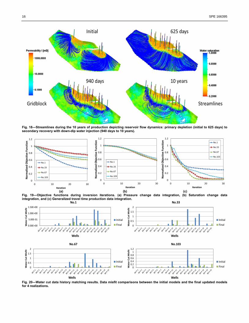
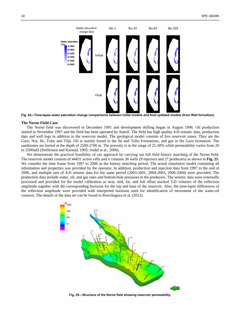
First, pressure change data is utilized to calibrate the models. The inversion performance is shown in Fig. 19a for each of the four models. Next, water saturation change is integrated to update the models as shown in Fig. 19b. Finally, the generalized travel time inversion is applied to integrate water cut data into the models (Fig. 19c). The improvements in well by well production response match are shown in Fig. 20. In particular, some improved well matching results from the realization No.67 are shown in Fig. 21. The final updated models are shown in Fig. 22. Compared to the initial models, major permeability changes occur in the Waal formation (layer 6, 7, 8), but overall geologic continuity is preserved for all realizations. The final model response in terms of pressure change and water saturation change for the Waal formation are compared in Fig. 23 and Fig. 24. Overall, the magnitude of pressure changes reduced from initial model responses for all realizations. As for water saturation changes, the improvements of the magnitude of changes and the distribution of water fronts are more evident in the final updated models. With these updated models, we can assess various schemes for production optimization, although this is not within the scope of our current study (Alhuthali et al., 2008).

SPE 166395 15

Fig. 15―Structure of the Brugge field showing the elevation depth (in feet) and 30 wells.

Fig. 16―Four realizations of the selected layers: namely Realization 1, 33, 67, and 103.

Fig. 17―Time-lapse pressure and water saturation changes vertically averaged over the four reservoir zones (from top Scheld, Maas, Waal, and Schie formations).

16 SPE 166395

Fig. 18―Streamlines during the 10 years of production depicting reservoir flow dynamics: primary depletion (initial to 625 days) to secondary recovery with down-dip water injection (940 days to 10 years).

(a) (b) (c) Fig. 19―Objective functions during inversion iterations. (a) Pressure change data integration, (b) Saturation change data integration, and (c) Generalized travel time production data integration.

Fig. 20―Water cut data history matching results. Data misfit comparisons between the initial models and the final updated models for 4 realizations.

0

0.2

0.4

0.6

0.8

1

1.2

0 10 20 30

Norm


Iteration

No.1

No.33

No.67

No.1030

0.2

0.4

0.6

0.8

1

1.2

0 10 20 30

Norm


Iteration

No.1

No.33

No.67

No.103

0

0.2

0.4

0.6

0.8

1

1.2

0 10 20 30

Norm


Iteration

No.1

No.33

No.67

No.103

0.00E+00

5.00E‐01

1.00E+00

1.50E+00

Water Cut Misfit

Wells

No.1

Initial

Final 0

0.5

1

1.5

2

Water Cut Misfit

Wells

No.33

Initial

Final

0

0.5

1

1.5

2

Water Cut Misfit

Wells

No.67

Initial

Final 00.20.40.60.81

1.2

Water Cut Misfit

Wells

No.103

Initial

Final

SPE 166395 17

Fig. 21―Production data history matching comparisons between the initial model and the final updated model of realization No. 67.

Fig. 22―Four final updated models of the selected layers: namely realization 1, 33, 67, and 103.

Fig. 23―Time-lapse pressure change comparisons between initial models and final updated models (from Waal formation).

18 SPE 166395

Fig. 24―Time-lapse water saturation change comparisons between initial models and final updated models (from Wall formation). The Norne Field Case

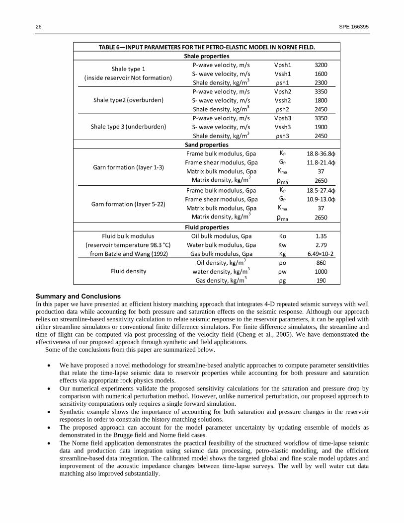
The Norne field was discovered in December 1991 and development drilling began in August 1996. Oil production started in November 1997 and the field has been operated by Statoil. The field has high quality 4-D seismic data, production data and well logs in addition to the reservoir model. The geological model consists of five reservoir zones. They are the Garn, Not, Ile, Tofte and Tilje. Oil is mainly found in the Ile and Tofte Formations, and gas in the Garn formation. The sandstones are buried at the depth of 2500-2700 m. The porosity is in the range of 25-30% while permeability varies from 20 to 2500mD (Steffensen and Karstad, 1995; Osdal et al., 2006).

We demonstrate the practical feasibility of our approach by carrying out full field history matching of the Norne field. The reservoir model consists of 44431 active cells and it contains 36 wells (9 injectors and 27 producers) as shown in Fig. 25. We consider the time frame from 1997 to 2006 as the history matching period. The actual simulation model containing all information and properties was provided by the operator. In addition, production and injection data from 1997 to the end of 2006, and multiple sets of 4-D seismic data for the same period (2003-2001, 2004-2003, 2006-2004) were provided. The production data include water, oil, and gas rates and bottom-hole pressures at the producers. The seismic data were externally processed and provided for the model calibration as near, mid, far, and full offset stacked 3-D volumes of the reflection amplitude together with the corresponding horizons for the top and base of the reservoir. Also, the time-lapse differences of the reflection amplitude were provided with interpreted horizons used for identification of movement of the water-oil contacts. The details of the data set can be found in Rwechugura et al. (2012).

Fig. 25―Structure of the Norne field showing reservoir permeability.

SPE 166395 19

Petro-Elastic Model Unlike the Brugge field case, where interpreted saturation and pressure changes are provided as part of the field data, this

is a much more realistic case in which seismic response is provided instead. To our strategy of using streamline based sensitivities to the inversion problem, we now need to introduce a petro-elastic model (PEM) and develop sensitivities to changes in reservoir properties, just as we have done given pressure and saturation data.

A petro-elastic model is a set of equations which relates reservoir properties (pore volume, pore fluid saturations, reservoir pressures and rock composition) to seismic rock elastic parameters (P-wave and S-wave velocities, Vp and Vs, respectively). Variations in rock elastic properties are functions of temperature, compaction, fluid saturation and reservoir pressure, although we may neglect the effects of temperature in this field. The Gassman equation (1951) and Hertz-Mindlin contact theory (Mindlin, 1949) are used to estimate seismic rock elastic parameter changes caused by fluid saturation and reservoir pressure changes, respectively.

The Hertz-Mindlin model is used to compute seismic rock elastic parameter changes from pressure changes (Mavko et al, 1998). The effective bulk modulus of a dry random identical sphere pack are given by

HM ma eff ext i⁄ , (32)

where HM is the bulk modulus at critical porosity (Dadashpour 2009, 2010). Here, eff is the effective pressure, which is the difference between the lithostatic pressure ext and the hydrostatic pressure (Christensen and Wang, 1985), ma is the bulk modulus of the matrix, and n is the coordination number. For the Norne field application, the initial pressure is set to 270 bar and the lithostatic pressure depends on the true vertical depth (TVD) as given by

ext 0.0981. 9 10 TVD 1.7252 TVD (33) The Hertz-Mindlin theory assumes that velocity varies with eff raised to the 1/6 th power, while some laboratory measurements on samples suggest other values. We use n equal to 5 from the literature (Dadashpour, 2009) for this field application.

The Gassman equation expresses the bulk modulus of a fluid saturated rock from three terms: (1) the bulk modulus of the mineral matrix HM, (2) the bulk modulus of the porous rock frame fr, (3) the bulk modulus of the pore-filling fluids f as given by the following formula (Dadashpour 2009),

sat frHM fr

HMHM

ffr

HM

(34)

Here is the effective porosity of the medium and the bulk modulus of the pore fluids (oil, water, and gas) f is estimated by Wood’s law given as (Reuss, 1929)

f

o

o

w

w

g

g (35)

Here o, w and g are oil, water and gas saturations, respectively, and o, w, and g are bulk moduli for oil, water, and gas, respectively. For the Norne field application, the rock elastic properties are provided in Table 6. The density of the saturated rock is given by the weighted average of the densities of the components:

sat 1 ma o o w w g g (36) Here o, w, g and ma are the densities of oil, water, gas and the rock matrix, respectively. With the saturated rock bulk modulus and shear modulus and density, we can compute the compressional (p-wave) velocity for an isotropic, layered, elastic medium (Kennett, 1983) as

psat fr

sat . (37)

Here the shear modulus fr is the frame shear modulus which is not affected by fluid saturations. The acoustic (p-wave) impedance can be computed as

p sat p sat sat fr . (38)

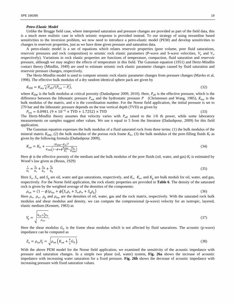
With the above PEM model for the Norne field application, we examined the sensitivity of the acoustic impedance with pressure and saturation changes. In a simple two phase (oil, water) system, Fig. 26a shows the increase of acoustic impedance with increasing water saturation for a fixed pressure. Fig. 26b shows the decrease of acoustic impedance with increasing pressure with fixed saturation values.

20 SPE 166395

(a) (b) Fig. 26―Acoustic impedance calculation sensitivity by PEM model in oil and water 2 phase system, (a) with respect to water saturation changes under a fixed pressure (270 bar) and (b) with respect to pressure changes under a fixed saturation value (Sw=0.5).

Seismic Data Processing The first step in our data calibration procedure is to invert the seismic volumes of reflection amplitude to changes in

acoustic (p-wave) impedance. Using commercial software, we conduct seismic data processing which consists of (1) time to depth data conversion, (2) well log quality check and acoustic impedance log calculation, and (3) genetic inversion for generating an acoustic impedance map from the seismic amplitude data. As for the post-stack seismic sections, we decided to use near-offset stacking data set, because the acoustic (p-wave) impedance changes are more evident in the small angle reflection waves in AVO analysis (Aki and Richards, 1980).

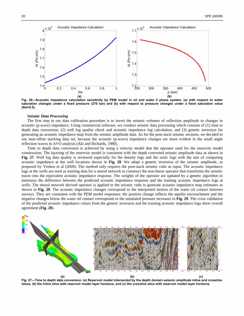
Time to depth data conversion is achieved by using a velocity model that the operator used for the reservoir model construction. The layering of the reservoir model is consistent with the depth converted seismic amplitude data as shown in Fig. 27. Well log data quality is reviewed especially for the density logs and the sonic logs with the aim of computing acoustic impedance at the well locations shown in Fig. 28. We adapt a genetic inversion of the seismic amplitude, as proposed by Veeken et al (2009). The method only requires the post-stack seismic cube as input. The acoustic impedance logs at the wells are used as training data for a neural network to construct the non-linear operator that transforms the seismic traces into the equivalent acoustic impedance response. The weights of the operator are updated by a genetic algorithm to minimize the difference between the predicted acoustic impedance response and the training acoustic impedance logs at wells. The neural network derived operator is applied to the seismic cube to generate acoustic impedance map estimates as shown in Fig. 29. The acoustic impedance changes correspond to the interpreted motion of the water oil contact between surveys. They are consistent with the PEM model responses: the positive change reflects the aquifer encroachment and the negative changes below the water oil contact corresponds to the simulated pressure increases in Fig. 29. The cross validation of the predicted acoustic impedance values from the genetic inversion and the training acoustic impedance logs show overall agreement (Fig. 28).

(a) (b) (c) Fig. 27―Time to depth data conversion. (a) Reservoir model intersected by the depth domain seismic amplitude inline and crossline slices, (b) the Inline slice with reservoir model layer horizons, and (c) the crossline slice with reservoir model layer horizons.

0 0.2 0.4 0.6 0.8 17.4

7.5

7.6

7.7

7.8

7.9

8x 10

6 Acoustic Impedance Calculation

Sw

AI

(Pa

s/m

)

250 300 350 400 450 5007.2

7.3

7.4

7.5

7.6

7.7x 10

6 Acoustic Impedance Calculation

p (bar)

AI

(Pa

s/m

)

SPE 166395 21

Fig. 28―The acoustic impedance log comparisons. The calculated acoustic impedance log (black) and the response extracted from the acoustic-impedance cube as a result of genetic inversion (red).

Fig. 29―Acoustic impedance change data in an inline slice between 2003 and 2001 surveys from genetic inversion. Water oil contact interpretations are superimposed (red line is at 2001 survey and black line is at 2003 survey). The water saturation and pressure changes from the initial model are compared.

Global to Local Hierarchical History Matching Workflow The reservoir model provided by the operator was already calibrated to match the reservoir energy (regional pressure and

pore volume). We adjusted fault transmissibility multipliers, regional relative permeability parameters, and large-scale absolute permeability and porosity heterogeneity using regional and constant multipliers. Our objective was to minimally update the permeability at locations and scales required to improve large scale transport within the reservoir induced by the production, water injection and aquifer support, but to otherwise leave the prior unchanged. We apply a hierarchical history matching workflow that consists of two stages (Yin et al., 2011): a global update and a local update. For the global update, the geological model is first parameterized using a Grid Connectivity Transform (GCT) (Bhark et al., 2011). It is a linear transformation where the heterogeneity is updated in a transform domain that is characterized by the spectral modes of the reservoir model grid. This change of basis from the spatial to spectral domain is performed by multiplication of the heterogeneity field with the GCT basis, which is constructed from the eigenvectors of a grid Laplacian. This parameterization method is efficient for parameter estimation by reducing the parameter dimensionality. A discrete spatial field is mapped to the transform domain using orthogonal transforms,

⇔ (39)

where represents a spatial field and has dimension N×1, where N is the discretization of the property field. The column vector is M-length spectrum of transform coefficients, or parameter set in the transform domain, and is a (N× M) matrix containing M-columns that define the discrete basis functions, each of length N. For model calibration, a spatial multiplier field has been posed in the multiplicative formulation as follows,

(40)

where is the prior property field, also called initial model, and defines the multiplier field in the spatial domain and ( ) is the element-wise multiplication (Schur product). This honors the prior permeability heterogeneity in the model updates.

Further, we utilize a Pareto-based multi-objective history matching workflow proposed by Park et.al (2013) to update the GCT coefficients leading to the global changes in the geologic model. This approach is particularly well suited for minimizing the multiple, and potentially conflicting, objectives involved in matching both seismic data and production data.

22 SPE 166395

For the local update, the gridblock permeability changes are introduced via the streamline-based inversion algorithm, introduced in the current study. The time-lapse acoustic impedance changes and well by well water cut production data are further integrated and the fine scale permeability variations between well locations are refined. The diagram of the workflow is shown in Fig. 30.

For the global update, we first parameterize the permeability field by each layer individually to preserve the vertical stratification. The GCT parameterization of a multiplier field is shown in Fig. 31. In this case, we used a total of 420 coefficients (20 basis vectors per layer x 21 active layers) to represent the geologic model consisting of 44431 active cells. As for the Pareto-based multi-objective minimization, we define three objective functions: (1) gridblock acoustic impedance change misfit , (2) cumulative field water production ( ) misfit, and (3) cumulative field gas production ( ) misfit expressed as

1 ∑ ∑ , , , (41)

2 ∑ ∑ , , , (42)

3 ∑ ∑ , , , (43)

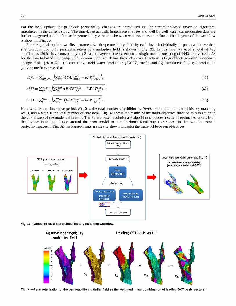
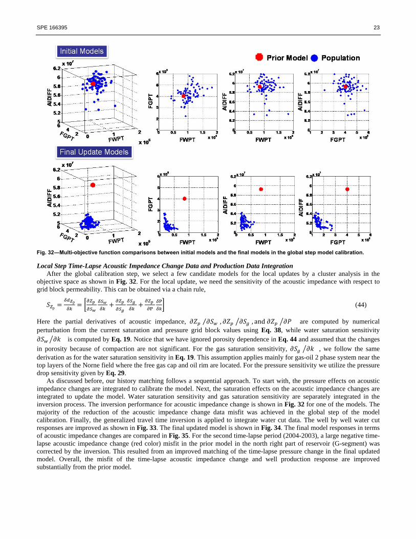
Here is the time-lapse period, is the total number of gridblocks, is the total number of history matching wells, and is the total number of timesteps. Fig. 32 shows the results of the multi-objective function minimization in the global step of the model calibration. The Pareto-based evolutionary algorithm produces a suite of optimal solutions from the diverse initial population around the prior model in a multi-dimensional objective space. In the two-dimensional projection spaces in Fig. 32, the Pareto-fronts are clearly shown to depict the trade-off between objectives.

Fig. 30―Global to local hierarchical history matching workflow.

Fig. 31―Parameterization of the permeability multiplier field as the weighted linear combination of leading GCT basis vectors.

SPE 166395 23

Fig. 32―Multi-objective function comparisons between initial models and the final models in the global step model calibration. Local Step Time-Lapse Acoustic Impedance Change Data and Production Data Integration

After the global calibration step, we select a few candidate models for the local updates by a cluster analysis in the objective space as shown in Fig. 32. For the local update, we need the sensitivity of the acoustic impedance with respect to grid block permeability. This can be obtained via a chain rule,

p

p (44)

Here the partial derivatives of acoustic impedance, ⁄ , , and are computed by numerical perturbation from the current saturation and pressure grid block values using Eq. 38, while water saturation sensitivity

is computed by Eq. 19. Notice that we have ignored porosity dependence in Eq. 44 and assumed that the changes

in porosity because of compaction are not significant. For the gas saturation sensitivity, , we follow the same derivation as for the water saturation sensitivity in Eq. 19. This assumption applies mainly for gas-oil 2 phase system near the top layers of the Norne field where the free gas cap and oil rim are located. For the pressure sensitivity we utilize the pressure drop sensitivity given by Eq. 29.

As discussed before, our history matching follows a sequential approach. To start with, the pressure effects on acoustic impedance changes are integrated to calibrate the model. Next, the saturation effects on the acoustic impedance changes are integrated to update the model. Water saturation sensitivity and gas saturation sensitivity are separately integrated in the inversion process. The inversion performance for acoustic impedance change is shown in Fig. 32 for one of the models. The majority of the reduction of the acoustic impedance change data misfit was achieved in the global step of the model calibration. Finally, the generalized travel time inversion is applied to integrate water cut data. The well by well water cut responses are improved as shown in Fig. 33. The final updated model is shown in Fig. 34. The final model responses in terms of acoustic impedance changes are compared in Fig. 35. For the second time-lapse period (2004-2003), a large negative time-lapse acoustic impedance change (red color) misfit in the prior model in the north right part of reservoir (G-segment) was corrected by the inversion. This resulted from an improved matching of the time-lapse pressure change in the final updated model. Overall, the misfit of the time-lapse acoustic impedance change and well production response are improved substantially from the prior model.

24 SPE 166395

Fig. 33―The objective function misfit for acoustic impedance change data integration comparisons among the prior model, global step calibrated model, and the final updated model from the local step calibration.

Fig. 34―Water cut production data history matching comparisons between the initial model and the final updated model.

0.75

0.8

0.85

0.9

0.95

1

1.05

Prior Global Local

Norm

alized AI Chan

ge M

isfit

SPE 166395 25

Fig. 35―Permeability model update comparison by layers. The prior model (Top), The final updated model (middle), and the model changes between the prior and the final models.

Fig. 36―Time-lapse acoustic impedance changes comparisons in selected layers among the observation data, the prior model responses and the final updated model responses.

26 SPE 166395

Summary and Conclusions In this paper we have presented an efficient history matching approach that integrates 4-D repeated seismic surveys with well production data while accounting for both pressure and saturation effects on the seismic response. Although our approach relies on streamline-based sensitivity calculation to relate seismic response to the reservoir parameters, it can be applied with either streamline simulators or conventional finite difference simulators. For finite difference simulators, the streamline and time of flight can be computed via post processing of the velocity field (Cheng et al., 2005). We have demonstrated the effectiveness of our proposed approach through synthetic and field applications.

Some of the conclusions from this paper are summarized below. We have proposed a novel methodology for streamline-based analytic approaches to compute parameter sensitivities

that relate the time-lapse seismic data to reservoir properties while accounting for both pressure and saturation effects via appropriate rock physics models.

Our numerical experiments validate the proposed sensitivity calculations for the saturation and pressure drop by comparison with numerical perturbation method. However, unlike numerical perturbation, our proposed approach to sensitivity computations only requires a single forward simulation.

Synthetic example shows the importance of accounting for both saturation and pressure changes in the reservoir responses in order to constrain the history matching solutions.

The proposed approach can account for the model parameter uncertainty by updating ensemble of models as demonstrated in the Brugge field and Norne field cases.

The Norne field application demonstrates the practical feasibility of the structured workflow of time-lapse seismic data and production data integration using seismic data processing, petro-elastic modeling, and the efficient streamline-based data integration. The calibrated model shows the targeted global and fine scale model updates and improvement of the acoustic impedance changes between time-lapse surveys. The well by well water cut data matching also improved substantially.

P‐wave velocity, m/s Vpsh1 3200

S‐ wave velocity, m/s Vssh1 1600

Shale density, kg/m3

ρsh1 2300




ρsh2 2450




ρsh3 2450

Frame bulk modulus, Gpa Kfr 18.8‐36.8φ

Frame shear modulus, Gpa Gfr 11.8‐21.4φ

Matrix bulk modulus, Gpa Kma 37

Matrix density, kg/m3 ρma 2650

Frame bulk modulus, Gpa Kfr 18.5‐27.4φ

Frame shear modulus, Gpa Gfr 10.9‐13.0φ

Matrix bulk modulus, Gpa Kma 37

Matrix density, kg/m3 ρma 2650

Oil bulk modulus, Gpa Ko 1.35

Water bulk modulus, Gpa Kw 2.79

Gas bulk modulus, Gpa Kg 6.49×10‐2

Oil density, kg/m3

ρo 860

water density, kg/m3

ρw 1000

Gas density, kg/m3

ρg 190

Garn formation (layer 1‐3)

Garn formation (layer 5‐22)

Fluid properties

Fluid bulk modulus

(reservoir temperature 98.3 °C)

from Batzle and Wang (1992)

Shale properties

Shale type 1

(inside reservoir Not formation)

Shale type2 (overburden)

Shale type 3 (underburden)

Sand properties

Fluid density

TABLE 6―INPUT PARAMETERS FOR THE PETRO‐ELASTIC MODEL IN NORNE FIELD.

SPE 166395 27

Nomenclature = Time of flight along streamlines = Streamline trajectory = Slowness = Interstitial velocity = Mobility = Permeability = Porosity = Water saturation = Fractional flow of water

= Hydrostatic pressure eff = Effective pressure ext = Lithostatic pressure ∆ = Pressure drop along streamlines

= Model parameter change HM = Bulk modulus of the Hertz-Mindlin formula ma = Bulk modulus of the matrix fr = Bulk modulus of the porous rock frame

f = Bulk modulus of the pore-filling fluids

sat = Bulk modulus of the fluid saturated rock sat = Density of the fluid saturated rock fr = Shear modulus of the porous rock frame

p = Compressional (p-wave) velocity

p = Acoustic (p-wave) impedance Acknowledgements The authors acknowledge the sponsors of Model Calibration and Efficient Reservoir Imaging (MCERI) at Texas A&M University. Also we would like to thank Statoil (operator of the Norne field) and its license partners ENI and Petoro for the release of the Norne data. Further, we acknowledge the Center for Integrated Operations at NTNU for cooperation and coordination of the Norne cases. References Aki, K., Richards, P.G. 1980. Quantitative seismology, Vol. 1424, Freeman San Francisco. Alhuthali, A., Datta-Gupta, A., Yuen, B., Fontanilla, J. 2008. Optimal rate control under geologic uncertainty. Paper SPE 113628 presented

at the SPE/DOE Symposium on Improved Oil Recovery, Tulsa, Oklahoma, USA, 20-23 April Arenas, E., Kruijsdijk, C.V., Oldenziel, T. 2001. Semi-Automatic History Matching Using the Pilot Point Method Including Time-Lapse

Seismic Data. Paper SPE71634 presented at the SPE Annual Technical Conference and Exhibition, New Orleans, Louisiana, USA, 30 September-3 October.

Behrens, R., Condon, P., Haworth, W., Bergeron, M., Wang, Z., Ecker, C. 2002. 4D seismic monitoring of water influx at bay marchand: the practical use of 4D in an imperfect world. SPE Reservoir Evaluation & Engineering 5 (5): 410-420.

Behrens, R., MacLeod, M., Tran, T., Alimi, A. 1998. Incorporating seismic attribute maps in 3D reservoir models. SPE Reservoir Evaluation & Engineering 1 (2): 122-126.

Bhark, E.W., Jafarpour, B., Datta‐Gupta, A. 2011. A generalized grid connectivity–based parameterization for subsurface flow model calibration. Water Resources Research 47 (6).

Burkhart, T., Hoover, A.R., Flemings, P.B. 2000. Time-lapse (4-D) seismic monitoring of primary production of turbidite reservoirs at South Timbalier Block 295, offshore Louisiana, Gulf of Mexico. Geophysics 65: 351.

Cheng, H., Dehghani, K., Billiter, T. 2008. A Structured Approach for Probabilistic-Assisted History Matching Using Evolutionary Algorithms: Tengiz Field Applications. Paper SPE 116212 presented at the SPE Annual Technical Conference and Exhibition, Denver, Colorado, USA, 21-24 September.

Cheng, H., Kharghoria, A., He, Z., Datta-Gupta, A. 2005. Fast History Matching of Finite-Difference Models Using Streamline-Based Sensitivities. SPE Reservoir Evaluation & Engineering 8 (5): 426-436.

Christensen, N., Wang, H. 1985. The influence of pore pressure and confining pressure on dynamic elastic properties of Berea sandstone. Geophysics 50 (2): 207-213.

Clifford, P., Robert, T., Parr, R., Moulds, T., Tim, C., Allan, P. 2003. Integration of 4D seismic data into the management of oil reservoirs with horizontal wells between fluid contacts. Paper SPE 83956 presented at Offshore Europe, Aberdeen, United Kingdom, 2–5 September.

Dadashpour, M., Ciaurri, D.E., Mukerji, T., Kleppe, J., Landrø, M. 2010. A derivative-free approach for the estimation of porosity and permeability using time-lapse seismic and production data. Journal of Geophysics and Engineering 7 (4): 351-368.

Dadashpour, M., Echeverría-Ciaurri, D., Kleppe, J., Landrø, M. 2009. Porosity and permeability estimation by integration of production and time-lapse near and far offset seismic data. Journal of Geophysics and Engineering 6 (4): 325-344.

Dadashpour, M., Landrø, M., Kleppe, J. 2008. Nonlinear inversion for estimating reservoir parameters from time-lapse seismic data. Journal of Geophysics and Engineering 5 (1): 54-66.

28 SPE 166395

Datta-Gupta, A., King, M.J. 2007. Streamline simulation: Theory and practice, Vol. 11, Society of Petroleum Engineers. Deutsch, C.V., Journel, A.G. 1992. Geostatistical software library and user&s guide, Vol. 1996, Oxford university press New York. Domenico, S. 1976. Effect of brine-gas mixture on velocity in an unconsolidated sand reservoir. Geophysics 41 (5): 882-894. Dong, Y., Oliver, D. 2005. Quantitative use of 4D seismic data for reservoir description. SPE J. 10 (1): 91-99. Doyen, P.M., Psaila, D.E., Jans, D. 1997. Reconciling data at seismic and well log scales in 3-D earth modelling. Paper SPE 38698

presented at the SPE Annual Technical Conference and Exhibition, San Antonio, Texas, USA, 5-8 October. Eastwood, J., Lebel, P., Dilay, A., Blakeslee, S. 1994. Seismic monitoring of steam-based recovery of bitumen. The Leading Edge 13 (4):

242-251. Fahimuddin, A., Aanonsen, S., Skjervheim, J.-A. 2010. 4D seismic history matching of a real field case with EnKF: use of local analysis

for model updating. Paper SPE 134894 presented at the SPE Annual Technical Conference and Exhibition, Florence, Italy, 19-22 September.

Falcone, G., Gosselin, O., Maire, F., Marrauld, J., Zhakupov, M. 2004. Petroelastic modelling as key element of 4D history matching: a field example. Paper SPE 90466 presented at the SPE Annual Technical Conference and Exhibition, Houston, Texas, USA, 26-29 September.

Fanchi, J.R. 2001. Time-lapse seismic monitoring in reservoir management. The Leading Edge 20 (10): 1140-1147. Feng, T., Mannseth, T. 2010. Impact of time-lapse seismic data for permeability estimation. Computational Geosciences 14 (4): 705-719. Foster, D. 2007. The BP 4-D story: Experience over the last 10 years and current trends. Paper IPTC 11757 presented at International

Petroleum Technology Conference, Dubai, U.A.E., 4-6 December. Gassmann, F. 1951. Elastic waves through a packing of spheres. Geophysics 16 (4): 673-685. Gosselin, O., Aanonsen, S., Aavatsmark, I., Cominelli, A., Gonard, R., Kolasinski, M., Ferdinandi, F., Kovacic, L., Neylon, K. 2003.

History matching using time-lapse seismic (HUTS). Paper SPE 84464 presented at the SPE Annual Technical Conference and Exhibition, Denver, Colorado, USA, 5-8 October.

Gosselin, O., van den Berg, S., Cominelli, A. 2001. Integrated history-matching of production and 4D seismic data. Paper SPE 71599 presented at the SPE Annual Technical Conference and Exhibition, New Orleans, Louisiana, USA, 30 September-3 October. .

Harris, J.M., Langan, R.T., Fasnacht, T.M., Melton, D.M., Smith, B.M., Sinton, J.M., Tan, H.M. 1996. Experimental verification of seismic monitoring of CO2 injection in carbonate reservoirs. Expanded Abstracts presented at the SEG Annual Meeting, Denver, Colorado, USA, November 10 - 15.

He, Z., Yoon, S., Datta-Gupta, A. 2002. Streamline-based production data integration with gravity and changing field conditions. SPE J. 7 (4): 423-436.

Huang, X., Meister, L., Workman, R. 1997. Reservoir characterization by integration of time-lapse seismic and production data. Paper SPE 38695 presented at the SPE Annual Technical Conference and Exhibition, San Antonio, Texas, USA, 5-8 October.

Jenkins, S., Waite, M., Bee, M. 1997. Time-lapse monitoring of the Duri steamflood: A pilot and case study. The Leading Edge 16 (9): 1267-1274.

Kennett, B. 1983. Seismic wave propagation in stratified media, Cambridge University Press Landa, J., Horne, R. 1997. A procedure to integrate well test data, reservoir performance history and 4-D seismic information into a

reservoir description. Paper SPE38653 presented at the SPE Annual Technical Conference and Exhibition, San Antonio, Texas, USA, 5-8 October. .

Landrø, M., Digranes, P., Strønen, L. 2001. Mapping reservoir pressure and saturation changes using seismic methods: possibilities and limitations. First break 19 (12): 671-677.

Landro, M., Solheim, O.A., Hilde, E., Ekren, B.O., Stronen, L.K. 1999. The Gullfaks 4D seismic study. Petroleum Geoscience 5 (3): 213-226.

Lumley, D., Behrens, R. 1998. Practical issues of 4D seismic reservoir monitoring: What an engineer needs to know. SPE Reservoir Evaluation & Engineering 1 (6): 528-538.

Lumley, D.E. 2001. Time-lapse seismic reservoir monitoring. Geophysics 66 (1): 50-53. Lumley, D.E., Behrens, R.A., Wang, Z. 1997. Assessing the technical risk of a 4-D seismic project. The Leading Edge 16 (9): 1287-1292. Mavko, G., Mukerji, T., Dvorkin, J. 1998. The Rock Physics Handbook: Tools for Seismic Analysis in Porous Media, 329 pp, Cambridge

Univ. Press, Cambridge, UK. Mindlin, R.D. 1949. Compliance of elastic bodies in contact. Journal of Applied Mechanics 16: 259-268. Nur, A. 1989. Four-dimesional seismology and (true) direct detection of hydrocarbons: The petrophysical basis. The Leading Edge 8 (9):

30-36. Nur, A., Tosaya, C., Vo-Thanh, D. 1984. Seismic monitoring of thermal enhanced oil recovery processes. Expanded Abstracts presented at

the SEG Annual Meeting, Atlanta, Georgia, December 2 - 6. O'Donovan, A., Smith, S., Pal, K. 2000. Foinaven 4D seismic-dynamic reservoir parameters and reservoir management. Paper SPE 63294

presented at the SPE Annual Technical Conference and Exhibition, Dallas, Texas, USA, 1-4 October. Osdal, B., Husby, O., Aronsen, H.A., Chen, N., Alsos, T. 2006. Mapping the fluid front and pressure buildup using 4D data on Norne Field.

The Leading Edge 25 (9): 1134-1141. Paige, C.C., Saunders, M.A. 1982. LSQR: An algorithm for sparse linear equations and sparse least squares. ACM Transactions on

Mathematical Software (TOMS) 8 (1): 43-71. Park, H.-Y., Datta-Gupta, A., King, M. 2013. Handling Conflicting Multiple Objectives Using Pareto-Based Evolutionary Algorithm for

History Matching of Reservoir Performance. Paper SPE 163623 presented at the SPE Reservoir Simulation Symposium, The Woodlands, Texas, USA, 18-20 February.

Peters, L., Arts, R., Brouwer, G., Geel, C., Cullick, S., Lorentzen, R., Chen, Y., Dunlop, N., Vossepoel, F., Xu, R. 2010. Results of the Brugge benchmark study for flooding optimization and history matching. SPE Reservoir Evaluation & Engineering 13 (3): 391-405.

Pullin, N., Matthews, L., Hirsche, K. 1987. Techniques applied to obtain very high resolution 3-D seismic imaging at an Athabasca tar sands thermal pilot. The Leading Edge 6 (12): 10-15.

SPE 166395 29

Reuss, A. 1929. Berechnung der Fließgrenze von Mischkristallen auf Grund der Plastizitätsbedingung für Einkristalle. ZAMM‐Journal of Applied Mathematics and Mechanics/Zeitschrift für Angewandte Mathematik und Mechanik 9 (1): 49-58.

Rey, A., Bhark, E., Gao, K., Datta-Gupta, A., Gibson, R. 2012. Streamline-based integration of time-lapse seismic and production data into petroleum reservoir models. Geophysics 77 (6): M73-M87.

Rwechungura, R., Bhark, E., Miljeteig, O., Suman, A., Kourounis, D., Foss, B., Hoier, L., Kleppe, J. 2012. Results of the First Norne Field Case on History Matching and Recovery Optimization Using Production and 4D Seismic Data. Paper SPE 157112 presented at the SPE Annual Technical Conference and Exhibition, San Antonio, Texas, USA, 8-10 October.

Skjervheim, J.-A., Evensen, G., Aanonsen, S., Ruud, B.O., Johansen, T.-A. 2007. Incorporating 4D seismic data in reservoir simulation models using ensemble Kalman filter. SPE J. 12 (3): 282-292.

Steffensen, I., Karstadt, P. 1996. Norne Field Development-Fast Track From Discovery to Production. Journal of Petroleum Technology 48 (4): 296-299, 339.

Stovas, A., Arntsen, B. 2006. Vertical propagation of low-frequency waves in finely layered media. Geophysics 71 (3): 87-94. Toinet, S. 2004. 4D Feasibility and Calibration Using 3D Seismic Modeling of Reservoir Models. Paper SPE 88783 presented at Abu

Dhabi International Conference and Exhibition, Abu Dhabi, United Arab Emirates,10-13 October. Tura, A., Lumley, D. 2000. Estimating pressure and saturation changes from time-lapse AVO data. Paper OTC 12130 presented at

Offshore Technology Conference, Houston, Texas, USA, 1-4 May. Veeken, P.C., Priezzhev, I.I., Shmaryan, L.E., Shteyn, Y.I., Barkov, A.Y., Ampilov, Y.P. 2009. Nonlinear multitrace genetic inversion

applied on seismic data across the Shtokman field, offshore northern Russia. Geophysics 74 (6): WCD49-WCD59. Wang, Z., Hirsche, W.K., Sedgwick, G. 1991. Seismic monitoring of water floods?-A petrophysical study. Geophysics 56 (10): 1614-1623. Wang, Z., Nur, A. 1988. Effect of temperature on wave velocities in sands and sandstones with heavy hydrocarbons. SPE Reservoir

Engineering 3 (1): 158-164. Williams, M., Keating, J., Barghouty, M. 1998. The stratigraphic method: a structured approach to history matching complex simulation

models. SPE Reservoir Evaluation & Engineering 1 (2): 169-176. Yin, J., Park, H.-Y., Datta-Gupta, A., King, M.J., Choudhary, M.K. 2011. A hierarchical streamline-assisted history matching approach

with global and local parameter updates. Journal of Petroleum Science and Engineering 80 (1): 116-130. Appendix―Water Saturation Change Sensitivity In the water saturation sensitivity derivation, we assumed that the streamline trajectory is fixed from the initial condition to the particular time of interest for calculating the sensitivity. Also, we used the Buckley-Leverett solution to estimate partial derivatives in Eq.18, which assumes uniform initial conditions. In order to generalize the formulation to account for changing field conditions, we separate the total time into small time step sizes as

∑ ∆ (A-1)

and the total change in the arrival time as the weighted average of arrival time change for each timestep as follows

∑ ∆ (A-2)

Then, the arrival time sensitivity becomes

∑ ∆

,∑ ∆

, ,∑ ∆

, ,∑ ∆

, , (A-3)

Substituting Eq. A-3 into Eq. 19, we obtain the generalized form of saturation sensitivity at grid block location x as

, ,∙ ∑

∆

,∙

,

, , ∆

∆∙ ∑

∆

,∙

, (A-4)

To account for the changing field conditions, the streamlines are traced for every time interval ∆ and the saturation sensitivity in Eq. A-4 is computed by integrating the sensitivity values for the entire time interval. Also, if the streamlines do not change, Eq. A-4 reverts back to Eq. 19. Now the saturation change sensitivity can be computed by calculating the saturation sensitivities at two different times ( , , as follows

∆ , , ,∙ ∑

∆

,∙

,

,∙ ∑

∆

,∙

, (A-5)

where the saturation time partial derivatives can be approximated by a backward differencing from the simulation responses as in Eq. A-4.

Spe 166395

Documents

Transcript of Spe 166395