
Spectroscopy of the doubly magic nucleus 100Sn and its decay · a unique identification 100Snwas...
107
Technische Universit¨ at M¨ unchen Physik-Department E12 Spectroscopy of the doubly magic nucleus 100 Sn and its decay Christoph B. Hinke Vollst¨ andiger Abdruck der von der Fakult¨ at f¨ ur Physik der Technischen Universit¨ at M¨ unchen zur Erlangung des akademischen Grades eines Doktors der Naturwissenschaften (Dr. rer. nat.) genehmigten Dissertation. Vorsitzende: Univ.-Prof. Dr. Nora Brambilla Pr¨ ufer der Dissertation: 1. Univ.-Prof. Dr. Reiner Kr¨ ucken 2. Univ.-Prof. Dr. Tobias Lachenmaier Die Dissertation wurde am 05.07.2010 bei der Technischen Universit¨ at M¨ unchen ein- gereicht und durch die Fakult¨ at f¨ ur Physik am 23.07.2010 angenommen.
Transcript of Spectroscopy of the doubly magic nucleus 100Sn and its decay · a unique identification 100Snwas...
Technische Universitat MunchenPhysik-Department E12
Spectroscopy of the doubly magicnucleus 100Sn and its decay
Christoph B. Hinke
Vollstandiger Abdruck der von der Fakultat fur Physik der Technischen UniversitatMunchen zur Erlangung des akademischen Grades eines
Doktors der Naturwissenschaften (Dr. rer. nat.)
genehmigten Dissertation.
Vorsitzende: Univ.-Prof. Dr. Nora BrambillaPrufer der Dissertation:
1. Univ.-Prof. Dr. Reiner Krucken2. Univ.-Prof. Dr. Tobias Lachenmaier
Die Dissertation wurde am 05.07.2010 bei der Technischen Universitat Munchen ein-gereicht und durch die Fakultat fur Physik am 23.07.2010 angenommen.

Zusammenfassung
Die Untersuchung des Kerns 100Sn war bereits das Ziel einer Reihe von experimentel-len Anlaufen. Aus verschiedenen Grunden ist dieser Kern von großem Interesse. Er istvermutlich der schwerste N=Z Kern, der gegenuber der Emission von Nukleonen stabilist, außerdem ist er doppelt magisch. Sein Beta Zerfall ist besonders bedeutsam, da essich wahrscheinlich um den reinsten Gamow-Teller Zerfall in der gesamten Nuklidkartehandelt. Er eignet sich daher bestens fur die Untersuchung der Frage nach der fehlendenGamow-Teller Starke bzw. des sogenannten “Gamow-Teller quenching“ beruhend aufCore-Polarisationseffekten. Mit Hilfe der beta-koinzidenten Gammaspektroskopie desTochterkerns 100In konnen Informationen uber die Proton-Neutron Wechselwirkung indiesem Bereich der Nuklidkarte gewonnen werden. Gleichzeitig mit der Implantationdes frisch produzierten Kerns im Detektoraufbau konnte die Suche nach verzogerterGamma Strahlung eines vorhergesagten isomeren Zustands in 100Sn erste Einblicke indie Struktur der Anregungszustande in diesem exotischen Kern ermoglichen.Die vorliegende Arbeit behandelt die Untersuchungsergebnisse der Spektroskopie desdoppelt magischen Kerns 100Sn und dessen Zerfall.Das Experiment fand im Marz 2008 an den Beschleunigereinrichtungen des GSI Helm-holtz Zentrums Darmstadt statt. Der neutronenarme Kern wurde in einer Projektilfrag-mentationsreaktion eines 124Xe Primarstrahls erzeugt, der auf ein Beryllium Target miteiner Energie von 1 GeV·A gerichtet wurde. Nach der Trennung von anderen Fragmen-tationsprodukten und einer eindeutigen Identifikation wurden die 100Sn Kerne in einemImplantationsdetektor gestoppt, der aus hochsegmentierten Siliziumstreifendetektorenbesteht und der Zerfallsspektroskopie dient. Neben der Bestimmung der Halbwertszeitkonnte die vollstandige Energie der emittierten Teilchenstrahlung im Implantationsde-tektor nachgewiesen werden. Die emittierte Gamma Strahlung wurde mit einem denImplantationsdetektor umgebenden Germanium Spektrometer gemessen.Aus ungefahr 70 beobachteten Zerfallen von 100Sn wurde eine Halbwertszeit von T1/2 =1.16±0.20s bestimmt. Die Beta Endpunktenergie unter Annahme des Zerfalls in einenEndzustand lieferte einen Wert von Eβ0
= 3.29 ± 0.20MeV . Der sich ergebende Wertder Gamow-Teller Ubergangsstarke im Zerfall von 100Sn mit BGT = 9.1+4.8
−2.3 ist uber-raschend hoch. Im Tochterkern 100In wurden erstmals funf Gamma Ubergange mitEnergien von Eγ=96 keV, 141 keV, 436 keV, 1297 keV und 2048 keV beobachtet, diebei der Abregung des im Beta Zerfall von 100Sn bevolkerten 1+ Zustandes emittiertwurden. Verschiedene Szenarien fur das Niveauschema von angeregten Zustanden in100In werden diskutiert. Aufgrund der vorliegenden Daten kann aber nicht zwischen denSzenarien klar unterschieden werden. Fur jedes Szenarium wurde ein Grundzustand-

ii
nach-Grundzustand QEC Wert des Zerfalls ermittelt.
Abstract
The nucleus 100Sn has been the aim of a number of experimental approaches. It is ofgreat interest for various reasons. It is presumably the heaviest particle-stable N=Znucleus and at the same time doubly magic. Its beta decay is of particular impor-tance because it is expected to be the purest Gamow-Teller decay in the nuclear chartand thus allows to study the question of the missing Gamow-Teller strength / theGamow-Teller quenching due to core polarisation effects. From the beta-coincident de-cay spectroscopy of the daughter nucleus 100In information about the proton-neutroninteraction in this region of the nuclear chart can be obtained. Simultaneously withthe implantation of the nucleus in the detector setup after production the search fordelayed gamma radiation from a predicted isomeric state in 100Sn could yield first in-sight into the structure of excited states in this exotic nucleus.This work presents investigation results concerning the spectroscopy of the doublymagic nucleus 100Sn and its decay.The experiment was performed in March 2008 at the accelerator facilities of the GSIHelmholtz Zentrum Darmstadt. The neutron deficient nucleus was produced in a pro-jectile fragmentation reaction of a 124Xe primary beam impinging on a Beryllium targetwith an energy of 1GeV ·A. After a separation from other fragmentation products anda unique identification 100Sn was stopped in an implantation detector consisting ofhighly segmented silicon strip detectors for decay spectroscopy. Beside the determina-tion of the half life it was possible to detect the total energy of the emitted particleradiation in the implantation detector as well as the emitted gamma radiation with asurrounding array of Germanium detectors.With a number of approximately 70 successfully observed decays of 100Sn a half lifeof T1/2 = 1.16 ± 0.20s was obtained. The beta endpoint energy of the single channeldecay yielded a value of Eβ0
= 3.29 ± 0.20MeV . The resultant Gamow-Teller tran-sition strength in the decay of 100Sn turned out to be a surprisingly high value ofBGT = 9.1+4.8
−2.3. In the daughter nucleus 100In five gamma rays with transition energiesof Eγ=96 keV, 141 keV, 436 keV, 1297 keV and 2048 keV deexciting the populated1+-state after the beta decay of 100Sn could be observed for the first time. Differentscenarios for the level structure in 100In are discussed but can unfortunately not bedistinguished on the basis of the present data. For each scenario a ground state toground state QEC value of the decay was calculated.

iv
Contents
1 Introduction and Physical Motivation 1
1.1 Nuclear Structure in the 100Sn-region . . . . . . . . . . . . . . . . . . . 1
1.1.1 The Gamow-Teller β-decay of 100Sn . . . . . . . . . . . . . . . . 3
1.1.2 Excited states in 100Sn . . . . . . . . . . . . . . . . . . . . . . . . 9
1.2 Previous 100Sn Experiments . . . . . . . . . . . . . . . . . . . . . . . . . 10
1.3 Structure of the Thesis . . . . . . . . . . . . . . . . . . . . . . . . . . . . 12
2 Production and Identification 13
2.1 Production of neutron deficient nuclei . . . . . . . . . . . . . . . . . . . 13
2.2 Separation in the Fragmentseparator FRS . . . . . . . . . . . . . . . . . 16
2.3 Unique Identification of 100Sn . . . . . . . . . . . . . . . . . . . . . . . . 18
2.3.1 Determination of the Nuclear Charge Z . . . . . . . . . . . . . . 19
2.3.2 Determination of the A/Q - ratio . . . . . . . . . . . . . . . . . . 20
2.3.3 PID Cleaning and Resolution in the 100Sn-setting . . . . . . . . 21
3 Detector Setup for Decay Spectroscopy 23
3.1 General Requirements . . . . . . . . . . . . . . . . . . . . . . . . . . . . 23
3.2 Implantation Area . . . . . . . . . . . . . . . . . . . . . . . . . . . . . . 25
3.3 Beta Calorimeter . . . . . . . . . . . . . . . . . . . . . . . . . . . . . . . 29
3.4 RISING γ-ray detectors . . . . . . . . . . . . . . . . . . . . . . . . . . . 30
3.5 Readout of the experimental setup . . . . . . . . . . . . . . . . . . . . . 30
3.6 Energy Calibration, γ-ray detection efficiency, β-decay correlation effi-ciency . . . . . . . . . . . . . . . . . . . . . . . . . . . . . . . . . . . . . 32
3.7 Cleaning Cuts for Decay Events . . . . . . . . . . . . . . . . . . . . . . . 36
4 Data Analysis of β-decays 39
4.1 Maximum Likelihood Analysis . . . . . . . . . . . . . . . . . . . . . . . 39
4.1.1 Example: Radioactive Decay . . . . . . . . . . . . . . . . . . . . 43
4.2 Determination of half lives . . . . . . . . . . . . . . . . . . . . . . . . . . 44
4.2.1 Test case: 101Sn . . . . . . . . . . . . . . . . . . . . . . . . . . . 49
4.3 Determination of beta-endpoint energies . . . . . . . . . . . . . . . . . . 50
4.3.1 Test case: 102Sn . . . . . . . . . . . . . . . . . . . . . . . . . . . 51
vi
5 Results obtained in the Spectroscopy of 100Sn 575.1 Half life T1/2 . . . . . . . . . . . . . . . . . . . . . . . . . . . . . . . . . 575.2 β-coincident γ-ray Spectroscopy: Deexcitation of 100In . . . . . . . . . . 59
5.2.1 γ-γ-Coincidences . . . . . . . . . . . . . . . . . . . . . . . . . . . 625.3 β-Endpoint energy in the decay of 100Sn . . . . . . . . . . . . . . . . . . 625.4 Observations concerning a possible 6+ Isomer in 100Sn . . . . . . . . . . 66
6 Discussion of the results 696.1 Populated excited states in 100In - interpretation in the context of shell
model calculations . . . . . . . . . . . . . . . . . . . . . . . . . . . . . . 696.2 Gamow-Teller strength and QEC-value in the β-decay of 100Sn - is there
a GT Quenching? . . . . . . . . . . . . . . . . . . . . . . . . . . . . . . . 76
7 Summary and Outlook 817.1 Summary of the results . . . . . . . . . . . . . . . . . . . . . . . . . . . 817.2 100Sn - still a challenge? Possibilities for further investigation in the
near future . . . . . . . . . . . . . . . . . . . . . . . . . . . . . . . . . . 82
A Appendix 85A.1 Complete set of formulas for the maximum-likelihood analysis of β-decays 85
A.1.1 General probability terms . . . . . . . . . . . . . . . . . . . . . . 85A.1.2 No event during the correlation time tc . . . . . . . . . . . . . . 86A.1.3 One event during the correlation time tc . . . . . . . . . . . . . . 86A.1.4 Two decay events within the correlation time tc . . . . . . . . . . 87A.1.5 Three decay events within the correlation time tc . . . . . . . . . 88
A.2 Technical data of the silicon detectors . . . . . . . . . . . . . . . . . . . 90
Bibliography 93
List of Figures
1.1 Single particle energies of shell model orbitals in 100Sn . . . . . . . . . . 2
1.2 Illustration of the nuclear chart . . . . . . . . . . . . . . . . . . . . . . . 4
1.3 Theoretical values of the GT-strength in even-even tin isotopes . . . . . 6
1.4 GT-strength distribution in the decay of 100Sn . . . . . . . . . . . . . . 8
1.5 Shell model prediction of the excitation spectrum of 100Sn . . . . . . . . 10
2.1 Overview of the GSI accelerator facility . . . . . . . . . . . . . . . . . . 14
2.2 Illustration of the GSI FRagment Separator . . . . . . . . . . . . . . . . 16
2.3 FRS detectors for the particle identification . . . . . . . . . . . . . . . . 19
2.4 Particle Identification Plot 100Sn FRS setting . . . . . . . . . . . . . . . 22
3.1 Schematic illustration of the SIMBA detector . . . . . . . . . . . . . . . 25
3.2 Picture of the assembled SIMBA detector . . . . . . . . . . . . . . . . . 26
3.3 Schematic illustration of the SIMBA detector mounted in the RISINGSetup . . . . . . . . . . . . . . . . . . . . . . . . . . . . . . . . . . . . . 27
3.4 Picture of the SIMBA detector surrounded by the RISING Setup . . . . 28
3.5 Read out scheme of the SIMBA detector . . . . . . . . . . . . . . . . . . 32
3.6 Calibration of silicon detectors . . . . . . . . . . . . . . . . . . . . . . . 33
3.7 Photopeak-efficiency curve of the SIMBA detector plus RISING setup . 35
4.1 Half life comparison - maximum likelihood method result versus Monte-Carlo simulation input . . . . . . . . . . . . . . . . . . . . . . . . . . . . 48
4.2 Experimental β-decay energy spectrum of 102Sn . . . . . . . . . . . . . 53
4.3 GEANT simulation of the beta decay energy spectrum of 102Sn . . . . . 55
5.1 100Sn decay curve plot superimposed on the number of 1st-decays versustime after implantation . . . . . . . . . . . . . . . . . . . . . . . . . . . 59
5.2 Probability distribution of observing a 100Sn decay . . . . . . . . . . . . 60
5.3 Probability distribution of observing a 100In decay . . . . . . . . . . . . 60
5.4 Probability distribution of observing a 100Cd decay . . . . . . . . . . . . 60
5.5 Probability distribution of observing a background decay event . . . . . 60
5.6 β-delayed γ-radiation emitted by 100In after the beta decay of 100Sn(addback mode) . . . . . . . . . . . . . . . . . . . . . . . . . . . . . . . . 61
5.7 Gamma-gamma coincidences . . . . . . . . . . . . . . . . . . . . . . . . 63
5.8 Distribution of the positron energies in the β-decay of 100Sn . . . . . . . 64
viii
5.9 Prompt γ-radiation emitted in the first 25ns after the implantation of100Sn . . . . . . . . . . . . . . . . . . . . . . . . . . . . . . . . . . . . . 68
6.1 Results of the calculations for the excitation spectrum of 100In . . . . . 706.2 100In level scheme from shell model calculations . . . . . . . . . . . . . 716.3 Absolute intensities of the γ-radiation emitted by excited 100In . . . . . 726.4 Tentative level schemes of states in 100In explaining the observed γ-
radiation . . . . . . . . . . . . . . . . . . . . . . . . . . . . . . . . . . . . 736.5 Experimental and theoretical values of the GT-strength in various even-
even tin isotopes . . . . . . . . . . . . . . . . . . . . . . . . . . . . . . . 78
Chapter 1
Introduction and PhysicalMotivation
The doubly magic N=Z nucleus 100Sn is far away from the valley of stability andrepresents a very special case for the investigation of weak interaction matrix elements.This unique nucleus is expected to have the purest and most simple Gamow-Teller betadecay of the heavier elements in the nuclear chart since it is predicted that essentiallyonly a single final state is populated in the daughter nucleus which can easily be accessedin the beta decay energy window. Furthermore, due to the unique constellation withtwo shell closures and thus a simpler theoretical description it might be possible toobtain new knowledge about the Gamow-Teller quenching caused by core polarisationeffects in this heavy nucleus. Information about excited states in the daughter nulceus100In can also provide insight into the proton-neutron interaction in the region closeto the proton drip line.First, general features of the shell structure in the 100Sn region are discussed, then theGamow-Teller decay is addressed in detail. In the subsequent subsection the resultsof shell model predictions concerning the excitation spectrum of 100Sn are presented.Finally, a brief history of previous attempts to produce and to perform spectroscopy ofthe exotic nucleus 100Sn is given. At the end of the chapter the overall outline of thisthesis is presented.
1.1 Nuclear Structure in the 100Sn-region
The investigation of the nuclear structure of doubly magic nuclei and their neighbouringnuclei is of great interest since they are an ideal testing ground for nuclear structuremodels because the modelling of these systems can be reduced to the coupling of a fewparticle- or hole-states to the, apart from that, closed core. The fundamental propertiesof the low lying nuclear states are determined by the interaction of only a few activeorbitals of the shell model. Doubly magic nuclei with an identical number of protonsand neutrons are of special interest since protons and neutrons occupy the same orbitalsand thus the spatial wave functions are identical. This symmetry basically enables thetest of the isospin dependent part of the residual interaction.The doubly magic nucleus 100
50 Sn50 is most probably the heaviest N=Z nucleus which is
2 Chapter 1. Introduction and Physical Motivation
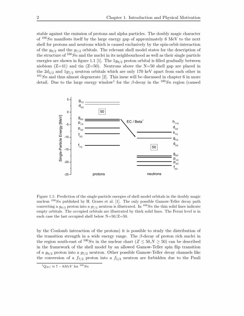
stable against the emission of protons and alpha particles. The doubly magic characterof 100Sn manifests itself by the large energy gap of approximately 6 MeV to the nextshell for protons and neutrons which is caused exclusively by the spin-orbit-interactionof the g9/2 and the g7/2 orbitals. The relevant shell model states for the description ofthe structure of 100Sn and the nuclei in its neighbourhood as well as their single particleenergies are shown in figure 1.1 [1]. The 1g9/2 proton orbital is filled gradually betweenniobiom (Z=41) and tin (Z=50). Neutrons above the N=50 shell gap are placed inthe 2d5/2 and 1g7/2 neutron orbitals which are only 170 keV apart from each other in101Sn and thus almost degenerate [2]. This issue will be discussed in chapter 6 in moredetail. Due to the large energy window1 for the β-decay in the 100Sn region (caused
-25
-20
-15
-10
-5
0
5
h11/2
d3/2
EC / Beta+
s1/2
g7/2
d5/2
g9/2
p1/2p3/2
f5/2
g7/2
d5/2
g9/2
p1/2
p3/2
f5/2
f7/2 50
50
neutronsprotons
Sin
gle-
Par
ticle
Ene
rgy
[MeV
]
Figure 1.1: Prediction of the single-particle energies of shell model orbitals in the doubly magic
nucleus 100Sn published by H. Grawe et al. [1]. The only possible Gamow-Teller decay path
converting a g9/2 proton into a g7/2 neutron is illustrated. In 100Sn the thin solid lines indicateempty orbitals. The occupied orbitals are illustrated by thick solid lines. The Fermi level is in
each case the last occupied shell below N=50/Z=50.
by the Coulomb interaction of the protons) it is possible to study the distribution ofthe transition strength in a wide energy range. The β-decay of proton rich nuclei inthe region south-east of 100Sn in the nuclear chart (Z ≤ 50,N ≥ 50) can be describedin the framework of the shell model by an allowed Gamow-Teller spin flip transitionof a g9/2 proton into a g7/2 neutron. Other possible Gamow-Teller decay channels likethe conversion of a f7/2 proton into a f5/2 neutron are forbidden due to the Pauli
1QEC ≈ 7 − 8MeV for 100Sn
1.1. Nuclear Structure in the 100Sn-region 3
principle since the final states are already completely occupied. Due to the residualinteraction the relevant configurations may be distributed among several final states.In the decay of 100Sn only a single final state in the daughter nucleus 100In is expectedto be populated as will be discussed later in this chapter. In contrast to this, for thedecay of 101Sn calculations already yield over 100 final states which can be populatedin the daughter nucleus 101In [8]. In the 100Sn region the Gamow-Teller decay is theonly allowed decay channel.In the region around 100Sn there is also the possibility of beta-delayed proton emission.With increasing distance from the valley of stability towards the proton drip line theproton separation energies decrease and Q-values of the beta-decay increase. Theconversion of a g9/2 proton into a g7/2 neutron may populate final states in the daughternucleus which are situated several MeV above the proton separation energy.
1.1.1 The Gamow-Teller β-decay of 100Sn
The β-decay in the framework of the weak interaction is mediated by the exchange ofa W boson (charged current) [3]. With the necessary contribution of the neutrino it isa three body decay whose characteristic is the partitioning of the decay energy on thereleased particles. Depending on the neutron or proton excess and the Q-value of thedecay the following reactions are possible2:
β− : n→ p+ e− + νe
β+ : p→ n+ e+ + νe
EC : p+ e− → n+ νe
The energy window for the electron capture (EC) decay is ≈1.022 MeV larger than forthe β+-decay 3.
There are two fundamental decay modes with distinct properties.In the Fermi decay the neutrino and electron are emitted with antiparallel spins. Theinteraction is mediated by the vector-current. The transition matrix element MV andthe Fermi strength BF can be written in the following way:
|MV |2 = BF = | < ψf |τ±|ψi > |2 (1.1)
The wave function of the initial state is represented by ψi, the wave function of the finalstate is represented by ψf . The strength of the transition / transition probability isgiven by the square of the absolute value of the matrix element. In the matrix elementthe isospin operator τ± changes the z-component (proton↔neutron) of the isospin butits absolute value remains unchanged. The transition yields the following selectionrules:
2Special issues like the double beta decay are not mentioned in this compilation.3To be precise: the binding energy of the captured electron of a few keV has to be subtracted.
4 Chapter 1. Introduction and Physical Motivation
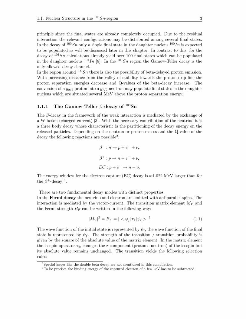
Figure 1.2: Illustration of the nuclear chart (proton number versus neutron number). Black
small boxes represent nuclei in the valley of stability. The region of light proton rich nuclei
where the Fermi decay occurs is indicated. Fermi decays are also possible for N=Z nuclei withodd proton- and neutronnumber. In contrast to this the Gamow-Teller decay is more frequent
and dominates the nuclear landscape. The pure Gamow-Teller decay in the neighbourhood of100Sn and especially the Gamow-Teller decay of 100Sn is expected to be very simple in the
context of involved configurations.
• ∆T = 0 : no change of the isospin
• ∆I = 0 : no change of the nuclear spin
• ∆π = 0 : no change of the parity
• ∆L = 0 : no change in the orbital angular momentum
The Fermi decay does not alter the absolute value of the isospin and the decays populatethe isobaric analogue state in the daughter nucleus. This state is only within reach ifthe Q-value of the decay is higher than the change of the Coulomb energy during thedecay of the proton. Fermi decays are thus limited to the β+-decay of light nuclei withZ > N as illustrated in figure 1.2. An exception are the nuclei with odd proton- andneutronnumber and N = Z which have a ground state or an isomer with the quantumnumbers T = 1 and Iπ = 0+. These nuclei decay via a Fermi decay to the 0+ groundstate of the daughter nucleus. These decays are suitable for a precise measurement ofthe vector coupling constant gV since no admixture of Gamow-Teller decays is possible(0+ → 0+ is forbidden for GT-decays).The second decay mode is the Gamow-Teller decay. In this mode the electron andthe neutrino are emitted with parallel spins. Consequently in the GT-β+-decay a protonis converted to a neutron with opposite spin direction. This transition is mediated by
1.1. Nuclear Structure in the 100Sn-region 5
the axial-vector current. The transition matrix element MAV can be written in thefollowing way:
|MAV |2 = BGT = | < ψf |~στ±|ψi > |2 (1.2)
The operator ~σ changes the spin of the converted nucleon and τ± flips the z-componentof the isospin. The selection rules for the transition can be summarized as follows:
• ∆T = 0,±1 : change of the isospin
• ∆I = 0, 1 : change of the nuclear spin by 0 or 1
• ∆π = 0 : no change of the parity
• ∆L = 0 : no change in the angular momentum
• Transitions from Iπ = 0+ to another 0+-state are forbidden
The Gamow-Teller decay occurs most frequently and can be found everywhere in thenuclear chart. This is in contrast to the competing Fermi decay which can only pop-ulate the isobaric analogue state. But this state is in most cases not reachable in theavailable energy window of the decay. In this case the Fermi decay is forbidden and theGamow-Teller decay is the only allowed decay channel. In the nuclear chart (figure 1.2)the region close to the doubly magic nucleus 100Sn is of great interest since the decayis a pure Gamow-Teller spin flip transition (the energy required for a Fermi decay iswith ≈13 MeV much too high for the available Q-values). Additionally, the main partof the GT-resonance in this region is lying low enough in energy so that it is possibleto be widely populated in GT-β+-decays.
In this thesis the pure GT-decay of 100Sn is investigated. It is of major interest tocompare the experimentally observable Gamow-Teller strength with predictions fromnuclear structure theory.The basic estimate for the Gamow-Teller strength in the decay of 100Sn comes fromthe extreme single particle shell model where no correlations between the nucleons aretaken into account. The Gamow-Teller transition strength can be calculated accordingto the following formula [5]:
BESMGT =
4ℓ
2ℓ+ 1· (1 −
Nνg7/2
8) ·Nπg9/2 (1.3)
The strength of the transition is related to the involved orbital angular momentum ℓ [5].In the case of the g-orbital ℓ is equal to four. The occupation number Nπg9/2 of theinitial proton orbital as well as the occupation Nνg7/2 of the final neutron orbital alsohave to be considered. For 100Sn the proton orbital is fully occupied and the neutronorbital is completely empty, thus the Gamow-Teller strength in the framework of theextreme single particle shell model yields a value of 17.78.
In figure 1.3 the Gamow Teller strength of all even-even tin isotopes is shown upto mass number 110 as calculated in the extreme single particle shell model. For the
6 Chapter 1. Introduction and Physical Motivation
100 102 104 106 108 1100
2
4
6
8
10
12
14
16
18
Gam
ow-T
elle
r Stre
ngth
BG
T
A
Extreme Single-particle Model
Shell Model FFS QRPA Measurement 1998 Measurement Isotopes
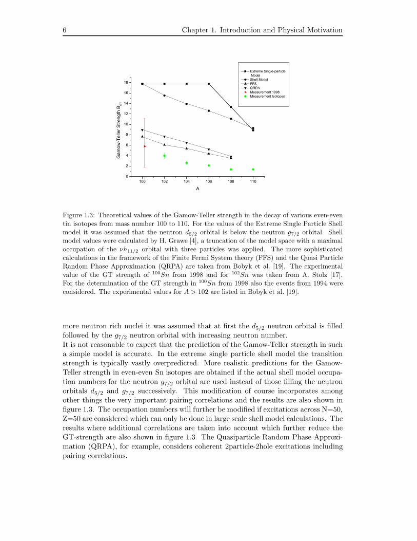
Figure 1.3: Theoretical values of the Gamow-Teller strength in the decay of various even-even
tin isotopes from mass number 100 to 110. For the values of the Extreme Single Particle Shell
model it was assumed that the neutron d5/2 orbital is below the neutron g7/2 orbital. Shellmodel values were calculated by H. Grawe [4], a truncation of the model space with a maximal
occupation of the νh11/2 orbital with three particles was applied. The more sophisticated
calculations in the framework of the Finite Fermi System theory (FFS) and the Quasi Particle
Random Phase Approximation (QRPA) are taken from Bobyk et al. [19]. The experimental
value of the GT strength of 100Sn from 1998 and for 102Sn was taken from A. Stolz [17].For the determination of the GT strength in 100Sn from 1998 also the events from 1994 were
considered. The experimental values for A > 102 are listed in Bobyk et al. [19].
more neutron rich nuclei it was assumed that at first the d5/2 neutron orbital is filledfollowed by the g7/2 neutron orbital with increasing neutron number.It is not reasonable to expect that the prediction of the Gamow-Teller strength in sucha simple model is accurate. In the extreme single particle shell model the transitionstrength is typically vastly overpredicted. More realistic predictions for the Gamow-Teller strength in even-even Sn isotopes are obtained if the actual shell model occupa-tion numbers for the neutron g7/2 orbital are used instead of those filling the neutronorbitals d5/2 and g7/2 successively. This modification of course incorporates amongother things the very important pairing correlations and the results are also shown infigure 1.3. The occupation numbers will further be modified if excitations across N=50,Z=50 are considered which can only be done in large scale shell model calculations. Theresults where additional correlations are taken into account which further reduce theGT-strength are also shown in figure 1.3. The Quasiparticle Random Phase Approxi-mation (QRPA), for example, considers coherent 2particle-2hole excitations includingpairing correlations.
1.1. Nuclear Structure in the 100Sn-region 7
A comparison of the calculated values of the Gamow-Teller strength coming fromsophisticated models (QRPA,FFS) to the experimental values of the Gamow-Tellerstrength in the decay of the even-even tin isotopes in figure 1.3 shows that the exper-imentally observed reduction of the Gamow-Teller strength cannot be reproduced toa satisfying level by the calculations. There is clearly an additional reduction of theobserved strength compared to the QRPA calculations. This discrepancy between the-ory and experiment is called Gamow-Teller quenching. Quantitatively it is describedby a hindrance factor i.e. the ratio between the calculated value of the Gamow-Tellerstrength and the experimentally determined value. In QRPA calculations the quench-ing is often generated artificially by an in medium modification of the weak couplingconstants to gV = gA = 1.From the experimental point of view there is always the question whether the wholeGamow-Teller strength has really been seen which is available in the energy window ofthe beta-decay. If there is a branching to high lying states and some fragmentation thenthe detection sensitivity might be too low, even if these states still carry a considerableamount of the transition strength.The other point is that there are still so called core polarisation effects which are nottaken into account in the calculations which would lead to a further reduction of thetheoretically predicted values. This quenching is caused mainly by effects of short rangecorrelations which are attributed to the neglect of deeper lying nucleons, the core ofthe nucleus. The core polarisation can be understood as a mechanism which admixesstates with much higher excitation energy than it is available in the energy windowof the decay to the Gamow-Teller resonance. This causes a decrease of the observablestrength of the GT resonance at low excitation energies and simultaneously offshoots athigh excitation energy arise which are out of reach in β-decay experiments but carry acertain amount of transition strength. The fundamental problem to get a grip on theseeffects is related to the fact that calculations which take into account the completeconfiguration space of all nucleons are out of reach - at least for the heavier nuclei. Thenature of the GT-Quenching is thus only partially understood.The following list provides an overview about several sources of core polarisation ef-fects [6]:
• Admixture of the ground state of 100Sn with two-particle two-hole excitationsfrom the core. This leads to a destructive interference with the GT-matrix ele-ment resulting in a reduction of the observed GT-strength [7].
• Consideration of configurations involving multi-nucleon excitations which yieldsstates lying at several 10 MeV above the energy window for β-decays which carrya certain amount of GT-transition strength [12].
• The excitation of a nucleon to a ∆-resonance leads to states with excitationenergies around 300 MeV which are admixed to the GT-resonance [11].
100Sn offers a unique opportunity to study the GT-Quenching due to core polarisationsince in the decay of this nucleus calculations from B.A. Brown [8] show that almost the
8 Chapter 1. Introduction and Physical Motivation
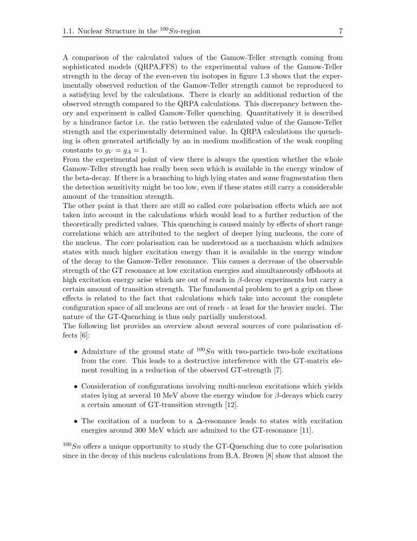
full Gamow-Teller strength (97%) is located in a single state which can be easily reachedin the β+-decay of this nucleus (figure 1.4) with an expected QEC of approximately 7MeV. The statistical uncertainty of the current literature value of the GT-strength inthe decay of 100Sn (figure 1.3) is much too large which makes a reasonable comparisonto theory impossible and consequently does not allow to make any statement aboutthe question of the missing GT-strength. By the way, the single final state for 100Snis very different to the situation in the lighter N=Z doubly magic nucleus 56Ni wherethe strength is spread over many states and is in particular very weak for the lowestlying 1+ state [9].
1 2 3 4 5 6 7 81E-3
0,01
0,1
1
10
Gam
ow-T
elle
r-S
treng
th B
GT
Excitation Energy in 100In [MeV]
Figure 1.4: Distribution of the Gamow-Teller strength in the decay of the doubly magic nucleus100Sn calculated by B.A. Brown [8] depending on the excitation energy of possible final states
in the daughter nucleus 100In. Since the QEC value of the decay is ≈ 7-8 MeV it is certain that
the single low lying state which carries 97% of the total Gamow-Teller strength can be reached
in the β-decay.
The investigation of the β-decay of 100Sn is also interesting due to the simple mod-elling of this doubly magic nucleus in calculations where some core excitation effectcould already be taken into account [8]. For this nucleus two-particle two-hole excita-tions were incorporated in the calculations. For the daughter nucleus 100In two-particletwo-hole and three-particle three-hole configuration admixtures were considered.From the experimental point of view it is very helpful that only one final state is ex-pected to be populated. Consequently no small branching ratios to high lying excitedstates in the daughter nucleus which might carry a lot of transition strength have tobe taken into account as a possible source of uncertainty. In this special case only anumber of ≈ 200 observed decays would be sufficient to extract new exciting informa-
1.1. Nuclear Structure in the 100Sn-region 9
tion about the Gamow-Teller strength of the simplest existing pure GT-decay in heavynuclei with a reasonable statistical error.Therefore the two main goals of the decay analysis are:
• The comparison of the experimental GT-strength in the decay of 100Sn to so-phisticated calculations should allow to make a statement about the amount ofGT-Quenching which is still present due to core polarisation and which is stillnot completely taken into account in the theoretical approach.
• From the structure of the populated excited states in the daughter nucleus 100Inafter the decay of 100Sn some interesting information can be deduced about theproton-neutron interaction in this region of the nuclear chart far away from thevalley of stability.
These two issues will be discussed in detail in chapter 6 where the observed data fromthe experiment is interpreted.
1.1.2 Excited states in 100Sn
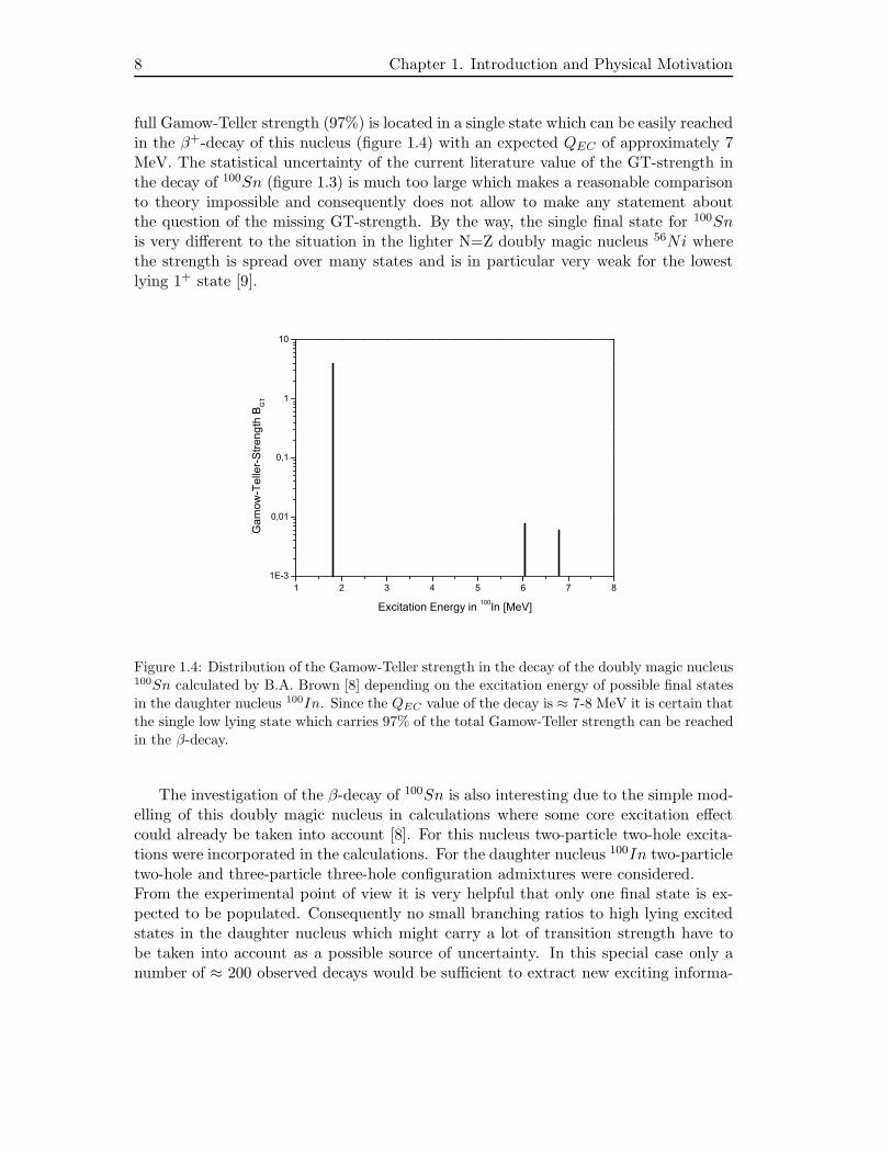
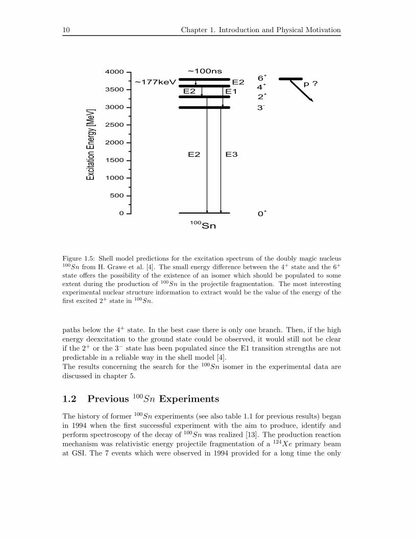
In figure 1.5 the results of shell model calculations for the excitation spectrum of thedoubly magic nucleus 100Sn are shown [4]. Due to the two shell closures predictions ofexcited states are very challenging since the necessary configuration space which has tobe taken into account easily exceeds the limits of the available computational power.The predicted excited states are formed by the breaking up of a pair of nucleons andmoving a particle into the next shell.
The shell model predicts a possible 6+ isomer with a half life that strongly dependson the available transition energy to the 4+ state. The approximate value from largescale shell model calculations (an extrapolation to many particle-hole excitations) is177 keV. Together with the reduced transition probability of B(E2)=1.085 W.u. ahalf life of about 100ns was obtained by H. Grawe [4]. Due to the high excitationenergy of the 6+ state there is also the possibility of a direct proton decay branch witha very short half life in the order of some nano seconds. Another prediction from aHartree Fock Random Phase Approximation (HF-RPA) calculation yields a B(E2) of1.06 W.u. together with a transition energy of 300 keV [10]. Since the phase spacefor the E2 transition depends on the fifth power of the transition energy the resultinghalf life is much shorter. From the HF-RPA calculations also the 2+ and 3− excitationenergies are taken which cannot be calculated reliably at present in the large scaleshell model calculations due to computational and model space limitations. The higherexcited states were determined in the large scale shell model calculations relative tothe position of the 2+ state.Assuming the half life of the 6+ state is in a reasonable range of several 100ns tosurvive the time of flight to the detector setup and also assuming that this state is inmost cases populated by the fragmentation production reaction of 100Sn there is stillthe possibility of a branching of the deexciting γ-ray cascade. In the worst case forthe experimental observation the decay cascade from the 6+ isomer splits up into two
10 Chapter 1. Introduction and Physical Motivation
0
500
1000
1500
2000
2500
3000
3500
4000
E2
E2
E3
~177keV E2E1
~100ns
100Sn
p ?6+
4+
3-
2+
0+
Excita
tion E
nergy
[MeV
]
Figure 1.5: Shell model predictions for the excitation spectrum of the doubly magic nucleus100Sn from H. Grawe et al. [4]. The small energy difference between the 4+ state and the 6+
state offers the possibility of the existence of an isomer which should be populated to some
extent during the production of 100Sn in the projectile fragmentation. The most interestingexperimental nuclear structure information to extract would be the value of the energy of the
first excited 2+ state in 100Sn.
paths below the 4+ state. In the best case there is only one branch. Then, if the highenergy deexcitation to the ground state could be observed, it would still not be clearif the 2+ or the 3− state has been populated since the E1 transition strengths are notpredictable in a reliable way in the shell model [4].The results concerning the search for the 100Sn isomer in the experimental data arediscussed in chapter 5.
1.2 Previous 100Sn Experiments
The history of former 100Sn experiments (see also table 1.1 for previous results) beganin 1994 when the first successful experiment with the aim to produce, identify andperform spectroscopy of the decay of 100Sn was realized [13]. The production reactionmechanism was relativistic energy projectile fragmentation of a 124Xe primary beamat GSI. The 7 events which were observed in 1994 provided for a long time the only
1.2. Previous 100Sn Experiments 11
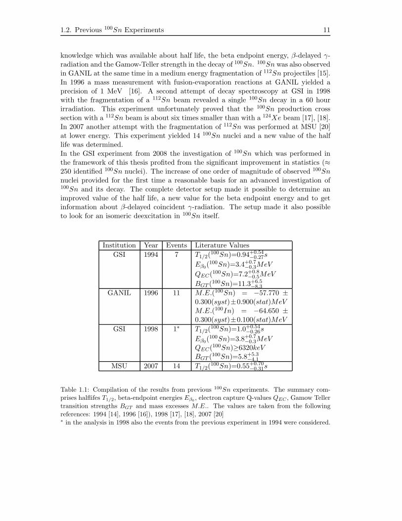
knowledge which was available about half life, the beta endpoint energy, β-delayed γ-radiation and the Gamow-Teller strength in the decay of 100Sn. 100Sn was also observedin GANIL at the same time in a medium energy fragmentation of 112Sn projectiles [15].In 1996 a mass measurement with fusion-evaporation reactions at GANIL yielded aprecision of 1 MeV [16]. A second attempt of decay spectroscopy at GSI in 1998with the fragmentation of a 112Sn beam revealed a single 100Sn decay in a 60 hourirradiation. This experiment unfortunately proved that the 100Sn production crosssection with a 112Sn beam is about six times smaller than with a 124Xe beam [17], [18].In 2007 another attempt with the fragmentation of 112Sn was performed at MSU [20]at lower energy. This experiment yielded 14 100Sn nuclei and a new value of the halflife was determined.In the GSI experiment from 2008 the investigation of 100Sn which was performed inthe framework of this thesis profited from the significant improvement in statistics (≈250 identified 100Sn nuclei). The increase of one order of magnitude of observed 100Snnuclei provided for the first time a reasonable basis for an advanced investigation of100Sn and its decay. The complete detector setup made it possible to determine animproved value of the half life, a new value for the beta endpoint energy and to getinformation about β-delayed coincident γ-radiation. The setup made it also possibleto look for an isomeric deexcitation in 100Sn itself.
Institution Year Events Literature Values
GSI 1994 7 T1/2(100Sn)=0.94+0.54
−0.27s
Eβ0(100Sn)=3.4+0.7
−0.3MeV
QEC(100Sn)=7.2+0.8−0.5MeV
BGT (100Sn)=11.3+6.5−8.3
GANIL 1996 11 M.E.(100Sn) = −57.770 ±0.300(syst)±0.900(stat)MeVM.E.(100In) = −64.650 ±0.300(syst)±0.100(stat)MeV
GSI 1998 1∗ T1/2(100Sn)=1.0+0.54
−0.26s
Eβ0(100Sn)=3.8+0.7
−0.3MeVQEC(100Sn)≥6320keVBGT (100Sn)=5.8+5.3
−4.1
MSU 2007 14 T1/2(100Sn)=0.55+0.70
−0.31s
Table 1.1: Compilation of the results from previous 100Sn experiments. The summary com-prises halflifes T1/2, beta-endpoint energies Eβ0
, electron capture Q-values QEC , Gamow Teller
transition strengths BGT and mass excesses M.E.. The values are taken from the following
references: 1994 [14], 1996 [16]), 1998 [17], [18], 2007 [20]∗ in the analysis in 1998 also the events from the previous experiment in 1994 were considered.
12 Chapter 1. Introduction and Physical Motivation
1.3 Structure of the Thesis
In chapter 2 the production of 100Sn in a fragmentation reaction and its separationfrom other products as well as the unique particle identification is described. Thenin chapter 3 the implantation detector which was developed in the framework of thisthesis for reliable β-decay detection and calorimetry is introduced. Furthermore theγ-ray detection system for delayed γ-radiation and β-coincident decay spectroscopyis discussed. In chapter 4 the maximum likelihood analysis of β-decays is presentedand as a fundamental test its successful application in the determination of alreadyknown half lives and β-endpoint energies of nuclei in the close neighbourhood of 100Snis shown. Chapter 5 is concerned with the experimental results of the spectroscopy of100Sn and its decay. In chapter 6 the experimental data are interpreted in the contextof theoretical expectations and various conclusions are drawn. Finally in chapter 7 theobtained results are summarized and future possibilities for a refined investigation of100Sn are discussed.
Chapter 2
Production and Identification
The purpose of this thesis was the investigation of the nuclear structure of the doublymagic nucleus 100Sn and its decay. Therefore it was necessary to produce this exoticnucleus in an excited state, make a clean separation from other contents of the beamcocktail and finally implant the uniquely identified nucleus in an implantation detectorwhere decay spectroscopy took place. The whole implantation detector setup made itpossible to observe emitted γ- and particle-radiation (α, β+, β− and protons) in nearly4π with high efficiency.
2.1 Production of neutron deficient nuclei
The exotic nucleus 100Sn is situated far away from the valley of stability on the neu-tron deficient side. It is an efficient method [14] to produce these rare isotopes inhigh-energy projectile fragmentation reactions and select the specific nuclei of interestwith the help of magnetic separators like the FRS at GSI in Darmstadt [21], Germany,the MSU A1900 at the Michigan State University [22], USA or the BigRIPS at theRIKEN Institute in Wako [23], Japan.The projectile fragmentation reaction mechanism can be described by a two stepmodel [24], [25].Due to the high beam energy of tens to hundreds of MeV per nucleon the projectile andthe target are in contact for a very short time in the order of about 10−22 seconds. Thislength of time is comparable to or even less than the time needed for the circulationof a single nucleon on its orbit in a nucleus. Therefore, during the first part of thereaction process, known as abrasion, all nucleons are effectively stationary with respectto the incident particle. In this pure nucleon-nucleon interaction the amount of nuclearmatter which interacts does only depend on the geometrical overlap of the two nuclei.The other nucleons which do not take part in the collision are known as the spectators.The geometrical overlap is removed from the projectile nucleus.In the second part of the reaction the remaining fragment, which is formed by the spec-tator nucleons of the projectile nucleus, is still travelling at almost the same velocityas the primary beam. This pre-fragment rearranges its constituents on a much longertime scale ranging from 10−21 seconds to 10−16 seconds in order to compensate for theloss of nucleons. This second phase is referred to as ablation. In this hot excited state
14 Chapter 2. Production and Identification
energy is released by the emission of γ-rays and light particles (p, n, α). Due to themissing Coulomb barrier the emission of neutrons is favoured which leads to a centreof gravity of the produced isotopic distribution on the proton rich side of the valley ofstability.If the projectile energy is higher than the Fermi energy in the nucleus of about 40MeV·Athe fragmentation production cross sections are independent of the energy. Of coursethe production of neutron deficient nuclei is favoured by the utilisation of a protonrich primary beam. Thus there are two possible stable candidates for the choice ofthe primary beam in the production of 100Sn via projectile fragmentation: 112Sn and124Xe.According to a former experiment from 1998 with a beam of 112Sn impinging on a Be-target at 1GeV·A the production cross section for 100Sn in this reaction was measuredto be only σ = 1.8(+3.2 − 1.3)pb [17], [18]. This is why the more promising but alsomuch more expensive 124Xe isotope as primary beam with a production cross sectionfor 100Sn of σ = 11(±4.6)pb at 1GeV·A on a Be target was chosen. The cross sectionis known from the pioneer experiment in 1994 when 100Sn was successfully indentifiedfor the first time [13], [14].
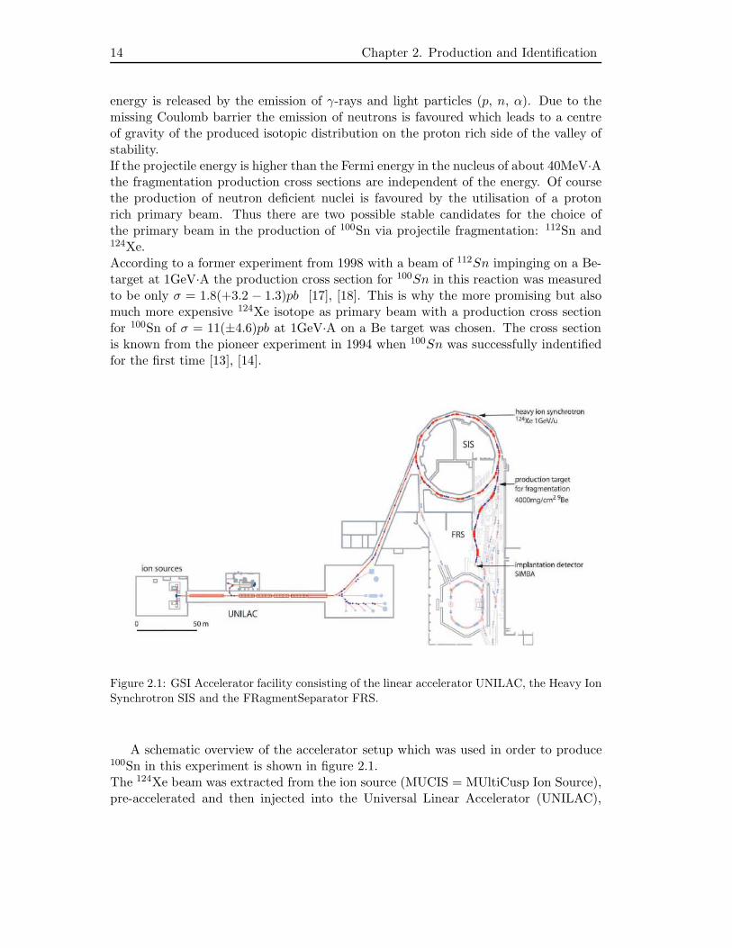
Figure 2.1: GSI Accelerator facility consisting of the linear accelerator UNILAC, the Heavy Ion
Synchrotron SIS and the FRagmentSeparator FRS.
A schematic overview of the accelerator setup which was used in order to produce100Sn in this experiment is shown in figure 2.1.The 124Xe beam was extracted from the ion source (MUCIS = MUltiCusp Ion Source),pre-accelerated and then injected into the Universal Linear Accelerator (UNILAC),
2.1. Production of neutron deficient nuclei 15
which accelerates primary beams up to 12MeV·A. The ions were then injected into theHeavy Ion Synchrotron (SIS) where they were further accelerated. A thin carbon foilin the transfer channel between the UNILAC and the SIS entrance was used to increasethe charge state of the ions to 48+ in order to be able to reach the desired final energy.The maximum energies achievable by the SIS are determined by its maximum bend-ing power of 18 Tm. Depending on the injected charge state and the N/Z ratio, themaximum energies vary from 1 to 4.5 GeV per nucleon. In our experiment 124Xe ionswere accelerated to a final energy of 1GeV·A. The SIS was operated in the relativelynew ”Fast Ramping”-mode of the magnets. This led to a total cycle time of 3 secondsand the beam was extracted with a spill length of approximately 1 second. The beamintensity was about ≤ 5 · 109 particles per spill. The length of the extraction time waschosen with regard to the finite count rates the various beamline detectors along theFRS can cope with.In the fragmentation process the highest yields can be achieved with a target materialhaving a small mass number A like Beryllium containing an increased density of scat-tering centres in contrast to heavier targets compared to the electron density that isresponsible for the energy loss. A small nuclear charge Z is also preferable because theenergy straggling of the fragmentation products caused by the different energy loss ofprojectile and fragment in the target is kept minimal. This optimizes the transmissionthrough the fragment separator (FRS). This device is described in the next section.The optimal thickness of the Be-target was determined with LISE++ [26], [27] andMOCADI [28] simulations. With increasing thickness of the target the productionrate of the fragments also increases, but their momentum spread also becomes largewhich leads to a decrease in the transmission of the fragments through the FRS. Thesecondary production rate1 also increases with target thickness but it is only a minorcontribution to the total cross section. A thicker target enhances the destruction of analready produced fragment of interest before it succeeds to escape from the target ma-terial. Taking all these mechanisms into account a Be-target with a thickness of 4008mg/cm2 has been chosen for the fragmentation reaction according to the simulationresults.After the production target the fragments had an energy of 850 MeV·A and were com-pletely stripped with a probability of 99% [29]. It is a big advantage of these highprimary beam energies that the ambiguities arising from different charge states do nothave to be considered. In the FRS the beam cocktail was now filtered in order totransmit the nuclei of interest and to suppress the background of unwanted fragments.The second stage with its beamline detectors also provided a unique event-by-eventparticle identification.
1an inter-nucleus is produced with a high cross section in a first fragmentation process and in theremaining target thickness it dissociates to the fragments of interest
16 Chapter 2. Production and Identification
2.2 Separation in the Fragmentseparator FRS
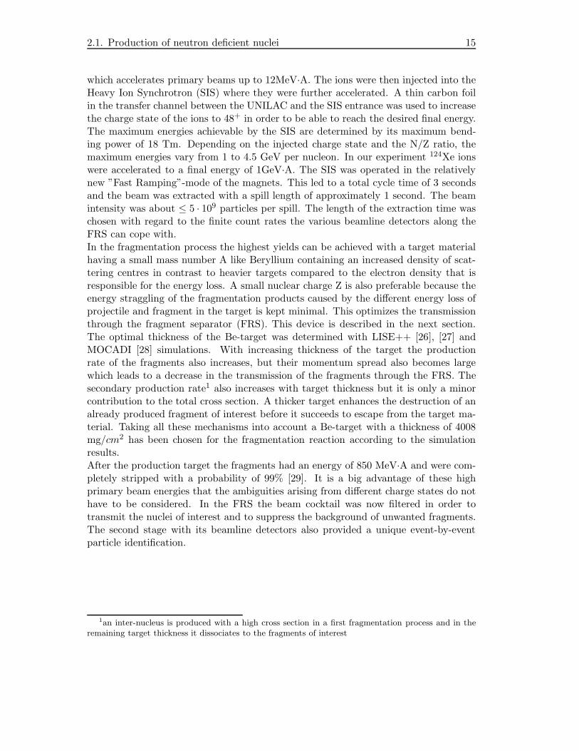
The GSI FRagment Separator (FRS) [21] is a high resolution magnetic spectrometerconsisting of four 30◦ dipole magnets which was designed to separate in mass and nu-clear charge the final residue nuclei of the full mass range produced in the projectilefragmentation reactions. The spectrometer is a symmetric two-stage device with adispersive focal plane (F2) between the two halves. Each stage is composed of twosimilar groups of quadrupole and sextupole magnets around the 30◦ dipole magnets inorder to obtain good ion optical properties. A schematic outline of the FRS is shownin figure 2.2. The magnetic rigidity of the four dipoles ranges from 5 to 18 Tm. Thetotal length of the FRS is approximately 70m. The fragments, which are produced inan excited state due to their production in the fragmentation reaction, travel about300ns through the FRS and might preserve their internal excitation facilitating isomerspectroscopy. With an energy of 850MeV·A in the first half of the FRS and an energyof about 500MeV·A in the second half of the FRS the relativistic time dilation effectis not negligible reducing the travel time in the rest frame of the nuclei to 200ns.
Figure 2.2: Schematic illustration of the FRagment Separator (FRS) at GSI with its four dipole
magnets (green) and the degrader matter which was inserted at F1 and F2.
The device was operated in the ”achromatic mode” which means that the dispersion∆x
∆p/p0vanishes at the final focal plane (F4). Here, p0 is the momentum of the nuclei on
the central optical axis of the FRS, ∆p is the deviation of the momentum from p0 and∆x is the horizontal deviation from the optical axis. All nuclei which are allowed topass through the FRS are focused to the same point at the final focal plane independentof their initial momentum spread (of course in the limits of the momentum acceptanceof the FRS). In this mode of operation the dispersion and the horizontal width of theparticle beam is maximal at the intermediate focal plane F2.The separation of the nucleus of interest, e.g. 100Sn, works in principle in the followingway (often referred to as Bρ − ∆E − Bρ-method): In the first stage (Target - F2)the nuclei are separated according to their magnetic rigidity Bρ. The momentum per
2.2. Separation in the Fragmentseparator FRS 17
nucleon p/A of all fragments is almost equal. According to the Lorentz-force onlynuclei with a certain mass-to-charge ratio A/q are able to pass the fragment separator,according to:
Bρ =p
A· Aq
; q = Z · e (2.1)
Due to the high beam energies of 1GeV·A the fragments are completely stripped witha probability of 99% and the electric charge q corresponds to the nuclear charge Z.In order to select a certain nucleus it is necessery to insert a piece of matter (mostoften aluminium) into the optical path at the intermediate focal plane F2. This socalled degrader induces a nuclear charge dependent energy loss (∆E ∝ Z2) in thefragment beam and makes it possible to select in the second stage (F2 - F4), withthe adjustment of the magnetic-rigidity to the new p/A, the nuclear charge of thetransmitted nuclei. The degrader, as depicted in figure 2.2, has a wedge shape whichis a necessary correction2 to maintain the good achromatic optical properties of thefragment separator. At the final focal plane F4 the selected nucleus with mass Aand nuclear charge Z is centered on the optical axis (horizontal deviation x = 0)with a Gaussian distribution to both sides. For the 100Sn-setting the FWHM3 ofthe horizontal distribution was ∆x = 3.5cm and for the vertical distribution it was∆y = 2.0cm according to simulations with MOCADI and LISE++. This width wasadjusted to the physical dimensions of the implantation detector of 60 x 40 mm2.During the experiment some fine tuning was performed with the quadrupole magnetswhich are situated behind the last FRS dipole magnet. Of course the separation isnot perfectly clean and other nuclei in the neighbourhood of 100Sn with partially muchhigher production cross sections are also transmitted to the final focal plane. Theircharge dependent separation at F4 leads to a Gaussian distribution shifted in thehorizontal direction with respect to the optical axis. The main contaminants were100In at x = +1.0cm and 101Sn at x = −2.4cm with a horizontal distribution of∆x = 3.3cm (FWHM). The separation in the horizontal direction gets better i.e. thecentroid of the distribution moves further away from the optical axis with increasingthickness of the degrader at F2, but the induced momentum spread makes the widthof the distribution broader. In the experiment a suitable degrader thickness of 4500mg/cm2 was chosen.Another crucial point is the estimated count rate at the intermediate focal plane F2. Inthis region several detectors (scintillators, Tracking Ionisation Chambers) are mountedfor position and Time-of-Flight (ToF) measurements in order to provide event-by-event particle identification of the transmitted nuclei. Details on the detectors usedfor particle identification are given in the next section. These detectors are limited tocount rates with a maximum of 100 kHz. The selection of the magnetic rigidity for theoptimal transmission of 100Sn from Target to F2 with an A/q ratio of 2.0 includes allthe light nuclei which are lying in the valley of stability and are consequently producedwith tremendous production cross sections in the fragmentation reaction. To get rid of
2The effects of the velocity dependent energy loss of the fragments in matter are compensated.3FWHM = Full Width at Half Maximum
18 Chapter 2. Production and Identification
this background it was necessary to induce a charge dependent separation already atthe first focal plane F1. According to simulations a degrader at F1 with a thickness of2000 mg/cm2 and the use of appropriate slits makes it possible to limit the count rateat F2 to 40 kHz.Despite the high selectivity of the FRS it is not possible to achieve a unique selection ofthe nuclei transmitted to the implantation detector which was situated at F4. Thus theunique event-by-event identification of each transmitted nucleus is an essential task.Altogether the fragment separator was able to reduce the rate of the primary beamof approximately 109 particles per second to still reasonable 300Hz at the final focalplane F4 of the FRS when the fragment separator was set to an optimal transmissionof 100Sn. In contrast to this observation MOCADI simulations predict a count rateat F4 in the order of 10Hz for the 100Sn-setting. Due to a hitherto not understoodtechnical problem which led to a significant energy loss of a small fraction of the primarybeam in the target frame after the Seetram4 (a device which measures the primarybeam intensities just in front of the production target) a lot of heavy fragments nearthe valley of stability were able to pass the fragment separator up to the final focalplane. Fortunately the additional activity which was implanted into the implantationdetector by this adversity was negligible. The dead time of the data aquisition due tothe inevitably increased trigger rate during the spill was in the order of 25%.With about 350MeV·A the energy of the fragments at the final focal plane F4 wasstill high enough to implant the nuclei of interest deep inside the implantation detectorstack. Details on the implantation detector are given in chapter 3. The implantationin the correct depth is guaranteed by the adjustment of the thickness of a variabledegrader which is installed in the beam line in front of the implantation detector.According to the simulation for the optimal 100Sn FRS setting the minimal ion opticaltransmission of 100Sn is 80% and the loss by nuclear destruction reactions in beam linematter until the nuclei are implanted accounts to 55% resulting in a total transmissionof 36% of all nuclei produced in the fragmentation reaction in the target.
2.3 Unique Identification of 100Sn
In the 100Sn FRS setting the spatial separation of the heavy ions is not good enoughto prevent nuclei in the neighbourhood (101Sn, 99In, 100In) which are significantlysuppressed in their ion optical transmission but which are produced with a much largerproduction cross-section than 100Sn from being implanted in the implantation detector.The reliable event-by-event particle identification is, apart from a low implantationand decay rate, most important for a successful experiment in the field of implantationcorrelated decay spectroscopy. Thus it was necessary to improve the resolution whichis achievable with the standard fragment separator detector equipment by means ofseveral additional detectors specifically installed for the 100Sn experiment [30].
4Seetram = Secondary electron transmission monitor
2.3. Unique Identification of 100Sn 19
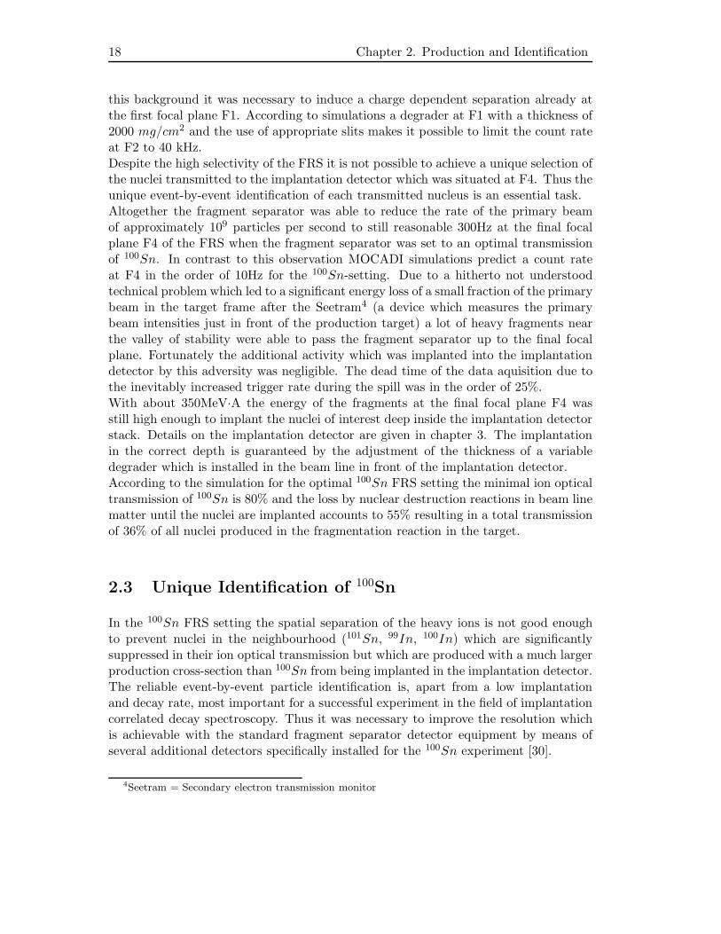
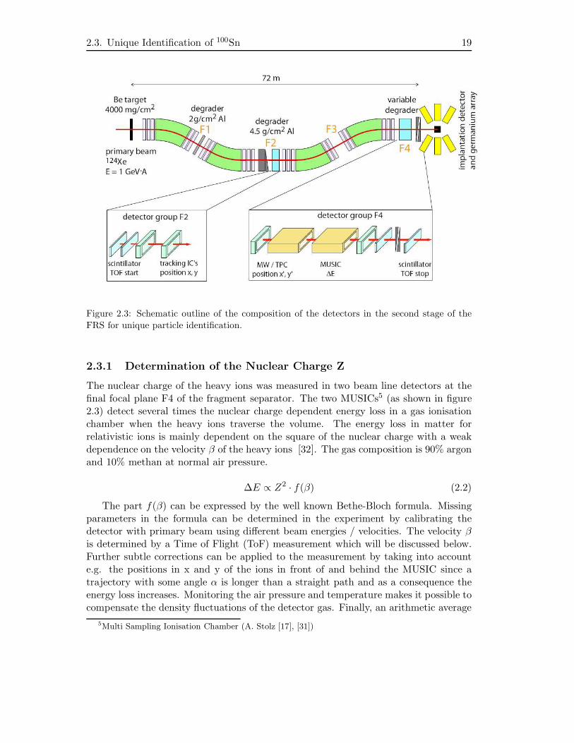
Figure 2.3: Schematic outline of the composition of the detectors in the second stage of the
FRS for unique particle identification.
2.3.1 Determination of the Nuclear Charge Z
The nuclear charge of the heavy ions was measured in two beam line detectors at thefinal focal plane F4 of the fragment separator. The two MUSICs5 (as shown in figure2.3) detect several times the nuclear charge dependent energy loss in a gas ionisationchamber when the heavy ions traverse the volume. The energy loss in matter forrelativistic ions is mainly dependent on the square of the nuclear charge with a weakdependence on the velocity β of the heavy ions [32]. The gas composition is 90% argonand 10% methan at normal air pressure.
∆E ∝ Z2 · f(β) (2.2)
The part f(β) can be expressed by the well known Bethe-Bloch formula. Missingparameters in the formula can be determined in the experiment by calibrating thedetector with primary beam using different beam energies / velocities. The velocity βis determined by a Time of Flight (ToF) measurement which will be discussed below.Further subtle corrections can be applied to the measurement by taking into accounte.g. the positions in x and y of the ions in front of and behind the MUSIC since atrajectory with some angle α is longer than a straight path and as a consequence theenergy loss increases. Monitoring the air pressure and temperature makes it possible tocompensate the density fluctuations of the detector gas. Finally, an arithmetic average
5Multi Sampling Ionisation Chamber (A. Stolz [17], [31])
20 Chapter 2. Production and Identification
of the information of the two MUSICs was taken which helped to improve the resolutionin Z by a factor of 1/
√2.
2.3.2 Determination of the A/Q - ratio
The principle to determine the mass to charge (AoQ) ratio is based on the equalitybetween the Lorentz-force acting on moving charged particles in the homogenous mag-netic field of the dipole-magnets and the centrifugal force which is due to the inertia ofthe mass of the particles.The measurement is done with beam line detectors at the intermediate focal plane F2and the final focal plane F4. Bearing in mind that one gets fully stripped ions wherethe charge is equal to the nuclear charge Q = Z ·e the magnetic rigidity Bρ, dependingon the A
Q ratio, can be expressed as:
B · ρ = c ·m0 ·β
√
1 − β2· AQ
(2.3)
Here c is the speed of light in vacuum, e is the elementary charge and m0 is the massof a nucleon in the rest frame. According to equation (2.3) one needs to measure themagnetic rigidity B · ρ and the velocity β = v
c of the heavy ions on their way throughthe second part (F2-F4) of the fragment separator in order to calculate the A
Q ratio.The magnetic rigidity Bρ of an ion on a track with horizontal positions x2 and x4 atthe focal planes F2 and F4, respectively, can be related in the following way to themagnetic rigidity Bρ0 of ions on the reference trajectory, the optical axis:
B · ρ = B · ρ0
(
1 − x4 −MF2−F4 · x2
DF2−F4
)
(2.4)
ρ0 is the effective radius of ions moving on the optical axis. MF2−F4 = ∂x4
∂x2and
DF2−F4 = ∂x4
∂p/p are the magnification and the dispersion, theoretical values which canbe taken from the ion optical mapping matrices of the FRS. The magnetic field Bbetween the dipoles is measured with Hall probes with a precision of 10−4 T. The hor-izontal positions x2 and x4 are measured with the help of MWPCs6 and TPCs7 at F4and at F2 the position can be measured in principal with the scintillators. However,for the purpose of the 100Sn experiment with its high requirements concerning the pu-rity of the particle identification the resolution of the scintillators is not good enough.Therefore, two additional TICs8 (figure 2.3) were set up at the focal plane F2 whichwere able to cope with high rates of up to 100kHz and have a position resolution of1mm. The rate at F2 was far below 100kHz for the 100Sn FRS setting.For the event-by-event determination of the velocity of the heavy ions a ToF measure-ment was used. Since the path length is approximately constant for all ions within theFRS acceptance a proper calibration with primary beam of different energies directly
6Multi Wire Proportional Counters [33]7Time Projection Chambers8Tracking Ionisation Chambers (A. Stolz [17])
2.3. Unique Identification of 100Sn 21
links the ToF between F2-F4 to the velocity of the nuclei [30]. The ToF was measuredfour times with two redundant combinations of scintillators between F2 and F4 (asshown in figure 2.3). The time resolution was approximately 100ps. Several redundantmeasurements helped to improve the AoQ resolution.A possible source of error for misidentifications between F2 and F4 is given by reac-tions of the nuclei with detector matter. There is a certain possibility that a nucleuswhich is fully stripped picks up an electron and becomes hydrogen-like. Then thisnucleus with A(N − 1, Z + 1)Z+ resembles a nucleus with A(N,Z)Z+. In the case of100Sn this scenario is not important since only even more proton-deficient nuclei couldbe misidentified as 100Sn which is very unlikely due to their much smaller productioncross section (approximately two orders of magnitude lower).
2.3.3 PID Cleaning and Resolution in the 100Sn-setting
In addition to the several redundant measurements of energy loss in matter, positions,and ToFs it is helpful to put some other constraints on the particle identification inorder to reduce the background of possible misidentifications [30].Of course the two redundant measurements of the nuclear charge Z in the MUSICs andthe two AoQ values should correlate to some extent and be consistent. Since the FRSis a spectrometer with well defined ion optical properties the angle of the ions at theintermediate focal plane F2 in x and y should correlate with the angle in x and y atthe final focal plane F4. The energy loss in the MUSICs should also correlate with theenergy loss in the scintillator which was placed behind the degrader for adjustment ofthe implantation position in the detector. This correlation helps to tag events wherethe nucleus has fragmented in the degrader matter and which therefore have to be dis-carded. Finally, the positions which were determined by the scintillators and the TICsat F2 should correlate with regard to the position resolution of the individual detector.In figure 2.4 the Z versus AoQ identification plot for the 100Sn setting is shown afterapplying all selections for cleaning the PID.
In the 100Sn FRS setting the resolution of the nuclear mass was ∆A = 0.42(FWHM) and for the nuclear charge ∆Z = 0.32 (FWHM). The nuclei of interest can bewell separated. If one considers a Gaussian distribution of the nuclear charge and massthen it is interesting to estimate e.g. for the nuclear mass A of a certain nucleus (A,Z)how many events originating from the nuclei with A+1 and A-1 (same nuclear chargeZ) overlap with the distribution of mass A. A rough calculation yields that a 3σ areaaround mass number A, which comprises 99.7% of all events, is approximately A±0.54or A
Z=50 ± 0.01 in our case. This means that in the area where almost all nuclei of typeA are situated there is only an overlap/admixture of 0.6% of neighbouring nuclei whichcould not be correctly identified. Thus the particle identification is very clean.
In 15 days of beamtime 259 100Sn nuclei were successfully identified enabling forthe first time a precise investigation of the Gamow Teller decay of this exotic nucleus.Apart from the high statistics of 100Sn the particle identification plot reveals the first
22 Chapter 2. Production and Identification
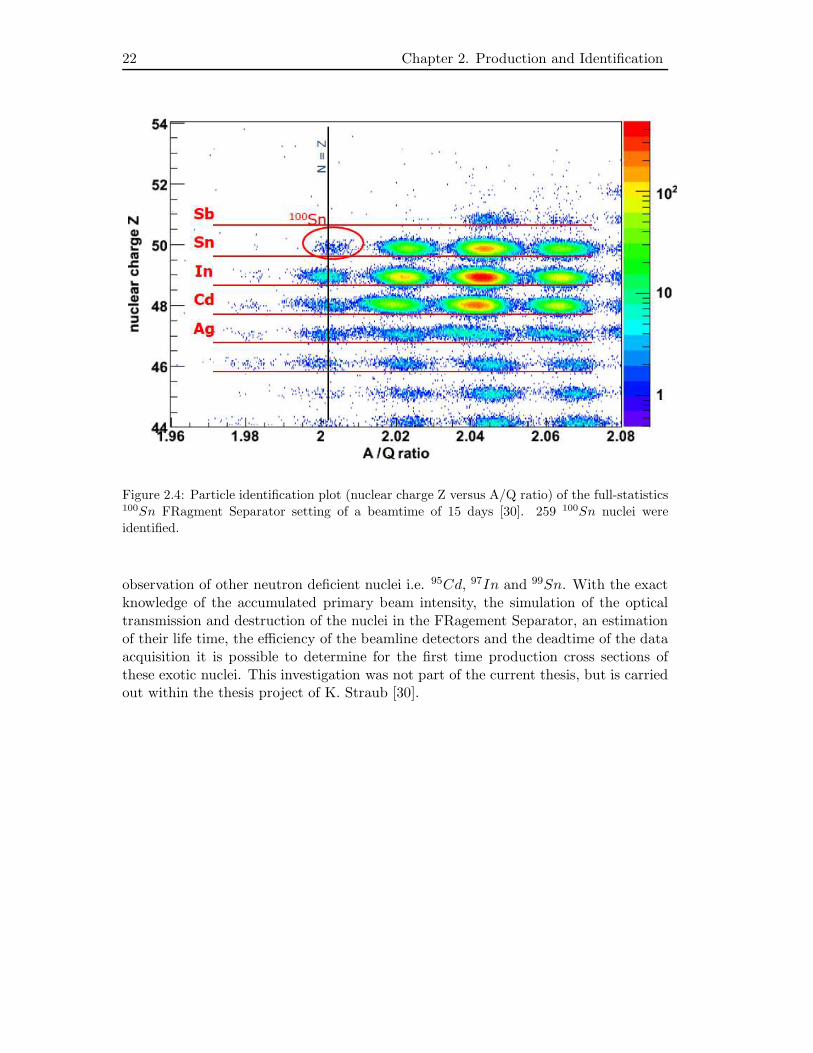
Figure 2.4: Particle identification plot (nuclear charge Z versus A/Q ratio) of the full-statistics100Sn FRagment Separator setting of a beamtime of 15 days [30]. 259 100Sn nuclei were
identified.
observation of other neutron deficient nuclei i.e. 95Cd, 97In and 99Sn. With the exactknowledge of the accumulated primary beam intensity, the simulation of the opticaltransmission and destruction of the nuclei in the FRagement Separator, an estimationof their life time, the efficiency of the beamline detectors and the deadtime of the dataacquisition it is possible to determine for the first time production cross sections ofthese exotic nuclei. This investigation was not part of the current thesis, but is carriedout within the thesis project of K. Straub [30].
Chapter 3
Detector Setup for DecaySpectroscopy
3.1 General Requirements
In order to study the decay properties of the neutron deficient nuclei of interest inthe region of 100Sn an appropriate highly efficient detector system for γ- and particle-radiation had to be provided. The development of the current setup was based on theexperiences made in the two former 100Sn experiments from 1996 and 1998, when thefirst successful production, identification, and spectroscopy of the decay of this exoticnucleus was performed [14], [17]. It turned out that it is the best choice for this task toutilize a closely packed stack of highly-segmented silicon detectors for the detection ofparticle-radiation where the nuclei of interest are implanted. This setup is surroundedby an array of Germanium detectors in close geometry for γ-ray spectroscopy.Concerning the exploration of the nuclear structure of 100Sn and the observation of itsdecay the basic requirements of the detector system are the following:
• There are theoretical shell-model predictions of an isomeric state in 100Sn whichmight be populated to some extent during the fragmentation production reaction.After the time of flight through the FRagment Separator, the unique particle iden-tification and the subsequent implantation in the detector system, it is desireableto look for the gamma decay of this isomer. This observation would for the firsttime establish excited states in 100Sn and would allow for crucial insights intothe nuclear structure of 100Sn.
• After the implantation it is necessary to extract the implantation position inx,y,z with high precision in order to correlate successive radioactive decays in thesame area with previous implantations and to measure the corresponding timedifferences for the determination of a half life of 100Sn. The spatial granularityshould be high to avoid as much background decay events as possible since theobserved activity scales with the detection area used for correlating implantationswith decays.
24 Chapter 3. Detector Setup for Decay Spectroscopy
• For the determination of the Gamow Teller Strength in the decay of 100Sn it isnecessary - in addition to a precise knowledge of the half-life and of the final statespopulated in the daughter nucleus - to measure the distribution of the energy ofthe emitted decay positrons. The detector should cover a solid angle of almost 4πaround the implantation area with sufficient matter to fully stop the emitted betaparticles and get a reliable measurement of their total energy (beta calorimeter).In case that a high-lying state in the daughter nucleus 100In above the protonseparation energy is populated the setup should also be able to distinguish betadecays from beta-delayed proton emission.
• The beta delayed gamma-radiation which is emitted by the excited states in thedaughter nucleus 100In should be detected with high efficiency. Thereby informa-tion can be obtained about the number of final states which are populated duringthe beta decay entailing some insight in the nuclear structure of the daughter nu-cleus. Valuable information about the effective neutron-proton interaction in thisregion of the nuclear chart can be extracted. Finally the γ-cascade and the betaendpoint energy(ies) make it possible to determine the Q value of the decay.
In order to fulfill all these requirements the detector setup for decay spectroscopyin the experiment was composed of the SIMBA-detector1 which was built in the frame-work of this thesis and the RISING-detector array2 consisting of a ball of 105 separateGermanium detectors for γ-ray spectroscopy [34].
In figure 3.1 a schematic plot of the implantation detector is shown. A detailedpicture of the actual design is presented in figure 3.2. The full configuration withthe surrounding Germanium detectors can be seen in figure 3.3 and figure 3.4. Theimplantation detector consists of 25 layers of silicon detectors. The beam enters thedetector from the right hand side. The first two detectors provide a redundant posi-tion information in x and y about the implantation positions of the heavy ions. Theimplantation area in the middle is composed of three highly segmented silicon stripdetectors which are described in further detail in section 3.2. This area is surroundedby a beta calorimeter (section 3.3) composed of ten beta absorbers on each side.The housing of the detector which is not shown in the schematic picture was constructedto shield the detector stack from electromagnetic noise and daylight. At the same timethe material should be as transparent as possible to γ-radiation emitted by implantedions. For small γ-ray energies the photo effect is the dominating process and the crosssection is proportional to the square of the nuclear charge. This is why the materialshould be composed of ingredients with very low Z. For higher energies between 500keV and 2000 keV the Compton effect has the largest cross section. It just depends onthe amount of material (mg/cm2) used for the housing. Consequently, the cover shouldbe as thin as possible. The best choice was a material called Pertinax3 with a thickness
1Silicon IMplantation Beta Absorber2Rare ISotope investIgatioNs at GSI3Hartpapier, FR4 Platinenmaterial
3.2. Implantation Area 25
of 1.5mm for sufficient mechanical stability with a vaporized thin layer of copper witha thickness of 50µm. During the experiment the housing of the detector was flushedwith cooled nitrogen with a temperature of about 283K in order to keep the surfacesof the detectors clean and to reduce the thermal excitation of charge carriers acrossthe band gap between valence and conduction band. This action prevented an increaseof leakage currents due to the growing defects in the detector lattice caused by heavyion implantations and helped to keep the detectors fully depleted. The full depletion ismandatory otherwise the energy loss of charged particles in the silicon detector wouldnot be completely detected leading to a systematic error of the measurement which isnot trivial to estimate.In the following sections the setup is discussed in more detail.
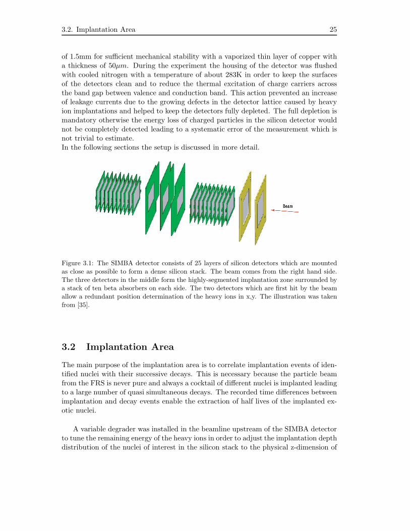
Figure 3.1: The SIMBA detector consists of 25 layers of silicon detectors which are mounted
as close as possible to form a dense silicon stack. The beam comes from the right hand side.
The three detectors in the middle form the highly-segmented implantation zone surrounded bya stack of ten beta absorbers on each side. The two detectors which are first hit by the beam
allow a redundant position determination of the heavy ions in x,y. The illustration was taken
from [35].
3.2 Implantation Area
The main purpose of the implantation area is to correlate implantation events of iden-tified nuclei with their successive decays. This is necessary because the particle beamfrom the FRS is never pure and always a cocktail of different nuclei is implanted leadingto a large number of quasi simultaneous decays. The recorded time differences betweenimplantation and decay events enable the extraction of half lives of the implanted ex-otic nuclei.
A variable degrader was installed in the beamline upstream of the SIMBA detectorto tune the remaining energy of the heavy ions in order to adjust the implantation depthdistribution of the nuclei of interest in the silicon stack to the physical z-dimension of
26 Chapter 3. Detector Setup for Decay Spectroscopy
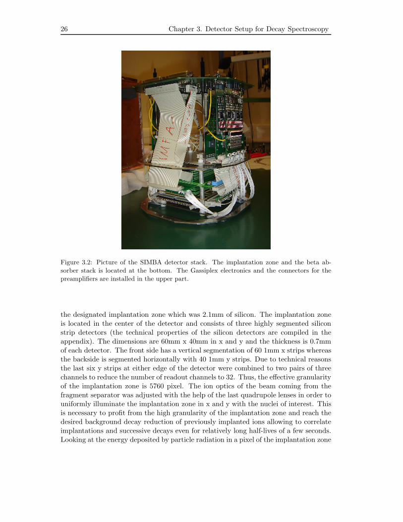
Figure 3.2: Picture of the SIMBA detector stack. The implantation zone and the beta ab-
sorber stack is located at the bottom. The Gassiplex electronics and the connectors for the
preamplifiers are installed in the upper part.
the designated implantation zone which was 2.1mm of silicon. The implantation zoneis located in the center of the detector and consists of three highly segmented siliconstrip detectors (the technical properties of the silicon detectors are compiled in theappendix). The dimensions are 60mm x 40mm in x and y and the thickness is 0.7mmof each detector. The front side has a vertical segmentation of 60 1mm x strips whereasthe backside is segmented horizontally with 40 1mm y strips. Due to technical reasonsthe last six y strips at either edge of the detector were combined to two pairs of threechannels to reduce the number of readout channels to 32. Thus, the effective granularityof the implantation zone is 5760 pixel. The ion optics of the beam coming from thefragment separator was adjusted with the help of the last quadrupole lenses in order touniformly illuminate the implantation zone in x and y with the nuclei of interest. Thisis necessary to profit from the high granularity of the implantation zone and reach thedesired background decay reduction of previously implanted ions allowing to correlateimplantations and successive decays even for relatively long half-lives of a few seconds.Looking at the energy deposited by particle radiation in a pixel of the implantation zone
3.2. Implantation Area 27
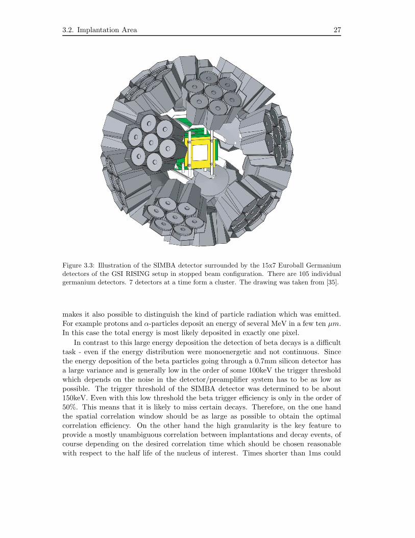
Figure 3.3: Illustration of the SIMBA detector surrounded by the 15x7 Euroball Germanium
detectors of the GSI RISING setup in stopped beam configuration. There are 105 individualgermanium detectors. 7 detectors at a time form a cluster. The drawing was taken from [35].
makes it also possible to distinguish the kind of particle radiation which was emitted.For example protons and α-particles deposit an energy of several MeV in a few ten µm.In this case the total energy is most likely deposited in exactly one pixel.
In contrast to this large energy deposition the detection of beta decays is a difficulttask - even if the energy distribution were monoenergetic and not continuous. Sincethe energy deposition of the beta particles going through a 0.7mm silicon detector hasa large variance and is generally low in the order of some 100keV the trigger thresholdwhich depends on the noise in the detector/preamplifier system has to be as low aspossible. The trigger threshold of the SIMBA detector was determined to be about150keV. Even with this low threshold the beta trigger efficiency is only in the order of50%. This means that it is likely to miss certain decays. Therefore, on the one handthe spatial correlation window should be as large as possible to obtain the optimalcorrelation efficiency. On the other hand the high granularity is the key feature toprovide a mostly unambiguous correlation between implantations and decay events, ofcourse depending on the desired correlation time which should be chosen reasonablewith respect to the half life of the nucleus of interest. Times shorter than 1ms could
28 Chapter 3. Detector Setup for Decay Spectroscopy
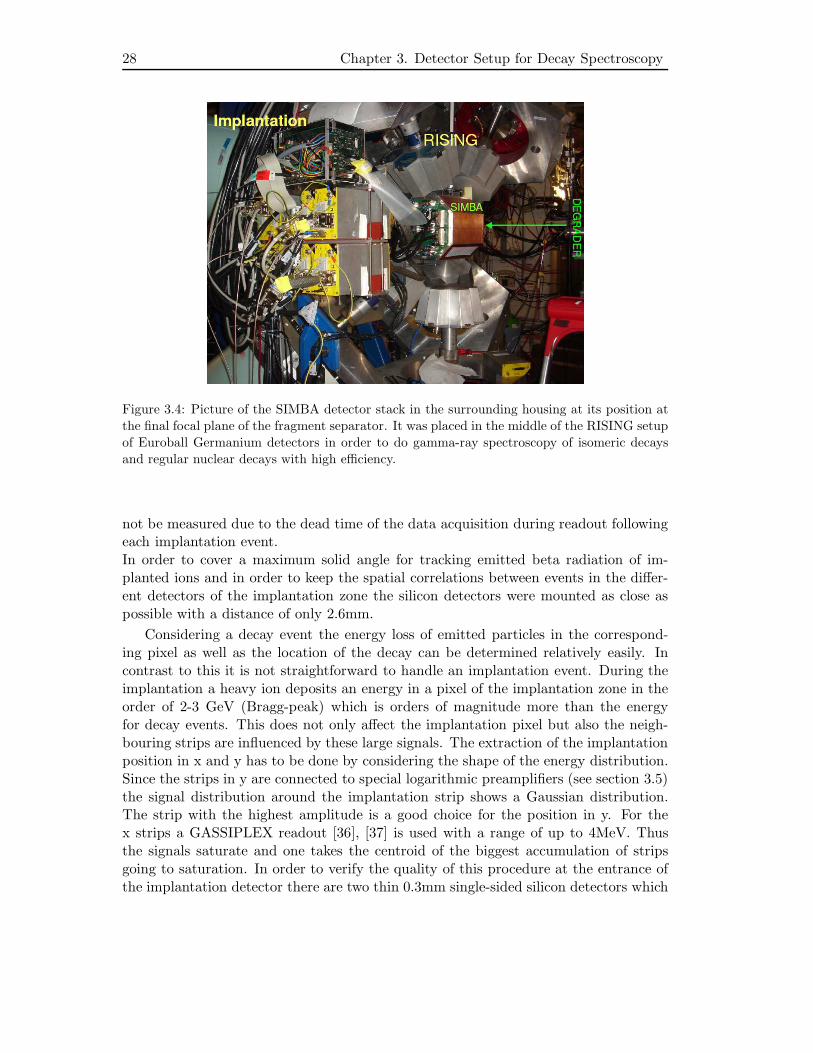
Figure 3.4: Picture of the SIMBA detector stack in the surrounding housing at its position at
the final focal plane of the fragment separator. It was placed in the middle of the RISING setup
of Euroball Germanium detectors in order to do gamma-ray spectroscopy of isomeric decays
and regular nuclear decays with high efficiency.
not be measured due to the dead time of the data acquisition during readout followingeach implantation event.In order to cover a maximum solid angle for tracking emitted beta radiation of im-planted ions and in order to keep the spatial correlations between events in the differ-ent detectors of the implantation zone the silicon detectors were mounted as close aspossible with a distance of only 2.6mm.
Considering a decay event the energy loss of emitted particles in the correspond-ing pixel as well as the location of the decay can be determined relatively easily. Incontrast to this it is not straightforward to handle an implantation event. During theimplantation a heavy ion deposits an energy in a pixel of the implantation zone in theorder of 2-3 GeV (Bragg-peak) which is orders of magnitude more than the energyfor decay events. This does not only affect the implantation pixel but also the neigh-bouring strips are influenced by these large signals. The extraction of the implantationposition in x and y has to be done by considering the shape of the energy distribution.Since the strips in y are connected to special logarithmic preamplifiers (see section 3.5)the signal distribution around the implantation strip shows a Gaussian distribution.The strip with the highest amplitude is a good choice for the position in y. For thex strips a GASSIPLEX readout [36], [37] is used with a range of up to 4MeV. Thusthe signals saturate and one takes the centroid of the biggest accumulation of stripsgoing to saturation. In order to verify the quality of this procedure at the entrance ofthe implantation detector there are two thin 0.3mm single-sided silicon detectors which
3.3. Beta Calorimeter 29
have a center-to-center distance from one strip to the adjacent strip of 1mm. They areread out by resistor chains. Since the heavy ions still have a considerable energy at theentrance of SIMBA and the two detectors are relatively thin, the energy deposition ofthe heavy ions is far less than in the implantation zone (≈ 300MeV). This redundantdetermination of the (x,y) position showed a good agreement with the determinationof the implantation position from the direct measurement in the implantation zone.
The implantation position in z is determined with the help of the y sides of thesilicon detectors and the logarithmic preamplifiers. Setting an appropriate thresholdand determining which detector still is affected by strong signals shows where the heavyion came to rest. Due to fragmentation reactions in the degrader in front of SIMBAand of course in the detector matter some of the nuclei of interest are destroyed. Thefragments of these nuclei in most cases have a lower nuclear charge Z which leads toless energy loss per path length. Consequently some of these destroyed nuclei will leavethe implantation zone and will be implanted in the neighbouring first beta absorberbehind the implantation zone. Its signal is taken as a veto. Simulations show that 15%of the 100Sn nuclei are destroyed in the degrader and detector matter. A simulationof the distribution in depth shows that 74% of the 100Sn nuclei are implanted into asingle detector of the implantation zone. The main contaminants 101Sn,100In and 99Inwhich are of course separated on the horizontal axis from 100Sn, but due to their largerproduction cross section still have a significant overlapping tail with 100Sn are stoppedabout one silicon detector (0.7mm) behind 100Sn.
3.3 Beta Calorimeter
In front of and behind the implantation area there are on either side ten 1mm thicksilicon detectors mounted as a beta calorimeter (the technical properties of the silicondetectors are compiled in the appendix). To optimize the solid angle coverage thedetectors were mounted as close as possible to each other. The distance between neigh-bouring silicon layers was only 2mm. This configuration makes it possible to reliablystop beta particles which are emitted from the implantation zone with a maximumenergy of 4-5 MeV [38]. The beta absorbers have the same dimensions in x and y asthe implantation zone (60mm x 40mm) and are verticaly segmented into 7 strips. Thissegmentation makes it possible to perform a kind of beta tracking through the detectorsand to identify the uninterrupted trace of the particle which is essential to reconstructthe total deposited energy. After the positron almost completely comes to rest it an-nihilates on an electron and the two 511keV γ-rays are emitted in opposite directions.There is a certain probability that the 511keV photons as well as the γ-rays emitted bythe daughter nucleus after the decay interact with the silicon and produce Compton orphotopeak events leading to distortions of the measured decay energy. However, theseinteractions will happen almost always at a substantial distance from the position ofthe decay. The granularity of the implantation zone and the segmentation of the betaabsorbers make it in most cases possible to detect these isolated energy depositionsand distinguish them from the track of the decay positron.
30 Chapter 3. Detector Setup for Decay Spectroscopy
The characteristics of the tracks and the energy deposition allows to distinguish realdecay events from light particles like protons and α-particles flying through the detec-tor during the spill which are not recognized as implantation triggers. Further cleaningcuts for decay events are discussed in section 3.7.
3.4 RISING γ-ray detectors
For the detection of γ-rays emitted directly after an implantation event coming fromthe deexcitation of isomeric states of the implanted nuclei as well as for γ-spectroscopyfollowing the radioactive decay the RISING array [34] (figure 3.3 and figure 3.4) which iscomposed of 15 Euroball Germanium detector clusters mounted in the so called StoppedBeam configuration was used. Each of the 15 clusters houses 7 separate Germaniumcrystals, amounting to a total of 105 independent Germanium detectors. In the StoppedBeam configuration the detectors are mounted in three rings each containing 5 detectorclusters with angles of 51, 90 and 129 degree around the beam axis. The distance ofthe detectors to the center on the beam axis is approximately 22cm. The measuredγ-photopeak efficiency is 15% at 661 keV without any other matter in the RISINGarray. The energy resolution is about 3keV FWHM at 1.3MeV.
3.5 Readout of the experimental setup
In this section the readout of the SIMBA detector is described. The problems whichoccur when a lot of energy is deposited in the detector and how to handle these largesignals have already been discussed in section 3.2. The horizontal y strips of the threedetectors of the implantation zone were read out with special logarithmic preamplifiers.These had the advantage of not going to saturation for very large signals, still bearingthe information on the shape of the energy distribution along adjacent strips. At thesame time the recovery time of the electronics after such an impact was only a few100 µs. The sevenfold segmented sides of the four beta absorbers lying closest to theimplantation zone as well as the back sides of all remaining 16 beta absorbers were alsoread out by these special preamplifiers. Behind the preamplifier the signal was split intotwo separate branches. One branch was composed of a fast timing filter preamplifier incombination with a leading edge discriminator. The threshold of the discriminator wasset as low as possible for each channel separately just above noise level. To generatea decay trigger the logical OR of all discriminator outputs was taken for the signalsof the implantation zone and the four beta absorbers in the closest neighbourhood.The other branch was processed by a spectroscopic shaping amplifier and the energyinformation represented in the pulse height of the output was recorded with peak-sensing ADCs. The vertical x strips of the implantation zone as well as the sevenfoldsegmented front sides of the 16 beta absorbers lying furthest from the implantationzone were read out by GASSIPLEX ASIC chips [36], [37]. Due to significant leakagecurrents the orginal DC coupling was discarded and a special AC coupling adapterwas introduced. A single GASSIPLEX chip, which was developed at CERN, consists
3.5. Readout of the experimental setup 31
of 16 charge sensitive preamplifiers, pulseshaping filteramplifiers as well as Track-and-Hold stages. The analogue signals of these channels are read out sequentially witha multiplexer on a single line. With the Track-and-Hold signal generated from theaccepted trigger of the data acquisition it is possible to select the exact time whenthe output value of the filteramplifiers is captured. The maximum value of the shapedsignal is reached after a delay of about 600ns with respect to the physical event. Theanalogue signal was then processed with an ADC, but only channels with a signal abovea certain threshold were read out by the data acquisition. This zero suppression wasused to minimize the dead time of the data acquisition to about 650 µs per event. Theenergy resolution FWHM of the channels read out by Mesytec preamplifiers was in theorder of 30keV and for the GASSIPLEX read out channels 40keV were achieved.The two single sided silicon detectors at the beam entrance of SIMBA were read outby two resistor chains and the four channels were processed by a standard preamplifierand recorded with a common shaping amplifier ADC combination.
The data acquisition accepted two separate types of events. A schematic overviewof the parts of the detector which are read out for implantations and decays is shownin (figure 3.5). For a decay event the implantation zone as well as adjacent betaabsorbers provide the trigger. The readout of the strips of the implantation detectorprovides the information about the place in x, y, z where the decay event took placeand the distribution of the energy of the emitted decay particle in the detector volume.The 105 Germanium detectors of the RISING array are also read out and provideinformation about the energy of prompt γ-rays. Since these detectors were read outby XIA DGF [39] modules it was also possible to look in an asymmetric 400µs windowmostly acquiring the time after the decay-trigger with a resolution of 25ns for transitionsin the daughter nucleus having deexcited some time after the decay.For an implantation event the trigger was taken from the last scintillator at the finalfocal plane F4 which was traversed by the heavy ion. The signals from SIMBA giveinformation about the location of the heavy ion, whether it missed the detector or wherein x,y,z it was implanted. The FRS beamline detectors provide information necessaryfor the particle idenfication. Another important tool to verify the correct FRS particleidentification is provided by the RISING array. With the implantation trigger it is againpossible to look for emitted γ-rays in a 400µs window after implantation. Lets assumea nucleus with an isomer which is populated during the production fragmentationreaction and survives the time of flight through the FRS. Then it is possible to observethe isomeric decay after implantation and cross check it with the particle identificationfor consistency.Finally, an absolute time measurement is done with the help of different scalers whichare triggered by clocks with various frequencies. The scaler value is written to the datastream for each decay or implantation event.The dead time inbetween two spills was negligible, but during the one second of fastbeam extraction every three seconds, the implantation trigger rate caused a deadtimeof approximately 25%.
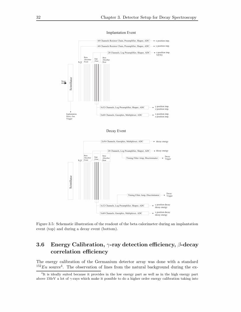
32 Chapter 3. Detector Setup for Decay Spectroscopy
S ci n t
i l l at o r
I m p l a n t a t i o n E v e n t
I m p l a n t a t i o n H e a v y I o nT r i g g e r
x , yI m pZ o n e
B e t aA b s o r b e rF r o n t
6 0 C h a n n e l s R e s i s t o r C h a i n , P r e a m p l i f i e r , S h a p e r , A D C
6 0 C h a n n e l s R e s i s t o r C h a i n , P r e a m p l i f i e r , S h a p e r , A D C
x p o s i t i o n i m p .y p o s i t i o n i m p .
3 x 3 2 C h a n n e l s , L o g P r e a m p l i f i e r , S h a p e r , A D C y p o s i t i o n i m p .z p o s i t i o n i m p .
B e t aA b s o r b e rR e a r
3 x 6 0 C h a n n e l s , G a s s i p l e x , M u l t i p l e x e r , A D C x p o s i t i o n i m p .z p o s i t i o n i m p .
2 8 C h a n n e l s , L o g P r e a m p l i f i e r , S h a p e r , A D C z p o s i t i o n i m p .V E T O
B e a m
S ci n t
i l l at o r
D e c a y E v e n t
x , yI m pZ o n e
B e t aA b s o r b e rF r o n t
3 x 3 2 C h a n n e l s , L o g P r e a m p l i f i e r , S h a p e r , A D C y p o s i t i o n d e c a yd e c a y e n e r g y
B e t aA b s o r b e rR e a r
3 x 6 0 C h a n n e l s , G a s s i p l e x , M u l t i p l e x e r , A D C x p o s i t i o n d e c a yd e c a y e n e r g y
2 8 C h a n n e l s , L o g P r e a m p l i f i e r , S h a p e r , A D C d e c a y e n e r g y
T i m i n g F i l t e r A m p , D i s c r i m i n a t o r D e c a yT r i g g e r
T i m i n g F i l t e r A m p , D i s c r i m i n a t o r D e c a yT r i g g e r
2 x 5 6 C h a n n e l s , G a s s i p l e x , M u l t i p l e x e r , A D C d e c a y e n e r g y
Figure 3.5: Schematic illustration of the readout of the beta calorimeter during an implantation
event (top) and during a decay event (bottom).
3.6 Energy Calibration, γ-ray detection efficiency, β-decay
correlation efficiency
The energy calibration of the Germanium detector array was done with a standard152Eu source4. The observation of lines from the natural background during the ex-
4It is ideally suited because it provides in the low energy part as well as in the high energy partabove 1MeV a lot of γ-rays which make it possible to do a higher order energy calibration taking into
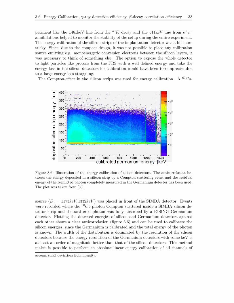
3.6. Energy Calibration, γ-ray detection efficiency, β-decay correlation efficiency 33
periment like the 1461keV line from the 40K decay and the 511keV line from e+e−
annihilations helped to monitor the stability of the setup during the entire experiment.The energy calibration of the silicon strips of the implantation detector was a bit moretricky. Since, due to the compact design, it was not possible to place any calibrationsource emitting e.g. monoenergetic conversion electrons between the silicon layers, itwas necessary to think of something else. The option to expose the whole detectorto light particles like protons from the FRS with a well defined energy and take theenergy loss in the silicon detectors for calibration would have been too unprecise dueto a large energy loss straggling.
The Compton-effect in the silicon strips was used for energy calibration. A 60Co-
Figure 3.6: Illustration of the energy calibration of silicon detectors. The anticorrelation be-tween the energy deposited in a silicon strip by a Compton scattering event and the residual
energy of the reemitted photon completely measured in the Germanium detector has been used.
The plot was taken from [30].
source (Eγ = 1173keV, 1332keV ) was placed in front of the SIMBA detector. Eventswere recorded where the 60Co photon Compton scattered inside a SIMBA silicon de-tector strip and the scattered photon was fully absorbed by a RISING Germaniumdetector. Plotting the detected energies of silicon and Germanium detectors againsteach other shows a clear anticorrelation (figure 3.6) and can be used to calibrate thesilicon energies, since the Germanium is calibrated and the total energy of the photonis known. The width of the distribution is dominated by the resolution of the silicondetectors because the energy resolution of the Germanium detectors with some keV isat least an order of magnitude better than that of the silicon detectors. This methodmakes it possible to perform an absolute linear energy calibration of all channels of
account small deviations from linearity.
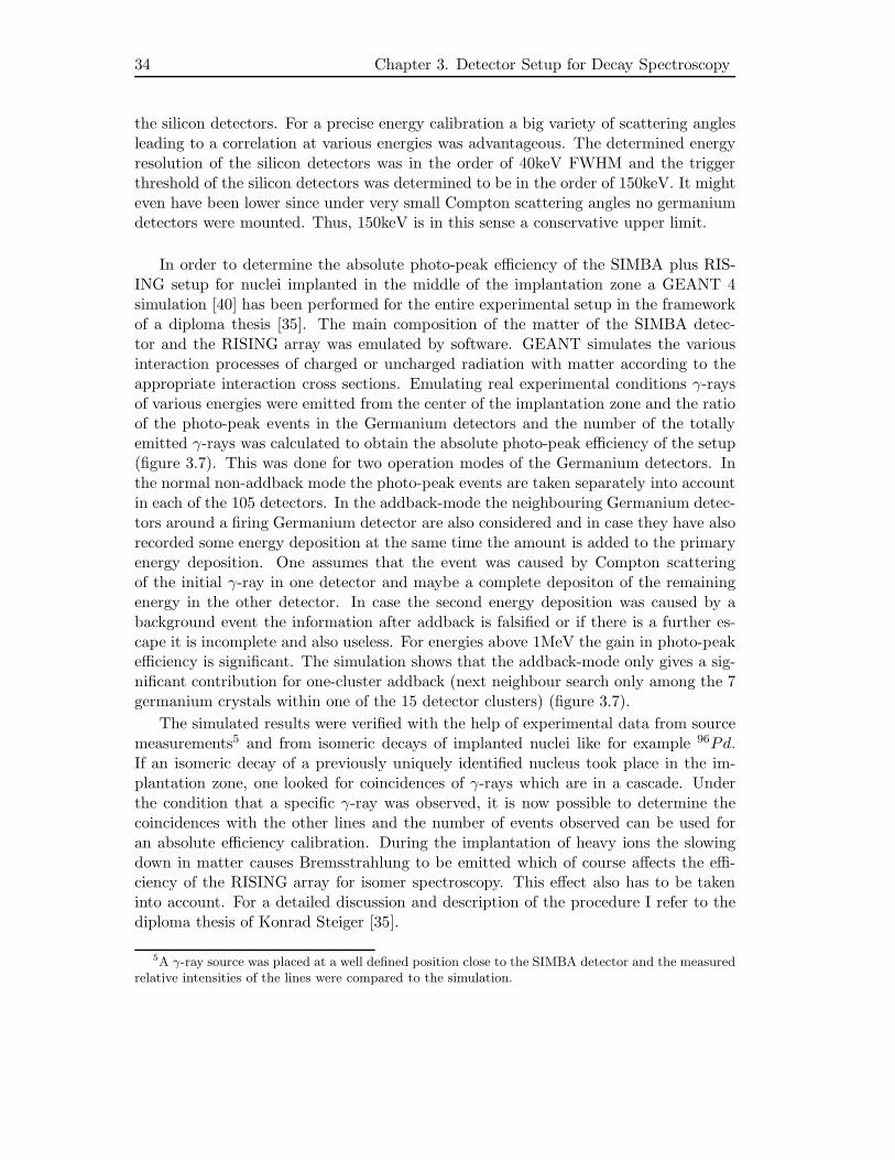
34 Chapter 3. Detector Setup for Decay Spectroscopy
the silicon detectors. For a precise energy calibration a big variety of scattering anglesleading to a correlation at various energies was advantageous. The determined energyresolution of the silicon detectors was in the order of 40keV FWHM and the triggerthreshold of the silicon detectors was determined to be in the order of 150keV. It mighteven have been lower since under very small Compton scattering angles no germaniumdetectors were mounted. Thus, 150keV is in this sense a conservative upper limit.
In order to determine the absolute photo-peak efficiency of the SIMBA plus RIS-ING setup for nuclei implanted in the middle of the implantation zone a GEANT 4simulation [40] has been performed for the entire experimental setup in the frameworkof a diploma thesis [35]. The main composition of the matter of the SIMBA detec-tor and the RISING array was emulated by software. GEANT simulates the variousinteraction processes of charged or uncharged radiation with matter according to theappropriate interaction cross sections. Emulating real experimental conditions γ-raysof various energies were emitted from the center of the implantation zone and the ratioof the photo-peak events in the Germanium detectors and the number of the totallyemitted γ-rays was calculated to obtain the absolute photo-peak efficiency of the setup(figure 3.7). This was done for two operation modes of the Germanium detectors. Inthe normal non-addback mode the photo-peak events are taken separately into accountin each of the 105 detectors. In the addback-mode the neighbouring Germanium detec-tors around a firing Germanium detector are also considered and in case they have alsorecorded some energy deposition at the same time the amount is added to the primaryenergy deposition. One assumes that the event was caused by Compton scatteringof the initial γ-ray in one detector and maybe a complete depositon of the remainingenergy in the other detector. In case the second energy deposition was caused by abackground event the information after addback is falsified or if there is a further es-cape it is incomplete and also useless. For energies above 1MeV the gain in photo-peakefficiency is significant. The simulation shows that the addback-mode only gives a sig-nificant contribution for one-cluster addback (next neighbour search only among the 7germanium crystals within one of the 15 detector clusters) (figure 3.7).
The simulated results were verified with the help of experimental data from sourcemeasurements5 and from isomeric decays of implanted nuclei like for example 96Pd.If an isomeric decay of a previously uniquely identified nucleus took place in the im-plantation zone, one looked for coincidences of γ-rays which are in a cascade. Underthe condition that a specific γ-ray was observed, it is now possible to determine thecoincidences with the other lines and the number of events observed can be used foran absolute efficiency calibration. During the implantation of heavy ions the slowingdown in matter causes Bremsstrahlung to be emitted which of course affects the effi-ciency of the RISING array for isomer spectroscopy. This effect also has to be takeninto account. For a detailed discussion and description of the procedure I refer to thediploma thesis of Konrad Steiger [35].
5A γ-ray source was placed at a well defined position close to the SIMBA detector and the measuredrelative intensities of the lines were compared to the simulation.
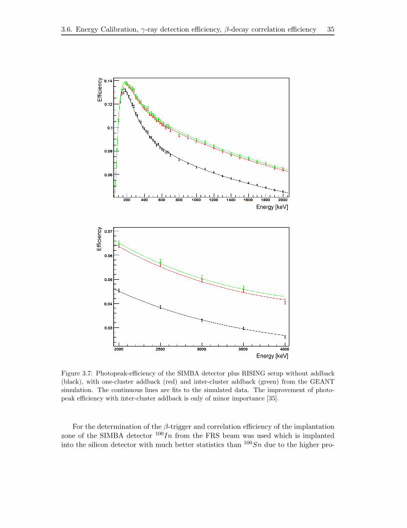
3.6. Energy Calibration, γ-ray detection efficiency, β-decay correlation efficiency 35
Figure 3.7: Photopeak-efficiency of the SIMBA detector plus RISING setup without addback
(black), with one-cluster addback (red) and inter-cluster addback (green) from the GEANT
simulation. The continuous lines are fits to the simulated data. The improvement of photo-
peak efficiency with inter-cluster addback is only of minor importance [35].
For the determination of the β-trigger and correlation efficiency of the implantationzone of the SIMBA detector 100In from the FRS beam was used which is implantedinto the silicon detector with much better statistics than 100Sn due to the higher pro-
36 Chapter 3. Detector Setup for Decay Spectroscopy
duction cross section although it is not directly in the focus. In the daughter nucleus100Cd it is known that all levels populated in the decay of 100In deexcite by passingthrough the 2+ to 0+ transition with an energy of 1004keV [41]. From the observationof the beta feeding of the decay of 100In to high-lying 100Cd states in a total absorptionspectrometer experiment [41] the electron capture fraction could be estimated to beabout 16% in the decay of 100In. Together with the known photo-peak efficiency ofthe SIMBA plus RISING setup and the known number of implanted 100In heavy ionsas well as a suitable correlation time (Tcorel ≈ T1/2 = 5.9s) for the detection of betadecays, it is possible to determine the beta decay trigger and correlation efficiency fromthe intensitiy of the 1004keV line. The obtained correlation efficiency was in the orderof 60%, depending on the exact constraints of the correlation procedure. In order toget a better correlation efficiency it is reasonable to go from a one pixel correlation totwo-dimensional 3x3 pixel correlations around the implantation position. Another stepis a three dimensional 3x(3x3) correlation with the help of the adjacent implantationdetectors which is of course only possible for the implantation detector in the center ofthe implantation zone. For the other detectors a 2x(3x3) solution remains. While thisincreases the correlation efficiency also the background decay rate increases with eachpixel considered for this correlation. In the experiment the average background decayrate per pixel was about 0.0011
s for the 100Sn FRagment Separator setting after theequilibrium between implantations and successive decays of all generations was reached.The background rate was determined by observing the average hit rate of various pixelsover a long time and calculating an appropriate average for the corresponding fragmentseparator setting.
For the β-decay also GEANT simulations have been performed [35]. A simulationof an emitted positron spectrum with an endpoint energy in the order of 3MeV showedthat a significant part of the positrons annihilate before they have completely stoppedand deposited all their energy in the silicon detectors. Consequently a fit applied tothe simulated energy spectrum shows a beta endpoint energy which is about 200keVless than the input value. This systematic deviation also has to be considered whenlooking at the β decay of 100Sn. More details will be discussed in chapter 4.
3.7 Cleaning Cuts for Decay Events
The main purpose of the data preparation for further analysis is the determinationof implantation correlated decay events in time and space with their properties likethe decay time after the implantation, the energy deposition and the shape of particletraces in the beta calorimeter for tracking as well as the accumulation of β-coincidentγ-ray spectroscopy data.The cleaning cuts for the particle identification in implantation events are discussed inthe previous chapter. For the analysis of decay events a few cleaning cuts / constraintswere applied:
3.7. Cleaning Cuts for Decay Events 37
• During the spill light particles like α-nuclei and protons travel along the beamline to the final focus of the fragment separator. They do not deposit enoughenergy in the scintillator in front of the implantation detector and consequentlydo not yield an implantation trigger. In most cases they traverse the implantationdetector stack by triggering a decay event. These events have to be excluded fromdata analysis. This can be done by comparing the entire energy deposition in thebeta absorber stack in front of the implantation zone with the entire energydepositon in the beta absorber stack behind the implantation zone. There is aclear correlation which allows to tag these events and separate them from β-decayswhere the energy depostion is in reasonable cases limited to the beta absorberstack in front of or behind the implantation zone.
• The multiplicity of decay events is limited to three hits per implantation detectorfor each event. This also covers decay events where the positron scatters backonce or twice. The x and y matching in a single detector in the case of several hitevents is done according to the amount of energy deposited in the correspondingstrips. Finally, this procedure yields up to three decay pixels per detector whichare hit with the corresponding energy.
• The rejection of noise in the detector where many single silicon detectors andstrips yield signals above a certain threshold is done by setting appropriate mul-tiplicity conditions and thresholds.
• The analysis of the pattern of hit detectors helps to clean for decay events whichhave their origin not in the implantation zone but in one of the β-absorbersnearby.

38 Chapter 3. Detector Setup for Decay Spectroscopy
Chapter 4
Data Analysis of β-decays
In the case of the observation of β-decays with a detector system, as it was discussedin the last chapter, some principal problems arise. Due to dead time of the data ac-quisition and a β-trigger efficiency which is below 100% there is the possibility that adecay after an implantation may be missed. Maybe only the decay of the daughter isobserved within the correlation time or even no correlated decay is detected.Furthermore the energy distribution of the positrons in the detector is very unspecificin contrast to an α-decay. This means that it is not possible to distinguish decays frombackground decay events, at least at first glance, when no β-tracking is considered.These circumstances lead to the necessity to use a special method for data analysis.Since one does not know exactly what the single events represent which we detect, it isreasonable to make a model of all possible scenarios explaining the observed data. Themodel which fits best i.e. which explains the observed data with the highest probabilitywill be chosen and unknown parameters e.g. for the life time of 100Sn can be extracted.This fundamental idea is the basis of the maximum likelihood analysis which will be in-troduced in general in the first section. Using the maximum likelihood analysis methodalso the information coming from successive decay generations is taken into account. Inthe next section its application for the determination of half lives is discussed and themethod is verified in the decay of 101Sn where the half life is already known. Finally, amaximum likelihood function for the analysis of β-endpoint energies is developed andit is applied to the beta decay spectrum of 102Sn. The beta endpoint energy of thestrongest decay channel is compared to previous measurements.
4.1 Maximum Likelihood Analysis
Given that there are n independent measurements of the probability variable x whichcan be a single variable or a vector of variables, the underlying probability densitydistribution f(x|a) for the measured values x1, x2, ..., xn is known and a represents oneor several unknown parameters on which the probability density distribution depends.The task is now to calculate the most adequate estimation a∗ of the parameter(s) aon the basis of the accumulated measured data. The maximum likelihood method[42], [43], [44] starts from the one- or multidimensional probability density distributionfunction f(x|a) of the measured values x and forms the likelihood function of the
40 Chapter 4. Data Analysis of β-decays
stochastical independent measurements1.
L(a) = f(x1|a) · f(x2|a) · · · f(xn|a) =
n∏
i=1
f(xi|a) (4.1)
The function L(a) is, for a given sample xi, a function of the parameter(s) a andyields the probability for a given choice of the parameter(s) a to obtain just the mea-sured values the data sample consists of. It is important to point out that L(a) is inprinciple no probability density in the parameter(s) a. According to the maximum like-lihood principle the most adequate estimation of the unknown parameter(s) a is/are thevalue(s) a∗ which maximize(s) L(a) i.e. which maximize(s) the probability to obtainin an observation just the recorded sample of the values xi of the probability variable.Thus the maximum likelihood condition is
L(a) = maximum. (4.2)
It is important to ensure that f(x|a) is normalized to 1 for all values of a. Thisnormalization has to be preserved during all steps of the variation of a to find themaximum of the function L(a).
∫
all possiblexf(x|a)dx = 1 ∀ a (4.3)
It is common to work with the logarithm of the likelihood function L(a). Becausethe logarithm is a monotonous function the new function has its maximum at the sameposition as the original one. The condition for the maximum can be written in thefollowing way in case the parameter a is one-dimensional which is the assumption fromnow on.
l(a) = lnL(a) =n∑
i=1
lnf(xi|a) = maximum ⇐⇒ dl(a)
da
∣∣∣∣amax
= 0 ;d2l(a)
da2
∣∣∣∣amax
< 0
(4.4)
A possible way of finding the solution is carrying out the first differentiation andmaybe also the second differentiation as a verification of the kind of local extremum.Since the equations are in most cases non-linear a numerical solution with the help ofcomputers has to be obtained. In the case the maximum is located at the border of theparameter space for a other methods have to be considered which are not discussed inthe framework of this thesis [43], [44].
The most adequate estimations a∗ of the parameter(s) a for different data samplesare themselves probability variables with a certain distribution. Different samples lead
1It is an important constraint of this method that the probability density distribution which is usedis an accurate a priori mathematical description of the physical system the data sample is taken fromotherwise the results obtained may be wrong.

4.1. Maximum Likelihood Analysis 41
to different likelihood functions and thus to different estimators. Of course not onlythe values a∗ are important but also their statistical errors which depend in generalon the size of the measured data sample. Uncertainties in the shape of the probabilitydensity distribution functions lead to a systematic error in the calculated parameter(s)a∗.In order to calculate the statistical error of the estimator a∗ we start from the generalcase. Let us assume a continuous probability variable x which behaves according to theprobability density distribution f(x). Then the expectation values of arbitrary functionsh(x) are defined in the following way:
E[h] =
∫ +∞
−∞
h(x)f(x)dx (4.5)
The probability density distribution can be completely characterized by its so calledmoments h(x) = xn n = 1, 2, ..., among them the most important are the meanvalue < x >= E[x] and the variance V [x] = E[(x− < x >)2] or standard devia-tion σ[x] =
√
V [x] to determine location and width of the distribution.
In order to determine the statistical error of the best estimator a∗ for a measuredsample of values x1, x2, ..., xn of the probability variable x the likelihood function isinterpreted as a probability density distribution in a. For the variance the follow-ing formula can be determined in a trivial way when considering that L has not yetbeen normalized on the parameter space for a. a∗ is the best estimation which wascalculated from the current data sample. Again we assume that the parameter a isone-dimensional.
V [a∗] =
∫(a− a∗(x1, x2, .., xn))2L(x1, x2, .., xn|a)da
∫L(x1, x2, .., xn|a)da
(4.6)
For large data samples it is not necessary to evaluate formula (4.6) directly becauseit can be shown that the likelihood function converges to a normal distribution in theregion of the maximum i.e. in the region of the best estimator for the parameter a.A Taylor expansion of the logarithmic likelihood function l(a) around the maximumis done in equations (4.7), (4.8) for the one-dimensional case in which the probabilitydensity distribution only depends on one parameter a.
l(x1, ..., xn|a) = l(x1, ..., xn|a∗)︸ ︷︷ ︸
=lmax
+ (a− a∗)∂l
∂a
∣∣∣∣a=a∗
︸ ︷︷ ︸
=0
+1
2(a− a∗)2
∂2l
∂a2
∣∣∣∣a=a∗
+ ... (4.7)
l(x1, ..., xn|a) ≈ lmax −1
2(a− a∗)2V −1[a∗] ⇒ L(x1, ..., xn|a) ≈ Lmax · e−
1
2(a−a∗)2V −1[a∗]
(4.8)Of course the first derivative vanishes. When we neglect terms of higher order and
go back to the usual logarithmic likelihood function a comparison of the exponent of
42 Chapter 4. Data Analysis of β-decays
the exponential-function with the normal distribution shows that the variance of thedistribution at the location of its maximum is given by the second derivative of thelogarithmic likelihood function with respect to the parameter a.
σ2(a∗) = V [a∗] =
(∂2lnL(x1, ..., xn|a)
∂a2
∣∣∣∣a=a∗
)−1
(4.9)
Due to the normal distribution it is an easy task to make a numerical estimationof the uncertainty of the estimator a∗. With a significance level of s = 1σ, 2σ, 3σ corre-sponding to 68.3%, 95.4% and 99.8% probability the true value of a∗ is located betweenthe values a where the logarithmic likelihood function has decreased to l(a) = lmax− s2
2from its maximum.
The following list gives an overview of the, in many respects, optimal properties ofthe maximum likelihood method [43], [44]:
• The estimation is consistent i.e. for large samples (n independent measure-ments) the estimation of the parameters(s) a∗ corresponds to the actual value:limn→∞ a∗ = aTRUE
• In an asymptotic manner for large samples the estimation is not distorted i.e. theexpectation value of the distribution E[a∗] of different data samples correspondsto the true parameter of the distribution: limn→∞E[a∗] = aTRUE
• The maximum likelihood estimator is asymptotically efficient i.e. the estimatedparameters have a minimal variance. At least for large samples no other estimatoris more precise: limn→∞V [a∗] = minimum
• The estimation is independent of the representation of the parameters. Thetransformation of parameters has no effect on the result.
• The estimation is sufficient. This means that all the information available fromthe sample related to the parameters a is used. This is especially important forlow statistics data. In the 100Sn case not only observed mother decays but alsodaughter decays and granddaughter decays yield valuable information about thehalf life of the mother.
Despite the good properties of the method the choice of an accurate probability den-sity distribution is crucial. The maximum likelihood estimation is not robust againstwrong assumptions. A common method to verify the consistency of the analysis is toprepare random data samples with a Monte Carlo simulation for various values of theparameter(s). These data samples should then be analysed with the maximum likeli-hood method and the result of the estimation of the parameter(s) should correspondto the input values of the Monte Carlo simulation with respect to the statistical errorbars.This point will be discussed again later in this chapter.
4.1. Maximum Likelihood Analysis 43
4.1.1 Example: Radioactive Decay
A very simple case and a good example for the application of the maximum likelihoodmethod is the radioactive decay of an α-source where the decay can be clearly taggeddue to the large monoenergetic energy deposition and a fictional detector efficiency of100%. A confusion with daughter decays or background decays is precluded.The radioactive decay is described by the well-known differential equation ∂N(t)
∂t =−λ ·N(t) which connects the decay rate of nuclei with the number of still not decayednuclei N(t) multiplied by a constant λ representing the decay probability. With thehelp of the solution of the differential equation N(t) = Nt=0 · e−λ·t it is easy to derive aprobability density distribution which is of course correctly normalized for all possiblevalues of the parameter λ. The probability that a decay happens between t = 0 andt > 0 is F (t|λ) = 1 − e−λ·t. The probability density that the decay happens between tand t + dt is f(t|λ) = λ · e−λ·tdt. The only free parameter of this probability densitydistribution is the decay probability λ = 1/τ . The density function f(t|λ) is properlynormalized to 1 for all possible values of the parameter λ:
∫∞
0 f(t|λ)dt = 1.The data sample consists of n decays which take place at the times ti with i = 1, ..., n.The corresponding likelihood function is given in equation (4.10).
L(t1, ..., tn|τ) =n∏
i=1
1
τe−ti/τ ⇒ l(t1, ..., tn|τ) =
n∑
i=1
(
−lnτ − tiτ
)
(4.10)
The search for the maximum of L results in the maximum likelihood estimator τ∗
of the lifetime τ .
∂l
∂t=
n∑
i=1
(
−1
τ+tiτ2
)
= 0 ⇒ τ∗ =1
n
n∑
i=1
ti∂2l
∂τ2
∣∣∣∣τ=τ∗
= − n
τ∗2< 0 (4.11)
The best estimation of the lifetime is the arithmetical mean of the measured decaytimes (4.11). This fact is especially interesting in the case of low statistics where nodirect fit of an exponential function to the measured values is possible due to the lowstatistics.As a side note, for a large amount of normal distributed events it is also possible to solvethe likelihood equation for the bin-contents of a histogramm. This leads, as a specialcase of the maximum likelihood method, to the usual fitting routine which minimizesthe square deviation χ2 between the fit function and the histogramm [45].Finally, the variance of the estimator (4.9) is given in formula (4.12). The standarddeviation is proportional to the reciprocal of the root of the number of values obtainedin the measurement.
σ2(τ∗) = V [τ∗] =
(∂2lnL
∂τ2
∣∣∣∣τ=τ∗
)−1
⇒ σ =τ√n
(4.12)
44 Chapter 4. Data Analysis of β-decays
4.2 Determination of half lives
Due to the lack of a unique signature of β-decays it is necessary to assign implantationsto successive decays with the help of a spatial correlation and a correlation in time.This method yields the problem that some decays may not be correlated due to effi-ciency reasons and the decays observed may also origin from daughter, granddaughteror uncorrelated background decays as was already discussed at the beginning of thischapter.Since the decays which occur during the correlation time are not statistically indepen-dent anymore, a more complex likelihood function has to be constructed. This will bediscussed on the following pages. For this thesis the principle method was used, thatwas developed by Andreas Stolz in the framework of the data analysis concerning the100Sn experiment from 1998 [17].The method is valid for correlation times which are short enough so that almost allrecorded events yield at most up to three decay events in the correlation time. Theanalysis is based on the assumption that in the selected time- and space-window of theimplantation of a uniquely identified nucleus only decay events of the first three gener-ations (mother-, daughter- and granddaughter-decays) or random background decaysoccur.The ingredients for the construction of the correct probability density distribution areas follows:λ1,λ2,λ3 denote the decay constants of the mother-decay, the daughter-decay and thegrandson-decay.The probability that a decay with the decay constant λ1 occurs in an interval betweenthe time t = 0 and t is given as F1(λ1, t) and the corresponding probability densitydistribution that the decay occurs between time t and t+dt with dt → 0 can be writtenas f1(λ1, t).
F1(λ1, t) = 1 − e−λ1t ; f1(λ1, t) =∂F1(λ1, t)
∂t= λ1 · e−λ1t (4.13)
For the observation of the second decay generation the probability to find a daughterdecay F2(λ1, λ2, t) with decay constant λ2 in the interval between the time t = 0 andt which was populated before by the mother decay with decay constant λ1 can bededuced from the solution of the two coupled differential equations ∂N1
∂t = −λ1N1 and∂N2
∂t = λ1N1 − λ2N2 where N1 denotes the particle number of not yet decayed mothernuclei and N2 denotes the particle number of not yet decayed daughter nuclei. Theprobability density distribution f2(λ1, λ2, t) of a daughter decay with decay constant λ2
taking place between time t and t+ dt with dt→ 0 which was populated by a motherdecay with decay constant λ1 is again the derivative.
F2(λ1, λ2, t) = 1− λ1λ2
λ2 − λ1
[1
λ1e−λ1t − 1
λ2e−λ2t
]
; f2(λ1, λ2, t) =∂F2(λ1, λ2, t)
∂t(4.14)
For the corresponding functions F3(λ1, λ2, λ3, t) and f3(λ1, λ2, λ3, t) for the granddaughter-decay it is explicitly referred to the work of A. Stolz [17] which are also presented in
4.2. Determination of half lives 45
the appendix of this thesis.The background decays during the correlation time are known from the analysis of thedata as average decay rate per pixel and the probability of observing a certain numberof events during the correlation time obeys the Poisson-statistics. For a backgrounddecay rate b the probability Br to observe exactly r background events during thecorrelation time tC is given in formula (4.15).
Br =(b · tC)r · e−b·tC
r!(4.15)
Depending on the number of observed decay events (0,1,2,3) during the correlationtime all possible scenarios have to be considered which could have caused the datasample as it was observed.For simplicity of describing the individual scenarios some abreviations are introduced:Di represents the probability that a decay of the generation i = 1, 2, 3 takes place,Oi represents the probability that a decay of the generation i = 1, 2, 3 is observed.ǫ1,ǫ2,ǫ3 are the efficiencies of the detector and data acquisition for the correspondingdecays to be observed. The general efficiency for e.g. detecting β-decays also has to becorrected by the individual electron capture fraction of each nucleus. The probabilityof the inverted event2 is denoted with F (λ, t) = 1−F (λ, t) and the same applies to theefficiency ǫ = 1 − ǫ.The probability of observing no event P0(λ1) during the correlation time is relativelyeasy to deduce3: There is the possibility that a mother decay does not take place or ittakes place but is not observed and a daughter decay does not take place. The nextscenario has a mother and daughter decay which take place but are not observed anda grandson decay does not take place. Finally all three decays take place within thecorrelation time but none of them is observed. The sum of these probabilities has to bemultiplied with the stochastical independent probability of no background event takingplace during correlation time.
P0(λ1) = (D1 +D1O1D2 +D1O1D2O2D3 +D1O1D2O2D3O3) · B0 (4.16)
P0(λ1) =[F 1(λ1, tC) +
(F 2(λ1, λ2, tC) − F 1(λ1, tC)
)· ǫ1 +
(F 3(λ1, λ2, λ3, tC)−
F 2(λ1, λ2, tC))· ǫ1ǫ2 + F3(λ1, λ2, λ3, tC) · ǫ1 · ǫ2 · ǫ3
]·B0 (4.17)
If only one decay event is observed during the correlation time tC at the time t1four scenarios are possible:(1) The first possibility is that the mother decay takes place and is observed, daughterand grandson do not decay or are not observed, no background decay takes place.
2The probability that the event does not occur3λ1, the decay constant of the mother nucleus, is finally the parameter of interest to be determined.
Thus the only free parameter in P0 is λ1.
46 Chapter 4. Data Analysis of β-decays
The formula for the probability is written in equation (4.18) and the correspondingprobability density distribution is given in equation (4.19). The probability densitydistribution is not yet properly normalized, therefore the normalization constant C1
is multiplied. For the composition of the likelihood function the probability densitydistributions for a decay event taking place at the time t1 instead of the probabilitiesfor a decay event taking place between time t = 0 and t1 are necessary.
P1⌣01 = D1O1 ·(D2 +D2O2D3 +D2O2D3O3
)· B0 (4.18)
p1⌣01(λ1) = C1 ·f1(λ1, t1)·ǫ1 ·[F 1(λ2, tC − t1) +
(F 2(λ2, λ3, tC − t1) − F 1(λ2, tC − t1)
)
·ǫ2 + F2(λ2, λ3, tC − t1) · ǫ2 · ǫ3] · B0 (4.19)
(2) In the second scenario the mother decay and daughter decay take place duringthe correlation time, but only the daughter decay is observed. The grandson decaytakes place and is not observed or it does not take place. No background decay isobserved.
P1⌣02 = D1O1D2O2 · (D3 +D3O3) ·B0 (4.20)
p1⌣02(λ1) = C1 · f2(λ1, λ2, t1) · ǫ1ǫ2 ·[F 1(λ3, tC − t1) + F1(λ3, tC − t1) · ǫ3
]·B0 (4.21)
(3) In the third scenario three decays of all three generations take place but only thegrandson decay is observed and no background decay takes place during the correlationtime.
P1⌣03 = D1O1D2O2D3O3 · B0 (4.22)
p1⌣03(λ1) = C1 · f3(λ1, λ2, λ3, t1) · ǫ1 · ǫ2 · ǫ3 ·B0 (4.23)
(4) The last possible scenario with one decay event during the correlation time isthe observation of a background decay whereas the mother, daughter and grandsondecays do not take place or do take place and are not observed.
P1⌣04 = (D1 +D1O1D2 +D1O1D2O2D3 +D1O1D2O2D3O3) · B1 (4.24)
p1⌣04(λ1) = C1 ·[F 1(λ1, tC) +
(F 2(λ1, λ2, tC) − F 1(λ1, tC)
)· ǫ1 +
(F 3(λ1, λ2, λ3, tC)−
F 2(λ1, λ2, tC))· ǫ1 · ǫ2 + F3(λ1, λ2, λ3, tC) · ǫ1 · ǫ2 · ǫ3
]· B1 · t−1
C (4.25)
4.2. Determination of half lives 47
The joint probability density distribution function for one observed decay event atthe time t1 is the sum of the four single probability density distributions (4.26).
p1(λ1) = p1⌣01(λ1) + p1⌣02(λ1) + p1⌣03(λ1) + p1⌣04(λ1) (4.26)
The normalization constant C1 has to be determined so that the integral of theprobability density distribution over the region where t1 is defined yields 1.
∫ tC
0p1(λ1)dt1 = 1 (4.27)
In the case of two decay events happening during the correlation time at t1, t2 it isnecessary to distinguish 10 different scenarios. The observation of three decay eventsat t1, t2, t3 yields 20 possible scenarios which could have lead to the observed data. Fora formalized description of the different scenarios and the normalized joint probabilitydensity distribution functions p2(λ1) and p3(λ1) the reader is referred to the work ofA. Stolz [17] and the formulas in the appendix of this thesis.Taking 0, 1, 2, 3 decay events during the correlation time into account the likelihoodfunction which has to be maximized with respect to the parameter λ1 can be writtenin the following way:N0 is the number of events where no decay occured during the correlation time.
L0,1,2,3(λ1) = P0(λ1)N0 ·
∏
all decay chains1 event
p1(λ1)∏
all decay chains2 events
p2(λ1)∏
all decay chains3 events
p3(λ1)
(4.28)
From equation (4.28) the best estimation of the unknown parameter, the decay con-stant of the mother λ1, can be calculated by solving the following differential equationas written in formula (4.4).
∂L0,1,2,3(λ1)
∂λ1= 0 (4.29)
It is important that the length of the correlation time tC is chosen in a reasonableway to avoid the observation of more than three decay events during the correlationtime. Otherwise the maximum likelihood method would lead to wrong results since theprobability density distribution does not support this scenario.For a large number of decay chains the probability distribution around the maximumresembles a gaussian distribution. The statistical uncertainty of the decay constantwith a confidence level of 68.3% can be determined as the 1σ-width of the gaussiancurve. This has been already discussed in the last chapter.
The verification of the applicability of the whole method with the various probabilitydensity distributions to evaluate decay chains can be done with the help of a Monte-Carlo-Simulation [44], [14], [17]. The decay times of the decay events are generatedwith a simulation program taking into account the known lifetimes of daughter-decay

48 Chapter 4. Data Analysis of β-decays
and granddaughter-decay, the individual detection efficiencies as well as the backgrounddecay rate. The half life of the mother nucleus can be chosen arbitrarily and finally theinput value of the half life of the mother is compared to the output of the analysis ofthe simulated decay chains done with the maximum likelihood method. For the currentanalysis with a maximum of three decays in the correlation time it was shown that e.g.for a decay simulation of 102Sn the arbitrary input value of the half life between oneand ten seconds of the mother is accurately reproduced within the statistical uncer-tainties without systematic deviations in the maximum likelihood analysis (see figure4.1) [17]. In these simulations it turned out that the limits to obtain accurate resultsare correlation times tC which are not much shorter than 5 ·T1/2 of the mother nucleus.Very high background decay rates of b > 0.1/s in combination with long half lifes ofthe mother T1/2 > 5s are also a limiting constraint of the maximum likelihood methodto obtain reasonable results.
Figure 4.1: Comparison of the half life calculated with the maximum likelihood method with
the input value from a Monte-Carlo simulation to generate decay chains. For the detector
efficiencies and background decay rates the same values were chosen as for the real analysis of
the decay data for 102Sn. [17]
4.2. Determination of half lives 49
4.2.1 Test case: 101Sn
Another important procedure to test the reliability of the maximum likelihood analysiswith its probability density distributions for the various scenarios is the determinationof the half life and its statistical error for an already well known nucleus which is alsoimplanted into the implantation detector in the 100Sn fragment separator setting withgood statistics. The half life of this nucleus should in the ideal case be similar to theexpected half life of 100Sn which is about 1 second.This test is also crucial because the analysis assumes an average, not time dependent,detection efficiency. This is only an approximation. In reality, the data acquisition hasa dead time of 25% during the spill (1 second) and during the spill free time (2 sec-onds) the dead time is negligible. This periodical modulation should only significantlyinfluence the efficiency for the detection of decays with a very short half life where thenucleus still decays during the spill. Any severe systematic errors in the determinationof the correlation efficiency or the background decay rate should also become obvious.For the test 101Sn was chosen for which the latest half life measurement with the small-est uncertainty is 1.9+0.3
−0.3s [46].The configuration of the correlation finder was set to a spatial two dimensional windowwith the pixel-size 1x(3x3). The two dimensional window was chosen to be able to dis-tinguish in a convenient way the β+ beta delayed proton events from pure beta decaysby the energy deposition in the decay pixel. The beta decay detection efficiency4 was45% in this configuration. Decays containing beta delayed protons were not consideredin the correlation procedure since the exact efficiency of the detector for proton decaysis not known. The correlation time was set to 15 seconds.The maximum likelihood analysis was fed with the decay data of 400 101Sn implan-tations. In 196 cases no decay event or only a beta delayed proton decay event wasobserved within 15 seconds after the implantation event. 139 events yielded one corre-lation event, 49 events had two correlation events, 16 events contained three correlationevents and four correlation events did not occur in the data sample. The backgrounddecay rate in this analysis for the applied two dimensional window was 0.01 events/s.26% of the 101Sn nuclei decay with a beta delayed proton emission [46]. This numberwas extracted in a comparison of the experimental proton energy spectrum with cal-culations assuming a 5/2+ ground state in 101Sn. The uncertainty of this number ishard to estimate. Other parameters which were taken from literature are the half lifeof the daughter 101In with 15.1 seconds and the half life of the granddaughter decay of101Cd with 81.6 seconds [47]. The electron capture fraction for 101Cd is 25.6% [47]. For101Sn and 101In an estimated value of 20% was assumed since no information aboutpopulated excited states in the decay is known.The final result of the maximum likelihood analysis with a significance level of 68% is2.0+0.4
−0.3s. This result is in good agreement with previous measurements. The uncer-tainty in the electron capture fraction for mother and daughter decays was treated asa 5% deviation from 20%. With these systematic deviations the maximum likelihoodmethod still yielded a value of the half life lying well within the statistical error.
4electron capture is not included
50 Chapter 4. Data Analysis of β-decays
4.3 Determination of beta-endpoint energies
A spectrum of the energy distribution of emitted β-particles after the decay of a cer-tain nucleus can be constructed by following the uninterrupted tracks of non-escapingparticles through the detector matter and by summing up the amount of their totalenergy loss.In order to analyse such a spectrum some useful information can be extracted from themaximum likelihood analysis of the unknown lifetime. Once a best fit value of the halflife is obtained it is possible to determine for each decay event the probability that itsorigin was a mother decay, a daughter decay, a grandson decay or a background decay.The spectrum can then be filled under the condition that it contains with a certainprobability mother decays, daughter decays and so on. Of course the probability of thedecays in the data sample to be a mother decay should be as high as possible. But withincreasing purity of the spectrum the statistics is reduced. The best way to analyse theresultant β-spectrum in case of low statistics is again the maximum likelihood methodand its application to a β-spectrum is outlined below.The energy distribution of the emitted β-particles for an allowed β-decay with themaximal emitted energy Ekin0
populating a single final state can be written as shownin formula (4.30) [48], [49].
p(ǫ, ǫ0)dǫ = C ·√
ǫ2 − 1 · ǫ · (ǫ0 − ǫ)2 · F (Z ′, ǫ)dǫ with ǫ =Ekin
mec2+ 1 (4.30)
C =
(∫ ǫmax
ǫmin
√
ǫ2 − 1 · ǫ · (ǫ0 − ǫ)2 · F (Z ′, ǫ)dǫ
)−1
(4.31)
The normalization constant C helps to obtain the correct probability density dis-tribution which states the probability that the energy Ekin of an emitted beta particlelies at a certain point in the interval between 0 ≤ Ekinmin
and Ekinmax≤ Ekin0
. Thelimits on both sides can be adjusted to cover only the centroid of the energy spectrumneglecting the low and high energy part. This can be reasonable if events which mighthave their origin in e.g. background decays should not have a too strong influence onthe result of the maximum likelihood method. For example a single high energy eventwill significantly shift the result towards high energies. For negative energies as well asfor energies above Ekin0
the probability density is defined to be zero.Z ′ denotes the nuclear charge of the daughter nucleus. The Fermi-function F (Z ′, ǫ)considers the perturbation of the electron/positron wave function caused by the nu-clear charge and can be approximately written as given in formula (4.32) [49]. It isonly a small correction to the general characteristics of the spectrum determined bythe shape of the available phase space for the decay.
F (Z ′, ǫ) ≈ 2πν
1 − e−2πνwith ν = ∓Z ′α
ve/cfor β± (4.32)
Here, α = 1/137.0388 represents the fine structure constant and ve is the velocityof the emitted electron/positron with the total energy ǫ.
4.3. Determination of beta-endpoint energies 51
The entire maximum-likelihood function can now be constructed in a simple way. Fora decay event all possible decay channels have to be considered i.e. the branching ratioof the mother decay to all possible final states, the same for the daughter nucleus andso on. The theoretical function (4.33) consists of a sum of normalized distributionfunctions p(ǫ, ǫ0) for each decay branch which are weighted according to their knownbranching ratios.
pdecayevent(ǫ, ǫ0)dǫ = D·
(
fm ·n∑
i=1
bmi · p(ǫ, ǫ0 +Oi)
)
+
fd ·m∑
j=1
bdj · p(ǫ, ǫ0 j)
+ ...
dǫ
(4.33)
D =
∫ ǫmax
ǫmin
(
fm ·n∑
i=1
bmi · p(ǫ, ǫ0 +Oi)
)
+
fd ·m∑
j=1
bdj · p(ǫ, ǫ0 j)
+ ...
dǫ
−1
(4.34)D is the normalization constant for the whole function, fm and fd are the percentage
of the mother and daughter fraction of the decay events in the spectrum with fm +fd + .... = 1, the incomplete sum indicates the optional consideration of granddaughterdecays and background decays. bi is the fraction of a certain decay branch to an excitedstate in the corresponding daughter nucleus with
∑ni=1 bi = 1. n is the number of all
decay branches, the fraction bi has to be corrected for electron capture decays whichare not visible in the spectrum. If the relative energy differences of the populated levelsin the mother decay are known from e.g. γ-spectroscopy the only unknown parameterin the mother decay which remains is the beta endpoint energy ǫ0 of one arbitrary level.It is reasonable to choose the strongest level which is populated since it dominates thespectrum. The endpoint energies of the other levels can be expressed with the relativeenergy offset parameters Oi.The likelihood function for the data sample of measured decay energies ǫ1, ..., ǫN canthen be written in the following way.
L(ǫ0) =
N∏
i=1
pdecayevent(ǫi, ǫ0) (4.35)
The likelihood function (4.35) which has to be maximized consists of the productof the probability density distributions pdecayevent(ǫ, ǫ0). The position of the maximumof this function yields the most probable value of the beta endpoint energy ǫ0. Thedetermination of the uncertainty is done in an analogous way as described before inthis chapter.
4.3.1 Test case: 102Sn
In order to verify the analysis method for the determination of β-endpoint energiesand the calorimetry of β-decays in the implantation detector the β-decay of 102Sn was
52 Chapter 4. Data Analysis of β-decays
chosen as a test case. 102Sn is implanted in the detector with good statistics. Un-fortunately, the centroid of the spatial distribution is shifted to the left side of theimplantation zone in beam direction which is due to the optimization of the fragmentseparator setting for 100Sn. The decay positrons are then in most cases emitted fromthe edge of the implantation area which makes escapes of the positrons with incompleteenergy deposition much more likely. The influence of this effect on the β-spectrum andthe β-endpoint energy is studied with the help of a GEANT simulation and will bediscussed later.Nevertheless, 102Sn is an ideal test case since a lot of information was already obtainedfor this nucleus. In the most recent publication from 2006 the β-endpoint energyof the strongest level which is populated in the daughter nucleus was measured to be3.19±0.10MeV and beta coincident γ-ray spectroscopy revealed a detailed level schemeof the excited states in the daughter nucleus and their relative population probabilityin the decay [50].
In a sample of β-decays taking place after 102Sn implantations which were recordedin the 100Sn fragment separator setting as a by-product it was possible to reconstruct338 uninterrupted tracks and sum up the deposited energies (see figure 4.2). Since thehalf life of 102Sn is 3.8± 0.2s [17] a correlation time which was set to one second of thedetector accepting decays after previous implantations yields, apart from 102Sn-decays,almost no contribution of daughter decays (102In-half life T1/2 = 22.1s [47]) and only acertain number of background decays. In order to get rid of a possible influence of thenon-dominant background contribution in the order of 5-10% it is reasonable to neglectthe low and high energy counts in the spectrum and to concentrate on the centroidof the energy distribution between 200keV and 2300keV for the maximum likelihoodanalysis.
In the maximum likelihood fit a multi-component probability density distributionwas used incorporating all final states which are populated in the daughter nucleus102In. The only free variable with respect to which the maximum likelihood functionof the data sample was maximized is the β-endpoint energy E0 of the strongest decaybranch populating an excited state in the daughter nucleus with an energy of 1546keV(table (4.1)).
The maximum likelihood analysis of the data sample yielded a result of E0 =2.78 ± 0.08MeV . At first glance this value seems not to be consistent with the expec-tation of 3.19 ± 0.10MeV .
For further investigation a GEANT simulation of β-decays was performed for the en-tire detector setup for a beta decay into a single final state with an endpoint energy of3.2MeV [35]. The input included a realistic spatial implantation position distribution ofthe 102Sn heavy ions i.e. the positions where the decay positrons were emitted are in ac-cordance with the recorded experimental data. The energy of the emitted positrons wasrandomly chosen, obeying the correct probability distribution of a single-componentbeta decay energy spectrum and the emission direction was isotropic. After selecting
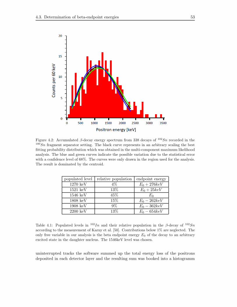
4.3. Determination of beta-endpoint energies 53
Figure 4.2: Accumulated β-decay energy spectrum from 338 decays of 102Sn recorded in the100Sn fragment separator setting. The black curve represents in an arbitrary scaling the bestfitting probability distribution which was obtained in the multi-component maximum likelihood
analysis. The blue and green curves indicate the possible variation due to the statistical error
with a confidence level of 68%. The curves were only drawn in the region used for the analysis.
The result is dominated by the centroid.
populated level relative population endpoint energy
1270 keV 4% E0 + 276keV
1521 keV 13% E0 + 25keV
1546 keV 45% E0
1808 keV 15% E0 − 262keV
1908 keV 9% E0 − 362keV
2200 keV 13% E0 − 654keV
Table 4.1: Populated levels in 102In and their relative population in the β-decay of 102Sn
according to the measurement of Karny et al. [50]. Contributions below 1% are neglected. Theonly free variable in our analysis is the beta endpoint energy E0 of the decay to an arbitrary
excited state in the daughter nucleus. The 1546keV level was chosen.
uninterrupted tracks the software summed up the total energy loss of the positronsdeposited in each detector layer and the resulting sum was booked into a histogramm
54 Chapter 4. Data Analysis of β-decays
event-by-event (see figure 4.3). In the interval between 200keV and 2300keV a one-component maximum likelihood analysis was performed on the complete spectrum.The simulation was done for 10000 decay events.
Due to an incomplete energy deposition of escaping positrons being caused by thedisplaced implantation position the β-spectrum is shifted to lower energies and theβ-endpoint energy is reduced by 0.17 MeV. Another contribution of 0.20 MeV which re-duces the observed endpoint energy comes from emitted Bremsstrahlung of the positronsand from annihilation in flight with incomplete energy deposition. Finally, a value of2.83 ± 0.02MeV was obtained.This result is in good agreement with the result of the analysis of the experimental β-spectrum - the beta endpoint energy E0 = 2.78±0.08MeV obtained from the observed102Sn decays for the most dominant decay branch to the 1546keV level.For the further analysis of 100Sn-decays only the systematic error resulting from theemitted Bremsstrahlung and the annihilation in flight has to be considered when de-termining the β-endpoint energy. Of course the magnitude of this effect is energydependent and has to be simulated for the individual experimentally observed energydistribution. The correction for an off center implantation is not important for 100Snsince its distribution was focused to the middle of the implantation zone in x and y.
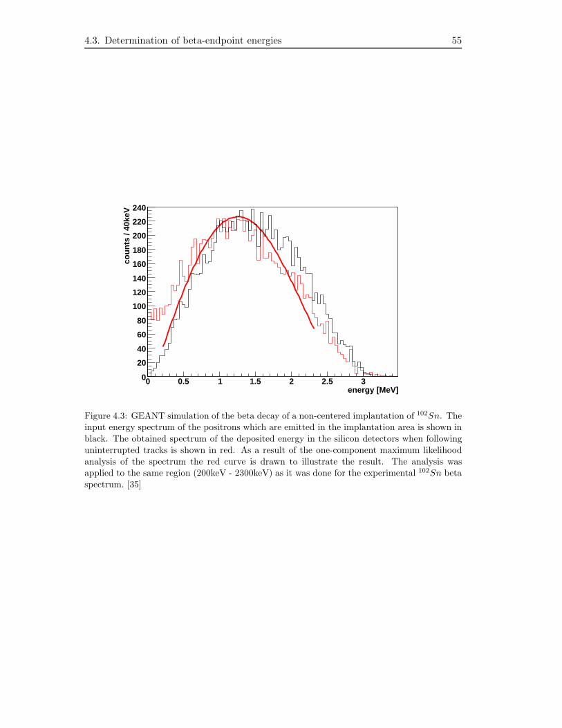
4.3. Determination of beta-endpoint energies 55
fit_mlh_beta_trackEntries 10000Mean 1.291RMS 0.6725
energy [MeV]0 0.5 1 1.5 2 2.5 3
cou
nts
/ 40
keV
0
20
40
60
80
100
120
140
160
180
200
220
240
fit_mlh_beta_trackEntries 10000Mean 1.291RMS 0.6725
Figure 4.3: GEANT simulation of the beta decay of a non-centered implantation of 102Sn. Theinput energy spectrum of the positrons which are emitted in the implantation area is shown in
black. The obtained spectrum of the deposited energy in the silicon detectors when following
uninterrupted tracks is shown in red. As a result of the one-component maximum likelihood
analysis of the spectrum the red curve is drawn to illustrate the result. The analysis wasapplied to the same region (200keV - 2300keV) as it was done for the experimental 102Sn beta
spectrum. [35]

56 Chapter 4. Data Analysis of β-decays
Chapter 5
Results obtained in theSpectroscopy of 100Sn
In a beamtime of 15 days 259 100Sn nuclei were successfully identified. Approximately160 of these exotic nuclei were implanted into the implantation detector without de-struction and could thus be used for further decay spectroscopy. In the followingsections the results of the analysis of the β-decay of 100Sn consisting of a new halflife measurement, the γ-ray spectroscopy of the excited states in the daughter nucleus100In and the β-calorimetry of emitted decay-positrons are discussed. Furthermore thequestion of the existence of an isomeric state in 100Sn is addressed.
5.1 Half life T1/2
Decay data were extracted with a maximum correlation time of 15 seconds after 100Snimplantations and analysed with the maximum likelihood method, that was discussedin the previous chapter.During this correlation time it was possible to assign 126 decay chains detected in athree dimensional 3 x(3 pixel x 3 pixel) window to the 163 previous 100Sn implantations.In 37 cases there were no decays dectected after an implantation. In 65 cases therewas one event during the correlation time, 38 decay chains yielded two decay events,22 decay chains yielded three decay events, and four decay events occurred only in onecase. The average uncorrelated background decay rate for the chosen spatial correlationwindow was b = 0.03s−1. The detection efficiency for decays is composed of the generaldetection efficiency1 for β-decays of the implantation detector which was 60% in thisconfiguration and the fraction of electron-capture decays of the individual nucleus.The energy threshold for triggering the data acquisition by a decay event is in theorder of 150keV. Therefore, it is relatively unlikely that a conversion electron can causea trigger, which is originating from a low energy transition in the daughter nucleusfollowing electron capture. The electron capture fraction for the beta decay of 100Sn
1Details concerning the determination of the detection efficiency and the uncorrelated backgrounddecay rate are given in chapter 3.
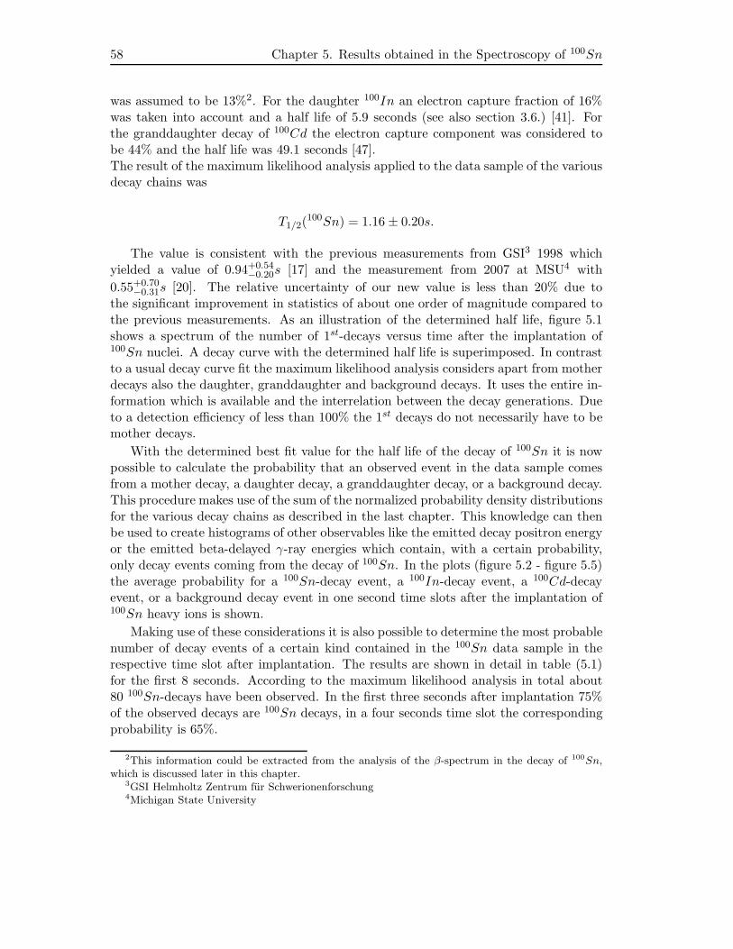
58 Chapter 5. Results obtained in the Spectroscopy of 100Sn
was assumed to be 13%2. For the daughter 100In an electron capture fraction of 16%was taken into account and a half life of 5.9 seconds (see also section 3.6.) [41]. Forthe granddaughter decay of 100Cd the electron capture component was considered tobe 44% and the half life was 49.1 seconds [47].The result of the maximum likelihood analysis applied to the data sample of the variousdecay chains was
T1/2(100Sn) = 1.16 ± 0.20s.
The value is consistent with the previous measurements from GSI3 1998 whichyielded a value of 0.94+0.54
−0.20s [17] and the measurement from 2007 at MSU4 with
0.55+0.70−0.31s [20]. The relative uncertainty of our new value is less than 20% due to
the significant improvement in statistics of about one order of magnitude compared tothe previous measurements. As an illustration of the determined half life, figure 5.1shows a spectrum of the number of 1st-decays versus time after the implantation of100Sn nuclei. A decay curve with the determined half life is superimposed. In contrastto a usual decay curve fit the maximum likelihood analysis considers apart from motherdecays also the daughter, granddaughter and background decays. It uses the entire in-formation which is available and the interrelation between the decay generations. Dueto a detection efficiency of less than 100% the 1st decays do not necessarily have to bemother decays.
With the determined best fit value for the half life of the decay of 100Sn it is nowpossible to calculate the probability that an observed event in the data sample comesfrom a mother decay, a daughter decay, a granddaughter decay, or a background decay.This procedure makes use of the sum of the normalized probability density distributionsfor the various decay chains as described in the last chapter. This knowledge can thenbe used to create histograms of other observables like the emitted decay positron energyor the emitted beta-delayed γ-ray energies which contain, with a certain probability,only decay events coming from the decay of 100Sn. In the plots (figure 5.2 - figure 5.5)the average probability for a 100Sn-decay event, a 100In-decay event, a 100Cd-decayevent, or a background decay event in one second time slots after the implantation of100Sn heavy ions is shown.
Making use of these considerations it is also possible to determine the most probablenumber of decay events of a certain kind contained in the 100Sn data sample in therespective time slot after implantation. The results are shown in detail in table (5.1)for the first 8 seconds. According to the maximum likelihood analysis in total about80 100Sn-decays have been observed. In the first three seconds after implantation 75%of the observed decays are 100Sn decays, in a four seconds time slot the correspondingprobability is 65%.
2This information could be extracted from the analysis of the β-spectrum in the decay of 100Sn,which is discussed later in this chapter.
3GSI Helmholtz Zentrum fur Schwerionenforschung4Michigan State University
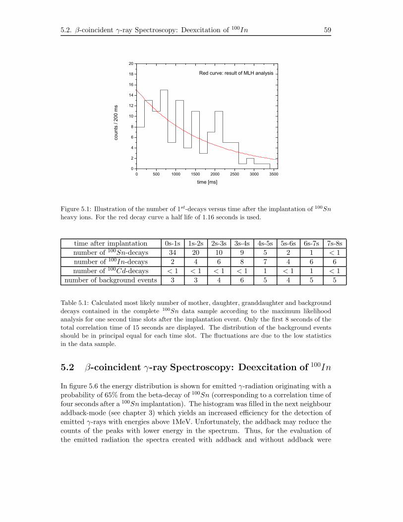
5.2. β-coincident γ-ray Spectroscopy: Deexcitation of 100In 59
0 500 1000 1500 2000 2500 3000 35000
2
4
6
8
10
12
14
16
18
20
Red curve: result of MLH analysis
coun
ts /
200
ms
time [ms]
Figure 5.1: Illustration of the number of 1st-decays versus time after the implantation of 100Sn
heavy ions. For the red decay curve a half life of 1.16 seconds is used.
time after implantation 0s-1s 1s-2s 2s-3s 3s-4s 4s-5s 5s-6s 6s-7s 7s-8s
number of 100Sn-decays 34 20 10 9 5 2 1 < 1
number of 100In-decays 2 4 6 8 7 4 6 6
number of 100Cd-decays < 1 < 1 < 1 < 1 1 < 1 1 < 1
number of background events 3 3 4 6 5 4 5 5
Table 5.1: Calculated most likely number of mother, daughter, granddaughter and background
decays contained in the complete 100Sn data sample according to the maximum likelihood
analysis for one second time slots after the implantation event. Only the first 8 seconds of the
total correlation time of 15 seconds are displayed. The distribution of the background eventsshould be in principal equal for each time slot. The fluctuations are due to the low statistics
in the data sample.
5.2 β-coincident γ-ray Spectroscopy: Deexcitation of 100In
In figure 5.6 the energy distribution is shown for emitted γ-radiation originating with aprobability of 65% from the beta-decay of 100Sn (corresponding to a correlation time offour seconds after a 100Sn implantation). The histogram was filled in the next neighbouraddback-mode (see chapter 3) which yields an increased efficiency for the detection ofemitted γ-rays with energies above 1MeV. Unfortunately, the addback may reduce thecounts of the peaks with lower energy in the spectrum. Thus, for the evaluation ofthe emitted radiation the spectra created with addback and without addback were
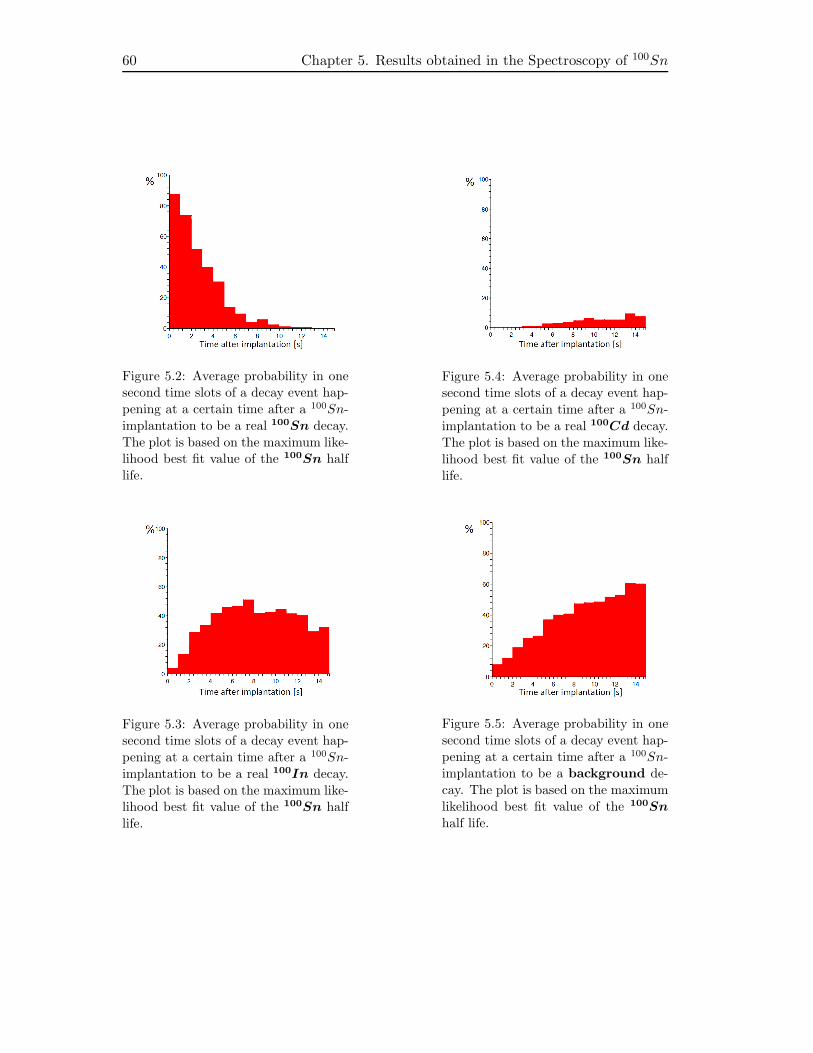
60 Chapter 5. Results obtained in the Spectroscopy of 100Sn
Figure 5.2: Average probability in onesecond time slots of a decay event hap-
pening at a certain time after a 100Sn-
implantation to be a real 100Sn decay.
The plot is based on the maximum like-lihood best fit value of the 100
Sn half
life.
Figure 5.3: Average probability in onesecond time slots of a decay event hap-
pening at a certain time after a 100Sn-
implantation to be a real 100In decay.
The plot is based on the maximum like-lihood best fit value of the 100
Sn half
life.
Figure 5.4: Average probability in onesecond time slots of a decay event hap-
pening at a certain time after a 100Sn-
implantation to be a real 100Cd decay.
The plot is based on the maximum like-
lihood best fit value of the 100Sn half
life.
Figure 5.5: Average probability in one
second time slots of a decay event hap-
pening at a certain time after a 100Sn-implantation to be a background de-
cay. The plot is based on the maximum
likelihood best fit value of the 100Sn
half life.
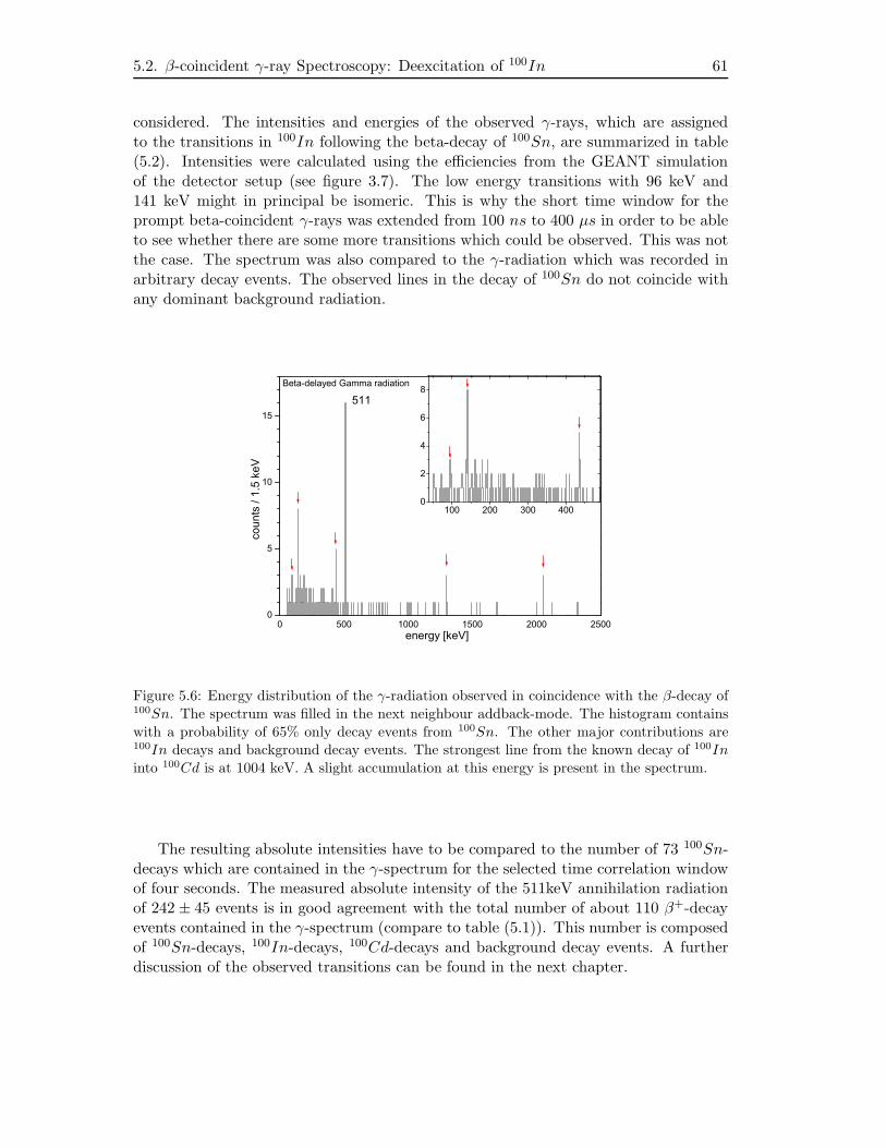
5.2. β-coincident γ-ray Spectroscopy: Deexcitation of 100In 61
considered. The intensities and energies of the observed γ-rays, which are assignedto the transitions in 100In following the beta-decay of 100Sn, are summarized in table(5.2). Intensities were calculated using the efficiencies from the GEANT simulationof the detector setup (see figure 3.7). The low energy transitions with 96 keV and141 keV might in principal be isomeric. This is why the short time window for theprompt beta-coincident γ-rays was extended from 100 ns to 400 µs in order to be ableto see whether there are some more transitions which could be observed. This was notthe case. The spectrum was also compared to the γ-radiation which was recorded inarbitrary decay events. The observed lines in the decay of 100Sn do not coincide withany dominant background radiation.
0 500 1000 1500 2000 25000
5
10
15
100 200 300 4000
2
4
6
8Beta-delayed Gamma radiation
511
coun
ts /
1.5
keV
energy [keV]
Figure 5.6: Energy distribution of the γ-radiation observed in coincidence with the β-decay of100Sn. The spectrum was filled in the next neighbour addback-mode. The histogram contains
with a probability of 65% only decay events from 100Sn. The other major contributions are100In decays and background decay events. The strongest line from the known decay of 100In
into 100Cd is at 1004 keV. A slight accumulation at this energy is present in the spectrum.
The resulting absolute intensities have to be compared to the number of 73 100Sn-decays which are contained in the γ-spectrum for the selected time correlation windowof four seconds. The measured absolute intensity of the 511keV annihilation radiationof 242 ± 45 events is in good agreement with the total number of about 110 β+-decayevents contained in the γ-spectrum (compare to table (5.1)). This number is composedof 100Sn-decays, 100In-decays, 100Cd-decays and background decay events. A furtherdiscussion of the observed transitions can be found in the next chapter.
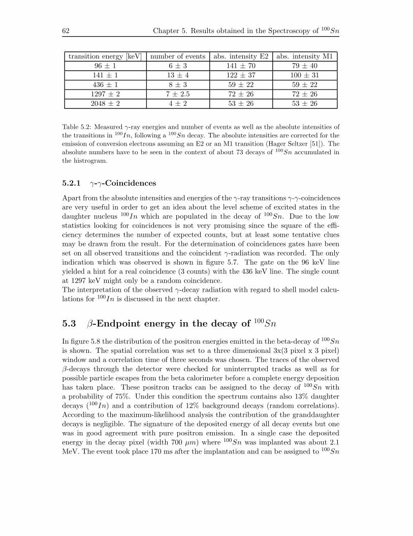
62 Chapter 5. Results obtained in the Spectroscopy of 100Sn
transition energy [keV] number of events abs. intensity E2 abs. intensity M1
96 ± 1 6 ± 3 141 ± 70 79 ± 40
141 ± 1 13 ± 4 122 ± 37 100 ± 31
436 ± 1 8 ± 3 59 ± 22 59 ± 22
1297 ± 2 7 ± 2.5 72 ± 26 72 ± 26
2048 ± 2 4 ± 2 53 ± 26 53 ± 26
Table 5.2: Measured γ-ray energies and number of events as well as the absolute intensities of
the transitions in 100In, following a 100Sn decay. The absolute intensities are corrected for theemission of conversion electrons assuming an E2 or an M1 transition (Hager Seltzer [51]). The
absolute numbers have to be seen in the context of about 73 decays of 100Sn accumulated in
the histrogram.
5.2.1 γ-γ-Coincidences
Apart from the absolute intensities and energies of the γ-ray transitions γ-γ-coincidencesare very useful in order to get an idea about the level scheme of excited states in thedaughter nucleus 100In which are populated in the decay of 100Sn. Due to the lowstatistics looking for coincidences is not very promising since the square of the effi-ciency determines the number of expected counts, but at least some tentative cluesmay be drawn from the result. For the determination of coincidences gates have beenset on all observed transitions and the coincident γ-radiation was recorded. The onlyindication which was observed is shown in figure 5.7. The gate on the 96 keV lineyielded a hint for a real coincidence (3 counts) with the 436 keV line. The single countat 1297 keV might only be a random coincidence.The interpretation of the observed γ-decay radiation with regard to shell model calcu-lations for 100In is discussed in the next chapter.
5.3 β-Endpoint energy in the decay of 100Sn
In figure 5.8 the distribution of the positron energies emitted in the beta-decay of 100Snis shown. The spatial correlation was set to a three dimensional 3x(3 pixel x 3 pixel)window and a correlation time of three seconds was chosen. The traces of the observedβ-decays through the detector were checked for uninterrupted tracks as well as forpossible particle escapes from the beta calorimeter before a complete energy depositionhas taken place. These positron tracks can be assigned to the decay of 100Sn witha probability of 75%. Under this condition the spectrum contains also 13% daughterdecays (100In) and a contribution of 12% background decays (random correlations).According to the maximum-likelihood analysis the contribution of the granddaughterdecays is negligible. The signature of the deposited energy of all decay events but onewas in good agreement with pure positron emission. In a single case the depositedenergy in the decay pixel (width 700 µm) where 100Sn was implanted was about 2.1MeV. The event took place 170 ms after the implantation and can be assigned to 100Sn
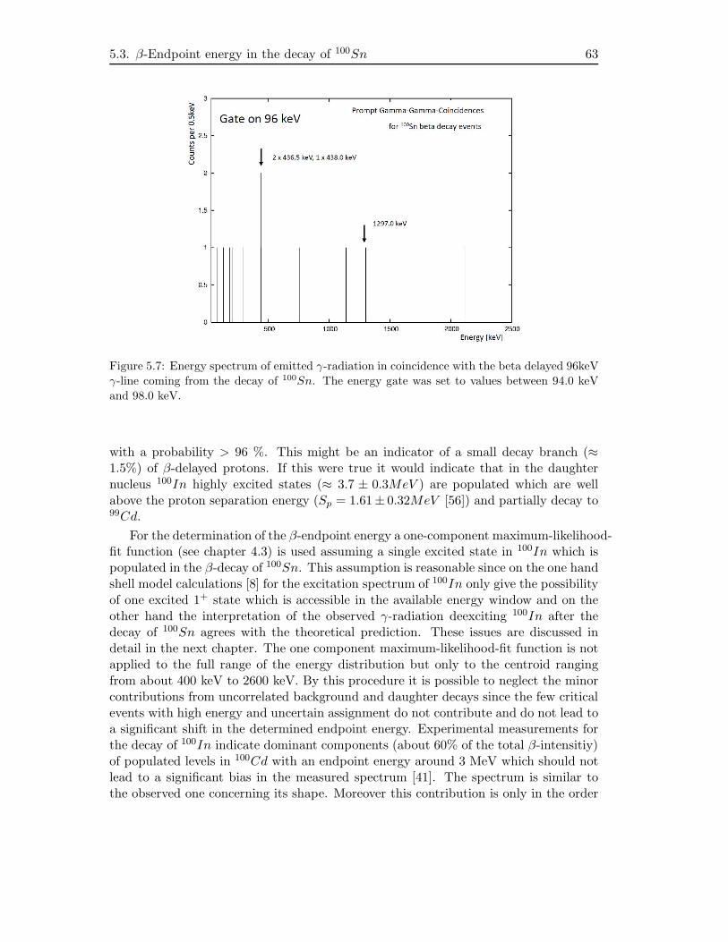
5.3. β-Endpoint energy in the decay of 100Sn 63
Figure 5.7: Energy spectrum of emitted γ-radiation in coincidence with the beta delayed 96keV
γ-line coming from the decay of 100Sn. The energy gate was set to values between 94.0 keV
and 98.0 keV.
with a probability > 96 %. This might be an indicator of a small decay branch (≈1.5%) of β-delayed protons. If this were true it would indicate that in the daughternucleus 100In highly excited states (≈ 3.7 ± 0.3MeV ) are populated which are wellabove the proton separation energy (Sp = 1.61± 0.32MeV [56]) and partially decay to99Cd.
For the determination of the β-endpoint energy a one-component maximum-likelihood-fit function (see chapter 4.3) is used assuming a single excited state in 100In which ispopulated in the β-decay of 100Sn. This assumption is reasonable since on the one handshell model calculations [8] for the excitation spectrum of 100In only give the possibilityof one excited 1+ state which is accessible in the available energy window and on theother hand the interpretation of the observed γ-radiation deexciting 100In after thedecay of 100Sn agrees with the theoretical prediction. These issues are discussed indetail in the next chapter. The one component maximum-likelihood-fit function is notapplied to the full range of the energy distribution but only to the centroid rangingfrom about 400 keV to 2600 keV. By this procedure it is possible to neglect the minorcontributions from uncorrelated background and daughter decays since the few criticalevents with high energy and uncertain assignment do not contribute and do not lead toa significant shift in the determined endpoint energy. Experimental measurements forthe decay of 100In indicate dominant components (about 60% of the total β-intensitiy)of populated levels in 100Cd with an endpoint energy around 3 MeV which should notlead to a significant bias in the measured spectrum [41]. The spectrum is similar tothe observed one concerning its shape. Moreover this contribution is only in the order
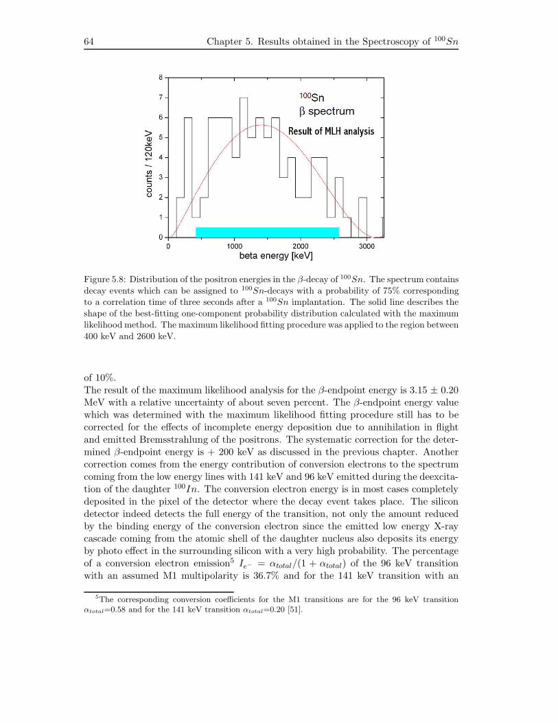
64 Chapter 5. Results obtained in the Spectroscopy of 100Sn
Figure 5.8: Distribution of the positron energies in the β-decay of 100Sn. The spectrum contains
decay events which can be assigned to 100Sn-decays with a probability of 75% correspondingto a correlation time of three seconds after a 100Sn implantation. The solid line describes the
shape of the best-fitting one-component probability distribution calculated with the maximum
likelihood method. The maximum likelihood fitting procedure was applied to the region between
400 keV and 2600 keV.
of 10%.The result of the maximum likelihood analysis for the β-endpoint energy is 3.15 ± 0.20MeV with a relative uncertainty of about seven percent. The β-endpoint energy valuewhich was determined with the maximum likelihood fitting procedure still has to becorrected for the effects of incomplete energy deposition due to annihilation in flightand emitted Bremsstrahlung of the positrons. The systematic correction for the deter-mined β-endpoint energy is + 200 keV as discussed in the previous chapter. Anothercorrection comes from the energy contribution of conversion electrons to the spectrumcoming from the low energy lines with 141 keV and 96 keV emitted during the deexcita-tion of the daughter 100In. The conversion electron energy is in most cases completelydeposited in the pixel of the detector where the decay event takes place. The silicondetector indeed detects the full energy of the transition, not only the amount reducedby the binding energy of the conversion electron since the emitted low energy X-raycascade coming from the atomic shell of the daughter nucleus also deposits its energyby photo effect in the surrounding silicon with a very high probability. The percentageof a conversion electron emission5 Ie− = αtotal/(1 + αtotal) of the 96 keV transitionwith an assumed M1 multipolarity is 36.7% and for the 141 keV transition with an
5The corresponding conversion coefficients for the M1 transitions are for the 96 keV transitionαtotal=0.58 and for the 141 keV transition αtotal=0.20 [51].
5.3. β-Endpoint energy in the decay of 100Sn 65
assumed M1 multipolarity it is 16.7%. From the observed intensities of the γ-rays itis a reasonable assumption that in each decay event the two transitions take place. Asdiscussed in the next chapter it is also a reasonable assumption that these transitionsare of the multipolarity M1. The average energy deposition in the detector can becalculated to be
E = 0.367 · 96keV + 0.167 · 141keV = 59keV.
The centroid of the energy distribution is thus shifted by this amount6 and thecorrection to the endpoint energy is - 59 keV. The deposition of energy from the ab-sorption of γ-rays in the silicon detector does not have to be considered since the highgranularity makes it possible to distinguish those isolated depositions from real tracksin most cases.Finally, the measured value of the β-endpoint energy in the decay of 100Sn under theassumption of a single populated final state is
Eβ0(100Sn) = 3.29 ± 0.20MeV.
From this value it is possible to calculate the fraction of β+-decays to be 87% whileelectron capture contributes with a minor fraction of 13%.The origin of the low energy peak at about 250 keV in the positron energy spectrumremains unclear. At first glance one might expect that it comes from electron capturedecay events where the only possible energy deposition which can trigger the data ac-quisition is due to conversion electrons from the 141 keV and the 96 keV line. Forregular β+-decays the energy of the conversion electrons is added to the energy of thepositrons which would not lead to a peak in the spectrum.In the silicon detector not only the energy of the conversion electrons plus the subse-quent X-ray cascade from the atomic shell of the daughter nucleus is deposited. Alsothe energy coming from the casacde of low energy X-ray transitions in the daughteratom 100In following the electron capture decay is detected. This adds up to the bind-ing energy of the captured electron in the daughter nucleus. In Indium this electronis in 90% of all cases an electron from the K-shell with a binding energy of 27.94 keV.This energy also adds up with the 141 keV and 96 keV conversion electron transitions.Since the trigger threshold of the implantation detector was about 150 keV only the141 keV conversion electron would be able to trigger the detector by itself.The problem with this interpretation is on the one hand that the energies of the sixevents do not show a good agreement with the expected energy sums (141 keV + 28keV, 141 keV + 96 keV + 28 keV) even when considering the large uncertainty of theenergy calibration of about 40keV FWHM7.On the other hand a simple estimation from the analysis with 70 observed 100Sn-decays
6In the case of a branching of the decay into two separate cascades and furthermore, if the 141 keVtransition were not in the same branch as the 96 keV transition the systematic correction would haveto be reduced by a factor of 2. This uncertainty is still well covered by the statistical uncertainty ofthe beta endpoint energy.
7FWHM=Full Width at Half Maximum
66 Chapter 5. Results obtained in the Spectroscopy of 100Sn
and an electron capture fraction of about 13% yields a number of 10 electron capturedecays. The probability of observing the 141 keV line with 16.7% leads to a numberof 1-2 decays with an energy of 141 keV + 28 keV. The probability of an additionalobservation of the 96 keV line which is emitted with a probability of 36.7% in an in-ternal conversion is extremely low. Thus the energy combination sum of 141 keV + 96keV + 28 keV can occur in less than one case. Other combinations do not have to beconsidered due to the 150 keV threshold of the detector. With the help of the γ-rayspectroscopy with a 400 µs time gate it was possible to verify that none of the observedlow energy transitions is isomeric. If this were the case the absolute intensity of thetransition might be higher and due to the long shaping time of the silicon branch theadditional energy deposition would be detected with the prompt events.However, assuming a contribution from another unobserved transition which is highlyconverted with an energy < 70keV did also not lead to a consistent interpretation of thedata due to the pattern of the energy spread of the observed events in the low energypeak which could not be explained in combination with the probability of observing anadditional converted transition in coincidence with one or two of the other convertedtransitions.It is therefore not possible to explain the accumulation of six decay events in the lowenergy part of the spectrum with internal conversion. It is worth noting that becausesimilar lines were observed in the precursor experiment for 102Sn and 98Cd [17] the lowenergy part of the β-spectrum was not used for the maximum likelihood analysis.
5.4 Observations concerning a possible 6+ Isomer in 100Sn
With respect to isomer spectroscopy it would be of particular interest to obtain for thefirst time direct nuclear structure information about excited states in 100Sn. As al-ready discussed in the introduction there is a prediction of a long lived excited 6+-statein 100Sn which should be populated to some extent during the production reaction of100Sn in the fragmentation target. The most important information from the observa-tion of the decaying isomer would be the energy of the first excited 2+ state. The halflife of this isomeric state was calculated to be in the order of 100ns which of coursestrongly depends on the exact value of the energy difference between the 6+-state andthe 4+-state to which it predominantly decays. Since the 6+-state with a predictedenergy of 4.5 MeV is highly excited another possible decay mode could be the protonemission to 99In which, depending on the decay energy, could shorten the half life to5ns.With a number of about 160 implanted 100Sn-nuclei, a flight time8 through the frag-ment separator in the order of the estimated half life, an isomeric ratio of 50% and aphoto peak efficieny in the order of ten percent it is quite a challenge to see evidence forthe existence of the isomer even if everything corresponds to these ideal assumptions.For each of the three transitions (3 MeV, 0.6 MeV, ≈ 150 keV) deexciting the 6+-stateto the 0+ ground state only a few counts (≈ 5) should be observable.
8200 ns in the rest frame of the heavy ions
5.4. Observations concerning a possible 6+ Isomer in 100Sn 67
The RISING germanium detectors made it possible to look for these γ-rays in a timewindow of 400 µs after the implantation of 100Sn in the silicon detector stack. Thetime binning was 25 ns. The time zero of the implantation is accompanied by a flashof γ-rays of various energies and multiplicity from Bremsstrahlung emitted during theslowing down of the heavy ions in matter. Due to this flash some of the 105 Germaniumdetectors are blinded and the detection efficiency for the isomeric decay decreases.The experimental result from this investigation showed that there is no delayed emis-sion of γ-rays after the first 25 ns time bin which coincides with the implantation. Infigure 5.9 a spectrum showing the observed prompt γ-ray energies versus time in thefirst 25 ns bin after the implantation of 100Sn heavy ions is displayed. The histogramis devided in counts per 10 keV bin. The further discussion concentrates on the highenergy transition which is expected to be in the range of 3 MeV. The accumulation of 4counts in the non-addback spectrum at 3 MeV gives rise to a discussion about a possi-ble observation of the high energy transition of the isomer. It should be mentioned thatthe four counts in the 10 keV bin do yield an average energy of 3004 keV and do notall lie within the expected FWHM of about 3-4 keV of the RISING Germanium detec-tors. A search for single escape events in the spectrum yields two possible candidates.According to the energy distribution in the spectrum it is also possible that there is aCompton distribution of the 3004 keV peak with a maximum energy at the Comptonedge of about 2770 keV. At least the number of four counts is in good agreement withthe rough estimation stated above.But it is still necessary to explain how it would be possible that the isomer survives200 ns during the flight of 100Sn through the fragment separator and decays within25ns after implantation. For this purpose the probabilities have to be calculated thata decay takes place in the first 25 ns after implantation and in the time > 25 ns afterimplantation. The ratio of the two probabilities should then clearly favour the first25ns bin and the calculated number of expected events should correspond to the ob-servation. The probability of 4 isomeric counts in the first 25 ns bin is then the directproduct of the single probabilities since the events are statistically independent.During the flight through the fragment separator the nuclei are completely strippedand for the low energy 6+ − 4+ transition the only possible decay channel is a γ-rayemission of multipolarity E2. After implantation an additional decay channel - the in-ternal conversion for the low energy transition - has to be taken into account. Assuminga half life of about 100 ns and a transition energy of 177 keV as it was determined inthe shell model calculations from H. Grawe [4] the corresponding reduced transitionprobability for the isomeric E2 transition is approximately 1.0 W.u.The calculation of the probabilities showed that the observed scenario is only possiblefor transition energies below 100 keV and reduced transition probabilities B(E2) inthe range of 40 W.u.. If this were the case then the first 25ns bin would be clearlyfavoured and the number of observed decays would be in reasonable agreement withthe observation. In the specific case of a transition energy of 50 keV and a reducedtransition probability of 40 W.u. the probability of observing 4 events in the first 25ns bin would be (0.8)4 = 41%. However for more realistic matrix elements in the orderof 1.0 W.u. the decay in the time bins > 25 ns is clearly favoured for all possible
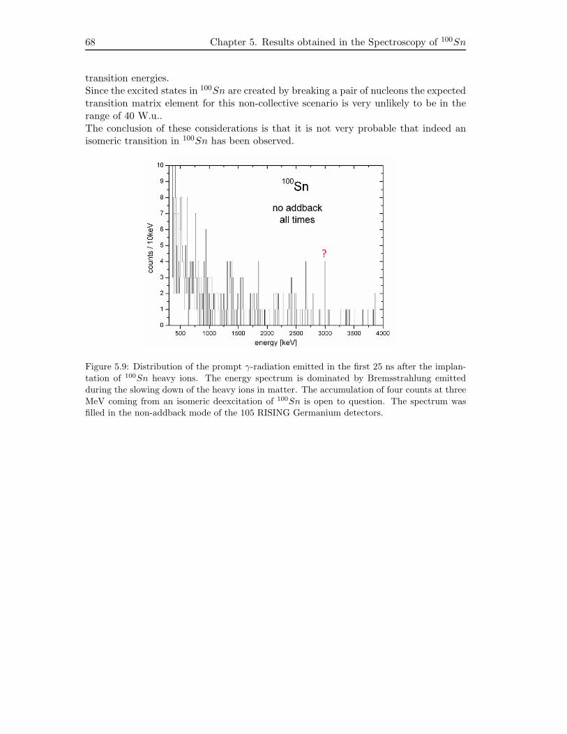
68 Chapter 5. Results obtained in the Spectroscopy of 100Sn
transition energies.Since the excited states in 100Sn are created by breaking a pair of nucleons the expectedtransition matrix element for this non-collective scenario is very unlikely to be in therange of 40 W.u..The conclusion of these considerations is that it is not very probable that indeed anisomeric transition in 100Sn has been observed.
Figure 5.9: Distribution of the prompt γ-radiation emitted in the first 25 ns after the implan-
tation of 100Sn heavy ions. The energy spectrum is dominated by Bremsstrahlung emitted
during the slowing down of the heavy ions in matter. The accumulation of four counts at three
MeV coming from an isomeric deexcitation of 100Sn is open to question. The spectrum wasfilled in the non-addback mode of the 105 RISING Germanium detectors.
Chapter 6
Discussion of the results
In this chapter the experimental results of the γ-ray spectroscopy of excited states in100In which are populated after the β-decay of 100Sn are discussed and compared totheoretical predictions of the level scheme. The obtained information concerning theβ-endpoint energy together with the interpretation of the data from γ-ray spectroscopyyields several new ground state to ground state QEC-values of the decay depending onthe different possible scenarios of the deexcitation of the daughter nucleus. In additionthe Gamow-Teller strength BGT in the decay of 100Sn is determined. The new value ofthe Gamow-Teller strength is interpreted in the context of the so called GT-quenching/ missing Gamow-Teller strength as it is observed consistently for more neutron-richeven-even tin isotopes.
6.1 Populated excited states in 100In - interpretation inthe context of shell model calculations
The new data on excited states in 100In obtained in this thesis is a challenging testingground for the effective proton-neutron interaction in this region far away from thevalley of stability and allows the exploration of the evolution of the shell structurewhen approaching the proton drip line.In shell model calculations the odd-odd nucleus 100In is relatively easy to treat sinceit has only one proton hole in the Z=28-50 shell and only one neutron particle in theN=50-82 shell. For the low lying excited states the proton hole is located in the π1g9/2
orbital, there are no excitations across the 100Sn shell gap and the neutron particleis located in the ν1g7/2 orbital or in the ν2d5/2 orbital. Consequently, the low-lying
excited states split up into two multiplets of almost pure π1g−19/2ν1g7/2 / π1g−1
9/2ν2d5/2
configuration. These configurations lead to multiplets of states with positive parityand spins ranging from 1+ to 8+ and from 2+ to 7+, respectively. For many yearsthe ν1g7/2 orbital and the ν2d5/2 orbital were considered to be degenerate. Recentmeasurements [2] showed that the difference of the single particle energies betweenthese two single particle orbitals is indeed only 170 keV in 101Sn. However, the orderingof the levels is still not clear. Due to the almost degenerate state of the neutronorbitals the splitting between the levels of the two multiplets only depends on the
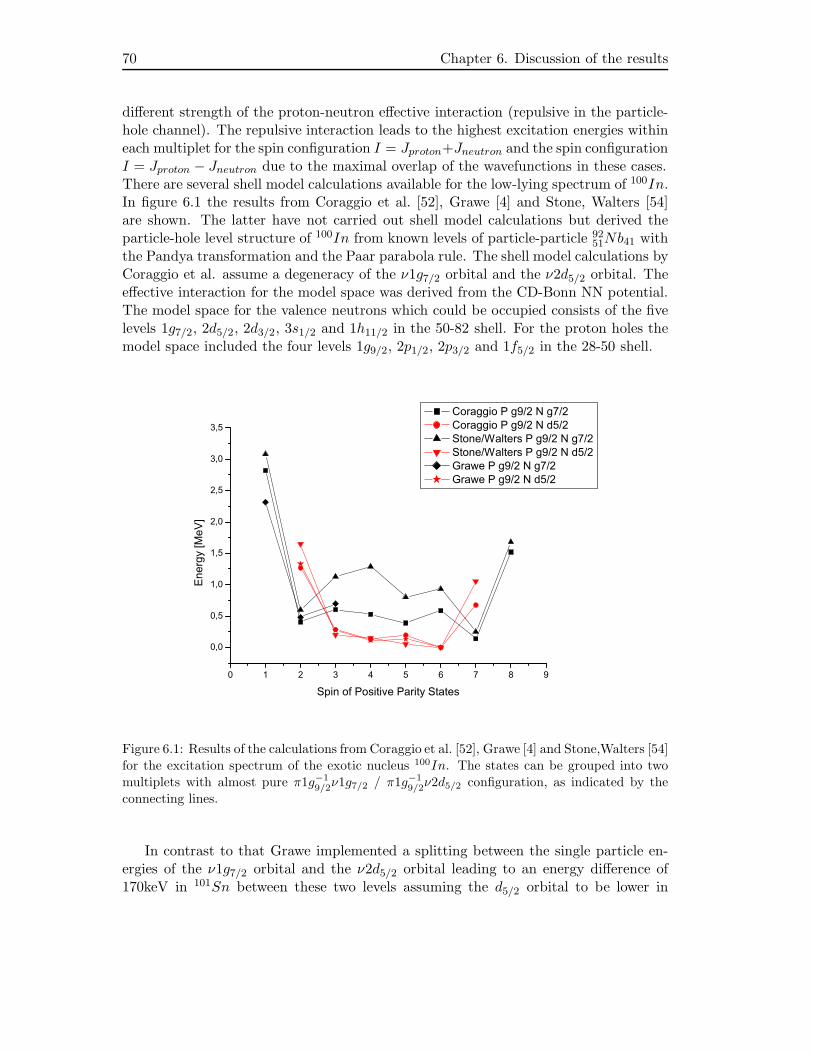
70 Chapter 6. Discussion of the results
different strength of the proton-neutron effective interaction (repulsive in the particle-hole channel). The repulsive interaction leads to the highest excitation energies withineach multiplet for the spin configuration I = Jproton+Jneutron and the spin configurationI = Jproton − Jneutron due to the maximal overlap of the wavefunctions in these cases.There are several shell model calculations available for the low-lying spectrum of 100In.In figure 6.1 the results from Coraggio et al. [52], Grawe [4] and Stone, Walters [54]are shown. The latter have not carried out shell model calculations but derived theparticle-hole level structure of 100In from known levels of particle-particle 92
51Nb41 withthe Pandya transformation and the Paar parabola rule. The shell model calculations byCoraggio et al. assume a degeneracy of the ν1g7/2 orbital and the ν2d5/2 orbital. Theeffective interaction for the model space was derived from the CD-Bonn NN potential.The model space for the valence neutrons which could be occupied consists of the fivelevels 1g7/2, 2d5/2, 2d3/2, 3s1/2 and 1h11/2 in the 50-82 shell. For the proton holes themodel space included the four levels 1g9/2, 2p1/2, 2p3/2 and 1f5/2 in the 28-50 shell.
0 1 2 3 4 5 6 7 8 9
0,0
0,5
1,0
1,5
2,0
2,5
3,0
3,5
Ene
rgy
[MeV
]
Spin of Positive Parity States
Coraggio P g9/2 N g7/2 Coraggio P g9/2 N d5/2 Stone/Walters P g9/2 N g7/2 Stone/Walters P g9/2 N d5/2 Grawe P g9/2 N g7/2 Grawe P g9/2 N d5/2
Figure 6.1: Results of the calculations from Coraggio et al. [52], Grawe [4] and Stone,Walters [54]
for the excitation spectrum of the exotic nucleus 100In. The states can be grouped into two
multiplets with almost pure π1g−1
9/2ν1g7/2 / π1g−1
9/2ν2d5/2 configuration, as indicated by the
connecting lines.
In contrast to that Grawe implemented a splitting between the single particle en-ergies of the ν1g7/2 orbital and the ν2d5/2 orbital leading to an energy difference of170keV in 101Sn between these two levels assuming the d5/2 orbital to be lower in
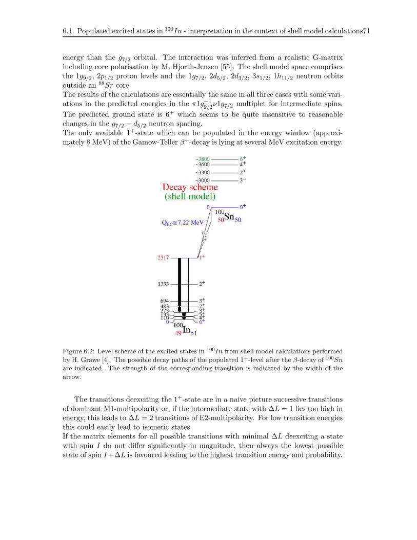
6.1. Populated excited states in 100In - interpretation in the context of shell model calculations71
energy than the g7/2 orbital. The interaction was inferred from a realistic G-matrixincluding core polarisation by M. Hjorth-Jensen [55]. The shell model space comprisesthe 1g9/2, 2p1/2 proton levels and the 1g7/2, 2d5/2, 2d3/2, 3s1/2, 1h11/2 neutron orbitsoutside an 88Sr core.The results of the calculations are essentially the same in all three cases with some vari-ations in the predicted energies in the π1g−1
9/2ν1g7/2 multiplet for intermediate spins.
The predicted ground state is 6+ which seems to be quite insensitive to reasonablechanges in the g7/2 − d5/2 neutron spacing.The only available 1+-state which can be populated in the energy window (approxi-mately 8 MeV) of the Gamow-Teller β+-decay is lying at several MeV excitation energy.
Figure 6.2: Level scheme of the excited states in 100In from shell model calculations performed
by H. Grawe [4]. The possible decay paths of the populated 1+-level after the β-decay of 100Snare indicated. The strength of the corresponding transition is indicated by the width of the
arrow.
The transitions deexciting the 1+-state are in a naive picture successive transitionsof dominant M1-multipolarity or, if the intermediate state with ∆L = 1 lies too high inenergy, this leads to ∆L = 2 transitions of E2-multipolarity. For low transition energiesthis could easily lead to isomeric states.If the matrix elements for all possible transitions with minimal ∆L deexciting a statewith spin I do not differ significantly in magnitude, then always the lowest possiblestate of spin I+∆L is favoured leading to the highest transition energy and probability.
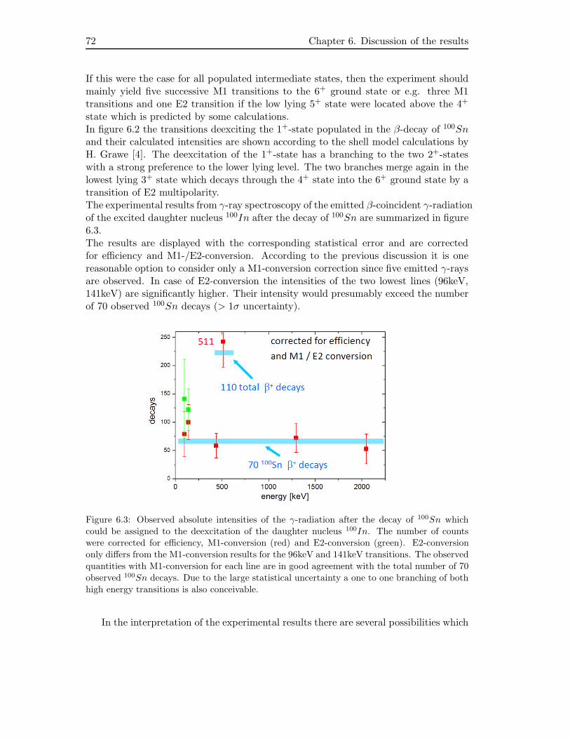
72 Chapter 6. Discussion of the results
If this were the case for all populated intermediate states, then the experiment shouldmainly yield five successive M1 transitions to the 6+ ground state or e.g. three M1transitions and one E2 transition if the low lying 5+ state were located above the 4+
state which is predicted by some calculations.In figure 6.2 the transitions deexciting the 1+-state populated in the β-decay of 100Snand their calculated intensities are shown according to the shell model calculations byH. Grawe [4]. The deexcitation of the 1+-state has a branching to the two 2+-stateswith a strong preference to the lower lying level. The two branches merge again in thelowest lying 3+ state which decays through the 4+ state into the 6+ ground state by atransition of E2 multipolarity.The experimental results from γ-ray spectroscopy of the emitted β-coincident γ-radiationof the excited daughter nucleus 100In after the decay of 100Sn are summarized in figure6.3.The results are displayed with the corresponding statistical error and are correctedfor efficiency and M1-/E2-conversion. According to the previous discussion it is onereasonable option to consider only a M1-conversion correction since five emitted γ-raysare observed. In case of E2-conversion the intensities of the two lowest lines (96keV,141keV) are significantly higher. Their intensity would presumably exceed the numberof 70 observed 100Sn decays (> 1σ uncertainty).
Figure 6.3: Observed absolute intensities of the γ-radiation after the decay of 100Sn which
could be assigned to the deexcitation of the daughter nucleus 100In. The number of countswere corrected for efficiency, M1-conversion (red) and E2-conversion (green). E2-conversion
only differs from the M1-conversion results for the 96keV and 141keV transitions. The observed
quantities with M1-conversion for each line are in good agreement with the total number of 70
observed 100Sn decays. Due to the large statistical uncertainty a one to one branching of both
high energy transitions is also conceivable.
In the interpretation of the experimental results there are several possibilities which
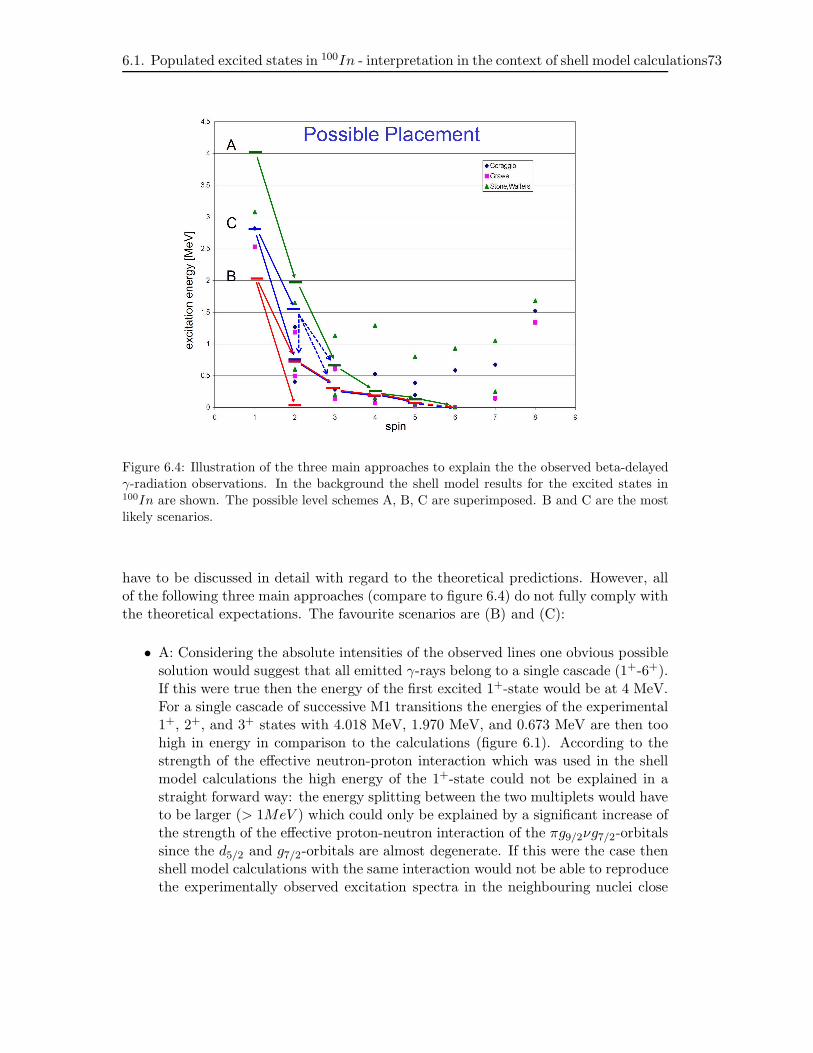
6.1. Populated excited states in 100In - interpretation in the context of shell model calculations73
Figure 6.4: Illustration of the three main approaches to explain the the observed beta-delayedγ-radiation observations. In the background the shell model results for the excited states in100In are shown. The possible level schemes A, B, C are superimposed. B and C are the most
likely scenarios.
have to be discussed in detail with regard to the theoretical predictions. However, allof the following three main approaches (compare to figure 6.4) do not fully comply withthe theoretical expectations. The favourite scenarios are (B) and (C):
• A: Considering the absolute intensities of the observed lines one obvious possiblesolution would suggest that all emitted γ-rays belong to a single cascade (1+-6+).If this were true then the energy of the first excited 1+-state would be at 4 MeV.For a single cascade of successive M1 transitions the energies of the experimental1+, 2+, and 3+ states with 4.018 MeV, 1.970 MeV, and 0.673 MeV are then toohigh in energy in comparison to the calculations (figure 6.1). According to thestrength of the effective neutron-proton interaction which was used in the shellmodel calculations the high energy of the 1+-state could not be explained in astraight forward way: the energy splitting between the two multiplets would haveto be larger (> 1MeV ) which could only be explained by a significant increase ofthe strength of the effective proton-neutron interaction of the πg9/2νg7/2-orbitalssince the d5/2 and g7/2-orbitals are almost degenerate. If this were the case thenshell model calculations with the same interaction would not be able to reproducethe experimentally observed excitation spectra in the neighbouring nuclei close
74 Chapter 6. Discussion of the results
to 100Sn accurately. But the agreement between theory and experiment in thisregion, e.g. in 102Sn or 98Cd, is good [59], [60].It is possible that shell model calculations which include cross shell excitationsmight increase the spreading within the valence multiplets which may increasethe 1+ excitation energy, but this should only be a minor effect [4].There is also the possibility that a highly excited 1+ state at 4.018 MeV directlydecays via proton emission with a certain branching ratio to 99Cd. 100In hasan approximate proton separation energy of Sp = 1.61 ± 0.32MeV [56] whichmeans that a proton decay to the g7/2 or the d5/2 neutron orbital in 99Cd wouldhave 2.4 ± 0.3MeV and could compete with the 2.048 MeV γ-ray emission. Asignature of a single proton decay in the data sample might have been observed,as discussed in the previous chapter. However, this evidence is rather tentative.Altogehter, with regard to the vast change of the interaction matrix elements,this scenario is not very likely.From the previous 100Sn experiment from 1994 it was determined that the totalenergy sum of the emitted γ-radiation by the daughter nucleus 100In after the de-cay of 100Sn is Eγ = 2.76±0.43MeV [13], [14]. This measurement also precludesthe single cascade scenario.
• B: The second option assumes an about equal branching of the high energy tran-sitions (2.048 MeV, 1.297 MeV) which is also possible with regard to the errorbars of the absolute intensities.A branching of the decay from the 1+-state is predicted in the calculations byH. Grawe. However, with the five observed γ-ray transitions no complete set ofdecays of both branches to the 6+ ground state can be constructed. Thus onemay assume that the 2.048 MeV transition goes to a low lying 2+ isomeric stateand is somehow trapped, while the other cascade reaches the 6+ ground state.One transition of the untrapped cascade in this scenario is then not observed(assuming five M1 transitions) which should have a very low transition energy(< 70keV ) and would be dominanted by internal conversion. Unfortunately theenergy resolution for detecting conversion electrons in SIMBA was relatively poor(≈40keV FWHM) and thus no clear conclusions can be drawn from the electronspectrum with regards to this scenario.Another problem with this interpretation is that the experimental 1+ and 2+
states with energies of E(1+1 )≈2.100 MeV and E(2+
2 )≈0.800 MeV / E(2+1 )≈ 0.050
MeV are a bit too low in energy compared to the calculations.Also a one to one branching of the transitions is not favoured in theory. A 4:1ratio emphasizing the 2.048 MeV transition is roughly expected using the calcu-lated transition matrix elements [4]. This can be easily understood since the lowlying 2+ state has the same configuration as the initial 1+ state.Nevertheless, this scenario shows a reasonably good agreement with shell modelcalculations since the prediction of the energies of the low lying states is typicallynot very accurate.
6.1. Populated excited states in 100In - interpretation in the context of shell model calculations75
• C: The third option assumes that the 2.048 MeV transition is followed by thecascade of observed transitions and the transitions succeeding the 1.297 MeVtransition are not observed. The branching ratio for the decay of the 1+-stateshould be roughly one to one again. Then all states would have reasonable ener-gies according to the current shell model calculations.Such a scenario could either result if the 2+-state fed by the 1.297 MeV tran-sition is isomeric or if its decay is so fragmented that the individual transitionsare too weak to be detected. In the actual case no trapped high lying isomeris expected since all states belong to similar configurations and the transitionmatrix elements between them do not vanish at all. It is much more likely thatthe 2+
2 state which is populated by the 1.297 MeV transition has three more orless equal decay branches dominated by M1 multipolarity transitions to the lowlying 2+
1 state and to the two low lying 3+ states. Shell model calculations wereperformed in the framework of this thesis with the code OXBASH [53] for 100In.The resulting reduced transition probabilities support this three branch option.Further E2 transitions from the 2+
2 level to the 4+ states are strongly suppressedand can be neglected. For each of the three transitions the intensity in the con-text of the measured statistics might have been too low to be detected in ourexperiment. Even if there are single counts in the spectrum it is not possibleto distinguish them from background. In the spectrum there is no clear sign fora 2+
2 → 2+1 transition at 751 keV and a 2+
2 → 3+1 transition at 1187 keV. An
unfavorable equal intensity spread between the three levels may indeed lead tononobservation.This scenario is also a reasonable option to explain the observed data.
Unfortunately, as outlined above, it is not possible to explain the observed datawith the current shell model calculations completely, but, beside the scenario (A),where a significant change in the proton-neutron interaction matrix elements would benecessary, scenario (C), where some transitions are presumably not observed due tothe low intensity caused by the splitting into three equal deexcitation branches of the2+2 level, and the second scenario (B) seem to be both reasonable.
For scenario (C) the experimental energies of the states are much closer to the resultsof the current calculations, however, from the viewpoint of the shell model calculationsthe intermediate option (B) is also plausible. Concerning the two decay paths from the1+-state as predicted in the shell model calculations by H. Grawe the calculation clearlyprefers one of them. But this pattern depends sensitively on the predicted transitionenergies and the E2/M1 mixing ratios. The latter are difficult to predict [4] whichcould lead to two parallel branches which do not end on the same state and togetherwith non-observed low-energy (isomeric) transitions they do not necessarily add up tothe same total energy. According to the uncertainty of the shell model predictions oneof the low-energy states could easily be depopulated by an isomeric E2 transition.
Clearly better statistics is needed to clarify the structure. It is necessary to be able todetect weaker transitions and to look for gamma-gamma coincidences.
76 Chapter 6. Discussion of the results
6.2 Gamow-Teller strength and QEC-value in the β-decayof 100Sn - is there a GT Quenching?
The Gamow-Teller Strength BGT in this single-channel β-decay (only one final state ispopulated) can be calculated from the half life T1/2 and the Fermi Phasespace Integralf(Z,E0) where E0 denotes the experimentally determined β-endpoint energy [61]:
f(Z,E0) · T1/2 =2π3h7
m5ec
4G2F
· ln2
g2V · |MF |2 + g2
A · |MGT |2(6.1)
The weak interaction vector-coupling constant GF can be determined from mea-surements of the super allowed 0+ → 0+ Fermi-decays [62]. The most recent value isGF /(hc)
3 = 1.16637(1) · 10−5GeV −2 [65]. The ratio of the weak coupling constants forthe vector- and axialvector current can be deduced most accurately from the decay ofthe free neutron [63]: gA/gV = 1.2695 ± 0.0029 [65]. Since the squares of the absolutevalues of the matrix elements correspond to the transition strengths equation 6.1 canbe rewritten in the following way:
f(Z,E0) · T1/2 =6142.8s
BF + (gA/gV )2 · BGT(6.2)
In the case of a pure Gamow-Teller decay populating a single final state the tran-sition strength can be calculated with the following relation:
BGT =3811.5s
f(Z,E0) · T1/2(6.3)
For the sake of completeness it should be mentioned that more complex GamowTeller decays which populate more than one final state require the sum of the singlevalues to determine the total strength:
BGT =∑
i
3811.5s
fi · ti(6.4)
The single GT values are calculated from the phasespace factor fi = f(Z,E0) withthe β-endpoint energy E0i
of the corresponding transition and the partial half lifeti = T1/2/(Iβ)i. The decay branches (Iβ)i to the corresponding final states can bedetermined with the help of γ-ray spectroscopy of the daughter nucleus.Since the Fermi Phasespace Integral f(Z,E0) depends approximately on the 5th-powerof the endpoint energy the precision of this value is decisive for the precision with whichthe Gamow-Teller strength can be determined. By application of this calculation pro-cedure of course only the fraction of the GT strength can be deduced which is accessiblein the energy window of the β+-decay1. A further difficulty in the determination of anexperimental value of the GT strength is due to the limited number of measured decays
1The energy window for an electron capture decay which competes with the positron emissiondepending on the β-endpoint energy of the transition is 1.022 MeV larger and thus may cover possiblefinal states with higher excitation energy.
6.2. Gamow-Teller strength andQEC-value in the β-decay of 100Sn - is there a GT Quenching?77
and the limited photo-peak efficiency of the Germanium detectors of the current setupwhich makes it impossible to measure small branching ratios (sensitivity limit) to levelsin the daughter nucleus with high excitation energy. Since the phase space volume inthe decay strongly depends on the available energy the branching ratio to energeticallyhigh lying states may get very small. This prevails even if the states contribute a largefraction to the Gamow-Teller strength.According to chapter 1 for the beta decay of 100Sn only one final state in the daughternucleus is predicted to be populated which is carrying almost the entire Gamow-Tellerstrength and which is easily accessible in the beta decay energy window. Therefore,the experimental problems just discussed for the general case should not matter.
In order to determine the experimentally observable Gamow-Teller strength BGT inthe decay of 100Sn the determined values of the half life T1/2 = 1.16 ± 0.20s and theβ-endpoint energy E0 = 3.29 ± 0.20MeV of the single-channel decay have to be con-sidered. The calculated experimental value of the Gamow-Teller strength for the decayof 100Sn is
BexpGT (100Sn) = 9.1+4.8
−2.3.
The uncertainty of the calculated value is dominated by the uncertainty of the valueof the β-endpoint energy. The calculation of the GT strength was performed withthe program LOGFT which can be found on the website of the Brookhaven NationalNuclear Data Center [64] which is able to precisely evaluate the Fermi-integral.The corresponding log-ft value of the decay is extremely small with 2.62+0.13
−0.19. Thisnumber is record in the nuclear chart since it is by far the smallest log-ft value for anynuclear decay. Thus, the Gamow-Teller β-decay of 100Sn is the most allowed β-decayin the nuclear chart. Since the entire strength is concentrated in a single final stateand the value of the strength clearly exceeds the Gamow-Teller strength of the barenucleon (neutron decay) of BGT = 3 the decay of 100Sn is a so called Super Gamow-Teller transition [58].The measured value is in good agreement with the previous measurement from 1998with BGT = 5.8+5.3
−4.1 [17]. Due to the better statistics the relative error improved from90% in the measurement from 1998 to 50% in the current analysis.
In figure 6.5 a compilation of theoretical and experimental values of the Gamow-Teller strength in various even-even tin isotopes from mass number 100 to 110 is shown.The values of the Gamow-Teller strength from the extreme single particle shell modelyield the highest transition strengths for all nuclei. Realistic orbital occupation num-bers from shell model calculations reveal a decrease of the predicted strength for theintermediate neutron rich nuclei between mass number 102 and 108. The theoreticalvalues of the Gamow-Teller strength calculated with more sophisticated models likethe Quasi Particle Random Phase Approximation2 and the self-consistent Finite Fermi
2BCS plus Quasiparticle Random Phase Approximation with G-matrix interaction and proton-neutron pairing
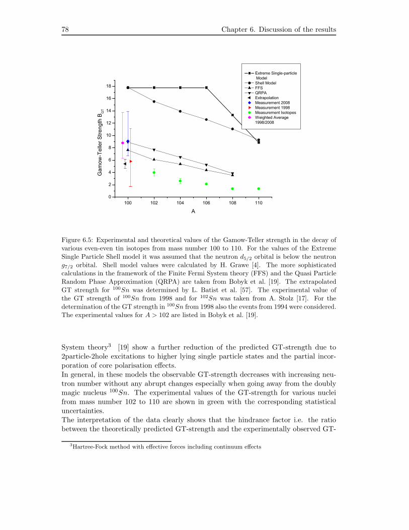
78 Chapter 6. Discussion of the results
100 102 104 106 108 1100
2
4
6
8
10
12
14
16
18
Gam
ow-T
elle
r Stre
ngth
BG
T
A
Extreme Single-particle Model
Shell Model FFS QRPA Extrapolation Measurement 2008 Measurement 1998 Measurement Isotopes Weighted Average
1998/2008
Figure 6.5: Experimental and theoretical values of the Gamow-Teller strength in the decay of
various even-even tin isotopes from mass number 100 to 110. For the values of the Extreme
Single Particle Shell model it was assumed that the neutron d5/2 orbital is below the neutron
g7/2 orbital. Shell model values were calculated by H. Grawe [4]. The more sophisticatedcalculations in the framework of the Finite Fermi System theory (FFS) and the Quasi Particle
Random Phase Approximation (QRPA) are taken from Bobyk et al. [19]. The extrapolated
GT strength for 100Sn was determined by L. Batist et al. [57]. The experimental value of
the GT strength of 100Sn from 1998 and for 102Sn was taken from A. Stolz [17]. For the
determination of the GT strength in 100Sn from 1998 also the events from 1994 were considered.The experimental values for A > 102 are listed in Bobyk et al. [19].
System theory3 [19] show a further reduction of the predicted GT-strength due to2particle-2hole excitations to higher lying single particle states and the partial incor-poration of core polarisation effects.In general, in these models the observable GT-strength decreases with increasing neu-tron number without any abrupt changes especially when going away from the doublymagic nucleus 100Sn. The experimental values of the GT-strength for various nucleifrom mass number 102 to 110 are shown in green with the corresponding statisticaluncertainties.The interpretation of the data clearly shows that the hindrance factor i.e. the ratiobetween the theoretically predicted GT-strength and the experimentally observed GT-
3Hartree-Fock method with effective forces including continuum effects
6.2. Gamow-Teller strength andQEC-value in the β-decay of 100Sn - is there a GT Quenching?79
strength decreases when approaching the neutron deficient nucleus 100Sn. This mightbe due to a decrease of cross Z=50 shell excitations. It should be noted that possiblynot the full GT-strength has been observed experimentally and the observed hindrancethus may not be due to problems with the theoretical GT-strength.For the doubly magic 100Sn nucleus the agreement of the experimental Gamow-Tellerstrength with the sophisticated theoretical predictions within the statistical error barscould mean that further core polarisation effects outside the model space are not rel-evant since no GT-quenching seems to be observed. The present calculations seem toalready incorporate the relevant physics.For the sake of completeness a recently extrapolated value of the expected GT-strengthin 100Sn from systematics in the neighbouring nuclei by L. Batist [57] is also shownwhich barely does not coincide with our measurement for 100Sn within the statisticalerror bars (1σ-significance level). The extrapolation is based on the observation thatin the region of nuclides near 100Sn where the β+-decay is dominated by the transfor-mation πg9/2 → νg7/2 the summed GT reduced probabilities can be approximated bylinear functions of the relative neutron excess (N-Z)/A. In this context an experimentalvalue of the GT strength in the N=Z nucleus 96Cd beside 100Sn would be interestingto compare with the extrapolation.
The QEC-value for the positron decay of 100Sn can be calculated using the β-endpointenergy E0 and the excitation energy E(1+) of the populated level in the daughternucleus 100In.
QEC = Eβ0+ E(1+) + 2mec
2 (6.5)
With the assumption that the five observed γ-rays represent a single cascade of tran-sitions (scenario (A)) to the ground state it follows that the energy of the first excited1+-state adds up to 4.018 MeV. From the observed data, as already discussed, therewas no clear indication of a missing unobserved low-energy γ-ray transition (< 80keV )which would be highly converted. This is in good agreement with theory, at first glance,since all five expected M1 transitions are present. However, one has to note the vastchange in the proton-neutron interaction matrix elements which would be needed toobtain the large energy splitting between the g9/2,d5/2 and the g9/2,g7/2 configurations.With the β-endpoint energy of E0 = 3.29 ± 0.20MeV a final QEC value of
QEC(100Sn→100 In)A = 8.33 ± 0.20MeV
is obtained for the first scenario (A) which is discussed in the previous section. ThisQEC value is in agreement with the previous measurement of 7.6+1.1
−0.4MeV from 1998by A. Stolz et al. [17] together with the results from R. Schneider from 1996 [14] andcannot be completely excluded with mass measurements performed in GANIL in 1996to obtain the 100In-100Sn mass difference yielding a QEC value of about 6.9 MeV withan uncertainty in the order of ±1 MeV [16].For the scenario (B) the energy of the first excited 1+ state is expected to be E(1+) ≈2.050keV . The lower limit is defined by the transition of the one branch with 2048
80 Chapter 6. Discussion of the results
keV presumably populating a low lying isomeric state of a few keV. The upper limitcan be estimated from the fact that for the given lower limit of E(1+) in the 1297keV-436keV-141keV-96keV cascade one transition seems to be missing to reach the groundstate and to cover the spin difference from 1+ to 6+. This transition was not observedin the experiment. This is only possible for highly converted transitions with energies< 80keV . Consequently the QEC-value for this scenario is approximately:
QEC(100Sn→100 In)B ≈ 6.36 ± 0.20MeV
The result is consistent with the measurement by A. Stolz from 1998 [17] yielding aQEC ≥ 6320keV .For the scenario (C) the cascade which populates the ground state is complete underthe assumption that there is one E2 transition. If only M1 transitions are involvedthen an unobserved transition < 80keV should exist which lifts the energy of the firstexcited 1+ state.The resulting QEC-value is situated in between the other two scenarios with
QEC(100Sn→100 In)C ≈ 7.03 ± 0.20 + xMeV (x < 0.08MeV ).
Unfortunately, the low statistics of the observed data does not allow to draw moreprecise conclusions.The result of these considerations is a possible range of the ground state to groundstate QEC value between 6.1 - 8.5 MeV for the decay of 100Sn.
Chapter 7
Summary and Outlook
7.1 Summary of the results
The investigation of the decay of the doubly magic nucleus 100Sn performed in theframework of this thesis yielded some remarkable results:
• The log-ft value in the decay of 100Sn with 2.62+0.13−0.19 is by far the smallest log-ft
value in the nuclear chart and thus the decay of 100Sn is the most allowed β-decay,even faster than superallowed Fermi transitions.
• The Gamow-Teller strength of the decay into a single final state withBGT (100Sn) =9.1+4.8
−2.3 exceeds the Gamow-Teller strength of the bare nucleon in the neutron de-cay of BGT = 3 and is thus called a Super Gamow-Teller Transition [58].In fact, there are only two transitions to specific final states observed so far whichare larger than the neutron value of 3. They are the 0+, T = 1, 6He to 1+, T = 0,6Li decay with BGT = 4.72 and the 0+, T = 1, 18Ne to 1+, T = 0, 18F decaywith BGT = 3.15 [58]. In other nuclei the transition strength is fragmented overseveral final states.The main condition for the existence of this isolated Super Gamow Teller transi-tion is that the spin-orbit gap between the ℓ+ 1
2 and ℓ− 12 orbits be sufficiently
small compared to the shell gap so that the 1particle-1hole states are isolatedbelow the 2particle-2hole states [58]. Consequently in 100Sn this seems to be thecase for the ℓ = 4 orbitals πg9/2,νg7/2 compared to the shell gap for protons andneutrons of about 6 MeV.
• Since in 100Sn no Gamow-Teller quenching seems to be observed this result couldmean that further core polarisation effects outside the model space of the currentcalculations are not relevant. The present calculations seem to already incorpo-rate the relevant physics for the doubly magic nucleus 100Sn.Of course the statistical uncertainty of the determined value of the Gamow-Tellerstrength in the decay of 100Sn is still too large to make a detailed comparison totheory and to draw further conclusions.
82 Chapter 7. Summary and Outlook
Unfortunaltely the investigation of the beta-delayed γ radiation from the daughternucleus 100In did not lead to any conclusive results concerning the level scheme ofexcited states in this exotic nucleus.There are several scenarios, as discussed in chapter 6, and none of them can be clearlyexcluded.In order to be able to make a reasonable comparison to shell model calculations andto extract information about the nature of the effective proton-neutron interactionin 100In it is necessary to obtain more statistics. This would allow to observe muchweaker transitions and could reveal small branching ratios to, up to now, unknownstates. Furthermore gamma-gamma coincidence spectroscopy becomes feasible whichwould help to clarify which transitions belong into cascades.
7.2 100Sn - still a challenge? Possibilities for further in-
vestigation in the near future
The most promising perspective for a high statistics 100Sn experiment in the near fu-ture is provided by the Radioactive Ion Beam Factory (RIBF) at the RIKEN Institutein Wako, Japan [23]. With an expected beam intensity of at least 10pnA for a 124Xeprimary beam it should be possible to obtain about 400 100Sn nuclei per day in theprojectile fragmentation reaction process. Thus an increase of the available statisticsby one order of magnitude should be easily possible in the next years.The achievable beam energies are much lower at RIBF than at the GSI accelaratorfacility. Due to the lower beam energies of about 350MeV · A the nuclei are not com-pletely stripped and there is a charge state distribution. Since one charge state has tobe selected for optimal transmission some produced 100Sn nuclei will be lost.With an energy of the fragments of about 50-100 MeV ·A at the final focal plane afterthe beam line detector matter the implantation detector SIMBA has to be modifiedsince the 100Sn nuclei will not be able to pass 10mm of silicon of the front beta absorberstack to reach the implantation zone. The front beta absorber stack of the implanta-tion zone has to be discarded. Consequently, the beta decay spectroscopy can only beperformed in the backward direction, but the loss in statistics of 50% should be easilycompensated by the higher production rate.For gamma ray spectroscopy no comparable advanced germanium array like the RIS-ING setup of Euroball detectors will be available at RIBF. The loss in efficiency alsohas to be compensated by the much higher statistics of the 100Sn decay events.A proposal for the 100Sn experiment at RIKEN1 has already been accepted with highpriority.
Unfortunately, since 100Sn is not a stable nucleus, it is not possible to obtain furtherinformation about the strength distribution of the Gamow-Teller resonance by meansof (p,n) reactions in energy regions above the energy window which is accessible in the
1lead by GANIL, TUM, RIKEN
7.2. 100Sn - still a challenge? Possibilities for further investigation in the near future83
beta decay.In order to exclude high lying states which are still reachable in the energy window ofthe beta decay and might be populated to some extent (although they are not predictedby shell model calculations for 100Sn as discussed in chapter 1) a suitable tool for reli-ably measuring the entire β-intensity distribution would be the total absorption γ-rayspectroscopy. In this method a large scintillator for γ-ray detection is used which hasan efficiency close to 100% and an acceptance close to 4π. The detector records the fullcascades of β-delayed γ-rays and therefore allows one to restore the entire β-intensitydistribution including especially the weak transitions to the high-lying excited statesin the daughter nucleus.

84 Chapter 7. Summary and Outlook
Appendix
A.1 Complete set of formulas for the maximum-likelihood
analysis of β-decays
A.1.1 General probability terms
λ1, λ2, λ3 denote the decay constants for the mother, daughter and granddaughterdecay.The probability that a decay with the decay constant λ1 takes place between t = 0 andthe time t can be written in the following way:
F1(λ1, t) = 1 − exp(−λ1t)
The probability density that a decay with the decay constant λ1 takes place in theinfinitesimal interval between t and t+ dt is given in the following equation:
f1(λ1, t) = λ1 · exp(−λ1t)
The probability that a daughter-decay with the decay constant λ2 takes place in theinterval between t = 0 and t which was populated by a preceding mother decay withthe decay constant λ1 is given by the expression:
F2(λ1, λ2, t) = 1 − λ1λ2
λ2 − λ1
[1
λ1exp(−λ1t) −
1
λ2exp(−λ2t)
]
The probability density that a daughter decay with the decay constant λ2 takes placein the infinitesimal interval between t and t + dt which was populated by a motherdecay with the decay constant λ1 can be written in the following way:
f2(λ1, λ2, t) =λ1λ2
λ2 − λ1[exp(−λ1t) − exp(−λ2t)]
The probability that a granddaughter decay with the decay constant λ3 takes place inthe time interval between t = 0 and t which was populated before by a mother decayand a daughter decay with the decay constants λ1 and λ2 is given in the followingequation:
F3(λ1, λ2, λ3, t) = 1 − λ1λ2λ3
(λ2 − λ1)(λ3 − λ1)(λ3 − λ2)
[(λ3 − λ2)
λ1exp(−λ1t)−
86 Chapter A. Appendix
−(λ3 − λ1)
λ2exp(−λ2t) +
(λ2 − λ1)
λ3exp(−λ3t)
]
The probability density that a granddaughter decay with decay constant λ3 takes placein the infinitesimal interval between t and t+dt which was populated by a mother decayand a daughter decay with the decay constants λ1 and λ2 can be written in the followingway:
f3(λ1, λ2, λ3, t) =λ1λ2λ3
(λ2 − λ1)(λ3 − λ1)(λ3 − λ2)[(λ3 − λ2)exp(−λ1t)−
−(λ3 − λ1)exp(−λ2t) + (λ2 − λ1)exp(−λ3t)]
The probability to observe exactly r background events during the correlation time tcwith an average background decay rate b is determined by the Poisson-statistics:
Br =(btc)
rexp(−btc)r!
The following abbreviations are defined from now on:Di is the probability that a decay of the generation i (i=1,2,3) takes place. Oi is theprobability that a decay which took place is also observed. ǫ1, ǫ2 and ǫ3 denote thedetection efficiencies of the detector for the corresponding decays of the generation i.This is the probability that a decay which takes place is also observed. The followingacronyms are also used:
F (λ, t) = 1 − F (λ, t), ǫ = 1 − ǫ
A.1.2 No event during the correlation time tc
The probability that no decay event happens during the correlation time can be writtenin the following way:
P0(λ1) = (D1 +D1O1D2 +D1O1D2O2D3 +D1O1D2O2D3O3) · B0
P0(λ1) = [F1(λ1, tc) + (F2(λ1, λ2, tc) − F1(λ1, tc)) · ǫ1 + (F3(λ1, λ2, λ3, tc)−−F2(λ1, λ2, tc)) · ǫ1ǫ2 + F3(λ1, λ2, λ3, tc) · ǫ1 · ǫ2 · ǫ3] · B0
A.1.3 One event during the correlation time tc
The single probabilities for the 4 possible scenarios are as follows:
P101 = P (d1) = D1O1 · (D2 +D2O2D3 +D2O2D3O3) · B0
P102 = P (d2) = D1O1D2O2 · (D3 +D3O3) · B0
P103 = P (d3) = D1O1D2O2D3O3 ·B0
P104 = P (b) = (D1 +D1O1D2 +D1O1D2O2D3 +D1O1D2O2D3O3) ·B1
The single probability densities for one observed decay event at the time t1:
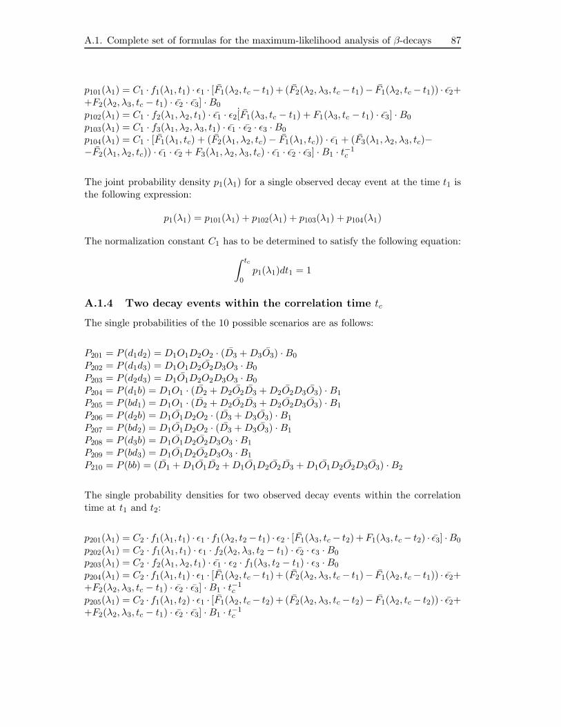
A.1. Complete set of formulas for the maximum-likelihood analysis of β-decays 87
p101(λ1) = C1 · f1(λ1, t1) · ǫ1 · [F1(λ2, tc − t1) + (F2(λ2, λ3, tc − t1)− F1(λ2, tc − t1)) · ǫ2++F2(λ2, λ3, tc − t1) · ǫ2 · ǫ3] · B0
p102(λ1) = C1 · f2(λ1, λ2, t1) · ǫ1 · ǫ2[F1(λ3, tc − t1) + F1(λ3, tc − t1) · ǫ3] · B0
p103(λ1) = C1 · f3(λ1, λ2, λ3, t1) · ǫ1 · ǫ2 · ǫ3 ·B0
p104(λ1) = C1 · [F1(λ1, tc) + (F2(λ1, λ2, tc) − F1(λ1, tc)) · ǫ1 + (F3(λ1, λ2, λ3, tc)−−F2(λ1, λ2, tc)) · ǫ1 · ǫ2 + F3(λ1, λ2, λ3, tc) · ǫ1 · ǫ2 · ǫ3] · B1 · t−1
c
The joint probability density p1(λ1) for a single observed decay event at the time t1 isthe following expression:
p1(λ1) = p101(λ1) + p102(λ1) + p103(λ1) + p104(λ1)
The normalization constant C1 has to be determined to satisfy the following equation:
∫ tc
0p1(λ1)dt1 = 1
A.1.4 Two decay events within the correlation time tc
The single probabilities of the 10 possible scenarios are as follows:
P201 = P (d1d2) = D1O1D2O2 · (D3 +D3O3) ·B0
P202 = P (d1d3) = D1O1D2O2D3O3 ·B0
P203 = P (d2d3) = D1O1D2O2D3O3 ·B0
P204 = P (d1b) = D1O1 · (D2 +D2O2D3 +D2O2D3O3) · B1
P205 = P (bd1) = D1O1 · (D2 +D2O2D3 +D2O2D3O3) · B1
P206 = P (d2b) = D1O1D2O2 · (D3 +D3O3) · B1
P207 = P (bd2) = D1O1D2O2 · (D3 +D3O3) · B1
P208 = P (d3b) = D1O1D2O2D3O3 ·B1
P209 = P (bd3) = D1O1D2O2D3O3 ·B1
P210 = P (bb) = (D1 +D1O1D2 +D1O1D2O2D3 +D1O1D2O2D3O3) ·B2
The single probability densities for two observed decay events within the correlationtime at t1 and t2:
p201(λ1) = C2 · f1(λ1, t1) · ǫ1 · f1(λ2, t2 − t1) · ǫ2 · [F1(λ3, tc − t2) +F1(λ3, tc − t2) · ǫ3] ·B0
p202(λ1) = C2 · f1(λ1, t1) · ǫ1 · f2(λ2, λ3, t2 − t1) · ǫ2 · ǫ3 ·B0
p203(λ1) = C2 · f2(λ1, λ2, t1) · ǫ1 · ǫ2 · f1(λ3, t2 − t1) · ǫ3 ·B0
p204(λ1) = C2 · f1(λ1, t1) · ǫ1 · [F1(λ2, tc − t1) + (F2(λ2, λ3, tc − t1)− F1(λ2, tc − t1)) · ǫ2++F2(λ2, λ3, tc − t1) · ǫ2 · ǫ3] · B1 · t−1
c
p205(λ1) = C2 · f1(λ1, t2) · ǫ1 · [F1(λ2, tc − t2) + (F2(λ2, λ3, tc − t2)− F1(λ2, tc − t2)) · ǫ2++F2(λ2, λ3, tc − t1) · ǫ2 · ǫ3] · B1 · t−1
c
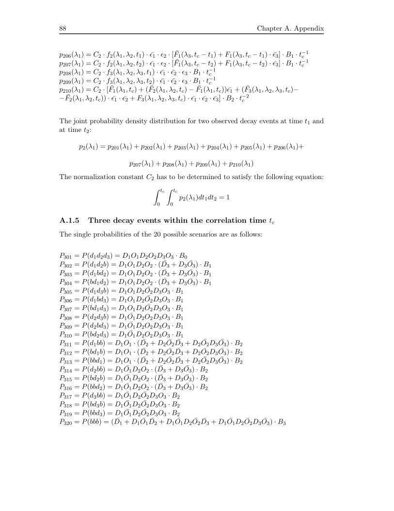
88 Chapter A. Appendix
p206(λ1) = C2 · f2(λ1, λ2, t1) · ǫ1 · ǫ2 · [F1(λ3, tc − t1) + F1(λ3, tc − t1) · ǫ3] · B1 · t−1c
p207(λ1) = C2 · f2(λ1, λ2, t2) · ǫ1 · ǫ2 · [F1(λ3, tc − t2) + F1(λ3, tc − t2) · ǫ3] · B1 · t−1c
p208(λ1) = C2 · f3(λ1, λ2, λ3, t1) · ǫ1 · ǫ2 · ǫ3 ·B1 · t−1c
p209(λ1) = C2 · f3(λ1, λ2, λ3, t2) · ǫ1 · ǫ2 · ǫ3 ·B1 · t−1c
p210(λ1) = C2 · [F1(λ1, tc) + (F2(λ1, λ2, tc) − F1(λ1, tc))ǫ1 + (F3(λ1, λ2, λ3, tc)−−F2(λ1, λ2, tc)) · ǫ1 · ǫ2 + F3(λ1, λ2, λ3, tc) · ǫ1 · ǫ2 · ǫ3] · B2 · t−2
c
The joint probability density distribution for two observed decay events at time t1 andat time t2:
p2(λ1) = p201(λ1) + p202(λ1) + p203(λ1) + p204(λ1) + p205(λ1) + p206(λ1)+
p207(λ1) + p208(λ1) + p209(λ1) + p210(λ1)
The normalization constant C2 has to be determined to satisfy the following equation:
∫ tc
0
∫ tc
0p2(λ1)dt1dt2 = 1
A.1.5 Three decay events within the correlation time tc
The single probabilities of the 20 possible scenarios are as follows:
P301 = P (d1d2d3) = D1O1D2O2D3O3 · B0
P302 = P (d1d2b) = D1O1D2O2 · (D3 +D3O3) ·B1
P303 = P (d1bd2) = D1O1D2O2 · (D3 +D3O3) ·B1
P304 = P (bd1d2) = D1O1D2O2 · (D3 +D3O3) ·B1
P305 = P (d1d3b) = D1O1D2O2D3O3 ·B1
P306 = P (d1bd3) = D1O1D2O2D3O3 ·B1
P307 = P (bd1d3) = D1O1D2O2D3O3 ·B1
P308 = P (d2d3b) = D1O1D2O2D3O3 ·B1
P309 = P (d2bd3) = D1O1D2O2D3O3 ·B1
P310 = P (bd2d3) = D1O1D2O2D3O3 ·B1
P311 = P (d1bb) = D1O1 · (D2 +D2O2D3 +D2O2D3O3) · B2
P312 = P (bd1b) = D1O1 · (D2 +D2O2D3 +D2O2D3O3) · B2
P313 = P (bbd1) = D1O1 · (D2 +D2O2D3 +D2O2D3O3) · B2
P314 = P (d2bb) = D1O1D2O2 · (D3 +D3O3) · B2
P315 = P (bd2b) = D1O1D2O2 · (D3 +D3O3) · B2
P316 = P (bbd2) = D1O1D2O2 · (D3 +D3O3) · B2
P317 = P (d3bb) = D1O1D2O2D3O3 ·B2
P318 = P (bd3b) = D1O1D2O2D3O3 ·B2
P319 = P (bbd3) = D1O1D2O2D3O3 ·B2
P320 = P (bbb) = (D1 +D1O1D2 +D1O1D2O2D3 +D1O1D2O2D3O3) ·B3
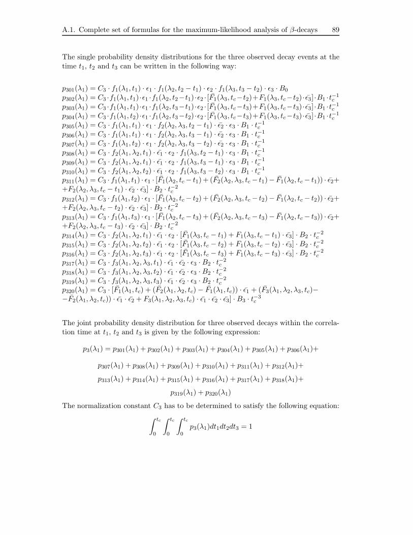
A.1. Complete set of formulas for the maximum-likelihood analysis of β-decays 89
The single probability density distributions for the three observed decay events at thetime t1, t2 and t3 can be written in the following way:
p301(λ1) = C3 · f1(λ1, t1) · ǫ1 · f1(λ2, t2 − t1) · ǫ2 · f1(λ3, t3 − t2) · ǫ3 ·B0
p302(λ1) = C3 ·f1(λ1, t1) ·ǫ1 ·f1(λ2, t2−t1) ·ǫ2 · [F1(λ3, tc−t2)+F1(λ3, tc−t2) · ǫ3] ·B1 ·t−1c
p303(λ1) = C3 ·f1(λ1, t1) ·ǫ1 ·f1(λ2, t3−t1) ·ǫ2 · [F1(λ3, tc−t3)+F1(λ3, tc−t3) · ǫ3] ·B1 ·t−1c
p304(λ1) = C3 ·f1(λ1, t2) ·ǫ1 ·f1(λ2, t3−t2) ·ǫ2 · [F1(λ3, tc−t3)+F1(λ3, tc−t3) · ǫ3] ·B1 ·t−1c
p305(λ1) = C3 · f1(λ1, t1) · ǫ1 · f2(λ2, λ3, t2 − t1) · ǫ2 · ǫ3 ·B1 · t−1c
p306(λ1) = C3 · f1(λ1, t1) · ǫ1 · f2(λ2, λ3, t3 − t1) · ǫ2 · ǫ3 ·B1 · t−1c
p307(λ1) = C3 · f1(λ1, t2) · ǫ1 · f2(λ2, λ3, t3 − t2) · ǫ2 · ǫ3 ·B1 · t−1c
p308(λ1) = C3 · f2(λ1, λ2, t1) · ǫ1 · ǫ2 · f1(λ3, t2 − t1) · ǫ3 ·B1 · t−1c
p309(λ1) = C3 · f2(λ1, λ2, t1) · ǫ1 · ǫ2 · f1(λ3, t3 − t1) · ǫ3 ·B1 · t−1c
p310(λ1) = C3 · f2(λ1, λ2, t2) · ǫ1 · ǫ2 · f1(λ3, t3 − t2) · ǫ3 ·B1 · t−1c
p311(λ1) = C3 · f1(λ1, t1) · ǫ1 · [F1(λ2, tc − t1) + (F2(λ2, λ3, tc − t1)− F1(λ2, tc − t1)) · ǫ2++F2(λ2, λ3, tc − t1) · ǫ2 · ǫ3] · B2 · t−2
c
p312(λ1) = C3 · f1(λ1, t2) · ǫ1 · [F1(λ2, tc − t2) + (F2(λ2, λ3, tc − t2)− F1(λ2, tc − t2)) · ǫ2++F2(λ2, λ3, tc − t2) · ǫ2 · ǫ3] · B2 · t−2
c
p313(λ1) = C3 · f1(λ1, t3) · ǫ1 · [F1(λ2, tc − t3) + (F2(λ2, λ3, tc − t3)− F1(λ2, tc − t3)) · ǫ2++F2(λ2, λ3, tc − t3) · ǫ2 · ǫ3] · B2 · t−2
c
p314(λ1) = C3 · f2(λ1, λ2, t1) · ǫ1 · ǫ2 · [F1(λ3, tc − t1) + F1(λ3, tc − t1) · ǫ3] · B2 · t−2c
p315(λ1) = C3 · f2(λ1, λ2, t2) · ǫ1 · ǫ2 · [F1(λ3, tc − t2) + F1(λ3, tc − t2) · ǫ3] · B2 · t−2c
p316(λ1) = C3 · f2(λ1, λ2, t3) · ǫ1 · ǫ2 · [F1(λ3, tc − t3) + F1(λ3, tc − t3) · ǫ3] · B2 · t−2c
p317(λ1) = C3 · f3(λ1, λ2, λ3, t1) · ǫ1 · ǫ2 · ǫ3 ·B2 · t−2c
p318(λ1) = C3 · f3(λ1, λ2, λ3, t2) · ǫ1 · ǫ2 · ǫ3 ·B2 · t−2c
p319(λ1) = C3 · f3(λ1, λ2, λ3, t3) · ǫ1 · ǫ2 · ǫ3 ·B2 · t−2c
p320(λ1) = C3 · [F1(λ1, tc) + (F2(λ1, λ2, tc) − F1(λ1, tc)) · ǫ1 + (F3(λ1, λ2, λ3, tc)−−F2(λ1, λ2, tc)) · ǫ1 · ǫ2 + F3(λ1, λ2, λ3, tc) · ǫ1 · ǫ2 · ǫ3] · B3 · t−3
c
The joint probability density distribution for three observed decays within the correla-tion time at t1, t2 and t3 is given by the following expression:
p3(λ1) = p301(λ1) + p302(λ1) + p303(λ1) + p304(λ1) + p305(λ1) + p306(λ1)+
p307(λ1) + p308(λ1) + p309(λ1) + p310(λ1) + p311(λ1) + p312(λ1)+
p313(λ1) + p314(λ1) + p315(λ1) + p316(λ1) + p317(λ1) + p318(λ1)+
p319(λ1) + p320(λ1)
The normalization constant C3 has to be determined to satisfy the following equation:
∫ tc
0
∫ tc
0
∫ tc
0p3(λ1)dt1dt2dt3 = 1
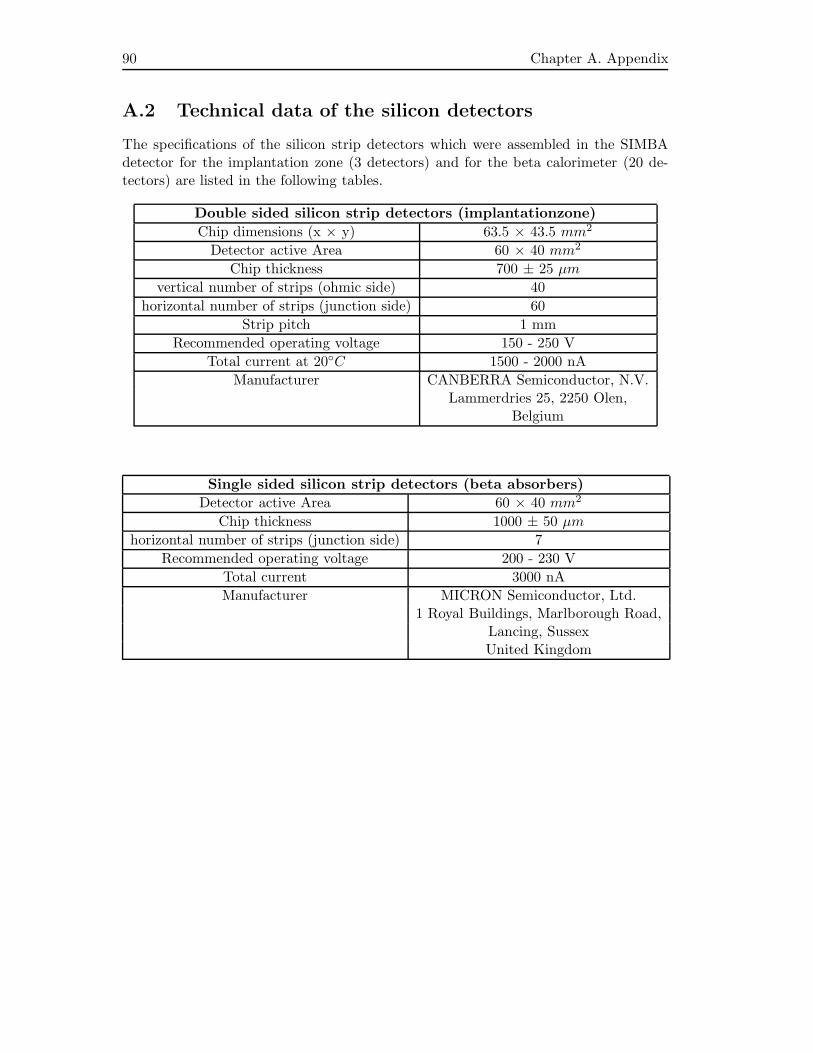
90 Chapter A. Appendix
A.2 Technical data of the silicon detectors
The specifications of the silicon strip detectors which were assembled in the SIMBAdetector for the implantation zone (3 detectors) and for the beta calorimeter (20 de-tectors) are listed in the following tables.
Double sided silicon strip detectors (implantationzone)
Chip dimensions (x × y) 63.5 × 43.5 mm2
Detector active Area 60 × 40 mm2
Chip thickness 700 ± 25 µm
vertical number of strips (ohmic side) 40
horizontal number of strips (junction side) 60
Strip pitch 1 mm
Recommended operating voltage 150 - 250 V
Total current at 20◦C 1500 - 2000 nA
Manufacturer CANBERRA Semiconductor, N.V.Lammerdries 25, 2250 Olen,
Belgium
Single sided silicon strip detectors (beta absorbers)
Detector active Area 60 × 40 mm2
Chip thickness 1000 ± 50 µm
horizontal number of strips (junction side) 7
Recommended operating voltage 200 - 230 V
Total current 3000 nA
Manufacturer MICRON Semiconductor, Ltd.1 Royal Buildings, Marlborough Road,
Lancing, SussexUnited Kingdom

A.2. Technical data of the silicon detectors 91
The two detectors which were used for a redundant position determination in (x,y)in front of the beta calorimeter stack in beam direction have the following specifications.
Single sided silicon strip detectors
Chip dimensions (x × y) 63.5 × 63.5 mm2
Detector active Area 60 × 60 mm2
Chip thickness 300 µm
vertical number of strips (ohmic side) 60
Strip pitch 1 mm
Recommended operating voltage 40 - 100 V
Total current at 20◦C 800 nA
Manufacturer CANBERRA Semiconductor, N.V.Lammerdries 25, 2250 Olen,
Belgium

92 Chapter A. Appendix
Bibliography
[1] H. Grawe et al., Phys. Scr. T56 (1995) 71.
[2] D. Seweryniak et al., Phys. Rev. Lett. 99 (2007) 022504.
[3] G. Musiol, J. Ranft, R. Reif, D. Seeliger, Kern- und Elementarteilchenphysik,Harri Deutsch, Frankfurt am Main, 2. Auflage, 1995
[4] H. Grawe, private communication, 2009.
[5] A. de Shalit and I. Talmi, Nuclear Shell Theory, Academic Press, New York andLondon, 1963.
[6] Caurier et al., Reviews of Modern Physics 77 (2005) 457.
[7] I.S. Towner, Nucl. Phys. A444 (1985) 402.
[8] B. A. Brown and K. Rykaczewski, Phys. Rev. C50 (1994) R2270.
[9] B. A. Brown, Nucl. Phys. A577 (1994) 13c-18c.
[10] V. I. Isakov et al., Phys. At. Nucl. 8 (2002) 1431.
[11] A. Arima et al., Phys. Lett 499B (2001) 104.
[12] N. D. Dang, A. Arima et al., Nucl. Phys. A621 (1997) 719.
[13] R. Schneider et al., Z. Phys. A348 (1994) 241.
[14] R. Schneider, Nachweis und Untersuchung des Zerfalls von 100Sn und benachbarterKerne, Dissertation, TU Munchen, 1996.
[15] M. Lewitowicz et al., Phys. Lett 332B (1994) 20.
[16] M. Chartier et al., Phys. Rev. Lett. 77(12) (1996) 2400.
[17] A. Stolz, Dissertation, TU Munchen, 2001.
[18] A. Stolz et al., Phys. Rev. C65 (2002) 064603.
[19] A. Bobyk, W. Kaminski, and I. N. Borzov, Acta Phys. Pol. B31 (2000) 953.
[20] D. Bazin et al., Phys. Rev. Lett. 101 (2008) 252501.
94 Literaturverzeichnis
[21] H. Geissel et al., Nucl. Instrum. Meth. B70 (1992) 286.
[22] D. J. Morrissey et al., Nucl. Instrum. and Meth. in Phys. Res. B204 (2003) 90.
[23] Y. Yano, Nucl. Instrum. and Meth. Phys. Res. B261 (2007) 1009.
[24] M. De Jong et al., Nucl. Phys. A613 (1997) 435.
[25] J.-J. Gaimard and K.-H. Schmidt, Nucl. Phys. A531 (1991) 709.
[26] D. Bazin, O. Tarasov, M. Lewitowicz and O. Sorlin, Nucl. Inst. Meth. A482 (2002)307.
[27] O. B. Tarasow and D. Bazin, Nucl. Phys. A746 (2004) 411.
[28] N. Iwasa, H. Geissel et al., Nucl. Instrum. Meth. B126 (1997) 284.
[29] T. Stohlker, H. Geissel et al., Nucl. Instrum. Meth. B61 (1991) 408.
[30] K. Straub, Dissertation, TU Munchen, 2010.
[31] M. Pfutzner et al., Nucl. Instrum. Meth. B86 (1994) 213.
[32] E. Wefers, Dissertation, TU Munchen, 2001.
[33] H. Stelzer, Nucl. Instrum. Meth. A310 (1991) 103.
[34] S. Pietri et al., Nucl. Instrum. Meth. B 261 (2007) 1079.
[35] K. Steiger, Diploma Thesis, TU Munchen, 2009.
[36] J. C. Santiard et al., GASPLEX, A low noise analog signal processor for readoutof gaseous detectors, CERN-ECP /94-17, 1994.
[37] A. Kastenmuller, 64 Channel Analog Multiplexing Frontend, Physik-DepartmentE12, TU Munchen, 1996.
[38] L. Pages et al., Atomic Data 4 (1972) 1.
[39] http://www.xia.com/DGF-4C.html
[40] Geant4 Collaboration, Physics Reference Manual Version: geant4 9.2, htt-ps://geant4.web.cern.ch/geant4/, 2008.
[41] C. Plettner et al., Phys. Rev. C66 (2002) 044319.
[42] A. Stuart and A. K. Ord, Kendall´s Advanced Theory of Statistics, Oxford Uni-versity Press, 5th edition, 1991.
[43] S. Brandt, Datenanalyse, Spektrum Akedemischer Verlag, Berlin, 4. Auflage, 1999.
Literaturverzeichnis 95
[44] V. Blobel, E. Lohrmann, Statistische und numerische Methoden der Datenanalyse,Teubner, Stuttgart, 1998.
[45] S. Baker and R. D. Cousins, Nucl. Instrum. Meth. 221 (1984) 437.
[46] O. Kavatsyuk et al., Eur. Phys. J A31 (2007) 319.
[47] Brookhaven National Nuclear Data Center
[48] H. Behrens and J. Jaenecke, Numerical Tables for Beta-decay and Electron Cap-ture, volume 4 of Landolt-Boernstein, Numerical Data and Functional Relation-ships in Science and Technology, Springer-Verlag, Berlin, 1969.
[49] Povh, Rith, Scholz, Zetsche, Teilchen und Kerne, Springer, Heidelberg, 5. Auflage,2001.
[50] M. Karny et al., Eur. Phys. J A27 (2006) 129.
[51] R. S. Hager and E. C. Seltzer, Nucl. Data A4 (1968) 1.
[52] L. Coraggio et al., Phys. Rev. C70 (2004) 034310.
[53] B. A. Brown, A. Etchegoyen, and W. D. M. Rae, The computer code OXBASH,MSU-NSCL, Report No. 534.
[54] C. A. Stone, W. B. Walters, Hyperfine Interactions 22 (1985) 363.
[55] M. Hjorth-Jensen, Phys. Rep. 261 (1995) 125.
[56] A. H. Wapstra, G. Audi et al., Nucl. Phys. A729 (2003) 129.
[57] L. Batist et al., submitted to Eur. Phys. J
[58] B. A. Brown, Progress in Particle and Nuclear Physics 47 (2001) 517.
[59] M. Lipoglavsek, Phys. Lett. B440 (1998) 246.
[60] A. Blazhev et al., Journal of Physics: Conference Series 205 (2010) 012035.
[61] T. Mayer-Kuckuck, Kernphysik, Teubner, Stuttgart, 4. Auflage, 1984
[62] J. C. Hardy, I. S. Towner at al., Nucl. Phys. A509 (1990) 429.
[63] D. Groom et al., Eur. Phys. J C15 (2000) 1.
[64] B. J. Barton and J. K. Tuli, Physics Analysis Programs for Nuclear StructureEvaluation, Report BNL-NCS-23375/R, Brookhaven National Laboratory, 1977.
[65] C. Amsler et al., Physics Letters B667 (2008) 1.

96 Literaturverzeichnis

Acknowledgement
Finally I would like to thank a few people for their contribution to this thesis:
The most important persons to thank have to be my superivisors Prof. Dr. ReinerKr”ucken, Dr. Thomas Faestermann and Dr. Roman Gernh”auser. They have been avital source of knowledge, advice and guidance in every aspect of this undertaking.
I also would like to thank the members of the 100Sn-team: Dr. Ludwig Maier, Dr.Michael B”ohmer, Dr. Florian Nebel, Katrin Straub and Konrad Steiger. Withouttheir support and the teamwork the experiment would certainly not have been such agreat success.In this context I would like to particularly emphasize the major contribution of Dr.Ludwig Maier during all stages of the project from the construction of the implantationdetector to the final data analysis.
For the last five years E12 was in a sense my second home. I enjoyed to spend my timethere and I got to know many interesting people. I would like to thank all members ofE12 for just having been there.