Subspace concentration of geometric measures · measures of convex bodies act as counterparts of...
107
Subspace Concentration of Geometric Measures vorgelegt von M.Sc. Hannes Pollehn geboren in Salzwedel von der Fakultät II - Mathematik und Naturwissenschaften der Technischen Universität Berlin zur Erlangung des akademischen Grades Doktor der Naturwissenschaften – Dr. rer. nat. – genehmigte Dissertation Promotionsausschuss: Vorsitzender: Prof. Dr. John Sullivan Gutachter: Prof. Dr. Martin Henk Gutachterin: Prof. Dr. Monika Ludwig Gutachter: Prof. Dr. Deane Yang Tag der wissenschaftlichen Aussprache: 07.02.2019 Berlin 2019
Transcript of Subspace concentration of geometric measures · measures of convex bodies act as counterparts of...

Subspace Concentration of GeometricMeasures
vorgelegt vonM.Sc. Hannes Pollehn
geboren in Salzwedel
von der Fakultät II - Mathematik und Naturwissenschaftender Technischen Universität Berlin
zur Erlangung des akademischen Grades
Doktor der Naturwissenschaften– Dr. rer. nat. –
genehmigte Dissertation
Promotionsausschuss:
Vorsitzender: Prof. Dr. John SullivanGutachter: Prof. Dr. Martin HenkGutachterin: Prof. Dr. Monika LudwigGutachter: Prof. Dr. Deane Yang
Tag der wissenschaftlichen Aussprache: 07.02.2019
Berlin 2019

iii
Zusammenfassung
In dieser Arbeit untersuchen wir geometrische Maße in zwei verschiedenenErweiterungen der Brunn-Minkowski-Theorie.
Der erste Teil dieser Arbeit befasst sich mit Problemen in der Lp-Brunn-Minkowski-Theorie, die auf dem Konzept der p-Addition konvexer Körper ba-siert, die zunächst von Firey für p ≥ 1 eingeführt und später von Lutwak et al.für alle reellen p betrachtet wurde. Von besonderem Interesse ist das Zusammen-spiel des Volumens und anderer Funktionale mit der p-Addition. Bedeutsameoffene Probleme in diesem Setting sind die Gültigkeit von Verallgemeinerungender berühmten Brunn-Minkowski-Ungleichung und der Minkowski-Ungleichung,insbesondere für 0 ≤ p < 1, da die Ungleichungen für kleinere p stärker werden.Die Verallgemeinerung der Minkowski-Ungleichung auf p = 0 wird als loga-rithmische Minkowski-Ungleichung bezeichnet, die wir hier für vereinzelte poly-topale Fälle beweisen werden. Das Studium des Kegelvolumenmaßes konvexerKörper ist ein weiteres zentrales Thema in der Lp-Brunn-Minkowski-Theorie,das eine starke Verbindung zur logarithmischen Minkowski-Ungleichung auf-weist. In diesem Zusammenhang stellen sich die grundlegenden Fragen nacheiner Charakterisierung dieser Maße und wann ein konvexer Körper durch seinKegelvolumenmaß eindeutig bestimmt ist. Letzteres ist für symmetrische konve-xe Körper unbekannt, während das erstere Problem in diesem Fall gelöst wurde.Die Schlüsseleigenschaft in der Lösung ist eine Konzentrationsgrenze eines gege-benen Kegelvolumenmaßes eingeschränkt auf lineare Unterräume. Wir werdeneine Charakterisierung von Kegelvolumenmaßen von Trapezen herleiten undneue Beispiele konvexer Körper mit nicht-eindeutigem Kegelvolumenmaß prä-sentieren. Dabei werden wir diskutieren, wie das Vorhandensein einer Schrankean die Konzentration auf Unterräumen die oben genannten Fragen beeinflusst.
Im zweiten Teil betrachten wir eine erst kürzlich entdeckte Familie geometri-scher Maße, die in der dualen Brunn-Minkowski-Theorie vorkommt. Die soge-nannten dualen Krümmungsmaße von konvexen Körpern fungieren als Gegen-stücke zu Krümmungsmaßen in der klassischen Brunn-Minkowski-Theorie undschließen das Kegelvolumenmaß als Sonderfall ein. Duale Krümmungsmaße ha-ben in den letzten Jahren großes Interesse geweckt. Die Aufgabe, die Resultate,die für Kegelvolumenmaße erzielt wurden, auf die allgemeineren dualen Krüm-mungsmaße auszudehnen, erfordert neuartige Abschätzungen der Unterraum-konzentration. Den Ideen von Kneser und Süss folgend, beweisen wir Variantender Brunn-Minkowski-Ungleichung unter gewissen Symmetrievoraussetzungen,mit deren Hilfe wir scharfe Schranken an die Unterraumkonzentration für nahe-zu alle dualen Krümmungsmaße symmetrischer konvexer Körper folgern.


v
Abstract
In this work we study geometric measures in two different extensions of theBrunn-Minkowski theory.
The first part of this thesis is concerned with problems in Lp Brunn-Minkowskitheory, that is based on the concept of p-addition of convex bodies, which wasfirst introduced by Firey for p ≥ 1 and later considered for all real p by Lutwaket al. The interplay of the volume and other functionals with the p-additionis of particular interest. Considerable open problems in this setting includethe validity of extensions of the celebrated Brunn-Minkowski inequality andMinkowski’s inequality, particularly for 0 ≤ p < 1 as the inequalities becomestronger for smaller p. The generalization of Minkowski’s inequality to p = 0is called logarithmic Minkowski inequality, which we will prove here for someparticular polytopal instances. The study of the cone-volume measure of con-vex bodies is another central subject in Lp Brunn-Minkowski theory, whichexhibits a strong connection to the logarithmic Minkowski inequality. Funda-mental questions in this context ask for a characterization of these measures andwhen a convex body is uniquely determined by its cone-volume measure. Thelatter is unknown even for symmetric convex bodies whereas the former prob-lem was solved in this case. The key property in the solution is a concentrationbound of a given cone-volume measure restricted to linear subspaces. We willestablish a characterization of cone-volume measures of trapezoids and presentnew examples of convex bodies with non-unique cone-volume measure. Therebywe will discuss how the presence of a subspace concentration bound affects theaforementioned questions.
In the second part we consider an only recently discovered family of geometricmeasures arising in dual Brunn-Minkowski theory. The so-called dual curvaturemeasures of convex bodies act as counterparts of curvature measures in theclassical Brunn-Minkowski theory and include the cone-volume measure as aspecial case. Dual curvature measures gained much interest in the last fewyears. The task of extending the results obtained for cone-volume measures tothe more general dual curvature measures requires novel subspace concentrationinequalities. Following the ideas of Kneser and Süss we establish variants ofthe Brunn-Minkowski inequality under some symmetry assumptions with theaid of which we prove sharp subspace concentration bounds on nearly all dualcurvature measures of symmetric convex bodies.

Acknowledgments
I am very grateful to my advisor Martin Henk for his support, guidance, knowl-edge and experience, and for fruitful discussions on various mathematical andnon-mathematical topics. Furthermore I would like to express my gratitude tomy thesis committee: Monika Ludwig, Deane Yang and John Sullivan.
To all my family and in particular my beloved parents: Thank you for yourlove and support under any circumstances throughout the years.
I further thank my co-auther Károly Böröczky, Jr., and all my current andformer colleagues at TU Berlin. Many thanks to Romanos Malikiosis for havingan open office door whenever I needed it. With a special mention to Sören Bergfor being my office neighbor, fellow and friend for almost ten years.
Moreover, I would like to thank all the people I got to know in Magdeburgduring my undergraduate and graduate studies. You made mathematics moreenjoyable than even the most beautiful theory ever could. My special thanks toChristan Günther for accompanying me and being my roommate, and to eachof the “Greenhornes” for being my second family.
Finally, I wish to thank my (underpaid) revisors Ali, Sören and Geno. Butmost of all I want to express my gratitude to Stephan. Thank you for being aclose friend for so long, and thank you for reading and revising this thesis withlimitless effort. You’re the real MVP.
vii

Contents
Introduction 1
1 Preliminaries 5
2 The logarithmic Minkowski inequality and the planar cone-volume measure 152.1 An introduction to Lp Brunn-Minkowski theory . . . . . . . . . . 152.2 The logarithmic Minkowski inequality for simplices . . . . . . . . 192.3 The logarithmic Minkowski inequality for parallelepipeds . . . . . 232.4 The logarithmic Minkowski problem for trapezoids . . . . . . . . 322.5 Subspace concentration and uniqueness of the cone-volume measure 40
3 Dual curvature measures 473.1 An introduction to dual Brunn-Minkowski theory . . . . . . . . . 473.2 A generalization of Anderson’s theorem on even quasiconcave
functions . . . . . . . . . . . . . . . . . . . . . . . . . . . . . . . 523.3 A Brunn–Minkowski type inequality for moments of the Euclidean
norm . . . . . . . . . . . . . . . . . . . . . . . . . . . . . . . . . . 563.4 Subspace concentration in the even dual Minkowski problem . . . 653.5 Further results . . . . . . . . . . . . . . . . . . . . . . . . . . . . 723.6 Lp dual curvature measures . . . . . . . . . . . . . . . . . . . . . 78
Conclusion 85
Bibliography 87
Index 93
List of Symbols 95
ix

Introduction
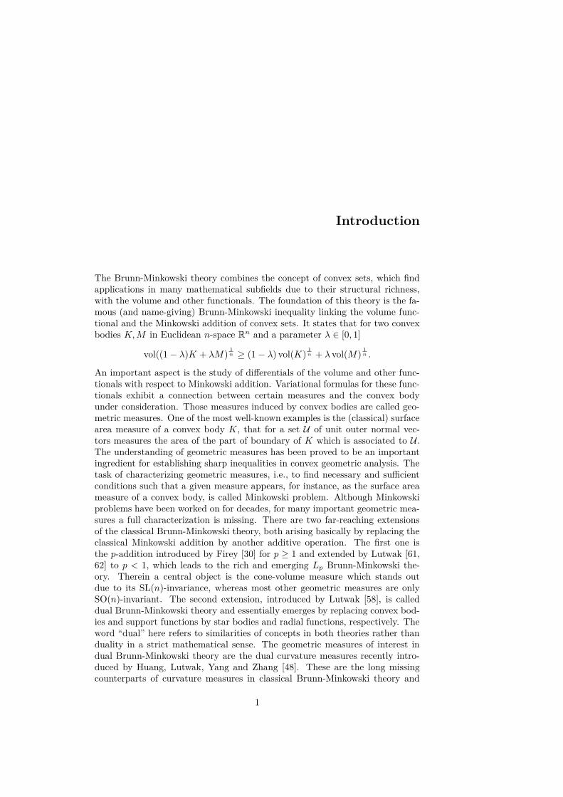
The Brunn-Minkowski theory combines the concept of convex sets, which findapplications in many mathematical subfields due to their structural richness,with the volume and other functionals. The foundation of this theory is the fa-mous (and name-giving) Brunn-Minkowski inequality linking the volume func-tional and the Minkowski addition of convex sets. It states that for two convexbodies K,M in Euclidean n-space Rn and a parameter λ ∈ [0, 1]
vol((1 − λ)K + λM) 1n ≥ (1 − λ) vol(K) 1
n + λ vol(M) 1n .
An important aspect is the study of differentials of the volume and other func-tionals with respect to Minkowski addition. Variational formulas for these func-tionals exhibit a connection between certain measures and the convex bodyunder consideration. Those measures induced by convex bodies are called geo-metric measures. One of the most well-known examples is the (classical) surfacearea measure of a convex body K, that for a set U of unit outer normal vec-tors measures the area of the part of boundary of K which is associated to U .The understanding of geometric measures has been proved to be an importantingredient for establishing sharp inequalities in convex geometric analysis. Thetask of characterizing geometric measures, i.e., to find necessary and sufficientconditions such that a given measure appears, for instance, as the surface areameasure of a convex body, is called Minkowski problem. Although Minkowskiproblems have been worked on for decades, for many important geometric mea-sures a full characterization is missing. There are two far-reaching extensionsof the classical Brunn-Minkowski theory, both arising basically by replacing theclassical Minkowski addition by another additive operation. The first one isthe p-addition introduced by Firey [30] for p ≥ 1 and extended by Lutwak [61,62] to p < 1, which leads to the rich and emerging Lp Brunn-Minkowski the-ory. Therein a central object is the cone-volume measure which stands outdue to its SL(n)-invariance, whereas most other geometric measures are onlySO(n)-invariant. The second extension, introduced by Lutwak [58], is calleddual Brunn-Minkowski theory and essentially emerges by replacing convex bod-ies and support functions by star bodies and radial functions, respectively. Theword “dual” here refers to similarities of concepts in both theories rather thanduality in a strict mathematical sense. The geometric measures of interest indual Brunn-Minkowski theory are the dual curvature measures recently intro-duced by Huang, Lutwak, Yang and Zhang [48]. These are the long missingcounterparts of curvature measures in classical Brunn-Minkowski theory and
1

2 Introduction
VK(η) SK(η)η
K
Figure 1: Surface area measure and cone-volume measure of a smooth convexbody
they have already been studied thoroughly since their discovery. This thesisis mainly concerned with Minkowski problems regarding cone-volume measuresand dual curvature measures.
We will provide notions and definitions that will be used later on in Chapter 1.In particular we will properly introduce the concept of area measures, includingthe classical surface area measure
SK(η) = Hn−1(ν−1K (η)),
where K ⊆ Rn is a convex body, η ⊆ Sn−1 a Borel set and Hn−1 the (n − 1)-dimensional Hausdorff measure. Here Sn−1 denotes the unit sphere in Euclideann-space and νK denotes the Gauss map (see p. 7 for the definition). The cone-volume measure of a convex body K ⊆ Rn with the origin in its interior is givenby
VK(η) = 1n
∫ν−1
K(η)
⟨x,νK(x)⟩ dHn−1(x)
for every Borel set η ⊆ Sn−1. It is closely related to the classical surface areameasure (see Fig. 1). We will state the Minkowski problems associated to therespective measures and present (partial) solutions to them.
Chapter 2 focuses on some problems in Lp Brunn-Minkowski theory that arerelated to the cone-volume measure of convex bodies. The task of characterizing,when a given measure is the cone-volume measure of a convex body, is alsoknown as the logarithmic Minkowski problem. Symmetric convex bodies arethe largest class this goal has been achieved for. It was proved in [19] that anon-zero finite even Borel measure µ on Sn−1 is the cone-volume measure of asymmetric convex body if and only if the subspace concentration inequality
µ(L ∩ Sn−1) ≤ dim(L)n
µ(Sn−1)
is satisfied for every proper subspace L ⊆ Rn, and equality is attained forsome L, if and only if there is a subspace L′ complementary to L such that
3
µ is concentrated on Sn−1 ∩ (L ∪ L′). In the general setting the gap betweenknown necessary and sufficient conditions is quite large. A little more is knownfor the two-dimensional case. Here we will examine the cone-volume measureof trapezoids explicitly to highlight the presence of conditions which are – incontrast to the subspace concentration inequality – non-linear in terms of cone-volumes. Moreover, we will discuss the question when a polygon is uniquelydetermined by its cone-volume measure. This has been answered by Stancu [77]for symmetric polygons, but for symmetric polytopes in higher dimensions itis an open problem. Here we will present examples of non-symmetric polygonswith few vertices and non-unique cone-volume measure. In addition, the cone-volume measure appears naturally in problems of Lp Brunn-Minkowski theoryaiming for results stronger than their counterpart in classical Brunn-Minkowskitheory. For two convex bodies K,M ⊆ Rn with the origin in their interiors theirlog-combination with respect to λ ∈ [0, 1] is given by
(1 − λ)K +0 λM
={
x ∈ Rn : ⟨u,x⟩ ≤ hK(u)1−λhM (u)λ for all u ∈ Sn−1} ,where hK and hM denote the support functions of K and M , respectively. Thelogarithmic Brunn-Minkowski inequality reads as
vol((1 − λ)K +0 λM) ≥ vol(K)1−λ vol(M)λ.As a consequence of the inequality of arithmetic and geometric means one caneasily check that the logarithmic Brunn-Minkowski inequality, if it holds true,is in fact stronger than the classical Brunn-Minkowski inequality. It was proved(among other cases) for pairs of symmetric convex bodies in the plane in [18]and if both K and M are unconditional convex bodies in arbitrary dimensionin [74]. It is conjectured that the logarithmic Brunn-Minkowski inequality holdswhenever K and M are symmetric. It was shown by Böröczky, Lutwak, Yangand Zhang [18] that the logarithmic Brunn-Minkowski inequality is equivalentto the logarithmic Minkowski inequality∫
Sn−1
log(
hM (u)hK(u)
)dVK(u) ≥ vol(K)
nlog(
vol(M)vol(K)
)in the sense that if one holds for all pairs of symmetric convex bodies K andM , the other one follows. The logarithmic Minkowski inequality does not holdfor arbitrary pairs of convex bodies with the origin as an interior point. Forcentered convex bodies, i.e., convex bodies whose centroid (or center of mass) isthe origin, there is no example known that violates the logarithmic Minkowskiinequality. Here we will verify the logarithmic Minkowski inequality for someparticular instances where one of the convex bodies is centered and the otherone is either a simplex or a parallelepiped. The presented results are based onjoint work with Martin Henk [43].
Chapter 3 revolves around Minkowski problems in dual Brunn-Minkowskitheory, namely regarding the dual curvature measures. For some q ∈ R and aconvex body K ⊆ Rn with the origin in its interior one may define the qth dualcurvature measure of K via˜Cq(K, η) = 1
n
∫νK (η)−1
|x|q−n ⟨νK(x),x⟩ dHn−1(x)

4 Introduction
for every Borel set η ⊆ Sn−1. They not only play an important role in dualBrunn-Minkowski theory, they also include well-known measures from classicalBrunn-Minkowski theory, e.g., the cone-volume measure in case q = n. Regard-ing the dual Minkowski problem, i.e., finding necessary and sufficient conditionson dual curvature measures, much progress has been made during the past cou-ple of years. In [48] it was shown that, given q ∈ (0, n) and a non-zero finiteeven Borel measure µ on the sphere, a certain subspace concentration inequalityis sufficent for the existence of a symmetric convex body K with µ = ˜Cq(K, ·).In this work we will establish tight subspace concentration bounds of dual cur-vature measures of symmetric convex bodies for the parameter ranges q ∈ (0, n)and q ∈ [n + 1,∞). The former supplements a result obtained by Böröczky,Lutwak, Yang, Zhang and Zhao [17] which lead to a solution of the even dualMinkowski problem for parameters q ∈ (0, n): A non-zero finite even Borel mea-sure µ on Sn−1 is the qth dual curvature measure of a symmetric convex bodyif and only if the subspace concentration inequality
µ(L ∩ Sn−1) < min{
dim(L)q
, 1}µ(Sn−1)
is satisfied for every proper subspace L ⊆ Rn. Our proofs of the necessity of thesubspace concentration inequality rely heavily on the symmetry of the involvedconvex bodies and variants of the Brunn-Minkowski inequality where the volumefunctional is replaced by a measure having a power of the Euclidean norm asLebesgue density function. Moreover, we will discuss which of these inequalitiescan be easily extended to other norms. The remaining range q ∈ (n, n + 1)in the symmetric setting is completely open as neither necessary nor sufficientconditions are known at this moment. At least in the planar case n = 2 we alsoprovide tight subspace concentration bounds by extending the abovementionedinequalities. The results presented in this chapter are based on joint works withKároly Böröczky, Jr., and Martin Henk [14, 42].
1 Preliminaries
The aim of this chapter is to provide the essential definitions and concepts usedthroughout the thesis. We recommend the books by Gardner [32], Gruber [36]and Schneider [75] as excellent references on convex geometry.
Foundations
We consider the Euclidean n-space Rn = {x = (x1, . . . , xn)T : x1, . . . , xn ∈ R}equipped with standard inner product ⟨x,y⟩ =
∑ni=1 xiyi for x,y ∈ Rn. The
Euclidean norm will be denoted by |x| =√
⟨x,x⟩ for x ∈ Rn and if x = 0 itsnormalization is x = x
|x| . We write e1, . . . , en for the standard basis vectors inRn. For any setX ⊆ Rn we write int(X) and ∂X for its interior and its boundarypoints, respectively. We denote by Bn the n-dimensional Euclidean unit ball,i.e., Bn = {x ∈ Rn : |x| ≤ 1}, and by Sn−1 = ∂Bn = {x ∈ Rn : |x| = 1} itsboundary.
For a linear subspace L ⊆ Rn, L⊥ is its orthogonal complement and theorthogonal projection onto L is denoted by ·|L. For a non-empty set X ⊆ Rnwe define its linear hull by
lin(X) ={
m∑i=1
λixi : m ∈ N, λi ∈ R,xi ∈ X for i = 1, . . . ,m},
its affine hull by
aff(X) ={
m∑i=1
λixi : m ∈ N, λi ∈ R,xi ∈ X for i = 1, . . . ,m,m∑i=1
λi = 1},
its positive hull
pos(X) ={
m∑i=1
λixi : m ∈ N, λi ≥ 0,xi ∈ X for i = 1, . . . ,m}
and its convex hull by
5
6 1 Preliminaries
conv(X)
={
m∑i=1
λixi : m ∈ N, λi ≥ 0,xi ∈ X for i = 1, . . . ,m,m∑i=1
λi = 1}.
The convex hull conv{x,y} of two points x,y ∈ Rn will be abbreviated by[x,y]. A set is called convex if it equals its convex hull. A set of pointsX ⊆ Rn is called affinely independent if aff(X \ {x}) = aff(X) for everyx ∈ X. Its dimension is the maximal number of affinely independent pointscontained in it minus 1 and will be denoted by dim(X). For convenience wealso define dim(∅) = −1. The relative interior of a set X is the interior of Xwith respect to its affine hull.
Convex bodiesA convex and compact set with non-empty interior is called a convex body.We write Kn for the set of all convex bodies in Rn and Kn
o for convex bodiescontaining the origin in the interior, i.e., Kn
o = {K ∈ Kn : 0 ∈ intK}.
As usual, Minkowski addition of subsets of Rn and multiplication withscalars are defined pointwise so that for X,Y ⊆ Rn and α, β ∈ R we write
αX + βY = {αx + βy : x ∈ X,y ∈ Y }. (1.1)
In case X,Y ∈ Kn and α, β ≥ 0 or 0 ≤ β = 1−α ≤ 1, we also speak of Minkowskicombination and convex combination between convex bodies, respectively. ForA ⊆ R we also define A ·X = {αx : α ∈ A,x ∈ X}.
The normalized k-dimensional Hausdorff measure will be denoted by Hk andinstead of it we will sometimes write volk for the volume or just vol if the dimen-sion is apparent from the context. The k-dimensional Hausdorff measure par-ticularly coincides with the k-dimensional Lebesgue measure in affine subspacesand k-dimensional spherical Lebesgue measure on subspheres. In integrals wewill often abbreviate dHn(x) by dx, when integrating with respect to Hn, anddHn−1(u) by du, when integrating with respect to Hn−1. According to this,the centroid c(X) of a Lebesgue measurable set X ⊆ Rn with positive volumeis defined by
c(X) = 1vol(X)
∫X
x dx.
If c(X) = 0, the set X is called centered. In addition, we will denote the set ofcentered convex bodies by Kn
c and the subclass of symmetric convex bodies byKns , i.e., convex bodies K with K = −K. An even stronger notion of symmetry
is held by unconditional convex bodies. These are symmetric about everycoordinate hyperplane, i.e., if K ∈ Kn is an unconditional convex body, then(x1, . . . , xn)T ∈ K implies (±x1, . . . ,±xn)T ∈ K.
By the well-known Brunn-Minkowski inequality we know that the nth rootof the volume of a Minkowski combination is a concave function.

7
u
HK(u)
hK(u)K
Figure 1.1: Smooth convex body and supporting hyperplane
Theorem 1.1 (Brunn-Minkowski inequality, see, e.g., [75, Thm. 7.1.1]). IfK,L ∈ Kn and 0 < λ < 1, then
vol((1 − λ)K + λL) 1n ≥ (1 − λ) vol(K) 1
n + λ vol(L) 1n (1.2)
and equality holds if and only if K and L are homothetic, i.e., they are equal upto translation and scaling.
For fixed a ∈ Rn \ {0} and α ∈ R the hyperplane given by the equation⟨a,x⟩ = α will be denoted by H(a, α). We will sometimes use a⊥ insteadof H(a, 0). We write H−(a, α) and H+(a, α) for the halfspaces defined by⟨a,x⟩ ≤ α and ⟨a,x⟩ ≥ α, respectively. For a convex and compact set K ⊆ Rnthe support function hK : Rn → R is defined by (see Fig. 1.1)
hK(x) = maxy∈K
⟨x,y⟩ .
It is worth noting that convex bodies are uniquely determined by their supportfunctions since for given K ∈ Kn the support function hK is the pointwiseminimal function with
K = {x ∈ Rn : ⟨u,x⟩ ≤ hK(u) for all u ∈ Sn−1}.
On the other hand, each convex, positively 1-homogeneous function Rn → R isthe support function of a convex and compact set. A boundary point x ∈ ∂Kis said to have a (not necessarily unique) unit outer normal vector u ∈ Sn−1
if ⟨u,x⟩ = hK(u), i.e., x ∈ H(u, hK(u)). The corresponding supporting hy-perplane H(u, hK(u)) will be denoted by HK(u). We write ∂′K for the set ofboundary points of K with unique outer normal vector and define the Gaussmap νK : ∂′K → Sn−1 such that νK(x) is the unique unit outer normal vectorof x ∈ ∂′K. Almost every boundary point of convex body has a unique outernormal vector in the sense that (∂K) \ (∂′K) has (n− 1)-dimensional Hausdorffmeasure 0 (see, e.g., [75, Thm. 2.2.5]). If ∂K = ∂′K, K is called smooth.
8 1 Preliminaries
PolytopesA polytope is the convex hull of finitely many points. If a polytope is k-dimensional, we also call it k-polytope. Fulldimensional polytopes are alsoconvex bodies and we will use the symbols Pn,Pn
c ,Pns ,Pn
o ⊆ Kn to denotethe sets of n-polytopes, centered n-polytopes, symmetric n-polytopes and poly-topes containing the origin in the interior, respectively. Polytopes in the planeR2 will also be called polygons. Each polytope can be written as the convexhull of a unique minimal set of points, called vertices. In addition to that,it is well known (c.f., e.g., [75, Sect. 2.4]) that a polytope can be equivalentlydescribed as a bounded intersection of finitely many halfspaces, i.e., a boundedset of the form
{x ∈ Rn : Ax ≤ b},where m ∈ N, A ∈ Rm×n and b ∈ Rm. For an n-polytope P ∈ Pn we saythat u ∈ Sn−1 is a unit outer normal vector of P if voln−1(P ∩HP (u)) > 0.The outer normal vectors of P are precisely the irredundant row vectors of Ascaled to unit length. In particular, there are only finitely many of them. Theset of all unit outer normal vectors of a polytope P is denoted by U(P ). For agiven u ∈ U(P ) we associate a set of points in the boundary of P arising fromthe intersection of P with the supporting hyperplane HP (u). This point setF (P,u) = P ∩HP (u) is called facet of P normal to u. Moreover, a given finiteset U ⊆ Sn−1 appears as the set of outer normal vectors of some fulldimensionalpolytope in Rn if and only if posU = Rn, i.e., we say that U is not concentratedon a closed hemisphere.
There are two notable instances of polytopes in this work. A k-simplex orjust simplex is the convex hull of k + 1 affinely independent points. Volumeand centroid of a simplex can be easily computed from their vertices, i.e., ifan n-simplex is given as S = conv{v1, . . . , vn+1} for some affinely independentpoints v1, . . . , vn+1 ∈ Rn, then
vol(S) = |det(vn+1 − v1,vn+1 − v2, . . . , vn+1 − vn)| ,
c(S) = 1n+ 1
n+1∑i=1
vi.
Moreover, n-simplices are the only polytopes in Rn having exactly n+ 1 outernormal vectors which is also minimal among all n-polytopes. Restricting tosymmetric polytopes Pn
s the latter role is taken by linear images of the cube[−1, 1]n. These are called parallelepipeds and are precisely the polytopesgiven as solution sets of systems of the form
|⟨ui,x⟩| ≤ hi, i = 1, . . . , n,
for some linearly independent u1, . . . ,un ∈ Sn−1 and h1, . . . , hn > 0. In thiscase the volume of the parallelepiped can be computed by
2n∏ni=1 hi
|det(u1, . . . ,un)| (1.3)
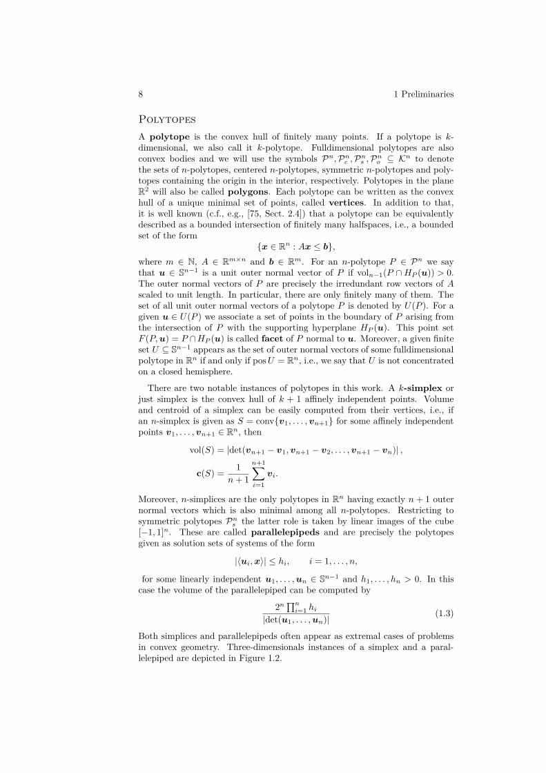
Both simplices and parallelepipeds often appear as extremal cases of problemsin convex geometry. Three-dimensionals instances of a simplex and a paral-lelepiped are depicted in Figure 1.2.

9
Figure 1.2: 3-simplex and 3-dimensional parallelepiped
Geometric measuresThe combination of the volume functional and Minkowski addition is fundamen-tal in the Brunn-Minkowki theory. The Minkowski sum K+M , K,M ∈ Kn, for“small” M may be interpreted as a pertubation of K. Intriguingly, since sup-port functions are linear with respect to Minkowski addition of convex bodies,the support function of the sum K + M is represented by the sum of supportfunctions hK+hM . When hM is replaced by an arbitrary function f : Sn−1 → R,the convex body defined by
[hK + f ] = {x ∈ Rn : ⟨u,x⟩ ≤ hK(u) + f(u) for all u ∈ Sn−1},
is called the Wulff shape of hK + f . The support function of the Wulff shape[hK + f ] does not necessarily agree with hK + f , but we always have [hK ] = Kfor K ∈ Kn. The variational formula
limϵ→0
vol([hK + εf ]) − vol([hK ])ε
=∫
Sn−1
f(u) dSK(u), (1.4)
for every continuous function f : Sn−1 → R, was originally established by Alek-sandrov ([2], see also [75, Lem. 7.5.3]). Here SK is the Borel measure on Sn−1
known as the surface area measure of the convex body K and defined by
SK(η) = Hn−1(ν−1K (η))
for each Borel set η ⊆ Sn−1. The notion of surface area measures goes backto Lebesgue and Minkowski. If K = P is a polytope, the surface area measureis discrete and concentrated on the outer normal vectors. Moreover, for eachouter normal vector it assigns the area of the facet. To be more precise, it holdsthat
SP (η) =∑
u∈U(P )∩η
voln−1(F (P,u))
for every Borel set η ⊆ Sn−1 (see Fig. 1.3). A common extension of the volumefunctional are the quermassintegrals Wi(K) of a convex body K ∈ Kn, whichmay be defined via the classical Steiner formula, expressing the volume of theMinkowski sum of K ∈ Kn and λBn, i.e., the volume of the parallel body of Kat distance λ ≥ 0, as a polynomial in λ (cf., e.g., [75, Sect. 4.2])
vol(K + λBn) =n∑i=0
λi(n
i
)Wi(K). (1.5)

10 1 Preliminaries
Pη
SP (η)
Figure 1.3: Surface area measure of a polygon
In particular, W0(K) = vol(K). The quermassintegrals of a convex body K maybe interpreted as – up to normalization – the average volume of projections of K,i.e., Kubota’s integral formula (cf., e.g., [75, Subsect. 5.3.2]) states that
Wn−i(K) = vol(Bn)voli(Bi)
∫G(i,n)
voli(K|L) dL, (1.6)
i = 0, . . . , n, where integration is taken with respect to the rotation-invariantprobability measure on the Grassmannian G(i, n) of all i-dimensional linearsubspaces. Aleksandrov [2] and Fenchel and Jessen [28] established a variatonalformula similar to (1.4) for quermassintegrals in case f is a support functionand only right limits are considered:
limε↘0
Wn−1−i(K + εM) − Wn−1−i(K)ε
=∫
Sn−1
hM (u) dSi(K,u) (1.7)
for K,M ∈ Kn, i = 0, . . . , n − 1, where Si(K, ·) are Borel measures on thesphere called area measures of K. The (n − 1)th area measure Sn−1(K, ·) isjust the surface area measure of K. Interestingly, the area measures of a convexbody admit a local Steiner-type formula like (1.5) in the following sense. Fora convex body K ∈ Kn and a point x ∈ Rn the metric projection pK(x)is the unique point in K that is closest to x. For x ∈ Rn \ K we also defineυK(x) = x − pK(x), i.e., υK(x) is a (not necessarily unique) unit outer normalvector of pK(x) and for every x ∈ Rn its distance to K by
d(K,x) ={
|x − pK(x)| , if x /∈ K,0, if x ∈ K.
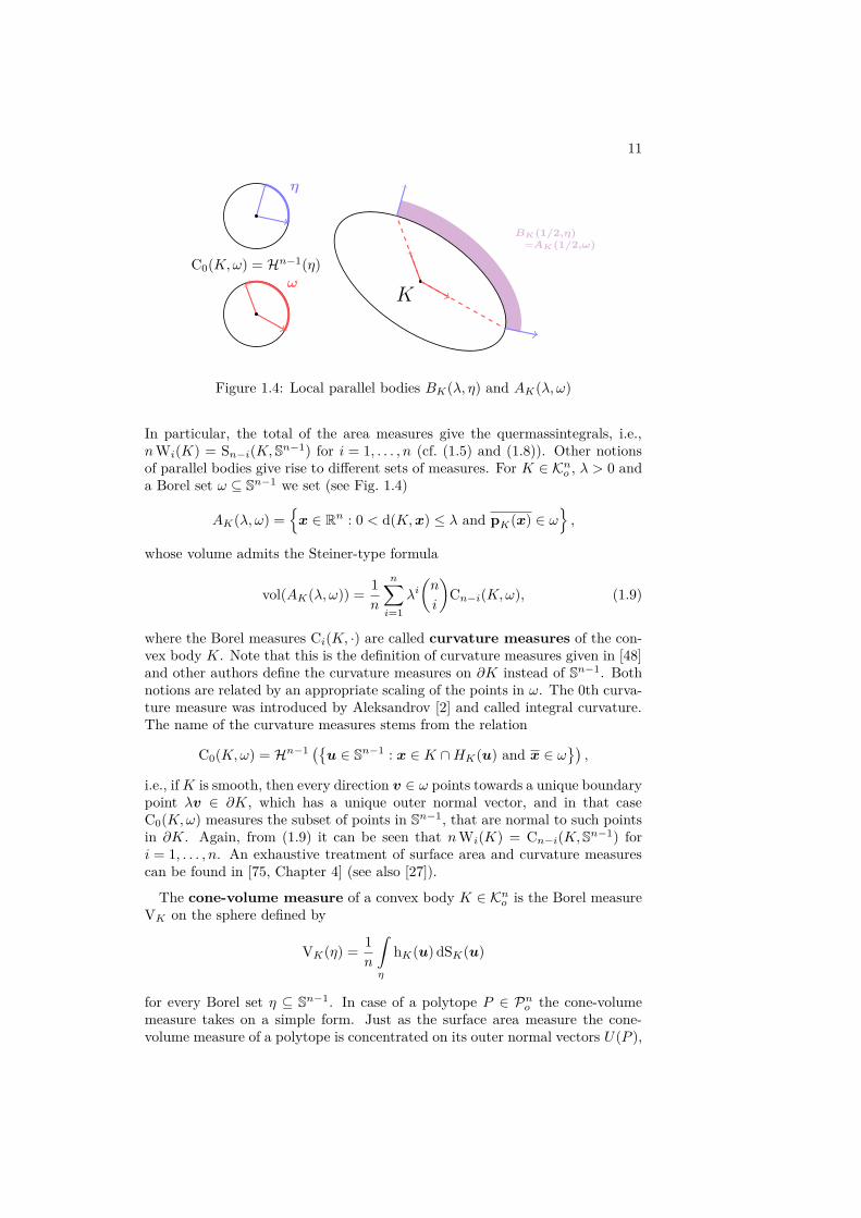
Then for a Borel set η ⊆ Sn−1 and λ > 0 we consider the local parallel body(see Fig. 1.4)
BK(λ, η) = {x ∈ Rn : 0 < d(K,x) ≤ λ and υK(x) ∈ η} .
The local Steiner formula expresses the volume of BK(λ, η) as a polynomial in λ.Its coefficients are – up to constants depending on i and n – the area measures(cf., e.g., [75, Sect. 4.2])
vol(BK(λ, η)) = 1n
n∑i=1
λi(n
i
)Sn−i(K, η). (1.8)
11
BK(1/2,η)=AK(1/2,ω)
η
ωK
C0(K,ω) = Hn−1(η)
Figure 1.4: Local parallel bodies BK(λ, η) and AK(λ, ω)
In particular, the total of the area measures give the quermassintegrals, i.e.,nWi(K) = Sn−i(K, Sn−1) for i = 1, . . . , n (cf. (1.5) and (1.8)). Other notionsof parallel bodies give rise to different sets of measures. For K ∈ Kn
o , λ > 0 anda Borel set ω ⊆ Sn−1 we set (see Fig. 1.4)
AK(λ, ω) ={
x ∈ Rn : 0 < d(K,x) ≤ λ and pK(x) ∈ ω},
whose volume admits the Steiner-type formula
vol(AK(λ, ω)) = 1n
n∑i=1
λi(n
i
)Cn−i(K,ω), (1.9)
where the Borel measures Ci(K, ·) are called curvature measures of the con-vex body K. Note that this is the definition of curvature measures given in [48]and other authors define the curvature measures on ∂K instead of Sn−1. Bothnotions are related by an appropriate scaling of the points in ω. The 0th curva-ture measure was introduced by Aleksandrov [2] and called integral curvature.The name of the curvature measures stems from the relation
C0(K,ω) = Hn−1 ({u ∈ Sn−1 : x ∈ K ∩HK(u) and x ∈ ω}),
i.e., if K is smooth, then every direction v ∈ ω points towards a unique boundarypoint λv ∈ ∂K, which has a unique outer normal vector, and in that caseC0(K,ω) measures the subset of points in Sn−1, that are normal to such pointsin ∂K. Again, from (1.9) it can be seen that nWi(K) = Cn−i(K, Sn−1) fori = 1, . . . , n. An exhaustive treatment of surface area and curvature measurescan be found in [75, Chapter 4] (see also [27]).
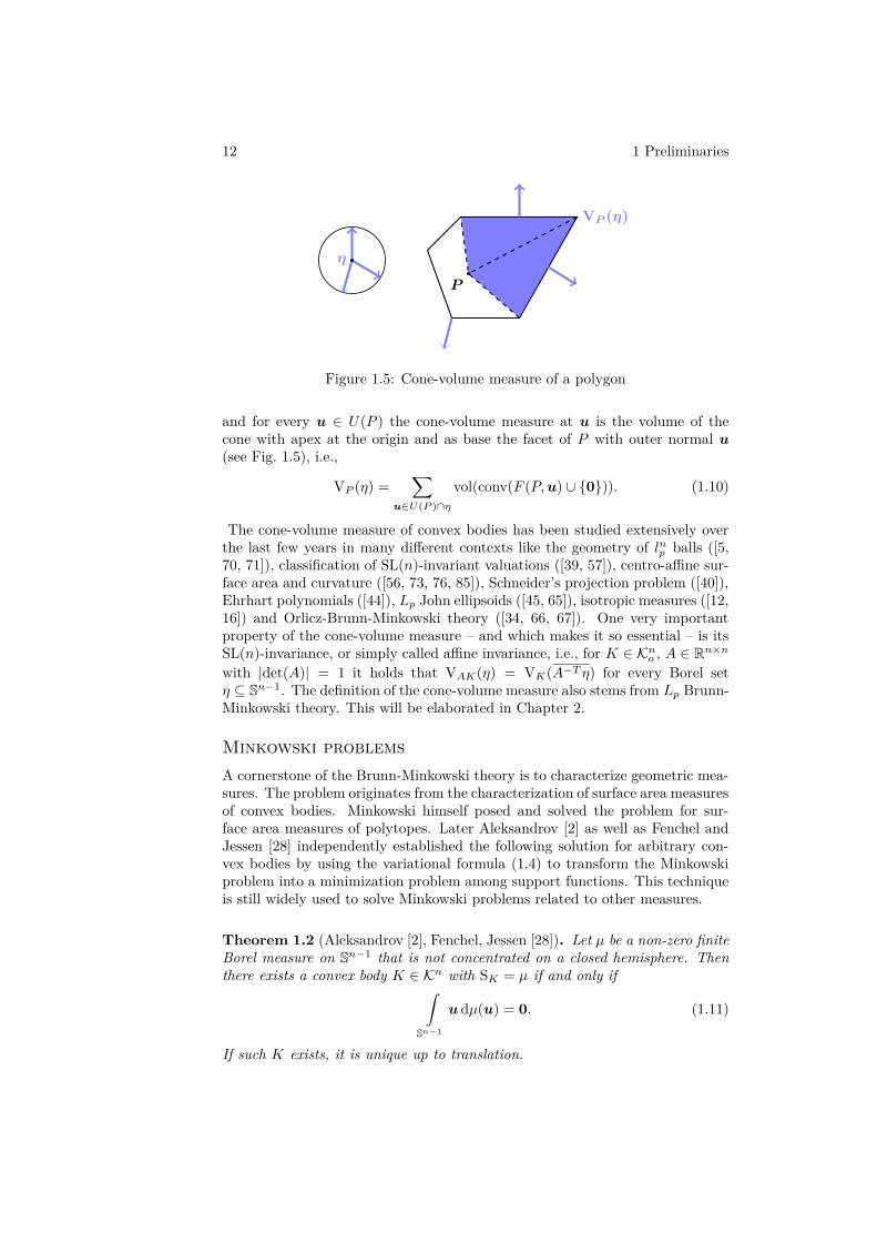
The cone-volume measure of a convex body K ∈ Kno is the Borel measure
VK on the sphere defined by
VK(η) = 1n
∫η
hK(u) dSK(u)
for every Borel set η ⊆ Sn−1. In case of a polytope P ∈ Pno the cone-volume
measure takes on a simple form. Just as the surface area measure the cone-volume measure of a polytope is concentrated on its outer normal vectors U(P ),
12 1 Preliminaries
P
η
VP (η)
Figure 1.5: Cone-volume measure of a polygon
and for every u ∈ U(P ) the cone-volume measure at u is the volume of thecone with apex at the origin and as base the facet of P with outer normal u(see Fig. 1.5), i.e.,
VP (η) =∑
u∈U(P )∩η
vol(conv(F (P,u) ∪ {0})). (1.10)
The cone-volume measure of convex bodies has been studied extensively overthe last few years in many different contexts like the geometry of lnp balls ([5,70, 71]), classification of SL(n)-invariant valuations ([39, 57]), centro-affine sur-face area and curvature ([56, 73, 76, 85]), Schneider’s projection problem ([40]),Ehrhart polynomials ([44]), Lp John ellipsoids ([45, 65]), isotropic measures ([12,16]) and Orlicz-Brunn-Minkowski theory ([34, 66, 67]). One very importantproperty of the cone-volume measure – and which makes it so essential – is itsSL(n)-invariance, or simply called affine invariance, i.e., for K ∈ Kn
o , A ∈ Rn×n
with |det(A)| = 1 it holds that VAK(η) = VK(A−T η) for every Borel setη ⊆ Sn−1. The definition of the cone-volume measure also stems from Lp Brunn-Minkowski theory. This will be elaborated in Chapter 2.
Minkowski problemsA cornerstone of the Brunn-Minkowski theory is to characterize geometric mea-sures. The problem originates from the characterization of surface area measuresof convex bodies. Minkowski himself posed and solved the problem for sur-face area measures of polytopes. Later Aleksandrov [2] as well as Fenchel andJessen [28] independently established the following solution for arbitrary con-vex bodies by using the variational formula (1.4) to transform the Minkowskiproblem into a minimization problem among support functions. This techniqueis still widely used to solve Minkowski problems related to other measures.
Theorem 1.2 (Aleksandrov [2], Fenchel, Jessen [28]). Let µ be a non-zero finiteBorel measure on Sn−1 that is not concentrated on a closed hemisphere. Thenthere exists a convex body K ∈ Kn with SK = µ if and only if∫
Sn−1
u dµ(u) = 0. (1.11)
If such K exists, it is unique up to translation.
13
Minkowski first solved the problem for measures which are either discrete orcontinuous, thus referred to as (classical) Minkowski problem. In case of apolytope P the equation (1.11) becomes∑
u∈U(P )
voln−1(F (P,u))u = 0. (1.12)
Today the characterization of area measures Si(K, ·) of convex bodies K ∈ Kn,i ∈ {1, . . . , n − 1}, among the finite Borel measures on the sphere is known asthe Minkowski–Christoffel problem, since for i = n − 1 it is the classicalMinkowski problem and for i = 1 it is known as Christoffel problem. Fori = 1 Firey [29] and Berg [6] solved the problem independently and deriveda necessary and sufficient condition which looks rather technical (see also [75,Thm. 8.3.8]). In the case 1 < i < n − 1 the characterization of area measuresSi(K, ·) still is a major open problem. If one considers the curvature measures wespeak of Aleksandrov problems since for C0 the problem has been solved byAleksandrov [2]. We refer to [75, Chapter 8] and [48, p. 4] for more informationand references on the Minkowski-Christoffel problem and also characterizationof curvature measures.
The Minkowski problem associated to cone-volume measures of convex bodiesin Kn
o is called logarithmic Minkowski problem. The discrete planar evenlogarithmic Minkowski problem was completely solved by Stancu [77, 78] viacrystalline flows. She also proved that cone-volume measures of polytopes inP2s are unique with parallelograms being the only exception. The latter result
was generalized to K2s by Böröczky, Lutwak, Yang and Zhang in [18]. Later,
the same authors used a variational approach to extend Stancu’s solution ofthe even logarithmic Minkowski problem for P2
s to arbitrary dimensions andeven measures on the sphere. One of the striking properties of cone-volumemeasures of symmetric convex bodies is an upper bound on the concentrationon subspaces.
Theorem 1.3 (Böröczky, Lutwak, Yang, Zhang [19]). Let µ be a non-zerofinite even Borel measure on Sn−1. Then there exists a symmetric convex bodyK ∈ Kn
s with VK = µ if and only if
µ(Sn−1 ∩ L) ≤ dimL
nµ(Sn−1) (1.13)
for every proper subspace L of Rn, and equality in (1.13) is attained for someL, if and only if there is a subspace L′ complementary to L such that µ isconcentrated on Sn−1 ∩ (L ∪ L′).
The inequality (1.13) along with its equality condition is known and will bereferred to as subspace concentration condition. The above result settlesthe logarithmic Minkowski problem for symmetric convex bodies. However, thequestion of uniqueness of cone-volume measures of symmetric convex bodies re-mains an open problem. The general setting is more challenging. The validityof the subspace concentration condition for cone-volume measures of centeredpolytopes was established by Henk and Linke [41] and extended to centeredconvex bodies by Böröczky and Henk [13]. In the latter paper another remark-able result states the existence of lower bounds on concentration of cone-volume
14 1 Preliminaries
measures of centered convex bodies on open hemispheres. Stability in (1.13) forcentered convex bodies is thematized in [12]. Regarding the general case, evenless is known. Zhu [86] proved that in the discrete case there are no additionalconditions on the measure if its support is in general position and not con-centrated on a closed hemisphere. A set of vectors is said to be in generalposition if each n-element subset is linearly independent. In other words, Zhushowed that every measure on Sn−1, that is concentrated on a finite subset ofSn−1 in general position, but not on a closed hemisphere, can be realized as thecone-volume measure of a polytope. A refinement of this result can be foundin [11], where it was proved that the validity of (1.13) (for a certain subsetof subspaces) is a sufficient condition when the given measure is discrete butnot necessarily symmetric. Chen, Li and Zhu [22] then used a sophisticatedapproximation argument to conclude that the strict inequality in (1.13) is alsosufficient in case of non-even measures. Moreover, they gave the first examplesof non-unique cone-volume measures not coming from parallelepipeds. On theother hand, necessary conditions on arbitrary cone-volume measures are widelymissing. In [10], Böröczky and Zhu established a sharp upper bound on sub-space concentration on 1-dimensional subspaces. Nevertheless, as they pointout, their condition is non-sufficient even in the planar case.
2 The logarithmic Minkowski inequality and theplanar cone-volume measure
2.1 An introduction to Lp Brunn-Minkowskitheory
The starting point of this chapter is the study of the volume of certain sums ofconvex bodies other than the Minkowski addition defined by (1.1). Recall thatthe support function of a Minkowski combination λK + (1 − λ)M , K,M ∈ Kn,λ ∈ [0, 1], is given by λhK +(1−λ)hM which represents the weighted arithmeticmean of hK and hM . It seems natural to consider other means of the respectivesupport functions as well, where p-means (also called Hölder or generealizedmeans) are the most well-known examples. For p ∈ R \ {0}, positive numberss, t ∈ R>0 and a weighting parameter λ ∈ [0, 1] the p-mean of s and t is givenby
Mp(s, t, λ) = [(1 − λ)sp + λtp]1p ,
where we may extend the definition to p = 0 via taking the limit
M0(s, t, λ) = limp→0
[(1 − λ)sp + λtp]1p = s1−λtλ,
which is the weighted geometric mean of s and t. The family of p-means includethe arithmetic mean as special case when p = 1. Moreover, the means aremonotone with respect to p, i.e., for p ≤ p′ it holds that
Mp(s, t, λ) ≤ Mp′(s, t, λ).
In order to consider the p-mean of support functions we have to assure positivity.That is why here only the class Kn
o is considered. Now for p = 0, K,M ∈ Kno ,
and scalars s, t ≥ 0 the p-combination of K and M with respect to s and t is(see Fig. 2.1)
s ·p K +p t ·p M
={
x ∈ Rn : ⟨u,x⟩ ≤ [shK(u)p + thM (u)p]1p for all u ∈ Sn−1
},
or in case s = λ, t = 1 − λ,
15

16 2 The log-Minkowski inequality and the planar cone-volume measure
p = 0 p = 1/2
p = 1 p = 5
Figure 2.1: p-combination 12K +p
12M for K = conv
{(02),( −1
−1/2),( 2
−1/2)}
andM = [−1, 1]2
(1 − λ) ·p K +p λ ·p M= {x ∈ Rn : ⟨u,x⟩ ≤ Mp(hK(u), hM (u), λ) for all u ∈ Sn−1}. (2.1)
In the context of p-combinations we will usually just write · instead of ·p.
We want to point out that one may study p-combinations in a slightly moregeneral way: The notion of p-means can be extended to p ∈ {±∞} via takingthe limit, and if p > 0, the p-mean can be defined on the set of nonnegativenumbers so that also convex bodies K with 0 ∈ ∂K may be considered in p-combinations. However, for the sake of simplicity we restrict ourselves to p ∈ Rand p-combinations within Kn
o .
The p-combination of convex bodies was first considered by Firey [30] forp ≥ 1. He also established an extension of the Brunn-Minkowski inequality (1.2)to p-combinations for p > 1. More precisely, he proved that for p > 1, K,M ∈ Kn
o
and λ ∈ [0, 1]
vol((1 − λ)K +p λM)pn ≥ (1 − λ) vol(K)
pn + λ vol(M)
pn . (2.2)
Very recently Kolesnikov and Milman [54] established (2.2) under some smooth-ness assumptions on K and M , if p < 1 and p is sufficiently close to 1. Due toLutwak [61] is the following variational formula
limε↘0
vol(K +p εM) − vol(K)ε
= 1p
∫Sn−1
hM (u)phK(u)1−p dSK(u). (2.3)
2.1 An introduction to Lp Brunn-Minkowski theory 17
for p > 1 and K,M ∈ Kno . The measure S(p)
K given by
dS(p)K = h1−p
K dSK
is called Lp surface area measure of K and can be defined this way for everyp ∈ R. In particular, the Lp surface area measure coincides with the classicalsurface area measure and – up to a factor – with the cone-volume measure inthe cases p = 1 and p = 0, respectively. The task of characterizing Lp surfacearea measures is known as Lp Minkowski problem and was first addressedby Lutwak [61]. The Lp Brunn Minkowski theory has gained much interestthroughout the years and has developed rapidly since 1990’s. We refer to [75,Chapter 9] for a comprehensive overview of Lp Brunn-Minkowski theory. Recentprogress on the Lp Minkowski problem was made in [7, 15, 21, 23, 24, 46, 49,50, 55, 63, 84, 85, 87, 88].
As Schneider points out, Lutwaks solution to the Lp Minkowski problem forp > 1 in [61] actually only requires p > 0. This was the dawn of the Lp Brunn-Minkowski theory for 0 < p < 1, which is both fascinating, since inequalities like(2.2) and (2.3) become stronger for smaller p, and challenging, since in generalthe p-mean of support functions is not the support function of the respective p-combination for p < 1. By taking the limit p → 0+ the inequality (2.2) becomesthe logarithmic Brunn-Minkowski inequality
vol((1 − λ) ·K +0 λ ·M) ≥ vol(K)1−λ vol(M)λ, (2.4)
where we define by
(1 − λ)K +0 λM
= {x ∈ Rn : ⟨u,x⟩ ≤ M0(hK(u), hM (u), λ) for all u ∈ Sn−1}
the log-combination of K and L with respect to λ (cf. (2.1)). It can be seenfrom the arithmetic-geometric mean inequality that the logarithmic Brunn-Minkowski inequality (2.4), if it holds true, is in fact stronger than (1.2).Böröczky, Lutwak, Yang and Zhang [18] conjectured that (2.4) holds for allpairs of symmetric convex bodies K,M ∈ Kn
s , but so far it has been verifiedonly in particular instances. In [18], the planar case n = 2 was established andSaroglou [74] showed that (2.4) holds for pairs of unconditional convex bodiesin arbitrary dimension, i.e., for convex bodies that are symmetric about everycoordinate hyperplane (see also [8, 25] for preliminary work). Both results weregiven alongside a characterization of the equality cases.
It is well-known that the classical Brunn-Minkowski inequality (1.2) is equiv-alent to Minkowski’s mixed volume inequality, which, for two convex bodiesK,M ∈ Kn
o , can be stated as∫Sn−1
hM (u)hK(u) dVK(u) ≥ vol(K)
n−1n vol(M) 1
n . (2.5)
Just as for the Brunn-Minkowski inequality, the Minkowski inequality (2.5)can be seen as a particular case of a family of Lp Minkowski inequalities in

18 2 The log-Minkowski inequality and the planar cone-volume measure
the Lp Brunn-Minkowski theory. The Lp Minkowski inequality states that forK,M ∈ Kn
o ∫Sn−1
(hM (u)hK(u)
)pdVK(u) ≥ vol(K)
n−pn vol(M)
pn (2.6)
and it was proved by Lutwak [61] for p > 1. So far, however, it is an openproblem if (2.6) holds even for pairs of symmetric convex bodies when 0 < p < 1.In a fundamental paper, Böröczky, Lutwak, Yang and Zhang [18] establishedthe Lp Minkowski inequality in the plane in the case where K,M ∈ K2
s and0 < p < 1. Moreover, they showed that in any dimension the Lp Brunn-Minkowski inequality (2.2) and the Lp Minkowski inequality (2.6) are equivalentin the class of symmetric convex bodies.
Theorem 2.1 (Böröczky, Lutwak, Yang, Zhang [18]). Let p > 0. The Lp Brunn-Minkowski inequality (2.2) holds for all K,M ∈ Kn
s and λ ∈ [0, 1] if and only ifthe Lp Minkowski inequality (2.6) holds true all K,M ∈ Kn
s .
The results extend to the limit case p → 0+ which is as follows.
Theorem 2.2 (Böröczky, Lutwak, Yang, Zhang [18]). The logarithmic Brunn-Minkowski inequality (2.4) holds for all K,M ∈ Kn
s and λ ∈ [0, 1] if and only ifthe logarithmic Minkowski inequality∫
Sn−1
log hM (u)hK(u) dVK(u) ≥ vol(K)
nlog vol(M)
vol(K) (2.7)
holds true all K,M ∈ Kns .
The inequality (2.7) is called the logarithmic Minkowski inequality and it wasproved to hold in the plane ([18], see [68] for a different proof) and for pairs ofunconditional convex bodies in any dimension ([74]).
In the general setting almost nothing is known. There are counterexamplesshowing that neither (2.4) nor (2.7) hold for pairs of arbitrary convex bodiescontaining the origin in the interior, e.g., a cube and a suitable translate of it.Instead one considers certain classes of convex bodies granting control over thelocation of the origin. Xi and Leng [80] proved that (2.4) holds if the two bodiesare in so-called dilation position, which includes the class Kn
s . Guan and Li [38]established among others the logarithmic Minkowski inequality when K is theEuclidean unit ball and the Santálo point of M is the origin. The Santálo pointof a convex body K is the point x ∈ intK minimizing vol([K − x]∗) where[K − x]∗ is the polar body of K − x (cf. (3.1)). Further results were obtainedby Stancu [79], e.g., she proved among others that the logarithmic Minkowskiinequality (2.7) holds true for convex bodies K,M ∈ Kn
o , when K is a polytopeand each facet of K touches the boundary of L. Stancu also established versionsof (2.7) where in place of M an affine image of M is used; for instance whenK is a centered simplex with constant edge length and M a given convex body,then there is an affine image M of M such that (2.7) holds for K and M .
In the Sections 2.2 and 2.3 we will study the logarithmic Minkowski (2.7) in-equality in the context of centered convex bodies. This particularly includes the
2.2 The log-Minkowski inequality for simplices 19
class of symmetric convex bodies. Here we will prove the logarithmic Minkowskiinequality in some very particular instances. More precisely, we establish the log-arithmic Minkowski inequality (2.7) when the gauge body is a centered simplexand the other one is centered, and also when the gauge body is a parallelepipedand the other one is symmetric. The main tool in the proofs are sharp volumebounds on intersections of centered convex bodies with hyperplanes and halfs-paces like Grünbaum’s inequality (2.9). Furthermore, we extend the logarithmicMinkowski inequality for parallelepipeds to the setting where the second body isonly centered rather than symmetric, but only in small dimensions. The resultsof the Sections 2.2 and 2.3 appeared as joint work with Martin Henk [43].
The Section 2.4 treats the logarithmic Minkowski problem in the plane fortrapezoids. Our main result is a full characterization of cone-volume measuresof trapezoids including the explicit computation of a trapezoid from a givencone-volume measure. Together with results stated in [78] this settles the loga-rithmic Minkowski problem for quadrilaterals. We discuss uniqueness of cone-volume measures in Section 2.5. Moreover, from the aforementioned explicitdescription we may derive a family of examples confirming non-uniqueness ofcone-volume measures of quadrilaterals. So far, the only examples, which arenot parallelepids, were given in [22] including fivegons in the planar case. Thelogarithmic Minkowski problem for polygons with at least five vertices is stillopen.
2.2 The logarithmic Minkowski inequality forsimplices
We will now prove the logarithmic Minkowski inequality (2.7) for some specialcases. They all have in common that one of the convex bodies under consider-ation is assumed to be centered and the other one is either a centered simplexor, in Section 2.3, a parallelepiped. One of the used tools is a reformulation ofMinkowski’s characterization theorem (Theorem 1.2). For a polytope P ∈ Pn
o
and a unit outer normal vector u ∈ U(P ) the volume of the corresponding conecan be computed by (cf. (1.10))
VP (u) = vol(conv(F (P,u) ∪ {0})) = hP (u)n
voln−1(F (P,u)),
which is the well-known pyramid formula. Substituting into (1.12) yields theequivalent equation ∑
u∈U(P )
VP (u)hP (u) u = 0, (2.8)
so that Minkowski’s characterization becomes a statement formulated entirely interms of support functions and cone-volumes. The second important ingredientin the proofs is Grünbaum’s inequality. Each symmetric convex body dividedby a hyperplane through the origin will have its volume split into equal parts.Due to Grünbaum is the following sharp bound for centered convex bodies(see Fig. 2.2).
20 2 The log-Minkowski inequality and the planar cone-volume measure
P
c(P )
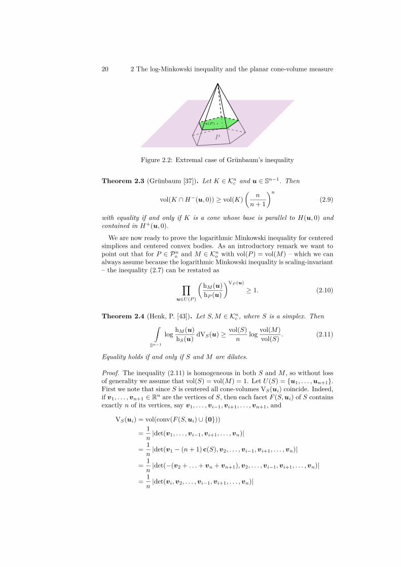
Figure 2.2: Extremal case of Grünbaum’s inequality
Theorem 2.3 (Grünbaum [37]). Let K ∈ Knc and u ∈ Sn−1. Then
vol(K ∩H−(u, 0)) ≥ vol(K)(
n
n+ 1
)n(2.9)
with equality if and only if K is a cone whose base is parallel to H(u, 0) andcontained in H+(u, 0).
We are now ready to prove the logarithmic Minkowski inequality for centeredsimplices and centered convex bodies. As an introductory remark we want topoint out that for P ∈ Pn
o and M ∈ Kno with vol(P ) = vol(M) – which we can
always assume because the logarithmic Minkowski inequality is scaling-invariant– the inequality (2.7) can be restated as
∏u∈U(P )
(hM (u)hP (u)
)VP (u)≥ 1. (2.10)
Theorem 2.4 (Henk, P. [43]). Let S,M ∈ Knc , where S is a simplex. Then∫
Sn−1
log hM (u)hS(u) dVS(u) ≥ vol(S)
nlog vol(M)
vol(S) . (2.11)
Equality holds if and only if S and M are dilates.
Proof. The inequality (2.11) is homogeneous in both S and M , so without lossof generality we assume that vol(S) = vol(M) = 1. Let U(S) = {u1, . . . ,un+1}.First we note that since S is centered all cone-volumes VS(ui) coincide. Indeed,if v1, . . . , vn+1 ∈ Rn are the vertices of S, then each facet F (S,ui) of S containsexactly n of its vertices, say v1, . . . , vi−1,vi+1, . . . , vn+1, and
VS(ui) = vol(conv(F (S,ui) ∪ {0}))
= 1n
|det(v1, . . . , vi−1,vi+1, . . . , vn)|
= 1n
|det(v1 − (n+ 1) c(S),v2, . . . , vi−1,vi+1, . . . , vn)|
= 1n
|det(−(v2 + . . .+ vn + vn+1),v2, . . . , vi−1,vi+1, . . . , vn)|
= 1n
|det(vi,v2, . . . , vi−1,vi+1, . . . , vn)|
2.2 The log-Minkowski inequality for simplices 21
= VS(u1).
Thus, for each i ∈ {1, . . . , n+1} we have VS(ui) = 1n+1 . Hence in view of (2.10)
we just have to verifyn+1∏i=1
hM (ui)hS(ui)
≥ 1 (2.12)
and by (2.8) we also know
n+1∑i=1
1hS(ui)
ui = 0. (2.13)
Grünbaum’s centroid inequality (2.9) applied to the centered convex body Mgives for 1 ≤ i ≤ n+ 1
vol(M ∩H−(ui, 0)) ≥ vol(M)(
n
n+ 1
)n(2.14)
and for the simplex S we have the equality
vol(S) = vol(S ∩H−(ui, 0))(n+ 1n
)n(2.15)
for i = 1, . . . , n+ 1. Now suppose (2.12) does not hold. Then there exist also nindices i = 1, . . . , n, say, with
n∏i=1
hM (ui) <n∏i=1
hS(ui). (2.16)
Since M ⊆ {x ∈ Rn : ⟨ui,x⟩ ≤ hM (ui), 1 ≤ i ≤ n}, we conclude in view of(2.14)(
n
n+ 1
)nvol(M) ≤ vol(M ∩H−(un+1, 0))
≤ vol({x ∈ Rn : ⟨ui,x⟩ ≤ hM (ui), 1 ≤ i ≤ n, ⟨un+1,x⟩ ≤ 0}).
Let T = {x ∈ Rn : ⟨ei,x⟩ ≤ 1, 1 ≤ i ≤ n, ⟨∑ni=1 ei,x⟩ ≥ 0} and A be the
(n× n)-matrix with columns ui
hM (ui) , i = 1, . . . , n. Then
A−TT = {x ∈ Rn : ⟨ui,x⟩ ≤ hM (ui), 1 ≤ i ≤ n, ⟨un+1,x⟩ ≤ 0}
and thus, by (2.16) and (2.15),(n
n+ 1
)nvol(M) ≤
det(
u1
hM (u1) , . . . ,un
hM (un)
)−1vol(T )
=∏ni=1 hM (ui)
|det(u1, . . . ,un)| vol(T )
<
∏ni=1 hS(ui)
|det(u1, . . . ,un)| vol(T )
= vol({x ∈ Rn : ⟨ui,x⟩ ≤ hS(ui), 1 ≤ i ≤ n, ⟨un+1,x⟩ ≤ 0})
22 2 The log-Minkowski inequality and the planar cone-volume measure
=(
n
n+ 1
)nvol(S).
This contradicts, however, the assumption that S and M have the same volume.
Suppose now we have equality in (2.12). Then we must also have equality foreach n-element subset of {1, . . . , n+ 1}, since in view of (2.16)
n+1∏i=1i =j
hM (ui) ≥n∏i=1i =j
hS(ui)
must hold for every j and
(hS(u1) . . . hS(un+1))n =n+1∏j=1
n∏i=1i =j
hS(ui)
≤n+1∏j=1
n∏i=1i =j
hM (ui) = (hM (u1) . . . hM (un+1))n.
Moreover, for every choice of n indices, say {1, . . . , n}, by repeating the stepsabove we have (
n
n+ 1
)nvol(M) =
(n
n+ 1
)nvol(S)
=∏ni=1 hS(ui)
|det(u1, . . . ,un)| vol(T )
=∏ni=1 hM (ui)
|det(u1, . . . ,un)| vol(T )
= vol(M ∩H−(un+1, 0))
and by the characterization of the equality case in Theorem 2.3 we know that Mis a simplex with outer normals ui and centroid at the origin. Hence Minkowski’scharacterization formula (2.13) also holds with hS(ui) replaced by hM (ui) whichshows that S and M must be equal.
It is not hard to see that the logarithmic Minkowski inequality for centeredsimplices (Theorem 2.4) implies the uniqueness of cone-volume measures con-centrated on n + 1 affinely independent directions. However, this is also aconsequence of Minkowski’s characterization theorem (cf. Theorem 1.2). For if,let u1, . . . ,un+1 be the outer unit normals of two simplices S, T ∈ Pn
o and thetwo simplices have equal cone-volumes γi = VS(ui) = VT (ui), 1 ≤ i ≤ n + 1.Let αi(S), αi(T ), 1 ≤ i ≤ n + 1, be the (n − 1)-dimensional volume of thefacet with outer normal vector ui of S and T , respectively. By (1.12) and theaffine independence of the normal vectors we get that (α1(S), . . . , αn+1(S))Tand (α1(T ), . . . , αn+1(T ))T are contained in a one-dimensional subspace, soαi(S) = µαi(T ) for 1 ≤ i ≤ n+ 1 and a positive scalar µ. Hence,
hS(ui)hT (ui)
=
(nγi
αi(S)
)(
nγi
αi(T )
) = αi(S)αi(T ) = µ,
2.3 The log-Minkowski inequality for parallelepipeds 23
and so S = µT . Since vol(S) = vol(T ) it follows that S = T .
2.3 The logarithmic Minkowski inequality forparallelepipeds
Using the same arguments as in the foregoing proof of Theorem 2.4 we may es-tablish the logarithmic Minkowski inequality when both bodies are o-symmetricand one is a parallelepiped. Instead of Grünbaum’s inequality (2.9) we use thefact that hyperplanes through the origin cut symmetric sets into equal halves.
Proposition 2.5 (Henk, P. [43]). Let Q,M ∈ Kns , where Q is a parallelepiped.
Then ∫Sn−1
log hM (u)hQ(u) dVQ(u) ≥ vol(Q)
nlog vol(M)
vol(Q) .
Equality holds if and only if M is a parallelepiped with U(M) = U(Q).
Proof. Without loss of generality we assume that vol(Q) = vol(M). Let U(Q) ={±u1, . . . ,±un}. First we note that all cone-volumes VQ(±ui) coincide as Qis the linear image of a cube, so each cone of Q is the linear image of a cone ofthe cube. Therefore and since M is symmetric we just have to verify
n∏i=1
hM (ui)hQ(ui)
≥ 1. (2.17)
Now suppose (2.17) does not hold. Since M ⊆ {x ∈ Rn : |⟨ui,x⟩| ≤ hM (ui), 1 ≤i ≤ n}, we get
vol(M) ≤ vol({x ∈ Rn : |⟨ui,x⟩| ≤ hM (ui), 1 ≤ i ≤ n}) (2.18)
=2n∏ni=1 hM (ui)
|det(u1, . . . ,un)|
<2n∏ni=1 hQ(ui)
|det(u1, . . . ,un)|= vol(Q).
This contradicts, however, the assumption of having the same volume.
Suppose now we have equality in (2.17). Then by the same arguments asabove
vol(Q) = vol(M) ≤ vol({x ∈ Rn : |⟨ui,x⟩| ≤ hM (ui), 1 ≤ i ≤ n})
=2n∏ni=1 hM (ui)
|det(u1, . . . ,un)|
=2n∏ni=1 hQ(ui)
|det(u1, . . . ,un)|= vol(Q),

24 2 The log-Minkowski inequality and the planar cone-volume measure
i.e., M = {x ∈ Rn : |⟨ui,x⟩| ≤ hM (ui), i = 1, . . . , n}. Thus, M is parallelepipedwith outer normals ±u1, . . . ,±un. On the other hand, if Q and M are paral-lelepipeds with the same volume and sets of outer normal vectors, then (2.17)is satisfied with equality since the volumes are proportional to the product ofthe supporting distances.
We conjecture that a similar result holds when the symmetry of M is replacedby the weaker assumption M ∈ Kn
c . In this case, however, we can prove it onlyin dimensions n ≤ 4.
Proposition 2.6 (Henk, P. [43]). Let n ∈ {2, 3, 4} and Q ∈ Kns , M ∈ Kn
c ,where Q is a parallelepiped. Then∫
Sn−1
log hM (u)hQ(u) dVQ(u) ≥ vol(Q)
nlog vol(M)
vol(Q) .
Equality holds if and only if M is a parallelepiped with U(M) = U(Q).
This case seems to be more intricate and the proof of the above statementneeds some preparation. Since the logarithmic Minkowski inequality only de-pends on the supporting distances in directions u ∈ U(Q), similar to (2.18)the problem becomes to find volume bounds for a certain M enclosing shiftedparallelepiped of the form
{x ∈ Rn : −α−1i ≤ ⟨ei,x⟩ ≤ αi, 1 ≤ i ≤ n}, (2.19)
with some constants α1, . . . , αn ≥ 1. More precisely, establishing the logarithmicMinkowski inequality in this setting is equivalent to proving that a centeredconvex body contained in (2.19) has a volume smaller than 2n unless αi = 1 forall i = 1, . . . , n (see Fig. 2.3).
For the proof of Proposition 2.6 we will need the following result by Milmanand Pajor [69] (see also [4]).
Theorem 2.7 (Milman, Pajor [69]). Let K ∈ Knc . Then
vol(K ∩ (−K)) ≥ 2−n vol(K).
From Theorem 2.7 one can easily deduce a volume bound for a centered convexbody with circumscribed axis-aligned parallelepiped.
Corollary 2.8. Let K ∈ Knc . Suppose there are numbers α1, . . . , αn ≥ 1 such
thatK ⊆ {x ∈ Rn : −α−1
i ≤ ⟨ei,x⟩ ≤ αi, 1 ≤ i ≤ n}Then α1 · . . . · αn ≤ 4n
vol(K) .
Proof. By Theorem 2.7 and since
K ∩ (−K) ⊆ {x ∈ Rn : −α−1i ≤ ⟨ei,x⟩ ≤ α−1
i , 1 ≤ i ≤ n}
we get
2−n vol(K) ≤ vol(K ∩ (−K)) ≤ 2nα−11 · . . . · α−1
n .
2.3 The log-Minkowski inequality for parallelepipeds 25
x1
x2
α−11 α1
α−12
α2
M
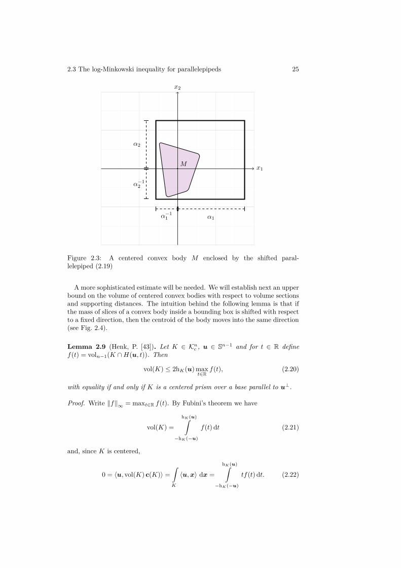
Figure 2.3: A centered convex body M enclosed by the shifted paral-lelepiped (2.19)
A more sophisticated estimate will be needed. We will establish next an upperbound on the volume of centered convex bodies with respect to volume sectionsand supporting distances. The intuition behind the following lemma is that ifthe mass of slices of a convex body inside a bounding box is shifted with respectto a fixed direction, then the centroid of the body moves into the same direction(see Fig. 2.4).
Lemma 2.9 (Henk, P. [43]). Let K ∈ Knc , u ∈ Sn−1 and for t ∈ R define
f(t) = voln−1(K ∩H(u, t)). Then
vol(K) ≤ 2hK(u) maxt∈R
f(t), (2.20)
with equality if and only if K is a centered prism over a base parallel to u⊥.
Proof. Write ∥f∥∞ = maxt∈R f(t). By Fubini’s theorem we have
vol(K) =hK (u)∫
−hK (−u)
f(t) dt (2.21)
and, since K is centered,
0 = ⟨u, vol(K) c(K)⟩ =∫K
⟨u,x⟩ dx =hK (u)∫
−hK (−u)
tf(t) dt. (2.22)

26 2 The log-Minkowski inequality and the planar cone-volume measure
−hK(−u) hK(u)s
∥f∥∞
t
f(t)
Figure 2.4: Mass distribution of a convex body shifted as in the proofof Lemma 2.9
By (2.21) we getvol(K) ≤ (hK(u) + hK(−u)) ∥f∥∞ .
Thus, for s = vol(K)∥f∥∞
we have −hK(−u) ≤ hK(u) − s ≤ hK(u) and (2.22) yields
0 =hK (u)−s∫
−hK (−u)
tf(t) dt+hK (u)∫
hK (u)−s
tf(t) dt
≤ (hK(u) − s)hK (u)−s∫
−hK (−u)
f(t) dt+hK (u)∫
hK (u)−s
tf(t) dt. (2.23)
With (2.21) it follows that
0 ≤ (hK(u) − s)
⎛⎜⎝vol(K) −hK (u)∫
hK (u)−s
f(t) dt
⎞⎟⎠+hK (u)∫
hK (u)−s
tf(t) dt
= (hK(u) − s)
⎛⎜⎝ hK (u)∫hK (u)−s
(∥f∥∞ − f(t)
)dt
⎞⎟⎠+hK (u)∫
hK (u)−s
tf(t) dt
≤hK (u)∫
hK (u)−s
t(
∥f∥∞ − f(t))
dt+hK (u)∫
hK (u)−s
tf(t) dt
=hK (u)∫
hK (u)−s
t ∥f∥∞ dt
=∥f∥∞
2(hK(u)2 − (hK(u) − s)2)
=∥f∥∞
2(2shK(u) − s2)
2.3 The log-Minkowski inequality for parallelepipeds 27
=s ∥f∥∞
2
(2hK(u) − vol(K)
∥f∥∞
).
From the latter inequality we obtain (2.20).
Suppose now we have equality in (2.20). Then we also have equality in(2.23), and since f is positive on the interval (−hK(−u), hK(u)) it follows that−hK(−u) = hK(u) − s. Hence vol(K) =
(hK(u) + hK(−u)
)∥f∥∞, which
by (2.21) shows that the volume sections f(t) are constant. Then (2.22) yieldshK(u) = hK(−u). Moreover, the equality conditions of the Brunn-Minkowskiinequality (1.2) assert that the sections K ∩ H(u, t), t ∈ [−hK(u), hK(u)], aretranslates. Thus K is a prism.
As above we apply the foregoing lemma to the parallelepiped (2.19).
Corollary 2.10. Let K ∈ Knc with voln(K) = 2n. Suppose there are numbers
α1, . . . , αn ≥ 1 such that
K ⊆ {x ∈ Rn : −α−1i ≤ xi ≤ αi, 1 ≤ i ≤ n}.
Thenn∏j=1j =i
(α−1j + αj
2
)≥ αi.
Proof. Let i ∈ {1, . . . , n}. By applying Lemma 2.9 with u = −ei we obtain
2n = vol(K) ≤ 2hK(−ei) maxt∈R
voln−1(K ∩H(ei, t))
≤ 2α−1i
n∏j=1j =i
(α−1j + αj).
As our next step we show that the inequalities obtained in the Corollaries 2.8and 2.10 admit only a trivial solution α1, . . . , αn if the dimension n is particu-larly small.
Lemma 2.11. Let n ∈ {2, 3, 4}. Then the system of inequalities
αi ≥ 1 for each i = 1, . . . , n, (2.24)α1 · . . . · αn ≤ 2n, (2.25)
n∏j=1j =i
(α−1j + αj
2
)≥ αi, for each i = 1, . . . , n, (2.26)
has the only solution α1 = . . . = αn = 1.
Proof. Without loss of generality we assume there is a solution to the abovesystem with α1 ≥ . . . ≥ αn.
28 2 The log-Minkowski inequality and the planar cone-volume measure
Case n = 2: By (2.26) we readily have
α−12 + α2 ≥ 2α1 ≥ 2α2,
which with (2.24) gives α1 = α2 = 1.
Case n = 3: Inequality (2.26) for i = 1 gives
(α22 + 1)(α2
3 + 1) ≥ 4α1α2α3 ≥ 4α22α3. (2.27)
Rearranging the terms yields
α23 + 1 − (4α3 − α2
3 − 1)α22 ≥ 0.
Note that (2.25) implies α3 ≤ 2 which in turn shows
4α3 − α23 − 1 ≥ 4α3 − 2α3 − 1 > 0.
Thusα2
3 + 14α3 − α2
3 − 1 ≥ α22 ≥ α2
3,
which again can be rearranged to the polynomial inequality
0 ≤ α43 − 4α3
3 + 2α23 + 1 = (α3 − 1)(α3
3 − 3α23 − α3 − 1).
Since for the latter factor we have
α33 − 3α2
3 − α3 − 1 ≤ 2α23 − 3α2
3 − α3 − 1 = −α23 − α3 − 1 < 0,
by (2.24) we find α3 = 1. By (2.27) then it follows that
2(α22 + 1) ≥ 4α1α2 ≥ 4α2
2.
Thus α1 = α2 = 1.
Case n = 4: From (2.26) for i = 1 we get
(α22 + 1)(α2
3 + 1)(α24 + 1) ≥ 8α1α2α3α4 ≥ 8α2
2α3α4
or
(α23 + 1)(α2
4 + 1) −(
8α3α4 − (α23 + 1)(α2
4 + 1))α2
2 ≥ 0. (2.28)
We will eliminate successively the variables α2 and α3 to obtain a poly-nomial inequality in the single variable α4.
Note that from (2.24) and (2.25) we have
α44 ≤ α1α2α3α4 ≤ 16,
α33 ≤ α3
3α4 ≤ α1α2α3α4 ≤ 16. (2.29)
Hence α4 ≤ 2 and α3 ≤ 24/3 ≤ 13/5. We aim to show that then
8α3α4 − (α23 + 1)(α2
4 + 1) > 0. (2.30)

2.3 The log-Minkowski inequality for parallelepipeds 29
To this end, define D = [1, 135 ] × [1, 2] and f : D → R with f(x, y) =
8xy− (x2 + 1)(y2 + 1). As a polynomial, f attains a minimum on D. Alsof is differentiable and its gradient and Hessian are given by
∇f(x, y) =(
8y − 2x(y2 + 1)8x− 2y(x2 + 1)
),
∇2f(x, y) =(
−2(y2 + 1) 8 − 4xy8 − 4xy −2(x2 + 1)
),
respectively. If (x, y) ∈ D is a solution of ∇f(x, y) = 0 we see from thefirst coordinate of ∇f that x = 4y
y2+1 . Then from the second coordinatewe find
0 = 8(
4yy2 + 1
)− 2y
((4y
y2 + 1
)2+ 1)
= (y2 + 1)−2y(
32(y2 + 1) − 32y2 − 2(y2 + 1)2)
= (y2 + 1)−2y(
− 2(y2 − 3)(y2 + 5)).
Since y ≥ 1, f has its only stationary point at y = x =√
3 which is a nota minimum since
∇2f(√
3,√
3) =(
−8 −4−4 −8
)is indefinite. Thus f attains its minimum at a point in ∂D, i.e., at somepoint (1, y), ( 13
5 , y), (x, 1) or (x, 2), where x ∈ [1, 135 ] and y ∈ [1, 2]. Since
f(1, y) = 8y − 2(y2 + 1) ≥ 8y − 2(2y + 1) = 4y − 2 > 0,
f(13/5, y) = 1045 y − 194
25 y2 − 194
25 = 19425
(26097 y − y2 − 1
)>
19425
(52y − y2 − 1
)= 194
25 (2 − y)(y − 1/2) ≥ 0,
f(x, 1) = 8x− 2(x2 + 1) ≥ 8x− 2(
135 x+ 1
)= 2
5(7x− 5) > 0
f(x, 2) = 16x− 5x2 − 5 = 5(
165 x− x2 − 1
)> 5
(19465 x− x2 − 1
)= 5(13/5 − x)(x− 5/13) ≥ 0,
are positive in the given range, we have proved (2.30).
From (2.28) it then follows that
(α23 + 1)(α2
4 + 1)8α3α4 − (α2
3 + 1)(α24 + 1) ≥ α2
2 ≥ α23
which can be rewritten as
α24 + 1α4
≥ 8α33
(α23 + 1)2 . (2.31)
30 2 The log-Minkowski inequality and the planar cone-volume measure
The left hand side is increasing in α4 when 1 ≤ α4. We distinguish nowtwo cases. First, if α3 < 2, we use α4 ≤ α3 to conclude from (2.31) that
α23 + 1α3
≥ 8α33
(α23 + 1)2
and so
0 ≤ (α23 + 1)3 − 8α4
3 = α63 − 5α4
3 + 3α23 + 1
= (α23 − 1)(α4
3 − 4α23 − 1) ≤ (α2
3 − 1)(α43 − 4α2
3)= α2
3(α23 − 1)(α2
3 − 4).
The only solution to this inequality in [1, 2) is α3 = 1.
Now suppose α3 ≥ 2. From (2.29) we know α4 ≤ 16α3
3, which we may
combine with (2.31) to obtain
8α33
(α23 + 1)2 ≤
(16α3
3
)2+ 1
16α3
3
= 256 + α63
16α33
or equivalently
0 ≤ (256 + α63)(α2
3 + 1)2 − 128α63
= α103 + 2α8
3 − 127α63 + 256α4
3 + 512α23 + 256.
Clearly, in the range α3 ∈ [2, 135 ] we have
192 + 1744(α23 − 4) + 16(α2
3 − 4)2 > 0
and therefore
0 < α103 + 2α8
3 − 127α63 + 256α4
3 + 512α23 + 256
+(192 + 1744(α2
3 − 4) + 16(α23 − 4)2)
= α103 + 2α8
3 − 127α63 + 272α4
3 + 2128α23 − 6272
= (α23 − 4)2(α2
3 − 7)(α43 + 17α2
3 + 56).
But this is false since α23 < 7. Thus, we have proved α3 = 1 and subse-
quently α4 = 1. But in this case (2.26) becomes α−12 + α2 ≥ 2α1 and as
above this implies α1 = α2 = 1.
If n ≥ 5, the system of inequalities (2.24), (2.25), (2.26) admits more solutions,e.g., for α1 = . . . = αn = 2 the inequalities (2.26) become (5/4)n−1 ≥ 2 whichis true for n ≥ 5.
We are now ready to give the proof of Proposition 2.6.
Proof of Proposition 2.6. Since Q is a parallelepiped, there exist linearly inde-pendent u1, . . . ,un ∈ Sn−1 such that
Q = {x ∈ Rn : |⟨ui,x⟩| ≤ hQ(ui)}
2.3 The log-Minkowski inequality for parallelepipeds 31
Let A be the matrix with columns u1, . . . ,un. Without loss of generality weassume that vol(Q) = vol(M) = 2n
| det(A)| . As in the proof of Proposition 2.5 wenote that all cone-volumes VQ(±ui) coincide. Hence we just have to verify
n∏i=1
hM (ui)hM (−ui)hQ(ui)2 ≥ 1. (2.32)
Note that under these assumptions it follows from (1.3) that
n∏i=1
hQ(ui) = | det(A)|2n vol(Q) = 1.
Hence, with K = ATM , i.e., hK(±ei) = hM (±ui), we only have to show
n∏i=1
(hK(ei)hK(−ei
)≥ 1, (2.33)
where vol(K) = 2n and the centroid of K is at the origin. Moreover, afterscaling by a suitable diagonal matrix of determinant 1 we may also assumehK(ei)hK(−ei) = γ, 1 ≤ i ≤ n, for a suitable constant γ > 0.
Suppose (2.33) does not hold. Then γ = hK(ei)hK(−ei) < 1 for 1 ≤ i ≤ n,and without loss of generality assume hK(ei) ≥ hK(−ei), i = 1, . . . , n. Thenfor every x ∈ K and i = 1, . . . , n,
−hK(ei)−1 < −hK(−ei) ≤ ⟨ei,x⟩ ≤ hK(ei).
Hence, K is strictly contained in a shifted parallelepiped
P = {x ∈ Rn : −α−1i ≤ ⟨ei,x⟩ ≤ αi}
for some α1, . . . , αn ≥ 1. Now Corollaries 2.8 and 2.10 yield α1 · . . . · αn ≤ 2nand
n∏j=1j =i
(α−1j + αj
2
)≥ αi
for each i = 1, . . . , n. By Lemma 2.11 it follows that α1 = . . . = αn = 1. Inparticular, vol(P ) = 2n which contradicts vol(P ) > vol(K) = 2n.
Suppose now we have equality in (2.32). Then we also have equality in (2.33).Repeating the steps above we find that K is contained in the cube [−1, 1]n.Since vol(K) = 2n it follows that K = [−1, 1]n. Thus, M is a parallelepipedwith outer normals ±u1, . . . ,±un.
We conjecture that Proposition 2.6 also holds in arbitrary dimension whichcould possibly be proved by establishing an analogue of Lemma 2.9 for lower-dimensional sections. It is, however, not clear how such an extension shouldlook like.

32 2 The log-Minkowski inequality and the planar cone-volume measure
Figure 2.5: Trapezoid violating the subspace concentration inequality (2.34)
2.4 The logarithmic Minkowski problem fortrapezoids
It was mentioned earlier that the even logarithmic Minkowski problem, i.e.,the task of characterizing the set of cone-volume measures of bodies in Kn
s , wassolved in [19] (see Theorem 1.3). As a starting point of the search for the solutionin the general setting we will consider the cone-volume measures of polygonswith few vertices. Restricting to the plane allows the use of tools that may nothave a direct extension to higher dimensions. For instance, the equality cases ofeven cone-volume measures in the plane were fully characterized by Böröczky,Lutwak, Yang and Zhang [18], but in higher dimensions this is considered asignificant open problem. Another example is the following result proved byStancu [78]. Here, for a discrete measure µ on the sphere, its support supp(µ)is the set of points u with µ(u) > 0.
Theorem 2.12 (Stancu [78]). Let µ be a non-zero, finite, discrete Borel mea-sure on S1, that is not concentrated on a closed hemisphere, and let m =#(supp(µ)) ≥ 4. If either m > 4 and
µ(S1 ∩ L) < 12µ(S1) (2.34)
for every proper subspace L of R2 with #(L ∩ supp(µ)) = 2, or supp(µ) is ingeneral position, then there exists a polygon P ∈ P2
o with VP = µ.
An extension of the preceding theorem to higher dimensions was discoveredonly after a decade by Böröczky, Hegedűs and Zhu [11]. The subspace concentra-tion inequality (2.34) is not necessary as can be easily seen from the trapezoidwith vertices
(±εε
),(±1
−1), for small ε > 0 (see Fig. 2.5). Still, Böröczky and
Hegedűs [10] proved a necessary condition for cone-volume measures evaluatedat antipodal points, which in the plane reads as follows.
Theorem 2.13 (Böröczky, Hegedűs [10]). Let K ∈ K2o and u ∈ S1. Then
VK({±u}) ≤ vol(K) − 2√
VK(u)VK(−u) (2.35)
and equality is attained if and only if K is trapezoid with two sides parallel tou⊥ and the intersection point of the diagonals is contained in u⊥.
2.4 The log-Minkowski problem for trapezoids 33
u4
u1
u2
u3
ω
supp(µ)
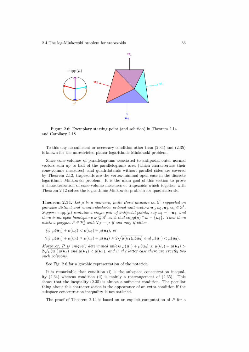
Figure 2.6: Exemplary starting point (and solution) in Theorem 2.14and Corollary 2.18
To this day no sufficient or necessary condition other than (2.34) and (2.35)is known for the unrestricted planar logarithmic Minkowski problem.
Since cone-volumes of parallelograms associated to antipodal outer normalvectors sum up to half of the parallelograms area (which characterizes theircone-volume measures), and quadrilaterals without parallel sides are coveredby Theorem 2.12, trapezoids are the vertex-minimal open case in the discretelogarithmic Minkowski problem. It is the main goal of this section to provea characterization of cone-volume measures of trapezoids which together withTheorem 2.12 solves the logarithmic Minkowski problem for quadrilaterals.
Theorem 2.14. Let µ be a non-zero, finite Borel measure on S1 supported onpairwise distinct and counterclockwise ordered unit vectors u1,u2,u3,u4 ∈ S1.Suppose supp(µ) contains a single pair of antipodal points, say u1 = −u3, andthere is an open hemisphere ω ⊆ S1 such that supp(µ) ∩ ω = {u3}. Then thereexists a polygon P ∈ P2
o with VP = µ if and only if either
(i) µ(u1) + µ(u3) < µ(u2) + µ(u4), or
(ii) µ(u1) + µ(u3) ≥ µ(u2) + µ(u4) ≥ 2√µ(u1)µ(u3) and µ(u1) < µ(u3).
Moreover, P is uniquely determined unless µ(u1) + µ(u3) ≥ µ(u2) + µ(u4) >2√µ(u1)µ(u3) and µ(u1) < µ(u3), and in the latter case there are exactly two
such polygons.
See Fig. 2.6 for a graphic representation of the notation.
It is remarkable that condition (i) is the subspace concentration inequal-ity (2.34) whereas condition (ii) is mainly a rearrangement of (2.35). Thisshows that the inequality (2.35) is almost a sufficient condition. The peculiarthing about this characterization is the appearance of an extra condition if thesubspace concentration inequality is not satisfied.
The proof of Theorem 2.14 is based on an explicit computation of P for a
34 2 The log-Minkowski inequality and the planar cone-volume measure
given µ. Thereby a polynomial system arises which is stated and solved in thefollowing lemma.
Lemma 2.15. Let a, b ∈ R with a < b, and γi ∈ R>0, 1 ≤ i ≤ 4. Writela =
√1 + a2, lb =
√1 + b2 and D = (γ2 + γ4)2 − 4γ1γ3. Consider the system
2γ1 = h1(−(b− a)h1 + lah2 + lbh4),2γ2 = lah2(h1 + h3),2γ3 = h3((b− a)h3 + lah2 + lbh4),2γ4 = lbh4(h1 + h3),lah2 + lbh4 > (b− a)h1,
h1, h2, h3, h4 > 0.
⎫⎪⎪⎪⎪⎪⎪⎪⎪⎬⎪⎪⎪⎪⎪⎪⎪⎪⎭(2.36)
(i) If either
(a) γ1 + γ3 ≥ γ2 + γ4 and γ1 ≥ γ3, or
(b) γ2 + γ4 < 2√γ1γ3,
then (2.36) admits no solutions.
(ii) If either
(a) γ1 + γ3 < γ2 + γ4,
(b) γ1 + γ3 = γ2 + γ4 and γ1 < γ3, or
(c) γ1 + γ3 > γ2 + γ4 = 2√γ1γ3 and γ1 < γ3,
then (2.36) has a unique solution given by
h1 = 1√2(b− a)
−2γ1 + γ2 + γ4 +√D√
γ3 − γ1 +√D
,
h2 =√
2(b− a)la
γ2√γ3 − γ1 +
√D,
h3 = 1√2(b− a)
2γ3 − γ2 − γ4 +√D√
γ3 − γ1 +√D
,
h4 =√
2(b− a)lb
γ4√γ3 − γ1 +
√D.
(iii) If γ1 + γ3 > γ2 + γ4 > 2√γ1γ3 and γ1 < γ3, then (2.36) has exactly two

2.4 The log-Minkowski problem for trapezoids 35
different solutions given by
h1 = 1√2(b− a)
−2γ1 + γ2 + γ4 ±√D√
γ3 − γ1 ±√D
,
h2 =√
2(b− a)la
γ2√γ3 − γ1 ±
√D,
h3 = 1√2(b− a)
2γ3 − γ2 − γ4 ±√D√
γ3 − γ1 ±√D
,
h4 =√
2(b− a)lb
γ4√γ3 − γ1 ±
√D.
We shall prove Theorem 2.14 first.
Proof of Theorem 2.14. After carrying out a suitable rotation and reflection wemay assume that u1 = (0, 1)T , u2 = 1
la(−1,−a)T , u3 = (0,−1)T and u4 =
1lb
(1, b)T , where a, b ∈ R, b > a and la =(−1,−a)T
, lb =
(1, b)T
. Suppose
h1, h2, h3, h4 > 0. A polygon
P =4⋂i=1
H−(ui, hi)
is a proper trapezoid if and only if the intersection point of H(u2, h2) andH(u4, h4) given by
1b− a
(−(labh2 + lbah4)lah2 + lbh4
)is contained in intH+(u1, h1), i.e., lah2 + lbh4 > (b− a)h1, since otherwise P isa triangle. Moreover, in this case the vertices of P are given as intersections ofindex-adjacent supporting hyperplanes, namely
v1 =(
−bh1 + lbh4h1
), v3 =
(ah3 − lah2
−h3
),
v2 =(
−ah1 − lah2h1
), v4 =
(bh3 + lbh4
−h3
),
so that
F (P,u1) = [v1,v2], F (P,u3) = [v3,v4]F (P,u2) = [v2,v3], F (P,u4) = [v4,v1].
Moreover, the cone-volumes of P (dependent on hi) are given by
VP (u1) = 12h1 · (−(b− a)h1 + lah2 + lbh4),
VP (u2) = 12h2 · la(h1 + h3),
36 2 The log-Minkowski inequality and the planar cone-volume measure
VP (u3) = 12h3 · ((b− a)h3 + lah2 + lbh4),
VP (u4) = 12h4 · lb(h1 + h3).
Applying Lemma 2.15 to the system VP (ui) = µ(ui), 1 ≤ i ≤ 4, yields thedesired assertion.
We finish this section with the proof of Lemma 2.15 where we reduce solving(2.36) to finding positive solutions of a biquadratic equation. To this end, werecall that for p, q ∈ R, and denoting D = p2 − q, the biquadratic equationx4 − 2px2 + q = 0 in the variable x ∈ R has
• no positive solution, if either D < 0 or p ≤ −√
|D|,
• exactly one positive solution, if either D ≥ 0 and p ∈ (−√D,
√D], or
D = 0 and p > 0, given by x =√p+
√D,
• exactly two positive solutions, if D > 0 and p >√D, given by x =√
p±√D.
Proof of Lemma 2.15. Suppose h1, h2, h3, h4 > 0 solve the system (2.36). Bothh2 and h4 can be computed from h1 and h3 and the given data, so that
h2 = 2l−1a γ2
h1 + h3, (2.37)
h4 =2l−1b γ4
h1 + h3, (2.38)
2γ1 = h1
(−(b− a)h1 + 2(γ2 + γ4)
h1 + h3
), (2.39)
2γ3 = h3
((b− a)h3 + 2(γ2 + γ4)
h1 + h3
). (2.40)
By considering the sum and difference of (2.39) and (2.40) and substituting thevariables h1, h3 > 0 by x > 0 and y ∈ R via
h1 = x2 − y
x√
2(b− a),
h3 = x2 + y
x√
2(b− a),
(2.41)
we find that the variables x =√
b−a2 (h1 + h3) and y = b−a
2 (h23 − h2
1) satisfy
2(γ1 + γ3) = (b− a)(h23 − h2
1) + 2(γ2 + γ4)= 2y + 2(γ2 + γ4), (2.42)
2(γ3 − γ1) = (b− a)(h21 + h2
3) + 2(γ2 + γ4)h3 − h1
h1 + h3
= (b− a)(
x2
b− a+ y2
(b− a)x2
)+ 2(γ2 + γ4) y
x2
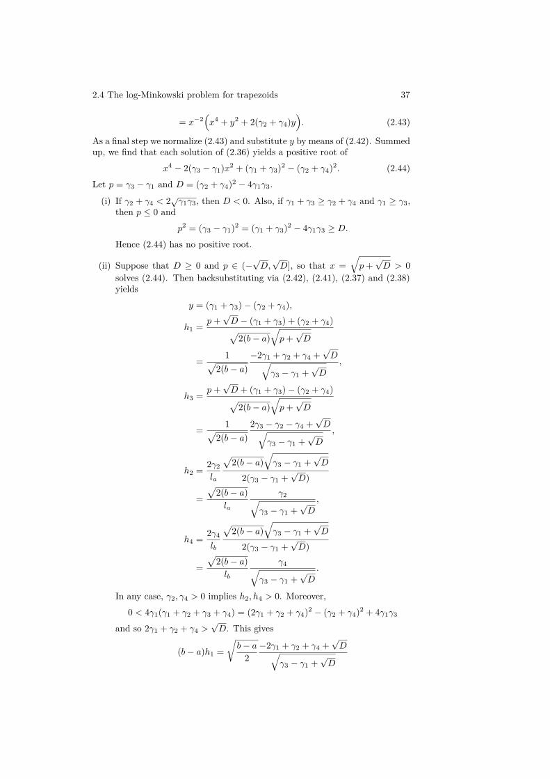
2.4 The log-Minkowski problem for trapezoids 37
= x−2(x4 + y2 + 2(γ2 + γ4)y
). (2.43)
As a final step we normalize (2.43) and substitute y by means of (2.42). Summedup, we find that each solution of (2.36) yields a positive root of
x4 − 2(γ3 − γ1)x2 + (γ1 + γ3)2 − (γ2 + γ4)2. (2.44)
Let p = γ3 − γ1 and D = (γ2 + γ4)2 − 4γ1γ3.
(i) If γ2 + γ4 < 2√γ1γ3, then D < 0. Also, if γ1 + γ3 ≥ γ2 + γ4 and γ1 ≥ γ3,
then p ≤ 0 and
p2 = (γ3 − γ1)2 = (γ1 + γ3)2 − 4γ1γ3 ≥ D.
Hence (2.44) has no positive root.
(ii) Suppose that D ≥ 0 and p ∈ (−√D,
√D], so that x =
√p+
√D > 0
solves (2.44). Then backsubstituting via (2.42), (2.41), (2.37) and (2.38)yields
y = (γ1 + γ3) − (γ2 + γ4),
h1 = p+√D − (γ1 + γ3) + (γ2 + γ4)√
2(b− a)√p+
√D
= 1√2(b− a)
−2γ1 + γ2 + γ4 +√D√
γ3 − γ1 +√D
,
h3 = p+√D + (γ1 + γ3) − (γ2 + γ4)√
2(b− a)√p+
√D
= 1√2(b− a)
2γ3 − γ2 − γ4 +√D√
γ3 − γ1 +√D
,
h2 = 2γ2
la
√2(b− a)
√γ3 − γ1 +
√D
2(γ3 − γ1 +√D)
=√
2(b− a)la
γ2√γ3 − γ1 +
√D,
h4 = 2γ4
lb
√2(b− a)
√γ3 − γ1 +
√D
2(γ3 − γ1 +√D)
=√
2(b− a)lb
γ4√γ3 − γ1 +
√D.
In any case, γ2, γ4 > 0 implies h2, h4 > 0. Moreover,
0 < 4γ1(γ1 + γ2 + γ3 + γ4) = (2γ1 + γ2 + γ4)2 − (γ2 + γ4)2 + 4γ1γ3
and so 2γ1 + γ2 + γ4 >√D. This gives
(b− a)h1 =√b− a
2−2γ1 + γ2 + γ4 +
√D√
γ3 − γ1 +√D
38 2 The log-Minkowski inequality and the planar cone-volume measure
<
√b− a
22γ2 + 2γ4√γ3 − γ1 +
√D
= lah2 + lbh4.
It remains to show, that in either of the cases D ≥ 0, p ∈ (−√D,
√D],
or D = 0 and p > 0, and that consequently h1, h3 > 0 holds. The latterinequalities are equivalent to
√D > max(2γ1 − γ2 − γ4, γ2 + γ4 − 2γ3).
Case γ1 + γ3 < γ2 + γ4. The assumption yields
D = (γ2 + γ4)2 − 4γ1γ3 > (γ1 + γ3)2 − 4γ1γ3 = (γ3 − γ1)2 ≥ 0,p2 = (γ3 − γ1)2 = (γ1 + γ3)2 − 4γ1γ3 < (γ2 + γ4)2 − 4γ1γ3 = D,
and√D =
√(γ2 + γ4)2 − 4γ1γ3
=√
(γ2 + γ4)2 + 4γ23 − 4γ3(γ1 + γ3)
>√
(γ2 + γ4)2 + 4γ23 − 4γ3(γ2 + γ4)
=√
(γ2 + γ4 − 2γ3)2
≥ γ2 + γ4 − 2γ3,
> γ2 + γ4 − 2γ3 + 2(γ1 + γ3 − γ2 − γ4),= 2γ1 − γ2 − γ4.
Case γ1 + γ3 = γ2 + γ4, γ1 < γ3. We have
D = (γ2 +γ4)2 −4γ1γ3 = (γ1 +γ3)2 −4γ1γ3 = (γ3 −γ1)2 = p2 > 0.
Hence 0 < p =√D. Therefore, from the assumptions we also find
2γ1 − γ2 − γ4 = γ2 + γ4 − 2γ3 = γ1 − γ3 < 0 <√D.
Case γ1 + γ3 > γ2 + γ4 = 2√γ1γ3, γ1 < γ3. We have
D = (γ2 + γ4)2 − 4γ1γ3 = 0
and p = γ3 − γ1 > 0. Furthermore,
2γ3 > γ1 + γ3 > γ2 + γ4 = 2√γ1γ3 > 2γ1,
so that 2γ1 − γ2 − γ4 < 0 =√D and γ2 + γ4 − 2γ3 < 0 =
√D.
(iii) From γ2 + γ4 > 2√γ1γ3 it follows that
D = (γ2 + γ4)2 − 4γ1γ3 > 0.
Furthermore we readily have p = γ3 − γ1 > 0. Then γ1 + γ3 > γ2 + γ4yields
p2 = (γ3 − γ1)2 = (γ3 + γ1)2 − 4γ1γ3 > (γ2 + γ4)2 − 4γ1γ3 = D,

2.4 The log-Minkowski problem for trapezoids 39
which shows that x =√p±
√D are the positive roots of (2.44). It remains
to show that both roots lead to distinct solutions of (2.36). In full analogyto (ii), backsubstituting gives
y = (γ1 + γ3) − (γ2 + γ4),
h1 = 1√2(b− a)
−2γ1 + γ2 + γ4 ±√D√
γ3 − γ1 ±√D
,
h3 = 1√2(b− a)
2γ3 − γ2 − γ4 ±√D√
γ3 − γ1 ±√D
,
h2 =√
2(b− a)la
γ2√γ3 − γ1 ±
√D,
h4 =√
2(b− a)lb
γ4√γ3 − γ1 ±
√D.
Again, γ2, γ4 > 0 implies h2, h4 > 0 and from h2 and h4 it can be seenthat both solutions are distinct. Moreover,
0 < 4γ1(γ1 + γ2 + γ3 + γ4) = (2γ1 + γ2 + γ4)2 − (γ2 + γ4)2 + 4γ1γ3
and so 2γ1 + γ2 + γ4 >√D > −
√D. This gives
(b− a)h1 =√b− a
2−2γ1 + γ2 + γ4 ±
√D√
γ3 − γ1 ±√D
<
√b− a
22γ2 + 2γ4√γ3 − γ1 ±
√D
= lah2 + lbh4.
It remains to show that in both cases h1, h3 > 0. From γ1 + γ3 > γ2 + γ4we find
√D =
√(γ2 + γ4)2 − 4γ1γ3
=√
(γ2 + γ4)2 + 4γ21 − 4γ1(γ1 + γ3)
<√
(γ2 + γ4)2 + 4γ21 − 4γ1(γ2 + γ4)
=√
(γ2 + γ4 − 2γ1)2.
Since γ2 + γ4 > 2√γ1γ3 > 2γ1 it follows that
−√D <
√D < γ2 + γ4 − 2γ1
< γ2 + γ4 − 2γ1 + 2(γ1 + γ3 − γ2 − γ4)= 2γ3 − γ2 − γ4.
Thus, h1, h3 > 0.
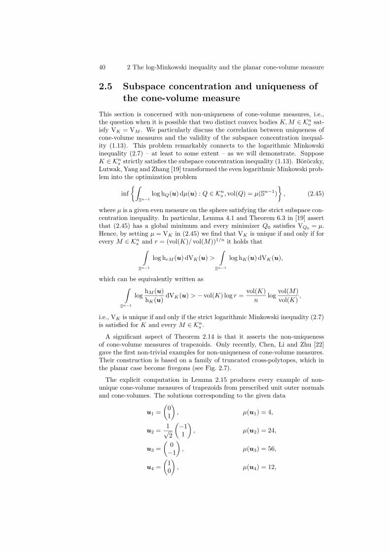
40 2 The log-Minkowski inequality and the planar cone-volume measure
2.5 Subspace concentration and uniqueness ofthe cone-volume measure
This section is concerned with non-uniqueness of cone-volume measures, i.e.,the question when it is possible that two distinct convex bodies K,M ∈ Kn
o sat-isfy VK = VM . We particularly discuss the correlation between uniqueness ofcone-volume measures and the validity of the subspace concentration inequal-ity (1.13). This problem remarkably connects to the logarithmic Minkowskiinequality (2.7) – at least to some extent – as we will demonstrate. SupposeK ∈ Kn
s strictly satisfies the subspace concentration inequality (1.13). Böröczky,Lutwak, Yang and Zhang [19] transformed the even logarithmic Minkowski prob-lem into the optimization problem
inf{∫
Sn−1log hQ(u) dµ(u) : Q ∈ Kn
s , vol(Q) = µ(Sn−1)}, (2.45)
where µ is a given even measure on the sphere satisfying the strict subspace con-centration inequality. In particular, Lemma 4.1 and Theorem 6.3 in [19] assertthat (2.45) has a global minimum and every minimizer Q0 satisfies VQ0 = µ.Hence, by setting µ = VK in (2.45) we find that VK is unique if and only if forevery M ∈ Kn
s and r = (vol(K)/ vol(M))1/n it holds that∫Sn−1
log hrM (u) dVK(u) >∫
Sn−1
log hK(u) dVK(u),
which can be equivalently written as∫Sn−1
log hM (u)hK(u) dVK(u) > − vol(K) log r = vol(K)
nlog vol(M)
vol(K) ,
i.e., VK is unique if and only if the strict logarithmic Minkowski inequality (2.7)is satisfied for K and every M ∈ Kn
s .
A significant aspect of Theorem 2.14 is that it asserts the non-uniquenessof cone-volume measures of trapezoids. Only recently, Chen, Li and Zhu [22]gave the first non-trivial examples for non-uniqueness of cone-volume measures.Their construction is based on a family of truncated cross-polytopes, which inthe planar case become fivegons (see Fig. 2.7).
The explicit computation in Lemma 2.15 produces every example of non-unique cone-volume measures of trapezoids from prescribed unit outer normalsand cone-volumes. The solutions corresponding to the given data
u1 =(
01
), µ(u1) = 4,
u2 = 1√2
(−11
), µ(u2) = 24,
u3 =(
0−1
), µ(u3) = 56,
u4 =(
10
), µ(u4) = 12,
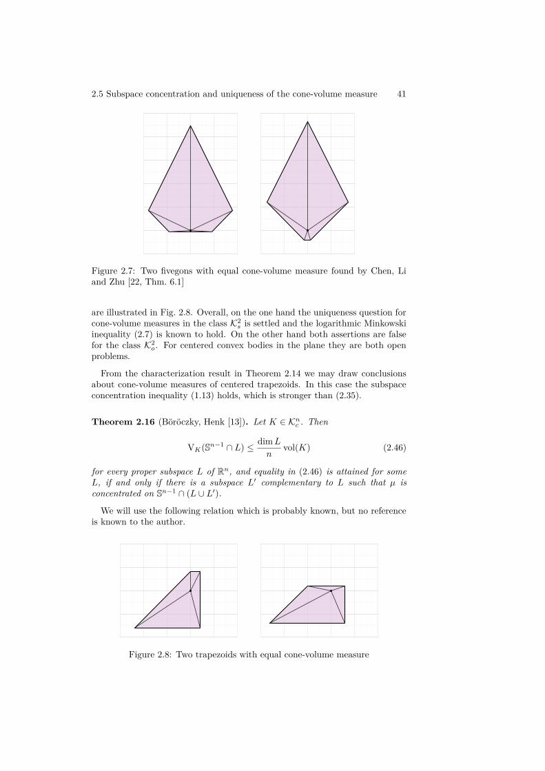
2.5 Subspace concentration and uniqueness of the cone-volume measure 41
Figure 2.7: Two fivegons with equal cone-volume measure found by Chen, Liand Zhu [22, Thm. 6.1]
are illustrated in Fig. 2.8. Overall, on the one hand the uniqueness question forcone-volume measures in the class K2
s is settled and the logarithmic Minkowskiinequality (2.7) is known to hold. On the other hand both assertions are falsefor the class K2
o. For centered convex bodies in the plane they are both openproblems.
From the characterization result in Theorem 2.14 we may draw conclusionsabout cone-volume measures of centered trapezoids. In this case the subspaceconcentration inequality (1.13) holds, which is stronger than (2.35).
Theorem 2.16 (Böröczky, Henk [13]). Let K ∈ Knc . Then
VK(Sn−1 ∩ L) ≤ dimL
nvol(K) (2.46)
for every proper subspace L of Rn, and equality in (2.46) is attained for someL, if and only if there is a subspace L′ complementary to L such that µ isconcentrated on Sn−1 ∩ (L ∪ L′).
We will use the following relation which is probably known, but no referenceis known to the author.
Figure 2.8: Two trapezoids with equal cone-volume measure

42 2 The log-Minkowski inequality and the planar cone-volume measure
v1
v2
v3
v4
c1
c3
c2
c4
ci = (v1 + v2 + v3 + v4 − vi)/3
Figure 2.9: Determining the centroid of a quadrilateral from triangulations asin the proof of Proposition 2.17
Proposition 2.17 (Xue1). Let Q ∈ P2o be a quadrilateral with counterclockwise
ordered vertices v1,v2,v3,v4 ∈ S1. Then Q is centered if and only if
det(v2,v4) = − det(v2,v1) + det(v3,v2) + det(v4,v3) − det(v1,v4),det(v3,v1) = − det(v2,v1) − det(v3,v2) + det(v4,v3) + det(v1,v4).
(2.47)
In particular, if Q is centered with ordered unit outer normals u1,u2,u3,u4 ∈ S1,then
VQ(u1)2 − VQ(u1)VQ(u3) + VQ(u3)2
= VQ(u2)2 − VQ(u2)VQ(u4) + VQ(u4)2. (2.48)
Proof. Let Q ∈ P2o with vertices v1,v2,v3,v4 ∈ R2 and ordered outer normals
u1,u2,u3,u4 ∈ S1 such that
F (Q,u1) = [v1,v2], F (Q,u3) = [v3,v4]F (Q,u2) = [v2,v3], F (Q,u4) = [v4,v1].
The centroid of any measurable set X ⊆ Rn with vol(X) > 0 satisfies for anypartition into measurable sets X1 ∪X2 = X, vol(X1 ∩X2) = 0, the relation
c(X) = vol(X1)vol(X) c(X1) + vol(X2)
vol(X) c(X2),
i.e., c(X) lies on the segment [c(X1), c(X2)]. Consider the partitions of Qcoming from its diagonals, i.e.,
Q = conv{v1,v2,v3}∪conv{v1,v3,v4} = conv{v2,v3,v4}∪conv{v1,v2,v4}.1Fei Xue, private communication.
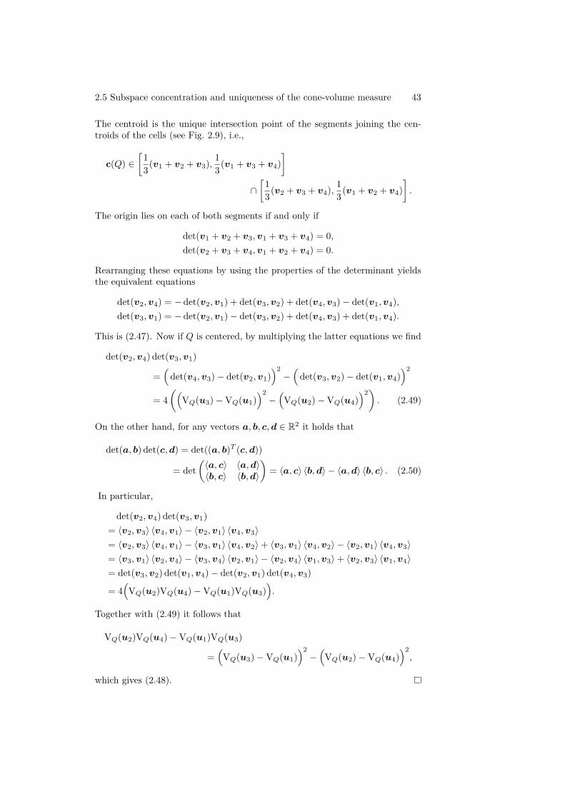
2.5 Subspace concentration and uniqueness of the cone-volume measure 43
The centroid is the unique intersection point of the segments joining the cen-troids of the cells (see Fig. 2.9), i.e.,
c(Q) ∈[
13(v1 + v2 + v3), 1
3(v1 + v3 + v4)]
∩[
13(v2 + v3 + v4), 1
3(v1 + v2 + v4)].
The origin lies on each of both segments if and only if
det(v1 + v2 + v3,v1 + v3 + v4) = 0,det(v2 + v3 + v4,v1 + v2 + v4) = 0.
Rearranging these equations by using the properties of the determinant yieldsthe equivalent equations
det(v2,v4) = − det(v2,v1) + det(v3,v2) + det(v4,v3) − det(v1,v4),det(v3,v1) = − det(v2,v1) − det(v3,v2) + det(v4,v3) + det(v1,v4).
This is (2.47). Now if Q is centered, by multiplying the latter equations we find
det(v2,v4) det(v3,v1)
=(
det(v4,v3) − det(v2,v1))2
−(
det(v3,v2) − det(v1,v4))2
= 4((
VQ(u3) − VQ(u1))2
−(
VQ(u2) − VQ(u4))2). (2.49)
On the other hand, for any vectors a, b, c,d ∈ R2 it holds that
det(a, b) det(c,d) = det((a, b)T (c,d))
= det(
⟨a, c⟩ ⟨a,d⟩⟨b, c⟩ ⟨b,d⟩
)= ⟨a, c⟩ ⟨b,d⟩ − ⟨a,d⟩ ⟨b, c⟩ . (2.50)
In particular,
det(v2,v4) det(v3,v1)= ⟨v2,v3⟩ ⟨v4,v1⟩ − ⟨v2,v1⟩ ⟨v4,v3⟩= ⟨v2,v3⟩ ⟨v4,v1⟩ − ⟨v3,v1⟩ ⟨v4,v2⟩ + ⟨v3,v1⟩ ⟨v4,v2⟩ − ⟨v2,v1⟩ ⟨v4,v3⟩= ⟨v3,v1⟩ ⟨v2,v4⟩ − ⟨v3,v4⟩ ⟨v2,v1⟩ − ⟨v2,v4⟩ ⟨v1,v3⟩ + ⟨v2,v3⟩ ⟨v1,v4⟩= det(v3,v2) det(v1,v4) − det(v2,v1) det(v4,v3)
= 4(
VQ(u2)VQ(u4) − VQ(u1)VQ(u3)).
Together with (2.49) it follows that
VQ(u2)VQ(u4) − VQ(u1)VQ(u3)
=(
VQ(u3) − VQ(u1))2
−(
VQ(u2) − VQ(u4))2,
which gives (2.48).
44 2 The log-Minkowski inequality and the planar cone-volume measure
The conditions of Theorem 2.16 and Proposition 2.17 together are almostsufficient for centered trapezoids. In fact, we may deduce a characterization ofcone-volume measures of centered trapezoids from Theorem 2.14 (see Fig. 2.6).
Corollary 2.18. Let µ be a non-zero, finite Borel measure on S1 supported onpairwise distinct and counterclockwise ordered unit vectors u1,u2,u3,u4 ∈ S1.Suppose supp(µ) contains a single pair of antipodal points, say u1 = −u3, andthere is open hemisphere ω ⊆ S1 such that supp(µ) ∩ ω = {u3}. Then thereexists a polygon P ∈ P2
c with VP = µ if and only if
(i) µ(u1) + µ(u3) < µ(u2) + µ(u4),
(ii) µ(u1)2 − µ(u1)µ(u3) + µ(u3)2 = µ(u2)2 − µ(u2)µ(u4) + µ(u4)2,
(iii) µ(u1) < µ(u3),
(iv) µ(u2) = µ(u4).
Moreover, P is uniquely determined.
Proof. We start by proving the necessity of all the conditions. Let T ∈ Pnc
be a centered trapezoid with order outer normal vectors u1,u2,u3,u4 ∈ S1,u1 = −u3, such that u3 = U(T ) ∩ ω for a suitable open hemisphere ω ⊆ S1.Condition (i) is just the strict subspace concentration inequality for centeredconvex polygons that are not parallelograms (see Theorem 2.16). The asser-tion (2.48) of Proposition 2.17 is condition (ii). For condition (iv) consider thesegment S connecting the midpoints of F (T,u1) and F (T,u3). It divides Tinto two parts of equal area such that exactly half of each segment T ∩H(u1, t),t ∈ R, lies on either side of S. This shows that c(T ) is contained in S. Moreover,S also divides the cones conv(F (T,ui) ∪ {0}), i ∈ {1, 3} into equal parts. Thus,VT (u2) = VT (u4). The condition (iii) can be seen as follows. We abbreviate
hi = hT (ui),fi = vol1(F (T,ui)),
for i = 1, 2, 3, 4. Since T is centered, Fubini’s theorem yields
0 =h1∫
−h3
t vol1(T ∩H(u1, t)) dt
=h1∫
−h3
t
(t+ h3
h1 + h3(f1 − f3) + f3
)dt
= h1 + h3
6
((2f1 + f3)h1 − (f1 + 2f3)h3
)= 2(h1 + h3)f1f3
3
((2f1 + f3)f3VT (u1) − (f1 + 2f3)f1VT (u3)
),
and soVT (u1) = VT (u3) · (f1 + 2f3)f1
(2f1 + f3)f3.
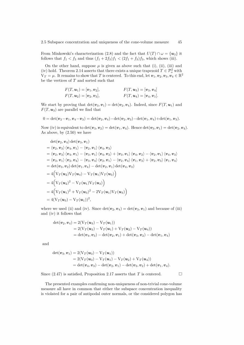
2.5 Subspace concentration and uniqueness of the cone-volume measure 45
From Minkowski’s characterization (2.8) and the fact that U(T ) ∩ ω = {u3} itfollows that f1 < f3 and thus (f1 + 2f3)f1 < (2f1 + f3)f3, which shows (iii).
On the other hand, suppose µ is given as above such that (i), (ii), (iii) and(iv) hold. Theorem 2.14 asserts that there exists a unique trapezoid T ∈ P2
o withVT = µ. It remains to show that T is centered. To this end, let v1,v2,v3,v4 ∈ R2
be the vertices of T and sorted such that
F (T,u1) = [v1,v2], F (T,u3) = [v3,v4]F (T,u2) = [v2,v3], F (T,u4) = [v4,v1].
We start by proving that det(v3,v1) = det(v2,v4). Indeed, since F (T,u1) andF (T,u3) are parallel we find that
0 = det(v2−v1,v4−v3) = det(v2,v4)−det(v2,v3)−det(v1,v4)+det(v1,v3).
Now (iv) is equivalent to det(v3,v2) = det(v1,v4). Hence det(v3,v1) = det(v2,v4).As above, by (2.50) we have
det(v2,v4) det(v3,v1)= ⟨v2,v3⟩ ⟨v4,v1⟩ − ⟨v2,v1⟩ ⟨v4,v3⟩= ⟨v2,v3⟩ ⟨v4,v1⟩ − ⟨v3,v1⟩ ⟨v4,v2⟩ + ⟨v3,v1⟩ ⟨v4,v2⟩ − ⟨v2,v1⟩ ⟨v4,v3⟩= ⟨v3,v1⟩ ⟨v2,v4⟩ − ⟨v3,v4⟩ ⟨v2,v1⟩ − ⟨v2,v4⟩ ⟨v1,v3⟩ + ⟨v2,v3⟩ ⟨v1,v4⟩= det(v3,v2) det(v1,v4) − det(v2,v1) det(v4,v3)
= 4(
VT (u2)VT (u4) − VT (u1)VT (u3))
= 4(
VT (u2)2 − VT (u1)VT (u3))
= 4(
VT (u1)2 + VT (u3)2 − 2VT (u1)VT (u3))
= 4(VT (u3) − VT (u1))2,
where we used (ii) and (iv). Since det(v2,v4) = det(v3,v1) and because of (iii)and (iv) it follows that
det(v2,v4) = 2(VT (u3) − VT (u1))= 2(VT (u3) − VT (u1) + VT (u2) − VT (u4))= det(v4,v3) − det(v2,v1) + det(v3,v2) − det(v1,v4)
and
det(v3,v1) = 2(VT (u3) − VT (u1))= 2(VT (u3) − VT (u1) − VT (u2) + VT (u4))= det(v4,v3) − det(v2,v1) − det(v3,v2) + det(v1,v4).
Since (2.47) is satisfied, Proposition 2.17 asserts that T is centered.
The presented examples confirming non-uniqueness of non-trivial cone-volumemeasure all have in common that either the subspace concentration inequalityis violated for a pair of antipodal outer normals, or the considered polygon has
46 2 The log-Minkowski inequality and the planar cone-volume measure
Figure 2.10: Fivegon in Proposition 2.19
no parallel sides. In case of quadrilaterals, Theorem 2.14 assures that this isnecessary. However, Malikiosis discovered the existence of a fivegon satisfy-ing the strict subspace concentration inequality with non-unqiue cone-volumemeasures.
Proposition 2.19 (Malikiosis2). There are two fivegons satisfying the strictsubspace concentration inequality that have the same cone-volume measure.
Proof. The fivegon given as (see Fig. 2.10)
P = conv{(
−36100
),
(−330100
),
(−330−98
),
(−30−98
),
(66−2
)},
has cone-volume data
u1 =(
1√2
1√2
), VP (u1) = 3264,
u2 =(
01
), VP (u2) = 14700,
u3 =(
−10
), VP (u3) = 32670,
u4 =(
0−1
), VP (u4) = 14700,
u5 =(
1√2
− 1√2
), VP (u5) = 3264.
In particular, P satisfies the subspace concentration inequality (2.34). Moreover,the cone-volume measure of P is invariant under reflection about e⊥
2 , but P isnot.
The results of this section raise the questions whether cone-volume measuresof centered polygons are unique and if the the number of distinct polygonsrealizing given cone-volume data can be bounded.
2Romanos Diogenes Malikiosis, private communication.
3 Dual curvature measures
3.1 An introduction to dual Brunn-Minkowskitheory
Duality of concepts generally describes the act of translating aspects of onetheory into another by an (often involutive) operation, e.g., dual spaces of vectorspaces or primal and dual linear programs in optimization. A duality within thespace of convex bodies is described by the following operation. For a non-emptyset X ⊆ Rn we define its polar set by
X∗ = {y ∈ Rn : ⟨x,y⟩ ≤ 1 for all x ∈ X}. (3.1)
The polar set is always a closed convex set containing the origin. Moreover, forK ∈ Kn
o its polar K∗ is a convex body in Kno and (K∗)∗ = K. There is no
relation between the support functions hK and hK∗ of the same simplicity, buthK∗ exhibits a geometric interpretation regarding K, which is
(hK∗(u))−1 = max{λ > 0 : λu ∈ K}, (3.2)
for u ∈ Sn−1. Its (−1)-homogeneous extension defined by ρK(x) = (hK∗(x))−1
for x ∈ Rn\{0} is called radial function of K. The geometric intuition behindthis duality is that points contained in K∗ interchange roles with halfspacescontaining K, i.e., x ∈ K∗ if and only if K ⊆ H−(x, 1), for x = 0, and viceversa.
The dual Brunn-Minkowski theory is a conceptually dual to the classicalBrunn-Minkowski theory which arises by replacing the Minkowski addition (1.1),i.e., the addition of support functions, by addition of radial functions in the fol-lowing way. For K,M ∈ Kn
o , and scalars s, t ≥ 0 the radial combination ofK and M with respect to s and t is
sK ˜+ tM = {x ∈ Rn : sρK(x) + tρM (x) ≥ 1} . (3.3)
In general, the radial combination of convex bodies is not necessarily a convexset, but it is always a star-shaped set, i.e., a non-empty set S ⊆ Rn suchthat for every x ∈ S the segment [0,x] is contained in S (see Fig. 3.1). The
47

48 3 Dual curvature measures
Figure 3.1: Radial combination 12K ˜+ 1
2M for K = conv{(0
2),( −1
−1/2),( 2
−1/2)}
and M = [−1, 1]2
definition (3.2) may be extended to compact star-shaped sets S ⊆ Rn via
ρS(x) = max{λ ≥ 0 : λx ∈ S},
for x ∈ Rn \ {0}. If ρS is positive and continuous, we call S a star body. Theset of star bodies in Rn will be denoted by Sno . Then the left hand side of (3.3)can be characterized as the unique star body with
ρsK + tM = sρK + tρM .
The dual Brunn-Minkowski theory was introduced by Lutwak [58]. His con-tributions include among others an analogue of the Minkowski inequality (2.5)from which the dual Brunn-Minkowski inequality
vol((1 − λ)K ˜+λM) 1n ≤ (1 − λ) vol(K) 1
n + λ vol(M) 1n ,
K,M ∈ Sno and λ ∈ [0, 1], may be derived (see also [59]). Moreover, there existfunctionals similar to the quermassintegrals defined in (1.5). Lutwak [58] foundthat for a star body K ∈ Sno its dual parallel body K ˜+λBn also admits apolynomial expansion given by
vol(K ˜+λBn) =n∑i=0
λi(n
i
)˜Wi(K),
where the functionals ˜Wi(K) defined this way are called dual quermassinte-grals of K. In analogy to Kubota’s formula (1.6) the dual quermassintegrals˜Wi(K) exhibit the following integral geometric representation as the means ofthe volumes of sections (see [60])
˜Wn−i(K) = vol(Bn)voli(Bi)
∫G(i,n)
voli(K ∩ L) dL,
for i = 0, . . . , n. The celebrated solution of the Busemann-Petty problem isamongst the recent successes of the dual Brunn-Minkowski theory (cf. [31,35, 81]) and it also has connections and applications to integral geometry,Minkowski geometry and the local theory of Banach spaces. For more infor-mation about the study of central sections of convex bodies we recommend the
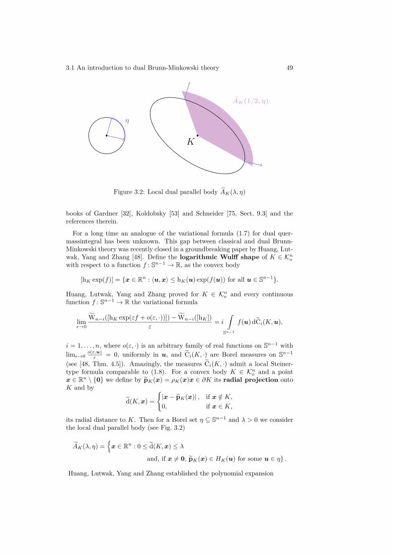
3.1 An introduction to dual Brunn-Minkowski theory 49
˜AK(1/2, η)
η
K
Figure 3.2: Local dual parallel body ˜AK(λ, η)
books of Gardner [32], Koldobsky [53] and Schneider [75, Sect. 9.3] and thereferences therein.
For a long time an analogue of the variational formula (1.7) for dual quer-massintegral has been unknown. This gap between classical and dual Brunn-Minkowski theory was recently closed in a groundbreaking paper by Huang, Lut-wak, Yang and Zhang [48]. Define the logarithmic Wulff shape of K ∈ Kn
o
with respect to a function f : Sn−1 → R, as the convex body
[hK exp(f)] = {x ∈ Rn : ⟨u,x⟩ ≤ hK(u) exp(f(u)) for all u ∈ Sn−1}.
Huang, Lutwak, Yang and Zhang proved for K ∈ Kno and every continuous
function f : Sn−1 → R the variational formula
limϵ→0
˜Wn−i([hK exp(εf + o(ε, ·))]) −˜Wn−i([hK ])ε
= i
∫Sn−1
f(u) d˜Ci(K,u),
i = 1, . . . , n, where o(ε, ·) is an arbitrary family of real functions on Sn−1 withlimϵ→0
o(ε,u)ε = 0, uniformly in u, and ˜Ci(K, ·) are Borel measures on Sn−1
(see [48, Thm. 4.5]). Amazingly, the measures ˜Ci(K, ·) admit a local Steiner-type formula comparable to (1.8). For a convex body K ∈ Kn
o and a pointx ∈ Rn \ {0} we define by ˜pK(x) = ρK(x)x ∈ ∂K its radial projection ontoK and by ˜d(K,x) =
{|x − ˜pK(x)| , if x /∈ K,0, if x ∈ K,
its radial distance to K. Then for a Borel set η ⊆ Sn−1 and λ > 0 we considerthe local dual parallel body (see Fig. 3.2)
˜AK(λ, η) ={
x ∈ Rn : 0 ≤ ˜d(K,x) ≤ λ
and, if x = 0, ˜pK(x) ∈ HK(u) for some u ∈ η} .
Huang, Lutwak, Yang and Zhang established the polynomial expansion
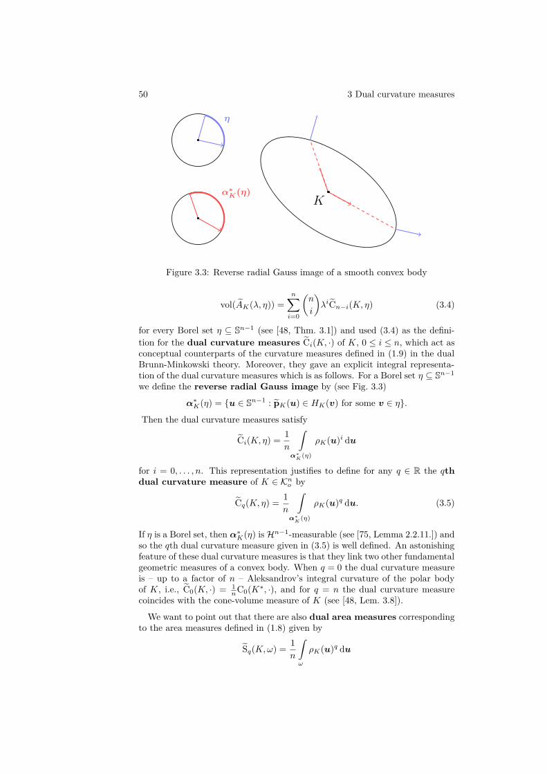
50 3 Dual curvature measures
η
α∗K(η)
K
Figure 3.3: Reverse radial Gauss image of a smooth convex body
vol( ˜AK(λ, η)) =n∑i=0
(n
i
)λi˜Cn−i(K, η) (3.4)
for every Borel set η ⊆ Sn−1 (see [48, Thm. 3.1]) and used (3.4) as the defini-tion for the dual curvature measures ˜Ci(K, ·) of K, 0 ≤ i ≤ n, which act asconceptual counterparts of the curvature measures defined in (1.9) in the dualBrunn-Minkowski theory. Moreover, they gave an explicit integral representa-tion of the dual curvature measures which is as follows. For a Borel set η ⊆ Sn−1
we define the reverse radial Gauss image by (see Fig. 3.3)
α∗K(η) = {u ∈ Sn−1 : ˜pK(u) ∈ HK(v) for some v ∈ η}.
Then the dual curvature measures satisfy
˜Ci(K, η) = 1n
∫α∗
K(η)
ρK(u)i du
for i = 0, . . . , n. This representation justifies to define for any q ∈ R the qthdual curvature measure of K ∈ Kn
o by
˜Cq(K, η) = 1n
∫α∗
K(η)
ρK(u)q du. (3.5)
If η is a Borel set, then α∗K(η) is Hn−1-measurable (see [75, Lemma 2.2.11.]) and
so the qth dual curvature measure given in (3.5) is well defined. An astonishingfeature of these dual curvature measures is that they link two other fundamentalgeometric measures of a convex body. When q = 0 the dual curvature measureis – up to a factor of n – Aleksandrov’s integral curvature of the polar bodyof K, i.e., ˜C0(K, ·) = 1
nC0(K∗, ·), and for q = n the dual curvature measurecoincides with the cone-volume measure of K (see [48, Lem. 3.8]).
We want to point out that there are also dual area measures correspondingto the area measures defined in (1.8) given by
˜Sq(K,ω) = 1n
∫ω
ρK(u)q du
3.1 An introduction to dual Brunn-Minkowski theory 51
for q ∈ R and Borel sets ω ⊆ Sn−1. An extensive description of the dualitybetween classical and dual area measures and curvature measures is containedin [48].
The analogue to the Minkowski-Christoffel problem in the dual Brunn-Min-kowski theory is the dual Minkowski problem. The task is, given q ∈ R and afinite Borel measure µ on Sn−1, to find necessary and sufficient conditions for theexistence of a convex body K ∈ Kn
o such that ˜Cq(K, ·) = µ. It was introducedin [48] and therein a sufficient condition for even measures was established.
Theorem 3.1 (Huang, Lutwak, Yang, Zhang [48]). Let q ∈ (0, n] and µ be anon-zero finite even Borel measure on Sn−1. If
µ(Sn−1 ∩ L) < min{
1 − q − 1q
n− dimL
n− 1 , 1}µ(Sn−1) (3.6)
for every proper subspace L of Rn, then there exists a symmetric convex bodyK ∈ Kn
s with ˜Cq(K, ·) = µ.
There are two remarkable aspects of Theorem 3.1. As for q = n the qth dualcurvature measure is equal to the cone-volume measure, also (3.6) becomesthe strict form of the subspace concentration inequality (1.13). Furthermore,for 0 < q ≤ 1 the inequality (3.6) only asserts that µ is not concentratedon a great subsphere. This is a necessary condition that can be seen from(3.5). In particular, Theorem 3.1 solves the even dual Minkowski problem inthe range q ∈ (0, 1]. Examples of convex bodies showing that for q ∈ (1, n)the inequality (3.6) is not a necessary condition were given in [14, Prop. 1.5]and [82, Prop. A.1]. A necessary subspace concentration inequality for qthdual curvature measures of symmetric convex bodies was proved by Böröczky,Henk and the author. It was also shown that the inequality is sharp since theaforementioned examples get arbitrarily close to the upper bound.
Theorem 3.2 (Böröczky, Henk, P. [14]). Let q ∈ (1, n) and K ∈ Kns . Then
˜Cq(K, Sn−1 ∩ L) < min{
dimL
q, 1} ˜Cq(K, Sn−1) (3.7)
for every proper subspace L of Rn.
We remark that since the bounds (3.6) and (3.7) coincide for dimL = 1, theTheorems 3.1 and 3.2 solved the even dual Minkowski problem in the plane forq ∈ (1, 2). The sufficiency of (3.7) was first proved by Zhao [82], when q is aninteger, and very recently in full generality by Böröczky, Lutwak, Yang, Zhangand Zhao [17].
Theorem 3.3 (Böröczky, Lutwak, Yang, Zhang, Zhao [17]). Let q ∈ (0, n) andµ be a non-zero finite even Borel measure on Sn−1. If
µ(Sn−1 ∩ L) < min{
dimL
q, 1}µ(Sn−1)
for every proper subspace L of Rn, then there exists a symmetric convex bodyK ∈ Kn
s with ˜Cq(K, ·) = µ.
52 3 Dual curvature measures
The Theorems 3.2 and 3.3 combined solve the dual Minkowski problem forsymmetric convex bodies in the range q ∈ (0, n). The case q < 0 was treated byZhao [83]. He proved the absence of a non-trivial subspace concentration boundeven without any symmetry assumptions on the given measure. Moreover, heestablished the uniqueness of dual curvature measures of convex bodies whenq < 0.
Theorem 3.4 (Zhao [83]). Let q < 0 and µ be a non-zero finite Borel measureon Sn−1. Then there exists a convex body K ∈ Kn
o with ˜Cq(K, ·) = µ if andonly if µ is not concentrated on any closed hemisphere. Moreover, K ∈ Kn
o isuniquely determined.
In the remaining paramater range q > n no sufficient condition in the (even)dual Minkowski problem is known. A necessary subspace concentration inequal-ity for dual curvature measures of symmetric convex bodies when q ≥ n+ 1 wasproved by Henk and the author.
Theorem 3.5 (Henk, P. [42]). Let q ≥ n+ 1 and K ∈ Kns . Then
˜Cq(K, Sn−1 ∩ L) < q − n+ dimL
q˜Cq(K, Sn−1) (3.8)
for every proper subspace L of Rn.
The main goal of this chapter is to present the proofs of the Theorems 3.2and 3.5 in full detail. We use the representation (3.5) to conclude that – sim-ilar to the cone-volume measure – ˜Cq(K, η) measures the cones associated tothe outer normals in η just by a measure different from the volume. We willfollow the approach of Henk, Schürmann and Wills [44] who proved the neces-sity of (1.13) for cone-volume measures of symmetric polytopes using only theBrunn-Minkowski inequality (1.2). To this end, we establish Brunn-Minkowskitype inequalities in the Sections 3.2 and 3.3, where the volume is replaced by ameasure with a Lebesgue-density that satisfies a convexity principle.
In Section 3.4 we will prove Theorems 3.2 and 3.5 and also the sharpnessof the given bounds. Moreover, in Section 3.5 we establish an extension ofTheorem 3.5 to the range q ∈ (n, n+ 1) in case n = 2 and discuss the occurringobstructions when n > 2.
Finally, we bring up a generalization of dual curvature measures proposedin [64] in Section 3.6 and survey extensions of Theorems 3.2 and 3.5 in thissetting.
The results of this chapter originally appeared as joint works with KárolyBöröczky, Jr., and Martin Henk [14, 42].
3.2 A generalization of Anderson’s theorem oneven quasiconcave functions
The integral representation of dual curvature measures (3.5) has a striking re-
3.2 Generalization of Anderson’s theorem on even quasiconcave functions 53
semblance to the well-known volume formula of convex bodies K ∈ Kno
vol(K) = 1n
∫Sn−1
ρK(u)n du,
which can be proved just by using spherical coordinates in Rn. Using the con-vention 0α = ∞, α < 0, for convenience, which is consistent to measure theoreticconsiderations, the same method yields the following formula.
Lemma 3.6. Suppose q > 0, K ∈ Kno and Q ∈ Sno . Let η ⊆ Sn−1 be a Borel
set. Then ∫α∗
K(η)
ρQ(u)n−qρK(u)q du = q
∫K∩(R≥0·α∗
K(η)) ρQ(x)n−q dx. (3.9)
Proof. Since q > 0, the integral∫ a
0 rq−1 dr exists for any a > 0. By using
spherical coordinates and (3.5)
q
∫K∩(R≥0·α∗
K(η)) ρQ(x)n−q dx = q
∫α∗
K(η)
⎛⎜⎝ ρK (u)∫0
ρQ(ru)n−qrn−1 dr
⎞⎟⎠ du
= q
∫α∗
K(η)
ρQ(u)n−q
⎛⎜⎝ ρK (u)∫0
rq−1 dr
⎞⎟⎠ du
=∫
α∗K
(η)
ρQ(u)n−qρK(u)q du.
The nature of Lemma 3.6 is revealed when we consider (3.5) for a polytopeP ∈ Pn
o rather than an arbitrary convex body K ∈ Kno . In this case (3.9) with
Q = Bn gives (cf. (1.10))
˜Cq(P, η) = 1n
∫α∗
P(η)
ρP (u)q du
= q
n
∫P∩(R≥0·α∗
P(η)) |x|q−n dx
= q
n
∑u∈U(P )∩η
⎛⎜⎝ ∫conv(F (P,u)∪{0})
|x|q−n dx
⎞⎟⎠ ,
(3.10)
i.e., the sum in (3.10) is taken over the same cones as the cone-volume measure,which are measured by |·|α dHn(·), for some α ∈ (−n,∞), rather than theLebesgue measure. Following the idea of Henk, Schürmann and Wills [44] wetherefore seek for Brunn-Minkowski type inequalities for measures of this kind.

54 3 Dual curvature measures
α = −1α = 1/2α = 4/3
Figure 3.4: Quasiconcave (red), quasiconvex (violet) and convex (blue) instanceof the family {|·|α : α ∈ R \ {0}}
We point out that Lemma 3.6 is crucial for this approach which is why it is onlyviable when q > 0.
For each α ∈ R \ {0} the function |·|α has a convexity property (see Fig. 3.4).If α ≥ 1, then it is convex. When α ∈ (0, 1), it is a quasiconvex function, butnot convex. For α < 0, the function is quasiconcave. We say that a nonnegativefunction f : Rn → R≥0 ∪ {∞} is quasiconvex if for every c ∈ R≥0 the sublevelset
{f ≤ c} = f−1([0, c]) = {x ∈ Rn : f(x) ≤ c}
is convex, and quasiconcave if the superlevel sets
{f ≥ c} = f−1([c,∞]) = {x ∈ Rn : f(x) ≥ c}
are convex. Since convex sets are measurable and measurability of sub-/superlevelsets implies measurability of functions, this definition yields that quasiconvexand quasiconcave functions are Hausdorff-measurable functions. In [3], Ander-son proved that if K ∈ Kn
s and f : Rn → R≥0 ∪ {∞} is quasiconcave and even,the minimum value of ∫
t+K
f(x) dx
with respect to t ∈ Rn is attained at t = 0. This is obvious if restricted to theone-dimensional case, since the evenness of f together with the quasiconcavityimplies that f is monotonically decreasing on any ray starting from the origin.The proof of Anderson relies only on the Brunn-Minkowski inequality (1.2),but the result can be strengthened to a Brunn-Minkowski type inequality forintegrals of quasiconcave functions. Here we compare the integral of f overa convex body K with the integral over Minkowski combinations of the form(1−λ)K+λ(−K). It can be observed, that on the one hand (1−λ)K+λ(−K)is larger than K regarding volume, but also it lies somewhat closer to the originwhere f attains its peak (see Fig. 3.5).
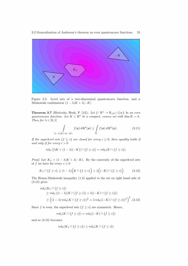
3.2 Generalization of Anderson’s theorem on even quasiconcave functions 55
K
−K
Kλ
Figure 3.5: Level sets of a two-dimensinal quasiconcave function, and aMinkowski combination (1 − λ)K + λ(−K)
Theorem 3.7 (Böröczky, Henk, P. [14]). Let f : Rn → R≥0 ∪ {∞} be an evenquasiconcave function. Let K ⊂ Rn be a compact, convex set with dimK = k.Then for λ ∈ [0, 1] ∫
(1−λ)K+λ(−K)
f(x) dHk(x) ≥∫K
f(x) dHk(x). (3.11)
If the superlevel sets {f ≥ c} are closed for every c ≥ 0, then equality holds ifand only if for every c > 0
volk ([λK + (1 − λ)(−K)] ∩ {f ≥ c}) = volk(K ∩ {f ≥ c}).
Proof. Let Kλ = (1 − λ)K + λ(−K). By the convexity of the superlevel setsof f we have for every c ≥ 0
Kλ ∩ {f ≥ c} ⊇ (1 − λ)(K ∩ {f ≥ c}
)+ λ
((−K) ∩ {f ≥ c}
). (3.12)
The Brunn-Minkowski inequality (1.2) applied to the set on right hand side of(3.12) gives
volk(Kλ ∩ {f ≥ c})≥ volk ((1 − λ)(K ∩ {f ≥ c}) + λ((−K) ∩ {f ≥ c}))
≥(
(1 − λ) volk(K ∩ {f ≥ c}) 1k + λ volk((−K) ∩ {f ≥ c}) 1
k
)k.(3.13)
Since f is even, the superlevel sets {f ≥ c} are symmetric. Hence,
volk(K ∩ {f ≥ c}) = volk((−K) ∩ {f ≥ c})
and so (3.13) becomes
volk(Kλ ∩ {f ≥ c}) ≥ volk(K ∩ {f ≥ c})
56 3 Dual curvature measures
for every c ≥ 0. Fubini’s theorem yields
∫Kλ
f(x) dHk(x) =∫Kλ
⎛⎜⎝ f(x)∫0
1 dc
⎞⎟⎠ dHk(x)
=∞∫
0
volk(Kλ ∩ {f ≥ c}) dc
≥∞∫
0
volk(K ∩ {f ≥ c}) dc
=∫K
f(x) dHk(x).
Suppose {f ≥ c} is closed for every c > 0, and we have equality in (3.11). Thenvolk(Kλ ∩ {f ≥ c}) is lower semi-continuous with respect to c, and for λ ∈ [0, 1]we find that
volk(Kλ ∩ {f ≥ c}) = volk(K ∩ {f ≥ c})
for every c > 0.
Theorem 3.7 includes the result of Anderson [3] as a special case when Kis the translate of a symmetric set. If f is chosen to be the constant functionf(x) = 1, x ∈ Rn, then (3.11) becomes the Brunn-Minkowski inequality (1.2)for M = −K. Another interpretation is as follows. For a quasiconcave functionf : Rn → R≥0 ∪ {∞} we denote by Ψf the measure with Hausdorff-densityfunction f , i.e., dΨf = f dHn. The inequality (3.11) for k = n states that
Ψf ((1 − λ)K + λ(−K)) ≥ Ψf (K)
for K ∈ Kn and λ ∈ [0, 1]. The natural extension reads
Ψf ((1 − λ)K + λM) ≥ min {Ψf (K),Ψf (M)} (3.14)
for any K,M ∈ Kn, which is known as quasiconcavity of the measure Ψf .However, the restriction to pairs (K,−K) ∈ (Kn)2 of Theorem 3.7 is crucial.Counterexamples to (3.14) can be easily found also when f is an even func-tion. As a matter of fact, the famous Borell-Brascamp-Lieb inequality assertsthat (3.14) holds if f− 1
n is a convex function (which is stronger than f beingquasiconcave). For more information on how convexity of measures and densityfunctions are related we refer to [9], [26] and [33, Sect. 15].
3.3 A Brunn–Minkowski type inequality formoments of the Euclidean norm
Establishing a Brunn-Minkowski type inequality like (3.11) for convex functionsf is significantly more challenging. In this case the sublevel sets {f ≤ c} areconvex, but adapting the proof of Theorem 3.7 is not possible. In fact, for any

3.3 Brunn–Minkowski type inequality for moments of the Euclidean norm 57
M ∈ Kns , and t ∈ Rn such that M ∩ (M + t) = ∅ we may choose f to be 0 on M
and 1 otherwise, and K = M + t. Then f is an even convex function, but (3.11)is wrong for any λ ∈ [0, 1] sufficently close to 1
2 . Nevertheless, in the specialcase when f is a power of the Euclidean norm we prove the following result.
Theorem 3.8 (Henk, P. [42]). Let α ≥ 1 and K ∈ Kn with dimK = k ≥ 1.Then for λ ∈ [0, 1] we have∫
(1−λ)K+λ(−K)
|x|α dHk(x) ≥ |2λ− 1|α∫K
|x|α dHk(x), (3.15)
with equality for λ ∈ (0, 1) if and only if α = 1, there exists a u ∈ Sn−1 suchthat K ⊂ lin u, and the origin is not in the relative interior of the segment(1 − λ)K + λ(−K).
Note, that when α = 0, also the inequality (3.15) becomes the Brunn-Minkowski inequality (1.2) for K and −K. The rest of this section is devotedto the proof of Theorem 3.8, but actually we prove a slightly more generalstatement.
Theorem 3.9 (Henk, P. [42]). Let α ≥ 1 and K0,K1 ∈ Kn such that dimK0 =dimK1 = k ≥ 1, volk(K0) = volk(K1) and their affine hulls are parallel. Forλ ∈ [0, 1] let Kλ = (1 − λ)K0 + λK1. Then we have∫Kλ
|x|α dHk(x) +∫
K1−λ
|x|α dHk(x)
≥ |2λ− 1|α⎛⎝ ∫
K0
|x|α dHk(x) +∫K1
|x|α dHk(x)
⎞⎠ (3.16)
with equality for λ ∈ (0, 1) if and only if α = 1, there exists a u ∈ Sn−1 suchthat K0,K1 ⊂ lin u, and the hyperplane H(u, 0) separates Kλ and K1−λ.
Now Theorem 3.8 follows by setting K = K0 = −K1. We start by recallinga variant of the well-known Karamata inequality which often appears in thecontext of Schur-convex functions.
Theorem 3.10 (Karamata’s inequality, see, e.g., [51, Theorem 1]). Let D ⊆ Rbe convex and let φ : D → R be a non-decreasing, convex function. Let x1, . . . , xk,y1, . . . , yk ∈ D such that
(i) x1 ≥ x2 ≥ . . . ≥ xk,
(ii) y1 ≥ y2 ≥ . . . ≥ yk, and
(iii) x1 + x2 + . . .+ xi ≥ y1 + y2 + . . .+ yi for all i = 1, . . . , k.
Then
φ(x1) + φ(x2) + . . .+ φ(xk) ≥ φ(y1) + φ(y2) + . . .+ φ(yk). (3.17)
58 3 Dual curvature measures
If φ is strictly convex, then equality in (3.17) holds if and only if xi = yi,i = 1, . . . , k.
As a consequence we obtain a 0-dimensional version of Theorem 3.9, i.e., whenthe convex sets are replaced by singletons.
Lemma 3.11 (Henk, P. [42]). Let α ≥ 1 and z0, z1 ∈ R. Then for λ ∈ [0, 1] wehave
|(1 − λ)z0 + λz1|α + |λz0 + (1 − λ)z1|α ≥ |2λ− 1|α(
|z0|α + |z1|α)
(3.18)
with equality for λ ∈ (0, 1) if and only if either
(i) z1 = −z0, or
(ii) α = 1, z0z1 < 0 and max{λ, 1 − λ} ≥ max{|z0|,|z1|}|z0|+|z1| .
Proof. By symmetry we may assume that λ ≤ 12 , |z0| ≥ |z1| and z0 ≥ 0. Write
x1 = |(1 − λ)z0 + λz1| ,x2 = |λz0 + (1 − λ)z1| ,y1 = (1 − 2λ)z0,
y2 = (1 − 2λ) |z1| .
We want to apply Karamata’s inequality with D = R≥0 and f(t) = tα. Wereadily have
y1 ≥ y2,
x21 − x2
2 = (1 − 2λ)(z20 − z2
1) ≥ 0,
which gives x1 ≥ x2. Since z1 ≥ −z0 we also have
(1 − λ)z0 + λz1 ≥ λz0 + λz1 = λ(z0 + z1) ≥ 0, (3.19)
from which we find
x1 = (1 − λ)z0 + λz1 ≥ (1 − λ)z0 − λz0 = y1.
It remains to show that x1 + x2 ≥ y1 + y2. The triangle inequality gives
|((1 − λ)z0 + λz1) ± (λz0 + (1 − λ)z1)| ≤ x1 + x2.
Hence
x1 + x2 ≥ max{|z0 + z1| , |(1 − 2λ)(z0 − z1)|}≥ (1 − 2λ) max{|z0 + z1| , |z0 − z1|}= (1 − 2λ)(z0 + |z1|)= y1 + y2
(3.20)
and Karamata’s inequality (3.17) yields xα1 + xα2 ≥ yα1 + yα2 .
Suppose now we have equality in (3.18) and as before we assume 0 < λ ≤ 12 ,
|z0| ≥ |z1| and z0 ≥ 0. In view of our assumptions we have (3.19). First let

3.3 Brunn–Minkowski type inequality for moments of the Euclidean norm 59
α > 1. In this case the equality condition of Karamata’s inequality assertsx1 = y1 and from (3.19) we conclude λz1 = −λz0. So for α > 1 equality in(3.18) is equivalent to z1 = −z0.
Now suppose α = 1, and z1 = −z0. In this case (3.18) becomes x1 + x2 =y1 + y2 and the equality in (3.20) yields
(1 − λ)z0 + λz1 + |λz0 + (1 − λ)z1| = x1 + x2 = |(1 − 2λ)(z0 − z1)| ,
i.e., we have equality in the triangle inequality
|((1 − λ)z0 + λz1) + (−λz0 − (1 − λ)z1)| ≤ x1 + x2.
Thus, by (3.19) it follows that λz0 + (1 − λ)z1 ≤ 0. Since z0 ≥ 0 and z1 = −z0we must have z1 < 0. Moreover, since z0 ≥ |z1| this also shows z0 > 0. Byrearranging λz0 + (1 − λ)z1 ≤ 0 the inequality becomes
1 − λ ≥ z0
z0 − z1.
In consideration of the made assumptions this is condition (ii). On the otherhand, following the same arguments condition (ii) implies x1 +x2 = y1 +y2.
At the present day there is a vast number of different proofs of the Brunn-Minkowski inequality (1.2). Here we want to emphasize the version of Kneserand Süss [52] who used an inductive argument and Fubini’s theorem to applya lower-dimensional Brunn-Minkowski inequality onto sections of convex bodieswith hyperplanes (see [75, Thm. 7.1.1] for an English version). An inductiveapproach in the setting of Theorem 3.9 comes with the task of consideringthe restriction of the function |·|α to sections of convex bodies. Instead, thenext lemma will allow us to replace spheres appearing as level sets of the normfunction by hyperplanes. It appeared first in Alesker [1] and for more explicitversions of it we refer to [72, Lemma 2.1] and [4, (10.4.2)].
Lemma 3.12. Let α > −1. There is a constant c = c(n, α) such that for everyx ∈ Rn
|x|α = c ·∫
Sn−1
|⟨θ,x⟩|α dθ.
Consequently, in the subsequent lemma we will prove a version of Theorem 3.9with the function |⟨θ, ·⟩|α, θ ∈ Sn−1 fixed, in place of |·|α.
Lemma 3.13 (Henk, P. [42]). Let α ≥ 1 and K0,K1 ∈ Kn such that dimK0 =dimK1 = k ≥ 1, volk(K0) = volk(K1) and their affine hulls are parallel. Letθ ∈ Sn−1 and for λ ∈ [0, 1] let Kλ = (1 − λ)K0 + λK1. Then we have∫Kλ
|⟨θ,x⟩|α dHk(x) +∫
K1−λ
|⟨θ,x⟩|α dHk(x)
≥ |2λ− 1|α⎛⎝ ∫
K0
|⟨θ,x⟩|α dHk(x) +∫K1
|⟨θ,x⟩|α dHk(x)
⎞⎠ . (3.21)
60 3 Dual curvature measures
Moreover, if K0 and K1 are not contained in affine spaces parallel to θ⊥ andequality holds in (3.21) for λ ∈ (0, 1), then α = 1, K0 and K1 are translates andthe hyperplane H(θ, 0) separates Kλ and K1−λ.
Proof. Without loss of generality we assume that volk(K0) = volk(K1) = 1.The Brunn-Minkowski-inequality (1.2) gives in this setting for any λ ∈ [0, 1]
volk(Kλ) ≥ 1. (3.22)
For t ∈ R denote
H(θ, t) = {x ∈ Rn : ⟨θ,x⟩ = t},H−(θ, t) = {x ∈ Rn : ⟨θ,x⟩ ≤ t}.
First suppose that K0 lies in a hyperplane parallel to θ⊥ (and therefore Kλ
for λ ∈ [0, 1]), i.e., Ki ⊂ H(θ, ti) for some ti ∈ R, i ∈ {0, 1}. By (3.22) andLemma 3.11 we find∫
Kλ
|⟨θ,x⟩|α dHk(x) +∫
K1−λ
|⟨θ,x⟩|α dHk(x)
= volk(Kλ) |(1 − λ)t0 + λt1|α + volk(K1−λ) |λt0 + (1 − λ)t1|α
≥ |(1 − λ)t0 + λt1|α + |λt0 + (1 − λ)t1|α
≥ |2λ− 1|α (|t0|α + |t1|α)= |2λ− 1|α (volk(K0) |t0|α + volk(K1) |t1|α)
= |2λ− 1|α⎛⎝ ∫
K0
|⟨θ,x⟩|α dHk(x) +∫K1
|⟨θ,x⟩|α dHk(x)
⎞⎠ .
Thus, in the following we may assume that K0 ⊆ v + θ⊥ for all v ∈ Rn andhence, −hKi(−θ) < hKi(θ) for i = 0, 1. For t ∈ R and for i = 0, 1 we set
vi(t) = volk−1(Ki ∩H(θ, t)),wi(t) = volk(Ki ∩H−(θ, t)),
so that wi(t) =∫ t
−∞ vi(ζ) dζ, i ∈ {0, 1}. On (−hKi(−θ), hKi
(θ)) the function viis continuous and hence wi is differentiable. For i ∈ {0, 1} let zi be the inversefunction of wi. Then zi is differentiable with
z′i(τ) = 1
w′i(zi(τ)) = 1
vi(zi(τ)) (3.23)
for τ ∈ (0, 1). Write zν(τ) = (1 − ν)z0(τ) + νz1(τ) for ν ∈ [0, 1]. By Fubini’stheorem and a change of variables via t = zν(τ) we find∫Kν
|⟨θ,x⟩|α dHk(x) =∞∫
−∞
|t|α volk−1(Kν ∩H(θ, t)) dt
=1∫
0
|zν(τ)|α volk−1
(Kν ∩H(θ, zν(τ))
)z′ν(τ) dτ.
(3.24)

3.3 Brunn–Minkowski type inequality for moments of the Euclidean norm 61
Since Kν ∩ H(θ, zν(τ)) ⊇ (1 − ν)(K0 ∩ H(θ, z0(τ))) + ν(K1 ∩ H(θ, z1(τ))) wemay apply the Brunn-Minkowski inequality (1.2) to the latter set and togetherwith (3.23) we get
volk−1
(Kν ∩H(θ, zν(τ))
)z′ν(τ)
≥ volk−1
((1 − ν)
(K0 ∩H(θ, z0(τ))
)+ ν(K1 ∩H(θ, z1(τ))
))z′ν(τ)
≥[(1 − ν)v0(z0(τ))
1k−1 + νv1(z1(τ))
1k−1
]k−1[
1 − ν
v0(z0(τ)) + ν
v1(z1(τ))
]≥[v0(z0(τ))
1−νk−1 v1(z1(τ))
νk−1
]k−1 [v0(z0(τ))−(1−ν)v1(z1(τ))−ν
]= 1,
(3.25)
where for the last inequality we used the weighted arithmetic-geometric meaninequality. Therefore, (3.24) and (3.25) yield∫
Kλ
|⟨θ,x⟩|α dHk(x) +∫
K1−λ
|⟨θ,x⟩|α dHk(x)
≥1∫
0
|zλ(τ)|α + |z1−λ(τ)|α dτ
=1∫
0
|(1 − λ)z0(τ) + λz1(τ)|α + |λz0(τ) + (1 − λ)z1(τ)|α dτ.
Next in order to estimate the integrand we use Lemma 3.11 and then we sub-stitute back via (3.23)∫
Kλ
|⟨θ,x⟩|α dHk(x) +∫
K1−λ
|⟨θ,x⟩|α dHk(x)
≥1∫
0
|(1 − λ)z0(τ) + λz1(τ)|α + |λz0(τ) + (1 − λ)z1(τ)|α dτ
≥1∫
0
|2λ− 1|α(
|z0(τ)|α + |z1(τ)|α)
dτ (3.26)
= |2λ− 1|α⎛⎝ 1∫
0
|z0(τ)|α dτ +1∫
0
|z1(τ)|α dτ
⎞⎠= |2λ− 1|α
⎛⎝ 1∫0
|z0(τ)|α v0(z0(τ)) · z′0(τ) dτ
+1∫
0
|z1(τ)|α v1(z1(τ)) · z′1(τ) dτ
⎞⎠
62 3 Dual curvature measures
= |2λ− 1|α⎛⎝ ∞∫
−∞
|t|α volk−1(K0 ∩H(θ, t)) dt
+∞∫
−∞
|t|α volk−1(K1 ∩H(θ, t)) dt
⎞⎠= |2λ− 1|α
⎛⎝ ∫K0
|⟨θ,x⟩|α dHk(x) +∫K1
|⟨θ,x⟩|α dHk(x)
⎞⎠ .
Now suppose that equality holds in (3.21) for two k-dimensional convex bodiesK0,K1 of k-dimensional volume 1 with Ki ⊆ v + θ⊥ for any v ∈ Rn, i ∈ {0, 1}.Without loss of generality we may assume that 0 < λ ≤ 1
2 . Then the equalityin (3.21) implies equality in (3.25) for ν = λ and thus
volk(Kλ) =1∫
0
volk−1
(Kλ ∩H(θ, zλ(τ))
)z′λ(τ) dτ
= 1 = λ volk(K0) + (1 − λ) volk(K1).
Hence, by the equality conditions of the Brunn-Minkowski inequality (1.2), K0and K1 are homothets and we conclude K0 = v + K1 for some v ∈ Rn. Thusfor τ ∈ [0, 1] and s = ⟨θ,v⟩
z0(τ) = z1(τ) + ⟨θ,v⟩ = z1(τ) + s. (3.27)
Since we must also have equality in (3.26) the equality conditions (i) and (ii) ofLemma 3.11 can be applied to zi(τ), i = 0, 1. If α > 1, then Lemma 3.11 (i)implies z0(τ) = −z1(τ) for τ ∈ [0, 1]. Together with (3.27), however, we getthat z0(τ) = s
2 is constant with respect to τ . Then v2 + θ⊥ contains K0, which
contradicts the assumption.
Thus we must have α = 1 and in this case we get from Lemma 3.11 (ii) and(3.27)
0 > z0(τ)z1(τ) = z0(τ)(z0(τ) − s), (3.28)
1 − λ = max{λ, 1 − λ} ≥ max{|z0(τ)| , |z0(τ) − s|}|z0(τ)| + |z0(τ) − s|
(3.29)
for every τ ∈ [0, 1] except when z1(τ) = −z0(τ). The above considerations showthat there is at most one element in τ ∈ [0, 1] satisfying the latter equation.
By interchanging the roles of z0(τ) and z1(τ), if necessary, we may additionallyassume that s ≥ 0. In particular, by (3.28) and since z0 is continuous andmonotone, it follows that s > z0(τ) > 0 for all τ ∈ (0, 1). Then (3.29) becomes
1 − λ ≥ max{z0(τ), s− z0(τ)}s
and we obtain
zλ(τ) = (1 − λ)z0(τ) + λ(z0(τ) − s) = z0(τ) − λs ≥ 0,

3.3 Brunn–Minkowski type inequality for moments of the Euclidean norm 63
z1−λ(τ) = λz0(τ) + (1 − λ)(z0(τ) − s) = z0(τ) − (1 − λ)s ≤ 0
for all τ ∈ (0, 1). By the continuity of z0 we have −hKλ(−θ) ≥ 0 ≥ hK1−λ
(θ),i.e., H(θ, 0) separates Kλ and K1−λ.
Now we are ready to prove Theorem 3.9.
Proof of Theorem 3.9. Without loss of generality we assume that volk(K0) =volk(K1) = 1. In order to prove the desired inequality (3.16) we first substitutethe integrand via Lemma 3.12 which leads, after an application of Fubini’stheorem, to the equivalent inequality
∫Sn−1
⎛⎜⎝ ∫Kλ
|⟨θ,x⟩|α dHk(x) +∫
K1−λ
|⟨θ,x⟩|α dHk(x)
⎞⎟⎠ dθ
≥ |2λ− 1|α ×∫Sn−1
⎛⎝ ∫K0
|⟨θ,x⟩|α dHk(x) +∫K1
|⟨θ,x⟩|α dHk(x)
⎞⎠ dθ.
(3.30)
By Lemma 3.13 this inequality holds pointwise for every θ ∈ Sn−1. Hence wehave shown (3.30) and thus (3.16).
Now suppose that λ ∈ (0, 1) and equality holds in (3.16) for two k-dimensionalconvex bodies K0,K1 of k-dimensional volume 1. Then we also have equal-ity in (3.30) for any θ ∈ Sn−1. In particular, since K0 contains at least twodistinct points x,y ∈ K0, we may choose θ = x − y, so that K0 is not con-tained in an affine space parallel to θ⊥. The necessary conditions for equality inLemma 3.13 assert that α = 1, K0 and K1 are translates, and H(θ, 0) separatesKλ and K1−λ. On the other hand, if x and y are linearly independent, we findv ∈ x⊥ \ y⊥ and ι ∈ R such that
⟨x + ιv,x⟩ = |x|2 > 0,⟨x + ιv,y⟩ = ⟨x,y⟩ + ι ⟨v,y⟩ < 0,
i.e., K0 has a non-empty intersection with H(x+ιv, 0). Setting θ = x + ιv thencontradicts Lemma 3.13 as Kλ and K1−λ cannot be separated by H(θ, 0). Thusevery two points in K0 are linearly dependent, which means that K ⊆ lin u forsome u ∈ Sn−1. Following the same line of reasoning for K1 leads to the sameconclusion and since the affine hulls of K0 and K1 are parallel we also haveK1 ⊆ lin u. In particular, the function ⟨u, ·⟩ is not constant on K0 or K1 andby Lemma 3.13 the hyperplane H(u, 0) separates Kλ and K1−λ.
It remains to show that this separating property also implies equality in (3.16).If there exists such a u, then with an appropriate choice of coordinates we mayassume that K0,K1 ⊆ R, i.e., K0 = [ξ0, ξ0 + 1] and K1 = [−(ξ1 + 1),−ξ1] forsome ξ0, ξ1 ≥ 0. By symmetry we may assume λ ≤ 1
2 . The assumption that
Kλ = [(1 − λ)ξ0 − λ(ξ1 + 1), (1 − λ)(ξ0 + 1) − λξ1]
64 3 Dual curvature measures
and
K1−λ = [λξ0 − (1 − λ)(ξ1 + 1), λ(ξ0 + 1) − (1 − λ)ξ1]
are separated by the origin, means λ(ξ0+1)−(1−λ)ξ1 ≤ 0 ≤ (1−λ)ξ0−λ(ξ1+1)and so∫
Kλ
|x| dx +∫
K1−λ
|x| dx
=(1−λ)(ξ0+1)−λξ1∫
(1−λ)ξ0−λ(ξ1+1)
t dt+λ(ξ0+1)−(1−λ)ξ1∫λξ0−(1−λ)(ξ1+1)
−t dt
= 12
[((1 − λ)(ξ0 + 1) − λξ1
)2−(
(1 − λ)ξ0 − λ(ξ1 + 1))2
−(λ(ξ0 + 1) − (1 − λ)ξ1
)2+(λξ0 − (1 − λ)(ξ1 + 1)
)2]= (2λ− 1)(ξ0 + ξ1 + 1)
= (2λ− 1) · 12
[(ξ0 + 1)2 − ξ2
0 + (ξ1 + 1)2 − ξ21
]= (2λ− 1)
⎛⎜⎝ ξ0+1∫ξ0
t dt+ξ1+1∫ξ1
t dt
⎞⎟⎠= (2λ− 1)
⎛⎝ ∫K0
|x| dx +∫K1
|x| dx
⎞⎠ .
We remark that the factor |2λ − 1|α in the Theorems 3.8 and 3.9 cannot bereplaced by a smaller one. This can be seen from the following example. LetC ∈ Kn
s , u ∈ Sn−1, and for every r ∈ R>0 set K(r)0 = C+r·u and K(r)
1 = −K(r)0 .
Then, for every ν ∈ [0, 1] we have K(r)ν = C − (2ν − 1)ru and∫
K(r)ν
|x|α dx = rα∫C
r−1x − (2ν − 1)u
α dx.
Moreover, the symmetry of C gives K(r)1−ν = −K(r)
ν . Therefore and sincer−1x − (2ν − 1)u
α ≤ (|x| + |(2ν − 1)u|)α
for r ≥ 1, for a given λ ∈ [0, 1], we conclude by the dominated convergencetheorem
limr→∞
∫K
(r)1−λ
|x|α dx∫K
(r)1
|x|α dx= limr→∞
∫K
(r)λ
|x|α dx∫K
(r)0
|x|α dx= |2λ− 1|α .
Although (3.15) also holds for α = 0 we point out that an extension of Theo-rem 3.8 to the intermediate cases α ∈ (0, 1), where |·|α is a non-convex function,is not possible.
3.4 Subspace concentration in the even dual Minkowski problem 65
Proposition 3.14 (Henk, P. [42]). Let α ∈ (0, 1). There is a closed intervalK ⊆ R and λ ∈ [0, 1] such that for Kλ = (1 − λ)K + λ(−K) we have∫
Kλ
|x|α dx < |2λ− 1|α∫K
|x|α dx.
Proof. Let ε > 0, K = [ε, 1 + ε] and λ = ε1+2ε <
12 so that Kλ = [0, 1]. Then
(1 + α)∫Kλ
|x|α dx = 1
and
(1 + α)(1 − 2λ)α∫K
|x|α dx = (1 + α)(1 + 2ε)−α1+ε∫ε
xα dx
= (1 + ε)1+α − ε1+α
(1 + 2ε)α .
Let f(t) = (1 + t)1+α − t1+α and g(t) = (1 + 2t)α. Since
f(0) = 1 = g(0),f ′(0) = (1 + α) > 2α = g′(0),
we have(1 + ε)1+α − ε1+α
(1 + 2ε)α > 1
for small ε and hence, ∫Kλ
|x|α dx < (1 − 2λ)α∫K
|x|α dx.
3.4 Subspace concentration in the even dualMinkowski problem
In this section we will prove bounds on the subspace concentration of dual curva-ture measures of symmetric convex bodies. In the following lemma we evaluatean integral that repeatedly appears in the proofs of Theorems 3.2 and 3.5.
Lemma 3.15. Let q > 0, K ∈ Kns , Q ∈ Sno and L be a k-dimensional subspace
of Rn, where 1 ≤ k ≤ n− 1. Then for any s < k
∫K|L
⎛⎜⎝ρK|L(y)s∫
KpK|L(y)
ρQ(z)n−q dz
⎞⎟⎠ dy = c
k − s, (3.31)
where for v ∈ K|L we write Kv = K ∩ (v + L⊥) and c = c(q,K,Q,L) is aconstant independent of s.
66 3 Dual curvature measures
Proof. Since ˜pK|L(y) is homogeneous of degree 0 in y we have ˜pK|L(y) =˜pK|L(y) for every y ∈ K|L, y = 0. Using spherical coordinates in K|L the lefthand side of (3.31) becomes
∫K|L
⎛⎜⎝ρK|L(y)s∫
KpK|L(y)
ρQ(z)n−q dz
⎞⎟⎠ dy
=∫
Sn−1∩L
ρK|L(u)∫0
ρK|L(ru)sg(u)rk−1 dr du,
where g(u) =∫KpK|L(u)
ρQ(z)n−q dz. Homogeneity of the radial function ρQ
and integration with respect to r yields
∫K|L
⎛⎜⎝ρK|L(y)s∫
KpK|L(y)
ρQ(z)n−q dz
⎞⎟⎠ dy
=∫
Sn−1∩L
ρK|L(u)sg(u)
ρK|L(u)∫0
rk−s−1 dr du
=∫
Sn−1∩L
ρK|L(u)sg(u)ρK|L(u)k−s
k − sdu
= 1k − s
∫Sn−1∩L
ρK|L(u)kg(u) du,
where we used that the involved integrals are finite since s < k.
Now we are ready to prove the Theorems 3.2 and 3.5. We use Fubini’s theoremto decompose the dual curvature measure of K ∈ Kn
s into integrals over sectionswith affine planes orthogonal to the given subspace L. These sections containMinkowski combinations of parallel sections which lie in ∂K (see Fig. 3.6), andby applying a Brunn-Minkowski type inequality we may compare these integralswith the corresponding integrals over sections associated to the dual curvaturemeasure of the Borel set Sn−1 ∩ L. We start with the case q ∈ (0, n) where weprove a slightly more general statement.
Theorem 3.16 ([14, cf. Rem. 4.1]). Let q ∈ (0, n) and K,Q ∈ Kns . Then∫
α∗K
(Sn−1∩L)
ρQ(u)n−qρK(u)q du <dimL
q
∫Sn−1
ρQ(u)n−qρK(u)q du (3.32)
for every proper subspace L of Rn.
Proof. Let dimL = k ∈ {1, . . . , n − 1}. For y ∈ K|L and u ∈ Sn−1 ∩ L we
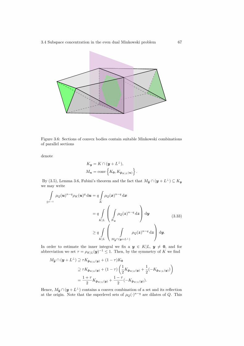
3.4 Subspace concentration in the even dual Minkowski problem 67
Figure 3.6: Sections of convex bodies contain suitable Minkowski combinationsof parallel sections
denote
Ky = K ∩ (y + L⊥),
Mu = conv{K0,KpK|L(u)
}.
By (3.5), Lemma 3.6, Fubini’s theorem and the fact that My ∩ (y + L⊥) ⊆ Ky
we may write∫Sn−1
ρQ(u)n−qρK(u)q du = q
∫K
ρQ(x)n−q dx
= q
∫K|L
⎛⎜⎝ ∫Ky
ρQ(z)n−q dz
⎞⎟⎠ dy
≥ q
∫K|L
⎛⎜⎝ ∫My∩(y+L⊥)
ρQ(z)n−q dz
⎞⎟⎠ dy.
(3.33)
In order to estimate the inner integral we fix a y ∈ K|L, y = 0, and forabbreviation we set τ = ρK|L(y)−1 ≤ 1. Then, by the symmetry of K we find
My ∩ (y + L⊥) ⊇ τKpK|L(y) + (1 − τ)K0
⊇ τKpK|L(y) + (1 − τ)(
12KpK|L(y) + 1
2(−KpK|L(y)))
= 1 + τ
2 KpK|L(y) + 1 − τ
2 (−KpK|L(y)).
Hence, My ∩ (y +L⊥) contains a convex combination of a set and its reflectionat the origin. Note that the superlevel sets of ρQ(·)n−q are dilates of Q. This
68 3 Dual curvature measures
allows us to apply Theorem 3.7 from which we obtain∫My∩(y+L⊥)
ρQ(z)n−q dz ≥∫
KpK|L(y)
ρQ(z)n−q dz (3.34)
for every y ∈ K|L, y = 0. Together with (3.33) we find
∫Sn−1
ρQ(u)n−qρK(u)q du ≥ q
∫K|L
⎛⎜⎝ ∫KpK|L(y)
ρQ(z)n−q dz
⎞⎟⎠ dy.
By using Lemma 3.15 with s = 0 we then obtain the lower bound∫Sn−1
ρQ(u)n−qρK(u)q du ≥ qc
k, (3.35)
where c is a constant independent of s.
In order to evaluate the left hand side of (3.32) we recall that for x ∈ K wehave x ∈ α∗
K(Sn−1 ∩ L) if and only if the boundary point ˜pK(x) has a unitouter normal in L. Hence,
K ∩(R≥0 · α∗
K(Sn−1 ∩ L))
=⋃
v∈∂(K|L)
conv({0} ∪Kv)
and in view of (3.5), Lemma 3.6 and Fubini’s theorem we obtain∫α∗
K(Sn−1∩L)
ρQ(u)n−qρK(u)q du
= q
∫K∩(R≥0·α∗
K(Sn−1∩L)
) ρQ(x)n−q dx
= q
∫K|L
⎛⎜⎜⎝ ∫conv
({0}∪KpK|L(y)
)∩(y+L⊥)
ρQ(z)n−q dz
⎞⎟⎟⎠ dy
= q
∫K|L
⎛⎜⎜⎝ ∫ρK|L(y)−1KpK|L(y)
ρQ(z)n−q dz
⎞⎟⎟⎠ dy
= q
∫K|L
ρK|L(y)k−q
⎛⎜⎝ ∫KpK|L(y)
ρQ(z)n−q dz
⎞⎟⎠ dy.
Using Lemma 3.15 again with s = k − q it follows from (3.35) that∫α∗
K(Sn−1∩L)
ρQ(u)n−qρK(u)q du = c ≤ k
q
∫Sn−1
ρQ(u)n−qρK(u)q du.
3.4 Subspace concentration in the even dual Minkowski problem 69
It remains to show that the inequality is strict. To this end, suppose that wehave equality in (3.32) for a proper subspace L. Then we must have equalityin (3.34) for almost every y in the relative interior of K|L. Hence, since q < nand in view of the equality condition of Theorem 3.7, the equality in (3.34)implies that My ∩ (y + L⊥) ∩ rQ and KpK|L(y) ∩ rQ have the same (n − k)-dimensional volume for almost every r > 0. Moreover, the equality in (3.33)shows Ky = My ∩ (y + L⊥) and therefore
voln−k(Ky ∩ rQ) = voln−k(KpK|L(y) ∩ rQ)
for almost every r > 0. Let ξ be a point maximizing ρQ over KpK|L(y). Inparticular, ρK|L(y)−1ξ ∈ Ky. Since y is a relative interior point of K|L, wehave ρK|L(y) > 1 and we may choose r > 0 such that
ρQ(ξ) < r−1 < ρK|L(y)ρQ(ξ) = ρQ(ρK|L(y)−1ξ
).
Since ξ maximizes ρQ on KpK|L(y) the former inequality gives KpK|L(y)∩rQ = ∅,whereas the latter shows
voln−k(Ky ∩ rQ) > 0.
In view of (3.5), Theorem 3.2 is an immediate consequence of Theorem 3.16.The proof of Theorem 3.5 is carried out analogously where instead of (3.11) weuse (3.15).
Proof of Theorem 3.5. Let dimL = k ∈ {1, . . . , n − 1}. For y ∈ K|L andu ∈ Sn−1 ∩ L we denote
Ky = K ∩ (y + L⊥),
Mu = conv{K0,KpK|L(u)
}.
By (3.5), Lemma 3.6, Fubini’s theorem and the fact that My ∩ (y + L⊥) ⊆ Ky
we may write (cf. (3.33))
˜Cq(K, Sn−1) = 1n
∫Sn−1
ρK(u)q du
≥ q
n
∫K|L
⎛⎜⎝ ∫My∩(y+L⊥)
|z|q−n dz
⎞⎟⎠ dy. (3.36)
In order to estimate the inner integral we fix a y ∈ K|L, y = 0, and forabbreviation we set τ = ρK|L(y)−1 ≤ 1. Then, by the symmetry of K we find
My ∩ (y + L⊥) ⊇ τ(KpK|L(y)) + (1 − τ)(K0)
⊇ τ(KpK|L(y)) + (1 − τ)(
12KpK|L(y) + 1
2(−KpK|L(y)))
= 1 + τ
2 KpK|L(y) + 1 − τ
2 (−KpK|L(y)).

70 3 Dual curvature measures
Hence, My ∩ (y +L⊥) contains a convex combination of a set and its reflectionat the origin. This allows us to apply Theorem 3.8 from which we obtain∫
My∩(y+L⊥)
|z|q−n dz ≥ τ q−n∫
KpK|L(y)
|z|q−n dz
for every y ∈ K|L, y = 0. By the equality characterization of Theorem 3.8 thelast inequality is strict whenever τ < 1, i.e., y belongs to the relative interior ofK|L. Together with (3.36) we find
˜Cq(K, Sn−1) > q
n
∫K|L
ρK|L(y)n−q
⎛⎜⎝ ∫KpK|L(y)
|z|q−n dz
⎞⎟⎠ dy.
By using Lemma 3.15 with Q = Bn and s = n − q we then obtain the lowerbound ˜Cq(K, Sn−1) > q
n
c
k + q − n,
where c is a constant independent of s.
On the other hand, in the same manner as in the proof of Theorem 3.16 wefind
˜Cq(K, Sn−1 ∩ L) = 1n
∫α∗
K(Sn−1∩L)
ρK(u)q du
= q
n
∫K|L
ρK|L(y)k−q
⎛⎜⎝ ∫KpK|L(y)
|z|q−n dz
⎞⎟⎠ dy.
Inequality (3.35) and Lemma 3.15, again, with Q = Bn and s = k − q yield
˜Cq(K, Sn−1 ∩ L) = q
n
c
q<k + q − n
q˜Cq(K, Sn−1).
Next we show that the bounds given in Theorem 3.5 are tight for every choiceof q ≥ n+ 1.
Proposition 3.17 (Henk, P. [42]). Let q > n and k ∈ {1, . . . , n − 1}. Thereexists a sequence of convex bodies Kl ∈ Kn
s , l ∈ N, and a k-dimensional subspaceL ⊆ Rn such that
liml→∞
˜Cq(Kl, Sn−1 ∩ L)˜Cq(Kl, Sn−1)= q − n+ k
q.
Proof. Let k ∈ {1, . . . , n− 1} and for l ∈ N, let Kl be the cylinder given as thecartesian product of two lower-dimensional balls
Kl = (lBk) ×Bn−k.
3.4 Subspace concentration in the even dual Minkowski problem 71
Let L = lin{e1, . . . , ek} be the k-dimensional subspace generated by the firstk canonical unit vectors ei. For x ∈ Rn write x = (x1,x2), where x1 ∈ Rkand x2 ∈ Rn−k. The supporting hyperplane of Kl with respect to a unit vectorv = (v1,v2) ∈ Sn−1 ∩ L is given by
HKl(v) = {x ∈ Rn : ⟨v1,x1⟩ = l}.
Hence the part of the boundary of Kl covered by all these supporting hyper-planes is given by lSk−1 × Bn−k. In view of Lemma 3.6 and Fubini’s theoremwe conclude
˜Cq(Kl, Sn−1 ∩ L) = q
n
∫lBk
⎛⎜⎜⎝ ∫|x1|
l Bn−k
(|x1|2 + |x2|2)q−n
2 dx2
⎞⎟⎟⎠ dx1. (3.37)
Denote the volume of Bn by ωn. Recall that the surface area of Bn is given bynωn and for abbreviation we set
c = c(q, k, n) = q
nkωk(n− k)ωn−k.
Switching to the cylindrical coordinates
x1 = su, s ≥ 0,u ∈ Sk−1, x2 = tv, t ≥ 0,v ∈ Sn−k−1,
transforms the right hand side of (3.37) to
˜Cq(Kl, Sn−1 ∩ L) = c
l∫0
s/l∫0
sk−1tn−k−1(s2 + t2)q−n
2 dt ds
= c
l∫0
1∫0
sq−1lk−ntn−k−1(1 + l−2t2)q−n
2 dt ds
= c lq−n+k1∫
0
1∫0
sq−1tn−k−1(1 + l−2t2)q−n
2 dt ds.
Analogously we obtain
˜Cq(Kl, Sn−1) = q
n
∫lBk
⎛⎜⎝ ∫Bn−k
(|x1|2 + |x2|2)q−n
2 dx2
⎞⎟⎠ dx1
= c
l∫0
1∫0
sk−1tn−k−1(s2 + t2)q−n
2 dt ds
= clk1∫
0
1∫0
sk−1tn−k−1(l2s2 + t2)q−n
2 dt ds
= clq−n+k1∫
0
1∫0
sk−1tn−k−1(s2 + l−2t2)q−n
2 dt ds.
72 3 Dual curvature measures
The monotone convergence theorem gives
liml→∞
(clq−n+k)−1˜Cq(Kl, Sn−1 ∩ L)
= liml→∞
1∫0
1∫0
sq−1tn−k−1(1 + l−2t2)q−n
2 dt ds
=1∫
0
sq−1 ds ·1∫
0
tn−k−1 dt = 1q(n− k)
and
liml→∞
(clq−n+k)−1˜Cq(Kl, Sn−1)
= liml→∞
1∫0
1∫0
sk−1tn−k−1(s2 + l−2t2)q−n
2 dt ds
=1∫
0
sq−n+k−1 ds ·1∫
0
tn−k−1 dt = 1(q − n+ k)(n− k) .
Hence,
liml→∞
˜Cq(Kl, Sn−1 ∩ L)˜Cq(Kl, Sn−1)= q − n+ k
q.
The optimality of (3.7) can be established with a similar example whereKl = Bk × (lBn−k) as it was done in [14] (see also [82]). Obviously this isalso a consequence of Theorem 3.3.
3.5 Further results
The Proposition 3.17 above particularly shows that the upper bound q−n+dimLq
would be also optimal in the range q ∈ (n, n+ 1). Unfortunately, our approachto prove Theorem 3.5 can not cover this missing range. One reason is that theBrunn-Minkowski-type inequality (3.15) does not extend to α ∈ (0, 1) as shownin Proposition 3.14. In the proof of Theorem 3.5 we applied (3.15) pointwiseonto the inner integral on the right hand side of (3.36). This brings up thequestion, whether (3.15) is correct on a certain average, i.e., when both sides areintegrated with respect to λ ∈ [0, 1]. Note that in order to extend Theorem 3.5to α ∈ (0, 1) we would need to prove
1∫0
|2λ− 1|m−1∫
(1−λ)K+λ(−K)
|x|α dHk(x) dλ
≥ 1m+ α
∫K
|x|α dHk(x), (3.38)
3.5 Further results 73
for m ∈ N, K ∈ Kn with dim(K) = k ≥ 1 and α ∈ (0, 1). But this is alsofalse for some examples like m = 2, α = 1
2 and K = [1, 5]. In this case one cancompute
1∫0
|2λ− 1|∫
(1−λ)K+λ(−K)
√|x| dx dλ = 4
945
(− 19 + 32
√2 + 275
√5)
≈ 2.713 . . .
and
12 + 1
2
∫K
√|x| dx = 4
15
(5√
5 − 1)
≈ 2.714 . . .
In the particular case when m = 1 we will prove (3.38). To this end, we startwith an integral version of (3.18) for α ∈ (0, 1).
Lemma 3.18. Let α ∈ (0, 1) and z0, z1 ∈ R. Then
1∫0
|(1 − λ)z0 + λz1|α dλ ≥ |z0|α + |z1|α
2(1 + α)
with equality if and only if z1 = −z0.
Proof. Without loss of generality we may assume that |z0| ≥ |z1| and, sincethe inequality holds for z0 = z1 = 0, also z0 = 0. Then the reverse triangleinequality yields
1∫0
|(1 − λ)z0 + λz1|α dλ
≥1∫
0
|(1 − λ) |z0| − λ |z1||α dλ
=
|z0||z0|+|z1|∫
0
(|z0| − λ(|z0| + |z1|)
)α dλ
+1∫
|z0||z0|+|z1|
(λ(|z0| + |z1|) − |z0|
)α dλ
= −(1 + α)−1(|z0| + |z1|)−1[
|z0| − λ(|z0| + |z1|))1+α
] |z0||z0|+|z1|
0
+ (1 + α)−1(|z0| + |z1|)−1[λ(|z0| + |z1|) − |z0|
)1+α]1
|z0||z0|+|z1|
= (1 + α)−1(|z0| + |z1|)−1( |z0|1+α + |z1|1+α )

74 3 Dual curvature measures
and equality holds in the first inequality if and only if z0z1 ≤ 0. It remains toshow that |z0|1+α+|z1|1+α
|z0|+|z1| ≥ |z0|α+|z1|α
2 . Indeed, since
0 ≤ (|z0|−|z1|)(
|z0|α−|z1|α)
=(
|z0|1+α+|z1|1+α)
−(
|z0| |z1|α+|z1| |z0|α),
we find(|z0|α + |z1|α
)(|z0| + |z1|) = |z0|1+α + |z1|1+α + |z0| |z1|α + |z1| |z0|α
≤ 2(
|z0|1+α + |z1|1+α)
with equality if and only if |z0| = |z1|.
Proposition 3.19. Let α ∈ (0, 1) and K ∈ Kn with dimK = k ≥ 1. Then1∫
0
∫(1−λ)K+λ(−K)
|x|α dHk(x) dλ > 11 + α
∫K
|x|α dHk(x). (3.39)
Proof. Without loss of generality we assume that volk(K) = 1. Denote Kλ =(1 − λ)K + λ(−K). As in the proof of Theorem 3.8 the inequality (3.39) isequivalent to
∫Sn−1
1∫0
∫Kλ
|⟨θ,x⟩|α dHk(x) dλ dθ ≥ 11 + α
∫Sn−1
∫K
|⟨θ,x⟩|α dHk(x) dθ.
by Lemma 3.12. In full analogy to the proof of Theorem 3.9 and using the samenotation z0, z1 where K0 = K and K1 = −K we find
∫Kλ
|⟨θ,x⟩|α dHk(x) ≥1∫
0
|(1 − λ)z0(τ) + λz1(τ)|α dτ.
Now Lemma 3.18 and backsubstituting yield1∫
0
∫Kλ
|⟨θ,x⟩|α dHk(x) dλ > 11 + α
∫K
|⟨θ,x⟩|α dHk(x),
where the inequality is strict since both z0 and z1 are strictly increasing functionswhenever hK(θ) = hK(−θ) and therefore z0(τ) = −z1(τ) cannot hold for everyτ ∈ (0, 1). This proves (3.39).
As a consequence we establish (3.8) when q ∈ (n, n + 1) and L is a one-dimensional subspace.
Theorem 3.20. Let q ∈ (n, n + 1), K ∈ Kns and L be a one-dimensional
subspace of Rn. Then
˜Cq(K, Sn−1 ∩ L) < q − n+ 1q
˜Cq(K, Sn−1).
3.5 Further results 75
Proof. Following the lines of the proof of Theorem 3.5 and using the samenotation we find
˜Cq(K, Sn−1) ≥ q
n
∫K|L
⎛⎜⎜⎝ ∫1+τ
2 KpK|L(y)− 1−τ2 KpK|L(y)
|z|q−n dz
⎞⎟⎟⎠ dy
and
˜Cq(K, Sn−1 ∩ L) = q
n
∫K|L
τ q−k
⎛⎜⎝ ∫KpK|L(y)
|z|q−n dz
⎞⎟⎠ dy,
where τ = ρK|L(y)−1. Using spherical coordinates in K|L, i.e., y = r · u, r ≥ 0,u ∈ Sn−1, and thereafter r = (1 − 2λ)ρK|L(u) the upper inequality becomes
˜Cq(K, Sn−1)
≥ q
n
∫Sn−1∩L
ρK|L(u)∫0
⎛⎜⎜⎝ ∫1+τ
2 KpK|L(u)− 1−τ2 KpK|L(u)
|z|q−n dz
⎞⎟⎟⎠ rk−1 dr du
= q
n
∫Sn−1∩L
12∫
0
⎛⎜⎜⎝ ∫(1−λ)KpK|L(u)−λKpK|L(u)
|z|q−n dz
⎞⎟⎟⎠×((1 − 2λ)ρK|L(u)
)k−1(2ρK|L(u)) dλ du
= q
n
∫Sn−1∩L
ρK|L(u)k
×1∫
0
|2λ− 1|k−1
⎛⎜⎜⎝ ∫(1−λ)KpK|L(u)−λKpK|L(u)
|z|q−n dz
⎞⎟⎟⎠ dλ du.
Since k = 1 we apply Proposition 3.19 to get˜Cq(K, Sn−1)
>q
n(q − n+ 1)
∫Sn−1∩L
ρK|L(u)k∫
KpK|L(u)
|z|q−n dz du
= q2
n(q − n+ 1)
∫Sn−1∩L
ρK|L(u)k−q
ρK|L(u)∫0
rq−1∫
KpK|L(u)
|z|q−n dz dr du
= q2
n(q − n+ 1)
∫Sn−1∩L
ρK|L(u)∫0
ρK|L(ru)k−qrk−1∫
KpK|L(u)
|z|q−n dz dr du
76 3 Dual curvature measures
= q2
n(q − n+ 1)
∫K|L
ρK|L(y)k−q∫
KpK|L(y)
|z|q−n dz dy
= q
q − n+ 1˜Cq(K, Sn−1 ∩ L).
This settles the extension of Theorem 3.5 to α ∈ (0, 1) when n = 2.
Corollary 3.21 (Henk, P. [42]). Let q > 2 and K ∈ K2s. Then
˜Cq(K, S1 ∩ L) < q − 1q˜Cq(K, S1) (3.40)
for every one-dimensional subspace L of R2.
The proof of Corollary 3.21 given in [42] is different and might be of someinterest on its own. It is based on sharp subspace concentration inequalities fordual curvature measures of parallelepipeds. To this end, we need a variant ofTheorem 3.7 for quasiconvex functions.
Lemma 3.22 (Henk, P. [42]). Let f : Rn → R≥0 be an even quasiconvex func-tion. Let K ⊂ Rn be a compact, convex set with dimK = k. Let λ ∈ [0, 1] andv ∈ Rn. Then ∫
K+λv
f(x) dHk(x) ≤∫
K+v
f(x) dHk(x).
If the sublevel sets {f ≤ c} are closed for every c ≥ 0, then equality holds if andonly if
(K + v) ∩ {f ≤ c} = (K ∩ {f ≤ c}) + v.
for every c > 0.
Proof. Apply Theorem 3.7 to the quasiconcave function f(x) = max(S−f(x), 0)where S = sup{f(x + v) : x ∈ K} and the convex body M = K + v withµ = 1−λ
2 , so that (1 − µ)M + µ(−M) = K + λv.
Based on Lemma 3.22 we can easily get a lower bound on the subspace con-centration of prisms.
Proposition 3.23. Let q > n and K ∈ Kns be a prism, i.e., there is a u ∈ Sn−1,
and Q ⊂ u⊥ with Q = −Q and dimQ = n− 1, such that
K = conv((Q− v) ∪ (Q+ v)
)for some v ∈ Rn \ u⊥. Then
˜Cq(K, {±u}) > 1q˜Cq(K, Sn−1). (3.41)
Proof. Let L = lin{u}. Since the dual curvature measure is homogeneous, wemay assume that |⟨u,v⟩| = 1. There exists an invertible matrix A ∈ Rn×n with
3.5 Further results 77
Av = u and Aw = w for all w ∈ u⊥, and our assumption yields |det(A)| = 1.By Lemma 3.6 we may write
˜Cq(K, Sn−1) = q
n
∫K
|x|q−n dx
= q
n
∫AK
A−1x
q−n dx.
Clearly AK = conv((Q− u) ∪ (Q+ u)
)and Fubini’s theorem gives
˜Cq(K, Sn−1) = q
n
1∫−1
∫Q+τu
A−1z
q−n dz dτ
= 2qn
1∫0
∫Q+τv
|z|q−n dz dτ.
Applying Lemma 3.22 to the inner integral gives
˜Cq(K, Sn−1) ≤ 2qn
1∫0
∫Q+v
|z|q−n dz dτ
= 2qn
∫Q+v
|z|q−n dz.
On the other hand,
˜Cq(K, {±u}) = 2qn
1∫0
∫τ(Q+v)
|z|q−n dz dτ
= 2qn
1∫0
∫Q+v
τ q−n |z|q−n · τn−1 dz dτ
= 2qn
∫Q+v
|z|q−n dz
1∫0
τ q−1 dτ
= 2n
∫Q+v
|z|q−n dz.
This gives (3.41) without strict inequality. Suppose we have equality. Then theequality characterization of Lemma 3.22 implies
(Q+ v) ∩ rBn = (Q ∩ rBn) + v
for almost all r > 0. But for small r the left hand side is empty and henceequality in (3.41) cannot be attained.
78 3 Dual curvature measures
As a consequence we deduce an upper bound on the subspace concentrationof dual curvature measures of parallelepipeds.
Corollary 3.24. Let q > n and P ∈ Pns be a parallelepiped. Then
˜Cq(P, Sn−1 ∩ L) < q − n+ dimL
q˜Cq(P, Sn−1)
for every proper subspace L of Rn.
Proof. Let ±u1, . . . ,±un ∈ Sn−1 be the outer normal vectors of P . In particu-lar, u1, . . . ,un are linearly independent. For a given k-dimensional subspace Lof Rn we may assume that uk+1, . . . ,un /∈ L. By Proposition 3.23
˜Cq(P, Sn−1 ∩ L) =k∑i=1
˜Cq(P, {ui,−ui})
= ˜Cq(P, Sn−1) −n∑
i=k+1
˜Cq(P, {ui,−ui})
< ˜Cq(P, Sn−1) −n∑
i=k+1
1q˜Cq(P, Sn−1)
= ˜Cq(P, Sn−1) − n− dimL
q˜Cq(P, Sn−1)
= q − n+ dimL
q˜Cq(P, Sn−1).
In particular this gives yet another proof of Corollary 3.21 as it can be reducedto proving a subspace bound for parallelograms as follows. Let K ∈ K2
s andL be a one-dimensional subspace of R2 spanned by u ∈ S1. If F = HK(u)is a singleton, inequality (3.40) trivially holds. If dimF = 1, by an inclusionargument it suffices to prove (3.40) for P = conv(F ∪ (−F )). Since F is a linesegment, P is a parallelogram and Corollary 3.24 gives (3.40) for P .
3.6 Lp dual curvature measuresIn their recent paper Lutwak, Yang and Zhang [64] unified some notions of LpBrunn-Minkowski theory and dual Brunn-Minkowski theory. Their frameworkis build upon the ith generalized dual curvature measure of K relativeto Q, i.e., for K ∈ Kn
o and Q ∈ Sno and i ∈ {0, . . . , n} it is a Borel measure onSn−1 × Sn−1 given by
˜Θi(K,Q,Ξ) = 1n
∫ψK (Ξ)
ρK(u)iρQ(u)n−i du
for every Borel set Ξ ⊆ Sn−1 × Sn−1, where
ψK(Ξ) ={
u ∈ Sn−1 : ˜pK(u) ∈ HK(v) for some v ∈ Sn−1 and (u,v) ∈ Ξ}.

3.6 Lp dual curvature measures 79
The ith dual area measure and the ith dual curvature measure of a convex bodyK arise as marginal measures from Θi via
˜Sq(K,ω) = ˜Θi(K,Bn, ω × Sn−1),˜Cq(K, η) = ˜Θi(K,Bn, Sn−1 × η),
where K ∈ Kno , i ∈ {0, . . . , n} and ω, η ⊆ Sn−1 are Borel sets. Moreover, for
each p, q ∈ R and Q ∈ Sno they define the Lp dual curvature measure or,more precisely, the (p, q)th dual curvature measure of a convex body K ∈ Kn
o
relative to Q by
˜Cp,q(K,Q, η) = 1n
∫α∗
K(η)
hK(αK(u))−pρK(u)qρQ(u)n−q du (3.42)
for Borel sets η ⊆ Sn−1, where αK(u) = {v ∈ Sn−1 : u ∈ HK(v)} for u ∈ Sn−1.The Lp dual curvature measures include the Lp surface area measures and thedual curvature measures as special cases since
˜Cp,q(K,K, ·) = ˜Cp,n(K,Bn, ·) = 1n
S(p)K ,˜C0,q(K,Bn, ·) = ˜Cq(K, ·),
for p, q ∈ R and K ∈ Kno (see [64, Prop. 5.4]). Given p, q ∈ R and Q ∈ Sno ,
the task of characterizing Lp dual curvature measures of convex bodies amongBorel measures on the sphere is called Lp dual Minkowski problem. It wasfirst posed in [64] where for p ≤ q uniqueness of Lp dual curvature measures ofpolytopes was studied. Given a Borel measure µ ∈ Sn−1, Huang and Zhao [47]related existence of solutions of ˜Cp,q(K,Q, ·) = µ when Q = Bn to an optimiza-tion problem which led to a characterization of Lp dual curvature measures inthe particular cases when p > 0 and q < 0, and when p, q > 0, p = q and µis even. In case p, q < 0, p = q and µ is even, they also proved a sufficientcondition. Böröczky and Fodor [20] established for arbitrary Q ∈ Sno a sufficentcondition when p > 1, q > 0, p = q and µ is discrete. In addition, regularity ofthe involved convex bodies is discussed. The main focus in this section is on thecase p = 0, i.e., for fixed Q ∈ Sno we consider the (0, q)th dual curvature mea-sures ˜C0,q(K,Q, ·) for K ∈ Kn
o . Here we discuss how the subspace concentrationinequalities presented in Section 3.4 may be generalized to Lp dual curvaturemeasures. For q ∈ (0, n) and Q ∈ Kn
s we already proved a straightforwardgeneralization of Theorem 3.2.
Theorem 3.25 (Böröczky, Henk, P. [14]). Let q ∈ (0, n) and K,Q ∈ Kns . Then
˜C0,q(K,Q, Sn−1 ∩ L) < min{
dimL
q, 1} ˜C0,q(K,Q, Sn−1) (3.43)
for every proper subspace L of Rn.
Proof. If dimL ≥ q, there is nothing to show. If dimL < q, by (3.42) and
80 3 Dual curvature measures
Theorem 3.16
˜C0,q(K,Q, Sn−1 ∩ L) = 1n
∫α∗
K(η)
ρK(u)qρQ(u)n−q du
<dimL
qn
∫Sn−1
ρK(u)qρQ(u)n−q du
= dimL
q˜C0,q(K,Q, Sn−1).
This bound is also optimal as the next example shows.
Proposition 3.26. Let q ∈ (0, n) and k ∈ {1, . . . , n − 1}. There exists asequence of convex bodies Kl ∈ Kn
s , l ∈ N, and a k-dimensional subspace L ⊆ Rnsuch that
liml→∞
˜C0,q(Kl, Q, Sn−1 ∩ L)˜C0,q(Kl, Q, Sn−1)={kq , if k < q,1, if k ≥ q.
The proof will be omitted since it repeats the arguments of the proof ofProposition 3.17 with Kl = Bk × (lBn−k) and ρn−q
Q instead of |·|q−n.
The point about (3.43), which deserves particular attention, is that the givenbound is independent of the body Q ∈ Kn
s . In fact, one cannot prove a Qindependent subspace concentration bound if either symmetry or convexity inthis assumption is dropped. We will prove this in the following two propositionsand begin with the case, when Q is not necessarily convex, but a star body.
Proposition 3.27. Let q ∈ (0, n). There is no non-trivial subspace concen-tration bound on the (0, q)th dual curvature measures of symmetric convex bod-ies that is uniform with respect to origin-symmetric star bodies, i.e., for everyk ∈ {1, . . . , n − 1} and ε > 0 there exist K ∈ Kn
s , an origin-symmetric Q ∈ Snoand a k-dimensional subspace L of Rn such that˜C0,q(K,Q, Sn−1 ∩ L) > (1 − ε)˜C0,q(K,Q, Sn−1).
Proof. Let K = Bk × Bn−k and L = lin{e1, . . . , ek} be the k-dimensionalsubspace generated by the first k canonical unit vectors ei. For x ∈ Rn writex = (x1,x2), where x1 ∈ Rk and x2 ∈ Rn−k. The supporting hyperplane of Kwith respect to a unit vector v ∈ Sn−1 ∩ L is given by
HK(v) = {x ∈ Rn : ⟨v1,x1⟩ = 1}.
Hence the part of the boundary of K covered by all these supporting hyperplanesis given by Sk−1 ×Bn−k. Let
Q = {(x1,x2) ∈ Rn : |x1| ≤ 1, |x2| ≤ |x1|}.
Thus Q is star-shaped and for (x1,x2) ∈ Rn with x1 = 0
ρQ(x1,x2) ={
0, if |x2| > |x1|,|x1|−1
, otherwise.
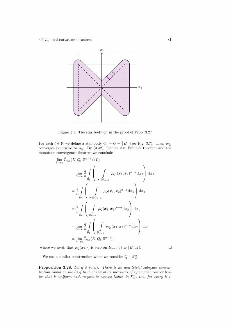
3.6 Lp dual curvature measures 81
1/l
x1
x2
Figure 3.7: The star body Ql in the proof of Prop. 3.27
For each l ∈ N we define a star body Ql = Q + 1lBn (see Fig. 3.7). Then ρQl
converges pointwise to ρQ. By (3.42), Lemma 3.6, Fubini’s theorem and themonotone convergence theorem we conclude
liml→∞
˜C0,q(K,Ql, Sn−1 ∩ L)
= liml→∞
q
n
∫Bk
⎛⎜⎝ ∫|x1|Bn−k
ρQl(x1,x2)n−q dx2
⎞⎟⎠ dx1
= q
n
∫Bk
⎛⎜⎝ ∫|x1|Bn−k
ρQ(x1,x2)n−q dx2
⎞⎟⎠ dx1
= q
n
∫Bk
⎛⎜⎝ ∫Bn−k
ρQ(x1,x2)n−q dx2
⎞⎟⎠ dx1
= liml→∞
q
n
∫Bk
⎛⎜⎝ ∫Bn−k
ρQl(x1,x2)n−q dx2
⎞⎟⎠ dx1
= liml→∞
˜C0,q(K,Ql, Sn−1),
where we used, that ρQ(x1, ·) is zero on Bn−k \ (|x1|Bn−k).
We use a similar construction when we consider Q ∈ Kno .
Proposition 3.28. Let q ∈ (0, n). There is no non-trivial subspace concen-tration bound on the (0, q)th dual curvature measures of symmetric convex bod-ies that is uniform with respect to convex bodies in Kn
o , i.e., for every k ∈

82 3 Dual curvature measures
{1, . . . , n − 1} and ε > 0 there exist K ∈ Kns , an Q ∈ Kn
o and a k-dimensionalsubspace L of Rn such that
˜C0,q(K,Q, Sn−1 ∩ L) > (1 − ε)˜C0,q(K,Q, Sn−1).
Proof. Let P = [−1, 1]n and L = lin{e1, . . . , ek} as above and define
Q = conv({0} ∪ F (P, e1)).
Thus Q is a convex body and for each l ∈ N we define Ql = Q + 1lBn ∈ Kn
o .In particular, ρQl
converges pointwise to ρQ. By (3.42), Lemma 3.6, Fubini’stheorem and the monotone convergence theorem we conclude
liml→∞
˜C0,q(P,Ql, Sn−1 ∩ L)
= liml→∞
q
n
k∑i=1
∫conv({0}∪F (P,ei))
ρQl(x)n−q + ρQl
(−x)n−q dx
= q
n
k∑i=1
∫conv({0}∪F (P,ei))
ρQ(x)n−q + ρQ(−x)n−q dx
= q
n
n∑i=1
∫conv({0}∪F (P,ei))
ρQ(x)n−q + ρQ(−x)n−q dx
= liml→∞
q
n
n∑i=1
∫conv({0}∪F (P,ei))
ρQl(x)n−q + ρQl
(−x)n−q dx
= liml→∞
˜C0,q(K,Ql, Sn−1).
The foregoing propositions suggest that if, for fixed q ∈ R and Q ∈ Sno , thereare any non-trivial subspace concentration bounds on ˜C0,q(K,Q, ·), they dependon Q.
As a final remark we want to discuss if and how Theorem 3.5 may be extendedto the (0, q)th dual curvature measure with respect to Q ∈ Kn
s . The mainingredient in our proof was Theorem 3.8. In this setting we would need toprove (3.15) with
∥·∥αQ = ρQ(·)−α
in place of |·|α. Note that for symmetric star bodies Q the function
∥x∥Q ={ρQ(x)−1, if x = 0,0, if x = 0,
defines a quasinorm on Rn, which is a norm if and only if Q is convex. In viewof Karamata’s inequality, which implies the 0-dimensional version of (3.15), onecould even consider φ(∥·∥Q) for a convex non-decreasing function φ : R≥0 → R≥0instead of |·|α. The major obstruction for generalizing our method is a missingvariant of Lemma 3.12 for arbitrary norms. Unfortunately, this is only possiblein some cases.
3.6 Lp dual curvature measures 83
Lemma 3.29 ([53, Lem. 6.4]). Let Q ∈ Sno be an origin-symmetric star bodyand α > 0. There exists a finite Borel measure µ on Sn−1 with
∥x∥αQ =∫
Sn−1
|⟨θ,x⟩|α dµ(θ)
for all x ∈ Rn, if and only if (Rn, ∥·∥Q) can be isometrically embedded into thespace of functions whose αth power of the absolute value is Lebesgue integrableover Rn.

84 3 Dual curvature measures

Conclusion
The present dissertation addressed Minkowski problems in Brunn-Minkowski,Lp-Brunn-Minkowski and dual Brunn-Minkowski theory and related topics.
In Chapter 2 we investigated the cone-volume measure, that takes on a sig-nificant role in the study of the logarithmic Brunn-Minkowski inequality (2.4)and the logarithmic Minkowski inequality (2.7), which are conjectured to holdfor pairs of symmetric convex bodies. Known examples violating (2.7) typicallyinvolve a convex body with boundary points close to the origin. We established(2.7) in the context of centered convex bodies when one of the convex bodies isa simplex, or a parallelepiped in dimensions up to four. It was pointed out thatthe logarithmic Minkowski inequality (2.7) is connected to the problem of deter-mining uniqueness of cone-volume measures. In Section 2.4 we fully character-ized cone-volume measures of trapezoids alongside with necessary and sufficientconditions for their uniqueness. On this basis, we constructed vertex-minimalpolygons with non-unique cone-volume measure in Section 2.5 and presented afivegon found by Malikiosis confirming that the strict subspace concentrationinequality (2.34) is not sufficent for uniqueness. From the characterization ofcone-volume measures of trapezoids (Theorem 2.14) we deduced necessary andsufficient conditions in the logarithmic Minkowski problem for centered trape-zoids. We are the first to state sufficient conditions for cone-volume measuresof centered bodies that are neither symmetric nor simplices. It remains an openproblem if in any dimension the cone-volume measures of centered convex bodiesare unique and if the logarithmic Minkowski inequality holds for pairs of cen-tered convex bodies. Future studies could also target the logarithmic problemfor polygons with five or more vertices.
Chapter 3 addressed subspace concentration of dual curvature measures ofsymmetric convex bodies, which are geometric measures recently introduced byHuang, Lutwak, Yang and Zhang. They fill a blank spot in the dual Brunn-Minkowski theory and consequently have been studied thoroughly since theirdiscovery. In addition, they deserve attention since the family of dual curvaturemeasures include cone-volume measures of convex bodies. While most publishedworks on the dual Minkowski problem aim for establishing sufficient conditions,we stated and proved – in the symmetric setting – the only known non-trivialnecessary conditions. The given proofs are based on sharp estimates of inte-grals of quasiconcave and convex density functions over certain regions withina convex body. To this end, we established new Brunn-Minkowski type in-
85
86 Conclusion
equalites for the measures defined by these density functions in the Sections 3.2and 3.3 leading to subspace concentration bounds on the qth dual curvaturemeasure of an n-dimensional symmetric convex body in the parameter ranges0 < q < n and q ≥ n + 1. The remaining range n < q < n+ 1 cannot be cov-ered by our approach as was pointed out in Section 3.5. A detailed analysisof the occurring obstructions enabled us to extend the subspace concentrationbounds to (n, n + 1) for one-dimensional subspaces or when the convex bodyis a parallelepiped. From each of these results we deduced a tight subspaceconcentration inequality for qth dual curvature measures of symmetric convexbodies in the plane when q > 2. In Section 3.6 we applied our methods to themore general theory of Lp dual curvature measures to prove another subspaceconcentration inequality in this setting at least for 0 < q < n. Future studiescould aim for an extension of Theorem 3.8 to arbitrary norms which seems torequire a different approach than the Kneser-Süss proof of Theorem 3.9. Othernoteworthy research directions include establishing sufficient conditions in thedual Minkowski problem for q > n or considering, e.g., centered convex bod-ies to investigate if known results for the cone-volume measure have naturalgeneralizations.
Bibliography
[1] S. Alesker. ψ2-estimate for the Euclidean norm on a convex body inisotropic position. Geometric aspects of functional analysis (Israel, 1992–1994). Vol. 77. Oper. Theory Adv. Appl. Birkhäuser, Basel, 1995, 1–4 (cit.on p. 59).
[2] A. D. Alexandrov. Selected works. Part I. Vol. 4. Classics of Soviet Mathe-matics. Selected scientific papers, Translated from the Russian by P. S. V.Naidu, Edited and with a preface by Yu. G. Reshetnyak and S. S. Kutate-ladze. Gordon and Breach Publishers, Amsterdam, 1996, x+322 (cit. onpp. 9–13).
[3] T. W. Anderson. The integral of a symmetric unimodal function overa symmetric convex set and some probability inequalities. Proc. Amer.Math. Soc. 6 (1955): 170–176 (cit. on pp. 54, 56).
[4] S. Artstein-Avidan, A. Giannopoulos, and V. D. Milman. Asymptotic geo-metric analysis. Part I. Vol. 202. Mathematical Surveys and Monographs.American Mathematical Society, Providence, RI, 2015, xx+451 (cit. onpp. 24, 59).
[5] F. Barthe, O. Guédon, S. Mendelson, and A. Naor. A probabilistic ap-proach to the geometry of the lnp -ball. Ann. Probab. 33 (2) (2005): 480–513 (cit. on p. 12).
[6] C. Berg. Corps convexes et potentiels sphériques. Mat.-Fys. Medd. DanskeVid. Selsk. 37 (6) (1969): 64 pp. (1969) (cit. on p. 13).
[7] G. Bianchi, K. J. Böröczky, A. Colesanti, and D. Yang. The Lp-Minkowskiproblem for −n < p < 1. Adv. Math. 341 (2019): 493–535 (cit. on p. 17).
[8] B. Bollobás and I. Leader. Products of unconditional bodies. Geometricaspects of functional analysis (Israel, 1992–1994). Vol. 77. Oper. TheoryAdv. Appl. Birkhäuser, Basel, 1995, 13–24 (cit. on p. 17).
[9] C. Borell. Convex set functions in d-space. Period. Math. Hungar. 6 (2)(1975): 111–136 (cit. on p. 56).
[10] K. J. Böröczky and P. Hegedűs. The cone volume measure of antipodalpoints. Acta Math. Hungar. 146 (2) (2015): 449–465 (cit. on pp. 14, 32).
[11] K. J. Böröczky, P. Hegedűs, and G. Zhu. On the discrete logarithmicMinkowski problem. Int. Math. Res. Not. IMRN, (6) (2016): 1807–1838(cit. on pp. 14, 32).
87

88 Bibliography
[12] K. J. Böröczky and M. Henk. Cone-volume measure and stability. Adv.Math. 306 (2017): 24–50 (cit. on pp. 12, 14).
[13] K. J. Böröczky and M. Henk. Cone-volume measure of general centeredconvex bodies. Adv. Math. 286 (2016): 703–721 (cit. on pp. 13, 41).
[14] K. J. Böröczky, M. Henk, and H. Pollehn. Subspace concentration of dualcurvature measures of symmetric convex bodies. J. Differential Geom. 109(3) (2018): 411–429 (cit. on pp. 4, 51, 52, 55, 66, 72, 79).
[15] K. J. Böröczky and H. T. Trinh. The planar Lp-Minkowski problem for0 < p < 1. Adv. in Appl. Math. 87 (2017): 58–81 (cit. on p. 17).
[16] K. J. Böröczky, E. Lutwak, D. Yang, and G. Zhang. Affine images ofisotropic measures. J. Differential Geom. 99 (3) (2015): 407–442 (cit. onp. 12).
[17] K. J. Böröczky, E. Lutwak, D. Yang, G. Zhang, and Y. Zhao. The dualMinkowski problem for symmetric convex bodies (2017). eprint: https://arxiv.org/abs/1703.06259 (cit. on pp. 4, 51).
[18] K. J. Böröczky, E. Lutwak, D. Yang, and G. Zhang. The log-Brunn-Minkowski inequality. Adv. Math. 231 (3-4) (2012): 1974–1997 (cit. onpp. 3, 13, 17, 18, 32).
[19] K. J. Böröczky, E. Lutwak, D. Yang, and G. Zhang. The logarithmicMinkowski problem. J. Amer. Math. Soc. 26 (3) (2013): 831–852 (cit. onpp. 2, 13, 32, 40).
[20] K. J. Böröczky and F. Fodor. The Lp dual Minkowski problem for p > 1and q > 0. 2018. eprint: https://arxiv.org/abs/1802.00933 (cit. onp. 79).
[21] S. Chen, Q.-R. Li, and G. Zhu. On the Lp Monge-Ampère equation. J.Differential Equations, 263 (8) (2017): 4997–5011 (cit. on p. 17).
[22] S. Chen, Q.-R. Li, and G. Zhu. The logarithmic Minkowski problem fornon-symmetric measures. Trans. Amer. Math. Soc. (2018). eprint: https://doi.org/10.1090/tran/7499 (cit. on pp. 14, 19, 40, 41).
[23] W. Chen. Lp Minkowski problem with not necessarily positive data. Adv.Math. 201 (1) (2006): 77–89 (cit. on p. 17).
[24] K.-S. Chou and X.-J. Wang. The Lp-Minkowski problem and the Minkowskiproblem in centroaffine geometry. Adv. Math. 205 (1) (2006): 33–83 (cit.on p. 17).
[25] D. Cordero-Erausquin, M. Fradelizi, and B. Maurey. The (B) conjecturefor the Gaussian measure of dilates of symmetric convex sets and relatedproblems. J. Funct. Anal. 214 (2) (2004): 410–427 (cit. on p. 17).
[26] S. Dancs and B. Uhrin. On a class of integral inequalities and theirmeasure-theoretic consequences. J. Math. Anal. Appl. 74 (2) (1980): 388–400 (cit. on p. 56).
[27] H. Federer. Curvature measures. Trans. Amer. Math. Soc. 93 (1959): 418–491 (cit. on p. 11).
[28] W. Fenchel and B. Jessen. Mengenfunktionen und konvexe Körper. Matematisk-fysiske meddelelser. Levin & Munksgaard, 1938, 31 (cit. on pp. 10, 12).
Bibliography 89
[29] W. J. Firey. Christoffel’s problem for general convex bodies. Mathematika,15 (1968): 7–21 (cit. on p. 13).
[30] W. J. Firey. p-means of convex bodies. Math. Scand. 10 (1962): 17–24(cit. on pp. 1, 16).
[31] R. J. Gardner. A positive answer to the Busemann-Petty problem in threedimensions. Ann. of Math. (2), 140 (2) (1994): 435–447 (cit. on p. 48).
[32] R. J. Gardner. Geometric tomography. Second. Vol. 58. Encyclopedia ofMathematics and its Applications. Cambridge University Press, Cam-bridge, 2006, xxii+492 (cit. on pp. 5, 49).
[33] R. J. Gardner. The Brunn-Minkowski inequality. Bull. Amer. Math. Soc.(N.S.) 39 (3) (2002): 355–405 (cit. on p. 56).
[34] R. J. Gardner, D. Hug, and W. Weil. The Orlicz-Brunn-Minkowski theory:a general framework, additions, and inequalities. J. Differential Geom. 97(3) (2014): 427–476 (cit. on p. 12).
[35] R. J. Gardner, A. Koldobsky, and T. Schlumprecht. An analytic solutionto the Busemann-Petty problem on sections of convex bodies. Ann. ofMath. (2), 149 (2) (1999): 691–703 (cit. on p. 48).
[36] P. M. Gruber. Convex and discrete geometry. Vol. 336. Grundlehren derMathematischen Wissenschaften [Fundamental Principles of Mathemati-cal Sciences]. Springer, Berlin, 2007, xiv+578 (cit. on p. 5).
[37] B. Grünbaum. Partitions of mass-distributions and of convex bodies byhyperplanes. Pacific J. Math. 10 (1960): 1257–1261 (cit. on p. 20).
[38] P. Guan and L. Ni. Entropy and a convergence theorem for Gauss curva-ture flow in high dimension. J. Eur. Math. Soc. (JEMS), 19 (12) (2017):3735–3761 (cit. on p. 18).
[39] C. Haberl and L. Parapatits. The centro-affine Hadwiger theorem. J.Amer. Math. Soc. 27 (3) (2014): 685–705 (cit. on p. 12).
[40] B. He, G. Leng, and K. Li. Projection problems for symmetric polytopes.Adv. Math. 207 (1) (2006): 73–90 (cit. on p. 12).
[41] M. Henk and E. Linke. Cone-volume measures of polytopes. Adv. Math.253 (2014): 50–62 (cit. on p. 13).
[42] M. Henk and H. Pollehn. Necessary subspace concentration conditions forthe even dual Minkowski problem. Adv. Math. 323 (2018): 114–141 (cit. onpp. 4, 52, 57–59, 65, 70, 76).
[43] M. Henk and H. Pollehn. On the log-Minkowski inequality for simplicesand parallelepipeds. Acta Math. Hungar. 155 (1) (2018): 141–157 (cit. onpp. 3, 19, 20, 23–25).
[44] M. Henk, A. Schürmann, and J. M. Wills. Ehrhart polynomials and suc-cessive minima. Mathematika, 52 (1-2) (2005): 1–16 (2006) (cit. on pp. 12,52, 53).
[45] J. Hu and G. Xiong. The logarithmic John ellipsoid. Geom. Dedicata(2018) (cit. on p. 12).
[46] Y. Huang and Q. Lu. On the regularity of the Lp Minkowski problem.Adv. in Appl. Math. 50 (2) (2013): 268–280 (cit. on p. 17).
90 Bibliography
[47] Y. Huang and Y. Zhao. On the Lp dual Minkowski problem. Adv. Math.332 (2018): 57–84 (cit. on p. 79).
[48] Y. Huang, E. Lutwak, D. Yang, and G. Zhang. Geometric measures in thedual Brunn-Minkowski theory and their associated Minkowski problems.Acta Math. 216 (2) (2016): 325–388 (cit. on pp. 1, 4, 11, 13, 49–51).
[49] D. Hug, E. Lutwak, D. Yang, and G. Zhang. On the Lp Minkowski problemfor polytopes. Discrete Comput. Geom. 33 (4) (2005): 699–715 (cit. onp. 17).
[50] H. Jian, J. Lu, and X.-J. Wang. Nonuniqueness of solutions to the Lp-Minkowski problem. Adv. Math. 281 (2015): 845–856 (cit. on p. 17).
[51] Z. Kadelburg, D. Ðukić, M. Lukić, and I. Matić. Inequalities of Karamata,Schur and Muirhead, and some applications. The Teaching of Mathemat-ics, 8 (1) (2005): 31–45 (cit. on p. 57).
[52] H. Kneser and W. Süss. Die Volumina in linearen Scharen konvexer Kör-per. Mat. Tidsskr. B (1932): 19–25 (cit. on p. 59).
[53] A. Koldobsky. Fourier analysis in convex geometry. Vol. 116. Mathemat-ical Surveys and Monographs. American Mathematical Society, Provi-dence, RI, 2005, vi+170 (cit. on pp. 49, 83).
[54] A. Kolesnikov and E. Milman. Local Lp-Brunn-Minkowski inequalities forp < 1. 2018. eprint: https://arxiv.org/abs/1711.01089 (cit. on p. 16).
[55] J. Lu and X.-J. Wang. Rotationally symmetric solutions to the Lp-Minkowskiproblem. J. Differential Equations, 254 (3) (2013): 983–1005 (cit. on p. 17).
[56] M. Ludwig. General affine surface areas. Adv. Math. 224 (6) (2010): 2346–2360 (cit. on p. 12).
[57] M. Ludwig and M. Reitzner. A classification of SL(n) invariant valuations.Ann. of Math. (2), 172 (2) (2010): 1219–1267 (cit. on p. 12).
[58] E. Lutwak. Dual mixed volumes. Pacific J. Math. 58 (2) (1975): 531–538(cit. on pp. 1, 48).
[59] E. Lutwak. Intersection bodies and dual mixed volumes. Adv. in Math. 71(2) (1988): 232–261 (cit. on p. 48).
[60] E. Lutwak. Mean dual and harmonic cross-sectional measures. Ann. Mat.Pura Appl. (4), 119 (1979): 139–148 (cit. on p. 48).
[61] E. Lutwak. The Brunn-Minkowski-Firey theory. I. Mixed volumes and theMinkowski problem. J. Differential Geom. 38 (1) (1993): 131–150 (cit. onpp. 1, 16–18).
[62] E. Lutwak. The Brunn-Minkowski-Firey theory. II. Affine and geominimalsurface areas. Adv. Math. 118 (2) (1996): 244–294 (cit. on p. 1).
[63] E. Lutwak and V. Oliker. On the regularity of solutions to a generalizationof the Minkowski problem. J. Differential Geom. 41 (1) (1995): 227–246(cit. on p. 17).
[64] E. Lutwak, D. Yang, and G. Zhang. Lp dual curvature measures. Adv.Math. 329 (2018): 85–132 (cit. on pp. 52, 78, 79).
[65] E. Lutwak, D. Yang, and G. Zhang. Lp John ellipsoids. Proc. LondonMath. Soc. (3), 90 (2) (2005): 497–520 (cit. on p. 12).
Bibliography 91
[66] E. Lutwak, D. Yang, and G. Zhang. Orlicz centroid bodies. J. DifferentialGeom. 84 (2) (2010): 365–387 (cit. on p. 12).
[67] E. Lutwak, D. Yang, and G. Zhang. Orlicz projection bodies. Adv. Math.223 (1) (2010): 220–242 (cit. on p. 12).
[68] L. Ma. A new proof of the log-Brunn-Minkowski inequality. Geom. Dedi-cata, 177 (2015): 75–82 (cit. on p. 18).
[69] V. D. Milman and A. Pajor. Entropy and asymptotic geometry of non-symmetric convex bodies. Adv. Math. 152 (2) (2000): 314–335 (cit. onp. 24).
[70] A. Naor. The surface measure and cone measure on the sphere of lnp . Trans.Amer. Math. Soc. 359 (3) (2007): 1045–1079 (electronic) (cit. on p. 12).
[71] A. Naor and D. Romik. Projecting the surface measure of the sphere oflnp . Ann. Inst. H. Poincaré Probab. Statist. 39 (2) (2003): 241–261 (cit. onp. 12).
[72] G. Paouris. Ψ2-estimates for linear functionals on zonoids. Geometric as-pects of functional analysis. Vol. 1807. Lecture Notes in Math. Springer,Berlin, 2003, 211–222 (cit. on p. 59).
[73] G. Paouris and E. M. Werner. Relative entropy of cone measures and Lpcentroid bodies. Proc. Lond. Math. Soc. (3), 104 (2) (2012): 253–286 (cit.on p. 12).
[74] C. Saroglou. Remarks on the conjectured log-Brunn-Minkowski inequality.Geom. Dedicata, 177 (2015): 353–365 (cit. on pp. 3, 17, 18).
[75] R. Schneider. Convex bodies: the Brunn-Minkowski theory. expanded. Vol. 151.Encyclopedia of Mathematics and its Applications. Cambridge UniversityPress, Cambridge, 2014, xxii+736 (cit. on pp. 5, 7–11, 13, 17, 49, 50, 59).
[76] A. Stancu. Centro-affine invariants for smooth convex bodies. Int. Math.Res. Not. IMRN, (10) (2012): 2289–2320 (cit. on p. 12).
[77] A. Stancu. On the number of solutions to the discrete two-dimensionalL0-Minkowski problem. Adv. Math. 180 (1) (2003): 290–323 (cit. on pp. 3,13).
[78] A. Stancu. The discrete planar L0-Minkowski problem. Adv. Math. 167(1) (2002): 160–174 (cit. on pp. 13, 19, 32).
[79] A. Stancu. The logarithmic Minkowski inequality for non-symmetric con-vex bodies. Adv. in Appl. Math. 73 (2016): 43–58 (cit. on p. 18).
[80] D. Xi and G. Leng. Dar’s conjecture and the log-Brunn-Minkowski in-equality. J. Differential Geom. 103 (1) (2016): 145–189 (cit. on p. 18).
[81] G. Zhang. A positive solution to the Busemann-Petty problem in R4. Ann.of Math. (2), 149 (2) (1999): 535–543 (cit. on p. 48).
[82] Y. Zhao. Existence of solutions to the even dual Minkowski problem. J.Differential Geom. 110 (3) (2018): 543–572 (cit. on pp. 51, 72).
[83] Y. Zhao. The dual Minkowski problem for negative indices. Calc. Var.Partial Differential Equations, 56 (2) (2017): Art. 18, 16 (cit. on p. 52).
[84] G. Zhu. Continuity of the solution to the Lp Minkowski problem. Proc.Amer. Math. Soc. 145 (1) (2017): 379–386 (cit. on p. 17).

92 Bibliography
[85] G. Zhu. The centro-affine Minkowski problem for polytopes. J. DifferentialGeom. 101 (1) (2015): 159–174 (cit. on pp. 12, 17).
[86] G. Zhu. The logarithmic Minkowski problem for polytopes. Adv. Math.262 (2014): 909–931 (cit. on p. 14).
[87] G. Zhu. The Lp Minkowski problem for polytopes for 0 < p < 1. J. Funct.Anal. 269 (4) (2015): 1070–1094 (cit. on p. 17).
[88] G. Zhu. The Lp Minkowski problem for polytopes for p < 0. Indiana Univ.Math. J. 66 (4) (2017): 1333–1350 (cit. on p. 17).

Index
affine hull, 5affinely independent, 6area measure, 10
Brunn-Minkowski inequality, 7
centroid, 6cone-volume measure, 11convex
body, 6hull, 5set, 6
curvature measure, 11
dimension, 6dual
area measure, 50, 79Brunn-Minkowski inequality, 48curvature measure, 50, 79
generalized, 78Minkowski problem, 51quermassintegral, 48
facet, 8
Gauss map, 7general position, 14Grünbaum’s inequality, 19
homothetic, 7
Karamata’s inequality, 57, 82
linear hull, 5log-combination, 17logarithmic
Brunn-Minkowski inequality, 17Minkowski inequality, 18Minkowski problem, 13
Lp
Brunn-Minkowski inequality, 16dual curvature measure, 79dual Minkowski problem, 79Minkowski inequality, 18Minkowski problem, 17surface area measure, 17, 79
metric projection, 10Minkowski
addition, 6inequality, 17problem, 13
orthogonalcomplement, 5projection, 5
outer normal vector, 7
p-combination, 15p-mean, 15parallelepiped, 8, 23, 24, 78polar set, 47polygon, 8polytope, 8
outer normal vector, 8positive hull, 5
quasiconcave function, 54quasiconvex function, 54quermassintegral, 9
radialcombination, 47function, 47projection, 49
relative interior, 6reverse radial Gauss image, 50
Santálo point, 18simplex, 8, 20
93
94 Index
smooth, 7star body, 48, 80subspace concentration condition, 13support, 32support function, 7surface area measure, 9
unconditional convex body, 6, 17
vertex, 8
Wulff shape, 9logarithmic, 49
List of Symbols
[x,y] convex hull/segment between x and y
#X number of elements of a finite set X
·|L orthogonal projection onto L
|·| (Euclidean) norm
x normalization x|x|
⟨·, ·⟩ standard inner product
(1 − λ)K +p λM p-combination of the convex bodies K and M w.r.t. λ(for p = 0 called log-combination)
(1 − λ)K ˜+λM radial combination of the star bodies K and M w.r.t. λ
aff affine hull
α∗K reverse radial Gauss image of a convex body K
Bn Euclidean unit ball
c centroid
Ci(K, ·) ith curvature measure of the convex body K˜Cq(K, ·) qth dual curvature measure of the convex body K˜Cp,q(K, ·) (p, q)th dual curvature measure of the convex body K
conv convex hull
∂X boundary of the set X
∂′K boundary points of convex body K with unique outernormal vector
dim dimension
ei ith standard basis vector of Rn
G(i, n) Grassmannian of i-dimensional subspaces of Rn
H(a, α) hyperplane defined by ⟨a,x⟩ = α
95
96 List of Symbols
H+(a, α) halfspace defined by ⟨a,x⟩ ≥ α
H−(a, α) halfspace defined by ⟨a,x⟩ ≤ α
Hk normalized k-dimensional Hausdorff measure
hK support function of convex body K
intX interior points of the set X
Kn set of convex bodies in Rn
Knc set of centered convex bodies in Rn
Kno set of convex bodies in Rn containing 0 in the interior
Kns set of symmetric convex bodies in Rn
lin linear hull
L⊥ orthogonal complement of the subspace L
Mp(·, ·, λ) p-mean with weighting parameter λ
N natural numbers 1, 2, . . .
νK Gauss map of K
pK metric projection map onto a convex body K˜pK radial projection map onto a convex body K
Pn set of n-polytopes in Rn
Pnc set of centered polytopes in Rn
Pno set of polytopes in Rn containing 0 in the interior
Pns set of symmetric n-polytopes in Rn
pos positive hull
ρK radial function of convex body K
R real numbers
R>0 (R≥0) positive (nonnegative) real numbers
Rn Euclidean n-space
Rn×n real n-by-n matrices
Sn−1 (n− 1)-dimensional sphere in Euclidean n-space
Si(K, ·) ith area measure of the convex body K˜Sq(K, ·) qth dual area measure of the convex body K
SK surface area measure of the convex body K
S(p)K Lp surface area measure of the convex body K
Sno set of star bodies in Rn
supp support
List of Symbols 97
U(P ) set of unit outer normal vectors of a polytope P
VK cone-volume measure of the convex body K
volk k-dimensional volume
Wi ith quermassintegral