Aus dem Max-Planck-Institut für Kolloid- und Grenzflächenforschung

____________________________________________________________________________

Superpara- and paramagnetic polymer colloids by miniemulsion processes

Dissertation zur Erlangung des akademischen Grades

„doctor rerum naturalium“ (Dr. rer. nat.)

in der Wissenschaftdisziplin Physikalische Chemie

eingereicht an der Mathemathisch-Naturwissenschaftlichen Fakultät

der Universität Potsdam

von Liliana Patricia Ramírez Ríos

Potsdam, Februar 2004

„Jedenfalls liebt der Magnetstein das Eisen.

Wenn er es nur sieht und berührt, zieht er es zu sich, als wenn er in sich Liebesfeuer hätte“

Achileus Tatios aus Alexandrien (zit. nach A. Kross, Geschichte des Magnetismus, 1994)[1]

To Gunnar Jochen Weimann

TABLE OF CONTENTS

1 INTRODUCTION ..................................................................................................... 1

2 THEORETICAL SECTION...................................................................................... 5

2.1 Miniemulsions and miniemulsion polymerization ........................................................ 5 2.1.1 Miniemulsions................................................................................................................. 6

2.1.1.1 Preparation and homogenization of miniemulsions .............................................. 8

2.1.1.2 Miniemulsion polymerization .............................................................................. 12

2.1.1.3 Encapsulations by miniemulsion polymerization................................................ 14

2.2 Magnetism........................................................................................................................ 15 2.2.1 Magnetism in materials................................................................................................. 17

2.2.1.1 Ferromagnetism.................................................................................................... 17

2.2.1.2 Diamagnetism....................................................................................................... 17

2.2.1.3 Paramagnetism...................................................................................................... 18

2.2.1.4 Superparamagnetism ............................................................................................ 18

2.2.1.5 Antiferromagnetism.............................................................................................. 20

2.2.1.6 Ferrimagnetism..................................................................................................... 20

2.2.2 Diameter determination from the magnetization measurements................................. 21

2.3 Ferrofluids........................................................................................................................ 22 2.3.1 Ferrofluids by miniemulsion polymerization............................................................... 24

2.3.2 Applications of ferrofluids............................................................................................ 25

2.4 Nanostructured composites from iron pentacarbonyl decomposition ..................... 27

2.5 Gadolinium-based nanoparticles .................................................................................. 29

2.5.1 Lanthanide shift reagents for nuclear magnetic resonance.......................................... 31

2.5.2 Nanostructured materials .............................................................................................. 32

2.5.3 Spin-lattice relaxation time (T1) on NMR imaging application .................................. 33

3 RELEVANT METHODS ........................................................................................ 37

3.1 Transmission electron microscopy................................................................................ 37

3.2 X-ray diffraction.............................................................................................................. 39

3.3 Dynamic light scattering ................................................................................................ 40

3.4 Preparative ultracentrifugation .................................................................................... 42

ii

3.5 Magnetometry ................................................................................................................. 44

4 RESULTS AND DISCUSSION ............................................................................. 46

4.1 Water-based ferrofluids containing magnetite polystyrene nanoparticles.............. 46

4.1.1 Hydrophobic magnetite nanoparticles.......................................................................... 48

4.1.2 Aqueous magnetite aggregate dispersion..................................................................... 50

4.1.3 Encapsulation of the magnetite particles in polymer................................................... 52

4.1.4 Magnetic properties ...................................................................................................... 58

4.1.5 Using biosurfactants...................................................................................................... 60

4.2 Nanostructured composites from the iron pentacarbonyl decomposition............... 61 4.2.1 Thermal decomposition in the monomer phase ........................................................... 62

4.2.2 Nanocomposite particles after miniemulsion polymerization ..................................... 67

4.2.3 Magnetic properties ...................................................................................................... 77

4.3 Gadolinium-based nanoparticles .................................................................................. 79 4.3.1 Nanostructured composites........................................................................................... 79

4.3.2 Magnetic properties ...................................................................................................... 89

4.3.3 Relaxation measurements ............................................................................................. 90

5 CONCLUSIONS AND OUTLOOK........................................................................ 93

6 EXPERIMENTAL SECTION ................................................................................. 95

6.1 Water based-ferrofluid containing magnetite polystyrene nanoparticles ............... 95

6.2 Nanostructured composites from iron pentacarbonyl decomposition ..................... 96

6.3 Gadolinium-based nanocomposites .............................................................................. 97

7 METHODS............................................................................................................. 99

8 REFERENCES .................................................................................................... 102

iii

LIST OF FIGURES

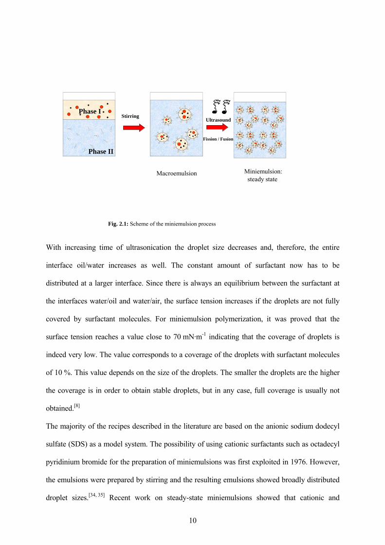
Fig. 2.1: Scheme of the miniemulsion process............................................................................. 10

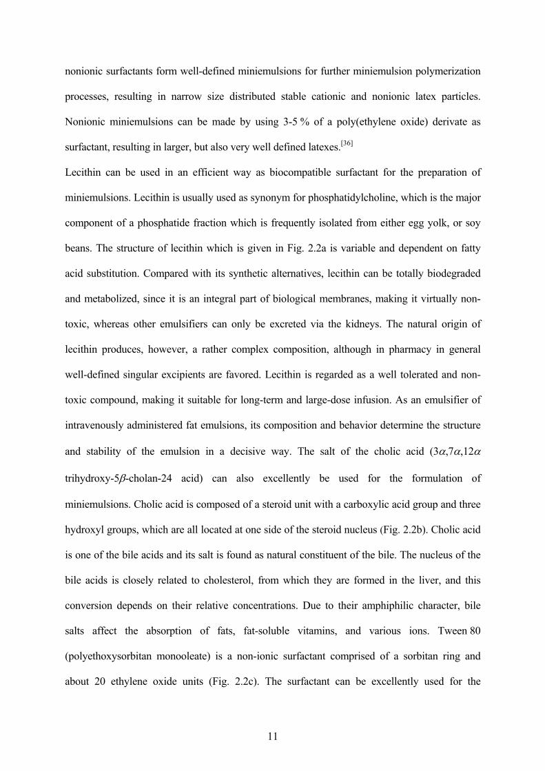
Fig. 2.2: Chemical structure of a) lecithin; R1, R2: typically linear aliphatic rests with 15 or 17 carbon atoms with up to 4 cis double bonds, b) the sodium salt of cholic acid; c) Tween 80, sum of w,x,y,z = 20 ............................................................................................................................... 12

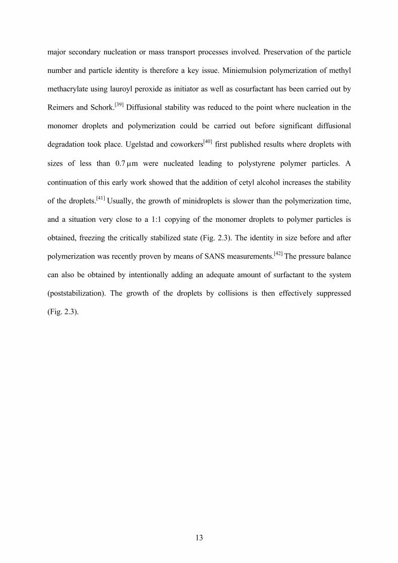
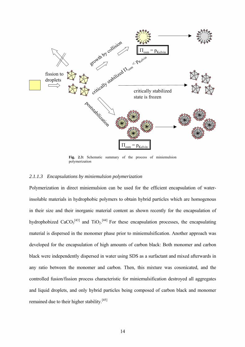
Fig. 2.3: Schematic summary of the process of miniemulsion polymerization .......................... 14

Fig. 2.4: Typical magnetization curve and hysteresis loop.......................................................... 16

Fig. 2.5: Variation of the intrinsic coercivity Hci with the particle diameter dmp ........................ 19

Fig. 2.6: Scheme of the encapsulation of magnetite into polystyrene by Hoffmann’s process.. 25

Fig. 2.7: Structure of the complex gadolinium tris(2,2,6,6-tetramethyl-3,5-heptanedionate) (Gd(tmhd)3).................................................................................................................................... 32

Fig. 2.8: Schematic representation of three types of interaction between water molecules and metal ion......................................................................................................................................... 35

Fig. 3.1: The major components of the TEM (right side) in comparison with the light microscopy (left side) (based on the ref.[[131]) ............................................................................... 38

Fig. 3.2: Scheme of the principle of the X-ray diffraction........................................................... 40

Fig. 3.3: Schematic setup of the vibrating sample magnetometer............................................... 45

Fig. 4.1: Formulation of polymer coated magnetite particles with a high magnetite ratio......... 48

Fig. 4.2: Thermogravimetric curves of magnetite particles coated with oleic acid .................... 49

Fig. 4.3: Magnetite aggregates obtained after a miniemulsion process in water ........................ 51

Fig. 4.4: Transmission electron micrograph (TEM) for magnetite polystyrene particles (Latex-1) at different magnifications. ....................................................................................................... 55

Fig. 4.5: Encapsulation of polystyrene/magnetite particles studied by ultracentrifuge experiments in a density gradient: a) samples with different magnetite aggregates and with or without acrylic acid; b) Mag-10 as magnetite aggregates were used at different magnetite contents, the latexes were prepared with acrylic acid. Note that the average density (arrows) is increasing with increasing magnetite load.................................................................................... 57

Fig. 4.6: The magnetic field dependence of magnetization a) of magnetite in octane, the magnetite aggregates in water (Mag-10) and the encapsulated magnetite particles (Latex-1); b) of different encapsulated magnetite particles (Latexes-1, -7, -8, and -9) .................................... 59

Fig. 4.7: Magnetite aggregates in water with cholic acid as surfactant....................................... 61

Fig. 4.8: FTIR spectra with air as background............................................................................. 63

Fig. 4.9: TEM pictures of the sample BMA-D2 .......................................................................... 64

Fig. 4.10: TGA measurements of the sample BMA-D4 under oxygen atmosphere................... 65

Fig. 4.11: 1H NMR in CDCl3 for a) the sample BMA-D4 and b) Butyl methacrylate ............... 65

Fig. 4.12: a) WAXS and b) SAXS measurements of sample BMA-D4 ..................................... 67

Fig. 4.13: TEM picture of sample PI3a (11.7 % SDS, 12.5 % oleic acid related to ipc) at low magnifications................................................................................................................................ 70

iv

Fig. 4.14: TEM picture of sample PI3a (11.7 % SDS, 12.5 % oleic acid related to ipc) at high magnifications................................................................................................................................ 71

Fig. 4.15: a) SAXS and b) WAXS measurements from sample PI3a (11.7 % SDS, 12.5 % of oleic acid related to ipc)................................................................................................................. 72

Fig. 4.16: TEM micrographs of sample PI3a-2hd after 2 h of thermal decomposition in the monomer BMA-D3 (11.7 % SDS, 12.5% oleic acid related to ipc)............................................ 73

Fig. 4.17: TEM pictures of the sample PI2a (11.7 % SDS, 1.2 % oleic acid related to ipc) ...... 74

Fig. 4.18: a) SAXS and b) WAXS measurements of the sample PI1a (from BMA-D1, without oleic acid)....................................................................................................................................... 75

Fig. 4.19: TEM pictures of sample PI1a....................................................................................... 76

Fig. 4.20: Ultracentrifuge experiments in a density gradient....................................................... 77

Fig. 4.21: Magnetic measurements of the samples PI1a, PI3a and PI4a..................................... 78

Fig. 4.22: TEM of the resulting nanocomposites a), b),and c) PGd-1 with 15 min preheating and d) PGd-1 without preheating)........................................................................................................ 81

Fig. 4.23: SAXS measurement of PGd-1 a) before; and b) after polymerization....................... 82

Fig. 4.24: SAXS measurements of the samples before polymerization (the abbreviation bp denotes “before polymerization”) ................................................................................................. 83

Fig. 4.25: WAXS of sample PGd-1.............................................................................................. 84

Fig. 4.26: TEM pictures of different lanthanide nanocomposites: a) Eu(thmd)3@PBA; b) Sm(thmd)3@PBA; c) Nd(thmd)3@PBA; d) Ho(thmd)3@PBA. ............................................. 86

Fig. 4.27: TEM micrographs of the LMA sample. ...................................................................... 87

Fig. 4.28: TEM micrographs of the sample PGd-Lu-1................................................................ 88

Fig. 4.29: Magnetization curve of the layered nanocomposites .................................................. 89

Fig. 4.30: Schematic representation of the quasi-inner-sphere coordination between carbonyl group of poly(butyl acrylate) and Gd nuclei. At the same time, this quasi-inner-sphere complex interacts with the water in the so-called outer-sphere mechanism............................................... 92

v

LIST OF TABLES

Table 4.1: Preparation conditions and influence of the concentration of surfactants on the water based ferrofluid particle size ......................................................................................................... 51

Table 4.2: Characteristics of the latexes consisting of the magnetite/polymer particles............ 54

Table 4.3: Magnetic properties of the ferrofluids. ....................................................................... 60

Table 4.4: Dispersion of iron in monomer using oleic acid as surfactant................................... 62

Table 4.5: Miniemulsion polymerization latexes based on 0.5 g monomer containing iron nanoparticles. ................................................................................................................................. 68

Table 4.6: Magnetic properties of the iron containing nanocomposites .................................... 78

Table 4.7: Characteristics of the prepared samples in miniemulsion after polymerization. ...... 80

Table 4.8: Magnetic properties of the layered nanocomposites.................................................. 90

Table 4.9: T1 relaxation time of the water protons of the sample PGd-1 at different dilutions . 91

ABBREVIATIONS AND SYMBOLS

SDS Sodium Dodecyl Sulfate

PEO-PMAA Poly(ethylene oxide)-b-poly(methacrylic acid)

HEMA 2-hydroxyethylmethacrylate

MAA Methacrylic acid

DTPA Diethylenetriamine penta-acetic acid

Gd-DTPA Gadolinium-(diethylenetriamine penta-acetic acid)

Gd-DOTA Gadolinium-(1,4,7,10-tetraazacyclododecan N, N’, N”, N’”-tetraacetic acid)

PEO-PMAA Poly(ethylene oxide)-b-poly(methacrylic acid)

KPS Potassium peroxodisulfate

tmhd 2,2,6,6, tetramethyl-3,5-heptandionate

DTA Differential thermal analysis

TGA Thermogravimetric analysis

DSC Differential scanning calorimetry

TEM Transmission electron microscopy

WAXS Wide angle X-ray

SAXS Small angle X-ray

FTIR Fourier transform infrared spectroscopy

IPC Iron pentacarbonyl

BA Butyl acrylate

PBA Poly(butyl acrylate)

AA Acryl acid

LMA Lauryl methacrylate

G∆ Free Gibbs energy difference

vi

γ Surface/interfacial tension

A∆ Newly formed interface

i Current

loopr Loop radius

M Magnetization

v Volume of the material

µ Magnetic dipole moment

µtotal Net magnetic dipole moment

B Magnetic induction

mC Magnetization constant

Bext Strength of the external magnetic field

0µ Permeability of the free space, 4π 10-7 T·m·A-1

H Magnetic field strength

χ Mass magnetic susceptibility of the material

Ms Saturation magnetization

Mr Remanence

Hci Intrinsic coercivity

T Temperature (K)

mpd Diameter of the magnetic particle

sd A critical diameter below which the particles become single domains

pd A diameter below which the particles are superparamagnetic

ms Saturation magnetization of the bulk material per volume

V Volume of a spherical particle

k Boltzmann constant

vii

0→Hχ Initial mass magnetic susceptibility in emu·Oe-1

∞→Hσ Specific saturation magnetization (σ, values extrapolated to H→∞) in emu·g-1 latex

T1 Spin-lattice relaxation time or longitudinal relaxation time

γ Proton gyromagnetic ratio

S Electron spin quantum number

g Electronic g factor

β Bohr magneton

Iω Larmor frequencies for nuclear

Sω Larmor frequencies for electron spins

inr Ion-nucleus distance

A/h Electron-nuclear hyperfine coupling constant

cτ Correlation times for dipolar

eτ Correlation times for scalar interactions

[M] Concentration of the paramagnetic species

R1 Relaxivity in M-1·s-1 or mM-1·s-1

MP Mole fraction of metal ion

wq Number of water molecules bound per metal ion

M1T Relaxation time of the bound water protons

Mτ Residence lifetime of the bound water

C Numerical constant

SN Number of metal ions per cubic centimeter

ad Distance of closest approach of the solvent molecule to the metal complex

h Dirac constant

viii

Dτ Relative translational diffusion

ID Diffusional coefficients of water

SD Diffusional coefficients of the metal complex

ρ Resolution for TEM

λ Wavelength

α Angle of the incoming beam in TEM

h Planck constant

em Mass of an electron

ev Electron velocity

d Separation between the planes for X-ray diffraction

θ Angle of incidence

n Order of the reflection (n= 1, 2,…) for X-ray diffraction

Turns of the coil for magnetometry

I Scattering intensity

S Inverse of the separation between the planes for X-ray diffraction ( ) 1S −= d

'tI Number of photons arriving at the detector at the time interval t’

t Delay time for X-ray diffraction

Γ Cumulant

D Diffusion coefficient

q Norm of the scattering vector

0n Refraction index for a pure solvent

b An instrumental constant

η Viscosity of the solvent

zD z-average diffusion coefficient

ix

im Total mass of the of the i particles

iM Molecular weight of the i particles

G Centrifugal force

bF Buoyant force

fF Frictional force

ω Angular velocity, rad·s-1

r Centrifugal radius, cm

pm Mass of the particle

_v

Partial specific volume of the particle

sρ Density of solvent

AN Avogadro’s number

f Frictional coefficient of a single particle

a Radius of the spherical particles

dtdr

Velocity of the particles

Θr Radial coordinate of the isopycnic point of the zone which corresponds to the maximal concentration ( )Θ,rc of the particles

rc Concentration at radius r

R Gas constant

Emf Electro-motive force

cn Turn in a coil

φ Magnetic flux through the loop

x

1

1 Introduction

Magnetisches Pulver hat die Fähigkeit,

„dicken Schleim abzuführen, wenn es mit Honig gemischt verabreicht wird“.

Psellus von Anazerba (zit. nach A. Kross, Geschichte des Magnetismus, 1994)[1]

Magnetism has always been conceived as something mysterious and mystic. During the process

of understanding of this phenomenon an extensive range of medical and technical applications

have emerged. Until today, magnetism continues to be in the focus of research predominantly as

regards finding new and powerful applications.

Magnetite is the oldest and most common iron oxide compound in the earth. Its natural form

was called lodestone by the ancients. Natural research has revealed that a large number of

species, from bacteria to humans, can produce magnetite. In the case of magnetotactic

bacteria,[2] the magnetite allows the bacteria to find their way downwards into areas of poor

oxygen conditions –their habitat medium- by the orientation they gain from the magnetic field

of the earth. Magnetite has also been found in animals that navigate by compass direction, such

as bees,[3] birds,[4] and fishes.[5] A very controversial paper was published by Kirschvink[6]

demonstrating the existence of magnetite crystals in the human brain. This raises the question as

to the usefulness of magnetite even in the human body. Research has not yet found an answer to

this question, but what this finding clearly demonstrates is that magnetism is an essential

phenomenon of the life that surrounds us and that, at present, the range of its potential

applications is only becoming apparent from a distance.

On the other hand, there is no doubt that nanotechnology has gained great relevance in the last

two decades due to the great variety of real and feasible applications in multidisciplinary fields

such as chemistry, physics, medicine, engineering, biology, pharmacy, among others.

2

Nanotechnology is making great steps forward in the improvement of existing materials and the

creation of innovative materials in the colloidal range based on both inorganic and polymeric

materials as well as nanocomposites consisting of a mixture of both of them.

According to the IUPAC,[7] the term colloid refers to a state of subdivision, implying that the

molecules or polymolecular particles dispersed in a medium have at least in one direction a

dimension roughly between 1 nm and 1 µm. In nature and daily life, it exists a great variety of

colloidal systems, such as fog, mist, smoke, aerosols, milk, mayonnaise, creams, soaps, blood,

bones, etc., to enumerate just some typical examples. Colloids can be produced by different

techniques. One of the best positioned techniques is the miniemulsion process. Miniemulsions

are described as stable emulsions of oil or water droplets having a size between 50-500 nm

prepared by shearing a system containing oil, water, a surfactant, and a highly water insoluble

compound, the so-called hydrophobe which suppresses Ostwald ripening of the droplets.[8, 9]

The fusion/fission process and the low amount of surfactant used during the miniemulsion

process turn the miniemulsion into a very suitable technique for the encapsulation process and

the generation of novel colloids having amazing properties.

Combining the magnetic properties of a given material with the tremendous advantages of

colloids can exponentially increase the advantages of both systems. This thesis deals with the

field of magnetic nanotechnology, thus it is that, the design and characterization of new

magnetic colloids with fascinating properties compared with the bulk materials is presented.

Ferrofluids are referred to either as water or organic stable dispersions of superparamagnetic

nanoparticles which respond to the application of an external magnetic field but lose their

magnetization in the absence of a magnetic field. This kind of magnetism is called

superparamagnetism or paramagnetism depending on several parameters such as particle size,

electronic configuration, chemical composition, among others. In section 4.1, a three-step

synthesis for the fabrication of a novel water-based ferrofluid is presented. The encapsulation of

high amounts of magnetite into polystyrene particles can efficiently be achieved by a new

3

process including two miniemulsion processes. The ferrofluids consist of novel magnetite

polystyrene nanoparticles dispersed in water which are obtained by three-step process including

coprecipitation of magnetite, its hydrophobization and further surfactant coating to enable the

redispersion in water and the posterior encapsulation into polystyrene by miniemulsion

polymerization.

The formulation and application of polymer particles and hybrid particles composed of

polymeric and magnetic material is of high interest for biomedical applications. Ferrofluids can

for instance be used in medicine for cancer therapy and magnetic resonance imaging.[10, 11] For

such applications, it is necessary that the materials or especially the surface of the particles are

biocompatible, non-toxic and sometimes also biodegradable. It is a desire to take advantage of a

potential thermodynamic control for the design of nanoparticles, and the concept of

“nanoreactors”[12] where the essential ingredients for the formation of the nanoparticles are

already in the beginning. It is the topic of this section to describe a recent development where

the availability of high shear devices such as ultrasound decrease the droplet or nanoreactor

diameter down to 30-100 nm and allows to formulate magnetite hybrid particles for biomedical

applications. Superparamagnetic or paramagnetic colloids containing iron or gadolinium are

also being used as magnetic resonance imaging contrast agent, for example as a important tool

in the diagnostic of cancer, since they enhance the relaxation of the water of the neighbouring

zones. New nanostructured composites by the thermal decomposition of iron pentacarbonyl in

the monomer phase and thereafter the formation of paramagnetic nanocomposites by

miniemulsion polymerization is discussed in section 4.2. In order to obtain the confined

paramagnetic nanocomposites a two-step process was used. In the first step, the thermal

decomposition of the iron pentacarbonyl was obtained in the monomer phase using oleic acid as

stabilizer. In the second step this iron containing monomer dispersion was used for making a

miniemulsion polymerization thereof.

4

The addition of lanthanide complexes to ester-containing monomers such as butyl acrylate and

subsequent polymerization leading to the spontaneous formation of highly organized layered

nanocomposites, is presented in section 4.3. By an one-step miniemulsion process, the

formation of lamellar structure within the polymer nanoparticles is developed. The

magnetization and the NMR relaxation measurements have shown these new layered

nanocomposites to be very apt for application as contrast agent in magnetic resonance imaging.

5

2 Theoretical Section

2.1 Miniemulsions and miniemulsion polymerization

Emulsions are metastable heterogeneous system of two immiscible liquids, in which small

droplets of one fluid (disperse phase) are dispersed in the other fluid (continuous phase) by

means of shaking, mechanical agitation or ultrasound. Depending on which compound is

forming the continuous phase, the emulsions can be classified as direct, oil in water (O/W), and

inverse, water in oil (W/O).

The emulsions are divided in macroemulsions, miniemulsions or microemulsions, depending on

the droplet size and the stabilization mechanism. The droplet size goes usually from about

100 nm to several µm for macroemulsions, between 50 and 500 nm for miniemulsions and

between 1 and 100 nm for microemulsions, approximately.

An emulsion tends to break over time because the system tries to be in the state of minimum

energy, to go back to his original state, it means, lower surface and interface tension and larger

volume. The principal, instabilization mechanisms are the coalescence and the Ostwald

ripening. Coalescence is the process of aggregation of two droplets to form one larger droplet

through collision, while Ostwald ripening is the process whereby large droplets grow at the

expense of smaller ones due to the transport of dispersed phase molecules from the smaller to

the larger droplets through the continuous phase.

The classification by size is more or less ambiguous and thus it is that they are also classified

depending on the stability mechanisms, amount of surfactant, etc. The predominant difference

between emulsions lies in their respective stability. Macroemulsions are kinetic stable,

microemulsions are thermodynamic stable and miniemulsions are stable against molecular

diffusion (Ostwald ripening) and against coalescence (for more details, see next section).

6

2.1.1 Miniemulsions

Miniemulsions[13] are emulsions wherein the droplets are stabilized against molecular diffusion

degradation (Ostwald ripening, a unimolecular process or τ1 mechanism) and against

coalescence by collisions (a bimolecular process or τ2 mechanism).

Stabilization against coalescence can be obtained in colloidal chemistry by means of the

addition of suitable surfactants which can act as steric, electrostatic, or electrosteric stabilizer

agents.

When an emulsion is prepared, a distribution of the droplet size is obtained. Even when the

surfactant provides the droplets with sufficient colloidal stability, the outcome of this size

distribution is determined by their droplet or Laplace pressures, which increase with decreasing

droplet size, resulting in a net mass flux by diffusion between the droplets. If the droplets are

not stabilized against diffusional degradation, small ones will disappear increasing the average

droplet size (Ostwald ripening).[8]

The addition of a small amount of a third component that is almost completely insoluble in the

continuous phase and is trapped within the droplets can stop the Ostwald ripening in the system.

The pioneer in the concept that unstable droplets of aerosols or fog can be stabilized by the

presence of a non-volatile third component was Köhler in 1922.[14] Higuschi and Misra [15] were

the first to report the use of small amounts of a component insoluble in the disperse medium but

distributed in the disperse in order to stop the Ostwald ripening.

This stabilization effect was described theoretically by Webster and Cates.[16] They considered

an emulsion whose droplets contain a trapped species (insoluble in the continuous phase) and

studied the emulsion's stability via the Lifshitz-Slyozov model[17] (based on Ostwald ripening).

Webster and Cates extended the work of Kabalnov and coworkers[18] and derived general

conditions regarding the mean initial droplet volume, which ensures stability in both size and

composition of the initial droplets, even when arbitrary polydispersity is present. They

7

distinguished nucleated coarsening, which requires either fluctuations in the mean-field

equations or a tail in the initial droplet size distribution, from spinodal coarsening in which a

typical droplet is locally unstable. A weaker condition for stability, previously suggested by

Kabalnov and coworkers, is sufficient only to prevent spinodal coarsening and is best viewed as

a condition for meta-stability. The coarsening of unstable emulsions after long times is

considered and shown to resemble that of ordinary emulsions with no trapped species, but with

a reduced value of the initial volume fraction of the dispersed phase. The evolution of the

emulsion is driven by the competition between the osmotic pressure of the trapped species and

the Laplace pressure of the droplets.

The rate of Ostwald ripening depends on the droplet size, polydispersity and solubility of the

dispersed phase in the continuous phase. This means that an already hydrophobic oil dispersed

in small droplets of low polydispersity shows low diffusion. But by adding an

“ultrahydrophobe”, the stability can even be increased by additionally building up an osmotic

pressure. It was used a small amount of perfluorodimorphinopropane to blood substitutes to

hinder the molecular diffusion, and therefore increase the stability.[19, 20]

Davis and coworkers[21] investigated the effect of various added third components such as

hexadecane and perfluorocarbon oil, in the stabilization against Ostwald ripening of hexane

emulsions stabilized by sodium dodecyl sulfate. Small droplets have higher solubilities (or

vapor pressures) than larger droplets or the bulk material and therefore smaller droplets tend to

diffuse in the medium, from the small droplets to the large droplets in order to reach a state of

equilibrium. Because of this mass transport, the difference of the solubility (vapor pressure)

between the small and the large droplets will increase and Ostwald ripening will be enhanced.

When small quantities of a third component, which has lower vapor pressure (solubility) than

the disperse phase, are present in the disperse phase, the loss of the oil within the small droplet

will cause an increment in the mole fraction of the third component in these small droplets and

therefore the small droplets will have now a more reduced pressure vapor than the larger

droplets. It is by this means that the increase of the Laplace pressure (size difference) will be

balanced by the decrease in the osmotic pressure (concentration difference). As a result, the

mean droplet size of the emulsion will change slightly before stability of Ostwald ripening is

reached. David and coworkers explained that with the addition of a small quantity of an

insoluble oil to the disperse phase in an O/W emulsion, stabilized by sodium dodecyl sulfate,

the Ostwald ripening is prevented.

The ripening inhibitors are called “ultrahydrophobe” or “hydrophobe” in O/W miniemulsions

and “lipophobe” and in W/O miniemulsions.

2.1.1.1 Preparation and homogenization of miniemulsions

Homogenization of the emulsions to obtain miniemulsions can be achieved by different

methods. In the first articles published, simple stirring was used. The use of an omnimixer and

ultra-turrax was also described in early articles. However, the shear obtained by these

techniques is not sufficient in order to obtain small and homogeneously distributed droplets.[22]

A much higher energy, with respect of the thermodynamic part ( AG ∆=∆ γ with - free

Gibbs energy difference, γ - surface/interfacial tension and

G∆

A∆ - the newly formed interface) is

required, since the comminution of large droplets into smaller ones involves additional forces,

so that the viscous resistance during agitation absorbs most of the energy.[23, 24] The excess

energy is dissipated as heat. Nowadays, ultrasonication is used especially for the

homogenzation of small quantities, whereas the microfluidizer or high pressure homogenizers

are necessary for the emulsification of larger quantities.

Power ultrasound is one means among others for mechanically producing emulsions.

Ultrasound emulsification was first reported in 1927.[25] There are several possible mechanisms

of droplet formation and disruption under the influence of ultrasound. [26-28]

Acoustic cavitation in liquids is a phenomenon of the formation of cavities or gas/vapor bubbles

cause by the rupture of the liquid by high intensity acoustic fields. The bubble collapse implies

8

9

drastic temperature and pressure conditions inside the bubbles. These “hot spots” have

temperatures of about 5000 °K, and pressures of about 1000 atm and heating and cooling rates

above 1010 K·s-1.[29] Parameters having a positive influence on cavitation in liquids, generally

speaking, improve emulsification in terms of a smaller droplet size of the dispersed phase right

after disruption. Imploding cavitation bubbles cause intensive shock waves in the surrounding

liquid and the formation of liquid jets of high liquid velocity.[30] This may cause droplet

disruption in the vicinity of the collapsing bubble. However, the exact process of droplet

disruption due to ultrasound as a result of cavitation is not yet fully understood. At constant

energy density during homogenization, droplet size decreases when adding stabilizers, whereas

the viscosity of the oil in w/o emulsions has no effect.[31] In monomeric miniemulsions, the

droplet size is in turn determined by monomer and water density, monomer solubility, level of

surfactant, level of hydrophobe, and volume fraction of the phases. It is found for monomeric

miniemulsions that the droplet size initially is a function of the amount of shear.[32] Monomer

droplets also change quite rapidly in size during sonication in order to approach a pseudo-steady

state. However, once this state is reached, the size of the monomer droplet no longer appears to

be a function of the amount of shear, assuming a required minimum is used. In the beginning of

homogenization, the polydispersity of the droplets is still quite high, but by constant fusion and

fission processes, polydispersity decreases. The miniemulsion then reaches a steady state (see

Fig. 2.1).[33]

Macroemulsion

Ultrasound

Phase II

Phase I

Miniemulsion:steady state

Stirring

Fission / Fusion

Fig. 2.1: Scheme of the miniemulsion process

With increasing time of ultrasonication the droplet size decreases and, therefore, the entire

interface oil/water increases as well. The constant amount of surfactant now has to be

distributed at a larger interface. Since there is always an equilibrium between the surfactant at

the interfaces water/oil and water/air, the surface tension increases if the droplets are not fully

covered by surfactant molecules. For miniemulsion polymerization, it was proved that the

surface tension reaches a value close to 70 mN·m-1 indicating that the coverage of droplets is

indeed very low. The value corresponds to a coverage of the droplets with surfactant molecules

of 10 %. This value depends on the size of the droplets. The smaller the droplets are the higher

the coverage is in order to obtain stable droplets, but in any case, full coverage is usually not

obtained.[8]

10

The majority of the recipes described in the literature are based on the anionic sodium dodecyl

sulfate (SDS) as a model system. The possibility of using cationic surfactants such as octadecyl

pyridinium bromide for the preparation of miniemulsions was first exploited in 1976. However,

the emulsions were prepared by stirring and the resulting emulsions showed broadly distributed

droplet sizes.[34, 35] Recent work on steady-state miniemulsions showed that cationic and

11

nonionic surfactants form well-defined miniemulsions for further miniemulsion polymerization

processes, resulting in narrow size distributed stable cationic and nonionic latex particles.

Nonionic miniemulsions can be made by using 3-5 % of a poly(ethylene oxide) derivate as

surfactant, resulting in larger, but also very well defined latexes.[36]

Lecithin can be used in an efficient way as biocompatible surfactant for the preparation of

miniemulsions. Lecithin is usually used as synonym for phosphatidylcholine, which is the major

component of a phosphatide fraction which is frequently isolated from either egg yolk, or soy

beans. The structure of lecithin which is given in Fig. 2.2a is variable and dependent on fatty

acid substitution. Compared with its synthetic alternatives, lecithin can be totally biodegraded

and metabolized, since it is an integral part of biological membranes, making it virtually non-

toxic, whereas other emulsifiers can only be excreted via the kidneys. The natural origin of

lecithin produces, however, a rather complex composition, although in pharmacy in general

well-defined singular excipients are favored. Lecithin is regarded as a well tolerated and non-

toxic compound, making it suitable for long-term and large-dose infusion. As an emulsifier of

intravenously administered fat emulsions, its composition and behavior determine the structure

and stability of the emulsion in a decisive way. The salt of the cholic acid (3α,7α,12α

trihydroxy-5β-cholan-24 acid) can also excellently be used for the formulation of

miniemulsions. Cholic acid is composed of a steroid unit with a carboxylic acid group and three

hydroxyl groups, which are all located at one side of the steroid nucleus (Fig. 2.2b). Cholic acid

is one of the bile acids and its salt is found as natural constituent of the bile. The nucleus of the

bile acids is closely related to cholesterol, from which they are formed in the liver, and this

conversion depends on their relative concentrations. Due to their amphiphilic character, bile

salts affect the absorption of fats, fat-soluble vitamins, and various ions. Tween 80

(polyethoxysorbitan monooleate) is a non-ionic surfactant comprised of a sorbitan ring and

about 20 ethylene oxide units (Fig. 2.2c). The surfactant can be excellently used for the

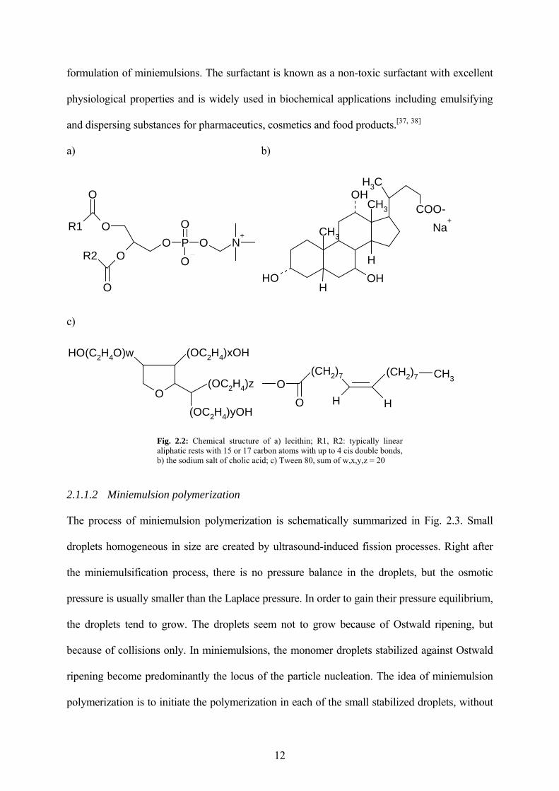
formulation of miniemulsions. The surfactant is known as a non-toxic surfactant with excellent

physiological properties and is widely used in biochemical applications including emulsifying

and dispersing substances for pharmaceutics, cosmetics and food products.[37, 38]

a) b)

N+

PO

OOO

O

OR1

O

R2

O

CH3

COO-CH3

HOH

H

CH3

OH

OH

Na+

c)

(OC2H4)zO

HO(C2H4O)w (OC2H4)xOH

(OC2H4)yOH

OO

(CH2)7

H

(CH2)7

H

CH3

Fig. 2.2: Chemical structure of a) lecithin; R1, R2: typically linear aliphatic rests with 15 or 17 carbon atoms with up to 4 cis double bonds, b) the sodium salt of cholic acid; c) Tween 80, sum of w,x,y,z = 20

2.1.1.2 Miniemulsion polymerization

The process of miniemulsion polymerization is schematically summarized in Fig. 2.3. Small

droplets homogeneous in size are created by ultrasound-induced fission processes. Right after

the miniemulsification process, there is no pressure balance in the droplets, but the osmotic

pressure is usually smaller than the Laplace pressure. In order to gain their pressure equilibrium,

the droplets tend to grow. The droplets seem not to grow because of Ostwald ripening, but

because of collisions only. In miniemulsions, the monomer droplets stabilized against Ostwald

ripening become predominantly the locus of the particle nucleation. The idea of miniemulsion

polymerization is to initiate the polymerization in each of the small stabilized droplets, without

12

13

major secondary nucleation or mass transport processes involved. Preservation of the particle

number and particle identity is therefore a key issue. Miniemulsion polymerization of methyl

methacrylate using lauroyl peroxide as initiator as well as cosurfactant has been carried out by

Reimers and Schork.[39] Diffusional stability was reduced to the point where nucleation in the

monomer droplets and polymerization could be carried out before significant diffusional

degradation took place. Ugelstad and coworkers[40] first published results where droplets with

sizes of less than 0.7 µm were nucleated leading to polystyrene polymer particles. A

continuation of this early work showed that the addition of cetyl alcohol increases the stability

of the droplets.[41] Usually, the growth of minidroplets is slower than the polymerization time,

and a situation very close to a 1:1 copying of the monomer droplets to polymer particles is

obtained, freezing the critically stabilized state (Fig. 2.3). The identity in size before and after

polymerization was recently proven by means of SANS measurements.[42] The pressure balance

can also be obtained by intentionally adding an adequate amount of surfactant to the system

(poststabilization). The growth of the droplets by collisions is then effectively suppressed

(Fig. 2.3).

growth by collis

ion

critically stabilizedstate is frozen

Πosm = pKelvin

critica

lly stabiliz

ed Π osm < p Kelv

in

poststabilization

Πosm = pKelvin

fission todroplets

Fig. 2.3: Schematic summary of the process of miniemulsion polymerization

2.1.1.3 Encapsulations by miniemulsion polymerization

Polymerization in direct miniemulsion can be used for the efficient encapsulation of water-

insoluble materials in hydrophobic polymers to obtain hybrid particles which are homogenous

in their size and their inorganic material content as shown recently for the encapsulation of

hydrophobized CaCO3[43] and TiO2.[44] For these encapsulation processes, the encapsulating

material is dispersed in the monomer phase prior to miniemulsification. Another approach was

developed for the encapsulation of high amounts of carbon black: Both monomer and carbon

black were independently dispersed in water using SDS as a surfactant and mixed afterwards in

any ratio between the monomer and carbon. Then, this mixture was cosonicated, and the

controlled fusion/fission process characteristic for miniemulsification destroyed all aggregates

and liquid droplets, and only hybrid particles being composed of carbon black and monomer

remained due to their higher stability.[45]

14

Thus, it is plausible the encapsulation of magnetic components through the miniemulsion

process.

2.2 Magnetism

Magnetic field origins from the movement of electric charges. An electrical current in a wire

produces a magnetic field that curls around the wire. A current loop surrounding an area

and carrying a current i, creates what is called magnetic dipole moment µ whose magnitude is

and has units of A·m

2looprπ

2loopriπ 2 in SI or emu (electromagnetic unit of magnetic moment ) in cgs.

Atoms have magnetic dipole moments, which are produced both for electron spin and for the

rotation of electrons around the nucleus. The nucleus has a small magnetic moment, which,

nevertheless is negligible compared to the one of the electrons. Electrons can be imagined as

tiny circuits and carrying tiny magnetic dipole moments. They respond to external magnetic

fields and give rise to a magnetization (M) that is defined as the net magnetic dipole moment

(µtotal ) per unit volume in the material (v):

vM totalµ

= Eq. 1

The total magnetic field inside such a material (the magnetic induction B) is a function of the

applied external field and the magnetization

MBB 0ext µ+= Eq. 2

where is the strength of the external magnetic field and extB 0µ is the permeability of the free

space, 4π 10-7 T·m·A-1.

The magnetic field strength H depend only on the strength of the external magnetic field:

0

ext

µB

H = Eq. 3

and replacing Eq. 3 in Eq. 2, it results

15

( )MHB += 0µ Eq. 4

The relationship between M in the material and the external field H is defined as:

HM χ= Eq. 5

where the proportional constant χ is the mass magnetic susceptibility of the material.

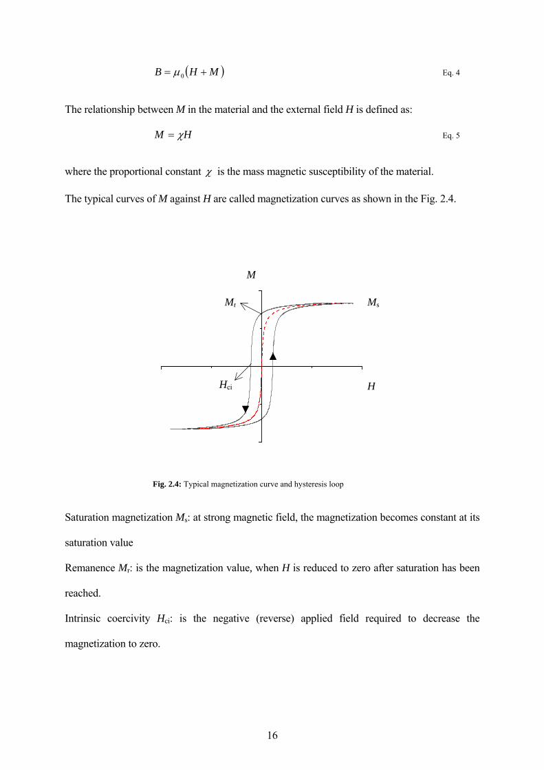
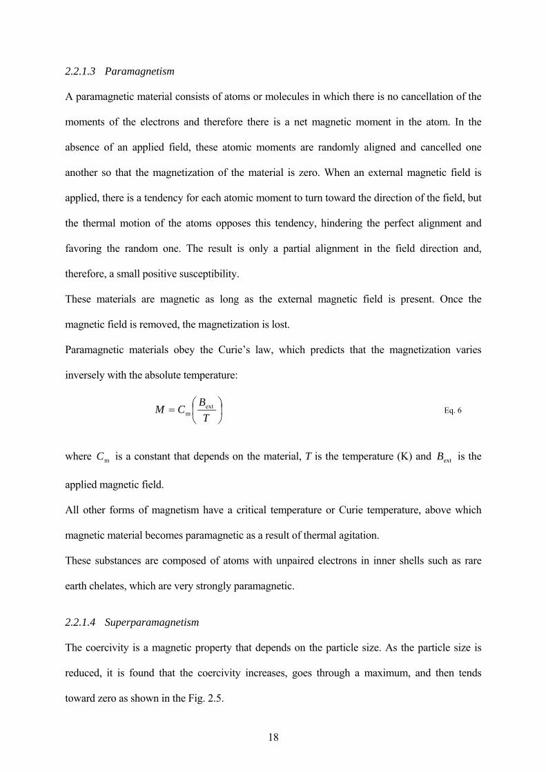
The typical curves of M against H are called magnetization curves as shown in the Fig. 2.4.

M

Hci

Mr Ms

H

Fig. 2.4: Typical magnetization curve and hysteresis loop

Saturation magnetization Ms: at strong magnetic field, the magnetization becomes constant at its

saturation value

Remanence Mr: is the magnetization value, when H is reduced to zero after saturation has been

reached.

Intrinsic coercivity Hci: is the negative (reverse) applied field required to decrease the

magnetization to zero.

16

17

2.2.1 Magnetism in materials

Materials can be classified by appropriate measurements in different types such as

ferromagnetic, diamagnetic, paramagnetic, superparamagnetic, antiferromagnetic,

ferromagnetic, etc, depending on the their response to an external applied magnetic field.

2.2.1.1 Ferromagnetism

In order to understand ferromagnetism, the Weiss theory has to be considered. A ferromagnetic

in the demagnetized state is divided into a number of small regions called domains. Each

domain is spontaneously magnetized to the saturation value Ms, but the directions of

magnetization of the various domains are such that the specimen as a whole has no net

magnetization. The process of magnetization is explained by converting the specimen from a

multi-domain state into a state in which it is a single domain magnetized in the same direction

as the applied flied.[46] The Weiss theory, therefore, contains two important postulates:

spontaneous magnetization and division into domains.

The atoms in a ferromagnetic material have magnetic dipole moments that tend to align parallel

within a domain throughout the bulk material. When an external magnetic field is applied, the

magnetic domains are aligned with the external field. When the external field is removed, the

domains maintain the alignment and the magnetism remains. The magnetic material has

"magnetic memory" (hysteresis loop in the Fig. 2.4). Iron, cobalt and nickel are typical

materials which exhibit ferromagnetism at room temperature.

2.2.1.2 Diamagnetism

When diamagnetic materials are placed in a strong magnetic field, the magnetic dipole moment

appears oppositely to the direction of the magnetic field. The susceptibilities of such materials

are negative and small, for this reason diamagnetism sometimes is called “negative magnetism”.

The electron shells in these materials are completely filled and there are no unpaired electrons.

He, Ne, H2, N2, some compounds formed with covalent bonding as NaCl, etc. are diamagnetics.

2.2.1.3 Paramagnetism

A paramagnetic material consists of atoms or molecules in which there is no cancellation of the

moments of the electrons and therefore there is a net magnetic moment in the atom. In the

absence of an applied field, these atomic moments are randomly aligned and cancelled one

another so that the magnetization of the material is zero. When an external magnetic field is

applied, there is a tendency for each atomic moment to turn toward the direction of the field, but

the thermal motion of the atoms opposes this tendency, hindering the perfect alignment and

favoring the random one. The result is only a partial alignment in the field direction and,

therefore, a small positive susceptibility.

These materials are magnetic as long as the external magnetic field is present. Once the

magnetic field is removed, the magnetization is lost.

Paramagnetic materials obey the Curie’s law, which predicts that the magnetization varies

inversely with the absolute temperature:

⎟⎠⎞

⎜⎝⎛=

TB

CM extm Eq. 6

where is a constant that depends on the material, T is the temperature (K) and is the

applied magnetic field.

mC extB

All other forms of magnetism have a critical temperature or Curie temperature, above which

magnetic material becomes paramagnetic as a result of thermal agitation.

These substances are composed of atoms with unpaired electrons in inner shells such as rare

earth chelates, which are very strongly paramagnetic.

2.2.1.4 Superparamagnetism

The coercivity is a magnetic property that depends on the particle size. As the particle size is

reduced, it is found that the coercivity increases, goes through a maximum, and then tends

toward zero as shown in the Fig. 2.5.

18

dp

superparamagnetic

0

single-domainmulti-domain

ds

Hci

dmp

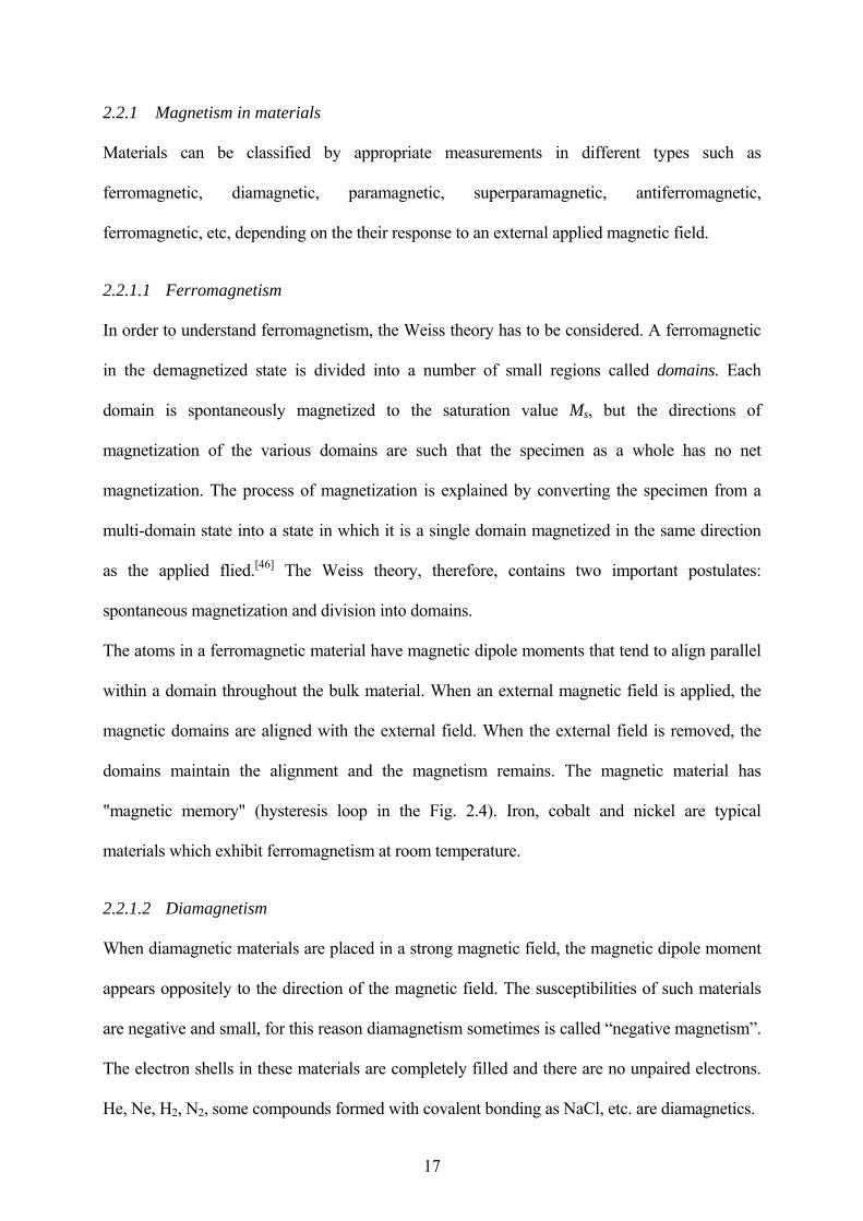
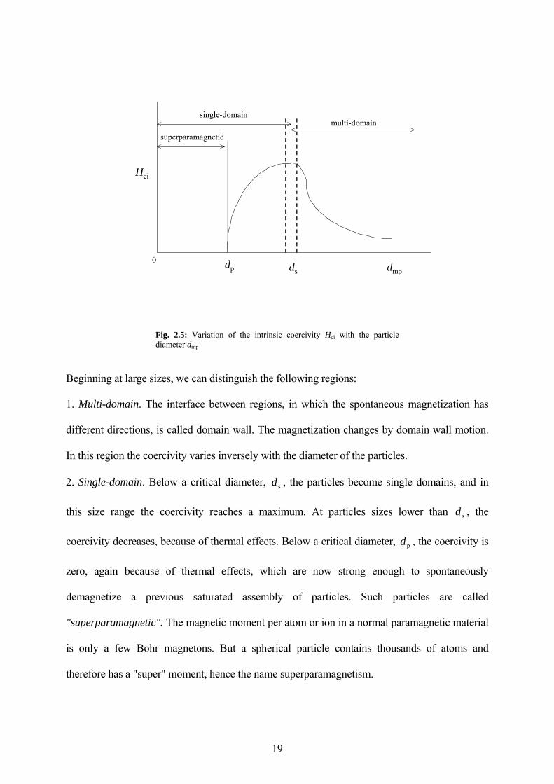
Fig. 2.5: Variation of the intrinsic coercivity Hci with the particle diameter dmp

Beginning at large sizes, we can distinguish the following regions:

1. Multi-domain. The interface between regions, in which the spontaneous magnetization has

different directions, is called domain wall. The magnetization changes by domain wall motion.

In this region the coercivity varies inversely with the diameter of the particles.

2. Single-domain. Below a critical diameter, , the particles become single domains, and in

this size range the coercivity reaches a maximum. At particles sizes lower than , the

coercivity decreases, because of thermal effects. Below a critical diameter, , the coercivity is

zero, again because of thermal effects, which are now strong enough to spontaneously

demagnetize a previous saturated assembly of particles. Such particles are called

"superparamagnetic". The magnetic moment per atom or ion in a normal paramagnetic material

is only a few Bohr magnetons. But a spherical particle contains thousands of atoms and

therefore has a "super" moment, hence the name superparamagnetism.

sd

sd

pd

19

20

Typical superparamagnetic behavior is shown in the Fig. 2.4 (red dashed line). In the

superparamagnetic behavior there is no hysteresis. Both remanence and coercivity are zero.

This means, when an external magnetic field is applied to the superparamagnetic particles, the

moments tend to align in direction of the applied magnetic field, but the alignment is imperfect

due to the thermal effects. When the magnetic field is removed, the superparamagnetic particles

do not remember that they were magnetized and they lose the magnetization.

2.2.1.5 Antiferromagnetism

These materials have a strong tendency toward an antiparallel alignment of magnetic moments

in the absence of an applied magnetic field, in special at lower temperatures where the thermal

effect is too low to allow random alignment. Thus, in the crystal it forms two sublattices having

opposed moments, which compensate each other.

2.2.1.6 Ferrimagnetism

The word "ferrimagnetism" is due to the certain oxides of iron called ferrites. Ferrites have the

general formula MO · Fe2O3 where M is a divalent metal ion. One of the most widely known

ferrite, is the magnetite Fe3+ [Fe2+ Fe3+]O4 (or FeO · Fe2O3). Ferrites have a spinel structure and

it is so-called because the structure is closed to the structure of the mineral spinel MgO · Al2O3.

Spinel lattice consist of face centred cubic arrangements of oxygen atoms with cations localized

in the center of tetrahedron and octahedron. In the mineral spinel, the Mg2+ ions are in the

tetrahedral sites (A) and the Al3+ ions are in octahedral sites (B), so-called normal spinel

structure. Other ferrites have the inverse spinel structure, in which the divalent ions are in the

octahedral sites and the trivalent ions are equally divided between tetrahedral and octahedral

positions. Magnetite has the inverse spinel structure, which it means the tetrahedral positions

(A) are filled by Fe3+ cations and octahedral positions (B) are equally filled by Fe3+ and Fe2+.

Ferrimagnetic substances exhibit a similar behavior as the ferromagnetics, but have an

antiparallel alignment of the magnetic moments as in the case of antiferromagnetism with the

difference that they do not compensate each other. There are AB, AA and BB interactions but

the strongest is AB so that all the A moments are parallel to one another and antiparallel to the

B moments but they do not cancel each other.[ ] Ferrimagnetism can be imagined as an

“imperfect antiferromagnetism”.

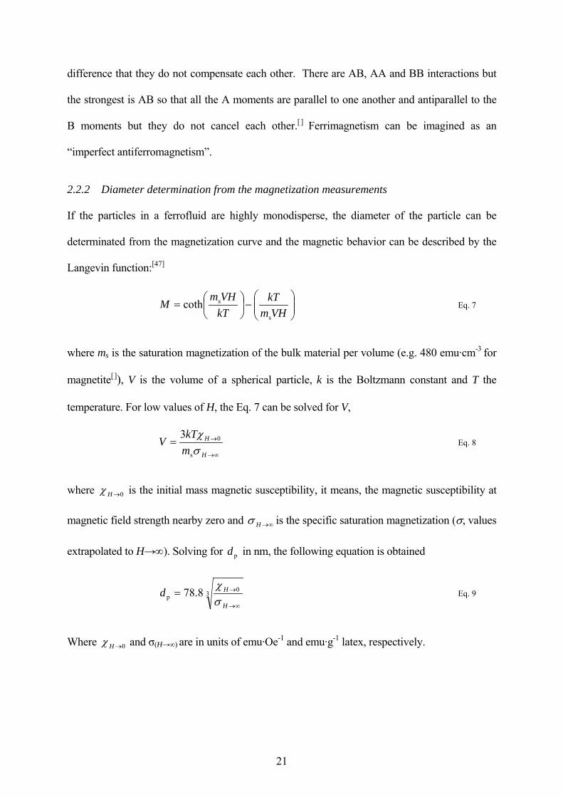
2.2.2 Diameter determination from the magnetization measurements

If the particles in a ferrofluid are highly monodisperse, the diameter of the particle can be

determinated from the magnetization curve and the magnetic behavior can be described by the

Langevin function:[47]

⎟⎟⎠

⎞⎜⎜⎝

⎛−⎟

⎠⎞

⎜⎝⎛=

VHmkT

kTVHm

Ms

scoth Eq. 7

where ms is the saturation magnetization of the bulk material per volume (e.g. 480 emu·cm-3 for

magnetite[ ]), V is the volume of a spherical particle, k is the Boltzmann constant and T the

temperature. For low values of H, the Eq. 7 can be solved for V,

∞→

→=H

H

mkT

Vσχ

s

03 Eq. 8

where 0→Hχ is the initial mass magnetic susceptibility, it means, the magnetic susceptibility at

magnetic field strength nearby zero and ∞→Hσ is the specific saturation magnetization (σ, values

extrapolated to H→∞). Solving for in nm, the following equation is obtained pd

3 0p 8.78

∞→

→=H

Hdσχ

Eq. 9

Where 0→Hχ and σ(H→∞) are in units of emu·Oe-1 and emu·g-1 latex, respectively.

21

22

2.3 Ferrofluids

Ferrofluids or magnetic fluids or magnetic colloids are stable dispersions of ultrafine ferro- or

ferrimagnetic particles or encapsulated ferro- or ferrimagnetic particles in an organic or aqueous

carrier medium. The stabilization of these particles is achieved through a surfactant which

hinders the particles from flocculation or sedimentation. Ideally, these particles remain

uniformly dispersed in the carrier medium although they are or have been exposed to magnetic

fields. Due to their small size, ferrofluids contain a single magnetic domain and although they

are either ferro- or ferrimagnetic in the molecular scale, they are like paramagnetic components

on the colloidal scale with magnetic moments which are much larger than the moments in a

paramagnet. Thus, ferrofluids commonly show a superparamagnetic behavior.

In early publications, magnetic fluids were produced by grinding magnetite with heptane or

long chain hydrocarbon and a grinding agent, e.g. oleic acid.[48] Later, magnetic fluids were

produced by precipitation of an aqueous Fe3+ / Fe2+ solution with a base, coating these particles

with an adsorbed layer of oleic acid and then dispersing them in a non-aqueous fluid.[49] Both

processes result in tiny magnetite particles, a surfactant coating these magnetite particles and a

non-aqueous liquid carrier in which the hydrophobic magnetite particles will be dispersed.

Obviously, the latter process is more feasible to apply in the production of more homogeneous

magnetite particles.

Other applications of ferrofluids rely on water as the continuous phase. Kelley[50] produced an

aqueous magnetic material suspension by the conversion of iron compounds to magnetic iron

oxide in the aqueous medium under controlled pH conditions in presence of a petroleum

sulfonate dispersant. Shimoiizaka and coworkers[51] developed a water-based ferrofluid from the

oleic acid coated magnetite particles dispersed by an anionic or nonionic surfactant solution,

which is suitable to form a second surfactant layer.

Polymer covered magnetic particles can also be produced by an in situ precipitation of magnetic

materials in the presence of polymer which acts as a stabilizer. In this way, magnetic polymer

23

nanoparticles are produced in presence of the water-soluble dextran,[52] poly(ethylene imine),[53]

poly(vinyl alcohol),[54] poly(ethylene glycol),[55] sodium poly(oxyalkylene di-phosphonates),[56]

and amylose starch.[57] In all cases, the magnetic particles are surrounded by a hydrophilic

polymer shell.

Another method to produce magnetic polymer particles consists of the synthesis of magnetic

particles and polymer particles separately and then mixing them together to enable either

physical or chemical adsorption of the polymer onto the material magnetic. The polymer

material can be produced by different ways, for instance by emulsion or precipitation

polymerization.[58]

It is also possible to use a strategy comprising the polymerization in heterophase in the presence

of magnetic particles. The magnetic material preferably having a surfactant layer is embedded

into a polymer using processes such as the suspension, the emulsion, or the precipitation

polymerization. Magnetic particles were encapsulated in hydrophilic polyglutaraldehyde by

suspension polymerization resulting in particles with an average diameter of 100 nm.[53]

Magnetite containing nanoparticles of 150 to 200 nm were also synthesized by seed

precipitation polymerization of methacrylic acid and hydroxyethyl methacrylate in presence of

magnetite particles containing tris(hydroxy methyl)aminomethane hydroxide in ethyl acetate

medium.[59] Polymethacrylate/poly(hydroxy methacrylate) coated magnetite particles could be

also prepared by a single inverse microemulsion process, leading to particles with a narrow size

distribution, but only with a magnetite content of 3.3 wt.-%.[60]

Daniel and coworkers[61] obtained magnetic polymer particles by dispersing a magnetic material

in an organic phase which consists of an organo-soluble initiator, vinyl aromatic monomers

and/or a water insoluble compound. The mixture was emulsified in water by using an emulsifier

and then polymerization took place in order to obtain polymer particles with a magnetite

content between 0.5 and 35 wt.-% with respect to the polymer. However the resulting particle

size distribution was rather broad (between 30-5000 nm). Charmot and Vidil[62] used a similar

24

method to produce magnetizable composite microspheres of a hydrophobic crosslinked

vinylaromatic polymer, but they obtained a mixture of magnetizable particles and non-

magnetizable blank microspheres.

Ugelstad and coworkers were the pioneers to obtain monodisperse magnetic polymer

microparticles by in situ precipitation of magnetic oxides inside preformed porous mono-sized

polymer particles, taking into account that the microparticles used as seed (0.5–1 µm) contain

metal-binding groups.[63] Magnetic polymer microparticles (0.5–100 µm) with a high degree of

monodispersity and up to 35 % of iron as magnetic oxides were obtained. It is important to

stress that Ugelstad’s work has to be considered as a great contribution in the magnetic carrier

technology. Nevertheless, his work was emphasized to produce microparticles whereas our

focus is addressed to the production of nano-sized magnetic polymer particles (50–500 nm).

2.3.1 Ferrofluids by miniemulsion polymerization

Wormuth[64] used the inverse miniemulsion process[65] to encapsulate magnetic particles by a

hydrophilic polymer. The dispersion of magnetic iron oxide into hydrophilic monomers,

followed by the inverse miniemulsion and a further polymerization process was carried out. The

magnetite was precipitated from an aqueous poly(ethylene oxide)-b-poly(methacrylic acid)

dispersion in short denoted as (PEO-PMAA) dispersion, containing iron III and II salts, by

means of the addition of a concentrated ammonium solution. After dialysis and drying, the

PEO-PMAA-magnetite wax-like solids were redispersed in a mixture of HEMA and MAA

monomers. After inverse miniemulsion polymerization, a magnetite latex dispersion was

obtained. With regard to the stabilization of the final dispersion, after certain time some

sediment was observed.

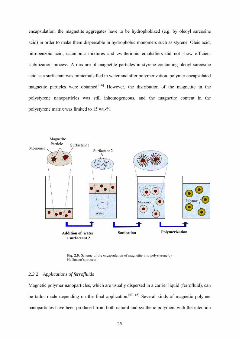
The strategy of dispersing the material being encapsulated into the monomer phase prior to

miniemulsification was also used for the encapsulation of hydrophilic magnetite into the

hydrophobic polystyrene as shown schematically in the Fig. 2.6. To obtain a successful

encapsulation, the magnetite aggregates have to be hydrophobized (e.g. by oleoyl sarcosine

acid) in order to make them dispersable in hydrophobic monomers such as styrene. Oleic acid,

nitrobenzoic acid, catanionic mixtures and zwitterionic emulsifiers did not show efficient

stabilization process. A mixture of magnetite particles in styrene containing oleoyl sarcosine

acid as a surfactant was miniemulsified in water and after polymerization, polymer encapsulated

magnetite particles were obtained.[66] However, the distribution of the magnetite in the

polystyrene nanoparticles was still inhomogeneous, and the magnetite content in the

polystyrene matrix was limited to 15 wt.-%.

Monomer Polymer

Addition of water + surfactant 2

Sonication Polymerization

Surfactant 2

Water

Surfactant 1MagnetiteParticle

Monomer

Fig. 2.6: Scheme of the encapsulation of magnetite into polystyrene by Hoffmann’s process

2.3.2 Applications of ferrofluids

Magnetic polymer nanoparticles, which are usually dispersed in a carrier liquid (ferrofluid), can

be tailor made depending on the final application.[67, 68] Several kinds of magnetic polymer

nanoparticles have been produced from both natural and synthetic polymers with the intention

25

26

to incorporate groups on the surface or to treat their surface to perform, for instance, selective

separations. In particular, magnetic nanoparticles with or without polymer encapsulation can be

used for magnetic drug targeting,[69, 70] tissue engineering,[71] magnetic resonance imaging,[72]

and hyperthermia.[73] There are also several applications for mechanical and electrical devices

which take advantage of the magneto-rheological properties of ferrofluids, e. g. in loudspeakers,

seals, sensors, dampers, etc.[74, 75]

Within the framework of the Deutsche Forschungsgemeinschaft (DFG) funded ferrofluid

program (SPP1104), several and promising applications of ferrofluids can be found in the

technical and medicine field. Ferrofluids used in the gap between the acting magnets in electric

machines can enhance the forces in these motors.[76] Abel-Keilhack and Hesselbach[77] showed

a comparison of the experimental and simulation of the hydrostatic bearing with magnetic fluids

and the calculation of the payload capacity from the flow simulation of magnetic fluids.

Magnetic drug targeting is a drug delivery system using ferrofluids for chemotherapeutics in

locoregional cancer treatment. Ferrofluids containing anthracendion-derivative mitoxantrone

are injected into the tumor while an external magnetic field is applied on the tumor. In this way,

the magnetic particles and mitoxantrone complex is concentrated in the tumor area in order to

minimize the undesirable side effects in the organism. In this investigation it was revealed that

the incorporation mechanism of the iron containing nanoparticles in the cells is the

endocytosis.[78]

Hyperthermia is one of the four principal therapies used against cancer, in line with surgery,

radiotherapy and chemotherapy. The principle of hyperthermia consists in the elevation of the

temperature within a tumor with the purpose of destructing the cancer cells. The magnetic

hyperthermia using ferrofluids is based on the generation of the heat by means of the interaction

between alternating magnetic fields and magnetic materials. One of the advantages of using

magnetic fluids is the possibility to increase the temperature within tumors without any effect in

the surrounding healthy tissues.[79, 80]

27

Magnetic polymer nanoparticles should fulfill some criteria to fit further biomedical

application: no sedimentation, uniform size and size distribution, high and uniform magnetic

content, superparamagnetic behavior, no toxicity, no iron leaking, high selectivity in case that

these particles are used for hyperthermia purposes, and sufficient heat generation at lower

frequencies to enhance selective heating.[81] Therefore, magnetite particles homogeneously

encapsulated in a hydrophobic polymer which keep away water-soluble components from

contacting the magnetite particles are of high interest. Another important condition in order to

implement the ferrofluids in the biomedicine is the use of biosurfactant in their synthesis,

increasing their biocompatibility. There are several reasons to use polystyrene as hydrophobic

encapsulation material in biomedical applications,[82] e.g. it is inexpensive and it is a

hydrophobic polymer which allows physical adsorption of antibodies or proteins, it can also be

functionalized e.g. by carboxylic groups which enables covalent binding of antibodies, proteins,

or cells.

2.4 Nanostructured composites from iron pentacarbonyl decomposition

For the preparation of magnetic particles in the nanoscale many different approaches are

known. Among them, the solution-phase metal salt reduction has the advantage to produce high

amounts of colloids which can be further handled for different purposes. However, the

reductant, as well as the counter-ion, is often an additional contamination source of the final

metal.[83, 84] The decomposition of metal carbonyl complexes is thus a nice alternative, which

has been used since many years to produce various metals (mainly Fe, Ni, Co).[85] Metal

carbonyls e.g. iron carbonyl are compounds in which carbon monoxide is coordinated to the

central metal atom. They act as intermediates in transition-metal catalysis, in which they largely

control the course of the reaction.[86] Of the iron carbonyls, iron pentacarbonyl Fe(CO)5, is the

most widely used.

28

The decomposition of the metal carbonyls can be carried out by thermal decomposition

(pyrolysis)[87] and sonochemical decomposition.[88] Pyrolysis allows the formation of crystalline

solids[89], while the ultrasonic procedure often produces amorphous materials.[90-92]The most

common method to obtain iron nanoparticles is by thermal decomposition of iron pentacarbonyl

using a solvent in presence of either surfactants, such as oleic acid, or a polymer as stabilizer

such as vinyl polymers[93] to avoid the sedimentation of the iron nanoparticles and to enable

their stabilization.

The presence of organic and polymeric material during the thermal decomposition allow the

formation of nanocomposite materials with the possibility to control the type and size of the

metallic particle and the composition. Burke and coworkers[94] prepared nanocomposites

consisting of polystyrene-coated iron nanoparticles by thermal decomposition of iron

pentacarbonyl in the presence of polystyrene-tetraethylene-pentamine dispersants (PS-TEPA)

using 1-methylnaphthalene as solvent. Pathmamanoharan and coworkers[95] used polyisobutene

and oleic acid as stabilizer for the decomposition of iron pentacarbonyl in decalin; iron particles

of approximately 10 nm were obtained. Using 3-mercaptopropyltrimethoxysilane as stabilizer

leads to a combination of spherical and rodlike iron oxide colloids, however the obtained

dispersions were not stable.

Hyeon and coworkers[96] reported the production of highly monodisperse maghemite particles

from the thermal decomposition of iron pentacarbonyl in a mixture of oleic acid and octyl ether

and further oxidation using trimethyl amine oxide. By changing the molar ratio of iron

pentacarbonyl and oleic acid (from 1:1 to 1:4) a very good control of the particle size between

4 and 16 nm was achieved. Tannenbaum and coworkers[97] obtained polymer metal

nanopyramides by thermal decomposition and simultaneous film formation of a mixture

consisting of iron pentacarbonyl and poly(vinylidene difluoride) which is dissolved in

dimethylformamide. The presence of solvent during the film formation allows the mobility of

29

the polymer chains and therefore an efficient adsorption of these chains on the surface of the

forming iron oxide particles.

2.5 Gadolinium-based nanoparticles

Gadolinium is a lanthanide with seven unpaired electrons and therefore it has a large magnetic

moment (7.9 Bohr magneton). Due to the toxicity of gadolinium as metal or ion, it is only used

as complexes. The most important application of gadolinium complexes is in nuclear magnetic

resonance as shift reagents[98] and imaging contrast agent,[99] but they can be also used as

gadolinium neutron capture therapy agent.[100]

The most common and simplest gadolinium hydrophilic complexes used are Gd-DTPA

[gadolinium-(diethylenetriamine penta-acetic acid)][101] and Gd-DOTA [gadolinium-(1,4,7,10-

tetraazacyclododecan N, N’, N”, N’”-tetraacetic acid)].[102] Both of them are water-soluble and

have a low molecular weight. To overcome the low molecular weight (and therefore the

problem of osmotic pressure), the gadolinium as ion or metal chelator can be coupled directly to

synthetic or natural macromolecules such as copolymers of polyethyleneglycol amine

derivates,[103] starch,[104] dextran,[105, 106] chitosan,[107] albumin,[108] cholesterol,[109] synthetic

polyaminoacid,[110] homopolypeptid,[111] dendrimers,[112] liposomes,[113]

polyaminocarboxilate,[114] polyester,[115] protein,[116] human and rat red blood cells.[117] One of

the advantages of the complexation of gadolinium to a macromolecule is the possibility of

attach multiple paramagnetic ions to one large molecule, therefore the molar dose of the

contrast agent can be reduced and hence its toxicity.

The macromolecular carrier can be either a fluid, particulate material, spherical particle or a

colloid. Compared with other forms of carriers, a colloid, which is the main focus of this work,

is well known to have a major surface area and hence a larger concentration of paramagnetic

ions on the surface. Thus, a higher relaxation time can be achieved. Braybrook and Hall[118]

synthesized particulate ion-exchange resins containing paramagnetic ions bound to their

30

surfaces with a water-soluble coating. The sulphonated or imino-diacetic acid cross-linked

polystyrene resins (45-170 µm) were stirred in solutions of metal salts and, after rinsing and

drying, metal-loaded resins were obtained. These particles are coated with a layer of cellulose

acetate butyrate or cellulose acetate phthalate by using a phase separation technique.

Another type of gadolinium-loaded nanoparticles is reported by Reynolds and coworkers.[119]

They synthesized metal-loaded core-shell nanoparticles of 120 nm by a three-step method. The

polymer core consists of acidic methacrylic acid, which forms a strong complex with

gadolinium, and is made using emulsion polymerization. Further, gadolinium nitrate is added to

load these particles with gadolinium. In the final step, these metal-loaded polymer cores are

encapsulated with a porous polymer shell by a second emulsion polymerization. The

gadolinium-loaded emulsion polymer had a loading of 0.045 g Gd per gram resin. The final

gadolinium-loaded core–shell nanoparticles consisted of 0.031 g Gd/g polymer.

Gadolinium oxide magnetoliposomes are synthesized from both lauric acid coated gadolinium

oxide nanoparticles (20 nm) and fluorescein labelled liposomes (70 nm). They are mixed with

and subjected to agitation for 24 h for favoring the formation of a bilayer membrane around the

gadolinium oxide particles.[113] Gadolinium oxide liposomes, which are paramagnetic, are

obtained, but an optimization of the synthesis were suggested to improve reproducibility.

Most of the polymeric gadolinium contrast agents are based on water soluble chelates, e. g.

DTPA. A water soluble functionalized polymer is commonly used for favoring the conjugate

process. Gd-DTPA has been covalently attached to epichlorohydrin cross-linked hydrolyzed

potato starch microspheres. These particles have a mean particle diameter of 1.50 µm and a

gadolinium content between 1.1 and 12.2 %.[104] Gadolinium-containing lipid emulsions with a

particle size between 78 and 280 nm were prepared by a thin-film hydratation method using a

bath-sonicator. The emulsions comprised soy bean oil, water, Gd-DTPA-disteraylamide,

hydrogenated egg yolk phosphatidylcholine as a surfactant and/or an appropriate co-surfactant

to reduce the particle size. The gadolinium content was 3.0 mg/ml.[120] Tournier and

31

coworkers[121] obtained gadolinium-containing micelles, mixing an amphiphilic gadolinium

chelate, phospholipids and/or non-ionic surfactant(s) (e.g. Tween). The amphiphilic gadolinium

chelate was obtained by esterification or amidation between DTPA and alcohols or amines. The

mean diameter of the micelles prepared was between 30 and 100 nm. In these two approaches,

the gadolinium chelate was emulsified but the molecular weight was not increased. Tokumitsu

and coworkers[107] have reported the preparation of gadolinium-loaded chitosan particulate for

cancer neutron capture therapy. Both glutaraldehyde cross-linked and non-crosslinked

gadolinium-loaded chitosan particulate system were synthesized. They demonstrated that the

use of glutaraldehyde as crosslinking agent reduced the loading amount of Gd-DTPA. The non-

crosslinked gadolinium-loaded chitosan nanoparticles were produced by the emulsion-droplet

coalescence technique. This technique involves the precipitation of chitosan in an aqueous

acidic Gd-DTPA solution by neutralization with an emulsion of sodium hydroxide. A

gadolinium content of up to 13.0 % and with a particle size of 452 nm was obtained.

As far as we can see, most of these approaches used water based polymers for the conjugation

the gadolinium ion or the metal chelator to the macromolecules. It seems reasonable to envisage

the encapsulation of chelates directly in a heterophase polymerization process to produce

hydrophobic polymeric nanoparticles containing gadolinium chelate. The chelate should be

compatible with the monomer in order to get better encapsulation.

2.5.1 Lanthanide shift reagents for nuclear magnetic resonance

Lanthanide materials have, due to their very special electronic structure, a number of

extraordinary properties, including their optical, electronic and magnetic behavior. However,

pure lanthanide compounds are usually crystalline and non-ductile and have low material

performance. This is why compounding or composite formation with a polymer would be

highly profitable, bringing in the potential for solvent processing, cohesive films, flexible

coating, plus some mechanical advantages.

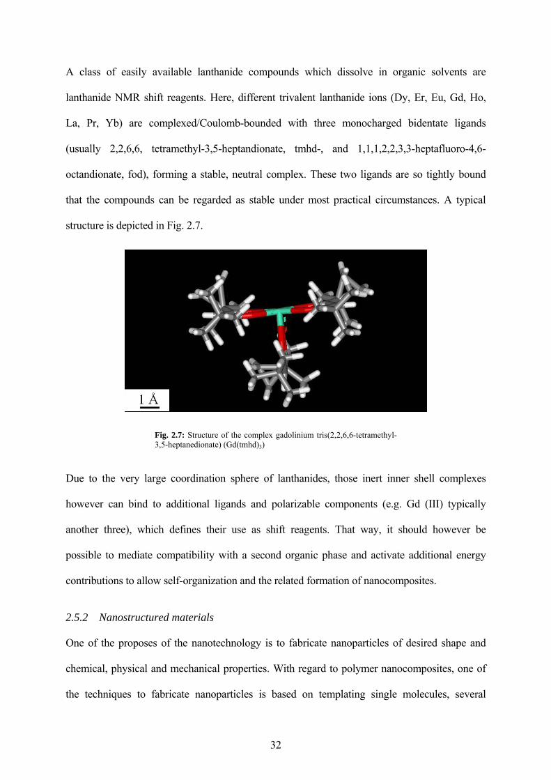
A class of easily available lanthanide compounds which dissolve in organic solvents are

lanthanide NMR shift reagents. Here, different trivalent lanthanide ions (Dy, Er, Eu, Gd, Ho,

La, Pr, Yb) are complexed/Coulomb-bounded with three monocharged bidentate ligands

(usually 2,2,6,6, tetramethyl-3,5-heptandionate, tmhd-, and 1,1,1,2,2,3,3-heptafluoro-4,6-

octandionate, fod), forming a stable, neutral complex. These two ligands are so tightly bound

that the compounds can be regarded as stable under most practical circumstances. A typical

structure is depicted in Fig. 2.7.

Fig. 2.7: Structure of the complex gadolinium tris(2,2,6,6-tetramethyl-3,5-heptanedionate) (Gd(tmhd)3)

Due to the very large coordination sphere of lanthanides, those inert inner shell complexes

however can bind to additional ligands and polarizable components (e.g. Gd (III) typically

another three), which defines their use as shift reagents. That way, it should however be

possible to mediate compatibility with a second organic phase and activate additional energy

contributions to allow self-organization and the related formation of nanocomposites.

2.5.2 Nanostructured materials

One of the proposes of the nanotechnology is to fabricate nanoparticles of desired shape and

chemical, physical and mechanical properties. With regard to polymer nanocomposites, one of

the techniques to fabricate nanoparticles is based on templating single molecules, several

32

molecules, colloids, crystals, gels, etc. Templating is classified in direct and indirect form.

Direct templating is called when the structure of the templating is still recognized in the final

material such as casting, coating, curing. When the original template is changed during the

templating process, the templating is called indirect.[122] Inorganic-organic nanocomposites can

commonly be obtained by templating techniques such as layered-silicate based polymer

nanocomposites.[123] Two types of hybrids were found. One is called intercalated in which a

polymer chain is intercalated between the silicate layers. The other one is called exfoliated in

which the silicate layers are dispersed in a polymer matrix.

2.5.3 Spin-lattice relaxation time (T1) on NMR imaging application

Nuclear magnetic resonance imaging techniques has been developed and widely used for the

diagnostic medicine application. Reviews in this topic can be found elsewhere.[124-126] In NMR

imaging technique, paramagnetic contrast agents are used to enhance the image contrast

between normal and diseased tissue, but they are not measured directly. Instead, they are

detected indirectly on the basis of changes in proton relaxation. Those protons are mainly from

water, which is the most composition of tissue. In principle, when a paramagnetic compound is

added, it shortens the relaxation time of neighbouring proton nuclei, resulting in the image

contrast enhancement.

The history of NMR imaging technique began in 1946 when Bloch and coworkers has first

reported the shortening of spin-lattice relaxation time or longitudinal relaxation time (T1) of 1H

water when ferric nitrate as a paramagnetic solute is added. [127] However, the mathematic

formulation of paramagnetic-enhanced solvent relaxation is first described by Solomon[128] in

1955 and later modified by Bloembergen in 1957. [129] The equation is represented as follows:

⎟⎟⎠

⎞⎜⎜⎝

⎛+

⎟⎠⎞

⎜⎝⎛++⎟⎟

⎠

⎞⎜⎜⎝

⎛+

++

+= 2

e2S

e2

2c

2S

c2c

2I

c6

in

222

1 1)1(

32

17

13)1(

1521

τωτ

τωτ

τωτβγ

h

ASSr

gSST

Eq. 10

33

where S is electron spin quantum number, γ is the proton gyromagnetic ratio, g is electronic g

factor, β is the Bohr magneton, Iω and Sω are Larmor frequencies for nuclear and electron

spins, is ion-nucleus distance, A/ is the electron-nuclear hyperfine coupling constant, and τinr h c

and eτ are correlation times for dipolar and scalar interactions.

In general, the relaxation rates observed in the presence of a paramagnetic molecule are the sum

of the proton relaxation rate caused by the paramagnetic and the proton relaxation rate that

would exist without the paramagnetic (diamagnetic) relaxation rate.

cdiamagneti1icparamagnet1observed1

111TTT

+= Eq. 11

In principle, the solvent relaxation rates are linearly dependent on the concentration of the

paramagnetic species, [M], in the absence of solute-solute interaction. In other words, the

paramagnetic concentration has an influence on nuclear relaxation rate, i.e. T1 is proportional to

the paramagnetic concentration

cdiamagneti11

observed1

1][1T

MRT

+= Eq. 12

The relaxivity, R1, can be then defined as the slope of this dependence in units of M-1·s-1 or

mM-1·s-1. Nevertheless, the Solomon-Bloembergen equation as mentioned above is based on the

relaxation of water proton in the proximity of metal complexes. Therefore the interactions of

water molecules to the paramagnetic species (either binding to the metal ion or coordination

with metal ligands) as well as translational diffusion of water molecules have to be considered.

Generally, the magnitude of relaxation enhancement depends on the proximity of the nuclear

and electronic spins and on the correlation time of their interaction. The Solomon-Bloembergen

theory classifies contributions for the water proton relaxivity due to three distinct types of

interactions as indicated schematically in Fig. 2.8.[130] The first type involves the primary

coordination of water molecules with the metal ion (Fig. 2.8a). This type of coordination is

34

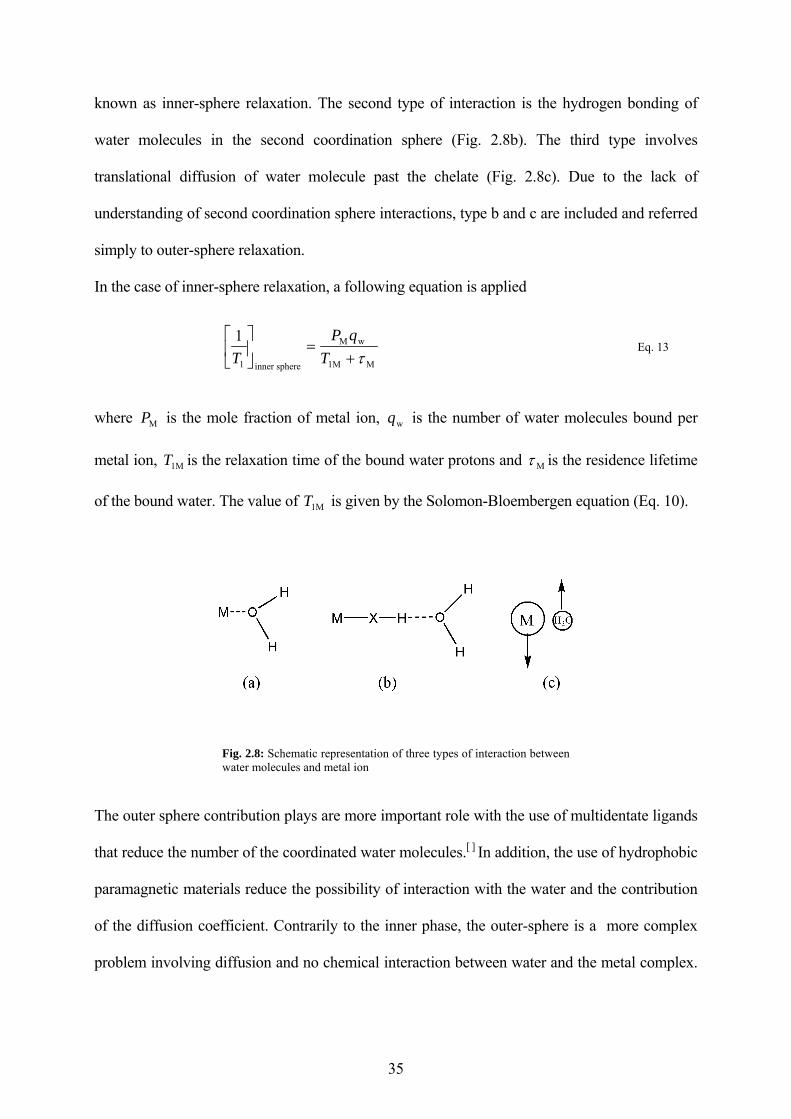
known as inner-sphere relaxation. The second type of interaction is the hydrogen bonding of

water molecules in the second coordination sphere (Fig. 2.8b). The third type involves

translational diffusion of water molecule past the chelate (Fig. 2.8c). Due to the lack of

understanding of second coordination sphere interactions, type b and c are included and referred

simply to outer-sphere relaxation.

In the case of inner-sphere relaxation, a following equation is applied

MM1

wM

sphereinner1

1τ+

=⎥⎦

⎤⎢⎣

⎡T

qPT

Eq. 13

where is the mole fraction of metal ion, is the number of water molecules bound per

metal ion, is the relaxation time of the bound water protons and

MP wq

M1T Mτ is the residence lifetime

of the bound water. The value of is given by the Solomon-Bloembergen equation (Eq. 10). M1T

Fig. 2.8: Schematic representation of three types of interaction between water molecules and metal ion

The outer sphere contribution plays are more important role with the use of multidentate ligands

that reduce the number of the coordinated water molecules.[ ] In addition, the use of hydrophobic

paramagnetic materials reduce the possibility of interaction with the water and the contribution

of the diffusion coefficient. Contrarily to the inner phase, the outer-sphere is a more complex

problem involving diffusion and no chemical interaction between water and the metal complex.

35

The most general equation for outer-sphere relaxivity have some similarities with the Solomon-

Bloembergen equation and is given in the Eq.14.

[ )(3)(7)1(1

SSD

3a

22S

2IS

sphereouter1

ωωτ

γγπjj

dSSNC

T+

+=⎥

⎦

⎤⎢⎣

⎡ h ] Eq. 14

where C is a numeral constant, is the number of metal ions per cubic centimeter, is the

distance of closest approach of the solvent molecule to the metal complex, is the Dirac

constant, and

SN ad

h

Dτ , the relative translational diffusion , ( )SI2aD 3/ DDd +=τ , where and

are the diffusional coefficients of water and the metal complex, respectively. The spectral

density functions, j in the Eq. 14, are mathematically complex and depend on the frequencies.

ID SD

[99]

36

37

3 Relevant Methods

In this section of the thesis, the relevant methods, which are used in the next section, are briefly

described.

3.1 Transmission electron microscopy

Transmission electron microscope (TEM) enables, through the interaction of the electron beam

with the sample, the direct production of an image. The main components of the TEM are

shown in the Fig. 3.1. TEM is based on the principles of the light microscope but is capable of

magnifications of 100,000 times and a high resolution of approximately 0.1 nm. As the name

indicates, TEM uses a high energy electron beam passing through (transmission) a very thin

slice of the specimen (sample) in a vacuum environment. The electrons in the microscope, are

accelerated with an electric voltage between 80 and 200 keV, which is used as “light”.

Electrostatic or magnetic “lenses” focus the electron beam, and project the highly-magnified

image onto a phosphor screen, special photographic film or a computer. The sample has to be

placed on an electron-transparent support that has to be extremely thin (50-200 nm) for

allowing the transmission of the electrons through it and to create an image. A thin carbon –film

is usually used for TEM, but its non-complete transparency contributes to the presence of the

noise in the final image.

The illumination source (or electron gun) is the thermo-ionic emission. A filament (cathode) is

the source of the electrons, usually a tungsten wire. The condenser has the function of gathering

the electrons of the first crossover image and focus them onto the specimen to illuminate only

the area being examined. The objective lens is used to focus an initial magnification of the

image. Intermediated lenses magnify the image coming from the objective lens. Finally,

projector lenses magnify the image coming from the intermediate lens and projects it onto the

fluorescent screen. The final image can be seen in the camera or computer localized under the

fluorescent screen.

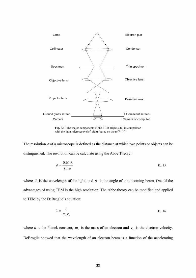
Electron gun

Condenser

Thin specimen

Objective lens

Projector lens

Fluorescent screen

Camera or computer

Lamp

Collimator

Specimen

Objective lens

Projector lens

Ground glass screen

Camera

Fig. 3.1: The major components of the TEM (right side) in comparison with the light microscopy (left side) (based on the ref.[[131])

The resolution ρ of a microscope is defined as the distance at which two points or objects can be

distinguished. The resolution can be calculate using the Abbe Theory:

αλρ

sin61.0

= Eq. 15

where λ is the wavelength of the light, and α is the angle of the incoming beam. One of the

advantages of using TEM is the high resolution. The Abbe theory can be modified and applied

to TEM by the DeBroglie’s equation:

eevmh

=λ Eq. 16

where h is the Planck constant, is the mass of an electron and is the electron velocity.

DeBroglie showed that the wavelength of an electron beam is a function of the accelerating

em ev

38

voltage. The bigger the accelerating voltage, the shorter the wavelength. Applying the Abbe

equation, it can be seen that a shorter wavelength leads to the better resolution.

TEM is typically used to examine the internal structure of materials both in biological and non-

biological precedence.

3.2 X-ray diffraction

X-rays were discovered by Wilhelm Konrad Röntgen in 1895. X-rays are produced by

bombarding a metal anode at high energy (grater than 20 eV) and can penetrate several atomic

layers of the materials and produce interference between the X-rays scattering from different

planes (Fig. 3.2). The Bragg’s law considers a crystal as a number of planes that can reflect the

light. The separation between the planes is d. The angle of incidence is θ which is equal to the

angle of reflection and from trigonometry the path difference is θsin2d .

Constructive interference is described by Bragg’s law:

λθ nd =sin2 Eq. 17

where λ is the wavelength of the X-rays s, and n is the order of the reflection (n= 1, 2,…).

Constructive interference means that the X-rays must have a path difference that is equal to the

wavelength.

39

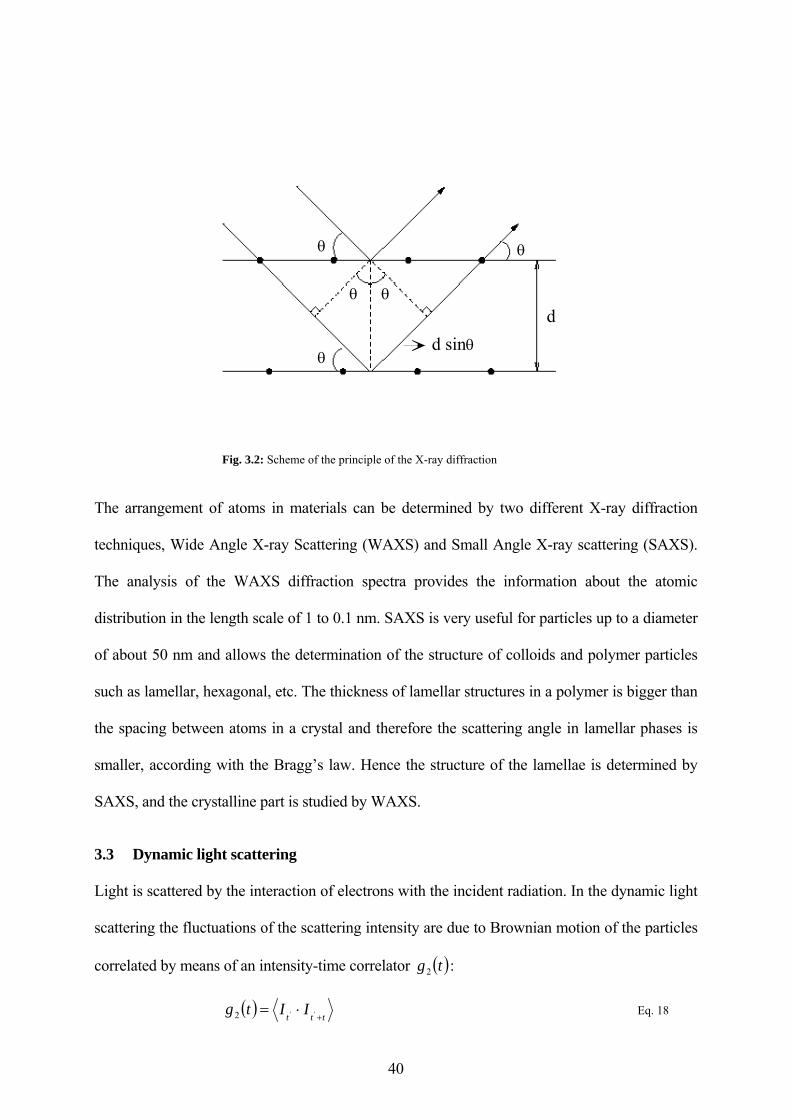
d d sinθ

θ

θ θ

θ

θ

Fig. 3.2: Scheme of the principle of the X-ray diffraction

The arrangement of atoms in materials can be determined by two different X-ray diffraction

techniques, Wide Angle X-ray Scattering (WAXS) and Small Angle X-ray scattering (SAXS).

The analysis of the WAXS diffraction spectra provides the information about the atomic

distribution in the length scale of 1 to 0.1 nm. SAXS is very useful for particles up to a diameter

of about 50 nm and allows the determination of the structure of colloids and polymer particles

such as lamellar, hexagonal, etc. The thickness of lamellar structures in a polymer is bigger than

the spacing between atoms in a crystal and therefore the scattering angle in lamellar phases is

smaller, according with the Bragg’s law. Hence the structure of the lamellae is determined by

SAXS, and the crystalline part is studied by WAXS.

3.3 Dynamic light scattering

Light is scattered by the interaction of electrons with the incident radiation. In the dynamic light

scattering the fluctuations of the scattering intensity are due to Brownian motion of the particles

correlated by means of an intensity-time correlator ( )tg2 :

( )ttt '' IItg

+⋅=2 Eq. 18

40

where is the number of photos arriving at the detector at the time interval t'tI ’, t is the delay

time and the brackets denote an average over typically 106 – 108 correlations. The

correlation function is calculated multiplying the number of photons from two successive time

intervals and storing the results in the first instrumental channel.

At the limits, it is found

( ) 220

'limtt

Itg =→

Eq. 19

and

( ) 2

2 'limtt

Itg =∞→

Eq. 20

because correlation is maximal for close instants and does not exist for very distant instants.

For small monodisperse particles and homogeneous spheres the normalized scattered electric

field autocorrelation function is

( ) tetg Γ−=1 Eq. 21

with

2qD

=Γ Eq. 22

where D is the diffusion coefficient, q is the norm of the scattering vector:

2sin

4 0 θλ

πnq = Eq. 23

where is the refraction index, 0n λ is the wavelength and θ is the angle of incidence.

( )tg1 is related to the intensity correlation function by the Siegert relation

( ) ( ) 221

22 '' tt ItgbItg +⋅⋅= Eq. 24

where b is an instrumental constant that reflects the deviations from ideal correlation.

41

The fluctuations of the intensity of the scattered light depend on the diffusion coefficient and

therefore on the particle size and shape. From the parameter Γ the diffusion coefficient can be

calculated, and hence by applying the Stokes-Einstein equation the hydrodynamic radius can be

evaluated:

DkTRh πη6

= Eq. 25

In colloid chemistry a polydisperse system is more common. In this case, has to be

integrated over all the possible sizes:

( )tg1

( ) ( ) ΓΓ= Γ−∞

∫ deGtg t

01 Eq. 26

where is a cumulant distribution function and can be evaluated by inverse Laplace

transform techniques. In order to calculate the hydrodynamic radius, a so-called z-average

diffusion coefficient has to be calculated.

( )ΓG

∑∑==i

iii

iiiz MmDMmDD / Eq. 27

where , , and represent the total mass, molecular weight, and diffusion coefficient of

kind i particles, respectively.

im iM iD

3.4 Preparative ultracentrifugation

The two types of the centrifugation techniques are the analytical and the preparative. The

analytical techniques involve the measurement of the sedimentation coefficient and the

molecular weight and use optical systems to analyze the sample during the process. On the

other hand, the preparative techniques refer to the isolation of particles for size or density in the

majority of the cases for posterior reuse. The term “ultra” means that centrifugation is carried

out at speed faster than 20,000 rpm.

42

Preparative centrifugation techniques can be classified in two main methods: differential

pelleting and density gradient centrifugation. In the differential pelleting, as its name indicates,

the particles, which are distributed in a solution, are centrifuged to obtain a pellet containing the

heaviest particles and a supernatant containing unsedimented particles. Purification of the

sample can be achieved with successive re-suspensions and centrifugations. This differential

pelleting is carried out in the so-called “velocity way”, and it means that the separation is

because of the centrifugal forces and no equilibrium or approach equilibrium is reached.

Separations involving the density gradient centrifugation may be due to differences in size or

differences in density between the particles. The rate-zonal centrifugation separates molecules

based on size, and the isopycnic centrifugation based on density. The isopycnic centrifugation

involves the sedimentation of particles in a density gradient column. Under centrifugal force,

the gradient redistributes and the particles will move to the position at which the gradient

density is equal to its own density. If there is not a gradient density in the sample the particles

will show only a Brownian motion in a layer corresponding to its density. Isopycnic

centrifugation works in the “approach equilibrium” where the concentration of the molecules

will be determined by a balance of the external centrifugal force with diffusion. It is an

“approach equilibrium” since to reach the true equilibrium an infinite time is necessary.

A particle under a centrifugal field will experiment three forces:

the centrifugal force,

rG 2ω= Eq. 28

the buoyant force,

rvmF spb2

_ωρ−= Eq. 29

and the frictional force

dtdrfNF Af −= Eq. 30

43

where ω is the angular velocity (rad·s-1), r is the centrifugal radius (cm), is the mass of the

particle, is the partial specific volume of the particle (the solvated volume of a unit mass of

particle),

pm

_v

sρ is the density of solvent, is the Avogadro’s number, f is the frictional

coefficient of a single particle (

AN

af πη6= which is the Stokes equation for spherical particles of

radius a in a solution of viscosity η ), and dtdr is the velocity of the particles.

The particles will move when the total of forces equal zero. After equating the total forces to

zero and solving dtdr , the following equation is obtained:

Nfvrm

dtdr s )1(

_2 ρω −

= Eq. 31

Very few theoretical considerations are involved in the isopycnic centrifugation however the

shape of a zone at equilibrium for a homogeneous zone can be expressed of the following way:

( ) ( ) ( ) ⎥⎦⎤

⎢⎣⎡ −−= ΘΘΘ RTrrdrdvmrcc rsrr 2exp 2

_2

, ρω Eq. 32

Here is the radial coordinate of the isopycnic point of the zone which corresponds to the

maximal concentration ( of the particles and is the concentration at radius r.

Θr

)Θ,rc rc [132] This

equation resembles a Gaussian shape.

3.5 Magnetometry

The propose of the magnetometry is to measure the magnetization of a material either intrinsic

or induced by application of an external magnetic field.

The most common technique employed for magnetization measurements at room temperature is

the Vibrating Sample Magnetometer (VSM). VSM measures the magnetic properties of a

44

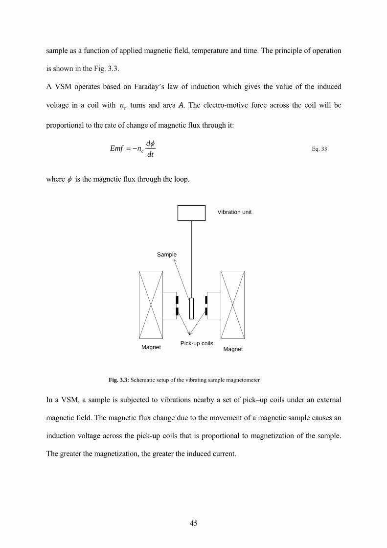
sample as a function of applied magnetic field, temperature and time. The principle of operation

is shown in the Fig. 3.3.

A VSM operates based on Faraday’s law of induction which gives the value of the induced

voltage in a coil with turns and area A. The electro-motive force across the coil will be

proportional to the rate of change of magnetic flux through it:

cn

dtdnEmf cφ

−= Eq. 33

where φ is the magnetic flux through the loop.

Sample

Vibration unit

Pick-up coilsMagnet Magnet

Fig. 3.3: Schematic setup of the vibrating sample magnetometer

In a VSM, a sample is subjected to vibrations nearby a set of pick–up coils under an external

magnetic field. The magnetic flux change due to the movement of a magnetic sample causes an

induction voltage across the pick-up coils that is proportional to magnetization of the sample.

The greater the magnetization, the greater the induced current.

45

46

4 Results and Discussion

4.1 Water-based ferrofluids containing magnetite polystyrene nanoparticles

This section deals with the developing of a new route which is based on miniemulsion processes

for the production of aqueous ferrofluids consisting of uniform and stable magnetic polystyrene

nanoparticles, which are highly homogeneous and possess high magnetite contents up to

40 wt.-%. The first step follows the classical procedure. Here, oleic acid coated magnetite

particles are dispersed in octane and combined with an aqueous surfactant solution. This

mixture is then miniemulsified and subsequently carefully heated to evaporate the octane which

leads to aqueous ferrofluid containing magnetite aggregates. To obtain an aqueous ferrofluid

consisting of polystyrene encapsulated magnetite particles, a second miniemulsion process is

used. Here, a mixture of the magnetite aggregate dispersion and a styrene miniemulsion are co-

sonicated, followed by a polymerization process. The final hybrid particles are characterized by

thermogravimetry, preparative ultracentrifugation, transmission electron microscopy and

magnetometry measurements.

In previous experiments,[ ] encapsulated magnetite particles were obtained by first mixing oleoyl

sarcosine acid coated magnetite into the monomer and then formulating a miniemulsion of the

monomer/magnetite dispersion in water. Due to aggregation of magnetite and the coupled

viscosity problems, the amount of magnetite in the monomer was limited to about 15 wt.-%.[66]

This reaction however still showed some imperfections since the distribution of magnetite

between the particles and within each particle was still rather heterogeneous, which was

presumably due to the interaction between the magnetite moieties and a related size- and

content-specific destabilization of the miniemulsion droplets. Also the influence of pH seemed

to be crucial, which was attributed to both the pH dependence of the surface charge of

magnetite and the protonation of the oleoyl sarcosine acid and the coupled interface energy.

47

In order to obtain homogeneous encapsulation with a high magnetite content, a three-step

process was intended to develop. In the first step, hydrophobized magnetite particles with a

diameter of about 10 nm were synthesized in a classical coprecipitation procedure. In a second

step, these magnetite particles were transformed to magnetite aggregates of about 40 to 200 nm

in water by using a miniemulsion process. In a third step, the magnetite aggregates were

encapsulated with a monomer by an ad-miniemulsification process and after polymerization,

polymer highly magnetite loaded particles were obtained.

The first step is already well known from the literature. It is the scope of this paper to develop

the second and the third step of the synthesis route.

The importance of the second step could be shown previously. If the small hydrophobized

magnetite particles obtained in the first step were dispersed in water as separate magnetite

particles, in the following fusion/fission process, only a very low number of these small

magnetite particles can collide with the monomer droplets resulting in a very low encapsulation

efficiency. Therefore, for a successful fusion/fission process larger magnetite aggregates are

necessary which could be obtained in the second step of the synthesis route by using the

miniemulsion process. The influence of reaction parameters on the magnetite aggregate size

will be discussed in detail.

The third step, the influence of the aggregate size and the presence of acrylic acid on the

encapsulation of the aggregates will be described. The three-step synthesis route is shown in

Fig. 4.1.

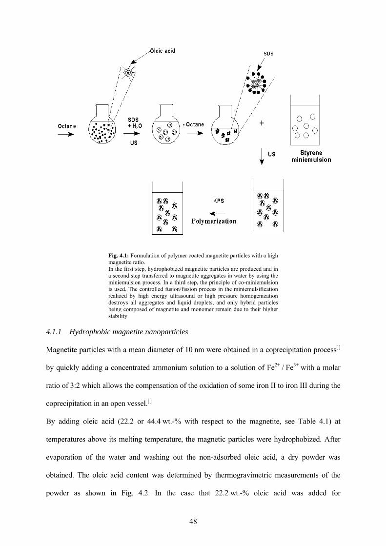
Fig. 4.1: Formulation of polymer coated magnetite particles with a high magnetite ratio. In the first step, hydrophobized magnetite particles are produced and in a second step transferred to magnetite aggregates in water by using the miniemulsion process. In a third step, the principle of co-miniemulsion is used. The controlled fusion/fission process in the miniemulsification realized by high energy ultrasound or high pressure homogenization destroys all aggregates and liquid droplets, and only hybrid particles being composed of magnetite and monomer remain due to their higher stability

4.1.1 Hydrophobic magnetite nanoparticles

Magnetite particles with a mean diameter of 10 nm were obtained in a coprecipitation process[ ]

by quickly adding a concentrated ammonium solution to a solution of Fe2+ / Fe3+ with a molar

ratio of 3:2 which allows the compensation of the oxidation of some iron II to iron III during the

coprecipitation in an open vessel.[ ]

By adding oleic acid (22.2 or 44.4 wt.-% with respect to the magnetite, see Table 4.1) at

temperatures above its melting temperature, the magnetic particles were hydrophobized. After

evaporation of the water and washing out the non-adsorbed oleic acid, a dry powder was

obtained. The oleic acid content was determined by thermogravimetric measurements of the

powder as shown in Fig. 4.2. In the case that 22.2 wt.-% oleic acid was added for

48

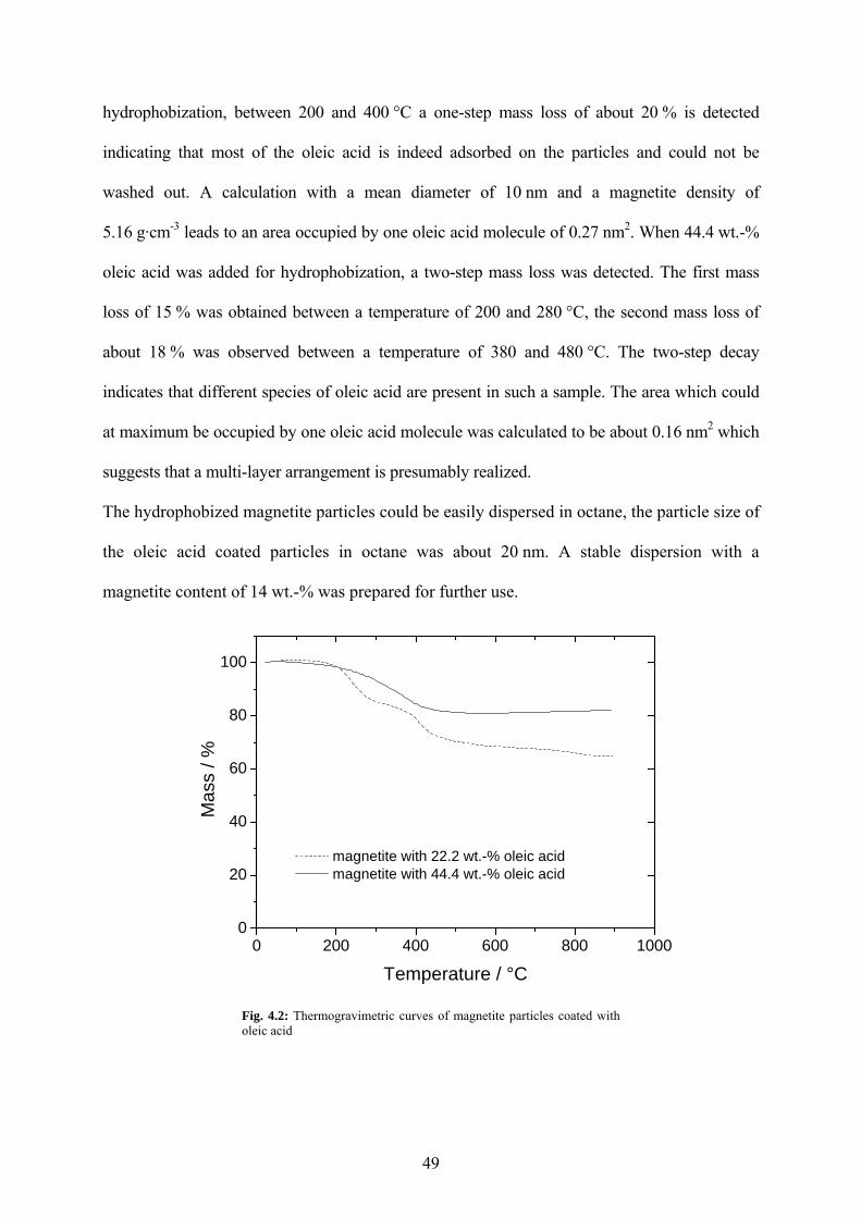
hydrophobization, between 200 and 400 °C a one-step mass loss of about 20 % is detected

indicating that most of the oleic acid is indeed adsorbed on the particles and could not be

washed out. A calculation with a mean diameter of 10 nm and a magnetite density of

5.16 g·cm-3 leads to an area occupied by one oleic acid molecule of 0.27 nm2. When 44.4 wt.-%

oleic acid was added for hydrophobization, a two-step mass loss was detected. The first mass

loss of 15 % was obtained between a temperature of 200 and 280 °C, the second mass loss of

about 18 % was observed between a temperature of 380 and 480 °C. The two-step decay

indicates that different species of oleic acid are present in such a sample. The area which could

at maximum be occupied by one oleic acid molecule was calculated to be about 0.16 nm2 which

suggests that a multi-layer arrangement is presumably realized.

The hydrophobized magnetite particles could be easily dispersed in octane, the particle size of

the oleic acid coated particles in octane was about 20 nm. A stable dispersion with a

magnetite content of 14 wt.-% was prepared for further use.

0 200 400 600 800 10000

20

40

60

80

100

magnetite with 22.2 wt.-% oleic acid magnetite with 44.4 wt.-% oleic acid

Mas

s / %

Temperature / °C

Fig. 4.2: Thermogravimetric curves of magnetite particles coated with oleic acid

49

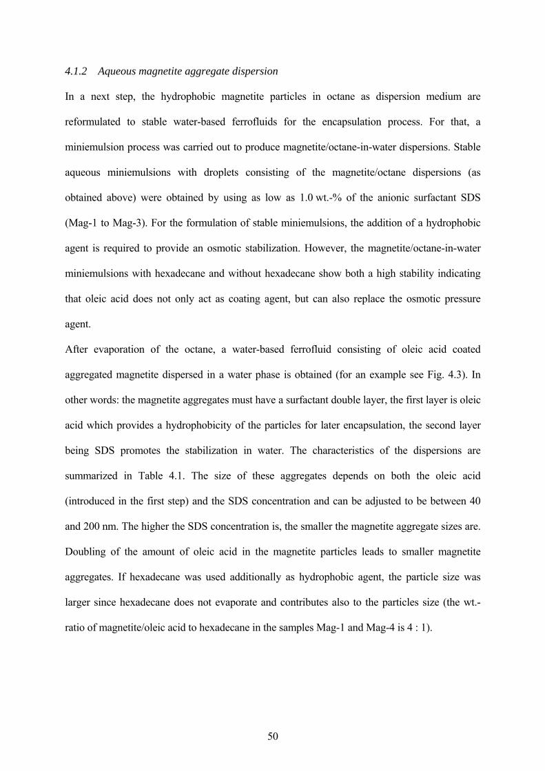
50

4.1.2 Aqueous magnetite aggregate dispersion

In a next step, the hydrophobic magnetite particles in octane as dispersion medium are

reformulated to stable water-based ferrofluids for the encapsulation process. For that, a

miniemulsion process was carried out to produce magnetite/octane-in-water dispersions. Stable

aqueous miniemulsions with droplets consisting of the magnetite/octane dispersions (as

obtained above) were obtained by using as low as 1.0 wt.-% of the anionic surfactant SDS

(Mag-1 to Mag-3). For the formulation of stable miniemulsions, the addition of a hydrophobic

agent is required to provide an osmotic stabilization. However, the magnetite/octane-in-water

miniemulsions with hexadecane and without hexadecane show both a high stability indicating

that oleic acid does not only act as coating agent, but can also replace the osmotic pressure

agent.

After evaporation of the octane, a water-based ferrofluid consisting of oleic acid coated

aggregated magnetite dispersed in a water phase is obtained (for an example see Fig. 4.3). In

other words: the magnetite aggregates must have a surfactant double layer, the first layer is oleic

acid which provides a hydrophobicity of the particles for later encapsulation, the second layer

being SDS promotes the stabilization in water. The characteristics of the dispersions are

summarized in Table 4.1. The size of these aggregates depends on both the oleic acid

(introduced in the first step) and the SDS concentration and can be adjusted to be between 40

and 200 nm. The higher the SDS concentration is, the smaller the magnetite aggregate sizes are.

Doubling of the amount of oleic acid in the magnetite particles leads to smaller magnetite

aggregates. If hexadecane was used additionally as hydrophobic agent, the particle size was

larger since hexadecane does not evaporate and contributes also to the particles size (the wt.-

ratio of magnetite/oleic acid to hexadecane in the samples Mag-1 and Mag-4 is 4 : 1).

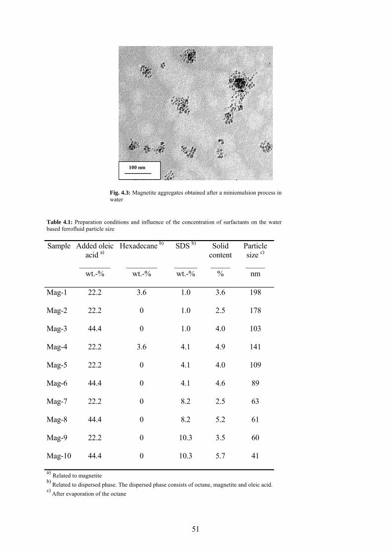
100 nm

Fig. 4.3: Magnetite aggregates obtained after a miniemulsion process in water

Table 4.1: Preparation conditions and influence of the concentration of surfactants on the water based ferrofluid particle size

Added oleic acid a)

________

Hexadecane b)

________

SDS b)

______

Solid content _____

Particle size c)

_____

Sample

wt.-%

wt.-% wt.-% % nm

Mag-1 22.2 3.6 1.0 3.6 198

Mag-2 22.2 0 1.0 2.5 178

Mag-3 44.4 0 1.0 4.0 103

Mag-4 22.2 3.6 4.1 4.9 141

Mag-5 22.2 0 4.1 4.0 109

Mag-6 44.4 0 4.1 4.6 89

Mag-7 22.2 0 8.2 2.5 63

Mag-8 44.4 0 8.2 5.2 61

Mag-9 22.2 0 10.3 3.5 60

Mag-10 44.4 0 10.3 5.7 41

a) Related to magnetite b) Related to dispersed phase. The dispersed phase consists of octane, magnetite and oleic acid.c) After evaporation of the octane

51

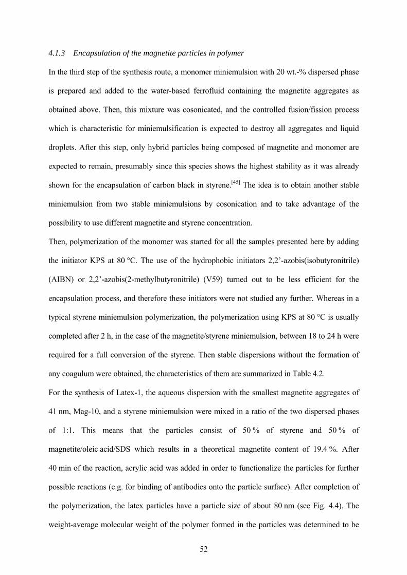
52

4.1.3 Encapsulation of the magnetite particles in polymer

In the third step of the synthesis route, a monomer miniemulsion with 20 wt.-% dispersed phase

is prepared and added to the water-based ferrofluid containing the magnetite aggregates as

obtained above. Then, this mixture was cosonicated, and the controlled fusion/fission process

which is characteristic for miniemulsification is expected to destroy all aggregates and liquid

droplets. After this step, only hybrid particles being composed of magnetite and monomer are

expected to remain, presumably since this species shows the highest stability as it was already

shown for the encapsulation of carbon black in styrene.[45] The idea is to obtain another stable

miniemulsion from two stable miniemulsions by cosonication and to take advantage of the

possibility to use different magnetite and styrene concentration.

Then, polymerization of the monomer was started for all the samples presented here by adding

the initiator KPS at 80 °C. The use of the hydrophobic initiators 2,2’-azobis(isobutyronitrile)

(AIBN) or 2,2’-azobis(2-methylbutyronitrile) (V59) turned out to be less efficient for the

encapsulation process, and therefore these initiators were not studied any further. Whereas in a

typical styrene miniemulsion polymerization, the polymerization using KPS at 80 °C is usually

completed after 2 h, in the case of the magnetite/styrene miniemulsion, between 18 to 24 h were

required for a full conversion of the styrene. Then stable dispersions without the formation of

any coagulum were obtained, the characteristics of them are summarized in Table 4.2.

For the synthesis of Latex-1, the aqueous dispersion with the smallest magnetite aggregates of

41 nm, Mag-10, and a styrene miniemulsion were mixed in a ratio of the two dispersed phases

of 1:1. This means that the particles consist of 50 % of styrene and 50 % of

magnetite/oleic acid/SDS which results in a theoretical magnetite content of 19.4 %. After

40 min of the reaction, acrylic acid was added in order to functionalize the particles for further

possible reactions (e.g. for binding of antibodies onto the particle surface). After completion of

the polymerization, the latex particles have a particle size of about 80 nm (see Fig. 4.4). The

weight-average molecular weight of the polymer formed in the particles was determined to be

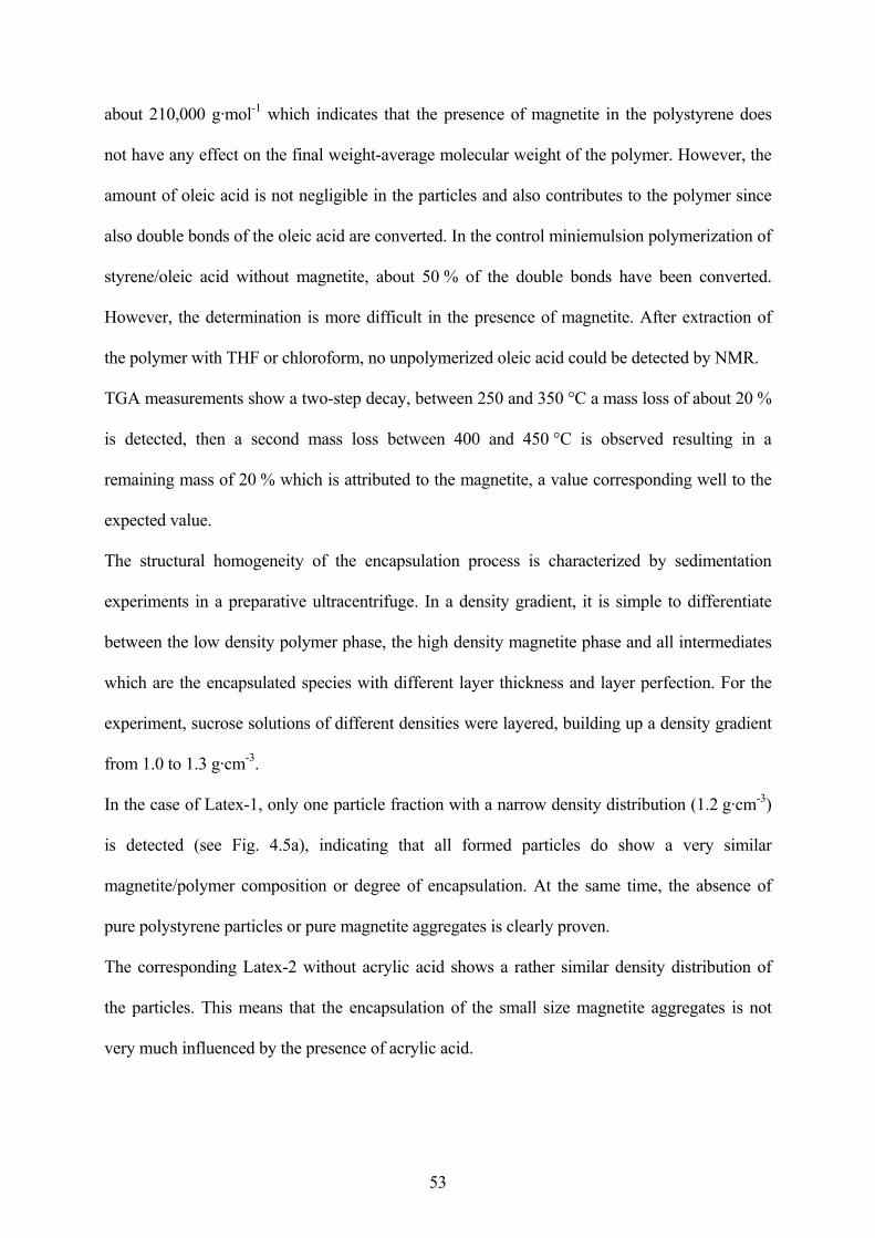
53

about 210,000 g·mol-1 which indicates that the presence of magnetite in the polystyrene does

not have any effect on the final weight-average molecular weight of the polymer. However, the

amount of oleic acid is not negligible in the particles and also contributes to the polymer since

also double bonds of the oleic acid are converted. In the control miniemulsion polymerization of

styrene/oleic acid without magnetite, about 50 % of the double bonds have been converted.

However, the determination is more difficult in the presence of magnetite. After extraction of

the polymer with THF or chloroform, no unpolymerized oleic acid could be detected by NMR.

TGA measurements show a two-step decay, between 250 and 350 °C a mass loss of about 20 %

is detected, then a second mass loss between 400 and 450 °C is observed resulting in a

remaining mass of 20 % which is attributed to the magnetite, a value corresponding well to the

expected value.

The structural homogeneity of the encapsulation process is characterized by sedimentation

experiments in a preparative ultracentrifuge. In a density gradient, it is simple to differentiate

between the low density polymer phase, the high density magnetite phase and all intermediates

which are the encapsulated species with different layer thickness and layer perfection. For the

experiment, sucrose solutions of different densities were layered, building up a density gradient

from 1.0 to 1.3 g·cm-3.

In the case of Latex-1, only one particle fraction with a narrow density distribution (1.2 g·cm-3)

is detected (see Fig. 4.5a), indicating that all formed particles do show a very similar

magnetite/polymer composition or degree of encapsulation. At the same time, the absence of

pure polystyrene particles or pure magnetite aggregates is clearly proven.

The corresponding Latex-2 without acrylic acid shows a rather similar density distribution of

the particles. This means that the encapsulation of the small size magnetite aggregates is not

very much influenced by the presence of acrylic acid.

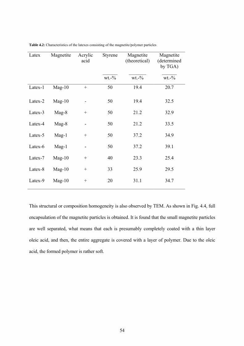
54

Table 4.2: Characteristics of the latexes consisting of the magnetite/polymer particles

Styrene

______

Magnetite (theoretical)

_______

Magnetite (determined

by TGA) ______

Latex Magnetite Acrylic acid

wt.-% wt.-% wt.-%

Latex-1 Mag-10 + 50 19.4 20.7

Latex-2 Mag-10 - 50 19.4 32.5

Latex-3 Mag-8 + 50 21.2 32.9

Latex-4 Mag-8 - 50 21.2 33.5

Latex-5 Mag-1 + 50 37.2 34.9

Latex-6 Mag-1 - 50 37.2 39.1

Latex-7 Mag-10 + 40 23.3 25.4

Latex-8 Mag-10 + 33 25.9 29.5

Latex-9 Mag-10 + 20 31.1 34.7

This structural or composition homogeneity is also observed by TEM. As shown in Fig. 4.4, full

encapsulation of the magnetite particles is obtained. It is found that the small magnetite particles

are well separated, what means that each is presumably completely coated with a thin layer

oleic acid, and then, the entire aggregate is covered with a layer of polymer. Due to the oleic

acid, the formed polymer is rather soft.

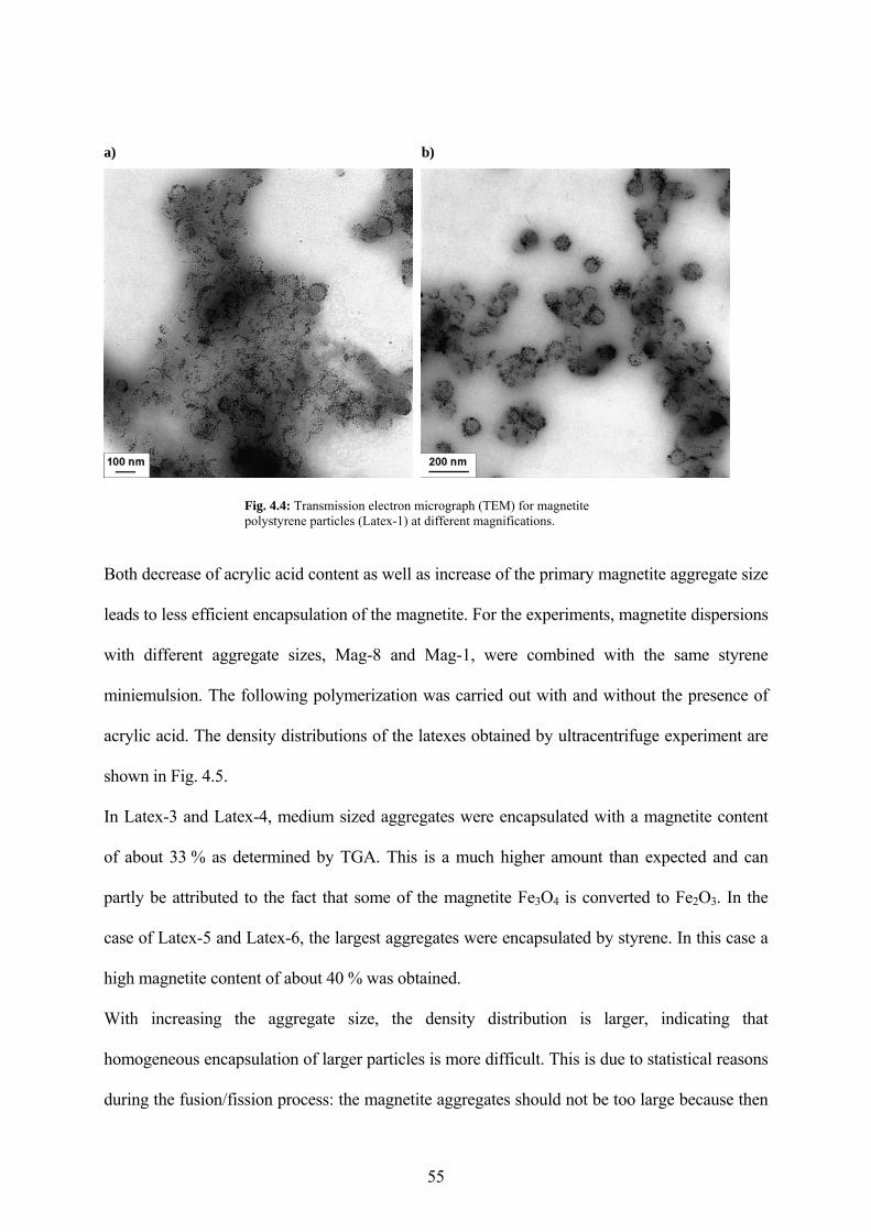
a) b)

Fig. 4.4: Transmission electron micrograph (TEM) for magnetite polystyrene particles (Latex-1) at different magnifications.

Both decrease of acrylic acid content as well as increase of the primary magnetite aggregate size

leads to less efficient encapsulation of the magnetite. For the experiments, magnetite dispersions

with different aggregate sizes, Mag-8 and Mag-1, were combined with the same styrene

miniemulsion. The following polymerization was carried out with and without the presence of

acrylic acid. The density distributions of the latexes obtained by ultracentrifuge experiment are

shown in Fig. 4.5.

In Latex-3 and Latex-4, medium sized aggregates were encapsulated with a magnetite content

of about 33 % as determined by TGA. This is a much higher amount than expected and can

partly be attributed to the fact that some of the magnetite Fe3O4 is converted to Fe2O3. In the

case of Latex-5 and Latex-6, the largest aggregates were encapsulated by styrene. In this case a

high magnetite content of about 40 % was obtained.

With increasing the aggregate size, the density distribution is larger, indicating that

homogeneous encapsulation of larger particles is more difficult. This is due to statistical reasons

during the fusion/fission process: the magnetite aggregates should not be too large because then

55

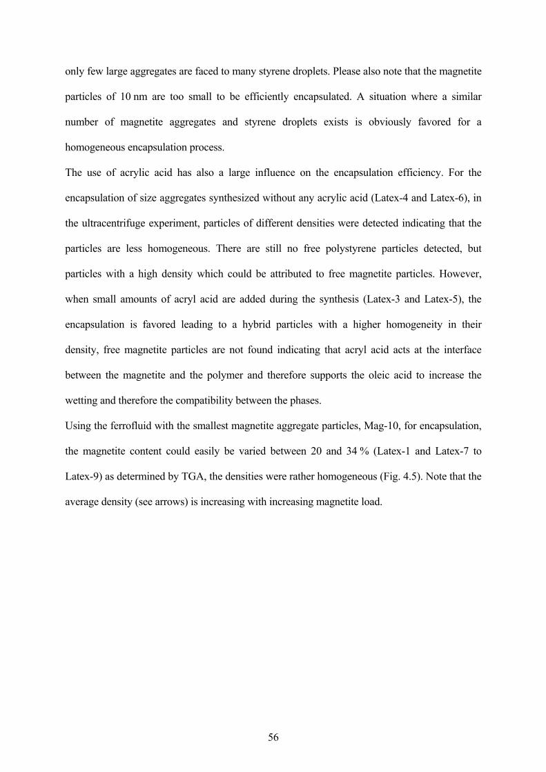
56

only few large aggregates are faced to many styrene droplets. Please also note that the magnetite

particles of 10 nm are too small to be efficiently encapsulated. A situation where a similar

number of magnetite aggregates and styrene droplets exists is obviously favored for a

homogeneous encapsulation process.

The use of acrylic acid has also a large influence on the encapsulation efficiency. For the

encapsulation of size aggregates synthesized without any acrylic acid (Latex-4 and Latex-6), in

the ultracentrifuge experiment, particles of different densities were detected indicating that the

particles are less homogeneous. There are still no free polystyrene particles detected, but

particles with a high density which could be attributed to free magnetite particles. However,

when small amounts of acryl acid are added during the synthesis (Latex-3 and Latex-5), the

encapsulation is favored leading to a hybrid particles with a higher homogeneity in their

density, free magnetite particles are not found indicating that acryl acid acts at the interface

between the magnetite and the polymer and therefore supports the oleic acid to increase the

wetting and therefore the compatibility between the phases.

Using the ferrofluid with the smallest magnetite aggregate particles, Mag-10, for encapsulation,

the magnetite content could easily be varied between 20 and 34 % (Latex-1 and Latex-7 to

Latex-9) as determined by TGA, the densities were rather homogeneous (Fig. 4.5). Note that the

average density (see arrows) is increasing with increasing magnetite load.

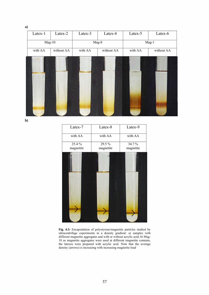
a)

Latex-1 Latex-2 Latex-3 Latex-4 Latex-5 Latex-6

Mag-10 Mag-8 Mag-1

with AA without AA with AA without AA with AA without AA

b)

Latex-7 Latex-8 Latex-9

with AA with AA with AA

25.4 % magnetite

29.5 % magnetite

34.7 % magnetite

Fig. 4.5: Encapsulation of polystyrene/magnetite particles studied by ultracentrifuge experiments in a density gradient: a) samples with different magnetite aggregates and with or without acrylic acid; b) Mag-10 as magnetite aggregates were used at different magnetite contents, the latexes were prepared with acrylic acid. Note that the average density (arrows) is increasing with increasing magnetite load

57

4.1.4 Magnetic properties

The magnetic properties of the synthesized ferrofluids with the polymer encapsulated magnetite

particles are of high interest for all further applications. The magnetic properties including the

saturation magnetization (Ms), the mass magnetic susceptibility (χ), the specific saturation

magnetization (σ, values extrapolated to H→∞), the relative saturation remanence (mr = Mr/Ms)

and the intrinsic coercivity (Hci) of some of the ferrofluids presented in this paper are presented

in Table 4.3 and Fig. 4.6. All of the ferrofluids show a typical superparamagnetic behavior at

room temperature without any hysteresis loop. The superparamagnetic behavior is also reflected

in the low Mr/Ms ratio and in the small Hci values. This clearly indicates that the magnetite

primary particles with a diameter of approximately 10 nm are still well separated in the polymer

particles (see diameter values, , Table 4.3). pd

In Fig. 4.6a, the magnetization curves for the samples at different stages of the synthesis are

compared, namely a) the oleic acid coated magnetite particles dispersed in octane (magnetite

particles in octane), b) the water-based ferrofluid containing the magnetite aggregates after

octane evaporation (Mag-10) and c) the polymer encapsulated magnetite aggregates (Latex-1).

For the oleic acid coated magnetite particles in octane, a saturation magnetization value of

87 emu·g-1 magnetite is obtained which is close to the saturation magnetization of the bulk

material (89 emu·g-1 magnetite). The magnetite aggregates in water, Mag-10, have a saturation

magnetization of 68 emu·g-1 magnetite, the loss of magnetization may be due to oxidation

processes during the sonication which leads to the formation of some non-magnetic iron oxide

(Fe2O3). For the polystyrene magnetite particles Latex-1, the saturation magnetization is still as

high as 53 emu·g-1 magnetite which is about 60 % of the magnetization of the bulk material. It

means that during the polymerization, probably again some of the magnetite converts to Fe2O3

due to the presence of the oxidizing initiator fragments.

58

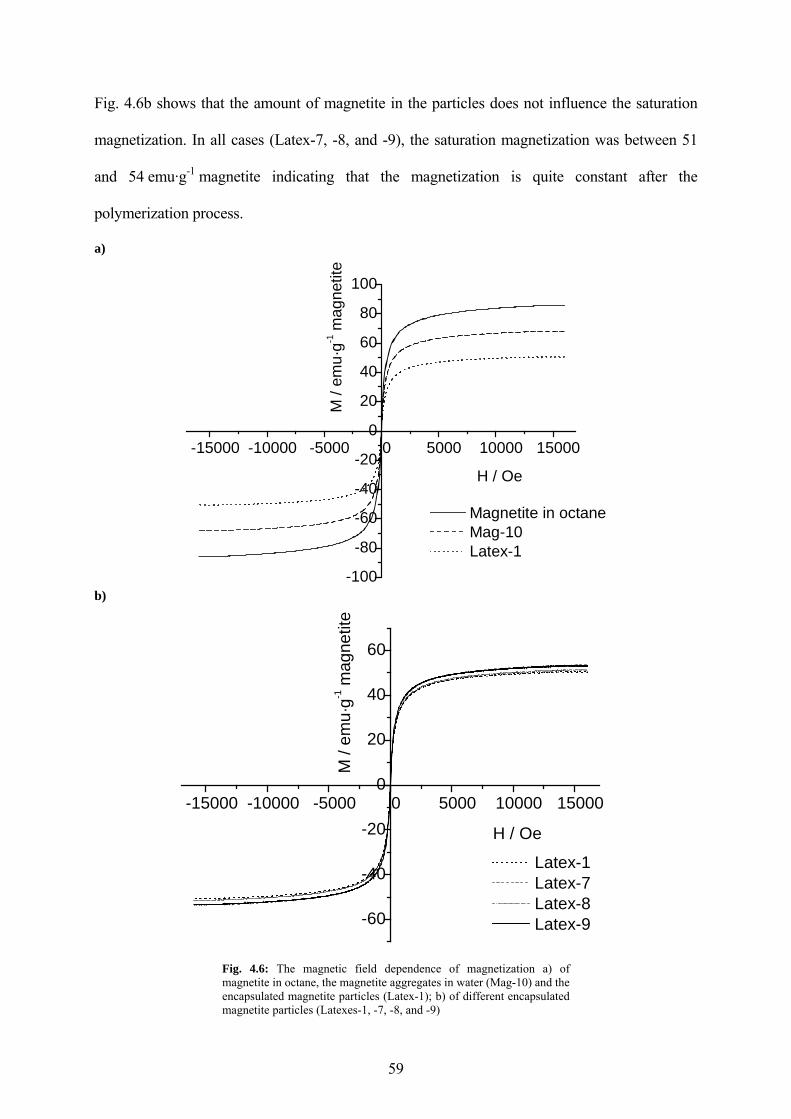
Fig. 4.6b shows that the amount of magnetite in the particles does not influence the saturation

magnetization. In all cases (Latex-7, -8, and -9), the saturation magnetization was between 51

and 54 emu·g-1 magnetite indicating that the magnetization is quite constant after the

polymerization process.

a)

-15000 -10000 -5000 0 5000 10000 15000

-100

-80

-60

-40

-20

0

20

40

60

80

100

Magnetite in octane Mag-10 Latex-1

M /

emu·

g-1 m

agne

tite

H / Oe

b)

-15000 -10000 -5000 0 5000 10000 15000

-60

-40

-20

0

20

40

60

Latex-1 Latex-7 Latex-8 Latex-9

M /

emu·

g-1 m

agne

tite

H / Oe

Fig. 4.6: The magnetic field dependence of magnetization a) of magnetite in octane, the magnetite aggregates in water (Mag-10) and the encapsulated magnetite particles (Latex-1); b) of different encapsulated magnetite particles (Latexes-1, -7, -8, and -9)

59

Table 4.3: Magnetic properties of the ferrofluids.

Ms

________

χ _____

∞→Hσ_______

Hci __

pd b) __

Sample

emu·g-1 magnetite

emu·Oe-1

emu·g-1 latex

Mr/Ms

Oe

nm

Magnetite particles in octanea)

~85.707 5.60·10-4 6.620 0.0026 1.12 2.20

Mag-10 67.939 1.03·10-4 1.108 0.0032 1.46 9.09

Latex-1 53.958 8.98·10-5 0.787 0.0034 1.54 9.77

Latex-7 52.910 1.71·10-3 0.764 0.0082 3.17 10.3

Latex-8 51.034 2.00·10-3 0.865 0.0059 2.28 10.59

Latex-9 52.81 2.40·10-3 0.909 0.0040 1.46 10.89

a) Little evaporation might have taken place during the measurement b) Values obtained from Eq. 9

4.1.5 Using biosurfactants

The sodium salt of the cholic acid (3α,7α,12α trihydroxy-5β-cholan-24 acid) was used instead

of SDS with the same conditions of the sample Mag-10 for the stabilization of the magnetite

particles in water. No stabilization of the magnetite particles was achieved with the use of

lecithin and Tween 80 due to probably to the absence of the carboxylic group. Cholic acid

sodium salt can excellently be used for the stabilization of magnetic aggregates in water (see

Fig. 4.7).

60

200nm

Fig. 4.7: Magnetite aggregates in water with cholic acid as surfactant.

4.2 Nanostructured composites from the iron pentacarbonyl decomposition

This section deals with the results and discussions of the approach for the production of new

confined paramagnetic nanocomposites directly from the thermal decomposition of iron

pentacarbonyl within the monomer phase containing oleic acid. Subsequently, a miniemulsion

polymerization process, using the iron containing monomer dispersion as dispersed phase, was

carried out. This two-step process enables the confinement of iron oxide nanoparticles in

poly(butyl methacrylate) and their high order structure. The first step consists of the thermal

decomposition of the iron pentacarbonyl containing in the monomer phase using oleic acid as

stabilizer without any solvent. In the second step this iron containing monomer dispersion was

used for making a miniemulsion polymerization thereof. The two-step process enables the

immediately polymerization of the monomer phase containing iron particles for the production

of nanostructured composites with paramagnetic properties.

The final high structured nanocomposites are mainly characterized by transmission electron

microscopy, thermogravimetry, small- and wide angle X-ray, measurements, preparative

ultracentrifugation, infrared spectroscopy and magnetization measurements.

61

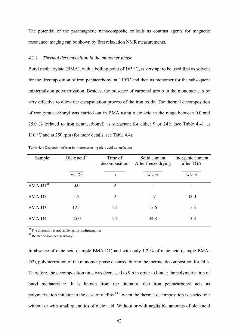
62

The potential of the paramagnetic nanocomposite colloids as contrast agents for magnetic

resonance imaging can be shown by first relaxation NMR measurements.

4.2.1 Thermal decomposition in the monomer phase

Butyl methacrylate (BMA), with a boiling point of 163 °C, is very apt to be used first as solvent

for the decomposition of iron pentacarbonyl at 110°C and then as monomer for the subsequent

miniemulsion polymerization. Besides, the presence of carbonyl group in the monomer can be

very effective to allow the encapsulation process of the iron oxide. The thermal decomposition

of iron pentacarbonyl was carried out in BMA using oleic acid in the range between 0.0 and

25.0 % (related to iron pentacarbonyl) as surfactant for either 9 or 24 h (see Table 4.4), at

110 °C and at 250 rpm (for more details, see Table 4.4).

Table 4.4: Dispersion of iron in monomer using oleic acid as surfactant

Sample Oleic acidb)

______ wt.-%

Time of decomposition

_________ h

Solid content After freeze drying

________ wt.-%

Inorganic content after TGA ________

wt.-%

BMA-D1a) 0.0 9 - -

BMA-D2 1.2 9 1.7 42.0

BMA-D3 12.5 24 15.6 15.3

BMA-D4 25.0 24 34.8 13.3

a) The dispersion is not stable against sedimentation b) Related to iron pentacarbonyl

In absence of oleic acid (sample BMA-D1) and with only 1.2 % of oleic acid (sample BMA-

D2), polymerization of the monomer phase occurred during the thermal decomposition for 24 h.

Therefore, the decomposition time was decreased to 9 h in order to hinder the polymerization of

butyl methacrylate. It is known from the literature that iron pentacarbonyl acts as

polymerization initiator in the case of olefins[133] when the thermal decomposition is carried out

without or with small quantities of oleic acid. Without or with negligible amounts of oleic acid

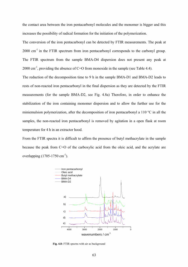
the contact area between the iron pentacarbonyl molecules and the monomer is bigger and this

increases the possibility of radical formation for the initiation of the polymerization.

The conversion of the iron pentacarbonyl can be detected by FTIR measurements. The peak at

2000 cm-1 in the FTIR spectrum from iron pentacarbonyl corresponds to the carbonyl group.

The FTIR spectrum from the sample BMA-D4 dispersion does not present any peak at

2000 cm-1, providing the absence of C=O from monoxide in the sample (see Table 4.4).

The reduction of the decomposition time to 9 h in the sample BMA-D1 and BMA-D2 leads to

rests of non-reacted iron pentacarbonyl in the final dispersion as they are detected by the FTIR

measurements (for the sample BMA-D2, see Fig. 4.8a) Therefore, in order to enhance the

stabilization of the iron containing monomer dispersion and to allow the further use for the

miniemulsion polymerization, after the decomposition of iron pentacarbonyl a 110 °C in all the

samples, the non-reacted iron pentacarbonyl is removed by agitation in a open flask at room

temperature for 4 h in an extractor hood.

From the FTIR spectra it is difficult to affirm the presence of butyl methacrylate in the sample

because the peak from C=O of the carboxylic acid from the oleic acid, and the acrylate are

overlapping (1705-1750 cm-1).

4000 3000 2000 1000 0

e)

d)

c)

b)

a)

Iron pentacarbonyl Oleic acid Butyl methacrylate BMA-D4 BMA-D2

wavenumbers / cm-1

Fig. 4.8: FTIR spectra with air as background

63

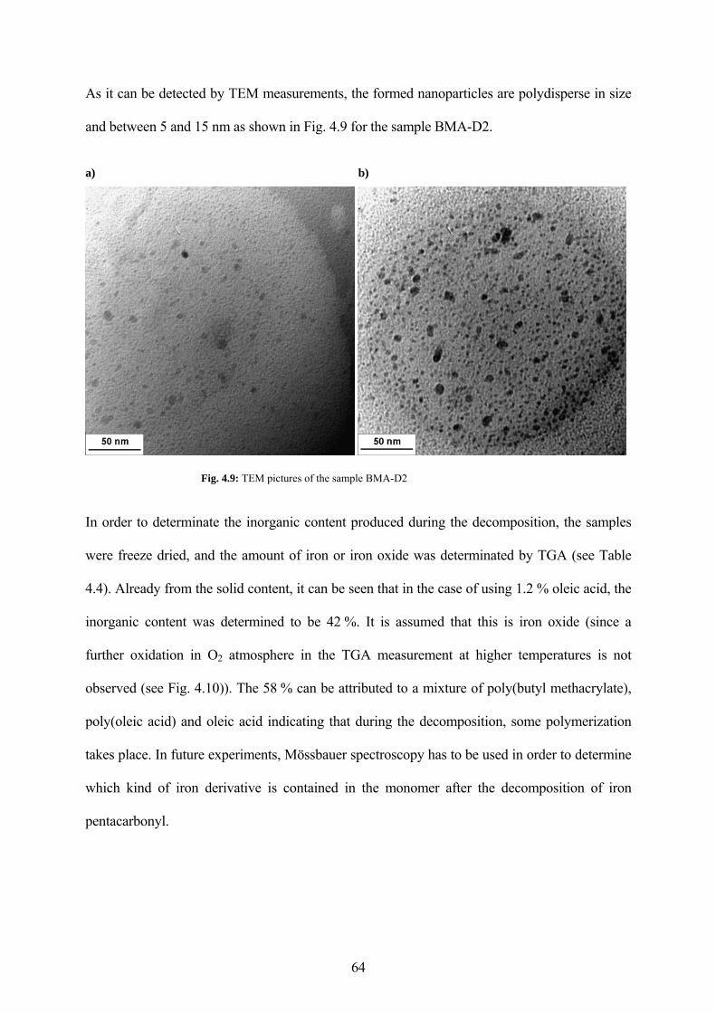
As it can be detected by TEM measurements, the formed nanoparticles are polydisperse in size

and between 5 and 15 nm as shown in Fig. 4.9 for the sample BMA-D2.

a) b)

Fig. 4.9: TEM pictures of the sample BMA-D2

In order to determinate the inorganic content produced during the decomposition, the samples

were freeze dried, and the amount of iron or iron oxide was determinated by TGA (see Table

4.4). Already from the solid content, it can be seen that in the case of using 1.2 % oleic acid, the

inorganic content was determined to be 42 %. It is assumed that this is iron oxide (since a

further oxidation in O2 atmosphere in the TGA measurement at higher temperatures is not

observed (see Fig. 4.10)). The 58 % can be attributed to a mixture of poly(butyl methacrylate),

poly(oleic acid) and oleic acid indicating that during the decomposition, some polymerization

takes place. In future experiments, Mössbauer spectroscopy has to be used in order to determine

which kind of iron derivative is contained in the monomer after the decomposition of iron

pentacarbonyl.

64

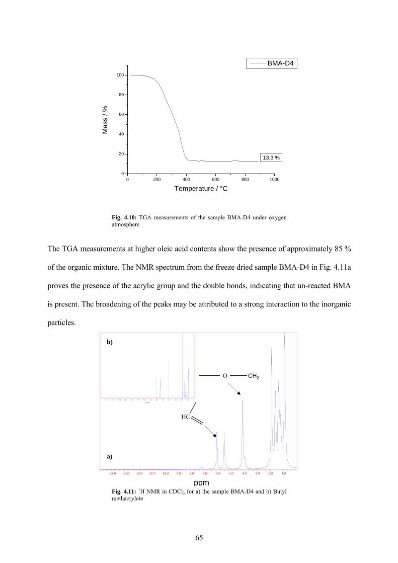
0 200 400 600 800 10000

20

40

60

80

100

13.3 %

Mas

s / %

Temperature / °C

BMA-D4

Fig. 4.10: TGA measurements of the sample BMA-D4 under oxygen atmosphere

The TGA measurements at higher oleic acid contents show the presence of approximately 85 %

of the organic mixture. The NMR spectrum from the freeze dried sample BMA-D4 in Fig. 4.11a

proves the presence of the acrylic group and the double bonds, indicating that un-reacted BMA

is present. The broadening of the peaks may be attributed to a strong interaction to the inorganic

particles.

(ppm)1.02.03.04.05.06.07.08.09.010.011.012.013.014.0

(ppm)1.02.03.04.05.06.07.08.09.010.011.012.013.014.0

65

Fig. 4.11: 1H NMR in CDCl3 for a) the sample BMA-D4 and b) Butyl methacrylate

HC

O CH2

ppm

a)

b)

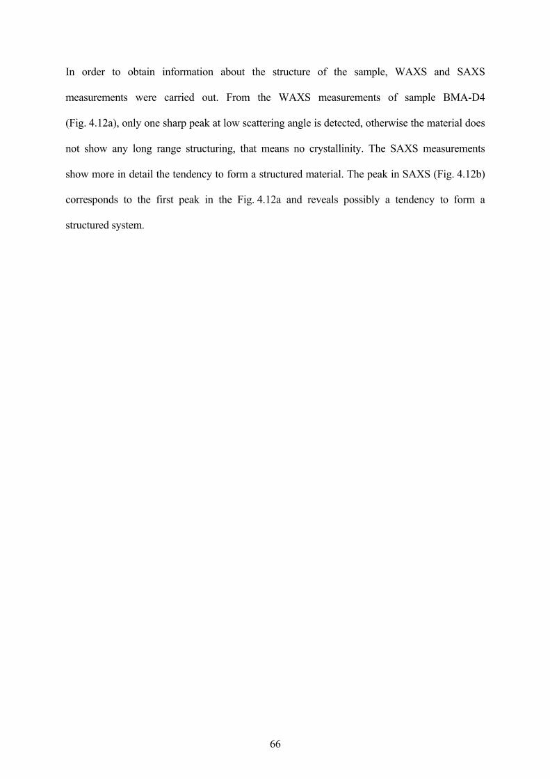
66

In order to obtain information about the structure of the sample, WAXS and SAXS

measurements were carried out. From the WAXS measurements of sample BMA-D4

(Fig. 4.12a), only one sharp peak at low scattering angle is detected, otherwise the material does

not show any long range structuring, that means no crystallinity. The SAXS measurements

show more in detail the tendency to form a structured material. The peak in SAXS (Fig. 4.12b)

corresponds to the first peak in the Fig. 4.12a and reveals possibly a tendency to form a

structured system.

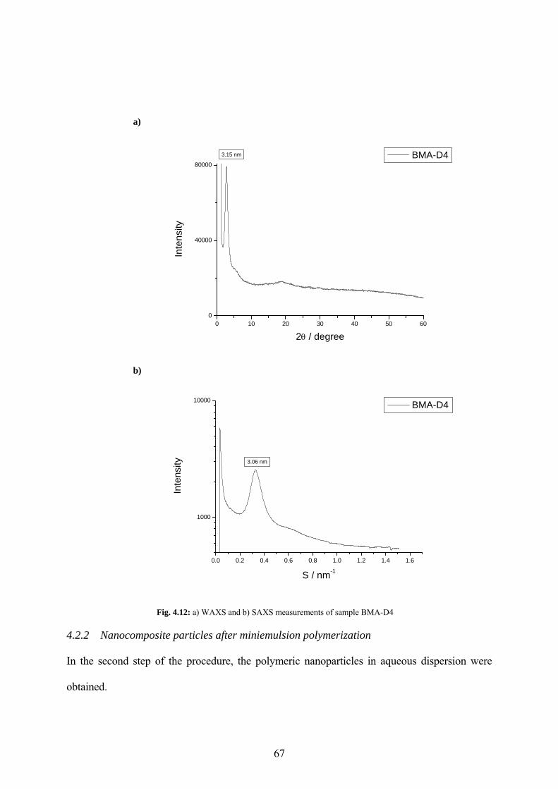
0 10 20 30 40 50 600

40000

80000

3.15 nm

Inte

nsity

2θ / degree

BMA-D4

a)

b)

67

0.0 0.2 0.4 0.6 0.8 1.0 1.2 1.4 1.6

1000

10000

3.06 nm

Inte

nsity

S / nm-1

BMA-D4

Fig. 4.12: a) WAXS and b) SAXS measurements of sample BMA-D4

4.2.2 Nanocomposite particles after miniemulsion polymerization

In the second step of the procedure, the polymeric nanoparticles in aqueous dispersion were

obtained.

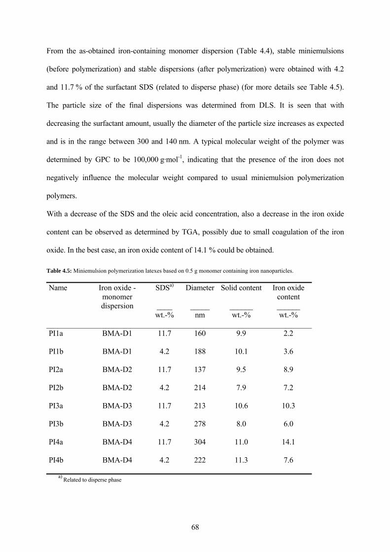
68

From the as-obtained iron-containing monomer dispersion (Table 4.4), stable miniemulsions

(before polymerization) and stable dispersions (after polymerization) were obtained with 4.2

and 11.7 % of the surfactant SDS (related to disperse phase) (for more details see Table 4.5).

The particle size of the final dispersions was determined from DLS. It is seen that with

decreasing the surfactant amount, usually the diameter of the particle size increases as expected

and is in the range between 300 and 140 nm. A typical molecular weight of the polymer was

determined by GPC to be 100,000 g·mol-1, indicating that the presence of the iron does not

negatively influence the molecular weight compared to usual miniemulsion polymerization

polymers.

With a decrease of the SDS and the oleic acid concentration, also a decrease in the iron oxide

content can be observed as determined by TGA, possibly due to small coagulation of the iron

oxide. In the best case, an iron oxide content of 14.1 % could be obtained.

Table 4.5: Miniemulsion polymerization latexes based on 0.5 g monomer containing iron nanoparticles.

Name Iron oxide -monomer dispersion

SDSa)

____ wt.-%

Diameter

_____ nm

Solid content

______ wt.-%

Iron oxide content ______ wt.-%

PI1a BMA-D1 11.7 160 9.9 2.2

PI1b BMA-D1 4.2 188 10.1 3.6

PI2a BMA-D2 11.7 137 9.5 8.9

PI2b BMA-D2 4.2 214 7.9 7.2

PI3a BMA-D3 11.7 213 10.6 10.3

PI3b BMA-D3 4.2 278 8.0 6.0

PI4a BMA-D4 11.7 304 11.0 14.1

PI4b BMA-D4 4.2 222 11.3 7.6

a) Related to disperse phase

69

TEM pictures of the sample PI3a-latex obtained after the miniemulsion polymerization from

sample BMA-D3-24 h decomposition are shown in the Fig. 4.13 and Fig. 4.14 at low and high

magnifications, respectively. In Fig. 4.13, iron containing aggregates can be observed which are

engulfed by the poly(butyl methacrylate) in an eye-like assembly. The size of the particles is

between 500 nm and 1 µm which is not in agreement with the size observed in the TEM

pictures, but can be explained by the low Tg of the polymer leading to pancake-like structures

while TEM-preparation. The iron containing aggregates consist of discrete iron oxide particles,

which are presumably oleic acid coated. Because of the oleic acid, strongly hydrophobic iron

oxide aggregates are demixed from the polymer phase. The polarity of the two phases is

presumably very different. At higher magnifications of this sample PI3a (see Fig. 4.14a, and b),

a highly ordered structure consisting of needles or bars which are presumably formed for the

assembly of iron containing nanoparticles which in turn are coated with a layer of oleic acid can

be observed. The SAXS measurement (Fig. 4.15a) reveals a lamellar structure with a repeat

period of 3.9 nm. Presumably, in the highly reductive presence of elemental iron, oleic acid is

reduced to stearic acid or to iron stearate. The stearic acid then can crystallize and is not able to

stabilize the iron particles in the polymer particles and therefore a very strong demixing is

obtained in the final composite nanoparticles. The WAXS spectrum (Fig. 4.15b) reveals rather

amorphous material as already seen in the first part of this section.

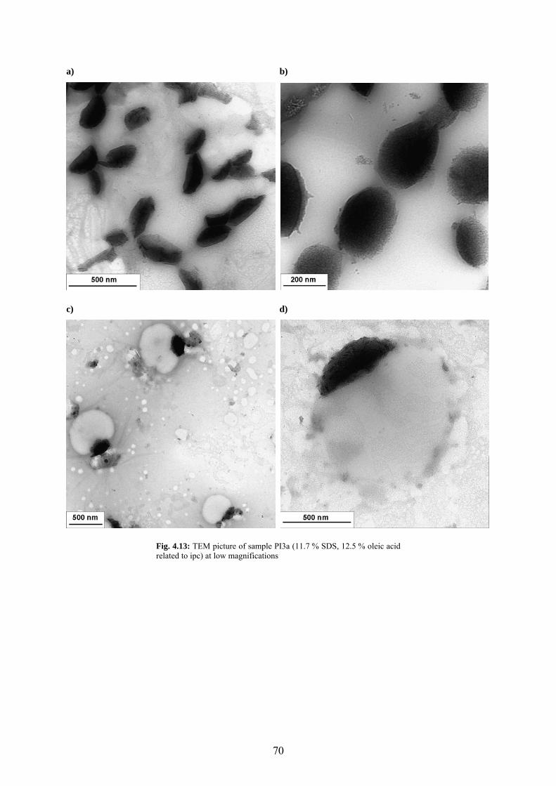
a) b)

c) d)

Fig. 4.13: TEM picture of sample PI3a (11.7 % SDS, 12.5 % oleic acid related to ipc) at low magnifications

70

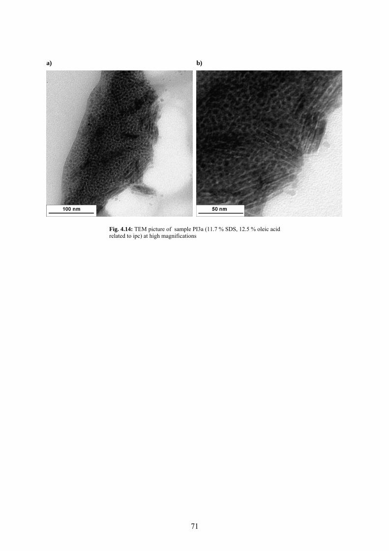
a) b)

Fig. 4.14: TEM picture of sample PI3a (11.7 % SDS, 12.5 % oleic acid related to ipc) at high magnifications

71

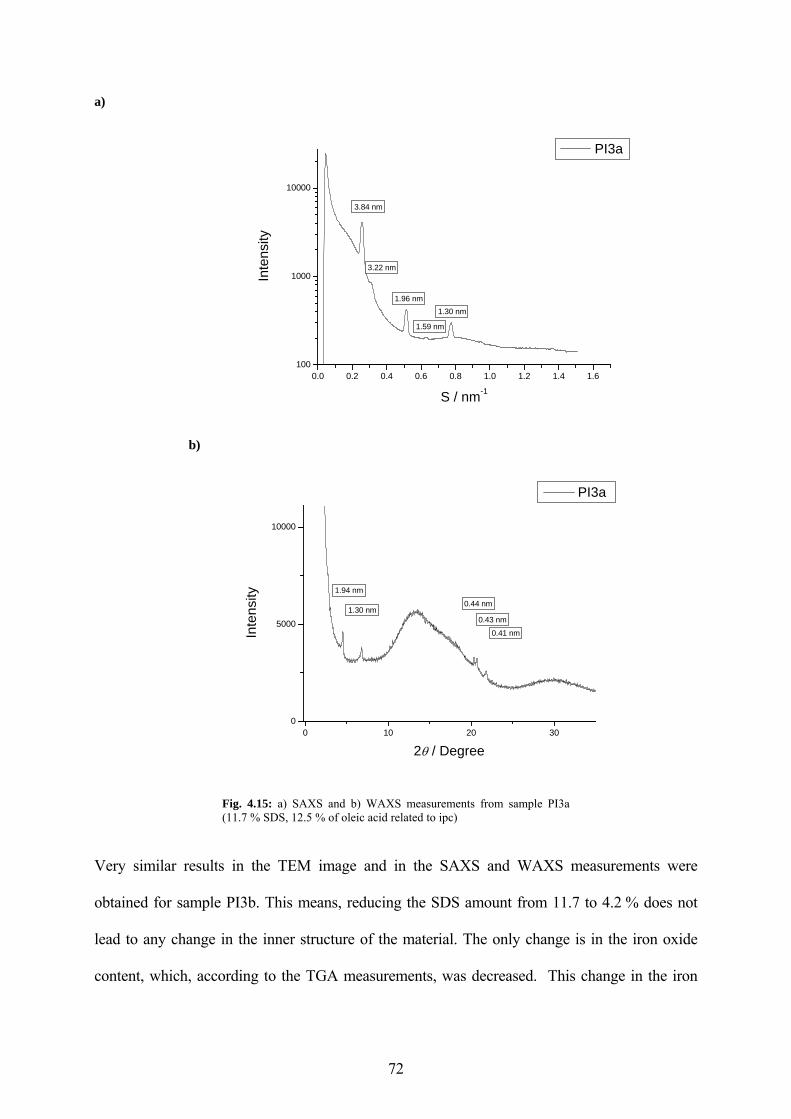
a)

0.0 0.2 0.4 0.6 0.8 1.0 1.2 1.4 1.6100

1000

10000

PI3a

1.30 nm

1.59 nm

1.96 nm

3.22 nm

3.84 nm

Inte

nsity

S / nm-1

0 10 20 300

5000

10000

0.41 nm

0.43 nm

0.44 nm1.30 nm

1.94 nm

Inte

nsity

2θ / Degree

PI3a

b)

Fig. 4.15: a) SAXS and b) WAXS measurements from sample PI3a (11.7 % SDS, 12.5 % of oleic acid related to ipc)

Very similar results in the TEM image and in the SAXS and WAXS measurements were

obtained for sample PI3b. This means, reducing the SDS amount from 11.7 to 4.2 % does not

lead to any change in the inner structure of the material. The only change is in the iron oxide

content, which, according to the TGA measurements, was decreased. This change in the iron

72

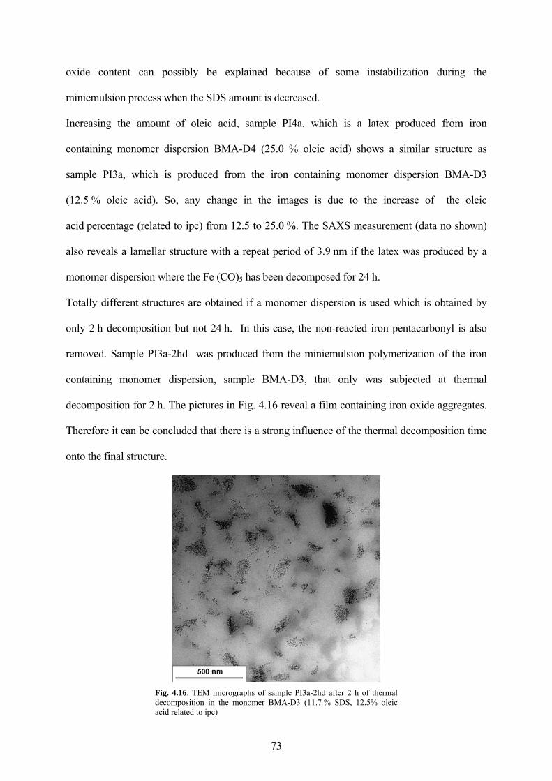
oxide content can possibly be explained because of some instabilization during the

miniemulsion process when the SDS amount is decreased.

Increasing the amount of oleic acid, sample PI4a, which is a latex produced from iron

containing monomer dispersion BMA-D4 (25.0 % oleic acid) shows a similar structure as

sample PI3a, which is produced from the iron containing monomer dispersion BMA-D3

(12.5 % oleic acid). So, any change in the images is due to the increase of the oleic

acid percentage (related to ipc) from 12.5 to 25.0 %. The SAXS measurement (data no shown)

also reveals a lamellar structure with a repeat period of 3.9 nm if the latex was produced by a

monomer dispersion where the Fe (CO)5 has been decomposed for 24 h.

Totally different structures are obtained if a monomer dispersion is used which is obtained by

only 2 h decomposition but not 24 h. In this case, the non-reacted iron pentacarbonyl is also

removed. Sample PI3a-2hd was produced from the miniemulsion polymerization of the iron

containing monomer dispersion, sample BMA-D3, that only was subjected at thermal

decomposition for 2 h. The pictures in Fig. 4.16 reveal a film containing iron oxide aggregates.

Therefore it can be concluded that there is a strong influence of the thermal decomposition time

onto the final structure.

Fig. 4.16: TEM micrographs of sample PI3a-2hd after 2 h of thermal decomposition in the monomer BMA-D3 (11.7 % SDS, 12.5% oleic acid related to ipc)

73

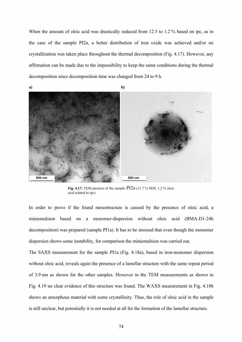
When the amount of oleic acid was drastically reduced from 12.5 to 1.2 % based on ipc, as in

the case of the sample PI2a, a better distribution of iron oxide was achieved and/or no

crystallization was taken place throughout the thermal decomposition (Fig. 4.17). However, any

affirmation can be made due to the impossibility to keep the same conditions during the thermal

decomposition since decomposition time was changed from 24 to 9 h.

a) b)

Fig. 4.17: TEM pictures of the sample PI2a (11.7 % SDS, 1.2 % oleic acid related to ipc)

In order to prove if the found mesostructure is caused by the presence of oleic acid, a

miniemulsion based on a monomer-dispersion without oleic acid (BMA-D1-24h

decomposition) was prepared (sample PI1a). It has to be stressed that even though the monomer

dispersion shows some instability, for comparison the miniemulsion was carried out.

The SAXS measurement for the sample PI1a (Fig. 4.18a), based in iron-monomer dispersion

without oleic acid, reveals again the presence of a lamellar structure with the same repeat period

of 3.9 nm as shown for the other samples. However in the TEM measurements as shown in

Fig. 4.19 no clear evidence of this structure was found. The WAXS measurement in Fig. 4.18b

shows an amorphous material with some crystallinity. Thus, the role of oleic acid in the sample

is still unclear, but potentially it is not needed at all for the formation of the lamellar structure.

74

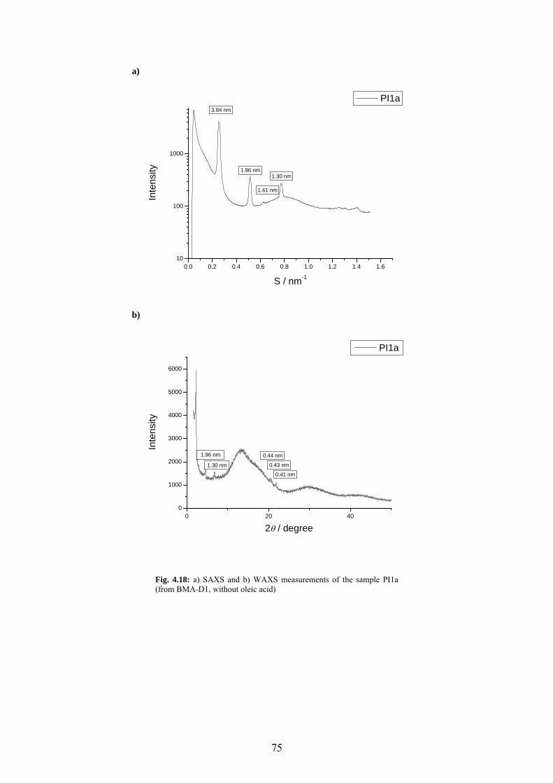
a)

0.0 0.2 0.4 0.6 0.8 1.0 1.2 1.4 1.610

100

1000

1.61 nm

1.30 nm1.96 nm

3.84 nm

Inte

nsity

S / nm-1

PI1a

b)

0 20 400

1000

2000

3000

4000

5000

6000

0.41 nm

0.43 nm

0.44 nm

1.30 nm

1.96 nm

Inte

nsity

2θ / degree

PI1a

Fig. 4.18: a) SAXS and b) WAXS measurements of the sample PI1a (from BMA-D1, without oleic acid)

75

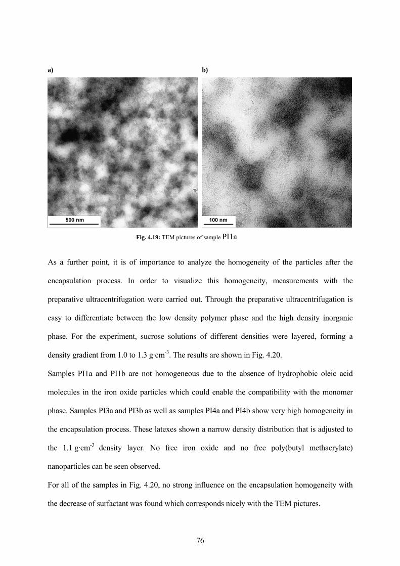
a) b)

Fig. 4.19: TEM pictures of sample PI1a

As a further point, it is of importance to analyze the homogeneity of the particles after the

encapsulation process. In order to visualize this homogeneity, measurements with the

preparative ultracentrifugation were carried out. Through the preparative ultracentrifugation is

easy to differentiate between the low density polymer phase and the high density inorganic

phase. For the experiment, sucrose solutions of different densities were layered, forming a

density gradient from 1.0 to 1.3 g·cm-3. The results are shown in Fig. 4.20.

Samples PI1a and PI1b are not homogeneous due to the absence of hydrophobic oleic acid

molecules in the iron oxide particles which could enable the compatibility with the monomer

phase. Samples PI3a and PI3b as well as samples PI4a and PI4b show very high homogeneity in

the encapsulation process. These latexes shown a narrow density distribution that is adjusted to

the 1.1 g·cm-3 density layer. No free iron oxide and no free poly(butyl methacrylate)

nanoparticles can be seen observed.

For all of the samples in Fig. 4.20, no strong influence on the encapsulation homogeneity with

the decrease of surfactant was found which corresponds nicely with the TEM pictures.

76

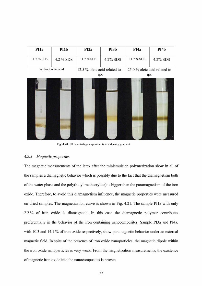
PI1a

PI1b

PI3a

PI3b

PI4a

PI4b

11.7 % SDS 4.2 % SDS 11.7 % SDS 4.2% SDS 11.7 % SDS 4.2% SDS

Without oleic acid

12.5 % oleic acid related to ipc

25.0 % oleic acid related to ipc

Fig. 4.20: Ultracentrifuge experiments in a density gradient

4.2.3 Magnetic properties

The magnetic measurements of the latex after the miniemulsion polymerization show in all of

the samples a diamagnetic behavior which is possibly due to the fact that the diamagnetism both

of the water phase and the poly(butyl methacrylate) is bigger than the paramagnetism of the iron

oxide. Therefore, to avoid this diamagnetism influence, the magnetic properties were measured

on dried samples. The magnetization curve is shown in Fig. 4.21. The sample PI1a with only

2.2 % of iron oxide is diamagnetic. In this case the diamagnetic polymer contributes

preferentially in the behavior of the iron containing nanocomposites. Sample PI3a and PI4a,

with 10.3 and 14.1 % of iron oxide respectively, show paramagnetic behavior under an external

magnetic field. In spite of the presence of iron oxide nanoparticles, the magnetic dipole within

the iron oxide nanoparticles is very weak. From the magnetization measurements, the existence

of magnetic iron oxide into the nanocomposites is proven.

77

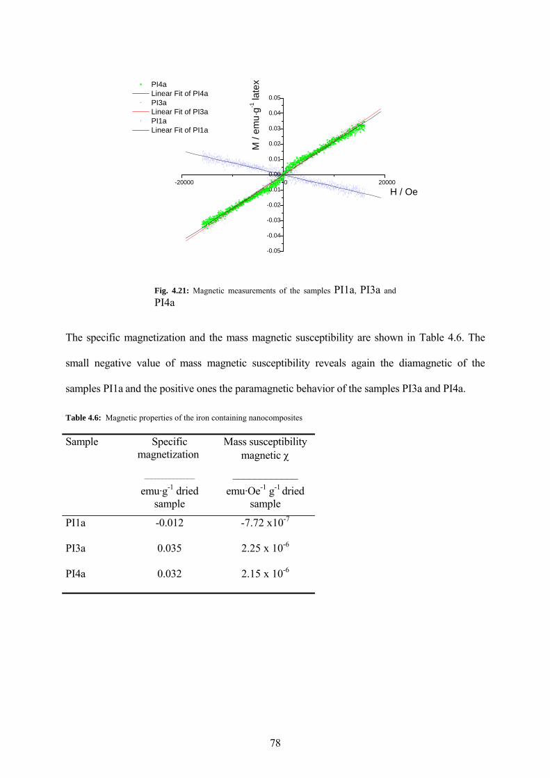
-20000 0 20000

-0.05

-0.04

-0.03

-0.02

-0.01

0.00

0.01

0.02

0.03

0.04

0.05

PI4a Linear Fit of PI4a PI3a Linear Fit of PI3a PI1a Linear Fit of PI1a

M /

emu·

g-1 la

tex

H / Oe

Fig. 4.21: Magnetic measurements of the samples PI1a, PI3a and PI4a

The specific magnetization and the mass magnetic susceptibility are shown in Table 4.6. The

small negative value of mass magnetic susceptibility reveals again the diamagnetic of the

samples PI1a and the positive ones the paramagnetic behavior of the samples PI3a and PI4a.

Table 4.6: Magnetic properties of the iron containing nanocomposites

Specific magnetization

______________

Mass susceptibility magnetic χ

____________

Sample

emu·g-1 dried sample

emu·Oe-1 g-1 dried sample

PI1a -0.012 -7.72 x10-7

PI3a 0.035 2.25 x 10-6

PI4a 0.032 2.15 x 10-6

78

79

4.3 Gadolinium-based nanoparticles

This section presents the results and discussion concerning with the research approach used for

the preparation of new nanolayered composites consisting of poly(butyl acrylate) (PBA) and

organic-soluble lanthanide chelates by miniemulsion process. Just by the miniemulsion process

and in a very simple way, nanolayered composites are formed. It should be stressed that the

most common way to produce nanolayered composites consisting of inorganic and polymer is

by templating process (see section 2.5.2). These layered nanocomposites present paramagnetic

behavior and a very high relaxivity, as shown in the magnetization and NMR relaxation

measurements, respectively. The term “layered nanocomposites” and “nanolayered composites”

are used synonymously.

4.3.1 Nanostructured composites

Here, we describe the polymerization of butyl acrylate in presence of different lanthanide

complexes and analyze the resulting structures mainly with transmission electron microscopy

(TEM), small angle X-ray scattering (SAXS), and thermogravimetry analysis (TGA). It will

turn out that all systems form highly organized lamellar nanocomposites with a spin rich

lanthanide subphase where the repeat period is of the order of 3-4 nm.

The composition of the samples discussed in this section is summarized in Table 4.7. All

polymerization reactions occur analogous to those of the pure monomer; especially, no

destabilization or macroscopic demixing throughout polymerization is obtained.

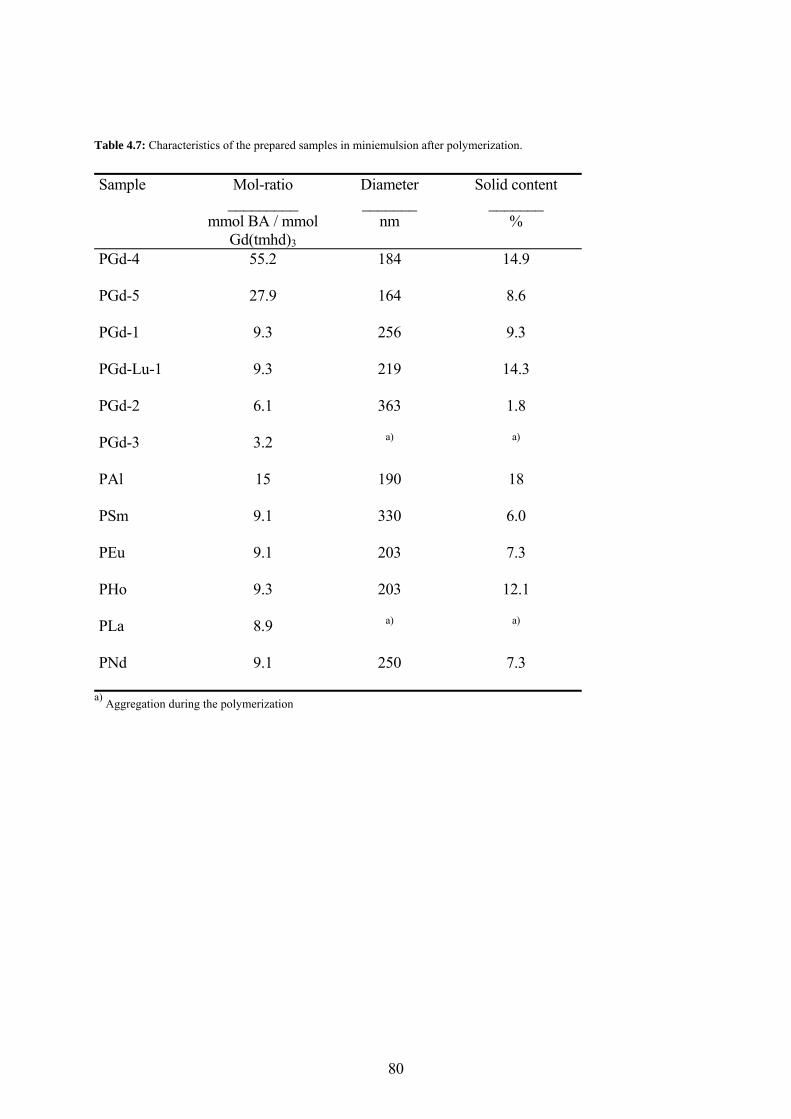
Table 4.7: Characteristics of the prepared samples in miniemulsion after polymerization.

a) Aggregation during the polymerization

Sample Mol-ratio _________

mmol BA / mmol Gd(tmhd)3

Diameter _______

nm

Solid content _______

%

PGd-4 55.2 184 14.9

PGd-5 27.9 164 8.6

PGd-1 9.3 256 9.3

PGd-Lu-1 9.3 219 14.3

PGd-2 6.1 363 1.8

PGd-3 3.2 a) a)

PAl 15 190 18

PSm 9.1 330 6.0

PEu 9.1 203 7.3

PHo 9.3 203 12.1

PLa 8.9 a) a)

PNd 9.1 250 7.3

80

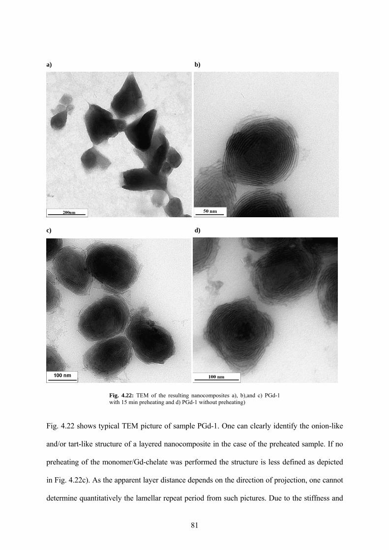
a) b)

c) d)

Fig. 4.22: TEM of the resulting nanocomposites a), b),and c) PGd-1 with 15 min preheating and d) PGd-1 without preheating)

Fig. 4.22 shows typical TEM picture of sample PGd-1. One can clearly identify the onion-like

and/or tart-like structure of a layered nanocomposite in the case of the preheated sample. If no

preheating of the monomer/Gd-chelate was performed the structure is less defined as depicted

in Fig. 4.22c). As the apparent layer distance depends on the direction of projection, one cannot

determine quantitatively the lamellar repeat period from such pictures. Due to the stiffness and

81

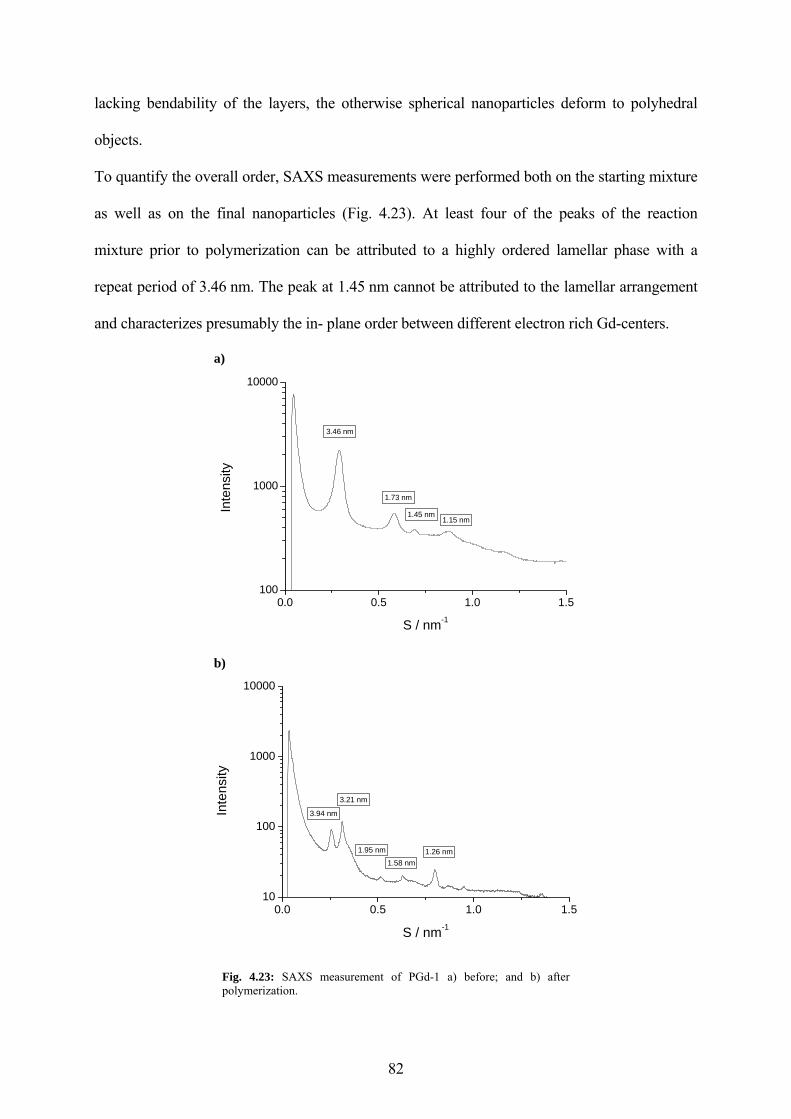
lacking bendability of the layers, the otherwise spherical nanoparticles deform to polyhedral

objects.

To quantify the overall order, SAXS measurements were performed both on the starting mixture

as well as on the final nanoparticles (Fig. 4.23). At least four of the peaks of the reaction

mixture prior to polymerization can be attributed to a highly ordered lamellar phase with a

repeat period of 3.46 nm. The peak at 1.45 nm cannot be attributed to the lamellar arrangement

and characterizes presumably the in- plane order between different electron rich Gd-centers.

a)

0.0 0.5 1.0 1.5100

1000

10000

1.15 nm1.45 nm

1.73 nm

3.46 nm

Inte

nsity

S / nm-1

b)

0.0 0.5 1.0 1.510

100

1000

10000

1.26 nm1.58 nm

1.95 nm

3.21 nm

3.94 nmInte

nsity

S / nm-1

Fig. 4.23: SAXS measurement of PGd-1 a) before; and b) after polymerization.

82

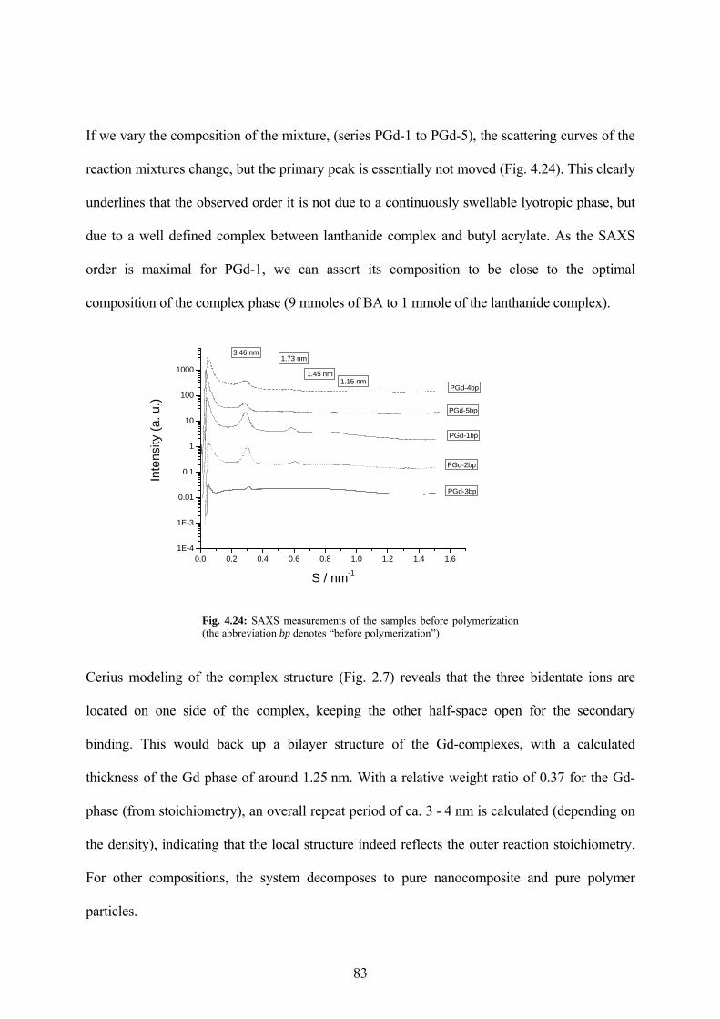
If we vary the composition of the mixture, (series PGd-1 to PGd-5), the scattering curves of the

reaction mixtures change, but the primary peak is essentially not moved (Fig. 4.24). This clearly

underlines that the observed order it is not due to a continuously swellable lyotropic phase, but

due to a well defined complex between lanthanide complex and butyl acrylate. As the SAXS

order is maximal for PGd-1, we can assort its composition to be close to the optimal

composition of the complex phase (9 mmoles of BA to 1 mmole of the lanthanide complex).

0.0 0.2 0.4 0.6 0.8 1.0 1.2 1.4 1.61E-4

1E-3

0.01

0.1

1

10

100

1000

PGd-3bp

PGd-1bp

PGd-2bp

PGd-5bp

PGd-4bp

3.46 nm1.73 nm

1.15 nm1.45 nm

Inte

nsity

(a. u

.)

S / nm-1

Fig. 4.24: SAXS measurements of the samples before polymerization (the abbreviation bp denotes “before polymerization”)

Cerius modeling of the complex structure (Fig. 2.7) reveals that the three bidentate ions are

located on one side of the complex, keeping the other half-space open for the secondary

binding. This would back up a bilayer structure of the Gd-complexes, with a calculated

thickness of the Gd phase of around 1.25 nm. With a relative weight ratio of 0.37 for the Gd-

phase (from stoichiometry), an overall repeat period of ca. 3 - 4 nm is calculated (depending on

the density), indicating that the local structure indeed reflects the outer reaction stoichiometry.

For other compositions, the system decomposes to pure nanocomposite and pure polymer

particles.

83

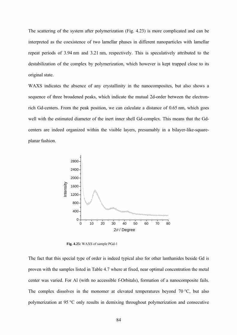
The scattering of the system after polymerization (Fig. 4.23) is more complicated and can be

interpreted as the coexistence of two lamellar phases in different nanoparticles with lamellar

repeat periods of 3.94 nm and 3.21 nm, respectively. This is speculatively attributed to the

destabilization of the complex by polymerization, which however is kept trapped close to its

original state.

WAXS indicates the absence of any crystallinity in the nanocomposites, but also shows a

sequence of three broadened peaks, which indicate the mutual 2d-order between the electron-

rich Gd-centers. From the peak position, we can calculate a distance of 0.65 nm, which goes

well with the estimated diameter of the inert inner shell Gd-complex. This means that the Gd-

centers are indeed organized within the visible layers, presumably in a bilayer-like-square-

planar fashion.

0 10 20 30 40 50 60 70 800

400

800

1200

1600

2000

2400

2800

Inte

nsity

2θ / Degree

Fig. 4.25: WAXS of sample PGd-1

The fact that this special type of order is indeed typical also for other lanthanides beside Gd is

proven with the samples listed in Table 4.7 where at fixed, near optimal concentration the metal

center was varied. For Al (with no accessible f-Orbitals), formation of a nanocomposite fails.

The complex dissolves in the monomer at elevated temperatures beyond 70 °C, but also

polymerization at 95 °C only results in demixing throughout polymerization and consecutive

84

85

aggregation. Also lanthanum (III), with no outer electrons, does form a stable monomer mixture

at higher temperatures, but forms unstable precipitates throughout polymerization.

All the other metal centers show similar layered nanocomposite morphologies as the Gd

complex, as presented in Fig. 4.26. The europium-based poly(butyl acrylate) nanoparticles have

an elongated layer-by-layer structure (Fig. 4.26a). The europium complex is fluorescent, and

this property is still found for the final Europium-based poly(butyl acrylate) latex. Opposite to

most other systems, the Eu-nanohybrid particles do spontaneously transfer to form a coloured,

but transparent film, indicating a weaker binding between polymer and complex layers.

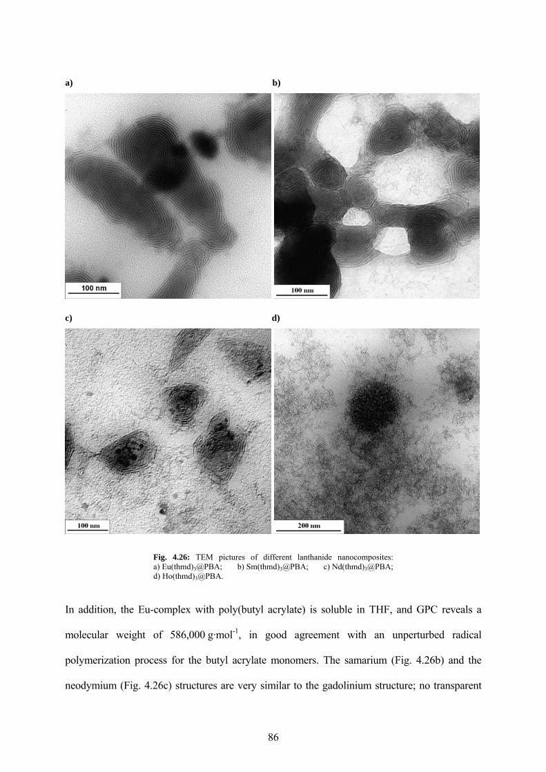
a) b)

c) d)

Fig. 4.26: TEM pictures of different lanthanide nanocomposites: a) Eu(thmd)3@PBA; b) Sm(thmd)3@PBA; c) Nd(thmd)3@PBA; d) Ho(thmd)3@PBA.

In addition, the Eu-complex with poly(butyl acrylate) is soluble in THF, and GPC reveals a

molecular weight of 586,000 g·mol-1, in good agreement with an unperturbed radical

polymerization process for the butyl acrylate monomers. The samarium (Fig. 4.26b) and the

neodymium (Fig. 4.26c) structures are very similar to the gadolinium structure; no transparent

86

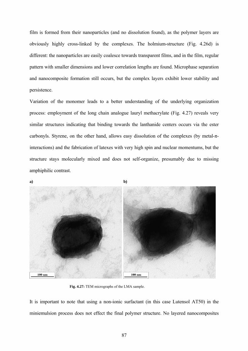
film is formed from their nanoparticles (and no dissolution found), as the polymer layers are

obviously highly cross-linked by the complexes. The holmium-structure (Fig. 4.26d) is

different: the nanoparticles are easily coalesce towards transparent films, and in the film, regular

pattern with smaller dimensions and lower correlation lengths are found. Microphase separation

and nanocomposite formation still occurs, but the complex layers exhibit lower stability and

persistence.

Variation of the monomer leads to a better understanding of the underlying organization

process: employment of the long chain analogue lauryl methacrylate (Fig. 4.27) reveals very

similar structures indicating that binding towards the lanthanide centers occurs via the ester

carbonyls. Styrene, on the other hand, allows easy dissolution of the complexes (by metal-π-

interactions) and the fabrication of latexes with very high spin and nuclear momentums, but the

structure stays molecularly mixed and does not self-organize, presumably due to missing

amphiphilic contrast.

a) b)

Fig. 4.27: TEM micrographs of the LMA sample.

It is important to note that using a non-ionic surfactant (in this case Lutensol AT50) in the

miniemulsion process does not effect the final polymer structure. No layered nanocomposites

87

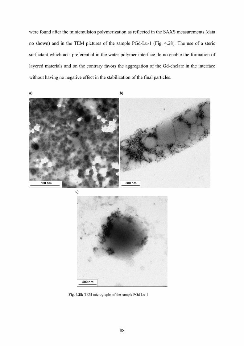
were found after the miniemulsion polymerization as reflected in the SAXS measurements (data

no shown) and in the TEM pictures of the sample PGd-Lu-1 (Fig. 4.28). The use of a steric

surfactant which acts preferential in the water polymer interface do no enable the formation of

layered materials and on the contrary favors the aggregation of the Gd-chelate in the interface

without having no negative effect in the stabilization of the final particles.

a) b)

c)

Fig. 4.28: TEM micrographs of the sample PGd-Lu-1

88

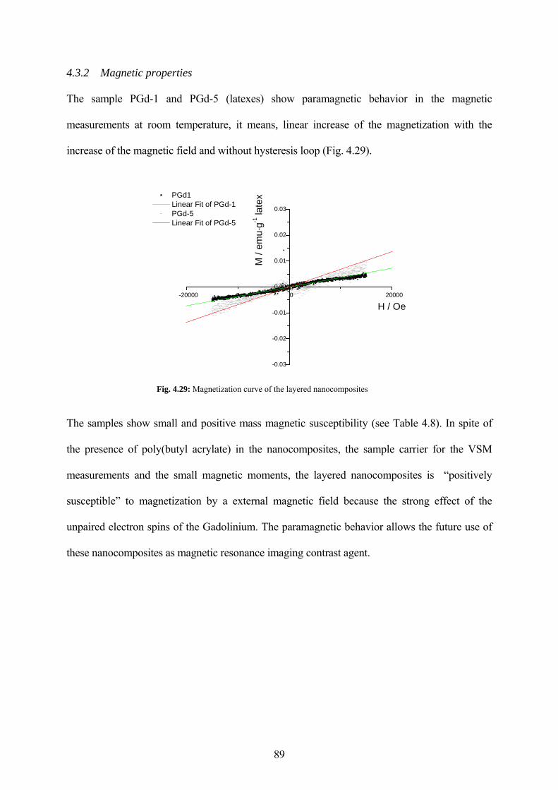
4.3.2 Magnetic properties

The sample PGd-1 and PGd-5 (latexes) show paramagnetic behavior in the magnetic

measurements at room temperature, it means, linear increase of the magnetization with the

increase of the magnetic field and without hysteresis loop (Fig. 4.29).

-20000 0 20000

-0.03

-0.02

-0.01

0.00

0.01

0.02

0.03

PGd1 Linear Fit of PGd-1 PGd-5 Linear Fit of PGd-5

M /

emu·

g-1 la

tex

H / Oe

Fig. 4.29: Magnetization curve of the layered nanocomposites

The samples show small and positive mass magnetic susceptibility (see Table 4.8). In spite of

the presence of poly(butyl acrylate) in the nanocomposites, the sample carrier for the VSM

measurements and the small magnetic moments, the layered nanocomposites is “positively

susceptible” to magnetization by a external magnetic field because the strong effect of the

unpaired electron spins of the Gadolinium. The paramagnetic behavior allows the future use of

these nanocomposites as magnetic resonance imaging contrast agent.

89

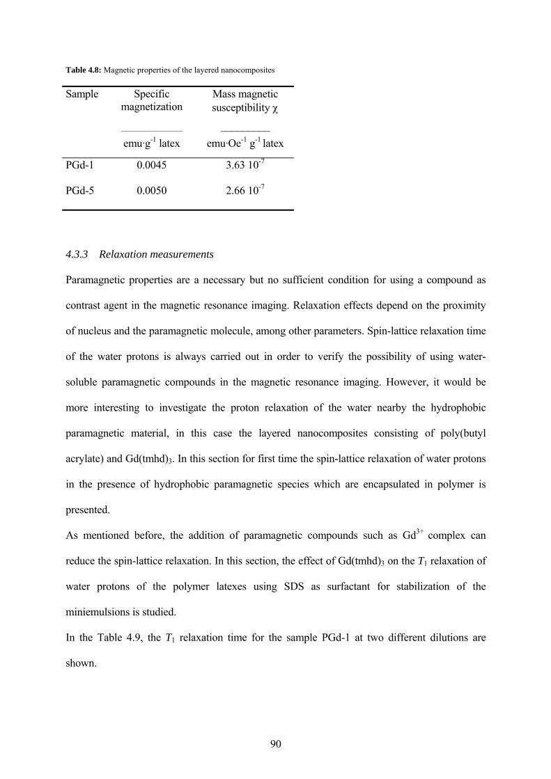
90

Table 4.8: Magnetic properties of the layered nanocomposites

Specific magnetization

_________________

Mass magnetic susceptibility χ

_________

Sample

emu·g-1 latex emu·Oe-1 g-1 latex

PGd-1 0.0045 3.63 10-7

PGd-5 0.0050 2.66 10-7

4.3.3 Relaxation measurements

Paramagnetic properties are a necessary but no sufficient condition for using a compound as

contrast agent in the magnetic resonance imaging. Relaxation effects depend on the proximity

of nucleus and the paramagnetic molecule, among other parameters. Spin-lattice relaxation time

of the water protons is always carried out in order to verify the possibility of using water-

soluble paramagnetic compounds in the magnetic resonance imaging. However, it would be

more interesting to investigate the proton relaxation of the water nearby the hydrophobic

paramagnetic material, in this case the layered nanocomposites consisting of poly(butyl

acrylate) and Gd(tmhd)3. In this section for first time the spin-lattice relaxation of water protons

in the presence of hydrophobic paramagnetic species which are encapsulated in polymer is

presented.

As mentioned before, the addition of paramagnetic compounds such as Gd3+ complex can

reduce the spin-lattice relaxation. In this section, the effect of Gd(tmhd)3 on the T1 relaxation of

water protons of the polymer latexes using SDS as surfactant for stabilization of the

miniemulsions is studied.

In the Table 4.9, the T1 relaxation time for the sample PGd-1 at two different dilutions are

shown.

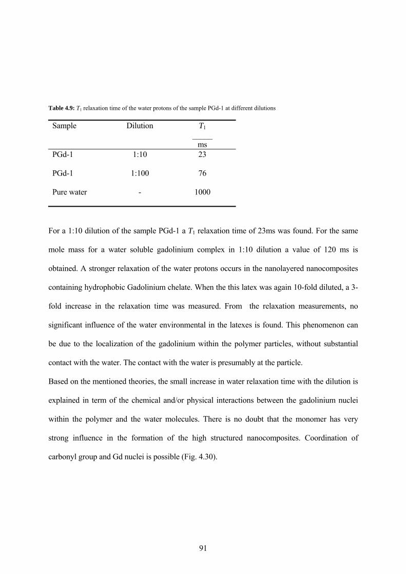
91

Table 4.9: T1 relaxation time of the water protons of the sample PGd-1 at different dilutions

Sample Dilution T1 _____

ms PGd-1 1:10 23

PGd-1 1:100 76

Pure water - 1000

For a 1:10 dilution of the sample PGd-1 a T1 relaxation time of 23ms was found. For the same

mole mass for a water soluble gadolinium complex in 1:10 dilution a value of 120 ms is

obtained. A stronger relaxation of the water protons occurs in the nanolayered nanocomposites

containing hydrophobic Gadolinium chelate. When the this latex was again 10-fold diluted, a 3-

fold increase in the relaxation time was measured. From the relaxation measurements, no

significant influence of the water environmental in the latexes is found. This phenomenon can

be due to the localization of the gadolinium within the polymer particles, without substantial

contact with the water. The contact with the water is presumably at the particle.

Based on the mentioned theories, the small increase in water relaxation time with the dilution is

explained in term of the chemical and/or physical interactions between the gadolinium nuclei

within the polymer and the water molecules. There is no doubt that the monomer has very

strong influence in the formation of the high structured nanocomposites. Coordination of

carbonyl group and Gd nuclei is possible (Fig. 4.30).

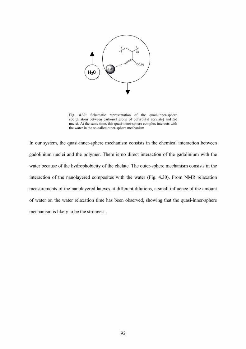
H20

Fig. 4.30: Schematic representation of the quasi-inner-sphere coordination between carbonyl group of poly(butyl acrylate) and Gd nuclei. At the same time, this quasi-inner-sphere complex interacts with the water in the so-called outer-sphere mechanism

In our system, the quasi-inner-sphere mechanism consists in the chemical interaction between

gadolinium nuclei and the polymer. There is no direct interaction of the gadolinium with the

water because of the hydrophobicity of the chelate. The outer-sphere mechanism consists in the

interaction of the nanolayered composites with the water (Fig. 4.30). From NMR relaxation

measurements of the nanolayered latexes at different dilutions, a small influence of the amount

of water on the water relaxation time has been observed, showing that the quasi-inner-sphere

mechanism is likely to be the strongest.

92

93

5 Conclusions and Outlook

In the first work presented in this thesis, it was shown that the encapsulation of high amounts

of magnetite particles into polystyrene particles can efficiently be achieved by a new three-

step preparation route including two miniemulsion processes. In the first step, oleic acid

coated magnetite particles in octane are prepared. In the second step, a dispersion of the

magnetite in octane is miniemulsified in water by using SDS as surfactant. After evaporation

of the octane, the magnetite aggregates which are covered by a oleic acid/SDS bilayer were

mixed with a monomer miniemulsion and in the third step of the synthesis route, a ad-

miniemulsification process is used to obtain final and full encapsulation. Here, a

fusion/fission process induced by ultrasound is just effective for the monomer droplets,

whereas the monomer coated magnetite aggregates stay intact. That way, all monomer droplet

are split and heteronucleated onto the magnetite aggregates to form a monomer film. After

polymerization, polymer encapsulated magnetite aggregates were obtained. Characterization

by thermogravimetry, preparative ultracentrifugation, and transmission electron microscopy

showed that up to 40 % magnetite could be encapsulated, resulting in particles with a high

homogeneity of the magnetite content. Magnetometry measurements reveal that the magnetite

aggregates still consist of separated superparamagnetic magnetite particles which is due to the

coverage by the oleic acid. During the encapsulation process, 60 % of the magnetization

compared to bulk magnetite is still preserved.

Secondly, it was shown the approach to fabricate novel iron oxide containing nanocomposites

with lamellar structure and by a two-step process including miniemulsion polymerization. The

first step consisting of the decomposition of iron pentacarbonyl using oleic acid as stabilizer

was used to obtain an iron containing monomer dispersion which is used in the second step

for the miniemulsion polymerization. The miniemulsion polymerization of the iron oxide

94

containing monomer-dispersion with different concentration of oleic acid enables the

production of either nanocomposites which have discrete iron oxide nanoparticles throughout

distributed in the polymer particle or eye-like nanocomposites which contain demixing

phases, one consisting of discrete iron oxide nanoparticles in a lamellar arrangement and the

other one the poly(butyl methacrylate), depending on the amount of oleic acid used for the

thermal decomposition. Magnetic measurements showed the paramagnetic behavior of the

final nanocomposites and the potential used as contrast agent for magnetic resonance

imaging.[124]

Finally, the spontaneous formation of nanohybrid materials made from a ligating monomer and

closed-shell lanthanide complexes is presented. The resulting structures seem to be well defined

with respect to stoichiometry, and are highly organized towards lamellar structures due to a

combination of amphiphilic contrast and -potentially- spin coupling. Relaxations as well as

magnetometry results shown that these new layered nanocomposites are paramagnetic and

possesses a very high relaxivity of the water protons. The as-synthesized particles can have

direct applications as magnetic and X-ray contrasting agents,[134] or for radioembolization

therapy.[135]

The influence of the temperature and composition on the magnetic behavior of these systems as

well as the T1 relaxation time depending on the composition at different dilutions has to be

explored in future work

95

6 Experimental Section

6.1 Water based-ferrofluid containing magnetite polystyrene nanoparticles

Materials

Ferric chloride anhydrous (FeCl3) and ferrous chloride tetrahydrate (FeCl2·4H2O) were

purchased from Fluka. Ammonium hydroxide (28-30 % NH3), octane (98 %), hexadecane

(99 %), sodium dodecyl sulfate (SDS), cholic acid sodium salt, potassium peroxodisulfate

(KPS), lecithin, Tween 80, and oleic acid (90 %) were purchased from Aldrich and used as

received.

The monomers acrylic acid and styrene from Aldrich were distilled under reduced pressure

before use.

Synthesis of hydrophobized magnetite nanoparticles

According to ref. [ ], the magnetite particles were produced by coprecipitation from an aqueous

Fe3+ / Fe2+ solution (ratio 3:2) using concentrated ammonium hydroxide in excess. The particles

were subsequently coated with oleic acid:

14.6 g of FeCl3 and 12.0 g of FeCl2·4 H2O were dissolved in 50 ml distilled water. 40 ml of

ammonium hydroxide were added rapidly. After coprecipitation of magnetite particles, oleic

acid (for quantities see Table 4.1) was added, and the suspension was heated to 70 °C for

30 min. Then, the temperature was increased to 110 °C in order to evaporate water and excess

of ammonium. The black lump-like residuum was cooled to room temperature and washed

several times with distilled water. After drying, a powder was obtained.

Octane / magnetite dispersion and water-based ferrofluid

1.0 g of oleic acid containing magnetite powder as received above was added to 6.0 g of octane

with or without hexadecane (for details see Table 4.1) to form a dispersion of hydrophobized

96

magnetite in octane as carrier medium. This dispersion was added to a solution consisting of

24 g water and SDS (for quantities see Table 4.1). After mixing for 1 h at 500 rpm, the mixture

was subjected to sonication twice for 2 min at 90 % amplitude with a Branson sonifier W450

digital in an ice-cooled bath. After carefully evaporating the octane at 80 °C for 6 h while

adding every 30 min approximately 2 ml of water to compensate the evaporation of water, a

stable water-based ferrofluid is obtained. For the use of biosurfactant, it was choice the

conditions of the sample Mag-10 but using sodium salt of cholic acid, lecithin and Tween 80.

Polymer encapsulation

A styrene miniemulsion was prepared using the following recipe: 6.0 g of styrene and 250 mg

of the hydrophobic agent hexadecane were added to a surfactant solution consisting of 72 mg of

SDS dissolved in 24 g of water. After stirring 1 h for pre-emulsification, the miniemulsion was

obtained by sonication for 2 min at 90 % amplitude in an ice-cooled bath.

For the encapsulation, the styrene miniemulsion and the water-based magnetite dispersions as

obtained above were combined and co-sonified twice for 1 min at 50 % amplitude in an ice-

cooled bath. Magnetite powder to monomer ratios of 4:1, 2:1, 3:2, 1:1, 7:8, 3:4, 1:2, 1:4, and 1:8

(for details see Table 4.1) were employed. To start the polymerization, 20 mg of KPS were

added, and the temperature was increased to 80 °C; after 40 min 30 mg of acryl acid were

added. The polymerization time was between 18 and 24 h.

6.2 Nanostructured composites from iron pentacarbonyl decomposition

Materials

Iron pentacarbonyl (ipc), Fe(CO)5 (purum, >> 97% (Fe)), was purchased from Aldrich and

filtered before used. Sodium dodecyl sulfate (SDS) oleic acid (90%), and butyl methacrylate

(BMA) (99%), hexadecane (99%), 2,2’-azo(2-methylbutyronitrile) (V59) were purchased from

Aldrich and used as received. Distilled water was used in all the experiments.

97

Thermal decomposition in the monomer phase

2 g of iron pentacarbonyl and the quantity of oleic acid (for quantities see Table 4.4) and 4 g of

butyl methacrylate were mixed and subjected in a three-neck flask to agitation at 250 rpm, at a

temperature of 110 °C under atmospheric pressure. After 9 h or 24 h (for details see Table 4.4),

depending on the oleic acid concentration, an iron containing monomer dispersion was

obtained.

Nanocomposite particles after miniemulsion polymerization

A miniemulsion polymerization was performed from the iron monomer dispersion that was

obtained before. The organic phase consisting of 0.5 g of iron containing monomer dispersion

as received above, 0.030 g of hexadecane and 0.040 g of V59 were mixed with the water phase

consisting of a solution of 4.5 g of water and either 11.7 or 4.2 % of SDS (for more details see

Table 4.5). After stirring 1 h for pre-emulsification, the miniemulsion was obtained by

microsonication using a microtip for 2 min (each 5 s a pause of 10 s) at 70 % amplitude with a

branson sonifier W450 digital in an ice-cooled bath. For the polymerization, the temperature

was increased to 80 °C. The polymerization was carried out for 24 h.

6.3 Gadolinium-based nanocomposites

Materials

Gadolinium tris(2,2,6,6-tetramethyl-3,5-heptanedionate) (Gd(tmhd)3), europium tris(2,2,6,6-

tetramethyl-3,5-heptanedionate) (Eu(tmhd)3), samarium tris(2,2,6,6-tetramethyl-3,5-

heptanedionate) (Sm(tmhd)3), holmium tris(2,2,6,6-tetramethyl-3,5-heptanedionate)

(Ho(tmhd)3), and lanthanium tris(2,2,6,6-tetramethyl-3,5-heptanedionate) (LA(tmhd)3) were

purchased from Strem. Hexadecane (99 %), sodium dodecyl sulfate (SDS), V59 (2,2’-azo(2-

methylbutyronitrile)) were purchased from Aldrich and used as received. The monomers butyl

98

acrylate (BA) and lauryl methacrylate (LMA) and methyl methacrylate (MMA) from Aldrich

were distilled under reduced pressure before use. Distilled water was used for all experiments.

Lutensol AT50 (C16-C18-fatty alcohol with a ethylene oxide block length of about 50 units) was

purchased from BASF AG.

Synthesis of the nanoparticles

For polymerization, the technique of miniemulsion polymerization was employed to result in

nanoparticles which are easier to analyze. A monomer miniemulsion was prepared using the

following recipe: the amount of lanthanide chelate given in Table 4.7 were dissolved in 0.5 g of

monomer (butyl acrylate or lauryl methyl acrylate) at 72 °C and subjected to a preheat at the

same temperature for 15 min. Then the 0.030 g of hexadecane, and 0.040 g of V59 were added

at room temperature to a surfactant solution consisting of surfactant dissolved in 4.5 g of water

and 0.066 g of SDS (or Lutensol AT50). After stirring 1 h for pre-emulsification, the

miniemulsion was obtained by microsonication for 2 min (each 5 s a pause of 10 s) at 70 %

amplitude with a Branson sonifier W450 digital in an ice-cooled bath. To start the

polymerization, the temperature was increased to 72 °C. The polymerization time was between

10 and 12 h.

99

7 Methods

DynamicLlight Scattering (DLS)

The particle size was determined using a Nicomp particle sizer (Model 370, PSS Santa Barbara,

CA) at a fixed scattering angle of 90°.

Gel Permeation Chromatography (GPC)

Gel permeation chromatography was used to obtain the weight-average molecular weight of the

polystyrene in the magnetite/polymer nanoparticles. A thermo-separation products’ GPC

equipment with a polyester without reactive functional groups as column packing

(PSS GRAM column) was used. The GPC separation was carried out at 70 °C, with a flow rate

of 0.7 ml·min-1, with N-methylpyrrolidone as mobile phase and with a UV detector operating at

270 nm. To obtain the weight-average molecular weight of the poly(butyl methacrylate) in the

iron containing poly(butyl methacrylate) latex, a column consisting of polystyrene

divinylbencene packing (MZ-Analysentechnik) was used. The GPC separation was carried out

at 70 °C, with a flow rate of 0.7 ml·min-1, with tetrahydrofuran (THF) as mobile phase and with

a UV detector operating at 260 nm.

Nuclear Magnetic Resonance(NMR)

1H NMR spectroscopy was performed on a Bruker DPX 400 operating a magnetic field strength

of 9.395 T and using deuterated chloroform as the solvent at room temperature. Win-NMR

(Bruker) program was used to work on the spectra.

Relaxation measurements

The spin-lattice or longitudinal relaxation time (T1) of the gadolinium polymer latexes was

measured on a Bruker DPX 400 spectrometer, operating a magnetic field strength of 9.395 T.

All T1 relaxation measurements were recorded with the combination of standard inversion-

100

recovery technique and magic angle spinning (MAS) technique. The latexes were sealed in 5 ml

glass tube. The inversion-recovery pulse programme can be written as (d1-180°x-d2-90x-FID)n.

The observed transverse relaxation rates were calculated from either the intensity at half height

or the area under the peak.

Preparative Ultracentrifugation

The preparative ultracentrifugation was used to obtain information about the encapsulation

distribution. A drop of the final dispersion consisting of inorganic/polymer particles was added

to a tube containing sucrose density gradients ranging between 1.00 to 1.30 g·cm-3 and

centrifugated at 4 °C for 120 min at 37,000 rpm in a Beckmann L-70 centrifuge.

Thermogravimetric Analysis (TGA)

The magnetite or iron oxide content of the dried samples was measured by thermogravimetry.

The thermogravimetric analysis (TGA) measurements were performed with a Netzsch-

Gerätebau TG 209 under nitrogen atmosphere at 20 ml·min-1. The temperature range is between

30 and 900 °C with a heating rate of 20 K·min-1.

Transmission Electron Microscopy (TEM)

The samples were characterized by a Zeiss 912 Omega Electron Microscope operating at

120 kV. The samples were diluted and mounted on carbon coated copper grids.

Vibrating Sample Magnetometer (VSM)

The magnetic properties of the particles were determinated by a PAR (Princeton Applied

Research) vibrating sample magnetometer ( Hmax =1200 kA·m-1).

Small Angle X-ray (SAXS)

101

SAXS patterns were recorded employing a Kratky camera or using a rotating anode with

pinhole collimation. A Nonius rotating anode (P = 4 kW, CuKα) and an image-plate detector

system was used.

Wide Angle X-ray (WAXS)

WAXS diffraction was measured with a Nonius CP-120 diffractometer using a Cu-Kα radiation

(λ = 0.154 nm) on the dried samples at room temperature.

Fourier Transform Infrared (FTIR) spectroscopy

For infrared measurements a BIORAD 6000 FTIR spectrometer was used. A Golden Gate

arrangement, single reflection diamond ATR, was used for the measurements of the liquid

samples.

102

8 References

1 A. Kross, Geschichte des Magnetismus, vde- verlag, Berlin 1994.

2 R. Blakemore, Science 1975, 190, 377-379.

3 J. L. Gould, J. L. Kirschvink, K. S. Deffeyes, Science 1978, 201, 1026-1028.

4 C. Walcott, R.P. Green, Science 1974, 184, 180-182.

5 M. M. Walker, J. L. Kirschvink, S.-B. R. Chang, A. E. Dizon, Science 1984, 224, 751-753.

6 J. L. Kirschvink, A. Kobayashi-Kirschvink, B. J. Woodford, Proc. Natl. Acd. Sci. USA 1992, 89, 7683-7687.

7 http://www.iupac.org/reports/2001/colloid_2001/manual_of_s_and_t.pdf

8 [a] K. Landfester, Miniemulsions for polymerizations processes and materials science, Habilitationsschrift, Universitat Potsdam, 2002; [b] K. Landfester, Macromol. Rapid. Comm. 2001, 22, 896-936.

9 M. Antonietti, K. Landfester, Prog. Polym. Sci. 2002, 27, 689-757.

10 P. Tartaj, M. Morales, S. Veintemillas-Verdaguer, T. González-Carreno, C. J. Serna, J. Phys. D: Appl. Phys. 2003, 36, R182-R197.

11 C. C. Berry, A. S. G. Curtis, J. Phys. D: Appl. Phys. 2003, 36, R198-R206.

12 J. V. Dawkins, Aqueous Suspension Polymerization in Comprehensive Polymer Science, Ed. Allen, Bevington, Pergamon Press, Oxford, 1989, 231-241.

13 Y. J. Chou, M.S. El-Aasser, J.W. Vanderhoff, J. Dispers. Sci. Technol. 1980, 1, 129-150.

14 H. Köhler, Geofysiske Publikasjoner 1922, 2, 3-15.

15 W. I. Higuchi, J. Misra, J. Pharmaceutical Sci 1962, 51, 459-466.

16 A. J. Webster, M. E. Cates, Langmuir 1998, 14, 2068-2079.

17 I. M. Lifshitz, V. V. Slyozov. Phys. Chem. Solids 1961, 19, 35-50.

18 A. S. Kalbalnov, A. V. Pertzov, E. D. Shchukin, J. Colloid Intef. Sci. 1987, 118, 590-597.

19 M. Postel, J. G. Riess, J. G. Weers, Artif. Cells, Blood Substitutes, Immobilization Biotechnol. 1994, 22, 991-1005.

20 K. C. Lowe, Artif. Cells, Blood Substitutes, Immobilization Biotechnol. 2000, 28, 25-38.

103

21 S. S. Davis, H. P. Round, T. S. Purewal J. Colloid Interf. Sci. 1981, 80, 508-511.

22 B. Abismail, J. P. Canselier, A. M. Wilhelm, H. Delmas, C. Gourdon, Ultrason. Sonochem. 1999, 6, 75-83.

23 P. Walstra, Chem. Eng. Sci. 1993, 48, 333-349.

24 S. E. Friberg, S. Jones, in: Kirk-Othmer, Encyclopedia of Chemical Technology, 4 ed., J. I. Kroschwitz, Ed., Wiley, New York 1994, Vol. 9, pp. 393-413.

25 R. W. Wood, A. L. Loomis, Phil. Mag. 1927, 4, 417-433.

26 V. I. Sorokin, Soviet Phys./Acoust. 1957, 3, 281-291.

27 M. K. Li, H. S. Fogler, J. Fluid Mech. 1978, 88, 499-511.

28 M. K. Li, H. S. Fogler, J. Fluid Mech. 1978, 88, 513-528.

29 K. S. Suslick, Science 1990, 247, 1439-1445.

30 W. Lauterborn, Ultrason. Sonochem. 1997, 4, 65-75.

31 O. Behrend, K. Ax, H. Schubert, Ultrason. Sonochem. 2000, 7, 77-85.

32 K. Fontenot, F. J. Schork, Ind. Eng. Chem. Res. 1993, 32, 373-385.

33 K. Landfester, N. Bechthold, F. Tiarks, M. Antonietti, Macromolecules 1999, 32, 5222-5228.

34 Y. J. Chou, M. S. El-Aasser, J. W. Vanderhoff, J. Dispers. Sci. Technol. 1980, 1, 129-150.

35 A. R. M. Azad, J. Ugelstad, R. M. Fitch, F. K. Hansen In Emulsion Polymerization; I. Piirma, Gardon, J.L., Ed.; ACS: Washington, D.C., 1976; Vol. 24, pp 1-23.

36 K. Landfester, N. Bechthold, F. Tiarks, M. Antonietti, Macromolecules 1999, 32, 2679-2683.

37 S. Lang, Curr. Opin. Colloid Interface Sci. 2002, 7, 12-20.

38 I. M. Banat, R. S. Makkar, S. S. Cameotra, Appl. Microbiol. Biotechnol. 2000, 53, 495-508.

39 J. L. Reimers, F. J. Schork, Ind. Eng. Chem. Res. 1997, 36, 1085-1087.

40 J. Ugelstad, M. S. EL Aasser, J. W. Vanderhoff, J. Polym. Sci. , Polym. Lett. Ed. 1973, 11, 503-513.

41 J. Ugelstad, F. K. Hansen, S. Lange, Makromol. Chem. 1974, 175, 507-521.

42 K. Landfester, N. Bechthold, S. Förster, M. Antonietti, Macromol. Rapid Comm. 1999, 20, 81-84.

104

43 N. Bechthold, F. Tiarks, M. Willert, K. Landfester, M. Antonietti, Macromol. Symp. 2000, 151, 549-555.

44 B. Erdem, E. D. Sudol, V. L. Dimonie, M.S. El-Aasser. Macromol. Symp. 2000, 155, 181-198.

45 F. Tiarks, K. Landfester, M. Antonietti, Macromol. Chem. Phys. 2001, 202, 51-60.

46 B. D. Cullity, Introduction to Magnetic Materials, Adisson-Wesley, reading, 1972.

47 R. W. Chantrell, J. Popplewell, S.W. Charles, IEEE T Magn. 1978, Mag-14, 975-977.

48 S. S. Papell, US Patent No. 3215572 (1965).

49 G. W. Reimers, S. E. Khalafalla, US Patent No. 3843540 (1976).

50 J. R. Kelley, U.S. Patent No. 4019994 (1977).

51 J. Shimoiizaka, K. Nakatsuka, T. Fujita, A. Kounosu, Fine particles Processing, Proceedings of the international symposium on fine particles processing, P. Somasundaran (ed.), 2nd vol., New York (1980).

52 R. S. Molday, US Patent No. 4452773 (1984).

53 A. Rembaum, U. S. Patent No. 4267234 (1981).

54 J. Lee, T. Isobe, M. Senna, Colloid Surface A 1996, 109, 121-127.

55 M. Suzuki, M. Shinkai, M. Kamihira, T. Kobayashi, Biotechnol. Appl. Bioc. 1995, 21, 335-345.

56 I. Dumazet-Bonnamour, I., P. Le Perchec, Colloid Surface A 2000, 173, 61-71.

57 V. Veiga, D.H. Ryan, E. Sourty, F. Llanes, R.H. Marchessault, Carbohyd. Polym. 2000, 42, 353-357.

58 F. Sauzedde, A. Elaïssari, C. Pichot, Colloid Polym. Sci. 1999, 277, 846-855.

59 V. S. Zaitsev, D. S. Filimonov, I. A. Presnyakov, R. J. Gambino, B. Chu, J. Colloid Interf. Sci. 1999, 212, 49-57.

60 P. A. Dresco, V.S. Zaitsev, R.J. Gambino, B. Chu, Langmuir 1999, 15, 1945-1951.

61 J. -C. Daniel, J.-L. Schuppiser, M. Tricot, U. S. Patent No. 4358388 (1982).

62 D. Charmot, C. Vidil, U. S. Patent No. 5356713 (1994).

63 [a] US Patent No. 4,654,267 (1987), invs.: J. Ugelstad, T.Ellingsen, A. Berge, O. B. Helgee; [b] J. Ugelstad, A. Berge, T. Ellingsen, R. Schmid, T.-N. Nilsen, P. C. Mørk, P. Stenstad, E. Hornes, Ø. Olsvik, Prog. Polym. Sci. 1992, 17, 87-161; [c] J. Ugelstad, P.

105

Stenstad, L. Kilaas, W. S. Prestvik, R. Herje, A. Berge, E. Hornes, Blood Purif. 1993, 11, 349-369.

64 K. Wormuth, J. Colloid Interf. Sci. 2001, 241, 366-377.

65 K. Landfester, M. Willert, M. Antonietti, Macromolecules 2000, 33, 2370-2376.

66 D. Hoffmann, K. Landfester, M. Antonietti, Magnetohydrodynamics 2001, 37, 217-221.

67 J. Roger, J. N. Pons, R. Massart, A. Halbreich, J. C. Bacri, Eur. Phys. J. – Appl. Phys. 1999, 5, 321-325.

68 C. Bergemann, D. Müller-Schulte, J. Oster, L.A. Brassard, A.S. Lübbe, J. Magn. Magn. Mater. 1999, 194, 45-52.

69 A. S. Lübbe, C. Bergemann, W. Huhnt, T. Fricke, H. Riess, J.W. Brock, D. Huhn, Cancer Res. 1996, 56, 4694-4701.

70 E. Viroonchatapan, M. Ueno, H. Sato, I. Adachi, H. Nagae, K. Tazawa, I. Horikoshi, Pharmaceut. Res. 1995, 12, 1176-1182.

71 J. Dobson, A. Keramane, A. J. El Haj, European Cells and Materials 2002, 4, 42-44.

72 D. K. Kim, Y. Zhang, W. Voit, K. V. Rao, J. Kehr, B. Bjelke, M. Muhammed, Scripta Mater. 2001, 44, 1713-1717.

73 M. Mitsumori, M. Hiraoka, T. Shibata, Y. Okuno, Y. Nagata, Y. Nishimura, M. Abe, M. Hasegawa, H. Nagae and Y. Ebisawa. Hepato-gastroenterol. 1996, 43,1431-1437.

74 K. Raj, B. Moskowitz, R. Casciari, J. Magn. Magn. Mater. 1995, 149, 174-180.

75 M. Zahn, J. Nanopart. Res. 2001, 3, 73-78.

76 A. Nethe, T. Scholz, H.-D. Stahlman, Magnetohydrodynamics 2001, 3, 312-317.

77 C. Abel-Keilhack, J. Hesselbach, J. Appl. Phys. 2003, 93, 8441-8443.

78 Ch. Alexiou, A. Schmidt, R. J. Klein, P. Hulin, Ch. Bergemann, W. Arnold, J. Magn. Magn. Mater. 2002, 252, 363-366.

79 A. Jordan, R. Scholz, P. Wust, H. Fähling, R. Felix, J. Magn. Magn. Mater. 1999; 201, 413-419.

80 R. Hiergeist, W. Andra, N. Buske, R. Hergt, I. Hilger, U. Richter, W. Kaiser, J. Magn. Magn. Mater. 1999, 201, 420-422.

81 M. Mitsumori, M. Hiraoka, T. Shibata, Y. Okuno, Y. Nagata, Y. Nishimura, M. Abe, M. Hasegawa, H. Nagae, Y. Ebisawa, Hepato-gastroenterol. 1996, 43,1431-1437.

106

82 J. M. Singer, NATO ASI Series E, No. 138, M. S. El- Aasser and R.M. Fitch (Eds.), p. 371, N. Nijhoff Publ., Dordrecht, The Netherlands (1987).

83 C. Petit, A. Taleb, M.P. Pileni, J. Phys. Chem. B 1999, 103, 1805-1810.

84 C. Petit, A. Taleb, M. P. Pileni, Adv. Mater.1998, 10, 259-261.

85 D. P. Dinega, M. G. Bawendi, Angew. Chem. Int. Ed. Engl. 1999, 38, 1788-1791.

86 Ullmann’s encyclopedia of industrial chemistry, Wiley, 2003 http://www.mrw.interscience.wiley.com/ueic/articles/a18_215/frame.html#

87 T. W. Smith, D. Wychick, J. Phys. Chem. 1980, 84, 1621-1629.

88 K. S. Suslick, M. Fang, T. Hyeon, J. Am. Chem. Soc. 1996, 118, 11960-11961.

89 V. F. Puntes, K.M. Krishnan, P. Alivisatos, Appl. Phys. Lett. 2001, 78, 2187-2189.

90 K.S. Suslick, S-B. Choe, A.A. Cichowlas, M. W. Grinstaff, Nature 1991, 353, 414-416.

91 Y. Koltypin, G. Kataby, X. Cao, R. Prozorov, A. Gedanken, J. Non-Cryst. Solids 1996, 201, 159-162.

92 G. Kataby, A. Ulman, R. Prozorov, A. Gedanken, Langmuir 1998, 14, 1512-1515.

93 C. H. Griffiths, M. P. O’Horo, T. W. Smith, J. Appl. Phys. 1979, 50, 7108-7115.

94 N. A. D. Burke, H. D. H. Stöver, F. P. Dawso, J. D. Lavers, P. K. Jain, H. Oka, IEEE Trans. Magn. 2001, 37, 2660-2662.

95 C. Pathmamanoharan, N. L. Zuiverloon, A. P. Philipse, Prog. Colloid Polym. Sci. 2000, 115, 141-145.

96 T. Hyeon, S. S. Lee, J. Park, Y. Chung, H. B. Na, J. Am. Chem. Soc. 2001, 123, 12798-12801.

97 R. Tannenbaum, S. Reich, C. L. Flenniken, E. P. Goldberg, Adv. Mater. 2002, 14, 1402-1405.

98 A. F. Cockerill, G. L. O. Davies, R.C: Harden, D. M. Rackham, Chem. Rev. 1973, 73, 553-588.

99 P. Caravan, J. J. Ellison, T. J. McMurry, R. B. Lauffer Chem. Rew, 1999, 99, 2293-2352.

100 G. De Stasio, P. Casalbore, R. Pallini et al. Cancer Res. 2001, 61, 4272-4277.

101 D. H. Carr, J. Brown, G. M. Bydder, R. E. Steiner, H.-J. Weinmann, U. Speck, A. S. Hall, I. R. Young, Am. J. Roentgenol. 1984, 143, 215-224.

102 K. Micskei, L. Helm, E. Brücher, A. E. Meherbach, Inorg. Chem. 1993, 32, 3844-3850.

107

103 D. L. Ladd, R. Holisster, X. Peng, et. al., Bioconjugate Chem. 1999, 10, 361-370.

104 P. Ronved, B. Lindberg, J. Klaveness, Carbohyd. Res. 1991, 214, 325-330.

105 F. E. Armitage, D.E. Richardson, K.C.P. Li, Bioconjugate Chem. 1990, 1, 365-374.

106 D. Meyer, M. Schaeffer, A. Bouillot, S. Beauté, C. Chambom, Invest. Radiol. 1991, 25, s50-s52.

107 H. Tokumitsu, H. Ichikawa, T.K. Saha, Y. Fukumori, L. H. Block., S. T. P. Pharma Sciences 2000, 10, 39-49.

108 U. Schmiedl, M. Ogan, H. Paajanen, M. Marotti, L. E. Crooks, A. C. Brito, R. C. Brasch Radiology 1987, 162, 205-210.

109 L. Lattuada, G.Lux, Tetrahedron Lett. 2003, 44, 3893-3895.

110 R. C. Brasch, Y. Berthezene, V.S Vexler, M. Moseley, O. Clément, A. Muehler, D. Price, H. Jeome, Invest. Radiol. 1991, 26, s42-s45

111 F. Cavagna, C. Luchinat, A. Scozzafava, Z. Xia, Magnet. Reson. Med. 1994, 31, 58-60.

112 E. C. Wiener, M.W. Brechbiel, H. Brothers, R.L. Magin, O. A. Gansow, D. A. Tomalia, P. C. Lauterbur, Magnet. Reson. Med. 1994, 31, 1-8.

113 D. Roberts, W.L. Zhu, C. M. Frommen, Z. Rosenzweig, J. Appl. Phys. 2000, 87, 6208-6210.

114 J. Guo, X. Jiang, C-Z Yang, J., Appl. Polm. Sci. 2003, 87,1358-1364.

115 K-C. Yu, H-B Hu, M-L Liu, H-Z Yuan, C-H Ye, R-X Zhuo, Chinese J. Polym. Sc. 1999, 17, 471-475.

116 E. Tóth, F Connac, L. Helm, K. Adzamli, A.E. Merbach, J Biol. Inorg. Chem. 1998, 3, 606-613.

117 K. M. Johnson, L.Z. Tao, R.P. Kennan, J. C. Gore, Magnet. Reson. Med. 1998, 40, 133-142.

118 J. H. Braybrook, D. H. Laurance, Polym. Inter. 1991, 26, 251-259.

119 C. H. Reynolds, N. Annan, K. Beshah, J.H. Huber, S.H. Shaber, R.R. Lenkiski,J. A. Wortman, J. Am. Chem. Soc. 2000, 122, 8940-8945.

120 M. Miyamoto, K. Hirano, H. Ichikawa, Y. Fukumori, Y. Akine, K. Tokuuye, Chem. Pharm. Bull. 1999, 47, 203-208.

121 H. Tournier, R. Hyacinthe, M. Schneider, Acad. Radiol. 2002, 9 (suppl 1):s20-s28.

108

122 J. H. Schattka, Synthese pöroser Metalloxidstrukturen durch Template Nanocoating,

Dissertation, Universität Potsdam, 2002.

123 E. P. Giannelis, R. Krishnamoorti, E. Manias, Adv. Polym. Sci. 1999, 38, 107-147.

124 P. Caravan, J. J. Ellison, T. J. McMurry , R.B. Lauffer, Chem. Rev. 1999, 99, 2293-2352.

125 T. L. James, Nuclear magnetic resonance in biochemistry, Academic Press, Inc., New York, 1975.

126 D. D. Stark and W.G. Bradley Magnetic resonance imaging, The C.V. Mosby Company, Missouri, 1988.

127 F. Bloch, W.W. Hansen, P. Packard, Physiol. Rev. 1946, 70, 474-485.

128 I. Solomon, Physiol. Rev. 1955, 99, 559-565.

129 N. Bloembergen, J. Chem. Phys. 1957, 27, 572-573.

130 R. B. Lauffer, Chem. Rev. 1987, 87, 901-927.

131 D. Chescoe, P. J. Goodhew, The operation of transmission and scanning electron microscopes, Oxford University Press, New York, 1990.

132 S. P. Spragg, J. Steensgaard, Theoretical aspects of practical centrifugation. In Preparative centrifugation. A practical Approach, (Ed. D. Rickwood), Oxford University, New York, 1992.

133 US patent 845,903, Improvements relating to the polymerization of olefins.

134 K. Rupp, K. Handreke, G. Schuhmann-Giampieri, Invest. Radio. 2002, 37, 241-247.

135 J. F. W. Nijsen, M. J. van Steenbergern, H. Kooijman, H. Talsma, L. M. J. Kroon-Batenburg, M. van de Weert, P. P. van Rijk, A. de Witte, A. D. V. Schip, Biomaterials 2001, 22, 3073.

109

Acknowledgments

This thesis was carried out from October 2001 to February 2004 in the Max Planck Institute of

Colloids and Interfaces in Golm, with the financial support of the Deutsche

Forschungsgemeinschaft and Max Planck Society.

I would like to express my enormous gratitude to my two supervisors: Prof. Dr. Markus

Antonietti, for giving me the opportunity to work in the colloid department with its unique

research infrastructure, for his open-mind scientific ideas and his encouragement, and to Prof.

Dr. Katharina Landfester for her constant readiness to assist me with helpful discussions and her

continuous interest in my work. I have learned a great deal from you.

My warmest thanks go to Regina Rothe for her being present and accessible at all times and for

helping me with the preparation of my talks in German.

Furthermore, I am deeply indebted to Dr. Hartmann and Rona Pietschke for introducing me in

the Transmission Electron Microscopy which allowed me to observe by myself the amazing

nanoworld.

My sincere gratitude also goes to Dr. Robert Müller of the Institute for Physical High

Technology in Jena for the magnetization measurements and training.

I would like to thank Dr. habil. Klaus Tauer for providing assistance with the FTIR

measurements and Dr. habil. Helmut Cölfen for teaching me the Cerius molecular modeling

software.

I still want to thank Dr. Oychai Tongcher for the kind cooperation in the relaxation part of this

thesis.

I would like to thank all the technicians of the department, in particular Ingrid Zenke for all

WAXS and SAXS measurements, Antje Völkel for the preparative ultracentrifugation

measurements, Olaf Niemeyer for the NMR measurements and Marlies Gräwert for the GPC

measurements.

I want to thank Samira Nozari for her friendship and moral support.

I would also like to thank the miniemulsion group that I had the chance to know and to share

experiences with: Dr. Mirjam Willert, Dr. Emmanuelle Marie, Dr. Matthieu Barrère, Dr. Ufuk

Yildiz, Dr. Oychai Tongcher, Dr. Rivelino Montenegro, Andreas Taden, Christian Holze.

Thank you for being the excellent colleagues you were.

Finally acknowledgement of my gratitude goes, in particular, to my family in Colombia: Doña

Lilia, Don Hernando, Miryam, Lady, Francisco, Albeiro, Sandra, Camilo, Claudia, Franklin,

Juan Esteban, Andrés, David and Uriel; and to my family in Germany: Astrid, Andreas, Dirk,

Elke, Holger, Dorothèe, Paul Jonas, Timo and Isabelle. Muchas gracias por su valioso apoyo en

la distancia.

I am very grateful to my husband, Gunnar Jochen Weimann, who enriches me with his

diplomatic personality, and who always supports me with his love. Mijo, te agradezco porque

siempre me reconfortas espiritualmente. I would also like to thank you for the final correction of

this thesis.

Last but not least, I thank colleagues and friends who contributed of whatever way to the

culmination of this thesis. It has been a pleasure to have had the opportunity to immerse myself

in such a good research and multicultural environment.

110