Synchronization in ensembles of nonisochronous oscillators
101
Aus dem Institut f¨ ur Physik der Universit¨ at Potsdam Synchronization in ensembles of nonisochronous oscillators Dissertation Zur Erlangung des akademischen Grades Doktor der Naturwissenschaften (Dr. rer. nat.) in der Wissenschaftsdisziplin Theoretische Physik eingereicht an der Mathematisch-Naturwissenschaftlischen Fakult¨ at der Universit¨ at Potsdam von Ernest Montbri´ o i Fairen Potsdam, im April 2004
Transcript of Synchronization in ensembles of nonisochronous oscillators
Aus dem Institut fur Physik der Universitat Potsdam
Synchronization in ensembles of
nonisochronous oscillators
Dissertation
Zur Erlangung des akademischen GradesDoktor der Naturwissenschaften
(Dr. rer. nat.)in der Wissenschaftsdisziplin Theoretische Physik
eingereicht an derMathematisch-Naturwissenschaftlischen Fakultat
der Universitat Potsdam
vonErnest Montbrio i Fairen
Potsdam, im April 2004

Contents
1 Introduction 1
2 Dynamics of perturbed oscillatory systems 7
2.1 Fundamental models for synchronization studies . . . . . . . . . . . 7
2.1.1 The Landau-Stuart model . . . . . . . . . . . . . . . . . . . . 7
2.1.2 Isochrons . . . . . . . . . . . . . . . . . . . . . . . . . . . . . 8
2.1.3 Phase dynamics . . . . . . . . . . . . . . . . . . . . . . . . . . 10
2.1.4 Two coupled phase oscillators . . . . . . . . . . . . . . . . . . 12
2.2 Synchronization of two oscillators . . . . . . . . . . . . . . . . . . . . 13
2.2.1 Synchronization of two phase oscillators . . . . . . . . . . . . 13
2.2.2 Synchronization of two Landau-Stuart oscillators . . . . . . . 16
3 Synchronization in an ensemble of nonidentical oscillators 21
3.1 The Kuramoto model . . . . . . . . . . . . . . . . . . . . . . . . . . 22
3.1.1 Asymmetric coupling function . . . . . . . . . . . . . . . . . . 29
3.2 Stability of incoherence in the Kuramoto model . . . . . . . . . . . . 30
3.2.1 Continuum limit of the Kuramoto model . . . . . . . . . . . 30
3.2.2 Linear stability analysis of the incoherent state . . . . . . . . 32
3.3 Ensemble of Landau-Stuart oscillators . . . . . . . . . . . . . . . . . 34
4 Anomalous synchronization 37
4.1 Numerical results for general systems . . . . . . . . . . . . . . . . . . 38
4.1.1 Anomalous synchronization in ecological models . . . . . . . 41
4.2 Analytical treatment . . . . . . . . . . . . . . . . . . . . . . . . . . . 46
4.2.1 Approximation as uncoupled oscillators . . . . . . . . . . . . 47
4.2.2 General approach . . . . . . . . . . . . . . . . . . . . . . . . . 49
4.2.3 Anomalous synchronization in the Rossler system . . . . . . . 53
4.3 Ensemble of Van-der-Pol oscillators . . . . . . . . . . . . . . . . . . . 54
4.3.1 Functional dependence between control parameters . . . . . . 55
4.3.2 Correlation between system parameters . . . . . . . . . . . . 57
4.4 Anomalous synchronization in the Landau-Stuart model . . . . . . . 59
iii

iv CONTENTS
4.4.1 Two coupled oscillators . . . . . . . . . . . . . . . . . . . . . 604.4.2 Asymmetric coupling and periodically forced oscillator . . . . 624.4.3 Ensemble of phase oscillators of Landau-Stuart type . . . . . 644.4.4 Linear stability analysis . . . . . . . . . . . . . . . . . . . . . 66
5 Synchronization between populations of phase oscillators 69
5.1 The model . . . . . . . . . . . . . . . . . . . . . . . . . . . . . . . . . 695.2 Linear stability analysis of the incoherent states . . . . . . . . . . . . 715.3 The symmetric case, α = 0 . . . . . . . . . . . . . . . . . . . . . . . 73
5.3.1 Higher-order entrainment . . . . . . . . . . . . . . . . . . . . 765.4 The asymmetric case, α > 0 . . . . . . . . . . . . . . . . . . . . . . 785.5 The limit γ = 0 . . . . . . . . . . . . . . . . . . . . . . . . . . . . . . 81
5.5.1 Linear stability analysis of the 2-oscillator locked state . . . . 82
6 Conclusion 85
6.1 Results . . . . . . . . . . . . . . . . . . . . . . . . . . . . . . . . . . . 866.1.1 Anomalous synchronization . . . . . . . . . . . . . . . . . . . 866.1.2 Synchronization between populations of oscillators . . . . . . 87
6.2 Outlook . . . . . . . . . . . . . . . . . . . . . . . . . . . . . . . . . . 89
Acknowledgment 90
Bibliography 92
Chapter 1
Introduction
This thesis analyses synchronization phenomena occurring in large ensembles ofinteracting oscillatory units.
The concept of macroscopic mutual synchronization (or macroscopic mutualentrainment) is essential in order to understand self-organization phenomena aris-ing at many levels in nature. This means that multiple periodic processes withdifferent natural frequencies come to acquire a common frequency (and in somecases also a common phase) as a result of their mutual influence. The importanceof the function of synchronization in the self-organization in nature may be realizedfrom the fact that what looks like a single periodic process on a macroscopic leveloften turns out to be a collective oscillation resulting from the mutual synchro-nization among an enormous number of the constituent oscillators. This notionwas first explored by Norbert Wiener in connection with the human alpha rhythmin the brain: He concluded that some physiological rhythms might reflect mutualsynchronization of myriads of individual oscillatory processes (Wiener, 1958).
In general the biological organisms are characterized by complex internal dy-namics. In some cases these dynamics are cyclic, so that an organism persistentlygoes through a closed sequence of states and in this sense, operates as a clock.Thus, these forms of internal dynamics can be viewed as an active motion alonga certain cyclic coordinate (Winfree, 1967). The actual processes underlying thecyclic behavior of a biological organism are typically very complex and may differgreatly from one organism to another (Winfree, 1980). Additionally, in biologythe oscillators must be self-sustained and nonidentical, in contrast to many-bodyphysics, where the oscillators are usually assumed to be conservative and identical.Here, self-sustained oscillator means that each oscillator is of a dissipative type,or equivalently that it rides a (stable) limit cycle corresponding to the individual’sfree-running oscillation. This assumption is appropriate, because perturbed biolog-ical oscillators generally regulate their amplitude, i.e. they return to their attractor,whereas conservative oscillators would remain in the perturbed state forever.
1

2 Introduction
Very often enormous communities of biological oscillators are found. In suchcases, the interaction between individual oscillators may lead to mutual entrain-ment of their cycles and thus to the emergence of coherent internal dynamics.There are many examples of collective synchronization in nature. For instance, animpressive example is that performed by the fireflies in the jungles of SoutheastAsia. Male fireflies emit light at regular intervals, typically twice per second. Largecommunities of such insects may cover the trees and when the cycles of the individ-ual insects are synchronized these trees are seen rapidly flashing (Buck and Buck,1968). In addition, visual and acoustic interactions also make crickets and frogschorus (Walker, 1969; Winfree, 1980) and an audience clap in synchrony (Nedaet al., 2000). Synchronization is therefore a phenomenon of self-organization intime.
Similar phenomena are known at a cellular level. For instance, oscillationsof the glycolysis in suspensions of yeast cells (Richard et al., 1996; Dano et al.,2001), or in the cells forming pacemaker nodes, may become synchronous so thata large amplitude periodic signal is generated (Winfree, 1980; Glass and Mackey,1988). Moreover, synchronization is related with several central issues in neuro-science (Singer, 1999; Varela et al., 2001): the simultaneous spiking in a neuronalpopulation is a typical response to visual (Eckhorn et al., 1988; Gray et al., 1989),odorous (Stopfer et al., 1997) or tactile (Steinmetz et al., 2000) stimuli and it isthe mechanism that maintains vital rhythms as respiration (Koshiya and Smith,1999). In contrast, synchronization is sometimes regarded as dangerous as in thecase of several neurological diseases, e.g. epilepsy (Engel and Pedley, 1975).
Another important example in nature is the synchronization of population cy-cles in ecology that takes place in very broad geographic regions (Blasius et al.,1999). In this context it is known that synchronization of fluctuating populationnumbers is strongly connected to the risk of global species extinction (Heino et al.,1997; Earn et al., 2000). On the other hand applications of synchronization ofmany systems in physics and engineering may be found in chemical reactions (Ertl,1991; Mikhailov and Loskutov, 1996), lasers (Garcia-Ojalvo et al., 1999; Garcia-Ojalvo and Roy, 2001), digital-logic circuitry (Wiesenfeld et al., 1996, 1998) and inneural networks (Hoppensteadt and Izhikevich, 1998, 1999, 2000). Moreover, theemergence and breakdown of coherent collective motion are not a unique propertyof the internal dynamics of the oscillators. Similar effects are possible when cycliccollective motions of swarms in physical coordinate space are considered (Gray,1928; Taylor, 1951).
The problem of synchronization can be formulated mathematically in termsof coupled nonlinear differential equations and hence, in the case of weak interac-tions, it becomes a problem of perturbations. In this context the concept ‘isochron’was developed by Winfree (1967) in order to treat with oscillators perturbed offtheir limit cycles. This is important because biological oscillators are almost never

Introduction 3
on their attracting cycles. In the present thesis these ideas are incorporated intothe Kuramoto model, which is a paradigmatic model to investigate mathematicallymacroscopic mutual synchronization (Kuramoto, 1974; Pikovsky et al., 2001).
This work is organized as follows: Chapters 2 and 3 intend to give the neces-sary background information. Chapter 2 briefly describes the two canonical modelsthat will be used to study synchronization. First the Landau-Stuart model, thatdescribes a general dissipative system close to the onset of oscillations (Hopf bifur-cation). This model contains two independent parameters: the natural frequencyand the nonisochronicity, that is a parameter related with the isochrons, and de-scribes the amplitude dependence of the frequency. The second model describesthe oscillators dynamics in terms of a single phase variable: Taking the effect ofthe perturbations on the evolution of the oscillators into account allows to reducea weakly perturbed oscillatory system to a single equation which describes the evo-lution of the phase. Therefore, the so called phase equations permit to write ageneric system of N weakly coupled, nearly identical, limit cycle oscillators as asystem consisting of N coupled differential equations of N phase variables. Finally,the synchronization of two phase oscillators is studied and compared with that oftwo diffusively coupled Landau-Stuart oscillators. This helps to determine the re-strictions imposed by the phase approximation and, particularly, to introduce theconcept of nonisochronicity.
Chapter 3 presents the most remarkable results concerning mutual synchroniza-tion in large populations of oscillators. The Kuramoto model (Kuramoto, 1974),that is the simplest possible phase model, is introduced and analyzed. Despite itssimplicity it still retains very fundamental information about the synchronizationprocess 1. In particular, if an order parameter (measuring the degree of phasecoherence in the model) is defined, the sudden transition from incoherent to syn-chronized motion at a critical value of the coupling strength, is strikingly similarto a thermodynamic second-order phase transition. Using the language of bifur-cations theory, the transition occurs through a Hopf bifurcation. In the course ofChapter 3 several analytical techniques that will be used later are developed andfinally the phase reduction of the Landau-Stuart model is presented.
In Chapter 4 the phenomenon called ’anomalous synchronization’ is described.Generally, it is assumed that diffusive interaction between nonlinear oscillators inone dynamical variable will eventually lead to synchronization of the phases ofsuch oscillators. However, it has been shown that weak diffusive interaction canalso lead to dephasing of the oscillators, which then entails a variety of new dynam-
1In fact, ensembles of superconducting Josephson junctions (Wiesenfeld et al., 1996; Kiss et al.,2002), lasers (Oliva and Strogatz, 2001) and electrochemical oscillators (Kiss et al., 2002) show atransition to synchronization exactly as the Kuramoto model predicts.

4 Introduction
ical phenomena such as chemical turbulence (Kuramoto, 1974; Kurrer, 1997) andintermittency (Han et al., 1995). Here, a novel mechanism is presented where thecoupling can enlarge the natural disorder of frequencies, desynchronizing the en-semble of oscillators (in the regime of weak coupling) (Blasius et al., 2003; Montbrioand Blasius, 2003; Montbrio et al., 2004a). This effect arises due to the presence ofnonisochronicity of the oscillators in the ensemble. In particular, the nonisochronic-ity must be correlated with the natural frequency of oscillation. This premise ispertinent because the inhomogeneities in the ensemble may, firstly, affect all theparameters in the system and, secondly, maintain certain correlations.
On the other hand, when nonisochronicity and natural frequency have nega-tive covariance synchronization can be enhanced. This allows for synchronizationcontrol: With a careful choice of oscillator parameters the effect of anomalous syn-chronization can be used to either enhance or inhibit the synchronization in theensemble. Similar strategies can be used in biological systems and thus anomaloussynchronization might play an important role in living systems.
Chapter 5 is devoted to a different problem where, again the effects of thenonisochronicity are remarkable (Montbrio et al., 2004b). In particular, in thischapter it is argued that nonisochronicity may have a fundamental influence inthe synchronization process taking place between two interacting populations ofoscillators, as it happens in the case of two coupled nonisochronous oscillators(Aronson et al., 1990).
The problem of coupling two different macroscopic populations has been mostlyunexplored, so far. The paradigmatic examples of synchronization in populations ofmany interacting oscillators are typically modelized as a single population of oscil-lators coupled via an equally weighted mean field coupling - all oscillators interactidentically with the mean field. This problem has been extensively studied con-sidering the distribution of natural frequencies to be unimodal (Kuramoto, 1974),symmetric (Kuramoto, 1974; Bonilla et al., 1992; Crawford, 1994) and asymmetricbimodal (Acebron et al., 1998), or multimodal (Acebron et al., 2001). However,all these studies do not account for the fact that many of such biological popula-tions may, in fact, be composed of sub-populations, that could be of different typeand that may interact in a different fashion internally and externally. For example,synchronization seems to be a central mechanism for neuronal information process-ing within a brain area as well as for communication between different brain areas(Singer and Gray, 1995; Singer, 1999). Moreover, Eckhorn et al. (1988) and Grayet al. (1989) have shown experimentally that synchronization arises between dif-ferent neighboring visual cortex columns, and also between different cortical areas.It is believed that such mechanisms play a crucial role in the pattern recognitiontasks. The last experiments motivated the first study about synchronization of twodifferent populations composed of identical phase oscillators under the influence ofwhite noises (Okuda and Kuramoto, 1991).
Introduction 5
Here, in Chapter 5, the results of Okuda and Kuramoto (1991) are generalizedfor the case of nonidentical oscillators. Moreover, in our study the coupling functionis of a more general form: The oscillators are considered to be phase oscillatorsof a Landau-Stuart type, i.e. the coupling possesses a parameter (a phase shift inthe Kuramoto’s coupling function), that accounts for the nonisochronicity effects(Sakaguchi and Kuramoto, 1986). Such a coupling function has also been proved tobe useful in modeling information concerning the synaptic connections in a neuralnetwork (Hoppensteadt and Izhikevich, 1998) and time delays (Izhikevich, 1998).On the other hand it also appears naturally in the phase reduction of an arrayof superconducting Josephson junctions (Wiensenfeld and Swift, 1995; Wiesenfeldet al., 1996).
In contrast to Chapter 4, the inhomogeneity in the ensemble is now introducedsimply through the natural frequencies, and not through the parameters relatedwith nonisochronicity. Additionally, the synchronization transition in the regimeof stronger interactions is considered. Here strong coupling means that the systemsare in regions of the parameter space close to criticality, i.e. close to the transitionbetween the incoherent and the synchronized motion.
The case of two coupled populations is especially interesting also from a theo-retical perspective, because is combines the concept of macroscopic synchronization(Chapter 3) with that of mutual synchronization of two oscillators (Chapter 2). Inthis respect the presence of nonisochronicity plays a prominent role.
Finally, in Chapter 6, the results of this work are summarized, discussed andsome directions for future work are proposed.

Chapter 2
Dynamics of perturbed
oscillatory systems
In this Chapter two fundamental models for oscillatory systems are presented whichwill be mainly used for analyzing synchronization phenomena.
The first model is the Landau-Stuart equation (Landau, 1944; Stuart, 1960)which describes a general dissipative system near a Hopf bifurcation point.
The second model are the so called phase equations (Kuramoto, 1974). Theyare based on a fundamental approximation applicable in general to weakly per-turbed limit cycle oscillators, and therefore to weakly coupled oscillators in general.Here the simplification of the dynamics comes essentially from the fact that theamplitude disturbances decay much faster than the phase disturbances and thusthe original dynamics is contracted to a much simpler one, which still retains a suf-ficiently large number of degrees of freedom to admit a variety of self-organizationphenomena.
Finally the synchronization of two coupled Landau-Stuart systems is studiedand compared with the synchronization process taking place between the corre-sponding phase oscillators for the Landau-Stuart system. This permits to checkthe validity of the phase approximation as well as to study the influence of thenonisochronicity of the original limit cycle system, into the corresponding phaseequations.
2.1 Fundamental models for synchronization studies
2.1.1 The Landau-Stuart model
Many theories on the nonlinear dynamics of dissipative systems are based on thefirst order ordinary differential equations
dx
dt= F(x;χ) (2.1)
7

8 Dynamics of perturbed oscillatory systems
where x ∈ Rn and χ represents some parameters of the system. Assume that for
some range of the parameters χ the system has a stable steady state which loses sta-bility at some critical value of χc, giving rise to a periodic motion. This phenomenonis generally called Hopf bifurcation. As the parameter χ is increased further, thesystem may show more complex behavior through a number of bifurcations, thatmay lead to quasi-periodic, chaotic or a variety of non-periodic behaviors. How-ever, all the systems come to behave in a similar manner sufficiently close to theHopf bifurcation. This important fact permits to reduce the system (2.1) to a verysimple universal equation sometimes called the Landau-Stuart (or λ−ω) equation.
The Landau-Stuart model in complex variables writes
z = z[1 + i(ω + q) − (1 + iq)zz], (2.2)
or in polar coordinates, z = reiθ,
r = r(1 − r2) (2.3)
θ = ω + q(1 − r2). (2.4)
The parameter ω is the natural frequency of the oscillator and q is the non-isochronicity, or shear term. It reflects that the oscillation frequency is a function ofthe amplitude of the oscillations 1. From Eq.(2.3 in follows that the origin (r = 0)is always an unstable fixed point, and that there are stable oscillations of radiusr = 1.
The solution of Eq.(2.2) with initial conditions r0 = r(0) and θ0 = θ(0) is
r(t) =
(
1 +1 − r2
0
r20e−2t
)−1/2
,
θ(t) = θ0 + ωt− q
2ln(r2
0 + (1 − r20)e
−2t).
(2.5)
For the case of zero nonisochronicity, q = 0, the Landau-Stuart system rotates withconstant velocity ω for all initial conditions (r0, θ0). However, if the nonisochronic-ity deviates from zero, the system still rotates with the natural frequency ω on thelimit cycle C, but it can have different frequencies in the other regions of the phasespace (r, θ).
2.1.2 Isochrons
In such a situation, when the rotation frequency depends on the location in thephase space, it is not clear a priori how to define the phase outside the limit cycle C.In order to deal with oscillatory systems perturbed off their limit cycles, Winfree
1The Landau-Stuart equations are not derived here. Some derivations can be found for instancein (Kuramoto, 1974; Aronson et al., 1990; Hoppensteadt and Izhikevich, 1998)).

2.1 Fundamental models for synchronization studies 9
−2 −1.5 −1 −0.5 0 0.5 1 1.5 2−2
−1.5
−1
−0.5
0
0.5
1
1.5
2
C
I0
I4π/3
I2π/3
Figure 2.1: Isochronous (q = 0) Landau-Stuart system (2.2). The isochrons (dashedlines) are orthogonal to the limit cycle C. A trajectory starting at time t with initialposition φ0 = θ0 at the isochron I0, crosses the isochron I0 at times t + n(2π/ω), wheren = 1, 2, . . . . The depicted trajectory (bold face line) is obtained through the solution(2.5) taking (r0 = 2, θ0 = 0).
x
y
−2 −1.5 −1 −0.5 0 0.5 1 1.5 2−2
−1.5
−1
−0.5
0
0.5
1
1.5
2
I0
I2π/3
I4π/3
C
Figure 2.2: Nonisochronous (q = 0.66) Landau-Stuart system (2.2). The isochrons(dashed lines) are given by (2.6). A trajectory starting at time t with initial positionφ0 at the isochron I0, crosses the isochron I0 at times t + n(2π/ω), where n = 1, 2, . . . .The depicted trajectory (bold face line) is obtained through the solution (2.5) taking(r0 = 2, θ0 = 0).
x
y
10 Dynamics of perturbed oscillatory systems
(1967) developed the concept ’isochron’. According to Winfree the phase variableφ is defined by the condition that all the points are rotating uniformly with thesame frequency ω in the neighborhood of C. Thus, the phase in not necessarily asimple angle in the phase space. Instead points of constant phase define curves inphase space which are called the isochrons. This concept is very useful for studyingsystems consisting of many interacting oscillators, because they will almost neverbe on their attractors.
In the case of the Landau-Stuart oscillator, from Eq. (2.5) we see that the newphase φ can be defined in a small region around cycle C as
φ(r, θ) = θ − q ln r,
since the additional phase shift of a trajectory starting at (r0, θ0) is −q ln r0. There-fore the isochrone Iφ0 is the curve of constant phase φ0 defined, for the Landau-Stuart system, as
Iφ0 : φ0 = θ − q ln r. (2.6)
• The isochrons for the case q = 0 are just lines perpendicular to the cycleC (see Fig. 2.1). In this case the definition of the new phase φ coincideswith the angle variable θ of the Landau-Stuart system (2.2). In general, werefer to the systems with amplitude-independent frequency (defined as thetime derivative of the angle variable of the original system) as isochronousoscillators.
• The isochrons of the Landau-Stuart system (and thus of any oscillatory sys-tem close to the onset of oscillations) for q 6= 0 are logarithmic spirals (seeFig. 2.2). We refer to such systems with an amplitude-dependent frequency(defined as the time derivative of the angle variable of the original system)as nonisochronous oscillators.
Similarly the isochrons can be defined for any system (2.1) as n−1 dimensionalsurfaces of constant phase.
2.1.3 Phase dynamics
In this section we describe a fundamental approximation which will be very muchused in this work. In the previous Section the individual system was supposedto be in the neighborhood of the Hopf bifurcation point. The description here isrelated with perturbations acting on the system: when the perturbations are weak,there exists another asymptotic regime where the description of the dynamics isgreatly simplified. In this context the concept of isochrons becomes very useful.
Later such perturbations will play the role of the coupling strength, i.e. theinteraction among the oscillators that will lead to collective behavior.

2.1 Fundamental models for synchronization studies 11
−2 −1.5 −1 −0.5 0 0.5 1 1.5 2−2
−1.5
−1
−0.5
0
0.5
1
1.5
2
C
Iφ
∇xφ
∇x
0
φ ≡ Z(φ)
Figure 2.3: The geometrical meaning of the vector ∇x0φ. When the state point x is in
the vicinity of the limit cycle, the gradient can be evaluated approximately by assumingthat x is on the limit cycle trajectory C (The limit cycle system is the nonisochronousLandau-Stuart (2.2) with three isochrons Iφ corresponding to Eq.(2.6) with q = 0.47 andfor the angles φ = 0, 2π/3, 4π/3 rad.).
x
y
We first consider a single limit cycle oscillator, with natural frequency ω, rep-resented by a n-dynamical system (2.1). We then can define the phase φ corre-sponding to an arbitrary x in the space state representing the system. The mostnatural treatment is to define a phase variable φ in such a way that, with thetime development of x given by Eq.(2.1) the phase evolves uniformly. Therefore φsatisfies
φ = ω, (2.7)
and using the original system (2.1), the new definition (2.7) implies
∇xφ · F(x) = ω.
The phase dynamics method is extremely effective in describing systems ofweakly coupled oscillators. In this case, we can treat the interactions effect on asingle oscillator as being generated by a weak external force p(t). Let us proceedin this manner, writing the forced system
dx
dt= F(x) + p(t).

12 Dynamics of perturbed oscillatory systems
Then, we consider the correspondingly perturbed motion of φ. Formally, we have
φ = ∇xφ · (F(x) + p(t)).
The vector ∇x is perpendicular to the isochron (surface of constant phase) Iφ (seeFig.2.3). If the perturbation in question is sufficiently weak, we expect that thepoint x representing the system’s state will be close to the limit cycle orbit C of theunperturbed system. Thus, we can replace ∇x by its realization at the intersectionof Iφ and C, so that ∇x0φ ≡ Z(φ), as it is shown in Fig. 2.3. In other words, wewrite
φ = ω + Z(φ) · p.Clearly, we have that Z(φ+ 2π) = Z(φ).
2.1.4 Two coupled phase oscillators
Let us now consider the situation in which the system consists in two coupledidentical oscillators in which the interaction between oscillators can be representedby a perturbation of the form p = V(x1,x2), where x1 is the state of the firstoscillator and x2 the state of the second one. Now, with x1 and x2 having theisochrons Iφ1 and Iφ2 , with the same reasoning used above. We can replace x1 andx2 in V by their values at the intersections of C with Iφ1 and C with Iφ2 by x10
and x20. We thus obtain for the first oscillator the following evolution equationinvolving only the phases
φ1 = ω +G(φ1, φ2), (2.8)
where
G(φ1, φ2) ≡ Z(φ1) ·V(x0(φ1),x0(φ2)),
is a 2π-periodic function in both φ1 and φ2. We further simplify this equation asfollows. First, introducing the phase disturbances ψ1 and ψ2 as φ1 = ωt+ ψ1, andφ2 = ωt+ ψ2. Replacing φ1 and φ2 in Eq.(2.8) with these expressions, we have
ψ1 = G(ωt+ ψ1, ωt+ ψ2). (2.9)
Since the coupling between the oscillators is weak, G is small and ψ1 and ψ2 changeslowly in time. Thus, in one period 2π/ω, ψ1 and ψ2 change only very slightly,and we can approximate them as constants. We thus average the right hand sideof Eq.(2.9) over one period and obtain, (in terms of φ1 and φ2)
φ1 = ω + Γ(φ1 − φ2),
with
Γ(φ1 − φ2) =1
2π
∫ 2π
0G(φ1, φ2)d(ωt).
2.2 Synchronization of two oscillators 13
The function Γ is called the interaction function, and it is a 2π periodic functionof the phase difference φ1 − φ2.
Next we generalize the previous discussion to two nonidentical (but nearlyidentical) oscillators. Considering the vector fields to be slightly different
F(x1) = F0(x1) + δF(x1), F(x2) = F0(x2) + δF(x2) (2.10)
the full equation of motion for each oscillator can be written in the form dx/dt =F(x), the vector field p can be included in the deviations δF(x), and under theapproximation made above, in which x is replaced by x0(φ), G comes to possessthe additional term Z(φ)δF(x0(φ)). Again, taking the average over one period, thisadditional term yields the constant value δω. This represents a constant shift fromthe characteristic frequency. With this, if the interaction is symmetric Eqs.(2.10)come to assume the form
φ1 = ω1 + δω1 + Γ(φ1 − φ2),
φ2 = ω2 + δω2 + Γ(φ2 − φ1).(2.11)
2.2 Synchronization of two oscillators
In the two oscillator model described in the previous section, if the phase differenceremains finite, i.e.
|φ1(t) − φ2(t)| < ct. for t→ ∞ (2.12)
then the average frequencies (or observed frequencies)
Ω = limt→∞
φ(t)
t. (2.13)
for the two oscillators are identical. If this case we say that the oscillators aremutually phase-synchronized (Pikovsky et al., 2001). When the phase differencediverges as t → ∞, the synchronization is said to be broken, and the oscillatorsdrift.
2.2.1 Synchronization of two phase oscillators
If we write Eqs. (2.11) in terms of the phase differences φ = φ1 − φ2, the timeevolution of φ can be expressed in a closed form
φ = ∆ω + 2Γodd(φ), (2.14)
where ∆ω ≡ ω1 − ω2, and Γodd(φ) is the anti-symmetric part of the interactionfunction Γ(φ). Since Γodd(φ) is both anti-symmetric and 2π periodic, it satisfies
Γodd(0) = Γodd(π) = 0.
14 Dynamics of perturbed oscillatory systems
For simplicity let us first assume that the oscillators are identical, i.e. ∆ω = 0.Then there exist at least two synchronized solutions, one with φ = 0 and one withφ = π. In order for these solutions to be stable, their corresponding differentialcoefficients Γ′(0) and Γ′(π) must be negative. For example, let us take
Γ(φ) = −K2
sin(φ+ α), (2.15)
with the coupling constant defined as K > 0. When synchronization has occurredthen φ has to remain constant and therefore if α < π/2 the motion of the oscillatorsbecomes synchronized (with frequency Ω−) in-phase, i.e. φ = 0. However, ifα > π/2 the oscillators synchronize (with frequency Ω+) in anti-phase, that isφ = π. For more complicated coupling functions Γ, states in which the pasedifference is neither 0 nor π can result. On the other hand, it is interesting to notethat the oscillators synchronize to the frequencies
Ω∓ = φ∓ = ω ∓ K
2sinα, (2.16)
that deviate from the individual frequencies of the oscillators if α is nonzero. Thus,although the oscillators are identical the oscillators modify their frequencies due tothe coupling.
When the oscillators are considered to be nonidentical, it is also clear that thesolutions exist over some finite range of ∆ω around 0. If we write the Eqs. (2.11)using the same coupling function (2.15) we have
φ1 = ω1 −K
2sin(φ1 − φ2 + α),
φ2 = ω2 −K
2sin(φ2 − φ1 + α). (2.17)
and the corresponding closed differential equation for the evolution of the phasedifference is given by
φ = ∆ω −K cosα sinφ. (2.18)
This equation it is known as the Adler equation. There are two cases in thedynamics of φ, as depicted in Fig.2.4. If the frequency detuning lies in the interval
−K cosα < ∆ω < K cosα (2.19)
then there is one pair of fixed points, i.e. a pair of stationary solutions for φ.It is easy to see that one of this fixed points is (asymptotically) stable and theother one unstable. Therefore, if (2.19) is fulfilled, the system evolves to one of
2.2 Synchronization of two oscillators 15
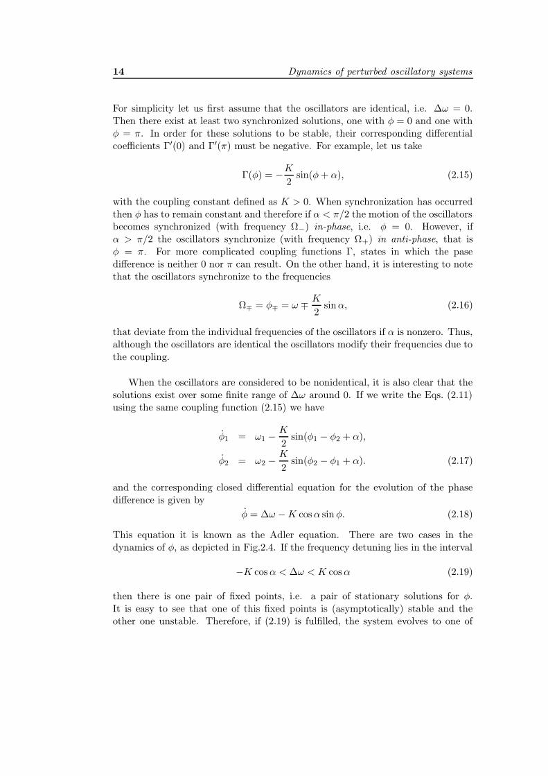
-π -π/2 0 π/2 πφ
0
1dφ
/dt
π -π/2 0 π/2 πφ
-π -π/2 0 π/2 πφ
bottleneck
K<∆ω K=∆ω K>∆ω(a) (b) (c)
Figure 2.4: The right hand side of Eq.(2.18) with α = 0 outside (a), at the border(b), and inside the synchronization region (c). The stable and the unstable fixed pointsare shown with the filled and open circles. In panel (b) the synchronization transition isshown. Here the stable and the unstable fixed points collide and form a half-stable fixedpoint which has been born in a saddle-node bifurcation.
the stable fixed points and stays there, so that the oscillators maintain a constantphase difference given by
φ∗ = arcsin
(
∆ω
K cosα
)
. (2.20)
This regime determines when the oscillators are synchronized, i.e. they posses acommon frequency Ω that in general (α 6= 0) deviates from the mean ω = (ω1 +ω2)/2 (see Fig.2.5). This regime exists inside the domain (2.19) on the parameterplane (∆ω,K), called the synchronization region, or range of entrainment.
Another situation is observed if the frequency detuning lies outside the synchro-nization region (2.19). Then the time derivative of φ is permanently positive (ornegative) and thus increases indefinitely, corresponding to phase drift (Fig. 2.4(a)).Notice that the phases do not separate at a uniform rate: φ increases most slowlywhen it passes under the minimum of the sine function (bottleneck), in Fig. 2.4(a)at φ = π/2, and most rapidly when it passes under the maximum at φ = −π/2.Moreover, the period of phase drift may be calculated as
T =
∫ 2π
0
dφ
φ(2.21)
which yields
T =2π
√
∆ω2 − (K cosα)2. (2.22)
The state of the system in the phase drift regime is quasiperiodic with two funda-mental frequencies: the beat frequency
∆Ω = 2π/T, (2.23)

16 Dynamics of perturbed oscillatory systems
0 0.5 1K
-0.25
0
0.25
Ω1,Ω
2
0 0.5 1K
0
0.5
∆Ω
Figure 2.5: Synchronization of two phase oscillators (2.17). Plotted is the averagedfrequencies (2.13) of each oscillator (left) and the beat frequency (2.23) ∆Ω(K) (right) asa function of the coupling strength, K.
and the observed frequency 〈φ〉 = Ω, (Eq. (2.13)).
The transition between phase drift and synchronization occurs in a saddle-nodebifurcation at
(∆ω)c =K
cosα, or Kc =
∆ω
cosα. (2.24)
Close to the synchronization region (2.19) it it possible to estimate the behaviorbeat frequency ∆Ω, that gives
∆Ω ∼√
∆ω −K cosα.
This shows that ∆Ω obeys the characteristic square root scaling law of a systemclose to a saddle-node bifurcation (see Fig. (2.4(b)). Therefore the oscillators spenda long time with some constant phase difference that it is interrupted by shortintervals where the phase difference φ increases (or decreases) by 2π: these eventsare called phase slips.
2.2.2 Synchronization of two Landau-Stuart oscillators
In the following section we obtain the phase equations of a system consisting intwo diffusively coupled Landau-Stuart oscillators,
z1,2 = z1,2[1 + i(ω1,2 + q1,2) − (1 + iq1,2)z1,2z1,2] +K
2(z2,1 − z1,2), (2.25)
where the subscripts refer to the oscillator 1 or 2. Aronson et al. (1990) showedthat the dynamics of (2.25) close to the transition to synchronization are greatly
2.2 Synchronization of two oscillators 17
0 0.5 1K
0
0.4
Ω1Ω
2
0 0.5 1K
0.8
1
r 1,r2
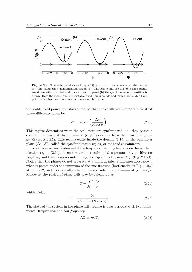
Figure 2.6: Frequencies (left) and averaged radius (right) of two coupled Landau-Stuartoscillators (2.25) (solid lines) versus coupling strength K. The dotted lines in the leftpanel correspond to the phase approximation (2.30) and the dotted lines in the right onecorrespond to Eq. (2.28) (q1 = q2 = 0.666, ω1 = 0.25, ω2 = −0.25).
complicated due to the presence of the nonisochronicity. However, the weakly cou-pled system presents an interesting property that was investigated and that willbe the the subject of Chapter 4. However, we first discuss briefly an importantphenomenon called oscillation death arising in the presence of both large param-eter mismatch and strong coupling strength. In such circumstances the diffusivecoupling acting in limit cycle systems can lead to the suppression of the oscillations(Bar-Eli, 1985; Aronson et al., 1990). The system (2.25) in polar coordinates writes
r1,2 = r1,2(1 − K
2− r21,2) +
K
2r2,1 cos(θ2,1 − θ1,2), (2.26)
θ1,2 = ω1,2 + q1,2(1 − r21,2) +
K
2
r2,1r1,2
sin(θ2,1 − θ1,2). (2.27)
In order to understand how oscillation death arises in the Landau-Stuart oscil-lators (2.25) let us assume that the oscillators are not synchronized. In thiscase, Eqs.(2.26) can be time-averaged over one period T of the phase differenceφ(t) = θ2 − θ1 in order to estimate the mean radius of the oscillators. Since theoscillators are unlocked, the phases perform a quasiperiodic motion on a torus withcoordinates θ1 and θ2, and therefore the integration of the trigonometric terms inthe right-hand side of Eqs. (2.26) and (2.27) vanish. In particular, the equation forthe radius has a stable fixed point located at
r1,2 =
√
1 − K
2, (2.28)

18 Dynamics of perturbed oscillatory systems
0 200t
0
1
r 1,r2
0 200t
0
1
r 1,r2
Figure 2.7: Time evolution of the radius of two coupled Landau-Stuart oscillators (2.25)for K = 0.05 (up) and for K = 0.47 (down). (q1 = q2 = 0.666, ω1 = 0.25, ω2 = −0.25).
and an unstable one at r1,2 = 0. Eq.(2.28) describes the effect of oscillation death:At K = 2 the unstable and the stable solutions meet and thus the origin r1,2 = 0becomes stable.
In Fig. (2.6) the transition to synchronization for two Landau-Stuart oscillatorsis shown numerically integrating Eqs.(2.25) and computing the frequencies Ω1,Ω2,as the coupling strength K is continuously increased from zero. The right panelshows, in solid lines, the time-average of the radius r1 and r2. The approximation(2.28) is plotted with dotted lines and presents good agreement with the numericsas far as the oscillators are not synchronized. As soon as the oscillators becomelocked, their radius increases reflecting the lower degree of interaction between theoscillators.
In the left panel of Fig. (2.6) the frequencies of the oscillators are depicted (assolid lines) as the coupling strength K is continuously increased from zero. Notethat there exists an important difference between Figs. (2.6)(left) and (2.5)(left).In the present case the oscillators increase their frequencies despite the fact thatthey are not synchronized: This reflects the presence of nonisochronicity in theLandau-Stuart systems. In addition, note that as soon as the synchronization isachieved the frequencies begin to decrease and tend to the mean ω = (ω1 + ω2)/2as K → ∞. This can be better understood by writing the corresponding phaseequations for the Landau-Stuart oscillators.Next, we derive the phase equations corresponding to the Landau-Stuart system
(2.25). If we assume that for weak coupling the time evolution of the radial partis approximately constant (see Fig. 2.7), ρ ≈ r1 ≈ r2 ≈ 0, then the Eqs.(2.26) for
2.2 Synchronization of two oscillators 19
the radius become
r21,2 = 1 − K
2+K
2
r2,1r1,2
cos(θ2,1 − θ1,2), (2.29)
and substituting this into Eqs. (2.27) we obtain
θ1,2 = ω1,2 +K
2q1,2 +
K
2
r2,1r1,2
[2 sin(θ2,1 − θ1,2) − q1,2 cos(θ2,1 − θ1,2)] , (2.30)
In Fig (2.6) a comparison of the phase Eqs.(2.30) with the original system (2.25)is shown. Clearly, the phase approximation is valid as far as the systems interactweakly and the amplitude of the oscillators remains constant in time. The validityof the phase approximation can be better understood comparing the left panel ofFig (2.6) with Figs. (2.7), where the time evolution of the oscillators amplitudesfor weak and for large (close to synchronization) coupling are shown.

Chapter 3
Synchronization in an ensemble
of nonidentical oscillators
”Below a threshold, anarchy prevails; above it, there is a collective rhythm (. . . )”
A. Winfree (2002)
This Chapter gives an overview on some of the main results that are knownabout macroscopic synchronization, especially for the case of global coupling. Thematerial here can be mostly found in the book of Kuramoto (1974), the book ofPikovsky et al. (2001) and in the papers Strogatz and Mirollo (1991) and Strogatz(2000). On one side, our aim is to put the results of this thesis in a general context.On the other, to present mathematical techniques that will be very much used inthe following chapters.
A starting date for the study of synchronization of many oscillators with dif-ferent natural frequencies can be probably set in the context of cybernetics, whenWiener (1958) suggested to approach the alpha rhythm in the brain as the entrain-ment of a large number of neurons with different period. About ten years later theproblem of synchronization was reconsidered by Winfree (1967) as an ubiquitousand central issue of biological systems.
Instead of the Fourier formalism used by Wiener, Winfree investigated theproblem looking at synchronization as a phase transition. As a simplified case, hestudied the behavior of a population of limit cycle oscillators with different naturalfrequencies and all-to-all coupling. He numerically found that for low values of thecoupling strength, the system was incoherent : On average no collective oscillationsappear in the ensemble. Increasing the coupling term, a critical value is reached, atwhich a small cluster of oscillators, rotating at the same frequency, emerges. Withfurther increase of coupling the cluster increases in size and the system enters
21

22 Synchronization in an ensemble of nonidentical oscillators
a region of partial locking. Using the centroid of the population of oscillatorsas an order parameter and the the coupling strength, or alternatively the widthof the distribution of natural frequencies, as a control parameter, a phenomenonanalogous to a second order phase transition appears.
Later this phenomenon was studied in more detail by Kuramoto (1974), whointroduced the model that now is the standard framework for studying synchro-nization phenomena, and is usually referred to as the Kuramoto model.
3.1 The Kuramoto model
We start analyzing the synchronization process in a macroscopic ensemble of Noscillators using the simplest possible model. In the Chapter 2 the phase equationscorresponding to two coupled oscillators were derived, under the assumption ofweak coupling and nearly identical natural frequencies (see Eq.(2.11)). Using thesame arguments, the phase equations for an ensemble of nearly identical, weaklycoupled oscillators can be obtained. Thus we have
θi = ωi −K
N
N∑
j=1
Γ(θi − θj), i = 1, . . . N (3.1)
where θi denotes the phase of the oscillator i in the ensemble and the frequencies ωiare distributed according to some probability density g(ω). The simplest possibleform of the coupling function corresponds to the Kuramoto model
θi = ωi −K
N
N∑
j=1
sin(θi − θj) (3.2)
where the frequency distribution g(ω) is assumed to be unimodal of width γ andsymmetric about its mean frequency ω, i.e. g(ω+ω) = g(ω−ω), for all ω. Moreover,we set ω = 0. This last assumption can be made without loss of generality (unlikethe hypothesis of symmetry) because the frequency distribution can be arbitrarilyshifted by choosing a frame of reference rotating with frequency −ω. In that case,the phase variables are tranformed according to θi → θi+ ωt, and using this changeof variables, Eq. (3.2) goes over to
θi = ωi − ω − K
N
N∑
j=1
sin(θi − θj). (3.3)
In order to study phase transitions, it is important to introduce an appropriateorder parameter, that is a macroscopic quantity defined between 0 and 1 whosevalue (first order phase transitions) or the value of whose derivative (second order
3.1 The Kuramoto model 23
phase transitions) is discontinuous at a critical point. A natural choice is thecentroid of the oscillator positions on the circle, defined as (Kuramoto, 1974)
Z = Reiψ =1
N
N∑
j=1
eiθj , (3.4)
where j is an index that characterizes each oscillator in the ensemble. Clearlythe quantity Z is an important measure for characterizing the amount of phaseclustering in large populations of oscillators. The order parameter R measures thephase coherence of the oscillators whereas ψ measures the average phase. Whenthe phases of the oscillators get closer to each other R tends to one whereas itsvalue fluctuates around zero when the oscillator phases are uncorrelated (withstandard deviation scaling as 1/
√N with the population size) and vanishes in
the thermodynamic limit. Intermediate values of R correspond to configurationswhere the oscillator density is neither localized nor uniform on the unit circle, likein the case of clustering. Thus, R quantifies the degree of synchronization of thepopulation and a phase transition can be detected looking at discontinuities in itsvalue when one of the control parameters is changed. On the other hand, notethat in contrast to the frequency disorder σ (see Chapter 4), the order parameterR does not provide direct information about the oscillator frequencies.
The order parameter as it has been defined in Eq.(3.4) has another importantadvantage beyond those discussed previously: thanks to the trigonometrical iden-tity obtained multiplying both sides of the order parameter equation (3.4) by eiθi ,the Eqs.(3.2) can be written in terms of the centroid as
θi = ωi −RK sin(θi − ψ). (3.5)
In this form the mean-field character of the Kuramoto model becomes very clear:The dynamical equation for each oscillator appears to be uncoupled from all theothers. In fact, each of them interacts only with the population as a whole, orequivalently with the mean field quantities R and ψ. The phase θi of each oscillatoris pulled toward the mean phase ψ, rather than toward the phase of each individualoscillator. Moreover, the effective strength of the coupling is proportional to thecoherence of the mean field R and therefore, in the incoherent state R = 0, allthe oscillators are uncoupled and the distribution of natural frequencies remainsunperturbed 1. This proportionality sets up a positive feedback loop betweencoupling and coherence: as the population becomes more coherent, R grows andso the effective coupling increases, which tends to recruit even more oscillators intothe synchronized cluster. If the coherence is further increased by new recruits, theprocess will continue. Otherwise, it becomes self-limiting.
1We will see in the next section that this is a specific property of the system Eq. (3.2). Thereforethis is not always true, for instance for the case of globally coupled nonisochronous oscillators.
24 Synchronization in an ensemble of nonidentical oscillators
-4 0 4coupling-modified freqs.
0
200
# os
cilla
tors
locked osc.
drifting osc.
Ω=ω
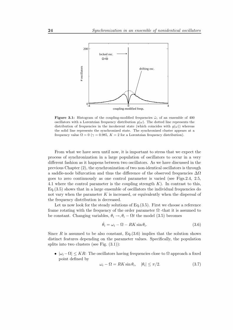
Figure 3.1: Histogram of the coupling-modified frequencies ωi of an ensemble of 400oscillators with a Lorentzian frequency distribution g(ω). The dotted line represents thedistribution of frequencies in the incoherent state (which coincides with g(ω)) whereasthe solid line represents the synchronized state. The synchronized cluster appears at afrequency value Ω = 0 (γ = 0.985, K = 2 for a Lorentzian frequency distribution).
From what we have seen until now, it is important to stress that we expect theprocess of synchronization in a large population of oscillators to occur in a verydifferent fashion as it happens between two oscillators. As we have discussed in theprevious Chapter (2), the synchronization of two non-identical oscillators is througha saddle-node bifurcation and thus the difference of the observed frequencies ∆Ωgoes to zero continuously as one control parameter is varied (see Figs.2.4, 2.5,4.1 where the control parameter is the coupling strength K). In contrast to this,Eq.(3.5) shows that in a large ensemble of oscillators the individual frequencies donot vary when the parameter K is increased, or equivalently when the dispersal ofthe frequency distribution is decreased.
Let us now look for the steady solutions of Eq.(3.5). First we choose a referenceframe rotating with the frequency of the order parameter Ω -that it is assumed tobe constant. Changing variables, θi →, θi − Ωt the model (3.5) becomes
θi = ωi − Ω −RK sin θi. (3.6)
Since R is assumed to be also constant, Eq.(3.6) implies that the solution showsdistinct features depending on the parameter values. Specifically, the populationsplits into two clusters (see Fig. (3.1)):
• |ωi−Ω| ≤ KR: The oscillators having frequencies close to Ω approach a fixedpoint defined by
ωi − Ω = RK sin θi, |θi| ≤ π/2. (3.7)
3.1 The Kuramoto model 25
The oscillators of this group are locked to the frequency Ω of the mean field.From Eq.(3.7) one can understand the basic mechanism of synchronization:In order to compensate the difference between the natural frequency ωi andthe frequency of the mean field Ω, the oscillators phases are shifted (withrespect to the centroid) by Ω − ωi, so that the frequency mismatch can beexactly balanced according to Eq.(3.7). Hence, in a typical locked state, theoscillators describe an arch of circumference around the centroid. The archis symmetric because of the symmetry of the sinusoidal coupling functionand because of the distribution of natural frequencies. The oscillators arelocated along the arch in order of natural frequency, the one with ωi = Ωbeing in the middle and thus having the same phase as the centroid. Fromthe symmetry properties of the frequency distribution it also follows that thelocking frequency Ω coincides with the average natural frequency ω. Thus,from Eq.(3.7) the locked oscillators have phases distributed according to
θ∗i = arcsin( ωiRK
)
. (3.8)
Fig. 3.2(d) presents a snapshot of the phases at a certain time t beyondthe transient period. The synchronized oscillators correspond to the centralcluster described by Eq.(3.8). Observe that the oscillators with natural fre-quency ωi = ω do not modify their frequencies whereas the rest of oscillatorsbelonging to the synchronized cluster form a frequency plateau depicted inFig. 3.2(c).
• |ωi − Ω| > KR: The oscillators of this group are called drifting oscillatorsand consists in those which fail to be entrained to the macroscopic field. Notethat Eq.(3.8) states that any finite population admits a fully locked solutionfor sufficiently large coupling strength, which increases with the width γ ofthe parameter distribution. Since the sine function is bounded, though, theoscillators with natural frequency very different from ω, i.e. those belongingto the tails of the frequency distribution g(ω), in practice can never be lockedand even large values of the coupling constant will lead at most to a partiallysynchronized solution. This is always the case for an infinite population sizewhen the distribution of natural frequencies is unbounded.
The Eq.(3.6) for the drifting oscillators can be integrated and gives
θi = ωit+ f((ωi − Ω)t), (3.9)
where the coupling-modified frequencies ω are given by
ωi = Ω + (ωi − Ω)
√
1 −(
KR
ωi − Ω
)2
, (3.10)
26 Synchronization in an ensemble of nonidentical oscillators
-3
0
3
ωi
-3
0
3
θ i
0 400i
-3
0
3
θ i
0 400i
-3
0
3
ωi
(a) (b)
(d)(c)
K<Kc
K>Kc
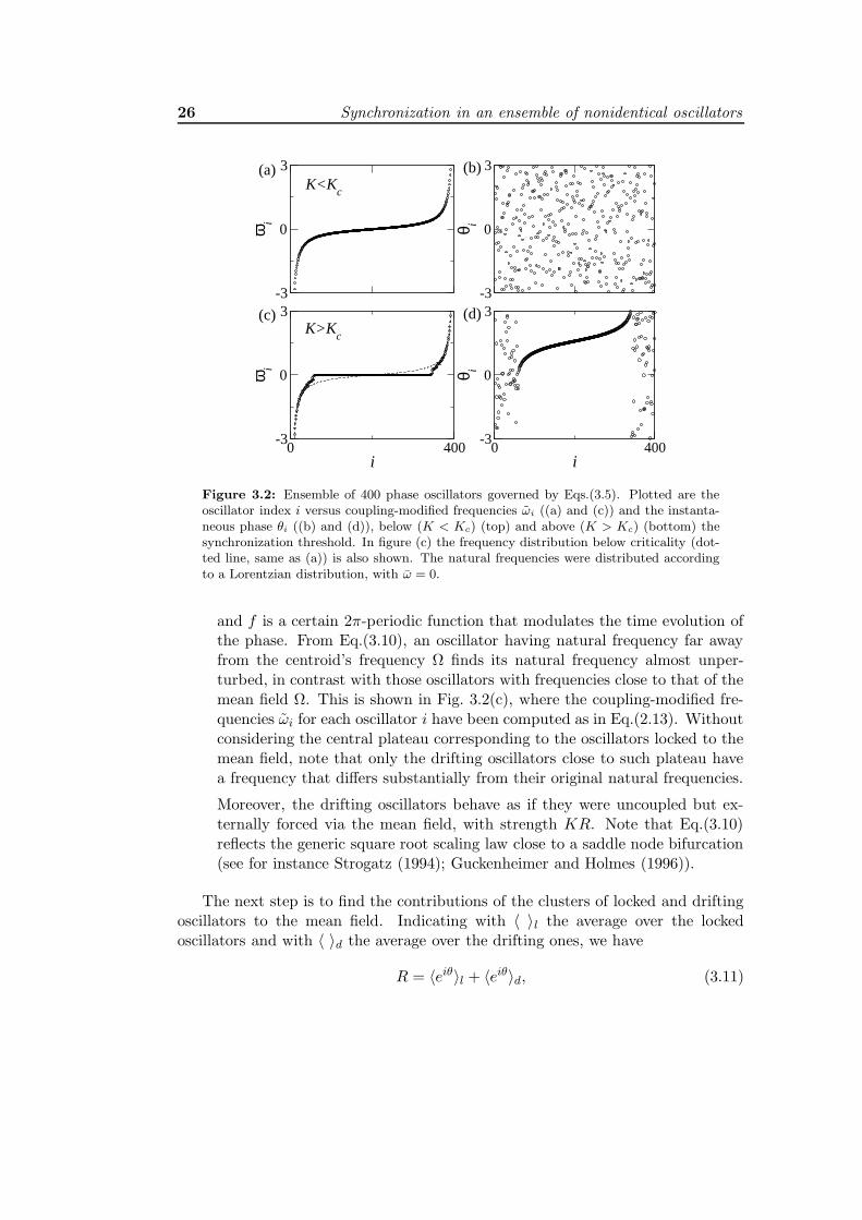
Figure 3.2: Ensemble of 400 phase oscillators governed by Eqs.(3.5). Plotted are theoscillator index i versus coupling-modified frequencies ωi ((a) and (c)) and the instanta-neous phase θi ((b) and (d)), below (K < Kc) (top) and above (K > Kc) (bottom) thesynchronization threshold. In figure (c) the frequency distribution below criticality (dot-ted line, same as (a)) is also shown. The natural frequencies were distributed accordingto a Lorentzian distribution, with ω = 0.
and f is a certain 2π-periodic function that modulates the time evolution ofthe phase. From Eq.(3.10), an oscillator having natural frequency far awayfrom the centroid’s frequency Ω finds its natural frequency almost unper-turbed, in contrast with those oscillators with frequencies close to that of themean field Ω. This is shown in Fig. 3.2(c), where the coupling-modified fre-quencies ωi for each oscillator i have been computed as in Eq.(2.13). Withoutconsidering the central plateau corresponding to the oscillators locked to themean field, note that only the drifting oscillators close to such plateau havea frequency that differs substantially from their original natural frequencies.
Moreover, the drifting oscillators behave as if they were uncoupled but ex-ternally forced via the mean field, with strength KR. Note that Eq.(3.10)reflects the generic square root scaling law close to a saddle node bifurcation(see for instance Strogatz (1994); Guckenheimer and Holmes (1996)).
The next step is to find the contributions of the clusters of locked and driftingoscillators to the mean field. Indicating with 〈 〉l the average over the lockedoscillators and with 〈 〉d the average over the drifting ones, we have
R = 〈eiθ〉l + 〈eiθ〉d, (3.11)

3.1 The Kuramoto model 27
where the index corresponding to the oscillator number has been dropped, since inthe thermodynamic limit N → ∞.
The contribution of the locked oscillators is simplified due to the symmetry ofthe distribution of the locked phases (3.8): Since the distribution of frequencies issymmetric, an oscillator with frequency ω gives exactly the opposite contributionas the corresponding oscillator with natural frequency −ω. Thanks to this fact,the imaginary part of 〈eiθ〉l averages out and hence in the thermodynamic limit
〈eiθ〉l = 〈cos θ〉l = KR
∫
|ω−Ω|≤KRcos θ g(ω) dθ.
From Eq.(3.7) it is possible to express the natural frequencies as a function ofthe angular position, and the contribution of the synchronized oscillators to thecentroid is
〈eiθ〉l = KR
∫ 2π
0cos2 θ g(KR sin θ + Ω) dθ. (3.12)
Now let us consider the drifting oscillators. In order to proceed Kuramoto madethe following additional hypothesis that he did not prove: the oscillators move on aunit circle with a speed that may change in time, but their distribution is stationary.If we define a density function so that ρ(θ, ω)dθ describes the number of oscillatorswith natural frequency ω that lie between θ and θ + dθ, Kuramoto’s hypothesisimplies that ρ must be stationary. The expression for ρ(θ, ω) is straightforwardlyobtained thinking that the oscillators will spend more time in a given small intervalwhen they have lower speed, and less where their velocity is higher. In other words,the function ρ(θ, ω) must be inversely proportional to the velocity (3.5), which againis a function of θ
ρ(θ, ω) =C
|ω −RK sin θ| . (3.13)
The normalization constant C is determined through the normalization conditionfor the density ρ
1 =
∫ 2π
0ρ(θ, ω)dθ =
∫ 2π
0
C
|ω −RK sin θ|dθ
which yields
C =1
2π
√
ω2 − (KR)2.
The contribution of the drifting oscillators can now be written as follows
〈eiθ〉d =
∫ 2π
0
∫
|ω−Ω|>KReiθρ(θ, ω)g(ω)dωdθ. (3.14)
Again we can use symmetry arguments to see that this integral vanishes, since g(ω)is an even function and, from Eq.(3.13), ρ(θ + π, ω) = ρ(θ,−ω).
28 Synchronization in an ensemble of nonidentical oscillators
The sums (3.12) and (3.14) yield the exact self-consistent equation
R = KR
∫ 2π
0cos2 θ g(KR sin θ + Ω) dθ,
that is always satisfied if R = 0, i.e., in the incoherent case. However, a nontrivialsolution, corresponding to the locked regime, can be found by eliminating R
1 = K
∫ 2π
0cos2 θ g(KR sin θ + Ω) dθ. (3.15)
Now the condition for the onset of synchronization can be obtained by solving theintegral for R→ 0+. This leads to the critical value of K
Kc =2
πg(ω), (3.16)
which is the Kuramoto’s critical coupling for the onset of collective synchronization.The behavior of the order parameter in the vicinity of the onset of synchroniza-
tion can be studied performing an expansion of Eq.(3.15) for K close to the criticalvalue
1 − π
2Kg(ω) − π
16K3g′′(ω)R2 +O(R3) = 0. (3.17)
It turns out that the character of the bifurcation, that is whether the centroid’soscillations amplitude increases for coupling larger (supercritical) or smaller (sub-critical) thanKc, is determined by the value of g′′(ω). In particular, we will considerthe supercritical case g′′(ω) < 0, when R can be estimated as
R ≈√
16
−πK3c g
′′(ω)
√
K −Kc
Kc. (3.18)
This relation also tells us that the order parameter scales as the square root of thedistance from the critical point, which is a generic feature of infinite dimensionalsystems and corresponds, from a dynamics systems perspective, to the order pa-rameter undergoing a supercritical Hopf bifurcation.
We want to stress that this self-consistent method has two important limita-tions:
• The analysis is concerned only with steady-state behavior and it thereforeprovides no information about stability. This important question will bediscussed in the Section 3.2.
• It depends crucially on the sinusoidal form of the coupling in the model(3.2). Because of a convenient trigonometric identity, the order parameter(3.4) appears in the governing equation (3.5). This is the coincidence whichallows the order parameter to be determined self-consistently.
3.1 The Kuramoto model 29
3.1.1 Asymmetric coupling function
This section is devoted to compare the results obtained for the Kuramoto modelwith the results obtained by Sakaguchi and Kuramoto (1986) using a more generalcoupling function Γ in Eq.(3.1)
θi = ωi −K
N
N∑
i=1
sin(θi − θj + α), (3.19)
where |α| < π/2. Using the order parameter (3.4), the model (3.19) becomes
θi = ωi −KR sin(θi − θj + α). (3.20)
The model (3.20) is essentially the Kuramoto model with a phase shift α in thecoupling function. This term in especially important when nonisochronicity isconsidered, as it will be shown in Section 3.3. On the other hand Eqs. (3.20) havealso been proved to be useful in modeling information concerning the synapticconnections in a neural network (Hoppensteadt and Izhikevich, 1998) and timedelays (Izhikevich, 1998) and they also appear naturally in the phase reductionof an array of superconducting Josephson junctions (Wiensenfeld and Swift, 1995;Wiesenfeld et al., 1996).
The fundamental difference between Eq.(3.19) and the Kuramoto model (3.2) isthat the in the present case the cluster of synchronized oscillators (i.e. the velocityof the order parameter Ω) is not determined trivially as in the previous case as themean bare frequency ω, and therefore Ω must be determined self-consistently aswell as the order parameter R. Sakaguchi and Kuramoto (1986) showed that thequantities R and Ω can be determined from the following self-consistency relation
Reiα = KR
(
iJ +
∫ π/2
π/2g(Ω +KR sin ξ)eiξ cos ξ dξ
)
, (3.21)
where
J =
∫ π/2
0
cos ξ(1 − cos ξ)
sin3 ξ[g(Ω + µ) − g(Ω − µ)] dξ (3.22)
with µ = KR/ sin ξ. Specifically, the critical point K = Kc is located at the pointwhere the R > 0 solution branches off the R = 0 solution.
Thus the synchronized cluster is Ω-shifted with respect the mean frequency.This fact in general is able to break the symmetry imposed through the choice of areflection-symmetric frequency distribution. In other words, the locked oscillatorsare in general not equally distributed around (ω − Ω), as it is shown in Fig 3.3.

30 Synchronization in an ensemble of nonidentical oscillators
-4 0 4coupling-mofified freqs.
0
250
# os
cilla
tors
drifting osc.
locked osc.
Figure 3.3: Histogram of the coupling-modified frequencies ωi of the model (3.19) (com-pare with Fig.3.1). The synchronized cluster appears at a frequency value Ω that differsfrom the mean of g(ω) (compare with Fig.3.1). (γ = 0.985, K = 2.8, α = π/4rad. for aLorentzian frequency distribution.)
3.2 Stability of incoherence in the Kuramoto model
As we have seen in the previous section, the stability properties of the steady solu-tions of the Kuramoto model can not be understood from the classical Kuramoto’sanalysis. Since the incoherent state and the partially synchronized state emergewhen the initial value problem is solved numerically, each must be stable in theappropriate range of K at least in an operational sense. However, the theoreticalexplanation of this stability has proved to be rather subtle even for the incoher-ent state (Strogatz and Mirollo, 1991; Strogatz et al., 1992; Strogatz, 2000). Thissection is devoted to explain the appropriate theoretical tools for the study of thestability of the possible dynamical states of the Kuramoto model. The theoreticaltreatment will be very much used in the rest of this PhD thesis.
3.2.1 Continuum limit of the Kuramoto model
The infinite system should be visualized as follows: for each frequency ω, there is acontinuum of oscillators distributed along the circle. Suppose then that this distri-bution is characterized by a density function ρ defined so that Ng(ω)ρ(θ, ω, t)dθdωdescribes the number of oscillators with natural frequencies in [ω, ω + dω] andphases in [θ, θ + dθ]. Thus ρ(θ, ω, t)dθ denotes the fraction of oscillators with nat-ural frequency ω and phase in [θ, θ + dθ] and satisfies the normalization
∫ π
−πρ(θ, ω, t)dθ = 1,

3.2 Stability of incoherence in the Kuramoto model 31
for all ω and t. Furthermore, the density ρ is required to be 2π-periodic in θ andnonnegative. The evolution of ρ is governed by the continuity equation
∂ρ
∂t= −∂(ρv)
∂θ, (3.23)
which expresses conservation of oscillators of frequency ω. Here the velocity v(θ, t, ω)is interpreted in an Eulerian sense as the instantaneous velocity of an oscillator atposition θ, given that it has natural frequency ω. From (3.5) that velocity is
vi(θ, t, ω) = ωi −RK sin(θi − ψ). (3.24)
The incoherent state is described by the uniform distribution
ρ0 =1
2π,
and defines an equilibrium for Eq.(3.23) since R = 0 at ρ0.The stationary states of the continuity equation (3.23) are the steady solutions
that we have seen in the previous section. The stationarity of Eq.(3.23) impliesthat
ρv = C(ω), (3.25)
and if C(ω) 6= 0, we recover the stationary density (3.13) that has been derivedintuitively for the drifting oscillators. On the other hand if C(ω) = 0 the densityfunction ρ must be a delta function in θ.
The order parameter (3.4) can be alternatively expressed in terms of the densityas
Reiψ =
∫ 2π
0dθ
∫ ∞
−∞eiθρ(θ, ω, t)g(ω)dω. (3.26)
The density function ρ(θ, t, ω) is 2π-periodic in θ and therefore it admits theFourier expansion
ρ(θ, ω, t) =l=∞∑
l=−∞ρl(ω, t)e
ilθ, (3.27)
with coefficients ρ−l = ρ∗−l since the density function is real. An important ob-servation to be done is that the purely sinusoidal coupling allows to express theorder parameter exclusively in terms of the first Fourier mode. Indeed, substituting(3.27) into the order parameter (3.4) yields
Reiψ = 2π
∫ ∞
−∞ρ∗1(ω, t)g(ω)dω, (3.28)
and so
−R sin(θi − ψ) =2πIm
[(∫ ∞
−∞ρ∗1(ω, t)g(ω)dω
)
e−iθ]
=iπ
(∫ ∞
−∞ρ1(ω, t)g(ω)dω
)
eiθ + c.c.,
(3.29)
32 Synchronization in an ensemble of nonidentical oscillators
where c.c. denotes the complex conjugate of the preceding term.The continuity equation (3.23) and the order parameter can be combined to
yield the equation for the evolution of the density ρ
∂ρ(θ, ω, t)
∂t= − ∂
∂θ
[
ρ(θ, ω, t)
(
ω +Kiπ
(∫ ∞
−∞ρ1(ω
′, t)g(ω′)dω′)
eiθ + c.c.
)]
.
This equation provides a continuum description of the oscillator population forwhich issues of stability and bifurcations can be analyzed in detail. It is equivalentto the following infinite system of integro-differential equations for the Fouriermodes
∂ρl(ω, t)
∂t= −iωlρl(ω, t) + lKπρl−1(ω, t)
∫ ∞
−∞ρ1(ω
′, t)g(ω′)dω′
− lKπρl+1(ω, t)
∫ ∞
−∞ρ∗1(ω
′, t)g(ω′)dω′.(3.30)
Note that equations corresponding to the negative modes are just the complexconjugate to the equations for the positive modes.
3.2.2 Linear stability analysis of the incoherent state
First note that the homogeneous distribution of the phases where all the Fouriermodes -except ρ0- vanish, is a solution of the system (3.30). Next, we study theevolution of a small perturbation of the incoherent state ρ0. This corresponds to
ρl = O(ε) ∀l 6= 0;
ρ0 = 1/2π,
where ε 1. Thus from Eqs. (3.30) it can be easily checked that all the modeshave the form
∂ρl(ω, t)
∂t= −ilωρl(ω, t) +O(ε2)
except the modes l = 1 and l = −1. The equation corresponding to the mode l = 1up to first order in ε is
∂ρ1(ω, t)
∂t= −iωρ1(ω, t) +
K
2
∫ ∞
−∞ρ1(ω
′, t)g(ω′)dω′ (3.31)
and the equation for the l = −1 is just the complex conjugate of Eq.(3.31). There-fore only these modes contribute to the linear stability of the incoherent stateρ0. Then the coherence R(t) is determined at this order by ρ1 via Eq.(3.31). Inparticular, if ρ1 grows exponentially, so does R(t).
Equation (3.31) reflects the mean-field character of the Kuramoto model: forany given ω, the evolution of ρ1(ω, t) depends on all the other frequencies through
3.2 Stability of incoherence in the Kuramoto model 33
the integrals in the right-hand side of Eq.(3.31). However, this dependence is thesame for all frequencies because the integral is independent of ω.
The right-hand side of Eq.(3.31) defines the following linear operator L
Lρ1(ω, t) = −iωρ1(ω, t) +K
2
∫ ∞
∞ρ1(ω
′, t)g(ω′)dω′ (3.32)
that has both, a continuous and a discrete spectrum. We concentrate the discussionon the discrete part since it is the only one that is relevant for our purposes.
The linear problem (3.31) has the solution
ρ1(ω, t) = b(ω)eλt,
that implies
λb(ω) = −iωb(ω) +K
2
∫ ∞
−∞b(ω′)g(ω′)dω′. (3.33)
Here, the integral in the right-hand side is just a real constant to be determinedself-consistently. Therefore the function b(ω) must satisfy
b(ω) =1
λ+ iω
K
2
∫ ∞
−∞b(ω′)g(ω′)dω′,
that can be substituted back to Eq.(3.33) in order to obtain the following condition
1 =K
2
∫ ∞
−∞
1
λ+ iωg(ω)dω, (3.34)
to be satisfied by the eigenvalues λ. Note that until now we have not made as-sumptions of any kind about the shape of the frequency distribution g(ω) nor aboutthe type of solutions that we expect. Eq.(3.34) gives the discrete spectrum of thesystem (3.31) that determines the linear stability properties of the incoherent stateρ0, in contrast to the Kuramoto analysis. In particular Eq.(3.34) also permits tocalculate the critical coupling Kc for which synchronization takes place for a givenfrequency distribution.
Eq.(3.34) can be alternatively written as
1 =K
2
(∫ ∞
−∞
λ∗
|λ|2 + ω2 − 2ωIm(λ)g(ω)dω −
∫ ∞
−∞
iω
|λ|2 + ω2 − 2ωIm(λ)g(ω)dω
)
,
(3.35)This equation can be simplified making two assumptions about g(ω):
• The function g(ω) is an even function, i.e. g(ω) = g(−ω). As we havealready discussed in previous section, in virtue of the reflection symmetryof the Kuramoto model it is always possible to go into a rotating framemoving with frequency ω the mean of g(ω). Therefore this condition holdsfor symmetric unimodal and bimodal frequency distributions.

34 Synchronization in an ensemble of nonidentical oscillators
• g(ω) is assumed to be nonincreasing on [0,∞), in the sense that g(ω) ≤ g(ω ′)for all ω ≥ ω′. Of course this property only holds for unimodal frequencydistributions.
If these two assumptions are fulfilled one can prove that Eq. (3.31) has at mostone solution for λ, and if such solution exists, it is necessarily real (Mirollo andStrogatz, 1990). Then the second integral of the r.h.s vanishes exactly since itsintegrand is an odd function of ω. Thus Eq.(3.34) reduces to
1 =K
2
∫ ∞
−∞
λ
λ2 + ω2g(ω)dω. (3.36)
This result is very interesting: It shows that the eigenvalue λ must be a positivenumber, since otherwise the right-hand side of Eq. (3.36) is negative or zero. Hence,the fundamental mode l = 1 is never linearly stable (Strogatz and Mirollo, 1991).
Now it is possible to calculate the critical coupling Kc of synchronization byletting λ→ 0+ on Eq.(3.36). Noting that
limλ→0+
λ
λ2 + ω2= πδ(ω),
Eq. (3.36) implies that
Kc =2
πg(ω),
which is the critical coupling (3.16) found by Kuramoto. However, note that thisis a demonstration that the the incoherent state becomes unstable at Kc.
3.3 Ensemble of Landau-Stuart oscillators
In the following we study the synchronization in an ensemble of globally coupledLandau-Stuart oscillators. The system is the following
zi = zi[1 + i(ωi + q) − (1 + iq)ziz∗i ] −
K
N
N∑
j=1
(zi − zj) (3.37)
where the natural frequencies ωi are assumed to be randomly selected from a fre-quency distribution g(ω). As usual it can be assumed that the sample mean of ωis zero: if the mean of ω is ω, ω 6= 0, we can go into a rotating frame definingz′i = zie
−iωt and then the equations for z ′i are identical to Eqs.(3.37) with zeromean frequency. We assume that g(ω) is symmetric and non-increasing on [0,∞).
If we use the order parameter (3.4), then Eq.(3.37) becomes
zi = zi[1 + i(ωi + q) − (1 + iq)ziz∗i ] −K(zi − Z) (3.38)
3.3 Ensemble of Landau-Stuart oscillators 35
A simple stability analysis can be carried out under the assumption that for a largedifference in the natural frequencies the phases of the individual oscillators arerandomly distributed, while the amplitudes rearrange themselves around a givenmean value, so that the value of the averaged position is close to zero Z ≈ 0. It isthen useful to rewrite Eq.(3.38) in the following way:
zi = zi[1 + i(ωi + q) − (1 + iq)ziz∗i ] −K(zi − Z)
≈ zi[1 −K + i(ωi + q) − (1 + iq)ziz∗i ].
(3.39)
The eigenvalues of the origin in Eq.(3.39) are 1−K±i(ωi+q) and therefore, as soonas K > 1, the origin becomes attracting. This phenomenon is known as oscillationdeath (Mirollo and Strogatz, 1990).
Next we reduce Eqs. (3.38) to their corresponding phase equations (in the limitof weak coupling K and narrowly distributed frequencies), as we made in Chapter 2in the case of two coupled Landau-Stuart oscillators. We start by rewriting theEqs. (3.38) in polar coordinates
ri = ri(1 − r2i ) +K[R cos(θi − ψ) − ri]
θi = ωi + q(1 − r2i ) −
KR
risin(θi − ψ).
(3.40)
In the incoherent state, the differential equations for the radial part of Eqs. (3.40)reduce to
1 − r2i = K[1 − R
ricos(θi − ψ)],
since ri ≈ 0 for all i. This can be substituted into the angular component ofEq.(3.40), and hence the angular part of Eqs. (3.40) reduce to
θi = ωi + qK −KR[sin(θi − ψ) + q cos(θi − ψ)]. (3.41)
This result confirms that any population of weakly and diffusively coupled limitcycles close to a Hopf bifurcation can be generically expressed in the form ofEqs. (3.41). Note that in the case of isochronous oscillators, q = 0, Eqs. (3.41)reduce to the Kuramoto model (3.2). We have written phase equations were theeffect of the frequency response to the small perturbation is taken into accountthrough the terms proportional to the nonisochronicity q.
The transformation α ≡ tan−1 q leaves the system
θi = ωi +K tanα− K
cosαsin(θi − θj + α), (3.42)
which is very similar to the model presented in Section 3.1.1. However, in thepresent case the coupling has a direct effect on the distribution of natural frequen-cies in the incoherent state due to the presence of nonisochronicity. This first effect

36 Synchronization in an ensemble of nonidentical oscillators
of α (realized by the factor K tanα in Eq.(3.42)) is the most relevant effect of thenonisochronicity far from the synchronization transition, i.e. for small coupling.The study of such effects in more general systems will be the subject of Chapter 4.On the other hand, close to the synchronization transition the angular terms inEqs. (3.42) are fundamental: In this regime Eqs. (3.42) behave essentially as theEqs. (3.19) studied Section 3.1.1. Therefore the nonisochronicity also breaks thesymmetry imposed through the distribution of frequencies. In the Chapter 5 weinvestigate the influence of such effects in the transition to synchronization of twocoupled populations of a Landau-Stuart type (3.42).
Chapter 4
Anomalous synchronization
In this Chapter the concept of anomalous synchronization is described. Whereas inthe previous Chapter the analysis of synchronization has been restricted to Landau-Stuart and phase oscillators, here synchronization is studied in a broader class ofsystems. However, the phase approximation described, described in Chapter 2, isstill of validity since we consider weakly coupled and nearly identical oscillators.
The phenomenon described here arises when the nonisochronicity of each os-cillator in the ensemble is related with its natural frequency. As it was shown inChapter 3, the heterogeneity in the ensemble is usually taken into account consid-ering that the oscillators have natural frequencies according to a certain distribu-tion. However, here we show that there are new collective phenomena emergingif there is disorder in other characteristics of the individual oscillators. Besidesthe natural frequency, the next relevant parameter in synchronization theory is thenonisochroncity.
The outline of this Chapter is as follows: first, in Section 4.1, we define the typeof systems under investigation as an interacting ensemble of limit cycle systems orchaotic oscillators. Further we review some basic properties of phase synchro-nization in chaotic systems. Next, we use these methods to numerically explorethe transition to phase synchronization in spatially extended ecological systemswith oscillating dynamics. This will lead us to the phenomenon of anomaloussynchronization. In the following Section 4.2 we present analytic arguments whichdemonstrate the origin of these effects and provide an exact criteria that permits toknow when anomalous effects are to be expected. In order to show that anomaloussynchronization appears universally, in Section 4.3 an ensemble of weakly nonlinearVan-der-Pol oscillators is analyzed and the theoretical results show effectively thatthe previously developed techniques are useful. The last Section is devoted to thestudy of anomalous synchronization in the Landau-Stuart model. This equationsare specially convenient because the natural frequency and the nonisochronicity
37

38 Anomalous synchronization
appear as independent parameters. This fact allows to apply the analytical tech-niques developed in Chapter 3 in order to calculate the synchronization threshold.The results obtained in this Chapter are summarized in (Blasius et al., 2003; Mont-brio and Blasius, 2003), and the last section will be published in (Montbrio et al.,2004a).
4.1 Numerical results for general systems
In this Section the systems under investigation consist in N -coupled nonidenticaloscillators of the following form
xi = F(xi;χi) +K
NC
N∑
j=1
(xj − xi), i = 1 . . . N. (4.1)
To be more specific, Eqs. (4.1) have the following properties:
• In the absence of coupling each oscillator follows its own local dynamicsx = F (x, χ) where x belongs to Rn. All oscillators have the same functionalform but depend on a set of l control parameters χ = (a, b..). It is alwaysassumed that each oscillator is parameterized either on a limit cycle or on aregime with phase coherent chaos. Thus every, possibly chaotic, oscillator ischaracterized by a well defined natural frequency which is given by the long
term average of phase velocity, ω = θ(t) (Pikovsky et al., 2001).
• Disorder or quenched noise is imposed onto the system by assigning to eachoscillator i an independent value for every control parameter out of the setχi, usually taken from a statistical distribution. Here, a uniform distributionis always used. However our results remain valid if different distributionssuch as a Gaussian are used. In general, the control parameters affect thenatural or unperturbed frequency of each oscillator, ωi = ω(χi). Therefore,the natural disorder in control parameters leads to a frequency mismatchbetween the oscillators which it is also referred to as frequency disorder.
• Each oscillator is coupled with strength K to a predefined set of m neighborsj. In this Chapter, only two cases are considered: either coupling to nextneighbors in a one or two dimensional lattice or global coupling. Howeverwe have obtained similar results with different coupling topologies. C =diag(c1, c2..., cn) is a diagonal matrix which indicates the strength of theinteraction in each component of the state vector x. We also assume thateven with the onset of coupling each oscillator is still rotating uniformly. Thismeans especially that we don’t allow for situations with oscillation death(Aronson et al., 1990; Mirollo and Strogatz, 1990). In practice, this can
4.1 Numerical results for general systems 39
always be realized if the coupling is restricted to be small enough and thevariance of the inhomogeneities in the ensemble parameters is not large.
Synchronization arises as an interplay between the interaction and the frequencymismatch of the oscillators. Thereby, in general, the frequency of each oscillatorwill be detuned
Ωi = Ωi(K). (4.2)
The process of synchronization between two mutually coupled phase oscillatorshas been described in Chapter 2. Interestingly, these ideas can directly be extendedto systems with self sustained chaotic dynamics (Rosenblum et al., 1996). For theseaims it is necessary to extend the concepts of phase and frequency to the case of achaotic attractor. This is well established in phase coherent chaotic systems. Letus take for example the Rossler system (Rossler, 1976)
x = −by − z,
y = bx+ ay,
z = 0.4 + (x− 8.5)z.
(4.3)
In the parameter range a ≈ 0.15 and b ≈ 1 the motion shows phase coherentdynamics (see also Fig.4.3). In this regime a phase can be defined as an anglein (x, y)-phase plane or via the Hilbert-transform (Rosenblum et al., 1996). Inthis work, the phase of chaotic systems is always estimated by counting successivemaxima, e.g. the times tn of the n’th local maxima of the y-variable are located.We define that the phase increases by 2π between two successive maxima andinterpolate linearly in between (Pikovsky et al., 2001)
φ(t) = 2πt− tn
tn+1 − tn+ 2πn, tn < t < tn+1. (4.4)
Next we explore the transition to synchronization in two mutually coupledRossler systems (see Fig. 4.1). The oscillators are nonidentical and vary in thevalue of parameter b. Both oscillators are diffusively coupled in the y variablewith strength K (i.e. by adding the term K(y2,1 − y1,2) in the equation of y1,2).As can be seen in Fig.4.1, despite the chaotic amplitudes the transition to thesynchronized state is very similar to the case of two coupled phase oscillators. Dueto the interaction both oscillators are detuned and the frequencies approach eachother. As a result the frequency difference, ∆Ω(K) decreases monotonically untilit becomes zero in the synchronized state. In the following we study how theseideas generalize to an ensemble of many interacting Rossler systems (Osipov et al.,1997)
xi = −biyi − ziyi = bixi + ayi +
Km
∑
j(yj − yi)
zi = 0.4 + (xi − 8.5)zi.
(4.5)

40 Anomalous synchronization
0.00 0.01 0.02 0.03K
0.00
0.01
0.02
∆Ω
0.00 0.01 0.02 0.03K
1.02
1.03
1.04
1.05
Ωι
Ω1
Ω2
Figure 4.1: Transition to synchronization in two coupled Rossler systems (4.3). Plottedis the frequency difference ∆Ω(K) (left) and the individual frequencies of each oscillator,Ω12(K) (right) as a function of coupling strength. Parameter values a = 0.15, b1,2 =1.0 ± 0.01.
Here, all Rossler oscillators are nonidentical. The disorder is realized by taking theparameters bi for each oscillator from a uniform distribution and thereby assigningit its own frequency ωi ≈ bi. In Fig. 4.2 we plot the numerical results in a ring of10 locally coupled Rossler oscillators. With the onset of coupling the frequencies ofall oscillators move towards each other forming synchronized clusters. At a certaincoupling strength only one cluster is left and the ensemble reaches the synchronizedstate.
In this Chapter we introduce another measure for detecting synchronization. InChapter 3 the complex order parameter (3.4) was defined in order to measure thephase coherence in the ensemble. However, in this Chapter we are also interestedin the behavior of the frequencies, and hence another measure for synchronizationis required. The frequency synchronization in the ensemble can be revealed bymeasuring the standard deviation of the frequencies (4.2), σ(K). As is shown inFig.4.2, σ(K) is a decreasing function of coupling strength. Global phase synchro-nization is achieved when σ(K > Kc) = 0 and all oscillators rotate with the samefrequency. By comparing Fig. 4.2 with Fig. 4.1 it follows that in interacting os-cillator systems the standard deviation σ(K) takes over the role of ∆Ω(K) in thecase of two coupled oscillators.
To summarize, in order to measure the transition to synchronization in a sys-tem of interacting oscillators (4.1) we identify the frequency of each oscillator independence of the coupling strength, ωi(K). For phase coherent chaotic dynamicsthis is done by counting the number of local maxima of a chosen variable. Wedefine the frequency disorder as the standard deviation of all oscillator frequen-cies σ(K). Then synchronization is given by the single criterion that σ(K) = 0.
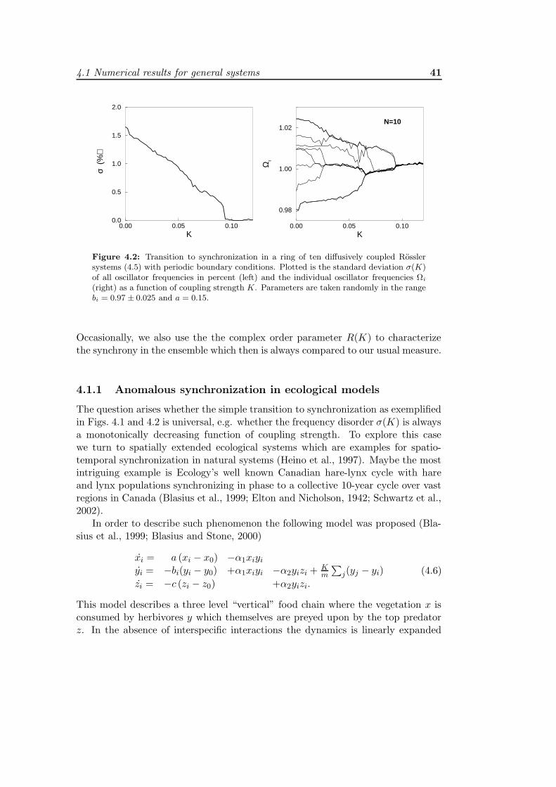
4.1 Numerical results for general systems 41
0.00 0.05 0.10K
0.0
0.5
1.0
1.5
2.0 σ
(%
)
0.00 0.05 0.10K
0.98
1.00
1.02
Ωι
N=10
Figure 4.2: Transition to synchronization in a ring of ten diffusively coupled Rosslersystems (4.5) with periodic boundary conditions. Plotted is the standard deviation σ(K)of all oscillator frequencies in percent (left) and the individual oscillator frequencies Ωi
(right) as a function of coupling strength K. Parameters are taken randomly in the rangebi = 0.97 ± 0.025 and a = 0.15.
Occasionally, we also use the the complex order parameter R(K) to characterizethe synchrony in the ensemble which then is always compared to our usual measure.
4.1.1 Anomalous synchronization in ecological models
The question arises whether the simple transition to synchronization as exemplifiedin Figs. 4.1 and 4.2 is universal, e.g. whether the frequency disorder σ(K) is alwaysa monotonically decreasing function of coupling strength. To explore this casewe turn to spatially extended ecological systems which are examples for spatio-temporal synchronization in natural systems (Heino et al., 1997). Maybe the mostintriguing example is Ecology’s well known Canadian hare-lynx cycle with hareand lynx populations synchronizing in phase to a collective 10-year cycle over vastregions in Canada (Blasius et al., 1999; Elton and Nicholson, 1942; Schwartz et al.,2002).
In order to describe such phenomenon the following model was proposed (Bla-sius et al., 1999; Blasius and Stone, 2000)
xi = a (xi − x0) −α1xiyiyi = −bi(yi − y0) +α1xiyi −α2yizi +
Km
∑
j(yj − yi)
zi = −c (zi − z0) +α2yizi.
(4.6)
This model describes a three level “vertical” food chain where the vegetation x isconsumed by herbivores y which themselves are preyed upon by the top predatorz. In the absence of interspecific interactions the dynamics is linearly expanded
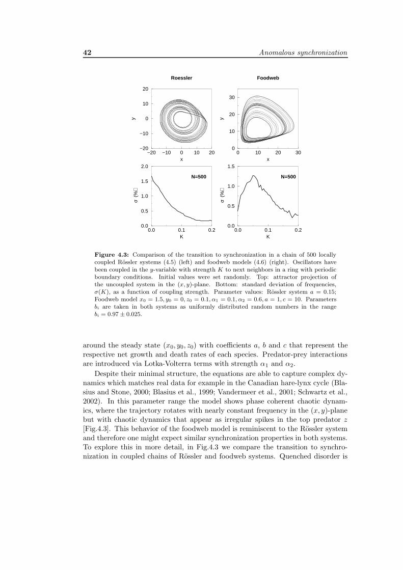
42 Anomalous synchronization
−20 −10 0 10 20x
−20
−10
0
10
20
y
Roessler
0 10 20 30x
0
10
20
30
y
Foodweb
0.0 0.1 0.2K
0.0
0.5
1.0
1.5
2.0
σ (%
)
0.0 0.1 0.2K
0.0
0.5
1.0
1.5
σ (%
)
N=500 N=500
Figure 4.3: Comparison of the transition to synchronization in a chain of 500 locallycoupled Rossler systems (4.5) (left) and foodweb models (4.6) (right). Oscillators havebeen coupled in the y-variable with strength K to next neighbors in a ring with periodicboundary conditions. Initial values were set randomly. Top: attractor projection ofthe uncoupled system in the (x, y)-plane. Bottom: standard deviation of frequencies,σ(K), as a function of coupling strength. Parameter values: Rossler system a = 0.15;Foodweb model x0 = 1.5, y0 = 0, z0 = 0.1, α1 = 0.1, α2 = 0.6, a = 1, c = 10. Parametersbi are taken in both systems as uniformly distributed random numbers in the rangebi = 0.97 ± 0.025.
around the steady state (x0, y0, z0) with coefficients a, b and c that represent therespective net growth and death rates of each species. Predator-prey interactionsare introduced via Lotka-Volterra terms with strength α1 and α2.
Despite their minimal structure, the equations are able to capture complex dy-namics which matches real data for example in the Canadian hare-lynx cycle (Bla-sius and Stone, 2000; Blasius et al., 1999; Vandermeer et al., 2001; Schwartz et al.,2002). In this parameter range the model shows phase coherent chaotic dynam-ics, where the trajectory rotates with nearly constant frequency in the (x, y)-planebut with chaotic dynamics that appear as irregular spikes in the top predator z[Fig.4.3]. This behavior of the foodweb model is reminiscent to the Rossler systemand therefore one might expect similar synchronization properties in both systems.To explore this in more detail, in Fig.4.3 we compare the transition to synchro-nization in coupled chains of Rossler and foodweb systems. Quenched disorder is
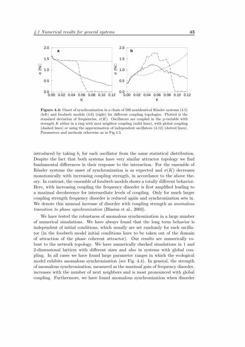
4.1 Numerical results for general systems 43
0.00 0.02 0.04 0.06 0.08 0.10 0.12K
0.0
0.5
1.0
1.5
2.0
σ (%
)
0.00 0.02 0.04 0.06 0.08 0.10 0.12K
0.0
0.5
1.0
1.5
2.0
σ (%
)
a b
Figure 4.4: Onset of synchronization in a chain of 500 nonidentical Rossler systems (4.5)(left) and foodweb models (4.6) (right) for different coupling topologies. Plotted is thestandard deviation of frequencies, σ(K). Oscillators are coupled in the y-variable withstrength K either in a ring with next neighbor coupling (solid lines), with global coupling(dashed lines) or using the approximation of independent oscillators (4.12) (dotted lines).Parameters and methods otherwise as in Fig.4.3.
introduced by taking bi for each oscillator from the same statistical distribution.Despite the fact that both systems have very similar attractor topology we findfundamental differences in their response to the interaction. For the ensemble ofRossler systems the onset of synchronization is as expected and σ(K) decreasesmonotonically with increasing coupling strength, in accordance to the above the-ory. In contrast, the ensemble of foodweb models shows a totally different behavior.Here, with increasing coupling the frequency disorder is first amplified leading toa maximal decoherence for intermediate levels of coupling. Only for much largercoupling strength frequency disorder is reduced again and synchronization sets in.We denote this unusual increase of disorder with coupling strength as anomaloustransition to phase synchronization (Blasius et al., 2003).
We have tested the robustness of anomalous synchronization in a large numberof numerical simulations. We have always found that the long term behavior isindependent of initial conditions, which usually are set randomly for each oscilla-tor (in the foodweb model initial conditions have to be taken out of the domainof attraction of the phase coherent attractor). Our results are numerically ro-bust to the network topology. We have numerically checked simulations in 1 and2-dimensional lattices with different sizes and also in systems with global cou-pling. In all cases we have found large parameter ranges in which the ecologicalmodel exhibits anomalous synchronization (see Fig. 4.4). In general, the strengthof anomalous synchronization, measured as the maximal gain of frequency disorder,increases with the number of next neighbors and is most pronounced with globalcoupling. Furthermore, we have found anomalous synchronization when disorder
44 Anomalous synchronization
is realized by different statistical distributions and it retains also in chains withlinearly increasing control parameters bi. Anomalous synchronization appears al-ready in two coupled chaotic foodweb models, albeit not as pronounced as in largeensembles. In general we find that the effect of anomalous synchronization appearsindependently of the number of oscillators, with a tendency to be more distinctin large systems. Note, that the strength of anomalous synchronization in generaldepends also on the choice of control parameters and may appear only in certainregimes in parameter space.
To gain more insight into the strikingly different behavior of Rossler and food-web systems in Fig.4.5 the frequency detuning of individual oscillators in a globallycoupled ensemble is depicted. In the Rossler system synchronization appears in theusual way. For small coupling levels the oscillator frequencies are not much affectedand fall down slightly with coupling strength. When coupling reaches a critical levelall oscillator frequencies are rapidly attracted towards each other and synchronizeto a common frequency. In the foodweb model the transition to the synchronizedstate is totally different. Compared to the Rossler system the average decrease ofoscillator frequencies is much stronger. Simultaneously, the interaction leads to arepelling of frequencies where the whole ensemble deviation is enlarged. In thisway σ(K) can reach values which are four times larger than the natural frequencydisorder σ(0). This picture is further complicated due to the appearance of clus-tering. Therefore, Fig.4.5 also includes a plot of the order parameter R(K). In theRossler system for small coupling levels R(K) remains nearly zero. At the criticallevel, K = Kth, cluster formation sets in and all oscillators fastly synchronize toone final cluster. This is reflected in the sudden increase of the order parameterR(K) which appears in the same coupling range as the rapid drop of σ(K). Incontrast, in the foodweb model clustering sets in already for small coupling levelswhere the oscillators start to form one main cluster at the high frequency range.This process is accompanied by a slow increase of R(K) and, simultaneously, bya rise of the frequency disorder σ(K). With increasing coupling strength the clus-ter is able to catch more and more oscillators until finally all frequencies becomeidentical for K > Kc.
The simultaneous increase of order parameter and frequency disorder with cou-pling as exemplified here in the foodweb model is rather unusual in the sense thatboth measures for synchronization lead to different results. Whereas the increaseof R(K) signifies the onset of synchronization it is evident from the increase ofσ(K) that the frequencies are driven away from each other. This apparent paradoxcan be explained by the fact that while the cluster is able to attract frequencies inclose range, at the same instant oscillators with a bigger frequency distance fromit are repelled off even stronger. As will be shown later anomalous synchronizationdoes not always go together with such complications and it is also possible that theoscillator frequencies simply split apart without simultaneous onset of clustering.
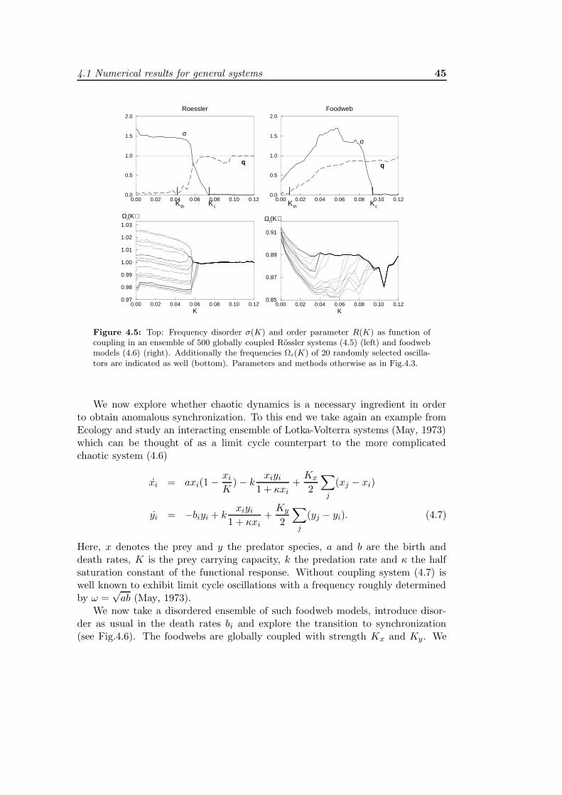
4.1 Numerical results for general systems 45
0.00 0.02 0.04 0.06 0.08 0.10 0.120.0
0.5
1.0
1.5
2.0Roessler
0.00 0.02 0.04 0.06 0.08 0.10 0.120.0
0.5
1.0
1.5
2.0Foodweb
0.00 0.02 0.04 0.06 0.08 0.10 0.12K
0.97
0.98
0.99
1.00
1.01
1.02
1.03
0.00 0.02 0.04 0.06 0.08 0.10 0.12K
0.85
0.87
0.89
0.91
q q
σσ
Κc ΚcΚthΚth
Ωi(Κ) Ωi(Κ)
Figure 4.5: Top: Frequency disorder σ(K) and order parameter R(K) as function ofcoupling in an ensemble of 500 globally coupled Rossler systems (4.5) (left) and foodwebmodels (4.6) (right). Additionally the frequencies Ωi(K) of 20 randomly selected oscilla-tors are indicated as well (bottom). Parameters and methods otherwise as in Fig.4.3.
We now explore whether chaotic dynamics is a necessary ingredient in orderto obtain anomalous synchronization. To this end we take again an example fromEcology and study an interacting ensemble of Lotka-Volterra systems (May, 1973)which can be thought of as a limit cycle counterpart to the more complicatedchaotic system (4.6)
xi = axi(1 − xiK
) − kxiyi
1 + κxi+Kx
2
∑
j
(xj − xi)
yi = −biyi + kxiyi
1 + κxi+Ky
2
∑
j
(yj − yi). (4.7)
Here, x denotes the prey and y the predator species, a and b are the birth anddeath rates, K is the prey carrying capacity, k the predation rate and κ the halfsaturation constant of the functional response. Without coupling system (4.7) iswell known to exhibit limit cycle oscillations with a frequency roughly determinedby ω =
√ab (May, 1973).
We now take a disordered ensemble of such foodweb models, introduce disor-der as usual in the death rates bi and explore the transition to synchronization(see Fig.4.6). The foodwebs are globally coupled with strength Kx and Ky. We
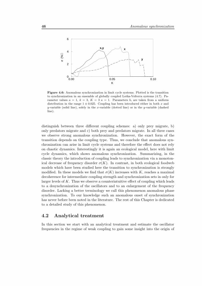
46 Anomalous synchronization
0.00 0.05 0.10Κ
0
2
4
6
σ (%
)
x
y
x,y
Figure 4.6: Anomalous synchronization in limit cycle systems. Plotted is the transitionto synchronization in an ensemble of globally coupled Lotka-Volterra systems (4.7). Pa-rameter values a = 1, k = 3, K = 3 κ = 1. Parameters bi are taken from a uniformdistribution in the range 1 ± 0.025. Coupling has been introduced either in both x andy-variable (solid line), solely in the x-variable (dotted line) or in the y-variable (dashedline).
distinguish between three different coupling schemes: a) only prey migrate, b)only predators migrate and c) both prey and predators migrate. In all three caseswe observe strong anomalous synchronization. However, the exact form of thetransition depends on the coupling type. Thus, we conclude that anomalous syn-chronization can arise in limit cycle systems and therefore the effect does not relyon chaotic dynamics. Interestingly it is again an ecological model, here with limitcycle dynamics, which shows anomalous synchronization. Summarizing, in theclassic theory the introduction of coupling leads to synchronization via a monoton-ical decrease of frequency disorder σ(K). In contrast, in both ecological foodwebmodels which have been studied here the transition to synchronization is stronglymodified. In these models we find that σ(K) increases with K, reaches a maximaldecoherence for intermediate coupling strength and synchronization sets in only forlarger levels of K. Thus we observe a counterintuitive effect of coupling which leadsto a desynchronization of the oscillators and to an enlargement of the frequencydisorder. Lacking a better terminology we call this phenomenon anomalous phasesynchronization. To our knowledge such an anomalous onset of synchronizationhas never before been noted in the literature. The rest of this Chapter is dedicatedto a detailed study of this phenomenon.
4.2 Analytical treatment
In this section we start with an analytical treatment and estimate the oscillatorfrequencies in the regime of weak coupling to gain some insight into the origin of
4.2 Analytical treatment 47
anomalous synchronization. The aim is to derive exact criteria which determinethe conditions when anomalous effects are to be expected.
4.2.1 Approximation as uncoupled oscillators
To explain the basic method we start with the examples of the Rossler and food-web models of the previous section. Later these results will be put into a moregeneral framework. Take again the interacting ensemble of Rossler systems (4.5)and rewrite the equation for the y variable in the following way
yi = bixi + ayi +K
m
m∑
j=1
(yj − yi) = bixi + (a−K)yi +K〈yj〉. (4.8)
Here, 〈yj〉 = 1m
∑
j yj denotes the average of the y-variable over all oscillators in acoupling neighborhood of oscillator i. For small coupling we can assume that theoscillators are nearly independent and therefore we can safely replace the ensembleaverage 〈yj〉 by the time average of the uncoupled oscillator yi. As a result, in thelimit of very small coupling the interacting system essentially behaves as a systemof independent oscillators with modified dynamics
xi = −biyi − ziyi = bixi + (a−K)yi +Kyizi = 0.4 + (xi − 8.5)zi.
(4.9)
Here, in the case of the Rossler system we can approximate the constant yi ≈ 0.Therefore, the only effect of weak coupling is to introduce a small damping intothe dynamics of each oscillator which is seen as an effective reduction of parametera→ a−K. To test this approximation of independent oscillators we have includedin Fig. 4.4 a plot of the frequency disorder calculated for system (4.9). Indeed, inthe range of small coupling the approximated frequency disorder closely follows thenumerical results of the full system. Using equation (4.9) it is possible in principleto calculate the frequency detuning of each oscillator in the ensemble as a functionof coupling strength Ωi(K). In order to proceed further we need to estimate theaverage rotating frequency of the chaotic system. As a crude approximation herewe simply use the imaginary part of the eigenvalues in a linear expansion aroundthe unstable fixed point. To simplify the algebra even more we make use of thefact that in the Rossler system the dynamics takes place mainly in z = 0 plane andset z ≈ 0. Putting all this together leads to
Ωi(K) ≈√
b2i −1
4(a−K)2 ≈ ωi +
a
4ωiK, (4.10)
where the natural frequency of the Rossler system has been approximated by ωi =√
b2i − 14a
2.

48 Anomalous synchronization
Ω
Κ
Ω
Κ
σ(Κ)
o2
o3
o1
o4
σ(Κ)
o1
o2
o3
o4
Figure 4.7: Frequency detuning here schematically indicated for 4 oscillators as a func-tion of coupling strength, Ωi(K) = ωi + Kκi. Left: the slope of each line, κi, decreaseswith ωi. Therefore, frequency disorder σ(K) is reduced leading to synchronization en-hancement. Right: anomalous synchronization when κi increases with ωi.
Eq. (4.10) tells that the mean frequency at the first order in K is a linearincreasing function of coupling strength with a slope κi = a
4ωithat depends on
the natural frequency of this unperturbed oscillator (see Fig. 4.7). In the usualparameter range the detuning is very small, κ ≈ 0.04, which corresponds very wellwith Fig. 4.5 where for small coupling ranges the frequencies are nearly unaffectedby coupling.
From this analysis (4.10) it is also clear that the Rossler systems in the form(4.5) cannot exhibit anomalous synchronization (see Fig.4.7). The simple reasonis that for every oscillator the slope κi is decreasing with the natural frequency,κi ∼ 1/ωi. Therefore, in oscillators which start out with higher natural frequencyωi, the oscillating frequency Ωi(K) is changing less with coupling than in oscillatorswith smaller ωi. By this mechanism all frequencies Ωi(K) are attracted togetherwith coupling, which finally confirms the usual synchronization transition of theinteracting Rossler systems.
We now proceed in a similar way for the ensemble of coupled foodweb models(4.6). Recall that this system shows an anomalous enlargement of the naturalfrequency disorder and therefore behaves exactly in the opposite way as the Rosslersystem. In analogy to (4.9) we replace the interacting ensemble with the followingsystem of uncoupled oscillators
xi = a (xi − x0) −α1xiyiyi = −(bi +K)yi + biy0 +α1xiyi −α2yizi +Kyizi = −c (zi − z0) +α2yizi.
(4.11)
From inspection of Fig.4 it is clear that in our parameter range y ≈ 10 and thereforethe time average cannot be set to zero as in the Rossler system. Probably forthis reason the simple scheme (4.10) is not applicable to estimate the averagerotating frequency of the model (4.11). When calculating the imaginary parts of theeigenvalue of the unstable fixed point and setting z = 0 we obtain a bad estimate of
4.2 Analytical treatment 49
Ωi(K). Despite these analytical difficulties, the numerically evaluated frequenciesof model (4.11) agree perfectly with the behavior of the full model as long asK Kc. The same holds for the frequency disorder of the uncoupled system,σ(K), which is plotted in Fig. 4.4b and shows similar anomalous synchronizationeffects. Thus again, for weak coupling the approximation of uncoupled oscillators(4.11) provides an excellent description for the full system dynamics.
The origin of this anomalous increase in σ(K) can be understood from Fig. 4.6which depicts the frequencies Ωi(K) for each oscillator. We find that in the foodwebmodel the frequencies are a nearly linear decreasing function of K with slope κi ≈−2. Careful inspection of Fig. 4.6 reveals that for different oscillators the slope κiincreases with the natural frequency ωi. Note, that this is just the opposite trendas exhibited in the Rossler system. As a result, in contrast to the Rossler systemhere the frequency disorder effectively can be enlarged with coupling strength.Schematically this situation is sketched in Fig. 4.7b which in this way gives avisualization of the basic mechanism underlying anomalous synchronization.
4.2.2 General approach
In the previous examples we have demonstrated how the frequency detuning canbe estimated in the weak coupling regime. Now we generalize the approach to gaindeeper theoretical understanding about the parameter regimes where anomaloussynchronization appears. Take again the general system of interacting oscillators(4.1). Without coupling the system is quasiperiodic and all oscillators are rotatingindependently from each other on a N -torus. Now suppose that weak couplingis switched on. As long as the coupling is very weak, K Kc, it is reasonableto assume that the system remains quasiperiodic and therefore is still filling theN -torus. In this limit we can replace the average over the coupling neighborhoodof oscillator i with the time average of the single oscillator. Thus for weak couplingthe interacting system (4.1) can be treated as a system of N uncoupled oscillatorswith modified dynamics (as in (4.9) and (4.11)),
xi = F(xi;χi) + CK
m
m∑
j=1
(xj − xi) ≈ F(xi;χi) − CK(xi − xi). (4.12)
Here, xi indicates the temporal average of each uncoupled oscillator. With the newterm −CK(xi− xi) effectively a damping proportional to the coupling strength hasbeen introduced. In our numerical simulations we have always found that (4.12) isa very good approximation as long as the coupling strength remains small enough.This is demonstrated for example in Fig. 4.4 where we have plotted σ(K) for theRossler and foodweb systems using approximation (4.12).
In the uncoupled system (4.12) the frequency of each oscillator depends onlyon its individual parameters and on coupling strength, but is independent of the
50 Anomalous synchronization
other oscillators, Ωi = Ωi(χi,K). If this expression is developed as a Taylor seriesin K we can write the frequency detuning in first order as follows
Ωi ≈ Ω(χi,K) ≈ ω(χi) + κ(χi) K. (4.13)
Here ω(χi) represents the natural frequency of each oscillator i in the absence ofcoupling. κ(χi) describes the frequency response of the system to the interaction.Similar to the natural frequency it is a characteristic of the unperturbed systemdynamics and, as will be shown later, it is closely related to the nonisochronicity ofoscillation. Both functions ω(χi) and κ(χi) depend only on the control parametersχi of each system i and, in principle, can be determined by various techniques.For example in the previous section we used a linearization about the unstablefixed point in order to estimate Ω(χi,K) for the Rossler system (4.10). Othermore rigorous approaches include for example normal form expansions or averagingmethods (see Section 4.3).
Note that relation (4.13) does not depend on the fact whether the system dy-namics is a limit cycle or phase coherent chaos. An alternative way to deriveformula (4.13) in the case of nearly identical oscillators goes back to the represen-tation of phase equations. Again assuming independently rotating oscillators forK << Kc the frequency response κ(χi) can be calculated as an average over theinteraction function
κ(χi) =1
m
m∑
j=1
1
2π
∫ 2π
0Γij(∆θij)d∆θij . (4.14)
Once ω(χi) and κ(χi) are known for every oscillator it is straightforward tocalculate ensemble magnitudes. The mean frequency Ω is simply given by
〈Ωi〉 = 〈ωi〉 + 〈κi〉 K. (4.15)
Similar, the standard deviation of the ensemble frequencies up to first order in Kis
σ(K) =√
σ2ω + 2Cov(ωi, κi)K ≈ σω +
K
σωCov(ωi, κi). (4.16)
Here σω represents the standard deviation of the natural frequencies ωi. Therefore,the appearance of anomalous effects depends on the the covariance
Cov(ωi, κi) = 〈(ωi − 〈ωi〉)(κi − 〈κi〉)〉 (4.17)
between the values ωi and κi of all oscillators in the ensemble. Note, that thiscorresponds to the schematic representation in Fig. 4.7. If Cov(ωi, κi) > 0 thenthe κi increase on average with the natural frequencies ωi and thus the frequencydisorder spreads out with increasing coupling strength.
4.2 Analytical treatment 51
Eq. (4.16) is our analytic expression for the frequency disorder of an interactingoscillator system. It provides a general criterion to decide under which conditionsanomalous synchronization can be observed. Anomalous enlargement of frequencydisorder appears if Cov(ω, κ) > 0 in the whole parameter range of the system. Onthe other hand if the covariance is negative then synchronization is enhanced. Inother words in order to achieve anomalous synchronization ω and κ must both beon average increasing or decreasing functions of the parameters χi.
Thus, if we want to observe anomalous synchronization in a specific system itis fundamental to know the regions in the parameter space where the correlationfunction is positive. More formally this can be phrased in the following terms.In order to calculate σ(K) we need to know the characteristics ωi and κi for alloscillators. They are determined for each oscillator by the value of the l controlparameters χi = (ai, bi, ..). Let us denote the parameter space for each individualoscillator by Σ ⊆ Rl. Then we are interested in the function
F : Σ → R2, χi 7→ (ω(χi), κ(χi)) . (4.18)
In the whole disordered ensemble the parameters are determined by a subset S ⊂ Σ.The mathematical problem now is to find an appropriate parameter set S so thatCov(F (S)) > 0. Furthermore we have to take care that the region in parameterspace which can physically be realized in a given system usually is much smallerthan the size of the full parameter space Σ.
In the remainder of this section we provide some simple criteria which allowto determine appropriate parameter sets. For simplicity, assume that system pa-rameters are uniformly distributed continuous variables. Different oscillators areidentified by the value of their control parameter. We first discuss the simplestcase l = 1 where the oscillators differ only in one control parameter b. Then (4.13)takes the form
Ωi ≈ Ω(b,K) ≈ ω(b) + κ(b) K.
It is straightforward to write down the conditions that the functions ω(b) and κ(b)have to fulfill in order that anomalous synchronization can be observed. Usingeither (4.16) or simply from inspection of Fig. 4.7 ω and κ must simultaneously beincreasing or decreasing functions of the system parameter b. Therefore, a sufficientcondition for anomalous synchronization can be written as
dκ
dω> 0. (4.19)
If this relation is fulfilled over the whole parameter range S of the interactingensemble anomalous synchronization will be achieved. In this case we call S an‘anomalous (parameter) set’. Similarly if over the whole parameter range dκ
dω < 0then σ(K) is a decreasing function of coupling and synchronization is enhanced.
52 Anomalous synchronization
So far the disorder has always been introduced only in one parameter. Nowwe extend the analysis to the case l = 2 when the disorder is distributed betweentwo control parameters a and b (the same ideas can then easily be generalized to alarger number of control parameters). In this case (4.13) takes the form
Ωi ≈ Ωi(a, b,K) ≈ ω(a, b) + κ(a, b) K. (4.20)
Now we cannot simply use condition (4.19) because it involves the differentials of aand b. Instead, in the case of several independently varying parameters a sufficientcondition for anomalous frequency enlargement is given by
∇ω · ∇κ > 0. (4.21)
Relation (4.21) defines regions in the parameter space where the angle betweenthe two gradients is smaller than π
2 . In these regions ω and κ are simultaneouslyincreasing or decreasing functions of the parameters a, b and as a result these regionsare anomalous. Similar we find for synchronization enhancement
∇ω · ∇κ < 0. (4.22)
From this we conclude that even in systems where no anomalous set can be foundwith l = 1, there is still a high chance to achieve anomalous synchronization whentwo parameters are varied simultaneously.
One particularly interesting case arises if different oscillators are parameterizedalong a one dimensional trajectory in Σ in such a way that both functions ω andκ are simultaneously increasing with the path length. This possibility depends onthe determinant of the Jacobian matrix of F in (4.18),
J =
∣
∣
∣
∣
∂(ω, κ)
∂(a, b)
∣
∣
∣
∣
. (4.23)
If J = 0 then the two functions ω(a, b) and κ(a, b) are functionally related and thesign of condition (4.19) cannot easily be controlled. However, if J 6= 0 the system(4.18) is invertible,
a = a(ω, κ), b = b(ω, κ). (4.24)
In this case any relation between ω and κ can be realized by simply pluggingκ = κ(ω) into (4.24) and calculating the values of a and b in a certain range offrequencies ω. In this way it is possible to systematically find parameter sets so thatour anomalous criteria (4.19) can be fulfilled. Such a parameter set correspondsto a trajectory in the parameter space Σ. Of course in practice one has to takecare that this trajectory in Σ intersects with the subset of parameters which canbe realized physically.

4.2 Analytical treatment 53
4.2.3 Anomalous synchronization in the Rossler system
Above we have demonstrated how anomalous effects may be achieved in a givensystem by simultaneous variation of two parameters. In order to demonstrate howall this works we now apply these ideas to the Rossler model. We have alreadycalculated an estimate for the frequency detuning (4.10) by linearizing the systemaround its fixed point
ω =√
b2 − a2/4, κ =a
4√
b2 − a2/4. (4.25)
For our purposes this crude approximation gives all information that is needed tocheck for the presence of anomalous synchronization. First we check for anomalousbehavior when, as usual, only one parameter b is varied. This corresponds to thecase l = 1. Application of criteria (4.19) yields dκ
dω = a−4b2/a > 0. This is fulfilledfor positive parameters only if 4b2 < a2. However in this regime the Rossler systemdoes not exhibit phase coherent chaos. This again confirms our simulation resultsthat Rossler systems cannot show anomalous synchronization if the oscillators varyonly in parameter b.
However, as mentioned above it might still be possible to observe anomaloussynchronization when a functional dependence between two system parameters canbe achieved. Using (4.25) we find for the Rossler system that the Jacobian J 6= 0and therefore the function F in (4.18) is invertible. The inverted system is givenby
a = 4κω, b = ω√
1 + 4κ2. (4.26)
Now, following the above outlined scheme, the procedure to achieve anomaloussynchronization in the Rossler system is as follows: take a certain distribution offrequencies ω, choose some appropriate values of κ(ω) and, finally, use (4.26) tocalculate the resulting set of control parameters (a, b). Usually we are consideringnearly identical oscillators and therefore our parameter range is very small. Thenthe relation κ(ω) can be linearized κ(ω) = cω + c0. Of course anomalous behaviorrelies on a choice of c > 0. For practical purposes we can use an even more simplescheme. Instead of implying a linear relation in (ω, κ) space we can also linearizedirectly in Σ. Thus we demand that parameters a and b are taken from a straightline with slope k in parameter space. This can be realized with a ‘test’ functiona − 〈a〉 = k(b − 〈b〉) where parameters b are uniformly distributed in the rangeb = 〈b〉 ± δ. To check for anomalous effects we have to find the projected gradientsof both functions κ(a, b) and ω(a, b) in all possible directions k. This is measuredby the scalar product of each gradient with the unit vector k = 1√
1+k2(k, 1), i.e.
by taking the directional derivative in all k directions Dk. In this way we candetermine the directions in parameter space where condition (4.21) is fulfilled. Inthis scheme the criterion for anomalous behavior becomes
DkωDkκ > 0. (4.27)
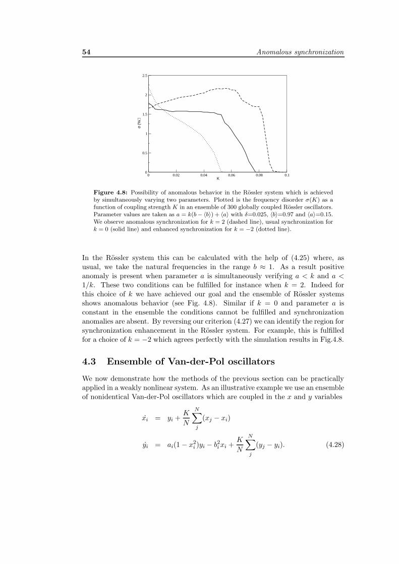
54 Anomalous synchronization
0 0.02 0.04 0.06 0.08 0.1Κ
0
0.5
1
1.5
2
2.5
σ (%
)
Figure 4.8: Possibility of anomalous behavior in the Rossler system which is achievedby simultaneously varying two parameters. Plotted is the frequency disorder σ(K) as afunction of coupling strength K in an ensemble of 300 globally coupled Rossler oscillators.Parameter values are taken as a = k(b− 〈b〉) + 〈a〉 with δ=0.025, 〈b〉=0.97 and 〈a〉=0.15.We observe anomalous synchronization for k = 2 (dashed line), usual synchronization fork = 0 (solid line) and enhanced synchronization for k = −2 (dotted line).
In the Rossler system this can be calculated with the help of (4.25) where, asusual, we take the natural frequencies in the range b ≈ 1. As a result positiveanomaly is present when parameter a is simultaneously verifying a < k and a <1/k. These two conditions can be fulfilled for instance when k = 2. Indeed forthis choice of k we have achieved our goal and the ensemble of Rossler systemsshows anomalous behavior (see Fig. 4.8). Similar if k = 0 and parameter a isconstant in the ensemble the conditions cannot be fulfilled and synchronizationanomalies are absent. By reversing our criterion (4.27) we can identify the region forsynchronization enhancement in the Rossler system. For example, this is fulfilledfor a choice of k = −2 which agrees perfectly with the simulation results in Fig.4.8.
4.3 Ensemble of Van-der-Pol oscillators
We now demonstrate how the methods of the previous section can be practicallyapplied in a weakly nonlinear system. As an illustrative example we use an ensembleof nonidentical Van-der-Pol oscillators which are coupled in the x and y variables
xi = yi +K
N
N∑
j
(xj − xi)
yi = ai(1 − x2i )yi − b2ixi +
K
N
N∑
j
(yj − yi). (4.28)

4.3 Ensemble of Van-der-Pol oscillators 55
Here a is the nonlinearity or stiffness of the system and b is the harmonic frequencyof oscillation. In the following we use frequencies in the range b ≈ 1 and furtherassume weak nonlinearity, a << 1. Our main goal now is to express the oscillationfrequency as a function of coupling strength. This can be achieved with the help ofperturbation techniques. Here we use a normal form expansion up to third orderin a (Kahn and Zarmi, 1998) and find for the radial and the angular equations
ri =1
2air(1 − 1
4r2) − rK +O(a3
i )
θi = bi −a2i
bi(1
8− 3
16r2 +
11
256r4) +O(a4
i ). (4.29)
Note, that in the Van-der-Pol oscillator non-isochronicities appear only with thesecond order in the nonlinearity a. The coupling term in the radial equation hasbeen calculated assuming that r = 0 after relaxation, and thus has a single stableequilibrium r∗2 = 4
(
1 − 2Ka
)
. Plugging this into the angular equation we obtainthe mean frequency in first order in K
Ωi(K) = bi −a2i
16bi+
5ai4bi
K. (4.30)
With this the system of Van-der-Pol oscillators has been brought into the generalform (4.13) with
ω(a, b) = b− a2
16b, κ(a, b) =
5a
4b. (4.31)
4.3.1 Functional dependence between control parameters
At this point we have to specify how the disorder is realized in the control param-eters a and b. The simplest possibility would be to introduce disorder only in theharmonic frequencies b. In this case ω(b) and κ(b) in (4.31) are functions of onlyone parameter b. It is straightforward to see that in this form it is not possibleto obtain anomalous desynchronization since inequality (4.19) can then only befulfilled if a < 0. However Van-der-Pol systems are not defined for negative valuesof the nonlinearity. Therefore, ensembles of Van der Pol oscillators do not showanomalous enlargement of frequency disorder if the oscillators are varying only intheir harmonic frequencies b.
However we have already demonstrated that, in general, it is possible to achieveanomalous synchronization if some functional dependence between control parame-ters can be maintained. This means that the disorder necessarily must be affectingboth parameters a and b. Here we show that anomalous synchronization can beobtained if we have the possibility to adjust the parameters of each oscillator inthe ensemble. To this aim we take parameters b from a uniform distribution withcenter 〈b〉=1 and width δ = 0.5 and adjust the system parameters in such a way
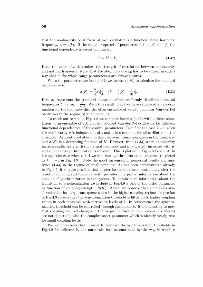
56 Anomalous synchronization
that the nonlinearity or stiffness of each oscillator is a function of the harmonicfrequency, a = a(b). If the range or spread of parameters δ is small enough thefunctional dependence is essentially linear,
a = kb− k0. (4.32)
Here, the value of k determines the strength of correlation between nonlinearityand natural frequency. Note, that the absolute value k0 has to be chosen in such away that in the whole range parameters a are always positive.
When the parameters are fixed (4.32) we can use (4.30) to calculate the standarddeviation σ(K)
σ(K) =5
4σb[
3
4+ (k − 1)(K − 1
10)]. (4.33)
Here σb represents the standard deviation of the uniformly distributed naturalfrequencies b, i.e. σb = δ√
12. With this result (4.33) we have calculated an approx-
imation for the frequency disorder of an ensemble of weakly nonlinear Van-der-Poloscillators in the regime of small coupling.
To check our results in Fig. 4.9 we compare formula (4.33) with a direct simu-lation in an ensemble of 800 globally coupled Van-der-Pol oscillators for differentfunctional dependencies of the control parameters. Take first the case k = 0 whenthe nonlinearity a is independent of b and it is a constant for all oscillators in theensemble. As mentioned above, in this case synchronization arises in the usual wayand σ(K) is a decreasing function of K. However, from (4.33) when nonlinearityincreases sufficiently with the natural frequency and k > 1, σ(K) increases with Kand anomalous synchronization is achieved. This is plotted in Fig. 4.9 for k = 3. Inthe opposite case when k < 1 we find that synchronization is enhanced (depictedas k = −3 in Fig. 4.9). Note the good agreement of numerical results and ana-lytics (4.33) in the regime of small coupling. As has been demonstrated alreadyin Fig.4.5, it is quite possible that cluster formation starts immediately after theonset of coupling and therefore σ(K) provides only partial information about theamount of synchronization in the system. To obtain more information about thetransition to synchronization we include in Fig.4.9 a plot of the order parameteras function of coupling strength, R(K). Again, we observe that anomalous syn-chronization has large consequences also in the higher coupling regime. Inspectionof Fig.4.9 reveals that the synchronization threshold is lifted up to higher couplingvalues in both measures with increasing levels of k. In consequence the synchro-nization threshold can be controlled through parameter k. It is interesting to notethat coupling induced changes in the frequency disorder (i.e. anomalous effects)are not detectable with the complex order parameter which is already nearly zerofor small coupling levels.
We want to stress that in order to compare the synchronization thresholds inFig.4.9 for different k, one must take into account that by the way in which k
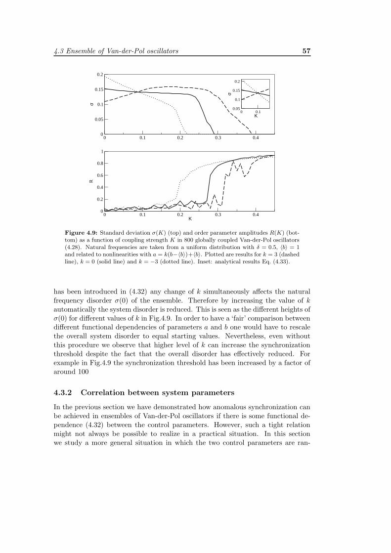
4.3 Ensemble of Van-der-Pol oscillators 57
0 0.1 0.2 0.3 0.40
0.05
0.1
0.15
0.2
σ
0 0.1 0.2 0.3 0.4Κ
0
0.2
0.4
0.6
0.8
1
R
0 0.1Κ
0.05
0.1
0.15
0.2
σFigure 4.9: Standard deviation σ(K) (top) and order parameter amplitudes R(K) (bot-tom) as a function of coupling strength K in 800 globally coupled Van-der-Pol oscillators(4.28). Natural frequencies are taken from a uniform distribution with δ = 0.5, 〈b〉 = 1and related to nonlinearities with a = k(b−〈b〉)+〈b〉. Plotted are results for k = 3 (dashedline), k = 0 (solid line) and k = −3 (dotted line). Inset: analytical results Eq. (4.33).
has been introduced in (4.32) any change of k simultaneously affects the naturalfrequency disorder σ(0) of the ensemble. Therefore by increasing the value of kautomatically the system disorder is reduced. This is seen as the different heights ofσ(0) for different values of k in Fig.4.9. In order to have a ‘fair’ comparison betweendifferent functional dependencies of parameters a and b one would have to rescalethe overall system disorder to equal starting values. Nevertheless, even withoutthis procedure we observe that higher level of k can increase the synchronizationthreshold despite the fact that the overall disorder has effectively reduced. Forexample in Fig.4.9 the synchronization threshold has been increased by a factor ofaround 100
4.3.2 Correlation between system parameters
In the previous section we have demonstrated how anomalous synchronization canbe achieved in ensembles of Van-der-Pol oscillators if there is some functional de-pendence (4.32) between the control parameters. However, such a tight relationmight not always be possible to realize in a practical situation. In this sectionwe study a more general situation in which the two control parameters are ran-
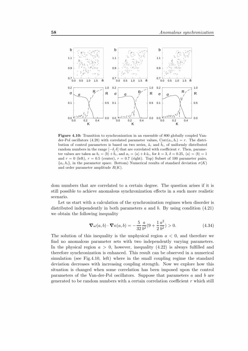
58 Anomalous synchronization
0.0 0.5 1.0 1.50.7
0.9
1.1
0.0 0.5 1.0 1.50.7
0.9
1.1
0.0 0.5 1.0 1.50.7
0.9
1.1
0.0
0.5
1.0
0.0
0.5
1.0
0.0 0.2 0.4Κ
0.0
0.5
1.0
0.0 0.2 0.4Κ
0.0
0.1
0.2
0.0 0.2 0.4Κ
0.0
0.1
0.2
0.0
0.1
0.2
a
b b b
a a
R R Rσ σ σσ σ σR R R
Figure 4.10: Transition to synchronization in an ensemble of 800 globally coupled Van-der-Pol oscillators (4.28) with correlated parameter values, Corr(ai, bi) = r. The distri-bution of control parameters is based on two series, ai and bi, of uniformly distributedrandom numbers in the range [−δ, δ] that are correlated with coefficient r. Then, parame-ter values are taken as bi = 〈b〉+ bi, and ai = 〈a〉+ k ai, for k = 3, δ = 0.25, 〈a〉 = 〈b〉 = 1and r = 0 (left), r = 0.5 (center), r = 0.7 (right). Top) Subset of 100 parameter pairs,ai, bi, in the parameter space. Bottom) Numerical results of standard deviation σ(K)and order parameter amplitude R(K).
dom numbers that are correlated to a certain degree. The question arises if it isstill possible to achieve anomalous synchronization effects in a such more realisticscenario.
Let us start with a calculation of the synchronization regimes when disorder isdistributed independently in both parameters a and b. By using condition (4.21)we obtain the following inequality
∇ω(a, b) · ∇κ(a, b) = − 5
32
a
b2(9 +
1
2
a2
b2) > 0. (4.34)
The solution of this inequality is the unphysical region a < 0, and therefore wefind no anomalous parameter sets with two independently varying parameters.In the physical region a > 0, however, inequality (4.22) is always fulfilled andtherefore synchronization is enhanced. This result can be observed in a numericalsimulation (see Fig.4.10, left) where in the small coupling regime the standarddeviation decreases with increasing coupling strength. Now we explore how thissituation is changed when some correlation has been imposed upon the controlparameters of the Van-der-Pol oscillators. Suppose that parameters a and b aregenerated to be random numbers with a certain correlation coefficient r which still
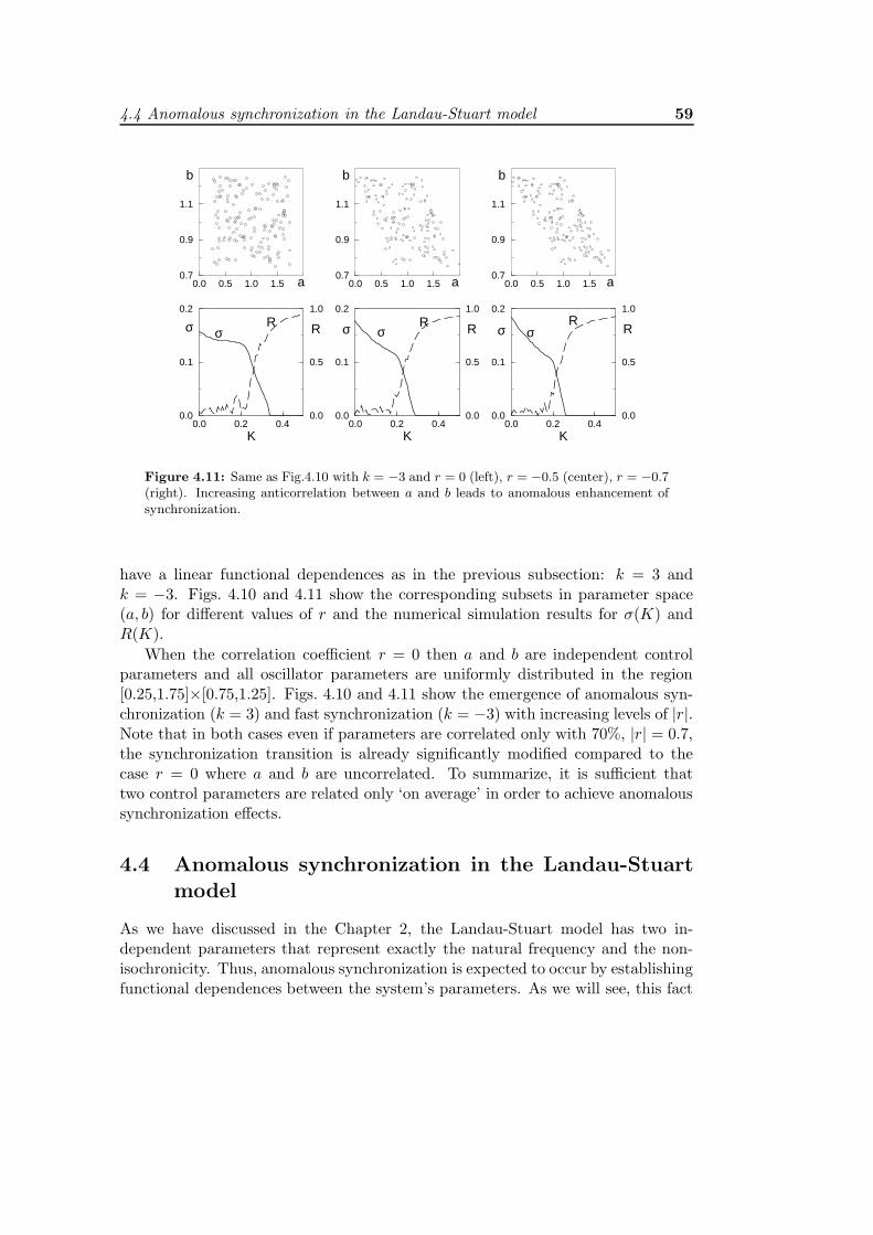
4.4 Anomalous synchronization in the Landau-Stuart model 59
0.0 0.5 1.0 1.50.7
0.9
1.1
0.0 0.5 1.0 1.50.7
0.9
1.1
0.0 0.5 1.0 1.50.7
0.9
1.1
0.0
0.5
1.0
0.0
0.5
1.0
0.0 0.2 0.4Κ
0.0
0.5
1.0
0.0 0.2 0.4Κ
0.0
0.1
0.2
0.0 0.2 0.4Κ
0.0
0.1
0.2
0.0
0.1
0.2
a
b b b
a a
R R Rσ σ σσ σ σR R R
Figure 4.11: Same as Fig.4.10 with k = −3 and r = 0 (left), r = −0.5 (center), r = −0.7(right). Increasing anticorrelation between a and b leads to anomalous enhancement ofsynchronization.
have a linear functional dependences as in the previous subsection: k = 3 andk = −3. Figs. 4.10 and 4.11 show the corresponding subsets in parameter space(a, b) for different values of r and the numerical simulation results for σ(K) andR(K).
When the correlation coefficient r = 0 then a and b are independent controlparameters and all oscillator parameters are uniformly distributed in the region[0.25,1.75]×[0.75,1.25]. Figs. 4.10 and 4.11 show the emergence of anomalous syn-chronization (k = 3) and fast synchronization (k = −3) with increasing levels of |r|.Note that in both cases even if parameters are correlated only with 70%, |r| = 0.7,the synchronization transition is already significantly modified compared to thecase r = 0 where a and b are uncorrelated. To summarize, it is sufficient thattwo control parameters are related only ‘on average’ in order to achieve anomaloussynchronization effects.
4.4 Anomalous synchronization in the Landau-Stuart
model
As we have discussed in the Chapter 2, the Landau-Stuart model has two in-dependent parameters that represent exactly the natural frequency and the non-isochronicity. Thus, anomalous synchronization is expected to occur by establishingfunctional dependences between the system’s parameters. As we will see, this fact
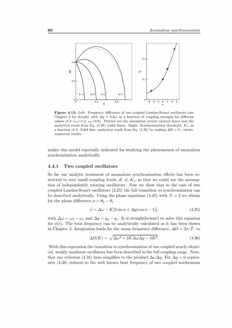
60 Anomalous synchronization
0 0.2 0.4Κ
0
0.2
0.4
∆Ω
k=0k=-5 k=2 k=5
-6 -4 -2 0 2 4 6k
0
0.2
0.4
Κ c
Figure 4.12: Left: Frequency difference of two coupled Landau-Stuart oscillators (seeChapter 2 for details) with ∆q = k∆ω as a function of coupling strength for differentvalues of k (ω1=1.2, ω2=0.8). Plotted are the simulation results (dotted lines) and theanalytical result from Eq. (4.36) (solid lines). Right: Synchronization threshold, Kc, asa function of k. Solid line: analytical result from Eq. (4.36) by making ∆Ω = 0 , circles:numerical results.
makes this model especially indicated for studying the phenomenon of anomaloussynchronization analytically.
4.4.1 Two coupled oscillators
So far our analytic treatment of anomalous synchronization effects has been re-stricted to very small coupling levels, K Kc, so that we could use the assump-tion of independently rotating oscillators. Now we show that in the case of twocoupled Landau-Stuart oscillators (2.25) the full transition to synchronization canbe described analytically. Using the phase equations (4.45) with N = 2 we obtainfor the phase difference φ = θ2 − θ1
φ = ∆ω −K[2 sinφ+ ∆q(cosφ− 1)], (4.35)
with ∆ω = ω2 − ω1 and ∆q = q2 − q1. It is straightforward to solve this equationfor φ(t). The beat frequency can be analytically calculated as it has been shownin Chapter 2. Integration leads for the mean frequency difference, ∆Ω = 2π/T , to
∆Ω(K) =√
∆ω2 + 2K∆ω∆q − 4K2. (4.36)
With this expression the transition to synchronization of two coupled nearly identi-cal, weakly nonlinear oscillators has been described in the full coupling range. Note,that our criterion (4.16) here simplifies to the product ∆ω∆q. For ∆q = 0 expres-sion (4.36) reduces to the well known beat frequency of two coupled isochronous

4.4 Anomalous synchronization in the Landau-Stuart model 61
phase oscillators. In general however, ∆q 6= 0 and we can write ∆q = k∆ω.Fig. 4.12 shows the results for different correlations between ∆ω and ∆q. Weobserve a good agreement of the analytical result (4.36) with the numerical simula-tions as long as both oscillators differ not too much. In particular, for positive valuesof k we find anomalous synchronization, whereas negative values of k lead to anenhancement of synchronization, as expected. Note that anomalous synchroniza-tion is effective not only at the onset of coupling but has important consequencesalso in the regime of larger coupling levels. This can be observed for example inthe synchronization threshold Kc which is shifted substantially by increasing levelsof |∆q|.
As a consequence, anomalous synchronization is also reflected in the Arnoldtongue structure of the system. Here, the idea is to indicate the synchronizationregion in the (∆ω,K)-plane (see Fig. 4.13). This region typically has the formof vertical (Arnold-)tongues. In our case the Arnold tongue is easily obtainedby setting ∆Ω(K) = 0 in (4.36). If ∆q = 0 we recover the usual result for twocoupled phase oscillators that the border of the tongues are the two straight linesK = |∆ω|/2.
When both oscillators differ in their respective value of nonisochronicity, ∆q 6=0, the Arnold tongue becomes asymmetrical with respect the ∆ω axis. A simplecalculation shows that the border of the tongue is still given by a straight line, butwith a modified slope which is scaled by a factor ξ and ξ−1 on the right and leftside, respectively. Thus, the anomalous synchronization borders are given by
K =
∆ω2 ξ(∆q
2 ), ∆ω > 0
−∆ω2
1ξ(∆q
2), ∆ω < 0
(4.37)
or in a more compact form
K =|∆ω|
2
[
ξ
(
∆q
2
)]sign(∆ω)
. (4.38)
Here, the function ξ(x) defines the modification of the slope in dependence onthe difference in nonisochronicity, 2x = ∆q, and is given by
ξ(x) = x+√
x2 + 1. (4.39)
Note, the special property ξ(x) = 1/ξ(−x). Fig. 4.13 shows the Arnold tongueof the system for a given value of ∆q > 0. In concord to our above discussionwe find that on the right side of Fig. 4.13a where there is a positive correlationbetween nonisochronicity and natural frequency, ∆ω∆q > 0, synchronization islargely inhibited, whereas on the left side with negative covariance the synchro-nization regime is enlarged.
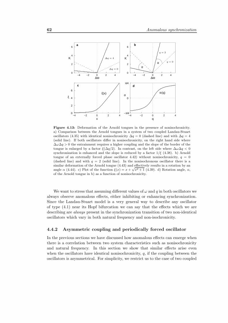
62 Anomalous synchronization
−4 −2 0 2 40
2
4
6
−4 −2 0 2 40
2
4
6
−4 −2 0 2 4
x
0
2
4
6
−4 −2 0 2 4
q
αα
ξ(x) α(q)
Κ
∆ω
Κ
αξ
∆ω
0
π/4
−π/4
a b
dc
PSfrag replacements
∆q = 4
∆q = 0
q = 2
q = 0
Figure 4.13: Deformation of the Arnold tongues in the presence of nonisochronicity.a) Comparison between the Arnold tongues in a system of two coupled Landau-Stuartoscillators (4.35) with identical nonisochronicity ∆q = 0 (dashed line) and with ∆q = 4(solid line). If both oscillators differ in nonisochronicity, on the right hand side where∆ω∆q > 0 the entrainment requires a higher coupling and the slope of the border of thetongue is enlarged by a factor ξ(∆q/2). In contrast, on the left side where ∆ω∆q < 0synchronization is enhanced and the slope is reduced by a factor 1/ξ (4.38). b) Arnoldtongue of an externally forced phase oscillator 4.42) without nonisochronicity, q = 0(dashed line) and with q = 2 (solid line). In the nonisochronous oscillator there is asimilar deformation of the Arnold tongue (4.43) and effectively results in a rotation by anangle α (4.44). c) Plot of the function ξ(x) = x+
√x2 + 1 (4.39). d) Rotation angle, α,
of the Arnold tongue in b) as a function of nonisochronicity.
We want to stress that assuming different values of ω and q in both oscillators wealways observe anomalous effects, either inhibiting or enhancing synchronization.Since the Landau-Stuart model is a very general way to describe any oscillatorof type (4.1) near its Hopf bifurcation we can say that the effects which we aredescribing are always present in the synchronization transition of two non-identicaloscillators which vary in both natural frequency and non-isochronicity.
4.4.2 Asymmetric coupling and periodically forced oscillator
In the previous sections we have discussed how anomalous effects can emerge whenthere is a correlation between two system characteristics such as nonisochronicityand natural frequency. In this section we show that similar effects arise evenwhen the oscillators have identical nonisochronicity, q, if the coupling between theoscillators is asymmetrical. For simplicity, we restrict us to the case of two coupled
4.4 Anomalous synchronization in the Landau-Stuart model 63
oscillators (2.25), where oscillators z1 and z2 are coupled with strength K1 and K2,respectively. In this case of asymmetrical coupling we find for the phase differencein a analogy to (4.35)
φ = ∆ω − (K2 +K1) sinφ− (K2 −K1)q(cosφ− 1). (4.40)
Proceeding as in the previous section the observed frequency difference yields
∆Ω(K) =√
∆ω2 + 2q∆ω(K2 −K1) − (K1 +K2)2. (4.41)
By comparison with (4.36) it is immediately evident that we find anomalous en-largement when the product q∆ω∆K > 0 and anomalous synchronization enhance-ment if q∆ω∆K < 0. Thus, if the oscillators are nonisochronous the asymmetryof coupling is reflected through an asymmetry of the synchronization regime andthe Arnold tongue.
It is especially important the limiting case of an externally forced oscillatorwhich arises when we set K1 = 0. In this case (4.40) goes over to (for simplicitywe denote K2 = K)
φ = ∆ω −K[sinφ+ q(cos φ− 1)]. (4.42)
This equation describes the evolution of the phase difference between a single non-isochronous oscillator and a periodically driving force, where the natural frequencyof the oscillator and the driving frequency have a frequency mismatch of ∆ω.
We now analyze the synchronization threshold and the geometry of the Arnoldtongue in dependence of the nonisochronicity q. If q = 0 the border of the Arnoldtongue is given by the two lines K = |∆ω| (see Fig. 4.13b). However, if q 6= 0 theslope of the lines is scaled similar to (4.38)
K = |∆ω| [ξ(q)]sign(∆ω) . (4.43)
Thus, the whole synchronization transition depends on the sign of ∆ω. If q > 0 andthe natural frequency of oscillation is larger than the driving frequency, then thesynchronization threshold is enlarged. Otherwise, the synchronization threshold isreduced. Indeed, here in the case of an externally forced phase oscillator it turns outthat the Arnold tongue is simply rotated due to the presence of nonisochronicity.The rotation angle α is given by
tan(2α) = q. (4.44)
In the limit of infinite large nonisochronicity the Arnold tongue is rotated by 900
degrees. In other words the rotation angle of the Arnold tongue is a measurement
64 Anomalous synchronization
for the nonisochronicity of oscillation (see Fig. 4.13b). Similar asymmetric Arnoldtongues are well known from many experimental data (Pikovsky et al., 2001). Inthese cases a simple measurement of the position and asymmetry of the Arnoldtongue can reveal valuable information about the dynamics of the observed oscil-lator.
4.4.3 Ensemble of phase oscillators of Landau-Stuart type
In the following we generalize our discussion to an ensemble of phase oscillatorsof Landau-Stuart type. It is important to stress that since in the Landau-Stuartmodel the parameters ω and q are independent, in order to observe anomaloussynchronization one must take correlated distributions.
As it has been shown in Chapter 3 the phase equations corresponding to theLandau-Stuart model are
θi = ωi −K
N
N∑
j=1
[sin(θi − θj) + qi(1 − cos(θi − θj)] . (4.45)
For small coupling levels, K Kc, the oscillators are rotating nearly independentlyand the trigonometric functions
N∑
j=1
sin(θi − θj) ≈N∑
j=1
cos(θi − θj) ≈ 0
and thus the system transforms into an ensemble of independent oscillators
θi(K) = ωi + qiK. (4.46)
Note, that this equation can also be obtained by using (4.14) and averaging overthe interaction function in (4.45).
With Eq.(4.46), the frequency of the system of interacting Landau-Stuart oscil-lators becomes fully described in the range of small coupling where it takes a verysimple form. The physical interpretation is straightforward. Due to the interac-tion the oscillators are perturbed off their limit cycle. On average this leads to aradial contraction of each limit cycle which produces a shift of the angular velocityproportional to the value of the shear term qi.
Note that formula (4.46) corresponds exactly to (4.13), and the nonisochronicityqi takes over the role of the κi in the general system. Obviously in Landau Stuartsystems the functions ω and q are directly the independent control parameters. Inthis respect system (4.45) is especially interesting for our studies since we don’thave to consider the roundabouts of mapping F (4.18) of the previous section.
Now assume again a disordered system where the oscillators differ in their re-spective values of ωi and qi. If the ‘faster’ oscillators (with higher natural frequency,

4.4 Anomalous synchronization in the Landau-Stuart model 65
0.0 0.1 0.2 0.3 0
5
10
σ (%
)
0.0 0.1 0.2 0.3Κ
0.8
1.0
1.2
Ωi
0.0 0.1 0.2 0.30
5
10
0.0 0.1 0.2 0.3Κ
0.8
1.0
1.2
0.0 0.1 0.2 0.30
5
10
0.0 0.1 0.2 0.3Κ
0.8
1.0
1.2
0.0
0.5
1.0
0.0
0.5
1.0
0.0
0.5
1.0k=−3k=0k=3
RR R R RR
σ σσ
Figure 4.14: Ensemble of 500 globally coupled Landau Stuart oscillators (4.45) with q =k(ω−〈ω〉)+ 〈ω〉. Natural frequencies are linearly increasing in the range δ = 0.25, 〈ω〉=1.Left) k = 3: anomalous synchronization; center) k = 0: usual synchronization; right)k = −3 enhanced synchronization. Top) Standard deviation of the ensemble frequenciesσ(K); numerical simulation (solid line) and analytical result using 4.48) (dashed line).Further indicated is the order parameter R(K) (dotted line). Bottom) Frequencies Ωi(K)of 11 equally spaced oscillators as a function of coupling strength K.
ωi) have a stronger shear of phase flow (higher value of qi) compared to the ‘slower’ones, then small coupling leads to an enlargement of the frequency difference be-tween the ‘faster’ and the ‘slower’ oscillators (see Fig.4.7). Therefore, if the ωicovary with qi then small coupling tends to desynchronize the oscillators. In fact,this is nothing else but our previous result (4.16) that anomalous effects arise onlyif the nonisochronicity of oscillation covaries with the natural frequency.
Suppose now that the nonisochronicity of each oscillator depends in some spe-cific way on the natural frequency q = q(ω). If the width of the distribution of ω issmall in the spirit of the previous section we can develop this dependence in firstorder as
q(ω) = kω + q0. (4.47)
Then it is straightforward to calculate the standard deviation of the ensemblefrequencies. Up to first order we find
σ(K) = (1 + kK)σω. (4.48)
Thus, the standard deviation is an increasing function of coupling strength whenk > 0 and a decreasing function when k < 0. When k = 0 we are only varyingthe natural frequency and the correlation term in Eq. (4.16) is zero. We have
66 Anomalous synchronization
tested these results in a direct simulation of 500 globally coupled Landau Stuartsystems for different values of k (see Fig. 4.14). Again, we find a perfect agreementbetween our theory and the numerical simulations. Note that σ(0) does not changewith k, or equivalently with q. This means that by increasing |k|, i.e. by makingthe ensemble more ‘non-identical’, σ(0) remains constant and the ensemble hasapparently the same ‘disorder’. Only when K 6= 0 coupling is able to reduce themean oscillation amplitudes and non-isochronicity effects begin to play a role.
4.4.4 Linear stability analysis
It is possible to apply the techniques developed in Chapter 3 in order to determinethe synchronization threshold in the phase equations of Landau-Stuart type (4.45).
The analytic treatment is similar to the one performed in Section 3.2. Thus, ifwe define an order parameter as in (3.4) the system (4.45) writes
θi = ωi −KR [sin(θi − θj) + qi(1 − cos(θi − θj)] . (4.49)
where now the parameters ω and q are both distributed according to the two dis-tributions g(ω) and h(ω), respectively. In order to proceed, we follow the followingstrategy: In the thermodynamic limit it is possible to define a density functionρ(θ, ω, t) that evolves according to the continuity equation (3.23). If we considerthe evolution of a small disturbance from the incoherent solution it is possible tolinearize the continuity equation around the incoherent solution ρ0, and from thisto determine when the stability of ρ0 is lost, i.e. the value of the synchronizationthreshold Kc.
Since the function ρ(θ, ω, t) is 2π periodic (and real) it can be developed inFourier series. This permits to write the linearized problem for the first Fouriermode as follows
∂ρ1
∂t= −i(ω + qK)ρ1 +
K
2(1 + iq)
∫ ∞
−∞
∫ ∞
−∞ρ1(t, ω
′, q′) g(ω′)h(q′)dω′dq′, (4.50)
and the same complex conjugate equation for the mode -1. The right-hand of (4.50)defines a linear operator that has both continuous and discrete parts. Let
ρ1(t, ω, q) = b(ω, q)eλt,
and hence Eq.(4.50) becomes
λb = −i(ω + qK)b+K
2(1 + iq)
∫ ∞
−∞
∫ ∞
−∞b(ω′, q′) g(ω′)h(q′)dω′dq′, (4.51)
where the average integral in the right-hand side of Eq. (4.51) is just a real constantB to be determined self-consistently. Hence solving (4.51) for b(ω, q) yields
b(ω, q) =K
2
(1 + iq)
λ+ i(ω + qK)B. (4.52)

4.4 Anomalous synchronization in the Landau-Stuart model 67
0 1 2K
0
0.5
1
R
k=-2 k=0 k=2
Figure 4.15: Transition to synchronization of 500 oscillators with uniform frequencydistribution (g(ω) = (2γ)−1) with γ = 0.5 and with q = kω for k=-2 (enhanced synchro-nization), k=0 and k=2 (anomalous synchronization).
Now invoking self-consistency and without considering the trivial solution b = 0,Eq. (4.52) gives
1 =K
2
∫ ∞
−∞
∫ ∞
−∞
1 + iq
λ+ i(ω + qK)g(ω)h(q)dωdq. (4.53)
Equation (4.53) can alternatively be written, separating real and imaginary parts,as
0 =
∫ ∞
−∞
∫ ∞
−∞
qRe(λ) − ω − Im(λ) − qK
Re(λ)2 + (Im(λ) + ω + qK)2g(ω)h(q)dωdq (4.54)
2
K=
∫ ∞
−∞
∫ ∞
−∞
Re(λ) + q(ω + Im(λ) + qK)
Re(λ)2 + (Im(λ) + ω + qK)2g(ω)h(q)dωdq (4.55)
Combining the last two equations, the Eq. (4.55) can be also written as
2
K=
∫ ∞
−∞
∫ ∞
−∞
Re(λ)(1 + q2)
Re(λ)2 + (Im(λ) + ω + qK)2g(ω)h(q)dωdq. (4.56)
The synchronization threshold Kc can be determined form Eq.(4.56) by per-forming the limit Re(λ) → 0 which yields
Kc =2
π
(∫ ∞
−∞
∫ ∞
−∞δ(ω + Im(λ) + qK)(1 + q2) g(ω)h(q)dωdq
)−1
(4.57)

68 Anomalous synchronization
using the fact that Re(λ)/(Re(λ)2 +x2) → πδ(x) as Re(λ) → 0. This equation hasto be calculated once Im(λ) is known through the equation (4.54)
∫ ∞
−∞
∫ ∞
−∞q δ(ω + Im(λ) + qK) g(ω)h(q)dωdq
=1
π
∫ ∞
−∞
∫ ∞
−∞
1
ω + Im(λ) + qKg(ω)h(q)dωdq
(4.58)
Let us now suppose that the nonisochronicity and the natural frequency arefunctionally related, for instance considering q = kω. Then assuming that g(ω)is symmetric, the integrals (4.57) and (4.58) can be straightforwardly calculated.Thus, the synchronization threshold yields
Kc =2
πg(0) − k. (4.59)
The Fig. 4.15 shows a numerical simulation of an ensemble of phase oscillatorsshowing anomalous synchronization and enhanced synchronization in good agree-ment with the critical coupling (4.59).
Chapter 5
Synchronization between
populations of phase oscillators
In this Chapter we investigate the possible routes to synchronization taking placebetween two populations of phase oscillators. Therefore we now combine the phe-nomenon of mutual synchronization taking place between two single oscillators(studied in Chapter 2) with that of macroscopic mutual entrainment (described inChapter 3). The results presented here are summarized in (Montbrio et al., 2004b).
The two ensembles are composed of phase oscillators of a Landau-Stuart type.In contrast with Chapter 4 here the inhomogeneities in the populations are onlytaken into account through a distribution of natural frequencies. Thus, we restrictour study to the phase equations given by (3.19), since the other terms introducedby the nonisochronicities into the phase equations have the trivial effect of rescalingthe coupling strength, and shifting the distributions of natural frequencies (seeEq.3.42). Additionally, the model (3.19) is also of interest because it appearsnaturally in the phase reduction of an array of superconducting Josephson junctions(Wiensenfeld and Swift, 1995; Wiesenfeld et al., 1996). It also has been proved tobe useful in modeling information concerning the synaptic connections in a neuralnetwork (Hoppensteadt and Izhikevich, 1998) and time delays (Izhikevich, 1998).
5.1 The model
The system under study is
θ(1,2)i =ω
(1,2)i − Kp
N
N∑
j=1
sin(θ(1,2)i − θ
(1,2)j + α)
− K
N
N∑
j=1
sin(θ(1,2)i − θ
(2,1)j + α),
(5.1)
69
70 Synchronization between populations of phase oscillators
where |α| < π/2 and i = 1, . . . , N 1. Here, θ(1,2)i describes the phase of the ith
oscillator in population 1 or 2, respectively. Both populations have the same sizeN and are coupled internally with intra-population coupling strength Kp, whereasthe inter-population coupling is determined by K. The oscillators within each
population have randomly distributed natural frequencies ω(1,2)i according to a
density g(1,2)(ω) of width γ that is assumed to be symmetric about the mean ω(1,2)
and unimodal. From now on we assume that ∆ω ≡ ω(1)−ω(2) > 0 and 0 ≤ α < π/2.The phase coherence within each population is described by the two complex
order parameters (3.4),
R(1,2)eiψ(1,2)
=1
N
N∑
j=1
eiθ(1,2)j , (5.2)
for each population, which permits to write system (5.1) in terms of the mean fieldquantities R(1,2) and ψ(1,2)
θ(1,2)i =ω
(1,2)i −KpR
(1,2) sin(θ(1,2)i − ψ(1,2) + α)
−K R(2,1) sin(θ(1,2)i − ψ(2,1) + α).
(5.3)
If the populations are uncoupled, i.e. K = 0, each of them reduces to the wellknown Kuramoto model with a phase shift α in the coupling function (3.42) studiedin Chapter 3. For a given Kp this model exhibits a phase transition at a criticalvalue of the frequency dispersal γc. For γ > γc the oscillators rotate with theirnatural frequencies and R(1,2) ∼ O(
√
1/N ), but for γ < γc mutual entrainmentoccurs among a small fraction of oscillators giving rise to a finite value of the orderparameter R(1,2). Thus, a cluster of locked oscillators emerges through a Hopf-bifurcation of frequency Ω(1,2) that, in general (α 6= 0), depends on the overallshape of g(1,2)(ω). The drifting oscillators arrange in a stationary distribution thatdoes not contribute to the order parameters.
On the other hand, in the limit of identical oscillators γ = 0, the oscillatorswithin each population are all identical and therefore they are able to synchronizein-phase (all the oscillator in each population have exactly the same phase for alltimes, i.e. R(1,2) = 1) for arbitrary small Kp, and hence each population mayact exactly as a single oscillator. Note that in this case the observed frequency isΩ(1,2) = ω(1,2) −Kp sinα, that therefore deviates from ω(1,2) because of α 6= 0, aswe have seen in Chapter 2.
When K > 0 the two locked clusters begin to interact. If this interaction issimilar to the frequency adjustment between two coupled oscillators, one expectsmutual locking between these two clusters to occur in a saddle-node bifurcation atsome critical value K = Kc, as we have seen in Chapter 2. Especially, for γ = 0,synchronization should arise at
Kc =∆ω
2 cosα. (5.4)
5.2 Linear stability analysis of the incoherent states 71
5.2 Linear stability analysis of the incoherent states
In the following we investigate the dynamics of (5.3) in the full (K, γ)-parameterplane. We proceed as in Chapter 3: In the thermodynamic limit a density functioncan be defined so that ρ(1,2)(θ, t, ω)dωdθ describes the number of oscillators withnatural frequencies in [ω, ω + dω] and phase in [θ, θ + dθ] at time t. For fixed ωthe distribution ρ(1,2)(θ, t, ω) of the phases θ is normalized to unity. The evolutionof ρ(1,2)(θ, t, ω) obeys the continuity equation ∂ρ(1,2)/∂t = −∂(ρ(1,2)θ(1,2))/∂θ, forwhich the incoherent state ρ0 = (2π)−1 is always a trivial solution. The functionρ(1,2)(θ, t, ω) is real and 2π-periodic in θ and therefore admits the Fourier expansion
ρ(1,2)(θ, t, ω) =∞∑
l=−∞ρ(1,2)l (t, ω)eilθ. (5.5)
where ρ(1,2)−l = ρ
∗(1,2)l . Using (5.2) and (5.5) the order parameter can be written in
terms of the Fourier components as R(1,2)eiψ(1,2)
= 2π⟨
ρ(1,2)∗1
⟩
(we use⟨
f (1,2)(ω)⟩
to denote frequency-average weighted with g(1,2)(ω), respectively). Now, after in-serting (5.3) into the continuity equation, we obtain an infinite system of integro-differential equations for the Fourier modes
ρ(1,2)l = − iωlρ
(1,2)l +
lρ(1,2)l−1 πe
iα(
Kp
⟨
ρ(1,2)1
⟩
+K⟨
ρ(2,1)1
⟩)
−
lρ(1,2)l+1 πe
−iα(
Kp
⟨
ρ∗(1,2)1
⟩
+K⟨
ρ∗(2,1)1
⟩)
.
(5.6)
The stability of ρ0 can be analyzed by studying the evolution of a perturbed state
ρ(1,2)(θ, t, ω) close to ρ0 (note that ρ(1,2)l are then small quantities). Linearization
of (5.6) reveals that the only potentially unstable modes are l = ±1 and hence
l = 1 has solution ρ(1,2)1 (t, ω) = b(1,2)(ω)eλt +O(|ρl|2). This leads to
b(1,2)(ω) =(
Kp
⟨
b(1,2)(ω)⟩
+K⟨
b(2,1)(ω)⟩) eiα/2
λ+ iω. (5.7)
the self-consistent problem (5.7) can be solved analytically. Eq (5.7) can be writtenas
2⟨
b(1,2)(ω)⟩
e−iα =(
Kp
⟨
b(1,2)(ω)⟩
+K⟨
b(2,1)(ω)⟩)
∫ ∞
−∞
1
λ+ iωg(1,2)(ω)dω.
(5.8)If the distribution of frequencies is considered to be of Lorentzian type, g (1,2)(ω) =(γ/π)[γ2 + (ω − ω(1,2))2]−1, then the integral in the right hand of Eq.(5.8) can besolved analytically. First, the integrand is extended to the complex plane∫ ∞
−∞
1
λ+ iωg(1,2)(ω)dω =
−iγπ
∮
C
dz
(z − iλ)(z − (ω(1,2) + iγ))(z − (ω(1,2) − iγ)),
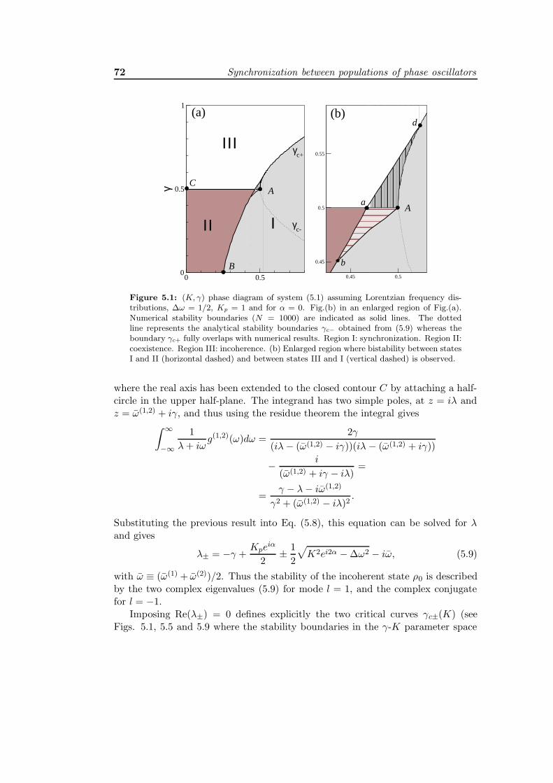
72 Synchronization between populations of phase oscillators
0 0.50
0.5
1
γ
0.45 0.5
0.45
0.5
0.55
C
B
(b)
ΙΙΙ
ΙΙ ΙA
a
d
b
γc+
γc-
(a)
A
Figure 5.1: (K, γ) phase diagram of system (5.1) assuming Lorentzian frequency dis-tributions, ∆ω = 1/2, Kp = 1 and for α = 0. Fig.(b) in an enlarged region of Fig.(a).Numerical stability boundaries (N = 1000) are indicated as solid lines. The dottedline represents the analytical stability boundaries γc− obtained from (5.9) whereas theboundary γc+ fully overlaps with numerical results. Region I: synchronization. Region II:coexistence. Region III: incoherence. (b) Enlarged region where bistability between statesI and II (horizontal dashed) and between states III and I (vertical dashed) is observed.
where the real axis has been extended to the closed contour C by attaching a half-circle in the upper half-plane. The integrand has two simple poles, at z = iλ andz = ω(1,2) + iγ, and thus using the residue theorem the integral gives
∫ ∞
−∞
1
λ+ iωg(1,2)(ω)dω =
2γ
(iλ− (ω(1,2) − iγ))(iλ − (ω(1,2) + iγ))
− i
(ω(1,2) + iγ − iλ)=
=γ − λ− iω(1,2)
γ2 + (ω(1,2) − iλ)2.
Substituting the previous result into Eq. (5.8), this equation can be solved for λand gives
λ± = −γ +Kpe
iα
2± 1
2
√
K2ei2α − ∆ω2 − iω, (5.9)
with ω ≡ (ω(1) + ω(2))/2. Thus the stability of the incoherent state ρ0 is describedby the two complex eigenvalues (5.9) for mode l = 1, and the complex conjugatefor l = −1.
Imposing Re(λ±) = 0 defines explicitly the two critical curves γc±(K) (seeFigs. 5.1, 5.5 and 5.9 where the stability boundaries in the γ-K parameter space
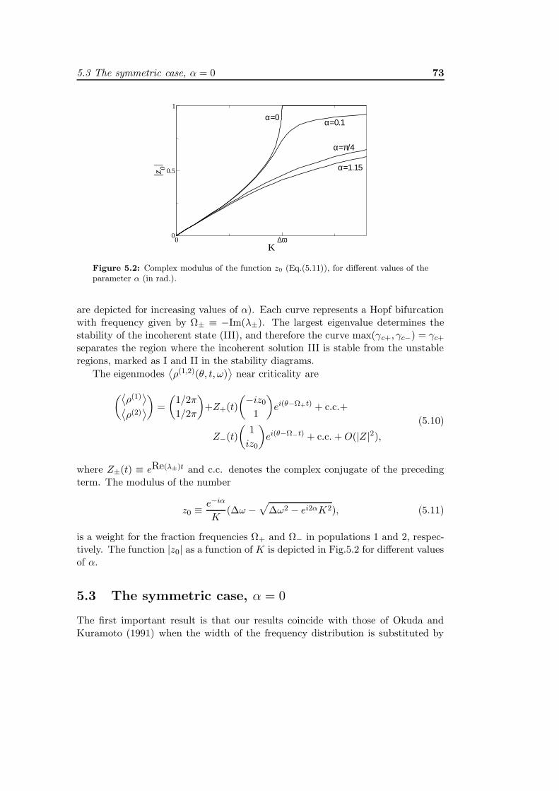
5.3 The symmetric case, α = 0 73
0 ∆ωK
0
0.5
1
|z0|
α=0 α=0.1
α=π/4
α=1.15
Figure 5.2: Complex modulus of the function z0 (Eq.(5.11)), for different values of theparameter α (in rad.).
are depicted for increasing values of α). Each curve represents a Hopf bifurcationwith frequency given by Ω± ≡ −Im(λ±). The largest eigenvalue determines thestability of the incoherent state (III), and therefore the curve max(γc+, γc−) = γc+separates the region where the incoherent solution III is stable from the unstableregions, marked as I and II in the stability diagrams.
The eigenmodes⟨
ρ(1,2)(θ, t, ω)⟩
near criticality are
(
⟨
ρ(1)⟩
⟨
ρ(2)⟩
)
=
(
1/2π
1/2π
)
+Z+(t)
(−iz01
)
ei(θ−Ω+t) + c.c.+
Z−(t)
(
1
iz0
)
ei(θ−Ω−t) + c.c. +O(|Z|2),(5.10)
where Z±(t) ≡ eRe(λ±)t and c.c. denotes the complex conjugate of the precedingterm. The modulus of the number
z0 ≡ e−iα
K(∆ω −
√
∆ω2 − ei2αK2), (5.11)
is a weight for the fraction frequencies Ω+ and Ω− in populations 1 and 2, respec-tively. The function |z0| as a function of K is depicted in Fig.5.2 for different valuesof α.
5.3 The symmetric case, α = 0
The first important result is that our results coincide with those of Okuda andKuramoto (1991) when the width of the frequency distribution is substituted by

74 Synchronization between populations of phase oscillators
the intensity of the noise. The eigenvalues in this case are simply
λ± = −γ +Kp
2± 1
2
√
K2 − ∆ω2 − iω, (5.12)
From the eigenvalues (5.12) the state III can become unstable in two different ways,depending on the sign of (K − ∆ω):
• When K > ∆ω the transition III-I takes place through a single Hopf bifur-cation and both populations synchronize to the same frequency Ω = ω. Thepresence of a single macroscopic oscillation is denoted as region I.
• When K < ∆ω the instability is through a degenerated Hopf bifurcation.Both (λ+, λ
∗+) and (λ−, λ∗−) cross simultaneously the imaginary axis at γc± =
γc = Kp/2 (line CA) and two macroscopic oscillations with frequencies
Ω± = ∓1
2
√
∆ω2 −K2 + ω, (5.13)
emerge. The region of coexistence of two different macroscopic fields is labeledas region II. Note that this result is a consequence of the reflectional symmetryof the model (5.1) 1.
Observe that when K = 0 the amplitudes are |z0| = 0 in (5.10), and hence, ifγ < γc, the phase of the order parameters evolves uniformly, i.e. ψ(1) = Ω−tand ψ(2) = Ω+t. On the other hand, when ∆ω = K then the function is|z0| = 1, indicating synchronization of the order parameters.
The coupling-modified frequencies of the individual oscillators, provide a usefulmeasure of synchronization: when K = 0 the frequency-locked oscillators form asingle plateau that is the only contribution to the fields (5.2), as it it shown inFig.5.3(a). Thus, the phase of each order parameter evolves linearly in time ac-cording to ψ(1) = ω(1)/t and ψ(2) = ω(2)/t, i.e. the phase difference of the orderparameters also grows uniformly as ∆ψ(t) = ψ(1)(t) − ψ(2)(t). The time evolutionof the order parameter of population 1 is depicted in Fig.5.4(a) (the population2 behaves as population 1 due to the reflection symmetry, and therefore we showonly the order parameters corresponding to the first population).
With further increases in K, some of the oscillators in populations 1 and 2begin to lock in a second plateau at Ω+ and Ω−, respectively, in accord to (5.10)(see Fig.5.3(b)). Hence, R(1,2) begin to oscillate with frequency ∆Ω = Ω− − Ω+
(Fig.5.4(b)). With further increases in K the system approaches the saddle node
1When α = 0, a reflection (θ(1,2)i → −θ(1,2)
i and ω(1,2)i → −ω(1,2)
i ) in the rotating frame movingwith frequency (ω(1) + ω(2))/2 leaves the system (5.1) invariant. Otherwise the system in invariant
under the transformation (θ(1,2)i → −θ(1,2)
i , ω(1,2)i → −ω(1,2)
i , α→ −α).

5.3 The symmetric case, α = 0 75
0 500 1000-1
-0.5
0
0.5
1
0 500 1000 0 500 1000-1
-0.5
0
0.5
1
0 500 1000i
-1
-0.5
0
0.5
1
0 500 1000i
-1
-0.5
0
0.5
1
Ω+
Ω−
Ω+
Ω−
Ω+
Ω−
Ω1
Ωn
(a) (b)
(c) (d)
Figure 5.3: Coupling-modified frequencies ωi of populations 1(:black) and 2(:grey) as
a function of the oscillator’s index i: oscillator i has natural frequency ω(1,2)i = ω(1,2) +
γ tan [(π/2)(2i −N − 1)/(N + 1)] (Lorentzian) α = 0, γ = 0.4 and (a) K = 0, (b) K =0.2, (c) K = 0.4, (d) K = 0.41. (∆ω = 1/2, ω = 0, Kp = 1 N = 1000).
0 400t
0
1
0 400t
0
1
R(1
)
60 80 100
0
10
∆ψ
0 3000
1
0 3000
1
R(1
)
100 200
20
40
∆ψ
200 4000
20
∆ψ
200 400
30
40
∆ψ
(a) (b)
(c) (d)
Figure 5.4: Time evolution of the order parameter of population 1 from a random initialcondition to the state I (Figs. (a,b,c)) or II (Fig.(c)) (α = 0, Kp = 1, γ = 0.4, Lorentziandistributions) for (a) K = 0, (b) K = 0.2,(c) K = 0.4, (d) K = 0.41. The population sizeis N = 1000 and the state of the system at time t = 0 random initial conditions
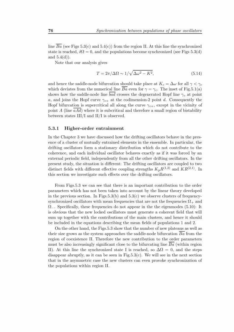
76 Synchronization between populations of phase oscillators
line Ba (see Figs 5.3(c) and 5.4(c)) from the region II. At this line the synchronizedstate is reached, δΩ = 0, and the populations become synchronized (see Figs 5.3(d)and 5.4(d)).
Note that our analysis gives
T = 2π/∆Ω ∼ 1/√
∆ω2 −K2, (5.14)
and hence the saddle-node bifurcation should take place at Kc = ∆ω for all γ < γcwhich deviates from the numerical line Ba even for γ = γc. The inset of Fig.5.1(a)shows how the saddle-node line bad crosses the degenerated Hopf line γc at pointa, and joins the Hopf curve γc+ at the codimension-2 point d. Consequently theHopf bifurcation is supercritical all along the curve γc+, except in the vicinity ofpoint A (line aAd) where it is subcritical and therefore a small region of bistabilitybetween states III/I and II/I is observed.
5.3.1 Higher-order entrainment
In the Chapter 3 we have discussed how the drifting oscillators behave in the pres-ence of a cluster of mutually entrained elements in the ensemble. In particular, thedrifting oscillators form a stationary distribution which do not contribute to thecoherence, and each individual oscillator behaves exactly as if it was forced by anexternal periodic field, independently from all the other drifting oscillators. In thepresent study, the situation is different: The drifting oscillators are coupled to twodistinct fields with different effective coupling strengths KpR
(1,2) and KR(2,1). Inthis section we investigate such effects over the drifting oscillators.
From Figs.5.3 we can see that there is an important contribution to the orderparameters which has not been taken into account by the linear theory developedin the previous section. In Figs.5.3(b) and 5.3(c) we observe clusters of frequency-synchronized oscillators with mean frequencies that are not the frequencies Ω+ andΩ−. Specifically, these frequencies do not appear in the the eigenmodes (5.10): Itis obvious that the new locked oscillators must generate a coherent field that willsum up together with the contributions of the main clusters, and hence it shouldbe included in the equations describing the mean fields of populations 1 and 2.
On the other hand, the Figs.5.3 show that the number of new plateaus as well astheir size grows as the system approaches the saddle-node bifurcation Ba from theregion of coexistence II. Therefore the new contribution to the order parametersmust be also increasingly significant close to the bifurcating line Ba (within regionII). At this line the synchronized state I is reached, so ∆Ω = 0, and the stepsdisappear abruptly, as it can be seen in Fig.5.3(c). We will see in the next sectionthat in the asymmetric case the new clusters can even provoke synchronization ofthe populations within region II.

5.3 The symmetric case, α = 0 77
From our numerics we observe that the new clusters emerge due to mutual
entrainment of the drifting oscillators having frequencies ω(1,2)i close to
Ωn = Ω− + n∆Ω, where n = 1,±2,±3.... (5.15)
In the following we discuss the dynamics of the drifting oscillators: If we startwith initial conditions corresponding to the incoherent state, the linear stabilityanalysis indicates that the first thing to occur is the emergence of the two clustersof frequencies Ω+ and Ω−. As we have seen, the degenerated Hopf bifurcationleading to region II is supercritical except in a small region close to point A (seediagram 5.5). Therefore the amplitude of the emergent fields is small close tocriticality and the solutions (5.10) are of validity.
Consequently, a drifting oscillator is actually forced by the two mean fields(5.10) not far -in the parameter space- from the incoherent state. Thus its dy-namical equation is given by Eq.(5.3) with the mean fields near criticality (5.10).Moreover, exploiting the rotational symmetry of the model (5.3) it is always pos-sible to go into a rotating frame such that in the new coordinates ω = 0 (seeChapter (3). After this the system is symmetric with respect reflections and there-fore R ≡ R(1) = R(2) and ψ ≡ ψ(1) = −ψ(2). This allows us to write without lossof generality the Eq.(5.3) for the drifting oscillators in population 1 as
θ(1)i = ω
(1)i −R[(K +Kp) sin θ
(1)i cosψ + (K −Kp) cos θ
(1)i sinψ], (5.16)
where R(t) is a time-periodic function given by Eq.(5.10) (with period T and givenby Eq.(5.14)), and ψ is a monotonically increasing function of t with slope Ω−.
In order to simplify the analysis let us assume that Kp = K, i.e. a bimodalfrequency distribution. Then Eq.(5.16) becomes
θ(1)i = ω
(1)i − f(t) sin θ
(1)i , (5.17)
where
f(t) ≡ 2KR(t) cosψ(t),
is a periodic function, with period given by 2T . The function R(t) is positive andhas its minimum exactly when ψ = π/2. Therefore we can consider that the driftingoscillators are governed by the Adler equation (2.18) with a time periodic coupling.Such system produces similar higher order entrainment as the one observed inFigs 5.3.
The observation of similar clusters was reported by Sakaguchi (1988) in anexternally periodically forced population of nonidentical phase oscillators, eventhough their origin was not explained. Additionally similar locking plateaus ap-pear in when an external periodic forcing is applied to a single phase oscillator(for a derivation for a weakly nonlinear Van der Pol oscillator under a general

78 Synchronization between populations of phase oscillators
0 0.5K
0 0.5K
0
0.5
1
γ0.43 0.44
0.44
0.48
0.555 0.57
0.14
0.16
B
C
(a)
ΙΙ
ΙΙ
ΙΙ
C
B
b
a
A
d
A
γc-
γc+
γc-
γc+
A
da
b
(b)
A
Figure 5.5: (K, γ) phase diagram of system (5.1) assuming Lorentzian frequency distri-butions, ∆ω = 1/2, Kp = 1, and for different values of α (in rad.): (a) α = 0.1 and (b)α = π/4. Numerical stability boundaries (N = 1000) are indicated as solid lines. Dottedlines represent analytical stability boundaries γc± obtained from (5.9). Note that γc+
fully overlaps with numerical results. Region I: synchronization. Region II: coexistence.Region III: incoherence. Insets: bistability in the dashed regions around A (see text).
external periodic forcing see Landa (1996)). In such case the emergent plateausare known as Shapiro steps (Shapiro, 1963; Shapiro et al., 1964), and it has beenshown that their effect over a population of nonidentical oscillators with randomlydistributed coupling strengths leads to periodic synchronization (Choi et al., 1994).
5.4 The asymmetric case, α > 0
As α is increased from zero the bifurcating lines γc+ and γc− split due to thebreaking of symmetry. Interestingly, the eigenmodes (5.10) do not reflect theasymmetry through the amplitudes |z0|, but only through the different exponentialgrowths Z±(t). Figs.5.6 show the modified frequencies of the oscillators for α = π/4(Fig.5.5(b)), keeping K constant and decreasing γ continuously from region III.
We find that incoherence (Fig.5.6(a)) only goes unstable through a single Hopfbifurcation γc+ (at Ω+ in Fig.5.6(b)) and hence nucleation first takes place mainlywithin population 2.
The second Hopf bifurcation (at Ω− in Fig.5.6(c)) follows γc− as far as thesystem is close enough to the incoherent state III. Fig.5.7(a) shows the order pa-rameters of the populations in the region II close to the bifurcating line γc−.As γ isdecreased further the system approaches the saddle-node bifurcation, Bd, and an
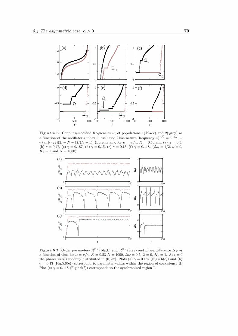
5.4 The asymmetric case, α > 0 79
-2
0
2
-1
-0.5
0
0 500 1000i
-1
-0.5
0
0 500 1000i
-1
-0.5
0
-1
-0.5
0
0 500 1000i
-1
-0.5
0
Ω+Ω+
Ω+Ω+
Ω−
Ω−
Ω−
(a) (b) (c)
(f)(e)(d)
Figure 5.6: Coupling-modified frequencies ωi of populations 1(:black) and 2(:grey) as
a function of the oscillator’s index i: oscillator i has natural frequency ω(1,2)i = ω(1,2) +
γ tan [(π/2)(2i −N − 1)/(N + 1)] (Lorentzian), for α = π/4, K = 0.53 and (a) γ = 0.5,(b) γ = 0.47, (c) γ = 0.187, (d) γ = 0.15, (e) γ = 0.13, (f) γ = 0.118. (∆ω = 1/2, ω = 0,Kp = 1 and N = 1000).
0 2500
1
R(1
) ,R(2
)
0 2500
2
∆ψ
0 250t
0
1
R(1
) ,R(2
)
0 250t
0
2
∆ψ
0 2500
1
R(1
) ,R(2
)
0 250
0
2
∆ψ
(a)
(b)
(c)
Figure 5.7: Order parameters R(1) (black) and R(2) (grey) and phase difference ∆ψ asa function of time for α = π/4, K = 0.53 N = 1000, ∆ω = 0.5, ω = 0, Kp = 1. At t = 0the phases were randomly distributed in (0, 2π]. Plots (a) γ = 0.187 (Fig.5.6(c)) and (b)γ = 0.13 (Fig.5.6(e)) correspond to parameter values within the region of coexistence II.Plot (c) γ = 0.118 (Fig.5.6(f)) corresponds to the synchronized region I.

80 Synchronization between populations of phase oscillators
-1 0 1-1
0
1
-1 0 1-1
0
1
195 215t
0
2
∆ψ
195 215t
0
1
R(1
) ,R(2
)
t1
t2t
3
t1
t2
t3
t2
t1
t3
t3
t2
t1
Z(1) Z
(2)
Figure 5.8: Characteristic population dynamics during a short period of time in theregion of coexistence II, close to the saddle-node bifurcation for α = π/4 (see diagram5.5(b)). The parameters have been set as in Fig.5.7(b) and Fig.5.6(e) (K = 0.53, γ = 0.13,∆ω = 0.5, ω = 0, Kp = 1, N = 1000, Lorentzian distribution). In the first row thecomplex order parameters Z(1) and Z(2) are shown for t : [195, 220] an well as the orderparameters at three different times t1, t2 = t1 + ∆t and t3 = t1 + 2∆t. In the second rowthe phase difference ∆ψ (in rad.) (right) and the order parameters R(1) and R(2) (left)in the corresponding time interval are shown.
increasing number of oscillators in population 1 become entrained to the frequen-cies given by (5.15) (see Figs.5.6(d,e)). In consequence the order parameter R(1)(t)oscillates with frequency ∆Ω with a large amplitude whereas R(2)(t) remains al-most constant (Fig.5.7(b)). The phase difference between the order parameters∆ψ(t) ≡ ψ(1) − ψ(2) reveals the presence of such clusters (see Fig. 5.8): ∆ψ(t)(Figs.5.7(a,b)) is bounded despite the fact that the populations are not locked infrequency (Fig.5.6(c,e)).
The bistability regions - enlarged in the insets of Figs.5.5(a,b) - are located nearthe intersection a of the Hopf line CA with the saddle-node line Bd. Within theregion enclosed by Aba the states I and II coexist, as in the α = 0 case. In contrast,the region enclosed byAad is surrounded only by the region I and bistability be-tween a small and a large amplitude of the synchronized oscillation in population1 is observed.
With increase in α, the synchronization regions I and II become graduallysmaller because as α → π/2 synchronization is increasingly inhibited due to frus-tration (Daido, 1987; Bonilla et al., 1993). At the same time, the number |z0|decreases indicating a lower degree of synchronization between the populations.
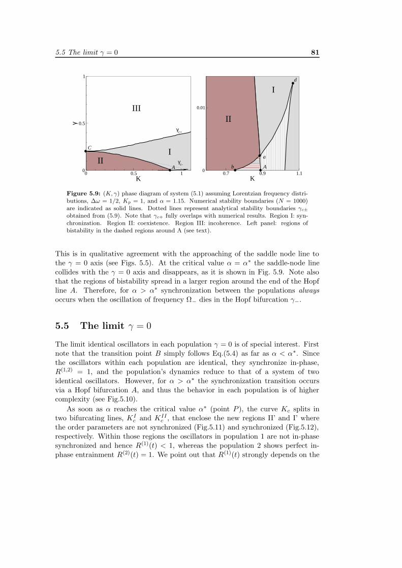
5.5 The limit γ = 0 81
0 0.5 1K
0
0.5
1γ
0.7 0.9 1.1K
0
0.01III
III
II
I
γc-
γc+
A
C
A
a
d
b
Figure 5.9: (K, γ) phase diagram of system (5.1) assuming Lorentzian frequency distri-butions, ∆ω = 1/2, Kp = 1, and α = 1.15. Numerical stability boundaries (N = 1000)are indicated as solid lines. Dotted lines represent analytical stability boundaries γc±
obtained from (5.9). Note that γc+ fully overlaps with numerical results. Region I: syn-chronization. Region II: coexistence. Region III: incoherence. Left panel: regions ofbistability in the dashed regions around A (see text).
This is in qualitative agreement with the approaching of the saddle node line tothe γ = 0 axis (see Figs. 5.5). At the critical value α = α∗ the saddle-node linecollides with the γ = 0 axis and disappears, as it is shown in Fig. 5.9. Note alsothat the regions of bistability spread in a larger region around the end of the Hopfline A. Therefore, for α > α∗ synchronization between the populations alwaysoccurs when the oscillation of frequency Ω− dies in the Hopf bifurcation γ−.
5.5 The limit γ = 0
The limit identical oscillators in each population γ = 0 is of special interest. Firstnote that the transition point B simply follows Eq.(5.4) as far as α < α∗. Sincethe oscillators within each population are identical, they synchronize in-phase,R(1,2) = 1, and the population’s dynamics reduce to that of a system of twoidentical oscillators. However, for α > α∗ the synchronization transition occursvia a Hopf bifurcation A, and thus the behavior in each population is of highercomplexity (see Fig.5.10).
As soon as α reaches the critical value α∗ (point P ), the curve Kc splits intwo bifurcating lines, KI
c and KIIc , that enclose the new regions II’ and I’ where
the order parameters are not synchronized (Fig.5.11) and synchronized (Fig.5.12),respectively. Within those regions the oscillators in population 1 are not in-phasesynchronized and hence R(1)(t) < 1, whereas the population 2 shows perfect in-phase entrainment R(2)(t) = 1. We point out that R(1)(t) strongly depends on the
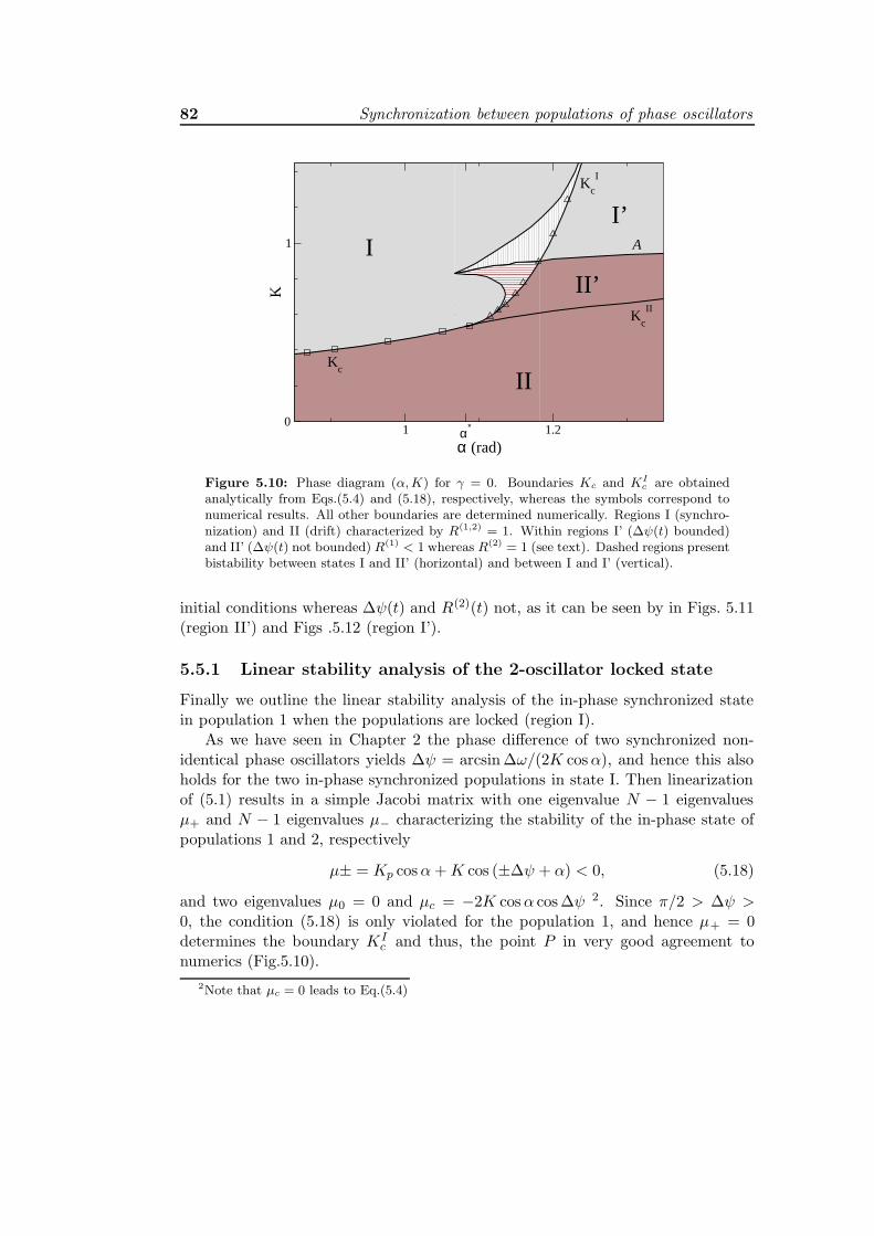
82 Synchronization between populations of phase oscillators
1 α∗ 1.2
α (rad)
0
1
K
I
II
I’
II’
Kc
Kc
I
Kc
II
A
Figure 5.10: Phase diagram (α,K) for γ = 0. Boundaries Kc and KIc are obtained
analytically from Eqs.(5.4) and (5.18), respectively, whereas the symbols correspond tonumerical results. All other boundaries are determined numerically. Regions I (synchro-nization) and II (drift) characterized by R(1,2) = 1. Within regions I’ (∆ψ(t) bounded)and II’ (∆ψ(t) not bounded) R(1) < 1 whereas R(2) = 1 (see text). Dashed regions presentbistability between states I and II’ (horizontal) and between I and I’ (vertical).
initial conditions whereas ∆ψ(t) and R(2)(t) not, as it can be seen by in Figs. 5.11(region II’) and Figs .5.12 (region I’).
5.5.1 Linear stability analysis of the 2-oscillator locked state
Finally we outline the linear stability analysis of the in-phase synchronized statein population 1 when the populations are locked (region I).
As we have seen in Chapter 2 the phase difference of two synchronized non-identical phase oscillators yields ∆ψ = arcsin ∆ω/(2K cosα), and hence this alsoholds for the two in-phase synchronized populations in state I. Then linearizationof (5.1) results in a simple Jacobi matrix with one eigenvalue N − 1 eigenvaluesµ+ and N − 1 eigenvalues µ− characterizing the stability of the in-phase state ofpopulations 1 and 2, respectively
µ± = Kp cosα+K cos (±∆ψ + α) < 0, (5.18)
and two eigenvalues µ0 = 0 and µc = −2K cosα cos ∆ψ 2. Since π/2 > ∆ψ >0, the condition (5.18) is only violated for the population 1, and hence µ+ = 0determines the boundary KI
c and thus, the point P in very good agreement tonumerics (Fig.5.10).
2Note that µc = 0 leads to Eq.(5.4)

5.5 The limit γ = 0 83
0 200t
0
1
R(1
) ,R
(2)
100 200t
20
40
60
∆ψ
0 2000
1
R(1
) ,R(2
)
100 2000
20
40
∆ψ
(a1) (a2)
(b1) (b2)
Figure 5.11: Order parameters R(1) (black) and R(2) (grey) and phase difference ∆ψ asa function of time (N = 1000, ∆ω = 0.5, ω = 0, Kp = 1). At t = 0 the phases were equallyspaced in (0, 2π]. corresponding to parameter values in region II’ (α = 1.2, K = 0.8), (seeFig.5.10).
0 100 2000
1
R(1
) ,R
(2)
100 200
0.5
1
∆ψ
0 150t
0
1
R(1
) ,R(2
)
0 100t
2.5
3
∆ψ
(a1) (a2)
(b1) (b2)
Figure 5.12: Order parameters R(1) (black) and R(2) (grey) and phase difference ∆ψ asa function of time (N = 1000, ∆ω = 0.5, ω = 0, Kp = 1). At t = 0 the phases randomlydistributed in (0, 2π]. (a) corresponds to parameter values within region I’ (α = 1.2,K = 1.05), (see Fig.5.10).
84 Synchronization between populations of phase oscillators
Notice that with K = 0 we recover the in-phase stability condition for a sin-gle population, Kp cosα > 0. For |α| > π/2 this state becomes unstable andreaches a new (splay) state, which is neutrally stable. The splay state has beenthe subject of intense theoretical work due to the applications in devices consistingof superconducting Josephson Junctions (Wiensenfeld and Swift, 1995; Watanabeand Strogatz, 1993). In the present case, however, even for |α| < π/2 the in-phasestate in one population can be destabilized (population 1) or overstabilized (pop-ulation 2) due to the interaction with the other population. The global stabilityproperties of the states I’ and II’ are interesting directions of further study.
Chapter 6
Conclusion
This work was devoted to an investigation of synchronization in large ensembles ofnonidentical oscillators, with special emphasis on the effects that nonisochronicitybears upon the synchronization process.
The work presented in this thesis has been focused on two particular problems:
• A population of oscillators with inherent disorder in the nonisochronicities,in addition to the disorder in the natural frequencies. In this context the newphenomenon of ‘anomalous synchronization’ has been discovered, in whichsmall coupling is able to increase the frequency disorder, inducing a spread ofthe oscillator frequencies. It has been demonstrated that occurs naturally ingroups of globally and locally coupled oscillatory systems of different types:phase oscillators, limit cycles and chaotic oscillators (Blasius et al., 2003;Montbrio and Blasius, 2003; Montbrio et al., 2004a) 1.
• A study of the routes leading to synchronization between two populations ofglobally coupled oscillators (Montbrio et al., 2004b). The systems that havebeen used are phase oscillators of a Landau-Stuart type. In this case the in-homogeneity in the ensemble has been introduced simply through the naturalfrequencies whereas the nonisochronicity has been considered to be constantfor all the elements in the ensembles. However, it has been demonstrated thatthe presence of nonisochronicity plays a significant role, because it inducesa breaking of the reflectional symmetry properties of the purely isochronoussystem.
Altogether these results stress the importance of considering the presence ofnonisochronicity in the synchronization theory.
1Additionally, anomalous synchronization has been recently observed in coupled spatially ex-tended systems of a Ginzburg-Landau type (Bragard et al., 2003, 2004), and also experimentallyin coupled Chua’s circuits (Dana et al., 2004).
85
86 Conclusion
6.1 Results
6.1.1 Anomalous synchronization
In the Chapter 4 of this thesis anomalous synchronization has been described an-alytically in the regime of weak coupling and the validity of these results has beennumerically confirmed for a number of different models. It has been demonstratedthat the effect emerges because the interaction perturbs the oscillators away fromtheir attractors. This brings the nonisochronicity of the oscillation into play. Disor-der enlargement occurs if nonisochronicity has positive covariance with the naturalfrequency of oscillation. As such, it is a universal effect and generically appearswhen inherent disorder is affecting more than one characteristics of the system.Among all known coupling-induced effects anomalous synchronization stands out,since the effect sets in without a threshold, whereas usually coupling-induced in-stabilities arise only when the coupling level is larger than a critical threshold.
On the other hand, it has been shown that anomalous synchronization effectshave consequences for the large coupling regime. In particular, they strongly con-trol the synchronization threshold. Therefore anomalous synchronization mighthave important applications for the synchronization and control of large ensemblesof coupled oscillators. With appropriate choice of system parameters it is possibleto change the synchronization transition of the system, and in this way either toincrease or decrease the onset of synchronization. This was particularly clear inthe case of ensembles of globally coupled phase oscillators, for which an analyticalexpression for the synchronization threshold was obtained (Montbrio et al., 2004a).For more general systems, the control of the onset of synchronization was achievedwhen different parameters of the system were simultaneously affected by the dis-order. On the other hand, it was shown that there are also classes of oscillators,like for example predator-prey systems, for which this is automatically achieved bydistributing only one parameter.
Anomalous synchronization has implications for biological systems which aretypically characterized by large amounts of inherent disorder. In many casesstrong synchronization is desirable for biological reasons. Therefore, it is quitepossible that evolution has made use of this effect by selecting organisms with(anti)correlated system parameters in such a way as to speed up synchronizationand by this to compensate the natural heterogeneity of all living environments.
On the other hand there are situations where synchronization is regarded asdangerous. For example, it is known that synchronization of fluctuating popula-tion numbers is strongly connected to the risk of global species extinction (Heinoet al., 1997; Earn et al., 2000). Such synchronization effects are now understoodto be critical in controlling the regional extinction rates of endangered species.This is because asynchrony between a set of patch populations makes it possible to‘spread the risk’ of survival in a fluctuating environment and increases the chances
6.1 Results 87
of global persistence. Synchronization, on the other hand, tends to increase theextinction probability. In this context, the above findings of the presence of anoma-lous synchronization in typical ecological models obtain a particular importance.Because of the presence of the anomaly spatially extended ecological systems arenot synchronized for levels of coupling which otherwise would have led to collective,and therefore dangerous, cycles. In this respect the anomalous synchrony inhibit-ing effect of coupling, which we find in ecological predator-prey models, may haveimportant consequences for conservation ecology.
6.1.2 Synchronization between populations of oscillators
In Chapter 5 the presence of nonisochronicity has been proved to be importantin the transition to synchronization of two globally coupled populations of non-identical phase oscillators of a Landau-Stuart type. The isochronicity in the phaseequations is modelized simply by introducing a phase shift α in the coupling func-tion of the usual Kuramoto model.
The system has been investigated numerically in a broad region of its parameterspace. Additionally analytical results were provided close to the onset of synchro-nization, studying the linear stability analysis of the incoherent states (or desyn-chronized states) of the ensembles. Altogether, the analytical and the numericalresults, have been presented in several bifurcating diagrams, whereas the param-eter regions with more interesting dynamical behavior have been analyzed in detail.
The analysis has been organized in two different sections in order to understandthe effect the nonisochronicity in the system:
• The isochronous case:
– We have found that the incoherent state can become unstable in twodifferent ways: Either through a single or through a degenerated Hopfbifurcation. The analytical stability boundaries show good agreementwith the numerics. The nonisochronous system possesses a reflectionalsymmetry, that produces identical behavior in both populations. Thissymmetry is reflected in the degeneracy of the Hopf bifurcating line,that leads to similar nucleation within each population.
– The synchronization between the macroscopic fields occurs always viaa saddle-node bifurcation, as in the synchronization of two single os-cillators. Around the intersection of the saddle-node with the Hopfbifurcations, bistability is observed.
– The coupling-modified frequencies show higher-order entrainment in theregion of coexistence of the oscillations. The effect of the new synchro-nized clusters on the order parameters is relevant when the systems are
88 Conclusion
close to the saddle-node bifurcation. This phenomenon is not explainedby the critical eigenvectors. However, it can be understood consider-ing that the drifting oscillators are forced by two order parameters (onefrom each population).
• The nonisochronous case:
– The main effect due to the presence of nonisochronicity in the systems isthe breaking of the reflectional symmetry of the model : The degeneracyof the Hopf lines is broken. Due to this fact the incoherent state becomesunstable either via a single Hopf bifurcation or via two different Hopfbifurcations (with different eigenvalues): This difference is the originof the dissimilar behavior shown by the two ensembles. The analyticalresults show good agreement with the numerics as far as the systemremains close enough to the incoherent state. On the other hand, thebistability regions are located at the intersection of the saddle-node linewith the second Hopf bifurcation.
– The behavior of the two populations is clearly asymmetric, as shown bythe coupling-modified frequencies and the order parameters. In someparameter regions (large values of Kp) the two order parameters arelocked in phase , even though the individual oscillators within the pop-ulations van possess very different frequencies. This phenomenon canbe explained taking into account the contribution of many oscillatorsentrained to higher order frequencies.
– As the nonisochronicity is increased further, the saddle-node line ap-proaches and collides with the γ = 0 axis. This establishes a criticalvalue α∗ of the nonisochronicity above which the synchronization be-tween the two populations always takes place through a Hopf bifurcation,in contrast to what happens for two single oscillators. Moreover, thebistability region spreads in a larger region around the end of the sec-ond Hopf line.
– It has been shown that the limit of identical oscillators in each pop-ulation presents interesting stability properties for α > α∗ since theidentical oscillators within one of the populations leave being in-phasesynchronized. The linear stability analysis of the in-phase synchronizedpopulations has confirmed the breakdown of the ’2-oscillator dynamics’in this limiting case. The global stability properties of this problemare interesting directions of further study, since they seem to be relatedwith the neutral stability of an splay state (Watanabe and Strogatz,1993; Wiensenfeld and Swift, 1995).
6.2 Outlook 89
6.2 Outlook
A number of interesting questions arise from the present level of understandingreached in this thesis, pointing to possible promising directions for future investi-gations in this field.
All realistic oscillatory systems are nonisochronous, and hence it is worth tostudy synchronization phenomena in the presence of nonisochonicity. Our studyhas been restricted to weakly coupled systems, in which the amplitude degrees offreedom of the oscillators have been neglected. However, we showed that someimportant effects of the nonisochronicity could be included in the phase equationsand thus the problem of synchronization in the presence of nonisochronicity couldbe significantly simplified. Nevertheless, when amplitude variations are not negli-gible, a number of intriguing new phenomena can occur. For instance, the simplestpossibility is amplitude death, that is a coupling induced stabilization of the originarising typically in presence of both large parameter mismatch and strong cou-pling (Yamaguchi and Shimizu, 1984; Bar-Eli, 1985; Mirollo and Strogatz, 1990;Reddy et al., 1999). Besides, it has been shown that isochronous Landau-Stuartoscillators present a plethora of nonsteady regimes, ranging from quasiperiodicityto high dimensional chaos, whose description require in general a higher numberof effective degrees of freedom (Matthews et al., 1991; Hakim and Rappel, 1992).Additionally, Aronson et al. (1990) showed that the nonisochronicity terms greatlycomplicate the dynamics in systems of two coupled oscillators. We have demon-strated that two populations of nonisochronous phase oscillators show already verycomplex dynamics (Montbrio et al., 2004b). However, one natural question wouldbe whether the inclusion of the amplitude terms can have interesting dynamicaleffects.
On the other hand, the mean field model studied in Chapter 5 is one of thesimplest models of coupled populations of nonidentical oscillators. Beyond its im-portance for theory of synchronization, oscillating systems consisting in asymmet-rically interacting subunits are common in neuroscience (Gray et al., 1989) and arelikely to be found in nature (Winfree, 1980). Moreover, the study of two coupledpopulations of oscillators is a first step in order to understand synchronization incomplex networks (Strogatz, 2001; Albert and Barabasi, 2002). Therefore, we be-lieve that considering more realistic models would be an interesting direction forfurther study. Such models would incorporate features such as different populationsizes, temporal delays, noise and the consideration of heterogeneity in more thatone parameter of the system (Montbrio and Blasius, 2003).
Acknowledgment
The completion of this thesis would not have been possible without the help ofmany people. In particular I want to express my thanks to:
Dr Bernd Blasius, my main supervisor, who tirelessly provided advice and a criticalatmosphere. I would also like to acknowledge Prof Dr Jurgen Kurths, who as mysecond supervisor provided constructive comments during my studies. It was apleasure for me to complete this thesis under their supervision. I am also gratefulfor their financial support.
All my colleagues at the AGNLD group for the friendly atmosphere. ParticularlyBirgit Nader for her friendness and help and Jorg-Uwe Tessmer for the perfectlyrunning computer network and his support in all technical problems.
Dr Grigory Osipov, Dr Damian Zanette and Dr Michael Zaks for fruitful stimu-lating discussions. I also would like to thank Dr Manuel Matıas for stimulatingdiscussions and for his warm hospitality during my stay at the research centerIMEDEA in Mallorca.
All the people with whom I have spent my time with in Potsdam. Especially JurgenSchmidt for the stimulating and useful discussions, Marcus Gellert, Gustavo Ro-drigues, Suso Kraut, and Douglas Maraun, for creating a really warm and friendlyatmosphere in our office. I also thank Miodrag Sremcevic, Ralf Steuer and DanielKubas for making my stay at the university more pleasant, as well as Diego Pazo,who helped me a great deal during my initial period in Potsdam.
Antonio Gamez, for his helpfulness and encouragement, and for bringing a bit ofhumor and good gastronomy into my daily routine. I am also grateful to MamenRomano and to Marco Thiel, who kindly helped me with the many administrativeand linguistic difficulties I have had with the University.
Finally, last but not least, I would like to thank my mother and my sister, for theircontinuing encouragement. I am also especially grateful to Angels Badal, Daniel
90

Acknowledgment 91
Martı and Matteo Rini for helping me throughout my four years in Germany.
Bibliography
Acebron, J. A., Bonilla, L. L., De Leo, S., and Springler, R. (1998). Breakingthe symmetry in bimodal frequency distributions of globally coupled oscillators.Phys. Rev. E, 57:5287–5290.
Acebron, J. A., Perales, A., and Springler, R. (2001). Bifurcations and globalstability of synchronized stationary states in the kuramoto model for oscillatorpopulations. Phys. Rev. E, 64:016218.
Albert, R. and Barabasi, A. L. (2002). Statistical mechanics of complex networks.Rev. Mod. Phys., 74:47–97.
Aronson, D. G., Ermentrout, G. B., and Kopell, N. (1990). Amplitude response ofcoupled oscillators. Physica D, 41:403–449.
Bar-Eli, K. (1985). On the stability of coupled chemical oscillators. Physica D,14:242–252.
Blasius, B., Huppert, A., and Stone, L. (1999). Complex dynamics and phasesynchronization in spatially extended ecological systems. Nature, 399:354–359.
Blasius, B., Montbrio, E., and Kurths, J. (2003). Anomalous phase synchonizationin populations of nonidentical oscillators. Phys. Rev. E, 67:035204.
Blasius, B. and Stone, L. (2000). Chaos and phase synchronization in ecologicalsystems. Int. J. Bif. and Chaos, 10:2361.
Bonilla, L. L., Neu, J. C., and Springler, R. (1992). Nonlinear stability of inco-herence and collective synchronization in a population of coupled oscillators. J.Stat. Phys., 67:313–330.
Bonilla, L. L., Perez Vicente, C. J., and Rubı, J. M. (1993). Glassy synchronizationin a population of coupled oscillators. J. Stat. Phys., 70:921–937.
Bragard, J., Boccaletti, S., and Mancini, H. (2003). Asymmetric coupling effectsin the synchronization of spatially extended chaotic systems. Phys. Rev. Lett.,61:064103.
92
BIBLIOGRAPHY 93
Bragard, J., Montbrio, E., Mendoza, C., Boccaletti, S., and Blasius, B. (2004). De-fect enhanced anomaly in frequency synchronization of asymmetrically coupledspatially extended systems. submitted to Phys Rev. Lett.
Buck, J. and Buck, E. (1968). Mechanism of rhythmic synchronous flashing offireflies. Science, 159:1319–1327.
Choi, M. Y., Kim, Y. W., and Hong, D. C. (1994). Periodic synchronization in adriven system of coupled oscillators. Phys. Rev. E, 49:3825–3832.
Crawford, J. D. (1994). Amplitude expansions for instabilities in populations ofglobally-coupled oscillators. J. Stat. Phys., 74:1047–1084.
Daido, H. (1987). Population dynamics of randomly interacting self-oscillators, i.Prog. Theor. Phys., 77:622–634.
Dana, S. K., Blasius, B., and Kurths, J. (2004). Experimental observation ofanomalous phase synchronization in coupled Chua’s oscillators. Preprint.
Dano, S., Sorensen, P. G., and Hynne, F. (2001). Sustained oscillations in livingcells. Nature, 402:320–322.
Earn, D. J. D., Levin, S. A., and Rohani, P. (2000). Coherence and conservation.Science, 290:1360.
Eckhorn, R., Bauer, R., Jordan, W., M., B., W., K., Munk, M., and Reitboeck,H. J. (1988). Coherent oscillations: A mechanism of feature linking in the visualcortex?. Biol. Cybern, 60:121–130.
Elton, C. and Nicholson, M. (1942). The ten year cycle in numbers of canadianlynx. J. Anim. Ecol., 11:215–244.
Engel, J. and Pedley, T. A. (1975). Epilepsy, a comprehensive textbook. Lippincott-Raven, Philadelphia.
Ertl, G. (1991). Oscillatory kinetics and spatio-temporal self-organization in reac-tions at solid surfaces. Science., 254:1750–1755.
Garcia-Ojalvo, J., Casademont, J., Torrent, M. C., Mirasso, C. R., and Sancho,J. M. (1999). Coherence and synchronization in diode-laser arrays with delayedglobal coupling. Int. J. Bif. Chaos., 9:2225–2229.
Garcia-Ojalvo, J. and Roy, R. (2001). Spatiotemporal communication with syn-chronized optical chaos. Phys. Rev. Lett., 86:5204.
Glass, L. and Mackey, M. C. (1988). From clocks to chaos: The rhythms of life.Princeton University Press, Princeton, New Jersey.
94 BIBLIOGRAPHY
Gray, C. M., Konig, P., Engel, A. K., and Singer, W. (1989). Oscillatory responsesin cat visual cortex exhibit inter-columnar synchronization which reflects globalstimulus properties. Nature, 338:334–337.
Gray, J. (1928). Ciliary movement. New York: MacMillan.
Guckenheimer, J. and Holmes, P. (1996). Nonlinear oscillations, dynamical systemsand bifurcations of vector fields. Springer, New York.
Hakim, V. and Rappel, W. J. (1992). Dynamics of the globally coupled complexginzburg-landau equation. Phys. Rev. A, 46:7347–7350.
Han, S. K., Kurrer, C., and Kuramoto, Y. (1995). Dephasing and bursting incoupled neural oscillators. Phys. Rev. Lett., 75:3190.
Heino, M., Kaitala, V., Ranta, E., and J, L. (1997). Synchronous dynamics andrates of extinction in spatially structured populations. Proc. R. Soc. Lond. B,264:481.
Hoppensteadt, F. C. and Izhikevich, E. M. (1998). Weakly connected neural net-works. Springer-Verlag New York Inc.
Hoppensteadt, F. C. and Izhikevich, E. M. (1999). Oscillatory neurocomputers anddynamics connectivity. Phys. Rev. Lett., 82:2983.
Hoppensteadt, F. C. and Izhikevich, E. M. (2000). Synchronization of laser oscil-lators, associative memory, and optical neurocomputing. Phys. Rev. E, 62:4010–4013.
Izhikevich, E. M. (1998). Phase models with explicit time delays. Phys. Rev. E,58:905–908.
Kahn, P. B. and Zarmi, Y. (1998). Nonlinear dynamics. Exploration through normalforms. Wiley, New York.
Kiss, I. Z., Zhai, Y., and Hudson, J. L. (2002). Emerging coherence in a populationof chemical oscillators. Science, 296:1676–1678.
Koshiya, N. and Smith, J. C. (1999). Neuronal pacemaker for breathing visualized.Nature, 400:360–363.
Kuramoto, Y. (1974). Chemical oscillations, waves, and turbulence. Springer-Verlag, Berlin.
Kurrer, C. (1997). Synchronization and desynchronization of weakly coupled oscil-lators. Phys. Rev. E, 56:3799–3802.
BIBLIOGRAPHY 95
Landa, P. S. (1996). Nonlinear oscillations and waves in dynamical systems. KluwerAcademic Publishers, Dordrecht-Boston-London.
Landau, L. D. (1944). On the problem of turbulence. C. R. Dokl. Acad. Sci. URSS,44:311.
Matthews, P. C., Mirollo, R. E., and Strogatz, S. H. (1991). Dynamics of a largesystem of coupled nonlinear oscillators. Physica D, 52:293–331.
May, R. (1973). Stability and complexity in model ecosystems. Princeton UniversityPress, Princeton, 1973.
Mikhailov, A. S. and Loskutov, A. Y. (1996). Foundations of synergetics II: Chaosand Noise. Springer, Berlin.
Mirollo, R. E. and Strogatz, S. H. (1990). Amplitude death in an array of limitcycle oscillators. J. Stat. Phys., 60:245–262.
Montbrio, E. and Blasius, B. (2003). Using nonisochronicity to control synchro-nization in ensembles of nonidentical oscillators. Chaos, 13:291–308.
Montbrio, E., Kurths, J., , and Blasius, B. (2004a). Synchronization in populationsof nonisochronous phase oscillators. In preparation.
Montbrio, E., Kurths, J., and Blasius, B. (2004b). Synchronization between non-identical populations of phase oscillators. submitted to Phys. Rev. Lett.
Neda, Z. ans Ravasz, E., Brechet, Y., and Barabasi, A. L. (2000). Tumultuous ap-plause can transform itself into waves of synchronized clapping. Nature, 403:849–850.
Okuda, K. and Kuramoto, Y. (1991). Mutual entrainment between populations ofcoupled oscillators. Prog. Theor. Phys., 86:1159–1176.
Oliva, R. and Strogatz, S. H. (2001). Dynamics of a large array of globaly coupledlasers with distributed frequencies. Int. J. Bif. Chaos., 11:2359–2374.
Osipov, G., Pikovsky, A. S., Rosenblum, M. G., and Kurths, J. (1997). Phasesynchronization effects in a lattice of nonidentical Rossler oscillators. Phys. Rev.E, 55:2353–2361.
Pikovsky, A. S., Rosenblum, M. G., and Kurths, J. (2001). Synchronization, auniversal concept in nonlinear sciences. Cambridge University Press, Cambridge.
Reddy, D. V. R., Sen, A., and Johnston, G. L. (1999). Time delay effects on coupledlimit cycles at hopf bifurcation. Physica D, 129:15–34.

96 BIBLIOGRAPHY
Richard, P., Bakker, B. M., Teusink, B., Van Dam, K., and Westerhoff, H. V.(1996). Acetaldehyde mediates the synchronization of sustained glycolytic oscil-lations in population of yeast cells. Eur. J. Biochem., 235:238–241.
Rosenblum, M. G., Pikovsky, A. S., and Kurths, J. (1996). Phase synchronizationof chaotic oscillators. Phys. Rev. Lett., 76:1804.
Rossler, O. E. (1976). An equation for continous chaos. Phys. Lett. A, 57:397.
Sakaguchi, H. (1988). Cooperative phenomena in coupled oscillator systems underexternal fields. Prog. Theor. Phys., 79:39–46.
Sakaguchi, H. and Kuramoto, Y. (1986). A soluble active rotator model showingphase transitions via mutual entertainment. Prog. Theor. Phys., 76:576–581.
Schwartz, M. K., Mills, L. S., McKelvey, K. S., Ruggiero, L. F., and Allendorf,F. W. (2002). DNA reveals high dispersal synchronizing the population dynamicsof Canada lynx. Nature, 415:520.
Shapiro, S. (1963). Josephson current in superconducting tunneling: The effect ofmicrowaves and other observations. Phys. Rev. Lett., 11:80–82.
Shapiro, S., Janus, A. R., and Holly, S. (1964). Effect of microwaves on Josephsoncurrents in superconducting tunnelling. Rev. Mod. Phys., 36:223–225.
Singer, W. (1999). Striving for coherence. Nature, 397:391–393.
Singer, W. and Gray, C. M. (1995). Visual feature integration and the temporalcorrelation hypothesis. Annu. Rev. Neurosci., 18:555–586.
Steinmetz, P. N., Roy, A., Fitzgerald, P. J., Hsiao, S. S., Johnson, K. O., andNiebur, E. (2000). Attention modualtes synchronized neural firing in primatesomatosensory cortex. Nature., 404:187–190.
Stopfer, M., Bhagavan, S., Smith, B. H., and Laurent, G. (1997). Impaired odourdiscrimination on desynchronization of odour-encoding neural assemblies. Na-ture., 390:70–74.
Strogatz, S. H. (1994). Nonlinear dynamics and chaos. Addison-Wesley, Reading.
Strogatz, S. H. (2000). From Kuramoto to Crawford: exploring the onset of syn-chronization in populations of coupled oscillators. Physica D, 143:1–20.
Strogatz, S. H. (2001). Exploring complex networks. Nature, 410:268–276.
Strogatz, S. H. and Mirollo, R. E. (1991). Stability of incoherence in a populationof coupled oscillators. J. Stat. Phys., 63:613–635.
BIBLIOGRAPHY 97
Strogatz, S. H., Mirollo, R. E., and Matthews, P. C. (1992). Coupled nonlinear os-cillators below the synchronization threshold: Relaxation by generalized Landaudamping. Phys. Rev. Lett., 68:2730–2733.
Stuart, J. T. (1960). On the nonlinear mechanics of wave disturbances in stableand unstable parallel flows. Part I: The basic behavior in plane Poseuille flow.J. Fluid Mech., 9:353.
Taylor, G. I. (1951). Analysis of the swimming of microscopic organisms. Proc.Roy. Soc. Lon. Ser. A, 209:447–461.
Vandermeer, J., Stone, L., and Blasius, B. (2001). Categories of chaos and fractalbasin boundaries in forced predator-prey models. Chaos, Solitons and Fractals,12:265.
Varela, F., Lachaux, J. P., Rodriguez, E., and Martinerie, J. (2001). The brainweb:phase synchronization and large-scale integration. Nature Rev. Neurosci., 2:229–239.
Walker, T. J. (1969). Two mechanisms in the snowy tree cricket. Science, 166:891–894.
Watanabe, S. and Strogatz, S. H. (1993). Integrability of a globally coupled oscil-lator array. Phys. Rev. Lett., 70:2391–2394.
Wiener, N. (1958). Nonlinear problems in random theory. MIT press, Cambridge,MA.
Wiensenfeld, K. and Swift, J. W. (1995). Averaged equations for Josephson junc-tion arrays. Phys. Rev. E, 51:1020–1025.
Wiesenfeld, K., Colet, P., and Strogatz, S. H. (1996). Synchronization transitionin a disordered Josephson array. Phys. Rev. Lett., 76:404–407.
Wiesenfeld, K., Colet, P., and Strogatz, S. H. (1998). Frequency locking in Joseph-son arrays: Connection with the Kuramoto model. Phys. Rev. E, 57:1563–1569.
Winfree, A. T. (1967). Biological rhythms and the behavior of populations ofcoupled oscillators. J. Theor. Biol., 16:15–42.
Winfree, A. T. (1980). The geometry of biological time. Springer, New York.
Winfree, A. T. (2002). On emerging coherence. Science, 298:2336–2337.
Yamaguchi, Y. and Shimizu, H. (1984). Theory of self-synchronization in thepresence of native frequency-distribution and external noise. Science, 11:212–226.