Technische Universität München Department Chemie ... · PDF fileTechnische...
172
Technische Universität München Department Chemie Fachgebiet Theoretische Chemie Self-Interaction, Delocalization, and Static Correlation Artifacts in Density Functional Theory: Studies with the Program ParaGauss Thomas Martin Soini Vollständiger Abdruck der von der Fakultät für Chemie der Technischen Universität München zur Erlangung des akademischen Grades eines Doktors der Naturwissenschaften (Dr. rer. nat.) genehmigten Dissertation. Vorsitzender: Univ.-Prof. Dr. Ville R. I. Kaila Prüfer der Dissertation: 1. Univ.-Prof. Dr. Dr. h.c. Notker Rösch (i.R.) 2. Univ.-Prof. Dr. Andreas Görling (Friedrich-Alexander Universität Erlangen-Nürnberg) Die Dissertation wurde am 08.01.2015 bei der Technischen Universität München eingereicht und durch die Fakultät für Chemie am 18.02.2015 angenommen.
Transcript of Technische Universität München Department Chemie ... · PDF fileTechnische...
Technische Universität München
Department Chemie
Fachgebiet Theoretische Chemie
Self-Interaction, Delocalization, and Static Correlation Artifacts
in Density Functional Theory: Studies with the Program ParaGauss
Thomas Martin Soini
Vollständiger Abdruck der von der Fakultät für Chemie der Technischen Universität
München zur Erlangung des akademischen Grades eines
Doktors der Naturwissenschaften (Dr. rer. nat.)
genehmigten Dissertation.
Vorsitzender: Univ.-Prof. Dr. Ville R. I. Kaila
Prüfer der Dissertation: 1. Univ.-Prof. Dr. Dr. h.c. Notker Rösch (i.R.)
2. Univ.-Prof. Dr. Andreas Görling
(Friedrich-Alexander Universität Erlangen-Nürnberg)
Die Dissertation wurde am 08.01.2015 bei der Technischen Universität München eingereicht
und durch die Fakultät für Chemie am 18.02.2015 angenommen.

i
Acknowledgements
The scientific work of this thesis was carried out at the Fachgebiet für Theoretische Chemie
of the Technische Universität München under the guidance of Prof. Dr. Dr. h.c. Notker
Rösch. To him I want to express my gratitude for providing me with the opportunity to study
this interesting topic in his group as well as for his supervision and his interest in my projects.
I am also very indebted to Dr. Sven Krüger for numerous scientific discussions as well as
for his continuous support over the last years, especially in the last phase of this thesis. My
special thanks also go to Dr. Alexei Matveev for his help in improving my programming
skills as well as to Dr. Alexander Genest for many valuable suggestions and discussions.
I especially want to thank my colleague and friend Cheng-chau Chiu for his help in
various aspects of my live. I also thank Dr. Astrid Nikodem for the good collaboration during
the completion of the parallelized exact-exchange implementation.
I further want to thank all my past and present colleagues Dr. Duygu Başaran, Dr. Ion
Chiorescu, Dr. Konstantina Damianos, Dr. Wilhelm Eger, Ralph Koitz, Dr. Alena Kremleva,
Bo Li, Dr. Remi Marchal, Dr. Raghunathan Ramakrishnan, Dr. Yin Wu and Dr. Zhijian Zhao
for providing a friendly working atmosphere.
I thank the International Graduate School of Science and Engineering at the Technische
Universität München for the generous scholarship and the Leibniz-Rechenzentrum of the
Bayerische Akademie der Wissenschaften for providing the computing resources used to
complete my scientific work.
Last but not least I thank my family for their love, support, and encouragement, which
enabled me to complete this work.

ii
iii
Content
1. Introduction
1.1. Quantum Chemistry 1
1.2 Thesis Outline 4
2. Theory
2.1. Aspects of Wave Function Theory 5
2.1.1. Exact-Exchange and Hartree‒Fock Theory 5
2.1.2. Post-HF Methods and Correlation Effects 7
2.2. Kohn‒Sham Density Functional Theory 10
2.2.1. Fundamental Concepts 10
2.2.2. Exchange-Correlation Holes 15
2.2.3. Adiabatic Connection 17
2.2.4. Local and Semi-Local Density Functional Approximations 18
2.2.5. Self-Interaction Error 21
2.2.6. Static Correlation Error 28
2.2.7. Non-Covalent Interaction Error 31
2.3. Hybrid Density Functional Theory 34
2.3.1. Rationale for Exact-Exchange Mixing 34
2.3.2. Exact-Exchange Potential 36
2.3.3. Hybrid Density Functionals 37
2.4. The DFT+U Method 40
3. Algorithms and Implementation
3.1. Exact-Exchange 45
3.1.1. Electron-Repulsion Integrals 45
3.1.2. Integral Processing and Symmetry Treatment 60
3.1.3. Integral Screening 65
3.1.4. Gradients 69
3.1.5. Parallelization and Run Time Aspects 71
3.2. Generalized DFT+U Method 76
3.2.1. Projector Generation 76
3.2.2. DFT+Umol Energy 79
3.2.3. DFT+Umol Gradients 79

iv
4. Applications
4.1. General Computational Details 81
4.2. DFT+Umol Analysis of the Self-Interaction Error in Ni(CO)m, m = 1 ‒ 4 83
4.2.1 Introduction 83
4.2.2 Molecular Geometries 84
4.2.3. Dissociation Energies 86
4.2.4. Electronic Structure Aspects 89
4.2.5. Summary and Conclusions 95
4.3. Transition Metal Cluster Scaling Study with Hybrid DFT 97
4.3.1 Introduction 97
4.3.2 Cluster Scaling Procedure and Computational Models 98
4.3.3. Structural, Energetic, and Ionization Properties 100
4.3.4. Electronic Structure Aspects 114
4.3.5. Conclusions 117
4.4. CO Adsorption on Platinum Model Clusters 118
4.4.1. The CO Puzzle 118
4.4.2. Adsorption Site Models 122
4.4.3 Structural Aspects 126
4.4.4. CO Adsorption Energies 127
4.4.5. Electronic Structure Aspects 134
4.4.6. Conclusions 139
5. Summary 143

v
List of Abbreviations
ACE Accompanying Coordinate Expansion (method)
ACM3, ACM1, … Adiabatic Connection Method (different variants)
AO Atomic Orbital
B88, B3, B97, … Becke Functionals (different variants)
CAS Complete Active Space (method)
CC Coupled Cluster
CGTO Contracted Gaussian Type Orbital
CPU Central Processing Unit
DFT Density Functional Theory
DLB Dynamic Load Balancing (library)
FCI Full Configuration Interaction (method)
ERI Electron-Repulsion Integral
EXX Exact-Exchange
FDO Functional Derivative with respect to Orbitals
FEN Fractional Electron Number
FLL Fully Localized Limit
FLOP Floating Point Operation
FMO Fragment Molecular Orbital
FON Fractional Occupation Number (technique)
GGA Generalized Gradient Approximation
GKS Generalized Kohn‒Sham (formalism)
HEG Homogeneous Electron Gas
HF Hartree‒Fock (method)
HFS Hartree‒Fock‒Slater (model)
HK Hohenberg‒Kohn
HLG HOMO-LUMO gap
HOMO Highest Occupied Molecular Orbital
HRR Horizontal Recursion Relation
KED Kinetic Energy Density
KS Kohn‒Sham (formalism)
LDA Local Density Approximation (method)
LSDA Local Spin Density Approximation (method)
LUMO Lowest Unoccupied Molecular Orbital
LYP Lee‒Yang‒Parr
M06, M06L, … Minnesota Functionals (different variants)
MBPT Many-Body Perturbation Theory
MCSCF Multi-Configuration Self-Consistent-Field (method)

vi
MD McMurchie‒Davidson
MGGA Meta Generalized Gradient Approximation
MO Molecular Orbital
MP Møller‒Plesset (method)
MPI Message Passing Interface (library)
MSIE Many-electron Self-Interaction Error
NCIE Non Covalent Interaction Error
NGA Non-Separable Gradient Approximation
OEP Optimized Effective Potential (method)
OER One-Electron Region
OPTX Optimized LDA Exchange Functionals (different variants)
OS Obara‒Saika
PBE Perdew‒Burke‒Ernzerhof
PGTO Primitive Gaussian Type Orbital
PH Pople‒Hehre
PKZB Perdew‒Kurth‒Zupan‒Blaha
PW Perdew‒Wang GGA
PWLDA Perdew‒Wang LDA
PZ Perdew‒Zunger
RKS Restricted Kohn‒Sham (formalism)
SCE Static Correlation Error
SCF Self-Consistent-Field (method)
SE Schrödinger Equation
SIC Self-Interaction Correction
SIE Self-Interaction Error
TPSS Tao‒Perdew‒Staroverov‒Scuseria
UKS Unrestricted Kohn‒Sham (formalism)
vdW van der Waals
VRR Vertical Recursion Relation
VSXC van Voorhis‒Scuseria Functional
VWN Vosko‒Wilk‒Nusair
WFT Wave Function Theory
XC Exchange-Correlation
1
1. Introduction
1.1. Quantum Chemistry
Electronic structure theory[1-7] of materials and molecules aims to obtain accurate
computational descriptions of such systems at an atomic length scale. Predictions of physical
observables of such quantum mechanical systems can then be computed from this
description. The fields of quantum chemistry and computational chemistry apply electronic
structure theory to chemical problems.[8-10] The studied chemical entities range from
individual atoms over common molecules to larger biomolecules, nanoparticles and extended
systems, like solids and their surfaces.
The electronic structure description of such systems is determined by the underlying
Schrödinger equation[11] (SE) which can be solved analytically only for a few one-electron
cases.[12,13] Thus, quantum chemistry needs to rely on approximate solution techniques for the
many-electron SE. To obtain useful predictions it is desirable to compute for example
reaction energies with a precision of ~2 kcal/mol (~8 kJ/mol, chemical precision). These
results are usually obtained from total energies of much larger values which therefore need to
be computed with a high relative accuracy. Except for high level quantum chemical
approximations, most methods do not reliably deliver chemical precision and their accuracy
usually varies depending on the type of systems at hand. While in the case of main group
compounds an accuracy of a few kcal/mol is feasible, a precision of 10 kcal/mol or more may
still be reasonable for reaction energies involving systems with transition metal elements.
The Hartree‒Fock (HF) method[2,14-16] is one of the earliest electronic structure
approximations and the simplest meaningful approach based on wave function theory (WFT).
The HF ansatz for the many-electron wave function as Slater-determinant fulfills the
requirements of electronic non-distinguishability and the antisymmetry principle, which
provides an “ab-initio” electronic structure description of chemical systems. However, being
an effective mean-field theory, HF neglects important aspects of the many-particle nature of
the electron-electron interactions and therefore most of the resulting correlation effects.
Within a finite basis set approximation introduced to represent the wave functions all
correlation effects are recovered by the full configuration interaction (FCI) method,[4,17-20]
which represents the exact solution in this case. FCI employs a many-electron basis set in the
form of determinants which is usually constructed from the corresponding HF solutions. As
this basis set grows exponentially with the system size, FCI is computationally intractable for
all but the smallest systems.[4,17-20] These extreme computational requirements motivated a
large variety of approximations to FCI.[21-26] All of these so-called post-HF methods aim to
Introduction
2
reduce the computational complexity of the calculation of the correlation energy while still
retaining all relevant physical effects.[26]
Density functional theory[27-33] (DFT) of the electronic structure stands in some sense
opposed to these methods as it is based on the idea to employ the electron density instead of
the many-body wave function as fundamental quantum mechanical variable. The theorems of
Hohenberg and Kohn (HK) show DFT to be an exact reformulation of many-body quantum
mechanics.[27] Furthermore, the HK theorems justify the total energy density functional for
any quantum chemical system, which is minimized by the electronic ground state density.[27]
Kohn and Sham (KS) subsequently proposed another important contribution which removed
many obstacles for the practical applicability of DFT.[28] Within the KS formalism only the
non-classical parts of the electron-electron interaction remain unknown and require to be
approximated. The earliest and simplest of such exchange-correlation (XC) approximations
were based on the homogeneous electron gas model (HEG).[28] Already these local density
approximations (LDA) often supersede the accuracy of lower-level post-HF methods,
especially in the case of systems involving transition metal elements.[34] Compared to the HF
method LDA approaches exhibit far lower computational requirements, when combined with
density fitting techniques.[35-43] Thus, the efficiency of LDA gave access to a theoretical
description of much larger systems and significantly extended the applicability of quantum
chemistry.
Further improved XC approximations beyond LDA, are based on adding a functional
dependence on the gradient of the electron density.[44] This approach led to the so-called
generalized gradient approximation (GGA).[45] A large variety of such semi-local XC
functionals were proposed in the following.[46-50] For many physical properties GGA methods
were found to provide a consistently improved accuracy over LDA.[51-57]
Despite their success, LDA and GGA density functionals still rely on several
approximations that eventually break down in some situations, which can lead to significant
failures. The most prominent examples of such a failure are the so-called self-interaction
error (SIE) and the closely connected delocalization error, for which a number of corrections
have been suggested.[58] The approach of Perdew and Zunger[59] (PZ) and the DFT+U
method[60-69] are probably the most widely applied self-interaction corrections (SIC).[58] In the
context of the present thesis, a generalization of the DFT+U method to molecular fragment
orbitals (DFT+Umol) has been implemented as part of the density functional program
package PARAGAUSS.[70] Furthermore, several classes of XC functionals have been proposed
that go beyond GGA and aim for being at least partially free of self-interaction artifacts. Most
of these methods do not only depend on the electron density and its gradient but also include
additional functional dependencies on the KS orbitals. In the case of the meta generalized
gradient approximation[71-78] (MGGA) the kinetic energy density is used as additional,
orbital-dependent variable.[79,80] As this quantity is computed from the local gradient of the
Quantum Chemistry
3
KS orbitals only, MGGA approximations are semi-local XC functionals as well and exhibit
computational costs which are comparable to those of GGA methods. This is different in the
case of hybrid DFT functionals where a part of the semi-local (GGA or MGGA) exchange
term is replaced by the exact-exchange (EXX) energy.[71,81-83] Being computed in the same
fashion as the HF exchange part, this latter term significantly increases the computational
costs of hybrid DFT methods compared to local or semi-local XC approximations. Several
hybrid DFT approximations have been implemented in the context of this thesis.
Furthermore, these functionals were assessed with regard to their accuracy for the description
of transition metal clusters. Also these performance studies are part of this thesis. Aside from
the commonly employed hybrid functionals,[50,75,81,82,84-90] also variations like range-separated
hybrid DFT[91-97] and screened exact-exchange DFT methods[98,99] exist. Even more elaborate
concepts like local hybrid functionals employ a locally varying exact-exchange energy
density and allow the design of hyper GGA functionals, which are exact for arbitrary one-
electron densities and thus, potentially more accurate for many-electron systems too.[100-103]
Like local and semi-local XC functionals also hybrid DFT methods do not account for
nonlocal correlation effects. Thus, all of these approximations are unable to describe van der
Waals (vdW) type interactions, which, among other consequences, leads to the non-covalent
interaction error (NCIE).[104] To improve the descriptions of such effects, empirical
corrections like DFT-D have been suggested.[95,105-107] Such correction terms represent an
efficient alternative to more advanced but significantly more expensive approaches like the
random phase approximation (RPA) or double hybrid DFT which have nonlocal
dependencies on the unoccupied KS orbitals as well.[108-114] Furthermore, the purely density-
dependent vdW-DFT approaches[115-119] were developed to describe the nonlocal correlation
interactions that cause the vdW interactions as well and thus essentially remove the NCIE.
Static correlation effects arise in situations where the ground state cannot be properly
approximated by a mean-field description. These effects represent another source of error in
DFT approximations. The lack of a proper, explicit description of static correlation and the
resulting static correlation error (SCE) become apparent mostly for systems with significant
multi-reference character like radical species or transition metal compounds. This type of
correlation is, however, implicitly included in local exchange functionals which leads to the
unfortunate situation that most modifications of these terms, e.g. by a SIE correction,
deteriorate the description with regard to static correlation aspects. The interplay between SIE
and SCE is examined and discussed for the employed hybrid DFT functionals and the
DFT+Umol method in the context of several applications which are part of this thesis. The
development of XC approximations that avoid self-interaction while simultaneously
including nonlocal and static correlation effects, hence tackle all three issues – SIE, SCE, and
NCIE, has begun only very recently.[97,102,120]
4
1.2. Thesis Outline
The present thesis is dedicated to the development, implementation, and assessment of hybrid
DFT functionals as well as the DFT+Umol method. The subsequent application of these
methods primarily aims at cases related to computational catalysis for which semi-local DFT
methods are unable to provide qualitatively correct results due to spurious self-interaction and
delocalization errors.
DFT and especially its more advanced XC approximations rely heavily on theoretical
concepts originating from WFT. While a detailed coverage of WFT is beyond the scope of
this thesis, some topics that are important for later discussions will be briefly highlighted in
the Chapter 2 which deals with theoretical concepts. The rest of that chapter addresses DFT.
Thereby, the most fundamental approaches and approximations to DFT are presented first.
Subsequently, the self-interaction and delocalization effects as well as the closely connected
implicit description of static correlation are introduced, which both arise in local and semi-
local DFT approximations. Chapter 2 concludes with a discussion of the theoretical aspects of
hybrid DFT and DFT+U methods in the context of the self-interaction error.
Chapter 3 is dedicated to algorithmic details and implementation aspects of the DFT
methods added to the parallel density functional program package PARAGAUSS[70] in the
context of this thesis. The first section covers exact-exchange and includes discussions about
the calculation of four-center electron-repulsion integrals, their contraction with the density
matrix, as well as serial and parallel efficiency aspects. The second part of this chapter deals
with the implementation of the DFT+Umol method which represents an extension of
conventional DFT+U approaches to linear combinations of orbitals.
Finally, Chapter 4 presents various applications of the methods implemented in the
framework of this thesis. First, the effects and origins of self-interaction artifacts are
examined by means of hybrid DFT and DFT+Umol calculations of metal-CO dissociation
energies of nickel (sub-) carbonyls. The trend of these dissociation energies represents an
example for a qualitative failure of GGA methods due to the self-interaction error. Second, in
a transition metal cluster scaling approach the performance of several hybrid DFT
approximations and the impact of the static correlation error is assessed. The same XC
functionals are subsequently applied to study the adsorption of CO molecules on the facets of
platinum clusters. The correct description of CO adsorption site preferences represents a
situation where the prediction of physical quantities by GGA methods is known to suffer
considerably from self-interaction artifacts. Simultaneously the description of the metallic
moiety requires including, at least implicitly, static correlation effects. This problem is
addressed with hybrid DFT methods as well as with the DFT+Umol correction, which allows
for a more detailed analysis of the general adsorption site behavior on the employed model
clusters.

5
2. Theory
2.1. Aspects of Wave Function Theory
2.1.1. Exact-Exchange and Hartree‒Fock Theory
The Schrödinger Equation[11] (SE) provides the fundamental quantum mechanical description
of molecular systems, solids and surfaces on an atomic scale. Within the Born‒Oppenheimer
approximation[121] the electronic and nuclear degrees of freedom are separated so that the SE
for the electronic components of the wave function reads as
ˆ | |el el el elH EΨ ⟩ = Ψ ⟩ . 2.1.1
The electronic wave functions are denoted as elΨ and the standard n-electron Hamiltonian
for molecular systems
21ext2
ˆ ˆ ˆ( ) ( , )el a a a b
a b a
H V W>
= − ∇ + +
∑ ∑r r r 2.1.2
is expressed in terms of spatial electronic coordinates ( , , )a a a ax y z=r , the external
potential1 extV which arises from the atomic nuclei, as well as the pairwise electron-electron
interaction ˆ ( , ) 1a b a bW = −r r r r . Of special interest is the ground state 0Ψ and the
corresponding ground state energy 0E . As Eq. 2.1.1 represents a generally unsolvable many-
body problem, the search for accurate approximations to elΨ is central to WFT.[2,4,6]
The approximate solution of the many-body SE remains a high-dimensional problem
though, which demands for reliable and efficient numerical techniques. The Hartree‒Fock
method[2,14-16] uses a Slater-determinant[122]
( )
1 1 1 2 1
2 1 2 2 21 2
1 2
( ) ( ) ( )
( ) ( ) ( )1, , ,
!
( ) ( ) ( )
n
n
n
n n n n
n
φ φ φ
φ φ φ
φ φ φ
Φ =
x x x
x x xx x x
x x x
⋯
⋯…
⋮ ⋮ ⋱ ⋮
⋯
2.1.3
as ansatz for elΨ , which fulfills the requirements of electronic non-distinguishability and
the Pauli antisymmetry principle.[123] The single-electron orbitals ( )a bφ x depend on
combined electronic spatial ar and spin aσ coordinates, ( ),a a aσ=x r , and can be interpreted
as wave functions of single electrons. Compared to the n-dimensional many-body wave
function these orbitals are much simpler and allow one to approximate efficiently the SE in
actual computations. After expressing ˆelHΦ Φ in terms of the orbitals ( )a bφ x , most
terms vanish as the latter are defined to be pairwise orthogonal. For the spin-restricted case,
1 The external potential includes the interaction between nuclei and electrons as well as the nuclear-nuclear
repulsion term. As the latter term is independent of the electronic degrees of freedom it enters the many-body Hamiltonian only in form of a constant energetic shift.
Theory
6
( , ) ( , ) ( )a a aφ φ φ↑ ↓= =r r r , the resulting total energy expression of the single-determinant
ansatz, SDE , reads as follows
( )2 2
SD 21ext2
ext Coul X
ˆ ˆ ˆ2 | | 2 | | | |n n
a a a b a b a b b a
a b
E V W W
T E E E
φ φ φ φ φ φ φ φ φ φ
= ⟨ − ∇ + ⟩ + ⟨ ⟩ − ⟨ ⟩
= + + +
∑ ∑ 2.1.4
with T and V denoting the one-electron terms for the kinetic energy and the external potential,
respectively. Note, that the electron-electron interaction ( ˆ 1 | |W ′= −r r ) is described by an
electrostatic Coulomb part CoulE (Hartree term) as well as by XE , the non-classical exchange
term. This latter term is a direct consequence of the determinant ansatz for elΨ and is
central for hybrid DFT methods as well (see Section 2.3).[81,82]
The HF energy HFE is obtained as the energetically lowest stationary point of SDE with
respect to variations of the arguments aφ while imposing pairwise orthonormality
conditions on them. The canonical spin-restricted Hartree‒Fock equations
( ) ( )21ext HF2
ˆˆ ˆ ˆ| 2 | | | | | | | |a b b a b a b a a a
b
V W W fφ φ φ φ φ φ φ φ ε φ− ∇ + ⟩ + ⟨ ⟩ ⟩ − ⟨ ⟩ ⟩ = ⟩ = ⟩∑ 2.1.5
result from this variation. Each of these equations in Eq. 2.1.5 describes an individual
electron as a particle that moves within the electrostatic field created by the atomic nuclei as
well as the Coulomb and exchange potentials arising from all other electrons of the system.
This makes HF an effective mean-field theory. The orbitals a
φ and orbital energies a
ε
emerge as solutions of the HF equations and represent the eigenfunctions and eigenvalues of
the corresponding single-particle Hamiltonian HFf (Fock operator), respectively. In the
context of an approximated ground state 0Ψ the n solutions that lead to the energetically
lowest total energy SDE are occupied by electrons and included in the determinant 0Φ , Eq.
2.1.3. The remaining unoccupied (virtual) orbitals do not affect the HF ground state and the
corresponding HF ground state energy HFE .
A finite set of N functions i
ϕ is commonly employed to represent the HF orbitals
according to
( ) ( ) a i ia
i
Cφ ϕ=∑r r , 2.1.6
whereas N ≥ n to account for the presence of all electrons in the system. Left-multiplication
of Eq. 2.1.5 by jϕ⟨ | (and integration) yields a single matrix equation[124,125]
=fC SCε 2.1.7
in terms of the Fock matrix
( ) HF
2 *1 ext 2
ˆ | 2
ˆ ˆ ˆ| | |
ij i j ij ij ij ij
i j ka la i k j l i k l j
a kl
f h T V J K
V C C W W
ϕ ϕ
ϕ ϕ ϕ ϕ ϕ ϕ ϕ ϕ ϕ ϕ
= ⟨ | ⟩ = + + +
= ⟨ | − ∇ + ⟩ + 2⟨ | ⟩ − ⟨ | ⟩∑∑ 2.1.8
and the overlap matrix ij i jS ϕ ϕ= ⟨ | ⟩ , whose non-diagonal elements arise in the case of non-
orthogonal basis functions. Thus, the integro-differential equations from HF theory are
Aspects of Wave Function Theory
7
reduced to the computation of the matrix elements in Eq. 2.1.8 and the solution of the
generalized eigenvalue problem in Eq. 2.1.7. Well-established algorithms exist for both of
these steps. However, Eq. 2.1.5 is non-linear in the HF orbitals a
φ due to the electron-
electron interactions. In consequence, also the Fock matrix f depends on its own eigenvectors.
Because of these dependencies the correct solution of Eq. 2.1.7 can only be obtained
iteratively, which is commonly achieved with the self-consistent-field (SCF)2 iteration.[2] The
density matrix †( )=P C C is obtained as the matrix representation of the density matrix
operator
ˆ el elρ = Ψ Ψ 2.1.9
in the case of a single-determinant ansatz. In this context P can be interpreted as a projector
onto the subspace of occupied HF orbitals.[126] This quantity allows one to avoid the
transformation of the electron-repulsion integrals (ERI) into the HF orbital basis in Eq. 2.1.8
ˆ | ( | ) ,ij kl i k j l kl
kl kl
J P W P ij klϕ ϕ ϕ ϕ= ⟨ | ⟩ =∑ ∑ 2.1.10a
ˆ | ( | ) ,ij kl i k l j kl
kl kl
K P W P ik ljϕ ϕ ϕ ϕ= ⟨ | ⟩ =∑ ∑ 2.1.10b
and simplifies the computation of the HF energy from the corresponding Fock matrix
HF Tr E = f P . 2.1.11
The size of the four-center two-electron integral tensor , ( | )ijkl ij kl=g g in Eqs. 2.1.10
formally scales in forth order 4( )NO with respect to the number of basis functions N. The
calculation of g and its contraction with P to the matrices J and K generally represent the
computationally most demanding steps in Hartree‒Fock calculations.
2.1.2. Post-HF Methods and Correlation Effects
Some concepts from WFT beyond HF theory are important in the context of this thesis as
well. This holds especially for the correlation energy, which is commonly subdivided into its
dynamic and static correlation components. The most important WFT approximations for the
correlation energy as well as the origin of dynamic and static correlation terms shall be
discussed in the following.
Each Hartree‒Fock equation describes only an individual electron while treating all other
particles in terms of their quantum mechanical distributions. Thus, the HF equations neglect
the particle nature of the electron-electron interaction, which essentially prevents the
electrons from correlating their motions beyond effects arising from spin interactions (Fermi
correlation). However, the mean-field description arises naturally from the ansatz of single-
2 SCF is often used synonymously for the HF method. However, the term HF itself denotes the analytical
theory in Eqs. 2.1.5 while SCF stands for the procedure used to converge the non-linear equations arising from single-determinant theories. As such the term SCF will also appear in the context of KS-DFT.

Theory
8
determinant approximation for elΨ in Eq. 2.1.3. This implies that the single-particle basis is
unable to describe correlation effects and that the missing correlation energy is recovered
only within a true many-electron basis.[127]
The Slater-determinant in Eq. 2.1.3 was chosen for its non-distinguishability and
antisymmetry properties but any linear combination of Slater-determinants
M
el i i
i
cΨ ≈ Φ∑ 2.1.12
meets these requirement as well.[4] Post-HF theories usually generate the elements of such a
basis of Slater-determinants by substituting occupied and virtual orbitals from a previously
obtained HF ground state solution.[4,17-26] The FCI method thereby employs a basis of all
possible determinants that can be generated with this approach and thus yields, within the
employed finite basis set, the exact solution of the n-electron SE, Eq. 2.1.1.[2] However, FCI
accounts for a very large number of determinants which exponentially grows with respect to
the basis set size N.[7] These unfavorable computational requirements essentially restrict FCI
to very small systems.[7] All other post-HF methods reduce the degrees of freedom of the
many-electron basis while aiming to retain most correlation effects covered by FCI.[4,17-20]
Like FCI, these methods always introduce the unoccupied orbitals3 of the HF ground state
solution into the expression of the correlation energy. The second-order many-body
perturbation theory[21] (MBPT2 or MP2) and coupled cluster (CC) approaches,[22] mostly in
form of its CCSD(T) variant,[23] are nowadays the most popular approaches of this type. The
former directly provides an estimate for the correlation energy
2
MP2 1C 4
ˆ ˆ| | | | | |a b u v a b v u
a b u vab uv
W WE
φ φ φ φ φ φ φ φε ε ε ε
⟨ ⟩ − ⟨ ⟩=
+ − −∑∑ , 2.1.13
from many-body perturbation theory.[21] In contrast to that, CC approaches employ an
exponential ansatz for the many-body wave function
ˆ
0T
el eΨ ≈ Φ 2.1.14
in terms of a truncated substitution operator T . Coupled cluster theory formally includes all
of the up to n-fold substituted determinants in the total energy expressions, although the
variation of the determinant coefficients ic is subject to specific restrictions.[26]
At this point some important considerations need to be made about the correlation
interactions that are recovered by MP2 and CCSD(T) approaches. In most cases the
electronic correlation is caused by the tendency of the electrons to avoid each other in their
dynamic motion due to electrostatic repulsion. The resulting electronic rearrangement is
rather limited and reflects itself in rather small correction terms to 0Φ in Eq. 2.1.12.
Dynamic correlation effects are mostly localized, except for long-range correlation effects
3 Denoted by the indices u and v.
Aspects of Wave Function Theory
9
that lead to vdW interactions. Both, short- and long-range dynamic correlation effects are
well handled by post-HF methods.[128]
However, in some cases the tendency of the electrons to avoid each other can be large
enough to cause dramatic rearrangements.[129-131] These relocations can locate the interaction
partners to entirely different spatial regions or even to different atomic centers.[129-131]
Compared to dynamic correlation effects such rearrangements are quite nonlocal and of a less
instantaneous nature.[129-131] Thus these relocations are denoted as non-dynamic or static
correlation effects.[129-131] At the level of wave functions, static correlation expresses itself in
the presence of one or more substituted determinants that are (nearly) degenerate to 0Φ in
HF theory. These determinants contribute to the eigenfunction of the many-body
Hamiltonian, Eq. 2.1.12, with similar prefactors4 ic as 0Φ .[132] While FCI covers all types
of correlation interactions, standard low-order post-HF methods like MP2 or CCSD(T) can
exhibit dramatic failures in cases where static correlation prevails.[133] Multi-reference
approaches like multi-configuration SCF[134,135] (MCSCF) or complete active space[136]
(CAS) methods are more reliable approximations in such cases.[137] However, these methods
are computationally far more demanding than MP2 or even CCSD(T).
4 Although the transition between dynamic and static correlation is smooth and not well defined, ci values
larger than 0.1 or 0.2 are usually considered as strong indicators for the presence of static correlation interactions (T1 diagnostics).[116]
10
2.2. Kohn‒Sham Density Functional Theory
2.2.1. Fundamental Concepts
The following section briefly presents the fundamentals of density functional theory, namely
the Hohenberg‒Kohn theorems, the Kohn‒Sham formalism and the Kohn‒Sham equations
which result from the latter.
The many-body SE has 3n dimensional solutions and is thus quite difficult to handle. This
leads to the high computational requirements (formal scaling of 5( )NO at least)5 of WFT
methods beyond HF. Density functional theory[27-33] follows a different approach. At its heart
lies the electron density
1( ) ( ) ( )el a el el el
a
nσ σ
ρ δ δ= Ψ − Ψ = Ψ − Ψ∑∑ ∑r x x x x , 2.2.1
and its usage as the fundamental quantity of electronic structure formalisms instead of
complicated many-body wave functions.[27,138] While WFT employs a wave function
functional for the total energy
ˆ[ ] |el el el el el elE E H= Ψ = Ψ Ψ ⟩ , 2.2.2
DFT formulates the ground state energy 0E as a functional of the ground state electron
density 0ρ
0 0[ ]elE E ρ= . 2.2.3
Given the fact that ( )ρ r is a three-dimensional function only, such a density based electronic
structure theory should be more efficient by orders of magnitude compared to WFT
approaches.
Density functional theory is justified by the theorems of Hohenberg and Kohn which
prove the uniqueness of the total energy density functional in Eq. 2.2.3.[27] While referring to
the original work[27] for the detailed mathematical proof, the essential argumentation of the
HK theorems can be outlined as follows: For a given number of electrons n each external
potential extV uniquely defines (up to a constant) a many-body Hamiltonian.[27] The
corresponding many-body wave function 0Ψ emerges as a uniquely defined solution of the
SE.[11] From the wave function 0Ψ the corresponding ground state electron density 0ρ is
obtained by means of Eq. 2.2.1, which gives rise to the following mapping
ext 0 0 b a
V ρ′ ′
Ψ֏ ֏ . 2.2.4
The first HK theorem (HK1) deals with the reverse mapping,[27] namely that every ground
state density 0ρ uniquely defines a corresponding external potential extV ,[138]
0 0 ext a b
Vρ Ψ֏ ֏ . 2.2.5
5 The effective cost scaling is reduced by various techniques (integral cutoffs, density fitting, orbital
localization etc.). Nevertheless, the formal scaling remains a useful measure to compare the computational efficiency of methods.

Kohn‒Sham Density Functional Theory
11
Hohenberg and Kohn proved the uniqueness of the mapping a and assumed that b is unique6
as well.[27] The so-called strong form of the HK theorem
ext( ) ( ) 0V dρ∆ ⋅∆ <∫ r r r , 2.2.6
represents a more modern alternative that does not rely on this assumption. Eq. 2.2.6 is more
general than the HK theorems, which are restricted to non-degenerate ground states.[139,140]
Eq. 2.2.6 is proven independently from the HK theorems by means of perturbation theory[141]
and predicts for any change extV∆ in the external potential a corresponding, non-vanishing
change ρ∆ of the electron density. Thus, two different external potentials cannot yield the
same 0ρ , which proves the one-to-one mapping 0 extVρ ֏ .
Because of the unique mapping 0 extVρ ֏ and the fact that 0ρ integrates to the number of
electrons n any quantum mechanical system is entirely defined by its ground state density.
Consequently, the information about any property of the quantum mechanical system at hand
is contained in 0ρ as well. Thus, 0ρ indeed qualifies as a substitute for the many-body wave
function. This holds especially for the total electronic energy so that the existence of a density
functional for the total electronic energy is guaranteed by the HK1 theorem and Eq. 2.2.6.
The second theorem of HK (HK2) formulates a variational principle
0[ ] [ ]el elE Eρ ρ ′< , 2.2.7
which states that the total energy [ ]elE ρ is a convex functional of the electron density. This
functional is minimized by the ground state density 0ρ . The HK2 theorem is proven using
the relations established by HK1 as well as the standard variational principle of quantum
mechanics. However, it assumes that any trial density ρ′ fulfills the requirements (i) to be
representable in terms of a many-body wave function as in Eq. 2.2.1 (n-representability) and
(ii) to be the ground state density of some system with external potential extV ′ (V-
representability). A violation of these conditions implies severe consequences as Eq. 2.2.7
holds for the domain of V-representable densities only. The constrained search of Levy and
Lieb represents an alternative to the variational principle in Eq. 2.2.7 as well as to the HK1
theorem.[142-145] It relaxes the V-representability requirement to the conditions
( ) 0ρ ′ ≥r , ( ) d nρ ′ =∫ r r , 2
( ) dρ ′∇ < ∞∫ r r , 2.2.8
which are known to suffice for a trial density ( )ρ ′ r to be n-representable.[142-146] These
requirements are considerably weaker than the not yet entirely understood V-representability
conditions.[146,147]
All of the approaches presented above can only be considered as theoretical proofs of
concepts and none of them actually provides a viable way to compute any physical quantity.
6 It can be proven as well that a many-body wave function cannot be simultaneously a ground state of two
external (physically meaningful) potentials. However, such a proof involves a much more complicated argumentation in terms of the topology of regions where the wave function vanishes and thus, is omitted in most presentations.

Theory
12
This holds even in cases where the correct ground state density is known. Indeed, the density
functionals for kinetic, exchange, and correlation energy terms are unknown and so is the
total energy functional in Eq. 2.2.3.
Especially the accurate representation of the kinetic energy density functional is utterly
important as the dramatic failures of early DFT approaches[148-150] trace back to poor
approximations of this term.[151] Some indications about how to include an accurate
formulation of the kinetic energy were provided by the Hartree‒Fock‒Slater model (HFS),
which was developed prior to the work of HK as an approximation to the HF method.[152] The
HFS approach employed an averaged exchange potential (Slater potential) which only
depends on the electron density while retaining the orbital-dependent kinetic energy term.[152]
Surprisingly, the HFS model was often found more accurate than HF itself.[153,154]
Kohn and Sham (KS) introduced an exact DFT formalism which shares many aspects with
the HFS model.[28] Their underlying idea was to replace the original many-body problem by a
fictitious auxiliary system of n non-interacting, independent particles.[28] As the HK
formalism does not depend on the specific type of electron-electron interaction, setting ˆ ( , ) 0a bW =r r in Eq. 2.1.2 is a valid choice from the formal viewpoint of HK theory. The
Hamiltonian of the KS system
( )KS 21KS2
ˆ ( )a a
a
H Vσ
σ
= − ∇ +∑ r 2.2.9
includes the usual kinetic energy operator as well as an effective potential KSV , which is
multiplicative as the electrons do not interact.[155] However, the electrons within the KS
reference system are still supposed to be non-distinguishable and their wave function needs to
obey the Pauli antisymmetry principle. Thus, the exact ground state of the KS Hamiltonian in
Eq. 2.2.9 is represented by a single Slater-determinant.[28] Just as in Eq. 2.1.3 the KS
determinant KSΦ is formed by single-particle wave functions. The single-particle wave
functions of the KS system differ from the HF orbitals as they include many-body effects
beyond HF theory.[28] To distinguish them from the HF orbitals, the KS molecular orbitals
(MO) will be denoted as aψ or aσψ in the following.
The original and KS systems are connected by the requirement that they exhibit equal
ground state densities KSρ and 0ρ ,[28] hence
2
0 KS( ) ( ) ( )a
a
σ
σ
ρ ρ ψ= =∑∑r r r or 2
0 KS( ) ( ) ( )a
a
σρ ρ ψ= =∑x x r 2.2.10
in the case of an unrestricted, spin-resolved treatment.7 This identity is fulfilled by a suitable
choice of KSVσ , which implies 0ρ to be V-representable in the KS system (non-interacting-V-
representable).[28] Figure 2.2.1 depicts the connections between density, potentials, and wave
functions in both systems.
7 A spin-resolved density is obtained likewise from a correspondingly adapted version of Eq. 2.2.1.
Kohn‒Sham Density Functional Theory
13
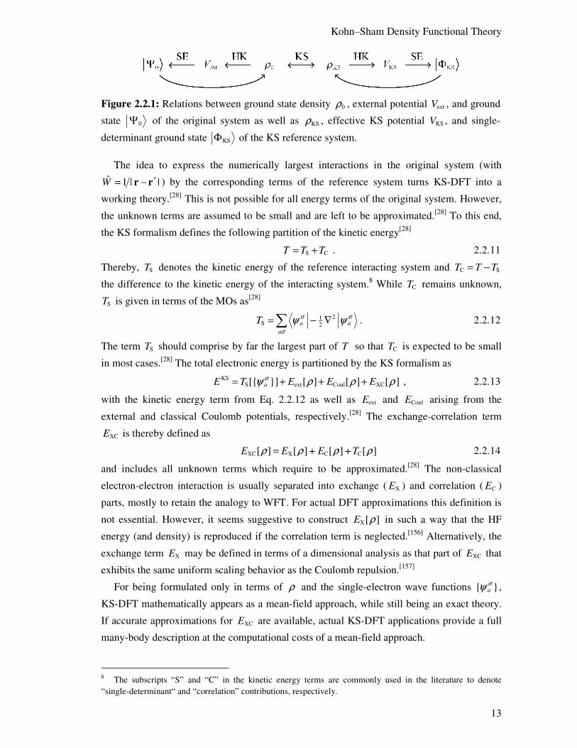
Figure 2.2.1: Relations between ground state density 0ρ , external potential extV , and ground
state 0Ψ of the original system as well as KSρ , effective KS potential KSV , and single-
determinant ground state KSΦ of the KS reference system.
The idea to express the numerically largest interactions in the original system (with ˆ 1 | |W ′= −r r ) by the corresponding terms of the reference system turns KS-DFT into a
working theory.[28] This is not possible for all energy terms of the original system. However,
the unknown terms are assumed to be small and are left to be approximated.[28] To this end,
the KS formalism defines the following partition of the kinetic energy[28]
S CT T T= + . 2.2.11
Thereby, ST denotes the kinetic energy of the reference interacting system and C ST T T= −
the difference to the kinetic energy of the interacting system.8 While CT remains unknown,
ST is given in terms of the MOs as[28]
21S 2a a
a
Tσ σ
σ
ψ ψ= − ∇∑ . 2.2.12
The term ST should comprise by far the largest part of T so that CT is expected to be small
in most cases.[28] The total electronic energy is partitioned by the KS formalism as
KSS ext Coul XC[ ] [ ] [ ] [ ]aE T E E E
σψ ρ ρ ρ= + + + , 2.2.13
with the kinetic energy term from Eq. 2.2.12 as well as extE and CoulE arising from the
external and classical Coulomb potentials, respectively.[28] The exchange-correlation term
XCE is thereby defined as
XC X C C[ ] [ ] + [ ] + [ ]E E E Tρ ρ ρ ρ= 2.2.14
and includes all unknown terms which require to be approximated.[28] The non-classical
electron-electron interaction is usually separated into exchange ( XE ) and correlation ( CE )
parts, mostly to retain the analogy to WFT. For actual DFT approximations this definition is
not essential. However, it seems suggestive to construct X[ ]E ρ in such a way that the HF
energy (and density) is reproduced if the correlation term is neglected.[156] Alternatively, the
exchange term XE may be defined in terms of a dimensional analysis as that part of XCE that
exhibits the same uniform scaling behavior as the Coulomb repulsion.[157]
For being formulated only in terms of ρ and the single-electron wave functions aσψ ,
KS-DFT mathematically appears as a mean-field approach, while still being an exact theory.
If accurate approximations for XCE are available, actual KS-DFT applications provide a full
many-body description at the computational costs of a mean-field approach.
8 The subscripts “S” and “C” in the kinetic energy terms are commonly used in the literature to denote “single-determinant“ and “correlation” contributions, respectively.

Theory
14
Just like in HF theory, the variational equations
KS
KSKS†
ˆ a a a a
a
Ef
σ σ σ σσσ
δψ ψ ε ψ
δψ
= =
2.2.15
for the spin-unrestricted KS orbitals (see below) emerge as stationary points of a Lagrangian,
which includes the boundary conditions of normalized and pairwise orthogonal MOs. The
eigenvalues of the KS spin-orbitals are thereby denoted as KS aσε . Despite of being a quantity
within a fictive system, the highest KS eigenvalue corresponds to the first ionization energy
of the system.[158,159] In contrast to the HF energy in Eq. 2.1.4, the last three terms on the right
side of Eq. 2.2.13 are defined as density functionals.[28] Thus, the single-particle Kohn‒Sham
Hamiltonian (KS operator) is derived with the chain rule for functional derivatives[29]
21KS
2 ext Coul XC
† † †
[ ] [ ] [ , ]b b
a a ab
E E E Eσ σ
σσ σ σ
σ σ σσ
δ ψ ψδ δ ρ δ ρ δ ρ ρ δρδψ δψ δρ δρ δρ δψ
′ ′
↑ ↓
′
− ∇ = + + + ∑ . 2.2.16
Thereby, XC XC[ , ]V Eσ
σδ ρ ρ δρ↑ ↓= is defined as a local and multiplicative potential9 arising
from the XC term.[28] From Eq. 2.2.16 the KS operator is identified as
21KS ext Coul XC2f V V Vσ σ= − ∇ + + + 2.2.17
and a comparison with Eq. 2.2.9 reveals the effective KS potential as
KS ext Coul XCV V V Vσ σ= + + . 2.2.18
Just as in Eq. 2.1.7, the introduction of a finite basis set allows one to formulate the KS
equations as a generalized eigenvalue problem, which needs to be solved iteratively e.g. by
the SCF method. The most striking technical difference to the Fock matrix of HF theory
consists in the term
XCXC[ , ]ij i jV Eσ σϕ δ ρ ρ δρ ϕ↑ ↓= , 2.2.19
which needs to be computed on numerical grids.[7,31,160-166] A correspondingly adapted variant
of Eq. 2.1.11 allows one to compute the estimate of KSE in a finite basis.
Note, that the original DFT treatment was established in terms of the total electronic
density, while the above discussion followed an alternative formulation in terms of the spin-
resolved density[167] KS( ) ( )σρ ρ=r x (spin density) in Eq. 2.2.10. Even more general DFT
formulations exist, dealing with time dependent[168] or current densities.[169] However, only
the spin-resolved variant is relevant in the context of this thesis and thus, demands further
explanation. Without external magnetic field, the exact total density and spin density
functional theories10 always yield the same ground state energy, even for spin-polarized
systems.[130] As the total density formulation restricts both spin components of the density to
be identical (restricted KS, RKS), it does not provide the correct spin-resolved density for
spin polarized systems.[130] Thus, actual spin-restricted KS-DFT approximations yield
9 As opposed to the nonlocal and non-multiplicative HF exchange potential. 10 Indeed, in the non-magnetic, non-relativistic, and time independent case the time dependent and current
density formulations of DFT yield the same ground state energy as well.
Kohn‒Sham Density Functional Theory
15
different total energies compared to corresponding spin-unrestricted (UKS) variants.[130] As
UKS approximations are formulated in terms of the more flexible variable ( )ρ x , their ground
state energies are likely to be closer to the exact result for spin-polarized systems.[170] Thus,
most DFT correlation approximations are specifically constructed as spin resolved density
functionals, while the spin scaling relation[171]
1 1X X X2 2[ , ] = [ ] + [ ]E E Eρ ρ ρ ρ↑ ↓ ↑ ↓ 2.2.20
provides an UKS formulation of the exchange term. Whenever more convenient, the UKS
formulation will be used for some expressions in the following sections.
2.2.2. Exchange-Correlation Holes
The exchange and correlation holes are important quantities in density functional theory.
Exchange and correlation holes provide useful insights to the properties of the exact XC
functional as well as to the behavior of XC approximation with regard to self-interaction and
static correlation effects (see Sections 2.2.5 and 2.2.6). Thus, the origin and properties of
these quantities will be addressed in the following section.
Approximations to the XC term can be obtained from either an empirical parameter
optimization of reasonable functional forms or by considering scaling relations, boundary
conditions, and other known properties of the exact XCE functional.[46,47,73,172-176] The XC
hole
XC X C( , ) ( , ) ( , ) ( , ) ( )h h h θ ρ′ ′ ′ ′ ′= + = −x x x x x x x x x 2.2.21
represents a common starting ground for both, empirical and non-empirical approaches. This
quantity derives from the conditional pair density11
1 2( 1)
( , ) ( ) ( )( )
el el
n nθ δ δ
ρ−
′ ′= Ψ − − Ψx x x x x xx
. 2.2.22
Thereby, ( , )θ ′x x is interpreted as the electron density appearing from the perspective of a
single electron, the so-called reference electron.[31] If an electron with spin σ is found at the
reference position r , ( , )θ ′x x provides the probability for finding another electron of spin σ ′
at another location ′r .[33] In this context the reference electron is described as a particle
located at x so that the pair density is normalized to 1n − electrons.[33] These 1n − electrons
comprise the electron density appearing from the perspective of the reference electron.[33]
However, if exchange-correlation effects are neglected, the particle description of the
reference electron at x does not hold any longer. In this case the conditional pair density
would equal ( )ρ ′x and consequently have an unphysical normalization factor of n . The
exchange-correlation hole XC ( , )h ′x x is introduced as the change of the conditional pair
density which arises from non-classical electron-electron interactions.[33] Its further purpose
11 Noting the analogy between the pair density and the electron density in Eqs. 2.2.1.
Theory
16
is to restore the particle nature12 of the reference electron at x by removing it from the
density. Thus the XC hole XC ( , )h ′x x is normalized to ‒1, in accordance with the
normalization factors in Eqs. 2.2.1 and 2.2.22.[31,33]
The XC hole is subdivided into exchange ( Xh ) and correlation terms ( Ch ); again to retain
the analogy to WFT. While each HF equation treats the residual particles of the system as
distributions, the actual electron described by it is considered a particle. Thus, the HF
exchange hole
2
HF *X ( , ) ( ) ( )
( )a a
a
hσσ σ σ
σ
δφ φ
ρ′ ′′ ′= − ∑x x r rr
2.2.23
exhibits already the correct normalization and prevents two electrons with identical spin from
being found at the same position (Fermi correlation).[29,31] Due to the nonlocal character of
the HF orbitals, the HF exchange hole is delocalized and may extend over many atomic
centers.[33,102]
A detailed analysis of Eq. 2.2.23 reveals the following properties
X X X X( , ) 1 , ( , ) ( , ) 0 , ( , ) ( )h d h h hσσδ ρ′′ ′ ′ ′= − = ≤ = −∫ x x x x x r r x x x , 2.2.24
which are attributed to the KS exchange hole as well. However, compared to the HF
exchange hole, Xh assumes a less extended shape and is more localized.[33] The correlation
hole integrates to zero
C ( , ) 0h d′ ′ =∫ x x x . 2.2.25
This normalization of Ch is to be expected as the presence of the electron at x arises already
from the ansatz of a determinant wave function that leads to the exchange term. The
singularity of ˆ 1 | |W ′= −r r at ′=r r causes Ch to exhibit distinct cusps whenever two
electrons of different spin assume identical positions.[18,31,102] Just as the correlation
interaction itself, the correlation hole is localized, apart from exceptions that arise from
nonlocal vdW or static correlation interactions. In the latter case, Ch is found to be large but
mostly independent of the reference point x over larger regions that may extend over entire
atoms.[177,178] In contrast to that, the hole describing normal, dynamic correlation interactions
varies stronger with respect to x.[177,178] Compared to the exchange hole which removes an
electron from ρ and can assume only negative values, Ch rearranges electrons due to their
Coulomb repulsion, hence depletes the electron density at x and augments it at other
locations ′x . Thus, both contributions cancel each other partially in the long-range and the
extent of the total XC hole is smaller than that of Xh . The properties of the XC hole in Eqs.
2.2.24 to 2.2.25, turn it into a useful quantity for the development of approximations to the
XC term. Furthermore, the picture of XCh as an incremental density that reduces or modifies
( )ρ r will be beneficial in subsequent discussions.
12 As well as the correct normalization of ( , )θ ′x x .

Kohn‒Sham Density Functional Theory
17
2.2.3. Adiabatic Connection
The adiabatic connection formalism provides a continuous link between the KS reference
system and the interacting system. This concept is briefly reviewed in the following, mainly
because of its importance for the theoretical justification of hybrid DFT methods.
In contrast to HFXh , the exchange-correlation hole in KS theory is just as unknown as the
XC functional itself. This is rationalized by considering the fact that it directly relates to the
energy density XC ( )ε r
XCXC XC
( , )[ ( ) [ ( ) ( )]
|]
|
hE d d dρ ρ ε ρ ρ
′′= ⋅ =
′−⌠ ⌠
⌡⌡∫
x xx x x x x x
x x , 2.2.26
thus to the exact XC energy functional.
The KS reference system is defined to be free of electron-electron interactions so that the
XC hole should vanish in this case. However, it is customary to define an XC hole according
to the single-determinant description of the KS reference system to restore the normalization
of ( , )θ ′x x in Eq. 2.2.22, thus the particle picture of a non-interacting reference electron (see
Section 2.2.2).[31,33,131,152,179-181] The resulting hole =0XChλ in the so-called KS exchange only
limit has the same form as HFXh in Eq. 2.2.23 and differs from it just by its definition in terms
of the KS orbitals aσψ instead of the HF orbitals.[31,33]
The adiabatic connection relates =0XChλ to the real XC hole of the interacting
system.[31,33,131,152,179-181] Thereby, a coupling parameter λ is defined on the interval between
0 and 1, which controls the strength of the electron-electron interaction W . The resulting λ -
dependent many-body Hamiltonian writes as
( )212
ˆ ˆ( ) ( , )el a a a ba b a
H V Wλ λ λ
>= − ∇ + + ⋅∑ ∑r r r 2.2.27
with the limiting cases 0KSV V= and 1
extV V= . Furthermore, a λ-dependent XC hole XChλ can
be defined which retains the ground state density for every value of λ in the interval between
0 and 1. The exact XC hole of the interacting system emerges then as the following coupling-
strength average[31,33,131]
1 1
XC XC0 0
( , ) ( , ) ( , ) ( )h h d dλ λλ θ λ ρ′ ′ ′ ′= = −∫ ∫x x x x x x x 2.2.28
with a correspondingly defined λ -dependent conditional pair density ( , )λθ ′x x . Like the XC
hole itself, the concept of adiabatic connection is utterly important for the theoretically driven
development and analysis of KS-DFT approximations. This is especially true for hybrid DFT
methods (Section 2.3).
Theory
18
2.2.4. Local and Semi-Local Density Functional Approximations
While hybrid DFT methods are one of the central topics of the present thesis, these
approximations are also compared to several semi-local XC functionals in the applications
presented in Sections 4.3 and 4.4. Furthermore, the behavior of hybrid functionals with
regard to self-interaction and static correlation effects (see Sections 2.2.5 and 2.2.6) is best
understood when considered together with that of semi-local DFT methods. Thus, the
following section provides a general discussion of local and semi-local DFT methods.
The exact XCh and XCE represent rather complicated quantities as they comprise a full
description of many-body effects. However, significant progress can be made with
comparatively simple approximations to them. Indeed, the most basic DFT approximation to
XE , hence the Dirac exchange functional and the exchange term resulting from the HFS
approximation to the exchange potential, existed already before KS-DFT.[150,152] Both
exchange functionals are examples of local density approximations (LDA), hence are local in
terms of the electron density. The corresponding exchange potential
X /LDA 1 3X
3 3( ) ( )
2V
α α ρπ = −
r r 2.2.29
has the same form for both, the Dirac exchange functional and the exchange term of the HFS
model.[28,150,152,182] For the potential of the Dirac exchange functional a value of 2 3α =
results, while 1α = is obtained when approximating XV directly by the corresponding
expression of the HEG model as in the HFS method. These different prefactors gave rise to
more empirical choices of α (Xα method, e.g. 0.75α ≈ ) in the early days of KS-
DFT.[37,38,183,184] Despite of being rather old, the idea of a modified α-parameter saw a recent
revival in form of the OPTX-type GGA and hybrid GGA functionals.[128] Such methods
include a scaled LDA exchange term to improve the implicit description of static correlation
(see Section 2.2.6).[128] OPBE and O3LYP are the most common OPTX functionals.[185]
LDA approximations to the correlation term existed before the formulation of KS-DFT
too.[186-190] These correlation functionals were later refined by means of the random phase
approximation as well as by quantum Monte Carlo simulations.[172-175] The nowadays most
widely used LDA correlation approximations are known as VWN[191] and PWLDA.[192] LDA
approximations to the XC term often exceed HF and sometimes also MP2 with regard to their
accuracy, especially in the case of transition metals.[34] This performance is rationalized by
the rather slowly varying density in solid state systems as well as by the behavior of the
spherically symmetric and very localized LDA exchange hole
( )LDA 1 3 4X ( , ) 1 ( ) | | for | h |ρ′ ′ ′∝ − − − → ∞r r r r r r r 2.2.30
in molecular systems.[152,193] While LDAXh and the exact Xh differ considerably, the spherically
averaged forms of both holes agree well.[193] As the radial behavior is most important for
exchange holes, this agreement rationalizes the accuracy of LDA for molecular systems.[193]
Kohn‒Sham Density Functional Theory
19
Despite the good performance of LDA, its absolute value of the exchange energy deviates
often by about 10% from the HF result, which may lead to errors in some cases as XE is
considerably larger than CE in most cases.[2,5-7] These problems can be partially resolved by
extending LDA to a spin-unrestricted formalism (LSDA).[28] Nevertheless, significant effort
was put forward to improve the exchange density functional beyond the LDA level. Such
improvements can consist in averaged, nonlocal functionals.[193,194] However, an expansion of
XCE in terms of spatial derivatives of the local density, hence of the dimensionless reduced
density gradient 2 1 3 4 31 | ( ) | [(24 ) ( ) ]s ρ π ρ= ∇ r r and its higher order analogues, represents a
far more viable and popular alternative.[28,195-197] The functionals resulting from this approach
are denoted as semi-local DFT approximations as they partially address the nonlocal
character the XC term while still retaining a mathematically local XC functional.[45] While
such an approach is certainly promising, the exact polynomial expansion of the exact
exchange hole in terms of 1s exhibits a divergent behavior for large values of this
variable.[195] Therefore, so-called “generalized gradient approximations” (GGA) were
introduced, which modify the exact gradient expansion, mostly for large gradients 1 3s > ,
and exhibit the following general form[45]
GGA GGAX X 1
LDA GGAX X 1
[ ] ( ) ( ( ), ( ), )
( ) ( ( )) ( ( ), ( ), ) .
E s d
F s d
ρ ρ ε ρ
ρ ε ρ ρ
=
=
∫∫
r r r r
r r r r r
…
…
2.2.31
The choice of the gradient exchange enhancement factor GGAXF adds some degree of
empiricism to KS-DFT. In consequence, many GGA variants have been proposed.[46-50]
Nevertheless, the enhancement factors of all GGA methods are always larger than one, which
yields more negative exchange energies compared to LDA.[31] The reduced density gradient
1s and thus also the absolute values of GGAXF and XE are reduced upon formation of chemical
bonds.[198] In consequence, GGA functionals tend to lower reaction energies, which often
reduces the overbinding tendency of LDA.[31,198] The most common GGA variants are the
B88[46] exchange term and the LYP[47] correlation functional as well as the XC formulations
PW91[192] and PBE.[49] Novel, non-separable gradient approximations (NGA) have recently
been proposed.[176] These functionals exhibit dependencies on ρ and 1s as well but, opposed
to the canonical separation in Eq. 2.2.14, are formulated as a combined XC term.[176]
When pursuing the argumentation, that led from LDA to GGA methods, one step further,
one arrives at XC functionals that also include the Laplacian of the electron density. Indeed,
the usage of Laplacian dependent exchange terms has been reported to improve over
functional forms purely dependent on the electron density gradient.[199] However, functionals
that include higher order density derivatives may tend to a more erratic behavior when
integrated numerically.[200,201] The electronic kinetic energy density (KED)[72,80,202,203]
21
2( ) ( ) ( )a
aσ σ
τ τ ψ= = ∇∑ ∑∑r x x , 2.2.32
Theory
20
is more stable in this regard. As one of the second-order derivative terms of the electron
density it includes similar information as the Laplacian of ρ.[72,80,202,203] Despite of being
orbital-dependent, τ is well justified by the HK formalism as a density functional variable as
the value of each KS orbital at x represents a density functional too. The optimized effective
potential (OEP, see Section 2.3.2) method allows one to compute XCE ρ∂ ∂ for orbital-
dependent XC functionals, thus to perform self-consistent calculations within the KS-
formalism.[204-206] However, this approach introduces very high computational costs, but
changes energies only slightly; it is mostly popular for properties like NMR shielding
constants.[206,207] The generalized Kohn‒Sham formalism (GKS, see Section 2.3.2) provides
an alternative justification for orbital-dependent XC approximations.[208] Within the GKS
formalism the XC potential can be computed in terms of functional derivatives with respect
to the orbitals (FDO) only.[208]
The KED exhibits several additional beneficial properties that go beyond what is provided
by derivatives of the density.[202] First, the KS orbitals are solutions of the nonlocal KS
equations and thus, represent nonlocal density functionals themselves. This nonlocal
character is included in τ as well, although only in an intrinsic fashion and not directly
accessible for the construction of XC approximations. Nevertheless, the nonlocal information
included in τ has been shown to provide, to some extent, a description of nonlocal properties
(see Section 2.2.7).[77] Second, the HEG limit of τ ,
( )HEG
5 32 2 3HEG
3lim ( ) ( ) (3 ) ( )
10ρ ρτ τ π ρ
→= =r r r , 2.2.33
allows detecting spatial regions where the density approaches a HEG-like behavior.[209] By
exploiting Eq. 2.2.33 the XC energy density XCε can be constructed to reduce to the
corresponding LDA form in these regions.[209,210] In this way, the violation of the HEG limit
can be avoided, thus eliminating a source of error in XC approximations.[198,209,210]
Furthermore, spatial regions which are dominated by a single KS spin orbital (thus individual
electrons), so-called one-electron regions[79] (OER, see Section 2.2.5), can be identified by
comparing the KED with the von Weizsäcker kinetic energy density Wτ ,
2
W1 | ( ) |
lim ( ) ( )8 ( )aρ ψ
ρτ τ
ρ→
∇= =
xx x
x . 2.2.34
As discussed in the next section, OERs are often responsible for the self-interaction error. It
is therefore beneficial to identify locally OERs and to adapt XCε to such situations.[72,74]
Functionals which depend on τ (besides depending on ρ and 1s ) are referred to as meta-
generalized gradient approximations (MGGA).[71,211] As expected from the aforementioned
properties of the KED, MGGA functionals provide improvements over GGA methods
although the additional gain in accuracy is usually not as large as when going from LDA to
GGA.[77,212,213] The functionals TPSS[75,76,212] and M06L[77] are the most common MGGA
methods; they are based on the earlier MGGA variants PKZB[74] and VSXC,[73] respectively.
Kohn‒Sham Density Functional Theory
21
2.2.5. Self-Interaction Error
The self-interaction error (SIE) is the most common artifact arising to some extent in all
current approximations to KS-DFT. This error and its consequences will be first explained on
the examples of single-electron systems and one-electron regions (OER). In the following the
many-electron self-interaction or delocalization error will be discussed. Although this latter
artifact has been recognized long time ago, the detailed study of its effects and implications
has begun only recently. In consequence the available literature on this topic is somewhat
sparse and ambiguous with regard to some details. While occasionally referring to the results
and explanations of Mori-Sánchez‒Cohen‒Yang,[101,120,214-217] the subsequent presentation
mainly follows the work of Perdew et al.[130,158,218-220] and employs the concept of fractional
electron numbers (FEN) for many explanations.
Despite the remarkable success of LDA, GGA, and MGGA KS-DFT methods one has to
consider that these methods are still far from being close to the exact XC functional. Indeed,
the local form of these methods represents the most striking difference to the exact XC term.
The implications of this difference become apparent when one considers the very simple
example of a system that includes a single electron only.13 Within such a system all electron-
electron interactions terms are supposed to vanish due to the lack of interaction partners.
Within HF theory this is always accomplished as the exchange and Coulomb terms cancel in
the case of a single occupied spin-orbital. Retaining the analogy of the exchange interaction
between HF and KS-DFT, the exact functional X[ ]E ρ should behave likewise. This implies
X Coul( ) ( )
[ ] [ ] | |
E E d dρ ρ
ρ ρ⌠ ⌠ ⌡⌡
′′= − = −
′−
r rr r
r r 2.2.35
for all densities that originate from a single occupied KS orbital, 21( ) =| ( ) |ρ ψr r . As visible
for example from Eq. 2.1.13 the correlation term in post-HF theories vanishes by a similar
cancellation mechanism. Therefore,
C[ ] 0E ρ = 2.2.36
must hold for single electron densities as well.
Thus, Eq. 2.2.35 clearly reflects the nonlocal character of the exact KS-DFT exchange.
However, for arbitrary single-electron densities local (LDA) or semi-local (GGA, MGGA)
exchange approximations can never completely cancel with the Coulomb
term.[101,214,215,217,218,220] In single-electron systems the latter term is generally found to prevail
over the exchange energy provided by local and semi-local exchange approximations.[101]
This excessive Coulomb interaction leads to an unphysical, residual self-repulsion, which is
known as the self-interaction error.[101]
13 The hydrogen atom and the 2H+ ion are thereby the most prominent examples and the most frequently studied model systems in this context.
Theory
22
The occurrence of self-interaction artifacts as introduced by the local ansatz for the XC
energy density represents a significant limitation already for one-electron systems alone.
However, the SIE is not limited to one-electron densities. Indeed, this artifact becomes
notable also in the aforementioned one-electron regions (OER) of many-electron systems.
Within an OER, a single electron can be found for each spin value at most. This electron
interacts with the electrons outside of the OER as well as with its eventual counterpart of
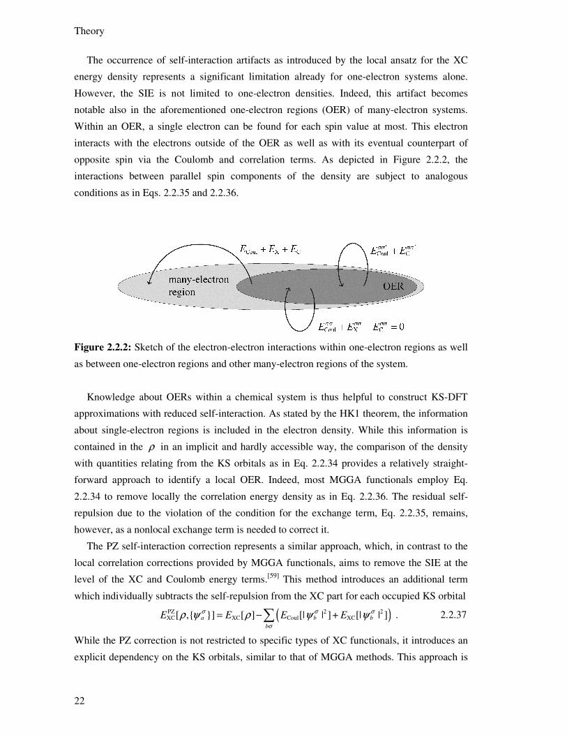
opposite spin via the Coulomb and correlation terms. As depicted in Figure 2.2.2, the
interactions between parallel spin components of the density are subject to analogous
conditions as in Eqs. 2.2.35 and 2.2.36.
Figure 2.2.2: Sketch of the electron-electron interactions within one-electron regions as well
as between one-electron regions and other many-electron regions of the system.
Knowledge about OERs within a chemical system is thus helpful to construct KS-DFT
approximations with reduced self-interaction. As stated by the HK1 theorem, the information
about single-electron regions is included in the electron density. While this information is
contained in the ρ in an implicit and hardly accessible way, the comparison of the density
with quantities relating from the KS orbitals as in Eq. 2.2.34 provides a relatively straight-
forward approach to identify a local OER. Indeed, most MGGA functionals employ Eq.
2.2.34 to remove locally the correlation energy density as in Eq. 2.2.36. The residual self-
repulsion due to the violation of the condition for the exchange term, Eq. 2.2.35, remains,
however, as a nonlocal exchange term is needed to correct it.
The PZ self-interaction correction represents a similar approach, which, in contrast to the
local correlation corrections provided by MGGA functionals, aims to remove the SIE at the
level of the XC and Coulomb energy terms.[59] This method introduces an additional term
which individually subtracts the self-repulsion from the XC part for each occupied KS orbital
( )PZ 2 2XC XC Coul XC[ , ] [ ] [| | ] + [| | ]a b b
b
E E E Eσ σ σ
σ
ρ ψ ρ ψ ψ= −∑ . 2.2.37
While the PZ correction is not restricted to specific types of XC functionals, it introduces an
explicit dependency on the KS orbitals, similar to that of MGGA methods. This approach is

Kohn‒Sham Density Functional Theory
23
less popular nowadays as it does not always lead to consistent improvements due to its
missing invariance with respect to unitary transformations of the KS orbitals.[58,221]
One-electron regions of many-electron systems are usually found distant from the atomic
nuclei, where the exact XC potential behaves as
XC ( ) 1 | | for | | V = − → ∞r r r 2.2.38
for electrically neutral, finite systems. In contrast, approximated local and semi-local XC
potentials decay exponentially at large distances.[33] This behavior originates from the
exponential decay of the density in this limit.[33] The incorrect form of the XC potentials of
LDA, GGA, and MGGA functionals has a significant effect on the KS aε values. The
eigenvalues of KS orbitals partially located in OERs are thereby most affected and raised in
energy due to the remaining self-repulsion.[29] Furthermore, the XC potential
XCXC XC
[ ( )( ) [ ( ) (
])
( )]V
δε ρε ρ ρ
δρ= +
xx x x
x 2.2.39
and thus also the eigenvalues of the KS orbitals are subject to a discontinuous shift at integer
values of n or at band gaps in the case of extended systems.[5] The second term on the right-
hand side of Eq. 2.2.39 represents the response potential and describes the changes in the XC
hole due to variations of the density.[222] For non-metallic systems this term causes the
aforementioned discontinuity of XCV whenever a new KS orbital starts to become occupied.
This sudden potential change leads then to the corresponding shift of all KS eigenvalues KS aε .[223-225] Thereby, the derivative discontinuity adjusts the eigenvalue of the highest
occupied orbital to the ionization energy of the system.[158,159]
It might appear odd that an infinitesimally small addition of electronic charge to a single
KS orbital changes the eigenvalues within the entire system, which may eventually be very
extended. Nevertheless, this behavior can be rationalized when considering that the KS
reference system and its orbitals do not have to represent physical quantities. Furthermore, as
KS-DFT uses an orbital-dependent kinetic energy term, the derivative of the formal
functional S[ ]T ρ must exhibit discontinuities as well.[5] An analogous argumentation reveals
such a behavior also for the effective KS potential.[5] As all terms of the KS potential, Eq.
2.2.18, except for XCV are explicitly known density functionals, only the XC potential can
adjust the discontinuous behavior of KSV .[5] Despite of eventual dependencies on the KS
orbitals, the behavior of local and semi-local approximations to KS-DFT is still largely
governed by the electron density. Therefore, LDA, GGA, and MGGA functionals are
generally unable to reproduce properly the discontinuity of the KS potential.[5]
Theory
24
In self-consistent applications of local KS-DFT approximations, the system at hand always
tends to lower the destabilizing self-repulsion to some extent. This relaxation can lead to
overly delocalized KS orbitals. This delocalization as well as the incorrect behavior of the
aforementioned eigenvalue shifts due to the SIE can significantly affect the description of
chemical bonds, ionic compounds, and of many electronic properties.14 Bonding energies are
thereby often overestimated, while anionic species can become destabilized.[101,214,215,217,226]
Aside from the well understood self-repulsion artifacts in one-electron situations, self-
interaction can affect many-electron regions as well.[214,218] The many-electron self-
interaction error[214] (MSIE) recently gained significant attention and was recognized on the
examples of improperly charged dissociation fragments,[218,220] spurious maxima in the
dissociation curves of small molecules,[220] and an incorrect behavior of the bond lengths in
conjugated π-systems.[216,227] These failures were found to be related self-interaction effects
as most other sources of errors could be excluded as cause.[214] However, methods like HF or
the PZ correction which do not exhibit single-electron self-interaction are unable to provide
the correct solutions in these cases as well.[214,220,228] Even functionals like B05[229] or
MCY,[230] which remain unchanged by the PZ correction, are affected by the MSIE.[214]
While MSIE-free XC approximations are not yet entirely explored,[120] the considerations
made in this context provide a generalized perspective on the self-interaction phenomenon
itself. As will be discussed in Section 2.2.6 the MSIE of local and semi-local XC
approximations is closely connected to their implicit description of static correlation. After
this relation was recognized, the term “delocalization error” was put forward by Mori-
Sánchez et al. to describe both, the MSIE and the implicit description of static
correlation.[101,215-217] However, this term will be less frequently used in the following, as both
aspects are mostly considered separately in the present discussion.
As mentioned above, the exact XC potential exhibits a discontinuous behavior at integer
occupation numbers of the KS orbitals.[158,219] This phenomenon is generalized by the concept
of fluctuating electron numbers (FEN), where an open subsystem S is introduced which is
well separated from a distant electron reservoir R that comprises the rest of the
system.[130,158,219] While S and R are separated, the KS orbitals can still extend over both
subsystems.[130,158,219] In consequence, electrons may fluctuate between R and S which in turn
leads to fractional electron numbers in the latter.[130,158,219] Nevertheless, the contribution SelE
of the subsystem S to the total electronic energy, is well defined for fully separated
subsystems S and R.[130,158,219] Although the complete system S+R is still covered by standard
KS-DFT, an extension of the formalism to density ensembles[29,231] is necessary to describe
14 Although not relevant for the present discussion, it is worth mentioning that quantities like electron
excitation energies and Rydberg states are even more affected by the SIE. This essentially limits local DFT methods to calculations of ground state properties, even if a proper time-dependent formalism would be employed.
Kohn‒Sham Density Functional Theory
25
correctly the isolated subsystem S.[219,232] Such an ensemble is represented by a generalization
of the density matrix operator in Eq. 2.1.9[126]
ˆ ni ni ni
n i
eρ = Ψ Ψ∑∑ , 2.2.40
to include projectors onto different states niΨ which can exhibit different numbers of
electrons n. In finite-temperature grand-canonical-ensemble theory the probabilities nie of
the ensemble elements optimize the grand potential
( )
( )
KSB
KSB
ˆˆ ˆ ˆ[ , ] Tr ln( )
ˆln( ) ,
ni ni
ni ni ni ni
n i
e k H n
e k e H n
ρ θ ρ µ
θ µ
Ω Ψ = ⋅ + + ⋅
= ⋅ + Ψ Ψ + ⋅∑∑ 2.2.41
with the Boltzmann constant Bk , the temperature θ , the chemical potential µ , and the
electron number operator n . Eq. 2.2.41 accounts for the contributions of different orthogonal
eigenfunctions of KSH as well as for a varying electron number of electrons n. In contrast to
this usual application of ensemble DFT, the FEN model employs density ensembles only for
the purpose of representing the electronic structure of the subsystem S. In this context the
probabilities nie are defined by the ground state of the system S+R and do not lead to
stationary points of the grand potential in Eq. 2.2.41. The FEN formalism provides a unified
approach for non-integer total electron counts as well as for fractional occupation numbers of
the KS orbitals.[233] The latter concept is also widely applied in form of the fractional
occupation number technique (FON).[234-237]
The exact total energy ( )SelE n of an open subsystem S must behave as a linear function in
terms of the electron count between integer values of N.[158] This behavior is known as the
linearity theorem[158] and is closely connected to the Janak theorem[233]
KS( )Sel a
a
a
E f
f
σσ
σ ε∂
=∂
, 2.2.42
which states a similar behavior for SelE in terms of individual orbital occupation numbers
af . Both, the linearity theorem and the Janak theorem extend and quantify the
aforementioned discontinuous behavior of the KS potential. Furthermore, these theorems
allow one to compare the behavior of the exact KS-DFT with that of DFT approximations,
especially with regard to the self-interaction error.
Fractional occupation numbers of KS orbitals and fractional electron counts of isolated
subsystems occur only in specific cases like transition metals treated with the FON technique
or ionic dissociation fragments (see above), respectively. However, the fact that the linearity
theorem is formulated in terms of an open subsystem does not imply that its violation affects
only such model systems. As will be discussed in the following, convex and concave
deviations from the linearity theorem reflect tendencies for localization or delocalization of
KS orbitals, respectively. Thus, any violations of the linearity theorem are likely to affect the
general description of chemical bonds in systems with integer occupation numbers as well. In

Theory
26
this context the FEN model can be considered as a formal approach to examine the many-
electron self-interaction and delocalization errors isolated from other interactions.
Figure 2.2.3 provides a graphical representation of the exact total electronic energy ( )SelE n
and of the eigenvalue of the highest occupied KS orbital GKSHOMO ( )nε between integer values of
the number of electrons in S. This comparison can even be extended to the HF method, which
qualifies as a density functional within the generalized Kohn‒Sham formalism (GKS, see
Section 2.3.2).[208] Note that in this context both, local DFT and HF, are assumed to provide
exact total energies at integer electron counts.
Figure 2.2.3: Qualitative comparison between exact DFT, local DFT, and HF results for the
total electronic energy ( )SelE n and the eigenvalue GKS
HOMO ( )nε of the highest molecular orbital
with varying electron count under the assumption that all methods yield the correct ( )SelE n
values at integer n. Figure adapted from Ref. [219].
Figure 2.2.3 shows that, compared to the exact ( )SelE n function, local and semi-local DFT
methods yield more negative total electronic energies between integer values of
n.[101,214,215,217-220,238] This deviation from the exact energy ( )SelE n agrees with the
aforementioned tendency of LDA, GGA, and MGGA for an overly large electronic
delocalization due to self-repulsion. Accordingly, these functionals also underestimate the
discontinuous shift of the eigenvalue GKSHOMO ( )nε and thus the HOMO-LUMO gap (HLG) or
band gap of the system. The convex behavior of local DFT methods can be rationalized with
Kohn‒Sham Density Functional Theory
27
the normalization of the XC hole in the fictitious KS exchange only limit.[219] The exchange
hole has the same form as HFXh in Eq. 2.2.23 (see Section 2.2.2), as the KS system is
described by a single Slater-determinant.[181] For fractional occupation numbers afσ the KS
exchange hole integrates[59,219] to
2
=0XC
( )( , ) 1 ( 1)
( )
a
a a
a
h d f f
σλ σ σ
σσ
ψ
ρ′ ′ = − + −⌠
⌡ ∑r
x x xr
. 2.2.43
As the exchange hole partially resides in R, this integral differs from the expected value of ‒1
unless all KS spin-orbitals exhibit integer occupations.[219] The normalization of the exact XC
hole behaves likewise.[239] However, the actual LDA exchange hole, Eq. 2.2.30, is more
localized than =0XChλ and Xh .[178,219] Thus, the exchange hole obtained with LDA remains
entirely located in S and still normalized to ‒1.[178] In consequence, this hole yields a higher
exchange energy density than the exact hole.[219] As a result also the corresponding exchange
energy will be more negative than in the exact case.[219] As nearly all semi-local DFT
approximations are based upon LDA exchange, such methods tend to favor fractional
electron counts as well.[49,75,219]
The behavior of ( )SelE n found in the case of the Hartree‒Fock method contrasts with that
of local DFT approximations. Compared to the exact results, HF yields less negative total
electronic energies for the subsystem S at non-integer electron counts. Furthermore, the
discontinuous shift of the frontier orbital eigenvalue GKSHOMO ( )nε is overestimated at integer
values of n, which causes the HF method to overestimate the HLG.[101,215,217,219] HF delivers a
concave shaped function ( )SelE n which can be interpreted as a tendency for an overly large
orbital localization (Figure 2.2.3). In the case of HF the higher ( )SelE n values at non-integer
electron counts can be rationalized by considering that the open subsystem S is described by
an ensemble of states.[219] Recall, that the probabilities nie for the ensemble elements in Eq.
2.2.40 are determined to represent the electronic structure of the subsystem S within the
whole system S+R but not by a minimization of the grand potential of S.[219] In consequence,
( )SelE n will be lower at integer electron counts where the corresponding electronic structures
can be described by pure states.[219]
Following the argumentation discussed above, DFT approximations are only considered
free of the MSIE when they are able to provide the correct linear variation of the total
electronic energy between integer electron counts for arbitrary systems.[101,215,217,230]
Theory
28
2.2.6. Static Correlation Error
Static correlation effects were defined in Section 2.1.2 as large reorganizations in the
electronic structure. These rearrangements arise from interactions between the HF ground
state and one or more other single-determinant states nearly degenerate to it. In contrast to
multi-reference approaches, KS-DFT relies on a purely single-determinant description of the
non-interacting reference system.[28] This situation leads to the question whether static
correlation can be reliably captured within the KS formalism.[130] Furthermore, the model of
fractional spins[215,217] will be discussed in this section, which allows one to examine the
description of static correlation by different methods isolated from self-interaction effects.
While KS-DFT is based on a single-determinant description, physically meaningful
densities exist which are not V-representable within the KS system in terms of a pure, single-
determinant state.[143,144,240-242] Such a missing V-representability indicates a strong influence
of static correlation effects. It is nevertheless always possible to restore this representability
in terms of the ensemble DFT approach (see Eqs. 2.2.40 and 2.2.41). In this context it is not
surprising, that FON techniques can be used to describe static correlation effects.[243]
HF and even low level post-HF methods (see Section 2.1.2) can exhibit an erratic behavior
for systems dominated by static correlation interactions.[133] Opposed to that, local and semi-
local KS-DFT approximations are often found to provide a reasonable accuracy, despite the
fact that they are based on a single-determinant approach.[129,177] This accuracy is especially
pronounced for transition metal compounds whose exact ground state wave functions include
many nearly degenerate single-determinant terms.[129,177] However, for systems like radicals
or atoms severe failures are known semi-local DFT approximations.[31,240,244] In such cases
broken symmetry treatments may yield more reliable results.[31,240,244]
Nevertheless, the reasonable description of transition metals provided by local and semi-
local KS-DFT approximations strongly indicates that these methods are, to some extent, able
to account implicitly for static correlation.[129,177] This description of static correlation was
traced back to the LDA exchange functional.[129,177] As GGA and MGGA exchange
functionals always include an LDA exchange energy density factor, these methods behave
likewise.[129,177] Nevertheless, the description of static correlation is most pronounced in
LDA.[129,177]
The finding that LDA can account for static correlation effects is again rationalized by
referring to its exchange hole.[129,177] Recall that static correlation locates electrons to
different regions in space (see Section 2.1.2) and thus, suppresses electron fluctuations
between these locations.[130] In theories like HF where this suppression is missing, the
exchange hole HFXh , Eq. 2.2.23, tends to be overly delocalized.[129,130,177] As the KS XC hole
in the exchange only limit
Kohn‒Sham Density Functional Theory
29
2
=0 *XC ( , ) ( ) ( )
( )a a
a
hσσλ σ σ
σ
δψ ψ
ρ′ ′′ ′= − ∑x x r rr
, 2.2.44
has the same form as HFXh , it is delocalized as well.[31,33] While the exact exchange hole Xh is
delocalized to a similar extent as HFXh , the total exact XC hole is more compact (see Section
2.2.2).[31,33,129,130,177] This implies a partial cancellation between the long-range parts of Xh
and Ch .[130] Such a cancellation can often only be provided from the static correlation part of
Ch , as dynamic correlation is a mostly small and very localized effect.[129,130,177]
While the static correlation hole and Xh cancel, the LDA exchange hole is already far
more compact than =0XChλ or HF
Xh .[178] With LDA correlation being an even more local
functional, the total LDA hole LDAXCh appears more similar to the exact XCh than =0
XChλ or
HFXh .[129,177] Thus, the overly compact LDA exchange hole can mimic the long-range
cancellation between the exact Xh and Ch holes which occurs in the presence of static
correlation effects.[129,177] In exchange approximations that admit the density gradient and/or
the kinetic energy density as variables, the corresponding hole becomes somewhat more
delocalized compared to the pure LDA case.[178] Compared to LDA the implicit static
correlation description can therefore be slightly reduced in GGA and MGGA methods.[178]
The above rationalization also depicts the intrinsic connection between the description of
static correlation provided by local DFT methods and the many-electron self-interaction
error.[58,129,177] Most corrections for the latter tend to bring the exchange hole of local and
semi-local KS-DFT approximations closer to the exact Xh , thus to delocalize it in most
situations.[58,129,177] This delocalization of the XC hole effectively reduces its capability to
mimic static correlation effects.[58,129,177] Indeed, the OPTX-type functionals (see Section
2.2.4) exhibit an increased prefactor of the LDA exchange term to address this problem in
parts.[128,185] However, any modification of this numerically largest term of the XC functional
is likely to affect the quality of the electronic structure in cases where static correlation is less
important. Thus, without a correlation functional CE that can properly account for static
correlation, any attempt to reduce the SIE and the delocalization error in local and semi-local
functionals will inevitably result in a deteriorated description of static correlation, thus in the
so-called static correlation error (SCE).[130,215,217,245,246]
Just as in the case of fractional electron numbers (see Section 2.2.5), special model
systems can be defined which allow one to examine specifically the static correlation
error.[177] An example for such a static correlation effect, which is not influenced by any self-
interaction artifacts, is provided by the fractional spin model.[101,215,217] This model considers
a single electron which is distributed over two KS spin orbitals, ψ ↑ and ψ ↓ .[101,215,217] Both
orbitals have opposite spin components but the same spatial form.[101,215,217] The spatial
component of these orbitals is defined to remain constant and may be even infinitely
extended to exclude any eventual self-interaction artifacts.[101,215,217]
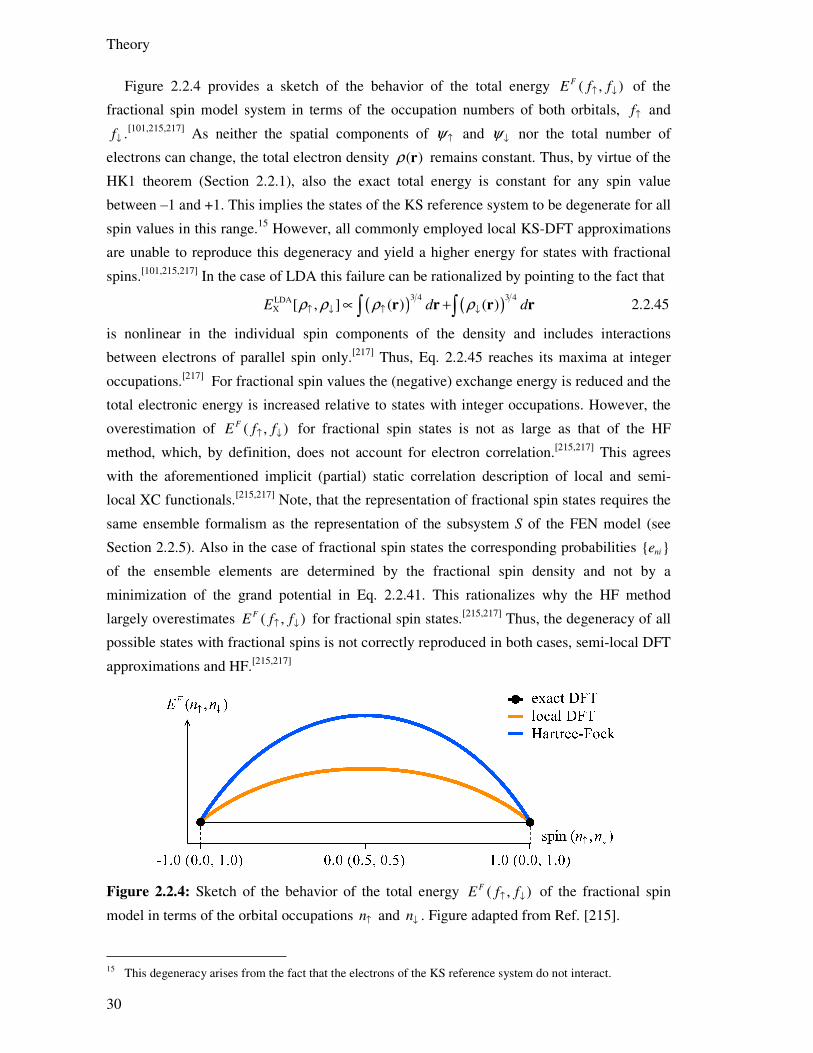
Theory
30
Figure 2.2.4 provides a sketch of the behavior of the total energy ( , )FE f f↑ ↓ of the
fractional spin model system in terms of the occupation numbers of both orbitals, f↑ and
f↓ .[101,215,217] As neither the spatial components of ψ ↑ and ψ ↓ nor the total number of
electrons can change, the total electron density ( )ρ r remains constant. Thus, by virtue of the
HK1 theorem (Section 2.2.1), also the exact total energy is constant for any spin value
between ‒1 and +1. This implies the states of the KS reference system to be degenerate for all
spin values in this range.15 However, all commonly employed local KS-DFT approximations
are unable to reproduce this degeneracy and yield a higher energy for states with fractional
spins.[101,215,217] In the case of LDA this failure can be rationalized by pointing to the fact that
( ) ( )3 4 3 4LDAX [ , ] ( ) ( )E d dρ ρ ρ ρ↑ ↓ ↑ ↓∝ +∫ ∫r r r r 2.2.45
is nonlinear in the individual spin components of the density and includes interactions
between electrons of parallel spin only.[217] Thus, Eq. 2.2.45 reaches its maxima at integer
occupations.[217] For fractional spin values the (negative) exchange energy is reduced and the
total electronic energy is increased relative to states with integer occupations. However, the
overestimation of ( , )FE f f↑ ↓ for fractional spin states is not as large as that of the HF
method, which, by definition, does not account for electron correlation.[215,217] This agrees
with the aforementioned implicit (partial) static correlation description of local and semi-
local XC functionals.[215,217] Note, that the representation of fractional spin states requires the
same ensemble formalism as the representation of the subsystem S of the FEN model (see
Section 2.2.5). Also in the case of fractional spin states the corresponding probabilities nie
of the ensemble elements are determined by the fractional spin density and not by a
minimization of the grand potential in Eq. 2.2.41. This rationalizes why the HF method
largely overestimates ( , )FE f f↑ ↓ for fractional spin states.[215,217] Thus, the degeneracy of all
possible states with fractional spins is not correctly reproduced in both cases, semi-local DFT
approximations and HF.[215,217]
Figure 2.2.4: Sketch of the behavior of the total energy ( , )FE f f↑ ↓ of the fractional spin
model in terms of the orbital occupations n↑ and n↓ . Figure adapted from Ref. [215].
15 This degeneracy arises from the fact that the electrons of the KS reference system do not interact.

Kohn‒Sham Density Functional Theory
31
2.2.7. Non-Covalent Interaction Error
The non-covalent interaction error (NCIE) represents the third important aspect that is not
accounted for by standard local and semi-local KS-DFT approximations. The non-covalent
interaction error recently gained much attention resulting in the development of various
classes of approximations and corrections.[77,105-107,111-119,210,247] The NCIE is of a lesser
relevance in the context of the present thesis compared to the SIE or the SCE. However, for
the sake of completeness, the approaches most commonly used for the description of non-
covalent interactions shall be briefly reviewed in the following as well.
The motion of electrons can create dynamic dipoles (or multipoles in general) even in
molecules that lack a permanent dipole (or multipole) moment. Such instantaneous dipoles
can affect the electronic structure of distant parts of the system and induce dipoles there as
well.[248] The attractive interaction between such dynamic dipoles located near different
atomic positions A and B is known as London dispersion energy dispE and is one of several
types of non-covalent (van der Waals, vdW) interactions.[248] The dispersion interaction
between distant atomic centers of a molecular system exhibits an asymptotic behavior
proportional to 66 | |C− AB , in terms of the interatomic distances | | | |= −AB A B and the
dispersion coefficients 6C .[248]
Although it originates from instantaneous effects, the dispersion energy still results from
the interactions of electrons which can be described by a time independent many-body wave
function. Indeed, these effects result from electron correlation as well and the only difference
between dispersive interactions and normal dynamic correlation interactions (see Section
2.1.2) consists in their locality. The nonlocal character of dispersive interactions implies that
any KS-DFT approximation which can account for such effects has to feature a nonlocal
correlation functional.[104] As LDA and GGA methods employ only local correlation terms,
these approximations are unable to capture dispersive interactions between distant parts of the
system.[104] On the other hand, the nonlocal correlation terms occurring in post-HF methods
like MP2 account for dispersion effects.[7] This led to the idea to employ the KS orbitals in an
MP2-type correlation term[109] which is then combined with a suitably adapted semi-local
correlation functional,[111-114]
2
DH DHGGAC 1 C 2 KS KS KS KS
ˆ ˆ| | | | | |a b u v a b v u
a b u vab uv
W WE E
ψ ψ ψ ψ ψ ψ ψ ψβ β
ε ε ε ε⟨ ⟩ − ⟨ ⟩
= ++ − −∑∑ . 2.2.46
The coefficients iβ and the local DHGGACE term of these so-called double hybrid functionals
were thereby fitted to experimental reference data.[111-114] Double hybrid functionals have the
same 5( )NO scaling computational requirements as the MP2 method, as they exhibit a
nonlocal dependency on both, occupied and unoccupied, KS orbitals.[109] Furthermore, these
methods are limited to non-self-consistent applications only as their XC potentials diverges
for many-electron systems.[109] A similar nonlocal dependency on the unoccupied KS orbitals
Theory
32
is found in random phase approximations (RPA), which, however, represent significantly less
empirical approaches to a nonlocal correlation functional.[108,110]
To circumvent these high computational requirements, a much simpler empirical
expression for the dispersion energy
D 616,2 (| |) | |disp damp AB
AB
E f C= − ∑ AB AB 2.2.47
was suggested by Wu and Yang which depends on the atomic positions only.[105] This so-
called DFT-D correction employs empirical pairwise dispersion coefficients 6,ABC as well as
a damping function dampf to reduce the double-counting between dispersion and semi-local
correlation terms.[105] The DFT-D method was subsequently refined by Grimme and
others.[95,106,249] Approaches to compute the 6,ABC coefficients in terms of the actual electron
density of the system were proposed as well.[107,247] While being very efficient compared to
double hybrid and RPA approaches, the DFT-D corrections in Eq. 2.2.47 are highly empirical
and not applicable in all situations. The vdW-driven adsorption of molecular species on
extended metal surfaces represents such an example in which DFT-D descriptions break
down.[250-252] Thereby the collective polarizability of the metallic moiety causes an
asymptotic 3R− scaling of vdW interactions which is not accounted for by DFT-D corrections
of the general form in Eq. 2.2.47.[250-252]
A different attempt to include vdW interactions into an efficient semi-local DFT
approximation has been proposed in form of the M06L MGGA functional.[77] As already
mentioned in Section 2.2.4, the value of the kinetic energy density ( )τ r at any point r
represents a nonlocal density functional itself.[202] In this context the usage of τ in MGGA
functionals implicitly introduces a small amount of nonlocal information into the semi-local
XC term.[202] This fact was exploited in the parametrization of the M06L functional on data
sets which emphasize vdW-type interactions.[77,210] Compared to most DFT-D approaches,
the M06L functionals describes dispersion interactions in a self-consistent fashion. However,
its extensive parametrization can lead to large deviations in the case of systems that are not
part of the data set used for the parametrization of M06L (see Sections 4.3 and 4.4).[253]
The so-called vdW functionals represent another approach to the description of non-
covalent interactions.[115-119] These methods exhibit the following functional form
( )VDW 1C 2[ ] = ( ) ( ), ( ), ( ), ( ) ( ) E d dρ ρ ρ ρ ρ ρ ρ⌠⌠
⌡⌡
′ ′ ′ ′⋅Θ ∇ ∇ ⋅r r r r r r r r 2.2.48
and employ a complicated integral kernel Θ to describe nonlocal aspects of the correlation
between electrons at two distant locations.[115-119] Such functionals are mostly based on non-
empirical considerations.[116] In contrast to the aforementioned RPA and double hybrid
approaches, vdW DFT methods are formulated only in terms of ρ and ρ∇ , and do not
depend on the KS orbitals. Compared to the high computational requirements of RPA and
double hybrid terms or the high empiricism of DFT-D corrections and the M06L functional

Kohn‒Sham Density Functional Theory
33
vdW DFT methods can be considered as a significant breakthrough.[131]. Despite the double
integral required in Eq. 2.2.48, vdW functionals can be applied quite efficiently, at least when
Fourier transformation techniques are employed.[254] In the case of systems including
appreciable vdW interactions, these functionals provide a significant gain in accuracy.[255]

34
2.3. Hybrid Density Functional Theory
2.3.1. Rationale for Exact-Exchange Mixing
The following discussion deals with the early attempts to include a nonlocal exact-exchange
(EXX) term in local KS-DFT approximations. In this context several theoretical justifications
for such an approach are presented.
The concept of incorporating an exact-exchange term into DFT is as old as the KS
formalism itself. In their seminal paper Kohn and Sham already considered the idea to
employ a nonlocal, HF-type exchange expression
* *
1 1EXX 2 2
( ) ( ) ( ) ( )ˆ| || |
a b b aa b a b b a a b
ab ab
E f f W f f d dψ ψ ψ ψ
ψ ψ ψ ψ′ ′
′= ⟨ ⟩ =′−
⌠⌠⌡⌡
∑ ∑ r r r rr r
r r, 2.3.1
in terms of the KS orbitals.[28] This would imply a reference system of non-correlated
particles (instead of non-interacting ones). Furthermore, also the corresponding effective
potential KSVσ would not be multiplicative; opposed to the requirements of the KS formalism
(see Section 2.2.1). Nevertheless, a multiplicative EXX potential can be obtained by means of
the optimized effective potential method (OEP), as discussed in Section 2.3.2.[204-206]
However, with regard to energetic properties the resulting functional
XC EXX[ , ] = [ ]a aE Eρ ψ ψ 2.3.2
will behave very similarly to the HF method. The addition of a local correlation term to Eq.
2.3.2 improves over HF but still yields less accurate atomization energies than LDA or GGA,
even in the case of main group compounds.[31,81,256-258]
Nevertheless, good reasons for adding a scaled EXX term to semi-local XC terms exist.
One example is the behavior of the electronic energy ( )SelE n of the FEN model obtained with
HF and semi-local DFT approximations at non-integer electron counts, respectively (see
Section 2.2.5). When combining the convex and concave functions of semi-local DFT
approximations and HF, respectively, the resulting ( )SelE n function should be closer to the
exact linear function, as illustrated by Figure 2.3.1.[101] It is emphasized that, although mostly
being a fictitious system, the FEN model provides an important reference for the
delocalization errors of different DFT approximations (see Section 2.2.5).[101,215,217] Thus, a
linear combination between EXX and a local exchange term
XC 1 EXX 2 X 3 C[ , ] = [ ]+ [ ]+ [ ]a aE E E Eρ ψ α ψ α ρ α ρ , 2.3.3
in terms of suitable mixing coefficients iα should provide a beneficial error cancellation with
regard to the delocalization error.[101,215,217]
Further justification for such hybrid DFT methods can be obtained when considering the
XC holes. As discussed in Sections 2.2.5 and 2.2.6, the exact XC hole is less localized than
those resulting from semi-local KS-DFT methods but more compact than the KS hole in the
exchange only limit. Thus, from the perspective of XC holes a significant error compensation
can be expected from the combination of semi-local and exact-exchange terms.[131]
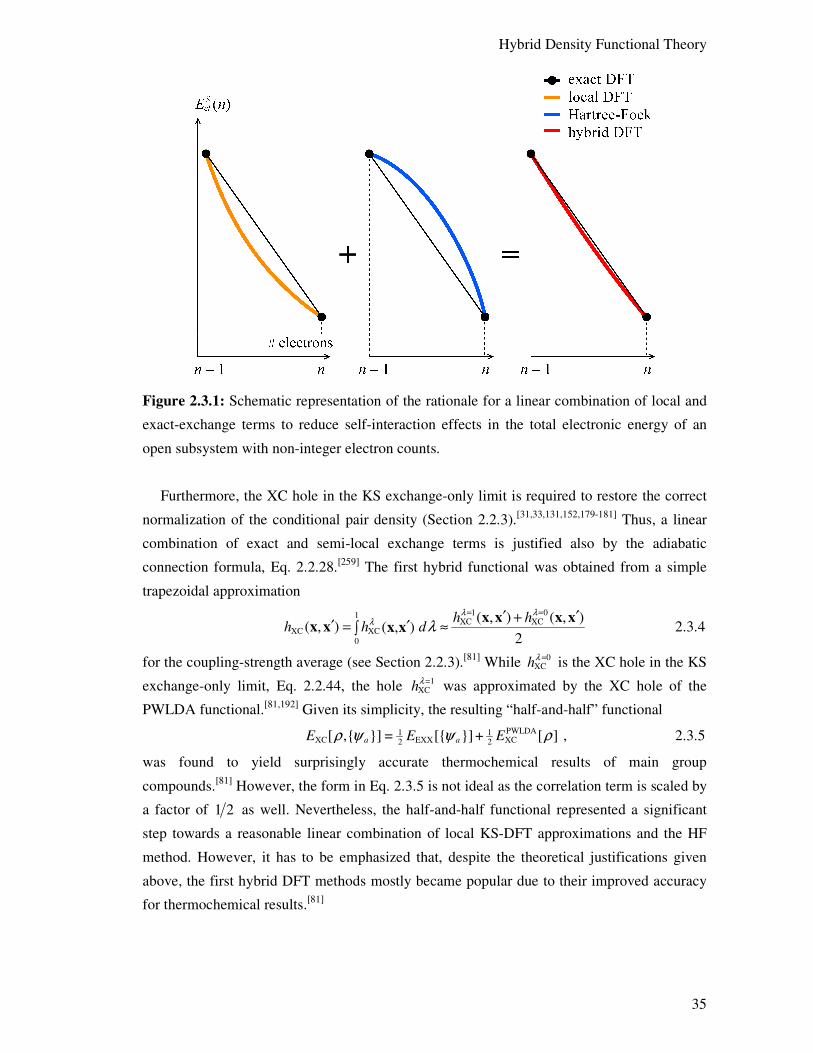
Hybrid Density Functional Theory
35
Figure 2.3.1: Schematic representation of the rationale for a linear combination of local and
exact-exchange terms to reduce self-interaction effects in the total electronic energy of an
open subsystem with non-integer electron counts.
Furthermore, the XC hole in the KS exchange-only limit is required to restore the correct
normalization of the conditional pair density (Section 2.2.3).[31,33,131,152,179-181] Thus, a linear
combination of exact and semi-local exchange terms is justified also by the adiabatic
connection formula, Eq. 2.2.28.[259] The first hybrid functional was obtained from a simple
trapezoidal approximation
1 01
XC XCXC XC
0
( , ) ( , )( , ) ( , )
2
h hh h d
λ λλ λ
= =′ ′+′ ′= ≈∫
x x x xx x x x 2.3.4
for the coupling-strength average (see Section 2.2.3).[81] While =0XChλ is the XC hole in the KS
exchange-only limit, Eq. 2.2.44, the hole =1XChλ was approximated by the XC hole of the
PWLDA functional.[81,192] Given its simplicity, the resulting “half-and-half” functional
PWLDA1 1XC EXX XC2 2[ , ] = [ ] + [ ]a aE E Eρ ψ ψ ρ , 2.3.5
was found to yield surprisingly accurate thermochemical results of main group
compounds.[81] However, the form in Eq. 2.3.5 is not ideal as the correlation term is scaled by
a factor of 1 2 as well. Nevertheless, the half-and-half functional represented a significant
step towards a reasonable linear combination of local KS-DFT approximations and the HF
method. However, it has to be emphasized that, despite the theoretical justifications given
above, the first hybrid DFT methods mostly became popular due to their improved accuracy
for thermochemical results.[81]
Theory
36
2.3.2. Exact-Exchange Potential
Before presenting the various functionals that followed the half-and-half formula, two
approaches for the self-consistent application of orbital-dependent XC approximations shall
be briefly discussed; the optimized effective potential (OEP) and the method of functional
derivatives with respect to KS orbitals (FDO).
The KS formalism requires the XC potential to be local, thus multiplicative. Opposed to
that, the potential resulting from the EXX term is entirely nonlocal. The question how to
obtain a local (multiplicative) potential from an orbital-dependent XC functional is rather
involved. The HF equations are obtained from a variation of the orbitals aφ leading to the
non-multiplicative HF exchange potential whereas the KS formalism requires a local
potential defined as XC XC[ ]V Eδ ρ δρ= . The optimized effective potential method can
provide such a multiplicative EXX potential.[204-206] Thereby, the chain rule for functional
derivatives16
EXX KSOEPEXX
KS
( ) ( )( )
( ) ( ) ( )a
aa
E VV d d
V
δ δψ δδψ δ δρ
′′ ′ ′′ ′= ⋅ ′′ ′
⌠⌠⌡⌡∑ r r
r r rr r r
, 2.3.6
is applied to obtain EXXV , whereas the individual partial derivatives can be expressed in terms
of a perturbative ansatz and response functions.[204-206] The double integral in Eq. 2.3.6
required to evaluate OEPEXXV at a single location r clearly illustrates the complexity of the OEP
method and the effort required to obtain EXX[ ]Eδ ρ δρ . Even in the form of the more efficient
Krieger‒Li‒Iafrate approximation, this approach remains far more expensive than the
computation of the EXX term itself.[206] Furthermore, while providing energetic results
similar to HF, the values HOMO-LUMO gaps obtained with the OEP treatment of the EXX
term are often closer to those of local KS-DFT methods.[223,260,261]
Self-consistent hybrid DFT calculations are mostly conducted in terms of the generalized
Kohn‒Sham (GKS) FDO-type approach.[96,208,262] The GKS formalism extends the orbital
dependent kinetic energy operator of the KS system (see Eq. 2.2.9) by all other orbital
dependent terms of the KS potential.[208] The resulting operator ( 21S 1 EXX2
ˆ ˆO V σα= − ∇ + in the
case of hybrid DFT) is then used in the Levy‒Lieb constrained search approach,[142-145] which
provides another formal justification for orbital dependent XC approximations like hybrid
DFT methods.[208] In a similar fashion the GKS single-particle equations
( ) 2 GKS1 GKS EXX ext Coul XC2
ˆ ˆ( ) ( ) ( )a a a af V V V Vσ σ σψ ψ ε ψ= − ∇ + + + + =x x x 2.3.7
can be derived. Opposed to the EXX potential resulting from the OEP method, EXXVσ in Eq.
2.3.7 is different for each individual KS orbital. Like the HF exchange potential in Eq. 2.1.5,
EXXVσ is defined in terms of its effect on aψ
16 In this notation, ( ) ( )a x b xδ δ ′ denotes the derivative of the functional ( )[ ]a x b with respect to b evaluated at
x′ , hence [ ]( ) ( )a b x b xδ δ ′ in a more explicit notation.
Hybrid Density Functional Theory
37
EXX ˆ ˆ( ) | | ( )a b a b
b
V Wσ ψ ψ ψ ψ= − ⟨ ⟩∑x x . 2.3.8
The local potential terms in Eq. 2.3.7 are again expressed as functional derivatives with
respect to the electron density (Eq. 2.2.16). It needs to be emphasized that the GKS
formalism mostly represents a theoretical justification. Apart from the computation of the
EXX term, the algorithms required for hybrid DFT methods are identical to those of standard
local and semi-local KS-DFT approximations.
2.3.3. Hybrid Density Functionals
The concepts upon which the most important hybrid DFT methods are based shall be
discussed in the following. In this context also the more advanced concepts of range-
separated hybrid and local hybrid DFT approximations are briefly presented.
Starting from the half-and-half functional in Eq. 2.3.5, the hybrid DFT approach was
refined further. The mixing coefficients iα were defined more flexibly and GGA correction
terms were added.[82] Initially these latter corrections were not directly applied to the semi-
local XC terms but merely at the level of the whole hybrid functional.[82] This approach led to
Becke’s B3 formula[82]
B3PW91 LDA B88 LDA PWLDA PW91 PWLDAXC 1 EXX 1 X 2 X X C 2 C C(1 ) ( ) ( )E E E E E E E Eα α α α= + − + − + + − 2.3.9
which is also known as 3-parameter adiabatic connection method (ACM3). The coefficients
in Eq. 2.3.9 were determined from a least-squares fit to experimental data as 1 0.20α = ,
2 0.72α = , and 3 0.81α = .[82] In this way, the ACM3 method acquires an empirical character.
Eq. 2.3.9 was modified by Stephens et al. who substituted the correlation terms in Eq. 2.3.9
by a linear combination of the VWN17 LDA and the LYP GGA functional[47,84,191]
B3LYP LDA B88 LDA VWN LYP VWNXC 1 EXX 1 X 2 X X C 3 C C(1 ) ( ) ( )E E E E E E E Eα α α α= + − + − + + − . 2.3.10
With the mixing coefficients from Eq. 2.3.9, this represents the B3LYP[84] functional which is
the most widely applied DFT method.[263] The popularity of B3LYP originated mostly from
its success when modeling main group compounds.[8,31] On the other hand, significant failures
with regard to transition metals are well known for B3LYP.[198,264] Also in the case of large
organic molecules the performance of the original B3PW91 variant in Eq. 2.3.9 is found to
perform consistently better.[212,265] These failures of B3LYP can be traced back to its LYP
correlation part, which does not exhibit the proper HEG limit.[198,266-270]
The local terms of hybrid DFT variants based on the ACM3 formula originate from linear
combinations of already existing local KS-DFT approximations. Therefore, such terms likely
are not optimal for being employed in nonlocal hybrid DFT expressions. In consequence,
17 A specific parametrization to RPA data was used, which is denoted as VWN3 and different from the more
common VWN5 variant.

Theory
38
subsequent developments focused on local XC terms that are specifically designed to be used
in combination with the EXX term.[85] The hybrid GGA B97
B97 B97 B97XC 1 EXX 1 X C(1 )E E E Eα α= + − + 2.3.11
was one of the first hybrid DFT methods based on this concept.[85] Due to the specific
adaption of its local terms, B97 allowed one to substitute the ACM3 formula by the simpler
single-parameter mixing scheme, ACM1. Thereby, B97 is used with an EXX mixing factor of
~0.19, while the semi-local terms B97XE and B97
CE include nine empirical parameters in total,
which were again adapted to experimental reference data. Other well-known examples of
ACM1 hybrid DFT approximations are the methods M05 und M06 whose semi-local terms
feature even more parameters.[77,89,90,210] M06 and its variants M06-2X and M06-HF include
the parameters 1 0.27,α = 0.54, and 1, respectively; they are based on the same construction
principles as the MGGA functional M06L (Sections 2.2.4 and 2.2.7). Indeed, in this context
M06L appears as a local re-parametrization of M06 under the constraint 1α = 0.[77]
Nevertheless, ACM1-type functionals were proposed from existing semi-local XC terms
as well. While the adaption of the semi-local XC term to the EXX part is neglected, such
approaches can significantly reduce the empiricism of hybrid DFT if based on non-empirical
DFT approximations. Indeed, the hybrid DFT variants of PBE and TPSS, PBEh, 1α =
0.32,[261] and TPSSh, 1α = 0.10,[212], include the EXX mixing factor as the only empirical
parameter.
It is not possible to construct a hybrid DFT functional without an empirically determined
EXX parameter.[271] However, Perdew et al.[83,259] rationalized a specific value for 1α with
the following ansatz for the coupling-strength dependence of the XC energy
( )
( )
11HYB HYB, GGA, GGA 1XC XC XC EXX X
0 0
GGA GGAXC EXX X
(1 )
1 ,
E E d E E E d
E E E
λ λ µλ λ λ
µ
−⌠⌡ = = + − −∫
= + −
2.3.12
where
( )GGA, 2 GGAXC XC[ ] [ ]E E
λ ρ λ ρ λλ∂
=∂
. 2.3.13
This was compared with the polynomial λ-dependence of the XC energy from many-body
perturbation theory (MBPT) of order µ
MP , 10 1 1XCE E E E
µ λ µµλ λ −
−≈ + + +… . 2.3.14
With increasing value of µ the EXX term in Eq. 2.3.12 is reduced in favor of the GGA term.
The order of MBPT which is used as reference for Eq. 2.3.12 has therefore to be as low as
possible to still include a numerically significant EXX term,. On the other hand the MBPT
method itself should still qualify as accurate reference. On the example of the atomization
energies of small main group compounds, Perdew et al. concluded that MP4, hence 4µ = ,
represents the lowest MBPT order able to provide an acceptable description of the XC energy
Hybrid Density Functional Theory
39
as a function of λ . Thus, 4µ = was considered a suitable order for the polynomial coupling
strength dependency in Eq. 2.3.12. In this context 11 4α = can be viewed as slightly less
empirical value for the EXX mixing factor compared in the ACM1 form. In this way, Perdew
et al. were led to suggest[83,259] the ACM0 hybrid DFT variant which was subsequently
employed in form of the PBE0[87] functional
PBE0 PBE PBE31XC EXX X C4 4E E E E= + + . 2.3.15
Nevertheless, the optimum value for 1α still depends on the specific type of the system.
Thus, other strategies are required to obtain further improvements. Range-separated hybrid
DFT (RSH) represents such a mixing strategy.[91-97] RSH approaches are based on the linear
combination of EXX and local DFT at the level of XC holes instead of exchange energy
terms.[91-97] The ratio of local and nonlocal exchange holes thereby depends on the electron-
electron distance | |′−r r . A second alternative consists in a linear combination of exchange
energy densities.[100,102,103,244,272] This leads to a position dependent admixture of EXX to a
semi-local MGGA exchange term, which potentially allows one to satisfy more properties of
the exact XC energy density.[100,271] Both of these alternative hybrid DFT approaches are not
entirely explored yet and combinations in form of a position dependent range separation have
been considered as well.[96,273,274]
40
2.4. The DFT+U Method
In the following the origins of the DFT+U method from the Hubbard model Hamiltonian are
presented. The DFT+U self-interaction correction term is then reformulated to be invariant
under unitary transformations of the KS orbitals. This reformulation is thereby based on
occupation matrices of specific target orbitals onto which the DFT+U self-interaction
correction is applied. The occupation matrices of localized target orbitals are then generalized
to linear combinations of atomic orbitals. This generalization leads to the DFT+Umol method
which was developed and applied in the context of this thesis.
As discussed in Section 2.3.1, hybrid DFT methods are expected to be less affected by the
SIE due to the error cancellation between convex and concave terms of the total energy at
fractional electron numbers (see Figure 2.3.1). Indeed, the nonlocal exchange term of
standard hybrid DFT methods can be considered as a global self-interaction and
delocalization correction which is applied to the entire system. While the SIE often manifests
itself only in specific parts of a system, e.g. an open atomic subshell, hybrid DFT methods
may not provide an optimal description for the other moieties of the system. Thus, the EXX
term may lead to an undesired deterioration of other aspects (see Section 2.2.6).[245]
In contrast, the DFT+U method[60-64,66-69,275] represents a locally confined correction for
the SIE.[65,67,276] The DFT+U framework has its roots in the field of theoretical solid state
physics and was proposed to correct the electronic structure description (and especially the
band gaps) of antiferromagnetic transition metal oxide insulators.[60,277] Prior to DFT+U,
these systems were often described by the empirical Hubbard model Hamiltonian.[278-280]
While the DFT results of such systems are heavily plagued by the delocalization of electrons
within partially filled bands,[60,277] the much simpler Hubbard model was often found to
provide a qualitatively correct description.[278-280] Apart from kinetic energy terms the
Hubbard model only accounts for the Coulomb repulsion between the IN different orbitals
tχ and uχ which both belong to the same atomic subshell I,[278-280]
HubCoul[ ]
2I
tt tt uutt uu
I t t u
JE n n n n nσ σ σ
σ↑ ↓
≠
= +
∑ ∑ ∑∑ . 2.4.1
Thereby, the Coulomb integrals are simplified to only depend on the corresponding orbital
occupation numbers ttn σ and a spherically averaged, subshell specific Coulomb interaction
parameter[60,277,281]
* *2
,
1( ) ( ) ( , ) ( ) ( )I t t u u
I t u I
J W d dN
χ χ χ χ∈
′ ′ ′ ′= ∑ ∫∫ r r r r r r r r . 2.4.2
The Hubbard model can be generalized to include also exchange interactions,[60,277] which are
given analogously to the Coulomb interactions in terms of the occupation numbers and a
spherically averaged exchange interaction parameter IK . The total Hubbard electron-electron
interaction term reads then as

The DFT+U Method
41
Hubee [ ]
2 2I I I
tt tt uutt uu
I t t u
J J KE n n n n nσ σ σ
σ↑ ↓
≠
− = +
∑ ∑ ∑∑ . 2.4.3
Note that the symbols IJ and IK were chosen here to keep the notation consistent with that
of the discussions in the previous sections. Within the DFT+U community the Coulomb and
exchange parameters are usually denoted as IU and IJ , respectively.[60-69]
The DFT+U method originated from the idea to describe the band structure by a KS-DFT
approximation while using the Hubbard model to approximate the electron-electron
interactions missing in this description.[60,61,275,280] In the context of a DFT+U self-interaction
correction the additional Hubbard terms are only applied to specific orthonormal target
orbitals tχ which are most affected by the SIE.[60,61,275] Furthermore, the resulting DFT+U
functional
DFT+U LDA Hub DCee[ , ] = [ ] + [ ] [ ]tt tt ttE n E E n E nσ σ σρ ρ − 2.4.4
includes an additional term DCE to prevent an eventual double counting of the on-site
interactions described by both, LDAE and HubE . While several approximations have been
proposed for DCE ,[68] its so-called fully localized limit (FLL) form represents its most widely
applied variant.[63] The FLL approximation assumes that HubeeE becomes identical to the
electron-electron interactions of the KS-DFT approximation in the case of fully localized
electrons, hence when all occupation numbers assume values of either 0 or 1.[63] With this
assumption Eq. 2.4.3 is used to express DCE after some manipulations as[281]
DCFLL[ ]
2 2I I I
tt tt uu uutt uu
I t tu t
J J KE n n n n n nσ σ σ σ
σ σ↑ ↓
− = + −
∑ ∑ ∑∑ ∑∑ . 2.4.5
When subtracting Eq. 2.4.5 from Eq. 2.4.3 the opposite-spin terms cancel and the factor
I IJ K− can be summarized to a single parameter IU . The residual term
( )U Hub DCee[ ] [ ] [ ]
2Ip
tt tt tt tt tt tt
I t
UE n E n E n n n nσ σ σ σ σ σ
σ
= − = −∑ ∑ 2.4.6
represents the DFT+U correction which is added to the total electronic energy from the
employed KS-DFT approximation (LDA in most early applications)[60,61,275]
DFT+U LDA U[ , ] = [ ] + [ ]ptt ttE n E E nσ σρ ρ . 2.4.7
Thus, the DFT+U energy is a functional in terms of the electron density and the occupation
numbers of the target orbitals
ˆ| | | |tt t t a t a a ta
n fσ χ σ ρ χ σ χ σ ψ ψ χ σ= ⟨ ⟩ = ⟨ ⟩⟨ ⟩∑ , 2.4.8
which are obtained as expectation values of the density matrix operator[126]
ˆ a a a
a
fρ ψ ψ=∑ . 2.4.9
The effective on-site parameter IU can thereby be interpreted as the strength with which the
DFT+U term is applied to the individual corrected subshells I.[60]
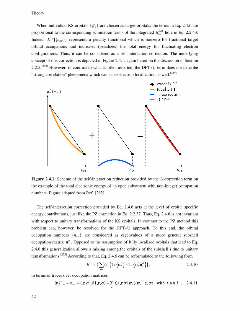
Theory
42
When individual KS orbitals aψ are chosen as target orbitals, the terms in Eq. 2.4.6 are
proportional to the corresponding summation terms of the integrated =0XChλ hole in Eq. 2.2.43.
Indeed, U [ ]pttE n σ represents a penalty functional which is nonzero for fractional target
orbital occupations and increases (penalizes) the total energy for fluctuating electron
configurations. Thus, it can be considered as a self-interaction correction. The underlying
concept of this correction is depicted in Figure 2.4.1; again based on the discussion in Section
2.2.5.[282] However, in contrast to what is often asserted, the DFT+U term does not describe
“strong correlation” phenomena which can cause electron localization as well.[219]
Figure 2.4.1: Scheme of the self-interaction reduction provided by the U-correction term on
the example of the total electronic energy of an open subsystem with non-integer occupation
numbers. Figure adapted from Ref. [282].
The self-interaction correction provided by Eq. 2.4.6 acts at the level of orbital specific
energy contributions, just like the PZ correction in Eq. 2.2.37. Thus, Eq. 2.4.6 is not invariant
with respect to unitary transformations of the KS orbitals. In contrast to the PZ method this
problem can, however, be resolved for the DFT+U approach. To this end, the orbital
occupation numbers ttn σ are considered as eigenvalues of a more general subshell
occupation matrix Iσn . Opposed to the assumption of fully localized orbitals that lead to Eq.
2.4.6 this generalization allows a mixing among the orbitals of the subshell I due to unitary
transformations.[275] According to that, Eq. 2.4.6 can be reformulated to the following form
( )U 12 Tr TrI I I I
I
E U σ σ σ
σ
= −∑ n n n , 2.4.10
in terms of traces over occupation matrices
ˆ | | | | with ,I tu tu t u a t a a ua
n f t u Iσ
σ χ σ ρ χ σ χ σ ψ ψ χ σ= = ⟨ ⟩ = ⟨ ⟩⟨ ⟩ ∈∑n , 2.4.11
The DFT+U Method
43
for individual subshells of target orbitals. This formulation exhibits the desired invariance
property while still retaining the purpose of the DFT+U term as an energy penalty functional
for fractional occupations. Thus, it can be used as correction term to local KS-DFT
functionals as well,
DFT+U KS-DFT UE E E= + . 2.4.12
To apply the DFT+U method in actual calculations the elements of the occupation
matrices in Eq. 2.4.11 need to be expressed in terms of basis functions iϕ . After the
corresponding expansion of aψ and tχ ,
( ) ( ) and ( ) ( ) a i ia t i it
i i
C vσψ ϕ χ ϕ= =∑ ∑x r r r , 2.4.13
Eq. 2.4.11 reads as
* *| |tu it i j a ja ka k l luijkl a
n v f C C vσ σ
σ ϕ ϕ ϕ ϕ= ⟨ ⟩ ⟨ ⟩∑ ∑ . 2.4.14
The overlap and density matrices can be identified in Eq. 2.4.14 as
*| and ij i j ij a ia jaa
S P f C Cσ σ
σϕ ϕ= ⟨ ⟩ = ∑ , 2.4.15
so that the target orbital occupation matrices result to
†I I Iσ σ=n v SP Sv . 2.4.16
Apart from this canonical definition of target orbital occupation matrices alternative variants
like
12 ( ) ,I I I
σ σ σ= +n v SP P S v 2.4.17a
1 2 1 2 , andI I Iσ σ=n v S P S v 2.4.17b
I I Iσ σ=n v P v 2.4.17c
have been rationalized, which resemble the common definitions of orbital occupation
numbers.[66,281]
It needs to be emphasized that in practical applications of the DFT+U method the orbitals
tχ do not exactly correspond to KS orbitals of the system. In fact projectors are used to
apply the self-interaction correction to the individual target orbitals.[60-64,66-69,275] While the
details of these projectors will be discussed in Section 3.2.1, several comments are
appropriate at this point. Selecting it itv δ= , hence projecting onto individual basis functions,
reduces Eq. 2.4.16 to the conventional atomic formulation of DFT+U.[281,283-285] However, the
formulation in Eq. 2.4.16 allows for projectors onto general linear combinations of basis
functions. This formulation provides some further flexibility which is exploited by the
DFT+Umol method to apply the DFT+U correction to fragment molecular orbitals
(FMO).[286,287]
Finally, different options for determining the effective on-site parameter IU shall be
discussed. While Eq. 2.4.2 and the analogous expression for IK are rarely used to compute
I I IU J K= − , this latter parameter is often determined empirically, by adjusting it to

Theory
44
spectroscopic quantities.[288] This strategy makes DFT+U a highly system specific
approach.[288] Alternatively, IU can be defined also in terms of the curvature of KS-DFTE with
respect to fractional occupation numbers, e.g.:
2 KS-DFT
2,
1 ( )II
I tu utt u I
EU
N n n
σ
σ σσ ∈
∂=
∂ ∂∑ ∑ n 2.4.18
The second derivative in Eq. 2.4.18 can be interpreted as the curvature that is required for the
DFT+U correction to restore the linear behavior of the total electronic energy between integer
values of n (Figure 2.4.1). Following this approach, IU can be obtained either in terms of
response properties or from numerical differentiation.[65,275] In any case, the DFT+U method
represents a viable option for studying solid state systems that are heavily affected by the
SIE.[275,277] In recent years, the DFT+U method has been applied to molecular systems as
well.[67,281,283-287]

45
3. Algorithms and Implementation
3.1. Exact-Exchange
3.1.1. Electron-Repulsion Integrals
The following section starts with a brief presentation of density fitting methods that allow one
to avoid the calculation of the four-center electron-repulsion integrals (ERI). As these
integrals cannot be avoided in most applications of hybrid DFT methods, the rest of this
section is dedicated to a detailed discussion of the most important concepts and algorithms
for the calculation of ERIs. This discussion of ERI algorithms is followed by a presentation
of the implementations in PARAGAUSS[70] which were carried out in the context of this thesis.
Within local and semi-local DFT approximations (Section2.2.4), the evaluation of the XC
term requires a computational effort of ( )gNO on a numerical grid of size gN and of 2( )gN NO to obtain the XC potential, Eq. 2.2.19. Thus, the evaluation of the Coulomb term
(Eq. 2.1.10) would dominate such calculations as its computational requirements formally
scale as 4( )NO . However, the Coulomb energy and potential (Eqs. 2.2.13 and 2.2.16) are
explicitly known functionals of the density. The density in turn can be approximated with an
auxiliary basis set mζ of the size18 aN as ( ) ( )
m m mdρ ζ≈ ∑r r .[35-43] In terms of the
approximated electron density the Coulomb potential from Eq. 2.1.10a reads then as[35-43]
( ) ( ) ( )
| |
i j mij kl ijkl m m ijm
kl m m
J P g d d d d gϕ ϕ ζ ′
′= ≈ =′−
⌠⌠⌡⌡
∑ ∑ ∑r r r
r rr r
ɶ . 3.1.1
Thus, the original formal 4( )NO scaling of the computational effort required for the
Coulomb term is reduced to 2( )aN NO .[35-43] This density fitting technique entails a
considerable reduction of the computational costs of local and semi-local DFT
calculations.[264,289] In consequence, this approximation significantly contributed to the
success of local and semi-local KS-DFT approximations.[264] The coefficients md in Eq.
3.1.1 may be obtained by minimizing the difference between the original and the
approximated density in either an overlap or a Coulomb metric.[35-43] The former approach is
known as “resolution of the identity” technique (RI).[35,36,41] Compared to that, the usage of a
Coulomb metric is more accurate for a given auxiliary basis as it directly minimizes the error
of the Coulomb self-energy of the charge density.[37-39,42,43] In the following this latter
technique will be denoted as fitting-function approach (FF or DF-FF).
18 The size aN of the auxiliary basis set usually needs to be larger than that of the orbitals basis N. This can be
understood by considering that the auxiliary basis ζk is required to cover the two-center contributions that appear when expressing Eq. 2.2.10 in terms of orbital basis functions.
Algorithms and Implementation
46
On the other hand, the EXX term as it appears in HF theory and hybrid DFT methods can
not be expressed as a simple density functional. Nevertheless, RI approaches to the exact-
exchange term have been suggested as well.[290] In contrast to the DF-FF representation of the
Coulomb potential, these approaches do not reduce the formal 4( )NO scaling of the EXX
term.[290] Furthermore, such methods mostly provide efficiency gains when systems of
moderate sizes are to be treated with a large basis set.[290]
Thus, the calculation of four-center electron-repulsion integrals19
( ) ( ) ( ) ( )ˆ( | ) |
| |i j k l
ijkl i k j lg ij kl W d dϕ ϕ ϕ ϕ
ϕ ϕ ϕ ϕ′ ′
′= = ⟨ | ⟩ =′−
⌠⌠⌡⌡
r r r rr r
r r , 3.1.2
cannot be avoided in most applications of HF and hybrid DFT methods. As the computation
and processing of ERIs represent the computationally most demanding steps in hybrid DFT
and HF calculations, they were extensively studied and influenced also other algorithmic
parts of quantum chemical calculations. The introduction of contracted Gaussian-type orbitals
(CGTO)
( ) ( )i
i i ii ii m a
i
c Gκ
ϕ ′′′
= −∑r r Aℓ 3.1.3
as elements of a single-electron atomic orbital (AO) basis is an example for such an influence
of the need for an efficient calculation of ERIs.[291-294] CGTOs are represented as linear
combinations of primitive Gaussian orbitals i i im aG ′ℓ (PGTO) with coefficients iic ′ .[291,295-298]
PARAGAUSS[70] employs real solid harmonic CGTO functions (SHCGTO) that consist of iκ
different primitive Gaussian functions (PGTO) with various exponents ia ′
( )2( ) ( ) ( ) expima i m iG N a S a′ ′ ′= −A A Ar r rℓ ℓ ℓ . 3.1.4
All functions of such a contraction are centered at the same nuclear position20 A
( = −Ar r A ). Every SHCGTO function exhibits a solid harmonic prefactor mSℓ and a
normalization factor ( )iN a ′ℓ , whereas ℓ denotes the angular momentum and m ( | | m ≤ ℓ )
the magnetic quantum number.[299-302]
The simplest approach to tackle Eq. 3.1.2 consists in first computing ERIs over PGTO
functions.[291] The final integral results then by a subsequent contraction of the primitive
indices.[291] Indices and factors related to the first spatial variable r are commonly designated
as bra-side ( |ij , while quantities related to ′r are denoted as ket-side | )kl . The ERI ( | )ij kl
over four CGTOs with angular momenta iℓ , jℓ , kℓ , and lℓ , magnetic quantum numbers im ,
jm , km , and lm , and atomic centers A, B, C, and D, respectively, then reads as21
19 A real basis set iϕ is thereby assumed throughout the entire presentation. Furthermore, the notation
( | )ijklg ij kl= will be employed, which is most commonly used in the context of algorithms for ERI calculation.
20 The center of the PGTO was actually allowed to vary slightly in early formulations to represent of Gaussian lobe functions, which nowadays are of purely historical importance only.
21 Using ( | ij k l′ ′ and | )i j kl′ ′ to denote bra and ket half-contracted integrals and | i j k l′ ′ ′ ′ for ERIs over PGTOs.
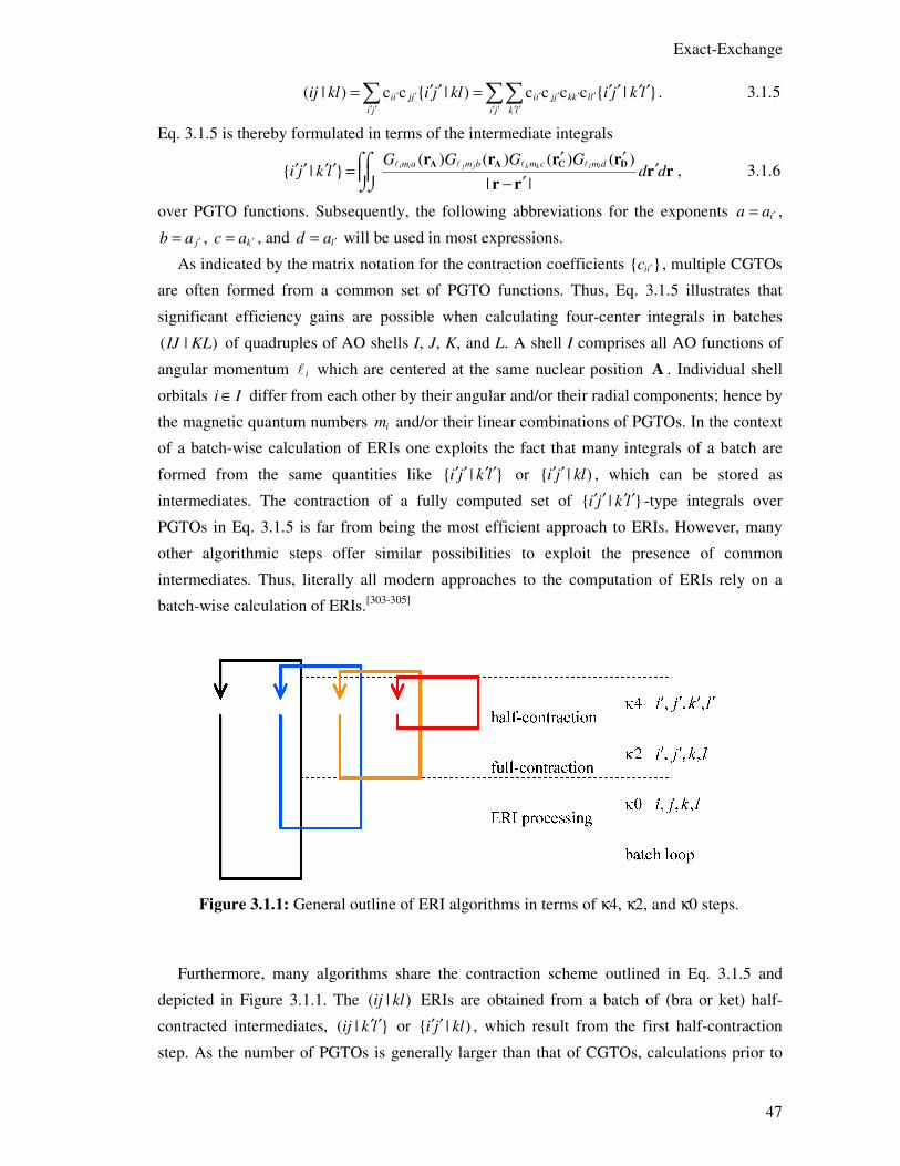
Exact-Exchange
47
( | ) c c | ) c c c c | ii jj ii jj kk ll
i j i j k l
ij kl i j kl i j k l′ ′ ′ ′ ′ ′′ ′ ′ ′ ′ ′
′ ′ ′ ′ ′ ′= =∑ ∑∑ . 3.1.5
Eq. 3.1.5 is thereby formulated in terms of the intermediate integrals
( ) ( ) ( ) ( )
| | |
i i j j k k l lm a m b m c m dG G G Gi j k l d d
′ ′′ ′ ′ ′ ′=
′−⌠⌠⌡⌡
A A C Dr r r rr r
r r
ℓ ℓ ℓ ℓ , 3.1.6
over PGTO functions. Subsequently, the following abbreviations for the exponents ia a ′= ,
jb a ′= , kc a ′= , and ld a ′= will be used in most expressions.
As indicated by the matrix notation for the contraction coefficients iic ′ , multiple CGTOs
are often formed from a common set of PGTO functions. Thus, Eq. 3.1.5 illustrates that
significant efficiency gains are possible when calculating four-center integrals in batches
( | )IJ KL of quadruples of AO shells I, J, K, and L. A shell I comprises all AO functions of
angular momentum iℓ which are centered at the same nuclear position A . Individual shell
orbitals i I∈ differ from each other by their angular and/or their radial components; hence by
the magnetic quantum numbers im and/or their linear combinations of PGTOs. In the context
of a batch-wise calculation of ERIs one exploits the fact that many integrals of a batch are
formed from the same quantities like | i j k l′ ′ ′ ′ or | )i j kl′ ′ , which can be stored as
intermediates. The contraction of a fully computed set of | i j k l′ ′ ′ ′ -type integrals over
PGTOs in Eq. 3.1.5 is far from being the most efficient approach to ERIs. However, many
other algorithmic steps offer similar possibilities to exploit the presence of common
intermediates. Thus, literally all modern approaches to the computation of ERIs rely on a
batch-wise calculation of ERIs.[303-305]
Figure 3.1.1: General outline of ERI algorithms in terms of κ4, κ2, and κ0 steps.
Furthermore, many algorithms share the contraction scheme outlined in Eq. 3.1.5 and
depicted in Figure 3.1.1. The ( | )ij kl ERIs are obtained from a batch of (bra or ket) half-
contracted intermediates, ( | ij k l′ ′ or | )i j kl′ ′ , which result from the first half-contraction
step. As the number of PGTOs is generally larger than that of CGTOs, calculations prior to

Algorithms and Implementation
48
the first half-contraction step on primitive intermediates are most expensive. These
algorithmic parts are denoted as κ4 steps and are followed by the less expensive κ2
operations on half-contracted quantities. Finally, the mostly inexpensive κ0 steps are entirely
formulated in terms of fully contracted quantities and only followed by the subsequent
processing of four-center integrals. Figure 3.1.1 depicts the general loop structure of these κ4,
κ2, and κ0 steps.
ERIs over four s-type PGTO functions represent the most simple case of Eq. 3.1.5 and are
denoted as | ss ss . The Gaussian product rule states that the multiplication of two Gaussian
functions results in another Gaussian function.[2,4] This product distribution exhibits the
exponent p a b= + , is centered at the exponent-weighted average position ( )a b p= +P A B
on the line segment connecting the centers of the two initial Gaussians and scaled by the
overlap between them,
( ) ( ) ( ) ( )22 2 2exp exp exp ( ) exp a b ab p p− − = − −A B Pr r AB r . 3.1.7
The uncontracted | ss ss -type integral results from using Eq. 3.1.4 in Eq. 3.1.6 with
( )3 40 00( ) ( ) 2N a S a π=Ar and the analogously defined other three PGTO prefactors. Applying
the Gaussian product rule of Eq. 3.1.7 as well as the following Laplace-like transformation of
the Coulomb operator
( )2 2
0
1 2exp | |
| |u du
π
∞
′= − −′− ∫ r r
r r 3.1.8
in Eq. 3.1.6 yields after several manipulations[4,291,305]
( ) ( ) ( )12 2 2 2
00 00 00 000
| exp ( ) exp ( ) exp a b c dG G G G Z ab p cd q u duγ= ⋅ − − −⌠⌡
AB CD PQ . 3.1.9
The variables q and Q are defined analogously to p and P, respectively. Furthermore, the
intermediates
3 416 ( )
and pq abcd
Zp q pq p q
γπ
= =+ +
3.1.10
are introduced. The integral in Eq. 3.1.9 is an example of the Boys function, which, for
reasons discussed below, is generalized to an arbitrary order M (with 0M ≥ )[4,291]
( )1
2 2
0
( ) expMMF x u xu du= −∫ . 3.1.11
The Mth-order Boys functions ( )MF x are related to the error function, the incomplete gamma
function, and other special functions.[4,291,306]
Subsequently, the final batch of ( | )ss ss integrals can be formed according to Eq. 3.1.5
from the | i j k l′ ′ ′ ′ ERIs for all quadruples of primitive exponents. The ERI in Eq. 3.1.6 has
thus been reduced to a much simpler one-dimensional integral over the finite interval [0,1] .
Having established a method to obtain ERIs over four s-type centers, this algorithm can be
generalized to the calculation of integral-classes over AOs of higher angular momenta like
Exact-Exchange
49
( | )ps ps , ( | )fd dp , … . In contrast to ( | )ss ss -type integrals, such ERIs include integrands
with angular degrees of freedom, hence 0>ℓ . Using the identity = +A Pr r PA and
expanding polynomial products of the form ( ) ( )r ri jr rr rr P PA r P PB− + − + allows one to
obtain the corresponding ERI formulae for general PGTOs from a derivation analogous to
that of Eq. 3.1.9.[307] Nevertheless, with growing angular momentum ℓ the resulting
expressions quickly become much more involved than Eq. 3.1.9.
PGTOs have the very useful property that their angular prefactors can be obtained from a
parameter differentiation with respect to their nuclear centers.[2,4] For a pz-type primitive AO
this concept is illustrated as follows:
( ) ( )2 2
10
10 00
1( ) ( ) exp ( ) exp ( )
2
1 | |
2
i
i i
a z i i
i z
a a
i z
G z A a aa A
G j k l G j k la A
′
′ ′
′ ′′
′
∂∝ − − − = − −
∂∂
′ ′ ′ ′ ′ ′⇒ ∝∂
Ar r A r A
3.1.12
When applied to Eq. 3.1.9 for general ERI classes of higher angular momenta, a repetitive
differentiation of both overlap and integral factors is required. Furthermore, cross-terms arise
for 1>ℓ or non-zero angular momenta on different centers so an explicit parameter
differentiation quickly becomes rather cumbersome that in such cases. General real solid
spherical harmonic angular GTO prefactors can be obtained from parameter differentiation as
well.[301,302,308-311] Such approaches are based on the application of the spherical harmonic
tensor gradient theory, which is formulated in terms polynomial differential operators of the
form ( )i imS ∇Aℓ .[301,302,308-311] Different rules are known for the coupling of angular momenta
and the application of spherical harmonic tensors which can be employed to compute ERIs
over SHCGTOs.[301,302,308-314]
However, most ERI algorithms do not directly compute integrals over SHCGTOs, but first
evaluate integrals over contracted Gaussian orbitals with Cartesian angular prefactors
(CCGTO)
( )2( ) ( ) ( )( ) ( ) ( ) expi i
yx z
i
ii ii ii a ii i x y z i
i i
c G c N a x A y A z A aκ κ
ϕ ′′ ′ ′ ′′ ′
= = − − − −∑ ∑i A i Ar r rɶ 3.1.13
with ( , , )x y zi i i=i and 0 , x y z x y z ii i i i i i≤ ≤ ≤ + + = ℓ . The resulting integrals are subsequently
transformed from the CCGTO to the SHCGTO basis.[315] Integrals over Cartesian GTOs will
be denoted as [ | ]ij kl in the following. For a given angular momentum ℓ , the magnetic
quantum number m varies from −ℓ to ℓ which results in 2 1+ℓ different functions mSℓ . In
contrast, the corresponding set of Cartesian prefactors includes ( 2)( 1) 2+ +ℓ ℓ elements and
thus, is larger than the number of spherical harmonic functions for 1>ℓ . The additional
Cartesian prefactors with 1>ℓ result in form of lower angular momentum functions; for
example 2Ar in the case of d-orbitals, 2( )rr A− Ar for f-type shells, and so on. Furthermore, the
repetitive differentiation of the PGTOs with respect to the nuclear coordinates
Algorithms and Implementation
50
( )
( )
2
2
( ) ( ) ( ) exp
( ) exp
i
yx z
a i i i i
ii i
i i
x y z
G N a a h a a
N a aA A A
′ ′ ′ ′ ′
′ ′
= −
∂ ∂ ∂ = − ∂ ∂ ∂
i A i i A A
i A
r r r
r
ɶɶ ɶ
ɶ 3.1.14
does not directly generate the Cartesian prefactors but rather yields angular components in
terms of Hermite polynomials h iɶ . Integrals over Hermite polynomials may either be
converted to the [ | ]ij kl batch or directly transformed to the SHCGTO basis.[316]
Despite their larger number for 1>ℓ and the need to convert the Hermite polynomials,
Cartesian prefactors allow for more transparent expressions which resulted in the
development of powerful and versatile recursion relations.[303] Corresponding recursion
techniques for ERIs over spherical harmonic PGTOs have been suggested as well, but are
either far more involved or less well applicable.[317] The recursion relations for ERIs over
Cartesian GTOs will be discussed after presenting the techniques for the computation of the
Boys functions.
Differentiating the integral factor in Eq. 3.1.9, hence the zero-order Boys function, with
respect to 2
x γ= PQ directly leads to the aforementioned Boys functions of order M,
( )1
0 2 2
0
( )( 1) exp ( 1) ( )
MM M M
MM
F xu xu du F x
x
∂= − − = −
∂ ∫ . 3.1.15
It can be shown that any ERI over PGTOs can be expressed as a linear combination of Boys
functions up to order tot i j k l= + + +ℓ ℓ ℓ ℓ ℓ ,
tot 2
0
| ( )M M
M
i j k l Z F γ=
′ ′ ′ ′ = Ω∑ PQℓ
, 3.1.16
whereas the coefficients MΩ denote complicated functions of ℓ , m , ia ′ , and A of all four
PGTOs, respectively.[307,318] Thus, ERIs over GTOs with nonzero angular momenta require
the calculation of the entire series of Boys functions from 0F to tot
Fℓ .
At 0x = the exponential factor of the integrand in Eq. 3.1.15 equals one. In consequence,
the remaining monomial integrates to
( )1
2
0
(0) 1 2 1MMF u du M= = +∫ . 3.1.17
In combination with 1( ) ( )M MF x x F x+∂ ∂ = − this allows for a Taylor-series expansion
( )
( )! (2 2 1)
i
M
i
xF x
i M i
∞ −=
+ +∑ 3.1.18
around 0x = . While this series is always convergent,[4] several hundred terms may be
required to compute ( )MF x from Eq. 3.1.18 with a sufficiently high accuracy.22 However, the
convergence of the series can be significantly improved if pre-tabulated ( )MF x values on a
regular grid tx x= are used,[4,318-320]
22 For the FORTRAN double precision floating point data type of 64 bit length this implies a relative precision
of 10‒16.
Exact-Exchange
51
0
( )( )( )
!
t iMM i t t
M
i
F x x xF x
i
+
=
−=∑ . 3.1.19
If x lies in between (sufficiently close) grid points, the Taylor expansion from the nearest grid
point converges after a few terms only.[4] Having obtained the value of tot
( )F xℓ , the Boys
functions of lower orders are computed in terms of the following “downward” recursion
12 ( ) exp( )( )
2 1M
M
x F x xF x
M
+⋅ + −=
+. 3.1.20
If the Boys functions are tabulated over a sufficiently large interval of x, the expression
1 2 1
(2 1)!!( ) , 1
2M M M
MF x x
x
π+ +
−≈ ≫ 3.1.21
can be used to compute ( )MF x for x values beyond the extent of the grid. In this case it may
be sufficient to use Eq. 3.1.21 to compute 0 ( )F x only. All other ( )MF x values can then be
obtained from the “upward” recursion formula
1(2 1) ( ) exp( )
( )2
MM
M F x xF x
x+
+ ⋅ − −= , 3.1.22
which becomes stable at sufficiently large values of x. The Boys functions MF of orders
0, , i j k lM = + + +… ℓ ℓ ℓ ℓ can then be converted into the derivatives of 0F with respect to the
distance between the product centers P and Q
2 2 22
02( ) ( ) ( 2 ) ( )
M
MMZ F Z Fγ γ γ γ
∂Γ = = − ∂
0 PQ PQ PQPQ
. 3.1.23
The use of recursion relations became popular with the approach of McMurchie and
Davidson (MD) to four-center integrals.[319] Indeed, the MD method was the first ERI
algorithm which was equally efficient for various ERI classes, over CGTOs with large
contraction length iκ as well as over CGTOs with higher angular momenta.[319] The MD
algorithm is based on the idea to generate higher angular momentum functions via derivatives
with respect to the centers P and Q,
2
0
2 200
( )
( 1) ( ) ( 1) ( ) .
y yx z x z
y yx z x z
y yx x z z
x y z x y z
y yx x z z
p qp p q q
p qp p q qx z x zy y
p qp q p qq q q q q q
p qp q p qx zy
Z FP P Q QP Q
Z FP PP
γ
γ γ++ +
+ + + ++++ +
∂ ∂ ∂ ∂ ∂ ∂∂ ∂ ∂ ∂∂ ∂
∂ ∂ ∂= − = − Γ
∂ ∂∂p q
PQ
PQ PQ
3.1.24
In this context it is common to define ( , , )x y zp p p=p , ( , , )x y zq q q=q , x x xp i j= + ,
x x xq j l= + , and so on. The first-order derivative with respect to a single Cartesian
component , ,r x y z= of P yields
2
2 20 20 2( ) ( 2 ) ( )M
r r
FF F
P Pγ γ γ
∂ ∂ ∂ = = − ∂ ∂ ∂
PQPQ PQ PQ
PQ, 3.1.25
whereas the partial derivative on the right hand side of Eq. 3.1.25 is provided by Eq. 3.1.23.
From the commutative behavior of the derivative operator

Algorithms and Implementation
52
1r r rp p p
rr r
r r r
PQ p PQP P P
−∂ ∂ ∂
= + ∂ ∂ ∂ , 3.1.26
the intermediates Γ in Eq. 3.1.24 are found to behave according to
2 2 21 1( ) ( ) ( )
r z
M M Mrr
PQ pγ γ γ+ ++ + + + −Γ = ⋅Γ + ⋅Γp q 1 p q p q 1PQ PQ PQ . 3.1.27
With 2
( )M γΓ0 PQ given by Eq. 3.1.23 this defines a recursion relation for Eq. 3.1.24 which
relates the order M of the Boys function to Hermite polynomials of varying degree. Thus,
Eqs. 3.1.24 to 3.1.27 lead to integrals over Gaussian product distributions with Hermite
polynomial prefactors, centered at P and Q, respectively.
These intermediates may be coupled with the Hermite functions that originate from the
differentiation of the overlap factors,23
2 2
0
2 20
0
exp ( )
exp ( ) .
r
r
rr
r r r
i
ir
t i tir
i t
r rt
abZ F
A p
ab PZ
A p A
γ
γ−
−=
∂− ∂
∂ ∂ = − Γ ∂ ∂ ∑ 1 1
AB PQ
AB PQ
3.1.28
The resulting integrals over GTOs with Hermite prefactors ( )hi Arɶ can then be converted into
integrals over ( )iaG ′i Ar . Originally, MD proposed an alternative approach to convert the 0
+Γp q
intermediates to the final ERIs.[319] Their approach consists in a direct transfer of angular
momentum from the Hermite product distributions to the Cartesian AO functions.[319] This
approach is understood best in terms of product distributions with combined Cartesian atom-
centered and product-centered Hermite angular components,
( ) ( )2 2 1 2
, ,
exp ( ) ( ) ( ) ( )r r r
r
i j pr r p r
r x y z
P r A r B p h p r P=
= − − − ⋅ − ⋅ −∏pij x P ɶɶ . 3.1.29
The results of the recursion in Eq. 3.1.27, hence the uncontracted ERIs over product
distributions with Hermite polynomial prefactors can then be rewritten as follows
20[ | ] ( 1) ( )x y zq q q
P Q γ+ ++= − Γp q
p q00 00 PQɶɶ . 3.1.30
After adding and subtracting rP in one of the ( )rr A− factors in Eq. 3.1.29 according to
1 1( ) ( )( ) ( )( )i r ru i ir r r r r rr A r P r A P A r A
− −− = − − + − − 3.1.31
and using the Hermite recursion formula
1 2 2 1 2 1 2 1 211 12( ) ( ) ( ) ( )r
r r r
pp r p pp r p h p r p h p r h p r− +⋅ = ⋅ +ɶ ɶ ɶ , 3.1.32
one obtains the recursive MD transfer relation[319]
, , ,
1( )
2r r
r r rr r rP p P P A P Pp
− +− − −= ⋅ + − +p p 1 p p 1
ij i 1 j i 1 j i 1 jɶ ɶ ɶ ɶ . 3.1.33
Eq. 3.1.33 and its analogues for the other Cartesian components and product centers include
only quantities over which ERIs were established above. Thus, one can equally well write
23 Note, that upon successive application of xB∂ ∂ to Eq. 3.1.28 various cross-terms have to be considered and
that the factor ( 1)u v w′ ′ ′+ +− needs to be included in the derivatives with respect to xC and xD .
Exact-Exchange
53
,
1[ | ] [ | ] [ | ] [ | ]
2r r
rrrP Q = p P Q + PA P Q P Q
p
− ++ ⋅ ⋅ +p q p 1 q p q p 1 q
kl kl kl klij ij iji 1 jɶ ɶ ɶ ɶɶ ɶ ɶ ɶ , 3.1.34a
,
1[ | ] [ | ] [ | ] [ | ]
2r r
r r rP Q = q P Q +QC P Q P Q
q
− ++ ⋅ ⋅ +p q p q 1 p q p q 1
kl kl klij ij ij ijk 1 lɶ ɶ ɶ ɶɶ ɶ ɶ ɶ , 3.1.34b
and obtain the final uncontracted integrals over Cartesian PGTOs as
[ | ] [ | ]P Q= 0 0ij klij kl ɶɶ . 3.1.35
Equivalent MD algorithms result when Eqs. 3.1.34 are reformulated as matrix multiplications
or by expanding Eq. 3.1.28 and subsequently transforming the resulting integrals.[4,316]
Recursion relations are not restricted to Hermite functions only. From combining the
parameter differentiation with the translational invariance property,
( )+ + + [ | ] =∇ ∇ ∇ ∇A B C D ij kl 0 , 3.1.36
Obara‒Saika[321,322] (OS) and others[323,324] discovered a recursion relation which provides a
direct transformation of the 2
[ | ] ( )M M α= Γ000 00 PQ intermediates into 0[ | ] [ | ]=ij kl ij kl
integrals,[303]
1
1
1
1 1
1[ , | ] [ | ] [ | ]
2
1[ , | ] [ , | ]
2 2
1[ , | ] [ , | ]
2 2
1 .[ | , ] [ | ]
4
M M Mrr r
r M Mr r
r M Mr r
M Mr x r x
PA PQp
i
p p
j
p p
k lpq
+
+
+
+ +
+ = +
+ − − −
+ − − −
+ − + −
i 1 j kl ij kl ij kl
i 1 j kl i 1 j kl
i j 1 kl i j 1 kl
ij k 1 l ij kl 1
3.1.37
Based on the MD and OS approaches a large number of variations were developed in the
following.[303,325-333] From using identities like ( ) ( ) ( )x x x xx B x A A B− = − + − inside the
electron repulsion integrals, another important connection can be established
[ , | ] [ , | ] +[ , | ]rr rAB+ = +i j 1 kl i j kl i 1 j kl , 3.1.38
which is known as horizontal recursion relation (HRR).[325] The horizontal recursion relation
effectively transfers angular momentum between the two bra-side centers (likewise for the
ket side).[325,334,335] Thus, Eq. 3.1.38 allows one to reduce the generation of angular momenta
to intermediate [ | ]e0 f0 -type classes. These intermediate classes include all integrals over
Cartesian GTOs with angular momenta ranging from e i=ℓ ℓ to i j+ℓ ℓ and, likewise,
, ,f k k l= +ℓ ℓ … ℓ ℓ . The number efN of such intermediates is at most equal than the size ijklN
of the final [ | ]ij kl class, as shown here for the bra side
( )( 1)( 2)( 3) ( 1)( 2) 6
( 1)( 2)( 1)( 2) 4 .
i j i j i j i i i
i i k k
+ + + + + + − + +
≤ + + + +
ℓ ℓ ℓ ℓ ℓ ℓ ℓ ℓ ℓ
ℓ ℓ ℓ ℓ 3.1.39
The HRR in Eq. 3.1.38 itself does not provide any significant benefit because a similar
number of elements needs to be processed to obtain the final [ | ]ij kl class of integrals as
during a direct generation of ERIs. The great advantage of the horizontal recursion relation

Algorithms and Implementation
54
derives from the fact that Eq. 3.1.38 does not comprise any primitive-related quantities (like
exponents or product center coordinates) and thus applies to fully contracted integral classes
as well. A significant amount of computational labor can thereby be shifted from the κ4 stage
to the κ2 and κ0 stages. Following this “earlier contraction” strategy, Head-Gordon‒Pople
(HGP) used the five-term variant of the OS recursion, Eq. 3.1.37, termed vertical recursion
relation (VRR) that results for ERI classes with = =j l 0 .[325] The VRR can be used to obtain
the intermediates [ | ]e0 f0 , which are subsequently contracted and then transformed into
integrals over CCGTOs by means of the HRR.[325] The MD algorithm benefits from the HRR
as well. Only uncontracted [ | ]e0 f0 classes have to be computed from Eq. 3.1.34, which
significantly simplifies the MD transfer step in Eq. 3.1.33.
The concept of early contraction can be extended even further.[303,326,327] In this context
one employs identities like
2
2
b
p=PA BA 3.1.40
and “pre-scaled” variants of the combined Hermite-Cartesian distributions from Eq. 3.1.29,
(2 )
(2 )
uuv
u v
bP P
p+
=p pij ijɶ ɶ . 3.1.41
The intermediates u vQ
′ ′qklɶ are analogously defined for the ket-side. When using Eqs. 3.1.40 and
3.1.41, the MD transfer relation can be reformulated as follows[303,326,327]
, 1, , 1,[ | ] [ | ] [ | ] [ | ]r r
r
uv u v uv u v u v u v u v u vrrP Q = p P Q + BA P Q P Q
′ ′ ′ ′ ′ ′ ′ ′− + + ++ ⋅ ⋅ +p q p 1 q p q p 1 q
kl kl kl klij ij iji 1 jɶ ɶ ɶ ɶɶ ɶ ɶ ɶ . 3.1.42
Apart from the integrals over the pre-scaled distributions from Eq. 3.1.41, this reformulation
is free from any quantities that depend on the primitive indices.[303,326,327] Thus, Eq. 3.1.42
applies to contracted [ | ]uv u vP Q′ ′p q
klijɶɶ integrals as well, just as the HRR. Indeed, the contracted
variant of Eq. 3.1.42 provides efficiency gains for batches with large contraction ratios, hence
the ratio between the number of CGTOs and PGTOs.[303,326,327] The identity
2 2
2 2
b d
p q= + −PQ AC BA DC 3.1.43
allows one to apply the early contraction concept to the HGP or OS equations, Eq. 3.1.37,
and even to the generation of Hermite Coulomb integrals in Eq. 3.1.27. Furthermore, the
electron transfer relation[328]
(
)[ | , ] [ , | ] [ | , ] 2 [ , | ]
2 [ | ] 2 [ | ] 2
r r r r r r
r r
e f p
b AB d CD q
+ = − + − − +
− ⋅ ⋅ + ⋅ ⋅
e0 f 1 0 e 1 0 f0 e0 f 1 0 e 1 0 f0
e0 f0 e0 f0 3.1.44
represents an additional recursion relation which, in its contracted variant, can occasionally
provide further computational savings.[303] Eq. 3.1.44 allows one to shift angular momentum
between bra and ket sides and emerges from Eq. 3.1.36 as well.[303,328] The algorithms
resulting from Eq. 3.1.43 permit one to carry out the contraction steps already at the stage of
derivatives of pre-scaled Boys functions
Exact-Exchange
55
2(2 ) (2 )
[ ] ( )(2 ) (2 )
u uM M
uv u v u v u v
b d
p qγ
′
′ ′ ′ ′+ += Γ00 PQ , 3.1.45
which are obtained directly from Eq. 3.1.23 and defined analogously to the pre-scaled
Hermite-Cartesian product distributions in Eq. 3.1.41.[327,330] However, as such early
contraction strategies can significantly increase the operation count at the κ0 step for larger ℓ
values, they may not always represent the optimal choice for a specific ERI class.[303] For a
given ERI batch selecting the optimal sequence of transformation and contraction steps out of
several different algorithmic pathways represents the key idea of the PRISM
algorithm.[303,326,327,329,331,333] Alternative MD based pre-scaling methods exist.[332]
In a similar fashion, computational workload can be shifted from the κ4 to the κ0 stage by
applying a rotation to the coordinates of the atomic centers, which is the key concept of the
Pople‒Hehre algorithm (PH).[336] The rotations are defined in such a way that many Cartesian
components of the distance vectors between the centers ( AB , PA , etc.) vanish, which
simplifies the recursions over uncontracted intermediates.[336] The number of κ0 operations is
increased though, as the corresponding inverse rotations need to be applied to the contracted
integrals.[336] Therefore, the original PH approach was limited to s and p-type CGTOs.[336]
Recently, more flexible combinations of PH-type rotations with the MD and PRISM
algorithms were proposed as well.[333,337]
block inc
block inc
block inc
block inc
beg block inc end block inc inc
FOR 0, INCREMENT
FOR 0, INCREMENT
FOR 0, INCREMENT
FOR 0, INCREMENT
1;
i
j
k
l
i = i
j = j
k = k
l = l
i i i i = i i i
κκ
κκ
′
′
′
′
′ ′ ′ ′= ⋅ + ⋅ +
beg
beg end beg end beg end beg end
COMPUTE [ | ]( : , : , : , : )
CONTRACT [ | ]
END
j
i i j j k k l l
′ =
′ ′ ′ ′ ′ ′ ′ ′e0 q
e0 q
…
⋯
Scheme 3.1.1: Block reformulation of the loops in the κ4 steps. The ranges beg end:i i′ ′ ,
beg end:j j′ ′ , beg end:k k′ ′ , and beg end:l l′ ′ denote the four fastest running array axes.
Apart from algorithmic reductions of the floating point operation (FLOP) counts, another
essential factor has to be considered for an efficient ERI computation.[338] Modern CPU
architectures are able to carry out an enormous number of FLOPs per second but exhibit only
a comparatively limited bandwidth to the main memory.[338] This mismatch is partially
resolved by a hierarchical structure of intermediate cache storages of successively higher
Algorithms and Implementation
56
bandwidth but decreasing size.[338] To use such architectures efficiently, as many operations
as possible have to be carried out on small data arrays whose sizes fit into the available cache
storages.[338] In the case of the most expensive κ4 steps of ERI algorithms, this implies
processing the primitive axes in blocks as shown in Scheme 3.1.1. For high angular momenta
the uncontracted intermediates have rather large pre-scaling index axes, which only admit for
short loops24 over the primitive quadruples or may not even fit at all into the low-level cache
storages.
This problem is less severe for Gauss-quadrature based algorithms, which represent
another important approach to ERIs.[339,340] The key concept of such methods is to carry out
the parameter differentiation before the one-dimensional integration in Eq. 3.1.9. To this end,
Eq. 3.1.16 is reformulated as
( )tot tot1
2 2 2 2
0 00
| ( ) exp MM M M
M M
i j k l Z F Z u u duγ γ= =
′ ′ ′ ′ = Ω = − Ω
⌠⌡
∑ ∑PQ PQℓ ℓ
. 3.1.46
Most important is the presence of the polynomial factor in terms the variable u on the right-
hand side of Eq. 3.1.46. According to the Gauss-quadrature formula, such polynomials
2 ( )M uℑ up to a degree m can be exactly integrated to
2 2( ) ( ) ( ) u m
M M t t
tu
u u du u wω′
′−
ℑ = ℑ∑∫ , 3.1.47
for a specific weighting function ( )uω and over a given interval [ , ]u u′ ′− . Here, tu and tw
are the roots and weights of the t-th member of the class of polynomials which are, for the
given weighting function ( )uω , orthogonal over the interval [ , ]u u′ ′− . In the case of
( )2 2( ) = expu uω γ− PQ 3.1.48
and = 1u′ this leads to the class of Rys polynomials whose roots and weights are determined
by the value of 2
γ PQ .[340,341]
While different Rys polynomials have to be computed for every quadruple of PGTOs,
most algorithmic parts of Gauss-quadrature based ERI algorithms exhibit a very favorable
scaling of operations with respect to the angular momenta.[340,341] This efficiency partially
results from 2 1m M= + , as the polynomials 2 ( )M uℑ are of even order, thus need to be
integrated over the interval [0,1] only.[340] The techniques for the calculation of the values for
tu and tw are significantly more involved but still resemble those used for the computation
of the Boys functions.[341-345] Yet, the main advantage of Gauss-quadrature based algorithms
consists in the fact that the polynomial 2 ( )M uℑ in Eq. 3.1.46 factorizes into its Cartesian
components
24 Note that long loops over fast running indices are still important for modern CPU architectures because their
large computing power partially results from an efficient hardware vectorization (pipelining).
Exact-Exchange
57
( )
1 2 2
0[ | ] exp ( , ) ( , ) ( , )
( , ) ( , ) ( , ) .
x x x x x y y y y y y z z z z
m
x x x x x t y y y y y t y z z z z t t
t
Z u i j k l u i j k l u i j k l u du
Z i j k l u i j k l u i j k l u w
γ= − ℑ ℑ ℑ
= ℑ ℑ ℑ
⌠⌡
∑
ij kl PQ
3.1.49
The two-dimensional integrals ( , )r r r r r ti j k l uℑ can be obtained from suitably adapted variants
of the MD or OS recursion relations, Eqs. 3.1.27, 3.1.34, and 3.1.37.[346] When combined
with the HRR, only quantities of the size25 3tot( )ℓO need to be computed before the assembly
of the six-dimensional [ | ]e0 f0 integrals, hence from a correspondingly adapted variant of Eq.
3.1.49. This is to be compared with the quantities which appear in the HGP or HRR+MD
approaches and whose numbers scale with 6tot( )ℓO at least. Even the very early contraction
algorithms have to deal with the pre-scaled Boys functions [ ]Muv u v′ ′0 , which scale as 5
tot( )ℓO .
Due to the small number of the intermediates rℑ , implementations of Gauss-quadrature
based ERI algorithms[339,340,346-348] can efficiently exploit cache memory[349] and are even
suitable for applications on general purpose graphic processing units.[350-352] However, it is a
general drawback of such algorithms that the ERI contraction step can not be carried out prior
to the assembly of the six-dimensional integrals in Eq. 3.1.49. Partial ameliorations of this
disadvantage have been proposed by combining Gauss-quadrature approaches to ERIs with
ideas from early contraction algorithms.[353] Nevertheless, compared to MD or OS, Gaussian-
quadrature methods perform best for basis sets with high angular momenta and low
contraction ratios as well as for ERI-derivatives (see Section 3.1.4).[349,354]
As their performance varies for batches with different contraction ratios, early contraction
and Gaussian-quadrature based algorithms are often implemented together in DFT
packages.[355] A specific algorithm is then selected according to the characteristics of the ERI
batch at hand (angular momenta, contraction ratios) to achieve an optimal performance. In
this context both types of algorithms complement each other with regard their performance
for different classes of ERI batches. However, methods that are able to efficiently compute
ERIs also in the case of highly contracted GTOs of high angular moments are still desirable.
Various algorithms with such capabilities have been derived by means of computer algebra
systems or implemented with metaprogramming approaches.[318,333,356-359] The most wide-
spread example for an ERI algorithm formulation is the accompanying coordinate expansion
(ACE), which, despite of being based on the Boys function, was originally derived from an
explicit expansion of the two-dimensional rℑ integrals.[314,318,360-366] Similar to the PRISM
algorithm, the ACE method exhibits different expansion paths, which exhibit very low
operation counts in the limit of high angular momenta or large contraction ratios,
respectively.[318] In the context of this thesis the ACE method has been extensively studied.
25 When comparing the amount of data and operations involved in different ERI algorithms, one commonly
assumes integral classes of the type ( | )ss ss , ( | )pp pp , ( | )dd dd , etc., thus i j k l= = =ℓ ℓ ℓ ℓ . Identical considerations in terms of more general classes can be made but are more cumbersome and unlikely to provide any further insights.
Algorithms and Implementation
58
However, as the definition of many relations between intermediate quantities remains unclear
in the literature, this method was found to be exceptionally cumbersome to implement
efficiently without the original computer algebra derivation at hand.
The rest of this section discusses the ERI implementations carried out as part of this thesis.
In this context it has been found useful to implement the calculation of ERI batches
separately from their subsequent treatment (see Sections 3.1.2 and 3.1.3). Thus, the modules
that perform the calculation of ERIs are only supposed to deliver the final ( | )IJ KL batch of
contracted ERIs. This separation allows one to employ a simpler parallelization concept (see
Section 3.1.5) and enables one to switch easily between different ERI implementations.
An early reference implementation was available as an extension of existing PARAGAUSS
modules. This implementation is based on the spherical harmonic tensor gradient approach,
which is also used to compute the three-center integrals required for calculating the Coulomb
repulsion matrix term within the DF-FF approximation, Eq. 3.1.1. However, without
significant algorithmic changes, this early implementation performs most of the
computational work within the κ4 steps. In consequence, this implementation imposed large
memory demands and was found to be not efficient enough for routine calculations.
Thus, a complete re-implementation of the ERI calculation was carried out in the form of
the newly developed integral package “ERI4C”. As part of this work, also the Boys function
was re-implemented with the aim to adapt it specifically to four-center integrals and modern
computer architectures. This implementation is based on pre-tabulated values of the Boys
function within the interval [0, 46]x ∈ and a bidirectional seven-term Taylor expansion
( 6tM = ) of ( )MF x (Eq. 3.1.19)
0
( )( )( )
!
t iMM i t t
M
i
F x x xF x
i
+
=
−=∑ . 3.1.50
A grid spacing of 0.05, hence max | | 0.025tx x− = , was employed for this table which
includes the values of the Boys functions for up to 32M = . These tabulated values allow one
to compute ERIs over up to i-type ( 6i =ℓ ) GTOs and, eventually, also the corresponding
first- and second-order ERI derivatives. Thus, the tabulated Boys function values suffice for
all ERI classes which are relevant for hybrid DFT calculations. While Eq. 3.1.50 is used to
compute the value of the Boys function of the highest order required, the lower orders result
from the “downward” recursion in Eq. 3.1.20, 1( ) (2 ( ) exp( )) (2 1)M MF x x F x x M+= ⋅ + − + .
The evaluation of exp( )x− is comparatively expensive on modern CPU architectures as it
needs to be computed iteratively which leads to so-called “pipeline bubbles”.[338] Therefore,
this function was also tabulated on the aforementioned grid and expanded as an eight-term
Taylor series, which exp( )x− with a precision of 16 digits on the interval [0, 46]x ∈ .[303,320]
For 46x > , 0 ( )F x is computed from its asymptotic form for large values of x, 12 xπ (see
Eq. 3.1.21). All other ( )MF x values result from the “upward” recursion formula, Eq. 3.1.22,
which was found stable at these x values for up to 28M = . In this latter case the exponential

Exact-Exchange
59
function is obtained from a standard function call. The calculation of the square roots in Eqs.
3.1.9 and 3.1.21 are expensive as well.[338] Although not addressed in the context of the
present thesis, this issue could be resolved by either low-level instruction calls or the fast
inverse square root technique.[338,367]
Figure 3.1.2: Individual steps of the MD+HRR algorithm as implemented in the integral
package ERI4C. The loop structures comprise iterations over κ2 (orange), κ4 (red), and κ0
(blue) quantities as well as over fully contracted ERIs (light blue).
The newly developed integral package ERI4C combines the MD approach with horizontal
recursion relations to expand the Boys function values 2
( )MF γ PQ to the final ERIs. This
implementation employs a matrix formulation of the MD transfer relations in Eqs. 3.1.34 to
obtain the intermediate [ | ]e0 f0 integrals. Figure 3.1.2 illustrates the various algorithmic steps
of this implementation. After entering the module various auxiliary quantities are initially
computed. The most crucial part of this stage is the calculation of the MD transfer matrix
representations of Eqs. 3.1.34 (step 1 in Figure 3.1.2), whose Cartesian components are
obtained recursively as
1 11
1 , ( 1)
2yx z r r r r
x y z r r r r
pp p p p p pr re e e e e e eE E E E E E PA E p E
p
− ++= = + ⋅ + + ⋅p
e0 , 3.1.51
whereas 0r
r
p
eE = for 0rp < or r rp e> .[4] Subsequently the κ4 section is entered, which
comprises the aforementioned calculation of the Boys function and its derivatives MΓ0
according to Eqs. 3.1.19 to 3.1.23 (step 2). From the MΓ0 values, integrals over Hermite
product distributions are obtained as in Eq. 3.1.27 (step 3). Like most recursion relations in
the context of ERI algorithms, Eq. 3.1.27 exhibits a certain degree of freedom with regard to
the order in which the intermediates are generated.[368] One may, for example, aim to generate
first the 0+Γp q quantities with the largest +p q values and then successively complete the
Hermite integrals for smaller angular momenta. An alternative approach consists in a
Algorithms and Implementation
60
recursion that focusses on evenly lowering the value of M. Both approaches were found to
comprise the same number of operations.
The effort required for the Hermite-to-Cartesian transformation step is reduced if only one
of the bra or ket side is transformed first (step 4). Furthermore, a three-step transformation
0
[ | ] = [ , , , | ] , [ , , , | ] [ , , , | ] ,
[ , , , | ] = ( 1)
yx
x y
x y
x y z z
z
z
ppx y z x y z x y ze e
p p
q q q px y z e
p
E p e e p e e E p p e
p p e E+ +
+
=
− Γ
∑ ∑
∑ p q
e0 q 0 q 0 q 0 q
0 q 3.1.52
allows for further computational savings.[4] As none of the subsequent steps involves
primitive quantities of the bra-side,26 the first half-contraction step can be carried out on the
[ | ]e0 q integrals. The half-contracted intermediates are converted into the ( | ]ij q integrals
over bra-side SGCTOs by means of the HRR and a subsequent transformation to spherical
harmonics (steps 5 and 6). Both steps are carried out as matrix multiplications to reduce the
memory access.[334,349] Likewise, the ket-side is transformed by the sequence of Hermite
transformation, second half-contraction, HRR, and spherical harmonics transformation (steps
7‒9), yielding the final ( | )IJ KL SHCGTO-ERI batch.
Compared to the aforementioned early reference implementation the ERI4C modules were
found be about 5‒12 times more efficient in the case of small to moderately large test
systems. However, a careful cache-optimization could not be carried out in the context of this
thesis. Therefore, the ERI4C implementation was still found to be slower by a factor of 6‒15
than the highly cache-efficient Gaussian-quadrature based ERD library of Flocke and
Lotrich.[349,369] Because of this, the ERD library was employed to compute the ( | )IJ KL
batches in most production calculations of this thesis.
3.1.2. Integral Processing and Symmetry Treatment
After being computed by means of one of the algorithms presented in Section 3.1.1, the ERI
batches are ready for their subsequent processing. For the present thesis only the contraction
with the density matrix to Coulomb and EXX matrices (Eqs. 2.1.10) is of interest. This
algorithmic step will be discussed in the following along with the symmetry treatment of
ERIs due to permutation and point group symmetries of the g tensor of electron-repulsion
integrals, ( | )ijkl ij kl=g .
Original SCF implementations of the HF method27 computed and stored the required
elements of the g tensor before the actual SCF iteration. These integrals were then retrieved
during every SCF iteration cycle from either computer memory or hard disk storage.
However, the number of ERIs and thus the required amount of data to be stored can become
26 The same holds for the ket-side if [ | ]p f0 is generated first. 27 Most of the techniques discussed in the following were developed long before the first hybrid functionals.

Exact-Exchange
61
tremendously large.28 In response, the direct SCF concept emerged as soon as HF
calculations with more than a dozen atoms became feasible.[370] Thereby, the ERI batches are
recalculated during every assembly step and immediately contracted with the corresponding
blocks of the density matrix.[370] The direct SCF approach avoids the exorbitant usage of
memory but in a straightforward implementation increases the computational effort
proportional to the number of SCF iteration cycles as the calculation of ERIs represents by
far the most expensive computational step. Thus, several measures need to be taken to reduce
the computational labor of self-consistent HF and hybrid DFT calculations, which are
discussed in this and the next Section.
First, the contraction of ERIs to EXX and Coulomb matrix elements can be exploited to
improve the efficiency of the ERI calculation itself. Examples are the J-engine method which
performs Coulomb-type density matrix contractions of ERI calculation intermediates,[371]
Pople‒Hehre-type rotations on Coulomb and exchange matrix elements,[328] and the storage
of coordinate independent ERI intermediates.[372,373]
An almost trivial way to reduce the computational effort of the calculation of ERIs is to
exploit the intrinsic permutation symmetry of the g-tensor,
( | ) ( | ) ( | ) ( | ) ( | ) ( | ) ( | ) ( | )ij kl ij lk ji kl ji lk kl ij kl ji lk ij lk ji= = = = = = = . 3.1.53
This reduces the number of required ERIs to pairs of pairs, 4 3 28 4 3 8 4N N N N+ + + .
Thus, the computational effort to compute the EXX and Coulomb matrix elements is reduced
approximatively by a factor of eight.
A similar reduction is achieved for ERI batches, hence for quadruples of atomic orbital
(AO) shell indices, whereas a permutation symmetry-unique batch ( | )IJ KL may be
determined by the conditions , ,I J K L≥ ≥ and ( 1) 2 ( 1) 2I N J K N L− + ≥ − + . In view to
restrictions due to the parallelization scheme employed in PARAGAUSS[70,374] for the ERI
calculation (Section 3.1.5), the intrinsic ERI symmetries were first considered by means of a
single quadruple index batchi which was mapped onto the four shell indices. While this
approach looks conceptually simple, the function MAP4 which maps the batch index batchi
back to the individual shell indices was found rather complicated. A later code restructuring
allowed an explicit fourfold loop over shell indices (or ranges thereof in the case of a parallel
run, see Section 3.1.5). This implementation avoids several disadvantages of the former
approach, like possible data overflows of batchi and the comparatively expensive mapping
function. Scheme 3.1.2 shows both variants on the example of a serial run; see Section 3.1.5
for a discussion of the corresponding parallelized implementation.
28 Taking as example the largest calculations that were performed as part of this thesis, systems of about 9500
CGTOs were computed which would, unless any measures like symmetry or screening treatment are taken, require about 60000 TB of memory or disk space for storing the entire g-tensor, ( | )ijkl ij kl=g .

Algorithms and Implementation
62
batch batch
batch
a) FOR 1, b) 0
, , , MAP4( ) FOR 1,
COMPUTE, PROCESS FOR 1,
END 1
0
FOR 1,
DO WHILE( AND )
1
COMPUTE, PROCESS
E
i N IJ
I J K L i I N
J I
IJ IJ
KL
K I
L K KL IJ
KL KL
= =
= =
=
= +
=
=
< <
= +
⋯
ND
Scheme 3.1.2: Loop structures for a serial run over quadruples of AO shells in terms of a) a
batch variable and b) an explicit fourfold loop over shell indices.
If the permutation symmetries of the g tensor in Eq. 3.1.53 are ignored, only a single
contribution JLIKK to the exchange matrix block IKK emerges from the contraction of the
batch ( | )IJ KL with the density matrix block JLP . Likewise, a single contribution KLIJJ to IJJ
is obtained in this case. However, as soon as permutation symmetry is exploited, the omitted
ERI batches need be compensated by a correspondingly adapted contraction scheme. In the
general case, four exchange and two Coulomb contributions result from a permutation
symmetry-unique batch:
( | ), , , , 2 , 2 , 2 , 2JL IL JK IKJL IL JK IK IK JK IL JLIJ KL →P P P P K K K K 3.1.54
( | ), , 4 , 4KL IJKL IJ IJ KLIJ KL →P P J J 3.1.55
Furthermore, several special cases need to be considered for the K and J matrix contributions
if two or more shell indices are equal:
( | ), , 2 , 2IK ILIK IL IL IKII KL →P P K K 3.1.56a
( | ), , 2 , 2IK JKIK JK JK IKIJ KK →P P K K 3.1.56b
( | ), , 2 , 2IK JKIK JK JK IKIJ KK →P P K K 3.1.56c
( | ), , , , 2 , II IJ JJII IJ JJ JJ JI IIIJ IJ →P P P K K K 3.1.56d
( | ), 2 IKIK IKII KK →P K 3.1.56e
( | ), IIII IIII II →P K 3.1.56f
( | ), , 2 , 2KL IIKL II II KLII KL →P P J J 3.1.57a
( | ), , 2 , 2KK IJKK IJ IJ KKIJ KK →P P J J 3.1.57b
( | ), , , II KKII KK KK IIII KK →P P J J 3.1.57c
( | ), 4 IJIJ IJIJ IJ →P J 3.1.57d
( | ), IIII IIII II →P J 3.1.57e

Exact-Exchange
63
Note, that the prefactors in Eqs. 3.1.54 ‒ 3.1.57 account for the (formal) coupling with
transposed density matrix blocks and/or the coupling to transposed matrix blocks. In the case
of the contributions to K, matrix blocks JKP and ILJKK appear with J K< . In the
PARAGAUSS[70] implementation of the exact-exchange and Coulomb matrix formation, the
atomic orbital basis representations of the matrices P, K, and J are stored only as lower
triangular matrices. In consequence, some of the matrix blocks of P and K need to be
transposed before the contraction or the addition to the full matrix K, respectively.
Aside from the permutation symmetries of the g-tensor, the system under study may also
exhibit spatial point group symmetries. If G denotes the order of a given point group, G
operations R can be identified which map various symmetry-equivalent nuclear centers onto
each other.[375,376] Likewise, the shell elements 1( , , )nϕ ϕ… centered on a nuclear center are
generally mapped onto linear combinations 1( , , )nϕ ϕɶ ɶ… of shell members located at other,
symmetry-equivalent centers.[375,376] This allows for the definition of an N N× matrix
representation R of the point group operations ˆ
i iRϕ ϕ= ɶ in terms of the vector representations
ib of the shell elements; i i=b b Rɶ .[375,376] The density matrix29 P and the Fock matrix f are
both representations of totally symmetric quantities and, therefore, are invariant under the
following transformations[375,376]
†=P RPR , 3.1.58 † =f R f R . 3.1.59
Like the shell elements themselves the pairs of shell elements, hence matrix blocks IJM , are
also mapped onto linear combinations of shell pair elements. The resulting linear
combinations are centered at the corresponding symmetry-equivalent pairs of nuclear
positions.[377] Similar relations hold for quadruples of shell elements, thus for ERI batches
( | )IJ KL .[377] One can now define IJG as the number of different matrix shell pair matrix
blocks IJM onto which IJM can be mapped by the collectivity of point group elements.[377]
Likewise, IJKLG is defined for quadruples of shell indices, hence batches.[377] Note, that
IJG G≤ and IJKLG G≤ always hold. Furthermore, a so-called skeleton matrix[377] M is
defined from the original matrix M by setting
IJ IJ IJG=M M 3.1.60
for a single block (e.g. with the lowest pair index IJ) out of the IJG symmetry-equivalent
matrix blocks and IJ=M 0 elsewhere.[377] A matrix can be symmetrized according to
† †sym
1( )
2G= +∑
R
M R M M R , 3.1.61
which corresponds to a transformation from an atom centered GTO basis into a basis of
symmetry adapted linear combinations of atomic orbitals.[375,376] For a given shell pair, Eq.
3.1.61 represents an average over all image pairs IJ onto which IJ is mapped.[375,376] As the
29 Note that the Hermitian adjoint in Eq. 3.1.58 appears on the right hand side of P because the density matrix
is a projector.
Algorithms and Implementation
64
Fock matrix is Hermitian and totally symmetric, applying Eq. 3.1.61 to the skeleton Fock
matrix f yields the original matrix f back, whereas the nonzero blocks IJf are mapped
exactly IJG G times onto each of their corresponding image shell pair blocks IJf .[377] This
implies that the symmetry-unique blocks in f suffice to obtain the full Fock matrix by
symmetrization.[377-384] Likewise, the unique contributions JLIKK , KL
IJJ , etc. can be shown to
yield the totally symmetric contributions after application of Eq. 3.1.61.[384] The above
argumentation justifies the “petit list” approach,[377] which allows one to compute and process
only one out of the IJKLG symmetry-equivalent ERI batches.[378-384]
This approach was implemented as symmetry treatment for the EXX matrix formation in
ParaGauss.[70] Thereby, a list is generated in preparation for the direct SCF part. This list
contains the shell indices that are obtained upon application of the individual point group
operations to each shell. Within the loop over ERI batches, the IJKLG different indices of
symmetry-equivalent batches are computed from the aforementioned list that contains the
mappings of the shell indices for every point group element. Whenever such an index of a
symmetry-equivalent batch is found to be lower than the original batch index, the
computation of the corresponding ERIs can be omitted.[377] Otherwise, the number of
occurrences IJKLN of the original batch index within the list of symmetry-equivalent indices
is determined. From IJKLN the symmetry weight IJKLG is easily determined as
IJKL IJKLG G N= .[375,376] After all symmetry-unique batches are processed, the resulting
skeleton matrices are symmetrized by existing PARAGAUSS procedures.[70]
The implemented symmetry treatment of the EXX term was found to provide significant
efficiency gains already in the case of small systems. The speed-up values were always
determined to be very close to the order G of the point group employed for the symmetry
constraints; e.g., ~47.9 in the case of an hO symmetric M13 cluster (see Section 4.3) where
48G = .
Exact-Exchange
65
3.1.3. Integral Screening
The treatment of spatial and index symmetries can significantly reduce the number of
operations involved in the calculation of EXX and Coulomb matrix elements.30 However,
these techniques do not affect the 4( )NO scaling of the computational requirements with
respect to the size N of the basis set. Thus, several measures shall be presented in the
following, which allow computing the numerically significant ERI batches only.
Furthermore, corresponding implementations completed as part of this thesis are explained in
detail.
The Gaussian products as in Eq. 3.1.7 include overlap factors which are exponentially
decreasing in terms of the squared distance 2| |−B A . In consequence, such overlap factors
will essentially vanish if the individual centers A and B are distant enough. The actual
distance | |−B A at which a product pair becomes numerically insignificant depends on the
angular momentum of the basis functions and especially on their radial extent, hence the
values of the exponents of the PGTOs involved. In any case, a specific orbital of a localized
atomic orbitals (AO) basis set can form a numerically significant overlap only with a limited
number of other orbitals located within a finite region around it. Therefore, in the limit of
very large systems, the number of significant product pairs only scales as ( )NO .[385]
Consequently, the tensor ( | )ijkl ij kl=g is sparse and the number of ERIs of non-negligible
numerical values approaches 2( )NO in that limit.[385]
While the computation of individual ERI batches remains demanding, significant
efficiency gains are possible if nearly vanishing batches can be identified as such and omitted
when their values are found below some specific threshold. Of course the identification of the
nearly vanishing batches has to be carried out by different means than the calculation of the
ERI themselves. Thus, integral estimates are employed for this task, which should provide a
sharp upper bound for the magnitude of the actual ERI.[385] In the case of ERIs over s-type
GTOs, the Boys function 2
0 ( ) 1F γ ≤PQ can be estimated as unity so that
( ) ( )2 2exp ( ) exp ( ) ,abcdES Z ab p cd q= ⋅ − −AB CD 3.1.62
represents such an upper bound for the absolute value of the integral.[370] This qualifies
abcdES as a valid integral estimate for the integral screening approach discussed above.[370]
On the other hand, Eq. 3.1.62 has several disadvantages as it is non-separable and thus needs
to be computed inside a 4( )NO loop.[4,382] Furthermore, abcdES is formulated in terms of
PGTO and is not well suited for CGTOs.[4,382] An additional disadvantage consists in the fact
that Eq. 3.1.62 is not easily generalized to ERIs over GTOs with higher angular
momenta.[4,382]
30 The reduction can amount up to a factor of 120 8 960× = for large systems with icosahedral symmetry.

Algorithms and Implementation
66
A better integral estimate can be obtained when considering that each ERI ( | )ij kl also
qualifies as an inner product for the pair distributions ij and kl with the metric
1 | |′−r r .[35,382,386,387] Thus, the Schwarz inequality
( | ) ( | ) ( | ) ij klij kl ij ij kl kl ES ES≤ ⋅ = ⋅ 3.1.63
provides an upper integral bound.[35,382,386,387] The Schwarz estimate is not only free of the
aforementioned disadvantages of Eq. 3.1.62 but also was shown to provide a considerably
tighter upper bound for ERIs.[382]
The integral estimates provided by the Schwarz inequality are generally useful in integral
screening approaches. However, the contributions of the ERIs to the EXX and Coulomb
matrices, Eqs. 3.1.54 ‒ 3.1.57, are far more relevant in the context of HF and hybrid DFT
calculations. Thus, the computation of a batch can be omitted if all of its contributions to K
and J are negligible. Also the upper bound of such contributions is estimated with the help of
the Schwarz inequality as
max , , , 2 max , , ,jl il jk ikjk jl ij kl jl il jk ikik ilK K K K ES ES P P P P≤ ⋅ ⋅ , 3.1.64
max , 4 max ,kl ijij ij kl lk ijklJ J ES ES P P≤ ⋅ ⋅ 3.1.65
in the case of exchange and Coulomb matrices, respectively.[382]
Apart from providing potentially lower estimates and a better error control for the
calculation of the matrices K and J, this latter screening approach is also essential for
reducing the computational requirements of the exchange term below 2( )NO .[382] Indeed, in
systems with a non-vanishing band gap, the density matrix can be shown to become
sparse.[371,388-392] In such systems the sparse density matrix leads to rather localized exchange
interactions.[371,388-392] The density matrix P couples the ( )NO scaling bra and ket sides of the
ERIs to yield exchange contributions.[385,393,394] Thus, the number of numerically significant
exchange contributions also scales with ( )NO .[385,393,394]
FOR 1, ( ) FOR 1, (1), coupled to pair partner FOR 1, (1), coupled to by DO WHILE ( AND ) (1) COMPUTE ( | )
CONTRACT ( | ),
END
IK
IKIK JL
I N N
J I I
K I I
L K KL IJ
IJ KL
IJ KL
= →= →
= →< < →
→
P
P K
⋯
O
O
O
O , coupled to pair partner K
Scheme 3.1.3: Loop structure over ERI batches ( | )IJ KL showing the relations that lead to a
number of exchange contributions that scales linearly with the number of basis functions N.
Schematics adapted from Ref. [385].
Exact-Exchange
67
Scheme 3.1.3 illustrates the relations between the individual, non-negligible shell pairs
and between non-negligible exchange contribution from individual pairs of bra and ket-
pairs.[385] Provided that the non-vanishing shell pairs are identified before entering the loop
over ERI batches, the EXX matrix and energy can be obtained with a computational effort
that scales linearly with the number of basis functions.[385,393,394] In practice, the density
matrix often turns out to be only moderately localized due to the basis set superposition error
(BSSE).[393,395] Thus, a true linear scaling is often obtained only for very large models of very
sparse materials.[393]
The 2( )NO scaling of the number of Coulomb contributions persists though, even when
one employs the estimate in Eq. 3.1.65. On the other hand, the number of contributions that
correspond to non-classical Coulomb interactions was shown to scale only as ( )NO ;[385] only
these contributions require four-center integrals. The remaining classical Coulomb
interactions between well separated charge distributions can be approximated by other
strategies and thereby be computed with a linear scaling computational effort.[4,40,385,390,396]
The density-matrix-weighted Schwarz screening can be made more efficient by the so-
called ∆SCF approach.[382] Instead of reconstructing the full EXX and Coulomb matrices
during every SCF iteration step, the ∆SCF method works in terms of incremental
matrices.[382] To this end, a difference density matrix
( ) ( ) ( 1)t t t−∆ = −P P P 3.1.66
is formed in each iteration step t. The matrix ( )t∆P is subsequently employed for the
screening, Eqs. 3.1.64 and/or 3.1.65, as well as for the contraction with the ERI batch. This
treatment yields the incremental matrices ( )t∆K and ( )t∆J . From these incremental matrices
the corresponding full matrices are then obtained according to
( ) ( 1) ( ) ( ) ( 1) ( ) and .t t t t t t− −= + ∆ = + ∆K K K J J J 3.1.67
The general idea behind the ∆SCF method is that ( )t∆P is very small if the SCF iteration
approaches convergence, so that most incremental contributions are small enough to be
neglected.
The density weighted Schwarz screening turns out to provide a relatively sharp upper
estimate for ERIs, which in some cases even allows to store a part of the ERIs, i.e. of the
computationally most demanding integrals (semi-direct SCF).[382] However, its effectiveness
decreases somewhat when very sharp and diffuse GTOs are involved in the same ERI as well
as in cases where the distance between the product centers becomes decisive for
screening.[382,397] More elaborate alternatives exist that show a behavior regarding these issues
that improves over the Schwarz screening method.[385,393,397-399] Such variants can provide an
even sharper upper integral estimate than the Schwarz screening approach.[385,393,397-399]
Within the PARAGAUSS implementation of the exact-exchange term completed as part of
this thesis, screening strategies are applied in a three-fold manner for both ERI libraries,
ERI4C and ERD. During the first SCF iteration the diagonal batches, ( | )IJ IJ , are computed

Algorithms and Implementation
68
and processed separately. From these batches the subshell- and batch-wise estimates, ijEC
and IJES are computed as
,
max ( | )i j
ijm m
EC ij ij= and 3.1.68
max ( | ) maxIJ ijij
ES IJ IJ EC= = , 3.1.69
where the maximum in Eq. 3.1.68 is to be understood over CGTOs of the same radial
components, but with different magnetic quantum numbers. Both, the IJES values and the
matrix ijEC are stored for later use along with the corresponding shell- and subshell-wise
maxima of the density matrix which are obtained at this stage in a similar fashion. All
estimates are then employed for the density-matrix-weighted Schwarz screening of the
Coulomb or the exchange contributions from correspondingly adapted variants of Eqs. 3.1.64
and/or 3.1.65, depending on whether K and/or J are needed.
A batch-wise screening is carried out first, as it involves just a single estimate, but would
allow one to omit most batches in the limit of large systems. Whenever a quadruple of shells
passes the batch-wise screening, it undergoes the petit-list symmetry treatment described in
Section 3.1.2. In the case of symmetric systems most non-negligible batches can also be
excluded in this way from the ERI calculation, as long as they are symmetry-equivalent to
another batch that was computed earlier (Section 3.1.2). Only the first of each group of non-
negligible, symmetry-equivalent batches is then analyzed for its non-vanishing contractions.
Whenever an ERI batch fulfills these conditions, Eqs. 3.1.64 and/or 3.1.65 are applied again
in terms of the aforementioned subshell maxima. Only the primitive exponents and
contraction coefficients iic ′ associated with subshells that lead to non-vanishing
contributions are handed over to the subroutines that calculate the ERIs. Finally, a screening
of the primitive pairs is carried out.[349] In contrast to the other screening stages, this selection
has to be carried out inside the ERI calculation subroutines. This approach was initially
present in the ERD library[349] but was implemented in the ERI4C library later as well.
During the screening of primitives the most extended bra- and ket-pairs are first identified by
the smallest exponent pairs min min minp a b= + and min min minq c d= + .[349] Subsequently, the
minimum distance minPQ between the two line segments AB and CD is determined. These
quantities provide an upper bound for any pair of primitives according to
( ) ( ) ( )min min
2 2 2min min min 0 min min min
| |
exp ( ) exp ( ) ( ) ,
ab cd ab c d
Z ab p c d q F pq p q PQ
≤
≤ ⋅ − − +AB CD 3.1.70
for the pair ab (and analogously for cd). Eq. 3.1.70 also represents an upper bound for ERIs
over PGTOs with higher angular momenta.[349] The indices of the non-negligible pairs are
stored in a list and the κ4 steps are carried out for pairs of significant pairs of primitives only.
The hybrid DFT calculations carried out as part of this thesis were mostly performed on
larger transition metal clusters (see Sections 4.3 and 4.4). Compared to typical hybrid DFT
Exact-Exchange
69
applications on systems that mostly consist of main group atoms, screening techniques are
less beneficial for transition metal clusters due to their compact structures and non-sparse
density matrices (see above). Taking the hO symmetric Pt55 cluster (see Section 4.3) as
example, the density-matrix-weighted Schwarz screening approach allows one to omit about
46% of the symmetry-unique integral batches when a rather conservative screening threshold
of 1010− au. is employed. This ratio increases to about 59% for the analogous calculation of
the Pt79 cluster. The second screening stage at the level of contractions can significantly
reduce the number of quartets of primitives and/or CGTOs that need to be computed by the
ERI module. In the case of the aforementioned examples this approach was observed to
provide further efficiency gains by factors of about 1.5‒2.5. This speedup is considerably
higher when all-electron basis sets are employed. As most of the significant pairs of PGTOs
are already identified at this stage, the screening of pairs of primitives provides only minor
efficiency gains by factors of ~1.2‒1.4 with a screening threshold of 1010− au.
In the context of this thesis also the aforementioned ∆SCF method, Eqs. 3.1.66 and 3.1.67,
was implemented in PARAGAUSS.[70] However, this approach was found to provide only
surprisingly small efficiency gains in the calculations which were carried out as part of this
thesis. This finding led to the conclusion that specialized SCF convergence acceleration
approaches are essential for the ∆SCF method to take effect. Indeed, such methods have been
proposed.[382] These convergence acceleration methods specifically aim to minimize the
contributions ( )t∆K and/or ( )t∆J in late SCF iteration cycles.[382]
3.1.4. Gradients of the Exact-Exchange Term
The ERI derivatives with respect to the nuclear coordinates are required for computing
molecular forces and vibrational frequencies. The calculation and treatment of ERI
derivatives as implemented in PARAGAUSS[70]
is discussed in the following.
The expressions of ERI derivatives are closely connected to the relations emerging from
the parameter differentiation technique used for the calculation of the actual ERIs. Although a
direct differentiation is possible,[323,324] the nuclear derivative of a single PGTO
( ) ( ) ( )2 1 1 2( ) exp ( ) 2 ( ) ( ) exp ( )r r ri i ir r r r r r
r
r A a r A a r A i r A a r AA
+ −∂− − − = − − − − −
∂ 3.1.71
provides an often advantageous alternative in terms of uncontracted Cartesian GTOs[327]
[ | ] = [ , | ] [ , | ]r r r
r
2a iA
∂+ − −
∂ij kl i 1 j kl i 1 j kl . 3.1.72
Depending on the ERI class at hand, Eq. 3.1.72 can be reformulated in terms of pre-
contracted intermediates, and/or combined with the MD transformation, the HRR and the OS
or HGP equations (see Section 3.1.1).[327] The HRR+MD implementation in the ERI4C
Algorithms and Implementation
70
library described in Section 3.1.1 was extended by routines for ERI derivatives in terms of a
pre-contracted variant of Eq. 3.1.72. Similar variants of Eq. 3.1.72 exist for the two-
dimensional intermediates ( , )r r r r r ti j k l uℑ as they appear in Gauss-quadrature based ERI
algorithms (see Section 3.1.1, Eq. 3.1.49), which are employed in the ERD library.[349,369] As
in the case of ERI batches, both of these alternative implementations were designed to deliver
also the ERI derivatives in a batch-wise fashion. In the implementation carried out as part of
this thesis the batch-wise calculation of ERI derivatives allowed one to process the results
from both libraries in a unified way.
Both implementations provide only a single batch of integral derivatives at a time; for
example, the entire batch of ( | ) rij kl A∂ ∂ derivatives. This approach does not only reduce the
amount of intermediate data, but also enables one to omit the calculation of several of the
generally twelve distinct derivatives of each ERI. Indeed, the translational invariance of
ERIs, Eq. 3.1.36, makes it possible to compute only nine of the twelve derivatives of each
ERI and to express the remaining ones as
( | ) ( | ) ( | ) ( | )
r r r r
ij kl ij kl ij kl ij kl
D C B A
∂ ∂ ∂ ∂= − − −
∂ ∂ ∂ ∂. 3.1.73
To reduce the amount of data involved, Eq. 3.1.73 can be applied also at the level of EXX
and Coulomb matrix contributions.[400] This approach was implemented in PARAGAUSS in
connection with both ERI libraries.[70] Although not employed in the present implementation,
even more reductions would be possible when one also exploits the rotational invariance
properties of ERIs.[400-402]
ERI gradients are directly contracted to the corresponding EXX and Coulomb gradient
contributions
, ,EXX EXX( | ) , , 4( ) , 4( )IK JL IL JK
r IK JL IL JK r rIJ KL A E A E A∂ ∂ → ∂ ∂ ∂ ∂P P P P 3.1.74
,Coul( | ) , 8( )IJ KL
r IJ KL rIJ KL A E A∂ ∂ → ∂ ∂P P 3.1.75
with correspondingly adapted special cases of Eqs. 3.1.56 ‒ 3.1.57 for two or more equal
shell indices (see Section 3.1.2). The estimates of gradient contributions were implemented
by a correspondingly adapted variant of density-matrix-weighted Schwarz screening (see
Section 3.1.3). In the case of first-order ERI derivatives the Schwarz screening method
requires the calculation of additional estimate
( )max max ( | ) , max ( | )ij r rr r
EG ij ij A ij ij B= ∂ ∂ ∂ ∂ 3.1.76
which is then used in the following upper bounds for EXX and Coulomb contributions
,EXXmax ( ) , 4 max , max , , ,ij kl
r ij kl ij kl jl il jk ikE A ES EG EG ES P P P P∂ ∂ ≤ ⋅ ⋅ ⋅… , 3.1.77
,Coulmax ( ) , 8 max , max ,ij kl
r ij kl ij kl ij klE A ES EG EG ES P P∂ ∂ ≤ ⋅ ⋅ ⋅… , 3.1.78
respectively. Thereby, an analogous three-fold screening strategy as described in Section
3.1.3 for the ERIs was employed for ERI gradients from both libraries. Also the treatment of
Exact-Exchange
71
point group symmetries was implemented analogously to that of ERI batches (see Section
3.1.2). Furthermore, the fact that the molecular forces are totally symmetric allows one to
further reduce the number of ERI derivatives that need to be computed. This was exploited
within the PARAGAUSS implementation in terms of a list of the nuclear gradients that can
contribute to the totally symmetric gradients. Within the loop over shell quadruples the calls
to the ERD or ERI4C subroutines were thereby restricted to only those derivatives contained
in the list. The symmetrization of the final gradients was achieved by using existing
PARAGAUSS subroutines.[70]
3.1.5. Parallelization and Run Time Aspects
As the computationally most demanding step, the computation of ERIs requires a careful
parallelization to ensure efficient hybrid DFT calculations on modern, highly parallel
computer platforms.[403] In the following the parallelization approach implemented in
PARAGAUSS[70] for the calculation of the exact-exchange matrix will be presented. The
parallel efficiency of this implementation is then discussed on the example of a test case.
Finally the serial and parallel efficiency of the PARAGAUSS implementation is compared with
that of another well established quantum chemistry program, namely the NWChem code.[404]
Within the exact-exchange implementation (EXX) of ParaGauss,[70] a dynamic load
balancing library[374,405] (DLB) is employed for an efficient parallelization. This library is
based on the message passing interface (MPI) communication library (version 2.2).[406] Like
most parallelization approaches, DLB subdivides the workload of a specific algorithmic step,
i.e. the computation of the EXX matrix, into individual larger independent tasks.[374,405] These
tasks are initially assigned to the CPUW cores (workers) on which the program is
executed.[374,405] The central aspect of DLB consist in eliminating the idle time (i.e. the
parallel overhead) that results if one of the workers approaches the end of the list of tasks
initially assigned to it.[374,405] In such a case, a worker can adopt some of the unprocessed
tasks at the end of the task list of another worker (work stealing) and thereby further
contribute to the completion of the algorithmic step at hand.[405] After the completion of all
tasks has been detected by a special mechanism, the DLB run is concluded and the
algorithmic step is finished up by collecting the results of the individual workers.[405]
When calculating the EXX matrix, the number of FLOPs and thus the runtime required to
calculate individual ERI batches can vary over several orders of magnitude. As such, the
parallelization scheme employed for calculation of the EXX matrix has to deal with highly
inhomogeneous tasks. To achieve an efficient parallelization with the DLB approach three
important prerequisites have to be met. (i) The initial distribution of the workload must be as
evenly as possible to reduce the need for load balancing. (ii) A number of comparably small
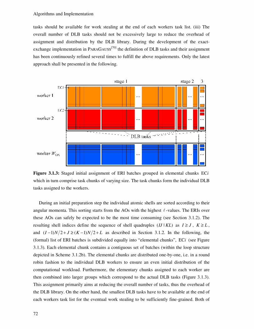
Algorithms and Implementation
72
tasks should be available for work stealing at the end of each workers task list. (iii) The
overall number of DLB tasks should not be excessively large to reduce the overhead of
assignment and distribution by the DLB library. During the development of the exact-
exchange implementation in PARAGAUSS[70] the definition of DLB tasks and their assignment
has been continuously refined several times to fulfill the above requirements. Only the latest
approach shall be presented in the following.
Figure 3.1.3: Staged initial assignment of ERI batches grouped in elemental chunks ECi
which in turn comprise task chunks of varying size. The task chunks form the individual DLB
tasks assigned to the workers.
During an initial preparation step the individual atomic shells are sorted according to their
angular momenta. This sorting starts from the AOs with the highest ℓ -values. The ERIs over
these AOs can safely be expected to be the most time consuming (see Section 3.1.2). The
resulting shell indices define the sequence of shell quadruples ( | )IJ KL as I J≥ , K L≥ ,
and ( 1) 2 ( 1) 2I N J K N L− + ≥ − + as described in Section 3.1.2. In the following, the
(formal) list of ERI batches is subdivided equally into “elemental chunks”, ECi (see Figure
3.1.3). Each elemental chunk contains a contiguous set of batches (within the loop structure
depicted in Scheme 3.1.2b). The elemental chunks are distributed one-by-one, i.e. in a round
robin fashion to the individual DLB workers to ensure an even initial distribution of the
computational workload. Furthermore, the elementary chunks assigned to each worker are
then combined into larger groups which correspond to the actual DLB tasks (Figure 3.1.3).
This assignment primarily aims at reducing the overall number of tasks, thus the overhead of
the DLB library. On the other hand, the smallest DLB tasks have to be available at the end of
each workers task list for the eventual work stealing to be sufficiently fine-grained. Both of

Exact-Exchange
73
these requirements can be fulfilled by a suitable definition of the DLB tasks, hence by
varying the number of elemental chunks in each task. The largest DLB tasks which comprise
the most elemental chunks are defined at the beginning of the task list of each worker. This
initial stage of the largest DLB tasks is then followed by additional stages of DLB tasks,
which are successively smaller, hence comprise fewer elemental chunks. The last stage
includes only DLB tasks with a single elemental chunk. The number of elemental chunks per
DLB task is decreased from stage to stage by the fixed factor stagr . All these assignments are
depicted by Figure 3.1.3. For the computing platforms employed in the context of this thesis
(see below), three stages, each with 160 DLB tasks per worker, and stag 15r = , were found to
provide a good trade-off between the parallel overhead and the overhead of the DLB library
itself.31
The run time Wt on a specific number CPUW of workers relative to the execution time REFt
on a reference number REFW of workers (whereas REF CPUW W≤ ) allows for the definition of
performance metrics like the parallel speedup CPU( )s W and the parallel efficiency CPU( )eff W .
These two performance metrics are defined as CPU REF( ) Ws W t t= and
REF REF CPUCPU
CPU CPU REF
( )( )
W
W t s Weff W
W t W W
⋅= =
⋅, 3.1.79
respectively. While REF 1W = allows to evaluate the total parallelization overhead, serial runs
can often not be carried out for large test systems with a reasonable effort. Thus, parallel runs
have to be taken as reference.
This is the case for TPSSh hybrid DFT calculations of the cluster Pt140(CO)8 (see Section
4.4), which were carried out on the computing platform SuperMUC of the Leibniz
Rechenzentrum, München.32 With 6096 CGTO basis functions this system represents a large
enough computational problem for REF 128W = to be a reasonable reference. The individual
timings Wt for the total SCF cycle and the computation of the EXX term where obtained as
averages over the first 10 SCF cycles at the beginning of the SCF process. For REF 128W = the
average run time of a single SCF cycle amounts to about 665 seconds on the SuperMUC
platform.
Figure 3.1.4 depicts the parallel speedup and efficiency for up to 2048 workers.33 For CPU
counts higher than 512 the timings for the total SCF cycle and the EXX assembly step start to
exhibit small, but notable deviations from the ideal speedup. Overall, the total SCF cycle
exhibits a slightly less ideal scaling than the EXX assembly step, as it comprises other,
computationally less demanding steps which cannot be parallelized as efficiently. The
31 With 1, 15, and 215 elemental chunks in the DLB tasks of the third, second, and first stage, respectively, and
160 DLB tasks in each stage, this implies that the entire list of ERI batches is (formally) subdivided into 2_EC 160 (1 15 15 ) 38560n = ⋅ + + = elemental chunks per worker. Whenever the elemental chunks exceed
the number of ERI batches, the number of the DLB tasks in the initial stages is reduced. 32 SuperMUC (LRZ), Intel Xeon (Sandy Bridge) CPU, Infiniband interconnect. 33 See Sections 4.1 and 4.4 for the detailed computational parameters.

Algorithms and Implementation
74
decrease of the parallel speedups is clearly noticeable at 2048 CPUs, although (2048)s is still
close to the ideal value for the EXX assembly. The parallel efficiency of the EXX assembly
decreases by about 3% at 2048 workers while the corresponding value of the total SCF cycle
differs by about 7% from the ideal scaling behavior. This behavior is most likely related to
the connectivity of the individual workers.
Figure 3.1.4: Parallel efficiency eff and speedup s for CPU 256,W = 512, 1024, and 2048
workers and REF 128W = on the example of a TPSSh hybrid DFT calculation of the Pt140(CO)8
5t cluster (see Section 4.4).
To characterize the efficiency further, the PARAGAUSS exact-exchange implementation is
compared to that of the NWChem program suite[404] on the example of a PBE0 single point
calculation on a small Mo-V mixed metal oxide cluster model (Mo4VO19H8) using 6-31G**
and Stuttgart-Dresden basis sets with the corresponding effective core potentials.[407-409] For
this example the PARAGAUSS implementation exhibits lower run times than NWChem, which
partially result from the different numbers of SCF cycles needed to converge the density
matrix: 39 with PARAGAUSS and 47 with NWChem. To allow for a better comparison, the
timings obtained with the NWChem have been multiplied by 39/47 to account for this
difference. Table 3.1.1 provides the total (scaled) run times and the parallel efficiencies
measured with both programs on 1 to 16 workers of the local Linux cluster.34
34 Intel Xeon (Nehalem) CPU, Gigabit connection.
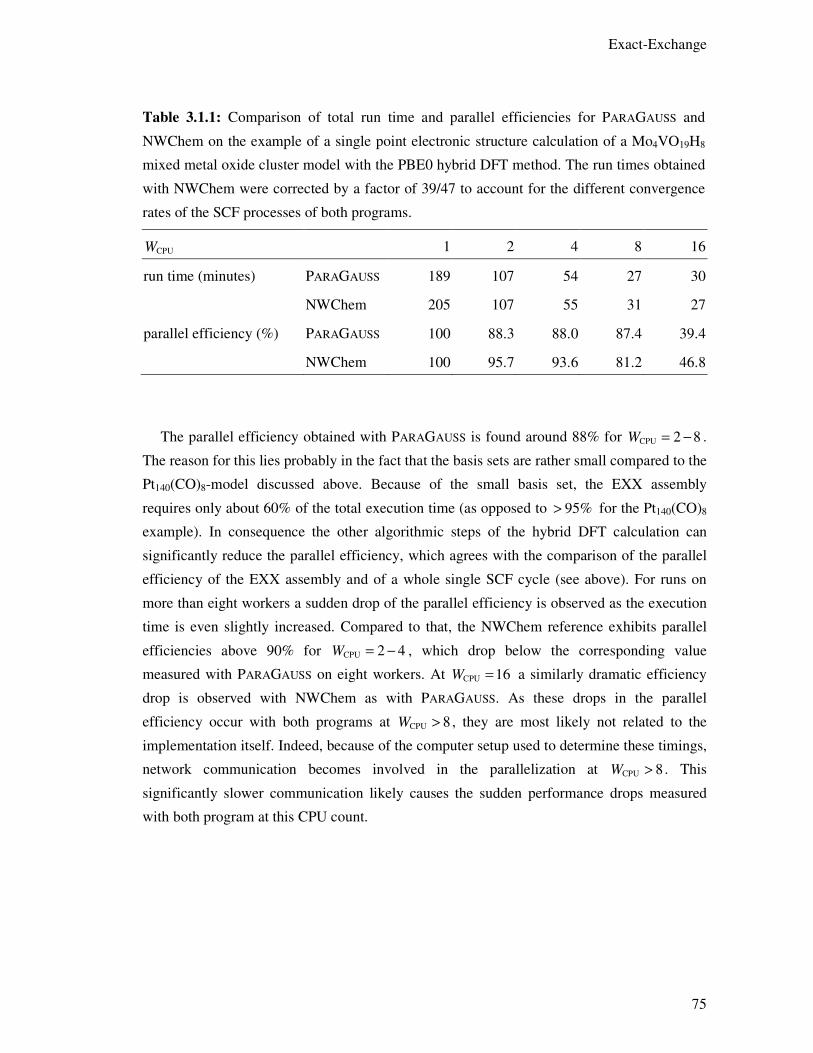
Exact-Exchange
75
Table 3.1.1: Comparison of total run time and parallel efficiencies for PARAGAUSS and
NWChem on the example of a single point electronic structure calculation of a Mo4VO19H8
mixed metal oxide cluster model with the PBE0 hybrid DFT method. The run times obtained
with NWChem were corrected by a factor of 39/47 to account for the different convergence
rates of the SCF processes of both programs.
CPUW 1 2 4 8 16
run time (minutes) PARAGAUSS 189 107 54 27 30
NWChem 205 107 55 31 27
parallel efficiency (%) PARAGAUSS 100 88.3 88.0 87.4 39.4
NWChem 100 95.7 93.6 81.2 46.8
The parallel efficiency obtained with PARAGAUSS is found around 88% for CPU 2 8W = − .
The reason for this lies probably in the fact that the basis sets are rather small compared to the
Pt140(CO)8-model discussed above. Because of the small basis set, the EXX assembly
requires only about 60% of the total execution time (as opposed to 95%> for the Pt140(CO)8
example). In consequence the other algorithmic steps of the hybrid DFT calculation can
significantly reduce the parallel efficiency, which agrees with the comparison of the parallel
efficiency of the EXX assembly and of a whole single SCF cycle (see above). For runs on
more than eight workers a sudden drop of the parallel efficiency is observed as the execution
time is even slightly increased. Compared to that, the NWChem reference exhibits parallel
efficiencies above 90% for CPU 2 4W = − , which drop below the corresponding value
measured with PARAGAUSS on eight workers. At CPU 16W = a similarly dramatic efficiency
drop is observed with NWChem as with PARAGAUSS. As these drops in the parallel
efficiency occur with both programs at CPU 8W > , they are most likely not related to the
implementation itself. Indeed, because of the computer setup used to determine these timings,
network communication becomes involved in the parallelization at CPU 8W > . This
significantly slower communication likely causes the sudden performance drops measured
with both program at this CPU count.

76
3.2. Generalized DFT+U Method
3.2.1. Projector Generation
In Section 2.4 the DFT+U term was formulated in terms of occupation numbers of target
orbitals tχ which correspond to individual KS orbitals, to which the self-interaction
correction is applied. The DFT+Umol method implemented in PARAGAUSS as part of this
thesis allows one to apply the self-interaction correction in terms of projectors that consist of
general linear combinations of atomic orbitals (AO). The generation of such projectors
represents a crucial part of the DFT+Umol method. Thus, their treatment is discussed in the
following, while the implementation of the DFT+Umol energy and gradient expressions in
PARAGAUSS are presented in the two subsequent sections, respectively.
The projector orbitals are labelled by the index I and either correspond to elements of
atomic subshells or to molecular orbitals of isolated fragments of the system. In any case the
DFT+Umol implementation retrieves the projector coefficients itv as converged KS orbital
coefficients from auxiliary SCF calculations on the isolated fragments or atomic systems.
While allowing the self-interaction correction to become independent of the employed AO
basis set, this detail represents a minor difference to the conventional DFT+U correction
implemented in PARAGAUSS if the DFT+Umol projectors target atomic subshells.[70,281,283-285]
However, if the MOs targeted by the DFT+U correction are very similar to single atomic
basis functions, both implementations essentially provide the same results. Furthermore, the
DFT+Umol implementation exactly reduces to that of the conventional DFT+U term if the
contraction coefficients of the applied CGTO basis are identical to the converged KS
eigenvectors of an atomic calculation.
The occupation matrix elements tun σ represent the main variable of any DFT+U
correction term. Thus, the reliability of the DFT+U approach depends on the quality of the
occupation numbers and the DFT+U projectors. The most important aspect of the definition
and computation of DFT+U projectors is that they remain as close as possible to the MOs
they target. In consequence the target orbitals tχ must overlap as much as possible with
these MOs but exhibit essentially no overlap with any other KS orbitals. In consequence, the
FLL formulations of DFT+U or DFT+Umol provide reasonable self-interaction corrections to
atomic subshells only if the corrected subshell elements essentially do not interact with any
other orbitals outside of the same subshell (see Section 2.4). The same holds if the correction
targets molecular fragment orbitals.
However, projectors obtained from molecular fragment orbitals are linear combinations of
AOs, thus exhibit additional degrees of freedom in terms of the coefficient vectors itv
compared to atomic subshell projectors. To ensure the best possible overlap between the
projector orbitals and the molecular fragment orbitals targeted by them, the former are
obtained from auxiliary calculations of the molecular fragment at the geometry that the
Generalized DFT+U Method
77
fragment exhibits within the complete system. In the case of a geometry relaxation the
auxiliary SCF calculation used to generate the DFT+Umol projectors therefore has to be
repeated at every geometry optimization step. In the context of the present thesis this was
enabled by conducting the DFT+Umol calculations within the suite PARATOOLS.[405,410] A
special interface of PARAGAUSS to this suite allowed one to extract the required molecular
fragment geometries during every step of the geometry optimization and subsequently to
carry out the required auxiliary calculations on them.
The molecular fragments on which the target orbitals are located may not be symmetric
while the total system is. Furthermore, the auxiliary SCF calculation of the isolated molecular
fragment may also be carried out with symmetry constraints to allow for an easier
identification of the projector coefficients itv . To ensure that the coefficients itv are
correctly imported before the main SCF iteration, the eigenvectors v are first unsymmetrized
according to 1−=v vRɶ (see Section 3.1.2). The resulting vectors vɶ are then stored in a
separate file for every group I of target orbitals.
3.2.2. DFT+Umol Energy and Potential
The following section discusses the implementation of the DFT+Umol energy correction
( )U 12 Tr TrI I I I
I
E U σ σ σ
σ
= −∑ n n n 3.2.1
which was established in Section 2.4 (Eq. 2.4.10) in terms of the target orbital occupation
matrices (Eq. 2.4.16)
†I I Iσ σ=n v SP Sv . 3.2.2
Furthermore, the implementation of the corresponding DFT+Umol potential is presented,
which is required for the self-consistent application of this method.
The DFT+Umol method requires several preparation steps before commencing the SCF
iteration. First, the unsymmetrized projector coefficients vɶ from the auxiliary calculations
(see Section 3.2.1) are imported from individual files for every group I of target orbitals.
Subsequently, the vectors vɶ are mapped onto the unsymmetrized AO basis set of the system.
In the next step these unsymmetric projectors would have to be transformed into the
symmetry adapted basis of the system. However, while Eq. 3.1.61 provides a comparatively
simple way to transform matrices from the AO basis to the symmetry adapted basis, the
corresponding transformation of vectors is not as easily achieved with the existing
PARAGAUSS subroutines. Indeed, this approach would require significant extensions in the
PARAGAUSS modules responsible for the computation of Clebsch‒Gordan coefficients.

Algorithms and Implementation
78
Thus, the DFT+Umol energy term was implemented in a different but equivalent
formulation. After inserting Eq. 3.2.2 into Eq. 3.2.1 and expanding the traces over matrix
products, the DFT+Umol energy term writes as
U † † †12 I I I ji ij I I li ij I I jk kl
I ij ijkl
E U P P Pσ σ σσ
= −
∑ ∑ ∑Sv v S Sv v S Sv v S . 3.2.3
The first term in the brackets of Eq. 3.2.3 appears as sum over the diagonal elements of the
product of the symmetric matrix †I I I=X Sv v S and the density matrix, hence as Tr I
σX P .
Likewise, the second term is identified as Tr( ) I Iσ σX P X P . Thus, the DFT+Umol energy
correction term writes as
( )U 12 Tr( ) ,I I I I
I
E Uσ σ
σ
= −∑ X X P X P 3.2.4
which allows one to carry out the transformation into the symmetry adapted basis on the
matrices IX instead of the vectors Iv .
As traces of matrix products with the density matrix represent expectation values, the
above reformulation in Eq. 3.2.4 also provides a definition of the DFT+Umol operator
( )12
ˆ ˆ ˆˆˆ I I I I
I
u U X X Xρ= −∑ 3.2.5
in terms of the projectors
ˆI t t
t I
X χ χ∈
=∑ 3.2.6
and the density matrix operator ρ from Eq. 2.4.9. The first term in brackets of Eq. 3.2.5
projects the self-interaction correction on all KS orbitals. The density matrix represents a
projector onto the occupied KS orbitals. In consequence, the second term in brackets can be
interpreted as a projector onto the occupied KS orbitals only. This latter term becomes
dominant for fully occupied target orbitals, while both terms cancel each other in the limit of
integer occupations. Thus, the operator in Eq. 3.2.5 provides a slightly different interpretation
of the linear and quadratic terms of the DFT+Umol penalty functional in Eq. 3.2.1.
A self-consistent DFT+Umol calculation requires the contribution of the correction term
in Eq. 3.2.4 to the matrix of the KS operator, hence the derivatives of UE with respect to the
elements of the density matrix. By exploiting the fact that the matrix IX is symmetric the
derivatives of the first term are obtained as
Tr = I I kl jk il I ij
ij klP
σσσ
σ
δ δ δ′′
∂=∑X P X X . 3.2.7
The derivatives of the second term, Tr( ) I Iσ σX P X P , result analogously. After reordering
one obtains
Tr( ) = 2 I I I I ij
ijP
σ σ σ
σ
′ ′∂X P X P X P X . 3.2.8
Generalized DFT+U Method
79
By combining Eqs. 3.2.7 and 3.2.8 the total contribution of the DFT+Umol term to the KS
matrix reads as
( )12 2I I I I
I
Uσ σ= −∑U X X P X . 3.2.9
During the SCF iteration the matrix σU is computed from Eq. 3.2.9 along with the
DFT+Umol energy (Eq. 3.2.4) in every iteration step.
3.2.3. DFT+Umol Gradients
This section describes the implementation of the contributions of the DFT+Umol term to the
gradients with respect to the nuclear positions.
These derivatives of the DFT+Umol term can be expressed in terms of the partial
derivatives of the matrices involved in the DFT+Umol energy expression
U U U U
ij ij it
r ij r ij r it rij ij it
P SE E E E v
A P A S A v A
σ
σσ
∂ ∂∂ ∂ ∂ ∂ ∂= + +
∂ ∂ ∂ ∂ ∂ ∂ ∂∑ ∑ ∑ . 3.2.10
The first sum in Eq. 3.2.10 is the so-called Pulay term. This term comprises the partial
derivatives UijE P σ∂ ∂ which are nothing else than the elements of the contribution σU to the
matrix of the KS operator (see Section 3.2.2). Thus, the calculation of the Pulay term is
actually not required within the DFT+Umol module as this contribution is computed from the
total KS operator matrix by existing modules of PARAGAUSS.[281]
The second term in Eq. 3.2.10 corresponds to the Hellmann‒Feynman term and is
computed analogously to the earlier DFT+U implementation in PARAGAUSS.[281] The partial
derivatives with respect to the overlap matrix elements result in
† †Tr ( ) = 2 2 I I I I I I I I I ij
ijS
σ σ σ σ σ σ σ σ σ∂− − + −X P X P X P Y P Y P X P P Y P X P Y . 3.2.11
Thereby the quantity †I I I=Y v v S is readily available as it occurs as intermediate during the
calculation of IX . The calculation of the matrices ij rS A∂ and their multiplication with the
results of Eq. 3.2.11 is then carried out by existing parts of the earlier DFT+U
implementation in PARAGAUSS.[281]
The third sum in Eq. 3.2.10 arises from eventual changes in the target orbitals due to
altered nuclear coordinates. In cases where the target orbitals correspond to molecular
fragment orbitals this term implies a calculation of derivatives of the KS eigenvectors with
respect to the nuclear coordinates. In the context of this thesis this term was neglected as the
implementation of the response property it rv A∂ would require significant reorganizations in
many modules of PARAGAUSS. A comparison between analytical and numerical derivatives
with respect to nuclear coordinates on the example of a PBE+Umol correction acting on the
CO 2π* fragment MOs of NiCO yields a maximum difference of less than 510− au. Thus, the

Algorithms and Implementation
80
negligence of the third term on the right-hand side of Eq. 3.2.10 does not lead to severe
consequences in the calculations carried out in the context of this thesis.

81
4. Applications
4.1. General Computational Details
All application calculations of this thesis were carried out with the linear combination of
Gaussian-type orbital fitting-function density functional (LCGTO-FF-DF) method as
implemented in the package PARAGAUSS.[39,43,70,289] More specifically, version 4.0 of the
PARAGAUSS package was employed. This version includes the hybrid DFT and DFT+Umol
capabilities that were implemented as part of this thesis (see Chapter 3). Further recent
extensions implemented by others[405,411] address parallelization and convergence acceleration
strategies.
Most of the calculations employ def2-type orbital basis sets,[412] which were chosen of
triple-zeta quality (triple-zeta valence polarized, TZVP) in the case of the studies presented in
Sections 4.3 and 4.4. For the elements C, O, and Ni this AO basis describes all electrons and
features the contractions (11 ,6 , 2 ,1 ) [5 ,3 ,2 ,1 ]s p d f s p d f→ for C and O, respectively, as well
as (17 ,11 ,7 ,1 ) [6 , 4 , 4 ,1 ]s p d f s p d f→ in the case of Ni.[412] In the case of the heavier
elements Pd and Pt effective core potentials (ECP) of the Stuttgart-Dresden-type
parametrization[413] were employed to represent the lowest 28 and 60 “small-core” spin-
orbitals, respectively. The corresponding AO basis set contractions account to
(7 ,7 ,6 ,1 ) [6 ,4 ,3 ,1 ]s p d f s p d f→ for Pd and (8 ,7 ,6 ,1 ) [6 ,4 ,3 ,1 ]s p d f s p d f→ for Pt.[412]
For the calculations on the nickel carbonyl complexes presented in Section 4.2 a quadruple-
zeta AO basis with additional polarization and diffuse functions (QZVPPD) was employed
which exhibits the contractions (16 ,8 ,4 ,2 ,1 )s p d f g → [8 ,4 ,4 ,2 ,1 ]s p d f g for C and
(16 ,9 ,4 ,2 ,1 )s p d f g → [8 ,4 ,4 ,2 ,1 ]s p d f g for O atoms.[412] Furthermore, the
def2-QZVPPD basis features a (24 ,18 ,10 ,4 ,2 )s p d f g → [11 ,6 ,5 ,4 , 2 ]s p d f g contraction
in the case of Ni.[412]
For the representation of the density during the evaluation of the Coulomb term within the
density fitting (DF-FF) approximation[35-43] Ahlrich’s Coulomb fitting basis set[414,415] was
employed in all cases. The density fitting approximation was also employed in the case of
hybrid DFT calculations to keep its effect constant when comparing semi-local with hybrid
functionals.
The local XC terms of the employed DFT methods were integrated numerically. The
corresponding numerical grids were constructed according to Becke’s prescription as a
superposition of atom-centered grids.[162] These atom centered grids exhibit Lebedev-type
angular components,[160,161] which were chosen to be locally exact for angular momenta up to
29=ℓ in the calculations in Sections 4.2 and 4.3 and up to 17=ℓ for the studies in Section

Applications
82
4.4. The radial grid components comprised 168, 146, 305, 315, and 305 shells for C, O, Ni,
Pd, and Pt in the former two cases as well as 134, 117, and 245 shells for the elements C, O,
and Pt for the calculations in Section 4.4.
The direct inversion of the iterative subspace (DIIS) method[405,416] was used to accelerate
the convergence of the density matrix during the SCF iteration. After reaching a maximum
change of 10‒6 in the density matrix elements, the SCF iteration was regarded as converged.
The cluster models studied in Sections 4.3 and 4.4 were calculated by using a fractional
occupation number (FON) technique with a Fermi-type broadening function.[39] The
corresponding broadening parameter was successively lowered during the geometry
optimization to final values of 0.05 and 0.01 eV for the calculations of Sections 4.3 and 4.4,
respectively.
The structures of all models were relaxed under the constraints of their respective point
group symmetry by using the molecular-dynamics based “fast inertial relaxation engine”
(FIRE) optimization method[417] as implemented in the utility suite PARATOOLS.[405,410] The
geometry optimization was pursued until the Cartesian components of all molecular forces
acting on the atomic centers dropped below 10‒6 au.
The CO adsorption energies discussed in Section 4.4 were corrected for the basis set
superposition error (BSSE)[395] using an estimate that was obtained with the counterpoise
approach.[418] The nickel-CO dissociation energies presented in Section 4.2 would require the
same treatment as well. However, due to the significantly larger basis set employed in this
latter case study, the BSSE was estimated to be less than 0.4 kJ/mol; its correction was
therefore neglected.
The occupation numbers and the projected density of states spectra discussed in Sections
4.2 and 4.4, respectively, were obtained on the basis of Mulliken population numbers.[419]
83
4.2. DFT+Umol Analysis of the Self-Interaction Error in
Ni(CO)m
, m = 1 ‒ 4
4.2.1. Introduction
This section presents the application of the DFT+Umol method to the nickel carbonyl
complexes Ni(CO)m ( 1 4m = − ). This discussion follows Ref. [287].
Because of its important applications in chemical industry the nickel tetracarbonyl
complex Ni(CO)4 is among the experimentally best studied transition metal carbonyl
compounds.[420-427] Furthermore, as they represent very simple transition metal complexes,
Ni(CO)4 and its subcarbonyls Ni(CO)m ( 1 3m = − ) have been characterized by means of
highly accurate post-HF and multi-reference calculations as well as in various DFT
studies.[57,425,428-434] The subcarbonyls Ni(CO)m ( 1 3m = − ) are very difficult to isolate
experimentally. Thus, corresponding experimental reference values are significantly more
sparse than in the case of Ni(CO)4.[423,425,426,435] For the same reason the first metal-CO
dissociation energies
( ) ( ) ( )dis tot tot 1 tot( ) Ni(CO) Ni(CO) COm mE m E E E−= − − 4.2.1
vary with the experimental method applied. Nevertheless, a clear trend among the dis ( )E m
values can always be observed. The first CO dissociation energies are found to increase when
going from Ni(CO)4 over Ni(CO)3 to Ni(CO)2, which is rationalized by the decreasing metal-
carbonyl bond competition among the CO ligands.[423-425,427,435] However, the dissociation
energy of NiCO, dis (1)E , is found to be lower than dis (2)E .[423,435] This latter behavior is
rationalized in terms of a formal electronic relaxation of the Ni-atom from the d10 closed-shell
configuration in the corresponding carbonyl complexes to its atomic ground state.[57,432,433]
This peculiar trend in the CO dissociation energies is reproduced by WFT methods as well
as by hybrid DFT calculations.[425,430,431] In contrast, local and semi-local DFT methods
predict dis (1)E larger than dis (2)E , hence provide a qualitatively incorrect ordering of the CO
dissociation energies. Cases, where hybrid DFT yields qualitatively correct results while
semi-local DFT methods fail, likely indicate an influence of the self-interaction error (see
Section 2.2.5). While the nickel carbonyls represent systems certainly small enough to allow
for an accurate WFT description, these entities can appear also as intermediates of much
larger models.[436] In such situations an efficient and reliable DFT description of the nickel
carbonyl complexes is highly desirable.
This observation is the starting ground for the following study.[287] The influence of the
SIE on the Ni(CO)4 compound, on the Ni(CO)m subcarbonyls, and on the nickel atom was
examined by means of a DFT+Umol correction (see Sections 2.4 and 3.2) to the GGA
functional PBE.[49] The DFT+Umol correction was applied to the Ni 3d valence subshell as
well as to the 2π* orbitals, which are the lowest unoccupied MOs (LUMO) of the CO ligand.
Applications
84
In the following, these two types of DFT+Umol corrections will be denoted as Umol(Ni 3d)
and Umol(CO 2π*), respectively. To assess the effect of the DFT+Umol term on either type
of orbitals, the corresponding IU parameters were varied between 3 3.0dU = eV and 6.0 eV
(in steps of 0.5 eV) for the former and between 2π* 1.0U = , 2.0, and 4.0 eV for the latter case.
The DFT+Umol results were compared with the values obtained with the uncorrected PBE
functional[49] as well as with the hybrid GGA PBE0.[87]
4.2.2. Molecular Geometries
The molecular systems were treated as symmetric structures and relaxed under the
corresponding symmetry constraints. 8vC symmetric models were employed for CO and
NiCO, while Ni(CO)2, Ni(CO)3, and Ni(CO)4 were treated with point group symmetry
constraints of 2v ,C 3h ,D and dT , respectively. All models were checked for possible
Jahn‒Teller distortions by computing the harmonic frequencies (see Section 4.2.4) of the
vibrational normal modes without symmetry constraints. The corresponding normal mode
analysis was carried out with the help of the ParaTools suite,[437] which allows one to
compute second-order numerical derivatives with respect to nuclear displacements.
Table 4.2.1 provides dC-O and dNi-C, the C-O distances of the gas phase CO molecule and
all nickel carbonyls and the corresponding Ni-C distances as obtained with PBE0, PBE, and
PBE+Umol with the DFT+Umol term applied to Ni 3d ( 3 6.0dU = eV), or CO 2π*
( 2π* 4.0U = eV), or a combination of both ( 3 3.0dU = eV, 2π* 1.0U = eV). Note, that for the
former two variants only the results at the maxima of the examined IU parameter values are
listed to assess the impact of the two DFT+Umol corrections on the geometries.
A dC-O value of 112 pm is obtained with PBE0 for the CO molecule in the gas phase.
Within the carbonyl complexes this distance is increased to about 115 pm to 113 pm, whereas
the largest bond elongation is determined in NiCO and the smallest in the nickel tetracarbonyl
complex. This behavior is predicted by the Blyholder model in terms of a partial electron
transfer into the antibonding CO 2π* orbitals.[438] This so-called back-bonding mechanism
enhances the bond strength between the CO ligand and the metal atom, but weakens the CO
bond.[438] Following this model, the back-bonding interaction is strongest in NiCO and
weakest in Ni(CO)4. The PBE functional yields longer dC-O bonds between 116 and 115 pm
for the nickel carbonyls. This is rationalized by the intrinsically longer C-O bonds that are
obtained with PBE compared to PBE0. Similar differences are also notable for the dC-O values
of CO in the gas phase (113 pm for PBE). The individual DFT+Umol corrections always lead
to longer C-O bonds than PBE0 but shorter ones than PBE. This is rationalized with the
reduced back-bonding interaction within the carbonyl complexes due to the increased orbital
localization caused by the DFT+Umol term (see Section 4.2.4).[287]
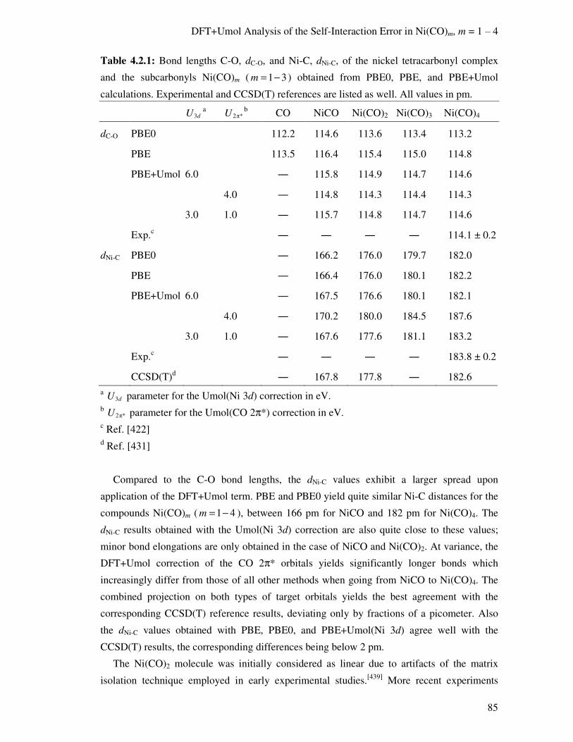
DFT+Umol Analysis of the Self-Interaction Error in Ni(CO)m, m = 1 ‒ 4
85
Table 4.2.1: Bond lengths C-O, dC-O, and Ni-C, dNi-C, of the nickel tetracarbonyl complex
and the subcarbonyls Ni(CO)m ( 1 3m = − ) obtained from PBE0, PBE, and PBE+Umol
calculations. Experimental and CCSD(T) references are listed as well. All values in pm.
3dUa 2π*U
b CO NiCO Ni(CO)2 Ni(CO)3 Ni(CO)4
dC-O PBE0 112.2 114.6 113.6 113.4 113.2
PBE 113.5 116.4 115.4 115.0 114.8
PBE+Umol 6.0 ― 115.8 114.9 114.7 114.6
4.0 ― 114.8 114.3 114.4 114.3
3.0 1.0 ― 115.7 114.8 114.7 114.6
Exp.c ― ― ― ― 114.1 ± 0.2
dNi-C PBE0 ― 166.2 176.0 179.7 182.0
PBE ― 166.4 176.0 180.1 182.2
PBE+Umol 6.0 ― 167.5 176.6 180.1 182.1
4.0 ― 170.2 180.0 184.5 187.6
3.0 1.0 ― 167.6 177.6 181.1 183.2
Exp.c ― ― ― ― 183.8 ± 0.2
CCSD(T)d ― 167.8 177.8 ― 182.6 a 3dU parameter for the Umol(Ni 3d) correction in eV. b 2π*U parameter for the Umol(CO 2π*) correction in eV. c Ref. [422] d Ref. [431]
Compared to the C-O bond lengths, the dNi-C values exhibit a larger spread upon
application of the DFT+Umol term. PBE and PBE0 yield quite similar Ni-C distances for the
compounds Ni(CO)m ( 1 4m = − ), between 166 pm for NiCO and 182 pm for Ni(CO)4. The
dNi-C results obtained with the Umol(Ni 3d) correction are also quite close to these values;
minor bond elongations are only obtained in the case of NiCO and Ni(CO)2. At variance, the
DFT+Umol correction of the CO 2π* orbitals yields significantly longer bonds which
increasingly differ from those of all other methods when going from NiCO to Ni(CO)4. The
combined projection on both types of target orbitals yields the best agreement with the
corresponding CCSD(T) reference results, deviating only by fractions of a picometer. Also
the dNi-C values obtained with PBE, PBE0, and PBE+Umol(Ni 3d) agree well with the
CCSD(T) results, the corresponding differences being below 2 pm.
The Ni(CO)2 molecule was initially considered as linear due to artifacts of the matrix
isolation technique employed in early experimental studies.[439] More recent experiments

Applications
86
showed this molecule to be bent.[440] For Ni(CO)2 a C-Ni-C angle of 140° is obtained with the
PBE method, while PBE0 and the PBE+Umol(Ni 3d) combination predict slightly larger
values of 146° and 148°, respectively. In contrast, application of the Umol(CO 2π*) term
yields a nearly linear Ni(CO)2 structure. The bond angles within all other complexes are
determined by their respective point group symmetries.
4.2.3. Dissociation Energies
In the following the first metal-CO dissociation energies dis ( )E m , 1 4m = − , as obtained from
PBE, PBE0, and both PBE+Umol variants according to Eq. 4.2.1 are discussed.
The dis (1)E result depends on the total electronic energy of the nickel atom. The atomic
system was treated with 2vC point group symmetry constraints to allow for a localized orbital
occupation within the 3d valence subshell.[244] Note that this broken symmetry treatment
leads to an 3d94s
1 configuration for the nickel atom as opposed to the experimentally found
3d84s
2 atomic ground state, which arises from spin-orbit interaction that was not considered
here.[441] Within a finite basis set the computed dissociation energies are subject to the basis
set superposition error (BSSE), thus would need to be corrected by the counterpoise
method.[395,418] However, due to the very flexible def2-QZVPPD basis set employed, the
BSSE in the dis ( )E m values was found to be less than 0.4 kJ/mol, thus can be safely
neglected in the present discussion.
Table 4.2.2 provides the values dis ( )E m obtained with the variants PBE+Umol(Ni 3d) and
PBE+Umol(CO 2π*), the uncorrected PBE functional, and the hybrid GGA PBE0. For
comparison the CCSD(T) reference values are shown as well. Note, that the CCSD(T) results
for dis (2)E and dis (3)E were determined for a linear Ni(CO)2 molecule.[431] In the case of
PBE the linear and 2vC symmetric structures of Ni(CO)2 differ by ~5 kJ/mol. Thus,
compared to the variations among the disagreeing experimental results listed in Table 4.2.2,
the CCSD(T) energies of the linear structure can be regarded as sufficiently accurate for the
present discussion of the trends of the dis ( )E m values.
In agreement with earlier studies,[57] the uncorrected semi-local DFT approximation PBE
does not provide the correct trend dis dis(1) (2)E E< of the first metal-CO dissociation energies.
With dis (1) 247E = kJ/mol the strength of the Ni-C bond in NiCO is considerably
overestimated and significantly larger than the corresponding dissociation energy of 208
kJ/mol obtained for Ni(CO)2. In contrast, the other two dis ( )E m values agree more with the
expected trend and are successively smaller; 148 kJ/mol for m = 3 and 121 kJ/mol for m = 4.
The CCSD(T) reference values amount to 144, 178, 145, and 125 kJ/mol for 1 4m = − ,
respectively. The PBE0 results agree considerably better with these reference values than the
PBE values. PBE0 yields a dis (2)E value of 178 kJ/mol, which is close to the CCSD(T)

DFT+Umol Analysis of the Self-Interaction Error in Ni(CO)m, m = 1 ‒ 4
87
reference and significantly larger than the dissociation energies of the other three complexes.
Also dis (3) 132E = kJ/mol is still higher than the dissociation energy of the NiCO molecule,
126 kJ/mol. The corresponding dis (4)E value amounts to 101 kJ/mol. Thus, despite somewhat
underestimating the Ni-CO dissociation energies, PBE0 is able to recover the trend
dis dis dis dis(2) (3) (1) (4)E E E E> ≈ > provided by CCSD(T).
Table 4.2.2: First metal-CO dissociation energies dis ( )E m of the Ni(CO)m complexes
( 1 4m = − ) obtained with PBE0, PBE, and the two projections of the DFT+Umol correction
as well as the corresponding CCSD(T) and experimental reference values. All energies in
kJ/mol.
3dUa 2π*U
b NiCO Ni(CO)2 Ni(CO)3 Ni(CO)4
PBE0 126 178 132 101
PBE 247 208 148 121
PBE+Umol 3.0 171 198 139 110
4.5 135 192 135 105
5.0 123 190 133 103
5.5 111 188 131 101
6.0 100 186 130 99
1.0 218 191 126 91
2.0 190 181 97 61
4.0 139 164 37 1
3.0 1.0 144 183 115 79
Exp. 1c 121 ± 63 226 ± 63 54 ± 8 105 ± 8
Exp. 2d 146 ± 13 213 ± 17 121 ± 8 ―
Exp. 3e 169 ± 24 197 ± 24 118 ± 10 ―
CCSD(T)f 144 178 145 125 a 3dU parameter for the Umol(Ni 3d) correction in eV. b 2π*U parameter for the Umol(CO 2π*) correction in eV. c Ref. [435] d Ref. [38] in Ref. [431] e Ref. [423] f Ref. [431]
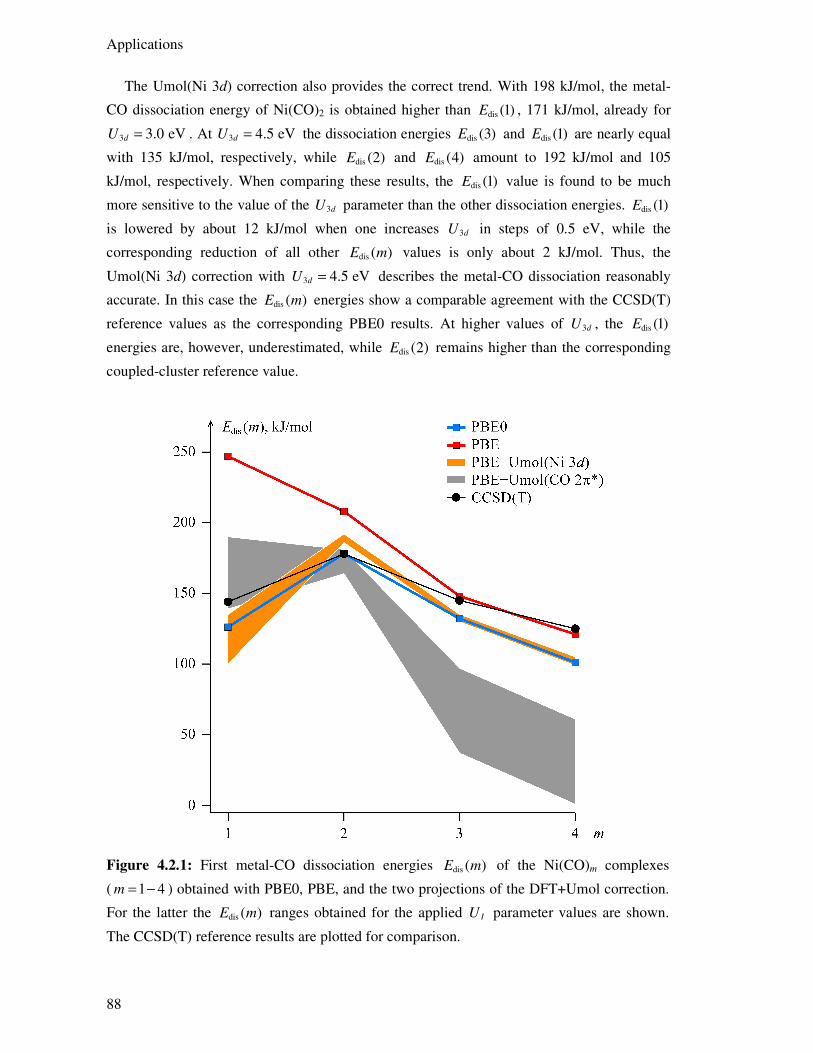
Applications
88
The Umol(Ni 3d) correction also provides the correct trend. With 198 kJ/mol, the metal-
CO dissociation energy of Ni(CO)2 is obtained higher than dis (1)E , 171 kJ/mol, already for
3 3.0 eVdU = . At 3 4.5 eVdU = the dissociation energies dis (3)E and dis (1)E are nearly equal
with 135 kJ/mol, respectively, while dis (2)E and dis (4)E amount to 192 kJ/mol and 105
kJ/mol, respectively. When comparing these results, the dis (1)E value is found to be much
more sensitive to the value of the 3dU parameter than the other dissociation energies. dis (1)E
is lowered by about 12 kJ/mol when one increases 3dU in steps of 0.5 eV, while the
corresponding reduction of all other dis ( )E m values is only about 2 kJ/mol. Thus, the
Umol(Ni 3d) correction with 3 4.5 eVdU = describes the metal-CO dissociation reasonably
accurate. In this case the dis ( )E m energies show a comparable agreement with the CCSD(T)
reference values as the corresponding PBE0 results. At higher values of 3dU , the dis (1)E
energies are, however, underestimated, while dis (2)E remains higher than the corresponding
coupled-cluster reference value.
Figure 4.2.1: First metal-CO dissociation energies dis ( )E m of the Ni(CO)m complexes
( 1 4m = − ) obtained with PBE0, PBE, and the two projections of the DFT+Umol correction.
For the latter the dis ( )E m ranges obtained for the applied IU parameter values are shown.
The CCSD(T) reference results are plotted for comparison.

DFT+Umol Analysis of the Self-Interaction Error in Ni(CO)m, m = 1 ‒ 4
89
From a qualitative point of view, the DFT+Umol correction of the CO 2π* orbitals
behaves analogously to the Umol(Ni 3d) term as it is able restore the trend dis dis(2) (1)E E> as
well. However, it requires 2π* 4.0U = eV to yield an dis (1)E value of 139 kJ/mol which is
close to the CCSD(T) reference and reasonably smaller than the corresponding dissociation
energy of Ni(CO)2, 164 kJ/mol. While also this latter value agrees reasonably well with the
CCSD(T) reference, the corresponding dissociation energies of the tri- and tetracarbonyl
complexes are strongly underestimated. For 2π* 4.0U = eV the dis (3)E and dis (4)E values are
calculated at 37 and 1 kJ/mol, respectively. This latter result, predicting the Ni(CO)4 complex
to be unstable, is a strong indication that the PBE+Umol(CO 2π*) combination provides an
unphysical description of the Ni(CO)m compounds. Furthermore, while the dis (2)E value
exhibits a similar sensitivity with respect to 2π*U as in the case of 3dU , the Umol(CO 2π*)
approach yields lower dissociation energies for Ni(CO)2 than the Umol(Ni 3d) term. Thus, a
stronger dependency of this energy on 2π*U is to be expected for parameter values below 1
eV. The plot of the dis ( )E m values obtained with the various computational methods (Figure
4.2.1) clearly depicts the deviations of the results obtained from the Umol(CO 2π*)
correction.
The combined DFT+Umol projection on both groups of target orbitals, with 3 3.0dU = eV
and 2π* 1.0U = eV, provides accurate molecular geometries, but was found to yield reasonable
dissociation energies only in the case of NiCO and Ni(CO)2. With dis (3) 115 kJ/molE = and
dis (4) 79 kJ/molE = , the dissociation energies of the other two carbonyls are considerably
underestimated. Inspecting both DFT+Umol contributions individually, reveals again the
Umol(CO 2π*) term to be mainly responsible for these deviations.
4.2.4. Electronic Structure Aspects and Vibrational Frequencies
The analysis of the electronic structure allows one to rationalize the behavior of both
DFT+Umol variants with regard to the dissociation energies.[287] More specifically, the
following questions are addressed; (i) Why is dis (1)E strongly overestimated by PBE and why
is it corrected by the Umol(Ni 3d) term? (ii) Why do all other dissociation energies remain
mostly unaffected by the Umol(Ni 3d) term? (iii) How can both DFT+Umol variants have a
similar qualitative effect on dis (1)E ? (iv) Why does the Umol(CO 2π*) correction deteriorate
the description of the Ni(CO)3 and Ni(CO)4 complexes to such an extent that the results
cannot be regarded as physically meaningful?
As already mentioned in Section 4.2.3, all computational methods applied here yield a d9s
1
triplet state for the nickel atom. In contrast, a formally closed shell d10 configurations was
identified from the individual Mulliken orbital populations[419] of the nickel atom in all
Ni(CO)m compounds, in agreement earlier studies.[433,434] The accumulated Mulliken
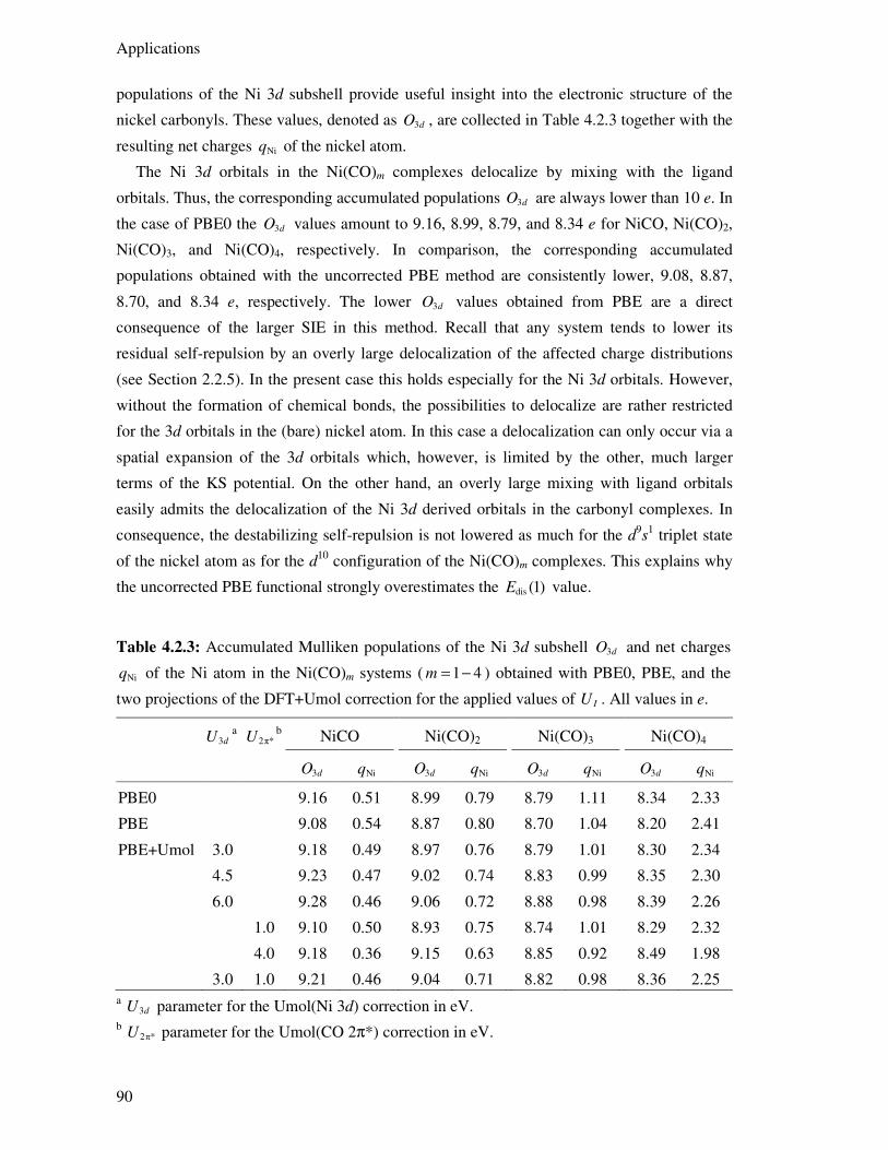
Applications
90
populations of the Ni 3d subshell provide useful insight into the electronic structure of the
nickel carbonyls. These values, denoted as 3dO , are collected in Table 4.2.3 together with the
resulting net charges Niq of the nickel atom.
The Ni 3d orbitals in the Ni(CO)m complexes delocalize by mixing with the ligand
orbitals. Thus, the corresponding accumulated populations 3dO are always lower than 10 e. In
the case of PBE0 the 3dO values amount to 9.16, 8.99, 8.79, and 8.34 e for NiCO, Ni(CO)2,
Ni(CO)3, and Ni(CO)4, respectively. In comparison, the corresponding accumulated
populations obtained with the uncorrected PBE method are consistently lower, 9.08, 8.87,
8.70, and 8.34 e, respectively. The lower 3dO values obtained from PBE are a direct
consequence of the larger SIE in this method. Recall that any system tends to lower its
residual self-repulsion by an overly large delocalization of the affected charge distributions
(see Section 2.2.5). In the present case this holds especially for the Ni 3d orbitals. However,
without the formation of chemical bonds, the possibilities to delocalize are rather restricted
for the 3d orbitals in the (bare) nickel atom. In this case a delocalization can only occur via a
spatial expansion of the 3d orbitals which, however, is limited by the other, much larger
terms of the KS potential. On the other hand, an overly large mixing with ligand orbitals
easily admits the delocalization of the Ni 3d derived orbitals in the carbonyl complexes. In
consequence, the destabilizing self-repulsion is not lowered as much for the d9s
1 triplet state
of the nickel atom as for the d10 configuration of the Ni(CO)m complexes. This explains why
the uncorrected PBE functional strongly overestimates the dis (1)E value.
Table 4.2.3: Accumulated Mulliken populations of the Ni 3d subshell 3dO and net charges
Niq of the Ni atom in the Ni(CO)m systems ( 1 4m = − ) obtained with PBE0, PBE, and the
two projections of the DFT+Umol correction for the applied values of IU . All values in e.
3dUa 2π*U
b NiCO Ni(CO)2 Ni(CO)3 Ni(CO)4
3dO Niq 3dO Niq 3dO Niq 3dO Niq
PBE0 9.16 0.51 8.99 0.79 8.79 1.11 8.34 2.33
PBE 9.08 0.54 8.87 0.80 8.70 1.04 8.20 2.41
PBE+Umol 3.0 9.18 0.49 8.97 0.76 8.79 1.01 8.30 2.34
4.5 9.23 0.47 9.02 0.74 8.83 0.99 8.35 2.30
6.0 9.28 0.46 9.06 0.72 8.88 0.98 8.39 2.26
1.0 9.10 0.50 8.93 0.75 8.74 1.01 8.29 2.32
4.0 9.18 0.36 9.15 0.63 8.85 0.92 8.49 1.98
3.0 1.0 9.21 0.46 9.04 0.71 8.82 0.98 8.36 2.25 a 3dU parameter for the Umol(Ni 3d) correction in eV. b 2π*U parameter for the Umol(CO 2π*) correction in eV.

DFT+Umol Analysis of the Self-Interaction Error in Ni(CO)m, m = 1 ‒ 4
91
Next, the changes of the dis (1)E value introduced by the Umol(Ni 3d) term will be
discussed. Recall that the effect of the DFT+Umol correction is equivalent to that of the
parabolic DFT+U penalty functional (see Eq. 2.4.10 in Section 2.4)
( )U 12 Tr TrI I I I
I
E U σ σ σ
σ
= −∑ n n n . 4.2.2
The individual populations of the elements of the Ni 3d subshell in NiCO suggest that all of
these orbitals are more than half occupied (at least by a fraction of 0.68). In consequence, the
derivative of Eq. 4.2.2 is negative, which implies that in this case the Ni 3d orbitals are
subject to an attractive potential contribution from the Umol(Ni 3d) term.[61] This attractive
contribution increases the 3dO value of NiCO compared to the corresponding population
resulting from the uncorrected PBE functional. Two conclusions can be drawn from the fact
that the Umol(Ni 3d) term increases the 3dO values. First, the increased localization of the Ni
3d orbitals in NiCO by the Umol(Ni 3d) correction implies a reduced mixing with the orbitals
of the CO ligand. According to the Blyholder model the mixing of these orbitals leads to the
back-bonding interaction.[438] Thus, the application of Umol(Ni 3d) reduces back-bonding in
NiCO. Equivalently, the Blyholder model predicts that the formation of the primary σ-
interaction between the Ni 4s and the CO 5σ orbitals increases the net charge Niq on the
nickel center.[438] In consequence, the Ni 3d orbitals are subject to a more repulsive
potential.[438] This repulsive potential is somewhat counteracted by the aforementioned
attractive potential contribution of the Umol(Ni 3d) term. The increased localization of the Ni
3d subshell by the Umol(Ni 3d) term also implies a higher self-repulsion in these orbitals.
Note, that both of these effects, the reduced amount of back-bonding and the increased self-
repulsion, have the same net influence on the NiCO system, namely the destabilization of its
delocalized d10 configuration with respect to the localized d9s
1 state of the nickel atom. This
destabilization lowers the Ni-CO dissociation energy of NiCO, which explains why the
Umol(Ni 3d) term is able to correct the dis (1)E value.
Also in the case of the other Ni(CO)m complexes, a d10 configuration can be deduced from
the more than half occupied Ni 3d orbitals. The individual orbital occupations obtained from
PBE amount to at least 0.71, 0.59, and 0.57 e in the case of Ni(CO)2, Ni(CO)3, and Ni(CO)4,
respectively. Thus, the Umol(Ni 3d) term has a similar effect on these systems as rationalized
above for NiCO. While accurate CASSCF calculations reveal the σ-interaction to prevail in
the NiCO system,[433] the amount of back-bonding is likely to increase with the number of
CO ligands. Indeed, this is the case, in agreement with the Blyholder model[438] (see above),
as can be deduced from the Niq values which are found to increase when going from NiCO to
Ni(CO)4 (Table 4.2.3). The Umol(Ni 3d) term localizes the Ni 3d orbitals and reduces back-
bonding which is well in line with the traditional explanation of the bonding situation in
NiCO and the other carbonyl complexes.[429-433] In consequence, the amount of back-bonding
interaction in the nickel carbonyls is corrected which is overestimated by PBE due to the SIE.
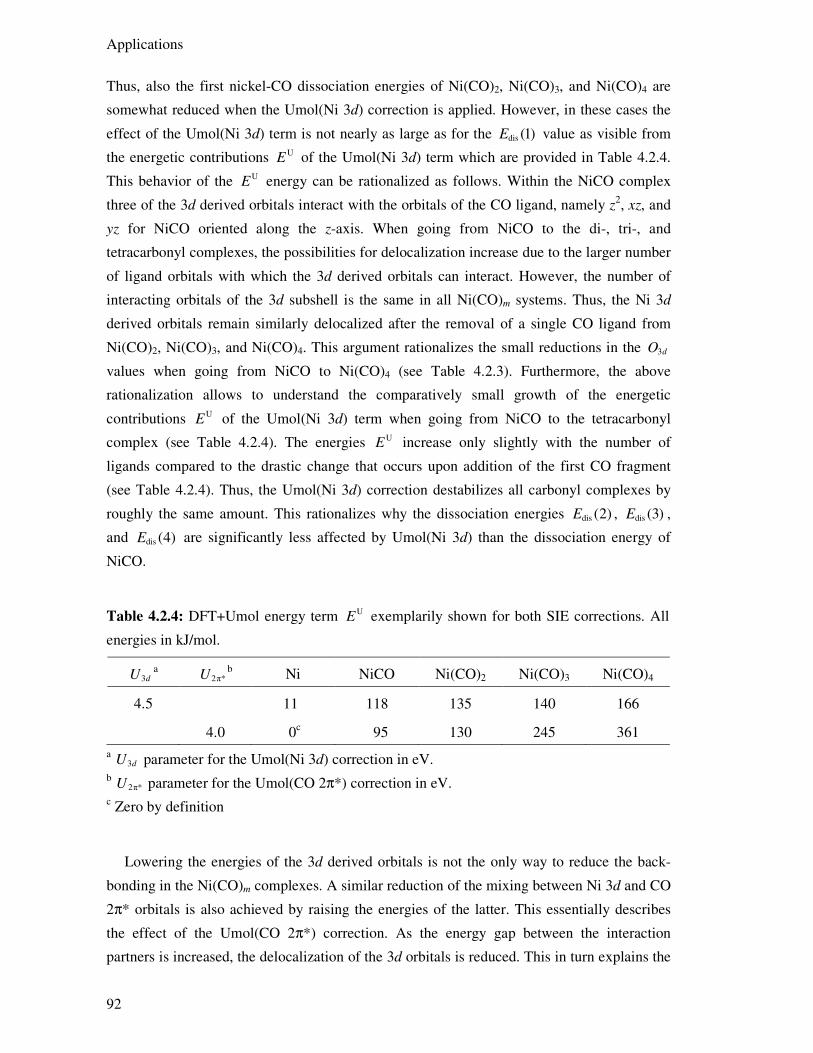
Applications
92
Thus, also the first nickel-CO dissociation energies of Ni(CO)2, Ni(CO)3, and Ni(CO)4 are
somewhat reduced when the Umol(Ni 3d) correction is applied. However, in these cases the
effect of the Umol(Ni 3d) term is not nearly as large as for the dis (1)E value as visible from
the energetic contributions UE of the Umol(Ni 3d) term which are provided in Table 4.2.4.
This behavior of the UE energy can be rationalized as follows. Within the NiCO complex
three of the 3d derived orbitals interact with the orbitals of the CO ligand, namely z2, xz, and
yz for NiCO oriented along the z-axis. When going from NiCO to the di-, tri-, and
tetracarbonyl complexes, the possibilities for delocalization increase due to the larger number
of ligand orbitals with which the 3d derived orbitals can interact. However, the number of
interacting orbitals of the 3d subshell is the same in all Ni(CO)m systems. Thus, the Ni 3d
derived orbitals remain similarly delocalized after the removal of a single CO ligand from
Ni(CO)2, Ni(CO)3, and Ni(CO)4. This argument rationalizes the small reductions in the 3dO
values when going from NiCO to Ni(CO)4 (see Table 4.2.3). Furthermore, the above
rationalization allows to understand the comparatively small growth of the energetic
contributions UE of the Umol(Ni 3d) term when going from NiCO to the tetracarbonyl
complex (see Table 4.2.4). The energies UE increase only slightly with the number of
ligands compared to the drastic change that occurs upon addition of the first CO fragment
(see Table 4.2.4). Thus, the Umol(Ni 3d) correction destabilizes all carbonyl complexes by
roughly the same amount. This rationalizes why the dissociation energies dis (2)E , dis (3)E ,
and dis (4)E are significantly less affected by Umol(Ni 3d) than the dissociation energy of
NiCO.
Table 4.2.4: DFT+Umol energy term UE exemplarily shown for both SIE corrections. All
energies in kJ/mol.
3dUa 2π*U
b Ni NiCO Ni(CO)2 Ni(CO)3 Ni(CO)4
4.5 11 118 135 140 166
4.0 0c 95 130 245 361 a 3dU parameter for the Umol(Ni 3d) correction in eV. b 2π*U parameter for the Umol(CO 2π*) correction in eV. c Zero by definition
Lowering the energies of the 3d derived orbitals is not the only way to reduce the back-
bonding in the Ni(CO)m complexes. A similar reduction of the mixing between Ni 3d and CO
2π* orbitals is also achieved by raising the energies of the latter. This essentially describes
the effect of the Umol(CO 2π*) correction. As the energy gap between the interaction
partners is increased, the delocalization of the 3d orbitals is reduced. This in turn explains the
DFT+Umol Analysis of the Self-Interaction Error in Ni(CO)m, m = 1 ‒ 4
93
increased 3dO values that result from the Umol(CO 2π*) correction (Table 4.2.3). Thus, also
the Umol(CO 2π*) term is able to reduce the delocalization within the Ni 3d subshell of the
carbonyl complexes. This indirect localization of the Ni 3d subshell by the Umol(CO 2π*)
correction rationalizes why both DFT+Umol variants have similar effects on the dissociation
energy dis (1)E , at least from a qualitative point of view.
However, the indirect effect of the Umol(CO 2π*) correction on the 3dO values is rather
small. In the case of NiCO, a relatively large value of 2π* 4.0U = eV is required to bring the
accumulated 3d population close to those obtained with PBE0 or PBE+Umol(Ni 3d), hence,
to achieve dis dis(2) (1)E E> (see Table 4.2.2 in Section 4.2.3). While the 3dO values of the
other nickel carbonyls are increased by the Umol(CO 2π*) correction, back-donation is
reduced in these cases too. The energy contributions UE of the Umol(CO 2π*) term are
provided in Table 4.2.4 for the nickel complexes and the nickel atom. Accordingly, the
reduced amount of back-bonding is accompanied by the steadily increasing UE values that
result from the Umol(CO 2π*) correction when going from NiCO to Ni(CO)4. However,
while back-donation is notable in the case of NiCO (see Section 4.2.2), this interaction also
represents an important factor for the stabilization of the Ni(CO)3 and Ni(CO)4 complexes
due to the larger number of Ni-CO bonds in these systems. Thus, the systems Ni(CO)3 and
Ni(CO)4 are notably destabilized at 2π* 4.0U = eV. A closely related consequence of the
reduced back-bonding by the Umol(CO 2π*) term are the reduced positive net charges Niq on
the nickel centers (see Table 4.2.3). As the delocalization of the 3d derived orbitals is rather
limited if the CO 2π* orbitals are too high in energy, more negative charge resides on the Ni
atom. This becomes also apparent from the accumulated 3d population of 8.49 e obtained at
2π* 4.0U = eV for Ni(CO)4. This value is considerably higher than those resulting from the
PBE0 and PBE+Umol(Ni 3d) calculations. The net charge of 1.98 e obtained with the
PBE+Umol(CO 2π*) combination is notably below the Niq values obtained with the former
two methods. Note, that σ-bonding and back-bonding represent two synergetic effects. As the
primary σ-bonding represents a dative interaction, it is further enhanced by the back-bonding
interaction, which transfers electronic charge away from the nickel center to the CO ligands.
Thus, the low charges Niq that result for Ni(CO)3 and Ni(CO)4 with 2π* 4.0U = eV most
likely indicate that the σ-bonding is hampered by the Umol(CO 2π*) term as well. Both, the
removal of back-bonding and the reduced strength of the σ-bonds, rationalize the strong
destabilization of the nickel carbonyls Ni(CO)3 and Ni(CO)4 that results when the
DFT+Umol correction is applied to the CO 2π* orbitals.

Applications
94
Table 4.2.5: Totally symmetric C-O and Ni-C stretching frequencies of the nickel carbonyl
complexes and the CO molecule in the gas phase. All values in cm‒1.
3dUa 2π*U
b CO NiCO Ni(CO)2 Ni(CO)3 Ni(CO)4
C-Oυ Ni-Cυ C-Oυ Ni-Cυ C-Oυ Ni-Cυ C-Oυ Ni-Cυ C-Oυ
PBE0 2238 601 2112 471 2190 416 2205 391 2218
PBE 2128 603 2008 526 2068 415 2087 392 2100
PBE+Umol 4.5 2128 593 2033 467 2087 410 2094 387 2103
4.0 2128 548 2068 416 2129 375 2108 360 2113
3.0 1.0 2128 583 2034 447 2100 402 2097 381 2105
Exp.c 2170 ― 2034d ― 2117e ― ― 380f 2155f a 3dU parameter for the Umol(Ni 3d) correction in eV. b 2π*U parameter for the Umol(CO 2π*) correction in eV. c The measured anharmonic frequency of the free CO molecule is 2143 cm‒1, the
experimentally derived harmonic value is larger by 27 cm‒1. All experimental C-O
stretching frequencies are corrected by this amount to account approximately for this
missing anharmonicity effect in the computational results.[442] d Ref. [439] e Ref. [440] f Ref. [421]
Finally, the totally symmetric vibrational C-O stretching frequencies C-Oυ of the carbonyl
complexes are discussed. These results provide a confirmation for the above rationalizations
of the effects of both DFT+Umol terms on the electronic structure of the nickel carbonyls.
Table 4.2.5 provides the C-Oυ values of these systems along with the corresponding totally
symmetric frequencies Ni-Cυ of the Ni-C stretching modes and the frequencies of the CO
molecule in the gas phase.
The Blyholder model predicts, that the charge transfer into the 2π* orbitals due to back-
bonding reduces the strengths of the C-O bonds and in consequence also the C-Oυ frequencies
of the Ni(CO)m systems.[438] Indeed, in nearly all cases the C-Oυ frequencies of the carbonyl
complexes are lower compared to those of the CO molecule in the gas phase. The C-Oυ value
obtained for the Ni(CO)2 complex with Umol(CO 2π*) and 2π* 4.0U = eV represents the only
exception. This outlier may be rationalized by the reduction of the orbital overlap in the
nearly linear Ni(CO)2 structure obtained in this case (see Section 4.2.2). Due to the parabolic
shape of the penalty functional, the DFT+Umol term lowers the energy of more than half
occupied orbitals, while less than half filled levels are raised on the energy scale.[63] Thus, the

DFT+Umol Analysis of the Self-Interaction Error in Ni(CO)m, m = 1 ‒ 4
95
energy gap between the Ni 3d and the CO 2π* orbitals of the nickel carbonyl complexes is
increased by both DFT+Umol variants; either by lowering the former or by increasing the
energies of the latter. In both cases, the amount of back-bonding is reduced while the C-Oυ
frequencies are increased relative to those obtained with the uncorrected PBE method. The
deviation of the C-Oυ values due to the DFT+Umol corrections is larger for Umol(CO 2π*) at
2π* 4.0U = eV than for Umol(Ni 3d) at 3 4.5dU = eV but decreases when going from NiCO to
the nickel tetracarbonyl. The PBE+Umol(Ni 3d) combination nearly matches the
experimental reference in the case of NiCO but deviates by ‒30 cm‒1 for Ni(CO)2 and by ‒52
cm‒1 for the tetracarbonyl complex. These deviations are in line with the slightly
underestimated dis ( )E m values for 2 4m = − and may indicate that the back-bonding
interaction in the di-, tri-, and tetracarbonyls is still somewhat overestimated by
PBE+Umol(Ni 3d). Also the description of the CO fragment by the underlying PBE
functional seems to contribute to these deviations. Indeed, the Umol(CO 2π*) term
essentially removes back-bonding which is reflected by the somewhat higher C-Oυ
frequencies. However, in this case the deviations from the experimental reference are still
comparable to those of the uncorrected PBE method. Nevertheless, the C-Oυ values obtained
with the PBE method as well as with both PBE+Umol combinations agree still better with the
experimental references than the frequencies that result from the PBE0 calculations.
The Ni-Cυ frequencies obtained with the functionals PBE and PBE0 as well as with the
PBE+Umol(Ni 3d) combination mostly agree with each other, within ~10 cm‒1. Only the
PBE result for the Ni-Cυ frequency of Ni(CO)2 differs more from the corresponding results of
the other methods. These deviations may be related to differences in the C-Ni-C angle. The
lower Ni-Cυ frequencies that result from the Umol(CO 2π*) projection are in line with the
corresponding underestimated metal-CO dissociation energies, obtained in this case.
4.2.5. Summary and Conclusions
The case study presented in this section employed the DFT+Umol correction to analyze the
impact of self-interaction artifacts on various properties of nickel carbonyl complexes. To
this end, the DFT+Umol correction was applied to the orbitals of the Ni 3d subshell as well as
to the manifold of the 2π* MOs of the CO ligands.
From specific IU values onward both types of DFT+Umol corrections are able to restore
the correct trend in the first metal-ligand dissociation energies dis ( )E m of the Ni(CO)m
complexes with 1 4m = − , specifically dis dis(1) (2)E E< . The application of the DFT+Umol
correction to the orbitals of the Ni 3d subshells provides a reasonable quantitative accuracy
for the dissociation energies, bond lengths and vibrational frequencies. Opposed to that, the
corresponding correction based on the CO 2π* orbitals leads to severely underestimated
Applications
96
dis ( )E m values for Ni(CO)3 and Ni(CO)4. In agreement with that, the Umol(CO 2π*) term
results in overly elongated Ni-C bonds and higher C-Oυ frequencies for these systems.
The aforementioned accurate results from the Umol(Ni 3d) correction are obtained at
values of the 3dU parameter which are close ~5.3 eV, a commonly employed value for this
subshell.[288] This leads to the conclusion that self-interaction artifacts within the Ni 3d shell
are the main reason for the erroneous dis ( )E m trend of GGA functionals, exemplified in the
present study for the PBE functional.
The interplay between the self-repulsion energy and the delocalization of the orbitals is
studied by examining some aspects of the electronic structures of the carbonyl complexes.
This analysis allows one to rationalize why the Umol(CO 2π*) correction yields, from a
quantitative perspective, only a poor description of the Ni(CO)m systems, while
PBE+Umol(Ni 3d) provides a reasonable accuracy in these cases.
As the Umol(Ni 3d) term reduces the delocalization of the Ni 3d orbitals, it increases the
corresponding Mulliken populations to similar values as those obtained in PBE0 calculations.
In consequence, the Umol(Ni 3d) destabilizes all carbonyl complexes by a similar amount.
Thereby the energy of the NiCO compound is adjusted relative to that of the free nickel atom
while the energy differences between the various Ni(CO)m systems are much less affected.
This rectifies the metal-CO dissociation energy of the NiCO system and restores the trend of
the dis ( )E m values. The Umol(CO 2π*) projection can achieve a similar localization of the Ni
3d shell, by increasing the energy of the CO 2π* orbitals which indirectly reduces the
possibility for the 3d orbitals to delocalize. However, due to the indirect nature of this
localization, large values of the 2π*U parameter are required to achieve effects of similar size
as with the Umol(Ni 3d) term. This in turn has a severe negative impact on the electronic
structure of the carbonyl complexes, especially on the back-bonding interaction within them.
Thus, the Umol(CO 2π*) term overly destabilizes especially the complexes Ni(CO)3, and
Ni(CO)4.
The case study presented clarified many SIE related aspects in the bonding of the Ni(CO)m
complexes as described by a semi-local exchange-correlation functional such as PBE.
Furthermore, this study also demonstrated that the flexibility of the DFT+Umol method can
be exploited for a detailed analysis of self-interaction artifacts in the electronic structure of
chemical systems as obtained with semi-local DFT approximations.
97
4.3. Transition Metal Cluster Scaling Study with Hybrid DFT
4.3.1. Introduction
In the following, semi-local and hybrid DFT approximations are compared regarding their
description of transition metals using a cluster scaling study as a vehicle. The discussion
thereby follows Ref. [443].
The description of transition metals by hybrid density functional theory is a difficult
problem. On the one hand, the reduced self-interaction error in hybrid DFT approximations
(see Sections 2.2.5 and 2.3) should lead to a generally improved description of such
materials. On the other hand, the self-interaction correction provided by the exact-exchange
term also leads to a deteriorated description of static correlation effects, hence to an increased
static correlation error (see Section 2.2.6). Static correlation effects can have an important
influence on the electronic structure of transition metals due to the high number of nearly
degenerate levels in the valence band.
The B3LYP hybrid GGA functional[47,82,84,191] is the most widely applied of all DFT
approximations.[263] As such it is also well known for its failures for systems containing
transition metal atoms.[245,246,444,445] These problems were often rationalized by reference to
the aforementioned negative influence of the EXX term on the description of static
correlation.[129] However, a recent analysis revealed the LYP correlation term to contribute
notably more.[198] Indeed, this term does not reduce to an LDA correlation form in the case of
the homogeneous electron gas model, which is important for slowly varying electron
densities as they occur in transition metals.[198] The parametrization of the B3 part as well as
the EXX term introduce errors too.[198] The contribution of these terms to the failures of the
B3LYP functionals for metals were, however, found to be less dramatic than that of the LYP
correlation part.[198]
As described in Section 2.3.3, various alternative hybrid DFT approximations followed the
B3LYP functional, which mostly avoid the problems associated with the LYP
term.[77,85,87,89,90,210,212,261] The subsequently presented study addresses the question whether
some of these functionals can provide a reasonable accuracy for transition metals.[443] While
comparable studies were previously conducted in terms of plane-wave studies,[198,446] the
present investigation was done on series of group 10 cluster models Nim, Pdm, and Ptm of
increasing size (see Section 4.3.2). [443] Following earlier assessments of density functional
methods,[447,448] cluster scaling techniques were used to extrapolate the results obtained for
these models to the corresponding bulk limits.[448-457] These extrapolations allow for a
comparison with the respective experimental reference values as well as with results from
plane-wave calculations. Thereby the performance of the hybrid DFT approximations
PBE0,[87] TPSSh,[212] and M06[77,90] is examined for the extrapolated description of structural,
energetic, and electronic properties of nickel, palladium, and platinum. It is worth noting that

Applications
98
the functionals PBE0 and M06 come with EXX mixing parameters 1α of 0.25 and 0.27,
respectively, whereas 1α = 0.1 for TPSSh (see Section 2.3.3). While hybrid functionals with
even higher EXX mixing factors exist, the former two methods are referred to as high-EXX
functionals in the following to distinguish them from TPSSh. To estimate the influence of the
exact-exchange term, these three hybrid functionals are also compared with their respective
semi-local counterparts PBE,[49] TPSS,[77,89,90,210] and M06L.[77] Finally, the analysis of
various aspects of the electronic structure provides insight why some of the examined
methods perform well while others do not.[443]
4.3.2. Cluster Scaling Procedure and Computational Models
Large transition metal clusters mM usually represent densely packed and highly symmetric
structures that consist of multiple layers of atoms (shells).[458,459] However, the environments
that surround the individual atoms of such a cluster can vary significantly. In the case of the
fcc metals Ni, Pd, and Pt the atoms that comprise the core moiety of a cluster are twelve-fold
coordinated by neighboring atoms. In consequence, such atoms experience an environment
which is close to that of the corresponding bulk material. On the other hand, the atoms
forming the surface layer are coordinated by a lower number of neighboring atoms and thus,
are located in an entirely different environment. This is even more the case for atoms which
comprise the edges and corners of the facets that form the cluster surfaces. The properties of
such clusters are influenced by all of their atoms and especially by the ratio between surface
and core atoms. Indeed, cluster scaling techniques are based upon the observation that the
surface to volume ratio largely governs many physical properties ( )X m of sufficiently large
metal clusters mM .
For very large atom counts the number of surface and core atoms scale with 2 3m and m ,
respectively. Thus, the surface to volume ratio can be expressed as 1 3m
− . When neglecting
the influence of facet edges and corners,[453] most properties are found to scale in a linear
fashion in terms of this variable
1 3( ) ( ) XX m X k m−= ∞ + ⋅ , 4.3.1
with ( )X ∞ being the corresponding bulk limit for m → ∞ and Xk the slope.[448,450-457] For a
property obeying Eq. 4.3.1 and a given series of corresponding results for increasingly large
clusters, the bulk limit ( )X ∞ and the Xk can be identified from a least square fit in terms of 1 3
m− .[448,450-457] Eq. 4.3.1 holds from a sufficiently large atom count scalm onwards, which
marks the boundary between the non-scaling regime of smaller clusters dominated by
quantum effects and the scaling regime of larger particles.[459] The specific value of scalm
depends thereby on the property and the element M at hand.

Transition Metal Cluster Scaling Study with Hybrid DFT
99
Larger transition metals clusters are hard to isolate for measurements and thus,
experimental results for them are rare. However, the bulk limit from cluster scaling
extrapolation is easily compared to the corresponding result of the bulk material.
Furthermore, the extrapolation as in Eq. 4.3.1 can be considered as a physically motivated
average over a series of systems. Apart from the bulk limit itself, the coefficient of
determination 2R represents a measure for the scalability of the results, while the slope Xk
describes the scaling behavior. Thus, the data obtained from cluster scaling extrapolations
provide more information than results from plane-wave calculations of the bulk material.
The comparably high computational costs of hybrid DFT methods impose a tradeoff
between an efficient calculation of the model clusters and a good quality of the extrapolation,
which is of course higher when mostly results for particles of sizes beyond scalm are included.
To nevertheless achieve the best possible scaling behavior, the actual cluster models were
constructed as close as possible to the corresponding bulk materials. Thus, the cluster
geometries were chosen as cut-outs of the corresponding fcc bulk structures. As similarity to
the bulk is most important, this choice is valid even when isomers of lower energies
exist.[453,460,461] To enforce an electronic structure close to that in the corresponding bulk
materials, hO symmetry constraints were imposed on all cluster models. Furthermore, strictly
octahedral systems as well as other structures with low coordinated corner atoms were
excluded to avoid electronic situations with no relevance to the bulk.
These principles lead to truncated octahedral structures which are bounded by (111) and
(100) type facets but do not exhibit four- and threefold coordinated corner- or add-atoms. The
cuboctahedral cluster models considered comprise up to three layers of atoms and have the
nuclearities 13, 38, 55, 79,m = and 116. The center of the clusters 13M , 55M , and 79M
consists thereby of a single atom, while the systems 38M and 116M exhibit an octahedral 6M
center. The cluster models employed in the present study are depicted in Figure 4.3.1.
Figure 4.3.1: Series of mM cluster models employed in the present study.
Applications
100
Analogously to the geometric aspects that determine the cluster models used in the
extrapolation series, their electronic structure may also be unified towards that of the
corresponding bulk materials. For this reason, also the effect of constraining the magnetic
moments per atom aµ of the model clusters to the corresponding value of the bulk materials,
hence zero for Pd and Pt as well as 0.616 Bohr magnetons in the case of Ni, was examined.
However, as the employed cluster models still tend to a notable molecular behavior (Section
4.3.3) these values are mostly discussed in comparison with the results from the spin-
unrestricted treatment to examine the influence of the spin states on the cluster properties.
Note, that this comparison provides only a rough indication for this influence and hybrid DFT
calculations on the 116M clusters are quite expensive, so that the spin-restricted calculations
were limited to cluster models up to 79M .
In the case of the cluster models Pdm and Ptm the high computational costs of hybrid DFT
calculations also dictate the use of basis sets with effective core potentials (ECP). Although
also the Stuttgart-Dresden ECP description[413] employed here affects the cluster scaling
extrapolations to some extend,[456] it still allows for a meaningful comparison of the
performance of the assessed functionals.
4.3.3. Structural, Energetic, and Ionization Properties
Out of the results calculated for the Nim, Pdm, and Ptm clusters, the average nearest-neighbor
distances avd and the corresponding extrapolations av ( )d ∞ to the bulk limit shall be
discussed first. These results provide some initial hints about the quality of the structure and
thus, about the quality of the electronic structure description itself. Within small to medium
sized clusters the lower coordinated atoms at the cluster surface comprise a large fraction of
the total atom count. Due to reduced bond competition, the interaction between these atoms
and its remaining neighbors is increased, which is reflected in shorter average bond lengths
for these systems.[448,451,452,454] With increasing cluster size the fraction of surface atoms is
reduced so that the average coordination number grows. In consequence, increased distances
avd and negative fitting slopes are to be expected in this case.[448,451,452,454]
The avd values as obtained from the spin-unrestricted calculations (u) of the cluster
models mM with 13,m = 38, 55, 79, and 116 are provided in Table 4.3.1 along with the
results from the spin-restricted treatment (r) of the series 13,m = 38, 55, and 79. Both of
these data series indeed show the increasing avd values with growing cluster size. Some
exceptions exist though, like the results from the unrestricted PBE calculation of Ni38 and
Ni55 or from the unrestricted TPSSh treatment of Pd38 and Pd55. However, these outliers are
rare and most likely related to either the remaining molecular character of the 38M clusters or
to the different cluster centers in 38M and 55M (single atom vs. octahedron).

Transition Metal Cluster Scaling Study with Hybrid DFT
101
Table 4.3.1: Average nearest-neighbor distances avd of the model clusters mM (M = Ni, Pd,
Pt) for the series 13,m = 38, 55, 79, and 116 from the spin-unrestricted treatment (u) of the
six examined functionals along with the corresponding results from the spin-restricted
treatment (r) of the series with nuclearities up to 79m = . All values in pm.
PBE PBE0 TPSS TPSSh M06L M06
m u r u r u r u r u r u r
Ni 13 246.9 246.9 248.5 248.5 245.9 245.9 246.7 246.7 247.9 247.9 248.8 248.8
38 249.2 247.4 251.9 251.3 247.9 247.8 248.7 249.3 249.9 249.9 252.7 252.9
55 249.0 249.0 253.1 252.3 247.7 247.7 248.5 248.5 250.0 250.0 253.1 253.1
79 249.7 249.7 253.4 252.5 248.4 248.4 249.3 249.3 250.5 250.5 253.2 253.4
116 249.9 ― 253.2 ― 248.5 ― 249.4 ― 250.5 ― 253.9 ―
Pd 13 269.6 270.2 268.2 270.3 267.4 268.1 267.1 268.7 270.6 271.6 274.1 276.5
38 272.6 272.5 271.5 272.0 270.2 270.0 270.3 269.5 273.6 272.9 279.9 279.6
55 273.1 273.0 272.8 272.3 270.6 270.4 270.3 270.5 273.5 273.3 279.5 279.6
79 274.5 274.2 273.8 272.9 271.9 271.6 271.6 271.1 274.7 274.4 280.6 280.8
116 274.8 ― 274.8 ― 272.2 ― 272.4 ― 275.1 ― 281.1 ―
Pt 13 269.3 269.0 267.2 266.6 268.0 267.5 267.4 266.7 271.1 270.8 274.9 278.0
38 274.3 274.2 272.0 271.8 272.7 272.7 272.0 271.9 275.6 275.4 280.0 279.9
55 274.9 274.8 273.2 272.2 273.2 273.1 272.4 272.2 276.2 275.8 281.1 280.8
79 276.2 276.1 274.1 273.9 274.6 274.5 274.0 273.8 277.6 276.9 282.3 282.7
116 276.6 ― 274.3 ― 275.0 ― 274.1 ― 277.8 ― 283.0 ―
Figure 4.3.2 depicts the plots of the avd results for the individual model clusters along
with the corresponding linear fit functions. Table 4.3.2 provides the avd results from the
corresponding extrapolations, av ( )d ∞ and rav ( )d ∞ , of spin-unrestricted and spin-restricted
results, respectively, along with the coefficients of determination 2R and the slopes from the
unrestricted data series. As can be seen from the comparison between of av ( )d ∞ and rav ( )d ∞
values, the avd bulk limits of both series are mostly close to each other. Compared to av ( )d ∞ ,
the rav ( )d ∞ limits usually differ by about 1 to 2 pm. The extrapolations that lead to the largest
differences (~3‒5 pm) are uniformly lower for the spin-restricted results. These larger
deviations only result for hybrid functionals and are related to the different scaling behavior
as the avd values obtained for the different cluster models do not differ that much. This
different scaling behavior likely originates from the molecular character of the smaller cluster
models, which is further amplified by the EXX term due to the increased HOMO-LUMO gap
(HLG, see Section 4.3.4). Therefore, and because the unrestricted treatment provides a better
description of the ionized clusters (see below), the discussion of structural results mainly
focusses on the data from the latter.

Applications
102
Figure 4.3.2: Average nearest-neighbor distances avd in pm for the a) Nim, b) Pdm, and c) Ptm
cluster models obtained from the six examined functionals (spin-unrestricted treatment)
along with the corresponding trend lines linear in 1 3m
− . Figure adapted from Ref. [443].
The coefficients of determination 2R are found typically to amount to ~0.95 for Ni,
around 0.98 for Pd and generally larger than that in the case of Pt. Only the value of 2 0.993R = resulting from the extrapolations of the Pd data obtained with PBE0 represents an
exception to these trends. In any case these values are quite large so that the extrapolation of
the avd values to the bulk limit is well justified and physically meaningful.
The av ( )d ∞ values obtained with the examined functionals generally result in the order
av av av av av av(TPSS) (TPSSh) (PBE) (M06L) (PBE0) (M06)d d d d d d≈ < ≈ < ≈ . Only in the case
of the Pt results for PBE0, a comparatively low bulk limit is obtained due to minor outliers in
the corresponding data series.

Transition Metal Cluster Scaling Study with Hybrid DFT
103
Table 4.3.2: Extrapolated bulk limits av ( )d ∞ of the average nearest-neighbor distances avd
of the model clusters mM (M = Ni, Pd, Pt) along with the corresponding 2R values and
fitting slopes dk for the series 13,m = 38, 55, 79, and 116 as obtained from the spin-
unrestricted treatment (u) of the six examined functionals. For comparison the bulk limits rav ( )d ∞ resulting from the spin-restricted treatment (r) of the series with nuclearities up to
79m = is shown as well as experimental reference values. 2R dimensionless, all other
values in pm.
PBE PBE0 TPSS TPSSh M06L M06 Exp.
Ni 2R 0.946 0.946 0.944 0.950 0.959 0.948 ―
dk ‒13.8 ‒23.4 ‒11.8 ‒12.1 ‒12.4 ‒23.1 ―
av ( )d ∞ 252.8 258.7 251.1 252.0 253.3 258.9 249a
rav ( )d ∞ 252.4 257.7 251.2 252.4 253.7 259.7 ―
Pd 2R 0.984 0.993 0.984 0.971 0.969 0.935 ―
dk ‒23.9 ‒30.0 ‒22.0 ‒23.0 ‒20.4 ‒31.9 ―
av ( )d ∞ 279.8 280.8 276.7 276.9 279.3 288.1 275b
rav ( )d ∞ 278.4 275.9 275.2 273.5 277.1 285.7 ―
Pt 2R 0.987 0.984 0.988 0.984 0.989 0.996 ―
dk ‒33.9 ‒33.4 ‒32.5 ‒31.8 ‒31.4 ‒37.4 ―
av ( )d ∞ 283.9 281.6 281.9 281.0 284.6 290.9 277c
rav ( )d ∞ 284.7 282.3 282.8 282.1 284.4 286.9 ―
a Ref. [462] b Ref. [463] c Ref. [464]
When comparing semi-local DFT approximations and hybrid functionals, one finds that
PBE0 and M06, hence the methods with a comparatively high contribution of exact-
exchange, mostly overestimate the metal-metal bond lengths. The av ( )d ∞ limits of the M06
functional are by about 5‒6 pm larger than those resulting from M06L. In the case of the
PBE/PBE0 pair the bulk limits differ by 5.9 and 1.0 pm for Ni and Pd, respectively. Only the
aforementioned low av ( )d ∞ value of Pt from PBE0 is an exception to this as it lies below the
bulk estimate of PBE. A significant impact of the EXX term on the structural results is
nevertheless apparent in this latter case as well. This influence is rationalized by the fact that
the admixture of exact-exchange leads to a different preference for the electronic ground state
(see Section 4.3.4). These altered ground states in turn can lead to different cluster structures.
The slopes dk as obtained from PBE0 and M06 for Ni and Pd are notably more negative than
those resulting from the other methods. While PBE0 yields even more compact Pdm
structures than the semi-local DFT approximations PBE and M06L, the steeper slope dk of
the corresponding linear trend function leads to a larger av ( )d ∞ value for PBE0 than for the
other two functionals. The situation is different for the pair TPSS/TPSSh where the EXX
Applications
104
mixing factor amounts to only 0.10. In this case the avd bulk limits are quite similar with
differences of less than 1 pm and very alike dk values.
All six examined functionals overestimate the experimental metal-metal distances of the
transition metal bulk materials. In the case of Ni, the TPSS result of 251.1 pm is closest to the
reference value of 249 pm.[462] The second-most accurate estimate of 252.0 pm is only
slightly larger than that and is obtained with TPSSh. The corresponding avd bulk limits of Pd
are even closer with 276.7 and 276.9 pm for TPSS and TPSSh, respectively. These two
functionals yield also the most accurate extrapolations for Pd, where the experimental value
is 275 pm.[463] For Pt, the TPSSh functional yields a bulk limit of 281.0 pm, which is even
closer to the experimental reference[464] of 277 pm than its semi-local counterpart.
Interestingly, also the avd bulk limit of 281.6 pm resulting from the PBE0 structures is
slightly closer to this experimental result than the extrapolation of the TPSS data, 281.9 pm.
In the case of Pt the bulk limits of PBE and M06L, 283.9 and 284.6 pm, exhibit somewhat
larger deviations than TPSSh, PBE0, and TPSS. A avd limit of 290.9 pm is obtained from the
M06 results which overestimates the experimental reference by far. With differences of about
0.5 pm the extrapolations from PBE and M06L are close to each other for the other metals as
well. In contrast to its accurate estimate for Pt, the PBE0 functional deviates significantly
more from the experiment in the case of the other two metals, by 5.8 pm and about 10 pm for
Pd and Ni, respectively. With regard to these extrapolations, PBE0 behaves close to the M06
hybrid MGGA, which always overestimates the avd values most.
When comparing the PBE estimate for Pd with the corresponding extrapolation of a recent
all-electron cluster scaling study one finds that the results differ by only 0.1 pm.[448] From
these extremely well agreeing bulk limits one can conclude that the usage of the Stuttgart-
Dresden ECPs does not impose any reduction of the accuracy on structural results.
Furthermore, the avd extrapolations can be compared with the metal-metal distances in the
bulk materials resulting from plane-wave calculations.[198,446] Despite the reasonable overall
agreement between the bulk limits in Table 4.3.2 and the values obtained in this plane-wave
study, the good performance of PBE0 for structural results is not confirmed by the present
results.
Next, the cohesive energies, cohE , of the cluster models are discussed along with the
corresponding bulk limits coh ( )E ∞ . In the present context, the cohesive energy is to be
understood as the atomization energy of the clusters per atom,
tot tot totcoh tot
( ) ( ) ( )( ) ( )m mm E M E M E M
E m E Mm m
⋅ −= = − . 4.3.2
Thus, the calculation of cohE requires also the total energies of the atomic systems. Similar to
the study presented in Section 4.2, the atomic systems were treated under 2vC constraints.
These calculations again lead to 3d94s
1 configurations in the case of nickel as spin-orbit
effects were not accounted for in the present calculations.[441] For Pd and Pt 4d10 and 5d
96s1
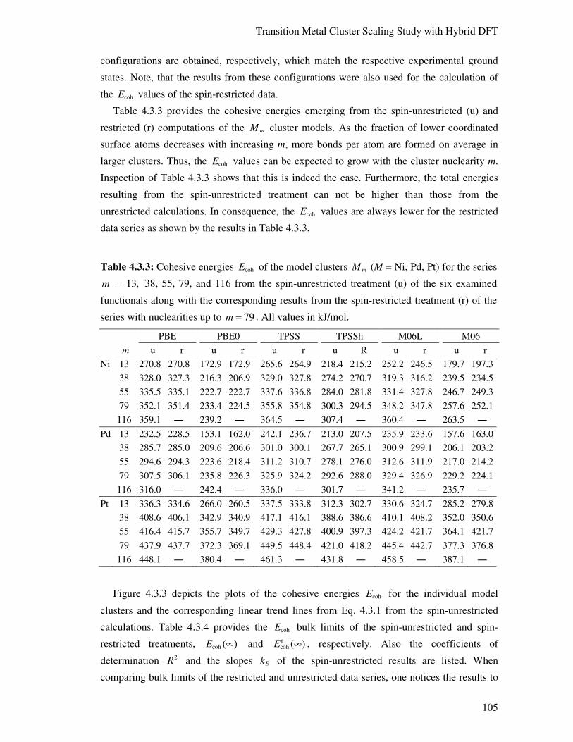
Transition Metal Cluster Scaling Study with Hybrid DFT
105
configurations are obtained, respectively, which match the respective experimental ground
states. Note, that the results from these configurations were also used for the calculation of
the cohE values of the spin-restricted data.
Table 4.3.3 provides the cohesive energies emerging from the spin-unrestricted (u) and
restricted (r) computations of the mM cluster models. As the fraction of lower coordinated
surface atoms decreases with increasing m, more bonds per atom are formed on average in
larger clusters. Thus, the cohE values can be expected to grow with the cluster nuclearity m.
Inspection of Table 4.3.3 shows that this is indeed the case. Furthermore, the total energies
resulting from the spin-unrestricted treatment can not be higher than those from the
unrestricted calculations. In consequence, the cohE values are always lower for the restricted
data series as shown by the results in Table 4.3.3.
Table 4.3.3: Cohesive energies cohE of the model clusters mM (M = Ni, Pd, Pt) for the series
13,m = 38, 55, 79, and 116 from the spin-unrestricted treatment (u) of the six examined
functionals along with the corresponding results from the spin-restricted treatment (r) of the
series with nuclearities up to 79m = . All values in kJ/mol.
PBE PBE0 TPSS TPSSh M06L M06
m u r u r u r u R u r u r
Ni 13 270.8 270.8 172.9 172.9 265.6 264.9 218.4 215.2 252.2 246.5 179.7 197.3
38 328.0 327.3 216.3 206.9 329.0 327.8 274.2 270.7 319.3 316.2 239.5 234.5
55 335.5 335.1 222.7 222.7 337.6 336.8 284.0 281.8 331.4 327.8 246.7 249.3
79 352.1 351.4 233.4 224.5 355.8 354.8 300.3 294.5 348.2 347.8 257.6 252.1
116 359.1 ― 239.2 ― 364.5 ― 307.4 ― 360.4 ― 263.5 ―
Pd 13 232.5 228.5 153.1 162.0 242.1 236.7 213.0 207.5 235.9 233.6 157.6 163.0
38 285.7 285.0 209.6 206.6 301.0 300.1 267.7 265.1 300.9 299.1 206.1 203.2
55 294.6 294.3 223.6 218.4 311.2 310.7 278.1 276.0 312.6 311.9 217.0 214.2
79 307.5 306.1 235.8 226.3 325.9 324.2 292.6 288.0 329.4 326.9 229.2 224.1
116 316.0 ― 242.4 ― 336.0 ― 301.7 ― 341.2 ― 235.7 ―
Pt 13 336.3 334.6 266.0 260.5 337.5 333.8 312.3 302.7 330.6 324.7 285.2 279.8
38 408.6 406.1 342.9 340.9 417.1 416.1 388.6 386.6 410.1 408.2 352.0 350.6
55 416.4 415.7 355.7 349.7 429.3 427.8 400.9 397.3 424.2 421.7 364.1 421.7
79 437.9 437.7 372.3 369.1 449.5 448.4 421.0 418.2 445.4 442.7 377.3 376.8
116 448.1 ― 380.4 ― 461.3 ― 431.8 ― 458.5 ― 387.1 ―
Figure 4.3.3 depicts the plots of the cohesive energies cohE for the individual model
clusters and the corresponding linear trend lines from Eq. 4.3.1 from the spin-unrestricted
calculations. Table 4.3.4 provides the cohE bulk limits of the spin-unrestricted and spin-
restricted treatments, coh ( )E ∞ and rcoh ( )E ∞ , respectively. Also the coefficients of
determination 2R and the slopes Ek of the spin-unrestricted results are listed. When
comparing bulk limits of the restricted and unrestricted data series, one notices the results to

Applications
106
be quite consistent. In most cases the differences are found below ~10 kJ/mol. The largest
deviations of about 30 kJ/mol result from the functionals PBE0 and M06 and may again be
rationalized with the preference of the EXX term for high-spin states.[198] This preference
most likely renders the results of the high-EXX functionals more sensitive to the spin state
compared to those from the semi-local DFT methods or TPSSh.
Figure 4.3.3: Cohesive energies cohE in kJ/mol for the a) Nim, b) Pdm, and c) Ptm cluster
models obtained from the six examined functionals (spin-unrestricted treatment) along with
the corresponding trend lines linear in 1 3m
− . The individual groups of functionals (see text)
are marked accordingly. Figure adapted from Ref. [443].
Compared to the avd values, the cohesive energies vary much more when going from the
smallest to the largest cluster models. In consequence, the coefficients of determination 2R
of the cohE trend lines are higher than those of the avd series. Indeed, the 2R values of the
cohesive energies are always found above 0.99, with the M06 results for the Nim cluster
model series as the only exception ( 2 0.98R ≈ ). In any case, the cohesive energy can be
considered as a quantity which is accurately described by the proposed scaling law, Eq. 4.3.1.
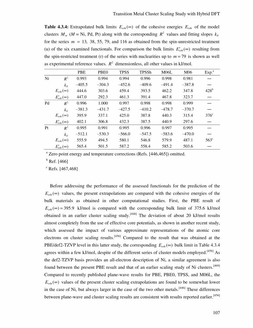
Transition Metal Cluster Scaling Study with Hybrid DFT
107
Table 4.3.4: Extrapolated bulk limits coh ( )E ∞ of the cohesive energies cohE of the model
clusters mM (M = Ni, Pd, Pt) along with the corresponding 2R values and fitting slopes Ek
for the series 13,m = 38, 55, 79, and 116 as obtained from the spin-unrestricted treatment
(u) of the six examined functionals. For comparison the bulk limits rcoh ( )E ∞ resulting from
the spin-restricted treatment (r) of the series with nuclearities up to 79m = is shown as well
as experimental reference values. 2R dimensionless, all other values in kJ/mol.
PBE PBE0 TPSS TPSSh M06L M06 Exp.a
Ni 2R 0.993 0.994 0.994 0.996 0.998 0.981 ―
Ek ‒405.5 ‒304.3 ‒452.6 ‒409.6 ‒491.4 ‒387.8 ―
coh ( )E ∞ 444.6 303.6 459.4 393.5 462.2 347.8 428b
rcoh ( )E ∞ 447.0 292.3 461.3 391.4 467.8 323.7 ―
Pd 2R 0.996 1.000 0.997 0.998 0.998 0.999 ―
Ek ‒381.3 ‒431.7 ‒427.5 ‒410.2 ‒478.7 ‒370.7 ―
coh ( )E ∞ 395.9 337.1 425.0 387.8 440.3 315.4 376c
rcoh ( )E ∞ 402.1 306.8 432.3 387.5 440.9 297.6 ―
Pt 2R 0.995 0.991 0.995 0.996 0.997 0.995 ―
Ek ‒512.1 ‒530.3 ‒566.0 ‒547.5 ‒583.6 ‒470.0 ―
coh ( )E ∞ 555.9 494.5 580.1 546.8 579.9 487.1 563c
rcoh ( )E ∞ 565.4 501.5 587.2 558.4 585.2 503.6 ―
a Zero point energy and temperature corrections (Refs. [446,465]) omitted. b Ref. [466] c Refs. [467,468]
Before addressing the performance of the assessed functionals for the prediction of the
coh ( )E ∞ values, the present extrapolations are compared with the cohesive energies of the
bulk materials as obtained in other computational studies. First, the PBE result of
coh ( ) 395.9E ∞ = kJ/mol is compared with the corresponding bulk limit of 375.6 kJ/mol
obtained in an earlier cluster scaling study.[448] The deviation of about 20 kJ/mol results
almost completely from the use of effective core potentials, as shown in another recent study,
which assessed the impact of various approximate representations of the atomic core
electrons on cluster scaling results.[456] Compared to the result that was obtained at the
PBE/def2-TZVP level in this latter study, the corresponding coh ( )E ∞ bulk limit in Table 4.3.4
agrees within a few kJ/mol, despite of the different series of cluster models employed.[456] As
the def2-TZVP basis provides an all-electron description of Ni, a similar agreement is also
found between the present PBE result and that of an earlier scaling study of Ni clusters.[469]
Compared to recently published plane-wave results for PBE, PBE0, TPSS, and M06L, the
coh ( )E ∞ values of the present cluster scaling extrapolations are found to be somewhat lower
in the case of Ni, but always larger in the case of the two other metals.[446] These differences
between plane-wave and cluster scaling results are consistent with results reported earlier.[456]
Applications
108
The deviations between cluster scaling and plane-wave results are most likely related to
methodological differences like the representation of the atomic core orbitals or the treatment
of atomic systems.
When comparing the semi-local DFT approximations with their corresponding hybrid
DFT counterparts one finds that the inclusion of the EXX term considerably reduces the
cohesive energies. This holds especially for the coh ( )E m values of the individual cluster
models. When comparing PBE0 with PBE, the slopes Ek of the former are found to be more
negative in the case of Pd and Pt. Even in these cases the bulk limits of PBE are always
higher than those of the hybrid functional. In the case of the other two pairs of functionals the
trend lines of the semi-local DFT approximations are always steeper. For the pairs PBE/PBE0
and TPSS/TPSSh the reduction of the coh ( )E ∞ bulk limit caused by the EXX term is largest
for Ni as the semi-local functionals always yield much steeper trend lines. This is most likely
related to the non-vanishing magnetic moment per atom aµ found for the corresponding bulk
material. In the case of the nonmagnetic bulk materials Pd and Pt the effect of the exact-
exchange term on the coh ( )E ∞ values is more comparable. In any case, the reduction of the
coh ( )E ∞ bulk limits seems to correlate roughly with the value of the EXX mixing factor as
the changes are found to be more than twice as large in the case of the PBE/PBE0 pair ( 1α =
0.25) than when going from TPSS to TPSSh ( 1α = 0.10). Thus, the EXX term seems affect
the bond strengths much more than the bond lengths in these two pairs of functionals, apart
from the PBE0 description of Ni, where also the quality of structural results breaks down.
The fact that a hybrid functional can yield similar metal-metal distances but much lower
cohesive energies compared to its semi-local counterpart has also been reported from plane-
wave calculations.[198] The situation appears to be different when the semi-local terms of a
hybrid functional are parametrized in the presence of exact-exchange as in M06. In this case
the slopes Ek are reduced by a similar amount for all three metals compared to those of
M06L. In consequence also the reduction of the coh ( )E ∞ values is always comparable when
going from the M06L to M06. For this pair of functionals the bond elongations due to the
EXX term are found to correlate with the resulting reductions of the bond strengths. While
still being comparable for all three metals, the changes of both bulk limits, av ( )d ∞ and
coh ( )E ∞ , appear to be slightly more pronounced for Pd.
To assess the performance of the six employed DFT approximations, the results of Figure
4.3.3 and Table 4.3.4 are compared to the experimental references for the cohesive energy
values. These reference values would have to be corrected for finite temperature and zero
point energy effects.[446,465] However, in the present case these corrections were omitted as
they are below 4 kJ/mol and thus not relevant in the present context.
The coh ( )E ∞ values from Table 4.3.4 allow for a classification of the assessed functionals
into four groups (see Figure 4.3.3). Group (i) includes thereby the semi-local MGGA
functionals TPSS and M06L, which always yield the highest cohesive energy extrapolations

Transition Metal Cluster Scaling Study with Hybrid DFT
109
for all three metals. In the case of Pt, the coh ( )E ∞ bulk limits yield result to nearly identical
values, 580.1 kJ/mol for TPSS and 579.9 kJ/mol for M06L. Thus, these two functionals
overestimate the experimental reference[467,468] of 563 kJ/mol by about 17 kJ/mol. The
overestimations of these functionals are somewhat more pronounced in the case of the other
two metals. The coh ( )E ∞ bulk limits of nickel amount to 459.4 kJ/mol (TPSS) and 462.2
kJ/mol (M06L) and exceed the experimental reference[466] of 428 kJ/mol by about 30 kJ/mol.
In the case of Pd the results of both functionals differ somewhat more from each other, 425.0
and 440.3 kJ/mol for TPSS and M06L, respectively, as well as from the experimental
result[467,468] of 376 kJ/mol. Thus, with deviations of 17, 30, and 49 kJ/mol for the cohE bulk
limit of Pt, Ni, and Pd, respectively, the exceptional performance of TPSS previously
reported[264,470] for smaller transition metal compounds cannot be confirmed by the present
results for larger cluster models. In contrast, the rather larger deviation of M06L is more in
line with specific deficiencies of this method that were previously noted in a study of smaller
Pd clusters.[447]
The pure GGA functional PBE yields the next highest cohE extrapolations for the three
examined transition metals and is assigned to group (ii). Its coh ( )E ∞ bulk limits of 444.6 and
395.9 kJ/mol obtained in the case of Ni and Pd, respectively, overestimate the experimental
results, while the cohE extrapolation for Pt (555.9 kJ/mol) underestimates the corresponding
experimental reference slightly. With deviations of about 17 and 7 kJ/mol PBE yields the best
estimates for the cohesive energy of bulk Ni and Pt, respectively.
Also group (iii) includes a single functional only, namely TPSSh with its low EXX mixing
factor. TPSSh yields coh ( )E ∞ extrapolations of 393.5, 387.8, and 546.8 kJ/mol for Ni, Pd,
and Pt, respectively. With a deviation of 12 kJ/mol, the TPSSh estimate for Pd exhibits the
best agreement with the experimental reference of all examined functionals. Also the
accuracy of the other two estimates remains still comparable to that of the PBE results.
Finally, the high exact-exchange functionals PBE0 and M06 comprise group (iv) and
always yield the lowest coh ( )E ∞ extrapolations. In most cases, however, this implies also the
worst accuracy as the cohesive energies of the bulk materials are often strongly
underestimated. In the case of Pt quite similar bulk limits are obtained with both functionals
which differ by about 70 kJ/mol from the experimental reference. Compared to that, the
coh ( )E ∞ values of 337.1 and 315.4 kJ/mol obtained for Pd with PBE0 and M06, respectively,
deviate somewhat less from the experimental result and are thus more accurate than the
corresponding M06L result. Most underestimated are the cohesive energies of bulk nickel.
The corresponding error of M06 (~80 kJ/mol) is smaller than that of PBE0, ~125 kJ/mol.
Thus, for the description of the bond strengths of metallic systems, the functionals with a
high fraction of exact-exchange exhibit show a somewhat erratic behavior. This holds
especially for the magnetic material Ni. The errors of PBE0 and M06 are likely related to the
static correlation error (see Section 2.2.6), which is most pronounced in these methods.[130,217]
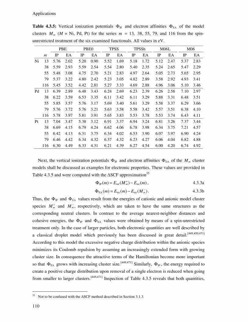
Applications
110
Table 4.3.5: Vertical ionization potentials IPΦ and electron affinities EAΦ of the model
clusters mM (M = Ni, Pd, Pt) for the series 13,m = 38, 55, 79, and 116 from the spin-
unrestricted treatment of the six examined functionals. All values in eV.
PBE PBE0 TPSS TPSSh M06L M06
m IP EA IP EA IP EA IP EA IP EA IP EA
Ni 13 5.76 2.02 5.20 0.90 5.52 1.69 5.18 1.72 5.12 2.47 5.37 2.83
38 5.59 2.93 5.59 2.54 5.54 2.80 5.40 2.35 5.24 2.65 5.47 2.29
55 5.48 3.08 4.75 2.70 5.21 2.83 4.97 2.64 5.05 2.73 5.65 2.95
79 5.37 3.22 4.80 2.42 5.23 3.05 4.82 2.89 3.58 2.92 4.93 3.41
116 5.45 3.52 4.42 2.81 5.27 3.33 4.69 2.88 4.96 3.06 5.10 3.46
Pd 13 6.39 2.89 6.48 3.43 6.24 2.69 6.23 2.39 6.26 2.58 7.10 2.97
38 6.22 3.59 6.53 3.35 6.11 3.42 6.11 3.29 5.88 3.31 6.48 3.51
55 5.85 3.57 5.76 3.17 5.69 3.40 5.61 3.29 5.58 3.37 6.29 3.66
79 5.76 3.72 5.76 3.21 5.63 3.58 5.58 3.42 5.57 3.51 6.38 4.10
116 5.78 3.97 5.81 3.91 5.65 3.83 5.53 3.78 5.53 3.74 6.43 4.11
Pt 13 7.04 3.47 5.38 3.12 6.91 3.37 6.94 3.24 6.81 3.26 7.37 3.44
38 6.69 4.15 6.79 4.24 6.62 4.06 6.78 3.98 6.34 3.75 7.21 4.57
55 6.42 4.13 6.31 3.75 6.34 4.02 6.53 3.90 6.07 3.97 6.90 4.24
79 6.46 4.42 6.34 4.32 6.37 4.32 6.23 4.27 6.06 4.04 6.82 4.88
116 6.30 4.49 6.33 4.31 6.21 4.39 6.27 4.54 6.00 4.20 6.74 4.92
Next, the vertical ionization potentials IPΦ and electron affinities EAΦ of the mM cluster
models shall be discussed as examples for electronic properties. These values are provided in
Table 4.3.5 and were computed with the ∆SCF approximation35
IP tot tot( ) ( ) ( )mm E M E m+Φ = − , 4.3.3a
EA tot tot( ) ( ) ( )mm E m E M−Φ = − . 4.3.3b
Thus, the IPΦ and EAΦ values result from the energies of cationic and anionic model cluster
species mM+ and mM
− , respectively, which are taken to have the same structures as the
corresponding neutral clusters. In contrast to the average nearest-neighbor distances and
cohesive energies, the IPΦ and EAΦ values were obtained by means of a spin-unrestricted
treatment only. In the case of larger particles, both electronic quantities are well described by
a classical droplet model which previously has been discussed in great detail.[449,450,471]
According to this model the excessive negative charge distribution within the anionic species
minimizes its Coulomb repulsion by assuming an increasingly extended form with growing
cluster size. In consequence the attractive terms of the Hamiltonian become more important
so that EAΦ grows with increasing cluster size.[449,471] Similarly, IPΦ , the energy required to
create a positive charge distribution upon removal of a single electron is reduced when going
from smaller to larger clusters.[449,471] Inspection of Table 4.3.5 reveals that both quantities,
35 Not to be confused with the ∆SCF method described in Section 3.1.3.
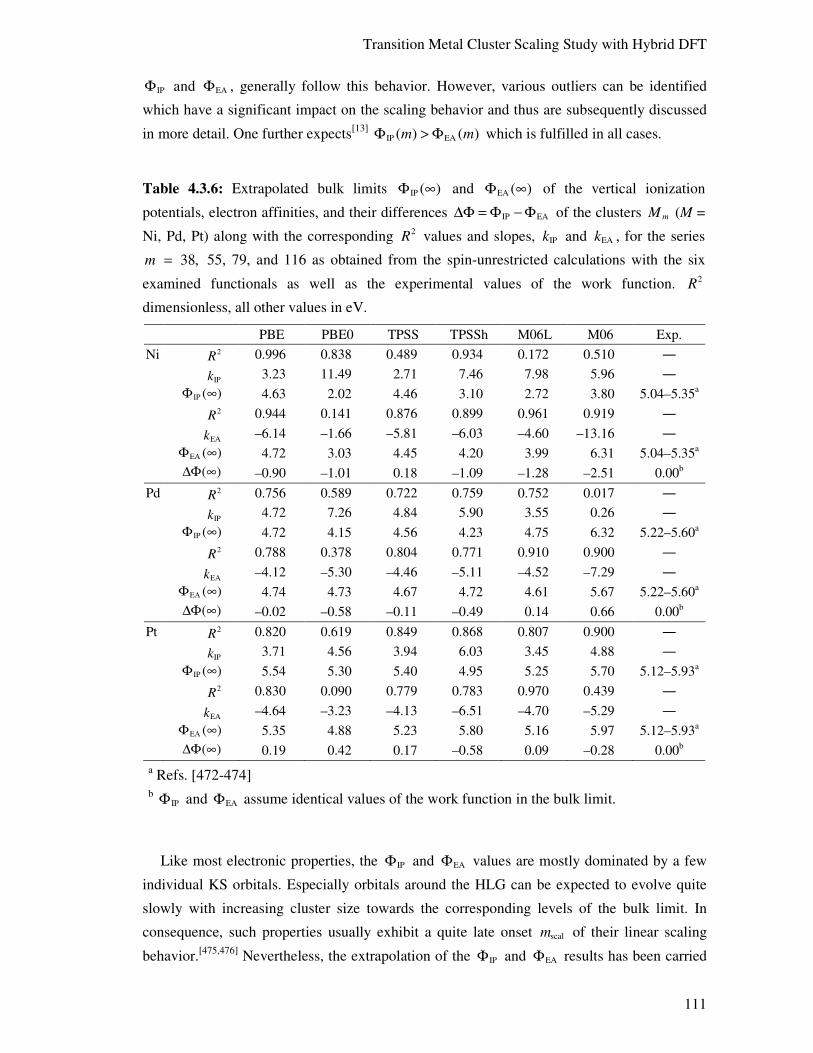
Transition Metal Cluster Scaling Study with Hybrid DFT
111
IPΦ and EAΦ , generally follow this behavior. However, various outliers can be identified
which have a significant impact on the scaling behavior and thus are subsequently discussed
in more detail. One further expects[13] IP EA( ) ( )m mΦ > Φ which is fulfilled in all cases.
Table 4.3.6: Extrapolated bulk limits IP ( )Φ ∞ and EA ( )Φ ∞ of the vertical ionization
potentials, electron affinities, and their differences IP EA∆Φ = Φ − Φ of the clusters mM (M =
Ni, Pd, Pt) along with the corresponding 2R values and slopes, IPk and EAk , for the series
38,m = 55, 79, and 116 as obtained from the spin-unrestricted calculations with the six
examined functionals as well as the experimental values of the work function. 2R
dimensionless, all other values in eV.
PBE PBE0 TPSS TPSSh M06L M06 Exp.
Ni 2R 0.996 0.838 0.489 0.934 0.172 0.510 ―
IPk 3.23 11.49 2.71 7.46 7.98 5.96 ―
IP ( )Φ ∞ 4.63 2.02 4.46 3.10 2.72 3.80 5.04–5.35a
2R 0.944 0.141 0.876 0.899 0.961 0.919 ―
EAk –6.14 –1.66 –5.81 –6.03 –4.60 –13.16 ―
EA ( )Φ ∞ 4.72 3.03 4.45 4.20 3.99 6.31 5.04–5.35a
( )∆Φ ∞ –0.90 –1.01 0.18 –1.09 –1.28 –2.51 0.00b
Pd 2R 0.756 0.589 0.722 0.759 0.752 0.017 ―
IPk 4.72 7.26 4.84 5.90 3.55 0.26 ―
IP ( )Φ ∞ 4.72 4.15 4.56 4.23 4.75 6.32 5.22–5.60a
2R 0.788 0.378 0.804 0.771 0.910 0.900 ―
EAk –4.12 –5.30 –4.46 –5.11 –4.52 –7.29 ―
EA ( )Φ ∞ 4.74 4.73 4.67 4.72 4.61 5.67 5.22–5.60a
( )∆Φ ∞ –0.02 –0.58 –0.11 –0.49 0.14 0.66 0.00b
Pt 2R 0.820 0.619 0.849 0.868 0.807 0.900 ―
IPk 3.71 4.56 3.94 6.03 3.45 4.88 ―
IP ( )Φ ∞ 5.54 5.30 5.40 4.95 5.25 5.70 5.12–5.93a
2R 0.830 0.090 0.779 0.783 0.970 0.439 ―
EAk –4.64 –3.23 –4.13 –6.51 –4.70 –5.29 ―
EA ( )Φ ∞ 5.35 4.88 5.23 5.80 5.16 5.97 5.12–5.93a
( )∆Φ ∞ 0.19 0.42 0.17 –0.58 0.09 –0.28 0.00b a Refs. [472-474] b IPΦ and EAΦ assume identical values of the work function in the bulk limit.
Like most electronic properties, the IPΦ and EAΦ values are mostly dominated by a few
individual KS orbitals. Especially orbitals around the HLG can be expected to evolve quite
slowly with increasing cluster size towards the corresponding levels of the bulk limit. In
consequence, such properties usually exhibit a quite late onset scalm of their linear scaling
behavior.[475,476] Nevertheless, the extrapolation of the IPΦ and EAΦ results has been carried
Applications
112
out as well, with the corresponding bulk limits provided in Table 4.3.6. The results for the
13M species were not included in this extrapolation as these clusters were found to exhibit
strongly molecular characteristics with regard to their electronic properties. Nevertheless, the
coefficients of determination 2R obtained from the extrapolation of the remaining IPΦ and
EAΦ data are found to be significantly lower compared to those from the extrapolations of
avd and cohE discussed above. In some cases, which mostly occur for the high EXX hybrid
functionals PBE0 and M06, the coefficients of determination are so low, 2 0.75R ≪ , that the
series of results obtained for the employed set of cluster models seem to scale hardly at all.
Before addressing the origin of this occasional behavior the results of the smoothly
extrapolating series shall be discussed first.
In the bulk limit an excessive charge distribution becomes infinitely extended and
therefore its Coulomb repulsion vanishes.[449,471] Thus, for metallic materials with vanishing
band gap both quantities, IPΦ and EAΦ , have the same bulk limit as the energy to create
positive or negative charge distribution is dominated by the work function Φ in both
cases.[449,471] However, this quantity is not only specific to the bulk material, but varies also
with the type of the crystalline surface.[468] Therefore the ranges of experimental values[472-474]
measured for different crystalline orientations are used as references.
In the case of Pt the bulk limits of the vertical ionization potentials that could be obtained
with 2 0.75R > result from the functionals PBE, TPSS, TPSSh, M06L, and M06 and amount
to 5.54, 5.40, 4.95, 5.25, and 5.70 eV, respectively. These values are all within the
corresponding range of experimental reference values for Φ , 5.12–5.93 eV,[472-474] except for
TPSSh, which slightly underestimates it. The EAΦ values of PBE0 and M06 do not scale
properly, while the EA ( )Φ ∞ bulk limits of all other functionals are within the experimental
range of Φ . For Pd, the functionals PBE, TPSSh, and M06L exhibit 2 0.75R > for both
series, IPΦ and EAΦ , but always underestimate the work function by about 0.5–1.0 eV. Also
the EAΦ values resulting from M06 scale well, while their bulk limit is found slightly above
the range of experimental Φ values. The IPΦ results for Ni can be extrapolated reasonably
well only in the case of PBE, PBE0, and TPSSh, whereas all functionals underestimate the
work function by about 0.4, 3.0, and 1.9 eV, respectively. The corresponding EAΦ values
exhibit a reasonable scaling behavior for all functionals, except for PBE0. The deviations of
the corresponding bulk limits from the experimental references are reduced to ~1 eV at most.
Table 4.3.6 also provides the bulk limits ( )∆Φ ∞ of the series of differences
IP EA( ) ( ) ( )m m m∆Φ = Φ − Φ . These extrapolations should yield a zero band gap and serve as
indicator for the consistency of the results for IPΦ and EAΦ . The strongest deviations of
( )∆Φ ∞ from the expected value of zero are obtained in the case of Ni, where only the TPSS
functionals yields a reasonably low estimate, ( ) 0.18∆Φ ∞ = eV. All other examined
functionals extrapolate the ∆Φ series to negative values which range from about ‒0.9 eV in
the case of PBE to the bulk limit of ( ) 2.5∆Φ ∞ ≈ − eV obtained with M06. The ( )∆Φ ∞
Transition Metal Cluster Scaling Study with Hybrid DFT
113
extrapolations are closer to the theoretical limit of zero for the other two elements, whereas
the semi-local DFT approximations always deviate by less than 0.2 eV. The hybrid
functionals always yield larger deviations than that. Indeed, hybrid DFT methods are known
to predict not necessarily a vanishing band gap for metallic systems. Therefore, one may
expect ( ) 0∆Φ ∞ > from hybrid functionals as opposed to some of the bulk limits for ∆Φ
listed in Table 4.3.6. These negative ( )∆Φ ∞ bulk limits are, however, mostly related to
outliers in the IPΦ and EAΦ series and not to the electronic structure description itself.
Compared to earlier all-electron PBE results for Pd,[448] the extrapolations of the
corresponding IPΦ and EAΦ values of the present study are lower by 0.33 and 0.15 eV,
respectively. These differences most likely arise from a stronger amount of level broadening
employed in the all-electron calculations as well as from a different choice of the model
clusters used for the extrapolation (Pd147 instead of Pd116). In any case, the bulk limit of
( )∆Φ ∞ obtained in the present extrapolation is significantly closer to zero.
As mentioned before, electronic properties like the vertical ionization potentials and
electron affinities are often dominated by individual orbitals. The effect of the applied FON
broadening technique is in some sense counteracting this aspect as it involves a potentially
larger number of orbitals in the ionization process if the HOMO-LUMO gap is small. Thus,
the FON broadening leads to an earlier onset of the aforementioned classical behavior of the
ionic clusters according to the droplet model. However, smaller clusters still exhibit HLGs
large enough to neglect these effects of the FON technique. In addition, the hybrid
functionals generally tend to increase the HOMO-LUMO gap further. In these cases the IPΦ
and EAΦ values remain mostly affected by the evolution of individual orbitals up to larger
cluster sizes. This generally reduces the scalability of vertical ionization potentials and
electron affinities. Furthermore, the striking outliers found in some of the series of IPΦ and
EAΦ results seem to be related to cases where one of these orbitals involved in the ionization
happens to be symmetry-degenerate (e- or t-type). In consequence, electron configurations
result where individual electrons (or holes) are distributed among two or three symmetry-
degenerate orbitals. This in turn leads to significant shifts in the IPΦ and EAΦ energies. The
occurrence of symmetry-degenerate orbitals is a direct consequence of the hO symmetry
constraints that were imposed on the cluster models. Thus, the highly symmetric treatment
represents a clear drawback for the calculation of electronic properties like IPΦ and EAΦ , at
least when point group symmetries with degenerate irreducible representations are employed.
Nevertheless, it has to be emphasized at this point again that high symmetries like hO do not
only reflect the electronic structure of the corresponding fcc bulk materials but are also
essential for obtaining suitably converged KS orbitals of larger transition metal clusters.
Applications
114
4.3.4. Electronic Structure Aspects
The application of FON techniques can have a significant influence on electronic properties
like ionization energies, as discussed in Section 4.3.3. This effect clearly warrants further
discussion. Apart from the LDA exchange term, level broadening favors electron
delocalization. Indeed, FON techniques are also known to provide an implicit description of
static correlation effects (see Section 2.2.6) as well.[235,236,243] This implicit description is of
course related to the employed XC approximation as well as to the system at hand. In this
context one can formulate several requirements, which are necessary to achieve an implicit
description of static correlation effects for transition metal clusters. These are (i) a sufficient
amount of LDA exchange present in the XC term to prevent the corresponding XC hole (see
Section 2.2.2) from becoming overly delocalized, (ii) a vanishing band gap in the case of
larger metallic systems, (iii) a nonzero density of states (DOS) around the HOMO-LUMO
gap, and (iv) the application of a FON technique with a sufficiently large broadening
parameter to include as many relevant orbitals near the HLG as possible.36
KS-DFT represents a single-determinant formulation only, hence, does not provide any
direct measure for static correlation effects. Thus, the aforementioned requirements represent
a rough guideline only. In the present context they are, however, sufficient to provide a
rationalization of the behavior observed for the assessed XC approximations. To this end, the
number of KS orbitals located within a certain energy interval near the HOMO-LUMO gap
was examined. Thereby the two intervals F F[ 0.5 eV, ]ε ε− and F F[ 0.5 eV, 0.5 eV]ε ε− +
where studied, with Fε being the center of the HLG, which in turn was defined as the energy
difference between the lowest KS orbital with a population below 1 2 and the highest orbital
with a population of more than that. The designators occDOSI and tot
DOSI are used to denote the
orbital counts obtained for the first and second interval, respectively. Note, that in the limit of
bulk materials, occDOSI and tot
DOSI are to be understood as integrals of the density of states over
the respective intervals. Figure 4.3.4 provides a plot of the values of both quantities on the
example of the Ptm cluster series and the functionals PBE, PBE0, and TPSSh.
Apart from minor deviations in the case of smaller systems, the number of KS orbitals
around the HLG grows as expected with the cluster nuclearity. Both, occDOSI and tot
DOSI are found
to be highest in the case of PBE as this functional yields comparatively small HOMO-LUMO
gaps. A similar behavior results also from both MGGA functionals. In contrast, both DOSI
values obtained from PBE0 (and M06 as well) remain small even for larger cluster sizes.
Especially the numbers of more than half populated KS orbitals remain very small, even for
larger clusters like Pt116. Thus, the behavior of high EXX hybrid functionals can be clearly
distinguished from that of semi-local DFT methods. However, the DOSI values resulting from
36 The actual value of the broadening parameter is restricted, of course, because a too extensive level
broadening does not lead to a realistic electronic structure description.

Transition Metal Cluster Scaling Study with Hybrid DFT
115
the low EXX hybrid functional TPSSh remain fairly large, despite of being lower than the
corresponding occDOSI and tot
DOSI counts from the semi-local functionals. A similar behavior is
also obtained for the other two examined transition metal elements.
Figure 4.3.4: Orbital counts occDOSI and tot
DOSI within the intervals F F[ 0.5 eV, ]ε ε− and
F F[ 0.5 eV, 0.5 eV]ε ε− + (see text) obtained for the Ptm cluster models ( 13,m = 38, 55, 79,
and 116) with PBE, PBE0, and TPSSh. Figure adapted from Ref. [443].
Thus, the amount of exact-exchange in TPSSh can be considered as small enough to yield
a reasonable narrow HOMO-LUMO gap in the case of larger clusters. In consequence, also
the number of orbitals near the HLG remains significantly large. As stated at the beginning of
this section, this is required for an adequate electronic structure description of metallic
systems influenced by static correlation effects. On the other hand, hybrid functionals with a
high EXX mixing factor such as PBE0 and M06 can be expected to behave similarly to the
HF method, which severely fails for metals due to its depleted density of states around the
Fermi level and its discontinuous behavior of the band dispersion.[477,478]

Applications
116
Table 4.3.7: Magnetic moments per atom aµ of the series of clusters mM (M = Ni, Pd, Pt) as
obtained from the six examined functionals. All values in Bohr magnetons.
m PBE PBE0 TPSS TPSSh M06L M06 Ni 13 0.615 0.615 0.615 0.615 0.655 0.615 38 0.795 0.842 0.891 0.895 0.895 0.895 55 0.722 0.618 0.733 0.837 0.870 0.836 79 0.682 0.785 0.730 0.760 0.778 0.658 116 0.787 0.810 0.792 0.793 0.793 0.793 Pd 13 0.461 0.462 0.461 0.462 0.461 0.462 38 0.214 0.211 0.216 0.474 0.473 0.316 55 0.184 0.400 0.211 0.219 0.282 0.182 79 0.413 0.430 0.429 0.455 0.421 0.405 116 0.398 0.379 0.398 0.397 0.499 0.483 Pt 13 0.461 0.462 0.462 0.462 0.462 0.462 38 0.116 0.158 0.140 0.158 0.192 0.158 55 0.177 0.473 0.181 0.182 0.242 0.436 79 0.192 0.278 0.208 0.405 0.602 0.228 116 0.000 0.034 0.000 0.018 0.334 0.241
The magnetic moments per atom aµ shall be briefly discussed as another aspect of the
electronic structure computed for the examined model clusters with the assessed functionals.
These values are provided in Table 4.3.7. Transition metal clusters are often magnetic even
for elements which exhibit 0aµ = in the bulk limit.[447,475,476] Furthermore, such systems
feature an oscillating behavior in their aµ values up to very large nuclearities.[447,475,476] This
essentially prevents any extrapolations of aµ results to the bulk limit from cluster sizes used
in the present study. A scaling approach was therefore not attempted for this quantity.
Instead, the general trends in the aµ values of the mM clusters were found to reflect some
construction principles of the assessed functionals. The employed functionals yield mostly
identical values for the 13M clusters due to the mostly molecular characteristics of these
systems. The aµ values from the various functionals start to differ at 38m = . For clusters of
this size and above, the plainly added EXX term as in PBE0 and TPSSh generally causes
larger magnetic moments compared to the corresponding local functionals. This propensity
for larger aµ values agrees with the previously reported preference of hybrid DFT methods
for high-spin states in the case of bulk materials.[479] In contrast, the M06L functional yields
mostly higher magnetic moments than its hybrid DFT counterpart M06. This agrees with the
recently observed behavior[447] for the magnetic moments of Pd clusters obtained with M06L
and may most likely arise from the different parametrization of the corresponding semi-local
XC terms in both functionals.
Transition Metal Cluster Scaling Study with Hybrid DFT
117
4.3.5. Conclusions
The addition of exact-exchange to local DFT approximations as in hybrid density functionals
leads to significant changes in the description of transition metal systems as shown in
Sections 4.3.3 and 4.3.4 for the group 10 model clusters Nim, Pdm, and Ptm. In summary,
hybrid DFT methods tend to underestimate the strengths of metal-metal bonds and to favor
high-spin states, which both leads to significantly altered structures in some cases.
As mentioned in Section 2.3.3, the EXX mixing factor 1α can only be chosen on empirical
grounds and a specific value for 1α may work well for systems of certain type but lead to
severe failures for other species. In the present case 1 0.25α ≥ as in PBE0 and M06 was
found to often cause an erratic behavior in the prediction of most quantities. While PBE0 is
still able to provide accurate structural results in some cases, M06 always fails for this task.
Furthermore, the M06 hybrid functional and its semi-local counterpart M06L, seem to suffer
from the empirical aspects of its construction.
In contrast, the hybrid functional TPSSh with 1 0.1α = provides an overall accurate
description of the examined transition metal clusters, which is at least on a par with that of
the PBE GGA functional for energetic quantities and better than that for structural results.
The good accuracy of this hybrid functional is somewhat surprising as its value for the EXX
mixing factor was obtained from a parametrization on properties of main group compounds
only.[212] The ability of the TPSSh approximation to describe transition metals was
rationalized with the density of states around the HOMO-LUMO gap which seems still
sufficiently large to allow for an implicit description of static correlation effects by means of
the local exchange term and level broadening. However, its actually good accuracy may be
rationalized with the partial self-interaction correction provided by its EXX term. While the
SIE does not cause as dramatic failures in the description of the mM species, as in the case of
nickel subcarbonyls (Section 4.2), the transition metal clusters can certainly not be considered
unaffected by this artifact. Indeed in this context the TPSSh functional seems to provide a
good tradeoff between the self-interaction error and the static correlation error, which may be
significant in cluster scaling approaches as residual self-repulsion can scale with the system
size.[215] Therefore, the TPSSh functional seems attractive for problems that simultaneously
involve metallic and molecular moieties as the latter may be more prone to suffer from self-
interaction artifacts.

Applications
118
4.4. CO Adsorption on Platinum Model Clusters
4.4.1. The CO Puzzle
The following sections discuss the results obtained with the semi-local functionals PBE,
TPSS, and M06L, with the hybrid DFT approximations PBE0, TPSSh, and M06 as well as
with the PBE+Umol method for the CO adsorption on the (111) facets of Pt model clusters.
The presentation of the results obtained with the latter method thereby follows Ref. [286].
The correct description of the adsorption of the CO molecule on extended transition metal
surfaces is a well-known challenge for semi-local DFT approximations.[480-484] Indeed, in the
case of the Pt(111) surface semi-local functionals often overestimate the corresponding CO
adsorption energy by more than 40 kJ/mol[482,483] compared to experimental reference values,
115±15 kJ/mol.[485-487]
Figure 4.4.1: Schematics of the back-bonding mechanism for the adsorption of the CO
molecule on extended transition metal surfaces. Due to the self-interaction error in semi-local
DFT methods the energy of the 2π* orbitals of the CO molecule is too low which artificially
enhances its back-bonding interaction with the metal d-band across the Fermi level Fε .
Figure adapted from Ref. [286].
This quantitative inaccuracy can be rationalized by referring to the back-bonding
interaction within the Blyholder model (see Section 4.2).[438,488-491] In the case of the
adsorption of CO on transition metal surfaces, the Blyholder model predicts a primary
interaction between the CO 5σ orbital and the surface (σ-bonding) as well a partial electron
transfer from the d-band of the extended surface back into the CO 2π* orbitals (back-
bonding).[438,488-491] Back-bonding between these two interaction partners is increased when
the CO 2π* orbitals are lowered in energy.[438,488-491] As a direct consequence of the missing
discontinuity of the XC potential at integer occupation numbers due to the self-interaction

CO Adsorption on Platinum Model Clusters
119
error (see Section 2.2.5), partially populated levels exhibit a too low energy.[480] This holds
especially for the KSε energies of the CO 2π* orbitals, which is depicted in Figure 4.4.1.
Thus, upon adsorption of the CO molecule on a transition metal surface, the SIE causes the
band gap to be too small which in turn leads to overestimated adsorption energies.[480]
Another important issue concerns the preferred site at which the CO molecule adsorbs on
the (111) surface. Figure 4.4.2 depicts the location of the four distinct, highly symmetric sites
for the CO adsorption on extended (111) surfaces: the 1µ -coordinated top site (denoted by
“t”), the twofold coordinated 2µ -type bridge site (“b”), and the hollow sites with a 3µ -
coordination. In the case of the latter one can further distinguish between fcc-type (“f”) and
hcp-type (“h”) hollow sites, depending on the position of the second atomic layer of the (111)
surface.[481,492]
Figure 4.4.2: Positions of the top (t), bridge (b), and hcp- (h) and fcc-hollow (f) adsorption
sites on the top (white) and sub-surface (dark grey) layers of an extended (111) surface.
The preference for the adsorption on a specific site depends on various properties of the
surface at hand like the work function, the filling of the individual bands (especially the d-
band), and the energetic position of the bands with respect to the Fermi level.[482,486,488-491,493]
In the case of the Pt(111) surface a preference for a CO adsorption at the top site is reported
by several experimental studies.[494-498] In contrast, semi-local DFT approximations yield a
preference for the fcc-hollow site.[480,481,499,500] After this qualitative failure of semi-local DFT
methods has been recognized, it was termed as the “CO puzzle”.[480,481] Subsequently a large
number of studies was dedicated to rationalize the origin of this problem. In this context, the
influences of the adsorption site model,[286,492,500,501] of relativistic effects,[500,502-504] of the
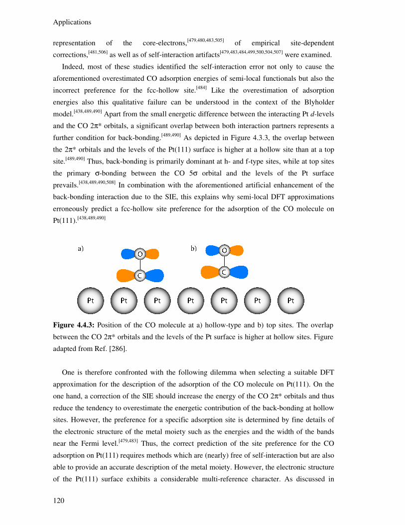
Applications
120
representation of the core-electrons,[479,480,483,505] of empirical site-dependent
corrections,[481,506] as well as of self-interaction artifacts[479,483,484,499,500,504,507] were examined.
Indeed, most of these studies identified the self-interaction error not only to cause the
aforementioned overestimated CO adsorption energies of semi-local functionals but also the
incorrect preference for the fcc-hollow site.[484] Like the overestimation of adsorption
energies also this qualitative failure can be understood in the context of the Blyholder
model.[438,489,490] Apart from the small energetic difference between the interacting Pt d-levels
and the CO 2π* orbitals, a significant overlap between both interaction partners represents a
further condition for back-bonding.[489,490] As depicted in Figure 4.3.3, the overlap between
the 2π* orbitals and the levels of the Pt(111) surface is higher at a hollow site than at a top
site.[489,490] Thus, back-bonding is primarily dominant at h- and f-type sites, while at top sites
the primary σ-bonding between the CO 5σ orbital and the levels of the Pt surface
prevails.[438,489,490,508] In combination with the aforementioned artificial enhancement of the
back-bonding interaction due to the SIE, this explains why semi-local DFT approximations
erroneously predict a fcc-hollow site preference for the adsorption of the CO molecule on
Pt(111).[438,489,490]
Figure 4.4.3: Position of the CO molecule at a) hollow-type and b) top sites. The overlap
between the CO 2π* orbitals and the levels of the Pt surface is higher at hollow sites. Figure
adapted from Ref. [286].
One is therefore confronted with the following dilemma when selecting a suitable DFT
approximation for the description of the adsorption of the CO molecule on Pt(111). On the
one hand, a correction of the SIE should increase the energy of the CO 2π* orbitals and thus
reduce the tendency to overestimate the energetic contribution of the back-bonding at hollow
sites. However, the preference for a specific adsorption site is determined by fine details of
the electronic structure of the metal moiety such as the energies and the width of the bands
near the Fermi level.[479,483] Thus, the correct prediction of the site preference for the CO
adsorption on Pt(111) requires methods which are (nearly) free of self-interaction but are also
able to provide an accurate description of the metal moiety. However, the electronic structure
of the Pt(111) surface exhibits a considerable multi-reference character. As discussed in
CO Adsorption on Platinum Model Clusters
121
Sections 2.2.5 and 2.2.6, any self-interaction correction automatically deteriorates the implicit
description of static correlation by local exchange functionals, unless the correlation term can
account for this latter effect. Thus, the rather unphysical description of the density of states
from hybrid DFT methods like PBE0 (see Section 4.3) also affects the results for the CO
adsorption site preference.[479,483]
The B3LYP functional was occasionally reported to predict the correct top site preference
for the CO adsorption on Pt(111) or to render both, top and fcc-hollow sites, nearly
degenerate.[479,500,501,507] However, given its notoriously bad description of transition
metals,[198,264,266-270] B3LYP is unlikely to deliver the top site preference for the correct
reason. The same is true for the vdW-DFT methods (see Section 2.2.7), which were reported
to predict a CO adsorption at the top site as well, but actually do not provide any self-
interaction correction at all.[509] Thus, the correct site preference obtained with vdW-DFT
functionals can only result from an altered description of the electronic structure of the metal
moiety compared to semi-local functionals, but not from the energy of the CO 2π* orbitals.
According to the results of the case study presented in Section 4.3 the hybrid functional
TPSSh provides an accurate description of late transition metals.[443] One may thus hope that
its comparatively small exact-exchange term ( 1 0.1α = ) reduces the self-interaction
sufficiently enough to correct the energy of the CO 2π* orbitals. This motivated the
subsequently presented study where the performance of six DFT approximations, namely
PBE,[49] PBE0,[87] TPSS,[75] TPSSh,[212] M06L,[77] and M06[77,90] was assessed on the example
of the CO adsorption at various sites on the (111) facets of different cluster models (see
Section 4.4.2). Furthermore, the influence of scalar relativistic effects was briefly examined.
Furthermore, these models were also studied with the PBE+Umol method, whose SIE
correction was projected onto the CO 2π* orbitals.[286] To assess the influence of this
correction the value of the parameter 2π*U (see Sections 2.4 and 4.2) was varied between 1.0,
1.5, and 2.0 eV.[286] At this point it is worth emphasizing that, while the Umol(CO 2π*) term
led to unphysical results for the nickel carbonyl complexes (see Section 4.2), the situation is
quite different in the case of larger Pt clusters. First, the Pt 5d subshell is rather delocalized in
larger transition metal particles so that the prerequisites for an application of the DFT+Umol
correction to the Pt 5d orbitals are not really met. While the correct localization of the Ni 3d
subshell in the nickel carbonyl complexes is important, its orbitals are significantly more
compact than those of the Pt 5d subshell. Thus, in the 5d orbitals, self-repulsion is much
lower and so is the tendency to minimize it through delocalization. Furthermore, the HOMO-
LUMO gap is smaller in larger transition metal clusters compared to the carbonyl complexes.
In consequence, the correct energy of the CO 2π* orbitals is, according to the above well-
established rationalization, most important for the correct prediction of the CO adsorption site
preference. Therefore, the application of the Umol(CO 2π*) correction term is well justified
in the case of the CO adsorption on Pt model clusters.

Applications
122
4.4.2. Adsorption Site Models
In the following the adsorption site models on the (111) facets of the Pt model clusters
employed in the present case study are presented. These sites are subject to two main effects
resulting from the finite size of the cluster models;[454,455,510-513] the influence of under-
coordinated atoms of the facet border and of elongated metal-metal distances between surface
atoms that are induced by the clusters core atoms. Especially the former effect can lead to
significantly higher adsorption energies, which demands a careful analysis. The effect of the
average metal-metal distances on the CO adsorption energies is briefly addressed at the end
of this section.
Figure 4.4.4: Position of the CO adsorption sites on the (111) facets of the model clusters
Pt79, Pt140, and Pt225 employed in the present case study.
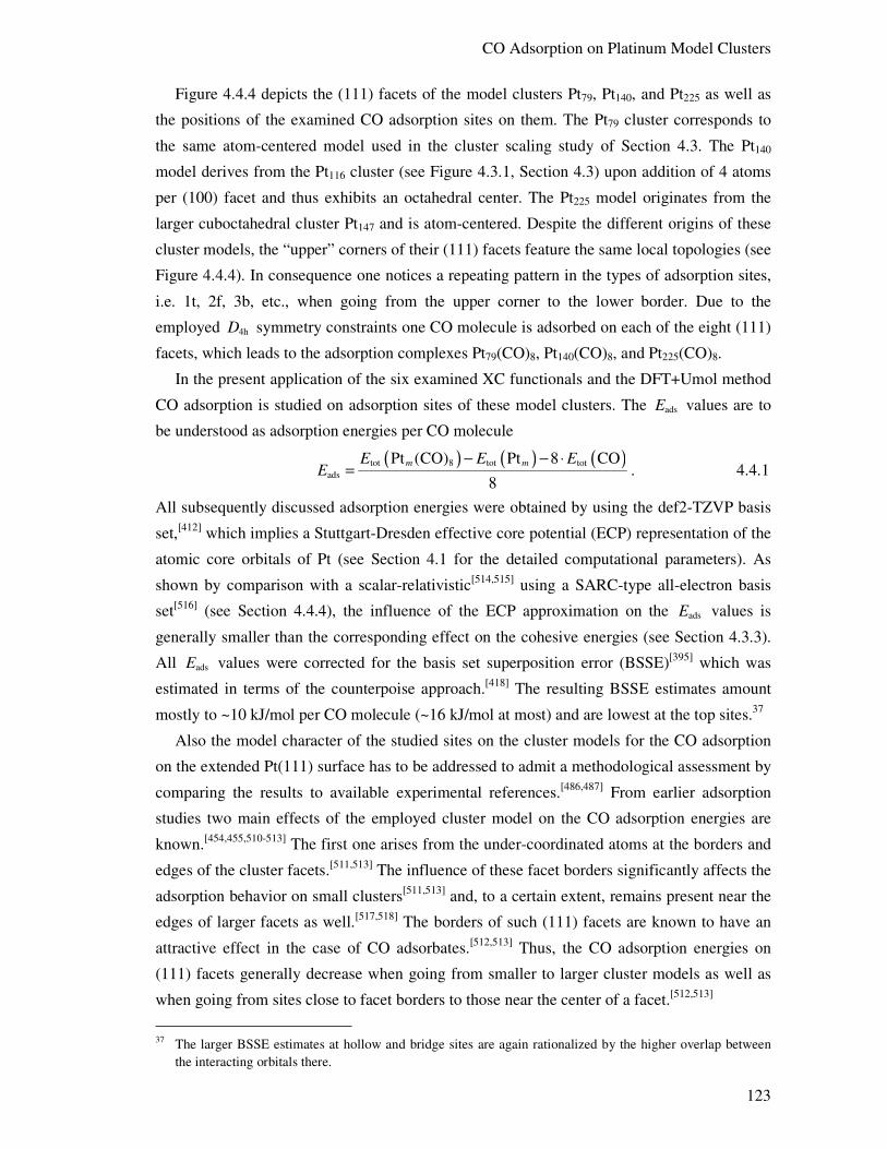
CO Adsorption on Platinum Model Clusters
123
Figure 4.4.4 depicts the (111) facets of the model clusters Pt79, Pt140, and Pt225 as well as
the positions of the examined CO adsorption sites on them. The Pt79 cluster corresponds to
the same atom-centered model used in the cluster scaling study of Section 4.3. The Pt140
model derives from the Pt116 cluster (see Figure 4.3.1, Section 4.3) upon addition of 4 atoms
per (100) facet and thus exhibits an octahedral center. The Pt225 model originates from the
larger cuboctahedral cluster Pt147 and is atom-centered. Despite the different origins of these
cluster models, the “upper” corners of their (111) facets feature the same local topologies (see
Figure 4.4.4). In consequence one notices a repeating pattern in the types of adsorption sites,
i.e. 1t, 2f, 3b, etc., when going from the upper corner to the lower border. Due to the
employed 4hD symmetry constraints one CO molecule is adsorbed on each of the eight (111)
facets, which leads to the adsorption complexes Pt79(CO)8, Pt140(CO)8, and Pt225(CO)8.
In the present application of the six examined XC functionals and the DFT+Umol method
CO adsorption is studied on adsorption sites of these model clusters. The adsE values are to
be understood as adsorption energies per CO molecule
( ) ( ) ( )tot 8 tot tot
ads
Pt (CO) Pt 8 CO
8m mE E E
E− − ⋅
= . 4.4.1
All subsequently discussed adsorption energies were obtained by using the def2-TZVP basis
set,[412] which implies a Stuttgart-Dresden effective core potential (ECP) representation of the
atomic core orbitals of Pt (see Section 4.1 for the detailed computational parameters). As
shown by comparison with a scalar-relativistic[514,515] using a SARC-type all-electron basis
set[516] (see Section 4.4.4), the influence of the ECP approximation on the adsE values is
generally smaller than the corresponding effect on the cohesive energies (see Section 4.3.3).
All adsE values were corrected for the basis set superposition error (BSSE)[395] which was
estimated in terms of the counterpoise approach.[418] The resulting BSSE estimates amount
mostly to ~10 kJ/mol per CO molecule (~16 kJ/mol at most) and are lowest at the top sites.37
Also the model character of the studied sites on the cluster models for the CO adsorption
on the extended Pt(111) surface has to be addressed to admit a methodological assessment by
comparing the results to available experimental references.[486,487] From earlier adsorption
studies two main effects of the employed cluster model on the CO adsorption energies are
known.[454,455,510-513] The first one arises from the under-coordinated atoms at the borders and
edges of the cluster facets.[511,513] The influence of these facet borders significantly affects the
adsorption behavior on small clusters[511,513] and, to a certain extent, remains present near the
edges of larger facets as well.[517,518] The borders of such (111) facets are known to have an
attractive effect in the case of CO adsorbates.[512,513] Thus, the CO adsorption energies on
(111) facets generally decrease when going from smaller to larger cluster models as well as
when going from sites close to facet borders to those near the center of a facet.[512,513]
37 The larger BSSE estimates at hollow and bridge sites are again rationalized by the higher overlap between
the interacting orbitals there.

Applications
124
To put the influence of the under-coordinated atoms on the (111) facets of the employed
cluster models in a more general context, the average coordination numbers of the surface
atoms associated with the individual adsorption sites are examined.[286] On (111) surfaces the
1, 2, and 3 atoms that form top, bridge, and hollow-type adsorption sites are surrounded by 6,
8, and 9 nearest-neighbor surface atoms, respectively. In this context a total of site 7,n = 10,
and 12 surface atoms are associated with the individual top, bridge, and hollow sites,
respectively. For each adsorption site the average nearest-neighbor coordination numbers
site
avsite
1 n
i
i
CN CNn
= ∑ 4.4.2
are computed as average of the nearest-neighbor coordination numbers iCN (including
surface and sub-surface atoms) of those siten atoms associated with the site.[286] The resulting
average nearest-neighbor coordination numbers of the groups of 7, 10, and 12 surface atoms
always amount to av 9CN = in the case of the extended (111) surface. For the sites on the
(111) facets of the three employed cluster models the avCN values are mostly lower and
range between ~7 and 9.[286]
Figure 4.4.5 provides a plot of the individual CO adsorption energies adsE (see Section
4.4.4) obtained with the PBE functional for all studied adsorption sites as a function of avCN .
The overall linear regression function, based on the results of all sites and cluster models,
ads av av( ) (282 16.3 ) kJ/molE CN CN= − ⋅ 4.4.3
reflects a rough trend only ( 2 0.64R = ) due to the different behavior of the various types of
adsorption sites. Much better correlations ( 2 0.9R ≈ ) are obtained when one eliminates the
effect of the different types of sites by calculating the linear regression functions tads av( )E CN ,
bads av( )E CN , and f
ads av( )E CN for the individual series of adsorption energies at t, b, and f sites,
respectively (see Figure 4.4.5).[286] The linear trends of the CO adsorption energies have a
certain empirical flavor and are not as well physically justified as the cluster scaling relations
(see Section 4.3.2). Nevertheless, they allow for several observations about the general
behavior of the employed CO adsorption site models.
When comparing these three linear functions one notices the much steeper slope of the bads av( )E CN values obtained at bride sites. At the 3b site of the Pt79 cluster the overall highest
CO adsorption energy is obtained (see Section 4.4.4). This large adsorption energy most
likely results from the influence of the adjacent facet edge (see Figure 4.4.4).[286] However,
on the (111) facets of the two larger cluster models this effect vanishes and the corresponding
adsorption energies are significantly smaller. Furthermore, one notices the slightly steeper
slope of tads av( )E CN compared to that of f
ads av( )E CN , which probably indicates that the 1t
sites of all cluster models are subject to a somewhat stronger influence of facet border than
the corresponding adjacent 2f sites.
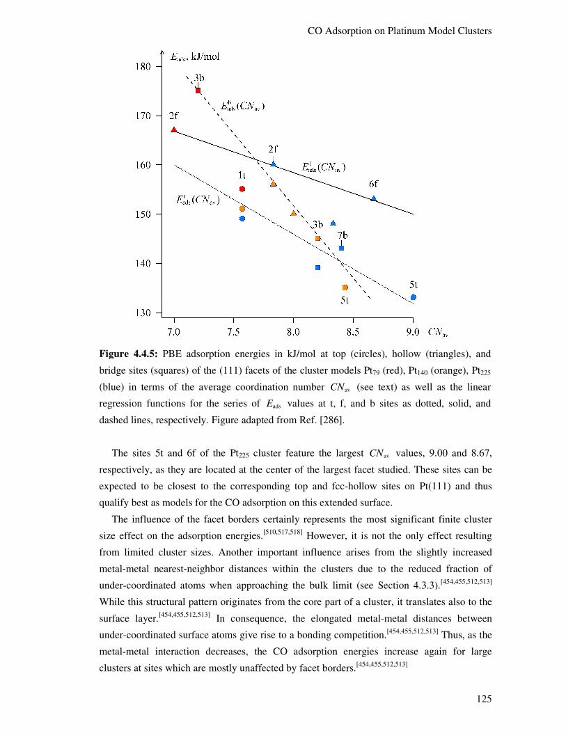
CO Adsorption on Platinum Model Clusters
125
Figure 4.4.5: PBE adsorption energies in kJ/mol at top (circles), hollow (triangles), and
bridge sites (squares) of the (111) facets of the cluster models Pt79 (red), Pt140 (orange), Pt225
(blue) in terms of the average coordination number avCN (see text) as well as the linear
regression functions for the series of adsE values at t, f, and b sites as dotted, solid, and
dashed lines, respectively. Figure adapted from Ref. [286].
The sites 5t and 6f of the Pt225 cluster feature the largest avCN values, 9.00 and 8.67,
respectively, as they are located at the center of the largest facet studied. These sites can be
expected to be closest to the corresponding top and fcc-hollow sites on Pt(111) and thus
qualify best as models for the CO adsorption on this extended surface.
The influence of the facet borders certainly represents the most significant finite cluster
size effect on the adsorption energies.[510,517,518] However, it is not the only effect resulting
from limited cluster sizes. Another important influence arises from the slightly increased
metal-metal nearest-neighbor distances within the clusters due to the reduced fraction of
under-coordinated atoms when approaching the bulk limit (see Section 4.3.3).[454,455,512,513]
While this structural pattern originates from the core part of a cluster, it translates also to the
surface layer.[454,455,512,513] In consequence, the elongated metal-metal distances between
under-coordinated surface atoms give rise to a bonding competition.[454,455,512,513] Thus, as the
metal-metal interaction decreases, the CO adsorption energies increase again for large
clusters at sites which are mostly unaffected by facet borders.[454,455,512,513]
Applications
126
In a previous CO adsorption study on Pd clusters the aforementioned effect of elongated
metal-metal distances was discussed in detail.[454] This study also showed that the effect of
elongated metal-metal distances can be mimicked by cluster models in which only the surface
layer was allowed to relax while the nearest-neighbor distances between all subsurface atoms
were fixed to the corresponding bulk limit.[454] The resulting CO adsorption behavior on such
cluster models is similar to that on much larger particles close to the bulk limit.[454]
This type of a cluster model was also employed during the assessment of the DFT+Umol
method.[286] Thereby the octahedral Pt44 core of the Pt140(CO)8 cluster model was fixed at the
bulk limit (281.3 pm) of the avd distances, which were obtained from a cluster scaling
extrapolation (see Section 4.3) of the series Pt79, Pt116, Pt140, Pt201, and Pt225.[286] However,
compared to the fully relaxed cluster model, only changes of about 4 kJ/mol or less were
observed in the corresponding CO adsorption energies.[286] Thus, this comparison leads to the
conclusion that influence of elongated metal-metal distances is only of a lesser importance
for the present methodological assessment.
4.4.3. Structural Aspects
Out of the different structural parameters of the various adsorption complexes and cluster
models, only the C-O distances C-Od are essential for the discussion of the description of the
CO adsorption in terms of the Blyholder model.[438,489,490] Furthermore, the present discussion
is restricted to some selected sites on the cluster models Pt79 and Pt225, namely 1t, 2f, and 3b
on Pt79 as well as 5t and 6f on Pt225. Table 4.4.1 provides the corresponding C-O bond lengths
for the methods PBE, PBE0, TPSS, TPSSh, M06L, and M06 as well as for the
PBE+Umol(CO 2π*) combination with the parameter value 2π* 2.0U = eV.
Upon adsorption of a CO molecule on the Pt cluster models, the C-O bond is weakened as
the anti-bonding CO 2π* orbitals are partially populated due to back-bonding.[438,488-491] The
elongation of the C-O bond roughly correlates with the amount of back-bonding at the
individual adsorption sites (see also Section 4.2.2).[438,488-491] The C-Od values found at the
three sites of the Pt79 model are ordered according to 1t < 3b < 2f, which reflects the expected
relative amount of back-bonding. The variants PBE0 and M06 always yield the shortest C-Od
values which partially results from the description of the CO molecule itself as these methods
yield the shortest C-O bonds already for CO in the gas-phase.
Relative to the respective gas-phase C-Od values, the examined hybrid DFT methods yield
less elongated C-O bonds than their semi-local counterparts. Thus, back-bonding is indeed
reduced by the EXX term. Compared to the sites on the Pt79 model, the C-Od values found in
the Pt225(CO)8 adsorption complexes are reduced further by a small amount (< 0.3 pm) as
finite cluster size effects are reduced in this case.
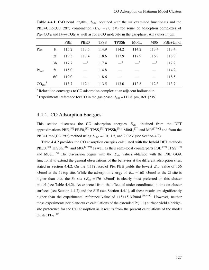
CO Adsorption on Platinum Model Clusters
127
Table 4.4.1: C-O bond lengths, C-Od , obtained with the six examined functionals and the
PBE+Umol(CO 2π*) combination ( 2π* 2.0U = eV) for some of adsorption complexes of
Pt79(CO)8 and Pt225(CO)8 as well as for a CO molecule in the gas-phase. All values in pm.
PBE PBE0 TPSS TPSSh M06L M06 PBE+Umol
Pt79 1t 115.2 113.5 114.9 114.2 114.2 113.4 113.4
2f 119.3 117.4 118.6 117.9 117.9 116.9 118.9
3b 117.7 ―a 117.4 ―a ―a ―a 117.2
Pt225 5t 115.0 ― 114.8 ― ― ― 114.2
6f 119.0 ― 118.6 ― ― ― 118.5
COgas b 113.7 112.4 113.5 113.0 112.8 112.3 113.7
a Relaxation converges to CO adsorption complex at an adjacent hollow-site. b Experimental reference for CO in the gas phase C-O 112.8d = pm, Ref. [519].
4.4.4. CO Adsorption Energies
This section discusses the CO adsorption energies adsE obtained from the DFT
approximations PBE,[49] PBE0,[87] TPSS,[75] TPSSh,[212] M06L,[77] and M06[77,90] and from the
PBE+Umol(CO 2π*) method using 2π* 1.0U = , 1.5, and 2.0 eV (see Section 4.2).
Table 4.4.2 provides the CO adsorption energies calculated with the hybrid DFT methods
PBE0,[87] TPSSh,[212] and M06[77,90] as well as their semi-local counterparts PBE,[49] TPSS,[75]
and M06L.[77] The discussion begins with the adsE values obtained with the PBE GGA
functional to extend the general observations of the behavior at the different adsorption sites,
stated in Section 4.4.2. On the (111) facet of Pt79 PBE yields the lowest adsE value of 156
kJ/mol at the 1t top site. While the adsorption energy of ads 168E = kJ/mol at the 2f site is
higher than that, the 3b site ( ads 176E = kJ/mol) is clearly most preferred on this cluster
model (see Table 4.4.2). As expected from the effect of under-coordinated atoms on cluster
surfaces (see Section 4.4.2) and the SIE (see Section 4.4.1), all these results are significantly
higher than the experimental reference value of 115±15 kJ/mol.[485-487] However, neither
these experiments nor plane-wave calculations of the extended Pt(111) surface yield a bridge-
site preference for the CO adsorption as it results from the present calculations of the model
cluster Pt79.[484]
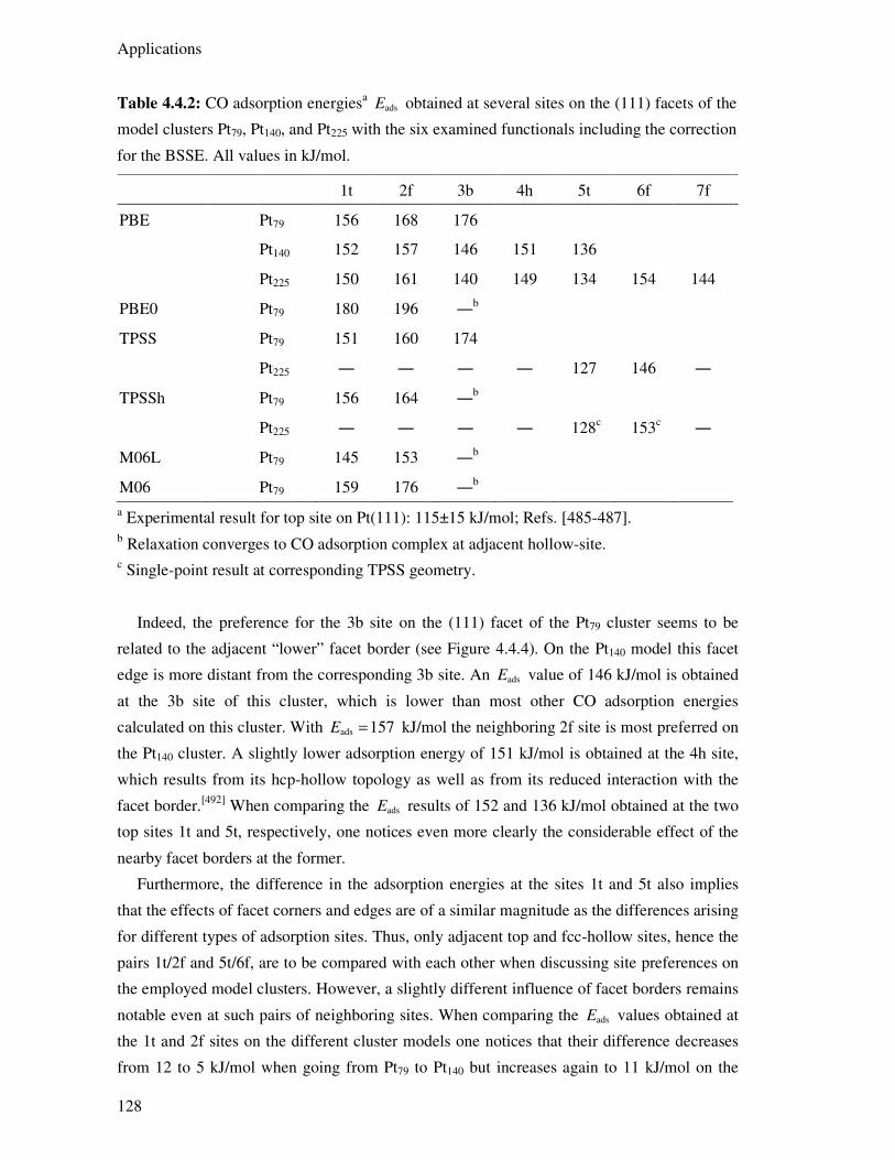
Applications
128
Table 4.4.2: CO adsorption energiesa adsE obtained at several sites on the (111) facets of the
model clusters Pt79, Pt140, and Pt225 with the six examined functionals including the correction
for the BSSE. All values in kJ/mol.
1t 2f 3b 4h 5t 6f 7f
PBE Pt79 156 168 176
Pt140 152 157 146 151 136
Pt225 150 161 140 149 134 154 144
PBE0 Pt79 180 196 ―b
TPSS Pt79 151 160 174
Pt225 ― ― ― ― 127 146 ―
TPSSh Pt79 156 164 ―b
Pt225 ― ― ― ― 128c 153c ―
M06L Pt79 145 153 ―b
M06 Pt79 159 176 ―b a Experimental result for top site on Pt(111): 115±15 kJ/mol; Refs. [485-487]. b Relaxation converges to CO adsorption complex at adjacent hollow-site. c Single-point result at corresponding TPSS geometry.
Indeed, the preference for the 3b site on the (111) facet of the Pt79 cluster seems to be
related to the adjacent “lower” facet border (see Figure 4.4.4). On the Pt140 model this facet
edge is more distant from the corresponding 3b site. An adsE value of 146 kJ/mol is obtained
at the 3b site of this cluster, which is lower than most other CO adsorption energies
calculated on this cluster. With ads 157E = kJ/mol the neighboring 2f site is most preferred on
the Pt140 cluster. A slightly lower adsorption energy of 151 kJ/mol is obtained at the 4h site,
which results from its hcp-hollow topology as well as from its reduced interaction with the
facet border.[492] When comparing the adsE results of 152 and 136 kJ/mol obtained at the two
top sites 1t and 5t, respectively, one notices even more clearly the considerable effect of the
nearby facet borders at the former.
Furthermore, the difference in the adsorption energies at the sites 1t and 5t also implies
that the effects of facet corners and edges are of a similar magnitude as the differences arising
for different types of adsorption sites. Thus, only adjacent top and fcc-hollow sites, hence the
pairs 1t/2f and 5t/6f, are to be compared with each other when discussing site preferences on
the employed model clusters. However, a slightly different influence of facet borders remains
notable even at such pairs of neighboring sites. When comparing the adsE values obtained at
the 1t and 2f sites on the different cluster models one notices that their difference decreases
from 12 to 5 kJ/mol when going from Pt79 to Pt140 but increases again to 11 kJ/mol on the
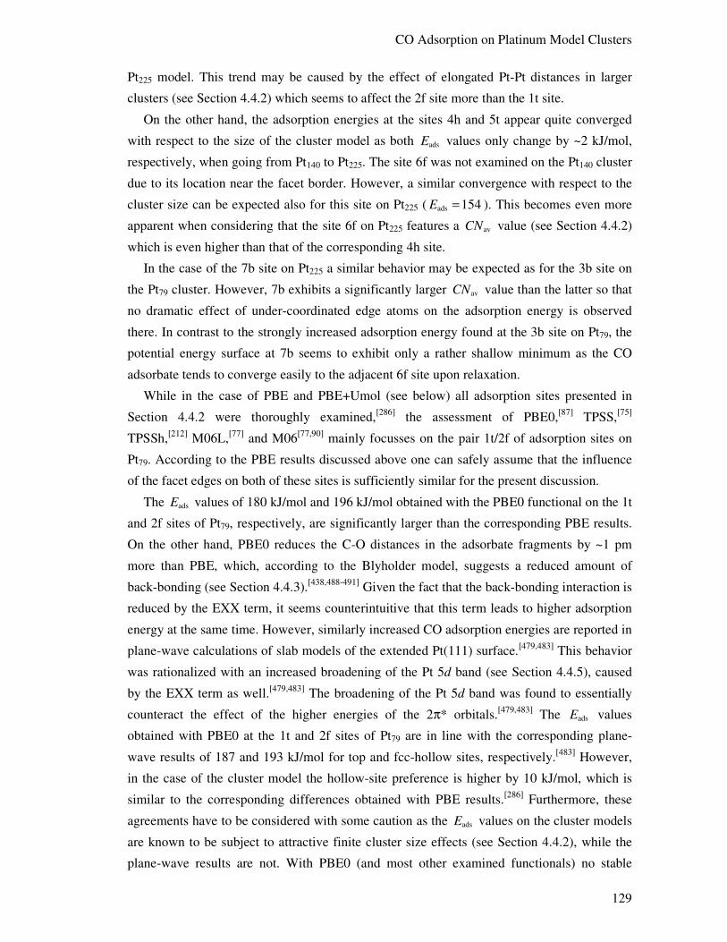
CO Adsorption on Platinum Model Clusters
129
Pt225 model. This trend may be caused by the effect of elongated Pt-Pt distances in larger
clusters (see Section 4.4.2) which seems to affect the 2f site more than the 1t site.
On the other hand, the adsorption energies at the sites 4h and 5t appear quite converged
with respect to the size of the cluster model as both adsE values only change by ~2 kJ/mol,
respectively, when going from Pt140 to Pt225. The site 6f was not examined on the Pt140 cluster
due to its location near the facet border. However, a similar convergence with respect to the
cluster size can be expected also for this site on Pt225 ( ads 154E = ). This becomes even more
apparent when considering that the site 6f on Pt225 features a avCN value (see Section 4.4.2)
which is even higher than that of the corresponding 4h site.
In the case of the 7b site on Pt225 a similar behavior may be expected as for the 3b site on
the Pt79 cluster. However, 7b exhibits a significantly larger avCN value than the latter so that
no dramatic effect of under-coordinated edge atoms on the adsorption energy is observed
there. In contrast to the strongly increased adsorption energy found at the 3b site on Pt79, the
potential energy surface at 7b seems to exhibit only a rather shallow minimum as the CO
adsorbate tends to converge easily to the adjacent 6f site upon relaxation.
While in the case of PBE and PBE+Umol (see below) all adsorption sites presented in
Section 4.4.2 were thoroughly examined,[286] the assessment of PBE0,[87] TPSS,[75]
TPSSh,[212] M06L,[77] and M06[77,90] mainly focusses on the pair 1t/2f of adsorption sites on
Pt79. According to the PBE results discussed above one can safely assume that the influence
of the facet edges on both of these sites is sufficiently similar for the present discussion.
The adsE values of 180 kJ/mol and 196 kJ/mol obtained with the PBE0 functional on the 1t
and 2f sites of Pt79, respectively, are significantly larger than the corresponding PBE results.
On the other hand, PBE0 reduces the C-O distances in the adsorbate fragments by ~1 pm
more than PBE, which, according to the Blyholder model, suggests a reduced amount of
back-bonding (see Section 4.4.3).[438,488-491] Given the fact that the back-bonding interaction is
reduced by the EXX term, it seems counterintuitive that this term leads to higher adsorption
energy at the same time. However, similarly increased CO adsorption energies are reported in
plane-wave calculations of slab models of the extended Pt(111) surface.[479,483] This behavior
was rationalized with an increased broadening of the Pt 5d band (see Section 4.4.5), caused
by the EXX term as well.[479,483] The broadening of the Pt 5d band was found to essentially
counteract the effect of the higher energies of the 2π* orbitals.[479,483] The adsE values
obtained with PBE0 at the 1t and 2f sites of Pt79 are in line with the corresponding plane-
wave results of 187 and 193 kJ/mol for top and fcc-hollow sites, respectively.[483] However,
in the case of the cluster model the hollow-site preference is higher by 10 kJ/mol, which is
similar to the corresponding differences obtained with PBE results.[286] Furthermore, these
agreements have to be considered with some caution as the adsE values on the cluster models
are known to be subject to attractive finite cluster size effects (see Section 4.4.2), while the
plane-wave results are not. With PBE0 (and most other examined functionals) no stable

Applications
130
adsorption geometry could be obtained at the site 3b on the cluster Pt79. The CO adsorbate
rather relaxes to the neighboring hcp-hollow site at the facet border, similarly to the behavior
observed with PBE and PBE+Umol (see below) at the 7b site on the Pt225 model.
The M06 functional yields CO adsorption energies of 159 kJ/mol and 176 kJ/mol for 1t
and 2f, respectively, which are considerably lower than the corresponding PBE0 results.
Indeed, the adsE values from M06 are closer to those from the PBE functional. When
considering that M06 features an even slightly larger EXX mixing factor of 1 0.27α = than
PBE0 ( 1 0.25α = ) this result is somewhat surprising. However, the low adsorption energies
from M06 may be related to its questionable description of the metal moiety (see Section 4.3)
as well as to the parametrization of its semi-local terms.[443] The adsE values resulting from
the M06L functional are even lower than those from M06 and with ads 145E = kJ/mol and
153 kJ/mol for the sites 1t and 2f the overall lowest adsorption energies calculated on the Pt79
cluster with the six examined functionals.
Also the TPSS functional yields lower CO adsorption energies than PBE: 151 kJ/mol and
160 kJ/mol for 1t and 2f, respectively. When comparing the adsorption energies of these two
sites, the slightly reduced preference of about 9 kJ/mol for the fcc-hollow site is noteworthy.
Furthermore, TPSS also yields a stable adsorption structure at the 3b site. The adsorption
energy of 174 kJ/mol computed at this site is very similar to the corresponding PBE result.
Due to its small EXX mixing factor ( 1 0.10α = ) the TPSSh functional yields only slightly
increased adsorption energies compared to TPSS. With 156 and 164 kJ/mol for 1t and 2f,
respectively, TPSSh yields even a slightly lower preference for the fcc-hollow site than its
semi-local counterpart.
Motivated by these comparatively low preferences for the 2f site as well as by the
surprisingly good description of metal-metal bonds provided by TPSSh (see Section 4.3), the
5t/6f pair of adsorption sites on the Pt225 cluster was studied with TPSS and TPSSh as well.
Compared to the adsE values obtained with PBE, the TPSS functional yields consistently
lower adsorption energies, whereas the differences of 7–8 kJ/mol are comparable to those of
the Pt79 cluster. The TPSS adsorption energies decrease when going from the sites 1t and 2f
on Pt79 to the sites 5t and 6f on Pt225. However, due to the aforementioned stronger influence
of the facet borders at 1t this decrease is not the same for both types of sites. In the case of the
top-sites the difference in the adsorption energies when going from Pt79 to Pt225 amounts to
24 kJ/mol but only to 14 kJ/mol for the fcc-hollow sites. Thus, the site preference between
the 5t/6f pair is increased to 19 kJ/mol in favor of the 6f site, similarly to the increased
preference of 20 kJ/mol found with PBE.
Given the substantial computational effort required to carry out hybrid DFT calculations
for the Pt225(CO)8 models, the application of TPSSh was restricted in that case to single-point
calculations at the corresponding TPSS geometries. To evaluate the effect of this strategy the
TPSSh functional was first applied to the TPSS geometries of the Pt79 cluster. The adsorption
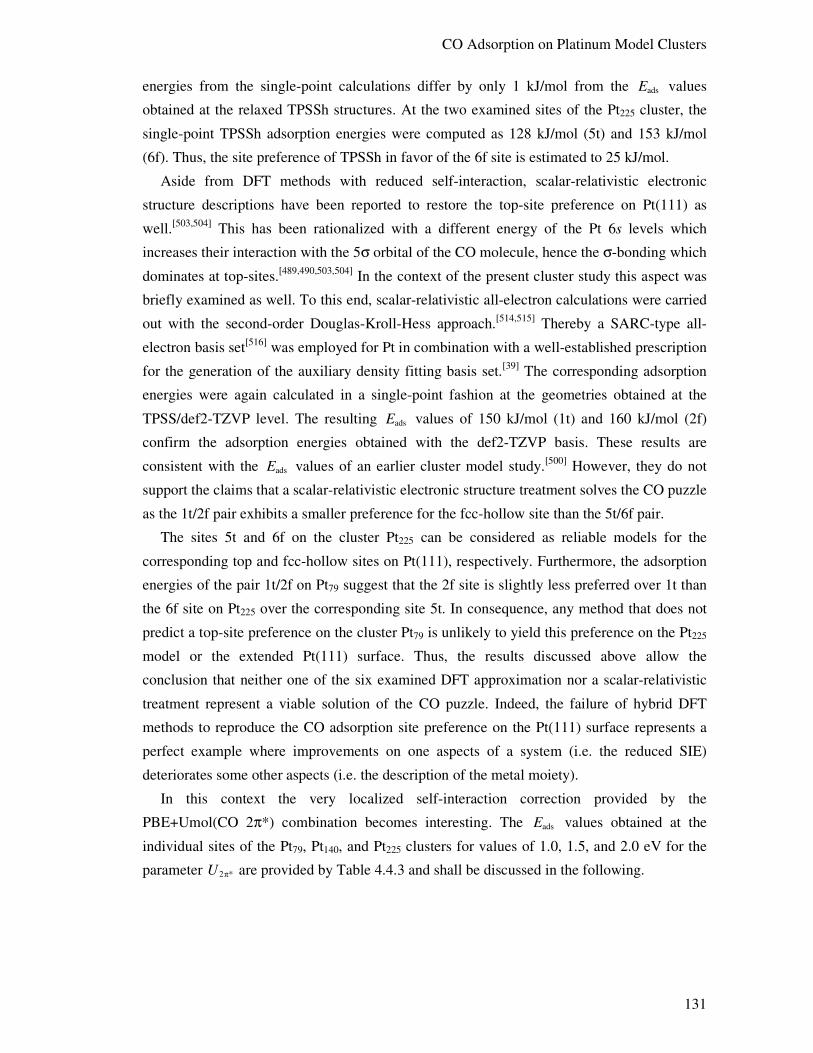
CO Adsorption on Platinum Model Clusters
131
energies from the single-point calculations differ by only 1 kJ/mol from the adsE values
obtained at the relaxed TPSSh structures. At the two examined sites of the Pt225 cluster, the
single-point TPSSh adsorption energies were computed as 128 kJ/mol (5t) and 153 kJ/mol
(6f). Thus, the site preference of TPSSh in favor of the 6f site is estimated to 25 kJ/mol.
Aside from DFT methods with reduced self-interaction, scalar-relativistic electronic
structure descriptions have been reported to restore the top-site preference on Pt(111) as
well.[503,504] This has been rationalized with a different energy of the Pt 6s levels which
increases their interaction with the 5σ orbital of the CO molecule, hence the σ-bonding which
dominates at top-sites.[489,490,503,504] In the context of the present cluster study this aspect was
briefly examined as well. To this end, scalar-relativistic all-electron calculations were carried
out with the second-order Douglas-Kroll-Hess approach.[514,515] Thereby a SARC-type all-
electron basis set[516] was employed for Pt in combination with a well-established prescription
for the generation of the auxiliary density fitting basis set.[39] The corresponding adsorption
energies were again calculated in a single-point fashion at the geometries obtained at the
TPSS/def2-TZVP level. The resulting adsE values of 150 kJ/mol (1t) and 160 kJ/mol (2f)
confirm the adsorption energies obtained with the def2-TZVP basis. These results are
consistent with the adsE values of an earlier cluster model study.[500] However, they do not
support the claims that a scalar-relativistic electronic structure treatment solves the CO puzzle
as the 1t/2f pair exhibits a smaller preference for the fcc-hollow site than the 5t/6f pair.
The sites 5t and 6f on the cluster Pt225 can be considered as reliable models for the
corresponding top and fcc-hollow sites on Pt(111), respectively. Furthermore, the adsorption
energies of the pair 1t/2f on Pt79 suggest that the 2f site is slightly less preferred over 1t than
the 6f site on Pt225 over the corresponding site 5t. In consequence, any method that does not
predict a top-site preference on the cluster Pt79 is unlikely to yield this preference on the Pt225
model or the extended Pt(111) surface. Thus, the results discussed above allow the
conclusion that neither one of the six examined DFT approximation nor a scalar-relativistic
treatment represent a viable solution of the CO puzzle. Indeed, the failure of hybrid DFT
methods to reproduce the CO adsorption site preference on the Pt(111) surface represents a
perfect example where improvements on one aspects of a system (i.e. the reduced SIE)
deteriorates some other aspects (i.e. the description of the metal moiety).
In this context the very localized self-interaction correction provided by the
PBE+Umol(CO 2π*) combination becomes interesting. The adsE values obtained at the
individual sites of the Pt79, Pt140, and Pt225 clusters for values of 1.0, 1.5, and 2.0 eV for the
parameter 2π*U are provided by Table 4.4.3 and shall be discussed in the following.

Applications
132
Table 4.4.3: CO adsorption energiesa adsE obtained at several sites on the (111) facets of the
model clusters Pt79, Pt140, and Pt225 with PBE+Umol(CO 2π*) method at several values of the
parameter 2π*U including the correction for the BSSE. All values in kJ/mol.
2π*Ub 1t 2f 3b 4h 5t 6f 7f
PBE Pt79 156 168 176
Pt140 152 157 146 151 136
Pt225 150 161 140 149 134 154 144
PBE+Umol 1.0 Pt79 119 120 132
Pt140 110 110 102 104 99
Pt225 113 114 95 102 97 107 ―c
1.5 Pt79 101 97 110
Pt140 92 86 80 80 81
Pt225 95 90 72 79 79 83 ―c
2.0 Pt79 83 73 88
Pt140 75 63 58 57 63
Pt225 77 67 51 55 62 60 ―c a Experimental result for top site on Pt(111): 115±15 kJ/mol; Refs. [485-487]. b 2π*U parameter for the Umol(CO 2π*) correction in eV. c Relaxation converges to CO adsorption complex at adjacent hollow-site.
When comparing the PBE+Umol results with those from the uncorrected PBE functional
the Umol(CO 2π*) correction is found to generally reduce the adsE values. This is to be
expected as the DFT+U energy correction in the fully localized limit, Eqs. 2.4.6 and 2.4.10, is
a strictly positive function of the occupation matrix elements tun σ . The same holds for the
DFT+Umol reformulation in terms of projectors, Eq. 3.2.4. Thus, the Umol(CO 2π*)
correction either directly destabilizes the Ptm(CO)8 adsorption complexes or leads to
destabilizing changes in their electronic structure (see Section 4.2).
However, this destabilization is different for the individual types of adsorption sites. When
going from PBE to PBE+Umol with 2π* 1.0U = eV the adsE value at the 1t site of the Pt79
cluster is reduced by 37 kJ/mol while the corresponding adsorption energy at 2f is decreased
by 48 kJ/mol down to 120 kJ/mol. With ads 119E = kJ/mol the 1t site is almost degenerate to
2f in this case and becomes preferred at higher values of the parameter 2π*U . For 2π* 1.5U =
and 2.0 eV the adsorption energy at the 1t site of Pt79 is reduced to 101 and 83 kJ/mol,
respectively, while the corresponding adsE values at the 2f site amount to 97 and 73 kJ/mol.
The effect of the Umol(CO 2π*) correction on the adsorption energies of the 3b site on Pt79 is

CO Adsorption on Platinum Model Clusters
133
only slightly weaker than for the 2f site as adsE is reduced by 44 kJ/mol when going from
PBE to PBE+Umol with 2π* 1.0U = eV. However, the effect of the Umol(CO 2π*) term is not
strong enough to overcome the influence of the adjacent facet border, so that the 3b site
remains favored on Pt79 even at 2π* 2.0U = eV.
On the larger cluster models the changes in the adsE values induced by the Umol(CO 2π*)
correction are remarkably similar to those observed for the corresponding top, hollow, and
bridge adsorption sites on Pt79, respectively. Compared to the results from the uncorrected
PBE method, the Umol(CO 2π*) term (with 2π* 1.0U = eV) again reduces the CO adsorption
energies; by ~37 kJ/mol at top sites, ~48 kJ/mol at hollow-type sites, and ~48 kJ/mol at
bridge sites. Only in the case of the 1t site on Pt140 the adsE value decreases by 42 kJ/mol,
down to 110 kJ/mol, when going from PBE to PBE+Umol(CO 2π*) with 2π* 1.0U = eV.
However, as the uncorrected PBE functional yields a comparatively small site preference of
only 5 kJ/mol for 2f over 1t on Pt140, both sites are also degenerate at 2π* 1.0U = eV. At
2π* 2.0U = eV the 1t site on Pt140 is preferred by 12 kJ/mol over the adjacent 2f site. For
2π* 1.0U = eV, the adsorption energies at the three remaining sites on the (111) facet of Pt140
are 102 kJ/mol at 3b, 104 kJ/mol at 4h, and 99 kJ/mol at 5t. At 2π* 1.5U = eV all three sites
are nearly degenerate with ads 80E ≈ kJ/mol, while at 2π* 2.0U = eV the expected ordering 5t
> 4h > 3b is reached (see Table 4.4.3).
Like on the Pt79 and Pt140 models, the 1t and 2f sites on the Pt225 cluster are found almost
isoenergetic ( ads 113E ≈ kJ/mol) at 2π* 1.0U = eV. The DFT+Umol method renders 3b the
least preferred site on the Pt225 cluster. While the shallow energetic minimum of the 7b site
has already been noticed with PBE, no minimum was found at this site with the PBE+Umol
combination. When comparing the pair 5t/6f at the center of the (111) facet of Pt225, the
Umol(CO 2π*) correction is found to reduce the initial preference for the fcc-hollow site of
20 kJ/mol to 10 kJ/mol at 2π* 1.0U = eV. The corresponding adsorption energies amount to
97 kJ/mol and 107 kJ/mol for 5t and 6f, respectively. When increasing the value of the 2π*U
parameter to 1.5 eV the site preference is further reduced to 4 kJ/mol. Finally, at 2π* 2.0U =
eV the 5t site becomes preferred over 6f.
Thus, the PBE+Umol method is able to correct the site preference on the employed cluster
model of the Pt(111) surface. However, while these results certainly represent an
improvement from a qualitative point of view, the corresponding CO adsorption energy of 62
kJ/mol computed at the 5t site with 2π* 2.0U = eV considerably underestimates the
experimental reference for the adsE value of 115±15 kJ/mol.[485-487]
The adsorption energy obtained at the 5t site of Pt255 is also lower than the adsE value
reported in an earlier application of the DFT+U method[499] to the CO 2π* fragment
molecular orbitals in a plane-wave study of CO/Pt(111). However, the fcc-hollow site
preference obtained with the uncorrected PBE functional in these plane-wave calculations is
already lower than in the present case (only ~12 kJ/mol compared to 20 kJ/mol here).[499] The

Applications
134
lower preference for the fcc-hollow site obtained in such plane-wave calculations likely
results from the details of the employed representation of the core electrons, hence the atomic
parameters employed in the projector-augmented wave (PAW) approach.[499] Indeed, the
difference in the CO adsorption energies obtained at fcc-hollow and top sites was found to be
quite sensitive to certain PAW parameters like the PAW cutoff-radius.[499] Furthermore, the
aforementioned better agreement of the plane-wave results with the experimental reference
was based on PAW parameter values that strongly reduce the preference of the PBE
functional for the fcc-hollow site.[499] Thus, the better quantitative agreement of the plane-
wave adsE results is likely an indirect consequence of the parametrization of the approximate
treatment of the core electrons of Pt. Second, the CO adsorption energies obtained with PBE
plane-wave calculations are already notably higher than the present PBE estimates for adsE .
Thus, the better quantitative agreement of the aforementioned top-site adsorption energy from
the DFT+U plane-wave calculation at least partially seems to result from a favorable error
compensation.
4.4.5. Electronic Structure Aspects
The subsequent section analyzes the electronic structure descriptions provided by PBE,
TPSS, TPSSh, and PBE0 on the example of the CO molecule in the gas phase, the bare Pt79
cluster, and its adsorption complexes formed with CO at the sites 1t and 2f. Furthermore, the
effect of the Umol(CO 2π*) term on the electronic structure of the aforementioned adsorption
complexes is examined as well.
On the case of the bare CO molecule one always obtains the expected energetic ordering
of the orbitals 4σ* < 1π < 5σ < 2π*.[520] The energies of the occupied orbitals 4σ*, 1π, and
5σ are successively lowered when going from TPSS to TPSSh and to PBE0, while the 2π*
LUMO is shifted up in energy. As expected, the increasing EXX mixing factor in these three
functionals yields a widened HOMO-LUMO gap (HLG) HLGε∆ , which amounts to 7.4, 8.6,
and 10.1 eV for TPSS, TPSSh, and PBE0, respectively.
Figure 4.4.6 provides the projected densities of states (PDOS) which were obtained on the
basis of Mulliken population numbers[419] with TPSS, TPSSh, PBE0, PBE, and
PBE+Umol(CO 2π*) with 2π* 2.0U = eV for the Pt79 cluster and the 1t and 2f Pt79(CO)8
adsorption complexes, respectively. To this end, the density of states was projected onto the
6s and 5d of the three Pt atoms at the center of the (111) facet of Pt79 (see Figure 4.4.4) as
well as onto the 2s and 2p orbitals of the C and O atoms.
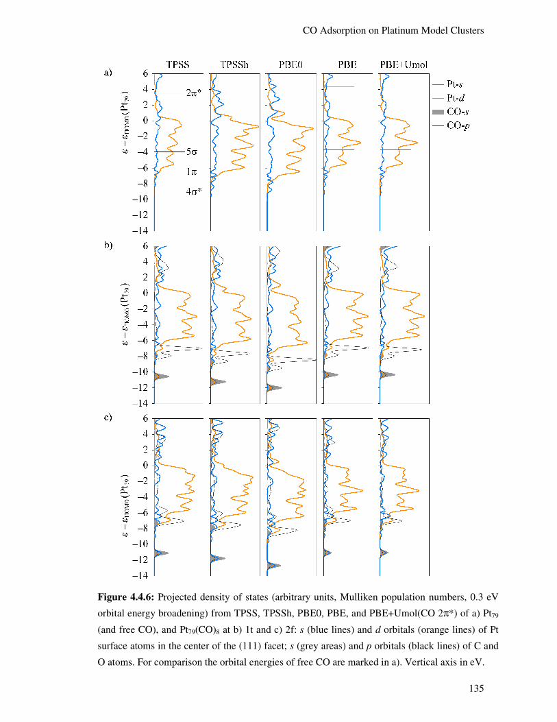
CO Adsorption on Platinum Model Clusters
135
Figure 4.4.6: Projected density of states (arbitrary units, Mulliken population numbers, 0.3 eV
orbital energy broadening) from TPSS, TPSSh, PBE0, PBE, and PBE+Umol(CO 2π*) of a) Pt79
(and free CO), and Pt79(CO)8 at b) 1t and c) 2f: s (blue lines) and d orbitals (orange lines) of Pt
surface atoms in the center of the (111) facet; s (grey areas) and p orbitals (black lines) of C and
O atoms. For comparison the orbital energies of free CO are marked in a). Vertical axis in eV.
Applications
136
The TPSS functional describes the Pt79 cluster and both adsorption complexes as
essentially metallic, hence yields HLG 0.0ε∆ ≈ . In contrast, the hybrid DFT methods TPSSh
and PBE0 yield HLG 0.2ε∆ = and 0.5 eV for Pt79, respectively, which is also notable in Figure
4.4.6 by the increasingly large dent at the upper edge of the Pt d-PDOS (with increasing
amount of EXX). Likewise, the Pt s-PDOS splits into two parts by the increased HLG as
well. TPSSh and PBE0 yield slightly increased HLGε∆ values for the 2f adsorption complex
compared to the bare Pt79 cluster (0.3 and 0.6 eV, respectively) as adsorbates may reduce the
metallic properties of finite clusters further.[521] Furthermore, the corresponding HOMO-
levels are found somewhat lower in energy. In contrast, slightly decreased HLGε∆ values and
upshifted HOMO levels result for the 1t adsorption complex with PBE and TPSSh. These
latter findings are rationalized by the net increase of negative charge at the adsorption site
due to the σ-bonding which prevails at top sites. The increased electronic charge raises the
electrostatic potential which in turn reduces the HOMO-LUMO gap. This is supported by the
Mulliken populations[419] obtained for the three Pt surface-atoms in the center of the (111)
facet of Pt79. Upon adsorption of the CO molecule at the 1t site the population is increased by
1.2 e, while the corresponding increase at 2f amounts to ~0.3 e only. In agreement with recent
plane-wave studies on slab-models,[479,522] one notices the increased width of the Pt 5d
manifold when going from TPSS over TPSSh to PBE0.
The DOS projections on the p orbitals of the C and O atoms exhibit two distinct peaks
near the lower edge of the Pt d-band. Out of these, the lower lying corresponds to the CO 5σ-
derived orbitals as it always coincides with a peak in the PDOS of the s-orbitals of the C and
O atoms. Thus, the higher of these two peaks corresponds to the CO 1π orbitals. Note, that
upon adsorption of the CO molecule the 5σ orbital is shifted below the 1π levels, which
agrees with spectroscopic results and other theoretical studies.[483,500,523,524]
The 5σ orbital of the CO molecule in the gas-phase always coincides with a local
maximum of the d-band of the bare Pt79 cluster (see Figure 4.4.6, panel a). The same holds
for the 5σ peak in the PDOS of both Pt79(CO)8 systems. However, in the 1t adsorption
complex the corresponding peak in the Pt d-PDOS is well-separated from the rest of the d-
manifold, while it is still part of the main d-band extension when CO adsorbs on the 2f site.
Furthermore, a significantly stronger Pt s-PDOS maximum can be found at the 5σ peak in the
case of the 2f adsorption complex. This indicates a mixing at this site between sd-hybridized
Pt levels and the CO 5σ orbital. With increasing amount of EXX the resulting σ-sd levels are
moved towards more negative energies. The downshift of these σ-sd levels with increasing
EXX mixing factor is stronger than the corresponding downshift of the HOMO-levels, which
indicates that the EXX term increases the σ-bonding interaction at the 2f site.
The energetically lowest peak in each of the PDOS spectra obtained with the various
methods corresponds to the CO 4σ∗ orbital. The presence of peaks in the Pt s- and d-PDOS
of the 2f adsorption complex indicates that the CO 4σ∗ orbital also contributes to the σ-sd
CO Adsorption on Platinum Model Clusters
137
interaction. Indeed, such a participation of the 4σ∗ orbital has previously been noticed in
theoretical and experimental studies of the CO adsorption on Ni and Cu surfaces.[489,490]
While both, the Pt s- and d-manifolds, seem to interact with the 4σ∗ orbital at the 2f site, the
PDOS spectra of the 1t adsorption complex only show an interaction with the Pt d-levels.
In the 1t adsorption complex the CO 1π orbitals always form a rather distinct peak in the
PDOS spectra obtained from the various methods. This is different when the CO molecule
adsorbs at the 2f site of Pt79. In this latter case all examined methods yield a broader 1π peak
in the PDOS which always coincides with a local maximum of the Pt s-PDOS at ‒5.8, ‒6.0,
and ‒6.3 eV for TPSS, TPSSh, and PBE0, respectively. Both of these observations indicate a
mixing of the 1π orbitals at the 2f site. Indeed, due to the presence of the Pt-moiety linear
combinations between the 1π and 2π* orbitals become feasible. As in the case of the 4σ∗
orbital, such a contribution of the 1π levels to the back-bonding interaction has already been
reported in earlier theoretical and experimental studies.[483,489,490] The EXX term appears to
broaden the 1π peak slightly more and to increase the corresponding local Pt s-PDOS
maximum. Thus, the EXX term seems to affect also the contribution of the 1π orbitals to the
back-bonding.
From the C and O p-DOS projections the CO 2π* derived orbitals are identified as
broadened peak which extends from 2 eV to 5 eV in the case of PBE and is, as expected,
shifted upward in energy when going over TPSSh to PBE0. The Umol(CO 2π*) correction
has a similar effect. Indeed the 2π* peak in the p-PDOS of the C and O atoms appears
upshifted by a comparable amount as the energies of the 2π* orbitals in the gas-phase CO
molecule. Apart from that, the PDOS spectra obtained from the PBE+Umol(CO 2π*)
combination are remarkably similar to those from the uncorrected PBE functional. This
indicates that the Umol(CO 2π*) term acts on the 2π* level of the Pt79(CO)8 adsorption
complex only and has no notable effect on the remaining electronic structure of the system.
This effect clearly differs from the influence of the Umol(CO 2π*) correction on the Ni 3d
orbitals of the nickel carbonyls studied in Section 4.2.
In the following the effect of the Umol(CO 2π*) term shall be examined further. To this
end, the elements of the occupation matrices Iσ
n are studied (see Section 2.4). As described
in Section 3.2.2, the DFT+Umol implementation in PARAGAUSS completely bypasses
calculation of occupation matrices Iσ
n .[286] Yet, under the assumption that the CO adsorbates
are sufficiently separated, the 2 2× occupation matrix block corresponding to the 2π* orbitals
of a single CO fragment can still be computed as †σ σ=n vSP Sv from the fragment MO
coefficients v . In the present case these matrix blocks are always found diagonal due to the
orientation of the CO fragment in the Pt79(CO)8 adsorption complexes. In any case only the
diagonal elements ttn σ need to be discussed as the occupation matrices can always be
diagonalized. Figure 4.4.7 shows a plot of the individual contributions to the DFT+U penalty
function in the fully localized limit for the employed values of 2π*U as a function of the
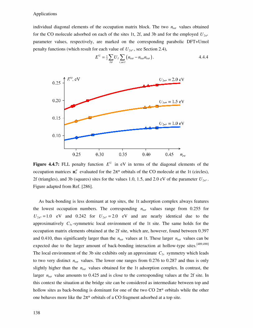
Applications
138
individual diagonal elements of the occupation matrix block. The two ttn σ values obtained
for the CO molecule adsorbed on each of the sites 1t, 2f, and 3b and for the employed 2π*U
parameter values, respectively, are marked on the corresponding parabolic DFT+Umol
penalty functions (which result for each value of 2π*U , see Section 2.4),
( )U 12
,I tt tt tt
I t u I
E U n n nσ σ σσ ∈
= −∑ ∑ . 4.4.4
Figure 4.4.7: FLL penalty function UE in eV in terms of the diagonal elements of the
occupation matrices Iσ
n evaluated for the 2π* orbitals of the CO molecule at the 1t (circles),
2f (triangles), and 3b (squares) sites for the values 1.0, 1.5, and 2.0 eV of the parameter 2π*U .
Figure adapted from Ref. [286].
As back-bonding is less dominant at top sites, the 1t adsorption complex always features
the lowest occupation numbers. The corresponding ttn σ values range from 0.255 for
2π* 1.0U = eV and 0.242 for 2π* 2.0U = eV and are nearly identical due to the
approximatively 3vC -symmetric local environment of the 1t site. The same holds for the
occupation matrix elements obtained at the 2f site, which are, however, found between 0.397
and 0.410, thus significantly larger than the ttn σ values at 1t. These larger ttn σ values can be
expected due to the larger amount of back-bonding interaction at hollow-type sites.[489,490]
The local environment of the 3b site exhibits only an approximate 2vC symmetry which leads
to two very distinct ttn σ values. The lower one ranges from 0.276 to 0.287 and thus is only
slightly higher than the ttn σ values obtained for the 1t adsorption complex. In contrast, the
larger ttn σ value amounts to 0.425 and is close to the corresponding values at the 2f site. In
this context the situation at the bridge site can be considered as intermediate between top and
hollow sites as back-bonding is dominant for one of the two CO 2π* orbitals while the other
one behaves more like the 2π* orbitals of a CO fragment adsorbed at a top site.

CO Adsorption on Platinum Model Clusters
139
The most important observation that can be made from Figure 4.4.7 is the fact that the
specific ttn σ values hardly change with increasing value of the parameter 2π*U . Only the
smaller occupation matrix elements, obtained at the 1t site and for one of the 2π* orbitals at
the 3b adsorption complex, seem to be slightly more affected. This is most likely a
consequence of the larger derivative of the parabolic penalty function at smaller ttn σ values
which is proportional to the DFT+Umol potential. As the ttn σ values remain essentially
unaffected by the value of the 2π*U parameter, the Umol(CO 2π*) correction appears to have
only a very limited effect on the electronic structure. This also agrees with its very localized
influence on the PDOS in Figure 4.4.6. Thus, in the case of the examined Ptn(CO)8 models,
the Umol(CO 2π*) term purely acts as a energetic correction. The top-site adsorption
preference obtained with the PBE+Umol(CO 2π*) combination is therefore a direct
consequence of the larger ttn σ values which result in the corresponding adsorption
complexes. The finding, that the electronic structure of the Ptn(CO)8 models does not relax
upon application of the Umol(CO 2π*) correction, also rationalizes the significant
destabilization of the adsorption complexes caused by this term and the resulting low CO
adsorption energies.
4.4.6. Conclusions
The adsorption of the CO molecule was studied on various top, bridge, fcc- and hcp-hollow
sites of the (111) facets of the model clusters Pt79, Pt140, and Pt225. First, the behavior of the
adsorption energy at these sites was examined on the basis of the corresponding results
obtained with the PBE method. Thereby the average coordination number avCN of the cluster
surface-atoms associated with the individual adsorption sites was employed to examine the
influence of the facet borders on the individual adsorption energies. This analysis revealed
that the sites 1t and 2f sites on the Pt79 cluster are significantly, but comparably affected by
the facet borders. Thus, these two sites qualify for the qualitative assessment of the
functionals PBE, PBE0, TPSS, TPSSh, M06L, and M06 regarding the relative top- vs.
hollow-site preference. Finally, the sites 5t and 6f on the much larger Pt225 model can be
considered as reliable qualitative and quantitative models for the CO adsorption on the
extended Pt(111) surface.
However, neither one of the semi-local approximations PBE, TPSS, and M06L nor any of
the assessed hybrid DFT methods PBE0, TPSSh, and M06 are able to provide the
experimentally characterized top-site preference. This finding is well in line with the results
from corresponding plane-wave studies on slab-models for the extended Pt(111)
surface.[479,483,484]
Applications
140
The rationalization that self-interaction effects prevent semi-local functionals from
predicting the correct site preference is widely accepted.[479,483,484,499,500] On the other hand,
the origin of the failure of hybrid DFT methods for the CO puzzle has been less well explored
in the past.[479,483] Indeed, the failure of hybrid functionals to describe properly the site
preference for CO on Pt(111) was rationalized in a rather unspecific way by the increased
broadening of the Pt 5d-manifold. While this latter effect is confirmed in the plots of the
projected density of states in Figure 4.4.6, the conclusions that can be made from the results
of the present study may provide a more detailed picture of the artifacts introduced by the
EXX term in the description of adsorption complexes.
As expected, hybrid DFT methods yield less elongated C-O bonds in the Pt79(CO)8
adsorption complexes, which suggests that back-bonding is reduced by the EXX term.
Furthermore, the reduction is slightly more pronounced at fcc-hollow sites as back-bonding is
more dominant there. From this reduction of the back-bonding interaction one might expect
lower adsorption energies. However, in agreement with the results from plane-wave studies
of slab-models for the Pt(111) surface,[479,483] the hybrid DFT methods were always found to
increase the adsE values compared to the results of the corresponding semi-local functionals.
These findings represent a strong indication for the EXX term to increase the σ-bonding
while reducing the back-bonding interaction at the same time. Furthermore, the increase of
the σ-bonding should be higher at fcc-hollow sites as the preference for these sites is even
slightly enhanced by the EXX term.
The analysis of the projected DOS plots confirms this assumption. In agreement with
earlier plane-wave studies,[479,483] the Pt-d band is found to be overly broadened by the EXX
term. Furthermore, the levels at the fcc-hollow sites are always somewhat downshifted
compared to those at top sites. This downshift is rationalized by the reduced electrostatic
potential due to the charge redistribution via the back-bonding. In combination with the
broadened Pt-d band, this brings the PDOS peak of the CO 5σ-derived levels inside the Pt-d
band at fcc-hollow sites. In consequence, an increased mixing of these levels with the Pt-d
band, hence σ-bonding, becomes feasible at fcc-hollow sites. Thus, the EXX term reduces
back-bonding at hollow-sites while simultaneously increasing the amount of σ-bonding there.
This conclusion provides a more precise picture about how the improved hybrid DFT
description of CO 2π* orbitals is abrogated by the deteriorated description of the metallic
moiety delivered by such methods.
The application of a DFT+Umol correction to the CO 2π* orbitals is found to restore the
experimentally determined top-site preference for the adsorption of the CO molecule on the
employed cluster models of the extended Pt(111) surface. At the sites on the Pt225 cluster
which were previously determined as the best models for the CO adsorption at the top and
fcc-hollow sites on the extended surface, this top-site preference is reached at DFT+U
parameter values of 2π* 2.0U ≈ eV. However, at these 2π*U values the experimental reference

CO Adsorption on Platinum Model Clusters
141
for adsE is considerably underestimated. The PDOS plots and the DFT+Umol occupation
numbers show that this qualitative inaccuracy derives from the fact that the DFT+Umol terms
essentially acts as a destabilizing energy term which does not induce any relaxation in the
electronic structure of the Ptm(CO)8 adsorption complexes.

Applications
142
143
5. Summary
The present thesis addresses self-interaction and delocalization artifacts in semi-local
approximations to Kohn‒Sham density functional theory (DFT) as well as the closely related
static correlation error in hybrid DFT methods. In this context also the methodological and
implementation aspects of hybrid density functionals and the DFT+Umol method are
discussed, which represent different approaches for correcting self-interaction and
delocalization errors. Both method variants have been implemented in the DFT program
PARAGAUSS as part of this thesis. Furthermore, these methods are applied in several case
studies to examine their performance for systems which are known to be strongly affected by
the aforementioned errors.
Hybrid DFT methods add a nonlocal exact-exchange (EXX) term to semi-local DFT
approximations. The EXX term in turn is computed from four-center electron-repulsion
integrals (ERI). As the number of ERIs scales with the fourth-order with respect to the
number of basis functions, the computation of the EXX term is very demanding. Thus, the
evaluation of ERIs has to be implemented by using an efficient algorithm as well as by taking
into account the structure of modern computer architectures. Most ERI algorithms are based
on the Boys function which represents a starting point for the ERI implementation made in
the context of this thesis. The Boys function and its derivatives are expanded to the final
integrals. Most ERI algorithms employ recursion relations for this expansion. A variant of the
McMurchie‒Davidson expansion has been implemented for this task, which employs so-
called horizontal recursion relations to reduce the amount of intermediate quantities. In the
case of strongly contracted Gaussian-type orbitals, early contraction strategies may allow for
a more efficient expansion of the Boys function. While all of these aforementioned
approaches become inefficient for basis functions of high angular momentum, Gauss-
quadrature based ERI algorithms, which are formulated in terms of roots and weights of Rys
polynomials instead of the Boys function, perform better in such cases. This holds especially
on modern computer architectures which allow for very rapid computations, provided that the
employed implementation features only a comparatively limited number of intermediates.
Thus, an existing, highly optimized implementation of a Gauss-quadrature based algorithm
was interfaced to the EXX calculation modules of PARAGAUSS as well and used in most
hybrid DFT production calculations.
The final ERIs are contracted with the density matrix to the EXX matrix and the EXX
energy term. Several measures need to be taken also at this stage to make hybrid DFT
calculations on larger systems feasible. Such measures rely on accounting for the internal
index symmetries of the tensor formed by all ERIs, as well as for spatial point group

Summary
144
symmetries. The EXX implementation carried out in this thesis takes into account both of
these symmetries. Thereby the so-called petit-list approach is employed to omit all but one of
the ERIs that are equivalent by point group symmetry. Integral screening approaches allow to
reduce further the effort when calculating the EXX term. Thereby one skips the computation
of ERIs that do not provide a numerically significant contribution to the EXX term. Integral
screening approaches can lower the formal forth-order scaling of the computational
requirements of the EXX term to a linear scaling in the limit of very large systems with a
notable HOMO-LUMO gap. The most important ERI-screening approach, namely the
density-weighted Schwarz screening ∆SCF method was implemented as part of this thesis for
the EXX term. Similar symmetry and screening treatments are used also in the
implementation of the gradients of the EXX term with respect to nuclear coordinates.
Finally, the application of hybrid DFT methods to larger systems requires an efficiently
parallelized implementation. The parallel implementation done in this thesis is based on an
existing dynamic load balancing (DLB) library which employs a work-stealing strategy to
achieve an efficient parallelization. In this implementation, a special algorithm assigns groups
of ERIs to the actual DLB tasks which are then dynamically allocated by the DLB library to
the individual CPU cores. On the example of a large transition metal cluster with ligands, a
parallel efficiency of ~93 % of the hybrid DFT SCF iteration was achieved for up to 2048
cores. Opposed to that, the parallelization of smaller unsymmetric systems still seems to
suffer from the comparatively slow exchange of data between computing nodes.
The DFT+Umol method as developed and implemented as part of this thesis represents an
extension of the conventional DFT+U method. Compared to hybrid DFT method, this
approach provides a more efficient, very localized correction for self-interaction and
delocalization errors. The DFT+Umol method is based on molecular fragment orbital
occupation numbers of those orbitals which are targeted by the self-interaction correction. To
avoid a complicated symmetrization of these fragment orbitals, the DFT+Umol energy and
potential terms have been implemented in terms of projectors. The DFT+Umol gradients are
computed largely with parts of an earlier implementation of the traditional DFT+U method.
Three case studies have been carried out as part of this thesis in which hybrid DFT
functionals and/or the DFT+Umol method are applied. The first application examined the
trend of the first metal-CO dissociation energies dis ( )E m of the nickel carbonyl complexes
Ni(CO)m with 1 4m = − . From experimental and accurate post-HF results these dissociation
energies are known to increase when going from Ni(CO)4 to Ni(CO)2 due to a reduced
bonding competition. This trend is broken by dis dis(2) (1)E E> as the electronic configuration
of the nickel atom formally relaxes from the d10 configuration which appears in the nickel
carbonyl complexes. The overall trend of the dis ( )E m values is predicted correctly by hybrid
DFT methods, but not by semi-local functionals. This situation in turn suggests that the
dissociation energies obtained with semi-local DFT approximations are affected by the self-
Summary
145
interaction error. To further examine these self-interaction artifacts, the DFT+Umol
correction was projected onto the Ni 3d subshell as well as onto the CO 2π* orbitals. Several
values of the DFT+Umol parameters 3dU and 2π*U were applied, which control the strength
of both self-interaction corrections. In the case of the DFT+Umol correction applied to the Ni
3d orbitals one finds that the correct trend in the dissociation energies is restored already at
3dU values below 3.0 eV. Around the parameter value of 5.3 eV, which is commonly
employed in the literature for this subshell, the DFT+Umol results agree well with CCSD(T)
reference values. Surprisingly, the correction of the 2π* orbitals yields the correct trend in the
dis ( )E m values as well, but only at a comparatively large value of 2π* 4.0U = eV. However, at
this parameter value the Ni(CO)3 and Ni(CO)4 complexes become unphysically destabilized.
A detailed analysis of the electronic structure reveals that the proper localization of the Ni 3d
subshell is essential to achieve dis dis(2) (1)E E> . Semi-local DFT methods overly delocalize
these orbitals within the carbonyl complexes, which lowers the energy of these systems with
respect to the nickel atom and yields the incorrect trend. The DFT+Umol correction of the Ni
3d subshell directly localizes these orbitals. Also the DFT+Umol correction of the CO 2π*
orbitals can achieve the same effect by essentially removing the back-bonding interaction,
which leads to the aforementioned destabilization of Ni(CO)3 and Ni(CO)4.
The second study addressed the description of transition metals provided by hybrid DFT
methods. To this end, the newly implemented hybrid functionals PBE0, TPSSh, and M06
were compared with their semi-local counterparts PBE, TPSS, and M06L for their
performance in a cluster scaling study of the cluster models Nim, Pdm, and Ptm (m = 13, 38,
55, 79, 116). The extrapolations of average nearest-neighbor distances, cohesive energies, as
well as vertical ionization energies and electron affinities to their respective bulk limits allow
a comparison with experimental references for the bulk systems. While PBE0 and M06 often
exhibit a quite erratic behavior, the hybrid DFT method TPSSh provided surprisingly
accurate results for most of these quantities. Inspection of the number of orbitals around the
HOMO-LUMO gap showed that TPSSh yields significantly large values for the examined
clusters. A large number of orbitals around the HOMO-LUMO gap is a prerequisite for
mimicking static correlation effects by a level broadening technique.
Finally, CO adsorption on the (111) facets of the cluster models Pt79, Pt140, and Pt225 was
studied with the aforementioned hybrid and semi-local functionals as well as with the
DFT+Umol correction of the CO 2π* orbitals. In the case of the extended Pt(111) surface
semi-local functionals are known to predict the fcc-hollow site to be preferred for the
adsorption of the CO molecule as opposed to the experimentally determined top-site
preference. Furthermore, the corresponding CO adsorption energies are significantly
overestimated. This failure of semi-local DFT methods, known as the “CO puzzle”,
originates from the self-interaction error which cases a too low energy of the CO 2π* orbitals.
Thus, the correct description of the CO adsorption on Pt(111) requires an electronic structure

Summary
146
description which is nearly free of self-interaction while simultaneously accounting for static
correlation effects in the metal moiety. As expected, the examined semi-local functionals
predict CO adsorption on the fcc-hollow site as preferred for the employed cluster models.
Furthermore, the three applied hybrid DFT methods yield a top-site preference while
overestimating the CO adsorption energy even slightly more. However, the smaller
elongation of the C-O bond in the adsorbed CO fragments indicates, as expected, that back-
bonding is reduced by the EXX term in hybrid functionals. As hybrid functionals yield higher
adsorption energies, the reduced amount of back-bonding has to be compensated by an
enhanced σ-bonding interaction. The analysis of the projected densities of states supports this
conclusion. The EXX term increases σ-bonding more at fcc-hollow sites due to a
combination of the overly broadened Pt d-band and the energetic lowering of all levels at this
site caused by the electrostatic effect of the remaining back-bonding charge transfer. On the
other hand, the DFT+Umol projection onto the CO 2π* orbitals restores the correct top-site
preference on the examined model clusters at a moderately large value of 2π* 2.0U ≈ eV.
However, the corresponding CO adsorption energies obtained in this case are found to
underestimate the experimental reference value. Inspection of the projected density of states
as well as of the DFT+Umol orbital occupation matrix elements reveals that the DFT+Umol
correction affects only the energy of the 2π* orbitals, while the residual electronic structure
of the Ptm(CO)8 systems remains essentially unchanged. Thus, the DFT+Umol term purely
acts as energetic penalty function as opposed to its behavior found in the nickel carbonyls.
The case studies made in this thesis provided new insight and rationalizations about the
behavior of self-interaction, delocalization, and static correlation errors in several types of
systems. However, the results of these studies also illustrated the limitations of the employed
methods. While the TPSSh hybrid functional can certainly be suggested for the study of
transition metal compounds, it fails to describe the adsorption of the CO molecule on Pt
surfaces. For this problem, local hybrid functionals which can adapt the amount of exact-
exchange to the local electronic situation or novel DFT approximations that feature explicit
static correlation terms may provide a better accuracy. The DFT+Umol method represents an
efficient method which provided qualitatively correct answers in the applications studied in
this thesis. This approach may be refined further, especially with regard to a non-empirical
determination of its parameters and by introducing variants that allow for a better
reorganization of the electronic structure.
The implementation work made in the context of this thesis can be refined as well. The
parallelization of the EXX term (and other parts of PARAGAUSS) may be improved by a
distributed memory strategy. Its serial efficiency should be increased by more advanced
screening strategies, a semi-direct SCF approach in which the computationally most
expensive ERI batches are stored in memory instead of being recalculated as well as by a
cache-efficient implementation of modern ERI algorithms.

147
References1. McWeeny, R. Methods of Molecular Quantum
Mechanics. second edition; Academic Press: London, 1989.
2. Szabo, A.; Ostlund, N.S. Modern Quantum
Chemistry: Introduction to Advanced Electronic
Structure Theory. revised edition; McGraw-Hill: New York, 1989.
3. Yarkony, D.R. Modern Electronic Structure
Theory. World Scientific: Singapore, 1995. 4. Helgaker, T.; Jørgensen, P.; Olsen, J. Molecular
Electronic-Structure Theory. Wiley: Chichester, 2000.
5. Martin, R.M. Electronic Structure. Basic Theory
and Practical Methods. Cambridge University Press: Cambridge, 2004.
6. Jensen, F. Introduction to Computational
Chemistry. Wiley: Chichester, 2007. 7. Piela, L. Ideas of Quantum Chemistry. second
edition; Elsevier: Amsterdam, 2013. 8. Cramer, C.J. Essentials of Computational
Chemistry. Theories and Models. second edition; Wiley: Chichester, 2004.
9. Heine, T.; Joswig, J.O.; Gelessus, A. Computational Chemistry Workbook. Wiley-VCH: Weinheim, 2009.
10. Lewars, E.G. Computational Chemistry:
Introduction to the Theory and Applications of
Molecular and Quantum Mechanics. second edition; Springer: Dordrecht, 2011.
11. Schrödinger, E. An Undulatory Theory of the Mechanics of Atoms and Molecules. Phys. Rev.
1926, 28, 1049-1070. 12. Burrau, Ø. Berechnung des Energiewertes des
Wasserstoffmolekel-Ions (H2+) im
Normalzustand. Naturwissenschaften 1927, 15, 16-17.
13. Levine, I.N. Quantum Chemistry, 7th editiion. Prentice Hall: Upper Saddle River, 2013.
14. Hartree, D.R. The Wave Mechanics of an Atom with a Non-Coulomb Central Field. Part I. Theory and Methods. Proc. Camb. Phil. Soc.
1928, 24, 89-312. 15. Hartree, D.R. The Wave Mechanics of an Atom
with a Non-Coulomb Central Field. Part II. Some Results and Discussion. Proc. Cambridge
Phil. Soc. 1928, 24, 111-132. 16. Fock, V. Näherungsmethode zur Lösung des
quantenmechanischen Mehrkörperproblems. Z.
Phys. 1930, 61, 126-148. 17. Hylleraas, E.A. Über den Grundzustand des
Heliumatoms. Z. Phys. 1928, 48, 469-494. 18. Parr, R.G.; Craig, D.P.; Roos, I.G. Molecular
Orbital Calculations of the Lower Excited Electronic Levels of Benzene, Configuration Interaction Included. J. Chem. Phys. 1950, 18, 1561-1563.
19. Boys, S.F. Electronic Wave Functions. IX. Calculations for the Three Lowest States of the Beryllium Atom. Proc. R. Soc. 1953, A217, 136-150.
20. Boys, S.F. Electronic Wave Functions. X. A Calculation of Eight Variational Poly-Detor Wave Functions for Boron and Carbon. Proc. R.
Soc. 1953, A217, 235-251. 21. Møller, C.; Plesset, M.S. Note on an
Approximation Treatment for Many-Electron Systems. Phys. Rev. 1934, 46, 618-622.
22. Paldus, J.; Čížek, J.; Shavitt, I. Correlation Problems in Atomic and Molecular Systems. IV. Extended Coupled-Pair Many-Electron Theory and Its Application to the BH3 Molecule. Phys.
Rev. A 1972, 5, 50-67. 23. Purvis, G.D.; Bartlett, R.J. A Full Coupled-
Cluster Singles and Doubles Model: The Inclusion of Disconnected Triples. J. Chem.
Phys. 1982, 76, 1910-1918. 24. Pople, J.A.; Head-Gordon, M.; Raghavachari, K.
Quadratic Configuration Interaction. A General Technique for Determining Electron Correlation Energies. J. Chem. Phys. 1987, 87, 5968-5975.
25. Sherrill, C.D.; Schaefer III, H.F. In Advances in
Quantum Chemistry, Löwdin, P.-O.; Sabin, J.R.; Zerner, M.C.; Brändas, E., Eds. Academic Press: San Diego, 1999; Vol. 34.
26. Shavitt, I.; Bartlett, R.J. Many-Body Methods in
Chemistry and Physics. Cambridge University Press: Cambridge, 2009.
27. Hohenberg, P.; Kohn, W. Inhomogeneous Electron Gas. Phys. Rev. 1964, 136, B864-B871.
28. Kohn, W.; Sham, L.J. Self-Consistent Equations Including Exchange and Correlation Effects. Phys. Rev. 1965, 140, A1133-A1138.
29. Yang, W.; Parr, R.G. Density-Functional Theory
of Atoms and Molecules. Oxford University Press: Oxford, 1989.
30. Joubert, D. Density Functionals: Theory and
Applications. Springer: Berlin, 1998. 31. Koch, W.; Holthausen, M.C. A Chemist's Guide
to Density Functional Theory. second edition; VCH: Weinheim, 2001.
32. Eschrig, H. The Fundamentals of Density
Functional Theory. second edition; Edition am Gutenbergplatz: Leibzig, 2003.
33. Fiolhais, C.; Nogueira, F.; Marques, M.A.L. A
Primer in Density Functional Theory. Springer: Berlin, 2003.
34. Ziegler, T. Approximate Density Functional Theory as a Practical Tool in Molecular Energetics and Dynamics. Chem. Rev. 1991, 91, 651-667.
References
148
35. Whitten, J.L. Coulombic Potential Energy Integrals and Approximations J. Chem. Phys.
1973, 58, 4496-4501. 36. Baerends, E.J.; Ellis, D.E.; Ros, P. Self-
Consistent Molecular Hartree-Fock-Slater Calculations I. The Computational Procedure. Chem. Phys. 1973, 2, 41-51.
37. Dunlap, B.I.; Connolly, J.W.D.; Sabin, J.R. On the Applicability of LCAO-Xα Methods to Molecules Containing Transition Metal Atoms: The Nickel Atom and Nickel Hydride. Int. J.
Quantum Chem. 1977, 12, 81-87. 38. Dunlap, B.I.; Connolly, J.W.D.; Sabin, J.R. On
Some Approximations in Applications of Xα Theory. J. Chem. Phys. 1979, 71, 3396-3402.
39. Dunlap, B.I.; Rösch, N. The Gaussian-Type Orbitals Density-Functional Approach to Finite Systems. Adv. Quantum Chem. 1990, 21, 317-339.
40. Vahtras, O.; Almlöf, J.; Feyereisen, M.W. Integral Approximations for LCAO-SCF Calculations. Chem. Phys. Lett. 1993, 213, 514-518.
41. Skylaris, C.-K.; Gagliardi, L.; Handy, N.C.; Ioannou, A.G.; Spencer, S.; Willetts, A. On the Resolution of Identity Coulomb Energy Approximation in Density Functional Theory. J.
Mol. Struct. Theochem 2000, 501, 229-239. 42. Domínguez-Soria, V.D.; Geudtner, G.; Morales,
J.L.; Calaminici, P.; Köster, A.M. Robust and Efficient Density Fitting. J. Chem. Phys. 2009, 131, 124102-9.
43. Dunlap, B.I.; Rösch, N.; Trickey, S.B. Variational Fitting Methods for Electronic Structure Calculations. Mol. Phys. 2010, 108, 3167-3180.
44. Ma, S.-K.; Brueckner, K.A. Correlation Energy of an Electron Gas with a Slowly Varying High Density. Phys. Rev. 1968, 165, 18-31.
45. Langreth, D.C.; Mehl, M.J. Beyond the Local-Density Approximation in Calculations of Ground-State Electronic Properties. Phys. Rev.
B 1983, 28, 1809-1834. 46. Becke, A. Density-Functional Exchange-Energy
Approximation with Correct Asymptotic Behavior. Phys. Rev. A 1988, 38, 3098-3100.
47. Lee, C.; Yang, W.; Parr, R.G. Development of the Colle-Salvetti Correlation-Energy Formula into a Functional of the Electron Density. Phys.
Rev. B 1988, 37, 785-789. 48. Perdew, J.P. In Electronic Structure of Solids
'91, Ziesche, P.; Eschrig, H., Eds. Akademie Verlag: Berlin, 1991.
49. Perdew, J.P.; Burke, K.; Ernzerhof, M. Generalized Gradient Approximation Made Simple. Phys. Rev. Lett. 1996, 77, 3865-3868.
50. Hamprecht, F.A.; Cohen, A.J.; Tozer, D.J.; Handy, N.C. Development and Assessment of New Exchange-Correlation Functionals. J.
Chem. Phys. 1998, 109, 6264-6271.
51. Kutzler, F.W.; Painter, G.S. Energies of Atoms with Nonspherical Charge Densities Calculated with Nonlocal Density-Functional Theory. Phys.
Rev. Lett. 1987, 59, 1285-1288. 52. Mlynarski, P.; Salahub, D.R. Self-Consistent
Implementation of Nonlocal Exchange and Correlation in a Gaussian Density-Functional Method. Phys. Rev. B 1991, 43, 1399-1410.
53. Becke, A. Density-Functional Thermochemistry. I. The Effect of the Exchange-Only Gradient Correction. J. Chem. Phys. 1992, 96, 2155-2160.
54. Becke, A. Density-Functional Thermochemistry. II. The Effect of the Perdew–Wang Generalized-Gradient Correlation Correction. J. Chem. Phys.
1992, 97, 9173-9177. 55. Perdew, J.P.; Chevary, J.A.; Vosko, S.H.;
Jackson, K.A.; Pederson, M.R.; Singh, D.J.; Fiolhais, C. Atoms, Molecules, Solids, and Surfaces: Applications of the Generalized Gradient Approximation for Exchange and Correlation. Phys. Rev. B 1992, 46, 6671-6687.
56. Johnson, B.G.; Gill, P.M.W.; Pople, J.A. The Performance of a Family of Density Functional Methods. J. Chem. Phys. 1993, 98, 5612-5626.
57. Matveev, A.; Staufer, M.; Mayer, M.; Rösch, N. Density Functional Calculations on Small Molecules and Transition Metal Carbonyls using Revised PBE Functionals. Int. J. Quantum
Chem. 1999, 75, 863-873. 58. Tsuneda, T.; Hirao, K. Self-Interaction
Corrections in Density Functional Theory. J.
Chem. Phys. 2014, 140, 18A513-13. 59. Perdew, J.P.; Zunger, A. Self-Interaction
Correction to Density-Functional Approximations for Many-Electron Systems. Phys. Rev. B 1981, 23, 5048-5079.
60. Anisimov, V.I.; Zaanen, J.; Andersen, O.K. Band Theory and Mott Insulators: Hubbard U instead of Stoner I. Phys. Rev. B 1991, 44, 943-953.
61. Anisimov, V.I.; Solovyev, I.V.; Korotin, M.A.; Czyzyk, M.T.; Sawatzky, G.A. Density-Functional Theory and NiO Photoemission Spectra Phys. Rev. B 1993, 48, 16929-16934.
62. Czyżyk, M.T.; Sawatzky, G.A. Local-Density Functional and on-Site Correlations: The Electronic Structure of La2CuO4 and LaCuO3. Phys. Rev. B 1994, 49, 14211-14228.
63. Dudarev, S.L.; Botton, G.A.; Savrasov, S.Y.; Humphreys, C.J.; Sutton, A.P. Electron-Energy-Loss Spectra and the Structural Stability of Nickel Oxide: An LSDA+U Study. Phys. Rev. B
1998, 57, 1505-1509. 64. Picket, W.E.; Erwin, S.C.; Ethridge, E.C.
Reformulation of the LDA+U Method for a Local-Orbital Basis. Phys. Rev. B 1998, 58, 1201-1209.
65. Cococcioni, M.; de Gironcoli, S. Linear Response Approach to the Calculation of the

References
149
Effective Interaction Parameters in the LDA+U Method. Phys. Rev. B 2005, 71, 035105-16.
66. Han, M.J.; Ozaki, T.; Yu, J. O(N) LDA+U Electronic Structure Calculation Method based on the Nonorthogonal Pseudoatomic Orbital Basis. Phys. Rev. B 2006, 73, 045110-11.
67. Kulik, H.J.; Cococcioni, M.; Scherlis, D.A.; Marzari, N. Density Functional Theory in Transition-Metal Chemistry: A Self-Consistent Hubbard U Approach. Phys. Rev. Lett. 2006, 97, 103001-4.
68. Ylvisaker, E.R.; Picket, W.E.; Koepernik, K. Anisotropy and Magnetism in the LSDA+U Method. Phys. Rev. B 2009, 79, 035103-12.
69. O’Regan, D.D.; Payne, M.C.; Mostofi, A.A. Subspace Representations in Ab Initio Methods for Strongly Correlated Systems. Phys. Rev. B
2011, 83, 245124-14. 70. Belling, T.; Grauschopf, T.; Krüger, S.;
Nörtemann, F.; Staufer, M.; Mayer, M.; Nasluzov, V.A.; Birkenheuer, U.; Hu, A.; Matveev, A.V.; Shor, A.V.; Fuchs-Rohr, M.S.K.; Neyman, K.M.; Ganyushin, D.I.; Kerdcharoen, T.; Woiterski, A.; Majumder, S.; Gordienko, A.B.; Huix i Rotllant, M.; Ramakrishnan, R.; Dixit, G.; Nikodem, A.; Soini, T.M.; Roderus, M.; Rösch, N. ParaGauss, Version 4.0, Technische Universität
München, 2012. 71. Becke, A. Density-Functional Thermochemistry.
IV. A New Dynamical Correlation Functional and Implications for Exact-Exchange Mixing. J.
Chem. Phys. 1996, 104, 1040-1046. 72. Becke, A. A New Inhomogeneity Parameter in
Density-Functional Theory. J. Chem. Phys.
1998, 109, 2092-2098. 73. Van Voorhis, T.; Scuseria, G.E. A Novel Form
of the Exchange-Correlation Energy Functional. J. Chem. Phys. 1998, 109, 400-410.
74. Perdew, J.P.; Kurth, S.; Zupan, A.; Blaha, P. Accurate Density Functional with Correct Formal Properties: A Step Beyond the Generalized Gradient Approximation. Phys.
Rev. Lett. 1999, 82, 2544-2547. 75. Tao, J.; Perdew, J.P.; Staroverov, V.N.;
Scuseria, G.E. Climbing the Density Functional Ladder: Nonempirical Meta-Generalized Gradient Approximation Designed for Molecules and Solids. Phys. Rev. Lett. 2003, 91, 146401-4.
76. Perdew, J.P.; Tao, J.; Staroverov, V.N.; Scuseria, G.E. Meta-Generalized Gradient Approximation: Explanation of a Realistic Nonempirical Density Functional. J. Chem.
Phys. 2004, 120, 6898-6911. 77. Zhao, Y.; Truhlar, D.G. A New Local Density
Functional for Main Group Thermochemistry, Transition Metal Bonding, Thermochemical Kinetics, and Noncovalent Interactions J. Chem.
Phys. 2006, 125, 194101-18.
78. Becke, A.; Johnson, E.R. A Simple Effective Potential for Exchange. J. Chem. Phys. 2006, 124, 221101-4.
79. Becke, A.; Edgecombe, K.E. A Simple Measure of Electron Localization in Atomic and Molecular Systems. J. Chem. Phys. 1990, 92, 5397-5403.
80. Becke, A. Hartree-Fock Exchange Energy of an Inhomogeneous Electron Gas. Int. J. Quantum
Chem. 1983, 23, 1915-1922. 81. Becke, A. A New Mixing of Hartree-Fock and
Local Density Functional Theories. J. Chem.
Phys. 1993, 98, 1372-1377. 82. Becke, A. Density Functional Thermochemistry.
III. The Role of Exact Exchange. J. Chem. Phys.
1993, 98, 5648-5652. 83. Perdew, J.P.; Ernzerhof, M.; Burke, K.
Rationale for Mixing Exact Exchange with Density Functional Approximations. J. Chem.
Phys. 1996, 105, 9982-9985. 84. Stephens, P.J.; Devlin, F.J.; Chabalowski, C.F.;
Frisch, M.J. Ab Initio Calculation of Vibrational Absorption and Circular Dichroism Spectra Using Density Functional Force Fields. J. Phys.
Chem. 1994, 98, 11623-11627. 85. Becke, A. Density-Functional Thermochemistry.
V. Systematic Optimization of Exchange-Correlation Functionals. J. Chem. Phys. 1997, 107, 8554-8560.
86. Schmider, H.L.; Becke, A. Optimized Density Functionals from the Extended G2 Test Set. J.
Chem. Phys. 1998, 108, 9624-9631. 87. Adamo, C.; Barone, V. Toward Reliable Density
Functional Methods without Adjustable Parameters: The PBE0 Model. J. Chem. Phys.
1999, 110, 6158-6170. 88. Boese, A.D.; Martin, J.M.L. Development of
Density Functionals for Thermochemical Kinetics. J. Chem. Phys. 2004, 121, 3405-3416.
89. Zhao, Y.; Schultz, N.E.; Truhlar, D.G. Exchange-Correlation Functionals with Broad Accuracy for Metallic and Nonmetallic Compounds, Kinetics, and Noncovalent Interactions. J. Chem. Phys. 2005, 123, 161103-4.
90. Zhao, Y.; Truhlar, D.G. The M06 Suite of Density Functionals for Main Group Thermochemistry, Thermochemical Kinetics, Noncovalent interactions, Excited States, and Transition Elements: Two New Functionals and Systematic Testing of Four M06 Functionals and Twelve Other Functionals. Theor. Chem.
Acc. 2008, 120, 215-241. 91. Iikura, H.; Tsuneda, T.; Yanai, T.; Hirao, K.
Long-Range Correction Scheme for Generalized-Gradient-Approximation Exchange Functionals. J. Chem. Phys. 2001, 115, 3540-3544.
92. Tawada, Y.; Tsuneda, T.; Yanagisawa, S.; Yanai, T.; Hirao, K. A Long-Range-Corrected
References
150
Time-Dependent Density Functional Theory. J.
Chem. Phys. 2004, 120, 8425-8433. 93. Vydrov, O.A.; Scuseria, G.E. Assessment of a
Long-Range Corrected Hybrid Functional. J.
Chem. Phys. 2006, 125, 234109-9. 94. Chai, J.-D.; Head-Gordon, M. Systematic
Optimization of Long-Range Corrected Hybrid Density Functionals. J. Chem. Phys. 2008, 128, 084106-15.
95. Chai, J.-D.; Head-Gordon, M. Long-Range Corrected Hybrid Density Functionals with Damped Atom-Atom Dispersion Corrections. Phys. Chem. Chem. Phys. 2008, 10, 6615-6620.
96. Baer, R.; Livshits, E.; Salzner, U. Tuned Range-Separated Hybrids in Density Functional Theory. Annu. Rev. Phys. Chem. 2010, 61, 85-109.
97. Peverati, R.; Truhlar, D.G. Screened-Exchange Density Functionals with Broad Accuracy for Chemistry and Solid-State Physics. Phys. Chem.
Chem. Phys. 2012, 14, 16187-16191. 98. Heyd, J.; Scuseria, G.E.; Ernzerhof, M. Hybrid
Functionals based on a Screened Coulomb Potential. J. Chem. Phys. 2004, 118, 8207-8215.
99. Heyd, J.; Scuseria, G.E.; Ernzerhof, M. Erratum: Hybrid Functionals based on a Screened Coulomb Potential. J. Chem. Phys. 2006, 124, 219906-1.
100. Jaramillo, J.; Scuseria, G.E.; Ernzerhof, M. Local Hybrid Functionals. J. Chem. Phys. 2003, 118, 1068-1073.
101. Cohen, A.J.; Mori-Sánchez, P.; Yang, W. Fractional Charge Perspective on the Band-Gap in Density-Functional Theory. Phys. Rev. B
2008, 77, 115123-6. 102. Becke, A. Density Functionals for Static,
Dynamical, and Strong Correlation. J. Chem.
Phys. 2013, 138, 074109-10. 103. Staroverov, V.N. In Matter of Density:
Exploring the Electron Density Concept in the
Chemical, Biological, and Materials Sciences, Sukumar, N., Ed. Wiley: Hoboken, NJ, 2013.
104. Sándor, K.; Pulay, P. Can (Semi)Local Density Functional Theory Account for the London Dispersion Forces? Chem. Phys. Lett. 1994, 229, 175-180.
105. Wu, Q.; Yang, W. Empirical Correction to Density Functional Theory for Van Der Waals Interactions. J. Chem. Phys. 2002, 116, 515-524.
106. Grimme, S. Semiempirical GGA-Type Density Functional Constructed with a Long-Range Dispersion Correction. J. Comput. Chem. 2006, 27, 1787-1799.
107. Tkatchenko, A.; Scheffler, M. Accurate Molecular Van Der Waals Interactions from Ground-State Electron Density and Free-Atom Reference Data. Phys. Rev. Lett. 2009, 102, 073005-4.
108. Bohm, D.; Pines, D. A Collective Description of Electron Interactions. I. Magnetic Interactions. Phys. Rev. 1951, 82, 625-634.
109. Görling, A.; Levy, M. Exact Kohn-Sham Scheme Based on Perturbation Theory. Phys.
Rev. A 1994, 50, 196-204. 110. Furche, F. Molecular Tests of the Random
Phase Approximation to the Exchange-Correlation Energy Functional. Phys. Rev. B
2001, 64, 195120-8. 111. Zhao, Y.; Lynch, B.J.; Truhlar, D.G. Doubly
Hybrid Meta DFT: New Multi-Coefficient Correlation and Density Functional Methods for Thermochemistry and Thermochemical Kinetics. J. Phys. Chem. A 2004, 108, 4786-4791.
112. Grimme, S. Semiempirical Hybrid Density Functional with Perturbative Second-Order Correlation. J. Chem. Phys. 2006, 124, 034108-16.
113. Chai, J.-D.; Mao, S.-P. Seeking for Reliable Double-Hybrid Density Functionals without Fitting Parameters: The PBE0-2 Functional. Chem. Phys. Lett. 2008, 538, 121-125.
114. Goerigk, L.; Grimme, S. Efficient and Accurate Double-Hybrid-Meta-GGA Density Functionals - Evaluation with the Extended GMTKN30 Database for General Main Group Thermochemistry, Kinetics, and Noncovalent Interactions. J. Chem. Theory Comput. 2011, 7, 291-309.
115. Andersson, Y.; Langreth, D.C.; Lundqvist, B.I. Van Der Waals Interactions in Density-Functional Theory. Phys. Rev. Lett. 1996, 76, 102-105.
116. Dion, M.; Rydberg, H.; Schröder, E.; Langreth, D.C.; Lundqvist, B.I. Van der Waals Density Functional for General Geometries. Phys. Rev.
Lett. 2004, 92, 246401-4. 117. Vydrov, O.A.; Van Voorhis, T. Nonlocal Van
Der Waals Density Functional Made Simple. Phys. Rev. Lett. 2009, 103, 063004-4.
118. Lee, K.; Murray, É.D.; Kong, L.; Lundqvist, B.I.; Langreth, D.C. Higher-accuracy van der Waals density functional. Phys. Rev. B 2010, 82, 081101-4.
119. Tkatchenko, A.; Scheffler, M. Accurate and Efficient Method for Many-Body van der Waals Interactions. Phys. Rev. Lett. 2012, 108, 236402-5.
120. Cohen, A.J.; Mori-Sánchez, P.; Yang, W. Development of Exchange-Correlation Functionals with Minimal Many-Electron Self-Interaction Error. J. Chem. Phys. 2007, 126, 191109-5.
121. Born, M.; Oppenheimer, J.R. Zur Quantentheorie der Molekeln. Ann. Phys. 1927, 389, 457-484.
122. Slater, J.C. The Theory of Complex Spectra Phys. Rev. 1929, 34, 1293-1322.

References
151
123. Slater, J.C. Note on Hartree's Method. Phys.
Rev. 1930, 35, 210-211. 124. Roothaan, C.C.J. New Developments in
Molecular Orbital Theory. Rev. Mod. Phys.
1951, 23, 69-89. 125. Pople, J.A.; Nesbet, R.K. Self-Consistent
Orbitals for Radicals. J. Chem. Phys. 1954, 22, 571-572.
126. Davidson, E.R. Reduced Density Matrices in
Quantum Chemistry. Academic Press: New York, 1976.
127. Löwdin, P.-O. Quantum Theory of Many-Particle Systems. III. Extension of the Hartree-Fock Scheme to Include Degenerate Systems and Correlation Effects. Phys. Rev. 1955, 97, 1509-1520.
128. Handy, N.C.; Cohen, A.J. Dynamic Correlation. Mol. Phys. 2001, 99, 607-615.
129. Handy, N.C.; Cohen, A.J. Left-Right Correlation Energy. Mol. Phys. 2001, 99, 403-412.
130. Perdew, J.P.; Ruzsinszky, A.; Constantin, L.A.; Sun, J.; Csonka, G.I. Some Fundamental Issues in Ground-State Density Functional Theory: A Guide for the Perplexed. J. Chem. Theory
Comput. 2009, 5, 902-908. 131. Becke, A. Perspective: Fifty Years of Density-
Functional Theory in Chemical Physics. J.
Chem. Phys. 2014, 140, 18A301-18. 132. Lee, T.J.; Taylor, P.R. A Diagnostic for
Determining the Quality of Single-Reference Electron Correlation Methods. Int. J. Quantum
Chem. Symp. 1989, 36, 199-207. 133. Lyakh, D.I.; Musiał, M.; Lotrich, V.F.; Bartlett,
R.J. Multireference Nature of Chemistry: The Coupled-Cluster View. Chem. Rev. 2012, 112, 182-243.
134. Yaeger, D.L.; Jørgensen, P. Convergency Studies of Second and Approximate Second Order Multiconfigurational Hartree-Fock Procedures. J. Chem. Phys. 1979, 71, 755-760.
135. Dalgaard, E.; Jørgensen, P. Optimization of Orbitals for Multiconfigurational Reference States. J. Chem. Phys. 1978, 69, 3833-3844.
136. Roos, B.O.; Taylor, P.R.; Siegbahn, P. A Complete Active Space SCF Method (CASSCF) Using a Density-matrix Formulated Super-CI Approach. Chem. Phys. 1980, 48, 157-173.
137. Froese Fischer, C.; Lagowski, J.B.; Vosko, S.H. Ground States of Ca- and Sc- from Two Theoretical Points of View. Phys. Rev. Lett.
1987, 59, 2263-2266. 138. Bright-Wilson, E. In Structural Chemistry and
Molecular Biology, Rich, A.; Davidson, N., Eds. W. H. Freeman: San Francisco, 1968.
139. Theophilou, A.K. The Energy Density Functional Formalism for Excited States J.
Phys. C: Solid State Phys. 1979, 12, 5419-5430. 140. Gritsenko, O.; Baerends, E.J. The Spin-
Unrestricted Molecular Kohn-Sham Solution
and the Analogue of Koopmans’s Theorem for Open-Shell Molecules J. Chem. Phys. 2004, 120, 8364-8372.
141. Strange, P. Relativistic Quantum Mechanics
With Applications in Condensed Matter and
Atomic Physics. Cambridge University Press: Cambridge, 1998.
142. Levy, M. Universal Variational Functionals of Electron Densities, First-Order Density Matrices, and Natural Spin-Orbitals and Solution of the V-Representability Problem Proc. Natl. Acad. Sci. U.S.A. 1979, 76, 6062-6065.
143. Levy, M. Electron Densities in Search of Hamiltonians. Phys. Rev. A 1982, 26, 1200-1208.
144. Lieb, E.H. Density Functionals for Coulomb Systems. Int. J. Quantum Chem. 1983, 24, 243-277.
145. Lieb, E.H. In Density Functional Methods In
Physics, Dreizler, R.M.d.P., J., Ed. Plenum: New York, 1985.
146. Gilbert, T.L. Hohenberg-Kohn Theorem for Nonlocal External Potentials. Phys. Rev. B 1975, 12, 2111-2120.
147. Harriman, J.E. Orthonormal Orbitals for the Representation of an Arbitrary Density. Phys.
Rev. A 1981, 24, 680-682. 148. Thomas, L.H. The Calculation of Atomic Fields.
Math. Proc. Cambridge Philos. Soc. 1927, 23, 542-548.
149. Fermi, E. Un Metodo Statistico per la Determinazione di alcune Prioprietà dell'Atomo. Rend. Accad. Naz. Lincei 1927, 6, 602-607.
150. Dirac, P.A.M. Note on Exchange Phenomena in the Thomas-Fermi Atom. Math. Proc.
Camb.Philos. Soc. 1930, 26, 376-385. 151. Teller, E. On the Stability of Molecules in the
Thomas-Fermi Theory. Rev. Mod. Phys. 1962, 34, 627-631.
152. Slater, J.C. A Simplification of the Hartree-Fock Method. Phys. Rev. 1951, 81, 385-390.
153. Becke, A. Numerical Hartree-Fock-Slater Calculations on Diatomic Molecules J. Chem.
Phys. 1982, 76, 6037-6045. 154. Becke, A. Numerical Hartree-Fock-Slater
Calculations on Diatomic Molecules: Addendum. J. Chem. Phys. 1983, 78, 4787-4788.
155. Slater, J.C. Statistical Exchange-Correlation in the Self-Consistent Field. Adv. Quantum Chem.
1972, 6, 1-92. 156. Perdew, J.P.; Yue, W. Accurate and Simple
Density Functional for the Electronic Exchange Energy: Generalized Gradient Approximation. Phys. Rev. B 1986, 33, 8800-8802.
157. Levy, M.; Perdew, J.P. Hellmann-Feynman, Virial, and Scaling Requisites for the Exact Universal Density Functionals. Shape of the Correlation Potential and Diamagnetic
References
152
Susceptibility for Atoms. Phys. Rev. A 1985, 32, 2010-2021.
158. Perdew, J.P.; Parr, G.R.; Levy, M.; Balduz, J.L.J. Density-Functional Theory for Fractional Particle Number: Derivative Discontinuities of the Energy. Phys. Rev. Lett. 1982, 49, 1691-1694.
159. Levy, M.; Perdew, J.P. Comment on ‘‘Significance of the Highest Occupied Kohn-Sham Eigenvalue’’. Phys. Rev. B 1997, 56, 16021-16028.
160. Lebedev, V.I. Values of the Nodes and Weights of Ninth to Seventeenth Order Gauss-Markov Quadrature Formulae Invariant Under the Octahedron Group with Inversion. Zh. vychisl.
Mat. mat. Fiz. 1975, 15, 48-54. 161. Lebedev, V.I. Quadratures on a Sphere. Zh.
vychisl. Mat. mat. Fiz. 1976, 16, 293-306. 162. Becke, A. A Multicenter Numerical Integration
Scheme for Polyatomic Molecules. J. Chem.
Phys. 1988, 88, 2547-2553. 163. Murray, C.W.; Handy, N.C.; Laming, G.J.
Quadrature Schemes for Integrals of Density Functional Theory. Mol. Phys. 1993, 78, 997-1014.
164. Treutler, O.; Ahlrichs, R. Efficient Molecular Numerical Integration Schemes. J. Chem. Phys.
1995, 102, 346-354. 165. Mura, M.E.; Knowles, P.J. Improved Radial
Grids for Quadrature in Molecular Density-Functional Calculations. J. Chem. Phys. 1996, 104, 9848-9858.
166. Stratmann, R.E.; Scuseria, G.E.; Frisch, M.J. Achieving Linear Scaling in Exchange-Correlation Density Functional Quadratures. Chem. Phys. Lett. 1996, 257, 213-223.
167. Von Barth, U.; Hedin, L. A Local Exchange-Correlation Potential for the Spin Polarized Case. I. J. Phys. C: Solid State Phys. 1972, 5, 1629-1642.
168. Runge, E.; Gross, E.K.U. Density-Functional Theory for Time-Dependent Systems. Phys.
Rev. Lett. 1984, 52, 997-1000. 169. Vignale, G.; Rasolt, M. Density-Functional
Theory in Strong Magnetic Fields. Phys. Rev.
Lett. 1987, 59, 2360-2363. 170. Gunnarsson, O.; Lundqvist, B.I.; Wilkins, J.W.
Contribution to the Cohesive Energy of Simple Metals: Spin-Dependent Effect. Phys. Rev. B
1974, 10, 1319-1327. 171. Oliver, G.L.; Perdew, J.P. Spin-Density
Gradient Expansion for the Kinetic Energy. Phys. Rev. A 1979, 20, 397-403.
172. Hedin, L.; Lundqvist, S. In Solid State Physics, Ehrenreich, H.; Seitz, F.; Turnbull, D., Eds. Academic Press: New York, 1969; Vol. 23.
173. Ceperley, D.M.; Alder, B.J. Ground State of the Electron Gas by a Stochastic Method. Phys. Rev.
Lett. 1980, 45, 566-569.
174. Ortiz, G.; Ballone, P. Correlation Energy, Structure Factor, Radial Distribution Function, and Momentum Distribution of the Spin-Polarized Uniform Electron Gas. Phys. Rev. B
1994, 50, 1391-1405. 175. Kwon, Y.; Ceperley, D.M.; Martin, R.M. Effects
of Backflow Correlation in the Three-Dimensional Electron Gas: Quantum Monte Carlo Study. Phys. Rev. B 1998, 58, 6800-6806.
176. Peverati, R.; Truhlar, D.G. Exchange-Correlation Functional with Good Accuracy for Both Structural and Energetic Properties while Depending Only on the Density and its Gradient. J. Chem. Theory Comput. 2012, 8, 2310-2319.
177. Cremer, D.; Filatov, M.; Polo, V.; Kraka, E.; Shaik, S. Implicit and Explicit Coverage of Multi-Reference Effects by Density Functional Theory. Int. J. Mol. Sci. 2002, 3, 604-638.
178. Polo, V.; Gräfenstein, J.; Kraka, E.; Cremer, D. Long-Range and Short-Range Coulomb Correlation Effects as Simulated by Hartree-Fock, Local Density Approximation, and Generalized Gradient Approximation Exchange Functionals. Theor. Chem. Acc. 2003, 109, 22-35.
179. Harris, J.; Jones, R.O. Surface-Energy of a Bounded Electron-Gas. J. Phys. F: Met. Phys.
1974, 4, 1170-1186. 180. Langreth, D.C.; Perdew, J.P. Exchange-
Correlation Energy of a Metal Surface. J. Solid
State Commun. 1975, 17, 1425-1429. 181. Gunnarsson, O.; Lundqvist, B.I. Exchange and
Correlation in Atoms, Molecules, and Solids by the Spin-Density-Functional Formalism. Phys.
Rev. B 1976, 13, 4274-4298. 182. Gáspár, R. Über eine Approximation des
Hartree-Fockschen Potentials durch eine Universelle Potentialfunktion. Acta Phys. Acad.
Scien. Hung. 1954, 3, 263-286. 183. Johnson, K.H.; Jr. Smith, F.C. Chemical
Bonding of a Molecular Transition-Metal Ion in a Crystalline Environment. Phys. Rev. B 1972, 5, 831-843.
184. Salahub, D.R. From Xα-Scattered Wave to End-of-the-Century Applications of Density Functional Theory in Chemistry. Perspective on "Chemical Bonding of a Molecular Transition-Metal Ion in a Crystalline Environment". Theor.
Chem. Acc. 2000, 103, 311-312. 185. Hoe, W.-M.; Cohen, A.J.; Handy, N.C.
Assessment of a New Local Exchange Functional OPTX. Chem. Phys. Lett. 2001, 341, 319-328.
186. Wigner, E.P. On the Interaction of Electrons in Metals. Phys. Rev. 1934, 46, 1002-1011.
187. Wigner, E.P. Effects of the Electron Interaction on the Energy Levels of Electrons in Metals. Trans. Faraday Soc. 1938, 34, 678-685.

References
153
188. Gell-Mann, M.; Brueckner, K.A. Correlation Energy of an Electron Gas at High-Density. Phys. Rev. 1957, 106, 364-368.
189. Carr, W.J. Energy, Specific Heat, and Magnetic Properties of the Low-Density Electron Gas. Phys. Rev. 1961, 122, 1437-1446.
190. Carr, W.J.; Maradudin, A.A. Ground-State Energy of a High-Density Electron Gas. Phys.
Rev. 1964, 133, A371-A374. 191. Vosko, S.H.; Wilk, L.; Nusair, M. Accurate
Spin-Dependent Electron Liquid Correlation Energies for Local Spin Density Calculations: A Critical Analysis. Can. J. Phys. 1983, 58, 1200-1211.
192. Perdew, J.P.; Wang, Y. Accurate and Simple Analytic Representation of the Electron-Gas Correlation Energy. Phys. Rev. B 1992, 45, 13244-13249.
193. Gunnarsson, O.; Jonson, M.; Lundqvist, B.I. Description of Exchange and Correlation Effects in Inhomogeneous Electron Systems. Phys. Rev.
B 1979, 20, 3136-3164. 194. Kim, Y.-H.; Lee, I.-H.; Nagaraja, S.; Leburton,
J.-P.; Hood, R.Q.; Martin, R.M. Two-Dimensional Limit of Exchange-Correlation Energy Functional Approximations. Phys. Rev.
B 2000, 61, 5202-5211. 195. Herman, F.; Van Dyke, J.P.; Ortenburger, I.B.
Improved Statistical Exchange Approximation for Inhomogeneous Many-Electron Systems. Phys. Rev. Lett. 1969, 22, 807-811.
196. Perdew, J.P.; Burke, K. Comparison Shopping for Gradient-Corrected Density Functionals. Int.
J. Quantum Chem. 1996, 57, 309-319. 197. Svedsen, P.S.; Von Barth, U. Gradient
Expansion of the Exchange from Second-Order Density Response Theory. Phys. Rev. B 1996, 54, 17402-17413.
198. Paier, J.; Marsman, M.; Kresse, G. Why Does the B3LYP Hybrid Functional Fail for Metals? J. Chem. Phys. 2007, 127, 024103-10.
199. Slamet, M.; Sahni, V. The Gradient Expansion Approximation for Exchange: A Physical Perspective. Int. J. Quantum Chem. 1992, 44, 333-345.
200. Jemmer, P.; Knowles, P.J. Exchange Energy in Kohn-Sham Density-Functional Theory. Phys.
Rev. A 1995, 51, 3571-3575. 201. Neumann, R.; Handy, N.C. Higher-Order
Gradient Corrections for Exchange-Correlation Functionals. Chem. Phys. Lett. 1997, 266, 16-22.
202. Boese, A.D.; Handy, N.C. New Exchange-Correlation Density Functionals: The Role of the Kinetic-Energy Density. J. Chem. Phys.
2002, 116, 9559-9569. 203. Perdew, J.P.; Constantin, L.A. Laplacian-Level
Density Functionals for the Kinetic Energy Density and Exchange-Correlation Energy. Phys. Rev. B 2007, 75, 155109-9.
204. Sharp, R.T.; Horton, G.K. A Variational Approach to the Unipotential Many-Electron Problem. Phys. Rev. 1953, 90, 317-317.
205. Talman, J.D.; Shadwick, W.F. Optimized Effective Atomic Central Potential. Phys. Rev. A
1976, 14, 36-40. 206. Krieger, J.B.; Li, Y.; Iafrate, G.J. Construction
and Application of an Accurate Local Spin-Polarized Kohn-Sham Potential with Integer Discontinuity: Exchange-Only Theory. Phys.
Rev. A 1992, 45, 101-126. 207. Arbuznikov, A.V.; Kaupp, M. The Self-
Consistent Implementation of Exchange-Correlation Functionals Depending on the Local Kinetic Energy Density. Chem. Phys. Lett. 2003, 381, 495-504.
208. Seidl, A.; Görling, A.; Vogl, P.; Majewski, J.A.; Levy, M. Generalized Kohn-Sham Schemes and the Band-Gap Problem. Phys. Rev. B 1996, 53, 3764-3774.
209. Perdew, J.P.; Ruzsinszky, A.; Tao, J.; Staroverov, V.N.; Scuseria, G.E.; Csonka, G.I. Prescription for the Design and Selection of Density Functional Approximations: More Constraint Satisfaction with Fewer Fits. J.
Chem. Phys. 2005, 123, 062201-9. 210. Zhao, Y.; Schultz, N.E.; Truhlar, D.G. Design of
Density Functionals by Combining the Method of Constraint Satisfaction with Parametrization for Thermochemistry, Thermochemical Kinetics, and Noncovalent Interactions. J.
Chem. Theory Comput. 2006, 2, 364-382. 211. Perdew, J.P.; Schmidt, K. In Density Functional
Theory and Its Application to Materials, Van Doren, V.; Van Alsenoy, C.; Geerlings, P., Eds. American Institute of Physics: New York, 2001.
212. Staroverov, V.N.; Scuseria, G.E.; Tao, J.; Perdew, J.P. Comparative Assessment of a New Nonempirical Density Functional: Molecules and Hydrogen-Bonded Complexes. J. Chem.
Phys. 2003, 119, 12129-12137. 213. Wilson, E.K. Battle of the 'Functionals'. Chem.
Eng. News 2008, 86, 34-37. 214. Mori-Sánchez, P.; Cohen, A.J.; Yang, W. Many-
Electron Self-Interaction Error in Approximate Density Functionals. J. Chem. Phys. 2006, 125, 201102-4.
215. Cohen, A.J.; Mori-Sánchez, P.; Yang, W. Insights into Current Limitations of Density Functional Theory. Science 2008, 321, 792-794.
216. Johnson, E.R.; Mori-Sánchez, P.; Cohen, A.J.; Yang, W. Delocalization Errors in Density Functionals and Implications for Main-Group Thermochemistry. J. Chem. Phys. 2008, 129, 204112-6.
217. Cohen, A.J.; Mori-Sánchez, P.; Yang, W. Challenges for Density Functional Theory. Chem. Rev. 2012, 112, 289-320.
218. Ruzsinszky, A.; Perdew, J.P.; Csonka, G.I.; Vydrov, O.A.; Scuseria, G.E. Spurious
References
154
Fractional Charge on Dissociated Atoms: Pervasive and Resilient Selfinteraction Error of Common Density Functionals. J. Chem. Phys.
2006, 125, 194112-8. 219. Perdew, J.P.; Ruzsinszky, A.; Csonka, G.I.;
Vydrov, O.A.; Scuseria, G.E.; Staroverov, V.N.; Tao, J. Exchange and Correlation in Open Systems of Fluctuating Electron Number. Phys.
Rev. A 2007, 76, 040501-4. 220. Ruzsinszky, A.; Perdew, J.P.; Csonka, G.I.;
Vydrov, O.A.; Scuseria, G.E. Density Functionals that are One- and Two- are not Always Many-Electron Selfinteraction-Free, as Shown for H2
+ , He2+, LiH+ , and Ne2
+. J. Chem.
Phys. 2007, 126, 104102-8. 221. Pederson, M.R.; Ruzsinszky, A.; Perdew, J.P.
Self-Interaction Correction with Unitary Invariance in Density Functional Theory. J.
Chem. Phys. 2014, 140, 121103-4. 222. Gritsenko, O.; van Leeuwen, R.; Baerends, E.J.
Analysis of Electron Interaction and Atomic Shell Structure in Terms of Local Potentials. J.
Chem. Phys. 1994, 101, 8955-8963. 223. Perdew, J.P.; Levy, M. Physical Content of the
Exact Kohn-Sham Orbital Energies: Band Gaps and Derivative Discontinuities. Phys. Rev. Lett.
1983, 51, 1884-1887. 224. Sham, L.J.; Schlüter, M. Density-Functional
Theory of the Energy Gap. Phys. Rev. Lett.
1983, 51, 1888-1891. 225. Almbladh, C.-O.; von Barth, U. Exact Results
for the Charge and Spin Densities, Exchange-Correlation Potentials, and Density-Functional Eigenvalues. Phys. Rev. B 1985, 31, 3231-3244.
226. Gill, P.M.W.; Johnson, B.G.; Gonzales, C.A.; Pople, J.A. A Density Functional Study of the Simplest Hydrogen Abstraction Reaction. Effect of Self-Interaction Correction. Chem. Phys. Lett.
1994, 221, 100-108. 227. Körzdörfer, T.; Parrish, R.M.; Sears, J.S.;
Sherrill, C.D.; Brédas, J.-L. On the Relationship between Bond-Length Alternation and Many-Electron Self-Interaction Error. J. Chem. Phys.
2012, 137, 124305-8. 228. Haunschild, R.; Henderson, T.M.; Jiménez-
Hoyos, C.A.; Scuseria, G.E. Many-Electron Self-Interaction and Spin Polarization Errors in Local Hybrid Density Functionals. J. Chem.
Phys. 2010, 133, 134116-10. 229. Becke, A. Real-Space Post-Hartree-Fock
Correlation Models. J. Chem. Phys. 2005, 122, 064101-6.
230. Mori-Sánchez, P.; Cohen, A.J.; Yang, W. Self-Interaction-Free Exchange-Correlation Functional for Thermochemistry and Kinetics. J.
Chem. Phys. 2006, 124, 091102-4. 231. Mermin, N.D. Thermal Properties of the
Inhomogeneous Electron Gas. Phys. Rev. 1965, 137, A1441-A1443.
232. Nesbet, R.K. Fractional Occupation Numbers in Density-Functional Theory. Phys. Rev. A 1997, 56, 2665-2669.
233. Janak, J.F. Proof that ∂E/∂ni=εi in Density-Functional Theory. Phys. Rev. B 1978, 18, 7165-7168.
234. Slater, J.C.; Mann, J.B.; Wilson, T.M.; Wood, J.H. Nonintegral Occupation Numbers in Transition Atoms in Crystals. Phys. Rev. 1969, 184, 672-694.
235. Dunlap, B.I.; Mei, W.N. Basis Set Effects on Spectroscopic Constants for C2 and Si2 and the Symmetry Dilemma in the Xα Model. J. Chem.
Phys. 1983, 78, 4997-5003. 236. Averill, F.W.; Painter, G.S. Steepest-Descent
Determination of Occupation Numbers and Energy Minimization in the Local-Density Approximation. Phys. Rev. B 1992, 2498-2502.
237. Wang, S.G.; Schwarz, W.H.E. Simulation of Nondynamical Correlation in Density Functional Calculations by the Optimized Fractional Orbital Occupation Approach: Application to the Potential Energy Surfaces of O3 and SO2. J. Chem. Phys. 1996, 105, 4641-4648.
238. Stein, T.; Autschbach, J.; Govind, N.; Kronik, L.; Bear, R. Curvature and Frontier Orbital Energies in Density Functional Theory. J. Phys.
Chem. Lett. 2012, 3, 3740-3744. 239. Dreizler, R.M.; da Providência, J. Density
Functional Methods in Physics. Plenum: 1985. 240. Schipper, P.R.T.; Gritsenko, O.; Baerends, E.J.
One-Determinantal Pure State Versus Ensemble Kohn-Sham Solutions in the Case of Strong Electron Correlation: CH2 and C2. Theor. Chem.
Acc. 1998, 99, 329-343. 241. Morrison, R.C. Electron Correlation and
Noninteracting V-Representability in Density Functional Theory: The Be Isoelectronic Series. J. Chem. Phys. 2002, 117, 10506-6.
242. Katriel, J.; Roy, S.; Springborg, M. A Study of the Adiabatic Connection for Two-Electron Systems. J. Chem. Phys. 2004, 121, 12179-12.
243. Chai, J.-D. Density Functional Theory with Fractional Orbital Occupations. J. Chem. Phys.
2012, 136, 154104-17. 244. Savin, A. In Recent Developments and
Applications of Modern Density Functional
Theory, Seminario, J.M., Ed. Elsevier: Amsterdam, 1996; Vol. 4.
245. Harvey, J.N. On the Accuracy of Density Functional Theory in Transition Metal Chemistry. Annu. Rep. Prog. Chem. Sect. C
2006, 102, 203-226. 246. Reiher, M.; Salomon, O.; Hess, B.A.
Reparameterization of hybrid functionals based on energy differences of states of different multiplicity. Theor. Chem. Acc. 2001, 107, 48-55.

References
155
247. Becke, A.; Johnson, E.R. A Density-Functional Model of the Dispersion Interaction. J. Chem.
Phys. 2005, 123, 154101-9. 248. London, F. Zur Theorie und Systematik der
Molekularkräfte. Z. Phys. 1930, 63, 245-279. 249. Grimme, S.; Antony, J.; Ehrlich, S.; Krieg, S. A
Consistent and Accurate ab Initio Parametrization of Density Functional Dispersion Correction (DFT-D) for the 94 Elements H-Pu. 2010.
250. Zaremba, E.; Kohn, W. Van der Waals Interaction Between an Atom and A Solid Surface. Phys. Rev. B 1976, 13, 2270-2285.
251. Nordlander, P.; Harris, J. The Interaction of Helium with Smooth Metal Surfaces. J. Phys. C:
Solid State Phys. 1984, 17, 1141-1152. 252. Mercurio, G.; McNellis, E.R.; Martin, I.; Hagen,
S.; Leyssner, F.; Soubatch, S.; Meyer, J.; Wolf, M.; Tegeder, P.; Tautz, F.S.; Reuter, K. Structure and Energetics of Azobenzene on Ag(111): Benchmarking Semiempirical Dispersion Correction Approaches. Phys. Rev.
Lett. 2010, 104, 036102-4. 253. Risthaus, T.; Grimme, S. Benchmarking of
London Dispersion-Accounting Density Functional Theory Methods on Very Large Molecular Complexes. J. Chem. Comput.
Theory 2013, 9, 1580-1591. 254. Román-Pérez, G.; Soler, J.M. Efficient
Implementation of a Van Der Waals Density Functional: Application to Double-Wall Carbon Nanotubes. Phys. Rev. Lett. 2009, 103, 096102-4.
255. Langreth, D.C.; Lundqvist, B.I.; Chakarova-Käck, S.D.; Cooper, V.R.; Dion, M.; Hyldgaard, P.; Kelkkanen, A.; Kleis, J.; Kong, L.; Li, S.; Moses, P.G.; Murray, E.; Rydberg, H.; Schröder, E.; Thonhauser, T. A Density Functional for Sparse Matter. J. Phys.: Condens.
Matter. 2009, 21, 084203-15. 256. Stoll, H.; Pavlidou, C.M.E.; Preuß, H. On the
Calculation of Correlation Energies in the Spin-Density Functional Formalism. Theor. Chim.
Acta 1978, 49, 143-149. 257. Stoll, H.; Golka, E.; Preuß, H. Correlation
Energies in the Spin-Density Functional Formalism. Theor. Chim. Acta 1980, 55, 29-41.
258. Clementi, E.; Chakravorty, S.J. A Comparative Study of Density Functional Models to Estimate Molecular Atomization Energies. J. Chem.
Phys. 1990, 93, 2591-2602. 259. Burke, K.; Ernzerhof, M.; Perdew, J.P. The
Adiabatic Connection Method: A Non-Empirical Hybrid. Chem. Phys. Lett. 1997, 265, 115-120.
260. Grüning, M.; Marini, A.; Rubio, A. Density Functionals from Many-Body Perturbation Theory: The Band Gap for Semiconductors and Insulators. J. Chem. Phys. 2006, 124, 154108-9.
261. Csonka, G.I.; Perdew, J.P.; Ruzsinszky, A. Global Hybrid Functionals: A Look at the Engine under the Hood. J. Chem. Theory
Comput. 2010, 6, 3688-3703. 262. Görling, A.; Levy, M. Correlation-Energy
Functional and its High-Density Limit Obtained from a Coupling-Constant Perturbation Expansion. Phys. Rev. B 1993, 47, 13105-13113.
263. Sousa, S.F.; Fernandes, P.A.; Ramos, M.J. General Performance of Density Functionals. J.
Phys. Chem. A 2007, 111, 10439-10452. 264. Furche, F.; Perdew, J.P. The Performance of
Semi-Local and Hybrid Density Functionals in 3d Transition Metal Chemistry. J. Chem. Phys.
2006, 124, 044103-27. 265. Staroverov, V.N.; Scuseria, G.E.; Tao, J.;
Perdew, J.P. Erratum: “Comparative Assessment of a New Nonempirical Density Functional: Molecules and Hydrogen-Bonded Complexes” [J. Chem. Phys. 119, 12129 (2003)] J. Chem. Phys. 2003, 121, 11507-11507.
266. Redfern, P.C.; Zapol, P.; Curtiss, L.A. Assessment of Gaussian-3 and Density Functional Theories for Enthalpies of Formation of C1−C16 Alkanes. J. Phys. Chem. A 2000, 104, 5850-5854.
267. Csonka, G.I.; Ruzsinszky, A.; Tao, J.; Perdew, J.P. Energies of Organic Molecules and Atoms in Density Functional Theory. Int. J. Quantum
Chem. 2005, 101, 506-511. 268. Check, C.E.; Gilbert, T.M. Progressive
Systematic Underestimation of Reaction Energies by the B3LYP Model as the Number of C−C Bonds Increases: Why Organic Chemists Should Use Multiple DFT Models for Calculations Involving Polycarbon Hydrocarbons. J. Org. Chem. 2005, 70, 9828-9834.
269. Grimme, S. Seemingly Simple Stereoelectronic Effects in Alkane Isomers and the Implications for Kohn-Sham Density Functional Theory. Angew. Chem., Int. Ed. 2006, 45, 4460-4464.
270. Wodrich, M.D.; Corminboeuf, C.; von Ragué Schleyer, P. Systematic Errors in Computed Alkane Energies Using B3LYP and Other Popular DFT Functionals. Org. Lett. 2006, 8, 3631-3634.
271. Perdew, J.P.; Staroverov, V.N.; Tao, J.; Scuseria, G.E. Density Functional with Full Exact Exchange, Balanced Nonlocality of Correlation, and Constraint Satisfaction. Phys.
Rev. A 2008, 78, 052513-13. 272. Della Sala, F.; Görling, A. Efficient Localized
Hartree-Fock Methods as Effective Exact-Exchange Kohn-Sham Methods for Molecules. J. Chem. Phys. 2001, 115, 5718-5732.
273. Krukau, A.V.; Scuseria, G.E.; Perdew, J.P.; Savin, A. Hybrid Functionals with Local Range

References
156
Separation. J. Chem. Phys. 2008, 129, 124103-7.
274. Janesko, B.G.; Krukau, A.V.; Scuseria, G.E. Self-Constistent Generalized Kohn-Sham Local Hybrid Functionals of Screened Exchange: Combining Local and Range-Separated Hybridization. J. Chem. Phys. 2008, 129, 124110-9.
275. Himmetoglu, B.; Floris, A.; de Gironcoli, S.; Cococcioni, M. Hubbard-corrected DFT energy functionals: The LDA+U description of correlated systems. Int. J. Quantum Chem. 2014, 114, 14-49.
276. Wang, L.; Maxisch, T.; Ceder, G. Oxidation Energies of Transition Metal Oxides Within the GGA+U Framework. Phys. Rev. B 2006, 73, 195107-6.
277. Anisimov, V.I.; Izyumov, Y. Electronic
Structure of Strongly Correlated Materials. Springer: Heidelberg, 2010.
278. Hubbard, J. Electron Correlations in Narrow Energy Bands. Proc. R. Soc. Lond. A 1963, 276, 238-257.
279. Kotliar, G.; Vollhardt, D. Strongly Correlated Materials: Insights from Dynamic Mean-Field Theory. Phys. Today 2004, 57, 53-59.
280. Kotliar, G.; Savrasov, S.Y.; Haule, K.; Oudovenko, V.S.; Parcollet, O.; Marianetti, C.A. Electronic Structure Calculations with Dynamical Mean-Field Theory. Rev. Mod. Phys.
2006, 78, 865-951. 281. Ramakrishnan, R. The DFT+U Method in the
Framework of the Parallel Density Functional Code ParaGauss. Doctoral dissertation, Technische Universität München, München, 2011.
282. Cococcioni, M. A LDA+U Study of Selected Iron Compounds. Doctoral dissertation, Trieste, 2002.
283. Ramakrishnan, R.; Matveev, A.; Rösch, N. The DFT+U Method in the Linear Combination of Gaussian-Type Orbitals Framework: Role of 4f Orbitals in the Bonding of LuF3. Chem. Phys.
Lett. 2009, 468, 158-161. 284. Ramakrishnan, R.; Matveev, A.V.; Krüger, S.;
Rösch, N. Self-Interaction Artifacts on Structural Features of Uranyl Monohydroxide from Kohn-Sham Calculations. Theor. Chem.
Acc. 2011, 130, 361-369. 285. Ramakrishnan, R.; Matveev, A.V.; Rösch, N.
Effects of the Self-Interaction Error in Kohn–Sham Calculations: A DFT+U Case Study on Penta-Aqua Uranyl(VI). Computational and
Theoretical Chemistry 2011, 963, 337-343. 286. Soini, T.M.; Krüger, S.; Rösch, N. The
DFT+Umol Method and its Application to the Adsorption of CO on Platinum Model Clusters. J. Chem. Phys. 2014, 140, 174709-9.
287. Soini, T.M.; Rösch, N. A DFT + Umol Model Study of the Self-Interaction Error in Standard
Density Functional Calculations of Ni(CO)m (m = 1-4). Theor. Chem. Acc. 2014, 133, 1561-9.
288. Rohrbach, A.; Hafner, J.; Kresse, G. Molecular Adsorption on the Surface of Strongly Correlated Transition-Metal Oxides: A Case Study for CO/NiO(100) Phys. Rev. B 2004, 69, 075413-13.
289. Belling, T.; Grauschopf, T.; Krüger, S.; Nörtemann, F.; Staufer, M.; Mayer, M.; Nasluzov, V.A.; Birkenheuer, U.; Rösch, N. In Scientific Computing in Chemical Engineering
II, Keil, F.; Mackens, M.; Voß, H.; Werthe, J., Eds. Springer: Heidelberg, 1999; Vol. 1.
290. Weigend, F. A Fully Direct RI-HF Algorithm: Implementation, Optimised Auxiliary Basis Sets, Demonstration of Accuracy and Efficiency. Phys. Chem. Chem. Phys. 2002, 4, 4285-4291.
291. Boys, S.F. Electronic Wave Functions. I. A General Method of Calculation for the Stationary States of Any Molecular System. Proc. R. Soc. Lond. A 1950, 200, 542-554.
292. Clementi, E. Ab Initio Computations in Atoms and Molecules. IBM J. Res. and Dev. 1965, 9, 2-19.
293. Hehre, W.J.; Stewart, R.F.; Pople, J.A. Self-Consistent Molecular-Orbital Methods. I. Use of Gaussian Expansions of Slater-Type Atomic Orbitals. J. Chem. Phys. 1969, 51, 2657-2664.
294. Shavitt, I. The History and Evolution of Gaussian Basis Sets. Isr. J. Chem. 1993, 33, 357-367.
295. Preuß, H. Bemerkung zum Self-Consistent-Field-Verfahren und zur Methode der Konfigurationswechselwirkung in der Quantenchemie. Z. Naturforsch. 1956, 11a, 823-831.
296. Shavitt, I.; Karplus, M. Multicenter Integrals in Molecular Quantum Mechanics. J. Chem. Phys.
1962, 36, 550-551. 297. Shavitt, I. In Methods in Computational Physics,
Alder, B.J.; Fernbach, S.; Rotenberg, M., Eds. Academic Press: New York, 1963; Vol. 2.
298. Davidson, E.R.; Feller, D. Basis Set Selection for Molecular Calculations. Chem. Rev. 1988, 86, 681-696.
299. Steinborn, E.O.; Ruedenberg, K. In Advances in
Quantum Chemistry, Löwdin, P.-O., Ed. Academic: New York, 1973.
300. Fieck, G. The Multi-Centre Integrals of Derivative, Spherical GTOs. Theor. Chim. Acta
1980, 54, 323-332. 301. Dunlap, B.I. Three-Center Gaussian-Type-
Orbital Integral Evaluation Using Spherical Harmonics. Phys. Rev. A 1990, 42, 1127-1137.
302. Görling, A. Zur Verwendung von Dipolmomenten in der LCGTO-LDF-Methode. Doctoral dissertation, Technische Universität München, München, 1990.
References
157
303. Gill, P.M.W. Molecular Integrals Over Gaussian Basis Functions. Adv. Quantum Chem. 1994, 25, 141-205.
304. Lindh, R. In Encyclopedia of Computational
Chemistry, Von Ragué Schleyer, P., Ed. Wiley: Hoboken, New Jersey, 1998; Vol. 2.
305. Reine, S.; Helgaker, T.; Lindh, R. Multi-Electron Integrals. WIREs Comput. Mol. Sci.
2012, 2, 290-303. 306. Abramowitz, M.; Stegun, I.A. Handbook of
Mathematical Functions. Dover: New York, 1965.
307. Taketa, H.; Huzinaga, S.; O-ohata, K. Gaussian-Expansion Methods for Molecular Integrals. J.
Phys. Soc. Jpn. 1966, 21, 2313-2324. 308. Dunlap, B.I. Direct Quantum Chemical Integral
Evaluation. Int. J. Quantum Chem. 2001, 81, 373-383.
309. Dunlap, B.I. Generalized Gaunt Coefficients. Phys. Rev. A 2002, 66, 032502-7.
310. Dunlap, B.I. Angular Momentum in Molecular Quantum Mechanical Integral Evaluation. Comput. Phys. Commun. 2005, 165, 18-36.
311. Weniger, E.J. The Spherical Tensor Gradient Operator. Collect. Czech. Chem. Commun.
2005, 70, 1225-1271. 312. Kuang, J.; Lin, C.D. Molecular Integrals Over
Spherical Gaussian-Type Orbitals: I. J. Phys. B:
At. Mol. Opt. Phys. 1997, 30, 2529-2548. 313. Matsuoka, O. Molecular Integrals Over Real
Solid Spherical Gaussian-Type Functions. J.
Chem. Phys. 1998, 108, 1063-1067. 314. Ishida, K. Accompanying Coordinate Expansion
Formulas Derived with the Solid Harmonic Gradient. J. Comput. Chem. 2002, 23, 378-393.
315. Schlegel, H.B.; Frisch, M.J. Transformation Between Cartesian and Pure Spherical Harmonic Gaussians. Int. J. Quantum Chem
1990, 54, 83-87. 316. Reine, S.; Tellgren, E.; Helgaker, T. A Unified
Scheme for the Calculation of Differentiated and Undifferentiated Molecular Integrals Over Solid-Harmonic Gaussians. Phys. Chem. Chem.
Phys. 2007, 9, 4771-4779. 317. Fortunelli, A.; Salvetti, O. Recurrence Relations
for the Evaluation of Electron Repulsion Integrals Over Spherical Gaussian Functions. Int. J. Quantum Chem. 1993, 48, 257-265.
318. Ishida, K. ACE Algorithm for the Rapid Evaluation of the Electron-Repulsion Integral over Gaussian-Type Orbitals. Int. J. Quantum
Chem. 1996, 59, 209-218. 319. McMurchie, L.E.; Davidson, E.R. One- and
Two-Electron Integrals Over Cartesian Gaussian Functions. J. Comp. Phys. 1978, 26, 218-231.
320. Gill, P.M.W.; Johnson, B.G.; Pople, J.A. Two-Electron Repulsion Integrals Over Gaussian s Functions. Int. J. Quantum Chem. 1991, 40, 745-752.
321. Obara, S.; Saika, A. Efficient Recursive Computation of Molecular Integrals over Cartesian Gaussian Functions. J. Chem. Phys.
1986, 84, 3963-3974. 322. Obara, S.; Saika, A. General Recurrence
Formulas for Molecular Integrals Over Cartesian Gaussian Functions. J. Chem. Phys.
1988, 89, 1540-1559. 323. Schlegel, H.B. An Efficient Algorithm for
Calculating Ab Initio Energy Gradients Using s, p Cartesian Gaussians. J. Chem. Phys. 1982, 77, 3676-3681.
324. Schlegel, H.B. Analytical Second Derivatives of Two Electron Integrals Over s and p Cartesian Gaussians J. Chem. Phys. 1989, 90, 5630-5634.
325. Head-Gordon, M.; Pople, J.A. A Method for Two-Electron Gaussian Integral and Integral Derivative Evaluation Using Recurrence Relations. J. Chem. Phys. 1988, 89, 5777-5786.
326. Gill, P.M.W.; Head-Gordon, M.; Pople, J.A. An Efficient Algorithm for the Generation of Two-Electron Repulsion Integrals Over Gaussian Basis Functions. Int. J. Quantum Chem. Symp.
1989, 23, 269-280. 327. Gill, P.M.W.; Head-Gordon, M.; Pople, J.A.
Efficient Computation of Two-Electron-Repulsion Integrals and Their nth-Order Derivatives Using Contracted Gaussian Basis Sets. J. Chem. Phys. 1990, 94, 5564-5572.
328. Hamilton, T.; Schaefer III, H.F. New Variations in Two-Electron Integral Evaluation in the Context of Direct SCF Procedures. Chem. Phys.
1991, 150, 163-171. 329. Gill, P.M.W.; Pople, J.A. The Prism Algorithm
for Two-Electron Integrals. Int. J. Quantum
Chem. 1991, 40, 753-772. 330. Ten-no, S. An Efficient Algorithm for Electron
Repulsion Integrals Over Contracted Gaussian-Type Functions. Chem. Phys. Lett. 1993, 211, 259-264.
331. Adams, T.R.; Adamson, R.D.; Gill, P.M.W. A Tensor Approach to Two-Electron Matrix Elements. J. Chem. Phys. 1997, 107, 124-131.
332. Fletcher, G.D. Recursion Formula for Electron Repulsion Integrals Over Hermite Polynomials. Int. J. Quantum Chem. 2006, 106, 355-360.
333. Sandberg, J.A.R.; Rinkevicius, Z. An Algorithm for the Efficient Evaluation of Two-Electron Repulsion Integrals Over Contracted Gaussian-Type Basis Functions. J. Chem. Phys. 2012, 137, 234105-10.
334. Johnson, B.G.; Gill, P.M.W.; Pople, J.A. The Efficient Transformation of (m0|n0) to (ab|cd) Two-Electron Repulsion Integrals. Chem. Phys.
Lett. 1993, 206, 229-238. 335. Makowski, M. Simple Yet Powerful Techniques
for Optimization of Horizontal Recursion Steps in Gaussian-Type Two-Electron Integral Evaluation Algorithms. Int. J. Quantum Chem.
2007, 107, 30-36.
References
158
336. Pople, J.A.; Hehre, W.J. Computation of Electron Repulsion Integrals Involving Contracted Gaussian Basis Functions. J. Comp.
Phys. 1978, 27, 161-168. 337. Ishimura, K.; Nagase, S. A New Algorithm of
Two-Electron Repulsion Integral Calculations: A Combination of Pople-Hehre and McMurchie-Davidson Methods. Theor. Chem.
Acc. 2008, 120, 185-189. 338. Hager, G.; Wellein, G. Introduction to High
Performance Computing for Scientists and
Engineers. CRC Press: Boca Raton, 2010. 339. Saunders, V.R. In Computational Techniques in
Quantum Chemistry and Molecular Physics, Diercksen, G.H.F.; Sutcliffe, B.T.; Veillard, A., Eds. Reidel: Dordrecht, 1975.
340. Dupuis, M.; Rys, J.; King, H.F. Evaluation of Molecular Integrals Over Gaussian Basis Functions. J. Chem. Phys. 1976, 65, 111-116.
341. King, H.F.; Dupuis, M. Numerical Integration Using Rys Polynomials. J. Comput. Phys. 1976, 21, 144-165.
342. Chin, R.C.Y. A Domain Decomposition Method for Generating Orthogonal Polynomials for a Gaussian Weight on a Finite Interval. J.
Comput. Phys. 1992, 99, 321-336. 343. Sagar, R.P.; Smith, V.H.J. On the Calculation of
Rys Polynomials and Quadratures. Int. J.
Quantum Chem. 1992, 42, 827-836. 344. Schneider, B.I.; Nygaard, N. Orthogonal
Functions, Discrete Variable Representation, and Generalized Gauss Quadratures. J. Phys.
Chem. A 2002, 106, 10773-10776. 345. Flocke, N. On the Use of Shifted Jacobi
Polynomials in Accurate Evaluation of Roots and Weights of Rys Polynomials J. Chem. Phys.
2009, 131, 064107-15. 346. Lindh, R.; Ryu, U.; Liu, B. The Reduced
Multiplication Scheme of the Rys Quadrature and New Recurrence Relations for Auxiliary Function Based Two-Electron Integral Evaluation. J. Chem. Phys. 1991, 95, 5889-5897.
347. Rys, J.; Dupuis, M.; King, H.F. Computation of Electron Repulsion Integrals Using the Rys Quadrature Method. J. Comput. Chem. 1983, 4, 154-157.
348. Saunders, V.R. In Methods in Computational
Molecular Physics, Diercksen, G.H.F.; Wilson, S., Eds. Reidel: Dordrecht, 1983.
349. Flocke, N.; Lotrich, V.F. Efficient Electronic Integrals and Their Generalized Derivatives for Object Oriented Implementations of Electronic Structure Calculations. J. Comput. Chem. 2008, 29, 2722-2736.
350. Yasuda, K. Two-Electron Integral Evaluation on the Graphics Processor Unit. J. Comput. Chem.
2008, 29, 334-342. 351. Asadchev, A.; Allada, V.; Felder, J.; Bode,
B.M.; Gordon, M.S.; Windus, T.L.
Uncontracted Rys Quadrature Implementation of up to G Functions on Graphical Processing Units. J. Chem. Theory Comput. 2010, 6, 696-704.
352. Wilkinson, K.A.; Sherwood, P.; Guest, M.F.; Naidoo, K.J. Acceleration of the GAMESS-UK Electronic Structure Package on Graphical Processing Units. J. Comput. Chem. 2011, 32, 2313-2318.
353. Dupius, M.; Marques, A. The Rys Quadrature Revisited: A Novel Formulation for the Efficient Computation of Electron Repulsion Integrals over Gaussian Functions. J. Chem. Phys. 2001, 114, 2067-2078.
354. Lindh, R. The Reduced Multiplication Scheme of the Rys-Gauss Quadrature for 1st Order Integral Derivatives. Theor. Chem. Acc. 1993, 85, 423-440.
355. Kong, J.; White, C.A.; Krylov, A.I.; Sherrill, D.; Adamson, R.D.; Furlani, T.R.; Lee, M.S.; Lee, A.M.; Gwaltney, S.R.; Adams, T.R.; Ochsenfeld, C.; Gilbert, A.T.B.; Kedziora, G.S.; Rassolov, V.A.; Maurice, D.R.; Nair, N.; Shao, Y.; Besley, N.A.; Maslen, P.E.; Dombroski, J.P.; Daschel, H.; Zhang, W.; Korambath, P.P.; Baker, J.; Byrd, E.F.C.; Van Voorhis, T.; Oumi, M.; Hirata, S.; Hsu, C.-P.; Ishikawa, N.; Florian, J.; Warshel, A.; Johnson, B.G.; Gill, P.M.W.; Head-Gordon, M.; Pople, J.A. Q-Chem 2.0: A High-Performance Ab Initio Electronic Structure Program Package. J. Comp. Chem.
2000, 21, 1532-1548. 356. Bracken, P.; Bartlett, R.J. Calculation of
Gaussian Integrals Using Symbolic Manipulation. Int. J. Quantum Chem. 1997, 62, 557-570.
357. Ufimtsev, I.S.; Martínez, T.J. Quantum Chemistry on Graphical Processing Units. 1. Strategies for Two-Electron Integral Evaluation. J. Chem. Theory Comput. 2008, 4, 222-231.
358. Ufimtsev, I.S.; Martínez, T.J. Quantum Chemistry on Graphical Processing Units. 2. Direct Self-Consistent-Field Implementation. J.
Chem. Theory Comput. 2009, 4, 1004-1015. 359. Ufimtsev, I.S.; Martínez, T.J. Quantum
Chemistry on Graphical Processing Units. 3. Analytical Energy Gradients, Geometry Optimization, and First Principles Molecular Dynamics. J. Chem. Theory Comput. 2009, 5, 2619-2628.
360. Ishida, K. Rigorous Formula for the Fast Calculation of the Electron Repulsion Integral Over the Solid Harmonic Gaussian-Type Orbitals. J. Chem. Phys. 1998, 109, 881-890.
361. Ishida, K. Rapid Algorithm for Computing the Electron Repulsion Integral Over Higher Order Gaussian-Type Orbitals: Accompanying Coordinate Expansion Method. J. Comput.
Chem. 1998, 19, 923-934.
References
159
362. Ishida, K. Rigorous and Rapid Calculation of the Electron Repulsion Integral Over the Uncontracted Solid Harmonic Gaussian-Type Orbitals. J. Chem. Phys. 1999, 111, 4913-4922.
363. Ishida, K. Rigorous Algorithm for the Electron Repulsion Integral over the Generally Contracted Solid Harmonic Gaussian-Type Orbitals. J. Chem. Phys. 2000, 113, 7818-7829.
364. Kobayashi, M.; Nakai, H. New Recurrence Relations for the Rapid Evaluation of Electron Repulsion Integrals Based on the Accompanying Coordinate Expansion Formula. J. Chem. Phys. 2004, 121, 4050-4058.
365. Katouda, M.; Kobayashi, M.; Nakai, H.; Nagase, S. Practical Performance Assessment of Accompanying Coordinate Expansion Recurrence Relation Algorithm for Computation of Electron Repulsion Integrals. J. Theor.
Comput. Chem. 2005, 4, 139-149. 366. Hayami, M.; Seino, J.; Nakai, H. Extension of
Accompanying Coordinate Expansion and Recurrence Relation Method for General-Contraction Basis Sets. J. Comput. Chem. 2014, 35, 1517-1527.
367. Kushner, D. The Wizardry of id. IEEE Spectrum
2002, 39, 42-47. 368. Johnson, B.G.; Gill, P.M.W.; Pople, J.A. Exact
and Approximate Solutions to the One-Center McMurchie-Davidson Tree-Search Problem. Int.
J. Quantum Chem. 1991, 40, 809-827. 369. Lotrich, V.F.; Flocke, N.; Ponton, M.; Yau, A.;
Perera, A.; Deumens, E.; Bartlett, R.J. Parallel Implementation of Electronic Structure Energy, Gradient and Hessian Calculation. J. Chem.
Phys. 2008, 128, 194104-15. 370. Almlöf, J.; Faegri Jr., K.; Korsell, K. Principles
for a Direct SCF Approach to LCAO-MO Ab-Initio Calculations. J. Comput. Chem. 1982, 3, 385-399.
371. White, C.A.; Head-Gordon, M. A J Matrix Engine for Density Functional Theory Calculations. J. Chem. Phys. 1996, 104, 2620-2629.
372. Takashima, H.; Kitamura, K. Rapid Computation of All Sets of Electron-Repulsion Integrals for Large-Scale Molecules. Chem.
Phys. Lett. 2003, 377, 43-48. 373. Nakai, H.; Kobayashi, M. New Algorithm for
the Rapid Evaluation of Electron Repulsion Integrals: Elementary Basis Algorithm. Chem.
Phys. Lett. 2004, 388, 50-54. 374. Nikodem, A.; Matveev, A.V.; Soini, T.M.;
Rösch, N. Load Balancing by Work-Stealing in Quantum Chemistry Calculations: Application to Hybrid Density Functional Methods. Int. J.
Quantum Chem. 2014, 114, 813-822. 375. Hamermesh, M. Group Theory and its
Application to Physical Problems, Reprint
Edition. Dover: New York, 1989.
376. Bishop, D.M. Group Theory and Chemistry,
Una Rev Edition. Dover: New York, 1993. 377. Dupuis, M.; King, H.F. Molecular Symmetry
and Closed-Shell SCF Calculations. I. Int. J.
Quantum Chem. 1977, 11, 613-625. 378. Dacre, P.D. On the Use of Symmetry in SCF
Calculations. Chem. Phys. Lett. 1970, 7, 47-48. 379. Brailsford, D.F.; Hylton, J. Fast Assembly of
Fock Matrices Utilising Symmetry Properties of the Basis Set. Chem. Phys. Lett. 1973, 18, 595-597.
380. Pitzer, R.M. Contribution of Atomic Orbital Integrals to Symmetry Orbital Integrals. J.
Chem. Phys. 1973, 58, 3111-3112. 381. Elder, M. Use of Molecular Symmetry in SCF
Calculations. Int. J. Quantum Chem. 1973, 7, 75-85.
382. Häser, M.; Ahlrichs, R. Improvements on the Direct SCF Method. J. Comput. Chem. 1989, 10, 104-111.
383. Häser, M.; Almlöf, J.; Feyereisen, M.W. Exploiting Non-Abelian Point Group Symmetry in Direct Two-Electron Integral Transformations. Theor. Chem. Acc. 1991, 79, 115-122.
384. Häser, M. Molecular Point-Group Symmetry in Electronic Structure Calculations. J. Chem.
Phys. 1991, 95, 8259-8265. 385. Ochsenfeld, C.; Kussmann, J.; Lambrecht, D.S.
In Reviews in Computational Chemistry, Lipkowitz, K.B.; Cundari, T.R., Eds. 2007; Vol. 23.
386. Power, J.D.; Pitzer, R.M. Inequalities For Electron Repulsion Integrals. Chem. Phys. Lett.
1974, 24, 478-483. 387. Ahlrichs, R. Methods for Efficient Evaluation of
Integrals for Gaussian Type Basis Sets. Theor.
Chem. Acc. 1974, 33, 157-167. 388. Böhm, H.J.; Ahlrichs, R. A Study of Short-
Range Repulsions. J. Chem. Phys. 1982, 77, 2028-2034.
389. Maeder, F.; Claverie, P. The Exact Multicenter Multipolar Part of a Molecular Charge Distribution and its Simplified Representations. J. Chem. Phys. 1988, 88, 4934-4948.
390. Panas, I.; Almlöf, J.; Feyereisen, M.W. Ab Initio Methods for Large Systems. Int. J. Quantum
Chem. 1991, 40, 797-807. 391. Termath, V.; Handy, N.C. A Kohn-Sham
Method Involving the Direct Determination of the Coulomb Potential on a Numerical Grid. Chem. Phys. Lett. 1994, 230, 17-24.
392. Ahmadi, G.R.; Almlöf, J. The Coulomb Operator in a Gaussian Product Basis. Chem.
Phys. Lett. 1995, 246, 364-370. 393. Schwegler, E.; Challacombe, M. Linear Scaling
Computation of the Hartree‒Fock Exchange Matrix. J. Phys. Chem. 1996, 105, 2726-2734.
394. Ochsenfeld, C.; White, C.A.; Head-Gordon, M. Linear and Sublinear Scaling Formation of

References
160
Hartree-Fock-type Exchange Matrices. J. Chem.
Phys. 1998, 109, 1663-1669. 395. Jansen, H.B.; Ros, P. Non-Empirical Molecular
Orbital Calculations on the Protonation of Carbon Monoxide. Chem. Phys. Lett. 1969, 3, 140-143.
396. Shao, Y.; White, C.A.; Head-Gordon, M. Efficient Evaluation of the Coulomb Force in Density Functional Theory Calculations. J.
Chem. Phys. 2001, 114, 6572-6577. 397. Gill, P.M.W.; Johnson, B.G.; Pople, J.A. A
Simple Yet Powerful Upper Bound for Coulomb Integrals. Chem. Phys. Lett. 1994, 217, 65-68.
398. Lambrecht, D.S.; Ochsenfeld, C. Multipole-Based Integral Estimates for the Eigorous Description of Distance Dependence in Two-Electron Integrals. J. Chem. Phys. 2005, 123, 184101-14.
399. Maurer, S.A.; Lambrecht, D.S.; Flaig, D.; Ochsenfeld, C. Distance-Dependent Schwarz-Based Integral Estimates for Two-Electron Integrals: Reliable Tightness vs. Rigorous Upper Bounds. J. Chem. Phys. 2012, 136, 144107-15.
400. Kahn, L.R. Relationships Among Derivatives of the Integrals in the Calculation of the Gradient of the Electronic Energy with Respect to the Nuclear Coordinates. J. Chem. Phys. 1981, 75, 3962-3966.
401. Banerjee, A.; Jensen, J.O.; Simons, J. Translational and Rotational Symmetries in Integral Derivatives. J. Chem. Phys. 1985, 82, 4566-4576.
402. Banerjee, A.; Jensen, J.O.; Simons, J. Translational and Rotational Symmetries in Integral Derivatives of Arbitrary Order. Chem.
Phys. 1986, 102, 45-54. 403. Jansen, C.L.; Nielsen, I.M.B. Parallel
Computing in Quantum Chemistry. CRC Press: Boca Raton, 2008.
404. Valiev, M.; Bylaska, E.J.; Govind, N.; Kowalski, K.; Straatsma, T.P.; Van Dam, H.J.J.; Wang, D.; Nieplocha, J.; Apra, E.; Windus, T.L.; de Jong, W.A. NWChem: A Comprehensive and Scalable Open-Source Solution for Large Scale Molecular Simulations. Comput. Phys. Commun. 2010, 181, 1477-1489.
405. Nikodem, A. ParaGauss and ParaTools – Transition State Search and Efficient Parallelization for Density Functional Calculations. Doctoral dissertation, Technische Universität München, München, 2013.
406. MPI: A Message-Passing Interface Standard,
Version 2.2. Specification, Message Passing Interface Forum: 2009.
407. Hariharan, P.C.; Pople, J.A. The Influence of Polarization Functions on Molecular Orbital Hydrogenation Energies. Theor. Chem. Acc.
1973, 28, 213-222. 408. Kaupp, M.; Von Ragué Schleyer, P.; Stoll, H.;
Preuß, H. Pseudopotential Approaches to Ca, Sr,
and Ba Hydrides. Why Are Some Alkaline Earth MX2 Compounds Bent? J. Chem. Phys. 1991, 94, 1360-1366.
409. Rassolov, V.A.; Pople, J.A.; Ratner, M.A.; Windus, T.L. 6-31G* Basis Set for Atoms K Through Zn J. Chem. Phys. 1998, 109, 1223-1229.
410. Nikodem, A.; Matveev, A.V.; Chaffey-Millar, H.; Soini, T.M.; Rösch, N. ParaTools, Version
2.0, Technische Universität München, 2012. 411. Roderus, M. Parallelization Strategies for
Density Functional Software. Doctoral dissertation, Technische Universität München, München, 2012.
412. Weigend, F.; Ahlrichs, R. Balanced Basis Sets of Split Valence, Triple Zeta Valence and Quadruple Zeta Valence Quality for H to Rn: Design and Assessment of Accuracy. Phys.
Chem. Chem. Phys. 2005, 7, 3297-3305. 413. Andrae, D.; Häußermann, U.; Dolg, M.; Stoll,
H.; Preuß, H. Energy-Adjusted Ab-Initio Pseudopotentials for the Second and Third Row Transition Elements. Theor. Chem. Acc. 1990, 77, 123-141.
414. Eichkorn, K.; Treutler, O.; Öhm, H.; Häser, M.; Ahlrichs, R. Auxiliary Basis Sets to Approximate Coulomb Potentials. Chem. Phys.
Lett. 1995, 240, 283-290. 415. Eichkorn, K.; Weigend, F.; Treutler, O.;
Ahlrichs, R. Auxiliary Basis Sets for Main Row Atoms and Transition Metals and their use to Approximate Coulomb Potentials. Theor. Chem.
Acc. 1997, 97, 119-124. 416. Pulay, P. Convergence Acceleration of Iterative
Sequences. The Case of SCF Iteration. Chem.
Phys. Lett. 1980, 73, 393-398. 417. Bitzek, E.; Koskinen, P.; Gähler, F.; Moseler,
M.; Gumbsch, P. Structural Relaxation Made Simple. Phys. Rev. Lett. 2006, 97, 170201-4.
418. Boys, S.F.; Bernardi, F. The Calculation of Small Molecular Interactions by the Differences of Separate Total Energies. Some Procedures with Reduced Errors. Mol. Phys. 1970, 19, 553-566.
419. Mulliken, R.S. Electronic Population Analysis on LCAO-MO Molecular Wave Functions. I. J.
Chem. Phys. 1955, 23, 1833-1849. 420. Mond, L.; Langer, C.; Quincke, F. Action of
Carbon Monoxide on Nickel. J. Chem. Soc.
Trans. 1890, 57, 749-753. 421. Stammreich, H.; Kawai, K.; Sala, O.; Krumholz,
P. Raman Spectra of Metal Carbonyl Compounds. III. Raman Spectrum, Vibrational Analysis, and Bond Structure of Nickel Tetracarbonyl. J. Chem. Phys. 1961, 35, 2168-2174.
422. Hedberg, L.; Ijima, T.; Hedberg, K. Nickel Tetracarbonyl, Ni(CO)4. I. Molecular Structure by Gaseous Electron Diffraction. II. Refinement
References
161
of Quadratic Force Field. J. Chem. Phys. 1979, 70, 3224-3229.
423. Sunderlin, L.S.; Wang, D.; Squires, R.R. Metal (Iron and Nickel) Carbonyl Bond Strengths in Fe(CO)n
- and Ni(CO)n-. J. Am. Chem. Soc. 1992,
114, 2788-2796. 424. Dyson, P.J.; McIndoe, J.S. Transition Metal
Carbonyl Cluster Chemistry. OPA: Amsterdam, 2000; Vol. 2.
425. Liang, B.; Zhou, M.; Andrews, L. Reactions of Laser-Ablated Ni, Pd, and Pt Atoms with Carbon Monoxide: Matrix Infrared Spectra and Density Functional Calculations on M(CO)n (n = 1-4), M(CO)n
- (n = 1-3), and M(CO)n+ (n = 1-2), (M = Ni, Pd, Pt). J. Phys. Chem. A 2000, 104, 3905-3914.
426. Macchia, P.; Sironi, A. Chemical Bonding in Transition Metal Carbonyl Clusters: Complementary Analysis of Theoretical and Experimental Electron Densities. Coord. Chem.
Rev. 2003, 238-239, 383-412. 427. Elschenbroich, C. Organometallics. Wiley
VCH: Weinheim, 2006. 428. Jörg, H.; Rösch, N. On the Bonding in
Transition-Metal Compounds: A Comparison of LDF and HF Results for Ni(CO)4. Chem. Phys.
Lett. 1985, 120, 359-362. 429. Rösch, N.; Jörg, H.; Kotzian, M.
Photofragments of Ni(CO)4: A Linear Combination of Gaussian-Type Orbitals (LCGTO) Xα Study. J. Chem. Phys. 1987, 86, 4038-4045.
430. Blomberg, M.; Brandemark, U.; Siegbahn, P.; Wennerberg, J.; Bauschlicher, C.W., Jr. The Ni-CO Binding Energy in Ni(CO)x (x = 1 - 4). A Theoretical Investigation. J. Am. Chem. Soc.
1988, 110, 6650-6655. 431. Blomberg, M.; Siegbahn, P.; Lee, T.J.; Rendell,
A.P.; Rice, J.E. Binding Energies and Bond Distances of Ni(CO)x , x=1–4: An Application of Coupled-Cluster Theory. . J. Chem. Phys.
1991, 95, 5898-5905. 432. Chung, S.-C.; Krüger, S.; Pacchioni, G.; Rösch,
N. Relativistic Effects in the Electronic Structure of the Monoxides and Monocarbonyls of Ni, Pd, and Pt: Local and Gradient-Corrected Density Functional Calculations. J. Chem. Phys.
1995, 102, 3695-3702. 433. Xu, X.; Lü, X.; Wang, N.; Zhang, Q.; Ehara, M.;
Nakatsuji, H. CASSCF Study of Bonding in NiCO and FeCO. Int. J. Quantum Chem. 1999, 72, 221-231.
434. Wolters, L.P.; Bickelhaupt, F.M. Nonlinear d10-ML2 Transition-Metal Complexes. ChemistryOpen 2013, 2, 106-114.
435. Stevens, A.E.; Feigerle, C.S.; Lineberger, W.C. Laser Photoelectron Spectrometry of Ni(CO)n
–, n = 1-3. J. Am. Chem. Soc. 1982, 104, 5026-5031.
436. Chang, C.-R.; Zhao, Z.-J.; Köhler, K.; Genest, A.; Rösch, N. Theoretical Study on the Leaching of Palladium in a CO Atmosphere. Catal. Sci.
Tech. 2012, 2, 2238-2248. 437. Nikodem, A.; Matveev, A.V.; Chaffey-Millar,
H.; Soini, T.M.; Rösch, N. 2012, ParaTools,
Version 2. 438. Blyholder, G. Molecular Orbital View of
Chemisorbed Carbon Monoxide. J. Phys. Chem.
1964, 68, 2772-2777. 439. DeKock, R.L. Preparation and Identification of
Intermediate Carbonyls of Nickel and Tantalum by Matrix Isolation. Inorg. Chem. 1971, 10, 1205-1211.
440. Manceron, L.; Alikhani, M.E. Infrared Spectrum and Structure of Ni(CO)2: A Matrix Isolation and DFT Study. Chem. Phys. 1999, 244, 215-226.
441. Warren, K.D. Ligand Field Theory of Metal Sandwich Complexes. Axial Field Spin-Orbit Perturbation Calculations for d1(d9), d2(d8), and d3(d7) Configurations. J. Phys. Chem. 1973, 77, 1681-1686.
442. Huber, K.P.; Herzberg, G. Constants of
Diatomic Molecules. Van Nostrand-Reinhold: New York, 1979.
443. Soini, T.M.; Genest, A.; Nikodem, A.; Rösch, N. Hybrid Density Functionals for Clusters of Late Transition Metals: Assessing Energetic and Structural Properties. J. Chem. Theory Comput.
2014, 10, 4408-4416. 444. Schultz, N.E.; Zhao, Y.; Truhlar, D.G.
Databases for Transition Element Bonding: Metal-Metal Bond Energies and Bond Lengths and Their Use To Test Hybrid, Hybrid Meta, and Meta Density Functionals and Generalized Gradient Approximations. J. Phys.
Chem. A 2005, 109, 4388-4403. 445. Schultz, N.E.; Zhao, Y.; Truhlar, D.G. Density
Functionals for Inorganometallic and Organometallic Chemistry. J. Phys. Chem. A
2005, 109, 11127-11143. 446. Janthon, P.; Luo, S.; Kozlov, S.M.; Viñes, F.;
Limtrakul, J.; Truhlar, D.G.; Illas, F. Bulk Properties of Transition Metals: A Challenge for the Design of Universal Density Functionals. J.
Chem. Theory Comput. 2014, 10, 3832-3839. 447. Koitz, R.; Soini, T.M.; Genest, A.; Trickey,
S.B.; Rösch, N. Structure-Dependence of the Magnetic Moment in Small Palladium Clusters: Surprising Results from the M06-L Meta-GGA Functional. Int. J. Quantum Chem. 2012, 112, 113-120.
448. Koitz, R.; Soini, T.M.; Genest, A.; Trickey, S.B.; Rösch, N. Scalable Properties of Metal Clusters: A Comparative Study of Modern Exchange-Correlation Functionals. J. Chem.
Phys. 2012, 137, 034102-9. 449. Pacchioni, G.; Chung, S.-C.; Krüger, S.; Rösch,
R. On the Evolution of Cluster to Bulk
References
162
Properties: A Theoretical LCGTO-LDF Study of Free and Coordinated Nin Clusters (n=6-147). Chem. Phys. 1994, 184, 125-137.
450. Häberlen, O.D.; Chung, S.-C.; Stener, M.; Rösch, N. From Clusters to the Bulk. A Relativistic Density Functional Investigation on a Series of Gold Clusters Aun, n = 6,...,147. J.
Chem. Phys. 1997, 106, 5189-5201. 451. Krüger, S.; Nörtemann, F.; Staufer, M.; Vent,
S.; Rösch, N. The Average Bond Length in Pd Clusters Pdn, n = 4-309: A Density-Functional Case Study on the Scaling of Cluster Properties. J. Chem. Phys. 2001, 115, 2082-2087.
452. Krüger, S.; Vent, S.; Rösch, N. Size Dependence of Bond Length and Binding Energy in Palladium and Gold Clusters. Ber.
Bunsenges. Phys. Chemie 1997, 101, 1640-1643.
453. Nava, P.; Sierka, M.; Ahlrichs, R. Density Functional Study of Palladium Clusters. Phys.
Chem. Chem. Phys. 2003, 5, 3372-3381. 454. Yudanov, I.V.; Metzner, M.; Genest, A.; Rösch,
N. Size-Dependence of Adsorption Properties of Metal Nanoparticles: A Density Functional Study on Palladium Nanoclusters. J. Phys.
Chem. C 2008, 112, 20269-20275. 455. Yudanov, I.V.; Genest, A.; Rösch, N. DFT
Studies of Palladium Model Catalysts: Structure and Size Effects. J. Clust. Sci. 2011, 22, 433-448.
456. Marchal, R.; Yudanov, I.V.; Matveev, A.V.; Rösch, N. Scalable Properties of Metal Clusters: A Comparative DFT Study of Ionic-Core Treatments. Chem. Phys. Lett. 2013, 578, 92-96.
457. Peng, D.; Middendorf, N.; Weigend, F.; Reiher, M. An Efficient Implementation of Two-Component Relativistic Exact-Decoupling Methods for Large Molecules. J. Chem. Phys.
2013, 138, 184105-14. 458. Braunstein, P.; Oro, L.A.; Raithby, P.R. Metal
Clusters in Chemistry. Wiley: Weinheim, 1999. 459. Heiz, U.; Landman, U. Nanocatalysis. Springer:
Berlin, Heidelberg, 2007. 460. Wang, L.-L.; Johnson, D.D. Density Functional
Study of Structural Trends for Late-Transition-Metal 13-Atom Clusters. Phys. Rev. B 2007, 75, 235405-10.
461. Zhang, M.; Fournier, R. Density-Functional-Theory Study of 13-Atom Metal Clusters M13, M = Ta-Pt. Phys. Rev. A 2009, 79, 043203-10.
462. Taylor, A. J. Inst. Metals 1950, 77, 585. 463. Rao, C.N.; Rao, K.K. Effect of Temperature on
Lattice Parameters of Some Silver-Palladium Alloys. Can. J. Phys. 1964, 42, 1336-1342.
464. Waseda, Y.; Hirata, K.; Ohtani, M. High Temp.
High Pressures 1975, 7, 221-226. 465. Lejaeghere, K.; Van Speybroeck, V.; Van Oost,
G.; Cottenier, S. Error Estimates for Solid-State Density-Functional Theory Predictions: An Overview by Means of the Ground-State
Elemental Crystals. Crit. Rev. Solid State Mater.
Sci 2014, 39, 1-24. 466. Chase, M.W.; Davies, C.A.; Downey, J.R.;
Frurip, D.J.; McDonald, R.A.; Syverud, A.N. JANAF Thermochemical Tables, Third Edition. J. Phys. Chem. Ref. Data 1985, 14, Suppl. 1.
467. Schumm, R.H.; Wagman, D.D.; Bailey, S.; Evans, W.H.; Parker, V.B. National Bureau of Standards (USA), Technical Notes 270-1 to 270-8: 1973.
468. Kittel, C. Introduction to Solid State Physics,
8th. edition. Wiley: New York, 2005. 469. Seemüller, T.J. Density Functional Studies on
Properties of Nickel Clusters and their Scaling with Cluster Size. Diploma Thesis, Technische Universität München, München, 2000.
470. Zhao, Y.; Truhlar, D.G. Comparative Assessment of Density Functional Methods for 3d Transition-Metal Chemistry. J. Chem. Phys.
2006, 124, 224105-6. 471. Häberlen, O.D.; Chung, S.-C.; Rösch, N. On the
Metallic Droplet Model for Successive Ionization Potentials of Metal Clusters-Relativistic Electronic Structure Investigations of the Icosahedral Gold Cluster Au55. Ber.
Bunsenges. Phys. Chemie 1994, 98, 882-885. 472. Riviere, J.C. Work Function: Measurements and
Results. In Solid State Surface Science, Green, M., Ed. Decker: New York, 1969.
473. Michaelson, H.B. The Work Function of the Elements and its Periodicity. J. Appl. Phys.
1977, 48, 4729-4733. 474. Hölzl, J.; Schulte, F.K. Work Functions of
Metals. In Solid Surface Physics, Höhler, G., Ed. Springer: Berlin, 1979.
475. Apsel, S.E.; Emmert, J.W.; Deng, J.; Bloomfield, A. Surface-Enhanced Magnetism in Nickel Clusters. Phys. Rev. Lett. 1996, 76, 1441-1444.
476. Alonso, J.A. Electronic and Atomic Structure, and Magnetism of Transition-Metal Clusters. Chem. Rev. 2000, 100, 637-677.
477. Bardeen, J. Theory of the Work Function. II. The Surface Double Layer. Phys. Rev. 1936, 49, 653-663.
478. Monkhorst, H.J. Hartree-Fock Density of States for Extended Systems. Phys. Rev. B 1979, 20, 1504-1513.
479. Stroppa, A.; Kresse, G. The shortcomings of semi-local and hybrid functionals: what we can learn from surface science studies. New J. Phys.
2008, 10, 063020-17. 480. Feibelman, P.J.; Hammer, B.; Nørskov, J.K.;
Wagner, F.; Scheffler, M.; Stumpf, R.; Watwe, R.; Dumesic, J. The CO/Pt(111) Puzzle. J. Phys.
Chem. B 2001, 105, 4018-4025. 481. Grinberg, I.; Yourdshahyan, Y.; Rappe, A.M.
CO on Pt(111) Puzzle: A Possible Solution. J.
Chem. Phys. 2002, 117, 2264-2270.

References
163
482. Gajdoš, M.; Eichler, A.; Hafner, J. CO Adsorption on Close-Packed Transition and Noble Metal Surfaces: Trends from Ab Initio Calculations. J. Phys.: Condens. Matter. 2004, 16, 1141-1164.
483. Stroppa, A.; Termentzidis, K.; Paier, J.; Kresse, G.; Hafner, J. CO Adsorption on Metal Surfaces: A Hybrid Functional Study with Plane-Wave Basis Set. Phys. Rev. B 2007, 76, 195440-12.
484. Schimka, L.; Harl, J.; Stroppa, A.; Grüneis, A.; Marsman, M.; Mittendorfer, F.; Kresse, G. Accurate Surface and Adsorption Energies from Many-Body Perturbation Theory. Nat. Mater.
2010, 9, 741-744. 485. Yeo, Y.Y.; Vattuone, L.; King, D.A.
Calorimetric Heats for CO and Oxygen Adsorption and for the Catalytic Oxidation Reaction on Pt(111). J. Chem. Phys. 1997, 106, 392-401.
486. Lu, C.; Lee, I.C.; Masel, R.I.; Wieckowski, A.; Rice, C. Correlations between the Heat of Adsorption and the Position of the Center of the D-Band: Differences between Computation and Experiment. J. Phys. Chem. A 2002, 106, 3084-3091.
487. Westerberg, S.; Wang, C.; Somorjai, G.A. Heat of Adsorption of CO on Pt(111) Obtained by Sum Frequency Generation Vibrational Spectroscopy - A New Technique to Measure Adsorption Isotherms. Surf. Sci. 2005, 582, 137-144.
488. Sung, S.S.; Hoffmann, R. How Carbon Monoxide Bonds to Metal Surfaces. J. Am.
Chem. Soc. 1985, 107, 578-584. 489. Föhlisch, A.; Nyberg, M.; Bennich, P.; Triguero,
L.; Hasselström, J.; Karis, O.; Pettersson, L.G.M.; Nilsson, A. The Bonding of CO to Metal Surfaces. J. Chem. Phys. 2000, 112, 1946-1958.
490. Föhlisch, A.; Nyberg, M.; Hasselström, J.; Karis, O.; Pettersson, L.G.M.; Nilsson, A. How Carbon Monoxide Adsorbs in Different Sites. Phys. Rev. Lett. 2000, 85, 3309-3312.
491. Groß, A. Theoretical Surface Science: A
Microscopic Perspective. Springer: Heidelberg, 2009.
492. Yang, H.; Sanz, J.F.; Wang, Y.; Whitten, J.L. Adsorption Energetics of NO and CO on Pt(111). J. Clust. Sci. 1999, 10, 581-590.
493. Hammer, B.; Nørskov, J.K. Theoretical Surface Science and Catalysis - Calculations and Concepts. Adv. Catal. 2000, 45, 71-129.
494. Steininger, H.; Lehwald, S.; Ibach, H. On the Adsorption of CO on Pt(111). Surf. Sci. 1982, 123, 264-282.
495. Ogletree, D.F.; Van Hove, M.A.; Somorjai, G.A. LEED Intensity Analysis of the Structures of Clean Pt(111) and of CO Adsorbed on
Pt(111) in the c(4 × 2) Arrangement. Surf. Sci.
1986, 173, 351-365. 496. Blackman, G.S.; Xu, M.L.; Ogletree, D.F.; Van
Hove, M.A.; Somorjai, G.A. Mix of Molecular Adsorption Sites Detected for Disordered CO on Pt(111) by Diffuse Low-Energy Electron Diffraction. Phys. Rev. Lett. 1988, 61, 2352-2355.
497. Bocquet, M.L.; Sautet, P. STM and Chemistry: A Qualitative Molecular Orbital Understanding of the Image of CO on a Pt Surface. Surf. Sci.
1996, 360, 128-136. 498. Pedersen, M.Ø.; Bocquet, M.L.; Sautet, P.;
Lægsgaard, E.; Stensgaard, I.; Besenbacher, F. CO on Pt(111): Binding Site Assignment from the Interplay Between Measured and Calculated STM Images. Chem. Phys. Lett. 1999, 299, 403-409.
499. Kresse, G.; Gil, A.; Sautet, P. Significance of Single-Electron Energies for the Description of CO on Pt (111). Phys. Rev. B 2003, 68, 073401-4.
500. Gil, A.; Clotet, A.; Ricart, J.M.; Kresse, G.; Garcia-Hernandez, M.; Rösch, N.; Sautet, P. Site Preference of CO Chemisorbed on Pt(111) from Density Functional Calculations. Surf. Sci.
2003, 530, 71-87. 501. Huang, Y.-W.; Lee, S.-L. Hybrid DFT and
Hyper-GGA DFT Studies of the CO Adsorption on Pt Nanoclusters: Effects of the Cluster Size and Better CO LUMO Description. Chem. Phys.
Lett. 2010, 492, 98-102. 502. Geschke, D.; Bastug, T.; Jacob, T.; Fritzsche, S.;
Sepp, W.-D.; Fricke, B.; Varga, S.; Anton, J. Adsorption of CO on Cluster Models of Platinum (111): A Four-Component Relativistic Density-Functional Approach. Phys. Rev. B
2001, 64, 235411-9. 503. Olsen, R.A.; Philipsen, P.H.T.; Baerends, E.J.
CO on Pt(111): A Puzzle Revisited. J. Chem.
Phys. 2003, 119, 4522-4528. 504. Orita, H.; Itoh, N.; Inada, Y. All Electron Scalar
Relativistic Calculations on Adsorption of CO on Pt(111) with Full-Geometry Optimization: A Correct Estimation for CO Site-Preference. Chem. Phys. Lett. 2004, 384, 271-276.
505. Grönbeck, H. CO Bonded to Platinum: Effects of Semi-Core Polarization. Surf. Sci. 2004, 559, 214-222.
506. Abild-Pedersen, F.; Andersson, M.P. CO Adsorption Energies on Metals with Correction for High Coordination Adsorption Sites - A Density Functional Study. Surf. Sci. 2007, 601, 1747-1753.
507. Doll, K. CO Adsorption on the Pt(111) Surface: a Comparison of a Gradient Corrected Functional and a Hybrid Functional. Surf. Sci.
2004, 573, 464-473. 508. Ganduglia-Pirovano, M.V.; Natoli, V.; Cohen,
M.H.; Kudrnovský, J.; Turek, I. Potential, Core-

References
164
Level, and d Band Shifts at Transition-Metal Surfaces. Phys. Rev. B 1996, 54, 8892-8898.
509. Lazić, P.; Alaei, M.; Atodiresei, N.; Caciuc, V.; Brako, R.; Blügel, S. Density Functional Theory with Nonlocal Correlation: A Key to the Solution of the CO Adsorption Puzzle. Phys.
Rev. B 2010, 81, 045401-6. 510. Yudanov, I.V.; Sahnoun, R.; Neyman, K.;
Rösch, R. Metal Nanoparticles as Models of Single Crystal Surfaces and Supported Catalysts: Density Functional Study of Size Effects for CO/Pd(111). J. Chem. Phys. 2002, 117, 9887-9896.
511. Yudanov, I.V.; Sahnoun, R.; Neyman, K.; Rösch, N.; Hoffmann, J.; Schauermann, S.; Johanek, V.; Unterhalt, H.; Rupprechter, G.; Libuda, J.; Freund, H.-J. CO Adsorption on Pd Nanoparticles: Density Functional and Vibrational Spectroscopy Studies. J. Phys.
Chem. B 2003, 107, 255-264. 512. Fischer-Wolfarth, J.-H.; Farmer, J.A.; Flores-
Camacho, J.M.; Genest, A.; Yudanov, I.V.; Rösch, N.; Campell, C.T.; Schauermann, S.; Freund, H.-J. Particle-Size Dependent Heats of Adsorption of CO on Supported Pd Nanoparticles as Measured with a Single-Crystal Microcalorimeter. Phys. Rev. B. 2010, 81, 241416-4.
513. Yudanov, I.V.; Genest, A.; Schauermann, S.; Freund, H.-J.; Rösch, N. Size-Dependence of the Adsorption Energy of CO on Metal Nanoparticles: A DFT Search for the Minimum Value. Nano Lett. 2012, 12, 2134-2149.
514. Buenker, R.J.; Chandra, P.; Hess, B.A. Matrix Representation of the Relativistic Kinetic Energy Operator: Two-Component Variational Procedure for the Treatment of Many-Electron Atoms and Molecules. Chem. Phys. 1984, 84, 1-9.
515. Rösch, N.; Matveev, A.V.; Nasluzov, V.A.; Neyman, K.M.; Moskaleva, L.V.; Krüger, S. In Relativistic Electronic Structure Theory -
Applications, Schwerdtfeger, P., Ed. Elsevier: Amsterdam, 2004.
516. Pantazis, D.A.; Chen, X.-Y.; Landis, C.R.; Neese, F. All-Electron Scalar Relativistic Basis Sets for Third-Row Transition Metal Atoms. J.
Chem. Theory Comput. 2008, 4, 908-919. 517. Neyman, K.; Vayssilov, G.N.; Rösch, N.
Transition Metal Clusters and Supported Species with Metal-Carbon Bonds from First-Principles Quantum Chemistry. J. Organomet.
Chem. 2004, 689, 4384-4394. 518. Neyman, K.; Inntam, C.; Gordienko, A.;
Yudanov, I.V.; Rösch, N. Adsorption of Carbon on Pd Clusters of Nanometer Size: A First-Principles Theoretical Study. J. Chem. Phys.
2005, 122, 174705-9. 519. Gilliam, O.R.; Johnson, C.M.; Gordy, W.
Microwave Spectroscopy in the Region from Two to Three Millimeters. Phys. Rev. 1950, 78, 140-144.
520. Hollas, M.J. Modern Spectroscopy, 4th edition. Wiley: Chichester, 2004.
521. Ackermann, L.; Rösch, N.; Dunlap, B.I.; Pacchioni, G. Electronic and Magnetic Properties of Organometallic Clusters: from the Molecular to the Metallic State. Int. J. Quantum
Chem: Quantum Chem. Symp. 1992, 26, 605-619.
522. Stroppa, A.; Termentzidis, K.; Paier, J.; Kresse, G.; Hafner, J. CO adsorption on metal surfaces: A hybrid functional study with plane-wave basis set. Phys. Rev. B 2007, 76, 195440.
523. Bare, S.R.; Griffiths, K.; Hofmann, P.; King, D.A.; Nyberg, G.L.; Richardson, N.V. A Synchrotron Radiation Study of the Electronic and Geometric Structure of CO on Pt110. Surf. Sci. 1982, 120, 367-375.
524. Tsimilis, G.; Kutzner, J.; Zacharias, H. Photoemission Study of Clean and c(4×2)-2CO-Covered Pt (111) Using High-Harmonic Radiation Appl. Phys. A 2003, 76, 743-749.