Technische Universität MünchenFakultät für Informatik

Lehrstuhl III – Datenbanksysteme

Community-Driven Data Grids

Diplom-Informatiker Univ.Tobias Scholl

Vollständiger Abdruck der von der Fakultät für Informatik der Technischen UniversitätMünchen zur Erlangung des akademischen Grades eines

Doktors der Naturwissenschaften (Dr. rer. nat.)

genehmigten Dissertation.

Vorsitzender: Univ.-Prof. Dr. Hans Michael Gerndt

Prüfer der Dissertation:1. Univ.-Prof. Alfons Kemper, Ph. D.2. Univ.-Prof. Dr. Dieter Kranzlmüller,

Ludwig-Maximilians-Universität München

Die Dissertation wurde am 17.09.2009 bei der Technischen Universität München eingereichtund durch die Fakultät für Informatik am 01.03.2010 angenommen.

To my daughter Julia Sophie

Abstract

E-science communities and especially the astronomy community have put tremendous ef-forts into providing global access to their distributed scientific data sets to foster vivid dataand knowledge sharing within their scientific federations. Beyond already existing huge datavolumes, the collaborative researchers face major challenges in managing the anticipated datadeluge of forthcoming projects with expected data rates of several terabytes a day, such as thePanoramic Survey Telescope and Rapid Response System (Pan-STARRS), the Large SynopticSurvey Telescope (LSST), or the Low Frequency Array (LOFAR).

In this thesis, we describe and investigate community-driven data grids as an e-sciencedata management solution. Community-driven data grids target at domain-specific federationsand provide a scalable, distributed, and collaborative data management. Our infrastructureoptimizes the overall query throughput by employing dominant data characteristics (e. g., dataskew) and query patterns. By combining well-established techniques for data partitioning andreplication with Peer-to-Peer (P2P) technologies, we can address several challenging problems:data load balancing, efficient data dissemination and query processing, handling of query hotspots, and the adaption to short-term query bursts as well as long-term load redistributions.

We propose a framework for investigating application-specific index structures to createlocality-aware partitioning schemes (so-called histograms) and to find appropriate data map-ping strategies. We particularly investigate how far mapping strategies based on space fillingcurves preserve query locality and achieve data load balancing depending on query patterns incomparison to a random mapping.

An efficient data dissemination technique for the anticipated large data volumes is importantfor several use cases within scientific federations, including initial data distribution and datareplication. A scalable solution should neither induce a high load on the transmitting serversnor create a high messaging overhead. Optimizing data distribution with regards to latency andbandwidth is infeasible in our scenario. Therefore, we propose several strategies that optimizenetwork traffic, use chunk-based feeding, and improve data processing at receiving nodes inorder to speed up data feeding.

In the face of different typical submission scenarios, we show how community-driven datagrids can adapt their query coordination strategies during query processing. We explore theimpact of uniform of skewed submission patterns and compare multiple strategies with regardsto their usability and scalability for data-intensive applications. Our techniques improve querythroughput considerably by increased parallelism and data load balancing in both local as wellas wide area deployments.

Addressing skewed query workloads, so-called query hot spots, by query load balancing anddirectly meet the requirements of a data-intensive e-science environment is another interestingand challenging task. We enhance our data-driven partitioning schemes to trade off data loadbalancing against handling query hot spots via splitting and replication. We use a cost-basedapproach for workload-aware data partitioning. Based on these workload-aware partitioningschemes, we use master-slave replication to compensate for short-term peaks in query load andaddress long-term shifts in data and query distributions by partitioning scheme evolution.

Our research prototype HiSbase realizes the concepts described within this thesis and offersa basis for further research shaping the data management of future scientific communities.

iii

Acknowledgements

First of all, I am grateful to my advisor Prof. Alfons Kemper, Ph. D., for giving me the opportu-nity to pursue this thesis under his guidance. During many discussions, he provided invaluableadvice, comments, and encouragements. I also thank Prof. Dr. Dieter Kranzlmüller from theLudwig-Maximilians-Universität München for serving as reviewer for my thesis.

During my time at the database group at TUM, I enjoyed working with my colleagues, es-pecially Dr. Angelika Reiser who coordinated our efforts in the AstoGrid-D project and hadan inexhaustible supply of knowledge and experience. For their help, the pleasant working at-mosphere, and insightful discussions, I thank Martina-Cezara Albutiu, Stefan Aulbach, VenetaDobreva, Dr. Daniel Gmach, Prof. Dr. Torsten Grust, Benjamin Gufler, Sebastian Hagen, DeanJacobs, Ph. D., Stefan Krompaß, Dr. Richard Kuntschke, Manuel Mayr, Jessica Müller, FabianPrasser, Jan Rittinger, Andreas Scholz, Michael Seibold, Dr. Bernhard Stegmaier, Dr. Jens Teub-ner, and Dr. Martin Wimmer. I particularly thank Evi Kollmann, our secretary.

Several students offered their support and devotion to implement our research prototypeHiSbase. I thank Daniel Weber for supporting the development of the first prototype. BernhardBauer helped implementing and evaluating the quadtree-based histograms and the workload-aware partitioning schemes. Achim Landschoof implemented parts of our framework for com-paring histograms and Dong Li implemented a statistics component to measure network traffic.Ella Qiu implemented the query coordinator selection strategies during her RISE internship,which was sponsored by the DAAD and TUM. Tobias Mühlbauer was a great support duringthe implementation and evaluation of the data feeding strategies. I also thank my colleaguesBenjamin Gufler and Jessica Müller for their contributions to the HiSbase project.

The HiSbase project is part of the AstroGrid-D project and is funded by the German Fed-eral Ministry of Education and Research (BMBF) within the D-Grid initiative under contract01AK804F. I thank Dr. Thomas Fuhrmann for providing access to the PlanetLab test bed andthe LRZ Grid team for their great support and resources.

Finally, I thank my wife Nina and my parents Elisabeth and Hartmut for their love, support,and endurance throughout the years.

Munich, September 2009 Tobias Scholl

v

Contents

1 Introduction 11.1 Problem Statement . . . . . . . . . . . . . . . . . . . . . . . . . . . . . . . . 21.2 Application Setting . . . . . . . . . . . . . . . . . . . . . . . . . . . . . . . . 21.3 Our Approach and Contributions . . . . . . . . . . . . . . . . . . . . . . . . . 61.4 Outline . . . . . . . . . . . . . . . . . . . . . . . . . . . . . . . . . . . . . . 7

2 HiSbase 92.1 Locality Preservation . . . . . . . . . . . . . . . . . . . . . . . . . . . . . . . 10

2.1.1 Data Skew . . . . . . . . . . . . . . . . . . . . . . . . . . . . . . . . 102.1.2 Histogram Data Structures . . . . . . . . . . . . . . . . . . . . . . . . 11

2.2 Architectural Design . . . . . . . . . . . . . . . . . . . . . . . . . . . . . . . 132.2.1 Training Phase (Histogram Build-Up) . . . . . . . . . . . . . . . . . . 132.2.2 HiSbase Network . . . . . . . . . . . . . . . . . . . . . . . . . . . . . 142.2.3 Data Distribution (Feeding) . . . . . . . . . . . . . . . . . . . . . . . 152.2.4 Query Processing . . . . . . . . . . . . . . . . . . . . . . . . . . . . . 162.2.5 Query Load Balancing . . . . . . . . . . . . . . . . . . . . . . . . . . 172.2.6 Evolving the Histogram . . . . . . . . . . . . . . . . . . . . . . . . . 172.2.7 HiSbase Evaluation . . . . . . . . . . . . . . . . . . . . . . . . . . . . 18

2.3 Related Work . . . . . . . . . . . . . . . . . . . . . . . . . . . . . . . . . . . 212.3.1 Distributed and Parallel Databases . . . . . . . . . . . . . . . . . . . . 212.3.2 P2P architectures . . . . . . . . . . . . . . . . . . . . . . . . . . . . . 212.3.3 Scientific and Grid-based Data Management . . . . . . . . . . . . . . 23

3 Community Training: Selecting Partitioning Schemes 273.1 Training Phase . . . . . . . . . . . . . . . . . . . . . . . . . . . . . . . . . . 273.2 Data Structures . . . . . . . . . . . . . . . . . . . . . . . . . . . . . . . . . . 283.3 Evaluation of Partitioning Scheme Properties . . . . . . . . . . . . . . . . . . 29

3.3.1 Duration . . . . . . . . . . . . . . . . . . . . . . . . . . . . . . . . . 313.3.2 Average Data Population . . . . . . . . . . . . . . . . . . . . . . . . . 313.3.3 Variation in Data Distribution . . . . . . . . . . . . . . . . . . . . . . 31

vi Contents

3.3.4 Empty Partitions . . . . . . . . . . . . . . . . . . . . . . . . . . . . . 343.3.5 Size of the Training Set . . . . . . . . . . . . . . . . . . . . . . . . . . 363.3.6 Baseline Comparison . . . . . . . . . . . . . . . . . . . . . . . . . . . 363.3.7 Discussion . . . . . . . . . . . . . . . . . . . . . . . . . . . . . . . . 38

3.4 Related Work . . . . . . . . . . . . . . . . . . . . . . . . . . . . . . . . . . . 393.5 Summary . . . . . . . . . . . . . . . . . . . . . . . . . . . . . . . . . . . . . 39

4 Community Placement: Better Serving Locality with Space Filling Curves 414.1 Random or Space Filling Curves . . . . . . . . . . . . . . . . . . . . . . . . . 414.2 Placement Evaluation . . . . . . . . . . . . . . . . . . . . . . . . . . . . . . . 42

4.2.1 Data Load Balancing . . . . . . . . . . . . . . . . . . . . . . . . . . . 434.2.2 Query Locality . . . . . . . . . . . . . . . . . . . . . . . . . . . . . . 45

4.3 Summary and Future Work . . . . . . . . . . . . . . . . . . . . . . . . . . . . 46

5 Feeding Community-Driven Data Grids 475.1 Feeding Scenarios . . . . . . . . . . . . . . . . . . . . . . . . . . . . . . . . . 47

5.1.1 Initial Load . . . . . . . . . . . . . . . . . . . . . . . . . . . . . . . . 485.1.2 New Node Arrival . . . . . . . . . . . . . . . . . . . . . . . . . . . . 485.1.3 Planned Node Departure . . . . . . . . . . . . . . . . . . . . . . . . . 485.1.4 Unplanned Node Departure . . . . . . . . . . . . . . . . . . . . . . . 485.1.5 Replicating Data to Other Nodes . . . . . . . . . . . . . . . . . . . . . 48

5.2 Pull-based and Push-based Feeding Strategies . . . . . . . . . . . . . . . . . . 495.2.1 Pull-based Feeding . . . . . . . . . . . . . . . . . . . . . . . . . . . . 495.2.2 Push-based Feeding . . . . . . . . . . . . . . . . . . . . . . . . . . . 50

5.3 An Optimization Model for Feeding . . . . . . . . . . . . . . . . . . . . . . . 515.3.1 Network Snapshots . . . . . . . . . . . . . . . . . . . . . . . . . . . . 515.3.2 A Model for Minimum Latency Paths . . . . . . . . . . . . . . . . . . 535.3.3 A Model for Maximum Bandwidth Paths . . . . . . . . . . . . . . . . 555.3.4 Combining Latency and Bandwidth . . . . . . . . . . . . . . . . . . . 575.3.5 Conclusions . . . . . . . . . . . . . . . . . . . . . . . . . . . . . . . . 57

5.4 Optimization by Bulk Feeding . . . . . . . . . . . . . . . . . . . . . . . . . . 585.4.1 Traffic Optimizations . . . . . . . . . . . . . . . . . . . . . . . . . . . 585.4.2 Chunk-based Feeding Strategies . . . . . . . . . . . . . . . . . . . . . 595.4.3 Optimizing Imports at Receiving Nodes . . . . . . . . . . . . . . . . . 60

5.5 Feeding Throughput Evaluation . . . . . . . . . . . . . . . . . . . . . . . . . 615.5.1 Initial Load Evaluation . . . . . . . . . . . . . . . . . . . . . . . . . . 615.5.2 Replication Evaluation . . . . . . . . . . . . . . . . . . . . . . . . . . 625.5.3 Discussion . . . . . . . . . . . . . . . . . . . . . . . . . . . . . . . . 63

5.6 Related Work . . . . . . . . . . . . . . . . . . . . . . . . . . . . . . . . . . . 635.7 Summary and Future Work . . . . . . . . . . . . . . . . . . . . . . . . . . . . 64

6 Running Community-Driven Data Grids 656.1 Query Processing . . . . . . . . . . . . . . . . . . . . . . . . . . . . . . . . . 65

6.1.1 Data Access Patterns . . . . . . . . . . . . . . . . . . . . . . . . . . . 666.1.2 Query Coordination Strategies . . . . . . . . . . . . . . . . . . . . . . 686.1.3 Evaluation of Query Coordination Strategies . . . . . . . . . . . . . . 726.1.4 Summary and Future Work . . . . . . . . . . . . . . . . . . . . . . . . 77

6.2 Throughput Measurements . . . . . . . . . . . . . . . . . . . . . . . . . . . . 78

Contents vii

6.2.1 General Definitions . . . . . . . . . . . . . . . . . . . . . . . . . . . . 786.2.2 Evaluations in a Local Area Network . . . . . . . . . . . . . . . . . . 796.2.3 Evaluations with AstroGrid-D and PlanetLab Instances . . . . . . . . . 806.2.4 Discussion . . . . . . . . . . . . . . . . . . . . . . . . . . . . . . . . 82

7 Workload-Aware Data Partitioning 837.1 Load Balancing Techniques . . . . . . . . . . . . . . . . . . . . . . . . . . . . 847.2 Region Weight Functions . . . . . . . . . . . . . . . . . . . . . . . . . . . . . 86

7.2.1 Point Weight . . . . . . . . . . . . . . . . . . . . . . . . . . . . . . . 867.2.2 Query Weight . . . . . . . . . . . . . . . . . . . . . . . . . . . . . . . 877.2.3 Combining Data and Query Weights . . . . . . . . . . . . . . . . . . . 877.2.4 Adding Query Extents . . . . . . . . . . . . . . . . . . . . . . . . . . 897.2.5 Cost Analysis . . . . . . . . . . . . . . . . . . . . . . . . . . . . . . . 90

7.3 Evaluation . . . . . . . . . . . . . . . . . . . . . . . . . . . . . . . . . . . . . 907.3.1 Partitioning Scheme Properties . . . . . . . . . . . . . . . . . . . . . . 917.3.2 Throughput Evaluation . . . . . . . . . . . . . . . . . . . . . . . . . . 997.3.3 Summary . . . . . . . . . . . . . . . . . . . . . . . . . . . . . . . . . 101

7.4 Related Work . . . . . . . . . . . . . . . . . . . . . . . . . . . . . . . . . . . 1027.5 Summary and Future Work . . . . . . . . . . . . . . . . . . . . . . . . . . . . 103

8 Load Balancing at Runtime 1058.1 Short-term Load Balancing . . . . . . . . . . . . . . . . . . . . . . . . . . . . 105

8.1.1 Replication Priority . . . . . . . . . . . . . . . . . . . . . . . . . . . . 1058.1.2 Monitoring Statistics . . . . . . . . . . . . . . . . . . . . . . . . . . . 1078.1.3 Master-Slave Replication . . . . . . . . . . . . . . . . . . . . . . . . . 107

8.2 Long-term Load Balancing . . . . . . . . . . . . . . . . . . . . . . . . . . . . 1088.2.1 Partitioning Scheme Evolution . . . . . . . . . . . . . . . . . . . . . . 1098.2.2 Data Dissemination during Histogram Evolution . . . . . . . . . . . . 110

8.3 Summary and Future Work . . . . . . . . . . . . . . . . . . . . . . . . . . . . 111

9 Outlook and Future Challenges 113

A Example Execution of the Minimum Latency Path Algorithm 115

Bibliography 117

ix

List of Figures

1.1 Database access within AstroGrid-D via the OGSA-DAI middleware . . . . . . 31.2 A multi-wavelength view on the milky way . . . . . . . . . . . . . . . . . . . 41.3 The observational data set and query set . . . . . . . . . . . . . . . . . . . . . 51.4 The uniform data set Pmil from the Millennium simulation . . . . . . . . . . . . 6

2.1 Architecture for community-driven data grids . . . . . . . . . . . . . . . . . . 102.2 Sample data space with skewed data distribution . . . . . . . . . . . . . . . . . 112.3 Application of the Z-quadtree to the data sample . . . . . . . . . . . . . . . . . 122.4 Mapping of the quadtree of Figure 2.3 to multiple nodes . . . . . . . . . . . . 142.5 Histogram evolution . . . . . . . . . . . . . . . . . . . . . . . . . . . . . . . 172.6 The HiSbase GUI . . . . . . . . . . . . . . . . . . . . . . . . . . . . . . . . . 192.7 Simulated and distributed evaluation environments on FreePastry . . . . . . . . 20

3.1 Partitioning scheme with 1 024 partitions based on quadtrees with regular de-composition and with median heuristics. . . . . . . . . . . . . . . . . . . . . . 29

3.2 Duration of the training phase . . . . . . . . . . . . . . . . . . . . . . . . . . 323.3 Average population of a partition in comparison to the partition with the highest

population . . . . . . . . . . . . . . . . . . . . . . . . . . . . . . . . . . . . . 333.4 Median-based quadtree for Pmil with 212, 213, and 214 partitions . . . . . . . . . 343.5 Variation in data distribution . . . . . . . . . . . . . . . . . . . . . . . . . . . 353.6 Empty partitions . . . . . . . . . . . . . . . . . . . . . . . . . . . . . . . . . . 353.7 Effect of decreasing sample ratio, Pobs . . . . . . . . . . . . . . . . . . . . . . 373.8 Baseline comparison for the standard quadtree, Pobs, and 1 024 partitions . . . . 38

4.1 Data load balancing for the Pobs data set on 1 000 nodes . . . . . . . . . . . . . 444.2 Query locality on 100 nodes with varying partitioning schemes . . . . . . . . . 454.3 Query locality for varying network sizes with 16 384 partitions . . . . . . . . . 45

5.1 Example for geometric predicate optimization with only minor improvements . 495.2 Tuple-based feeding strategy (TBFS) . . . . . . . . . . . . . . . . . . . . . . . 505.3 “Wolf”-based feeding strategy (WBFS) . . . . . . . . . . . . . . . . . . . . . 50

x List of Figures

5.4 Overview of network snapshots . . . . . . . . . . . . . . . . . . . . . . . . . . 525.5 Result of Algorithm 5.1 for G∗ and s as source node . . . . . . . . . . . . . . . 545.6 Communication pattern for creation of region-to-node mapping during data re-

plication . . . . . . . . . . . . . . . . . . . . . . . . . . . . . . . . . . . . . . 585.7 Buffer-based feeding strategy (BBFS) . . . . . . . . . . . . . . . . . . . . . . 595.8 File-based feeding strategy (FBFS) . . . . . . . . . . . . . . . . . . . . . . . . 605.9 Results for the initial load scenario . . . . . . . . . . . . . . . . . . . . . . . . 625.10 Results for the replication scenario . . . . . . . . . . . . . . . . . . . . . . . . 63

6.1 Portal-based query submission . . . . . . . . . . . . . . . . . . . . . . . . . . 666.2 Institution-based query submission . . . . . . . . . . . . . . . . . . . . . . . . 666.3 Example to illustrate query processing . . . . . . . . . . . . . . . . . . . . . . 686.4 Key for the Figures 6.5 and 6.6 . . . . . . . . . . . . . . . . . . . . . . . . . . 696.5 Message exchange for coordination strategies where the submitting peer (PS) is

the coordinator . . . . . . . . . . . . . . . . . . . . . . . . . . . . . . . . . . 706.6 Message exchange for coordination strategies where a region with relevant data

(D1) is coordinator . . . . . . . . . . . . . . . . . . . . . . . . . . . . . . . . 716.7 Percentage of queries that require data from different number of partitions . . . 736.8 Average number of routed messages per strategy with workload Qobs and portal-

based query submission (sp) . . . . . . . . . . . . . . . . . . . . . . . . . . . 746.9 Average number of routed messages per strategy with Qscaled and portal-based

query submission (sp) . . . . . . . . . . . . . . . . . . . . . . . . . . . . . . . 746.10 Average number of routed messages per strategy with Qscaled and institution-

based query submission (si) . . . . . . . . . . . . . . . . . . . . . . . . . . . . 756.11 Network traffic statistics for workload Qobs and institution-based query submis-

sion (si) . . . . . . . . . . . . . . . . . . . . . . . . . . . . . . . . . . . . . . 756.12 Lorenz curves of the coordination load distribution on 3 000 nodes and portal-

based query submission (sp) . . . . . . . . . . . . . . . . . . . . . . . . . . . 766.13 Lorenz curves of the coordination load distribution on 3 000 nodes and institution-

based query submission (si) . . . . . . . . . . . . . . . . . . . . . . . . . . . . 776.14 Query throughput results for the standalone database and single node configu-

ration . . . . . . . . . . . . . . . . . . . . . . . . . . . . . . . . . . . . . . . 796.15 Throughput comparison of the multi-node instance with the projected values of

the single-node configuration . . . . . . . . . . . . . . . . . . . . . . . . . . . 806.16 Throughput for 32 nodes with MPL=500 for workload Qobs and Qeval_scaled . . 816.17 Fraction of nodes contributing 90% of the overall queries when intreasing the

network size . . . . . . . . . . . . . . . . . . . . . . . . . . . . . . . . . . . . 82

7.1 Balancing query load (gray query rectangles) via splitting and replication . . . 847.2 Impact of skew on the height of the leaves . . . . . . . . . . . . . . . . . . . . 857.3 Impact of splitting a leaf on its ratio to a query area . . . . . . . . . . . . . . . 857.4 The observational data and workload . . . . . . . . . . . . . . . . . . . . . . . 927.5 Percentage of queries in Qobs that are answered by consulting more than one

partition . . . . . . . . . . . . . . . . . . . . . . . . . . . . . . . . . . . . . . 937.6 Quadtree-based partitioning schemes of Pobs with 16 384 regions . . . . . . . . 937.7 Lorenz curves for Pobs for partitioning schemes with 4 096 regions and weight

functions wp and wpq . . . . . . . . . . . . . . . . . . . . . . . . . . . . . . . 947.8 Comparison of the Gini coefficients for different training workload sizes for Qobs 95

List of Figures xi

7.9 Comparison of the percentage of regions that receive no queries from Qobs . . . 957.10 Communication overhead for partitioning schemes of Pobs in comparison to a

centralized setting . . . . . . . . . . . . . . . . . . . . . . . . . . . . . . . . . 967.11 Data load of Pmil for quadtree-based partitioning schemes with 4 096 partitions

for the data-based weight function (wp) and the heat-based weight function (wpq) 977.12 Region load of Pmil for quadtree-based partitioning schemes with the 4 096 par-

titions for the data-based weight function (wp) and the heat-based weight func-tion (wpq) . . . . . . . . . . . . . . . . . . . . . . . . . . . . . . . . . . . . . 98

7.13 Partitioning with 1 024 regions for Pmil . . . . . . . . . . . . . . . . . . . . . . 987.14 Throughput of deployments with 16 and 32 nodes . . . . . . . . . . . . . . . . 1007.15 Throughput on the observational query workload with simulated networks . . . 1007.16 Throughput for the region-uniform query workload . . . . . . . . . . . . . . . 101

8.1 Evolution of histograms within HiSbase . . . . . . . . . . . . . . . . . . . . . 1098.2 Example time line for the transition of histograms . . . . . . . . . . . . . . . . 110

A.1 Example graph G∗ . . . . . . . . . . . . . . . . . . . . . . . . . . . . . . . . 115A.2 Minimum latency path between node s and node v3 . . . . . . . . . . . . . . . 115A.3 Example execution of Algorithm 5.1 on G∗ . . . . . . . . . . . . . . . . . . . 116

xiii

List of Tables

1.1 Size of current astronomical data sets . . . . . . . . . . . . . . . . . . . . . . 31.2 Estimated data grow rates for upcoming e-science projects . . . . . . . . . . . 4

3.1 Parameters for the training phase evaluation . . . . . . . . . . . . . . . . . . . 303.2 Sizes of the used training samples . . . . . . . . . . . . . . . . . . . . . . . . 36

4.1 General parameters for the evaluation of mapping strategies . . . . . . . . . . . 434.2 Additional space required by placing partitions randomly on 32 nodes . . . . . 44

5.1 Parameters for the evaluation of feeding strategies . . . . . . . . . . . . . . . . 61

6.1 General parameters for the evaluation of coordination strategies . . . . . . . . 73

7.1 Categorization of regions for the replication-aware weight function . . . . . . . 867.2 Overview of region weight functions in Section 7.2.3 . . . . . . . . . . . . . . 887.3 General parameters for the evaluation of workload-aware partitioning schemes . 917.4 Weight function specific parameters . . . . . . . . . . . . . . . . . . . . . . . 91

xv

List of Algorithms

2.1 Z-quadtree implementation of lookupArea(h,a) . . . . . . . . . . . . . . . . . 132.2 Publish data in HiSbase . . . . . . . . . . . . . . . . . . . . . . . . . . . . . . 132.3 Query data in HiSbase . . . . . . . . . . . . . . . . . . . . . . . . . . . . . . . 142.4 Handling node arrivals . . . . . . . . . . . . . . . . . . . . . . . . . . . . . . . 155.1 Minimum latency path . . . . . . . . . . . . . . . . . . . . . . . . . . . . . . . 536.1 Algorithm for submitQuery . . . . . . . . . . . . . . . . . . . . . . . . . . . . 666.2 Algorithm for coordinateQuery . . . . . . . . . . . . . . . . . . . . . . . . . . 676.3 Algorithm for processPartialQueryMsg . . . . . . . . . . . . . . . . . . . . . . 676.4 Algorithm for processPartialAnswerMsg . . . . . . . . . . . . . . . . . . . . . 68

1

CHAPTER 1

Introduction

E-science projects of many research communities, e. g., biology, the geosciences, high-energyphysics, or astrophysics, face huge data volumes from existing experiments. Due to the expecteddata rates of upcoming astrophysical projects, e. g., the Panoramic Survey Telescope and RapidResponse System (Pan-STARRS)1, producing several terabytes a day, current centralized datamanagement approaches offer only limited scalability.

Combining and correlating information from various experiments or observations are thekey to finding new scientific insights. Mostly, the institutions conducting the experiments pro-vide the data results to the whole community by hosting the data on their own servers. Thisapproach of autonomous data management is not well-suited for the application scenario justdescribed as each data source needs to be queried individually and (probably large) intermediateresults need to be shipped across the network.

In astronomy, for example, most often the individual projects provide interfaces to their owndata set for interactive or service-based data retrieval. These service interfaces are standardizedby the International Virtual Observatory Alliance (IVOA)2 in order to ensure interoperabilitybetween the various interfaces. User queries can consume only a limited amount of CPU re-sources, have a result size limit, and the number of parallel queries per user is restricted inorder to allow fair use and to avoid overloading the servers. Examples of such restrictions arequery cancellation after 10 minutes running time or a maximum result size of 100 000 rows.Batch systems (such as CasJobs (O’Mullane et al., 2005)) offer less restrictive access to thedata sources and sometimes even a private database for later processing or sharing the resultswith colleagues. However, some queries might suffer from long queuing times.

Furthermore, we observe that in many e-science communities, data sets are highly skewedand scientific data analysis tasks exhibit a large degree of spatial locality. Dealing with dataskew while preserving spatial locality is fundamental to realize a scalable information infra-structure for these communities. Section 1.2 gives a more detailed scenario from the astro-physics domain exhibiting these characteristics.

1http://pan-starrs.ifa.hawaii.edu2http://www.ivoa.net

2 1. Introduction

To avert the scalability issues of their current systems, communities investigate differenttechnologies. The adaption to domain-specific data and query characteristics is fundamentalfor these approaches to result in benefits for the researchers. These characteristics can includeproperties such as data skew and complex multi-dimensional range queries.

Future e-science communities require the efficient processing of data volumes that central-ized data processing or a data warehouse approach cannot sufficiently scale up to. Centralizeddata processing, where researchers ship data on demand from the distributed sources to a pro-cessing site—most often their own computer—has the deficiency of high transmission cost. Onthe other hand, a data warehouse does not cope with the high query load and the demandingthroughput requirements.

1.1 Problem StatementIn order to deal with the sheer size of their resulting data, researchers within a communityjoin forces in Virtual Organizations and build infrastructures for their scientific federations, so-called data grids (Venugopal et al., 2006). These data grids interconnect dedicated resourcesusing high-bandwidth networks and enable researchers to share and correlate their data setswithin the community. In order to ensure reproducibility, published data sets are not changed.Instead, new additional versions are made available. Moreover, an increasing popularity withinthe user community puts high demands on the various architectural design choices, such asproviding high query throughput. Further challenging aspects are skewed data distributions inthe data sets as well as query hot spots.

E-Science communities need support for building an infrastructure for data sharing that 1)is able to directly deal with several terabytes or even petabytes of data, 2) integrates the existinghigh-bandwidth networks with several hundred nodes within the communities, and 3) offershigh throughput to cope with a steadily growing user community. Given these requirements,how can we provide a scalable infrastructure that is capable of using the shared resources andperforms data as well as query load balancing?

1.2 Application SettingIn astrophysics as well as in other scientific communities we expect exponential data growthrates in addition to already existing enormous data volumes. Furthermore, the increasing accessrates by researchers to these information systems support the need for a scalable and efficientdata management. The correlation and combination of observational data or data gained fromscientific simulations (e. g., covering different wave bands) is the key for gaining new scientificinsights. The creation of likelihood maps for galaxy clusters (Carlson et al., 2007; Schückeret al., 2004) or the classification of spectral energy distributions (Kuntschke et al., 2006) areexamples for such applications. Together with our cooperation partners from the AstroGrid-Dcommunity project (Enke et al., 2007) within the D-Grid initiative, we construct a grid envi-ronment that supports users in bringing their everyday science to the grid. Many typical as-trophysical applications have been identified and in order to successfully port them to the grid,we developed a collection of grid tools and services. These applications range over distributedcomputation-intensive simulations or data-analysis tasks, steering robotic telescopes, and com-plex parallel workflows. Our main focus are data-intensive applications that access scientificdatabases from the grid or use grid-based data stream management (Kuntschke et al., 2006).

1.2 Application Setting 3

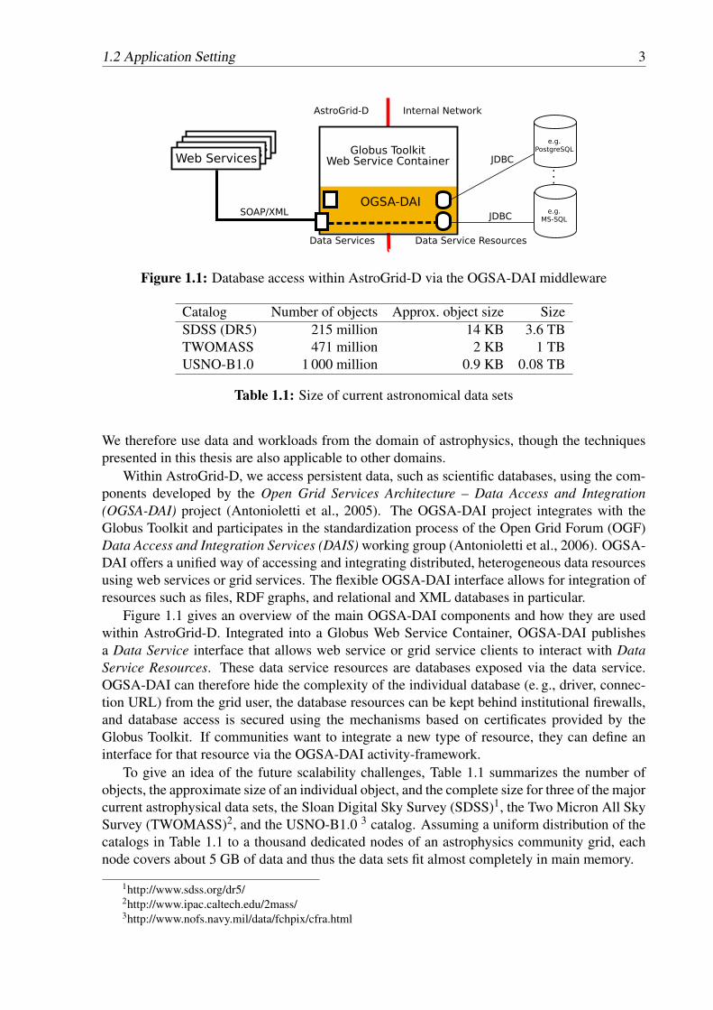
Figure 1.1: Database access within AstroGrid-D via the OGSA-DAI middleware

Catalog Number of objects Approx. object size SizeSDSS (DR5) 215 million 14 KB 3.6 TBTWOMASS 471 million 2 KB 1 TBUSNO-B1.0 1 000 million 0.9 KB 0.08 TB

Table 1.1: Size of current astronomical data sets

We therefore use data and workloads from the domain of astrophysics, though the techniquespresented in this thesis are also applicable to other domains.

Within AstroGrid-D, we access persistent data, such as scientific databases, using the com-ponents developed by the Open Grid Services Architecture – Data Access and Integration(OGSA-DAI) project (Antonioletti et al., 2005). The OGSA-DAI project integrates with theGlobus Toolkit and participates in the standardization process of the Open Grid Forum (OGF)Data Access and Integration Services (DAIS) working group (Antonioletti et al., 2006). OGSA-DAI offers a unified way of accessing and integrating distributed, heterogeneous data resourcesusing web services or grid services. The flexible OGSA-DAI interface allows for integration ofresources such as files, RDF graphs, and relational and XML databases in particular.

Figure 1.1 gives an overview of the main OGSA-DAI components and how they are usedwithin AstroGrid-D. Integrated into a Globus Web Service Container, OGSA-DAI publishesa Data Service interface that allows web service or grid service clients to interact with DataService Resources. These data service resources are databases exposed via the data service.OGSA-DAI can therefore hide the complexity of the individual database (e. g., driver, connec-tion URL) from the grid user, the database resources can be kept behind institutional firewalls,and database access is secured using the mechanisms based on certificates provided by theGlobus Toolkit. If communities want to integrate a new type of resource, they can define aninterface for that resource via the OGSA-DAI activity-framework.

To give an idea of the future scalability challenges, Table 1.1 summarizes the number ofobjects, the approximate size of an individual object, and the complete size for three of the majorcurrent astrophysical data sets, the Sloan Digital Sky Survey (SDSS)1, the Two Micron All SkySurvey (TWOMASS)2, and the USNO-B1.0 3 catalog. Assuming a uniform distribution of thecatalogs in Table 1.1 to a thousand dedicated nodes of an astrophysics community grid, eachnode covers about 5 GB of data and thus the data sets fit almost completely in main memory.

1http://www.sdss.org/dr5/2http://www.ipac.caltech.edu/2mass/3http://www.nofs.navy.mil/data/fchpix/cfra.html

4 1. Introduction

Project Data growth ratePer day Per year

Pan-STARRS 10 TB 4 PBLSST 18 TB 7 PBLOFAR 33 TB 12 PBLHC 42 TB 15 PB

Table 1.2: Estimated data grow rates for upcoming e-science projects

(a) Optical wavelength

(b) X-ray wavelength

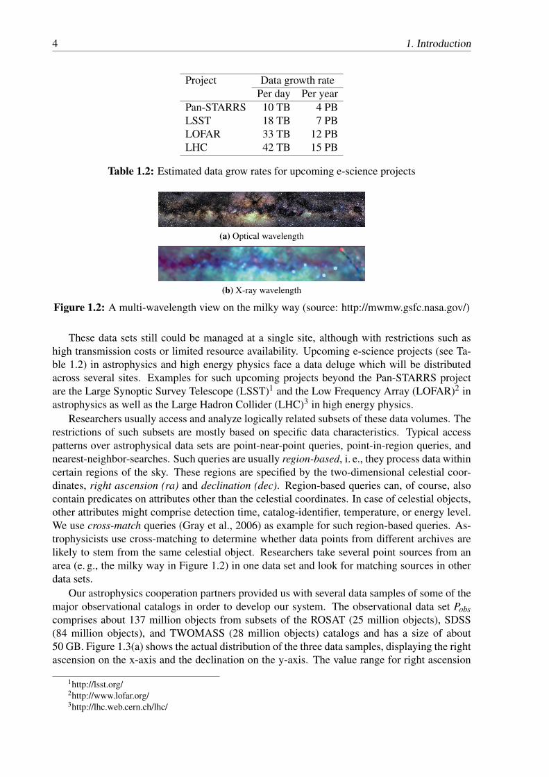
Figure 1.2: A multi-wavelength view on the milky way (source: http://mwmw.gsfc.nasa.gov/)

These data sets still could be managed at a single site, although with restrictions such ashigh transmission costs or limited resource availability. Upcoming e-science projects (see Ta-ble 1.2) in astrophysics and high energy physics face a data deluge which will be distributedacross several sites. Examples for such upcoming projects beyond the Pan-STARRS projectare the Large Synoptic Survey Telescope (LSST)1 and the Low Frequency Array (LOFAR)2 inastrophysics as well as the Large Hadron Collider (LHC)3 in high energy physics.

Researchers usually access and analyze logically related subsets of these data volumes. Therestrictions of such subsets are mostly based on specific data characteristics. Typical accesspatterns over astrophysical data sets are point-near-point queries, point-in-region queries, andnearest-neighbor-searches. Such queries are usually region-based, i. e., they process data withincertain regions of the sky. These regions are specified by the two-dimensional celestial coor-dinates, right ascension (ra) and declination (dec). Region-based queries can, of course, alsocontain predicates on attributes other than the celestial coordinates. In case of celestial objects,other attributes might comprise detection time, catalog-identifier, temperature, or energy level.We use cross-match queries (Gray et al., 2006) as example for such region-based queries. As-trophysicists use cross-matching to determine whether data points from different archives arelikely to stem from the same celestial object. Researchers take several point sources from anarea (e. g., the milky way in Figure 1.2) in one data set and look for matching sources in otherdata sets.

Our astrophysics cooperation partners provided us with several data samples of some of themajor observational catalogs in order to develop our system. The observational data set Pobscomprises about 137 million objects from subsets of the ROSAT (25 million objects), SDSS(84 million objects), and TWOMASS (28 million objects) catalogs and has a size of about50 GB. Figure 1.3(a) shows the actual distribution of the three data samples, displaying the rightascension on the x-axis and the declination on the y-axis. The value range for right ascension

1http://lsst.org/2http://www.lofar.org/3http://lhc.web.cern.ch/lhc/

1.2 Application Setting 5

(a) The observational data set Pobs consisting of data samples from three catalogsshowing data skew, i. e., a combination of densely populated areas wit data fromall catalogs and areas without any data

(b) The observational query set Qobs exhibiting query hot spots, i. e., several areaswith many queries such as the intersection of the three catalogs

Figure 1.3: The observational data set and query set

and declination is [0◦,360◦[ and [−90◦,90◦], respectively.For Pobs, we constructed the corresponding observational query set Qobs from real queries

submitted to the web interface1 of the SDSS catalog in August 2006.2 We translated the originalcone searches (with a circular search area) to queries having a square search area. For eachquery, we used the same midpoint and an edge length corresponding to the diameter of thecircular search area. Queries using the default search parameters of the web interface make up12% of the entire query log. Thus, we removed that particular query from our query set andused the remaining 1 100 000 queries during our evaluation. Figure 1.3(b) shows the queriedareas and we clearly see that the workload is non-uniform and exhibits many query hot spots.Remarkably, these hot spots are in areas where the catalogs overlap.

The second data sample Pmil (Figure 1.4) originates from the Millennium simulation con-

1http://cas.sdss.org/astrodr7/en/tools/search/2The query trace was kindly provided by Milena Ivanova and Martin Kersten from CWI, Amsterdam. It is the

same workload used for their experience report on migrating SkyServer on MonetDB (Ivanova et al., 2007).

6 1. Introduction

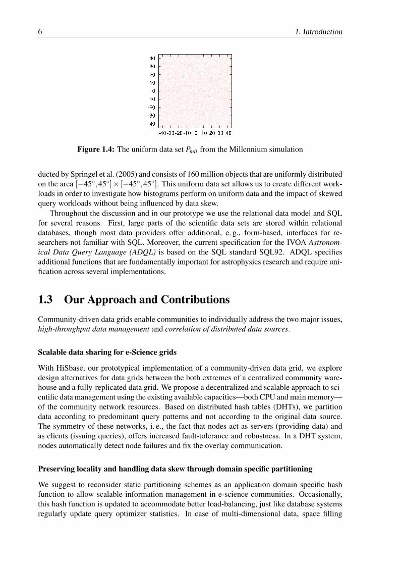
Figure 1.4: The uniform data set Pmil from the Millennium simulation

ducted by Springel et al. (2005) and consists of 160 million objects that are uniformly distributedon the area [−45◦,45◦]× [−45◦,45◦]. This uniform data set allows us to create different work-loads in order to investigate how histograms perform on uniform data and the impact of skewedquery workloads without being influenced by data skew.

Throughout the discussion and in our prototype we use the relational data model and SQLfor several reasons. First, large parts of the scientific data sets are stored within relationaldatabases, though most data providers offer additional, e. g., form-based, interfaces for re-searchers not familiar with SQL. Moreover, the current specification for the IVOA Astronom-ical Data Query Language (ADQL) is based on the SQL standard SQL92. ADQL specifiesadditional functions that are fundamentally important for astrophysics research and require uni-fication across several implementations.

1.3 Our Approach and ContributionsCommunity-driven data grids enable communities to individually address the two major issues,high-throughput data management and correlation of distributed data sources.

Scalable data sharing for e-Science grids

With HiSbase, our prototypical implementation of a community-driven data grid, we exploredesign alternatives for data grids between the both extremes of a centralized community ware-house and a fully-replicated data grid. We propose a decentralized and scalable approach to sci-entific data management using the existing available capacities—both CPU and main memory—of the community network resources. Based on distributed hash tables (DHTs), we partitiondata according to predominant query patterns and not according to the original data source.The symmetry of these networks, i. e., the fact that nodes act as servers (providing data) andas clients (issuing queries), offers increased fault-tolerance and robustness. In a DHT system,nodes automatically detect node failures and fix the overlay communication.

Preserving locality and handling data skew through domain specific partitioning

We suggest to reconsider static partitioning schemes as an application domain specific hashfunction to allow scalable information management in e-science communities. Occasionally,this hash function is updated to accommodate better load-balancing, just like database systemsregularly update query optimizer statistics. In case of multi-dimensional data, space filling

1.4 Outline 7

curves preserve the spatial locality between closely related data. HiSbase targets collaborativecommunities having vast data volumes with fairly stable data distributions. Long-term distribu-tion changes can also be leveled by reorganizing the histogram.

Increased Query Throughput by parallelism and workload-awareness

We investigate the potential offered by P2P networks for increasing query throughput in data-intensive e-science applications. Achieving sufficient query throughput constitutes one of themain deficiencies of centralized data management. Moreover, by enhanced workload-awarenessduring the creation of the partitioning scheme and during runtime additional throughput im-provements are possible.

1.4 OutlineIn Chapter 2, we provide the reader with a general overview of HiSbase and describe the generaldesign choices and decisions. Parts of this section have been presented at BTW 2007 (Schollet al., 2007b), VLDB 2007 (Scholl et al., 2007a), and in an overview article in the FGCS jour-nal (Scholl et al., 2009a).

The following chapters provide a more detailed discussion about the individual parts thatorchestrate the data management infrastructure in community-driven data grids. The Chapters 3through 6 describe the basic building blocks.

Chapter 3 focuses on the training phase where the partitioning scheme for distributing thedata among the resources is built. This material has been presented at the IEEE e-ScienceConference 2007 (Scholl et al., 2007c).

We describe how the data partitions are mapped to the nodes participating in a community-driven data grid in Chapter 4 and present our bulk feeding techniques for efficient data dissem-ination in Chapter 5.

Chapter 6 describes collaborative query processing and coordination and presents the setupand results of our throughput experiments within a community-driven data grid. The evaluationof the different coordination strategies has been presented at HPDC 2009 (Scholl et al., 2009c).

How the training phase can be extended to address also workload-awareness is described inChapter 7. The results have been presented at EDBT 2009 (Scholl et al., 2009b).

We then describe our concepts for achieving further load balancing within community-driven data grids during runtime (Chapter 8). Parts of this chapter have been presented in theDatenbank-Spektrum (Scholl et al., 2008) and the Proceedings of the VLDB Endowment (Scholland Kemper, 2008).

8 1. Introduction

9

CHAPTER 2

HiSbase

This chapter gives an overview of the basic principles behind community-driven data grids. Itprovides enough background to selectively choose one of the following chapters to receive moredetailed information about a particular aspect.

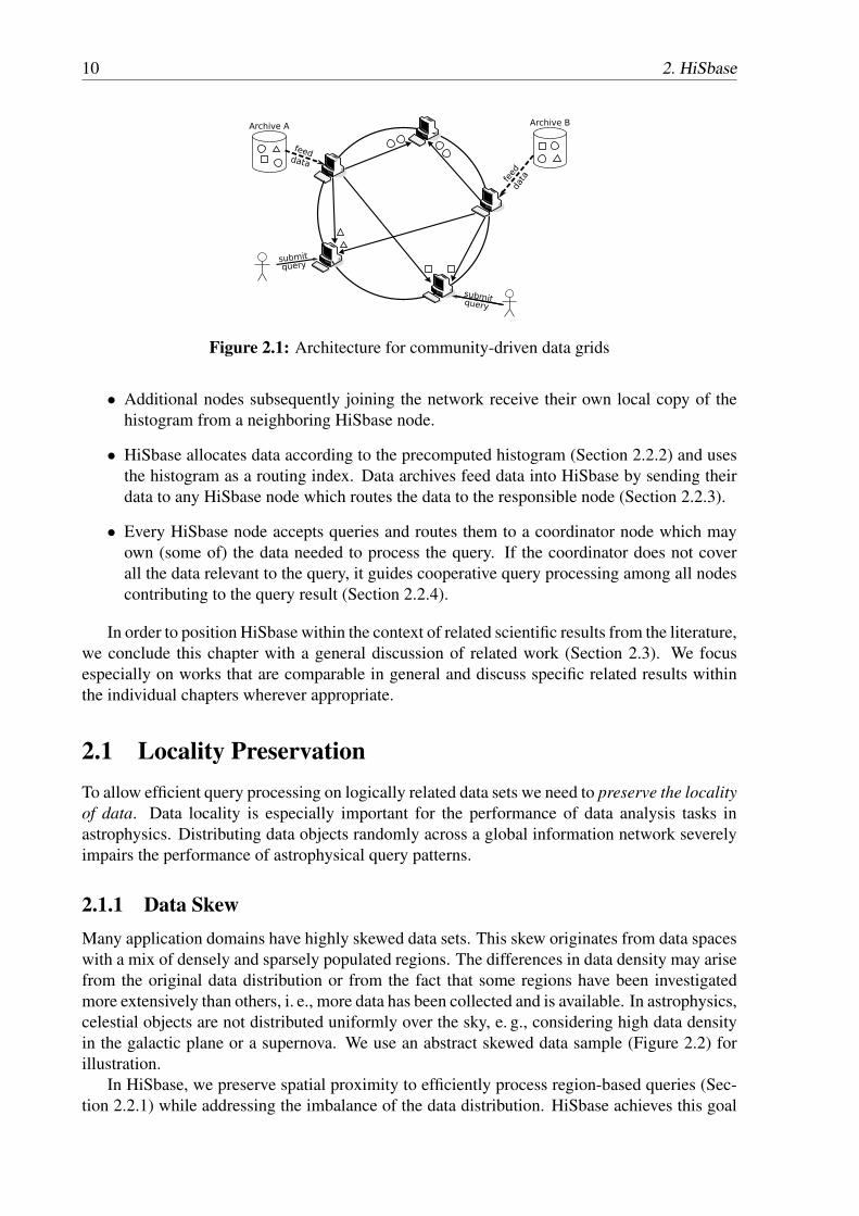
Our prototype HiSbase defines a distributed information infrastructure that allows the shar-ing of CPU resources and storage across scientific communities to build a community-drivendata grid. We distribute data across nodes according to predominant query patterns to achievehigh throughput for data analysis tasks. Therefore, most processing tasks can be performedlocally, achieving high cache locality as nodes mainly process queries on logically related datahosted by themselves as illustrated in Figure 2.1. In the figure, the same geometric shapes de-note logically related data originating from (possibly) different distributed sources. HiSbasepartitions and allocates data fed into the system by means of community-specific distributionfunctions, called histograms. Thereby, related data objects of various sources are mapped to thesame nodes. The original archive servers, which still serve as data sources, are complementedby our HiSbase infrastructure for high throughput query processing. In Section 2.1, we show acandidate data structure that preserves spatial locality and adapts to the data distribution.

HiSbase builds on the advances and maturity of distributed hash table (DHT) implementa-tions (e. g., Stoica et al., 2001) which were devised in order to provide a scalable and failure-resilient data management for large-scale, distributed information systems. Objects and nodesare randomly mapped to a one-dimensional key space, e. g., by using a secure hash algorithmon either the IP address of a node or on a checksum of the content of an object. Nodes areresponsible for a subspace of the key space and thus data load balancing is achieved. The initialversions of these protocols only offer scalable query access for exact-match queries.

HiSbase partitions multi-dimensional e-science data across an initial set of nodes for dataload balancing. Later on, of course, additional resources (data and nodes) can be added to thecommunity network, which is constructed as follows.

• We precompute the histogram of the actual data space in a preparatory training phasebased on a training set and pass it to the initial HiSbase node during startup (Section 2.2.1).

10 2. HiSbase

Figure 2.1: Architecture for community-driven data grids

• Additional nodes subsequently joining the network receive their own local copy of thehistogram from a neighboring HiSbase node.

• HiSbase allocates data according to the precomputed histogram (Section 2.2.2) and usesthe histogram as a routing index. Data archives feed data into HiSbase by sending theirdata to any HiSbase node which routes the data to the responsible node (Section 2.2.3).

• Every HiSbase node accepts queries and routes them to a coordinator node which mayown (some of) the data needed to process the query. If the coordinator does not coverall the data relevant to the query, it guides cooperative query processing among all nodescontributing to the query result (Section 2.2.4).

In order to position HiSbase within the context of related scientific results from the literature,we conclude this chapter with a general discussion of related work (Section 2.3). We focusespecially on works that are comparable in general and discuss specific related results withinthe individual chapters wherever appropriate.

2.1 Locality PreservationTo allow efficient query processing on logically related data sets we need to preserve the localityof data. Data locality is especially important for the performance of data analysis tasks inastrophysics. Distributing data objects randomly across a global information network severelyimpairs the performance of astrophysical query patterns.

2.1.1 Data SkewMany application domains have highly skewed data sets. This skew originates from data spaceswith a mix of densely and sparsely populated regions. The differences in data density may arisefrom the original data distribution or from the fact that some regions have been investigatedmore extensively than others, i. e., more data has been collected and is available. In astrophysics,celestial objects are not distributed uniformly over the sky, e. g., considering high data densityin the galactic plane or a supernova. We use an abstract skewed data sample (Figure 2.2) forillustration.

In HiSbase, we preserve spatial proximity to efficiently process region-based queries (Sec-tion 2.2.1) while addressing the imbalance of the data distribution. HiSbase achieves this goal

2.1 Locality Preservation 11

Figure 2.2: Sample data space with skewed data distribution

by calculating a histogram that equips the data grid with a community-specific data distribution.Among others, we describe the Z-quadtree histogram data structure that we designed to preservespatial locality for astrophysics data sets. Z-quadtrees are quadtrees whose leaves correspondto histogram buckets and are linearized on the key space of the DHT using a space filling curve.These trees provide efficient access to histogram buckets (regions) while balancing the data loadacross data nodes.1 Section 2.2.5 outlines how we additionally consider query load balancingwithin HiSbase.

2.1.2 Histogram Data StructuresHiSbase enables communities to design data structures for distributing their data across severalnodes and to adapt to data and query characteristics of that particular community. We call thesedata structures histograms for their similarities to standard histograms. Histograms are, forexample, commonly used in relational database management systems as means for selectivityestimations (Poosala et al., 1996).

Within HiSbase, a histogram is used in order to look up multi-dimensional areas and datapoints.

lookupArea(h,a) : S This function plays a central part during query processing. Given a multi-dimensional data area a, lookupArea returns the set S of region identifiers of the his-togram h which intersect with a.

lookupPoint(h,p) : r Mainly used during data distribution, lookupPoint returns the regionidentifier r of the histogram h which contains a multi-dimensional data point p.

Most of the following histogram data structures are inspired by the intensive research con-ducted by the computer science community on locality-aware data structures developed for ac-cessing and efficiently storing multi-dimensional data (Gaede and Günther, 1998; Samet, 2006).The individual community is free to choose any data structures implementing the interface re-quired by HiSbase. Therefore, we are strengthening the histogram-related aspect rather than theaspect of indexing multi-dimensional data.

Z-quadtree: A Histogram Based on Quadtrees

The shape of data partitions defined by candidate data structures should be simple (e. g., squares).This allows simple (SQL) queries to retrieve data during the process of integrating new nodes(Section 2.2.2).

1In the following, we use the terms regions and histogram buckets interchangeably. The leaves of a Z-quadtreerepresent the histogram buckets for that particular histogram data structure.

12 2. HiSbase

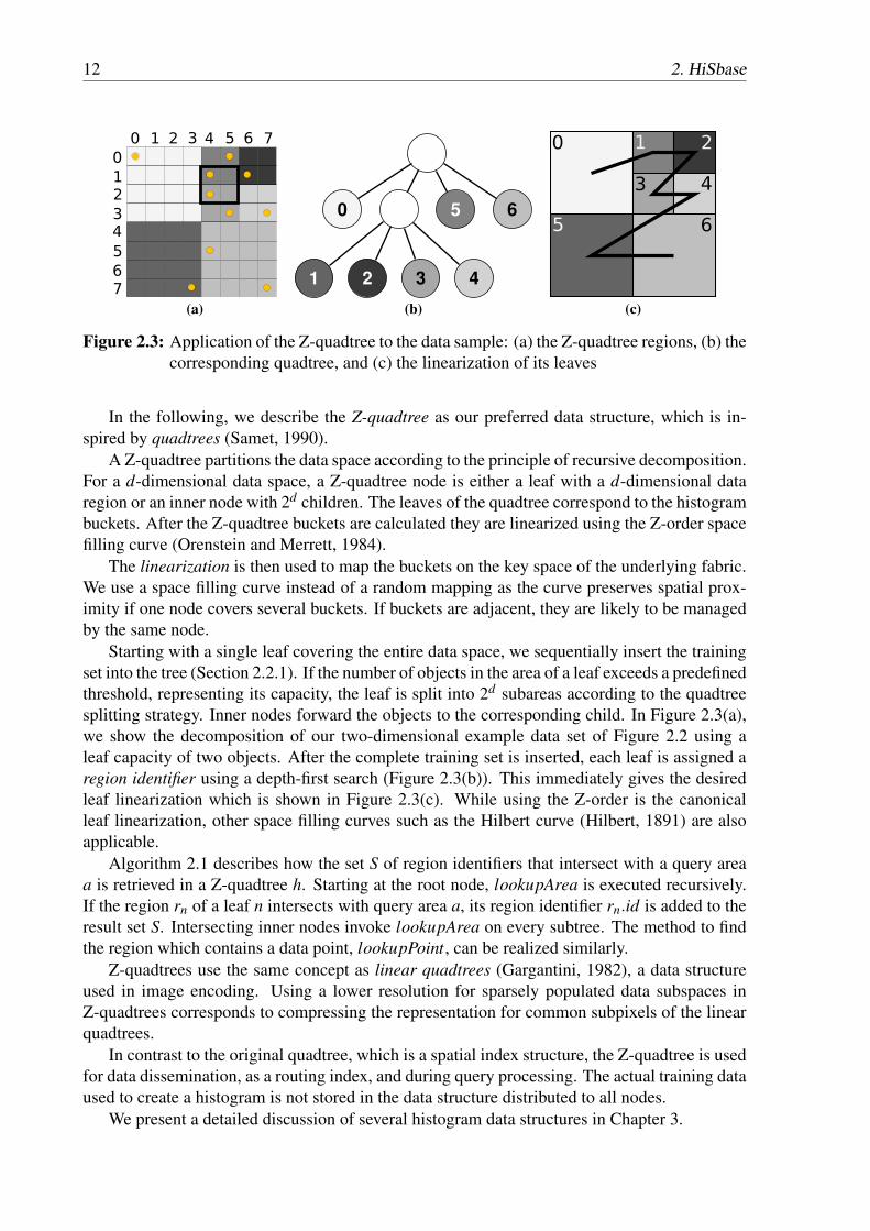
(a) (b) (c)

Figure 2.3: Application of the Z-quadtree to the data sample: (a) the Z-quadtree regions, (b) thecorresponding quadtree, and (c) the linearization of its leaves

In the following, we describe the Z-quadtree as our preferred data structure, which is in-spired by quadtrees (Samet, 1990).

A Z-quadtree partitions the data space according to the principle of recursive decomposition.For a d-dimensional data space, a Z-quadtree node is either a leaf with a d-dimensional dataregion or an inner node with 2d children. The leaves of the quadtree correspond to the histogrambuckets. After the Z-quadtree buckets are calculated they are linearized using the Z-order spacefilling curve (Orenstein and Merrett, 1984).

The linearization is then used to map the buckets on the key space of the underlying fabric.We use a space filling curve instead of a random mapping as the curve preserves spatial prox-imity if one node covers several buckets. If buckets are adjacent, they are likely to be managedby the same node.

Starting with a single leaf covering the entire data space, we sequentially insert the trainingset into the tree (Section 2.2.1). If the number of objects in the area of a leaf exceeds a predefinedthreshold, representing its capacity, the leaf is split into 2d subareas according to the quadtreesplitting strategy. Inner nodes forward the objects to the corresponding child. In Figure 2.3(a),we show the decomposition of our two-dimensional example data set of Figure 2.2 using aleaf capacity of two objects. After the complete training set is inserted, each leaf is assigned aregion identifier using a depth-first search (Figure 2.3(b)). This immediately gives the desiredleaf linearization which is shown in Figure 2.3(c). While using the Z-order is the canonicalleaf linearization, other space filling curves such as the Hilbert curve (Hilbert, 1891) are alsoapplicable.

Algorithm 2.1 describes how the set S of region identifiers that intersect with a query areaa is retrieved in a Z-quadtree h. Starting at the root node, lookupArea is executed recursively.If the region rn of a leaf n intersects with query area a, its region identifier rn.id is added to theresult set S. Intersecting inner nodes invoke lookupArea on every subtree. The method to findthe region which contains a data point, lookupPoint, can be realized similarly.

Z-quadtrees use the same concept as linear quadtrees (Gargantini, 1982), a data structureused in image encoding. Using a lower resolution for sparsely populated data subspaces inZ-quadtrees corresponds to compressing the representation for common subpixels of the linearquadtrees.

In contrast to the original quadtree, which is a spatial index structure, the Z-quadtree is usedfor data dissemination, as a routing index, and during query processing. The actual training dataused to create a histogram is not stored in the data structure distributed to all nodes.

We present a detailed discussion of several histogram data structures in Chapter 3.

2.2 Architectural Design 13

Algorithm 2.1: Z-quadtree implementation of lookupArea(h,a)Input: Z-quadtree h with root node nroot , query area aOutput: Set S = {regionid r.id | region r intersects with a}

S ←{}n ← nrootif region rn of n intersects with a then

if n is leaf thenS ← S∪{rn.id}

else /* n is inner node */for all subtrees hchild of n do

S ← S∪ lookupArea(hchild,a)end for

end ifend if

Algorithm 2.2: Publish data in HiSbaseInput: Histogram h, multi-dimensional data point p

Region id r ← lookupPoint(h, p)Send newPointMessage(p) to r.

2.2 Architectural DesignThe architectural design of HiSbase offers scientific researchers a framework for data and re-source sharing within their community. Algorithms 2.2 and 2.3 formally define the interface fordata publication and access within HiSbase.

In this section, we outline the creation of histograms during the training phase and theinformation maintained at HiSbase nodes. Finally, we describe data publication and node col-laboration during query processing.

2.2.1 Training Phase (Histogram Build-Up)Extracting the training samples, defining the partitioning of the data space, and distributing thepartitions to the data nodes comprise the three steps of our training phase.

For constructing the histogram, data from each data source is taken into account. We caneither use the entire data archive or a representative subsample. However, transmitting the en-tire data archive for histogram extraction is presumably prohibitive. For example, the subsetcould be extracted using a random sample. During our experiments, we achieved good his-tograms using 10% data samples in our a priori analysis. The data distribution does not changesignificantly very often (e. g., once a year), which makes such an a priori analysis applicable.

After the training set is inserted into the histogram, we serialize the histogram structure fordistribution within the network. The training data itself is discarded.

The resulting histogram is passed to the initial node in the HiSbase network. Nodes subse-quently joining the network receive the histogram from any other node in the network, mostlyfrom one of their neighboring nodes. Hence, each node keeps a copy of the histogram.

The number of histogram regions is determined before the training phase. In our experi-ments, we used histograms with up to 250 000 regions in order to enable a flexible distribution

14 2. HiSbase

Algorithm 2.3: Query data in HiSbaseInput: Histogram h, multi-dimensional query area a.

Set SR of relevant region ids ← lookupArea(h,a)Select coordinator rc from SRSend newQueryMessage(a,SR) to rc.

Figure 2.4: Mapping of the quadtree of Figure 2.3 to multiple nodes

of the individual data regions. The memory requirements of a histogram are small comparedto the amount of data transmitted during query processing. As nodes presumably get their his-togram from a physical neighbor, histogram distribution adds little overhead to the setup phaseof the HiSbase network.

2.2.2 HiSbase NetworkWhile the overall design of HiSbase abstracts from the underlying DHT implementation, weuse the DHT infrastructure Pastry (Rowstron and Druschel, 2001) to manage nodes and routemessages in HiSbase. Like Chord (Stoica et al., 2001), Pastry maps data and nodes to a one-dimensional key ring. In contrast to Chord, Pastry optimizes the initial phase of routing bypreferring physical neighbors to speed up communication within the overlay network.

Mapping Nodes to Regions

The histogram regions are uniformly mapped onto the DHT ring identifiers. Due to this uni-form distribution, all regions are mapped to a node with equal probability regardless of theirindividual size. The size of regions might vary due to the adaption to data skew. The nodes geta random identifier and are responsible for regions close to their identifier. Pastry, for example,uses 160-bit identifiers and ordinary comparisons in order to determine the closeness of identi-fiers. Figure 2.4 illustrates the evenly distributed regions (0–6) and their mapping to randomlydistributed nodes (a, b, c, d) on the DHT key space. We use the routing of the underlying DHTsystem to automatically assign regions to nodes. To ensure that messages destined for a specificregion are received by the appropriate node, we use the region identifiers for message routing.

We prefer to use the key-based routing functionality of the underlying DHT infrastructureover using a direct mapping of histogram buckets on nodes or using a centralized directory for

2.2 Architectural Design 15

Algorithm 2.4: Handling node arrivalsNode p covers a set P of regions. Let Pnew be the set of regions which node p isresponsible for after a new node has arrived. The area ai is the area of region i.

if Pnew 6= P thenfind Pmove = P\Pnewfor all r ∈ Pmove do

ar = getArea(r)redistribute data from ar to region r

end forend if

the histogram in combination with a histogram cache at the individual nodes. A direct mappingwould require every node to maintain the complete list of participating nodes and also the map-ping of the individual histogram buckets to the nodes. Using the key-based routing, each nodestores only O(logn) neighbors and the mapping is done automatically by the underlying fabric.Updating a histogram via a distributed broadcast is not more expensive than distributing an up-dated histogram from a central site. Furthermore, we reuse functionality already implementedby the Peer-to-Peer (P2P) substrate and leverage the increased flexibility and the automatic han-dling of node failures. In Chapter 4, we present a detailed comparison between several mappingstrategies with regards to data load balancing and query locality.

Node Arrival

When a node joins the HiSbase network, the active histogram will be transmitted to that nodeand the node needs to receive the data according to its responsibilities. For this purpose, HiS-base reuses the mechanisms of the DHT structure to determine the arrival of new nodes. InPastry (Rowstron and Druschel, 2001), nodes are notified if the leaf set (the nodes which havesimilar identifiers) changes. Algorithm 2.4 describes how a notified node determines the data itis no longer responsible for. For this purpose, it compares its set of regions before and after thenotification. The node then redistributes the moveable data and the newly joined node updatesits database.

Node Departure

HiSbase is developed for an environment where the participating servers are quite reliable. Highchurn is currently not in our focus as distributing the envisioned amounts of data across unreli-able nodes is not very useful. Nonetheless, some nodes might temporarily fail. As mentionedin the introduction of this chapter, HiSbase does not replace but complement the “traditional”data centers since these also serve as data sources for distributing the data in HiSbase. If a nodeleaves the network its direct neighbor nodes take over part of its data. The neighboring nodesrefetch that data from the appropriate archives.

2.2.3 Data Distribution (Feeding)Connected data centers directly feed data into HiSbase as illustrated by Figure 2.1. In HiSbase,the histogram is used to determine how to allocate data on nodes. All nodes maintain the data

16 2. HiSbase

objects which are in their histogram buckets, independently from the archive the data comesfrom. HiSbase abstracts from the specific database system, which allows the use and evaluationof various traditional as well as main memory database systems.

Data archives that want to publish their data in HiSbase connect to any HiSbase node, prefer-ably to a node nearby or to a node that has a high network bandwidth. Proceeding according toAlgorithm 2.2, the contacted node uses the lookupPoint method of its histogram to locate thehistogram bucket that contains a data object. Then it routes the object to the DHT identifier ofthis region. The message contains the data object and information about the data source. Viathe underlying DHT mechanism, the data item arrives at the responsible node, which updatesits database.

Distributing each data item individually results in a very high overhead. The precomputedhistogram allows us to optimize the feeding stage by introducing bulk feeding. A node that feedsdata into the network buffers multiple objects for the same region until a threshold is reached.Time-based as well as count-based thresholds are applicable.

Integrating new data sets is achieved by feeding them into the network as described aboveafter the according tables are created at each node. If the new data set is a detailed survey ofa sky region that has not yet been covered by any existing archive in the community network,it might be appropriate to create a new histogram in order to improve the data load balancing(Section 2.2.5). In that case, a data sample of the survey is extracted and integrated into thetraining phase. Chapter 5 discusses data feeding in more detail.

2.2.4 Query Processing

Region-based queries are submitted to any node of the HiSbase network. The node extractsthe multi-dimensional area A from the query predicate. It selects an arbitrary identifier rc fromthe set of intersecting regions, which is determined by lookupArea. The node pc which isresponsible for region rc is the coordinator. The coordinator collects intermediate results andperforms post-processing tasks (e. g., duplicate elimination).

Let us assume a region-based query was issued at node d in Figure 2.4. The area of the queryis marked with the thick-lined rectangle in Figure 2.3(a). Thus, relevant to our example queryare regions 1 and 3. If node d covers regions relevant to the query, it becomes the coordinatoritself. This is not the case in our example. We select region 1 as rc and thus node a becomesthe coordinator. Node d forwards a coordination request to node a. The coordination requestcontains the query and the relevant regions. After node a receives the coordination request, itissues the query to its own database (as it covers relevant regions) and sends the query to allother relevant regions. Node b also participates in the query processing in our example as itcovers region 3. It sends its intermediate results back to the coordinator, node a. After havingreceived all intermediate results, node a returns the complete result to node d.

Nodes may cover several regions. As region identifiers are used for submitting queries,nodes can receive the same query several times. Each node stores a hash of currently processedqueries to avoid multiple evaluations of the same query. Results and error messages are di-rectly transmitted to the coordinator or the submitting node without using the overlay routingalgorithm. Chapter 6 discusses more details on query processing and query coordination withincommunity-driven data grids and presents the evaluation results from our query throughputmeasurements.

2.2 Architectural Design 17

Figure 2.5: Histogram evolution

2.2.5 Query Load BalancingThere are several techniques for combining our data load balancing approach described so farwith query load balancing techniques to efficiently handle query hot spots. In order to achievethis, we extend the use of our training phase and employ techniques that redistribute load atruntime.

We enhance the training phase with query statistics such as earlier workloads. Based onthese statistics, the data partitioning can be modified to enable the application of query loadbalancing techniques such as replication or load migration. For a detailed discussion about thisworkload-aware data partitionings, we refer the reader to Chapter 7.

Using two parallel Pastry rings with different histograms increases the data availabilitywithin the HiSbase network. By changing the offset (or the space filling curve) of the map-ping process from Section 2.2.2, the second histogram stores the data on different nodes andboth copies are available during query processing.

We also introduce a master-slave hierarchy, where idle nodes can support overloaded nodesby offering their storage and compute resources. These may be necessary to cope with short-term changes in query load distribution. Whether a node is overloaded or constitutes a potentialslave-node is determined based on workload statistics collected during run-time. These statisticscan also augment the training phase for the next histogram evolution.

2.2.6 Evolving the HistogramThe histogram serves HiSbase as a partitioning function, defining the data set which a node isresponsible for. HiSbase nodes maintain three histograms and their accompanying data sets toimprove load balancing or level long-term data shifts. From our perspective, three data copiesoffer a good data availability at a reasonable management overhead for e-science scenarios.Each pair of histogram and data set can evolve during the lifetime of a HiSbase instance andhas one of the following three functionalities: the in-progress, active, and passive functionality.

in-progress The currently running feeding process, which is described above, distributes dataaccording to the in-progress histogram. After a new histogram has been distributed, theHiSbase nodes build this in-progress data set and store it on disk.

active Once the build-up phase of the in-progress histogram is completed, they become the

18 2. HiSbase

active histogram and data set. Both are used during query processing and nodes keepthem completely (or at least the relevant parts) in main memory. Furthermore, HiSbasenodes use the active histogram for messaging.

passive The completely updated data set is additionally kept on disk as backup for the activedata set. This preserves the active data set beyond the lifetime of the current network andcan be used if a node is restarted with the same identifier.

Figure 2.5 illustrates a scenario where the in-progress histogram contains additional regionswhile the active and passive histograms are the same as in Figure 2.4.

Any of the participating nodes can be used to inject an updated version of a histogram bybroadcasting it to the HiSbase network. Our concepts for query load balancing at runtime arediscussed in Chapter 8.

2.2.7 HiSbase EvaluationWe use three different evaluation settings in order to measure the features of community-drivendata grids: a set of tools to analyze various characteristics of partitioning schemes, HiSbaseinstances running within an overlay network simulator, and deployments in various test beds.

The analysis of the individual partitioning scheme characteristics provides us with valuableinsights for comparing and choosing different candidate data structures. Simulated instancesallow us to explore systematically the network flow or communication patters under variousconditions. Finally, the distributed instances are the key to test our system in a realistic environ-ment and to evaluate the merits for scientific users.

Partitioning Schemes

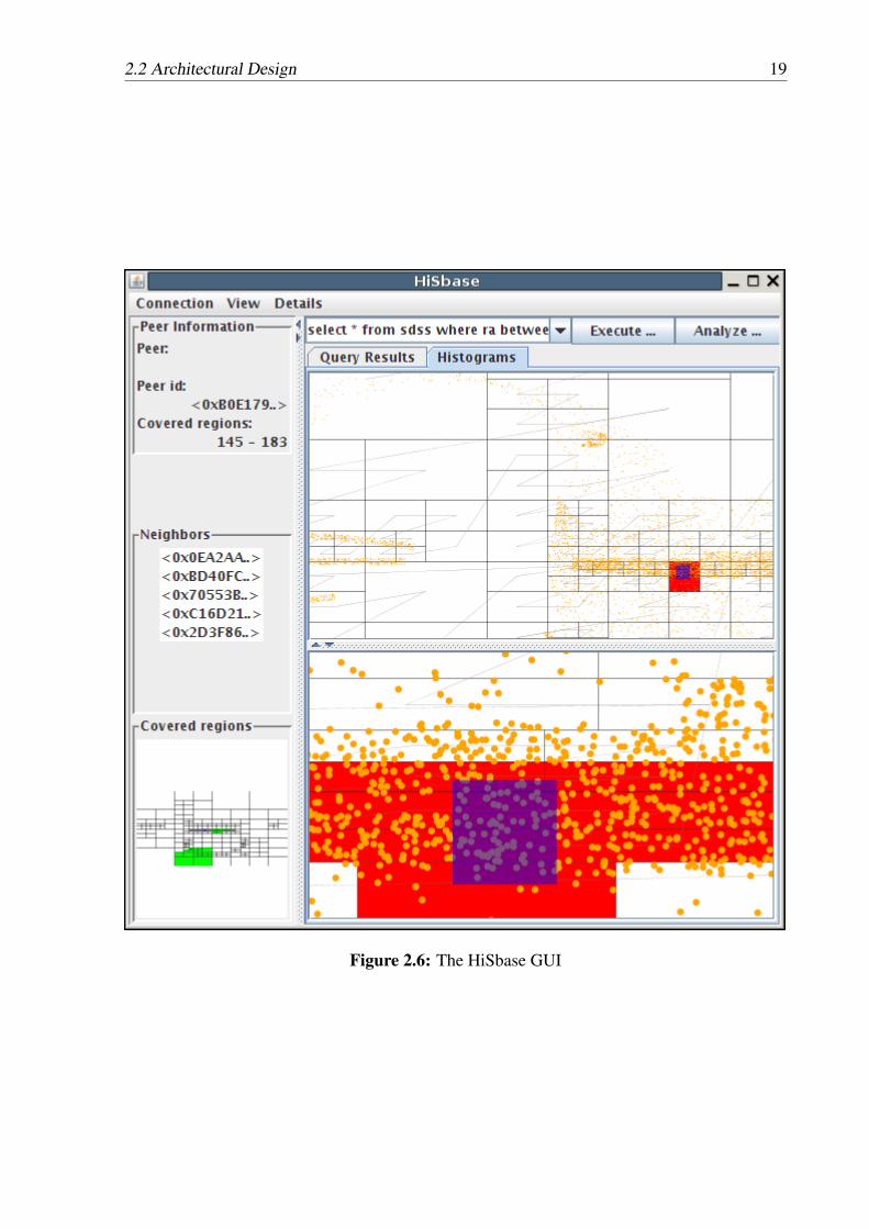
Although many e-science communities require a scalable data management, they mostly haveslightly different types of analysis tasks and therefore a wide range of requirements for thedata management infrastructures. The scientific researchers require support and simple toolsthat help them to find an optimal partitioning scheme for their particular interest. Our testingframework developed within the HiSbase project enables the researchers to compare variouscandidate partitioning schemes based on several properties and to choose the one partitioningscheme which fits best their needs. Among these tools is a graphical user interface (GUI,shown in Figure 2.6) which allows for comparing different histogram data structures. Moreover,the GUI supports query submission and query analysis and shows status information on theconnected HiSbase nodes.

The FreePastry Library

For the implementation of our prototype we use FreePastry1, the open source Java-implementationof Pastry (Rowstron and Druschel, 2001), currently maintained by the Max-Planck-Institut forSoftware Systems. FreePastry provides the underlying key-based routing fabric and P2P-basedmulticast communication (i. e., Scribe by Castro et al., 2002).

FreePastry provides an implementation of the Common API (Dabek et al., 2003), whichdescribes a common interface for DHT-based implementations. During our implementation,we aimed at programming only against those interfaces in order retain as much independencefrom the underlying overlay network implementation as possible.

1http://freepastry.org/

2.2 Architectural Design 19

Figure 2.6: The HiSbase GUI

20 2. HiSbase

(a) FreePastry Simulator (b) Distributed FreePastry

Figure 2.7: Simulated and distributed evaluation environments on FreePastry

Simulation Environment

Moreover, FreePastry provides enough abstraction from the underlying network layers, in orderto use our application unmodified for both simulation and distributed deployments. Reusingthe same code in both environments was one of our major incentives to favor this simulatorover other prominent simulators such as ns-21. In Figure 2.7(a), we give an coarse overviewof the simulator environment within FreePastry. The simulator uses discrete events and thusallows non-linear execution to speed-up simulations considerably. It also provides a modulewith various topologies to model network latency, e. g., Euclidean or spherical networks orexplicit latency matrices. Above this layer, FreePastry has its network layer and allows to runseveral thousand nodes within a single Java virtual machine. The simulator does not modelnetwork bandwidth, message loss, nor varying latency due to congested network resources. AsHiSbase aims at grid-based community infrastructures having dedicated resources and we alsoperform evaluations in real deployments, the benefits of using a single code base outweighs themissing features of the simulator.

Distributed Instances

Due to the simplifications within our simulation environment, we consider it as very importantto deploy our prototype also in real test beds. Tests in real deployments exemplify actual benefitsfor the research communities. Figure 2.7(b) shows the communication layers for the distributedscenario.

We deployed HiSbase on several nodes within our lab. Measurements with these nodesshow the performance using high bandwidth networks and low latency within a single institu-tion. Our measurements using nodes of the AstroGrid-D test bed represent the performance ofour community-driven approach within a nation-wide data grid using high-bandwidth networksto interconnect dedicated, powerful resources. Finally, we used PlanetLab2 for performing ex-periments. PlanetLab is a test bed for distributed applications. Though the test bed rather targetsprojects that evaluate distributed algorithms or protocols, we integrated several PlanetLab nodesinto a network with our AstroGrid-D resources, reaching up to one hundred nodes.

1http://nsnam.isi.edu/nsnam/index.php/Main_Page2http://planet-lab.org/

2.3 Related Work 21

2.3 Related Work

The HiSbase approach provides several benefits to e-science communities by addressing domain-specific data and query characteristics. HiSbase offers high throughput via parallelization,higher cache locality, and load balancing across several sites compared to centralized data man-agement. HiSbase enables scalable sharing of decentralized resources within a community as ituses the DHT mechanism of key-based routing for data distribution and message routing. Us-ing these techniques, new nodes can be easily added to the network and heterogeneous databasemanagement systems can be integrated with little effort as each HiSbase node only maintainsits own local database configuration.

In the following, we present related work from areas such as distributed databases, P2Parchitectures, and scientific data management.

2.3.1 Distributed and Parallel Databases

Using parallelism and data partitioning to increase query throughput are well-established tech-niques from distributed and parallel databases which motivated us to use them as pillars for thearchitectural design of community-driven data grids. For example, Özsu and Valduriez (1999)describe in depth the general concepts and algorithms for distributed databases.

Kossmann (2000) provides a detailed survey of query processing techniques within dis-tributed systems. Intelligent query processing and well-designed data placement are key tech-niques for realizing scalable data management solutions such as an information economy (Brau-mandl et al., 2003).

The field of parallel databases (e. g., Abdelguerfi and Wong, 1998) has brought up valu-able insights in the area of query parallelization and infrastructure designs. A shared-nothingapproach (DeWitt and Gray, 1992) where each node has an individual data storage and nodescommunicate only via a shared network is considered the most scalable technique.

Compared to HiSbase, distributed databases run in a more homogeneous setting whereasparallel databases are not designed for world-wide distributed resources. Autonomous databasesystems (Pentaris and Ioannidis, 2006) also deal with the correlation of several data sources.However, data is not distributed across participating servers (adhering to the nodes’ autonomy)and thus correlation needs to be done at the client sites which leads to additional data traffic.

Another important aspects induced by the vast number of distributed data sources are het-erogeneity and provenance. Recently, a new pay-as-you-go approach (Salles et al., 2007) withinso-called dataspaces (Franklin et al., 2005) was identified. As opposed to data integration sys-tems (Naumann et al., 2006; Rahm and Bernstein, 2001), data co-existence is possible in datas-paces. Monitoring data provenance becomes increasingly important within distributed systemsintegrating data from various sources on demand, e. g., to ensure reproducibility of results. Re-cent work on provenance in databases includes, for example, Buneman and Tan (2007) andDavidson et al. (2007). A further treatment of data integration, dataspaces, or provenance isbeyond the scope of this thesis. We therefore assume that data being fed into HiSbase eitheradheres to a common schema or has already been transformed properly.

2.3.2 P2P architectures

DHT architectures such as CAN (Ratnasamy et al., 2001), Chord (Stoica et al., 2001), Pastry(Rowstron and Druschel, 2001), and Tapestry (Zhao et al., 2004) overcome the limitations of

22 2. HiSbase

centralized information systems by storing data in a distributed one-dimensional key space (ex-cept for CAN which uses a d-dimensional torus). While these systems achieve load balancingby randomly hashing data and peers to their key space, they neither support multi-dimensionalrange queries nor preserve spatial locality. HiSbase work is reminiscent of the achievements inP2P-based query processing (Huebsch et al., 2003).

Instead of DHTs, other proposals build distributed tree-based structures that already incor-porate range query capabilities for one-dimensional data. For example, Jagadish et al. (2005)describe a distributed balanced binary tree, BATON. If the target node of a message is not withinthe subtree of the sender, the message is routed towards the root of the tree. In order to reducethe routing overhead on the nodes close to the root of the tree, BATON also builds “vertical”routing paths. Ranges can be queried by seeking the start of the range and then perform anin-order traversal until the range is completely processed. P-Grid (Aberer et al., 2003) uses atrie-based infrastructure and performs routing along these prefixes. Besides additional supportfor replication, Datta et al. (2005) describe a “shower” algorithm on P-Grid in order to trade animproved response time for range queries for more messages.

A large variety of systems have been proposed to augment DHTs in order to support (multi-dimensional) range queries (Banaei-Kashani and Shahabi, 2004; Ganesan et al., 2004b; Shuet al., 2005; Tanin et al., 2007) or to address data (or execution) load balancing in P2P envi-ronments (Aspnes et al., 2004; Crainiceanu et al., 2007; Ganesan et al., 2004a; Pitoura et al.,2006). These systems are predominantly designed for settings that are very dynamic, i. e., datahot spots and the data itself change very frequently and the systems have a very high churn.This flexibility comes at the price of dealing with each data object (of several hundred milliondata objects) individually. We exemplify some of these systems below and discuss how theyrelate to HiSbase.

One approach (Banaei-Kashani and Shahabi, 2004) uses Voronoi diagrams in order to parti-tion the data space and to support queries on multi-dimensional data. Independently, the MURKsystem (Ganesan et al., 2004b) uses k-d trees to realize a similar idea. In these systems, peerscovering large data partitions have more neighbors, while in HiSbase the number of neighborsis independent from the number and size of covered regions. SCRAP (Ganesan et al., 2004b)directly applies a space filling curve to the data and assigns one-dimensional ranges to peers. InHiSbase, the submitting peer exactly determines the histogram regions in the multi-dimensionaldata space and only these peers are contacted during query processing while SCRAP can onlyapproximate a multi-dimensional query range using multiple one-dimensional ranges.

The distributed quadtree index (Tanin et al., 2007) is a distributed data structure for objectswith multi-dimensional extents and supports range queries. Each quadtree node is representedby its centroid and these are randomly placed on the key space of an underlying DHT structure(e. g., Chord). Two levels of the distributed quadtrees can be configured to limit where objectsare stored: one level ( fmin) defines the minimum depth, the other level ( fmax) defines the maxi-mum depth. Thus, distributed quadtrees aim both at avoiding the bottleneck of congested nodesin layers above layer fmin and too much fragmentation by storing objects in layers below layerfmax. When HiSbase applies the Z-quadtree as partitioning scheme it only maps the leaves tothe key space and does this equidistantly according to a space filling curve. Thus a peer coversdata from neighboring regions which then can be stored in the same database with a higherprobability than in the distributed quadtree. Each peer within the distributed quadtree cachesdirect links to the children of the quadtree nodes it is covering. Thus, it takes O(logn) hops tofind an fmin-node and then a constant number of steps to reach the relevant leaves. These stepsalso have to be processed with data objects without an extent which are stored at level fmax.

2.3 Related Work 23

In HiSbase, no additional routing steps are necessary. HiSbase discovers the relevant regiondirectly and routes to the responsible peer using O(logn) messages.

Shu et al. (2005) describe an online balancing algorithm for frequent changes in data hotspots which is also based on quadtrees. The quadtree leaves are mapped on a skip graph (Asp-nes and Shah, 2003) layer using a space filling curve. Aiming at data sets with high updaterates, the authors devise algorithms that require an initial phase such as the training phase ofHiSbase and each peer only needs partial knowledge of the complete data distribution. How-ever, peers are only allowed to manage regions on the same Z-level while in HiSbase there isno such restriction. Accounting for the rather stable data sets of e-science communities, thesecommunities benefit more from techniques increasing the query throughput of data managementinfrastructures than from such an approach.

How to achieve load balancing in one-dimensional, range-partitioned data is describedin (Aspnes et al., 2004; Ganesan et al., 2004a). Ganesan et al. (2004a) show that load balanc-ing schemes for range-partitioned data in highly dynamic P2P networks either need to adjustthe load between neighbors or need to change peer positions within the range. SCRAP is anextension of (Ganesan et al., 2004a) to multi-dimensional data. Aspnes et al. (2004) only main-tain representative values of the data ranges in the skip graph. Load balancing between thesedata ranges is achieved by arranging less-filled (open) buckets close to full (closed) buckets.HotRod (Pitoura et al., 2006) addresses query hot spots on one-dimensional data by replicat-ing popular data ranges on additional rings. Data is stored on the DHT using order preservinghash functions and as soon as access statistics show that a peer is increasingly accessed HotRodreplicates (hot) data to other virtual rings. While HotRod determines the ranges to be replicatedduring runtime, HiSbase has opted for replicating the partitioning scheme (the histogram) to allparticipating nodes, as the overall data distribution is fairly stable. Moreover, HiSbase allows ahigh flexibility regarding the actual histogram used by a particular community.

P-Ring (Crainiceanu et al., 2007) approaches data skew in an orthogonal manner in compar-ison to HiSbase. While HiSbase adapts the buckets of the histogram data structure to data skewand distributes these across the cooperating peers, P-Ring has the notion of “helper peers” thatsupport peers which are overloaded by skewed insertions either by data redistribution betweenneighbors or by merging their data into a neighbor’s range. Considering multi-dimensionalrange queries, P-Ring would need to approximate the query area with multiple one-dimensionalintervals. Using the insertion rate of 4 data items per second as in the simulation study ofP-Ring, importing 80 million objects would last 33 weeks (20 million seconds), which is inap-propriate for e-science communities having terabyte-scale data sets.

2.3.3 Scientific and Grid-based Data Management

Within many scientific communities, data management challenges propelled and are still trig-gering many innovative ideas and technologies in order to ease the day-to-day experience ofthe researchers. The D-Grid initiative accommodates several community-driven efforts in or-der to build scalable grid-based infrastructures in various research areas. The research-specificservices offered by the individual communities range from user-friendly secure grid access inmedical applications by MediGRID (Krefting et al., 2009) to a collaborative data and processinggrid for the climate community provided by C3Grid (Kindermann et al., 2007). Together withAstroGrid-D, these communities have also identified synergies within the individual data man-agement services (Plantikow et al., 2009). Other groups within the framework of D-Grid alsofocus on security (Gietz et al., 2009) and VO management (Kirchler et al., 2008) aspects which

24 2. HiSbase

are important to ensure the acceptance of grid-based solutions within the scientific community.Several areas have been identified (Foster and Iamnitchi, 2003; Ledlie et al., 2003) where P2Ptechnologies and grid computing can be combined in order to provide scalable infrastructures.We agree that this combination indeed fosters interesting options for the data management de-sign and, with this in mind, we designed community-driven data grids accordingly. In thefollowing, we describe other proposals for scientific data management.

MAAN (Cai et al., 2004) adds multi-attribute and range-queries to grid information systems.While string-attributes are still randomly hashed on the key space, they use a locality preserv-ing hash function (and if the distribution function is known, a uniform locality preserving hashfunction) for numerical values. Query processing is done in an iterative way (by queryingeach attribute individually, or using a single-attribute dominated query processing algorithm).According to each attribute, the data objects are inserted. So if a data object consists of 140 at-tributes, it is stored 140 times in the overlay network. This amount of redundancy is prohibitivefor large multi-attribute e-science data sets. HiSbase additionally accelerates query processingby contacting the relevant nodes in parallel.

VoroNet (Beaumont et al., 2007) creates a P2P overlay network based on Voronoi tessella-tions of high dimensional data spaces and offers poly-logarithmical routing performance withregards to the data objects. It builds the overlay network between the data objects which storeinterconnections to objects close-by (with regard to a distance metric) and a far-distant in orderto get short-cuts for routing. It is required that all nodes know the total number of objects forwhich the system was optimized in order for routing algorithms to function properly. Althoughthey can handle data skew via the Voronoi tessellations, data remains on the publishing nodeswhich can result in an imbalance, e. g., if one node shares more data with the community thanothers. The experiments were conducted with up to 300 000 two-dimensional objects from bothskewed and uniform distributions. Their flexibility in changing the tessellation comes at theprice that each data object is treated individually. It is unclear how the approach scales withseveral millions of objects and if the expected number of objects is guessed wrong.

GIME (Zimmermann et al., 2006) takes a different approach to geotechnical informationmanagement in federated data grids. The system adheres to the data autonomy of the partici-pating institutions and uses a replicated index (based on quadtrees or R-trees) for managing thebounding boxes of participating archives. Thus, it reduces the number of messages by submit-ting the query only to such archives whose minimum bounding box actually intersects the queryarea. Load imbalance can arise for data archives covering a large area. These archives have toprocess more queries than small archives and several data sets cannot be combined directlyon-site. AstroPortal (Raicu et al., 2006) combines digital images from several astronomicalarchives by offering a grid-based stacking service in order to create a “complete picture”.

OGSA-DAI is widely used as data access interface in several Grid communities world wide.Therefore, OGSA-DAI would be the perfect candidate to offer Grid-based access to HiSbase ina production system. Kottha et al. (2006) have conducted a performance evaluation of OGSA-DAI within the MediGrid project for medical applications.

Several inspiring ideas with regards to scientific data management have been proposed inthe context of a technique called Bypass-Yield Caching (Malik et al., 2005). The goal of thistechnique is to cache results from federated scientific archives close to the user in order toreduce network traffic and shorten response times. Based on the estimated result set size ofa query the cache decides whether to cache a result. The result size estimation uses querytemplates (Malik et al., 2006) extracted from the query history. For selectivity estimations,Malik and Burns (2008) propose a technique which exploits the workload information and query

2.3 Related Work 25

feedback by applying a recursive least square algorithm in order to minimize the estimationerrors. When the scientific partners retain data autonomy, a distributed join has to be scheduledacross several sites. In order to increase the throughput in such scenarios, Wang et al. (2007)propose algorithms based on spanning tree approximations for optimizing the scheduling ofthe distributed joins. It is an interesting issue for future research to combine their cachingtechniques with our throughput optimizing infrastructure and to evaluate synergies.

26 2. HiSbase

27

CHAPTER 3

Community Training: Selecting Partitioning Schemes

This chapter provides an in-depth discussion of the training phase, where the partitioningscheme for a community-driven data grid is created (Section 3.1). We discuss a variety of candi-date data structures for such a partitioning scheme, ranging from traditional multi-dimensionalindexes to application domain-specific data structures (Section 3.2). In Section 3.3, we de-scribe several criteria for comparing such partitioning data structures and apply these criteriaduring the evaluation of the variants described in Section 3.2. Related work (Section 3.4) and asummary (Section 3.5) conclude this chapter.

3.1 Training PhaseWe use a training phase to create and distribute partitioning schemes that describe how dataobjects from various archives are to be partitioned. The training phase comprises three steps:

1. Extract the training samples,

2. Create the partitioning scheme, and

3. Distribute data according to the partitioning scheme.

The training samples are representative subsets from all data archives that are to be dis-tributed within the network. Given the size of existing and anticipated data sources (severalterabytes each), it is not feasible to perform the training on the complete data sets. We usefunctionality provided by relational database systems to extract random samples. Based onthese training samples, we build the partitioning scheme. The created partitioning scheme isthen evaluated considering the identified application-specific data and query properties. Afterhaving selected a partitioning scheme, we create the individual data partitions from the partici-pating data archives. These data partitions are then distributed to the shared resources within thedata grid, e. g., using GridFTP or our data feeding techniques from Section 5. At the resources,the data is loaded into a database and made accessible via the middleware infrastructure.

28 3. Community Training: Selecting Partitioning Schemes

Quadtrees and the zones index are the two data structures we compare in the following withregard to their fitness for being used as a partitioning scheme for community-driven data gridsin astrophysics.

3.2 Data StructuresIn quadtree-based partitioning schemes, the partitions correspond to the leaves of a quadtree.Quadtrees (Finkel and Bentley, 1974; Samet, 1990) are a well-known spatial data structure anduse the principle of recursive decomposition to partition a d-dimensional data space. Quadtreesare recursively defined to be either a leaf with a d-dimensional hypercube data region or aninner node with 2d subtrees. In a 2-dimensional data space, an inner node has four children(quadrants) that cover equal-sized convex data regions.

In particular, communities having skewed data sets can benefit from the capability of quad-trees to adapt to the data distribution. Sparsely populated areas of the data space are representedby leaves covering a large data region and densely populated areas are partitioned into severalleaves covering small areas. Thus, the amount of data within each leaf, and therefore withineach partition, can be held approximately equal. In very pathological cases, however, wheredata is concentrated in a very small area, quadtrees degenerate to a tree having many emptyleaves. Partitioning schemes without empty leaves are preferable in our setting because theyallow us to directly map data partitions to shared resources.

One approach to address the issue of empty leaves is a median-based heuristics that splitsa leaf at the median instead of at the center. For our astronomical example, the heuristicsdetermines the split point (mra,mdec) by computing the median for ra-coordinates and dec-coordinates independently. Our heuristics is similar to the technique used by optimized pointquadtrees (Finkel and Bentley, 1974), which only compute the median in the first dimension andthus guarantee that no leaf contains more than half the data of the original leaf. Our heuristics,which computes the median in all dimensions independently, offers a better data distribution inthe average case. Figures 3.1(a) and 3.1(b) show a quadtree with regular decomposition and aquadtree using our median heuristics, respectively, both built during our evaluation.

Quadtrees can be created either top-down or bottom-up. Both approaches start with a singleempty quadtree leaf. During top-down creation, the training sample is sequentially inserted intothe leaf until a predefined threshold for the leaf capacity is reached. The leaf is split up and itsdata is distributed among its new subtrees. In the bottom-up approach, leaves have an unlimitedcapacity and all data is inserted into the initial leaf first. In the following, the biggest leaf is splitin turn until a predefined number of partitions has been reached.

We prefer the bottom-up approach over the top-down approach for several reasons. Buildingquadtrees top-down requires to guess the leaf capacity in advance, which is hard for highlyskewed data sets. Furthermore, building the partitioning scheme bottom-up is a requirement forother splitting strategies to work properly. For example, the median-based heuristics dependson all points within a leaf and would be inaccurate if calculated incrementally when the leafthreshold is reached. We furthermore consider it easier to give a rough estimate of the numberof nodes participating in a network than providing a good guess for the leaf capacity.

The zones index (Gray et al., 2006) is an index structure developed in order to improvethe performance of typical query patterns in astrophysics such as points-in-region queries, self-match queries, and cross-match queries. The principle behind the zones index is to divide thedata space into zones of equal height h. The zone identifier of a point (ra, dec) is calculated byf loor((dec+90.0)/h) because the domain of the declination coordinate is [−90.0,+90.0]. Due

3.3 Evaluation of Partitioning Scheme Properties 29

(a) without median heuristics (b) with median heuristics

Figure 3.1: Partitioning scheme with 1 024 partitions based on quadtrees (a) with regular de-composition and (b) with median heuristics

to their simplicity, zones are efficiently implemented directly in SQL and thus exhibit very goodperformance in tracking down relevant zones for a particular task. Applying the zones indexto the algorithm for finding maximum-likelihood brightest cluster galaxies (Nieto-Santistebanet al., 2005) is a very good example for increased performance by implementing an algorithm asclose as possible to the data: directly inside the database. The zones algorithm preserves spatiallocality by grouping data elements from the same area in the sky into the same zone. Usingzones as a clustered index, which also defines the physical layout of data besides acceleratingdata access, allows database optimizers to efficiently determine the query result.

We limit our discussion to these three data structures—the two variants of the quadtree andthe zones—and refer the interested reader to the survey by Gaede and Günther (1998) or thebook by Samet (2006) on multi-dimensional and metric data structures for more information onmulti-dimensional access methods.

3.3 Evaluation of Partitioning Scheme Properties

We evaluated the fitness of the three different data structures described in the previous sectionby collecting several statistics. For the evaluation, we used our Java-based prototype of theHiSbase system, which also employs a training phase.

We drew training samples from the skewed observational data set Pobs and the uniformlydistributed simulation data set Pmil provided by our cooperation partners and both described inthe introduction (Section 1.2). The samples are roughly of equal size in order to specificallystudy the impact of data skew on the partitioning schemes. We varied the size s of the trainingsamples to benchmark the quality of results obtained from small data samples. Finally, wegenerated partitioning schemes of different sizes n, with n varying from 16 (24) to 262 144 (218)partitions. If the partitioning scheme generates only non-empty partitions, we may generate as

30 3. Community Training: Selecting Partitioning Schemes

Parameter Value(s) DescriptionP Pobs, Pmil Data set used for training sample extraction

s 0.01%, 0.1%, 1%, 10% Size of the training set

n 24,25,26,27,28,29,210,211, Size of the partitioning scheme212,213,214,215,216,217,218

Table 3.1: Parameters for the training phase evaluation

many partitions as we have distributed grid servers available for distributing the data. If theconstruction method cannot guarantee the absence of empty partitions (which is generally thecase), it is better to generate more partitions and assign multiple partitions to a server. We chose218 partitions as upper limit, since partitioning schemes at this scale offer us high flexibility withregards to transferring the partitions and gives a good ratio between number of partitions andnumber of nodes. We refrained from building a partitioning scheme, if the desired sizes wouldlead to splitting empty partitions due to a data sample with too little data. Therefore, as wewill discuss in Section 3.3.5, we did not construct partitioning schemes with more than 16 384(214) partitions from the 0.01% training sample and more than 131 172 (217) partitions from the0.1% training sample, respectively, as this would have resulted in further splitting completelyempty partitions. Table 3.1 summarizes the evaluation parameters.

During the training phase, we gathered the following information: 1) the duration, 2) thedata distribution across partitions (measured in comparison to the partition storing the largestamount of data), 3) the variance in data population, 4) the number of empty partitions, 5) thedifferences among the results of training sets of varying size, and 6) the accuracy obtainedduring the training phase in comparison to calculating the partitioning schemes on the completedata set. The rationale behind investigating these characteristics is as follows.

1) Duration The duration1 of the training phase provides a notion of how long it takes to get agood partitioning scheme. We observe that in many e-science communities, data sets areupdated only every few months or on a yearly basis. Due to the invariance of the data, thetraining phase merely is a one-time cost.

2) Average data population The average data population in comparison to the biggest leavesgives a notion about how similar the data distribution is among the individual leaves.

3) Variance in partition population The variance is similar to the average data population. Alow variance implies that all partitions contain approximately the same number of objects.

4) Empty partitions Without empty partitions, we can directly map data partitions to the sharedservers. In cases where we cannot avoid empty leaves, we can create more partitions thanthe anticipated number of servers and assign multiple partitions to a server.

5) Size of the training set If outcomes of a small training set are comparable to the results ofa large training set, we can use the smaller one and thus reduce the cost of the trainingphase.

1We performed the evaluation of the training phase on a Linux server equipped with four Intel Xeon processorsat 2.33 GHz and 16 GB of RAM.

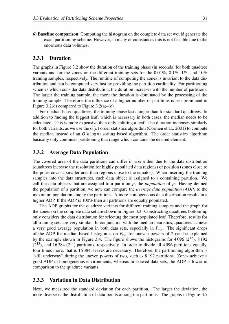
3.3 Evaluation of Partitioning Scheme Properties 31

6) Baseline comparison Computing the histogram on the complete data set would generate theexact partitioning scheme. However, in many circumstances this is not feasible due to theenormous data volumes.

3.3.1 DurationThe graphs in Figure 3.2 show the duration of the training phase (in seconds) for both quadtreevariants and for the zones on the different training sets for the 0.01%, 0.1%, 1%, and 10%training samples, respectively. The runtime of computing the zones is invariant to the data dis-tribution and can be computed very fast by providing the partition cardinality. For partitioningschemes which consider data distribution, the duration increases with the number of partitions.The larger the training sample, the more the duration is dominated by the processing of thetraining sample. Therefore, the influence of a higher number of partitions is less prominent inFigure 3.2(d) compared to Figure 3.2(a)–(c).

For median-based quadtrees, the training phase lasts longer than for standard quadtrees. Inaddition to finding the biggest leaf, which is necessary in both cases, the median needs to becalculated. This is more expensive than only splitting a leaf. The duration increases similarlyfor both variants, as we use the O(n) order statistics algorithm (Cormen et al., 2001) to computethe median instead of an O(n logn) sorting-based algorithm. The order statistics algorithmbasically only continues partitioning that range which contains the desired element.

3.3.2 Average Data PopulationThe covered area of the data partitions can differ in size either due to the data distribution(quadtrees increase the resolution for highly populated data regions) or position (zones close tothe poles cover a smaller area than regions close to the equator). When inserting the trainingsamples into the data structures, each data object is assigned to a containing partition. Wecall the data objects that are assigned to a partition p, the population of p. Having definedthe population of a partition, we now can compare the average data population (ADP) to themaximum population among the partitions. A more homogeneous data distribution results in ahigher ADP. If the ADP is 100% then all partitions are equally populated.

The ADP graphs for the quadtree variants for different training samples and the graph forthe zones on the complete data set are shown in Figure 3.3. Constructing quadtrees bottom-uponly considers the data distribution for selecting the most populated leaf. Therefore, results forall training sets are very similar. In conjunction with the median heuristics, quadtrees achievea very good average population in both data sets, especially in Pmil . The significant dropsof the ADP for median-based histograms on Pmil for uneven powers of 2 can be explainedby the example shown in Figure 3.4. The figure shows the histograms for 4 096 (212), 8 192(213), and 16 384 (214) partitions, respectively. In order to divide all 4 096 partitions equally,four times more, that is 16 384, leaves are necessary. Therefore, the partitioning algorithm is“still underway” during the uneven powers of two, such as 8 192 partitions. Zones achieve agood ADP in homogeneous environments, whereas in skewed data sets, the ADP is lower incomparison to the quadtree variants.

3.3.3 Variation in Data DistributionNext, we measured the standard deviation for each partition. The larger the deviation, themore diverse is the distribution of data points among the partitions. The graphs in Figure 3.5

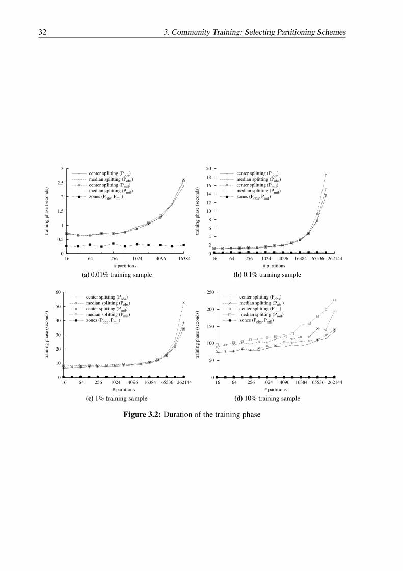
32 3. Community Training: Selecting Partitioning Schemes

0

0.5

1

1.5

2

2.5

3

16 64 256 1024 4096 16384

trai

nin

g p

has

e (s

eco

nd

s)

# partitions

center splitting (Pobs)

median splitting (Pobs)

center splitting (Pmil)

median splitting (Pmil)

zones (Pobs, Pmil)

(a) 0.01% training sample

0

2

4

6

8

10

12

14

16

18

20

16 64 256 1024 4096 16384 65536 262144

trai

nin

g p

has

e (s

eco

nd

s)

# partitions

center splitting (Pobs)

median splitting (Pobs)

center splitting (Pmil)

median splitting (Pmil)

zones (Pobs, Pmil)

(b) 0.1% training sample

0

10

20

30

40

50

60

16 64 256 1024 4096 16384 65536 262144

trai

nin

g p

has

e (s

eco

nd

s)

# partitions

center splitting (Pobs)

median splitting (Pobs)

center splitting (Pmil)

median splitting (Pmil)

zones (Pobs, Pmil)

(c) 1% training sample

0

50

100

150

200

250

16 64 256 1024 4096 16384 65536 262144

trai

nin

g p

has

e (s

eco

nd

s)

# partitions

center splitting (Pobs)

median splitting (Pobs)

center splitting (Pmil)

median splitting (Pmil)

zones (Pobs, Pmil)

(d) 10% training sample

Figure 3.2: Duration of the training phase

3.3 Evaluation of Partitioning Scheme Properties 33

0%

10%

20%

30%

40%

50%

60%

70%

80%

90%

100%

16 64 256 1024 4096 16384

aver

age

dat

a p

op

ula

tio

n (

%)

# partitions

center splitting (Pobs)

median splitting (Pobs)

center splitting (Pmil)

median splitting (Pmil)

(a) 0.01% training sample

0%

10%

20%

30%

40%

50%

60%

70%

80%

90%

100%

16 64 256 1024 4096 16384 65536 262144

aver

age

dat

a p

op

ula

tio

n (

%)

# partitions

center splitting (Pobs)

median splitting (Pobs)

center splitting (Pmil)

median splitting (Pmil)

(b) 0.1% training sample

0%

10%

20%

30%

40%

50%

60%

70%

80%

90%

100%

16 64 256 1024 4096 16384 65536 262144

aver

age

dat

a p

op

ula

tio

n (

%)

# partitions

center splitting (Pobs)

median splitting (Pobs)

center splitting (Pmil)

median splitting (Pmil)

(c) 1% training sample

0%

10%

20%

30%

40%

50%

60%

70%

80%

90%

100%

16 64 256 1024 4096 16384 65536 262144

aver

age

dat

a p

op

ula

tio

n (

%)

# partitions

center splitting (Pobs)

median splitting (Pobs)

center splitting (Pmil)

median splitting (Pmil)

(d) 10% training sample

0%

10%

20%

30%

40%

50%

60%

70%

80%

90%

16 64 256 1024 4096 16384 65536 262144

aver

age

dat

a p

op

ula

tio

n (

%)

# partitions

zones (Pobs)

zones (Pmil)

(e) Complete data

Figure 3.3: Average population of a partition in comparison to the partition with the highestpopulation

34 3. Community Training: Selecting Partitioning Schemes

Figure 3.4: Median-based quadtree for Pmil with 212, 213, and 214 partitions

depict the standard deviation on a logarithmic scale. The median-based heuristics decreases thedeviation for both data sets, especially for the uniform data. Generating 4 096 partitions fromthe 10% training sample results in a standard deviation of 1 432 and 92 for the median-basedvariant and of 1 827 and 446 for the standard quadtree for Pobs and Pmil , respectively. In eachgraph, the variance decreases because the size of the training set is kept constant and thereforethe amount of data objects for each partition is reduced. The standard deviation of the zonesapproach (not shown) develops similar to the standard deviation of the quadtree. Due to theadoption to the data distribution, the deviation of the quadtree-based partitioning schemes isslightly (by a factor between 3 to 10) lower than the standard deviation of the zones.

3.3.4 Empty Partitions

The next comparison deals with the number of empty partitions. The results are presented inFigure 3.6 as percentage of all partitions. While Pobs has large areas with no data (Figure 1.3(a)on page 5), Pmil does not. For both small samples (0.01% and 0.1%), however, the number ofempty leaves increases significantly for both datasets from 16 384 partitions onwards (see Fig-ure 3.6(a)). We discuss this deficiency of small data samples in the following section. For Pobs,all zones configurations have about 7% empty partitions. Roughly 13 ◦ of 180◦ at the bottomof Figure 1.3(b) contain no data, i. e., 7% of the declination domain are empty. As the zonesdivide the data space regularly, this ratio remains constant. For Pmil , no empty zone partitionsexist. For the 1% and 10% training samples of Pobs (the latter is shown in Figure 3.6(b)), from2 048 partitions onwards the percentage of empty partitions steadily decreases for the standardquadtree. The highest percentage of empty partitions is for the standard quadtree with 128leaves. This is due to the fact that the percentage of additional spits that result in additionalempty partitions is the highest when going from 64 to 128 partitions. From that on, the emptyareas (the “withe space”) of our data sample have been roughly approximated and additionalempty regions only appear at the “edges” of dense data areas, which explains our measurementsfor Pobs. The median heuristics completely eliminates empty regions. In Figure 3.6(b), we donot show the graphs for the samples of the uniform data set Pmil as all three data structurescreated no empty partitions if the training sample is sufficiently large.

3.3 Evaluation of Partitioning Scheme Properties 35

0.1

1

10

100

1000

16 64 256 1024 4096 16384

stan

dar

d d

evia

tio

n

# partitions

center splitting (Pobs)

median splitting (Pobs)

center splitting (Pmil)

median splitting (Pmil)

(a) 0.01% training sample

0.1

1

10

100

1000

10000

16 64 256 1024 4096 16384 65536 262144

stan

dar

d d

evia

tio

n

# partitions

center splitting (Pobs)

median splitting (Pobs)

center splitting (Pmil)

median splitting (Pmil)

(b) 0.1% training sample

1

10

100

1000

10000

100000

16 64 256 1024 4096 16384 65536 262144

stan

dar

d d

evia

tio

n

# partitions

center splitting (Pobs)

median splitting (Pobs)

center splitting (Pmil)

median splitting (Pmil)

(c) 1% training sample

1

10

100

1000

10000

100000

1e+06

16 64 256 1024 4096 16384 65536 262144

stan

dar

d d

evia

tio

n

# partitions

center splitting (Pobs)

median splitting (Pobs)

center splitting (Pmil)

median splitting (Pmil)

(d) 10% training sample

Figure 3.5: Variation in data distribution

0%

5%

10%

15%

20%

25%

30%

35%

16 64 256 1024 4096 16384 65536 262144

emp

ty p

arti

tio

ns

(%)

# partitions

center splitting (Pobs)

median splitting (Pobs)

center splitting (Pmil)

median splitting (Pmil)

(a) 0.1% training sample

0%

1%

2%

3%

4%

5%

6%

7%

8%

9%

16 64 256 1024 4096 16384 65536 262144

emp

ty p

arti

tio

ns

(%)

# partitions

center splitting

median splitting

zones

(b) 10% training sample, Pobs

Figure 3.6: Empty partitions

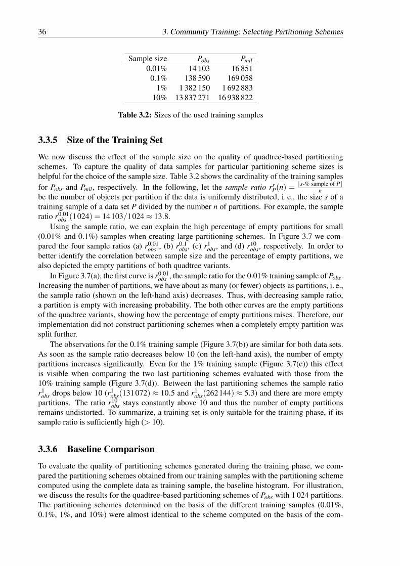
36 3. Community Training: Selecting Partitioning Schemes

Sample size Pobs Pmil0.01% 14 103 16 851

0.1% 138 590 169 0581% 1 382 150 1 692 883

10% 13 837 271 16 938 822

Table 3.2: Sizes of the used training samples

3.3.5 Size of the Training Set

We now discuss the effect of the sample size on the quality of quadtree-based partitioningschemes. To capture the quality of data samples for particular partitioning scheme sizes ishelpful for the choice of the sample size. Table 3.2 shows the cardinality of the training samplesfor Pobs and Pmil , respectively. In the following, let the sample ratio rs

P(n) = |s-% sample of P |n

be the number of objects per partition if the data is uniformly distributed, i. e., the size s of atraining sample of a data set P divided by the number n of partitions. For example, the sampleratio r0.01

obs (1024) = 14103/1024 ≈ 13.8.Using the sample ratio, we can explain the high percentage of empty partitions for small

(0.01% and 0.1%) samples when creating large partitioning schemes. In Figure 3.7 we com-pared the four sample ratios (a) r0.01

obs , (b) r0.1obs, (c) r1

obs, and (d) r10obs, respectively. In order to

better identify the correlation between sample size and the percentage of empty partitions, wealso depicted the empty partitions of both quadtree variants.

In Figure 3.7(a), the first curve is r0.01obs , the sample ratio for the 0.01% training sample of Pobs.

Increasing the number of partitions, we have about as many (or fewer) objects as partitions, i. e.,the sample ratio (shown on the left-hand axis) decreases. Thus, with decreasing sample ratio,a partition is empty with increasing probability. The both other curves are the empty partitionsof the quadtree variants, showing how the percentage of empty partitions raises. Therefore, ourimplementation did not construct partitioning schemes when a completely empty partition wassplit further.

The observations for the 0.1% training sample (Figure 3.7(b)) are similar for both data sets.As soon as the sample ratio decreases below 10 (on the left-hand axis), the number of emptypartitions increases significantly. Even for the 1% training sample (Figure 3.7(c)) this effectis visible when comparing the two last partitioning schemes evaluated with those from the10% training sample (Figure 3.7(d)). Between the last partitioning schemes the sample ratior1

obs drops below 10 (r1obs(131072) ≈ 10.5 and r1

obs(262144) ≈ 5.3) and there are more emptypartitions. The ratio r10

obs stays constantly above 10 and thus the number of empty partitionsremains undistorted. To summarize, a training set is only suitable for the training phase, if itssample ratio is sufficiently high (> 10).

3.3.6 Baseline Comparison

To evaluate the quality of partitioning schemes generated during the training phase, we com-pared the partitioning schemes obtained from our training samples with the partitioning schemecomputed using the complete data as training sample, the baseline histogram. For illustration,we discuss the results for the quadtree-based partitioning schemes of Pobs with 1 024 partitions.The partitioning schemes determined on the basis of the different training samples (0.01%,0.1%, 1%, and 10%) were almost identical to the scheme computed on the basis of the com-

3.3 Evaluation of Partitioning Scheme Properties 37

0.1

1

10

100

1000

16 64 256 1024 4096 163840%

5%

10%

15%

20%

25%

30%

35%

40%

sam

ple

rat

io

emp

ty p

artition

s (%)

# partitions

sample ratio

empty partitions (center)

empty partitions (median)

(a) 0.01% training sample

0.1

1

10

100

1000

10000

16 64 256 1024 4096 16384 65536 2621440%

5%

10%

15%

20%

25%

30%

35%

sam

ple

rat

io

emp

ty p

artition

s (%)

# partitions

sample ratio

empty partitions (center)

empty partitions (median)

(b) 0.1% training sample

1

10

100

1000

10000

100000

16 64 256 1024 4096 16384 65536 2621440%

1%

2%

3%

4%

5%

6%

7%

8%

9%

sam

ple

rat

io

emp

ty p

artition

s (%)

# partitions

sample ratio

empty partitions (center)

empty partitions (median)

(c) 1% training sample

10

100

1000

10000

100000

1e+06

16 64 256 1024 4096 16384 65536 2621440%

1%

2%

3%

4%

5%

6%

7%

8%

9%

sam

ple

rat

io

emp

ty p

artition

s (%)

# partitions

sample ratio

empty partitions (center)

empty partitions (median)

(d) 10% training sample

Figure 3.7: Effect of decreasing sample ratio, Pobs

38 3. Community Training: Selecting Partitioning Schemes

0%

0.05%

0.1%

0.15%

0.2%

0.25%

0.3%

0.35%

0 200 400 600 800 1000

par

titi

on

po

pu

lati

on

(%

)

partitions (ascending order)

0.01% sample

0.1% sample

1% sample

10% sample

complete data set

(a)

-0.01%

0%

0.01%

0.02%

0.03%

0.04%

0.05%

0.06%

0.07%

0 200 400 600 800 1000

po

pu

lati

on

dif

fere

nce

to

bas

elin

e h

isto

gra

m (

%)

partitions (ascending order)

0.01% sample

0.1% sample

1% sample

10% sample

complete data set

(b)

Figure 3.8: Baseline comparison for the standard quadtree, Pobs, and 1 024 partitions

plete data. Thus, in this particular case (quadtrees, Pobs, 1 024 regions), all our training sets yieldvery good partitioning schemes. Figure 3.8(a) shows the population of each individual partitionrelative to the size of the corresponding training sample, sorted in ascending order. We can seethat the training samples are indeed representative because the distribution of the population issimilar for all samples as well as for the original data. That is, the first partition contains no dataand the last partition contains between 0.25% and 0.31% (for the 0.01% training sample) of thesamples or the complete data set, respectively. In Figure 3.8(b), we see that the differences com-pared to the baseline histogram are negligible. The histogram created with the 0.01% trainingsample has the most differences, but the maximum deviation is at 0.07%. Note that comput-ing partitioning schemes based on complete data sets is prohibitively expensive when dealingwith very large current or future data sets, especially if verifying the median heuristics. Thus, abaseline comparison as the one above is infeasible under such circumstances.

3.3.7 DiscussionWe shortly summarize the observations made during our evaluation. The training phase itselfdoes not take very long, so it could be worthwhile comparing several training sets. Generatingall 250 partitioning schemes1 lasted about 120 minutes in our evaluation setup. This, for ex-ample, allows the detection of non-representative samples, if the curve in Figure 3.8 divergestoo much from the curve of the complete data set. If a baseline comparison is infeasible, forexample when using partitioning schemes such as median-based quadtrees, outliers can at leastindicate differences between the drawn data samples. If training samples have a sufficiently highsample ratio, comparatively small data samples already provide good partitioning schemes. Inour evaluation, using 10-times more data objects than partitions provided a good rule-of-thumbfor reliable results. For our skewed data sample, median-based quadtrees achieved the bestload-balancing and had quite homogeneous average data populations. Depending on the datastructure, the number of partitions influences the data distribution characteristics. For example,2-dimensional quadtrees should be generated with powers of 4 as partition cardinalities. Be-sides the parameters used in our evaluation, there are several other means to compare the data

1To avoid splitting empty partitions, we created only 11 quadtree-based histograms from the 0.01% trainingsample and only 14 histograms for the 0.1% sample, respectively. Thus, we created 2 · (11+14+15+15) = 110histograms for each quadtree variant and 2 ·15 = 30 zone-based histograms.

3.4 Related Work 39

structures and further properties of the data or queries that can be relevant for choosing the bestpartitioning scheme. If the partitioning scheme changes frequently and is transmitted regularly,the size of the data structure is also relevant for the decision process. Furthermore, consideringa typical workload during the training phase can give further valuable insights as we will discussin Chapter 7.

3.4 Related WorkCreating general purpose or application-driven multi-dimensional index structures has been andcontinues to be an active field of database research. Besides the survey of Gaede and Günther(1998), the book by Samet (2006) provides an encyclical source for index data structures. Onthe application-driven side, Csabai et al. (2007) compared the performance of k-d trees andVoronoi diagrams for scientific data sets. They also experienced boxes of multi-dimensional k-d trees to elongate along the second and higher dimensions, a similar effect as in Figure 3.1(b).

3.5 SummaryIn this chapter, we describe a flexible framework for investigating community-specific indexstructures used as a partitioning scheme for data grid federations. Distributing the data acrossseveral grid resources to level skewed data distributions while preserving spatial locality yieldsimproved throughput and better load balancing for data-intensive applications. We evaluatedquadtree variants and the zones algorithm and their capabilities to partition data from severalrepositories for federated data grids. Our criteria can be applied or extended in many othere-science communities. The choice of mapping the data partitions to the grid nodes is up to thecommunity. Possible options are random distribution or using space filling curves in order tofurther preserve data locality. The trade-offs between these various choices are discussed in thefollowing chapter.

40 3. Community Training: Selecting Partitioning Schemes

41

CHAPTER 4

Community Placement: Better Serving Locality withSpace Filling Curves

Within this chapter, we discuss how the data partitions are mapped to the nodes within thecommunity-driven data grid. We especially want to focus on which data mapping strategyimproves query processing throughput.

We focus on two general options for achieving a data mapping to the nodes: random distri-bution and using a space filling curve (Section 4.1). After discussing the rationales for eitherchoice, we evaluate the different placement strategies (Section 4.2). From our results, we con-clude that using a space filling curve for data placement is preferable to a random assignmentin many application scenarios.

4.1 Random or Space Filling CurvesWhile the previous section focused on balancing the data load on the partitions from our parti-tioning scheme, we discuss now the options for mapping those partitions to data nodes.

Within a central cluster environment, it is common practise to distribute the data partitionsrandomly on the individual nodes in order to achieve a good data load balancing. This is par-tially also motivated by the high-bandwidth interconnections which render the communicationbetween the nodes a less important bottleneck as in a distributed scenario. Assuming a uniformworkload with queries that have a high data locality, such random placement introduces a highparallelism. However, this comes at the cost of sacrificing the spatial locality between neigh-boring data areas. Changes in the access patterns, e. g., the researchers are interested in largersky areas, might result in increased communication overhead.

Space filling curves aim at preserving this spatial locality to some extent while providinga linearization or a one-dimensional mapping for multi-dimensional data objects (as shown inFigure 2.3 on page 12 in our overview section). Closeness within the data space should result ina low distance within the identifier space. Space filling curves have been discussed extensivelyin the literature (e. g., Samet, 2006) and we therefore only consider the most prevalent, the Z-

42 4. Community Placement: Better Serving Locality with Space Filling Curves

order (Orenstein and Merrett, 1984) and the Hilbert curve (Hilbert, 1891). Range queries inmulti-dimensional space are translated to several interval-queries for the one-dimensional map-ping. Asano et al. (1997) propose a space filling curve for squared queries in two-dimensionalspace which is optimal in the sense that it guarantees to need only three one-dimensional in-tervals to answer a query. Remarkably, new interesting insights about space filling curves andtheir locality properties have been investigated very recently by Haverkort and van Walderveen(2008).

Besides the fundamental aspect of preserving spatial locality, other factors can also influ-ence the data mapping, such as the workload characteristics or the individual node capacities.For example, distributing popular data on multiple data nodes in order to increase the queryparallelism is widely used in parallel databases and current data center layouts. In our opinion,preserving locality is the key in order to achieve a high throughput.

For the choice of the correct data placement, again properties of the partitioning schemeplay an important role, e. g., the size of individual partitions. For community-driven data grids,small partitions enable us to migrate or copy partitions between nodes either for compensatinga node failure or for replication purposes. For our quadtree-based partitioning schemes, thepartitions are approximately of the same size by the adoption to data distribution. We thereforeachieve data load balancing by placing roughly the same number of partitions on each node.

Within community-driven data grids, we prefer inter-query parallelism over intra-query par-allelism and we therefore aim at sending queries to a single host where all data is locally avail-able. We achieve this goal, if a query only requires one data region, as these regions are themost atomic data building block and guaranteed to be completely on a single node. Whenqueries span multiple partitions and these partitions are all managed by a single node, no ad-ditional overhead is necessary in order to merge or transmit intermediate results. Otherwise acoordination node needs to be selected during query processing, as discussed in Section 6.1.

As described in the architectural overview (Section 2.2), our HiSbase prototype realizes thedata mapping by using the key-based routing functionality of an overlay network. The regionidentifiers are uniformly mapped to the one-dimensional key ring. When a node arrives at thenetwork for the first time, it receives a random identifier. During the join process, the arrivingnode is informed about its both neighbors and thereby can compute the range of identifiers, it isresponsible for. The data is then transferred to this node by employing one of the disseminationtechniques (either via data feeding or direct extraction from an archive) which are discussed inSection 5. Should a node return to the network, it reuses its previous identifier as it already hasstored the relevant data locally.

4.2 Placement EvaluationDuring our experiments, we evaluated how the various mapping options affect the data loadbalancing and query locality of our queries. We used the quadtree-based partitioning schemescreated during the evaluation of the training phase presented in the previous chapter. Dataload balancing and preservation of query locality are the two criteria to assess our various dataplacement strategies. A good data load balancing is achieved if all nodes manage the sameamount of data. With regard to query locality, we evaluate how many nodes are required inorder to answer a single query.

Queries that intersect a single partition are answered by a single node and thus have optimalquery locality. We note that this is independent of the placement strategy because a partition isnot further split across multiple nodes. However, queries spanning multiple partitions that are

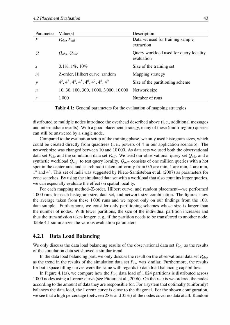
4.2 Placement Evaluation 43

Parameter Value(s) DescriptionP Pobs, Pmil Data set used for training sample

extraction

Q Qobs, Qmil′ Query workload used for query localityevaluation

s 0.1%, 1%, 10% Size of the training set

m Z-order, Hilbert curve, random Mapping strategy

p 42, 43, 44, 45, 46, 47, 48, 49 Size of the partitioning scheme

n 10, 30, 100, 300, 1 000, 3 000, 10 000 Network size

r 1 000 Number of runs

Table 4.1: General parameters for the evaluation of mapping strategies

distributed to multiple nodes introduce the overhead described above (i. e., additional messagesand intermediate results). With a good placement strategy, many of these (multi-region) queriescan still be answered by a single node.

Compared to the evaluation setup of the training phase, we only used histogram sizes, whichcould be created directly from quadtrees (i. e., powers of 4 in our application scenario). Thenetwork size was changed between 10 and 10 000. As data sets we used both the observationaldata set Pobs and the simulation data set Pmil . We used our observational query set Qobs and asynthetic workload Qmil′ to test query locality. Qmil′ consists of one million queries with a hotspot in the center area and search radii taken uniformly from 0.5 arc min, 1 arc min, 4 arc min,1◦ and 4◦. This set of radii was suggested by Nieto-Santisteban et al. (2007) as parameters forcone searches. By using the simulated data set with a workload that also contains larger queries,we can especially evaluate the effect on spatial locality.

For each mapping method–Z-order, Hilbert curve, and random placement—we performed1 000 runs for each histogram size, data set, and network size combination. The figures showthe average taken from these 1 000 runs and we report only on our findings from the 10%data sample. Furthermore, we consider only partitioning schemes whose size is larger thanthe number of nodes. With fewer partitions, the size of the individual partition increases andthus the transmission takes longer, e. g., if the partition needs to be transferred to another node.Table 4.1 summarizes the various evaluation parameters.

4.2.1 Data Load BalancingWe only discuss the data load balancing results of the observational data set Pobs as the resultsof the simulation data set showed a similar trend.

In the data load balancing part, we only discuss the result on the observational data set Pobs,as the trend in the results of the simulation data set Pmil was similar. Furthermore, the resultsfor both space filling curves were the same with regards to data load balancing capabilities.

In Figure 4.1(a), we compare how the Pobs data load of 1 024 partitions is distributed across1 000 nodes using a Lorenz curve (see Pitoura et al., 2006). On the x-axis we ordered the nodesaccording to the amount of data they are responsible for. For a system that optimally (uniformly)balances the data load, the Lorenz curve is close to the diagonal. For the shown configuration,we see that a high percentage (between 28% and 35%) of the nodes cover no data at all. Random

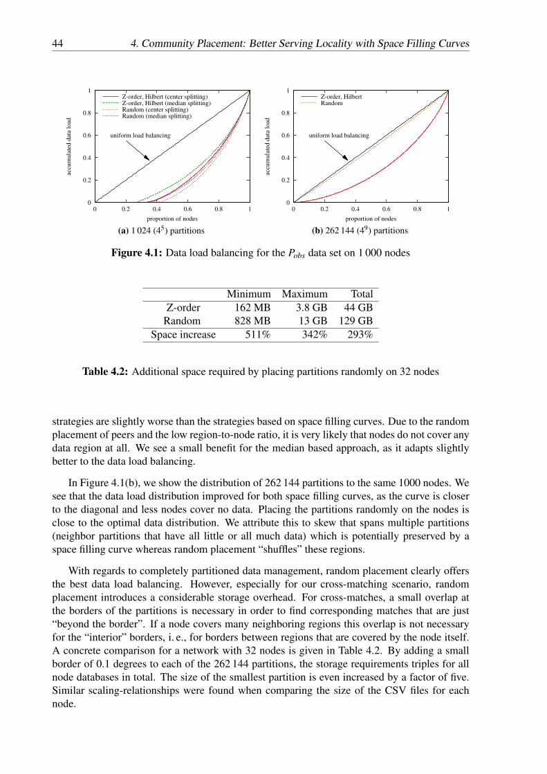
44 4. Community Placement: Better Serving Locality with Space Filling Curves

0

0.2

0.4

0.6

0.8

1

0 0.2 0.4 0.6 0.8 1

accu

mula

ted

dat

a lo

ad

proportion of nodes

uniform load balancing

Z-order, Hilbert (center splitting)Z-order, Hilbert (median splitting)Random (center splitting)Random (median splitting)

(a) 1 024 (45) partitions

0

0.2

0.4

0.6

0.8

1

0 0.2 0.4 0.6 0.8 1

accu

mula

ted

dat

a lo

ad

proportion of nodes

uniform load balancing

Z-order, HilbertRandom

(b) 262 144 (49) partitions

Figure 4.1: Data load balancing for the Pobs data set on 1 000 nodes

Minimum Maximum TotalZ-order 162 MB 3.8 GB 44 GB

Random 828 MB 13 GB 129 GBSpace increase 511% 342% 293%

Table 4.2: Additional space required by placing partitions randomly on 32 nodes

strategies are slightly worse than the strategies based on space filling curves. Due to the randomplacement of peers and the low region-to-node ratio, it is very likely that nodes do not cover anydata region at all. We see a small benefit for the median based approach, as it adapts slightlybetter to the data load balancing.

In Figure 4.1(b), we show the distribution of 262 144 partitions to the same 1000 nodes. Wesee that the data load distribution improved for both space filling curves, as the curve is closerto the diagonal and less nodes cover no data. Placing the partitions randomly on the nodes isclose to the optimal data distribution. We attribute this to skew that spans multiple partitions(neighbor partitions that have all little or all much data) which is potentially preserved by aspace filling curve whereas random placement “shuffles” these regions.

With regards to completely partitioned data management, random placement clearly offersthe best data load balancing. However, especially for our cross-matching scenario, randomplacement introduces a considerable storage overhead. For cross-matches, a small overlap atthe borders of the partitions is necessary in order to find corresponding matches that are just“beyond the border”. If a node covers many neighboring regions this overlap is not necessaryfor the “interior” borders, i. e., for borders between regions that are covered by the node itself.A concrete comparison for a network with 32 nodes is given in Table 4.2. By adding a smallborder of 0.1 degrees to each of the 262 144 partitions, the storage requirements triples for allnode databases in total. The size of the smallest partition is even increased by a factor of five.Similar scaling-relationships were found when comparing the size of the CSV files for eachnode.

4.2 Placement Evaluation 45

0%

1%

2%

3%

4%

5%

6%

7%

256 1024 4096 16384 65536 262144

quer

ies

span

nin

g m

ult

iple

nodes

(in

%)

partitions

Z-orderHilbertRandom

(a) Qobs

0%

10%

20%

30%

40%

50%

60%

70%

256 1024 4096 16384 65536 262144

quer

ies

span

nin

g m

ult

iple

nodes

(in

%)

partitions

Z-orderHilbertRandom

(b) Qmil′

Figure 4.2: Query locality on 100 nodes with varying partitioning schemes

0%

0.5%

1%

1.5%

2%

2.5%

3%

10 30 100 300 1000 3000 10000

quer

ies

span

nin

g m

ult

iple

nodes

(in

%)

nodes

Z-orderHilbertRandom

(a) Qobs

0%

10%

20%

30%

40%

50%

60%

10 30 100 300 1000 3000 10000

quer

ies

span

nin

g m

ult

iple

nodes

(in

%)

nodes

Z-orderHilbertRandom

(b) Qmil′

Figure 4.3: Query locality for varying network sizes with 16 384 partitions

4.2.2 Query LocalityBesides data load balancing, we also evaluated the preservation of query locality for the map-ping strategies. Figure 4.2 shows the percentage of queries that span multiple nodes duringquery processing while increasing the histogram size for a network with 100 nodes. For theobservational workload Qobs (Figure 4.2(a)), the queries exhibit a high degree of locality andwhen using space filling curves, only a tiny fraction needs data from several nodes. This queryratio increases for random placement when the partitioning scheme contains more partitions upto 6.4% percent. Though the queries span multiple regions when increasing the histogram size,the space filling curves ensure that the overall level of locality remains stable. Put differently:space filling curves are better in keeping the work on a single node.

This observation holds also for the simulation data set Pmil and query set Qmil′ , although ona different scale (Figure 4.2(b)). This workload has 30% queries spanning multiple nodes andboth space filling curves are good in keeping the ratio stable. When used with 262 144 partitions,randomly placing the partitions on nodes results in 70% of the queries to span multiple nodes.The results for other network sizes show similar trends.

Above results suggest that it is reasonable to create a partitioning scheme with many parti-tions, even if the initial number of nodes is small. The locality-preservation by the space filling

46 4. Community Placement: Better Serving Locality with Space Filling Curves

curves will still keep queries on a single node. Thereby, HiSbase can accommodate situationswhen institutions join with several nodes at once. As a side effect the size of the partitionsbecomes even smaller.

Figure 4.3 again shows the percentage of queries that require data from multiple nodes. Incontrast to Figure 4.2, the histogram size is fixed at 16 384 partitions and shows the evolutionwhen additional nodes join the network. The more nodes are added, the more both space fillingcurves approach the values of the random partitioning.

4.3 Summary and Future WorkAchieving good data load-balancing as well as preserving query locality is important for scal-able data management solutions in e-science environments. Therefore the choices of partition-ing scheme and of mapping strategy contribute significantly to how well the initial setup ofthe community grid will scale. From our experiments we draw two conclusions as advice forbuilding community-driven data grids: 1) create a partitioning scheme with many partitionsand 2) use space filling curves for mapping the partitions on the available nodes. Through thiscombination the query locality remains stable for a network with fixed size. When adding morenodes to a running setup the query locality for a fixed partitioning scheme remains higher thanfor placing the partitions randomly. In very restricted application scenarios, e. g., when queriesare extremely local (one partition) and no “boundary data” is necessary, random placement of-fers a reasonable choice as the data load balancing capabilities are amenable to their full extent.Further studies which apply advanced space filling curves (e. g., Asano et al., 1997; Haverkortand van Walderveen, 2008) probably will provide additional insights.

47

CHAPTER 5

Feeding Community-Driven Data Grids

Scientific archives currently provide access to already existing huge data sets. Moreover, re-cently started scientific instruments, such as LOFAR and LHC, generate data at an enormousspeed and scale. In order to cope with this data deluge, scalable high-throughput data manage-ment infrastructures, such as HiSbase, need to employ efficient data dissemination techniques.

Within this chapter, we discuss how to efficiently distribute data within community-drivendata grids. First, we describe several scenarios where we apply data feeding to transmit databetween the collaborating data nodes (Section 5.1). Then, we compare a pull-based approach,where each client pulls the required data, with two basic push-based techniques, where thearchives publish the data to the clients either tuple-wise or the complete data at once (Sec-tion 5.2). We identify the major limitations of these approaches in the face of the require-ments of e-science data grids and propose efficient bulk feeding techniques that transmit data inchunks. In order to tune our feeding strategies, we describe a model that optimizes data feedingby using paths with minimal latency and maximum bandwidth (Section 5.3). As we cannotuse an optimal solution due to the problem’s complexity, we present our chunk-based feedingtechniques. We describe how to optimize the network traffic, the configuration of the feedingstrategies, and the data processing at the receiving nodes in Section 5.4. Our evaluation re-sults (Section 5.5) show that our bulk feeding techniques considerably accelerate data feeding.We conclude this chapter with related work (Section 5.6) and give an outlook on future issues(Section 5.7) in the context of data dissemination within scientific data grids.

5.1 Feeding Scenarios

In the following, we discuss five exemplary use cases for data feeding within community-drivendata grids. They range from the initial feeding to node arrivals, node departures, and to datadistribution according to an additional histogram. Nodes that receive feeding messages in ourscenarios directly store the data in their local database.

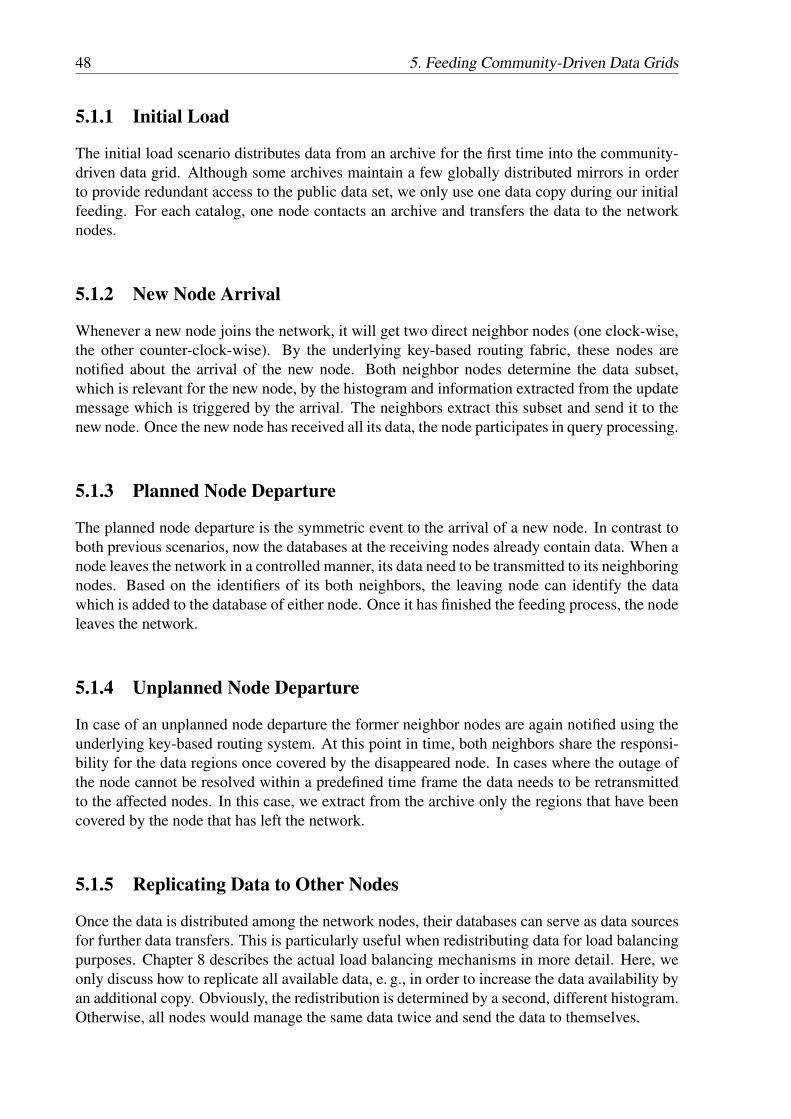
48 5. Feeding Community-Driven Data Grids

5.1.1 Initial Load

The initial load scenario distributes data from an archive for the first time into the community-driven data grid. Although some archives maintain a few globally distributed mirrors in orderto provide redundant access to the public data set, we only use one data copy during our initialfeeding. For each catalog, one node contacts an archive and transfers the data to the networknodes.

5.1.2 New Node Arrival

Whenever a new node joins the network, it will get two direct neighbor nodes (one clock-wise,the other counter-clock-wise). By the underlying key-based routing fabric, these nodes arenotified about the arrival of the new node. Both neighbor nodes determine the data subset,which is relevant for the new node, by the histogram and information extracted from the updatemessage which is triggered by the arrival. The neighbors extract this subset and send it to thenew node. Once the new node has received all its data, the node participates in query processing.

5.1.3 Planned Node Departure

The planned node departure is the symmetric event to the arrival of a new node. In contrast toboth previous scenarios, now the databases at the receiving nodes already contain data. When anode leaves the network in a controlled manner, its data need to be transmitted to its neighboringnodes. Based on the identifiers of its both neighbors, the leaving node can identify the datawhich is added to the database of either node. Once it has finished the feeding process, the nodeleaves the network.

5.1.4 Unplanned Node Departure

In case of an unplanned node departure the former neighbor nodes are again notified using theunderlying key-based routing system. At this point in time, both neighbors share the responsi-bility for the data regions once covered by the disappeared node. In cases where the outage ofthe node cannot be resolved within a predefined time frame the data needs to be retransmittedto the affected nodes. In this case, we extract from the archive only the regions that have beencovered by the node that has left the network.

5.1.5 Replicating Data to Other Nodes

Once the data is distributed among the network nodes, their databases can serve as data sourcesfor further data transfers. This is particularly useful when redistributing data for load balancingpurposes. Chapter 8 describes the actual load balancing mechanisms in more detail. Here, weonly discuss how to replicate all available data, e. g., in order to increase the data availability byan additional copy. Obviously, the redistribution is determined by a second, different histogram.Otherwise, all nodes would manage the same data twice and send the data to themselves.

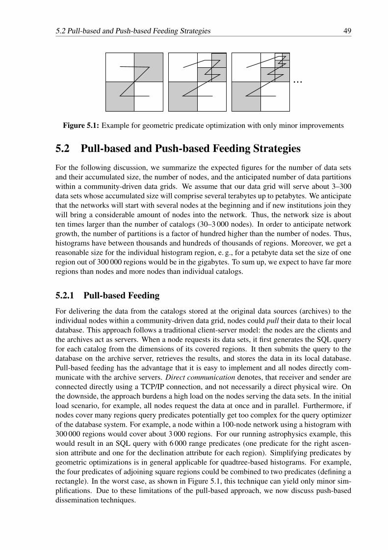
5.2 Pull-based and Push-based Feeding Strategies 49

Figure 5.1: Example for geometric predicate optimization with only minor improvements

5.2 Pull-based and Push-based Feeding StrategiesFor the following discussion, we summarize the expected figures for the number of data setsand their accumulated size, the number of nodes, and the anticipated number of data partitionswithin a community-driven data grids. We assume that our data grid will serve about 3–300data sets whose accumulated size will comprise several terabytes up to petabytes. We anticipatethat the networks will start with several nodes at the beginning and if new institutions join theywill bring a considerable amount of nodes into the network. Thus, the network size is aboutten times larger than the number of catalogs (30–3 000 nodes). In order to anticipate networkgrowth, the number of partitions is a factor of hundred higher than the number of nodes. Thus,histograms have between thousands and hundreds of thousands of regions. Moreover, we get areasonable size for the individual histogram region, e. g., for a petabyte data set the size of oneregion out of 300 000 regions would be in the gigabytes. To sum up, we expect to have far moreregions than nodes and more nodes than individual catalogs.

5.2.1 Pull-based FeedingFor delivering the data from the catalogs stored at the original data sources (archives) to theindividual nodes within a community-driven data grid, nodes could pull their data to their localdatabase. This approach follows a traditional client-server model: the nodes are the clients andthe archives act as servers. When a node requests its data sets, it first generates the SQL queryfor each catalog from the dimensions of its covered regions. It then submits the query to thedatabase on the archive server, retrieves the results, and stores the data in its local database.Pull-based feeding has the advantage that it is easy to implement and all nodes directly com-municate with the archive servers. Direct communication denotes, that receiver and sender areconnected directly using a TCP/IP connection, and not necessarily a direct physical wire. Onthe downside, the approach burdens a high load on the nodes serving the data sets. In the initialload scenario, for example, all nodes request the data at once and in parallel. Furthermore, ifnodes cover many regions query predicates potentially get too complex for the query optimizerof the database system. For example, a node within a 100-node network using a histogram with300 000 regions would cover about 3 000 regions. For our running astrophysics example, thiswould result in an SQL query with 6 000 range predicates (one predicate for the right ascen-sion attribute and one for the declination attribute for each region). Simplifying predicates bygeometric optimizations is in general applicable for quadtree-based histograms. For example,the four predicates of adjoining square regions could be combined to two predicates (defining arectangle). In the worst case, as shown in Figure 5.1, this technique can yield only minor sim-plifications. Due to these limitations of the pull-based approach, we now discuss push-baseddissemination techniques.

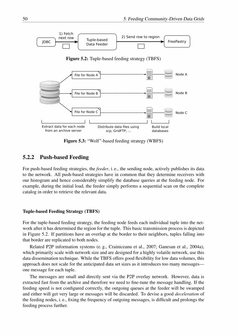
50 5. Feeding Community-Driven Data Grids

Figure 5.2: Tuple-based feeding strategy (TBFS)

Figure 5.3: “Wolf”-based feeding strategy (WBFS)

5.2.2 Push-based Feeding

For push-based feeding strategies, the feeder, i. e., the sending node, actively publishes its datato the network. All push-based strategies have in common that they determine receivers withour histogram and hence considerably simplify the database queries at the feeding node. Forexample, during the initial load, the feeder simply performs a sequential scan on the completecatalog in order to retrieve the relevant data.

Tuple-based Feeding Strategy (TBFS)

For the tuple-based feeding strategy, the feeding node feeds each individual tuple into the net-work after it has determined the region for the tuple. This basic transmission process is depictedin Figure 5.2. If partitions have an overlap at the border to their neighbors, tuples falling intothat border are replicated to both nodes.

Related P2P information systems (e. g., Crainiceanu et al., 2007; Ganesan et al., 2004a),which primarily scale with network size and are designed for a highly volatile network, use thisdata dissemination technique. While the TBFS offers good flexibility for low data volumes, thisapproach does not scale for the anticipated data set sizes as it introduces too many messages—one message for each tuple.

The messages are small and directly sent via the P2P overlay network. However, data isextracted fast from the archive and therefore we need to fine-tune the message handling. If thefeeding speed is not configured correctly, the outgoing queues at the feeder will be swampedand either will get very large or messages will be discarded. To devise a good deceleration ofthe feeding nodes, i. e., fixing the frequency of outgoing messages, is difficult and prolongs thefeeding process further.

5.3 An Optimization Model for Feeding 51

“Wolf”-based Feeding Strategy (WBFS)

The “wolf”-based feeding strategy (WBFS) distributes the data for each node in a single bigmessage and is depicted in Figure 5.3.1 Assuming that the positions of the nodes are knownin advance, this strategy uses a single sequential scan on each catalog in order to extract theindividual tuples. Similar to the TBFS, this strategy identifies tuples which need to be sent tomultiple nodes. Instead of creating a message for each such tuple, this strategy stores all tuplesfor a specific node in appropriate data files (e. g., CSV files). These files are then transmitted tothe data nodes using a suitable protocol such as scp, rsync, or GridFTP. Each node compiles itsown database based on these data files.

Using the WBFS, we increase the parallelism of the data extraction at the sources and of thedatabase creation at the receivers. Additionally, feeders and receivers use direct communication.However, the WBFS still has some major drawbacks. Although the WBFS is push-based, itrequires a high storage capacity at the feeders in order to create the data files for all nodes inparallel. Furthermore, this strategy performs data extraction as a blocking operator. Only ifall files for a particular catalog are completed, the data files are transferred to the appropriatenodes.

We see from the two basic push-based strategies, TBFS and WBFS, that is critical to definean appropriate size for data chunks, i. e., to define how many objects are combined into a singlemessage. Using only one tuple per messages induces too many messages and sending all dataat once offers only a limited parallelism and pipelining. We need to trade off high parallelismagainst network overhead when designing our bulk feeding techniques. For this purpose, weanalyze how to optimize these feeding strategies by a mathematical model. Although the op-timal solution is not applicable in our context, we derive several useful indications that haveinfluenced our feeding strategies.

5.3 An Optimization Model for Feeding

In order to optimize the feeding process, efficient data transfers are required to reduce both theload and space requirements on the archive nodes as well as the messaging overhead duringtransmission. The efficiency and speed of our feeding strategies is therefore determined by thelatency and bandwidth constraints within the network. For creating a model which allows usto describe the latency and bandwidth constraints, we require a network snapshot of the currentnetwork configuration.

5.3.1 Network Snapshots

In oder to find the appropriate abstraction of the network configuration, we compare differentviews of the communication network of community-driven data grids as shown in Figure 5.4.

In general, we use the key-based routing protocols of the overlay network (Figure 5.4(a)).However, we cannot directly derive the properties of the physical network—such as latency,bandwidth, or closeness between nodes—from the overlay network links. Overlay links abstracton purpose from the actual network and this fact renders this view of the network as infeasiblefor building a mathematical model for latency and bandwidth constraints.

1Due to the fact that nodes get a single “big bite”, we denoted this strategy “wolf”-based inspired by the verbto wolf: to eat greedily (source: http://www.merriam-webster.com/dictionary/wolf).

52 5. Feeding Community-Driven Data Grids

(a) Network snapshot using over-lay paths

(b) Physical network snapshot ascomplete undirected graphG′ = (V ′,E ′, l′,b′)

(c) Physical network snapshotas undirected graph G =(V,E, l,b) with transit nodes(inner nodes)

Figure 5.4: Overview of network snapshots

In the following, we will use specific network snapshots that enable us to better describe thephysical network configuration:

Definition 5.1 (Network Snapshot) A network snapshot is a graph G = (V,E, l,b) that de-scribes a static view of a physical network. Let V be the set of nodes within the physicalnetwork and E the set of communication links (i, j) between two nodes i, j ∈V . Then let func-tion l : E → R+ define the latency of an edge and function b : E → R+ define the bandwidth ofan edge, respectively. ¤

One example of such view of the physical network is the complete undirected graph, asshown in Figure 5.4(b). This model represents the direct communication paths between allnodes participating in the common data grid. The graph is complete, as we can assume that allnodes within a community data grid allow for direct communication, i. e., all nodes within thenetwork can establish pairwise connections. Furthermore, the graph is undirected, as data gridsusually use bidirectional, high-bandwidth communication links. Unfortunately, this view doesnot capture cross-traffic, i. e., traffic between two independent pairs of nodes that will influenceeach other’s performance as they share a common subpath in the physical network.

We will therefore use network snapshots that include transit nodes and that enable us tocreate a more realistic network model. Transit nodes represent those routing nodes that connectseveral nodes within the same institution or campus to the other nodes within the data gridinfrastructure. If two nodes share a common transit node, they compete for the transit node’sbandwidth and influence each other. For example in Figure 5.4(c), node i and node j share acommon transit node.

In order to create network snapshots, one needs to measure connection channels betweennodes. In order to collect latency and bandwidth information network, nodes could ping othernodes or transmit sample data, respectively. Transit nodes on the communication paths couldbe identified using tools such as traceroute. Caching the information of previous transfers couldalso be a suitable mean to collect such network snapshots. We refrained from modelling furtheraspects such as failing nodes or skewed demand on the individual links as these would furtheradd to the complexity of the problem.

Thus, we use network snapshots with transit nodes for our model in order to identify optimalpaths for data dissemination. We consider a path optimal, if it offers both low latency and highbandwidth.

5.3 An Optimization Model for Feeding 53

5.3.2 A Model for Minimum Latency PathsFirst, we construct a model based on a network snapshot G = (V,E, l) that only uses the latencyfunction. During data feeding, messages should be sent on paths that offer the lowest latencypossible. We show one approach for finding minimum latency paths based on Algorithm 5.1 andour network snapshot. The algorithm is a modified version of the Dijkstra-Algorithm (Cormenet al., 2001). Within the algorithm, we denote the set of nodes adjacent to a node subset S ⊆Vas the neighborhood of S in network snapshot G.

Definition 5.2 (Neighborhood N(G,S)) For any node set S ⊆ V , we define the neighborhoodof set S in network snapshot G as N(G,S) = { n ∈V | ∃ s ∈ S : (s,n) ∈ E }. ¤

Algorithm 5.1: Minimum latency pathData: Network snapshot G = (V,E, l), latency function l : E → R+, node s ∈VResult: Latency L(v) of a minimum latency path for all nodes v ∈V reachable from sbegin1

S ←{s}2

L(s) ← 03

L(v) ← ∞ ∀v ∈V \{s}4

for v ∈ N(G,S) do5

L(v) ← l((s,v))6

end for7

while N(G,S)\S 6= /0 do8

Choose vmin ∈ N(G,S)\S with L(vmin) = min{ L(v) : v ∈ N(G,S)\S }9

for v ∈ N(G,{vmin})\S do10

L ← min{ L(v), max{ L(vmin), l((vmin,v)) } }11

end for12

S ← S∪{vmin}13

end while14

end15

Theorem (Minimum Latency Path) Let G = (V,E, l) be an undirected graph with the latencyfunction l : E → R+ and s ∈ V be an arbitrary source. Algorithm 5.1 solves the problem ofminimum latency paths by annotating nodes v ∈V with the latency L(v) of a minimum latencypath from s to v. Using a depth-first search that purges edges e with l(e) > L(v) starting in sdetermines the actual minimum latency path.

PROOF: Let Si be the set S in step i. We show that in every step of the algorithm, L(v)with v∈Vis the latency of a minimum latency path from s to v that only uses intermediate nodes from Si.In proof of the theorem we use induction over |S| = i+1:

Base Case: For |S| = 1, set S0 only contains node s and all nodes v in the neighborhood of s(i. e., v ∈ N(G,s)) are initialized with the latency L(v) = l((s,v)) of the direct edge to s(line 6 of Algorithm 5.1). All remaining nodes—those which are not in the neighborhoodof s—are not reachable, because s is the only possible intermediate node (S0 = {s}) atthis point. Hence we label these nodes with ∞. Therefore, the current minimum latencypaths, i. e., the direct edges, from the source s are correctly identified.

54 5. Feeding Community-Driven Data Grids

Inductive Step: Let the hypothesis hold for set Sn−1 = {s,v1,v2, . . . ,vn−1} for the inductivestep. Therefore L(v), with node v ∈ V , denotes the latency of a minimum latency pathfrom s to v with intermediate nodes in Sn−1. The next step adds vn to the set Sn−1.For all nodes v ∈ Sn−1, we have L(vn) ≥ L(v), because L(vn) is the minimal latencyannotation of nodes not in Sn−1 and latency annotations are monotonically increasing. Ifnow there exists a node v∗ /∈ Sn = {s,v1,v2, . . . ,vn} for which exists a path using onlyintermediate nodes in Sn that yields a lower latency annotation than L(v∗), this node mustbe a neighbor of node vn. The hypothesis states that the labels L(v1),L(v2), . . . ,L(vn−1) donot change in step n. In step n, therefore, a path from s to v∗ that uses only nodes in Sn−1as intermediate nodes cannot lead to a lower value for L(v∗) than the one that is set afterstep n− 1. Thus, the minimum latency path from source s to node v∗ with intermediatenodes in Sn is made up of a minimum latency path from s to vn with intermediate nodesonly in Sn−1 and latency l((vn,v∗)). According to the base case, the latency L(v∗) ismax{ L(vn), l((vn,v∗)) }. This is exactly the way label updates are handled in line 11 ofAlgorithm 5.1. Hence the hypothesis is justified.

For a proof of correctness for the pruning depth-first search algorithm to determine theactual minimum latency path we refer the reader to the respective literature (Cormen et al.,2001). ¥

Running Time Algorithm 5.1 runs the outer while-loop |V | times as in each round a node isadded to set S (|S| is increased by 1) and set S initially only contains node s. In the worstcase, the inner for-loop cycles |V | times for a complete graph. Therefore the running time ofAlgorithm 5.1 is in O

(|V |2

). A depth-first search has a worst case running time of O(|V |+ |E|).

Hence, the running time to find minimum latency paths is in O(|V |2

).

Example 5.1 We execute Algorithm 5.1 on the example graph G∗ depicted in Figure 5.5(a)using s as a source node. For the sake of simplicity, edges are labeled with integer valuesinstead of real latency values. Appendix A provides a stepwise execution of the algorithm. Theresulting graph with latency annotations is depicted in Figure 5.5(b).

.

.

. ...v1 . ...v2

...s . ...v3 .

. ...v4 . ...v5

.0

.∞ .∞

.∞

.∞ .∞

.4

.1

.5

.3

.8

.3(a) Undirected graph G∗

.

.

. ...v1 . ...v2

...s . ...v3 .

. ...v4 . ...v5

.0

.4 .5

.5

.1 .3

.4

.1

.5

.3

.8

.3(b) Result of Algorithm 5.1 for s as source

node

Figure 5.5: Result of Algorithm 5.1 for G∗ and s as source node

We assume that sending individual messages has only a negligible influence on the latencyof the link. This allows us to reuse a network snapshot for all messages. We therefore create

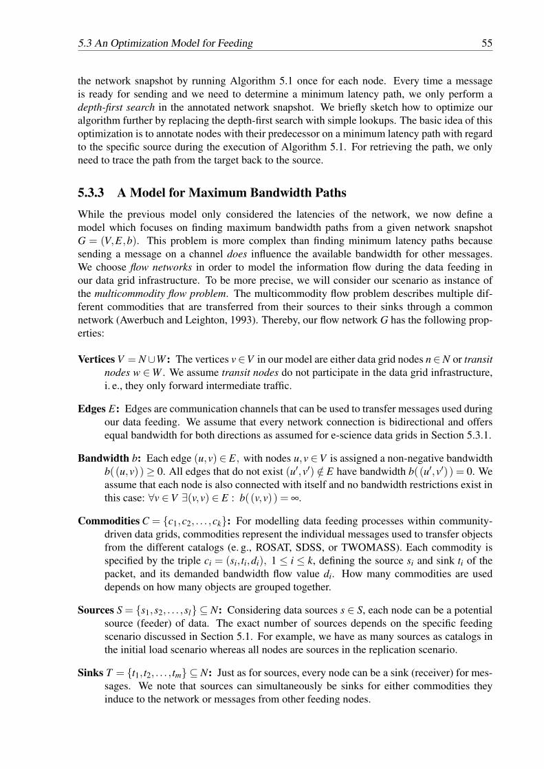
5.3 An Optimization Model for Feeding 55

the network snapshot by running Algorithm 5.1 once for each node. Every time a messageis ready for sending and we need to determine a minimum latency path, we only perform adepth-first search in the annotated network snapshot. We briefly sketch how to optimize ouralgorithm further by replacing the depth-first search with simple lookups. The basic idea of thisoptimization is to annotate nodes with their predecessor on a minimum latency path with regardto the specific source during the execution of Algorithm 5.1. For retrieving the path, we onlyneed to trace the path from the target back to the source.

5.3.3 A Model for Maximum Bandwidth PathsWhile the previous model only considered the latencies of the network, we now define amodel which focuses on finding maximum bandwidth paths from a given network snapshotG = (V,E,b). This problem is more complex than finding minimum latency paths becausesending a message on a channel does influence the available bandwidth for other messages.We choose flow networks in order to model the information flow during the data feeding inour data grid infrastructure. To be more precise, we will consider our scenario as instance ofthe multicommodity flow problem. The multicommodity flow problem describes multiple dif-ferent commodities that are transferred from their sources to their sinks through a commonnetwork (Awerbuch and Leighton, 1993). Thereby, our flow network G has the following prop-erties:

Vertices V = N ∪W : The vertices v∈V in our model are either data grid nodes n∈N or transitnodes w ∈W . We assume transit nodes do not participate in the data grid infrastructure,i. e., they only forward intermediate traffic.

Edges E: Edges are communication channels that can be used to transfer messages used duringour data feeding. We assume that every network connection is bidirectional and offersequal bandwidth for both directions as assumed for e-science data grids in Section 5.3.1.

Bandwidth b: Each edge (u,v) ∈ E, with nodes u,v ∈V is assigned a non-negative bandwidthb((u,v)) ≥ 0. All edges that do not exist (u′,v′) /∈ E have bandwidth b((u′,v′)) = 0. Weassume that each node is also connected with itself and no bandwidth restrictions exist inthis case: ∀v ∈V ∃(v,v) ∈ E : b((v,v)) = ∞.

Commodities C = {c1,c2, . . . ,ck}: For modelling data feeding processes within community-driven data grids, commodities represent the individual messages used to transfer objectsfrom the different catalogs (e. g., ROSAT, SDSS, or TWOMASS). Each commodity isspecified by the triple ci = (si, ti,di), 1 ≤ i ≤ k, defining the source si and sink ti of thepacket, and its demanded bandwidth flow value di. How many commodities are useddepends on how many objects are grouped together.

Sources S = {s1,s2, . . . ,sl} ⊆ N: Considering data sources s ∈ S, each node can be a potentialsource (feeder) of data. The exact number of sources depends on the specific feedingscenario discussed in Section 5.1. For example, we have as many sources as catalogs inthe initial load scenario whereas all nodes are sources in the replication scenario.

Sinks T = {t1, t2, . . . , tm} ⊆ N: Just as for sources, every node can be a sink (receiver) for mes-sages. We note that sources can simultaneously be sinks for either commodities theyinduce to the network or messages from other feeding nodes.

56 5. Feeding Community-Driven Data Grids

Connectivity of G: We further assume that the graph G is connected. This property states, thatfor all nodes v ∈V , all sources s ∈ S, and all sinks t ∈ T a path s ; v ; t exists.

Definition 5.3 (Bandwidth Flow Functions) Using our flow network G we can now define thebandwidth flow functions for commodities ci ∈C, 1 ≤ i ≤ k : fi : V ×V → R as follows:

Bandwidth capacity: ∀u,v ∈ V : ∑ki=1 fi(u,v) ≤ b((u,v)). This states that all flows must not

surmount the available bandwidth of the network links.

Skew symmetry: ∀u,v ∈V : fi(u,v) = − fi(v,u)

Flow conservation: No node should retain a commodity if it is not its sink. Thereby, the in-flow must be equal to the out-flow on such nodes: ∑u∈V fi(v,u) = 0, for u ∈ V that areneither a source nor a sink for commodity ci. In particular this constraint must hold for alltransit nodes w ∈W because they do not participate in the data grid and therefore cannotact as a sink.

Demand satisfaction: To satisfy the specified demand for all commodities, the source musthave an accumulated outflow in size of the bandwidth in demand: ∀ci = (si, ti,di) :∑v∈V fi(si,v) = di, 1 ≤ i ≤ k. ¤

Our goal is to maximize the aggregated bandwidth flow in our flow network. Hence wemaximize the demand for all commodities, so that each can be satisfied and the aggregated flowis maximized:

maxk

∑i=1

di = maxk

∑i=1

∑v∈V

fi(si,v), with si being the source for commodity ci ∈C (5.1)

When all nodes are centrally coordinated such that only a single feeding message is sentthrough the network, finding a maximum bandwidth flow is straight-forward. Messages corre-spond to commodities in our model, and therefore this case is a one-commodity flow problemand we can compute an optimal solution, e. g., by applying the Ford-Fulkerson Algorithm (Cor-men et al., 2001). However, performing feeding according to this scenario would deterioratethe overall performance significantly.

According to the literature, our model for maximizing the bandwidth flow corresponds to theundirected maximum multicommodity real flow problem. Finding a polynomial-time algorithmfor more than two commodities causes major difficulties (Even et al., 1975). The only knownefficient way to compute the exact maximum bandwidth flow for our scenario according toEquation (5.1) is to solve a linear program because there are likely more than two commodities.Even though we can solve linear programs with polynomial-time algorithms (Cormen et al.,2001), the solution needs to be recomputed every time a message was transferred successfullyor is about to be sent. Furthermore, all nodes in the optimal flow plan are involved in thecalculation of routing decisions and usable bandwidth.

Awerbuch and Leighton (1993) describe a local-control approximation for multicommodityflow. The introduced algorithm is faster than solving a linear program. As it is a local-controlapproach, routing decisions do not have to be delegated to other nodes. The algorithm’s runningtime is bound by O

(|E|3|C|5/2Lε−3 log |C|

)where L is a parameter that bounds the maximum

path length of any flow from source to sink and ε−1 defines the accuracy of the approximatedresult.

5.3 An Optimization Model for Feeding 57

5.3.4 Combining Latency and BandwidthBoth models for the individual targets of minimizing the latency and maximizing the bandwidthshow that quite an effort is necessary in order to provide an optimal solution. Solving bothproblems at once requires to solve two objective functions. However, solving the combinedproblem is even harder, as both parameters are not necessarily correlated. High bandwidthcommunication links not always have a low latency, such as satellite links. Thus, meticuloustuning is required in order to achieve an optimal solution.

5.3.5 ConclusionsBased on these findings, we aim for using our chunk-based techniques, which we describe inthe following, instead of striving for an optimal solution. Nonetheless, we can draw severalconclusions from the discussion so far.

Enabling Direct Communication to Nodes

Using the overlay routing fabric for data transfers during feeding incurs a high messaging over-head and probably results in sub-optimal dissemination paths. This implies that feeding nodesare required to generate a region-to-node mapping before they start feeding. Therefore, we needto communicate the mapping information efficiently between the nodes of our data grid. Oncethe mapping information is complete, the feeders can create data chunks according to nodes.Moreover, building the chunks based on nodes and not based on regions simplifies duplicateeliminations at the end of the feeding process. If the regions of a node are known, the feedercan ensure that objects that lie within the border of two regions of the same node are not senttwice.

Enable Parallelism and Pipelining during Feeding

Currently each project stores its data set in a separate database. Thus, the individual catalogsare prevalently stored at different sites. Therefore, we can use one node per catalog to dissem-inate the data into the network and use the available bandwidth of that node optimally for asingle catalog. As these catalogs can be processed independently, the data distribution time isdominated by the distribution time of the largest catalog. If one node feeds several catalogs,e. g., during the replication scenario, it is reasonable to feed catalog by catalog as this favors touse the complete bandwidth for a single catalog. Once a node has finished its first catalog it canimmediately begin to publish the next catalog.

Choosing a good chunk size improves the pipelining within the feeding process. Once achunk has the configured size it can be forwarded to the receiving node for processing whilethe feeder already prepares the next chunk (potentially for a different node). We do not furtherconsider other thresholds at the feeder side such as time thresholds, as these can be expressedby a size limit. Given a time threshold, we can compute the message size which is generated bythe feeder in the given time and use that size as limit.

Flow Control at the Feeder

Finally, we implement flow control at the feeding nodes, as these can directly influence theamount of data within the network. Other strategies, such as buffering data at intermediatenodes, would ultimately need to stop the inflow at feeders requiring sophisticated congestion

58 5. Feeding Community-Driven Data Grids

Figure 5.6: Communication pattern for creation of region-to-node mapping during data repli-cation

control protocols. The aggregated network flow depending on the outflow at the sources inEquation (5.1) states that we should optimize the outflow at the feeding nodes as good as pos-sible. Moreover, many feeding processes are likely to run in the background (except for theinitial load). Therefore, we limit the number of parallel connections between two nodes as wellas all outgoing parallel connections of a single node. Once one of these thresholds is reachedthe according feeder pauses feeding until the load is reduced.

5.4 Optimization by Bulk FeedingIn the following, we describe our different design choices with regards to optimizing the net-work traffic, the different chunk-based strategies, and the process of importing data at the re-ceiver side.

5.4.1 Traffic OptimizationsOne conclusion from Section 5.3.5 was to enable direct communication during the feedingprocess. For this purpose, a feeding node caches the region-to-node mapping, the so-calledCoveredRegionMap locally. In order to exchange the mapping information at the beginningof a feeding process, the nodes communicate via a multicast-channel that transmits broadcastsefficiently.1 The receivers of the broadcast return their covered interval of the key ring as ac-knowledgement. Thus the initiator of the broadcast can verify that all nodes have received itsmessage. Based on these acknowledgement messages, the feeder builds its CoveredRegionMap.

We can further improve the exchange of mapping information during the replication process.All nodes will work as feeders and receivers, concurrently. In order to avoid the overhead foreach node requiring the CoveredRegionMap, we identify a single node as feeding coordinator.This feeding coordination node initiates a data replication and realizes a Two Phase-Commit

1Scribe (Castro et al., 2002) is one such multicast-implementation based on the Pastry system.

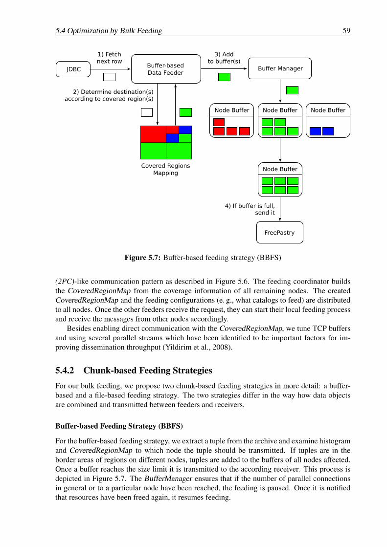
5.4 Optimization by Bulk Feeding 59

Figure 5.7: Buffer-based feeding strategy (BBFS)

(2PC)-like communication pattern as described in Figure 5.6. The feeding coordinator buildsthe CoveredRegionMap from the coverage information of all remaining nodes. The createdCoveredRegionMap and the feeding configurations (e. g., what catalogs to feed) are distributedto all nodes. Once the other feeders receive the request, they can start their local feeding processand receive the messages from other nodes accordingly.

Besides enabling direct communication with the CoveredRegionMap, we tune TCP buffersand using several parallel streams which have been identified to be important factors for im-proving dissemination throughput (Yildirim et al., 2008).

5.4.2 Chunk-based Feeding StrategiesFor our bulk feeding, we propose two chunk-based feeding strategies in more detail: a buffer-based and a file-based feeding strategy. The two strategies differ in the way how data objectsare combined and transmitted between feeders and receivers.

Buffer-based Feeding Strategy (BBFS)

For the buffer-based feeding strategy, we extract a tuple from the archive and examine histogramand CoveredRegionMap to which node the tuple should be transmitted. If tuples are in theborder areas of regions on different nodes, tuples are added to the buffers of all nodes affected.Once a buffer reaches the size limit it is transmitted to the according receiver. This process isdepicted in Figure 5.7. The BufferManager ensures that if the number of parallel connectionsin general or to a particular node have been reached, the feeding is paused. Once it is notifiedthat resources have been freed again, it resumes feeding.

60 5. Feeding Community-Driven Data Grids

Figure 5.8: File-based feeding strategy (FBFS)

File-based Feeding Strategy (FBFS)

The file-based feeding strategy is similar to the previously described feeding strategy usingbuffers. Instead of keeping the chunks in memory, a chunk-file per node is created on disk.As soon as a file reaches the size limit, it is transmitted to the receiving node. As Figure 5.8shows, the process is similar to the BBFS. In comparison to the WBFS which transmitted thewhole database at once, it allows for better pipelining as the data is now split up into severalfiles which are transmitted consecutively.

5.4.3 Optimizing Imports at Receiving Nodes

Database vendors and implementations have been very active in order to improve the perfor-mance of their bulk loading tools as this is an important and critical step e. g., during the datastaging into a data warehouse for business analytical processing. Therefore the performanceof these tools is superior to a series of individual insert-statements or even several blocked in-sert-statements.1. Therefore, once data is transmitted to the receiving node, it is converted intoa CSV file and the database load utility is used for import. So whenever multiple rows are in-serted into a database, we use the load utility of the database. In general, of course, it is possibleto adapt the import strategy to the amount of data which needs to be imported.

1A blocked SQL insert-statement combines several tuples in a single command, i. e., insert into values (. . . ),(. . . ).

5.5 Feeding Throughput Evaluation 61

Parameter Value(s) Descriptionf TBFS, WBFS, BBFS, FBFS Feeding strategy

P Pobs Data set

p 262144 Size of the partitioning scheme

n 16, 32 Network size

u initial load, replication Feeding use case

c 512 KB, 4 MB, 32 MB Chunk size

Table 5.1: Parameters for the evaluation of feeding strategies

5.5 Feeding Throughput EvaluationIn the following, we present the evaluation results for the different push-based feeding strategiesintroduced in this chapter.1 Table 5.1 summarizes the evaluation parameters. As use casesfor our evaluation, we selected the initial load scenario and the scenario for replicating alldata. Based on the observational data set Pobs, we created a partitioning scheme with 262 144partitions. We used two network setups: The first used 16 nodes from our lab and the secondsetup consisted of 32 nodes from the AstroGrid-D and the PlanetLab test bed. For the chunk-based techniques, we used chunk sizes of 512 KB, 4 MB, and 32 MB in order to evaluate theimportance of the chunk size for the feeding process.

5.5.1 Initial Load EvaluationIn the following, we present runtime results for initially loading data into our community-drivendata grid.

Running Time for the “Wolf”-based Feeding Strategy

For the “wolf”-based strategy, we ran the export of the three observational catalogs in paral-lel. Hence, the biggest archive determined the complete running time for the initial step. Aftercreating the CSV files, we combined these files into a database for each node. This completedatabase was finally copied to the participating nodes either with scp or GridFTP. The extrac-tion of the CSV files lasted 1 hour for the SDSS archive and 30 minutes for the ROSAT andTWOMASS archives, each. As we extracted the data in parallel, this step lasted 1 hour and thedata was extracted with roughly 23 000 tuples per second. Copying the data to the nodes, lastedup to 4 hours (depending on the node bandwidth). Finally, the creation of the node databaseslasted about 3 hours, depending on the total number of nodes. Therefore, the whole processrequired about 8 hours in total.

Running Time for the Tuple-based Feeding Strategy

For the tuple-based implementation, we set the frequency to 1 000 tuples per second. Thisconfiguration was necessary in order to keep the underlying FreePastry implementation from

1The TBFS, BBFS, FBFS, and the pull-based strategy have been integrated into the HiSbase prototype. Onlythe WBFS is realized as an external program because we mostly use it to prepare databases offline, e. g., for thePlanetLab nodes.

62 5. Feeding Community-Driven Data Grids

0

1

2

3

4

5

512 KB 4 MB 32 MB

runnin

g t

ime

(hours

)

chunk size

FBFS

BBFS

(a) 16 nodes

0

1

2

3

4

5

6

7

512 KB 4 MB 32 MB

runnin

g t

ime

(hours

)

chunk size

FBFS

BBFS

(b) 32 nodes

Figure 5.9: Results for the initial load scenario

dropping messages. Based on the fixed frequency we can compute the actual duration. Theduration for our initial load scenario was about 23 hours. Crainiceanu et al. (2007), for example,used an insertion rate of 4 items per second during their experiments. However, feeding ourSDSS sample (80 million objects) at that speed would last 33 weeks.

Running Time for the Chunk-based Feeding Strategies

Figure 5.9(a) shows the results for the buffer-based (BBFS) and file-based (FBFS) strategies onour 16 nodes setup with different chunk sizes. Both strategies are faster than the WBFS as nowall tasks (extraction, distribution, and data import) are performed in parallel. In addition, initialfeeding is accelerated by using chunk sizes in the megabytes compared to the 512 KB chunk.However, the difference between 4 MB and 32 MB was not significant. The BBFS createsbuffers in memory and submits them as serialized messages to the receiving nodes. Creatingthe CSV files for the database import is executed on the receiver side. Therefore the feederscan generate the next chunk faster and BBFS outperforms FBFS regardless of chunk size byapproximately one hour. The results for the 32 nodes are similar though some measurements(especially those for the FBFS with 4 MB chunks) were distorted due to high loads on PlanetLabnodes which run several experiments in parallel.

5.5.2 Replication Evaluation

For the evaluation of the replication scenario, we used the databases created during the previousexperiment as data sources. In order to ensure that all nodes redistribute their data, we assignednodes with new key space identifiers.

Running Time for the Tuple-based Feeding Strategy

For the TBFS, we estimated the runtime using the largest databases on individual nodes. Ofcourse, the exact size varies depending on the setup. Using the 1 000 tuples per second from theinitial load scenario, our network with 16 (32) nodes was replicated in 6 hours and the 32-nodenetwork in 3.5 hours.

5.6 Related Work 63

0

0.5

1

1.5

512 KB 4 MB 32 MB

runnin

g t

ime

(hours

)

chunk size

FBFS

BBFS

(a) 16 nodes

0

0.5

1

1.5

2

2.5

512 KB 4 MB 32 MB

runnin

g t

ime

(hours

)

chunk size

FBFS

BBFS

(b) 32 nodes

Figure 5.10: Results for the replication scenario

Running Time for the Chunk-based Feeding Strategies

From Figure 5.10(a) we see, both strategies greatly reduce the overall running time to 1 hourdue to the increased parallelism. Again, the buffer-based strategy is slightly better, howeverboth strategies are now more comparable. The results for 32 nodes, shown in Figure 5.10(b),are in accordance with those of our local setup. The result for 32 MB chunks of the BBFS mustagain be attributed to the high load on the PlanetLab resources.

5.5.3 DiscussionTo summarize, the buffer-based strategy outperforms the file-based strategy in our measuredscenarios as it introduces further parallelism by migrating tasks to receiving nodes. This isespecially beneficial for settings where only a small number of sources feed their data into thesystem. Based on the current results, we suggest to use a chunk size of 4 MB. The differencesbetween the measurements with 4 MB and 32 MB, respectively, were not significant and feederscomplete 4 MB chunks faster. We plan further experiments with chunk sizes in the gigabytesand currently redo the experiments with 32 nodes in a setup with dedicated resources.

5.6 Related WorkP-Ring (Crainiceanu et al., 2007) and online load balancing (Ganesan et al., 2004a) are exam-ples for extremely scalable P2P based infrastructures which achieve good load balancing fordynamic data distributions. Both show that two operations—either splitting existing data parti-tions or moving them—are required in order to achieve provable load balancing guarantees fordata load balancing. However, the fact that they perform tuple-based insertion introduces anoverhead which is too high for data-intensive e-science workloads.

Silberstein et al. (2008) propose a bulk insertion technique for range partitioned data storageused in hosted data services, such as PNuts (Cooper et al., 2008). Similar to our work, theypropose to use a initial phase in order to achieve a good data load balancing among the storagenodes to spread the insert load across multiple machines. During their planning phase, datasamples approximate the actual data distribution and a mapping from partitions to nodes iscomputed. The authors show that it is NP-hard to find a perfect mapping (by defining the

64 5. Feeding Community-Driven Data Grids

vector packing problem, a variant of the bin packing problem) and propose a technique thatoffers provable, approximative guarantees by repartitioning and moving partitions before datais actually inserted. Similar to the techniques proposed for P-Ring and for online load balancing,PNuts repartitions and moves data. An interesting concept are so-called staging servers, wherenew data is randomly partitioned to in order to sample data sets and increase the throughputduring the insertion by parallelism. While HiSbase enables different applications to access thesame data and thus enable cross-application data sharing, PNuts keeps different applicationsseparated, e. g., offering users flexible service level agreements. As a final difference, PNutsmaintains the complete data set at each cluster that participates within the distributed storagewhereas our work partitions the data across institutional boundaries.

BitTorrent (Cohen, 2003) is probably one of the most prominent P2P infrastructures. Itsdesign aims at improving the overall systems throughput by using not only the download ca-pacity but also the upload bandwidth by participating nodes. In contrast to HiSbase, however,BitTorrent clients, which cooperate in a download session, download the complete content. InHiSbase, we partition the content across multiple nodes.

Related work in high-performance computing has also investigated how to improve the datadistribution throughput. Proposals range from using TCP in combination with deadlock-freerouting in order to increase the overall throughput (Hironaka et al., 2009) to shaping the datatransfer rates by increasing the TCP buffer sizes and using several parallel streams (Yildirimet al., 2008).

Rehn et al. (2006) report on their experience for providing a data distribution service PhEDExto one of the LHC experiments and what challenges still need to be addressed in order to makedata transfer architectures robust and scalable. For full integration into Grid middleware, themethod of choice for data transfers is GridFTP (Allock et al., 2005). It offers certificate-basedauthorization and authentication as well as striping data transfers across multiple channels. Guet al. (2006) describe their distributed storage system Sector using a UDP-based protocol forlarge message transfers.

Query processing on radio frequency identification (RFID) data, such as tracking the pathsof different items along a production line also benefit from bulk data transfers. Krompaß et al.(2007) have identified considerable benefits of bulk data staging compared to tuple-wise stagingwhen transferring RFID reader events from on-line caches to a data warehouse.

5.7 Summary and Future WorkIn this chapter, we presented several push-based data dissemination techniques that use datachunks in order to accelerate data feeding compared to tuple-based or pull-based data distribu-tion. Interesting topics for future work includes further increasing the parallelism of the initialfeeding phase, e. g., using several staging servers as in PNuts. Improving the handling of borderdata when multiple feeders send the same catalog is another optimization which could yieldinteresting insights and benefits. Feeders, for example, could distinguish between original andborder data. Once all sources have notified a receiving node that they have completed theirfeeding, these nodes only need to eliminate duplicates from the border data.

Efficient data dissemination is important for several scenarios within community-driven datagrids, e. g., initially distributing data sets. Once all data sets are distributed, we can performquery processing and evaluate the throughput of our infrastructure, the topics of the followingchapter.

65

CHAPTER 6

Running Community-Driven Data Grids

Within this chapter, we give more details of the query processing techniques of community-driven data grids. We present detailed query processing algorithms and discuss various querycoordination techniques applicable for e-science communities (Section 6.1). In Section 6.2, wepresent the settings for throughput evaluations of our prototype and demonstrate the increasedquery throughput compared to centralized data management.

6.1 Query ProcessingDue to the distributed nature of e-science collaborations, query processing will require a nodewhich coordinates the common effort of data nodes that manage data which is relevant for aspecific query. We denote this node as coordinator and it will collect intermediate results inorder to perform the post-processing, e. g., duplicate elimination or further filtering. Dependingon which node coordinates the query processing, some things might change: the amount of datawhich is needed to be transmitted, the distribution of the coordination load, the response timefor the query processing. We will discuss in detail what design choices are relevant for a goodstrategy to coordinate the distributed query processing in community-driven data grids.

We describe the various design options for selecting a node as coordinator during queryprocessing within community-driven data grids. First, we describe the data access patterns andalgorithms of our query processing in Section 6.1.1. We then define five coordination strategies(Section 6.1.2) that either choose the node that submits the query or a node which containsrelevant data. In our analysis (Section 6.1.3), we evaluate how many messages are requiredby each strategy, how much traffic is generated, and how the strategies level the coordinationload among the nodes involved in the query processing based on results from simulation runs.Our results show that coordination strategies which use the relevant data nodes as coordinatorsachieve a good trade-off between fair load-balancing and reducing data-shipping during thequery coordination independent of skew within the workload submission. Besides that, also thenumber of messages is significantly lower for such coordination strategies. Only for workloadswith low coordination load, selecting the submitting node as coordinator is a feasible choice.

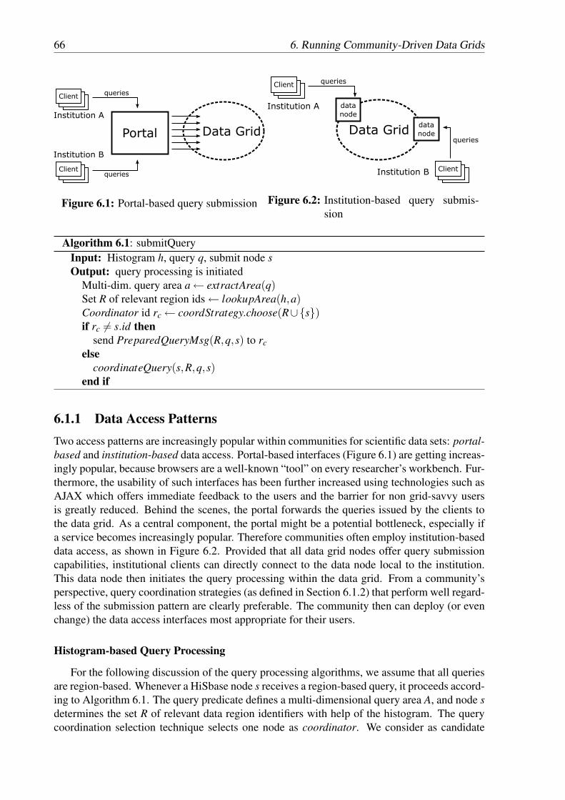
66 6. Running Community-Driven Data Grids

Figure 6.1: Portal-based query submission Figure 6.2: Institution-based query submis-sion

Algorithm 6.1: submitQueryInput: Histogram h, query q, submit node sOutput: query processing is initiated

Multi-dim. query area a ← extractArea(q)Set R of relevant region ids ← lookupArea(h,a)Coordinator id rc ← coordStrategy.choose(R∪{s})if rc 6= s.id then

send PreparedQueryMsg(R,q,s) to rcelse

coordinateQuery(s,R,q,s)end if

6.1.1 Data Access PatternsTwo access patterns are increasingly popular within communities for scientific data sets: portal-based and institution-based data access. Portal-based interfaces (Figure 6.1) are getting increas-ingly popular, because browsers are a well-known “tool” on every researcher’s workbench. Fur-thermore, the usability of such interfaces has been further increased using technologies such asAJAX which offers immediate feedback to the users and the barrier for non grid-savvy usersis greatly reduced. Behind the scenes, the portal forwards the queries issued by the clients tothe data grid. As a central component, the portal might be a potential bottleneck, especially ifa service becomes increasingly popular. Therefore communities often employ institution-baseddata access, as shown in Figure 6.2. Provided that all data grid nodes offer query submissioncapabilities, institutional clients can directly connect to the data node local to the institution.This data node then initiates the query processing within the data grid. From a community’sperspective, query coordination strategies (as defined in Section 6.1.2) that perform well regard-less of the submission pattern are clearly preferable. The community then can deploy (or evenchange) the data access interfaces most appropriate for their users.

Histogram-based Query Processing

For the following discussion of the query processing algorithms, we assume that all queriesare region-based. Whenever a HiSbase node s receives a region-based query, it proceeds accord-ing to Algorithm 6.1. The query predicate defines a multi-dimensional query area A, and node sdetermines the set R of relevant data region identifiers with help of the histogram. The querycoordination selection technique selects one node as coordinator. We consider as candidate

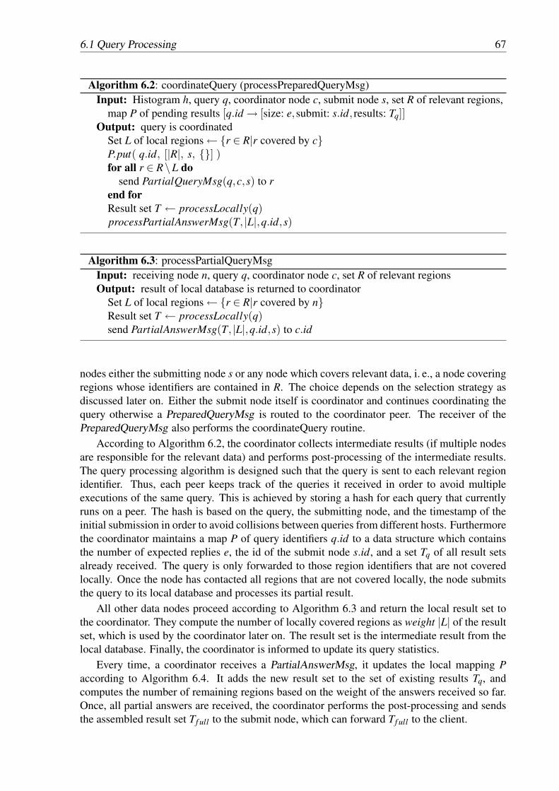
6.1 Query Processing 67

Algorithm 6.2: coordinateQuery (processPreparedQueryMsg)Input: Histogram h, query q, coordinator node c, submit node s, set R of relevant regions,

map P of pending results [q.id → [size: e,submit: s.id, results: Tq]]Output: query is coordinated

Set L of local regions ←{r ∈ R|r covered by c}P.put( q.id, [|R|, s, {}] )for all r ∈ R\L do

send PartialQueryMsg(q,c,s) to rend forResult set T ← processLocally(q)processPartialAnswerMsg(T, |L|,q.id,s)

Algorithm 6.3: processPartialQueryMsgInput: receiving node n, query q, coordinator node c, set R of relevant regionsOutput: result of local database is returned to coordinator

Set L of local regions ←{r ∈ R|r covered by n}Result set T ← processLocally(q)send PartialAnswerMsg(T, |L|,q.id,s) to c.id

nodes either the submitting node s or any node which covers relevant data, i. e., a node coveringregions whose identifiers are contained in R. The choice depends on the selection strategy asdiscussed later on. Either the submit node itself is coordinator and continues coordinating thequery otherwise a PreparedQueryMsg is routed to the coordinator peer. The receiver of thePreparedQueryMsg also performs the coordinateQuery routine.

According to Algorithm 6.2, the coordinator collects intermediate results (if multiple nodesare responsible for the relevant data) and performs post-processing of the intermediate results.The query processing algorithm is designed such that the query is sent to each relevant regionidentifier. Thus, each peer keeps track of the queries it received in order to avoid multipleexecutions of the same query. This is achieved by storing a hash for each query that currentlyruns on a peer. The hash is based on the query, the submitting node, and the timestamp of theinitial submission in order to avoid collisions between queries from different hosts. Furthermorethe coordinator maintains a map P of query identifiers q.id to a data structure which containsthe number of expected replies e, the id of the submit node s.id, and a set Tq of all result setsalready received. The query is only forwarded to those region identifiers that are not coveredlocally. Once the node has contacted all regions that are not covered locally, the node submitsthe query to its local database and processes its partial result.

All other data nodes proceed according to Algorithm 6.3 and return the local result set tothe coordinator. They compute the number of locally covered regions as weight |L| of the resultset, which is used by the coordinator later on. The result set is the intermediate result from thelocal database. Finally, the coordinator is informed to update its query statistics.

Every time, a coordinator receives a PartialAnswerMsg, it updates the local mapping Paccording to Algorithm 6.4. It adds the new result set to the set of existing results Tq, andcomputes the number of remaining regions based on the weight of the answers received so far.Once, all partial answers are received, the coordinator performs the post-processing and sendsthe assembled result set Tf ull to the submit node, which can forward Tf ull to the client.

68 6. Running Community-Driven Data Grids

Algorithm 6.4: processPartialAnswerMsgInput: receiving node n, result set T of the partial answer, weight w of the result set, query

identifier q.id, map P of pending results [q.id → [size: e,submit: s.id, results: Tq]]Output: result T is added to the appropriate query and if all results have been received the

final result set Tf ull is computed and returned to the submit nodeMap entry m ← P.get(q.id)m.size ← m.size−wm.results.add(T )if m.size = 0 then

Result set Tf ull ← per f ormPostProcessing(m.results)send FullAnswerMsg(Tf ull,qid) to m.submitP.remove(qid)

end if

(a) (b) (c)

Figure 6.3: Example to illustrate query processing: (a) sample data set with exemplary query,(b) linearization of the histogram, and (c) the mapping of the regions to nodes

Example Query

For the following discussion of query processing, we use Figure 6.3 as a running example. Thehistogram regions (Figure 6.3(a)) are mapped to the identifier space preserving the order ofthe space filling curve (Figure 6.3(b)). Figure 6.3(c) shows a possible mapping of the sevenpartitions (0–6) to the identifier space of a HiSbase network with four nodes (a–d).

Let us assume that the query from Figure 6.3(a)—shown as the thick-lined rectangle—issubmitted at node d. Node d analyses the received query and determines that regions 1, 2,3, and 4 potentially contain relevant data. In the next section, we discuss now several designchoices, whether node d itself or any of the nodes being responsible for relevant data (nodes a,b, and c) should coordinate the collaborative query processing.

6.1.2 Query Coordination StrategiesWe now provide more details on the query processing within HiSbase. We especially discussthe various strategies to select a query coordinator that are provided by our framework.

In order to emphasize the various design options, we show the communication patterns forthe various strategies. The used symbols are summarized in Figure 6.4. The node which per-forms the query coordination, i. e., either the submit node PS or a node with relevant data Di, ishighlighted. We furthermore differentiate between messages that are routed via the underlyingkey-based routing mechanism (dashed arrows) or directly between nodes (continuous arrows).

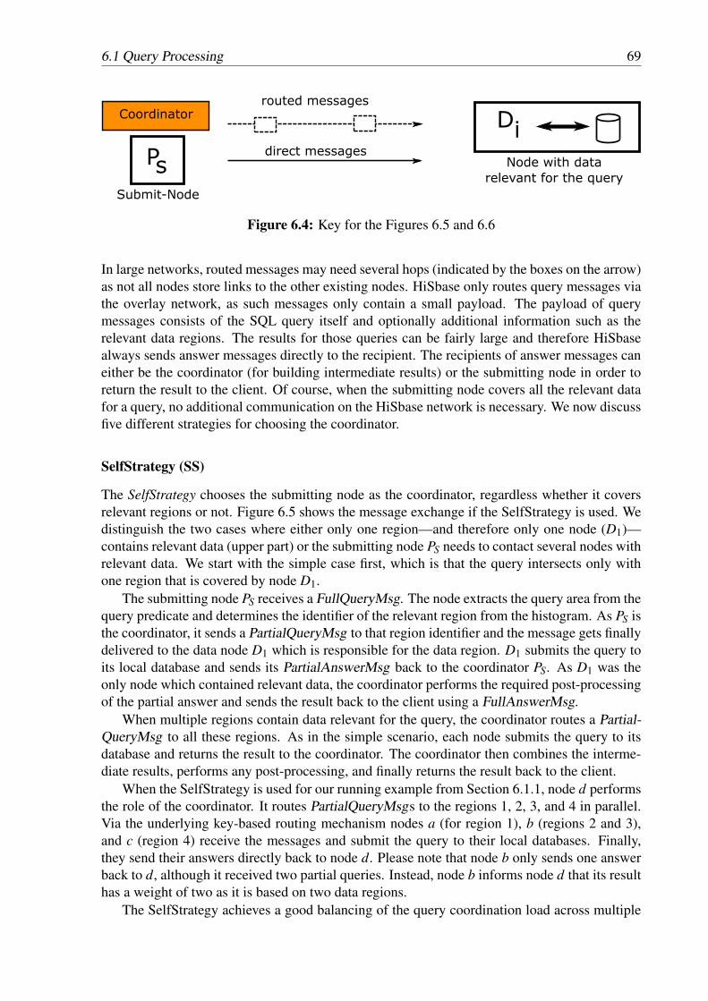
6.1 Query Processing 69

Figure 6.4: Key for the Figures 6.5 and 6.6

In large networks, routed messages may need several hops (indicated by the boxes on the arrow)as not all nodes store links to the other existing nodes. HiSbase only routes query messages viathe overlay network, as such messages only contain a small payload. The payload of querymessages consists of the SQL query itself and optionally additional information such as therelevant data regions. The results for those queries can be fairly large and therefore HiSbasealways sends answer messages directly to the recipient. The recipients of answer messages caneither be the coordinator (for building intermediate results) or the submitting node in order toreturn the result to the client. Of course, when the submitting node covers all the relevant datafor a query, no additional communication on the HiSbase network is necessary. We now discussfive different strategies for choosing the coordinator.

SelfStrategy (SS)

The SelfStrategy chooses the submitting node as the coordinator, regardless whether it coversrelevant regions or not. Figure 6.5 shows the message exchange if the SelfStrategy is used. Wedistinguish the two cases where either only one region—and therefore only one node (D1)—contains relevant data (upper part) or the submitting node PS needs to contact several nodes withrelevant data. We start with the simple case first, which is that the query intersects only withone region that is covered by node D1.

The submitting node PS receives a FullQueryMsg. The node extracts the query area from thequery predicate and determines the identifier of the relevant region from the histogram. As PS isthe coordinator, it sends a PartialQueryMsg to that region identifier and the message gets finallydelivered to the data node D1 which is responsible for the data region. D1 submits the query toits local database and sends its PartialAnswerMsg back to the coordinator PS. As D1 was theonly node which contained relevant data, the coordinator performs the required post-processingof the partial answer and sends the result back to the client using a FullAnswerMsg.

When multiple regions contain data relevant for the query, the coordinator routes a Partial-QueryMsg to all these regions. As in the simple scenario, each node submits the query to itsdatabase and returns the result to the coordinator. The coordinator then combines the interme-diate results, performs any post-processing, and finally returns the result back to the client.

When the SelfStrategy is used for our running example from Section 6.1.1, node d performsthe role of the coordinator. It routes PartialQueryMsgs to the regions 1, 2, 3, and 4 in parallel.Via the underlying key-based routing mechanism nodes a (for region 1), b (regions 2 and 3),and c (region 4) receive the messages and submit the query to their local databases. Finally,they send their answers directly back to node d. Please note that node b only sends one answerback to d, although it received two partial queries. Instead, node b informs node d that its resulthas a weight of two as it is based on two data regions.

The SelfStrategy achieves a good balancing of the query coordination load across multiple

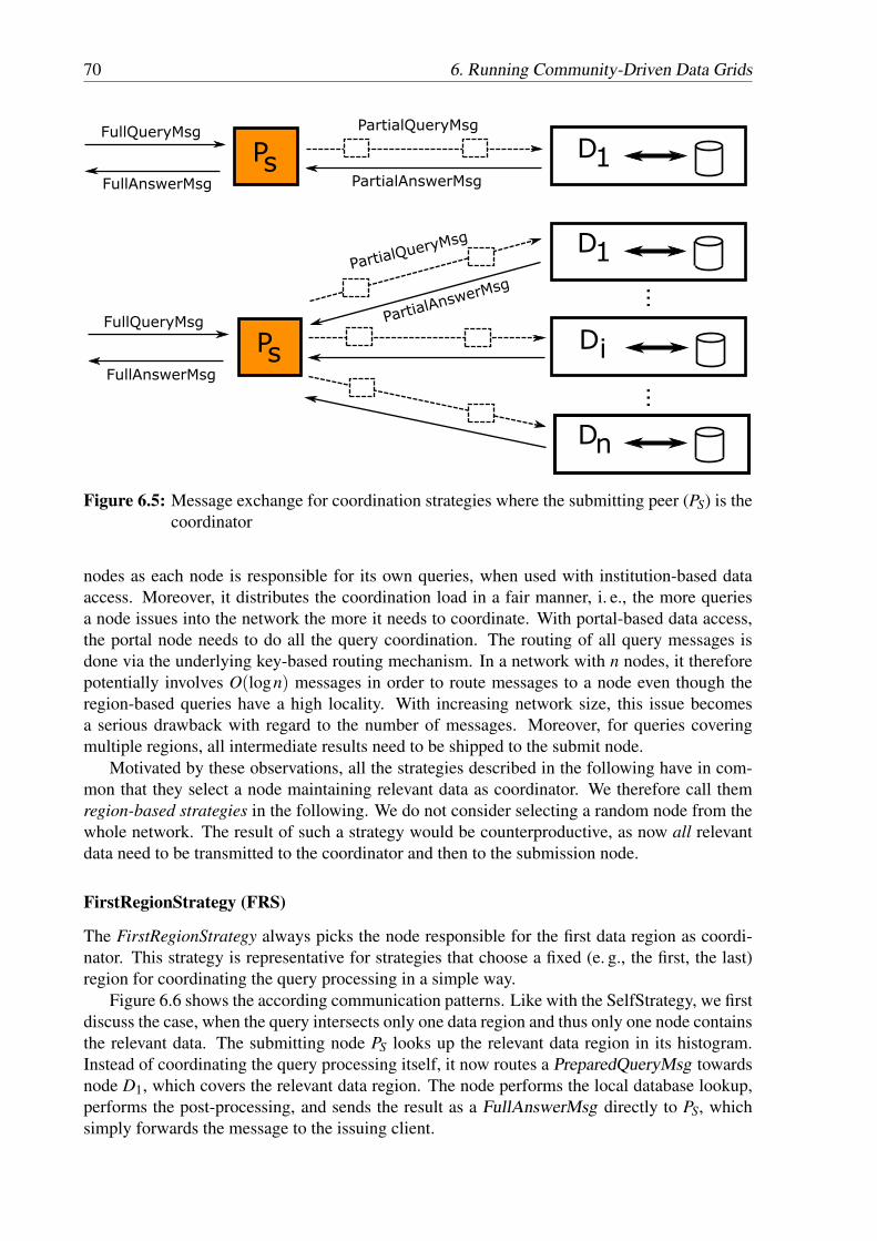
70 6. Running Community-Driven Data Grids

Figure 6.5: Message exchange for coordination strategies where the submitting peer (PS) is thecoordinator

nodes as each node is responsible for its own queries, when used with institution-based dataaccess. Moreover, it distributes the coordination load in a fair manner, i. e., the more queriesa node issues into the network the more it needs to coordinate. With portal-based data access,the portal node needs to do all the query coordination. The routing of all query messages isdone via the underlying key-based routing mechanism. In a network with n nodes, it thereforepotentially involves O(logn) messages in order to route messages to a node even though theregion-based queries have a high locality. With increasing network size, this issue becomesa serious drawback with regard to the number of messages. Moreover, for queries coveringmultiple regions, all intermediate results need to be shipped to the submit node.

Motivated by these observations, all the strategies described in the following have in com-mon that they select a node maintaining relevant data as coordinator. We therefore call themregion-based strategies in the following. We do not consider selecting a random node from thewhole network. The result of such a strategy would be counterproductive, as now all relevantdata need to be transmitted to the coordinator and then to the submission node.

FirstRegionStrategy (FRS)

The FirstRegionStrategy always picks the node responsible for the first data region as coordi-nator. This strategy is representative for strategies that choose a fixed (e. g., the first, the last)region for coordinating the query processing in a simple way.

Figure 6.6 shows the according communication patterns. Like with the SelfStrategy, we firstdiscuss the case, when the query intersects only one data region and thus only one node containsthe relevant data. The submitting node PS looks up the relevant data region in its histogram.Instead of coordinating the query processing itself, it now routes a PreparedQueryMsg towardsnode D1, which covers the relevant data region. The node performs the local database lookup,performs the post-processing, and sends the result as a FullAnswerMsg directly to PS, whichsimply forwards the message to the issuing client.

6.1 Query Processing 71

Figure 6.6: Message exchange for coordination strategies where a region with relevant data(D1) is coordinator

If the query area intersects multiple relevant regions, the coordinator submits additional Par-tialQueryMsgs to the other data regions and receives the PartialAnswerMsgs from the accordingnodes, performs the post-processing, and collects them into a FullAnswerMsg.

For our running example query, node d would send the submitted query together with itsrelevant regions to region identifier 1, as region 1 is the region with the lowest region identifiercontaining relevant data. Therefore, node a becomes the coordinator and informs nodes b and cabout the query. Having received the intermediate results from its local database and from bothother nodes, node a delivers the final result to node d.

As noted in the previous section on the SelfStrategy, collaborating nodes are neighbors onthe identifier space with high probability. This is due to the use of a space filling curve formapping the data regions on the identifier space and because the high degree of spatial localityof the queries. Thus, the coordinator knows the direct link to the other data regions and can routethe messages directly. As our evaluation in Section 6.1.3 shows, this can significantly reducethe number of messages during query processing. Moreover, this strategy benefits from thecoordinator covering some relevant data which needs not to be transmitted for post-processing.This benefit is common to all region-based strategies.

SelfOrFirstRegionStrategy (SOFRS)

The SelfOrFirstRegionStrategy is a combination of the both previously discussed strategies.Whenever the submitting node covers data relevant for the query itself, it performs the querycoordination. Otherwise, the node covering the first region is selected as coordinator.

When issuing our example query, e. g., to node c (instead of node d) using SelfOrFirstRe-gionStrategy, node c would coordinate the query itself.

The incentive for using the SelfOrFirstRegionStrategy is that if data is already at the sub-mitting node it would be unreasonable to send that data across the network and returning it afterpost-processing. However, the number of regions that an individual node covers decreases withgrowing network size when keeping the partitioning scheme fixed. Thus, it becomes less likely

72 6. Running Community-Driven Data Grids

that a submitting node covers any relevant regions itself.

CenterOfGravityStrategy (COGS)

While looking for similar ways to minimize the amount of data shipping like the SelfOrFirstRe-gionStrategy does, the center of gravity, the average location of the weight of an object, seems tobe the “perfect spot” for minimizing the data transfer. Therefore, we define the CenterOfGrav-ityStrategy which selects that node as coordinator that covers the partition which contains thecenter of gravity for an query area. As regular-shaped query areas (such as circles or rectangles)are very popular for specifying query areas in many scientific domains (e. g., the cone-searchesin astrophysics) this approach is viable. Assuming, the relevance of data within intersectedpartitions is proportional to the intersection area between partition and query, the regions in thecenter of the query area cover more relevant data. Regions at the border of the query area arenot completely covered and not that relevant under this assumption.

For our example query, the center of gravity lies within region 3, thus node b is selected ascoordinator. Once node b has received the intermediate results of peer a and c, it creates thefinal result and sends it to peer d. In this case, the coordinator even covers most of the relevantregions (region 2 and 3) which is also good for reducing the amount of data to be shipped.

Unfortunately, the computation of the center of gravity can become quite complex or theregion containing the center of gravity might not even be within the query area (e. g., for anO-shaped query area).

RandomRegionStrategy (RRS)

The final strategy presented in this section is the RandomRegionStrategy. As its name suggests,this strategy randomly selects one of the identifiers of the relevant data regions to determine thecoordinator. For the example query any of the nodes a, b, or c could be selected as coordinatorby this strategy. Note, however, that the probability of node b becoming coordinator is twicethe probability of node a and c, respectively. The selection process is based on the number ofrelevant regions and therefore nodes covering more regions are more likely to be coordinators.

The strategy reduces the amount of data shipping between collaborative nodes, it only re-trieves the relevant data regions and it is applicable for query areas of any shape. By design, itachieves a good trade-off between balancing the coordination load multiple nodes (as each nodehaving relevant data can be selected) and reducing the data shipping for query coordination (asit prefers nodes with many regions as coordinator).

6.1.3 Evaluation of Query Coordination StrategiesFor our evaluation, we used HiSbase, our Java-based prototype for community-driven datagrids. As histogram data structure we used a quadtree-based partitioning scheme with 262 144partitions as defined in Chapter 3. The data set, Pobs, consists of 137 million objects fromsubsets of the ROSAT, SDSS, and TWOMASS archives as described in Chapter 1.

The network size was varied from 100, 300, 1 000, to 3 000 nodes in order to evaluate thescalability of the five strategies described in the previous section. In the experiments, we usetwo query sets. The first query set, Qobs, comprises about 100 000 queries and was constructedfrom real queries issued on the SDSS web interface. The second workload, Qscaled , was createdby scaling all queries of Qobs whose search radii were among the five most frequent searchradii to cover an area of one square-degree. Thus a significant fraction of the workload Qscaled

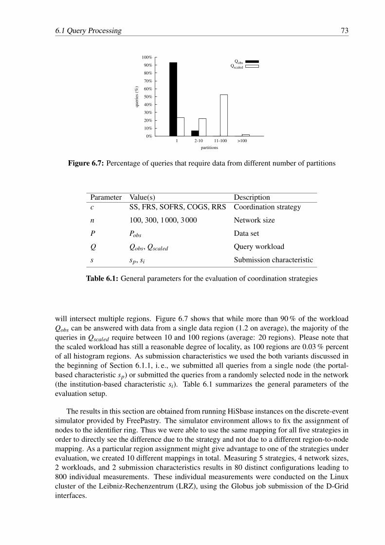
6.1 Query Processing 73

0%

10%

20%

30%

40%

50%

60%

70%

80%

90%

100%

1 2-10 11-100 >100qu

erie

s (%

)

partitions

QobsQscaled

Figure 6.7: Percentage of queries that require data from different number of partitions

Parameter Value(s) Descriptionc SS, FRS, SOFRS, COGS, RRS Coordination strategy

n 100, 300, 1000, 3000 Network size

P Pobs Data set

Q Qobs, Qscaled Query workload

s sp, si Submission characteristic

Table 6.1: General parameters for the evaluation of coordination strategies

will intersect multiple regions. Figure 6.7 shows that while more than 90 % of the workloadQobs can be answered with data from a single data region (1.2 on average), the majority of thequeries in Qscaled require between 10 and 100 regions (average: 20 regions). Please note thatthe scaled workload has still a reasonable degree of locality, as 100 regions are 0.03 % percentof all histogram regions. As submission characteristics we used the both variants discussed inthe beginning of Section 6.1.1, i. e., we submitted all queries from a single node (the portal-based characteristic sp) or submitted the queries from a randomly selected node in the network(the institution-based characteristic si). Table 6.1 summarizes the general parameters of theevaluation setup.

The results in this section are obtained from running HiSbase instances on the discrete-eventsimulator provided by FreePastry. The simulator environment allows to fix the assignment ofnodes to the identifier ring. Thus we were able to use the same mapping for all five strategies inorder to directly see the difference due to the strategy and not due to a different region-to-nodemapping. As a particular region assignment might give advantage to one of the strategies underevaluation, we created 10 different mappings in total. Measuring 5 strategies, 4 network sizes,2 workloads, and 2 submission characteristics results in 80 distinct configurations leading to800 individual measurements. These individual measurements were conducted on the Linuxcluster of the Leibniz-Rechenzentrum (LRZ), using the Globus job submission of the D-Gridinterfaces.

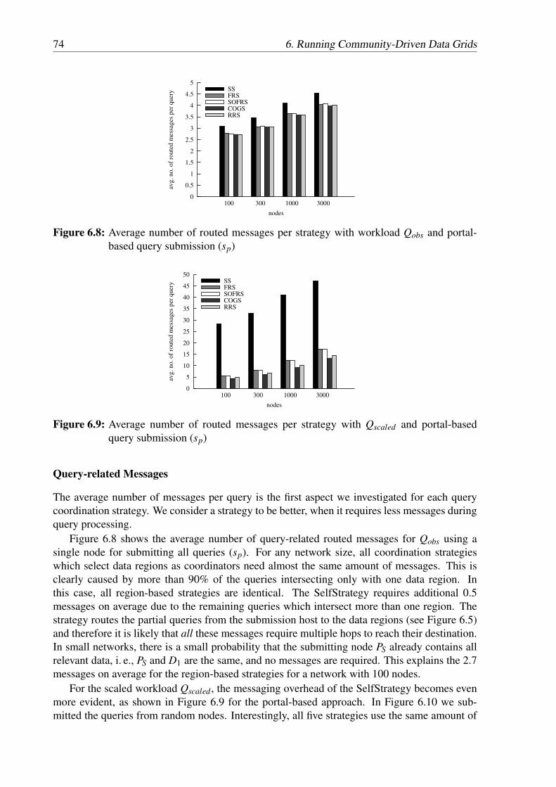
74 6. Running Community-Driven Data Grids

0

0.5

1

1.5

2

2.5

3

3.5

4

4.5

5

100 300 1000 3000

avg.

no. of

route

d m

essa

ges

per

quer

y

nodes

SSFRSSOFRSCOGSRRS

Figure 6.8: Average number of routed messages per strategy with workload Qobs and portal-based query submission (sp)

0

5

10

15

20

25

30

35

40

45

50

100 300 1000 3000

avg

. no

. of

route

d m

essa

ges

per

quer

y

nodes

SSFRSSOFRSCOGSRRS

Figure 6.9: Average number of routed messages per strategy with Qscaled and portal-basedquery submission (sp)

Query-related Messages

The average number of messages per query is the first aspect we investigated for each querycoordination strategy. We consider a strategy to be better, when it requires less messages duringquery processing.

Figure 6.8 shows the average number of query-related routed messages for Qobs using asingle node for submitting all queries (sp). For any network size, all coordination strategieswhich select data regions as coordinators need almost the same amount of messages. This isclearly caused by more than 90% of the queries intersecting only with one data region. Inthis case, all region-based strategies are identical. The SelfStrategy requires additional 0.5messages on average due to the remaining queries which intersect more than one region. Thestrategy routes the partial queries from the submission host to the data regions (see Figure 6.5)and therefore it is likely that all these messages require multiple hops to reach their destination.In small networks, there is a small probability that the submitting node PS already contains allrelevant data, i. e., PS and D1 are the same, and no messages are required. This explains the 2.7messages on average for the region-based strategies for a network with 100 nodes.

For the scaled workload Qscaled , the messaging overhead of the SelfStrategy becomes evenmore evident, as shown in Figure 6.9 for the portal-based approach. In Figure 6.10 we sub-mitted the queries from random nodes. Interestingly, all five strategies use the same amount of

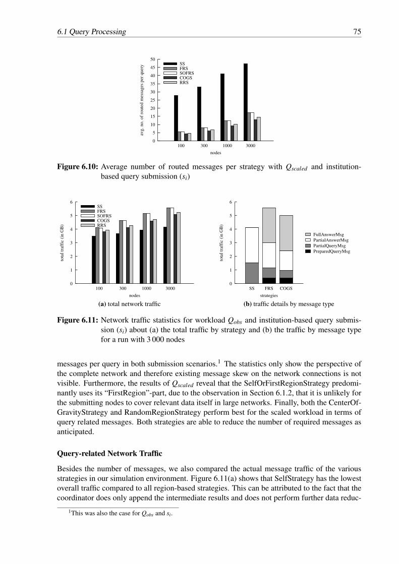
6.1 Query Processing 75

0

5

10

15

20

25

30

35

40

45

50

100 300 1000 3000av

g.

no. of

route

d m

essa

ges

per

quer

y

nodes

SSFRSSOFRSCOGSRRS

Figure 6.10: Average number of routed messages per strategy with Qscaled and institution-based query submission (si)

0

1

2

3

4

5

6

100 300 1000 3000

tota

l tr

aff

ic (

in G

B)

nodes

SSFRSSOFRSCOGSRRS

(a) total network traffic

0

1

2

3

4

5

6

SS FRS COGS

tota

l tr

affi

c (i

n G

B)

strategies

PreparedQueryMsg

PartialQueryMsg

PartialAnswerMsg

FullAnswerMsg

(b) traffic details by message type

Figure 6.11: Network traffic statistics for workload Qobs and institution-based query submis-sion (si) about (a) the total traffic by strategy and (b) the traffic by message typefor a run with 3 000 nodes

messages per query in both submission scenarios.1 The statistics only show the perspective ofthe complete network and therefore existing message skew on the network connections is notvisible. Furthermore, the results of Qscaled reveal that the SelfOrFirstRegionStrategy predomi-nantly uses its “FirstRegion”-part, due to the observation in Section 6.1.2, that it is unlikely forthe submitting nodes to cover relevant data itself in large networks. Finally, both the CenterOf-GravityStrategy and RandomRegionStrategy perform best for the scaled workload in terms ofquery related messages. Both strategies are able to reduce the number of required messages asanticipated.

Query-related Network Traffic

Besides the number of messages, we also compared the actual message traffic of the variousstrategies in our simulation environment. Figure 6.11(a) shows that SelfStrategy has the lowestoverall traffic compared to all region-based strategies. This can be attributed to the fact that thecoordinator does only append the intermediate results and does not perform further data reduc-

1This was also the case for Qobs and si.

76 6. Running Community-Driven Data Grids

0

0.2

0.4

0.6

0.8

1

0 0.2 0.4 0.6 0.8 1

accu

mula

ted c

oo

rdin

atio

n l

oad

proportion of nodes

uniform load balancing(Gini coefficient 0)

SS (Gini coefficient 1.00)

FRS, SOFRS (Gini coefficient 0.76)

COGS (Gini coefficient 0.75)

RRS (Gini coefficient 0.74)

Figure 6.12: Lorenz curves of the coordination load distribution on 3 000 nodes and portal-based query submission (sp)

tion. Therefore, for region-based strategies both PartialAnswerMsgs and FullAnswerMsgs aretransmitted.

When splitting the traffic into the constituents by the different message types, as shownin Figure 6.11(b), we see the major trade-offs between using the SelfStrategy or region-basedstrategies such as FirstRegionStrategy or CenterOfGravityStrategy. Region-based strategiesreduce the traffic during the query initialization phase, i. e., for both region-based strategiesthe combined traffic of PreparedQueryMsgs and PartialQueryMsgs is less than the traffic ofPartialQueryMsgs sent by the SelfStrategy. By choosing the coordinator region wisely (Cen-terOfGravityStrategy), we can reduce data shipping to the coordinator (PartialAnswerMsgs).However, the overall traffic for region-based strategies increases when the FullAnswerMsg isbuilt by appending the intermediate results. As a consequence, the traffic by PartialAnswerMsgsfor the SelfStrategy is equal to the traffic by FullAnswerMsgs from region-based strategies.

Coordination Load-Balancing

The last aspect we analyzed in our simulations was the ability of each strategy to balance thecoordination load evenly across multiple nodes. The more nodes are involved the more evenlythe coordination load is distributed. We evaluate the uniformness of the load distribution usingthe Lorenz curve and the Gini coefficient (see Pitoura et al., 2006). In our case, the Lorenz curveaccumulates the queries coordinated by all HiSbase nodes in ascending order, i. e., it starts withnodes which do not coordinate queries and finishes with the node which has the highest load.The Gini coefficient is defined as the area between the Lorenz curve for the distribution and thediagonal. The lower the Gini coefficient, i. e., the closer the graph to the diagonal, the moreuniform the load is distributed among the nodes. The final accumulated coordination load is thecomplete size of the query workload.

In the setup with portal-based data access, the SelfStrategy does not perform any load-balancing as all queries are coordinated by the single submitting node. This results in a Ginicoefficient of 1 and therefore the curve is hardly visible in Figure 6.12 as it coincides with thex-axis and the y-axis on the right-hand side. The coordinator selection strategies based on dataregions have Gini coefficients of around 0.75, the RandomRegionStrategy and CenterOfGrav-ityStrategy being slightly better than the other two strategies. When submitting queries fromrandom nodes (Figure 6.13), the SelfStrategy almost evenly distributes the coordination loadwhile the level of load-balancing of the other strategies remains the same.

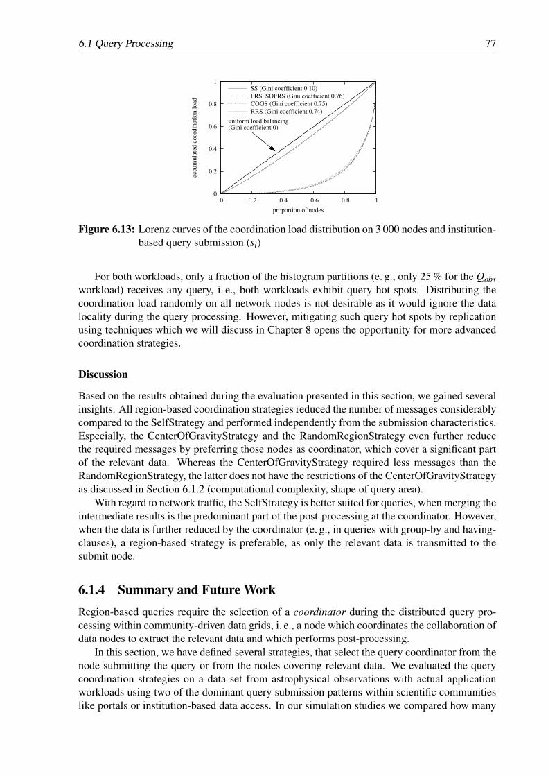
6.1 Query Processing 77

0

0.2

0.4

0.6

0.8

1

0 0.2 0.4 0.6 0.8 1ac

cum

ula

ted c

oo

rdin

atio

n l

oad

proportion of nodes

uniform load balancing(Gini coefficient 0)

SS (Gini coefficient 0.10)

FRS, SOFRS (Gini coefficient 0.76)

COGS (Gini coefficient 0.75)

RRS (Gini coefficient 0.74)

Figure 6.13: Lorenz curves of the coordination load distribution on 3 000 nodes and institution-based query submission (si)

For both workloads, only a fraction of the histogram partitions (e. g., only 25 % for the Qobsworkload) receives any query, i. e., both workloads exhibit query hot spots. Distributing thecoordination load randomly on all network nodes is not desirable as it would ignore the datalocality during the query processing. However, mitigating such query hot spots by replicationusing techniques which we will discuss in Chapter 8 opens the opportunity for more advancedcoordination strategies.

Discussion

Based on the results obtained during the evaluation presented in this section, we gained severalinsights. All region-based coordination strategies reduced the number of messages considerablycompared to the SelfStrategy and performed independently from the submission characteristics.Especially, the CenterOfGravityStrategy and the RandomRegionStrategy even further reducethe required messages by preferring those nodes as coordinator, which cover a significant partof the relevant data. Whereas the CenterOfGravityStrategy required less messages than theRandomRegionStrategy, the latter does not have the restrictions of the CenterOfGravityStrategyas discussed in Section 6.1.2 (computational complexity, shape of query area).

With regard to network traffic, the SelfStrategy is better suited for queries, when merging theintermediate results is the predominant part of the post-processing at the coordinator. However,when the data is further reduced by the coordinator (e. g., in queries with group-by and having-clauses), a region-based strategy is preferable, as only the relevant data is transmitted to thesubmit node.

6.1.4 Summary and Future WorkRegion-based queries require the selection of a coordinator during the distributed query pro-cessing within community-driven data grids, i. e., a node which coordinates the collaboration ofdata nodes to extract the relevant data and which performs post-processing.

In this section, we have defined several strategies, that select the query coordinator from thenode submitting the query or from the nodes covering relevant data. We evaluated the querycoordination strategies on a data set from astrophysical observations with actual applicationworkloads using two of the dominant query submission patterns within scientific communitieslike portals or institution-based data access. In our simulation studies we compared how many

78 6. Running Community-Driven Data Grids

messages are sent and how much network traffic is generated by each strategy and how theybalance the coordination load. The results show that strategies that aim at reducing the amountof data transmitted to the coordinator (CenterOfGravityStrategy and RandomRegionStrategy)offer the best trade-off between both criteria independently of the submission characteristic. Ifcoordination load is low (the coordinator performs no complex filtering tasks) then the SelfS-trategy is the strategy of choice.

In the results of the coordination load-balancing, the influence of query hot spots has beenclearly visible. In order to mitigate query hot spots at runtime, one approach is to replicate thepopular data regions to multiple nodes. To devise a coordination strategy that also considersreplicated data regions during the selection process is an interesting issue for future research.

Furthermore, an interesting direction for further investigations is to analyze the individualqueries in more detail and choose the coordination strategy based on structural properties andexpected coordination workload. The results presented in this chapter provide a solid base forsuch developments.

6.2 Throughput MeasurementsIn the following, we evaluate the throughput performance of our system. We begin with an out-line of the general definitions used during our throughput experiments. Initially, we comparea HiSbase instance with one node against a single database server and scale the instance to 16nodes within our computing lab. In this setting, we achieve a super-linear throughput improve-ment. We then describe measurements conducted in the AstroGrid-D and PlanetLab test bedsto discuss the impact of coordination strategies on the overall throughput. Based on the findingsof this chapter, we identify the areas that offer further improvements for query throughput.

6.2.1 General DefinitionsWe measure throughput for varying multi-programming levels (MPLs), i. e., a varying number ofparallel queries in the system, to evaluate at what degree of parallelism a distributed architecturecan outperform a centralized solution. Each run has k nodes, a batch containing l queries, andan MPL m. MPL=m denotes that each node keeps m parallel queries in the system. At the startof a run, each node immediately submits m queries. We measure the timestamp sn,q when noden has submitted its q-th query and the timestamp rn,q when it has received the correspondingresults. After receiving an answer, nodes submit their next query in order to sustain their multi-programming level.

For measuring the throughput, we only consider queries processed in the time span whenevery node is guaranteed to work on MPL=m parallel queries, the saturation phase Isat . Thetime interval between the point in time when the last peer has submitted its m-th query and thefirst peer has submitted its last query denotes Isat , which is expressed formally as:

Isat =[

max1≤n≤k

(sn,m), min1≤n≤k

(sn,l)]

(6.1)

Let Isat be the length of the saturation phase in seconds. The throughput per second T isbased on the number of successfully processed queries during the saturation phase Isat :

T =|{(n,q) | rn,q ∈ Isat ,1 ≤ n ≤ k,1 ≤ q ≤ l}|

Isat(6.2)

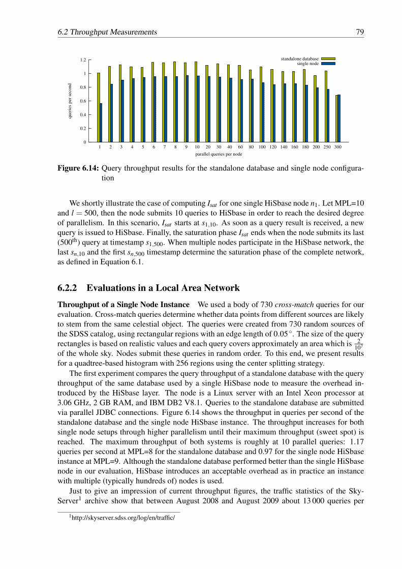
6.2 Throughput Measurements 79

0

0.2

0.4

0.6

0.8

1

1.2

1 2 3 4 5 6 7 8 9 10 20 30 40 60 80 100 120 140 160 180 200 250 300

quer

ies

per

sec

ond

parallel queries per node

standalone databasesingle node

Figure 6.14: Query throughput results for the standalone database and single node configura-tion

We shortly illustrate the case of computing Isat for one single HiSbase node n1. Let MPL=10and l = 500, then the node submits 10 queries to HiSbase in order to reach the desired degreeof parallelism. In this scenario, Isat starts at s1,10. As soon as a query result is received, a newquery is issued to HiSbase. Finally, the saturation phase Isat ends when the node submits its last(500th) query at timestamp s1,500. When multiple nodes participate in the HiSbase network, thelast sn,10 and the first sn,500 timestamp determine the saturation phase of the complete network,as defined in Equation 6.1.

6.2.2 Evaluations in a Local Area Network

Throughput of a Single Node Instance We used a body of 730 cross-match queries for ourevaluation. Cross-match queries determine whether data points from different sources are likelyto stem from the same celestial object. The queries were created from 730 random sources ofthe SDSS catalog, using rectangular regions with an edge length of 0.05◦. The size of the queryrectangles is based on realistic values and each query covers approximately an area which is 2

107

of the whole sky. Nodes submit these queries in random order. To this end, we present resultsfor a quadtree-based histogram with 256 regions using the center splitting strategy.

The first experiment compares the query throughput of a standalone database with the querythroughput of the same database used by a single HiSbase node to measure the overhead in-troduced by the HiSbase layer. The node is a Linux server with an Intel Xeon processor at3.06 GHz, 2 GB RAM, and IBM DB2 V8.1. Queries to the standalone database are submittedvia parallel JDBC connections. Figure 6.14 shows the throughput in queries per second of thestandalone database and the single node HiSbase instance. The throughput increases for bothsingle node setups through higher parallelism until their maximum throughput (sweet spot) isreached. The maximum throughput of both systems is roughly at 10 parallel queries: 1.17queries per second at MPL=8 for the standalone database and 0.97 for the single node HiSbaseinstance at MPL=9. Although the standalone database performed better than the single HiSbasenode in our evaluation, HiSbase introduces an acceptable overhead as in practice an instancewith multiple (typically hundreds of) nodes is used.

Just to give an impression of current throughput figures, the traffic statistics of the Sky-Server1 archive show that between August 2008 and August 2009 about 13 000 queries per

1http://skyserver.sdss.org/log/en/traffic/

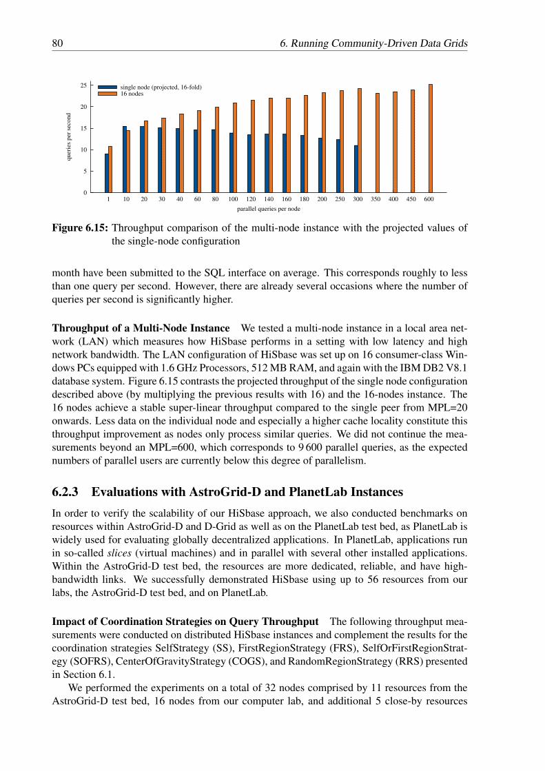
80 6. Running Community-Driven Data Grids

0

5

10

15

20

25

1 10 20 30 40 60 80 100 120 140 160 180 200 250 300 350 400 450 600

quer

ies

per

sec

ond

parallel queries per node

single node (projected, 16-fold)16 nodes

Figure 6.15: Throughput comparison of the multi-node instance with the projected values ofthe single-node configuration

month have been submitted to the SQL interface on average. This corresponds roughly to lessthan one query per second. However, there are already several occasions where the number ofqueries per second is significantly higher.

Throughput of a Multi-Node Instance We tested a multi-node instance in a local area net-work (LAN) which measures how HiSbase performs in a setting with low latency and highnetwork bandwidth. The LAN configuration of HiSbase was set up on 16 consumer-class Win-dows PCs equipped with 1.6 GHz Processors, 512 MB RAM, and again with the IBM DB2 V8.1database system. Figure 6.15 contrasts the projected throughput of the single node configurationdescribed above (by multiplying the previous results with 16) and the 16-nodes instance. The16 nodes achieve a stable super-linear throughput compared to the single peer from MPL=20onwards. Less data on the individual node and especially a higher cache locality constitute thisthroughput improvement as nodes only process similar queries. We did not continue the mea-surements beyond an MPL=600, which corresponds to 9 600 parallel queries, as the expectednumbers of parallel users are currently below this degree of parallelism.

6.2.3 Evaluations with AstroGrid-D and PlanetLab InstancesIn order to verify the scalability of our HiSbase approach, we also conducted benchmarks onresources within AstroGrid-D and D-Grid as well as on the PlanetLab test bed, as PlanetLab iswidely used for evaluating globally decentralized applications. In PlanetLab, applications runin so-called slices (virtual machines) and in parallel with several other installed applications.Within the AstroGrid-D test bed, the resources are more dedicated, reliable, and have high-bandwidth links. We successfully demonstrated HiSbase using up to 56 resources from ourlabs, the AstroGrid-D test bed, and on PlanetLab.

Impact of Coordination Strategies on Query Throughput The following throughput mea-surements were conducted on distributed HiSbase instances and complement the results for thecoordination strategies SelfStrategy (SS), FirstRegionStrategy (FRS), SelfOrFirstRegionStrat-egy (SOFRS), CenterOfGravityStrategy (COGS), and RandomRegionStrategy (RRS) presentedin Section 6.1.

We performed the experiments on a total of 32 nodes comprised by 11 resources from theAstroGrid-D test bed, 16 nodes from our computer lab, and additional 5 close-by resources

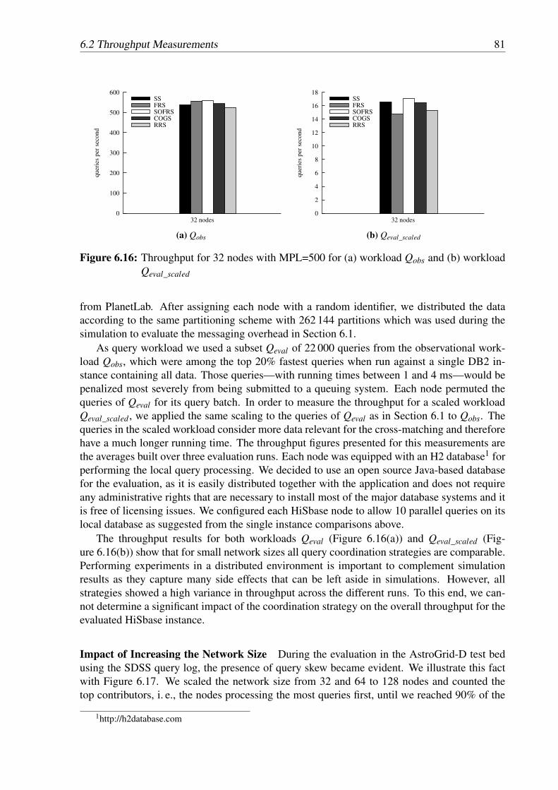
6.2 Throughput Measurements 81

0

100

200

300

400

500

600

32 nodes

quer

ies

per

sec

ond

SSFRSSOFRSCOGSRRS

(a) Qobs

0

2

4

6

8

10

12

14

16

18

32 nodes

quer

ies

per

sec

ond

SSFRSSOFRSCOGSRRS

(b) Qeval_scaled

Figure 6.16: Throughput for 32 nodes with MPL=500 for (a) workload Qobs and (b) workloadQeval_scaled

from PlanetLab. After assigning each node with a random identifier, we distributed the dataaccording to the same partitioning scheme with 262 144 partitions which was used during thesimulation to evaluate the messaging overhead in Section 6.1.

As query workload we used a subset Qeval of 22 000 queries from the observational work-load Qobs, which were among the top 20% fastest queries when run against a single DB2 in-stance containing all data. Those queries—with running times between 1 and 4 ms—would bepenalized most severely from being submitted to a queuing system. Each node permuted thequeries of Qeval for its query batch. In order to measure the throughput for a scaled workloadQeval_scaled , we applied the same scaling to the queries of Qeval as in Section 6.1 to Qobs. Thequeries in the scaled workload consider more data relevant for the cross-matching and thereforehave a much longer running time. The throughput figures presented for this measurements arethe averages built over three evaluation runs. Each node was equipped with an H2 database1 forperforming the local query processing. We decided to use an open source Java-based databasefor the evaluation, as it is easily distributed together with the application and does not requireany administrative rights that are necessary to install most of the major database systems and itis free of licensing issues. We configured each HiSbase node to allow 10 parallel queries on itslocal database as suggested from the single instance comparisons above.

The throughput results for both workloads Qeval (Figure 6.16(a)) and Qeval_scaled (Fig-ure 6.16(b)) show that for small network sizes all query coordination strategies are comparable.Performing experiments in a distributed environment is important to complement simulationresults as they capture many side effects that can be left aside in simulations. However, allstrategies showed a high variance in throughput across the different runs. To this end, we can-not determine a significant impact of the coordination strategy on the overall throughput for theevaluated HiSbase instance.

Impact of Increasing the Network Size During the evaluation in the AstroGrid-D test bedusing the SDSS query log, the presence of query skew became evident. We illustrate this factwith Figure 6.17. We scaled the network size from 32 and 64 to 128 nodes and counted thetop contributors, i. e., the nodes processing the most queries first, until we reached 90% of the

1http://h2database.com

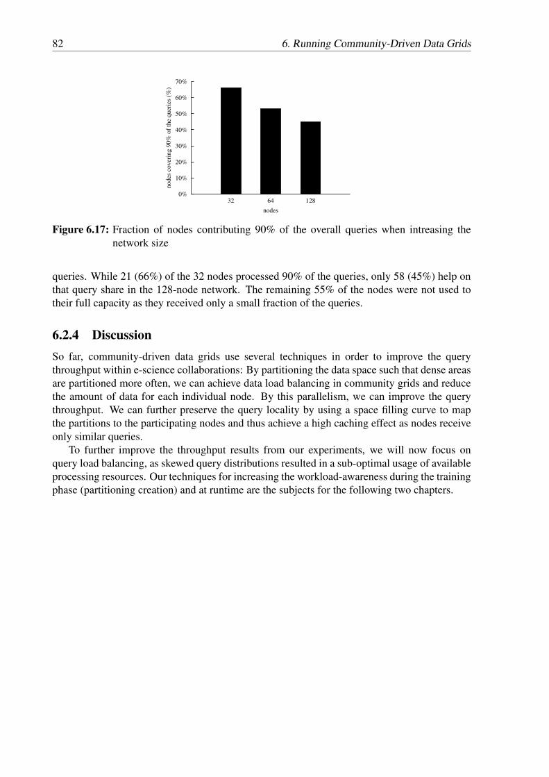
82 6. Running Community-Driven Data Grids

0%

10%

20%

30%

40%

50%

60%

70%

32 64 128

nodes

cover

ing 9

0%

of

the

quer

ies

(%)

nodes

Figure 6.17: Fraction of nodes contributing 90% of the overall queries when intreasing thenetwork size

queries. While 21 (66%) of the 32 nodes processed 90% of the queries, only 58 (45%) help onthat query share in the 128-node network. The remaining 55% of the nodes were not used totheir full capacity as they received only a small fraction of the queries.

6.2.4 DiscussionSo far, community-driven data grids use several techniques in order to improve the querythroughput within e-science collaborations: By partitioning the data space such that dense areasare partitioned more often, we can achieve data load balancing in community grids and reducethe amount of data for each individual node. By this parallelism, we can improve the querythroughput. We can further preserve the query locality by using a space filling curve to mapthe partitions to the participating nodes and thus achieve a high caching effect as nodes receiveonly similar queries.

To further improve the throughput results from our experiments, we will now focus onquery load balancing, as skewed query distributions resulted in a sub-optimal usage of availableprocessing resources. Our techniques for increasing the workload-awareness during the trainingphase (partitioning creation) and at runtime are the subjects for the following two chapters.

83

CHAPTER 7

Workload-Aware Data Partitioning

In the preceding chapters, we have described the core building blocks of community-driven datagrids and how the combination of these building blocks results in an increased throughput dur-ing query processing. To further improve the throughput gains by our data management infras-tructure, we now discuss techniques to incorporate workload-awareness into community-drivendata grids. In this chapter, we generalize the data-driven partitioning schemes of community-driven data grids to a cost-based partitioning in order to address two important challenges inscientific federations: data and query load balancing.

When some areas of the data space are very popular within the community, data nodescovering these areas, so-called query hot spots, tend to become the bottleneck during queryprocessing. In general, query load balancing can be achieved via splitting (partitioning) andreplication (Section 7.1).

For our cost model, we define several weight functions (Section 7.2). Besides data parti-tionings which consider only data load, we propose weight functions that allow advanced andworkload-aware weighting schemes. One weight function, for example, combines the weightfor points and queries to compute the heat of regions as the product of the associated data pointsand queries. Finally, we describe a weight function that decides by using the extent of querieswhether replication is better than splitting a region.

In Section 7.3, we evaluate our approach using quadtree-based partitioning schemes as in-troduced in Chapter 3. We use a sample of one million queries from an SDSS query trace Qobson the skewed, observational data set Pobs and a synthetic workload on the uniform data samplePmil from the Millennium simulation, as we have introduced in Section 1.2. We furthermoreperform several throughput measurements on our local resources of the AstroGrid-D testbed aswell as in a simulated network with the various partitioning schemes. The evaluation resultsassess the effectiveness and applicability of our load balancing techniques. We discuss relatedwork in Section 7.4 and conclude this chapter in Section 7.5.

84 7. Workload-Aware Data Partitioning

(a) Splitting (Partitioning) (b) Replication

Figure 7.1: Balancing query load (gray query rectangles) via splitting and replication

7.1 Load Balancing TechniquesQuery load balancing is a challenging task in distributed query processing. When dealing withpopular (“hot”) data, two strategies are generally applied in order to reduce the heat at the nodepredominantly responsible for the data:

Splitting (Partitioning) By further dividing the partition, parts of the query load can be movedto a different partition. If that partition is covered by another node, load is balanced be-tween these nodes. If hot areas are distributed among multiple nodes, good load balancingis achieved.

Replication Sometimes migration is not possible (e. g., one single data object is “hot”) or de-sirable (e. g., the query processing would result in more communication overhead). Insuch cases, load balancing can only be achieved by making multiple copies of the hotregion at several locations. If all replicas participate equally during query processing, ourdesign again achieves good load balancing.

Figure 7.1 shows the increased flexibility of load balancing techniques that apply both par-titioning and replication. Initially, partitioning succeeds in dividing the two hot spot areas de-noted by several gray query rectangles. The second partitioning step in Figure 7.1(a), however,would introduce additional communication overhead. In such situations, we can mitigate queryhot spots better by replicating the original data area. Thus, multiple copies are available duringquery processing, as illustrated in Figure 7.1(b).

For deciding whether we gain more from replicating a region instead of splitting it, thefollowing information is considered in our heuristics:

amount of data we still prefer to split those regions first that contain a considerable amount ofdata due to the importance of data load balancing,

number of queries regions with many queries should be handled before those regions whoseworkload is considerably low for query load balancing reasons,

extent of regions and queries in order to balance query load, we rather replicate regions whoseworkload predominantly consists of queries having a large extent, i. e., they cover a largearea compared to the area of the region itself.

Figure 7.2 depicts the basic idea, why it is important to incorporate the relationship betweenthe extents of regions and queries in a replication-aware weighting scheme. If all data andqueries were uniformly distributed, a quadtree-based partitioning scheme with n regions has amaximum height of log2d n in the general case and log4 n for our running example. If either

7.1 Load Balancing Techniques 85

Figure 7.2: Impact of skew on the height of the leaves

Figure 7.3: Impact of splitting a leaf on its ratio to a query area

data or queries are skewed, the regions with less “load” are leaves with height h < log4 n (witha larger area) and those in a hot spot area have h > log4n (with a smaller area). A query areawhich covers about 1

16 of a region, will cover 14 on the next level and eventually will have the

same size as a region after another split, as shown in Figure 7.3. Thus, the query is very likelyto span multiple regions and to produce additional communication overhead.

In order to take the aspects just described into account, a weight function needs to adhere tothe following heuristics. The weight function distinguishes regions with many data points fromregions with only a few data points. Similarly, it regards workloads with many and few queriesseparately and moreover pays attention to whether queries have a small or large extent.

If a region contains little data and only a few queries, it should be neither split nor replicatedas it does not contribute significantly to the overall load of the system.In case of regions that contain little data which is interesting to many queries, we replicate thoseregions that have many big queries. These data partitions can be replicated at several nodes andthen all replica are available for query processing. Partitions with many small queries are furthersplit, as the resulting partitions possibly will fall into the category with few data points and fewqueries.If a partition contains many data points but is only relevant to few queries, we prefer to split thepartition. The performance of the small queries might increase as they run on smaller data setswhich will even out the additional communication overhead for the big queries with regard tothe overall performance.The crucial class for the weighting scheme is the forth category of regions which contain muchdata as well as many queries. This category requires a good choice between splitting a regionif small queries mainly constitute the workload and replicating the region if the ratio of bigqueries is higher.

Table 7.1 summarizes the options to either split or replicate regions based on their associatednumber of data points and queries.

After having described the intuition about our criteria for query load balancing, we nowpresent our approach to create workload-aware data partitionings using weight functions.

86 7. Workload-Aware Data Partitioning

Data points Few queries Many queriesSmall Big Small Big

Few – – SPLIT REPLICATEMany SPLIT SPLIT SPLIT REPLICATE

Table 7.1: Categorization of regions for the replication-aware weight function

7.2 Region Weight FunctionsIn the following, we define a set of three weight functions for points, queries, and regions. Thisenables communities to create partitioning schemes for their data grids with a higher flexibility.

During the course of discussion, we will use several variables for points, queries, and regionswhich we will define in this paragraph. While creating our partitioning scheme, in the trainingphase, we use a representative training data set P and a training workload Q. The variable pdenotes a data point from P and q is a query from Q. Note that scientific data sets often comprisemany dimensions. For simplicity and ease of presentation, we only consider the projection tothe most predominant attributes from the query patterns (such as the two celestial coordinatesin our astrophysics example) during the training phase. When distributing the data partitions,the complete data is distributed.

The hyperrectangle Aq describes the boundaries of query q within the data space of thepartitioning scheme. Likewise, we define the area Ar covered by the region r. These areas areimportant building blocks for our weight functions.

We consider data points as relevant for query q if they reside within Aq. We further denotethe set of points relevant for query q as Pq and define Qp as the queries for which p is relevant.

Pq = {p ∈ P | p ∈ Aq} (7.1)Qp = {q ∈ Q | p ∈ Aq} (7.2)

The set Pr of data points within a region r and the set Qr of queries which intersect region r aredefined in a similar fashion.

Pr = {p ∈ P | p ∈ Ar} (7.3)Qr = {q ∈ Q | Aq ∩Ar 6= /0} (7.4)

7.2.1 Point WeightIf a partitioning scheme is targeted at balancing data skew, the weight of a data point is relevant.Data skew can originate from data spaces with a mix of densely and sparsely populated regions.The differences in data density may arise from the original data distribution or from the factthat some regions have been investigated more extensively than others, i. e., more data has beencollected and is available.

In general, we can define the weight w(p) of a point p as a function of its default weight σand the queries Qp it is relevant for:

w(p) = σ + f (Qp) (7.5)

When weighting data points, each point has a default weight σ , e. g., σ = 1. Now, we alsowant to consider queries for which a point p is relevant. For example, if a point is relevant for10 queries, it will have an additional weight of 10. Note that if we set default weight σ = 0,only data points which are relevant to any query are considered during the training phase.

7.2 Region Weight Functions 87

Example 1: Cardinality Function In the introductory example from above, we used thefunction f : Qp 7→ |Qp|. It is a reasonable candidate function: easy to understand, strictlymonotonically increasing, and easy to compute.

Example 2: Scaled Weight Function for Point Data The extent of the actual query hotspot(s) is unknown during the training phase. While we can locate the positions of query hotspots with our representative training workload Q, we can only approximate the extent of thearea of the data space that will be subject to high query workload. Cases where only a limitednumber of queries is available during training make such estimates more difficult. As a conse-quence, we try to approximate the actual hot spots by increasing the query area Aq for all queriesq by a scaling factor φ ≥ 1 in every dimension. We denote this area as Aq,φ in the following.1

Also, we introduce a new parameter λ in the weight function of data points in order to scale theimportance of Qp in relation to the default weight σ . Thus, we extend Equation 7.5 to:

wscaled,λ ,φ (p) = σ + λ · |{q ∈ Q | p ∈ Aq,φ}| (7.6)

It is important to note that tuning the parameters φ and λ for wscaled can be quite difficult.Choosing the wrong scaling factor can yield counterproductive partitioning schemes, which wasconfirmed by our experimental results (Section 7.3.1).

7.2.2 Query WeightThe weight for queries is defined in a similar fashion. We assign a default weight γ to eachquery, which represents the default processing cost for any query. Depending on the set Pq, weadd an additional query weight g(Pq). In the following, we use g(Pq) = |Pq|.

w(q) = γ + g(Pq) (7.7)

7.2.3 Combining Data and Query WeightsThe weight functions for data points (Equations 7.5 and 7.6) and queries (Equation 7.7) consti-tute the basic building blocks for defining the weight of a region. Based on the weight of theindividual partitions, we always split the partition with the highest weight next. The weight of aregion r depends on a function h of the data points Pr it contains and a function i of the queriesQr which intersect with its area.

w(r) = h(Pr) ⊗ i(Qr), where ⊗ ∈ {+, ·} (7.8)

In the following, we will only discuss the multiplication of both weights (· is used for ⊗).Combining the weight functions for points and queries to the weight of a region will result

in partitioning schemes that are optimized for various load balancing goals. Depending on thecombination, a partitioning scheme can achieve load balancing for data, for queries, or for both.In Table 7.2, we summarize five general patterns of how the weight functions of points andqueries are combined for the weight of a region. We associate the examples discussed in thefollowing with their corresponding pattern and state their load balancing capabilities.

Weight functions for the first two approaches consider either only the data points or only thequeries for computing the weight of a region. The first (wp) just counts the data points within aregion, the second (wq) only considers the number of queries intersecting with each partition.

1Equation 7.1 and 7.2 are still valid, as Aq,1 = Aq.

88 7. Workload-Aware Data Partitioning

Points Queries Regions Example Load balancing1 – h(Pr) wp Data– 1 i(Qr) wq Queries

f (Qp) – h(Pr) wQp Data and queries– g(Pq) i(Qr) wPq Data and queries1 1 h(Pr) · i(Qr) wpq Data and queries

Table 7.2: Overview of region weight functions in Section 7.2.3

All remaining three alternatives consider both data and queries for weighting the regions. Inthe third and fourth approach (wQp and wPq), the weight of a data region only depends on one ofthe building blocks—either points or queries—however the weight of the chosen building blockis influenced by the other, e. g., we weight each data point according to its relevance for queries.The last weight function wpq computes the heat of a region by multiplying the number ofobjects within a region and the number of queries intersecting the region. This weight functionimplicitly scales all queries until they cover the entire area of the region(s) they intersect andassigns more weight to regions that contain lots of data and receive many queries. Thus, thisweight function provides a notion of the overall load based both on data and on queries. If theregion contains no data, its weight is 0 and therefore it is unlikely to be split. If regions receiveno queries, we prefer to split those regions that contain more data. We therefore use (|Qr|+1)in case of queries. Thus, if a region receives no queries, it still has the same weight as whenusing wp.

After we have introduced the five weight functions intuitively, the Equations 7.9–7.13 givetheir formal definition.

wp(r) = |Pr| (7.9)wq(r) = |Qr| (7.10)

wQp(r) = ∑p∈Pr

w(p) (7.11)

wPq(r) = ∑q∈Qr

w(q) (7.12)

wpq(r) = |Pr| · (|Qr|+1) (7.13)

The relevance of data points for a particular query q can also be described using the indicatorfunction 1Aq : P →{0,1}:

1Aq(p) ={

0 if p /∈ Aq ,1 if p ∈ Aq .

(7.14)

Equation 7.15 shows that wQp and wPq define the same weight function if we set the defaultweights to σ = γ = 0 in Equations 7.5 and 7.7 and f (Qp) = |Qp| and g(Pq) = |Pq|, respec-tively. Intuitively, counting points weighted by the queries they are relevant for is equivalent tocounting queries weighted by the points that are relevant for them.

wQp(r) = ∑p∈Pr

w(p) = ∑p∈Pr

∑q∈Qr

1Aq(p) = ∑q∈Qr

w(q) = wPq(r) (7.15)

For the sake of simplicity, we use the weight-factors σ , γ , φ , and λ as constants. Otherscenarios, where σ , for example, is a function that returns the average size of a data point pdepending on the catalog it originates from, are also applicable but are not discussed further.

7.2 Region Weight Functions 89

7.2.4 Adding Query ExtentsThe pure heat-based weight function wpq captivates with its simplicity. However, if there isa small hot-spot area, heat-based partitioning may split that area multiple times as it tries toreduce the query load imbalance. This can lead to communication-thrashing, i. e., too muchcommunication between nodes covering neighboring partitions to retrieve the complete result.

For example in our two-dimensional quadtree-based partitioning schemes for astrophysicsdata, a query area Aq containing the centroid of the region area Ar, would be split into foursubqueries. In the worst case, four different nodes are responsible for these regions. This wouldresult in four-times overhead, as intermediate results need to be transmitted and the query usesCPU resources on four nodes. Under such circumstances, we prefer to keep the region as awhole and rather replicate it with our master-slave approach as described in Chapter 8.

Our replication-aware weight function wAq incorporates the extents of queries and regionsby classifying the queries according to the fraction of the area Aq of query q and the area Ar ofregion r. Thus, the weight function wAq realizes the behavior from Table 7.1 in Section 7.1. For0 < α ≤ β < 1, the sets of small (big) queries Qsmall

r (Qbigr ) are defined in Equations 7.16 and

7.17, respectively.

Qsmallr = {q ∈ Qr | Aq ≤ α ·Ar} (7.16)

Qbigr = {q ∈ Qr | Aq > β ·Ar} (7.17)

Based on the classification for Qr, we define the splitting gain for region r, gains(r), as thenumber of small queries in r (Equation 7.18). Analogously, we define gainr(r), the replicationgain for region r with the number of big queries intersecting r (Equation 7.19). For the samereason as in wpq, we add one to both cardinalities to deal with regions that receive no queries orwhose query sets Qsmall or Qbig are empty.

gains(r) = |Qsmallr |+1 (7.18)

gainr(r) = |Qbigr |+1 (7.19)

The replication-aware cost function wAq compares gains(r) and gainr(r) to determine whethera region should be split or not. As long as splitting a region is considered beneficial, only thevalue of gains(r) is used. As soon as the “big” queries outnumber the “small” queries, we re-duce the weight of a region considerably, by multiplying the size of |Pr| with the fraction of thesmall queries and big queries. In some application domains it might be desirable to additionallyspecify the preference τ for either splitting or replication. This is formalized by Equation 7.20.

wAq,α,β ,τ(r) =

|Pr| ·gains(r)gainr(r)

, if τ ·gains(r) < gainr(r) ,

|Pr| ·gains(r) , otherwise .(7.20)

The values for α and β strongly depend on workload characteristics of the applicationdomain, as we realized during our evaluation. At first thought, values like α = 1

4 , β = 34 or

α = 110 , β = 9

10 seem reasonable. Remarkably, those combinations have a fairly large “blindangle”, i. e., they ignore queries which have area extents between both thresholds. Especially,the decision in favor of splitting a region is sensitive to this gap. After having made the decisionto split a region, those “hidden” queries will probably intersect multiple regions causing highoverhead. Thus, we suggest to use the same values for α and β .

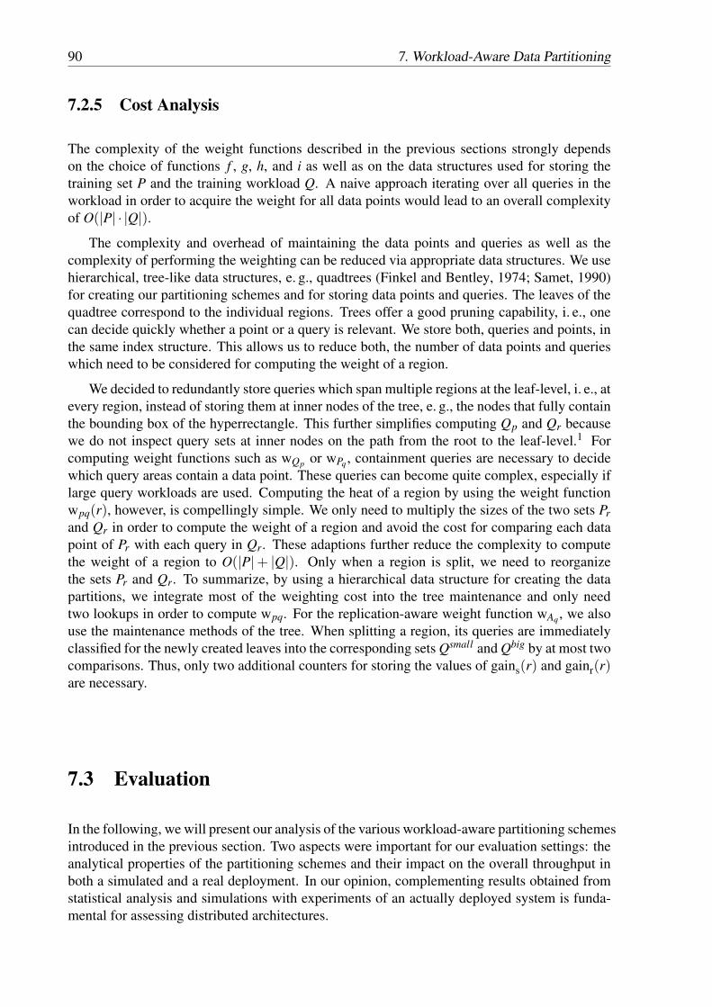
90 7. Workload-Aware Data Partitioning

7.2.5 Cost Analysis

The complexity of the weight functions described in the previous sections strongly dependson the choice of functions f , g, h, and i as well as on the data structures used for storing thetraining set P and the training workload Q. A naive approach iterating over all queries in theworkload in order to acquire the weight for all data points would lead to an overall complexityof O(|P| · |Q|).

The complexity and overhead of maintaining the data points and queries as well as thecomplexity of performing the weighting can be reduced via appropriate data structures. We usehierarchical, tree-like data structures, e. g., quadtrees (Finkel and Bentley, 1974; Samet, 1990)for creating our partitioning schemes and for storing data points and queries. The leaves of thequadtree correspond to the individual regions. Trees offer a good pruning capability, i. e., onecan decide quickly whether a point or a query is relevant. We store both, queries and points, inthe same index structure. This allows us to reduce both, the number of data points and querieswhich need to be considered for computing the weight of a region.

We decided to redundantly store queries which span multiple regions at the leaf-level, i. e., atevery region, instead of storing them at inner nodes of the tree, e. g., the nodes that fully containthe bounding box of the hyperrectangle. This further simplifies computing Qp and Qr becausewe do not inspect query sets at inner nodes on the path from the root to the leaf-level.1 Forcomputing weight functions such as wQp or wPq , containment queries are necessary to decidewhich query areas contain a data point. These queries can become quite complex, especially iflarge query workloads are used. Computing the heat of a region by using the weight functionwpq(r), however, is compellingly simple. We only need to multiply the sizes of the two sets Prand Qr in order to compute the weight of a region and avoid the cost for comparing each datapoint of Pr with each query in Qr. These adaptions further reduce the complexity to computethe weight of a region to O(|P|+ |Q|). Only when a region is split, we need to reorganizethe sets Pr and Qr. To summarize, by using a hierarchical data structure for creating the datapartitions, we integrate most of the weighting cost into the tree maintenance and only needtwo lookups in order to compute wpq. For the replication-aware weight function wAq , we alsouse the maintenance methods of the tree. When splitting a region, its queries are immediatelyclassified for the newly created leaves into the corresponding sets Qsmall and Qbig by at most twocomparisons. Thus, only two additional counters for storing the values of gains(r) and gainr(r)are necessary.

7.3 Evaluation

In the following, we will present our analysis of the various workload-aware partitioning schemesintroduced in the previous section. Two aspects were important for our evaluation settings: theanalytical properties of the partitioning schemes and their impact on the overall throughput inboth a simulated and a real deployment. In our opinion, complementing results obtained fromstatistical analysis and simulations with experiments of an actually deployed system is funda-mental for assessing distributed architectures.

7.3 Evaluation 91

Parameter Value(s) DescriptionP Pobs, Pmil Data sets used for training sample extraction

Q Qobs, Qmil Workloads used for workload-aware training

s 0.1%, 1%, 10% Size of the training set

n 42, 43, 44, 45, Size of the partitioning scheme46, 47, 48, 49

Table 7.3: General parameters for the evaluation of workload-aware partitioning schemes

Weight function Parameter and value(s)wQp , wscaled,λ ,φ λ = 0.01, φ = 10,20,40,80 (for Pobs)

λ = 1, φ = 10,50,100,200,400 (for Pmil)σ = 1 (both data sets)

wAq α , β ∈ { 14096 (≈ 0.0002), 1

256 (≈ 0.004),1

16 (= 0.0625), 14 (= 0.25) }, τ = 1

Table 7.4: Weight function specific parameters

7.3.1 Partitioning Scheme PropertiesIn order to evaluate the analytical properties of the partitioning schemes created with the data-based (wp), query-based (wQp), heat-based (wpq), and extent-based (wAq) weight functionsoutlined in this chapter, we conducted several experiments. We give a detailed description ofthe parameters, data sets, and query workloads used during our evaluation. We present anddiscuss results with respect to our goal of achieving a workload-aware data partitioning.

For the evaluation, we used our Java-based prototype HiSbase which created partitioningschemes according to our weight functions, based on a training data sample P and a represen-tative query workload Q. The remaining queries, not used during training, were used duringtesting and evaluating the partitioning schemes. We applied a tenfold cross-validation, which isa common setup for machine learning techniques (Witten and Frank, 2005). First, we evaluatedthe performance of our technique on data samples from three astrophysical catalogs using aquery trace from the SDSS catalog. Afterwards, we assessed the effect of our workload-awaretraining on a data sample from astrophysical simulations using a synthetic workload. This gavevaluable additional information, as the simulation data is quite uniformly distributed and so theimpact of some parameters was more clearly visible.

We constructed quadtree-based partitioning schemes using the standard splitting strategyas well as the median-based heuristics from Chapter 3. Here, we only discuss results withstandard quadtrees. For each approach, we varied the number of partitions to be all powersof four between 16 (42) and 262 144 (49) as these can be generated exactly by quadtrees andcorrespond to the values used in the previous evaluations.

For both data sets used during the evaluation, we drew several training samples of differentsizes (0.1%, 1%, and 10%) to benchmark the quality of results produced from small data sets.We extracted the random samples with functionality provided by relational database systems.We report on the results obtained from quadtree-based partitioning schemes using the stan-dard splitting strategy based on the 0.1% and 1% samples, each containing about 150 000 and

1This is basically the same trade-off as between MX-CIF and extended MX-CIF quadtrees (Samet, 1998).

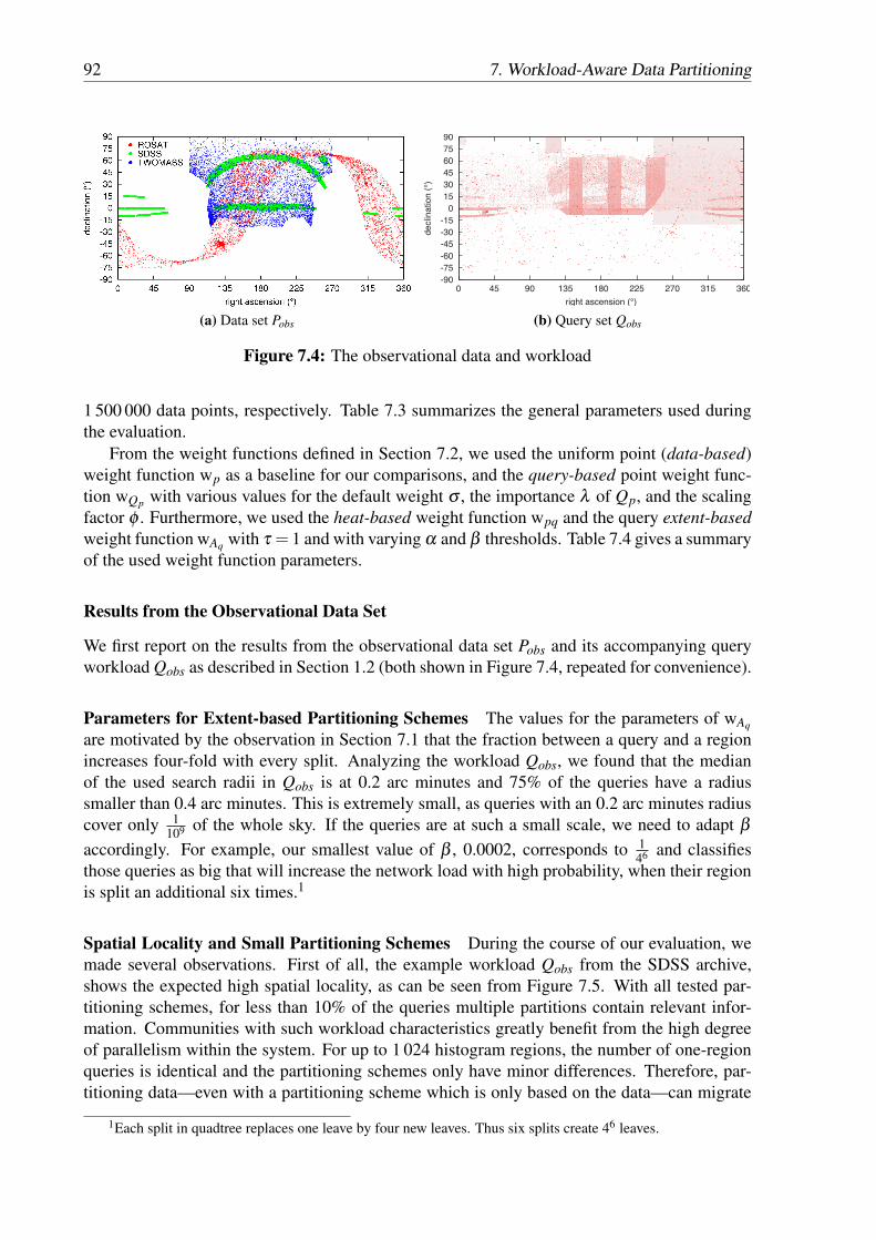
92 7. Workload-Aware Data Partitioning

(a) Data set Pobs (b) Query set Qobs

Figure 7.4: The observational data and workload

1 500 000 data points, respectively. Table 7.3 summarizes the general parameters used duringthe evaluation.

From the weight functions defined in Section 7.2, we used the uniform point (data-based)weight function wp as a baseline for our comparisons, and the query-based point weight func-tion wQp with various values for the default weight σ , the importance λ of Qp, and the scalingfactor φ . Furthermore, we used the heat-based weight function wpq and the query extent-basedweight function wAq with τ = 1 and with varying α and β thresholds. Table 7.4 gives a summaryof the used weight function parameters.

Results from the Observational Data Set

We first report on the results from the observational data set Pobs and its accompanying queryworkload Qobs as described in Section 1.2 (both shown in Figure 7.4, repeated for convenience).

Parameters for Extent-based Partitioning Schemes The values for the parameters of wAq

are motivated by the observation in Section 7.1 that the fraction between a query and a regionincreases four-fold with every split. Analyzing the workload Qobs, we found that the medianof the used search radii in Qobs is at 0.2 arc minutes and 75% of the queries have a radiussmaller than 0.4 arc minutes. This is extremely small, as queries with an 0.2 arc minutes radiuscover only 1

109 of the whole sky. If the queries are at such a small scale, we need to adapt βaccordingly. For example, our smallest value of β , 0.0002, corresponds to 1

46 and classifiesthose queries as big that will increase the network load with high probability, when their regionis split an additional six times.1

Spatial Locality and Small Partitioning Schemes During the course of our evaluation, wemade several observations. First of all, the example workload Qobs from the SDSS archive,shows the expected high spatial locality, as can be seen from Figure 7.5. With all tested par-titioning schemes, for less than 10% of the queries multiple partitions contain relevant infor-mation. Communities with such workload characteristics greatly benefit from the high degreeof parallelism within the system. For up to 1 024 histogram regions, the number of one-regionqueries is identical and the partitioning schemes only have minor differences. Therefore, par-titioning data—even with a partitioning scheme which is only based on the data—can migrate

1Each split in quadtree replaces one leave by four new leaves. Thus six splits create 46 leaves.

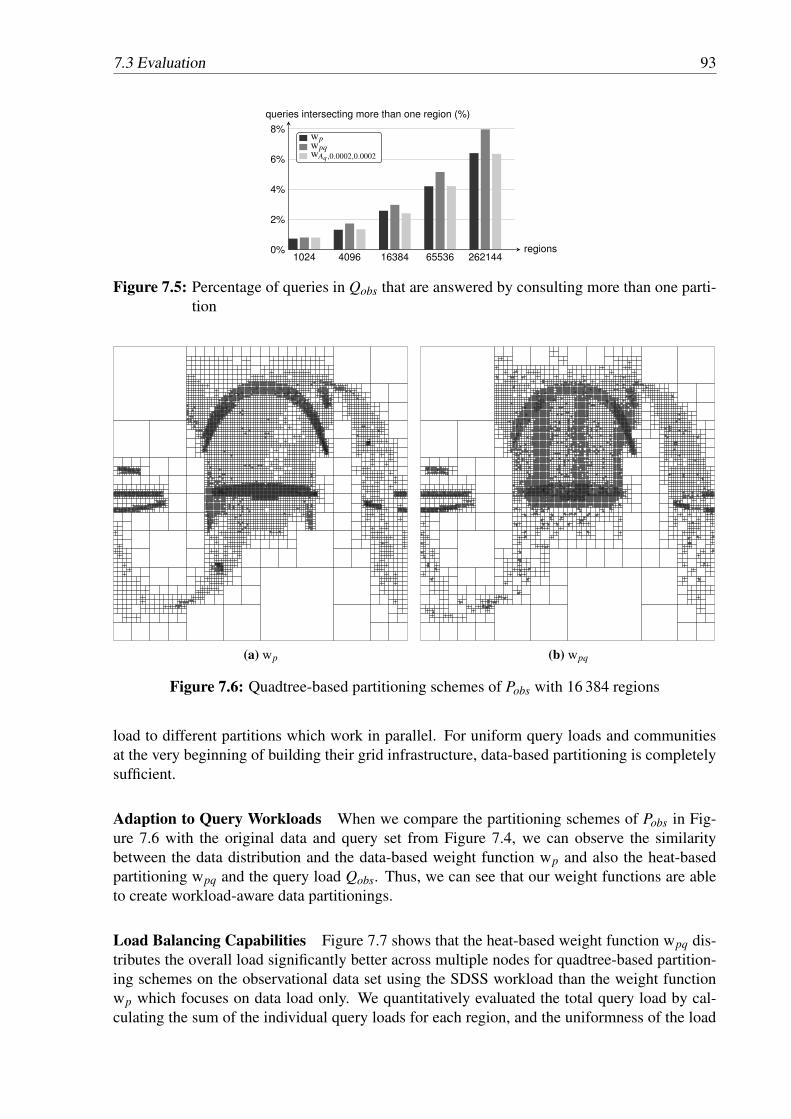
7.3 Evaluation 93

..0%

.2%

.4%

.6%

.8%

.1024 .4096 .16384 .65536 .262144

.queries intersecting more than one region (%)

.regions

.wp

.wpq

.wAq ,0.0002,0.0002

Figure 7.5: Percentage of queries in Qobs that are answered by consulting more than one parti-tion

(a) wp (b) wpq

Figure 7.6: Quadtree-based partitioning schemes of Pobs with 16 384 regions

load to different partitions which work in parallel. For uniform query loads and communitiesat the very beginning of building their grid infrastructure, data-based partitioning is completelysufficient.

Adaption to Query Workloads When we compare the partitioning schemes of Pobs in Fig-ure 7.6 with the original data and query set from Figure 7.4, we can observe the similaritybetween the data distribution and the data-based weight function wp and also the heat-basedpartitioning wpq and the query load Qobs. Thus, we can see that our weight functions are ableto create workload-aware data partitionings.

Load Balancing Capabilities Figure 7.7 shows that the heat-based weight function wpq dis-tributes the overall load significantly better across multiple nodes for quadtree-based partition-ing schemes on the observational data set using the SDSS workload than the weight functionwp which focuses on data load only. We quantitatively evaluated the total query load by cal-culating the sum of the individual query loads for each region, and the uniformness of the load

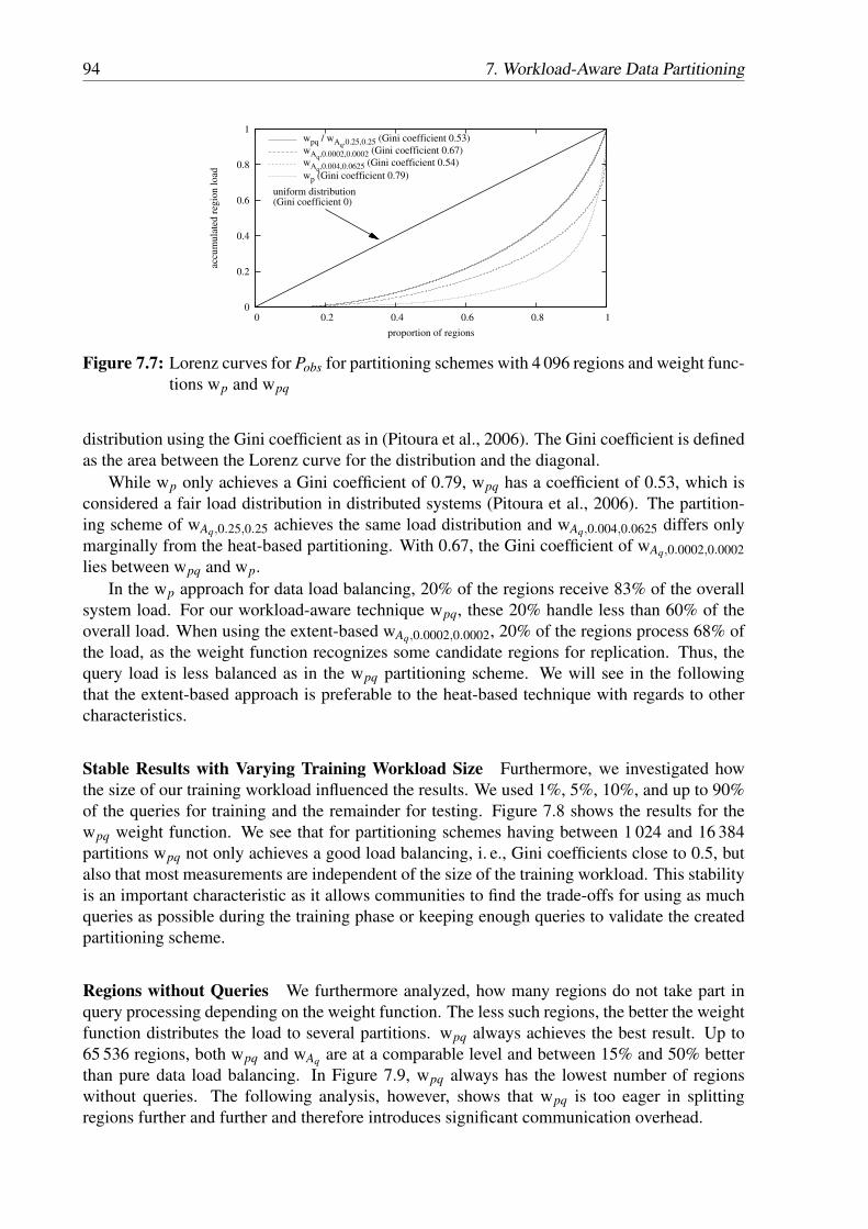
94 7. Workload-Aware Data Partitioning

0

0.2

0.4

0.6

0.8

1

0 0.2 0.4 0.6 0.8 1

accu

mula

ted

reg

ion l

oad

proportion of regions

uniform distribution(Gini coefficient 0)

wpq / wAq,0.25,0.25 (Gini coefficient 0.53)

wAq,0.0002,0.0002 (Gini coefficient 0.67)

wAq,0.004,0.0625 (Gini coefficient 0.54)

wp (Gini coefficient 0.79)

Figure 7.7: Lorenz curves for Pobs for partitioning schemes with 4 096 regions and weight func-tions wp and wpq

distribution using the Gini coefficient as in (Pitoura et al., 2006). The Gini coefficient is definedas the area between the Lorenz curve for the distribution and the diagonal.

While wp only achieves a Gini coefficient of 0.79, wpq has a coefficient of 0.53, which isconsidered a fair load distribution in distributed systems (Pitoura et al., 2006). The partition-ing scheme of wAq,0.25,0.25 achieves the same load distribution and wAq,0.004,0.0625 differs onlymarginally from the heat-based partitioning. With 0.67, the Gini coefficient of wAq,0.0002,0.0002lies between wpq and wp.

In the wp approach for data load balancing, 20% of the regions receive 83% of the overallsystem load. For our workload-aware technique wpq, these 20% handle less than 60% of theoverall load. When using the extent-based wAq,0.0002,0.0002, 20% of the regions process 68% ofthe load, as the weight function recognizes some candidate regions for replication. Thus, thequery load is less balanced as in the wpq partitioning scheme. We will see in the followingthat the extent-based approach is preferable to the heat-based technique with regards to othercharacteristics.

Stable Results with Varying Training Workload Size Furthermore, we investigated howthe size of our training workload influenced the results. We used 1%, 5%, 10%, and up to 90%of the queries for training and the remainder for testing. Figure 7.8 shows the results for thewpq weight function. We see that for partitioning schemes having between 1 024 and 16 384partitions wpq not only achieves a good load balancing, i. e., Gini coefficients close to 0.5, butalso that most measurements are independent of the size of the training workload. This stabilityis an important characteristic as it allows communities to find the trade-offs for using as muchqueries as possible during the training phase or keeping enough queries to validate the createdpartitioning scheme.

Regions without Queries We furthermore analyzed, how many regions do not take part inquery processing depending on the weight function. The less such regions, the better the weightfunction distributes the load to several partitions. wpq always achieves the best result. Up to65 536 regions, both wpq and wAq are at a comparable level and between 15% and 50% betterthan pure data load balancing. In Figure 7.9, wpq always has the lowest number of regionswithout queries. The following analysis, however, shows that wpq is too eager in splittingregions further and further and therefore introduces significant communication overhead.

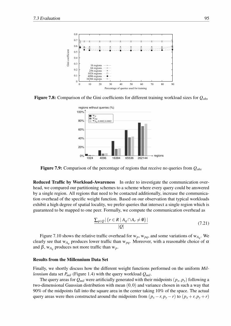
7.3 Evaluation 95

0

0.1

0.2

0.3

0.4

0.5

0.6

0.7

0.8

0 10 20 30 40 50 60 70 80 90

Gin

i co

effi

cien

t

Percentage of queries used for training

16 regions64 regions

256 regions1024 regions4096 regions

16384 regions

Figure 7.8: Comparison of the Gini coefficients for different training workload sizes for Qobs

..0%

.20%

.40%

.60%

.80%

.100%

.1024 .4096 .16384 .65536 .262144

.regions without queries (%)

.regions

.wp

.wpq

.wAq ,0.0002,0.0002

Figure 7.9: Comparison of the percentage of regions that receive no queries from Qobs

Reduced Traffic by Workload-Awareness In order to investigate the communication over-head, we compared our partitioning schemes to a scheme where every query could be answeredby a single region. All regions that need to be contacted additionally, increase the communica-tion overhead of the specific weight function. Based on our observation that typical workloadsexhibit a high degree of spatial locality, we prefer queries that intersect a single region which isguaranteed to be mapped to one peer. Formally, we compute the communication overhead as

∑q∈Q |{r ∈ R | Aq ∩Ar 6= /0}||Q|

(7.21)

Figure 7.10 shows the relative traffic overhead for wp, wpq, and some variations of wAq . Weclearly see that wAq produces lower traffic than wpq. Moreover, with a reasonable choice of αand β , wAq produces not more traffic than wp.

Results from the Millennium Data Set

Finally, we shortly discuss how the different weight functions performed on the uniform Mil-lennium data set Pmil (Figure 1.4) with the query workload Qmil .

The query areas for Qmil were artificially generated with their midpoints (px, py) following atwo-dimensional Gaussian distribution with mean (0,0) and variance chosen in such a way that90% of the midpoints fall into the square area in the center taking 10% of the space. The actualquery areas were then constructed around the midpoints from (px − r, py − r) to (px + r, py + r)

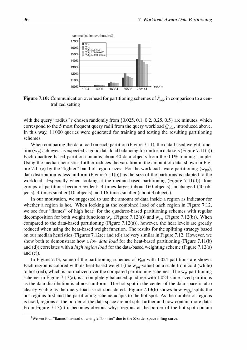
96 7. Workload-Aware Data Partitioning

..100%

.110%

.120%

.130%

.140%

.150%

.160%

.170%

.1024 .4096 .16384 .65536 .262144

.communication overhead (%)

.regions

.wAq ,0.0002,0.0002

.wAq ,0.004,0.0625

.wAq ,0.25,0.25

.wpq

.wp

Figure 7.10: Communication overhead for partitioning schemes of Pobs in comparison to a cen-tralized setting

with the query “radius” r chosen randomly from {0.025, 0.1, 0.2, 0.25, 0.5} arc minutes, whichcorrespond to the 5 most frequent query radii from the query workload Qobs, introduced above.In this way, 11 000 queries were generated for training and testing the resulting partitioningschemes.

When comparing the data load on each partition (Figure 7.11), the data-based weight func-tion (wp) achieves, as expected, a good data load balancing for uniform data sets (Figure 7.11(a)).Each quadtree-based partition contains about 40 data objects from the 0.1% training sample.Using the median-heuristics further reduces the variation in the amount of data, shown in Fig-ure 7.11(c) by the “tighter” band of region sizes. For the workload-aware partitioning (wpq),data distribution is less uniform (Figure 7.11(b)) as the size of the partitions is adapted to theworkload. Especially when looking at the median-based partitioning (Figure 7.11(d)), fourgroups of partitions become evident: 4-times larger (about 160 objects), unchanged (40 ob-jects), 4-times smaller (10 objects), and 16-times smaller (about 3 objects).

In our motivation, we suggested to use the amount of data inside a region as indicator forwhether a region is hot. When looking at the combined load of each region in Figure 7.12,we see four “flames” of high heat1 for the quadtree-based partitioning schemes with regulardecomposition for both weight functions wp (Figure 7.12(a)) and wpq (Figure 7.12(b)). Whencompared to the data-based partitioning (Figure 7.12(a)), however, the heat levels are greatlyreduced when using the heat-based weight function. The results for the splitting strategy basedon our median heuristics (Figures 7.12(c) and (d)) are very similar in Figure 7.12. However, weshow both to demonstrate how a low data load for the heat-based partitioning (Figure 7.11(b)and (d)) correlates with a high region load for the data-based weighting scheme (Figure 7.12(a)and (c)).

In Figure 7.13, some of the partitioning schemes of Pmil with 1 024 partitions are shown.Each region is colored with its heat-based weight (the wpq-value) on a scale from cold (white)to hot (red), which is normalized over the compared partitioning schemes. The wp-partitioningscheme, in Figure 7.13(a), is a completely balanced quadtree with 1 024 same-sized partitionsas the data distribution is almost uniform. The hot spot in the center of the data space is alsoclearly visible as the query load is not considered. Figure 7.13(b) shows how wQp splits thehot regions first and the partitioning scheme adapts to the hot spot. As the number of regionsis fixed, regions at the border of the data space are not split further and now contain more data.From Figure 7.13(c) it becomes obvious why: regions at the border of the hot spot contain

1We see four “flames” instead of a single “bonfire” due to the Z-order space filling curve.

7.3 Evaluation 97

0

20

40

60

80

100

120

140

160

180

0 500 1000 1500 2000 2500 3000 3500 4000

dat

a p

oin

ts

region ID

(a) with regular decomposition, wp

0

20

40

60

80

100

120

140

160

180

0 500 1000 1500 2000 2500 3000 3500 4000

dat

a p

oin

ts

region ID

(b) with regular decomposition, wpq

0

20

40

60

80

100

120

140

160

180

0 500 1000 1500 2000 2500 3000 3500 4000

dat

a p

oin

ts

region ID

(c) with median heuristics, wp

0

20

40

60

80

100

120

140

160

180

0 500 1000 1500 2000 2500 3000 3500 4000

dat

a p

oin

ts

region ID

(d) with median heuristics, wpq

Figure 7.11: Data load of Pmil for quadtree-based partitioning schemes with 4 096 partitions forthe data-based weight function (wp) and the heat-based weight function (wpq)

98 7. Workload-Aware Data Partitioning

0

100

200

300

400

500

600

0 500 1000 1500 2000 2500 3000 3500 4000

reg

ion

lo

ad

region ID

(a) with regular decomposition, wp

0

100

200

300

400

500

600

0 500 1000 1500 2000 2500 3000 3500 4000

reg

ion

lo

ad

region ID

(b) with regular decomposition, wpq

0

100

200

300

400

500

600

0 500 1000 1500 2000 2500 3000 3500 4000

reg

ion

lo

ad

region ID

(c) with median heuristics, wp

0

100

200

300

400

500

600

0 500 1000 1500 2000 2500 3000 3500 4000

reg

ion

lo

ad

region ID

(d) with median heuristics, wpq

Figure 7.12: Region load of Pmil for quadtree-based partitioning schemes with the 4 096 parti-tions for the data-based weight function (wp) and the heat-based weight function(wpq)

(a) wp (b) wQp , wscaled,λ=1,φ=50 (c) wQp , wscaled,λ=1,φ=400 (d) wpq, wAq

Figure 7.13: Partitioning with 1 024 regions for Pmil

7.3 Evaluation 99

16-times the data than in the wp partitioning but also receive many queries and thus their loadwill be too high. Finally, we see in Figure 7.13(d) that the heat-based weighting scheme wpqapproximates the extent of the hot spot very good but does not lose sight of data load balancing.Actually, the extent-based weight function wAq produced the same partitioning scheme. Notethe four different sizes of regions in our workload-aware partitionings as in Figure 7.11(b): someregions are 16-times smaller (in the very center of the hot spot), 4-times smaller, unchanged,and 4-times larger (the cold regions at the border of the data space) than the regions of the wppartitioning scheme.

7.3.2 Throughput EvaluationThe previous analysis of the histograms was based on the training data and both the trainingand testing workloads. The following throughput measurements are conducted on distributed orsimulated HiSbase instances. We intentionally do not use the master-slave replication approachat runtime as described in Chapter 8 in order to emphasize the throughput variations purelybased on the choice of the weight function.

For the throughput experiments we use the same definitions for saturation phase Isat andthroughput T as in Chapter 6.2. During the throughput evaluation, we used partitioning schemescreated with the data-based (wp), heat-based (wpq), and extent-based (wAq,0.0002,0.0002) weightfunctions, respectively. The size of the histogram—4 096 for real and 262 144 for simulatednetworks—is chosen to be large enough to ensure that all peers are responsible for data parti-tions. The results shown are the averages built over three evaluation runs in both (the real andsimulated) cases.

Each single HiSbase node was configured to allow ten parallel queries on its local database,as suggested in Chapter 6.2. The following evaluation shows that especially higher multi-programming levels for the HiSbase nodes increase the overall throughput; we report on MPLsselected from {10, 50, 100, 300, 500}.

Results from the Observational Workload

For our throughput experiments, we used the same 22 000 queries from Qobs as in the throughputevaluation for coordination strategies in Section 6.2.3. Each node randomly selected 5 000queries from Qeval for its query batch.

Our 16 computer lab nodes are consumer-class Linux PCs equipped with 1.6 GHz pro-cessors, 512 MB RAM and running DB2 V9.1.4. For the measurements with 32 nodes, weadditionally used 16 nodes from our local AstroGrid-D resources having between 1 and 4 GBmain memory and 2.8 GHz Intel Xeon CPUs. We used the H2 database for performing thelocal query processing. After assigning each node a random identifier, we distributed the dataaccording to the partitioning scheme.

Figure 7.14 shows the throughput achieved by a HiSbase network using a partitioningscheme with 4 096 partitions which are distributed among 16 and 32 nodes, respectively. For16 peers, we see that the wp partitioning scheme surprisingly achieves the highest throughput,while for the setup with 32 nodes, the extent-based technique wAq outperforms both wp andwpq. Due to several query hot spots in Qeval , only a fraction of the additional nodes can signifi-cantly participate during query processing. While wAq increases the throughput in a near-linearfashion, the gain of wp and wpq is only sub-linear.

We have successfully demonstrated HiSbase (Scholl et al., 2007a) on PlanetLab and wesee great value of PlanetLab for evaluating the algorithmic properties (like messaging over-

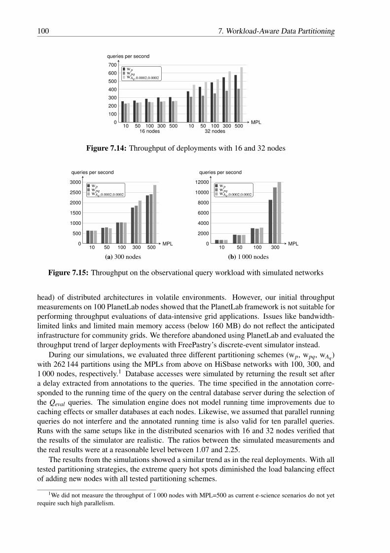
100 7. Workload-Aware Data Partitioning

..0

.100

.200

.300

.400

.500

.600

.700

.10 .50 .100 .300 .500 .10 .50 .100 .300 .500

.queries per second

.16 nodes .32 nodes

.MPL

.wp

.wpq.wAq ,0.0002,0.0002

Figure 7.14: Throughput of deployments with 16 and 32 nodes

..0

.500

.1000

.1500

.2000

.2500

.3000

.10 .50 .100 .300 .500

.queries per second

.MPL

.wAq ,0.0002,0.0002

.wpq

.wp

(a) 300 nodes

..0

.2000

.4000

.6000

.8000

.10000

.12000

.10 .50 .100 .300

.queries per second

.MPL

.wAq ,0.0002,0.0002

.wpq

.wp

(b) 1 000 nodes

Figure 7.15: Throughput on the observational query workload with simulated networks

head) of distributed architectures in volatile environments. However, our initial throughputmeasurements on 100 PlanetLab nodes showed that the PlanetLab framework is not suitable forperforming throughput evaluations of data-intensive grid applications. Issues like bandwidth-limited links and limited main memory access (below 160 MB) do not reflect the anticipatedinfrastructure for community grids. We therefore abandoned using PlanetLab and evaluated thethroughput trend of larger deployments with FreePastry’s discrete-event simulator instead.

During our simulations, we evaluated three different partitioning schemes (wp, wpq, wAq)with 262 144 partitions using the MPLs from above on HiSbase networks with 100, 300, and1 000 nodes, respectively.1 Database accesses were simulated by returning the result set aftera delay extracted from annotations to the queries. The time specified in the annotation corre-sponded to the running time of the query on the central database server during the selection ofthe Qeval queries. The simulation engine does not model running time improvements due tocaching effects or smaller databases at each nodes. Likewise, we assumed that parallel runningqueries do not interfere and the annotated running time is also valid for ten parallel queries.Runs with the same setups like in the distributed scenarios with 16 and 32 nodes verified thatthe results of the simulator are realistic. The ratios between the simulated measurements andthe real results were at a reasonable level between 1.07 and 2.25.

The results from the simulations showed a similar trend as in the real deployments. With alltested partitioning strategies, the extreme query hot spots diminished the load balancing effectof adding new nodes with all tested partitioning schemes.

1We did not measure the throughput of 1 000 nodes with MPL=500 as current e-science scenarios do not yetrequire such high parallelism.

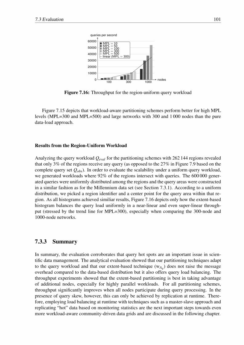
7.3 Evaluation 101

..0

.10000

.20000

.30000

.40000

.50000

.60000

.100 .300 .1000

.queries per second

.nodes

.MPL = 500

.MPL = 300

.MPL = 100

.MPL = 50

.MPL = 10

.linear (MPL = 300)

Figure 7.16: Throughput for the region-uniform query workload

Figure 7.15 depicts that workload-aware partitioning schemes perform better for high MPLlevels (MPL=300 and MPL=500) and large networks with 300 and 1 000 nodes than the puredata-load approach.

Results from the Region-Uniform Workload

Analyzing the query workload Qeval for the partitioning schemes with 262 144 regions revealedthat only 3% of the regions receive any query (as opposed to the 27% in Figure 7.9 based on thecomplete query set Qobs). In order to evaluate the scalability under a uniform query workload,we generated workloads where 92% of the regions intersect with queries. The 600 000 gener-ated queries were uniformly distributed among the regions and the query areas were constructedin a similar fashion as for the Millennium data set (see Section 7.3.1). According to a uniformdistribution, we picked a region identifier and a center point for the query area within that re-gion. As all histograms achieved similiar results, Figure 7.16 depicts only how the extent-basedhistogram balances the query load uniformly in a near-linear and even super-linear through-put (stressed by the trend line for MPL=300), especially when comparing the 300-node and1000-node networks.

7.3.3 Summary

In summary, the evaluation corroborates that query hot spots are an important issue in scien-tific data management. The analytical evaluation showed that our partitioning techniques adaptto the query workload and that our extent-based technique (wAq) does not raise the messageoverhead compared to the data-based distribution but it also offers query load balancing. Thethroughput experiments showed that the extent-based partitioning is best in taking advantageof additional nodes, especially for highly parallel workloads. For all partitioning schemes,throughput significantly improves when all nodes participate during query processing. In thepresence of query skew, however, this can only be achieved by replication at runtime. There-fore, employing load balancing at runtime with techniques such as a master-slave approach andreplicating “hot” data based on monitoring statistics are the next important steps towards evenmore workload-aware community-driven data grids and are discussed in the following chapter.

102 7. Workload-Aware Data Partitioning

7.4 Related Work

The fact that workloads on astrophysical data sets are mostly spatial queries (selections onthe celestial coordinates or corresponding stored procedures) and that these workloads ex-hibit a high query skew is supported by an extensive analysis of the traffic for the SDSSSkyServer (Singh et al., 2006) and an experience report on migrating the SkyServer on Mon-etDB (Ivanova et al., 2007).

Papadomanolakis and Ailamaki (2004) propose an automatic categorical data partitioningalgorithm based on queries from a representative workload. Categorical partitionings are basedon attributes which take only a small number of discrete values and identify objects, i. e., aTYPE-attribute within an astrophysical data set having values like “Star” or “Galaxy”. How-ever, their approach only deals with optimizing the database structure (indices, restructuredtables) within the database of a single node.

In the following, we discuss related work (Crainiceanu et al., 2007; Ganesan et al., 2004a;Pitoura et al., 2006) investigating techniques of load balancing for P2P networks. The majordifference of these techniques compared to our solution is that load balancing in P2P networksis designed for networks with highly dynamic data and mostly deals with either skewed datadistributions or skewed query load, but not both. The flexibility needed in such a fast changingenvironment comes at the price of dealing with each data object individually, which can resultin prohibitive costs for disseminating vast amounts of data to multiple nodes. Ganesan et al.(2004a) show that load balancing schemes for range-partitioned data in highly dynamic P2Pnetworks either need to adjust the load between neighbors or need to change peer positionswithin the range. HotRod (Pitoura et al., 2006) addresses query hot spots on one-dimensionaldata by replicating popular data ranges on additional rings but does not deal with skewed datadistributions. P-Ring (Crainiceanu et al., 2007) addresses data skew in an orthogonal manner incomparison to the partitioning-based approach, but does not consider query hot spots. While ourpartitioning schemes adapt the regions to data skew and query skew by distributing these acrossthe cooperating peers, P-Ring has the notion of “helper peers” that support peers which areoverloaded by skewed insertions either by data redistribution between neighbors or by mergingtheir data into a neighbor’s range. In P-Ring it is required that there are less data partitionsthan peers. If P-Ring would be extended in order to support these large data sets by supportingour notion of regions, that requirement would lead to larger partitions which are not as easilydistributed as the regions created with our workload-aware partitioning schemes. Furthermore,P-Ring does not perform data replication.

SD-Rtree (du Mouza et al., 2007, 2009) is a Scalable Distributed Data Structure (SDDS)which targets large data sets of spatial objects. An SDDS has the following characteristics: 1) Ithas no central data index, 2) servers are dynamically added to the system when needed, and 3)the clients access the SDSS through an image which is potentially outdated. SD-Rtrees performdata load-balancing by data partitioning and reorganization similar to AVL trees. The histogramin HiSbase differs from the SD-Rtree index in that it is used also for query load balancing andit uses the multi-dimensional index structure to determine candidate regions for replication.

Related work in sensor networks (e. g., Aly et al., 2005, 2006) illuminates aspects of datadistribution and load balancing from a different perspective where data is created within the net-work and the predominant goal is to increase quality of data and reduce the power consumptionin order to increase the lifetime of a sensor network. As these solutions also deal with individualdata objects, it is currently unclear whether they can be directly applied to petabyte-scale datasets of e-science communities. However, it is an interesting question for future investigations.

7.5 Summary and Future Work 103

7.5 Summary and Future WorkSupporting the efforts for building global-scale data management solutions within many e-science communities such as biology or astrophysics is a challenging task. In this chapter, wehave described several weight functions to create cost-based partitioning schemes for community-driven data grids that address data skew, query hot spots—each on its own or in combination—and finally, a weight function that only splits data regions if the gain of doing so is higher thanthe gain of replicating that region.

We evaluated our weight functions on a data set from astrophysical observations and datafrom an astrophysical simulation with actual application workloads. For small communities,surprisingly simple partitioning schemes already achieved good load balancing results. With in-creasing number of partitions, the extent-based weight function outperforms the other schemeswith regards to reduced communication overhead and load balancing. Based on our throughputevaluation, workload-aware partitioning alone is not sufficient to completely level out query hotspots. As a consequence, we discuss how to incorporate load balancing techniques such as amaster-slave hierarchy in our data grid infrastructure in the following chapter.

Further interesting open research issues are adaption to heterogeneous nodes with differentcapacities or whether the complementary approach of merging cold regions can be included inour training phase and how communities can benefit from that.

104 7. Workload-Aware Data Partitioning

105

CHAPTER 8

Load Balancing at Runtime

In the previous chapter, we have provided several weight functions for regions. We apply theseregion weight functions during data partitioning. Beginning with pure data-based weight func-tions, we proposed several weight functions that additionally take the workload into account.

In this chapter, we discuss load balancing techniques used in community-driven data gridsat runtime. We distinguish between short-term imbalance due to sudden and transient changesin the current system workload (Section 8.1) and long-term changes in both data and querydistributions (Section 8.2).

8.1 Short-term Load Balancing

In order to support overloaded nodes at runtime with additional resources, HiSbase builds amaster-slave hierarchy: overloaded nodes are masters while lightly loaded nodes are slaves thatstore less data or process fewer queries. Slave nodes offer some of their capacity to masternodes in order to achieve load balancing. The master-slave relationship is defined with regardto a single region. Thus, a node can be master for one of its own regions as well as slave forother regions in parallel. Once connected with a slave node, master nodes send some of theirfrequently accessed—so-called hot—data subsets to this node. During query processing allreplicas are available for query load-balancing purposes.

If a region is replicated on another node, this information is stored in a replica dictionaryat the master node. The dictionary uses region identifiers as keys and stores lists of nodes asvalues. For a particular region identifier the list contains the nodes with a copy of the region.

8.1.1 Replication Priority

Having distributed the partitions according to the partitioning scheme, we need to ensure atruntime that we replicate hot regions more often than regions that are likely to be relevant foronly a few queries. By defining a replication priority for each region, we provide a notion

106 8. Load Balancing at Runtime

for the urgency for copying this region to a different node. Regions having a high replicationpriority need to be replicated more often.

Initially, the following priorities can be computed based on the information from the trainingphase and define a starting point for a static replication. Combined with load monitoring, thesepriorities can also be dynamically maintained and thus result in a dynamic data replication.

Training-Based Replication Priority ϕtraining During the training process, we can identifythe replication candidates by our replication-aware weight-function wAq as defined in Equa-tion (7.20) on page 89. At the end of the training phase, we annotate those regions accordingly.Nodes then can explicitly prefer those regions for replication. Besides annotating hot regionswe can furthermore annotate empty regions, which received no data during training. Thus, wecan exclude empty partitions from the replication process.

Size-Based Replication Priority ϕsize For defining the replication priority ϕsize, we recon-sider the heat-based weight-function wpq (from Chapter 7.2.3). The weight function defines theweight of a region as the product of the number of objects and the number of queries within thatregion. Let P and Q be the set of all data points and queries, respectively. Let Pr and Qr denotethe corresponding subsets that reside within region r. Let w be the weight for any region, then

w = 1w = |P| · |Q|

|P| =1|Q|

(8.1)

From Equation (8.1) it becomes evident, that wpq focuses on reducing the overall load forqueries and data on individual regions. The equation states that the number of data objects ina region is inversely proportional to the number of queries on this region, assuming the load isevenly distributed over all regions r. The fewer data objects are within a region the more queriesthis region receives. In other words: the real amount of data in these regions will be less due tothe increased weight from the queries.

Using Rr as the replica set of a region r, i. e., the set of nodes that maintain a copy ofregion r, we define the size-based replication priority ϕsize as

ϕsize(r) =1

|Pr| · |Rr|(8.2)

When data set Pr within a region is smaller than a specific threshold, the region is a hot spot withhigh probability and needs to be replicated. A good estimate for such a threshold could be theoverall data volume divided by the number n of regions in our partitioning scheme: d|P|/ne · k,given a node covers k regions. We note that this priority assumes the validity of Equation (8.1),i. e., the overall load is evenly distributed. Otherwise, the replication priority does not offerreliable results.

Query-Based Replication Priority ϕquery With ϕquery, we describe the “pressure” on a regionthat grows with increasing number of queries and decreases with additional replicas.

ϕquery(r) =|Qr||Rr|

(8.3)

8.1 Short-term Load Balancing 107

For a community-driven data grid with similar resources, we use a global threshold forthe query-based replication priority. However, finding a suitable threshold for the query-basedreplication priority is more difficult than for the size-based priority. For heterogeneous environ-ments, probably more advanced approaches are required. For example, each node can exchangereplication priorities with its neighbors in order to assess which regions are overloaded.

The query-based replication priority ϕquery can even detect new short-term query hot spotswhen we combine it with monitoring statistics about queries and the current load on a node.

8.1.2 Monitoring Statistics

In order to monitor the load on each node, we need to store the statistics about the queriescurrently running on a node, including their query text and the extracted query area. On anode, queries can have one of three states: waiting, active, or processed. These states representwhether a query is currently in the processing queue, actively running, or completely processed.

Queries in the waiting-state are migration candidates. Once an overloaded node has repli-cated some hot spot regions, it can look for waiting queries that can be migrated to replicasinstead of being processed by itself.

Once processed, all query statistics are persistently stored, e. g., by writing the query statis-tics to a log file. Even if the responsibility of a node changes, the log files of processed queriesare preserved. An example for such change is if a new node joins the network and overtakesresponsibility for a part of regions managed by the existing node.

Region-specific data collected during monitoring comprises concurrently waiting queriesper region, the size of a region, and the replication dictionary. These query and region statisticsare used to identify the current load of nodes—low load, normal load, or overloaded.

Both monitoring statistics, query log files and region specific data, also deliver importantdetails for reorganizations, e. g., future histogram evolutions.

8.1.3 Master-Slave Replication

Once we identified an overloaded node, we need to decide which data to replicate, how manycopies to create, and which HiSbase nodes are suited best for managing the replicas.

For these three criteria we need load statistics as well as information about the stability ofthe individual data nodes. In the context of community-driven data grids such as HiSbase, loadinformation might be of primary interest as we can assume dedicated, highly available nodeswith high-bandwidth network interconnections. Such an assumption seems reasonable whendealing with the anticipated amounts of data. If two machines have the same load profile, i. e.,based on the load statistics both nodes are candidates for replication, we prefer to replicate thedata of the machine with lower availability.

The number of copies is proportional to the ratio between the load on the overloaded nodeand the load of neighboring nodes. If the load on a node is a factor of three higher than the loadon its neighbors, we need to replicate the data three-times in order to level the load between theindividual nodes.

There exist multiple criteria for selecting a node that is responsible for a newly added replica.In general, we can choose between logical neighbors (nodes that are neighbors on the underly-ing P2P key space) and physical neighbors (nodes that are close within the physical network).

For the decision, we need to trade off a fast replication that requires high bandwidth, whichphysical neighbors can provide, against preserving the query locality, which is achieved by

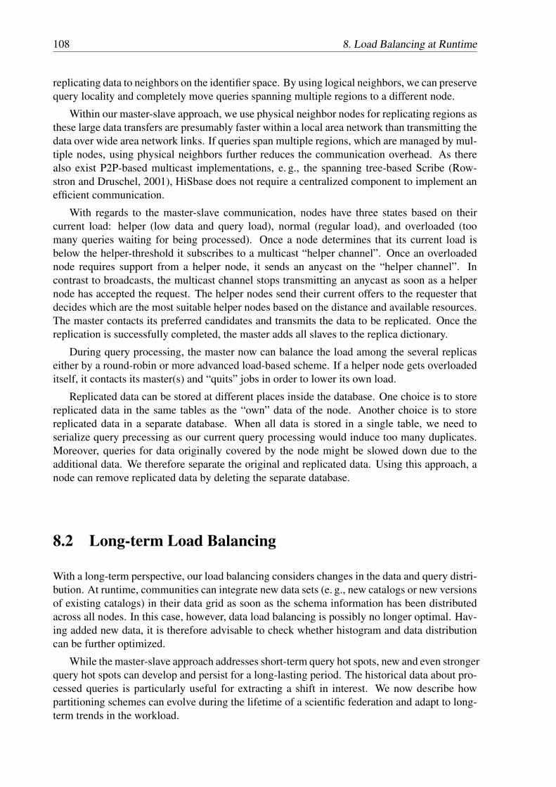
108 8. Load Balancing at Runtime

replicating data to neighbors on the identifier space. By using logical neighbors, we can preservequery locality and completely move queries spanning multiple regions to a different node.

Within our master-slave approach, we use physical neighbor nodes for replicating regions asthese large data transfers are presumably faster within a local area network than transmitting thedata over wide area network links. If queries span multiple regions, which are managed by mul-tiple nodes, using physical neighbors further reduces the communication overhead. As therealso exist P2P-based multicast implementations, e. g., the spanning tree-based Scribe (Row-stron and Druschel, 2001), HiSbase does not require a centralized component to implement anefficient communication.

With regards to the master-slave communication, nodes have three states based on theircurrent load: helper (low data and query load), normal (regular load), and overloaded (toomany queries waiting for being processed). Once a node determines that its current load isbelow the helper-threshold it subscribes to a multicast “helper channel”. Once an overloadednode requires support from a helper node, it sends an anycast on the “helper channel”. Incontrast to broadcasts, the multicast channel stops transmitting an anycast as soon as a helpernode has accepted the request. The helper nodes send their current offers to the requester thatdecides which are the most suitable helper nodes based on the distance and available resources.The master contacts its preferred candidates and transmits the data to be replicated. Once thereplication is successfully completed, the master adds all slaves to the replica dictionary.

During query processing, the master now can balance the load among the several replicaseither by a round-robin or more advanced load-based scheme. If a helper node gets overloadeditself, it contacts its master(s) and “quits” jobs in order to lower its own load.

Replicated data can be stored at different places inside the database. One choice is to storereplicated data in the same tables as the “own” data of the node. Another choice is to storereplicated data in a separate database. When all data is stored in a single table, we need toserialize query precessing as our current query processing would induce too many duplicates.Moreover, queries for data originally covered by the node might be slowed down due to theadditional data. We therefore separate the original and replicated data. Using this approach, anode can remove replicated data by deleting the separate database.

8.2 Long-term Load Balancing

With a long-term perspective, our load balancing considers changes in the data and query distri-bution. At runtime, communities can integrate new data sets (e. g., new catalogs or new versionsof existing catalogs) in their data grid as soon as the schema information has been distributedacross all nodes. In this case, however, data load balancing is possibly no longer optimal. Hav-ing added new data, it is therefore advisable to check whether histogram and data distributioncan be further optimized.

While the master-slave approach addresses short-term query hot spots, new and even strongerquery hot spots can develop and persist for a long-lasting period. The historical data about pro-cessed queries is particularly useful for extracting a shift in interest. We now describe howpartitioning schemes can evolve during the lifetime of a scientific federation and adapt to long-term trends in the workload.

8.2 Long-term Load Balancing 109

Figure 8.1: Evolution of histograms within HiSbase

8.2.1 Partitioning Scheme Evolution

During the lifetime of a community-driven data grid, additional data sources might be added orthe interest of a community might shift towards a different area in the data space. Therefore,we need a mechanism to evolve our histogram. For example, if no previous query logs areavailable, a community can start with a histogram that is only based on the data distribution.Depending on the change characteristics of the community (e. g., every six months or everyyear), the data distribution can be reorganized according to the analysis of monitored workloadsusing a workload-aware partitioning scheme as described in Chapter 7. Therefore, a histogramsometimes needs to be recreated and data needs to be redistributed accordingly.

Each HiSbase histogram passes through three development phases: in-progress, active, andpassive. The in-progress histogram is used to distribute the data within the HiSbase network.As long as the feeding process (see Section 5) has not finished, histogram and data are not usedduring query processing. Once the data distribution according to the in-progress histogram iscompleted, the histogram and the newly distributed data are activated. Similar to the feedingprocess, we coordinate the transitions from the different histogram states at the HiSbase nodesusing the multicast channel. The active histogram and active data are used during query process-ing; the histogram for retrieving the relevant data regions and the data for the actual databasequeries. In order to prolong the use of data once distributed and thus amortize the cost of thedata transfers, each node additionally keeps a passive histogram and a passive data set. Thepassive histogram is primarily used in order to provide data availability and as fallback supportduring query processing.

Figure 8.1 shows an example for a snapshot within a histogram evolution. The active his-togram has seven partitions and is used during query processing, while the passive histogramfunctions as backup copy. The region mapping to the key space has a different origin for thepassive histogram and therefore is likely to replicate regions to different nodes. The in-progress

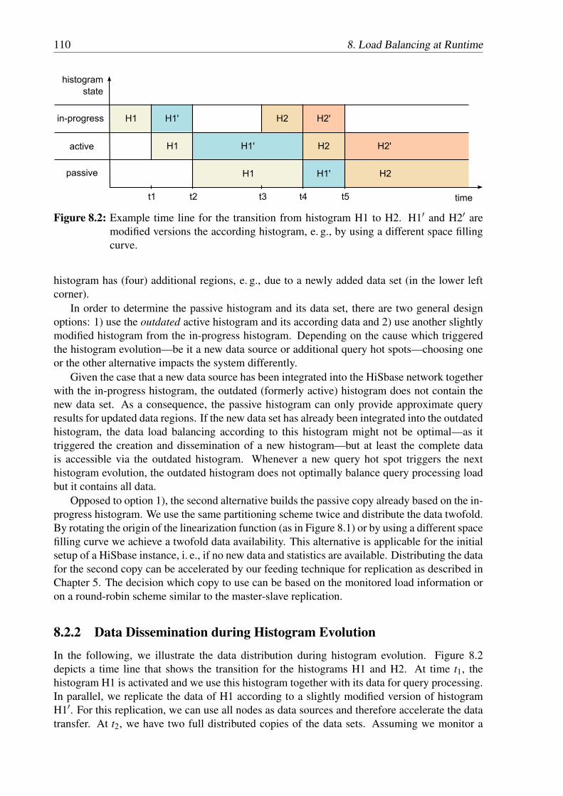
110 8. Load Balancing at Runtime

Figure 8.2: Example time line for the transition from histogram H1 to H2. H1′ and H2′ aremodified versions the according histogram, e. g., by using a different space fillingcurve.

histogram has (four) additional regions, e. g., due to a newly added data set (in the lower leftcorner).

In order to determine the passive histogram and its data set, there are two general designoptions: 1) use the outdated active histogram and its according data and 2) use another slightlymodified histogram from the in-progress histogram. Depending on the cause which triggeredthe histogram evolution—be it a new data source or additional query hot spots—choosing oneor the other alternative impacts the system differently.

Given the case that a new data source has been integrated into the HiSbase network togetherwith the in-progress histogram, the outdated (formerly active) histogram does not contain thenew data set. As a consequence, the passive histogram can only provide approximate queryresults for updated data regions. If the new data set has already been integrated into the outdatedhistogram, the data load balancing according to this histogram might not be optimal—as ittriggered the creation and dissemination of a new histogram—but at least the complete datais accessible via the outdated histogram. Whenever a new query hot spot triggers the nexthistogram evolution, the outdated histogram does not optimally balance query processing loadbut it contains all data.

Opposed to option 1), the second alternative builds the passive copy already based on the in-progress histogram. We use the same partitioning scheme twice and distribute the data twofold.By rotating the origin of the linearization function (as in Figure 8.1) or by using a different spacefilling curve we achieve a twofold data availability. This alternative is applicable for the initialsetup of a HiSbase instance, i. e., if no new data and statistics are available. Distributing the datafor the second copy can be accelerated by our feeding technique for replication as described inChapter 5. The decision which copy to use can be based on the monitored load information oron a round-robin scheme similar to the master-slave replication.

8.2.2 Data Dissemination during Histogram Evolution

In the following, we illustrate the data distribution during histogram evolution. Figure 8.2depicts a time line that shows the transition for the histograms H1 and H2. At time t1, thehistogram H1 is activated and we use this histogram together with its data for query processing.In parallel, we replicate the data of H1 according to a slightly modified version of histogramH1′. For this replication, we can use all nodes as data sources and therefore accelerate the datatransfer. At t2, we have two full distributed copies of the data sets. Assuming we monitor a

8.3 Summary and Future Work 111

long-term shift in interest in our statistics. As a consequence, we create a new histogram H2.Like at the beginning of this example, we first distribute the new histogram and start a newfeeding process at time t3. At time t4 and time t5, each nodes delete one of the old histogramsand its data set.

8.3 Summary and Future WorkIn this chapter, we described several approaches to address load balancing challenges at run-time of a community-driven data grid. We differentiated between short-term peaks and long-term trends of query distribution. For short-term load balancing, we propose a master-slavereplication scheme combined with statistics monitoring. For long-term trends, we evolve ourhistogram and thereby adapt the histogram to shifts in the data or query distribution.

Our current master-slave replication scheme uses physical neighbors for load balancing.A further in-depth comparison between choosing physical neighbors or neighbors within theidentifier space for such a replication could provide additional interesting insights. Based on thedescribed initial replication design for community-driven data grids, more advanced replicationstrategies are a challenging issue. While we focused on the replication of individual regionsthere might be some benefits from replicating all regions of a node (“region clusters”) at once.This can reduce the management overhead and further preserve the query locality.

112 8. Load Balancing at Runtime

113

CHAPTER 9

Outlook and Future Challenges

Community-driven data grids provide a scalable, distributed data management solution for e-science communities. In this thesis, we described the fundamental design choices for suchdata grids and evaluated our infrastructure on real-life data and query workloads. In additionto simulation studies, we deployed and conducted experiments with our infrastructure in theAstroGrid-D test bed as well as in the PlanetLab framework which helped us to increase therobustness of our system. We first described the core building blocks of training, feeding, andrunning community-driven data grids. From that foundation we built load balancing techniquessuch as workload-aware training, master-slave replication, and histogram evolution to shapecommunity-driven data grids along the changes of the communities themselves.

From our point of view, this thesis offers a starting point for collaborative researchers toactively explore and design scalable data management solutions. In the following, we give afew examples of the topics we consider interesting for future research.

In order to directly deal with the existing and envisioned scale of scientific data sets, weused a training phase to create a partitioning scheme based on the major data characteristicsand predominant query patterns. This approach is viable as the majority of scientific data setsdoes not change once published. We envision two aspects that can be further investigated in thiscontext: 1) Based on an initial histogram from the training phase, how can we locally adapt thepartitioning and replication scheme without creating a new histogram and thus increasing thedynamics of the system, and 2) how can we achieve data and query load balancing if there is ahigh update rate.

Data-driven applications become an increasingly important field in academia as well as inindustrial business applications. Extending the use of community-driven data grids to datamining tasks beyond pure database queries could extend the number of use cases that benefitfrom the scalable infrastructure. Instead of bare queries, data mining tasks would be directedtowards the data sites. Challenges within that area are identifying effective communicationpatterns and finding good data distribution schemes.

Dealing with terabyte to petabyte-scale data sets has recently triggered interesting devel-opments like provenance-aware database systems (Groffen et al., 2007), data-aware batch pro-

114 9. Outlook and Future Challenges

cessing (Wang et al., 2009), and adaptive physical design tools (Malik et al., 2008, 2009). Itwould be interesting to deliver the synergies of our technique and their approach to scientificresearchers. Recent work (Raicu et al., 2009, 2008) on data-aware scheduling of scientificworkloads proposes interesting concepts for dynamic resource provisioning and adaptive datacaching. Furthermore, systems like GrayWulf (Simmhan et al., 2009; Szalay et al., 2009) showinteresting developments for designing petascale cluster environments.

Besides scalable data management, exploring the vast amounts of data visually becomesincreasingly important. Both interactive visualizations using grid middleware (Polak and Kran-zlmüller, 2008) as well as asynchronous collaborative visualizations (Heer et al., 2009) showinteresting proposals in that area. Building virtual laboratories by integrating remote sensorsand instruments (Płóciennik et al., 2008) offers new perspectives for scientific cooperations.

Our work heavily profited from the fact that we had several use cases to derive actual re-quirements from and that we had the opportunity to evaluate our ideas and prototypes withina real deployment. How can other computer scientists experience a similar benefit like testingtheir research and ideas with real data sets? From the astronomers’ perspective, however, theresearchers see themselves confronted with several data management solutions that hopefullyease their day-to-day data-intensive research. So how can they eventually validate these sys-tems? Motivated by the experience that standardized benchmarks such as the TPC series1 orXMark2 have propelled the research in their area, we proposed a benchmark for astrophysicalwork benches (Nieto-Santisteban et al., 2007). This benchmark is envisioned to provide as-tronomers with a unified setup for testing their environments and to provide computer scientistswith a specific setup to test their systems against. There are additional notable efforts such asSciDB3 (Stonebraker et al., 2009), which focus on delivering a new database model especiallyaimed at scientific data management.

HiSbase, our prototype of community-driven data grids, allows e-science communities tobuild up decentralized and cooperative information networks and offers a framework to de-sign histogram data structures for accommodating specific data characteristics and dominantquery patterns. The histogram data structure defines a partitioning scheme to benefit from highthroughput via parallelism and high cache locality and is also used as routing index for in-creased flexibility. Given the enormous variety of use cases and applications it is unlikely tofind a single best solution. Working closely with the actual scientists is an effort that not onlyfosters great inter-disciplinary collaborations. Furthermore, addressing their challenges allowsus to shape the data management for future e-science communities.

1http://www.tpc.org/2http://monetdb.cwi.nl/xml/3http://scidb.org/

115

APPENDIX A

Example Execution of the Minimum Latency PathAlgorithm

In this section we will execute Algorithm 5.1 presented in Section 5.3 (page 53) on the examplegraph G∗ depicted in Figure A.1. For the sake of simplicity, edges are labeled with integervalues instead of real latency values. In this scenario, the node labeled s denotes the source.Furthermore, let v1, v2, v4, and v5 be data grid nodes or transit nodes. Assuming that node v3 isa data grid node, we send a packet from s to v3. In order to find a minimum latency path from sto v3 (Figure A.2), we compute all minimum latency paths from s by executing the algorithm asshown in Figure A.3. As latency L(v3) is 5, we know that the minimum latency path from s tov3 has a latency of 5. A depth-first search on the completely annotated graph G∗ (Figure A.3(f))yields the path that offers the lowest possible latency between s and v3.

.

.

. ...v1 . ...v2

...s . ...v3 .

. ...v4 . ...v5

.0

.∞ .∞

.∞

.∞ .∞

.4

.1

.5

.3

.8

.3

Figure A.1: Example graph G∗ with latency ofnon-source nodes set to ∞

.

.

. ...v1 . ...v2

...s . ...v3 .

. ... . .

.0

.4 .5

.5.4

.5

.3

Figure A.2: Minimum latency path betweennode s and node v3

116 Appendix A. Example Execution of the Minimum Latency Path Algorithm

.

.

. ...v1 . ...v2

...s . ...v3 .

. ...v4 . ...v5

.0

.4 .∞

.∞

.1 .∞

.4

.1

.5

.3

.8

.3(a) Updating latency for neighbors of s

.

.

. ...v1 . ...v2

...s . ...v3 .

. ...v4 . ...v5

.0

.4 .∞

.8

.1 .3

.4

.1

.5

.3

.8

.3(b) Updating latency for neighbors of v4

.

.

. ...v1 . ...v2

...s . ...v3 .

. ...v4 . ...v5

.0

.4 .∞

.8

.1 .3

.4

.1

.5

.3

.8

.3(c) Adding v5 to S, but no labels are updated

.

.

. ...v1 . ...v2

...s . ...v3 .

. ...v4 . ...v5

.0

.4 .5

.8

.1 .3

.4

.1

.5

.3

.8

.3(d) Updating latency for neighbors of v1

.

.

. ...v1 . ...v2

...s . ...v3 .

. ...v4 . ...v5

.0

.4 .5

.5

.1 .3

.4

.1

.5

.3

.8

.3(e) Updating latency for neighbors of v2

.

.

. ...v1 . ...v2

...s . ...v3 .

. ...v4 . ...v5

.0

.4 .5

.5

.1 .3

.4

.1

.5

.3

.8

.3(f) Adding v3 to set S and the algorithm termi-

nates as N(G,S)\S = /0

Figure A.3: Example execution of Algorithm 5.1 on G∗ depicted in Figure A.1 (gray nodes arein S)

117

Bibliography

ABDELGUERFI, M. AND WONG, K.-F.: Parallel Database Techniques. Wiley-IEEE ComputerSociety Press, 1998, ISBN 978-0-8186-8398-5.

ABERER, K., CUDRÉ-MAUROUX, P., DATTA, A., DESPOTOVIC, Z., HAUSWIRTH, M.,PUNCEVA, M., AND SCHMIDT, R.: P-Grid: a self-organizing structured P2P system. SIG-MOD Record, 32(3):29–33, 2003.

ALLOCK, W., BRESNAHAN, J., KETTIMUTHU, R., LINK, M., DUMITRESCU, C., RAICU,I., AND FOSTER, I.: The Globus Striped GridFTP Framework and Server. In: Proc. of theACM/IEEE SC Conf., Seattle, WA, USA, November 2005.

ALY, M., MORSILLO, N., CHRYSANTHIS, P. K., AND PRUHS, K.: Zone Sharing: A Hot-Spots Decomposition Scheme for Data-Centric Storage in Sensor Networks. In: Proc. of theIntl. Workshop on Data Management for Sensor Networks, pp. 21–26, Trondheim, Norway,August 2005.

ALY, M., PRUHS, K., AND CHRYSANTHIS, P. K.: KDDCS: A Load-Balanced In-NetworkData-Centric Storage Scheme for Sensor Networks. In: Proc. of the ACM Intl. Conf. onInformation and Knowledge Management, pp. 317–326, Arlington, VA, USA, November2006.

ANTONIOLETTI, M., ATKINSON, M., BAXTER, R., BORLEY, A., HONG, N. C., COLLINS,B., HARDMAN, N., HUME, A., KNOX, A., JACKSON, M., KRAUSE, A., LAWS, S.,MAGOWAN, J., PATON, N., PEARSON, D., SUGDEN, T., WATSON, P., AND WESTHEAD,M.: The design and implementation of Grid database services in OGSA-DAI. Concurrencyand Computation: Practice and Experience, 17(2-4):357–376, 2005.

ANTONIOLETTI, M., ATKINSON, M., KRAUSE, A., LAWS, S., MALAIKA, S., PATON,N. W., PEARSON, D., AND RICCARDI, G.: Web Services Data Access and Integration -The Core (WS-DAI) Specification, Version 1.0. http://www.ogf.org/documents/GFD.74.pdf,July 2006.

118 Bibliography

ASANO, T., RANJAN, D., ROOS, T., WELZL, E., AND WIDMAYER, P.: Space-filling curvesand their use in the design of geometric data structures. Theoretical Computer Science,181(1):3–15, July 1997.

ASPNES, J., KIRSCH, J., AND KRISHNAMURTHY, A.: Load Balancing and Locality in Range-Queriable Data Structures. In: Proc. of ACM Symposium on Principles of Distributed Com-puting, pp. 115–124, St. John’s, Newfoundland, Canada, July 2004.

ASPNES, J. AND SHAH, G.: Skip Graphs. In: Proc. of the ACM/SIAM Symposium on DescreteAlgorithms, pp. 384–393, Baltimore, MD, USA, January 2003.

AWERBUCH, B. AND LEIGHTON, T.: A Simple Local-Control Approximation Algorithmfor Multicommodity Flow. In: Proc. of the Annual Symposium on Foundations of Com-puter Science, pp. 459–468, Palo Alto, CA, USA, November 1993, URL http://doi.ieeecomputersociety.org/10.1109/SFCS.1993.366841.

BANAEI-KASHANI, F. AND SHAHABI, C.: SWAM: A Family of Access Methods forSimilarity-Search in Peer-to-Peer Data Networks. In: Proc. of the ACM Intl. Conf. on In-formation and Knowledge Management, pp. 304–313, Washington, DC, USA, November2004.

BEAUMONT, O., KERMARREC, A.-M., MARCHAL, L., AND RIVIÈRE, É.: VoroNet: A scal-able object network based on Voronoi tessellations. In: Proc. of the Intl. Parallel and Dis-tributed Processing Symposium, pp. 1–10, Long Beach, CA, USA, March 2007.

BRAUMANDL, R., KEMPER, A., AND KOSSMANN, D.: Quality of Service in an InformationEconomy. ACM Trans. on Internet Technology, 3(4):291–333, November 2003.

BUNEMAN, P. AND TAN, W. C.: Provenance in Databases. In: Proc. of the ACM SIGMODIntl. Conf. on Management of Data, pp. 1171–1173, Beijing, China, June 2007.

CAI, M., FRANK, M., CHEN, J., AND SZEKELY, P.: MAAN: A Multi-Attribute AddressableNetwork for Grid Information Services. Journal of Grid Computing, 2(1):3–14, March 2004.

CARLSON, A., BÖHRINGER, H., SCHOLL, T., AND VOGES, W.: Finding Galaxy Clustersusing Grid Computing Technology. In: Proc. of the IEEE Intl. Conf. on e-Science and GridComputing (demo), Bangalore, India, December 2007.

CASTRO, M., DRUSCHEL, P., KERMARREC, A.-M., AND ROWSTRON, A.: Scribe: A large-scale and decentralized application-level multicast infrastructure. IEEE Journal on SelectedAreas in Communications, 20(8):100–110, 2002.

COHEN, B.: Incentives Build Robustness in BitTorrent. In: Proc. of the Workshop on Eco-nomics of Peer-to-Peer Systems, Berkeley, CA, USA, June 2003.

COOPER, B. F., RAMAKRISHNAN, R., SRIVASTAVA, U., SILBERSTEIN, A., BOHANNON, P.,JACOBSEN, H.-A., PUZ, N., WEAVER, D., AND YERNENI, R.: PNUTS: Yahoo!’s HostedData Serving Platform. Proc. of the VLDB Endowment, 1(2):1277–1288, 2008.

CORMEN, T. H., LEISERSON, C. E., RIVEST, R. L., AND STEIN, C.: Introduction to algo-rithms. MIT Press, Cambridge, MA, USA, second edition, 2001, ISBN 0-262-03293-7.

Bibliography 119

CRAINICEANU, A., LINGA, P., MACHANAVAJJHALA, A., GEHRKE, J., AND SHANMUGA-SUNDARAM, J.: P-Ring: An Efficient and Robust P2P Range Index Structure. In: Proc. ofthe ACM SIGMOD Intl. Conf. on Management of Data, pp. 223–234, Beijing, China, June2007.

CSABAI, I., TRENCSÉNI, M., HERCZEGH, G., DOBOS, L., JÓZSA, P., PURGER, N., BU-DAVÁRI, T., AND SZALAY, A.: Spatial Indexing of Large Multidimensional Databases. In:Proc. of the Conference on Innovative Data Systems Research, pp. 207–218, Asilomar, CA,USA, January 2007.

DABEK, F., ZHAO, B., DRUSCHEL, P., KUBIATOWICZ, J., AND STOICA, I.: Towards a Com-mon API for Structured Peer-to-Peer Overlays. In: International Workshop on Peer-to-PeerSystems (IPTPS), LNCS, vol. 2, 2003.

DATTA, A., HAUSWIRTH, M., JOHN, R., SCHMIDT, R., AND ABERER, K.: Range Queries inTrie-Structured Overlays. In: Proc. of the IEEE Intl. Conf. on Peer-to-Peer Computing, pp.57–66, Konstanz, Germany, August 2005.

DAVIDSON, S. B., BOULAKIA, S. C., EYAL, A., LUDÄSCHER, B., MCPHILLIPS, T. M.,BOWERS, S., ANAND, M. K., AND FREIRE, J.: Provenance in Scientific Workflow Systems.IEEE Data Engineering Bulletin, 30(4):44–50, 2007.

DEWITT, D. J. AND GRAY, J.: Parallel Database Systems: The Future of High PerformanceDatabase Systems. Communications of the ACM, 35(6):85–98, 1992.

DU MOUZA, C., LITWIN, W., AND RIGAUX, P.: SD-Rtree: A Scalable Distributed Rtree. In:Proc. of the Intl. Conf. on Data Engineering, pp. 296–305, Istanbul, Turkey, April 2007.

DU MOUZA, C., LITWIN, W., AND RIGAUX, P.: Large-scale indexing of spatial data in dis-tributed repositories: the SD-Rtree. VLDB Journal, 2009, doi: 10.1007/s00778-009-0135-4.

ENKE, H., STEINMETZ, M., RADKE, T., REISER, A., RÖBLITZ, T., AND HÖGQVIST, M.:AstroGrid-D: Enhancing Astronomic Science with Grid Technology. In: Proc. of the Germane-Science Conference, Baden-Baden, Germany, May 2007.

EVEN, S., ITAI, A., AND SHAMIR, A.: On the complexity of time table andmulti-commodity flow problems. In: Proc. of the Annual Symposium on Foun-dations of Computer Science, pp. 184–193, Berkeley, CA, USA, October 1975,URL http://ieeexplore.ieee.org/search/srchabstract.jsp?arnumber=4567876&isnumber=4567845&punumber=4567844&k2dockey=4567876@ieeecnfs.

FINKEL, R. A. AND BENTLEY, J. L.: Quad Trees: A Data Structure for Retrieval on CompositeKeys. Acta Informatica, 4:1–9, March 1974.

FOSTER, I. AND IAMNITCHI, A.: On Death, Taxes, and the Convergence of Peer-to-Peer andGrid Computing. In: International Workshop on Peer-to-Peer Systems (IPTPS), LNCS, vol. 2,2003.

FRANKLIN, M., HALEVY, A., AND MAIER, D.: From Databases to Dataspaces: A NewAbstraction for Information Management. SIGMOD Record, 34(4):27–33, 2005.

120 Bibliography

GAEDE, V. AND GÜNTHER, O.: Multidimensional Access Methods. ACM Computing Surveys,30(2):170–231, June 1998.

GANESAN, P., BAWA, M., AND GARCIA-MOLINA, H.: Online Balancing of Range-Partitioned Data with Applications to Peer-to-Peer Systems. In: Proc. of the Intl. Conf. onVery Large Data Bases, pp. 444–455, Toronto, Canada, September 2004a.

GANESAN, P., YANG, B., AND GARCIA-MOLINA, H.: One Torus to Rule them All: Multi-dimensional Queries in P2P Systems. In: Proc. of the Intl. Workshop on the Web andDatabases, pp. 19–24, Maison de la Chimie, Paris, France, June 2004b.

GARGANTINI, I.: An Effective Way to Represent Quadtrees. Communications of the ACM,25(12):905–910, December 1982.

GIETZ, P., GRIMM, C., GRÖPER, R., MAKEDANZ, S., PFEIFFENBERGER, H., SCHIF-FERS, M., AND ZIEGLER, W.: A concept for attribute-based authorization on D-Grid resources. Future Generation Computer Systems, 25(3):275–280, March 2009, doi:10.1016/j.future.2008.05.008.

GRAY, J., SANTISTEBAN, M. A. N., AND SZALAY, A. S.: The Zones Algorithm for FindingPoints-Near-Point or Cross-Matching Spatial Datasets. Technical Report MSR-TR-2006-52,Microsoft Research, Microsoft Cooperation, Redmond, WA, USA, April 2006.

GROFFEN, F., KERSTEN, M. L., AND MANEGOLD, S.: Armada: a Reference Model for anEvolving Database System. In: Proc. of the GI Conference on Database Systems for Business,Technology, and Web, pp. 417–435, Aachen, Germany, March 2007.

GU, Y., GROSSMAN, R. L., SZALAY, A., AND THAKAR, A.: Distributing the Sloan DigitalSky Survey Using UDT and Sector. In: Proc. of the IEEE Intl. Conf. on e-Science and GridComputing, p. 56, Amsterdam, The Netherlands, December 2006.

HAVERKORT, H. J. AND VAN WALDERVEEN, F.: Locality and Bounding-Box Quality of Two-Dimensional Space-Filling Curves. Computing Research Repository, abs/0806.4787, 2008.

HEER, J., VIÉGAS, F. B., AND WATTENBERG, M.: Voyagers and Voyeurs: Supporting Asyn-chronous Collaborative Visualization. Communications of the ACM, 52(1):87–97, January2009.

HILBERT, D.: Über die stetige Abbildung einer Linie auf ein Flächenstück. Math. Ann.,38:459–460, 1891.

HIRONAKA, K., SAITO, H., AND TAURA, K.: High Performance Wide-area Overlay usingDeadlock-free Routing. In: Intl. Symposium on High Performance Distributed Computing,pp. 81–90, Munich, Germany, June 2009.

HUEBSCH, R., HELLERSTEIN, J. M., LANHAM, N., LOO, B. T., SHENKER, S., AND STO-ICA, I.: Querying the Internet with PIER. In: Proc. of the Intl. Conf. on Very Large DataBases, pp. 321–332, Berlin, Germany, September 2003.

IVANOVA, M., NES, N., GONCALVES, R., AND KERSTEN, M.: MonetDB/SQL Meets Sky-Server: the Challenges of a Scientific Database. In: Proc. of the Intl. Conf. on Scientific andStatistical Database Management, p. 13, Banff, Canada, July 2007.

Bibliography 121

JAGADISH, H. V., OOI, B. C., AND VU, Q. H.: BATON: a balanced tree structure for peer-to-peer networks. In: Proc. of the Intl. Conf. on Very Large Data Bases, pp. 661–672, Trond-heim, Norway, August 2005.

KINDERMANN, S., STOCKHAUSE, M., AND RONNEBERGER, K.: Intelligent Data Network-ing for the Earth System Science Community. In: Proc. of the German e-Science Conference,Baden-Baden, Germany, May 2007.

KIRCHLER, W., SCHIFFERS, M., AND KRANZLMÜLLER, D.: Harmonizing the Managementof Virtual Organizations Despite Heterogeneous Grid Middleware – Assessment of Two Dif-ferent Approaches. In: Proc. of the Cracow Grid Workshop, pp. 245–253, Cracow, PL, Octo-ber 2008.

KOSSMANN, D.: The State of the Art in Distributed Query Processing. ACM Computing Sur-veys, 32(4):422–469, December 2000.

KOTTHA, S., ABHINAV, K., MÜLLER-PFEFFERKORN, R., AND MIX, H.: Accessing Bio-Databases with OGSA-DAI – A Performance Analysis. In: Proc. of the Intl. Workshop onDistributed, High-Performance and Grid Computing in Computational Biology, Eilat, Israel,2006.

KREFTING, D., BART, J., BERONOV, K., DZHIMOVA, O., FALKNER, J., HARTUNG, M.,HOHEISEL, A., KNOCH, T. A., LINGNER, T., MOHAMMED, Y., PETER, K., RAHM,E., SAX, U., SOMMERFELD, D., STEINKE, T., TOLXDORFF, T., VOSSBERG, M.,VIEZENS, F., AND WEISBECKER, A.: MediGRID: Towards a user friendly secured gridinfrastructure. Future Generation Computer Systems, 25(3):326–336, March 2009, doi:10.1016/j.future.2008.05.005.

KROMPASS, S., AULBACH, S., AND KEMPER, A.: Data Staging for OLAP- and OLTP-Applications on RFID Data. In: Proc. of the GI Conference on Database Systems for Busi-ness, Technology, and Web, pp. 542–561, Aachen, Germany, March 2007.

KUNTSCHKE, R., SCHOLL, T., HUBER, S., KEMPER, A., REISER, A., ADORF, H.-M.,LEMSON, G., AND VOGES, W.: Grid-based Data Stream Processing in e-Science. In: Proc.of the IEEE Intl. Conf. on e-Science and Grid Computing, p. 30, Amsterdam, The Nether-lands, December 2006.

LEDLIE, J., SHNEIDMAN, J., SELTZER, M., AND HUTH, J.: Scooped, Again. In: Interna-tional Workshop on Peer-to-Peer Systems (IPTPS), LNCS, vol. 2, 2003.

MALIK, T. AND BURNS, R.: Workload-Aware Histograms for Remote Applications. In: DataWarehousing and Knowledge Discovery, pp. 402–412, Turin, Italy, September 2008.

MALIK, T., BURNS, R., AND CHAUDHARY, A.: Bypass Caching: Making ScientificDatabases Good Network Citizens. In: Proc. of the Intl. Conf. on Data Engineering, pp.94–105, Tokyo, Japan, April 2005.

MALIK, T., BURNS, R., CHAWLA, N. V., AND SZALAY, A.: Estimating Query Result Sizesfor Proxy Caching in Scientific Ddatabase Federations. In: Proc. of the ACM/IEEE SC Conf.,p. 36, Tampa, FL, USA, November 2006.

122 Bibliography

MALIK, T., WANG, X., BURNS, R., DASH, D., AND AILAMAKI, A.: Automated PhysicalDesign in Database Caches. In: Proc. of the Intl. Conf. on Data Engineering Workshops, pp.27–34, Cancun, Mexico, April 2008.

MALIK, T., WANG, X., DASH, D., CHAUDHARY, A., AILAMAKI, A., AND BURNS, R.:Adaptive Physical Design for Curated Archives. In: Proc. of the Intl. Conf. on Scientific andStatistical Database Management, pp. 148–166, New Orleans, LA, USA, June 2009.

NAUMANN, F., BILKE, A., BLEIHOLDER, J., AND WEIS, M.: Data Fusion in Three Steps:Resolving Schema, Tuple, and Value Inconsistencies. IEEE Data Engineering Bulletin,29(2):21–31, 2006.

NIETO-SANTISTEBAN, M. A., GRAY, J., SZALAY, A. S., ANNIS, J., THAKAR, A. R., AND

O’MULLANE, W. J.: When Database Systems Meet the Grid. In: Proc. of the Conferenceon Innovative Data Systems Research, pp. 154–161, Asilomar, CA, USA, January 2005.

NIETO-SANTISTEBAN, M. A., SCHOLL, T., KEMPER, A., AND SZALAY, A.: 20 SpatialQueries for an Astronomer’s Bench(mark). In: Proc. of the Astronomical Data Analysis Soft-ware & Systems Conference, London, UK, September 2007.

O’MULLANE, W., LI, N., NIETO-SANTISTEBAN, M., SZALAY, A., THAKAR, A., AND

GRAY, J.: Batch is back: CasJobs, serving multi-TB data on the Web. In: Proc. of the Intl.Conf. on Web Services, pp. 33–40, Orlando, FL, USA, July 2005.

ORENSTEIN, J. AND MERRETT, T.: A Class of Data Structures for Associative Searching. In:Proc. of the ACM SIGACT-SIGMOD Symp. on Principles of Database Sys., pp. 181–190,Waterloo, Ontario, Canada, April 1984.

ÖZSU, M. T. AND VALDURIEZ, P.: Principles of Distributed Database Systems. Prentice-Hall,1999.

PAPADOMANOLAKIS, S. AND AILAMAKI, A.: AutoPart: Automating Schema Design forLarge Scientific Databases Using Data Partitioning. In: Proc. of the Intl. Conf. on Scientificand Statistical Database Management, pp. 383–392, Stantorini Island, Greece, June 2004.

PENTARIS, F. AND IOANNIDIS, Y.: Query Optimization in distributed Networks of Au-tonomous Database Systems. ACM Trans. on Database Systems, 31(2):537–583, June 2006.

PITOURA, T., NTARMOS, N., AND TRIANTAFILLOU, P.: Replication, Load Balancing, andEfficient Range Query Processing in DHT Data Networks. In: Proc. of the Intl. Conf. onExtending Database Technology, pp. 131–148, Munich, Germany, March 2006.

PLANTIKOW, S., PETER, K., HÖGQVIST, M., GRIMME, C., AND PAPASPYROU, A.: General-izing the data management of three community grids. Future Generation Computer Systems,25(3):281–289, March 2009, doi: 10.1016/j.future.2008.05.001.

PŁÓCIENNIK, M., ADAMI, D., BARCELÓ, Á. D. G., COZ, I. C., DAVOLI, F., GAMBA, P.,KELLER, R., KRANZLMÜLLER, D., LABOTIS, I., MEYER, N., MONTEOLIVA, A., PRICA,M., PUGLIESE, R., SALON, S., SCHIFFERS, M., WATZL, J., ZAFEIROPOULOS, A., AND

DE LUCAS, J. M.: DORII – Deployment of Remote Instrumentation Infrastructure. In: Proc.of the Cracow Grid Workshop, pp. 78–85, Cracow, PL, October 2008.

Bibliography 123

POLAK, M. AND KRANZLMÜLLER, D.: Interactive videostreaming visualizationon grids. Future Generation Computer Systems, 24(1):39–45, January 2008, doi:10.1016/j.future.2007.03.006.

POOSALA, V., IOANNIDIS, Y. E., HAAS, P. J., AND SHEKITA, E. J.: Improved Histogramsfor Selectivity Estimation of Range Predicates. In: Proc. of the ACM SIGMOD Intl. Conf. onManagement of Data, pp. 294–305, Montreal, Quebec, Canada, June 1996.

RAHM, E. AND BERNSTEIN, P. A.: A survey of approaches to automatic schema matching.VLDB Journal, 10(4):334–350, 2001.

RAICU, I., FOSTER, I., SZALAY, A., AND TURCU, G.: AstroPortal: A Science Gateway forLarge-scale Astronomy Data Analysis. In: Proc. of the TeraGrid Conf., June 2006.

RAICU, I., FOSTER, I. T., ZHAO, Y., LITTLE, P., MORETTI, C. M., CHAUDHARY, A., AND

THAIN, D.: The Quest for Scalable Support of Data-Intensive Workloads in DistributedSystems. In: Intl. Symposium on High Performance Distributed Computing, pp. 207–216,Munich, Germany, June 2009.

RAICU, I., ZHAO, Y., FOSTER, I., AND SZALAY, A.: Accelerating Large-Scale Data Explo-ration through Data Diffusion. In: Proc. of the Intl. Workshop on Data-Aware DistributedComputing, pp. 9–18, Boston, MA, USA, June 2008.

RATNASAMY, S., FRANCIS, P., HANDLEY, M., KARP, R., AND SHENKER, S.: A ScalableContent-Addressable Network. In: Proc. of the ACM SIGCOMM Intl. Conf. on Data Com-munication, pp. 161–172, 2001.

REHN, J., BARRASS, T., BONACORSI, D., HERNANDEZ, J., SEMENIOUK, I., TUURA, L.,AND WU, Y.: PhEDEx high-throughput data transfer management system. In: Proc. of theIntl. Conf. on Computing in High Energy and Nuclear Physics, Mumbai, India, February2006.

ROWSTRON, A. I. T. AND DRUSCHEL, P.: Pastry: Scalable, Decentralized Object Locationand Routing for Large-Scale Peer-to-Peer Systems. In: Proc. of the IFIP/ACM Intl. Conf. onDistributed Systems Platforms (Middleware), pp. 329–350, Heidelberg, Germany, November2001.

SALLES, M. A. V., DITTRICH, J.-P., KARAKASHIAN, S. K., GIRARD, O. R., AND BLUN-SCHI, L.: iTrails: Pay-as-you-go Information Integration in Dataspaces. In: Proc. of the Intl.Conf. on Very Large Data Bases, pp. 663–674, Vienna, Austria, September 2007.

SAMET, H.: The Design and Analysis of Spatial Data Structures. Addison Wesley, 1990, ISBN0-201-50255-0.

SAMET, H.: Hierarchical Representations of Collections of Small Rectangles. ACM ComputingSurveys, 20(4):271–309, December 1998.

SAMET, H.: Foundations of Multidimensional and Metric Data Structures. Morgan Kaufmann,2006, ISBN 0-12-369446-9.

124 Bibliography

SCHOLL, T., BAUER, B., GUFLER, B., KUNTSCHKE, R., REISER, A., AND KEMPER, A.:Scalable community-driven data sharing in e-science grids. Future Generation ComputerSystems, 25(3):290–300, March 2009a, doi: 10.1016/j.future.2008.05.006.

SCHOLL, T., BAUER, B., GUFLER, B., KUNTSCHKE, R., WEBER, D., REISER, A., AND

KEMPER, A.: HiSbase: Histogram-based P2P Main Memory Data Management. In: Proc. ofthe Intl. Conf. on Very Large Data Bases (demo), pp. 1394–1397, Vienna, Austria, September2007a.

SCHOLL, T., BAUER, B., KUNTSCHKE, R., WEBER, D., REISER, A., AND KEMPER, A.:HiSbase: Informationsfusion in P2P Netzwerken. In: Proc. of the GI Conference on DatabaseSystems for Business, Technology, and Web (demo), pp. 602–605, Aachen, Germany, March2007b.

SCHOLL, T., BAUER, B., MÜLLER, J., GUFLER, B., REISER, A., AND KEMPER, A.:Workload-Aware Data Partitioning in Community-Driven Data Grids. In: Proc. of the Intl.Conf. on Extending Database Technology, pp. 36–47, Saint-Petersburg, Russia, March2009b.

SCHOLL, T., GUFLER, B., MÜLLER, J., REISER, A., AND KEMPER, A.: P2P-Datenmanagement für e-Science-Grids. Datenbank-Spektrum, 8(26):26–33, September2008.

SCHOLL, T. AND KEMPER, A.: Community-Driven Data Grids. Proc. of the VLDB Endow-ment, 1(2):1672–1677, 2008.

SCHOLL, T., KUNTSCHKE, R., REISER, A., AND KEMPER, A.: Community Training: Parti-tioning Schemes in Good Shape for Federated Data Grids. In: Proc. of the IEEE Intl. Conf.on e-Science and Grid Computing, pp. 195–203, Bangalore, India, December 2007c.

SCHOLL, T., REISER, A., AND KEMPER, A.: Collaborative Query Coordination inCommunity-Driven Data Grids. In: Intl. Symposium on High Performance Distributed Com-puting, pp. 197–206, Munich, Germany, June 2009c.

SCHÜCKER, P., BÖHRINGER, H., AND VOGES, W.: Detection of X-ray Clusters of Galaxiesby Matching RASS Photons and SDSS Galaxies within GAVO. Astronomy & Astrophysics,420:61–74, 2004.

SHU, Y., OOI, B. C., TAN, K.-L., AND ZHOU, A.: Supporting Multi-dimensional RangeQueries in Peer-to-Peer Systems. In: Proc. of the IEEE Intl. Conf. on Peer-to-Peer Comput-ing, pp. 173–180, Konstanz, Germany, August 2005.

SILBERSTEIN, A., COOPER, B. F., SRIVASTAVA, U., VEE, E., YERNENI, R., AND RA-MAKRISHNAN, R.: Efficient Bulk Insertion into a Distributed Ordered Table. In: Proc. of theACM SIGMOD Intl. Conf. on Management of Data, pp. 765–778, Vancouver, Canada, June2008.

SIMMHAN, Y., BARGA, R., VAN INGEN, C., NIETO-SANTISTEBAN, M., DOBOS, L., LI,N., SHIPWAY, M., SZALAY, A. S., WERNER, S., AND HEASLEY, J.: GrayWulf: ScalableSoftware Architecture for Data Intensive Computing. In: Hawaii Intl. Conference on SystemSciences, Waikoloa, HI, USA, January 2009.

Bibliography 125

SINGH, V., GRAY, J., THAKAR, A., SZALAY, A., RADDICK, J., BOROSKI, B., LEBEDEVA,S., AND YANNY, B.: SkyServer Traffic Report – The First Five Years. Technical Report MS-TR-2006-190, Microsoft Research, Microsoft Cooperation, Redmond, WA, USA, December2006.

SPRINGEL, V., WHITE, S. D. M., JENKINS, A., FRENK, C. S., YOSHIDA, N., GAO, L.,NAVARRO, J., THACKER, R., CROTON, D., HELLY, J., PEACOCK, J. A., COLE, S.,THOMAS, P., COUCHMAN, H., EVRARD, A., COLBERG, J., AND PEARCE, F.: Simulatingthe joint evolution of quasars, galaxies and their large-scale distribution. Nature, 435:629–636, June 2005.

STOICA, I., MORRIS, R., KARGER, D. R., KAASHOEK, M. F., AND BALAKRISHNAN, H.:Chord: A Scalable Peer-to-peer Lookup Service for Internet Applications. In: Proc. of theACM SIGCOMM Intl. Conf. on Data Communication, pp. 149–160, San Diego, CA, USA,August 2001.

STONEBRAKER, M., BECLA, J., DEWITT, D., LIM, K.-T., MAIER, D., RATZESBERGER,O., AND ZDONIK, S.: Requirements for Science Data Bases and SciDB. In: Proc. of theConference on Innovative Data Systems Research, Asilomar, CA, USA, January 2009.

SZALAY, A. S., BELL, G., VANDENBERG, J., WONDERS, A., BURNS, R., FAY, D.,HEASLEY, J., HEY, T., NIETO-SANTISTEBAN, M., THAKAR, A., VAN INGEN, C., AND

WILTON, R.: GrayWulf: Scalable Clustered Architecture for Data Intensive Computing. In:Hawaii Intl. Conference on System Sciences, Waikoloa, HI, USA, January 2009.

TANIN, E., HARWOOD, A., AND SAMET, H.: Using a distributed quadtree index in peer-to-peer networks. VLDB Journal, 16:165–178, February 2007.

VENUGOPAL, S., BUYYA, R., AND RAMAMOHANARAO, K.: A Taxonomy of Data Grids forDistributed Data Sharing, Management, and Processing. ACM Computing Surveys, 38(1):3,March 2006.

WANG, X., BURNS, R., AND MALIK, T.: LifeRaft: Data-Driven, Batch Processing for theExploration of Scientific Databases. In: Proc. of the Conference on Innovative Data SystemsResearch, Asilomar, CA, USA, January 2009.

WANG, X., BURNS, R., AND TERZIS, A.: Throughput-Optimized, Global-Scale Join-Processing in Scientific Federations. In: Intl. Workshop on Networking Meets Databases,Cambridge, UK, April 2007.

WITTEN, I. AND FRANK, E.: Data Mining. Morgan Kauffmann, second edition, 2005, ISBN0-12-088407-0.

YILDIRIM, E., YIN, D., AND KOSAR, T.: Balancing TCP Buffer vs Parallel Streams in Ap-plication Level Throughput Optimization. In: Proc. of the Intl. Workshop on Data-AwareDistributed Computing, pp. 21–30, Munich, Germany, June 2008.

ZHAO, B., HUANG, L., STRIBLING, J., RHEA, S., JOSEPH, A., AND KUBIATOWICZ, J.:Tapestry: a resilient global-scale overlay for service deployment. IEEE Journal on SelectedAreas in Communications, 22(1):41–53, January 2004.

126 Bibliography

ZIMMERMANN, R., KU, W.-S., WANG, H., ZAND, A., AND BARDET, J.-P.: A DistributedGeotechnical Information Management and Exchange Architecture. IEEE Internet Comput-ing, 10(5):26–33, 2006.