The Impact of Receiving Price and Climate Information in …uniandes.edu.co. Emily Conover,...

econstor www.econstor.eu

Der Open-Access-Publikationsserver der ZBW – Leibniz-Informationszentrum WirtschaftThe Open Access Publication Server of the ZBW – Leibniz Information Centre for Economics

Standard-Nutzungsbedingungen:

Die Dokumente auf EconStor dürfen zu eigenen wissenschaftlichenZwecken und zum Privatgebrauch gespeichert und kopiert werden.

Sie dürfen die Dokumente nicht für öffentliche oder kommerzielleZwecke vervielfältigen, öffentlich ausstellen, öffentlich zugänglichmachen, vertreiben oder anderweitig nutzen.

Sofern die Verfasser die Dokumente unter Open-Content-Lizenzen(insbesondere CC-Lizenzen) zur Verfügung gestellt haben sollten,gelten abweichend von diesen Nutzungsbedingungen die in der dortgenannten Lizenz gewährten Nutzungsrechte.

Terms of use:

Documents in EconStor may be saved and copied for yourpersonal and scholarly purposes.

You are not to copy documents for public or commercialpurposes, to exhibit the documents publicly, to make thempublicly available on the internet, or to distribute or otherwiseuse the documents in public.

If the documents have been made available under an OpenContent Licence (especially Creative Commons Licences), youmay exercise further usage rights as specified in the indicatedlicence.

zbw Leibniz-Informationszentrum WirtschaftLeibniz Information Centre for Economics

Camacho, Adriana; Conover, Emily

Working Paper

The Impact of Receiving Price and ClimateInformation in the Agricultural Sector

IDB Working Paper Series, No. IDB-WP-220

Provided in Cooperation with:Inter-American Development Bank, Washington, DC

Suggested Citation: Camacho, Adriana; Conover, Emily (2011) : The Impact of Receiving Priceand Climate Information in the Agricultural Sector, IDB Working Paper Series, No. IDB-WP-220

This Version is available at:http://hdl.handle.net/10419/89099

The Impact of Receiving Price and Climate Information in the Agricultural Sector

Adriana Camacho Emily Conover

Department of Research and Chief Economist

IDB-WP-220IDB WORKING PAPER SERIES No.

Inter-American Development Bank

May 2011

The Impact of Receiving Price and Climate Information in the

Agricultural Sector

Adriana Camacho* Emily Conover**

* Universidad de los Andes ** Hamilton College

2011

Inter-American Development Bank

http://www.iadb.org Documents published in the IDB working paper series are of the highest academic and editorial quality. All have been peer reviewed by recognized experts in their field and professionally edited. The information and opinions presented in these publications are entirely those of the author(s), and no endorsement by the Inter-American Development Bank, its Board of Executive Directors, or the countries they represent is expressed or implied. This paper may be freely reproduced.

Cataloging-in-Publication data provided by the Inter-American Development Bank Felipe Herrera Library Camacho, Adriana. The impact of receiving price and climate information in the agricultural sector / Adriana Camacho, Emily Conover. p. cm. (IDB working paper series ; 220) Includes bibliographical references. 1. Agriculture—Colombia—Information services—Case studies. 2. Agriculture—Information technology—Colombia—Case studies. I. Conover, Emily. II. Inter-American Development Bank. Research Dept. III. Title. IV. Series.

1

Abstract1

Previous studies indicate that Colombian farmers make production decisions based on informal sources of information, such as family and neighbors or tradition. In this paper we randomize recipients of price and weather information using text messages (SMS technology). We find that relative to those farmers who did not receive SMS information, the farmers who did were more likely to provide market price information, had a narrower dispersion in the expected price of their crops, and had a significant reduction in crop loss. Farmers also report that text messages provide useful information, especially in regards to sale prices. We do not find, however, a significant difference between the treated and untreated farmers in the actual sale price, nor changes in farmers’ revenues or household expenditures. JEL codes: D62, Q11, Q12, Q13 Keywords: Randomized evaluation, Price and weather information in agriculture, Bargaining, Spillovers, SMS technology

1 Contact information: Adriana Camacho, Department of Economics and CEDE, Universidad de Los Andes, email: [email protected]. Emily Conover, Department of Economics at Hamilton College, email: [email protected]. Research assistance from Alejandro Hoyos and Román A. Zarate is gratefully acknowledged. This project was developed and implemented in a joint collaboration of the following institutions: Agricultural Secretary of Boyacá, Asusa, CCI (Corporación Colombiana Internacional), Celumanía, Ideam, Inalambria, USAID-MIDAS, Usochicamocha, Universidad de los Andes. The project received financial support funding from the IDB. Comments welcome. All errors are ours.

2

1. Introduction

Many agricultural products in Colombia today are not produced, or are commercialized

inefficiently due to farmers’ lack of information on prices. Access to such information in rural

areas is limited and costly. A recent study of information demand and supply in the agricultural

sector, conducted by USAID-MIDAS (2007-2008), found that the sources of information are not

well known (Perfetti et al., 2007). Small producers usually sell their products on their own farms,

knowing only prices in the local area. Our baseline survey assesses farmers’ knowledge of prices

by asking if they had to sell their product today, at what price would they sell it. We find that 26

percent of farmers do not report any price for their product if someone came to their farm to buy

it; 43 percent do not know it for the municipal market; 6 percent do not know it for Bogotá, and

55 percent do not know it for the market of their department (the largest unit of sub-national

government in Colombia). In light of these figures, this study randomizes provision of weather

and price information to farmers and determines whether this information improved their

welfare.

Colombia’s mobile phone technology has almost full connectivity coverage across the

population and territory. There were 37.8 million activated lines during the period of this study,

corresponding to a coverage rate of 96 percent for the population over 5 years of age.2 Two

important reasons why SMS can be a successful tool to disseminate information include the

relatively low cost of a SMS (40 percent of the cost of a one-minute cell phone call), and the

ability to send information to many farmers at the same time. In this study we exploit the high

levels of connectivity in Colombia and the low cost and high use3

We evaluate the impact of the program on three types of outcomes: i) agricultural

activities, ii) farmers’ welfare, and iii) spillover effects of the program. The first group,

agricultural activities, includes the following measures: ability to report a price in different

of SMS technology to estimate

the improvement in welfare of farmers randomly selected to receive detailed weather and price

information via text messages.

2 Population counts in 2008 correspond to the projections reported by Departamento Nacional de Estadísticas (DANE). Number of lines active in the second trimester 2008 comes from the quarterly report from Comisión Regulación Telecomunicaciones (CRT). 3 In the baseline survey, 78 percent of farmers indicated that they knew how to receive text messages and 34 percent indicated that they knew how to send text messages. This difference is not significant between the treatment and control group.

3

markets, price differential and dispersion of data reported by farmers relative to officially

reported data, crop loss, harvest delay, crop storage, SMS as a substitute of sources of

information on planting and selling, change in the crops that are planted or markets where

products are sold. The second group of outcomes includes household revenue and expenditures.

The third group of outcomes examines externalities of the program by measuring a change in the

number of contracts or agreements made with other farmers.

This paper is structured as follows. The next section includes a review of the literature on

the relation of technology adoption to welfare and peer effects. In Section 3 we provide a

detailed description of the experimental design, and Section 4 describes the data from our two

rounds of surveys and other sources of price and weather information that we used. In Section 5

we explain the empirical specification, followed by the results in Section 6. We conclude in

Section 7.

2. Previous Literature 2.1 Papers on Technology Adoption and Welfare Using the roll-out of cell phone coverage as a quasi-experimental design, researchers have

looked at cell phones’ impact on welfare and price dispersion across markets. These studies

found that with the introduction of cell phones, welfare improved and price dispersion

diminished (Jensen 2007; Aker, 2008). These improvements appear to be due to a reduction in

search costs. Similarly, Beuermann (2010) shows how the introduction of at least one payphone

in rural villages in Peru generated great improvements in sale prices and reduction of agricultural

production, which in turn reduced the use of child labor for agricultural production. Montenegro

and Pedraza (2009) suggest that the improvements in speed and quality of communications in

Colombia in the period from 2000 to 2008 due to cell phones may have resulted in welfare

improvement because those changes in communications can partly explain the fall in kidnapping

rates. Their hypothesis is that mobile phone technology improves communication between the

targeted individual and the police.

Unlike the papers cited above, in this study, rather than using the roll-out of cell phone

coverage as a quasi-experimental design, we directly test the hypothesis that reductions in search

costs affect welfare by randomly selecting farmers to receive price information for their crops in

4

different markets via text messages. We then test the extent to which this reduction in search

costs affects different measures of farmers’ welfare.

2.2 Papers on Technology Adoption and Peer Effects/Externalities Papers that have looked at peer effects on technology adoption include Foster and Rosenzweig

(1995) and Oster and Thorton (2009). The first paper finds that imperfect management of new

technologies and farmers’ experience are barriers for adoption, but own experience and

neighbors’ experience with technology increases farmers’ profitability. The second paper finds

that peers provide information about the new technology, but adoption depends on the value

given by the individual to the technology. Like these two papers, we also study the influence of

technology adoption by neighbors or relatives.

3. Experimental Design of the Project The study took place in the departamento of Boyacá, where two irrigation associations,

Usochicamocha and Asusa, provide their services. The irrigation associations provided a

complete list of members including their cell phone numbers. Among the users there are (crop)

farmers and cattle ranchers, but given that our population of interest is farmers, we used the

census of economic activity to determine the proportion of farmers in each unit. We then

calculated the proportion of surveys needed in each irrigation unit to have a (15 percent)

proportional sample of farmers in each area. Our sample includes 500 surveys, 66 percent (335)

of them in Usochicamocha municipalities and 33 percent (165) in Asusa municipality.

We isolate the program effect by using random treatment assignment. Specifically, we

randomly assigned farmers who received the information to the treatment group, while the other

farmers who signed up for the initiative were in the control group. To participate in the study the

farmers needed to fulfill the following conditions: i) cell phone ownership; ii) voluntarily agree

to sign a consent form authorizing us to send text messages with relevant agricultural

information; iii) be at least half-time employed in commercial farming activities (other than for

self-consumption); and iv) belong to one of the irrigation associations.

At the time of the baseline survey farmers were told that about half of them would be

randomly selected to receive the “treatment” (price, weather and administrative information).

255 individual farmers received the treatment. The remaining 245 farmers were assigned to the

5

“control” group. We conducted an additional randomization at the unit level to capture spillover

effects of the information shared among neighbors. Each area of irrigation is divided into 11

units, for a total of 22 irrigation units. The 22 units were paired according to their observable

characteristics and we randomly chose 143 farmers in 10 of the 22 units as a source of extra

treatment.

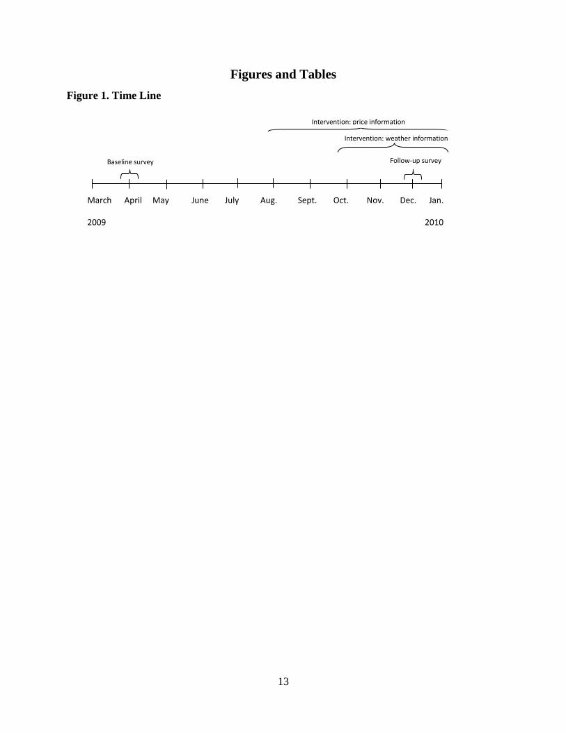
The time line for the intervention is given in Figure 1. The baseline was conducted in

March-April 2009, before the SMS intervention. The treatment group of farmers received the

intervention beginning on July 29. The first day of the intervention we sent text messages giving

instructions on how to read and understand the price and weather information that we would be

sending by SMS during the following six months. Treated farmers received daily text messages

on prices for three markets and eight products grown in their region.4 They also received weekly

weather information for a period of four months, starting on September 20, 2009. Out of the 185

days of the intervention, all farmers received price information every weekday except for 10

days, when information was not provided to us by the primary source.5 A total of 72,834 SMS

were sent, of which 79 percent were on prices, 19 percent on weather, and 2 percent

administrative. On average a treated farmer received 144 price messages, 34 weather messages,

and four administrative messages.6

The follow-up survey was conducted in November-

December 2009, after the farmers had made their decisions on sales and commercialization of

their products. Our experimental design compares the treatment to the control group, before and

after the intervention, by using information from the baseline and follow-up surveys.

3.1 Source of Price Data The Corporación Colombiana Internacional (CCI) administers the System of Price Information

in the Agricultural Sector (SIPSA—Acronym in Spanish). SIPSA includes information for more

than 700 products in 66 markets in 18 departamentos. Each day at 9 a.m. we received

information provided by the CCI. This price information corresponds to the average prices of

transactions made earlier that day. Markets operate from 11 p.m. to 5 a.m. Although the price

4 The markets and products were chosen according to the reported relevant market of the area, and conditional on availability of information. The main crops grown in this region in order of importance are: onions, potatoes, corn, beans, peas, beet, lettuce, and broccoli. Since certain crops are sold in specific days of the week, the information sent accounted for the seasonality of products sold in markets. 5 In these 10 day the person from the CCI at Tunja, our source of information, was not able to send daily prices. 6 Administrative messages were sent by the irrigation associations and typically meeting or payment reminders.

6

information provided by the CCI is publicly available by internet at 3 p.m.,7

the farmers have

limited internet access at home and in their village. In the survey, 4 percent of farmers reported

having home internet access and 15 percent reported access in their village.

3.2 Source of Weather Data The Instituto de Hidrología, Metereología y Estudios Ambientales (IDEAM) provides a weekly

report with weather forecasts including minimum and maximum temperatures, probability of rain

fall, drought, floods and frost alerts. The IDEAM agreed to include our areas of study within

their forecast models, which allowed us to provide accurate information for this intervention.

4. Description of Baseline and Follow-Up Survey Data We collected baseline characteristics in the first round of surveys prior to the intervention and

report these in Table 1. Table 1 also includes some socio-demographic characteristics that we

were able to match from the Census of the Poor Survey.8

The average farmer in our sample is 50 years old, and 70 percent of the farmers are male,

with 6 years of education and 29 year of experience in farming activities. They spend 34 hours a

week working on agricultural activities.

The baseline survey includes

socioeconomic questions, as well as information on agricultural production and

commercialization decisions. As Table 1 reports there is only one significant difference across

the treatment and control group, indicating that before the intervention the two groups are very

similar.

To ensure the quality of the information collected we asked farmers to keep records on

the price, quantity, date and location of the products sold. The second round of surveys collected

follow-up information on the key outcome variables: sale price, production, transport, crop

information shared with neighbors, crop loses and specific questions about the intervention for

those who reported receiving SMS information useful for their agricultural activities. We

followed 95 percent of the people in the second round. To encourage participation there was a

raffle of a pesticide spraying machine.

7 Available at: http://www.cci.org.co/cci/cci_x/scripts/home.php?men=101&con=192&idHm=2&opc=199 8 We have personal identifiers in the Census of the Poor and in the baseline survey which enable us to match the information to the whole family. The match rate was approximately 86 percent for Asusa and 75 percent for farmers in Usochicamocha.

http://www.cci.org.co/cci/cci_x/scripts/home.php?men=101&con=192&idHm=2&opc=199�

7

Since the price information sent via text messages corresponded to the typical crops

grown in the region and not necessarily those grown by an individual farmer, there was variation

across farmers on the number of crops for which they received prices that coincided with their

particular crops. Some farmers may have received information on all of their crops while others

on none. We exploit this variation in our analysis.

5. Empirical Specification Since we observed the same farmer in two periods to evaluate the effect of the text messages we

used a difference-in-differences approach, and a first differences with farmer fixed effects. Our

estimating difference-in-differences equation is:

iuptpuittiptittipt

iptittitipttiutitiupt

XPostodTPostododTPostTodPostExtraTY

εγγβββ

βββββββ

++++++

++++++=

987

6543210

PrPr

PrPr (1)

And our estimating first difference with farmer fixed effects equation is:

(2) where i denotes the individual farmer; p denotes the product; u denotes the irrigation unit; and t

denotes the first or second round of surveys. Yiupt corresponds to the outcome of interest. Tit is a

treatment indicator which takes the value of 1 if the farmer received text message information.

Postt is an indicator variable which takes a value of 1 after the initiation of the program.9

9 We use different definitions of post depending on the timing of the outcome of interest. We use: post to take into account the period after the initiation of the program; post_crop takes into account that the farmer planted after the initiation of the program; and post_sale takes into account that the farmer sold its product after the initiation of the program.

Prodipt

is an indicator variable which takes a value of 1 if farmer i received text message information

regarding one of his product. Extraiu corresponds to the number of producers who received

treatment in the farmer’s irrigation unit. Xit is a vector of farmers’ characteristics including:

education, experience, age, gender, percentage of time dedicated to farming, size of the crop,

storage capacity, own means of transport, whether the farmer is credit constrained, distance from

the farm to markets, γu are irrigation unit indicators to capture any characteristics that are

common across irrigation units but do not change over time, and γp are dummy variables for the

iuptpiittiptittipt

iptittitiptiutiupt

XPostodTPostododTPostTodExtraYεγγβββ

βββββ

++++++

++++=

987

65420

PrPr

PrPr

8

importance of the product, within the products of the farmer. Equation (2) includes γi farmer

fixed effects, therefore we do not control for individual characteristics which do not vary much

between both rounds of surveys.

Additionally, we estimate an alternative model where we control for the outcome at

baseline as follows:

iuptpu

itiptitiptiuptiutitiupt XodTodYExtraTYεγγ

βββββββ

+++

++++++= − 46413210 PrPr (3)

where the variables are defined the same way as in equation (1). This specification could help to

absorb noise and give more flexibility in the parameter β3 than the fixed effect specification.

Parallel to the three equations presented above, we test for spillover effects by interacting

these same specifications with the following measures: number of text messages received

(directly from the program or indirectly from a participant), frequency of visits to neighbor

farmers, and the number of people the farmer knows who are enrolled in the program interacted

with frequency of visits to neighbor farmers. All of these different measures are used as proxies

for the amount of contact with information that an individual can have, and we expect to get

from them a measure of the externality effect of the program.

6. Results We are interested in the following outcomes: i) whether the farmer is able to report prices in

different markets, ii) whether the farmer is using text messages as a substitute for sources of

information to plant or sell, iii) the difference between the officially reported price and the price

reported by the farmer at the time of sale; iv) the difference between the expected sale price and

the officially reported price, and the dispersion in prices reported by the farmers, and v) the

extent of crop loss.

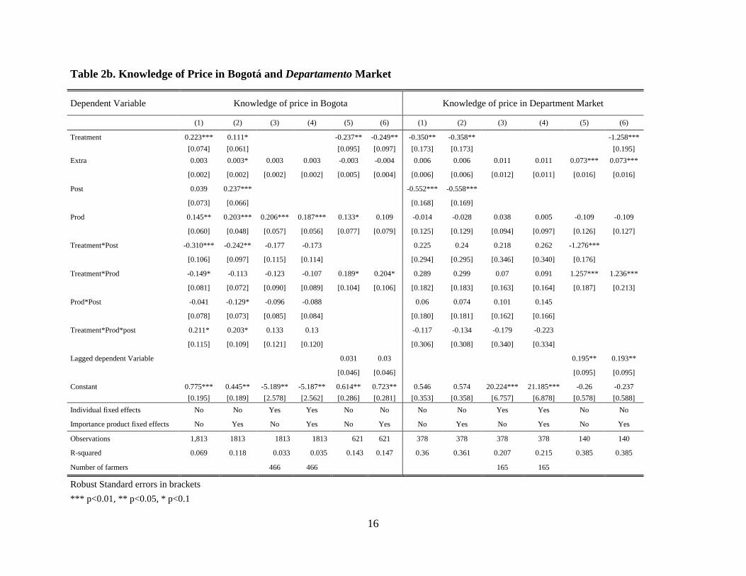
6.1 Reporting Prices in Different Markets Reporting a price corresponds to the simplest outcome we can test in this experiment. We want

to know whether sending price text message information can have an impact on the self-reported

knowledge of prices by product and market. The dependent variable is constructed from the

question in the survey where we ask the farmer: “If you had to sell your product today, what

9

would be the price you think you will get after a negotiation in the farm, municipal market,

Bogotá and departamento market?” Independent of the accuracy of the value reported, we give

the value of 1 if there was a price reported and 0 if the respondent answers that he or she does

not know.

Tables 2a and 2b include the same empirical specification for the four different markets:

farm and municipal market, Bogotá and departamento market, respectively. Columns 1 and 2

correspond to the estimation in equation (1), Columns 3 and 4 correspond to the estimation in

equation (2), and Columns 5 and 6 correspond to the estimation in equation (3). The difference

between each pair of columns is that the second column in each pair includes economic

importance of product fixed effect, while the first one does not include this control. On average,

according to the specification given by equation (1) farmers receiving text messages

corresponding to their crop are between 20 and 30 percentage points more likely to report a price

in all markets except for the departamental market.

6.2 Text Messages as a Substitute of Sources of Sales Information We test whether the information received by farmers has been useful for their agricultural

activities, specifically for sales. In Table 3 we use four different outcome variables: i) the farmer

reported text messages as a source of information in the follow-up survey; ii) the farmer reported

changes in the source of information used for selling relative to the sources of information

reported in the baseline; iii) an interaction of these two outcomes that captures a change in source

of information including text messages as an important source of information; and iv) the farmer

reports text messages as a new source of information and there are changes in the importance of

sources of information.

The table shows that the coefficient related to the treatment effect is positive and

significant at the 1 percent level for all outcomes except for change in source of information

(column 2), we also include the treatment interacted with the dummy variable that indicates that

the prices sent via text messages coincided with the products that the farmer is planting, but we

do not find a differential effect of the treatment for different products.10

10 Our survey also includes data to test whether the information sent affected planting decision or helped in solving problems related to the crop. This hypothesis has not yet been tested.

10

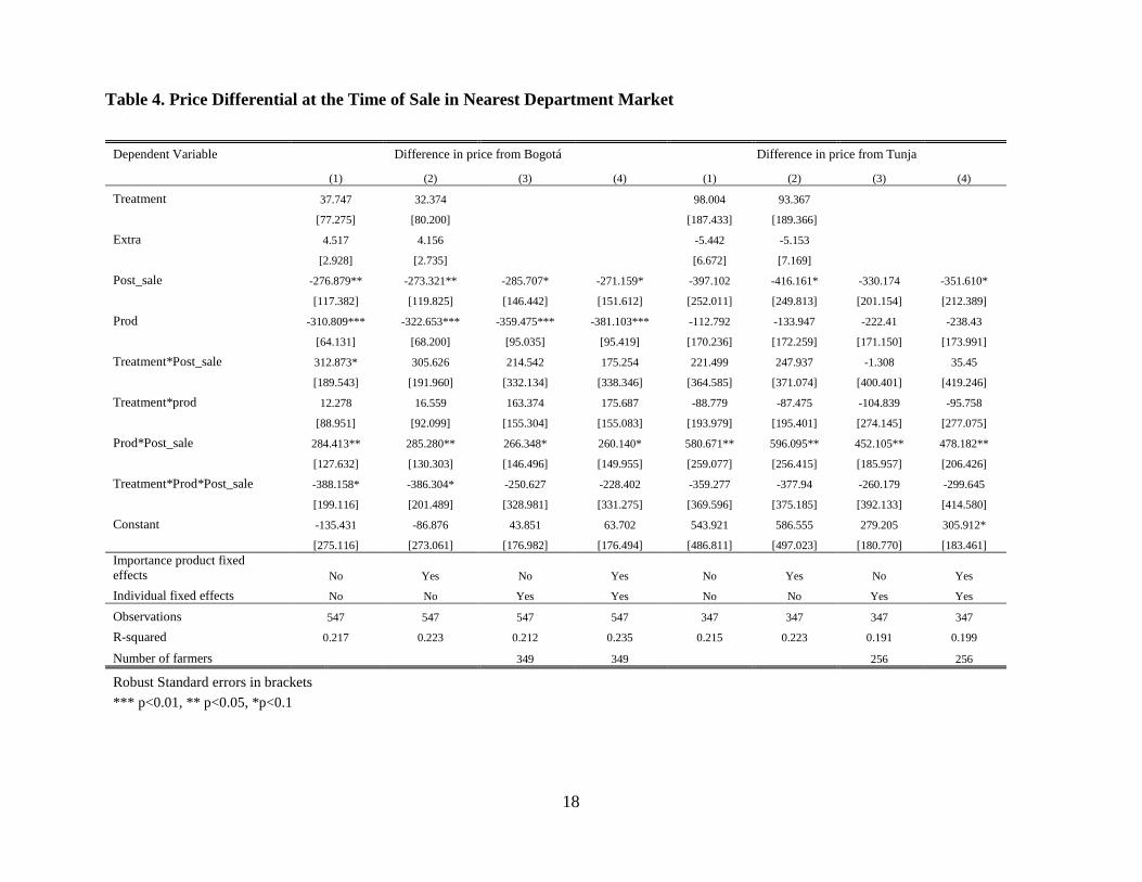
6.3 Price Differential at the Time of Sale We construct the difference between the sale price reported by the farmer and the sale price

reported by the official data from CCI in a given week in Bogotá and Tunja, two markets where

these farmers sell and where we have official data from CCI. Table 4 does not show a significant

difference, consistent throughout different specifications, in the sale prices obtained by treated

farmers compared to the farmers in the control group. But there is a positive and significant

effect of the sale prices of the products reported in the text message information for the whole

sample after the intervention, which could be interpreted as a spillover effect of the program.

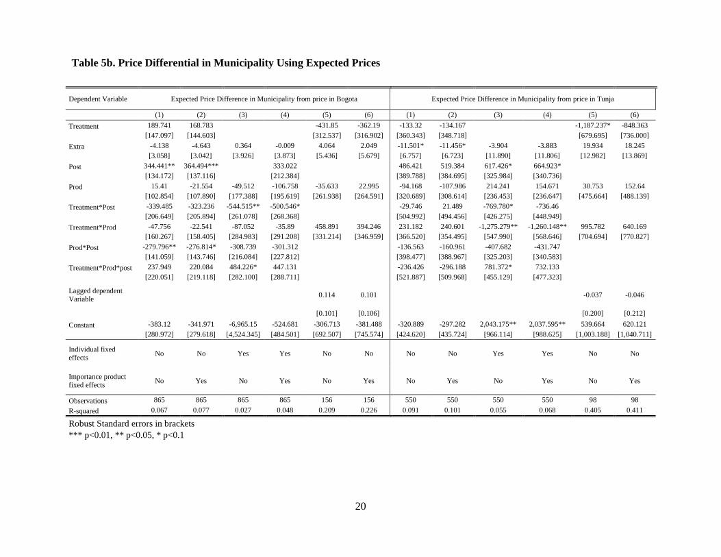
6.4 Price Differential and Price Dispersion Using Expected Prices Using the same question as in the first outcome (reporting a price in different markets), we

construct the difference between the sale price reported by the farmer at a given market and the

sale price from the CCI official data in a given week for the corresponding market (we call this

the expected sale price), results are reported in Tables 5a, 5b, 5c. There is some evidence that the

treatment group reported a higher sale price in Bogotá, but we do not generally find evidence

that treated farmers differ much from the control group in the expected price reported.

We also construct monthly price dispersion of expected prices. The results, presented in

Tables 6a and 6b, show that in the four different markets treated farmers have lower price

dispersion in the price they report than the control group of farmers. This implies that farmers are

able to negotiate and sell their product closer to the market price, which will be a fair price.

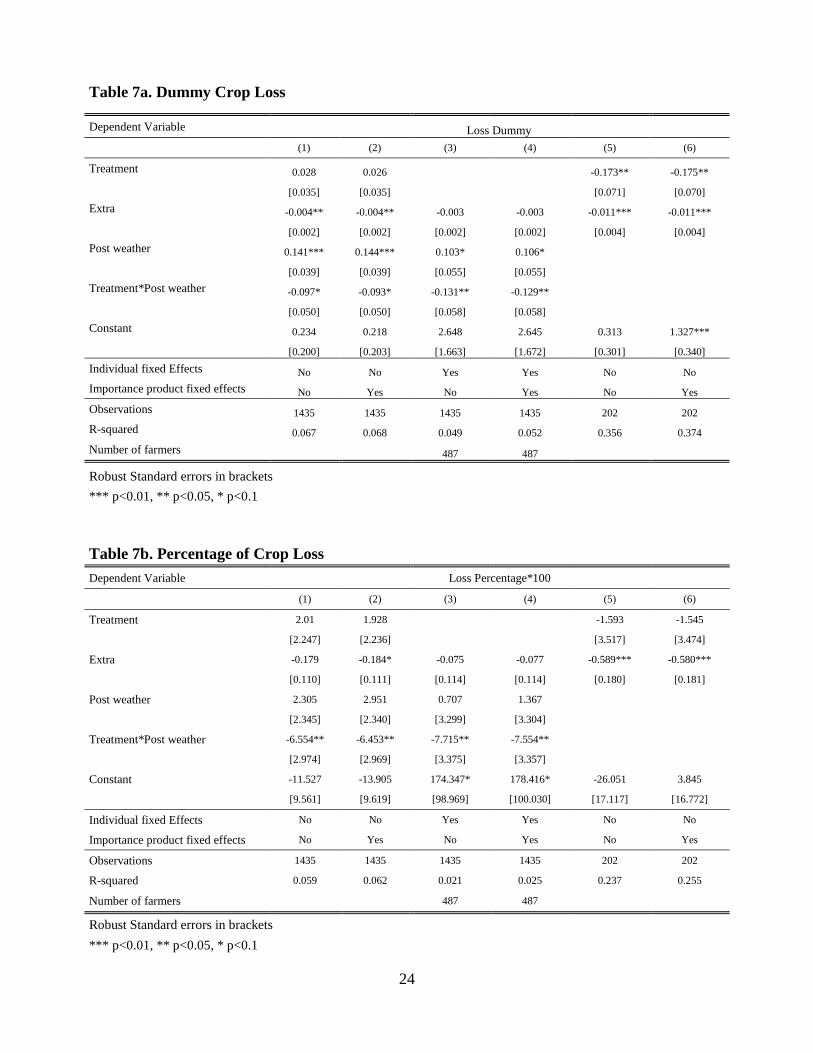
6.5 Crop Loss We constructed the three following measures of crop loss: i) a dummy variable that takes the

value of 1 if the farmer had any type of loss in his crop, ii) a continuous variable corresponding

to the percentage of crop loss, and iii) a dummy variable that takes the value of 1 if the farmer

had weather related loss. The results related to these three variables are reported in Tables 7a,

7b and 7c respectively. All of the specifications in Table 7a consistently show statistically

significant differences between treated and control farmers; treated farmers are between 11 and

14 percentage points less likely to suffer a crop loss.

11

6.6 Additional Outcomes Other outcomes that we could study in the future include behaviors with respect to harvest delay,

crop storage, profits, change in the crops that are planted or markets where products are sold. We

did not find significant effects for household revenue and expenditures, which might be due to

the short period of the implementation of the program.

We have explored the externality effect of the program and have some preliminary

findings that consistently point to a positive and significant effect only when the data are used as

a cross-section. Once the individual fixed effect or lagged variable models are used, however,

there are no significant effects. Specifically we see positive externality effects in terms of crop

loss due to weather. This is consistent with what treated farmers say about the usefulness of the

information received, where they give a grade of 4.1 out of 5 to the weather information.

7. Conclusion and Policy Relevance

In this paper we tested if access to price information via text messages changed farmers’

behaviors. In particular, we analyzed whether treated farmers had better knowledge of prices and

as a consequence were able to extract higher prices for their products. We found that the

information sent indicated a change in the treated farmers’ perceptions of prices, but did not

seem to affect their actual sale prices. Other results indicate that inexpensive technological

interventions quickly become useful sources of price information and reduce the probability of

weather-related crop loss. In terms of welfare improvement we did not find an effect on profits

or household expenditures, but this might be due to the short-term nature of the intervention.

In the future we plan to study the external effects of SMS technology use in communities

when family and neighbors share information. In particular, we will explore whether farmers are

transporting their products to other markets as a result of this information.

12

References Aker, J.C. 2008. “Does Digital Divide or Provide? The Impact of Cell Phones on Grain Markets

in Niger.” Bread Working Paper 177. Durham, United States: Bureau for Research and

Economic Analysis of Development

Beuermann, D. 2010. “Telecommunications Technologies, Agricultural Productivity, and Child

Labor in Rural Peru.” College Park, Maryland, United States: University of Maryland.

Manuscript. Available at http://www.bus.miami.edu/_assets/files/events/Beuermann

Foster, A., and M. Rosenzweig. 1995. “Learning by Doing and Learning from Others: Human

Capital and Technical Change in Agriculture.” Journal of Political Economy

103(6):1176-1209.

Jensen, R. 2007. “The Digital Provide: Information (Technology), Market Performance, and

Welfare in the South Indian Fisheries Sector.” Quarterly Journal of Economics 122(3):

879-924.

Montenegro, S., and A. Pedraza. 2009. “Falling Kidnapping Rates and the Expansion of Mobile

Phones in Colombia.” Documento CEDE 39-2009. Bogota, Colombia: Universidad de

los Andes, Centro de Estudios sobre el Desarrollo Económico.

Oster, E.F., and R.L. Thornton. 2009. “Determinants of Technology Adoption: Private Value and

Peer Effects in Menstrual Cup Take-Up.” NBER Working Papers 14828. Cambridge,

United States: National Bureau of Economic Research.

Perfetti, J.J. et al. 2007. “Oferta de Información Agropecuaria en Colombia – Análisis y

Propuestas.” Programa MIDAS (Más Inversión para el Desarrollo Alternativo

Sostenible), Proyecto Sistemas de Información Agropecuaria.

Perfetti del Corral, J.J. 2008. “Demanda de Información en el Sector Agropecuario.” Programa

MIDAS (Más Inversión para el Desarrollo Alternativo Sostenible), Proyecto Sistemas de

Información Agropecuaria.

13

Figures and Tables Figure 1. Time Line

Follow-up survey

Intervention: weather information

Baseline survey

March April May June July Aug. Sept. Oct. Nov. Dec. Jan.

2009 2010

Intervention: price information

14

Table 1.Baseline Summary Statistics Demographic Control Treatment Producer age 50.36 49.48 Producer is female 0.343* 0.271* Years of schooling 6.03 5.83 Years of experience 29.59 28.84 Household size 4.22 4.10 Number of hours per week dedicated to farming 34.20 34.29 Income and Poverty indicators Finished floors 0.68 0.71 Number of rooms in dwelling 3.05 3.03 Number of people per room 1.55 1.50 Dwelling has permanent electricity 0.99 0.99 Dwelling has land line telephone 0.14 0.11 Dwelling has access to potable water 0.96 0.97 Producer takes public transport to city 0.44 0.43 Cell phone Good (or better) quality of cell phone signal 0.97 0.97 Always reads text messages 0.71 0.71 Producer monthly cell phone expenditure (in pesos) 23,762 27,704 Farm Household members in agriculture labors 0.80 0.75 Farm area (Ha) 1.40 1.56 Total farm area (Ha) 1.74 2.02 Area - All crops (Ha) 1.10 1.24 Did not store main crop 0.79 0.81 Percent of main crop stored 69.04 62.62 Number of days main crop stored or delayed 27.52 34.06 Loss of any crop 0.49 0.50 Loss of main crop due to weather 0.71 0.77 Number cows and/or horses owned 1.17 1.07 Number of farm equipment (hoses, sprinklers) 5.32 4.79 Farm ownership 0.60 0.61 Number of neighbors or friends mentioned 1.53 1.62 Cost and Prices Number of potential buyers that came to the farm 2.07 2.12 Monthly transport costs (in pesos) 128,327 218,414 Neighbors as source of price information 0.10 0.10 No sources of price information 0.07 0.08 Requested credit 0.32 0.29 Denied credit application 0.05 0.06 Distance (Km) nearest department market 17.91 18.31 Road quality 1.96 1.89 Market type Collection 0.18 0.18 Department market or Bogota 0.30 0.30 Municipal market 0.18 0.24 Other 0.08 0.08 Note: The unit of observation is the farmer; there are 500 farmers. * Significant at 10%; ** significant at 5%; *** significant at 1%

15

*** p<0.01, ** p<0.05, * p<0.1

Robust Standard errors in brackets *** p<0.01, ** p<0.05, * p<0.1

Dependent Variable Knowledge of price in farm Knowledge of price in Municipality

(1) (2) (3) (4) (5) (6) (1) (2) (3) (4) (5) (6)

Treatment 0.223*** 0.201*** -0.08 -0.098 0.218*** 0.201** -0.133 -0.15 [0.074] [0.073] [0.110] [0.112] [0.079] [0.078] [0.112] [0.115] Extra 0.003 0.003 0.002 0.002 -0.002 -0.003 0.003 0.003 0.003 0.003 -0.004 -0.006 [0.002] [0.002] [0.002] [0.002] [0.005] [0.005] [0.002] [0.002] [0.003] [0.003] [0.006] [0.005] Post 0.039 0.043 0.139* 0.142* [0.073] [0.072] [0.076] [0.076] Prod 0.145** 0.097 0.099 0.061 0.133* 0.095 0.221*** 0.184*** 0.169** 0.143** 0.159** 0.122 [0.060] [0.059] [0.062] [0.062] [0.072] [0.073] [0.062] [0.062] [0.069] [0.068] [0.075] [0.076] Treatment*Post -0.310*** -0.305*** -0.256** -0.249** -0.339*** -0.336*** -0.214 -0.209 [0.106] [0.106] [0.110] [0.109] [0.113] [0.113] [0.132] [0.131] Treatment*Prod -0.149* -0.12 -0.115 -0.085 0.065 0.089 -0.174** -0.152* -0.152 -0.131 0.114 0.137 [0.081] [0.080] [0.085] [0.082] [0.116] [0.118] [0.088] [0.087] [0.097] [0.095] [0.121] [0.124] Prod*Post -0.041 -0.02 -0.053 -0.037 -0.182** -0.167** -0.134 -0.123 [0.078] [0.077] [0.064] [0.064] [0.083] [0.082] [0.090] [0.090] Treatment*Prod*post 0.211* 0.207* 0.187* 0.18 0.305** 0.302** 0.191 0.186 [0.115] [0.115] [0.112] [0.111] [0.124] [0.124] [0.134] [0.133] Lagged dependent Variable 0.076* 0.067 -0.05 -0.053 [0.042] [0.043] [0.043] [0.043] Constant 0.775*** 0.962*** 1.359 1.364 0.790** 0.972*** 0.699*** 0.841*** -0.132 -0.129 0.775** 0.947*** [0.195] [0.206] [2.030] [2.025] [0.353] [0.343] [0.205] [0.210] [2.858] [2.855] [0.366] [0.356]

Individual fixed effects No No Yes Yes No No No No Yes Yes No No Importance product fixed effects No Yes No Yes No Yes No Yes No Yes No Yes

Observations 1813 1813 1813 1813 621 621 1813 1813 1813 1813 621 621 R-squared 0.069 0.085 0.024 0.035 0.126 0.139 0.066 0.073 0.019 0.024 0.076 0.085 Number of farmers 466 466 466 466

Table 2a. Knowledge of Price in the Farm and Municipal Market

16

Table 2b. Knowledge of Price in Bogotá and Departamento Market

Dependent Variable Knowledge of price in Bogota Knowledge of price in Department Market

(1) (2) (3) (4) (5) (6) (1) (2) (3) (4) (5) (6)

Treatment 0.223*** 0.111* -0.237** -0.249** -0.350** -0.358** -1.258***

[0.074] [0.061] [0.095] [0.097] [0.173] [0.173] [0.195] Extra 0.003 0.003* 0.003 0.003 -0.003 -0.004 0.006 0.006 0.011 0.011 0.073*** 0.073***

[0.002] [0.002] [0.002] [0.002] [0.005] [0.004] [0.006] [0.006] [0.012] [0.011] [0.016] [0.016]

Post 0.039 0.237*** -0.552*** -0.558***

[0.073] [0.066] [0.168] [0.169] Prod 0.145** 0.203*** 0.206*** 0.187*** 0.133* 0.109 -0.014 -0.028 0.038 0.005 -0.109 -0.109

[0.060] [0.048] [0.057] [0.056] [0.077] [0.079] [0.125] [0.129] [0.094] [0.097] [0.126] [0.127]

Treatment*Post -0.310*** -0.242** -0.177 -0.173 0.225 0.24 0.218 0.262 -1.276***

[0.106] [0.097] [0.115] [0.114] [0.294] [0.295] [0.346] [0.340] [0.176] Treatment*Prod -0.149* -0.113 -0.123 -0.107 0.189* 0.204* 0.289 0.299 0.07 0.091 1.257*** 1.236***

[0.081] [0.072] [0.090] [0.089] [0.104] [0.106] [0.182] [0.183] [0.163] [0.164] [0.187] [0.213]

Prod*Post -0.041 -0.129* -0.096 -0.088 0.06 0.074 0.101 0.145

[0.078] [0.073] [0.085] [0.084] [0.180] [0.181] [0.162] [0.166] Treatment*Prod*post 0.211* 0.203* 0.133 0.13 -0.117 -0.134 -0.179 -0.223

[0.115] [0.109] [0.121] [0.120] [0.306] [0.308] [0.340] [0.334] Lagged dependent Variable 0.031 0.03 0.195** 0.193**

[0.046] [0.046] [0.095] [0.095]

Constant 0.775*** 0.445** -5.189** -5.187** 0.614** 0.723** 0.546 0.574 20.224*** 21.185*** -0.26 -0.237 [0.195] [0.189] [2.578] [2.562] [0.286] [0.281] [0.353] [0.358] [6.757] [6.878] [0.578] [0.588] Individual fixed effects No No Yes Yes No No No No Yes Yes No No

Importance product fixed effects No Yes No Yes No Yes No Yes No Yes No Yes

Observations 1,813 1813 1813 1813 621 621 378 378 378 378 140 140

R-squared 0.069 0.118 0.033 0.035 0.143 0.147 0.36 0.361 0.207 0.215 0.385 0.385

Number of farmers 466 466 165 165

Robust Standard errors in brackets

*** p<0.01, ** p<0.05, * p<0.1

17

Table 3. Text Messages as a Substitute for Sources of Sales Information

Dependent variable SMS as a source of info

useful for selling in follow-up

Relative to baseline, changes in source of info

for selling

Change in source of info and including SMS as an important source of info

for selling

Change importance of source of info and

including SMS as an important source of info

for selling

Treatment 0.382*** 0.164 0.411*** 0.382***

[0.134] [0.143] [0.126] [0.134]

Extra 0.003** 0.004** 0.004*** 0.003**

[0.001] [0.002] [0.001] [0.001]

Treatment*Prod -0.057 -0.162 -0.173 -0.057

[0.148] [0.159] [0.139] [0.148]

Prod 0.006 -0.094 0.023 0.006

[0.103] [0.110] [0.097] [0.103]

Constant 0.035 0.827*** 0.01 0.035

[0.092] [0.099] [0.087] [0.092]

Observations 475 475 475 475

R-squared 0.166 0.027 0.129 0.166


18

Table 4. Price Differential at the Time of Sale in Nearest Department Market

Dependent Variable Difference in price from Bogotá Difference in price from Tunja

(1) (2) (3) (4) (1) (2) (3) (4)

Treatment 37.747 32.374 98.004 93.367

[77.275] [80.200] [187.433] [189.366]

Extra 4.517 4.156 -5.442 -5.153

[2.928] [2.735] [6.672] [7.169]

Post_sale -276.879** -273.321** -285.707* -271.159* -397.102 -416.161* -330.174 -351.610*

[117.382] [119.825] [146.442] [151.612] [252.011] [249.813] [201.154] [212.389]

Prod -310.809*** -322.653*** -359.475*** -381.103*** -112.792 -133.947 -222.41 -238.43

[64.131] [68.200] [95.035] [95.419] [170.236] [172.259] [171.150] [173.991]

Treatment*Post_sale 312.873* 305.626 214.542 175.254 221.499 247.937 -1.308 35.45

[189.543] [191.960] [332.134] [338.346] [364.585] [371.074] [400.401] [419.246]

Treatment*prod 12.278 16.559 163.374 175.687 -88.779 -87.475 -104.839 -95.758

[88.951] [92.099] [155.304] [155.083] [193.979] [195.401] [274.145] [277.075]

Prod*Post_sale 284.413** 285.280** 266.348* 260.140* 580.671** 596.095** 452.105** 478.182**

[127.632] [130.303] [146.496] [149.955] [259.077] [256.415] [185.957] [206.426]

Treatment*Prod*Post_sale -388.158* -386.304* -250.627 -228.402 -359.277 -377.94 -260.179 -299.645

[199.116] [201.489] [328.981] [331.275] [369.596] [375.185] [392.133] [414.580]

Constant -135.431 -86.876 43.851 63.702 543.921 586.555 279.205 305.912*

[275.116] [273.061] [176.982] [176.494] [486.811] [497.023] [180.770] [183.461] Importance product fixed effects No Yes No Yes No Yes No Yes

Individual fixed effects No No Yes Yes No No Yes Yes

Observations 547 547 547 547 347 347 347 347

R-squared 0.217 0.223 0.212 0.235 0.215 0.223 0.191 0.199

Number of farmers 349 349 256 256

Robust Standard errors in brackets *** p<0.01, ** p<0.05, *p<0.1

19

Table 5a. Price Differential in Farm Using Expected Prices

Dependent Variable Expected Price Difference in Farm from price in Bogota Expected Price Difference in Farm from price in Tunja

(1) (2) (3) (4) (5) (6) (1) (2) (3) (4) (5) (6) Treatment 81.454 58.933 -69.549 -35.809 198.059 186.394 -567.971 -493.268 [141.442] [142.644] [208.455] [203.531] [376.130] [378.427] [378.115] [389.272] Extra -0.858 -0.956 -0.294 -0.531 1.221 0.783 -5.583 -5.445 -1.874 -1.754 12.289 10.618 [2.438] [2.426] [2.556] [2.568] [5.333] [5.388] [6.492] [6.521] [8.896] [8.917] [9.950] [10.893] Post 124.247 122.211 60.847 51.699 220.3 211.51 [141.731] [143.350] [163.638] [170.928] [283.188] [283.475] Prod -118.382 -147.341 -182.832 -230.279 74.587 107.69 -54.852 -66.075 -121.724 -119.838 402.096 471.445 [119.711] [123.189] [150.171] [159.676] [161.105] [154.825] [218.183] [221.496] [272.315] [273.816] [361.360] [359.767] Treatment*Post -45.641 -28.786 -228.606 -183.646 -463.238 -426.825 -821.719 -779.922 [196.106] [196.814] [212.657] [223.087] [456.258] [458.904] [577.984] [598.461] Treatment*Prod -17.318 6.834 -84.68 -21.684 13.414 -20.843 -173.007 -161.7 -1,031.447* -1,020.623* 350.301 274.522 [152.573] [153.714] [198.361] [209.162] [217.659] [212.800] [380.510] [383.682] [544.330] [554.280] [398.701] [416.273] Prod*Post -77.488 -65.09 -63.564 -42.096 -11.302 -6.152 137.201 138.859 [148.679] [150.133] [171.933] [179.155] [298.766] [299.036] [253.343] [261.582] Treatment*Prod *post -10.641 -27.533 187.782 145.361 307.817 271.437 828.966 785.468

[207.599] [207.913] [226.262] [235.361] [472.278] [476.527] [589.838] [609.766]

Lagged dependent Variable

0.037 0.04 0.031 0.04

[0.026] [0.027] [0.064] [0.069] Constant -112.355 -30.966 -128.235 -189.053 -446.394 -459.993 172.554 129.587 1,080.10 1,281.72 302.83 341.822 [467.786] [479.635] [483.738] [494.879] [473.402] [486.114] [327.843] [332.864] [7,576.739] [7,872.178] [680.756] [690.599]

Individual fixed effects No No Yes Yes No No No No Yes Yes No No


Observations 1107 1107 1107 1107 270 270 700 700 700 700 163 163 R-squared 0.05 0.056 0.017 0.028 0.157 0.16 0.068 0.073 0.046 0.049 0.316 0.325


20

Table 5b. Price Differential in Municipality Using Expected Prices

Dependent Variable Expected Price Difference in Municipality from price in Bogota Expected Price Difference in Municipality from price in Tunja

(1) (2) (3) (4) (5) (6) (1) (2) (3) (4) (5) (6) Treatment 189.741 168.783 -431.85 -362.19 -133.32 -134.167 -1,187.237* -848.363 [147.097] [144.603] [312.537] [316.902] [360.343] [348.718] [679.695] [736.000] Extra -4.138 -4.643 0.364 -0.009 4.064 2.049 -11.501* -11.456* -3.904 -3.883 19.934 18.245 [3.058] [3.042] [3.926] [3.873] [5.436] [5.679] [6.757] [6.723] [11.890] [11.806] [12.982] [13.869] Post 344.441** 364.494*** 333.022 486.421 519.384 617.426* 664.923* [134.172] [137.116] [212.384] [389.788] [384.695] [325.984] [340.736] Prod 15.41 -21.554 -49.512 -106.758 -35.633 22.995 -94.168 -107.986 214.241 154.671 30.753 152.64 [102.854] [107.890] [177.388] [195.619] [261.938] [264.591] [320.689] [308.614] [236.453] [236.647] [475.664] [488.139] Treatment*Post -339.485 -323.236 -544.515** -500.546* -29.746 21.489 -769.780* -736.46 [206.649] [205.894] [261.078] [268.368] [504.992] [494.456] [426.275] [448.949] Treatment*Prod -47.756 -22.541 -87.052 -35.89 458.891 394.246 231.182 240.601 -1,275.279** -1,260.148** 995.782 640.169 [160.267] [158.405] [284.983] [291.208] [331.214] [346.959] [366.520] [354.495] [547.990] [568.646] [704.694] [770.827] Prod*Post -279.796** -276.814* -308.739 -301.312 -136.563 -160.961 -407.682 -431.747 [141.059] [143.746] [216.084] [227.812] [398.477] [388.967] [325.203] [340.583] Treatment*Prod*post 237.949 220.084 484.226* 447.131 -236.426 -296.188 781.372* 732.133 [220.051] [219.118] [282.100] [288.711] [521.887] [509.968] [455.129] [477.323]

Lagged dependent Variable 0.114 0.101 -0.037 -0.046

[0.101] [0.106] [0.200] [0.212] Constant -383.12 -341.971 -6,965.15 -524.681 -306.713 -381.488 -320.889 -297.282 2,043.175** 2,037.595** 539.664 620.121 [280.972] [279.618] [4,524.345] [484.501] [692.507] [745.574] [424.620] [435.724] [966.114] [988.625] [1,003.188] [1,040.711]





21

Table 5c. Price Differential in Bogota Using Expected Prices

Dependent Variable Expected Price Difference in Bogota from price in Bogota Expected Price Difference in Bogota from price in Tunja

(1) (2) (3) (4) (5) (6) (1) (2) (3) (4) (5) (6) Treatment 353.579* 305.313 6.189 14.328 -637.024 -650.267 -33.611 -22.709 [204.056] [212.477] [110.517] [113.538] [618.723] [608.069] [220.743] [193.179] Extra -4.11 -4.3 -0.467 -0.99 5.341 5.551 9.332 9.581 25.570* 28.601** 17.397 0.045 [3.286] [3.275] [4.557] [4.887] [7.059] [8.167] [9.669] [9.885] [13.196] [13.371] [11.182] [12.955] Post 518.011** 472.708* 369.883 330.072 43.144 47.306 97.248 [245.085] [243.372] [360.757] [384.941] [663.903] [672.434] [296.260] Prod 181.837 144.9 11.561 -35.746 407.968* 432.313* -615.211 -650.334 -195.972 -268.044 613.667 914.837** [199.887] [206.723] [350.255] [386.202] [237.803] [258.111] [563.951] [559.493] [284.691] [276.487] [397.152] [448.067] Treatment*Post -551.530* -495.991 -877.852* -772.901 -158.355 -168.971 -398.544 -299.875 [327.410] [320.640] [449.870] [479.337] [853.182] [848.891] [737.528] [817.440] Treatment*Prod -249.53 -203.498 -568.066 -453.462 883.489 906.009 -358.335 -242.172 [220.575] [228.448] [408.143] [451.299] [653.031] [648.627] [746.193] [791.486] Prod*Post -504.110** -457.986* -515.229 -472.512 144.759 157.743 -375.837 -326.351 [252.156] [249.902] [371.277] [397.458] [675.728] [676.071] [341.754] [365.040] Treatment*Prod*post 457.904 409.757 948.184** 853.255* -269.45 -259.816 473.969 378.444 [343.253] [336.028] [459.958] [489.255] [874.011] [871.068] [780.409] [869.399]

Lagged dependent Variable -0.01 -0.012 -0.036 -0.052

[0.019] [0.021] [0.052] [0.048] Constant -355.934 -370.304 46.213 -186.136 -188.331 -257.29 666.172 773.703 4,422.173*** 2,962.52 -132.505 118.711 [349.978] [353.403] [724.397] [796.178] [537.488] [579.126] [793.387] [780.680] [1,118.928] [9,392.038] [842.429] [851.320]





22

Table 6a. Price Dispersion Using Expected Prices

Dependent variable:

Expected price per kilogram standard deviation in: Farm Municipality

(1) (2) (3) (4) (5) (6) (1) (2) (3) (4) (5) (6) Treatment -102.695* -111.588* -221.443 -197.022 41.514 68.318* -304.460*** -278.426***

[60.769] [61.587] [179.719] [186.915] [38.041] [41.097] [91.851] [92.623] Extra -7.937*** -7.928*** -7.240** -7.254** 3.79 5.657 -2.359 -2.485 -1.537 -1.601 1.64 4.024

[2.993] [2.988] [3.062] [3.063] [8.065] [7.154] [2.250] [2.263] [1.936] [1.924] [4.398] [4.060]

Post 420.073*** 420.111*** 501.428*** 502.161*** 306.782*** 300.591*** 320.867***

[77.719] [78.020] [85.119] [85.090] [52.301] [52.264] [63.087] Prod 339.588*** 325.162*** 308.593** 282.242** 470.052** 522.976** 478.883*** 510.640*** 467.875*** 502.284*** 37.536 100.374

[58.667] [61.152] [132.697] [133.081] [225.143] [218.305] [45.656] [49.225] [55.057] [59.314] [75.370] [74.561] Treatment*post 6.364 10.94 -40.93 -28.783 104.718 82.181 97.6 60.356 [104.446] [104.541] [117.387] [119.125] [133.369] [133.214] [160.448] [159.380] Treatment*prod 557.976*** 569.157*** 400.681** 430.503** -343.791 -380.313 195.367*** 162.818** 26.591 -18.195 329.480*** 291.399***

[85.828] [87.901] [164.828] [168.506] [249.898] [253.363] [62.310] [66.276] [112.329] [112.926] [100.457] [100.246] Prod*post -72.307 -64.887 -144.928 -131.442 -425.787*** -437.357*** -440.175*** -453.544*** [110.993] [115.145] [111.553] [115.300] [64.259] [64.904] [70.703] [73.314] Treatment*prod*post

-773.940***

-778.782***

-746.434***

-758.751**

* -304.989** -281.705* -311.366* -273.794

[153.197] [155.371] [162.521] [166.502] [146.177] [146.721] [169.294] [169.172] Lagged dependent variable 0.253*** 0.256*** 0.213*** 0.213***

[0.049] [0.049] [0.045] [0.043] Constant -282.04 -224.689 -267.099 -206.08 -468.04 -711.808 -172.858 -308.895 -838.880*** -10,233.520*** 124.904 -163.772

[308.324] [313.929] [604.474] [621.099] [752.775] [737.510] [267.674] [270.787] [176.674] [1,949.891] [287.840] [282.134] Importance product fixed effects

No Yes No Yes No Yes No Yes No Yes No Yes




23

Table 6b. Price Dispersion Using Expected Prices

Dependent variable:

Expected price per kilogram standard deviation in: Bogotá Department Market

(1) (2) (3) (4) (5) (6) (1) (2) (3) (4) (5) (6) Treatment -185.624 -176.42 -218.014* -188.886 278.207 283.796 -2.435 -4.545

[182.819] [199.199] [114.087] [170.892] [171.391] [184.279] [27.715] [28.110] Extra 1.763 1.58 2.455 2.36 5.361* 4.638* -20.903 -20.991 -7.239 -7.462 2.643 3.268

[3.158] [3.161] [2.838] [2.812] [2.768] [2.704] [17.806] [17.946] [22.138] [22.501] [5.349] [5.425] Post 16.446 -21.734 375.355* 376.635* [181.558] [197.599] [193.879] [195.120] Prod 400.004** 421.466** 202.769 207.452 103.398 132.249 464.786*** 469.008*** 219.345*** 237.664*** [182.386] [199.406] [125.024] [143.904] [87.037] [150.374] [134.647] [143.507] [6.271] [52.167] Treatment* post -108.794 -88.402 136.338 152.074 -1,310.250*** -1,762.097*** -1,760.427***

[193.668] [208.847] [177.364] [188.640] [177.848] [241.679] [243.351] Treatment* prod 599.436*** 580.668*** 651.620*** 622.492*** 146.99 105.071 1,010.100*** 1,003.695*** 1,567.777*** 1,548.562***

[198.588] [214.437] [201.466] [211.517] [117.146] [173.016] [236.451] [251.379] [247.016] [258.222] Prod*post -273.981 -266.12 -61.933 -36.409 -539.322*** -542.232*** -211.691 -231.727 [196.326] [210.351] [141.641] [158.018] [198.914] [201.886] [155.411] [160.432] Treatment* prod*post -313.972 -333.052 -600.844*** -615.529*** -1,309.457***

[213.530] [225.841] [198.397] [207.995] [178.832] Lagged dependent variable 0.152*** 0.153*** 0.019 0.017

[0.027] [0.026] [0.016] [0.016] Constant 255.414 88.064 2314.482 5702.301 55.526 -63.597 0 10.078 98.369 40.663 66.117 76.042

[500.920] [513.068] [2,797.904] [4,579.557] [215.139] [242.671] [0.000] [65.130] [61.541] [89.251] [101.464] [105.480] Importance product fixed effects

No Yes No Yes No Yes No Yes No Yes No Yes




24

Table 7a. Dummy Crop Loss

Dependent Variable Loss Dummy (1) (2) (3) (4) (5) (6)

Treatment 0.028 0.026

-0.173** -0.175**

[0.035] [0.035]

[0.071] [0.070] Extra -0.004** -0.004** -0.003 -0.003 -0.011*** -0.011***

[0.002] [0.002] [0.002] [0.002] [0.004] [0.004] Post weather 0.141*** 0.144*** 0.103* 0.106*

[0.039] [0.039] [0.055] [0.055]

Treatment*Post weather -0.097* -0.093* -0.131** -0.129**

[0.050] [0.050] [0.058] [0.058] Constant 0.234 0.218 2.648 2.645 0.313 1.327***

[0.200] [0.203] [1.663] [1.672] [0.301] [0.340] Individual fixed Effects No No Yes Yes No No Importance product fixed effects No Yes No Yes No Yes Observations 1435 1435 1435 1435 202 202 R-squared 0.067 0.068 0.049 0.052 0.356 0.374 Number of farmers 487 487


Table 7b. Percentage of Crop Loss Dependent Variable Loss Percentage*100

(1) (2) (3) (4) (5) (6)

Treatment 2.01 1.928 -1.593 -1.545

[2.247] [2.236] [3.517] [3.474]

Extra -0.179 -0.184* -0.075 -0.077 -0.589*** -0.580***

[0.110] [0.111] [0.114] [0.114] [0.180] [0.181]

Post weather 2.305 2.951 0.707 1.367

[2.345] [2.340] [3.299] [3.304] Treatment*Post weather -6.554** -6.453** -7.715** -7.554**

[2.974] [2.969] [3.375] [3.357] Constant -11.527 -13.905 174.347* 178.416* -26.051 3.845

[9.561] [9.619] [98.969] [100.030] [17.117] [16.772]

Individual fixed Effects No No Yes Yes No No

Importance product fixed effects No Yes No Yes No Yes

Observations 1435 1435 1435 1435 202 202

R-squared 0.059 0.062 0.021 0.025 0.237 0.255

Number of farmers 487 487


25

Table 7c. Percentage of Crop loss Due to Weather Dependent Variable Loss Percentage due to weather*100

(1) (2) (3) (4) (5) (6)

Treatment 0.432 0.461 -3.52 -3.566

[1.693] [1.689] [2.312] [2.331]

Extra -0.02 -0.02 0.059 0.058 -0.077 -0.066

[0.078] [0.078] [0.088] [0.089] [0.076] [0.082]

Post weather 4.822** 4.696** 4.496* 4.419

[1.964] [1.986] [2.726] [2.746] Treatment*Post weather -6.333*** -6.316*** -7.298*** -7.206***

[2.385] [2.388] [2.650] [2.655] Constant -11.228* -10.634* 75.372 73.847 -31.828** -33.169**

[6.240] [6.364] [74.606] [74.922] [14.763] [13.852]

Individual fixed Effects No No Yes Yes No No

Importance product fixed effects No Yes No Yes No Yes

Observations 1435 1435 1435 1435 202 202

R-squared 0.061 0.062 0.017 0.019 0.256 0.259

Number of farmers 487 487


The Impact of Receiving Price and Climate Information in …uniandes.edu.co. Emily Conover,...

Documents

Transcript of The Impact of Receiving Price and Climate Information in …uniandes.edu.co. Emily Conover,...