
The In°uence of Expectations, Risk Attitudes, and ... · us with the data, but also for very...
195
Alen Nosi´ c The Influence of Expectations, Risk Attitudes, and Behavioral Biases on Investment Decisions Inauguraldissertation zur Erlangung des akademischen Grades eines Doktors der Wirtschaftswissenschaften der Universit¨ at Mannheim vorgelegt im Herbst-/Wintersemester 2009/2010
Transcript of The In°uence of Expectations, Risk Attitudes, and ... · us with the data, but also for very...

Alen Nosic
The Influence of Expectations, Risk Attitudes, and
Behavioral Biases on Investment Decisions
Inauguraldissertation
zur Erlangung des akademischen Grades
eines Doktors der Wirtschaftswissenschaften
der Universitat Mannheim
vorgelegt im Herbst-/Wintersemester 2009/2010

ii
Dekan: Professor Dr. Hans H. Bauer
Referent: Professor Dr. Dr. h.c. Martin Weber
Korreferent: Professor Dr. Peter Albrecht
Tag der mundlichen Prufung: 5. Oktober 2009

iii
Meiner Familie


v
Acknowledgements
This thesis is a result of a three years and nine months working period at the University
of Mannheim. I have to thank many for their encouragement and help during this period.
I am greatly indebted to my supervisor, Prof. Dr. Dr. h.c. Martin Weber, for most helpful
suggestions, numerous stimulating discussions, and invaluable motivating support. Many
thanks are also due to Prof. Dr. Peter Albrecht, my second examiner.
I appreciate insightful remarks by Anders Anderson, Ph.D., Sina Borgsen, Dr. Silvia
Elsland, Daniel Foos, PD Dr. Markus Glaser, Jun.-Prof. Dr. Jens Grunert, Heiko Jacobs,
Christine Kaufmann, Jun.-Prof. Dr. Alexander Klos, Dr. Christopher Koch, Christoph
Merkle, Sebastian Muller, Prof. Dr. Markus Noth, Prof. Dr. Lars Norden, Dr. Adelson
Pinon, Dr. Sava Savov, Dr. Philipp Schmitz, Christopher Sheldon, Dr. Sascha Steffen,
Dr. Ulrich Sonnemann, Dr. Frank Welfens, and members of the National Research Center
“Concepts of Rationality, Decision Making and Economic Modelling” (SFB 504).
Special thanks go to Prof. Dr. Bruno Biais, who coauthored one study in this dissertation
(chapter 4). Thanks to Barclays Wealth for providing the data necessary for chapter 3 of
this thesis. I would like to thank in particular the behavioral finance team at Barclays
Wealth, Peter Brooks, Ph.D., Greg Davies, Ph.D., and Daniel Egan for not only providing
us with the data, but also for very helpful comments and stimulating discussions. I am
also thankful to Dominic Weiner for IT assistance in the market experiment in chapter 5.

vi
Furthermore, I am very thankful to many anonymous but highly motivated students at
the University of Mannheim who participated in the experiments. Acknowledgements for
funding the experiments in chapter 2, 4, and 5 are due to the Deutsche Forschungsge-
meinschaft (DFG) and to the European Network for the Advancement of Behavioural
Economics (ENABLE).
Most of all, I would like to thank my family for their help and support. My parents
supported me on every educational step with their unlimited encouragement and my
girlfriend Franziska supported and helped me throughout my whole studies and was by
my side whenever I needed her.
Mannheim, October 2009

Contents
List of Figures xi
List of Tables xiii
1 General Introduction 1
1.1 Motivation . . . . . . . . . . . . . . . . . . . . . . . . . . . . . . . . . . . . 1
1.2 Normative Theory vs. Behavioral Finance . . . . . . . . . . . . . . . . . . 3
1.3 Overview on Important Aspects of Risky Choice . . . . . . . . . . . . . . . 7
1.3.1 Determinants of Risk Taking Behavior . . . . . . . . . . . . . . . . 7
1.3.2 The Effect of Behavioral Biases on the Processing of New Informa-
tion and Risk Taking Behavior . . . . . . . . . . . . . . . . . . . . . 10
1.4 Outline of the Thesis and Main Results . . . . . . . . . . . . . . . . . . . . 14
2 How Risky Do I Invest: The Role of Risk Attitudes, Risk Perceptions,
and Overconfidence 19
2.1 Introduction . . . . . . . . . . . . . . . . . . . . . . . . . . . . . . . . . . . 19
2.2 Design and Descriptives . . . . . . . . . . . . . . . . . . . . . . . . . . . . 25
2.2.1 Questionnaire . . . . . . . . . . . . . . . . . . . . . . . . . . . . . . 25
vii

viii CONTENTS
2.2.2 Descriptive Statistics . . . . . . . . . . . . . . . . . . . . . . . . . . 31
2.3 Results . . . . . . . . . . . . . . . . . . . . . . . . . . . . . . . . . . . . . . 33
2.3.1 Determinants of Risk Taking Behavior in Stocks on an Aggregate
Level . . . . . . . . . . . . . . . . . . . . . . . . . . . . . . . . . . . 34
2.3.2 Determinants of Risk Taking Behavior in Stocks on a Disaggregate
Level . . . . . . . . . . . . . . . . . . . . . . . . . . . . . . . . . . . 38
2.3.3 Further Results . . . . . . . . . . . . . . . . . . . . . . . . . . . . . 44
2.4 Conclusion . . . . . . . . . . . . . . . . . . . . . . . . . . . . . . . . . . . . 45
2.5 Appendix . . . . . . . . . . . . . . . . . . . . . . . . . . . . . . . . . . . . 48
3 Changes of Expectations and Risk Attitudes and Their Impact on Risk
Taking Behavior 55
3.1 Introduction . . . . . . . . . . . . . . . . . . . . . . . . . . . . . . . . . . . 55
3.2 Related Literature and Hypotheses . . . . . . . . . . . . . . . . . . . . . . 60
3.3 Data . . . . . . . . . . . . . . . . . . . . . . . . . . . . . . . . . . . . . . . 66
3.3.1 Survey Respondents . . . . . . . . . . . . . . . . . . . . . . . . . . 66
3.3.2 Survey Design . . . . . . . . . . . . . . . . . . . . . . . . . . . . . . 70
3.3.3 Differences in Groups . . . . . . . . . . . . . . . . . . . . . . . . . . 73
3.4 Results . . . . . . . . . . . . . . . . . . . . . . . . . . . . . . . . . . . . . . 74
3.4.1 On the stability of risk taking, risk attitudes, and expectations . . . 74
3.4.2 What Drives Changes in Risk Taking? . . . . . . . . . . . . . . . . 78
3.4.3 Overconfidence over Time . . . . . . . . . . . . . . . . . . . . . . . 87
3.5 Conclusion . . . . . . . . . . . . . . . . . . . . . . . . . . . . . . . . . . . . 90
CONTENTS ix
4 Overreaction and Investment Choices: An Experimental Analysis 93
4.1 Introduction . . . . . . . . . . . . . . . . . . . . . . . . . . . . . . . . . . . 93
4.2 Experimental Design . . . . . . . . . . . . . . . . . . . . . . . . . . . . . . 96
4.2.1 Theoretical Framework . . . . . . . . . . . . . . . . . . . . . . . . . 96
4.2.2 Simulated Price Paths . . . . . . . . . . . . . . . . . . . . . . . . . 98
4.2.3 Questionnaires and Measurement . . . . . . . . . . . . . . . . . . . 99
4.2.4 Participants . . . . . . . . . . . . . . . . . . . . . . . . . . . . . . . 101
4.3 Empirical Analysis . . . . . . . . . . . . . . . . . . . . . . . . . . . . . . . 103
4.3.1 The Level of Overreaction . . . . . . . . . . . . . . . . . . . . . . . 103
4.3.2 Miscalibration Determining the Level of Overreaction . . . . . . . . 105
4.3.3 Economic Significance of Overreaction . . . . . . . . . . . . . . . . 107
4.4 Conclusion . . . . . . . . . . . . . . . . . . . . . . . . . . . . . . . . . . . . 121
4.5 Appendix . . . . . . . . . . . . . . . . . . . . . . . . . . . . . . . . . . . . 124
5 Overreaction in Stock Forecasts and Prices 129
5.1 Introduction . . . . . . . . . . . . . . . . . . . . . . . . . . . . . . . . . . . 129
5.2 Related Literature and Hypotheses . . . . . . . . . . . . . . . . . . . . . . 133
5.2.1 Related Literature . . . . . . . . . . . . . . . . . . . . . . . . . . . 133
5.2.2 Hypotheses . . . . . . . . . . . . . . . . . . . . . . . . . . . . . . . 137
5.3 Experimental Design and Procedure . . . . . . . . . . . . . . . . . . . . . . 140
5.3.1 Theoretical Framework . . . . . . . . . . . . . . . . . . . . . . . . . 140
5.3.2 Basic Design . . . . . . . . . . . . . . . . . . . . . . . . . . . . . . . 141

x CONTENTS
5.3.3 Procedure and Descriptive Statistics . . . . . . . . . . . . . . . . . 146
5.4 Results . . . . . . . . . . . . . . . . . . . . . . . . . . . . . . . . . . . . . . 147
5.4.1 Existence of Overreaction . . . . . . . . . . . . . . . . . . . . . . . 147
5.4.2 Learning to Overreact Less . . . . . . . . . . . . . . . . . . . . . . . 153
5.4.3 Differences of Opinion and Trading Volume . . . . . . . . . . . . . 157
5.5 Conclusion . . . . . . . . . . . . . . . . . . . . . . . . . . . . . . . . . . . . 161
Bibliography 163

List of Figures
1.1 A hypothetical value function . . . . . . . . . . . . . . . . . . . . . . . . . 7
1.2 Relation of psychological biases and economic variables . . . . . . . . . . . 12
1.3 Outline of the thesis . . . . . . . . . . . . . . . . . . . . . . . . . . . . . . 15
4.1 Payment per subject . . . . . . . . . . . . . . . . . . . . . . . . . . . . . . 102
4.2 Overview of hypotheses . . . . . . . . . . . . . . . . . . . . . . . . . . . . . 103
4.3 Histogram of Median-Overreaction-Ratio and Overreaction-Beta . . . . . . 105
4.4 Relation overreaction and overconfidence . . . . . . . . . . . . . . . . . . . 107
4.5 Relation overreaction and portfolio risk (questions with positive signal) . . 109
4.6 Relation overreaction and portfolio risk (questions with negative signal) . . 110
4.7 Relation overreaction and Sharpe ratio . . . . . . . . . . . . . . . . . . . . 117
5.1 Estimation screen . . . . . . . . . . . . . . . . . . . . . . . . . . . . . . . . 142
5.2 Trading screen . . . . . . . . . . . . . . . . . . . . . . . . . . . . . . . . . . 143
5.3 Course of the experiment . . . . . . . . . . . . . . . . . . . . . . . . . . . . 144
5.4 Overreaction histograms . . . . . . . . . . . . . . . . . . . . . . . . . . . . 149
5.5 Overreaction prices vs. overreaction forecasts . . . . . . . . . . . . . . . . . 151
xi

xii LIST OF FIGURES
5.6 Learning within a round . . . . . . . . . . . . . . . . . . . . . . . . . . . . 154
5.7 Differences of opinion and trading volume . . . . . . . . . . . . . . . . . . 160

List of Tables
2.1 Definition of variables . . . . . . . . . . . . . . . . . . . . . . . . . . . . . . 26
2.2 Descriptive statistics on demographics and risk . . . . . . . . . . . . . . . . 32
2.3 Correlation coefficients . . . . . . . . . . . . . . . . . . . . . . . . . . . . . 36
2.4 Determinants of risk taking behavior on an aggregate level . . . . . . . . . 37
2.5 Determinants of risk taking behavior in stocks on a disaggregate level . . . 40
3.1 Demographic characteristics and descriptive statistics . . . . . . . . . . . . 69
3.2 Definition of dynamic variables . . . . . . . . . . . . . . . . . . . . . . . . 71
3.3 Differences in repeatedly elicited variables between rounds . . . . . . . . . 76
3.4 Changes in risk taking I . . . . . . . . . . . . . . . . . . . . . . . . . . . . 80
3.5 Changes in risk taking II . . . . . . . . . . . . . . . . . . . . . . . . . . . . 83
3.6 Changes in risk taking III . . . . . . . . . . . . . . . . . . . . . . . . . . . 86
4.1 Median risk regressions . . . . . . . . . . . . . . . . . . . . . . . . . . . . . 113
4.2 Risk regressions . . . . . . . . . . . . . . . . . . . . . . . . . . . . . . . . . 114
4.3 Median Sharpe ratio regressions . . . . . . . . . . . . . . . . . . . . . . . . 119
4.4 Sharpe ratio regressions . . . . . . . . . . . . . . . . . . . . . . . . . . . . 120
xiii

xiv LIST OF TABLES
5.1 Misreaction in prices vs. misreaction in forecasts . . . . . . . . . . . . . . . 152
5.2 Learning within a round . . . . . . . . . . . . . . . . . . . . . . . . . . . . 155
5.3 Learning over rounds . . . . . . . . . . . . . . . . . . . . . . . . . . . . . . 156
5.4 Trading volume and differences of opinion vs. differences in risk attitudes . 158

Chapter 1
General Introduction
1.1 Motivation
Due to demographic changes social pension funds will be facing financing problems in
the future and therefore, individuals are increasingly asked to take care of additional
private retirement provisions by their own. In Germany, the legislator introduced various
regulations and laws in the last few years in order to incentivize and increase amounts
allocated to private retirement provisions with the help of governmentally subsidized
pension plans such as Riester Rente or Rurup-Rente. Beyond the issue how much to save
or invest for retirement the main issue investors have to deal with is asset allocation, i.e.
how to divide savings or wealth in risky and risk free assets. The main focus of this thesis
is to shed light on various important aspects of the asset allocation problem.
Economic research as well as evidence from the banking and finance industry indicates
that individuals have problems dealing with these complex asset allocation tasks.
First, many subjects lack knowledge about financial markets in general and about the
variety of financial products. This absence of sound financial literacy makes it hard for
them to choose an ideal asset allocation. Second, many individuals suppress the retire-
ment savings problem as they do not want to deal with these important decisions and
postpone them again and again. Third, individuals err in their judgment of financial prod-

2 CHAPTER 1. GENERAL INTRODUCTION
ucts and are prone to behavioral biases. For example, individuals are overconfident and
overestimate their own abilities (for various facets of overconfidence see Langer (1975),
Lichtenstein et al. (1982), Alpert and Raiffa (1982), and Russo and Schoemaker (1992)),
they are prone to the hindsight bias and fail to remember how ignorant they were initially
as “they knew it all along” (see Fischhoff (1975)) or they misinterpret the law of large
numbers (Samuelson (1963)). As a result observed decision making in financial markets
does not always appear to be consistent with rational behavior. Private investors tend to
trade too much (see Odean (1999) and Barber and Odean (2000)), hold stocks of only a
few companies in their portfolio (see Glaser (2003)), tend to prefer domestic stocks (see
Lewis (1999) and Kilka and Weber (2000)) or apply naıve diversification strategies (Be-
nartzi and Thaler (2001)). Oftentimes, these deviations from rational behavior are costly
for private investors implying a reduction in net-wealth at the retirement age.
To know how to correct for behavioral biases that harm private investors’ portfolio per-
formance one needs to obtain a better understanding of the underlying mechanisms of
these biases. How exactly and why do behavioral biases affect investors’ decision making
are two important questions which will be addressed in this thesis.
Governments and financial regulators have also recognized that these problems are highly
relevant for individuals. Various regulations such as the Markets in Financial Instruments
Directive (MiFID, 2004 and 2006) instruct financial institutions to assist customers as
good as possible in these asset allocation tasks. More precisely, MiFID requires financial
institutions to elicit information regarding the investment horizon, the holding period,
and the client’s risk profile.
In order to contribute to an enhanced understanding of how individuals reach asset allo-
cation decisions, we us an inter-disciplinary approach to connect insights and knowledge
from three fields of research: finance, economics, and psychology. Analyzing the asset al-
location problem in more depth, this thesis provides new evidence on the influence of
expectations, risk attitudes, and behavioral biases on investment decisions. Note that this
thesis does not explicitly analyze the role of financial intermediaries in household finance
(for an overview on this issue see Bluethgen et al. (2008)).

1.2. NORMATIVE THEORY VS. BEHAVIORAL FINANCE 3
1.2 Normative Theory vs. Behavioral Finance
Risky decisions are ever present in finance. All financial investments be it the singular
investment of 10,000 Euro or the decision for a pension plan involve decisions about
risky prospects. Thus, risk plays a pervasive role when subjects need to evaluate financial
investments or prospects. Until the 18th century the maximization of the expected value
of a prospect or an investment was assumed to be the only rational decision rule. More
formally, if pi denotes the probability of an outcome xi of a random variable X then
according to the expected value maximization principle a subject should maximize the
expected value of a prospect as follows:
EV (X) =n∑
i=1
pi · xi. (1.1)
However, using the St. Petersburg paradox Bernoulli argues that most individuals are not
willing to pay an infinite amount of money for prospects with infinite expected monetary
value. He interprets this observation as evidence against the maximization of the expected
value by subjects. Introducing the idea of subjects who maximize their expected utility and
not the expected value, Bernoulli (1738 and 1954) solves the Paradox. The main feature
of his expected utility framework is a diminishing marginal utility of wealth. Extending
Bernoulli’s work, von Neumann and Morgenstern (1947) provide an axiomatic foundation
of normative decision behavior. The advantage of their approach is that they form a set
of axioms how an expected utility maximizer should act instead of simply making loose
assumptions. According to these axioms subjects maximize the expected utility E[u(X)]
of their individual utility u(X) as follows:
E[u(X)] =n∑
i=1
pi · u(xi). (1.2)
In this setup a subject prefers lottery X to lottery Y (X Â Y ) if and only if E[u(X)] >
E[u(Y )]. Thus, differences in risky choice between two subjects need to arise because
of differences in the specific shape of the utility function u(.) of each subject. Under
expected utility theory risk aversion is equivalent to a concave utility function whereas

4 CHAPTER 1. GENERAL INTRODUCTION
risk proneness corresponds to a convex utility function. Straightforward, a subject with a
linear utility function is a risk neutral expected value maximizer.
Just a few years later Markowitz (1952) introduced a somewhat different approach of
solving the St. Petersburg paradox in the context of financial economics. In Markowitz’s
framework a subject’s preference or willingness to pay for a risky investment reflects a
trade-off between the investment’s expected return, which he calls a desirable thing, and
its expected risk which he terms an undesirable thing. More formally a subject’s preference
for a risky prospect X is given by the following equation:
Preference (X) = Expected Return (X)−Risk Attitude · Expected V ariance (X).
(1.3)
Building on the premises of the risk-return trade-off and on the two-fund separation re-
sult (Tobin (1958), Treynor (1962), Sharpe (1964), Lintner (1965) and Mossin (1966)
independently developed a single period financial market equilibrium model subsequently
known as the Capital Asset Pricing Model (CAPM). This model argues that investors
should invest into a mix of a risk free asset and the market portfolio and that the in-
dividual risk attitude determines the exact combination between these two investments.
The CAPM is consistent with expected utility maximization for investors with quadratic
utility functions or assets with normally distributed returns. Sarin and Weber (1993b),
Albrecht et al. (1998), Jia et al. (1999) and Butler et al. (2005) show that it is possible to
obtain consistency of risk-value models and expected utility preferences with a broader
range of utility functions if the assumption that risk has to be equated by the variance of
an asset is relaxed.
Both expected utility theory and traditional risk-return models have in common that dif-
ferences in risky choices are based on differences in one single parameter, the individual
risk attitude. In a normative framework risk attitude is simply a descriptive label for the
shape of the utility function. If the utility function is twice differentiable, an investor’s
absolute level of risk aversion is traditionally measured by the absolute Arrow-Pratt coeffi-
cient: ARA(x) = −u′′(x)u′(x)
(see Pratt (1964) and Arrow (1965)). Another prominent measure

1.2. NORMATIVE THEORY VS. BEHAVIORAL FINANCE 5
of risk aversion is the relative Arrow-Pratt coefficient of risk aversion RRA(x)= −u′′(x)u′(x)
·x.
Two examples for commonly used utility functions in financial economics are exponential
functions (e.g. u(x) = α + β · e−cx) and power utility functions (e.g. u(x) = x(1−α)
1−α). Ex-
ponential functions are characterized by constant absolute risk aversion (CARA) which
implies that the willingness to pay for a risky prospect or to insure against risks is not
affected by initial wealth. Moreover, power utility functions have the property of constant
relative risk aversion (CRRA). CRRA has the appealing intuition that investors always
distribute their wealth identically between a risky and a risk free asset, independently of
the amount to be invested.
Although risk attitudes are technically only parameters of a utility function in these con-
texts, they are often assumed to be stable personality traits (see Weber (1997)). However,
evidence in the literature suggests that this has not to be true. First, Slovic (1964 and
1972) shows that different assessment methods do not have to generate the same results.
Second, Weber et al. (2002), Johnson et al. (2004) and Hanoch et al. (2006) find evidence
for domain specific risk taking behavior as subjects do not take the same degree of risk in
different decision domains such as recreational, financial, or safety decisions. Third, based
on propositions in Kahneman and Tversky (1979) subjects seem to exhibit risk averse
behavior with respect to gains and risk seeking behavior with respect to losses. Fourth,
analyzing repeated decision making Samuelson (1963) finds that subjects’ preference for
some lotteries depends on whether they are played repeatedly or not. These findings are a
first hint that risk attitudes are no stable personality trait and that there is no generally
accepted measure for a subject’s attitude towards risks. This is because differences in risk
taking do not have to arise due to differences in risk attitudes but could arise due to
differences in other factors (for an overview on this issue see Weber and Johnson (2009)).
Behavioral extensions of risk-value models try to incorporate these findings by arguing
that two subjects interpret or perceive the risk of a prospect differently depending on both
personal and situational characteristics (see e.g. Sarin and Weber (1993b)). In these mod-
els risk taking behavior can be influenced by three different variables: subjective return
expectations, individual risk attitudes, and subjective risk perceptions. More formally, in

6 CHAPTER 1. GENERAL INTRODUCTION
line with equation 1.3 the risk taking behavior or preference for an alternative can be
decomposed as follows:
Preference (X) = Expected Return (X)−Risk Attitude · Perceived Risk (X). (1.4)
In contrast to traditional risk-return models in which expectations are homogenous and
only risk attitudes differ between two subjects these more general models that have their
roots in psychology are better able to explain seemingly puzzling findings on the non
existent stability of risk taking behavior. The more general decomposition of risk taking
behavior can explain differences in observed risk taking behavior between situations or
over time as a consequence of different return expectations, different risk attitudes, and/or
different risk perceptions. Experimental evidence in the behavioral literature suggests that
there are significant differences in the level of risk perceptions and return expectations that
might explain inconsistent risk taking behavior (see e.g. Weber and Bottom (1989), Weber
and Milliman (1997), and Mellers et al. (1997)). Interestingly, a first glance at changes
in risk attitudes across domains or over time in these studies seems to indicate that risk
attitudes are not consistent. However, controlling for differences in risk perceptions across
situations or over time all these studies show that the so called perceived risk attitude is
a fairly stable construct.
Another behavioral approach addressing differences in risk taking behavior is Kahne-
man’s and Tversky’s prospect theory (see Kahneman and Tversky (1979) for the original
idea of prospect theory and Tversky and Kahneman (1992) for an extension to cumula-
tive prospect theory which solves the problem that stochastically dominated alternatives
might be preferred). Prospect theory is a descriptive theory of choice that tries to explain
how people make choices involving risk. The three main differences between prospect the-
ory and expected utility theory are the following: first, within an editing phase subjects
try to simplify their choice set. Second, instead of optimizing final overall wealth subjects
maximize gains and losses relative to a reference point. Third, differences in the subjec-
tive evaluation of probabilities are captured by a probability weighting function which is
typically said to overweight small probabilities and to underweight moderate and large
1.3. OVERVIEW ON IMPORTANT ASPECTS OF RISKY CHOICE 7
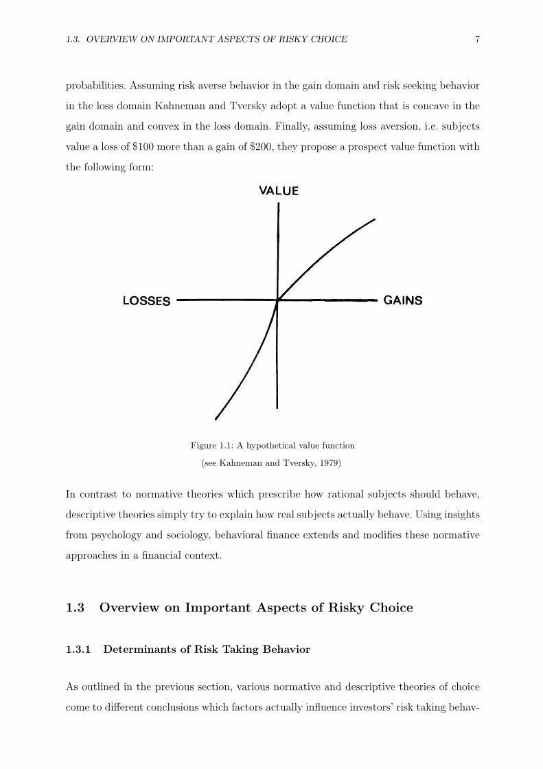
probabilities. Assuming risk averse behavior in the gain domain and risk seeking behavior
in the loss domain Kahneman and Tversky adopt a value function that is concave in the
gain domain and convex in the loss domain. Finally, assuming loss aversion, i.e. subjects
value a loss of $100 more than a gain of $200, they propose a prospect value function with
the following form:
Figure 1.1: A hypothetical value function
(see Kahneman and Tversky, 1979)
In contrast to normative theories which prescribe how rational subjects should behave,
descriptive theories simply try to explain how real subjects actually behave. Using insights
from psychology and sociology, behavioral finance extends and modifies these normative
approaches in a financial context.
1.3 Overview on Important Aspects of Risky Choice
1.3.1 Determinants of Risk Taking Behavior
As outlined in the previous section, various normative and descriptive theories of choice
come to different conclusions which factors actually influence investors’ risk taking behav-

8 CHAPTER 1. GENERAL INTRODUCTION
ior. However, experimental and empirical evidence on determinants of risky choice is not
abound. Whereas expected utility theory suggests that differences in risk taking behavior
are only due to varying risk attitudes, more general risk-value models argue that the three
factors subjective risk perceptions, risk attitude, and subjective return expectations can
influence risky choices. Most evidence in the experimental psychological literature seems
to provide evidence for the usefulness of these more general risk-value models such as the
ones in Sarin and Weber (1993b), Bell (1995) and Butler et al. (2005).
Analyzing cross-cultural differences in choices for lotteries between subjects from the US,
China, Germany, and Poland, Weber and Hsee (1998) detect substantial differences in
risk taking behavior. However, they find remarkably high similarities in attitudes towards
perceived risk indicating that differences in risky choices are mainly due to varying risk
perceptions between respective countries and not due to differing risk attitudes. Moreover,
Weber et al. (2005) show experimentally that the presentation format affects the risk
taking behavior of subjects. Analyzing the effect of different presentation formats such
as bar charts or density functions, they find that risk taking behavior can be biased in
systematic ways depending on the way information about an asset is presented. More
specifically, they illustrate that differences in subjective risk perceptions and subjective
return expectations affect the risk taking behavior.
Similarly, Weber et al. (2002), Johnson et al. (2004), and Hanoch et al. (2006) show that
subjects take different levels of risk depending on the domain they have to make the
decision; i.e. subjects who engage in high recreational risk (sports & leisure domain) do
not need to be derivatives traders (financial domain). The results of all studies suggest
that risk taking is highly domain specific and that conventional risk attitudes that can be
inferred from the shape of the utility function or from the actual behavior are no stable
personality trait. Moreover, these studies suggest that risk taking within a broad domain
tends to be fairly stable. However, it remains ambiguous how far-reaching these results
are and what really constitutes a domain. Thus, it is still an open question whether risk
attitudes that are inferred from lottery decisions should be used to predict investment
behavior in a financial investment context.

1.3. OVERVIEW ON IMPORTANT ASPECTS OF RISKY CHOICE 9
Another interesting point concerning risk taking behavior of individual investors is that
it seems to vary quite substantially over time. Staw (1976) finds evidence for greater risk
taking after losses and less risk taking after gains and terms this finding “escalation of
commitment”. One of two major explanations for observing this effect is the shape of
the value function in the gain and loss domain, respectively. The second explanation for
an “escalation of commitment” effect in the loss domain is based on the self-justification
hypothesis which argues that subjects stick to their actions as they do not want to admit
that their past decisions were incorrect. Contrary to the findings on the “escalation of
commitment” effect, Thaler and Johnson (1990) find that in some situations subjects
take more risks following a gain and less risks after a loss and term this a “house money
effect”. Weber and Zuchel (2005) unify these apparently contradictory strands in the
literature by providing evidence for the “house money effect” if decisions are framed as
lotteries and evidence for “escalation of commitment” if decisions are framed as portfolio
choices.
According to more general risk-value models changes in risk taking behavior over time
could be triggered by changes in subjective risk perceptions, individual risk attitudes
and/or subjective return expectations. The evidence in the literature indicates that risk
attitudes seem to be fairly stable constructs if one accounts for changes in beliefs. Using
large scale panel survey data Sahm (2007) (Michigan Health and Retirement Survey -
HRS) and Klos (2008) (Socio-Economic-Panel - SOEP) provide first evidence for relatively
high levels of stability over time. Moreover, studies analyzing the stability of risk attitudes
in field experiments (see Andersen et al. (2008)) or in laboratory experiments (see Harrison
et al. (2005) and Baucells and Villasis (2009)) tend to find the same result. All studies
illustrate that the relation over time is not perfectly consistent. However, Sahm (2007)
and Baucells and Villasis (2009) argue that observed deviations of risk attitudes from one
period to the other can mostly be attributed to noise or errors and that risk attitudes
tend to be perfectly stable if one accounts for these errors.
Thus, if risk attitudes tend to be fairly stable, then observable differences in risk taking
are most probably due to changes in return expectations and/or changes in risk percep-
tions. Studies analyzing the dynamics of risk perceptions or return expectations find first

10 CHAPTER 1. GENERAL INTRODUCTION
indications for these propositions. On the one hand, Weber and Milliman (1997) and
Mellers et al. (1997) show that risk perceptions vary over time but that perceived risk
attitudes remain highly stable. On the other hand, Shiller et al. (1996), Vissing-Jorgensen
(2003) and Dominitz and Manski (2005) illustrate that return expectations also vary sub-
stantially over time. However, these studies do not analyze the economic consequences
of changes in beliefs and do not relate changes in expectations to changes in risk taking
behavior. Moreover, these studies cannot analyze whether changes in beliefs are due to
past investment failure or success.
The presented evidence indicates that risk taking behavior is no stable trait but influenced
by various factors such as the context of a decision or prior gains and losses. This implies
that traditional risk attitudes as inferred from risky choices are no stable personality trait
but influenced by various situational factors. However, perceived risk attitudes, i.e. risk
attitudes that factor out situational differences seem to be more consistent across domains
than conventional risk attitudes. Sarin and Weber (1993, p. 148) already argue in their
overview of risk-value models that “except for some simple models, e.g. mean-variance,
there is little empirical evidence on the predictive ability of risk-value models.” Therefore,
further research is needed to shed light on the determinants of risky choice in financial
decisions in more detail.
1.3.2 The Effect of Behavioral Biases on the Processing of New Information
and Risk Taking Behavior
Theoretical behavioral models show that various individual biases affect information pro-
cessing and subsequently impact risk taking behavior as well. Some psychological biases
that are often used in these models are overconfidence (see for various facets of overcon-
fidence Langer (1975), Lichtenstein et al. (1982), Alpert and Raiffa (1982), and Russo
and Schoemaker (1992)), hindsight bias (see Fischhoff (1975)), representativeness (see
Kahneman and Tversky (1973)) or disposition effect (see Shefrin and Statman (1985)).
Many behavioral finance models motivate irrational investment behavior using overconfi-
dent investors. In these models all subjects receive private information and overconfident

1.3. OVERVIEW ON IMPORTANT ASPECTS OF RISKY CHOICE 11
investors are too sure that the received signal is correct and hence, put too much weight
on it (see e.g. Kyle and Wang (1997), Benos (1998), Odean (1998b), Wang (1998), Daniel
et al. (1998 and 2001), Fischer and Verrecchia (1999), Hirshleifer and Luo (2001), and
Caballe and Sakovics (2003)). This results in a wrong assessment of means, i.e. individ-
ual misreaction to the signal and subsequently affects trading behavior as overconfident
subjects trade more aggressively and diversify more poorly.
In addition to overconfidence, Biais and Weber (2007 and 2009) develop a theoretical
model in which they study the consequences of the hindsight bias for investment and
trading decisions. They show that hindsight biased agents are not able to remember their
prior expectations correctly after observing a new signal and never seem to be surprised
by new information, as “they knew it all along” (see e.g. Fischhoff (1975) and Camerer
et al. (1989)). This results in hindsight biased agents underestimating the volatility of
risky assets and overweighing the informational content of a signal and thus, overreacting
to this signal. In addition, they illustrate that subjects who overreact more heavily due
to the hindsight bias will invest in less efficient portfolios. Further behavioral biases that
are modeled in theoretical studies are e.g. the disposition effect (see Grinblatt and Han
(2005)) or the representativeness heuristic (see Barberis et al. (1998) and Sorescu and
Subrahmanyam (2006)).
Regardless of the modeling approach all these studies show that behavioral biases result
in enhanced trading volume, lower portfolio performance or more risky investment
decisions. However, as we have seen in the previously presented models the link from a
psychological bias to real economic consequences is a chain of various events. In most
studies a bias leads subjects to misjudge the informational content of a signal. This
results in a misreaction to the new signal which in turn can have various direct or
indirect economic consequences. Figure 1.2 illustrates the chain of events in these models
graphically.
However, empirical evidence on the relationship between psychological biases and eco-
nomic variables is scarce as it is hard to relate underlying and unobservable personal
attributes to economic decisions. Therefore, most empirical studies rely on crude prox-

12 CHAPTER 1. GENERAL INTRODUCTION
Psychological bias(e.g. Overconfidence,
Hindsight Bias)
Economic consequence(e.g. Portfolio Performance,
Trading Volume)
Misre-
action… … … …
Figure 1.2: Relation of psychological biases and economic variables
ies for psychological biases such as gender, age or experience. Barber and Odean (2001)
use the gender of subjects to proxy for overconfidence and show that more overconfident
subjects, i.e. males, trade substantially more. In a similar vein, Barber and Odean (2002)
analyze the trading behavior of subjects who switched from phone-based trading to on-
line trading empirically. They argue that investors who had a good past performance
attribute this good performance to their own abilities, grow more overconfident over time
and switch to online trading. However, overconfidence leads subjects to trade more ac-
tively which in the end results in a subpar performance. Goetzmann and Kumar (2008)
illustrate that under-diversification is correlated with investment decisions that are in line
with overconfidence. They proxy for overconfidence using a subject’s trading volume.
An obvious disadvantage of all purely empirical studies is their use of crude proxies for be-
havioral biases. Trying to improve this by combining survey responses with actual trading
behavior of investors Dorn and Huberman (2005) show that those who think they know
more about finance than the average investor churn their portfolios more often. Similarly
Glaser and Weber (2007) find a relation between overconfidence and trading volume of
real online broker customers. However, they show that only subjects who think they are
better than the average trade more, whereas they cannot find a relationship between mis-
calibration and trading volume. Both studies elicit individual measures of overconfidence
using responses to a questionnaire. Moreover, Fenton-O’Creevy et al. (2003) measure over-
confidence of real traders in British investment banks or more precisely their illusion of
control score within a laboratory experiment. Relating this illusion of control score to
trading performance of traders the authors show that more illusion of control results in
lower performance. Using a purely experimental approach, Biais et al. (2005) measure
miscalibration of students in a questionnaire and subsequently let these students partic-
ipate in an experimental trading market. Their results indicate a significantly negative
relationship between miscalibration and trading performance.

1.3. OVERVIEW ON IMPORTANT ASPECTS OF RISKY CHOICE 13
However, previous empirical and experimental studies still treat the chain of events that is
modeled in theoretical studies as some sort of black box. A noteable exception is the study
by Biais and Weber (2009) who analyze the relationship between hindsight bias and risk
perceptions as well as investment performance in a class experiment with students and
in an experiment with investment bankers. First, they show that hindsight bias reduces
volatility estimates. Second, they illustrate that more hindsight biased agents have lower
performance. Extending their approach and shedding more light on the chain of events
seems to be a promising road for future research. In particular, it seems interesting to
analyze whether behavioral biases lead subjects to over- or underreact to new information
and to relate this misreaction to an intuitive and direct economic measure of performance.
As already pointed out by Biais et al. (2005, p. 308) “it could be interesting in future work
to study when, why, and how particular forms of overconfidence (and other behavioral
biases) will influence economic behavior”.
Even though most researchers agree on the existence of psychological biases at an indi-
vidual level and on their impact on individual risky decisions there is a fierce dispute
if these behavioral biases affect outcomes in financial markets. Proponents of rationality
often argue that in actual markets:
• agents have enough financial incentive and experience to avoid mistakes
• only a small number of rational agents are needed to make market outcomes rational
• agents who are less rational may learn implicitly from the actions of more rational
agents
• agents who are less rational may be driven from the market by bankruptcy, either
by natural forces or at the hands of more rational competitors
For an interesting discussion of these points, see Camerer (1987 and 1992).
Previous findings in the experimental literature show that individual biases do persist in
market settings and do not vanish totally. Some studies find evidence for a lower bias in a
market setting (see e.g. Camerer et al. (1989), Ganguly et al. (2000) or Sonnemann et al.
(2008)), whereas other studies find evidence for even more pronounced degrees of bias in

14 CHAPTER 1. GENERAL INTRODUCTION
market settings (see e.g. Gillette et al. (1999) or Seybert and Bloomfield (2009)). If a bias
is lowered or even elevated in a market setting depends amongst others on the specific bias
at hand and on the experimental approach of the study. Thus, if studies analyze the chain
of events from a psychological bias to economic consequences in more depth using a novel
experimental approach on an individual level, then it is not clear to what degree this bias
will persist in a market setting. Hence, a further promising approach is to analyze these
novel experimental approaches not only on an individual level but also in a real market
environment.
1.4 Outline of the Thesis and Main Results
In order to contribute to a better understanding of individual and aggregate decision
making under risk this thesis addresses the following research questions:
1. What are the main determinants of risky choice? Should financial institutions use
lottery questions to elicit risk attitudes in a financial context? (Chapter 2)
2. Are risk attitudes and expectations stable over time? What drives changes in risk
taking behavior? (Chapter 3)
3. Is overconfidence related to overreaction to new information? Do overreacting sub-
jects invest in less efficient portfolios? (Chapter 4)
4. Is overreaction to new information present in a market setting where subjects receive
feedback and can learn over time? (Chapter 5)
Thus, the main goal of this thesis is to analyze the influence of risk attitudes, expectations,
and biases on decision making under risk. Figure 1.3 illustrates how the respective chapters
of this thesis are related. The remainder of the general introduction will shortly summarize
each chapter.
Chapter 2 of this thesis (joint work with Martin Weber) analyzes determinants of investors’
risk taking behavior as well as the question how financial institutions should elicit their

1.4. OUTLINE OF THE THESIS AND MAIN RESULTS 15
Individual Investment Decisions
Chapter 2: How Risky Do
I Invest
Chapter 4: Overreaction
and Investment Choices
Chapter 3: Changes of
Expectations and Risk
Attitudes
Market Outcomes
Chapter 5: Overreaction in Stock Forecasts and Prices
Market Experiment
Do individual biases translate
into market outcomes?
Individual Experiment
Individual Experiment
Panel Survey
Static - One Point in Time Dynamic - Over Time
Are determinants of risk
taking stable over time?
Figure 1.3: Outline of the thesis
customers’ risk attitudes. Conducting a paper and pencil experiment at the University
of Mannheim with 78 advanced students we show that investors’ risk taking behavior in
financial markets is highly affected by their subjective risk attitude and by the individuals’
subjective risk and return expectations. However, the results indicate that statistical risk
and return measures such as historical volatility or historical returns cannot predict risk
taking behavior. In addition, we provide first evidence for extended domain specific risk
taking behavior. We show that risk attitudes and risk perceptions that are inferred from
lottery related investment tasks are not related to risk perceptions and risk taking behavior
in a stock investment task. Hence, we conclude that financial institutions should not use
lotteries to infer their customers’ risk attitudes. In particular with regards to the MiFID
which urges financial institutions to elicit their customers’ risk preferences and risk profiles
we believe this result to be also important for financial supervisors and practitioners.
In chapter 3 (joint work with Martin Weber) we analyze changes in expectations and risk
attitudes and their impact on risk taking behavior. We use data from a repeated survey
panel that was run with real online broker customers in September 2008, December 2008,
16 CHAPTER 1. GENERAL INTRODUCTION
and March 2009. In all three surveys subjects’ risk attitudes, risk expectations, return
expectations, and risk taking behavior, i.e. the proportion of wealth they are willing to
invest into the stock market compared to a risk free asset, were elicited. Using this unique
dataset we analyze whether risk taking, risk attitudes, and expectations change from one
quarter to the other and whether the latter two have an impact on risk taking behavior.
Our results indicate that risk taking behavior decreases substantially from September to
December and from December to March. Similarly, risk expectations and return expec-
tations also change substantially from one survey to the next one. In contrast, various
measures of risk attitudes are fairly stable over the time periods. Interestingly, observed
changes in risk taking behavior can primarily be attributed to changes in risk and re-
turn expectations but not to changes in past performance or changes in risk attitudes.
Moreover, our findings are valuable for practitioners - who are urged by MiFID (2006) to
elicit their customers’ risk profiles and risk preferences - since we show that risk attitudes
remain fairly stable and that changes in investment behavior can mainly be attributed
to changes in expectations. Lastly, we illustrate that overconfidence seems to be a fairly
stable construct between September and December and tends to decrease slightly from
December to March.
Chapter 4 (joint work with Bruno Biais and Martin Weber) studies the degree of over-
reaction in a novel experimental setup. Replicating the design in the empirical study by
Thomas and Zhang (2008) we are able to analyze the chain of events in behavioral models
in a clean experimental environment. Our three main objectives are to find evidence for
overreaction to new information in a novel experimental design, to relate overreaction to
psychological biases, and to analyze whether overreaction has substantial financial con-
sequences. The experimental study was conducted with 104 students in September 2007
at the University of Mannheim. The majority of participants tend to overreact, however,
the degree of overreaction is very heterogeneous. A few subjects even underreact. Measur-
ing the degree of overconfidence (miscalibration) of each participant we find, consistent
with theoretical predictions, that more overconfident subjects overreact more heavily. In
a second step, we illustrate that overreaction has substantial economic consequences. Us-
ing two directly related economic consequences, portfolio risk and portfolio efficiency, we
find evidence for the following main findings: first, subjects who overreact more heavily

1.4. OUTLINE OF THE THESIS AND MAIN RESULTS 17
invest into riskier portfolios after good signals and less risky portfolios after bad signals.
Second, we show that misreaction to new information, i.e. over- and underreaction harms
portfolio efficiency, as measured by the Sharpe ratio. Providing experimental evidence for
a relation of overreaction to overconfidence and to portfolio efficiency we shed first light
on the chain of events in figure 1.2.
In chapter 5 (joint work with Martin Weber), we study the degree of individual and
aggregate market overreaction in a dynamic experimental auction market in a similar
design as in Thomas and Zhang (2008). In 13 sessions with overall 101 students we find
overreaction to new information both in stock price forecasts and transaction prices.
Interestingly, market forces seem not to help in lowering overreaction to new information
in our novel experimental setting. Moreover, we uncover that subjects are not able to
learn from their previous failures and thus do not correct their erroneous beliefs over the
course of the experiment. That is to say, overreaction in our setting remains on a stable
level although subjects can - at least in theory - learn from other market participants or
from outcome feedback that has been provided to them. Finally, our experimental design
allows us to test the relationship between heterogeneity of beliefs and trading volume.
Previous theoretical studies on this issue show that the higher differences of opinion in a
market are the higher the degree of trading volume (see e.g. Varian (1989) and Kandel and
Pearson (1995)). The study in this chapter is the first that finds experimental evidence
for a positive relation between differences of opinion and trading volume in a continuous
auction market with several market participants.

18 CHAPTER 1. GENERAL INTRODUCTION
Chapter 2
How Risky Do I Invest: The Role of
Risk Attitudes, Risk Perceptions,
and Overconfidence
2.1 Introduction
In the finance literature portfolio choices of investors are typically conceptualized in a
risk-return framework. They are assumed to be a function of expected returns, expected
risk and a subject’s risk attitude. Most of these studies assume that investors employ
the variance-covariance structure of an investment alternative to calculate its risk. Hence,
individual risk attitude determines how much an investor allocates to risky and risk free
assets, respectively. The line of reasoning is that all other things being equal more risk
averse individuals should be inclined to hold less risky assets (see Samuelson (1969)).
Recently, studies have shown that intuitive risk measures such as subjective risk perception
can better proxy for investors’ intuition about financial risks than variance and standard
deviation (see e.g. Weber et al. (2004) and Klos et al. (2005)). More general risk-return
frameworks such as Sarin and Weber (1993b) and Jia et al. (1999) make it possible to
incorporate these more appropriate measures of perceived risk so that the investment
decision can be decomposed as follows:

20 CHAPTER 2: HOW RISKY DO I INVEST
Risk Taking = Perceived Return − Risk Attitude · (Risk Perception). (2.1)
Hence, in this framework risk taking behavior is determined by three major components,
perceived returns, subjects’ risk attitudes, and perceived risks. Research in psychology and
decision analysis has shown that risk perception does not need to be a stable construct and
is influenced by various determinants (see Sitkin and Pablo (1992)). Weber and Milliman
(1997) show that risk perception can vary over time and given previous investment success.
Weber et al. (2005) and Diacon and Hasseldine (2007) document that the presentation
format affects risk perception and consequently risk taking. Rettinger and Hastie (2001)
and Weber et al. (2002) illustrate that differences in risk taking over various domains such
as the financial domain (e.g. investment decision) and the health domain (e.g. seat-belt
usage) can mainly be explained by differences in risk perceptions. More precisely, they
show that risk perceptions vary substantially between different domains.
The present study offers a questionnaire analysis of portfolio choices, i.e. risk taking
behavior of individual investors. We identify determinants actually driving the risk taking
behavior of individuals, and analyze whether objective or subjective measures of risk
and return are better able to explain subjects’ risk taking behavior. In addition, we
evaluate whether the domain in which perceived risk and return are elicited influence our
findings and whether behavioral biases such as overconfidence and optimism can affect
risk taking. To accomplish this we have to elicit risk attitudes, risk and return perceptions,
and overconfidence in several domains, using various methods. This can be only done in
an experimental or questionnaire setup. Therefore, we conducted a questionnaire study
that allows us to assess the respective variables using a variety of approaches. In contrast
to other studies, we analyze the effects of these variables elicited with various methods
on risk taking behavior in two different domains in one single study.
We extend findings in the literature as follows: in line with more general risk-value models
the risk taking behavior in the stock domain, i.e. portfolio choices, is determined by the
riskiness and the return of an investment and also by the individual risk attitude. However,
we show that not only subjective risk expectations but also subjective return expectations
2.1. INTRODUCTION 21
are way better predictors of risk taking behavior in stocks than objective measures of risk
and return such as historical volatilities and returns. Our results add to findings in Weber
and Hsee (1998) who show that including subjective risk expectations instead of the
variance of outcomes in lottery tasks improves the goodness of fit of regression analyses.
We also show that these objective measures do not need to be related with the subjective
ones as the within subject correlations between these variables are modestly positive at
best and sometimes even negative. In addition, our results suggest that even two measures
of subjective risk such as risk perception - measured on an 11-point Likert scale - and
estimated volatility - as inferred from interval bounds - do not need to be highly correlated.
In line with many models on overconfidence and optimism (see e.g. Hirshleifer and Luo
(2001)) we find that more overconfident and more optimistic subjects are going to invest
into riskier portfolios. Previous experimental studies on the interaction between risk taking
and overconfidence (Dorn and Huberman (2005) and Menkhoff et al. (2006)) were not able
to detect a significant relationship between the two variables.
Furthermore, our results supplement findings in the literature on domain specificity (see
e.g. Rettinger and Hastie (2001) and Weber et al. (2002)). First, we show that risk per-
ception does not only vary between two distinct domains such as health and finance or
between investment and gambling decisions but that risk perception can substantially
vary even within a single domain between two very closely related investment opportu-
nities. Second, our extended domain specificity result also applies to return expectations
as only subjective return expectations are able to determine risk taking behavior in the
stock domain. Third, only overconfidence in the stock domain is related to risk taking in
stocks. Fourth, we find that subjective financial risk attitudes affect portfolio choices but
that risk attitudes elicited in the lottery domain do not.
The problem to identify determinants of risk taking correctly is also highly relevant for
practitioners in the financial sector. On the one hand, being able to assess behavior accu-
rately is a competitive advantage for practitioners since it enables them to offer customized
investment advice and bespoken products which are in line with the needs of their cus-
tomers. On the other hand, in many countries financial advisors are legally obliged to
evaluate the appropriateness of an investment for each customer. For example, in Europe

22 CHAPTER 2: HOW RISKY DO I INVEST
the Markets in Financial Instruments Directive (MiFID) by the European Parliament and
the European Council (2004 and 2006) requires financial institutions to collect “informa-
tion as is necessary for the firm to understand the essential facts about the customer
(Article 35, 1)” and to elicit the customers’ “preferences regarding risk taking, his risk
profile, and the purpose of the investment (Article 35, 4).” With respect to the imple-
mentation of the MiFID, it is certainly interesting to notice that we cannot infer anything
about subjects’ risk taking decisions in stocks by asking them to judge artificial lotter-
ies. In addition, our results show that investment advisors could also try to lower their
customers’ overconfidence level and explain them the consequences and risks of their de-
cisions more thoroughly so that heavily overconfident subjects do not take risks that they
do not want.
Our ultimate question in this chapter is centered around an investor who has to decide how
much to invest into a risk free and a risky asset, respectively. Investors in financial markets
are regularly exposed to these kinds of decisions and have to make a trade-off between risk
and return. Typically, financial institutions ask their customers to make their investment
decisions by showing them historical stock price charts of various investments. Hence, the
main feature of our study is the following: participants were shown the stock price path
of five different stocks over the last five years (see question 3.1.5 in the appendix of this
chapter). For each stock they were asked to forecast the price in one year by submitting a
best guess and an upper/lower bound. In addition, participants had to divide an amount
of 10,000 Euro between a risk free asset and the respective stock. The main goal of our
study is to offer direct evidence on how the determinants of risk taking, i.e. risk and return
perceptions and risk attitudes, influence investment behavior in these kind of investment
decisions. Before analyzing this question in more detail we want to illustrate the related
literature more comprehensively.
Analyzing the link between risk attitude and risk taking Fellner and Maciejovsky (2007)
report that the explanatory power of risk attitudes depends on the way these risk attitudes
are elicited. To examine this more thoroughly we want to test which method of risk
attitude elicitation allows us to make inferences about risk taking behavior of subjects in
investments. Amongst others, Warneryd (1996), Kapteyn and Teppa (2002), and Klos and

2.1. INTRODUCTION 23
Weber (2003) provide evidence that intuitive subjective measures of risk seem to be better
predictors of portfolio choice than more sophisticated methods such as lottery questions.
Therefore, we use two risk attitude elicitation methods, based on certainty equivalents
and on subjective self assessments, to analyze which of those two is a better predictor
of risk taking. Thus, if risk attitudes are elicited in a lottery context, the typical line of
reasoning that more risk averse individuals are going to invest into less risky portfolios
should not be validated.
The riskiness and returns of an investment are unambiguously important determinants of
risk taking behavior. However, analyzing individuals’ decisions in lotteries Weber and Hsee
(1998) find that objective risk, i.e. volatility, is not able to explain risk taking behavior
as good as subjective risk. On the other hand, Klos et al. (2005) demonstrate that it is
ambiguous how to measure subjective risk perception in repeated gambles and that it
might be advisable to use various measures of subjective risk.
Moreover, Sitkin and Pablo (1992) and other models in the management literature posit
that risk behavior is mainly determined by risk propensity and subjective risk perception
and that this risk perception does not need to be stable but is influenced by domain
specificity. Amongst others, Slovic (1972) and Rettinger and Hastie (2001) have shown
that risk perceptions can vary over distinct domains such as financial and ethical and that
this disparity can explain differences in observed risk behavior. Weber et al. (2002) even
show that subjects might have differing risk perceptions in two closely related domains
such as investment and gambling but that within a domain risk perceptions are pretty
stable constructs.
In contrast, Dohmen et al. (2009) argue that eliciting individuals’ global assessment of
willingness to take risks is a useful predictor of their risk taking behavior in various
domains. They show that a broadly formulated question such as “How willing are you to
take risks, in general?” is the best all-around predictor of risk taking behavior in different
domains. However, in contrast to our study which measures risk taking as the proportion
a household invests in risky and risk free assets, respectively, they use binary variables
that take the value 1 if a subject engages in the risky action at all and 0 otherwise. A
possible explanation for the seemingly puzzling findings can be found in Brunnermeier

24 CHAPTER 2: HOW RISKY DO I INVEST
and Nagel (2008). They show that changes in wealth are related to the decision to invest
in stocks, i.e. to a binary participation variable, but that changes in wealth essentially
play no role in explaining changes in asset allocation, i.e. the decision how much to invest
into a risk free and risky asset, respectively.
Since we elicit individuals’ asset allocation decisions and not only their binary choice
whether to engage in a risky action or not we hypothesize that the domain specificity
result (see Weber et al. (2002)) should be prevalent in our study. More precisely, we think
there should be an extended within domain specificity in the sense that risk perception
and risk taking behavior in lottery investments does not need to be the same as in stock
investments.
In addition, behavioral biases such as excessive optimism and overconfidence have been
shown to have an influence on risk taking in various theoretical economic models (see
e.g. Odean (1998b), Daniel et al. (2001) or Hirshleifer and Luo (2001)). These models
argue that excessively optimistic subjects will have a higher expected value and hence a
higher demand for a risky asset. In addition, they propose that overconfident investors
have more extreme and in absolute values higher conditional expectation estimates and a
lower conditional variance. Therefore, overconfident traders are going to take larger long
or short positions in the risky asset.
However, theoretical predictions and empirical findings regarding the effect of overcon-
fidence and risk taking do not coincide. For example, Dorn and Huberman (2005) and
Menkhoff et al. (2006) show that risk taking behavior is not significantly related to over-
confidence. Based on previous findings on domain specificity we think that this discrepancy
exists because the empirical studies do not measure overconfidence and risk taking in the
same closely related domain.
The remainder of this chapter is organized as follows. In section 2.2 we describe the design
of the study and illustrate descriptive results. Section 2.3 contains the main results of the
study, and section 2.4 provides a short summary and a conclusion.

2.2. DESIGN AND DESCRIPTIVES 25
2.2 Design and Descriptives
2.2.1 Questionnaire
In this section, we present a detailed overview of the variables and measures employed
throughout our study. All variables were elicited in a questionnaire study. Overall, the
questionnaire consisted of 11 pages, including a cover page and was divided into four
main parts. A shortened version of the questionnaire can be found in the appendix. In
part 1 we measured risk perception and risk taking with two different lottery approaches
and subjective risk attitude in the financial domain. The second part of the questionnaire
was used to elicit various overconfidence scores in a broader context. In part 3, the main
part of the study, subjects were shown five stock price charts, displaying the stock price
development over the last five years. This part was designed to measure subjective as well
as objective risk and return measures and the resulting portfolio choice. Part 4 was used
to measure familiarity with investments, knowledge and various personal variables. Table
2.1 summarizes and defines all variables used in the study and presents the method used
to measure the respective variable.
Part 1
The first lottery task in part 1 asked subjects to divide an amount of 10,000 Euro be-
tween a risk free asset that pays a dividend of 3% and an infinitely divisible lottery that
costs 10,000 Euro and pays out with a probability of 1/2, 12,000 Euro and 9,000 Euro,
respectively. The score Risk Taking (Lottery 1) takes the value 0 if the subject invests the
whole amount into the risk free asset and 100 if the subject invests only into the lottery.
Moreover, Risk Perception (Lottery 1) reflects the perceived riskiness of a lottery and is
measured on a Likert-scale from 0-10, where 0 indicates that subjects perceived no risk at
all and 10 indicates that subjects perceived the risk to be very high. Using Likert-scales to
elicit individual risk perception is a common procedure in the literature (see for example
Weber and Hsee (1998) and Pennings and Wansink (2004)).
The second lottery in part 1 took a different approach of eliciting subjects’ risk taking
behavior by asking them to state their certainty equivalent for a lottery that pays 10,000

26 CHAPTER 2: HOW RISKY DO I INVEST
Table
2.1:D
efinitionof
variables
This
table
sum
marizes
and
defi
nes
varia
bles
used
inth
eem
pirica
lanaly
sisand
illustra
testh
eresp
ective
mea
surem
ent
meth
od.
Varia
ble
Measu
rem
ent
Desc
rip
tion
Part
1
Risk
Takin
g(L
ottery
1)
Sca
le(0
-100)
Mea
sures
the
pro
portio
nofw
ealth
an
indiv
idualin
vests
into
lottery
1(p
=12,12000
Euro
and
q=
12,9000
Euro
).
Risk
Percep
tion
(Lottery
1)
Sca
le(0
-10)
Mea
sures
an
indiv
idual’s
subjectiv
erisk
percep
tion
for
lottery
1w
ithen
dpoin
ts“0
=no
riskat
all”
and
“10
=very
hig
hrisk
”.
Risk
Takin
g(L
ottery
2)
Certa
inty
Equiv
alen
tM
easu
resan
indiv
idual’s
riskta
kin
gfo
rlo
ttery2
(p=
12,10000
Euro
;q
=12,0
Euro
)based
on
the
certain
ty-eq
uiv
alen
tm
ethod.
Ahig
her
certain
tyeq
uiv
alen
tin
dica
tesa
low
erlev
elofrisk
aversio
n.
Risk
Attitu
de
(Lottery
2)
Certa
inty
Equiv
alen
tM
easu
resan
indiv
idual’s
riskattitu
des
usin
gth
epow
erutility
functio
nu(x
)=
xα
.
Risk
Percep
tion
(Lottery
2)
Sca
le(0
-10)
Mea
sures
an
indiv
idual’s
subjectiv
erisk
percep
tion
for
lottery
2w
ithen
dpoin
ts“0
=no
riskat
all”
and
“10
=very
hig
hrisk
”.
Subjective
Risk
Attitu
de
Sca
le(1
-5)
Mea
sures
an
indiv
idual’s
subjectiv
erisk
attitu
de
usin
gth
em
ost
com
mon
elicitatio
nm
ethod
inin
vestm
ent
advice.
Asco
reof1
indica
tesa
hig
hlev
elofrisk
aversio
nand
asco
reof5
alo
wlev
el.
Part
2
Misca
libratio
n(G
enera
lK
now
ledge)
Confiden
ceIn
tervals
Mea
sures
an
indiv
idual’s
deg
reeofm
iscalib
ratio
nw
ithresp
ectto
10
questio
ns
concern
ing
gen
eralknow
ledge.
Better
Than
Avera
ge(G
enera
lSelf
assessm
ent
vs.
Mea
sures
overco
nfiden
cebased
on
the
com
pariso
nbetw
eenth
eassessm
ent
ofone’s
ow
nperfo
rmance
and
the
Know
ledge)
assessm
ent
ofoth
ersassessm
ent
ofth
eperfo
rmance
ofth
eavera
ge
subject
inth
egen
eralknow
ledge
task
.
Illusio
nofC
ontro
lSca
le(0
-1)
Based
on
answ
ersto
two
statem
ents,
this
varia
ble
mea
sures
the
exten
tto
which
an
indiv
idualth
inks
he
/sh
e
can
contro
lra
ndom
even
ts.T
he
endpoin
tsin
dica
te“0
=no
contro
lat
all”
and
“1
=to
talco
ntro
l”.
Part
3
Risk
Percep
tion
(Stocks)
Sca
le(0
-10)
Mea
sures
an
indiv
idual’s
subjectiv
erisk
percep
tion
for
asto
ckw
ithen
dpoin
ts“0
=no
riskat
all”
and
“10
=very
hig
hrisk
”.
Risk
Takin
g(S
tocks)Sca
le(0
-100)
Mea
sures,
on
apercen
tages
basis,
the
am
ount
ofm
oney
an
indiv
idualis
willin
gto
invest
into
each
ofth
e5
stock
s
com
pared
toa
riskfree
asset
and
isused
as
apro
xy
for
portfo
lioch
oice.
Expected
Retu
rn(S
tocks)Poin
tE
stimate
Mea
sures
an
indiv
idual’s
expected
return
for
5diff
erent
stock
s.
Expected
Vola
tility(S
tocks)B
ounds
Mea
sures
an
indiv
idual’s
expected
vola
tilityby
transfo
rmin
gestim
ates
ofbounds
into
vola
tilityestim
ates.
Optim
ism(S
tocks)Poin
tE
stimate
Mea
sures
the
diff
erence
betw
eensu
bjectiv
eex
pected
and
histo
ricalretu
rn.
Misca
libratio
n(S
tocks)B
ounds
Mea
sures
an
indiv
idual’s
misca
libra
tion
by
standard
izing
expected
vola
tilityw
ithhisto
ricalvola
tility.
Better
Than
Avera
ge(S
tocks)Self
assessm
ent
vs
Mea
sures
overco
nfiden
cebased
on
the
com
pariso
nbetw
eenth
eassessm
ent
ofone’s
ow
nperfo
rmance
and
the
assessm
ent
ofoth
ersassessm
ent
ofth
eperfo
rmance
ofth
eavera
ge
subject
inth
esto
ckprice
task
.
Part
4
Dem
ographics
Vario
us
dem
ogra
phic
varia
bles
such
as
age,
gen
der,
field
ofstu
dies
and
the
num
ber
ofterm
salrea
dy
studied
.
Fam
iliarity
Dum
my
varia
ble
that
takes
the
valu
e1
ifan
indiv
idualhas
ow
ned
investm
ent
pro
ducts
with
inth
ela
styea
rand
0oth
erwise.
Fin
ancia
lK
now
ledge
Sca
le(1
-5)
Mea
sures
selfassessed
financia
land
statistica
lknow
ledge
ofsu
bjects
with
endpoin
ts“1
=very
good”
and
“5
=bad”.

2.2. DESIGN AND DESCRIPTIVES 27
Euro with probability 1/2 and 0 Euro otherwise. We elicited Risk Taking (Lottery 2) with
the certainty equivalence method by repeatedly asking subjects whether they prefer a sure
payment of x Euro or the lottery, with x ranging from 1,000 Euro to 9,000 Euro. This
method also allows us to calculate risk attitudes in a lottery context utilizing a specific
utility function. Inferring risk attitudes from certainty equivalents using a parametric
approach is a common method in the literature (see e.g. Krahnen et al. (1997) and Dohmen
et al. (2009)). To construct an explicit Risk Attitude (Lottery 2) score we follow the
literature in decision analysis (see Tversky and Kahneman (1992)) and transform the
stated certainty equivalents for lottery 2 into risk aversion parameters using the power
utility function u(x) = xα.1 In addition, Risk Perception (Lottery 2) was elicited in the
same way as for lottery 1.
The last question in part 1 (Subjective Risk Attitude) asked participants to rate their
willingness to take financial risks on a scale from 1 to 5 with the endpoints “1 = very low
willingness” and “5 = very high willingness”. This easy and quick classification method
is the common method used in investment advice. In addition, subjective risk attitudes
on Likert scales are also used in large scale survey such as the SOEP (see Dohmen et al.
(2009)).
Part 2
In the second part of the questionnaire, participants first had to state 90% confidence
intervals to 10 general knowledge questions, such as “How long is the Mississippi”. More
precisely, they had to submit upper (lower) bounds such that the true answer to each
question should not exceed the upper bound (not fall short of the lower bound) with
a probability of 95%. Confidence intervals are often used to detect miscalibration, i.e.
overconfidence (Alpert and Raiffa (1982) and Russo and Schoemaker (1992)). A subject
is classified as miscalibrated if he / she answers less than 9 questions correctly, i.e. the
lower the Miscalibration (General Knowledge) score, the more overconfident the subject
is.
1Note that our results in section 2.3 remain stable if we simply use the certainty equivalents or CRRA transformations
to derive a risk aversion parameter.

28 CHAPTER 2: HOW RISKY DO I INVEST
To measure whether an individual is prone to the better than average effect in the general
knowledge context we asked subjects to assess how many intervals they and the average
participant, respectively, answered correctly in the general knowledge task. The relating
variable Better Than Average (General Knowledge) is calculated as the difference between
these two answers and takes positive values for subjects that think they have answered
more questions correctly than the average subject.
Moreover, within part 2 we also elicited Illusion of Control following the method in Dorn
and Huberman (2005) and Glaser and Weber (2007). To estimate illusion of control, we
consider the extent to which survey participants agree on a five-point scale from 1 (fully
agree) to 5 (totally disagree) with the following statements: “I am able to identify stocks
that will beat the market in the future” and “My stock forecasts are always correct”.
The Cronbach alpha for these two variables is 0.71 and is above the threshold which is
normally assumed to indicate reliability (see Nunnally (1978)). Hence, we aggregate the
answers to both questions, normalize them on a scale between 0 and 1 and calculate a
joint illusion of control score. This illusion of control score takes a value of 1 if subjects
are prone to the illusion of control bias and 0 if they are absolutely not prone to it.2
Part 3
In part 3, subjects were shown charts illustrating the stock price development of the
following five DAX companies over the course of the last five years (see question 3.1.5 in
the appendix): DaimlerChrysler, Infineon Technologies, Continental, Munchener Ruck and
Adidas. We used real stocks to make the task more realistic and controlled for individual
experiences using subjective risk and return expectations. To construct the five stock
charts we used daily closing prices for the time period November 2001 to November
2006 obtained from Thomson Financial Datastream. In line with, Glaser et al. (2007) we
included firms with stable, upward and downward stock price trends. Furthermore, we
standardized the area in which the stock graphs were displayed according to the method
proposed by Lawrence and O’Connor (1993): the two bounds were chosen such that the
2We also asked subjects whether they agree to the following statement “losses and gains in stock markets are just a
matter of chance”. Our results in the following sections do not change if we calculate illusion of control taking all three
questions. However, the Cronbach alpha for all three questions decreases substantially to 0.5.

2.2. DESIGN AND DESCRIPTIVES 29
price at the end was approximately in the middle of the chart and the area in which
the stock price chart was displayed fills about 40% of the total vertical dimension of the
graph. This procedure was carried out to avoid that subjects would interpret the vertical
endpoints of the graph as boundaries.
For all five stocks we elicited the following variables:
• Risk Perception (Stocks)
• Risk Taking (Stocks)
• Expected Return (Stocks)
• Expected Volatility (Stocks)
• Better Than Average (Stocks)
Risk Perception (Stocks) reflects the perceived riskiness of each stock and is measured
on a Likert-scale from 0-10. Again, lower scores of risk perception indicate that subjects
perceived the risk of the respective stock to be lower. To measure individuals’ risk taking
behavior or portfolio choice we asked them to allocate 10,000 Euro between the particular
stock and a risk free asset that yields a yearly return of 3%, assuming an investment
horizon of one year. The corresponding variable Risk Taking (Stocks) takes values from
0 to 100 with the endpoint 0 (100) indicating that the subject invests the whole amount
into the risk free asset (risky stock).3
To measure the expected volatility and expected returns in the stock domain we asked
individuals to state a median stock price forecast as well as upper and lower bounds for
90% confidence intervals for the stock price in one year. More precisely, we asked them
to submit what they consider to be lower and upper bounds so that there is only a 5%
chance that the price in one year will be below the lower bound and a 5% chance that it
will be higher than the upper bound. We transformed all three stock price estimates for
each subject and for all five stock charts into return estimates.4
3Warneryd (1996) illustrates that questions involving hypothetical risky choices seem to work quite well.
4The return estimates r(s) for the three stock price estimates p(s) for each stock i and each subject j are calculated as
follows: r(s)ji =
p(s)ji−valuei
valuei), with valuei indicating the price of stock i in November 2006.

30 CHAPTER 2: HOW RISKY DO I INVEST
Since we asked subjects to state median returns we first transform median estimates into
mean estimates using the method proposed by Keefer and Bodily (1983) (Expected Return
(Stocks) = 0.63 · r(0.5) + 0.185 · (r(0.05) + r(0.95)). Furthermore, we calculate a subject’s
optimism regarding the return of a stock as the difference between the expected and
the historic return (Optimism (Stocks) = Expected Return (Stocks) - Historical Return
(Stocks)). A higher score indicates a higher level of optimism.
Using the median forecast and both the upper and the lower bound allows us to get a
measure for the expected volatility in the stock domain by using the methodology sug-
gested in Keefer and Bodily (1983). This method transforms stated confidence intervals
into volatility estimates5 and has been widely used in the empirical literature (e.g. Gra-
ham and Harvey (2005), Ben-David et al. (2007), and Glaser et al. (2007)). The resulting
variable Expected Volatility (Stocks) measures an individual’s subjective volatility forecast
for each stock. In addition to the expected volatility we can also compute an easily inter-
pretable and standardized measure of miscalibration in the stock domain by dividing the
estimated one year volatility by minus one times the historical volatility (Miscalibration
(Stocks) = −Expected V olatility (Stocks)Historical V olatility
). This standardization yields a miscalibration mea-
sure which is close to 0 for excessively overconfident subjects and equal to -1 for perfectly
calibrated subjects.6
Furthermore, we also asked individuals to assess for how many of the interval questions
they and the average subject, respectively, indicated wide enough confidence intervals.
Subjects prone to the better than average effect will assess their performance in the
stock domain to be better than the average subject’s performance. Hence, their Better
Than Average (Stocks) score, representing the spread between these two answers, will be
positive.
5Keefer and Bodily (1983) propose that an extended Pearson-Turkey approximation is a widely applicable approxima-
tion for continuous probability distributions if one has information on the upper bound r(0.95), the lower bound r(0.05)
and the median r(0.5). Since we collected exactly these three point estimates for every stock, we can use their proposed
method to recover each respondents’ probability distribution for each stock i by using the following formula: Volatilityi =√[0.185 * r(0.05)2i + 0.63 * r(0.5)2i + 0.185 * r(0.95)2i ]− [0.63 * r(0.5)i + 0.185 * r(0.05)i + 0.185 * r(0.95)i]
2.
6We calculated one year volatilities for each stock by using daily returns for the last five years, exactly the same time
period subjects were given in the questionnaire. To check for robustness, we computed historical one year volatility using
non overlapping monthly and quarterly returns. The results are essentially the same and since the division is only a
standardization we will in the following only report results with respect to one year volatilities on the basis of daily returns.

2.2. DESIGN AND DESCRIPTIVES 31
Part 4
Within part 4 we elicited demographic variables, knowledge, and familiarity with invest-
ments. Demographics include age, gender, field of study, and terms studied. We proxied
for familiarity by asking the subjects to indicate the number of investment products they
have owned within the last year. Subsequently, we generated a dummy variable Familiar-
ity that takes the value 1 if a subject has invested in the last year and 0 otherwise. In the
end, we measured both financial and statistical knowledge using simple self-assessment
questions. Subjects had to indicate their knowledge in each field on a scale from 1 to 5,
with 1 indicating very good knowledge and 5 indicating bad knowledge in the respective
field.
2.2.2 Descriptive Statistics
The questionnaire was filled out by 78 students of a Behavioral Finance class and a
Decision Analysis class at Mannheim University on November 15 and 16, 2006. It took the
students on average 30 minutes to complete the questionnaire. All students who returned
a completely filled out questionnaire automatically participated in a lottery which paid
out in each case 30 Euro to overall 9 randomly selected participants. This amounts to an
average payment of approximately 3.5 Euro per person. Since we asked students for their
subjective perception of risky situations and for their subjective estimates of future stock
prices we chose to pay out fixed amounts to avoid strategic behavior.7
The mean and median scores for all demographic and risk variables are presented in table
2.2. The average age of the participants is 24 years, with 32% of the respondents being
female. Approximately 90% of the students in our sample study business administration or
economics and are within their fourth year on average (6.8 semesters studied). About 57%
of all respondents have held stocks or other assets within the last year. The self-reported
7In addition, it is not common to pay participants with an incentive compatible payment scheme in surveys in which
participants are asked to state confidence intervals or to submit their individual risk perception. A common example of
such a large scale survey is the Duke/CFO Outlook Survey (see http://www.cfosurvey.org). Moreover, Cesarini et al.
(2006) provide evidence that monetary incentives do not decrease miscalibration significantly. In a similar vein Camerer
and Hogarth (1999) argue in their review of 74 experiments that rationality violations do not disappear purely by raising
incentives.

32 CHAPTER 2: HOW RISKY DO I INVEST
Table 2.2: Descriptive statistics on demographics and risk
This table reports mean and median scores and standard deviations on demographic and risk variables. Num-
bers in parentheses indicate the possible range of answers for the respective variable.
Mean Score Median Score Standard deviation
Female 0.316 0
Age 24.027 23 5.288
Semester 6.808 7 1.751
Familiarity 0.566 1
Statistical Knowledge 2.776 3 0.838
(1-5)
Financial Knowledge 3.342 3 1.009
(1-5)
Subjective Risk Attitude 2.592 2.5 0.877
(1-5)
Risk Perception (Lottery 1) 4.105 3 1.820
(1-10)
Risk Taking (Lottery 1) 58.75 60 28.914
(1-100)
Risk Perception (Lottery 2) 7.118 7 1.664
(1-10)
Risk Taking (Lottery 2) 4144.737 4000 1201.406
(1000-9000)
Risk Perception (Stocks) 5.426 6 1.914
(1-10)
Risk Taking (Stocks) 43.639 40 26.332
2.3. RESULTS 33
statistical knowledge score on a scale from 1 (very good) to five (bad) is approximately
2.8 and the one for financial knowledge is 3.3 indicating that students were slightly more
confident in their statistical knowledge. For Financial Knowledge we find a significant
difference for students in our Decision Analysis class (3.5) and our Behavioral Finance
class (2.95). Table 2.2 further documents that participants stated an average subjective
risk attitude of 2.6 on a scale from 1 to 5. The risk of participating in a two outcome lottery
was perceived as higher (7.1) than the average risk for all five stocks (5.4). Moreover,
the table shows that subjects invest on average 43.6% of their funds in part 3 of the
questionnaire into the risky asset.
Analyzing the various overconfidence measures we have elicited, we find substantial de-
grees of overconfidence among subjects for most of our measures. However, the degree of
overconfidence varies substantially, being relatively low for both better than average scores
and being substantially high for both miscalibration scores. More precisely, for miscalibra-
tion in the general knowledge context we find that the average subject submits only six
correct answers and for miscalibration in the stock context we find that the average sub-
ject states wide enough confidence intervals for less than two questions. Using Wilcoxon
matched-pairs signed rank tests for both measures shows that there is substantial mis-
calibration in both domains (p-values < 0.0001). These findings are approximately in the
same range as the results by Russo and Schoemaker (1992) who show that individuals
submit on average answers that include the true answer in 40%-60%. Analyzing illusion
of control, we find consistent with Dorn and Huberman (2005) that subjects are prone to
the illusion of control bias. However, for better than average effects our results are not as
clear-cut. On the one hand, we find slightly positive better than average scores in both
domains. On the other hand, these effects are only weakly significant or not significant at
all.
2.3 Results
In this section we analyze which factors actually govern risk taking behavior in a stock
related context. As illustrated in section 2.1 individuals’ risk taking behavior is argued to
34 CHAPTER 2: HOW RISKY DO I INVEST
be determined by three major components: risk attitude, perceived return and perceived
risk (see equation 2.1). Recent work by Weber and Milliman (1997), Weber et al. (2002),
and Klos et al. (2005) shows that subjectively perceived risks do not need to coincide
with variance estimates and that perceived risks in one domain do not need to coincide
with perceived risks in another one. To allow for these findings we elicited in our setup
risk attitudes, risk perceptions, and return perceptions using various methods. In the
following, we will first analyze determinants of risk taking behavior in the stock domain
on an aggregate level before we turn to analyses on a disaggregate, single-stock level. In
addition, we will also perform further robustness checks of our results.
2.3.1 Determinants of Risk Taking Behavior in Stocks on an Aggregate Level
Before analyzing factors that determine aggregate risk taking behavior, i.e. portfolio
choices, in a multivariate setting we first carry out simple bivariate interactions between
aggregated portfolio choice and variables argued to affect risk taking behavior of individ-
uals. We use two major categories of determinants: first, variables that are not directly
related to the stock domain such as Subjective Risk Attitude and lottery related variables
(i.e. Risk Perception (Lottery 1), Risk Perception (Lottery 2) and Risk Attitude (Lottery
2)). Second, risk and return perceptions in the stock domain such as Risk Perception
(Stocks), Miscalibration (Stocks), and Optimism (Stocks).8
To aggregate the variables in the stock domain we make use of three aggregation methods:
first, we take the mean over all five stock questions. Second, we take the median over
all five stock questions and third we use a dummy variables method for Miscalibration
(Stocks) and Optimism (Stocks). This dummy method assigns for each question a value of
1 to individuals who are excessively optimistic or overconfident and a value of 0 otherwise.
8Using Expected Volatility (Stocks) and Expected Return (Stocks) instead of the standardized scores Miscalibration
(Stocks) and Optimism (Stocks) yields robust results. However, as we use aggregated scores the interpretation of these
scores that are not standardized by the respective historical variable is not as straightforward.

2.3. RESULTS 35
Since all three measures essentially yield the same results, subsequently we will only report
the results for the aggregation rule using the mean score.9
However, before using these aggregated scores we have to assess the internal validity of
each variables over the five questions. We have to check whether we find stable individ-
ual differences for the level of Risk Taking (Stocks), Risk Perception (Stocks), Optimism
(Stocks) and Miscalibration (Stocks), respectively. Hence, we calculate the Cronbach al-
phas for the four variables over all five questions. The Cronbach alphas vary between 0.59
(Risk Perception (Stocks)) and 0.88 (Miscalibration (Stocks) and Risk Taking (Stocks)).
Since Nunnally (1978) argues that alphas above 0.7 are an indication for stable individual
differences we will in the following aggregate analyses exclude Risk Perception (Stocks).10
Having assessed the internal validity of our aggregated scores we study simple correlation
coefficients between risk taking in the stock domain and determinants of risk taking. Panel
A of table 2.3 illustrates Spearman correlation coefficients (1) and Pearson correlation
coefficients (2) between Risk Taking (Stocks) and related variables. The results show that
Subjective Risk Attitude is strongly positively related with Mean Risk Taking (Stocks).
Hence, subjects who have a higher Subjective Risk Attitude also invest on average into
more risky portfolios. Panel A also shows that neither risk perceptions in both of our
lotteries nor risk attitudes as inferred from certainty equivalents are able to determine
individuals’ average risk taking behavior. Moreover, we also find that Mean Optimism
(Stocks) is not related to portfolio choices. However, Miscalibration (Stocks) is positively
related to the average portfolio risk indicating that individuals who are more overconfident
invest into substantially more risky portfolios.
To further strengthen our results on determinants of risk taking we analyze the rela-
tion between portfolio choice and its determinants in a multivariate setting controlling
for various effects.11 Panel A in table 2.4 presents results of ordinary least squares re-
9Using the mean as an aggregation rule the stock related variables are calculated as follows: Mean Risk Taking (Stocks)
= [∑5
i=1Risk Takingi]/5, Mean Risk Perception (Stocks) = [
∑5
i=1Risk Perceptioni]/5, Mean Miscalibration (Stocks) =
[∑5
i=1−Estimated volatilityi
Historical volatilityi]/5 and Mean Optimism (Stocks) = [
∑5
i=1Optimismi]/5.
10Our results in the following analyses of aggregate risk taking are robust even if we include Risk Perception (Stocks).
11Throughout the chapter we report results of simple ordinary least square regressions and fixed or random effects panel
regressions although all of our dependent variables are theoretically bounded from both sides. However, in our dataset

36 CHAPTER 2: HOW RISKY DO I INVEST
Table 2.3: Correlation coefficients
Panel A of this table reports correlation coefficients between Mean Risk Taking (Stocks) and various aggregate
determinants of risk taking behavior. Column (1) reports Spearman rank correlations whereas column (2)
reports Pearson correlation coefficients. Panel B reports Spearman rank correlation coefficients between Risk
Taking (Lottery 1) (column 3) or Risk Taking (Lottery 2) (column 4) and various aggregate determinants of
risk taking behavior. p-values are reported in parentheses. * indicates significance at the 10% level, ** indicates
significance at the 5% level and *** indicates significance at the 1% level.
Panel A Panel B
(1) (2) (3) (4)
Subjective Risk Attitude 0.350 0.415 0.427 0.445
(0.002)*** (0.002)*** (0.000)*** (0.000)***
Risk Perception (Lottery 1) -0.008 -0.053 -0.460 -0.313
(0.949) (0.648) (0.000)*** (0.006)***
Risk Perception (Lottery 2) -0.023 -0.083 -0.329 -0.504
(0.847) (0.474) (0.004)*** (0.000)***
Risk Attitude (Lottery 2) 0.034 0.173 0.359
(0.770) (0.136) (0.002)***
Mean Optimism (Stocks) 0.046 -0.013 0.001 0.130
(0.692) (0.915) (0.990) (0.263)
Mean Miscalibration (Stocks) 0.256 0.286 -0.083 -0.129
(0.025)** (0.012)** (0.476) (0.266)

2.3. RESULTS 37
Table 2.4: Determinants of risk taking behavior on an aggregate level
This table presents results of ordinary least squares regressions with heteroscedasticity consistent standard
errors. Dependent variable in panel A (model 1 - 3) is Mean Risk Taking (Stocks), dependent variable in panel B
(model 4) is the level of risk taking in lottery 2 and in model (5) the level of risk taking in lottery 1. Independent
variables are Subjective Risk Attitude, risk perceptions in lotteries, Risk Attitude (Lottery 2), Mean Optimism
(Stocks), Mean Miscalibration (Stocks) and additional controls such as demographics, familiarity with stock
investments, knowledge and various overconfidence measures. We report regression coefficients and p-values
in parentheses. * indicates significance at the 10% level, ** indicates significance at the 5% level and ***
indicates significance at the 1% level.
Panel A Panel B
(1) (2) (3) (4) (5)
Subjective Risk Attitude 10.087 9.725 9.209 193.371 14.283
(0.000)*** (0.000)*** (0.008)*** (0.218) (0.001)***
Mean Optimism (Stocks) 17.369 27.099 -924.998 8.055
(0.468) (0.391) (0.534) (0.824)
Mean Miscalibration (Stocks) 13.594 17.157 -281.341 9.018
(0.002)*** (0.013)** (0.555) (0.362)
Risk Perception (Lottery 1) 0.054 -147.161 -5.132
(0.971) (0.037)** (0.003)***
Risk Perception (Lottery 2) -0.651 -260.806 -1.546
(0.672) (0.006)*** (0.344)
Risk Attitude (Lottery 2) -1.496 6.974
(0.814) (0.179)
Controls No No Yes Yes Yes
Constant 17.493 31.192 0.238 3,524.679 2.659
(0.015)** (0.001)*** (0.995) (0.082)* (0.955)
Observations 76 76 71 71 71
Adjusted R-squared 0.161 0.221 0.083 0.308 0.322

38 CHAPTER 2: HOW RISKY DO I INVEST
gressions with Mean Risk Taking (Stocks) as dependent variable. Regression (1) shows
that Subjective Risk Attitude can explain individuals’ average risk taking in stocks sig-
nificantly. Adding subjective risk and return perceptions in regression (2) in the form of
Miscalibration (Stocks) and Mean Optimism (Stocks) improves the goodness of fit of our
regression substantially. Including these subjective expectations yields the results that
both Subjective Risk Attitude and Miscalibration (Stocks) are significant determinants of
risk taking but not Mean Optimism (Stocks). In regression (3) we add risk perceptions and
risk attitude inferred from lotteries and further dependent variables such as demograph-
ics, familiarity with stock investments, knowledge and overconfidence measures in other
domains. The results with regard to the significance of the two main dependent variables
Subjective Risk Attitude and Miscalibration (Stocks) remain constant. However, none of
our additional variables is significantly related to portfolio choices. In addition, adding all
additional control variables decreases the goodness of fit of our regression indicated by
the adjusted R-squared.
Overall, our analyses on the aggregate level suggest that risk taking of individuals is
determined by their subjectively elicited risk attitude and by their level of overconfidence,
i.e. miscalibration, and that other variables are not able to determine individuals’ risk
taking behavior. In the following subsection we will analyze whether our results also hold
if we study the effects on a disaggregated single stock level.
2.3.2 Determinants of Risk Taking Behavior in Stocks on a Disaggregate
Level
The analyses in the previous subsection have the disadvantage that we have to use ag-
gregate scores and cannot control for question specific effects. To mitigate these problems
we document in the following results of multivariate regressions of subjects’ risk taking
behavior performed on a single stock level. However, since it is possible that risk taking
behavior between the five stocks may be correlated within individuals we cannot analyze
the data by running simple ordinary least squares regressions. We account for the problem
these theoretical bounds are almost never reached. In addition, we ran all our multivariate analyses using censored tobit
regressions and obtained essentially the same results.

2.3. RESULTS 39
of possible non-independent residuals within individuals by using two approaches. First,
we cluster our observations over subjects and analyze the relationship between risk and
overconfidence on a single stock level using clustered ordinary least squares regressions.
Clustering the data over subjects allows us to examine the individual effects on risk taking
for each stock. Second, we use fixed effects and random effects panel regressions with the
two dimensions subjects and stocks. Table 2.5 presents the results of these estimations.12
We have illustrated in previous sections that risk taking in a risk-return framework is
assumed to be governed by a tradeoff between the return of an investment and its risk
and also by an individual’s risk attitude. In the finance literature it is common to equate
expected returns by historical returns and expected risks by historical variance. Hence, the
first regression in table 2.5 tries to explain subjects’ risk taking in the stock domain using
these variables. The regression results show that Subjective Risk Attitude and Historical
Volatility (Stocks) determine the risk taking behavior. Subjects invest more into stocks if
they are less risk averse and if the historical volatility of the stock is lower. Interestingly,
historical stock returns are not able to determine the investment decision of subjects.
However, this is not surprising as subjects in our study were mainly business students who
learn in their studies that past performance is no perfect indication for future performance.
More general risk-value models argue that subjects might base their decisions more on
subjective measures of risk and return instead of objective ones. Hence, it might be more
appropriate to include subjective measures of risk and return such as Expected Return
(Stocks) as well as Risk Perception (Stocks) and Expected Volatility (Stocks) into our re-
gression as they could actually affect the level of risk taking more heavily. To accommodate
for this proposition we include these variables instead of the historical ones in regression
(2). Using both Risk Perception (Stocks) and Expected Volatility (Stocks) in a single re-
gression might cause multicollinearity problems if the two variables were highly correlated
with each other. However, we find that Risk Perception (Stocks) is hardly related with
Expected Volatility (Stocks) as the within subject correlations are at best moderately pos-
itive with rank correlations of 0.12 (Kendall tau) and 0.16 (Spearman rho), respectively.
This result suggests that the two subjective risk measures do not need to coincide and
12Again, our results remain stable if we run the regressions using censored tobit instead of ordinary least squares.

40 CHAPTER 2: HOW RISKY DO I INVEST
Table 2.5: Determinants of risk taking behavior in stocks on a disaggregate level
This table presents clustered ordinary least squares as well as fixed effects and random effects panel regressions
with the two dimensions subjects and stocks. Dependent variable in all regressions is Risk Taking (Stocks).
Regressions (1)-(4) present results of clustered ordinary least squares regressions where standard errors take
clustering over subjects into account. Regression (5) presents results of a fixed effects model and column (6)
documents results of a random effects model. Independent variables are Subjective Risk Attitude, Risk Atti-
tude (Lottery 2), Optimism (Stocks), Miscalibration (Stocks), historical return and volatility of each stock,
subjective risk and return measures such as risk perception, expected volatility and expected return. More-
over, we include additional controls such as stock dummies, demographics, familiarity with stock investments,
knowledge and various overconfidence measures. We report regression coefficients and p-values in parentheses.
* indicates significance at the 10% level, ** indicates significance at the 5% level and *** indicates significance
at the 1% level.
(1) (2) (3) (4) (5) (6)
Subjective Risk Attitude 10.087 9.514 9.225 9.236 9.136
(0.000)*** (0.001)*** (0.003)*** (0.003)*** (0.015)**
Risk Perception (Lottery 1) 0.297 0.226 0.350
(0.826) (0.866) (0.822)
Risk Perception (Lottery 2) -0.218 -0.231 -0.121
(0.874) (0.866) (0.947)
Risk Attitude (Lottery 2) -0.730 -0.291 -0.764
(0.905) (0.962) (0.912)
Historical Return (Stocks) 2.569 4.339 4.290 4.310
(0.654) (0.387) (0.436) (0.431)
Historical Volatility (Stocks) -50.558 -30.484 -39.377 -37.865
(0.004)*** (0.119) (0.013)** (0.014)**
Expected Return (Stock) 24.622 30.851 30.034 30.349
(0.018)** (0.004)*** (0.000)*** (0.000)***
Optimism (Stocks) 33.690
(0.001)***
Risk Perception (Stocks) -3.723 -3.398 -3.280 -3.940 -3.873
(0.000)*** (0.002)*** (0.003)*** (0.000)*** (0.000)***
Expected Volatility (Stock) -26.530 -28.292 -18.331 -20.017
(0.003)*** (0.007)*** (0.016)** (0.005)***
Miscalibration (Stocks) 11.215
(0.003)***
Controls No No Yes Yes Yes
Stock Dummies No No No Yes No
Constant 34.449 46.521 30.057 1.409 83.746 37.432
(0.000)*** (0.000)*** (0.418) (0.969) (0.000)*** (0.408)
Observations 380 377 352 352 352 352
Adjusted R-squared 0.136 0.260 0.262 0.271
Number of Groups 71 71
R-squared overall 0.166 0.301
R-squared within 0.308 0.308
R-squared between 0.093 0.296

2.3. RESULTS 41
is consistent with previous findings in the literature (see e.g. Klos et al. (2005) and We-
ber et al. (2005)). Furthermore, to control for possible multicollinearity problems in this
regression we carry out variance inflation factor tests.
The results of regression (2) document that indeed Subjective Risk Attitude and both
subjective risk and return measures in the stock domain significantly influence the risk
taking decision in the stock domain. We find on a single stock level that the higher a
subject perceives the expected return the more he / she invests into the stock. In a
similar vein the lower he /she perceives the risk of the investment subjectively and the
lower he / she expects the volatility to be the more risk he / she will take. Interestingly,
the adjusted R-squared in regression (2) is nearly twice as high as in the first regression.
Comparing these fits shows that regressions using objective risk measures do not predict
risk taking behavior nearly as well as regressions using subjective measures which provides
support for similar findings by Weber and Hsee (1998) in another context. Moreover, as
indicated by the results of the within subject correlations multicollinearity seems to be
no problem as all variance inflation factor scores are way below the critical threshold of
10, indicating a low degree of multicollinearity, if any.
In a next step we want to disentangle the role of objective and subjective risk and return
measures and analyze the interesting question on which measures subjects rather rely on
when making their decisions. To do this we run regression (3) and include both objective
and subjective measures at once. In addition, as various studies in the literature argue
that gender (see e.g. Eckel and Grossman (2008)), age, experience and knowledge (see e.g.
Barsky et al. (1997) and Donkers et al. (2001) who both use large scale survey studies
analyzing the whole population) might influence risk taking behavior we test this by
adding these variables in the same regression. We also include risk perceptions and risk
attitude in lotteries as additional control variables. As we might run into multicollinearity
problems in our analysis we first want to find if objective and subjective variables measure
distinct things before we carry out the regression.
Analyzing the within subject rank correlation coefficients (Kendall tau and Spearman)
between objective and subjective measures of risk and return we actually find support
for this proposition. Comparing historical returns with expected returns we even find a
42 CHAPTER 2: HOW RISKY DO I INVEST
slightly negative relation indicated by negative within subject rank correlations of -0.26
(Kendall tau) and -0.31 (Spearman rho). Taking a closer look at these within subject
rank correlations we find that for less than 25% of all subjects the relationship between
historical and expected returns is positive. These results suggest that subjects in our study
exhibit slightly mean reverting beliefs. This mean reverting pattern can be explained by
findings in Glaser et al. (2007) who show that studies asking subjects to submit price
forecasts, such as ours, mostly document mean reverting beliefs whereas studies asking
for returns document beliefs in trend continuation. Analyzing the relationship between
historical and expected risk we find mixed evidence. Whereas expected and historical
volatility are positively correlated (Kendall tau = 0.48; Spearman rho = 0.59) we do
not find the same pattern for subjective risk perceptions and historical volatilities. The
two variables have very low within subject correlations of 0.09 (Kendall tau) and 0.12
(Spearman rho) with only 52% of the subjects having positive correlation coefficients.
These results suggest that objective and subjective risk and return variables do not need to
measure the same thing and hence we include them in the same regression as independent
variables.
The results in regression (3) confirm the proposition that individuals base their decisions
more on subjective perceptions and expectations about risk and return than on historical
measures of the same variables. Whereas historical risk and return measures do not affect
risk taking significantly, all three of our subjective risk and return measures are highly
significant. Interestingly, in line with previous findings in the literature (see e.g. Kapteyn
and Teppa (2002) and Guiso and Paiella (2006)) and also in line with our findings on the
aggregate level we find that risk perceptions and risk attitude elicited in a lottery context
are not related to subjects’ risk taking behavior.
Moreover, we cannot find a significant effect of demographics, familiarity with investments
and knowledge on risk taking. We offer three explanations why this might be the case.
First, our method of eliciting risk taking behavior is different from the self assessments
and from lottery type questions typically used in the literature. Second, the variation
with respect to age, experience and knowledge in our sample is much lower than in large
surveys analyzing a representative sample of the total population. Third, in contrast to

2.3. RESULTS 43
other studies we are able to control for subjective risk and return estimates. Overall, taking
a look at variance inflation factors reveals that multicollinearity should be no problem in
our data as all scores are way below the critical threshold of 10.
In column (4) we re-run our regression from column (3) using the two standardized mea-
sures for risk and return expectations, Optimism (Stocks) and Miscalibration (Stocks)
instead of Expected Return (Stocks) and Expected Volatility (Stocks). Consistent with the-
oretical models on overconfidence and optimism (see e.g. Odean (1998b) and Coval and
Thakor (2005)) and contrary to previous empirical studies (see e.g. Dorn and Huberman
(2005) and Menkhoff et al. (2006)) we find that more overconfident and more optimistic
subjects take more risks. Interestingly, this effect can only be found for miscalibration in
the stock domain and not for any of our other overconfidence measures. This result is
in line with theoretical studies that model overconfidence exclusively as miscalibration.
The disadvantage of using Optimism (Stocks) and Miscalibration (Stocks) is that we use
historical risk and return measures to standardize these variables. Hence, we have to drop
Historical Return (Stocks) and Historical Risk (Stocks) as additional dependent variables
in all regressions and cannot analyze whether objective or subjective measures are more
appropriate determinants of risk taking. To control for stock specific characteristics we
include stock dummies as additional control variables.
Instead of clustering over subjects and questions to control for non-independent residuals
we also re-run the regressions using fixed and random effects models. Using a fixed effects
model (see regression (5)) generates consistent estimates, however, its major disadvantage
is that we cannot make a statement about the effect of risk attitude, demographics,
knowledge and various overconfidence measures on risk taking since these variables do
not vary over stocks for a subject. However, Hausman tests show that the null hypothesis
that the coefficients estimated by the efficient random effects estimator are the same as the
ones estimated by the consistent fixed effects estimator cannot be rejected. Hence, we use
random effects regressions to test the robustness of our results in the following. Regression
(6) documents the results using random effects regressions. Overall, the results are pretty
much in line with the findings of the clustered ordinary least squares regressions. Variables
previously found to affect risk taking are again significant. In addition, Historical Volatility

44 CHAPTER 2: HOW RISKY DO I INVEST
(Stocks) has a significantly negative effect on risk taking. Other factors, in particular, risk
attitude and risk perception in a lottery context and historical stock returns and a wide
range of demographic variables are not able to determine subjects’ risk taking behavior.
2.3.3 Further Results
In the previous sections we have shown that risk taking behavior is affected by an individ-
ual’s risk attitude and by his / her subjective perceptions of risk and return. However, not
all measures of risk perception, miscalibration, and risk attitude affect portfolio choices
significantly. Risk perceptions and risk attitude inferred from lotteries or overconfidence
measured in a more general domain are not able to determine risk taking behavior. We
argue that this can be explained by an extended domain specificity or within domain
specificity. This extended domain specificity goes beyond results on domain specificity by
Rettinger and Hastie (2001) and Weber et al. (2002) who show that risk perceptions vary
substantially over various distinct domains such as health and finance. More precisely, we
argue that even within the domain of investment decisions risk perceptions differ if the
decision is illustrated as a lottery or as a stock price chart and this has an impact on risk
taking behavior. To test the robustness of extended domain specific behavior we analyze
in the following determinants of risk taking in lotteries.
Analyzing the bivariate relation between Risk Taking (Lottery 1) or Risk Taking (Lottery
2) and various variables assumed to affect the risk taking behavior of individuals we find
support for our extended domain specificity result. Panel B in table 2.3 illustrates that
in contrast to risk taking behavior in the stock domain (panel A) both risk perceptions
in the lottery domain (Risk Perception (Lottery 1) and Risk Perception (Lottery 2)) and
Risk Attitude (Lottery 2) are related to risk taking in the lottery domain. Moreover, panel
B also shows that previously highly significant determinants of risk taking behavior in
the stock domain such as Mean Miscalibration (Stocks) are not related to risk taking
behavior in lotteries. Controlling for additional effects in a multivariate analysis we find
further support for the extended domain specificity in panel B of table 2.4. On the one
hand, subjective risk and return perceptions in the stock domain affect portfolio choices
2.4. CONCLUSION 45
but do not affect risk taking behavior in the two different lottery tasks. On the other hand,
risk perception in a lottery domain affects risk taking behavior in lotteries significantly.
Moreover, we also find evidence that this extended domain specificity result not only
applies to risk perceptions but also to overconfidence. In the previous analyses we found
that miscalibration in the stock domain significantly affects portfolio choices but that
other measures of overconfidence do not. Analyzing the effect of overconfidence on risk
taking in lotteries (Panel B of table 2.4) we find that no overconfidence measure can
significantly determine risk taking behavior in both lotteries. We argue that this is due
to the fact that risk taking and overconfidence are not elicited in the same domain. This
extended domain specificity can also explain why previous empirical studies (see e.g. Dorn
and Huberman (2005) and Menkhoff et al. (2006)) were not able find the theoretically
proposed relationship between overconfidence and risk taking.
2.4 Conclusion
The main goal of this study was to analyze determinants of risk taking behavior. Consis-
tent with risk-return models we present evidence that risk taking behavior is affected by
subjective risk attitudes, risk perceptions, and return expectations. Analyzing determi-
nants of risk taking behavior is also important for practitioners. This is in particular true
because of the implementation of the MiFID which urges financial institutions to know
their customers’ risk preferences regarding risk taking and their risk profile.
One implication of our study is that objective measures of risk such as historical volatility
and return are not able to determine risk taking behavior nearly as good as subjective
measures, i.e. subjective risk and return perceptions. In particular historical returns seem
to be a poor predictor of risk taking behavior. Moreover, we find substantial differences
between subjective risk perceptions inferred from interval estimates and inferred from
Likert scales. Our results also suggest that in line with theoretical models (e.g. Odean
(1998b)) behavioral biases such as overconfidence and excessive optimism affect risk be-
havior significantly. Investment advisors could try to incorporate some of these findings in
their advisory process by correcting for investors’ erroneous beliefs. This correction could

46 CHAPTER 2: HOW RISKY DO I INVEST
be accomplished by enhancing the financial literacy of customers and by showing them
that their desired investment is maybe more risky than initially thought.
We also find evidence for an extended domain specificity in our data. Determinants of
risk taking behavior not only vary between two very distinct domains as was previously
demonstrated by Weber et al. (2002) but even within the domain of investments. We show
that determinants of risk behavior in the domain of lottery investments do not need to
be able to predict risk taking in stock investments and vice versa. Hence, measuring risk
attitudes using a lottery approach is useless if we want to predict risk taking behavior
in the stock domain. Thus, eliciting customers’ risk attitudes by asking them for their
certainty equivalents, a method that has for example been used frequently in large scale
panel surveys such as the Socio-Economic-Panel (SOEP) but also in the banking industry
cannot predict risk taking behavior of individuals. The same extended domain specificity
result also applies for the measures of overconfidence. Only miscalibration in the stock
domain has an effect on portfolio choices but not overconfidence in a more general setup.
Future research needs to address whether our results for hypothetical and simplified port-
folio decisions can be generalized to actual portfolio decisions. To accomplish this sort
of study it could be insightful to cooperate with a bank and analyze bank customers’
portfolio decisions in light of our findings. In addition, it is certainly of interest to analyze
how these determinants of risk taking behavior change over time and how these changes
influence risk taking behavior. More precisely, it could be interesting to find out whether
previous investment success affects risk perception or overconfidence as has been argued in
the literature. Moreover, since we have shown that overconfidence, i.e. miscalibration, has
an impact on risk taking behavior it might be insightful to analyze possibilities to reduce
the level of overconfidence. Studies in the psychological literature show that feedback can
help in lowering the overconfidence bias (see for an extensive literature overview Balzer
et al. (1989)), however, the sort of feedback that is given to subjects seems to be crucial.
Hence, further research could also analyze effective ways of debiasing customers. Another
promising line of research would be to analyze the question how to measure financial
risk attitudes efficiently. Since we have shown that risk attitudes inferred from certainty
equivalents are not an efficient way to measure risk preferences it might be interesting to

2.4. CONCLUSION 47
analyze in more depth the reliability and validity of graphical risk attitude measurement
tools (see e.g. Goldstein et al. (2008)).

48 CHAPTER 2: HOW RISKY DO I INVEST
2.5 Appendix
1
1 Some Questions Concerning your Attitude towards Risk
In the first part of the questionnaire we would like to ask you to evaluate the riskiness of given situa-
tions. We are interested in finding out more about your personal preferences and attitudes with regard
to the alternatives.
1.1 Consider the following situation:
You have an initial wealth of 10,000 Euro, which could be invested in a lottery (risky investment).
Your wealth could increase to 12,000 Euro or decrease to 9,000 Euro, each with a probability of 50%.
How do you assess the risk of the aforementioned lottery (risky investment) on a scale from 0 (no risk
at all) to 10 (very high risk).
You could also invest the 10,000 Euro in a risk free alternative with a safe 3% interest rate.
Now consider the following scenario. You could invest your initial wealth of 10,000 Euro in either the
lottery (risky investment) or in the risk free asset. How much would you invest in the lottery (risky
investment) and in the risk free investment, respectively?
Please mark your answer on the following scale from 0 to 100, where 0 indicates that the full amount
will be invested in the risk free alternative and 100 indicates that the full amount will be invested in
the lottery (risky alternative).
Lottery
50%
50% +9,000 Euro
+12,000 Euro
100%+10,300 Euro
Risk free
investment
Total amount invested in
the risk free alternative
Total amount invested in the
lottery (risky alternative)
No risk
at all
Very high
risk
0 1 2 3 4 5 6 7 8 9 10
+10,000 Euro
+10,000 Euro
0 10 20 30 40 50 60 80 90 70 100

2.5. APPENDIX 49
2
1.2 In the following situation you can again choose between a lottery (risky investment) and a risk
free alternative.
The lottery either returns you an amount of 10,000 Euro or it returns nothing.
How do you assess the risk of the aforementioned lottery (risky investment) on a scale from 0 (no risk
at all) to 10 (very high risk) if you can alternatively get 4,000 Euro.
Now the amount you could alternatively get if you pick the risk free alternative will vary from 0 Euro
to 10,000 Euro.
Please mark for each amount whether you prefer the participation in the lottery or the risk free amount.
Lottery Risk – free amount I prefer the lottery I prefer the risk
free amount
9,000 Euro O O
8,000 Euro O O
7,000 Euro O O
6,000 Euro O O
5,000 Euro O O
4,000 Euro O O
3,000 Euro O O
2,000 Euro O O
1,000 Euro O O
1.3 How would you classify your willingness to take risks in financial decisions?
50%
50% 0 Euro
10,000 Euro
Lottery
No risk
at all
Very high
risk
0 1 2 3 4 5 6 7 8 9 10
50%
50% 0 Euro
10,000
Euro
Very low
willingness
Very high
willingness
1 2 3 4 5

50 CHAPTER 2: HOW RISKY DO I INVEST
3
2 Estimation Questions
2.1 General Knowledge Task
We would like to know your estimates concerning the following 10 knowledge questions. Please state
an upper and a lower bound to emphasize your estimates.
The correct answer should not:
… fall short of the lower bound with a high probability (95%). I.e. with 95% probability the
correct answer should be above your lower bound.
… exceed the upper bound with a high probability (95%). I.e. with 95% probability the correct
answer should be below your upper bound.
In other words we ask you to provide 10 intervals which contain the correct answer with a prob-
ability of 90%.
Please give us an estimate for the number of questions you answered correctly. How many times was
the correct answer inside the range you gave?
________ (Please give a number between 0 and 10)
Now we kindly ask you to give us an estimate for the number of questions the average participant in
this study answered correctly. How many times was the correct answer inside the intervals the average
participant gave?
________ (Please give a number between 0 and 10)
Lower bound
(with 95% the value
will be higher)
Upper bound
(with 95% the value
will be lower)
How long is the Mississippi in kilometers?
In what year was Alfred Nobel born?
How many countries are member of the NATO?
How high is the Frankfurt „Messe Turm“?
How many people are members of the 16th Ger-
man “Bundestag” (= House of Parliament)?
In which year did India gain its independence?
How many country teams will participate in the
qualifying for the UEFA European Football
Championship 2008?
How big is the equatorial diameter of the planet
Mars in kilometers?
What is the length of the Tower Bridge (London)
in meters?
How many people were employed at the Deut-
sche Bank in 2005?

2.5. APPENDIX 51
4
2.2 Subjective self-estimation of your forecast ability
In the following, we kindly ask you to rate your forecasting ability. Therefore, you should tell us, to
what extent you agree with each of the following statements:
I am able to identify stocks that will beat the market in the future.
My stock forecasts are always correct.
Losses and gains in stock markets are just a matter of chance.
3 Stock Task
In the next question we are interested in getting to know your personal forecasts for real stock prices.
For this purpose we show you the historical price charts of five stocks for five years. You should –
given this information – make three statements concerning the future price of each stock. More pre-
cisely you should provide a best guess, a lower and an upper bound such that the correct answer to
each question should:
… not fall short of the lower bound with a high probability (95%). I.e. with 95% probability
the correct answer should be above your lower bound.
… equally likely be above respectively below the Best Guess (I.e. with a probability of 50% it
should not be below your Best Guess and with a probability of 50% it should not be above your
Best Guess)
… not exceed the upper bound with a high probability (95%). I.e. with 95% probability the
correct answer should be below your upper bound.
…
In other words we kindly ask you to provide 5 ranges which contain the correct answer with a
probability of 90%.
Fully agree Totally disagree
1 2 3 4 5
Fully agree Totally disagree
1 2 3 4 5
Fully agree Totally disagree
1 2 3 4 5

52 CHAPTER 2: HOW RISKY DO I INVEST
5
3.1.1 …
3.1.5) The chart below shows the historical stock price movements of Adidas for the last five years.
What is your forecast for the price of the Adidas stock in one year? Please provide the following three
estimates:
Lower bound (will be
exceeded with a probability
of 95%)
Estimate
(median)
Upper bound (will fall
short with a probability
of 95%)
How do you assess the risk of the Adidas stock on a scale from 0 (no risk at all) to 10 (very high risk).
Now imagine you have an initial wealth of 10,000 Euro and you could invest this amount either in a
risk free investment with a safe interest rate of 3% or in Adidas stocks. How much would you invest in
the risk free alternative and in Adidas stocks, respectively?
Please mark your answer on the following scale from 0 to 100, where 0 indicates that the full amount
will be invested in the risk free alternative and 100 indicates that the full amount will be invested in
Adidas stocks.
Please give us an estimate for the number of stock price intervals you answered correctly. I.e. how
many times was the correct answer inside the range you gave?
________ (Please give a number between 0 and 5)
Now we kindly ask you to give us an estimate for the number of stock price intervals the average par-
ticipant in this study answered correctly. How many times was the correct answer inside the intervals
the average participant gave?
________ (Please give a number between 0 and 5)
No risk
at all
Very high
risk
0 1 2 3 4 5 6 7 8 9 10
Total amount invested in
the risk free alternative
Total amount invested
in Adidas stock
0 10 20 30 40 50 60 80 90 70 100
10
20
30
40
50
60
Nov. 01 Nov. 02 Nov. 03 Nov. 04 Nov. 05 Nov. 06

2.5. APPENDIX 53
6
4 Demographics
Age: _______
Sex: female male
Line of studies: ________________________________
Semester: ___________
How many different investments products (e.g. shares, funds, bonds, certificates) did you hold within
the last year?
0 1-5 6-10 more than 10
How do you rate your statistical knowledge?
How do you rate your knowledge about stock markets and financial markets?
1 2 3 4 5
very good bad
1 2 3 4 5
very good bad

54 CHAPTER 2: HOW RISKY DO I INVEST
Chapter 3
Changes of Expectations and Risk
Attitudes and Their Impact on Risk
Taking Behavior
3.1 Introduction
Both investment firms and researchers are eager to learn more about factors that influence
subjects’ risk taking behavior. In classic portfolio theory (see e.g. Markowitz (1952)) risk
taking is argued to depend mainly on individuals’ risk attitudes with the risk and return
of an investment being equated by historical returns and historical volatilities. However,
more general risk-value frameworks (see Sarin and Weber (1993b), Weber (1997), and
Jia et al. (1999)) allow for heterogenous beliefs about the riskiness and the returns of an
investment and model subjects’ risk taking behavior as follows:
Risk Taking = f (Return Expectations, Risk Attitude, Risk Expectations) (3.1)
Hence, changes in risk taking behavior should be caused by changes in one or more of
these determinants of risk taking. Trying to incorporate this into the above equation we
reformulate equation 3.1 as follows:
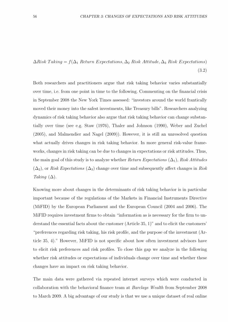
56 CHAPTER 3: CHANGES OF EXPECTATIONS AND RISK ATTITUDES
∆Risk Taking = f(∆1 Return Expectations, ∆2 Risk Attitude, ∆3 Risk Expectations)
(3.2)
Both researchers and practitioners argue that risk taking behavior varies substantially
over time, i.e. from one point in time to the following. Commenting on the financial crisis
in September 2008 the New York Times assessed: “investors around the world frantically
moved their money into the safest investments, like Treasury bills”. Researchers analyzing
dynamics of risk taking behavior also argue that risk taking behavior can change substan-
tially over time (see e.g. Staw (1976), Thaler and Johnson (1990), Weber and Zuchel
(2005), and Malmendier and Nagel (2009)). However, it is still an unresolved question
what actually drives changes in risk taking behavior. In more general risk-value frame-
works, changes in risk taking can be due to changes in expectations or risk attitudes. Thus,
the main goal of this study is to analyze whether Return Expectations (∆1), Risk Attitudes
(∆2), or Risk Expectations (∆3) change over time and subsequently affect changes in Risk
Taking (∆).
Knowing more about changes in the determinants of risk taking behavior is in particular
important because of the regulations of the Markets in Financial Instruments Directive
(MiFID) by the European Parliament and the European Council (2004 and 2006). The
MiFID requires investment firms to obtain “information as is necessary for the firm to un-
derstand the essential facts about the customer (Article 35, 1)” and to elicit the customers’
“preferences regarding risk taking, his risk profile, and the purpose of the investment (Ar-
ticle 35, 4).” However, MiFID is not specific about how often investment advisors have
to elicit risk preferences and risk profiles. To close this gap we analyze in the following
whether risk attitudes or expectations of individuals change over time and whether these
changes have an impact on risk taking behavior.
The main data were gathered via repeated internet surveys which were conducted in
collaboration with the behavioral finance team at Barclays Wealth from September 2008
to March 2009. A big advantage of our study is that we use a unique dataset of real online

3.1. INTRODUCTION 57
broker customers that includes information on the customers’ expectations, risk attitudes,
and risk taking behavior.1
Selected customers of Barclays Wealth were asked to participate repeatedly in a question-
naire survey. The survey was run on a quarterly basis from September 2008 to March 2009.
Overall 617 subjects participated at least once in the three surveys. Of these 617 subjects,
287 participated once, 181 twice, and 149 thrice. In all three surveys we elicited amongst
others financial risk taking by asking subjects to divide an amount of £100,000 either into
the stock market (FTSE-All-Share) or into a risk free asset with a safe interest rate of
4%. We also elicited subjective risk attitudes using three questions of Barclays Wealth’s
psychometrically validated risk attitude scale. In addition, we elicited risk and return
expectations of subjects for their own portfolio and for the market (FTSE-All-Share).
Using survey data has some pros and cons. On the one hand, it has the disadvantage that
we do not observe actual behavior of people and that there might be potential selection
and response biases. On the other hand, a big advantage is that relevant variables can
be elicited in a clean environment and do not need to be indirectly inferred from actions
and that in contrast to choice data one does not need to maintain the strong assumption
that decision makers have objectively correct (i.e. rational) expectations (for an overview
of some pros and cons of survey data see Manski (2005)). Surveys asking for individuals’
expectations and beliefs are very common2 and are highly influential both in academia
and practice.
Our results indicate that - consistent with evidence in the financial media and with findings
in the literature - risk taking behavior in the financial domain is indeed varying over time.
1We would like to thank the behavioral finance team at Barclays Wealth, Pete Brooks, Greg Davies and Dan Egan for
not only providing us with the data but also for very helpful comments, stimulating discussions, and help in designing the
survey in collaboration with us. We are particularly grateful to Dan Egan for his invaluable help in collecting and collating
the data and running the survey over multiple periods.
2A non exclusive list of such surveys in the U.S. are the University of Michigan Health and Retirement Study
(HRS) survey http://hrsonline.isr.umich.edu/index.php?p=qnaires, the Survey of Economic Expectations http://www.
disc.wisc.edu/econexpect/Index.html, the University of Michigan Survey of Consumers http://www.sca.isr.umich.edu,
the UBS/Gallup survey http://www.ropercenter.uconn.edu/data_access/data/datasets/ubs_investor.html, and the
Duke/CFO Business Outlook survey http://www.cfosurvey.org/duke. Two examples from Germany are the ZEW
Bankprognosen survey http://www.zew.de/de/publikationen/bankprognosen/index.php and the Socio-Economic Panel
http://www.diw.de/deutsch/soep/29004.html. Findings in some of these surveys are going to be discussed in section 3.2.
58 CHAPTER 3: CHANGES OF EXPECTATIONS AND RISK ATTITUDES
Risk taking is defined as the hypothetical amount subjects would invest into the stock
market and a risk free asset, respectively. Subjects invest substantially less into risky
assets in December than in September and also substantially less risky in March than
in December. More specifically, the percentage invested into the risky asset drops from
56.02% in September to 52.77% in December and to 46.52% in March. Analyzing the main
determinants of risk taking - risk attitudes as well as risk and return expectations - our
findings are twofold. First, risk attitudes seem to remain fairly stable as the risk attitude
score on a 7-point Likert scale changes from one survey to the other by more than 1 point
only for approximately 20% of all subjects. Second Wilcoxon signed-rank tests show that
risk and return expectations vary significantly from one survey to the other. Moreover, we
show that changes in risk taking can mainly be attributed to changes in risk and return
expectations and not to changes in risk attitudes. This result remains stable even if we
control for individual past performance. Finally, we compare changes in risk expectations
in relation to changes in actual risk, which is a measure of overconfidence. We show that
this measure of overconfidence seems to be fairly stable initially and decreases in the long
run.
These findings are important for practitioners in two ways: first, we show that risk atti-
tudes are stable individual constructs that do not need to be elicited on a quarterly basis.
Note that this line of argument cannot be generalized to all risk attitude measures cur-
rently used by practitioners. In particular inappropriate measures such as the ones that
confound risk attitudes and expectations do not need to be stable over time. Second, we
illustrate that subjective expectations are important determinants of risk taking behav-
ior and that it might be worthwhile for practitioners to elicit their clients’ expectations
regularly.
Our study extends findings in the empirical and experimental literature. Up to now, there
is no study documenting whether changes in expectations and/or changes in risk attitudes
drive changes in risk taking behavior. However, there are several papers analyzing whether
risk taking behavior actually changes over time. Malmendier and Nagel (2009) use real
world data to show that individuals’ personal experiences of macroeconomic shocks have
long-lasting effects on their risk taking behavior. In the experimental literature Staw

3.1. INTRODUCTION 59
(1976) and Thaler and Johnson (1990) show that risk taking behavior can depend on
individual prior gains and losses. But both empirical and experimental studies are not
able to disentangle the channel through which individual risk taking behavior changes
over time; i.e. they are not able to analyze whether changes in risk taking behavior can
be attributed to changes in risk attitudes or expectations or both. In contrast, our data
basis allow us to explicitly analyze this issue for a sample of real bank customers.
Furthermore, most studies analyzing changes in expectations and risk attitudes inves-
tigate either changes in risk expectations (e.g. Weber and Milliman (1997)) or changes
in return expectations (e.g. Shiller et al. (1996)) or changes in risk attitudes (e.g. Sahm
(2007) and Klos (2008)) separately but not in one single study. Moreover, most of these
studies are not able to relate changes in expectations and risk attitudes to changes in risk
taking. Vissing-Jorgensen (2003) and Dominitz and Manski (2007) analyze the relation
between the probability of holding stocks and expected equity returns. Using large scale
survey data, they find that the probability of holding stocks is higher the higher expected
returns are. We extend their findings in two ways: first, they do not analyze changes in
expectations and consequently their influence on changes in risk taking behavior. Second,
they proxy for risk taking by the probability of holding stocks whereas we analyze asset
allocation decisions.
Another important advantage of our study is that the surveys we use were conducted in
early September 2008 (6-20), December 2008 (6-20), and March 2009 (21-30). This unique
dataset allows us to test if the turmoil on financial markets during this period such as
the collapse of Lehman Brothers had substantial effects on risk attitudes, expectations,
and risk taking behavior. In addition, using repeated survey data on real online broker
customers to analyze changes in risk attitudes adds to the literature which often relies on
student populations (see e.g. Baucells and Villasis (2009) or Harrison et al. (2005)) and
offers substantial advantages. For example, we are able to control if differences in past
portfolio performance or changes in market conditions drive changes in risk attitudes,
expectations or risk taking behavior.
This chapter proceeds as follows: in section 3.2 we provide a literature review and formu-
late our hypotheses. Section 3.3 presents information on survey respondents and on the
60 CHAPTER 3: CHANGES OF EXPECTATIONS AND RISK ATTITUDES
survey design. The main results are reported in section 3.4 while the last section provides
a discussion of our results and a short conclusion.
3.2 Related Literature and Hypotheses
Anecdotal evidence suggests that risk taking behavior of investors, i.e. their division of
wealth between risky and risk free assets, can substantially vary over time and does not
need to be perfectly stable. According to the Deutsche Aktieninstitut in the year 2000, at
the height of the internet boom, 6.2 million people in Germany held part of their wealth in
stocks. By 2008, in the course of the financial crisis, this number had dropped to only 3.5
million. In a similar vein, the Wall Street Journal (2008) reports in an article on December
5, 2008 that in response to the dramatic events on financial markets “investors pulled $
72 billion from stock funds in October alone” and moved their money into government
bonds and cash holdings.
Thus, individuals risk taking behavior, i.e. their choice between risky and risk free as-
sets, seems not to be perfectly stable over time. This temporal instability can be due
to various factors: first, subjects do not need to exhibit the same level of risk aversion
over time. Second, individual risk expectations and return expectations do not need to be
stable and might be shaped by personal experiences. Third, important personal aspects
such as income and wealth might change over time. All these factors can individually or
jointly lead to changes in risk taking behavior over time. In the following we are going to
illustrate general findings in the literature on the stability or non-stability of risk taking
behavior. Subsequently, we are going to present more recent studies analyzing changes in
risk attitudes and expectations over time, before we pick up the question why changes in
risk taking over time occur.
Earlier studies in decision analysis on the stability of risk preferences or risky choices seem
to confirm the anecdotal evidence. Camerer (1989) and Hey and Orme (1994) investigate
the short term temporal reliability and stability of risky choices. Both studies confront
subjects with the same set of choices at two points in time (less than 10 days apart).
Their results indicate that individuals change their risk taking behavior in 25%-30% of

3.2. RELATED LITERATURE AND HYPOTHESES 61
all cases. However, these studies do not explicitly analyze the role of prior gains or losses
on subsequent risk taking behavior.
Staw (1976) analyzes exactly this and shows that risk taking behavior does not need
to be stable and substantially depends on prior personal outcomes. He illustrates that
subjects take significantly more risks following a loss than following a gain and terms
this “escalation of commitment”. The “escalation of commitment” hypothesis is also in
line with findings in the literature on the disposition effect (see e.g. Odean (1998a) and
Weber and Camerer (1998)). On the other hand, Thaler and Johnson (1990) argue that
it is difficult to make generalizations about risk taking preferences. They show a reverse
effect, i.e. enhanced risk taking in the gain domain, in two stage gambles which they
term the “house money effect”. Weber and Zuchel (2005) conduct an in-depth analysis
of the two conflicting effects “escalation of commitment” and “house money effect” and
show that the framing of the situation is important when analyzing changes in risk taking
behavior. On the one hand, the “house money effect” is prevalent if a situation is framed
as a lottery, on the other hand, the “escalation of commitment” effect is predominant if
the situation resembles a portfolio investment.
These studies show that the personal experience of gains or losses in the past can influence
subsequent risk taking behavior. In a slightly related context Malmendier and Nagel (2009)
show that personal macroeconomic experiences seem to have a great impact on personal
decisions and on the risk taking behavior of individuals. They illustrate that subjects
who have experienced high inflation and bad market-returns throughout their lives invest
substantially less risky than subjects who have experienced excellent market-returns in
the course of their lives. However, they do explicitly state that their goal is not to analyze
whether changes in beliefs or in risk aversion or a mix of both drive observed differences
in risk taking behavior.
Overall, the presented evidence suggests that subjects need not take constant levels of risks
in their investment decisions. Various factors such as changes in personal macroeconomic
experiences or gains and losses in own investments might affect risk taking behavior in a
dynamic setting. In a first step, we simply want to find evidence for the well-established
claim that risk taking behavior does not need to be stable in our survey for the sample

62 CHAPTER 3: CHANGES OF EXPECTATIONS AND RISK ATTITUDES
period September 2008 to March 2009. Consistent with the aforementioned anecdotal
evidence and findings in the literature we formulate hypothesis 1 as follows:
Hypothesis 1: Financial risk taking behavior varies over time
One important explanation for varying risk taking behavior over time often brought for-
ward are changes in income or wealth. The fact that an increase in wealth should result
in a higher level of risk taking or a decrease in relative risk aversion is a key implication
of various difference habits models. Brunnermeier and Nagel (2008) use microdata to an-
alyze this key implication of difference-habit models empirically. They show that wealth
changes affect the decision to participate in stock markets but that they have hardly any
effect on asset allocation decisions, i.e. on the proportion a household invests in risky and
risk free assets, respectively. In a similar vein, Guiso et al. (2003) analyze stock ownership
in major European countries and illustrate that the share of wealth invested in the stock
market is independent of investors’ wealth. Thus, both papers show that wealth effects
cannot explain observed changes in risk taking behavior over time.
In more general risk-value frameworks variations in financial risk taking behavior over
time can mainly be attributed to changes in risk and return expectations and/or changes
in risk attitudes (see equation 3.1 and 3.2). In the following, we will review some more
recent findings in the empirical and experimental literature on long run changes in risk
attitudes and changes in expectations over time.
Changes in risk attitudes:
Studies analyzing long term changes in risk attitudes by confronting the same set of sub-
jects with the same set of questions can be roughly classified into two groups. First, studies
using data from large scale panel surveys such as the Socio-Economic Panel (SOEP) or the
Michigan Health and Retirement Survey (HRS) which mostly use self-assessment tasks
with answer possibilities on Likert-scales. Second, laboratory and field experiments using
lottery related tasks to elicit risk attitudes and subsequently, changes in risk attitudes.

3.2. RELATED LITERATURE AND HYPOTHESES 63
Using data from simple 11-point self-assessment tasks from the SOEP waves in 2004 and
2006, Klos (2008) analyzes the temporal stability of risk attitude measures. He shows
that individual risk attitudes tend to be fairly stable over time and that the effect is in
particular strong for those subjects that indicated the central category. Similarly, Sahm
(2007) finds evidence for persistent differences between individuals but relatively high
stability of risk attitudes within individuals over time using the HRS panel data set with
more than 12,000 observations.
Andersen et al. (2008) use a field experiment with a representative sample of the Danish
population and Harrison et al. (2005) a laboratory study with students to analyze the
temporal stability of risk attitudes. Both studies obtain subjects’ risk aversion measures
using a multiple price list approach (see e.g. Holt and Laury (2002)). They find only slight
variation of risk attitudes over time and conclude that risk attitudes seem to be a stable
construct. In addition, Baucells and Villasis (2009) find similar results in a laboratory
study in which they elicit risk attitudes using binary lottery choice tasks. They also find
only small deviations in risk attitudes over time and argue that most of these changes
disappear if one introduces noise.
Overall, evidence in research implies that risk attitudes seem not to change too much over
the course of time and that observed changes can mainly be attributed to errors. Hence,
our hypothesis is the following:
Hypothesis 2: Risk attitudes are fairly stable over time
Changes in risk and return expectations:
The original formulation of the capital asset pricing model (CAPM) is a static one-period
model that assumes homogenous expectations (see e.g. Sharpe (1964) and Lintner (1965)).
Subsequent studies extended these assumptions by considering heterogenous beliefs, time-
varying expectations, and a dynamic investment problem of rational investors (see e.g.
Merton (1973) and Miller (1977)). In contrast, behavioral approaches argue that some
subjects misinterpret the informational content of a new signal and adjust their expecta-
64 CHAPTER 3: CHANGES OF EXPECTATIONS AND RISK ATTITUDES
tions inappropriately. Consequently, they over- or underreact to new information because
of their biased expectations (see for an overview DeBondt (2000)). Both rational and
behavioral studies agree that risk and return expectations can vary between subjects and
also within subjects over time when new information comes into the market.
Changes in return expectations have been analyzed extensively in the empirical and ex-
perimental literature, mostly with repeatedly carried out large scale surveys. Dominitz
and Manski (2005) analyze the dynamics of expectations in the Survey of Economic Ex-
pectations (1999-2001) and in the Michigan Survey of Consumers (2002-2004). They find
that expectations are not perfectly stable over time but that differences between persons
are larger than differences within persons over time.
Using a series of cross-section UBS/Gallup surveys, Fisher and Statman (2002) and
Vissing-Jorgensen (2003) show that subjects’ long and short term expectations change
substantially over the course of time. Taking data from the 1998-2003 surveys, Vissing-
Jorgensen (2003) illustrates that average 1-year expectations vary substantially from a
high of 15.8% in January 2000 to a low of around 6% at the end of 2002. She argues that
expectations and actual returns almost seem to move together. Analyzing the crash in the
Japanese stock market Shiller et al. (1996) illustrate that a sharp drop in expectations for
long run earnings growth could be observed for the period 1989-1994. They argue that
changes in expectations probably have substantial economic effects but do not provide
direct and unambiguous evidence on this issue.
Using a between-subjects design, Glaser and Weber (2005) demonstrate that return ex-
pectations after September 11 and the following market downturn are significantly higher
than return expectations before the event indicating that subjects did believe in some
sort of mean reversion. However, they note that there is no unambiguous ex ante predic-
tion whether subjects will expect mean reversion or trend continuation in stock prices in
response to such a dramatic event.
Risk perception or risk expectations are also often argued to be based on individuals’ past
experiences of a similar event or situation (see e.g. Ricciardi (2004)). In a similar vein,
Loewenstein et al. (2001) hypothesize that decisions are evaluated at an emotional level

3.2. RELATED LITERATURE AND HYPOTHESES 65
and that prior outcomes, good as well as bad ones, influence this emotional level and the
way individuals perceive the risk of a situation.
Consistent with these hypotheses, Weber and Milliman (1997) and Mellers et al. (1997)
experimentally show that risk perceptions change significantly over time after subjects
have experienced either good or bad outcomes. More precisely, they show that risk atti-
tudes are almost perfectly stable if one controls for changes in risk perceptions. Similarly,
Glaser and Weber (2005) find that volatility estimates are significantly higher after the
terror attacks of September 11 than before.
Overall, the evidence in the literature indicates that both risk and return expectations
can vary substantially over time as they can e.g. be influenced by macroeconomic devel-
opments or individually experienced gains and losses. However, to come up with a general
hypothesis whether risk and return expectations should rise or fall in response to the
dramatic events in late 2008 is difficult. Hence, hypothesis 3 follows:
Hypothesis 3: Expectations vary over time
On the one hand, the presented evidence at the start of this section indicates that financial
risk taking behavior does not need to be constant over the course of time and may vary
given prior gains and losses or given macroeconomic changes. On the other hand, risk and
return expectations - two major determinants of risk taking in risk-value models - have
also been shown to vary over time, whereas risk attitudes seem to be fairly stable. Our
data allow us to test explicitly what actually drives changes in risk taking. Consistent
with the previously presented literature we assume that changes in risk taking over time
are mainly driven by changes in risk and return expectations and not by changes in risk
attitudes or past performance.3
3Note that the goal of this study is not to test whether changes in risk and return expectations are based on rational
motives or whether they are due to irrational motives such as misreaction to new information.

66 CHAPTER 3: CHANGES OF EXPECTATIONS AND RISK ATTITUDES
3.3 Data
3.3.1 Survey Respondents
Our analysis is based on a repeated questionnaire study that was run as part of a joint
collaborative research project with the behavioral finance team at Barclays Wealth in
September 2008, December 2008, and March 2009. About 90% of all subjects in the
September sample completed the survey before September 12, i.e. before the bankruptcy
of Lehman Brothers and the subsequent downturn on financial markets. Unfortunately,
we do not have explicit information on the specific date each individual has completed
the survey.
Before the September wave, a stratified sample of Barclays Stockbrokers ’ client base was
drawn. To accomplish stratification, we grouped subjects according to their Age, Number
of deals per year, Number of holdings, and Portfolio value into non-overlapping subgroups,
so called strata. This procedure was used to improve the representativeness of the sample
and in order to take care of our collaborating bank’s desire to undersample subjects
who trade very little (Number of deals per year≤1) or have a relatively low portfolio value
(Portfolio value< £1,000). Thus, in all strata in which subjects were included that traded
less than once a year or had a portfolio value of less than £1,000 a lower percentage of
subjects were invited to participate in the survey than in the remaining strata. Note that
although we did undersample, we did not exclude these subjects totally as still more than
16% of all approached individuals had a portfolio value below £1,000.
Overall, 19,251 clients were emailed and invited to participate in a repeated survey. This
equals approximately 5% of all customers. Of the 19,251 individuals that were approached
by email in late August/early September 2008 about 4,520 (23%) opened the email. Of
those that opened the email, 849 (20%) went to the website and in the end, 479 out of
these 849 subjects completed the survey in September. The response rate is slightly lower
but still in the same ballpark as in similar studies by Dorn and Huberman (2005, 4%)
and Glaser and Weber (2007, 7%). Both studies also sent an email to customers of an

3.3. DATA 67
online broker and asked them to participate in an online questionnaire. It took subjects
on average 24 minutes to answer the survey.
The 479 subjects who participated in September were contacted again by email in late
November/early December 2008 and invited to participate in a shorter version of the ques-
tionnaire.4 Overall, 240 of the 479 subjects participated for a second time in December.
In addition, Barclays Wealth sent out an email to further 700 customers that had not
been contacted yet, in order to increase the number of subjects in future surveys.5 This
resulted in an additional 138 subjects joining the panel in December. These 138 subjects
received the same questionnaire that was filled out by the 479 subjects in September and
not the shorter December version. In March 2009, all 617 subjects that had previously
participated in at least one round were contacted again and invited to participate in a fur-
ther study. This time all subjects received the same, shorter version of the questionnaire.
Overall, 287 subjects participated only once (214 in September and 73 in December) and
149 subjects participated in all three surveys. Of the remaining 181 subjects who partic-
ipated twice, 91 participated in September and December, 65 in December and March,
and 25 in September and March.
The main goal of the study is to analyze whether risk taking behavior, risk attitudes,
and expectations change from September to December and from December to March and
what might drive these changes. To analyze this we want to compare on an individual
level subjects’ responses to survey questions at the three points in time. In contrast to
previous studies using one-time survey responses from online broker customers (see e.g.
Dorn and Huberman (2005) and Glaser and Weber (2007)) our dataset consists of repeated
observations and allows us to analyze changes in the main variables. However, an analysis
of individual changes in the main variables is only possible for subjects that took part at
least in two consecutive surveys, i.e. in September and in December or in December and
March or in all three surveys. 240 subjects participated both in September and December
4In contrast to the second version of the questionnaire we elicited in the first, longer version demographics, further
individual characteristics and various behavioral client profiling questions. These questions are psychometrically validated
and used by Barclays Wealth within the advisory process.
5These 700 had previously participated in another marketing related event of Barclays Wealth and had indicated their
willingness to participate in surveys.

68 CHAPTER 3: CHANGES OF EXPECTATIONS AND RISK ATTITUDES
and 214 subjects participated both in December and March. In addition, 149 subjects
participated in all three surveys.
To address a potential selection bias we compare the overall adult British population
with survey participants and we also compare subjects who participated once with those
that participated twice and thrice, respectively. Table 3.1 illustrates mean scores of de-
mographics and further characteristics for various groups. The first two columns illustrate
mean scores for all participants of our study (Groupall) and for the adult British popu-
lation (GBall), respectively. The next three columns illustrate the same scores separately
for subjects that participated only once (Grouponce, N=287), twice (Grouptwice, N=181),
and subjects that participated in all three surveys (Groupthrice, N=149).
The average age of all survey participants is 51.65 with two thirds of the subjects aged
between 40 and 66; four years older than the average British adult. In addition, subjects
in our sample are more likely to be married (0.65 vs. 0.52) or male (0.93 vs 0.49) compared
to the British average. Gross income is highly skewed with an overall mean of £76,615.73
and an overall median of £55,000 and substantially larger than for the average Briton
(£30,000). Clearly, our subjects are not likely to be representative of the typical British
adult. However, we find a considerable variation in subject’s answers which allows us
to test our hypotheses. In addition, our finding that respondents to this kind of survey
are predominately male and have a substantially larger gross income than the overall
population is consistent with Dorn and Huberman (2005).
Comparing subjects that participated once (Grouponce), twice (Grouptwice), and thrice
(Groupthrice), respectively, we find hardly any differences for the three subgroups. Only
for the level of investable wealth that is measured in 9 categories from 1 (£0 - £10,000)
to 9 (> £ 1 million) we find significant differences between the subgroups. Subjects
that participated only once in the survey have a substantially lower investable wealth
than subjects who participated thrice. Moreover subjects who participated thrice indicate
higher wealth levels than those who participated twice. Since the main goal of our study
is to analyze changes in various variables on an individual level over time, differences in
wealth between the three subgroups should not be problematic.

3.3. DATA 69
Tab
le3.
1:D
emog
raph
icch
arac
teri
stic
san
dde
scri
ptiv
est
atis
tics
The
firs
ttw
oco
lum
ns
of
this
table
report
mea
nvalu
esof
vari
ous
dem
ogra
phic
sand
des
crip
tive
stati
stic
sfo
rpart
icip
ants
of
our
study
(Gro
up
all)
and
for
the
adult
Bri
tish
popula
tion
(GB
all)
(GB
all
data
are
supplied
thro
ugh
the
Offi
cefo
rN
ati
onalSta
tist
ics)
.T
he
nex
tth
ree
colu
mns
report
mea
nvalu
esofvari
ous
dem
ogra
phic
sand
des
crip
tive
stati
stic
sfo
ra
subse
tofpart
icip
ants
that
took
part
inall
thre
esu
rvey
sonly
once
(Gro
up
on
ce),
only
twic
e(G
roup
twic
e)
or
inall
thre
esu
rvey
s(G
roup
thric
e),
separa
tely
.Age
,
Num
ber
ofdep
endants
,and
Gro
ssin
com
eare
self-e
xpla
nato
ry.G
ender
and
Mari
talst
atu
sare
two
dum
my
vari
able
sth
at
take
the
valu
e1
ifth
esu
bje
ctis
male
and
marr
ied,
resp
ecti
vel
y.In
ves
table
wea
lth
ism
easu
red
in9
cate
gori
esfr
om
1(£
0-£10,0
00)
to9
(>£
1m
illion).
The
last
thre
eco
lum
ns
report
z-sc
ore
sof
Mann-W
hit
ney
rank-s
um
test
sor
bin
om
ialte
sts
(for
the
two
dum
my
vari
able
s)w
hic
hte
stw
het
her
subje
cts
that
part
icip
ate
donce
,tw
ice
or
thri
cediff
erfr
om
the
resp
ecti
ve
subgro
up
of
subje
cts.
*
indic
ate
ssi
gnifi
cance
at
the
5%
level
and
**
indic
ate
ssi
gnifi
cance
at
the
1%
level
.
Gro
up
all
GB
all
Gro
up
on
ce
Gro
up
twic
eG
roup
thric
eD
iff.t
wic
e−
on
ce
Diff
.th
ric
e−
on
ce
Diff
.th
ric
e−
twic
e
Age
51.6
547.6
651.6
950.5
252.9
6-0
.667
1.0
82
1.5
95
Num
ber
ofdep
enden
ts1.1
4-
1.1
71.1
31.0
8-0
.328
-0.3
09
0.0
56
Gen
der
0.9
30.4
90.9
20.9
30.9
50.6
74
0.2
38
0.4
53
Gro
ssin
com
e76,6
15.7
330,0
00
71,4
46.5
985,7
18.9
276,6
31.4
1.1
57
0.9
02
-0.2
07
Mari
talst
atu
s0.6
50.5
20.6
70.6
50.6
20.6
47
0.3
14
0.6
01
Inves
table
wea
lth
4.8
0-
4.5
84.5
25.5
51.0
82
3.6
60**
3.4
88**

70 CHAPTER 3: CHANGES OF EXPECTATIONS AND RISK ATTITUDES
After having introduced the main variables in the following subsection, we are going to
analyze whether the three groups of subjects (Grouponce, Grouptwice, and Groupthrice)
differ in their response behavior in subsection 3.3.3.
3.3.2 Survey Design
This subsection presents the main variables that were elicited repeatedly within the sur-
veys. All surveys were designed in close collaboration with the behavioral finance team
at Barclays Wealth in order to get a better understanding of investors’ behavior. Besides
demographics and further individual characteristics that were described above and col-
lected only in the first survey in which a subject participated we elicited the following
variables repeatedly. The main variables are summarized in table 3.2.
(Financial) Risk taking: In the hypothetical risk taking task subjects were asked to
invest an amount of £100,000 either into the stock market (FTSE-All-Share) or into a
risk free asset with a safe interest rate of 4%. The higher the amount subjects allocate
to the stock market the more risk are they willing to take in this hypothetical task. A
big disadvantage of real transaction data is that it is hardly possible to obtain complete
information on total asset holdings of individuals at all banks at which they have an
account. Thus, although hypothetical risk taking is only an indirect proxy of risk taking
behavior it is a measure for which we have all necessary information.
Risk attitudes: In the September and December surveys we use three questions from
Barclays Wealth’s 8-question psychometric scale to assess subjects’ risk attitudes. Brooks
et al. (2008) show that this scale efficiently differentiates individuals from low risk toler-
ance to high risk tolerance and that the scale has high levels of reliability and validity.
The three questions used in our study can be found in table 3.2. For all three questions we
used a 7-point Likert scale with the endpoints “1 = Strongly Disagree” and “7 = Strongly
Agree”.6 In the March survey only one of these three risk attitude measures was elicited
6Amongst others Bollen and Barb (1981), Cicchetti et al. (1985), Preston and Colman (2000), Alwin and Krosnick (1991),
and Weng (2004) show that reliability, validity, and discriminating power increases up to 7-point scales and that after this
additional effects can hardly be observed. Moreover, Viswanathan et al. (2004) argue that the number of categories should
be picked such that it is as close as possible to a natural number of categories for a specific question and that one shouldn’t

3.3. DATA 71
Tab
le3.
2:D
efini
tion
ofdy
nam
icva
riab
les
This
table
sum
mari
zes
and
defi
nes
vari
able
sth
at
wer
eel
icit
edre
pea
tedly
.N
ote
thatRis
kA
ttitude
6and
Ris
kA
ttitude
7w
ere
not
elic
ited
inth
eM
arc
hsu
rvey
.
Varia
ble
Quest
ion
/D
esc
rip
tion
Ris
kTakin
g
Ris
kTaki
ng
Mea
sure
s,on
aper
centa
ges
basi
s,th
e(h
ypoth
etic
al)
am
ount
ofm
oney
an
indiv
idualis
willing
toin
ves
tin
toth
eFT
SE
-All-S
hare
com
pare
dto
a
risk
free
ass
etw
ith
a4%
retu
rn.(0
=in
ves
tev
eryth
ing
into
the
risk
free
ass
et...100
=in
ves
tev
eryth
ing
into
the
risk
yst
ock
mark
et)
Ris
kA
ttit
ude
Ris
kA
ttitude
2”It
islikel
yI
would
inves
ta
signifi
cant
sum
ina
hig
hri
skin
ves
tmen
t.”
(1=
Str
ongly
dis
agre
e...7
=Str
ongly
Agre
e)
Ris
kA
ttitude
6”I
am
afinanci
alri
skta
ker
.”(1
=Str
ongly
dis
agre
e...7
=Str
ongly
Agre
e)
Ris
kA
ttitude
7”E
ven
ifI
exper
ience
da
signifi
cant
loss
on
an
inves
tmen
t,I
would
stillco
nsi
der
makin
gri
sky
inves
tmen
ts.”
(1=
Str
ongly
dis
agre
e...7
=Str
ongly
Agre
e)
Expecta
tions
Mark
et-R
eturn
-Num
.M
easu
res
indiv
iduals
’re
turn
expec
tati
ons
for
the
FT
SE
-All-S
hare
in3
month
sin
per
cent
Mark
et-R
isk-
Num
.M
easu
res
indiv
iduals
’vola
tility
expec
tati
ons
for
the
FT
SE
-All-S
hare
in3
month
sby
transf
orm
ing
esti
mate
sofbounds
into
vola
tility
esti
mate
s.
Mark
et-R
eturn
-Subj
.”H
ow
would
you
rate
the
retu
rns
you
expec
tfr
om
an
inves
tmen
tin
the
UK
stock
mark
et(F
TSE
-All-
Share
)over
the
nex
t3
month
s?”
(1=
Extr
emel
ybad
...7
=E
xtr
emel
ygood)
Mark
et-R
isk-
Subj
.”O
ver
the
nex
t3
month
s,how
risk
ydo
you
thin
kth
eU
Kst
ock
mark
et(F
TSE
-All-
Share
)is
?”
(1=
Not
risk
yat
all
...7
=E
xtr
emel
yri
sky)
Own-R
eturn
-Num
.M
easu
res
indiv
iduals
’re
turn
expec
tati
ons
for
the
ow
nport
folio
at
the
bank
in3
month
sin
per
cent
Own-R
isk-
Num
.M
easu
res
indiv
iduals
’vola
tility
expec
tati
ons
for
the
ow
nport
folio
at
the
bank
in3
month
sby
transf
orm
ing
esti
mate
sofbounds
into
vola
tility
esti
mate
s.
Own-R
eturn
-Subj
.”H
ow
would
you
rate
the
retu
rns
you
expec
tfr
om
your
ow
nport
folio
over
the
nex
t3
month
s?”
(1=
Extr
emel
ybad
...7
=E
xtr
emel
ygood)
Own-R
isk-
Subj
.”O
ver
the
nex
t3
month
s,how
risk
ydo
you
thin
kth
ein
ves
tmen
tsin
your
ow
nport
folio
are
?”
(1=
Not
risk
yat
all
...7
=E
xtr
emel
yri
sky)
Past
Perfo
rm
ance
Per
f.-E
xter
nal
What
do
you
thin
kth
ere
turn
ofyour
inves
tmen
tshel
dat
oth
erbanks
over
the
past
3m
onth
sw
as?
Per
f.-M
ark
et-N
um
.”W
hat
isyour
bes
tes
tim
ate
ofth
ere
turn
ofth
eU
Kst
ock
mark
et(F
TSE
-All-S
hare
)over
the
past
3m
onth
s?”
Per
f.-M
ark
et-S
ubj
.”H
ow
would
you
rate
the
retu
rns
ofth
eU
Kst
ock
mark
ets
(FT
SE
-All-S
hare
)over
the
past
3m
onth
s?”
(1=
Extr
emel
ybad
...7
=E
xtr
emel
ygood)
Per
f.-O
wn-N
um
.”W
hat
do
you
thin
kth
ere
turn
ofyour
ow
nport
folio
over
the
past
3m
onth
sw
as?
”
Per
f.-O
wn-S
ubj
.”H
ow
would
you
rate
the
retu
rns
ofyour
ow
nport
folio
over
the
past
3m
onth
s?”
(1=
Extr
emel
ybad
...7
=E
xtr
emel
ygood)

72 CHAPTER 3: CHANGES OF EXPECTATIONS AND RISK ATTITUDES
(Risk Attitude 2 ). We do not elicit risk attitudes from lotteries because of the extended
domain specificity result in chapter 2 where we showed that risk attitudes inferred from
lotteries are not related to investment behavior in stocks.
Expected return and expected risk: Since we have argued in sections 3.1 and 3.2
that subjective risk and return expectations are important determinants of risk taking
behavior, we tried to elicit them extensively in the questionnaire. To do this we elicited
subjects three months expectations for their own portfolio as well as for the overall stock
market (FTSE-All-Share). We chose the three months forecasting period because the
survey panel is also conducted on a quarterly basis. Since we have shown in chapter
2 that risk expectations elicited on a purely subjective scale need not to coincide with
risk expectations elicited via confidence intervals, we utilize both qualitative and numeric
approaches to measure subjects’ expectations.
To measure risk and return expectations numerically we asked individuals to state a best
guess (mean estimate) for the three month return as well as upper and lower bounds for
90% confidence intervals for the return in three months. More precisely, we asked them to
submit what they consider to be lower and upper bounds so that there is only a 5% chance
that the return in three months will be below the lower bound and a 5% chance that it will
be higher than the upper bound. Numeric return expectations for the market (Market-
Return-Num.) or for a subject’s own portfolio (Own-Return-Num.) are simply equal to the
best guess for the return of the market and for the own portfolio, respectively. However,
to obtain a measure of numeric risk expectations is not as straightforward. We use the
two point approximation suggested in Keefer and Bodily (1983) which transforms stated
confidence intervals into volatility estimates and has been widely used in the empirical
literature (e.g. chapter 2 of this thesis, Graham and Harvey (2005), Ben-David et al.
(2007), and Glaser et al. (2005)). This transformation gives us the two risk expectation
measures Market-Risk-Num. and Own-Risk-Num.
To get the two qualitative measures of return expectations (Market-Return-Subj. and
Own-Return-Subj.) we ask subjects to classify both expected market and own portfolio
use too many scales as this overburdens subjects and is too hard of a cognitive task for them. Hence, using 7-point Likert
scales seems to be the best trade-off between understandability and reliability for our sample of Barclays Wealth customers.
3.3. DATA 73
returns on a 7-point Likert scale with the endpoints “1 = Extremely bad return” and
“7 = Extremely good return”. Similarly, the qualitative measures of risk expectations
(Market-Risk-Subj. and Own-Risk-Subj.) are obtained by asking subjects to classify both
expected market and own portfolio risk on a 7-point Likert scale with the endpoints “1
= Not risky at all” and “7 = Extremely risky”.
Past performance: We use the following approach to control for the possibility that past
investment returns affect changes in risk taking behavior. We elicit individuals’ subjective
estimates of past performance, both past stock markets performance (FTSE-All-Share)
and past own portfolio performance within the last three months on a repeated basis.
Similar to expectations we use two elicitation methods. First, we ask subjects to give us a
numerical estimate of their own past returns or the stock markets past return in percent.
Second, we ask subjects to judge past returns on 7-point Likert scales with the endpoints
“1 = Extremely bad return” and “7 = Extremely good return”. In addition, we also ask
subjects to indicate their past performance at other online brokers, if applicable.
3.3.3 Differences in Groups
In the following, we analyze the selection bias problem and in this connection in particular
the question if subjects that participated once, twice, and thrice, respectively, differ in
their response style to the repeatedly elicited variables. Overall, we have 17 repeatedly
elicited variables in September and December (and 15 in March): 1 · risk taking, 3 · risk
attitude (1 · risk attitude in March), 8 · expectations, and 5 · past performance. The mean
and median values for all variables in a given month are very similar between the three
groups of subjects: Grouponce, Grouptwice, and Groupthrice.
We use a series of Mann-Whitney rank-sum tests to analyze whether the response behavior
in the separate groups differs significantly. Comparing responses of Grouponce subjects in
September and December with those of subjects that participated repeatedly (Grouptwice
and Groupthrice) we find that only for 3 out of 34 variables there are statistically signif-
icant differences. Similarly, comparing subjects that participated twice with those that

74 CHAPTER 3: CHANGES OF EXPECTATIONS AND RISK ATTITUDES
participated thrice, we only find significant differences for 3 out of 49 variables.7 In addi-
tion, the few significant differences are scattered over various variables with no clear-cut
uniform effect. Hence, we argue that there is no indication that subjects who participated
once differ substantially in their response behavior from those that participated twice or
thrice. In addition, the same seems to be true if we compare subjects that participated
twice and thrice directly.
3.4 Results
3.4.1 On the stability of risk taking, risk attitudes, and expectations
This subsection analyzes if risk taking, risk attitude, expectations, and past performance
are stable individual traits or whether they change over our three observation periods.
Thus, we compare the response behavior in September with the one in December and the
one in December with the one in March. Table 3.3 reports mean scores of all repeatedly
elicited variables in our sample, separately for the three months. We report mean values
in each of the three months only for subjects that participated at least twice in the
survey, however, our results are essentially the same if we compute the numbers for all
617 subjects or for the 149 subjects that participated thrice. The last two columns in
table 3.3 report results of Wilcoxon signed-rank tests analyzing whether the difference
between the two respective months is significant. To avoid the problem that differences in
repeatedly elicited variables are driven by the fact that different subjects participated in
separate months, we run these tests only for those subjects that participated in the two
respective months.
For Risk-Taking we observe, consistent with hypothesis 1, that the share subjects are
willing to invest into the market (FTSE-All-Share) varies substantially. It decreases from
56.02% in September to 52.77% in December to 46.52% in March. All differences are
highly significant at the 1% level.
7We compare response behavior of subjects that participated twice and thrice, respectively, for 17 variables in September,
17 variables in December, and 15 variables in March. This gives us a total of 49 comparisons.

3.4. RESULTS 75
Changes in risk attitudes are hardly observable for all three risk attitude measures. Risk
Attitude 2 and Risk Attitude 7 are virtually the same in September and in December. Risk
Attitude 6 rises slightly from 4.43 to 4.61 from September to December. This difference
is significant at the 5% level. However, this rise indicates that subjects seem to be less
risk averse in December than in September which is seemingly at odds with our previous
finding on lower levels of risk taking behavior in December. Since we only elicited Risk
Attitude 2 in March we can just analyze the change of this risk attitude measure from
December to March. Table 3.3 shows that Risk Attitude 2 decreased slightly from 3.63 to
3.55 in this time period with the decrease being not significant. In addition, analyzing the
stability of risk attitudes on an individual level, we find that around 40% of all subjects
do not change self-reported risk attitudes at all and that around 80% of all subjects do
not change their self-reported risk attitude score by more than one point on the 7-point
Likert scales. This stability of risk attitudes is consistent with findings in Sahm (2007)
and Baucells and Villasis (2009) as well as with hypothesis 2.
Risk expectations or risk perceptions on the other hand, seem to change considerably over
time. On the one hand, all four risk expectation measures Market-Risk-Num., Market-
Risk-Subj., Own-Risk-Num., and Own-Risk-Subj. are substantially higher in December
than in September. On the other hand, Own-Risk-Num. is substantially lower in March
than in December. All differences are highly significant on the 1% level. More precisely,
both numerical risk measures or three month volatility estimates (Market-Risk-Num. and
Own-Risk-Num.) rise from approximately 0.05 in September to 0.075 in December and
drop slightly to around 0.07 in March.8 The extreme rise of volatility estimates from
September to December is consistent with Glaser and Weber (2005) who show in a
between-subjects design that volatility estimates before 9/11 were substantially lower
than after 9/11. In a similar vein, subjective risk expectations also rise substantially from
September to December and remain almost stable from December to March. These find-
ings indicate that subjects perceived both their own investments and investments into the
market to be riskier in December than in September and that they perceived Own-Risk-
8We will compare this change in volatility estimates with actual changes in market risk in subsection 3.4.3 in more detail.
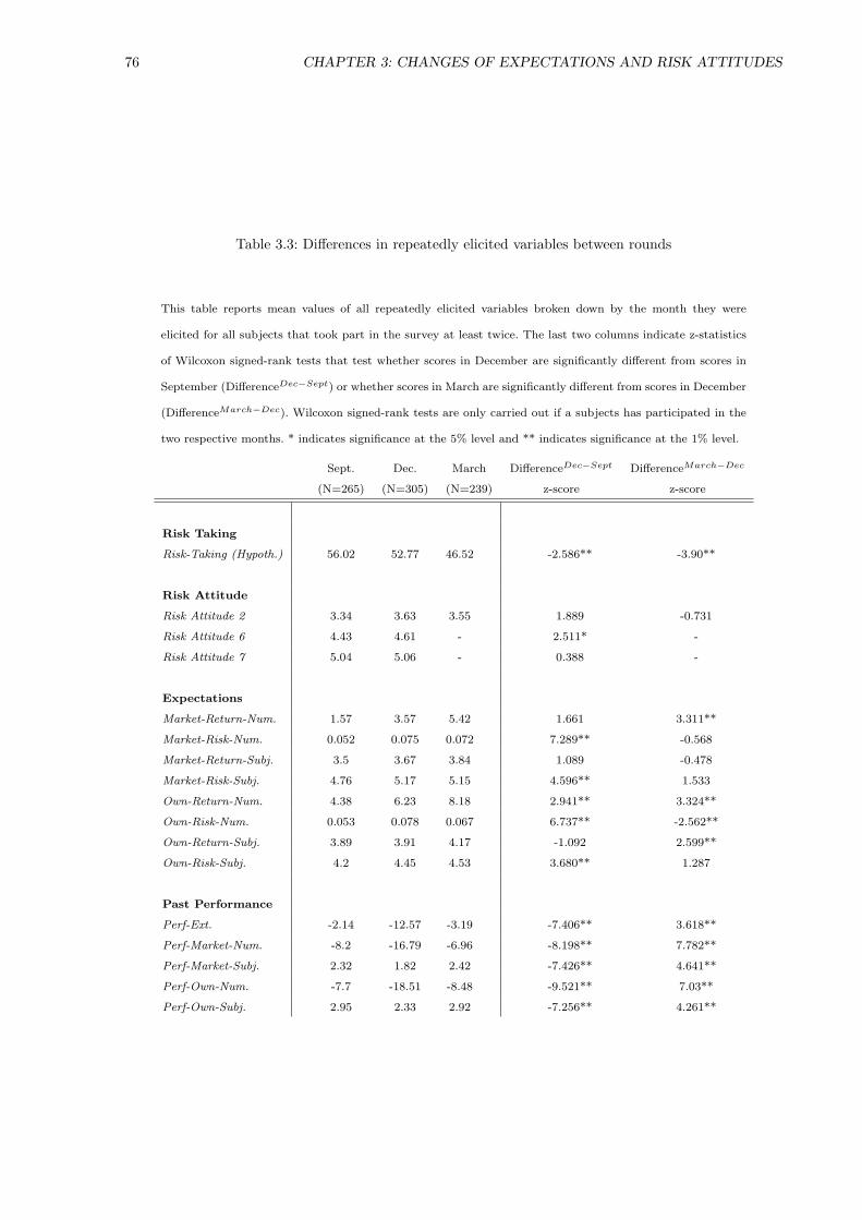
76 CHAPTER 3: CHANGES OF EXPECTATIONS AND RISK ATTITUDES
Table 3.3: Differences in repeatedly elicited variables between rounds
This table reports mean values of all repeatedly elicited variables broken down by the month they were
elicited for all subjects that took part in the survey at least twice. The last two columns indicate z-statistics
of Wilcoxon signed-rank tests that test whether scores in December are significantly different from scores in
September (DifferenceDec−Sept) or whether scores in March are significantly different from scores in December
(DifferenceMarch−Dec). Wilcoxon signed-rank tests are only carried out if a subjects has participated in the
two respective months. * indicates significance at the 5% level and ** indicates significance at the 1% level.
Sept. Dec. March DifferenceDec−Sept DifferenceMarch−Dec
(N=265) (N=305) (N=239) z-score z-score
Risk Taking
Risk-Taking (Hypoth.) 56.02 52.77 46.52 -2.586** -3.90**
Risk Attitude
Risk Attitude 2 3.34 3.63 3.55 1.889 -0.731
Risk Attitude 6 4.43 4.61 - 2.511* -
Risk Attitude 7 5.04 5.06 - 0.388 -
Expectations
Market-Return-Num. 1.57 3.57 5.42 1.661 3.311**
Market-Risk-Num. 0.052 0.075 0.072 7.289** -0.568
Market-Return-Subj. 3.5 3.67 3.84 1.089 -0.478
Market-Risk-Subj. 4.76 5.17 5.15 4.596** 1.533
Own-Return-Num. 4.38 6.23 8.18 2.941** 3.324**
Own-Risk-Num. 0.053 0.078 0.067 6.737** -2.562**
Own-Return-Subj. 3.89 3.91 4.17 -1.092 2.599**
Own-Risk-Subj. 4.2 4.45 4.53 3.680** 1.287
Past Performance
Perf-Ext. -2.14 -12.57 -3.19 -7.406** 3.618**
Perf-Market-Num. -8.2 -16.79 -6.96 -8.198** 7.782**
Perf-Market-Subj. 2.32 1.82 2.42 -7.426** 4.641**
Perf-Own-Num. -7.7 -18.51 -8.48 -9.521** 7.03**
Perf-Own-Subj. 2.95 2.33 2.92 -7.256** 4.261**
3.4. RESULTS 77
Num. to be lower in March than in December. These changes in risk expectations are also
in line with hypothesis 3.
For return expectations a similar picture emerges. For all return expectations measures
(Market-Return-Num., Market-Return-Subj., Own-Return-Num., and Own-Return-Subj.)
subjects expect on average higher returns in December than in September. The same is
true if we compare return expectations in March and in December, indicating that subjects
became more and more optimistic over the three time periods. Wilcoxon signed-rank tests
show that four of eight return expectations turn out to rise significantly (p< 0.01) from one
quarter to the other. Overall, consistent with Vissing-Jorgensen (2003) and Shiller et al.
(1996) as well as with hypothesis 3, we show that return expectations do vary substantially
over time. More specifically, in our sample subjects get more and more optimistic over
time.
Analyzing changes in past performance, we obtain a simple result. Most subjects judge
past performance, be it their own or the markets’ performance, from June to August
and from December to March to be substantially higher than the performance in the
time span September to December. This result is not surprising considering the fact
that stock markets took a severe downturn in the last quarter of 2008. The performance
of the FTSE-All-Share from September to December was approximately -20% and thus
substantially worse than the performance in the time periods June to September (-10%)
and December to March (-7%). Two interesting findings on subjects self-assessed past
performance emerge: first, subjects numerical estimates of past market performance are
not too far-off real market returns. Second, subjects judge their own past performance to
be lower than the market performance, although they do not expect their own portfolio
to be more risky than the market.
Our main findings are in line with previous findings in the literature and with our hy-
potheses 1 - 3. Risk taking behavior (see Malmendier and Nagel (2009)), risk expectations
(see Glaser and Weber (2005)), and return expectations (see Vissing-Jorgensen (2003))
seem to vary over time whereas risk attitudes tend to be fairly stable (see Sahm (2007)).
Moreover, our results remain stable if we analyze differences only for those subjects that
participated thrice or if we include all observations at each point of time.

78 CHAPTER 3: CHANGES OF EXPECTATIONS AND RISK ATTITUDES
3.4.2 What Drives Changes in Risk Taking?
Having provided evidence for changes in risk taking behavior and expectations as well
as evidence for relative high stability of risk attitudes we want to analyze what actually
influences changes in risk taking behavior over time. As a first test of the functional
relationship in equation 3.1 and 3.2 we analyze whether subjects’ behavior is in accordance
with the model propositions. Hence, we study whether subjects that take more risks in
December (March) than in September (December) (∆ R.T.+) become less risk averse,
expect higher returns and/or perceive the risk of an investment in the market to be lower.
And for subjects that take less risks in December (March) than in September (December)
(∆ R.T.−) we analyze whether they become more risk averse, expect lower returns and/or
perceive the risk of an investment in the market to be higher.
A simple sign test indicates that 74 subjects in the period September to December and
99 subjects in the period December to March take less (more) risks over time although
they become less (more) risk averse. We also find that 77 [64] subjects take more (less)
risks although they expect numerical and subjective market returns to be lower (higher)
in December than in September [in March than in December]. Finally, our results also
indicate that 55 [67] subjects take more (less) risks although they perceive the riskiness of
the market (numerical and subjective) to be higher (lower) in December than in September
[in March than in December].
However, these numbers do not indicate that subjects behave not according to the model.
It might well be that subjects who are less risk averse in December than in September [in
March than in December] take a substantially lower level of risks because of lower return
expectations and/or higher risk expectations. Hence, only those subjects that take more
(less) risks although they are more (less) risk averse, expect lower (higher) returns and
perceive the risk to be higher (lower) in December than in September [in March than in
December] do not behave in accordance with the functional form.
Our results indicate that subjects do not behave in accordance with the functional form
and thus violate some sort of dominance concept in less than 8.8% of all cases. If we assume
that the probability to submit non intuitively correct risk attitude, risk expectations, and

3.4. RESULTS 79
return expectations to be 12, respectively, then about 12.5% (1
2· 1
2· 1
2) of all subjects should
not behave in accordance with the functional form. Since our results indicate this to be
slightly lower, we interpret our findings as a first hint for the usefulness of more general
risk-value frameworks (see Sarin and Weber (1993b) and Jia et al. (1999)).
Admittedly, the previous test is a weak test of model consistency and doesn’t allow us to
make inferences about what actually drives changes in risk taking behavior. To improve on
this we analyze in table 3.4 the value of all risk attitude, expectation, and past performance
measures separately for the two time periods September to December (left panel) and
December to March (right panel). In each panel we report mean values of all variables
for two distinct groups of subjects: first, subjects who take more risks from one survey
to the next one (∆ R.T.+) and second, subjects who take less risks from one survey to
the next one (∆ R.T.−). The last column in each panel reports results on Mann-Whitney
rank-sum tests comparing the two groups ∆ R.T.+ and ∆ R.T.−.
Comparing changes in risk attitudes between the two groups shows hardly any differences
for both panels.9 Mann-Whitney rank-sum tests indicate that there is no significant rela-
tion between the way subjects adjust their risk attitude scores over time and changes in
their risk taking behavior over time.
In addition, analyzing whether there are any differences in the way subjects update their
own portfolio expectations between the two groups we mostly find no significant differences
as changes in own portfolio expectations are fairly similar for both groups (∆ R.T.+ and ∆
R.T.−). The only significant difference between the two groups of subjects can be observed
for Diff. Own-Risk-Num. in the December to March panel. Subjects who take more risks
in March than in December (∆ R.T.+) expect their own portfolio returns to be higher in
March than in December whereas subjects that take less risks in March than in December
(∆ R.T.−) expect their own portfolio returns to be lower in March than in December.
This result is not highly significant and gets insignificant if we only analyze the subgroup
of subjects that has participated in all three surveys.
9Note that Diff. Risk Attitude 6 and Diff. Risk Attitude 7 were not elicited in March. Therefore, we cannot analyze
changes in these variables from December to March.
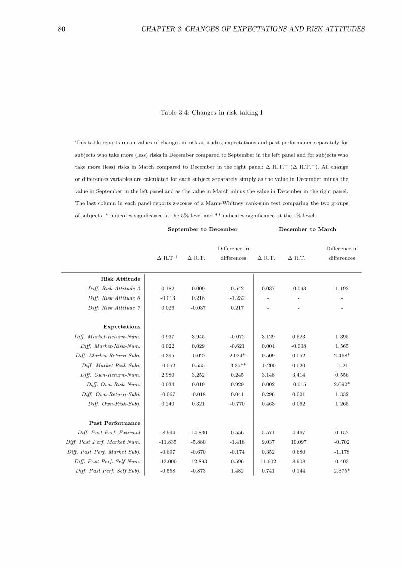
80 CHAPTER 3: CHANGES OF EXPECTATIONS AND RISK ATTITUDES
Table 3.4: Changes in risk taking I
This table reports mean values of changes in risk attitudes, expectations and past performance separately for
subjects who take more (less) risks in December compared to September in the left panel and for subjects who
take more (less) risks in March compared to December in the right panel: ∆ R.T.+ (∆ R.T.−). All change
or differences variables are calculated for each subject separately simply as the value in December minus the
value in September in the left panel and as the value in March minus the value in December in the right panel.
The last column in each panel reports z-scores of a Mann-Whitney rank-sum test comparing the two groups
of subjects. * indicates significance at the 5% level and ** indicates significance at the 1% level.
September to December December to March
Difference in Difference in
∆ R.T.+ ∆ R.T.− differences ∆ R.T.+ ∆ R.T.− differences
Risk Attitude
Diff. Risk Attitude 2 0.182 0.009 0.542 0.037 -0.093 1.192
Diff. Risk Attitude 6 -0.013 0.218 -1.232 - - -
Diff. Risk Attitude 7 0.026 -0.037 0.217 - - -
Expectations
Diff. Market-Return-Num. 0.937 3.945 -0.072 3.129 0.523 1.395
Diff. Market-Risk-Num. 0.022 0.029 -0.621 0.004 -0.008 1.565
Diff. Market-Return-Subj. 0.395 -0.027 2.024* 0.509 0.052 2.468*
Diff. Market-Risk-Subj. -0.052 0.555 -3.35** -0.200 0.020 -1.21
Diff. Own-Return-Num. 2.980 3.252 0.245 3.148 3.414 0.556
Diff. Own-Risk-Num. 0.034 0.019 0.929 0.002 -0.015 2.092*
Diff. Own-Return-Subj. -0.067 -0.018 0.041 0.296 0.021 1.332
Diff. Own-Risk-Subj. 0.240 0.321 -0.770 0.463 0.062 1.265
Past Performance
Diff. Past Perf. External -8.994 -14.830 0.556 5.571 4.467 0.152
Diff. Past Perf. Market Num. -11.835 -5.880 -1.418 9.037 10.097 -0.702
Diff. Past Perf. Market Subj. -0.697 -0.670 -0.174 0.352 0.680 -1.178
Diff. Past Perf. Self Num. -13.000 -12.893 0.596 11.602 8.908 0.403
Diff. Past Perf. Self Subj. -0.558 -0.873 1.482 0.741 0.144 2.375*
3.4. RESULTS 81
Interestingly, there are no significant differences between the two groups (∆ R.T.+ and ∆
R.T.−) for Diff. Market-Return-Num. and Diff. Market-Risk-Num. in both panels. Diff.
Market-Return-Num. is simply the numerical return estimate in December (March) minus
the one in September (December) and positive in both groups and panels. Our results are
the same if we calculate the numerical variables not as simple differences but as percentage
changes. A similar picture emerges if we analyze Diff. Market-Risk-Num.
However, for subjective market risk and market return expectations we find substantial
and stable differences between the two groups. Subjects who take more risks from one
survey to the next one (∆ R.T.+) expect subjective market returns (Diff. Market-Return-
Subj.) to become substantially higher over time and grow by on average 0.395 and 0.509,
respectively. Whereas subjects who take less risks in December than in September or less
risks in March compared to December (∆ R.T.−) expect subjective market returns to stay
fairly stable over time. Differences in differences between the two groups are significant in
both panels as indicated by z-scores of 2.024 and 2.468 and a first indication that changes
in subjective market return expectations seem to be related to changes in investment
behavior. This result remains stable even if re-run the analysis only for subjects that
participated in all three surveys.
We find a reverse pattern for subjective market risk expectations: subjects in the group ∆
R.T.− expect Diff. Market-Risk-Subj. to be positive on average (0.555 and 0.02) whereas
subjects in the group ∆ R.T.+ expect it to be negative on average (-0.052 and -0.2). The
difference in differences in the September to December panel is highly significant with a
z-score of -3.35. In contrast, the difference in differences in the December to March panel
is in the right direction but not significant. Moreover, table 3.4 also shows that changes in
past performance estimates are hardly related to changes in risk taking behavior as only
Diff. Past Perf. Self Subj. is significantly different for both groups.
These findings are first indications that changes in subjective market return and market
risk expectations seem to be related to changes in investment behavior in markets. How-
ever, one problem of the previous analyses is that we can only apply it to subjects who
take more or less risks from one period to the other. Thus, we omit all subjects that take

82 CHAPTER 3: CHANGES OF EXPECTATIONS AND RISK ATTITUDES
the same level of risk in two subsequent periods. The following analyses try to alleviate
this problem.
In order to investigate the question what drives changes in risk taking behavior in more
depth we use multivariate tobit regressions. We use tobit since our variables are censored
from below (-100) and from above (+100). In table 3.5 we report results of clustered tobit
regressions of changes in risk taking, from one point in time to the next one. Since we use
both changes from September to December and changes from December to March in these
analyses we need to drop Diff. Risk Attitude 6 and Diff. Risk Attitude 7 as they were not
elicited in March. In addition, we also need to take into account that our observations do
not need to be independent as 149 subjects participated in all three surveys and appear
repeatedly in our sample of differences. We control for this by clustering our regressions
over subjects.
The results in the first regression of table 3.5 indicate that Diff. Risk Attitude 2 cannot
explain changes in risk taking behavior. Interestingly, our results hold even if we re-run
the regressions and exclude subjects that report the same risk attitude in September and
in December or the same risk attitude in December and March.
Column 2 of table 3.5 illustrates that in contrast to changes in risk attitudes, changes
in subjective expectations can explain changes in risk taking behavior. More precisely,
the positive coefficient of 2.348 indicates a positive relation between Diff. Market-Return-
Subj. and Diff. Risk Taking. The larger the market return expectations in December
(March) are compared to September (December), the larger is the level of risk taking
in December (March) compared to September (December). For changes in subjective
market risk expectations (Diff. Market-Risk-Subj.) we find a reverse effect, indicated by
the significantly negative coefficient of -2.208. Hence, the higher subjects’ perceive the
risk of the market in December (March) in comparison to September (December) the less
risky they invest in December (March) compared to September (December). Our results
remain essentially the same if we further require that Diff. Risk Attitude 2 is not equal
to zero.

3.4. RESULTS 83
Table 3.5: Changes in risk taking II
This table reports results of clustered tobit regressions where standard errors take clustering over subjects into
account. Dependent variable in each model is changes in risk taking (Diff. Risk Taking). Independent variables
are changes in: risk attitude, expectations, and past performance as well as demographic variables. All change
or differences variables are calculated for each subject separately simply as the value in December (March)
minus the value in September (December). p-values are reported in parentheses. * indicates significance at the
10% level, ** indicates significance at the 5% level, and *** indicates significance at the 1% level.
(1) (2) (3) (4) (5)
Risk Attitude
Diff. Risk Attitude 2 0.936 1.071 1.001 0.933
(0.220) (0.149) (0.216) (0.252)
Expectations
Diff. Market-Return-Num. 0.151 0.038
(0.256) (0.714)
Diff. Market-Risk-Num. 4.451 5.349
(0.870) (0.846)
Diff. Market-Return-Subj. 2.348 2.327 1.934 2.013
(0.017)** (0.018)** (0.049)** (0.046)**
Diff. Market-Risk-Subj. -2.208 -2.303 -2.529 -2.631
(0.016)** (0.015)** (0.010)** (0.009)***
Past Performance
Diff. Past Perf. Market Num. -0.164
(0.056)*
Diff. Past Perf. Market Subj. 0.137
(0.872)
Demographics No No No Yes Yes
Dummy-Period -2.124 -3.441 -2.978 -0.464 -3.489
(0.470) (0.242) (0.312) (0.886) (0.283)
Constant -4.366 -3.601 -3.803 4.694 5.478
(0.021)** (0.069)* (0.054)* (0.524) (0.468)
Observations 434 435 431 396 396

84 CHAPTER 3: CHANGES OF EXPECTATIONS AND RISK ATTITUDES
In additional robustness tests we check whether our results also hold for the numerical
risk and return expectations. Running the same regressions with numerical expectations
instead of ordinal ones, we find that changes in numerical expectations cannot explain
changes in risk taking behavior. This result remains stable even if we check for robustness
by e.g. running the regressions separately for subjects that participated twice and thrice,
respectively, or for those subjects that indicated certain levels of income or wealth, or for
those that stated positive expected returns. This finding is consistent with first results in
table 3.4 and in contrast to first findings in chapter 2 were we show with business and
economics students that risk taking behavior can also be heavily influenced by subjective
numerical risk and return expectations.
We can only hypothesize why we do not find a significant effect for the numerical variables
in our dataset: first, in numerical values outliers such as an expected market return of
143% in three months which we actually observe in our dataset could affect our results.10
Second, practitioners argue that ordinal ratings are more feasible and that most individu-
als with no specific background in economics seem to understand subjective ordinal ratings
better than numerical ones. Thus, e.g. all rating agencies transform default probabilities
or expected losses into ordinal scales. Since subjects in our study do not necessarily have
a background in finance or economics this argument might be relevant for our dataset.
Third, scanning the personal comments that subjects could submit after the March sur-
vey we find that many subjects regard the numerical questions to be too technical and
confusing to answer. A further indication that subjects had problems stating numerical
risk and return expectations is the fact that almost 23% (September), 24% (December),
and 17% (March) of all subjects expect three month market (FTSE-All-Share) returns to
be negative. Similarly, 9% (September), 13% (December), and 6% (March) of all subjects
expect their own portfolio to generate negative returns. Although they expect negative
market returns, most of these subjects allocate a positive amount of their money in the
hypothetical risk taking task into the market.11
10Note that this reasoning alone cannot explain the entire finding as it remains stable, even if we winsorize the data.
11An in depth analysis of why some subjects state negative expected returns and still invest into a portfolio is certainly
interesting but not the scope of the present study.

3.4. RESULTS 85
The third regression tests whether our findings prevail if we analyze changes in subjective
market expectations and Diff. Risk Attitude 2 as independent variables jointly. Our main
results remain stable. In the fourth and fifth column we include numerical expectations,
past market performance, and various demographics as additional independent variables.
Multicollinearity is no issue for the numerical expectations since the correlation between
numerical and subjective risk and return expectations is relatively low, consistent with
findings in chapter 2. However, multicollinearity becomes an issue if we try to include
both past market performance measures at the same time. To avoid this problem we
include Diff. Past Perf. Market Num. in regression four and Diff. Past Perf. Market
Subj. in regression five, separately. Our main results with regard to expectations remain
stable as both Diff. Market-Risk-Subj. and Diff. Market-Return-Subj. are still significant
determinants of Diff. Risk Taking.
In addition, we find a slightly significant effect for Diff. Past Perf. Market-Num. in re-
gression 4 if we run the regressions for all subjects. However, this result is not very stable
as Diff. Past Perf. Market-Num. is not a significant determinant of Diff. Risk Taking if
we re-run the regression only for those subjects that participated in all three surveys.
After having analyzed which factors drive changes in risk taking behavior from Septem-
ber to December and from December to March jointly, we turn to analyze this question
separately for the two time periods. Table 3.6 reports results of simple tobit regression of
changes in risk taking (Diff. Risk Taking) on various independent variables. All odd num-
bered models run the regressions for all difference variables in the time period September
to December, whereas all even numbered models run the regressions for all difference vari-
ables in the time period December to March. We run the regressions only for those subjects
that participated in all three surveys, i.e. for subjects for that we have an observation in
both time periods.
Our finding that changes in Diff. Risk Attitude 2 cannot explain changes in risk taking
remains stable. In addition, for regressions which rely on data that were collected in
September and December 2008 (1, 5, 7, and 9) we can also include Diff. Risk Attitude
6 and Diff. Risk Attitude 7 as additional independent variables. Both measures are also

86 CHAPTER 3: CHANGES OF EXPECTATIONS AND RISK ATTITUDES
Table
3.6:C
hangesin
risktaking
III
This
table
reports
results
of
tobit
regressio
ns
of
changes
inrisk
takin
g(D
iff.
Risk
Takin
g)
on
changes
inrisk
attitu
des,
expecta
tions,
and
past
perfo
rmance
as
well
as
dem
ogra
phic
varia
bles,
separa
telyfo
rth
etw
otim
eperio
ds
Sep
tember-D
ecember
and
Decem
ber-March
.A
llch
ange
or
diff
erences
varia
bles
inreg
ressions
1,3,5,7,and
9are
calcu
lated
for
all
subjects
that
particip
ated
inSep
tember
and
Decem
ber
simply
as
the
valu
ein
Decem
ber
min
us
the
valu
ein
Sep
tember.
All
change
or
diff
erences
varia
bles
in
regressio
ns
2,4,6,8,and
10
are
calcu
lated
for
all
subjects
that
particip
ated
inD
ecember
and
March
simply
as
the
valu
ein
March
min
us
the
valu
ein
Decem
ber.
Subjects
are
only
inclu
ded
inth
eanaly
sesif
they
particip
ated
inall
three
surv
eys.
p-v
alu
esare
reported
inparen
theses.
*in
dica
tessig
nifi
cance
at
the
10%
level,
**
indica
tessig
nifi
cance
at
the
5%
level,
and
***
indica
tessig
nifi
cance
at
the
1%
level.
(1)
(2)
(3)
(4)
(5)
(6)
(7)
(8)
(9)
(10)
Diff
.Risk
Attitu
de
20.7
60
-0.4
62
1.4
12
-0.3
21
1.5
86
-0.8
46
1.2
60
-0.9
21
(0.6
06)
(0.7
28)
(0.3
87)
(0.8
10)
(0.3
45)
(0.5
20)
(0.4
83)
(0.4
86)
Diff
.Risk
Attitu
de
60.4
69
1.9
00
2.0
11
2.0
43
(0.8
33)
(0.3
48)
(0.3
97)
(0.3
89)
Diff
.Risk
Attitu
de
71.4
33
1.1
50
0.9
59
1.0
83
(0.3
32)
(0.4
71)
(0.5
75)
(0.5
25)
Diff
.M
arket-R
eturn
-Num
.-0
.019
0.2
80
-0.0
75
0.1
65
(0.9
13)
(0.2
53)
(0.4
55)
(0.4
49)
Diff
.M
arket-R
isk-Num
.-4
8.9
40
41.8
31
-52.7
45
42.4
04
(0.4
07)
(0.2
84)
(0.3
77)
(0.2
76)
Diff
.M
arket-R
eturn
-Subj.
2.8
32
3.7
94
2.9
37
3.7
25
3.1
53
2.7
16
2.8
71
2.9
41
(0.1
08)
(0.0
14)*
*(0
.054)*
(0.0
19)*
*(0
.094)*
(0.0
71)*
(0.1
35)
(0.0
48)*
*
Diff
.M
arket-R
isk-Subj.
-4.4
97
-0.5
34
-4.8
83
-0.5
37
-4.4
65
-0.8
67
-4.5
03
-1.0
19
(0.0
05)*
**
(0.7
16)
(0.0
04)*
**
(0.7
46)
(0.0
07)*
**
(0.6
17)
(0.0
08)*
**
(0.5
57)
Diff
.Past
Perf.
Market
Num
.-0
.066
-0.1
56
(0.6
43)
(0.2
57)
Diff
.Past
Perf.
Market
Subj.
1.5
49
-0.3
08
(0.3
44)
(0.8
04)
Dem
ographics
No
No
No
No
No
No
Yes
Yes
Yes
Yes
Consta
nt
-3.3
13
-5.9
66
-1.4
23
-7.3
26
-2.1
84
-7.0
62
0.3
39
-3.5
16
2.3
77
-6.5
18
(0.1
63)
(0.0
06)*
**
(0.5
75)
(0.0
00)*
**
(0.3
66)
(0.0
01)*
**
(0.9
83)
(0.7
70)
(0.8
81)
(0.5
92)
Observa
tions
149
140
149
141
149
140
140
130
140
130

3.4. RESULTS 87
not able to explain changes in risk taking. These results remain stable even if we run the
regressions for each risk attitude measure individually.
Interestingly, our result that changes in subjective market risk and return expectations can
best explain Diff. Risk Taking remains fairly stable even if we run the analyses for the two
subsample of observations separately. The coefficients for Diff. Market-Return-Subj. are
almost stable and between 2.7 and 3.7 and mostly significant. Lower levels of significance
can be driven by a lower number of observations. The results for Diff. Market-Risk-Subj.
are not as clear-cut. Diff. Market-Risk-Subj. is always negative, however, only significant
in odd-numbered regressions.
Why can changes in subjective risk expectations explain changes in risk taking only for the
period September to December but not for the one from December to March? We can only
speculate about this. A possible explanation could be that changes in risk expectations
and subsequently changes in risk taking behavior are smaller and hardly existent in the
second period from December to March, whereas they are existent in the period September
to December, i.e. the period of large turmoils on financial markets.
Overall, all coefficients for Diff. Market-Return-Subj. and Diff. Market-Risk-Subj. point
into the correct direction, however, the significance of our results is lower than in table
3.5. A possible explanation for the lower significance are a lower number of observations
in the separated analyses.
3.4.3 Overconfidence over Time
Besides changes in risk and return expectations there is also a large strand of literature
analyzing changes in the level of overconfidence over time. Gervais and Odean (2001)
illustrate in a theoretical model that investors often attribute success to their own acumen
while attributing failure to chance and term this “learning to be overconfident”. This self-
serving attribution bias results in subjects getting more overconfident after investment
success and subsequently taking more risky actions but not more underconfident after
investment failure. In the long run, however, frequent feedback lowers the self attribution
bias and subjects get less overconfident. In line with the self attribution hypothesis, Barber

88 CHAPTER 3: CHANGES OF EXPECTATIONS AND RISK ATTITUDES
and Odean (2002) and Statman et al. (2006) show that overconfidence varies with prior
past performance.
Experimental evidence on the evolution of overconfidence is equivocal. Deaves et al. (2005)
find evidence for the “learning to be overconfident” hypothesis whereas Jonsson and All-
wood (2003) find evidence for individual stability of overconfidence over time. To analyze
the question whether overconfidence is stable or varies over time in more depth we compare
the level of overconfidence (miscalibration) on an individual level in September, December,
and March with each other using a confidence interval approach. Following the two-point
approximation methodology suggested by Keefer and Bodily (1983) we transform esti-
mates of confidence intervals, i.e. upper and lower bounds, into volatility estimates. To
get a measure of overconfidence we simply compare the estimated volatility with a volatil-
ity benchmark: Overconfidence = − Estimated volatilityV olatility of the benchmark
. This overconfidence measure
enables us to analyze to what degree subjects adjusted their risk expectations in reaction
to changes on financial markets and is thus related to our analyses in the previous sub-
sections. Since we cannot calculate a volatility benchmark for each subject’s portfolio we
can only analyze individual overconfidence with regard to the market.
Our measure for estimated volatility is simply Market-Risk-Num. To obtain an adequate
measure for the volatility of the benchmark, the FTSE-All-Share we can use two ap-
proaches. First, we can try to calculate historical volatilities for the FTSE-All-Share and
relate these to the estimated volatilities (Market-Risk-Num.). However, one big disadvan-
tage of historical volatilities is that the results heavily depend upon the time span that
is used to calculate the historical volatility. This disadvantage is in particular severe due
to the extreme turmoils that financial markets around the world have been experiencing
between September and December. Second, we can use a measure of the implied volatility
of the British stock market embedded in prices of out of the money index call and put
options. However, there is no implied volatility index that is calculated for the FTSE-
All-Share but only one for the FTSE-100 (VFTSE-100). Since the correlation between
FTSE-All-Share and FTSE-100 is almost 1 (ρ > 0.99) we use the average VFTSE-100
levels for September 6-20 (0.15), December 6-20 (0.22), and March 21-30 (0.18) as our

3.4. RESULTS 89
volatility benchmarks. Thus, subjects who end up with an overconfidence score above -1
are overconfident whereas subjects with a score below -1 are underconfident.
As we have seen in table 3.3 our measure of estimated volatility (Market-Risk-Num.) in
September is substantially smaller than in December and March implying that subjects
adjusted their volatility estimates upwards. However, this adjustment of volatilities might
be perfectly rational as subjects correctly incorporated that markets became substan-
tially more risky over time. Our overconfidence measures which are simply the estimated
volatilities inferred from the bounds divided by the average implied volatility in Septem-
ber, December, and March and normalized by minus one control for possible changes in
the riskiness of the benchmark. We find mean overconfidence in September to be -0.36
(median=-0.31), mean overconfidence in December to be -0.34 (median=-0.28), and mean
overconfidence in March to be -0.4 (median=-0.38). All scores are significantly larger than
-1 indicating that subjects tend to set too tight bounds and thus underestimate volatilities.
Testing for differences in the degree of overconfidence between the September and the De-
cember wave we find no statistically significant difference using a Wilcoxon signed-rank
test (p=0.28). Subjects correctly adjusted their volatility estimates upwards in reaction to
the dramatic changes on financial markets. A similar result has been indirectly observed
by Glaser and Weber (2005) in their analyses of DAX volatility forecasts before and after
9/11. However, analyzing the differences in the degree of overconfidence between March
and December we find a significantly lower level of overconfidence in March than in De-
cember (p=0.002). Our results do not change if we control for subjects’ past performance
in the analyses.
Hence, the level of overconfidence remains fairly stable from September to December,
i.e. in the phase of a huge downturn, and gets smaller from December to March. Why
can we not find evidence for a self-serving attribution bias and thus initial increases in
overconfidence after investment success and later on a reduction in overconfidence as
subjects gain experience as proposed in the model of Gervais and Odean (2001)? The
reason might simply be the fact that there is hardly any investment success in the first
period from September to December. More than 87% of all investors state they did not
have a positive portfolio return between September and December. Thus, overconfidence

90 CHAPTER 3: CHANGES OF EXPECTATIONS AND RISK ATTITUDES
remains fairly stable initially before a slight learning effect sets in. However, to analyze
the dynamics of overconfidence in more depth we would need more observations over time.
3.5 Conclusion
Based on a repeated survey study that was run in collaboration with Barclays Wealth we
document that real online broker customers’ risk taking or investment behavior changes
substantially from one quarter to the other. According to more general risk-value models
these changes can be attributed to changes in expectations or changes in risk attitudes
or both. We show that expectations vary substantially over time whereas risk attitudes
seem to be fairly stable and do not vary too much over time. Furthermore, we show that
changes in risk taking behavior seem to be mainly driven by changes in expectations and
not changes in attitudes. This result is stable even if we control for past performance and
demographics. Lastly, we provide evidence that overconfidence (miscalibration) of real
investors seems to be relatively stable from September to December 2008 and tends to
decrease slightly thereafter.
We extend previous findings in the literature on changes in risk taking, expectations, and
risk attitudes as follows: first, our unique dataset allows us to analyze changes in risk
taking, expectations, and risk attitudes of real online broker customers. Second, previous
studies in the literature analyze only changes in risk taking (see e.g. Malmendier and Nagel
(2009)) or only changes in expectations (see e.g. Vissing-Jorgensen (2003)) or only changes
in risk attitudes (see e.g. Sahm (2007)) individually but not jointly. Thus, in contrast to
our study they are not able to disentangle the channel through which risk taking behavior
changes over time or they are not able to observe changes in risk taking behavior at all.
Third, a major advantage of our survey is that the first round of surveys was conducted in
the beginning of September 2008, i.e. just before the extreme turmoils recently experienced
in financial markets. Hence, we are able to analyze the effect of substantial stock price
drops on risk attitudes and expectations by comparing the expectations and attitudes
shortly before the crisis and during the crisis using the same panel of investors. Fourth,
our dataset is the first one that allows us to test predictions in the study by Gervais and

3.5. CONCLUSION 91
Odean (2001) on the stability of overconfidence with real investors where one is able to
control for previous investment success.
Our findings should be valuable for practitioners in banking. We show that risk attitudes
- if measured correctly and without confounding effects - seem to be fairly stable and
that changes in risk taking behavior seem to be caused by changes in expectations and
not by changes in risk attitudes or changes in past performance. Thus, practitioners who
are urged by MiFID (2006) to elicit their customers’ risk profiles and risk preferences
can argue that elicitation of risk attitudes needs not to be carried out on a quarterly
basis. Moreover, our results indicate that it might be worthwhile for practitioners to elicit
their clients’ expectations as they seem to underestimate the volatility of the market
substantially and as this underestimation seems to persist over time.
Future research could combine repeatedly elicited survey data with data on portfolio
holdings and trading activity and thus extend findings in previous studies who analyze
the relationship between trading data and a one-time survey (see Dorn and Huberman
(2005) and Glaser and Weber (2007)). Moreover, it seems interesting to analyze whether
the extreme events in financial markets in recent months have long-lasting effects on risk
attitudes and expectations as well as on the actual asset allocations of economic agents.

92 CHAPTER 3: CHANGES OF EXPECTATIONS AND RISK ATTITUDES
Chapter 4
Overreaction and Investment
Choices: An Experimental Analysis
4.1 Introduction
On observing new information, agents should update their beliefs. Rational agents will
do so using Bayes rule. But irrational agents may overreact to the signals they observe.
Such agents, after observing positive news would become exaggeratedly optimistic, and
after bad news exaggeratedly pessimistic. Kahneman and Tversky (1973) offer one of the
first experimental studies of this phenomenon.1
Overreaction can have significant economic effects, especially in financial markets where
information and signal processing are crucial. In this context, it can generate mispric-
ing and reduce investment performance. Odean (1998b) analyzes a model where some
investors think their signal is more accurate than it is really. Consequently, they overreact
to their signals, and market prices also overreact. Daniel et al. (2001) extend the CAPM
to the case of overconfident investors. Such investors form what they perceive to be mean-
1Subjects were given information and asked to predict the future grades of students. The information they were given
could be of one of three possible types: i) the previous grades of the students, ii) a measure of their mental concentration, iii)
a measure of their sense of humor. While i) was a useful signal, participants should have realized that ii) was less relevant,
and iii) practically irrelevant. And yet, participants reacted almost as strongly to ii) and iii) as to i).
94 CHAPTER 4: OVERREACTION AND INVESTMENT CHOICES
variance efficient portfolios. But, to the extent that they overreact to signals, they fail to
diversify properly, and stocks are mispriced.
Several empirical studies based on stock market data are consistent with these views. If
prices initially overreact to information and then drift back towards rational pricing, there
will be mean reversion. This is what DeBondt and Thaler (1985, 1987) found. In their sam-
ple, past winners end up earning negative returns, while past losers earn positive returns.
While these early studies were based on stock prices only, more recent studies endeav-
ored to take into account information and forecasts. DeBondt and Thaler (1990) study
analysts’ forecasts. Regressing actual earnings changes onto forecasted earning per shares
they rejected the hypothesis that forecasts were unbiased expectations. Their results sug-
gest that forecasts are too extreme and then tend to be corrected. This is consistent with
overreaction.
Thomas and Zhang (2008) study market reactions to earnings announcements. They con-
sider pairs of stocks in the same industry for which earnings announcements occur sequen-
tially. Suppose earnings are announced first for stock G, and then, some time later, for H.
Since G and H are in the same industry, the first announcement is relevant for the second
stock. Consistently with this view, Thomas and Zhang (2008) find that the price of stock
H reacts to the announcement for stock G. But, if investors were rational this reaction
should be on average correct. In contradiction with this hypothesis, Thomas and Zhang
(2008) find that positive stock H reactions are followed by price declines when earnings
are announced for H. And negative reactions tend to be followed by price increases. This,
again, is consistent with overreaction.
The goal of the present chapter is to complement these studies by offering direct evidence
on information signals, beliefs and financial decisions. We take advantage of a controlled
experimental setting to directly test if agents’ beliefs overreact to signals and whether
this affects performance. To achieve this, we designed a new financial decision making
experiment in which we gave signals to participants, and then elicited their forecasts and
observed their investment decisions. The experiment was run at Mannheim University in
September 2007. 104 students participated and the experiment lasted around one hour.
To strengthen the incentives of the students, we paid them according to the accuracy of

4.1. INTRODUCTION 95
their forecasts and the performance of their financial decisions. Payment per participant
ranged between 23.38 Euro and 49.74 Euro, with an average of 37.87 Euro.
The main features of the experimental design were the following. For 20 pairs of stocks,
participants were shown price paths. For each pair of stocks, participants were told that
the two stocks were in the same industry and that the return on each stock reflected
common market shocks and common industry shocks, as well as idiosyncratic shocks. For
each pair of stocks (G and H), participants were shown the price path of stock G for the
whole year. For stock H, participants were shown the price path for the first half of the
year only. Participants were asked to forecast the price of H at the end of the year. To do
so they could use the path of G during the entire year as a signal.2
A strong positive return on G during the second half of the year is a positive signal
for H, signalling a positive return for that stock. Rational participants should take this
into account, while bearing in mind that this signal is imperfect, since each stock also
has an idiosyncratic component. But if agents are prone to overreaction, they will react
too optimistically after positive signals, and too pessimistically after negative signals. To
test if participants overreact we study whether their forecast error is correlated with the
signals they receive. The forecast error is defined as the difference between the forecast
of the agent and the conditional expected value of the stock at the end of the year. For
each participant, we regressed across stocks this error onto the signal. While under rational
expectations the regression coefficient which we will later on refer to as Overreaction-Beta
should be 0, for the majority of participants we obtained positive estimates.
As an alternative measure of overreaction, we took the ratio of forecasting error to the
innovation in the signal. If they overreact, agents will overestimate the final price of H
after seeing good signals, and they will underestimate it after negative signals. Hence the
ratio will tend to be positive. In contrast, if agents are rational, the ratio will on average
2This task is thus similar to that analyzed by Thomas and Zhang (2008): both their paper and ours consider pairs
of stocks; and in both studies information on G is obtained before information on H, and can thus serve as a signal to
forecast the evolution of H. The difference is that Thomas and Zhang (2008) run a field experiment while we conduct a lab
experiment. The advantage of the former approach is that observed outcomes are unquestionably economically meaningful
while the advantage of the latter is that beliefs and information can be observed more directly. It is interesting that, in the
present case, the results of both approaches are consistent with one another.

96 CHAPTER 4: OVERREACTION AND INVESTMENT CHOICES
be zero. Thus, to measure the overreaction bias of the agent, we took the median of this
ratio (Median-Overreaction-Ratio), across the 20 stocks the agents had to forecast. We
find that, on average, participants tend to overreact. We also found this second measure
of overreaction to be highly correlated with the first one.
In addition to their forecast of the price at the end of the year, participants are asked to
give an upper bound and a lower bound, such that there is only one chance out of ten that
the final price is outside these bounds. Thus, we can estimate the degree of overconfidence,
or miscalibration, of the participants. Basically, miscalibrated agents estimate confidence
intervals which are too narrow. In line with the theoretical model of Odean (1998b), we
find that overconfidence and overreaction are significantly positively correlated.
We also asked the participants to form portfolios combining the stocks for which they
had to form predictions. Correlating these portfolio choices to overreaction, we can test if
this bias affects financial decisions and performance. We find that, when they overreact
more, agents allocate a greater (resp. lower) fraction of their wealth to stocks with positive
(resp. negative) signals. We also find that such over– and under–weighting reduces the
performance of the portfolios, measured by their Sharpe ratio.
In the next section we describe our experimental design. In section 4.3 the results are
presented. Section 4.4 concludes.
4.2 Experimental Design
4.2.1 Theoretical Framework
In our experiment, participants observe the realization of the price of a stock. They must
use it as a signal about the price of another stock in the same industry. Denote by s the
signal and by v the price to be forecasted. They are such that:
s = v + e,

4.2. EXPERIMENTAL DESIGN 97
where v and e are independent. A rational forecast F (s) = E(v|s) must be such that
the prediction error F − v is independent from the signal. Hence, for a cross section of
independent stocks j = 1, ..., N , we must have that, in the regression:
F (sj)− vj = α + βsj + zj, (4.1)
the two coefficients are not significantly different from 0. In contrast, if the agent overre-
acts, he / she will put too much weight on the signals. As a result β will not be equal to
0.
To gain more insights on this point in a tractable framework, assume the random variables
are jointly normal. Thus,
E(v|s) = E(v) + δ(s− E(s)),
where:
δ =cov(v, s)
var(s)=
cov(v, v + e)
var(v + e)=
V ar(v)
V ar(v) + V ar(e).
δ measures the reaction of the agent to the innovation in the signal. An agent who over-
reacts will overestimate δ. His biased forecast will be:
E(v|s) = E(v) + δ(s− E(s)),
with δ > δ.
In this context, when observing the forecast F of an agent, we can infer if this agent is bi-
ased, and how much. In the experiment, as explained below, we know the data generating
process and can thus compute the rational forecast: E(v|s). We can then infer the mag-
nitude bias by subtracting the rational forecast from the observed one, and normalizing
this difference by the innovation in the signal. Indeed:
F − E(v|s)s− E(s)
=E(v|s)− E(v|s)
s− E(s)= δ − δ. (4.2)

98 CHAPTER 4: OVERREACTION AND INVESTMENT CHOICES
If the agent is rational, this ratio is equal to 0, while if the agent is prone to the overreaction
bias, the ratio will be positive.
Odean (1998b) and Daniel et al. (2001) model investment decisions when investors are
overconfident in the sense that they are miscalibrated, i.e., they overestimate the precision
of their information. In our simple specification, this can be modeled as underestimating
the variance of the noise term e in the signal s. Thus, while a rational agent correctly
estimates the variance V ar(e), a miscalibrated agent underestimates it and perceives the
variance to be κV ar(e), where κ < 1. Hence, the miscalibrated agent will form conditional
expectations using a biased coefficient to react to the signal:
δ =V ar(v)
V ar(v) + κV ar(e)> δ.
Thus, miscalibration generates overreaction to signals.
4.2.2 Simulated Price Paths
As explained below, we asked participants to process information inferred from stock
price paths. We had the choice between showing participants real stock price paths from
field data and simulated price paths. We chose the latter for two reasons. First, this
enabled us to control the data generating process, make sure that the 20 tasks are indeed
independently and identically distributed, and compute rational expectations forecasts,
reactions to signals and confidence intervals. Second, this made the task anonymous and
minimized the risk that participants would project into the task views from their personal
experience.
To generate twenty pairs of price paths over one year, we drew for each trading day
i = 1, ..., 252 and each pair j = 1, ..., 20 three shocks: εi,j (corresponding to the common
industry shock), ηGi,j (corresponding to the idiosyncratic shock of stock G) and ηH
i,j (corre-
sponding to the idiosyncratic shock of stock H). All these daily shocks are i.i.d, normally
distributed with mean 0.025 and standard deviation 2.0. We then calculated the stock
price for trading day i by adding the industry and firm specific shocks onto the stock
price of the previous day.

4.2. EXPERIMENTAL DESIGN 99
4.2.3 Questionnaires and Measurement
The questionnaire was filled out by 104 students, from two classes at the University of
Mannheim, in September 2007 (see an extract of the questionnaire in the appendix).
Participants were shown 20 pairs of stock price paths, generated as explained above. In
each pair, for one stock (G) they saw the path of daily stock prices for the whole year, while
for the other stock (H) they only saw the first six months. Two examples of such graphs
are depicted in the questionnaire in the appendix. For each pair of stocks, participants
were told that the two stocks were in the same industry and that the return on each stock
reflected common market shocks and common industry shocks, as well as idiosyncratic
shocks specific to that stock. For each pair of stocks the subjects were asked to forecast
the final price of stock H at the end of the year. In the notations we introduced above,
the final price of stock H at the end of the year corresponds to v, while the signal s
corresponds to the return on stock G over the second half of the year.
To incentivize the participants we rewarded them as a function of the accuracy of their
forecast, as explained in the questionnaire in the appendix. We were also concerned that
the participants would find the task too repetitive. To avoid this we scaled up each pair
of stocks, by multiplying the initial value and all shocks for each pair by a random num-
ber between 0 and 2. We also constructed each graph with great care in order to avoid
distorting effects. All graphs had the same size and look and varied only in the scaling on
the vertical axes. Since the scaling can influence the risk perception of subjects we stan-
dardized the scaling procedure using insights from Lawrence and O’Connor (1992 and
1993) and Glaser et al. (2007). The scaling on the vertical axes was chosen such that the
differences between the highest and lowest stock price over the course of twelve months
fill approximately 40% of the vertical dimension of the graph. In addition, the number of
horizontal lines is standardized to be either three or four. Also, to control for order effects
we randomized the 10 questions and distributed six different versions of the questionnaire.
We used the forecasts of the participants to measure their overreaction bias. We thus
constructed two measures of the bias for each participant.

100 CHAPTER 4: OVERREACTION AND INVESTMENT CHOICES
• We refer to the first measure as the Overreaction-Beta. Consider a given participant:
in line with equation 4.1 we regressed, across the 20 stocks, the forecast error of the
participant onto the signal he / she observed. The regression coefficient obtained
for this participant is referred to hereafter as his / her Overreaction-Beta.3 Rational
agents will have an Overreaction-Beta equal to 0. But agents who overreact will have
positive betas.4
• We refer to the second measure as the Median-Overreaction-Ratio. Again consider
a given participant. In line with equation 4.2 we computed for this participant, for
each of the 20 stocks, the ratio of forecast error to the innovation in his / her signal
(Overreaction-Ratio). We then took the median across the 20 stocks and refer to the
aggregate score hereafter as the Median-Overreaction-Ratio of this agent. For rational
agents Median-Overreaction-Ratio should be 0. Agents who overreact to signals will
have a positive Median-Overreaction-Ratio.
The participants were also asked to give an upper bound and a lower bound such that
there was one only one chance out of ten that the final price would be outside the bounds.
One way to measure the miscalibration of the agent is to count the number of cases for
which the final price was outside the confidence interval given by the agent (see Biais
et al. (2005)). The measure we use is slightly different. It relies on the notion, well fitted
for investment contexts, that miscalibrated agents tend to underestimate risk. For each
stock, we infer from the confidence interval given by the agent the standard deviation
it implies for returns. To do this, we use the two point approximation method proposed
by Keefer and Bodily (1983). And then we divide this implied standard deviation by the
conditional standard deviation of the returns and standardize everything by multiplying
it with -1 (see e.g. Glaser and Weber (2007), Graham and Harvey (2005), and chapter 2
of this thesis). Finally, we take the average of this ratio across the 20 stocks to generate
3As we multiplied each stock price with a random number between 0 and 2 to make the task less repetitive we divide
both forecast error and signal with this random number to run the regressions with i.i.d. variables. However, our results are
robust if we simply run the regressions using forecast error and signal without adjusting for the standardization parameter.
4Our results in the following sections are essentially the same if we use the true drawn realizations instead of relying on
the parametric assumptions. Using realizations we calculate the forecasting error simply as the difference between forecast
and realization.

4.2. EXPERIMENTAL DESIGN 101
our Overconfidence-Person score. The larger this score, the more overconfident the agent
with extremely overconfident subjects having a score close to zero.
After having provided their forecasts for two stocks (Gj and Gj+1) subjects were asked
to allocate an amount of 10,000 Euro between these two stocks and a risk free asset
generating a return of 0%. These kinds of portfolio allocation tasks are pretty common
in the literature (see e.g. Kroll et al. (1988) and Weber and Milliman (1997)). Subjects
were explicitly told that the two risky assets were from different industries and hence not
correlated with each other. This portfolio allocation task was carried out for ten pairs
of stocks. Short sales and borrowing were not allowed. In this portfolio allocation task,
subjects were paid according to the returns of their constructed portfolios. More precisely,
we told them that we would randomly pick one of the portfolios and calculate the return
of this portfolio. The payment for this task being then equal to 15 Euro times one plus
the return on the portfolio. The exact payment mechanism is illustrated in the appendix
in section 4.5.
Finally, we also asked subjects questions about how they perceived themselves (see ques-
tionnaire in the appendix.) For example we asked how much they were averse to risk, how
competent they felt about statistics and how competent they felt in finance. We asked
them to answer on a scale ranging from 1 (very good / very risk averse) to 5 (bad / less
risk averse).
4.2.4 Participants
The data was collected on September 19, 2007. One week before the data collection we
announced within the lectures Decision Analysis and Behavioral Finance that we would
perform an interesting experiment for which students could register. This registration
process was carried out to ensure that only participants with a minimum level of knowl-
edge of financial markets would participate. The study was carried through in one large
auditorium and subjects were randomly assigned a seat when entering the auditorium.
In order to avoid cheating we distributed six versions of the questionnaire that differed

102 CHAPTER 4: OVERREACTION AND INVESTMENT CHOICES
in the order of the questions and instructed subjects that they would not be paid if they
would try to collude with others.
By and large, 104 students participated in the paper and pencil experiment. 56 students
were enrolled in the Behavioral Finance class, 31 in the Decision Analysis class, and 15
students attended both classes while two students did not indicate the class they were
attending. It took subjects approximately 55 minutes to finish the questionnaire.5 The
average subject was 24 years old with 83% of the subjects aged between 21 and 26. We
find an almost equal split between males and females for our Decision Analysis class and
a strong majority (76%) of males for the Behavioral Finance class. Overall, subjects in
our experiment were predominantly male 70%.
To obtain the Risk Aversion score we multiply subjects’ willingness to take risks with
-1. The average subjective Risk Aversion score was -2.9 and subjects indicated a slightly
better knowledge in statistics (2.9) than in finance (3.1). Subjects attending both classes
indicated a slightly better self-assessed knowledge in statistics (2.5) and in finance (2.7).
The overall payment for all subjects was on average 37.87 Euro with payments ranging
from 23.38 Euro to 49.74 Euro. The heterogeneity of the overall payment structure can
be seen in figure 4.1.
05
1015
Fre
quen
cy
25 30 35 40 45 50Payment per subject
Figure 4.1: Payment per subject
5Interestingly, subjects in a pre-test without payments needed only approximately 35 minutes to finish the questionnaire.

4.3. EMPIRICAL ANALYSIS 103
4.3 Empirical Analysis
Overall, we have three main hypotheses that we want to test with our experimental
setup. First, we argue that overreaction to new signals should be prevalent in our setting.
Second, overreaction should be related to psychological biases such as miscalibration.
And third, overreaction should have some real financial consequences, i.e. we should find
a relation between overreaction and portfolio risk as well as portfolio efficiency. Our three
main blocks of hypotheses are illustrated in figure 4.2 and discussed more thoroughly in
the respective subsections.
Overreaction
1. Detect overreaction
SuboptimalInvestments
3. Detect consequences
Investment Risk
Overconfidence
2. Relate to psychology
Figure 4.2: Overview of hypotheses
4.3.1 The Level of Overreaction
The first goal of this study is to detect the degree of misreaction for each subject in our
setting. Some studies analyzing the level of misreaction find evidence for overreaction
whereas other studies find that subjects exhibit the tendency to underreact to signals
(for an overview of the diverging results in the literature see Barberis et al. (1998) and

104 CHAPTER 4: OVERREACTION AND INVESTMENT CHOICES
DeBondt (2000)). Both Griffin and Tversky (1992) and Bloomfield et al. (2000) argue that
the weight of a signal, i.e. its statistical reliability, and the strength of a signal, i.e. its
magnitude, determine if subjects overreact or underreact. They reason that overreaction
should be prevalent if the signal is of high strength and low weight. In line with the
findings by Thomas and Zhang (2008) who analyze a similar setting as ours empirically
we hypothesize that subjects tend on average to overreact to information about a related
stock as the signal in our setting is of relatively high strength and low weight. Observing
overreaction in our experimental setting is also consistent with Odean (1998b) who argues
that subjects tend to overweight attention-grabbing, anecdotal and graphical information,
just the type of information we gave subjects.6
Both measures of overreaction are highly correlated with each other (Spearman Rho =
0.85). Figure 4.3 shows that subjects tend on average to overreact in our setting no matter
if we measure overreaction as Median-Overreaction-Ratio or Overreaction-Beta. For both
measures, a large majority of subjects have a positive overreaction score and exhibit the
tendency to overreact to the signal, whereas only a few subjects underreact to the signal.7
The average Median-Overreaction-Ratio is 0.33. To assess the internal psychometric con-
sistency of this overreaction measure we compute its Cronbach alpha. The Cronbach alpha
is 0.8 and thus above the threshold of 0.7 that is often assumed to indicate acceptable
psychometric reliability (see Nunnally (1978)). The beta coefficients in our regression of
forecast error onto signal are also mostly positive with an average Overreaction-Beta of
0.37. Taking a closer look at the coefficients we find 91 (2) significantly positive (negative)
coefficients and only 11 insignificant coefficients. However, there seems to be substantial
variation in the degree of both Median-Overreaction-Ratio and Overreaction-Ratio with
the scores ranging from -0.67 to 0.76. In the following subsections, we want to analyze
whether these individual differences in overreaction are systematically related with other
traits like overconfidence and performance.
6Overreaction to the graphical signal might also be interpreted as underreaction to the verbal information that was
provided to subjects.
7We obtain very similar results if we aggregate Median-Overreaction-Ratio using the mean instead of the median.
Moreover, there are no substantial differences if we run our analyses for questions with a positive and negative signal
separately.
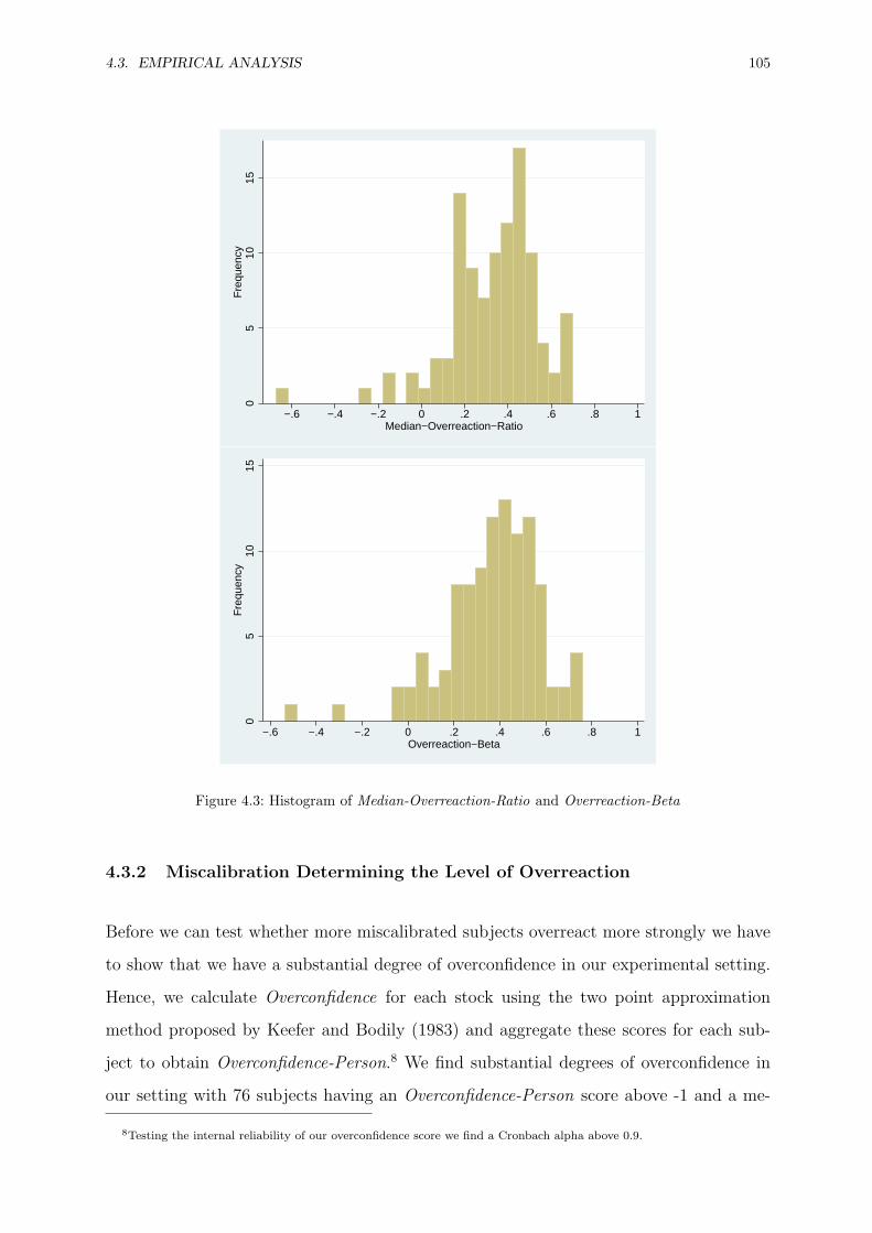
4.3. EMPIRICAL ANALYSIS 105
05
1015
Fre
quen
cy
−.6 −.4 −.2 0 .2 .4 .6 .8 1Median−Overreaction−Ratio
05
1015
Fre
quen
cy
−.6 −.4 −.2 0 .2 .4 .6 .8 1Overreaction−Beta
Figure 4.3: Histogram of Median-Overreaction-Ratio and Overreaction-Beta
4.3.2 Miscalibration Determining the Level of Overreaction
Before we can test whether more miscalibrated subjects overreact more strongly we have
to show that we have a substantial degree of overconfidence in our experimental setting.
Hence, we calculate Overconfidence for each stock using the two point approximation
method proposed by Keefer and Bodily (1983) and aggregate these scores for each sub-
ject to obtain Overconfidence-Person.8 We find substantial degrees of overconfidence in
our setting with 76 subjects having an Overconfidence-Person score above -1 and a me-
8Testing the internal reliability of our overconfidence score we find a Cronbach alpha above 0.9.
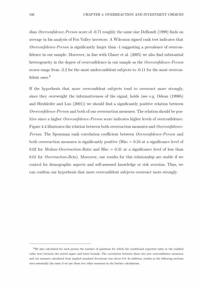
106 CHAPTER 4: OVERREACTION AND INVESTMENT CHOICES
dian Overconfidence-Person score of -0.71 roughly the same size DeBondt (1998) finds on
average in his analysis of Fox Valley investors. A Wilcoxon signed rank test indicates that
Overconfidence-Person is significantly larger than -1 suggesting a prevalence of overcon-
fidence in our sample. Moreover, in line with Glaser et al. (2005) we also find substantial
heterogeneity in the degree of overconfidence in our sample as the Overconfidence-Person
scores range from -2.2 for the most underconfident subjects to -0.11 for the most overcon-
fident ones.9
If the hypothesis that more overconfident subjects tend to overreact more strongly,
since they overweight the informativeness of the signal, holds (see e.g. Odean (1998b)
and Hirshleifer and Luo (2001)) we should find a significantly positive relation between
Overconfidence-Person and both of our overreaction measures. The relation should be pos-
itive since a higher Overconfidence-Person score indicates higher levels of overconfidence.
Figure 4.4 illustrates the relation between both overreaction measures and Overconfidence-
Person. The Spearman rank correlation coefficient between Overconfidence-Person and
both overreaction measures is significantly positive (Rho = 0.24 at a significance level of
0.02 for Median-Overreaction-Ratio and Rho = 0.31 at a significance level of less than
0.01 for Overreaction-Beta). Moreover, our results for this relationship are stable if we
control for demographic aspects and self-assessed knowledge or risk aversion. Thus, we
can confirm our hypothesis that more overconfident subjects overreact more strongly.
9We also calculated for each person the number of questions for which the conditional expected value or the realized
value were between the stated upper and lower bounds. The correlation between these two new overconfidence measures
and our measure calculated from implied standard deviations was above 0.9. In addition, results in the following sections
were essentially the same if we use these two other measures in the further calculations.
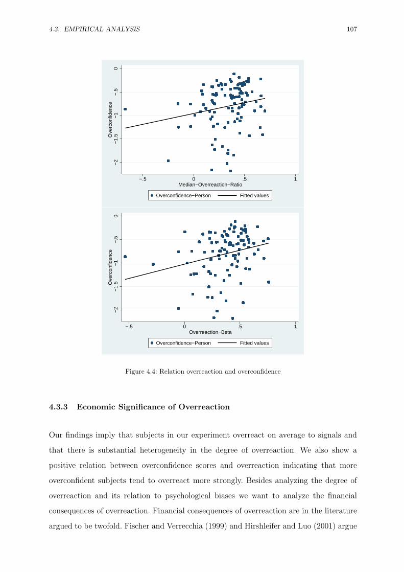
4.3. EMPIRICAL ANALYSIS 107
−2
−1.
5−
1−
.50
Ove
rcon
fiden
ce
−.5 0 .5 1Median−Overreaction−Ratio
Overconfidence−Person Fitted values
−2
−1.
5−
1−
.50
Ove
rcon
fiden
ce
−.5 0 .5 1Overreaction−Beta
Overconfidence−Person Fitted values
Figure 4.4: Relation overreaction and overconfidence
4.3.3 Economic Significance of Overreaction
Our findings imply that subjects in our experiment overreact on average to signals and
that there is substantial heterogeneity in the degree of overreaction. We also show a
positive relation between overconfidence scores and overreaction indicating that more
overconfident subjects tend to overreact more strongly. Besides analyzing the degree of
overreaction and its relation to psychological biases we want to analyze the financial
consequences of overreaction. Financial consequences of overreaction are in the literature
argued to be twofold. Fischer and Verrecchia (1999) and Hirshleifer and Luo (2001) argue

108 CHAPTER 4: OVERREACTION AND INVESTMENT CHOICES
that subjects who overreact are - owing to overconfidence - willing to take more risks in
their investments to exploit mispricings. Daniel et al. (2001) and Biais and Weber (2007)
show that subjects who overreact fail to diversify properly and hold less efficient portfolios
than subjects who do not overreact.
The Effect of Overreaction on Risk Taking
The main goal of this section is to analyze whether overreaction has an influence on the
riskiness of portfolio decisions. As we did not allow subjects to take short positions in
any asset we should observe a twofold effect of overreaction on risk taking. After a good
signal overreacting subjects overweight the positive effects of the signal and invest more
heavily in the risky asset whereas after a bad signal they overweight the negative effects
of the signal and invest less heavily into the risky asset.10 Before we test this relationship
on a disaggregate level, we want to test if it also holds on an aggregate level. Therefore,
we correlate each subject’s median portfolio risk which equals his / her median portfolio
volatility with both overreaction measures. However, since our hypothesis depends on the
sign of the signal we do this analysis separately for questions for which subjects received
positive (Median Risk+) and negative (Median Risk−) signals. Our hypothesis is that we
should find a significantly positive correlation between both constructs for good signals
and a significantly negative correlation for bad signals.
Indeed, for portfolios with a positive signal the Spearman rank correlation of Median
Risk+ with Median-Overreaction-Ratio is 0.28 (p-value < 0.01) and the correlation with
Overreaction-Beta is 0.24 (p-value = 0.01). For portfolios with a negative signal the Spear-
man rank correlation of Median Risk− with Median-Overreaction-Ratio is -0.21 (p-value
= 0.03) and the correlation with Overreaction-Beta is -0.28 (p-value < 0.01).11 These
relations are illustrated in figure 4.5 and figure 4.6.
10If we would have allowed short sales more overreacting subjects should have taken larger short positions in stocks with
a negative signal than rational subjects.
11If we exclude subjects that decide not to invest into any of the risky assets, i.e. subjects whose portfolio risk is zero,
our results weaken as we lose a substantial number of observations. The correlation coefficients are still negative, however,
not statistically significant.
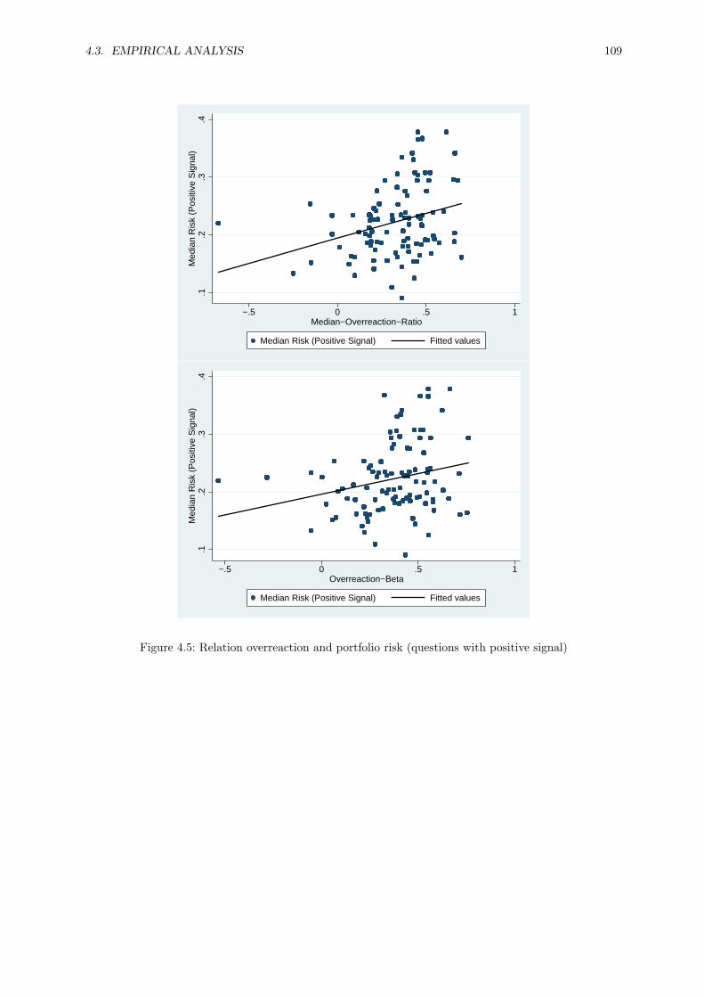
4.3. EMPIRICAL ANALYSIS 109
.1.2
.3.4
Med
ian
Ris
k (P
ositi
ve S
igna
l)
−.5 0 .5 1Median−Overreaction−Ratio
Median Risk (Positive Signal) Fitted values
.1.2
.3.4
Med
ian
Ris
k (P
ositi
ve S
igna
l)
−.5 0 .5 1Overreaction−Beta
Median Risk (Positive Signal) Fitted values
Figure 4.5: Relation overreaction and portfolio risk (questions with positive signal)
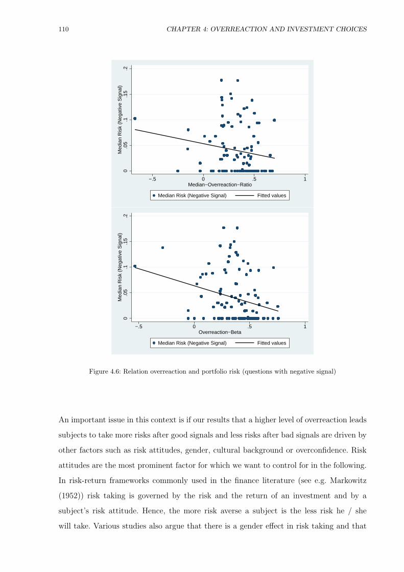
110 CHAPTER 4: OVERREACTION AND INVESTMENT CHOICES
0.0
5.1
.15
.2M
edia
n R
isk
(Neg
ativ
e S
igna
l)
−.5 0 .5 1Median−Overreaction−Ratio
Median Risk (Negative Signal) Fitted values
0.0
5.1
.15
.2M
edia
n R
isk
(Neg
ativ
e S
igna
l)
−.5 0 .5 1Overreaction−Beta
Median Risk (Negative Signal) Fitted values
Figure 4.6: Relation overreaction and portfolio risk (questions with negative signal)
An important issue in this context is if our results that a higher level of overreaction leads
subjects to take more risks after good signals and less risks after bad signals are driven by
other factors such as risk attitudes, gender, cultural background or overconfidence. Risk
attitudes are the most prominent factor for which we want to control for in the following.
In risk-return frameworks commonly used in the finance literature (see e.g. Markowitz
(1952)) risk taking is governed by the risk and the return of an investment and by a
subject’s risk attitude. Hence, the more risk averse a subject is the less risk he / she
will take. Various studies also argue that there is a gender effect in risk taking and that

4.3. EMPIRICAL ANALYSIS 111
females take substantially less risks than men in investment decisions (for an overview of
the literature see Eckel and Grossman (2008)).
Moreover, we want to analyze whether the cultural background of subjects could influence
the risk taking behavior. In line with Weber and Hsee (1998) we argue that German
subjects who are from a more individualistic society should invest into less risky portfolios
than subjects from more collectivist societies.12 Furthermore, our data allows us to test
an assumption common in various models on overconfidence (see e.g. Odean (1998b) and
Daniel et al. (2001)) that more overconfident subjects are going to take more risks. In
addition to these factors, we will also control for the age of the subjects, the course they
are enrolled, their semester, and their self assessed knowledge in finance and in statistics.
Table 4.1 documents that both Median-Overreaction-Ratio and Overreaction-Beta are
significantly related to Median Risk+ and Median Risk− even if we control for additional
factors. Regressions in columns 1 - 4 analyze portfolios for which subjects receive a positive
signal. For these portfolios we find that an in increase in the overreaction score by one
results in a 5.4 to 7.0 percentage points increase of Median Risk+ no matter if we control
for overconfidence in the regression (columns 2 and 4) or not. Since Median Risk+ is
on average 0.22 this implies that the effect of both overreaction scores on portfolio risk
is also of high economic significance. Analyzing portfolios for which subjects receive a
negative signal (see regressions 5 & 6) we find, consistent with the bivariate analyses, a
negative effect indicating that more overreacting subjects take substantially less risks in
these scenarios.
Moreover, for those questions for which subjects received a positive signal our control
variables indicate additional statistically significant effects. First, Median Risk+ of males
12Hsee and Weber (1999) and Weber and Hsee (1998) find significant cross-cultural differences in risk taking. More
specifically, they argue that subjects who live in a more collectivist society like China take substantially more risks than
subjects who live in a more individualistic society such as the USA. They term this the “cushion-hypothesis”. The line of
reasoning is that subjects from less individualistic societies can rely on their family, i.e. have a cushion, to help them in case
of need. Since we collected data on the native-language of the subjects we are able to test this cultural hypothesis. As only
29 out of 104 subjects are not Germans we generate a dummy variable that takes the value of 1 if the subject is a native
speaker in German and 0 otherwise. The average individualism score according to Hofstede (1980) in the Non-German
group which consists of Russian, Chinese, Bulgarian, and French subjects is 36.7 and thus lower than the one for Germans
which is 67. Hence, Germans who are part of a more individualistic society should invest into less risky portfolios.

112 CHAPTER 4: OVERREACTION AND INVESTMENT CHOICES
is approximately 4 percentage points higher than the one of females. This result is in line
with findings in Donkers et al. (2001) and Dohmen et al. (2005) who show that males
take substantially more risks in their financial decisions. As hypothesized we also find
a significant negative effect of Risk Aversion on Median Risk+. Thus, less risk averse
subjects are investing into riskier portfolios. In addition, we also find weak support for
cultural differences (see Bontempo et al. (1997) and Weber and Hsee (1998)) as German
subjects hold less risky portfolios than Non-Germans. However, this effect is only weakly
significant and vanishes if we control for overconfidence. However, we cannot observe these
effects for Median Risk− in columns 5 & 6. This difference between questions for which
subjects received a positive or a negative signal could be analyzed more thoroughly in
future research. Furthermore, in line with Dorn and Huberman (2005) and Menkhoff et al.
(2006) we do not find a direct effect of overconfidence on portfolio risk but only an indirect
effect of overconfidence on risk taking mediated by overreaction.
Now that we have found evidence for the hypothesized relationship between overreaction
and portfolio risk on the aggregate level, we turn to analyze the relationship on a disaggre-
gate level. Hence, we re-run the regressions from table 4.1, but instead of using aggregate
scores for each subject we run our regressions for each question individually controlling for
question fixed effects using dummies. As Overreaction-Beta is an aggregate measure that
is constant for each person over all questions we use in the following disaggregated anal-
yses only Overreaction-Ratio.13 To account for non-independent residuals within subjects
we cluster our observations over subjects.
A first look at the results in table 4.2 reveals that the results are mainly consistent with
our previous findings in table 4.1. Higher levels of overreaction result in riskier portfolio
investments after positive signals and less risky portfolio investments after negative sig-
nals. The effect of Overreaction-Ratio on Risk+ and Risk− is highly significant regardless
whether we control for overconfidence or not. In addition, we find that after having ob-
served a positive signal men hold substantially more risky portfolios than women, and
more risk averse subjects invest into less risky positions. We also find support for the
13To get a single score for the two variables Overreaction-Ratio and Overconfidence that are calculated for each stock,
i.e. twice for every portfolio allocation question, we simply take the mean of the variables for each portfolio allocation task.
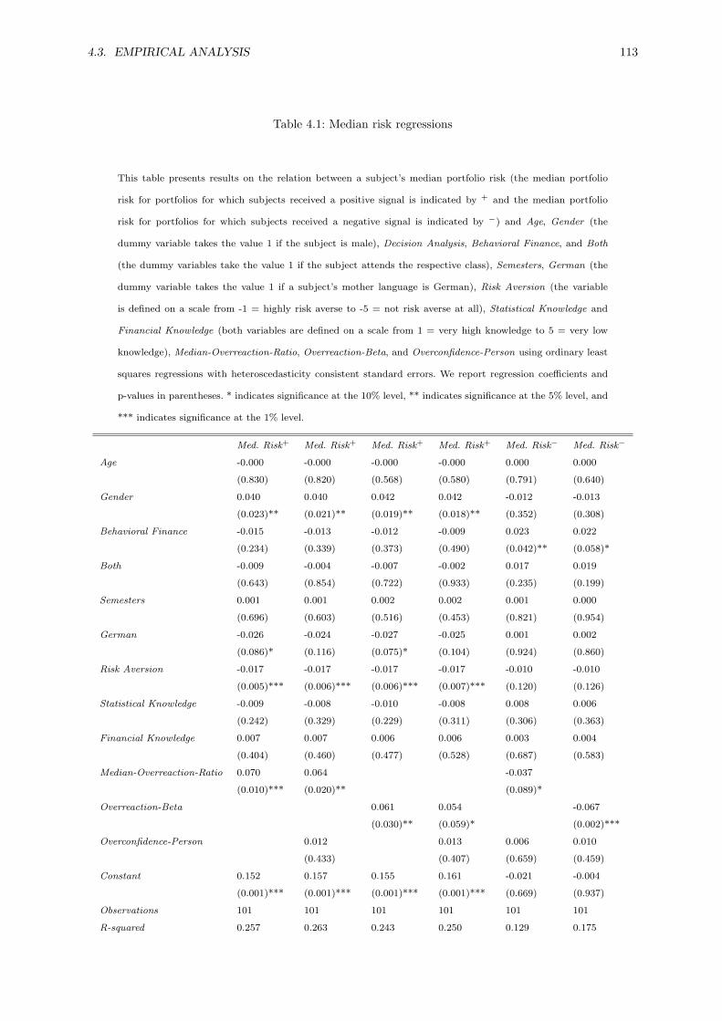
4.3. EMPIRICAL ANALYSIS 113
Table 4.1: Median risk regressions
This table presents results on the relation between a subject’s median portfolio risk (the median portfolio
risk for portfolios for which subjects received a positive signal is indicated by + and the median portfolio
risk for portfolios for which subjects received a negative signal is indicated by −) and Age, Gender (the
dummy variable takes the value 1 if the subject is male), Decision Analysis, Behavioral Finance, and Both
(the dummy variables take the value 1 if the subject attends the respective class), Semesters, German (the
dummy variable takes the value 1 if a subject’s mother language is German), Risk Aversion (the variable
is defined on a scale from -1 = highly risk averse to -5 = not risk averse at all), Statistical Knowledge and
Financial Knowledge (both variables are defined on a scale from 1 = very high knowledge to 5 = very low
knowledge), Median-Overreaction-Ratio, Overreaction-Beta, and Overconfidence-Person using ordinary least
squares regressions with heteroscedasticity consistent standard errors. We report regression coefficients and
p-values in parentheses. * indicates significance at the 10% level, ** indicates significance at the 5% level, and
*** indicates significance at the 1% level.
Med. Risk+ Med. Risk+ Med. Risk+ Med. Risk+ Med. Risk− Med. Risk−
Age -0.000 -0.000 -0.000 -0.000 0.000 0.000
(0.830) (0.820) (0.568) (0.580) (0.791) (0.640)
Gender 0.040 0.040 0.042 0.042 -0.012 -0.013
(0.023)** (0.021)** (0.019)** (0.018)** (0.352) (0.308)
Behavioral Finance -0.015 -0.013 -0.012 -0.009 0.023 0.022
(0.234) (0.339) (0.373) (0.490) (0.042)** (0.058)*
Both -0.009 -0.004 -0.007 -0.002 0.017 0.019
(0.643) (0.854) (0.722) (0.933) (0.235) (0.199)
Semesters 0.001 0.001 0.002 0.002 0.001 0.000
(0.696) (0.603) (0.516) (0.453) (0.821) (0.954)
German -0.026 -0.024 -0.027 -0.025 0.001 0.002
(0.086)* (0.116) (0.075)* (0.104) (0.924) (0.860)
Risk Aversion -0.017 -0.017 -0.017 -0.017 -0.010 -0.010
(0.005)*** (0.006)*** (0.006)*** (0.007)*** (0.120) (0.126)
Statistical Knowledge -0.009 -0.008 -0.010 -0.008 0.008 0.006
(0.242) (0.329) (0.229) (0.311) (0.306) (0.363)
Financial Knowledge 0.007 0.007 0.006 0.006 0.003 0.004
(0.404) (0.460) (0.477) (0.528) (0.687) (0.583)
Median-Overreaction-Ratio 0.070 0.064 -0.037
(0.010)*** (0.020)** (0.089)*
Overreaction-Beta 0.061 0.054 -0.067
(0.030)** (0.059)* (0.002)***
Overconfidence-Person 0.012 0.013 0.006 0.010
(0.433) (0.407) (0.659) (0.459)
Constant 0.152 0.157 0.155 0.161 -0.021 -0.004
(0.001)*** (0.001)*** (0.001)*** (0.001)*** (0.669) (0.937)
Observations 101 101 101 101 101 101
R-squared 0.257 0.263 0.243 0.250 0.129 0.175
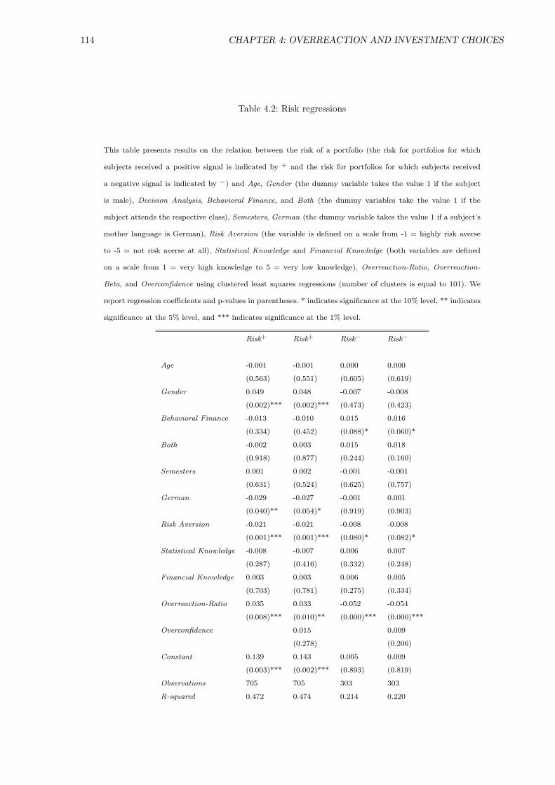
114 CHAPTER 4: OVERREACTION AND INVESTMENT CHOICES
Table 4.2: Risk regressions
This table presents results on the relation between the risk of a portfolio (the risk for portfolios for which
subjects received a positive signal is indicated by + and the risk for portfolios for which subjects received
a negative signal is indicated by −) and Age, Gender (the dummy variable takes the value 1 if the subject
is male), Decision Analysis, Behavioral Finance, and Both (the dummy variables take the value 1 if the
subject attends the respective class), Semesters, German (the dummy variable takes the value 1 if a subject’s
mother language is German), Risk Aversion (the variable is defined on a scale from -1 = highly risk averse
to -5 = not risk averse at all), Statistical Knowledge and Financial Knowledge (both variables are defined
on a scale from 1 = very high knowledge to 5 = very low knowledge), Overreaction-Ratio, Overreaction-
Beta, and Overconfidence using clustered least squares regressions (number of clusters is equal to 101). We
report regression coefficients and p-values in parentheses. * indicates significance at the 10% level, ** indicates
significance at the 5% level, and *** indicates significance at the 1% level.
Risk+ Risk+ Risk− Risk−
Age -0.001 -0.001 0.000 0.000
(0.563) (0.551) (0.605) (0.619)
Gender 0.049 0.048 -0.007 -0.008
(0.002)*** (0.002)*** (0.473) (0.423)
Behavioral Finance -0.013 -0.010 0.015 0.016
(0.334) (0.452) (0.088)* (0.060)*
Both -0.002 0.003 0.015 0.018
(0.918) (0.877) (0.244) (0.160)
Semesters 0.001 0.002 -0.001 -0.001
(0.631) (0.524) (0.625) (0.757)
German -0.029 -0.027 -0.001 0.001
(0.040)** (0.054)* (0.919) (0.903)
Risk Aversion -0.021 -0.021 -0.008 -0.008
(0.001)*** (0.001)*** (0.080)* (0.082)*
Statistical Knowledge -0.008 -0.007 0.006 0.007
(0.287) (0.416) (0.332) (0.248)
Financial Knowledge 0.003 0.003 0.006 0.005
(0.703) (0.781) (0.275) (0.334)
Overreaction-Ratio 0.035 0.033 -0.052 -0.054
(0.008)*** (0.010)** (0.000)*** (0.000)***
Overconfidence 0.015 0.009
(0.278) (0.206)
Constant 0.139 0.143 0.005 0.009
(0.003)*** (0.002)*** (0.893) (0.819)
Observations 705 705 303 303
R-squared 0.472 0.474 0.214 0.220

4.3. EMPIRICAL ANALYSIS 115
cultural hypothesis as the dummy variable German is significantly negative. Once again,
the additional effects of Gender and German cannot be observed for portfolios for which
subjects received a negative signal.14
The Effect of Overreaction on Portfolio Efficiency
A further consequence of overreaction that we want to test in the following is the rela-
tionship between overreaction and portfolio performance. Biais and Weber (2007) show in
their theoretical model that subjects who overreact, i.e. put too much weight on private
signals, will have a lower investment performance. Hence, in our experimental setting we
expect to observe that subjects will hold less efficient portfolios the more they overreact.
However, we found a substantial degree of heterogeneity in the level of overreaction with
some subjects even underreacting and thus putting not enough weight on the signal (see
subsection 4.3.1). We argue that these underreacting subjects should also invest into less
efficient portfolios than rational subjects. This should result in a hump-shaped relation
between overreaction and portfolio efficiency with rational subjects having the highest
efficiency and efficiency decreasing with higher levels of misreaction.
To analyze this relationship in more detail we first have to define the term efficiency
of a portfolio. Our measure of portfolio efficiency is the ex-ante Sharpe-Ratio for each
subject and each portfolio. To calculate the Sharpe-Ratio for a subject’s portfolio we use
conditional expected returns and conditional expected standard deviation. Calculating the
Sharpe-Ratio makes only sense for stocks with a positive conditional expected return, and
thus we exclude in the following analyses all stocks with a negative conditional expected
return.
In addition, as we imposed short selling constraints on our subjects, i.e. we did not allow
them to short sell assets in order to invest more into the other assets, the capital market
14Instead of clustering over subjects to control for non-independent residuals we also re-run the regressions using fixed
and random effects models. We obtain essentially the same results using these models. However, both models have their
disadvantages. A Hausman test shows that the random effects model needs not to generate consistent estimates. Although,
the fixed effects model generates consistent estimates its major disadvantage is that we cannot make a statement about the
effect of demographics, risk attitude, and knowledge on risk taking. Hence, we only make use of clustered ordinary least
squares regressions where we control for question specific effects.

116 CHAPTER 4: OVERREACTION AND INVESTMENT CHOICES
line is no straight-line. Thus, we cannot make the general statement that a higher Sharpe-
Ratio implies a more efficient portfolio as it is possible that subjects that want to take
more risks can only do so by investing a relatively large amount into the riskier stock.
Due to the short selling constraint portfolios of these subjects have a lower Sharpe ratio
than portfolios of subjects that invest into the market portfolio. But we cannot infer that
they are less efficient as they offer the only possibility to take on more risk. However,
for subjects that invest in portfolios that are less risky than the market portfolio and for
subjects that invest into the risk free asset the risk constraint is not binding. Hence, in
our further analyses we omit 152 out of 728 portfolios that are to the right of the market
portfolio, i.e. that are riskier than the market portfolio, and for which subjects did not
invest into the risk free asset. Therefore, in the following analyses we only take portfolios
for which the short selling constraint is not binding.
To document the link between overreaction and portfolio efficiency we calculate Spearman
rank correlation coefficients between portfolio efficiency and Median-Overreaction-Ratio
and Overreaction-Beta, respectively. However, as our hypothesis implies that stronger
misreaction (overreaction or underreaction) leads to less efficient portfolios we divide our
sample into two unbalanced parts. One part is composed of subjects that overreact and the
other, substantially smaller one of subjects that underreact. Calculating Spearman rank
correlation coefficients for the two parts separately we find a negative relation for subjects
that overreact with coefficients of -0.33 for Median-Overreaction-Ratio (p− value < 0.01)
and -0.18 for Overreaction-Beta (p−value = 0.07) and a tentatively positive effect for the
six subjects that underreact. This relation is illustrated by the dashed (dotted) lines in
figure 4.7 for subjects that overreact (underreact). The figure demonstrates that a higher
level of over/underreaction gives rise to less efficient portfolios.
While the above evidence indicates an effect of overreaction on portfolio efficiency we want
to analyze whether this effect is stable if we control for additional variables. To analyze
this in more detail we run regressions with the median Sharpe ratio (see table 4.3) and the
disaggregated Sharpe ratio (see table 4.4) as dependent variables. Table 4.3 documents the
relation between portfolio efficiency and both overreaction measures on an aggregate level
using additional controls for all observations for which subjects overreact. Consistent with

4.3. EMPIRICAL ANALYSIS 117
.51
1.5
2M
edia
n S
harp
e R
atio
−.5 0 .5 1Median−Overreaction−Ratio
Median Sharpe RatioFit if Median−Overreaction−Ratio>0Fit if Median−Overreaction−Ratio<0
.51
1.5
2M
edia
n S
harp
e R
atio
−.5 0 .5 1Overreaction−Beta
Median Sharpe RatioFit if Overreaction−Beta>0Fit if Overreaction−Beta<0
Figure 4.7: Relation overreaction and Sharpe ratio

118 CHAPTER 4: OVERREACTION AND INVESTMENT CHOICES
our previous findings both overreaction measures have a significantly negative coefficient
indicating that higher levels of overreaction lead to lower levels of portfolio efficiency.15
In addition, we re-run our regressions on a single question level instead of an aggregate
level and account for non-independent residuals within subjects by clustering over sub-
jects. Again, we only make use of Overreaction-Ratio as Overreaction-Beta is constant
for all subjects. Additionally, we control for question effects using dummy variables. The
results of these regressions are illustrated in table 4.4. In regressions 1 & 2 we only take
observations for which Overreaction-Ratio is greater than zero indicating overreaction
whereas in regressions 3 & 4 we only take observations for which Overreaction-Ratio is
below zero indicating underreaction.
The regressions in table 4.4 show the twofold effect of overreaction on portfolio efficiency
on a single stock level. The more subjects misreact the lower is their portfolio efficiency.
On the one hand, we find highly significantly negative overreaction coefficients of approx-
imately -0.145 in the first two regressions no matter if we control for overconfidence or
not. On the other hand, our results in regressions 3 & 4 indicate a highly negative ef-
fect of underreaction of approximately -0.3 on portfolio efficiency. Thus, the higher the
overreaction score, i.e. the less subjects underreact, the more efficient is their portfolio.
Consistent with Daniel et al. (2001) and Biais and Weber (2007) we show that misreac-
tion to signals, i.e. overreaction or underreaction, is costly for investors and harms their
performance. Minimizing the level of misreaction can have a substantial effect on a sub-
jects portfolio efficiency as measured with the Sharpe-Ratio. Interestingly, the coefficient
of Overreaction-Ratio on portfolio efficiency is in absolute terms much larger if we analyze
underreaction than if we analyze overreaction. Future research might want to analyze this
difference in more depth. Overall, our findings are in line with the hypothesis of a hump-
15Regressing the median Sharpe ratio of subjects’ portfolios on various control variables for underreacting subjects only is
not reasonable as the number of underreacting subjects is six and four, respectively, and thus too low to make any inferences
about the relationship between overreaction and portfolio efficiency while controlling for additional variables.

4.3. EMPIRICAL ANALYSIS 119
Table 4.3: Median Sharpe ratio regressions
This table presents results on the relation between a subject’s median portfolio efficiency measured with
the Sharpe ratio and Age, Gender (the dummy variable takes the value 1 if the subject is male), Decision
Analysis, Behavioral Finance, and Both (the dummy variables take the value 1 if the subject attends the
respective class), Semesters, German (the dummy variable takes the value 1 if a subject’s mother language
is German), Risk Aversion (the variable is defined on a scale from -1 = highly risk averse to -5 = not risk
averse at all), Statistical Knowledge and Financial Knowledge (both variables are defined on a scale from
1 = very high knowledge to 5 = very low knowledge), Median-Overreaction-Ratio, Overreaction-Beta, and
Overconfidence-Person using ordinary least squares regressions with heteroscedasticity consistent standard
errors. Both regressions are only run for subjects for which the respective overreaction score was greater
than zero indicating overreaction. We report regression coefficients and p-values in parentheses. * indicates
significance at the 10% level, ** indicates significance at the 5% level, and *** indicates significance at the
1% level.
Median-SharpeOR>0 Median-SharpeOR>0
Age 0.007 -0.006
(0.729) (0.397)
Gender -0.049 -0.082
(0.555) (0.345)
Behavioral Finance 0.049 0.001
(0.540) (0.991)
Both 0.081 0.019
(0.441) (0.862)
Semesters 0.011 0.016
(0.559) (0.325)
German -0.052 -0.044
(0.578) (0.658)
Risk Aversion 0.060 0.059
(0.137) (0.170)
Statistical Knowledge -0.040 -0.027
(0.373) (0.566)
Financial Knowledge -0.007 -0.006
(0.877) (0.904)
Median-Overreaction-Ratio -0.772
(0.001)***
Overreaction-Beta -0.450
(0.034)**
Overconfidence-Person 0.024 0.016
(0.743) (0.821)
Constant 1.717 1.885
(0.000)*** (0.000)***
Observations 95 97
R-squared 0.189 0.118

120 CHAPTER 4: OVERREACTION AND INVESTMENT CHOICES
Table 4.4: Sharpe ratio regressions
This table presents results on the relation between the efficiency of a portfolio measured as the Sharpe-Ratio
and Age, Gender (the dummy variable takes the value 1 if the subject is male), Decision Analysis, Behavioral
Finance, and Both (the dummy variables take the value 1 if the subject attends the respective class), Semesters,
German (the dummy variable takes the value 1 if a subject’s mother language is German), Risk Aversion
(the variable is defined on a scale from -1 = highly risk averse to -5 = not risk averse at all), Statistical
Knowledge and Financial Knowledge (both variables are defined on a scale from 1 = very high knowledge
to 5 = very low knowledge), Overreaction-Ratio, Overreaction-Beta, and Overconfidence using clustered least
squares regressions (number of clusters is equal to 101). Regression 1 & 2 are run using only observations for
which the respective overreaction score indicates overreaction: we indicate this by SharpeOR>0. For regression
3 & 4 we use only observations for which we find negative overreaction, i.e. underreaction and indicate this
with SharpeOR<0. * indicates significance at the 10% level, ** indicates significance at the 5% level, and ***
indicates significance at the 1% level.
SharpeOR>0 SharpeOR>0 SharpeOR<0 SharpeOR<0
Age 0.004 0.005 -0.002 -0.003
(0.435) (0.343) (0.506) (0.448)
Gender -0.067 -0.067 0.129 0.136
(0.055)* (0.057)* (0.122) (0.094)*
Behavioral Finance 0.090 0.082 0.015 0.005
(0.025)** (0.038)** (0.793) (0.922)
Both 0.113 0.093 0.023 0.008
(0.018)** (0.045)** (0.800) (0.939)
Semesters -0.009 -0.010 -0.012 -0.014
(0.247) (0.174) (0.334) (0.275)
German 0.037 0.028 -0.109 -0.115
(0.358) (0.501) (0.165) (0.131)
Risk Aversion 0.032 0.030 -0.024 -0.023
(0.104) (0.112) (0.416) (0.442)
Statistical Knowledge -0.025 -0.031 0.053 0.048
(0.212) (0.114) (0.105) (0.151)
Financial Knowledge -0.021 -0.018 -0.048 -0.047
(0.248) (0.329) (0.095)* (0.102)
Overreaction-Ratio -0.145 -0.142 0.297 0.308
(0.000)*** (0.000)*** (0.007)*** (0.005)***
Overconfidence -0.052 -0.041
(0.059)* (0.409)
Constant 1.994 1.963 1.982 1.980
(0.000)*** (0.000)*** (0.000)*** (0.000)***
Observations 421 421 137 137
R-squared 0.811 0.812 0.654 0.655
4.4. CONCLUSION 121
shaped relation between portfolio efficiency and overreaction. Hence, the closer subjects
are to the rational benchmark the more efficient the portfolios are they are investing.16
Moreover, for regressions 1 & 2 we find a significant effect for the course subjects are
enrolled. Subjects that are enrolled in the Decision Analysis class which is a more general
topic course not only for students specializing in finance tend to invest into worse per-
forming portfolios than subjects that are enrolled in the Behavioral Finance class which
is part of the specialization in finance. This is indicated by the positive coefficients of
Behavioral Finance and Both. Mahani and Poteshman (2008) provide similar evidence
by showing that unsophisticated option market investors overreact to news on underly-
ing stock and consequently have a lower performance. Further control variables are not
strongly significant, just as in the regressions on the aggregate level.
4.4 Conclusion
This study experimentally analyzes the existence of overreaction, its relation to psycholog-
ical biases, and its financial consequences. We introduce a new experimental design that
asks subjects to estimate the future price of an asset given the information on another,
related asset. This design allows us to measure the level of overreaction explicitly. We mea-
sure overreaction using two highly correlated measures: our first measure of overreaction
is simply the ratio of forecasting error to innovation in the signal (Overreaction-Ratio)
and our second measure of overreaction is the slope of a regression of error onto signal
(Overreaction-Beta). Overall, we find evidence for strong overreaction in our data which
is consistent with findings in Thomas and Zhang (2008) who analyze a similar scenario
empirically. However, there seems to be large heterogeneity in the level of overreaction as
few subjects are even prone to underreaction.
Examining the relationship between overreaction and psychological biases we focus on
overconfidence and more exactly on miscalibration. We document a substantial level of
16As in section 4.3.3 we re-run the regressions using fixed and random effects models. We obtain essentially the same
results using these models. However, a Hausman test shows that the random effects model needs not to generate consistent
estimates and thus we abstain from using it.

122 CHAPTER 4: OVERREACTION AND INVESTMENT CHOICES
overconfidence with the majority of subjects being overconfident but also a few subjects
being underconfident. Relating overconfidence to overreaction we find, as hypothesized,
that more overconfident subjects tend to overreact more heavily.
Moreover, we analyze the effect of overreaction on subjects’ portfolio risk and on their
portfolio efficiency. We show that after having received a positive signal overreacting
subjects take substantially more risks than rational subjects. In addition, our results
support findings in the literature that show an effect of gender (see Eckel and Grossman
(2008)), risk aversion (see Barsky et al. (1997)), and culture (see Weber and Hsee (1998))
on risk taking. Also in line with our hypothesis we show that after receiving a negative
signal overreacting subjects invest into substantially less risky portfolios. This effect can
be attributed to the short selling constraint which was imposed by us to make the task
more realistic and less complex.
Relating portfolio efficiency to overreaction we find no linear relation but more of a hump-
shaped relation. This hump-shape implies that portfolio efficiency is lower the more a
subject overreacts or underreacts. Analyzing the effect of overreaction and underreaction
separately we find exactly this effect. Moreover, our results rely on decisions that have
substantial monetary effects. We pay subjects an hourly compensation that is on average
five times as high as the hourly wage of undergraduate research assistants.
Our experimental approach offers the advantage that we can explicitly measure the level of
overreaction and relate it to psychological biases and financial consequences. In a similar
experiment that was run with professional bond traders we used price paths from real
assets instead of artificial ones. The results are robust and show that even professional
bond traders tend to overreact to these kind of signals.
Future research could utilize our experimental approach and analyze whether other psy-
chological traits such as the use of the representativeness heuristic (see Barberis et al.
(1998)) or the hindsight bias (see Biais and Weber (2007)) influence subjects’ information
processing, i.e. their level of overreaction, and subsequently their investment behavior. It
could also be of interest to analyze whether other forms of overconfidence like the better
than average effect or illusion of control are related to overreaction and correspondingly

4.4. CONCLUSION 123
to investment behavior in this context. Moreover, future research could study in an ex-
perimental market setting whether markets populated with agents who overreact more
strongly will yield different price patterns or even less efficient prices. Another promising
direction, in the spirit of Griffin and Tversky (1992) and Bloomfield et al. (2000), would
be to study whether the level of overreaction varies depending on the weight of the signal
subjects receive. Higher weight levels and subsequently lower levels of overreaction should
be observed if the industry specific shock is of higher weight than the firm specific shock,
i.e. if the two stocks in one graph are more highly correlated. In a similar vein, it would
also be interesting to analyze how the level of overreaction changes if the time periods for
which subjects receive graphical information are varied. Finally, it would be interesting
to analyze whether subjects that overreact in our experimental setting and consequently
have less efficient portfolios will also tend to invest into less efficient portfolios in reality.

124 CHAPTER 4: OVERREACTION AND INVESTMENT CHOICES
4.5 Appendix
1
Questionnaire
Dear participants,
we would like to welcome you to this questionnaire study which is a joint research project of the Univer-
sity of Mannheim and Toulouse University. The study is sponsored by the European Union within the
„European Network for the Advancement of Behavioural Economics“ (ENABLE). The main part of the
study consists of 10 questions that should be answered sequentially. Each of the 10 questions is made up
of two parts, part A and part B. Within part A we kindly ask you to submit your stock price forecasts for
two stocks by stating a lower bound, a best estimate, and an upper bound. Part B asks you to construct
your preferred portfolio, choosing between two stocks and a risk free asset. In addition to these ten ques-
tions we are going to ask you several shorter questions where you have to indicate how you see yourself
and your colleagues, respectively.
As a thank you for taking part in our survey, we are paying you a performance-related participation com-
pensation. This compensation depends only upon your performance in the two parts A and B of the ques-
tionnaire. How your compensation is determined exactly is going to be explained in the instructions to
this study, following on the next pages.
As researchers we heavily rely on the quality of our collected data. Thus, we would kindly ask you to take
your time filling out this questionnaire and not to communicate with other participants of the study.
Thank you very much for your assistance and enjoy the questionnaire.
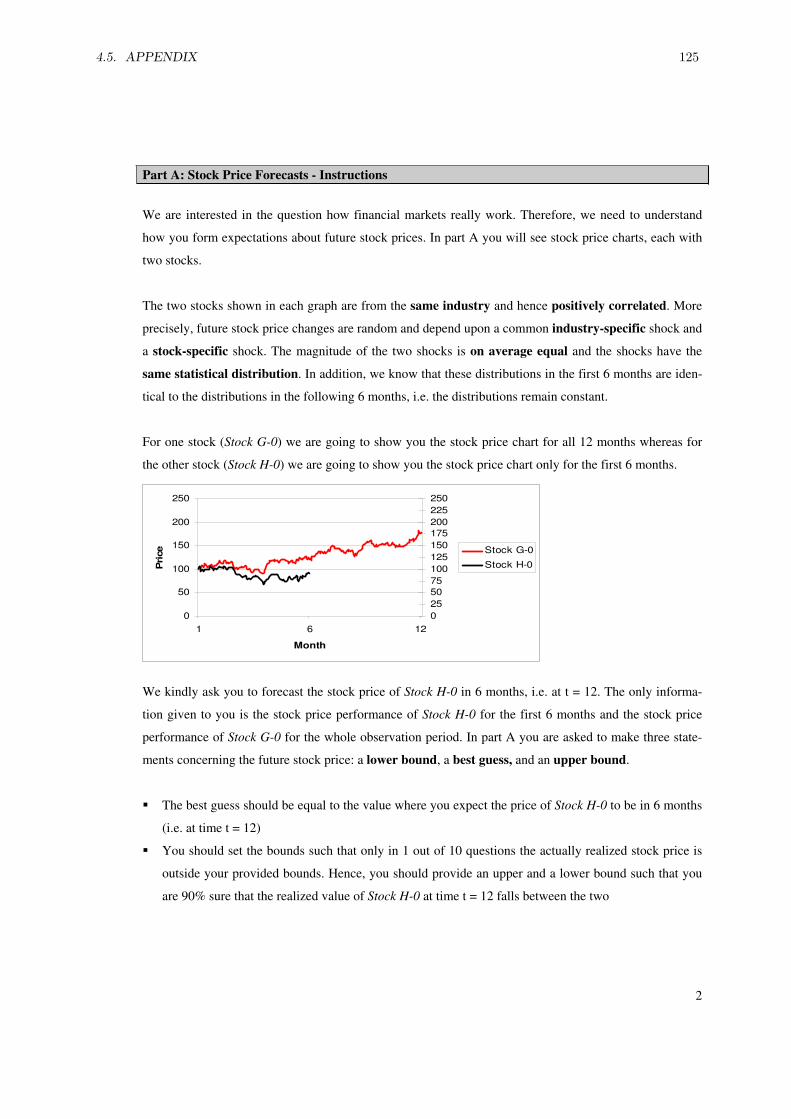
4.5. APPENDIX 125
Part A: Stock Price Forecasts - Instructions
We are interested in the question how financial markets really work. Therefore, we need to understand
how you form expectations about future stock prices. In part A you will see stock price charts, each with
two stocks.
The two stocks shown in each graph are from the same industry and hence positively correlated. More
precisely, future stock price changes are random and depend upon a common industry-specific shock and
a stock-specific shock. The magnitude of the two shocks is on average equal and the shocks have the
same statistical distribution. In addition, we know that these distributions in the first 6 months are iden-
tical to the distributions in the following 6 months, i.e. the distributions remain constant.
For one stock (Stock G-0) we are going to show you the stock price chart for all 12 months whereas for
the other stock (Stock H-0) we are going to show you the stock price chart only for the first 6 months.
0
50
100
150
200
250
1 6 12
Month
Price
0
25
50
75
100
125
150
175
200
225
250
Stock G-0
Stock H-0
We kindly ask you to forecast the stock price of Stock H-0 in 6 months, i.e. at t = 12. The only informa-
tion given to you is the stock price performance of Stock H-0 for the first 6 months and the stock price
performance of Stock G-0 for the whole observation period. In part A you are asked to make three state-
ments concerning the future stock price: a lower bound, a best guess, and an upper bound.
The best guess should be equal to the value where you expect the price of Stock H-0 to be in 6 months
(i.e. at time t = 12)
You should set the bounds such that only in 1 out of 10 questions the actually realized stock price is
outside your provided bounds. Hence, you should provide an upper and a lower bound such that you
are 90% sure that the realized value of Stock H-0 at time t = 12 falls between the two
2

126 CHAPTER 4: OVERREACTION AND INVESTMENT CHOICES
Part A: Stock Price Forecasts – Payment Scheme
Your payment in part A depends only on the quality of your best guesses. I.e. the smaller the difference
between your best guess and the actually realized stock price is, the higher is your payment going to be.
To determine your payment exactly we calculate for each of the 20 exercises (10 questions each with 2
exercises) in part A your so called error. This error is the absolute margin between your best guess and
the actually realized stock price:
Error i = | Best Guess i – Actually Realied Price i | i = 1, 2, …, 20
Then we calculate your average error over all 20 exercises in part A as:
Average Error = 20
Error 20
1i
i
Your final payment for part A is the maximum of 0 € and 50 € minus your average error and is calculated
using the following formula:
ErrorAverage - € 50;€ 0 Max PaymentA
Thus, in a best case scenario your payment in part A can be up to 50 € and in the worst case your payment
is going to be 0 €.
Part B: Portfolio Allocation - Instructions
In every of the 10 portfolio allocation questions in part B we kindly ask you to invest at time t = 6 a given
amount of 10,000 €. Your investment opportunities in every question include a risk free asset that gener-
ates a return of 0% and two risky stocks. The two stocks in part B are the same stocks for which you pro-
vided stock price estimates in part A of the respective question.
You are asked to allocate the amount of 10,000 € – from your point of view – optimally between the risk
free asset and the two stocks. However, you can only invest amounts greater or equal to zero into each
of the three assets. I.e. you cannot sell one asset short and invest a higher amount of money into the re-
maining two assets. Moreover, you are only offered these three investment opportunities and hence you
must divide the whole amount of 10,000 € between them.
Part B: Portfolio Allocation - Payment Scheme
At the end of the study we are going to calculate realized returns for each stock for the time period t = 6
to t = 12. Then we are going to pick 1 of the 10 questions randomly and are going to calculate the real-
ized return of your stated portfolio.
Your final payment for part B is equal to:
Payment B = 15 € * (1 + Realized Portfolio Return)
3
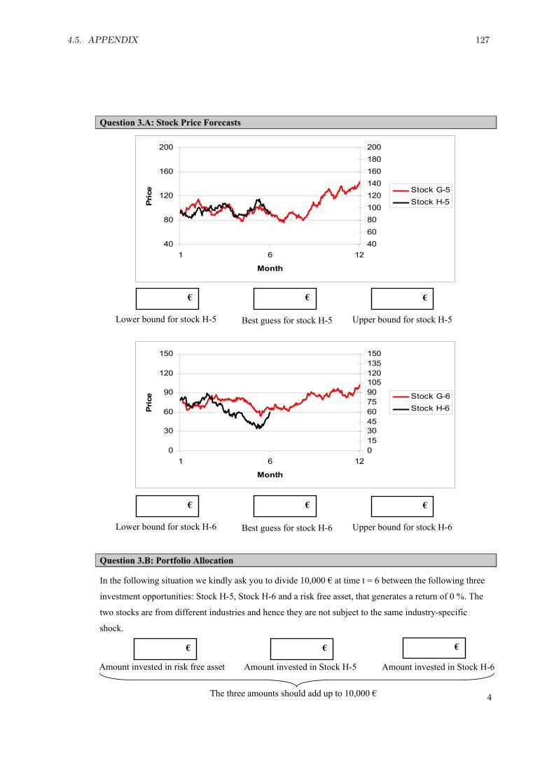
4.5. APPENDIX 127
4
Question 3.A: Stock Price Forecasts
Question 3.B: Portfolio Allocation
In the following situation we kindly ask you to divide 10,000 € at time t = 6 between the following three
investment opportunities: Stock H-5, Stock H-6 and a risk free asset, that generates a return of 0 %. The
two stocks are from different industries and hence they are not subject to the same industry-specific
shock.
Best guess for stock H-5 Upper bound for stock H-5
€ €
Lower bound for stock H-5
€
Best guess for stock H-6 Upper bound for stock H-6
€ €
Lower bound for stock H-6
€
40
80
120
160
200
1 6 12
Month
Price
40
60
80
100
120
140
160
180
200
Stock G-5
Stock H-5
0
30
60
90
120
150
1 6 12
Month
Price
0
15
30
45
60
75
90
105
120
135
150
Stock G-6
Stock H-6
Amount invested in Stock H-6
€
Amount invested in Stock H-5
€
The three amounts should add up to 10,000 €
Amount invested in risk free asset
€

128 CHAPTER 4: OVERREACTION AND INVESTMENT CHOICES
Some questions about how you see yourself:
How do you rate your statistical knowledge?
1 2 3 4 5
very good bad
How do you rate your knowledge about stock markets and financial markets?
1 2 3 4 5
very good bad
In this questionnaire, we asked you to provide upper and lower bounds for 20 exercises related to stock
price expectations (part A). For how many of these exercises do you think the final value is outside the
range you gave?
________ (Please give a number between 0 and 20)
In this questionnaire, we asked all subjects to provide upper and lower bounds for 20 exercises related to
stock price expectations (part A). For how many of these exercises do you think the final value is outside
the range provided by the average participant?
________ (Please give a number between 0 and 20)
Some final questions about you:
Age: __________
Gender: female male
Line of studies: ________________________________
Semester: ____________________
How would you classify your willingness to take risks in financial decisions?
1 2 3 4 5
Very low
willingness
Very high
willingness
5
Chapter 5
Overreaction in Stock Forecasts and
Prices
5.1 Introduction
Behavioral finance shows that individual biases such as the disposition effect (Odean
(1998a) and Weber and Camerer (1998)), hindsight bias (Biais and Weber (2009)) or
overconfidence (Camerer and Lovallo (1999) and Biais et al. (2005)) can affect individual
decision making. In addition, both theoretical and experimental behavioral studies argue
that markets are not always fully efficient and that market forces are not fully able to
correct for individual biases (see e.g. Camerer (1987), Jegadeesh and Titman (1995), or
Scheinkman and Xiong (2003)). However, it is still ambiguous whether and why individual
biases prevail in market outcomes and if rational explanations are more capable to explain
some market anomalies. Some studies for example show that individual biases vanish
totally or are significantly reduced by market forces whereas other studies illustrate that
individual biases remain fairly stable or even get more pronounced on an aggregate level.
On the one hand, analyzing abstract Bayesian updating tasks Camerer (1987) and Gan-
guly et al. (1994 and 2000) show that probability judgment errors or biases can indeed
persist in market settings. However, they show that the bias on an aggregate level is
reduced. In a similar vein, Camerer et al. (1989) analyzing the hindsight bias, Kluger

130 CHAPTER 5: OVERREACTION IN STOCK FORECASTS AND PRICES
and Wyatt (2000) studying judgment errors in the Monty Hall problem, and Sonnemann
et al. (2008) analyzing partition-dependence, show that market experience mitigates the
respective bias but is not able to eliminate it completely. On the other hand, Gillette et al.
(1999), Bloomfield et al. (2000), and Nelson et al. (2001) find that underreaction to sig-
nals in a coin-spin scenario shows the same extent in markets and on an individual level.
Similarly, Seybert and Bloomfield (2009) find hardly any evidence for a wishful thinking
bias on an individual level but strong evidence for wishful betting on an aggregate market
level.
In addition, van Boven et al. (2003) and Weber and Welfens (2007) show that a bias gets
smaller over repeated interactions of the same commodity or in the course of a trading
round but that this learning does not generalize to interactions with a new asset or com-
modity. Budescu and Maciejovsky (2005) conclude that “expecting biases to disappear
completely or, alternatively, to always persist are overly simplistic positions”. Overall,
findings in the literature indicate that the question whether markets can correct for in-
dividual biases depends on the structure of the market, the task on hand, the sort of
feedback that subjects receive or the individual bias that is analyzed.
The main goal of this chapter is to analyze whether individual over- or underreaction
to changes in the fundamental value of a stock, i.e. to new information, affects market
outcomes in a setting similar to the one empirically analyzed by Thomas and Zhang
(2008). Thomas and Zhang (2008) study market reactions to earnings announcements by
considering pairs of stocks from the same industry which announce earnings sequentially.
More precisely, they show that the market price of a firm that has not yet announced
earnings moves too far upward (downward) in reaction to good (bad) earnings reports of
an early-announcing peer and is corrected when the late-announcing firm’s earnings are
subsequently revealed. Thus, their findings suggest that stock prices for the late announc-
ers overreact to the information transfer from the early-announcing peer. Overreaction
(underreaction) in this context means that subjects put too much (little) weight on new
information. However, using empirical data it is not possible to rule out other explana-
tions for misreaction or to analyze in more detail, how individuals react to new information
about the fundamental value of a stock and whether this individual misreaction affects

5.1. INTRODUCTION 131
market variables. Misreaction in this context is simply defined as the absolute level of
over- or underreaction.
Since the empirical and experimental evidence on how individual misreaction affects mar-
ket outcomes is scarce, we apply the individual level approach of chapter 4 to an ex-
perimental trading market. The main features of our design are as follows: first, we give
subjects the stock price charts of two related stocks (G and H) for the last six months and
ask them to estimate the price of one of the two stocks (H) in six months. After having
provided a best estimate for stock H subjects are able to trade this stock for two minutes
in a single-unit open-book double auction market. After two minutes of trading the sub-
jects receive additional information about the other stock (G) and are asked to update
their estimates regarding the price of stock H in six months. Subsequently, subjects get
the possibility to trade stock H in a single-unit open-book double auction market again
for two minutes. Overall, each subject trades in 8 of these experimental rounds, consisting
of two trading periods of 120 seconds and two estimation tasks.
This experimental design allows us to relate individual level overreaction to market level
overreaction in an almost realistic setting, similar to the one in Thomas and Zhang (2008).
However, in contrast to their empirical approach we are able to explicitly calculate the
rational benchmark, and thus can rule out that risk or market microstructure effects
drive results on overreaction in markets. Moreover, using this clean design we are able
to quantify the exact degree of overreaction both on an individual and market level, and
thus can compare findings in the individual-level-study of chapter 4 with the aggregate
level study by Thomas and Zhang (2008).
Previous empirical and experimental evidence on the relation between individual level
misreaction and its effect on market parameters is scarce. On the one hand, most experi-
mental studies investigate the level of overreaction or underreaction on an individual level
(see e.g. Kahneman and Tversky (1973), Griffin and Tversky (1992), Bloomfield and Hales
(2002), Offerman and Sonnemans (2004), and chapter 4 of this thesis). On the other hand,
empirical studies are mostly providing evidence for aggregate market overreaction (see e.g.
DeBondt and Thaler (1985, 1987, and 1990)), Sorescu and Subrahmanyam (2006), and
Thomas and Zhang (2008)). Evidence on the question how individual misreaction to new

132 CHAPTER 5: OVERREACTION IN STOCK FORECASTS AND PRICES
information translates into market outcomes is scarce (see for notable exceptions Gillette
et al. (1999), Bloomfield et al. (2000), and Nelson et al. (2001)) and relies almost exclu-
sively on the classical Griffin and Tversky (1992) coin-spin scenario where subjects need
to indicate if a coin is heads- or tail-biased.
Our main findings can be summarized as follows: we observe strong and persistent overre-
action for individual estimates as well as for market prices following both - good and bad
news. The level of overreaction in estimates is in the same range as in the individual-level
experiment in chapter 4 of this thesis. Interestingly, aggregate overreaction in transaction
prices is not substantially lower. Thus, market forces are not able to correct for individual
biases which is in line with experimental findings in Gillette et al. (1999) who show that
underreaction in their experiment is even slightly higher in markets than on an individual
level. Moreover, our finding that overreaction does prevail in markets is also consistent
with behavioral models arguing that individual biases affect market outcomes (Odean
(1998b), Sorescu and Subrahmanyam (2006), and Biais et al. (2005)). In addition, we
provide evidence that learning effects within a 120-second trading period and learning ef-
fects over the course of the experiment are hardly observable. Lastly, up to our knowledge
our study is the first to find experimental evidence for the theoretically proposed positive
relation between differences of opinion and trading volume (Varian (1989), Harris and
Raviv (1993), and Kandel and Pearson (1995)) in experimental markets with more than
two traders.
In the next section we review the related literature on misreaction and their impact on
market factors and form our hypotheses. Section 5.3 presents our experimental design
and procedure as well as some descriptive statistics. The main results of our study are
reported in section 5.4. Section 5.5 concludes with a short discussion of our findings and
an outlook for future research.

5.2. RELATED LITERATURE AND HYPOTHESES 133
5.2 Related Literature and Hypotheses
5.2.1 Related Literature
The study in chapter 4 of this thesis offers direct experimental evidence on the relationship
between information signals, beliefs, and financial decisions. Using a novel experimental
design in which subjects are asked to estimate the future price of an asset, incorporating
the stock price development of a related asset as information signal, the study in chapter
4 has three main findings: first, in this experimental environment a substantial level of
overreaction seems to exist which is in line with findings in Griffin and Tversky (1992) on
an individual level and Thomas and Zhang (2008) on an aggregate level. Second, analyzing
the relation between individual overreaction and psychological biases it is evident that
more overconfident subjects tend to overreact more heavily. Third, the results of the study
in chapter 4 show that individual overreaction has an impact on financial variables such
as portfolio risk and portfolio efficiency.
However, it is not clear whether overreaction on an individual level translates to overre-
action in a market setting. Proponents of rational approaches often argue that just a few
rational subjects are sufficient to make market outcomes rational, that random mistakes
cancel out or that in the long run less rational subjects learn from more rational subjects
in the market (for further comments on this debate see Camerer (1987)). In the following,
we will first review the theoretical literature on individual and market overreaction and
then illustrate existing empirical and experimental evidence on this issue.1
Theoretical models
Using various behavioral biases such as overconfidence or hindsight many behavioral mod-
els argue that individual overreaction has a substantial impact on market variables.2
Amongst others, Daniel et al. (1998 and 2001), Odean (1998b), and Fischer and Verrec-
1We have argued in section 5.1 that the question whether individual biases can be corrected by market forces seems to
depend amongst others on the bias that is analyzed. Since we analyze over- or underreaction to new information we will
only illustrate studies analyzing this sort of bias.
2In addition, Grinblatt and Han (2005) show that individual underreaction caused by behaviorally affected traders has
also an influence on market prices in the equilibrium

134 CHAPTER 5: OVERREACTION IN STOCK FORECASTS AND PRICES
chia (1999) model financial markets with overconfident individuals. These overconfident
individuals overweight the precision and overestimate the quality of a private signal that
they receive. This directly results in an individual overreaction to the signal. Consequences
of this individual overreaction are the wrong assessment of means, a more aggressive trad-
ing behavior, and a poor portfolio diversification. How exactly this individual overreaction
affects market variables depends on the information structure of the market and on the
proportion of overconfident investors in the market. However, almost all studies show
that individual overreaction of some investors results in aggregate, market overreaction
and has substantial effects on market demand and market prices.
In a similar vein, Biais and Weber (2007) theoretically show that hindsight biased agents
overreact to new information and put too much weight on a private signal. The intuition
behind is that hindsight biased agents incorrectly remember their prior expectations,
and thus overweight the informational content of new information. In their CAPM-like
framework individual overreaction of hindsight biased agents affects equilibrium prices
and holdings.
A third strand of literature tries to reconcile two patterns that seem contradictory: the
representativeness heuristic (Kahneman and Tversky, 1973) and the conservatism bias
(Edwards, 1968). Griffin and Tversky (1992) argue that subjects focus too much on the
strength of a new information, i.e. the degree to which it is favorable, and not enough on
its weight, i.e. its statistical reliability. They use the evaluation of recommendation letters
as an example. Here the strength refers to how positive or warm the letter’s content is and
the weight refers to the credibility and knowledge of the writer. They argue that the rep-
resentativeness heuristic and hence overreaction to new information prevails in situations
in which subjects receive new information which is characterized by high strength and low
weight. In the recommendation letter example this corresponds to a very nice recommen-
dation letter from a person with low credibility. Barberis et al. (1998) and Sorescu and
Subrahmanyam (2006) develop theoretical models that extend these findings and implica-
tions to financial markets. In line with the proposition in Griffin and Tversky (1992) both
studies propose that individual overreaction is present in situations that are characterized
by high strength and low weight and affects aggregate market prices and overall demand.

5.2. RELATED LITERATURE AND HYPOTHESES 135
Empirical and experimental evidence
Although most behavioral models argue that individual overreaction automatically im-
pacts market variables and does not cancel out in the aggregate, the experimental and
empirical evidence on this issue is not unequivocal. Most empirical and experimental stud-
ies analyze either the level of overreaction on an individual level or on an aggregate level
but not simultaneously. In the following we will first review selected studies analyzing
individual overreaction before we document findings in the literature on aggregate mar-
ket overreaction. In the end we will present some of the very few studies analyzing both
individual and aggregate market overreaction.3
In one of the first experimental studies on overreaction Kahneman and Tversky (1973)
show that subjects tend to put too much weight on meaningless and practically irrelevant
information. Another strand of the literature uses the so called coin-spin design to detect
over- or underreaction on an individual level (see Griffin and Tversky (1992)). In this
design subjects know that the coin that is going to be spun is either heads- or tails-biased
with a prior probability of 0.5. After having observed a specific number of spins subjects
are asked to report an updated probability conditional on the observed signal which is
simply the number of heads and tails in the conducted spins. Findings in Griffin and
Tversky (1992), Offerman and Sonnemans (2004), and Massey and Wu (2005) confirm
that individual overreaction is present if subjects receive information with relatively high
strength and low weight. A different kind of test of individual overreaction to new infor-
mation has been carried out by Bloomfield and Hales (2002). They test the predictions
in the theoretical model of Barberis et al. (1998) in a simple experimental environment
in which subjects have to predict the next step of a random walk. They find substantial
levels of individual overreaction in this setting.
The overreaction phenomenon on the aggregate market level has also been amply docu-
mented in the empirical literature. DeBondt and Thaler (1985 and 1987) find that past
3Since the study in chapter 4 has shown that overreaction should be prevalent in our experimental setting as the
signal seems to be of relatively low weight and high strength we will only list a few exemplary studies finding empirical
or experimental evidence for underreaction: Abarbanell and Bernard (1992), Hong et al. (2000), and Weber and Welfens
(2007).

136 CHAPTER 5: OVERREACTION IN STOCK FORECASTS AND PRICES
winners tend to be future losers and vice versa which they interpret as evidence for over-
reaction. Analyzing the price reaction to analysts’ forecast revisions Sorescu and Sub-
rahmanyam (2006) find evidence for the strength and weight hypothesis by Griffin and
Tversky (1992). Using an analyst’s ability and experience as a proxy for the weight of a
signal and the dramatic nature of an event, i.e. the level of a down- or upgrade, as a proxy
for the strength of a signal they test the hypotheses in Griffin and Tversky (1992). Con-
sistent with their hypothesis, they show that for signals with relatively high strength and
low weight market prices tend to overreact. Their results imply aggregate overreaction for
large down- or upgrades (high strength) by inexperienced analysts from investment banks
with a relatively bad reputation (low weight). The study by Thomas and Zhang (2008)
which resembles our experimental design the best also finds evidence for overreaction on
a market level. Analyzing subsequent earnings announcements by different firms from the
same industry they document that both the price of an announcing firm and the price
of a non-announcing firm from the same industry move in the same direction. However,
this price response of the non-announcing firm is negatively related to its price response
when it subsequently announces earnings. This result indicates that prices for subsequent
announcers overreact to an early announcer’s earnings and are corrected later on.
As mentioned above the empirical and experimental findings on overreaction on both -
individual and aggregate level - are scarce. Using a security markets task that is closely
related to the previously described coin-spin scenarios Bloomfield et al. (2000) and Nel-
son et al. (2001) document that individual misreaction, i.e. misreaction in stock forecasts,
also translates into aggregate misreaction, i.e. misreaction in prices. However, their anal-
yses show that underreaction in prices and forecasts is approximately the same whereas
overreaction is significantly larger in stock forecasts than in prices. Both studies use a
clearinghouse market where all three individuals’ in a market have to choose a linear
demand schedule by setting a reservation price and a slope. Market clearing prices are
determined by a computer and set such that demand equals supply in the three person
economy.
Moreover, Hommes et al. (2005) find evidence for individual and aggregate overreaction
in an experimental prediction market. In their setting market prices are generated by an
5.2. RELATED LITERATURE AND HYPOTHESES 137
asset pricing model with heterogenous beliefs. More specifically, in this design a computer
determines market prices by taking the average beliefs of all market participants and
adding some extra noise term. The authors find that in 8 out of 10 markets individual
overreaction results in aggregate overreaction.
In another experimental asset market, Gillette et al. (1999) give participants public in-
formation about the liquidating dividend of an asset in every third trading period. They
use both double-continuous auction markets and call markets with trading periods of 120
seconds. The trading structure of their market closely resembles ours. Their main results
show that underreaction in forecasts is even larger than underreaction in market prices
indicating that the standard argument that individual mistakes will cancel out and in-
dividual misreaction will be corrected by market forces does not need to apply to these
kind of asset markets.
5.2.2 Hypotheses
We analyze a similar setting in a static environment with no trading market and no
feedback in chapter 4. Consistent with these findings, we expect that after observing a
good signal subjects state expectations that are higher than the fundamental value and
after observing a bad signal expectations that are lower than the fundamental value. As
they put too much weight on these signals subjects are expected to overreact in their
stock forecasts.
Moreover, we hypothesize that the results with regard to market prices should resemble
empirical findings in Thomas and Zhang (2008). They analyze aggregate overreaction in
prices in a dynamic empirical setting that is very similar to ours. Their main finding is
that stock prices for a late announcing firm overreact to the information signal inherent
in the early announcer’s earnings and that this overreaction is not corrected till the late
announcing firm reveals its earnings. Thus, in our design we should observe that prices
for a firm should overreact to information or signals about a related firm in the same
industry.
138 CHAPTER 5: OVERREACTION IN STOCK FORECASTS AND PRICES
Furthermore, in agreement with Gillette et al. (1999) and Nelson et al. (2001) we assume
that misreaction (i.e. the absolute value of over- or underreaction) in market prices is not
substantially smaller than misreaction in individual forecasts as individual biases are not
corrected by market forces. Hypotheses 1a, 1b and 1c capture these intuitions.
Hypothesis 1a: Subjects tend to overreact to new information about related
stocks when submitting stock forecasts.
Hypothesis 1b: Market prices tend to overreact to new information about
related stocks.
Hypothesis 1c: Misreaction in market prices is not lower than misreaction in
stock forecasts.
Besides analyzing how individuals process new information and how market prices react
to new information we want to analyze the effects of overreaction in the long run. If
overreaction in our experimental setting is a systematic bias then it should not diminish,
even though subjects have the possibility to learn from the past and to acquire experience.
Stable levels of overreaction over the course of the 120 seconds of a trading round imply
that less rational subjects are not able to learn from the actions of more rational subjects.
Moreover, we argue that there is no learning effect over various rounds. The level of
overreaction in the first few rounds is not significantly larger than the level of overreaction
in the later rounds.
The view that overreaction does not vanish with the course of the experiment is consistent
with findings in Offerman and Sonnemans (2004) who show that overreaction in the coin-
spin scenario does not disappear even if subjects are trained and have more experience
with the task at hand.
Furthermore, psychological evidence indicates that outcome feedback is not as efficient at
lowering biases as other forms of feedback such as cognitive or task information feedback
(see e.g. Benson and Onkal (1992) or Goodwin et al. (2004)). Since outcome feedback is
the major feedback subjects receive in financial markets and in order to keep our design as
realistic as possible we restrict our feedback to simple outcome feedback. Moreover, most

5.2. RELATED LITERATURE AND HYPOTHESES 139
other studies analyzing whether individual biases are corrected by market forces also only
give subjects outcome feedback.
Consistent with findings in Offerman and Sonnemans (2004) who also analyze the role of
overreaction in a dynamic setting we propose the following three learning hypotheses:
Hypothesis 2a: Learning within a round: Overreaction in stock prices remains
stable in the course of a round.
Hypothesis 2b: Learning over rounds: Overreaction in stock forecasts does not
diminish over the course of the experiment.
Hypothesis 2c: Learning over rounds: Overreaction in stock prices does not
diminish over the course of the experiment.
In addition to analyzing the level of individual and market overreaction in an experi-
mental asset market our design allows us to test further insights from theoretical models.
According to Milgrom and Stokey (1982) even in the wake of new private information no
trade should occur if agents have rational expectations. However, Varian (1989) argues
that trade can be triggered by heterogenous beliefs of market participants. These het-
erogenous beliefs or differences in opinion appear if subjects have differing prior beliefs
and/or if subjects interpret new public information differently. Related to this Harris and
Raviv (1993) and Kandel and Pearson (1995) show that in speculative markets differences
of opinion can explain observed high levels of trading volume. In a similar vein, Cao and
Ou-Yang (2009) show that differences of opinion or disagreement about the mean of new
information has an impact on trading volume in stocks but does not affect trading volume
in options. All models on differences of opinion have one thing in common: the straightfor-
ward implication that trading volume is higher the more heterogenous the traders’ beliefs
are.
Empirical and experimental evidence on the relation between differences of opinion and
trading volume is scarce but seems to confirm the theoretical models. Antweiler and Frank
(2004) analyze the effect of Internet stock message boards on trading volume in stock mar-
kets. Comparing the level of disagreement in these messages with trading volume they
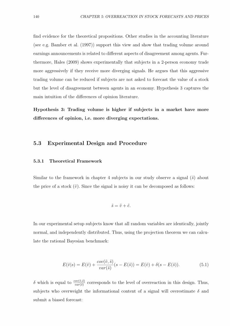
140 CHAPTER 5: OVERREACTION IN STOCK FORECASTS AND PRICES
find evidence for the theoretical propositions. Other studies in the accounting literature
(see e.g. Bamber et al. (1997)) support this view and show that trading volume around
earnings announcements is related to different aspects of disagreement among agents. Fur-
thermore, Hales (2009) shows experimentally that subjects in a 2-person economy trade
more aggressively if they receive more diverging signals. He argues that this aggressive
trading volume can be reduced if subjects are not asked to forecast the value of a stock
but the level of disagreement between agents in an economy. Hypothesis 3 captures the
main intuition of the differences of opinion literature.
Hypothesis 3: Trading volume is higher if subjects in a market have more
differences of opinion, i.e. more diverging expectations.
5.3 Experimental Design and Procedure
5.3.1 Theoretical Framework
Similar to the framework in chapter 4 subjects in our study observe a signal (s) about
the price of a stock (v). Since the signal is noisy it can be decomposed as follows:
s = v + e.
In our experimental setup subjects know that all random variables are identically, jointly
normal, and independently distributed. Thus, using the projection theorem we can calcu-
late the rational Bayesian benchmark:
E(v|s) = E(v) +cov(v, s)
var(s)(s− E(s)) = E(v) + δ(s− E(s)). (5.1)
δ which is equal to cov(v,s)var(s)
corresponds to the level of overreaction in this design. Thus,
subjects who overweight the informational content of a signal will overestimate δ and
submit a biased forecast:

5.3. EXPERIMENTAL DESIGN AND PROCEDURE 141
F = E(v|s) = E(v) + δ(s− E(s)), (5.2)
Comparing equations 5.1 and 5.2 we can derive a simple measure of overreaction:
F − E(v|s)s− E(s)
=E(v|s)− E(v|s)
s− E(s)= δ − δ. (5.3)
If δ > δ we observe overreaction as a subject’s forecast to a surprisingly good signal is
larger than the conditional expectation (F > E(v|s)) and smaller than the conditional
expectation (F < E(v|s)) in case of a surprisingly bad signal. If on the other hand our
overreaction measure is smaller than 0 we observe underreaction. If misreaction in our
experiment is not systematic we should find that it should cancel out on average.4 We
are going to describe the data generating process, the experimental procedure and the
calculation of the rational benchmark in more detail in the following subsections.
5.3.2 Basic Design
The experiment consists of three main parts: an instruction phase, a trading phase, and
a questionnaire. The instruction phase allows subjects to get familiar with the trading
environment and to gain experience with the trading mechanism. It also gives subjects
information about the payoff structure.
The trading phase consists of a sequence of 8 consecutive rounds. At the beginning of each
round subjects were shown a graph illustrating the stock price movement of two related
stocks G and H for the last 6 months. Subjects were told that stock price changes of both
stocks at a given day i in trading round j depend upon a firm specific shock ηHi,j (for
stock H) and ηGi,j (for stock G) and upon an industry shock εi,j which is common to both
stocks. Moreover, subjects knew that these daily shocks are i.i.d., normally distributed,
4In contrast to the analyses in chapter 4 we do not use Overreaction-Beta as additional measure of overreaction in this
study. Since Overreaction-Beta is simply defined as the coefficient of a simple ordinary least squares regression of forecasting
error onto signal for each person it is not really applicable to use it in our market design as subjects have traded only with
8 different stocks and we would need to base our analyses on regression coefficients that are based on 8 observations.
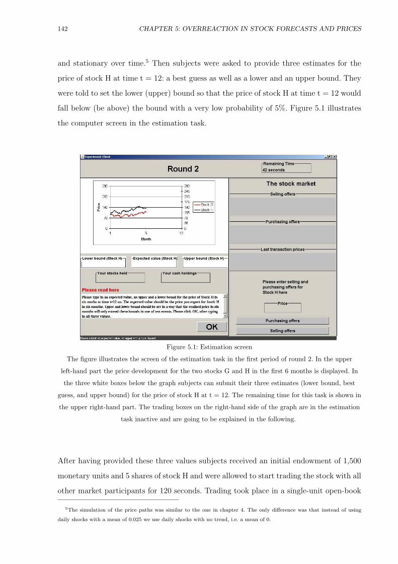
142 CHAPTER 5: OVERREACTION IN STOCK FORECASTS AND PRICES
and stationary over time.5 Then subjects were asked to provide three estimates for the
price of stock H at time t = 12: a best guess as well as a lower and an upper bound. They
were told to set the lower (upper) bound so that the price of stock H at time t = 12 would
fall below (be above) the bound with a very low probability of 5%. Figure 5.1 illustrates
the computer screen in the estimation task.
Figure 5.1: Estimation screen
The figure illustrates the screen of the estimation task in the first period of round 2. In the upper
left-hand part the price development for the two stocks G and H in the first 6 months is displayed. In
the three white boxes below the graph subjects can submit their three estimates (lower bound, best
guess, and upper bound) for the price of stock H at t = 12. The remaining time for this task is shown in
the upper right-hand part. The trading boxes on the right-hand side of the graph are in the estimation
task inactive and are going to be explained in the following.
After having provided these three values subjects received an initial endowment of 1,500
monetary units and 5 shares of stock H and were allowed to start trading the stock with all
other market participants for 120 seconds. Trading took place in a single-unit open-book
5The simulation of the price paths was similar to the one in chapter 4. The only difference was that instead of using
daily shocks with a mean of 0.025 we use daily shocks with no trend, i.e. a mean of 0.
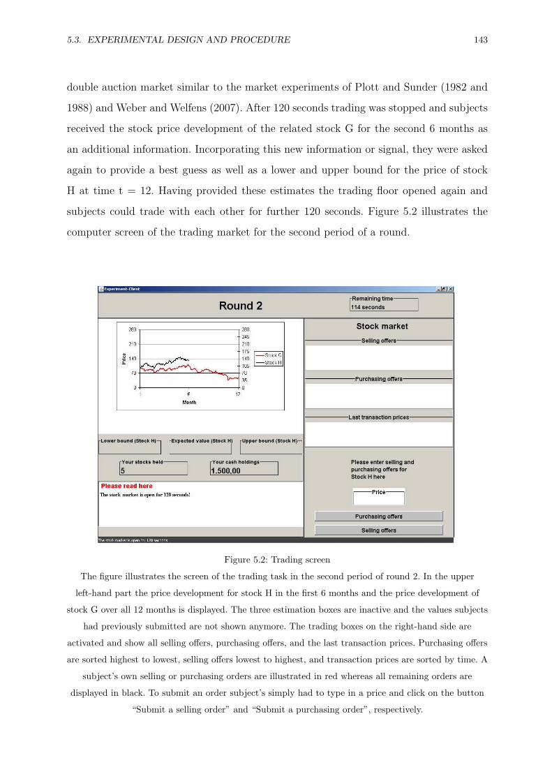
5.3. EXPERIMENTAL DESIGN AND PROCEDURE 143
double auction market similar to the market experiments of Plott and Sunder (1982 and
1988) and Weber and Welfens (2007). After 120 seconds trading was stopped and subjects
received the stock price development of the related stock G for the second 6 months as
an additional information. Incorporating this new information or signal, they were asked
again to provide a best guess as well as a lower and upper bound for the price of stock
H at time t = 12. Having provided these estimates the trading floor opened again and
subjects could trade with each other for further 120 seconds. Figure 5.2 illustrates the
computer screen of the trading market for the second period of a round.
Figure 5.2: Trading screen
The figure illustrates the screen of the trading task in the second period of round 2. In the upper
left-hand part the price development for stock H in the first 6 months and the price development of
stock G over all 12 months is displayed. The three estimation boxes are inactive and the values subjects
had previously submitted are not shown anymore. The trading boxes on the right-hand side are
activated and show all selling offers, purchasing offers, and the last transaction prices. Purchasing offers
are sorted highest to lowest, selling offers lowest to highest, and transaction prices are sorted by time. A
subject’s own selling or purchasing orders are illustrated in red whereas all remaining orders are
displayed in black. To submit an order subject’s simply had to type in a price and click on the button
“Submit a selling order” and “Submit a purchasing order”, respectively.

144 CHAPTER 5: OVERREACTION IN STOCK FORECASTS AND PRICES
After further 120 seconds the trading floor closed for a second time and subjects were
informed about the realized price of stock H at time t = 12, the round ended and the
next round started. Thus, in each trading round the trading floor is open for overall four
minutes, two minutes before signal revelation and two minutes after signal revelation. Note
that the 2·2 minute trading periods are exactly the same as the ones in Weber and Welfens
(2007). Moreover, other studies that analyze the existence of individual biases in market
settings also use two minute (Gillette et al. (1999)), three minute (Camerer (1987)),
and four minute (Camerer (1987), Camerer et al. (1989), and Lei et al. (2001)) trading
periods. Since some of these studies show that individual biases are reduced substantially
by market forces the length of our periods should be sufficient to offer the possibility
of learning in our experimental design as well. Figure 5.3 summarizes the course of an
experimental round.
Value of stock H is randomly drawn and
determines final payoff
Subjects are shown initial graph of two
stocks (G & H) and asked to provide
forecasts for stock H
Initial endowment of 5 H stocks and
1500 monetary units
Two minutes of trading stock H
New information about stock G appears
in the market. Subjects are asked to
update forecasts for stock H
Two minutes of trading stock H
Figure 5.3: Course of the experiment
The figure shows the course of each round in the market experiment.
Subjects know that the true price of stock H at the end of each round is determined by
the sum of all daily firm H specific shocks and all industry shocks that are common to

5.3. EXPERIMENTAL DESIGN AND PROCEDURE 145
both firms in each graph. Using Bayesian updating subjects have all necessary information
to calculate the conditional expected value of stock H at time t = 12 (trading day 252)
in round j as well as the variance given a particular signal s explicitly. The signal in
this case is simply the stock price development of the related stock (G) in the second 6
months which is given to subjects before the second turn of trading. Hence, the conditional
expectation follows:
E(vHi,j | sj) = vH
i,j + E∑ ·[(ηH
i,j)] +1
2· sj. (5.4)
Using the conditional expectation in equation 5.4 we can calculate the level of overreaction
for each stock price forecast and each transaction price by plugging it into equation 5.3.
Subjects in our market are informed about the exact underlying process that generates
stock prices and they see the entire order book with all purchase and sell orders as well
as past transaction prices. Own orders are illustrated in red whereas orders from all other
subjects are illustrated in black. Purchase orders in the experimental markets require
that a subject has enough monetary units to pay the specified price as we did not allow
for any short sales. Selling orders only enter the order book if a subject holds a positive
number of shares. In addition, subjects can not submit a selling order which is below their
own already existing purchasing order or set a purchasing order which is above their own
already existing selling order.
Since our experimental market is a single-unit open-book double auction market subjects
can only place one selling order and one purchasing order at a time. If subjects already
have a purchasing (selling) order in the books, they can replace it by entering a new
purchasing (selling) order. Market clearing happens automatically and in continuous time
and transaction prices are always equal to the price of the more senior order. To control
for order effects the order in which various stocks appear is varied over different markets.
After having finished all 8 rounds of trading with two trading periods each, a questionnaire
starts automatically. In the questionnaire we elicit demographics such as age, gender, and
line of studies.

146 CHAPTER 5: OVERREACTION IN STOCK FORECASTS AND PRICES
5.3.3 Procedure and Descriptive Statistics
The experiment was programmed in Java and run at the University of Mannheim in
November 2008. In 11 of overall 13 sessions we had 8 students who made up one market
whereas in the other two sessions we had 6 and 7 students, respectively. Since Lei et al.
(2001) and Noussair et al. (2008) also have markets with varying numbers of participants
(6-8) we carry out the analyses for all 13 sessions. However, our results remain stable if
we exclude the two sessions with less than 8 subjects.
Thus, we had a total of 101 students, 51 male and 50 female, who participated in our
experiments. In every session we had 8 rounds of trading, each with two 120-second
trading periods which gives us a total of 208 trading periods or 416 minutes of trading.6
The average age of all subjects was 24.7 and approximately one half of the participants
studied economics or business administration. The average processing time for the whole
experiment including the instruction phase, the trading phase, and the questionnaire was
80 minutes.
Subjects’ payment was determined as follows: subjects received a flat payment of 4 Euro
for filling out the questionnaire and a variable, performance based payment for their par-
ticipation in the 8 rounds of the experimental market. More specifically, the performance
based payment was equal to 0.06% of the overall final wealth for all 8 rounds. The final
wealth at the end of a single round was simply the amount of monetary units at the end of
the round plus the number of stocks held multiplied with the realized value of the stock.
Earnings averaged 13.35 Euro per subject.
Overall, we observe 4,157 buy orders and 4,282 sell orders with a total of 2,063 transac-
tions. Interestingly, the number of trades in the first trading period of a round, i.e. before
subjects received a signal, is substantially higher than the number of trades in the second
trading period of a round, i.e. after subjects received the signal. In the first part of a round
1,194 transactions were conducted whereas in the second part of a round only 869 trans-
6In pre-tests with more than 8 rounds of two 120-second trading periods subjects indicated to us that the task was to
strenuous and advised us to reduce the number of rounds. Moreover, the number of rounds is close to the one in various
other studies such as Sarin and Weber (1993, 2 and 8 rounds) or Weber and Welfens (2007, 10 rounds).
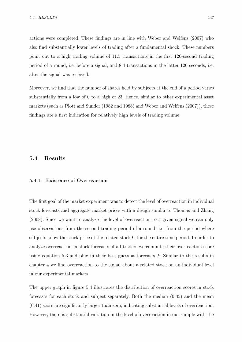
5.4. RESULTS 147
actions were completed. These findings are in line with Weber and Welfens (2007) who
also find substantially lower levels of trading after a fundamental shock. These numbers
point out to a high trading volume of 11.5 transactions in the first 120-second trading
period of a round, i.e. before a signal, and 8.4 transactions in the latter 120 seconds, i.e.
after the signal was received.
Moreover, we find that the number of shares held by subjects at the end of a period varies
substantially from a low of 0 to a high of 23. Hence, similar to other experimental asset
markets (such as Plott and Sunder (1982 and 1988) and Weber and Welfens (2007)), these
findings are a first indication for relatively high levels of trading volume.
5.4 Results
5.4.1 Existence of Overreaction
The first goal of the market experiment was to detect the level of overreaction in individual
stock forecasts and aggregate market prices with a design similar to Thomas and Zhang
(2008). Since we want to analyze the level of overreaction to a given signal we can only
use observations from the second trading period of a round, i.e. from the period where
subjects know the stock price of the related stock G for the entire time period. In order to
analyze overreaction in stock forecasts of all traders we compute their overreaction score
using equation 5.3 and plug in their best guess as forecasts F. Similar to the results in
chapter 4 we find overreaction to the signal about a related stock on an individual level
in our experimental markets.
The upper graph in figure 5.4 illustrates the distribution of overreaction scores in stock
forecasts for each stock and subject separately. Both the median (0.35) and the mean
(0.41) score are significantly larger than zero, indicating substantial levels of overreaction.
However, there is substantial variation in the level of overreaction in our sample with the

148 CHAPTER 5: OVERREACTION IN STOCK FORECASTS AND PRICES
scores ranging from -1.5 to 3.2. In other words, for a majority of 599 observations we find
forecasts indicating overreaction, but for 195 forecasts we also observe underreaction.7
The middle graph in figure 5.4 shows the average overreaction score in forecasts for each
person. Interestingly, mean (0.41) and median (0.41) overreaction are in the same range
as for each stock separately. However, almost all subjects tend to overreact on average
with only 6 out of 101 subjects having a mean overreaction score of less than 0. This
finding is a first hint that the level of overreaction varies heavily over different rounds but
that there is a general and highly significant (p < 0.01) tendency for overreaction (more
details on this issue will follow later in this subsection).
Analyzing the level of overreaction in market prices, a similar picture arises with a mean
overreaction score in prices of 0.42 and a median score of 0.32. The lower graph in figure
5.4 illustrates the level of overreaction in market prices. We find that a large majority
of 637 transactions are conducted at overreacting prices whereas only 232 transactions
are conducted at underreacting prices. Using a Wilcoxon signed-rank test and a t-test we
find that overreaction in prices is significantly larger than 0 (p < 0.01). However, both
tests implicitly assume that transaction prices are independent. This is not the case as our
experimental market is a single-unit open-book double auction market where subjects can
repeatedly buy and sell the asset. To control for this we analyze the level of overreaction
only for the first transaction in each trading period after subjects received a signal which
gives us a total of 104 observations (13 sessions · 8 rounds). The mean (median) level
of overreaction for the first transaction in each trading period is 0.43 (0.30) which is
significantly larger than 0. In addition, a Mann-Whitney rank-sum test shows that the
level of overreaction for the first transactions is not substantially different from the level
of all other transactions (p = 0.85).
Another problem for the interpretation of overreaction in transaction prices might be
the existence of short selling constraints. For example, after a good signal subjects who
overreact are willing to buy the stock at prices which are too high whereas subjects who
react rationally are not able to drive the market prices down to the rational level by
7Keep in mind that both overreaction in forecasts and overreaction in prices can only be calculated for the second two
minute trading period in each round, i.e. after the signal was revealed.
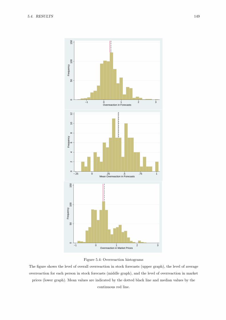
5.4. RESULTS 149
050
100
150
Fre
quen
cy
−1 0 1 2 3Overreaction in Forecasts
02
46
810
12F
requ
ency
−.25 0 .25 .5 .75 1Mean Overreaction in Forecasts
050
100
150
Fre
quen
cy
−1 0 1 2 3Overreaction in Market Prices
Figure 5.4: Overreaction histograms
The figure shows the level of overall overreaction in stock forecasts (upper graph), the level of average
overreaction for each person in stock forecasts (middle graph), and the level of overreaction in market
prices (lower graph). Mean values are indicated by the dotted black line and median values by the
continuous red line.

150 CHAPTER 5: OVERREACTION IN STOCK FORECASTS AND PRICES
selling more than their five inventory stocks at seemingly inflated prices. We control for
the short selling problem using two approaches: first, similar to the non-independency
problem above, we show that overreaction for the first transaction in each trading period
is not smaller than for all observations (p = 0.85). The fact that the short selling constraint
is not binding in the first transaction after a signal revelation and that overreaction is
still present is a first indication that without short selling constraints overreaction would
not abate. Second, we exclude all markets in which at least one subject hits the boundary
and ends up with 0 assets in his / her portfolio. Analyzing the level of overreaction for
markets where the short selling constraint is not binding we find a significantly positive
mean overreaction score in prices of 0.5 and a median score of 0.41. A Mann-Whitney
rank-sum test shows that the level of overreaction in prices is even larger than the level of
overreaction in markets where the short selling constraint is binding (p < 0.01). Thus, we
believe that short selling constraints cannot explain the substantial levels of overreaction
in our markets.
Overall, both overreaction in forecasts and in prices are in the same ballpark as the level
of overreaction in chapter 4 where we find average median overreaction scores of 0.33 and
0.37. Similar to these results, we also observe large heterogeneity of overreaction, with
some subjects providing almost rational estimates and trading at rational prices but with
a majority of subjects overreacting to the new information. Moreover, our results support
empirical findings on overreaction in Thomas and Zhang (2008) in a clean experimental
design, where we can control for other possible explanations. Thus, both hypothesis 1a
and hypothesis 1b are supported by our results.
Next, we turn to hypothesis 1c and analyze whether market forces help reducing the
level of misreaction, i.e. over- or underreaction. Figure 5.5 illustrates the median level of
misreaction in forecasts and market prices for each stock separately. Comparing the level
of misreaction in forecasts and prices for each stock separately we find that self-regulating
forces of the market do not seem to help in lowering misreaction of subjects. For 7 out of
8 stocks median misreaction in prices is even larger than the median misreaction in stock
forecasts. Thus, the standard argument that self-regulating forces of markets will correct
for erroneous individual beliefs and hence result in less overreaction does not apply in our

5.4. RESULTS 151
experimental market. We have illustrated previously, that there is a large heterogeneity
of overreaction with some subjects having almost perfectly rational expectations. Thus,
we can rule out the argument that market forces do not help in lowering the individual
bias due to the fact that there are no traders in the market with rational expectations.
This finding is in line with Gillette et al. (1999) who show for a different kind of task
that individual misreaction in a continuous double auction market is slightly smaller than
aggregate market misreaction which supports hypothesis 1c.
−.2
5.2
5.7
51.
25O
verr
eact
ion
1 2 3 4 5 6 7 8
OR − Estimate OR − Price
Figure 5.5: Overreaction prices vs. overreaction forecasts
The figure illustrates the level of overreaction in transaction prices (OR - Price) and in estimates (OR -
Estimate) for all 8 stocks separately. A positive value on the y-axis indicates overreaction whereas a
negative value indicates underreaction.
In the following we want to analyze in more detail why market forces or more specifically
traders with rational estimates fail to lower misreaction. The first 3 columns of table
5.1 show the median overreaction score in stock forecasts of subjects who bought stocks
(Median−ORBuyer), subjects who sold stocks (Median−ORSeller), and all subjects, re-
gardless whether they traded the stock or not (Median−ORAll), for each stock separately.
Column 4 shows the median overreaction score derived from prices (Median−ORPrices)
broken down by stocks. The results confirm our previous assumption that the level of
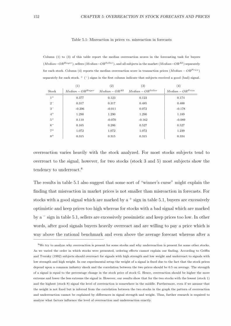
152 CHAPTER 5: OVERREACTION IN STOCK FORECASTS AND PRICES
Table 5.1: Misreaction in prices vs. misreaction in forecasts
Column (1) to (3) of this table report the median overreaction scores in the forecasting task for buyers
(Median−ORBuyer), sellers (Median−ORSeller), and all subjects in the market (Median−ORAll) separately
for each stock. Column (4) reports the median overreaction score in transaction prices (Median − ORPrice)
separately for each stock. + (−) signs in the first column indicate that subjects received a good (bad) signal.
(1) (2) (3) (4)
Stock Median−ORBuyer Median−ORAll Median−ORSeller Median−ORPrice
1+ 0.377 0.123 0.123 0.174
2− 0.317 0.317 0.485 0.400
3− -0.206 -0.011 0.072 -0.178
4+ 1.290 1.290 1.290 1.189
5+ 0.110 -0.070 -0.162 -0.089
6− 0.165 0.286 0.527 0.527
7+ 1.072 1.072 1.072 1.239
8+ 0.315 0.315 0.315 0.334
overreaction varies heavily with the stock analyzed. For most stocks subjects tend to
overreact to the signal, however, for two stocks (stock 3 and 5) most subjects show the
tendency to underreact.8
The results in table 5.1 also suggest that some sort of “winner’s curse” might explain the
finding that misreaction in market prices is not smaller than misreaction in forecasts. For
stocks with a good signal which are marked by a + sign in table 5.1, buyers are excessively
optimistic and keep prices too high whereas for stocks with a bad signal which are marked
by a − sign in table 5.1, sellers are excessively pessimistic and keep prices too low. In other
words, after good signals buyers heavily overreact and are willing to pay a price which is
way above the rational benchmark and even above the average forecast whereas after a
8We try to analyze why overreaction is present for some stocks and why underreaction is present for some other stocks.
As we varied the order in which stocks were presented, ordering effects cannot explain our finding. According to Griffin
and Tversky (1992) subjects should overreact for signals with high strength and low weight and underreact to signals with
low strength and high weight. In our experimental setup the weight of a signal is fixed due to the fact that the stock prices
depend upon a common industry shock and the correlation between the two prices should be 0.5 on average. The strength
of a signal is equal to the percentage change in the stock price of stock G. Hence, overreaction should be higher the more
extreme and lower the less extreme the signal is. However, our results show that for the two stocks with the lowest (stock 1)
and the highest (stock 8) signal the level of overreaction is somewhere in the middle. Furthermore, even if we assume that
the weight is not fixed but is inferred from the correlation between the two stocks in the graph the pattern of overreaction
and underreaction cannot be explained by differences in signal strength and weight. Thus, further research is required to
analyze what factors influence the level of overreaction and underreaction exactly.

5.4. RESULTS 153
bad signal sellers heavily overreact and are willing to sell at a price which is way below
the rational benchmark and even below the average forecast. Thus, buyers - after a good
signal - and sellers - after a bad signal - suffer from what we call a “winner’s curse” and
cause transactions to be executed at overreacting prices.
5.4.2 Learning to Overreact Less
In addition to finding evidence for the existence of individual and market overreaction
we are interested in analyzing the effects of overreaction in the long-run. More precisely,
we would like to know if subjects are able to learn to overreact less with more trading
experience. Subjects gain trading experience in two ways: first, within the course of a
round as they are able to learn from the bids and asks of other subjects and second, over
rounds as they receive outcome feedback at the end of each round. In the following, we
will first analyze learning within a round and then learning over rounds.
Figure 5.6 shows the average (upper graph) and the median (lower graph) overreaction
scores for each trading second in the second trading period of a round. To measure whether
there is a learning effect within a round we estimate a simple partial adjustment model
similar to the one in Camerer (1987), Camerer et al. (1989), and Weber and Welfens
(2007):
ORt = α + β ·ORt−1. (5.5)
Hence, we calculate the level of average overreaction in second t as a function of average
overreaction in the previous second. As also can be seen in the graphs there are hardly any
learning effects and the level of overreaction remains fairly stable over time. Moreover,
in line with Camerer (1987) we estimate the degree of equilibrium bias OREquilibrium
consistently by the estimator OR = α(1−β)
, where α and β denote ordinary least squares
estimators of α and β from equation 5.5. Fitting with an ordinary least squares regression
results in α = 0.456 and β = −0.112 with β not being significantly different from 0.
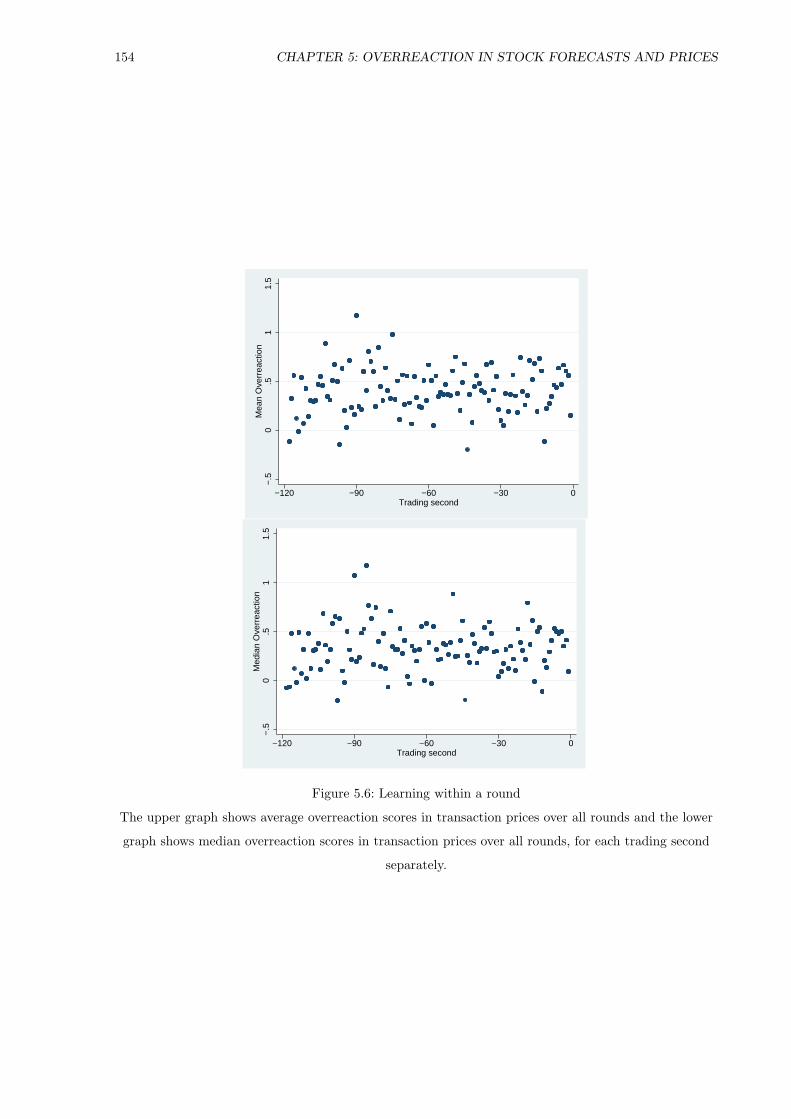
154 CHAPTER 5: OVERREACTION IN STOCK FORECASTS AND PRICES
−.5
0.5
11.
5M
ean
Ove
rrea
ctio
n
−120 −90 −60 −30 0Trading second
−.5
0.5
11.
5M
edia
n O
verr
eact
ion
−120 −90 −60 −30 0Trading second
Figure 5.6: Learning within a round
The upper graph shows average overreaction scores in transaction prices over all rounds and the lower
graph shows median overreaction scores in transaction prices over all rounds, for each trading second
separately.

5.4. RESULTS 155
Table 5.2: Learning within a round
This table reports mean (OverreactionMean) and median (OverreactionMedian) overreaction scores in trans-
action prices as well as the proportion of transactions at overreacting prices for six time intervals of twenty
seconds. Overreaction is calculated for every transaction separately and afterwards aggregated for each twenty
seconds trading period.
Seconds OverreactionMean OverreactionMedian OverreactionProportion
-120 to -101 0.354 0.296 68.14
-100 to -81 0.451 0.315 71.85
-80 to -61 0.411 0.322 69.33
-60 to -41 0.429 0.325 77.27
-40 to -21 0.403 0.315 75.17
-20 to -0 0.454 0.372 76.16
Furthermore, the equilibrium bias OR = α(1−β)
= 0.41 and thus substantially larger than
0.
To analyze findings on learning within a round in more depth we split the 120-second
trading period into six 20 seconds intervals and calculate three overreaction scores for each
interval separately. Table 5.2 reports OverreactionMean and OverreactionMedian which are
simply the mean and median overreaction in each time span and OverreactionProportion
which is the proportion of transactions that were carried out at overreacting prices in
a given time span. A series of binomial tests which analyzes whether most transactions
were carried out at overreacting prices indicates that overreaction is prevalent in each
time interval. The same results emerge if we use Wilcoxon signed-rank tests.
Moreover, the numbers in the respective time intervals seem to be very similar and closely
related. Using a series of Mann-Whitney rank-sum test we find that no single difference
between two time spans is significant indicating that learning effects are hardly existent
within a round and that the level of overreaction is stable over time. Hence, we do not
observe any learning effects within a round, consistent with hypothesis 2a.9
Besides learning within a round subjects could also gain experience over the course of the
experiment and learn from the outcome feedback that is provided to them. For a more
9Our results remain stable if we split the 120-second trading period in 3, 4, or 10 time spans of equal length.
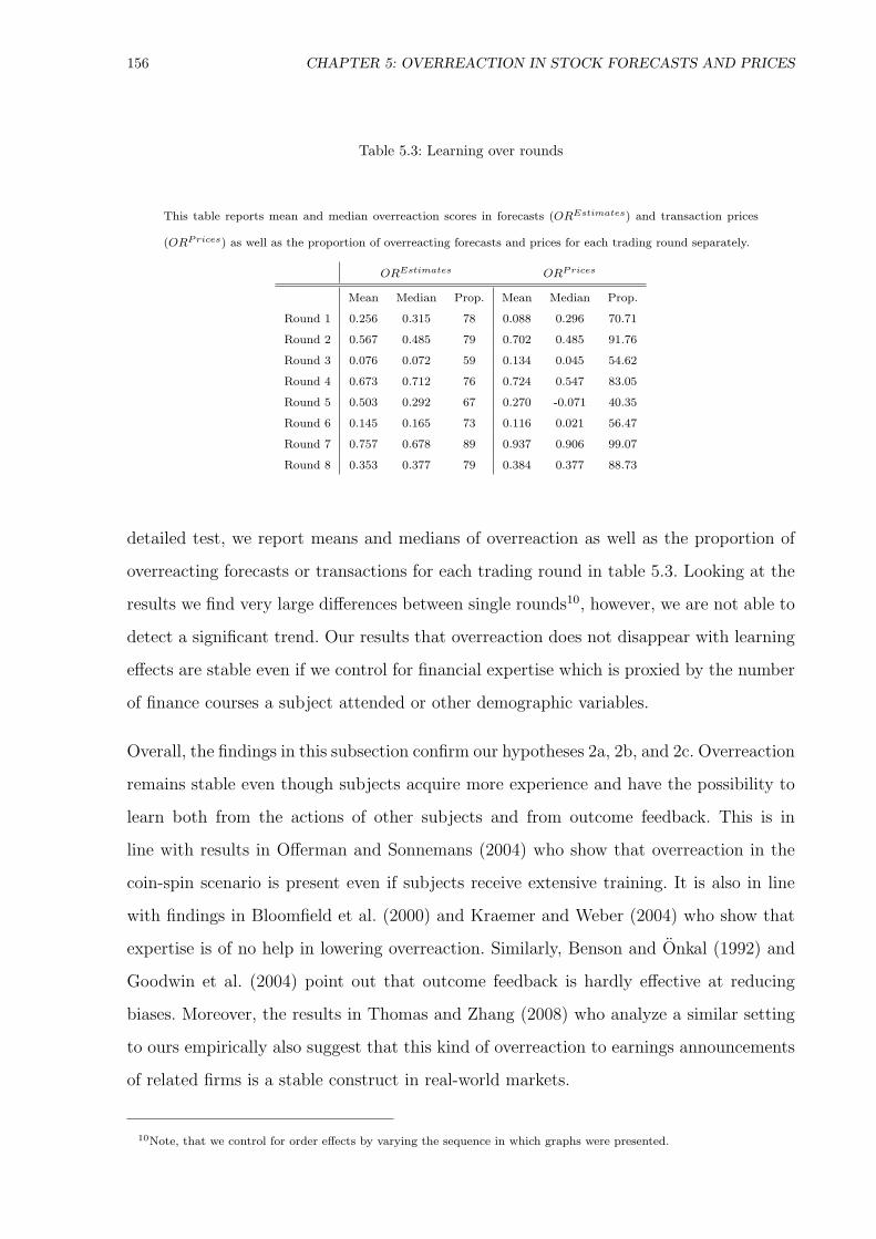
156 CHAPTER 5: OVERREACTION IN STOCK FORECASTS AND PRICES
Table 5.3: Learning over rounds
This table reports mean and median overreaction scores in forecasts (OREstimates) and transaction prices
(ORPrices) as well as the proportion of overreacting forecasts and prices for each trading round separately.
OREstimates ORPrices
Mean Median Prop. Mean Median Prop.
Round 1 0.256 0.315 78 0.088 0.296 70.71
Round 2 0.567 0.485 79 0.702 0.485 91.76
Round 3 0.076 0.072 59 0.134 0.045 54.62
Round 4 0.673 0.712 76 0.724 0.547 83.05
Round 5 0.503 0.292 67 0.270 -0.071 40.35
Round 6 0.145 0.165 73 0.116 0.021 56.47
Round 7 0.757 0.678 89 0.937 0.906 99.07
Round 8 0.353 0.377 79 0.384 0.377 88.73
detailed test, we report means and medians of overreaction as well as the proportion of
overreacting forecasts or transactions for each trading round in table 5.3. Looking at the
results we find very large differences between single rounds10, however, we are not able to
detect a significant trend. Our results that overreaction does not disappear with learning
effects are stable even if we control for financial expertise which is proxied by the number
of finance courses a subject attended or other demographic variables.
Overall, the findings in this subsection confirm our hypotheses 2a, 2b, and 2c. Overreaction
remains stable even though subjects acquire more experience and have the possibility to
learn both from the actions of other subjects and from outcome feedback. This is in
line with results in Offerman and Sonnemans (2004) who show that overreaction in the
coin-spin scenario is present even if subjects receive extensive training. It is also in line
with findings in Bloomfield et al. (2000) and Kraemer and Weber (2004) who show that
expertise is of no help in lowering overreaction. Similarly, Benson and Onkal (1992) and
Goodwin et al. (2004) point out that outcome feedback is hardly effective at reducing
biases. Moreover, the results in Thomas and Zhang (2008) who analyze a similar setting
to ours empirically also suggest that this kind of overreaction to earnings announcements
of related firms is a stable construct in real-world markets.
10Note, that we control for order effects by varying the sequence in which graphs were presented.

5.4. RESULTS 157
5.4.3 Differences of Opinion and Trading Volume
As reported in subsection 5.3.3 subjects seem to be engaged in relatively high levels of
trading volume with on average 9.9 transaction in each 120-second trading period. In
this experimental setup two testable explanations for the observed high trading volume
can be brought forward: first, differences in risk attitudes between traders and second,
heterogenous beliefs about the value of a stock, i.e. differences of opinion.
To show whether trading volume can be explained by risk sharing motives we compare the
trading volume, i.e. the number of shares traded, in each trading period with the level of
differences in risk attitudes between buyer and seller (Differences Risk AversionMaxMin).
Risk Aversion was simply measured for each person on a five point Likert scale with
the endpoints “1 = high risk aversion” and “5 = very low risk aversion”. Differ-
ences Risk AversionMaxMin is simply defined as the difference between the most risk
averse and the least risk averse subject in each session.11 Running a clustered least square
regression of the level of trading volume on the differences in risk attitudes between the
two traders we are not able to find a significant effect. Differences in risk attitudes cannot
explain the observed high levels of trading volume (see model 1 in table 5.4).
The second argument that is often brought forward to explain high levels of trading
are differences of opinion. Amongst others, Varian (1989), Harris and Raviv (1993) or
Kandel and Pearson (1995) propose that excessive trading volume can be explained by
heterogenous beliefs among market participants. Since we elicited beliefs of all market
participants in each period in the estimation phases we are able to analyze this theoretical
proposition in our experimental setup.
Using forecasts (best guesses) that were submitted by all subjects in the estimation part
of the experiment before each 120-second trading period we construct three distinct differ-
ences of opinion measures. Our first measure (Differences of OpinionMaxMin) is simply
the difference between the most optimistic, i.e. highest best guess, and the most pes-
11Alternatively, we also compute Differences Risk AversionStd. which is the standard deviation of all subjects’ risk
attitude measures in each session and relate it to the varying measures of differences of opinion. The results of the following
analyses are essentially the same.
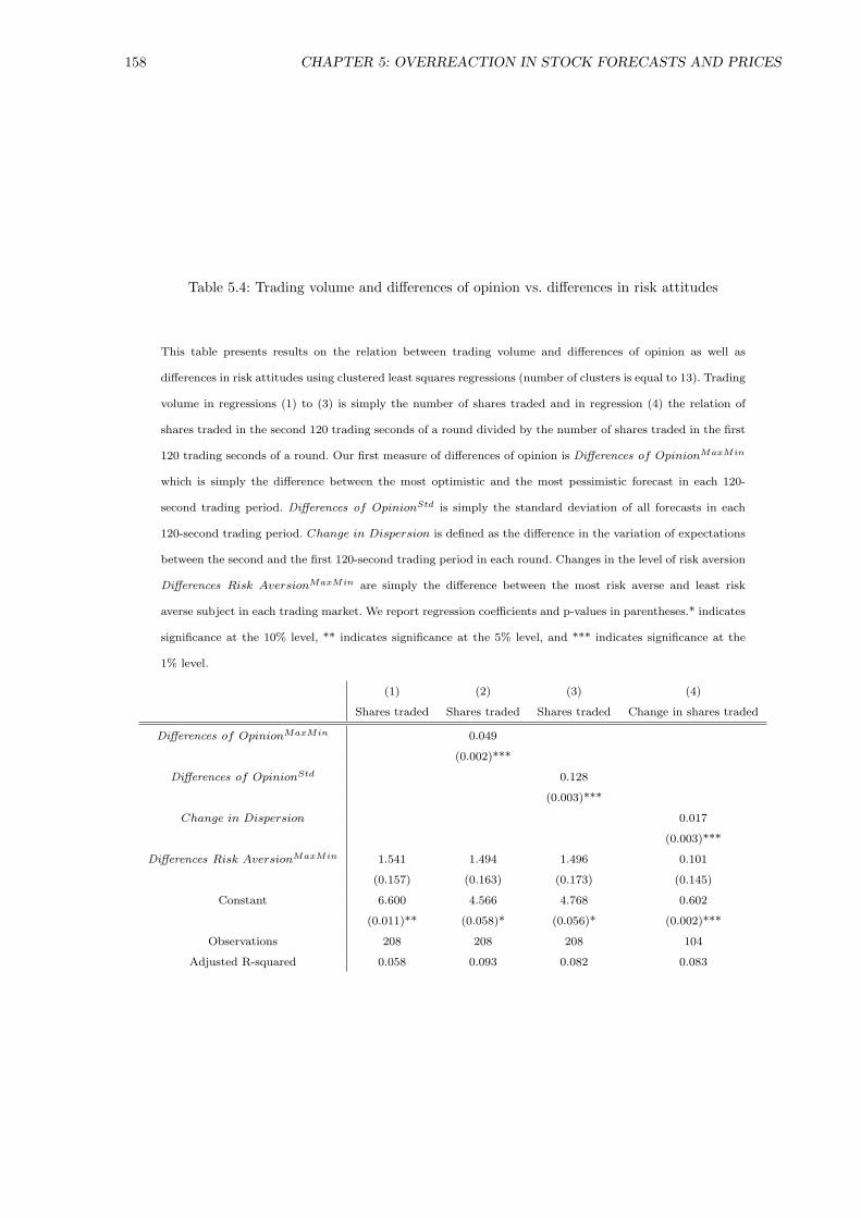
158 CHAPTER 5: OVERREACTION IN STOCK FORECASTS AND PRICES
Table 5.4: Trading volume and differences of opinion vs. differences in risk attitudes
This table presents results on the relation between trading volume and differences of opinion as well as
differences in risk attitudes using clustered least squares regressions (number of clusters is equal to 13). Trading
volume in regressions (1) to (3) is simply the number of shares traded and in regression (4) the relation of
shares traded in the second 120 trading seconds of a round divided by the number of shares traded in the first
120 trading seconds of a round. Our first measure of differences of opinion is Differences of OpinionMaxMin
which is simply the difference between the most optimistic and the most pessimistic forecast in each 120-
second trading period. Differences of OpinionStd is simply the standard deviation of all forecasts in each
120-second trading period. Change in Dispersion is defined as the difference in the variation of expectations
between the second and the first 120-second trading period in each round. Changes in the level of risk aversion
Differences Risk AversionMaxMin are simply the difference between the most risk averse and least risk
averse subject in each trading market. We report regression coefficients and p-values in parentheses.* indicates
significance at the 10% level, ** indicates significance at the 5% level, and *** indicates significance at the
1% level.
(1) (2) (3) (4)
Shares traded Shares traded Shares traded Change in shares traded
Differences of OpinionMaxMin 0.049
(0.002)***
Differences of OpinionStd 0.128
(0.003)***
Change in Dispersion 0.017
(0.003)***
Differences Risk AversionMaxMin 1.541 1.494 1.496 0.101
(0.157) (0.163) (0.173) (0.145)
Constant 6.600 4.566 4.768 0.602
(0.011)** (0.058)* (0.056)* (0.002)***
Observations 208 208 208 104
Adjusted R-squared 0.058 0.093 0.082 0.083

5.4. RESULTS 159
simistic, i.e. lowest best guess, in each 120-second trading period. The second measure
is the standard deviation of all subjects’ best guesses (Differences of OpinionStd) before
each 120-second trading period (see Morse et al. (1991) and Bamber et al. (1997)). Our last
measure of differences of opinion, Change in Dispersion, is also adopted from Bamber
et al. (1997). It measures the change in the standard deviation of forecasts in each trading
round before and after signal revelation. More specifically, it is defined as the standard
deviation of beliefs in the second trading period of a round minus the standard deviation
of beliefs in the previous 120-second trading period of a round. For the first two measures
we have 208 different observations (13 sessions · 8 rounds · 2 trading periods per round)
and for the third measure we have 104 observations (13 sessions · 8 rounds).
The upper graph in figure 5.7 illustrates the relation between Differ-
ences of OpinionMaxMin and the number of shares traded in each of the 208 periods. The
fitted line of a clustered least square regression and the positive Spearman correlation of
0.23 (Wilcoxon signed-rank test: p < 0.01) are a first indication that trading volume is
positively related to differences of opinion. A similar picture emerges if we take a look at
the middle graph in figure 5.7. Differences of OpinionStd is positively related to trading
volume (Spearman’s rho = 0.21 and p < 0.01). The lower graph in figure 5.7 illustrates
the relation between Change in Dispersion and Change in shares traded. The variable
Change in shares traded is defined as the relation between the number of shares traded
in the second period of a round (i.e. after signal revelation), divided by the number of
shares traded in the first period of a round. Similar to the results in the two upper graphs
we observe a positive relation (Spearman’s rho = 0.20 and p = 0.04).
However, one problem of correlation analysis is that we cannot account for non-
independent residuals over sessions. Hence, we additionally run ordinary least squares
regressions in which we cluster our observations over sessions for each difference of opin-
ion measure separately and additionally control for differences in risk attitudes. The result
in the second column of table 5.4 supports our graphical findings as the coefficient of Dif-
ferences of OpinionMaxMin is significantly positive. If the difference between the most
optimistic and the most pessimistic forecast is 50, then the number of shares traded in a
market rises by 2.45 compared to a market with perfectly homogenous beliefs. Interest-

160 CHAPTER 5: OVERREACTION IN STOCK FORECASTS AND PRICES
05
1015
2025
Sha
res
trad
ed b
y tr
adin
g ph
ase
0 50 100 150Differences of Opinion (MaxMin)
Shares traded by trading phase Fitted values
05
1015
2025
Sha
res
trad
ed b
y tr
adin
g ph
ase
0 10 20 30 40Differences of opinion (Std)
Shares traded by trading phase Fitted values
0.5
11.
52
2.5
Cha
nge
shar
es tr
aded
by
roun
d
−20 −10 0 10 20Change in dispersion
Change shares traded by round Fitted values
Figure 5.7: Differences of opinion and trading volume
The two upper graphs illustrate the relation between number of shares that were traded in each
120-second trading period and two distinct measures for differences of opinion. The differences of
opinion measure in the upper graph is simply the absolute difference between the most optimistic
forecast and the most pessimistic forecast of subjects (Differences of Opinion (MaxMin)) in each
120-second trading period. Similarly, the differences of opinion measure in the middle graph is the
standard deviation of all forecasts (Differences of Opinion (Std.)) in each 120-second trading period.
The lower graph illustrates for each session and stock separately, how a change in the variation of
expectations (Change in Dispersion) is related to a change in trading volume.
5.5. CONCLUSION 161
ingly, Differences Risk AversionMaxMin cannot explain trading volume. Similar results
emerge if we analyze the relation between Differences of OpinionStd and trading volume
in regression 3. Our second measure of difference of opinion is also positively related to
the number of shares traded in each period.
Regression 4 analyzes the relation between Change in Dispersion and the change in the
number of shares traded in the second period of a round compared to the first period of
a round. Since we only have one observation for each round the number of observations
drops to 104 (13 sessions · 8 rounds). The positive coefficient of Change in Dispersion
indicates that the larger the standard deviation in forecasts in the second period of a
round, compared to the first one, the larger the fraction of shares traded in the second
period of a round compared to the first one. Again, Differences Risk AversionMaxMin are
not able to explain trading volume.
Overall, the findings on the positive relation between differences of opinion and trading
volume are consistent with first experimental evidence in simple 2-subject call markets
(see Hales (2009)) and support our hypothesis 3. Interestingly, not the differences in
risk attitudes but solely the differences of opinions are significantly related to trading
volume. In addition, one could argue that finding evidence on the theoretically proposed
relationship between differences of opinion and trading volume is a further indication that
our data seems to be quite reasonable.
5.5 Conclusion
This chapter extends the individual-level-study of the previous chapter to a simple ex-
perimental trading market. We analyze if subjects are able to update their beliefs ac-
cording to Bayes rule or if they misreact when they receive new information about a
stock and consequently if market prices overreact. Consistent with findings in chapter 4,
subjects in our setting overreact to new information on an individual level. Additionally,
we find evidence for aggregate overreaction in market prices, consistent with Thomas and
Zhang (2008). Interestingly, consistent with propositions in theoretical models (e.g. Odean
(1998b) and Biais and Weber (2007)) and findings in the experimental literature (Gillette

162 CHAPTER 5: OVERREACTION IN STOCK FORECASTS AND PRICES
et al. (1999)) individual misreaction translates into market outcomes as misreaction in
transaction prices is not lower than in individual estimates.
Furthermore, we analyze if overreaction both on an individual and market level diminishes
over time, i.e. if subjects are able to learn from the actions of other subjects or from the
outcomes in previous rounds. Our results indicate that learning effects can neither be
observed within a two minute trading period nor over various rounds. Hence, overreaction
in this setting seems to be a stable construct. This finding is consistent with Offerman
and Sonnemans (2004) who illustrate individual overreaction to be persistent in their
coin-spin design even though subjects receive extensive training. In addition, evidence in
psychology indicates that outcome feedback, exactly the sort of feedback subjects receive
in our experiment, is not very effective at reducing biases (Benson and Onkal (1992) and
Goodwin et al. (2004)).
Lastly, we are able to provide experimental evidence for a positive relation between dif-
ferences of opinion and trading volume. Although theoretical evidence on this relation
is prevalent (Varian (1989), Harris and Raviv (1993), and Kandel and Pearson (1995))
empirical and experimental studies have mainly ignored this relation. A notable exception
is the study by Hales (2009) who shows that trading volume is larger if two traders receive
more differing signals in a simple two-trader call market. We extend his findings to a more
realistic environment by showing that trading volume is also larger if the disagreement
about future stock price among all market participants is larger in a continuous auction
market.
Further research should analyze if different sorts of feedback, such as cognitive or task
information feedback, could help in lowering both individual and market biases. Previous
findings on the role of different sorts of feedback on the level of overconfidence has shown
that in particular outcome feedback is not helpful in lowering biases. In addition, it could
be fruitful to study the high differences in the level of overreaction between stocks in
more detail. Varying the degree of signal strength and weight or the length of the fore-
casting period might help in determining reasons for the large heterogeneity of over- and
underreaction.

Bibliography
Abarbanell, J. S., and V. L. Bernard, 1992, “Tests of Analysts’ Overreac-
tion/Underreaction to Earnings Information as an Explanation for Anomalous Stock
Price Behavior,” Journal of Finance, 47, 1181–1207.
Albrecht, P., R. Maurer, and M. Moller, 1998, “Shortfall-Risiko/Excess-Chance-
Entscheidungskalkule: Grundlagen und Beziehungen zum Bernoulli-Prinzip,” Zeitschrift
fur Wirtschafts- und Sozialwissenschaften, 118, 249–274.
Alpert, M., and H. Raiffa, 1982, A Progress Report on the Training of Probability Asses-
sors. in: Judgment under Uncertainty: Heuristics and Biases, edited by: D. Kahneman,
P. Slovic and A. Tversky, Cambridge University Press.
Alwin, D. F., and J. A. Krosnick, 1991, “The Reliability of Survey Attitude Measure-
ment: The Influence of Question and Respondent Attributes,” Sociological Methods &
Research, 20, 139–181.
Andersen, S., G. W. Harrison, M. I. Lau, and E. E. Rutstrom, 2008, “Lost in State Space:
Are Preferences Stable?,” International Economic Review, 49, 1091–1112.
Antweiler, W., and M. Z. Frank, 2004, “Is All That Talk Just Noise? The Information
Content of Internet Stock Message Boards,” Journal of Finance, 59, 1259–1294.
Arrow, K. J., 1965, Essays in the Theory of Risk-Bearing. North-Holland Publishing
Company, Amsterdam-London.
Balzer, W. K., M. E. Doherty, and R. O’Connor, Jr., 1989, “Effects of Cognitive Feedback
on Performance,” Psychological Bulletin, 106, 410–433.
163
164 BIBLIOGRAPHY
Bamber, L. S., O. E. Barron, and T. L. Stober, 1997, “Trading Volume and Different
Aspects of Disagreement Coincident with Earnings Announcements,” The Accounting
Review, 72, 575–597.
Barber, B. M., and T. Odean, 2000, “Trading Is Hazardous to Your Wealth: The Common
Stock Investment Performance of Individual Investors,” Journal of Finance, 55, 773–
806.
, 2001, “Boys will be Boys: Gender, Overconfidence and Common Stock Invest-
ment,” Quarterly Journal of Economics, 116, 261–292.
, 2002, “Online Investors: Do the Slow Die First?,” Review of Financial Studies,
15, 455–487.
Barberis, N., A. Shleifer, and R. Vishny, 1998, “A Model of Investor Sentiment,” Journal
of Financial Economics, 49, 307–343.
Barsky, R. B., F. T. Juster, M. S. Kimball, and M. D. Shapiro, 1997, “Preference Pa-
rameters and Behavioral Heterogeneity: An Experimental Approach in the Health and
Retirement Study,” Quarterly Journal of Economics, 112, 537–579.
Baucells, M., and A. Villasis, 2009, “Stability of Risk Preference and the Reflection Effect
of Prospect Theory,” Theory and Decision, forthcoming.
Bell, D. E., 1995, “Risk, Return, and Utility,” Management Science, 41, 23–30.
Ben-David, I., J. R. Graham, and C. Harvey, 2007, “Managerial Overconfidence and
Coporate Policies,” Working Paper.
Benartzi, S., and R. H. Thaler, 2001, “Naive Diversification Strategies in Defined Contri-
bution Saving Plans,” American Economic Review, 91, 79–98.
Benos, A. V., 1998, “Aggressiveness and survival of overconfident traders,” Journal of
Financial Markets, 1, 353–383.
Benson, P. G., and D. Onkal, 1992, “The Effects of Feedback and Training on the Perfor-
mance of Probability Forecasters,” International Journal of Forecasting, 8, 559–573.
Bernoulli, D., 1738, “Specimen Theoriae Novae de Mensura Sortis,” Commentarii
Academiae Scientiarum Imperialis Petropolitanae, 5, 175–192.

BIBLIOGRAPHY 165
, 1954, “Exposition of a new Theory of the Measurement of Risk,” Econometrica,
22, 23–36.
Biais, B., D. Hilton, K. Mazurier, and S. Pouget, 2005, “Judgemental Overconfidence, Self-
Monitoring, and Trading Performance in an Experimental Financial Market,” Review
of Economic Studies, 72, 287–312.
Biais, B., and M. Weber, 2007, “Hindsight Bias and Investment Performance,” Working
Paper.
, 2009, “Hindsight Bias, Risk Perception, and Investment Performance,” Manage-
ment Science, 55, 1018–1029.
Bloomfield, R., and J. Hales, 2002, “Predicting the Next Step of a Random Walk: Ex-
perimental Evidence of Regime-Shifting Beliefs,” Journal of Financial Economics, 65,
397–414.
Bloomfield, R., R. Libby, and M. W. Nelson, 2000, “Underreactions, Overreactions and
Moderated Confidence,” Journal of Financial Markets, 3, 113–137.
Bluethgen, R., A. Gintschel, A. Hackethal, and A. Mller, 2008, “Financial Advice and
Individual Investors’ Portfolios,” Working Paper.
Bollen, K. A., and K. H. Barb, 1981, “Pearson’s R and Coarsely Categorized Measures,”
American Sociological Review, 46, 232–239.
Bontempo, R. N., W. P. Bottom, and E. U. Weber, 1997, “Cross-Cultural Differences in
Risk Perception: A Model-Based Approach,” Risk Analysis, 17, 479–488.
Brooks, P., G. B. Davies, and D. P. Egan, 2008, “Linking Psychometrically Measured
Risk Tolerance with Choice Behaviour,” Working Paper.
Brunnermeier, M. K., and S. Nagel, 2008, “Do Wealth Fluctuations Generate Time-
Varying Risk Aversion? Micro-Evidence on Individuals’ Asset Allocation,” American
Economic Review, 98, 713–736.
Budescu, D. V., and B. Maciejovsky, 2005, “The Effect of Payoff Feedback and Informa-
tion Pooling on Reasoning Errors: Evidence from Experimental Markets,” Management
Science, 51, 1829–1843.
166 BIBLIOGRAPHY
Butler, J. C., J. S. Dyer, and J. Jia, 2005, “An Empirical Investigation of the Assumptions
of Risk-Value Models,” Journal of Risk and Uncertainty, 30, 133–156.
Caballe, J., and J. Sakovics, 2003, “Speculating Against an Overconfident Market,” Jour-
nal of Financial Markets, 6, 199–225.
Camerer, C. F., 1987, “Do Biases in Probability Judgement Matter in Markets? Experi-
mental Evidence,” American Economic Review, 77, 981–997.
, 1989, “An Experimental Test of Several Generalized Utility Theories,” Journal
of Risk and Uncertainty, 2, 61–104.
, 1992, “The Rationality of Prices and Volume in Experimental Markets,” Orga-
nizational Behavior and Human Decision Processes, 51, 237–272.
Camerer, C. F., and R. M. Hogarth, 1999, “The Effects of Financial Incentives in Ex-
periments: A Review and Capital-Labor-Production Framework,” Journal of Risk and
Uncertainty, 19, 7–42.
Camerer, C. F., G. Loewenstein, and M. Weber, 1989, “The Curse of Knowledge in Eco-
nomic Settings: An Experimental Analysis,” Journal of Political Economy, 97, 1232–
1254.
Camerer, C. F., and D. Lovallo, 1999, “Overconfidence and Excess Entry: An Experimen-
tal Approach,” American Economic Review, 89, 306–318.
Cao, H. H., and H. Ou-Yang, 2009, “Differences of Opinion of Public Information and
Speculative Trading in Stocks and Options,” Review of Financial Studies, 22, 300–335.
Cesarini, D., Orjan Sandewall, and M. Johannesson, 2006, “Confidence Interval Estima-
tion Tasks and the Economics of Overconfidence,” Journal of Economic Behavior &
Organization, 61, 453–470.
Cicchetti, D. V., D. Showalter, and P. J. Tyrer, 1985, “The Effect of Number of Rat-
ing Scale Categories on Levels of Interrater Reliability: A Monte Carlo Investigation,”
Applied Psychological Measurement, 9, 31–36.
Coval, J. D., and A. V. Thakor, 2005, “Financial Intermediation as a Beliefs-Bridge be-
tween Optimists and Pessimists,” Journal of Financial Economics, 75, 535–569.

BIBLIOGRAPHY 167
Daniel, K. D., D. Hirshleifer, and A. Subrahmanyam, 1998, “Investor Psychology and
Security Market Under- and Overreactions,” Journal of Finance, 53, 1839–1885.
, 2001, “Overconfidence, Arbitrage, and Equilibrium Asset Pricing,” Journal of
Finance, 56, 921–965.
Deaves, R., E. Luders, and M. Schroder, 2005, “The Dynamics of Overconfidence: Evi-
dence from Stock Market Forecasters,” Working Paper.
DeBondt, W. F. M., 1998, “Behavioural Economics: A Portrait of the Individual Investor,”
European Economic Review, 42, 831–844.
, 2000, The Psychology of Underreaction and Overreaction in World Equity Mar-
kets. in: Security Market Imperfections in World Wide Equity Markets, edited by: D.
B. Keim and W. T. Ziemba, Cambridge University Press.
DeBondt, W. F. M., and R. H. Thaler, 1985, “Does the Stock Market Overreact?,” Journal
of Finance, 40, 793–805.
, 1987, “Further Evidence on Investor Overreaction and Stock Market Seasonality,”
Journal of Finance, 42, 557–581.
, 1990, “Do Security Analysts Overreact?,” American Economic Review, 80, 52–57.
Deutsches Aktieninstitut, 2008, “In turbulenten Zeiten - Aktionarszahlen rucklaufig,”
DAI-Kurzstudie 2 - 2008, pp. 1–2.
Diacon, S., and J. Hasseldine, 2007, “Framing Efects and Risk Perception: The Effect
of Prior Performance Presentation Format on Investment Fund Choice,” Journal of
Economic Psychology, 28, 31–52.
Dohmen, T., A. Falk, D. Huffman, U. Sunde, J. Schupp, and G. G. Wagner, 2005, “In-
dividual Risk Attitudes: New Evidence from a Large, Representative, Experimentally
Validated Survey,” IZA Discussion Paper No. 1730.
, 2009, “Individual Risk Attitudes: Measurement, Determinants and Behavioral
Consequences,” Journal of the European Economic Association, forthcoming.
Dominitz, J., and C. F. Manski, 2005, “Measuring and Interpreting Expectations of Equity
Returns,” Working Paper.
168 BIBLIOGRAPHY
, 2007, “Expected Equity Returns and Portfolio Choice: Evidence from the Health
and Retirement Study,” Journal of the European Economic Association, 5, 369–379.
Donkers, B., B. Melenberg, and A. van Soest, 2001, “Estimating Risk Attitudes Using
Lotteries: A Large Sample Approach,” Journal of Risk and Uncertainty, 22, 165–195.
Dorn, D., and G. Huberman, 2005, “Talk and Action: What Individual Investors Say and
What They Do,” Review of Finance, 9, 437–481.
Eckel, C. C., and P. J. Grossman, 2008, Men, Women and Risk Aversion: Experimental
Evidence. in: Handbook of Experimental Results, edited by: C. R. Plott and V. L. Smith,
New York/Elsevier Press.
Edwards, W., 1968, Conservatism in Human Information Processing. in: Formal Repre-
sentation of Human Judgement, edited by: B. Kleinmuntz.
Fellner, G., and B. Maciejovsky, 2007, “Risk Attitude and Market Behavior: Evidence
from Experimental Asset Markets,” Journal of Economic Psychology, 28, 338–350.
Fenton-O’Creevy, M., N. Nicholson, E. Soane, and P. Willman, 2003, “Trading on Illu-
sions: Unrealistic Perceptions of Control and Trading Performance,” Journal of Occu-
pational and Organizational Psychology, 76, 53–68.
Fischer, P. E., and R. E. Verrecchia, 1999, “Public Information and Heuristic Trade,”
Journal of Accounting and Economics, 27, 89–124.
Fischhoff, B., 1975, “Hindsight 6= Foresight: The Effect of Outcome Knowledge on Judg-
ment Under Uncertainty,” Journal of Experimental Psychology: Human Perception and
Performance, 1, 288–299.
Fisher, K. L., and M. Statman, 2002, “Blowing Bubbles,” Journal of Psychology and
Financial Markets, 3, 53–65.
Ganguly, A. R., J. H. Kagel, and D. V. Moser, 1994, “The Effects of Biases in Probability
Judgements on Market Prices,” Accounting Organizations and Society, 19, 675–700.
, 2000, “Do Asset Market Prices Reflect Traders’ Judgment Biases?,” Journal of
Risk and Uncertainty, 20, 219–245.
BIBLIOGRAPHY 169
Gervais, S., and T. Odean, 2001, “Learning to Be Overconfident,” Review of Financial
Studies, 14, 1–27.
Gillette, A. B., D. E. Stevens, S. G. Watts, and A. W. Williams, 1999, “Price and Volume
Reactions to Public Information Releases: An Experimental Approach Incorporating
Traders Subjective Beliefs,” Contemporary Accounting Research, 16, 437–479.
Glaser, M., 2003, “Online Broker Investors: Demographic Information, Investment Strat-
egy, Portfolio Positions, and Trading Activity,” Working Paper.
Glaser, M., T. Langer, J. Reynders, and M. Weber, 2007, “Framing Effects in Stock
Market Forecasts: The Difference Between Asking for Prices and Asking for Returns,”
Review of Finance, 11, 325–357.
Glaser, M., T. Langer, and M. Weber, 2005, “Overconfidence of Professionals and Laymen:
Individual Differences Within and Between Tasks?,” Working Paper.
Glaser, M., and M. Weber, 2005, “September 11 and Stock Return Expectations of Indi-
vidual Investors,” Review of Finance, 9, 243–279.
, 2007, “Overconfidence and Trading Volume,” Geneva Risk and Insurance Review,
32, 1–36.
Goetzmann, W. N., and A. Kumar, 2008, “Equity Portfolio Diversification,” Review of
Finance, 12, 433–463.
Goldstein, D. G., E. J. Johnson, and W. F. Sharpe, 2008, “Choosing Outcomes ver-
sus Choosing Products: Consumer-Focused Retirement Investment Advice,” Journal of
Consumer Research, 35, 440–456.
Goodwin, P., D. Onkal-Atay, M. E. Thomson, A. C. Pollock, and A. Macaulay, 2004,
“Feedback-Labelling Synergies in Judgmental Stock Price Forecasting,” Decision Sup-
port Systems, 37, 175–186.
Graham, J. R., and C. Harvey, 2005, “The Long-Run Equity Risk Premium,” Finance
Research Letters, 2, 185–194.
Griffin, D., and A. Tversky, 1992, “The Weighing of Evidence and the Determinants of
Confidence,” Cognitive Psychology, 24, 411–435.

170 BIBLIOGRAPHY
Grinblatt, M., and B. Han, 2005, “Prospect Theory, Mental Accounting, and Momentum,”
Journal of Financial Economics, 78, 311–339.
Guiso, L., M. Haliassos, and T. Jappelli, 2003, “Household Stockholding in Europe: Where
Do We Stand and Where Do We Go?,” Working Paper.
Guiso, L., and M. Paiella, 2006, The Role of Risk Aversion in Predicting Individual Be-
havior. in: Competitive Failures in Insurance Markets: Theory and Policy Implications,
edited by: Pierre-Andre Chiappori and Christian Gollier, The MIT Press.
Hales, J., 2009, “Are Investors Really Willing to Agree to Disagree? An Experimental
Investigation of How Disagreement and Attention to Disagreement Affect Trading Be-
havior,” Organizational Behavior and Human Decision Processes, 108, 230–241.
Hanoch, Y., J. G. Johnson, and A. Wilke, 2006, “Domain Specificity in Experimental
Measures and Participant Recruitment An Application to Risk-Taking Behavior,” Psy-
chological Science, 17, 300–304.
Harris, M., and A. Raviv, 1993, “Differences of Opinion Make a Horse Race,” Review of
Financial Studies, 6, 473–506.
Harrison, G. W., E. Johnson, M. M. McInnes, and E. E. Rutstrom, 2005, “Temporal
Stability of Estimates of Risk Aversion,” Applied Financial Economics Letters, 1, 31–
35.
Hey, J. D., and C. Orme, 1994, “Investigating Generalizations of Expected Utility Theory
Using Experimental Data,” Econometrica, 62, 1291–1326.
Hirshleifer, D., and G. Y. Luo, 2001, “On the Survival of Overconfident Traders in a
Competitive Securities Market,” Journal of Financial Markets, 4, 73–84.
Hofstede, G. H., 1980, Culture’s Consequences: International Differences in Work-Related
Values. Sage Publ.
Holt, C. A., and S. K. Laury, 2002, “Risk Aversion and Incentive Effects,” American
Economic Review, 92, 1644–1655.
Hommes, C., J. Sonnemans, J. Tuinstra, and H. van de Velden, 2005, “Coordination of
Expectations in Asset Pricing Experiments,” Review of Financial Studies, 18, 955–980.

BIBLIOGRAPHY 171
Hong, H., T. Lim, and J. C. Stein, 2000, “Bad News Travels Slowly: Size, Analyst Cover-
age, and the Profitability of Momentum Strategies,” Journal of Finance, 55, 265–295.
Hsee, C., and E. U. Weber, 1999, “Cross-National Differences in Risk Preference and Lay
Predictions,” Journal of Behavioral Decision Making, 12, 165–179.
Jegadeesh, N., and S. Titman, 1995, “Overreaction, Delayed Reaction and Contrarian
Profits,” Review of Financial Studies, 8, 973–993.
Jia, J., J. S. Dyer, and J. C. Butler, 1999, “Measures of Perceived Risk,” Management
Science, 45, 519–532.
Johnson, J. G., A. Wilke, and E. U. Weber, 2004, “Beyond a Trait view of Risk Taking: A
Domain-Specific Scale Meausuring Risk Perceptions, Expected Benefits, and Perceived-
Risk Attitudes in German-Speaking Populations,” Polish Psychological Bulletin, 35,
153–163.
Jonsson, A.-C., and C. M. Allwood, 2003, “Stability and Variability in the Realism of
Confidence Judgments over Time, Content Domain, and Gender,” Personality and In-
dividual Differences, 34, 559–574.
Kahneman, D., and A. Tversky, 1973, “On the Psychology of Prediction,” Psychological
Review, 80, 237–251.
, 1979, “Prospect Theory: An Analysis of Decision Under Risk,” Econometrica,
47, 263–292.
Kandel, E., and N. D. Pearson, 1995, “Differential Interpretation of Public Signals and
Trade in Speculative Markets,” Journal of Political Economy, 103, 831–872.
Kapteyn, A., and F. Teppa, 2002, “Subjective Measures of Risk Aversion and Portfolio
Choice,” CentER Discussion Paper, 2002-11.
Keefer, D. L., and S. E. Bodily, 1983, “Three-Point Approximations for Continuous Ran-
dom Variables,” Management Science, 29, 595–609.
Kilka, M., and M. Weber, 2000, “Home Bias in International Stock Return Expectations,”
Journal of Psychology and Financial Markets, 1, 176–192.
172 BIBLIOGRAPHY
Klos, A., 2008, “Retail Banking, the Central Tendency Error, and the Temporal Stability
of Risk Preferences,” Working Paper.
Klos, A., E. U. Weber, and M. Weber, 2005, “Investment Decisions and Time Horizon:
Risk Perception and Risk Behavior in Repeated Gambles,” Management Science, 51,
1777–1790.
Klos, A., and M. Weber, 2003, “Experimental Evidence on the Relationship Between
Common Measures of Risk Aversion and Portfolio Choice,” Working Paper.
Kluger, B. D., and S. B. Wyatt, 2000, “Are Judgment Errors Reflected in Market Prices
and Allocations? Experimental Evidence Based on the Monty Hall Problem,” Journal
of Finance, 59, 969–997.
Kraemer, C., and M. Weber, 2004, “How Do People Take into Account Weight, Strength
and Quality of Segregated vs. Aggregated Data? Experimental Evidence,” Journal of
Risk and Uncertainty, 29, 113–142.
Krahnen, J. P., C. Rieck, and E. Theissen, 1997, “Inferring Risk Attitudes from Cer-
tainty Equivalents: Some Lessons from an Experimental Study,” Journal of Economic
Psychology, 18, 469–486.
Kroll, Y., H. Levy, and A. Rapoport, 1988, “Experimental Tests of the Separation Theo-
rem and the Capital Asset Pricing Model,” American Economic Review, 78, 500–519.
Kyle, A. S., and F. A. Wang, 1997, “Speculation Duopoly with Agreement to Disagree:
Can Overconfidence survive the market Test?,” Journal of Finance, 52, 2073–2090.
Langer, E. J., 1975, “The Illusion of Control,” Journal of Personality and Social Psychol-
ogy, 32, 311–328.
Lawrence, M., and M. O’Connor, 1993, “Scale, Variability, and the Calibration of Judg-
mental Prediction Intervals,” Organizational Behavior and Human Decision Processes,
56, 441–458.
Lei, V., C. N. Noussair, and C. R. Plott, 2001, “Nonspeculative Bubbles in Experimental
Asset Markets: Lack of Common Knowledge of Rationality vs. Actual Irrationality,”
Econometrica, 69, 831–859.
BIBLIOGRAPHY 173
Lewis, K., 1999, “Trying to Explain Home Bias in Equities and Consumption,” Journal
of Economic Literature, 37, 571–608.
Lichtenstein, S., B. Fischhoff, and L. D. Phillips, 1982, Calibration of Probabilities: The
State of the Art to 1980. in: Judgment under Uncertainty: Heuristics and Biases, edited
by: D. Kahneman, P. Slovic and A. Tversky, Cambridge University Press.
Lintner, J., 1965, “The Valuation of Risk Assets and the Selection of Risky Investments in
Stock Portfolios and Capital Budgets,” Review of Economics and Statistics, 47, 13–37.
Loewenstein, G. F., E. U. Weber, C. K. Hsee, and N. Welch, 2001, “Risks as Feelings,”
Psychological Bulletin, 127, 267–286.
Mahani, R. S., and A. M. Poteshman, 2008, “Overreaction to Stock Market News and
Misevaluation of Stock Prices by Unsophisticated Investors: Evidence from the Option
Market,” Journal of Empirical Finance, 15, 635–655.
Malmendier, U., and S. Nagel, 2009, “Depression Babies: Do Macroeconomic Experiences
Affect Risk-Taking?,” Working Paper.
Manski, C. F., 2005, “Measuring Expectations,” Econometrica, 72, 1329–1376.
Markowitz, H., 1952, “Portfolio Selection,” Journal of Finance, 7, 77–91.
Massey, C., and G. Wu, 2005, “Detecting Regime Shifts: The Causes of Under- and
Overreaction,” Management Science, 51, 932–947.
Mellers, B. A., A. Schwartz, and E. U. Weber, 1997, Do Risk Attitudes Reflect in the Eye
of the Beholder? in: Choice, Decision, and Measurement: Essays in Honor of R. Duncan
Luce, edited by: A. J. J. Marley, Lawrence Erlbaum Associates.
Menkhoff, L., U. Schmidt, and T. Brozynski, 2006, “The Impact of Experience on Risk
Taking, Overconfidence, and Herding of Fund Managers: Complementary Survey Evi-
dence,” European Economic Review, 50, 1753–1766.
Merton, R. C., 1973, “An Intertemporal Capital Asset Pricing Model,” Econometrica, 41,
867–887.
Milgrom, P., and N. Stokey, 1982, “Information, Trade and Common Knowledge,” Journal
of Economic Theory, 26, 17–27.

174 BIBLIOGRAPHY
Miller, E. M., 1977, “Risk, Uncertainty, and Divergence of Opinion,” Journal of Finance,
32, 1151–1168.
Morse, D., J. Stephan, and E. K. Stice, 1991, “Earnings Announcements and the Conver-
gence (or Divergence) of Beliefs,” The Accounting Review, 66, 376–388.
Mossin, J., 1966, “Equilibrium in a Capital Asset Market,” Econometrica, 34, 768–783.
Nelson, M. W., R. Bloomfield, J. W. Hales, and R. Libby, 2001, “The Effect of Information
Strength and Weight on Behavior in Financial Markets,” Organizational Behavior and
Human Decision Processes, 86, 168–196.
New York Times, September 17, 2008, “Financial Crisis Enters New Phase,” .
Noussair, C. N., G. Richter, and J.-R. Tyran, 2008, “Money Illusion and Nominal Inertia
in Experimental Asset Markets,” Working Paper.
Nunnally, J. C., 1978, Psychometric Theory. McGraw-Hill.
O’Connor, M., and M. Lawrence, 1992, “Time Series Characteristics and the Widths of
Judgemental Confidence Intervals,” International Journal of Forecasting, 7, 413–420.
Odean, T., 1998a, “Are Investors Reluctant to Realize Their Losses?,” Journal of Finance,
53, 1775–1798.
, 1998b, “Volume, Volatility, Price, and Profit: When All Traders Are Above
Average,” Journal of Finance, 53, 1887–1934.
, 1999, “Do Investors Trade Too Much?,” American Economic Review, 89, 1279–
1298.
Offerman, T., and J. Sonnemans, 2004, “What’s Causing Overreaction? An Experimental
Investigation of Recency and the Hot-hand Effect,” Scandinavian Journal of Economics,
106, 533–553.
Pennings, J. M. E., and B. Wansink, 2004, “Channel Contract Behavior: The Role of
Risk Attitudes, Risk Perceptions, and Channel Members’ Market Structures,” Journal
of Business, 77, 697–723.

BIBLIOGRAPHY 175
Plott, C. R., and S. Sunder, 1982, “Efficiency of Experimental Security Markets with
Insider Information: An Application of Rational-Expectations Models,” Journal of Po-
litical Economy, 90, 663–698.
, 1988, “Rational Expectations and the Aggregation of Diverse Information in
Laboratory Security Markets,” Econometrica, 56, 1085–1118.
Pratt, J. W., 1964, “Risk Aversion in the Small and in the Large,” Econometrica, 32,
122–136.
Preston, C. C., and A. M. Colman, 2000, “Optimal Number of Response Categories in
Rating Scales: Reliability, Validity, Discriminating Power, and Respondent Preferences,”
Acta Psychologica, 104, 1–15.
Rettinger, D. A., and R. Hastie, 2001, “Content Effects on Decision Making,” Organiza-
tional Behavior and Human Decision Processes, 85, 336–359.
Ricciardi, V., 2004, “A Risk Perception Primer: A Narrative Research Review of the
Risk Perception Literature in Behavioral Accounting and Behavioral Finance,” Working
Paper.
Russo, J. E., and P. J. Schoemaker, 1992, “Managing Overconfidence,” MIT Sloan Man-
agement Review, 33, 7–17.
Sahm, C. R., 2007, “Does Risk Tolerance Change?,” Working Paper.
Samuelson, P. A., 1963, “Risk and Uncertainty: A Fallacy of Large Numbers,” Scientia,
98, 108–113.
, 1969, “Lifetime Portfolio Selection By Dynamic Stochastic Programming,” Re-
view of Economics and Statistics, 51, 239–246.
Sarin, R., and M. Weber, 1993a, “The Effect of Ambiguity in Market Setting,” Manage-
ment Science, 39, 602–615.
, 1993b, “Risk-Value Models,” European Journal of Operational Research, 70,
135–149.
Scheinkman, J. A., and W. Xiong, 2003, “Overconfidence and Speculative Bubbles,” Jour-
nal of Political Economy, 111, 1183–1219.
176 BIBLIOGRAPHY
Seybert, N., and R. Bloomfield, 2009, “Contagion of Wishful Thinking in Markets,” Man-
agement Science, 55, 738–751.
Sharpe, W. F., 1964, “Capital Asset Prices: A Theory of Market Equilibrium under Con-
ditions of Risk,” Journal of Finance, 19, 425–442.
Shefrin, H., and M. Statman, 1985, “The Disposition to Sell Winners too Early and Ride
Losers too Long: Theory and Evidence,” Journal of Finance, 40, 777–790.
Shiller, R. J., F. Kon-Ya, and Y. Tsutsui, 1996, “Why Did the Nikkei Crash? Expanding
the Scope of Expectations Data Collection,” Review of Economics and Statistics, 78,
156–164.
Sitkin, S. B., and A. L. Pablo, 1992, “Reconceptualizing the Determinants of Risk Behav-
ior,” Academy of Management Review, 17, 9–38.
Slovic, P., 1964, “Assessment of Risk Taking Behavior,” Psychological Bulletin, 61, 220–
233.
, 1972, “Information Processing, Situation Specificity and the Generality of Risk-
Taking Behavior,” Journal of Personality and Social Psychology, 22, 128–134.
Sonnemann, U., C. F. Camerer, C. R. Fox, and T. Langer, 2008, “Partition-Dependent
Framing Effects in Lab and Field Prediction Markets,” Working Paper.
Sorescu, S., and A. Subrahmanyam, 2006, “The Cross Section of Analyst Recommenda-
tions,” Journal of Financial and Quantitative Analysis, 41, 139–168.
Statman, M., S. Thorley, and K. Vorkink, 2006, “Investor Overconfidence and Trading
Volume,” Review of Financial Studies, 19, 1531–1565.
Staw, B. M., 1976, “Knee-Deep in the Big Muddy: A Study of Escalating Commitment
to a Chosen Course of Action,” Organizational Behavior and Human Performance, 16,
27–44.
Thaler, R. H., and E. J. Johnson, 1990, “Gambling with the House Money and Trying to
Break Even: The Effect of Prior Outcomes on Risky Choice,” Management Science, 36,
643–660.
BIBLIOGRAPHY 177
The European Parliament and the European Council, 2004, Markets in Financial Instru-
ments Directive. Directive 2004/39/EC.
, 2006, Markets in Financial Instruments Directive: Implementing Directive.
Comission Directive 2006/73/EC.
Thomas, J., and F. Zhang, 2008, “Overreaction to Intra-Industry Information Transfers?,”
Journal of Accounting Research, 46, 909–940.
Tobin, J., 1958, “Liquidity Preference as Behavior toward Risk,” Review of Economic
Studies, 25, 65–86.
Treynor, J. L., 1962, “Toward a Theory of Market Value of Risky Assets,” Unpublished
manuscript.
Tversky, A., and D. Kahneman, 1992, “Advances in Prospect Theory: Cumulative Rep-
resentation of Uncertainty,” Journal of Risk and Uncertainty, 5, 297–323.
van Boven, L., G. Loewenstein, and D. Dunning, 2003, “Mispredicting the Endowment
Effect: Underestimation of Owners’ Selling Prices by Buyer’s Agents,” Journal of Eco-
nomic Behavior & Organization, 51, 351–365.
Varian, H. R., 1989, Differences of Opinion in Financial Markets. in: Financial Risk:
Theory, Evidence, and Implications, edited by: C.C. Stone, Boston: Kluwer.
Vissing-Jorgensen, A., 2003, “Perspectives on Behavioral Finance: Does ”Irrationality”
Disappear with Wealth? Evidence from Expectations and Actions,” NBER Macroeco-
nomics Annual, pp. 139–208.
Viswanathan, M., S. Sudman, and M. Johnson, 2004, “Maximum versus Meaningful Dis-
crimination in Scale Response: Implications for Validity of Measurement of Consumer
Perceptions about Products,” Journal of Business Research, 57, 108–124.
von Neumann, J., and O. Morgenstern, 1947, Theory of Games and Economic Behavior.
Princeton University Press.
Wall Street Journal, December 22, 2008, “Stock Investors Lose Faith, Pull Out Record
Amounts,” .

178 BIBLIOGRAPHY
Wang, F. A., 1998, “Strategic Trading, Asymmetric Information and Heterogenous Prior
Beliefs,” Journal of Financial Markets, 1, 321–352.
Warneryd, K.-E., 1996, “Risk Attitudes and Risky Behavior,” Journal of Economic Psy-
chology, 17, 749–770.
Weber, E. U., 1997, The Utility of Measuring and Modeling Perceived Risk. in: Choice,
Decision, and Measurement: Essays in Honor of R. Duncan Luce, edited by: A. J. J.
Marley, Lawrence Erlbaum Associates.
Weber, E. U., A.-R. Blais, and N. E. Betz, 2002, “A Domain-specific Risk-attitude Scale:
Measuring Risk Perceptions and Risk Behaviors,” Journal of Behavioral Decision Mak-
ing, 15, 263–290.
Weber, E. U., and W. P. Bottom, 1989, “Axiomatic Measures of Perceived Risk: Some
Tests and Extensions,” Journal of Behavioral Decision Making, 2, 113–131.
Weber, E. U., and C. Hsee, 1998, “Cross-Cultural Differences in Risk Perception, but
Cross-Cultural Similiarities in Attitudes towards Perceived Risk,” Management Science,
44, 1205–1217.
Weber, E. U., and E. J. Johnson, 2009, Decisions under Uncertainty: Psychological, Eco-
nomic and Neuroeconomic Explanations of Risk Preferences. in: Neuroeconomics - De-
cision Making and the Brain, edited by: P. W. Glimcher, C. F. Camerer, E. Fehr, and
R. A. Poldrack, Elsevier.
Weber, E. U., and R. A. Milliman, 1997, “Perceived Risk Attitudes: Relating Risk Per-
ception to Risky Choice,” Management Science, 43, 123–144.
Weber, E. U., S. Shafir, and A.-R. Blais, 2004, “Predicting Risk-Sensitivity in Humans
and Lower Animals: Risk as Variance or Coefficient of Variation,” Psychological Review,
111, 430–445.
Weber, E. U., N. Siebenmorgen, and M. Weber, 2005, “Communicating Asset Risk,” Risk
Analysis, 25, 597–609.
Weber, M., and C. F. Camerer, 1998, “The Disposition Effect in Securities Trading: An
Experimental Analysis,” Journal of Economic Behavior & Organization, 33, 167–184.

BIBLIOGRAPHY 179
Weber, M., and F. Welfens, 2007, “How Do Markets React to Fundamental Shocks? An
Experimental Analysis of Underreaction and Momentum,” Working Paper.
Weber, M., and H. Zuchel, 2005, “How Do Prior Outcomes Affect Risk Attitude? Com-
paring Escalation of Commitment and the House Money Effect,” Decision Analysis, 2,
30–43.
Weng, L.-J., 2004, “Impact of the Number of Response Categories and Anchor Labels on
Coefficient Alpha and Test-Retest Reliability,” Educational and Psychological Measure-
ment, 64, 956–972.


Alen Nosic
geboren am 23. August 1979 in Singen.
Anschrift: S3, 4, 68161 Mannheim.
Schulausbildung und akademischer Werdegang:
Juni 1999 Abitur, Hegau-Gymnasium Singen.
Oktober 2000 Studium der Volkswirtschaftslehre, Universitat Mannheim und
bis Juni 2005 University of Toronto; Abschluß als Diplom-Volkswirt.
Seit Oktober 2005 Wissenschaftlicher Mitarbeiter am Lehrstuhl fur ABWL, Finanz-
wirtschaft, insb. Bankbetriebslehre der Universitat Mannheim
sowie von 2005-2008 kooptiertes Mitglied des Sonderforschungs-
bereichs 504 “Rationalitatskonzepte, Entscheidungsverhalten
und okonomische Modellierung”.


![arXiv:1106.3826v2 [cs.SI] 2 Aug 2011 progressive model … · 2018. 10. 10. · In this paper, we study the spread of in uence in the non-progressive model under the strict majority](https://static.fdokument.com/doc/165x107/5fd9c609b633f85f203b7b99/arxiv11063826v2-cssi-2-aug-2011-progressive-model-2018-10-10-in-this-paper.jpg)