econstor www.econstor.eu

Der Open-Access-Publikationsserver der ZBW – Leibniz-Informationszentrum WirtschaftThe Open Access Publication Server of the ZBW – Leibniz Information Centre for Economics

Standard-Nutzungsbedingungen:

Die Dokumente auf EconStor dürfen zu eigenen wissenschaftlichenZwecken und zum Privatgebrauch gespeichert und kopiert werden.

Sie dürfen die Dokumente nicht für öffentliche oder kommerzielleZwecke vervielfältigen, öffentlich ausstellen, öffentlich zugänglichmachen, vertreiben oder anderweitig nutzen.

Sofern die Verfasser die Dokumente unter Open-Content-Lizenzen(insbesondere CC-Lizenzen) zur Verfügung gestellt haben sollten,gelten abweichend von diesen Nutzungsbedingungen die in der dortgenannten Lizenz gewährten Nutzungsrechte.

Terms of use:

Documents in EconStor may be saved and copied for yourpersonal and scholarly purposes.

You are not to copy documents for public or commercialpurposes, to exhibit the documents publicly, to make thempublicly available on the internet, or to distribute or otherwiseuse the documents in public.

If the documents have been made available under an OpenContent Licence (especially Creative Commons Licences), youmay exercise further usage rights as specified in the indicatedlicence.

zbw Leibniz-Informationszentrum WirtschaftLeibniz Information Centre for Economics

Hendricks, Lutz; Schoellman, Todd

Working Paper

Student Abilities During the Expansion of USEducation

CESifo Working Paper, No. 4537

Provided in Cooperation with:Ifo Institute – Leibniz Institute for Economic Research at the University ofMunich

Suggested Citation: Hendricks, Lutz; Schoellman, Todd (2013) : Student Abilities During theExpansion of US Education, CESifo Working Paper, No. 4537

This Version is available at:http://hdl.handle.net/10419/89731

Student Abilities During the Expansion of US Education

Lutz Hendricks Todd Schoellman

CESIFO WORKING PAPER NO. 4537 CATEGORY 6: FISCAL POLICY, MACROECONOMICS AND GROWTH

DECEMBER 2013

An electronic version of the paper may be downloaded • from the SSRN website: www.SSRN.com • from the RePEc website: www.RePEc.org

• from the CESifo website: Twww.CESifo-group.org/wp T

CESifo Working Paper No. 4537

Student Abilities During the Expansion of US Education

Abstract The US experienced two dramatic changes in the structure of education in a fifty year period. The first was a large expansion of educational attainment; the second, an increase in test score gaps between college bound and non-college bound students. We study the impact of these two trends on the composition of school groups by observed ability and the importance of these composition effects for wages. Our main finding is that there is a growing gap between the abilities of high school and college-educated workers that accounts for one-half of the college wage premium for recent cohorts and for the entire rise of the college wage premium for the 1910-1960 birth cohorts.

JEL-Code: I200, J240.

Keywords: education, ability, skill premium.

Lutz Hendricks Department of Economics

University of North Carolina USA - 27599-3305 Chapel Hill NC

lutz@lhendricks.org

Todd Schoellman Department of Economics

W.P. Carey School of Business Arizona State University

USA - Tempe, AZ 85287-9801 todd.schoellman@gmail.com

August 2013 For helpful comments we thank our editor, an anonymous referee, Berthold Herrendorf, Richard Rogerson, Guillaume Vandenbroucke, and seminar participants at the Federal Reserve Banks of Atlanta and Cleveland, North Carolina State University, the University of Georgia, the University of Iowa, the University of Pittsburgh, the Clemson University Bag Lunch, the Triangle Dynamic Macro Workshop, the 2009 Midwest Macroeconomic Meeting, the 2009 NBER Macroeconomics Across Time and Space Meeting, the 2009 North American Summer Meeting of the Econometric Society, the 2009 Society for Economic Dynamics, and the 2010 Canadian Macro Study Group. The usual disclaimer applies.

1 Introduction

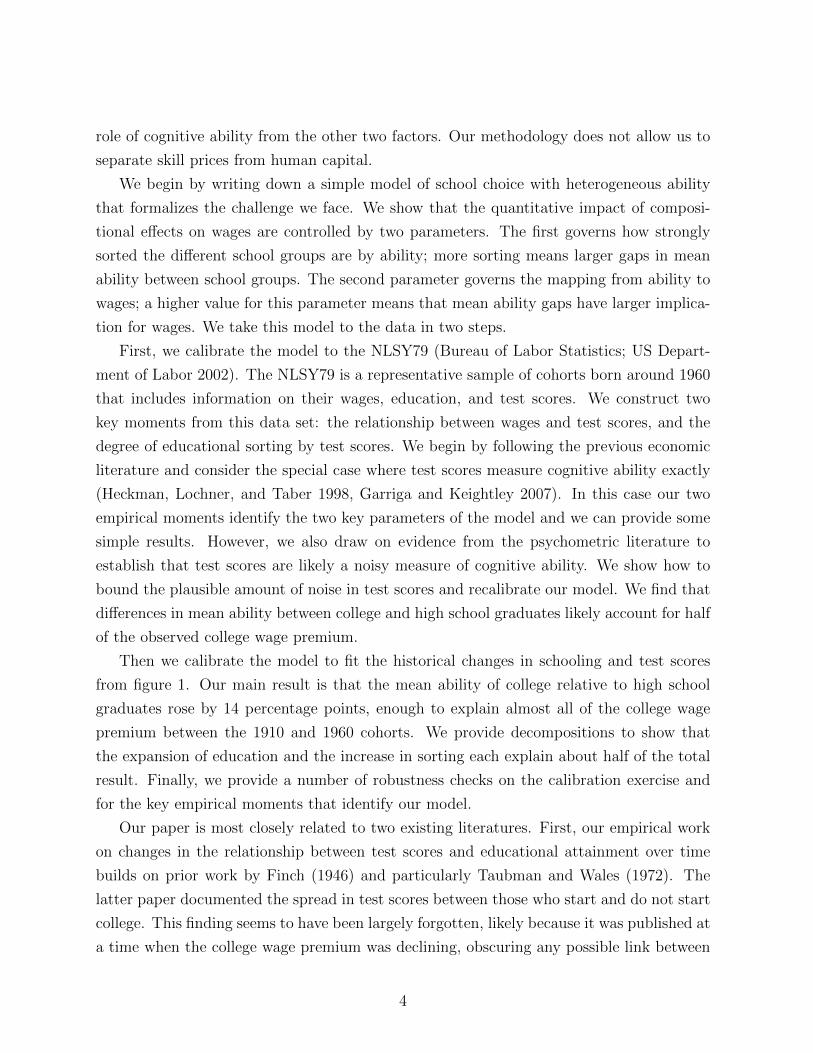
The twentieth century witnessed an extraordinary and well-documented expansion of ed-

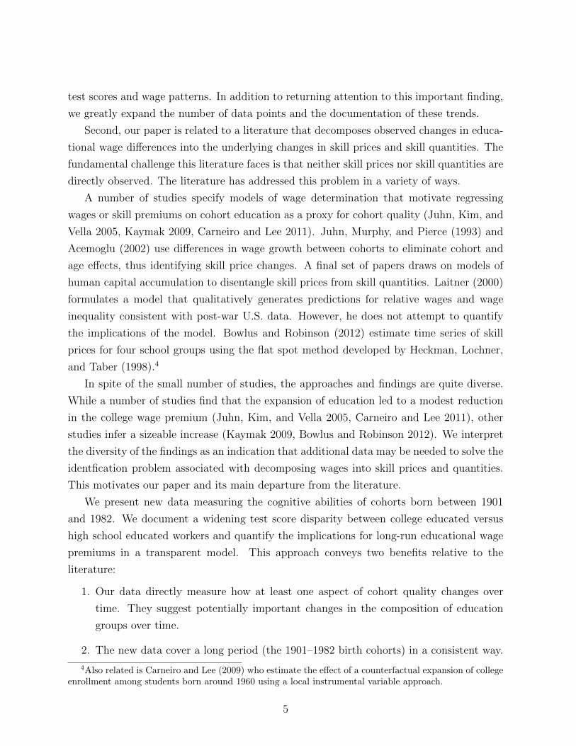
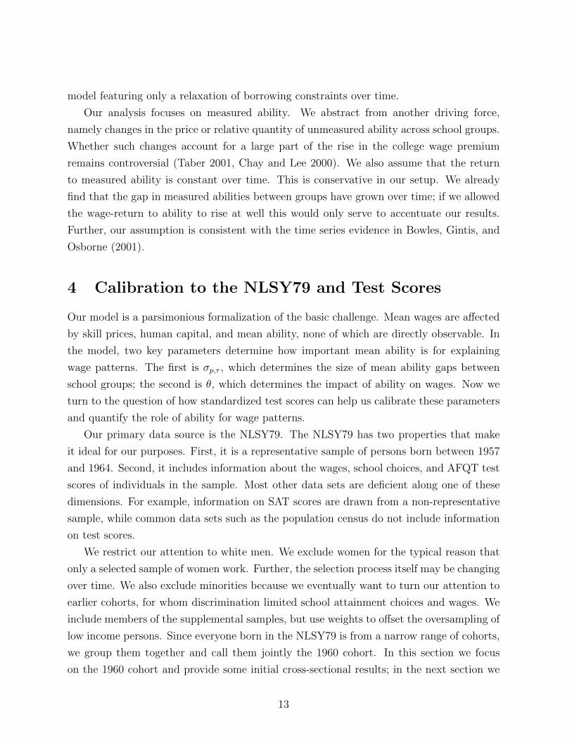
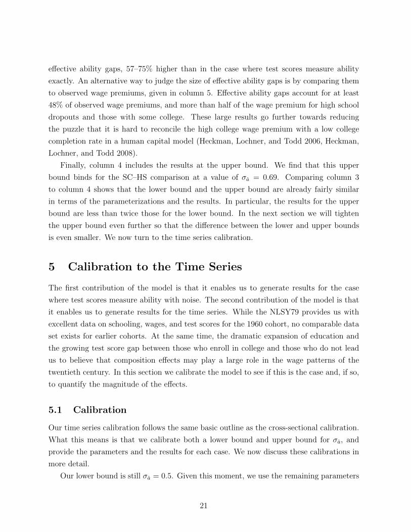
ucation in the United States (Goldin and Katz 2008). Figure 1a illustrates this trend.

For the birth cohorts born every ten years between 1910 and 1960, it displays the fraction

of white men in four exhaustive and mutually exclusive education categories: high school

dropouts (<HS), high school graduates (HS), those with some college but not a four-year

degree (SC), and college graduates with at least a four-year degree (C+). Of the men born

in 1910, only one-third finished high school. By the 1960 cohort, high school graduation

had become nearly universal and the median man attended at least some college.1

At the same time that high school completion and college enrollment were expanding,

there was also a systematic and less well-known change in who pursued higher education.

The general trend was for education to become more meritocratic, with ability and prepa-

ration becoming better predictors of educational attainment. In this paper we build on

earlier work by Taubman and Wales (1972) and provide systematic evidence of this trend

by comparing the standardized test scores for those who stop their education with a high

school degree (the HS group) and those who continue to college (the SC and C+ groups).

Figure 1b plots the average percentile rank of these two groups against the birth cohort;

as is explained in Section 2, each pair of data points represents the results of a separate

study. The trend is striking. For the very earliest cohorts, students who did not continue

on to college scored only ten percentage points lower than students who did. By the 1940s

cohorts, that gap had grown to nearly thirty percentage points.

Our main idea is that these two trends have combined to change the composition of

cognitive abilities by educational attainment for different cohorts. For example, it is unlikely

that the ability of high school dropouts is the same for the 1910 and 1960 cohorts, given

that more than half of the 1910 cohort dropped out but less than ten percent of the 1960

cohort did. Likewise, the ability of college graduates is likely to have changed given the

large expansion of college enrollment and the changes in how college students are selected.

Our primary motivation for studying compositional effects is to understand their im-

portance for the evolution of wage patterns over the course of the twentieth century. To

be concrete, we focus on two well-known features of the college wage premium. First, the

college wage premium rose by 15 percentage points between the 1910 and 1960 cohorts.2

1These data are derived from the 1950–2000 population censuses. We focus on cohorts born at tenyear intervals to match with the ten year intervals between censuses. Each data point represents averageschooling at age 40 for the relevant cohort. For more details on the construction of the data in figure 1, seeAppendix A.1 and the Online Appendix.

2Katz and Murphy (1992), Bound and Johnson (1992), Autor, Katz, and Krueger (1998), and Goldin

2

Figure 1: Changes in US Education in the Twentieth Century

(a) The Expansion of Education

.1.2

.3.4

.5.6

Frac

tion

in S

choo

l Gro

up

1910 1920 1930 1940 1950 1960Birth Cohort

<HS HS SC C+

(b) Changes in Test Scores by Attainment

3040

5060

7080

Aver

age

Perc

entile

Tes

t Sco

re

1900 1920 1940 1960 1980Birth Cohort

High School Only (HS) Enrolled in College (SC and C+)

Second, the current college wage premium is 50 percentage points, which is difficult to

reconcile with the low college completion rate in human capital models.3 We establish in

this paper that changes in the composition of student abilities by educational attainment

between the 1910 and 1960 cohorts can quantitatively explain the entire rise in the college

wage premium while simultaneously making it easier to reconcile the current college wage

premium with human capital theory.

To fix ideas, we think of the average log-wages of workers with a particular educational

attainment as being a function of the price of skills specific to that education group and

the quantity of those skills the average worker provides. The quantity is in turn determined

by workers’ cognitive abilities and the human capital they acquire over the course of their

lives. Much of the previous literature seeking to explain the college wage premium holds

the quantity of skills fixed and focuses on reasons why skill prices may have changed –

for example, due to skill-biased technological change. We allow for either component of

wages to change. The primary challenge we face is that while mean wages are observed

directly, the other terms – skill prices, human capital, and ability – are not. Our approach

to this problem is to use the information provided by standardized test scores. We treat

test scores as observed, noisy proxies for cognitive ability. We use them to disentangle the

and Katz (2008) propose skill-biased technological change as an explanation for the rising skill premium.Bound and Johnson (1992) and the survey of Levy and Murnane (1992) propose other explanations includinginternational trade or migration.

3See for example Heckman, Lochner, and Todd (2006) and Heckman, Lochner, and Todd (2008), whoalso propose an alternative extension to reconcile the model with the data.

3

role of cognitive ability from the other two factors. Our methodology does not allow us to

separate skill prices from human capital.

We begin by writing down a simple model of school choice with heterogeneous ability

that formalizes the challenge we face. We show that the quantitative impact of composi-

tional effects on wages are controlled by two parameters. The first governs how strongly

sorted the different school groups are by ability; more sorting means larger gaps in mean

ability between school groups. The second parameter governs the mapping from ability to

wages; a higher value for this parameter means that mean ability gaps have larger implica-

tion for wages. We take this model to the data in two steps.

First, we calibrate the model to the NLSY79 (Bureau of Labor Statistics; US Depart-

ment of Labor 2002). The NLSY79 is a representative sample of cohorts born around 1960

that includes information on their wages, education, and test scores. We construct two

key moments from this data set: the relationship between wages and test scores, and the

degree of educational sorting by test scores. We begin by following the previous economic

literature and consider the special case where test scores measure cognitive ability exactly

(Heckman, Lochner, and Taber 1998, Garriga and Keightley 2007). In this case our two

empirical moments identify the two key parameters of the model and we can provide some

simple results. However, we also draw on evidence from the psychometric literature to

establish that test scores are likely a noisy measure of cognitive ability. We show how to

bound the plausible amount of noise in test scores and recalibrate our model. We find that

differences in mean ability between college and high school graduates likely account for half

of the observed college wage premium.

Then we calibrate the model to fit the historical changes in schooling and test scores

from figure 1. Our main result is that the mean ability of college relative to high school

graduates rose by 14 percentage points, enough to explain almost all of the college wage

premium between the 1910 and 1960 cohorts. We provide decompositions to show that

the expansion of education and the increase in sorting each explain about half of the total

result. Finally, we provide a number of robustness checks on the calibration exercise and

for the key empirical moments that identify our model.

Our paper is most closely related to two existing literatures. First, our empirical work

on changes in the relationship between test scores and educational attainment over time

builds on prior work by Finch (1946) and particularly Taubman and Wales (1972). The

latter paper documented the spread in test scores between those who start and do not start

college. This finding seems to have been largely forgotten, likely because it was published at

a time when the college wage premium was declining, obscuring any possible link between

4

test scores and wage patterns. In addition to returning attention to this important finding,

we greatly expand the number of data points and the documentation of these trends.

Second, our paper is related to a literature that decomposes observed changes in educa-

tional wage differences into the underlying changes in skill prices and skill quantities. The

fundamental challenge this literature faces is that neither skill prices nor skill quantities are

directly observed. The literature has addressed this problem in a variety of ways.

A number of studies specify models of wage determination that motivate regressing

wages or skill premiums on cohort education as a proxy for cohort quality (Juhn, Kim, and

Vella 2005, Kaymak 2009, Carneiro and Lee 2011). Juhn, Murphy, and Pierce (1993) and

Acemoglu (2002) use differences in wage growth between cohorts to eliminate cohort and

age effects, thus identifying skill price changes. A final set of papers draws on models of

human capital accumulation to disentangle skill prices from skill quantities. Laitner (2000)

formulates a model that qualitatively generates predictions for relative wages and wage

inequality consistent with post-war U.S. data. However, he does not attempt to quantify

the implications of the model. Bowlus and Robinson (2012) estimate time series of skill

prices for four school groups using the flat spot method developed by Heckman, Lochner,

and Taber (1998).4

In spite of the small number of studies, the approaches and findings are quite diverse.

While a number of studies find that the expansion of education led to a modest reduction

in the college wage premium (Juhn, Kim, and Vella 2005, Carneiro and Lee 2011), other

studies infer a sizeable increase (Kaymak 2009, Bowlus and Robinson 2012). We interpret

the diversity of the findings as an indication that additional data may be needed to solve the

identfication problem associated with decomposing wages into skill prices and quantities.

This motivates our paper and its main departure from the literature.

We present new data measuring the cognitive abilities of cohorts born between 1901

and 1982. We document a widening test score disparity between college educated versus

high school educated workers and quantify the implications for long-run educational wage

premiums in a transparent model. This approach conveys two benefits relative to the

literature:

1. Our data directly measure how at least one aspect of cohort quality changes over

time. They suggest potentially important changes in the composition of education

groups over time.

2. The new data cover a long period (the 1901–1982 birth cohorts) in a consistent way.

4Also related is Carneiro and Lee (2009) who estimate the effect of a counterfactual expansion of collegeenrollment among students born around 1960 using a local instrumental variable approach.

5

The longer coverage is important because the data indicate that the largest changes

in the test score gap occurred before the 1930 cohort, with the rate of change slowing

over time.

Our approach is designed primarily to quantify the importance of changing test score gaps as

a proxy for changing cognitive ability gaps. It follows that we do not quantify abilities that

are uncorrelated with test scores or are unobserved altogether. We refer interested readers

to an existing literature especially on changes in the price and quantity of unobserved

abilities. That literature has not reached a consensus on whether these changes contribute

to the rise in the college wage premium in an important way (Chay and Lee 2000, Taber

2001, Deschenes 2006). It is possible that such changes may accentuate or partly undo our

conclusion about changes in cognitive abilities.

The rest of the paper is organized as follows. Section 2 briefly gives details on the rising

test score gap between high school graduates and college-goers. Section 3 introduces our

model of school choice. Section 4 calibrates the model to the NLSY79 and derives cross-

sectional results. Section 5 calibrates the model to the time series data and derives further

results. Section 6 provides robustness checks and the final section concludes.

2 The Changing Relationship Between Test Scores and

College Attendance

The first contribution of this paper is to provide extensive documentation on the divergence

of test scores between high school graduates who continued to college and those who did not.

Our main source of data is two dozen studies conducted by psychologists and educational

researchers around the country. In this section we provide a brief overview of the content

of these studies and how we combined them with results from the more recent, nationally

representative samples such as the NLSY79 to generate Figure 1b. A longer description

of our procedures, along with references, detailed metadata on the different studies, and a

number of robustness checks, is available in an online appendix.

Our starting point was to collect every study we could find with data on the test scores

of high school graduates who do and do not continue to college. We focused particularly on

studies that predate the availability of large, nationally representative datasets such as the

NLSY. The first such studies were conducted shortly after World War I and tested students

who were born just after the turn of the century.5 We have collected more than two dozen

5The U.S. Armed Forces made heavy use of group intelligence tests in assigning recruits to positions

6

such studies. The studies vary in terms of size, geographic scope, test instrument, and

so on, but it is useful to describe a typical study, which comes in two parts. First, the

researcher would arrange for a large number of high schools in a metropolitan area or a

state (sometimes all such high schools) to administer an aptitude or achievement test to

high school seniors. Second, the researcher would collect information on the college-going

behavior of the students, either by asking them their plans as high school seniors, or by re-

surveying the students, their parents, or schools a year or two later after their graduation.

We are interested in cross-tabulations of test scores and college-going behavior.

Since many of these studies are quite old the original raw data do not exist. In-

stead, we rely on the reported summary statistics and tabulations from published articles,

mimeographs, books, and dissertations. One commonly reported table gives the number

of students with scores in various ranges that did and did not continue to college. Follow-

ing Taubman and Wales (1972), we convert score levels to percentiles, and then compute

the average percentile rank of those who do and do not continue to college from these

discretized distributions. This measure can be computed from most of the studies. We

then add to these data by computing the same figure for recent, nationally representative

samples, including the NLSY79.

The resulting data are plotted in Figure 1b. The trend is striking. For cohorts born

around the turn of the 20th century there was a very small test score gap between those

who continued to college and those who did not, on the order of 10 percentage points. The

earliest studies expressed consistent surprise at how many low-scoring students continued

to college and how many high-scoring students did not. The gap between the two groups

grew steadily from the 1900 to the 1940 cohort, at which point it plateaued at nearly 30

percentage points.6 Contemporary sources pointed to two reasons why the gap was growing.

First, it became increasingly common for universities to administer tests to applicants as

an admissions tool. Second, high schools administered tests to their students with an aim

towards vocational guidance. Since tests were often interpreted as measures of academic

ability, students who scored well were encouraged to continue their education while those

who did not were pushed towards vocational tracks.

We document in the Online Appendix the robustness of this basic finding. We show

there that a similar pattern emerges if we use alternative metrics to measure how strongly

during the War. Their use in this context increased awareness and interest among the public and researchers,and provided an opening for their broader acceptance and adoption. Hence, the first studies were conductedimmediately after the War (Cremin 1961).

6Our finding is closely related to that of Hoxby (2009), who documents a complementary trend ofincreasing sorting of students by test scores among colleges.

7

sorted the college goers and non-goers are. We provide references and evidence that the tests

used in early years appear to have been of quality similar to those from more recent years,

as measured by inter-test correlations or the usefulness of tests for predicting subsequent

college grades. Finally, although there are methodological differences between studies, such

as when they followed up with students or where the survey was conducted, we find similar

trends if we restrict our attention to studies that were similar along multiple dimensions.

We conclude that the testing movement influenced who chose to stop their education with

high school and who pursued college. In the next section we introduce a model to allow us

to analyze the importance of such a shift for wage patterns.

3 A Model of School Choice

Our first goal is to specify a parsimonious model of school choice that formalizes the intuition

from the introduction. We show that the quantitative magnitude of our results depends on

two key parameters. The model guides our subsequent empirical work.

The basic environment is a discrete time overlapping generations model. Each year a

cohort of unit measure is born. Individuals are indexed by their year of birth τ as well

as their age v, with the current period given by τ + v − 1. Individuals live for a fixed T

periods.

3.1 Endowments

Each person is endowed with a variety of idiosyncratic, time-invariant traits that affect

their wages and schooling.7 We assume that these traits are captured by a two-dimensional

endowment (a, p). a represents ability. Ability is useful for both work and school, because

it makes it easier to learn and process new information or perform new tasks. p represents

the taste for schooling. It is a preference parameter that captures the relative disutility

that a person derives from spending time in school instead of working. The two traits are

assumed to be independent without loss of generality. We assume that abilities are drawn

from a time-invariant standard normal distribution. Given the assumptions that we make

below, both the mean and the standard deviation of this distribution can be normalized

in this way. An individual’s tastes for schooling are also drawn from a normal distribution

with mean 0 and a standard error σp,τ . Given that these are the only two endowments in

7These traits may be malleable earlier in life. We focus on school choices made from young adulthoodonward. Many of the relevant traits appear to difficult to change by age 16.

8

the model, we can denote by q = (a, p, τ) the type of an agent, their endowment and their

birth cohort.

3.2 Preferences

Let c(q, v) denote the consumption of a person of type q at age v, and let β > 0 be the

common discount factor. Then lifetime utility is given by:

T∑v=1

βv log[c(q, v)]− exp[−(p+ a)]χ(s, τ). (1)

Workers value consumption in the standard way. They also place a direct utility value

on their time spent in school, which is determined by the interaction between a worker-

specific component (p+ a) and a cohort and school-specific component χ(s, τ). The former

term captures how enjoyable (p) and easy (a) a particular individual finds schooling to

be. The functional form − exp[−(p + a)] assumes that school is distasteful, but less so

for more cognitively able students or those with higher taste for schooling. The latter

term captures how desirable school type s and its associated career paths are for cohort

τ . It varies by cohort to capture changes in school and work, such as the amount of

studying required to succeed in college or the career paths open to those with a particular

educational attainment. We restrict χ to be positive and increasing in s. In this case, the

preferences show complementarity between school and cognitive ability or taste for school.

This complementarity is essential for our results. We could adopt alternative functional

forms that preserve complementarity and our results would obtain; we have chosen this

functional form as the simplest.

3.3 Budget Constraint

School type s takes T (s) years to complete. While in school, students forego the labor

market. After graduation, workers receive earnings w(s, q, v) that depend on their school

attainment, age, and ability. Their budget constraint requires them to finance lifetime

consumption through lifetime earnings,

T∑v=1

c(q, v)

Rv=

T∑v=T (s)+1

w(s, q, v)

Rv, (2)

where R is the exogenous interest rate.

9

In keeping with much of the literature, we assume that workers with different educational

attainments provide different labor inputs.8 We assume that wages are given by

log[w(s, q, v)] = θa+ z(s, τ + v − 1) + h(s, v).

Wages have three determinants in our model. As mentioned before, ability affects wages di-

rectly. Since we have assumed that ability is distributed standard normal, θ is an important

parameter. It measures the increase in wages that comes from a one standard deviation

rise in ability. z(s, τ + v − 1) is the price per unit of type s labor supplied by cohort τ at

age v. Finally h(s, v) captures the human capital accumulated by workers of education s

at age v through experience or learning-by-doing, which has a systematic effect on wages.

3.4 Characterization of School Choice

Workers choose their school attainment s and a consumption path c(q, v) to maximize

preferences (1) subject to their budget constraint (2). We characterize the solution in two

steps: first, we find the optimal allocation of consumption over time given school choice;

then we find the school choice that maximizes lifetime utility.

Consumption in this model satisfies the standard Euler equation, c(q, v+1) = βRc(q, v).

If we combine this equation with the budget constraint and then plug into the utility

function, we can rewrite lifetime utility as:

θaT∑v=1

βv +T∑v=1

βv log

R(βR)v−1∑Tu=1 β

u−1

T∑u=T (s)+1

eh(s,u)+z(s,τ+u−1)

Ru

− exp[−(p+ a)]χ(s, τ). (3)

This equation has three additive terms. The first term captures the effect of ability

on lifetime utility: higher ability allows for higher lifetime consumption. The second term

captures the impact of school attainment on lifetime utility: more schooling means fewer

years in the labor market but also changes the skill price and the rate of human capital

accumulation. Finally, the last term captures the direct utility effect of schooling.

A key property of our model is that school choices depend only on the sum p+a, and not

on other individual-specific attributes or on p or a independently.9 To see this, note that

8For example, our setup is consistent with the literature that allows high school and college-educatedworkers to be imperfect substitutes in aggregate production. However, we do not take a stand on thedemand side of the market since doing so is not essential to our model. One channel that we are implicitlyruling out is that the rising skill premium may reflect an increase in the rental price of high ability laborrelative to low ability labor (Juhn, Murphy, and Pierce 1993, Murnane, Willett, and Levy 1995).

9This is the model property that makes it innocuous to assume that p and a are independent. If they

10

the first term of our indirect utility function depends on ability but does not interact with

school choices, so that it drops out of the individual’s optimization problem. The second

term does not depend on p or a. So endowments interact with school choice only through

the third term, which includes the linear combination p+a. Our model includes the common

property that ability does not affect school choice through the earnings channel, because it

raises both the benefits of schooling (higher future wages) and the opportunity cost (higher

foregone wages today) proportionally. Instead, ability, tastes, and school choice interact

through preferences in the third term. Given our assumptions on χ(s, τ), school attainment

in our model is increasing in p + a. The individuals who have the highest combination of

p+ a will choose college; those with middling values will choose high school graduation or

some college; and those with the lowest values will choose to drop out of high school.

Since ability is one component of the sum p + a, the model generates positive but

imperfect sorting by ability into school attainment. Further, since the standard deviation

of ability is normalized to 1, the degree of sorting by ability into educational attainment is

controlled by a single parameter, σp,τ . As σp,τ rises, more of the variation in p + a comes

from variation in p. In this case, workers are less sorted by ability across school groups and

mean ability gaps are smaller. In the limiting case of σp,τ = ∞, educational choices are

explained entirely by tastes for schooling. In this case, E(a|s) = E(a) = 0 for all school

groups.

3.5 Implications for Mean Ability and Wages

Since the model allows for positive sorting by ability, it generates composition effects that

matter for wages. The average wage of workers from cohort τ with education s at age v is

given by:

E[log(w)|s, τ, v] = θE[a|s, τ ] + z(s, τ + v − 1) + h(s, v).

In our model, these wages are affected by three terms: by θE[a|s, τ ], which we call effective

ability; by skill prices, z; and by human capital, h. Our goal is to separate out the role of

effective ability in explaining wage patterns from the other two terms. We make no attempt

to separate out skill prices from human capital endowments in this paper.

The quantitative magnitude of our results depends on two key model parameters. The

first is σp,τ , which determines the strength of sorting by ability into different school groups,

were correlated, we could always re-define a as ability plus the correlated component of tastes, and p as theorthogonal component of taste; given that our model depends only on p+ a, the results will be the same.

11

which is reflected in E[a|s, τ ] in the average wage equation. The second is θ, which deter-

mines the impact of ability on wages. In general, the smaller is σp,τ and the larger is θ, the

larger is the quantitative role for mean ability in explaining observed wage patterns. Other

parameters such as β or R matter little or not at all for our quantitative results. Perfect

sorting by p+ a is critical for this simplification.

3.6 Model Discussion

Our model admits other interpretations that yield similar results. One useful reinterpreta-

tion follows Manski (1989). Students still possess ability a, which makes school easier and

raises wages, just as in our baseline interpretation. However, students have no tastes for

schooling. If they knew their own ability, they would perfectly sort by ability into school

attainment. Imperfect sorting in this model comes from the assumption that students are

imperfectly informed about their ability, with p representing signal noise and p + a rep-

resenting their signal of their own ability. Students with better signals of ability further

their education, because they anticipate that schooling will be relatively painless. This

reinterpretation generates the same prediction of perfect sorting by p + a. Because of this

the calibration and results from this alternative model would be identical to those derived

from our baseline model.

Our model does assume only a single stand-in friction that prevents perfect sorting

by ability. An alternative approach taken elsewhere is to model multiple frictions in detail

(Cunha, Heckman, and Navarro 2005, Navarro 2008). Doing so would complicate our model

and identification. However, the primary impediment is that we lack sufficient historical

data to calibrate multiple frictions in detail.

An alternative friction to perfect sorting by ability that is not nested by our setup is

borrowing constraints. Borrowing constraints differ from tastes because they are asym-

metric: they prevent some high-ability students from furthering their education, but have

no effect on low-ability students. By contrast, variation in tastes causes some high-ability

students to drop out, but it also causes some low-ability students to attain high levels of

education. The literature has not arrived at a consensus about the quantitative importance

of borrowing constraints. Cameron and Taber (2004) and Stinebrickner and Stinebrickner

(2008) find no evidence of borrowing constraints in the United States for recent cohorts of

college attendees. We have little evidence as to whether credit constraints were quantita-

tively important for earlier cohorts. However, evidence gathered in Herrnstein and Murray

(1994) suggests that low-ability students are becoming less likely to attend college over

time. This information is consistent with a decline in the dispersion of tastes, but not a

12

model featuring only a relaxation of borrowing constraints over time.

Our analysis focuses on measured ability. We abstract from another driving force,

namely changes in the price or relative quantity of unmeasured ability across school groups.

Whether such changes account for a large part of the rise in the college wage premium

remains controversial (Taber 2001, Chay and Lee 2000). We also assume that the return

to measured ability is constant over time. This is conservative in our setup. We already

find that the gap in measured abilities between groups have grown over time; if we allowed

the wage-return to ability to rise at well this would only serve to accentuate our results.

Further, our assumption is consistent with the time series evidence in Bowles, Gintis, and

Osborne (2001).

4 Calibration to the NLSY79 and Test Scores

Our model is a parsimonious formalization of the basic challenge. Mean wages are affected

by skill prices, human capital, and mean ability, none of which are directly observable. In

the model, two key parameters determine how important mean ability is for explaining

wage patterns. The first is σp,τ , which determines the size of mean ability gaps between

school groups; the second is θ, which determines the impact of ability on wages. Now we

turn to the question of how standardized test scores can help us calibrate these parameters

and quantify the role of ability for wage patterns.

Our primary data source is the NLSY79. The NLSY79 has two properties that make

it ideal for our purposes. First, it is a representative sample of persons born between 1957

and 1964. Second, it includes information about the wages, school choices, and AFQT test

scores of individuals in the sample. Most other data sets are deficient along one of these

dimensions. For example, information on SAT scores are drawn from a non-representative

sample, while common data sets such as the population census do not include information

on test scores.

We restrict our attention to white men. We exclude women for the typical reason that

only a selected sample of women work. Further, the selection process itself may be changing

over time. We also exclude minorities because we eventually want to turn our attention to

earlier cohorts, for whom discrimination limited school attainment choices and wages. We

include members of the supplemental samples, but use weights to offset the oversampling of

low income persons. Since everyone born in the NLSY79 is from a narrow range of cohorts,

we group them together and call them jointly the 1960 cohort. In this section we focus

on the 1960 cohort and provide some initial cross-sectional results; in the next section we

13

generate time series results.

We use as our measure of test score their Armed Forces Qualifying Test (AFQT) score.

The AFQT is widely recognized as a cognitive test and AFQT scores are highly correlated

with the scores from other aptitude tests. For each person, we construct real hourly wage

at age 40, educational attainment, and AFQT score. Students did not take the AFQT

at the same age, which affects average scores. We use regressions to remove age effects

from AFQT scores in the standard way, then standard normalize the residual. Details are

available in the Appendix.

Since test scores play a central role in our analysis, it is important to be precise about

how we interpret them. We think of test scores as noisy, scaled proxies for cognitive ability,

a = η (a+ εa), where η is an unknown scaling factor and εa is a normal random variable

with mean 0 and standard deviation σa. We standard normalize test scores to remove the

scaling factor. Once standard normalized, test scores and the noise term are given by:

a =a√

1 + σ2a

+ εa

εa ∼ N

(0,

σa√1 + σ2

a

)

We now turn to using test scores to quantify the role of ability in wage patterns.

4.1 Results When Test Scores Measure Ability Exactly

Test scores provide us with useful information on the role of ability in school choices and

wages. Intuitively, we can use the degree of sorting by test scores into educational attain-

ment as a proxy for the degree of sorting by ability into educational attainment, which

helps identify σp,1960. Likewise, we can use the effect of test scores on wages as a proxy for

the effect of ability on wages, which helps identify θ. To see how this process works, we

begin with a special case: σa = 0. In this special case, test scores measure ability exactly,

and our identification and results are straightforward.

We begin by identifying θ. The wage generating process in our model is:

log[w(s, q, v)] = θa+ z(s, τ + v − 1) + h(s, v).

Generally, we do not have direct information on a. Instead, we have measured test scores.

Our empirical counterpart to this regression is to regress wages at age 40 on test scores and

14

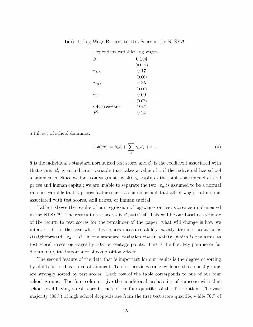
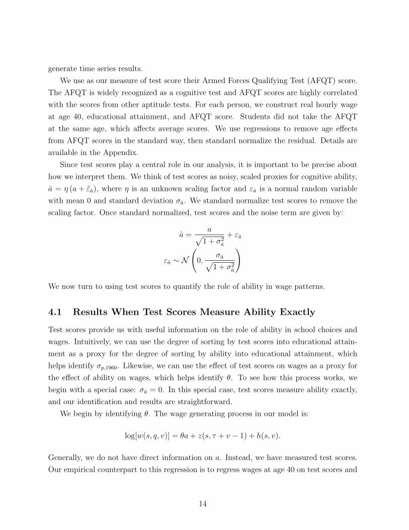
Table 1: Log-Wage Returns to Test Score in the NLSY79

Dependent variable: log-wages

βa 0.104(0.017)

γHS 0.17(0.06)

γSC 0.35(0.06)

γC+ 0.69(0.07)

Observations 1942R2 0.24

a full set of school dummies:

log(w) = βaa+∑s

γsds + εw. (4)

a is the individual’s standard normalized test score, and βa is the coefficient associated with

that score. ds is an indicator variable that takes a value of 1 if the individual has school

attainment s. Since we focus on wages at age 40, γs captures the joint wage impact of skill

prices and human capital; we are unable to separate the two. εw is assumed to be a normal

random variable that captures factors such as shocks or luck that affect wages but are not

associated with test scores, skill prices, or human capital.

Table 1 shows the results of our regression of log-wages on test scores as implemented

in the NLSY79. The return to test scores is βa = 0.104. This will be our baseline estimate

of the return to test scores for the remainder of the paper; what will change is how we

interpret it. In the case where test scores measures ability exactly, the interpretation is

straightforward: βa = θ. A one standard deviation rise in ability (which is the same as

test score) raises log-wages by 10.4 percentage points. This is the first key parameter for

determining the importance of composition effects.

The second feature of the data that is important for our results is the degree of sorting

by ability into educational attainment. Table 2 provides some evidence that school groups

are strongly sorted by test scores. Each row of the table corresponds to one of our four

school groups. The four columns give the conditional probability of someone with that

school level having a test score in each of the four quartiles of the distribution. The vast

majority (86%) of high school dropouts are from the first test score quartile, while 76% of

15

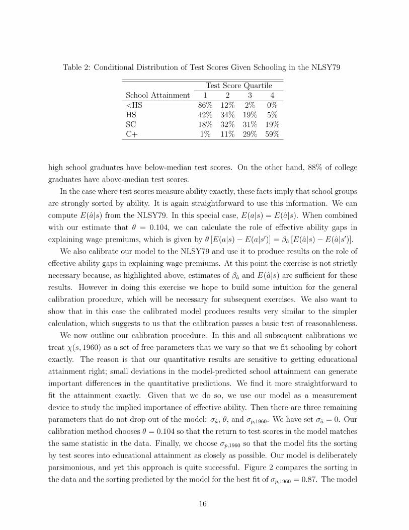
Table 2: Conditional Distribution of Test Scores Given Schooling in the NLSY79

Test Score QuartileSchool Attainment 1 2 3 4<HS 86% 12% 2% 0%HS 42% 34% 19% 5%SC 18% 32% 31% 19%C+ 1% 11% 29% 59%

high school graduates have below-median test scores. On the other hand, 88% of college

graduates have above-median test scores.

In the case where test scores measure ability exactly, these facts imply that school groups

are strongly sorted by ability. It is again straightforward to use this information. We can

compute E(a|s) from the NLSY79. In this special case, E(a|s) = E(a|s). When combined

with our estimate that θ = 0.104, we can calculate the role of effective ability gaps in

explaining wage premiums, which is given by θ [E(a|s)− E(a|s′)] = βa [E(a|s)− E(a|s′)].We also calibrate our model to the NLSY79 and use it to produce results on the role of

effective ability gaps in explaining wage premiums. At this point the exercise is not strictly

necessary because, as highlighted above, estimates of βa and E(a|s) are sufficient for these

results. However in doing this exercise we hope to build some intuition for the general

calibration procedure, which will be necessary for subsequent exercises. We also want to

show that in this case the calibrated model produces results very similar to the simpler

calculation, which suggests to us that the calibration passes a basic test of reasonableness.

We now outline our calibration procedure. In this and all subsequent calibrations we

treat χ(s, 1960) as a set of free parameters that we vary so that we fit schooling by cohort

exactly. The reason is that our quantitative results are sensitive to getting educational

attainment right; small deviations in the model-predicted school attainment can generate

important differences in the quantitative predictions. We find it more straightforward to

fit the attainment exactly. Given that we do so, we use our model as a measurement

device to study the implied importance of effective ability. Then there are three remaining

parameters that do not drop out of the model: σa, θ, and σp,1960. We have set σa = 0. Our

calibration method chooses θ = 0.104 so that the return to test scores in the model matches

the same statistic in the data. Finally, we choose σp,1960 so that the model fits the sorting

by test scores into educational attainment as closely as possible. Our model is deliberately

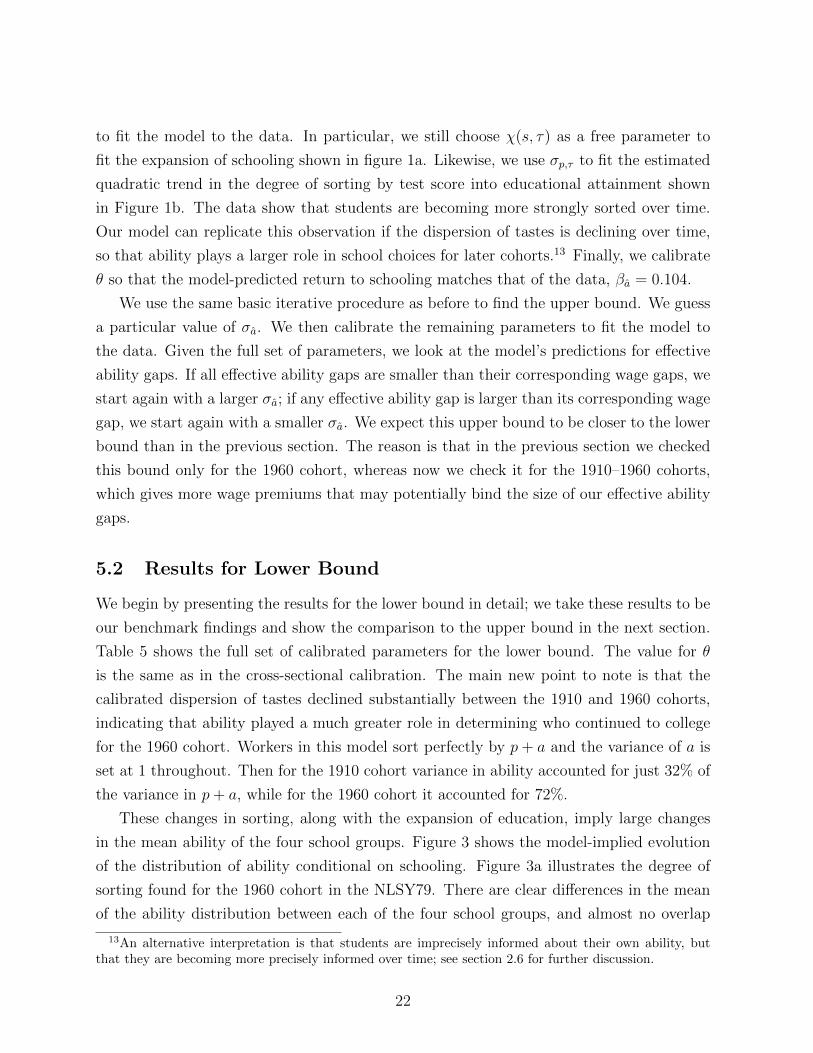
parsimonious, and yet this approach is quite successful. Figure 2 compares the sorting in

the data and the sorting predicted by the model for the best fit of σp,1960 = 0.87. The model

16

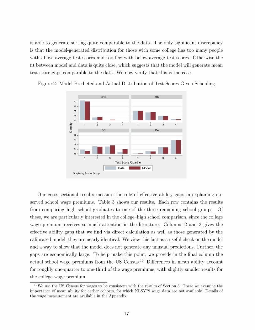
is able to generate sorting quite comparable to the data. The only significant discrepancy

is that the model-generated distribution for those with some college has too many people

with above-average test scores and too few with below-average test scores. Otherwise the

fit between model and data is quite close, which suggests that the model will generate mean

test score gaps comparable to the data. We now verify that this is the case.

Figure 2: Model-Predicted and Actual Distribution of Test Scores Given Schooling

0.2

.4.6

.80

.2.4

.6.8

1 2 3 4 1 2 3 4

1 2 3 4 1 2 3 4

<HS HS

SC C+

Data Model

Den

sity

Test Score Quartile

Graphs by School Group

Our cross-sectional results measure the role of effective ability gaps in explaining ob-

served school wage premiums. Table 3 shows our results. Each row contains the results

from comparing high school graduates to one of the three remaining school groups. Of

these, we are particularly interested in the college–high school comparison, since the college

wage premium receives so much attention in the literature. Columns 2 and 3 gives the

effective ability gaps that we find via direct calculation as well as those generated by the

calibrated model; they are nearly identical. We view this fact as a useful check on the model

and a way to show that the model does not generate any unusual predictions. Further, the

gaps are economically large. To help make this point, we provide in the final column the

actual school wage premiums from the US Census.10 Differences in mean ability account

for roughly one-quarter to one-third of the wage premiums, with slightly smaller results for

the college wage premium.

10We use the US Census for wages to be consistent with the results of Section 5. There we examine theimportance of mean ability for earlier cohorts, for which NLSY79 wage data are not available. Details ofthe wage measurement are available in the Appendix.

17

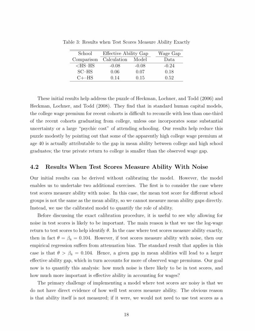
Table 3: Results when Test Scores Measure Ability Exactly

School Effective Ability Gap Wage GapComparison Calculation Model Data<HS–HS -0.08 -0.08 -0.24SC–HS 0.06 0.07 0.18C+–HS 0.14 0.15 0.52

These initial results help address the puzzle of Heckman, Lochner, and Todd (2006) and

Heckman, Lochner, and Todd (2008). They find that in standard human capital models,

the college wage premium for recent cohorts is difficult to reconcile with less than one-third

of the recent cohorts graduating from college, unless one incorporates some substantial

uncertainty or a large “psychic cost” of attending schooling. Our results help reduce this

puzzle modestly by pointing out that some of the apparently high college wage premium at

age 40 is actually attributable to the gap in mean ability between college and high school

graduates; the true private return to college is smaller than the observed wage gap.

4.2 Results When Test Scores Measure Ability With Noise

Our initial results can be derived without calibrating the model. However, the model

enables us to undertake two additional exercises. The first is to consider the case where

test scores measure ability with noise. In this case, the mean test score for different school

groups is not the same as the mean ability, so we cannot measure mean ability gaps directly.

Instead, we use the calibrated model to quantify the role of ability.

Before discussing the exact calibration procedure, it is useful to see why allowing for

noise in test scores is likely to be important. The main reason is that we use the log-wage

return to test scores to help identify θ. In the case where test scores measure ability exactly,

then in fact θ = βa = 0.104. However, if test scores measure ability with noise, then our

empirical regression suffers from attenuation bias. The standard result that applies in this

case is that θ > βa = 0.104. Hence, a given gap in mean abilities will lead to a larger

effective ability gap, which in turn accounts for more of observed wage premiums. Our goal

now is to quantify this analysis: how much noise is there likely to be in test scores, and

how much more important is effective ability in accounting for wages?

The primary challenge of implementing a model where test scores are noisy is that we

do not have direct evidence of how well test scores measure ability. The obvious reason

is that ability itself is not measured; if it were, we would not need to use test scores as a

18

proxy for ability. However, we will establish that we can make inferences that enable us

to bound usefully the noise in test scores. We begin by demonstrating how to construct a

lower bound on the noise in test scores.

To construct a lower bound on the noise in test scores, we draw on the well-known

property that repeatedly administering similar or even identical tests to a group yields

positively correlated but not identical results. We construct our lower bound on the noise

in test scores by requiring that a given test score not be a better predictor of ability than

it is of other subsequent test scores. To quantify this statement, recall that we think of

test scores as noisy, scaled proxies for ability. In this context it is natural to think of the

noise in tests εa as being an independent, test-specific draw. Then the correlation between

two different test scores for a given individual is (1 + σ2a)−1

. We have ample evidence on

the magnitude of this correlation. Herrnstein and Murray (1994, Appendix 3) document

the correlation between AFQT scores and scores from six other standardized tests taken by

some NLSY79 individuals. The correlations range from 0.71 to 0.9, with a median score of

0.81.11 Cawley, Conneely, Heckman, and Vytlacil (1997) show that the correlation between

AFQT scores and the first principal component of the ASVAB scores is 0.83.

Putting these correlations together, we use (1 + σ2a)−1

= 0.8. In turn this suggests a

lower bound σa ≥ 0.5.12 If test scores were any more precise as measures of ability, then the

correlation between scores from different tests should be higher. We use this lower bound

by fixing σa = 0.5 in the model, then calibrating θ and σp,1960 to fit the log-wage return

to test scores and the school-test score sorting as well as possible. We are able to hit the

former moment exactly. We showed earlier that even with only a single parameter σp,1960

we are able to replicate the school-test score sorting closely (Figure 2); that continues to be

the case here and throughout the remainder of the paper. We do not show the remaining

figures to conserve space.

We also want to establish an upper bound on the plausible noise in test scores. The

purpose of this bound is not to argue that the true results are at some midpoint of the

lower and upper bounds. Instead, we establish an upper bound to show that a bounding

argument in this case is effective in the sense that the range of results is fairly narrow.

Given this fact, it is innocuous to use the lower bound as our benchmark, which we do.

11A slight complication arises from the fact that Herrnstein and Murray compute correlations betweenpercentile ranks rather than raw scores. We conducted simulations to verify that this has only a minorquantitative effect on the resulting correlation.

12A similar approach is taken by Bishop (1989) to estimate the measurement error in the PSID’s GIAscore. Based on the GIA’s KR-20 reliability of 0.652, Bishop’s result implies σa = 0.73, which would implya larger role for ability than what we find here. In fact, we construct an upper bound for σa that is lowerthan this value below, suggesting that Bishop’s results may have counterfactual implications for wages.

19

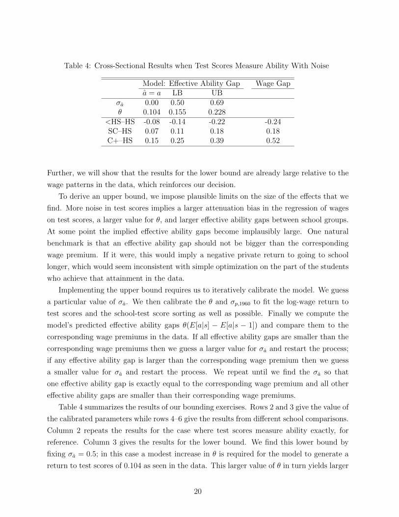
Table 4: Cross-Sectional Results when Test Scores Measure Ability With Noise

Model: Effective Ability Gap Wage Gapa = a LB UB

σa 0.00 0.50 0.69θ 0.104 0.155 0.228

<HS–HS -0.08 -0.14 -0.22 -0.24SC–HS 0.07 0.11 0.18 0.18C+–HS 0.15 0.25 0.39 0.52

Further, we will show that the results for the lower bound are already large relative to the

wage patterns in the data, which reinforces our decision.

To derive an upper bound, we impose plausible limits on the size of the effects that we

find. More noise in test scores implies a larger attenuation bias in the regression of wages

on test scores, a larger value for θ, and larger effective ability gaps between school groups.

At some point the implied effective ability gaps become implausibly large. One natural

benchmark is that an effective ability gap should not be bigger than the corresponding

wage premium. If it were, this would imply a negative private return to going to school

longer, which would seem inconsistent with simple optimization on the part of the students

who achieve that attainment in the data.

Implementing the upper bound requires us to iteratively calibrate the model. We guess

a particular value of σa. We then calibrate the θ and σp,1960 to fit the log-wage return to

test scores and the school-test score sorting as well as possible. Finally we compute the

model’s predicted effective ability gaps θ(E[a|s] − E[a|s − 1]) and compare them to the

corresponding wage premiums in the data. If all effective ability gaps are smaller than the

corresponding wage premiums then we guess a larger value for σa and restart the process;

if any effective ability gap is larger than the corresponding wage premium then we guess

a smaller value for σa and restart the process. We repeat until we find the σa so that

one effective ability gap is exactly equal to the corresponding wage premium and all other

effective ability gaps are smaller than their corresponding wage premiums.

Table 4 summarizes the results of our bounding exercises. Rows 2 and 3 give the value of

the calibrated parameters while rows 4–6 give the results from different school comparisons.

Column 2 repeats the results for the case where test scores measure ability exactly, for

reference. Column 3 gives the results for the lower bound. We find this lower bound by

fixing σa = 0.5; in this case a modest increase in θ is required for the model to generate a

return to test scores of 0.104 as seen in the data. This larger value of θ in turn yields larger

20

effective ability gaps, 57–75% higher than in the case where test scores measure ability

exactly. An alternative way to judge the size of effective ability gaps is by comparing them

to observed wage premiums, given in column 5. Effective ability gaps account for at least

48% of observed wage premiums, and more than half of the wage premium for high school

dropouts and those with some college. These large results go further towards reducing

the puzzle that it is hard to reconcile the high college wage premium with a low college

completion rate in a human capital model (Heckman, Lochner, and Todd 2006, Heckman,

Lochner, and Todd 2008).

Finally, column 4 includes the results at the upper bound. We find that this upper

bound binds for the SC–HS comparison at a value of σa = 0.69. Comparing column 3

to column 4 shows that the lower bound and the upper bound are already fairly similar

in terms of the parameterizations and the results. In particular, the results for the upper

bound are less than twice those for the lower bound. In the next section we will tighten

the upper bound even further so that the difference between the lower and upper bounds

is even smaller. We now turn to the time series calibration.

5 Calibration to the Time Series

The first contribution of the model is that it enables us to generate results for the case

where test scores measure ability with noise. The second contribution of the model is that

it enables us to generate results for the time series. While the NLSY79 provides us with

excellent data on schooling, wages, and test scores for the 1960 cohort, no comparable data

set exists for earlier cohorts. At the same time, the dramatic expansion of education and

the growing test score gap between those who enroll in college and those who do not lead

us to believe that composition effects may play a large role in the wage patterns of the

twentieth century. In this section we calibrate the model to see if this is the case and, if so,

to quantify the magnitude of the effects.

5.1 Calibration

Our time series calibration follows the same basic outline as the cross-sectional calibration.

What this means is that we calibrate both a lower bound and upper bound for σa, and

provide the parameters and the results for each case. We now discuss these calibrations in

more detail.

Our lower bound is still σa = 0.5. Given this moment, we use the remaining parameters

21

to fit the model to the data. In particular, we still choose χ(s, τ) as a free parameter to

fit the expansion of schooling shown in figure 1a. Likewise, we use σp,τ to fit the estimated

quadratic trend in the degree of sorting by test score into educational attainment shown

in Figure 1b. The data show that students are becoming more strongly sorted over time.

Our model can replicate this observation if the dispersion of tastes is declining over time,

so that ability plays a larger role in school choices for later cohorts.13 Finally, we calibrate

θ so that the model-predicted return to schooling matches that of the data, βa = 0.104.

We use the same basic iterative procedure as before to find the upper bound. We guess

a particular value of σa. We then calibrate the remaining parameters to fit the model to

the data. Given the full set of parameters, we look at the model’s predictions for effective

ability gaps. If all effective ability gaps are smaller than their corresponding wage gaps, we

start again with a larger σa; if any effective ability gap is larger than its corresponding wage

gap, we start again with a smaller σa. We expect this upper bound to be closer to the lower

bound than in the previous section. The reason is that in the previous section we checked

this bound only for the 1960 cohort, whereas now we check it for the 1910–1960 cohorts,

which gives more wage premiums that may potentially bind the size of our effective ability

gaps.

5.2 Results for Lower Bound

We begin by presenting the results for the lower bound in detail; we take these results to be

our benchmark findings and show the comparison to the upper bound in the next section.

Table 5 shows the full set of calibrated parameters for the lower bound. The value for θ

is the same as in the cross-sectional calibration. The main new point to note is that the

calibrated dispersion of tastes declined substantially between the 1910 and 1960 cohorts,

indicating that ability played a much greater role in determining who continued to college

for the 1960 cohort. Workers in this model sort perfectly by p+ a and the variance of a is

set at 1 throughout. Then for the 1910 cohort variance in ability accounted for just 32% of

the variance in p+ a, while for the 1960 cohort it accounted for 72%.

These changes in sorting, along with the expansion of education, imply large changes

in the mean ability of the four school groups. Figure 3 shows the model-implied evolution

of the distribution of ability conditional on schooling. Figure 3a illustrates the degree of

sorting found for the 1960 cohort in the NLSY79. There are clear differences in the mean

of the ability distribution between each of the four school groups, and almost no overlap

13An alternative interpretation is that students are imprecisely informed about their own ability, butthat they are becoming more precisely informed over time; see section 2.6 for further discussion.

22

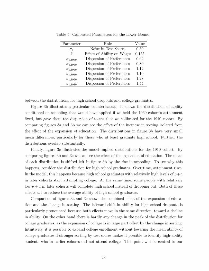
Table 5: Calibrated Parameters for the Lower Bound

Parameter Role Valueσa Noise in Test Scores 0.50θ Effect of Ability on Wages 0.155

σp,1960 Dispersion of Preferences 0.62σp,1950 Dispersion of Preferences 0.80σp,1940 Dispersion of Preferences 1.12σp,1930 Dispersion of Preferences 1.10σp,1920 Dispersion of Preferences 1.28σp,1910 Dispersion of Preferences 1.44

between the distributions for high school dropouts and college graduates.

Figure 3b illustrates a particular counterfactual: it shows the distribution of ability

conditional on schooling that would have applied if we held the 1960 cohort’s attainment

fixed, but gave them the dispersion of tastes that we calibrated for the 1910 cohort. By

comparing figures 3a and 3b we can see the effect of the increase in sorting isolated from

the effect of the expansion of education. The distributions in figure 3b have very small

mean differences, particularly for those who at least graduate high school. Further, the

distributions overlap substantially.

Finally, figure 3c illustrates the model-implied distributions for the 1910 cohort. By

comparing figures 3b and 3c we can see the effect of the expansion of education. The mean

of each distribution is shifted left in figure 3b by the rise in schooling. To see why this

happens, consider the distribution for high school graduates. Over time, attainment rises.

In the model, this happens because high school graduates with relatively high levels of p+a

in later cohorts start attempting college. At the same time, some people with relatively

low p+ a in later cohorts will complete high school instead of dropping out. Both of these

effects act to reduce the average ability of high school graduates.

Comparison of figures 3a and 3c shows the combined effect of the expansion of educa-

tion and the change in sorting. The leftward shift in ability for high school dropouts is

particularly pronounced because both effects move in the same direction, toward a decline

in ability. On the other hand there is hardly any change in the peak of the distribution for

college graduates, as the expansion of college is in large part offset by the change in sorting.

Intuitively, it is possible to expand college enrollment without lowering the mean ability of

college graduates if stronger sorting by test scores makes it possible to identify high-ability

students who in earlier cohorts did not attend college. This point will be central to our

23

Figure 3: The Distribution of Ability Conditional on Schooling

(a) 1960 Cohort

0.1

.2.3

Density

-4 -3 -2 -1 0 1 2 3 4Ability

<HS HSSC C+

(b) Counterfactual: 1960 Cohort with 1910 Sorting

0.1

.2.3

Density

-4 -3 -2 -1 0 1 2 3 4Ability

<HS HSSC C+

(c) 1910 Cohort

0.1

.2.3

Density

-4 -3 -2 -1 0 1 2 3 4Ability

<HS HSSC C+

subsequent results.

We have two main sets of time series results. First, we examine how changes in effective

ability between cohorts have affected wage growth. These results are presented in table 6.

Our measured time series for wages and our model-implied time series for mean ability by

school group are smooth, so we focus only on the total change between the first and last

cohorts. The second column gives the model-predicted change in effective ability between

the 1910 and 1960 cohorts for each of the four school groups. In the fourth column we

give the measured wage growth conditional on schooling, taken from census data. Given

the observed wage growth and the model-implied change in mean ability, we back out the

implied growth in h + z in the third column. This column measures the growth in skill

24

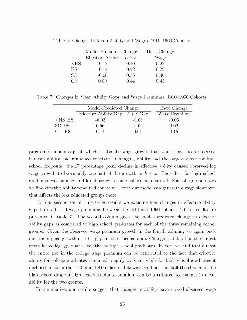
Table 6: Changes in Mean Ability and Wages, 1910–1960 Cohorts

Model-Predicted Change Data ChangeEffective Ability h+ z Wage

<HS -0.17 0.40 0.22HS -0.14 0.42 0.29SC -0.08 0.38 0.30C+ 0.00 0.44 0.43

Table 7: Changes in Mean Ability Gaps and Wage Premiums, 1910–1960 Cohorts

Model-Predicted Change Data ChangeEffective Ability Gap h+ z Gap Wage Premium

<HS–HS -0.03 -0.03 -0.06SC–HS 0.06 -0.04 0.02C+–HS 0.14 0.01 0.15

prices and human capital, which is also the wage growth that would have been observed

if mean ability had remained constant. Changing ability had the largest effect for high

school dropouts: the 17 percentage point decline in effective ability caused observed log

wage growth to be roughly one-half of the growth in h + z. The effect for high school

graduates was smaller and for those with some college smaller still. For college graduates

we find effective ability remained constant. Hence our model can generate a wage slowdown

that affects the less educated groups more.

For our second set of time series results we examine how changes in effective ability

gaps have affected wage premiums between the 1910 and 1960 cohorts. These results are

presented in table 7. The second column gives the model-predicted change in effective

ability gaps as compared to high school graduates for each of the three remaining school

groups. Given the observed wage premium growth in the fourth column, we again back

out the implied growth in h+ z gaps in the third column. Changing ability had the largest

effect for college graduates, relative to high school graduates. In fact, we find that almost

the entire rise in the college wage premium can be attributed to the fact that effective

ability for college graduates remained roughly constant while for high school graduates it

declined between the 1910 and 1960 cohorts. Likewise, we find that half the change in the

high school dropout-high school graduate premium can be attributed to changes in mean

ability for the two groups.

To summarize, our results suggest that changes in ability have slowed observed wage

25

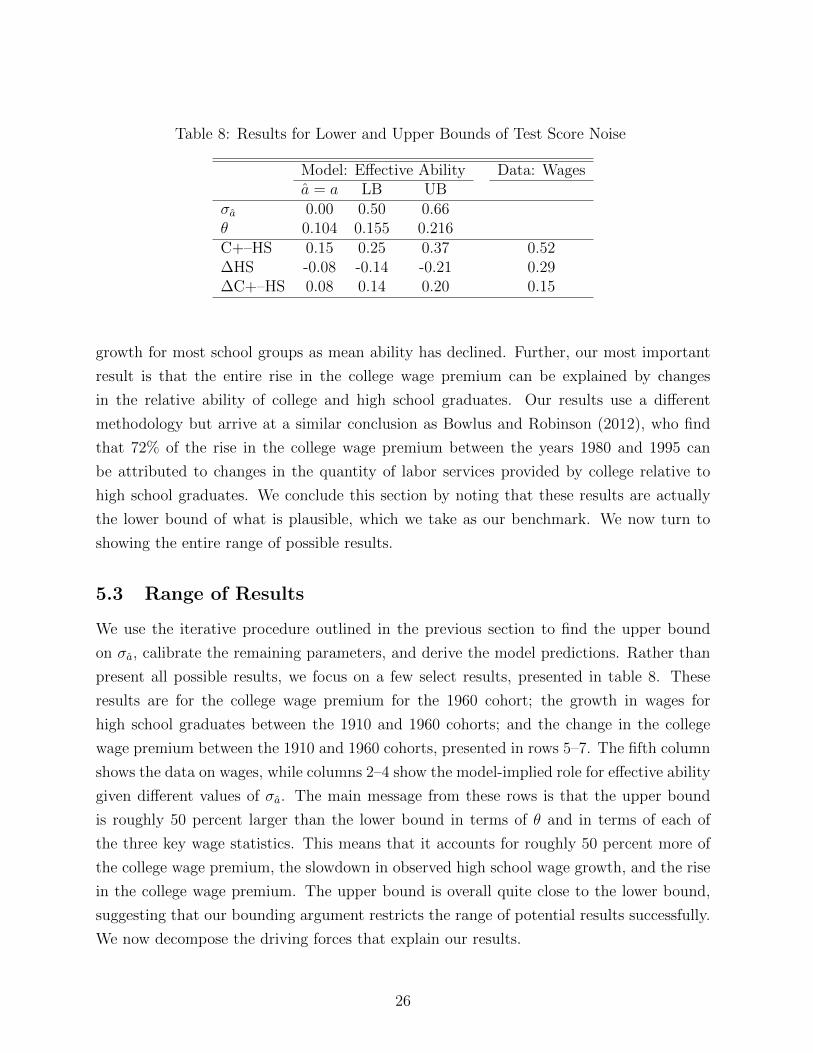
Table 8: Results for Lower and Upper Bounds of Test Score Noise

Model: Effective Ability Data: Wagesa = a LB UB

σa 0.00 0.50 0.66θ 0.104 0.155 0.216C+–HS 0.15 0.25 0.37 0.52∆HS -0.08 -0.14 -0.21 0.29∆C+–HS 0.08 0.14 0.20 0.15

growth for most school groups as mean ability has declined. Further, our most important

result is that the entire rise in the college wage premium can be explained by changes

in the relative ability of college and high school graduates. Our results use a different

methodology but arrive at a similar conclusion as Bowlus and Robinson (2012), who find

that 72% of the rise in the college wage premium between the years 1980 and 1995 can

be attributed to changes in the quantity of labor services provided by college relative to

high school graduates. We conclude this section by noting that these results are actually

the lower bound of what is plausible, which we take as our benchmark. We now turn to

showing the entire range of possible results.

5.3 Range of Results

We use the iterative procedure outlined in the previous section to find the upper bound

on σa, calibrate the remaining parameters, and derive the model predictions. Rather than

present all possible results, we focus on a few select results, presented in table 8. These

results are for the college wage premium for the 1960 cohort; the growth in wages for

high school graduates between the 1910 and 1960 cohorts; and the change in the college

wage premium between the 1910 and 1960 cohorts, presented in rows 5–7. The fifth column

shows the data on wages, while columns 2–4 show the model-implied role for effective ability

given different values of σa. The main message from these rows is that the upper bound

is roughly 50 percent larger than the lower bound in terms of θ and in terms of each of

the three key wage statistics. This means that it accounts for roughly 50 percent more of

the college wage premium, the slowdown in observed high school wage growth, and the rise

in the college wage premium. The upper bound is overall quite close to the lower bound,

suggesting that our bounding argument restricts the range of potential results successfully.

We now decompose the driving forces that explain our results.

26

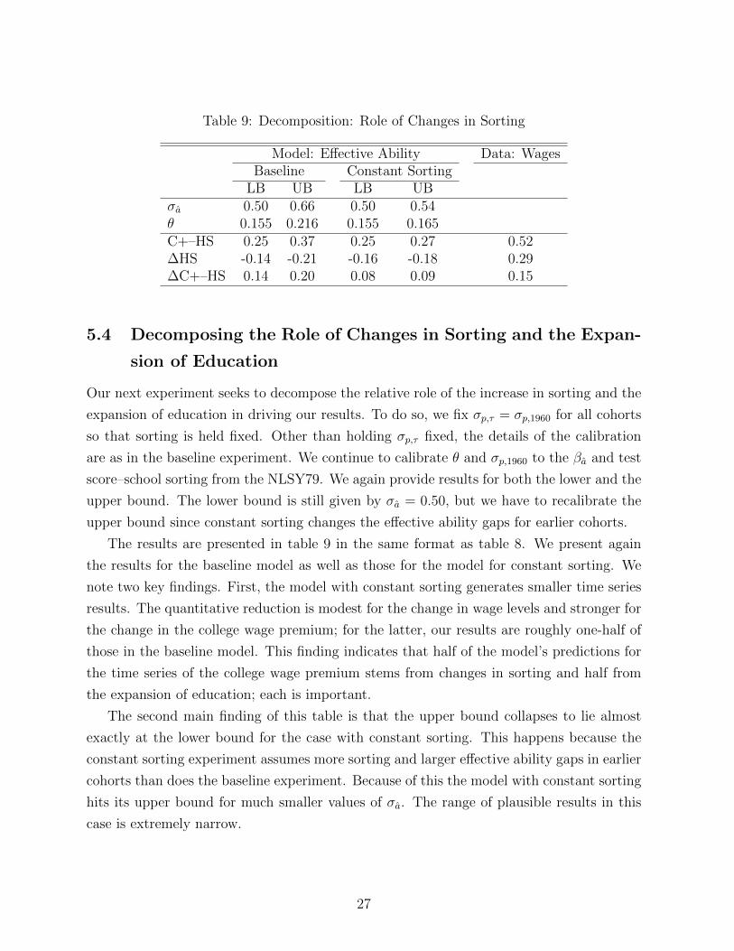
Table 9: Decomposition: Role of Changes in Sorting

Model: Effective Ability Data: WagesBaseline Constant Sorting

LB UB LB UBσa 0.50 0.66 0.50 0.54θ 0.155 0.216 0.155 0.165C+–HS 0.25 0.37 0.25 0.27 0.52∆HS -0.14 -0.21 -0.16 -0.18 0.29∆C+–HS 0.14 0.20 0.08 0.09 0.15

5.4 Decomposing the Role of Changes in Sorting and the Expan-

sion of Education

Our next experiment seeks to decompose the relative role of the increase in sorting and the

expansion of education in driving our results. To do so, we fix σp,τ = σp,1960 for all cohorts

so that sorting is held fixed. Other than holding σp,τ fixed, the details of the calibration

are as in the baseline experiment. We continue to calibrate θ and σp,1960 to the βa and test

score–school sorting from the NLSY79. We again provide results for both the lower and the

upper bound. The lower bound is still given by σa = 0.50, but we have to recalibrate the

upper bound since constant sorting changes the effective ability gaps for earlier cohorts.

The results are presented in table 9 in the same format as table 8. We present again

the results for the baseline model as well as those for the model for constant sorting. We

note two key findings. First, the model with constant sorting generates smaller time series

results. The quantitative reduction is modest for the change in wage levels and stronger for

the change in the college wage premium; for the latter, our results are roughly one-half of

those in the baseline model. This finding indicates that half of the model’s predictions for

the time series of the college wage premium stems from changes in sorting and half from

the expansion of education; each is important.

The second main finding of this table is that the upper bound collapses to lie almost

exactly at the lower bound for the case with constant sorting. This happens because the

constant sorting experiment assumes more sorting and larger effective ability gaps in earlier

cohorts than does the baseline experiment. Because of this the model with constant sorting

hits its upper bound for much smaller values of σa. The range of plausible results in this

case is extremely narrow.

27

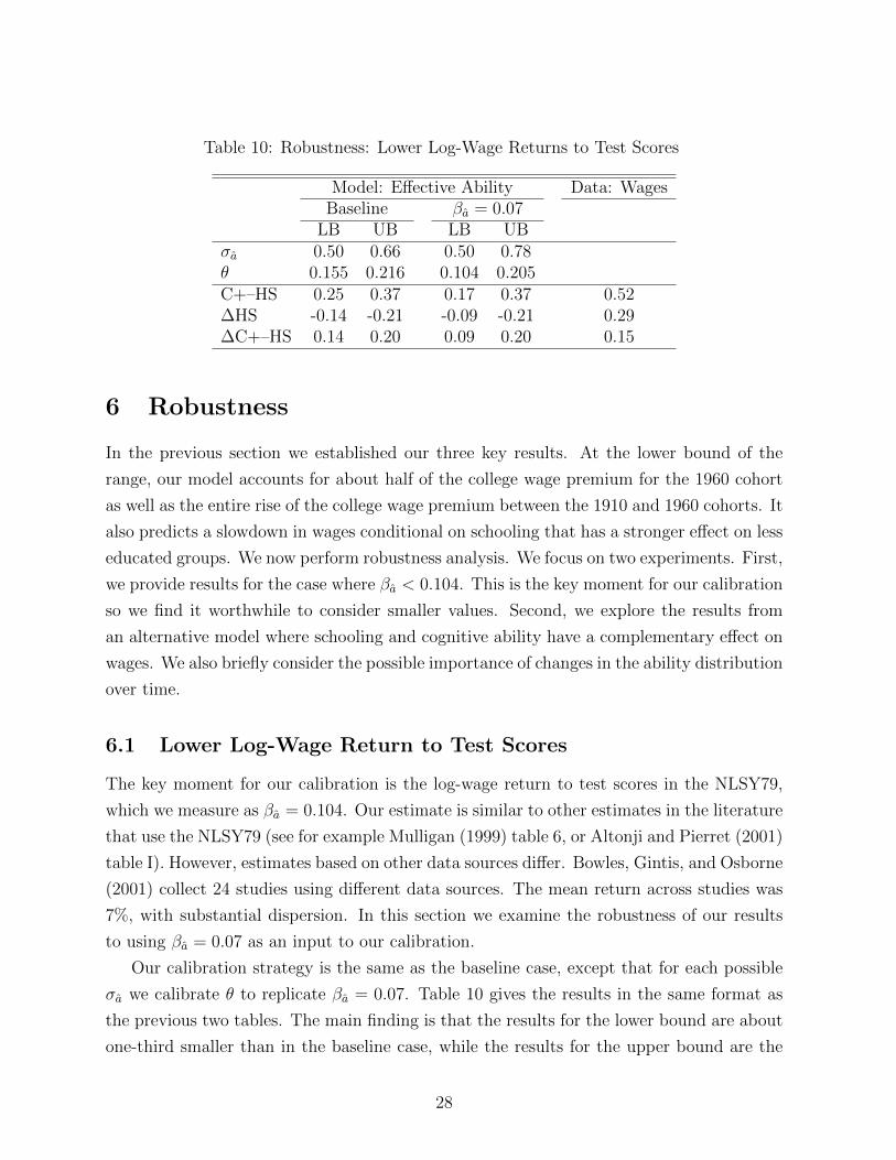
Table 10: Robustness: Lower Log-Wage Returns to Test Scores

Model: Effective Ability Data: WagesBaseline βa = 0.07

LB UB LB UBσa 0.50 0.66 0.50 0.78θ 0.155 0.216 0.104 0.205C+–HS 0.25 0.37 0.17 0.37 0.52∆HS -0.14 -0.21 -0.09 -0.21 0.29∆C+–HS 0.14 0.20 0.09 0.20 0.15

6 Robustness

In the previous section we established our three key results. At the lower bound of the

range, our model accounts for about half of the college wage premium for the 1960 cohort

as well as the entire rise of the college wage premium between the 1910 and 1960 cohorts. It

also predicts a slowdown in wages conditional on schooling that has a stronger effect on less

educated groups. We now perform robustness analysis. We focus on two experiments. First,

we provide results for the case where βa < 0.104. This is the key moment for our calibration

so we find it worthwhile to consider smaller values. Second, we explore the results from

an alternative model where schooling and cognitive ability have a complementary effect on

wages. We also briefly consider the possible importance of changes in the ability distribution

over time.

6.1 Lower Log-Wage Return to Test Scores

The key moment for our calibration is the log-wage return to test scores in the NLSY79,

which we measure as βa = 0.104. Our estimate is similar to other estimates in the literature

that use the NLSY79 (see for example Mulligan (1999) table 6, or Altonji and Pierret (2001)

table I). However, estimates based on other data sources differ. Bowles, Gintis, and Osborne

(2001) collect 24 studies using different data sources. The mean return across studies was

7%, with substantial dispersion. In this section we examine the robustness of our results

to using βa = 0.07 as an input to our calibration.

Our calibration strategy is the same as the baseline case, except that for each possible

σa we calibrate θ to replicate βa = 0.07. Table 10 gives the results in the same format as

the previous two tables. The main finding is that the results for the lower bound are about

one-third smaller than in the baseline case, while the results for the upper bound are the

28

same. Note, however, that even for the lower bound of the robustness check βa = 0.07,

we still account for nearly two-thirds of the rise in the college wage premium and nearly

one-third of the current college wage premium.

Our results do not change at the upper bound because of our bounding methodology. We

choose the upper bound so that ability gaps are as large as plausible. To do so, the model

chooses a calibrated value of θ similar to the upper bound in the baseline. It rationalizes

the low measured return to IQ as being the result of higher levels of calibrated noise in

test scores and a larger degree of attenuation bias in the regression. Hence, the essentially

unchanged results at the upper bound are driven by our requirement that the upper bound

be defined as the point where ability gaps are as large as plausible.

6.2 Ability-School Complementarity in Wages

Empirically, high test score students tend to go to school longer (see for example figure

2). In our baseline model we use complementarity between cognitive ability and school in

the utility function to match this fact. A common alternative in the literature is instead

to use complementarity that comes through wages. In this case, more able workers go to

school longer because their wage payoff to doing so is higher, not because they find it less

distasteful. We show in this subsection that the exact form of the complementarity is not

important for our key results.

To introduce ability-school complementarity we change the period log-wage function to:

log[w(s, q, v)] = θsa+ z(s, τ + v − 1) + h(s, v).

Complementarity requires that θs be weakly increasing in s. We find it useful to focus on

the alternative interpretation of the model discussed in Section 3.6. In this interpretation

a is still a worker’s cognitive ability but p represents noise in the worker’s signal about

that ability and p + a is the signal. This interpretation offers the convenient feature that

workers sort perfectly by p + a, as in the baseline model. Hence, the basic mechanics of

this wage complementarity model will be the same as the mechanics of the baseline model,

which allows us to focus on whether there are any important quantitative differences in

their implications.

To explore wage complementarity we split the NLSY sample in two groups: we pool <HS

and HS, and then SC and C+. We estimate the log-wage return to test scores separately

for each, finding γHS = 0.076 and γC = 0.120, as opposed to γ = 0.104 when the data

are pooled. We then recalibrate the model as above, but require the model to match the

29

Table 11: Robustness: Ability-School Complementarity in Wages

Model: Effective Ability Data: WagesBaseline Complementarity in Wages

LB UB LB UBσa 0.50 0.66 0.50 0.54θHS 0.155 0.216 0.117 0.184θC 0.155 0.216 0.178 0.266C+–HS 0.25 0.37 0.25 0.40 0.52∆HS -0.14 -0.21 -0.11 -0.18 0.29∆C+–HS 0.14 0.20 0.10 0.17 0.15

separate estimated return to test scores for each of the two groups.

Table 11 shows our results in the same format as for the previous robustness check.

Overall, a model with complementarity that comes through wages produces results quite

similar to the baseline model, but slightly smaller in the time series. The main reason for

the smaller results can be understood by comparing the importance of cognitive ability

for wages across school types and models, θHS < θ < θC , with θ referring to the shared

importance of ability for wages in the baseline model. The alternative model implies that

cognitive ability is more important for wages for college students but less important for high

school students. This in turn leads to smaller results since across all of our calibrations the

model finds a much larger decline in mean cognitive ability for high school dropouts and high

school graduates than for those who attend college; see for example table 6. In fact, many of

our calibrations imply almost no change in the mean ability of college students between the

1910 and 1960 cohorts. Hence, the main impact of allowing for complementarity through

wages is that it amplifies the relatively small changes in mean ability for students who

attend college and compresses the relatively large changes in mean ability for students who

do not, with a net result of modestly lower results. Still, we emphasize that even our lower

bound would imply that changes in mean ability between high school and college graduates

account for two-thirds of the rise in the college wage premium. We conclude that the exact

way in which we introduce school-cognitive ability complementarity is not central to our

conclusions.

6.3 The Flynn Effect

Our results so far have assumed that the distribution of abilities is time-invariant. There is,

however, substantial evidence of a sustained rise in test scores throughout our time period,

30

a phenomenon known as the Flynn effect (Flynn 1984, Flynn 2009). There is disagreement

in the psychometric literature as to whether the Flynn effect represents real gains in skills,

improvements in test-taking skills, or some other possibility (see Flynn (2009)). Here we

explore the implications for our measurements if the Flynn Effect captures actual rises in

ability.

Although it is still somewhat controversial, the evidence now seems to suggest that the

rise in ability is a mean shift that affects all parts of the distribution more or less equally. In

this case, our approach is simple. Flynn (2009) documents that average test scores on the

WISC, a broad-based IQ exam, rose 1.2 standard deviations between 1947 and 2002, which

corresponds roughly to our cohorts. He also conjectures (based on incomplete evidence)

that test scores on the Raven’s Progressive Matrix Exam, a test of spatial recognition, rose

1.83 standard deviations over the same years. We measure the implications in our model if

these two changes represent real gains in ability.

The Flynn effect has modest implications for our work. An increase in the entire distri-

bution of ability changes the mean ability of workers E(a|s) by a constant amount, but does

not affect the mean ability gaps E(a|s)−E(a|s′). In particular, a rise in ability of 1.2–1.83

standard deviations implies a rise in effective ability θE(a|s) by 19–28 percentage points,

if we use the benchmark θ = 0.155. Any of these results implies that the mean ability

of all school groups actually rose between the 1910 and 1960 cohorts, so that our model

does not help explain the wage slowdown. Otherwise, the Flynn Effect has no important

implications for our results about wage premiums because it affected different school groups

equally.

7 Conclusion

Between the 1910 and 1960 cohorts the college wage premium widened substantially. Today

the college wage premium is sufficiently large that it may be difficult to reconcile with a

model of individual human capital investment. Most papers have tried to understand these

movements as the result of changes in skill prices, roughly the wage per unit of labor. We

break with this literature by asking instead whether changes in the units of labor per worker

may be responsible. Large changes in the school attainment of workers and the degree of

sorting by test scores into educational attainment suggest that the mean ability of workers

with different education levels may have changed. The main purpose of this paper is to

quantify these compositional effects and their impact on wages.

Our results suggest that much of the most important wage questions can be attributed

31

to changes in the mean ability of students by school attainment. Our benchmark results can

explain all of the rise in the college wage premium as well as half of the currently high college

wage premium. Additionally, our model can help explain some of the wage slowdown as the

result of declining mean ability conditional on schooling. Our robustness checks indicate

that roughly half of our time series results come from the expansion of education and half

from the increase in sorting. Our results would still be economically significant even if test

scores measured ability exactly or if we used more conservative moments for our calibration.

We have relied on a simplified model with one dimension of ability and one generic

friction to sorting, the tastes of workers. Future work could make progress by developing

a more detailed model of ability or the frictions that act to prevent stronger sorting by

ability, and by finding more historical data on these forces for empirical use.

32

References

Acemoglu, D. (2002): “Technical Change, Inequality, and the Labor Market,” Journal

of Economic Literature, 40, 7–72.

Altonji, J. G., and C. R. Pierret (2001): “Employer Learning and Statistical Dis-

crimination,” The Quarterly Journal of Economics, 116(1), pp. 313–350.

Autor, D. H., L. F. Katz, and A. B. Krueger (1998): “Computing Inequality: Have

Computers Changed the Labor Market?,” The Quarterly Journal of Economics, 113(4),

1169–1213.

Bishop, J. H. (1989): “Is the Test Score Decline Responsible for the Productivity Growth

Decline?,” The American Economic Review, 79(1), pp. 178–197.

Bound, J., and G. Johnson (1992): “Changes in the Structure of Wages in the 1980’s:

An Evaluation of Alternative Explanations,” The American Economic Review, 82(3), pp.

371–392.

Bowles, S., H. Gintis, and M. Osborne (2001): “The Determinants of Earnings: A

Behavioral Approach,” Journal of Economic Literature, 39(4), pp. 1137–1176.

Bowlus, A. J., and C. Robinson (2012): “Human capital prices, productivity, and

growth,” The American Economic Review, 102(7), 3483–3515.

Bureau of Labor Statistics; US Department of Labor (2002): “National Lon-

gitudinal Survey of Youth 1979 cohort,” Produced and distributed by the Center for

Human Resource Research, The Ohio State University. Columbus, OH.

Cameron, S. V., and C. Taber (2004): “Estimation of Educational Borrowing Con-

straints Using Returns to Schooling,” The Journal of Political Economy, 112(1), pp.

132–182.

Carneiro, P., and S. Lee (2009): “Estimating distributions of potential outcomes using

local instrumental variables with an application to changes in college enrollment and

wage inequality,” Journal of Econometrics, 149(2), 191–208.

(2011): “Trends in Quality Adjusted Skill Premia in the US, 1960-2000,” American

Economic Review, 101(6), 2309–2349.

33

Cawley, J., K. Conneely, J. Heckman, and E. Vytlacil (1997): “Cognitive Ability,

Wages, and Meritocracy,” in Intelligence, Genes, and Success: Scientists Respond to The

Bell Curve, ed. by B. Devlin, S. Fienberg, D. Resnick, and K. Roeder. New York: Springer.

Chay, K. Y., and D. S. Lee (2000): “Changes in relative wages in the 1980s Returns to

observed and unobserved skills and black–white wage differentials,” Journal of Econo-

metrics, 99(1), 1–38.

Cremin, L. A. (1961): The Transformation of the School: Progressivism in American

Education, 1876-1957. Knopf, New York.

Cunha, F., J. J. Heckman, and S. Navarro (2005): “Separating uncertainty from

heterogeneity in life cycle earnings,” Oxford Economic Papers, 57, 191–261.

Deschenes, O. (2006): “Unobserved Ability, Comparative Advantage, and the Rising

Return to Education in the United States 1979-2002,” mimeo, University of California

at Santa Barbara.

Finch, F. H. (1946): Enrollment Increases and Changes in the Mental Level. Stanford

University Press.

Flynn, J. R. (1984): “The Mean IQ of Americans: Massive Gains 1932 to 1978,” Psycho-

logical Bulletin, 95, 29–51.

(2009): What Is Intelligence? Beyond the Flynn Effect. Cambridge University

Press.

Garriga, C., and M. P. Keightley (2007): “A General Equilibrium Theory of College

with Education Subsidies, In-School labor Supply, and Borrowing Constraints,” Mimeo.

Federal Reserve Bank of St Louis.

Goldin, C., and L. F. Katz (2008): The Race between Education and Technology.

Harvard University Press.

Heckman, J. J., L. Lochner, and C. Taber (1998): “Explaining Rising Wage Inequal-

ity: Explorations with a Dynamic General Equilibrium Model of Labor Earnings with

Heterogeneous Agents,” Review of Economic Dynamics, 1(1), 1–58.

Heckman, J. J., L. J. Lochner, and P. E. Todd (2006): “Earnings Functions, Rates

of Return and Treatment Effects: The Mincer Equation and Beyond,” in Handbook of the

34

Economics of Education, ed. by E. Hanushek, and F. Welch, vol. 1, chap. 7, pp. 307–458.

Elsevier.

(2008): “Earnings Functions and Rates of Return,” Journal of Human Capital,

2(1), 1–31.

Herrnstein, R. J., and C. A. Murray (1994): The Bell Curve: Intelligence and Class

Structure in American Life. New York: Free Press.

Hoxby, C. M. (2009): “The Changing Selectivity of American Colleges,” The Journal of

Economic Perspectives, 23(4), 95–118.

Juhn, C., D. I. Kim, and F. Vella (2005): “The expansion of college education in the

United States: Is there evidence of declining cohort quality?,” Economic Inquiry, 43(2),

303–315.

Juhn, C., K. Murphy, and B. Pierce (1993): “Wage Inequality and the Rise in the

Return to Skill,” Journal of Political Economy, 101(3), 410–442.

Katz, L. F., and K. M. Murphy (1992): “Changes in Relative Wages, 1963-1987:

Supply and Demand Factors,” The Quarterly Journal of Economics, 107(1), 35–78.

Kaymak, B. (2009): “Ability Bias and the Rising Education Premium in the United

States: A Cohort-Based Analysis,” Journal of Human Capital, 3(3), 224–267.

Laitner, J. (2000): “Earnings within Education Groups and Overall Productivity

Growth,” The Journal of Political Economy, 108(4), pp. 807–832.

Levy, F., and R. J. Murnane (1992): “U.S. Earnings Levels and Earnings Inequality: A

Review of Recent Trends and Proposed Explanations,” Journal of Economic Literature,

30(3), pp. 1333–1381.

Manski, C. F. (1989): “Schooling as experimentation: a reappraisal of the postsecondary

dropout phenomenon,” Economics of Education Review, 8(4), 305–312.

Mulligan, C. B. (1999): “Galton versus the Human Capital Approach to Inheritance,”

The Journal of Political Economy, 107(6), pp. S184–S224.

Murnane, R. J., J. B. Willett, and F. Levy (1995): “The Growing Importance of

Cognitive Skills in Wage Determination,” The Review of Economics and Statistics, 77(2),

pp. 251–266.

35

Navarro, S. (2008): “Using Observed Choices to Infer Agent’s Information: Reconsid-

ering the Importance of Borrowing Constraints, Uncertainty and Preferences in College

Attendance,” Mimeo: University of Wisconsin.

NLS User Services (1992): “NLS79 Profiles of American Youth. Addendum to Attach-

ment 106,” http://www.nlsinfo.org/ordering/display db.php3.

Ruggles, S., and M. Sobeck (2007): “Integrated Public Use Microdata Series: Version

2.0,” Minneapolis: Historical Census Projects, University of Minnesota.

Stinebrickner, R., and T. R. Stinebrickner (2008): “The Effect of Credit Con-

straints on the College DropOut Decision: A Direct Approach Using a New Panel Study,”

American Economic Review, 98(5), 2163–2184.

Taber, C. R. (2001): “The rising college premium in the eighties: Return to college or

return to unobserved ability?,” The Review of Economic Studies, 68(3), 665–691.

Taubman, P., and T. Wales (1972): Mental ability and higher educational attainment

in the 20th Century. Berkeley: National Bureau of Economic Research and Carnegie

Commission on Higher Education.

36

Table 12: Summary statistics: Census data

Census Year1950 1960 1970 1980 1990 2000

Number of Observations 17,503 74,744 72,873 379,087 539,145 562,262Fraction <HS 59% 45% 35% 20% 10% 10%Fraction HS 23% 32% 35% 39% 25% 31%Fraction SC 9% 11% 12% 17% 32% 30%Fraction C+ 9% 12% 18% 25% 33% 29%w<HS 9.6 13.0 15.3 12.4 12.7 12.0wHS 11.4 15.7 18.3 16.4 16.7 15.2wSC 13.4 18.0 21.1 18.6 19.3 18.1wC+ 16.5 22.7 28.5 25.1 26.5 25.4College wage premium 0.37 0.37 0.44 0.42 0.47 0.52

A Appendix

A.1 Census Data

Samples. The census is taken every ten years; we have data from many birth cohorts

spanning multiple censuses. We focus our attention on the cohorts that are exactly 40

years of age in the 1950–2000 censuses, or the cohorts born every ten years from 1910–1960.

Focusing on one age eliminates any problems associated with comparability of educational

data and wages at different ages. We use the public-use micro data files available from

Ruggles and Sobeck (2007). We use 1% samples for 1950–1970 and 5% samples thereafter.

In 1950, only sample line individuals report wages and hours worked. This reduces the

effective sample size to only one quarter of the 1960 sample. Table 12 shows descriptive

statistics for each census year.

Educational attainment. Our measure of educational attainment is derived from the

variables EDUCREC and HIGRADE (both detailed). For the 1990 and 2000 censuses we

use the variable EDUCREC, which records the information on degrees obtained. We include

those with GEDs among high school graduates and those with 2 year degrees among those

with some college. For earlier censuses we have only the variable HIGRADE, which records

the number of years of education a person has obtained. We classify persons into four

school groups as follows: we call those with fewer than 12 years of schooling high school

dropouts; those with exactly 12 years of schooling high school graduates; those with 13–15

37

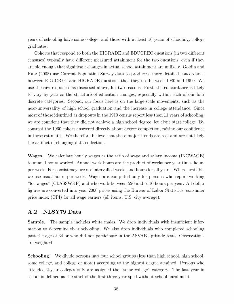
years of schooling have some college; and those with at least 16 years of schooling, college

graduates.

Cohorts that respond to both the HIGRADE and EDUCREC questions (in two different

censuses) typically have different measured attainment for the two questions, even if they

are old enough that significant changes in actual school attainment are unlikely. Goldin and

Katz (2008) use Current Population Survey data to produce a more detailed concordance

between EDUCREC and HIGRADE questions that they use between 1980 and 1990. We

use the raw responses as discussed above, for two reasons. First, the concordance is likely

to vary by year as the structure of education changes, especially within each of our four

discrete categories. Second, our focus here is on the large-scale movements, such as the

near-universality of high school graduation and the increase in college attendance. Since

most of those identified as dropouts in the 1910 census report less than 11 years of schooling,

we are confident that they did not achieve a high school degree, let alone start college. By

contrast the 1960 cohort answered directly about degree completion, raising our confidence

in these estimates. We therefore believe that these major trends are real and are not likely

the artifact of changing data collection.

Wages. We calculate hourly wages as the ratio of wage and salary income (INCWAGE)

to annual hours worked. Annual work hours are the product of weeks per year times hours

per week. For consistency, we use intervalled weeks and hours for all years. Where available

we use usual hours per week. Wages are computed only for persons who report working

“for wages” (CLASSWKR) and who work between 520 and 5110 hours per year. All dollar

figures are converted into year 2000 prices using the Bureau of Labor Statistics’ consumer

price index (CPI) for all wage earners (all items, U.S. city average).

A.2 NLSY79 Data

Sample. The sample includes white males. We drop individuals with insufficient infor-

mation to determine their schooling. We also drop individuals who completed schooling

past the age of 34 or who did not participate in the ASVAB aptitude tests. Observations

are weighted.

Schooling. We divide persons into four school groups (less than high school, high school,

some college, and college or more) according to the highest degree attained. Persons who

attended 2-year colleges only are assigned the “some college” category. The last year in

school is defined as the start of the first three year spell without school enrollment.

38

Wages. We calculate hourly wages as the ratio of labor income to annual hours worked.

Labor income includes wages, salaries, bonuses, and two-thirds of business income. We

delete wage observations prior to the last year of school enrollment or with hours worked

outside the range [520, 5110]. We also delete wage observations outside the range [0.02, 100]

times the median wage. Wages are deflated by the CPI.

We remove from the wage data variation that is due to demographic characteristics not

captured by our model. This is done by regressing log wages on schooling, experience, and

region of residence. Separate regressions are estimated for each year and schooling group.

The adjusted wage removes the effects of years of schooling (within school groups) and

region.

For consistency with the Census data, we focus on wages earned at age 40. Since not

all persons are interviewed at age 40, we interpolate these wages using data for ages 39 to

41.

AFQT. The measure of standardized test score in the NLSY79 is the 1980 Armed Forces

Qualification Test (AFQT) percentile rank (variable R1682). The AFQT aggregates vari-

ous ASVAB aptitude test scores into a scalar measure. The tests cover numerical opera-

tions, word knowledge, paragraph comprehension, and arithmetic reasoning (see (NLS User

Services 1992) for details). We remove age effects by regressing AFQT scores on the age at

which the test was administered.

39