To the best of our knowledge, no empirical analyses have … · · 2016-06-15from the sample...

econstor www.econstor.eu

Der Open-Access-Publikationsserver der ZBW – Leibniz-Informationszentrum WirtschaftThe Open Access Publication Server of the ZBW – Leibniz Information Centre for Economics

Standard-Nutzungsbedingungen:

Die Dokumente auf EconStor dürfen zu eigenen wissenschaftlichenZwecken und zum Privatgebrauch gespeichert und kopiert werden.

Sie dürfen die Dokumente nicht für öffentliche oder kommerzielleZwecke vervielfältigen, öffentlich ausstellen, öffentlich zugänglichmachen, vertreiben oder anderweitig nutzen.

Sofern die Verfasser die Dokumente unter Open-Content-Lizenzen(insbesondere CC-Lizenzen) zur Verfügung gestellt haben sollten,gelten abweichend von diesen Nutzungsbedingungen die in der dortgenannten Lizenz gewährten Nutzungsrechte.

Terms of use:

Documents in EconStor may be saved and copied for yourpersonal and scholarly purposes.

You are not to copy documents for public or commercialpurposes, to exhibit the documents publicly, to make thempublicly available on the internet, or to distribute or otherwiseuse the documents in public.

If the documents have been made available under an OpenContent Licence (especially Creative Commons Licences), youmay exercise further usage rights as specified in the indicatedlicence.

zbw Leibniz-Informationszentrum WirtschaftLeibniz Information Centre for Economics

Kappeler, Andreas; Välilä, Timo

Working Paper

Composition of public investment and fiscalfederalism: panel data evidence from Europe

Economic and financial reports / European Investment Bank, No. 2007/02

Provided in Cooperation with:European Investment Bank (EIB), Luxembourg

Suggested Citation: Kappeler, Andreas; Välilä, Timo (2007) : Composition of public investmentand fiscal federalism: panel data evidence from Europe, Economic and financial reports /European Investment Bank, No. 2007/02

This Version is available at:http://hdl.handle.net/10419/45276

Economic and Financial Report 2007/02

COMPOSITION OF PUBLIC INVESTMENT AND FISCAL FEDERALISM:

PANEL DATA EVIDENCE FROM EUROPE

Andreas Kappeler and Timo Välilä* †

Disclaimer: This Economic and Financial Report should not be reported as

representing the views of the EIB. The views expressed in this EFR are those of the

author(s) and do not necessarily represent those of the EIB or EIB policy. EFRs

describe research in progress by the author(s) and are published to elicit comments

and further debate.

JEL Classification codes: H54, H77, H72, C23, C24

* Andreas Kappeler is a PhD student at Munich Graduate School of Economics/LMU. He visited the Economic and Financial Studies Division of the European Investment Bank during this research. Timo Välilä is Senior Economist, Economic and Financial Studies Division of the European Investment Bank. † The authors would like to thank Eric Perée and the participants of the Public Economics Seminar at the University of Munich (LMU), Department of Economics, for comments on an earlier draft.

COMPOSITION OF PUBLIC INVESTMENT AND FISCAL FEDERALISM:

PANEL DATA EVIDENCE FROM EUROPE

Abstract

We present some stylised facts about the composition of public investment in Europe and

analyse its determinants, with a special focus on the role of fiscal decentralisation. The

empirical analysis is conducted both for levels of different types of public investment and

for their shares in total public investment. The results suggest that fiscal decentralisation

boosts economically productive public investment, notably infrastructure, and curbs the

relative share of economically less productive public investment, such as recreational

facilities. While not readily reconcilable with the traditional theory of fiscal federalism,

especially as regards the provision of local public goods, these findings can be interpreted

in terms of the literature on fiscal competition, with not only tax rates but also the quality

of public expenditure weighing in firms’ location decisions.

2

1. Introduction

Public investment has received only limited academic attention as an aggregate variable,

and its composition has to our knowledge received none at all, at least in the European

context. This paper seeks to fill that gap at least in part by presenting some stylised facts

about the composition of public investment in Europe and by presenting an empirical

analysis of what drives different types of public investment, with a special focus on the

impact of fiscal federalism.

Perhaps because of lack of academic attention, misconceptions abound concerning the

nature, drivers, and impact of public investment. Most notably, there is often confusion

about what it is in the first place. Perhaps the most prominent example of this type of

confusion is the customary synonymous use of “public investment” and “infrastructure

investment” in much of economic literature. There is, however, a great deal of

infrastructure investment that is not public, and there is a great deal of public investment

that is not infrastructure investment. While it is well-known that many roads, water and

sanitation networks, and municipal swimming pools are publicly funded and provided,

neither economic theory nor empirical analyses have really distinguished between them

when studying what determines “public investment” or how productive “public

investment” is.

As a starting point for a more nuanced analysis and understanding of public investment,

we first break it down into different types with distinctly different economic

characteristics in section 2. We then propose to use the traditional theory of fiscal

federalism and some of its more recent extensions, reviewed in section 3, to derive

hypotheses about the link between fiscal decentralisation and the composition of public

investment. Section 4 seeks to articulate empirical tests of the hypotheses, and their

results are interpreted from an economic perspective in section 5, before concluding in

section 6.

3

2. Composition of Public Investment in Europe: Stylised Facts

To the best of our knowledge, no empirical analyses have been conducted with a focus on

the composition of public investment, at least in the European context. Therefore, we

start off by describing the available data in this section. Special attention is paid to the

link between the composition of public investment and fiscal federalism, which is the

focus of our subsequent empirical analysis.

Based on the functional classification of government expenditure in the 1993 UN System

of National Accounts and in the 1995 European System of Accounts (ESA 95), Eurostat

provides a breakdown of public investment for EU countries starting in the early 1990s.

Complete data are available for EU15 countries from 1995 (i.e, the introduction of ESA

95) through 2005.1 However, many countries have back-dated their time series to 1990.

The “public investment” variable is gross capital formation of the general government.

This includes changes in inventories, which may create some undesired noise for our

analysis; however, the breakdown between gross fixed capital formation and changes in

inventories is not available.

The functional breakdown of public investment is presented in Table 1. The right-hand

side column shows the functional classification (Classification of Functions of

Government, COFOG for short) in ESA 95. The left-hand side shows our aggregation of

the 10 available “functions” into four types of public investment with economically

distinct roles. This aggregation will be used in the remainder of this paper.

The four different types of public investment affect the economy through different

channels, with varying degrees of directness, and over different time horizons. Public

1 EU15 comprises Austria, Belgium, Denmark, Finland, France, Germany, Greece, Ireland, Italy, Luxembourg, the Netherlands, Portugal, Spain, Sweden, and the United Kingdom. We exclude Luxemburg from the sample because of its small size and special macroeconomic and structural characteristics.

4

investment in Infrastructure, consisting of just Economic Affairs in the ESA 95 COFOG,2

seeks to measure public investment in traditional infrastructure, mainly transport. This

type of public investment has the most direct economic impact by reducing firms’

production and transaction costs. The economic impact of public investment in Hospitals

and Schools is more long-term and less direct in character, as it facilitates the building up

and maintenance of the economy’s stock of human capital. Investment in Public Goods

affects the economy’s allocative efficiency indirectly through framework conditions for

productive activity. Finally, Redistribution affects the economy’s income distribution

rather than allocative or productive efficiency per se.

Table 1: Functional breakdown of public investment

Aggregation ESA 95 COFOG 1. Infrastructure (INF) Economic Affairs

2. Hospitals and Schools (HS) Health Education

3. Public Goods (PG) Defence General Public Services Environment Order and Safety

4. Redistribution (RED) Housing Recreation Social Protection

Source: Eurostat; own aggregation.

In addition to the composition of Infrastructure investment (see footnote 2), some other

aggregates shown in Table 1 contain undesirable “noise” as no further breakdowns of the

right-hand side “functions” are available. For example, public investment in water supply

and wastewater management are not part of Infrastructure as one would wish; instead,

they are part of Redistribution (Housing) and Public Goods (Environment), respectively.

Similarly, one would wish to include street lightning in Public Goods; now it is in

Housing and thereby Redistribution. However, as with Infrastructure, we expect such

2 Economic Affairs comprise a number of different sectors, including agriculture; fuel and energy; mining, manufacturing and construction; transport; communication; R&D; and others. Among these sectors, transport is likely to be by far the dominant recipient of public investment. Note that investment by energy companies owned by the public sector, for example, is classified as private investment in national accounts statistics as long as such companies are commercially run.

5

“noise” to be of sufficiently small magnitude so as not to invalidate the empirical analysis

below.

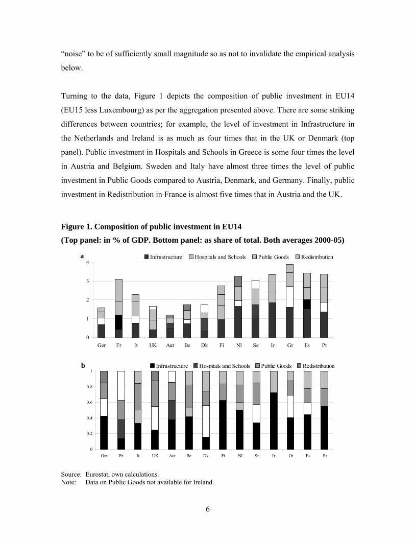
Turning to the data, Figure 1 depicts the composition of public investment in EU14

(EU15 less Luxembourg) as per the aggregation presented above. There are some striking

differences between countries; for example, the level of investment in Infrastructure in

the Netherlands and Ireland is as much as four times that in the UK or Denmark (top

panel). Public investment in Hospitals and Schools in Greece is some four times the level

in Austria and Belgium. Sweden and Italy have almost three times the level of public

investment in Public Goods compared to Austria, Denmark, and Germany. Finally, public

investment in Redistribution in France is almost five times that in Austria and the UK.

Figure 1. Composition of public investment in EU14

(Top panel: in % of GDP. Bottom panel: as share of total. Both averages 2000-05)

0

1

2

3

4

Ger Fr It UK Aut Be Dk Fi Nl Se Ir Gr Es Pt

Infrastructure Hospitals and Schools Public Goods Redistributiona

0

0.2

0.4

0.6

0.8

1


Infrastructure Hospitals and Schools Public Goods Redistributionb

Source: Eurostat, own calculations. Note: Data on Public Goods not available for Ireland.

6

In terms of shares of total public investment (bottom panel in Figure 1), we note that

traditional Infrastructure accounts on average for about one-third and Hospital and

Schools—which are sometimes denoted human capital infrastructure—account for

another 20 percent. Thus, infrastructure in a broad sense accounts on average for half of

public investment in EU14. Public Goods and Redistribution account for about one-

quarter each.

Figure 2 shows the evolution over time of the level and share of the different types of

public investment. Public investment appears more volatile in level terms, suggesting that

the cyclical ups and downs hit the various types of public investment relatively evenly,

thus keeping their shares rather stable. In terms of trends, Infrastructure has been on an

uptrend in levels and as a share of total owing mostly to the Cohesion countries (Greece,

Ireland, Portugal, and Spain), approaching 40 percent in recent years. The clearest

downtrend is in Public Goods, which has declined from well over a quarter of total

toward 20 percent.

7

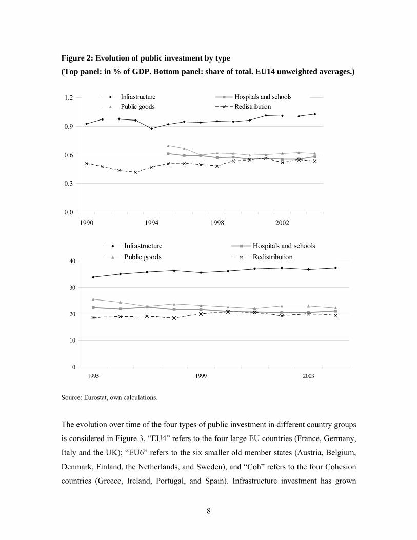
Figure 2: Evolution of public investment by type

(Top panel: in % of GDP. Bottom panel: share of total. EU14 unweighted averages.)

0.0

0.3

0.6

0.9

1.2

1990 1994 1998 2002

Infrastructure Hospitals and schoolsPublic goods Redistribution

0

10

20

30

40

1995 1999 2003

Infrastructure Hospitals and schoolsPublic goods Redistribution

Source: Eurostat, own calculations.

The evolution over time of the four types of public investment in different country groups

is considered in Figure 3. “EU4” refers to the four large EU countries (France, Germany,

Italy and the UK); “EU6” refers to the six smaller old member states (Austria, Belgium,

Denmark, Finland, the Netherlands, and Sweden), and “Coh” refers to the four Cohesion

countries (Greece, Ireland, Portugal, and Spain). Infrastructure investment has grown

8

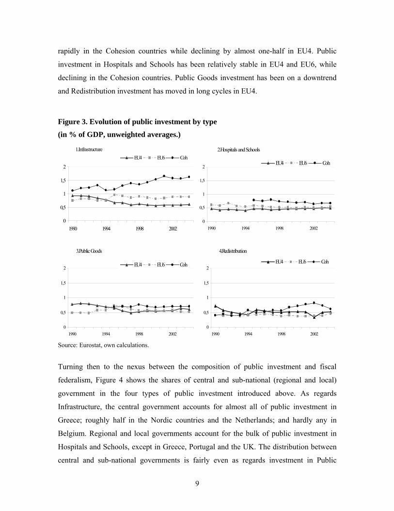
rapidly in the Cohesion countries while declining by almost one-half in EU4. Public

investment in Hospitals and Schools has been relatively stable in EU4 and EU6, while

declining in the Cohesion countries. Public Goods investment has been on a downtrend

and Redistribution investment has moved in long cycles in EU4.

Figure 3. Evolution of public investment by type

(in % of GDP, unweighted averages.)

1.Infrastructure

0

0,5

1

1,5

2

1990 1994 1998 2002

EU4 EU6 Coh2.Hospitals and Schools

0

0,5

1

1,5

2

1990 1994 1998 2002

EU4 EU6 Coh

3.Public Goods

0

0,5

1

1,5

2

1990 1994 1998 2002

EU4 EU6 Coh

4.Redistribution

0

0,5

1

1,5

2

1990 1994 1998 2002

EU4 EU6 Coh


Turning then to the nexus between the composition of public investment and fiscal

federalism, Figure 4 shows the shares of central and sub-national (regional and local)

government in the four types of public investment introduced above. As regards

Infrastructure, the central government accounts for almost all of public investment in

Greece; roughly half in the Nordic countries and the Netherlands; and hardly any in

Belgium. Regional and local governments account for the bulk of public investment in

Hospitals and Schools, except in Greece, Portugal and the UK. The distribution between

central and sub-national governments is fairly even as regards investment in Public

9

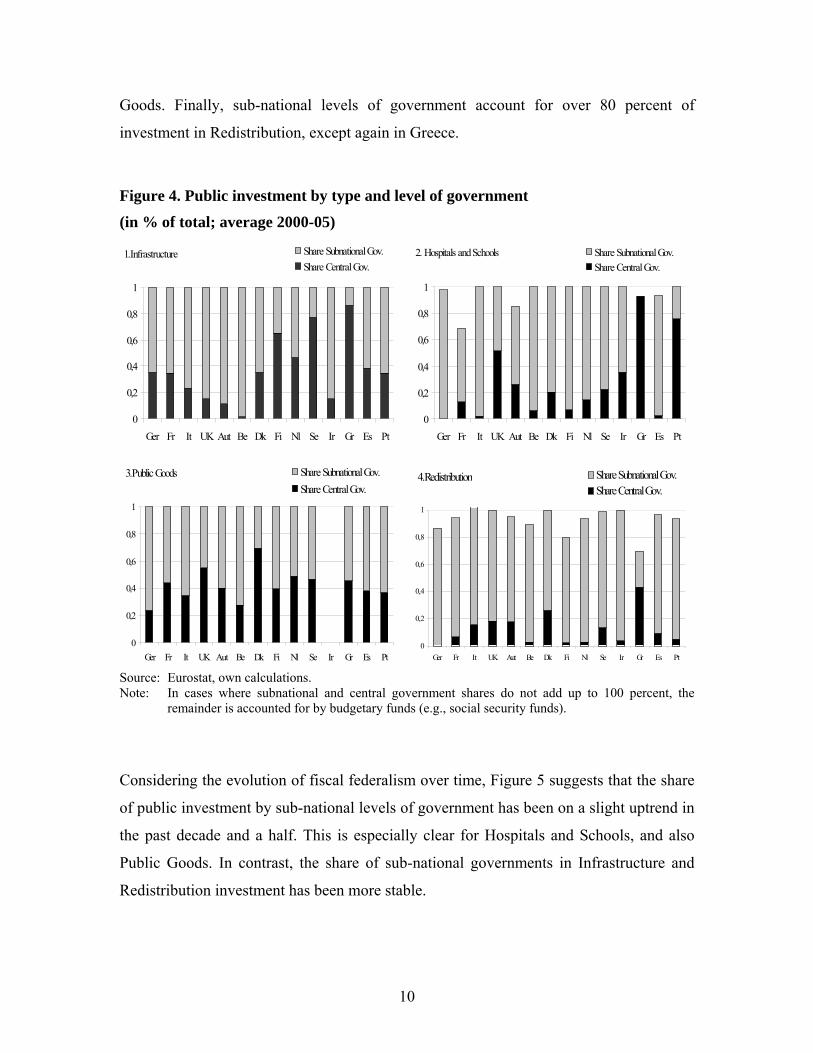
Goods. Finally, sub-national levels of government account for over 80 percent of

investment in Redistribution, except again in Greece.

Figure 4. Public investment by type and level of government

(in % of total; average 2000-05)

1.Infrastructure

0

0,2

0,4

0,6

0,8

1


Share Subnational Gov.Share Central Gov.

2. Hospitals and Schools

0

0,2

0,4

0,6

0,8

1



3.Public Goods

0

0,2

0,4

0,6

0,8

1



4.Redistribution

0

0,2

0,4

0,6

0,8

1



Source: Eurostat, own calculations. Note: In cases where subnational and central government shares do not add up to 100 percent, the

remainder is accounted for by budgetary funds (e.g., social security funds).

Considering the evolution of fiscal federalism over time, Figure 5 suggests that the share

of public investment by sub-national levels of government has been on a slight uptrend in

the past decade and a half. This is especially clear for Hospitals and Schools, and also

Public Goods. In contrast, the share of sub-national governments in Infrastructure and

Redistribution investment has been more stable.

10

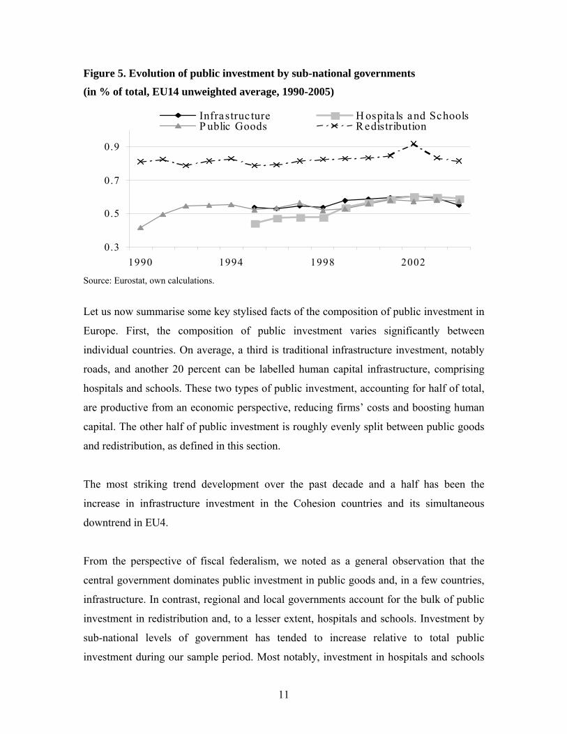
Figure 5. Evolution of public investment by sub-national governments

(in % of total, EU14 unweighted average, 1990-2005)

0.3

0.5

0.7

0.9

1990 1994 1998 2002

Infrastruc ture H ospita ls and SchoolsP ublic Goods Redistribution


Let us now summarise some key stylised facts of the composition of public investment in

Europe. First, the composition of public investment varies significantly between

individual countries. On average, a third is traditional infrastructure investment, notably

roads, and another 20 percent can be labelled human capital infrastructure, comprising

hospitals and schools. These two types of public investment, accounting for half of total,

are productive from an economic perspective, reducing firms’ costs and boosting human

capital. The other half of public investment is roughly evenly split between public goods

and redistribution, as defined in this section.

The most striking trend development over the past decade and a half has been the

increase in infrastructure investment in the Cohesion countries and its simultaneous

downtrend in EU4.

From the perspective of fiscal federalism, we noted as a general observation that the

central government dominates public investment in public goods and, in a few countries,

infrastructure. In contrast, regional and local governments account for the bulk of public

investment in redistribution and, to a lesser extent, hospitals and schools. Investment by

sub-national levels of government has tended to increase relative to total public

investment during our sample period. Most notably, investment in hospitals and schools

11

as well as in public goods have increasingly become the responsibility of sub-national

levels of government.

3. Public Investment and the Theory of Fiscal Federalism

Having reviewed the stylised facts of the composition of public investment and fiscal

federalism in Europe, we now proceed to an overview of the “traditional” theory of fiscal

federalism. The purpose of this section is to derive empirically testable hypotheses about

the relationship between fiscal federalism and different types of public investment.

However, a caveat is in order to start with. The theory of fiscal federalism—or any other

theory for that matter—does not deal explicitly with the composition of public

investment. At best, it distinguishes between consumption-oriented public expenditure

and public expenditure to produce “public inputs” for the production processes of private

firms. In what is to come we do not consider differences between current public spending

and public investment per se; rather, we consider the various types of public investment

as enhancements of production potential for different public services. Thus, infrastructure

investment is considered to produce more future transportation services, and

redistribution investment is considered to produce, e.g., more future recreation services.

This perspective allows us to link the theory of fiscal federalism with the kind of data on

the composition of public investment that we have.

The traditional theory of fiscal federalism is based on the seminal contributions by

Tiebout (1956), Oates (1972), and Musgrave (1959). The underlying assumptions

include, most importantly, the benevolence of the policy-maker in the centre (that is, his

objective is the maximisation of social welfare); the existence of pure local public goods

and global public goods (whose benefits accrue locally and nation-wide, respectively);

benefit taxation (same incidence for the cost and benefit of public spending); factor

mobility; and absence of spill-over effects of fiscal decisions horizontally (between

regions) and vertically (between regions and the centre).

12

Considering the responsiveness of public spending to local preferences and the creation

of incentives for economic efficiency as policy goals, the theory derives normative

conclusions about the optimal task assignment between the central and sub-national

levels of government. Responsiveness to local preferences implies that decentralisation

and fiscal competition are preferable in the provision of local public goods whenever

local preferences are heterogeneous. On the other hand, centralisation is warranted in the

provision of public goods whose optimal supply cannot be achieved by fiscal

competition. Such goods include most notably global public goods, and it also includes

the macroeconomic stabilisation and income redistribution functions of the government

(which may be interpreted as providing global public goods as well). Public goods may

also have spillover effects, with one region benefiting from a highway built by its

neighbouring region, for example. Fiscal competition among sub-national levels of

government will result in a sub-optimally low level of provision of such goods, as regions

do not consider the spillover benefits in their individual decision-making. Oates (1972)

suggests that the optimal provision can be achieved by means of matching grants from

the centre, which act to internalise the externality.

We have thus far identified three types of public goods (local, global, and spillover public

goods) and the optimal level of government to provide each of them. We can now

consider the different types of public investment in Table 1 against this background.

Infrastructure, such as roads and other transportation infrastructure, provide both local

benefits and positive spillover effects, in so far as it connects localities and regions.

Hospitals and Schools provide also local benefits and positive spillover effects; the latter

is especially the case when the labour force and population at large are mobile and move

across regions. Public Goods, as defined in Table 1, is a mixture of local and global

public goods, while Redistribution comprises chiefly local public goods.

So how would one expect fiscal decentralisation to affect the different types of public

investment? Investment in local public goods, most notably Redistribution, would

unambiguously increase with decentralisation. Investment in Infrastructure as well as

Hospitals and Schools would also increase with decentralisation, especially if

13

supplemented with grants from the centre. Investment in Public Goods could go either

way, depending on whether the aggregate Public Goods is more local or global in

character.

More recent literature on fiscal federalism has relaxed the assumption of no spillover

effects in policy-making. Focussing on horizontal policy spillovers, consider regional tax

competition.3 With capital mobile across regions that seek to attract it, tax competition

can lead to sub-optimally low tax rates (“race to the bottom”) and, as a consequence,

insufficient provision of public services (both public consumption goods and

“infrastructure”). The standard reference is Zodrow and Mieszkowski (1986); however,

Sinn (2003) has come out strongly against their analysis (see also Matsumoto, 1998).

Hulten and Schwab (1997) discuss the circumstances where tax competition can lead to a

sub-optimally low level of public capital. Competition between regions for an industry

with external scale economies is a case in point: in competing for the location of such an

industry, regions may reduce their tax rates so low as to unduly suppress public

investment.

Considering the impact of fiscal competition on the composition of public expenditure,

Keen and Marchand (1997) argue that uncoordinated fiscal competition induces regions

to over-invest in “local public inputs” at the cost of (consumption-oriented) local public

goods. Investment in public inputs increases the potential of regions to attract mobile

private capital, since public inputs reduce production costs for private firms. This

generates distortions in the composition of public expenditure. Decentralisation leads to

an over-supply of public inputs and an under-supply of local public goods.

To sum up, fiscal competition has been argued to reduce public investment across the

board (tax competition), but it has also been argued to boost productive public

investment, at least relative to local public goods (broader fiscal competition). In terms of

the public investment types in Table 1, these results would imply that decentralisation

3 We ignore here the literature of vertical fiscal externalities (see, e.g., Dahlby, 1996; Dahlby and Wilson, 2003; Martinez-López, 2005). The predictions of that literature are ambiguous, hinging on assumptions whose relevance for our data sample we cannot assess.

14

increase investment in Infrastructure as well as Hospitals and Schools, while reducing

investment in Redistribution, at least in relative terms. This contrasts, notably, with the

hypotheses above based on the older fiscal federalism literature.

4. Empirical Analysis

To study the impact of fiscal federalism (fiscal decentralisation) on the four different

types of public investment identified in Table 1, we conduct two complementary

empirical analyses. First we study the impact of decentralisation on the level of each type

of public investment. Second we study the impact of decentralisation on the share of each

type of public investment in total public investment. Before presenting the methodologies

and results of these analyses, we specify the model to be estimated and discuss the

sample used in the estimations.

4.1 Model Specification

Although it is possible to formulate hypotheses of the relationship between

decentralisation and the composition of public expenditure (investment) as in section 3,

there is no explicit theoretical framework that could be used to derive a model of the

determination of different types of public investment. We will therefore proceed directly

to the specification of a reduced-form model to be estimated. In so doing we seek to

identify exogenous variables measuring the impact of decentralisation on public

investment, as well as a set of control variables that render the model empirically well-

specified.

The reduced-form specification to be used in both levels and shares estimation is as

follows:

ititititit

itit

upoplenddebtgdpcaptaxI

+ ++ ++++

++=

−−−−

−

it716151413

211itc,

year

γβββββββα

(1)

15

where uit ∼ i.i.d (0, σ2), with subscript i referring to observations in the cross-section

dimension (individual countries) and t to observations in the time dimension. The

dependent variable Ic represents public investment of type c, c=1,…,4, as shown in Table

1. In the levels analysis Ic is expressed relative to trend GDP,4 5 thus in theory assuming

values in ℜ+. In the shares analysis it is expressed as a share of total public investment,

assuming values in the interval (0, 1).

Fiscal decentralisation is measured by two explanatory variables. First, our primary

interest is in the share of tax revenue attributed to sub-national levels of government

(regional and local governments), which is denoted tax.6 Second, we control for

investment grants from the central government to sub-national levels of government

(cap); in the empirical analyses it is measured in relation to trend GDP. 7 The tax share is

lagged by one period to reflect the fact that investment decisions are most often taken a

year before, based on knowledge about the revenue situation at that time. In contrast,

capital transfers are contemporaneous with investment, as they finance investment the

same year it is undertaken.8

Turning then to the control variables, they seek to capture the general economic, fiscal,

and demographic developments of significance for the determination of public

investment. Real GDP, denoted gdp in (1), is measured in per capita terms and lagged by

one period to remove any simultaneity bias. The short- and longer term fiscal

environment is captured by the budget surplus of the general government (lend) and

public debt (debt). Both are measured in relation to trend GDP and lagged by one period,

4 Trend GDP is calculated using the Hodrick-Prescott Filter with a smoothing parameter λ=100. 5 Considering ratios to (trend) GDP improves the time series properties of the variables and facilitates the economic interpretation of the estimation results. 6 Stegarescu (2004). We also considered other measures of decentralization, including total revenue share of sub-national levels of government, expenditure share of sub-national levels of government; and the ratio of sub-national tax revenue to expenditure. However, none of these alternative measures is conceptually superior to the tax share variable used; and all of them are empirically inferior, as they risk spurious correlation by including capital transfers (total revenue share) or the dependent variable (expenditure share), or by exhibiting non-stationarity (sub-national revenue-to expenditure ratio). 7 The interaction term of tax and cap turned out to be insignificant in most of the estimations below and is therefore not reported. 8 See Rodden (2003) for more details.

16

for the reasons mentioned above. We also control for population density (pop).9 γi

denotes unobserved time-invariant country-specific effects that are included in the

estimations (unless otherwise indicated). Finally, as explained below in greater detail, a

linear time trend (year) is included, as some of the time series are trend stationary.

4.2 Sample Data

The main sample used in the estimations consists of a panel of EU10 countries (EU15

less the Cohesion countries less Luxembourg) during the period 1990-2005. We exclude

the Cohesion countries from our sample, because public investment in those countries has

been significantly influenced by the receipt of EU support. As explained in section 2, not

all countries have back-dated all relevant series to 1990, so the panel is unbalanced.

The main data source is Eurostat’s New Cronos database. Data on the fiscal variables

(budgetary surplus and public debt) as well as population come from the OECD.

As regards the properties of our sample data, unit root tests indicate that our variables are

either stationary or trend stationary (Annex 1, table A.1.1), thus warranting the inclusion

of a time trend as another explanatory variable. We perform Levin, Lin, and Chu test

(LLC, see Levin et al., 2002) as well as Im, Pesaran, and Chin test (IPS, see Im et al.,

1997) to verify the stationarity properties of our variables.

The dependent variables are highly autocorrelated and persistent (Annex 1, Table A.1.2),

with first-order autocorrelation coefficients between 0.8 and 0.9 for all types of public

investment, in both levels and shares.

Correlation among our explanatory variables is mostly negligible (Annex 1, Table A.1.3).

Only correlation coefficients between the tax share variable and GDP per capita and

population density are rather high at 0.65 and -0.44, respectively. 9 As a robustness check we also considered unemployment, birth rates, migration rates, and mortality rates as additional control variables. They turned out to be mostly insignificant and did not change the estimation results materially.

17

4.3 Analysis in Levels

4.3.1 Estimation Methodology10

As our dependent variables are highly autocorrelated (Annex 1, Table A.1.2.), we choose

a dynamic specification of the model (1) for the levels analysis, including the lagged

dependent variable as another explanatory variable. The dynamic model specification

thus becomes:

itiitititit

itititc

upoplenddebtgdp

captaxII

++ + ++++

+++=

−−−−

−−

γβββββ

βββα

year

t716151413

2111,1itc, (2)

The estimation of specification (2) will have to account for the correlation between the

regressors (lagged dependent) and the composite term (γi + uit), which renders least

squares estimators inconsistent even asymptotically. To circumvent this problem we

employ General Method of Moments (GMM) estimation, which has become the

workhorse in estimating dynamic panel data models.11

To test the robustness of the results, we compare several GMM and least squares -based

estimation methods. We use various GMM estimation procedures (1-step and 2-step

difference-GMM as well as system-GMM). In addition, we present the results of the

following least squares –based estimations: (1) as a “benchmark”, fixed effects OLS (FE

OLS) with the lagged dependent variable, which we know to be inconsistent; (2) fixed

effects two-stage least squares (FE 2SLS) estimation of the first-differenced regression

equation (2) with the second lag of the dependent variable as an instrument. If now the

error term is serially uncorrelated and the initial conditions Ic,i1 predetermined (i.e.,

uncorrelated with subsequent error terms), the FE 2SLS estimators are consistent for

panels with large N and fixed T dimensions. However, with further lags of the dependent

10 All estimations are conducted using eViews 5.1 or Stata 8.e or 9. 11 Arellano and Bond (1991) and Bond (2002).

18

as additional instruments, the FE 2SLS estimators are not asymptotically efficient, while

GMM estimators are.

In sum, we use the Sargan and residual autocorrelation tests to select the preferred GMM-

based estimation method. We then compare the results obtained with FE OLS estimation

and FE 2SLS estimation, which we know are inconsistent, by way of robustness

checking.

4.3.2 Results

Table 2 presents the results of the preferred estimation method, which is one-step

difference-GMM. All other results are shown in Annex 2, which also contains the results

of the estimation of (1) with the aggregate public investment as the dependent variable.

One-step difference-GMM estimation is alone in passing the Sargan test for

overidentifying restrictions and residual autocorrelation tests (labelled m1 for first-order

and m2 for second-order autocorrelation) for all four estimated models in levels. Two-

step difference-GMM estimation is associated with the absence of first-degree residual

autocorrelation throughout. The difference-Sargan test for system-GMM estimation, in

turn, rejects the validity of the additional differenced instruments for two out of four

estimated models.

As shown in Annex 2, the residuals from the least squares –based estimations are not

always well-behaved. The FE OLS estimation suffers from residual non-normality, as

indicated by the p-value of the Jarque-Bera (JB) test statistic. The FE 2SLS, on the other

hand, is in many cases associated with a relatively low value of the Durbin-Watson test

statistic, indicating first-order residual autocorrelation.

19

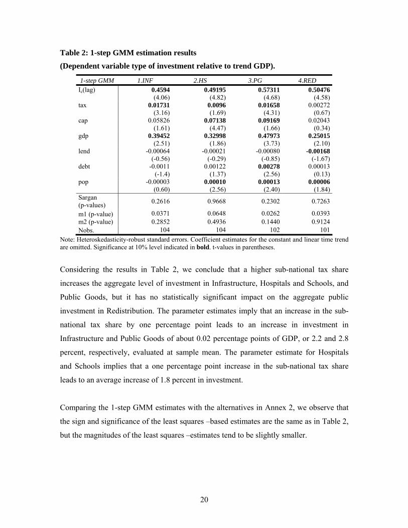
Table 2: 1-step GMM estimation results

(Dependent variable type of investment relative to trend GDP).

1-step GMM 1.INF 2.HS 3.PG 4.RED Ic(lag) 0.4594

(4.06)0.49195

(4.82)0.57311

(4.68)0.50476

(4.58)tax 0.01731

(3.16)0.0096(1.69)

0.01658(4.31)

0.00272(0.67)

cap 0.05826(1.61)

0.07138(4.47)

0.09169(1.66)

0.02043(0.34)

gdp 0.39452(2.51)

0.32998(1.86)

0.47973(3.73)

0.25015(2.10)

lend -0.00064(-0.56)

-0.00021(-0.29)

-0.00080(-0.85)

-0.00168(-1.67)

debt -0.0011(-1.4)

0.00122(1.37)

0.00278(2.56)

0.00013(0.13)

pop -0.00003(0.60)

0.00010(2.56)

0.00013(2.40)

0.00006(1.84)

Sargan (p-values) 0.2616 0.9668 0.2302 0.7263

m1 (p-value) 0.0371 0.0648 0.0262 0.0393m2 (p-value) 0.2852 0.4936 0.1440 0.9124Nobs. 104 104 102 101

Note: Heteroskedasticity-robust standard errors. Coefficient estimates for the constant and linear time trend are omitted. Significance at 10% level indicated in bold. t-values in parentheses.

Considering the results in Table 2, we conclude that a higher sub-national tax share

increases the aggregate level of investment in Infrastructure, Hospitals and Schools, and

Public Goods, but it has no statistically significant impact on the aggregate public

investment in Redistribution. The parameter estimates imply that an increase in the sub-

national tax share by one percentage point leads to an increase in investment in

Infrastructure and Public Goods of about 0.02 percentage points of GDP, or 2.2 and 2.8

percent, respectively, evaluated at sample mean. The parameter estimate for Hospitals

and Schools implies that a one percentage point increase in the sub-national tax share

leads to an average increase of 1.8 percent in investment.

Comparing the 1-step GMM estimates with the alternatives in Annex 2, we observe that

the sign and significance of the least squares –based estimates are the same as in Table 2,

but the magnitudes of the least squares –estimates tend to be slightly smaller.

20

Returning to Table 2 and considering the coefficient estimates for capital transfers, we

observe a significant positive impact on investment in Hospitals and Schools as well as

Public Goods. An increase of capital transfers by 1 percent of GDP boosts these types of

investment by 0.07 and 0.09 percentage points of GDP (14 percent and 15 percent,

respectively, at sample mean). The FE OLS results are remarkably similar in terms of

significance, sign and magnitude, and while the magnitude of the FE 2SLS estimates is

also equally close to the 1-step GMM estimates, there are discrepancies in terms of

significance.

As regards other control variables, real per capita GDP is significant and positive in all

four models, with a coefficient estimate of 0.3-0.5 in the 1-step GMM estimations and

0.2-0.3 in the least squares –based estimations; however, two of the FE 2SLS estimates

are again insignificant. The fiscal variables are mostly insignificant, except that higher

budgetary surpluses reduce investment in Redistribution and that higher public debt goes

hand in hand with higher investment in Public Goods. This latter result is confirmed in

the least squares –estimations, with the coefficient estimate virtually the same across all

methods. However, the coefficient estimates for the fiscal variables in the other models

are less similar in terms of even significance and signs. Finally, population density turns

out to be significant for all types of investment except for Infrastructure. This pattern also

appears in the least squares estimations.

4.4 Analysis in Shares

4.4.1 Estimation Methodology

The econometric analysis of the determinants of shares of the different types of public

investment has to tackle some additional challenges. The dependent variable is now

fractional, limited to the interval (0, 1) with no observations at the endpoints. These

features necessitate the employment of a non-linear estimation method while, at the same

time, excluding the use of some recent innovations, such as the tobit specification for

dynamic panel data with endpoint observations proposed by Loudermilk (2005).

21

Again, we employ a number of alternative estimation methods for comparison. The focus

will be on Quasi-Maximum Likelihood Estimation (QMLE), based on Papke and

Wooldridge (1996 and 2005). This approach has been labelled fractional logit, or “flogit”

for short—a label we adopt below.

In the presence of panel fixed effects, flogit estimation may suffer from inconsistency due

to the so-called incidental parameter problem.12 To address the problem, Papke and

Wooldridge (2005) propose the use of pooled QMLE. The pooled QMLE is based on

accounting for the fixed effects without including dummies to that end. Instead, the

average value of each explanatory variable (average over time) is added as additional

explanatory variable, so the coefficient estimate for each initial explanatory variable

measures the impact of the deviation from the average. Cross-section fixed effects are

now captured by the averages, and inconsistently estimated fixed effects are removed as a

source of inconsistency in other parameter estimates.

The model to be estimated in pooled QMLE is thus:

c,it 1 1 2 3 1 4 1 5 1 6 1

i i7 t 8 9 10 i 11 12 13i i

year it it it it it it

i it

I tax cap gdp debt lend pop

tax cap gdp debt lend pop u

α β β β β β β

β β β β β β β− − − − −= + + + + + + +

+ + + + + + + +

(3)

where bars above variables denotes averages over time.

Given the relatively small number of observations in our panel, the increase in the

number of parameters to be estimated from (1) to (3)—together with the low variance of

our dependent variable—can, however, take a crucial toll on efficiency and significance.

Besides, it is not clear whether and to what extent this incidental parameter problem and

the resulting inconsistency are problems in our case to start with. Our panel has more

observations in the T dimension (up to 16) than in the N dimension; hence, the problem is

less obvious than in typical micro-data panels with just a few observations in time. For

12 See Greene (2003) or Lancaster (2000) for more details.

22

these reasons, we consider the results of pooled QMLE just as a robustness check for the

flogit results.

Yet further estimation methods employed as robustness checks include OLS with fixed

effects; 2SLS; and one-step GMM. These methods do not account for the fractional

character of our dependent variable, and may therefore result in loss in terms of

efficiency and significance (Papke and Wooldridge, 2005). When considering the results

from these supplementary estimations we focus therefore more on the signs of the

coefficient estimates than on their significance and magnitude.

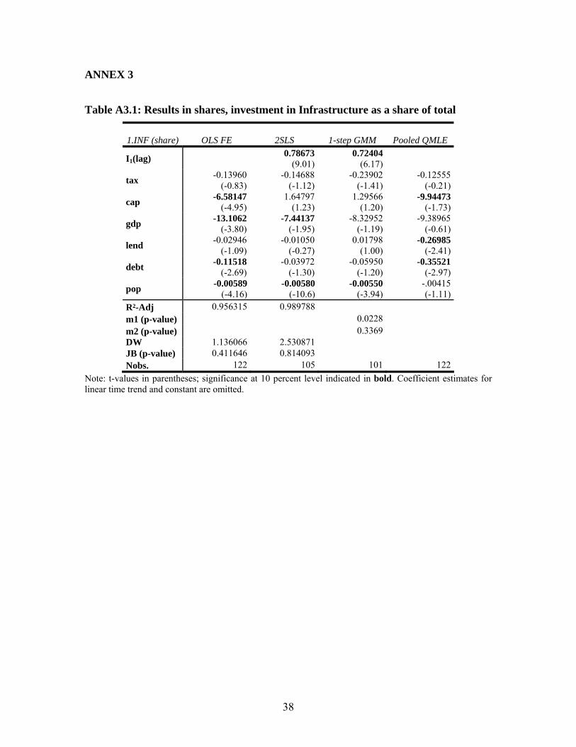
4.4.2 Results

Table 4 shows the flogit results. Results obtained with the other estimation methods are

reported in Annex 3. Note that we do not include the lagged dependent variable as an

explanatory variable in the QMLEs. In principle this could well be done; however, due to

the high degree of persistence in our dependent variables, the inclusion of the lagged

dependent only exhausts all explanatory power of the model and renders the other

explanatory variables insignificant.13

The numerical parameter estimates shown for the flogit and pooled QMLE should,

notably, be interpreted as marginal effects at sample mean. Non-linearities can in general

cause a difference between marginal effects at sample mean and Average Partial Effects

(APE); however, given that our observations on the dependent variable are located in the

interior of the interval (0, 1), with no observations at the endpoints, the estimates shown

should not be very different from the APE.

Table 3: Flogit estimation results 13 As Arze del Granado et al. (2005) and Wagner (2003), we employ White’s (1982) robust “sandwich” estimator to improve the consistency of our variance-covariance matrix. Greene (2003) points out that the sandwich estimator provides in most cases an appropriate asymptotic covariance matrix for an estimator that is biased in an unknown direction due to omitted variables, autocorrelation, or heteroskedasticity.

23

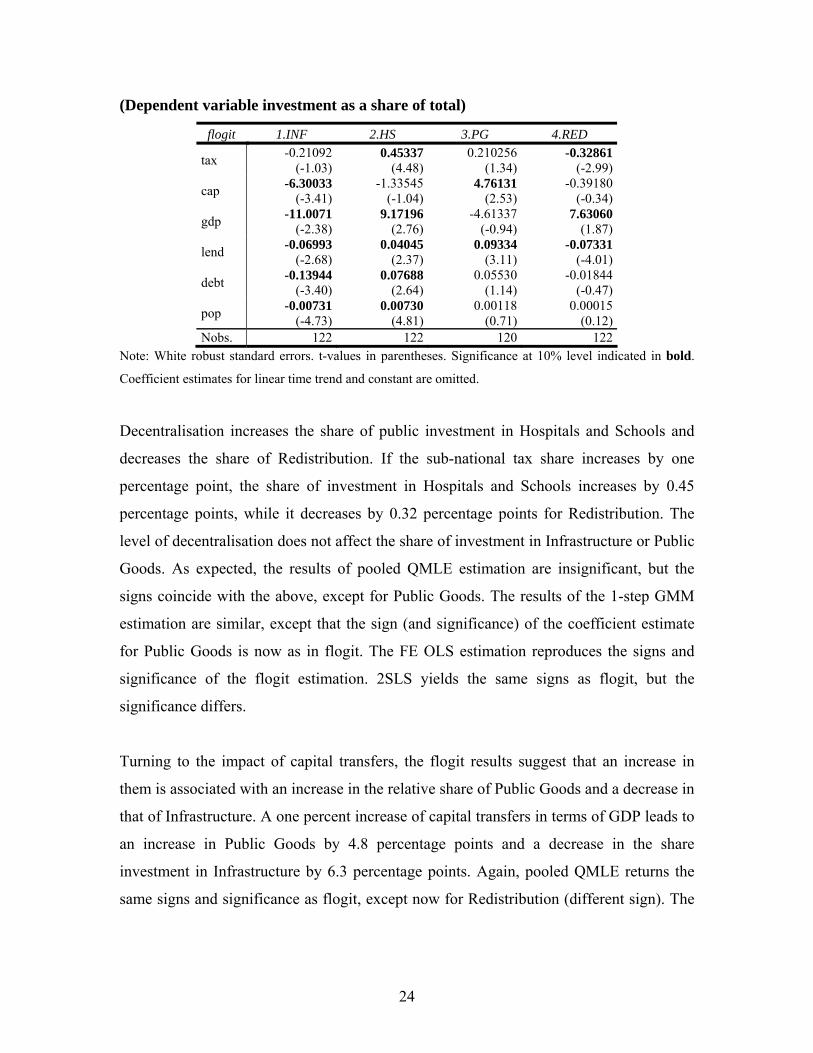
(Dependent variable investment as a share of total)

flogit 1.INF 2.HS 3.PG 4.RED

tax -0.21092(-1.03)

0.45337(4.48)

0.210256(1.34)

-0.32861 (-2.99)

cap -6.30033(-3.41)

-1.33545(-1.04)

4.76131(2.53)

-0.39180 (-0.34)

gdp -11.0071(-2.38)

9.17196(2.76)

-4.61337(-0.94)

7.63060 (1.87)

lend -0.06993(-2.68)

0.04045(2.37)

0.09334(3.11)

-0.07331 (-4.01)

debt -0.13944(-3.40)

0.07688(2.64)

0.05530(1.14)

-0.01844 (-0.47)

pop -0.00731(-4.73)

0.00730(4.81)

0.00118(0.71)

0.00015 (0.12)

Nobs. 122 122 120 122 Note: White robust standard errors. t-values in parentheses. Significance at 10% level indicated in bold.

Coefficient estimates for linear time trend and constant are omitted.

Decentralisation increases the share of public investment in Hospitals and Schools and

decreases the share of Redistribution. If the sub-national tax share increases by one

percentage point, the share of investment in Hospitals and Schools increases by 0.45

percentage points, while it decreases by 0.32 percentage points for Redistribution. The

level of decentralisation does not affect the share of investment in Infrastructure or Public

Goods. As expected, the results of pooled QMLE estimation are insignificant, but the

signs coincide with the above, except for Public Goods. The results of the 1-step GMM

estimation are similar, except that the sign (and significance) of the coefficient estimate

for Public Goods is now as in flogit. The FE OLS estimation reproduces the signs and

significance of the flogit estimation. 2SLS yields the same signs as flogit, but the

significance differs.

Turning to the impact of capital transfers, the flogit results suggest that an increase in

them is associated with an increase in the relative share of Public Goods and a decrease in

that of Infrastructure. A one percent increase of capital transfers in terms of GDP leads to

an increase in Public Goods by 4.8 percentage points and a decrease in the share

investment in Infrastructure by 6.3 percentage points. Again, pooled QMLE returns the

same signs and significance as flogit, except now for Redistribution (different sign). The

24

1-step GMM estimates yields consistently the same signs. The least squares –based

methods give more mixed results.

As regards other control variables, the logit estimation results suggest that GDP growth

comes with relatively more investment in Hospitals and Schools and Redistribution but

less in Infrastructure. A worsening budgetary situation reduces the relative share of

investment in Hospitals and Schools and Public Goods, while increasing the share of

Infrastructure and Redistribution. Finally, increasing public debt reduces the share of

Infrastructure investment, but benefits Hospitals and Schools.

Put differently, investment in Infrastructure on the one hand and Hospitals and Schools

on the other hand appear to crowd out one another. Whenever the cyclical situation

improves, there is more investment in Hospitals and Schools, at the cost of Infrastructure.

The same situation arises when public debt increases.

Finally, the share of Infrastructure investment decreases with population density, while

the share of investment in Hospitals and Schools increases. This pattern is confirmed by

most other estimation methods reported in Annex 3.

5. Economic Interpretation of Results

We saw in section 3 how the traditional theory of fiscal federalism could be used to

derive some hypotheses about the composition of public investment. Most notably, it

suggests that a higher degree of fiscal decentralisation should result in more public

investment in spillover goods, such as Infrastructure as well as Hospital and Schools,

especially if accompanied by capital transfers from the centre to internalise the spillover

effects of such investments. Furthermore, more decentralisation should result in more

investment in Redistribution (local public goods)—a result challenged by the more recent

theory of fiscal competition. Finally, the impact of decentralisation on our variable Public

Goods was considered ambiguous, depending on whether it is dominated by local or

global public goods.

25

The key results of the empirical analysis of section 4 are summarised in Table 4. It shows

the signs of the estimated coefficients in both levels and shares analyses. This section

seeks to interpret these results from the perspective of the theory of fiscal federalism.

Table 4: Signs of estimated coefficients for the tax share variable

1.INF 2.HS 3.PG 4.RED

Level + + + 0

Share 0 + 0 -

As shown in Table 4, decentralisation in terms of tax shares increases public investment

in Infrastructure; Hospitals and Schools; and Public Goods, with investment in Hospitals

and Schools increasing more than the others. The “excess” increase in Hospital and

School investment comes at the expense of Redistribution investment, whose relative

share (but not level) drops with decentralisation.

In other words, the estimated impact of full decentralisation on the composition of public

investment can be interpreted in terms of fiscal competition, (Keen and Marchand, 1997).

Decentralisation increases the level of investment in especially Infrastructure as well as

Hospitals and Schools, both providing “public inputs”. What is more, the increase in

investment in Hospitals and Schools suppresses the share of investment in Redistribution

(local public consumption-oriented goods). It is noteworthy that decentralisation does not

lower the level of any type of public investment. This being the case, we do not see any

evidence of decentralisation being associated with tax competition that would have a

detrimental impact on public investment.

The result that full decentralisation reduces the share of Redistribution investment is,

however, more difficult to reconcile with the traditional theory of fiscal federalism. Our

Redistribution variable is meant to capture consumption-oriented local public goods, such

26

as recreational facilities, and full decentralisation should lead to an increase, not relative

decline, in their provision.

As suggested above, fiscal competition may play a role by biasing sub-national

governments’ spending in favour of public inputs, at the expense of consumption-

oriented local public goods. However, the relative decline in Redistribution investment

can be given another interpretation as well. That its share actually declines with

decentralisation can signal over-investment in Redistribution in centralised systems

(Rattsø, 2003). With lower level governments competing for a “common pool” of

resources, there may be strategic reasons for them to misrepresent the local (or regional)

demand for public services captured in Redistribution. This being the case,

decentralisation would reduce such strategic behaviour and bring Redistribution in line

with local demand.

In sum, our results suggest that decentralisation increases economically productive public

investment, notably investment in public spillover goods (Infrastructure; Hospitals and

Schools) and in local and global public goods. There is no statistically significant impact

of decentralisation on public investment in consumption-oriented local public goods

(Redistribution). Decentralisation changes the composition of public investment by

boosting the relative share of Hospitals and Schools, at the expense of the share of

Redistribution.

While not readily reconcilable with the traditional theory of fiscal federalism, especially

as regards the provision of local public goods, these findings can be interpreted in terms

of the literature on fiscal competition, with not only tax rates but also the quality of public

expenditure weighing in firms’ location decisions. The finding that decentralisation

reduces the relative share of Redistribution investment can also signal over-investment in

more centralised system with competition for a common pool of resources.

27

6. Conclusion

The contribution of this paper is twofold. First, the presentation of the stylised facts of the

composition of public investment in Europe is a novelty. Especially the insight that less

than half of all public investment supports “infrastructure” in some sense of the word is

noteworthy, given that it is customary in both theoretical and empirical literature to use

“public investment” and “infrastructure investment” almost synonymously.

Second, the empirical analysis of the relationship between fiscal decentralisation and the

composition of public investment is also first–of–a–kind, at least in the European context.

It yields some interesting insights, most notably that fiscal decentralisation seems to boost

economically productive public investment and to curb the relative share of economically

less productive public investment.

Clearly, this is but a first step in the analysis of the composition of public investment.

There is plenty of scope for future research to tackle issues that our analysis leaves open.

The theoretical foundations for studying the composition of public investment remain

thin, especially as regards the articulation of an explicit link between fiscal federalism

and different types of investment. Empirical examination of different types of public

investment could usefully focus on differences in their productivity, as well as on a more

nuanced examination of what drives the different types of investment, including but not

limited to fiscal federalism.

28

Literature

Arrelano, M., Bond, S., 1991. Some Tests of Specification for Panel Data: Monte Carlo

Evidence and an Application to Employment Equations. Review of Economics Studies

58, 277-297.

Arze del Granado, F.J., Martinez-Vazquez, J., McNab, R., 2005. Fiscal Decentralization

and the Functional Composition of Public Expenditures. Working Paper 05-01, Andrew

Young School of Policy Studies, Georgia State University

Bond, S., 2002. Dynamic Panel Data Models: A Guide to Micro Data Methods and

Practice. cemmap working paper CWP09/02

Dahlby, B., 1996. Fiscal Externalities and the Design of Intergovernmental Grants.

International Tax and Public Finance 3, 397-412

Dahlby, B., Wilson, L.S., 2003. Vertical fiscal externalities in a federation. Journal of

Public Economics 87, 917-930

Greene,W.H., 2003. Econometric Analysis, 5th edition. International Edition, New York:

Prentice Hall.

Hulten, C.R., Schwab R.M., 1997. A fiscal federalism approach to infrastructure policy.

Regional Science and Urban Economics 27, 139-159

Im, K.S., Pesaran, M.H., Shin, Y., 1997. Testing for Unit Roots in Heterogeneous

Panels. Department of Applied Economics, University of Cambridge, mimeo

Keen, M., Marchand, M., 1997. Fiscal Competition and the Pattern of Public Spending.

Journal of Public Economics 66(1), 33-53

29

Lancaster, T., 2000. The incidental parameter problem since 1948. Journal of

Econometrics 95, 391-413

Levin, A., Lin, C-F., Chu, C-S.J., 2002. Unit root tests in panel data: asymptotic and

finite-sample properties. Journal of Econometrics 108, 1-24

Loudermilk, M.S., 2005. Estimation of Fractional Dependent Variables in Dynamic

Panel Data Models with an Application to Firm Dividend Policy. Journal of Business

and Economic Statistics (forthcoming)

Martínez-López, D., 2005. Fiscal Federalism and Public Inputs Provision – Vertical

Externalities Matter. European Central Bank, Working Paper Series No. 484

Matsumoto, M., (1998). A note on tax competition and public input provision. Regional

Science and Urban Economics, 28, 456-473

Musgrave, R.A., 1959. The Theory of Public Finance, New York: McGraw-Hill.

Oates, W., 1972. Fiscal Federalism, New York: Harcourut Brace Jovanovich.

Papke, L.E., Wooldridge J.M., 1996. Econometric Methods for Fractional Response

Variables with an Application to 401(k) Plan Participation Rates. Journal of Applied

Econometrics 11, 619-632

Papke, L.E., Wooldridge J.M., 2005. Panel Data Methods for Fractional Response

Variables with an Application to Test Pass Rates. Michigan State University, mimeo

Rattsø, J., 2003. Fiscal federation or confederation in the European Union: The challenge

of the common pool problem. Department of Economics, Norwegian University of

Science and Technology, mimeo

30

Sinn, H.W., 2003. The new systems competition, Oxford, Basil Blackwell.

Stegarescu, D., (2004). Public Sector Decentralization: Measurement Concepts and

Recent International Trends. ZEW Mannheim, Discussion Paper No. 04-74

Tiebout, C.M., 1956. A pure theory of local public expenditures. Journal of Political

Economy 64, 416-424

Zodrow, G., Mieszkowski, P., 1986. Pigou, Tiebout, Property Taxation, and the

Underprovision of Local Public Goods. Journal of Urban Economics 19, 356-370

31

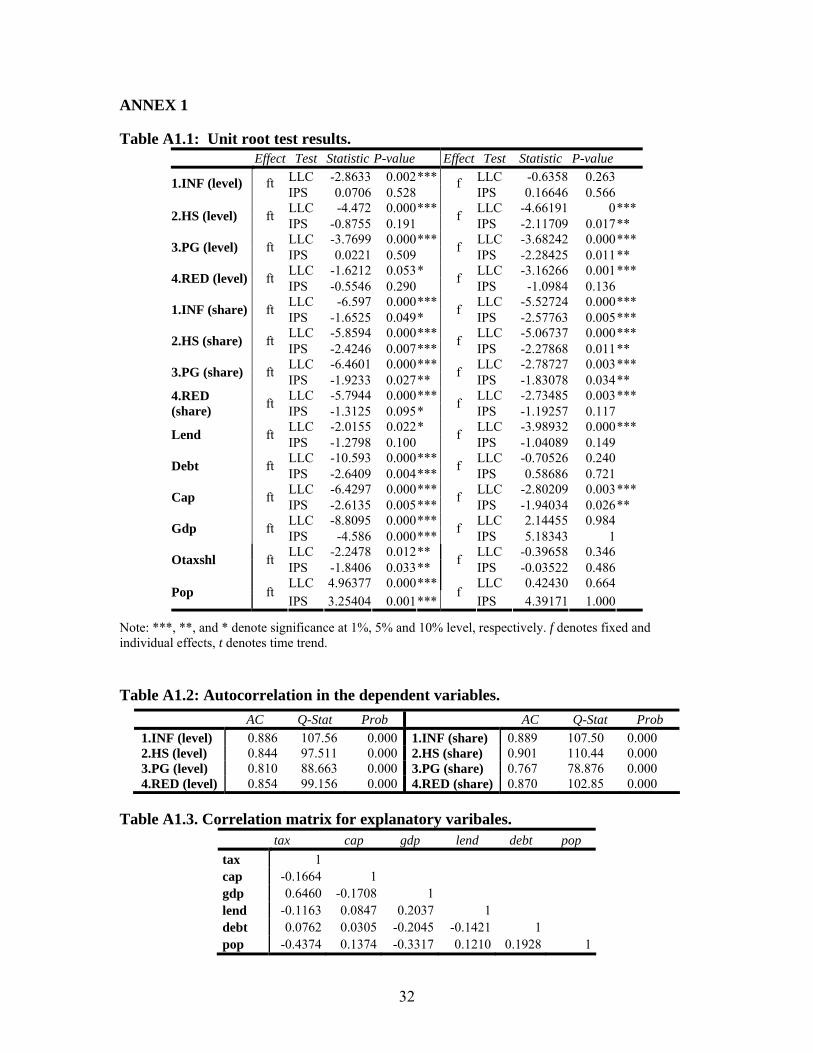
ANNEX 1 Table A1.1: Unit root test results.

Effect Test Statistic P-value Effect Test Statistic P-value LLC -2.8633 0.002*** LLC -0.6358 0.263 1.INF (level) ft IPS 0.0706 0.528

f IPS 0.16646 0.566

LLC -4.472 0.000*** LLC -4.66191 0 *** 2.HS (level) ft IPS -0.8755 0.191 f IPS -2.11709 0.017 ** LLC -3.7699 0.000*** LLC -3.68242 0.000 *** 3.PG (level) ft IPS 0.0221 0.509 f IPS -2.28425 0.011 ** LLC -1.6212 0.053* LLC -3.16266 0.001 *** 4.RED (level) ft IPS -0.5546 0.290 f IPS -1.0984 0.136 LLC -6.597 0.000*** LLC -5.52724 0.000 *** 1.INF (share) ft IPS -1.6525 0.049* f IPS -2.57763 0.005 *** LLC -5.8594 0.000*** LLC -5.06737 0.000 *** 2.HS (share) ft IPS -2.4246 0.007*** f IPS -2.27868 0.011 ** LLC -6.4601 0.000*** LLC -2.78727 0.003 *** 3.PG (share) ft IPS -1.9233 0.027** f IPS -1.83078 0.034 ** LLC -5.7944 0.000*** LLC -2.73485 0.003 *** 4.RED

(share) ft IPS -1.3125 0.095* f IPS -1.19257 0.117 LLC -2.0155 0.022* LLC -3.98932 0.000 *** Lend ft IPS -1.2798 0.100 f IPS -1.04089 0.149 LLC -10.593 0.000*** LLC -0.70526 0.240 Debt ft IPS -2.6409 0.004*** f IPS 0.58686 0.721 LLC -6.4297 0.000*** LLC -2.80209 0.003 *** Cap ft IPS -2.6135 0.005*** f IPS -1.94034 0.026 ** LLC -8.8095 0.000*** LLC 2.14455 0.984 Gdp ft IPS -4.586 0.000*** f IPS 5.18343 1 LLC -2.2478 0.012** LLC -0.39658 0.346 Otaxshl ft IPS -1.8406 0.033** f IPS -0.03522 0.486 LLC 4.96377 0.000*** LLC 0.42430 0.664

Pop ft IPS 3.25404 0.001***

f IPS 4.39171 1.000

Note: ***, **, and * denote significance at 1%, 5% and 10% level, respectively. f denotes fixed and individual effects, t denotes time trend.

Table A1.2: Autocorrelation in the dependent variables.

AC Q-Stat Prob AC Q-Stat Prob 1.INF (level) 0.886 107.56 0.000 1.INF (share) 0.889 107.50 0.000 2.HS (level) 0.844 97.511 0.000 2.HS (share) 0.901 110.44 0.000 3.PG (level) 0.810 88.663 0.000 3.PG (share) 0.767 78.876 0.000 4.RED (level) 0.854 99.156 0.000 4.RED (share) 0.870 102.85 0.000

Table A1.3. Correlation matrix for explanatory varibales.

tax cap gdp lend debt pop tax 1 cap -0.1664 1 gdp 0.6460 -0.1708 1 lend -0.1163 0.0847 0.2037 1 debt 0.0762 0.0305 -0.2045 -0.1421 1 pop -0.4374 0.1374 -0.3317 0.1210 0.1928 1

32

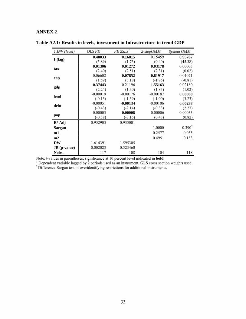
ANNEX 2

Table A2.1: Results in levels, investment in Infrastructure to trend GDP

1.INV (level) OLS FE FE 2SLS1 2-stepGMM System GMM

I1(lag) 0.48033(5.89)

0.16815(1.73)

0.15459(0.40)

0.95767 (45.38)

tax 0.01306(2.40)

0.01272(2.51)

0.03178(2.31)

0.00003 (0.02)

cap 0.06602(1.59)

0.07852(3.18)

-0.81917(-1.75)

-0.01021 (-0.81)

gdp 0.37443(2.24)

0.21196(1.30)

1.55163(1.83)

0.02180 (1.02)

lend -0.00019(-0.15)

-0.00176(-1.59)

-0.00187(-1.00)

0.00060 (3.23)

debt -0.00051(-0.43)

-0.00134(-2.14)

-0.00106(-0.33)

0.00233 (2.27)

pop -0.00003(-0.58)

-0.00008(-3.15)

0.00006 (0.43)

0.00033 (0.82)

R²-Adj 0.952903 0.935001 Sargan 1.0000 0.3902 m1 0.2577 0.035 m2 0.4951 0.183 DW 1.614391 1.595305 JB (p-value) 0.002023 0.523460 Nobs. 117 108 104 118

Note: t-values in parentheses; significance at 10 percent level indicated in bold. 1 Dependent variable lagged by 2 periods used as an instrument, GLS cross section weights used. 2 Difference-Sargan test of overidentifying restrictions for additional instruments.

33

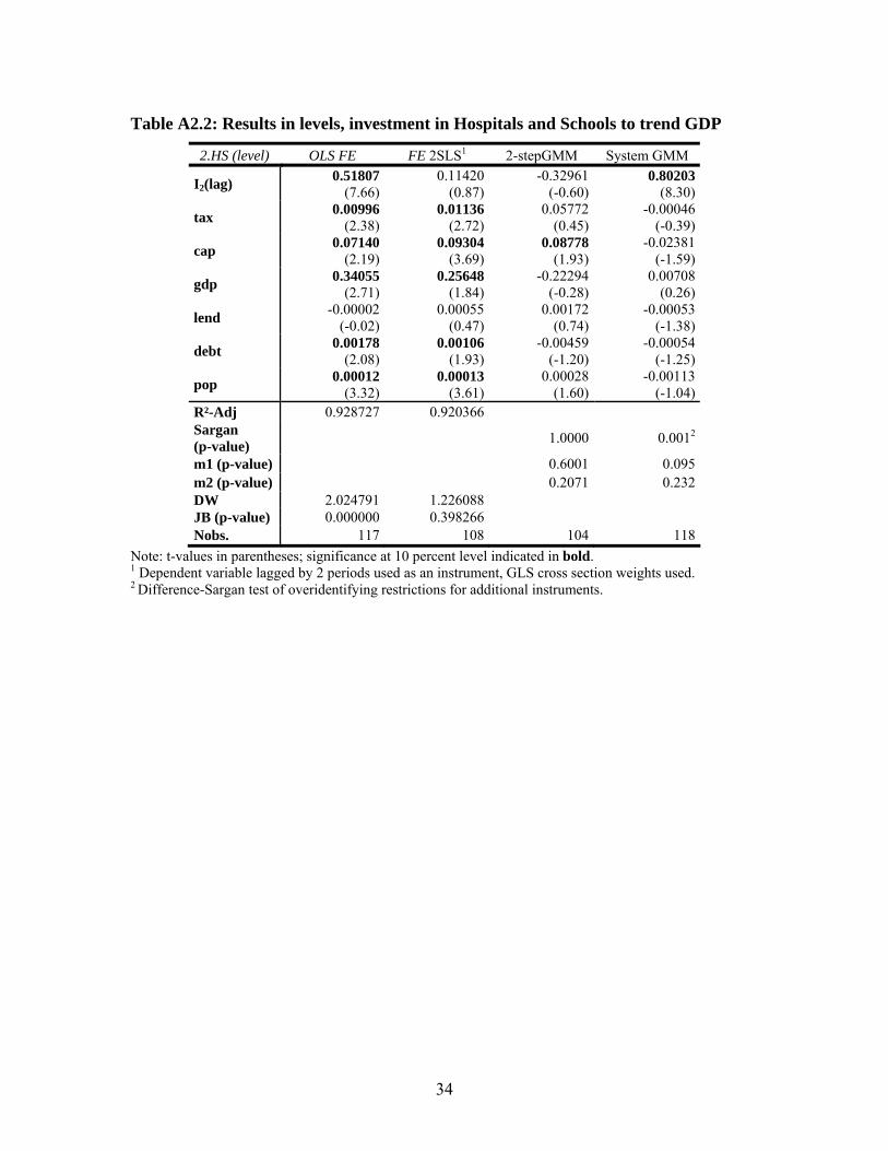
Table A2.2: Results in levels, investment in Hospitals and Schools to trend GDP

2.HS (level) OLS FE FE 2SLS1 2-stepGMM System GMM

I2(lag) 0.51807(7.66)

0.11420(0.87)

-0.32961(-0.60)

0.80203 (8.30)

tax 0.00996(2.38)

0.01136(2.72)

0.05772(0.45)

-0.00046 (-0.39)

cap 0.07140(2.19)

0.09304(3.69)

0.08778(1.93)

-0.02381 (-1.59)

gdp 0.34055(2.71)

0.25648(1.84)

-0.22294(-0.28)

0.00708 (0.26)

lend -0.00002(-0.02)

0.00055(0.47)

0.00172(0.74)

-0.00053 (-1.38)

debt 0.00178(2.08)

0.00106 (1.93)

-0.00459(-1.20)

-0.00054 (-1.25)

pop 0.00012(3.32)

0.00013(3.61)

0.00028 (1.60)

-0.00113 (-1.04)

R²-Adj 0.928727 0.920366 Sargan (p-value) 1.0000 0.0012

m1 (p-value) 0.6001 0.095 m2 (p-value) 0.2071 0.232 DW 2.024791 1.226088 JB (p-value) 0.000000 0.398266 Nobs. 117 108 104 118


34

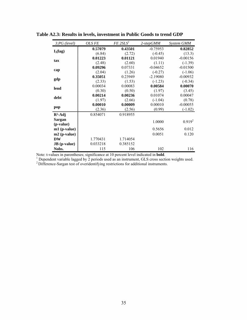
Table A2.3: Results in levels, investment in Public Goods to trend GDP

3.PG (level) OLS FE FE 2SLS1 2-stepGMM System GMM

I3(lag) 0.57079(6.84)

0.43501(2.72)

-0.75953(-0.45)

0.82852 (13.3)

tax 0.01223(2.48)

0.01121(2.60)

0.01940(1.11)

-0.00156 (-1.39)

cap 0.09296(2.04)

0.07331(1.26)

-0.04652(-0.27)

-0.01500 (-1.06)

gdp 0.35051(2.33)

0.23949(1.53)

-2.19080(-1.23)

-0.00932 (-0.34)

lend 0.00034(0.30)

0.00083(0.50)

0.00584(1.97)

0.00070 (3.45)

debt 0.00214(1.97)

0.00236(2.66)

0.01074(-1.04)

0.00047 (0.78)

pop 0.00010(2.36)

0.00009(2.56)

0.00010 (0.99)

-0.00055 (-1.02)




35

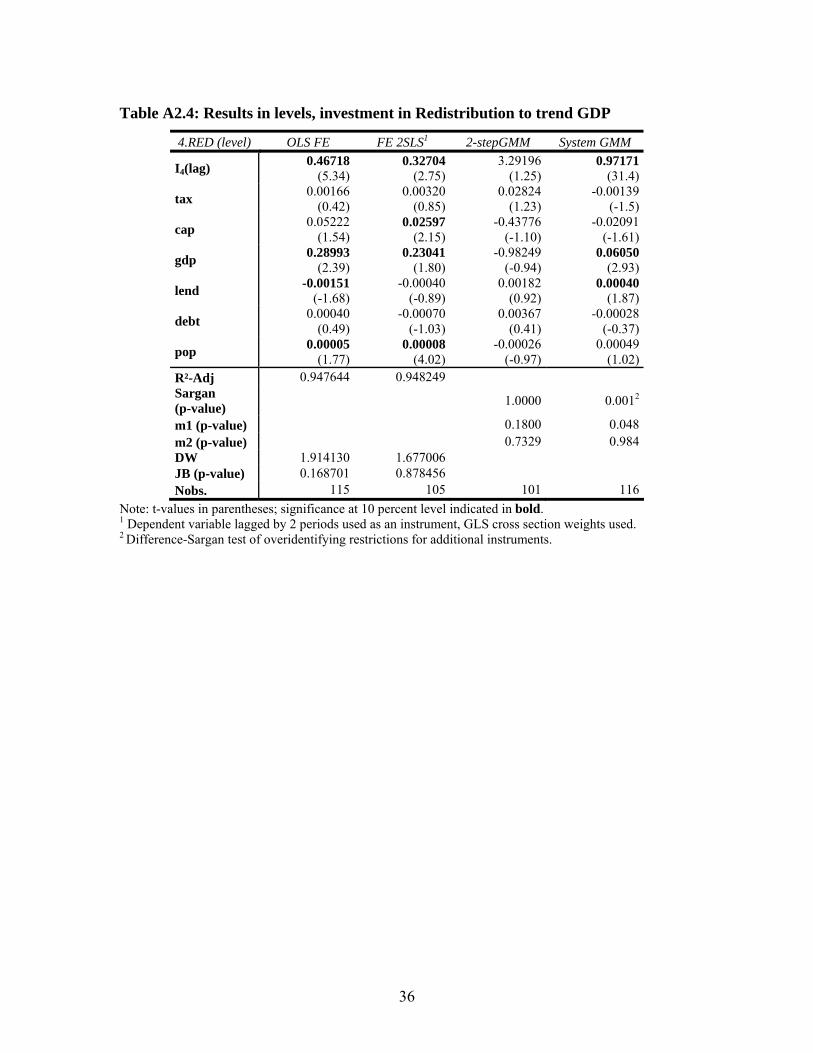
Table A2.4: Results in levels, investment in Redistribution to trend GDP

4.RED (level) OLS FE FE 2SLS1 2-stepGMM System GMM

I4(lag) 0.46718(5.34)

0.32704(2.75)

3.29196(1.25)

0.97171 (31.4)

tax 0.00166(0.42)

0.00320(0.85)

0.02824(1.23)

-0.00139 (-1.5)

cap 0.05222(1.54)

0.02597(2.15)

-0.43776(-1.10)

-0.02091 (-1.61)

gdp 0.28993(2.39)

0.23041(1.80)

-0.98249 (-0.94)

0.06050 (2.93)

lend -0.00151(-1.68)

-0.00040(-0.89)

0.00182(0.92)

0.00040 (1.87)

debt 0.00040(0.49)

-0.00070 (-1.03)

0.00367(0.41)

-0.00028 (-0.37)

pop 0.00005(1.77)

0.00008(4.02)

-0.00026 (-0.97)

0.00049 (1.02)




36

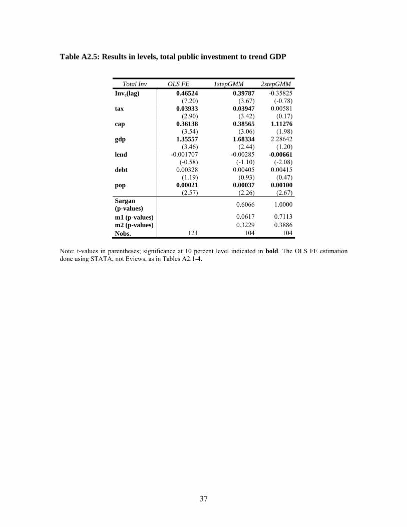
Table A2.5: Results in levels, total public investment to trend GDP

Total Inv OLS FE 1stepGMM 2stepGMM Invc(lag) 0.46524

(7.20)0.39787

(3.67)-0.35825

(-0.78) tax 0.03933

(2.90)0.03947

(3.42)0.00581

(0.17) cap 0.36138

(3.54)0.38565

(3.06)1.11276

(1.98) gdp 1.35557

(3.46)1.68334

(2.44)2.28642

(1.20) lend -0.001707

(-0.58)-0.00285

(-1.10)-0.00661

(-2.08) debt 0.00328

(1.19)0.00405

(0.93)0.00415

(0.47) pop 0.00021

(2.57)0.00037

(2.26)0.00100

(2.67) Sargan (p-values) 0.6066 1.0000

m1 (p-values) 0.0617 0.7113 m2 (p-values) 0.3229 0.3886 Nobs. 121 104 104

Note: t-values in parentheses; significance at 10 percent level indicated in bold. The OLS FE estimation done using STATA, not Eviews, as in Tables A2.1-4.

37

ANNEX 3

Table A3.1: Results in shares, investment in Infrastructure as a share of total

1.INF (share)

OLS FE

2SLS 1-step GMM Pooled QMLE

I1(lag) 0.78673(9.01)

0.72404(6.17)

tax -0.13960(-0.83)

-0.14688(-1.12)

-0.23902(-1.41)

-0.12555 (-0.21)

cap -6.58147(-4.95)

1.64797(1.23)

1.29566(1.20)

-9.94473 (-1.73)

gdp -13.1062(-3.80)

-7.44137(-1.95)

-8.32952(-1.19)

-9.38965 (-0.61)

lend -0.02946(-1.09)

-0.01050(-0.27)

0.01798(1.00)

-0.26985 (-2.41)

debt -0.11518(-2.69)

-0.03972(-1.30)

-0.05950(-1.20)

-0.35521 (-2.97)

pop -0.00589(-4.16)

-0.00580(-10.6)

-0.00550 (-3.94)

-.00415 (-1.11)

R²-Adj 0.956315 0.989788 m1 (p-value) 0.0228 m2 (p-value) 0.3369 DW 1.136066 2.530871 JB (p-value) 0.411646 0.814093 Nobs. 122 105 101 122

Note: t-values in parentheses; significance at 10 percent level indicated in bold. Coefficient estimates for linear time trend and constant are omitted.

38

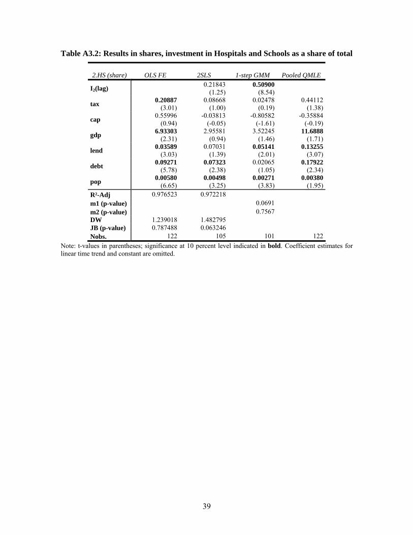
Table A3.2: Results in shares, investment in Hospitals and Schools as a share of total

2.HS (share)

OLS FE

2SLS 1-step GMM

Pooled QMLE

I2(lag) 0.21843(1.25)

0.50900(8.54)

tax 0.20887(3.01)

0.08668(1.00)

0.02478(0.19)

0.44112 (1.38)

cap 0.55996(0.94)

-0.03813(-0.05)

-0.80582(-1.61)

-0.35884 (-0.19)

gdp 6.93303(2.31)

2.95581(0.94)

3.52245(1.46)

11.6888 (1.71)

lend 0.03589(3.03)

0.07031(1.39)

0.05141(2.01)

0.13255 (3.07)

debt 0.09271(5.78)

0.07323(2.38)

0.02065(1.05)

0.17922 (2.34)

pop 0.00580(6.65)

0.00498(3.25)

0.00271(3.83)

0.00380 (1.95)



39

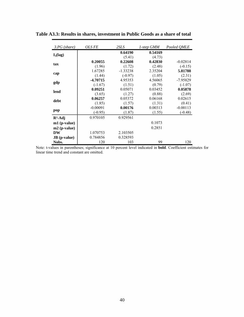
Table A3.3: Results in shares, investment in Public Goods as a share of total

3.PG (share)

OLS FE

2SLS 1-step GMM

Pooled QMLE

I3(lag) 0.64190(5.41)

0.54169(4.73)

tax 0.20055(1.96)

0.22608(1.72)

0.42830(2.48)

-0.02814 (-0.15)

cap 1.67285(1.44)

-1.33238(-0.97)

2.35204(1.05)

5.81788 (2.31)

gdp -4.70715(-1.67)

4.95353(1.51)

4.56065(0.79)

-7.95829 (-1.07)

lend 0.09251(3.65)

0.05071(1.27)

0.03452(0.88)

0.05878 (2.69)

debt 0.06257(1.85)

0.05372(1.57)

0.06168(1.31)

0.02615 (0.41)

pop -0.00091(-0.95)

0.00176(1.87)

0.00313 (1.55)

-0.00113 (-0.48)



40

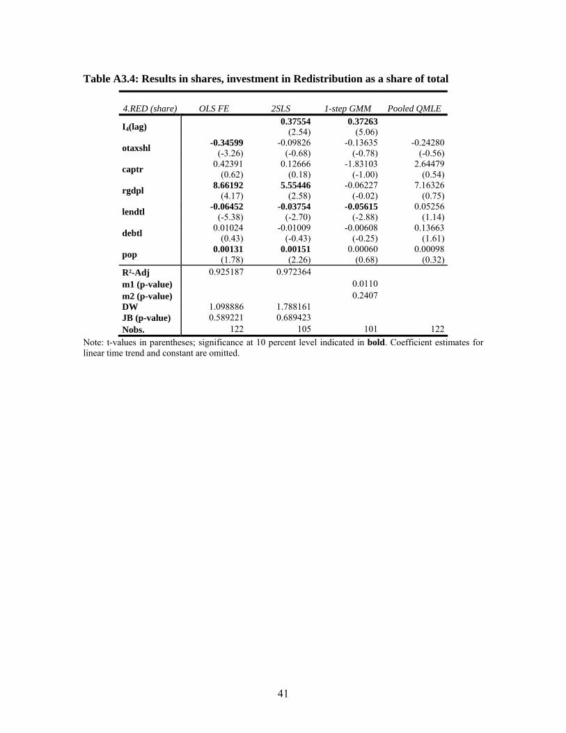
Table A3.4: Results in shares, investment in Redistribution as a share of total

4.RED (share)

OLS FE

2SLS 1-step GMM Pooled QMLE

I4(lag) 0.37554(2.54)

0.37263(5.06)

otaxshl -0.34599(-3.26)

-0.09826(-0.68)

-0.13635(-0.78)

-0.24280 (-0.56)

captr 0.42391(0.62)

0.12666(0.18)

-1.83103(-1.00)

2.64479 (0.54)

rgdpl 8.66192(4.17)

5.55446(2.58)

-0.06227(-0.02)

7.16326 (0.75)

lendtl -0.06452(-5.38)

-0.03754(-2.70)

-0.05615(-2.88)

0.05256 (1.14)

debtl 0.01024(0.43)

-0.01009(-0.43)

-0.00608(-0.25)

0.13663 (1.61)

pop 0.00131(1.78)

0.00151(2.26)

0.00060 (0.68)

0.00098 (0.32)



41

To the best of our knowledge, no empirical analyses have … · · 2016-06-15from the sample...

Documents

Transcript of To the best of our knowledge, no empirical analyses have … · · 2016-06-15from the sample...