
Two interacting atoms in a quantum optical potential · seine kompromisslose Weise beigebracht hat,...
51
Two interacting atoms in a quantum optical potential Diplomarbeit zur Erlangung des Grades einer Magistra an der Fakult ¨ at f ¨ ur Mathematik, Informatik und Physik der Leopold-Franzens-Universit ¨ at Innsbruck eingereicht von Katharina Renz im Dezember 2005 durchgef ¨ uhrt am Institut f ¨ ur Theoretische Physik bei A. Univ.-Prof. Dr. Helmut Ritsch
Transcript of Two interacting atoms in a quantum optical potential · seine kompromisslose Weise beigebracht hat,...
Two interacting atoms
in a quantum optical potential
Diplomarbeit
zur Erlangung des Grades einer Magistraan der Fakultat fur Mathematik, Informatik und Physik
der Leopold-Franzens-Universitat Innsbruck
eingereicht vonKatharina Renz
im Dezember 2005
durchgefuhrt am Institut fur Theoretische Physikbei A. Univ.-Prof. Dr. Helmut Ritsch
Danke...
Als erstes danke ich Helmut Ritsch, meinem Betreuer, fur sein Vertrauenin mich, das mir eine große Motivation war, und das kollegiale und fre-undliche Arbeitsklima in seiner Arbeitsgruppe.Danke auch an Thomas Salzburger, meinen Burokollegen, der mir mit Ratund Tat zur Seite stand, wenn man ihn mal aus seinen hoheren Spharendes Denkens reißen konnte...!Nicht zuletzt danke ich Marion Grunbacher, der guten Seele des Institutes,fur die aufmunternden Gesprache.
Ein großes Dankeschon gebuhrt meinen Eltern, die mich in der lan-gen Zeit des Studiums ausgehalten haben! Besonderer Dank gilt meinerMama, die seit mein Sohn Nuno auf der Welt ist, fast ihre gesamte Freizeitfur Babysitten geopfert hat, damit ich uberhaupt die Chance hatte dieseDiplomarbeit zu schreiben!Ganz besonders danke ich meinem kleinen Sohnchen Nuno, der mir aufseine kompromisslose Weise beigebracht hat, dass jeder Tag sinnvoll genutztsein will!
Danke an die ”Physikerinnen” fur die lustigen Abende!Besonderer Dank geht an Magdalena Mair, fur ihre Freundschaft und dafur,dass sie sich mein Gejammere angehort hat!Danke auch an Sabine Kreidl fur die Kaffee-Pausen und die interessantenGesprache!
Diese Diplomarbeit widme ich meiner Oma!
I
Contents
1 Introduction 2
2 One atom interacting with a single cavity mode 72.1 Introduction . . . . . . . . . . . . . . . . . . . . . . . . . . . . 72.2 The setup . . . . . . . . . . . . . . . . . . . . . . . . . . . . . . 72.3 The Hamiltonian and the master equation . . . . . . . . . . . 82.4 Heisenberg-Langevin equations and
the low saturation limit . . . . . . . . . . . . . . . . . . . . . . 102.5 Steady state dynamics,
mean photon number and the force . . . . . . . . . . . . . . . 11
3 One atom in a time-dependent harmonic trap 143.1 Introduction . . . . . . . . . . . . . . . . . . . . . . . . . . . . 143.2 The model . . . . . . . . . . . . . . . . . . . . . . . . . . . . . 153.3 Time-independent treatment . . . . . . . . . . . . . . . . . . . 173.4 Time-dependent perturbation δ(t) . . . . . . . . . . . . . . . 21
4 Two interacting atoms inside a cavity 264.1 Introduction . . . . . . . . . . . . . . . . . . . . . . . . . . . . 264.2 The Hamiltonian . . . . . . . . . . . . . . . . . . . . . . . . . 264.3 The differential equation for the coefficients in the harmonic
eigenbasis . . . . . . . . . . . . . . . . . . . . . . . . . . . . . 274.4 Numerical solutions . . . . . . . . . . . . . . . . . . . . . . . 31
4.4.1 Initial conditions . . . . . . . . . . . . . . . . . . . . . 324.5 Self consistent eigenstates . . . . . . . . . . . . . . . . . . . . 384.6 Stationary state solutions . . . . . . . . . . . . . . . . . . . . . 444.7 Conclusions . . . . . . . . . . . . . . . . . . . . . . . . . . . . 46
Bibliography 48
Curriculum vitae 49
1
Chapter 1
Introduction
During the last decades a great deal of theoretical and experimental re-search was focused on cavity QED - the study of a single two-level atominteracting with a single or a few field modes of an optical resonator. Var-ious configurations to analyze the atom-field dynamics have been inves-tigated theoretically (cavity QED) [1, 2, 3]. Experiments combining cavityQED with optical trapping and cooling experiments have been realized inrecent works [4, 5]. The basic idea for the research on light and matteris rooted in the Jaynes-Cummings model [6]. This at first only theoreti-cal model of a two-level atom interacting with a single mode of the elec-tromagnetic field was developed by E. T. Jaynes and F. W. Cummings inthe 1960′ies in order to compare the predictions of Quantum Mechanicswith those of the classical Maxwell equations. It could be realized ex-perimentally with good adjustment to the theoretical idealization in themeanwhile. The idealization in this model is the restriction to a two-levelsystem and to one single mode of the electromagnetic field. Although eachatom has an infinite number of states with an infinite number of permittedtransitions between them, it is possible to neglect all energy levels exceptthe two levels whose energy difference is near the energy of the field. Sucha two-level system can be described by the Pauli spinoperator σz and thetransition frequency of the 2-level system ωa. The operator-representationof the field is more complex. The simplest case that though describes ba-sic aspects of the interaction is to disregard all field modes except for one.A single mode is comparatively easy to describe by the creation a† andannihilation a operators. The Hamiltonian of the field contains the laserfrequency ωL and the operator product a†a which counts the number ofphotons.
2
- INTRODUCTION -
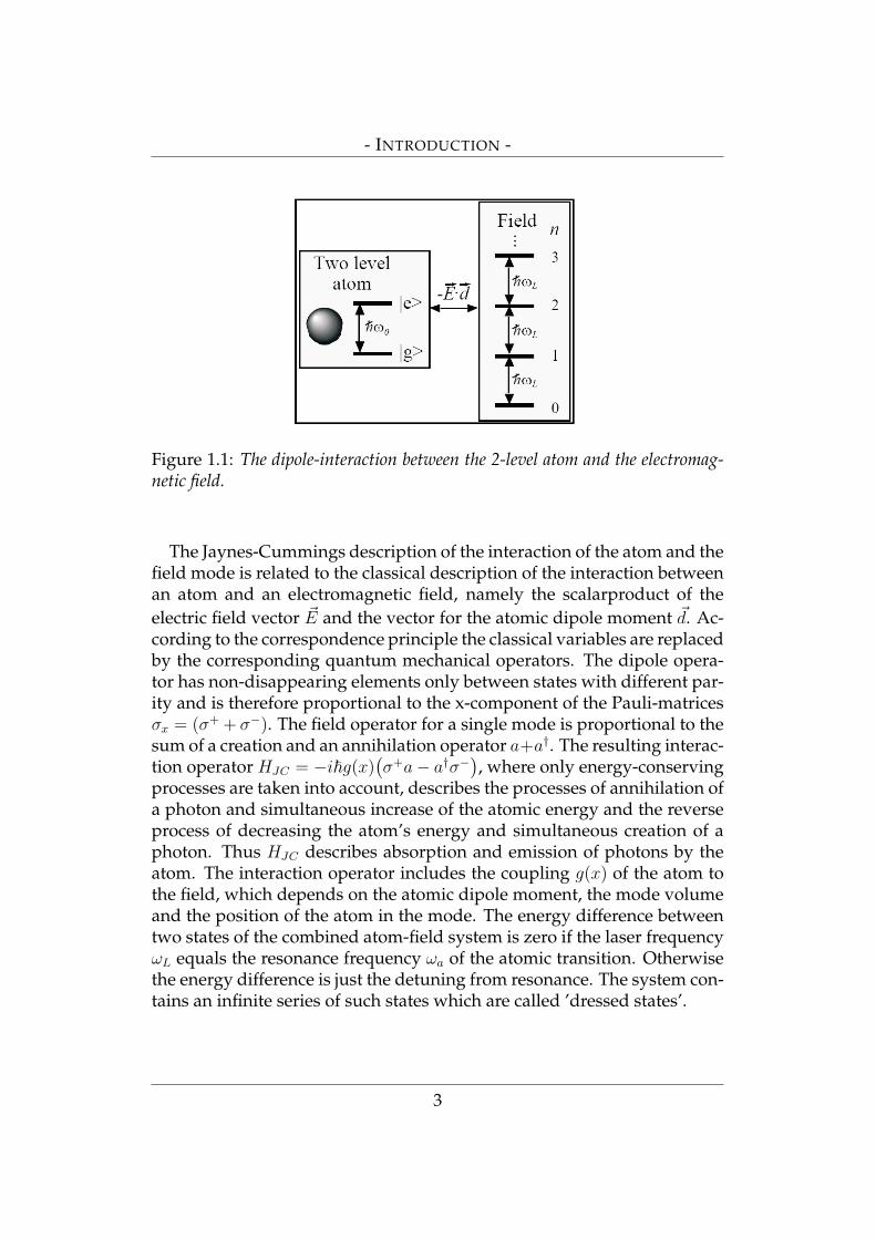
Figure 1.1: The dipole-interaction between the 2-level atom and the electromag-netic field.
The Jaynes-Cummings description of the interaction of the atom and thefield mode is related to the classical description of the interaction betweenan atom and an electromagnetic field, namely the scalarproduct of theelectric field vector ~E and the vector for the atomic dipole moment ~d. Ac-cording to the correspondence principle the classical variables are replacedby the corresponding quantum mechanical operators. The dipole opera-tor has non-disappearing elements only between states with different par-ity and is therefore proportional to the x-component of the Pauli-matricesσx = (σ+ + σ−). The field operator for a single mode is proportional to thesum of a creation and an annihilation operator a+a†. The resulting interac-tion operator HJC = −i~g(x)
(σ+a− a†σ−
), where only energy-conserving
processes are taken into account, describes the processes of annihilation ofa photon and simultaneous increase of the atomic energy and the reverseprocess of decreasing the atom’s energy and simultaneous creation of aphoton. Thus HJC describes absorption and emission of photons by theatom. The interaction operator includes the coupling g(x) of the atom tothe field, which depends on the atomic dipole moment, the mode volumeand the position of the atom in the mode. The energy difference betweentwo states of the combined atom-field system is zero if the laser frequencyωL equals the resonance frequency ωa of the atomic transition. Otherwisethe energy difference is just the detuning from resonance. The system con-tains an infinite series of such states which are called ’dressed states’.
3
- INTRODUCTION -
The exchange of photon momentum between light and matter is used tocontrol atomic motion. An atom interacting with an electromagnetic fieldwill experience forces occurring on the one hand from the radiation pres-sure of the electromagnetic field and on the other hand from the electricdipole interaction.
The radiation pressure force arises from absorption and spontaneousemission of photons and can be described as the product of the transferredphoton momentum ~k and the photon scattering rate Γ of the atom, whichis the rate of absorption-spontaneous emission cycles. This force can ac-celerate or slow down atoms respectively. The mechanism is based on theDoppler effect and therefore is called Doppler-cooling [7, 8]. The movingparticle tends to absorb photons from the laser wave counterpropagatingits velocity rather than from the copropagating wave, if the laser is tunedbelow resonance. The Doppler-cooling though is limited by the atomiclinewidth such that after some cycles the force decreases and the mini-mum attainable temperature is reached. This minimum temperature iscalled the Doppler limit kBT ≈ ~Γ [9, 10, 11]. The cooling force can be in-creased by imposing a magnetic field gradient on the system which variesthe energy of the atomic states via the Zeeman effect. Nevertheless thereare fundamental limits of this cooling method arising from the quantummechanical behavior of the radiation field. In fact there are fluctuationsaround the mean value of the force, due to the discrete photon momen-tum transfer. These fluctuations give rise to diffusion due to the randomdirections of spontaneous emission of photons which leads to a broaden-ing of the velocity distribution. Diffusion thus counteracts as a heatingprocess.
The dipole force is independent of spontaneous emission. It arises fromthe induced dipole moment of the atom which according to the detuningof the laser draws the atom to high or low intensity regions of the field re-spectively. The steady state dipole force for the case of a motionless atomshows that atoms are attracted to high intensity regions for a red detun-ing, which means the laser frequency is bigger than the atomic transitionfrequency. The induced dipole moment is in phase with the laser field andthe atom can decrease its energy in a field of high intensities - the atomis said to be a ’high field seeker’. For blue detuning, meaning the laserfrequency is smaller than the atomic transition frequency and the induceddipole moment is 180◦ out of phase with the laser, the atoms are drawnto low intensity regions (low field seeker). To investigate the dipole force
4
- INTRODUCTION -
independent of spontaneous emission, it is useful to operate with high de-tunings of the laser frequency from atomic transition frequency. One thenfinds that the dipole force is proportional to the gradient of the interactionenergy F = −∇HJC . In contrast to the radiation pressure force, the dipoleforce is not limited by the atomic linewidth. A very interesting feature ofthe dipole force is that it does not depend on the details of the structureof the atom, therefore it is applicable to molecules and even macroscopicobjects. One takes advantage of this feature in so-called optical tweezers,where the objects of interest are trapped in the focus of a laser.
The idea now is to put the atom inside a cavity and study the interactionwith the standing laser cavity field. Trapping and cooling properties areinvestigated in models of an atom strongly coupled to a single mode ofa cavity standing laser field, where one gets alternative cooling methods.The conventional methods rely on cycles of optical pumping and sponta-neous emission of a photon by the atom. Cavity cooling, however, doesnot require spontaneous emission by the atom, but cavity loss replaces thisrole. Cavity cooling can be related to a classical picture based on the no-tion of a refractive index. For strong atom-cavity coupling the intracavityintensity is strongly affected by the atomic motion. At a node of the cavitystanding mode the atom is not coupled to the field. For resonant pumpingthe field intensity is large, whereas if the atom is at an antinode, it shifts thecavity out of resonance which leads to a small intracavity intensity. Sinceatomic excitation is low at all times, the minimum attainable temperatureis not limited by the atomic linewidth but by the linewidth of the cavity,which can be much smaller, and temperatures below the Doppler limit canbe reached.
This thesis is organized as follows:The first chapter will be a review of the case of one atom interacting witha single mode of the cavity field. We will derive the Hamiltonian in therotating frame approximation and calculate the Heisenberg equations ofmotion for the atom and the cavity field in the good cavity limit and byassuming the atomic excited state weakly populated. Finally with theseapproximations we will present the force acting on the atom.In the second chapter we will enclose the backaction of the atom on the
5
- INTRODUCTION -
field. This backaction will be modelled by a time-dependent potential,which we model as a harmonic potential with a time-dependent perturba-tion δ(t). At first we will check the quality of this model by keeping thisperturbation time-independent in our calculations. Then we will calculatethe time-dependent case and find numerical solutions for expectation val-ues of the atom and the field amplitude.The third chapter deals with the interaction between two atoms and thecavity field. We will apply the perturbative treatment of the previouschapter. And we will try a different ansatz and look for the eigensystemin order to find self-consistent eigenstates of the system.
6
Chapter 2
One atom interacting with asingle cavity mode
2.1 Introduction
In the following chapter, we shortly review the case of one atom interact-ing with a single mode of a cavity standing field, including losses throughdecay of cavity photons. The Hamiltonian, describing a Jaynes-Cummingstype interaction between the atom and a single mode of the standing laserfield and the interaction of the cavity field with an external heat bath, willbe calculated in a rotating frame to derive a master equation for the sys-tem. We will derive the Heisenberg-Langevin equations of motion for theatomic and mode operators, where we assume that the excited state of theatom is weakly populated (low saturation) and, as we consider the goodcavity limit (κ À g), the atomic operators are treated as stationary values.With these approximations we will find an equation for the cavity fieldand the force acting on the atom.
2.2 The setup
We consider a 2-level atom with transition frequency ωa and mass m cou-pled to a single mode of a high-finesse cavity with resonance frequency ωc.The system is driven by a coherent laser field of frequency ωL with pumprate η, injected through one of the mirrors of the cavity. For simplicity weneglect spontaneous emission of the atom, which is true for large atomicdetunings |ωa − ωL| À γ, and restrict atomic motion to one dimension.The cavity field is being damped by coupling to the environment, photons
7
- ONE ATOM INTERACTING WITH A SINGLE CAVITY MODE -
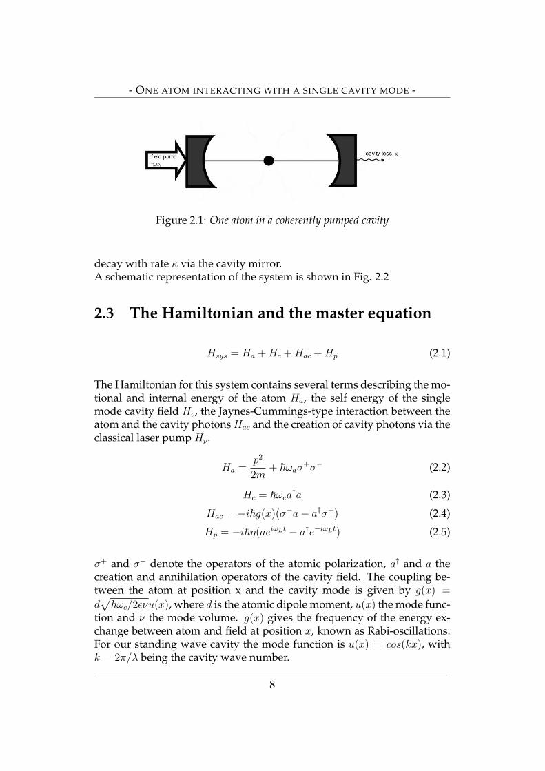
Figure 2.1: One atom in a coherently pumped cavity
decay with rate κ via the cavity mirror.A schematic representation of the system is shown in Fig. 2.2
2.3 The Hamiltonian and the master equation
Hsys = Ha + Hc + Hac + Hp (2.1)
The Hamiltonian for this system contains several terms describing the mo-tional and internal energy of the atom Ha, the self energy of the singlemode cavity field Hc, the Jaynes-Cummings-type interaction between theatom and the cavity photons Hac and the creation of cavity photons via theclassical laser pump Hp.
Ha =p2
2m+ ~ωaσ
+σ− (2.2)
Hc = ~ωca†a (2.3)
Hac = −i~g(x)(σ+a− a†σ−) (2.4)
Hp = −i~η(aeiωLt − a†e−iωLt) (2.5)
σ+ and σ− denote the operators of the atomic polarization, a† and a thecreation and annihilation operators of the cavity field. The coupling be-tween the atom at position x and the cavity mode is given by g(x) =
d√~ωc/2ενu(x), where d is the atomic dipole moment, u(x) the mode func-
tion and ν the mode volume. g(x) gives the frequency of the energy ex-change between atom and field at position x, known as Rabi-oscillations.For our standing wave cavity the mode function is u(x) = cos(kx), withk = 2π/λ being the cavity wave number.
8
- ONE ATOM INTERACTING WITH A SINGLE CAVITY MODE -
In order to get rid of the explicit time dependence appearing in Hp weapply the unitary transformation U on the Hamiltonian Hsys so we get thenew Hamiltonian H in a frame rotating with the pump frequency ωL.
U = eiωLt(a†a + σ+σ−) (2.6)
H = UHsysU† + i~(
dU
dt)U † (2.7)
The new Hamiltonian in a rotating frame, where ∆a = (ωL − ωa), ∆c =(ωL− ωc) are the frequency shifts for the atom and the cavity mode, reads:
H =p2
2m− ~∆aσ
+σ− − ~∆ca†a− i~g(x)(σ+a− a†σ−)− i~η(a− a†) (2.8)
As mentioned above, in our model there is no spontaneous emission ofphotons by the atom, which is approximately true if the photon scatteringrate Γ0 - which describes the loss of photons via the atom - tends to zero.
Γ0 =γ
∆2a + γ2
g20n . (2.9)
Here γ denotes the spontaneous emission rate of the atom (inverse linewidth),g0 = d
√~ωc/2εν is the coupling constant and n the average photon num-
ber.This is true for large atomic detuning
∆a À γ . (2.10)
To complete the Hamiltonian we have to add another term describingthe interaction of the cavity field with the environment, i.e. the annihila-tion of a cavity photon and the simultaneous creation of a photon in thereservoir
Vcr = ~∫
dω B(ω)(b(ω) + b†(ω)
)(a + a†) . (2.11)
Where b(ω) are the bosonic field operators of the reservoir. They fulfill[b(ω), b†(ω′)
]= δ(ω − ω′) . (2.12)
The evolution of the system can be described in terms of the densityoperator
ρtot(t) = − i
~[Htot(t), ρtot(t)
], (2.13)
with the total Hamiltonian Htot = Hsys+Vcr. We cannot solve this equationin general but with a few approximations the equation becomes solvable:
9
- ONE ATOM INTERACTING WITH A SINGLE CAVITY MODE -
• The initial state of system and reservoir is assumed to be not entan-gled.
• Markoff-approximation: The autocorrelation time τc (i.e. the inversebandwidth) of the reservoir is much smaller than any other charac-teristic time scale of the system.
• The density operator can be factorized for all times, which means thereservoir has to be large enough that the backaction of the system canbe widely neglected.
ρtot(t) = ρsys(t) ⊗ | vac >< vac | (2.14)
By applying these approximations we know the density operator for thesystem for all times by tracing out the environment
ρsys(t) = Trres
(ρtot(t)
)= ρ(t) , (2.15)
and we get the master equation [12]
ρ(t) = −i[Hsys, ρ(t)
]+ Lρ(t) . (2.16)
The Liouville operator L includes the effects of cavity losses due to cou-pling to the environment.The Hamiltonian and the Liouville operators in an interaction picture read
H =p2
2m− ~∆aσ
+σ−− ~∆ca†a− i~g(x)(σ+a− a†σ−)− i~η(a− a†) , (2.17)
Lρ(t) = κ(2aρa† − a†aρ− ρa†a) , (2.18)
where κ denotes the decay rate for the cavity mode.
2.4 Heisenberg-Langevin equations andthe low saturation limit
An equivalent way of treating this problem is via the Heisenberg-Langevinequations for the atomic and mode operators. The internal dynamics fol-low the equations
a = (i∆c − κ)a + g(x)σ− + η + ξ(t) (2.19)
σ− = i∆aσ− + g(x)σza + ξ(t) . (2.20)
10
- ONE ATOM INTERACTING WITH A SINGLE CAVITY MODE -
where ξ(t) denotes the noise operator [12]. Noise originates from fluctua-tions due to the coupling to the environment. The reservoir is assumed inthe vacuum state (T=0), hence their expectation values vanish:
< vac|ξ|vac >= 0. (2.21)
In the low saturation limit, which means that the atomic excited state isweakly populated, we can approximate the population inversion opera-tor σz by −1. Furthermore, in the good cavity limit (κ À g) the operatorsσ± evolve on a much faster timescale than the cavity field operators a, a†.Hence the atomic operators can be approximated by their stationary val-ues, i.e. we set σ± ≈ 0. This yields for the atomic dipole moment
σ− = −ig(x)
∆a
a . (2.22)
By inserting this in the equation for the cavity field, we get
a = −κa + i(∆c − U0u
2(x))a + η , (2.23)
where U0 =g20
∆ais a measure for the shift of the cavity resonance frequency
caused by the presence of the atom at position x. The atom shifts the cavityfield into resonance with the pumping field if U0 ≈ ∆c.
2.5 Steady state dynamics,mean photon number and the force
As already mentioned in the previous section, the atom causes an effectivecavity frequency shift which depends on the position distribution of theatom, i.e. the atom acts as a refractive index.In order to get an overview of these dynamics it is useful to have a lookat the steady state situation, i.e. the limit of a very slow atom such that astationary value of the field according to the atom’s position is obtained.
Taking the expectation value of the above equation for the cavity field(2.23) and substituting < a >= α, one gets the equation for the coherentfield amplitude α
α = −κ + i(∆c − U0u
2(x))α + η . (2.24)
By setting α = 0, the steady state solution can be easily calculated
αs =η
−κ + i(∆c − U0u2(x)
) . (2.25)
11
- ONE ATOM INTERACTING WITH A SINGLE CAVITY MODE -
-3 -2 -1 1 2 3
200
250
300
mean photon number n�
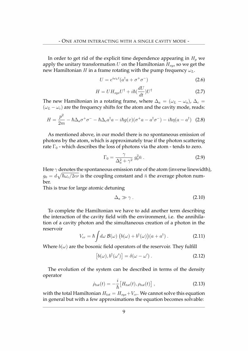
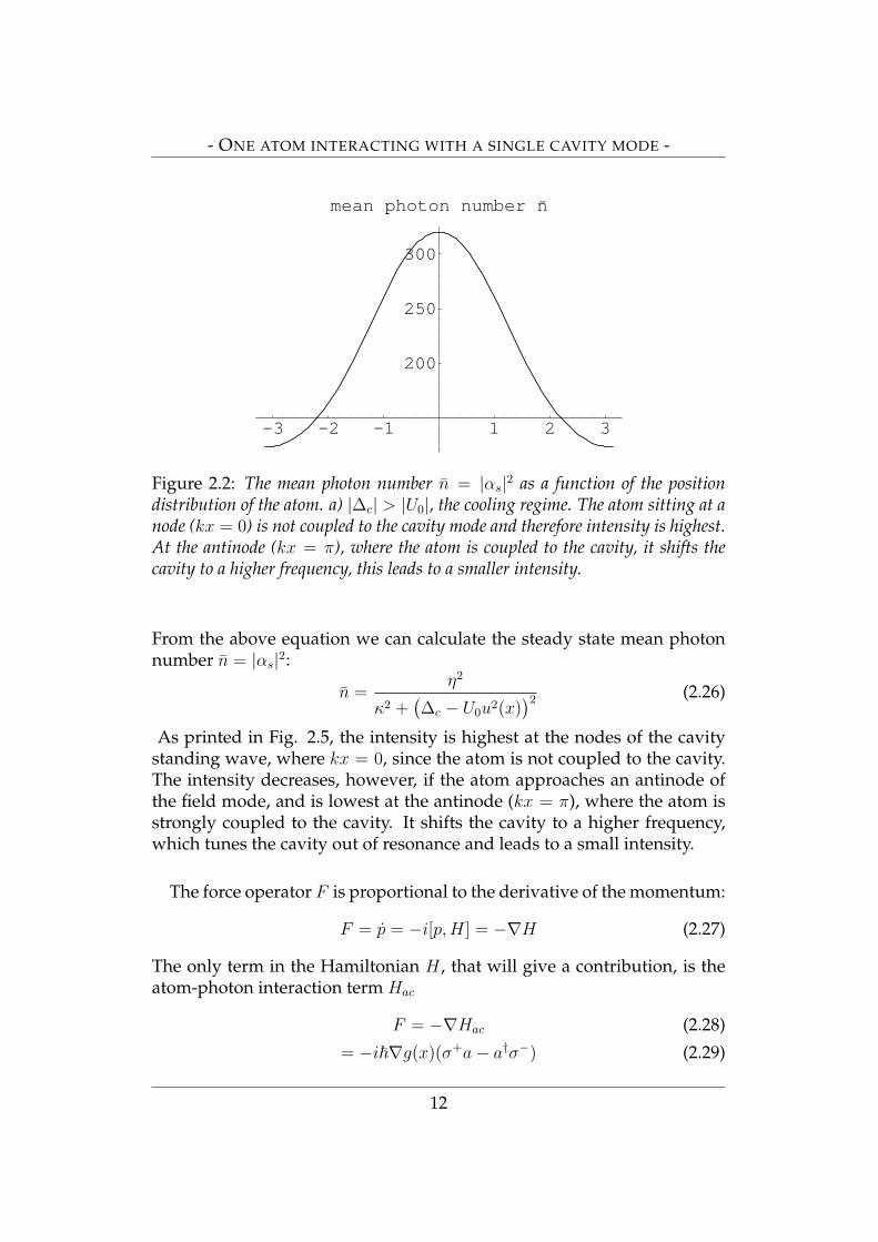
Figure 2.2: The mean photon number n = |αs|2 as a function of the positiondistribution of the atom. a) |∆c| > |U0|, the cooling regime. The atom sitting at anode (kx = 0) is not coupled to the cavity mode and therefore intensity is highest.At the antinode (kx = π), where the atom is coupled to the cavity, it shifts thecavity to a higher frequency, this leads to a smaller intensity.
From the above equation we can calculate the steady state mean photonnumber n = |αs|2:
n =η2
κ2 +(∆c − U0u2(x)
)2 (2.26)
As printed in Fig. 2.5, the intensity is highest at the nodes of the cavitystanding wave, where kx = 0, since the atom is not coupled to the cavity.The intensity decreases, however, if the atom approaches an antinode ofthe field mode, and is lowest at the antinode (kx = π), where the atom isstrongly coupled to the cavity. It shifts the cavity to a higher frequency,which tunes the cavity out of resonance and leads to a small intensity.
The force operator F is proportional to the derivative of the momentum:
F = p = −i[p,H] = −∇H (2.27)
The only term in the Hamiltonian H , that will give a contribution, is theatom-photon interaction term Hac
F = −∇Hac (2.28)
= −i~∇g(x)(σ+a− a†σ−) (2.29)
12
- ONE ATOM INTERACTING WITH A SINGLE CAVITY MODE -
If we do the adiabatic elimination σ± ≈ 0 of the atomic operators σ+ andσ−, we get for their stationary values:
σ+ = ig(x)
∆a
a†
σ− = −ig(x)
∆a
a (2.30)
By inserting these equations in eq.3.2, we get an effective Hamiltonian
Heff =p2
2m− ~(∆c − U0u
2(x))a†a− i~η(a− a†) , (2.31)
where U0 =g20
∆a, as specified above.
Now we can find the force acting on a motionless atom by taking thedirectional derivative of the effective Hamiltonian Heff
F (x) = −~U0
(∇u2(x))a†a (2.32)
When we take the mean value of the force, we can insert the mean photonnumber (2.26) for < a†a >= |α|2 and get
F (x) = −~U0
(∇u2(x))n
= −~U0η2 ∇u2(x)
κ2 +(∆c − U0 < u2(x) >
)2 (2.33)
Hence the force is proportional to the photon number and the gradient ofthe square of the mode function.For U0 > 0 the atom is drawn to field maxima (high field seekers), whileU0 < 0 corresponds to low field seeking atoms.
13
Chapter 3
One atom in a time-dependentharmonic trap
3.1 Introduction
In most applications of laser-atom interaction, the backaction of the atom(s)on the field can be largely neglected. For large enough atom-field detun-ing the influence of atoms on the field can be understood as a kind ofdynamic refractive index. The field then forms a time dependent potentialin the atomic Hamiltonian. In order to study this backaction, we consideran atom strongly coupled to a single mode of a driven high-Q optical res-onator. The laser field is chosen far off resonance with the atomic transi-tion frequency but close to cavity resonance, such that a coherent field canbuild up in the cavity but almost no spontaneous emission occurs. Thus,the atom basically acts as a moving refractive index, being large close toantinodes and showing almost no effect at a node of the cavity mode. Ina first approximation the system can be related to a particle in a time-dependent harmonic trap, which is formed by the cavity field. For thiswe consider the atom well localized around a field antinode, where it seesa potential minimum. This allows to replace the optical potential locallyby a harmonic potential. This suggests a mapping to a harmonic oscillatorwith time-dependent frequency. A method using parametrized oscillatoreigenfunctions for any given ω(t) to solve such problems has been pre-sented by Lewis and Riesenfeld [13]. In our case, however, we have noprescribed explicit form for the time-dependent frequency ω(t) and thuswe will go for numerical solutions for the atomic expectation values andfinding the field dynamics in parallel.
14
- ONE ATOM IN A TIME-DEPENDENT HARMONIC TRAP -
In this chapter, we investigate the coupled quantum dynamics of anatom in the cavity field by studying a system of an atom in a time-dependentharmonic trap. As a first step we start with a fixed harmonic potential andtreat the time dependence by a time-dependent perturbation δ(t)x2. Wewill model the optical potential by a harmonic potential and rewrite theHamiltonian for the atomic energy as a harmonic oscillator of frequencyω0 to which the small perturbation δ(t)x2 is added. To check the validity ofthis perturbation expansion, we will keep δ constant and see if we get thesame results as for a Hamiltonian with ω2 = ω2
0 + δ. Then we will applythis model to a time-dependent perturbation δ(t) where we will find, thatthe system traps and localizes itself dynamically due to the backaction ofthe atom on the field.
3.2 The model
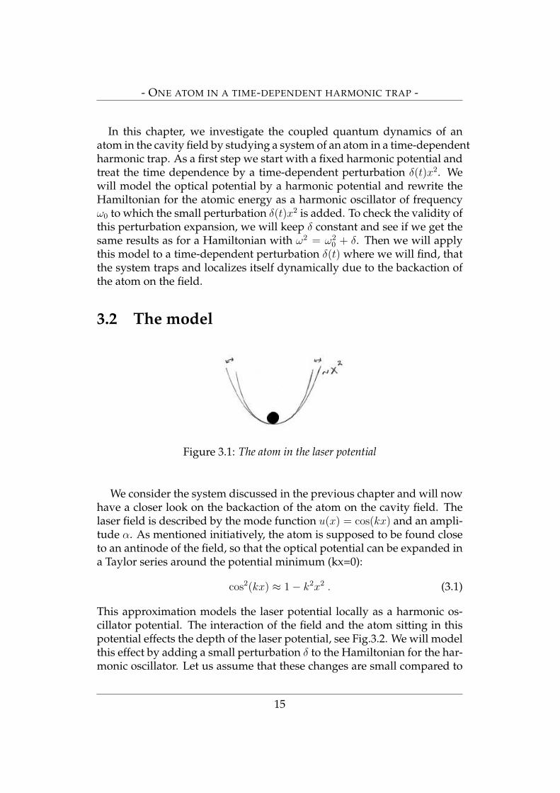
Figure 3.1: The atom in the laser potential
We consider the system discussed in the previous chapter and will nowhave a closer look on the backaction of the atom on the cavity field. Thelaser field is described by the mode function u(x) = cos(kx) and an ampli-tude α. As mentioned initiatively, the atom is supposed to be found closeto an antinode of the field, so that the optical potential can be expanded ina Taylor series around the potential minimum (kx=0):
cos2(kx) ≈ 1− k2x2 . (3.1)
This approximation models the laser potential locally as a harmonic os-cillator potential. The interaction of the field and the atom sitting in thispotential effects the depth of the laser potential, see Fig.3.2. We will modelthis effect by adding a small perturbation δ to the Hamiltonian for the har-monic oscillator. Let us assume that these changes are small compared to
15
- ONE ATOM IN A TIME-DEPENDENT HARMONIC TRAP -
the average field.The Hamiltonian for the atom then reads
H(t) = H0 + δ(t)x2 , (3.2)
with
H0 =p2
2m+
mω20
2x2 . (3.3)
H(t) thus describes a harmonic oscillator with time dependent frequency.We will perform this approximation by rewriting the Hamiltonian withfrequency ω as harmonic oscillator H0 to which the perturbation term δx2
is added
H(t) =p2
2m+
mω(t)2
2x2
=p2
2m+
mω20
2x2 +
m
2(ω2 − ω2
0)︸ ︷︷ ︸δ(t)
x2 . (3.4)
One can see, δ is proportional to the difference of the frequency ω and theharmonic oscillator eigenfrequency
δ(t) =m
2(ω(t)2 − ω2
0) . (3.5)
Rewriting ω in terms of the potential depth, which depends on the photonnumber |α|2, we get
ω(t)2 =2
mU0|αt|2 . (3.6)
In order to calculate ω0 in a way to keep δ(t) small, we choose the averagefield amplitude |α0|2 in the unperturbed system (δ = 0), and by taking< x2 >= 0, as a reference field.α0 = α|<x2>=0
|α0|2 =η2
κ2 + (∆c − U0)2. (3.7)
With this, we can calculate the Eigenfrequency in terms of the field ampli-tude
ω20 =
2
mU0|α0|2 . (3.8)
Inserting the equations for ω and ω0 in equation (3.5) we get the time-dependent δ(t)
δ(t) = U0(|αt|2 − |α0|2) . (3.9)
16
- ONE ATOM IN A TIME-DEPENDENT HARMONIC TRAP -
3.3 Time-independent treatment
The idea is now to use the eigenstates of H0 as a basis for the time-dependentcalculation.Nevertheless, at first we choose δ time-independent, in order to test thevalidity of the model and the calculations.For a time-independent δ the results for the expectation values of positionand momentum of the atom have to be the same as the solutions for theharmonic oscillator of frequency ω expressed in the basis ω0. We will see inthe further treatment, if we do our calculations in the basis of the harmonicoscillator | φi > the corrections to the expectation values for the atom willbe proportional c∗ncn′ and therefore will have no effect. Of course, the addi-tional term δx2 will lead to a coupling of the equations for the coefficientscn(t), meaning that coefficients that initially are zero will start oscillating.
In order to calculate the expectation values for the system we expandthe wavefunction | ψ > in the Eigenbasis | φn > of the harmonic oscillatorH0
| ψ >=∞∑
n=0
cn | φn >, (3.10)
and insert this ansatz in the Schrodinger equation, where we used theHamiltonian (3.2).
< φm |/
i ˙| ψ > = H | ψ > (3.11)
By doing the scalar product with < φm | we get the differential equationfor the coefficients
cm = −iωmcm − icnδ < φm | x2 | φn >︸ ︷︷ ︸kmn
, (3.12)
where kmn are the elements of the matrix
K =1
2mω
. . . 0. . . 0 0
0. . . 0
√n + 1
√n + 2 0
. . . 0 2n + 1 0. . .
0√
n + 1√
n + 2 0. . . 0
0 0. . . 0
. . .
. (3.13)
17
- ONE ATOM IN A TIME-DEPENDENT HARMONIC TRAP -
So we have a set of coupled differential equations for the coefficients:
cm = −iωmcm − iδ
2mωkmncn . (3.14)
We find the numerical solutions and calculate the expectation values forthe position < x > and momentum < p > of the atom
< x >=< ψ | x | ψ >=∑
n,n′Lnn′c
∗ncn′ , (3.15)
< p >=< ψ | p | ψ >=∑
n,n′Mnn′c
∗ncn′ . (3.16)
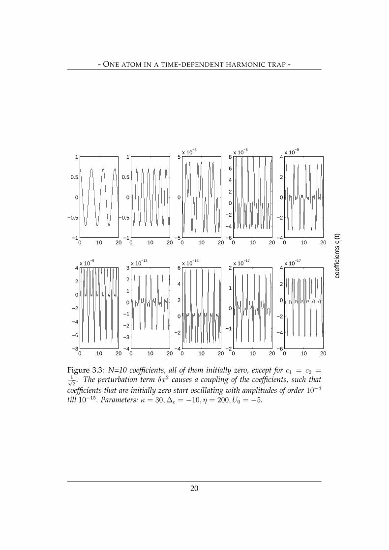
Where L and M are the matrices we find when calculating the expectationvalues < φ | x | φ > and < φ | p | φ > in the basis | φ > of the harmonicoscillator. As one can see in the above equations, the solutions for a time-independent δ are similar to the solutions for the harmonic oscillator H0,since the real numbers c∗ncn′ do not contribute to the expectation values.But, as the additional term δx2 causes a coupling of the coefficients, thecoefficients that are initially zero start oscillating with amplitudes of order10−4 till 10−15, see Fig. 3.4. We choose the initial wavefunction as a super-position of the ground state and the first excited state of the unperturbedoscillator. The operating parameters are chosen: ∆c = −10 and U0 = −5.
We compare the solutions of the method described above with the nu-merical solutions of the coupled differential equations that we derive fromthe time-independent Hamiltonian with frequency ω:
H =p2
2m+
mω2
2x2 (3.17)
where ω2 = 2m
δ + ω20 .
d
dt(x2) = −i[x2, H] =
1
m(xp + px) (3.18)
d
dt(p2) = −i[p2, H] = −mω2(xp + px) (3.19)
d
dt(xp + px) = −i[xp + px,H] = 2
p2
m− 2mω2x2 (3.20)
d
dt(x) = −i[x,H] =
p
m(3.21)
18
- ONE ATOM IN A TIME-DEPENDENT HARMONIC TRAP -
0 2 4 6 8 10 12 14 16 18 20−0.04
−0.02
0
0.02
0.04<x>
0 2 4 6 8 10 12 14 16 18 20−15
−10
−5
0
5
10
15
κ = 30, ∆c = −10, η = 200, U
0 = −5
<p>
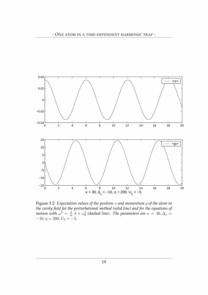
Figure 3.2: Expectation values of the position x and momentum p of the atom inthe cavity field for the perturbational method (solid line) and for the equations ofmotion with ω2 = 2
mδ + ω2
0 (dashed line). The parameters are κ = 30, ∆c =−10, η = 200, U0 = −5.
19
- ONE ATOM IN A TIME-DEPENDENT HARMONIC TRAP -
0 10 20−1
−0.5
0
0.5
1
0 10 20−1
−0.5
0
0.5
1
0 10 20−5
0
5x 10
−5
0 10 20−6
−4
−2
0
2
4
6
8x 10
−5
0 10 20−4
−2
0
2
4x 10
−9
0 10 20−8
−6
−4
−2
0
2
4x 10
−9
0 10 20−4
−3
−2
−1
0
1
2
3x 10
−13
0 10 20−4
−2
0
2
4
6x 10
−13
0 10 20−2
−1
0
1
2x 10
−17
0 10 20−6
−4
−2
0
2
4x 10
−17
coef
ficie
nts
c i(t)
Figure 3.3: N=10 coefficients, all of them initially zero, except for c1 = c2 =1√2. The perturbation term δx2 causes a coupling of the coefficients, such that
coefficients that are initially zero start oscillating with amplitudes of order 10−4
till 10−15. Parameters: κ = 30, ∆c = −10, η = 200, U0 = −5.
20
- ONE ATOM IN A TIME-DEPENDENT HARMONIC TRAP -
d
dt(p) = −i[p,H] = −mω2x (3.22)
These coupled differential equations are fairly easy to solve numerically,independent of the form of the initial wavefunction.We find the same curves when we plot the expectation values < x > and< p >, as shown in Fig. 3.3.Hence we see that our model works out right and we will use it to calculatethe time-dependent Hamiltonian H(t) in the next section and we will alsoapply it on the calculations for a system of two atoms inside a cavity, whichwill be performed in the next chapter.
3.4 Time-dependent perturbation δ(t)
Now lets come to the full time dependent case and include the equationfor αt as well.In the case of a time-dependent system, the Hamiltonian reads
H(t) =p2
2m+
m
2ω(t)2x2 (3.23)
Again, we split the Hamiltonian into a harmonic part plus the time-dependentperturbation term
H(t) = H0 + δ(t)x2 (3.24)
withδ(t) = U0(|αt|2 − |α0|2) (3.25)
now being time-dependent.Again we solve the equations
cm = −iωmcm − iδ(t)
2mωkmncn (3.26)
andαt = −κ + i
(∆c − U0(1− k2 < x2 >)
)α + η , (3.27)
numerically. Note that Eq. (3.27) contains < x2 > which depends on thestate of the atom described by the cn.
Again, we choose the initial wavefunction as a superposition of theground state and the first excited state and take a weak initial value forthe field α(0) = 1. The operating parameters ∆c = −10 and U0 = −5 arechosen such that the system is in the cooling regime, the optical potential
21
- ONE ATOM IN A TIME-DEPENDENT HARMONIC TRAP -
0 5 10 15 20 25 30 35 40 45 50−0.03
−0.02
−0.01
0
0.01
0.02
0.03<x>
0 5 10 15 20 25 30 35 40 45 50−40
−20
0
20
40
κ = 1, ∆c = 10, η = 200, U
0 = −5
<p>
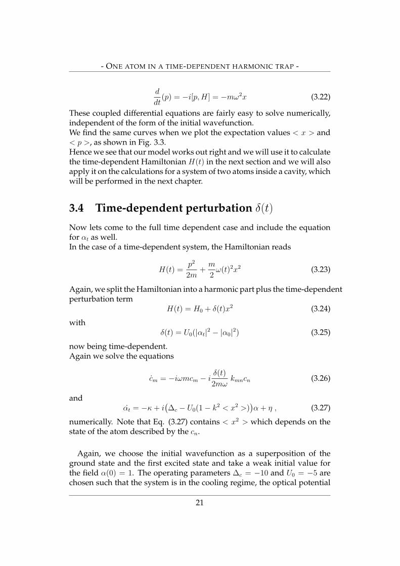
Figure 3.4: Expectation values for the position and momentum of the atom. Theexpectation values < x > and < p > are damped. We chose κ = 1, ∆c = 10, η =200, U0 = −5.
22
- ONE ATOM IN A TIME-DEPENDENT HARMONIC TRAP -
0 5 10 15 20 25 30 35 40 45 50−5
0
5
10
15x 10
−4
<x²>
0 5 10 15 20 25 30 35 40 45 500
500
1000
1500<p²>
0 5 10 15 20 25 30 35 40 45 50−10
0
10
20
κ = 1, ∆c = 10, η = 200, U
0 = −5
<α>
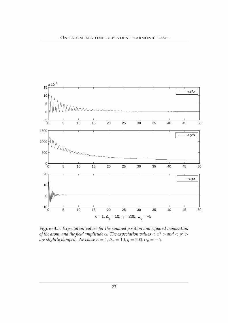
Figure 3.5: Expectation values for the squared position and squared momentumof the atom, and the field amplitude α. The expectation values < x2 > and < p2 >are slightly damped. We chose κ = 1, ∆c = 10, η = 200, U0 = −5.
23
- ONE ATOM IN A TIME-DEPENDENT HARMONIC TRAP -
0 50−1
−0.5
0
0.5
1
0 50−0.6
−0.4
−0.2
0
0.2
0.4
0.6
0.8
0 50−0.4
−0.3
−0.2
−0.1
0
0.1
0.2
0.3
0 50−0.3
−0.2
−0.1
0
0.1
0.2
0.3
0.4
0 50−0.1
−0.05
0
0.05
0.1
0 50−0.15
−0.1
−0.05
0
0.05
0.1
0 50−0.03
−0.02
−0.01
0
0.01
0.02
0.03
0 50−0.04
−0.02
0
0.02
0.04
0.06
0 50−0.01
−0.005
0
0.005
0.01
0 50−0.02
−0.015
−0.01
−0.005
0
0.005
0.01
0.015
coef
ficie
nts
c i(t)
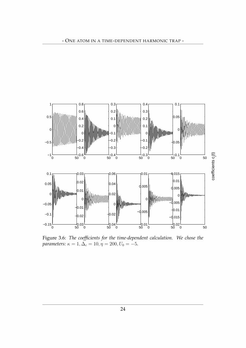
Figure 3.6: The coefficients for the time-dependent calculation. We chose theparameters: κ = 1, ∆c = 10, η = 200, U0 = −5.
24
- ONE ATOM IN A TIME-DEPENDENT HARMONIC TRAP -
attracts the atom. Looking at Fig. 3.4, we see, that the the average potentialenergy proportional < x2(t) > and the cavity field amplitude α(t) tend toa stationary value, while the atomic motion is very weakly damped (Fig.3.4). Hence, after some time the atom oscillates in self generated deep po-tential well with an almost constant field, i.e. the system dynamically trapsand localizes itself around an antinode of the field. In contrast to classicalmechanics, quantum mechanics allows states where < x2(t) > is constantwhile < x(t) > is oscillating.
Cavity cooling in the quantum regime:The cavity damping is used to extract energy from the system which al-lows dynamic localization of the wavefunction.If ∆a < 0, which is equivalent to a red detuning from the transition fre-quency, the atom is pushed towards a field antinode, where it is stronglycoupled to the field. When the atom moves away from a node, the in-tensity in the high-finesse cavity does not drop instantaneously, but leadsto an increase of the energy stored in the field. The photons escape fromthe cavity and this extracts kinetic energy from the atom. The effect ofacceleration of the atom when approaching the antinode is much smallerbecause the intracavity intensity there is small. This cooling process doesnot require atomic excitation and the lowest attainable temperature is notlimited by atomic linewidth but by the cavity linewidth.
25
Chapter 4
Two interacting atoms inside acavity
4.1 Introduction
We have seen in the one atom case, using the coupled atom-field dynam-ics, that the atom generates a potential well, where it traps itself dynami-cally.Now if we put two atoms in the cavity together, they interact with thesame field and although they are localized at distant positions they seeeach other through the cavity field. So even without direct coupling be-tween the atoms one atom can influence the other because they commu-nicate via the same field [14]. We additionally take into account a directinteraction between the atoms, i.e. if we allow collisions between themin our model. The interaction-potential is modelled by a delta-functionmultiplied with the parameter a which describes the interaction strength[15] between the atoms: V (x1, x2) = a δ(x1 − x2). This shape-independentapproximation where the physical interaction is replaced by a point-likepotential of zero range is well justified for ultracold atoms since theirde Broglie wavelength is large enough to neglect the finer details of the in-teraction potential. One can relate the one-dimensional parameter a withthe scattering length in 3 dimensions.
4.2 The Hamiltonian
We now are interested in the effects of two atoms in a cavity. The laserfield is described by the mode function u(x) = cos(kx). The approxima-tion u2(x) ≈ 1 − k2x2 near the potential minima we already introduced in
26
- TWO INTERACTING ATOMS INSIDE A CAVITY -
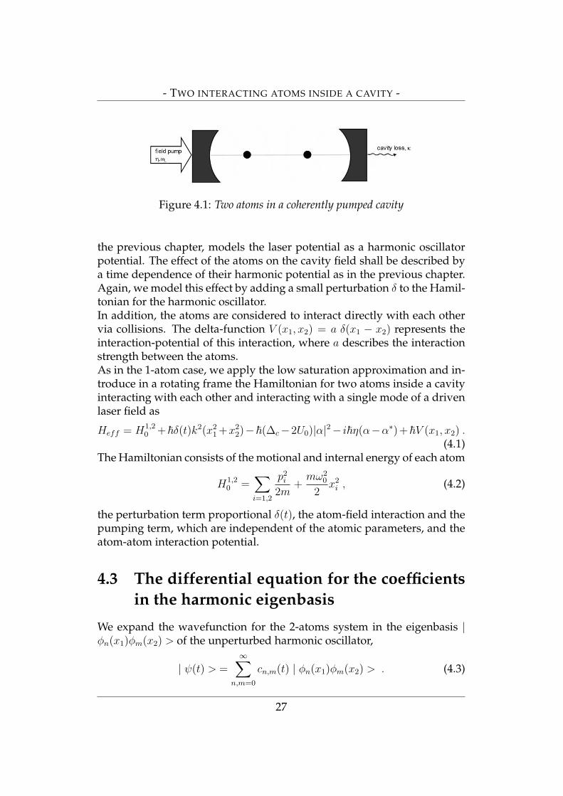
Figure 4.1: Two atoms in a coherently pumped cavity
the previous chapter, models the laser potential as a harmonic oscillatorpotential. The effect of the atoms on the cavity field shall be described bya time dependence of their harmonic potential as in the previous chapter.Again, we model this effect by adding a small perturbation δ to the Hamil-tonian for the harmonic oscillator.In addition, the atoms are considered to interact directly with each othervia collisions. The delta-function V (x1, x2) = a δ(x1 − x2) represents theinteraction-potential of this interaction, where a describes the interactionstrength between the atoms.As in the 1-atom case, we apply the low saturation approximation and in-troduce in a rotating frame the Hamiltonian for two atoms inside a cavityinteracting with each other and interacting with a single mode of a drivenlaser field as
Heff = H1,20 +~δ(t)k2(x2
1 +x22)−~(∆c−2U0)|α|2− i~η(α−α∗)+~V (x1, x2) .
(4.1)The Hamiltonian consists of the motional and internal energy of each atom
H1,20 =
∑i=1,2
p2i
2m+
mω20
2x2
i , (4.2)
the perturbation term proportional δ(t), the atom-field interaction and thepumping term, which are independent of the atomic parameters, and theatom-atom interaction potential.
4.3 The differential equation for the coefficientsin the harmonic eigenbasis
We expand the wavefunction for the 2-atoms system in the eigenbasis |φn(x1)φm(x2) > of the unperturbed harmonic oscillator,
| ψ(t) > =∞∑
n,m=0
cn,m(t) | φn(x1)φm(x2) > . (4.3)
27
- TWO INTERACTING ATOMS INSIDE A CAVITY -
By inserting this wavefunction in the Schrodinger equation
| ψ(t) >= − i
~Heff | ψ(t) > (4.4)
we get the following differential equation for each coefficient ckl(t)
ckl(t) = −i(ω0(k + l)ckl − iEαckl + δ(t)A+ U)
, (4.5)
As Eα is independent of n,m, k, l, it gives only a global phase shift. So wewill omit this term in the further calculations.
Eα = i(∆c − 2U0)|α|2 − η(α− α∗) (4.6)
A contributes to the perturbation term, which is calculated via the expec-tation values for the unperturbed system
A =∑n,m
k2cnm(t) < φ1kφ
2l |(x2
1 + x22)|φ1
nφ2m > , (4.7)
which yields
A =k2x2
0
2
∑n,m
cnm(t)(δlmxkn + δknxlm)
=k2x2
0
2
∑n,m
(cnl(t)xkn + ckm(t)xlm) .
The xij denote the matrix elements we get when calculating the expecta-tion values for the harmonic system and k2 is the wave vector of the fieldmode.As the first nontrivial case we restrict ourselves to n,m = 1, 2. Hence,we only take into account the first two levels in the harmonic oscillatorpotential for each atom. The wavefunction for the system then reads
| ψ > = c11 | φ0(x1)φ0(x2) > + c12 | φ0(x1)φ1(x2) > +
c21 | φ1(x1)φ0(x2) > + c22 | φ1(x1)φ1(x2) > . (4.8)
The coefficients describe both atoms in the ground state (c11), one atom inthe ground state, one atom in the first excited state and vice versa (c12, c21)and both atoms in the first excited state (c22).Taking into account that we are dealing with only 2 states of the atoms, weget
A =k2x2
0
2(2x11c11 + 2x22c22 + (x12 + x21)(c12 + c21)) , (4.9)
28
- TWO INTERACTING ATOMS INSIDE A CAVITY -
which yields the matrix
A =k2x2
0
2
6 0 0 00 8 0 00 0 8 00 0 0 10
. (4.10)
As one can see, the matrix is diagonal and does not couple different co-efficients ckl. Hence, the perturbation thus does not lead to vibrationaltransitions, but only to time dependent phase shifts.
The last term, describing the direct interaction between the two atoms,reads
U =∑n,m
cnm(t) < φ1kφ
2l |V (x1, x2)|φ1
nφ2m > . (4.11)
We model the potential by the delta function described above
V (x1, x2) = aδ(x1 − x2) , (4.12)
with a being the interaction parameter of the two atoms.Let us now have a deeper look at the scalar product in equation (4.11). Weintegrate the delta function and are left with the 1-dimensional integral
< φ1kφ
2l |δ(x1 − x2)|φ1
nφ2m >=
∫ ∫dx1dx2φ1∗
k φ2∗l δ(x1 − x2)φ
1nφ
2m
=
∫dx1φ∗kφ
∗l φnφm =: Uklnm . (4.13)
The two possible states for each atom are the ground state
φ0(x) = 4
√mω
~πe− 1
2( x
x0)2
, (4.14)
and the first excited state of the oscillator potential
φ1(x) =2x
x0
4
√mω
~πe− 1
2( x
x0)2
. (4.15)
If we are looking at the integrals Uklnm, we can exclude those combinationsof φi
′s that have an impair part of antisymmetric wavefunctions φ2, i.e.U1222, U1112, U2122, etc. , because integration of an odd function gives zero.We can separate the treatment of all other Uklnm into solving 3 different
29
- TWO INTERACTING ATOMS INSIDE A CAVITY -
integrals:case I: all φ are in the ground state
U1111 =mω
~π
∫dxe
−2( xx0
)2, (4.16)
case II: all φ are in the 1st excited state
U2222 =mω
~π
∫dx(2
x
x0
)4e−2( x
x0)2
, (4.17)
case III: two φ in ground state, two φ in the 1st excited state
Umixed =mω
~π
∫dx(2
x
x0
)2e−2( x
x0)2
, (4.18)
where the index ’mixed’ = 1212, 2121, 1122, 2211, 1221, 2112.The integrals are of the form:
∫ ∞
−∞e−px2
x2qdx =(2q − 1)!!
(2p)q
√π
p. (4.19)
In our case p = 1, q = 0, 1, 2. By substituting ξ =√
2 xx0−→ dx = x0√
2dξ and
writing the constant mω~ in terms of x0 we get
2q
x0π√
2
∫ ∞
−∞dξe−ξ2
ξ2q =2q
x0π√
2
(2q − 1)!!
2q
√π
=(2q − 1)!!
x0
√2π
. (4.20)
case I: q = 0∫∞−∞ dξe−ξ2
=√
π
U1111 =1
x0
√2π
. (4.21)
case II: q = 2∫∞−∞ dξ e−ξ2
ξ4
U2222 =3
x0
√2π
. (4.22)
case III: q = 1∫∞−∞ dξ e−ξ2
ξ2
Umixed =1
x0
√2π
, (4.23)
30
- TWO INTERACTING ATOMS INSIDE A CAVITY -
We resume the Uklnm in matrix form and obtain
U =1
x0
√2π
1 0 0 10 1 1 00 1 1 01 0 0 3
. (4.24)
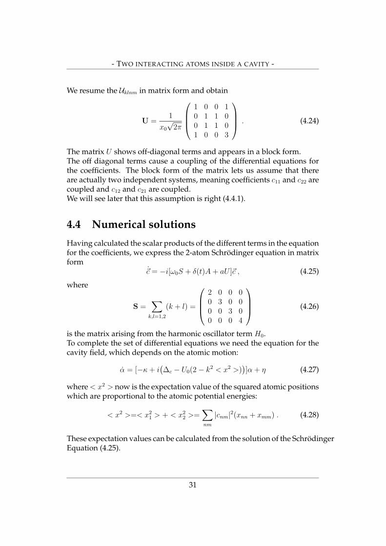
The matrix U shows off-diagonal terms and appears in a block form.The off diagonal terms cause a coupling of the differential equations forthe coefficients. The block form of the matrix lets us assume that thereare actually two independent systems, meaning coefficients c11 and c22 arecoupled and c12 and c21 are coupled.We will see later that this assumption is right (4.4.1).
4.4 Numerical solutions
Having calculated the scalar products of the different terms in the equationfor the coefficients, we express the 2-atom Schrodinger equation in matrixform
~c = −i[ω0S + δ(t)A + aU ]~c , (4.25)
where
S =∑
k,l=1,2
(k + l) =
2 0 0 00 3 0 00 0 3 00 0 0 4
(4.26)
is the matrix arising from the harmonic oscillator term H0.To complete the set of differential equations we need the equation for thecavity field, which depends on the atomic motion:
α = [−κ + i(∆c − U0(2− k2 < x2 >)
)]α + η (4.27)
where < x2 > now is the expectation value of the squared atomic positionswhich are proportional to the atomic potential energies:
< x2 >=< x21 > + < x2
2 >=∑nm
|cnm|2(xnn + xmm) . (4.28)
These expectation values can be calculated from the solution of the SchrodingerEquation (4.25).
31
- TWO INTERACTING ATOMS INSIDE A CAVITY -
Again as a reference state for detuning the unperturbed basis, we chooseα0 by setting < x2 >= 0α|<x2
1>+<x22>=0 = α0
|α0|2 =η2
κ2 + (∆c − 2U0)2. (4.29)
And the equation for δ(t) according to the previous chapter reads
δ(t) = ω2t − ω2
0 =2
mU0(|αt|2 − |α0|2) . (4.30)
We numerically solve the coupled differential equations
~c = −i[ω0S + δ(t)A + aU ]~c (4.31)
andα = [−κ + i(∆c − U0(2− k2 < x2 >))]α + η . (4.32)
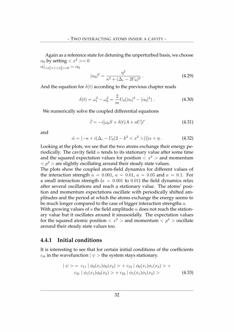
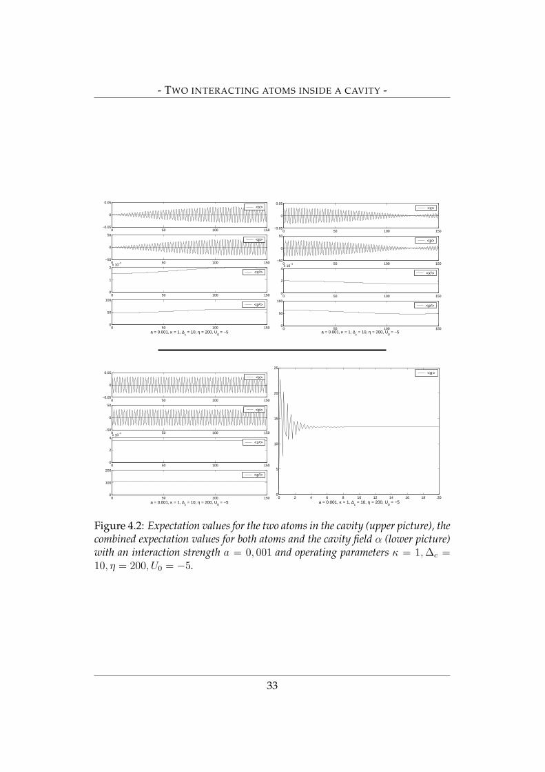
Looking at the plots, we see that the two atoms exchange their energy pe-riodically. The cavity field α tends to its stationary value after some timeand the squared expectation values for position < x2 > and momentum< p2 > are slightly oscillating around their steady state values.The plots show the coupled atom-field dynamics for different values ofthe interaction strength a = 0.001, a = 0.01, a = 0.05 and a = 0.1. Fora small interaction strength (a = 0.001 to 0.01) the field dynamics relaxafter several oscillations and reach a stationary value. The atoms’ posi-tion and momentum expectations oscillate with periodically shifted am-plitudes and the period at which the atoms exchange the energy seems tobe much longer compared to the case of bigger interaction strengths a.With growing values of a the field amplitude α does not reach the station-ary value but it oscillates around it sinusoidally. The expectation valuesfor the squared atomic position < x2 > and momentum < p2 > oscillatearound their steady state values too.
4.4.1 Initial conditions
It is interesting to see that for certain initial conditions of the coefficientscik in the wavefunction | ψ > the system stays stationary.
| ψ > = c11 | φ0(x1)φ0(x2) > + c12 | φ0(x1)φ1(x2) > +
c21 | φ1(x1)φ0(x2) > + c22 | φ1(x1)φ1(x2) > (4.33)
32
- TWO INTERACTING ATOMS INSIDE A CAVITY -
0 50 100 150−0.05
0
0.05<x>
0 50 100 150−50
0
50<p>
0 50 100 1500
1
2x 10
−3
<x²>
0 50 100 1500
50
100
a = 0.001, κ = 1, ∆c = 10, η = 200, U
0 = −5
<p²>
0 50 100 150−0.05
0
0.05<x>
0 50 100 150−50
0
50<p>
0 50 100 1500
2
4x 10
−3
<x²>
0 50 100 1500
50
100
a = 0.001, κ = 1, ∆c = 10, η = 200, U
0 = −5
<p²>
0 50 100 150−0.05
0
0.05<x>
0 50 100 150−50
0
50<p>
0 50 100 1500
2
4x 10
−3
<x²>
0 50 100 1500
100
200
a = 0.001, κ = 1, ∆c = 10, η = 200, U
0 = −5
<p²>
0 2 4 6 8 10 12 14 16 18 200
5
10
15
20
25
a = 0.001, κ = 1, ∆c = 10, η = 200, U
0 = −5
<α>
Figure 4.2: Expectation values for the two atoms in the cavity (upper picture), thecombined expectation values for both atoms and the cavity field α (lower picture)with an interaction strength a = 0, 001 and operating parameters κ = 1, ∆c =10, η = 200, U0 = −5.
33
- TWO INTERACTING ATOMS INSIDE A CAVITY -
0 5 10 15 20 25 30 35 40 45 50−0.05
0
0.05<x>
0 5 10 15 20 25 30 35 40 45 50−50
0
50<p>
0 5 10 15 20 25 30 35 40 45 500
2
4x 10
−3
<x²>
0 5 10 15 20 25 30 35 40 45 500
50
100
a = 0.01, κ = 1, ∆c = 10, η = 200, U
0 = −5
<p²>
0 5 10 15 20 25 30 35 40 45 50−0.05
0
0.05<x>
0 5 10 15 20 25 30 35 40 45 50−50
0
50<p>
0 5 10 15 20 25 30 35 40 45 500
2
4x 10
−3
<x²>
0 5 10 15 20 25 30 35 40 45 500
50
100
a = 0.01, κ = 1, ∆c = 10, η = 200, U
0 = −5
<p²>
0 5 10 15 20 25 30 35 40 45 50−0.05
0
0.05<x>
0 5 10 15 20 25 30 35 40 45 50−50
0
50<p>
0 5 10 15 20 25 30 35 40 45 500
2
4x 10
−3
<x²>
0 5 10 15 20 25 30 35 40 45 500
100
200
a = 0.01, κ = 1, ∆c = 10, η = 200, U
0 = −5
<p²>
0 5 10 15 20 25 30 35 40 45 500
5
10
15
20
25
a = 0.01, κ = 1, ∆c = 10, η = 200, U
0 = −5
<α>
Figure 4.3: Expectation values of the position x and momentum p of the firstand second atom in the cavity field (upper picture) and expectation values of theposition x and momentum p of both atoms in the cavity field and the expectationvalue of the cavity field α (lower picture). Parameters: κ = 1, ∆c = 10, η =200, U0 = −5, interaction strength a = 0, 01.
34
- TWO INTERACTING ATOMS INSIDE A CAVITY -
0 5 10 15 20 25 30 35 40 45 50−0.05
0
0.05<x>
0 5 10 15 20 25 30 35 40 45 50−50
0
50<p>
0 5 10 15 20 25 30 35 40 45 500
2
4x 10
−3
<x²>
0 5 10 15 20 25 30 35 40 45 500
50
100
a = 0.05, κ = 1, ∆c = 10, η = 200, U
0 = −5
<p²>
0 5 10 15 20 25 30 35 40 45 50−0.05
0
0.05<x>
0 5 10 15 20 25 30 35 40 45 50−50
0
50<p>
0 5 10 15 20 25 30 35 40 45 500
2
4x 10
−3
<x²>
0 5 10 15 20 25 30 35 40 45 500
50
100
a = 0.05, κ = 1, ∆c = 10, η = 200, U
0 = −5
<p²>
0 5 10 15 20 25 30 35 40 45 50−0.05
0
0.05<x>
0 5 10 15 20 25 30 35 40 45 50−50
0
50<p>
0 5 10 15 20 25 30 35 40 45 500
2
4x 10
−3
<x²>
0 5 10 15 20 25 30 35 40 45 500
100
200
a = 0.05, κ = 1, ∆c = 10, η = 200, U
0 = −5
<p²>
0 5 10 15 20 25 30 35 40 45 500
5
10
15
20
25
a = 0.05, κ = 1, ∆c = 10, η = 200, U
0 = −5
<α>
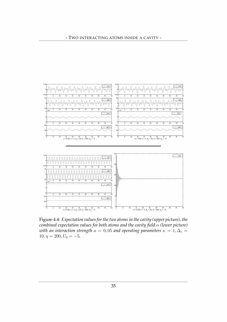
Figure 4.4: Expectation values for the two atoms in the cavity (upper picture), thecombined expectation values for both atoms and the cavity field α (lower picture)with an interaction strength a = 0, 05 and operating parameters κ = 1, ∆c =10, η = 200, U0 = −5.
35
- TWO INTERACTING ATOMS INSIDE A CAVITY -
0 5 10 15 20 25 30−0.05
0
0.05<x>
0 5 10 15 20 25 30−50
0
50<p>
0 5 10 15 20 25 300
2
4x 10
−3
<x²>
0 5 10 15 20 25 300
50
100
a = 0.1, κ = 1, ∆c = 10, η = 200, U
0 = −5
<p²>
0 5 10 15 20 25 30−0.05
0
0.05<x>
0 5 10 15 20 25 30−50
0
50<p>
0 5 10 15 20 25 300
2
4x 10
−3
<x²>
0 5 10 15 20 25 300
50
100
a = 0.1, κ = 1, ∆c = 10, η = 200, U
0 = −5
<p²>
0 5 10 15 20 25 30−0.05
0
0.05<x>
0 5 10 15 20 25 30−50
0
50<p>
0 5 10 15 20 25 300
2
4x 10
−3
<x²>
0 5 10 15 20 25 300
100
200
a = 0.1, κ = 1, ∆c = 10, η = 200, U
0 = −5
<p²>
0 5 10 15 20 25 300
5
10
15
20
25
a = 0.1, κ = 1, ∆c = 10, η = 200, U
0 = −5
<α>
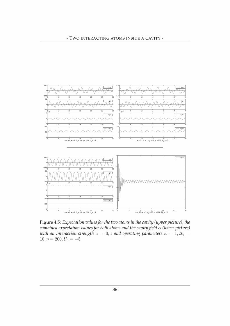
Figure 4.5: Expectation values for the two atoms in the cavity (upper picture), thecombined expectation values for both atoms and the cavity field α (lower picture)with an interaction strength a = 0, 1 and operating parameters κ = 1, ∆c =10, η = 200, U0 = −5.
36
- TWO INTERACTING ATOMS INSIDE A CAVITY -
As an example, if the system initially is in a superposition of both atomsin the ground state and both atoms in the first excited state (c11 = c22 =1√2
, c12 = c21 = 0), i.e.
| ψ > =1√2| φ0(x1)φ0(x2) > +
1√2| φ1(x1)φ1(x2) >, (4.34)
the expectation values for the position and momentum remain stationarywhile those for the potential and kinetic energies of each atom are slightlyoscillating. The field is damped after some oscillations but it keeps oscillat-ing with bigger a amplitude the bigger the value of the atomic interactionstrength a.If we choose the superposition of one atom being in the ground state, thesecond in the first excited state and vice versa, i.e. c12 = c21 = 1√
2, c11 =
c22 = 0,
| ψ > =1√2| φ0(x1)φ1(x2) > +
1√2| φ1(x1)φ0(x2) > , (4.35)
the expectation values for the position and momentum and the squaredposition and squared momentum remain stationary. The field is oscillat-ing and reaches a stationary value after some time independent of the in-teraction strength a between the atoms.
Recalling the matrix U , which describes the direct interaction betweenthe two atoms,
U =1
x0
√2π
1 0 0 10 1 1 00 1 1 01 0 0 3
, (4.36)
we see that the observations described above are a consequence of thespecial shape of the matrix U . As we already assumed in section 4.3, if wetake either c11, c22 non-zero or c12, c21 non-zero for the initial conditions,the cases described above will occur because the differential equations for˙c11 and ˙c22 such as ˙c12 and ˙c21 are not independent.
On the other hand, if we initially take any mixture of the two sets, sayc11 = c12 = 1√
2, c22 = c21 = 0,
| ψ > =1√2| φ0(x1)φ0(x2) > +
1√2| φ0(x1)φ1(x2) > , (4.37)
the atomic position and momentum expectation values oscillate with shiftedperiodically varying amplitudes, as shown in fig 4.4, where we chose the
37

- TWO INTERACTING ATOMS INSIDE A CAVITY -
above initial condition.
There is another interesting feature if we are looking at the matrix Aarising from the perturbation term. As we already pointed out in section4.3, the matrix A is diagonal. We compare it with the matrix K (Eq.(3.13),section 3.3) in the perturbation term in the one atom case, where the matrixis of the form
K =1
2mω
. . . 0. . . 0 0
0. . . 0
√n + 1
√n + 2 0
. . . 0 2n + 1 0. . .
0√
n + 1√
n + 2 0. . . 0
0 0. . . 0
. . .
. (4.38)
in contrast to the matrix K in the perturbation term for the one-atom case,which shows entries in the main diagonal and in the two second diag-onals. In the one-atom case this matrix causes the coupling of the dif-ferential equations for the coefficient with the effect, that coefficients thatinitially are zero start oscillating. The coupling does not effect the expec-tation values for the atom and field.Here, in the case of two atoms in the cavity, if we consider no interactionbetween the atoms, i.e. a=0, we make the following observations:If initially there is a superposition of both atoms in the ground state andboth atoms in the first excited state the system will remain steady, same forthe superposition of one atom in the ground state, one in the first excitedand vice versa. In the latter case this is also true for a 6= 0.For the remaining possible initial conditions only one atom remains steady,for the other one we find harmonically oscillating expectation values <x > and < p >. As an example, we initially take the first atom in theground state, the second in the first excited state and both atoms in thefirst excited state. We will see, only the first atom will have oscillatingexpectation values for < x > and < p >, the second will remain steady.
4.5 Self consistent eigenstates
Let us now try to investigate the stationary states of the system in moredetail.We are interested in an analytical treatment of the problem, so we consider
38
- TWO INTERACTING ATOMS INSIDE A CAVITY -
the algebraic method of finding stationary states of the atom field dynam-ics. The idea is to look for the eigensystem of the matrix equation (4.25) forthe coefficients in order to find a solution of the form c(t) = vie
−ipt spannedby the eigenvectos vi. Using such coefficients in Eq. (4.28) the calculationof the expectation values will yield constant values since the time depen-dence cancels. When we look for the corresponding field α which dependson < x2 >, thus will be a constant in this case. By these means we thenfound a stationary state of the total system. For self consistency we try tofind an η such that it matches the found α and δ.
To start, we first calculate the eigensystem of the matrix M appearing inthe differential equation for the coefficients
~c = −iM~c , (4.39)
whereM = [ω0S + δ(t)A + aU ] . (4.40)
Introducing the abbreviations u =k2x2
0
2and v = 1
x0
√2π
the matrix M reads
M =
2ω0 + 6δu + av 0 0 av0 3ω0 + 8δu + av av 00 av 3ω0 + 8δu + av 0av 0 0 4ω0 + 10δu + 3av
By diagonalizing the matrix M we find the eigenvalues
p1 = 3ω0 + 8δu (4.41)p2 = 3ω0 + 8δu + 2av (4.42)
p3 = 3ω0 + 8δu + 2av −√
(ω0 + 2δu + av)2 + a2v2 (4.43)
p4 = 3ω0 + 8δu + 2av +√
(ω0 + 2δu + av)2 + a2v2 (4.44)
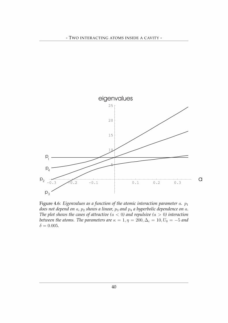
where p1 does not depend on a, p2 shows a linear, p3 and p4 a hyperbolicdependence on a, see fig 4.5. The plot shows also the dependence of theeigenvalues for a negative interaction strength a < 0, which correspondsto an attractive interaction between the atoms, and a positive interactionstrength a > 0, resembling a repulsive interaction. For a < 0 the energylevels are shifted downward and for a > 0 levels are shifted upward. Inthe case a = 0, meaning no interaction between the atoms, the eigenvaluesp1 and p2 are degenerate.
39
- TWO INTERACTING ATOMS INSIDE A CAVITY -
eigenvalues
a
p
p
p
p
4
2
3
1
Figure 4.6: Eigenvalues as a function of the atomic interaction parameter a. p1
does not depend on a, p2 shows a linear, p3 and p4 a hyperbolic dependence on a.The plot shows the cases of attractive (a < 0) and repulsive (a > 0) interactionbetween the atoms. The parameters are κ = 1, η = 200, ∆c = 10, U0 = −5 andδ = 0.005.
40
- TWO INTERACTING ATOMS INSIDE A CAVITY -
The corresponding eigenvectors are:
v1 =
0− 1√
21√2
0
, v2 =
01√2
1√2
0
(4.45)
and
v3 =
− x√1+x2
001√
1+x2
, v4 =
− y√1+y2
001√
1+y2
(4.46)
where
x =(ω0 + 2δu + av) +
√(ω0 + 2δu + av)2 + a2v2
av, (4.47)
y =(ω0 + 2δu + av)−
√(ω0 + 2δu + av)2 + a2v2
av. (4.48)
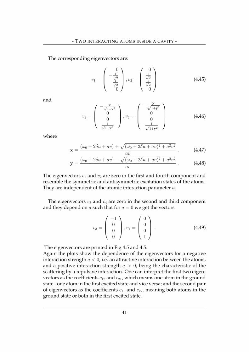
The eigenvectors v1 and v2 are zero in the first and fourth component andresemble the symmetric and antisymmetric excitation states of the atoms.They are independent of the atomic interaction parameter a.
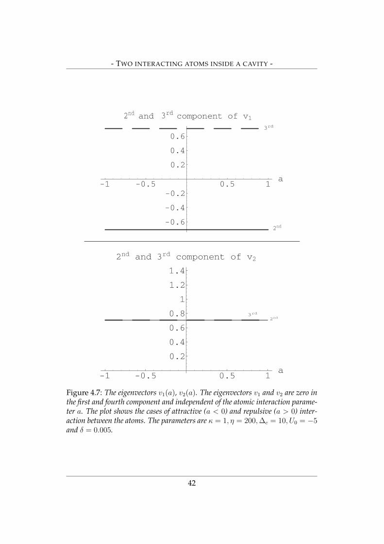
The eigenvectors v3 and v4 are zero in the second and third componentand they depend on a such that for a = 0 we get the vectors
v3 =
−1000
, v4 =
0001
. (4.49)
The eigenvectors are printed in Fig 4.5 and 4.5.Again the plots show the dependence of the eigenvectors for a negativeinteraction strength a < 0, i.e. an attractive interaction between the atoms,and a positive interaction strength a > 0, being the characteristic of thescattering by a repulsive interaction. One can interpret the first two eigen-vectors as the coefficients c12 and c21, which means one atom in the groundstate - one atom in the first excited state and vice versa; and the second pairof eigenvectors as the coefficients c11 and c22, meaning both atoms in theground state or both in the first excited state.
41
- TWO INTERACTING ATOMS INSIDE A CAVITY -
Figure 4.7: The eigenvectors v1(a), v2(a). The eigenvectors v1 and v2 are zero inthe first and fourth component and independent of the atomic interaction parame-ter a. The plot shows the cases of attractive (a < 0) and repulsive (a > 0) inter-action between the atoms. The parameters are κ = 1, η = 200, ∆c = 10, U0 = −5and δ = 0.005.
42
- TWO INTERACTING ATOMS INSIDE A CAVITY -
Figure 4.8: The eigenvectors v3(a), v4(a). The eigenvectors v3 and v4 are zero inthe second and third component and depend on the atomic interaction parametera. The plot shows the cases of attractive (a < 0) and repulsive (a > 0) interactionbetween the atoms. The parameters are κ = 1, η = 200, ∆c = 10, U0 = −5 andδ = 0.005.
43
- TWO INTERACTING ATOMS INSIDE A CAVITY -
For fixed δ the solution for the coefficients is obtained by transformingthe equation for the eigenvalues of the matrix M
M~ci = λi~ci (4.50)
into an equation for the eigenvalues using the eigenvectors of M .
D~vi = λi~vi (4.51)
Where D is the diagonal matrix we find when applying the linear trans-formation D = P−1MP :
D = P−1MP =
p1
p2
p3
p4
, (4.52)
whereP =
(v1 v2 v3 v4
). (4.53)
The solution for equation (4.51) is
~v(t) = e−iDt~v(0) (4.54)
with
e−iDt =
e−ip1t
. . .e−ip4t
. (4.55)
Doing the reverse transformation, we get for the coefficients
~c(t) = P~v(t)
= P e−iDt~v(0). (4.56)
And finally, by transforming ~v(0) = P−1~c(0), we get an equation for thecoefficients ~c(t):
~c(t) = P e−iDtP−1~c(0). (4.57)
Hence we have derived a solution of Eq. (4.25) in the desired form.
4.6 Stationary state solutions
Our final goal is now to find a general solution to the problem. This moti-vates to find stationary solutions for each eigenvector vi and find out if a
44
- TWO INTERACTING ATOMS INSIDE A CAVITY -
general solution by superpositions of the eigenvectors is possible.We calculate the expectation value for the squared atomic position usingthe eigenvectors vi. Hence we get four constant expectation values < x2
i >:
< x2i >= v∗i Avi , (4.58)
with
A =k2x2
0
2
6 0 0 00 8 0 00 0 8 00 0 0 10
. (4.59)
We now use these solutions < x2i > to calculate the corresponding field
amplitudes αi for each eigenvector vi:
αi =η
κ− i(∆c − U0(2− k2 < x2 >i)). (4.60)
Note that < x2i > does not depend on the phase of vi, so that αi does not
depend on this phase too.
Hence the solutions (4.57) correspond to a constant field and hence con-stant δ(t).The remaining problem is now to find conditions for which δi is consistentwith αi. As αi is a monotonic function of ηi, we can try to find the neededηi by choosing δi suitably.For this we want to find η as a function of δi. We try to find it from theequation for δi:
δi = U0(|αi|2 − |α0|2) (4.61)
Note that η also appears in the equation for α0 and therefore, as we de-
fined ω20 = 2
mU0|α0|2, ω0 and x0 =
√~
mω0are also functions of η.
The expectation values < x2i > enter the equation for αi (4.60), hence an
analytic calculation of ηi(δi) from the above equation (4.61) is only possi-ble for the cases i = 1 and i = 2, i.e. for the first two eigenvectors v1 andv2, whose components do not depend on ηi. If we do so, we get a cubicequation for η1 and η2.For the eigenvectors v3 and v4 an analytic treatment is not possible, be-cause the expectation values < x2
3 > and x24 who enter the equation for the
field α3 and α4 depend on polynomials in η3 and η4 of a non-trivial form.But if we choose for α0 a constant η = η0, ω0 and x0 depending on η0 too,
45
- TWO INTERACTING ATOMS INSIDE A CAVITY -
we can easily calculate η(δi) for each eigenvector vi:
ηi(δi) =
√(δi
U0
+ |α0|2)(κ2 +
(∆c − U0(2− < x2
i >))2
)(4.62)
0.02 0.04 0.06 0.08 0.1∆i
199.74
199.76
199.78
199.82
199.84
Pumprate Ηi
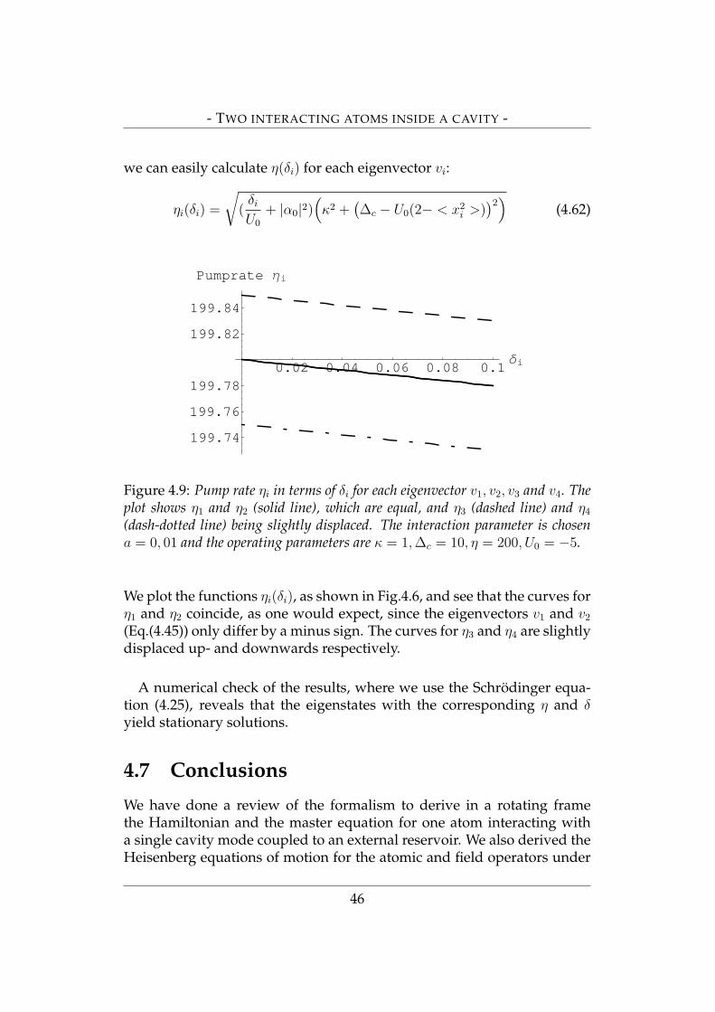
Figure 4.9: Pump rate ηi in terms of δi for each eigenvector v1, v2, v3 and v4. Theplot shows η1 and η2 (solid line), which are equal, and η3 (dashed line) and η4
(dash-dotted line) being slightly displaced. The interaction parameter is chosena = 0, 01 and the operating parameters are κ = 1, ∆c = 10, η = 200, U0 = −5.
We plot the functions ηi(δi), as shown in Fig.4.6, and see that the curves forη1 and η2 coincide, as one would expect, since the eigenvectors v1 and v2
(Eq.(4.45)) only differ by a minus sign. The curves for η3 and η4 are slightlydisplaced up- and downwards respectively.
A numerical check of the results, where we use the Schrodinger equa-tion (4.25), reveals that the eigenstates with the corresponding η and δyield stationary solutions.
4.7 Conclusions
We have done a review of the formalism to derive in a rotating framethe Hamiltonian and the master equation for one atom interacting witha single cavity mode coupled to an external reservoir. We also derived theHeisenberg equations of motion for the atomic and field operators under
46
- TWO INTERACTING ATOMS INSIDE A CAVITY -
the assumption of good cavity and low saturation limits. The force actingon the atom was found to push the atom to low intensity regions if thelaser field is blue detuned and to high intensity regions for a red detuningrespectively.As a next step we concentrated on the backaction of the atom on the cav-ity field. We introduced a model for this backaction which resembles thetime-dependent frequency as a perturbation δ(t) to a harmonic potential.We found that the system dynamically traps and localizes itself around anantinode of the field.The actual field of interest were two interacting atoms in a cavity stand-ing field mode, thus the direct interaction between them and the respec-tive interaction between the atom and field. We applied the model of theperturbed harmonic potential on the case of two atoms in the same fieldand modelled the direct interaction between the atoms by a delta functionparametrized by the interaction parameter a. We found that the atoms pe-riodically exchange energy.As we are interested in analytic stationary states for the system we cal-culated the eigenstates of the matrix in the matrix representation of theSchrodinger equation and due to the special shape of the matrix we foundtwo sets of eigenvectors, linearly independent of each other.We see that there are two possible classes of states. A first class whereonly one atom is excited, thus the coefficients c12 and c21 are non-zero, anda second class, where either both or none of the atoms are excited, i.e. thecoefficients c11 and c22 are non-zero.Dynamics only couples states within its class, that means for example ifwe have the situation that only one atom is excited, according to our re-sults the situation that both atoms are excited will not occur.Hence effectively we have two separate two state systems. These statescould then be used as a basis of further studies of atoms in periodic lat-tices [16].A further interesting research topic would be the extension to three ormore states of the atoms or even more than two atoms in the cavity.
47

Bibliography
[1] J. I. Cirac, M. Lewenstein and P. Zoller, Phys. Rev. A 51, 1650, (1995)
[2] A. C. Doherty, A. S. Parkins, S. M. Tan and D. F. Walls, Phys. Rev. A56, 833, (1997)
[3] M. Gangl and H. Ritsch, Phys. Rev. A 61, 043405, (2000)
[4] P. Maunz, T. Puppe, I. Schuster, N. Syassen, P. W. H. Pinkse andG. Rempe, Nature 428, 4, (2004)
[5] J. McKeever, J. R. Buck, A. D. Boozer, A. Kuzmich, H.-C. Nagerl,D. M. Stamper-Kurn and H. J. Kimble, Phys. Rev. Lett. 90, 13, (2003)
[6] E. T. Jaynes and F. W. Cummings, Proc. IEEE 51, 89, (1963)
[7] T. W. Hansch and A. Shawlow, Opt. Commun. 13, 68 (1975)
[8] D. Wineland and H. Dehmelt, Bull. Am. Phys. Soc. 20, 637 (1975)
[9] S. Stenholm, Rev. Mod. Phys. 58, 699, (1986)
[10] D. Wineland and W. Itano, Phys. Rev. A 20, 1521, (1979)
[11] V. S. Letokhov and V. G. Minogin, Phys. Rev. 73, 1, (1981)
[12] C. W. Gardiner and P. Zoller, Quantum Noise, Springer Berlin (2000)
[13] H. R. Lewis and W. B. Riesenfeld, J. Math. Phys. 10, 1458, (1969)
[14] J. K. Asboth, P. Domokos and H. Ritsch, Phys. Rev. A 70, 013414(2004)
[15] T. Busch, B. G. Englert, K. Rzazewski and M. Wilkens, Foundationsof Physics 28, 4, (1998)
[16] K. Winkler, G. Thalhammer, M. Theis, H. Ritsch, R. Grimm andJ. Hecker Denschlag, Phys. Rev. Lett. 95, 063202, (2005)
48

Curriculum vitae
Personal data
Name Katharina RenzDate of Birth November 27, 1977Place of Birth Lilienfeld, Austria
Education
1984 - 1988 Elementary school, Innsbruck1988 - 1996 High school, WRG Ursulinen InnsbruckJune 1996 General qualification for university entrancesince 1996 Diploma studies in physics
at the University of Innsbruck
49


![Phase transitions in Interacting Systems · 2020. 5. 28. · Moreover, in statistical mechanics [Rue99], two kinds of phase transitions are con-sidered: First order phase transitions,](https://static.fdokument.com/doc/165x107/60d3dac1d3bdbc1a9f6f5fe4/phase-transitions-in-interacting-systems-2020-5-28-moreover-in-statistical.jpg)