Two zone SSC model for blazar jets - WordPress.com€¦ · Two zone SSC model for blazar jets D I P...

Two zone SSC model for blazar jets

D I P L O M A T H E S I S

by

Leonard Burtscher

Lehrstuhl fur Astronomie

Institut fur Theoretische Physik und Astrophysik

Bayerische Julius-Maximilians-Universitat Wurzburg

Wurzburg, July 2007

Contents

1 Introduction 1

1.1 Blazars in the unified model of Active Galactic Nuclei . . . . . . . . . . . . 1

1.2 AGN Jet Modelling . . . . . . . . . . . . . . . . . . . . . . . . . . . . . . . 3

1.3 Outline . . . . . . . . . . . . . . . . . . . . . . . . . . . . . . . . . . . . . . 4

2 Theoretical Background 7

2.1 AGN ingredients . . . . . . . . . . . . . . . . . . . . . . . . . . . . . . . . 7

2.1.1 Relativistic Jet(s) . . . . . . . . . . . . . . . . . . . . . . . . . . . . 7

2.1.2 Cosmological redshift . . . . . . . . . . . . . . . . . . . . . . . . . . 9

2.1.3 Particle Acceleration at Shock Fronts . . . . . . . . . . . . . . . . . 10

2.2 Radiation Processes . . . . . . . . . . . . . . . . . . . . . . . . . . . . . . . 13

2.2.1 Definitions . . . . . . . . . . . . . . . . . . . . . . . . . . . . . . . . 13

2.2.2 Overview of relevant loss processes for electrons . . . . . . . . . . . 14

2.2.3 Photon losses . . . . . . . . . . . . . . . . . . . . . . . . . . . . . . 16

2.2.4 Synchrotron Radiation . . . . . . . . . . . . . . . . . . . . . . . . . 16

2.2.5 Inverse Compton Effect . . . . . . . . . . . . . . . . . . . . . . . . . 18

2.3 Luminosity distance . . . . . . . . . . . . . . . . . . . . . . . . . . . . . . . 22

2.4 Extragalactic Background Light (EBL) . . . . . . . . . . . . . . . . . . . . 22

2.5 Data fitting . . . . . . . . . . . . . . . . . . . . . . . . . . . . . . . . . . . 23

3 Analytic Model 25

3.1 Generic Blazar SED . . . . . . . . . . . . . . . . . . . . . . . . . . . . . . 25

3.2 Homogeneous two zone model . . . . . . . . . . . . . . . . . . . . . . . . . 26

3.3 Acceleration zone . . . . . . . . . . . . . . . . . . . . . . . . . . . . . . . . 27

3.3.1 Kinetic Equation . . . . . . . . . . . . . . . . . . . . . . . . . . . . 27

3.3.2 Solution . . . . . . . . . . . . . . . . . . . . . . . . . . . . . . . . . 28

3.4 Radiation Zone . . . . . . . . . . . . . . . . . . . . . . . . . . . . . . . . . 32

3.4.1 Kinetic Equation . . . . . . . . . . . . . . . . . . . . . . . . . . . . 32

3.4.2 Analytic Approximation for xcool? . . . . . . . . . . . . . . . . . . . 37

iii

Contents

3.5 Synchrotron Spectrum . . . . . . . . . . . . . . . . . . . . . . . . . . . . . 39

3.5.1 Contribution from the acceleration zone . . . . . . . . . . . . . . . 39

3.5.2 Contribution from the radiation zone . . . . . . . . . . . . . . . . . 40

3.5.3 Transformation to the observer’s frame . . . . . . . . . . . . . . . . 40

3.5.4 Synchrotron fit for Markarian 501 . . . . . . . . . . . . . . . . . . . 41

4 Inverse Compton (IC) contribution 43

4.1 Extension of the model . . . . . . . . . . . . . . . . . . . . . . . . . . . . . 43

4.2 Computation of the IC spectrum . . . . . . . . . . . . . . . . . . . . . . . 44

4.3 Time-dependent Inverse Compton Spectrum . . . . . . . . . . . . . . . . . 45

4.4 SSC fit for Mrk 501 . . . . . . . . . . . . . . . . . . . . . . . . . . . . . . . 46

5 Variability 49

5.1 Modelling a flare . . . . . . . . . . . . . . . . . . . . . . . . . . . . . . . . 49

5.2 Flaring behaviour I: Intensity profiles . . . . . . . . . . . . . . . . . . . . . 50

5.3 Flaring behaviour II: Spectral Index variation . . . . . . . . . . . . . . . . 53

5.4 Variation of spectral index with flux (Hysteresis) . . . . . . . . . . . . . . . 53

5.5 Timescales . . . . . . . . . . . . . . . . . . . . . . . . . . . . . . . . . . . . 58

5.6 Observations of variable high-energy spectra . . . . . . . . . . . . . . . . . 59

6 Summary and Discussion 61

6.1 Summary . . . . . . . . . . . . . . . . . . . . . . . . . . . . . . . . . . . . 61

6.2 Discussion . . . . . . . . . . . . . . . . . . . . . . . . . . . . . . . . . . . . 62

6.3 Prospects . . . . . . . . . . . . . . . . . . . . . . . . . . . . . . . . . . . . 64

7 Zusammenfassung (German Summary) 65

Bibliography 69

A Acknowledgements 73

B Numerical Calculations with Mathematica 75

C Program Listing 77

C.1 Init.nb . . . . . . . . . . . . . . . . . . . . . . . . . . . . . . . . . . . . . . 77

C.2 Run.nb . . . . . . . . . . . . . . . . . . . . . . . . . . . . . . . . . . . . . . 81

D Eigenstandigkeitserklarung (Declaration of Autonomy) 87

iv

1 Introduction

Blazar jet modelling is a tightly interconnected field of study. If one could study a

relativistic jet with sufficiently high temporal and spatial resolution and over large enough

times, one could resolve many of the issues discussed below. But, as astronomy is the

science of observation – not experimentation –, one has to be content with what can

be observed from earth, although many such observations do not stand for themselves

but depend on a couple of other unsolved problems. I want to show up some of these

interconnections in this introduction, concentrating more on the details in the following

sections.

1.1 Blazars in the unified model of Active Galactic Nuclei

The systematic study of active galactic nuclei began about twenty years after Edwin

Hubble showed in 1923 that the Andromeda ‘Nebula’ was in fact a galaxy far away and

not some nearby galactic nebulous object. In 1943, Carl Seyfert obtained spectrograms

with emission lines of several galaxies clearly demonstrating the non-stellar origin of the

radiation coming from the very centre of star-like galaxies.

The amount of radiation coming from these galaxies’ core regions which have diameters

of the order of parsecs or less, sometimes can exceed the radiation from the entire rest

of the galaxy with hundreds of billions of stars spread over typical diameters of 30 kpc.

As nuclear fusion is not efficient enough to produce luminosities as high as the ones

observed in such a small volume, more efficient emission mechanisms were sought, and

found: Nowadays there is little doubt that the so called active galactic nuclei (AGN) are

powered by accretion onto a central supermassive black hole with typically some hundred

million solar masses (Rees 1984).

Interestingly many of these AGN drive jets of several kiloparsecs length into the inter-

galactic medium. The exact mechanism for the production of these jets is still not entirely

clear although many ideas have been proposed (Blandford and Znajek 1977; Meier et al

2001). In any case, the visibility of the jet to an observer on earth seems to depend

mostly on the angle between the jet axis and the line of sight. In the unified model for

1

1 Introduction

AGN, see Fig. 1.3 for an illustration and Antonucci (1993); Urry and Padovani (1995)

as a reference, the line of sight and possibly the spin of the central black hole determine

the appearance and radio-loudness of an AGN. For example, a blazar, and in particular

BL Lac objects, which are the most extreme AGN with the shortest time variabilities, is

a radio-loud active galaxy observed under a very small angle to the jet. This is the type

of galaxy I want to focus on for this thesis. Due to special relativistic effects, variability

times in blazars appear to be shorter, radiation appears to be bluer and luminosities ap-

pear to be higher than in radio galaxies (that are more or less ”edge-on” active galaxies).

For recent reviews see (Mukherjee 2002; Coppi 2002).

While the galaxy’s radiation is dominated by the thermal emission from stars, the core

and jet of an AGN are dominated by a wide range of nonthermal and line emission from

radio to ultra-high-energy gamma rays. In the case of blazars, no emission lines are seen

which is generally attributed to the fact that the jet’s emission is so strongly Doppler

boosted (see section 2.1.1) that it outshines the line emission from the (broad and narrow

line) clouds at the centre of the AGN. The fact that no emission lines are seen also implies

that the target radiation for inverse Compton radiation (see section 2.2.5) is dominated

by the synchrotron emission of the jet, therefore an SSC model (see later) appears very

attractive for blazars. A blazar’s spectrum can roughly be described as a double hump

structure in the spectral energy distribution of the emitted photons. The origin of these

two humps has been discussed extensively in the literature, see chapter 1.2 for an overview

and references.

Apart from being one of the most luminous gamma-ray emitters in the known universe

(and therefore their nature is important to understand anyway), the field of blazar re-

search is intimately connected to several other areas of current research. Concerning

accretion, the production and emission mechanism of jets, micoquasars exhibit very simi-

lar phenomena, when reducing the relevant scales to the respective central mass – a super

massive black hole of several million solar masses in the case of AGNs and a stellar mass

black hole in the case of microquasars (see Fig. 1.1).

Even stronger is the link between blazars and early star formation and cosmology as

the TeV photons emitted by the blazar jets are attenuated due to γγ −→ e+e− pair

production. The cross section for this process is largest when εIR ≈ 2(mc2)2/Eγ =

0.5 (1TeV/E) eV, corresponding to a wavelength of ≈ 2.5µm for a 1 TeV photon, which is

just the wavelength where dust-enshrouded galaxies emit. Lower energy photons will be

absorbed by near-IR, optical or UV photons that come predominantely from stars. What

at first sight appears to be a disadvantage to blazar research (only nearby blazars will be

seen at energies above 1 TeV) is at second sight a unique probe for star-formation in the

2

1.2 AGN Jet Modelling

2 I. F. Mirabel

Figure 1. The same physical mechanism can be responsible for the three di!erent types ofobjects: microquasars, quasars/AGN and massive stars that collapse (“collapsars”) to form ablack hole producing Gamma-Ray-Bursts. Each one of these objects contains a black hole, anaccretion disk and relativistic particles jets. Credit: Mirabel & Rodrıguez (2002).

black hole with mass larger than 14 solar masses? Is this due to poor statistics or to largemass losses in stellar winds by the metal rich progenitors in the Milky Way?

Kinematic studies of black hole binaries suggest that some stellar black holes formassociated to very energetic supernova explosions (see figure 2). In some cases, this kine-matic evidence is reinforced by the chemical composition of the donor star, when itcontains elements produced in supernova explosions. However, kinematic studies suggestthat black holes may also form by direct collapse, namely, in the dark (figure 3). There-fore, it is an open question when stellar black holes form in energetic supernovae andwhen by direct core collapse; more specifically, whether the presence of an energetic ex-plosion depends or not on the mass of the collapsing stellar core. In fact, the kinematicsof the microquasars Cygnus X-1 and GRS 1915+105, which contain black holes of ! 10and ! 14 solar masses, respectivelly, did not receive strong kicks from natal energeticsupernova explosions.

This question on the explosive or implosive black hole formation can be approachedby observations of nearby gamma-ray bursts of long duration, which are believed to takeplace when stellar black holes are form by core collapse of massive stars. Therefore, thequestion on whether all collapsar GRBs are associated with supernovae of type Ia/b,or some are not, is of topical interest for the understanding of the very last phases ofmassive stellar evolution and black hole formation.

Figure 1.1: The ‘microquasar connection’ suggests that similar processes are at work inquasars, microquasars and Gamma Ray Bursts alike with time scales scaling accordingto the mass of the central black hole. By observing both microquasars and ‘real’ quasars,different time scales can thus be probed. Image credit: Mirabel and Rodriguez (2002)

early universe.

1.2 AGN Jet Modelling

Many models have been constructed to account for the multitude of AGN observations.

Generally one has to distinguish between leptonic and hadronic models. In hadronic

models protons are accelerated to very high energies (≈ 1020 eV) and initiade synchrotron

cascades that are responsible for the spectra we see (Mannheim 1993). These models are

promising as they could also explain the origin of Cosmic Rays that are seen up to such

high energies. A possible verification of these models would be neutrino emission from

extragalactic point sources – but the angular resolution of today’s neutrino telescopes

unfortunately is not good enough yet to detect those.

In leptonic models, the dynamical content of the jet is electrons and positrons that are

responsible for the synchrotron radiation and upscatter photons to very high energies.

The source of those low-energy photons (‘seed photons’) differs depending on the flavour

of the leptonic model. In so called ‘External Compton’ models the seed photons come

from the accretion disk (Dermer and Schlickeiser 1993) or are reflected into the jet by

surrounding material (Sikora et al 1994) and numerous other sources of seed photons

have also been proposed. The most widely used and, indeed, most successful model for

AGN jets has proven to be the so called ‘Synchrotron Self-Compton’ (SSC) model, where

3

1 Introduction

synchrotron photons are Compton up-scattered by the very same high energy electrons

that produced them via synchrotron radiation in the first place. SSC models are popular

as in those models X-ray flares are naturally correlated with VHE flares, as observed.

Those correlated flares can also be produced in the context of hadronic models (e.g.

Rachen 2001; Mannheim and Biermann 1992) but the calculations involved are a little

more complicated than with the SSC model, so – for economy and for the sake of Occam’s

razor – SSC models are the ones that are most widely ones.

Within those models one further distinguishes between homogeneous and inhomogeneous

models with the former consisting of a constant magnetic field and particle distribution

function throughout the source region. This constraint is dropped in the inhomogeneous

models.

Further distinctions can be made regarding the number of electron populations (e.g. to

account for a low-energy radio emission of the jet and a variable high-energy emission of a

blob) and, importantly, the number of zones the source region consists of. While one zone

models inject a distribution of high-energy electrons, two zone models can also explain the

acceleration, thus producing some spectral features that one-zone models cannot explain

as will be seen.

1.3 Outline

In chapter 2 the physical processes and mathematical relations relevant for the model are

explained such as relativistic Doppler boosting, (a simplistic view of) particle acceleration

at shock fronts and synchrotron and inverse Compton radiation formulae. The analytic

model of Kirk et al (1998) is explained and some minor corrections are given in chapter

3. Here it will become clear why it is necessary to use numerical calculations in deriving

the IC spectrum. In chapter 4 the assumptions and simplifications are given that lead to

the IC spectrum and a sample SSC fit for the Mrk 501 spectral energy distribution (SED)

is given. The time-dependence of the model will be discussed in chapter 5 where the

evolution of the spectrum and spectral index during a flare is shown. Chapter ?? will give

a brief overview of the currently available very high energy data on hour-scale variability

and discuss the possibility of future (multiwavelength) observations. In chapter 6 a brief

summary is given and some of the limitations of the model are discussed and possibilities

to validate or falsify the model are pointed out.

In appendix B a brief explanation of the Mathematica program written for the calculation

of the spectra is given, I want to thank several people in appendix A and appendix D

contains the mandatory Declaration of Autonomy.

4

1.3 Outline

Figure 1.2: ‘The Cosmic Cascade’, an illustration by K. Sutliff from Buckley (1998),depicting various scenarios for gamma-ray production in AGN jets, see chapter 1.2.

All calculations and units are written in the CGS system for better comparability with

the relevant literature.

5

1 Introduction

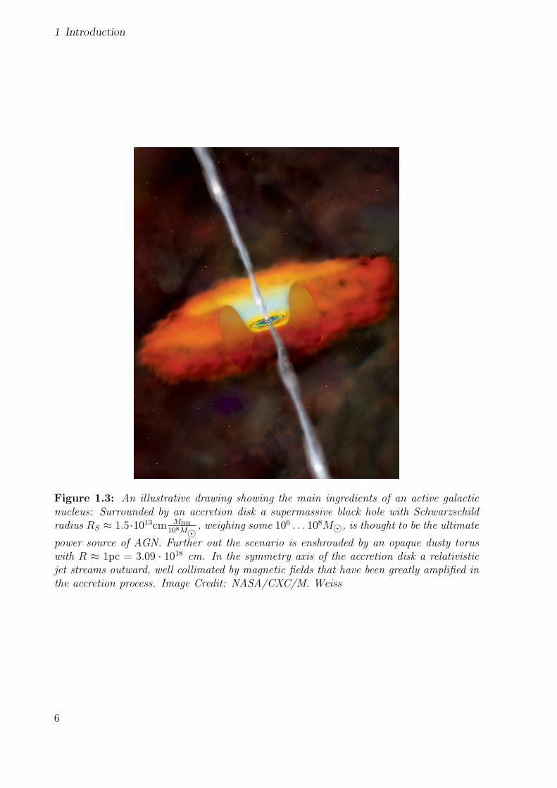
Figure 1.3: An illustrative drawing showing the main ingredients of an active galacticnucleus: Surrounded by an accretion disk a supermassive black hole with Schwarzschildradius RS ≈ 1.5·1013cm MBH

108M, weighing some 106 . . . 108M, is thought to be the ultimate

power source of AGN. Further out the scenario is enshrouded by an opaque dusty toruswith R ≈ 1pc = 3.09 · 1018 cm. In the symmetry axis of the accretion disk a relativisticjet streams outward, well collimated by magnetic fields that have been greatly amplified inthe accretion process. Image Credit: NASA/CXC/M. Weiss

6

2 Theoretical Background

This chapter gives an overview of the theoretical background, including the relevant for-

mulae, for the calculations done in this work. As the model describes radiation coming

from relativistic jets I will give the relevant relativistic transformation formulae. A main

part of this chapter covers particle acceleration (at shock fronts) where I want to justify

the use of an energy-independent ‘acceleration time’ in the model. After some definitions

concerning radiation processes, loss mechanisms for high energy electrons traversing dilute

plasmas will be discussed, finding that only synchrotron and Inverse Compton losses are

relevant here. Those two processes are then discussed in greater detail. The section on

the ‘luminosity distance’ will explain how the distance to a blazar can be calculated from

the observationally measured redshift z. For large z or very high energies (VHE, above

100 GeV), the Extragalactic Background Light (EBL) attenuates high-energy gamma ra-

diation. Although all data points used are already unfolded for EBL absorption, i.e. the

spectra used are the ones one would see on earth if there were no EBL, I will give a short

explanation of why EBL is important for blazar spectra modellers. Finally, a section on

data fitting describes the commonly used χ2 value to test the quality of a fit.

2.1 AGN ingredients

2.1.1 Relativistic Jet(s)

The jets of AGN show several remarkable features: they are very well collimated over vast

distances, sometimes up to a MPc, show (apparent) superluminal motion of individual

‘knots’, as identified by radio interferometry, and have highly variable polarised emission

from radio to gamma-rays – sometimes on the order of minutes. In some sources only one

jet is visible and the termination shock of the presumed ‘counter-jet’ seems to come from

nowhere. Some of these phenomena can easily be explained by the relativistic Doppler

effect.

7


Relativistic Doppler Effect

Let us look at the Doppler factor δ for a blob of matter moving relativistically towards

an observer in a relativistic jet

δ = [Γ (1− β cos θ)]−1 (2.1)

Γ = (1 − β2)−1, the (bulk) Lorentz factor of the blob, β = vc

and θ is the angle between

the line of sight and the direction of motion of the jet / blob.

To get rid of θ, let us have a look at blazars where cos θ ≈ 1 and one can write

δ ≈ [Γ(1− β)]−1 = [Γ(1− β)(1 + β)(1 + β)−1]−1 ≈ 2Γ (2.2)

Several observable quantities are transformed by the Doppler factor, see Blandford and

Konigl (1979) for detailed calculations. I will express the relevant transformations here in

terms of Γ for better comparability with blazar models. All quantities in the blob frame

are denoted by em, quantities in the observer’s frame by obs.

Due to relativistic dilation, time scales are shortened in the observer’s frame with respect

to the jet frame,

tobs =temΓ, (2.3)

frequencies are shifted towards higher values,

νobs ≈ 2 Γνem, (2.4)

and intensities are ‘boosted’ to

Iobs(νobs) ≈ (2 Γ)3−α Iem(νobs) (2.5)

The intensity transformation (‘Doppler boosting’) can hand-wavingly be explained by

attributing two factors of Γ to the effect of relativistic aberration (radiation is only emitted

in a narrow cone of half angle Γ) and one that comes from time dilation of the dt in the

definition of the intensity (see chapter 2.2.1). The additional factor of (2 Γ)α accounts for

the blue-shift of the intensity.1

Now one-sided jets can readily be explained as one of them being ‘Doppler boosted’ while

the other, moving away from us (with cos θ < 0 in Eq. (2.1)), being ‘Doppler de-boosted’

1Since the specific intensity is assumed to be Iν ∝ να, this is equivalent to Iobs(νobs ≈ 2Γνem) ≈8 Γ3Iem(νem).

8

2.1 AGN ingredients

Figure 2.1: A radio image of the quasar 3C175 (the tiny bright spot in the centre), itsover a million light years long one-sided radio jet and its radio lobes. Although this jet isnot thought to be directed at a very small angle towards an observer (3C175 is no blazar),the angle between the jet and the line of sight might still be narrow enough that a possiblecounter-jet is ‘Doppler-hidden’ and so we only see one jet. Large radio lobes are seen onboth sides of the quasar as here the bulk motion is thought to be non-relativistic, allowingthe electrons to radiate their synchrotron emission isotropically. Also visible is anothercharacteristic of radio galaxies: the hot spots, the very bright spots visible in both lobeswhere the jets are thought to collide with the intergalactic medium. Image Credit: AlanBridle (NRAO Charlottesville) VLA, NRAO, NSF

and thus emission from the far side of the AGN is only visible when the motion has slowed

down to sub-relativistic speeds (see Fig. 2.1).

2.1.2 Cosmological redshift

To fully switch to the observer’s frame one further has to take into account the cosmo-

logical redshift z so that the transformation formula for the frequencies becomes

νobs ≈2 Γ

1 + zνem (2.6)

For the two best studied nearby BL Lac objects Mrk 421 and Mrk 501, z is ≈ 0.03, TeV

blazars have been detected up to z = 0.186 (Aharonian et al. (H.E.S.S. collaboration)

2007) with a possible detection at z = 0.74 (Albert et al. (MAGIC collaboration) 2007a)

and the highest redshift blazar detected so far being at z ≈ 5.5 (Romani 2006). Those very

9


distant blazars are not detectable at very high energies, however, as high-energy gamma-

rays are efficiently absorbed by Extragalactic Background Light (EBL, see section 2.4).

2.1.3 Particle Acceleration at Shock Fronts

A mechanism is needed to explain the acceleration of charged particles up to energies of

1020 eV and possibly beyond (Sigl 2001) that we see in the form of isotropic cosmic rays.

Also, the nearly perfect power-laws both in the energy distribution of these cosmic rays

and in the spectra of most extragalactic nonthermal sources such as radio galaxies and

quasars need theoretical understanding.

As Longair (1994) has noted, it is ironic that we have to build the world’s largest experi-

ments to accelerate particles to a mere 1012 eV, but when we try to store high-temperature

plasmas inside a fusion reactor, we run into trouble because of numerous plasma instabil-

ities that readily accelerate particles to suprathermal energies. As it is generally implau-

sible that natural mechanisms rely on extremely fine-tuned ‘machines’, a simple process

is sought to produce power-laws that reach up to very high energies.

Long before sophisticated plasma instabilities could be calculated to great detail numer-

ically, Enrico Fermi has come up with a simple, yet brilliant idea (Fermi 1949). Trying

to explain the origin of cosmic rays, he presumed that particles were accelerated in the

interstellar space of the galaxy by the ‘collision against moving magnetic fields’, nowadays

known as collisionless shock acceleration. The term ‘collisionless’ refers to the fact that

particles in tenuous interstellar plasmas get scattered only via collective plasma interac-

tions and not by their immediate electric fields.

There are two classes of approaches to calculate the spectra that would result from such a

physical scenario: one can either treat the interstellar plasma as a fluid, model the shock

using the magnetohydrodynamic (MHD) approximation and put in particles using test-

particle simulations, or one can use the more physical microscopic approach and follow

the particles’ distribution function, the diffusion-loss equation. While the first method

is more suited for incorporating many concurring effects and numerically calculating the

resulting spectra, kinetic equations for distribution functions can more easily describe

physical processes that are self-similar over several orders of magnitude in particle energy.

Also, only the kinetic approach is suited for analytic calculations giving greater insight into

the physics going on but with the disadvantage of requiring some crude approximations

to keep the equations simple.

Here, only the original version of Fermi acceleration (‘second order Fermi’) shall be dis-

cussed briefly to justify the energy-independent ‘acceleration time’ used in the model to

10

2.1 AGN ingredients

describe particle acceleration. A good starting point for a more detailed overview of shock

acceleration and an enjoyable reading for almost any topic in high energy astrophysics is

Longair (1994). Jones and Ellison (1991) cover the plasma physics of shock acceleration

in parallel shocks (the simplest scenario, where the magnetic field direction is parallel to

the normal of the shock front), give a review of computer simulations and introduce to

nonlinear theories for shock acceleration.

The second order Fermi Mechanism of particle acceleration Consider a particle’s

reflection off an infinitely massive2 ‘magnetic mirror’ – in reality that might be a massive

cloud of plasma – moving at an average velocity V relative to the particle. The mirror

reflects the particle so that the angle between the inital direction of the particle and the

normal of the mirror is θ. Then the particle’s energy is conserved in the collision and its

momentum reversed.

Figure 2.2: A particle of speed c collides head-on with a ‘magnetic mirror’ of infinitemass moving at velocity V and subtends an angle θ between the incoming direction andthe mirror’s normal.

Working out the relativistic transformations – into the cloud’s frame (the centre of mo-

mentum frame) and back into the observer’s frame – and expanding in second order of

V/c, one readily arrives at, assuming the particle’s velocity is c,

∆E

E=

2V cos θ

c+ 2

(V

c

)2

(2.7)

2so that its velocity is unchanged by the collision

11


From this equation one can easily see that, when cos θ = 1, i.e. when only head-on

collisions are considered, the energy gain is first order in V/c which is the outcome of the

so-called ‘Fermi I’ mechanism. Now for Fermi II, let us assume that particles quickly lose

their directional information due to isotropic ‘pitch-angle scattering’ (the pitch-angle is

the angle between the direction of motion of the particle and the magnetic field) in the

irregular magnetic fields of the clouds. They will then leave the cloud isotropised so that

we can average over all angles to get the average energy gain of a particle

⟨2V cos θ

c

⟩=

2

3

(V

c

)2

(2.8)

Thus, one arrives at the famous result first derived by Fermi

∆E

E=

8

3

(V

c

)2

(2.9)

stating that the energy gain is only second order in V/c.

Second order Fermi acceleration was originally applied to randomly moving clouds and

Fermi could demonstrate that statistical acceleration leads to a power law energy spec-

trum. Although in strong shocks Fermi I acceleration is normally said to be more efficient,

this is not true when considering also decelerating effects. In fact, the acceleration ef-

ficiencies of Fermi I and II are not much different, even in strong shocks (Jones 1994).

Furthermore, large shocks are not expected at the base of the jet where the gamma ra-

diation is thought to originate (Pelletier 1997) so that Fermi II seems to be a plausible

mechanism there albeit with some difficulties and limitations (see below).

To derive the fractional increase per unit time, we further need to consider the time

between collisions which is given by 2L/c when L is the mean free path between clouds.

So the rate of energy increase is then given by

dE

dt=

4

3

(V 2

cL

)E =

E

tacc(2.10)

This is a very important and useful equation as it says that particles are accelerated

within an energy-independent acceleration time tacc. With the further assumption that

the particle will leave (‘escape’) the acceleration region after a time tesc, we can substitute

the relevant expressions in the equation describing the evolution of the electron density

Eq. (3.2) and get

− d

dE

[E

taccN(E)

]− N(E)

tesc= 0 (2.11)

12

2.2 Radiation Processes

The solution to this equation is the simple power-law relation

N(E) ∝ E−x (2.12)

with x = 1 + tacc/tesc. The choice of tacc/tesc = 1/2 leads to the desired (i.e. measured)

low-frequency spectral index α = 0.25. Taking synchrotron losses (chapter 2.2.4) into

account, we will get a spectral break at a characteristic energy where cooling and escape

are balanced and the electron spectrum will steepen by 1, i.e. from 1.5 to 2.5, see chapter

3.1.

This mechanism has received much attention because it explains naturally the power-law

shape of the spectrum. Another benefit is that this mechanism works ‘in situ’, i.e. parti-

cles are accelerated where the energetic phenomena like strong shocks are, thus avoiding

adiabatic (expansion) losses. But we had to put in tacc/tesc = 1/2 a posteriori to get the

desired spectral index of 2.5 which fits very well to the power-law spectra of radio-sources

and is close enough to the one measured over most part of the cosmic ray spectrum (2.7).

Also, losses in the acceleration process such as ionisation losses and geometrical effects

expected to arise in non-parallel shocks have not been considered and are expected to

modify the spectrum more or less dramatically. Furthermore, this has only been a test

particle approach where the back-reaction effects of the particles on the shock are ne-

glected. For a recent review of the applicability of Fermi acceleration to astrophysical jets

see Rieger (2006).

Although there are certainly many objections to this simple picture of particle acceleration

at shock fronts, it can nonetheless be used as a simple method to implement acceleration

in a time-dependent model of blazar spectra.


2.2.1 Definitions

For the further discussion we need a few definitions concerning radiative processes (Rybicki

and Lightman 1979). When calculating the synchrotron and Inverse Compton spectrum,

one usually gets the spectrum in the form of the specific intensity:

Iν =dI

dν=

dE

dA cos θ dt dν dΩ[erg cm−2 s−1 Hz−1 sr−1] (2.13)

where I, the intensity (erg cm−2 s−1 sr−1), is the amount of energy E received in the area

dA (perpendicular to the direction of incidence of the radiation) in the time dt, frequency

13


interval [ν, ν + dν], from the solid angle dΩ.

For an unresolved source, i.e. a source which appears smaller than the smallest resolved

angle θmin, the specific radiative flux is more appropriate

Fν =

∫d Ω cos θ Iν (2.14)

For the graphical display, one usually plots log νFν on the ordinate and log ν on the

abscissa as this is a plot of logarithmic radiation energy density per logarithmic frequency

interval and therefore it is easy to see at which frequencies most of the radiation energy

density is: an equal amount of energy emitted per logarithmic frequency interval would

be a horizontal line.

2.2.2 Overview of relevant loss processes for electrons

Four main processes are to be discussed when considering the problem of a high energy

electron traversing a dilute partially ionised gas (Blumenthal and Gould 1970). Here I

will give a brief overview and then discuss in more detail the two most important ones in

this context: synchrotron and Inverse Compton radiation. See Schlickeiser (2002, p. 100

et seq.) for a detailed account of all processes possible.

None of the following processes causes more losses for an electron in a blazar than syn-

chrotron and IC losses (see Fig. 2.3).

Ionisation Losses / inelastic collisions occur when electrons scatter inelastically with

other particles, thereby ionising them:

−(

dE

dt

)ion

= 7.64 · 10−21N(3 ln γ + 19.8)eV s−1cm−3 (2.15)

where N is the number density of hydrogen atoms per cubic centimetre. Ionisation losses

are only important at very low energies.

Bremsstrahlung – sometimes referred to as ‘free-free radiation’ – is emitted by the

electrons in scatterings as they are deflected by the electric fields of other particles. In a

fully ionised plasma the loss rate is:

−(

dE

dt

)brems

= 3.6 · 10−23N γ(ln γ + 0.36)eV s−1cm−3 (2.16)

14


1 100 104Eel!GeV

0.001

1

1000

106

109

Loss rate!eV s^!1

Figure 2.3: Overview of loss processes for high-energy electrons traversing a thin plasmawith values appropriate for blazar jets: magnetic field B = 0.1 G, number density ofhydrogen atoms N = 105 cm−3. The curves correspond to synchrotron / Inverse Comptonlosses (red), ionisation losses (horizontal blue line) and bremsstrahlung losses (blue). Thetotal loss rate is displayed in purple. As it can clearly be seen, only synchrotron / IC lossesare relevant for the the blazar environment. This plot was created using a Mathematicanotebook written by Tobias Hein.

Adiabatic Losses occur when the relativistic gas carries out volume work in the ex-

pansion and therefore loses internal energy. In the simple case of a uniformly expanding

sphere, the energy loss is given by

−(

dE

dt

)adiabatic

= 1.2 · 105γ

(1

R4

dR

dt

)eV s−1 cm−3 (2.17)

Synchrotron and Inverse Compton losses In the Thomson limit of Inverse Compton

scattering (see later) and assuming roughly equipartition between the energy densities

in the magnetic field and in the synchrotron radiation field, both processes contribute

equally to the energy loss of electrons, namely (expressed for synchrotron losses)

−(

dE

dt

)syn

= 6.6 · 10−4γ2B2eV s−1 cm−3 (2.18)

15


2.2.3 Photon losses

Photon losses relevant here are mainly catastrophic losses such as losses due to Compton-

upscattering of synchrotron photons. The low energy synchrotron photon is destroyed in

that process and a new high-energy electron is produced.

Another important loss mechanism for photons is pair production

γ γ −→ e+ e− (2.19)

From the fact that we see sources at TeV energies (i.e. they are transparent to gamma

rays) we can derive a lower limit on the Doppler factor (Dondi and Ghisellini 1995) which

generally agrees with estimates from spectral modelling (δ ≈ 10 . . . 50).

Another photon sink is synchrotron self absorption. This process becomes important at

low frequencies as the brightness temperature3 of the source equals the kinetic temperature

of the electrons. According to the priniciple of detailed balance a source cannot emit

radiation of brightness temperature greater than its kinetic temperature.

2.2.4 Synchrotron Radiation

Synchrotron Emissivity The total synchrotron power (summed over all polarisations)

is given by Ginzburg and Syrovatskii (1965)

Ps(ν, γ) =

√3 e2B⊥mc2

ν

νc

∫ ∞ν/νc

K5/3(η) dη [erg s−1 Hz−1] (2.20)

where e is the elementary charge, m the electron rest mass, νc the characteristic syn-

chrotron frequency (see below) and K5/3 the modified Bessel function of order 5/3.

The synchrotron intensity that a distribution of electrons n(γ) produces, is then calculated

by convolving the distribution with the synchrotron power:

I(ν) =

∫dγ P (ν, γ)n(γ) (2.21)

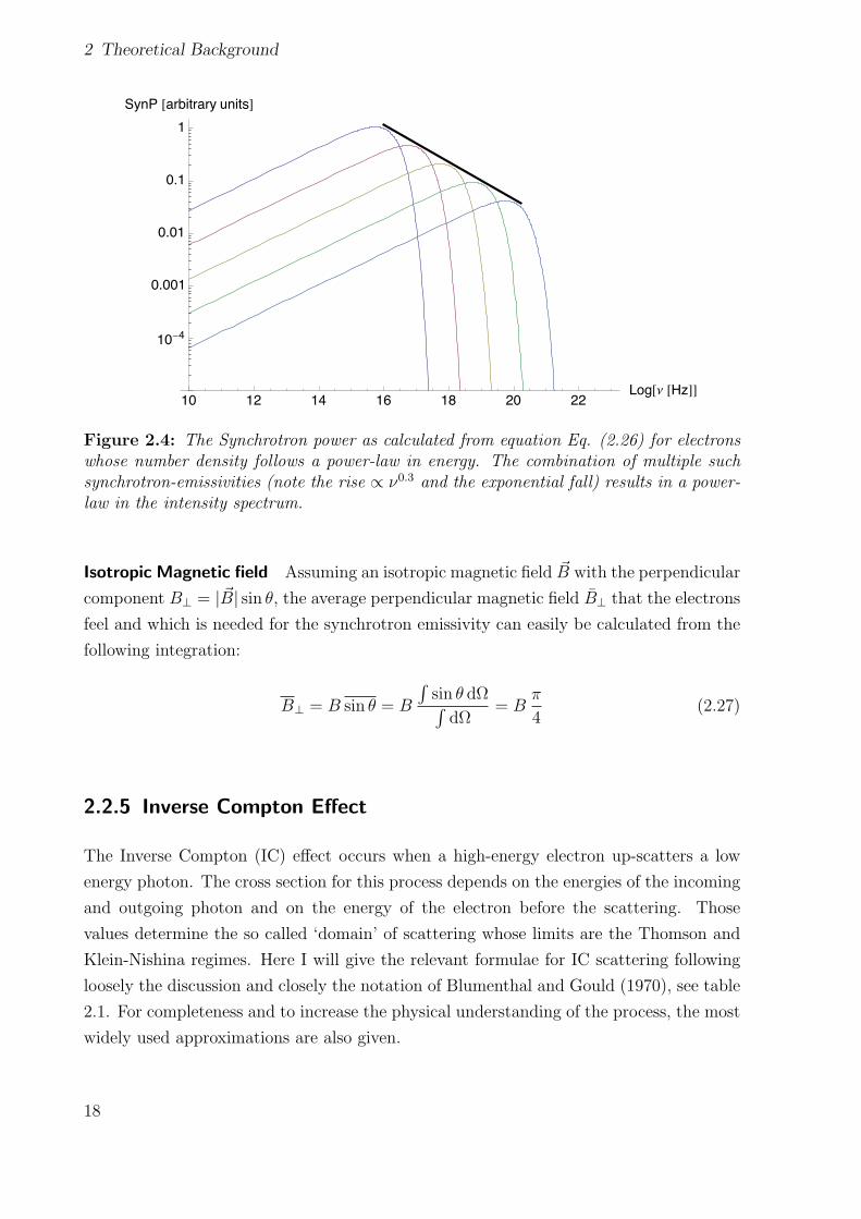
Monochromatic Approximation A characteristic synchrotron frequency is introduced

to quickly estimate the emission of a (power-law) distribution of electrons, see Fig. 2.4.

If the spectral shape of the synchrotron emission is governed by the power-law of the

electrons (i.e. if it is not too steep) rather than by Ps(ν, γ), the synchrotron emissivity

3A radio astronomers’ quantity that refers to the temperature a source would need to have if it attemptedto emit the radiation at a certain frequency sustaining a black-body distribution.

16


can be written as (Felten and Morrison 1966)

Ps(ν, γ) ≈ Ps(γ) δ(ν − νc(γ)) ≡ Ps(γ) (6ν ν0)−12 δ(γ − γ0) (2.22)

where the characteristic frequency νc is given by

νc =3 e

4 πme cB⊥γ

2 =3

2ν0 γ

2 (2.23)

and the total power in synchrotron radiation Ps(γ) is

Ps(γ) =

∫ ∞0

dνPs(ν, γ) =2

3r2

0cγ2B2⊥ (2.24)

with the classical electron radius r0 = e2/mc2.

Integrating this ‘monochromatic approximation’ over a power law distribution of electrons

with index s, defined by n(γ) ∝ γs, a power law in photons with index α = (s + 1)/2 is

obtained, where α is defined as4

F (ν) ∝ να (2.25)

Melrose Approximation The monochromatic approximation is not good for electron

distributions where the electron number density rises too steeply because of mathematical

rather than physical effects like the electron distribution that will result from the first-

order differential equation Eq. (3.18). In those cases a smoother approximation like the

one given by Felten and Morrison (1966) and later by Melrose (1980) is needed to avoid

the numerically expensive integration of the modified Bessel function. This approximation

is

P (ν, γ) = asz0.3 exp(−z) (2.26)

where as =√

3 e2 Ω/(2πc) with the electron gyro frequency Ω = eB/(mc) and the param-

eter z = 4 π ν/(3Ωπ/4γ2). Here, the isotropic magnetic field has already been averaged

over θ, the angle between the magnetic field direction and the line of sight, to yield the

average perpendicular magnetic field for an electron (see right below).

4In the literature the spectral index of a power-law is often defined as αlit = −α. When followingspectral changes during flares, it is more intuitive, however, to define the spectral index positively.

17


10 12 14 16 18 20 22Log!! !Hz""

10"4

0.001

0.01

0.1

1SynP !arbitrary units"

Figure 2.4: The Synchrotron power as calculated from equation Eq. (2.26) for electronswhose number density follows a power-law in energy. The combination of multiple suchsynchrotron-emissivities (note the rise ∝ ν0.3 and the exponential fall) results in a power-law in the intensity spectrum.

Isotropic Magnetic field Assuming an isotropic magnetic field ~B with the perpendicular

component B⊥ = | ~B| sin θ, the average perpendicular magnetic field B⊥ that the electrons

feel and which is needed for the synchrotron emissivity can easily be calculated from the

following integration:

B⊥ = B sin θ = B

∫sin θ dΩ∫

dΩ= B

π

4(2.27)

2.2.5 Inverse Compton Effect

The Inverse Compton (IC) effect occurs when a high-energy electron up-scatters a low

energy photon. The cross section for this process depends on the energies of the incoming

and outgoing photon and on the energy of the electron before the scattering. Those

values determine the so called ‘domain’ of scattering whose limits are the Thomson and

Klein-Nishina regimes. Here I will give the relevant formulae for IC scattering following

loosely the discussion and closely the notation of Blumenthal and Gould (1970), see table

2.1. For completeness and to increase the physical understanding of the process, the most

widely used approximations are also given.

18


ε Energy of the photon before collision (far observer’s frame)ε1 Energy of the photon after collision (far observer’s frame)γ Lorentz factor of the electron before collision (far observer’s frame)

Table 2.1: IC notation

General case – Scattered photon distribution The exact expression for the spectrum

of Compton upscattered photons as calculated from quantum electrodynamics (Jauch and

Rohrlich 1976) is a rather unwieldy expression (Jones 1968; Coppi and Blandford 1990).

However, spectra calculated with the approximate expression given by Jones (1968) and

Blumenthal and Gould (1970) are almost indistinguishable from the spectra calculated

from the exact expression as long as the electron Lorentz factor γ 1, which is certainly

the case for the radiation that is of interest here. Then, one can write

dNγ,ε

dtdε1=

2π r20 mc

γ2

n(ε) dε

ε

[2q ln q + (1 + 2q) (1− q) +

1

2

(Γε q)2

1 + Γε q(1− q)

]︸︷︷︸

F (E1,Γε)

(2.28)

where E1 = ε1(γ m c2) is the outgoing photon energy in terms of the electron rest mass,

Γε = 4 ε γ/(mc2) denotes the ‘domain of scattering’ and q = E1/[Γε(1−E1)] is a parameter.

In the Thomson limit Γε 1 and also E1 1 and so Eq. (2.28) reduces to the Thomson

limit expression Eq. (2.31). Eq. (2.28) is valid for any value of Γε, but the assumption

γ 1 has been made in its derivation.5

The function F (E1,Γε), where the energy of the scattered photon is expressed in terms

of its maximum value E1 = E1(1 + Γε)/Γε, is plotted in Fig. 2.5. The transition from

the Thomson regime – where the scattered photon distribution is broad and favours the

low-energy photons – to the Klein-Nishina regime – where the high-energy end is favoured

and a single scattering results in a large energy loss for the scattering electron – can be

seen.

It is important to note that only a small region in the parameter space (ε, ε1, γ) contributes

to the scattered spectrum. The range of values for E1 that have to be considered for the

spectrum is given by

1 ε/(γ m c2) ≤ E1 ≤ Γε/(1 + Γε) (2.29)

Outside that range there is no IC effect.

5The assumption γ 1 is useful in the derivation because in that case in the electron’s frame all photonscome from inside a cone with the small half-angle θ = 1/γ → 0.

19


0.2 0.4 0.6 0.8 1.0 E^

1

2

3

4

5

6

F!E^ ,!""

Figure 2.5: The spectrum of Compton scattered photons, F (E1,Γε), as calculated fromEq. (2.28) and normalised so that the integral over each curve is 1. The curves correspondto Γε = 0.001 (blue), 1 (purple), 10 (yellow), 100 (green). The transition from theThomson to the extreme Klein-Nishina regime can clearly be seen.

General case – Electron energy loss The total energy loss rate for IC scattering in the

general case is given by

− dE

dt=

∫(ε1 − ε)

dN

dtdε1dε1 (2.30)

The exact solution of this integral is a little complicated (Jones 1968; Blumenthal and

Gould 1970) but approximate expressions can be given (see below).

Thomson limit In the Thomson limit Eq. (2.28) reduces to (Blumenthal and Gould

1970)

dNγ,ε

dtdε1=π r2

0 c

2γ4

n(ε) dε

ε2

(2ε1 ln

[ε1

4γ2ε

]+ ε1 + 4γ2 ε− ε21

2γ2 ε

)(2.31)

20


The expression vanishes for scattered energies larger than the maximum scattered energy

4εγ2.

The expression for electron losses due to IC scattering in the Thomson regime is very

similar to the expression for synchrotron losses (Blumenthal and Gould 1970).6

− dγ

dt= βicγ

2 (2.32)

where

βic =4

3mecσTEiso (2.33)

and

Eiso =1

c

∫dνIν (2.34)

is the energy of the isotropic radiation field.

Klein-Nishina limit In the extreme Klein-Nishina limit F (E1,Γε) from Eq. (2.28) be-

comes

F (E1,Γε) = (ln Γε)−1

[1 +

1

2

(Γεq)2

1 + Γεq(1− q)

](2.35)

For the electron losses, an integral expression is introduced as individual losses can alter

the energy of the electrons significantly in this limit and therefore make the use of a

differential expression inaccurate.

− dE

dt= πr2

0m2ec

5

∫n(ε)

ε

[ln

(4εγ

mc2

)− 11

6

]dε (2.36)

Total Compton Spectrum The expressions dNγ,εdtdε1

stated above give the spectrum of

Compton-scattered photons from the interaction of electrons of energy γmec2 with an

isotropic density segment dn = n(ε) dε of photons within energy dε. To calculate the

total Compton spectrum, one needs to integrate over all inital photon energies ε and over

all scattering electron Lorentz factors γ. With the differential number density of electrons

dNe = Ne(γ) dγ, the total Compton spectrum is given by

6This is not by chance as both processes can be ascribed to Compton scattering of photons: IC is elec-trons scattering real photons, while the synchrotron process can be understood as Compton scatteringof the virtual photons from the static magnetic field.

21


dNtot

dtdε1=

∫ε

∫γ

dγ Ne(γ)dNγ,ε

dtdε1(2.37)

The order of integration is irrelevant.

2.3 Luminosity distance

The luminosity distance is defined as the distance that has to be used for the inverse

square law for the observed flux:

d2L ≡

L

4πF(2.38)

In astrophysics, the measurable quantity is usually the redshift z. So one wants a relation

between z and dL:

dL(z) ≈ c z

H0

[1 +

1

2(1− q0)z

](2.39)

where H0 is the Hubble parameter today (H0 = 73.2+0.031−0.032 km s−1 MPc−1) and q0 =

Ωm,0/2 − ΩΛ,0 is the cosmological deceleration parameter. With WMAP values for the

(baryonic and dark) matter and dark energy densities Ωm,0 and ΩΛ,0, the deceleration pa-

rameter q0 = −0.60 (Spergel et al 2007). More about cosmological distance measurements

can be found in any astrophysics textbook (e.g. Carroll and Ostlie 2006).

2.4 Extragalactic Background Light (EBL)

Far away blazars cannot be observed at Very High Energies, though, due to absorption

of high-energy gamma rays by pair production with the Extragalactic Background Light

(EBL), produced by galaxies throughout the history of the universe and possibly also by

first stars. The observed spectra Fobs are modified by gamma - gamma pair production

Fobs(E) = Fint(E) exp[−τγγ(E, z)] (2.40)

where τγγ(E, z) is the optical depth for this process, effectively producing a ‘gamma-ray

horizon’ that depends on the threshold of the gamma-ray telescope used (see Fig. 2.6).

This so called ‘Fazio-Stecker relation’ can already become important for nearby extreme

blazars (such as Mrk 501) whose IC emission peaks at energies greater than about a TeV.

To compare measured SEDs with model SEDs one has to unfold the measured data points

22

2.5 Data fitting

T. M. Kneiske et al.: Implications of cosmological gamma-ray absorption. II. 813

0,01 0,1 110

100

1000

10000

1e+05

Gam

ma E

ner

gy [

GeV

]

0 1 2 3 4 5Redshift z

10

100

1000

10000

1e+05G

am

ma E

ner

gy [

GeV

]

H1426+428

Mkn421

Mkn501

Mkn501

Mkn421

H1426+428

Fig. 6. Upper panel: Fazio-Stecker relation with logarithmic redshift axis (best-fit model – thick solid line; low-IR model – dot-dashed line;

warm-dust model – thin dashed line low-S FRmodel – thin solid line). Lower panel: Fazio-Stecker relation with linear redshift axis showing the

asymptotic far-zone (best-fit model – thick solid line; stellar-UV model – dashed line; high-stellar-UV model – dotted line; low-S FR model –

thin solid line). Also plotted are published cut-o! energies of Mkn 501, Mkn 421, and an upper limit of H1426+428 coming from not detecting

the cut-o! energy with HEGRA (for references, see text). The horizontal lines at 50 GeV and 100 GeV represent guide lines showing how the

asymptotic branch of the Fazio-Stecker relation can be tapped by lowering the detection threshold to below 50 GeV (e.g. using the MAGIC

telescope).

respectively). The expected exponential cut-o! energy at a red-

shift of z = 0.129 obtains values of 100–200 GeV, i.e. at en-ergies below the threshold energy of the detecting instruments

(Whipple, HEGRA).

Calculating the intrinsic spectral range we find for the best-

fit model the same result as Costamante et al. (2003). The en-

ergy spectrum increases with energy. However, inspection of

Fig. 5 shows that the intrinsic energy flux spectrum inferred

from the low-IR model remains rather flat, or even shows a

shallow downturn, implying a peak energy an order of magni-

tude lower than in the calculation of Costamante et al. (2003).

As shown in Costamante et al. (2001), the X-Ray peak is at an

energy around or larger than 100 keV, and this would argue in

favor of the gamma-ray peak larger than 12 TeV (adopting an

SSC model). In Bretz et al. (2003), we discuss in detail the fate

of the absorbed gamma ray photons which carry a substantial

energy flux.

4. The Fazio-Stecker relation

The energy-redshift relation resulting from the cosmic gamma-

ray photosphere !""(E", z) = 1 depends on the column-depthof the absorbing photons, as can be seen from inspection of

Eq. (6). We coin this relation, plotted in Fig. (6), which proves

to be very useful to study the MRF, the “Fazio-Stecker

relation (FSR)” (first shown by Fazio & Stecker 1970)1. The

theoretically predicted FSR (depending on the MRF model and

cosmological parameters) can then be compared with a mea-

sured one, by determining e-folding cut-o! energies for a large

sample of gamma ray sources at various redshifts. Two impor-

tant corollaries follow from inspecting the Fazio-Stecker re-

lation: (i) gamma-ray telescopes with thresholds much lower

than 40 GeV are necessary to determine the cut-o! for sourceswith redshifts around the maximum of star formation z ! 1.5,and (ii) gamma-ray telescopes with a threshold below 10 GeV

have access to extragalactic sources of any redshift (another

cosmological attenuation e!ect sets in at z ! 200, Zdziarski1989).

The main obstacle for this method to indirectly mea-

sure the MRF by achieving convergence between theoretical

and observed FSR is the uncertainty about the true shape of

the gamma ray spectra before cosmological absorption has

ocurred. In the simplest case, the intrinsic spectra would be just

power law extensions of the (definitively unabsorbed) lower en-

ergy spectra to higher energies, representative of non-thermal

1 In 1968, Greisen has already suggested (in a lecture Brandeis

Summer Institute in Physics) that pair-production at high red-

shift between optical and gamma photons would produce a cut-o!

around 10 GeV.

Figure 2.6: Fazio-Stecker relation for different amounts of extragalactic background light(different curves) dividing the Gamma Energy cutoff – Redshift z plane into a region wheregamma-rays can reach earth (below the curves) and a region where they are effectivelyabsorbed by intergalactic absorption. Measured cut-offs for three blazars are also shown.The two horizontal curves correspond to 100 and 50 GeV and show that with currentgamma-ray telescopes the gamma-ray horizon lies at z ≈ 1. One can also see that agamma-ray telescope with a threshold energy of about 10 GeV would be able to observe thevery early universe.

using an EBL absorption model like the one described by Kneiske et al (2004). On the

other hand, measurements of blazar cut-off energies can give an upper limit on the EBL

(Aharonian et al. (H.E.S.S. collaboration) 2006).

2.5 Data fitting

The χ2 test To test whether a specific set of parameters for a specific model matches a

set of data points, the χ2 test is used, where χ2 is defined as

χ2 =1

N − dof

N∑i=1

(yi − yiσi

)2

. (2.41)

Here, N is the number of data points and dof are the degrees of freedom, i.e. the number

of free parameters used for the plot. The yi are the expected values from the model and

the yi are the observed values (data). σi is the (symmetric) Gaussian standard deviation

for each data point.

23


χ2 is an expression of how good the fit matches the data scaled to the square-averaged

standard deviation of the data points. If the sample is large enough and dof and the σi

are correct, one would expect χ2 = 1, much smaller χ2s are indicative of either too large

σi or too few stated degrees of freedom. Values for χ2 much larger than 1 mean that

the model doesn’t fit the data points, potentially because the chosen parameters – or the

entire model – are wrong.

A χ2 fit has been used to find the best parameters for Fig. 4.2 on page 47.

24

3 Analytic Model

In this section I will describe in detail the (semi-)analytic model used by Kirk et al (1998)

to explain spectral hysteresis curves in the X-ray band after short sections on the generic

form of blazar spectra and a motivation for using a two-zone model instead of a sim-

pler one-zone model. I will also explain why this model cannot be used for an analytic

expression of the IC spectrum and show a fit to the synchrotron model.

3.1 Generic Blazar SED

A blazar’s spectral energy distribution (SED) generally consists of two broad humps which

together cover about 19 orders of magnitude in energy, from ≈ 109 Hz up to ≈ 1028 Hz.

As can be imagined, different energy processes dominate when going from low to high

frequencies. At very low frequencies (below about 109 Hz, but differing from source to

source) the source is self-absorbed (section 2.2.3). This leads to a generic spectral index

α (where α is defined as Iν ∝ να) of 5/2. In a νIν plot the slope of the power-law is of

course α + 1.

Going further up, we start with the low frequency spectral index that is canonically

α = −0.25 (+ 0.75 in νIν) arising from the standard electron acceleration scenario (chapter

2.1.3) where electrons have s = 2. In this regime escape losses dominate, as cooling is

much slower than escape. At higher energies, synchrotron cooling eventually dominates

as synchrotron losses are ∝ γ2 (and escape losses are at least less energy-dependent). The

electron index then gets reduced by one and the photon spectrum steepens to α = −0.75

(+ 0.25 in νIν). At some point the maximum electron Lorentz factor γmax is reached, as

losses (∝ −γ2) balance gains (∝ γ) and the spectrum falls off steeply after that.

Generally the shape of the spectrum is reproduced in the high-energy range but taking

into account the distribution of scattered photons according to the Klein-Nishina cross

section (see Fig. 2.5), the features of the synchrotron branch (see below) get washed out.

As the IC peak results roughly from multiplying the synchrotron spectrum with γamax with

a > 1 (and dependent on the scattering regime), it is also broader than the synchrotron

peak.

25

3 Analytic Model

3.2 Homogeneous two zone model

Most current homogeneous SSC models for blazar jets (e.g. Tavecchio et al 1998; Krawczyn-

ski et al 2004) use only one zone, but sometimes several electron populations (Krawczynski

et al 2004) to account for the blob and jet emission. In those ad-hoc-models a power-law

of particles is injected in just the way needed to produce the observed spectrum. If avail-

able, the optical - X-ray data are used to find the break energy where the spectral index

changes. The spectral indices before and after the break do not result from physical

modelling here but are free fit parameters. By varying Doppler factor, magnetic field and

source region, the IC peak is then fitted which normally is much easier as the error bars

are quite large there. It is obvious that those models produce ‘better’ fits in terms of

smaller values of χ2. . . But do they also explain the observations?

During a flare most times a ‘soft lag’ (i.e. the spectral index hardens / flattens first and

softens / steepens later) is observed (e.g. Gear et al 1986; Takahashi et al 1996). This

behaviour could already be explained by the above-mentioned one zone models: It arises

whenever the cooling mechanism is more efficient at higher energies and a flare is produced

by enhancing the injected power-law distribution by an energy-independent factor. Then,

of course, more radiation is first produced at high energies, flattening the spectrum and

thus leading to the desired behaviour.

But in some sources the spectral index softens first and hardens later (e.g. Sembay et al

1993) which cannot be explained in those one zone models.

To overcome this difficulty, Kirk et al (1998) used a time-dependent model that was orig-

inally applied to the expansion of supernova shock waves (Ball and Kirk 1992) and that

splits the source region into two spatially separated zones: an acceleration and a radiation

zone. In the former, thought to be around the shock, particles are accelerated from some

intial value of the electron Lorentz factor γ0 up to γmax and then escape after an energy-

independent time tesc into the radiation zone which lies downstream. A finite extent of

the radiation zone is used to get a very hard low frequency spectral index and a break

at a characteristic energy where the cooling time equals the escape time. See Fig. 3.3 on

page 36 for a sketch of the model geometry.

26

3.3 Acceleration zone


3.3.1 Kinetic Equation

If the electrons suffer continous losses (as in synchrotron cooling and in the Thomson

regime of IC scattering), one can formulate the total rate of energy loss for an electron

as γ(γ) where −γ/γ Nscσ with γ =(√

1− β2)−1

, β = v/c, Ns the number density

of particles scattering off the electron and σ is the total cross-section for the process. In

other words, the electron must not lose a significant amount of energy per collision for

this approximation to be good.

Using the reasoning presented in e.g. Blumenthal and Gould (1970); Longair (1994),

one can then write a differential equation for the evolution of the number of electrons

N(γ, t) dγ within the interval [γ, γ+dγ] at time t since N(γ, t) γ(γ) is the flux of electrons

entering this interval d γ and N(γ + d γ, t)γ(γ + d γ) is the flux leaving it. If d γ > 0 the

electrons gain energy. One then arrives at the differential equation by equating the net

flux entering the interval to the increase of electrons within d γ;

∂

∂tN(γ, t)dγ = N(γ, t)γ(γ)−N(γ + d γ, t)γ(γ + d γ) +

∑i

Qi(γ, t)dE (3.1)

where Qi(γ, t) stands for sources and sinks of electrons. A possible source would arise

in the rest frame of the blob simply from the fact that the blob picks up electrons while

moving through space. A possible sink would be electrons that ‘escape’ from the region, cf.

the section about Fermi acceleration (2.1.3). One then arrives at the continuity equation

for electrons in energy space1

∂N(γ, t)

∂t+

∂

∂γ(γN(γ, t)) =

∑i

Qi (3.2)

The general solution for this equation has been given by Ginzburg and Syrovatskii (1964)

and several applications have been discussed by Kardashev (1962). Specific solutions for

this equation will be discussed in sections (3.3.2) and (3.4.1).

In the model of Kirk et al (1998), two instances of this equation are used for the two dif-

ferent zones. In the acceleration zone, the electrons gain energy by stochastic acceleration

and suffer synchrotron losses:

γ =γ

tacc− βsγ2 (3.3)

1I.e. the diffusion-loss equation without diffusion

27

3 Analytic Model

where tacc is the characteristic time for shock acceleration gains. See section 2.1.3 for a

motivation of this energy-independent acceleration time scale.

βs =4

3

σTmc

B2

8π(3.4)

describes the synchrotron losses with the electron rest mass m and the isotropic magnetic

field B.

To account for the losses that occur when particles leave the acceleration region, the simple

‘leaky box’ term is used where catastrophic losses are described by the characteristic

(energy independent) time tesc it takes for a particle to ‘escape’ from the acceleration

region.

Qescape = − N

tesc(3.5)

Other losses such as synchrotron self-absorption (SSA) are not included. SSA in particular

is not included because this model tries to explain radiation processes at or near the peak

frequency of the spectrum where SSA is irrelevant. Besides, the SSA cut-off so far is not

measurable.2

We further need to include a source term that describes the injection of low energy

electrons of energy γ into the acceleration process:

Qinjection = Q0 Θ(γ1(t)− γ) δ(γ − γ0) = Q(γ, t) δ(γ − γ0)[cm−2s−1

](3.6)

Summing up all energy gain and loss terms and all source terms, one then gets the kinetic

equation that governs the number density3 N(γ, t)dγ of particles in the acceleration zone.

∂N(γ, t)

∂t+

∂

∂γ

[(γ

tacc− βsγ2

)N(γ, t)

]+N(γ, t)

tesc= Q0 δ(γ − γ0) Θ(γ1(t)− γ) (3.7)

3.3.2 Solution

To solve this linear inhomogeneous first order partial differential equation (PDE) the

method of characteristics is employed. This method is described in more detail in section

3.4.1 for the radiation zone equation as the latter is more compact and the method is

2This might change in the near future by observing the SSA cut-off in the submillimetre to FIR rangewith satellites like Planck and ground-based telescopes like APEX (Rachen and Enßlin 2007)

3The number density has units cm−2 here because the acceleration zone is thought to be infinitely thin(like a plane) in the model.

28


more obvious there. For a strictly mathematical treatment see Meyberg and Vachenauer

(2003).

The ‘kernel’ of the PDE is∂γ

∂t=

γ

tacc− βsγ2 (3.8)

Integrating the kernel from t0 = 0 to t and from ξ to γ and solving for ξ(γ, t) and γ(ξ, t)

respectively we get the transformation rules for (γ, t)↔ (ξ, t), where t = t:

ξ(γ, t) =

(taccβ +

et

tacc (1− taccβγ)

γ

)−1

(3.9)

γ(ξ, t) =e

ttacc ξ

1 +(e

ttacc − 1

)taccβξ

(3.10)

As desired, the PDE in N(γ, t) reduces to an ordinary differential equation (ODE) in

N(ξ, t) that is easy to solve:

∂N(ξ, t)

∂t+

(1

tacc+

1

tesc− 2βsγ(ξ, t)

)N(ξ, t) = Q0Θ(γ1(t)− γ)δ(γ(ξ, t)− γ0) (3.11)

The homogeneous solution is

N(ξ, t) = N0 exp

[−∫ t

0

dt′(

1

tacc+

1

tesc− 2βsγ(ξ, t′)

)](3.12)

Varying the constant N0 → N0(ξ, t) one arrives at

N0(ξ, t) =

∫ t

0

dt′ exp

[∫ t′

0

dt′′(

1

tacc+

1

tesc− 2βsγ(ξ, t′′)

)]Q0Θ(γ1(t′)− γ)δ(γ(ξ, t′)− γ0)

(3.13)

Now, using the definition of the δ-function (Bronstein et al 2001)

δ(g(x)) =n∑i=1

1

|g′(xi)|δ(x− xi) (3.14)

with g(xi) = 0 and g′(xi) 6= 0, (i = 1, 2, . . . , n),

we can transform

29

3 Analytic Model

δ(γ(ξ, t)− γ0) ≡

∣∣∣∣∣[∂γ(ξ, t)

∂t

]−1

t0

∣∣∣∣∣ δ(t− t0) ≡ taccγ0(1− taccβγ0)

δ(t− t0) (3.15)

where

t0 = tacc ln

[γ0(taccβξ − 1)

ξ(taccβγ0 − 1)

]. (3.16)

So the solution in (ξ, t) is

N(ξ, t) =Θ(t− t0)Q0Θ(γ1(t)− γ)tacc

taccβγ20 − γ0

exp

[∫ t0

0

dt′(

1

tacc+

1


)]

exp

[−∫ t

0

dt′(

1

tacc+

1


)] (3.17)

where the first Θ-function comes from the integration over the δ-function.

Evaluating the integrals and transforming back to (γ, t), one finally arrives at

N(γ, t) = a1

γ2

(1

γ− 1

γmax

) tacc−tesctesc

Θ(γ − γ0)Θ(γ1(t)− γ) (3.18)

for γ0 < γ < γ1(t), N(γ, t) = 0 otherwise. Θ(x) is the Heaviside step function

Θ(x− x0) =

0 for x ≤ x0

1 for x > x0

(3.19)

and Θ(t− t0) ≡ Θ(γ − γ0), see (3.15). The following abbreviations from Kirk et al (1998)

have been used:

a = Q0taccγtacctesc0

(1− γ0

γmax

)− tacctesc [

cm−2]

(3.20)

γ1(t) =

(1

γmax+

[1

γ0

− 1

γmax

]e−

tacctesc

)−1

(3.21)

with γmax = (βstacc)−1. The solution is identical to equation (3) in Kirk et al (1998) but

note that they omitted the definition of Q = Q0Θ(γ1(t)− γ).

30


10 15 20 25t!tacc

1000

104

105

106

107!1"t!tacc#

Figure 3.1: γ1(t/tacc) as a function of t/tacc for γmax = 1 · 104 (blue), 1 · 105 (purple),1 · 106 (yellow) and 1 · 107 (green). γmax is reached after ca. 11, 13, 15, 17 accelerationtimes respectively.

As one can see from the solution, Eq. (3.18), the particle density in the acceleration zone

rises steeply for tesc/tacc > 1 near γmax and would diverge if it were not cut off abruptly

by the second Θ function (Kardashev 1962). Although tesc/tacc needs to be set to 2 (> 1)

to get the hard low frequency spectral index of 0.25 in the context of Fermi acceleration

(see section 2.1.3), this does not make the use of such an equation unphysical since it is

still possible to integrate the distribution. But one has to take care when computing the

synchrotron and IC emissivities from such a distribution: The monochromatic (Delta)

approximation is not applicable here.

Other than that, the equation represents a simple power-law in energy with a fixed low

energy cut-off at γ0 and a time-dependent high-energy cut-off at γ1(t). γ1(t) → γmax for

large times, see Fig. 3.1 for a plot of the time evolution of γ1(t). The power-law solution

Eq. (3.18) is plotted together with the electron density in the radiation zone (see below)

in Fig. 3.2.

31

3 Analytic Model

10!5 0.001 0.1"!"max

10!10

10!7

10!4

0.1

" n#x,",t#$xc$%x

Figure 3.2: The integrated electron density (normalised) in the acceleration zone (red)and in the radiation zone (blue) for large times. The steep increase of the electron numberin the acceleration zone near γmax occurs in this model when tesc/tacc > 1 (Kardashev1962). Other parameters as in Fig. 3.4.

3.4 Radiation Zone

3.4.1 Kinetic Equation

The differential electron density dn(x, γ, t) [cm−3] for particles in the radiation zone in the

range dx, dγ at time t obeys the following kinetic equation (see section 3.3)

∂n(γ, t)

∂t− ∂

∂γ

(βsγ

2n(γ, t))

=N(γ, t)

tesc· δ(x− xs(t)) (3.22)

The term −βsγ2 again describes synchrotron losses, the acceleration term of Eq. (3.7) is

not included here because particles only get accelerated in the shock zone in this model.

The source function is equivalent to the rate of electrons that escape from the acceleration

zone, i.e. N(γ,t)tesc

. They enter the radiation zone at the shock, i.e. at x = xs(t).

Solution

Again, the method of characteristics is used to solve this PDE. It is described in more

detail here.

32

3.4 Radiation Zone

The kernel of the PDE (3.22) is∂γ

∂t= −βsγ2 (3.23)

To find the characteristic equation of the PDE, the kernel has to be integrated:[− 1

γ′

]γξ

=1

ξ− 1

γ= −βs(t− t0) (3.24)

t0 will be set to 0 in the following. The integration over γ can be thought as looking for

the value of the Lorentz factor ξ an electron had to have at time t0 to have γ at time t.

The integrated kernel gives the transformation rules for (γ, t)→ (ξ, t):

ξ(γ, t) =

(−βst+

1

γ

)−1

(3.25)

t = t (3.26)

and for (ξ, t)→ (γ, t):

γ(ξ, t) =

(βst+

1

ξ

)−1

(3.27)

t = t (3.28)

To substitute the transformation into the PDE, one needs to evaluate the transformation

rules for the derivatives:(∂n(ξ, t)

∂t

)γ

=

(∂n(ξ, t)

∂ξ

)γ

∂ξ

∂t+

(∂n(ξ, t)

∂t

)γ

∂t

∂t︸︷︷︸=1

(3.29)

(∂n(ξ, t)

∂γ

)t

=

(∂n(ξ, t)

∂ξ

)t

∂ξ

∂γ+

(∂n(ξ, t)

∂t

)t

∂t

∂γ︸︷︷︸=0

(3.30)

∂t/∂γ vanishes as t = t and therefore ∂t = ∂t = 0 as we are evaluating the partial

derivative with t fixed.

In going from n(γ, t)→ n(ξ, t) we now have

∂n(ξ, t)

∂t+

(∂n(ξ, t)

∂ξ

∂ξ

∂t

)−2βsγ(ξ, t)n(ξ, t)−βsγ2

(∂n(ξ, t)

∂ξ

∂ξ

∂γ

)=N(γ(ξ, t), t)

tescδ(x−xs(t))

(3.31)

33

3 Analytic Model

with∂ξ

∂γ=

−1/γ2

(−βt+ 1/γ)2 (3.32)

and∂ξ

∂t=

−βs(−βst+ 1/γ)2 . (3.33)

Substituting in Eq. (3.31), the PDE reduces to

∂n(ξ, t)

∂t− 2βsγ(ξ, t)n(ξ, t) =

N(γ(ξ, t), t)

tescδ(x− xs(t)) (3.34)

which is the ODE we wanted to arrive at.

The homogeneous solution is

n(ξ, t) = n0 exp

[∫ t

0

dt′2βsγ(ξ, t)

]. (3.35)

Varying the constant n0 → n0(ξ, t), we get

n0 =

∫ t

0

dt′N(γ(ξ, t′), t′)

tescδ(x− xs(t))e

R t′0 2βsγ(ξ,t′′)dt′′ . (3.36)

To evaluate the integration over t, the Delta function needs to be rewritten with xs = tus

using the definition (3.14):

δ(x− xs(t)) −→1

usδ

(t− x

us

)(3.37)

Substituting in n(ξ, t) and integrating over the Delta function

n(ξ, t) = eR t0 dt′2βsγ(ξ,t)

[N(γ(ξ, x

us), xus

)

tescusΘ(t′ − x

us)eR xus

0 2βsγ(ξ,t′′)dt′′]

(3.38)

With the definition of the Heaviside function (3.19). The Θ function comes again from

the integration over the δ-function.

Evaluating ∫ t

0

γ(ξ, t′)dt′ =

∫ t

0

dt′(βst′ +

1

ξ

)−1

=ln(1 + βstξ)

βs(3.39)

and substituting in (3.38) with (3.18) we have the solution for n(ξ, t):

34

3.4 Radiation Zone

n(ξ, t) =a

ustesc

(1 + βtξ)2(1 + β x

usξ)2

(1

ξ+ β

x

us

)2 [(βsx

us+

1

ξ

)− 1

γmax

] tacc−tesctesc

Θ

((1

ξ+ βs

x

us

)−1

− γ0

)Θ

(γ1x

us−(

1

ξ+ βs

x

us

)−1)

Θ

(t− x

us

) (3.40)

Simplifying and transforming back to (γ, t) we arrive at the solution for n(γ, t), valid for

all γ > γ0:

n(γ, t) =a

ustesc

1

γ2

[1

γ− βs

(t− x

us

)− 1

γmax

] tacc−tesctesc

Θ(γ − γ0)︸︷︷︸=1

Θ

[γ1

(x

us

)−(

1

γ− βst+ βs

x

us

)−1]

Θ

(t− x

us

) (3.41)

The solution to the PDE (3.22) has also been given in equation (7) of Kirk et al (1998)

but they omitted the last Θ function.

Integration over x

As we are not interested in the dependence on position of the synchrotron spectrum,4

we integrate the electron distribution over the emitting region. We note that the specific

intensity at a position x = X(> ust) on the symmetry axis of the jet at a time t depends

on the retarded time t = t− Xc

.

∫ x1

x0

dxn(x, γ, t+

x

c

)=

a(1− us

c

)γtacc+tesc

tescmax

·(γmaxγ

)2(γmax

γ− t

tacc+x(1− us

c

)ustacc

− 1

) tacctesc

x1(t)

x0(γ,t)

(3.42)

where the limits of the integration are given by the Θ-functions in Eq. (3.41) and are

illustrated in Fig. 3.3.

The upper boundary is given by the retarded position of the shock front

4Otherwise we would have had to properly treat the diffusion-loss equation in the first place and notjust approximate it by a delta-shaped shock and an energy-independent escape time.

35

3 Analytic Model

Figure 3.3: Blazar model geometry in the shock reference frame where the shock isat rest. Plasma flows towards the shock from upstream. Particles (electrons, positrons)thereby undergo diffusive shock acceleration and escape into the downstream region wherethey radiate. The limits for the spatial integration are given either by the assumed extentof the emitting region or by xcool(γ, t), the position where particles have cooled so far thattheir emission is negligible.

x1(t) =ust

1− usc

(3.43)

The lower boundary is either given by the assumed maximum extent of the emitting region

at x1(t) − L or by xcool(γ, t), the point furthest from the shock at which particles have

enough energy (Lorentz factor γ) to cool (radiate) efficiently at time t + x0

cwhich is the

physical reason for the appearance of the second Θ-function in Eq. (3.41). So the lower

boundary is given by

x0(γ, t) = Max[xcool(γ, t), x1(t)− L] (3.44)

It is useful to express L in terms of the retarded time tb (b for break as this time determines

the break in the electron distribution) the plasma needs to cross the emitting region

(measured in the plasma rest frame)

tb =(1− us/c)L

us(3.45)

and xcool can only be derived numerically from the transcendental equation one gets when

substituting Eq. (3.21) into the second Θ-function of Eq. (3.41):[γmaxγ−t+ xcool

c

tacc+

xcoolustacc

]= 1 +

(γmaxγ0

− 1

)exp

[− xcoolustacc

](3.46)

Note that Eq. (3.41) vanishes before the ’switch-on’ time

36

3.4 Radiation Zone

10!5 0.001 0.1"!"max

10!10

10!7

10!4

0.1

" n#x,",t#$xc$%x

Figure 3.4: Time evolution of the integrated electron density (normalised) in the radi-ation zone as given by equation Eq. (3.42). The curves correspond to 5 tacc (blue line),10 tacc (purple), 100 tacc (yellow) and 500 tacc (green). At later times the distribution doesnot change significantly for a shock speed us = 0 (as chosen for this plot), for us > 0the break (see text) moves very slowly to lower energies until a power law with constantindex is reached (at t ≈ 108 tacc for us = 0.1 c). Further parameters for this plot aretesc = 2 tacc, tb = 100 tesc.

t > ton = tacc

(1− us

c

)ln

[γmax/γ0 − 1

γmax/γ − 1

](3.47)

This is the time it takes for particles of γ0 to accelerate to γ and γmax appears because

all γs are expressed in terms of γmax.

The break in the distribution function appears only at times where electrons have had

time to escape and then divides the region where escaping occurs faster than cooling

(left, lower energies) from the region where the electrons cool so rapidly that they lose all

their energy in the radiation zone before they have time to escape. The time-dependent

integrated particle density in the radiation zone is plotted in Fig. 3.4.

3.4.2 Analytic Approximation for xcool?

xcool can only be computed numerically since it is given as the solution of the transcen-

dental equation Eq. (3.46), see Fig. 3.5 for a plot of xcool vs. electron Lorentz factor

37

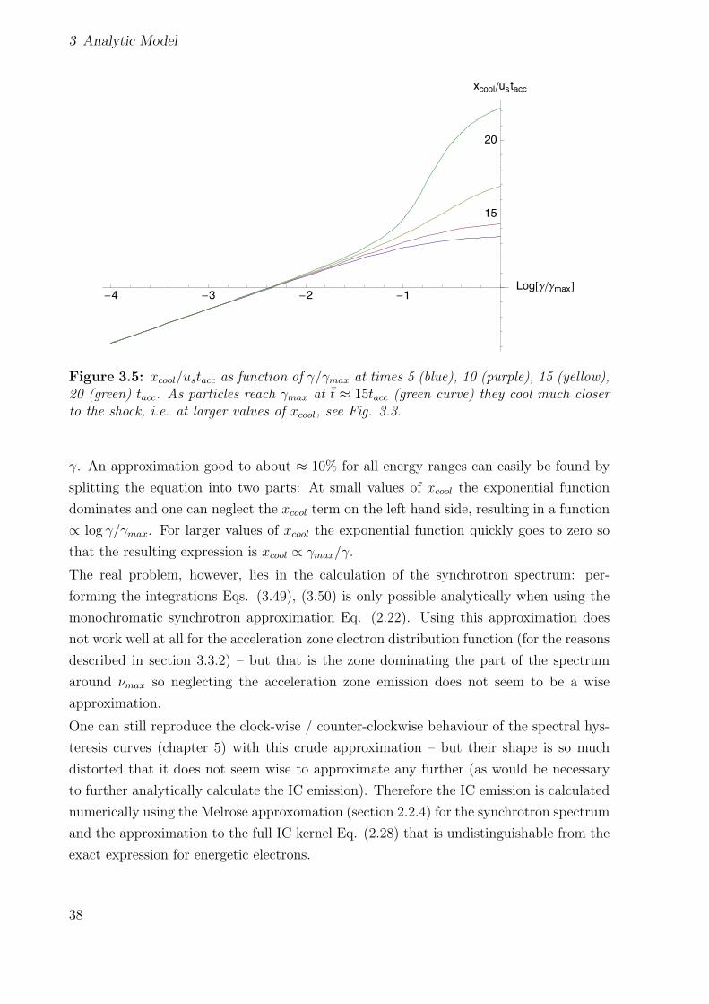
3 Analytic Model

!4 !3 !2 !1Log!"""max#

15

20

xcool"ustacc

Figure 3.5: xcool/ustacc as function of γ/γmax at times 5 (blue), 10 (purple), 15 (yellow),20 (green) tacc. As particles reach γmax at t ≈ 15tacc (green curve) they cool much closerto the shock, i.e. at larger values of xcool, see Fig. 3.3.

γ. An approximation good to about ≈ 10% for all energy ranges can easily be found by

splitting the equation into two parts: At small values of xcool the exponential function

dominates and one can neglect the xcool term on the left hand side, resulting in a function

∝ log γ/γmax. For larger values of xcool the exponential function quickly goes to zero so

that the resulting expression is xcool ∝ γmax/γ.

The real problem, however, lies in the calculation of the synchrotron spectrum: per-

forming the integrations Eqs. (3.49), (3.50) is only possible analytically when using the

monochromatic synchrotron approximation Eq. (2.22). Using this approximation does

not work well at all for the acceleration zone electron distribution function (for the reasons

described in section 3.3.2) – but that is the zone dominating the part of the spectrum

around νmax so neglecting the acceleration zone emission does not seem to be a wise

approximation.

One can still reproduce the clock-wise / counter-clockwise behaviour of the spectral hys-

teresis curves (chapter 5) with this crude approximation – but their shape is so much

distorted that it does not seem wise to approximate any further (as would be necessary

to further analytically calculate the IC emission). Therefore the IC emission is calculated

numerically using the Melrose approxomation (section 2.2.4) for the synchrotron spectrum

and the approximation to the full IC kernel Eq. (2.28) that is undistinguishable from the

exact expression for energetic electrons.

38

3.5 Synchrotron Spectrum

1012 1014 1016 1018 1020! !Hz"1000

105

107

109

! I! !arbitrary units"

Figure 3.6: The spectrum from the acceleration zone as calculated from Eq. (3.49) fort =10 (blue), 15 (purple) and 20 (yellow) tacc. For later times the spectrum does notchange anymore as γ1(t = 20tacc) ≈ γmax for the parameters chosen.


Now to calculate the spectrum, the electron distributions that have already been inte-

grated over the x coordinate need to be convolved with the synchrotron emissivity P (ν, γ),

Eq. (2.26) and transformed into the observer’s frame (see chapter 2.1.1).

3.5.1 Contribution from the acceleration zone

Since the acceleration zone is assumed to be infinitely thin the contribution to the intensity

from the acceleration zone is easily found using a Dirac Delta function:

Is(ν, t) =

∫dxP (ν, γ)

∫dxN(γ, t)δ(x− us(t+ x/c)) (3.48)

Rewriting the Delta function and performing the integration, one finds the intensity from

the shock to be

Is(ν, t) =a

1− us/cγ−(tacc+tesc)/tescmax

∫ γ1(t)

γ0

dγ P (ν, γ)

(γmaxγ

)2(γmaxγ− 1

) tacc−tesctesc

(3.49)

39

3 Analytic Model

1012 1014 1016 1018 1020! !Hz"105

106

107

108

109


Figure 3.7: The spectrum from the radiation zone as calculated from Eq. (3.50) fort =10 (blue), 20 (purple), 50 (yellow), 500 (green) tacc. One can clearly see how thebreak develops only at later times, because only then electrons have enough energy to coolcompletely inside the radiating region before escaping, resulting in a harder spectral index.

3.5.2 Contribution from the radiation zone

In the acceleration zone we have to perform a real integration over x, where the compli-

cated behaviour of xcool comes in (section 3.4.2). Again the spatially integrated electron

distribution is convolved with the synchrotron power P (ν, γ) to yield the specific intensity:

I0(ν, t) =

∫dγPs(ν, γ)

∫ x1

x0

dxn(x, γ, t+

x

c

)(3.50)

3.5.3 Transformation to the observer’s frame

The total intensity is then given as the sum over the Eqs. (3.49), (3.50)

I1(ν, t) = I0(ν, t) + Is(ν, t) (3.51)

The specific intensity found this way (Fig. 3.8) has to be transformed to the observer’s

frame (see chapter 2.1.1) and multiplied by the ratio of projected jet cross section to the

square of the distance to account for the size of the jet and the distance-square-law:

Iobs(νobs, tobs) =πR2

d2L

8Γ2

z + 1I1(νobs/2Γ,Γ(tobs − βb dL/c)) (3.52)

40


1012 1014 1016 1018 1020! !Hz"1000

105

107

109


Figure 3.8: The synchrotron emissivity from both the acceleration (yellow) and radiationzones (blue) as calculated from Eq. (3.49) and Eq. (3.50) for the stationary case t =500tacc. The total spectrum (purple) is dominated by the emission from the much largerradiation zone for all but the highest energies.

where Γ(tobs−βbdL/c) takes into account the (Lorentz transformed) light travel time from

the distant blazar to the telescope on earth and dL is the luminosity distance of the blazar

(section 2.3). βb is the bulk velocity in units of c.

3.5.4 Synchrotron fit for Markarian 501

Finally I show a fit to historical synchrotron data5 for the extreme BL Lac object Markar-

ian (Mrk) 501 (Fig. 3.9). Mrk 501 has a redshift of z = 0.034 which corresponds to a

luminosity distance of 4.43 ·1026 cm using best values for the cosmological parameters (see

section 2.3). One can clearly see the spectral break just above 1012 Hz. Below, electrons

have so little energy that their cooling times tcool = 1/(βsγ) are much longer than the

energy-independent escape time tesc so that they leave the source without having cooled

completely, resulting in a relatively steep spectral index. Beyond the break all electrons

cool completely within the source and the spectral index flattens from 0.75 to 0.25 in the

νFν plot. At the maximum frequency observed, taken to be 5 · 1017 Hz, tcool = tacc so

that particles cannot be accelerated any further. In fact, the electron distribution cuts

5Model and data (Catanese et al 1997) are the same as for Fig. 2 of Kirk et al (1998) but here allparameters are stated explicitly as needed later for the IC model – although some of them are notconstrained by the synchrotron peak alone.

41

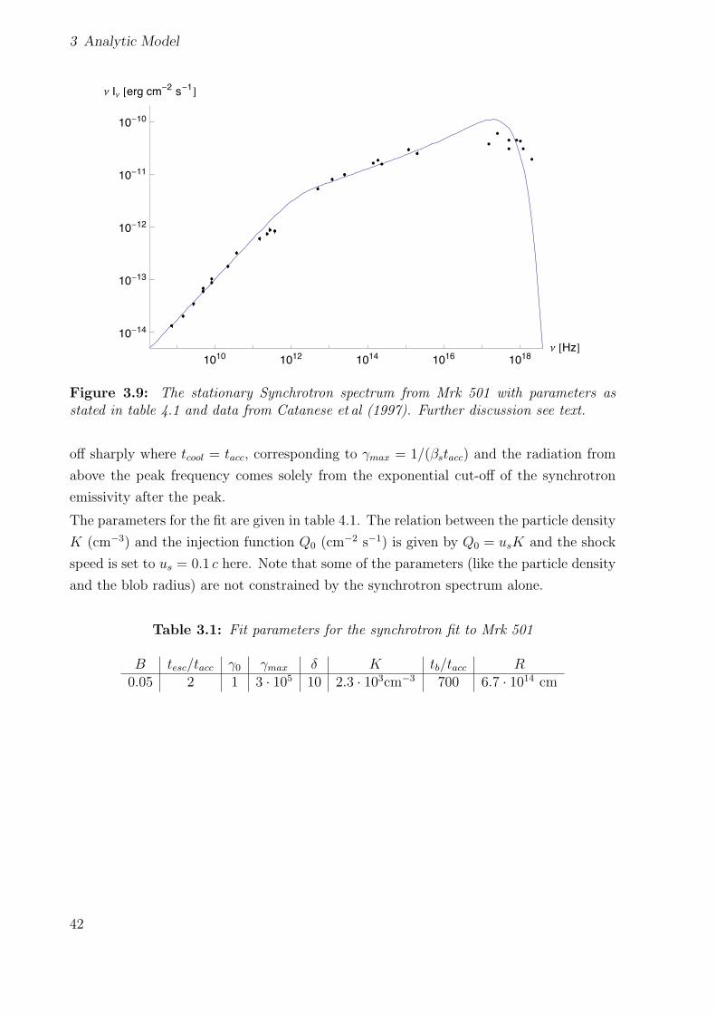
3 Analytic Model

1010 1012 1014 1016 1018! !Hz"10"14

10"13

10"12

10"11

10"10

! I! !erg cm"2 s"1"

Figure 3.9: The stationary Synchrotron spectrum from Mrk 501 with parameters asstated in table 4.1 and data from Catanese et al (1997). Further discussion see text.

off sharply where tcool = tacc, corresponding to γmax = 1/(βstacc) and the radiation from

above the peak frequency comes solely from the exponential cut-off of the synchrotron

emissivity after the peak.

The parameters for the fit are given in table 4.1. The relation between the particle density

K (cm−3) and the injection function Q0 (cm−2 s−1) is given by Q0 = usK and the shock

speed is set to us = 0.1 c here. Note that some of the parameters (like the particle density

and the blob radius) are not constrained by the synchrotron spectrum alone.

Table 3.1: Fit parameters for the synchrotron fit to Mrk 501

B tesc/tacc γ0 γmax δ K tb/tacc R0.05 2 1 3 · 105 10 2.3 · 103cm−3 700 6.7 · 1014 cm

42

4 Inverse Compton (IC) contribution

Here I will specify which parts of the model are affected in what way when IC scattering

is considered. I will then carefully weigh those modifications against each other to find

out which of them needs to be included for a first approximation. The IC spectrum is

then calculated numerically and a fit for some of the latest correlated data for Mrk 501

is produced and discussed.

4.1 Extension of the model

To include the Inverse Compton (IC) effect in this model to a first approximation all losses

will be neglected and the IC spectrum will be calculated from the scattering of the electron

distributions, Eqs. (3.18) and (3.22), with the unaltered synchrotron spectra from both

zones, Eqs. (3.49) and (3.50). The effects neglected and the reasons and justifications to

do so are given here.

• IC losses for the electron distributions The electron distributions in both the

acceleration and radiation zone would have to be corrected for IC losses according

to Eq. (2.30). In BL Lac objects, however, IC scattering is thought not to dominate

electron losses (Comastri et al 1997). Indeed, most observed BL Lacs show approx-

imately equally strong synchrotron and IC peaks (in a νFν plot) suggesting (very

roughly) equipartition between the energy densities in the magnetic field and in the

synchrotron photons. Another indication that IC scatterings are not dominant in

BL Lacs is that this model works very well for the synchrotron emission without

considering these losses (see Fig. 3.9).

• Losses for synchrotron photons due to Compton upscattering IC losses

for photons can also be neglected here since the number density of IC photons is

smaller than the synchrotron photon number density by a factor ≈ γ2max. All higher

order photon loss processes, such as IC photon losses due to the ‘normal’ Compton

effect will consequently also be neglected.

• Photon pair production (γ γ → e+e−) becomes important for very high energy

43


gamma rays. But for a first approximation this can also be neglected, as the min-

imum required Doppler factor for gamma-ray transparency (Dondi and Ghisellini

1995) is chosen so that pair production is not the dominant mechanism.

These are the physical reasons for neglecting those IC-related losses here. A more technical

reason for not including IC losses of the electrons is that, in the current framework of

this semi-analytical model, it would only be possible using very crude monochromatic

approximations. But as the use of the Delta approximation for the synchrotron emissivity

already leads to very distorted synchrotron spectra (cf. section 3.4.2), this does not seem

the right way to go. On the other hand, if one wanted to include IC losses properly (Eq.

(2.30)), it would require a completely numerical model as the resulting integro-differential

equations are no longer analytically solvable.

So it seems a good compromise between computational effort and quality of the spectra

to stay with the semi-analytical model for another while and calculate the IC spectrum

for the unaltered electron and photon distributions but use the (approximation to the)

full Klein-Nishina cross-section.1

After all, as the result will demonstrate, the way I calculate the IC spectrum here can

already give a good approximation to the IC emission of blazars.

4.2 Computation of the IC spectrum

The time-dependent Inverse Compton spectrum is obtainted from two numerical inte-

grations using the approximation to the full Klein-Nishina Compton kernel Eq. (2.28) in

Mathematica. The computer-algebra software Mathematica is described in appendix

B and complete and commented program (‘notebook’) listings are given in appendix C.

The IC spectrum is then given as

dNtot(t)

dtdε1=

∫ε

∫γ

dγ

[N(γ, t)

dNγ,ε,acc

dtdε1

]+

[n(γ, t)

dNγ,ε,rad

dtdε1

](4.1)

where dNγ,ε,acc,rad/dtdε1 is the Compton kernel Eq. (2.28) with the number densities of

photons for the two zones

n(ε)acc,rad(t) ∝I0,s(ε/h, t)

ν(4.2)

1Nonetheless it is somehow ironic to neglect IC losses: When the IC effect was first applied to as-trophysical scenarios in the late 1940s, it was only included to describe energy losses and no onethought about the corresponding gains for photons. Only when the observational windows of X- andGamma-ray astronomy were opened in the late 1950s, this process received interest as an energy gainmechanism for photons (Felten and Morrison 1966).

44

4.3 Time-dependent Inverse Compton Spectrum

1018 1019 1020 1021 1022 1023 1024! !Hz"10"12

10"11

10"10

10"9

10"8

10"7

10"6

! I! !erg cm"2 s"1"

Figure 4.1: The time-dependent Inverse Compton spectrum obtainted from two numericalintegrations as described in the text. The spectra are plotted for times t =8, 9, 10, 20, 50and 500 tacc (more energetic spectra correspond to later times). The spectral index beforethe peak is α = −0.5 for early times and flattens to α ≈ −0.8 for high energies at latertimes.

4.3 Time-dependent Inverse Compton Spectrum

In Fig. 4.1 the time-dependent IC spectrum is shown as it is building up from zero

emission at t = 0 to the spectra plotted. At early times, where the spectrum builds up

with a spectral index of -0.75 (definition see Eq. (2.25)) in the synchrotron regime, it is

already flatter in the IC branch with α = −0.5. Also, the break, visible in the synchrotron

spectrum (Fig. 3.7) for times greater than about 20 tacc at the position where tcool = tesc,

is smeared out here. At times later than ≈ 20tacc, where the break begins to develop in

the synchrotron spectrum, the spectrum flattens to α = −0.82.2

While the spectral index of -0.5 is in accordance with other SSC models (e.g. Krawczynski

et al 2004) one would still expect the IC spectral index to be the same as in the synchrotron

regime, i.e. -0.25 for the early-time spectrum or at later times -0.25 and -0.75 before and

after the break respectively. This is not the case here due to IC scattering in the Thomson

regime which favours the low energy end and thus produces relatively flat spectra. The

small curvature of the IC peak is problematic, however, as it does not fit very well to

observations (see Fig. 4.2).

2For −1 < α < 0 the spectrum flattens in the νFν plot when it steepens in the Fν plot.

45


4.4 SSC fit for Mrk 501

In Fig. 4.2 the full spectral energy distribution for Mrk 501 is given as calculated from

the synchrotron and IC emissions from both zones. Also plotted are simultaneous optical

(KVA), X-Ray (ASM) and gamma-ray (MAGIC) data. The χ2 value (section 2.5) has

been used to find the best fit to the data. Still χ2/ndof = 19.712/11 = 1.79 for the VHE

points because the curvature of the fit is a bit too large, but cannot be altered in this

model.

The X-Ray peak is at νmax,X = 6 · 1020 Hz, very high compared to νmax,X = 5 · 1017

Hz from Fig. 3.9. But Mrk 501 is an extreme BL Lac object which has shown X-Ray

radiation up to ≈ 1020 Hz in the past (Katarzynski et al 2001) and as this is a fit to one of

the highest IC fluxes ever observed from Mrk 501 (Albert et al. (MAGIC collaboration)

2007b) the peak frequency might not be all to unrealistic.

Another feature that requires careful examination it the relation between the synchrotron

and IC peak heights: In this fit the synchrotron peak outshines the IC peak by about one

order of magnitude. Although this is a bit away from equipartition between magnetic and

radiation field energy density, it seems required for these data also for other SSC models,

see Albert et al. (MAGIC collaboration) (2007b) and references therein.

At least this synchrotron to IC peak flux ratio is consistent with the approximation that

IC losses are not dominant here.

Table 4.1: Fit parameters for the full SED for Mrk 501

B tesc/tacc γ0 γmax δ K tb/tacc R0.1 2 1 7 · 106 25 2.3 · 103cm−3 500 2.42 · 1014 cm

46

4.4 SSC fit for Mrk 501

1015 1020 1025! !Hz"10"11

10"10

10"9

! I! !erg cm"2 s"1"

Figure 4.2: The full synchrotron and Inverse Compton stationary spectral energy dis-tribution from Mrk 501 with fit parameters as given in table 4.1 and data from the ob-servational campaign from May through July 2005 (Albert et al. (MAGIC collaboration)2007b). The optical data point is from the KVA observatory with the error coming mostlyfrom the large uncertainty in subtracting the host galaxy. The X-Ray points are from theRXTE satellite’s all-sky monitor (ASM) and the high-energy points are from MAGIC. Thegamma-ray data have been corrected for EBL using the ‘low’ EBL model from Kneiskeet al (2004). Light blue points are the average low-flux emission during the observationalcampaign, dark blue points correspond to medium flux and green points to the high-fluxdataset (integral flux above 150 GeV > 1.0 Crab unit, where one ‘Crab unit’ is the fluxfrom the supernova remnant and gamma-ray standard candle Crab nebula). The opticaldata have been averaged over all times as they do not show much variability. Black pointsare from the strongest flare seen during that campaign (June 30) for which the parametershave been optimized. As can be seen, the curvature of the VHE points is not correctlygiven by the model, see text for further discussion.

47


48

5 Variability

Variability can occur for a number of reasons. In the shock-in-jet model the easiest way to

produce a flare is to set the particle injection function Q(t) to a higher value for a certain

time. This could be the case if the shock runs over a region of increased particle density.

As magnetic fields are frozen into the particles in highly conductive plasmas, one might

then expect the magnetic field to vary, too, i.e. the maximum attainable electron Lorentz

factor to change. Therefore, another value that could be varied to produce a flare is the

maximum electron Lorentz factor γmax = 1/βstacc.

5.1 Modelling a flare

During a flare of time tf , the injection function is enhanced by a factor of ηf simply by

setting

Q(t) =

Q0 for t < 0 and t > tf

(1 + ηf )Q0 for 0 < t < tf(5.1)

The intensity during a flare is then given by

Iflare(ν, t) = I1(ν,∞) + ηf,syn,ic[I1(ν, t)− I1(ν, t− (1− us/c)tf )] (5.2)

where ηf,syn = ηf and ηf,ic = (1 + ηf )2 − 1 because in the inverse Compton regime the

peak height is ∝ Q2 as both the particle density and the seed photons are increased by

ηf .

The flare presented in the following discussion is produced using the model parameters

of table 5.1 and the flare parameters tf = 10tacc, ηf = 1, i.e. a doubling of the injection

function for 10 acceleration times. With respect to the fit parameters for the Mrk 501 fit,

Fig. 4.2, less extreme values have been chosen to calculate the flare spectra. The choice

of parameters is not overly important for the production of flares within this model.

However, the reason for chosing a rather conservative set of parameters (no extreme value

for γmax, for example) is that these seem to be the more general case, applicable to a large

49

5 Variability

number of blazars.

Also the (unphysical) choice us = 0 is made to simplify calculations. At any time this

does not alter the spectra in the region of interest here, namely the one close and around

the maximum of the emission.

Table 5.1: Model parameters for the flare

B γ0 γmax δ K tb/tacc R0.3 G 1 1 · 104 25 6 · 104cm−3 100 1 · 1015 cm

5.2 Flaring behaviour I: Intensity profiles

In Figures 5.1 and 5.2 a flare of duration 10tacc is produced as described above and

followed over 50tacc with only characteristic times plotted. To reach γmax = 104 electrons

take trise ≈ 11 acceleration times (cf. Fig. 3.1). Since for electrons with γ = γmax the

cooling time equals the acceleration time it is to be expected that after tmax ≈ tf+trise/2 =

15.5tacc the maximum should be reached. Indeed, after≈ 17tacc (red curves) the maximum

is reached. Cooling sets in after that and it can clearly be seen that cooling is more efficient

at higher energies: 26tacc (blue curves) after the beginning of the flare the emission has

almost fallen back to the stationary level at the peak frequency, while it is still going

on at lower frequencies. In the IC peak the flare takes longer at the peak frequency

because lower energy photons still get upscattered to the maximum frequency when the

synchrotron flare has already decayed at the peak frequency. Both spectra cover roughly

five orders of magnitude in frequency and about one and a half orders of magnitude in

intensity.

In Figures 5.3 and 5.4 the intensity (normalised to the stationary emission at the respective

frequency) at the four frequencies ν/νmax = 1/100, 1/10, 1, 10 is plotted against time. The

most prominent feature here is that, at the lowest frequency (red curve), the fall time is

considerably longer than at higher frequencies due to the energy-dependent cooling rate.

The rise time, on the other hand, is similar for all four curves. Note that all curves start at

later times in the IC plot since the IC emission can only flare after the seed photons have

been produced. A discontinuity arises 10tacc after the rise sets in due to the modelling of

the emission mechanism, Eq. (5.1). Also, in order not to consume too much computer

time, only one spectrum per tacc has been produced which is responsible for the remaining

parts where the curves are not differentiable.

50

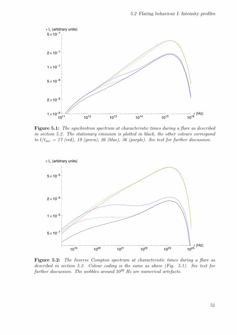
5.2 Flaring behaviour I: Intensity profiles

1011 1012 1013 1014 1015 1016! !Hz"1"10#8

2"10#8

5"10#8

1"10#7

2"10#7

5"10#7! I! !arbitrary units"

Figure 5.1: The synchrotron spectrum at characteristic times during a flare as describedin section 5.2. The stationary emission is plotted in black, the other colours correspondto t/tacc = 17 (red), 19 (green), 26 (blue), 36 (purple). See text for further discussion.

1019 1020 1021 1022 1023 1024! !Hz"

5"10#7

1"10#6

2"10#6

5"10#6


Figure 5.2: The Inverse Compton spectrum at characteristic times during a flare asdescribed in section 5.2. Colour coding is the same as above (Fig. 5.1). See text forfurther discussion. The wobbles around 1020 Hz are numerical artefacts.

51

5 Variability

10 15 20 25 30 35 40 t!!tacc1.2

1.4

1.6

1.8

2.0I" "normalised#

Figure 5.3: Plot of synchrotron intensity versus time of a flare as described in section 5.2at frequencies 1/100 (red), 1/10 (green), 1 (purple), 10 (black) times νmax. The intensityhas been normalised to the stationary (pre-flare) emission at that frequency. Furtherdiscussion see text.

10 15 20 25 30 35 40 t!!tacc1.5

2.0

2.5

3.0

3.5

4.0I" "normalised#

Figure 5.4: Plot of Inverse Compton intensity versus time (in tacc) of a flare resultingfrom an increase in electron injection of a factor of 2 for a duration of 10 tacc at differentfrequencies. Colour coding as in Fig. 5.3.

52

5.3 Flaring behaviour II: Spectral Index variation

5.3 Flaring behaviour II: Spectral Index variation

In Figures 5.5 and 5.6 the change of the spectral index with respect to the spectral index

for the stationary (pre-flare) state is plotted

∆α(t) = αflare(ν, t)− α(ν) (5.3)

So, curves for different frequencies (colour coding from low to high frequencies according

to the visible spectrum of colours) can be shown in one plot and the differences can be

seen easily. Also, as the absolute spectral index is not a very reliable prediction of this

model, the relative values should compensate for some of the inaccuracies of the model.

The spectral index is defined here as

α(ν1) = log

[F (ν2)

F (ν1)

]/ log

[ν2

ν1

](5.4)

with ν2 > ν1 and close to each other.

The general behaviour is the same in both the synchrotron and the IC regime: At low

frequencies a hard lag behaviour (hardening follows softening) is seen, at high frequencies

the situation is vice versa, a soft lag is produced. Considering the discussion in this

section the behaviour is immediately clear: Radiation is more efficient at high than at

low frequencies so that more radiation is produced there at the beginning, resulting in

a steepening (in the νFν plot, ∆α > 0) at low and a flattening (∆α < 0) at high

frequencies. Later, when electrons have had time to cool, more radiation is produced

at lower frequencies resulting in the opposite behaviour. There is not much difference

between the synchrotron and IC plots here, except that the amplitude of the spectral

index variation is almost twice as large in the IC regime. Non-differentiable and ragged

parts of the curves are due to numerical resolution effects. But notice how e.g. the second

peak of the red curve (more distinguished in the synchrotron plot) evolves to the purple

‘full’ peak for higher frequencies.

5.4 Variation of spectral index with flux (Hysteresis)

Now, plotting the flare-intensity and spectral index curves in one plot using the flare time

as the parameter one arrives at the well known spectral hysteresis curves that are shown

in Figures 5.7 to 5.12 for ν/νmax = 1/100, 1/10, 1 on the following pages. Discussion

follows in section 5.6.

53

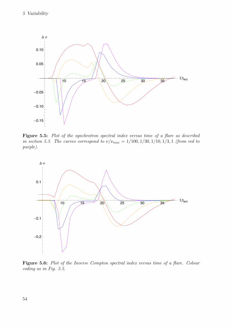
5 Variability

10 15 20 25 30 35 t!!tacc

"0.15

"0.10

"0.05

0.05

0.10

# $

Figure 5.5: Plot of the synchrotron spectral index versus time of a flare as describedin section 5.3. The curves correspond to ν/νmax = 1/100, 1/30, 1/10, 1/3, 1 (from red topurple).

10 15 20 25 30 35 t!!tacc

"0.2

"0.1

0.1

# $

Figure 5.6: Plot of the Inverse Compton spectral index versus time of a flare. Colourcoding as in Fig. 5.5.

54


1.1 1.2 1.3 1.4 1.5 1.6I! !normalised"

"0.10

"0.05

0.05

0.10

# $

Figure 5.7: Parametric plot of synchrotron intensity versus synchrotron spectral indexwith the parameter time (t/tacc = 1 . . . 34) of a flare resulting from an increase in electroninjection of a factor of 2 for a duration of 10 tacc at low frequencies, ν = 1/100νmax.

1.2 1.4 1.6 1.8 2.0I! !normalised"

"0.15

"0.10

"0.05

0.05

0.10

# $

Figure 5.8: Spectral hysteresis curve of the synchrotron flare as in Fig. 5.7, but at themaximum frequency.

55

5 Variability

1.5 2.0 2.5 3.0 3.5I! !normalised"

"0.10

"0.05

0.05

0.10

0.15

# $

Figure 5.9: Parametric plot of Inverse Compton intensity versus Inverse Compton spec-tral index with the parameter time (t/tacc = 1 . . . 34) of a flare resulting from an in-crease in electron injection of a factor of 2 for a duration of 10 tacc at low frequencies,ν = 1/100νmax.

1.5 2.0 2.5 3.0 3.5I! !normalised"

"0.2

"0.1

0.1

# $

Figure 5.10: Spectral hysteresis curve of the IC flare as in Fig. 5.9, but at the maximumfrequency.

56


1.2 1.4 1.6 1.8 2.0I! !normalised"

"0.08

"0.06

"0.04

"0.02

0.02

0.04

0.06# $

Figure 5.11: Parametric plot of synchrotron intensity versus synchrotron spectral indexwith the parameter time (t/tacc = 1 . . . 34) of a flare resulting from an increase in electroninjection of a factor of 2 for a duration of 10 tacc at medium frequencies, ν = 1/10νmaxwhere the transition between clock-wise and counter-clock-wise behaviour occurs.

1.5 2.0 2.5 3.0 3.5 4.0I! !normalised"

"0.10

"0.08

"0.06

"0.04

"0.02

0.02

0.04

# $

Figure 5.12: Spectral hysteresis curve at the medium frequency as in Fig. 5.11, but forthe IC regime.

57

5 Variability

5.5 Timescales

The Synchrotron model was originally built to explain spectral variability in X-Rays of

the order of several hours (103 . . . 104 s) as observed in various sources (Gear et al 1986;

Sembay et al 1993; Takahashi et al 1996). It is obvious to first apply the IC extension to

the same timescales since the IC spectrum is produced by the same electrons that are made

responsible for the synchrotron flares. However, the model is largely scale-invariant since

all transient phenomena are expressed in terms of tacc. But of course there are physical

limits for the observable variability time scale. A lower limit is given by the causality

relation tvar R/c, reasoning, that time variability shorter than the light travel time

through the source would be dominated by geometrical effects rather than the intrinsic

spectral behaviour ascribed to acceleration and cooling. Assuming tvar ≈ tcool one gets

the following lower limit on the observable variability time that could be explained with

this model

tvar,obs,min ≥ 400 s

(0.1 G

B

)2(107

γmax

)(25

δ

)(Rjet

1014 cm

)(5.5)

So, time variability much shorter than several hours could be explained in principle and

variability in the range of the very fast flux doubling times of just two minutes that

MAGIC has recently seen in Mrk 501 (Albert et al. (MAGIC collaboration) 2007b) can

also be described with the model. Although the flare was produced for different parameters

as the SSC fit for the Mrk 501 emission, the model can also produce spectral hysteresis

curves for different parameters. Nonetheless it would be very interesting to observe the

same variability also on an hour-scale – if it looks similar one might reason that the same

processes are at work on different time scales.

Variability in the VHE band might also be modulated by a precessing jet, bent by the

tidal forces of a putative central super-massive black-hole binary system, as has been put

forward to explain the 23 day variability in Mrk 501 (Rieger and Mannheim 2000).

To get an impression of the size of the emitting blob, consider the knot HST-1 in M87

that is believed to be a site of gamma ray flaring emission. In the blob in jet model only

a small region inside this structure could be responsible for the gamma-ray emission as

the size of the blob is canonically 1015 cm = 3 · 10−4 pc whereas the HST-1 knot is about

1 pc in diameter. The VLBI knots C2, 3, 4 of Mrk 501 are also ≈ 1 pc in diameter.

58

5.6 Observations of variable high-energy spectra

5.6 Observations of variable high-energy spectra

In Figures 5.7 to 5.12, spectral hysteresis curves for the synchrotron and IC regime and at

different frequencies were plotted, showing that both a clock-wise (at lower frequencies)

and a counter-clockwise (at higher frequencies) behaviour can be produced with this model

– also in the IC regime, which, in the context of an SSC model, has not been shown before.

Again, differences between the synchrotron and IC curves are small and probably more

due to numerical resolution problems than due to physical differences (in this model). Of

course the intensity amplitude is larger in the IC case, but we put that in in the beginning,

Eq. (5.2).

In a recent campaign MAGIC has observed Mrk 501 over several months in 2005 and

caught two very bright flares on June 30 and July 9 for which it was possible to produce

spectra – or at least the so called ‘hardness ratio’ that is defined as the ratio of the flux

at two specified energy ranges. Here, as the peak lies at ≈ 1 TeV (see Fig. 4.2), the

energy bins to calculate the hardness ratio from were chosen as 0.25 to 1.2 TeV and 1.2

to 10 TeV. The so derived hardness ratio vs. flux plots are reproduced in Fig. 5.13.

The comparison with the corresponding theoretical curve Fig. 5.10 on page 56 is very

encouraging: The qualitative behaviour of the observed hysteresis is consistent with the

prediction from the model. By lucky coincidence the peak emission during that flare was

in the observable window of the MAGIC telescope and so the comparison with the model

was easily possible. The observed intensity amplitude of the July 9th’s flare, taken to be

the ratio of the fluxes from points ‘9’ and ‘7’ of Fig. 5.13, is about 3.3 – suggesting roughly

doubling of the injected electrons. Of course absolute values for the hardness ratio do not

correspond to the calculated ∆α values. A model plot of hardness ratio against flux might

try to even give a quantitative fit to the observed short-time variability, constraining the

acceleration mechanism at work. Future simultaneous observations of a peak in the IC

spectrum at energies well below the peak could help confirming – or disproving – the

model.

To better constrain the model it would be very helpful to have good simultaneous X-Ray

data. Then one could test if the spectral hysteresis is described in the same sense in the

X-Ray regime or, with even better spectral coverage, if the different variability patterns

can be seen at different frequencies.

Let me add a short note concerning the observability of hour-scale variability with a

ground-based gamma-ray telescope. It would be difficult for such a telescope to observe

a specific source over more than a few hours as the zenith angle of the sources changes

dramatically in that time and with that the energy-cutoff of the telescope changes as

59

5 Variability

– 48 –

]-1 s-2F(>0.25 TeV) [cm

0.2 0.3 0.4 0.5 0.6 0.7 0.8 0.9 1.0 1.1

-910!

Hard

ness r

ati

o

0.0

0.1

0.2

0.3

0.4

0.5

1 23

4

5

6

7

8 9

10

1112

13

14

15

16

2005 Jun 30

]-1 s-2F(>0.25 TeV) [cm

0.2 0.3 0.4 0.5 0.6 0.7 0.8 0.9 1.0 1.1

-910!

Hard

ness r

ati

o

0.0

0.1

0.2

0.3

0.4

0.5

12

3

4

5

6

7

8

9

10

11

12

2005 Jul 9

Fig. 17.— Hardness ratio F (1.2 ! 10 TeV)/F (0.25 ! 1.2 TeV) vs F (> 0.25 TeV) for thenights of June 30 and July 9. Horizontal and vertical bars denote 1! statistical uncertainties.

Black/red symbols denote pre-burst (’stable’)/in-burst (’variable’) emission (see sect. 3.3 andFig. 5). The numbers inside the markers denote the position of the points in the LCs. Theconsecutive (in time) points of the in-burst LC are connected by red lines for better clarity.

Figure 5.13: Spectral hysteresis curves for two strong flares in Mrk 501 seen by MAGICon June 30 and July 9, 2005 (Albert et al. (MAGIC collaboration) 2007b). Black andred numbers indicate pre-burst and in-burst emisssion and the numbers give correspondloosely to the time with the total time of the flares being about 20 minutes. Note the closeresemblance to the spectral hysteresis pattern that has been produced from the model, Fig.5.10.

well, leading to higher cut-off energies for larger zenith distances. Observing a source

with multiple gamma-ray telescope spread over the longitudes, this problem could in

principle be overcome.

60

6 Summary and Discussion

6.1 Summary

In this work I extended the semi-analytic two-zone model for particle acceleration and

synchrotron emission in blazar jets of Kirk et al (1998) with the Self-Compton contribution

and looked at the time-dependence of the spectra in the Inverse Compton (IC) regime. As

expected, spectral variations were found that are very similar to those in the synchrotron

regime. The most important point here is that, both in the synchrotron and in the IC

branch, spectral hystereses are produced by that model when looking at a flare.

After giving a brief introduction, chapter 1, where the complexity of the topic was il-

lustrated and some connections to other areas of current research in astrophysics and

cosmology were shown up, I explained the most important theoretical background, chap-

ter 2. The advantage of using two zones was explained in section section 3.2 – namely,

being able to model the acceleration process time-dependently and thus producing cer-

tain spectral patterns that cannot be explained in a simple one zone model. In chapter 3

the analytical model of Kirk et al (1998) was reproduced and thereby some minor errors

and imperfections of the original paper were found and – thanks to helpful discussion

with Prof. John Kirk – corrected. section 3.4.2 explains why the analytical model gets

numerical in the end and shows that good analytic approximations for the transcendental

equation responsible for this may be found but in the end one has to use a formular for

the synchrotron emissivity that makes it impossible to proceed analytically.

In section 3.5 the calculation of the synchrotron spectra from both zones is shown and

the reproduction of the original paper is completed by fitting the model to archival data

for the well-studied blazar Mrk 501.

Chapter 4 first gives an overview of how the model would need to be changed to include

all implications of IC scattering. It is then argued that for finding the desired spectral

behaviour, several terms can be neglected as they do not influence the blazar spectra

significantly. The IC spectrum is then calculated from the unaltered photon and elec-

tron distributions using an approximation to the full Klein-Nishina cross-section and the

spectrum is fitted to recent simultaneous optical, X-Ray and VHE data. Although the

61


curvature of the IC emission around the peak is not exactly matched, the fit shows that

the approximations taken can well reproduce the spectral behaviour.

In chapter 5 it is demonstrated that a flare can be produced in the context of this model by

setting the electron injection function temporarily to a higher value. In sections 5.2 and

5.3 the flaring behaviour of the intensity and the spectral index is studied and physical

explanations for it are given. A section on timescales, section 5.5, justifies the applica-

tion of this model not only to the hour-scale variability, it was originally designed for,

but also for the much shorter variability times, down to two minutes, that is seen by

modern gamma-ray telescopes. Comparing the spectral behaviour of such a flare (Albert

et al. (MAGIC collaboration) 2007b) with the theoretical prediction, one finds a nice

consistency.

6.2 Discussion

While giving approximate fits to observational data, the time-dependent spectral be-

haviour can only be claimed to be given qualitatively at the moment, as the curvature of

the IC spectrum in the fit Fig. 4.2 is not matched good enough. This might be an effect

of overestimation of the high-energy electron population due to the neglectance of the IC

losses of the electron distribution. Another indication that the high-energy part of the

electron distribution needs to be modified comes from looking at the most recent X-Ray

data from the Japanese satellite Suzaku (Hayashida et al. 2007, to be published) for the

same source, Mrk 501. Due to the use of first-order differential equations a Θ function

appears in the electron distribution that cuts it off in the sharpest possible way: The

electron distribution function falls abruptly to zero at γ = γmax. While for the archival

data Kirk et al (1998) chose, that produced a very good fit (see, e.g., Fig. 3.9), in the light

of more recent observations like the one from the recent Suzaku campaign this aspect of

the model needs to be taken to reconsideration as well. An improvement might result

from including energy-space diffusion effects (second order derivatives in energy), that

would smoothen the cut-off. Webb et al (1984) tried this for a time-independent model

which resulted in a set of rather unhandy equations that they solved numerically. Another

way to produce a smooter cut-off would be to assume an inhomogeneous source region

or different acceleration mechanisms. A power law fit beyond γmax as often included by

ad hoc modelers (Krawczynski et al 2004; Tavecchio et al 1998). Although that might

readily produce very good fits in terms of small values of χ2, I think the more physical

approach undertaken here will eventually be more successful in giving a profound physical

modelling of the phenomena related to relativistic jets.

62

6.2 Discussion

1014 1015 1016 1017 1018! !Hz"

1.0"10#11

5.0"10#11

2.0"10#11

3.0"10#11

1.5"10#11


Figure 6.1: After γmax the electron distribution of the model fit is cut-off abruptly as aconsequence of using first order differential equations for the electron distribution function.As a result, the synchrotron emission after the peak comes solely from the exponentiallydecaying part of the synchrotron’s emissivity function and falls too steep to explain theserecent Suzaku observations (Hayashida et al. 2007, to be published). Further discussionsee text.

Acceleration is another weak point of the model. While the use of two zones with its

time-dependent modelling of acceleration is a huge improvement over one-zone models,

a more physical treatment of acceleration would involve the energy-dependent diffusion

coefficients so that the acceleration and escape times would become energy-dependent.

Kirk et al (1998) give the energy-dependent solution in the appendix1 for a simple ‘gyro-

Bohm’ diffusion coefficient, i.e. tesc,acc ∝ γ. Bhattacharyya et al (2002) found that in the

case of energy-dependent acceleration time, no ‘hard lag’ behaviour is produced. Also, rise

and decay times of the flaring behaviour strongly depend on whether or not acceleration

and escape are modelled time-dependently, the system reaching a steady state much faster

in the case of energy-dependent time scales. As the spectral behaviour of the flares can

give clues to the acceleration mechanism involved, a close interplay between model builders

and observers is needed to constrain the model further.

Another point that would also need to be overcome in a more physical model is the

production of a flare. Here, a flare is modelled as a sudden increase in the particle

injection function – which is certainly unphysical. This might actually be a good starting

1But note that all γs in the brackets of their Equation (A5) should be squared, as discovered byBhattacharyya et al (2002))

63


point for further work as the shape of the particle injection function Q(t) is likely to

influence the flares produced.

6.3 Prospects

Several new observatories for the most violent processes at work in the universe are being

constructed at the moment. One of the most eagerly longed for is the new Gamma Ray

Large Area Space Telescope (GLAST) (Gehrels and Michelson 1999) that will probably

detect several hundreds sources of high energy photons greatly improving the statistics

on these sources. With an energy range of roughly 20 MeV to 300 GeV and simultaneous

observations with ground-based gamma-ray telescopes that cover the energy-range up to

several TeV, a much larger part of the VHE part of the spectrum will be accessible for

observation. This will also help models such as this one as it will be possible to observe

a flare over both the regimes where a hard and a soft lag is expected from this model. If

the transition from hard to soft lag in going from frequencies around the peak to smaller

ones, is not seen, this two zone model can effectively be ruled out as an approximation

to blazar physics. If, on the other hand, both hard and soft lags could be seen from the

same flare this would strongly speak in favour of this model.

64

7 Zusammenfassung (German

Summary)

In dieser Arbeit wurde das zeitabhangige Zweizonenmodell von Kirk et al (1998), das

die Teilchenbeschleunigung und Synchrotronemission in Blazar-Jets beschreibt, um den

Selbst-Compton Beitrag erweitert. Mit dem so erweiterten Modell war es moglich, Stra-

hlungsausbruche (Flares) im hochenergetischen Gamma-Bereich zu modellieren und den

spektralen Verlauf eines Flares qualitativ korrekt zu bestimmen.

Im Einzelnen wurde nach einer Einfuhrung in die Thematik (Kapitel 1), bei der die Ver-

wobenheit des Themas mit zahlreichen anderen aktuellen Fragestellungen aus der Astro-

physik und Kosmologie deutlich wurde, und der Erklarung einiger grundsatzlicher Zusam-

menhange (Kapitel 2) zunachst das analytische Zweizonen-Modell nachgerechnet (Kapitel

3).

Der Vorteil einer Zweizonen-Geometrie wurde in Abschnitt 3.2 grundlich diskutiert und

die Details des Modells in Abschnitt 3.3 vorgestellt. Bei einem Zweizonen-Modell wird die

betrachtete Region unterteilt in eine Beschleunigungszone, in dem Teilchen (hier: Elek-

tronen und Positronen) durch Schockbeschleunigung (siehe Kapitel 2.1.3) Energie gewin-

nen und durch Synchrotronstrahlung Energie verlieren und eine Strahlungszone, in der

Teilchen nur noch Energie verlieren. Als wesentlich stellte sich heraus, dass es nur in einem

solchen Modell moglich ist, das in manchen Quellen beobachtete ‘hard lag’-Verhalten zu

erklaren, bei dem das Spektrum einer Quelle wahrend eines Flares zunachst weicher und

dann erst harter wird. Bei den meisten Quellen wurde im Rontgenbereich das umgekehrte

‘soft lag’-Verhalten gesehen, das auch mit Einzonenmodellen leicht erklarbar ist. Es tritt

auf, wenn der Kuhlungsprozess bei großeren Energien effizienter wird, wie es bei der Syn-

chrotronstrahlung der Fall ist, und so bei einem Flare, der durch eine vorubergehend

gesteigerte Teilcheninjektion charakterisiert wird, zunachst mehr Strahlung im hoheren-

ergetischen Bereich auftritt, bis die Teilchen soweit gekuhlt haben, dass das Spektrum

abflacht, bevor es wieder seinen stationaren Zustand annimmt.

Beim Nachrechnen des Modells wurden einige kleinere Fehler und Unvollstandigkeiten

im Originalpaper Kirk et al (1998) gefunden, die aber dank hilfreicher Diskussionen mit

65

7 Zusammenfassung (German Summary)

Herrn Prof. John Kirk behoben werden konnten.

Im Kapitel 3 wurde auch kurz darauf eingegangen, wieso das analytische Modell am

Ende doch numerisch wird und Versuche beschrieben, die transzendente Gleichung, die

dafur verantwortlich ist, durch geeignete Ausdrucke zu nahern. Obgleich die Naherung

fur xcool ausreichend gut war, war es nicht moglich, analytisch weiter zu rechnen, da die

einzige in diesem Zusammenhang verwendbare Naherung fur die Synchrotronemissivitat,

die monochromatische oder Delta-Naherung, die Spektren nur sehr verzerrt widergab.

Daraufhin wurden die Intensitaten der beiden Zonen numerisch bestimmt und disku-

tiert. Die gewunschten Verhalten in den Spektren ließen sich reproduzieren, insbesondere

der spektrale Bruch bei einer durch die Große der Quelle bestimmten Frequenz, wurde

erzeugt. Die Reproduktionsphase wurde mit einem Fit an historische Daten fur den Blazar

Markarian 501 abgeschlossen.

Die Erweiterung des Modells um den Beitrag durch den Invers-Compton-Effekt (IC-

Effekt) wurde in Kapitel 4 diskutiert. Dabei wurde zunachst aufgefuhrt, an welchen

Stellen das Modell verandert werden musste, um alle Auswirkungen des neu hinzugefugten

Prozesses zu berucksichtigen. Nach vorsichtiger Abwagung wurde festgestellt, dass das

gesuchte zeitabhangige IC-Spektrum in einer guten Naherung im Rahmen des semi-

analytischen Modells bestimmt werden kann. Die sehr viel aufwandigere Berechnung der

Energieverluste der Elektronen durch IC-Streuungen konnten nur in einem numerischen

Modell angemessen berucksichtigt werden. Das zeitabhangige IC-Spektrum wurde dann

in Abschnitt 4.3 vorgestellt und die Entstehung aus dem Synchrotronspektrum erlautert.

Zum Schluss wurde die spektrale Energieverteilung von Mrk 501 modelliert. Dazu wurden

das Synchrotron und IC-Spektrum an optische, Rontgen- und Gamma-Daten angepasst.

Der so erzeugte Fit wies im Invers-Compton-Bereich eine etwas zu weiche Krummung

des Spektrums auf, so dass nur ein reduziertes χ2 von 1.79 erreicht werden konnte. Die

insgesamt aber dennoch gute Ubereinstimmung von Modell und Beobachtungsdaten bei

der Wahl von ublichen SSC-Fit-Parametern zeigte aber, dass die Erweiterung um den

Invers-Compton-Effekt gelungen ist und die verwendeten Naherungen akzeptabel waren.

Im Kapitel 5 ging es schließlich um die Variabilitat der Spektren. Dazu wurde zunachst

vorgestellt, wie ein Flare im Rahmen des Modells ‘erzeugt’ werden kann, namlich durch

kurzzeitige Erhohung der Injektionsfunktion, und zu welcher Anderung in der Intensitat

dies fuhrt. Die einfache Modellierung einer abrupten Zunahme und ebenso abrupten Nor-

malisierung der Injektionsfunktion wurde dabei gewahlt, weil so die Injektionsfunktion

zeitunabhangig bleiben und die Linearitat der Intensitat ausgenutzt werden kann, um

die Flare-Intensitat zu bestimmen. In den folgenden Abschnitten 5.2 und 5.3 wurden

Intensitat und Spektralindex wahrend eines Flares genauer untersucht und physikalische

66

Grunde fur die Form der Spektren angegeben. In Abschnitt 5.4 wurde schließlich die

aus Beobachter-Papieren gewohnte Darstellung fur den spektralen Verlauf eines Flares

gezeigt, namlich der parametrische Plot Spektralindex gegen Intensitat mit Kurvenpa-

rameter Zeit. In Abschnitt 5.5 wurden Zeitskalen fur die Hysterese diskutiert. Dabei

konnte mittels einer groben Abschatzung gezeigt werden, dass das Modell durchaus nicht

nur fur Stundenvariabilitat geeignet ist, wie sie im Rontgenbereich gesehen und mit diesem

Modell erklart wurde. Mit gewissen Einschrankungen bei der Wahl der Parameter kann es

auch die extrem kurzzeitige Variabilitat von wenigen Minuten erklaren, wie sie moderne

Gamma-Teleskope fur einige AGNs gemessen haben. Als sehr hoffnungsvoll fiel dabei im

letzten Abschnitt des Kapitels, 5.6, auf, dass das spektrale Verhalten des Blazars Mrk 501

wahrend eines Flares im Jahr 2005 qualitativ mit dem von dem Modell erzeugten Verlauf

fur spektrale Variabilitat im entsprechenden Bereich des Spektrums ubereinstimmt.

67

7 Zusammenfassung (German Summary)

68

Bibliography

Aharonian et al. (H.E.S.S. collaboration)2006 Aharonian et al. (H.E.S.S. collab-

oration), F. A.: A low level of extragalac-tic background light as revealed by γ-rays fromblazars. In: Nature 440 (2006), april, p. 1018–1021

Aharonian et al. (H.E.S.S. collaboration)2007 Aharonian et al. (H.E.S.S. collab-

oration), F. A.: Detection of VHE gamma-rayemission from the distant blazar 1ES 1101-232with H.E.S.S. and broadband characterisation.In: ArXiv e-prints 705 (2007), may

Albert et al. (MAGIC collaboration) 2007aAlbert et al. (MAGIC collaboration), J.:Detection of Very High Energy Radiation fromthe BL Lacertae Object PG 1553+113 with theMAGIC Telescope. In: Astrophysical JournalLetters 654 (2007), january, p. L119–L122

Albert et al. (MAGIC collaboration) 2007bAlbert et al. (MAGIC collaboration),J.: Variable VHE Gamma-Ray emission fromMarkarian 501. In: astro-ph/0702008 (2007)

Antonucci 1993 Antonucci, R.: Unified mod-els for active galactic nuclei and quasars. In: An-nual Review of Astronomy and Astrophysics 31(1993), p. 473–521

Ball and Kirk 1992 Ball, L. ; Kirk, J. G.:Diffusive acceleration of electrons in SN 1987A.In: Astrophysical Journal Letters 396 (1992),september, p. L39–L42

Bhattacharyya et al 2002 Bhattacharyya,S. ; Sahayanathan, S. ; Kaul, C. L.: Effect of

Particle Acceleration Process on the Flare Char-acteristics of Blazars. In: Journal of Astrophysicsand Astronomy 23 (2002), june, p. 95–+

Blandford and Konigl 1979 Blandford,R. D. ; Konigl, A.: Relativistic jets as compactradio sources. In: The Astrophysical Journal 232(1979), august, p. 34–48

Blandford and Znajek 1977 Blandford,R. D. ; Znajek, R. L.: Electromagnetic extrac-tion of energy from Kerr black holes. In: MonthlyNotices of the Royal Astronomical Society 179(1977), may, p. 433–456

Blumenthal and Gould 1970 Blumenthal,G. R. ; Gould, R. J.: Bremsstrahlung, Syn-chrotron Radiation, and Compton Scattering ofHigh-Energy Electrons Traversing Dilute Gases.In: Reviews of Modern Physics 42 (1970),p. 237–271

Bronstein et al 2001 Bronstein, I. N. ; Se-

mendjajew, K. A. ; Musiol, G. ; Muhlig, H.:Taschenbuch der Mathematik. Harri Deutsch,2001

Buckley 1998 Buckley, J. H.: ASTRO-PHYSICS: What the Wild Things Are. In: Sci-ence 279 (1998), january, p. 676–+

Carroll and Ostlie 2006 Carroll, B. W. ;Ostlie, D. A.: An introduction to modern as-trophysics. An introduction to modern astro-physics / B. W. Carroll and D. A. Ostlie. 2nd edi-tion. San Francisco: Pearson, Addison-Wesley,ISBN 0-8053-0402-9. 2007, XVI+1278+A32+I31pp., july 2006

Catanese et al 1997 Catanese, M. ; Brad-

bury, S. M. ; Breslin, A. C. ; Buckley, J. H. ;Carter-Lewis, D. A. ; Cawley, M. F. ; Der-

mer, C. D. ; Fegan, D. J. ; Finley, J. P. ; Gai-

dos, J. A. ; Hillas, A. M. ; Johnson, W. N. ;Krennrich, F. ; Lamb, R. C. ; Lessard,R. W. ; Macomb, D. J. ; McEnery, J. E. ; Mo-

riarty, P. ; Quinn, J. ; Rodgers, A. J. ; Rose,

69

Bibliography

H. J. ; Samuelson, F. W. ; Sembroski, G. H. ;Srinivasan, R. ; Weekes, T. C. ; Zweerink,J.: Multiwavelength Observations of a Flarefrom Markarian 501. In: Astrophysical JournalLetters 487 (1997), october, p. L143+

Comastri et al 1997 Comastri, A. ; Fossati,G. ; Ghisellini, G. ; Molendi, S.: On the SoftX-Ray Spectra of gamma -loud Blazars. In: TheAstrophysical Journal 480 (1997), may, p. 534–+

Coppi 2002 Coppi, P. S.: Blazars – TheoreticalAspects. In: The Universe Viewed in Gamma-Rays (Conference), 2002, p. 1–10

Coppi and Blandford 1990 Coppi, P. S. ;Blandford, R. D.: Reaction rates and en-ergy distributions for elementary processes in rel-ativistic pair plasmas. In: Monthly Notices of theRoyal Astronomical Society 245 (1990), august,p. 453–507

Dermer and Schlickeiser 1993 Dermer,C. D. ; Schlickeiser, R.: Model for the High-Energy Emission from Blazars. In: The Astro-physical Journal 416 (1993), october, p. 458–+

Dondi and Ghisellini 1995 Dondi, L. ; Ghis-

ellini, G.: Gamma-ray-loud blazars and beam-ing. In: Monthly Notices of the Royal Astronom-ical Society 273 (1995), april, p. 583–595

Felten and Morrison 1966 Felten, J. E. ;Morrison, P.: Omnidirectional Inverse Comp-ton and Synchrotron Radiation from Cosmic Dis-tributions of Fast Electrons and Thermal Pho-tons. In: The Astrophysical Journal 146 (1966),december, p. 686–+

Fermi 1949 Fermi, E.: On the Origin ofthe Cosmic Radiation. In: Physical Review 75(1949), april, p. 1169–1174

Gear et al 1986 Gear, W. K. ; Robson, E. I. ;Brown, L. M. J.: Infrared variability of the BLLacertae object OJ287 since its outburst in 1983.In: Nature 324 (1986), december, p. 546–+

Gehrels and Michelson 1999 Gehrels, N. ;Michelson, P.: GLAST: the next-generationhigh energy gamma-ray astronomy mission. In:Astroparticle Physics 11 (1999), june, p. 277–282

Ginzburg and Syrovatskii 1964 Ginzburg,V. L. ; Syrovatskii, S. I.: The Origin of Cos-mic Rays. The Origin of Cosmic Rays, New York:Macmillan, 1964, 1964

Ginzburg and Syrovatskii 1965 Ginzburg,V. L. ; Syrovatskii, S. I.: Cosmic Magne-tobremsstrahlung (synchrotron Radiation). In:Annual Review of Astronomy and Astrophysics3 (1965), p. 297–+

Hayashida et al. 2007, to be publishedHayashida et al., M.: Wide-range multiwave-length observations of northern TeV blazars withMAGIC/HESS, Suzaku and KVA. In: Proceed-ings of the 30th International Cosmic Ray Con-ference, Merida, Yucatan, Mexiko, 2007, to bepublished, p. –

Jauch and Rohrlich 1976 Jauch, J. M. ;Rohrlich, F.: The theory of photons and elec-trons. The relativistic quantum field theory ofcharged particles with spin one-half. Texts andMonographs in Physics, New York: Springer,1976, 2nd ed., 1976

Jones 1994 Jones, F. C.: A theoretical reviewof diffusive shock acceleration. In: The Astro-physical Journal Supplement Series 90 (1994),february, p. 561–565

Jones and Ellison 1991 Jones, F. C. ; Elli-

son, D. C.: The plasma physics of shock accel-eration. In: Space Science Reviews 58 (1991),p. 259–346

Jones 1968 Jones, Frank C.: Calculated Spec-trum of Inverse-Compton-Scattered Photons. In:Phys. Rev. 167 (1968), Mar, Nr. 5, p. 1159–1169

70

Bibliography

Kardashev 1962 Kardashev, N. S.: Nonsta-tionarity of Spectra of Young Sources of Non-thermal Radio Emission. In: Soviet Astronomy6 (1962), december, p. 317–+

Katarzynski et al 2001 Katarzynski, K. ;Sol, H. ; Kus, A.: The multifrequency emissionof Mrk 501. From radio to TeV gamma-rays. In:Astronomy and Astrophysics 367 (2001), march,p. 809–825

Kirk et al 1998 Kirk, J. G. ; Rieger, F. M. ;Mastichiadis, A.: Particle acceleration andsynchrotron emission in blazar jets. In: Astron-omy and Astrophysics 333 (1998), may, p. 452–458

Kneiske et al 2004 Kneiske, T. M. ; Bretz,T. ; Mannheim, K. ; Hartmann, D. H.: Impli-cations of cosmological gamma-ray absorption.II. Modification of gamma-ray spectra. In: As-tronomy and Astrophysics 413 (2004), january,p. 807–815

Krawczynski et al 2004 Krawczynski, H. ;Hughes, S. B. ; Horan, D. ; Aharonian,F. ; Aller, M. F. ; Aller, H. ; Bolt-

wood, P. ; Buckley, J. ; Coppi, P. ; Fos-

sati, G. ; Goetting, N. ; Holder, J. ;Horns, D. ; Kurtanidze, O. M. ; Marscher,A. P. ; Nikolashvili, M. ; Remillard,R. A. ; Sadun, A. ; Schroeder, M.: Multi-wavelength Observations of Strong Flares Fromthe TeV-Blazar 1ES 1959+650. In: TheAstrophysical Journal 601 (2004), p. 151.– URL http://www.citebase.org/abstract?

id=oai:arXiv.org:astro-ph/0310158

Longair 1994 Longair, Malcom S.: High En-ergy Astrophysics, Volume 2 (Stars, the galaxyand the interstellar medium). 2. Cambridge Uni-versity Press, 1994

Mannheim 1993 Mannheim, K.: The protonblazar. In: Astronomy and Astrophysics 269(1993), march, p. 67–76

Mannheim and Biermann 1992 Mannheim,K. ; Biermann, P. L.: Gamma-ray flaring of3C 279 - A proton-initiated cascade in the jet?In: Astronomy and Astrophysics 253 (1992), jan-uary, p. L21–L24

Meier et al 2001 Meier, D. L. ; Koide, S. ;Uchida, Y.: Magnetohydrodynamic Productionof Relativistic Jets. In: Science 291 (2001), jan-uary, p. 84–92

Melrose 1980 Melrose, D. B.: Plasma astro-hysics. Nonthermal processes in diffuse magne-tized plasmas - Vol.1: The emission, absorptionand transfer of waves in plasmas; Vol.2: Astro-physical applications. New York: Gordon andBreach, 1980, 1980

Meyberg and Vachenauer 2003 Meyberg,Kurt ; Vachenauer, Peter: Hohere Mathematik2. 4th. Springer, 2003

Mirabel and Rodriguez 2002 Mirabel,I. F. ; Rodriguez, L. F.: Microquasars in theMilky Way. In: Sky and Telescope 103 (2002),may, Nr. 5, p. 32–+

Mukherjee 2002 Mukherjee, R: Blazars –Observational Aspects. In: The Universe Viewedin Gamma-Rays (Conference), 2002, p. 1–10

Pelletier 1997 Pelletier, G.: High EnergyPlasma Physics in Black Hole Environment withJets. In: Giraud-Heraud, Y. (Editor) ; Tran

Thanh van, J. (Editor): Very High Energy Phe-nomena in the Universe; Moriond Workshop,1997, p. 27–+

Rachen 2001 Rachen, J. P.: Hadronic Cor-related Flares from Mrk 501. In: Aharonian,F. A. (Editor) ; Volk, H. J. (Editor): Ameri-can Institute of Physics Conference Series, 2001,p. 704–+

Rachen and Enßlin 2007 Rachen, J.P. ;Enßlin, T.: Testing the consistency of blazar

71

http://www.citebase.org/abstract?id=oai:arXiv.org:astro-ph/0310158

http://www.citebase.org/abstract?id=oai:arXiv.org:astro-ph/0310158

Bibliography

emission models by submillimetre to FIR obser-vations (in preparation). (2007)

Rees 1984 Rees, M. J.: Black Hole Models forActive Galactic Nuclei. In: Annual Review ofAstronomy and Astrophysics 22 (1984), p. 471–506

Rieger 2006 Rieger, F. M.: Fermi accelerationin astrophysical jets. In: ArXiv Astrophysics e-prints (2006)

Rieger and Mannheim 2000 Rieger, F. M. ;Mannheim, K.: Implications of a possible 23day periodicity for binary black hole models inMkn 501. In: Astronomy and Astrophysics 359(2000), july, p. 948–952

Romani 2006 Romani, R. W.: The Spec-tral Energy Distribution of the High-z BlazarQ0906+6930. In: The Astronomical Journal 132(2006), november, p. 1959–1963

Rybicki and Lightman 1979 Rybicki,George B. ; Lightman, Alan P.: Radiative Pro-cesses in Astrophysics. John Wiley & Sons, 1979

Schlickeiser 2002 Schlickeiser, R.: Cos-mic Ray Astrophysics. Cosmic ray astrophysics/ Reinhard Schlickeiser, Astronomy and Astro-physics Library; Physics and Astronomy OnlineLibrary. Berlin: Springer. ISBN 3-540-66465-3,2002, XV + 519 pp., 2002

Sembay et al 1993 Sembay, S. ; Warwick,R. S. ; Urry, C. M. ; Sokoloski, J. ; George,I. M. ; Makino, F. ; Ohashi, T. ; Tashiro, M.:The X-ray spectral variability of the BL Lacertaetype object PKS 2155-304. In: The AstrophysicalJournal 404 (1993), february, p. 112–123

Sigl 2001 Sigl, G.: Ultrahigh-Energy CosmicRays: Physics and Astrophysics at Extreme En-ergies. In: Science 291 (2001), january, p. 73–79

Sikora et al 1994 Sikora, M. ; Begelman,M. C. ; Rees, M. J.: Comptonization of dif-fuse ambient radiation by a relativistic jet: Thesource of gamma rays from blazars? In: The As-trophysical Journal 421 (1994), january, p. 153–162

Spergel et al 2007 Spergel, D. N. ; Bean, R. ;Dore, O. ; Nolta, M. R. ; Bennett, C. L. ;Dunkley, J. ; Hinshaw, G. ; Jarosik, N. ; Ko-

matsu, E. ; Page, L. ; Peiris, H. V. ; Verde,L. ; Halpern, M. ; Hill, R. S. ; Kogut, A. ;Limon, M. ; Meyer, S. S. ; Odegard, N. ;Tucker, G. S. ; Weiland, J. L. ; Wollack,E. ; Wright, E. L.: Three-Year WilkinsonMicrowave Anisotropy Probe (WMAP) Obser-vations: Implications for Cosmology. In: TheAstrophysical Journal Supplement Series 170(2007), june, p. 377–408

Takahashi et al 1996 Takahashi, T. ;Tashiro, M. ; Madejski, G. ; Kubo, H. ; Ka-

mae, T. ; Kataoka, J. ; Kii, T. ; Makino, F. ;Makishima, K. ; Yamasaki, N.: ASCA Ob-servation of an X-Ray/TeV Flare from the BLLacertae Object Markarian 421. In: Astrophysi-cal Journal Letters 470 (1996), october, p. L89+

Tavecchio et al 1998 Tavecchio, F. ;Maraschi, L. ; Ghisellini, G.: Constraintson the Physical Parameters of TeV Blazars. In:The Astrophysical Journal 509 (1998), decem-ber, p. 608–619

Urry and Padovani 1995 Urry, C. M. ;Padovani, P.: Unified Schemes for Radio-LoudActive Galactic Nuclei. In: Publications of theAstronomical Society of the Pacific 107 (1995),september, p. 803–+

Webb et al 1984 Webb, G. M. ; Drury, L. O. ;Biermann, P.: Diffusive shock acceleration ofenergetic electrons subject to synchrotron losses.In: Astronomy and Astrophysics 137 (1984), au-gust, p. 185–201

72

A Acknowledgements

This work would not be what it is without the support of many people.

I would like to thank

• Prof. Dr. Karl Mannheim for motivating the work and for giving me the opportunity

to work in his group. I am also very grateful for the opportunity to get to know

many interesting aspects of theoretical astrophysics.

• Dr. Felix Spanier for his support concerning problems of all kinds, especially math-

ematical problems, and for insights into the art of programming with Mathematica.

• Prof. Dr. John Kirk of the Max-Planck-Institut fur Kernphysik, Heidelberg, for his

patience in answering my questions and for two very helpful discussions.

• My roommates and colleagues Dominik Elsasser, Tobias Hein, Surajit Paul, Michael

Ruger and Tobias Viering for many fruitful and interesting discussions, not just

about astrophysics.

• Stefan Rugamer and Markus Meyer of the MAGIC collaboration for giving many

useful insights into observational gamma ray astronomy.

• Gisela Heyder for much help with bureaucracy.

I also acknowledge helpful talks and e-mail correspondence with Dr. Jorg Rachen (MPA,

Garching), Dr. Daniel Kranich (ETH, Zurich), Dr. Dieter Horns (Institut fur Astronomie

und Astrophysik, Universitat Tubingen) and Dr. David Paneque (Kavli Institute for

Particle Astrophysics and Cosmology, Stanford University).

Apart from technical help from the people stated above I gratefully acknowledge ma-

terial and immaterial support from my family during all of my studies in physics and

astrophysics. I would especially like to thank my parents, Dr. Irmgard and Dr. Helmut

Burtscher, and my fiancee, Cordula Overesch, for support over many years.

73

A Acknowledgements

74

B Numerical Calculations with

Mathematica

For the numerical calculations involved in solving the transcendental equation for xcool Eq.

(3.46) and for the numerical integrations that followed to calculate the synchrotron and

Inverse Compton spectra, the computer-algebra software Mathematica (version 6.0)

by Wolfram Research Inc. was used. Mathematica offers a functional programming

language similar to C with a huge library of mathematical functions including the most

widely used strategies for numerical integrations within the NIntegrate command. The

strategy is automatically chosen to best fit the kind of integrand. NIntegrate also auto-

matically chooses the kind of adaptive integration method that fits best to the integrand

providing a higher resolution at regions where the integrand changes quickly.

The structure of my program (see listing, Appendix C) – consisting of three ‘Notebook’

(.nb) files in Mathematica – is as follows: all definitions that do not change (constants,

functions) are in Init.nb which has to be loaded into memory before the actual integra-

tions are performed in the notebook Run.nb. In the latter notebook also all model pa-

rameters (JetB, usinc, tescintacc, γ0, γmax, JetDoppler, K, tbintacc, RJet)

are defined so that multiple sets of parameters can be tested easily. The data files (one

for each time step) are then exported in HDF5 format into the directory specified at the

beginning of Run.nb and read into Plot.nb where the evaluation takes place. The evalu-

ation then includes generation of the time-independent spectrum (tbarintacc=500) and

the evolution of spectral index and intensity over time for a certain frequency. Finally

the parametric plot spectral index vs. intensity is generated.

In Mathematica front end (notebook editor) and back end (‘kernel’) are two separate

processes that can be run on different machines by defining remote kernels. That’s why

calculation and evaluation were split up in two different notebooks: multiple Run.nb

files can so be run on different ‘kernels’ on different machines, thus parallelising the

computation and achieving a result much quicker (or much better resolved) than when

computing on a single machine.

75

B Numerical Calculations with Mathematica

76

C Program Listing

C.1 Init.nb

Natural constants (all in CGS)

elementarQ = 4.803*∧-10(*esu*);elementarQ = 4.803*∧-10(*esu*);elementarQ = 4.803*∧-10(*esu*);

me = 9.109*∧-28(*g*);me = 9.109*∧-28(*g*);me = 9.109*∧-28(*g*);

c = 2.998*∧10(*cm/s*);c = 2.998*∧10(*cm/s*);c = 2.998*∧10(*cm/s*);

h = 6.626*∧-27(*erg s*);h = 6.626*∧-27(*erg s*);h = 6.626*∧-27(*erg s*);

eVinerg = 1.602*∧-12;eVinerg = 1.602*∧-12;eVinerg = 1.602*∧-12;

r0 = elementarQ2

mec2; (*CGS*)r0 = elementarQ2

mec2; (*CGS*)r0 = elementarQ2

mec2; (*CGS*)

σT = 6.653*∧-25; (*incm∧2*)σT = 6.653*∧-25; (*incm∧2*)σT = 6.653*∧-25; (*incm∧2*)

Other relations

as:=Sqrt[3]elementarQ∧2Ω/(2Pic); (*CGS*)as:=Sqrt[3]elementarQ∧2Ω/(2Pic); (*CGS*)as:=Sqrt[3]elementarQ∧2Ω/(2Pic); (*CGS*)

βs:=43σTmec

JetB2

8Pi; (*1/s; ausBlumenthal&Gould1970*)βs:=4

3σTmec

JetB2

8Pi; (*1/s; ausBlumenthal&Gould1970*)βs:=4

3σTmec

JetB2

8Pi; (*1/s; ausBlumenthal&Gould1970*)

a:=Q0taccγ0∧(1/tescintacc)(

1− γ0γmax

)−1/tescintacc

; (*1/cm∧2*)a:=Q0taccγ0∧(1/tescintacc)(

1− γ0γmax

)−1/tescintacc

; (*1/cm∧2*)a:=Q0taccγ0∧(1/tescintacc)(

1− γ0γmax

)−1/tescintacc

; (*1/cm∧2*)

Ω:=elementarQJetB/(mec); (*1/s*)Ω:=elementarQJetB/(mec); (*1/s*)Ω:=elementarQJetB/(mec); (*1/s*)

βIC:=43σTmec

urad; (*1/s;βIC:=43σTmec

urad; (*1/s;βIC:=43σTmec

urad; (*1/s;

ausBlumenthal&Gould1970*)ausBlumenthal&Gould1970*)ausBlumenthal&Gould1970*)

νmax[tbarintacc ]:=3.7*∧6γ1[tbarintacc]∧2JetBνmax[tbarintacc ]:=3.7*∧6γ1[tbarintacc]∧2JetBνmax[tbarintacc ]:=3.7*∧6γ1[tbarintacc]∧2JetB

νmaxmax:=3.7*∧6γmax∧2JetBνmaxmax:=3.7*∧6γmax∧2JetBνmaxmax:=3.7*∧6γmax∧2JetB

νmaxmaxobs:=3.7*∧6γmax∧2JetB ∗ 2JetDopplerνmaxmaxobs:=3.7*∧6γmax∧2JetB ∗ 2JetDopplerνmaxmaxobs:=3.7*∧6γmax∧2JetB ∗ 2JetDoppler

Dependent model parameters

γmaxinγ0:=γmax/γ0γmaxinγ0:=γmax/γ0γmaxinγ0:=γmax/γ0

tacc:=1/(βsγmax)tacc:=1/(βsγmax)tacc:=1/(βsγmax)

Q0:=0.1cK(*1/(cm∧2s)*)Q0:=0.1cK(*1/(cm∧2s)*)Q0:=0.1cK(*1/(cm∧2s)*)

77

C Program Listing

Exact solution for y (xcool)

ynumerischnorel[logγ , tbarintacc ]:=ynumerischnorel[logγ , tbarintacc ]:=ynumerischnorel[logγ , tbarintacc ]:=

y/.FindRoot[γmax10logγ − tbarintacc + y(1− usinc) == 1 + (γmaxinγ0− 1)Exp[−y],y/.FindRoot[γmax10logγ − tbarintacc + y(1− usinc) == 1 + (γmaxinγ0− 1)Exp[−y],y/.FindRoot[γmax10logγ − tbarintacc + y(1− usinc) == 1 + (γmaxinγ0− 1)Exp[−y],

y, 0]y, 0]y, 0]yexaktnorel[logγ , tbarintacc ]:=yexaktnorel[logγ , tbarintacc ]:=yexaktnorel[logγ , tbarintacc ]:=

Max[ynumerischnorel[logγ, tbarintacc], tbarintacc− tbintacc]Max[ynumerischnorel[logγ, tbarintacc], tbarintacc− tbintacc]Max[ynumerischnorel[logγ, tbarintacc], tbarintacc− tbintacc]

Electron density in radiation zone with exact solution for

y (xcool)

nradexaktnorel[logγ , tbarintacc ]:=nradexaktnorel[logγ , tbarintacc ]:=nradexaktnorel[logγ , tbarintacc ]:=

Re[If[tbarintacc > (1− usinc)Log

[(γmaxinγ0)−1

γmax

10logγ−1

],Re

[If[tbarintacc > (1− usinc)Log

[(γmaxinγ0)−1

γmax

10logγ−1

],Re

[If[tbarintacc > (1− usinc)Log

[(γmaxinγ0)−1

γmax

10logγ−1

],

a(1−usinc)γmax1/tescintacc+1

(γmax10logγ

)2a(1−usinc)γmax1/tescintacc+1

(γmax10logγ

)2a(1−usinc)γmax1/tescintacc+1

(γmax10logγ

)2((γmax10logγ − 1

) 1tescintacc −

((γmax10logγ − 1

) 1tescintacc −

((γmax10logγ − 1

) 1tescintacc −(

γmax10logγ − tbarintacc− 1+(γmax10logγ − tbarintacc− 1+(γmax10logγ − tbarintacc− 1+

(1− usinc)yexaktnorel[logγ, tbarintacc])1

tescintacc

), 0]]

;(1− usinc)yexaktnorel[logγ, tbarintacc])1

tescintacc

), 0]]

;(1− usinc)yexaktnorel[logγ, tbarintacc])1

tescintacc

), 0]]

;

Synchrotron emissivity

γ1[tbarintacc ]:=(

1γmax

+(

1γ0− 1

γmax

)Exp[−tbarintacc]

)−1

γ1[tbarintacc ]:=(

1γmax

+(

1γ0− 1

γmax

)Exp[−tbarintacc]

)−1

γ1[tbarintacc ]:=(

1γmax

+(

1γ0− 1

γmax

)Exp[−tbarintacc]

)−1

Melrose approximation

znorel[logγ , logν ]:= 4Pi10logν

3ΩPi4

102logγ (*mitSinus−Mittelung*)znorel[logγ , logν ]:= 4Pi10logν

3ΩPi4

102logγ (*mitSinus−Mittelung*)znorel[logγ , logν ]:= 4Pi10logν

3ΩPi4

102logγ (*mitSinus−Mittelung*)

SynchrotronPnorel[logγ , logν ]:=SynchrotronPnorel[logγ , logν ]:=SynchrotronPnorel[logγ , logν ]:=

asznorel[logγ, logν]∧0.3Exp[−znorel[logγ, logν]]asznorel[logγ, logν]∧0.3Exp[−znorel[logγ, logν]]asznorel[logγ, logν]∧0.3Exp[−znorel[logγ, logν]]

Synchrotron spectrum rad zone numerical - Definition of

I0

Multipliedwith10logγ,

sincetheintegrationisoverlogγ, notoverγ...

78

C.1 Init.nb

I0norel[logν , tbarintacc ]:=I0norel[logν , tbarintacc ]:=I0norel[logν , tbarintacc ]:=

NIntegrate[10logγSynchrotronPnorel[logγ, logν]NIntegrate[10logγSynchrotronPnorel[logγ, logν]NIntegrate[10logγSynchrotronPnorel[logγ, logν]

nradexaktnorel[logγ, tbarintacc],nradexaktnorel[logγ, tbarintacc],nradexaktnorel[logγ, tbarintacc],

logγ,Log[10, γ0],Log[10, γ1[tbarintacc]],WorkingPrecision→ 10]logγ,Log[10, γ0],Log[10, γ1[tbarintacc]],WorkingPrecision→ 10]logγ,Log[10, γ0],Log[10, γ1[tbarintacc]],WorkingPrecision→ 10]

Synchrotron spectrum acc zone numerical - Definition of

Is and nacc

naccnorel[logγ , tbarintacc ]:=naccnorel[logγ , tbarintacc ]:=naccnorel[logγ , tbarintacc ]:=a

(1−usinc)γmax1/tescintacc+1γmax2

102logγ

(γmax10logγ − 1

)1/tescintacc−1a(1−usinc)γmax1/tescintacc+1

γmax2

102logγ

(γmax10logγ − 1

)1/tescintacc−1a(1−usinc)γmax1/tescintacc+1

γmax2

102logγ

(γmax10logγ − 1

)1/tescintacc−1

UnitStep[Log[10, γ1[tbarintacc]]− logγ]UnitStep[Log[10, γ1[tbarintacc]]− logγ]UnitStep[Log[10, γ1[tbarintacc]]− logγ]

Multipliedwith10logγ,

sincetheintegrationisoverlogγ, notoverγ...

Isnorel[logν , tbarintacc ]:=Isnorel[logν , tbarintacc ]:=Isnorel[logν , tbarintacc ]:=

NIntegrate[10logγSynchrotronPnorel[logγ, logν]NIntegrate[10logγSynchrotronPnorel[logγ, logν]NIntegrate[10logγSynchrotronPnorel[logγ, logν]

naccnorel[logγ, tbarintacc],naccnorel[logγ, tbarintacc],naccnorel[logγ, tbarintacc],

logγ,Log[10, γ0],Log[10, γ1[tbarintacc]],WorkingPrecision→ 10]logγ,Log[10, γ0],Log[10, γ1[tbarintacc]],WorkingPrecision→ 10]logγ,Log[10, γ0],Log[10, γ1[tbarintacc]],WorkingPrecision→ 10]

Total observed synchrotron intensity (acc + rad zone)

incl. Doppler factor - Definition of Iobs

I1[logν , tbarintacc ]:=I1[logν , tbarintacc ]:=I1[logν , tbarintacc ]:=

I0norel[logν, tbarintacc] + Isnorel[logν, tbarintacc]I0norel[logν, tbarintacc] + Isnorel[logν, tbarintacc]I0norel[logν, tbarintacc] + Isnorel[logν, tbarintacc]

Definition of Iobs with the ratio of projected jet diameter / distance to blazar, Doppler

factor for intensity (boosting) and blue-shift (Observed intensity at ν is related to emitted

intensity at ν/δ.

Iobs[logν , tbarintacc ]:=Iobs[logν , tbarintacc ]:=Iobs[logν , tbarintacc ]:=(PiRJet2

)/(DBlazar2

)8JetDoppler∧3

(PiRJet2

)/(DBlazar2

)8JetDoppler∧3

(PiRJet2

)/(DBlazar2

)8JetDoppler∧3

I1[logν + Log[10, 2JetDoppler], tbarintacc]I1[logν + Log[10, 2JetDoppler], tbarintacc]I1[logν + Log[10, 2JetDoppler], tbarintacc]

IC kernel (Blumenthal & Gould)

G[q ,Γ ]:=2qLog[q] + (1 + 2q)(1− q) + 12

(Γq)2

1+Γq(1− q)G[q ,Γ ]:=2qLog[q] + (1 + 2q)(1− q) + 1

2(Γq)2

1+Γq(1− q)G[q ,Γ ]:=2qLog[q] + (1 + 2q)(1− q) + 1

2(Γq)2

1+Γq(1− q)

F [ε1 , ε , γ ]:=If

[ε1

γmec2

4εγ

mec2

“1− ε1

γmec2

” ≤ 1&&ε1

γmec2

4εγ

mec2

“1− ε1

γmec2

” ≥ 1 /(4γ2) ,F [ε1 , ε , γ ]:=If

[ε1

γmec2

4εγ

mec2

“1− ε1

γmec2

” ≤ 1&&ε1

γmec2

4εγ

mec2

“1− ε1

γmec2

” ≥ 1 /(4γ2) ,F [ε1 , ε , γ ]:=If

[ε1

γmec2

4εγ

mec2

“1− ε1

γmec2

” ≤ 1&&ε1

γmec2

4εγ

mec2

“1− ε1

γmec2

” ≥ 1 /(4γ2) ,

79

C Program Listing

2Pir02me2c5

γ2εG

[ε1

γmec2

4εγ

mec2

“1− ε1

γmec2

” , 4εγmec2

], 0

]2Pir02me2c5

γ2εG

[ε1

γmec2

4εγ

mec2

“1− ε1

γmec2

” , 4εγmec2

], 0

]2Pir02me2c5

γ2εG

[ε1

γmec2

4εγ

mec2

“1− ε1

γmec2

” , 4εγmec2

], 0

]

80

C.2 Run.nb

C.2 Run.nb

Modell Parameters

JetB = 0.7;JetB = 0.7;JetB = 0.7;

(*G*)(*G*)(*G*)

usinc = 0.1;usinc = 0.1;usinc = 0.1;

tescintacc = 2;tescintacc = 2;tescintacc = 2;

γ0 = 1;γ0 = 1;γ0 = 1;

γmax = 5*∧6;γmax = 5*∧6;γmax = 5*∧6;

JetDoppler = 10;JetDoppler = 10;JetDoppler = 10;

K = 7.2*∧5; (*cm∧ − 3*)K = 7.2*∧5; (*cm∧ − 3*)K = 7.2*∧5; (*cm∧ − 3*)

tbintacc = 100;tbintacc = 100;tbintacc = 100;

Other source-specific parameters, here: Mrk 501

DBlazar = 4.55*∧26; (*Luminositydistanceforz = 0.034,H0 = 71,DBlazar = 4.55*∧26; (*Luminositydistanceforz = 0.034,H0 = 71,DBlazar = 4.55*∧26; (*Luminositydistanceforz = 0.034,H0 = 71,

cm*)cm*)cm*)

Synchrotron

Set directory and initiaise array

SetDirectory[SetDirectory[SetDirectory[

"/Users/leo/Documents/Studium/Astro/Diplomarbeit/Mathematica-Files/MMA-"/Users/leo/Documents/Studium/Astro/Diplomarbeit/Mathematica-Files/MMA-"/Users/leo/Documents/Studium/Astro/Diplomarbeit/Mathematica-Files/MMA-

DATA/"];DATA/"];DATA/"];

Loop to calculate several timesteps in a single evaluation

tbarintaccmin = 4;tbarintaccmin = 4;tbarintaccmin = 4;

tbarintaccmax = 50;tbarintaccmax = 50;tbarintaccmax = 50;

syndataobs = Table[i, i, 1, tbarintaccmax];syndataobs = Table[i, i, 1, tbarintaccmax];syndataobs = Table[i, i, 1, tbarintaccmax];icdataobs = Table[i, i, 1, tbarintaccmax];icdataobs = Table[i, i, 1, tbarintaccmax];icdataobs = Table[i, i, 1, tbarintaccmax];Until tbarintacc = 4 nothing happens at all (emission only below ν = 1*∧9 Hz, so probably

self-absorbed and not of interest here)

For[tbarintacc = tbarintaccmin, tbarintacc ≤ tbarintaccmax, tbarintacc++,For[tbarintacc = tbarintaccmin, tbarintacc ≤ tbarintaccmax, tbarintacc++,For[tbarintacc = tbarintaccmin, tbarintacc ≤ tbarintaccmax, tbarintacc++,

tablesyn =tablesyn =tablesyn =

81

C Program Listing

Timing[Table

[10logν , I1[logν, tbarintacc]

,Timing

[Table


,Timing

[Table


,

logν, 13,Log[10, νmax[tbarintacc]] + 1, 0.1]];logν, 13,Log[10, νmax[tbarintacc]] + 1, 0.1]];logν, 13,Log[10, νmax[tbarintacc]] + 1, 0.1]];syn = Re[tablesyn[[2]]];syn = Re[tablesyn[[2]]];syn = Re[tablesyn[[2]]];

syndataobs[[tbarintacc]] =syndataobs[[tbarintacc]] =syndataobs[[tbarintacc]] =

Transpose[Map[#[[1]]&, syn] ∗ 2JetDoppler,Transpose[Map[#[[1]]&, syn] ∗ 2JetDoppler,Transpose[Map[#[[1]]&, syn] ∗ 2JetDoppler,

Map[#[[1]]&, syn] ∗ 2JetDoppler(PiRJet2

)/(DBlazar2

)8Map[#[[1]]&, syn] ∗ 2JetDoppler

(PiRJet2

)/(DBlazar2

)8Map[#[[1]]&, syn] ∗ 2JetDoppler

(PiRJet2

)/(DBlazar2

)8

JetDoppler∧3Map[#[[2]]&, syn]];JetDoppler∧3Map[#[[2]]&, syn]];JetDoppler∧3Map[#[[2]]&, syn]];Export["syndataobs" <> ToString[tbarintacc] <> ".h5",Export["syndataobs" <> ToString[tbarintacc] <> ".h5",Export["syndataobs" <> ToString[tbarintacc] <> ".h5",

syndataobs[[tbarintacc]]];syndataobs[[tbarintacc]]];syndataobs[[tbarintacc]]];

nγr = Interpolation[Table

[10logγ, nradexaktnorel[logγ, tbarintacc]

,nγr = Interpolation

[Table


,nγr = Interpolation

[Table


,

logγ, 0,Log[10, γ1[tbarintacc]], 0.01]];logγ, 0,Log[10, γ1[tbarintacc]], 0.01]];logγ, 0,Log[10, γ1[tbarintacc]], 0.01]];nγa = Interpolation

[Table

[10logγ, naccnorel[logγ, tbarintacc]

,nγa = Interpolation

[Table


,nγa = Interpolation

[Table


,

logγ, 0,Log[10, γ1[tbarintacc]]− 0.01, 0.01]];logγ, 0,Log[10, γ1[tbarintacc]]− 0.01, 0.01]];logγ, 0,Log[10, γ1[tbarintacc]]− 0.01, 0.01]];nεrad =nεrad =nεrad =

Interpolation[Table

[h10logν , I0norel[logν, tbarintacc]/(10∧(logν) ∗ h)

,Interpolation

[Table


,Interpolation

[Table


,

logν, 9,Log[10, νmax[tbarintacc]] + 0.2, 0.1]];logν, 9,Log[10, νmax[tbarintacc]] + 0.2, 0.1]];logν, 9,Log[10, νmax[tbarintacc]] + 0.2, 0.1]];logεradmin = Log[10, nεrad[[1]][[1]][[1]]];logεradmin = Log[10, nεrad[[1]][[1]][[1]]];logεradmin = Log[10, nεrad[[1]][[1]][[1]]];

logεradmax = Log[10, nεrad[[1]][[1]][[2]]];logεradmax = Log[10, nεrad[[1]][[1]][[2]]];logεradmax = Log[10, nεrad[[1]][[1]][[2]]];

nεacc =nεacc =nεacc =

Interpolation[Table

[h10logν , Isnorel[logν, tbarintacc]/(10∧(logν) ∗ h)

,Interpolation

[Table


,Interpolation

[Table


,

logν, 9,Log[10, νmax[tbarintacc]] + 0.2, 0.1]];logν, 9,Log[10, νmax[tbarintacc]] + 0.2, 0.1]];logν, 9,Log[10, νmax[tbarintacc]] + 0.2, 0.1]];logεaccmin = Log[10, nεacc[[1]][[1]][[1]]];logεaccmin = Log[10, nεacc[[1]][[1]][[1]]];logεaccmin = Log[10, nεacc[[1]][[1]][[1]]];

logεaccmax = Log[10, nεacc[[1]][[1]][[2]]];logεaccmax = Log[10, nεacc[[1]][[1]][[2]]];logεaccmax = Log[10, nεacc[[1]][[1]][[2]]];

tableic =tableic =tableic =

Timing[Timing[Timing[

Table[Table[Table[10logε1,NIntegrate

[(nεrad

[10logε

]nγr[γ] + nεacc

[10logε

]nγa[γ]

)10logε1,NIntegrate

[(nεrad

[10logε

]nγr[γ] + nεacc

[10logε

]nγa[γ]

)10logε1,NIntegrate

[(nεrad

[10logε

]nγr[γ] + nεacc

[10logε

]nγa[γ]

)F[10logε1, 10logε, γ

]10logε, logε, logεradmin, logεradmax,F

[10logε1, 10logε, γ

]10logε, logε, logεradmin, logεradmax,F

[10logε1, 10logε, γ

]10logε, logε, logεradmin, logεradmax,

γ, 1, γ1[tbarintacc]], logε1,−4.5, 1.5, 0.1]];γ, 1, γ1[tbarintacc]], logε1,−4.5, 1.5, 0.1]];γ, 1, γ1[tbarintacc]], logε1,−4.5, 1.5, 0.1]];ic = Re[tableic[[2]]];ic = Re[tableic[[2]]];ic = Re[tableic[[2]]];

icI =icI =icI =

Transpose[Map[#[[1]]&, ic]/h,Transpose[Map[#[[1]]&, ic]/h,Transpose[Map[#[[1]]&, ic]/h,

(Map[#[[1]]&, ic]/h)hMap[#[[2]]&, ic]];(Map[#[[1]]&, ic]/h)hMap[#[[2]]&, ic]];(Map[#[[1]]&, ic]/h)hMap[#[[2]]&, ic]];icdataobs[[tbarintacc]] =icdataobs[[tbarintacc]] =icdataobs[[tbarintacc]] =

Transpose[Map[#[[1]]&, icI] ∗ 2JetDoppler,Transpose[Map[#[[1]]&, icI] ∗ 2JetDoppler,Transpose[Map[#[[1]]&, icI] ∗ 2JetDoppler,

Map[#[[1]]&, icI] ∗ 2JetDoppler(PiRJet2

)/(DBlazar2

)8Map[#[[1]]&, icI] ∗ 2JetDoppler

(PiRJet2

)/(DBlazar2

)8Map[#[[1]]&, icI] ∗ 2JetDoppler

(PiRJet2

)/(DBlazar2

)8

82

C.2 Run.nb

JetDoppler∧3Map[#[[2]]&, icI]];JetDoppler∧3Map[#[[2]]&, icI]];JetDoppler∧3Map[#[[2]]&, icI]];Export["icdataobs" <> ToString[tbarintacc] <> ".h5",Export["icdataobs" <> ToString[tbarintacc] <> ".h5",Export["icdataobs" <> ToString[tbarintacc] <> ".h5",

icdataobs[[tbarintacc]]];icdataobs[[tbarintacc]]];icdataobs[[tbarintacc]]];

]]]

83

C Program Listing

Plot.nb

Model

SetDirectory[SetDirectory[SetDirectory[

"/Users/leo/Documents/Studium/Astro/Diplomarbeit/Mathematica-Files/MMA-"/Users/leo/Documents/Studium/Astro/Diplomarbeit/Mathematica-Files/MMA-"/Users/leo/Documents/Studium/Astro/Diplomarbeit/Mathematica-Files/MMA-

DATA/"];DATA/"];DATA/"];

tbarintaccmin = 4;tbarintaccmin = 4;tbarintaccmin = 4;

tbarintaccmax = 50;tbarintaccmax = 50;tbarintaccmax = 50;

Synchrotron data

syndata = Table[i, i, 1, 500];syndata = Table[i, i, 1, 500];syndata = Table[i, i, 1, 500];For[tbarintacc = tbarintaccmin, tbarintacc ≤ tbarintaccmax,For[tbarintacc = tbarintaccmin, tbarintacc ≤ tbarintaccmax,For[tbarintacc = tbarintaccmin, tbarintacc ≤ tbarintaccmax,

tbarintacc++, syndata[[tbarintacc]] =tbarintacc++, syndata[[tbarintacc]] =tbarintacc++, syndata[[tbarintacc]] =

Import["syndataobs" <> ToString[tbarintacc] <> ".h5",Import["syndataobs" <> ToString[tbarintacc] <> ".h5",Import["syndataobs" <> ToString[tbarintacc] <> ".h5",

"Datasets", "/Dataset1"]]"Datasets", "/Dataset1"]]"Datasets", "/Dataset1"]]syndata[[500]] = Import["syndataobs500.h5", "Datasets", "/Dataset1"];syndata[[500]] = Import["syndataobs500.h5", "Datasets", "/Dataset1"];syndata[[500]] = Import["syndataobs500.h5", "Datasets", "/Dataset1"];

IC data

icdata = Table[i, i, 1, 500];icdata = Table[i, i, 1, 500];icdata = Table[i, i, 1, 500];For[tbarintacc = tbarintaccmin, tbarintacc ≤ tbarintaccmax,For[tbarintacc = tbarintaccmin, tbarintacc ≤ tbarintaccmax,For[tbarintacc = tbarintaccmin, tbarintacc ≤ tbarintaccmax,

tbarintacc++, icdata[[tbarintacc]] =tbarintacc++, icdata[[tbarintacc]] =tbarintacc++, icdata[[tbarintacc]] =

Import["icdataobs" <> ToString[tbarintacc] <> ".h5",Import["icdataobs" <> ToString[tbarintacc] <> ".h5",Import["icdataobs" <> ToString[tbarintacc] <> ".h5",

"Datasets", "/Dataset1"]]"Datasets", "/Dataset1"]]"Datasets", "/Dataset1"]]icdata[[500]] = Import["icdataobs500.h5", "Datasets", "/Dataset1"];icdata[[500]] = Import["icdataobs500.h5", "Datasets", "/Dataset1"];icdata[[500]] = Import["icdataobs500.h5", "Datasets", "/Dataset1"];

Plot spectra

Temporal evolution

ListLogLogPlot[syndata[[20;;50]], Joined→ True]ListLogLogPlot[syndata[[20;;50]], Joined→ True]ListLogLogPlot[syndata[[20;;50]], Joined→ True]

Time - independent spectrum

ListLogLogPlot[syndata[[500]], Joined→ True]ListLogLogPlot[syndata[[500]], Joined→ True]ListLogLogPlot[syndata[[500]], Joined→ True]

84

C.2 Run.nb

Produce flares (Synchrotron + IC)

synflaredata[frqpart ]:=synflaredata[frqpart ]:=synflaredata[frqpart ]:=

Table[tbarintacc, syndata[[500, frqpart, 2]]+Table[tbarintacc, syndata[[500, frqpart, 2]]+Table[tbarintacc, syndata[[500, frqpart, 2]]+

(If[Length[syndata[[tbarintacc]]] ≥ frqpart,(If[Length[syndata[[tbarintacc]]] ≥ frqpart,(If[Length[syndata[[tbarintacc]]] ≥ frqpart,

syndata[[tbarintacc, frqpart, 2]], 0]−syndata[[tbarintacc, frqpart, 2]], 0]−syndata[[tbarintacc, frqpart, 2]], 0]−If[tbarintacc− 10 > 1, If[Length[syndata[[tbarintacc− 10]]] ≥ frqpart,If[tbarintacc− 10 > 1, If[Length[syndata[[tbarintacc− 10]]] ≥ frqpart,If[tbarintacc− 10 > 1, If[Length[syndata[[tbarintacc− 10]]] ≥ frqpart,

syndata[[tbarintacc− 10, frqpart, 2]], 0], 0]),syndata[[tbarintacc− 10, frqpart, 2]], 0], 0]),syndata[[tbarintacc− 10, frqpart, 2]], 0], 0]),tbarintacc, 2, tbarintaccmax]tbarintacc, 2, tbarintaccmax]tbarintacc, 2, tbarintaccmax]icflaredata[frqpart ]:=icflaredata[frqpart ]:=icflaredata[frqpart ]:=

Table[Table[Table[

tbarintacc, icdata[[500, frqpart, 2]]+tbarintacc, icdata[[500, frqpart, 2]]+tbarintacc, icdata[[500, frqpart, 2]]+

2(If[Length[icdata[[tbarintacc]]] ≥ frqpart,2(If[Length[icdata[[tbarintacc]]] ≥ frqpart,2(If[Length[icdata[[tbarintacc]]] ≥ frqpart,

icdata[[tbarintacc, frqpart, 2]], 0]−icdata[[tbarintacc, frqpart, 2]], 0]−icdata[[tbarintacc, frqpart, 2]], 0]−If[tbarintacc− 10 > 1, If[Length[icdata[[tbarintacc− 10]]] ≥ frqpart,If[tbarintacc− 10 > 1, If[Length[icdata[[tbarintacc− 10]]] ≥ frqpart,If[tbarintacc− 10 > 1, If[Length[icdata[[tbarintacc− 10]]] ≥ frqpart,

icdata[[tbarintacc− 10, frqpart, 2]], 0], 0]),icdata[[tbarintacc− 10, frqpart, 2]], 0], 0]),icdata[[tbarintacc− 10, frqpart, 2]], 0], 0]),tbarintacc, 2, tbarintaccmax]tbarintacc, 2, tbarintaccmax]tbarintacc, 2, tbarintaccmax]ListPlot[synflaredata[51], Joined→ True]ListPlot[synflaredata[51], Joined→ True]ListPlot[synflaredata[51], Joined→ True]

ListPlot[icflaredata[51], Joined→ True]ListPlot[icflaredata[51], Joined→ True]ListPlot[icflaredata[51], Joined→ True]

Spectral index

αdatasyn[frqpart ]:=αdatasyn[frqpart ]:=αdatasyn[frqpart ]:=

Table[Table[Table[

tbarintacc,tbarintacc,tbarintacc,

Log[10, If[Length[syndata[[tbarintacc]]] ≥ frqpart + 1,Log[10, If[Length[syndata[[tbarintacc]]] ≥ frqpart + 1,Log[10, If[Length[syndata[[tbarintacc]]] ≥ frqpart + 1,

synflaredata[frqpart + 1][[tbarintacc, 2]], 0]/synflaredata[frqpart + 1][[tbarintacc, 2]], 0]/synflaredata[frqpart + 1][[tbarintacc, 2]], 0]/

synflaredata[frqpart][[tbarintacc, 2]]]/synflaredata[frqpart][[tbarintacc, 2]]]/synflaredata[frqpart][[tbarintacc, 2]]]/

Log[10, syndata[[500, frqpart + 1, 1]]/syndata[[500, frqpart, 1]]],Log[10, syndata[[500, frqpart + 1, 1]]/syndata[[500, frqpart, 1]]],Log[10, syndata[[500, frqpart + 1, 1]]/syndata[[500, frqpart, 1]]],tbarintacc, tbarintaccmin, tbarintaccmax− 1]tbarintacc, tbarintaccmin, tbarintaccmax− 1]tbarintacc, tbarintaccmin, tbarintaccmax− 1]αdataic[frqpart ]:=αdataic[frqpart ]:=αdataic[frqpart ]:=

Table[Table[Table[

tbarintacc,tbarintacc,tbarintacc,

Log[10, If[Length[icdata[[tbarintacc]]] ≥ frqpart + 1,Log[10, If[Length[icdata[[tbarintacc]]] ≥ frqpart + 1,Log[10, If[Length[icdata[[tbarintacc]]] ≥ frqpart + 1,

icflaredata[frqpart + 1][[tbarintacc, 2]], 0]/icflaredata[frqpart + 1][[tbarintacc, 2]], 0]/icflaredata[frqpart + 1][[tbarintacc, 2]], 0]/

icflaredata[frqpart][[tbarintacc, 2]]]/icflaredata[frqpart][[tbarintacc, 2]]]/icflaredata[frqpart][[tbarintacc, 2]]]/

85

C Program Listing

Log[10, icdata[[500, frqpart + 1, 1]]/icdata[[500, frqpart, 1]]],Log[10, icdata[[500, frqpart + 1, 1]]/icdata[[500, frqpart, 1]]],Log[10, icdata[[500, frqpart + 1, 1]]/icdata[[500, frqpart, 1]]],tbarintacc, 9, tbarintaccmax− 1]tbarintacc, 9, tbarintaccmax− 1]tbarintacc, 9, tbarintaccmax− 1]ListPlot[αdatasyn[50],PlotRange→ All, Joined→ True]ListPlot[αdatasyn[50],PlotRange→ All, Joined→ True]ListPlot[αdatasyn[50],PlotRange→ All, Joined→ True]

ListPlot[αdataic[50],PlotRange→ All, Joined→ True]ListPlot[αdataic[50],PlotRange→ All, Joined→ True]ListPlot[αdataic[50],PlotRange→ All, Joined→ True]

Hysteresis

Adjust these values according to your set of parameters! Depending on the parameter

set the flare will start at different times.

a = 5;a = 5;a = 5;

b = 3;b = 3;b = 3;

imin = 6;imin = 6;imin = 6;

imax = 43;imax = 43;imax = 43;

ai = 5;ai = 5;ai = 5;

bi = 3;bi = 3;bi = 3;

imini = 6;imini = 6;imini = 6;

imaxi = 43;imaxi = 43;imaxi = 43;

synhystdata[frqpart ]:=synhystdata[frqpart ]:=synhystdata[frqpart ]:=

Table[synflaredata[frqpart][[i+ a, 2]], αdatasyn[frqpart][[i+ b, 2]],Table[synflaredata[frqpart][[i+ a, 2]], αdatasyn[frqpart][[i+ b, 2]],Table[synflaredata[frqpart][[i+ a, 2]], αdatasyn[frqpart][[i+ b, 2]],i, imin, imax];i, imin, imax];i, imin, imax];ichystdata[frqpart ]:=ichystdata[frqpart ]:=ichystdata[frqpart ]:=

Table[icflaredata[frqpart][[i+ ai, 2]], αdataic[frqpart][[i+ bi, 2]],Table[icflaredata[frqpart][[i+ ai, 2]], αdataic[frqpart][[i+ bi, 2]],Table[icflaredata[frqpart][[i+ ai, 2]], αdataic[frqpart][[i+ bi, 2]],i, imini, imaxi];i, imini, imaxi];i, imini, imaxi];

86

D Eigenstandigkeitserklarung

(Declaration of Autonomy)

Hiermit erklare ich, dass ich die vorliegende Arbeit ohne unerlaubte fremde Hilfe angefer-

tigt und keine anderen als die angegebenen Hilfsmittel und Quellen verwendet habe.

Wurzburg, 3. Juli 2007

Leonard Burtscher

87

Two zone SSC model for blazar jets - WordPress.com€¦ · Two zone SSC model for blazar jets D I P...

Documents

Transcript of Two zone SSC model for blazar jets - WordPress.com€¦ · Two zone SSC model for blazar jets D I P...