
· UNIVERSIT AT LINZ JOHANNES KEPLER JKU Technisch-Naturwissenschaftliche Fakultat Dependency...
163
UNIVERSIT ¨ AT LINZ JOHANNES KEPLER JKU Technisch-Naturwissenschaftliche Fakult¨ at Dependency Schemes and Search-Based QBF Solving: Theory and Practice DISSERTATION zur Erlangung des akademischen Grades Doktor im Doktoratsstudium der Technischen Wissenschaften Eingereicht von: Dipl.-Ing. Florian Lonsing Angefertigt am: Institut f¨ ur Formale Modelle und Verifikation Johannes Kepler Universit¨ at Altenbergerstr. 69 4040 Linz ¨ Osterreich Beurteilung: Univ.-Prof. Dr. Armin Biere (Betreuung) Ao. Univ.-Prof. Dr. Uwe Egly Mitwirkung: Assist.-Prof. Dr. Martina Seidl Linz, M¨ arz 2012
Transcript of · UNIVERSIT AT LINZ JOHANNES KEPLER JKU Technisch-Naturwissenschaftliche Fakultat Dependency...
UNIVERSITAT LINZJOHANNES KEPLER JKU
Technisch-NaturwissenschaftlicheFakultat
Dependency Schemes and Search-Based QBFSolving: Theory and Practice
DISSERTATION
zur Erlangung des akademischen Grades
Doktor
im Doktoratsstudium der
Technischen Wissenschaften
Eingereicht von:
Dipl.-Ing. Florian Lonsing
Angefertigt am:
Institut fur Formale Modelle und VerifikationJohannes Kepler UniversitatAltenbergerstr. 694040 LinzOsterreich
Beurteilung:
Univ.-Prof. Dr. Armin Biere (Betreuung)Ao. Univ.-Prof. Dr. Uwe Egly
Mitwirkung:
Assist.-Prof. Dr. Martina Seidl
Linz, Marz 2012

ii

Abstract
The logic of quantified Boolean formulae (QBF) extends propositional logicwith universal quantification over propositional variables. The presence ofuniversal quantifiers in QBF does not add expressiveness, but often allows formore compact encodings of problems. From a theoretical point of view, thedecision problems of propositional logic (SAT) and QBF are NP-completeand PSPACE-complete, respectively. Compared to SAT, which successfullyhas been used for practical applications in model checking or formal verifi-cation, for example, empirical studies show that current approaches to QBFsolving do not scale well in practice.
The quantifier prefix of QBFs in prenex conjunctive normal form (PCNF)imposes a linear ordering on the variables. In general, the ordering of the pre-fix gives rise to dependencies between variables which are differently quan-tified. Variable dependencies restrict the freedom of QBF solvers and mustbe respected during semantical evaluation to avoid incorrect results.
We consider dependency schemes, which were introduced in related work,to overcome the drawbacks of quantifier prefixes in PCNFs. A dependencyscheme is a binary relation over the set of variables of a PCNF which ex-presses independence between variables. If two variables are independentthen a search-based QBF solver can safely assign them in arbitrary order.Thus independence increases the freedom for QBF solvers.
We analyze theoretical properties of different dependency schemes whichcan be computed by analyzing the syntactic structure of a PCNF. We showthat the common approach of mini-scoping is not optimal among syntacticmethods of dependency analysis. As an alternative, we introduce specificapproaches to compute and represent the standard dependency scheme ef-ficiently. As a byproduct, we obtain compact dependency graphs as a rep-resentation of arbitrary dependency schemes. A main contribution of thiswork is the combination of arbitrary dependency schemes and search-basedQBF solvers relying on the QDPLL algorithm. This way, QDPLL can profitfrom independence of variables which otherwise is hidden by the quantifierprefix. We implemented the solver DepQBF which tightly integrates de-pendency schemes. Experimental results confirm the potential benefits forpractical QBF solving in contrast to quantifier prefixes. Our results motivatefurther research on dependency schemes for applications in QBF solving.
iii

iv
Zusammenfassung
Die Logik quantifizierter Boolescher Formeln (QBF) stellt eine Erweiterungder klassischen Aussagenlogik dar, bei der die in der Formel auftretenden,aussagenlogischen Variablen existentiell oder universell quantifiziert sind.Auch wenn der Einsatz von Quantoren in QBF nicht zu einer hoherenAusdrucksstarke dieser Sprache fuhrt, so lassen sich dadurch Kodierun-gen von Problemstellungen meist kompakter darstellen. Hinsichtlich derKomplexitat ist das Entscheidungsproblem der Aussagenlogik (SAT) NP-vollstandig wahrend jenes fur QBF PSPACE-vollstandig ist. In der Praxiskommen heute im Bereich der formalen Verifikation oder Modellprufungunterschiedliche, auf SAT basierende Verfahren zum Einsatz, deren An-wendung durch effiziente Entscheidungsverfahren fur SAT erst ermoglichtwurde. Im Gegensatz dazu verhindert die in Fallstudien zu beobachtendemangelnde Effizienz aktueller Entscheidungsverfahren fur QBF eine um-fassende praktische Anwendung.
Hinsichtlich QBF betrachten wir Formeln in PKNF, also Formeln, die auseinem quantorenfreien Teil in konjunktiver Normalform (KNF) und einemseparaten Quantorenprafix bestehen. Die lineare Anordnung der quan-tifizierten Variablen im Prafix fuhrt zu Abhangigkeiten zwischen Variablenunterschiedlichen Quantorentyps in einer PKNF. Variablenabhangigkeitenschranken die Freiheit von suchbasierten Entscheidungsverfahren fur QBFinsofern ein, als die Bewertungsreihenfolge der Variablen der Prafixordnunggenugen muss und eine Nichtbeachtung dieser Bedingung falsche Auswer-tungsergebnisse zur Folge haben kann.
Wir versuchen, die durch das Quantorenprafix einer PKNF hervorgeruf-enen Einschrankungen anhand sogenannter Abhangigkeitsschemata (engl.dependency schemes), welche in verwandten Arbeiten eingefuhrt wurden,zu uberwinden. Ein Abhangigkeitsschema ist eine binare Relation uber derVariablenmenge einer gegebenen PKNF, welche Unabhangigkeit von Vari-ablen ausdruckt. Zwei voneinander unabhangige Variablen konnen in einersuchbasierten semantischen Auswertung der PKNF in beliebiger Reihenfolgebewertet werden. Somit erhoht die Unabhangigkeit von Variablen in einerPKNF also die Freiheiten von Entscheidungsverfahren.
Wir untersuchen die theoretischen Eigenschaften verschiedener Abhang-igkeitsschemata, welche mittels einer Analyse der syntaktischen Struktur
v
vi
einer PKNF berechnet werden konnen. Wir zeigen, dass bekannte Ver-fahren zur Antipranexierung (engl. mini-scoping oder anti-prenexing), wenndiese zur Analyse von Variablenabhangigkeiten eingesetzt werden, nichtin der Lage sind, jene volle Information uber Unabhangigkeit von Vari-ablen zu ermitteln, welche durch syntaktische Analyse im Grunde gewon-nen werden kann. Stattdessen schlagen wir vor, das sogenannte Standard-abhangigkeitsschema (engl. standard dependency scheme) zur Abhangigkeits-analyse zu verwenden und fuhren Algorithmen und Datenstrukturen zudessen effizienter Berechnung und Reprasentation ein. Damit verbundenerhalten wir kompakte Abhangigkeitsgraphen, welche als Reprasentation furbeliebige Abhangigkeitsschemata geeignet sind. Als einen zentralen Beitragdieser Arbeit kombinieren wir Abhangigkeitsschemata mit Entscheidungsver-fahren, welche auf dem suchbasierten QDPLL-Algorithmus beruhen. Aufdiese Weise kann QDPLL von der Unabhangigkeit von Variablen profi-tieren, welche durch das jeweilige Abhangigkeitsschema gegeben ist. Umdie Kombination von Abhangigkeitsschemata und QDPLL experimentellzu evaluieren, haben wir diesen Ansatz in DepQBF implementiert. DieErgebnisse unserer Experimente zeigen die potentiellen Vorteile auf, welcheEntscheidungsverfahren fur QBF aus Abhangigkeitsschemata ziehen konnenund motivieren gleichzeitig weiterfuhrende Untersuchungen.

Eidesstattliche Erklarung
Ich erklare an Eides statt, dass ich die vorliegende Dissertation selbststandigund ohne fremde Hilfe verfasst, andere als die angegebenen Quellen undHilfsmittel nicht benutzt bzw. die wortlich oder sinngemaß entnommenenStellen als solche kenntlich gemacht habe.
Die vorliegende Dissertation ist mit dem elektronisch ubermittelten Text-dokument identisch.
vii

viii
Acknowledgements
I am grateful for the support of my advisor Armin Biere. In 2008, he offeredme a position as an assistant in his group, the Institute of Formal Modelsand Verification (FMV) at Johannes Kepler University in Linz. I highlyappreciate Armin’s informal and cooperative style of working together withcolleagues and students in his group. Sharing his ideas and, in particular, hispractical experience in SAT solving was a great benefit for my work on QBF.He also encouraged me to attend conferences and workshops. Armin alwaysgranted full independence to me regarding topics and working style whichallowed me to develop my own ideas. Personally, I consider this attitude asmost important for conducting research.
My colleague Martina Seidl helped me a lot during my time at the FMVand she was always open for valuable discussions. I gratefully took her com-ments on early versions of this work for improvements. I want to thank UweEgly for proof reading, giving me comprehensive feedback and for the op-portunity of future collaboration. I had many discussions, mostly by e-mail,with Allen Van Gelder related to my research which gave me new insights.
I owe very much to the work of Marko Samer. Without his papers wherehe prepared the theoretical foundation of dependency schemes, I would nothave been able to work out the practical aspects of dependency schemes andQBF solving presented in this work.
Many thanks to Reiner Hahnle and his colleagues for hosting me duringmy Short Term Scientific Mission (STSM) at Chalmers University of Tech-nology in Gothenburg, Sweden, in September 2010.1 In particular, I wantto thank Richard Bubel for giving me tutorials on the KeY System.
I am indebted to my parents Irmgard and Wolfgang, my brother Michaeland my dear friends for the unconditional support with the same strongcommitment throughout the years. Thank you so much!
1Funded by COST Action IC0901: http://richmodels.epfl.ch/.
ix

x
Contents
1 Introduction 1
2 Preliminaries 7
2.1 Syntax . . . . . . . . . . . . . . . . . . . . . . . . . . . . . . . 7
2.1.1 Propositional Logic . . . . . . . . . . . . . . . . . . . . 7
2.1.2 Conjunctive Normal Form . . . . . . . . . . . . . . . . 8
2.1.3 Quantified Boolean Formulae . . . . . . . . . . . . . . 9
2.1.4 Prenex Conjunctive Normal Form . . . . . . . . . . . 10
2.2 Semantics . . . . . . . . . . . . . . . . . . . . . . . . . . . . . 11
2.2.1 Assignments and Assignment Trees . . . . . . . . . . . 11
2.2.2 Recursive Semantical Evaluation . . . . . . . . . . . . 13
2.2.3 Complexity . . . . . . . . . . . . . . . . . . . . . . . . 15
2.3 Decision Procedures: An Overview . . . . . . . . . . . . . . . 16
2.3.1 Backtracking Search . . . . . . . . . . . . . . . . . . . 16
2.3.2 Variable Elimination . . . . . . . . . . . . . . . . . . . 18
3 Dependency Schemes 23
3.1 Introduction . . . . . . . . . . . . . . . . . . . . . . . . . . . . 23
3.1.1 Variable Orderings by Prefixes in PCNFs . . . . . . . 23
3.1.2 The Need for Dependency Analysis . . . . . . . . . . . 26
3.2 Methods of Dependency Analysis . . . . . . . . . . . . . . . . 27
3.2.1 Maximizing Quantifier Scopes: Prenexing . . . . . . . 27
3.2.2 Minimizing Quantifier Scopes: Anti-Prenexing . . . . 29
3.3 Quantifier Trees are not Optimal . . . . . . . . . . . . . . . . 30
3.3.1 Dependency Schemes: An Informal View . . . . . . . 31
3.3.2 The Standard Dependency Scheme vs. Quantifier Trees 32
3.3.3 The Benefits of More Powerful Dependency Schemes . 34
3.4 The Theory of Dependency Schemes . . . . . . . . . . . . . . 37
3.4.1 Variable Independence . . . . . . . . . . . . . . . . . . 37
3.4.2 Dependency Schemes . . . . . . . . . . . . . . . . . . . 44
3.4.3 Tractable Dependency Schemes . . . . . . . . . . . . . 47
3.4.4 Comparing Dependency Schemes . . . . . . . . . . . . 50
3.4.5 Dependency Schemes in Practice . . . . . . . . . . . . 53
xi
xii CONTENTS
3.5 Summary . . . . . . . . . . . . . . . . . . . . . . . . . . . . . 55
4 The Standard Dependency Scheme 57
4.1 Introduction . . . . . . . . . . . . . . . . . . . . . . . . . . . . 57
4.2 General Dependency Graphs . . . . . . . . . . . . . . . . . . 58
4.3 Theoretical Properties . . . . . . . . . . . . . . . . . . . . . . 61
4.4 Towards Efficient Computation . . . . . . . . . . . . . . . . . 67
4.4.1 A Tree-Shaped Representation of Connections . . . . 67
4.4.2 Dependency Computation Using Connection Forests . 68
4.5 Compact Dependency Graphs . . . . . . . . . . . . . . . . . . 70
4.5.1 Approximations . . . . . . . . . . . . . . . . . . . . . . 70
4.5.2 Computing Approximations . . . . . . . . . . . . . . . 74
4.5.3 Graph Example . . . . . . . . . . . . . . . . . . . . . . 78
4.6 Experimental Results . . . . . . . . . . . . . . . . . . . . . . . 79
4.7 Summary . . . . . . . . . . . . . . . . . . . . . . . . . . . . . 82
5 QDPLL and Dependency Schemes 85
5.1 Introduction . . . . . . . . . . . . . . . . . . . . . . . . . . . . 85
5.2 QDPLL with Constraint Learning . . . . . . . . . . . . . . . 87
5.2.1 Basics . . . . . . . . . . . . . . . . . . . . . . . . . . . 87
5.2.2 Generation of Assignments . . . . . . . . . . . . . . . 89
5.2.3 Constraint Learning . . . . . . . . . . . . . . . . . . . 91
5.2.4 Q-Resolution Proofs . . . . . . . . . . . . . . . . . . . 94
5.3 QBCP . . . . . . . . . . . . . . . . . . . . . . . . . . . . . . . 96
5.3.1 Constraint Reduction . . . . . . . . . . . . . . . . . . 96
5.3.2 Unit Literal Detection . . . . . . . . . . . . . . . . . . 101
5.3.3 Pure Literal Detection . . . . . . . . . . . . . . . . . . 102
5.3.4 Putting It All Together . . . . . . . . . . . . . . . . . 103
5.4 Decision Making . . . . . . . . . . . . . . . . . . . . . . . . . 107
5.4.1 Maintaining Decision Candidates . . . . . . . . . . . . 109
5.5 Dependency Checking . . . . . . . . . . . . . . . . . . . . . . 112
5.6 Constraint Learning . . . . . . . . . . . . . . . . . . . . . . . 113
5.6.1 Generation of Learnt Constraints . . . . . . . . . . . . 115
5.6.2 Optimizations . . . . . . . . . . . . . . . . . . . . . . . 121
5.7 Experimental Results . . . . . . . . . . . . . . . . . . . . . . . 121
5.7.1 QDPLL with Different Dependency Schemes . . . . . 122
5.7.2 General Performance Analysis . . . . . . . . . . . . . . 127
5.8 Summary . . . . . . . . . . . . . . . . . . . . . . . . . . . . . 130
6 Summary and Outlook 131

CONTENTS xiii
A 135A.1 Cube Learning . . . . . . . . . . . . . . . . . . . . . . . . . . 135
A.1.1 Pivot Selection for Cubes . . . . . . . . . . . . . . . . 135A.2 Brief Biography . . . . . . . . . . . . . . . . . . . . . . . . . . 136

xiv CONTENTS

Chapter 1
Introduction
Propositional logic is a formalism which first has been of theoretical interestonly since the 1970s. The satisfiability problem of propositional logic (SAT)was the first problem to be proved NP-complete [34], a result which entailedfurther research on related combinatorial problems [49] in the complexityclass NP. Assuming that P 6= NP, there is no polynomial-time algorithm tosolve the decision problem of propositional logic.
It was not until the 1990s that impressive progress in SAT solving en-abled practical applications. Despite exponential run time in the worst case,modern SAT solvers can efficiently tackle encodings of problems from real-world applications like bounded model checking [19], for example. Successfulapplications in practice motivate researchers to get involved in SAT, whichin turn speeds up the overall progress in SAT research. As a result, modernand robust SAT solvers are widely applied in industry and academia.
Since SAT is NP-complete, it is natural to use SAT for encodings ofproblems from that complexity class. However, in practice SAT is also usedto encode problems which are presumed to be in higher complexity classes.For example, the model checking problem for linear temporal logic (LTL)is PSPACE-complete [120], whereas its bounded variant is in NP [19]. Tomake bounded model checking (BMC) complete, the diameter of a systemhas to be computed, a problem which is in PSPACE [19, 92].
The question arises why not to tackle problems from classes like PSPACEusing specific solvers in practice. Just as SAT is the prototypical problem forNP, the decision problem of quantified Boolean formulae (QBF) is PSPACE-complete [124]. QBF can be regarded as a generalization of SAT wherepropositional variables are existentially (∃) or universally (∀) quantified.Whereas explicit quantifiers do not add to expressiveness, problems likeBMC can often be encoded more compactly in QBF than in SAT [14, 73].
The success of SAT solving originated from the classical DPLL algo-rithm [37].1 DPLL is a backtracking algorithm which systematically enu-
1Modern SAT solvers differ substantially from basic DPLL due to several optimizations.
1

2 CHAPTER 1. INTRODUCTION
merates assignments to the variables in a given propositional formula. In thelate 1990ies, DPLL was extended to QBF by handling universal quantifiersaccordingly, which brought up the QDPLL algorithm [30].2
In contrast to SAT, neither QDPLL-based QBF solvers nor alternativeapproaches based on variable elimination have been found competitive forapplications. In Section 2.6 of [14], references to a series of negative resultsare given, along with the following statement:
Unfortunately, the SAT arena has turned out to be quite unfa-vorable to QBF. All the experimental comparisons carried outrecently yield (extremely) negative results (. . . )
Solving a QBF seems to be inherently more difficult than solving a for-mula in propositional logic. It is only universal quantification which makesthe difference between QBF and SAT at the syntactic level. A commonsyntactic structure of QBFs is prenex conjunctive normal form (PCNF).A PCNF consists of a propositional formula with a quantifier prefix. Thequantifier prefix specifies whether variables are existentially or universallyquantified and introduces an ordering on the variables. For example, theformula
∀x∃y. φ (1.1)
in general expresses something different than
∃y∀x. φ (1.2)
To see the difference, let us consider a high-level example from a first-yearundergraduate course on mathematics which the author of this work at-tended at JKU Linz.
Variable Dependencies
Assume that we are given a set of locks and keys. Let φ in Formulae 1.1and 1.2 represent the following proposition:
Key y unlocks lock x.
Formula 1.1 amounts to the proposition:
For all locks x there exists a key y such that y unlocks x,
whereas Formula 1.2 amounts to:
There exists a key y for all locks x such that y unlocks x.
2The (Q)DPLL algorithm is also called (Q)DLL in some publications. We stick to(Q)DPLL in this work.
3
According to the first proposition, there is a key for every lock but thekeys can be different. For example, key k1 unlocks lock x1, key k2 unlockslock x2 but k1 6= k2. That is, key k1 does not unlock lock x2. Hence thechoice of the key might depend on the given lock.
According to the second proposition there exists one particular key kwhich unlocks all locks. We can think of k as the master key for all thelocks. If the second proposition is true then so is the first one but notnecessarily vice versa. The fact that for every lock there is a key does notnecessarily imply that there is a master key for all locks.
There is strong indication in QBF research that the hardness of QBFobserved in practice is due to dependencies between variables as pointedout in our example. If a QBF solver is given Formula 1.1 then in general itmust not assign variable y before x because otherwise y can no longer takevalues with respect to the value of x. Hence the value of y might dependon the value of x. Neglecting dependencies can cause a QBF solver toreturn incorrect results. For example, if Formula 1.1 is satisfiable, it mighterroneously be found unsatisfiable if y is assigned before x. In general,variables have to assigned in the ordering of the quantifier prefix duringsemantical evaluation of a QBF using QDPLL. Therefore the prefix orderingimposes restrictions on the set of assignments that QDPLL can enumerate.
Quantifier Prefixes vs. Dependency Schemes
In this work, we consider approaches to overcome the restrictions result-ing from quantifier prefixes in PCNFs. The prefix ordering might be toostrict in the sense that relaxations are possible without affecting the resultdetermined by QBF solvers. Any relaxation of the prefix ordering grantsadditional freedom to a QBF solver. For example, in SAT solving where allvariables are (implicitly) existentially quantified, a solver is free to assignvariables in arbitrary order. By relaxing the prefix ordering of PCNFs, it ispossible to bring QDPLL-based QBF solvers closer to the freedom of SATsolvers, as far as the selection of variables is concerned.
As a means for relaxing the prefix ordering in PCNFs, we consider theframework of dependency schemes. Dependency schemes were introducedby Samer and Szeider, first for QBF [112, 113] and and later for quantifiedconstraint satisfaction problems (CSPs) [111]. A dependency scheme D isa binary relation over the set of variables of a given PCNF which expressesinformation on independence of variables. If (x, y) 6∈ D then variable y doesnot depend on variable x. Otherwise, if (x, y) ∈ D then we conservativelyregard y to depend on x. If y does not depend on x then a QBF solver is freeto assign x before y or vice versa. The relative order of these assignmentsdoes not cause the solver to produce incorrect result. Once D has beencomputed for a given PCNF ψ, independence represented by D can be used
4 CHAPTER 1. INTRODUCTION
to relax the ordering of the quantifier prefix of ψ.Informally, the quality of a dependency scheme D can be expressed in
terms of the amount of independence that is represented by D for a givenPCNF. If (x, y) ∈ D then y either indeed depends on x or it is foundindependent with respect to some other, “better” dependency scheme D′.
It is possible to compute precise and optimal information on indepen-dence in a given PCNF using the framework of dependency schemes. Thatis, for every PCNF there exists an optimal dependency scheme. However,obtaining such optimal information is at least as hard as QBF solving. Hencein practice we have to trade optimality for efficiency of computation.
We focus on tractable dependency schemes which can be computed inpolynomial time by analyzing the syntactic structure of a given PCNF. Thecost of tractability comes at a reduced amount of independence that canbe identified. It is well known that the dependency scheme given by theordering of quantifier prefixes in PCNFs is not the best we can get. Forexample, the approach of mini-scoping (also called anti-prenexing), whichis common in first-order theorem proving and QBF solving, allows to shiftquantifiers in a PCNF from the prefix into its quantifier-free part. This way,the prefix ordering can be relaxed in terms of tree-like quantifier structure.That is, mini-scoping produces a quantifier tree which corresponds to apartial ordering of quantifiers. This is in contrast to the linear orderinggiven by the quantifier prefix.
We can think of the binary relation D given by a dependency schemeas a general form of non-linear quantifier structure. Dependency schemesrepresent a partial ordering on the variables, just as quantifier trees. How-ever, it turns out that tree-like quantifier structure given by mini-scoping isnot the best we can get by syntactic analysis. There is the tractable stan-dard dependency scheme Dstd [113] which improves upon mini-scoping inthe sense that it identifies at least the same (and possibly more) amount ofindependence in a given PCNF. In contrast to mini-scoping, the standarddependency scheme can be computed deterministically.
We attempt to present a uniform view on dependency schemes for QBFwhich allows for applications in QBF solvers. Dependency schemes are rel-evant for QBF solvers based on QDPLL as well as on variable elimination.Our goal is to combine QDPLL with dependency schemes such that infor-mation on independence can be exploited during the evaluation of a PCNF.We describe how to integrate dependency schemes seamlessly into QDPLL.Actually, dependency schemes are intrinsic to QBF semantics. Our inte-grated view generalizes the classical QDPLL algorithm [30] from quantifierprefixes to arbitrary dependency schemes. This generalization directly en-ables applications of advanced dependency schemes such as the triangle [113]or quadrangle dependency scheme [51].
We evaluated the performance of QDPLL relying on quantifier pre-fixes, mini-scoping and the standard dependency scheme Dstd. For ex-

5
periments we implemented the solver DepQBF [84] based on QDPLL withconflict-directed clause learning (CDCL) and solution-directed cube learn-ing (SDCL). DepQBF tightly integrates dependency schemes as compactdependency graphs. We present compact dependency graphs as a repre-sentation of arbitrary dependency schemes. Similarly, our solver DepQBFcan be combined with arbitrary dependency schemes. Experimental resultsin our setting show that QDPLL performs best when combined with thestandard dependency scheme Dstd in terms of solved instances and averagerun time. Compared to quantifier trees obtained by mini-scoping and thestandard dependency scheme, we observed larger numbers of backtracks forclassical QDPLL with quantifier prefixes. Hence our experimental resultsillustrate the potential improvements that can be drawn from dependencyschemes in QBF solving in general. These observations apply to approachesalternative to QDPLL like variable elimination as well.
Outline and Contributions
The structure and main contributions of this work are outlined as follows.
• In Chapter 2 we introduce basic terminology and concepts related tosyntax and semantics of QBF. Different from most publications inQBF literature, our semantical definition relies on assignment trees,which we adopt from related work. In contrast to common, recursivedefinitions of QBF semantics, the concept of assignment trees allowsto describe dependency schemes naturally.
• We introduce the theory of dependency schemes in Chapter 3. Thetheoretical framework is due to Samer and Szeider [111, 112, 113]. Weattempt to present a uniform view which allows for applications inpractical QBF solving. As an important result, we prove that quanti-fier trees obtained by mini-scoping never identify more independencethan the standard dependency scheme. We favour the standard de-pendency for practical applications because it can be computed deter-ministically in contrast to quantifier trees.
• Chapter 4 considers efficient representations of dependency schemes.We introduce directed acyclic dependency graphs (DAGs) in order torepresent the binary relation given by a dependency scheme D. Wepoint out how to obtain compressed dependency DAGs by definingequivalence relations over the set of variables of a PCNF. Equivalencesbetween variables are given with respect to dependency informationin D. Compressed dependency DAGs can be used to represent arbi-trary dependency schemes in general. Taking the standard dependency
6 CHAPTER 1. INTRODUCTION
scheme Dstd as a concrete example, we present an algorithm to com-pute a compressed dependency DAG for Dstd. Related experimentalresults illustrate the efficiency of our approach in practice.
• In Chapter 5, we consider applications of dependency schemes in search-based QBF solving. We show how to combine arbitrary dependencyschemes and QDPLL. Compressed dependency graphs introduced inChapter 4 are the key to efficient combinations. Further, we presentQDPLL with conflict-directed clause learning (CDCL) and solution-directed cube learning (SDCL) as implemented in our solver DepQBF.By analyzing the parts of QDPLL, we point out how to profit fromdependency schemes in practice. Comprehensive empirical results con-firm the potential benefits compared to classical QDPLL in practice.

Chapter 2
Preliminaries
We introduce syntax and semantics of QBF. Our focus is on specific syntacticforms and semantic concepts that are relevant in the context of dependencyschemes. This yields definitions related to semantics which can be considerednon-standard compared to variants prevalent in QBF literature. Below weclearly motivate deviations from the de facto standard by applications ofdependency schemes as illustrated in Chapter 3.
2.1 Syntax
The syntax of some logic specifies how formulae are structured. Formulaewhich do not comply with syntactic rules are not part of the language of thelogic. We first introduce syntactic definitions of QBF which are standardin literature. Then, for the purpose of dependency schemes, we focus onsyntactically restricted formulae. We define the syntax of QBF on top ofpropositional logic and hence regard QBF as an extension thereof. For ageneral introduction to propositional logic we refer to [28], for example. Thefollowing syntax definitions in this section are common in QBF literature.
2.1.1 Propositional Logic
The basic building blocks of propositional logic are propositional variables,also called atoms, and truth constants. We write “variables” instead of“propositional variables”. Such variables represent propositions which canbe either true or false. Truth constants represent propositions which arealways false (⊥) or always true (>).
Definition 2.1.1. Given a set of variables V , a formula of propositionallogic is built from variables in V and the propositional operators negation¬, disjunction ∨ and conjunction ∧ according to the following rules:
1. ⊥ and > are propositional formulae.
7

8 CHAPTER 2. PRELIMINARIES
2. If x ∈ V then x is a propositional formula.
3. If φ is a propositional formula then ¬(φ) is also a propositional formula.
4. If φ and φ′ are propositional formulae then (φ⊗φ′), where ⊗ ∈ {∧,∨},is also a propositional formula.
Given formula φ, V (φ) is the set of variables occurring in φ. For brevity,we write V if φ is clear from the context. Apart from negation, disjunctionand conjunction as introduced above, there are further propositional oper-ators such as exclusive disjunction ⊕, implication →, or biconditional ↔.It is well known that the latter operators can be expressed in terms of ¬combined with either ∨ or ∧ under a potential size increase of a formula.
The set of rules defined above allows to build propositional formulae witharbitrary structure. There is no restriction on how propositional operatorsare nested. For practical applications, it is often convenient to allow onlyformulae which have a particular uniform structure, called normal form.
Example 2.1.1. A propositional formula in negation normal form (NNF)is built from the same rules as in Definition 2.1.1, except that for rule 3 φmust be a truth constant or a propositional variable.
In the following, we introduce a popular normal form based on NNFwhich is widely used in the domain of automated reasoning. We also considerdependency schemes and QBF solving entirely in the context of that normalform in the forthcoming chapters.
2.1.2 Conjunctive Normal Form
The following definitions are standard in propositional logic. For a variablex, a literal is either x or its negation ¬x where v(x) = x and v(¬x) = xdenotes the variable of the literal. A literal l is positive if l = x and negativeif l = ¬x. A clause is a disjunction Ci := (l1 ∨ . . . ∨ lki) over literals. Forclauses Ci, a propositional formula φ := C1∧. . .∧Cn is in conjunctive normalform (CNF).
Definition 2.1.2. For a CNF φ and a literal l, O(l) := {C | C ∈ φ, l ∈ C}is the set of literal occurrences of l, that is the set of all clauses in φ whichcontain literal l. For a variable x, note that O(x) 6⊆ O(¬x).
Definition 2.1.3. Given a variable x, the set of variable occurrences of avariable x is O(x) ∪O(¬x).
The empty clause and the empty formula are empty disjunctions andconjunctions, respectively, and are denoted by the empty set ∅.

2.1. SYNTAX 9
In general, we assume that a clause neither contains multiple nor comple-mentary literals of one and the same variable. A clause containing comple-mentary literals is redundant and can be eliminated from the CNF. Further,we require that a clause does not contain truth constants > and ⊥.
2.1.3 Quantified Boolean Formulae
It is appropriate to regard the logic of quantified Boolean formulae (QBF) asan extension of propositional logic. In QBF variables can explicitly be asso-ciated with universal (∀) or existential (∃) quantifiers. We rely on definitionsfrom [26].
Definition 2.1.4. A quantified Boolean formula is built from propositionalformulae and quantifiers according to the following rules:
1. Every propositional formula according to Definition 2.1.1 is a QBF.
2. If φ is a QBF then ¬(φ) is also a QBF.
3. If φ and φ′ are QBFs then (φ⊗ φ′), where ⊗ ∈ {∧,∨}, is also a QBF.
4. If φ is a QBF, x ∈ V (φ) and expression Qx does not occur in φ thenQ′x. (φ), where Q,Q′ ∈ {∀,∃}, is also a QBF.
Like above for CNFs, V (φ) the set of variables occurring in a QBF φ.Propositional operators and quantifiers can be arbitrarily nested in QBFsaccording to the building rules in Definition 2.1.4. We abbreviate sequencesQx1Qx2 . . . Qxn. (φ) of equally quantified variables by Qx1, x2, . . . , xn. (φ),where Q ∈ {∀,∃}. It is common to visualize the syntactic structure of QBFsby parse trees.
Definition 2.1.5 (taken from [28]). A parse tree T (φ) of a QBF φ is definedrecursively based on the syntactic structure of φ:
1. If φ is a truth constant or a variable then T (φ) consists of only onenode representing φ.
2. If φ = ¬φ′ or φ = φ′ ⊗ φ′′ where ⊗ ∈ {∧,∨}, or φ = Qx. (φ′) whereQ ∈ {∀, ∃}, then parse trees T (φ) look as shown below.
¬
φ′
⊗
φ′ φ′′
Qx
φ′
Given a QBF of the form Qx. (φ) where φ is a QBF, x ∈ V (φ) and Q ∈{∀, ∃}. The scope of the quantified variable Qx is the QBF φ. The followingdefinitions were adopted from [26]. For QBF Qx. φ, where Q ∈ {∀,∃},
10 CHAPTER 2. PRELIMINARIES
the occurrence of x in expression Qx is a quantified occurrence. Any otheroccurrence of x is non-quantified. An occurrence of a variable x is bound ifthe occurrence is in the scope of Qx. All the non-quantified occurrences of avariable x which are not in the scope of Qx are free occurrences. A variableis free in a QBF φ if there is a free occurrence of x in φ. Otherwise, x isbound in φ. A QBF is closed if it does not contain free variables. In general,we consider only closed QBFs. We omit parentheses in Qx. (φ) and writeQx. φ, where Q ∈ {∀,∃}, if the scope of Qx is clear from the context.
2.1.4 Prenex Conjunctive Normal Form
A quantified Boolean formula (QBF) ψ := Q1B1 . . . QnBn. φ in prenex con-junctive normal form (PCNF) consists of a propositional formula φ in CNFover a set of variables V and a quantifier prefix Q1B1 . . . QnBn, whereQi ∈ {∀,∃}. The quantifier prefix is a linearly ordered set of quantifierblocks Bi, where B1 < . . . < Bn, which forms a partition on the set of vari-ables: V =
⋃Bi where Bi 6= ∅ and Bi ∩ Bj = ∅ for 1 ≤ i, j ≤ n and i 6= j.
For PCNF ψ, V (ψ) is the set of variables occurring in ψ.
A quantifier block Bi is existential (Qi = ∃) if it is associated with anexistential quantifier and universal (Qi = ∀) otherwise. The set of existentialand universal variables is denoted by V∃ =
⋃{Bi | Qi = ∃} and V∀ =⋃{Bi | Qi = ∀}, respectively. For a literal l with v(l) ∈ Bi, b(l) = Biis the quantifier block of (the variable of) l and q(l) := q(v(l)) := Qi isthe quantifier type of (the variable of) l. Two adjacent quantifier blocks Biand Bi+1 in the prefix are always differently quantified, that is Qi 6= Qi+1
for 1 ≤ i < n. Given a QBF with n quantifier blocks, there are n − 1quantifier alternations. For a quantifier block Bi and literal l, δ(Bi) = i andδ(l) = δ(b(v(l))) denote the level of Bi and of l, respectively. Blocks B1 andBn are the outermost and innermost quantifier blocks.
For quantifier blocks Bi and Bj , Bj is larger than Bi, written as Bi < Bj ,if i < j. The linear ordering of quantifier blocks is extended to literals asfollows. For each quantifier block Bi, let li be an arbitrary but fixed linearordering on the variables of Bi. Given literals l and l′, l′ is larger than l,written as l < l′ if and only if either δ(l) < δ(l′), that is l and l′ are fromdifferent quantifier blocks, or lli l
′, that is v(l) and v(l′) are from the sameblock Bi and li is the corresponding linear ordering on variables in Bi.
For convenience, we only consider PCNFs where, for all clauses Ci :=(l1 ∨ . . . ∨ lki) , lj < lj′ for 1 ≤ j < j′ ≤ ki and q(v(lki)) = ∃. That is, allliterals are sorted ascendingly and the largest literal is existential. Literalslki where q(v(lki)) = ∀ can always be eliminated by universal reduction asdescribed in Section 5.3.1 on page 96.
Additionally, we assume that, for all variables x ∈ V , at least O(x) 6= ∅or O(¬x) 6= ∅. That is, there occurs at least one literal for each quantifiedvariable in the formula. Note that V =
⋃Bi as defined above. Further,
2.2. SEMANTICS 11
if there is a literal l in some clause Ci with v(l) = x, then by definitionof literals, also x ∈ V . Thus all variables which occur in the formula arequantified and hence all formulae are closed.
QDIMACS Format
Our syntax definition of PCNF from Section 2.1.4 is close to the QDIMACSformat [106] which is a standardized format of QBFs in PCNF. The formatdoes not prohibit free variables but treats them in a special way. Let aPCNF Q1B1, . . . , QnBn. φ be given. If the outermost quantifier block B1 isexistential then any free variable x is quantified in B1. Otherwise, if B1 isuniversal then an additional existential quantifier block B0 is added where allfree variables are quantified, thus obtaining ∃B0Q1B1, . . . , QnBn. φ. Givena CNF φ where all variables are free, this way a PCNF can be obtained forφ where all variables are existentially quantified.
2.2 Semantics
Now that we have defined the syntactic structure of QBFs and PCNFsin particular, we address semantical evaluation. Semantics provide a setof rules to assign meaning to formulae. We are concerned with proposi-tional logic and a generalization thereof. Therefore, a semantical evaluationamounts to assign truth values true (>) or false (⊥) to variables. For sim-plicity, we use the symbols > and ⊥ both for the syntactic truth constantsas in Definition 2.1.1 as well as for truth values in semantics. The truthvalue of a formula can be determined based on its syntactic structure.
In the following, we introduce the semantics of PCNFs based on tree-likerepresentations of truth assignments. Although not being new [111, 114],this particular semantic definition deviates from recursive semantics which isestablished in QBF literature. Our approach has advantages when it comesto dependency schemes, which is pointed out in Section 2.2.2 below.
2.2.1 Assignments and Assignment Trees
We adopt definitions from [111, 114].
Definition 2.2.1. Given PCNF ψ, an assignment A is a function A : V →{>,⊥} which maps variables V in ψ to truth values true (>) and false (⊥).An assignment A is complete if function A is total and partial otherwise.
We represent an assignment A as a set of literals {l1, . . . , ln} such that,for a variable x ∈ V , li = x if A(x) = > and li = ¬x if A(x) = ⊥. Henceliterals in A represent truth assignments to variables.
Given an assignment A and PCNF ψ, ψ[A] is the formula under as-signment A. Let A := {l} be an assignment with δ(v(l)) = i and ψ :=
12 CHAPTER 2. PRELIMINARIES
Q1B1 . . . Qi(Bi ∪ {v(l)}) . . . QnBn. φ. The formula ψ[{l}] is obtained fromψ by substituting the occurrences of v(l) by truth constants and by delet-ing v(l) from the prefix. That is ψ[{l}] := Q1B1 . . . QiBi . . . QnBn. (φ[{l}])where φ[{l}] is obtained from φ as follows. Given the assignment {l}, foreach variable occurrence l′ of v(l) by Definition 2.1.3, where l′ = v(l) orl′ = ¬v(l), v(l) in l′ is replaced by > if l = v(l) and by ⊥ if l = ¬v(l).
Further, φ[{l}] is simplified by applying the following well-known equiv-alences of Boolean algebra as rewrite rules until saturation:
¬>; ⊥ ¬⊥; > > ∧ φ; φ
⊥ ∨ φ; φ > ∨ φ; > ⊥ ∧ φ; ⊥
Additionally, quantifiers of variables which do no longer occur in ψ[A]are removed from the prefix of ψ[A]. Note that notation ψ[A] is applica-ble to CNFs as well. The result of simplifying a formula under a completeassignment is always either > or ⊥. We define ψ[∅] := ψ for the emptyassignment ∅ and ψ[{l1, l2, . . . , ln}] := (ψ[l1])[{l2, . . . , ln}] for compound as-signments. For simplicity, we omit parentheses in ψ[{l1, . . . , ln}] and writeψ[l1, . . . , ln].
Example 2.2.1. Given the PCNF ψ := ∀x∃y. (x∨¬y)∧ (¬x∨ y). We haveψ[∅] = ψ, ψ[y] = ∀x. (x), ψ[¬x] = ∃y. (¬y), ψ[x, y] = > and ψ[x,¬y] = ⊥.
Definition 2.2.2. A (complete or partial) assignment m is a CNF-modelof a CNF φ, written as m |= φ, if φ[m] = >.
Definition 2.2.3. Given a PCNF ψ := Q1B1 . . . QnBn. φ. An assignmenttree T is a tree of complete assignments according to the following restric-tions. Every node N in T except the root r represents a truth assignmentto a variable v in V . Node N assigns literal v (¬v) if variable v is assignedto > (⊥). A node has exactly one sibling if and only if it assigns a truthvalue to a universal variable. Nodes which assign existential variables donot have siblings. Two siblings altogether denote assignments > and ⊥ touniversal variables. In this case the left (right) sibling assigns ⊥ (>) to therespective variable. Every path P from the root to a leaf of T correspondsto a complete assignment A for variables in ψ. A node N for variable v is anancestor of another node N ′ for variable v′ in P if and only if v < v′. Thatis, assignments along every path P respect the variable ordering as definedin Section 2.1.4.
Example 2.2.2. Figure 2.1 shows three assignment trees for the PCNFψ := ∀x∃y. (x ∨ ¬y) ∧ (¬x ∨ y). Note that the assignments along the pathsare ordered with respect to the quantifier prefix. Further, the left sibling ofuniversal nodes assigns always ⊥ to x.
2.2. SEMANTICS 13
r
¬x
¬y
x
y
r
¬x
y
x
y
r
¬x
¬y
x
¬y
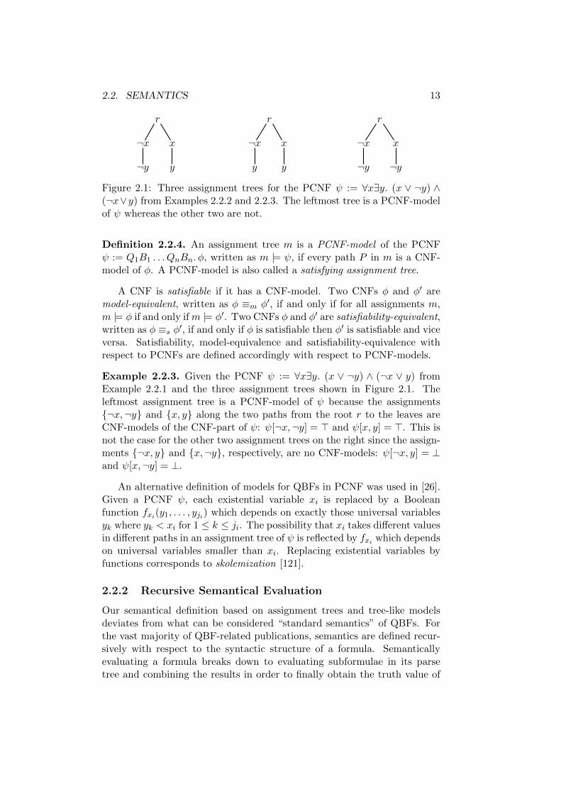
Figure 2.1: Three assignment trees for the PCNF ψ := ∀x∃y. (x ∨ ¬y) ∧(¬x∨y) from Examples 2.2.2 and 2.2.3. The leftmost tree is a PCNF-modelof ψ whereas the other two are not.
Definition 2.2.4. An assignment tree m is a PCNF-model of the PCNFψ := Q1B1 . . . QnBn. φ, written as m |= ψ, if every path P in m is a CNF-model of φ. A PCNF-model is also called a satisfying assignment tree.
A CNF is satisfiable if it has a CNF-model. Two CNFs φ and φ′ aremodel-equivalent, written as φ ≡m φ′, if and only if for all assignments m,m |= φ if and only ifm |= φ′. Two CNFs φ and φ′ are satisfiability-equivalent,written as φ ≡s φ′, if and only if φ is satisfiable then φ′ is satisfiable and viceversa. Satisfiability, model-equivalence and satisfiability-equivalence withrespect to PCNFs are defined accordingly with respect to PCNF-models.
Example 2.2.3. Given the PCNF ψ := ∀x∃y. (x ∨ ¬y) ∧ (¬x ∨ y) fromExample 2.2.1 and the three assignment trees shown in Figure 2.1. Theleftmost assignment tree is a PCNF-model of ψ because the assignments{¬x,¬y} and {x, y} along the two paths from the root r to the leaves areCNF-models of the CNF-part of ψ: ψ[¬x,¬y] = > and ψ[x, y] = >. This isnot the case for the other two assignment trees on the right since the assign-ments {¬x, y} and {x,¬y}, respectively, are no CNF-models: ψ[¬x, y] = ⊥and ψ[x,¬y] = ⊥.
An alternative definition of models for QBFs in PCNF was used in [26].Given a PCNF ψ, each existential variable xi is replaced by a Booleanfunction fxi(y1, . . . , yji) which depends on exactly those universal variablesyk where yk < xi for 1 ≤ k ≤ ji. The possibility that xi takes different valuesin different paths in an assignment tree of ψ is reflected by fxi which dependson universal variables smaller than xi. Replacing existential variables byfunctions corresponds to skolemization [121].
2.2.2 Recursive Semantical Evaluation
Our semantical definition based on assignment trees and tree-like modelsdeviates from what can be considered “standard semantics” of QBFs. Forthe vast majority of QBF-related publications, semantics are defined recur-sively with respect to the syntactic structure of a formula. Semanticallyevaluating a formula breaks down to evaluating subformulae in its parsetree and combining the results in order to finally obtain the truth value of
14 CHAPTER 2. PRELIMINARIES
the formula. We call this kind of semantics “standard” because it prevailsin QBF literature.
In the following we introduce the well-known alternative semantical defi-nition of QBF based on recursive evaluation. The purpose is to show that ouroriginal definition relying on assignment trees and tree-like models is moresuitable to act as a framework for the theory of dependency schemes. Weargue that in the context of standard recursive semantics like [26, 28], it isnot possible in a straightforward way to distinguish multiple QBF models.We are concerned with situations where existential variables are assigneddifferently with respect to the values of universal variables.
In order to apply the following definition to PCNFs, we temporarilyassume that quantifier blocks contain exactly one variable and that adjacentblocks are not necessarily differently quantified. For example ∀x,y∃a,b. φ istreated as ∀x∀y∃a∃b. φ.
Definition 2.2.5. Given a closed QBF ψ, satisfiability is determined recur-sively based on the syntactic structure of ψ as follows:
1. If ψ := ⊥ then ψ is unsatisfiable.
2. If ψ := > then ψ is satisfiable.
3. If ψ := φ ∨ φ′ then ψ is satisfiable if and only if φ or φ′ is satisfiable.Otherwise ψ is unsatisfiable.
4. If ψ := φ ∧ φ′ then ψ is satisfiable if and only if both φ and φ′ aresatisfiable. Otherwise ψ is unsatisfiable.
5. If ψ := ∃x. φ then ψ is satisfiable if and only if φ[x] or φ[¬x] issatisfiable. Otherwise ψ is unsatisfiable.
6. If ψ := ∀x. φ then ψ is satisfiable if and only if both φ[x] and φ[¬x]are satisfiable. Otherwise ψ is unsatisfiable.
Note that in Definition 2.2.5 there is no case for ψ := x where x is avariable. Since we consider only closed QBFs ψ, this case cannot occur. Allvariables are assigned in the subcases of ψ := ∃x. φ and ψ := ∀x. φ, whichamounts to evaluating ψ := ⊥ and ψ := > in the end. Further, semanticsbased on assignment trees and recursive evaluation from Definitions 2.2.3and 2.2.5, respectively, are compatible. That is, a PCNF has a PCNF-modelif and only if it is satisfiable by Definition 2.2.5. The ordering of assignmentsalong paths in assignment trees corresponds to recursive applications byrules 5 and 6 in Definition 2.2.5.
Example 2.2.4. Given the PCNF ψ := ∀x∃y. (x ∨ ¬y) ∧ (¬x ∨ y) fromExample 2.2.1. Due to ∀x we have to check if both ψ[x] = ∃y. (φ[x]) andψ[¬x] = ∃y. (φ[¬x]) are satisfiable. For ψ[x] = ∃y. (φ[x]), φ[x, y] or φ[x,¬y]
2.2. SEMANTICS 15
must be satisfiable. Similarly for ψ[¬x] = ∃y. (φ[¬x]), φ[¬x, y] or φ[¬x,¬y]must be satisfiable. As pointed out in Example 2.2.3, we have ψ[x, y] = >and ψ[¬x,¬y] = >.
For the PCNF ψ from Example 2.2.4, we find out that φ[x, y] andφ[¬x,¬y] are satisfiable but neither φ[x,¬y] nor φ[¬x, y] are. This is suffi-cient to justify satisfiability of ψ. In fact we could come to that conclusionwithout evaluating all four base cases but just the two satisfiable ones. As-sume we are given ψ[x]. Once we know that φ[x, y] is satisfiable, there is noneed to consider φ[x,¬y], and similarly for ψ[¬x]. This is due to the rulefor evaluating ∃y in ψ[x] and ψ[¬x]. There is no predefined ordering forconsidering subcases, hence the choice is arbitrary and non-deterministic.
The construction of dependency schemes, which is part of Chapter 3,requires to analyze dependencies between variables in a PCNF. From a the-oretical point of view, dependency analysis in a PCNF ψ reduces to checkingwhether a variable takes different values in different subtrees of a satisfyingassignment tree ψ. Referring to Example 2.2.4, we need to know if changingthe value of x forces the value of y to change as well. That is, are both φ[x, y]and φ[¬x, y] or both φ[x,¬y] and φ[¬x,¬y] satisfiable? If one of these is truethen x and y are independent because changing the value of x does not forcea change of the value of y to satisfy the formula. However, regarding PCNFψ from Example 2.2.4, x and y are not independent because none of thetwo possible assignment trees (see the two trees on the right in Figure 2.1)where the value of y is the same in the two subtrees is a PCNF-model of ψ.Hence changing the value of x forces a change of the value of y to satisfy ψ.
From that perspective, recursive semantics as defined above seems to betoo coarse. The relation of values between different variables is not reflectedexplicitly as in assignment trees. This is the reason why we prefer assignmenttrees and tree-like models in the context of dependency schemes.
2.2.3 Complexity
SAT, the satisfiability problem of propositional logic, is the classical NP-complete problem [34]. Unrestricted occurrences of different quantifiers inQBFs render the corresponding decision problem PSPACE-complete [49,124]. The number of quantifier alternations of a PCNF is related to thepolynomial-time hierarchy [90, 123] as follows.
Definition 2.2.6. (copied from Definition 23.3.1 in [26]) The prefix type ofa QBF1 is defined as follows. Every propositional formula by Definition 2.1.1has prefix type Σ0 = Π0. Given a PCNF ψ with prefix type Σn (Πn), thePCNF ∀x1, . . . , xm. ψ (∃x1, . . . , xm. ψ) has prefix type Πn+1 (Σn+1).
1We consider only PCNFs, but Definition 2.2.6 can be adapted to non-CNF formulaewith quantifier prefixes as well.

16 CHAPTER 2. PRELIMINARIES
Definition 2.2.7. (copied from Section 23.3 in [26]) The polynomial-timehierarchy is defined as follows for k ≥ 0:
∆P0 := ΣP
0 := ΠP0 := P ,
ΣPk+1 := NPΣP
k , ΠPk+1 := coΣP
k+1, ∆Pk+1 := PΣP
k
where ∆Pk+1 (ΣP
k+1) is the class of all problems which can be decided deter-ministically (non-deterministically) in polynomial-time with the help of anoracle for a problem in ΣP
k . An oracle for a problem in ΣPk is a subroutine
which solves a problem in ΣPk in constant time. The class ΠP
k+1 contains ev-
ery problem whose complement is in ΣPk+1. We have ΣP
1 = NP , ΠP1 = coNP ,
∆P1 = P and, for k ≥ 1, ∆P
k ⊆ (ΣPk ∩ΠP
k ).
Theorem 2.2.1 (copied from Theorem 23.3.2 in [26], respectively [123,129]). For k ≥ 1, the satisfiability problem for QBFs with prefix type Σk
(Πk) is ΣPk -complete (ΠP
k -complete).
It is unknown how the complexity classes P, NP and PSPACE are exactlyrelated to each other. So far no polynomial time algorithms are known forSAT or QBF. There are subclasses of QBF based on syntactic restrictionswhich can be decided in polynomial time, for example a specific form ofquantified Horn formulae or QBFs with at most two literals per clause [2].We refer to [24, 26, 28] for further details.
2.3 Decision Procedures: An Overview
We briefly give an overview of the two main approaches for checking sat-isfiability of a QBF, that is variable elimination and backtracking search.There is an abundance of literature on SAT and QBF solving, and a com-prehensive treatment is out of scope of this work. In Chapter 5 we deal withthe practice of backtracking search in detail. This section provides only anoverview sufficient to understand the motivation of dependency schemes inthe context of QBF solving in Chapter 3.
2.3.1 Backtracking Search
Semantics by Definitions 2.2.4 and 2.2.5 naturally form a framework forsearch-based decision procedures for QBF. Definition 2.2.5 can be turnedinto a recursive algorithm in a straightforward way. Rules for evaluatingψ := ∀x. φ and ψ := ∃x. φ correspond to case splits into subgoals φ[x] andφ[¬x], respectively. Splitting the proof into subgoals is also called branch-ing or decision making. Depending on the result of checking subgoals, thealgorithm backtracks to the most recent unsolved subgoal and continues. Inthe following, we focus on solving PCNFs.

2.3. DECISION PROCEDURES: AN OVERVIEW 17
Definition 2.2.4 gives rise to a simple yet infeasible algorithm. GivenPCNF ψ, we can try to construct a PCNF-model m by generating assign-ments A iteratively. If A satisfies the CNF-part of a PCNF then A can beturned into a path in m. Paths have to be added for siblings of universalnodes in m. If ψ is satisfiable then finally a complete PCNF-model m isobtained. Otherwise, there is at least one universal node for which no satis-fying path starting at its sibling can be found, and so ψ is unsatisfiable. Inthe worst case the explicit representation of assignment trees requires spacewhich is exponential in the number of variables of the QBF.
Given a QBF, the previously described algorithm searches for assign-ments which satisfy the CNF-part and checks whether these CNF-modelscan be combined to form a PCNF-model. The problem of exponential spaceis avoided in algorithms relying on the classical DPLL approach [37]. Origi-nating from [38], DPLL2 generates assignments recursively like in Definition2.2.5. Assignments are represented implicitly by the structure of recursiveapplications of the semantical rules. Hence classical DPLL requires onlyspace which is linear in the number of variables.
A first description of a DPLL-based algorithm for QBF was given in [30,31]. We refer to this QBF-specific variant as QDPLL3 and present a de-tailed description in Chapter 5. Modern implementations of SAT and QBFsolvers highly differ from the original formulation of DPLL. The algorithmis typically not implemented recursively but iteratively. Splitting the proofinto subcases is deferred as much as possible by applying rules like booleanconstraint propagation (BCP). We consider a QBF-specific variant of BCPin Chapter 5. Parallel variants of QDPLL like [48, 79, 80], for example,might benefit from modern multicore architectures and distributed comput-ing environments.
Clause Learning
The method of clause learning, also called conflict-directed clause learn-ing (CDCL) [117, 118], aims at guiding the search process out of regionsof the search space which do not contain solutions. The theoretical foun-dation of clause learning for SAT and QBF is resolution and Q-resolution,respectively [27, 108], which we consider in Chapter 5. Using (Q-)resolution,clauses derived from the original formula and can be added thereto. Suchlearnt clauses are logically implied by the formula and hence are also satis-fied by all CNF-models. Learnt clauses rule out certain assignments whichare not satisfying anyway. Thus the solver does not have to consider suchassignments. Learning methods for QBF were developed independently in[58, 78, 133, 134] under the terms lemma and model caching, or clause and
2Although Hilary Putnam is not co-author of [37], it is common to refer to the algorithmas DPLL, DLL or CDCL [118], if clause learning is applied (see next section).
3We also find other names such as QSAT and Q-DLL in literature.
18 CHAPTER 2. PRELIMINARIES
cube learning. A cube is a conjunction of literals. Different from clauses,cubes are used to rule out assignments which satisfy the CNF-part of a CNF.We introduce clause and cube learning for QBF in Chapter 5.
Adding learnt clauses increases both the space and time requirementsof a solver. The latter is due to rules like BCP which involve inspection oflearnt clauses as well. Clause learning might increase the space complexityof DPLL from linear to exponential, because in the worst case exponentiallymany learnt clauses can be derived. To prevent this behaviour, learnt clausesare periodically discarded according to some heuristic strategy. The goalis to keep those learnt clauses where the solver effectively benefits from.Related approaches from SAT solving like [3, 5, 42] could also be adaptedto QBF. We describe a trivial variant in Section 5.6.2 on page 121.
Branching Heuristics
The ordering in which variables are assigned might substantially influencethe overall performance of a QBF solver (see also Example 3.3.6 on page 34).Branching heuristics determine the selection and ordering of variables whichare used for case splits in the proof. Dynamic variants allow the solver toadapt the search with respect to those parts of the search space that havebeen visited recently. As with clause learning, work from the SAT domainrelated to branching heuristics [40, 42, 64, 93, 116, 118] might be applied toQBF as well but, to the best of our knowledge, there is no comprehensiveempirical study in the context of QBF.
Non-Normal Form Solving
In the description of QDPLL, we focused on QBFs in PCNF. Definition 2.2.5provides rules to evaluate arbitrary QBFs, and a corresponding recursive al-gorithm can be obtained in a straightforward way. Although original DPLLoperates on CNF only, it is common to use the term QDPLL for generaliza-tions to arbitrary QBFs as well. This approach has been implemented alongwith extensions like learning in [45, 46, 66, 67, 68], for example.
2.3.2 Variable Elimination
Backtracking search as described above in Section 2.3.1 is closely related tosemantical definitions. In either of Definitions 2.2.4 and 2.2.5 variables areassigned in the ordering given by the quantifier prefix or parse tree. Forassignment trees we explicitly require that assignments along paths fulfillthis requirement. In recursive semantics, such ordering is implicitly givenby nested evaluation. Due to this property, we call backtracking searcha top-down approach, since variables are assigned from left (top) to right(bottom) in the prefix or parse tree, respectively. Example 3.1.1 on page 24shows that this condition cannot be relaxed in general.
2.3. DECISION PROCEDURES: AN OVERVIEW 19
Variable elimination, the second major approach to solve QBFs, doesnot fit into that top-down framework. Differently from backtracking search,variable elimination does not explicitly try to generate a PCNF-model. In-stead, the goal is to successively get rid of quantified variables until finallythe formula reduces to> or⊥. Our focus is on PCNF but the approaches canbe generalized to arbitrary QBFs. We briefly outline common approachesbelow and list related work at the end of this chapter with respect to datastructures used in practice. Eliminating a variable typically increases thesize of the formula. Practical applicability of variable elimination is deter-mined by the amount of that size increase. In the worst case, the size of theformula doubles each time and hence induces an exponential growth over asequence of elimination steps.
Shannon Expansion
In the following, we introduce Shannon expansion [38, 41, 115] for variableelimination. We first consider QBFs in PCNF where all variables are exis-tentially quantified and then address expansion for general QBFs below.
Lemma 2.3.1. The PCNF
ψ := ∃x1, . . . , xi−1, xi, xi+1, . . . , xn. (φ)
is satisfiability-equivalent to
∃x1, . . . , xi−1, xi+1, . . . , xn. (φ[xi] ∨ φ[¬xi]).
Note that φ[xi] and φ[¬xi] is the formula obtained from φ by assigningxi as defined in Section 2.2.1. Variable xi is permanently assigned to truein one, and to false in another copy of CNF φ, respectively. The effects ofassigning x to either truth value are simultaneously and directly encodedinto the two copies of φ. This is different from backtracking search wherevariable assignments are made tentatively and retracted if no solution wasfound. Expansion by Lemma 2.3.1 eliminates one variable at the cost ofdoubling the size of the formula. In practice the variable to be expandedoften occurs only in a small part of φ, which is different from the generalpattern. In this case, expansion is much cheaper in terms of size increasebecause only the relevant parts of φ have to be copied. The approach ofmini-scoping, which we consider in Section 3.2.2, can be used to find outparts which are relevant for expansion.
Elimination Ordering
We consider expansion for arbitrary PCNFs. The presence of both univer-sal and existential variables in PCNFs complicates variable elimination ingeneral. This is in contrast to the following straightforward adaption ofLemma 2.3.1 to arbitrary PCNFs.
20 CHAPTER 2. PRELIMINARIES
Lemma 2.3.2. The PCNF
ψ := Q1B1, . . . , Qn(Bn ∪ {x}). φ
is satisfiability-equivalent to
Q1B1, . . . , QnBn. (φ[x]⊗ φ[¬x])
where ⊗ := ∧ if Qn = ∀ and ⊗ := ∨ if Qn = ∃.The two copies of φ are conjoined by conjunction or disjunction with
respect to the quantifier type of x. Note that the expanded variable x inLemma 2.3.2 is from the innermost quantifier block. Variables must be elim-inated from right to left in general, which differs from backtracking search.Therefore, we call methods of variable elimination bottom-up approaches. InChapter 3, we show by Examples 3.1.1 and 3.1.2 that respecting the orderingis crucial both for backtracking search and variable elimination.
Universal Expansion
Different from Lemma 2.3.2, universal variables from the innermost quan-tifier block of a PCNF do not have to be expanded but can be eliminatedright away by universal reduction (see also Section 5.3.1 on page 96) with-out incurring any size increase. This approach works only on PCNF and itis not clear, to the best of our knowledge, how to extend it to arbitrarilystructured QBFs.
It is possible to extend Lemma 2.3.2 to expansion of universal variablesfrom arbitrary quantifier blocks. This was done in [25] which built uponideas from [16]. The potential drawback of this approach is a larger sizeincrease. We introduce expansion of universal variables from the first non-innermost quantifier block Bn−1 and refer to Lemma 3.4.4 on page 53.
Lemma 2.3.3. The PCNF
ψ := Q1B1, . . . ,∀(Bn−1 ∪ {x})∃Bn. φ
is satisfiability-equivalent to
ψ := Q1B1, . . . ,∀Bn−1∃(Bn ∪B′n). (φ[x] ∧ φ′[¬x]).
Set B′n consists of fresh variables obtained from duplicating Bn, and in φ′
occurrences of variables in Bn are replaced by duplicated ones in B′n.
In all preceding definitions of expansion we copied the entire formula φwhich is conservative but usually pessimistic. In practice, it suffices to copyonly those parts of φ where the expanded variable occurs. Additionallywhen applying Lemma 2.3.3, parts with occurrences of duplicated variablesmust be copied. Therefore, the number of duplicated variables in the set B′nusually has an impact on the size of that part of φ that must be copied.
2.3. DECISION PROCEDURES: AN OVERVIEW 21
Example 2.3.1. Given the satisfiable PCNF ψ := ∀x∃y. (x∨¬y)∧(¬x∨y).By Lemma 2.3.3 formula ψ is satisfiability-equivalent to
∀x∃y,y′. ((x ∨ ¬y) ∧ (¬x ∨ y))[x] ∧ ((x ∨ ¬y′) ∧ (¬x ∨ y′))[¬x],
which further reduces to the satisfiable formula ∃y,y′. (y) ∧ (¬y′).
We point out by Example 3.1.2 on page 24 that the requirement ofduplicating variables cannot be relaxed in general. However, as we pointout in Chapter 3, dependency schemes might be able to reduce the numberof duplicated variables in B′n in practice and hence limit the cost of variableelimination (see also Example 3.3.7 on page 36).
Data Structures and Formula Representation
The rules for expansion of variables work for arbitrary QBFs although indefinitions above we considered only PCNFs. This gives rise to non-normalform solvers relying on variable elimination and either prenex non-CNF ornon-prenex non-CNF formulae. For the latter, in general the eliminationordering has to follow the sequence of quantified occurrences ∀x and ∃x in theparse tree in bottom-up fashion. In contrast to PCNF, data structures likeand-inverter graphs (AIGs) often allow for a more compact representation ofa QBF [101, 102, 107]. Negation normal form (NNF) is close to the originalparse tree of a QBF and was used in [6, 81].
The classical Davis-Putnam (DP) algorithm [38] can be used to elimi-nate existential variables in PCNFs by resolution. The resolution operationwas originally introduced for first-order logic [108]. Variable eliminationby resolution typically generates many redundant clauses. Sophisticatedapproaches like subsumption removal [16, 131] or methods of preprocess-ing [21, 41, 55] can be applied to reduce the size of the formula.
Binary decision diagrams (BDDs) [23] were used for QBF solving inseveral ways. Search-based approaches were coupled with representationsof CNF-models by BDDs [4]. The implementation of standard Booleanoperators enables the use of BDDs for variable elimination by expansion [75,97, 99]. BDDs can also be used to encode sets [91] of clauses in combinationwith the Davis-Putnam algorithm [32, 33, 99].
Skolemization [121] is relevant for theoretical concepts of QBF mod-els [26], but was also applied in practice to eliminate existential variablesfrom QBFs [13, 74]. The QBF solver presented in [13] integrates skolemiza-tion with BDDs and SAT solving techniques and can therefore be considereda hybrid approach.

22 CHAPTER 2. PRELIMINARIES
Chapter 3
Dependency Schemes
3.1 Introduction
In Section 2.3, we briefly introduced the two approaches of variable elimina-tion and backtracking search for SAT and QBF solving. Backtracking searchby means of DPLL [37] and QDPLL [30, 31]1 is the core of many state-of-the-art SAT and QBF solvers, respectively. There have been continuousimprovements of the basic algorithm since the early 1990ies. Apart fromtechnical issues such as efficient data structures and implementation details,DPLL was enhanced, for example, with clause learning and activity-baseddecision heuristics.
The latter approach is a strategy to dynamically change the assignmentordering of variables in paths of the decision tree constructed by DPLL-basedalgorithms. The SAT solver keeps track of how important a particular vari-able was during the search by maintaining a heuristic per-variable activityscore. This way the solver can adapt the search process on the currentbranch with respect to information that was learnt from previous branchesin the decision tree. The goal is to steer the solver out of parts of the searchspace which seem to be irrelevant to the solution of the problem. The useof activity scores for dynamic assignment orderings in SAT solvers is jus-tified by semantics since, in contrast to general PCNFs, DPLL can assignvariables in arbitrary order to decide the formula.
3.1.1 Variable Orderings by Prefixes in PCNFs
When it comes to QBF solving using QDPLL, variables must not be assignedin arbitrary order in general. This is due to the quantifier prefix. Occur-rences of universal quantifiers which are interleaved with existential ones inthe quantifier prefix might introduce dependencies between differently quan-
1We write DPLL to denote the algorithm for propositional logic and QDPLL for theQBF-specific variant of DPLL.
23

24 CHAPTER 3. DEPENDENCY SCHEMES
r
¬y
¬x x
r
y
¬x x
Figure 3.1: Two possible assignment trees of the PCNF ψ := ∀x∃y. (x ∨¬y)∧ (¬x∨ y) from Example 3.1.1 where y is erroneously assigned before x.
tified variables. We address variable dependencies formally in Section 3.4below. Actually, it is more important to know which variables do not dependon each other. For now, we confine our presentation to illustrative examplesand to a informal notion of the term “dependency”. Informally, dependen-cies require to choose the value of variables with respect to the value of someother variables when a PCNF is semantically evaluated. Some variable ymay only be assigned by QDPLL as soon as all variables x where y dependson have been assigned already. Although activity scores for variables couldbe applied in QDPLL for QBF as well like in DPLL for SAT, dependenciesin QBFs limit their potential positive effects. Given the quantifier prefix ofa PCNF, dependencies are respected if variables are assigned “from left toright“. Neglecting this condition might yield unsound results.
Example 3.1.1. Given the satisfiable PCNF ψ := ∀x∃y. (x∨¬y)∧(¬x∨y).We assign variables from left to right using recursive semantics from Section2.2.2. Formula ψ is satisfiable if and only if both ψ[x] and ψ[¬x] are satisfi-able, which is the case: both ψ[x, y] and ψ[¬x,¬y] are satisfiable. The leftassignment tree in Figure 2.1 on page 13 is the corresponding PCNF-model.The value of y depends on the value of x: y must take the same value as x.Thus neither ψ[x,¬y] nor ψ[¬x, y] is satisfiable. On the contrary, assume weassign y before x, thus breaking the prefix ordering and also the dependencybetween x and y. Then neither ψ[y] nor ψ[¬y] is satisfiable because y doesnot take values with respect to x since it was assigned before x. Figure 3.1shows the two corresponding assignment trees which are no PCNF-models.Consequently we cannot conclude that ψ is satisfiable.
Example 3.1.1 points out that the prefix ordering matters if QBFs aresolved using QDPLL. We now show a similar result for QBF solving by vari-able elimination. Expanding universal variables by Lemma 2.3.3 on page 20without duplicating larger existential variables might be unsound.
Example 3.1.2. Given the satisfiable PCNF ψ := ∀x∃y. (x∨¬y)∧ (¬x∨y)from Example 3.1.1 and Example 2.3.1 on page 21. Expanding x, whichis not from the innermost quantifier block, by Lemma 2.3.3 is unsound.Formula ψ is not satisfiability-equivalent to
∀x∃y. ((x ∨ ¬y) ∧ (¬x ∨ y))[x] ∧ ((x ∨ ¬y) ∧ (¬x ∨ y))[¬x],
3.1. INTRODUCTION 25
r
¬y
¬x x
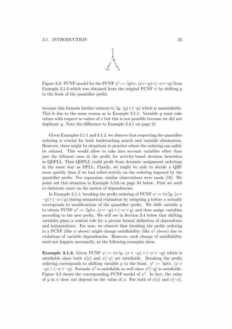
Figure 3.2: PCNF-model for the PCNF ψ′ := ∃y∀x. (x∨¬y)∧(¬x∨¬y) fromExample 3.1.3 which was obtained from the original PCNF ψ by shifting yto the front of the quantifier prefix.
because this formula further reduces to ∃y. (y)∧ (¬y) which is unsatisfiable.This is due to the same reason as in Example 3.1.1. Variable y must takevalues with respect to values of x but this is not possible because we did notduplicate y. Note the difference to Example 2.3.1 on page 21.
Given Examples 3.1.1 and 3.1.2, we observe that respecting the quantifierordering is crucial for both backtracking search and variable elimination.However, there might be situations in practice where the ordering can safelybe relaxed. This would allow to take into account variables other thanjust the leftmost ones in the prefix for activity-based decision heuristicsin QDPLL. Thus QDPLL could profit from dynamic assignment orderingsin the same way as DPLL. Finally, we might be able to decide a QBFmore quickly than if we had relied strictly on the ordering imposed by thequantifier prefix. For expansion, similar observations were made [16]. Wepoint out this situation in Example 3.3.6 on page 34 below. First we needto elaborate more on the notion of dependencies.
In Example 3.1.1, breaking the prefix ordering of PCNF ψ := ∀x∃y. (x∨¬y)∧ (¬x∨ y) during semantical evaluation by assigning y before x actuallycorresponds to modifications of the quantifier prefix. We shift variable yto obtain PCNF ψ′ := ∃y∀x. (x ∨ ¬y) ∧ (¬x ∨ y) and then assign variablesaccording to the new prefix. We will see in Section 3.4 below that shiftingvariables plays a central role for a precise formal definition of dependenceand independence. For now, we observe that breaking the prefix orderingin a PCNF (like ψ above) might change satisfiability (like ψ′ above) due toviolations of variable dependencies. However, such change of satisfiabilityneed not happen necessarily, as the following examples show.
Example 3.1.3. Given PCNF ψ := ∀x∃y. (x ∨ ¬y) ∧ (¬x ∨ ¬y) which issatisfiable since both ψ[x] and ψ[¬x] are satisfiable. Breaking the prefixordering corresponds to shifting variable y to the front: ψ′ := ∃y∀x. (x ∨¬y) ∧ (¬x ∨ ¬y). Formula ψ′ is satisfiable as well since ψ′[¬y] is satisfiable.Figure 3.2 shows the corresponding PCNF-model of ψ′. In fact, the valueof y in ψ does not depend on the value of x. For both of ψ[x] and ψ[¬x],
26 CHAPTER 3. DEPENDENCY SCHEMES
assigning y to false satisfies the formula.2
Example 3.1.4. Given PCNF ψ := ∀x∃y. (x∨¬y)∧(¬x∨¬y) from Example3.1.3. When expanding universal variable x without duplicating y like inExample 3.1.2 then expansion is sound in this case. The expanded formula∀x∃y. ((x ∨ ¬y) ∧ (¬x ∨ ¬y))[x] ∧ ((x ∨ ¬y) ∧ (¬x ∨ ¬y))[¬x] reduces to∃y. (¬y) ∧ (¬y) which is satisfiable.
3.1.2 The Need for Dependency Analysis
Examples 3.1.1 to 3.1.4 point out two different situations in the contextof backtracking search and variable elimination. First, breaking the prefixordering, that is not assigning variables from left-to-right, could violate vari-able dependencies and change satisfiability. This must be avoided in prac-tice when evaluating PCNFs and QBFs in general. However, as in Examples3.1.3 and 3.1.4, we could benefit from situations where shifting variables inthe prefix does not change satisfiability. Formula ψ from Example 3.1.3 canbe decided by showing that either the original PCNF ψ or the modified ψ′ issatisfiable. Here we can first assign x and then y or vice versa, and the resultis sound in any case. This corresponds to increased freedom during seman-tical evaluation. Given ψ from Example 3.1.3, first we may only assign xunless we know that shifting y to front as in ψ′ does not change satisfiability.This property of ψ′ allows us to assign y before x. In order to decide ψ weactually have two possible choices of assigning variables although there isonly one choice with respect to the original quantifier prefix of ψ.
Increased freedom during semantical evaluation as pointed out aboveallows to overcome the effects of restricted assignment orderings that fol-low from the quantifier prefix. The effects of such restricted orderings canbe negative for QDPLL-based QBF solvers just as was reported for DPLL-based SAT solvers [72]. Assigning variables in restricted order might causethe QBF solver to spend overly much time in parts of the search space of aformula which are irrelevant to its truth value. We consider an example re-lated to these observations in Section 3.3.3 below. Altogether, the quantifierprefix of PCNFs and the resulting kind of dependencies severely limit thefreedom of QBF solvers. This does not only apply to search-based QBF solv-ing using QDPLL but also to variable elimination. Therefore, it is crucialfrom a practical perspective to analyze whether variables are independent ina given PCNF since this increases the freedom for QBF solvers. For variableelimination, independence amounts to situations where the size of the set ofduplicated variables B′n by Lemma 2.3.3 on page 20 can be reduced. This inturn might reduce the size of the expanded formula (see also Example 3.3.7on page 36). We now focus on QDPLL.
2See also Example 3.4.3 on page 41 for the dual case of unsatisfiable formulae.

3.2. METHODS OF DEPENDENCY ANALYSIS 27
3.2 Methods of Dependency Analysis
In the previous section we observed that the quantifier prefix of PCNFsmight introduce a left-to-right ordering of variables which could be too strict.In practice it might often be possible to relax such ordering, thereby obtain-ing more freedom for QBF solving. For that purpose, it is crucial to knowprecisely which variables do not depend on other ones. In terms of prefixpatterns like . . . ∀x . . .∃y . . . or . . . ∃y . . .∀x . . ., this amounts to situationswhere x and y are independent and hence can be assigned independently byQDPLL. We refer to the act of finding out whether x is independent fromy, for all variables x and y in a given PCNF, as dependency analysis.
In the following section, we review a well-known approach of depen-dency analysis for PCNFs based on scope minimization of quantifiers, calledmini-scoping. We focus on QBFs in PCNF because it is a common formatwhich is widely used. We also rely on PCNF when we introduce a for-mal framework of variable dependencies and dependency analysis in Section3.4, called dependency schemes. Dependency schemes are relations overvariables which represent independence. We point out severe drawbacks ofmini-scoping which can be overcome by dependency schemes. Further, de-pendency schemes allow to assess the quality of dependency analysis. At thispoint, by quality we informally refer to the amount of independence identi-fied by some approach (see also Definition 3.4.18 on page 50). Dependencyanalysis in PCNFs actually involves a tradeoff between quality and compu-tational effort. Although optimal dependency analysis is infeasible, certaindependency schemes can be computed efficiently. At the same time theyprovide considerable information about independence between variables.
3.2.1 Maximizing Quantifier Scopes: Prenexing
PCNF is a widely used input format for QBF solvers just as CNF for SATsolving. QBF encodings of problems are typically not in PCNF right fromthe beginning but in arbitrary syntactic form. Given a QBF ρ with non-prenex non-CNF syntactic structure, the conversion of ρ into PCNF consistsof two steps:
1. Converting ρ into a QBF ρ′ which is in prenex normal form, that isall quantifiers occur in the quantifier prefix.
2. Converting ρ′ into PCNF ψ.
The first step is commonly referred to as prenexing. Given QBF ρ,quantifiers are successively shifted towards the top of the parse-tree of ρ (seeDefinition 2.1.5 on page 9), starting at topmost quantifiers, until finally ρ′ inprenex normal form is obtained. This maximizes the scopes of quantifiers,hence this approach is also called maxi-scoping [6]. The following well-known
28 CHAPTER 3. DEPENDENCY SCHEMES
schema of shifting rules is used for prenexing [43, 44, 47, 96]:3
(Qx. φ)⊗ φ′ ≡ Qx. (φ⊗ φ′) where Q ∈ {∀,∃},⊗ ∈ {∧,∨} and x 6∈ V (φ′).
After generating ρ′ in prenex normal form in the first step, its quantifier-free part is converted into CNF. In principle, this can be done by applyinglaws of distributivity of Boolean operators ∧ and ∨. However, this simpleapproach might yield a CNF which is exponentially larger than the originalformula ρ′. There are alternative approaches to obtain a CNF which is linearwith respect to ρ′ [39, 87, 104, 127]. The idea is to encode the output functionof Boolean operators in ρ′ by clauses involving fresh existential variables.These variables can then be put into the innermost quantifier block Bn, orif Bn is not existential, into a new innermost existential block [53].
Prenexing is Non-Deterministic
Quantifier shifting for QBF is a well-known and established technique forprenexing, although it has a severe drawback. There are formulae where, ata certain step during prenexing, more than one shifting rule is applicable.
Example 3.2.1 (taken from [62]). Given non-prenex non-CNF formula ρ :=(∃x. φ) ∧ (∀y. φ′). When prenexing ρ, there is a non-deterministic choiceof whether first shifting ∃x and then ∀y to the prefix or vice versa. Theresulting formulae are ρ′ := ∃x∀y. φ∧φ′ and ρ′′ := ∀y∃x. φ∧φ′, respectively.
Prenexing by non-deterministic applications of quantifier shifting rulesmight produce quantifier prefixes with different shape. This applies to thenumber quantifier alternations as well as to the final position of variables inthe prefix. Overall, the possibility of having multiple different prefixes forone and the same formula can be a serious problem in practice.
First, it is unnatural to have multiple PCNFs with different prefixes,and thus potentially different dependencies, for one and the same non-prenexnon-CNF formula ρ. By the term “dependencies” we refer to informal prefix-induced dependencies as in Examples 3.1.1 and 3.1.3 above. It is unknownin advance which prefix might be suited for one particular solver to showbest performance. By Theorem 2.2.1 on page 16, the number of quantifieralternations in a PCNF has an impact on the theoretical complexity of thedecision problem with respect to the polynomial-time hierarchy by Defini-tion 2.2.7. As argued in [47], the position of variables in the prefix couldalso have an influence on solver performance in practice.
Second, different prefixes might not only introduce different dependen-cies, but dependencies might also be spurious. The following situation wasreported in [47, 62] as well. In the original formula ρ from Example 3.2.1,neither y depends on x nor vice versa. The two variables are unrelated since
3For simplicity, we assume that all variables in a QBF are named differently.
3.2. METHODS OF DEPENDENCY ANALYSIS 29
none of them occurs in the quantifier scope of the other. In contrast to that,y depends on x in ρ′ and x depends on y in ρ′′ when taking dependenciesby prefixes. Following the quantifier ordering, a QDPLL-based solver canstart with assigning x (but not y) in ρ′ and with assigning y (but not x)in ρ′′. However, dependencies in these prenex formulae are spurious in thesense that they were introduced only by prenexing but are not inherent tothe original non-prenex non-CNF formula ρ.
3.2.2 Minimizing Quantifier Scopes: Anti-Prenexing
There has been research on how to alleviate the drawbacks of prenexing. Theapproach of anti-prenexing or mini-scoping aims at reversing the effects ofprenexing for a given PCNF. Mini-scoping is common in first-order logicand QBF solving [6, 12, 43, 96, 101]. The idea is to apply the same setof quantifier shifting rules as used for prenexing. Quantifiers are shiftedfrom the prefix back into the CNF-part of the PCNF, starting at innermostquantifiers. This way, the linear quantifier structure of the prefix is convertedinto a tree-like one, and so are dependencies derived therefrom. By “tree-like” we refer to information on quantifier structure which is present in theparse-tree of a formula (see Definition 2.1.5 on page 9). If Qx is a predecessorof Q′y in the parse-tree, where Q,Q′ ∈ {∀,∃} and Q 6= Q′, that is x andy are differently quantified, then we consider y to depend on x. Otherwise,like in formula ρ from Example 3.2.1, x and y are independent. Note thatthis notion of dependence is still informal. We call such tree-like quantifierstructure a quantifier tree [12] and consider examples below.
Anti-Prenexing is Non-Deterministic
Anti-prenexing converts a PCNF into a QBF in non-prenex CNF. The re-sulting quantifier structure is tree-like and we can extract dependency in-formation from the quantifier tree of the formula as described above. Sincethis approach applies the same set of quantifier shifting rules as prenexing,it suffers from the same drawback of non-determinism.
Example 3.2.2 (taken from [85]). Consider the PCNF
∃a,b∀x,y∃c,d. (a ∨ b) ∧ (a ∨ x ∨ c) ∧ (b ∨ c) ∧ (b ∨ y ∨ d).
Minimizing the scopes of ∃c,∃d,∀x and ∀y is deterministic and yields
∃a,b. (a ∨ b) ∧ (∀x∃c. (a ∨ x ∨ c) ∧ (b ∨ c)) ∧ (∀y∃d. (b ∨ y ∨ d)).
Now there is the non-deterministic choice of whether to first minimize ∃aand then ∃b (right tree in Figure 3.3) or vice versa (left tree in Figure 3.3).Note that the left tree induces a dependency between a and y which is notthe case in the right tree. Further, the left tree can be transformed into the
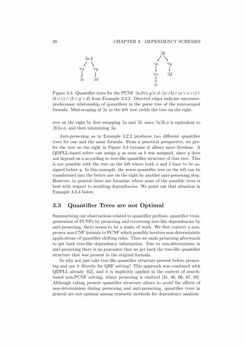
30 CHAPTER 3. DEPENDENCY SCHEMES
∃a,b
∀x
∃c
∀y
∃d
∃b
∃a
∀x
∃c
∀y
∃d
Figure 3.3: Quantifier trees for the PCNF ∃a,b∀x,y∃c,d. (a∨b)∧ (a∨x∨c)∧(b ∨ c) ∧ (b ∨ y ∨ d) from Example 3.2.2. Directed edges indicate successor-predecessor relationship of quantifiers in the parse tree of the mini-scopedformula. Mini-scoping of ∃a in the left tree yields the tree on the right.
tree on the right by first swapping ∃a and ∃b, since ∃a∃b.φ is equivalent to∃b∃a.φ, and then minimizing ∃a.
Anti-prenexing as in Example 3.2.2 produces two different quantifiertrees for one and the same formula. From a practical perspective, we pre-fer the tree on the right in Figure 3.3 because it allows more freedom. AQDPLL-based solver can assign y as soon as b was assigned, since y doesnot depend on a according to tree-like quantifier structure of that tree. Thisis not possible with the tree on the left where both a and b have to be as-signed before y. In this example, the worse quantifier tree on the left can betransformed into the better one on the right by another anti-prenexing step.However, in general there are formulae where none of the possible trees isbest with respect to resulting dependencies. We point out that situation inExample 3.3.4 below.
3.3 Quantifier Trees are not Optimal
Summarizing our observations related to quantifier prefixes, quantifier trees,generation of PCNFs by prenexing and recovering tree-like dependencies byanti-prenexing, there seems to be a waste of work. We first convert a non-prenex non-CNF formula to PCNF which possibly involves non-deterministicapplications of quantifier shifting rules. Then we undo prenexing afterwardsto get back tree-like dependency information. Due to non-determinism inanti-prenexing there is no guarantee that we get back the tree-like quantifierstructure that was present in the original formula.
So why not just take tree-like quantifier structure present before prenex-ing and use it directly for QBF solving? This approach was combined withQDPLL already [62], and it is implicitly applied in the context of search-based non-PCNF solving, where prenexing is omitted [45, 46, 66, 67, 68].Although taking present quantifier structure allows to avoid the effects ofnon-determinism during prenexing and anti-prenexing, quantifier trees ingeneral are not optimal among syntactic methods for dependency analysis.

3.3. QUANTIFIER TREES ARE NOT OPTIMAL 31
In the following, we point out that there are more sophisticated meth-ods for dependency analysis in PCNFs than quantifier trees. In particular,these methods have the potential to improve upon both quantifier structurepresent in non-PCNFs and quantifier trees by anti-prenexing. The methodswe consider can all be described in the framework of dependency schemes.We introduce the theory of dependency schemes in Section 3.4 below. Fornow we focus on an informal notion of the so called standard dependencyscheme (see also Definition 3.4.17 on page 49). We consider the standarddependency scheme to be more sophisticated than quantifier trees because itcan be computed deterministically. Further, it might prove certain tree-likedependencies spurious. We will see that the standard dependency scheme isnever worse than quantifier trees with respect to dependencies. It is oftenable to grant more freedom to a QBF solver than quantifier trees. Theseobservations motivate the use of dependency schemes instead of quantifiertrees for dependency analysis in the context of QBF solving.
3.3.1 Dependency Schemes: An Informal View
Dependency schemes provide a formal framework to express the notion ofvariable dependencies [111, 113]. Given some PCNF ψ, a dependency schemefor ψ is a binary relation D on the set of variables V of ψ where (x, y) ∈D if y is assumed to depend on x. We point out in Section 3.4 that adependency scheme D must be constructed such that no actual dependenciesare missed. However, D might contain spurious ones. If (x, y) 6∈ D then it isguaranteed that y is independent from x, and there is no actual dependencybetween x and y. Note that, as above, we use the term “dependencies” ratherinformally in this section. Independence can be exploited by a QBF solver.
Example 3.3.1. Given PCNF ψ := ∀x∃y. (x∨¬y)∧(¬x∨y) from Example3.1.1 and relations D := {(x, y)} and D′ := ∅. Relation D is a correctdependency scheme for ψ since, as pointed out in Example 3.1.1, y dependson x. A QDPLL-based solver relying on D will have to assign x before y. Incontrast to that, D′ is no dependency scheme since (x, y) 6∈ D′ but there isan actual dependency between x and y. Assigning y before x as suggestedby D′ is unsound.
Example 3.3.2. Given PCNF ψ := ∀x∃y. (x∨¬y)∧(¬x∨¬y) from Example3.1.3 and relations D := {(x, y)} and D′ := ∅. Both relations D and D′ arecorrect dependency schemes. Variables x and y are independent as arguedin Example 3.1.3 and so y can be assigned before x as suggested by D′.A QDPLL-based solver relying on D would not be able to do so due todependency (x, y) ∈ D, which is actually spurious.
In practice, a dependency scheme D must be computed according tosome strategy which influences the quality of D in terms of spurious depen-dencies. For example, we could analyze the syntactic structure of a PCNF
32 CHAPTER 3. DEPENDENCY SCHEMES
to figure out dependencies. Trivially, D could be defined to correspond tothe quantifier prefix: (x, y) ∈ D if y occurs to the right of x in the prefixand is quantified differently. Such trivial dependency scheme is usually toorestrictive and contains spurious dependencies. The goal is to minimize thesize of a dependency scheme to allow more freedom during QBF solving.
Example 3.3.3. Given formula ρ := (∃x. φ)∧ (∀y. φ′) from Example 3.2.1.We construct a dependency scheme Dtree for ρ from tree-like quantifier struc-ture by adding pair (x, y) to Dtree if x and y are differently quantified andQx is a predecessor Q′y in the parse tree, where Q,Q′ ∈ {∀, ∃} and Q 6= Q′.However, in this case Dtree = ∅ since x and y are unrelated. If we take theprenex formulae ρ′ := ∃x∀y. φ∧φ′ or ρ′′ := ∀y∃x. φ∧φ′ from Example 3.2.1,then the trivial dependency scheme Dtriv based on the prefix contains either(x, y) or (y, x), respectively. In this case we consider Dtree better than eitherof Dtriv because it allows more freedom due to fewer dependencies.
In Example 3.3.3 we constructed dependency schemes Dtree and Dtriv
from tree-like quantifier structure and quantifier prefixes, respectively. Hencethese two approaches for dependency analysis fit into the general frameworkof dependency schemes. We observed that Dtree was better than Dtriv inthe sense of fewer dependencies. Actually, as shown in Section 3.4.4 below,we can compare dependency schemes in that respect.
In the following, we show by examples that Dtree is not optimal amongsyntactic approaches for dependency analysis in PCNFs. There are moresophisticated dependency schemes which can be computed from the syntac-tic structure. We point out that the so called standard dependency schemeDstd has advantages over Dtree. Construction is entirely deterministic andthus Dstd is unique for every PCNF. It is superior to Dtree in the sense thatit will never identify more dependencies than Dtree. We elaborate more onDtriv, Dtree and Dstd in Section 3.4.3 below. Now we consider a concreteexample illustrating the advantages of Dstd on a given PCNF.
3.3.2 The Standard Dependency Scheme vs. Quantifier Trees
Example 3.3.4. Given PCNF
∃a,b∀x,y∃c,d. (a ∨ x ∨ c) ∧ (a ∨ b) ∧ (b ∨ y ∨ d).
Minimizing the scopes of ∃c, ∃d, ∀x and ∀y yields
∃a,b. (∀x∃c. (a ∨ x ∨ c)) ∧ (a ∨ b) ∧ (∀y∃d. (b ∨ y ∨ d)).
Now there is the non-deterministic choice whether to first minimize ∃b andthen ∃a or vice versa. Figure 3.4 shows the quantifier trees (left and middle)for the two alternatives. Dependency schemes resulting from the trees are
D := {(a, x), (x, c), (a, y), (b, y), (y, d)}

3.3. QUANTIFIER TREES ARE NOT OPTIMAL 33
∃a
∀x
∃c
∃b
∀y
∃d
∃b
∃a
∀x
∃c
∀y
∃d
∃a
∀x
∃c
∃b
∀y
∃d
Figure 3.4: Two possible quantifier trees for the PCNF ∃a,b∀x,y∃c,d. (a ∨x ∨ c) ∧ (a ∨ b) ∧ (b ∨ y ∨ d) from Example 3.3.4 obtained by anti-prenexing(left and middle) and dependencies by the standard dependency scheme Dstd
from Example 3.3.5 (right).
and
D′ := {(b, x), (a, x), (x, c), (b, y), (y, d)}for the tree on the left and in the middle of Figure 3.4, respectively.
The standard dependency scheme Dstd was introduced in [113] and isbased on ideas from expansion-based solvers [16, 25]. Dependencies areidentified by analyzing connections between variables in a PCNF over se-quences of clauses. We present an algorithm for constructing Dstd and re-lated theoretical properties in Chapter 4. The following example illustratesthe construction informally (see also Definition 3.4.17 on page 49).
Example 3.3.5. Given the PCNF ∃a,b∀x,y∃c,d. (a∨x∨c)∧(a∨b)∧(b∨y∨d)from Example 3.3.4. There is a connection between a, x and c because theyoccur in the common clause (a ∨ x ∨ c). Similarly there is a connectionbetween b, y and d by clause (b∨y∨d). However, there is a connection neitherbetween a and y nor between b and x. We could establish a connectionbetween a and y, for example, by clause (a∨ b) and then continue with b inclause (b ∨ y ∨ d) but this is ruled out by definition of Dstd. When startingfrom a or b, clause (a∨b) is no connection point because the two variables arein the same quantifier block. Dependencies follow from connections betweendifferently quantified variables: Dstd := {(a, x), (x, c), (b, y), (y, d)}.
Note that in Example 3.3.5 (a, y) 6∈ Dstd and (b, x) 6∈ Dstd, hence y doesnot depend on a and x not on b by Dstd. Comparing dependencies in Dtree
from Examples 3.3.4 and 3.3.5 shows a crucial difference between tree-likequantifier structure and Dstd. Dependencies by Dstd can be strictly lessrestrictive. No matter which of the two non-deterministically constructedquantifier trees in Figure 3.4 is taken for dependency computation, either(a, y) or (b, x) is included in the resulting dependency scheme but neither inDstd. For the PCNF from Example 3.3.4, Dstd is clearly superior than Dtriv
and Dtree. Different sets of dependencies in dependency schemes might havesevere impacts on the performance of QBF solvers.
34 CHAPTER 3. DEPENDENCY SCHEMES
3.3.3 The Benefits of More Powerful Dependency Schemes
Above we pointed out that the standard dependency scheme Dstd for a givenPCNF might be superior to dependency analysis based on tree-like quantifierstructure. Now we consider a more realistic, practical example related toQBF solving. In the following, we introduce a family of PCNFs containingspecific subformulae which are provably hard to decide for QDPLL-basedsolvers. On these PCNFs, QDPLL relying on Dstd can avoid to tackle thehard subformulae. Instead, solving other, easier parts of the formula yielda quick answer for the entire PCNF. As we are going to show, such quickanswer cannot be obtained using QDPLL with Dtree in general.
Similar observations were made with respect to Dtree and the prefix-based trivial dependency scheme Dtriv we computed in Example 3.3.3 [62].Different from that we do not restrict ourselves to Dtree. We argue thatQBF solvers in general can benefit from more powerful dependency analy-sis relying on dependency schemes. This also applies to schemes that havenot yet been applied in practical QBF solving, like the triangle dependencyscheme [111, 113], or the quadrangle dependency scheme and resolution pathdependencies [51]. Although our example points out that Dstd is favourablecompared to Dtree, this also holds with respect to Dtriv since Dtree is neverworse than Dtriv (see also Example 3.3.3 and Section 3.4.4 below). In ad-dition to search-based QBF solving, we argue that QBF solvers based onvariable elimination can benefit from dependency schemes as well.
Search-Based QBF Solving
Example 3.3.6. Given the unsatisfiable PCNF
ψ := ∃a,b,b1, . . . , bn∀x,y∃c,d. (a∨x∨c)∧(a∨b∨b1∨. . .∨bn)∧(b∨y∨d)∧φ′∧φ′′,where φ′ := (x ∨ c) ∧ (x ∨ ¬c) is a CNF which is unsatisfiable under thequantifier prefix of ψ. Let φ′′ be a pigeon hole formula [35, 69] in CNFover n variables {b1, . . . , bn}, which is unsatisfiable as well. Figure 3.5 showsquantifier trees for ψ obtained by anti-prenexing like in Figure 3.4. Againthere is the non-deterministic choice whether to first minimize a and then band all bi or vice versa like in Example 3.3.4. The right part of Figure 3.5shows dependencies in ψ by the standard dependency scheme Dstd similarto Figure 3.4.
The pigeon hole formula φ′′ of ψ from Example 3.3.6 is propositional sinceit does not contain universal variables. This class of unsatisfiable formulaeis hard for DPLL-based solvers [69].4 For a sufficiently large number of
4It was proved in [69] that any resolution refutation of a pigeon hole formula involvesan exponential number of resolvents. Due to related results [9, 10, 22], general resolution isexponentially stronger than classical DPLL [37], which corresponds to tree-like resolution.Therefore, DPLL-based algorithms including QDPLL require exponential time to solve apigeon hole formula as in Example 3.3.6.

3.3. QUANTIFIER TREES ARE NOT OPTIMAL 35
∃a
∀x
∃c
∃b, b1, . . . , bn
∀y
∃d
∃b, b1, . . . , bn
∃a
∀x
∃c
∀y
∃d
∃a
∀x
∃c
∃b, b1, . . . , bn
∀y
∃d
Figure 3.5: Two possible quantifier trees for the PCNF ψ from Example 3.3.6shown above on the left have similar shape as the ones in Figure 3.4. Thegraph on the right shows dependencies by the standard dependency scheme.
variables b1, . . . , bn, any such solver will spend exponential time to decidethat the pigeon hole formula is unsatisfiable.
Although formula ψ contains the hard subfomula φ′′, it can be decidedquickly using a QDPLL-based solver that relies on Dstd and clause learningthat we briefly addressed in Section 2.3.1. Once variable a is assigned,subformula φ′ can be found unsatisfiable by assigning x and c. Note that xis universally quantified under the prefix of ψ and that x does not depend onvariables b and b1, . . . , bn as shown on the right in Figure 3.5. Starting fromthe particular clause of φ′ which is falsified under the current assignment,that is either (x ∨ c) or (x ∨ ¬c), the clause learning mechanism derivesthe empty clause from clauses (x ∨ c) and (x ∨ ¬c) by Q-resolution. Thisimmediately shows unsatisfiability of the entire PCNF ψ. We deal withQ-resolution and the practice of clause learning in detail in Chapter 5.
The quick answer by QDPLL based on Dstd outlined above in generalcannot be obtained when using Dtree from the quantifier tree in the middle ofFigure 3.5. Apart from a, variable b and all of b1, . . . , bn have to be assignedbefore x and c due to dependencies by the quantifier tree, which are spuriousin contrast to Dstd. This causes the solver to tackle the hard pigeon holeformula φ′′ where it spends an exponential amount of time. Clauses in φ′
cannot be falsified by assigning b, b1, . . . , bn because those variables do notoccur in φ′. Hence the clause learning heuristics will not be able to infer theempty clause from φ′ as before when Dstd was used.
It is important to note that general Q-resolution without QDPLL is ofcourse able to derive the empty clause from clauses in φ′ independently fromdependency schemes. In contrast to that, here we focus on a combination ofQDPLL and heuristic clause learning which is common in search-based QBFsolving [58, 78, 133, 134]. Example 3.3.6 shows that more powerful depen-dency schemes might uncover additional heuristic Q-resolution derivations,which could yield exponential gaps in solving times as shown above.
However, Example 3.3.6 does not show that more powerful dependencyschemes always guarantee better performance of QDPLL-based solvers. In-stead, such schemes might grant solvers the freedom to enter promising parts
36 CHAPTER 3. DEPENDENCY SCHEMES
of the search space, but they do not prevent worst-case behaviour. Aftervariable a was assigned in the example above, according to Dstd QDPLLis free to assign x or b, b1, . . . , bn. In the latter case, the solver just as wellattempts to solve the pigeon hole formula, thus running into exponentialtime behaviour. However, it could have assigned x according to Dstd, whichis impossible if Dtree is used. Consequently, decision heuristics also influencethe benefits resulting from more powerful dependency schemes in practice.
It is straightforward to adapt the formula from Example 3.3.6 such thatQDPLL with Dtree from the first quantifier tree in Figure 3.5 exhibits ex-ponential behaviour as well. Hence this example shows that QDPLL withDtree obtained by mini-scoping might be strictly worse than QDPLL withDstd. In Section 3.4.4 below we argue that Dstd never contains more spu-rious dependencies than Dtree. If we combine QDPLL with Dstd then wewill have at least the same, and possibly more, amount of freedom for as-signing variables than with Dtree. Together with observations related tonon-determinism of mini-scoping in Section 3.2.2, this property clearly mo-tivates to use of dependency schemes like Dstd which are superior to Dtree
by mini-scoping.
Variable Elimination
Apart from search-based QBF solvers, more powerful dependency schemeshave the potential to improve QBF solving by variable elimination as well.According to Lemma 2.3.3 on page 20, expansion of universal variables in-volves duplication of existential variables which are larger by the prefix or-dering. The prefix ordering actually corresponds to the trivial dependencyscheme Dtriv. The number of duplicated variables influences the size of thesubformula that has to be copied. Consequently, our goal is to minimizethat size, which can be achieved by dependency schemes other than Dtriv.
Example 3.3.7 (taken from [113]). Given PCNF
ψ := ∀x, y∃a1, . . . , an. (x∨¬a1)∧ (a1 ∨¬a2)∧ . . .∧ (an−1 ∨¬an)∧ (y ∨ an).
Expansion of x by Lemma 2.3.3 and Dtriv has to duplicate a1, . . . , an andhence copy all clauses of the formula although x itself occurs only in thefirst clause. This doubles the size of the formula. Neither Dstd nor any non-deterministically constructed Dtree can improve this situation since Dtriv =Dtree = Dstd in this case. On the contrary, the triangle dependency schemeand generalizations thereof [51, 111, 113] find out that none of a1, . . . , andepends on x. The triangle dependency scheme is similar to Dstd, but itis based on a more refined notion of connections between variables. We donot introduce it formally and only argue that it is superior to Dstd. Thusthe prefix of ψ can be modified to ∀y∃a1, . . . , an∀x by shifting x to the rightover all ai. Now x is innermost and can be expanded by Lemma 2.3.2 on
3.4. THE THEORY OF DEPENDENCY SCHEMES 37
page 20 where duplication of variables is not required. Actually, x can alsobe eliminated by universal reduction (see Section 5.3.1 on page 96). Theresult is similar to expansion by Lemma 2.3.2 and does not increase the sizeof the formula at all. This was observed in [113] already.
3.4 The Theory of Dependency Schemes
In the previous sections, we introduced the notion of variable dependenciesand dependency schemes for PCNFs informally. We observed that inde-pendence between variables can be exploited by QBF solvers to relax thelinear ordering in the quantifier prefix of PCNFs. This might enable solversto tackle subproblems which can be decided quickly, which in turn couldhave positive effects on the overall solving process. Related observationswere made in Examples 3.3.6 and 3.3.7 above. In the best case, exponentialimprovements with respect to solving time and space requirements can beachieved. At the same time, it is crucial to be aware of which variablesdepend on each other. Neglecting such dependencies in QBF solving canyield unsound results. This was pointed out in Examples 3.1.1 and 3.1.2 forsolvers based on search and on variable elimination, respectively.
In this section we introduce the theoretical framework of dependencyschemes, which was first presented in the context of QBF [112, 113]. Laterthis concept was extended to quantified constraint satisfaction problems(CSP) [111]. QBFs can be regarded as a special type of quantified CSPswhere variables have Boolean domain with only two values true and false.Therefore, dependency schemes related to CSPs can also be applied to QBF.One of our goals is to apply the theoretical concept of dependency schemes inpractical QBF solving. In Chapter 5 we point out that dependency schemesin general are inherent to QBF semantics. This is true even for work fromthe early days of QBF solving when dependency schemes were still unknown,like for the original QDPLL algorithm [30], for example.
We adopt the theoretical framework of dependency schemes introducedin this section from related work [111, 113], particularly from the field ofquantified CSPs. As observed in [111], dependency schemes for quantifiedCSPs are based on a more precise notion of independence compared to theoriginal definitions made in the context of QBF [113]. This is the reasonwhy we rely on definitions related to quantified CSPs. Additionally, inSection 3.4.5 we attempt to summarize and extend observations made in[111, 113] with respect to practical applications of dependency schemes.
3.4.1 Variable Independence
We define independence between variables in a given PCNF ψ with respectto PCNF-models of ψ [111]. Variable independence is the foundation of de-pendency schemes which are formally introduced in Section 3.4.2 below. We

38 CHAPTER 3. DEPENDENCY SCHEMES
already considered dependency schemes informally in Section 3.3.1. Exam-ples 3.1.1 and 3.1.3 point out that changing the quantifier ordering of theprefix by shifting variables might change satisfiability of a PCNF. If shiftingpreserves satisfiability, then this is due to independence between variablesthe relative order of which was changed by shifting. This idea led to the firsttheoretical framework of independence and dependency schemes [112, 113].However, it turned out that quantifier shifting is not adequate. There areformulae where changing the relative ordering of two variables by shiftingchanges satisfiability [111], although these variables are independent accord-ing to the model-based definition we focus on (see also Example 3.4.5 below).
Independence of Existential Variables
Differently from the original definition [111], we present independence be-tween variables separately with respect to quantifier types. That is, weare interested whether two variables x and y in PCNFs with prefix pat-terns . . . ∀x . . .∃y . . . or . . . ∃y . . .∀x . . . are independent. Variables with samequantifier types are always independent. We refer to Sections 1 and 3 of theoriginal work [111]. Example 3.4.1 below illustrates the following definitions.
Definition 3.4.1. Given an assignment tree T and a node N in T , the depthof N is d(N) := 0 if N is the root of T , and d(N) := d(p(N)) + 1 otherwise,where p(N) is the unique parent node N ′ such that N is a child of N ′.
Definition 3.4.2 (adapted from [111]). Given an assignment tree T and avariable x, T [x] is the sequence of all literals l1, . . . , lm with v(li) = x whichare assigned by nodes N1, . . . , Nm in T .
Note that all nodes Ni in Definition 3.4.2 have the same depth sinceassignments along paths in assignment trees are complete. Further, sequenceT [x] is uniquely determined for universal variables because siblings of nodeswhich assign universal variables are ordered by Definition 2.2.3 on page 12.
Definition 3.4.3. Given a PCNF ψ := Q1({x} ∪ B1) . . . QnBn. φ and anassignment tree T with root node r. Then Tx (T¬x) with root r′ denotesthe immediate assignment subtree of T such that r′ assigns x to true (false)and r is parent of r′.
Example 3.4.1. Let T be the left assignment tree in Figure 3.6 on page 40.Nodes which assign variable y1 all have depth two. Given variables x2 andy2, T [x2] = ¬x2, x2,¬x2, x2 and T [y2] = ¬y2,¬y2, y2, y2 are the sequences ofliterals assigned by nodes in T , respectively. For the two siblings of universalnodes in T , always the left (right) sibling assigns ⊥ (>) to a variable. Theleft (right) child of the root r of T is the immediate subtree T¬x1 (Tx1) ofT . Note that notation Tx2 , for example, is undefined.
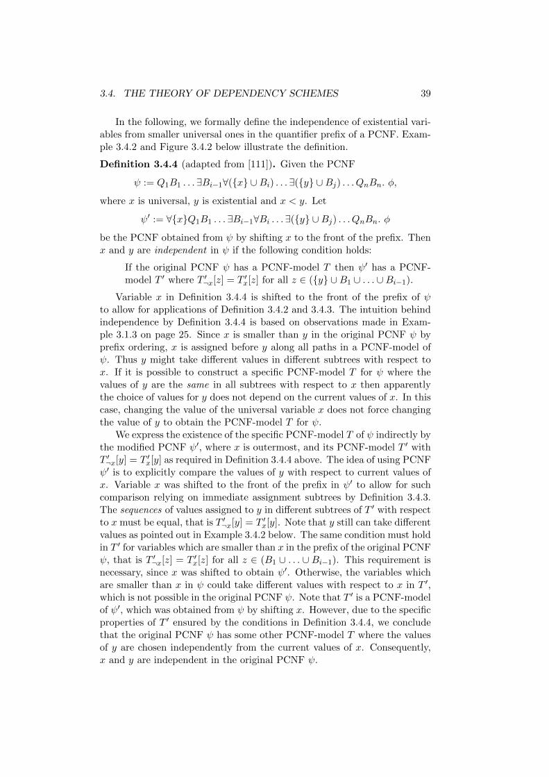
3.4. THE THEORY OF DEPENDENCY SCHEMES 39
In the following, we formally define the independence of existential vari-ables from smaller universal ones in the quantifier prefix of a PCNF. Exam-ple 3.4.2 and Figure 3.4.2 below illustrate the definition.
Definition 3.4.4 (adapted from [111]). Given the PCNF
ψ := Q1B1 . . . ∃Bi−1∀({x} ∪Bi) . . . ∃({y} ∪Bj) . . . QnBn. φ,where x is universal, y is existential and x < y. Let
ψ′ := ∀{x}Q1B1 . . . ∃Bi−1∀Bi . . . ∃({y} ∪Bj) . . . QnBn. φbe the PCNF obtained from ψ by shifting x to the front of the prefix. Thenx and y are independent in ψ if the following condition holds:
If the original PCNF ψ has a PCNF-model T then ψ′ has a PCNF-model T ′ where T ′¬x[z] = T ′x[z] for all z ∈ ({y} ∪B1 ∪ . . . ∪Bi−1).
Variable x in Definition 3.4.4 is shifted to the front of the prefix of ψto allow for applications of Definition 3.4.2 and 3.4.3. The intuition behindindependence by Definition 3.4.4 is based on observations made in Exam-ple 3.1.3 on page 25. Since x is smaller than y in the original PCNF ψ byprefix ordering, x is assigned before y along all paths in a PCNF-model ofψ. Thus y might take different values in different subtrees with respect tox. If it is possible to construct a specific PCNF-model T for ψ where thevalues of y are the same in all subtrees with respect to x then apparentlythe choice of values for y does not depend on the current values of x. In thiscase, changing the value of the universal variable x does not force changingthe value of y to obtain the PCNF-model T for ψ.
We express the existence of the specific PCNF-model T of ψ indirectly bythe modified PCNF ψ′, where x is outermost, and its PCNF-model T ′ withT ′¬x[y] = T ′x[y] as required in Definition 3.4.4 above. The idea of using PCNFψ′ is to explicitly compare the values of y with respect to current values ofx. Variable x was shifted to the front of the prefix in ψ′ to allow for suchcomparison relying on immediate assignment subtrees by Definition 3.4.3.The sequences of values assigned to y in different subtrees of T ′ with respectto x must be equal, that is T ′¬x[y] = T ′x[y]. Note that y still can take differentvalues as pointed out in Example 3.4.2 below. The same condition must holdin T ′ for variables which are smaller than x in the prefix of the original PCNFψ, that is T ′¬x[z] = T ′x[z] for all z ∈ (B1 ∪ . . . ∪ Bi−1). This requirement isnecessary, since x was shifted to obtain ψ′. Otherwise, the variables whichare smaller than x in ψ could take different values with respect to x in T ′,which is not possible in the original PCNF ψ. Note that T ′ is a PCNF-modelof ψ′, which was obtained from ψ by shifting x. However, due to the specificproperties of T ′ ensured by the conditions in Definition 3.4.4, we concludethat the original PCNF ψ has some other PCNF-model T where the valuesof y are chosen independently from the current values of x. Consequently,x and y are independent in the original PCNF ψ.

40 CHAPTER 3. DEPENDENCY SCHEMES
r
¬x1
y1
¬x2
¬y2
x2
¬y2
x1
y1
¬x2
y2
x2
y2
r
¬x2
¬x1
y1
¬y2
x1
y1
y2
x2
¬x1
y1
¬y2
x1
y1
y2
Figure 3.6: Given a satisfiable PCNF ψ := ∀x1∃y1∀x2∃y2. φ. Variable y2
is independent of x2 by Definition 3.4.4. Assume that the assignment treeT on the left is a PCNF-model of ψ. Based on the PCNF-model T ′ ofψ′ := ∀x2,x1∃y1,y2. φ shown on the right, sequences of values of y2 can becompared. See also Example 3.4.2.
Example 3.4.2. Figure 3.6 illustrates independence by Definition 3.4.4.Given the satisfiable PCNF ψ := ∀x1∃y1∀x2∃y2. φ. Assume that the assign-ment tree T on the left in Figure 3.6 is a PCNF-model of the original PCNFψ. Variable y2 is independent of x2 in ψ. This is due to PCNF-model T ′ ofψ′ := ∀x2,x1∃y1,y2. φ on the right in Figure 3.6 where x2 was shifted to thefront of the prefix. The sequence T ′¬x2 [y2] = ¬y2, y2 in subtree T ′¬x2 is equalto the sequence T ′x2 [y2] = ¬y2, y2 in subtree T ′x2 . Additionally, as requiredby Definition 3.4.4, we have T ′¬x2 [y1] = T ′x2 [y1] and T ′¬x2 [x1] = T ′x2 [x1] forvariables y1 and x1 which are smaller than x2 with respect to ψ.
Related to Example 3.4.2, it is important to note that the value of theexistential variable y in Definition 3.4.4 does not have to be either only > oronly ⊥ in both immediate assignment subtrees. The value of y can changebut it is crucial whether such change is due to x or some other universalvariable. In Example 3.4.2, the universal variable x1 forces the change of thevalue of y2 but not x2, as can be seen from the PCNF-models in Figure 3.6.
Further, note that by Definition 3.4.4 any existential variable y largerthan x in the original PCNF ψ is trivially independent from x if ψ is unsatis-fiable. In this case, ψ does not have a PCNF-model and hence the conditionof independence is vacuously true.
The additional criterion for restricting the value of variables (B1 ∪ . . . ∪Bi−1) which are smaller than x in ψ takes into account universal variablesas well. Actually, this requirement is crucial for existential variables only.Nodes assigning universal variables always have exactly one sibling. ByDefinition 2.2.3 on page 12, the siblings of universal nodes in assignmenttrees are ordered. Therefore, the sequences of values of universal variablesby Definition 3.4.2 are always unique.
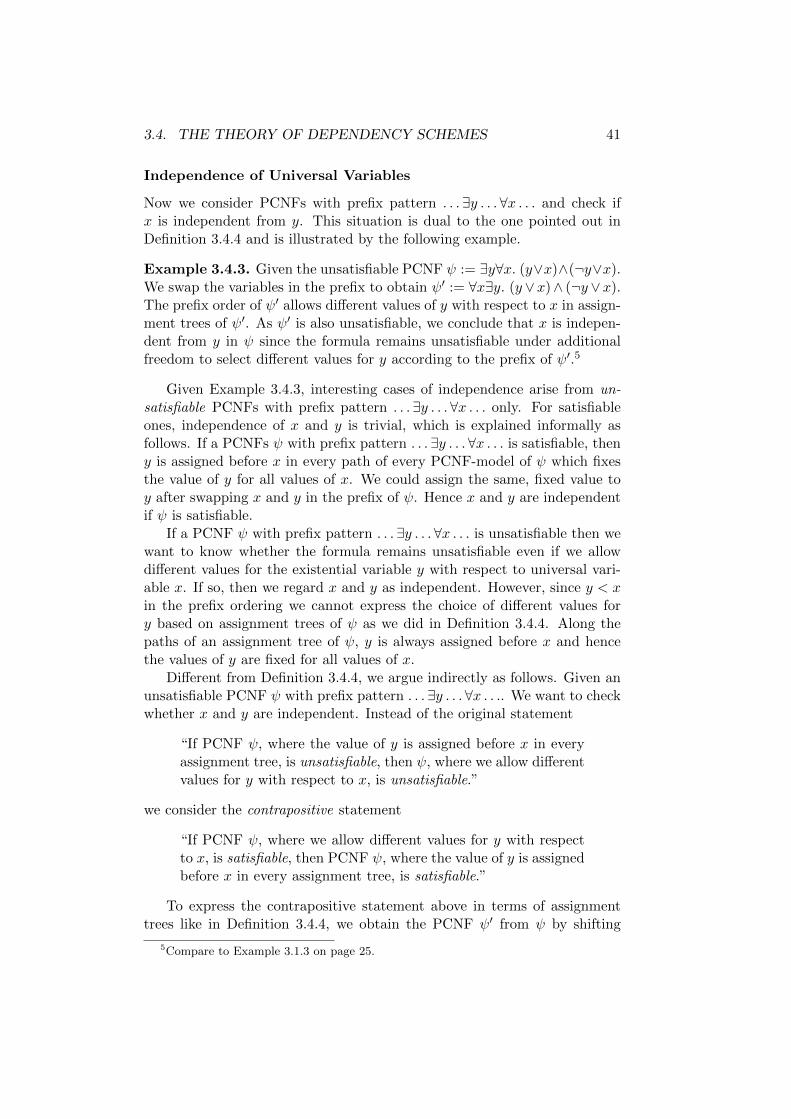
3.4. THE THEORY OF DEPENDENCY SCHEMES 41
Independence of Universal Variables
Now we consider PCNFs with prefix pattern . . . ∃y . . .∀x . . . and check ifx is independent from y. This situation is dual to the one pointed out inDefinition 3.4.4 and is illustrated by the following example.
Example 3.4.3. Given the unsatisfiable PCNF ψ := ∃y∀x. (y∨x)∧(¬y∨x).We swap the variables in the prefix to obtain ψ′ := ∀x∃y. (y ∨x)∧ (¬y ∨x).The prefix order of ψ′ allows different values of y with respect to x in assign-ment trees of ψ′. As ψ′ is also unsatisfiable, we conclude that x is indepen-dent from y in ψ since the formula remains unsatisfiable under additionalfreedom to select different values for y according to the prefix of ψ′.5
Given Example 3.4.3, interesting cases of independence arise from un-satisfiable PCNFs with prefix pattern . . . ∃y . . .∀x . . . only. For satisfiableones, independence of x and y is trivial, which is explained informally asfollows. If a PCNFs ψ with prefix pattern . . . ∃y . . .∀x . . . is satisfiable, theny is assigned before x in every path of every PCNF-model of ψ which fixesthe value of y for all values of x. We could assign the same, fixed value toy after swapping x and y in the prefix of ψ. Hence x and y are independentif ψ is satisfiable.
If a PCNF ψ with prefix pattern . . . ∃y . . .∀x . . . is unsatisfiable then wewant to know whether the formula remains unsatisfiable even if we allowdifferent values for the existential variable y with respect to universal vari-able x. If so, then we regard x and y as independent. However, since y < xin the prefix ordering we cannot express the choice of different values fory based on assignment trees of ψ as we did in Definition 3.4.4. Along thepaths of an assignment tree of ψ, y is always assigned before x and hencethe values of y are fixed for all values of x.
Different from Definition 3.4.4, we argue indirectly as follows. Given anunsatisfiable PCNF ψ with prefix pattern . . . ∃y . . .∀x . . .. We want to checkwhether x and y are independent. Instead of the original statement
“If PCNF ψ, where the value of y is assigned before x in everyassignment tree, is unsatisfiable, then ψ, where we allow differentvalues for y with respect to x, is unsatisfiable.”
we consider the contrapositive statement
“If PCNF ψ, where we allow different values for y with respectto x, is satisfiable, then PCNF ψ, where the value of y is assignedbefore x in every assignment tree, is satisfiable.”
To express the contrapositive statement above in terms of assignmenttrees like in Definition 3.4.4, we obtain the PCNF ψ′ from ψ by shifting
5Compare to Example 3.1.3 on page 25.
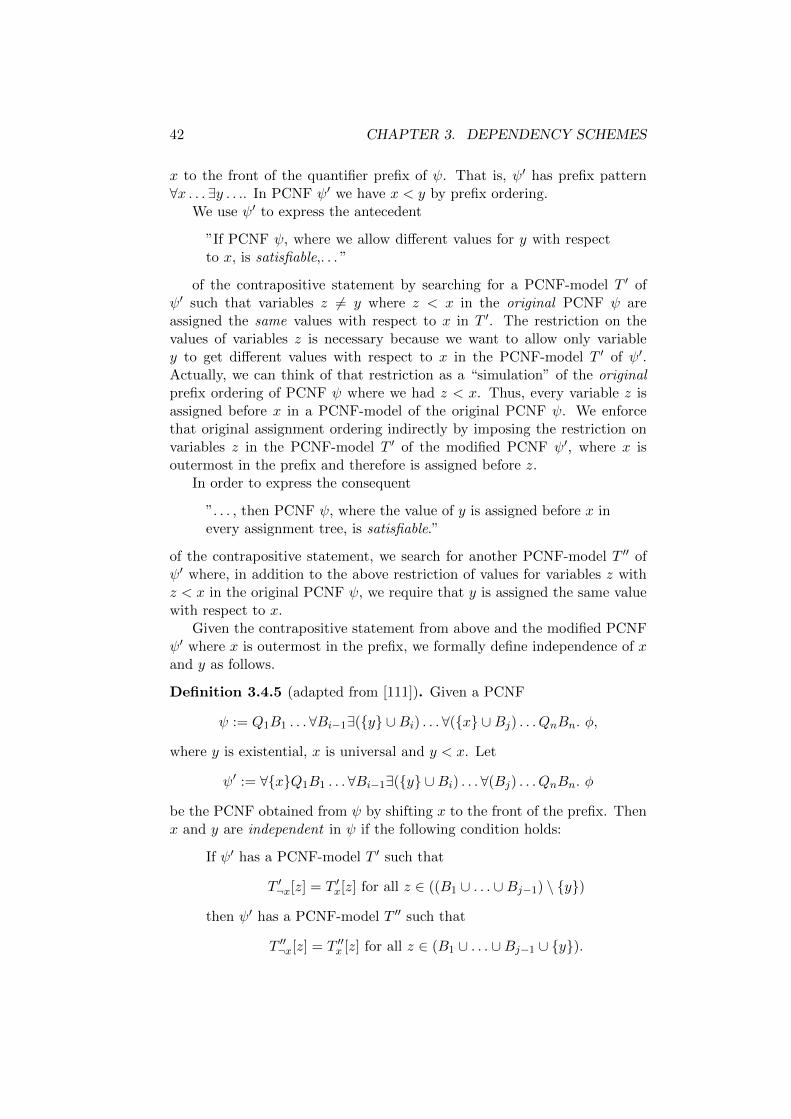
42 CHAPTER 3. DEPENDENCY SCHEMES
x to the front of the quantifier prefix of ψ. That is, ψ′ has prefix pattern∀x . . .∃y . . .. In PCNF ψ′ we have x < y by prefix ordering.
We use ψ′ to express the antecedent
”If PCNF ψ, where we allow different values for y with respectto x, is satisfiable,. . . ”
of the contrapositive statement by searching for a PCNF-model T ′ ofψ′ such that variables z 6= y where z < x in the original PCNF ψ areassigned the same values with respect to x in T ′. The restriction on thevalues of variables z is necessary because we want to allow only variabley to get different values with respect to x in the PCNF-model T ′ of ψ′.Actually, we can think of that restriction as a “simulation” of the originalprefix ordering of PCNF ψ where we had z < x. Thus, every variable z isassigned before x in a PCNF-model of the original PCNF ψ. We enforcethat original assignment ordering indirectly by imposing the restriction onvariables z in the PCNF-model T ′ of the modified PCNF ψ′, where x isoutermost in the prefix and therefore is assigned before z.
In order to express the consequent
”. . . , then PCNF ψ, where the value of y is assigned before x inevery assignment tree, is satisfiable.”
of the contrapositive statement, we search for another PCNF-model T ′′ ofψ′ where, in addition to the above restriction of values for variables z withz < x in the original PCNF ψ, we require that y is assigned the same valuewith respect to x.
Given the contrapositive statement from above and the modified PCNFψ′ where x is outermost in the prefix, we formally define independence of xand y as follows.
Definition 3.4.5 (adapted from [111]). Given a PCNF
ψ := Q1B1 . . . ∀Bi−1∃({y} ∪Bi) . . . ∀({x} ∪Bj) . . . QnBn. φ,
where y is existential, x is universal and y < x. Let
ψ′ := ∀{x}Q1B1 . . . ∀Bi−1∃({y} ∪Bi) . . . ∀(Bj) . . . QnBn. φ
be the PCNF obtained from ψ by shifting x to the front of the prefix. Thenx and y are independent in ψ if the following condition holds:
If ψ′ has a PCNF-model T ′ such that
T ′¬x[z] = T ′x[z] for all z ∈ ((B1 ∪ . . . ∪Bj−1) \ {y})
then ψ′ has a PCNF-model T ′′ such that
T ′′¬x[z] = T ′′x [z] for all z ∈ (B1 ∪ . . . ∪Bj−1 ∪ {y}).
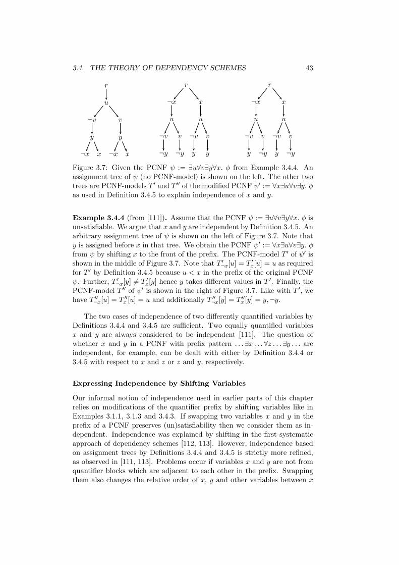
3.4. THE THEORY OF DEPENDENCY SCHEMES 43
r
u
¬v
y
¬x x
v
y
¬x x
r
¬x
u
¬v
¬y
v
¬y
x
u
¬v
y
v
y
r
¬x
u
¬v
y
v
¬y
x
u
¬v
y
v
¬y
Figure 3.7: Given the PCNF ψ := ∃u∀v∃y∀x. φ from Example 3.4.4. Anassignment tree of ψ (no PCNF-model) is shown on the left. The other twotrees are PCNF-models T ′ and T ′′ of the modified PCNF ψ′ := ∀x∃u∀v∃y. φas used in Definition 3.4.5 to explain independence of x and y.
Example 3.4.4 (from [111]). Assume that the PCNF ψ := ∃u∀v∃y∀x. φ isunsatisfiable. We argue that x and y are independent by Definition 3.4.5. Anarbitrary assignment tree of ψ is shown on the left of Figure 3.7. Note thaty is assigned before x in that tree. We obtain the PCNF ψ′ := ∀x∃u∀v∃y. φfrom ψ by shifting x to the front of the prefix. The PCNF-model T ′ of ψ′ isshown in the middle of Figure 3.7. Note that T ′¬x[u] = T ′x[u] = u as requiredfor T ′ by Definition 3.4.5 because u < x in the prefix of the original PCNFψ. Further, T ′¬x[y] 6= T ′x[y] hence y takes different values in T ′. Finally, thePCNF-model T ′′ of ψ′ is shown in the right of Figure 3.7. Like with T ′, wehave T ′′¬x[u] = T ′′x [u] = u and additionally T ′′¬x[y] = T ′′x [y] = y,¬y.
The two cases of independence of two differently quantified variables byDefinitions 3.4.4 and 3.4.5 are sufficient. Two equally quantified variablesx and y are always considered to be independent [111]. The question ofwhether x and y in a PCNF with prefix pattern . . . ∃x . . .∀z . . .∃y . . . areindependent, for example, can be dealt with either by Definition 3.4.4 or3.4.5 with respect to x and z or z and y, respectively.
Expressing Independence by Shifting Variables
Our informal notion of independence used in earlier parts of this chapterrelies on modifications of the quantifier prefix by shifting variables like inExamples 3.1.1, 3.1.3 and 3.4.3. If swapping two variables x and y in theprefix of a PCNF preserves (un)satisfiability then we consider them as in-dependent. Independence was explained by shifting in the first systematicapproach of dependency schemes [112, 113]. However, independence basedon assignment trees by Definitions 3.4.4 and 3.4.5 is strictly more refined,as observed in [111, 113]. Problems occur if variables x and y are not fromquantifier blocks which are adjacent to each other in the prefix. Swappingthem also changes the relative order of x, y and other variables between x
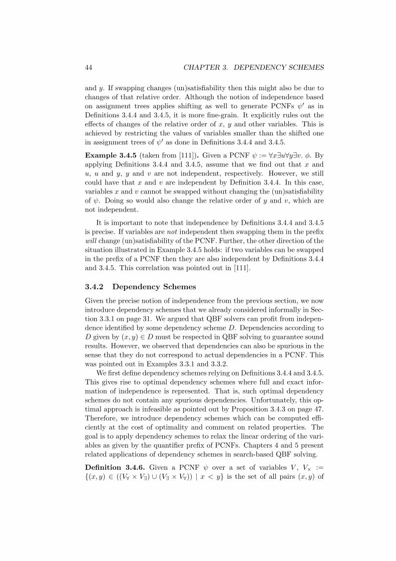
44 CHAPTER 3. DEPENDENCY SCHEMES
and y. If swapping changes (un)satisfiability then this might also be due tochanges of that relative order. Although the notion of independence basedon assignment trees applies shifting as well to generate PCNFs ψ′ as inDefinitions 3.4.4 and 3.4.5, it is more fine-grain. It explicitly rules out theeffects of changes of the relative order of x, y and other variables. This isachieved by restricting the values of variables smaller than the shifted onein assignment trees of ψ′ as done in Definitions 3.4.4 and 3.4.5.
Example 3.4.5 (taken from [111]). Given a PCNF ψ := ∀x∃u∀y∃v. φ. Byapplying Definitions 3.4.4 and 3.4.5, assume that we find out that x andu, u and y, y and v are not independent, respectively. However, we stillcould have that x and v are independent by Definition 3.4.4. In this case,variables x and v cannot be swapped without changing the (un)satisfiabilityof ψ. Doing so would also change the relative order of y and v, which arenot independent.
It is important to note that independence by Definitions 3.4.4 and 3.4.5is precise. If variables are not independent then swapping them in the prefixwill change (un)satisfiability of the PCNF. Further, the other direction of thesituation illustrated in Example 3.4.5 holds: if two variables can be swappedin the prefix of a PCNF then they are also independent by Definitions 3.4.4and 3.4.5. This correlation was pointed out in [111].
3.4.2 Dependency Schemes
Given the precise notion of independence from the previous section, we nowintroduce dependency schemes that we already considered informally in Sec-tion 3.3.1 on page 31. We argued that QBF solvers can profit from indepen-dence identified by some dependency scheme D. Dependencies according toD given by (x, y) ∈ D must be respected in QBF solving to guarantee soundresults. However, we observed that dependencies can also be spurious in thesense that they do not correspond to actual dependencies in a PCNF. Thiswas pointed out in Examples 3.3.1 and 3.3.2.
We first define dependency schemes relying on Definitions 3.4.4 and 3.4.5.This gives rise to optimal dependency schemes where full and exact infor-mation of independence is represented. That is, such optimal dependencyschemes do not contain any spurious dependencies. Unfortunately, this op-timal approach is infeasible as pointed out by Proposition 3.4.3 on page 47.Therefore, we introduce dependency schemes which can be computed effi-ciently at the cost of optimality and comment on related properties. Thegoal is to apply dependency schemes to relax the linear ordering of the vari-ables as given by the quantifier prefix of PCNFs. Chapters 4 and 5 presentrelated applications of dependency schemes in search-based QBF solving.
Definition 3.4.6. Given a PCNF ψ over a set of variables V , V× :={(x, y) ∈ ((V∀ × V∃) ∪ (V∃ × V∀)) | x < y} is the set of all pairs (x, y) of
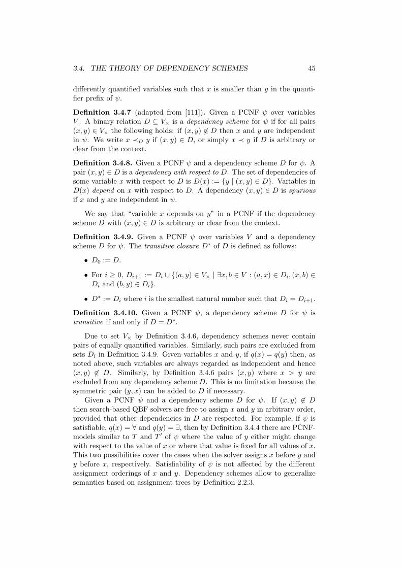
3.4. THE THEORY OF DEPENDENCY SCHEMES 45
differently quantified variables such that x is smaller than y in the quanti-fier prefix of ψ.
Definition 3.4.7 (adapted from [111]). Given a PCNF ψ over variablesV . A binary relation D ⊆ V× is a dependency scheme for ψ if for all pairs(x, y) ∈ V× the following holds: if (x, y) 6∈ D then x and y are independentin ψ. We write x ≺D y if (x, y) ∈ D, or simply x ≺ y if D is arbitrary orclear from the context.
Definition 3.4.8. Given a PCNF ψ and a dependency scheme D for ψ. Apair (x, y) ∈ D is a dependency with respect to D. The set of dependencies ofsome variable x with respect to D is D(x) := {y | (x, y) ∈ D}. Variables inD(x) depend on x with respect to D. A dependency (x, y) ∈ D is spuriousif x and y are independent in ψ.
We say that “variable x depends on y” in a PCNF if the dependencyscheme D with (x, y) ∈ D is arbitrary or clear from the context.
Definition 3.4.9. Given a PCNF ψ over variables V and a dependencyscheme D for ψ. The transitive closure D∗ of D is defined as follows:
• D0 := D.
• For i ≥ 0, Di+1 := Di ∪ {(a, y) ∈ V× | ∃x, b ∈ V : (a, x) ∈ Di, (x, b) ∈Di and (b, y) ∈ Di}.
• D∗ := Di where i is the smallest natural number such that Di = Di+1.
Definition 3.4.10. Given a PCNF ψ, a dependency scheme D for ψ istransitive if and only if D = D∗.
Due to set V× by Definition 3.4.6, dependency schemes never containpairs of equally quantified variables. Similarly, such pairs are excluded fromsets Di in Definition 3.4.9. Given variables x and y, if q(x) = q(y) then, asnoted above, such variables are always regarded as independent and hence(x, y) 6∈ D. Similarly, by Definition 3.4.6 pairs (x, y) where x > y areexcluded from any dependency scheme D. This is no limitation because thesymmetric pair (y, x) can be added to D if necessary.
Given a PCNF ψ and a dependency scheme D for ψ. If (x, y) 6∈ Dthen search-based QBF solvers are free to assign x and y in arbitrary order,provided that other dependencies in D are respected. For example, if ψ issatisfiable, q(x) = ∀ and q(y) = ∃, then by Definition 3.4.4 there are PCNF-models similar to T and T ′ of ψ where the value of y either might changewith respect to the value of x or where that value is fixed for all values of x.This two possibilities cover the cases when the solver assigns x before y andy before x, respectively. Satisfiability of ψ is not affected by the differentassignment orderings of x and y. Dependency schemes allow to generalizesemantics based on assignment trees by Definition 2.2.3.

46 CHAPTER 3. DEPENDENCY SCHEMES
Proposition 3.4.1. Given a PCNF ψ and a dependency scheme D for ψ,ψ is satisfiable if and only if it has a PCNF-model T such that if (x, y) ∈ Dthen x is predecessor of y on every path in T .
Proof. Due to Proposition 3.4.5 on page 51 below, the trivial dependencyscheme Dtriv given by the prefix of ψ is the largest possible dependencyscheme for ψ. Therefore, we have D ⊆ Dtriv. If (x, y) 6∈ D then x and y canbe assigned in arbitrary order along the paths in an assignment tree. In thiscase, independence by Definitions 3.4.4 and 3.4.5 guarantees that a PCNF-model can (not) be constructed. Thus (un)satisfiability is preserved.
Satisfiability of PCNFs by Proposition 3.4.1 in general imposes weakerconstraints on PCNF-models with respect to the ordering of assignmentsalong paths. The prefix-based linear ordering of paths in assignment treesby Definition 2.2.3 can be relaxed by any arbitrary dependency scheme D(see also Example 3.4.8 and Figure 3.9 on page 51). Spurious dependenciesin a dependency scheme restrict the freedom of QBF solvers as pointed outin Example 3.3.2. If the dependency (x, y) ∈ D is spurious then the solvernever assigns y before x although the two variables are independent.
Intractability of Optimal Dependency Schemes
Definition 3.4.7 does not prevent spurious dependencies. The fewer depen-dencies in D are spurious, the more freedom is granted by D to QBF solvers.Based on that, we define a criterion of optimality of dependency schemes.
Definition 3.4.11. A dependency scheme Dopt for PCNF ψ is optimal ifand only if the following condition holds for all pairs (x, y) ∈ V×:
(x, y) 6∈ Dopt if and only if x and y are independent in ψ.
Proposition 3.4.2. The optimal dependency scheme Dopt for a PCNF ψis unique.
Proof. Given PCNF ψ, assume that dependency schemes D and D′ for ψare both optimal and that D 6= D′ due to, for example, (x, y) 6∈ D but(x, y) ∈ D′. Since D is optimal and (x, y) 6∈ D, x and y are independent byDefinition 3.4.11. As (x, y) ∈ D′ and D′ is optimal, x and y are not inde-pendent by Definition 3.4.11, which is a contradiction. Hence D = D′.
Definition 3.4.11 improves upon Definition 3.4.7 by including the otherdirection of the implication: if x and y are independent then (x, y) 6∈ D.This way, spurious dependencies are avoided at all. Consequently, thereis no dependency scheme D with D ⊂ Dopt. If any pair (x, y) ∈ Dopt isremoved, then Dopt is no longer a dependency scheme. Given a PCNF ψ,we can compute the optimal dependency scheme Dopt by checking if x andy are independent for all pairs (x, y) ∈ V×. While Dopt grants full freedomto QBF solvers, it typically cannot be applied in practice.
3.4. THE THEORY OF DEPENDENCY SCHEMES 47
Proposition 3.4.3 (related to Proposition 2 in [113]). Computing the opti-mal dependency scheme Dopt for a PCNF ψ is at least as hard as solving ψ.
Proof. The conditions in Definitions 3.4.4 and 3.4.5 involve searching forPCNF-models. Thus the satisfiability of the PCNFs ψ and ψ′ must bedecided, a problem which is PSPACE-complete. To compute Dopt, thismust be carried out O(|V×|) times in the worst case.
3.4.3 Tractable Dependency Schemes
Following from Proposition 3.4.3, optimal dependency schemes cannot beapplied for QBF solving in practice. Therefore, we have to trade optimalityfor efficiency. Different from optimal dependency schemes, we want to allowspurious dependencies in dependency schemes. Under that relaxation, itturns out that there are several dependency schemes which can be computedefficiently. At the same time, these schemes are able to grant considerablefreedom to QBF solvers to improve their performance in practice. We showrelated experimental results in Chapter 5. In this section, we introducedependency schemes that we considered informally in Section 3.3.1 on page31. All of these schemes can be computed in polynomial-time with respectto the size of a PCNF ψ. For convenience, we also use the term “dependencyscheme” to denote an approach to construct a relation D which then has theproperties of a dependency scheme for some PCNF ψ by Definition 3.4.7.
Definition 3.4.12 ([113]). A dependency scheme D is tractable if, for allPCNFs ψ and for all pairs (x, y) ∈ V×, it can be decided in polynomial-timewhether (x, y) ∈ D or (x, y) 6∈ D.
Tractability of dependency schemes is a rather theoretical concept. In theworst case, O(|V |2) pairs have to be considered to compute D which yields atleast a quadratic overhead in the end. Although being polynomial-time, thiscould be too expensive for practical applications if the number of variablesis large. In Chapter 4 we present an algorithm to compute the standarddependency scheme Dstd which was briefly illustrated in Example 3.3.5. Itturns out that Dstd can be computed and represented efficiently in practice.
Tractable dependency schemes by Definition 3.4.12 do not prevent spu-rious dependencies. Depending on the concrete algorithm that is used tocompute D, a dependency (x, y) ∈ D might be spurious. If (x, y) 6∈ Dthen variables x and y must be independent because otherwise D is not adependency scheme by Definition 3.4.7.
In the following, we define tractable dependency schemes which can becomputed by analyzing the syntactic structure of a PCNF. In Section 3.4.4below, we compare these schemes by the number of spurious dependencies,which gives rise to a hierarchy of dependency schemes.
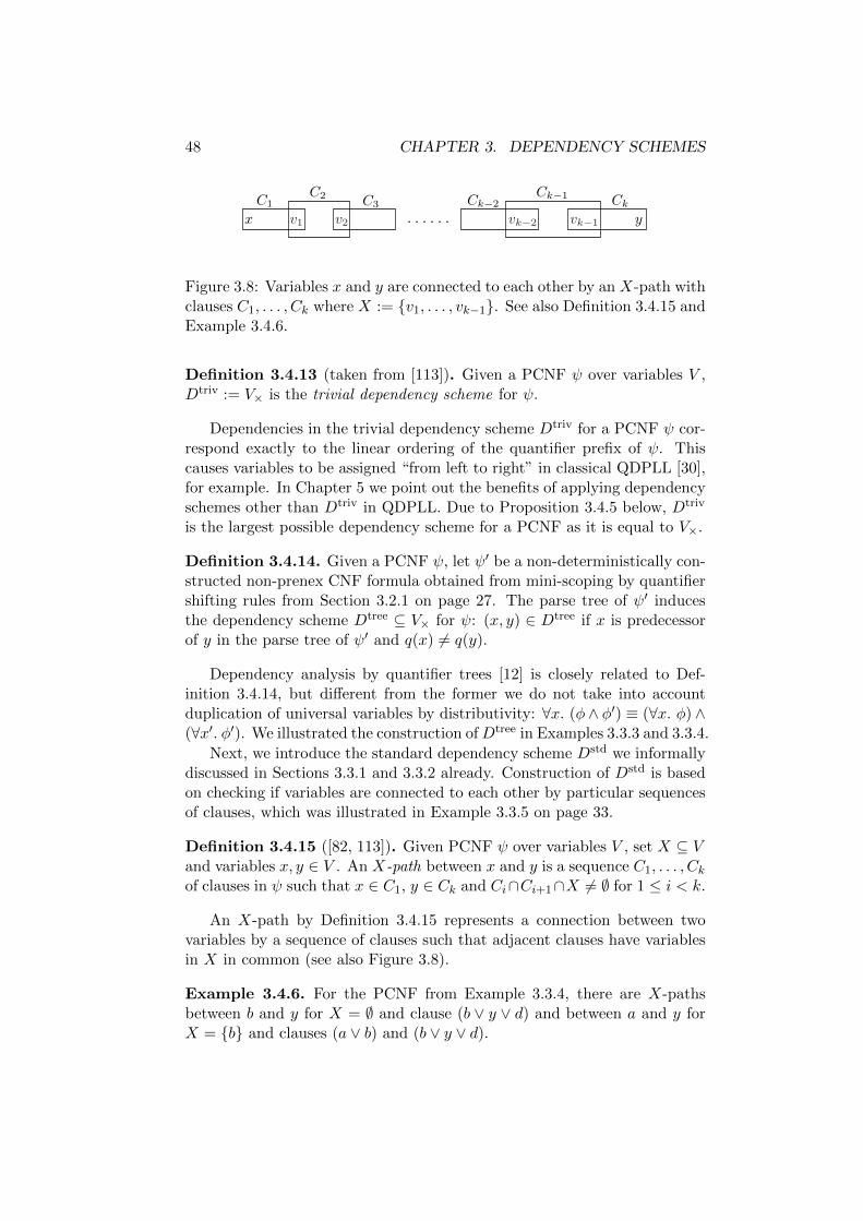
48 CHAPTER 3. DEPENDENCY SCHEMES
y
C3 Ck−2C2 Ck−1 Ck
v1 v2 vk−1vk−2
C1
. . . . . .x
Figure 3.8: Variables x and y are connected to each other by an X-path withclauses C1, . . . , Ck where X := {v1, . . . , vk−1}. See also Definition 3.4.15 andExample 3.4.6.
Definition 3.4.13 (taken from [113]). Given a PCNF ψ over variables V ,Dtriv := V× is the trivial dependency scheme for ψ.
Dependencies in the trivial dependency scheme Dtriv for a PCNF ψ cor-respond exactly to the linear ordering of the quantifier prefix of ψ. Thiscauses variables to be assigned “from left to right” in classical QDPLL [30],for example. In Chapter 5 we point out the benefits of applying dependencyschemes other than Dtriv in QDPLL. Due to Proposition 3.4.5 below, Dtriv
is the largest possible dependency scheme for a PCNF as it is equal to V×.
Definition 3.4.14. Given a PCNF ψ, let ψ′ be a non-deterministically con-structed non-prenex CNF formula obtained from mini-scoping by quantifiershifting rules from Section 3.2.1 on page 27. The parse tree of ψ′ inducesthe dependency scheme Dtree ⊆ V× for ψ: (x, y) ∈ Dtree if x is predecessorof y in the parse tree of ψ′ and q(x) 6= q(y).
Dependency analysis by quantifier trees [12] is closely related to Def-inition 3.4.14, but different from the former we do not take into accountduplication of universal variables by distributivity: ∀x. (φ ∧ φ′) ≡ (∀x. φ) ∧(∀x′. φ′). We illustrated the construction ofDtree in Examples 3.3.3 and 3.3.4.
Next, we introduce the standard dependency scheme Dstd we informallydiscussed in Sections 3.3.1 and 3.3.2 already. Construction of Dstd is basedon checking if variables are connected to each other by particular sequencesof clauses, which was illustrated in Example 3.3.5 on page 33.
Definition 3.4.15 ([82, 113]). Given PCNF ψ over variables V , set X ⊆ Vand variables x, y ∈ V . An X-path between x and y is a sequence C1, . . . , Ckof clauses in ψ such that x ∈ C1, y ∈ Ck and Ci∩Ci+1∩X 6= ∅ for 1 ≤ i < k.
An X-path by Definition 3.4.15 represents a connection between twovariables by a sequence of clauses such that adjacent clauses have variablesin X in common (see also Figure 3.8).
Example 3.4.6. For the PCNF from Example 3.3.4, there are X-pathsbetween b and y for X = ∅ and clause (b ∨ y ∨ d) and between a and y forX = {b} and clauses (a ∨ b) and (b ∨ y ∨ d).
3.4. THE THEORY OF DEPENDENCY SCHEMES 49
Definition 3.4.16. Given PCNF over variables V and q ∈ {∃,∀}, Vq,i :={x ∈ Vq | i ≤ δ(x)} is the set of all variable whose quantifier type equals qand which are from quantifier block Bi or any larger block.
Definition 3.4.17 ([82, 113]). Given PCNF ψ over variables V , the stan-dard dependency scheme for ψ is Dstd := {(x, y) ∈ V× | there is an X-pathbetween x and y for X := V∃,i where i := δ(x) + 1}.
There is a dependency x ≺ y by the standard dependency scheme if xis connected to y by existential variables larger than x. This requirement isexpressed by setting i := δ(x) + 1 and X := V∃,i. Alternatively, Dstd canbe computed with i := δ(x) [113] but the variant from Definition 3.4.17 ismore refined because it allows fewer variables to be used for X-paths.
Example 3.4.7. For the PCNF ∃a,b∀x,y∃c,d. (a∨x∨c)∧(a∨b)∧(b∨y∨d)from Example 3.3.4 on page 32, we have Dtriv := {(a, x), (a, y), (b, x), (b, y),(x, c), (x, d), (y, c), (y, d)}. For Dstd and Dtree, we refer to Examples 3.3.4and 3.3.5.
Lemma 3.4.1. Dtriv, Dtree and Dstd are dependency schemes for a PCNFψ by Definition 3.4.7.
Proof. Our definition of independence is based on assignment trees [111]whereas the one in [113] relies on shifting variables in the quantifier prefix ofa PCNF. As argued in Example 3.4.5 above, our definition is strictly morerefined. Therefore, the proof in [113] that Dstd is a dependency schemeapplies to our context as well. Both Dtriv and Dtree are dependency schemessince Dstd ⊆ Dtree ⊆ Dtriv by Proposition 3.4.5 below.
Lemma 3.4.2. Dtriv, Dtree and Dstd are transitive for all PCNFs ψ.
Proof. Let ψ be an arbitrary but fixed PCNF and Dtriv, Dtree and Dstd bethe respective dependency schemes for ψ. Since Dtriv = V×, transitivityfollows immediately because V× is a transitive relation. For Dtree, assume(a, x) ∈ Dtree, (x, b) ∈ Dtree and (b, y) ∈ Dtree. Then by Definition 3.4.14,a is predecessor of x, which is predecessor of b, which is predecessor of y inthe parse tree of the mini-scoped formula ψ′. Thus a is also predecessor ofy and q(a) 6= q(y), hence (a, y) ∈ Dtree.
For Dstd, assume that (a, x) ∈ Dstd, (x, b) ∈ Dstd, (b, y) ∈ Dstd andq(a) = ∀ (the proof works analogously for q(a) = ∃). Then q(x) = ∃,q(b) = ∀ and q(y) = ∃. By Definition 3.4.17 a < x < b < y in the prefix ofPCNF ψ. Therefore, the X-paths from a to x, from x to b and from b to ycan be chained to obtain an X-path from a to y. Such connection can beestablished with existential variables only, which fulfills the requirement ofDefinition 3.4.17. Particularly, the clause containing b in the path from x tob must contain at least one existential variable which is larger than x and,due to a < x, also larger than a. Hence (a, y) ∈ Dstd.
50 CHAPTER 3. DEPENDENCY SCHEMES
Proposition 3.4.4. Dtriv, Dtree and Dstd are tractable.
Proof. Given a PCNF ψ over variables V , Dtriv can be computed in O(|V |2)time by traversing the quantifier prefix of ψ and collecting pairs in Dtriv.For Dtree and Dstd, polynomial-time algorithms were suggested in [12] and[113], respectively.
We consider efficient computation and representation of Dstd in Chap-ter 4. As argued in Example 4.1.1 on page 57, a direct application of Defi-nition 3.4.17 might be too costly for practical applications.
3.4.4 Comparing Dependency Schemes
Tractable dependency schemes by Definition 3.4.12 do not prevent spuriousdependencies. Actually, tractability comes at the cost of a loss of optimality.In this section we compare dependency schemes by the number of spuriousdependencies. This way, we introduce a refinement relation on dependencyschemes which also affects practical applications.
Definition 3.4.18 (corresponds to Definition 2 in [85], related to Proposi-tion 6 in [113]). Given two dependency schemes D and D′, D refines D′ ifD ⊆ D′ for all PCNFs ψ. D strictly refines D′ if additionally D 6= D′ for atleast one PCNF ψ.
Equivalently, if D refines D′ then we can regard D as more refined thanD′. See also [51] for observations related to refinements of dependencyschemes. If a dependency scheme D (strictly) refines some other schemeD′, then this is always due to spurious dependencies which occur in D′ butnot in D. Therefore, we favour D over D′ for practical applications becauseit grants more freedom to QBF solvers. In general, we consider all depen-dency schemes D for a PCNF ψ other than the optimal dependency schemeDopt by Definition 3.4.11 as overapproximations thereof, since Dopt refinesall other dependency schemes for ψ (see also Proposition 3.4.5 below).
Given such overapproximation D, we can think of pairs in D as pairs ofvariables for which independence as required by Definition 3.4.7 could notbe proved by the particular algorithm A used to compute D. In practice,dependencies have to be added to D in conservative fashion. If independencebetween variables x and y cannot be proved by algorithm A then still thedependency (x, y) must be added to D in order to fulfill the formal require-ments of a dependency scheme. Otherwise, if (x, y) 6∈ D and the dependency(x, y) is not spurious, then D is in fact not a dependency scheme and usingD for QBF solving will yield unsound results if the solver assigns y beforex. This is due to the precise notion of independence by Definitions 3.4.4 and3.4.5. If (x, y) ∈ D and the dependency (x, y) is spurious, then D is a depen-dency scheme and thus guarantees sound results, yet it misses independenceof x and y at the cost of additional freedom in QBF solving.

3.4. THE THEORY OF DEPENDENCY SCHEMES 51
Prefix ∀x∃y Prefix ∃y∀xr
¬x
¬y
x
¬y
r
¬x
¬y
x
y
r
¬x
y
x
¬y
r
¬x
y
x
y
r
¬y
¬x x
r
y
¬x x
M M
Figure 3.9: All four possible assignment trees for the PCNF ψ := ∀x∃y. (x∨¬y)∧ (¬x∨¬y) from Example 3.4.8 are shown on the left. Since x and y areindependent, these variables can be swapped in the prefix. The two possibleassignment trees for the modified PCNF ψ′ := ∃y∀x. (x∨¬y)∧(¬x∨¬y) areshown on the right. Assignment trees marked with “M” are PCNF-models.
Example 3.4.8. Given the satisfiable PCNF ψ := ∀x∃y. (x∨¬y)∧(¬x∨¬y)from Example 3.1.3 on page 25. We have Dopt = ∅ and Dtriv = {(x, y)} forψ. A search-based solver relying on Dtriv must assign x before y. Possibleassignment trees that can be constructed by such solver are shown on theleft in Figure 3.9. If Dopt is applied instead, then additionally the solver canassign y before x, which corresponds to swapping x and y in the prefix ofψ. Additional assignment trees are shown on the right in Figure 3.9. GivenDopt, the solver can construct six assignment trees, where two are PCNF-models (2
6 = 33%). In contrast to that, a solver with Dtriv can constructfour assignment trees where only one is a PCNF-model (1
4 = 25%). Hence inthis example, chances to discover a PCNF-model are higher if a dependencyscheme is used which refines Dtriv.
As illustrated by Example 3.4.8, dependency schemes which strictly re-fine Dtriv grant additional freedom to QBF solvers. This increases the num-ber of assignment trees and PCNF-models that can be constructed. Our goalis to apply dependency schemes other than Dtriv, which prevails in QBF lit-erature, in QBF solving. However, the actual proof-theoretic effects relatedto dependency schemes are still unknown and thus considered future work.
Partial Order on Dependency Schemes
Given the refinement relation from Definition 3.4.18, we consider depen-dency schemes Dopt and Dtriv to be best and worst, respectively, for practi-cal applications in QBF solving. For a given PCNF ψ, the former is free ofspurious dependencies by definition whereas the latter contains the largestpossible number of spurious ones.
Proposition 3.4.5 (see also Figure 1 in [51]). Given a PCNF ψ. Therefinement relation from Definition 3.4.18 based on subset properties induces

52 CHAPTER 3. DEPENDENCY SCHEMES
.............
.............
.............
..........
..........
..........
..........
Dtriv
⊆
⊆
⊆
⊆
Dopt ⊆ ⊆
Figure 3.10: Partial order on dependency schemes by Proposition 3.4.5.
a partial order on all dependency schemes for ψ with Dtriv and Dopt as leastand greatest elements, respectively (see Figure 3.10).
Lemma 3.4.3. For every PCNF ψ, Dstd ⊆ Dtree ⊆ Dtriv.
Proof. We show Dstd ⊆ Dtree and Dtree ⊆ Dtriv. The claim then follows bytransitivity of ⊆.
Dtree ⊆ Dtriv: if (x, y) ∈ Dtree then x is predecessor of y in the parsetree of the mini-scoped formula ψ′ by Definition 3.4.14. Then y was shiftedbefore x during mini-scoping. Therefore, x < y by the quantifier prefix of ψand hence (x, y) ∈ Dtriv.
Dstd ⊆ Dtree: if (x, y) ∈ Dstd then there is an X-path between x and yfor clauses C1, . . . , Ck and X = V∃,i where i = δ(x)+1. By Definition 3.4.15,x occurs in C1 and y in Ck. See also Figure 3.8. When constructing Dtree,then y and variables in X are shifted before x since x < y and x < yi for allyi ∈ X. Clauses C1 and Ck are in the minimized scopes of x and y in themini-scoped formula ψ′. Since variables in X are common to at least twoclauses in the X-path, finally x is a predecessor of y and all yi in X in theparse tree of ψ′. Hence (x, y) ∈ Dtree.
Example 3.3.5 on page 33 shows a concrete PCNF where Dstd containsfewer spurious dependencies than any non-deterministically constructed vari-ant of Dtree. Hence Dstd ⊂ Dtree and also Dtree ⊂ Dtriv in that example.Actually, by Lemma 3.4.3, Dstd is never worse than Dtree for any PCNFwith respect to the number of spurious dependencies. For QBF solving,Dstd grants at least the same amount of freedom as Dtree and possibly more,which could improve the performance as pointed out in Example 3.3.6 onpage 34. Together with arguments from Section 3.3, these observations areour motivation to apply Dstd instead of Dtree in practice.
Note that Dtree by Definition 3.4.14 is based on given PCNFs. In fact, itis unknown whether Lemma 3.4.3 also holds even if Dtree is computed rightfrom the parse tree of a non-prenex non-CNF formulae. In this case, Dtree
and Dstd cannot easily be compared. The problem is that CNF conversion

3.4. THE THEORY OF DEPENDENCY SCHEMES 53
introduces clauses and new variables if Tseitin transformation [127] is ap-plied. Thus two variables x and y might be connected by Definition 3.4.15in the resulting PCNF which were unrelated in the parse tree of the originalformula because neither was predecessor of the other one. That is, we couldhave (x, y) ∈ Dstd but (x, y) 6∈ Dtree, which contradicts Lemma 3.4.3. Asimilar effect might occur if a CNF is obtained by applying the laws of dis-tributivity which, different from Tseitin transformation, avoids introductionof new variables. Given all that, we are not aware of a proof of Lemma 3.4.3under the assumption that Dtree is computed from quantifier structure ofthe parse tree of non-prenex non-CNF formula. Such proof would finallyallow to prefer Dstd instead of Dtree in QBF solving in general. However, aswe observed already, Dtree obtained by mini-scoping is strictly worse thanDstd due to non-deterministic construction and spurious dependencies.
3.4.5 Dependency Schemes in Practice
Classical approaches of QBF solving like QDPLL [30] were implicitly intro-duced with respect to the trivial dependency scheme Dtriv, even if at thetime of publication the notion of dependency schemes was still unknown.The left-to-right ordering of variables in the quantifier prefix of a PCNF cor-responds exactly to Dtriv. Natural exceptions are approaches of search-basedQBF solving for non-PCNFs which we sketched in Section 2.3 on page 16, orQDPLL where tree-like dependency information is extracted from the parsetree of a non-PCNF [62] or from quantifier trees obtained by mini-scoping[12]. In Chapter 5, we present a novel view on search-based QBF solvingwhich extends QDPLL from Dtriv to arbitrary dependency schemes. Thisdirectly enables the potential benefits from dependency schemes more re-fined than Dtriv. Note that Dtriv is the worst of all dependency schemes byDefinition 3.4.13 and Proposition 3.4.5. Modifications of basic QDPLL arenot required and hence dependency schemes can be integrated seamlesslyinto search-based QBF solving. From the tractable dependency schemespresented in Section 3.4.3, we prefer Dstd since it strictly refines both Dtriv
and Dtree. Different from Dtree, it can be constructed deterministically.
Variable Elimination
Dependency schemes can also be used to improve the performance of QBFsolvers based on variable elimination. As an example, we extend univer-sal expansion for variables from the first non-innermost quantifier block byLemma 2.3.3 on page 20 to arbitrary universal variables. Additionally wecomment on related observations made in [113].
Lemma 3.4.4 ([16, 25]). The PCNF
ψ := Q1B1, . . . ,∀(Bi ∪ {x})∃Bi+1∀Bi+2∃Bi+3 . . . ∀Bn−1∃Bn. φ
54 CHAPTER 3. DEPENDENCY SCHEMES
is satisfiability-equivalent to
ψ′ := Q1B1, . . . ,∀Bi∃(Bi+1 ∪B′i+1)∀Bi+2∃(Bi+3 ∪B′i+3) . . .
. . . ∀Bn−1∃(Bn ∪B′n). (φ[x] ∧ φ′[¬x]).
Sets B′i+1, B′i+3, . . . , B
′n consist of fresh variables obtained from duplicating
Bi+1, Bi+3, . . . , Bn, and in φ′ occurrences of variables in Bi+1, Bi+3, . . . , Bnare replaced by occurrences of duplicated ones in B′i+1, B
′i+3, . . . , B
′n.
As noted with respect to Lemma 2.3.3 in Section 2.3.2, not necessarilyall variables in Bi+1, Bi+3, . . . , Bn have to be duplicated. Actually, in Lem-mata 2.3.3 and 3.4.4 we implicitly rely on Dtriv. If we apply a dependencyscheme D which refines Dtriv then we might be able to find out that somevariables in Bi+1, Bi+3, . . . , Bn are independent from x. This might reducethe number of duplicated variables in B′i+1, B
′i+3, . . . , B
′n and hence also the
size of the copied part φ′. In the best case, all variables Bi+1, Bi+3, . . . , Bnare independent and x can be eliminated without increasing the size of theformula at all. This was pointed out by Example 3.3.7 on page 36. How-ever, in general all existential variables in the transitive closure D∗(x) of adependency scheme D have to be duplicated.
Proposition 3.4.6 (related to Remarks 1 and 2 in [113]). Given a PCNFψ over variables V and some x ∈ V where q(x) = ∀. Let D be a dependencyscheme for ψ. Expanding variable x by Lemma 3.4.4 produces a satisfiability-equivalent formula ψ′ if all existential variables in D∗(x) are duplicated andrespective parts of ψ are copied.
Example 3.4.9 (taken from Remark 2 in [113]). Given the satisfiable PCNF
ψ := ∀x∃u∀y∃v. (x ∨ y ∨ ¬v) ∧ (¬x ∨ ¬y ∨ ¬v) ∧ (u ∨ y ∨ v) ∧(¬u ∨ y ∨ ¬v) ∧ (¬u ∨ ¬y ∨ v) ∧ (u ∨ ¬y ∨ ¬v).
The triangle dependency scheme D4 was introduced in [113] and refinesDstd. Similarly to Dstd, it is based on X-paths by Definition 3.4.15 butit takes the polarities of literals into account. For the given PCNF ψ, wehave D4 := {(x, u), (u, y), (y, v)}. None of the dependencies in D4 is spu-rious in this case, that is D4 = Dopt. Assume that we want to expand xby Lemma 3.4.4 with respect to D4 and not D4∗, which contradicts therequirement in Proposition 3.4.6. Hence we duplicate variables and clauseswith respect to D4(x) = {u} only. However, the expanded formula is unsat-isfiable. Instead, as noted in Remark 2 in [113], we must duplicate variablesand clauses with respect to the transitive closure D4∗(x) = {u, v}.
Example 3.4.9 shows that the requirement stated in Proposition 3.4.6cannot be relaxed in general. That might seem surprising given the fact thatall transitive dependencies which are added to obtain the transitive closure
3.5. SUMMARY 55
of a dependency scheme D are actually spurious. This follows right fromDefinition 3.4.7: if (x, y) ∈ D∗ but (x, y) 6∈ D then the dependency (x, y) isspurious because otherwise relation D is not a dependency scheme. Still, ifonly variables D(x) instead of D∗(x) are duplicated then expansion mightalso copy clauses which contain variables in D∗(x), as in Example 3.4.9. Inorder to preserve satisfiability, these variables have to be duplicated as well.
According to Remark 1 in [113], it suffices to consider variables inDstd in-stead of Dstd∗ for expansion. This observation does not conflict with Propo-sition 3.4.6 since Dstd is transitive by Lemma 3.4.2, that is Dstd = Dstd∗.To the best of our knowledge, it is unknown whether, for a specific depen-dency scheme D, always the full set D∗(x) has to be duplicated. Possibly, amore refined analysis with respect to the given PCNF could find out whichvariables can safely be excluded.
Dependency Schemes for Non-PCNFs – A Challenge
The theory of independence between variables and dependency schemes byDefinitions 3.4.4, 3.4.5 and 3.4.7 takes only QBFs in PCNF into account.In the previous section we argued that dependency schemes which strictlyrefine Dtriv could improve QBF solvers both based on search and on vari-able elimination. Solvers for non-PCNFs might also profit from dependencyschemes which refine Dtree in terms of quantifier structure present in theparse tree of a non-PCNF. We observed that Dstd refines Dtree on PCNFsby Lemma 3.4.3. However, as noted above, that result cannot easily beobtained with respect to non-PCNFs.
A possible, theoretical framework of dependency schemes for non-PCNFsdoes not directly allow for practical applications. Optimal dependencyschemes for non-PCNFs are intractable as well like they are for PCNFsby Proposition 3.4.3. Dtree, which follows right from the syntactic structureof non-PCNFs, can be used directly by QBF solvers which do not rely onPCNF like [46, 62, 66], for example. Apart from that, it is unknown howto compute tractable dependency schemes like Dstd and related refinementsif the formula is not in clausal form. In that respect, the approach of [81],where universal variables are expanded in QBFs in prenex NNF rather thanPCNF, extends ideas from [16, 25]. The set of variables to be duplicated iscomputed by an algorithm presented in [25] which also allows to computeDstd. However, only variables from the innermost universal quantifier blockare considered in [81], like in [16].
3.5 Summary
Given a PCNF ψ, search-based solvers must assign variables in “left-to-right” ordering with respect to the quantifier prefix of ψ. Violations of thisrequirement might cause the solver to produce incorrect results. However,
56 CHAPTER 3. DEPENDENCY SCHEMES
there are situations where the assignment ordering can safely be relaxed,which increases the freedom of QBF solvers. Variable independence is thetheoretical foundation of possible relaxations of prefix orderings.
A dependency scheme D for a PCNF ψ is a binary relation over the setof variables of a PCNF which expresses independence between variables. If(x, y) 6∈ D then x and y are independent and can be assigned in arbitraryorder by a search-based QBF solver. This allows a solver to construct ad-ditional assignment trees where the strict ordering of paths based on thequantifier prefix of PCNFs is relaxed. Solvers based on variable elimina-tion might profit from independence by reducing the costs of eliminatinga variable. Since computing optimal dependency schemes is infeasible inpractice, we have to make a tradeoff between tractability and optimality.A dependency scheme D is not optimal for a PCNF if it contains spuriousdependencies. A dependency (x, y) ∈ D is spurious if x and y are actu-ally independent. Comparing dependency schemes with respect to subsetrelationship gives rise to a hierarchy in terms of a partial order.
We considered three tractable dependency schemes which can be con-structed by analyzing the syntactic structure of a given PCNF. The trivialdependency scheme Dtriv corresponds to the prefix ordering of variables ina PCNF. It is the worst of all possible dependency schemes in the sensethat it is most restrictive for QBF solvers. The dependency scheme Dtree
can be obtained from tree-like quantifier structure given by mini-scoping.Mini-scoping suffers from non-deterministic applications of quantifier shift-ing rules. We pointed out that the standard dependency scheme Dstd refinesboth Dtriv and Dstd and can be computed deterministically.

Chapter 4
The Standard DependencyScheme
4.1 Introduction
In the previous chapter, we considered dependency schemes as a meansof dependency analysis for PCNFs. We observed that the computation ofoptimal dependency schemes is infeasible and cannot be applied in practice.Instead, we have to confine our interest to tractable dependency schemes.Whereas until now our focus was on theoretical aspects, we move on topractical applications in this chapter. Tractable dependency schemes byDefinition 3.4.12 on page 47 can be computed in polynomial time, but thatdoes not necessarily imply feasibility in practice. For example, the run timeof a quadratic algorithm to compute the standard dependency scheme Dstd
can still be too large.
Example 4.1.1. Given PCNF ψ := Q1B1 . . . QnBn. φ over variables Vwhere |V | and |φ| are the numbers of variables and clauses, respectively. Tocompute Dstd for ψ by Definition 3.4.17 on page 49, we have to search forX-paths. If we do this explicitly, then in the worst case O(|φ|) clauses mustbe checked to find out whether (x, y) ∈ Dstd for variables x, y ∈ V . This hasto be carried out for all variables to obtain Dstd. Thus it takes O(|V | · |φ|)time in the worst case to compute the full dependency scheme Dstd for ψ.
Although the worst case run time of the algorithm sketched in Exam-ple 4.1.1 is polynomial, the observed run time might be too large for practicalapplications as shown in Section 4.6 below. For large values of |V | and |ψ|,which are not uncommon in real-world instances,1 the cost of computing
1In the benchmark set used for QBFEVAL’10 [100], formulae have 23546 variablesand 53857 clauses on average. The largest formula c1 BMC p1 k2048-shuffled.qdimacs,which encodes an instance of bounded model checking (BMC) [19], has 2202779 variablesand 5534890 clauses.
57

58 CHAPTER 4. THE STANDARD DEPENDENCY SCHEME
Dstd might outweigh the benefits when combining QDPLL with Dstd, forexample. This holds for dependency schemes in general.
In order to overcome this problem, we address the question of how tocompute and represent the standard dependency scheme Dstd efficiently. Wefocus on Dstd because it refines both Dtriv and Dtree and can be computeddeterministically. First, in Section 4.2 we introduce a general representa-tion of dependency schemes as directed acyclic graphs (DAGs) which is notlimited to Dstd. Such trivial DAGs follow right from a given dependencyscheme D if dependencies (x, y) ∈ D are interpreted as edges in the DAG.Further, we obtain compressed DAGs with respect to particular equivalencerelations over variables. These compressed DAGs can represent any arbi-trary dependency scheme. Relying on certain theoretical properties of Dstd
to be observed in Section 4.3, we point out how to compute such compressedDAGs for Dstd efficiently. Thereby, we improve upon direct applications ofDefinition 3.4.17 as demonstrated in Example 4.1.1. In Section 4.6 we showby experimental analysis that computation time is negligible in practicewhile, at the same time, the defined equivalence relations allow for compactrepresentations. Informally, we consider a representation of a dependencyscheme to be compact if it makes use of equivalence classes rather thanindividual variables. Our presented algorithms are tailored towards Dstd.However, they might also give insights into novel approaches to computedependency schemes which refine Dstd like the triangle or quadrangle de-pendency schemes [51, 113].
As described in Chapter 5, our goal is to combine graph-based repre-sentations of dependency schemes with search-based QBF solvers relyingon QDPLL. Despite the compactness of DAG-based representations to beintroduced below, additional efforts have to be made to apply them effi-ciently in the context of QDPLL. We show how the compact DAGs fromthis chapter can be augmented for that purpose. In general, these DAGscan be combined with any kind of QBF solver.
4.2 General Dependency Graphs
In this section, we develop a general graph representation suitable for anyarbitrary dependency scheme. We begin with a trivial directed acyclic graph(DAG) which directly corresponds to the dependency scheme. This DAG isrevised step by step, until we finally obtain a graph over equivalence classesof variables. We illustrate the definitions by Example 4.2.1 below.
Definition 4.2.1. Given a dependency scheme D for a PCNF ψ, D−1 :={(y, x) ∈ V × V | (x, y) ∈ D} is the inverse of D.
Definition 4.2.2. Given a dependency scheme D for a PCNF ψ over vari-ables V , the explicit dependency graph for D is the DAG G(D) with verticesV and directed edges E := {(x, y) | (x, y) ∈ D}.

4.2. GENERAL DEPENDENCY GRAPHS 59
In Definition 4.2.2, vertices in G(D) are variables and edges are depen-dencies by D, which is explicitly represented by G(D). We might find outthat, for two variables x and x′, the same set of variables depends on x andx′, that is D(x) = D(x′). In this case, the vertices of x and x′ have thesame set of “outgoing” edges in G(D). With respect to that, there is noneed to distinguish between x and x′. Based on this observation, we definean equivalence relation on variables as follows.
Definition 4.2.3. Given a dependency scheme D for a PCNF ψ over vari-ables V , two variables x and x′ are equivalent with respect to D, written asx ≈D,↓ x′, if and only if D(x) = D(x′). If D is arbitrary or clear from thecontext, then we write x ≈↓ x′.
The symbol ↓ which appears as subscript in ≈D,↓ and ≈↓ indicates thatthe equivalence relation by Definition 4.2.3 merges vertices in G(D) whichhave the same set of outgoing edges. Similar to the observation above,we might find out that two variables y and y′ depend on the same set ofvariables, that is D−1(y) = D−1(y′). Consequently, the vertices of y andy′ have the same set of “incoming” edges in G(D). Like before, there is noneed to distinguish between y and y′ with respect to that.
Definition 4.2.4. Given a dependency scheme D for a PCNF ψ over vari-ables V , two variables y and y′ are equivalent with respect to D−1, writtenas y ≈D,↑ y′, if and only if D−1(y) = D−1(y′). If D is arbitrary or clearfrom the context, then we write y ≈↑ y′.
The symbol ↑ which appears as subscript in ≈D,↑ and ≈↑ indicates thatthe equivalence relation by Definition 4.2.4 merges vertices in G(D) whichhave the same set of incoming edges.
Definition 4.2.5. Given a PCNF ψ over variables V , a dependency schemeD and the equivalence relation ≈↓ on V , the set
V/≈↓ := {S ⊆ V | S = {x ∈ V | ∃x′ ∈ V : x ≈↓ x′}}
is the set of equivalence classes or the partition of V induced by ≈↓. Given≈↑ by Definition 4.2.4, V/≈↑ is defined analogously.
Definition 4.2.6. Given a PCNF ψ over variables V , a dependency schemeD for ψ and the equivalence relations ≈↓ and ≈↑ by Definitions 4.2.3 and4.2.4. For x ∈ V , [x]↓ and [x]↑ is the equivalence class of x with respect tothe partitions V/≈↓ and V/≈↑ of V , respectively. We also refer to [x]↓ and[x]↑ as representatives of the respective classes of x.
The equivalence relations ≈↓ and ≈↑ also induce partitions on the setof vertices in the explicit dependency graph G(D) by Definition 4.2.2. Weobtain a graph over equivalence classes which is potentially more compact.

60 CHAPTER 4. THE STANDARD DEPENDENCY SCHEME
Definition 4.2.7. Given a dependency scheme D for a PCNF ψ over vari-ables V , the compressed dependency graph for D is the DAG G≈(D) withvertices V/≈↓ ∪ V/≈↑ and directed edges E := {([x]↓, [y]↑) | (x, y) ∈ D}.
Edges in graph G≈(D) connect classes of variables instead of individualones. Thus we expect a smaller number of edges altogether compared toexplicit dependency graphs by Definition 4.2.2. Finally, we add auxiliaryedges to G≈(D) based on subset relationships with respect to D−1 and ≈↑.
Definition 4.2.8. Given a dependency scheme D for a PCNF ψ over vari-ables V , the augmented compressed dependency graph for D is the DAGG≈,⊆(D) with vertices V/≈↓ ∪ V/≈↑ and directed edges E := Ed ∪ Es,where Ed := {([x]↓, [y]↑) | (x, y) ∈ D} is the set of dependency edges andEs := {([x]↑, [x′]↑) | D−1(x) ⊆ D−1(x′)} is the set of subset edges.
By Definition 4.2.8, an edge ([x]↑, [x′]↑) in Es connects the classes [x]↑ and[x′]↑ if [x′]↑ has at least the same and possibly more incoming dependencyedges than [x]↑. This set Es of auxiliary edges does not add additionalinformation related to dependencies. Due to edges in Es, we even expectthe graph G≈,⊆(D) to be larger than G≈(D) by Definition 4.2.7. Despite ofthat overhead, in Chapter 5 we point out that subset edges Es are importantto efficiently integrate dependency schemes into QDPLL-based QBF solvers.Further, in practice it is actually not necessary to include transitive edgesin Es (see also Section 4.5.2 for related comments).
In general, G≈,⊆(D) can be constructed for any arbitrary dependencyscheme D. In a trivial approach, we could start with the explicit dependencygraph G(D) by Definition 4.2.2 and then obtain G≈(D) and G≈,⊆(D) bymerging variables into equivalence classes and finally adding subset edges.However, we want to avoid the construction of the explicit graph G(D) atall because it might be large for PCNFs with large numbers of variables andclauses. In Sections 4.4 and 4.5 below, we argue that for D := Dstd a variantof the graph G≈,⊆(D) is compact and can be constructed efficiently. Thisallows QDPLL to benefit from Dstd, which is the topic of Chapter 5.
Example 4.2.1. Assume that we are given a PCNF with prefix
∀a∃x1,x2,x3∀y1,y2,y3∃z1,z2
and some dependency scheme D. On the left in Figure 4.1 the explicitdependency graphG(D) by Definition 4.2.2 is shown. We list the members ofequivalence classes in brackets ’[’ and ’]’. We have D(x1) = D(x2) and hencex1 ≈D,↓ x2 or simply x1 ≈↓ x2. Trivially, also D−1(x1) = D−1(x2) = ∅ andhence x1 ≈↑ x2. Further D−1(y1) = D−1(y2) = {x1, x2} and hence y1 ≈↑ y2.The augmented compressed dependency graph G≈,⊆(D) by Definition 4.2.8is shown on the right in Figure 4.1. We have D−1(x3) = {a}, D−1(z2) ={a, y1, y2, y3}, D−1(x3) ⊆ D−1(z2) and hence we add a subset edge (dashed)
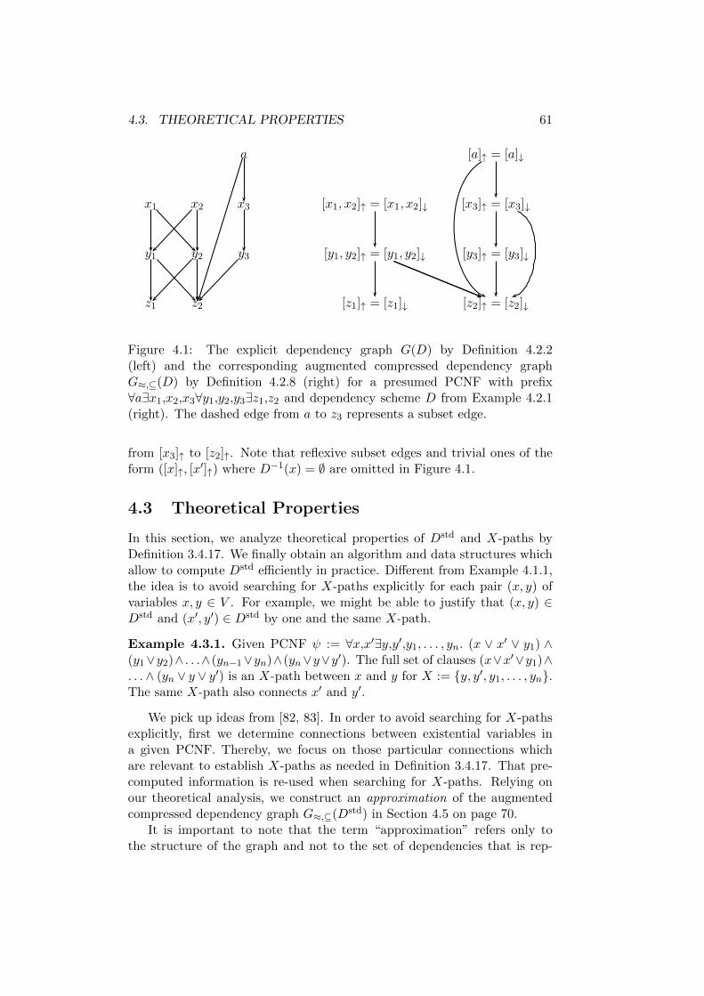
4.3. THEORETICAL PROPERTIES 61
a
x1 x2 x3
y1 y2 y3
z1 z2
[a]↑ = [a]↓
[x1, x2]↑ = [x1, x2]↓ [x3]↑ = [x3]↓
[y1, y2]↑ = [y1, y2]↓ [y3]↑ = [y3]↓
[z1]↑ = [z1]↓ [z2]↑ = [z2]↓
Figure 4.1: The explicit dependency graph G(D) by Definition 4.2.2(left) and the corresponding augmented compressed dependency graphG≈,⊆(D) by Definition 4.2.8 (right) for a presumed PCNF with prefix∀a∃x1,x2,x3∀y1,y2,y3∃z1,z2 and dependency scheme D from Example 4.2.1(right). The dashed edge from a to z3 represents a subset edge.
from [x3]↑ to [z2]↑. Note that reflexive subset edges and trivial ones of theform ([x]↑, [x′]↑) where D−1(x) = ∅ are omitted in Figure 4.1.
4.3 Theoretical Properties
In this section, we analyze theoretical properties of Dstd and X-paths byDefinition 3.4.17. We finally obtain an algorithm and data structures whichallow to compute Dstd efficiently in practice. Different from Example 4.1.1,the idea is to avoid searching for X-paths explicitly for each pair (x, y) ofvariables x, y ∈ V . For example, we might be able to justify that (x, y) ∈Dstd and (x′, y′) ∈ Dstd by one and the same X-path.
Example 4.3.1. Given PCNF ψ := ∀x,x′∃y,y′,y1, . . . , yn. (x ∨ x′ ∨ y1) ∧(y1∨y2)∧ . . .∧(yn−1∨yn)∧(yn∨y∨y′). The full set of clauses (x∨x′∨y1)∧. . .∧ (yn ∨ y ∨ y′) is an X-path between x and y for X := {y, y′, y1, . . . , yn}.The same X-path also connects x′ and y′.
We pick up ideas from [82, 83]. In order to avoid searching for X-pathsexplicitly, first we determine connections between existential variables ina given PCNF. Thereby, we focus on those particular connections whichare relevant to establish X-paths as needed in Definition 3.4.17. That pre-computed information is re-used when searching for X-paths. Relying onour theoretical analysis, we construct an approximation of the augmentedcompressed dependency graph G≈,⊆(Dstd) in Section 4.5 on page 70.
It is important to note that the term “approximation” refers only tothe structure of the graph and not to the set of dependencies that is rep-

62 CHAPTER 4. THE STANDARD DEPENDENCY SCHEME
resented thereby. That is, the approximation of G≈,⊆(Dstd) we introducein Section 4.5 below is precise with respect to Dstd. There is a dependency(x, y) in the approximation of the graph if and only if there is a dependency(x, y) with respect to Dstd by Definition 3.4.17. However, the approximationof G≈,⊆(Dstd) might not be as compact as the original graph G≈,⊆(Dstd)by Definition 4.2.8. The reason for less compaction is that equivalences be-tween variables by Definitions 4.2.3 and 4.2.4 might not be considered to thefull extent. Concerning practical applications, it is not necessary to startwith G(Dstd) and then merge classes explicitly, as in the trivial approachoutlined above. Instead, as we show, the approximation of G≈,⊆(Dstd) canlargely be computed right away from a given PCNF. Although we focus oncompact representations of Dstd in this chapter, our approaches related tothe computation of approximations of G≈,⊆(Dstd) might also be extendedto other dependency schemes which refine Dstd.
In the remaining parts of this section, we apply the following notion oftransitive relations.
Definition 4.3.1 ([1]). Let R ⊆ V × V be a binary relation on some set ofvariables V . The reflexive and transitive closure of R is the smallest reflexiveand transitive R′ ⊆ V × V such that R ⊆ R′. The reflexive and transitivereduction of R is the smallest R′ ⊆ V ×V such that R and R′ have the samereflexive and transitive closure.
Definition 4.3.1 differs from transitivity of dependency schemes by Defi-nition 3.4.9 on page 45. The former is related to arbitrary binary relationsand is well-known. In this section we refer to transitive closure by Defini-tion 4.3.1, unless stated otherwise.
We consider closed PCNFs where, for all clauses Ci := (l1 ∨ . . . ∨ lki),lj < lj′ for 1 ≤ j < j′ ≤ ki and q(v(lki)) = ∃. That is, literals in clausesare sorted ascendingly with respect to prefix ordering and the largest literalis existential. Further, we assume that clauses neither contain multiple norcomplementary literals of one and the same variable.
Recall Definition 3.4.17 on page 49 where the standard dependencyscheme Dstd was introduced. By setting i := δ(x) + 1 and X := V∃,i,universal variables as well as variables which are from the block of x orfrom any smaller block are excluded from X. Hence these variables cannotparticipate in any X-path.
Example 4.3.2. For the PCNF in Figure 4.2, we have i = δ(a1) = 1,e13 ∈ Dstd(a1) by clauses (a1 ∨ a6 ∨ e8 ∨ e14) and (e3 ∨ e8 ∨ e13), and X =V∃,i+1 = {e3, e4, e5, e8, e9, e10, e13, e14, e15}. Note that variable e8 connectsthe two clauses and e8 ∈ V∃,i+1 since i ≤ δ(e8). However, e14 6∈ Dstd(a7)since a7 and e10 occur only in clause (e4 ∨ a7 ∨ e10). Variable e4 cannot beused to connect a7 and e14 by clause (e4 ∨ e13 ∨ e14) because δ(e4) < δ(a7).

4.3. THEORETICAL PROPERTIES 63
i q(Bi) Bi (a2 ∨ e5 ∨ e9)1 ∀ a1, a2 (e5 ∨ e9 ∨ e15)2 ∃ e3, e4, e5 (e3 ∨ e8 ∨ e13)3 ∀ a6, a7 (e4 ∨ a7 ∨ e10)4 ∃ e8, e9, e10 (e4 ∨ e13 ∨ e14)5 ∀ a11, a12 (a1 ∨ a6 ∨ e8 ∨ e14)6 ∃ e13, e14, e15 (a11 ∨ a12 ∨ e13)
Figure 4.2: PCNF example used in Sections 4.3 and 4.5.3. The table showsthe levels, quantifiers and variables for each quantifier block in the first threecolumns and clauses in the last column. Variable names are prefixed with“e” and “a” to indicate their types ∃ and ∀, respectively.
Building on related work precedingDstd by Definition 3.4.17 [16, 25, 113],we first introduce a connection relation between variables which is aware ofthe levels of quantifier blocks.
Definition 4.3.2. For x, y ∈ V , x is connected to y with respect to blockBi, written as x →i y, if and only if y ∈ V∃,i and there is a clause C suchthat x ∈ C and y ∈ C. Relation →∗i is the reflexive and transitive closureof →i.
Relation →∗i is defined with respect to some block Bi. If x→∗i y then xis connected to y over existential variables from blocks larger than or equalto Bi only. As pointed out in Theorem 4.3.2 below, this relation can beapplied to compute Dstd. There is a close correspondence between X-pathsas used in Definition 3.4.17 and relation →∗i .
Corollary 4.3.1. Given x, y ∈ V , if x→∗i y then there is an X-path betweenx and y for X = V∃,i.
Note that, due to Definition 4.3.2, the converse of Corollary 4.3.1 doesnot hold in general. For example, if there is an X-path between x ∈ V∃ andy ∈ V∀ then x 6→∗i y for all i. A weaker variant can be stated as follows.
Corollary 4.3.2. Given x ∈ V and y ∈ V∃, if there is an X-path betweenx and y for X = V∃,i and i ≤ min(δ(x), δ(y)) then x→∗i y.
We observe that connections with respect to a block Bj are preservedfor any smaller block Bi.
Corollary 4.3.3. Given x, y ∈ V and i ≤ j, if x→∗j y then also x→∗i y.
For proper values of i in Definition 4.3.2, connections between existentialvariables are symmetric because X-paths resulting from Corollary 4.3.1 cantrivially be reversed.

64 CHAPTER 4. THE STANDARD DEPENDENCY SCHEME
Lemma 4.3.1. Given x, y ∈ V∃ and i ≤ min(δ(x), δ(y)), if x →∗i y theny →∗i x.
Example 4.3.3. For the PCNF in Figure 4.2, e3 →4 e8 by clause (e3 ∨e8 ∨ e13) but e3 6→5 e8, e8 →6 e14 by clause (a1 ∨ a6 ∨ e8 ∨ e14) and byCorollary 4.3.3 also e8 →1 e14. Further e3 →∗2 e14 by clauses (e3 ∨ e8 ∨ e13)and (e4 ∨ e13 ∨ e14) and by Lemma 4.3.1 also e14 →∗2 e3.
As a first step towards efficient computation and compact representationof Dstd we want to take advantage of situations where two variables can beregarded as equivalent with respect to connections by Definition 4.3.2.
Definition 4.3.3. For x, y ∈ V , x is equivalent to y with respect to connec-tion relation →∗i , written as x ≈ y, if and only if either (1) x = y or (2)q(x) = q(y) = ∃, δ(x) = δ(y) = i and x→∗i y.
Variables x and y are equivalent by Definition 4.3.3 if x = y or bothare from the same existential block Bi and are connected by existentialvariables larger than or equal to Bi. Note that relation≈ is different from theequivalence relations ≈↓ and ≈↑ introduced previously in Definitions 4.2.3and 4.2.4. However, as pointed out in Section 4.5.1 below, ≈ has certainproperties which allow to obtain an approximation of ≈↑ for existentialvariables in order to construct an approximation of graph G≈,⊆(Dstd).
Theorem 4.3.1. Given a PCNF ψ over variables V , relation ≈ by Defini-tion 4.3.3 is an equivalence relation.
Proof. Reflexivity is trivial since x ≈ x for x ∈ V by Definition 4.3.3. Ifnot q(x) = q(y) = ∃ then by Definition 4.3.3 x ≈ y if and only if x = y.Since = is an equivalence relation, symmetry and transitivity of ≈ followimmediately.
Otherwise, assume q(x) = q(y) = ∃. If x ≈ y and x = y, then alsoy ≈ x by Definition 4.3.3. If x ≈ y and x 6= y then by Definition 4.3.2and Definition 4.3.3 δ(x) = δ(y) and x →∗i y for i = δ(x) = δ(y). Then byLemma 4.3.1 also y →∗i x and hence y ≈ x. Therefore, ≈ is symmetric.
To show transitivity, assume x ≈ y′ and y′ ≈ y for y′ ∈ V . Thenmore precisely y′ ∈ V∃ (because otherwise x 6≈ y′ and y′ 6≈ y) and byDefinition 4.3.3 also x →∗i y′, y′ →∗i y for i = δ(x) = δ(y′) = δ(y) andq(x) = q(y′) = q(y). By x →∗i y′, y′ →∗i y and transitivity of →∗i , alsox→∗i y, hence x ≈ y.
Definition 4.3.4. Given a PCNF ψ over variables V , the partition V/≈ ofV induced by ≈ is obtained similarly to Definition 4.2.5. Given x ∈ V , [x]is the equivalence class of x with respect to partition V/≈.
Example 4.3.4. For the PCNF in Figure 4.2, e3 ≈ e4 since q(e3) = q(e4) =∃, δ(e3) = δ(e4) = 2 and e3 →∗2 e4 by e3 →2 e8 →2 e14 →2 e4. Also e13 ≈ e14
4.3. THEORETICAL PROPERTIES 65
since e13 →6 e14 but e5 6≈ e4 because e5 6→∗2 e4. Trivially, a11 ≈ a11 ande3 6≈ e14.
Relation →∗i is compatible with ≈. If two variables are connected thenso are all members of their respective classes and vice versa as stated in thefollowing lemma.
Lemma 4.3.2. Given x, y ∈ V and i ≤ min(δ(x), δ(y)). Then x →∗i y ifand only if x′ →∗i y′ for all x′ ∈ [x], y′ ∈ [y].
Proof. The proof works regardless of the types of x and y by Definition 4.3.2(reflexivity of →∗i ), Corollary 4.3.3 and Definition 4.3.3. Trivial cases arisefor V∀. Assume x →∗i y for x, y ∈ V and i ≤ min(δ(x), δ(y)). Then forx′ ∈ [x], y′ ∈ [y], x′ →∗i x and y →∗i y′ by Corollary 4.3.3 and Definition 4.3.3.Since x′ →∗i x, x→∗i y (by assumption), y →∗i y′, also x′ →∗i y′ by transitiv-ity of →∗i . The other direction can be shown similarly by Lemma 4.3.1.
As in Definition 4.2.6, we regard [x] as an arbitrary member of the equiv-alence class. We can write, for example, [x] →∗i [y] by Lemma 4.3.2. Thisnotation denotes connections between classes. Note that Lemma 4.3.2 wouldnot hold for arbitrary values of i. For example, if δ(x) < i then x 6→∗i x′for x′ ∈ [x], which contradicts Definition 4.3.3. The following variant ofLemma 4.3.2 does not refer to [x] and holds for arbitrary values of i.
Lemma 4.3.3. Let x, y ∈ V with δ(x) ≤ δ(y). Then x →∗i y if and only ifx→∗i y′ for all y′ ∈ [y].
Example 4.3.5. For the PCNF in Figure 4.2, e3 ≈ e4, e10 ≈ e10, where[e10] is a singleton class, and e4 →∗2 e10 because e4 →2 e10. By Lemma 4.3.2,also e3 →∗2 e10 because e3 →2 e8 →2 e14 →2 e4 →2 e10.
Apart from considering equivalence classes in →∗i by Lemma 4.3.2, thefollowing relation allows to share information about connections, which ispointed out in Section 4.4.1 below.
Definition 4.3.5. Relation ;∗ denotes the directed connection relation.Given x ∈ V and y ∈ V∃, [x] ;∗ [y] if and only if δ(x) ≤ δ(y) and x →∗i yfor i = δ(x). The reflexive and transitive reduction of ;∗ is denoted by ;.
Corollary 4.3.4. Given x, y ∈ V , if [x] ;∗ [y] then either [x] = [y] orδ(x) < δ(y).
Relation ;∗ is defined on equivalence classes with respect to ≈ only andrespects the ordering of quantifier blocks in the prefix. If [x] ;∗ [y] thenvariables smaller than x are excluded in the connection between x and y.By Corollary 4.3.4, if [x] ;∗ [y] then either x and y are in the same classor in different classes but also from different blocks. We now prove that thedefinitions introduced above can be used to compute Dstd.
66 CHAPTER 4. THE STANDARD DEPENDENCY SCHEME
Theorem 4.3.2. Given PCNF ψ over variables V , Dstd for ψ can be com-puted as follows:
Dstd = {(x, y) ∈ V× | i := δ(x) + 1,∃w ∈ V∃,i : (4.1)
x→∗i w and y →∗i w}= {(x, y) ∈ V× | i := δ(x) + 1,∃w ∈ V∃,i : (4.2)
x→∗i [w] and [y]→∗i [w]}= {(x, y) ∈ V× | i := δ(x) + 1,∃w ∈ V∃,i : (4.3)
x→∗i [w] and [y] ;∗ [w]}
Proof. We prove equivalence of left (LHS) and right-hand sides (RHS) ofEquations 4.1 to 4.3.
In order to show that LHS(4.1) = RHS(4.1), assume by Definition 3.4.17that there is an X-path P between x and y by clauses C1, . . . , Ck whereq(x) 6= q(y). P can be split into P1 between x,w for clauses C1, . . . , Cj wherew ∈ Cj , 1 ≤ j ≤ k,w ∈ V∃,i and P2 between w, y by clauses Cj , . . . , Ck. ByP1 and Corollary 4.3.2 also x→∗i w and by reversing P2 and Corollary 4.3.2,also y →∗i w and hence y ∈ RHS(4.1). For the other direction, assumex→∗i w and y →∗i w. Then by Corollary 4.3.1 there are X-paths P1 betweenx,w and P2 between y, w for X = V∃,i. An X-path P between x, y can beconstructed by combining P1 with reversed P2, thus y ∈ LHS(4.1).
In order to show that RHS(4.1) = RHS(4.2), assume x →∗i w andy →∗i w. Since w ∈ V∃,i, also δ(x) ≤ δ(w) and hence by Lemma 4.3.3and Definition 4.3.3 also x→∗i [w]. Further, because i ≤ δ(y) and i ≤ δ(w)and hence i ≤ min(δ(y), δ(w)), also [y]→∗i [w] by Lemma 4.3.2 and Defini-tion 4.3.3. Since x→∗i [w] and [y]→∗i [w], also y ∈ RHS(4.2). For the otherdirection, assume x→∗i [w] and [y]→∗i [w]. Similar arguments apply to de-rive x→∗i w and y →∗i w by Lemma 4.3.2, Lemma 4.3.3 and Definition 4.3.3.Hence y ∈ RHS(4.1).
In order to show that RHS(4.2) = RHS(4.3), assume x →∗i [w] and[y] →∗i [w]. Since LHS(4.1) = RHS(4.1) = RHS(4.2), there is an X-pathP between x, y for X = V∃,i and clauses C1, . . . , Ck where y ∈ Ck. Let ldenote the largest literal in Ck. By assumptions in Section 2.1.4, clausesare sorted by prefix ordering and the largest literal is existential. That is,v(l) ∈ V∃ and δ(y) ≤ δ(l) (if q(y) = ∀ then δ(y) < δ(l)). Assume thatw = v(l). Then δ(y) ≤ δ(w). By y, w ∈ Ck also y →j w for j = δ(y) andy →∗j w by Definition 4.3.2. By y →∗j w and δ(y) ≤ δ(w) also [y] ;∗ [w].Since x →∗i [w] and [y] ;∗ [w] also y ∈ RHS(4.3). For the other direction,Definition 4.3.5, Corollary 4.3.3 and Lemma 4.3.2 apply.

4.4. TOWARDS EFFICIENT COMPUTATION 67
4.4 Towards Efficient Computation
According to Equation 4.1 in Theorem 4.3.2, Dstd can be computed by ap-plying relation →∗i , which corresponds to computation by X-paths in Def-inition 3.4.17. Equation 4.2 refers to equivalence classes by ≈ rather thanindividual variables, which is already an improvement. The step from Equa-tion 4.2 to Equation 4.3 is the most interesting one for practical applications,yet this is not apparent from theory. Since ;∗ is directed, it restricts the setof classes to be considered when connections of a variable are determined.
In this section, we first examine properties of ;∗ over existential vari-ables. We observe that its reflexive and transitive reduction ; can be rep-resented efficiently as a compact tree over equivalence classes with respectto ≈. As pointed out in Section 4.5.2 below, this tree can be shared betweenall variables and is the basis for constructing approximations of the graphG≈,⊆(Dstd) by Definition 4.2.8.
4.4.1 A Tree-Shaped Representation of Connections
Since ;∗ is directed by Definition 4.3.5 and hence also antisymmetric andacyclic, its transitive reduction ; is unique by Theorem 1 in [1]. The fol-lowing lemma states a property of ;∗ which accounts for the tree structureof ;.
Lemma 4.4.1. Given x, y, z ∈ V∃ where δ(x) ≤ δ(y), if [x] ;∗ [z] and[y] ;∗ [z] then [x] ;∗ [y].
Proof. Assume [x] ;∗ [z] and [y] ;∗ [z] where δ(x) ≤ δ(y). Then byDefinition 4.3.5, x →∗i z for i = δ(x) and y →∗j z for j = δ(y) and δ(x) ≤δ(y) ≤ δ(z). By Corollary 4.3.3 also y →∗i z and by Lemma 4.3.1 z →∗i y.By Definition 4.3.2, x→∗i z and z →∗i y, also x→∗i y and [x] ;∗ [y].
If [x] ;∗ [z] and [y] ;∗ [z] for existential variables x, y, z and δ(x) ≤ δ(y)then [x] ;∗ [z] is transitive by Lemma 4.4.1. Consequently, [x] is not relatedto [z] in the transitive reduction of ;∗, that is [x] 6; [z]. Hence at most oneclass is related to another one in ;. Therefore, ; can be represented as aforest, that is a collection of trees, which we introduce informally.
Definition 4.4.1. Given a PCNF ψ over variables V with m existentialquantifier blocks. The connection forest for ψ is a collection of trees overthe set V∃/≈ of vertices with the following properties:
1. For x, y ∈ V∃, there is an edge ([x], [y]) if and only if [x] ; [y].
2. For x, y ∈ V∃ there is a path from [x] to [y] if and only if [x] ;∗ [y].
3. The maximum length of a path by counting the number of edges ism− 1 (by Corollary 4.3.4).

68 CHAPTER 4. THE STANDARD DEPENDENCY SCHEME
4.4.2 Dependency Computation Using Connection Forests
The connection forest represents directed connections between existentialvariables. In general, we expect it to be compact due to equivalence classesin partition V∃/≈ and because it considers the transitive reduction ; insteadof ;∗. Our goal is to compute and represent Dstd efficiently by making useof the connection forest of a PCNF (see also Section 4.5.3 below).
To compute Dstd(x) for an arbitrary x ∈ V , a set of proper classesof V∃/≈ has to be found in the connection forest which exactly denote allconnections of variable x to larger existential variables. Exactly those vari-ables are relevant by Definition 3.4.17 and Theorem 4.3.2. Classes in sucha proper set must be connected to x and be minimal with respect to theprefix ordering since edges in the connection forest are directed. We requireminimality since if there is a non-trivial path from [x] to [y] in the connec-tion forest then δ(x) < δ(y) by Corollary 4.3.4. Hence [x] can only reachclasses of larger variables. Descendants of such minimal classes in the con-nection forest comprise all connections of x by ;∗ which are relevant forthe computation of Dstd. We identify the desired set of minimal classes bysmallest ancestors in the connection forest.
Definition 4.4.2. For y ∈ V∃ and i ≤ δ(y), the smallest ancestor of [y]with respect to i in the connection forest is the class h(i, [y]) := [y′] suchthat y′ ∈ V∃,i, [y′] ;∗ [y] and there is no y′′ ∈ V∃,i with i ≤ δ(y′′) < δ(y′)and [y′′] ;∗ [y].
Class h(i, [y]) is the smallest ancestor of [y] in the connection forest whichis larger than or equal to block Bi. Hence h(i, [y]) is minimal with respect toBi and the prefix ordering. Smallest ancestors are used to compute the set ofdescendants, which are classes reachable by directed edges in the connectionforest, as follows.
Definition 4.4.3. For x ∈ V and the connection forest, the set of descen-dants H∗i (x) with respect to x and block Bi is defined as follows:
1. VC,i(x) := {[y] | y ∈ V∃,i and x→i y}
2. Hi(x) := {[z] | [z] = h(i, [y]) for [y] ∈ VC,i(x)}
3. H∗i (x) := {[y] | [z] ;∗ [y] for [z] ∈ Hi(x)}
Note that in the definition of set VC,i(x), we have x →i y if there is aclause which contains both x and y for proper values of i. Starting fromclauses containing a literal of variable x, classes of existential variables largerthan or equal to Bi are collected in VC,i(x). Set Hi(x) contains all smallestancestors with respect to Bi for classes in VC,i(x). Finally, H∗i (x) com-prises descendants of classes in Hi(x) and represents all connections of x toexistential variables larger than or equal to Bi.

4.4. TOWARDS EFFICIENT COMPUTATION 69
Corollary 4.4.1. Given x ∈ V , if [y] ∈ H∗i (x) then x→∗i y.
For some variable x ∈ V , the set H∗i (x) of descendants in the connectionforest exactly characterizes relevant connections of x to existential variableswhich are from block Bi or any larger block. This is precisely what is neededto compute Dstd. Informally, there is a dependency (x, y) ∈ Dstd if the setsof descendants of x and y are not disjoint. In this case, there exists anX-path between x and y as required by Definition 3.4.17.
Theorem 4.4.1. For a PCNF ψ over variables V,
Dstd = {(x, y) ∈ V× | H∗i (x) ∩H∗j (y) 6= ∅ for i := δ(x) + 1, j := δ(y)}.
Proof. We show that Dstd by Definition 3.4.17 is equal to the definitionshown above. Assume x ∈ V and i = δ(x) + 1. Direction ⊇ follows rightfrom Definition 4.4.3, Corollary 4.4.1, Corollary 4.3.3 and Theorem 4.3.2.
To show ⊆, assume (x, y) ∈ Dstd. Then there is an X-path P betweenx, y for X = V∃,i. Hence there are clauses C1, . . . , Ck where y, yk ∈ Ck forsome yk ∈ V∃,i with δ(y) ≤ δ(yk). Such yk always exists since by assumptionthe largest literal in a clause is existential (if x ∈ V∀ then y ∈ V∃ and we canchoose yk := y). Then P is also an X-path between x and yk by C1, . . . , Ckand hence x→∗i yk and δ(x) < δ(yk) since i ≤ δ(yk), i = δ(x) + 1. We showthat [yk] ∈ H∗i (x) ∩H∗j (y) for i = δ(x) + 1, j = δ(y).
First, we show that [yk] ∈ H∗j (y) for j = δ(y). Since y, yk ∈ Ck by P ,also [yk] ∈ VC,j(y). Then [z′] ∈ Hj(y) where [z′] = h(j, [yk]) for j = δ(y).By Definition 4.4.2, [z′] ;∗ [yk], hence [yk] ∈ H∗j (y).
Second, we show that [yk] ∈ H∗i (x) for i = δ(x) + 1. Since P connectsx and yk, also x, y1 ∈ C1 for some y1 ∈ V∃,i. Thus [y1] ∈ VC,i(x) and[z1] ∈ Hi(x) for [z1] = h(i, [y1]). Then by Definition 4.4.2, [z1] ;∗ [y1]. Pis also an X-path between y1 and yk by C1, . . . , Ck, hence y1 →∗i yk andδ(x) < δ(y1), δ(x) < δ(yk). Let w denote the smallest connecting variable inP between y1, yk: m = δ(w) = min({δ(v) | v ∈ Ci ∩ Ci+1 ∩X, 1 ≤ i < k}).Since m is minimal, also y1 →∗m w, w →∗m yk and by Lemma 4.3.1 w →∗m y1.By Definition 4.3.5 and since m = δ(w), also [w] ;∗ [y1], [w] ;∗ [yk].By Lemma 4.4.1, [z1] ;∗ [y1] and [w] ;∗ [y1], also [z1] ;∗ [w]. Then by[z1] ;∗ [w], [w] ;∗ [yk] and transitivity also [z1] ;∗ [yk], hence [yk] ∈ H∗i (x)because [z1] ∈ Hi(x).
Since [yk] ∈ H∗j (y) and [yk] ∈ H∗i (x), also [yk] ∈ H∗i (x) ∩ H∗j (y) fori = δ(x) + 1 and j = δ(y).
In contrast to Theorem 4.3.2, practical application follows right fromTheorem 4.4.1. Dependencies in Dstd can be identified by checking descen-dants in the connection forest of a PCNF ψ. The advantage compared toTheorem 4.3.2 is that the connection forest for a PCNF ψ can be computedonce and for all. It can be re-used each time the condition H∗i (x)∩H∗j (y) 6= ∅
70 CHAPTER 4. THE STANDARD DEPENDENCY SCHEME
in Theorem 4.4.1 is checked. This way, we also avoid searching for X-pathsexplicitly like in direct applications of Definition 3.4.17. Further, we expectthe connection forest to be compact because it is defined over equivalenceclasses of variables.
4.5 Compact Dependency Graphs
In the previous section, we observed several theoretical properties of connec-tions involved in the computation of Dstd. Starting from explicit connectionsas in Equation 4.1, we defined the equivalence relation ≈ on variables. InEquation 4.2 we pointed out that dependencies can be computed by consid-ering connections between equivalence classes. Finally, we applied a tree-likerepresentation of connections between classes of existential variables as inEquation 4.3 and Theorem 4.4.1.
Now we focus on practical application. Our goal is to obtain a compactgraph representation for Dstd. Instead of the augmented compressed de-pendency graph G≈,⊆(Dstd) by Definition 4.2.8 on page 60, we construct anapproximation thereof. As noted at the beginning of Section 4.3, the approx-imation is precise with respect to dependencies by Dstd but not with respect tograph structure. There is a dependency with respect to the approximation ifand only if there is a dependency with respect to Dstd. In Section 4.6 below,we show that the approximation can be computed efficiently for formulaefrom real-world applications, although it might not allow for full compact-ness as the original graph G≈,⊆(Dstd) by Definition 4.2.8. Thus we tradecompactness for efficiency of computation.
First, in Section 4.5.1 we relate theoretical results from the previous sec-tion to the definition of the original graph G≈,⊆(Dstd). These observationsare the basis for defining an approximation of G≈,⊆(Dstd). As we consideronly Dstd, we write ≈↑ and ≈↓ instead of ≈Dstd,↑ and ≈Dstd,↓ throughoutthis section. It turns out that on existential variables the equivalence rela-tion ≈↑ by Definition 4.2.4 can be approximated by equivalence relation ≈by Definition 4.3.3. Further, on universal variables the equivalence relation≈↑ can be approximated by ≈↓. For existential variables, subset edges Esby Definition 4.2.8 can be approximated by the directed connection relation;∗ from Definition 4.3.5, which is represented by the connection forest.
Based on these observations, we present an algorithm to construct anapproximation of G≈,⊆(Dstd) for a given PCNF ψ in Section 4.5.2. Anexperimental evaluation in Section 4.6 confirms its practical efficiency onformulae from recent QBF evaluations.
4.5.1 Approximations
We point out properties of Dstd related to theoretical results from Sec-tion 4.3. We want to approximate G≈,⊆(Dstd) by Definition 4.2.8 by approx-
4.5. COMPACT DEPENDENCY GRAPHS 71
imating the set V/≈↓ ∪ V/≈↑ of vertices and edges E. The idea is to avoidcomputing the exact equivalence relations ≈↑ and ≈↓ by Definitions 4.2.3and 4.2.4 where G≈,⊆(Dstd) is based on. Instead, we approximate ≈↑ and≈↓ by other equivalence relations to be introduced below.
Definition 4.5.1 (see also [98], for example). Given a set of variables V ,equivalence relations ∼ and ∼ over V and the partitions V/∼ and V/∼ of Vinduced by ∼ and ∼, respectively. Partition V/∼ is an underapproximationof V/∼ and V/∼ is an overapproximation of V/∼ if for each equivalence classS ∈ V/∼ there is an equivalence class S′ ∈ V/∼ such that S ⊆ S′.
If variables x, x′ ∈ V are equivalent with respect to V/∼ in Defini-tion 4.5.1, then also with respect to V/∼ but not necessarily vice versa.Therefore, the underapproximation V/∼ might achieve less compaction onthe set of variables than V/∼ because of smaller equivalence classes.
In this section, we show how to underapproximate ≈↑ and ≈↓ from Defi-nitions 4.2.3 and 4.2.4. In these underapproximations defined below, we onlyconsider variables within the same quantifier block as equivalent under cer-tain additional criteria. This way, we obtain a partition of quantifier blocksrather than variables which allows for simpler implementation as pointedout in Section 4.5.2. Finally, the underapproximations of ≈↑ and ≈↓ giverise to an approximation of G≈,⊆(Dstd). Note that here we focus on Dstd. Itis unclear how to obtain similar theoretical results and approximations withrespect to other dependency schemes which refine Dstd such as the triangleor quadrangle dependency scheme [51, 113].
In the following, we present the theoretical background where the un-derapproximations of ≈↑ and ≈↓ and finally the approximation of graphG≈,⊆(Dstd) are based on.
Lemma 4.5.1. Given a PCNF ψ over variables V and y, y′ ∈ V whereq(y) = q(y′) = ∃ and δ(y) = δ(y′) = j: if y ≈ y′ then y ≈↑ y′.
Proof. Assume that y ≈ y′ and that there is x ∈ V such that x ∈ (Dstd)−1(y).Note that actually q(x) = ∀ and δ(x) = i for some i with i < j by Theo-rem 4.3.2. We show that also x ∈ (Dstd)−1(y′) and hence y ≈↑ y′ by Defini-tion 4.2.4. Alternatively to x ∈ (Dstd)−1(y) we can write (x, y) ∈ Dstd. ByEquation 4.2 in Theorem 4.3.2 there is w ∈ V∃,δ(x)+1 such that x→∗δ(x)+1 [w]
and [y]→∗δ(x)+1 [w]. Since y ≈ y′, by Definition 4.3.3 y →∗j y′ for j = δ(y) =
δ(y′) where δ(x) + 1 ≤ j. Hence [y′]→∗δ(x)+1 [w] and therefore (x, y′) ∈ Dstd
by Equation 4.2 in Theorem 4.3.2 and finally x ∈ (Dstd)−1(y′).
By Lemma 4.5.1, if two existential variables y and y′ from the sameblock are connected with respect to variables from the same or any largerexistential block as in Definition 4.3.3, then they are equivalent with respectto ≈. In this case, y and y′ also depend on the same set of universal variables

72 CHAPTER 4. THE STANDARD DEPENDENCY SCHEME
and hence are equivalent by ≈↑. The converse does non necessarily hold.Two variables from different blocks but of the same quantifier type coulddepend on the same set of variables even if they are not equivalent by ≈.
Lemma 4.5.2. Given a PCNF ψ over variables V and y, y′ ∈ V whereq(y) = q(y′) = ∀ and δ(y) = δ(y′) = j: if y ≈↓ y′ then y ≈↑ y′.
Proof. Assume that y ≈↓ y′. By Definition 4.2.3 Dstd(y) = Dstd(y′). As-sume that (x, y) ∈ Dstd for some x ∈ V∃ and i = δ(x) where i < j by The-orem 4.3.2. By Equation 4.3 there is an arbitrary but fixed w ∈ V∃,δ(x)+1
such that x→∗δ(x)+1 [w] and [y] ;∗ [w]. By [y] ;∗ [w], Definition 4.3.5 and
Theorem 4.3.2, also (y, w) ∈ Dstd. By assumption Dstd(y) = Dstd(y′), also(y′, w) ∈ Dstd. Since (y′, w) ∈ Dstd, by Equation 4.3 in Theorem 4.3.2 alsoy′ →∗δ(y′)+1 [w] and [w] ;∗ [w]. By y′ →∗δ(y′)+1 [w], Definition 4.3.5 and
Corollary 4.3.3, also [y′] ;∗ [w]. By assumption x →∗δ(x)+1 [w] and since
[y′] ;∗ [w], also (x, y′) ∈ Dstd by Equation 4.3 in Theorem 4.3.2.
By Lemma 4.5.2, if two universal variables from the same block haveequal sets of depending variables, then they also depend on the same set ofvariables.
Lemma 4.5.3. Given a PCNF ψ over variables V and x, x′ ∈ V whereδ(x) = δ(x′) = i: if Hi+1(x) = Hi+1(x′) then x ≈↓ x′.
Proof. Assume that Hi+1(x) = Hi+1(x′). Then by Definition 4.4.3 alsoH∗i+1(x) = H∗i+1(x′). Assume that (x, y) ∈ Dstd by Theorem 4.4.1, thatis H∗i+1(x) ∩ H∗j (y) 6= ∅ for j := δ(y). Let [z] ∈ H∗i+1(x) ∩ H∗j (y). Sinceby assumption H∗i+1(x) = H∗i+1(x′), also [z] ∈ H∗i+1(x′) ∩ H∗j (y). ThenH∗i+1(x′) ∩ H∗j (y) 6= ∅ for j := δ(y) and by Theorem 4.4.1 also (x′, y) ∈Dstd.
By Lemma 4.5.3, variables with equal sets of ancestors in the connectionforest also have equal sets of depending variables. This follows right fromDefinition 4.4.3. If the sets of descendants in the connection forest are equal,then the sets of connected existential variables are equal. By Theorem 4.4.1this information is precise and relevant to compute dependencies.
Lemma 4.5.4. Given y, y′ ∈ V∃, if [y] ;∗ [y′] then ([y]↑, [y′]↑) ∈ Es, whereEs as in Definition 4.2.8.
Proof. We show that if [y] ;∗ [y′] then (Dstd)−1(y) ⊆ (Dstd)−1(y′) andhence ([y]↑, [y′]↑) ∈ Es by Definition 4.2.8. Assume that [y] ;∗ [y′] and x ∈(Dstd)−1(y) for some x ∈ V∀. Alternatively to x ∈ (Dstd)−1(y) we can write(x, y) ∈ Dstd. By Equation 4.3 in Theorem 4.3.2, there is an arbitrary butfixed w ∈ V∃,δ(x)+1 such that x→∗δ(x)+1 [w] and [y] ;∗ [w]. Since [y] ;∗ [w],
also δ(y) ≤ δ(w) and [y]→∗δ(y) [w] by Definition 4.3.5. Then by Lemma 4.3.1,
4.5. COMPACT DEPENDENCY GRAPHS 73
also [w] →∗δ(y) [y]. Since [y] ;∗ [y′], also δ(y) ≤ δ(y′) and [y] →∗δ(y) [y′] by
Definition 4.3.5. From [w] →∗δ(y) [y], [y] →∗δ(y) [y′] and transitivity, we
obtain [w] →∗δ(y) [y′]. By Lemma 4.3.1, also [y′] →∗δ(y) [w]. Since δ(x) <
δ(y) ≤ δ(y′), also [y′] →∗δ(x)+1 [w] by Corollary 4.3.3. From x →∗δ(x)+1
[w], [y′] →∗δ(x)+1 [w] and Equation 4.2 in Theorem 4.3.2, we conclude that
(x, y′) ∈ Dstd, or alternatively x ∈ (Dstd)−1(y′). Therefore (Dstd)−1(y) ⊆(Dstd)−1(y′) and hence ([y]↑, [y′]↑) ∈ Es by Definition 4.2.8.
Lemma 4.5.4 relates paths between classes in the connection forest tosubset edges in G≈,⊆(Dstd). Given existential variables y and y′ such that[y] ;∗ [y′], the connection from a universal variable x to y can be extendedto y′. Thus if (x, y) ∈ Dstd then also (x, y′) ∈ Dstd and hence there is asubset edge ([y]↑, [y′]↑). Relying on the lemmata introduced above, we defineapproximations of equivalence relations ≈↓ and ≈↑ from Definitions 4.2.3and 4.2.4.
Definition 4.5.2. Given a PCNF over variables V and x, x′ ∈ V suchthat δ(x) = δ(x′) = i. The equivalence relation ≈↓ is defined based onLemma 4.5.3:
x ≈↓ x′ if and only if Hi+1(x) = Hi+1(x′).
Given x ∈ V , [x]↓ is the class of x with respect to V/≈↓ .
Corollary 4.5.1. Given a PCNF over variables V, the partition V/≈↓ is anunderapproximation of V/≈↓ due to Lemma 4.5.3.
Definition 4.5.3. Given a PCNF over variables V and x, x′ ∈ V suchthat δ(x) = δ(x′) = i. The equivalence relation ≈↑ is defined based onLemmata 4.5.1 to 4.5.3 with respect to the type of x and x′:
• q(x) = q(x′) = ∃: x ≈↑ x′ if and only if x ≈ x′.
• q(x) = q(x′) = ∀: x ≈↑ x′ if and only if Hi+1(x) = Hi+1(x′).
Given x ∈ V , [x]↑ is the class of x with respect to V/≈↑ .
Corollary 4.5.2. Given a PCNF over variables V , the partition V/≈↑ isan underapproximation of V/≈↑ due to Lemmata 4.5.1 to 4.5.3.
Given the underapproximations ≈↓ and ≈↑ from Definitions 4.5.2 and4.5.3, we introduce an approximation of the graph G≈,⊆(Dstd) from Defini-tion 4.2.8. This approximation goes without the original equivalence rela-tions ≈↓ and ≈↑ from Definitions 4.2.3 and 4.2.4.
Definition 4.5.4. Given the standard dependency scheme Dstd for a PCNFψ over variables V and equivalence relations ≈↓ and ≈↑. The approximated,
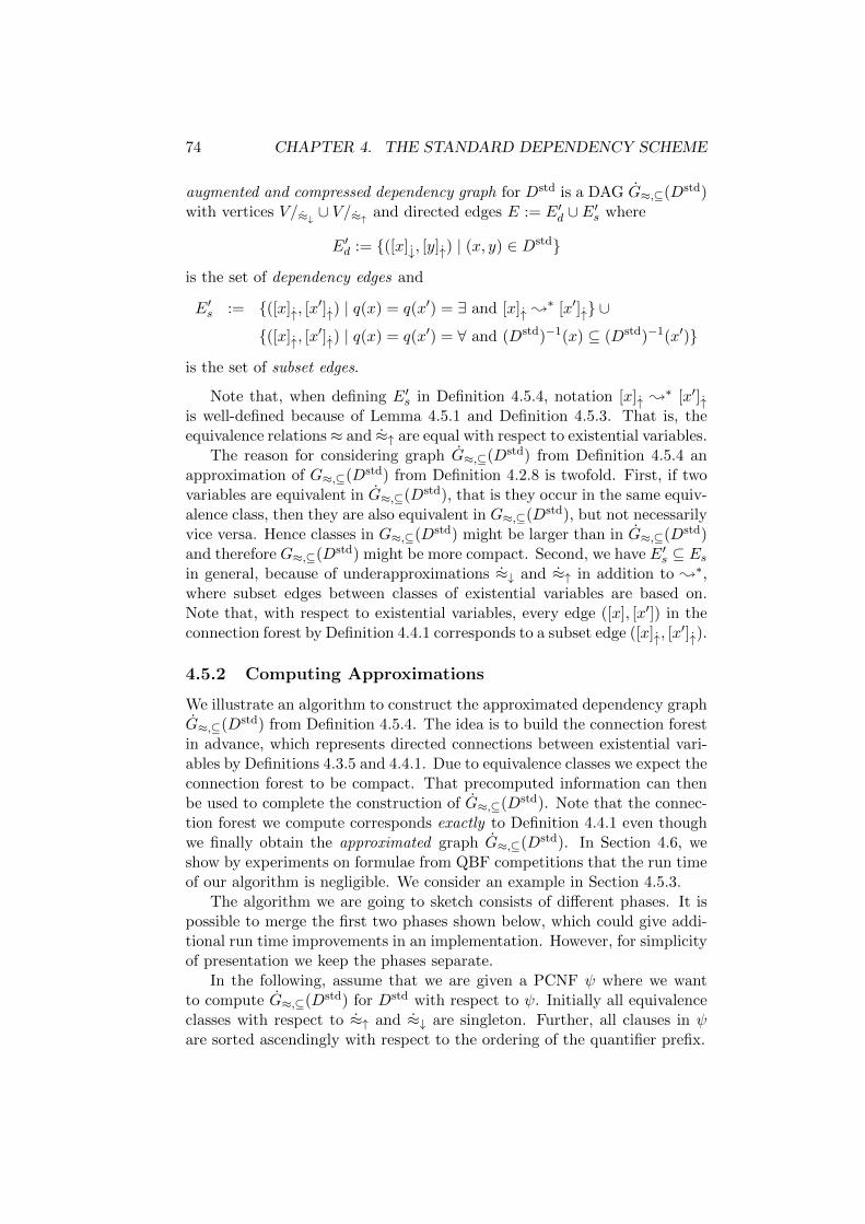
74 CHAPTER 4. THE STANDARD DEPENDENCY SCHEME
augmented and compressed dependency graph for Dstd is a DAG G≈,⊆(Dstd)with vertices V/≈↓ ∪ V/≈↑ and directed edges E := E′d ∪ E′s where
E′d := {([x]↓, [y]↑) | (x, y) ∈ Dstd}
is the set of dependency edges and
E′s := {([x]↑, [x′]↑) | q(x) = q(x′) = ∃ and [x]↑ ;
∗ [x′]↑} ∪{([x]↑, [x
′]↑) | q(x) = q(x′) = ∀ and (Dstd)−1(x) ⊆ (Dstd)−1(x′)}
is the set of subset edges.
Note that, when defining E′s in Definition 4.5.4, notation [x]↑ ;∗ [x′]↑
is well-defined because of Lemma 4.5.1 and Definition 4.5.3. That is, theequivalence relations≈ and ≈↑ are equal with respect to existential variables.
The reason for considering graph G≈,⊆(Dstd) from Definition 4.5.4 anapproximation of G≈,⊆(Dstd) from Definition 4.2.8 is twofold. First, if twovariables are equivalent in G≈,⊆(Dstd), that is they occur in the same equiv-alence class, then they are also equivalent in G≈,⊆(Dstd), but not necessarilyvice versa. Hence classes in G≈,⊆(Dstd) might be larger than in G≈,⊆(Dstd)and therefore G≈,⊆(Dstd) might be more compact. Second, we have E′s ⊆ Esin general, because of underapproximations ≈↓ and ≈↑ in addition to ;∗,where subset edges between classes of existential variables are based on.Note that, with respect to existential variables, every edge ([x], [x′]) in theconnection forest by Definition 4.4.1 corresponds to a subset edge ([x]↑, [x
′]↑).
4.5.2 Computing Approximations
We illustrate an algorithm to construct the approximated dependency graphG≈,⊆(Dstd) from Definition 4.5.4. The idea is to build the connection forestin advance, which represents directed connections between existential vari-ables by Definitions 4.3.5 and 4.4.1. Due to equivalence classes we expect theconnection forest to be compact. That precomputed information can thenbe used to complete the construction of G≈,⊆(Dstd). Note that the connec-tion forest we compute corresponds exactly to Definition 4.4.1 even thoughwe finally obtain the approximated graph G≈,⊆(Dstd). In Section 4.6, weshow by experiments on formulae from QBF competitions that the run timeof our algorithm is negligible. We consider an example in Section 4.5.3.
The algorithm we are going to sketch consists of different phases. It ispossible to merge the first two phases shown below, which could give addi-tional run time improvements in an implementation. However, for simplicityof presentation we keep the phases separate.
In the following, assume that we are given a PCNF ψ where we wantto compute G≈,⊆(Dstd) for Dstd with respect to ψ. Initially all equivalenceclasses with respect to ≈↑ and ≈↓ are singleton. Further, all clauses in ψare sorted ascendingly with respect to the ordering of the quantifier prefix.
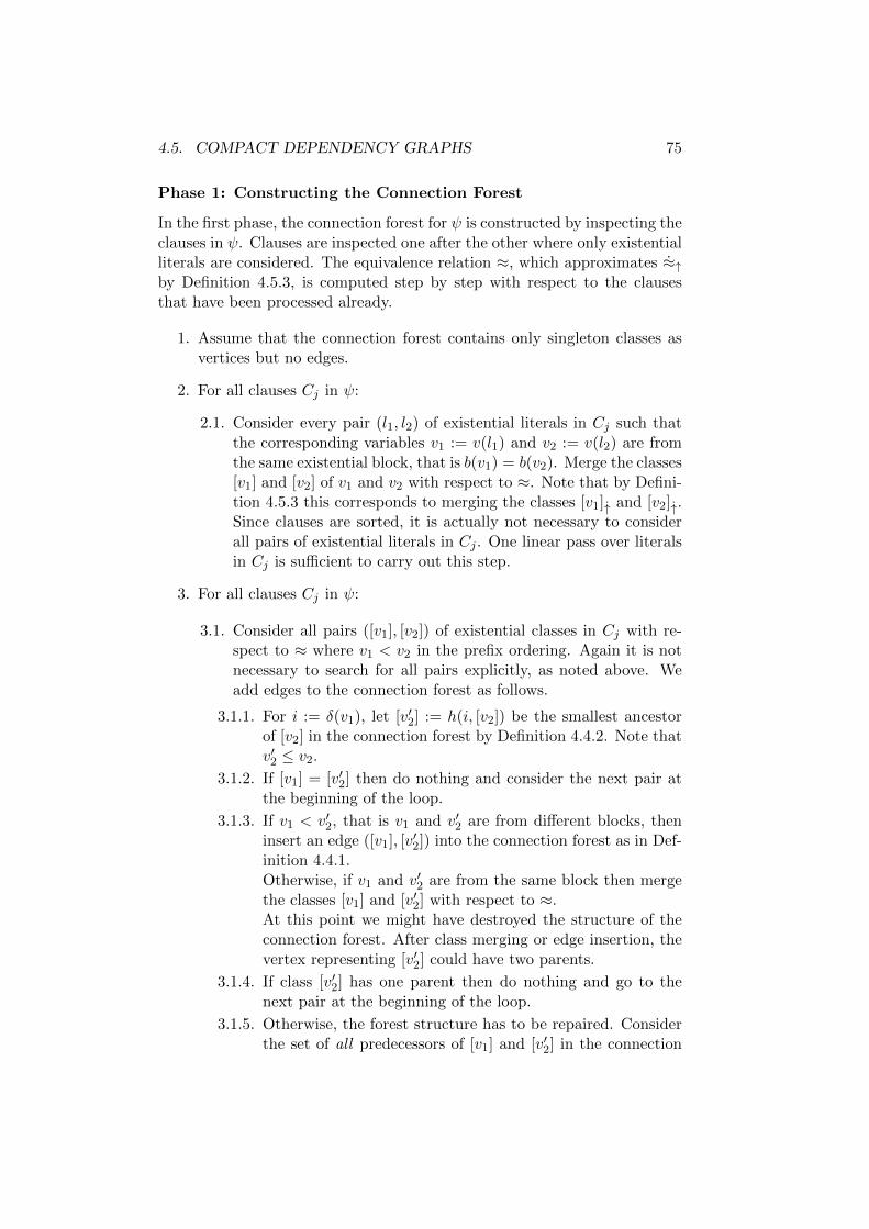
4.5. COMPACT DEPENDENCY GRAPHS 75
Phase 1: Constructing the Connection Forest
In the first phase, the connection forest for ψ is constructed by inspecting theclauses in ψ. Clauses are inspected one after the other where only existentialliterals are considered. The equivalence relation ≈, which approximates ≈↑by Definition 4.5.3, is computed step by step with respect to the clausesthat have been processed already.
1. Assume that the connection forest contains only singleton classes asvertices but no edges.
2. For all clauses Cj in ψ:
2.1. Consider every pair (l1, l2) of existential literals in Cj such thatthe corresponding variables v1 := v(l1) and v2 := v(l2) are fromthe same existential block, that is b(v1) = b(v2). Merge the classes[v1] and [v2] of v1 and v2 with respect to ≈. Note that by Defini-tion 4.5.3 this corresponds to merging the classes [v1]↑ and [v2]↑.Since clauses are sorted, it is actually not necessary to considerall pairs of existential literals in Cj . One linear pass over literalsin Cj is sufficient to carry out this step.
3. For all clauses Cj in ψ:
3.1. Consider all pairs ([v1], [v2]) of existential classes in Cj with re-spect to ≈ where v1 < v2 in the prefix ordering. Again it is notnecessary to search for all pairs explicitly, as noted above. Weadd edges to the connection forest as follows.
3.1.1. For i := δ(v1), let [v′2] := h(i, [v2]) be the smallest ancestorof [v2] in the connection forest by Definition 4.4.2. Note thatv′2 ≤ v2.
3.1.2. If [v1] = [v′2] then do nothing and consider the next pair atthe beginning of the loop.
3.1.3. If v1 < v′2, that is v1 and v′2 are from different blocks, theninsert an edge ([v1], [v′2]) into the connection forest as in Def-inition 4.4.1.Otherwise, if v1 and v′2 are from the same block then mergethe classes [v1] and [v′2] with respect to ≈.At this point we might have destroyed the structure of theconnection forest. After class merging or edge insertion, thevertex representing [v′2] could have two parents.
3.1.4. If class [v′2] has one parent then do nothing and go to thenext pair at the beginning of the loop.
3.1.5. Otherwise, the forest structure has to be repaired. Considerthe set of all predecessors of [v1] and [v′2] in the connection
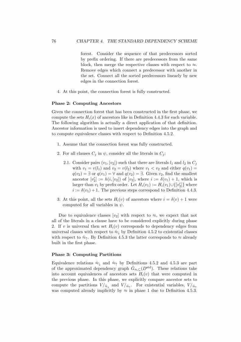
76 CHAPTER 4. THE STANDARD DEPENDENCY SCHEME
forest. Consider the sequence of that predecessors sortedby prefix ordering. If there are predecessors from the sameblock, then merge the respective classes with respect to ≈.Remove edges which connect a predecessor with another inthe set. Connect all the sorted predecessors linearly by newedges in the connection forest.
4. At this point, the connection forest is fully constructed.
Phase 2: Computing Ancestors
Given the connection forest that has been constructed in the first phase, wecompute the sets Hi(x) of ancestors like in Definition 4.4.3 for each variable.The following algorithm is actually a direct application of that definition.Ancestor information is used to insert dependency edges into the graph andto compute equivalence classes with respect to Definition 4.5.2.
1. Assume that the connection forest was fully constructed.
2. For all clauses Cj in ψ, consider all the literals in Cj :
2.1. Consider pairs (v1, [v2]) such that there are literals l1 and l2 in Cjwith v1 = v(l1) and v2 = v(l2) where v1 < v2 and either q(v1) =q(v2) = ∃ or q(v1) = ∀ and q(v2) = ∃. Given v2, find the smallestancestor [v′2] := h(i, [v2]) of [v2], where i := δ(v1) + 1, which islarger than v1 by prefix order. Let Hi(v1) := Hi(v1)∪{[v′2]} wherei := δ(v1) + 1. The previous steps correspond to Definition 4.4.3.
3. At this point, all the sets Hi(v) of ancestors where i = δ(v) + 1 werecomputed for all variables in ψ.
Due to equivalence classes [v2] with respect to ≈, we expect that notall of the literals in a clause have to be considered explicitly during phase2. If v is universal then set Hi(v) corresponds to dependency edges fromuniversal classes with respect to ≈↓ by Definition 4.5.2 to existential classeswith respect to ≈↑. By Definition 4.5.3 the latter corresponds to ≈ alreadybuilt in the first phase.
Phase 3: Computing Partitions
Equivalence relations ≈↓ and ≈↑ by Definitions 4.5.2 and 4.5.3 are partof the approximated dependency graph G≈,⊆(Dstd). These relations takeinto account equivalences of ancestors sets Hi(v) that were computed inthe previous phase. In this phase, we explicitly compare ancestor sets tocompute the partitions V/≈↓ and V/≈↑ . For existential variables, V/≈↑was computed already implicitly by ≈ in phase 1 due to Definition 4.5.3.

4.5. COMPACT DEPENDENCY GRAPHS 77
Additionally by Definition 4.5.2, ≈↓ equals ≈↑ for universal variables. Thusit remains to consider ≈↓ for both universal and existential variables.
1. Assume that the connection forest and sets Hi(v) where i = δ(v) + 1for all variables v were constructed previously.
2. For all existential blocks Bj :
2.1. As long as there are classes [e]↓ and [e′]↓ with [e]↓ 6= [e′]↓ by ≈↓for variables e and e′ in Bi such that Hi+1(e) = Hi+1(e′), merge[e]↓ and [e′]↓.
3. For all universal blocks Bj :
3.1. As long as there are classes [a]↓ and [a′]↓ with [a]↓ 6= [a′]↓ by ≈↓for variables a and a′ in Bi such that Hi+1(a) = Hi+1(a′), merge[a]↓ and [a′]↓ as well as [a]↑ and [a′]↑.
Phase 4: Inserting Dependency Edges
In phase 2 we computed ancestor sets Hi(v) for all variables in ψ andi := δ(v)+1. Regarding universal variables v, each ancestor [v′] in Hi(v) cor-responds to a dependency edge ([v]↓, [v
′]↑) in the approximated dependencygraph by Definition 4.5.4. For existential variables, we explicitly insert de-pendency edges based on the connection forest and partitions V/≈↓ that werecomputed in the previous phase. Thereby, we directly apply Theorem 4.4.1.
1. Assume that the connection forest and partitions V/≈↓ and V/≈↑ werecomputed.
2. For all universal variables a in ψ, consider the class [a]↓ with respectto ≈↓:
2.1. For all classes [e] of existential variables with respect to ≈ (notethat [e] corresponds to [e]↑ by Definition 4.5.3) such that [e] ∈Hi(a) where i = δ(a) + 1:
2.1.1. For all predecessors [e′] of [e] (including [e′] := [e] itself) inthe connection forest:
2.1.1.1. If there is a class [e′′]↓ with respect to ≈↓ where e′′ is
existential such that [e′] ∈ Hi(e′′) and i = δ(e′′) + 1, then
insert a dependency edge ([e′′]↓, [a]↓). Note that we may
write ([e′′]↓, [a]↓) instead of ([e′′]↓, [a]↑) since [a]↓ equals[a]↑ by Definitions 4.5.2 and 4.5.3.
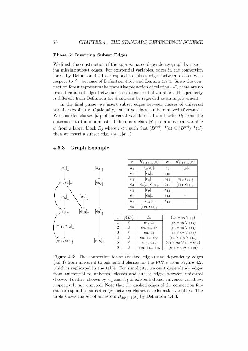
78 CHAPTER 4. THE STANDARD DEPENDENCY SCHEME
Phase 5: Inserting Subset Edges
We finish the construction of the approximated dependency graph by insert-ing missing subset edges. For existential variables, edges in the connectionforest by Definition 4.4.1 correspond to subset edges between classes withrespect to ≈↑ because of Definition 4.5.3 and Lemma 4.5.4. Since the con-nection forest represents the transitive reduction of relation ;∗, there are notransitive subset edges between classes of existential variables. This propertyis different from Definition 4.5.4 and can be regarded as an improvement.
In the final phase, we insert subset edges between classes of universalvariables explicitly. Optionally, transitive edges can be removed afterwards.We consider classes [a]↑ of universal variables a from blocks Bi from the
outermost to the innermost. If there is a class [a′]↑ of a universal variable
a′ from a larger block Bj where i < j such that (Dstd)−1(a) ⊆ (Dstd)−1(a′)then we insert a subset edge ([a]↑, [a
′]↑).
4.5.3 Graph Example
[a1]↓ [a2]↓
[e3, e4]↑ [e5]↑
[a6]↓ [a7]↓
[e8]↑ [e10]↑ [e9]↑
[a11, a12]↓
[e13, e14]↑ [e15]↑
x Hδ(x)+1(x) x Hδ(x)+1(x)
a1 [e3, e4]↑ e9 [e15]↑a2 [e5]↑ e10 –
e3 [e8]↑ a11 [e13, e14]↑e4 [e8]↑, [e10]↑ a12 [e13, e14]↑e5 [e9]↑ e13 –
a6 [e8]↑ e14 –
a7 [e10]↑ e15 –
e8 [e13, e14]↑
i q(Bi) Bi (a2 ∨ e5 ∨ e9)1 ∀ a1, a2 (e5 ∨ e9 ∨ e15)2 ∃ e3, e4, e5 (e3 ∨ e8 ∨ e13)3 ∀ a6, a7 (e4 ∨ a7 ∨ e10)4 ∃ e8, e9, e10 (e4 ∨ e13 ∨ e14)5 ∀ a11, a12 (a1 ∨ a6 ∨ e8 ∨ e14)6 ∃ e13, e14, e15 (a11 ∨ a12 ∨ e13)
Figure 4.3: The connection forest (dashed edges) and dependency edges(solid) from universal to existential classes for the PCNF from Figure 4.2,which is replicated in the table. For simplicity, we omit dependency edgesfrom existential to universal classes and subset edges between universalclasses. Further, classes by ≈↓ and ≈↑ of existential and universal variables,respectively, are omitted. Note that the dashed edges of the connection for-est correspond to subset edges between classes of existential variables. Thetable shows the set of ancestors Hδ(x)+1(x) by Definition 4.4.3.

4.6. EXPERIMENTAL RESULTS 79
Figure 4.3 shows part of the approximated graph for the PCNF fromFigure 4.2 as constructed by the algorithm described in the previous sec-tion. Dashed edges are part of the connection forest. Solid edges representdependencies of universal classes by equivalence relation ≈↓ according toDefinition 4.5.2. For example, we have a11 ≈↓ a12 because Hδ(a11)+1(a11) =Hδ(a12)+1(a12) = {[e13, e14]↑} as indicated in the table. Hence variablesa11 and a12 have the same set of dependencies and the single dependencyedge from [a11, a12]↓ to [e13, e14]↑ in the graph compactly represents the four
explicit dependencies (a11, e13), (a11, e14), (a12, e13) and (a12, e14) in Dstd.Further, we have e13 ≈↑ e14 by Definition 4.5.3, which is due to e13 ≈ e14
by Definition 4.3.3 and by clause (e4 ∨ e13 ∨ e14).In addition to classes, subset edges between existential variables in Fig-
ure 4.3 allow to reduce the number of explicit dependency edges. For ex-ample, the dependency (a2, e15) is represented implicitly by the dependencyedge from [a2]↓ to [e5]↑ and by the path from [e5]↑ to [e15]↑ given by dashedsubset edges.
We briefly sketch how to insert dependency edges from existential touniversal classes (not shown in Figure 4.3) as done in phase four of thealgorithm from the previous section. Recall that, for a universal variablea, [a]↓ equals [a]↑ by Definitions 4.5.2 and 4.5.3. We start at the universalclass [a11, a12]↓ and consider the existential class [e13, e14]↑, which is the onlyclass in the set Hδ(a11)+1(a11). Further, we consider predecessors of [e13, e14]↑in the connection forest, which are [e13, e14]↑, [e8]↑ and [e3, e4]↑. We have[e13, e14]↑ ∈ Hδ(e8)+1(e8) for predecessor [e13, e14]↑ and [e8]↑ ∈ Hδ(e3)+1(e3)and [e8]↑ ∈ Hδ(e4)+1(e4) for predecessor [e8]↑. Therefore, we add dependencyedges ([e8]↓, [a11, a12]↑), ([e3]↓, [a11, a12]↑) and ([e4]↓, [a11, a12]↑).
For example, note that e3 6≈↓ e4 by Definition 4.5.2 since Hδ(e3)+1(e3) 6=Hδ(e4)+1(e4). Hence a7 ∈ Dstd(e4) but a7 6∈ Dstd(e3).
4.6 Experimental Results
We implemented a variant of the algorithm presented in Section 4.5.2 inan experimental tool called qdag.2 The tool constructs the approximatedgraph G≈,⊆(Dstd) similar to Definition 4.5.4 for a given PCNF ψ. An effi-cient union-find data structure [126] is used to represent equivalence classes.However, the tool is actually subsumed by an implementation of approx-imated dependency graphs which is part of the search-based QBF solverDepQBF described in Chapter 5.
In this section, we report experimental results with respect to qdagwhich were already published in [82]. Different from the algorithm fromSection 4.5.2, the first two phases were merged in the implementation ofqdag. Thus one of the passes over the set of clauses of PCNF ψ can be
2A binary and log-files of experiments are available from http://fmv.jku.at/qdag/.

80 CHAPTER 4. THE STANDARD DEPENDENCY SCHEME
2005 2006 2007 2008
Size 211 216 1136 3328
Explicit Search for X-Paths
Total Time 19527.3 132.04 101424 173349
Max. Time 900 (15) 8.67 900 (83) 900 (135)
Avg. Time 92.54 0.61 89.28 52.12
Graph-Based Computation
Total Time 7.94 1.35 227.05 300.31
Max. Time 0.58 0.03 7.96 8.11
Avg. Time 0.04 0.01 0.2 0.09
x ∈ V∀Max. |Dstd(x)| 256535 9993 2177280 2177280Avg. |Dstd(x)| 82055.87 4794.60 33447.6 19807
Max. |Hi(x)| 256 1 518 518Avg. |Hi(x)| 3.26 0.98 2.02 1.14
Max. |H∗i (x)| 797 5 797 1872Avg. |H∗i (x)| 19.51 1.12 39.06 8.24
Avg.|{[y]↑|y∈Dstd(x)}||{y|y∈Dstd(x)}| 3.44% 0.04% 6.42% 1.21%
Classes per Variables 28.2% 10.23% 40.31% 21.29%
x ∈ V∃Max. |Dstd(x)| 5040 440 5040 22696Avg. |Dstd(x)| 12.76 2.98 3.24 4
Max. |Hi(x)| 24 7 490 490Avg. |Hi(x)| 0.14 0.13 0.17 0.13
Max. |H∗i (x)| 797 7 797 1872Avg. |H∗i (x)| 5.16 0.16 1.32 1.31
Avg.|{[y]↑|y∈Dstd(x)}||{y|y∈Dstd(x)}| 2.37% 0.4% 2.76% 2.09%
Classes per Variables 10.96% 4.99% 11.45% 7.11%
Table 4.1: Computing the standard dependency scheme Dstd on structuredinstances from QBF evaluations 2005 to 2008 [56]. We compare explicitsearch for X-paths to our algorithm which constructs a variant of the ap-proximated, augmented and compressed dependency graph G≈,⊆(Dstd).
4.6. EXPERIMENTAL RESULTS 81
avoided. The remaining phases consider equivalence classes rather than in-dividual variables. Depending on the size of the classes, we expect that theeffort spend on that phases can be kept low in practice. In our implemen-tation of qdag, we also skip phase five where subset edges between classesof universal variables are inserted. This information is not relevant as weare only interested in the sets of dependencies by Dstd in the experimentsreported here. Further, the partition with respect to ≈↓ for existential vari-ables is not computed in phase three. This was included in a later version ofDepQBF. For the experimental analysis, we considered structured instances(called “fixed class”) from QBF evaluations 2005 to 2008 [56]. We did notinclude random instances. Experiments were run on 64-bit Ubuntu Linux8.04, Intel R© Q6700 at 2.66 GHz and 8 GB of memory.
Table 4.1 shows experimental results. For all formulae in the benchmarksets a variant of the approximated dependency graph G≈,⊆(Dstd) was con-structed using the tool qdag as described above. The first line in Table 4.1shows the numbers of formulae per benchmark set.
First, we compare the effort of computing Dstd by explicit search forX-paths by Definition 3.4.17 on page 49 and by construction of G≈,⊆(Dstd).The former approach was pointed out in Example 4.1.1 on page 57 and isalso implemented in qdag.
We report the total run time, the maximum over all formulae and theaverage per formula in seconds for the two approaches in the table. It can beseen that explicit search is significantly worse. In contrast to the graph-basedapproach, explicit search times out on several formulae, where we used a timelimit of 900 seconds. The number of timeouts is given in parentheses in row“Max. Time”. Further, the average time spent by the graph-based approachis negligible in practice. Consequently, when computing G≈,⊆(Dstd) to beused in combination with a QBF solver, we expect almost no overhead withrespect to run time. Combinations of dependency graphs with search-basedQBF solvers are the topic of Chapter 5.
Next, we measure the quality of G≈,⊆(Dstd) in terms of compactnesswith respect to partitions V/≈↓ and V/≈↑ . We relate the number of depen-dencies of a variable to the sizes of the equivalence classes which representthat dependencies in the graph. This way, the effectiveness of the graph-based approach can be evaluated. Statistics are divided into two sectionsfor existential and universal variables, respectively. Maximum and averagenumbers of dependencies by Dstd over all variables are shown.
Compactness of the graph is indicated several times. For x ∈ V∀, theset H∗i (x) of descendants for i = δ(x) + 1 in the connection forest efficientlyrepresents Dstd(x). These classes are reachable from ancestors in Hi(x).When comparing the numbers |Hi(x)|, |H∗i (x)| and |Dstd(x)|, it becomesapparent that G≈,⊆(Dstd) is compact. For example, on the benchmark setfrom 2008, universal variables have 19807 dependencies on average but thisinformation is stored in G≈,⊆(Dstd) using only 8.24 descendants on average.
82 CHAPTER 4. THE STANDARD DEPENDENCY SCHEME
Recall that the connection forest is computed only once an thus sharedbetween all the variables in a PCNF. Descendants H∗i (x) are not storedexplicitly for each variable. The data reported for |H∗i (x)| in the tablewas obtained by traversing the connection forest starting from ancestorsHi(x). The small values of |H∗i (x)| for universal variables x show that manyexistential variables occur in the same equivalence class by partition V/≈↑ .
For existential variables x ∈ V∃, |Hi(x)| and |H∗i (x)| measure the effortfor inserting dependency edges in phase four since Hi(x) and H∗i (x) have tobe checked explicitly. Note that in these experiments we did not computethe partition V/≈↓ for existential variables with respect to sets |Hi(x)| byDefinitions 4.5.2. Making use of classes with respect to V/≈↓ rather thanindividual variables as we did in Section 4.5.2 could further improve thecomputation of dependency edges.
Finally, we evaluate the size of equivalence classes in partition V/≈↑ .Recall that for universal variables V/≈↑ is equal to V/≈↓ . For existentialvariables, we did not construct V/≈↓ as noted above. Given a variable x,
we computed the number |{y | Dstd(x)}| of dependencies and the number|{[y]↑ | y ∈ Dstd(x)}| of classes of depending variables by ≈↑. The averagefraction of these numbers is shown in the table. The worst-case is 100%,where each depending variable occurs in a singleton class with respect to≈↑. This is clearly not the case. The partition V/≈↑ compactly representsthe sets of dependencies. Line “Classes per Variables” shows the averagenumber of classes per variable with respect to partition V/≈↑ in each formula.Again, values are far below 100%, hence many variables can be regarded asequivalent by ≈↑.
4.7 Summary
The standard dependency scheme Dstd can be computed in polynomial timeby direct applications of Definition 3.4.17. However, explicitly searching forconnections between variables can be infeasible on large formulae.
As an alternative, we considered graph representations for arbitrary de-pendency schemes. In explicit dependency graphs, edges correspond exactlyto dependencies of the form (x, y) in a given dependency scheme D. Weintroduced equivalence relations over the set of variables (or vertices) basedon dependency information by D. Thereby, we obtained graphs over classesof variables which are potentially more compact than explicit graphs. Fi-nally, we suggested augmented, compressed dependency graphs to representarbitrary dependency schemes. These graphs contain auxiliary edges whichare useful for practical applications, as pointed out in the following chapter.
As an example for our graph-based representations, we presented analgorithm to compute an approximation of the augmented, compressed de-pendency graph for Dstd. The approximation is precise with respect to
4.7. SUMMARY 83
dependencies by Dstd but might achieve less compaction than the exactgraph. We observed that X-paths by Definition 3.4.15 on page 48 oftenconnect multiple variables. Hence it is not necessary to compute that infor-mation from scratch for each pair (x, y) of variables to check if (x, y) ∈ Dstd.Instead, given a PCNF ψ, we first determine all connections between exis-tential variables which are relevant for X-paths in terms of the connectionforest of ψ. The connection forest is used to complete the construction ofthe graph by inserting missing dependency and auxiliary edges.
Although our presented algorithm construct only an approximation ofthe augmented, compressed dependency graph for Dstd, experimental re-sults on benchmarks from QBF evaluations show that the approximation iscompact and that is can be computed efficiently in practice.

84 CHAPTER 4. THE STANDARD DEPENDENCY SCHEME
Chapter 5
QDPLL and DependencySchemes
5.1 Introduction
In Chapter 3 we argued that the linear quantifier prefix of QBFs in PCNFmight be a severe drawback for QBF solvers. The quantifier prefix naturallyinduces a linear ordering on the variables. This ordering restricts the set ofpossible assignment a search-based QBF solver can consider, for example.As pointed out in Example 3.3.6 on page 34, there might be an exponentialgap between the run time of solvers relying on the quantifier prefix andsolvers which carry out a more sophisticated dependency analysis.
In order to alleviate the limitations of quantifier prefixes, we introduceddependency schemes as a framework for dependency analysis in PCNFs inSection 3.4. Due to Proposition 3.4.5 on page 51, the linear quantifier prefixof PCNFs constitutes the worst of all dependency schemes. In contrast toquantifier prefixes, the use of dependency schemes in general allows a QBFsolver to profit from additional freedom to assign variables. This way, thepolicy of assigning variables strictly from “left to right” in prefix orderingcan be overcome.
In this chapter, we combine dependency schemes with search-based QBFsolvers relying on QDPLL, which we briefly introduced in Section 2.3.1. Thegoal is to enable QBF solvers to profit from dependency information which ismore refined than what can be obtained from quantifier prefixes. Althoughwe focus on PCNF and search-based QBF solving by QDPLL, our approachis relevant for non-PCNF formulae and variable elimination as well. It turnsout that the combination of dependency schemes and QDPLL does notrequire to change the overall structure of the algorithm.
Throughout QBF literature, QDPLL has been described based on thelinear quantifier prefix. Since the prefix gives rise to the trivial depen-dency scheme by Definition 3.4.13, we can regard the original QDPLL al-
85
86 CHAPTER 5. QDPLL AND DEPENDENCY SCHEMES
gorithm [30] to be combined with that particular dependency scheme. Wegeneralize that combination of QDPLL and the prefix-based trivial depen-dency scheme to arbitrary dependency schemes.
Apart from theoretical aspects of dependency schemes and QDPLL, weare interested in efficient practical applications. It is crucial to check fordependencies between variables within certain parts of QDPLL such as deci-sion making or clause learning. In order to carry out such checks efficiently,we apply compact dependency graphs which we introduced in Section 4.2.These graphs are general and not limited to representations of particulardependency schemes.
We provide an experimental evaluation of QDPLL with dependencyschemes. Our QDPLL-based QBF solver DepQBF [84] integrates depen-dency schemes as compact dependency graphs. We analyze the costs ofmoving from simple dependency information like linear quantifier prefixesof PCNFs or quantifier trees to more general dependency schemes. The re-sults of this analysis give insights into practical applicability. Further, weevaluate the dynamic effects on QDPLL when combined with various depen-dency schemes. For that purpose, we implemented a common frameworkfor compact dependency graphs in DepQBF. In addition to the standarddependency scheme Dstd, this framework is able to represent the trivialdependency scheme Dtriv arising from linear quantifier prefixes and Dtree
given by quantifier trees as well. We compare the effects of Dtriv, Dtree
and Dstd on the performance of QDPLL. Our experiments indicate that,despite increased overhead, the combination of QDPLL with Dstd outper-forms QDPLL relying on Dtriv and Dtree. These results motivate the use ofgeneral dependency schemes in QDPLL.
The combination of QDPLL with dependency schemes is closely relatedto an approach which aims at exploiting tree-based quantifier structurewithin QDPLL [62]. However, our work generalizes observations made in[62] from quantifier trees to arbitrary dependency schemes.
In addition to combinations of QDPLL with dependency schemes, an-other contribution of this chapter is a description of clause and cube learn-ing, also called constraint learning. From the theoretical point of view,learning methods for QDPLL were presented independently in related work[58, 78, 133, 134]. From a high level perspective, QDPLL with constraintlearning resembles the well-known and widely applied DPLL algorithm forpropositional logic (SAT). Implementations of DPLL are available in popularopen source SAT solvers like MiniSAT [42] or PicoSAT [18]. However, im-plementations of clause learning for SAT cannot directly be ported to QBF.Therefore, we aim at providing an integrated view of constraint learning asimplemented in our QDPLL-based, open source solver DepQBF.
We give an overview of QDPLL with constraint learning in Section 5.2.Starting with boolean constraint propagation for QBF (QBCP) in Section 5.3,we point out how to profit from dependency schemes within QDPLL. Appli-
5.2. QDPLL WITH CONSTRAINT LEARNING 87
cations of QBCP infer additional assignments from given ones, which reducesthe need for explicit branching during the search process. As noted above,the freedom for branching, also called decision making, in QDPLL is limitedby the linear ordering of the quantifier prefix. In order to overcome theselimitations, we apply arbitrary dependency schemes for decision making inSection 5.4. We describe constraint learning in Section 5.6 and concludewith experimental results in Section 5.7.
5.2 QDPLL with Constraint Learning
In the following sections, we informally describe QDPLL with conflict-directed clause and solution-directed cube learning, called constraint learn-ing, based on the presentation in [134]. Learning methods for QBF werepublished independently in [58, 78, 133, 134]. We consider the details ofconstraint learning in Section 5.6 below. For a description of DPLL withclause learning for SAT, we refer to [36, 117], for example.
5.2.1 Basics
From a very simplistic point of view, QDPLL with constraint learning suc-cessively generates (partial) assignments of the variables in a given PCNFψ. These assignments correspond to paths in an assignment tree as definedin Section 2.2.1 which is implicitly constructed. The algorithm terminatesif either a satisfying assignment tree was found or if it was proved that nosuch assignment tree exists. Note that assignment trees are never explicitlyrepresented in QDPLL. Instead, only the paths in such trees are enumeratedby means of assignments to variables. Although QDPLL is often presentedas a recursive algorithm, it is typically implemented iteratively.
The ordering in which variables are assigned must follow the structureof dependencies in the PCNF. This corresponds to the requirement statedin Definition 2.2.3 that assignments along paths in assignment trees mustbe ordered. Information on dependencies can be drawn from the quantifierprefix or, as we point out later in this chapter, from more sophisticateddependency schemes computed for the PCNF. Informally, QDPLL checksthe truth value of ψ under the current assignment A, that is ψ[A]. If thetruth value can not yet be determined, then A is extended with furtherassignments. Otherwise, assignment A is analyzed to find out which parts ofit were responsible for the resulting truth value. Depending on the outcomeof that analysis, a learnt clause or learnt cube is constructed and added to ψ.
Definition 5.2.1. A cube is a conjunction Ci := (l1 ∧ . . .∧ lki) over literals.The empty cube is an empty conjunction and is denoted by ∅.
Similar to clauses, we assume that a cube neither contains multiple norcomplementary literals of a variable, nor truth constants > and ⊥.

88 CHAPTER 5. QDPLL AND DEPENDENCY SCHEMES
Definition 5.2.2. A constraint is either a clause or a cube.
After a learnt constraint has been added to ψ, QDPLL retracts certainassignments in A in order to continue the search in a different search space.Thus another path of the assignment tree is entered. Informally, the purposeof constraint learning is to prevent the generation of assignments which donot contribute to overall progress of the search. Further, QDPLL withconstraint learning can produce a proof which allows to verify its resultusing independent proof checkers. We briefly address proofs in Section 5.2.4below. We may think of QDPLL with constraint learning like presented inthis chapter as an algorithm which guides the search for a proof by successivegeneration of assignments. For DPLL-based solvers with clause learning,such view was suggested in [70], for example.
QDPLL with constraint learning does not directly operate on a givenPCNF ψ := Q1B1 . . . QnBn. φ but on a formula with specific structure. Theidea is to extend the CNF-part φ of ψ in order to represent learnt clausesand learnt cubes in addition to original clauses.
Definition 5.2.3 ([134]). Given a PCNF
ψ := Q1B1 . . . QnBn. φ
with CNF-part φ. Let φOCL := φ. The QBF
ψ′ := Q1B1 . . . QnBn. (φOCL ∧ φLCL) ∨ φLCU
is represented as augmented CNF (ACNF), where φOCL and φLCL are con-junctions over original and learnt clauses, respectively, and φLCU is a dis-junction over learnt cubes.
Alternatively, a formula in ACNF is called extended QBF [58]. Given aPCNF ψ, the ACNF ψ′ by Definition 5.2.3 is satisfiable if and only if ψ issatisfiable. This is due to properties of learnt clauses and learnt cubes whichare generated by Q-resolution. In Section 5.6 below, we address Q-resolutionand the construction of learnt constraints. The semantics of PCNFs basedon assignment trees from Section 2.2.1 can be extended to ACNFs. InDefinition 2.2.4 on page 13, assignments along paths in satisfying assignmenttrees must satisfy all the clauses of a PCNF. Additionally, an ACNF issatisfied if at least one cube is satisfied under the assignment along a path.
During the search, learnt clauses and cubes are added to φLCL and φLCU ,respectively. Initially, subformulae φLCL and φLCU are empty. Differentfrom the approach in [134], we do not consider to learn constraints contain-ing complementary literals (called long-distance resolution). Instead, ourdescription of the learning procedure is based on [61]. We consider con-straint learning in detail in Section 5.6 below.

5.2. QDPLL WITH CONSTRAINT LEARNING 89
State qdpll ()
while (true)
State s = qbcp ();
if (s == UNDET)
// Make decision.
v = select_dec_var ();
assign_dec_var (v);
else
// Conflict or solution.
// s == UNSAT or s == SAT.
btlevel = analyze_leaf (s);
if (btlevel == INVALID)
return s;
else
backtrack (btlevel);
DecLevel analyze_leaf (State s)
R = get_initial_constraint (s);
// s == UNSAT: ’R’ is empty clause.
// s == SAT: ’R’ is sat. cube...
// ..or new cube from assignment.
while (!stop_res (R))
p = get_pivot (R);
R’ = get_antecedent (p);
R = constraint_res (R, p, R’);
add_to_formula (R);
return get_asserting_level (R);
Figure 5.1: Pseudo-code of QDPLL with conflict-directed clause andsolution-directed cube learning [58, 78, 134]. Code blocks are indicatedby indentation level.
5.2.2 Generation of Assignments
Figure 5.1 shows a high-level pseudo-code of QDPLL with constraint learn-ing. The algorithm consists of two major parts. Function qdpll successivelygenerates assignments as described above and checks the truth value of thegiven ACNF ψ to be evaluated. Constraint learning is performed in functionanalyze leaf.
An important approach is the propagation of implications, which is car-ried out in function qbcp. Given an ACNF ψ and an assignment A, animplication is an additional assignment to a variable which is not yet part ofA and which can be inferred from the formula ψ[A]. Thus QDPLL considersthe formula ψ[A] under the current assignment A each time A was modi-fied. Propagation is the iterative inference of implications. This process inQDPLL is called quantified boolean constraint propagation (QBCP). We ex-plicitly distinguish QBCP from boolean constraint propagation (BCP) whichis commonly applied in SAT solvers because QBCP and BCP typically relyon different inference rules. In Section 5.3 below, we consider common QBF-specific inference rules implemented in qbcp. QDPLL is complete withoutthe rules in QBCP, that is it always terminates even if no implications areinferred. However, in general QBCP is able to improve the performanceof QDPLL. Apart from propagating implications, qbcp evaluates the truthvalue of ψ under the current assignment A.
Definition 5.2.4. Given an ACNF ψ and an assignment A, the formulaψ[A] is obtained similarly as defined in Section 2.2.1 by substituting truthconstants for literals of assigned variables and performing simplifications.Additionally, empty constraints are handled as follows. If there is a clause

90 CHAPTER 5. QDPLL AND DEPENDENCY SCHEMES
C ∈ ψ[A] such that C[A] = ∅ then C is replaced by ⊥ in ψ[A]. If there is acube C ∈ ψ[A] such that C[A] = ∅ then C is replaced by > in ψ[A]. All truthconstants that were introduced this way are eliminated subsequently in ψ[A].
Definition 5.2.5. Given an ACNF ψ and a (partial) assignment A, thestate of ψ under A is defined as follows. If ψ[A] = ⊥ then A is a conflictingassignment, also called a conflict, and ψ is falsified under A. If ψ[A] = >then A is a satisfying assignment, also called a solution, and ψ is satisfiedunder A. If A is neither conflicting nor satisfying then A is an inconclusiveassignment and ψ is undetermined under A. We may drop “. . . under A”from definitions if assignment A is clear from the context.
Definition 5.2.5 is based on the current assignment only and ignores theQBF-specific rule of constraint reduction to be introduced in Section 5.3.Given an assignment, constraint reduction allows to ignore certain literals ofuniversal variables in clauses and existential variables in cubes. This way, itmight be be found out earlier than by Definition 5.2.5 that some assignmentA cannot be part of a PCNF-model of ψ (see also Definition 5.3.7 below).
Function qbcp in Figure 5.1 propagates implications until saturationand checks the truth value of the ACNF under the current assignment A.If A is neither conflicting nor satisfying (s == UNDET) then some variablex is assigned as the next decision in function select dec var. This pro-cess is called decision making or branching. Different from decision makingin DPLL for SAT, the choice of variables for decisions is not arbitrary inQDPLL. With respect to the current assignment A, a variable x can beassigned as decision only if all variables where x depends on are assigned inA already. For example, when relying on the quantifier prefix, then x canbe assigned as decision only if all variables which are differently quantifiedto the left of x are assigned. This policy corresponds to decision making inclassical descriptions of QDPLL like [31, 57]. In Section 5.4 below, we con-sider decision making by means of arbitrary dependency schemes which arerepresented by compact dependency graphs. Note that assignments madeas implications by inference rules during QBCP do not have to respect de-pendencies.
Decision Levels and Trail Levels
Decisions are numbered ascendingly by decision levels, starting at decisionlevel one. Once a variable x with decision level dl(x) has been selectedby select dec var, the value to be assigned is typically chosen accordingto certain heuristics in assign dec var. Given the current assignment A,assigning x to true or false produces a new, extended assignment A′ := A∪{x} or A′ := A∪ {¬x}, respectively. All implications y that can be inferredfrom the current assignment A′ are propagated in turn by qbcp, where

5.2. QDPLL WITH CONSTRAINT LEARNING 91
dl(y) := dl(x). Hence, implications get the same decision level as the mostrecent decision or decision level zero if no decision has been made before.
In addition to decision levels, every single assignment of a variable, re-gardless of whether it was made as a decision or implication, is numberedchronologically starting from zero in the order of assignments made. Thisnumbering is called the trail level tl(x) of an assigned variable x. Differentfrom decision levels, the trail level of every assigned variable is unique. Weregard assignments A := {l0, l1, . . . , lm−1} to be sorted chronologically bytrail levels, where i is the trail level of assignment li ∈ A. Trail levels arerelated to the following property of assignments generated by QDPLL.
Definition 5.2.6. Given an assignment A := {l0, l1, . . . , lm−1} sorted as-cendingly by trail levels 0 to m − 1 and a dependency scheme D. Assign-ment A is admissible with respect to D if and only if, for every assignmentli ∈ A made as decision, the following holds: given the set V<i := {x | x =v(lj), lj ∈ A, j < i} of variables which were assigned before li in A, everyvariable where the decision variable v(li) depends on by D must have beenassigned before v(li) in A, that is D−1(v(li)) ⊆ V<i.
Note that assignments generated in QDPLL as shown in Figure 5.1 arealways admissible by Definition 5.2.6 with respect to the dependency schemeD that was used throughout all parts of QDPLL. This property also appliesto classical descriptions of QDPLL where decisions have to be made de-pending on the quantifier prefix, as pointed out above. Actually, admissibleassignments in classical QDPLL can be described by setting D := Dtriv inDefinition 5.2.6. This way, QDPLL implicitly constructs assignment treeswhich correspond exactly to the original Definition 2.2.1 on page 11.
Further, admissible assignments are closely related to relaxed orderingsof paths in PCNF-models by Proposition 3.4.1 on page 46. Given a depen-dency scheme D, the assignments along every path in a PCNF-model of aformula must respect dependencies in D. If two variables are independentthen they can be assigned as decisions in arbitrary relative order along thepaths, which increases the freedom for decision making. We consider thegeneration of admissible assignments in the context of arbitrary dependencyschemes by QBCP and decision making in Sections 5.3 and 5.4.
5.2.3 Constraint Learning
Decision making as described above extends the current assignment A if A isneither conflicting nor satisfying. Otherwise, the ACNF ψ is either satisfiedor falsified under A. This situation corresponds to a leaf in the assignmenttree implicitly constructed by QDPLL. The current state of ψ under A iscaused by at least one clause or cube in ψ.
Definition 5.2.7. Given an ACNF ψ, let C ∈ ψ be a clause or cube and Abe a (partial) assignment. The state of C under A is defined as follows. If

92 CHAPTER 5. QDPLL AND DEPENDENCY SCHEMES
C[A] = ⊥ then C is falsified under A. If C[A] = > then C is satisfied underA. Otherwise, if C is neither falsified nor satisfied, then C is undeterminedunder A. We may drop “. . . under A” from definitions if assignment A isclear from the context.
With respect to Definition 5.2.5, falsified clauses and satisfied cubes arerelated to satisfying and falsifying assignments, respectively. This relationis due to the structure of ACNFs by Definition 5.2.3. Similar to Defini-tion 5.2.5, the effects of constraint reduction are ignored in Definition 5.2.7.We present an adapted variant in Section 5.3.4 below.
Proposition 5.2.1 ([134]). Given an ACNF ψ and a (partial) assignmentA. There is a clause C ∈ ψ such that C is falsified under A if and only ifA is conflicting. If there is a cube C ∈ ψ such that C is satisfied under Athen A is satisfying.
Note that it is not possible to have a falsified clause and a satisfied cubeunder the same assignment in an ACNF. This is due to the way how learntconstraints are generated as described in Section 5.6.1.
Given an assignment A which is conflicting or satisfying, certain as-signments to variables in A have to be retracted in order to continue thesearch in a different search space. The process of retracting assignments iscalled backtracking. The notion of “backtracking” is often associated witha chronological way of retracting assignments: the truth value of the mostrecently assigned decision variable x is flipped and implications with traillevels larger than the one of x are retracted.
Different from that, in modern implementations of QDPLL and DPLLwith learning, like in Figure 5.1, in general assignments are retracted non-chronologically. That is, depending on the learning procedure, the effectsof assignments that have been made earlier than the most recent decisioncould be undone. This policy is called non-chronological backtracking orbackjumping, see also [36, 59, 117], for example. For simplicity, we use“backtracking” to denote the non-chronological variant.
Further, in contrast to the classical notion of backtracking, the truthvalues of decision variables are not explicitly flipped if the learning proce-dure always generates asserting clauses and cubes. Modern SAT and QBFsolvers relying on (Q)DPLL like [18, 42, 54, 84, 93] only generate assertingclauses. Informally, a learnt constraint C is asserting if QBCP is able to inferan implication from C after backtracking to a certain decision level calledasserting level. We refer to [36, 118, 132], for example, for further detailsrelated to the generation of asserting clauses in SAT solvers. In Section 5.6below, we focus on the generation of asserting constraints in QDPLL.
Learnt constraints are generated in function analyze leaf in Figure 5.1.The idea is to apply Q-resolution to derive new learnt constraints, called re-solvents, with respect to the current conflicting or satisfying assignment. Q-

5.2. QDPLL WITH CONSTRAINT LEARNING 93
resolution is the QBF-specific variant of the resolution operation for propo-sitional logic. Resolution is also the core of clause learning in SAT solvers.In addition to clauses, cubes are learnt in QDPLL based on term resolutionsteps [61] involving cubes which have been learnt previously. Term resolutionfor cubes can be regarded to be dual to Q-resolution for clauses. For simplic-ity, we use “Q-resolution” to denote either Q-resolution over clauses or termresolution over cubes. We introduce Q-resolution formally in Section 5.6below. According to our experimental results in Section 5.7, Q-resolutionis able to generate shorter learnt constraints in the context of the standarddependency scheme Dstd compared to the prefix ordering of PCNFs.
Learning from Conflicts
If the current assignment A is conflicting (s == UNSAT) then the ACNFcontains at least one falsified clause. Function get initial constraint
returns a reference to one such clause R which is called initial constraint.Given the initial constraint, new clauses are constructed using Q-resolution.In function constraint res, clause R is resolved with the antecedent clauseR′ of an existential variable p which occurs in R and which was assignedas an implication in the current assignment A (see also Section 5.3.2 be-low). Variable p is the pivot of the current Q-resolution step and functionget antecedent returns its antecedent clause. The selection of pivots fromthe current constraint R by function get pivot is not arbitrary. It de-pends on the current assignment. Care has to be taken in order to avoidthe generation of constraints which contain complementary literals. We ad-dress the details of pivot selection in Section 5.6.1. Function stop res stopsthe resolution process if the current clause R is asserting. The generatedclause R is added to the set φLCL of learnt clauses in the ACNF. Func-tion get asserting level computes the asserting level d such that, afterbacktracking to d, QBCP can infer a new implication from R.
Learning from Solutions
If the current assignment A is satisfying (s == SAT) then either the ACNFcontains at least one satisfied learnt cube or all clauses in the ACNF aresatisfied. The idea is to produce a learnt cube by Q-resolution starting froman initial constraint. If there is a satisfied learnt cube R in the ACNF thenR is the initial constraint. Otherwise, an initial constraint is computed byselecting a subset A′ ⊆ A of the assignment A such that A′ is satisfying.
Definition 5.2.8 ([134]). Given an ACNF ψ := Q1B1 . . . QnBn. (φOCL ∧φLCL)∨ φLCU and a (partial) assignment A as generated by QDPLL like inFigure 5.1. A cover set A′ ⊆ A is a subset of A such that A′ ∩Ci 6= ∅ for alloriginal clauses Ci ∈ φOCL.
94 CHAPTER 5. QDPLL AND DEPENDENCY SCHEMES
A cover set A′ satisfies at least one literal in each original clause. Dueto properties of ACNFs, it is not necessary to consider learnt constraints inDefinition 5.2.8 to make A′ satisfying. Note that there might be multiplecover sets for a given assignment A and set of original clauses.
The cover set A′ constitutes the initial constraint R. Apart from obtain-ing initial constraints, learnt cubes are generated dually to learnt clauses.Q-resolution is applied to antecedent cubes of universal pivot variables. Theprocess stops if the current cube R is asserting and R is added to the setφLCU of learnt cubes in the ACNF. Finally, the asserting level is computedand returned to algorithm qdpll.
After backtracking to the asserting level d and unassigning all variableswith decision levels larger than d in function backtrack, QBCP is carriedout again. A new implication is inferred by qbcp from the previously gen-erated learnt constraint, possibly in addition to further implications.
5.2.4 Q-Resolution Proofs
Algorithm qdpll in Figure 5.1 terminates (btlevel == INVALID) if andonly if Q-resolution produces an empty clause or an empty cube in functionanalyze leaf. In this case, the learning procedure of QDPLL completed aQ-resolution proof of unsatisfiability or satisfiability of the given ACNF.
Definition 5.2.9 (terminology adapted from Section 2.3 of [9]). Given anACNF ψ := Q1B1 . . . QnBn. (φOCL ∧ φLCL) ∨ φLCU . The sequence P :=(C1, C2, . . . , Cm) of clauses is a Q-resolution proof of unsatisfiability of ψ ifCm = ∅ and Ci ∈ (φOCL∪φLCL) for all Ci ∈ P such that if Ci ∈ φLCL then Cican be derived by Q-resolution from two clauses Cj , Ck ∈ P where j, k < i.
Definition 5.2.10 (terminology adapted from Section 2.3 of [9]). Givenan ACNF ψ := Q1B1 . . . QnBn. (φOCL ∧ φLCL) ∨ φLCU . The sequence P :=(C1, C2, . . . , Cm) of cubes is a Q-resolution proof of satisfiability of ψ if Cm =∅ and Ci ∈ φLCU for all Ci ∈ P such that Ci is either a cover set or Ci canbe derived by Q-resolution from two cubes Cj , Ck ∈ P where j, k < i.
For simplicity, we write “proof” if the result of QDPLL is clear from thecontext. Note that in proofs P by Definitions 5.2.9 and 5.2.10 we do notassume any particular order for the generation of the constraints. That is,for Ci ∈ P and Cj ∈ P where i < j, the learning procedure of QDPLL as inFigure 5.1 might have derived Cj before Ci.
Proposition 5.2.2. Given an ACNF ψ. If QDPLL with constraint learningas shown in Figure 5.1 derives the empty constraint then there is a proof byDefinitions 5.2.9 or 5.2.10, respectively.
After termination of QDPLL with constraint learning, a proof P for anACNF by Proposition 5.2.2 can trivially be obtained from the sets of clauses

5.2. QDPLL WITH CONSTRAINT LEARNING 95
or cubes, respectively: let P := φOCL ∪ φLCL for unsatisfiable ACNFs orP := φLCU for satisfiable ones. However, not all constraints in φOCL ∪φLCL
or φLCU might be necessary to derive the empty constraint.Proposition 5.2.2 asserts the correctness of QDPLL with learning based
on the correctness of Q-resolution [27, 61, 134]. The other direction, whichamounts to completeness, also holds. If a PCNF is (un)satisfiable thenQDPLL with learning will derive the empty constraint.
A comprehensive treatment of work related to proofs for QBFs is outof scope of this work. An overview of the topic is given in [94]. Proofs byDefinitions 5.2.9 and 5.2.10 allow to verify the result of QDPLL based onthe underlying proof system of Q-resolution. For example, if a formula isunsatisfiable and QDPLL returns a proof P then it can be checked whetherthe empty clause indeed can be derived from the clauses in P . This ap-proach was considered in [130] and in a variant of the QuBE solver [94].However, the proof P does not contain information on concrete values thathave to be chosen for universal variables of a PCNF in order to explain un-satisfiability with respect to assignment trees. Dually, values for existentialvariables in satisfiable PCNFs explain satisfiability. Representations of val-ues for variables are called certificates. As an alternative to merely checkingQ-resolution proofs, Skolem functions [121] were suggested to represent cer-tificates of a formula [11, 74]. A uniform approach combining Q-resolutionproofs and certificates allows to construct a certificate for a PCNF from agiven Q-resolution proof of (un)satisfiability [8]. This approach was imple-mented and evaluated using our QDPLL-based solver DepQBF [95, 105].
In addition to QDPLL with learning as shown in Figure 5.1, we im-plemented optimizations in our QBF solver DepQBF [84] presented in Sec-tion 5.6.2. These approaches are inspired by modern SAT solvers. For exam-ple, learnt constraints are heuristically deleted to speed up QBCP. Instead ofbacktracking to the asserting level, the solver periodically retracts all assign-ments made so far and thus restarts the search process. Our experimentalanalysis in Section 5.7 demonstrates the potential of these optimizations.
At the beginning of this chapter, we argued that QDPLL with constraintlearning could profit from dependency schemes which refine the trivial de-pendency scheme given by the quantifier prefix. However, when consideringFigure 5.1, dependency information is not explicitly used, although it iscrucial to respect dependencies within QDPLL as pointed out.
In the following sections, we take a closer look on the core parts such asQBCP, decision making and constraint learning. We point out how theseparts can profit from more refined dependency information than quantifierprefixes. Thereby, we obtain a generalization of QDPLL with constraintlearning to arbitrary dependency schemes. The overall picture of the algo-rithm does not change. We consider a dependency scheme as an additionalparameter passed to QDPLL. Compact dependency graphs from the previ-ous chapter allow for efficient applications of the generalization of QDPLL.

96 CHAPTER 5. QDPLL AND DEPENDENCY SCHEMES
5.3 QBCP
In this section, we focus on the details of quantified boolean constraint propa-gation (QBCP) which is carried out in function qbcp in Figure 5.1. Given anACNF and an assignment A, the purpose of QBCP is to infer implications,that is additional assignments not yet being part of A by certain inferencerules. This way, the number of decisions can be reduced which in turn mightincrease the performance of QDPLL. We report on the results of a relatedexperiment in Section 5.7.
We introduce universal and existential reduction, also called constraintreduction, and rules for the detection of unit literals and pure literals. Thisset of rules is standard in QBF literature and it is part of QBCP in mostQDPLL-based solvers [30, 52, 54, 60, 84]. In state-of-the-art SAT solvers,typically only unit literal detection is carried out in boolean constraint prop-agation (BCP). Apart from a variant based on tree-like dependency structure[62], usually QBCP is defined with respect to the linear ordering of quanti-fier prefixes, that is the trivial dependency scheme Dtriv. We point out howto generalize the rules applied in QBCP from quantifier prefixes to arbitrarydependency schemes. Experimental results presented in Section 5.7 showthat QBCP based on dependency schemes which refine Dtriv infers moreimplications than classical variants based on Dtriv.
In the following, we assume that we are given the ACNF ψ for a PCNFto be solved by QDPLL with constraint learning like in Figure 5.1. Further,we consider ψ[A] at an arbitrary point of time during the solving processwith respect to the current assignment A. That is, learnt constraints mighthave been added to the ACNF. Originally, the rules of constraint reductionand detection of unit and pure literals were introduced for PCNF. However,we focus on ACNF as the representation used in practice.
5.3.1 Constraint Reduction
As pointed out in Section 5.2.3 above, Q-resolution is applied to generatelearnt constraints in QDPLL. Different from propositional resolution as usedin SAT solvers, resolvents obtained by Q-resolution in general can be simpli-fied further by deleting certain literals. Actually, Q-resolution as originallyintroduced for clauses [27] differs from propositional resolution exactly inthat additional reduction step.
Recall notation ≺ and ≺D from Definition 3.4.7 on page 45. Further, byDefinition 5.2.4, ψ[A] is the ACNF ψ simplified under the assignment A byfully eliminating truth constants.
Definition 5.3.1. Given an ACNF ψ, a constraint C ∈ ψ and Q ∈ {∀, ∃},LQ(C) := {l ∈ C | q(l) = Q}.
5.3. QBCP 97
Definition 5.3.2 ([27, 30, 61]). Given an ACNF
ψ := Q1B1Q2B2 . . . QnBn. (φOCL ∧ φLCL) ∨ φLCU ,
a constraint C ∈ ψ such that there is no variable x with {x,¬x} ⊆ C anda dependency scheme D defining the relation ≺D. Let Q := ∀ and Q := ∃if C is a clause and Q := ∃ and Q := ∀ if C is a cube. The application ofconstraint reduction to C with respect to D produces the constraint
CRD(C) := C \ {l ∈ LQ(C) | ∀l′ ∈ LQ(C) : l 6≺D l′}.
We may write CR instead of CRD if D is clear from the context. Constraintreduction is generalized from constraints to ACNFs:
CR(ψ) is the ACNF such that if C ∈ ψ then CR(C) ∈ CR(ψ).
Additionally, the quantifier prefix of CR(ψ) is simplified by removing quan-tified occurrences of variables which do no longer occur in the quantifier freepart of CR(ψ) after reduction.
Constraint reduction by Definition 5.3.2 operates on clauses and cubes.Originally, this operation was introduced explicitly for clauses [27] underthe names universal reduction or forall reduction. Later, it was extended tocubes [61], where reduced constraints were referred to as minimal. Implicitly,constraint reduction appears in early descriptions of QDPLL like [30] whereliterals are not removed but ignored in order to detect unit literals. Weconsider unit literal detection in Section 5.3.2 below.
Note that the dependency scheme D in Definition 5.3.2 is arbitrary.Actually, early definitions of constraint reduction took into account the or-dering of the quantifier prefix, which is Dtriv in our framework. Therefore,Definition 5.3.2 generalizes constraint reduction from quantifier prefixes toarbitrary dependency schemes.
Informally, constraint reduction removes literals from a constraint Cwhich are irrelevant to satisfy or falsify C, depending on whether C is aclause or a cube. In the following, we assume that D is an arbitrary butfixed dependency scheme applied in constraint reduction by Definition 5.3.2.We prove the correctness of constraint reduction with respect toD separatelyfor reductions of clauses and cubes in Theorems 5.3.1 and 5.3.2 below.
Theorem 5.3.1 (see also Theorem 1 in [61]). Given an ACNF
Q. (φOCL ∧ φLCL ∧ C) ∨ φLCU
where C is a clause and Q is the quantifier prefix. Constraint reduction onclause C produces a model-equivalent ACNF:
Q. (φOCL ∧ φLCL ∧ C) ∨ φLCU ≡m Q′. (φOCL ∧ φLCL ∧ CR(C)) ∨ φLCU ,
where Q′ is obtained from Q by deleting superfluous quantifiers.
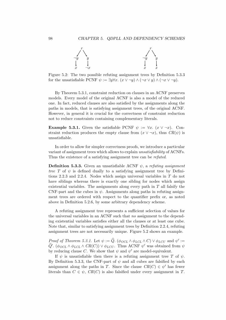
98 CHAPTER 5. QDPLL AND DEPENDENCY SCHEMES
r
¬y
x
y
¬x
r
¬y
x
y
x
Figure 5.2: The two possible refuting assignment trees by Definition 5.3.3for the unsatisfiable PCNF ψ := ∃y∀x. (x ∨ ¬y) ∧ (¬x ∨ y) ∧ (¬x ∨ ¬y).
By Theorem 5.3.1, constraint reduction on clauses in an ACNF preservesmodels. Every model of the original ACNF is also a model of the reducedone. In fact, reduced clauses are also satisfied by the assignments along thepaths in models, that is satisfying assignment trees, of the original ACNF.However, in general it is crucial for the correctness of constraint reductionnot to reduce constraints containing complementary literals.
Example 5.3.1. Given the satisfiable PCNF ψ := ∀x. (x ∨ ¬x). Con-straint reduction produces the empty clause from (x ∨ ¬x), thus CR(ψ) isunsatisfiable.
In order to allow for simpler correctness proofs, we introduce a particularvariant of assignment trees which allows to explain unsatisfiability of ACNFs.Thus the existence of a satisfying assignment tree can be refuted.
Definition 5.3.3. Given an unsatisfiable ACNF ψ, a refuting assignmenttree T of ψ is defined dually to a satisfying assignment tree by Defini-tions 2.2.3 and 2.2.4. Nodes which assign universal variables in T do nothave siblings whereas there is exactly one sibling for nodes which assignexistential variables. The assignments along every path in T all falsify theCNF-part and the cubes in ψ. Assignments along paths in refuting assign-ment trees are ordered with respect to the quantifier prefix or, as notedabove in Definition 5.2.6, by some arbitrary dependency scheme.
A refuting assignment tree represents a sufficient selection of values forthe universal variables in an ACNF such that no assignment to the depend-ing existential variables satisfies either all the clauses or at least one cube.Note that, similar to satisfying assignment trees by Definition 2.2.4, refutingassignment trees are not necessarily unique. Figure 5.2 shows an example.
Proof of Theorem 5.3.1. Let ψ := Q. (φOCL ∧ φLCL ∧ C) ∨ φLCU and ψ′ :=Q′. (φOCL ∧ φLCL ∧ CR(C)) ∨ φLCU . Thus ACNF ψ′ was obtained from ψby reducing clause C. We show that ψ and ψ′ are model-equivalent.
If ψ is unsatisfiable then there is a refuting assignment tree T of ψ.By Definition 5.3.3, the CNF-part of ψ and all cubes are falsified by eachassignment along the paths in T . Since the clause CR(C) ∈ ψ′ has fewerliterals than C ∈ ψ, CR(C) is also falsified under every assignment in T .

5.3. QBCP 99
...
¬x
v(l′)
¬v(l) v(l)
x
Figure 5.3: Part of a satisfying assignment tree m which illustrates theproof of Theorem 5.3.1. Variable x is universal and irrelevant. Variable v(l)is universal and was reduced by constraint reduction from clause C to obtainclause CR(C). A literal of the existential variable v(l′) satisfies both C andCR(C), since v(l′) was assigned before v(l) along the path in m.
The other constraints in ψ′ are the same as in ψ. Therefore, T is a refutingassignment tree of ψ′ as well and hence ψ′ is unsatisfiable.
If ψ is satisfiable, let m be a satisfying assignment tree of ψ, that ism |= ψ. Assume that all assignments along the paths in m are completeand admissible with respect to D where D is the dependency scheme thatwas applied for constraint reduction. We show that also m |= ψ′.
By definition of satisfying assignments trees, assignments along paths inm must satisfy the quantifier-free part of ψ. We consider all assignmentsalong paths at the leaves of m. If such an assignment satisfies a cube in ψthen that cube is also satisfied in ψ′ since constraint reduction did not affectcubes in ψ. The same holds for all clauses in ψ′ other than CR(C) sincethey were not affected by constraint reduction.
Consider the clauses C and CR(C) and, without loss of generality, as-sume that exactly one universal literal l was removed from C to obtainCR(C). We can assume that, among all variables occurring in CR(C), vari-able v(l) was assigned last on the current path in m since all assignmentsare admissible. Figure 5.3 illustrates the situation. Further, due to Defini-tion 5.3.2, there is no other variable v′′ in C such that v(l) ≺ v′′. Therefore,clause C must be satisfied by some other existential literal l′ because v(l)is universal: otherwise, considering the sibling of node v(l) which assignsthe opposite truth value, C would no longer be satisfied. Since literal l′ isexistential, it cannot be removed by constraint reduction and therefore l′
will also satisfy CR(C).
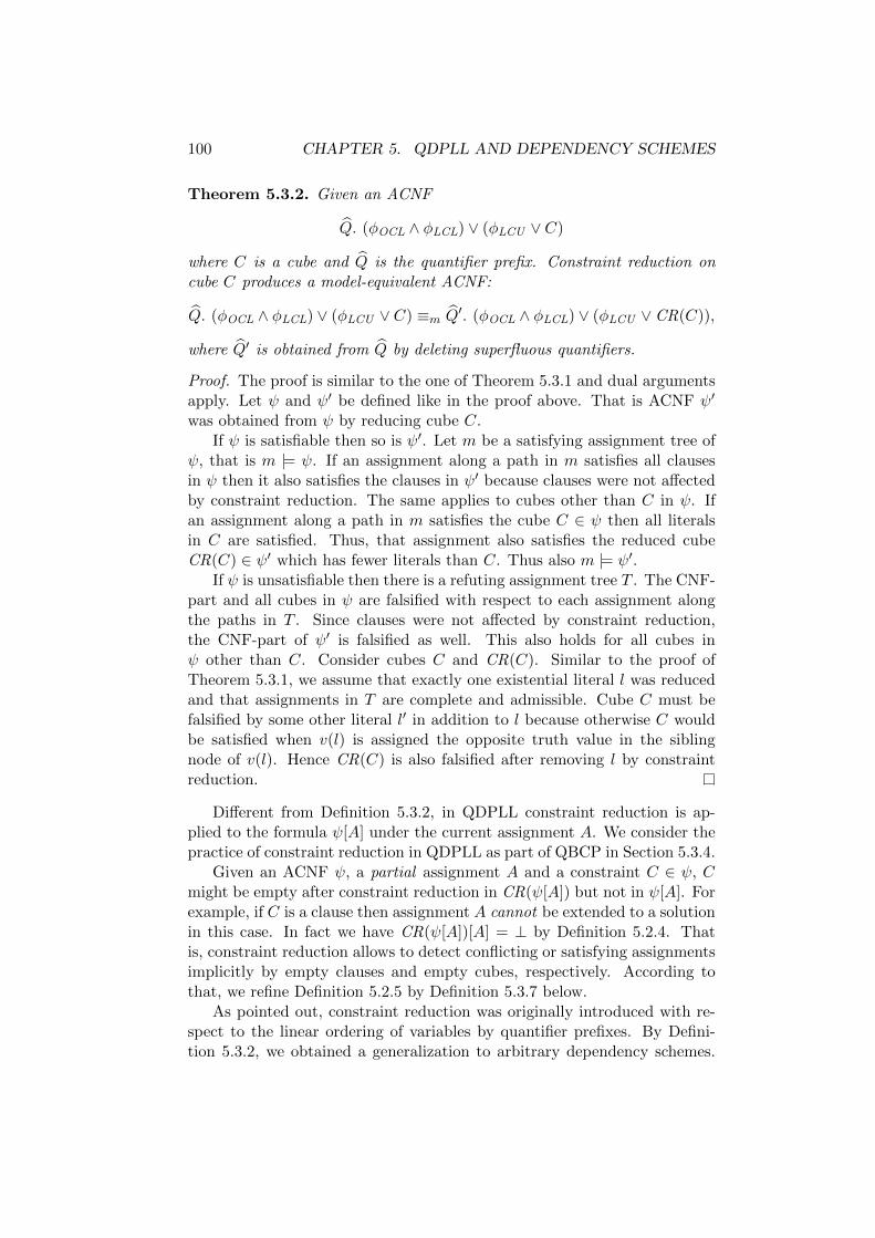
100 CHAPTER 5. QDPLL AND DEPENDENCY SCHEMES
Theorem 5.3.2. Given an ACNF
Q. (φOCL ∧ φLCL) ∨ (φLCU ∨ C)
where C is a cube and Q is the quantifier prefix. Constraint reduction oncube C produces a model-equivalent ACNF:
Q. (φOCL ∧ φLCL) ∨ (φLCU ∨ C) ≡m Q′. (φOCL ∧ φLCL) ∨ (φLCU ∨ CR(C)),
where Q′ is obtained from Q by deleting superfluous quantifiers.
Proof. The proof is similar to the one of Theorem 5.3.1 and dual argumentsapply. Let ψ and ψ′ be defined like in the proof above. That is ACNF ψ′
was obtained from ψ by reducing cube C.If ψ is satisfiable then so is ψ′. Let m be a satisfying assignment tree of
ψ, that is m |= ψ. If an assignment along a path in m satisfies all clausesin ψ then it also satisfies the clauses in ψ′ because clauses were not affectedby constraint reduction. The same applies to cubes other than C in ψ. Ifan assignment along a path in m satisfies the cube C ∈ ψ then all literalsin C are satisfied. Thus, that assignment also satisfies the reduced cubeCR(C) ∈ ψ′ which has fewer literals than C. Thus also m |= ψ′.
If ψ is unsatisfiable then there is a refuting assignment tree T . The CNF-part and all cubes in ψ are falsified with respect to each assignment alongthe paths in T . Since clauses were not affected by constraint reduction,the CNF-part of ψ′ is falsified as well. This also holds for all cubes inψ other than C. Consider cubes C and CR(C). Similar to the proof ofTheorem 5.3.1, we assume that exactly one existential literal l was reducedand that assignments in T are complete and admissible. Cube C must befalsified by some other literal l′ in addition to l because otherwise C wouldbe satisfied when v(l) is assigned the opposite truth value in the siblingnode of v(l). Hence CR(C) is also falsified after removing l by constraintreduction.
Different from Definition 5.3.2, in QDPLL constraint reduction is ap-plied to the formula ψ[A] under the current assignment A. We consider thepractice of constraint reduction in QDPLL as part of QBCP in Section 5.3.4.
Given an ACNF ψ, a partial assignment A and a constraint C ∈ ψ, Cmight be empty after constraint reduction in CR(ψ[A]) but not in ψ[A]. Forexample, if C is a clause then assignment A cannot be extended to a solutionin this case. In fact we have CR(ψ[A])[A] = ⊥ by Definition 5.2.4. Thatis, constraint reduction allows to detect conflicting or satisfying assignmentsimplicitly by empty clauses and empty cubes, respectively. According tothat, we refine Definition 5.2.5 by Definition 5.3.7 below.
As pointed out, constraint reduction was originally introduced with re-spect to the linear ordering of variables by quantifier prefixes. By Defini-tion 5.3.2, we obtained a generalization to arbitrary dependency schemes.

5.3. QBCP 101
In the forthcoming sections of this chapter, we consider how QDPLL mightbenefit from dependency schemes which are more refined than the trivial onearising from quantifier prefixes. For example, constraint reduction mightproduce shorter constraints.
Proposition 5.3.1. Given two dependency schemes D and D′ such thatD ⊆ D′. Let CRD and CRD′ denote constraint reduction with respect to Dand D′, respectively. Given a constraint C, CRD(C) ⊆ CRD′(C).
As pointed out below, constraint reduction is a crucial part of QBCP.Due to Proposition 5.3.1, using more refined dependency schemes for con-straint reduction might influence unit and pure literal detection positively.
5.3.2 Unit Literal Detection
We consider a common rule in QBCP which allows to infer forced assign-ments to variables from a given ACNF. For example, if there is a clause ina CNF which consists of only one existential literal, then that clause canonly be satisfied by assigning the variable of the literal accordingly. Suchliterals are called unit literals. The rule for the detection of unit literalsallows to identify forced assignments in an ACNF during QBCP. In general,unit literals can appear in clauses as well as in cubes of an ACNF.
In state-of-the-art SAT solvers, unit literals are detected during BCP.Classical definitions of unit literal detection for QBF [31] typically differfrom the rule applied in SAT solvers. That difference is due to a combina-tion of constraint reduction and unit literal detection into one single rule.We introduce unit literal detection for ACNFs separately from constraintreduction. Our definition corresponds exactly to the rule which is com-mon for SAT solving, as far as clauses are concerned. That is, we focuson constraints in ACNFs which contain exactly one literal. In Section 5.3.4below, we explicitly combine constraint reduction and unit literal detectionin QBCP. This way, we obtain the same effects as the original definition ofunit literal detection [31] which implicitly includes constraint reduction.
Definition 5.3.4 (see also [30, 61, 134], for example). Given an ACNF ψand constraint C ∈ ψ. Let Q := ∃ if C is a clause and Q := ∀ if C is a cube.Constraint C is unit if and only if C = (l1) and q(v(l1)) = Q, where l1 iscalled a unit literal. Given a constraint C, unit literal detection
UL(C) := {l}
collects the assignment {l} from C if C = (l1) and C is unit, where l := l1if C is a clause and l := ¬l1 if C is a cube. Constraint C = ante(l) is theantecedent constraint of assignment {l}. Otherwise, if C is not unit thenUL(C) := ∅ is the empty assignment. Unit literal detection is extended
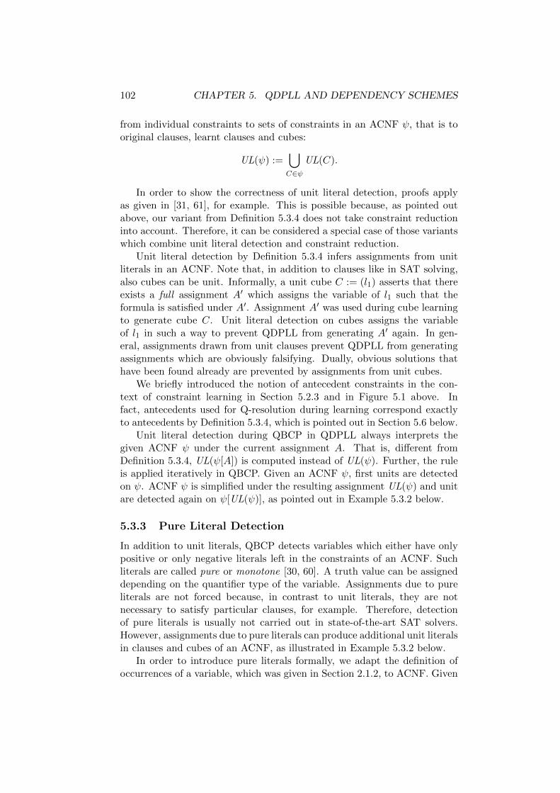
102 CHAPTER 5. QDPLL AND DEPENDENCY SCHEMES
from individual constraints to sets of constraints in an ACNF ψ, that is tooriginal clauses, learnt clauses and cubes:
UL(ψ) :=⋃C∈ψ
UL(C).
In order to show the correctness of unit literal detection, proofs applyas given in [31, 61], for example. This is possible because, as pointed outabove, our variant from Definition 5.3.4 does not take constraint reductioninto account. Therefore, it can be considered a special case of those variantswhich combine unit literal detection and constraint reduction.
Unit literal detection by Definition 5.3.4 infers assignments from unitliterals in an ACNF. Note that, in addition to clauses like in SAT solving,also cubes can be unit. Informally, a unit cube C := (l1) asserts that thereexists a full assignment A′ which assigns the variable of l1 such that theformula is satisfied under A′. Assignment A′ was used during cube learningto generate cube C. Unit literal detection on cubes assigns the variableof l1 in such a way to prevent QDPLL from generating A′ again. In gen-eral, assignments drawn from unit clauses prevent QDPLL from generatingassignments which are obviously falsifying. Dually, obvious solutions thathave been found already are prevented by assignments from unit cubes.
We briefly introduced the notion of antecedent constraints in the con-text of constraint learning in Section 5.2.3 and in Figure 5.1 above. Infact, antecedents used for Q-resolution during learning correspond exactlyto antecedents by Definition 5.3.4, which is pointed out in Section 5.6 below.
Unit literal detection during QBCP in QDPLL always interprets thegiven ACNF ψ under the current assignment A. That is, different fromDefinition 5.3.4, UL(ψ[A]) is computed instead of UL(ψ). Further, the ruleis applied iteratively in QBCP. Given an ACNF ψ, first units are detectedon ψ. ACNF ψ is simplified under the resulting assignment UL(ψ) and unitare detected again on ψ[UL(ψ)], as pointed out in Example 5.3.2 below.
5.3.3 Pure Literal Detection
In addition to unit literals, QBCP detects variables which either have onlypositive or only negative literals left in the constraints of an ACNF. Suchliterals are called pure or monotone [30, 60]. A truth value can be assigneddepending on the quantifier type of the variable. Assignments due to pureliterals are not forced because, in contrast to unit literals, they are notnecessary to satisfy particular clauses, for example. Therefore, detectionof pure literals is usually not carried out in state-of-the-art SAT solvers.However, assignments due to pure literals can produce additional unit literalsin clauses and cubes of an ACNF, as illustrated in Example 5.3.2 below.
In order to introduce pure literals formally, we adapt the definition ofoccurrences of a variable, which was given in Section 2.1.2, to ACNF. Given
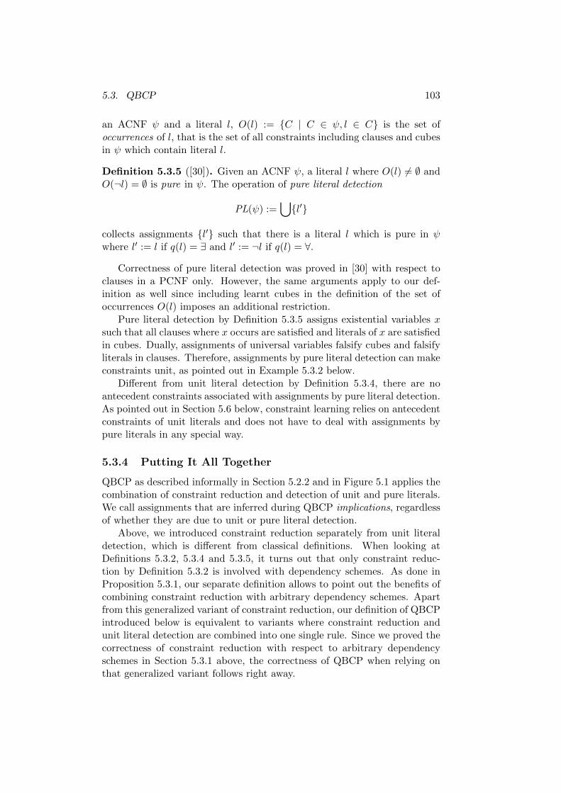
5.3. QBCP 103
an ACNF ψ and a literal l, O(l) := {C | C ∈ ψ, l ∈ C} is the set ofoccurrences of l, that is the set of all constraints including clauses and cubesin ψ which contain literal l.
Definition 5.3.5 ([30]). Given an ACNF ψ, a literal l where O(l) 6= ∅ andO(¬l) = ∅ is pure in ψ. The operation of pure literal detection
PL(ψ) :=⋃{l′}
collects assignments {l′} such that there is a literal l which is pure in ψwhere l′ := l if q(l) = ∃ and l′ := ¬l if q(l) = ∀.
Correctness of pure literal detection was proved in [30] with respect toclauses in a PCNF only. However, the same arguments apply to our def-inition as well since including learnt cubes in the definition of the set ofoccurrences O(l) imposes an additional restriction.
Pure literal detection by Definition 5.3.5 assigns existential variables xsuch that all clauses where x occurs are satisfied and literals of x are satisfiedin cubes. Dually, assignments of universal variables falsify cubes and falsifyliterals in clauses. Therefore, assignments by pure literal detection can makeconstraints unit, as pointed out in Example 5.3.2 below.
Different from unit literal detection by Definition 5.3.4, there are noantecedent constraints associated with assignments by pure literal detection.As pointed out in Section 5.6 below, constraint learning relies on antecedentconstraints of unit literals and does not have to deal with assignments bypure literals in any special way.
5.3.4 Putting It All Together
QBCP as described informally in Section 5.2.2 and in Figure 5.1 applies thecombination of constraint reduction and detection of unit and pure literals.We call assignments that are inferred during QBCP implications, regardlessof whether they are due to unit or pure literal detection.
Above, we introduced constraint reduction separately from unit literaldetection, which is different from classical definitions. When looking atDefinitions 5.3.2, 5.3.4 and 5.3.5, it turns out that only constraint reduc-tion by Definition 5.3.2 is involved with dependency schemes. As done inProposition 5.3.1, our separate definition allows to point out the benefits ofcombining constraint reduction with arbitrary dependency schemes. Apartfrom this generalized variant of constraint reduction, our definition of QBCPintroduced below is equivalent to variants where constraint reduction andunit literal detection are combined into one single rule. Since we proved thecorrectness of constraint reduction with respect to arbitrary dependencyschemes in Section 5.3.1 above, the correctness of QBCP when relying onthat generalized variant follows right away.

104 CHAPTER 5. QDPLL AND DEPENDENCY SCHEMES
Definition 5.3.6. Let ψ be an ACNF and A an assignment.
• QBCP0(ψ[A]) := ψ′[A∪A′] where A′ := (UL(ψ′)∪PL(ψ′)) and ψ′ :=CR(ψ[A]).
• QBCP i(ψ[A]) := QBCP0(QBCP i−1(ψ[A])) for natural number i > 0.
• QBCP(ψ[A]) := QBCP i(ψ[A]) for the smallest natural number i suchthat QBCP i(ψ[A]) = QBCP i+1(ψ[A]).
QBCP by Definition 5.3.6 infers additional assignments from a givenone in QDPLL. For an ACNF ψ and the current assignment A generated byQDPLL, first constraint reduction is applied to ψ[A] to obtain the reducedformula ψ′. Implications A′ by unit and pure literal detection are inferredfrom ψ′. Extending the current assignment A with the set of implicationsA′ yields a new assignment A∪A′ which is used to simplify ψ′ further. Thisprocess is repeated until no more implications can be found.
Constraint reduction is crucial in QBCP. The deletion of literals fromconstraints can enable the detection of both new unit and new pure literals.Due to Proposition 5.3.1, the use of more refined dependency schemes inconstraint reduction can produce shorter constraints. This in turn mightallow to identify more unit and pure literals. Further, as noted in Sec-tion 5.3.1, constraints might become empty exclusively due to constraintreduction. This property allows to generalize the state of a formula underan assignment by Definition 5.2.5 to QBCP including constraint reduction.
Definition 5.3.7. Given an ACNF ψ and a (partial) assignment A, thestate of ψ under QBCP and A is defined as follows. If QBCP(ψ[A]) = ⊥then A is a conflicting assignment, also called a conflict, and ψ is falsifiedunder A. If QBCP(ψ[A]) = > then A is a satisfying assignment, also called asolution, and ψ is satisfied under A. If A is neither conflicting nor satisfyingthen A is an inconclusive assignment and ψ is undetermined under A.
Notation QBCP(ψ[A]) = ⊥ and QBCP(ψ[A]) = > is well-defined dueto Definition 5.2.4. Empty constraints produced by constraint reductionare replaced by truth constants which in turn are eliminated in the formulaQBCP(ψ[A]). Function qbcp in Figure 5.1 typically implements QBCP anddetermines the state of the formula according to Definitions 5.3.6 and 5.3.7,respectively. Proposition 5.2.1 is adapted to QBCP accordingly.
It is desirable to maximize the number of implications during QBCP. Ingeneral, the more implications are inferred, the fewer decisions have to madeby QDPLL. Each of the three rules applied in Definition 5.3.6 contributesto the inference of implications, as illustrated in the following example.
Example 5.3.2. Given the ACNF ψ which, for simplicity, only containsclauses:
ψ := ∃e1∀a2∃e3,e4. (e1∨a2∨e3∨e4)∧(e1∨a2∨¬e4)∧(¬e1∨e3∨¬e4)∧(¬a2∨¬e3).

5.3. QBCP 105
Assume that the current assignment is A := {e4}. We consider ψ under A:
ψ[A] = ∃e1∀a2∃e3. (e1 ∨ a2) ∧ (¬e1 ∨ e3) ∧ (¬a2 ∨ ¬e3).
Neither the unit nor the pure literal rule is applicable to ψ[A]. Constraintreduction with respect to Dtriv on ψ[A] deletes the universal literal a2 fromclause (e1, a2) to obtain the reduced clause (e1):
CR(ψ[A]) = ∃e1∀a2∃e3. (e1) ∧ (¬e1 ∨ e3) ∧ (¬a2 ∨ ¬e3).
Variable a2 has only one negative occurrence left and is pure in CR(ψ[A]).Pure literal detection assigns variable a2 to true to obtain the new as-signment A′ := {a2}. Further, clause (e1) is unit in CR(ψ[A]) and thenew assignment A′ is extended by setting variable e1 to true, which yieldsA′ := {a2, e1}. No further implications can be inferred from CR(ψ[A]).Formula CR(ψ[A]) is simplified using the new, current assignment A ∪A′:
CR(ψ[A])[A ∪A′] = ∃e3. (e3) ∧ (¬e3).
Assume that unit literal detection infers the assignment A′′ := {e3} fromCR(ψ[A])[A ∪A′]. Simplifications under A′′ produce the empty clause:
CR(ψ[A])[A ∪A′][A′′] = ⊥.QBCP without constraint reduction could miss the inference of both unit
and pure literals. In Example 5.3.2 above, variable a2 becomes pure onlyafter constraint reduction was applied. Similarly, the clause (e1, a2) becomesunit only by constraint reduction. Dual effects on cubes can be observedin general. Further, pure literal detection is crucial for QBCP to detectadditional unit clauses. In Example 5.3.2, clause (¬a2,¬e3) is unit onlyafter variable a2 becomes pure. Dually, cubes can become unit by assigningexistential variables by pure literal detection. Therefore, none of the threerules of constraint reduction, unit and pure literal detection can be omittedfrom QBCP without harming its ability to infer implications.
Note that, due to lack of decisions, new assignments generated by unitand pure literal detection in QBCP according to Definition 5.3.6 are triviallyadmissible by Definition 5.2.6 with respect to the same dependency schemeD that was used for constraint reduction (we require that one and the sameD is used in all parts of QDPLL). As noted, variables assigned by unitand pure literal rule during QBCP get trail levels in chronological fashion.Additionally, we distinguish assignments to variables as follows.
Definition 5.3.8. Given an assignment A generated by QDPLL, the as-signment mode of a literal l ∈ A assigned by A is am(l) := D if l wasassigned as decision, am(l) := U if l was assigned by unit literal rule andam(l) := P if l was assigned by pure literal rule.
Definition 5.3.9. Given a decision level i ∈ {1, 2, . . . , n}, the unique vari-able x with dl(x) = i and am(x) = D is the decision variable at decisionlevel i.
106 CHAPTER 5. QDPLL AND DEPENDENCY SCHEMES
Implementation
Different from Definition 5.3.6, in our QBF solver DepQBF QBCP is notimplemented recursively but iteratively. Literals reduced by constraint re-duction with respect to the current assignment are never explicitly deletedfrom constraints but disabled instead. This way, reduced literals do not haveto be introduced again during backtracking.
Additionally, the application of constraint reduction is merged with unitliteral detection. For that purpose, the approach of two-literal watching [93],which is commonly applied in modern SAT solvers, can be extended to QBF[52]. The following description was published previously in [84].
Two unassigned literals l1 and l2 are watched in each constraint C underthe following restrictions. If C is a clause, then either (1) q(l1) = q(l2) = ∃or (2) q(l1) = ∀, q(l2) = ∃ and l1 ≺D l2 where D is the dependency schemeapplied in QDPLL. Otherwise, C is a cube and either (1) q(l1) = q(l2) = ∀or (2) q(l1) = ∃, q(l2) = ∀ and l1 ≺D l2.
If variable x is assigned in QDPLL then the watchers of all constraints Cwhere a literal of x is watched will be updated under the restrictions statedabove. That is, watchers must be set such that either case (1) or case (2)holds. Whenever a current watcher already satisfies clause C (or falsifiescube C) then no update is made. If a clause (cube) C contains exactly oneunassigned existential (universal) literal then C is unit. If clause (cube) Cdoes not contain unassigned existential (universal) literals then C is falsified(satisfied). During watcher update of C, constraint reduction is applied onthe fly to C by ignoring any universal (existential) literals in C which areunassigned or false (true). Dependency checking during watcher updates,which is needed in case (2) only, can be carried out efficiently as describedin Section 5.5 below.
Pure literal detection in QBCP considers the given ACNF ψ under thecurrent assignment A. Since learnt constraints have to be taken into accountby Definition 5.3.5, it might become expensive to search for pure literals inψ explicitly if the number of learnt constraints becomes large. In order toovercome this problem in implementations, constraints can be watched [52].A literal of variable x is not pure as long as x has at least one positive andone negative occurrence in ψ[A]. For each variable a, one negative and onepositive occurrence C¬x and Cx of x is watched, respectively. Whenevereither C¬x or Cx are satisfied (or falsified, if C¬x or Cx are cubes) undera modified assignment A′ 6= A then new watched constraints are selectedfor x. If this is not possible because x does not have positive or negativeoccurrences in ψ[A′] then x is pure.
In addition to constraint watching, learnt constraints could be ignoredduring pure literal detection. That is, only the set φOCL of original clauses ofthe ACNF ψ := (φOCL∧φLCL)∨φLCU is taken into consideration. Variablesmight be pure with respect to φOCL but not with respect to ψ if learnt
5.4. DECISION MAKING 107
constraints are included. This approach might produce spurious pure literals[60], which have to be treated in a special way whenever they are involvedin the detection of new unit literals or empty constraints. In our QBFsolver DepQBF we implemented both constraint watching and spurious pureliterals [84]. We refer to [52, 60, 84] for further details.
As noted above, assignments made during QBCP are always admissible.In order to guarantee admissible assignments not only by QBCP but alsoby decision making, that is in entire QDPLL, variable dependencies have tobe taken into account as follows.
5.4 Decision Making
In classical descriptions of QDPLL [30] which rely on the variable orderinggiven by the quantifier prefix, decisions have to be made with respect to thatlinear ordering. That is, function select dec var in Figure 5.1 must selectdecision variables “from left to right”, which corresponds to the naturalordering by variable dependencies in the quantifier prefix. We extend thisapproach from the prefix-based trivial dependency scheme to arbitrary ones.Thereby, QDPLL can benefit from more freedom in decision making becausethe linear prefix ordering is relaxed, as shown in Example 3.1.3 on page 25.Instead of the linear prefix ordering, decisions are made with respect to thepartial ordering defined by the dependency scheme.
The requirement of respecting variable dependencies in decision mak-ing is necessary in QDPLL to generate assignments which are admissibleby Definition 5.2.6. This way, the assignment tree implicitly constructedby QDPLL complies with semantics of PCNF (and also ACNF) from Sec-tion 2.2 and, when generalized to arbitrary dependency schemes, by Proposi-tion 3.4.1. Assignment which are not admissible might yield unsound results,as pointed out in Example 3.1.1 on page 24.
Implications assigned during QBCP are exempted from the requirementsstated in Definition 5.2.6. Assignments to some variable x by unit or pureliteral rule can always be made even if not all variables where x dependson are assigned already. Note that Definitions 5.3.4 and 5.3.5 do not referto dependency schemes. Therefore, the extension of an admissible assign-ment by implications detected in QBCP will again produce an admissibleassignment. The problem of generating admissible assignments in QDPLLis limited to decision making only. In the following, we assume that anarbitrary dependency scheme D is applied for QBCP and decision making.
QDPLL as illustrated in Figure 5.1 generates assignments starting fromthe empty assignment A := ∅, which is trivially admissible with respect to D.We have to ensure that every decision selected by function select dec var
results in a new admissible assignment. From a theoretical point of view,we adopt Definition 5.2.6 to obtain a sufficient condition as follows.

108 CHAPTER 5. QDPLL AND DEPENDENCY SCHEMES
Definition 5.4.1. Given a dependency scheme D, an admissible assignmentA generated by QDPLL and a variable x. Let VA := {z | z = v(l), l ∈ A} bethe set of variables assigned in A. A variable x is a decision candidate withrespect to D and A if and only if D−1(x) ⊆ VA. If x is a decision candidatethen x is enabled under A, otherwise x is disabled.
By Definition 5.4.1, every variable y where a decision candidate x de-pends on must be assigned already. Checking the condition explicitly mightbe expensive in practice if the set D−1(x) is large.
Therefore, our goal is to maintain the set DC of decision candidatesincrementally based on the current assignment A. Initially, A = ∅ and allvariables x where D−1(x) = ∅ are decision candidates. For example, in termsof quantifier prefixes likes in classical QDPLL, this situation correspondsto the left-most quantifier block in an ACNF. Each additional assignmentto a variable potentially enables some variable x. Variable x is enabled ifall variables in D−1(x) are assigned. When it comes to decision making,function select dec var must select variables from the set DC only. Ifassignments are retracted during backtracking in function backtrack, thena candidate x ∈ DC must be removed from this set if there is at least onevariable in D−1(x) which was unassigned, thus disabling x.
In order to maintain the set DC of decision candidates incrementally,we present an approach relying on the augmented compressed dependencygraph G≈,⊆(D) for D by Definition 4.2.8 on page 60. First, the idea is notto check the condition of decision candidates by Definition 5.4.1 explicitlyfor each variable, but to focus on equivalence classes of variables as part ofgraph G≈,⊆(D) instead. Second, the set DC of decision candidates does nothave to be updated each time the current assignment A is modified. Wewant to check the condition only if modifying A potentially changes the setDC . For that purpose, equivalence classes are applied as follows.
Given variables x and x′, if D−1(x) = D−1(x′) then also x ≈↑ x′ byDefinition 4.2.4. Since x and x′ depend on the same set of variables, xbecomes a decision candidate if and only if x′ becomes one. Thus, the wholeclass [x]↑ becomes enabled.
Further, if some variable y is assigned then that single assignment doesnot enable some variable x ∈ D(y) if there is an unassigned variable y′ withy′ 6= y where x depends on. Consider the classes [y]↓ induced by relation≈↓ according to Definition 4.2.3, which checks equality of the sets D(y) ofdependencies. A variable x in D(y) might become enabled as soon as allvariables in the class [y]↓ are assigned. Note that x might depend on othervariables in addition to [y]↓. Thus having all variables in class [y]↓ assignedis a necessary but not a sufficient condition to enable new variables in D(y).In practice, we count the number of assigned variables in classes [y]↓.
In addition to equivalence classes given by relations ≈↑ and ≈↓, subsetedges in the graph G≈,⊆(D) can be used to reduce the amount of work that

5.4. DECISION MAKING 109
has to be carried out in order to update the set DC of decision candidates.In the following, we describe how to maintain the set DC incrementallyand lazily based on modifications of the current assignment A by QBCP,decision making and backtracking. For that purpose, we assume that thedependency scheme D that is used in QDPLL is represented as the aug-mented compressed dependency graph G≈,⊆(D) by Definition 4.2.8.
5.4.1 Maintaining Decision Candidates
Each time some variable y is assigned during QBCP or decision making,potentially some other variable x ∈ D(y) is enabled. QDPLL starts withthe empty assignment A = ∅ and the set DC := {x | D−1(x) = ∅} ofvariables which do not depend on other ones as decision candidates. Giventhe current assignment A and the current set DC of decision candidates,assume that variable y is unassigned in A. Let A′ be a new assignmentobtained from A by assigning y. We present an algorithm to obtain thenew set DC ′ of decision candidates with respect to A′ based on the graphG≈,⊆(D), which includes subset edges.
1. Let DC ′ := DC .
2. Given the assigned variable y, consider the class [y]↓ of variables whichhave the same set of dependencies as y.
3. If there is an unassigned variable y′ in class [y]↓ then no additionalvariables are enabled after y was assigned. No additional work has tobe done.
4. Otherwise, all variables in class [y]↓ are assigned. Consider the setREF := {[x]↑ | ([y]↓, [x]↑) ∈ Ed} of classes which are referenced fromclass [y]↓ by a dependency edge and possibly from other classes as well.These classes have to be checked as follows.
5. For all classes [x]↑ ∈ REF :
5.1. If class [x]↑ is referenced by a dependency edge from a class [y′]↓such that [y′]↓ contains an unassigned variable then continue withthe next class in REF . No additional work has to be done.
5.2. Otherwise, given the class [x]↑, all variables in D−1(x) are as-signed and the set DC is updated as follows.
5.3. For all classes [x′]↑ which are reachable from [x]↑ over zero ormore subset edges:
5.3.1. If class [x′]↑ is referenced by a dependency edge from a class[y′′]↓ such that [y′′]↓ contains an unassigned variable, thencontinue with the next class. No additional work has to bedone.
110 CHAPTER 5. QDPLL AND DEPENDENCY SCHEMES
5.3.2. Otherwise, given the class [x′]↑, all variables in D−1(x) areassigned and the new set DC ′ is updated by DC ′ := DC ′ ∪{[x′]↑}.
6. Finally, set DC ′ contains all decision candidates with respect to thenew assignment A′.
The algorithm described above keeps track of the number of unassignedvariables in a class with respect to relation ≈↓. The only situation wherepotentially any work has to be done is when that number becomes zerodue to assigning variable y. In this case, at least the class [y]↓ does notprevent other variables in the set D(y) from becoming enabled. Note that ifassigning y enables any variable x then x ∈ D(y). Therefore, it is sufficientto check the set D(y) for new decision candidates. Classes [x′]↑ of variablesin the set D(y) are visited by traversing subset edges in graph G≈,⊆(D). Thetraversal implicitly performs a check whether, given a visited class [x′]↑, allvariables in D−1(x′) are assigned. If so then the whole class [x′]↑ is enabled.
As an optimization, subset edges in graph G≈,⊆(D) allow to skip allsuccessors of visited classes [x′]↑ in step 5.3 if it was found out that [x′]↑ isnot enabled. In this case, class [x′]↑ is referenced by at least one class whichcontains an unassigned variable. If there is a class [x′′]↑ which is reachablefrom [x′]↑ by subset edges then [x′′]↑ is (implicitly) referenced by the sameunassigned variable. Thus the traversal can stop at class [x′]↑.
If assignments are retracted in function backtrack in Figure 5.1 thendecision candidates in the set DC will be disabled. However, as noted abovesimilarly for enabling variables, not every single variable y which is unas-signed will disable decision candidates. Unassigning some variable y fromthe current assignment A produces the new assignment A′ := A \ {y}. Vari-ables from the set D(y) which are decision candidates under A potentiallyare disabled under A′. Note that if unassigning y disables any variable xthen x ∈ D(y). Consider the class [y]↓ containing all variables which havethe same set of dependencies as y. If there is another variable y′ ∈ [y]↓ whichis unassigned already under the old assignment A then unassigning y cannotdisable additional variables since D(y) = D(y′). Like for enabling variables,we assume that retracting assignments and disabling decision candidates isdone for each unassigned variable separately. Only if y is the first variable tobe unassigned in [y]↓ we have to check if variables in D(y) are disabled. Inthis case, all classes [x′]↑ of variables in the set D(y) are visited by traversingsubset edges in graph G≈,⊆(D). Analogously to the optimization describedabove, classes [x′]↑ and all of their successors by subset edges can be skippedif [x′]↑ was already disabled before y was unassigned.
Example 5.4.1. Consider graph on the left in Figure 5.4. Assigning x3
does not enable any new decision candidates since x4 is still unassignedin the class [∀x3, x4]↓. After x4 was assigned, the class [∀x3, x4]↓ does not

5.4. DECISION MAKING 111
[∃y1, y2]↑
[∀x5]↓
[∃y3, y4]↑ [∃y5]↑
[∃y6]↑
[∀x3, x4]↓
[∀x1, x2]↓
DC DC
DC
[∃y1, y2]↑ DC
[∀x5]↓
[∃y5]↑
[∃y6]↑ DC
[∀x3, x4]↓
[∀x1, x2]↓
DC DC
DC
DC [∃y3, y4]↑
Figure 5.4: Illustration of a compressed augmented dependency graphG≈,⊆(D) by Definition 4.2.8 for an arbitrary dependency scheme D andPCNF. Examples 5.4.1 and 5.4.2, point out enabling and disabling of vari-ables. For simplicity, not all edges are shown. Solid and dashed edges repre-sent dependency and subset edges, respectively. Dotted edges in the graphon the right indicate that the respective dependency edge is disabled due toassigned variables. Classes labeled with “DC” are decision candidates.
contain assigned variables anymore. Class [∃y3, y4]↑ is not directly referencedby a dependency edge from another class. However, there is an implicitdependency edge by the subset edge from class [∃y1, y2]↑ to [∃y3, y4]↑. Class[∃y1, y2]↑ is referenced by a dependency edge from class [∀x1, x2]↓ whichhas unassigned variables. This dependency edge refers to [∃y3, y4]↑ as wellimplicitly by the subset edge. Therefore, none of class [∃y3, y4]↑ and itssuccessors by subset edges is enabled. Due to subset edges, it is sufficientto find out that the parent class [∃y1, y2]↑ of class [∃y3, y4]↑ is not enabled.No other classes in the graph have to be checked. Further, assigning x1
does not enable new decision candidates since x2 is still unassigned in theclass [∀x1, x2]↓. After x2 was assigned, the class [∃y1, y2]↑ is enabled sinceit is not referenced by dependency edges from classes containing unassignedvariables. Class [∃y5]↑ is not enabled due to the reference from class [∀x5]↓.All successors [∃y3, y4]↑ and [∃y6]↑ of [∃y1, y2]↑ by subset edges are nowenabled, which is shown in the graph on the right.
Example 5.4.2. Consider graph on the right in Figure 5.4. Variablesx1, x2, x3 and x4 are assigned, hence all variables except the class [∃y5]↑ are

112 CHAPTER 5. QDPLL AND DEPENDENCY SCHEMES
decision candidates. During backtracking, decision candidates are disabledas follows. Unassigning x3 disables the class [∃y3, y4]↑ which is referencedfrom class [∀x3, x4]↓ by a dependency edge. All successors of [∃y3, y4]↑ bysubset edges, in this case only [y6]↑, are disabled as well. Unassigning x4
does not incur any additional work since the class [∀x3, x4]↓ already containsan unassigned variable. It is not necessary to traverse subset edges again.
In our solver DepQBF, decision candidates are maintained as describedabove based on the approximated dependency graph G≈,⊆(Dstd) for thestandard dependency scheme Dstd by Definition 4.5.4 on page 73. In ourimplementation, the graph G≈,⊆(Dstd) neither contains transitive subsetedges nor transitive dependency edges. In order to avoid additional overheadduring QBCP, the function for enabling variables is called only right beforea decision is made in function select dec var in Figure 5.1. The effects ofall assignments that were made since the most recent decision are then takeninto account one after the other to update the set DC . Our experimentalresults presented in Section 5.7 show that this way decision candidates canbe maintained efficiently.
The set DC of decision candidates with respect to the current assign-ment and the dependency scheme applied in QDPLL contains all variableswhich can be assigned as decisions. In SAT solving, where at any pointof time in QDPLL all variables are decision candidates, several branchingheuristics have been suggested to select a variable from the set DC as nextdecision. We referred to related work in Section 2.3.1 on page 16. Branch-ing heuristics from the domain of SAT solving basically can be extended toQBF by restricting the selection to set DC . In our QBF solver DepQBF [84],we implemented variable state independent decaying sum heuristic (VSIDS)[93] similarly to the MiniSAT solver [42].
5.5 Dependency Checking
Constraint reduction by Definition 5.3.2 shortens constraints with respectto dependencies between variables occurring in the constraint. Due to appli-cations in QBCP, a slow implementation of constraint reduction will likelyhave a negative effect on the overall run time of QBCP. In fact, the vastmajority of assignments in QDPLL are due to implications in QBCP.1 Weconclude that constraint reduction is performed frequently during QBCPand we aim at efficient application in practice.
1For example, on 372 formulae solved by DepQBF out of total 568 formulae fromQBFEVAL’10[100], on average 19.08 implications were detected per decision during QBCPin function qbcp in Figure 5.1. On the benchmark set from in QBFEVAL’08 (3326 formu-lae), 88% of total assignments in DepQBF were implications, with 59% unit literals and29% pure literals [84].

5.6. CONSTRAINT LEARNING 113
With respect to the trivial dependency scheme Dtriv, variable y dependson variable x if x < y by prefix ordering. This way, dependencies can easilybe checked by comparing the levels of quantifier blocks. However, this is nolonger possible if more refined dependency schemes D ⊆ Dtriv are applied.
In order to check for dependencies with respect to an arbitrary depen-dency scheme D, we consider a similar approach as for decision makingdescribed in the previous section.
Let D be a dependency scheme and G≈,⊆(D) be the compressed aug-mented dependency graph for D by Definition 4.2.8. We assume that thegraph G≈,⊆(D) does not contain dependency edges which are implicitlyrepresented by subset edges. This also applies to our implementation ofthe graph-based representation of the standard dependency scheme Dstd inDepQBF (see Section 4.5.3 for an illustration). Given two variables x and y,we can check if x ≺D y as follows.
1. Find the classes [x]↓ and [y]↑ of x and y, respectively.
2. Consider all ancestors [y′]↑ of [y]↑ which are reachable over zero ormore subset edges in G≈,⊆(D):
2.1. If ancestor [y′]↑ is referenced by a dependency edge from class[x]↓ then x ≺D y.
3. At this point, all ancestors of [y]↑ have been checked and hence x 6≺D y.
5.6 Constraint Learning
In the previous sections, we considered the generation of assignments inQDPLL as shown in Figure 5.1 by means of decision making and QBCP.We generalized these parts to arbitrary dependency schemes. As the finalstep of combining QDPLL with arbitrary dependency schemes, we addressconstraint learning in this section. Similarly to QBCP, it turns out thatthe classical approach of constraint learning can be adapted by applying thegeneralized variant of constraint reduction from Definition 5.3.1.
As noted in Section 5.2.3 above, constraint learning in QDPLL relieson Q-resolution, the QBF-specific variant of resolution [27, 108]. Given aPCNF ψ, Q-resolution is a sound and complete approach to solve ψ [27].PCNF ψ is unsatisfiable if and only if the empty clause can be derived fromψ by Q-resolution. Otherwise, if the set of all possible Q-resolvents that canbe derived from ψ does not contain the empty clause then ψ is satisfiable.In contrast to that, the application of Q-resolution for constraint learningin QDPLL does not focus on the generation of all possible Q-resolvents.Instead, Q-resolvents are derived selectively with respect to the current con-flicting assignment that was enumerated by QDPLL. Thus we may thinkof constraint learning in QDPLL as a heuristic application of Q-resolution

114 CHAPTER 5. QDPLL AND DEPENDENCY SCHEMES
guided by the generation of assignments. A similar view was presented forpropositional resolution in SAT solvers [70].
In the following, we present constraint learning for QDPLL as imple-mented in our solver DepQBF. Function analyze leaf in Figure 5.5 showsa high-level workflow. We focus on practical aspects such as the selectionof pivot variables to generate asserting constraints. We begin with a formaldefinition of Q-resolution.
Definition 5.6.1 ([26, 27, 61, 134]). Let C1 and C2 either be two clausesor two cubes such that, for some variable v, v ∈ C1,¬v ∈ C2 and q(v) = ∃if C1 and C2 are clauses and q(v) = ∀ otherwise. The tentative Q-resolventof C1 and C2 on pivot variable v is the constraint
C1 ⊗ C2 := (CR(C1) ∪ CR(C2)) \ {v,¬v}.
If the tentative Q-resolvent C1 ⊗ C2 contains complementary literals, thatis {x,¬x} ⊆ C1 ⊗ C2 for some variable x, then no Q-resolvent exists. Oth-erwise, the Q-resolvent
C := CR(C1 ⊗ C2)
is obtained by an additional application of constraint reduction to C1 ⊗C2.
Although Q-resolution is originally defined for clauses, we extend thedefinition to cubes for simplicity. Q-resolution on cubes is also called consen-sus [134]. Note that by Definition 5.6.1 the pivot variable must be existentialif clauses are resolved and universal otherwise.
As far as clauses are concerned, the application of constraint reductionis the only difference between Q-resolution by Definition 5.6.1 and propo-sitional resolution as applied in SAT solvers. In fact, Q-resolution is in-complete if constraint reduction is not applied [26] as pointed out in thefollowing example.
Example 5.6.1 (see also Section 23.5 in [26] for a related example). Giventhe unsatisfiable PCNF ψ := ∃x∀y. (x∨y)∧(¬x∨¬y). If constraint reductionis omitted in Q-resolution then the empty clause cannot be derived from ψsince the tentative resolvent (x∨y)⊗(¬x∨¬y) = (y∨¬y) on x is tautological.
Due to constraint reduction, as pointed out in Example 5.3.1 above, ingeneral it is crucial for the correctness of Q-resolution to prevent comple-mentary literals in Q-resolvents.
Example 5.6.2. Given the satisfiable PCNF ψ := ∀x∃y. (x∨¬y)∧(¬x∨y).If the requirement that tentative Q-resolvents must not contain complemen-tary literals is dropped from Definition 5.6.1, then Q-resolution can de-rive the empty clause from ψ: (x ∨ ¬y) ⊗ (¬x ∨ y) = (x ∨ ¬x) and finallyCR((x ∨ ¬x)) = ∅.
5.6. CONSTRAINT LEARNING 115
DecLevel analyze_leaf (State s)
R = get_initial_constraint (s);
// s == UNSAT: ’R’ is empty clause.
// s == SAT: ’R’ is sat. cube...
// ..or new cube from assignment.
while (!stop_res (R))
p = get_pivot (R);
R’ = get_antecedent (p);
R = constraint_res (R, p, R’);
add_to_formula (R);
return get_asserting_level (R);
Figure 5.5: Function analyze leaf from Figure 5.1. Assuming thatthe current assignment A generated by decision making and QBCPis conflicting (s == UNSAT), initially R is a clause which is falsified(get initial constraint). Q-resolution generates a new learnt clause bysuccessively resolving the antecedent clauses R′ (get pivot) of unit literalsin the current clause R with R. The process stops if clause R is asserting(stop res) and QDPLL backtracks to the asserting level where the newlearnt clause R triggers an implication (get asserting level).
We assume that formulae do not contain clauses or cubes with com-plementary literals. This way, incorrectness of constraint reduction andQ-resolution as pointed out in Examples 5.3.1 and 5.6.2 is avoided.
Note that dependency schemes affect Q-resolution only with respect toconstraint reduction. Due to Proposition 5.3.1, the use of more refineddependency schemes potentially produces shorter resolvents. This propertymotivates combinations of constraint learning for QDPLL based on morerefined dependency schemes. Altogether, this adds to the benefits that canbe drawn from dependency schemes in QBCP and decision making as arguedin Sections 5.3.4 and 5.4 above.
Recall that we apply one and the same dependency scheme D in allparts of QDPLL, that is constraint reduction in QBCP, decision makingand constraint learning to be discussed below.
5.6.1 Generation of Learnt Constraints
In the following, we describe the generation of learnt constraints in QDPLL.Our description largely relies on insights presented in [61, 134], but we alsoaddress the implementation of our solver DepQBF [84]. Thereby, we includepractical aspects of constraint learning. For simplicity, we confine the pre-sentation of constraint learning to the generation of learnt clauses. Apartfrom initialization, the generation of learnt cubes is entirely dual to clauselearning. We refer to Section A.1.1 in the appendix for related definitions.
116 CHAPTER 5. QDPLL AND DEPENDENCY SCHEMES
Initialization - Clause Learning
Given the current ACNF ψ, where learnt constraints might have been addedpreviously, and the current admissible assignment A := {l1, l2, . . . , ln} gen-erated by QBCP which is sorted by trail levels 1, 2, . . . , n. Assume that Ais conflicting by Definition 5.3.7, that is QBCP(ψ[A]) = ψ′[A] = ⊥. Fig-ure 5.5 shows function analyze leaf from Figure 5.1 again. Note that byassumption s == UNSAT in the figures. Since A is conflicting, there mustbe at least one clause R ∈ ψ such that R either is empty (thus falsified)under assignment A, that is R[A] = ⊥, or R became empty by constraintreduction in QBCP(ψ[A]), that is CR(R[A]) = ∅. If there are multiple suchclauses in ψ then let R be an arbitrary one. Clause R could be an originalor a learnt clause. Starting from R, clause learning produces a new learntclause C such that, after backtracking to a specific decision level, QBCPcan infer an additional implication from C by the unit literal rule.
In practice, function get initial constraint in Figure 5.5 selects Raccording to the requirements stated above. Clause R is used as initial clausefor the process of generating a new learnt clause by Q-resolution accordingto Definition 5.6.1. Antecedent clauses R′ of unit literals assigned in R byDefinition 5.3.4 are successively resolved with R to obtain a new clause.In order to carry out constraint reduction efficiently during Q-resolution, asimilar approach as described in Section 5.5 can be applied. If the currentresolvent R is asserting, that is a new implication can be inferred from Rafter backtracking, then the process stops. Clause R is added to the setof learnt clauses and QDPLL backtracks to the asserting level of R. Weconsider asserting clauses and asserting levels in Section 5.6.1 below.
Initialization - Cube Learning
Assume that the current assignment A is satisfying by Definition 5.3.7, thatis QBCP(ψ[A]) = ψ′[A] = > (s == SAT in Figure 5.5). Either there is acube R ∈ ψ which became empty (thus satisfied) by QBCP or all clauses inψ are satisfied under A. The former case is dual to an empty clause under aconflicting assignment A and function get initial constraint select onesuch cube R to generate a new learnt cube according to Figure 5.5.
If all clauses in ψ are satisfied under A then a cover set A′ ⊆ A isgenerated from A by Definition 5.2.8. Function get initial constraint
constructs a new cube R′ containing all the literals in A′ and returns thereduced cube R := CR(R′). Although cube R is not necessarily a cover set,Proposition 5.2.1 still holds due to the correctness of constraint reduction byTheorem 5.3.2. The cube to be learnt is generated from R dually to clauselearning, which is described below.

5.6. CONSTRAINT LEARNING 117
Pivot Selection
In modern SAT solvers like PicoSAT or MiniSAT [18, 42], for example, func-tion get pivot in Figure 5.5 typically selects pivot variables from variablesin the current clause R in reverse trail ordering. Hence the variable whichwas assigned as unit literal most recently in clause R is selected. Accord-ing to that policy, a learnt clause related to the first unique implicationpoint (1UIP) in the implication graph, which is associated with the currentassignment A, is obtained. Informally, an implication graph represents im-plications in A as a directed acyclic graph [36, 117, 118, 132]. To the best ofour knowledge, there is no comprehensive theoretical framework of implica-tion graphs and 1UIPs in the context of QBF. We concentrate on practicalaspects in our description of learning for QDPLL.
The strategy to select pivot variables in reverse trail ordering like inclause learning for SAT cannot directly be applied to QBF. If that strategywas applied then, due to combinations of constraint reduction and the unitliteral rule, universal literals which were reduced from antecedent clauses byQBCP might produce tautological resolvents during Q-resolution (functionconstraint res in Figure 5.5). The dual problem can occur in cube learningif complementary existential literals are introduced into the resolvent.
One approach to tackle the problem of resolvents containing complemen-tary literals is to integrate them into the theoretical and practical frameworkof QDPLL with constraint learning. The resulting variant of Q-resolutionis called long-distance resolution [133]. The rules for unit literal detectionand constraint reduction have to be adapted accordingly.
As an alternative, resolvents containing complementary literals can beprevented by selecting other pivot variables whenever Q-resolution on thepreviously selected pivot would introduce complementary literals into theresolvent [61]. We implemented this approach in our solver DepQBF. Ourpresentation below relies on the algorithm sketched in Figure 6 in [61]. Ad-ditionally, we address pitfalls related to bad selections of pivot variables.
Let A be the current assignment and R be the current resolvent in theloop in Figure 5.5. At any time during the generation of a learnt clause,all existential literals in R are falsified by A. Additionally, there might beunassigned universal literals in R which are reducible by constraint reduc-tion. Thus clause R is falsified under A, that is QBCP(R[A]) = ⊥. Thepivot variable is selected with respect to A and R as follows.
1. Let R be the current resolvent (line p = get pivot (R) in Figure 5.5).
2. Let P (R) := {y | y = v(l), l ∈ R, q(l) = ∃, am(l) = U} be the set ofexistential variables in R which were assigned by the unit literal rule.Set P (R) contains all potential pivot variables to be selected.
3. Select p ∈ P (R) such that p has the maximum trail level of variablesin P (R), that is tl(p) = max ({tl(y) | y ∈ P (R)}).

118 CHAPTER 5. QDPLL AND DEPENDENCY SCHEMES
4. If the tentative resolvent R⊗R′ of R and the antecedent R′ = ante(p)of p does not contain complementary literals, then variable p is thepivot for the next application of Q-resolution (line R = constraint res
(R, p, R’) in Figure 5.5).
5. Otherwise, if {x,¬x} ⊆ (R ⊗ R′) for some variable x ∈ R then analternative pivot is selected as follows.
5.1. Let x be one of the variables which occur both positively andnegatively in the tentative resolvent (R⊗R′).
5.2. Let P ′(R) := P (R) \ {y | y ∈ P (R), x 6≺ y} \ {y | y ∈ P (R),{x′,¬x′} ⊆ R ⊗ R′′ where R′′ = ante(y)}. In addition to therestrictions on set P (R) as defined above, the set P ′(R) containsonly existential variables which depend on variable x. Further,the resolvent of R and the antecedent of variables in P ′(R) doesnot contain complementary literals.
5.3. Select p ∈ P ′(R) such that p has the maximum trail level ofvariables in P ′(R), that is tl(p) = max ({tl(y) | y ∈ P ′(R)}).
5.4. Variable p is the pivot for the next application of Q-resolution(line R = constraint res (R, p, R’)).
Note that complementary literals in resolvents are always due to uni-versal variables which were reduced by constraint reduction in the currentresolvent and the antecedent. Therefore, this problem cannot occur duringclause learning in SAT solvers since all variables are existential. Dually incube learning, complementary existential literals might be introduced.
The idea behind the two-phase selection process described in the algo-rithm above is to always pick the existential variable p which was assignedas unit literal most recently. Only if resolution on p would introduce com-plementary literals of some variable x then an alternative pivot is selected.In this case, the goal is to resolve out existential variables which prevent theliteral of x in the current resolvent from being removed by constraint reduc-tion. Therefore, it is necessary to focus on variables which depend on x withrespect to the dependency scheme that is used in QDPLL. During the gener-ation of a learnt constraint, complementary literals which were removed byconstraint reduction might be introduced again into the current resolvent.In the worst case, an exponential number of intermediate resolvents has tobe produced until the final learnt constraint is obtained [50].
For cube learning, pivot selection is dual to clause learning. The goalis to select universal variables assigned by the unit literal rule, where theintroduction of complementary literals into the resolvent has to be avoidedanalogously. We refer to the appendix in for related algorithms.
The algorithm presented above is in essence equivalent to Figure 6 in[61], where it was proved that an asserting clause can always be generated

5.6. CONSTRAINT LEARNING 119
according to that algorithm (see Lemma 4 in [61]). Note that in our pre-sentation, we generalize dependency checking by quantifier prefixes as in[61] to arbitrary dependency schemes. We conjecture that the proof can beadapted in a similar way.
Stop Criteria and Asserting Levels
After a suitable pivot variable p has been selected, the current resolvent Ris resolved with the antecedent R′ of p (line R = constraint res (R, p,
R’) in Figure 5.5). The resolution process stops if the current resolvent isasserting according to the current assignment A (function stop res). Seealso Example 5.6.3 below.
Definition 5.6.2 ([53, 133]). Given the current resolvent R. Let m :=max ({d | d = dl(y), y = v(l), l ∈ R, q(l) = ∃}) be the largest decision levelof existential variables in R. Clause R is asserting if and only if:
1. There is exactly one literal l ∈ R with q(l) = ∃ such that dl(v(l)) = m.Let va := v(l).
2. The decision variable at decision level m is existential.
3. Variables where va depends on must be assigned where the decisionlevels must be smaller than m = dl(va), that is:
∀y ∈ {y | y = v(l), l ∈ R, y ≺ va} : dl(y) < m.
If R is asserting then variable va is asserted by R.
Different from the definition of asserting clauses in [133], Condition 2 isnot included in [53]. Asserting clauses are generated in DepQBF with respectto Definition 5.6.2. For cube learning, the conditions of asserting cubes aredual. We refer to Definition A.1.1 in the appendix.
As pointed out in Section 5.2.3, QDPLL by Figure 5.1 does not explicitlyflip the value of decision variables. Instead, every learnt constraint R isconstructed in such way that QBCP can infer an additional unit literal fromR after backtracking. Given the current conflicting assignment A and theasserting clause R that was learnt according to Definition 5.6.2, QDPLLbacktracks to the asserting level with respect to R defined as follows.
Definition 5.6.3. Given an asserting clause R by Definition 5.6.2 and thevariable va asserted by R.
1. Let DL∃(R) := {d | d = dl(y), y = v(l), l ∈ R, q(l) = ∃, y 6= va} be theset of decision levels of existential variables in R, excluding va.
2. Let DL≺(R) := {d | d = dl(y), y = v(l), l ∈ R, y ≺ va} be the set ofdecision levels of variables in R where va depends on.

120 CHAPTER 5. QDPLL AND DEPENDENCY SCHEMES
3. The asserting level da with respect to R is da := max (DL∃(R) ∪DL≺(R)).
Given the current conflicting assignment A, asserting clause R and theasserting level da by Definition 5.6.3, QDPLL retracts all assignments whichhave decision levels larger than da during backtracking, yielding a new as-signment A′ ⊆ A. The assignment l, where l ∈ R is the literal of variableva in R, can now be inferred from R by unit literal detection because Ris unit under A′ with constraint reduction, that is CR(R[A′]) = (l). Dueto Definition 5.6.3, universal literals of variables where va depends on arefalsified by A′ in R. All other universal literals are removed by constraint re-duction from the clause R[A′]. For cube learning, the definition of assertinglevels is dual. We refer to Definition A.1.2 in the appendix. Definitions 5.6.2and 5.6.3 are illustrated by the following example.
Example 5.6.3. Given the quantifier prefix ∃x∀a∃y∀b∃z and the clauseC := (x(1)∨a(4)∨y(3)∨b(3)∨z(3)), where numbers in parenthesis indicatedecision levels. We are using the prefix ordering for dependency analysis.
Clause C is not asserting since variables y and z have decision level 3,which is the largest decision levels of existential variables in C.
Clause C := (x(1)∨a(4)∨y(3)∨b(3)∨z(2)) is not asserting since variablea, where y depends on, is assigned at a decision level larger than y.
Clause C := (x(1)∨a(2)∨y(3)∨b(3)∨z(2)) is asserting since the assertedvariable y is the only variable at the largest decision level of all existentialvariables. Further, variable a, where y depends on, is assigned at a decisionlevel smaller than y.
Given the asserting clause C := (x(10) ∨ a(15) ∨ y(30) ∨ b(25) ∨ z(20)),where variable y is asserted by C. Decision level da := 20 is the assertinglevel with respect to R. Variable b is ignored for the computation of da sincey does not depend on b.
Given the asserting clause C := (x(10) ∨ a(20) ∨ y(30) ∨ b(25) ∨ z(10)),where variable y is asserted by C. Decision level da := 20 is the assertinglevel with respect to R. Variable a is taken into account for the computationof da since y depends on b.
Note that clause (cube) learning does not treat literals of universal (exis-tential) variables in the current resolvent R in any special way. For example,assume that there is a literal l of an unassigned universal variable in clause Rwhich prevents R from being asserting. The criterion of asserting clauses byDefinition 5.6.2 (Condition 3) makes sure that the variable v(l) of l is eventu-ally reduced by constraint reduction during forthcoming Q-resolution steps.
Constraint Learning and Dependency Schemes
It is important to note that the general workflow of constraint learning asillustrated by Figure 5.5 is independent of the dependency scheme that is

5.7. EXPERIMENTAL RESULTS 121
used in QDPLL. This applies to the high-level view of QDPLL with con-straint learning shown in Figure 5.1 as well. Actually, the only differencebetween our description and classical ones implicitly relying on the trivialdependency scheme Dtriv [61, 134] is the generalization to arbitrary depen-dency schemes. This affects dependency checking for pivot selection, stopcriteria and the computation of asserting levels. Actually, we may think ofa dependency scheme as an additional parameter that is passed to QDPLL.The generalization of constraint learning to arbitrary dependency schemespresented in this section completes the combination of QDPLL with depen-dency schemes.
5.6.2 Optimizations
The basic framework of QDPLL with constraint learning as shown in Fig-ure 5.1 does not differ from DPLL for SAT, apart from cube learning. Severaloptimizations have been suggested for DPLL which address the selection ofdecision variables or the management of learnt clauses, for example. Weconsidered related work in Section 2.3.1. We refer to [84] for further detailson the implementation of the following optimizations.
In DepQBF, learnt constraints in φLCL and φLCU are periodically deleted.Deletion is necessary to avoid overhead in QBCP. The idea is to keep thoseconstraints which are considered to be important with respect to a certainheuristic criterion. Learnt clauses and cubes are kept in doubly linked lists.The idea is to let frequently used learnt constraints appear at the head ofthe lists by a simple move-to-front strategy. When deleting constraints, thelists are processed starting from the tail, thus removing least-recently usedand possibly less important constraints.
In SAT solving, restarting the search has been found useful to improveperformance [17, 65, 70, 109, 119]. Instead of backtracking to the assertinglevel as described in Section 5.6.1, the solver periodically retracts all assign-ments made so far and thus restarts the search process, while keeping learntconstraints. DepQBF implements a restart schedule inspired by PicoSAT [18]which is based on ideas from [15]. Different from typical restarts in SATsolvers, DepQBF restarts the search from the decision level of the most re-cently assigned universal decision variable. Like many SAT solvers, DepQBFcombines restarts with assignment caching [103]. Decision variables are as-signed a cached value, if possible. The cache of the values of variables isupdated whenever assignments are made. In Section 5.7.2 below, we reportthe results of related experiments.
5.7 Experimental Results
In this chapter, we combined the classical QDPLL algorithm [30] with arbi-trary dependency schemes. Actually, we extended QDPLL from the trivial
122 CHAPTER 5. QDPLL AND DEPENDENCY SCHEMES
dependency scheme, which is implicitly applied in its classical variant, toarbitrary ones. This way, QDPLL can profit from additional informationon independence of variables in a given PCNF. Apart from decision mak-ing, constraint reduction is the central point where independence mighthave a positive influence. Since constraint reduction removes literals fromconstraints, we might detect more unit literals during QBCP and generateshorter learnt constraints, for example.
Given the theoretical framework of QDPLL with dependency schemes,we now focus on practical aspects. In addition to comparing the effectsof different dependency schemes in QDPLL in the following section, weprovide a general performance analysis of our solver DepQBF in Section 5.7.2.Thereby, we also briefly address the role of preprocessing.
5.7.1 QDPLL with Different Dependency Schemes
In this section, we evaluate the performance of QDPLL when combined withthe three dependency schemes Dtriv, Dtree and Dstd as introduced in Sec-tion 3.4.3. We want to find out whether the theoretical advantages of morerefined dependency schemes due to Dstd ⊆ Dtree ⊆ Dtriv also show up inpractice. The number of solved formulae or average run times indicate over-all performance. Additionally, the number of backtracks, implications anddecision candidates allow for a more fine-grain analysis of dynamic effects.
For experiments, we used a variant of our solver DepQBF.2 The standarddependency scheme Dstd is represented as the approximated dependencygraph G≈,⊆(Dstd) by Definition 4.5.4 on page 73. For Dtriv and Dtree, weimplemented augmented compressed dependency graphs G≈,⊆(Dtriv) andG≈,⊆(Dtree) by Definition 4.2.8 on page 60, where transitive dependencyedges and subset edges were omitted. Actually, the graph G≈,⊆(Dtriv) cor-responds to a linear list of equivalence classes of variables.
Apart from the different dependency graphs for representing the depen-dency schemes, the implementation of QDPLL by Figure 5.1 in DepQBF isthe same regardless of whether Dtriv, Dtree or Dstd is applied. This tight in-tegration of QDPLL and dependency schemes allows for a direct comparisonof the effects observed in practice. In order to construct one out of possiblymany non-deterministic dependency graphs (trees) for Dtree, we adapted theapproach from [12] to our framework.
Table 5.1 shows a comparison3 of DepQBF with Dtriv, Dtree and Dstd
on instances from previous QBF competitions [56]. Benchmarks include allstructured formulae from QBFEVAL’07, QBFEVAL’08 and from set Herb-
2Experimental data on the comparison of dependency scheme combined with QDPLLin Tables 5.1 to 5.3 was published in [85]. The publicly available DepQBF version 0.1described in [84] is different and supports only Dtriv and Dstd.
3Setup for all experiments reported in Section 5.7.1, unless stated otherwise: UbuntuLinux 9.04, Intel R© [email protected] GHz, 3 GB/900 seconds memory and time limit.
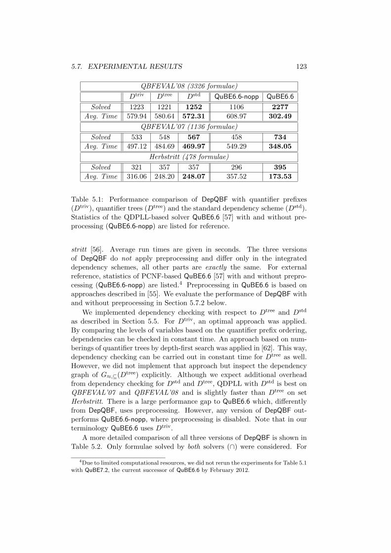
5.7. EXPERIMENTAL RESULTS 123
QBFEVAL’08 (3326 formulae)
Dtriv Dtree Dstd QuBE6.6-nopp QuBE6.6
Solved 1223 1221 1252 1106 2277
Avg. Time 579.94 580.64 572.31 608.97 302.49
QBFEVAL’07 (1136 formulae)
Solved 533 548 567 458 734
Avg. Time 497.12 484.69 469.97 549.29 348.05
Herbstritt (478 formulae)
Solved 321 357 357 296 395
Avg. Time 316.06 248.20 248.07 357.52 173.53
Table 5.1: Performance comparison of DepQBF with quantifier prefixes(Dtriv), quantifier trees (Dtree) and the standard dependency scheme (Dstd).Statistics of the QDPLL-based solver QuBE6.6 [57] with and without pre-processing (QuBE6.6-nopp) are listed for reference.
stritt [56]. Average run times are given in seconds. The three versionsof DepQBF do not apply preprocessing and differ only in the integrateddependency schemes, all other parts are exactly the same. For externalreference, statistics of PCNF-based QuBE6.6 [57] with and without prepro-cessing (QuBE6.6-nopp) are listed.4 Preprocessing in QuBE6.6 is based onapproaches described in [55]. We evaluate the performance of DepQBF withand without preprocessing in Section 5.7.2 below.
We implemented dependency checking with respect to Dtree and Dstd
as described in Section 5.5. For Dtriv, an optimal approach was applied.By comparing the levels of variables based on the quantifier prefix ordering,dependencies can be checked in constant time. An approach based on num-berings of quantifier trees by depth-first search was applied in [62]. This way,dependency checking can be carried out in constant time for Dtree as well.However, we did not implement that approach but inspect the dependencygraph of G≈,⊆(Dtree) explicitly. Although we expect additional overheadfrom dependency checking for Dstd and Dtree, QDPLL with Dstd is best onQBFEVAL’07 and QBFEVAL’08 and is slightly faster than Dtree on setHerbstritt. There is a large performance gap to QuBE6.6 which, differentlyfrom DepQBF, uses preprocessing. However, any version of DepQBF out-performs QuBE6.6-nopp, where preprocessing is disabled. Note that in ourterminology QuBE6.6 uses Dtriv.
A more detailed comparison of all three versions of DepQBF is shown inTable 5.2. Only formulae solved by both solvers (∩) were considered. For
4Due to limited computational resources, we did not rerun the experiments for Table 5.1with QuBE7.2, the current successor of QuBE6.6 by February 2012.

124 CHAPTER 5. QDPLL AND DEPENDENCY SCHEMES
QBFEVAL’08 (solved only)
Dtriv ∩Dtree Dtriv ∩Dstd Dtree ∩Dstd
solved 1172 1196 1206
time 23.15 26.68 23.73 25.93 25.63 22.37
implied/assigned 90.4% 90.7% 88.6% 90.5% 90.9% 92.1%
backtracks 32431 27938 34323 31085 25106 26136
sat. cubes/sol. 1.8% 2.9% 1.8% 2.6% 3.6% 3.1%
learnt constr. size 157 99 150 96 102 95
QBFEVAL’07 (solved only)
solved 501 513 537
time 31.22 34.46 32.76 32.66 33.31 28.33
implied/assigned 89.0% 89.2% 87.7% 89.5% 89.9% 91.9%
backtracks 35131 22334 39906 26362 21945 22323
sat. cubes/sol. 4.0% 10.0% 4.0% 9.5% 10.8% 9.9%
learnt constr. size 150 101 134 113 100 96
Herbstritt (solved only)
solved 312 308 348
time 26.86 19.28 24.41 19.28 20.46 20.83
implied/assigned 96.6% 97.4% 96.2% 97.4% 97.4% 97.4%
backtracks 26565 1329 26733 1482 1615 1800
sat. cubes/sol. 0% 0% 0% 0% 0% 0%
learnt constr. size 174 306 173 323 407 410
Table 5.2: Comparing combinations of DepQBF with quantifier prefixes(Dtriv), quantifier trees (Dtree) and the standard dependency scheme (Dstd)on the intersection of solved formulae.
example, in section “Dtriv∩Dstd”, the left column reports statistics for Dtriv,the right one for Dstd. Average values are given for run time in seconds,ratio of implications among all assignments, number of backtracks, ratioof satisfied learnt cubes among all identified solutions and size (number ofliterals) of learnt constraints.
In general, Dtriv is slightly faster on the QBFEVAL sets. However, Dtriv
yields more backtracks than Dtree and Dstd on all sets. On set Herbstritt,the difference in this respect is a factor of up to 20. Dtree and Dstd, bothbeing more refined than Dtriv, produce smaller learnt constraints on theQBFEVAL sets. Furthermore, Dstd triggers more implications in QBCP onall sets and Dtriv fewer satisfied learnt cubes. These effects can be attributedto unit literal detection and constraint reduction, which benefit from morerefined dependency schemes.
The results from Table 5.2 indicate that moving from Dtriv to more

5.7. EXPERIMENTAL RESULTS 125
refined dependency schemes incurs run time overhead (except on set Herb-stritt), but also allows QDPLL to produce shorter runs in terms of back-tracks. Dependency checking is not a constant-time operation in generaldependency DAGs used to represent Dtree and Dtriv, for example. Instead,such DAGs are inspected explicitly as described in Section 5.5. Addition-ally, maintaining the set of decision candidates as described in Section 5.4is more expensive than with respect to Dtriv. As indicated in Table 5.1,QDPLL still seems to profit from using more refined dependency schemessuch as Dtree and Dstd.
In order to assess both the costs and benefits of combining dependencyschemes with QDPLL in more detail, we carried out the following experi-ment. In addition to the dependency DAG which is used to represent thedependency scheme in QDPLL, called primary DAG G1, another depen-dency scheme is represented by a secondary dependency DAG G2. Thesecondary DAG G2 is independent from G1 and used in parallel for statisti-cal computations only. The idea is to compare the effects of using differentdependency schemes dynamically, that is during a run of QDPLL.
This setup allows to compute more fine-grain statistics than overall runtime or number of backtracks, as listed in Tables 5.1 and 5.2. During a runof QDPLL, it is interesting to compare the numbers of decision candidates(DC ) by Definition 5.4.1 with respect to G1 and G2 under the current as-signment. These numbers are computed each time before a decision is madeand reflect the degree of freedom resulting from more refined dependencyschemes. For example, we expect Dstd to allow more decision candidatesthan Dtriv and Dtree. Apart from that, we want to measure the averagecosts of dependency checking and decision candidate maintenance for de-pendency DAGs resulting from different dependency schemes.
For G1 and G2, we compared Dstd to Dtriv and Dtree , where all fourcombinations were run to even out biased solver behaviour. Due to limitedcomputational resources, we did not compare Dtriv to Dtree and omittedQBFEVAL’07.
Table 5.3 shows the results of the experiments described above with atime out of 900 seconds. DepQBF maintains two dependency DAGs G1 (pri-mary) and G2 (secondary) in parallel. For example, in section “DtrivnDstd”,G1 is obtained from Dtriv (left column), G2 from Dstd (right column). Notethat columns “Dstd” in “Dstd nDtriv” and “Dstd nDtree” are incomparablesince G2 influences run time, that is “Dstd nDtriv” and “Dstd nDtree” mayrun at different speeds. We compare the numbers of decision candidates (setDC as introduced in Section 5.4) when using different dependency schemes.Each time before decision making, the size of the set DC under the cur-rent assignment is computed. Row “DC/d” shows the total sum of decisioncandidates over the total number of decisions in the benchmark set after atmost 900 seconds run time.
As indicated for sets QBFEVAL’08 and Herbstritt, the difference in DC

126 CHAPTER 5. QDPLL AND DEPENDENCY SCHEMES
QBFEVAL’08 (3326 formulae)
Dtriv nDstd Dstd nDtriv
DC/d 13801.0 13801.6 11409.7 11409.0
DC-updt. 3.23 3.16 3.30 3.43
≺ 1 - 6.21 -
C-red. 1.18 - 535.62 -
Herbstritt (478 formulae)
DC/d 21.3 26.55 20.14 20.13
Pan (384 formulae) ∪ Sorting-Networks (84 formulae)
DC/d 75.81 93.87 117.50 109.66
QBFEVAL’08 (3326 formulae)
Dtree nDstd Dstd nDtree
DC/d 8932.5 8933.0 15625.6 15625.3
DC-updt. 3.38 3.37 3.30 3.36
≺ 7.15 - 6.26 -
C-red. 538.30 - 540.94 -
Herbstritt (478 formulae)
DC/d 20.67 20.67 20.16 20.16
Pan (384 formulae) ∪ Sorting-Networks (84 formulae)
DC/d 86.89 86.90 120.03 119.98
Table 5.3: Comparing the costs and benefits of Dtriv, Dtree and Dstd inDepQBF on the intersection of solved formulae.
statistics is very small in general, sometimes less than one candidate onaverage per decision. However, it seems that this is already enough forQDPLL with Dstd to outperform Dtriv and Dtree by Table 5.1. Further, DCstatistics are also family-dependent, as shown by the results for sets Panand Sorting-Networks in Table 5.3.
Additionally, we measured the costs of integrating dependency DAGsin QDPLL. Cost statistics in Table 5.3 (rows “DC-updt.”, “≺”, “C-red.”)are correlated to the number of equivalence classes of variables that haveto be visited (pointer dereferences) when inspecting a dependency DAG.Such inspections are necessary for decision candidate management and de-pendency checking as described in Sections 5.4 and 5.5. Average costs arelisted for (un)assigning an assignment as defined in Section 5.4 to updatethe set DC of decision candidates (DC-updt.), for constraint reduction asneeded in QBCP and for the stop criterion during constraint learning (≺),and separately for constraint reduction per Q-resolution operation (C-red.).
5.7. EXPERIMENTAL RESULTS 127
The latter are irrelevant for G2 (“-”).
Average costs for dependency checking and (un)assigning variables forupdating DC before decisions or during backtracking are small. This is dueto equivalence classes in dependency DAGs. However, costs of constraint re-duction during constraint learning are very high for Dtree and Dstd. Theseeffects are closely related to implementation. When using Dtriv, all con-straints C can be kept sorted according to prefix ordering, which allows forefficient constraint reduction. This was implemented in DepQBF with Dtriv
and is reflected by low costs in Table 5.3. In general, such an approach is im-possible for arbitrary dependency schemes. Instead, we reduce constraintsbased on classes in the dependency DAG for Dtree and Dstd. Classes arecollected for all literals in a constraint C before reduction, where the size ofC (particularly for cubes) can be large. This effort is included in the statis-tics shown in Table 5.3. Despite that overhead in Dtree and Dstd, overallperformance by Tab. 5.1 is still better than with Dtriv.
5.7.2 General Performance Analysis
Experimental results in the previous sections illustrate that combiningQDPLL with dependency schemes other than Dtriv potentially increasesthe performance. Despite additional overhead for constructing and main-taining dependency DAGs, more refined dependency schemes such as Dtree
and Dstd might allow to detect more implications and produce shorter learntconstraints. We conclude that the use of an arbitrary dependency schemeD where D ⊂ Dtriv can pay off in practice, provided that the augmentedcompressed dependency graph G≈,⊆(D) by Definition 4.2.8 on page 60 isimplemented carefully.
In this section, we analyze the general performance of DepQBF withDstd.5 We address the effects of optimizations described in Section 5.6.2and compare DepQBF to other solvers, with and without preprocessing.Parts of the experimental results in this section were previously publishedin [21, 84, 86] and reported in related conference talks.
Improvements of QDPLL
Table 5.4 shows experimental results of DepQBF 0.1 with Dstd where opti-mizations of QDPLL such as pure literal detection, restarts and assignmentcaching were disabled. The time limit was set to 900 seconds. DepQBFperforms best if all of these techniques are enabled. Switching off restartsin DepQBF-nr affects the number of solved satisfiable instances negatively.Without assignment caching but with restarts (DepQBF-nc), the perfor-mance is even worse. DepQBF performs worst if neither restarts nor as-
5Setup for all experiments reported in Section 5.7.2, unless stated otherwise: UbuntuLinux 9.04, Intel R© [email protected] GHz, 7 GB/900 seconds memory and time limit.

128 CHAPTER 5. QDPLL AND DEPENDENCY SCHEMES
QBFEVAL’10 (568 formulae)
Solved Avg. Time SAT UNSAT
DepQBF 370 337.10 165 205
DepQBF-nr 360 352.33 154 206
DepQBF-nc 350 384.66 157 193
DepQBF-np 345 398.12 141 204
DepQBF-ncnr 340 400.24 147 193
Table 5.4: The influence of optimization such as restarts (disabled inDepQBF-nr), assignment caching (disabled in DepQBF-nc) and pure literaldetection (disabled in DepQBF-np) on the performance of DepQBF 0.1.
QBFEVAL’10 (568 formulae) – with preprocessing
Solved Avg. Time SAT UNSAT
Bloqqer + QxBF + DepQBF 468 197.31 (16.47) 224 244Bloqqer + DepQBF 466 198.50 (7.69) 223 243
QuBE7.2 435 264.70 (–) 202 233QxBF+ DepQBF 378 323.19 (7.21) 167 211
QBFEVAL’10 (568 formulae) – without preprocessing
DepQBF 372 334.60 166 206QuBE7.2-nopp 319 431.47 144 175
Nenofex 211 573.65 103 108Quantor 3.0 203 590.15 99 104squolem 2.02 124 708.80 53 71
Table 5.5: DepQBF and other solvers with and without preprocessing.
signment caching is enabled (DepQBF-ncnr). Pure literal detection, whichis disabled in DepQBF-np, has a substantial negative influence on the num-ber of solved satisfiable instances. This is interesting because modern SATsolvers typically do not detect pure literals. As argued in Section 5.3.4, pureliteral detection during QBCP might cause additional constraints to becomeunit. As future work, we want to analyze the actual effects in detail.
Preprocessing and Other Solvers
DepQBF version 0.1 [84] using Dstd took first place in QBFEVAL’10 [100].The lower part of Table 5.5 shows statistics for an improved, non-public ver-sion of DepQBF and other solvers without preprocessing. In fact, QuBE isthe only solver listed in Table 5.5 which applies preprocessing natively [55].Both DepQBF and QuBE are search-based solvers relying on QDPLL withconstraint learning whereas all other solvers eliminate variables. On theconsidered benchmark set, QDPLL outperforms variable elimination. Withrespect to QDPLL, DepQBF performs better than QuBE7.2-nopp where pre-processing was disabled. However, there is a huge performance gap between
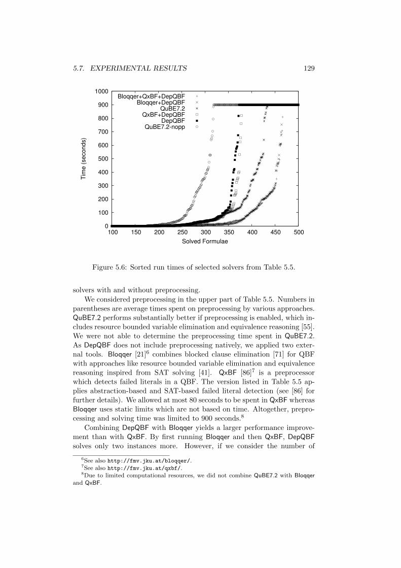
5.7. EXPERIMENTAL RESULTS 129
0
100
200
300
400
500
600
700
800
900
1000
100 150 200 250 300 350 400 450 500
Tim
e (
seconds)
Solved Formulae
Bloqqer+QxBF+DepQBFBloqqer+DepQBF
QuBE7.2QxBF+DepQBF
DepQBFQuBE7.2-nopp
Figure 5.6: Sorted run times of selected solvers from Table 5.5.
solvers with and without preprocessing.
We considered preprocessing in the upper part of Table 5.5. Numbers inparentheses are average times spent on preprocessing by various approaches.QuBE7.2 performs substantially better if preprocessing is enabled, which in-cludes resource bounded variable elimination and equivalence reasoning [55].We were not able to determine the preprocessing time spent in QuBE7.2.As DepQBF does not include preprocessing natively, we applied two exter-nal tools. Bloqqer [21]6 combines blocked clause elimination [71] for QBFwith approaches like resource bounded variable elimination and equivalencereasoning inspired from SAT solving [41]. QxBF [86]7 is a preprocessorwhich detects failed literals in a QBF. The version listed in Table 5.5 ap-plies abstraction-based and SAT-based failed literal detection (see [86] forfurther details). We allowed at most 80 seconds to be spent in QxBF whereasBloqqer uses static limits which are not based on time. Altogether, prepro-cessing and solving time was limited to 900 seconds.8
Combining DepQBF with Bloqqer yields a larger performance improve-ment than with QxBF. By first running Bloqqer and then QxBF, DepQBFsolves only two instances more. However, if we consider the number of
6See also http://fmv.jku.at/bloqqer/.7See also http://fmv.jku.at/qxbf/.8Due to limited computational resources, we did not combine QuBE7.2 with Bloqqer
and QxBF.
130 CHAPTER 5. QDPLL AND DEPENDENCY SCHEMES
instances that were solved solely by preprocessing then it turns out thatQxBF has a considerable positive effect. QxBF solves 30 and Bloqqer 148instances. The combination Bloqqer + QxBF as applied in Table 5.5 solves172 instances, which amounts to 36.7% of the 468 instances solved by De-pQBF combined with Bloqqer and QxBF. With respect to the full set of 568instances, 30% are solved solely by preprocessing.
The results in Table 5.5 point out that QDPLL without preprocessingas in Figure 5.1 on page 89 is by far not competitive. Further experimentalevaluation is necessary to analyze the actual role and interplay of individualpreprocessing approaches applied in QuBE7.2, Bloqqer and QxBF.
5.8 Summary
In this chapter, we considered combinations of QDPLL and dependencyschemes. The classical variant of QDPLL implicitly relies on the quantifierprefix of the given PCNF, that is the trivial dependency scheme Dtriv. Weextended QDPLL to arbitrary dependency schemes. We may think of a de-pendency scheme D as an additional parameter of QDPLL. By analyzingthe core parts of QDPLL, we figured out that the decision making, depen-dency checking and constraint reduction in QDPLL must be adapted fromDtriv to arbitrary schemes D. Apart from that, the high-level workflow ofthe algorithm does not change. Hence the theoretical framework of depen-dency schemes introduced in Chapter 3 fits seamlessly into QDPLL, whichis a state-of-the-art approach in QBF solving.
In general, it is important to apply one and the same dependency schemeD throughout all parts of QDPLL. Our generalization of QDPLL is indepen-dent from the actual dependency scheme. That is, approaches of decisionmaking or dependency checking as presented in Sections 5.4 and 5.5 applyto arbitrary dependency schemes.
In our experimental analysis, QDPLL with the standard dependencyscheme Dstd outperformed combinations of QDPLL with Dtriv and Dtree,which relies on quantifier trees obtained by mini-scoping. We representdependency schemes as augmented compressed dependency graphs by Def-inition 4.2.8 on page 60. Despite additional overhead compared to Dtriv,QDPLL with Dtree and Dstd showed better overall performance.
Chapter 6
Summary and Outlook
The presence of universally and existentially quantified variables in quanti-fied Boolean formulae (QBF) gives rise to dependencies between variables.If variable y depends on another variable x in some QBF ψ, then in generaly must not be assigned before x during a semantical evaluation of ψ. Thusvariable dependencies restrict the freedom of QBF solvers to assign valuesto variables. Violations of such restrictions might cause QBF solvers to pro-duce incorrect results. This property is a crucial difference to propositionallogic (SAT). SAT solvers are free to assign any variables, all of which are(implicitly) existentially quantified.
Variable dependencies are intrinsic to QBF. For example, given a QBFψ in prenex CNF (PCNF), the classical QDPLL algorithm requires to assignvariables “from left to right” in the ordering of the quantifier prefix of ψ. Ifvariable x occurs to the left of some other, differently quantified variable yin the prefix, then y is regarded to depend on x. However, there are QBFswhere dependencies of that kind are spurious. In this case, even if a QBFsolver assigns y before x during semantical evaluation, the result returned bythe solver will be correct. Thus spurious dependencies impose unnecessaryrestrictions to QBF solvers.
We considered dependency schemes as a means of analyzing variabledependencies in PCNFs. A dependency scheme D for a given PCNF ψis a binary relation over the set of variables in ψ such that if (x, y) 6∈ Dthen y does not depend on x. The theoretical framework of dependencyschemes allows to figure out precisely all dependencies between variables,thereby entirely avoiding spurious ones. However, obtaining such optimalinformation on dependencies is at least as hard as QBF solving and thereforenot feasible in practice.
A trade-off has to be made between optimality and efficiency of com-putation of dependency schemes. Consequently, dependency schemes whichcan be computed efficiently, that is in polynomial time, necessarily con-tain spurious dependencies. Dependency schemes can be compared with
131
132 CHAPTER 6. SUMMARY AND OUTLOOK
respect to the amount of independence that can be identified. We pre-sented the tractable dependency schemes Dtriv, Dtree and Dstd. All threecan be computed by analyzing the syntactic structure of a given PCNF.We pointed out that the standard dependency scheme Dstd never containsmore spurious dependencies than Dtree and Dtriv, which are based on tree-like quantifier structure present in PCNFs and on the quantifier prefixes,respectively. Since Dstd ⊆ Dtree ⊆ Dtriv, Dstd potentially allows more free-dom on a given PCNF than Dtree and Dtriv. Differently from Dtree, Dstd canbe computed deterministically. Therefore, we combined Dstd with search-based QBF solvers relying on QDPLL. This way, QDPLL can profit fromadditional information on independent variables.
In order to apply some tractable dependency scheme D in QDPLL, firstD must be computed and also represented efficiently. Since D is a binaryrelation over the set V of variables in a given PCNF, D contains |V |·|V | pairsof variables in the worst case. Hence it might be prohibitive to represent Dexplicitly as a graph, for example, if the value of |V | is large.
We presented a way to compute and represent the standard dependencyscheme Dstd efficiently. By partitioning the set of variables into equivalenceclasses with respect to dependency information, we obtained a compactdependency graph over classes rather than individual variables. Althoughour algorithms are tailored towards Dstd, they might give insights into newalgorithms to construct graphs for other dependency schemes. Further, theconcept of compact dependency graphs based on equivalence classes can beused to represent arbitrary dependency schemes. Experimental analysis oninstances from QBF evaluations showed that the time for computing andrepresenting Dstd by our approaches is negligible.
Relying on compact dependency graphs as a general way to representdependency schemes efficiently, we considered to combine QDPLL with ar-bitrary dependency schemes. The original variant of QDPLL implicitly usesDtriv where variables must be assigned in the ordering of the quantifier prefixof the given PCNF. Thus combinations of QDPLL with dependency schemesare generalizations of classical QDPLL rather than novel approaches.
We described QDPLL and analyzed its core parts. It turned out thatarbitrary dependency schemes can seamlessly be integrated into QDPLLwithout the need to change its high-level workflow. The crucial parts aremaintenance of decision candidates and dependency checking. A decisioncandidate is a variable which, given the current assignment generated byQDPLL, can safely be assigned as decision variable without risking incor-rect results. Maintaining decision candidates with respect to arbitrary de-pendency schemes generalizes the “left-to-right” policy of Dtriv in classicalQDPLL. Given two variables x and y, dependency checking finds out if(x, y) ∈ D, where D is the dependency scheme applied in QDPLL. Thiskind of information is necessary for constraint reduction and for the genera-tion of asserting constraints during constraint learning. In general, one and

133
the same dependency scheme D must be used in all parts of QDPLL.
We evaluated combinations of QDPLL with dependency schemes Dtriv,Dtree and Dstd in a variant of our QBF solver DepQBF. Experimental resultson instances from QBF competitions show that QDPLL with Dstd outper-forms both Dtree and Dtriv. However, the performance was only slightlybetter than with Dtree. Still we favour Dstd because it can be constructeddeterministically and is more refined than Dtree, that is Dstd ⊆ Dtree.
We observed more implications, shorter learnt constraints and fewerbacktracks for QDPLL with Dstd or Dtree compared to Dtriv. These observa-tions clearly motivate further research related to dependency schemes whichrefine Dstd such as the triangle [113] or quadrangle dependency scheme [51].
Despite promising experimental results, combining QDPLL with depen-dency schemes other than Dtriv is not free of costs. Whereas checking ifvariable y depends on another variable x by Dtriv is a constant time opera-tion, in general dependency graphs have to be inspected explicitly for otherdependency schemes. The approach presented in [62], which allows for de-pendency checking based on Dtree in contant time as well, cannot be appliedfor arbitrary dependency schemes. We presented approaches based on com-pact dependency graphs which allow to keep the overhead of dependencychecking and decision candidate maintenance low.
It is important to note that dependency schemes are in fact not a newconcept. Rather, they are inherent to QBF semantics. Implicitly, classicaldescriptions of QDPLL [30] apply the ordering of quantifier prefixes in givenPCNFs. Such orderings correspond exactly to the trivial dependency schemeDtriv. The theoretical framework of dependency schemes [111, 112, 113] al-lows to generalize the classical QDPLL algorithm naturally from Dtriv toarbitrary dependency schemes. There is a close interplay between depen-dency schemes and QBF semantics. Therefore, we believe that dependencyschemes D which strictly refine Dstd, that is D ⊂ Dstd, have the potentialto improve the state-of-the-art in QBF solving considerably.
Outlook
Although we pointed out the potential of using advanced dependency schemes,QDPLL still suffers from severe drawbacks. First, constraint learning isbased on resolution over clauses or cubes, which is applied only heuristi-cally. Constraint learning produces a constraint by selecting pivot variablesfor resolution with respect to the current assignment that was generated byQDPLL. Variable dependencies restrict the set of assignments that can beenumerated by QDPLL. Therefore, pivot selection heuristics in constraintlearning are also restricted by variable dependencies. As illustrated by Ex-ample 3.3.6 on page 34, restricted constraint learning could miss short proofswhich otherwise could be found with general resolution strategies.
134 CHAPTER 6. SUMMARY AND OUTLOOK
Further, the selection of pivot variables in constraint learning is biasedtowards quantifier types. When generating a clause, all pivot variables areexistential. This is due to the fact that clause learning relies on antecedentsof existential unit literals detected in clauses during QBCP. Dually, learntcubes are generated by resolutions over universal variables. Although thesepivot-restricted variants of resolution are complete [27], we conjecture thatallowing clause (cube) resolutions over universal (existential) variables couldproduce shorter proofs in certain cases. In general, it would be interestingto address proof theoretic properties of QDPLL with dependency schemes.
From the practical side, most QDPLL-based QBF solvers lack featuresfor incremental solving. In contrast to that, support for incremental solvingis common in modern SAT solvers like MiniSAT or PicoSAT, for example.In bounded model checking (BMC) [19] based on QBF [14, 73], a sequenceψ1, ψ2, . . . , ψn of PCNFs is solved where the structure of ψi is typicallyrelated to the previously solved instance ψi−1. A QBF solver could re-useinformation learnt from ψi−1 in order to solve ψi. An approach for BMC ofblack box designs relying on a specific variant of incremental QBF solvingwas presented in [88], but we are not aware of a general-purpose incrementalQBF solver. Further challenges arise from the use of dependency schemesother than Dtriv in an incremental setting. So far it is not clear how toefficiently update dependency information which is represented by compactdependency graphs if clauses are added to or removed from an instance.Learnt constraints might have to be discarded if the underlying dependencyscheme in QDPLL is modified.
We have not yet considered the role of dependency schemes in prepro-cessing like blocked clause elimination [21] or failed literal detection [86]for QBF. Dependency schemes might also give rise to smaller certificatesif approaches based on resolution proofs are used [8, 95, 105]. In general,optimizations of DPLL which have been proved very effective in SAT solv-ing could be ported to QDPLL for QBF. For example, as experimentalresults show, our variants of restarts and assignment caching inspired bySAT solvers improve the performance of our solver DepQBF considerably.Further promising approaches are clause minimization techniques like [122],to take a single example.
By the year 2012, there have been about 20 years of active research onpractical SAT solving. Continuous improvements led to robust SAT solversbeing capable of effectively tackling instances with thousands of variablesand millions of clauses. In contrast to that, we are still waiting for thebreakthrough of QBF. The success of SAT solving is driven both by the ap-plication side and the implementation side. We believe that similar synergyeffects are necessary to boost QBF solving and applications. If we take theadvent of the classical QDPLL algorithm [30] in the year 1998 as a startingpoint, then we have about 10 more years to bring QBF solving within a timespan of 20 years to where SAT solving is now in the year 2012.
Appendix A
A.1 Cube Learning
A.1.1 Pivot Selection for Cubes
1. Let R be the current resolvent (line p = get pivot (R) in Figure 5.5).
2. Let P (R) := {y | y = v(l), l ∈ R, q(l) = ∀, am(l) = U} be the set ofuniversal variables in R which were assigned by the unit literal rule.Set P (R) contains all potential pivot variables to be selected.
3. Select p ∈ P (R) such that p has the maximum trail level of variablesin P (R), that is tl(p) = max ({tl(y) | y ∈ P (R)}).
4. If the tentative resolvent R⊗R′ of R and the antecedent R′ = ante(p)of p does not contain complementary literals, then variable p is thepivot for the next application of Q-resolution (line R = constraint res
(R, p, R’) in Figure 5.5).
5. Otherwise, if {x,¬x} ⊆ (R ⊗ R′) for some variable x ∈ R then analternative pivot is selected as follows.
(a) Let x be one of the variables which occur both positively andnegatively in the tentative resolvent (R⊗R′).
(b) Let P ′(R) := P (R) \ {y | y ∈ P (R), x 6≺ y} \ {y | y ∈ P (R),{x′,¬x′} ⊆ R ⊗ R′′ where R′′ = ante(y)}. In addition to therestrictions on set P (R) as defined above, the set P ′(R) containsonly universal variables which depend on variable x. Further, theresolvent of R and the antecedent of variables in P ′(R) does notcontain complementary literals.
(c) Select p ∈ P ′(R) such that p has the maximum trail level ofvariables in P ′(R), that is tl(p) = max ({tl(y) | y ∈ P ′(R)}).
(d) Variable p is the pivot for the next application of Q-resolution(line R = constraint res (R, p, R’)).
135
136 APPENDIX A.
Definition A.1.1 ([53, 133]). Given the current resolvent R. Let m :=max ({d | d = dl(y), y = v(l), l ∈ R, q(l) = ∀}) be the largest decision levelof universal variables in R. Clause R is asserting if and only if:
1. There is exactly one literal l ∈ R with q(l) = ∀ such that dl(v(l)) = m.Let va := v(l).
2. The decision variable at decision level m is universal.
3. Variables where va depends on must be assigned at decision levelssmaller than m = dl(va), that is ∀y ∈ {y | y = v(l), l ∈ R, y ≺ va} :DL(y) < m.
If R is asserting then variable va is asserted by R.
Definition A.1.2. Given an asserting clause R by Definition A.1.1 and thevariable va asserted by R.
1. Let DL∀(R) := {d | d = dl(y), y = v(l), l ∈ R, q(l) = ∀, y 6= va} be theset of decision levels of universal variables in R, excluding va.
2. Let DL≺(R) := {d | d = dl(y), y = v(l), l ∈ R, y ≺ va} be the set ofdecision levels of variables in R where va depends on.
3. The asserting level da with respect to R is da := max (DL∀(R) ∪DL≺(R)).
A.2 Brief Biography
Personal Details
Name: Florian Matthias Lonsing
Private Address:Im Weideland 14060 LeondingAustria
Date and Place of Birth: 12th April 1983 in Linz, Austria
Research
Feb. 2008 – Feb. 2012
Research and Teaching Assistant at the In-stitute for Formal Models and Verification(FMV), Johannes Kepler Universitat Linz.Research Interests: QBF, SAT, Formal Veri-fication.Website: http://fmv.jku.at/lonsing/

A.2. BRIEF BIOGRAPHY 137
Education
Feb. 2008 – Apr. 2012Doctorate Computer Science,Johannes Kepler Universitat Linz
Oct. 2005 – Feb. 2008Master Computer Science,Johannes Kepler Universitat Linz
Oct. 2002 – Oct. 2005Bachelor Computer Science,Johannes Kepler Universitat Linz
Okt. 2001 – Apr. 2002 Military Service
Sep. 1993 – Jun. 2001Grammar School (Allgemeinbildende HohereSchule) in Linz
Sep. 1989 – Jul. 1993 Primary School in Linz

138 APPENDIX A.

Bibliography
[1] A. V. Aho, M. R. Garey, and J. D. Ullman. The Transitive Reductionof a Directed Graph. SIAM J. Comput., 1(2):131–137, 1972.
[2] B. Aspvall, M. F. Plass, and R. E. Tarjan. A Linear-Time Algorithmfor Testing the Truth of Certain Quantified Boolean Formulas. Inf.Process. Lett., 8(3):121–123, 1979.
[3] G. Audemard, J. Lagniez, B. Mazure, and L. Sais. On Freezing andReactivating Learnt Clauses. In Sakallah and Simon [110], pages 188–200.
[4] G. Audemard and L. Sais. A Symbolic Search Based Approach forQuantified Boolean Formulas. In Bacchus and Walsh [7], pages 16–30.
[5] G. Audemard and L. Simon. Predicting Learnt Clauses Quality inModern SAT Solvers. In C. Boutilier, editor, IJCAI, pages 399–404,2009.
[6] A. Ayari and D. A. Basin. QUBOS: Deciding Quantified BooleanLogic Using Propositional Satisfiability Solvers. In M. Aagaard andJ. W. O’Leary, editors, FMCAD, volume 2517 of LNCS, pages 187–201. Springer, 2002.
[7] F. Bacchus and T. Walsh, editors. Theory and Applications of Satisfi-ability Testing, 8th International Conference, SAT 2005, St. Andrews,UK, June 19-23, 2005, Proceedings, volume 3569 of LNCS. Springer,2005.
[8] V. Balabanov and J. R. Jiang. Resolution Proofs and Skolem Func-tions in QBF Evaluation and Applications. In G. Gopalakrishnanand S. Qadeer, editors, CAV, volume 6806 of LNCS, pages 149–164.Springer, 2011.
[9] P. Beame, H. A. Kautz, and A. Sabharwal. Towards Understandingand Harnessing the Potential of Clause Learning. J. Artif. Intell. Res.(JAIR), 22:319–351, 2004.
139

140 BIBLIOGRAPHY
[10] E. Ben-Sasson, R. Impagliazzo, and A. Wigderson. Near-Optimal Sep-aration of Treelike and General Resolution. Electronic Colloquium onComputational Complexity (ECCC), 7(5), 2000.
[11] M. Benedetti. Extracting Certificates from Quantified Boolean For-mulas. In L. P. Kaelbling and A. Saffiotti, editors, IJCAI, pages 47–53.Professional Book Center, 2005.
[12] M. Benedetti. Quantifier Trees for QBFs. In Bacchus and Walsh [7],pages 378–385.
[13] M. Benedetti. sKizzo: A Suite to Evaluate and Certify QBFs. InR. Nieuwenhuis, editor, CADE, volume 3632 of LNCS, pages 369–376.Springer, 2005.
[14] M. Benedetti and H. Mangassarian. QBF-Based Formal Verification:Experience and Perspectives. JSAT, 5:133–191, 2008.
[15] A. Bhalla, I. Lynce, J. T. de Sousa, and J. Marques-Silva. Heuristic-Based Backtracking Relaxation for Propositional Satisfiability. Jour-nal of Automated Reasoning (JAR), 35(1-3):3–24, 2005.
[16] A. Biere. Resolve and Expand. In H. H. Hoos and D. G. Mitchell,editors, SAT (Selected Papers), volume 3542 of LNCS, pages 59–70.Springer, 2004.
[17] A. Biere. Adaptive Restart Strategies for Conflict Driven SAT Solvers.In Buning and Zhao [29], pages 28–33.
[18] A. Biere. PicoSAT Essentials. JSAT, 4(2-4):75–97, 2008.
[19] A. Biere, A. Cimatti, E. M. Clarke, and Y. Zhu. Symbolic ModelChecking without BDDs. In R. Cleaveland, editor, TACAS, volume1579 of LNCS, pages 193–207. Springer, 1999.
[20] A. Biere, M. Heule, H. van Maaren, and T. Walsh, editors. Handbookof Satisfiability, volume 185 of Frontiers in Artificial Intelligence andApplications. IOS Press, 2009.
[21] A. Biere, F. Lonsing, and M. Seidl. Blocked Clause Elimination forQBF. In N. Bjørner and V. Sofronie-Stokkermans, editors, CADE,volume 6803 of LNCS, pages 101–115. Springer, 2011.
[22] M. L. Bonet, J. L. Esteban, N. Galesi, and J. Johannsen. On theRelative Complexity of Resolution Refinements and Cutting PlanesProof Systems. SIAM J. Comput., 30(5):1462–1484, 2000.
[23] R. E. Bryant. Graph-Based Algorithms for Boolean Function Manip-ulation. IEEE Trans. Computers, 35(8):677–691, 1986.
BIBLIOGRAPHY 141
[24] U. Bubeck. Model-Based Transformations for Quantified Boolean For-mulas, volume 329 of Dissertations in Artificial Intelligence. IOSPress, 2010.
[25] U. Bubeck and H. Kleine Buning. Bounded Universal Expansion forPreprocessing QBF. In Marques-Silva and Sakallah [89], pages 244–257.
[26] H. Kleine Buning and U. Bubeck. Theory of Quantified Boolean For-mulas. In Biere et al. [20], pages 735–760.
[27] H. Kleine Buning, M. Karpinski, and A. Flogel. Resolution for Quan-tified Boolean Formulas. Inf. Comput., 117(1):12–18, 1995.
[28] H. Kleine Buning and T. Lettmann. Propositional Logic: Deductionand Algorithms. Cambridge University Press, New York, NY, USA,1999.
[29] H. Kleine Buning and X. Zhao, editors. Theory and Applications ofSatisfiability Testing - SAT 2008, 11th International Conference, SAT2008, Guangzhou, China, May 12-15, 2008. Proceedings, volume 4996of LNCS. Springer, 2008.
[30] M. Cadoli, A. Giovanardi, and M. Schaerf. An Algorithm to EvaluateQuantified Boolean Formulae. In AAAI/IAAI, pages 262–267, 1998.
[31] M. Cadoli, M. Schaerf, A. Giovanardi, and M. Giovanardi. An Algo-rithm to Evaluate Quantified Boolean Formulae and Its ExperimentalEvaluation. J. Autom. Reasoning, 28(2):101–142, 2002.
[32] P. Chatalic and L. Simon. Multi-resolution on Compressed Sets ofClauses. In ICTAI, pages 2–10. IEEE Computer Society, 2000.
[33] P. Chatalic and L. Simon. ZRES: The Old Davis-Putman ProcedureMeets ZBDD. In D. A. McAllester, editor, CADE, volume 1831 ofLNCS, pages 449–454. Springer, 2000.
[34] S. A. Cook. The Complexity of Theorem-Proving Procedures. InSTOC, pages 151–158. ACM, 1971.
[35] S. A. Cook and R. A. Reckhow. The Relative Efficiency of Proposi-tional Proof Systems. J. Symb. Log., 44(1):36–50, 1979.
[36] A. Darwiche and K. Pipatsrisawat. Complete Algorithms. In Biereet al. [20], pages 99–130.
[37] M. Davis, G. Logemann, and D. Loveland. A Machine Program forTheorem-proving. Commun. ACM, 5(7):394–397, 1962.
142 BIBLIOGRAPHY
[38] M. Davis and H. Putnam. A Computing Procedure for QuantificationTheory. J. ACM, 7(3):201–215, 1960.
[39] T. Boy de la Tour. An Optimality Result for Clause Form Translation.J. Symb. Comput., 14(4):283–302, 1992.
[40] N. Dershowitz, Z. Hanna, and A. Nadel. A Clause-Based Heuristic forSAT Solvers. In Bacchus and Walsh [7], pages 46–60.
[41] N. Een and A. Biere. Effective Preprocessing in SAT Through Variableand Clause Elimination. In Bacchus and Walsh [7], pages 61–75.
[42] N. Een and N. Sorensson. An Extensible SAT-Solver. In Giunchigliaand Tacchella [63], pages 502–518.
[43] U. Egly. On the Value of Antiprenexing. In F. Pfenning, editor, LPAR,volume 822 of LNCS, pages 69–83. Springer, 1994.
[44] U. Egly, M. Seidl, H. Tompits, S. Woltran, and M. Zolda. ComparingDifferent Prenexing Strategies for Quantified Boolean Formulas. InGiunchiglia and Tacchella [63], pages 214–228.
[45] U. Egly, M. Seidl, and S. Woltran. A Solver for QBFs in NonprenexForm. In Gerhard Brewka, Silvia Coradeschi, Anna Perini, and PaoloTraverso, editors, ECAI, volume 141 of Frontiers in Artificial Intelli-gence and Applications, pages 477–481. IOS Press, 2006.
[46] U. Egly, M. Seidl, and S. Woltran. A solver for QBFs in negationnormal form. Constraints, 14(1):38–79, 2009.
[47] U. Egly, H. Tompits, and S. Woltran. On Quantifier Shifting for Quan-tified Boolean Formulas. In In Proceedings of the SAT-02 Workshopon Theory and Applications of Quantified Boolean Formulas (QBF-02,pages 48–61, 2002.
[48] R. Feldmann, B. Monien, and S. Schamberger. A Distributed Al-gorithm to Evaluate Quantified Boolean Formulae. In AAAI/IAAI,pages 285–290. AAAI Press / The MIT Press, 2000.
[49] M. R. Garey and D. S. Johnson. Computers and Intractability: AGuide to the Theory of NP-Completeness. W. H. Freeman, 1979.
[50] A. Van Gelder. Contributions to the Theory of Practical QBF Solving.In Pragmatics of SAT (POS) Workshop, 2011.
[51] A. Van Gelder. Variable Independence and Resolution Paths for Quan-tified Boolean Formulas. In Lee [77], pages 789–803.

BIBLIOGRAPHY 143
[52] I. P. Gent, E. Giunchiglia, M. Narizzano, A. G. D. Rowley, and A. Tac-chella. Watched Data Structures for QBF Solvers. In Giunchiglia andTacchella [63], pages 25–36.
[53] E. Giunchiglia, P. Marin, and M. Narizzano. Reasoning with Quanti-fied Boolean Formulas. In Biere et al. [20], pages 761–780.
[54] E. Giunchiglia, P. Marin, and M. Narizzano. QuBE7.0. JSAT, 7(2-3):83–88, 2010.
[55] E. Giunchiglia, P. Marin, and M. Narizzano. sQueezeBF: An EffectivePreprocessor for QBFs Based on Equivalence Reasoning. In Strichmanand Szeider [125], pages 85–98.
[56] E. Giunchiglia, M. Narizzano, and A. Tacchella. Quantified BooleanFormulas Satisfiability Library (QBFLIB), 2001. http://www.
qbflib.org.
[57] E. Giunchiglia, M. Narizzano, and A. Tacchella. QUBE: A Systemfor Deciding Quantified Boolean Formulas Satisfiability. In R. Gore,A. Leitsch, and T. Nipkow, editors, IJCAR, volume 2083 of LNCS,pages 364–369. Springer, 2001.
[58] E. Giunchiglia, M. Narizzano, and A. Tacchella. Learning for Quanti-fied Boolean Logic Satisfiability. In AAAI/IAAI, pages 649–654, 2002.
[59] E. Giunchiglia, M. Narizzano, and A. Tacchella. Backjumping forQuantified Boolean Logic satisfiability. Artif. Intell., 145(1-2):99–120,2003.
[60] E. Giunchiglia, M. Narizzano, and A. Tacchella. Monotone Literalsand Learning in QBF Reasoning. In Wallace [128], pages 260–273.
[61] E. Giunchiglia, M. Narizzano, and A. Tacchella. Clause/Term Resolu-tion and Learning in the Evaluation of Quantified Boolean Formulas.J. Artif. Intell. Res. (JAIR), 26:371–416, 2006.
[62] E. Giunchiglia, M. Narizzano, and A. Tacchella. Quantifier Structurein Search-Based Procedures for QBFs. TCAD, 26(3):497–507, 2007.
[63] E. Giunchiglia and A. Tacchella, editors. Theory and Applications ofSatisfiability Testing, 6th International Conference, SAT 2003. SantaMargherita Ligure, Italy, May 5-8, 2003 Selected Revised Papers, vol-ume 2919 of LNCS. Springer, 2004.
[64] E. I. Goldberg and Y. Novikov. BerkMin: A Fast and Robust SAT-Solver. In DATE, pages 142–149. IEEE Computer Society, 2002.
144 BIBLIOGRAPHY
[65] C. P. Gomes, B. Selman, and H. A. Kautz. Boosting CombinatorialSearch Through Randomization. In AAAI/IAAI, pages 431–437, 1998.
[66] A. Goultiaeva and F. Bacchus. Exploiting Circuit Representations inQBF Solving. In Strichman and Szeider [125], pages 333–339.
[67] A. Goultiaeva and F. Bacchus. Exploiting QBF Duality on a CircuitRepresentation. In M. Fox and D. Poole, editors, AAAI. AAAI Press,2010.
[68] A. Goultiaeva, V. Iverson, and F. Bacchus. Beyond CNF: A Circuit-Based QBF Solver. In Kullmann [76], pages 412–426.
[69] A. Haken. The Intractability of Resolution. Theor. Comput. Sci.,39:297–308, 1985.
[70] J. Huang. The Effect of Restarts on the Efficiency of Clause Learning.In M. M. Veloso, editor, IJCAI, pages 2318–2323, 2007.
[71] M. Jarvisalo, A. Biere, and M. Heule. Blocked Clause Elimination. InJ. Esparza and R. Majumdar, editors, TACAS, volume 6015 of LNCS,pages 129–144. Springer, 2010.
[72] M. Jarvisalo, T. A. Junttila, and I. Niemela. Unrestricted vs. Re-stricted Cut in a Tableau Method for Boolean Circuits. Ann. Math.Artif. Intell., 44(4):373–399, 2005.
[73] T. Jussila and A. Biere. Compressing BMC Encodings with QBF.ENTCS, 174(3):45–56, 2007.
[74] T. Jussila, A. Biere, C. Sinz, D. Kroning, and C. M. Wintersteiger. AFirst Step Towards a Unified Proof Checker for QBF. In Marques-Silvaand Sakallah [89], pages 201–214.
[75] T. Jussila, C. Sinz, and A. Biere. Extended Resolution Proofs for Sym-bolic SAT Solving with Quantification. In Armin Biere and Carla P.Gomes, editors, SAT, volume 4121 of LNCS, pages 54–60. Springer,2006.
[76] Oliver Kullmann, editor. Theory and Applications of Satisfiabil-ity Testing - SAT 2009, 12th International Conference, SAT 2009,Swansea, UK, June 30 - July 3, 2009. Proceedings, volume 5584 ofLNCS. Springer, 2009.
[77] J. Ho-Man Lee, editor. Principles and Practice of Constraint Pro-gramming - CP 2011 - 17th International Conference, CP 2011, Peru-gia, Italy, September 12-16, 2011. Proceedings, volume 6876 of LNCS.Springer, 2011.

BIBLIOGRAPHY 145
[78] R. Letz. Lemma and Model Caching in Decision Procedures for Quan-tified Boolean Formulas. In U. Egly and C. G. Fermuller, editors,TABLEAUX, volume 2381 of LNCS, pages 160–175. Springer, 2002.
[79] M. D. T. Lewis, P. Marin, T. Schubert, M. Narizzano, B. Becker, andE. Giunchiglia. PaQuBE: Distributed QBF Solving with AdvancedKnowledge Sharing. In Kullmann [76], pages 509–523.
[80] M. D. T. Lewis, T. Schubert, B. Becker, P. Marin, M. Narizzano,and E. Giunchiglia. Parallel QBF Solving with Advanced KnowledgeSharing. Fundam. Inform., 107(2-3):139–166, 2011.
[81] F. Lonsing and A. Biere. Nenofex: Expanding NNF for QBF Solving.In Buning and Zhao [29], pages 196–210.
[82] F. Lonsing and A. Biere. A Compact Representation for SyntacticDependencies in QBFs. In Kullmann [76], pages 398–411.
[83] F. Lonsing and A. Biere. Efficiently Representing Existential Depen-dency Sets for Expansion-based QBF Solvers. ENTCS, 251:83–95,2009.
[84] F. Lonsing and A. Biere. DepQBF: A Dependency-Aware QBF Solver.JSAT, 7(2-3):71–76, 2010.
[85] F. Lonsing and A. Biere. Integrating Dependency Schemes in Search-Based QBF Solvers. In Strichman and Szeider [125], pages 158–171.
[86] F. Lonsing and A. Biere. Failed Literal Detection for QBF. In Sakallahand Simon [110], pages 259–272.
[87] P. Manolios and D. Vroon. Efficient Circuit to CNF Conversion. InMarques-Silva and Sakallah [89], pages 4–9.
[88] P. Marin, C. Miller, M. Lewis, and B. Becker. Verification of PartialDesigns Using Incremental QBF Solving. In DATE. IEEE, 2012.
[89] J. Marques-Silva and K. A. Sakallah, editors. Theory and Applica-tions of Satisfiability Testing - SAT 2007, 10th International Confer-ence, Lisbon, Portugal, May 28-31, 2007, Proceedings, volume 4501 ofLNCS. Springer, 2007.
[90] A. R. Meyer and L. J. Stockmeyer. The Equivalence Problem forRegular Expressions with Squaring Requires Exponential Space. InSWAT (FOCS), pages 125–129. IEEE Computer Society, 1972.
[91] S. Minato. Zero-Suppressed BDDs for Set Manipulation in Combina-torial Problems. In DAC, pages 272–277, 1993.

146 BIBLIOGRAPHY
[92] M. N. Mneimneh and K. A. Sakallah. Computing Vertex Eccentricityin Exponentially Large Graphs: QBF Formulation and Solution. InGiunchiglia and Tacchella [63], pages 411–425.
[93] M. W. Moskewicz, C. F. Madigan, Y. Zhao, L. Zhang, and S. Malik.Chaff: Engineering an Efficient SAT Solver. In DAC, pages 530–535.ACM, 2001.
[94] M. Narizzano, C. Peschiera, L. Pulina, and A. Tacchella. Evaluatingand Certifying QBFs: A Comparison of State-of-the-Art Tools. AICommun., 22(4):191–210, 2009.
[95] A. Niemetz. Extracting and Checking Q-Resolution Proofs from aState-Of-The-Art QBF Solver. Master’s thesis, Johannes Kepler Uni-versitat, Linz, Austria, 2012 (to appear).
[96] A. Nonnengart and C. Weidenbach. Computing Small Clause NormalForms. In J. A. Robinson and A. Voronkov, editors, Handbook ofAutomated Reasoning, pages 335–367. Elsevier and MIT Press, 2001.
[97] O. Olivo and E. Allen Emerson. A More Efficient BDD-Based QBFSolver. In Lee [77], pages 675–690.
[98] R. Paige and R. E. Tarjan. Three Partition Refinement Algorithms.SIAM J. Comput., 16(6):973–989, 1987.
[99] G. Pan and M. Y. Vardi. Symbolic Decision Procedures for QBF. InWallace [128], pages 453–467.
[100] C. Peschiera, L. Pulina, A. Tacchella, U. Bubeck, O. Kullmann, andI. Lynce. The Seventh QBF Solvers Evaluation (QBFEVAL’10). InStrichman and Szeider [125], pages 237–250.
[101] F. Pigorsch and C. Scholl. Exploiting Structure in an AIG Based QBFSolver. In DATE, pages 1596–1601. IEEE, 2009.
[102] F. Pigorsch and C. Scholl. An AIG-Based QBF-solver Using SAT forPreprocessing. In Sachin S. Sapatnekar, editor, DAC, pages 170–175.ACM, 2010.
[103] K. Pipatsrisawat and A. Darwiche. A Lightweight Component CachingScheme for Satisfiability Solvers. In Marques-Silva and Sakallah [89],pages 294–299.
[104] D. A. Plaisted and S. Greenbaum. A Structure-Preserving ClauseForm Translation. J. Symb. Comput., 2(3):293–304, 1986.
BIBLIOGRAPHY 147
[105] M. Preiner. Extracting and Validating Skolem/Herbrand Function-Based QBF Certificates. Master’s thesis, Johannes Kepler Universitat,Linz, Austria, 2012 (to appear).
[106] QBFLIB. QDIMACS Standard v1.1, 2005. http://www.qbflib.org/qdimacs.html.
[107] S. Reimer, F. Pigorsch, C. Scholl, and B. Becker. Integration of Or-thogonal QBF Solving Techniques. In DATE, pages 149–154. IEEE,2011.
[108] J. A. Robinson. A Machine-Oriented Logic Based on the ResolutionPrinciple. J. ACM, 12(1):23–41, 1965.
[109] V. Ryvchin and O. Strichman. Local Restarts. In Buning and Zhao[29], pages 271–276.
[110] K. A. Sakallah and L. Simon, editors. Theory and Applications ofSatisfiability Testing - SAT 2011 - 14th International Conference, SAT2011, Ann Arbor, MI, USA, June 19-22, 2011. Proceedings, volume6695 of LNCS. Springer, 2011.
[111] M. Samer. Variable Dependencies of Quantified CSPs. In I. Cervesato,H. Veith, and A. Voronkov, editors, LPAR, volume 5330 of LNCS,pages 512–527. Springer, 2008.
[112] M. Samer and S. Szeider. Backdoor Sets of Quantified Boolean For-mulas. In Marques-Silva and Sakallah [89], pages 230–243.
[113] M. Samer and S. Szeider. Backdoor Sets of Quantified Boolean For-mulas. Journal of Automated Reasoning (JAR), 42(1):77–97, 2009.
[114] H. Samulowitz, J. Davies, and F. Bacchus. Preprocessing QBF. InF. Benhamou, editor, CP, volume 4204 of LNCS, pages 514–529.Springer, 2006.
[115] C. E. Shannon. The Synthesis of Two Terminal Switching Circuits.Bell System Technical Journal, 28(1):59–98, 1949.
[116] J. P. Marques Silva. The Impact of Branching Heuristics in Propo-sitional Satisfiability Algorithms. In P. Barahona and J. J. Alferes,editors, EPIA, volume 1695 of LNCS, pages 62–74. Springer, 1999.
[117] J. P. Marques Silva, I. Lynce, and S. Malik. Conflict-Driven ClauseLearning SAT Solvers. In Biere et al. [20], pages 131–153.
[118] J. P. Marques Silva and K. A. Sakallah. GRASP: A Search Algorithmfor Propositional Satisfiability. IEEE Trans. Computers, 48(5):506–521, 1999.
148 BIBLIOGRAPHY
[119] C. Sinz and M. Iser. Problem-Sensitive Restart Heuristics for theDPLL Procedure. In Kullmann [76], pages 356–362.
[120] A. P. Sistla and E. M. Clarke. The Complexity of Propositional LinearTemporal Logics. J. ACM, 32(3):733–749, 1985.
[121] T. Skolem. Logisch-kombinatorische Untersuchungen uber dieErfullbarkeit und Beweisbarkeit mathematischen Satze nebst einemTheoreme uber dichte Mengen. Translation in: From Frege to Godel,van Heijenoort, Harvard Univ. Press, 1971.
[122] N. Sorensson and A. Biere. Minimizing Learned Clauses. In Kullmann[76], pages 237–243.
[123] L. J. Stockmeyer. The Polynomial-Time Hierarchy. Theor. Comput.Sci., 3(1):1–22, 1976.
[124] L. J. Stockmeyer and A. R. Meyer. Word Problems Requiring Expo-nential Time: Preliminary Report. In STOC, pages 1–9. ACM, 1973.
[125] O. Strichman and S. Szeider, editors. Theory and Applications ofSatisfiability Testing - SAT 2010, 13th International Conference, SAT2010, Edinburgh, UK, July 11 - July 14, 2010. Proceedings, LNCS.Springer, 2010.
[126] R. E. Tarjan. Efficiency of a Good But Not Linear Set Union Algo-rithm. J. ACM, 22(2):215–225, 1975.
[127] G. S. Tseitin. On the Complexity of Derivation in Propositional Cal-culus. Studies in Constructive Mathematics and Mathematical Logic,1968.
[128] M. Wallace, editor. Principles and Practice of Constraint Program-ming - CP 2004, 10th International Conference, CP 2004, Toronto,Canada, September 27 - October 1, 2004, Proceedings, volume 3258 ofLNCS. Springer, 2004.
[129] C. Wrathall. Complete Sets and the Polynomial-Time Hierarchy. The-oretical Computer Science, 3(1):23 – 33, 1976.
[130] Y. Yu and S. Malik. Validating the Result of a Quantified BooleanFormula (QBF) Solver: Theory and Practice. In T. Tang, editor,ASP-DAC, pages 1047–1051. ACM Press, 2005.
[131] L. Zhang. On Subsumption Removal and On-the-Fly CNF Simplifica-tion. In Bacchus and Walsh [7], pages 482–489.
BIBLIOGRAPHY 149
[132] L. Zhang, C. F. Madigan, M. W. Moskewicz, and S. Malik. EfficientConflict Driven Learning in Boolean Satisfiability Solver. In ICCAD,pages 279–285, 2001.
[133] L. Zhang and S. Malik. Conflict Driven Learning in a QuantifiedBoolean Satisfiability Solver. In L. T. Pileggi and A. Kuehlmann,editors, ICCAD, pages 442–449. ACM, 2002.
[134] L. Zhang and S. Malik. Towards a Symmetric Treatment of Satis-faction and Conflicts in Quantified Boolean Formula Evaluation. InP. Van Hentenryck, editor, CP, volume 2470 of LNCS, pages 200–215.Springer, 2002.


![Modulhandbuch Fakultat fur Architektur 7048196 20181213154147 · [AR20022] Städtische Architektur (Urban Architecture) [WP21] [AR20061] Robot Oriented Design (Robot Oriented Design)](https://static.fdokument.com/doc/165x107/5d49e7bb88c9934c608b4732/modulhandbuch-fakultat-fur-architektur-7048196-20181213154147-ar20022-staedtische.jpg)


![JavaEE 7 vs Spring MVC - tschutschu.de€¦ · Dependency Injection (Teil 2) –IoC Container ... •ApplicationContext context = new ClassPathXmlApplicationContext(new String []](https://static.fdokument.com/doc/165x107/5b14c1647f8b9a201a8baf68/javaee-7-vs-spring-mvc-dependency-injection-teil-2-ioc-container-.jpg)