
Validation of Acoustic Boundary Conditions in OpenFOAM · Validation of Acoustic Boundary...
81
Professur für Thermofluiddynamik B ACHELOR Validation of Acoustic Boundary Conditions in OpenFOAM Autor: Ulrich Hartmann Matrikel-No: 03662110 Betreuer: Simon van Buren, M. Sc. Prof. Wolfgang Polifke, Ph. D. September 28, 2018 Professur für Thermofluiddynamik Prof. Wolfgang Polifke, Ph. D.
Transcript of Validation of Acoustic Boundary Conditions in OpenFOAM · Validation of Acoustic Boundary...

Professur für Thermofluiddynamik
BACHELOR
Validation of Acoustic Boundary Conditions in OpenFOAM
Autor:Ulrich Hartmann
Matrikel-No:03662110
Betreuer:Simon van Buren, M. Sc.
Prof. Wolfgang Polifke, Ph. D.
September 28, 2018
Professur für ThermofluiddynamikProf. Wolfgang Polifke, Ph. D.


Erklärung
Hiermit versichere ich, die vorliegende Arbeit selbstständig verfasst zu haben. Ich habe keineanderen Quellen und Hilfsmittel als die angegebenen verwendet.
Ort, Datum Ulrich Hartmann

Abstract
This thesis investigates the implementation of a new acoustic boundary condition in a simu-lation environment - the Characteristic Based State-Space Boundary Condition (CBSBC).
The new boundary conditions were applied at the inlet and outlet of a 2D channel. Theinfluence of slip and no-slip wall boundary conditions to the reflection coefficient in a laminarflow is validated.
For the slip simulation cases, defined reflection coefficients are proving the behavior ofthe CBSBC. Possibilities to set a mean-flow in the new boundary conditions are discussed.Resulting f and g waves are evaluated for different mean-flows.
For the investigation of the influence of no-slip boundary condition to the reflection coef-ficient, the outlet was set to be non-reflecting in the CBSBC. A development of the reflectioncoefficient perpendicular to the flow direction as well as in x-direction is observed. Addition-ally, the influence of higher frequencies and the effect of different mean-flows to the CBSBCare investigated.
iv
Contents
Nomenclature vii
1 Introduction 1
2 Theoretical Background 42.1 Calculation of the Wave Equation . . . . . . . . . . . . . . . . . . . . . . . . . . . . 42.2 Solution of the Wave Equation . . . . . . . . . . . . . . . . . . . . . . . . . . . . . . 72.3 Plane Acoustic Waves . . . . . . . . . . . . . . . . . . . . . . . . . . . . . . . . . . . . 82.4 Navier-Stokes Characteristic Boundary Conditions (NSCBC) . . . . . . . . . . . . 92.5 The Local One-Dimensional Inviscide (LODI) Relations . . . . . . . . . . . . . . . 122.6 NSCBC with Plane Wave Masking (PVW) . . . . . . . . . . . . . . . . . . . . . . . . 142.7 Characteristic Based State-Space Boundary Conditions (CBSBC) . . . . . . . . . . 172.8 Stokes Boundary Layer . . . . . . . . . . . . . . . . . . . . . . . . . . . . . . . . . . . 192.9 OpenFOAM . . . . . . . . . . . . . . . . . . . . . . . . . . . . . . . . . . . . . . . . . 21
3 Simulation Results for Slip Boundary Conditions 233.1 Simulation Setup of Slip Case . . . . . . . . . . . . . . . . . . . . . . . . . . . . . . . 233.2 Generation of Results for Slip Case . . . . . . . . . . . . . . . . . . . . . . . . . . . . 243.3 Applying Reflecting CBSBC . . . . . . . . . . . . . . . . . . . . . . . . . . . . . . . . 253.4 Applying Non-Reflecting CBSBC . . . . . . . . . . . . . . . . . . . . . . . . . . . . . 283.5 Applying a Mean-Flow to the Slip Simulation Case . . . . . . . . . . . . . . . . . . 293.6 Comparison of Rc for different Mean-Flows . . . . . . . . . . . . . . . . . . . . . . 313.7 Discussion about Slip Boundary Conditions . . . . . . . . . . . . . . . . . . . . . . 33
4 Simulation Results for No-Slip Boundary Condition 354.1 Simulation Setup of No-Slip Case . . . . . . . . . . . . . . . . . . . . . . . . . . . . . 354.2 Generation of Results for No-Slip Case . . . . . . . . . . . . . . . . . . . . . . . . . 374.3 Development of Rc in Flow Direction . . . . . . . . . . . . . . . . . . . . . . . . . . 424.4 Comparison of Rc for different Frequencies . . . . . . . . . . . . . . . . . . . . . . . 454.5 Discussion about Rc Evolution for No Mean-Flow . . . . . . . . . . . . . . . . . . . 484.6 Applying a Mean-Flow to the No-Slip Simulation Case . . . . . . . . . . . . . . . . 494.7 Development of Rc in Flow Direction with Mean-Flow . . . . . . . . . . . . . . . . 514.8 Comparison of Rc for different Mean-Flows . . . . . . . . . . . . . . . . . . . . . . 524.9 Influence of Mean-Flow to Rc . . . . . . . . . . . . . . . . . . . . . . . . . . . . . . . 55
5 Summary and Conclusion 56
v

CONTENTS
Appendices 57
A Inlet Pressure 58A.1 Linearization of the Inlet Pressure . . . . . . . . . . . . . . . . . . . . . . . . . . . . 58A.2 CBSBC Implementation in OpenFOAM . . . . . . . . . . . . . . . . . . . . . . . . . 59
A.2.1 FractionExpression . . . . . . . . . . . . . . . . . . . . . . . . . . . . . . . . . 59A.2.2 ValueExpression . . . . . . . . . . . . . . . . . . . . . . . . . . . . . . . . . . 59A.2.3 GradExpression . . . . . . . . . . . . . . . . . . . . . . . . . . . . . . . . . . . 59
B Outlet Pressure 60B.1 Linearization of the Outlet Pressure . . . . . . . . . . . . . . . . . . . . . . . . . . . 60B.2 CBSBC Implementation in OpenFOAM . . . . . . . . . . . . . . . . . . . . . . . . . 61
B.2.1 FractionExpression . . . . . . . . . . . . . . . . . . . . . . . . . . . . . . . . . 61B.2.2 ValueExpression . . . . . . . . . . . . . . . . . . . . . . . . . . . . . . . . . . 61B.2.3 GradExpression . . . . . . . . . . . . . . . . . . . . . . . . . . . . . . . . . . . 62
C Inlet Temperature 63C.1 Linearization of the Inlet Temperature . . . . . . . . . . . . . . . . . . . . . . . . . 63C.2 CBSBC Implementation in OpenFOAM . . . . . . . . . . . . . . . . . . . . . . . . . 64
C.2.1 FractionExpression . . . . . . . . . . . . . . . . . . . . . . . . . . . . . . . . . 64C.2.2 ValueExpression . . . . . . . . . . . . . . . . . . . . . . . . . . . . . . . . . . 64C.2.3 GradExpression . . . . . . . . . . . . . . . . . . . . . . . . . . . . . . . . . . . 65
D Outlet Temperature 66D.1 Linearization of the Outlet Temperature . . . . . . . . . . . . . . . . . . . . . . . . 66D.2 CBSBC Implementation in OpenFOAM . . . . . . . . . . . . . . . . . . . . . . . . . 67
D.2.1 FractionExpression . . . . . . . . . . . . . . . . . . . . . . . . . . . . . . . . . 67D.2.2 ValueExpression . . . . . . . . . . . . . . . . . . . . . . . . . . . . . . . . . . 67D.2.3 GradExpression . . . . . . . . . . . . . . . . . . . . . . . . . . . . . . . . . . . 68
E Extract of Velocity Boundary Condition File 69
F Matlab Code 70
G Ux for selected Mean-Flows 72
Bibliography 73
vi

Nomenclature
Roman Symbols
p Mean value of pressure [Pa]
u Mean value of velocity[m
s
]~u Velocity vector
[ms
]~x Position vector [m]
c0 Speed of sound[m
s
]e Internal Energy [J]
F Frequency [Hz]
f f wave[m
s
]g g wave
[ms
]p Pressure [Pa]
p ′A Acoustic fluctuation of pressure [Pa]
p ′T Turbulent fluctuation of pressure [Pa]
Pr Prandtl number [-]
qi Heat flux[
Wm2
]Rc Reflection coefficient [-]
Rs Specific gas constant[
Jkg ·K
]T Temperature [K]
t Time [s]
u′A Acoustic fluctuation of velocity
[ms
]vii
CONTENTS
u′T Turbulent fluctuation of velocity
[ms
]Greek Symbols
δ Stokes boundary layer thickness [m]
κ Thermal conductivity[ W
m·K]
λi Characteristic wave amplitude[m
s
]µ Dynamic viscosity
[kgm·s
]ν Kinematic viscosity
[m2
s
]ω Angular frequency [rad]
ρ Density[
kgm3
]Acronyms
CBSBC Characteristic Based State Space Boundary Condition
CFD Computational Fluid Dynamics
LODI Local One-Dimensional Inviscide
NSCBC Navier-Stokes Characteristic Boundary Condition
PVM Plane Wave Masking
viii

1 Introduction
When constructing a rocket combustion chamber, the extremely thermal and mechanic pres-sure has to be calculated. The process of burning hydrogen creates acoustic noise, which canbe reflected off combustion walls. This reflections can be unstable and can causing mechan-ical failures within the chamber, resulting in unsuccessful take-offs. Therefore, a reliable de-sign for a rocket’s combustion chamber is crucial to avoid any problems.
A resonator acts as an acoustic dampener, which would help to reduce the reflection. How-ever, due to the big dimension of the combustion chamber, a detailed numerical investigationof the acoustic influence can not be performed. Instead, the simulation must concentrate onthe immediate surroundings of the resonator to gain accurate readings. Hence, in order toobtain the full acoustic behavior within the combustion chamber, the environment aboveand below the resonator is modeled using a state-space model. The pairing of numerical andstate-space data is achieved using the acoustic CBSBC - the Characteristic Based State-SpaceBoundary Condition, see figure 1.1.
simulation domain
CBSBCCBSBC
Figure 1.1: Model of coupling between the CBSBC and the simulation domain with resonator.
The CBSBC boundary conditions are already implemented in the CFD software Open-FOAM, but not fully validated. This thesis concentrates on the verification of the boundarycondition for a channel flow without a resonator, see figure 1.2.
The thesis is structured as follows. In chapter 2, the theoretical background of the acousticinvolved formula and the related equations concerning the new introduced boundary con-
1

Introduction
simulation domain
CBSBCCBSBC
Figure 1.2: Model of coupling between the CBSBC and the simulation domain without res-onator.
dition are explained. As acoustic waves are investigated, the wave equation and its solutionare introduced in the beginning. After that, the development to obtain the CBSBC boundarycondition is reproduced shortly. Figure 1.3 is showing the steps in a diagram. An assumptionis made by considering plane waves. Then Navier-Stokes Characteristic Boundary ConditionsNSCBC) are explained, to model the behavior of the acoustic at the boundaries and to obtaina physical correct reflection. After applying the NSCBC for a two-dimensional case (LODI-Relations), the plane wave masking is shown, which is a modifications for reflecting bound-ary conditions. Finally, the Characteristic Based State Space Boundary Condition (CBSBC) isintroduced, which contains the related equations for the investigated simulations. The de-scription of the used simulation software and the implementation of the CBSBC boundarycondition in OpenFOAM is done in the section 2.9.
NSCBC
LODI
NSCBC with PWM
CBSBC
Figure 1.3: Derivation of CBSBC displayed in a diagram.
Chapter 3 is dealing with the simulations for slip boundary conditions. In the beginning,the general behavior of the CBSBC condition for slip wall boundary conditions is introduced.Simulations with reflecting and non-reflecting boundary conditions are shown. Furthermore,few options to set a mean-flow to the simulation are investigated. The chapter ends with adiscussion about the resulting reflection coefficient graphs for different mean-flows.
Simulations for no-slip wall boundary conditions are investigated in chapter 4. The reflec-tion coefficient is set to zero in the CBSBC. Nevertheless, the wall has an high influence to the
2
reflection coefficient perpendicular to the flow direction. In the beginning of the chapter, theprocedure to calculate the reflection coefficient is demonstrated for five selected cells alongthe y-axis. Figures of velocity and pressure for the selected cells are displayed. Furthermore,the calculated f and g waves are presented to help understanding the resulting reflection co-efficient graph. Additionally, the development of the reflection coefficient in flow directionwas investigated. After, different frequencies were applied to the setup, to investigate the in-fluence of frequency to the reflection behavior of the CBSBC. Finally a mean-flow was appliedfor the no-slip part. Again, figures of pressure and velocity for selected cells are demonstrated.It ends with a discussion about the development of the reflection coefficient along the x-axisfor different mean-flow setups.
3
2 Theoretical Background
The related equations for the propagation of acoustic waves are introduced in this chapter.Furthermore, the development to obtain the CBSBC is reproduced here shortly. This chapteris closing with basic information about OpenFOAM and the implementation of the CBSBC inOpenFOAM.
2.1 Calculation of the Wave Equation
This thesis contains the propagation of acoustic waves and their reflection behavior for a newintroduced boundary condition type. For this reason, the wave equation is introduced here.Starting point are the base equations of fluid mechanics, the Navier-Stokes Equations. Theyare considering Newtonian, compressible fluid and consists of the continuity, the momentumand the energy equation. The continuity (2.1) and the momentum (2.2) equations are writtenin Einstein notation with the relation between the density ρ and the velocity of the fluid ui inspace xi and in time t .
• continuityDρ
Dt+ρDui
Dxi= 0, (2.1)
• momentum
ρDui
Dt=− ∂p
∂xi+ ∂
∂x j
(2µSi j − 2
3µ∂uk
∂xkδi j
), (2.2)
• energy
ρDe
Dt=−p
∂ui
∂xi+2µSi j Si j − 2
3µSkk Si i + ∂
∂xi
(κ∂T
∂xi
), (2.3)
where
Si j = 1
2
(∂ui
∂x j+ ∂u j
∂xi
).
Here, D·Dt = ∂·
∂t +ui∂·∂xi
is defined as the material derivative. For the transport equation for theinternal energy e (2.3), the variables T and κ are defined as the temperature and the thermalconductivity.
4

2.1 Calculation of the Wave Equation
In addition to the partial different equations (PDEs) above, two other equations are intro-duced to obtain a complete description of the problem. The first equation treats the ideal gaslaw, which is defined as
p = ρRsT, (2.4)
where Rs is the specific gas constant. As we assume an ideal gas, the internal energy e and thetemperature T are linked by the relation
e =∫
cv dT =∫
cp dT − p
ρ. (2.5)
Here, cv and cp denote the heat capacities at constant specific volume and at constant pres-sure. In the following, the viscous stress and the bulk viscosity are neglected for simplificationreasons. This results in the so called Euler equation for equation (2.2), which describes theconservation of momentum for a friction-less fluid without volume forces to
ρDui
Dt+ ∂p
∂xi= 0. (2.6)
As we are interested in the acoustic behavior, isotropic disturbances of flow variables areconsidered. Ehrenfried [2] proposed to linearize and decompose the equations (2.1) and (2.6)into its mean and fluctuation parts as
p = p0 +p ′, (2.7)
ρ = ρ0 +ρ′, (2.8)
~u =~u0 +~u′ ≡~u′. (2.9)
Following, every term with higher order in the fluctuation part is neglect. For (2.9), the assumethat the fluid is situated in a state of rest ~u0 = 0 and every movement is only caused by itsfluctuation [2].
Insert the linearization into the continuity equation (2.1) and assuming that ρ′ << ρ, thelinear continuity equation gets to
∂ρ′
∂t+ρ0
∂u′i
∂xi= 0. (2.10)
Consequently, the Euler equation transforms to
ρ0∂~u′
∂t+ ∂p ′
∂xi= 0, (2.11)
where ∂·∂t describes the material derivative D·
Dt = ∂·∂t +ui
∂·∂xi
for a mean-flow~u0 = 0. Furthermorethe time derivation for ρ0 and p0 are zero, as the density and the pressure are a constant value.For an isotropic compression, the relation between pressure and force is obtained to
p = p(ρ). (2.12)
5

Theoretical Background
As the definition of pressure force relation (2.12) is a function and therefore can not be sep-arated into mean and fluctuation parts, equation (2.12) is developed with the Taylor seriesas
p(ρ) = p(ρ0)+ (ρ−ρ0)dp
dρ(ρ0)+ ... (2.13)
Applying (2.13) into (2.12) and neglecting higher order terms, we get
p ′ = ρ′ dp
dρ
(ρ0
). (2.14)
The derivation above is shortened with
dp
dρ
(ρ0
)= c20 . (2.15)
Finally, the linearized pressure-force relation is
p ′ = c20ρ
′, (2.16)
where
c20 =
(∂p
∂ρ
)s
. (2.17)
The variable c0 is defined as speed of sound, where the index s indicates the isentropic relation.As it can be seen in the gaining wave equation, the acoustic perturbations propagate in spacewith the speed of sound. For an ideal gas, the speed of sound can be calculated using thisformula
c0 =√γRsT . (2.18)
It is to mention here that the linearized equations (2.11), (2.10) and (2.16) are only valid, if theamplitudes of the disturbance are small in comparison to the mean part
|p ′|¿ p0 and |ρ′0|¿ ρ0.
To obtain the wave equation for the sound pressure, the linearized continuity equation(2.10) is derivated by time. After interchanging the time derivative with the divergence, thefollowing equation is produced as
∂2ρ′
∂t 2+ρ0
∂
∂xi
(∂~v ′
∂t
)= 0 (2.19)
For the linearized Euler equation (2.11), its divergence will be calculated to
∂
∂xi
(∂~v
∂t
)+ ∂
∂xi
∂p ′
∂xi= 0. (2.20)
After subtracting equation (2.20) from (2.19), the terms with~v ′ vanish and the equation belowis generated
∂2ρ′
∂t 2+ ∂2p ′
∂x2i
= 0. (2.21)
6

2.2 Solution of the Wave Equation
After all, the fluctuation density ρ′ can be replaced by p ′ using the linearized force-pressurerelation (2.16). The wave equation for the sound pressure is finally calculated appearing
∂2p ′
∂t 2− c2
0∂2p ′
∂xi∂xi= 0. (2.22)
The second order partial differential wave equation as seen in (2.22) describes the propaga-tion of small disturbances, if the medium is at rest.
2.2 Solution of the Wave Equation
For a 1-D problem, the wave equation (2.22) can be factorized as follows, if the speed of soundc0 is constant (
∂
∂t+ c0
∂
∂x
)(∂
∂t− c0
∂
∂x
)p ′ = 0. (2.23)
According to Ehrenfried [2], an easy solution of the wave equation is the one dimensionalwave development. It is assumed that the wave is only travelling in x-direction. This leads to
p ′ (x, t ) = f (x − ct )+ g (x + ct ) . (2.24)
The solution of the one-dimensional wave equation are sums of two waves. One right travel-ing function f and one left traveling function g , both travelling with speed of sound c0 relativeto the mean fluid motion. These two characteristic waves, also known as Riemann invariants,can be defined as [3]
f = 1
2
(p ′
ρc+u′
)and g = 1
2
(p ′
ρc−u′
). (2.25)
Characteristic wave amplitudes f, g and acoustic fluctuations of pressure p’ and velocity u’ arerelated to each other as follows
p ′
ρc= f + g and u′ = f − g . (2.26)
A model of the f and g wave in a 2D channel can be seen in figure 2.1. The f wave is travellingin x-direction, while the g wave is propagating in negative flow direction.
To avoid any further uncertainties between the common acronym for frequency and thehere introduced f wave, the shortcut for the frequency in this thesis is F .
The reflection coefficient Rc is a possibility to characterize acoustically the ratio of theoncoming wave (g ) to the expatiate wave ( f ). It is defined as
Rc = g
f. (2.27)
Here, the variables are denoted in the frequency domain · . The reflection coefficient is a goodvalue to qualify the reflection behavior of a boundary.
7

Theoretical Background
f
g
y
x
Figure 2.1: Model of f and g wave in a channel.
2.3 Plane Acoustic Waves
For simplification reason and assuming that the frequency is lower than the cut-off frequencyof the first order, the waves are behaving in a plane characteristic way [6]. The assumptionallows an easy and fast separation of the acoustic fluctuation from the mean-flow. The flowvariables, p and u, can be separated as
p(t , x, y, z) = p(t , x, y, z)+p ′T (t , x, y, z)+p ′
A(t , x), (2.28)
u(t , x, y, z) = u(t , x, y, z)+u′T (t , x, y, z)+u′
A(t , x). (2.29)
The temporal averaged fields denotes the bar (·), while the turbulent and acoustic fluctua-tions are marked by the indexes ’T’ and ’A’. Pressure and velocity are propagating in time tand in the spatial coordinates x, y, z. As plane waves are assumed, the acoustic fluctuationonly depends on time and on the x-direction.
Considering the perturbation amplitudes are small enough, acoustic signal componentscan be described in terms of the linearized characteristic wave amplitudes f and g as
f = f (x − (u + c)) , (2.30)
g = g (x − (u − c)) , (2.31)
travelling in the positive and negative x-direction (see figure 2.1). Plane acoustic waves cannow be described by the characteristic wave amplitudes f and g , in which acoustic fluctua-tions of pressure p ′
A and velocity u′A are related to each other as
f = 1
2
(p ′
A
ρc+u′
A
), (2.32)
g = 1
2
(p ′
A
ρc−u′
A
). (2.33)
Here, ρ and c are the density and the speed of sound, respectively. f corresponds to the wavetraveling in downstream direction and g is travelling in upstream direction. The characteristicwave amplitudes f and g are related to each other as
p ′A
ρc= f + g , (2.34)
u′A = f − g . (2.35)
8
2.4 Navier-Stokes Characteristic Boundary Conditions (NSCBC)
To identify the acoustic signal components f and g from the flow variables u and p, the acous-tic fluctuation p ′
A and u′A has to be separated from the flow field. According to Polifke [9], ”an
area average over sampling planes perpendicular to the duct axis” is applied to the turbulentfluctuation. As the spatial correlation length of the turbulent fluctuation is very small, the tur-bulent eddies vanish ⟨p ′
T ⟩ = 0 and ⟨u′T ⟩ = 0 [9]. This leads to the correlation of the acoustic
fluctuation as
p ′A = ⟨p − p⟩ , (2.36)
u′A = ⟨u − u⟩ . (2.37)
Here, ⟨·⟩ represents a spatial average of a plane perpendicular to the traveling direction of theacoustic waves. Applying this new correlation to the general equations of f (2.32) and g (2.33)results in
f = 1
2
(⟨p − p⟩ρc
+⟨u − u⟩)
(2.38)
g = 1
2
(⟨p − p⟩ρc
−⟨u − u⟩)
(2.39)
The new correlation can now be used to calculate the f and g waves, especially when a mean-flow is applied, this formula helps to separate the acoustic fluctuation part from its mean part.
2.4 Navier-Stokes Characteristic Boundary Conditions (NSCBC)
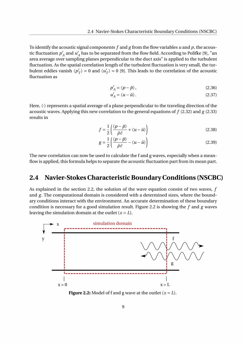
As explained in the section 2.2, the solution of the wave equation consist of two waves, fand g . The computational domain is considered with a determined sizes, where the bound-ary conditions interact with the environment. An accurate determination of these boundarycondition is necessary for a good simulation result. Figure 2.2 is showing the f and g wavesleaving the simulation domain at the outlet (x = L).
f
g
y
x simulation domain
x = Lx = 0
Figure 2.2: Model of f and g wave at the outlet (x = L).
9
Theoretical Background
In this thesis, the NSCBC approach by Poinsot and Lele [8] is used to determine the bound-ary conditions. The method is explained as an ”appealing technique for specifying boundaryconditions for hyperbolic systems [..] to use relations based on characteristic lines” [8] and issummarized here shortly. A detailed description of the mathematical background of bound-ary conditions based on characteristic lines can be seen in the papers of Kreiss [7] or Engquistand Majda [5].
To obtain the NSCBC, the Navier-Stokes Equations for a compressible flow in Cartesiancoordinates are shown [12]:
∂ρ
∂t+ ∂
∂xi(mi ) = 0, (2.40)
∂ρE
∂t+ ∂
∂xi
[(ρE +p
)ui
]= ∂
∂u jτi j− ∂qi
∂xi, (2.41)
∂mi
∂t+ ∂
∂x j
(mi u j
)+ ∂p
∂xi= ∂t aui j
∂x j, (2.42)
where
ρE = 1
2ρuk uk +
p
γ−1, (2.43)
mi = ρui , (2.44)
τi j =µ(∂ui
∂x j+ ∂u j
∂xi− 2
3δi j
∂uk
∂xk
). (2.45)
The thermodynamic pressure is given by the variable p, the total energy density (kinetic +thermal) is defined as ρE , while mi shows the momentum density in the xi direction.Additionally, the equations of the heat flux qi and of the thermal conductivity λ are
qi =−λ ∂t
∂xi, (2.46)
λ= µCp
Pr, (2.47)
where Pr is the Prandtl number, and µ is the viscosity coefficient.
As explained in the paper of Poinsot and Lele [8], the approach to apply the conservationequations directly on the boundary is used to complement the set of physical boundary con-ditions. To do so, a boundary located at x = L is considered and the characteristic analysis
10
2.4 Navier-Stokes Characteristic Boundary Conditions (NSCBC)
from Thompson [10] is applied at this patch. The equations (2.40) - (2.42) transform to:
∂ρ
∂t+d1 + ∂
∂x2(m2)+ ∂
∂x3(m3) = 0, (2.48)
∂ρE
∂t+ 1
2(uk uk )d1 + d2
γ−1+m1d3 +m2d4 +m3d5+
+ ∂
∂x2
[(ρE +p
)u2
]+ ∂
∂x3
[(ρE +p
)]= ∂
∂xi
(u jτi j
)− ∂qi
∂xi, (2.49)
∂m1
∂t+u1d1 +ρd3 + ∂
∂x2(m1u2)+ ∂
∂x3(m1u3) = ∂τ1 j
∂x j, (2.50)
∂m2
∂t+u2d1 +ρd4 + ∂
∂x2(m2u2)+ ∂
∂x3(m2u3)+ ∂p
∂x2= ∂τ2 j
∂x j, (2.51)
∂m3
∂t+u3d1 +ρd5 + ∂
∂x2(m3u2)+ ∂
∂x3(m3u3)+ ∂p
∂x3= ∂τ3 j
∂x j. (2.52)
It can be observed that the equations above contain two types of derivatives. One derivativenormal to the x1 boundary, defined as (d1 to d6), and derivatives parallel to the x1 boundarylike (∂/∂x2)(m2u2) and local viscous terms.
The vector d is given by characteristic analysis (Thompson [10]) and can be expressed as
d =
d1
d2
d3
d4
d5
=
12
[L2 + 1
2 (L5 +L1)]
12 (L5 +L1)1
2ρc (L5 −L1)
L3
L4
=
∂m1∂x1
∂(c2m1)∂x1
+ (1−γ)
µ∂p∂x1
u1∂u1∂x1
+ 1ρ∂p∂x1
u1∂u2∂x1
∂u3∂x1
. (2.53)
According to Poinsot and Lele, the L′i s are the amplitudes of characteristic waves associated
with each characteristic velocity λi [8]. Each characteristic velocity is related to the flow ve-locity ui and to the speed of sound c as [10]
λ1 = u1 − c, (2.54)
λ2 =λ2 =λ4 = u1, (2.55)
λ5 = u1 + c, (2.56)
where c is defined as
c2 = γp
ρ. (2.57)
While λ1 is the velocity of wave propagating in the negative x-direction, λ5 is moving in pos-itive direction, respectively. The convection velocity is related to λ2, and λ3 and λ4 are theadvection velocity for u2 and u3 into the x1 direction. The Li ’s are related to the characteristic
11
Theoretical Background
waves λi as
L1 =λ1
(∂p
∂x1−ρc
∂u1]
∂x1
), (2.58)
L2 =λ2
(c2 ∂ρ
∂x1− ∂p
∂x1
), (2.59)
L3 =λ3∂u2
∂x1, (2.60)
L4 =λ4∂u3
∂x1, (2.61)
L5 =λ5
(∂p
∂x1+ρc
∂u1
∂x1
). (2.62)
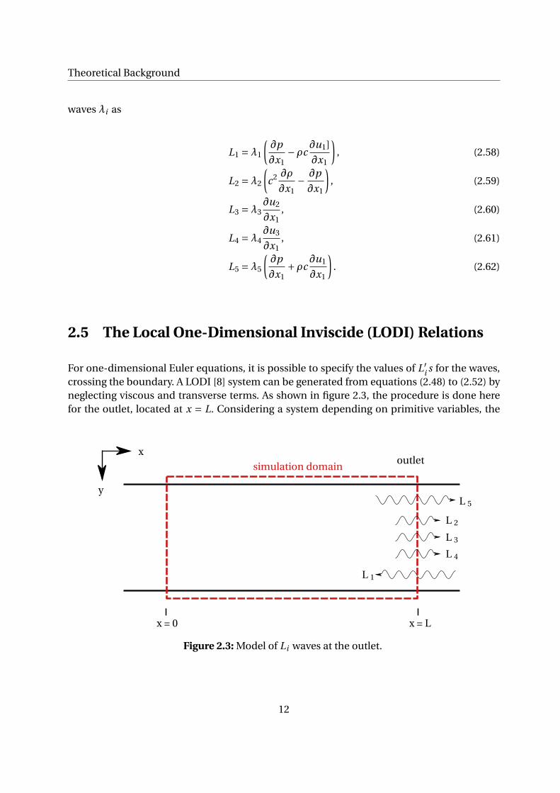
2.5 The Local One-Dimensional Inviscide (LODI) Relations
For one-dimensional Euler equations, it is possible to specify the values of L′i s for the waves,
crossing the boundary. A LODI [8] system can be generated from equations (2.48) to (2.52) byneglecting viscous and transverse terms. As shown in figure 2.3, the procedure is done herefor the outlet, located at x = L. Considering a system depending on primitive variables, the
L 5
L 2
L 3
L 4
L 1
x
y
x = 0 x = L
outletsimulation domain
Figure 2.3: Model of Li waves at the outlet.
12

2.5 The Local One-Dimensional Inviscide (LODI) Relations
equations (2.48) to (2.52) simplify to
∂ρ
∂t+ 1
c2
[L2 + 1
2(L5 +L1)
]= 0, (2.63)
∂p
∂t+ 1
2(L5 +L1) = 0, (2.64)
∂u1
∂t+ 1
2ρc(L5 −L1) = 0, (2.65)
∂u2
∂t+L3 = 0, (2.66)
∂u3
∂t+L4 = 0. (2.67)
Poinsot [8] explained the gained relation as not of ”physical conditions but should be moreviewed as a compatibility relations made by the physical boundary conditions and the waveamplitudes crossing the boundary”.
The relations above can also be combined to get a system of equation of the temperatureT , the flow rate m1 = ρu1, the entropy s, or the stagnation enthalpy h.
∂T
∂t+ T
ρc2
[−L2 + 1
2
(γ−1
)(L5 +L1)
]= 0, (2.68)
∂m1
∂t+ 1
c
[ML2 + 1
2{(M −1)L1 + (M +1)L5}
]= 0, (2.69)
∂s
∂t− 1(
γ−1)ρT
L2 = 0, (2.70)
∂h
∂t+ 1(
γ−1)ρ
[−L2 + γ−1
2{(1−M)L1 + (1+M)L5}
]= 0. (2.71)
Here, the enthalpy and the entropy are defined as h = (ρE+p)/ρ = 12 u2
i +Cp T and s =Cv logp/ργ+const . Furthermore, Cp and Cv are the specific heat capacities at constant pressure and vol-ume, respectively. M is the local Mach number: M = u1/c.
The system above shows the LODI relations in time derivatives. However, it is also possibleto set up such a system in terms of gradients. There, all gradient normal to the boundary x1
can be calculated with
∂ρ
∂x1= 1
c2
[L2
u1+ 1
2
(L5
u1 + c+ L1
u1 − c
)], (2.72)
∂p
∂x1= 1
2
(L5
u1 + c+ L1
u1 − c
), (2.73)
∂u1
∂x1= 1
2ρc
(L5
u1 + c− L1
u1 − c
), (2.74)
∂T
∂x1= T
ρc2
[−L2
u1+ 1
2
(γ−1
)( L5
u1 + c+ L1
u1 − c
)]. (2.75)
13

Theoretical Background
A quick example demonstrates the easy application and usage of the LODI system. Saying,a constant pressure is applied at the inlet. The corresponding LODI relation (2.64) is rewrittenhere again
∂p
∂t+ 1
2(L5 +L1) = 0,
it can be seen that the wave amplitudes have to be set in relation L5 = −L1, to guarantee theconstant pressure assumption.
∂p
∂t= 0 → L5 =−L1.
2.6 NSCBC with Plane Wave Masking (PVW)
For a one-dimensional Euler equation system, the LODI relations allow to determine the val-ues of L′
I s, as introduced in the previous section 2.5. One advantage of using the NSCBC ap-proach is the identification of the waves crossing the boundary. According to figure 2.3, twowave directions can be observed. At the outlet, L2 to L5 are leaving the simulation domain,while L1 is entering it. For calculating the wave exiting the domain, the points inside the do-main can be used to determine its further behavior. For waves, accessing the domain, thebehavior has to be specified by some approximations. A method to determine these waves isnow introduced.
Rewriting the LODI relations for pressure and velocity, we get
∂p
∂t+ 1
2(L5 +L1) = 0, (2.76)
∂u
∂t+ 1
2ρc(L5 −L1) = 0. (2.77)
Two types of reflecting boundary conditions are distinguish, a fully reflecting boundary con-dition and a partially reflecting boundary condition.
Fully reflecting boundary conditions
Examples for a fully reflecting boundary condition are an open end or a closed end. Imposingan open end at the outlet, the acoustic fluctuation of pressure is defined as p A = f + g = 0 [9],which leads to a LODI relation (2.76) of L1 +L5 = 0. While for a closed end inflow boundary,the acoustic fluctuation is obtained by the velocity to the formula of uA = f −g = 0 that resultsin a LODI relation (2.77) of L1 = L5.
Partially reflecting boundary conditions
For the partially reflecting boundary condition, some specifications has to be done to usethem reasonable. Poinsot [8] constructed a low reflecting outflow boundary condition withthe help of a relaxation factor σ. Without the linear relaxation term, Poinsot investigated a
14
2.6 NSCBC with Plane Wave Masking (PVW)
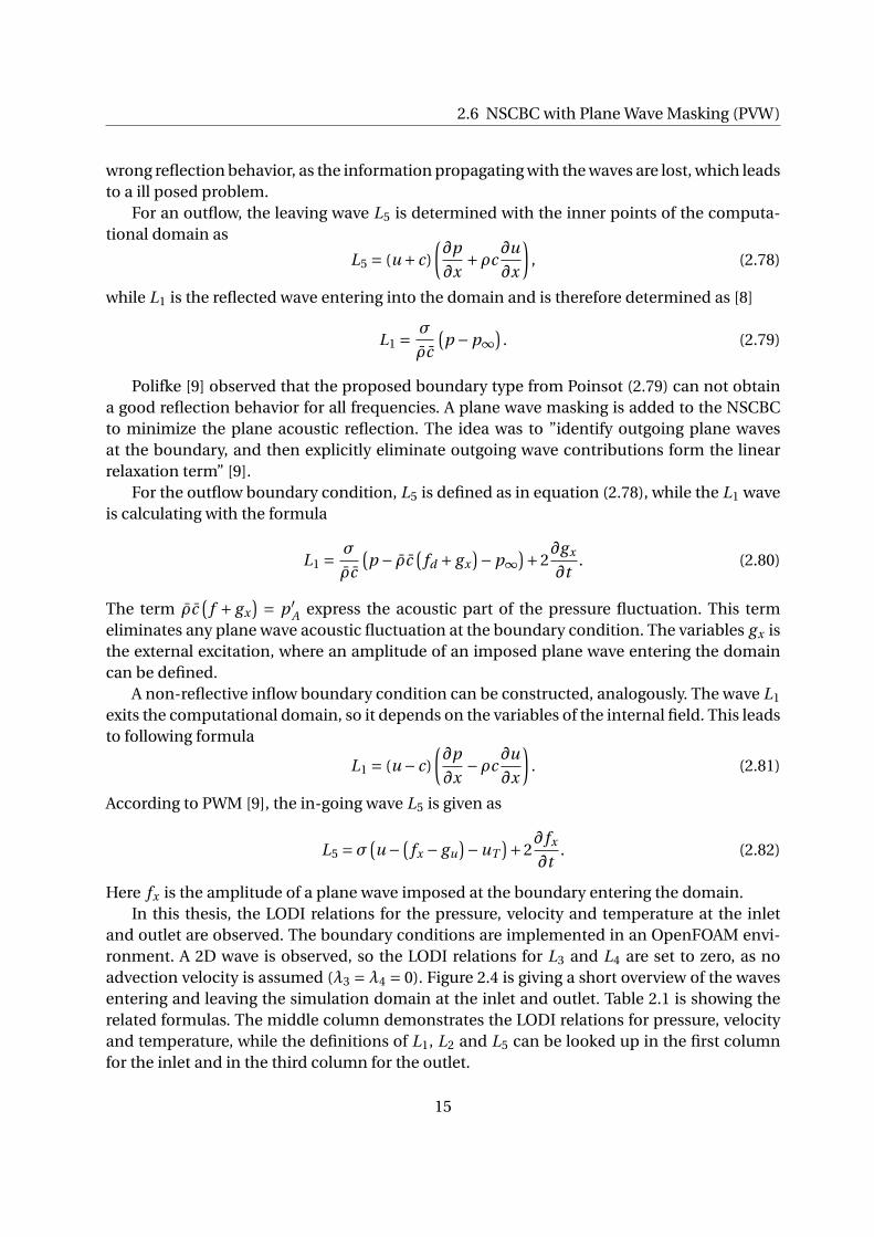
wrong reflection behavior, as the information propagating with the waves are lost, which leadsto a ill posed problem.
For an outflow, the leaving wave L5 is determined with the inner points of the computa-tional domain as
L5 = (u + c)
(∂p
∂x+ρc
∂u
∂x
), (2.78)
while L1 is the reflected wave entering into the domain and is therefore determined as [8]
L1 = σ
ρc
(p −p∞
). (2.79)
Polifke [9] observed that the proposed boundary type from Poinsot (2.79) can not obtaina good reflection behavior for all frequencies. A plane wave masking is added to the NSCBCto minimize the plane acoustic reflection. The idea was to ”identify outgoing plane wavesat the boundary, and then explicitly eliminate outgoing wave contributions form the linearrelaxation term” [9].
For the outflow boundary condition, L5 is defined as in equation (2.78), while the L1 waveis calculating with the formula
L1 = σ
ρc
(p − ρc
(fd + gx
)−p∞)+2
∂gx
∂t. (2.80)
The term ρc(
f + gx) = p ′
A express the acoustic part of the pressure fluctuation. This termeliminates any plane wave acoustic fluctuation at the boundary condition. The variables gx isthe external excitation, where an amplitude of an imposed plane wave entering the domaincan be defined.
A non-reflective inflow boundary condition can be constructed, analogously. The wave L1
exits the computational domain, so it depends on the variables of the internal field. This leadsto following formula
L1 = (u − c)
(∂p
∂x−ρc
∂u
∂x
). (2.81)
According to PWM [9], the in-going wave L5 is given as
L5 =σ(u − (
fx − gu)−uT
)+2∂ fx
∂t. (2.82)
Here fx is the amplitude of a plane wave imposed at the boundary entering the domain.In this thesis, the LODI relations for the pressure, velocity and temperature at the inlet
and outlet are observed. The boundary conditions are implemented in an OpenFOAM envi-ronment. A 2D wave is observed, so the LODI relations for L3 and L4 are set to zero, as noadvection velocity is assumed (λ3 = λ4 = 0). Figure 2.4 is giving a short overview of the wavesentering and leaving the simulation domain at the inlet and outlet. Table 2.1 is showing therelated formulas. The middle column demonstrates the LODI relations for pressure, velocityand temperature, while the definitions of L1, L2 and L5 can be looked up in the first columnfor the inlet and in the third column for the outlet.
15

Theoretical BackgroundO
verv
iew
oft
he
rela
ted
form
ula
sfo
rth
eim
ple
men
tati
on
oft
he
bo
un
dar
yco
nd
itio
nin
this
thes
is:
L5
L2
L1
x
y
x=
0x
=L
ou
tlet
sim
ula
tio
nd
om
ain
L5
L2
L1
inle
t
Figu
re2.
4:M
od
elo
frel
ated
Li
wav
esfo
rth
esi
mu
lati
on
inth
isth
esis
.
Inle
tLO
DI
syst
emO
utl
et
L1=
(u−c
)[ ∂p ∂x−ρ
c∂
u∂
x
]∂
p ∂t+
1 2(L
5+L
1)=
0L
1=
σ1
ρc
[ p−ρ
c( f d
+gx) −p
∞] +2
∂g
x∂
t
L5=σ
5[ u
−( f x−g
u) −u
T] +2
∂f x ∂t
∂u
1∂
t+
12ρ
c(L
5−L
1)
L5=
(u−c
)[ ∂p ∂x+ρ
c∂
u∂
x
]L
2=σ
2
[ T−
γ−1 γ
( f d+g
x) −T
t]∂
T ∂t+
T ρc2
( −L2+
1 2
( γ−1) (L
5+L
1))
L2=
u[ c2
( ∂ρ ∂x−
∂p∂
x
)]Ta
ble
2.1:
LOD
Ire
lati
on
san
dth
ed
efin
itio
no
fL1,L
2an
dL
5at
the
inle
tan
do
utl
et.
16

2.7 Characteristic Based State-Space Boundary Conditions (CBSBC)
2.7 Characteristic Based State-Space Boundary Conditions (CB-SBC)
The simulation domain is only a small part of the whole combustion chamber. The remain-ing fluid flow is modeled by one-dimensional state space systems. Therefore, a good couplingbetween the CFD domain and the state space model is essential. It is realized by the Charac-teristic Based State Space Boundary condition (CBSBC).
According to Polifke [9], CBSBC is a continuous-time state-space model to describe thefrequency dependent reflection of acoustic waves. As linearized Euler and Navier-Stokes equa-tions are used, the state-space model can be determine with a set of linear partial differentialequations (PDE). An exhaust duct is used as a example to explain the usage of the CBSBC.Figure (2.5) is showing the model of the CBSBC at the outlet of the simulation domain.
simulation domain
CBSBC
f d
g d
f 1 f 2
g 1 g 2 g N
∆ x
f Nf
g
R L
e x,d
outlet
0 L
x
y
Figure 2.5: Model of CBSBC located at the outlet of the simulation domain.
The fd wave is leaving the simulation domain and entering into the CBSBC model. It is thenpropagating through the time-domain model till it reaches the distance x = L. At this point,the reflection coefficient RL is multiplied to wave fn , an external source acoustic source ex,d
can be additionally added to obtain gN . The g wave is then propagating back till it leaving theCBSBC domain at g1 and is reentering the simulation domain via the wave gd . The set up forthe matrices is showed now:
Considering the one dimensional Euler equation and neglecting mean-flow gradients, theformulas are gained
∂ f
∂t+ (u − c)
∂ f
∂x= 0, (2.83)
∂g
∂t+ (u − c)
∂g
∂x= 0. (2.84)
17
Theoretical Background
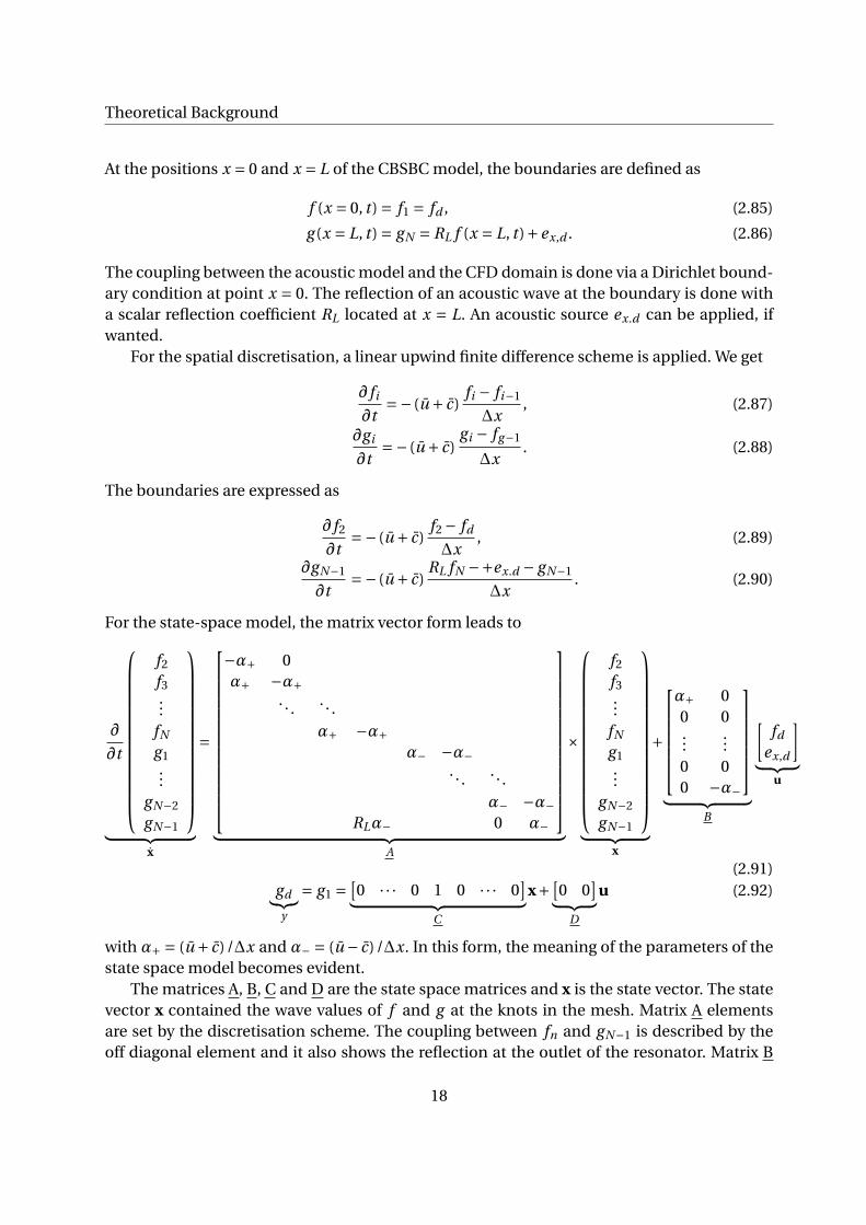
At the positions x = 0 and x = L of the CBSBC model, the boundaries are defined as
f (x = 0, t ) = f1 = fd , (2.85)
g (x = L, t ) = gN = RL f (x = L, t )+ex,d . (2.86)
The coupling between the acoustic model and the CFD domain is done via a Dirichlet bound-ary condition at point x = 0. The reflection of an acoustic wave at the boundary is done witha scalar reflection coefficient RL located at x = L. An acoustic source ex.d can be applied, ifwanted.
For the spatial discretisation, a linear upwind finite difference scheme is applied. We get
∂ fi
∂t=− (u + c)
fi − fi−1
∆x, (2.87)
∂gi
∂t=− (u + c)
gi − fg−1
∆x. (2.88)
The boundaries are expressed as
∂ f2
∂t=− (u + c)
f2 − fd
∆x, (2.89)
∂gN−1
∂t=− (u + c)
RL fN −+ex.d − gN−1
∆x. (2.90)
For the state-space model, the matrix vector form leads to
∂
∂t
f2
f3...
fN
g1...
gN−2
gN−1
︸ ︷︷ ︸
x
=
−α+ 0α+ −α+
. . . . . .α+ −α+
α− −α−. . . . . .
α− −α−RLα− 0 α−
︸ ︷︷ ︸
A
×
f2
f3...
fN
g1...
gN−2
gN−1
︸ ︷︷ ︸
x
+
α+ 00 0...
...0 00 −α−
︸ ︷︷ ︸
B
[fd
ex,d
]︸ ︷︷ ︸
u
(2.91)gd︸︷︷︸
y
= g1 =[0 · · · 0 1 0 · · · 0
]︸ ︷︷ ︸C
x+ [0 0
]︸ ︷︷ ︸D
u (2.92)
with α+ = (u + c)/∆x and α− = (u − c)/∆x. In this form, the meaning of the parameters of thestate space model becomes evident.
The matrices A, B, C and D are the state space matrices and x is the state vector. The statevector x contained the wave values of f and g at the knots in the mesh. Matrix A elementsare set by the discretisation scheme. The coupling between fn and gN−1 is described by theoff diagonal element and it also shows the reflection at the outlet of the resonator. Matrix B
18
2.8 Stokes Boundary Layer
models, how the input signal u affects the temporal derivative of the state vector. As in MatrixA and B are set by the discretisation scheme. The feed through is defined as a null vector (D).In the matrix C, the element unlike zero, gives the output g1 by multiplying the matrix C withthe state vector x. g1 is equal to gd = y .
In this thesis, the CBSBC is mainly set to be non-reflecting. Possibilities to generate non-reflection boundary condition is to set the matrices A, B or C equal to zero. By setting one ofthe matrices equal to zero, the propagation of the waves through the CBSBC model is inter-rupted, as the information can not be transported through the whole domain, see (2.91) and2.92.
2.8 Stokes Boundary Layer
Considering an oscillation flow, a boundary layer close to the wall is generated. For a lami-nar flow, a exact solution of the Navier-Stokes equations can be calculated. The equation isintroduced for the case with an oscillating wall and a viscous fluid in rest and will be thenextended to the case for oscillating flow and rigid wall. Considering an oscillating plate, theNavier-Stokes equation simplify to [1]
∂u
∂t= ν∂
2u
∂y, (2.93)
describing the viscosity evolution away from the wall. The velocity is assumed to propagatein the x-direction, parallel to the oscillation direction. y is showing the distance from the wall.Following boundary conditions arise for this problem
t ≤ 0 : y ≥ 0 : u1(y, t ) = 0,
t > 0 : y = 0 : u1(0, t ) =U0 · cos(ωt ),
y →∞ : u1(∞, t ) = 0.
For a time t ≤ 0s, the wall is considered in rest. After that, the motion of the wall is U0 ·cos (ωt ).After some transformation, the solution of the flow velocity is gained in the formula (see in [1]for a detailed transformation)
u1(y, t ) =U0 ·exp
(−
√ω
2νy
)· cos
(ωt
√ω
2νy
)(2.94)
where
κ=√
ω
2ν, (2.95)
can be defined as the wave number in y-direction.ω is defined as the angular frequency of themotion and can be calculated by using the relation between angular frequency and frequency
19

Theoretical Background
0 200 400 600 800 1000 1200 1400 1600 1800 2000
Frequency [Hz]
0.2
0.4
0.6
0.8
1
1.2
1.4
Sto
kes b
oundary
layer
thic
kness [m
m]
Figure 2.6: Stokes Boundary Layer Thickness over frequency.
ω= 2πF , while ν is showing the viscosity. Furthermore, a stokes boundary thickness is definedby
δ= 2π
κ= 2π
√2ν
ω. (2.96)
The stokes boundary layer thickness was used in this thesis to identify a fully generated bound-ary layer at the no-slip wall. Figure 2.6 is showing the stokes boundary layer thickness over thefrequency.
Considering an oscillating flow near a rigid wall, the solution of the flow velocity changesto
u1(y, t ) =U0 ·[
cos (ωt ) ·exp
(−
√ω
2 ·ν y
)· cos
(ωt
√ω
2νy
)]. (2.97)
20
2.9 OpenFOAM
2.9 OpenFOAM
Basic
The investigation of the validation of the CBSBC were done using OpenFOAM Version 2.3.1.OpenFOAM is an open source Computational Fluid Dynamic (CFD) software tool. CFD al-lows to predict and analyze fluid flows by numerical simulation. It plays an important role,as it allows a cheap method to investigate the flow dynamics in early states of a design pro-cess. The open code allow to implement and modify models in a huge range, which is veryhelpful and beneficial for academical research investigations. That’s also why the CBSBCs areimplemented in this.
The CBSBC were applied as a boundary condition for OpenFOAM and compiled. As a 2Dchannel were investigated, the geometry and mesh were created using the blockMesh dict. Toread out pressure and velocity for the related cells, the swak4Foam [4] toolbox was embed intothe software. The rhoPimpleFoam solver was used, as compressible flow is considered. Thevalues from swak4Foam were read into Matlab, from where the f and g waves were calculated.
Implementation of CBSBC in OpenFOAM
The boundary conditions used for the simulations in OpenFOAM were created by the chair”Professur für Thermofluiddynamik” of the TUM. It was integrated into the OpenFOAM en-vironment. Following six boundary types were used: CBSBCInletPressure, CBSBCInletTem-perature, CBSBCInletVelocity, CBSBCOutletPressure, CBSBCOutletTemperature, CBSBCOut-letVelocity.
The implementation in OpenFOAM was done using a Transient Robin Boundary Con-ditions according to Vilums [11]. In OpenFOAM, the boundary conditions of type Dirichletand Neumann respectively fixedValue and fixedGradient are pre-defined. With the help of theswak4foam library from B. Gschnaider, a mixed boundary condition, called groovyBC can beconstructed [4]. This boundary condition allows also to define variables and functions on theboundary calculated at every internal iteration. By looking into the source code of mixed BC[4], the LODI relations equations has to look like:
P n+1f ace = f · valueE xpr + (
1− f)(
P n+1centr e + g r adE xpr ·δ)
. (2.98)
Exemplary, the pressure is shown in (2.98). For the temperature, use T instead of P . Here, f isdefined as the fractionExpression and has to be obtained by user. The distance between thecell centre and cell face is represented by δ.
To gain the form of equation as seen in (2.98), the LODI relations has to be linearized.The linearization and the comparison with the implemented values in the .C file are shown inthe annex A - D. For the CBSBCInletPressure and CBSBCInletTemperature cases, the differentalgebraic sign is because the normal patch vector is in the opposite direction than the flowdirection.
An extract of the velocity boundary condition, defined in the 0-folder of the simulation, is
21

Theoretical Background
shown in the annex E and will be described here shortly. For the inlet boundary field, the typeof the CBSBC (here CBSBCInletVelocity) and some constant variables are defined in the be-ginning. The sub-folder of the velocity allows to define a target value. Compare with section2.6, where the formula for the inlet velocity is shown. This value will be changed to set up amean-flow, but it is considered in more detail in the section 3.5. The text-file of the incom-ing f wave is determined in the sub-folder tableFileCoeffs. In the text-file inletf_700.txt , awave with a frequency of F = 700Hz and a sound pressure level of SPL = 75dB is selected. Forall simulation cases, no changes in SPL are made. Only the frequency is modified in section4.4. The ssFileName defines the state-space model, named here as ”statespace.dat”. The state-space model contains two patch numbers of CBSBC. Here, patch -1 is used for the inlet while-2 is used for the outlet. Furthermore, a characteristic acoustic length scale and a initial valuecan be defined.
The outlet definition has the similar beginning. But for this case, a target value for thepressure is defined. Compare again with 2.6, where the LODI relation and the related formulafor the outlet pressure is defined. Furthermore, an excitation signal can be obtained. For theoutlet, the ssPatch with number -2 is used.
22

3 Simulation Results for Slip BoundaryConditions
Chapter 3 is beginning with the introduction of the geometry and its meshing. The next sec-tion displays the general behavior of the CBSBC with a defined reflection coefficient. Figuresof velocity, pressure and the waves are demonstrated to get a first impression of the simu-lation. Then, the CBSBC is set to be non-reflecting, the resulting reflection coefficient is cal-culated. Furthermore, different options for setting a mean-flow to the simulation are investi-gated. The chapter slip 3 is closing with investigations for the reflecting coefficient of differentmean-flows. If not mentioned explicit, a frequency of F = 700Hz is used for all setups.
3.1 Simulation Setup of Slip Case
For the slip case, a 2D channel with dimensions of (600 mm x 20 mm x 1 mm) and a meshingof (400 20 1) is used. The mesh of the geometry can be seen in figure 3.1, and a detailed view tosee the cell size is done in figure 3.2. This big size of geometry was set because the first simula-tions does not need this many computational hours and the development of the longitudinalwaves (wave crest and wave trough) can be seen (fig. 3.3).
The CBSBC boundary condition is applied at the outlet and inlet patch, while top andbottom wall are set as slip boundary conditions. Waves, with a frequency of F = 700Hz and asound pressure level of SPL = 75dB are propagating through the inlet into the channel and arethen interacting with the reflection coefficient at the outlet. As slip boundary conditions areapplied, no wall interfaces are expected. So a surface area expression was set in OpenFOAM,to evaluate the values for pressure and velocity. Figure 3.2 is showing a detailed view on the
inlet
slip
slip
400 mm
20 mmoutlet
x
y
Figure 3.1: Mesh of geometry for the slip case.
mesh. The cell size in x-direction is given as∆x = 1.5mm, while in y-direction, it is∆y = 1mm.The extract is showing 20 cells in y-direction and 12 cells in x-direction.
23

Simulation Results for Slip Boundary Conditions
Δx
Δy
Figure 3.2: Detailed view of the mesh for the slip case.
Having a closer look to the velocity distribution for a time t = 1.9ms, displayed in figure3.3, the longitudinal wave can be detected. As plane waves are treated, the red area is showingthe wave crest, while the blue area stands for the wave trough. This figure should manifest the
Figure 3.3: Velocity distribution for the time-step t = 1.9ms; showing wave crest (red) andwave trough (blue).
choice of the selected geometry. A whole wave period can be seen along the x-axis, which wasa good help for understanding the results of the first simulations.
3.2 Generation of Results for Slip Case
The procedure for calculating the reflection coefficient for the slip case is shown in the dia-gram below (figure 3.4).
From OpenFOAM, two vectors, one for velocity (uOF ) and one for pressure (pOF ), are eval-uated for every time step with the help of the swak4Foam library. To ensure a good quality ofthe wave propagation, a time step of t = 1 ·10−6 s is used. The velocity and pressure vectorsare then written into the MATLAB environment. Applying a mean-flow to the simulation re-quires an elimination of it. To do so, a mean value over a period time is calculated and thensubtracted from the variables. This leads to the acoustic fluctuation of pressure and velocityuA and p A. Applying no mean-flow does not need to eliminate the mean variable, however itis done to ensure its quality. With the help of p A and uA, the f and g waves can be calculated.
24

3.3 Applying Reflecting CBSBC
pOF
u uA
pA
OpenFOAM Rc
f
g
^
g^
fOF
Figure 3.4: Diagram for calculating R c for the slip case.
The equations are shown here again quickly.
f = 1
2
(p A
ρc+uA
),
g = 1
2
(p A
ρc−uA
).
Applying a Fourier transformation on the f and g waves leads to the corresponding ampli-tudes ( f and g ) . By setting these in relation, the reflection coefficient Rc is generated with theformula
Rc = g
f.
3.3 Applying Reflecting CBSBC
First, the behavior of the CBSBC boundary condition is introduced in a general case. The re-flection coefficient is defined as Rc = 0.8 at the outlet and at the inlet. To evaluate the pressureand velocity, surface averages at positions x = 0.005m and x = 0.595m are defined in Open-FOAM. These values were written into the MATLAB environment, to generate the f and gwaves.
Inlet
Figure 3.5 is showing the pressure and velocity evolution over time at the inlet. After a timeof t = 0.004s, a little disturbance in the velocity graph can be detected, due to the interactionwith the new generated g wave, compare with figure 3.6. After passing this time, a smalleramplitude of the velocity oscillation can be seen. The pressure graph does not have this dis-turbance, however, it is changing its amplitude to a higher value after it passes t = 0.004s.
Figure 3.6 is showing the calculated f and g wave. The generation of g wave is beginningat the time t = 0.004s. As explained, this leads to the disturbance seen in the velocity plot
25

Simulation Results for Slip Boundary Conditions
0 0.001 0.002 0.003 0.004 0.005 0.006 0.007 0.008 0.009 0.01
Time [s]
-4
-2
0
2
4u
[m
/s]
10-4
0 0.001 0.002 0.003 0.004 0.005 0.006 0.007 0.008 0.009 0.01
Time [s]
-0.2
-0.1
0
0.1
0.2
p [
ba
r]
Figure 3.5: Velocity and pressure evolution at the inlet.
of figure 3.5. The f wave is continuing its behavior without any loose in its amplitude value.Comparing both amplitudes a reflection coefficient of Rc = 0.80 is calculated.
0 0.001 0.002 0.003 0.004 0.005 0.006 0.007 0.008 0.009 0.01
Time [s]
-4
-3
-2
-1
0
1
2
3
4
Am
plit
ud
e [
m/s
]
10-4
f
g
Figure 3.6: The f and g wave evolution at the inlet.
Outlet
Having now a look at the outlet, following velocity and pressure evolution is generated, seefig. 3.7. It takes nearly 0.0017 s for the velocity and pressure waves to reach the position ofthe surface average (x = 0.595m). After this, it takes one oscillation with a smaller amplitude
26

3.3 Applying Reflecting CBSBC
0 0.001 0.002 0.003 0.004 0.005 0.006 0.007 0.008 0.009 0.01
Time [s]
-1
-0.5
0
0.5
1
u [
m/s
]
10-3
0 0.001 0.002 0.003 0.004 0.005 0.006 0.007 0.008 0.009 0.01
Time [s]
-0.1
0
0.1
0.2
p [
ba
r]
Figure 3.7: Velocity and pressure evolution at the outlet.
for the velocity graph to reach its harmonious oscillation behavior. The pressure is raisingstrongly after the f wave is reaching the outlet patch, then it has a little kink at the time oft = 0.023s, and it is then oscillating till the end of simulation time.
The resulting f and g wave plots can be seen in figure 3.8. Similar to the velocity and
0 0.001 0.002 0.003 0.004 0.005 0.006 0.007 0.008 0.009 0.01
Time [s]
-4
-3
-2
-1
0
1
2
3
4
Am
plit
ud
e [
m/s
]
10-4
f
g
Figure 3.8: The f and g wave evolution at the outlet.
pressure graphs, it took t = 0.0017s for the f wave to reach the outlet. Then it took additionally0.007 s for the f wave to cross the state-space model. After 0.025 s the g wave is generated. Thebeginning of the g wave and the kink in the pressure graph (fig. 3.7) are happening at the sametime-step, so the pressure kink is due to the generation of the g wave. Again, a comparison of
27
Simulation Results for Slip Boundary Conditions
the amplitude of f and g waves lead to a reflection coefficient of Rc = 0.80, same as for theinlet observation.
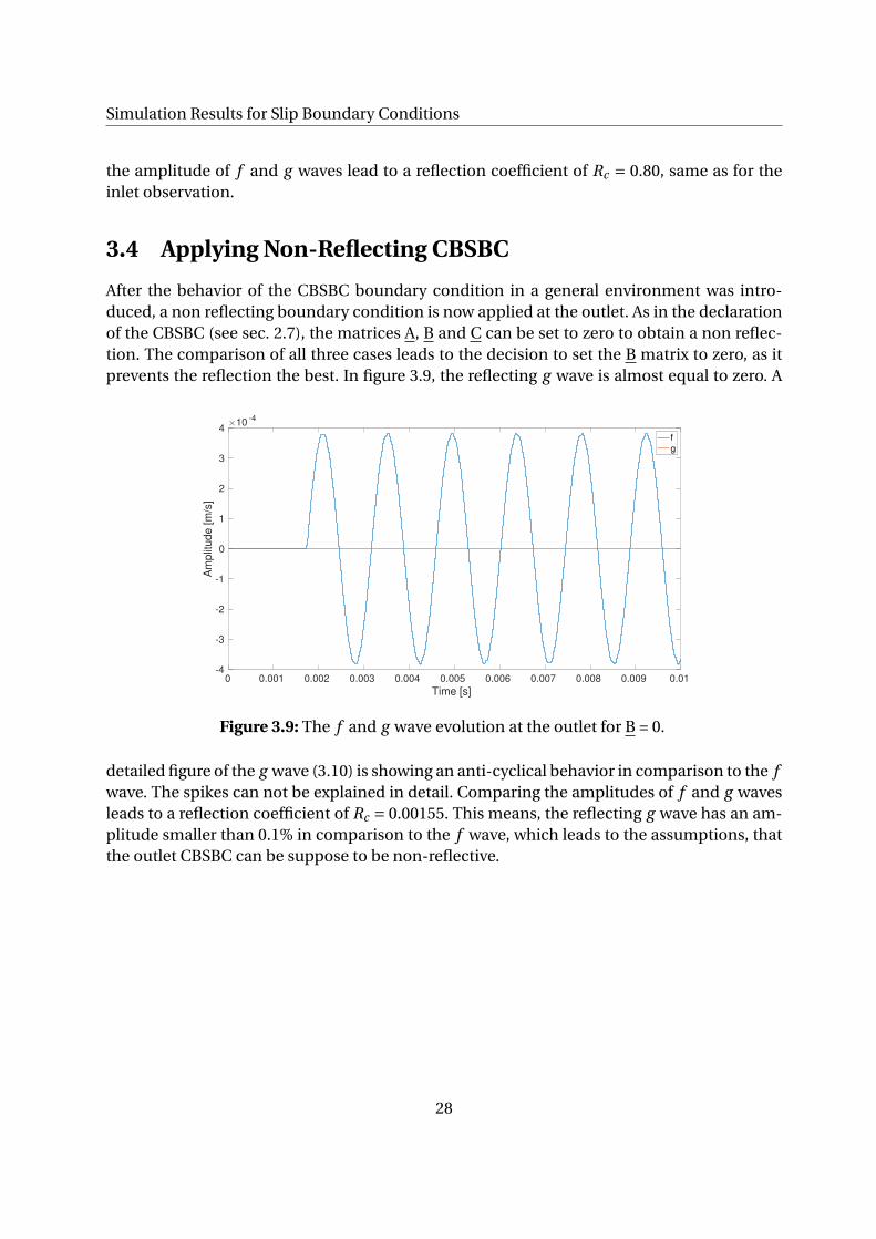
3.4 Applying Non-Reflecting CBSBC
After the behavior of the CBSBC boundary condition in a general environment was intro-duced, a non reflecting boundary condition is now applied at the outlet. As in the declarationof the CBSBC (see sec. 2.7), the matrices A, B and C can be set to zero to obtain a non reflec-tion. The comparison of all three cases leads to the decision to set the B matrix to zero, as itprevents the reflection the best. In figure 3.9, the reflecting g wave is almost equal to zero. A
0 0.001 0.002 0.003 0.004 0.005 0.006 0.007 0.008 0.009 0.01
Time [s]
-4
-3
-2
-1
0
1
2
3
4
Am
plit
ud
e [
m/s
]
10-4
f
g
Figure 3.9: The f and g wave evolution at the outlet for B = 0.
detailed figure of the g wave (3.10) is showing an anti-cyclical behavior in comparison to the fwave. The spikes can not be explained in detail. Comparing the amplitudes of f and g wavesleads to a reflection coefficient of Rc = 0.00155. This means, the reflecting g wave has an am-plitude smaller than 0.1% in comparison to the f wave, which leads to the assumptions, thatthe outlet CBSBC can be suppose to be non-reflective.
28

3.5 Applying a Mean-Flow to the Slip Simulation Case
0 0.001 0.002 0.003 0.004 0.005 0.006 0.007 0.008 0.009 0.01
Time [s]
-8
-6
-4
-2
0
2
4
6
8
Am
plit
ud
e [
m/s
]
10-7
g
Figure 3.10: Detailed view on the g wave for B = 0.
0-Folder Sub-item Option 1 Option 2 Option 3 Option 4
U uniform (0 0 0) (0.001 0 0) (0 0 0) (0.001 0 0)targetValue (0.001 0 0) (0.001 0 0) (0.001 0 0) (0.001 0 0)
p targetValue (0 0 0) (0 0 0) (0.001 0 0) (0.001 0 0)T targetValue (0 0 0) (0 0 0) (0.001 0 0) (0.001 0 0)
Table 3.1: Options to define a mean-flow in the boundary conditions.
3.5 Applying a Mean-Flow to the Slip Simulation Case
The previous chapter investigated the behavior of reflection and non-reflection without amean-flow. Now, a mean-flow is applied to the system. By looking at the CBSBC boundarycondition .H file, few options could be detected to generate a mean flow (see appendix E). Inthe 0-folder, the velocity can be set to an uniform value for the internal field. Also, a targetvelocity value can be defined at the inlet in the velocity, pressure and temperature file. Thissection wants to point out the best apply to set a mean-flow. The investigation is done using amean-flow of u = 0.001m/s, to see its behavior and not wasting much computational power.
Four cases, see table 3.1, are compared for setting a mean-flow to the boundary condi-tions. Setting the mean-flow only as a targetValue for the velocity, leads to mean value notequal to u = 0.001m/s. Adding a uniform velocity to the first setup (Option 2) also does notprovide the defined mean-flow. So both Options are not suitable configurations. Option 3 andOption 4 are a good choice to set up mean-flows, as the applied mean-flow is reached aftert = 0.0075s. Option 3 was selected, as a consistent evolution of the velocity and pressure graphcould be detected.
For a better understanding, the velocity and pressure evolution and the f and g waves for
29

Simulation Results for Slip Boundary Conditions
0 0.005 0.01 0.015 0.02 0.025 0.03 0.035 0.04 0.045 0.05
Time [s]
-1
0
1
2[m
/s]
10-3
uof
umean
uA
0 0.005 0.01 0.015 0.02 0.025 0.03 0.035 0.04 0.045 0.05
Time [s]
-0.5
0
0.5
[bar]
pof
pmean
pA
Figure 3.11: Velocity and pressure evolution for Option 3.
a mean-flow of u = 0.001m/s are displayed now for Option 3. Having a look at figure 3.11, itis showing three velocities. The blue graph refers to the velocity evaluated from OpenFOAM(uOF ). Starting from a value of u = 0m/s, a mean velocity u = 0.001m/s of the velocity fluc-tuation is reached after nearly t = 0.0075s. Variable umean is calculated for one time period(∆T = 1428s ) to a value of umean = 0.001m/s. For calculating the f and g waves, the velocityfrom OpenFOAM has to be subtracted by the calculated mean velocity. The yellow graph isshowing the resulting velocity, the acoustic fluctuation velocity (uA). For the evolution of thethree pressure variables, similar behavior is detected. The acoustic fluctuation pressure partp A was generated by subtracting pmean = 0.4074Pa from pOF . Both yellow graphs (uA and p A)are then used to calculate the f and g waves, see in fig. 3.12. The blue graph is showing the re-sulting f wave, while the g wave is displayed in red. Due to the generation of the acoustic partof velocity and pressure, the f wave is starting with a negative value of f = −0.001m/s. Aftert = 0.01s, a stable oscillation around the x-axis can be detected. The maximum amplitude off wave is equal to f = 3.08 ·10−4 , while g wave is reaching a maximum value of g = 6.6 ·10−7.Comparing both values leads to a reflection coefficient of Rc = 0.00155, which is assumed hereas non-reflective.
30

3.6 Comparison of Rc for different Mean-Flows
0 0.005 0.01 0.015 0.02 0.025 0.03 0.035 0.04 0.045 0.05
Time [s]
-10
-5
0
5A
mp
litu
de
[m
/s]
10-4
f g
Figure 3.12: The f and g wave evolution for Option 3.
3.6 Comparison of Rc for different Mean-Flows
This section investigates the behavior of the acoustic fluctuation for setups with differentmean-flows. Beginning with a mean-flow of u = 0.001m/s the applied mean-flow is increased.Setting a mean-flow leads to some beginning pressure and velocity fluctuations before veloc-ity and pressure oscillate around a mean value. This is sometimes not this easy, as the velocityand pressure are growing small over time. We set a special mean-flow, and therefore a threetime period is selected from velocity and pressure graph, where the difference between theset mean-flow and the mean value, the acoustic parts are oscillating, having a small differ-ence. Especially when the mean-flow is raised to a value u > 1m/s, it needs more time tooscillate around the mean value and therefore, more computational time has to be taken. Theinvestigations here are having a mean-flow range starting for a mean-flow of u = 0.001m/s tillu = 1m/s with a difference of ∆u = 10. So four mean-flows are investigated. The mean-floware applied in behavior as Option 3 as investigated in the previous section (3.5).
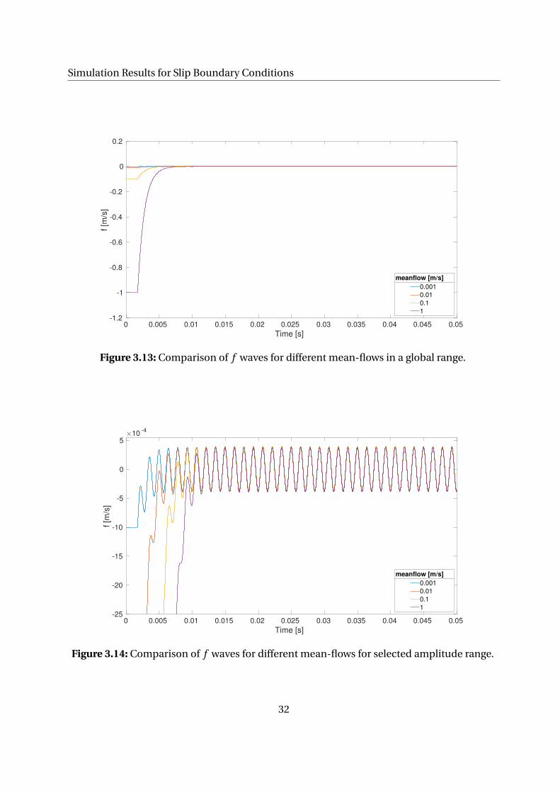
First, the f wave is shown in figure 3.13. Generally, as the global y range of the f wave is thisbig, a converged behavior can be seen after a time period of t = 0.01s for all mean-flow setups.For a higher mean-flow, the beginning of the f wave is having a lower value. The beginning ofeach graph is defined by the subtracted mean value and should not be considered in detail.For example, a mean-flow of u = 1m/s is beginning with a value of f =−1m/s.
Having now a closer look at the f waves for a selected amplitude range leads to figure3.14. Comparing all four lines, it is taking longer for a higher mean-flow value to stabilizearound the zero value. For the lowest mean-flow u = 0.001m/s, it takes nearly t = 0.006s toreach a converged state. For the purple graph (u = 1m/s), it nearly takes t = 0.013s to reachits converged state. Also, the local maximum in the area t < 0.01s are behaving different forevery mean-flow. Small mean-flow are having a big local maximum amplitude, while highermean-flow only having a little hill till it starts to converge. A Fourier transformation over the
31
Simulation Results for Slip Boundary Conditions
0 0.005 0.01 0.015 0.02 0.025 0.03 0.035 0.04 0.045 0.05
Time [s]
-1.2
-1
-0.8
-0.6
-0.4
-0.2
0
0.2
f [m
/s]
0.001
0.01
0.1
1
meanflow [m/s]
Figure 3.13: Comparison of f waves for different mean-flows in a global range.
0 0.005 0.01 0.015 0.02 0.025 0.03 0.035 0.04 0.045 0.05
Time [s]
-25
-20
-15
-10
-5
0
5
f [m
/s]
10-4
0.001
0.01
0.1
1
meanflow [m/s]
Figure 3.14: Comparison of f waves for different mean-flows for selected amplitude range.
32

3.7 Discussion about Slip Boundary Conditions
0 0.005 0.01 0.015 0.02 0.025 0.03 0.035 0.04 0.045 0.05
Time [s]
-1
-0.8
-0.6
-0.4
-0.2
0
0.2
0.4
0.6
0.8
1
g [m
/s]
10-5
0.001
0.01
0.1
1
meanflow [m/s]
Figure 3.15: Comparison of g waves for different mean-flows for selected amplitude range.
frequency for every line can be seen in table 3.2.Having now a look at the reflecting g wave at figure 3.15. For a mean-flow of u = 0.001m/s
and u = 0.01m/s, a similar behavior for the g wave can be observed. Raising the mean valueto u = 0.1m/s, a falling behavior for the g wave can be observed. Raising the mean-flow toa value of u = 1m/s results in no converged status in the investigated time, but a decreasingbehavior of the amplitude can be detected. The results of the Fourier transformation of the gwaves can be looked up in table 3.2.
3.7 Discussion about Slip Boundary Conditions
In the beginning, the general behavior of the CBSBC was introduced, figures of f and g wavedemonstrates its behavior at the inlet and outlet. The calculated reflection coefficient wasequal to the defined CBSBC one.
Then, the CBSBC was set to be non-reflecting at the outlet, by setting the B matrix to zero.A reflection coefficient of Rc = 0.00155 was calculated, which is assumed as non-reflecting.
After this, the non-reflection is observed for different mean-flows. Firstly, different optionsfor setting the mean-flow are investigated. Option 3 is showing the best behavior for the in-vestigated mean-flow, it is used for the further observations. Applying a mean-flow does notchange the reflection coefficient, as it was also calculated as Rc = 0.00155 for the mean-flowobservations.
Closing this chapter with the investigations of f and g waves for the mean-flow range ofu = 0.001m/s− u = 1m/s. The f wave evolution are behaving the same for different mean-flows. Similar amplitudes around f = 3.8 ·10−4 were calculated. However, the g wave investi-
33

Simulation Results for Slip Boundary Conditions
mean-flow u [m/s]0.001 0.01 0.1 1
f[10−4
]3.7997 3.7998 3.800 3.800
g[10−7
]5.9783 5.976 5.9401 5.5241
R c[10−3
]1.5733 1.5727 1.5632 1.4537
Table 3.2: Overview of amplitudes for f and g waves and the corresponding reflection coeffi-cient for different mean-flows.
gations are leading to different evolution for the investigated mean-flows. A mean-flow lowerthan u < 0.01m/s generates g waves with similar oscillations. Increasing the mean-flow oc-curs different graphs. The highest investigated mean-flow u = 1m/s is generating a g wave,which is producing a high oscillation in the beginning time, and then having a damped char-acter. For a more detailed investigation, a longer time should be simulated. However, a con-verged state can be assumed.
The resulting reflection coefficient for the mean-flows, investigated in section 3.6 can belooked up at table 3.2. Here, f corresponds to the calculated amplitude of the Fourier trans-formation for the f wave belonging frequency of F = 700Hz, while g corresponds to the g
wave amplitude. The reflection coefficient is then calculated as Rc = g
f. Comparing the reflec-
tion coefficient, no big difference can be detected. By increasing the mean velocity, a lowerreflection coefficient is calculated. However, the changes are in dimensions of 10−4.
Further investigations for higher mean-flows is proposed. This will probably help to un-derstand more clearly, why the g wave is having the damping wave character for higher mean-flows, while the f waves amplitudes are not changing this much.
34

4 Simulation Results for No-SlipBoundary Condition
In this chapter, the influence of a no-slip wall boundary condition to the reflection behaviorof the CBSBC is investigated. In all configurations, the reflection coefficient of the CBSBC atthe outlet is set to zero (see 3.4). Beginning with the introduction of a new geometry channel,the generation of the reflection coefficient is explained again shortly. Afterwards, the devel-opment of Rc in flow direction is observed, and the influence of higher frequencies is investi-gated. It ends with a discussion of the reflection coefficient, while a mean-flow is applied.
4.1 Simulation Setup of No-Slip Case
The simulated domain is reduced to the dimensions of (30 mm x 5 mm x 1 mm) with a mesh-ing of (200 70 1). The cell size in x-direction is ∆x = 0.15mm (fig. 4.1). A higher resolutionof cells at the close wall area is necessary, to investigate the influence of the no-slip wallto the flow. Therefore, a grading of 0.01 in negative y-direction is applied in OpenFOAM.This leads to a minimum cell size directly at the wall of ∆y1 = 3.25 ·10−3 mm and a cell sizeof ∆y70 = 0.325mm at the symmetry patch. The cell-to-cell expansion rate is calculated ase = 0.935.
The top wall is defined as a no-slip condition. To safe computational time, the bottompatch is set as symmetry. The acoustic wave is entering the domain by the inlet, implementedin the CBSBC. If not mentioned explicitly, a frequency of F = 700Hz with a sound pressurelevel of SPL = 75dB is used for the incoming wave. At the outlet, a non-reflection is applied.
x
y
no-slip
symmetry
outletinlet
30 mm
5 mm
Figure 4.1: Mesh of geometry for the no-slip case.
35
Simulation Results for No-Slip Boundary Condition
∆ x∆ y 1
∆ y25
Figure 4.2: Detailed view of the mesh from figure 4.1 for the no-slip case.
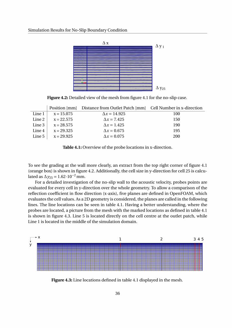
Position [mm] Distance from Outlet Patch [mm] Cell Number in x-directionLine 1 x = 15.075 ∆x = 14.925 100Line 2 x = 22.575 ∆x = 7.425 150Line 3 x = 28.575 ∆x = 1.425 190Line 4 x = 29.325 ∆x = 0.675 195Line 5 x = 29.925 ∆x = 0.075 200
Table 4.1: Overview of the probe locations in x-direction.
To see the grading at the wall more clearly, an extract from the top right corner of figure 4.1(orange box) is shown in figure 4.2. Additionally, the cell size in y-direction for cell 25 is calcu-lated as ∆y25 = 1.62 ·10−2 mm.
For a detailed investigation of the no-slip wall to the acoustic velocity, probes points areevaluated for every cell in y-direction over the whole geometry. To allow a comparison of thereflection coefficient in flow direction (x-axis), five planes are defined in OpenFOAM, whichevaluates the cell values. As a 2D geometry is considered, the planes are called in the followinglines. The line locations can be seen in table 4.1. Having a better understanding, where theprobes are located, a picture from the mesh with the marked locations as defined in table 4.1is shown in figure 4.3. Line 5 is located directly on the cell centre at the outlet patch, whileLine 1 is located in the middle of the simulation domain.
1 2 3 4 5x
y
Figure 4.3: Line locations defined in table 4.1 displayed in the mesh.
36

4.2 Generation of Results for No-Slip Case
4.2 Generation of Results for No-Slip Case
The procedure of calculating the reflection coefficient is shown in the diagram below (figure4.4). From OpenFOAM, a vector of velocity and pressure is written out for every cell along
p
uOFuA
pA
OpenFOAM
Af
Ag
Rc
Af^
Ag^
OF
Figure 4.4: Diagram for calculation of Rc for the no-slip case.
the line, named here as uOF and pOF . The acoustic fluctuation is then separated from themean part, resulting in vectors for the acoustic pressure p A and for the acoustic velocity uA
(sec. 2.3). With these, the f and g wave can be calculated and are saved in the A f and Ag
matrices. For every cell along the line, the variables are calculated. This results in a matriceswith a number of columns of 70. For these matrices, we want to get the maximal amplitudeof our related frequency. To do so, a fast Fourier transformation is applied for each row ofthe matrices A f and Ag . The coefficient of the frequencies are saved in the matrices A f andAg . The reflection coefficient is then calculated with the division of maximum amplitude of gwave over maximum amplitude of f wave for the related frequency.
This procedure is now shown for five selected cells along Line 2. To have a better under-standing how the calculation was done, figures are displayed for every step. The center of thefive cells are located with distances away from wall as shown in table 4.2.
Cells y-distance from wall [mm]Cell 5 y = 0.012
Cell 10 y = 0.036Cell 15 y = 0.069Cell 20 y = 0.115Cell 50 y = 1.155
Table 4.2: Five selected cells with the corresponding distance from the no-slip wall.
The graphs of velocity and pressure for the selected cells evaluated from OpenFOAM aredisplayed in figure 4.5. As no mean-flow is applied, the velocity fluctuation is around u =0m/s. Cells located closer to the wall are having a lower amplitude of the velocity. Plus, a
37

Simulation Results for No-Slip Boundary Condition
Figure 4.5: Velocity and pressure for selected cells along line 2.
phase displacement for the different cells in the velocity plot can be observed. The pressurefluctuation is done around p = 1·105 Pa, with same values independently of the cell locations.The acoustic fluctuation of pressure and velocity is now subtracted from its mean value. Usingthe formula uA = u − u for velocity and p A = p − p for pressure with the mean value for thetime starting at 0.05 s with a time length of three periods 3∆T = 0.04286s, results in figure4.6. The acoustic fluctuation of velocity uA has no changes in comparison to figure 4.5, the
Figure 4.6: Acoustic velocity and pressure for selected cell along Line 2.
phase displacement stays. The amplitude range was adapted manually. The acoustic pressurefluctuation is now oscillation around a zero mean value.
38

4.2 Generation of Results for No-Slip Case
Figure 4.7: The f and g wave for selected cell along Line 2.
Figure 4.7 is showing the f and g wave evolution. It can be seen, that the f wave for Cell5 has the smallest amplitude in comparison to the other cells, while it has the highest g waveamplitude. Which means, the reflection coefficient for this cell is quite high. Cell 50 has a highamplitude for f and a small amplitude for the g wave, which leads to a nearly zero reflectioncoefficient.
Applying a fast Fourier transformation to the f and g waves for the selected cells of figure4.7, results in the stem plot in figure 4.8, showing the frequency amplitudes of the f and gwaves. As expected, the highest peak arises for the applied frequency of F = 700Hz. The max-
0
1
2
3
4
|Âf|
10 -4
0 500 1000 1500 2000 2500 3000 3500 4000 4500 5000Frequency [Hz]
Cell 5Cell 10Cell 15Cell 20Cell 50
0
0.5
1
1.5
|Âg|
10 -4
0 500 1000 1500 2000 2500 3000 3500 4000 4500 5000Frequency [Hz]
Cell 5Cell 10Cell 15Cell 20Cell 50
Figure 4.8: A f and Ag for selected cell along Line 2.
imum amplitudes of the f and g waves for F = 700Hz, A f and Ag , are now used to calculatethe reflection coefficient with the formula Rc = Ag /A f . These three values for each cell can
39
Simulation Results for No-Slip Boundary Condition
Cell number A f[10−4
]Ag
[10−4
]R c
Cell 5 2.300 1.555 0.677Cell 10 2.847 1.141 0.401Cell 15 3.400 0.7343 0.216Cell 20 3.802 0.3959 0.104Cell 50 3.817 0.0188 0.005
Table 4.3: Selected cells with the corresponding amplitudes for f and g wave and the resultingreflection coefficient.
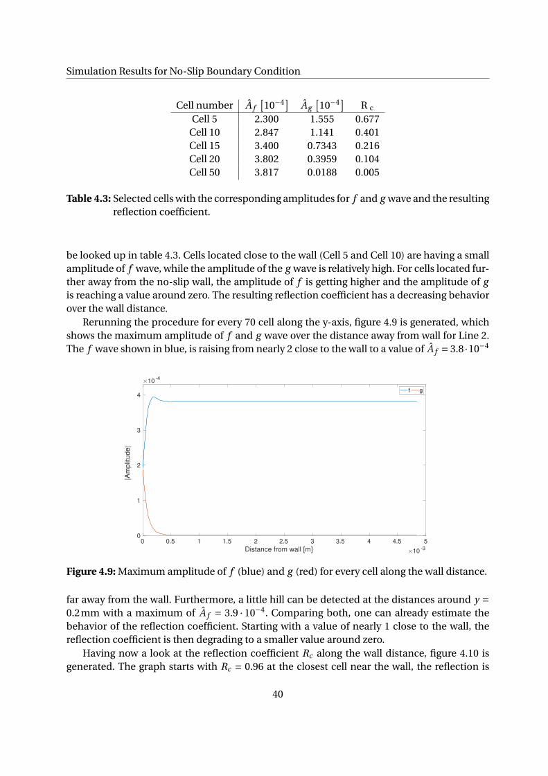
be looked up in table 4.3. Cells located close to the wall (Cell 5 and Cell 10) are having a smallamplitude of f wave, while the amplitude of the g wave is relatively high. For cells located fur-ther away from the no-slip wall, the amplitude of f is getting higher and the amplitude of gis reaching a value around zero. The resulting reflection coefficient has a decreasing behaviorover the wall distance.
Rerunning the procedure for every 70 cell along the y-axis, figure 4.9 is generated, whichshows the maximum amplitude of f and g wave over the distance away from wall for Line 2.The f wave shown in blue, is raising from nearly 2 close to the wall to a value of A f = 3.8 ·10−4
0 0.5 1 1.5 2 2.5 3 3.5 4 4.5 5
Distance from wall [m] 10-3
0
1
2
3
4
|Am
plit
ud
e|
10-4
f g
Figure 4.9: Maximum amplitude of f (blue) and g (red) for every cell along the wall distance.
far away from the wall. Furthermore, a little hill can be detected at the distances around y =0.2mm with a maximum of A f = 3.9 · 10−4. Comparing both, one can already estimate thebehavior of the reflection coefficient. Starting with a value of nearly 1 close to the wall, thereflection coefficient is then degrading to a smaller value around zero.
Having now a look at the reflection coefficient Rc along the wall distance, figure 4.10 isgenerated. The graph starts with Rc = 0.96 at the closest cell near the wall, the reflection is
40
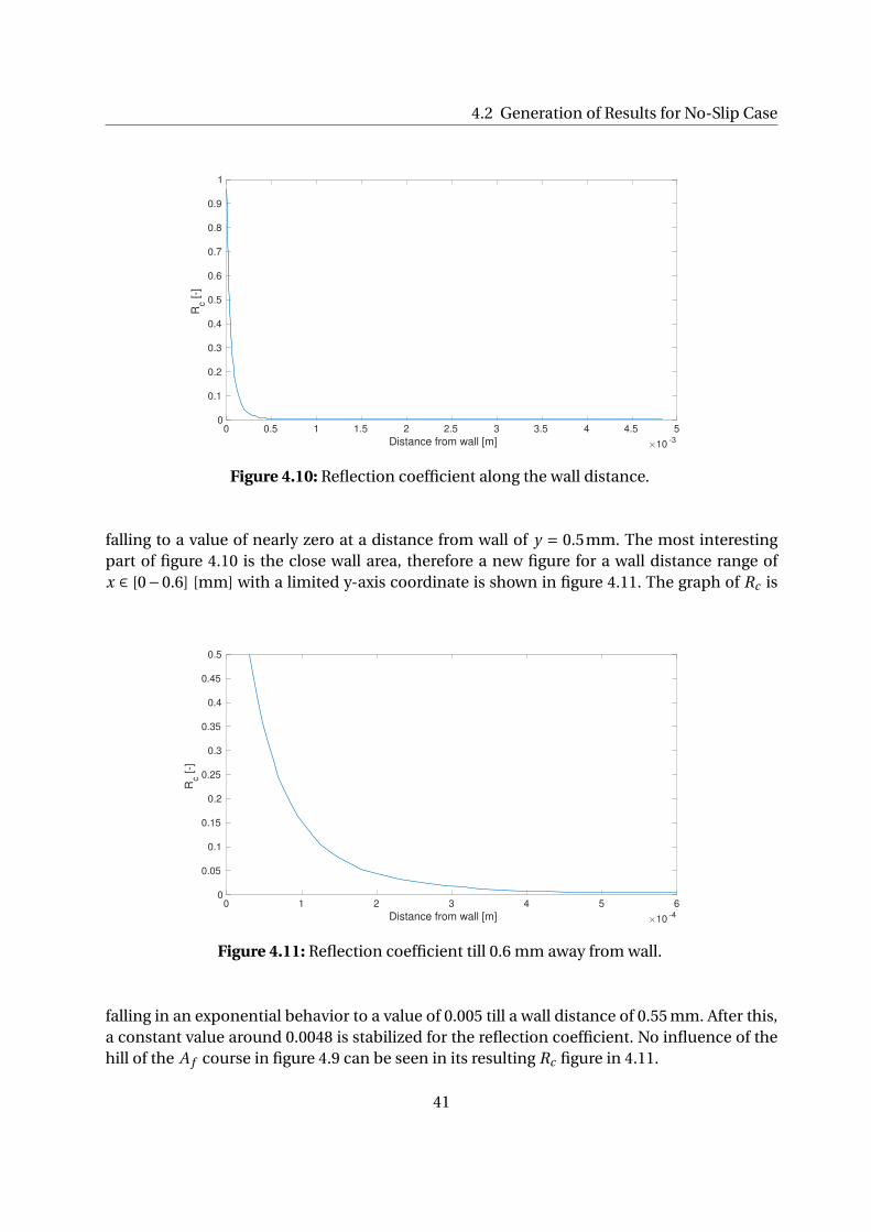
4.2 Generation of Results for No-Slip Case
0 0.5 1 1.5 2 2.5 3 3.5 4 4.5 5
Distance from wall [m] 10-3
0
0.1
0.2
0.3
0.4
0.5
0.6
0.7
0.8
0.9
1
Rc [
-]
Figure 4.10: Reflection coefficient along the wall distance.
falling to a value of nearly zero at a distance from wall of y = 0.5mm. The most interestingpart of figure 4.10 is the close wall area, therefore a new figure for a wall distance range ofx ∈ [0−0.6] [mm] with a limited y-axis coordinate is shown in figure 4.11. The graph of Rc is
0 1 2 3 4 5 6
Distance from wall [m] 10-4
0
0.05
0.1
0.15
0.2
0.25
0.3
0.35
0.4
0.45
0.5
Rc [
-]
Figure 4.11: Reflection coefficient till 0.6 mm away from wall.
falling in an exponential behavior to a value of 0.005 till a wall distance of 0.55 mm. After this,a constant value around 0.0048 is stabilized for the reflection coefficient. No influence of thehill of the A f course in figure 4.9 can be seen in its resulting Rc figure in 4.11.
41

Simulation Results for No-Slip Boundary Condition
4.3 Development of Rc in Flow Direction
The procedure for calculating the reflection coefficient was shown in detail in the previoussection (sec. 4.2). Now, only the resulting reflection coefficient graphs are investigated. Thissection observes the development of the reflection coefficient over the x-axis for a frequencyof F = 700Hz. Reflection coefficient graphs for the five line locations, introduced in sectionGeometry (4.1) are calculated and set in relation in one figure.
Figure 4.12 is showing the reflection coefficient over the whole wall distance. In general,all lines are having a low reflection coefficient value of Rc < 0.01 from a wall distance ofy > 0.5mm. Line 5, located directly at the outlet is having the best non-reflection behaviorin comparison to the other lines. At the closest wall cell, a value of only Rc = 0.43 is calculated.Line 5 is then directly falling to a reflection coefficient value lower than 0.001 at a wall dis-tance y = 0.031mm. The other lines starting with values of Rc ≈ 0.96, are then decreasing witha lower gradient, and are reaching reflection coefficient values lower than 0.01 at distancesy > 1mm away from the no-slip wall.
0 0.5 1 1.5 2 2.5 3 3.5 4 4.5 5
Distance from wall [m] 10-3
0
0.1
0.2
0.3
0.4
0.5
0.6
0.7
0.8
0.9
1
Rc [
-]
Line 1
Line 2
Line 3
Line 4
Line 5
Figure 4.12: Development of Rc along the x-axis.
In figure 4.13, the range of the reflection coefficient is limited by the values Rc ∈ [0−0.05],to allow a more detailed investigation of the line evolution. Firstly, a remark of the gradientsat a close wall distance area lower than y < 0.5mm is made. As already indicated in figure4.12, Line 5 is having the highest gradient of all compared lines. It is falling with a value of∆Rc = 0.43 in a distance area of ∆y = 0.031. Looking now at Line 4, which is located the sec-ond closest to the wall. It has the lowest descent value of all lines. Therefore, Line 4 and Line5 are setting the limits of the gradients at a wall distance of 0.5 mm. Line 3 is having the sec-ond lowest gradient, while Line 1 and Line 2 are falling with the same gradient, the secondhighest in comparison to all observed. In figure 4.13, the black dotted line is showing the cor-responding stokes boundary layer thickness for a frequency of F = 700Hz, which is calculatedas δ700Hz = 0.519mm. A relation between the development of stokes layer and the locations
42

4.3 Development of Rc in Flow Direction
0 0.5 1 1.5 2 2.5 3 3.5 4 4.5 5
Distance from wall [m] 10-3
0
0.005
0.01
0.015
0.02
0.025
0.03
0.035
0.04
0.045
0.05R
c [
-]Line 1
Line 2
Line 3
Line 4
Line 5
Figure 4.13: Development of Rc along the x-axis for a selected range.
of lines can be observed. Already for Line 4, the kink locates the end of the layer. Lines, lo-cated further away from the outlet (Line 1 to Line 3) are having a more significant change inits reflection coefficient graphs.
Now, the development of each line along the wall distance is observed in more detail. Anon-reflection behavior is assumed by a value lower than Rc < 0.005, to allow a compari-son between every line. Line 5 is reaching a non reflection behavior for a wall distance ofy = 0.031mm with a value lower than Rc < 0.0001, which is the lowest Rc of all observed lines.Related to the whole wall distance, 99.5% of the y-axis have a behavior of non reflection. Line2, distant ∆x = 0.675mm away from outlet patch, is shown in the purple graph. It is fallingtill a wall distance around y = 0.5mm, where a kink can be detected. After, it is falling againwith a lower gradient till its stabilized around Rc = 0.0012 for wall distances y > 3mm. Theassumed non-reflection value is reached for a distance of y = 1.35mm, which corresponds toa non-reflection behavior over the whole wall distance for 73 %. Line 3 has a higher gradientthan Line 4, the kink is located at the same wall distance with a more distinct behavior. After,it is falling till it reaches values of Rc = 0.002 at the end wall distances. Non-reflection is guar-anteed for about 65 % over the whole wall distance. For Line 1 (∆x = 14.925mm) and Line 2(∆x = 7.425mm), the behavior of the reflection coefficient over the wall distance are similar.The graphs are falling with the second highest gradient till its ending in a kink for a wall dis-tance around y = 0.5mm. After the kink, the reflection coefficient is stabilized over the wholewall distance at a value of Rc = 0.0048. Non-reflection is ensured for 90 % of the whole walldistance.
In the following, the effect of Line 5 having the lowest reflection coefficient for nearly thewhole wall distances is pointed out. With the help of paraView, the velocity solution fieldsare demonstrated. Figure 4.14 is showing the velocity field in x-direction for a time t = 75ms,while in figure 4.15, the velocity in y-direction can be detected. In both figures only the top
43

Simulation Results for No-Slip Boundary Condition
right corner of the geometry are displayed, as the biggest changes are happening in this area.
Line 5Cell 1Cell 2
outlet
no-slipx
y
Figure 4.14: Velocity (x) at close wall outlet area for t=75 ms; Low velocity (ux ≈ 0m/s) shownin blue and high velocity
(ux = 4.4 ·10−4 m/s
)shown in red.
Looking at the cells along Line 5, located the closest to the outlet, a homogeneous velocityfield till the last two top cells can be seen. Only the two top cells are having a different velocityvalue. Comparing with the cells located further away from the outlet patch, a big differenceis detected. Especially the influence of the no-slip wall can not be seen this clear for the cellsalong Line 5. It seems like the velocity are defined by the outlet boundary condition.
Line 5
Cell 10
Cell 20
outlet
x
y
no-slip
Figure 4.15: Velocity (y) at close wall outlet area for t=75 ms; Negative velocity(uy =−4.4 ·10−5 m/s
)shown in red and zero velocity (grey).
In figure 4.15, showing the solution field for the velocity in y-direction, velocities arounda value of uy = −4.4 · 10−5 m/s are marked as red, while the grey color represents a velocity
44

4.4 Comparison of Rc for different Frequencies
of zero. Along Line 5, the cells between cell 10 and cell 20 are marked high red, which corre-sponds to a velocity value in negative y-direction. Cells located further away from the outletpatch are having a lower respectively no velocity component in y-direction. It seems like they-component of velocity reduces the influence of the no-slip wall (fig. 4.14) for the cells alongLine 5.
4.4 Comparison of Rc for different Frequencies
Simulations with frequencies of 300 Hz, 500 Hz, 700 Hz, 1000 Hz and 1500 Hz are now ob-served. In particular, how the boundary layer is developing for every frequency. As seen inthe previous chapter 4.3, the reflection coefficient for Line 1 and Line 2 are behaving almostequal. So only Line 2, Line 3, Line 4 and Line 5 are observed. Furthermore, all figures are shownout in a determined range of Rc ∈ [0−0.05].
Line 2
Starting with Line 2, located at the position x = 22.575mm. The resulting reflection coefficientalong the wall distance is plotted in figure 4.16. Starting to observe the graph for a frequency
0 0.5 1 1.5 2 2.5 3 3.5 4 4.5 5
Distance from wall [m] 10-3
0
0.005
0.01
0.015
0.02
0.025
0.03
0.035
0.04
0.045
0.05
Rc [
-]
f=300 Hz
f=500 Hz
f=700 Hz
f=1000 Hz
f=1500 Hz
Figure 4.16: Reflection coefficient for different frequencies in a certain distance range alongLine 2.
of F = 300Hz. It has the lowest gradient in comparison to the other one till it stabilized at avalue of nearly Rc = 0.009, meaning the highest reflection coefficient value of all observed fre-quencies. The stabilization starts at a wall distance of y = 0.75mm, comparing with the stokesboundary layer for this frequency δ300H z = 0.793mm, it is located in the same cell. The higherthe frequency gets, the closer the stabilization around a mean value is happening. So a rela-
45

Simulation Results for No-Slip Boundary Condition
tion between stokes boundary layer and frequency can be observed for Line 2. Furthermore,the local minimum before it stabilized is getting bigger marked, the higher the frequency gets.
Line 3
Having now a look at the x-distance x = 28.575mm, means closer to the outlet boundarycondition, figure 4.17 is created. In comparison to Line 2, the fall before reaching the related
0 0.5 1 1.5 2 2.5 3 3.5 4 4.5 5
Distance from wall [m] 10-3
0
0.005
0.01
0.015
0.02
0.025
0.03
0.035
0.04
0.045
0.05
Rc [
-]
f=300 Hz
f=500 Hz
f=700 Hz
f=1000 Hz
f=1500 Hz
Figure 4.17: Reflection coefficient for different frequencies along Line 3.
stokes boundary layer is not this high. The local minimum is not this developed as for Line2. After each graph is passing its turning point, it keeps falling with a lower gradient. No di-rect stable coefficient is observed. Especially for the graph for a frequency of F = 1500Hz is tomention, as it is intersecting with the purple and yellow graph and is increasing along the walldistance.
Line 4
Reflection coefficient evolution along the wall distance for Line 4 is showing in figure 4.18. Adevelopment of a boundary layer for a frequency of F = 300Hz can not be observed clearly,moreover a stabilized state at a wall distance of y = 4.5mm can not be detected. For a fre-quency of F = 700Hz, a kink in its fall can be assumed, however, higher frequencies are show-ing a more clear difference in the graph when the boundary layer is finished. The green graphis raising after passing a wall distance of y = 2mm and is intersecting with all other graphs,leading to the highest reflection coefficient at the symmetry patch of the simulated domain.Furthermore, the purple graph is also cutting line yellow and red.
46

4.4 Comparison of Rc for different Frequencies
0 0.5 1 1.5 2 2.5 3 3.5 4 4.5 5
Distance from wall [m] 10-3
0
0.005
0.01
0.015
0.02
0.025
0.03
0.035
0.04
0.045
0.05R
c [
-]f=300 Hz
f=500 Hz
f=700 Hz
f=1000 Hz
f=1500 Hz
Figure 4.18: Reflection coefficient for different frequencies along Line 4.
Line 5
As a last investigation, the cells, located directly at the outlet are observed. The resulting re-flection coefficient plot can be seen in figure 4.19. As the effect are this small, the y range of theplot was adapted, which leads to a range of Rc ∈ [
0 − 5 ·10−3]. The gradient of the observed
0 0.5 1 1.5 2 2.5 3 3.5 4 4.5 5
Distance from wall [m] 10-3
0
0.5
1
1.5
2
2.5
3
3.5
4
4.5
5
Rc [
-]
10-3
f=300 Hz
f=500 Hz
f=700 Hz
f=1000 Hz
f=1500 Hz
Figure 4.19: Reflection coefficient for different frequencies along Line 5.
frequencies are all falling in a similar behavior till a wall distance of 0.03 mm, the blue plot iseven falling to the lowest value. For a frequency F = 300Hz, the reflection coefficient is thenraising again to a value of Rc = 0.0012 for a wall distance of y = 0.12mm. After this, it is fallingagain. It behaves like a damping wave. For the other frequencies, the damping of the first hill
47

Simulation Results for No-Slip Boundary Condition
is getting smaller, the higher the frequency is. It then stabilized after 0.5 mm at a reflectioncoefficient of Rc = 0.0005.
4.5 Discussion about Rc Evolution for No Mean-Flow
Firstly the development in flow direction is discussed here. Then the influence of differentfrequencies are investigated more detailed.
Comparing to section 4.3, an evolution of the reflection coefficient perpendicular to theflow direction can be observed. The Rc graph needs a certain distance away from the outletto generate a clear stokes boundary layer. Cells along Line 5, located directly at the outletare having the lowest reflection coefficient value. It seems like the CBSBC is influencing thecells directly at the outlet (compare fig. 4.14), as the influence of the no-slip wall is reduced.For a distance away from the outlet of ∆x = 0.675mm, a little kink can only assume a stokesboundary layer, while for Line 3 and especially for Line 1 and Line 2, a clear generation ofthe stokes boundary layer can be seen in the Rc plot. It would be interesting to investigate,at which exact distance away from the outlet patch a fully generated boundary layer can bedetected.
For higher frequencies, a change in the graph while passing the stokes boundary layer canbe clearly detected for all lines. But for a frequency of F = 300Hz, a clear generation of thestokes boundary layer can only be observed for distances higher than ∆x = 7.425mm awayfrom the outlet patch.
Polifke [9] added a plane wave masking to the LODI relation, as higher frequencies lead toa bad construction of the reflection coefficient. For Line 2, this can be clearly seen. However,an ascent in the Rc graphs for higher frequencies can be observed, which results in intersec-tions of graphs with lower frequencies along the wall distance for the close outlet lines. Thisleads to a higher and therefore worse reflection coefficient in the middle of the domain. Es-pecially for Line 4, a frequency of F = 1500Hz leads to the highest reflection coefficient of allobserved frequencies in the middle of the domain. Table 4.4 is showing the calculated reflec-tion coefficient to the corresponding frequencies for a wall distance of y = 4.5mm for Line 4.The relatively high Rc value for F = 300Hz can be explained, as no converged status is reachedfor this wall distance.
Lower frequencies leads to a higher amplitude of the damping wave along Line 5, lo-cated directly at the outlet patch. However, the range of the damping is in dimensions ofRc ∈ 0.0005−0.001.
Because of time constraints, the investigation could not be done more detailed. A modifi-cation in the CBSBC boundary file could maybe help to understand the issue more clearly.
F [Hz] 300 500 700 1000 1500Rc [-] 0.016 0.0001 0.0001 0.0014 0.0025
Table 4.4: Rc for different frequencies for Line 4 at wall distance y = 4.5mm.
48

4.6 Applying a Mean-Flow to the No-Slip Simulation Case
4.6 Applying a Mean-Flow to the No-Slip Simulation Case
Applying a mean-flow to the simulation requires also its elimination to calculate the f and gwaves. Additionally, the influence of the no-slip top wall leads to different velocity evolutionfor every cell along the y-axis. For that reason, five cells are printed out to see the change ofamplitude and mean-value for every cell. Cell 66 is added, as it is located close to the sym-metry patch wall and therefore receives low influence from the no-slip wall. Furthermore, toobtain a converged state of the variables, the end time of simulation is extended to tend = 0.1s.Firstly, the velocity and pressure evolution for the selected cells is shown in figure 4.20. Cell 66
0 0.01 0.02 0.03 0.04 0.05 0.06 0.07 0.08 0.09 0.1
Time [s]
0
10
20
u [m
/s]
10-4
Cell 5 Cell 10 Cell 20 Cell 50 Cell 66
0 0.01 0.02 0.03 0.04 0.05 0.06 0.07 0.08 0.09 0.1
Time [s]
1
1.000002
1.000004
1.000006
p [P
a]
105
Cell 5 Cell 10 Cell 20 Cell 50 Cell 66
Figure 4.20: Velocity and pressure evolution over time for selected cells.
is having the highest mean value of velocity, as the influence of the no-slip wall is the lowest.It is growing constantly to a mean value around u = 0.0012m/s till a time of t = 0.1s. A stabi-lized manner with a low gradient can be assumed for further time steps. Cell 50 is growing inthe same behavior as Cell 66 up to t = 0.01s, then it is falling till it stabilized around a meanvelocity of u = 0.0008m/s. Looking at Cell 20, an incline in the first time steps is observed,afterwards the graph is stabilized around u ≈ 0m/s. The closer cells are oscillating aroundu = 0m/s, while Cell 10 has a higher amplitude than Cell 5. For the pressure graphs, every cellbehaves the same, the oscillations is made around p = 100000.4Pa.
The mean velocity and pressure are calculated in the time interval from 0.095 s to 0.099286 s,as a stable manner for all cells can be assumed. Subtracting the mean values from the vari-ables, seen in figure 4.20, leads to the acoustic fluctuation of pressure and velocity. With thehelp of these, the f and g waves can be calculated and are shown in figure 4.21. For Cell 66and Cell 50, a similar amplitude for the f wave can be adopted. Cell 20 received a phase shift,while Cell 5 and Cell 10 are oscillating with a smaller amplitude and a phase shift in compar-
49

Simulation Results for No-Slip Boundary Condition
0.095 0.0955 0.096 0.0965 0.097 0.0975 0.098 0.0985 0.099
Time [s]
-4
-2
0
2
4
f [m
/s]
10-4
Cell 5 Cell 10 Cell 20 Cell 50 Cell 66
0.095 0.0955 0.096 0.0965 0.097 0.0975 0.098 0.0985 0.099
Time [s]
-2
-1
0
1
2
g [m
/s]
10-4
Cell 5 Cell 10 Cell 20 Cell 50 Cell 66
Figure 4.21: The f and g wave evolution over selected time.
ison to Cell 50. By observing the g waves, Cell 50 and Cell 66 are having approximately a zeroamplitude. Whereas Cell 5 is having the highest amplitude and phase shift.
Cell number Wall distance [mm] A f[10−4
]Ag
[10−4
]R c [-]
Cell 5 0.017 2.3010 1.5544 0.6756Cell 10 0.042 2.8585 1.1419 0.3995Cell 20 0.126 3.8192 0.4078 0.1068Cell 50 1.238 3.8146 0.1712 0.0045Cell 66 3.693 3.8201 0.1974 0.0052
Table 4.5: Selected cells with the corresponding amplitudes (F = 700Hz) for f and g wavesand the resulting reflection coefficient Rc .
Table 4.5 is showing the maximal amplitudes of f and g waves and the correspondingreflection coefficient for the selected cells. By looking at the Rc value, a tendency can be de-tected. The reflection coefficient is falling with a high gradient at the close wall area till Cell 50.But for Cell 60, the reflection coefficient is increasing again. So the reflection coefficient is notstable for cells located further away from the outlet. As the reflection coefficient is calculatedonly for five cells, the point of Rc , changing from falling to increasing can not be located thisclearly. This will be investigated in more detail in the further section. Additionally, the figureof reflection coefficient over the wall distance can be looked up in figure 4.22. Starting with avalue of Rc ≈ 1, the graph is falling strongly till it reaches a value Rc < 0.01 for wall distance ofy > 0.5mm. As a global range of Rc is shown, the growth of Rc can not be seen this clearly.
50

4.7 Development of Rc in Flow Direction with Mean-Flow
0 0.5 1 1.5 2 2.5 3 3.5 4 4.5 5
Distance from wall [m] 10-3
0
0.1
0.2
0.3
0.4
0.5
0.6
0.7
0.8
0.9
1
Rc [-]
Figure 4.22: Reflection coefficient over wall distance
The increasing behavior of Rc can be detected more clearly for higher mean-flows. Thereader is referred at this point to the next section 4.7, where a mean-flow of u = 0.005m/s isinvestigated.
4.7 Development of Rc in Flow Direction with Mean-Flow
As already mentioned in the last section, a growth of the reflection coefficient graph over thewall distance was detected. This will now be observed in more detail for a limited Rc range.The mean-flow is set to u = 0.005m/s.
Figure 4.23 is showing the reflection coefficient for selected line locations along the x-axis. The black dotted line is marking the end of the stokes boundary layer thickness for afrequency F = 700Hz. Comparing figure 4.23 with the figure 4.13, displaying the reflectioncoefficient along the lines with no mean-flow, two big differences can be detected. Firstly,Line 1 and Line 2 are raising slowly after passing the stokes thickness to a wall distance ofy = 2.6mm, where the graph is receiving an inflection point. A reflection coefficient value ofRc = 0.008 is calculated for the close symmetry area. In comparison to the no mean-flow case,the reflection coefficient of Line 1 and Line 2 is staying stable after passing the stokes layerthickness (Rc = 0.0048). The other big difference can be seen for the graph of line 5. It is alsonot staying in an converged state along the wall distance as for the no mean-flow case. It isbehaving in an wave characteristic way, starting at a distance, lower than the stokes thickness.Furthermore, for a wall distance higher than 1.6 mm, a zigzag behavior for Line 5 and Line 4can be observed.
51
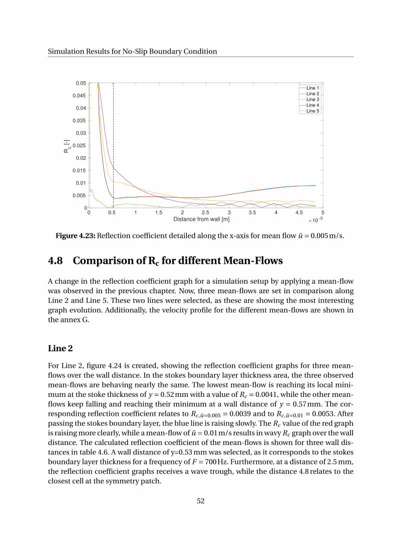
Simulation Results for No-Slip Boundary Condition
0 0.5 1 1.5 2 2.5 3 3.5 4 4.5 5
Distance from wall [m] 10-3
0
0.005
0.01
0.015
0.02
0.025
0.03
0.035
0.04
0.045
0.05
Rc [-]
Line 1
Line 2
Line 3
Line 4
Line 5
Figure 4.23: Reflection coefficient detailed along the x-axis for mean flow u = 0.005m/s.
4.8 Comparison of Rc for different Mean-Flows
A change in the reflection coefficient graph for a simulation setup by applying a mean-flowwas observed in the previous chapter. Now, three mean-flows are set in comparison alongLine 2 and Line 5. These two lines were selected, as these are showing the most interestinggraph evolution. Additionally, the velocity profile for the different mean-flows are shown inthe annex G.
Line 2
For Line 2, figure 4.24 is created, showing the reflection coefficient graphs for three mean-flows over the wall distance. In the stokes boundary layer thickness area, the three observedmean-flows are behaving nearly the same. The lowest mean-flow is reaching its local mini-mum at the stoke thickness of y = 0.52mm with a value of Rc = 0.0041, while the other mean-flows keep falling and reaching their minimum at a wall distance of y = 0.57mm. The cor-responding reflection coefficient relates to Rc,u=0.005 = 0.0039 and to Rc,u=0.01 = 0.0053. Afterpassing the stokes boundary layer, the blue line is raising slowly. The Rc value of the red graphis raising more clearly, while a mean-flow of u = 0.01m/s results in wavy Rc graph over the walldistance. The calculated reflection coefficient of the mean-flows is shown for three wall dis-tances in table 4.6. A wall distance of y=0.53 mm was selected, as it corresponds to the stokesboundary layer thickness for a frequency of F = 700Hz. Furthermore, at a distance of 2.5 mm,the reflection coefficient graphs receives a wave trough, while the distance 4.8 relates to theclosest cell at the symmetry patch.
52

4.8 Comparison of Rc for different Mean-Flows
0 0.5 1 1.5 2 2.5 3 3.5 4 4.5 5
Distance from wall [m] 10-3
0
0.005
0.01
0.015
0.02
0.025
0.03
0.035
0.04
0.045
0.05
Rc [-]
0.001
0.005
0.01
meanflow [m/s]
Figure 4.24: Reflection coefficient for different mean-flows along Line 2
Wall DistanceMean-Flow [m/s] 0.53mm 2.5mm 4.8mm
0.001 Rc = 0.0041 Rc = 0.0047 Rc = 0.00540.005 Rc = 0.0040 Rc = 0.0042 Rc = 0.00890.01 Rc = 0.0054 Rc = 0.0041 Rc = 0.0139
Table 4.6: Reflection coefficient for different mean-flows for selected wall distances at Line 2.
53
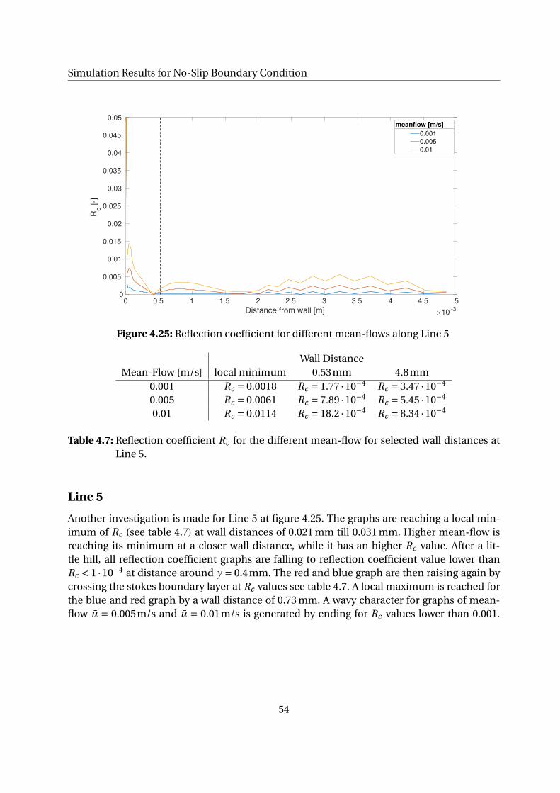
Simulation Results for No-Slip Boundary Condition
0 0.5 1 1.5 2 2.5 3 3.5 4 4.5 5
Distance from wall [m] 10-3
0
0.005
0.01
0.015
0.02
0.025
0.03
0.035
0.04
0.045
0.05
Rc [-]
0.001
0.005
0.01
meanflow [m/s]
Figure 4.25: Reflection coefficient for different mean-flows along Line 5
Wall DistanceMean-Flow [m/s] local minimum 0.53mm 4.8mm
0.001 Rc = 0.0018 Rc = 1.77 ·10−4 Rc = 3.47 ·10−4
0.005 Rc = 0.0061 Rc = 7.89 ·10−4 Rc = 5.45 ·10−4
0.01 Rc = 0.0114 Rc = 18.2 ·10−4 Rc = 8.34 ·10−4
Table 4.7: Reflection coefficient Rc for the different mean-flow for selected wall distances atLine 5.
Line 5
Another investigation is made for Line 5 at figure 4.25. The graphs are reaching a local min-imum of Rc (see table 4.7) at wall distances of 0.021 mm till 0.031 mm. Higher mean-flow isreaching its minimum at a closer wall distance, while it has an higher Rc value. After a lit-tle hill, all reflection coefficient graphs are falling to reflection coefficient value lower thanRc < 1 ·10−4 at distance around y = 0.4mm. The red and blue graph are then raising again bycrossing the stokes boundary layer at Rc values see table 4.7. A local maximum is reached forthe blue and red graph by a wall distance of 0.73 mm. A wavy character for graphs of mean-flow u = 0.005m/s and u = 0.01m/s is generated by ending for Rc values lower than 0.001.
54

4.9 Influence of Mean-Flow to Rc
4.9 Influence of Mean-Flow to Rc
Applying a mean-flow to the no-slip cases requires to expand the end of simulation time,as the velocity graphs for cells, located further away from the no-slip wall keeps increasing.This leads to some problems by calculating the acoustic fluctuation of pressure and velocity.As some waves have not reached their converged state, the calculation of the mean velocityis not this exact. However, setting the range to a high time reduces the impact of the nonconverged state. But this affect should be integrated in the discussion, as it could be possible,that it influence the calculation of the f and g wave and therefore the reflection coefficientRc .
By looking at the resulting reflection coefficient figures for the mean-flow cases, a generallow reflection coefficient is calculated. However, investigations were made in small Rc range,as differences to the cases without mean-flow could be observed.
Two areas were observed for the no-slip mean-flow case. One area, located far away fromthe CBSBC outlet (Line 2), and one located directly at the close outlet cell (Line 5). For botharea, applying a mean-flow results in a wavy character of the reflection coefficient in the chan-nel interior. The development of Rc in the stokes layer are almost similar, however highermean-flows results in higher reflection coefficient values.
Furthermore, for higher mean-flows, the mesh has to be adapted. The cell size in the inte-rior of the geometry has to be smaller to avoid the zigzag behavior as seen in figure 4.25.
Because of time constraints, no further investigations could be done. Especially the result-ing reflection coefficient graph for higher mean-flows would be an interesting investigation.
55

5 Summary and Conclusion
This thesis concentrated on the validation of a new acoustic boundary condition, the CBSBC,in OpenFOAM. In the beginning, the related equations and the CBSBC approach were intro-duced. Furthermore, the implementation of the CBSBC in OpenFOAM is shown.
At the outset, a geometry with slip boundary condition at the wall was used. Test casesdemonstrated the behavior of the new boundary condition. In general, the CBSBC is workinggood in a slip boundary environment. An applied reflection coefficient was proven. Applyinghigh mean-flow leads to damping character of the g wave. This effect could not be explainedin detail and should be investigated extensively in further projects.
For a no-slip boundary condition geometry, an evolution of the reflection coefficient inflow direction was observed. The stokes boundary layer was fully generated for a distance ofabout 7.5 mm away from the outlet CBSBC. Especially at the closest outlet cells, the no-sliparea of the wall was not this distinct, which could be traced back to the CBSBC. Observing dif-ferent frequencies leads to an increase of the reflection coefficient over the wall distance. Forcells, located far away from the outlet, higher frequency leads to good Rc values. The closeryou get to the CBSBC outlet, the higher the reflection coefficient is increasing near the sym-metry patch. Applying a mean-flow to the no-slip setup leads also to an increase of Rc . TheRc evolution perpendicular to the flow direction has a damping wave character for a distancehigher than 7.5 mm away from the outlet. Further investigations are proposed in particularfor the mean-flow cases, as the damping character is not this clear.
By assuming a non-reflection behavior of the CBSBC for reflection coefficient value ofRc < 1%, validations for slip boundary condition is proven. Furthermore, for the no-slip caseswithout mean-flow, it is also correct for a wall distance higher than the stokes boundary layerthickness. A validation of higher frequencies close to the outlet patch should be investigatedin more detail. Additionally, high mean-flows applied to the no-slip boundary condition casecan not be validated properly and should be examined in further projects.
The follows remark should give a short overview of some problems and difficulties, arisesduring writing the thesis. Generally, profound background knowledge in acoustic and in theused software tools would have been a benefit. Visiting fundamental acoustic lecture beforewriting the thesis would have allow to understand the subject more clearly. Furthermore,more practical experiences in OpenFOAM would have allow to set up a appropriate meshin less time.
Because of time constraint and a limited background knowledge especially in acoustic,no detailed investigation of the concerning effects could be reached. Therefore, this thesisgives good basic informations about the CBSBC and can be used for further reseaches anddiscussions.
56

Appendices
57
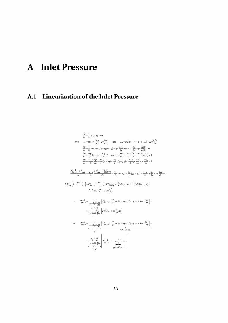
A Inlet Pressure
A.1 Linearization of the Inlet Pressure
∂p
∂t+ 1
2
(L5 +L1
)= 0
with L1 = (u −c)
[∂p
∂x−ρc
∂u
∂x
]and L5 =σ5
[u − (
fx − gu)−ut
]+2ρc∂ fx∂t
∂p
∂t+ 1
2
[σ5
(u − ( fx − gu )−ut
)+2ρc∂ fx∂t
+ (u − c)
(∂p
∂x−ρc
∂u
∂x
)]= 0
∂p
∂t+ σ5
2
(u −ut
)− σ52
(fx − gu
)+ρc∂ fx∂t
+ u − c
2
∂p
∂x− u − c
2ρc
∂u
∂x= 0
∂p
∂t+ u − c
2
∂p
∂x− σ5
2
(u −ut
)− σ52
(fx − gu
)− u − c
2ρc
∂u
∂x+ρc
∂ fx∂t
= 0
Pn+1f ace
−Pnf ace
d t+ u − c
2
Pn+1f ace
−Pn+1centr e
d x− σ5
2
(u −ut
)− σ52
(fx − gu
)− u −c
2ρc
∂u
∂x+ρc
∂ fx∂t
= 0
Pn+1f ace
(1+ u −c
2
d t
d x
)= Pn
f ace + u −c
2
d t
d xPn+1
centr e + σ52
d t(u −ut
)− σ52
d t(
fx − gu)−
− u − c
2ρcd t
∂u
∂x+d tρc
∂ fx∂t
→ Pn+1f ace = 1
1+ u−c2
d td x
[Pn
f ace − σ52
d t[(u −ut )+ ( fx − gu )
]+d tρc∂ fx∂t
]+
+u−c
2d td x
1+ u−c2
d td x
[Pn+1
centr e +ρc∂u
∂xd x
]
⇒ Pn+1f ace = 1
1+ u−c2
d td x︸ ︷︷ ︸
f
[Pn
f ace − σ52
d t[(u −ut )+ ( fx − gu )
]+d tρc∂ fx∂t
]︸ ︷︷ ︸
valueE xpr
+
+u−c
2d td x
1+ u−c2
d td x︸ ︷︷ ︸
1− f
Pn+1centr e + ρc
∂u
∂x︸ ︷︷ ︸g r adE xpr
d x
58

A.2 CBSBC Implementation in OpenFOAM
A.2 CBSBC Implementation in OpenFOAM
A.2.1 FractionExpression
The implementation in OpenFOAM for the fractionExpression f is:
valueF r acti on() = 1.0/(1.0+d t ∗ thi s−> patch().del t aCoe f f s()∗ (aP + cP )/2.0)
= 1
1+ aP+cP2 ∗ thi s−> patch().del t aCoe f f s()
⇒ f = 1
1+ u+c2
d td x
A.2.2 ValueExpression
The implementation in OpenFOAM for the valueExpression = refValue() is:
r e f V alue() = ( f i eld .ol dT i me().bound ar yF i eld()[patchi ]++et a Ac ∗ r hop ∗ sqr (cP )∗ (1.0− sqr (aP/cP ))/2.0/l In f ∗d t∗∗ [(thi s−> patch().n f () & (Up −uIn f ))+ f − g ]+ r hop ∗ cP ∗ ( f − f 0)
= Pnf ace +et a Ac(1− sqr
(aP
cP
)cP
l In f∗ cP ∗ r hop
2∗d t
(∂(Up −uIn f )
∂x+ f − g
)+
+ r hop ∗ cP ∗ ( f − f 0)
as K = ηc (1−M2)c
l[Poi nsot ]
= Pnf ace +K
ρc
2d t
(∂(Up −uIn f )
∂x+ f − g
)+ρ∗ c ∗ ( f − f 0)
as L1 = K (p −p∞) = σ
ρc(p −p∞) → K = σ
ρc
⇒ r e f V alue() = Pnf ace + σ5
2d t
[∂(Up −uIn f )
∂x+ f − g
]+ρc( f − f 0)
A.2.3 GradExpression
The implementation in OpenFOAM for the gradientExpression = refGrad() is:
r e f Gr ad() =−1.0∗ r hop ∗ cP ∗ (thi s−> patch().n f () & Up.snGr ad()
)⇒ r e f Gr ad() =−ρc
∂u
∂x
59

B Outlet Pressure
B.1 Linearization of the Outlet Pressure
∂p
∂t+ 1
2
(L5 +L1
)= 0
with L5 = 1
2
[(u + c)
(∂p
∂x+ρc
∂u
∂x
)]and L1 = σ
ρc
[p −ρc( fd + gx )−p∞
]+2∂gx∂t
∂p
∂t+ 1
2
[(u + c)
(∂p
∂x+ρc
∂u
∂x
)+ σ
ρc
(p −ρc
(fd + gx
)−p∞)+2
∂gx∂t
]= 0
∂p
∂t+ u +c
2
∂p
∂x+ρc
u + c
2
∂u
∂x+ σ
2ρc
(p −p∞
)− σ
2
(fd + gx
)+ ∂gx∂t
= 0
Pn+1f ace
−Pnf ace
d t+ u + c
2
Pn+1f ace
−Pn+1centr e
d x+ρc
u +c
2
∂u
∂x+ σ
2ρc
(Pn+1
f ace −p∞)− σ
2
(fd + gx
)+ ∂gx∂t
= 0
Pn+1f ace −Pn
f ace + u + c
2
d t
d x
(Pn+1
f ace −Pn+1centr e
)+ρc
u +c
2d t
∂u
∂x+ σ
2ρcd t
(Pn+1
f ace −p∞)− σ
2d t
(fd + gx
)++ ∂gx
∂td t = 0
Pn+1f ace
(1+ u + c
2
d t
d x+ σ
2ρcd t
)= Pn
f ace + u +c
2
d t
d xPn+1
centr e −ρcu +c
2d t
∂u
∂x+ σ
2d t
(fd + gx
)+ σ
2ρcd t p∞−
− ∂gx∂t
d t
Pn+1f ace =
1+ σd t2ρc
1+ u+c2
d td x + σd t
2ρc
Pnf ace
+ σd t2ρc p∞+ σd t
2(
fd + gx)−d t
∂gx∂t
1+ σd t2ρc
+u+c
2d td x
1+ u+c2
d td x + σd t
2ρc
[Pn+1
centr e+
+(−ρc
∂u
∂xd x
)]
Pn+1f ace =
1+ σd t2ρc
1+ u+c2
d td x + σd t
2ρc︸ ︷︷ ︸f
Pnf ace
+ σd t2ρc p∞+ σd t
2(
fd + gx)−d t
∂gx∂t
1+ σd t2ρc
︸ ︷︷ ︸
valueExpr
+
+u+c
2d td x
1+ u+c2
d td x + σd t
2ρc︸ ︷︷ ︸1-f
Pn+1centr e + ( −ρc
∂u
∂x︸ ︷︷ ︸g r adE xpr
d x)
60

B.2 CBSBC Implementation in OpenFOAM
B.2 CBSBC Implementation in OpenFOAM
B.2.1 FractionExpression
The implementation in OpenFOAM for the fractionExpression f is :
f = (1.0+et a Ac ∗ cP ∗d t ∗ (1.0− sqr (aP/cP ))/2.0/l In f )/(1.0+et a Ac ∗ cP ∗d t∗∗ (1.0− sqr (aP/cP ))/2.0/l In f + (aP + cP )∗d t/2.00∗ thi s−> patch().del t aCoe f f s())
f =1.0+et a Ac ∗ cP ∗d t ∗
1.0−sqr(
aPcP
)2.0∗l In f
1+et a Ac ∗ cP ∗d t ∗1.0−sqr
(aPcP
)2.0∗l In f + (aP+cP )∗d t
2.0 ∗ thi s−> patch().del t aCoe f f s()
=
as K =σ(1−M2
) c
L∼ et a Ac
(1− sqr
aP
cP
)cP
l In f[Poinsot]
and thi s−> patch().del t aCoe f f s() ∼ 1
∆x
→ f =1+K d t
2
1+K d t2 + (aP+cP )∗d t
2 ∗ 1∆x
=
as L1 = K(p −p∞
)∼ σ
ρc
(p −p∞
)[Poinsot]
→ f =1+ σ
ρcd t2
1+ σρc
d t2 + (aP+cP )
2 ∗ d t∆x
⇒ f =1+ σd t
2ρc
1+ (u+c)2
d t4x + σd t
2ρc
B.2.2 ValueExpression
The implementation in OpenFOAM for the valueExpression = refValue() is:
r e f V alue() = [ f i eld .ol dT i me().bound ar yF i eld()[patchi ]+et a Ac ∗ cP ∗d t∗∗ (1.0− sqr (aP/cP )/2.0/l In f ∗ (
pIn f + r hoP ∗ cP ∗ g + r hoP ∗ cP ∗ f)+
+ r hop ∗ cP ∗ (g − g 0)]/[1.0+et a Ac ∗ cP ∗d t ∗ (1.0− sqr (aP )(cP ))/2.0/l In f ] =
= f i eld .ol dT i me().bound ar yF i eld()[patchi ]+
1.0+η∗ cP ∗d t ∗ 1.0−sqr aPcP
2.0∗l In f
+η∗ cP ∗d t1.0−sqr aP
cP2.0∗l In f ∗ (
pIn f +ρ∗ cP ∗ g +ρ∗ cP ∗ f)+ρ∗ cP ∗ (g − g 0)
1.0+η∗ cP ∗d t ∗ 1.0−sqr aPcP
2.0∗l In f
as K =σ(1−M2
) c
L∼ et a Ac
(1− sqr
aP
cP
)cP
l In f[Poinsot]
as f i el d .ol dT i me().bound ar yF i eld()[patchi ] = Pnf ace
→ r e f V alue() =Pn
f ace+K d t
2 ∗ [p∞+ρ∗ cP ∗ (g + f )
]+ρ∗ cP ∗ (g − g 0
)1.0+K d t
2
=
as L1 = K(p −p∞
)∼ σ
ρc
(p −p∞
)[Poinsot]
⇒ r e f V alue() =Pn
f ace+ σd t
2ρc p∞+ σd t2
(f + g
)+ρc(g − g 0
)1+ σd t
2ρc
61

Outlet Pressure
B.2.3 GradExpression
The implementation in OpenFOAM for the gradientExpression = refGrad() is:
r e f Gr ad() =−r hoP ∗ cP ∗ thi s−> patch().n f () & Up.snGr ad()
⇒ r e f Gr ad() =−ρc∂u
∂x
62
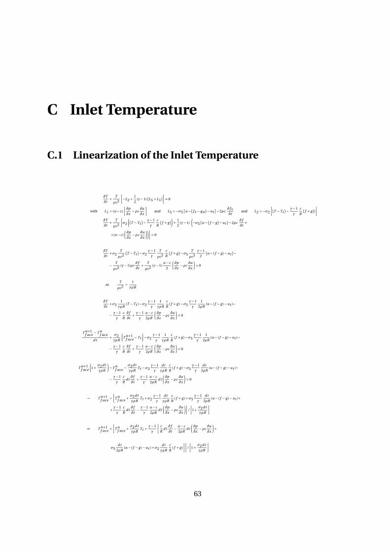
C Inlet Temperature
C.1 Linearization of the Inlet Temperature
∂T
∂t+ T
ρc2
[−L2 + 1
2(γ−1)
(L5 +L1
)]= 0
with L1 = (u −c)
[∂p
∂x−ρc
∂u
∂x
]and L5 =−σ5
[u − (
fx − gu)−ut
]−2ρc∂ fx∂t
and L2 =−σ2
[(T −Tt
)− γ−1
γ
c
R
(f + g
))
]∂T
∂t+ T
ρc2
[σ2
((T −Tt
)− γ−1
γ
c
R
(f + g
))+ 1
2(γ−1)
(−σ5
(u − (
f − g)−ut
)−2ρc∂ f
∂t+
+(u −c)
(∂p
∂x−ρc
∂u
∂x
))]= 0
∂T
∂t+σ2
T
ρc2
(T −Tt
)−σ2γ−1
γ
T
ρc2c
R
(f + g
)−σ5T
ρc2γ−1
2
(u − ( f − g )−ut
)−− T
ρc2(γ−1)ρc
∂ f
∂t+ T
ρc2(γ−1)
u − c
2
(∂p
∂x−ρc
∂u
∂x
)= 0
asT
ρc2= 1
γρR
∂T
∂t+σ2
1
γρR(T −Tt )−σ2
γ−1
γ
1
γρR
c
R( f + g )−σ5
γ−1
γ
1
2ρR(u − ( f − g )−ut )−
− γ−1
γ
c
R
∂ f
∂t+ γ−1
γ
u − c
2ρR
(∂p
∂x−ρc
∂u
∂x
)= 0
T n+1f ace
−T nf ace
d t+ σ2γρR
(T n+1
f ace −Tt
)−σ2
γ−1
γ
1
γρR
c
R( f + g )−σ5
γ−1
γ
1
2ρR(u − ( f − g )−ut )−
− γ−1
γ
c
R
∂ f
∂t+ γ−1
γ
u − c
2ρR
(∂p
∂x−ρc
∂u
∂x
)= 0
T n+1f ace
(1+ σ2d t
γρR
)−T n
f ace − σ2d t
γρRTt −σ2
γ−1
γ
d t
γρR
c
R( f + g )−σ5
γ−1
γ
d t
2ρR(u − ( f − g )−ut )−
− γ−1
γ
c
Rd t
∂ f
∂t+ γ−1
γ
u − c
2ρRd t
(∂p
∂x−ρc
∂u
∂x
)= 0
→ T n+1f ace =
[T n
f ace + σ2d t
γρRTt +σ2
γ−1
γ
d t
γρR
c
R( f + g )+σ5
γ−1
γ
d t
2ρR(u − ( f − g )−ut )+
+ γ−1
γ
c
Rd t
∂ f
∂t− γ−1
γ
u − c
2ρRd t
(∂p
∂x−ρc
∂u
∂x
)]/
[1+ σ2d t
γρR
]
⇒ T n+1f ace =
[T n
f ace + σ2d t
γρRTt +
γ−1
γ
[c
Rd t
∂ f
∂t− u −c
2ρRd t
(∂p
∂x−ρc
∂u
∂x
)+
σ5d t
2ρR(u − ( f − g )−ut )+σ2
d t
γρR
c
R( f + g )
]]/
[1+ σ2d t
γρR
]
63

Inlet Temperature
C.2 CBSBC Implementation in OpenFOAM
C.2.1 FractionExpression
The implementation in OpenFOAM for the fractionExpression f is:
thi s−>valueF r acti on() = 1.0
⇒ f = 1.0
C.2.2 ValueExpression
The implementation in OpenFOAM for the valueExpression = refValue() is:
r e f V alue() ==[ f i eld .ol dT i me().bound ar yF i eld()[patchi ]
+et aT ∗ cP ∗d t/g amma/l In f ∗ t In f ++(g amma −1)/g amma ∗ (cP/R ∗ ( f − f 0)−−(aP + cP )/r hoP/R/2.0∗d t ∗ (pp.snGr ad()++r hop ∗ cP ∗ (thi s−> patch().n f () & Up − snGr ad()))++et a Ac ∗ sqr (cP )/R ∗ (1.0− sqr (aP/cP ))/2.0/l In f ∗∗d t ∗ (thi s−> patch().n f () & (Up −uIn f ))
+sqr (cP )/R/l In f ∗d t ∗ (et aT /g amma +et a Ac ∗ (1.0− sqr (aP/cP ))/2.0)∗ f
+sqr (cP )/R/l In f ∗d t ∗et aT /g amma ∗ g
−sqr (cP )/R/l In f ∗d t ∗et a Ac ∗ (1.0− sqr (aP/cP )/2.0∗ g
]
/(1.0+et aT ∗ cP ∗d t/g amma/l In f )
=[
T nf ace + et aT ∗ cP ∗d t
γ∗ l In f∗T t + γ−1
γ
[cP
R( f − f 0)− aP +cP
2ρRd t
[∂p
∂x+ρc
∂u
∂x
]+
+ et a Ac
(1−
(aP
cP
)2)
cP
l In f
cP
2Rd t
(u −ut
)+ cP2
l In f ∗Rd t
et aT
γ( f + g )+
+ et a Ac
(1−
(aP
cP
)2)
cP
l In f
cP
2Rd t ( f − g )
]]
/
[1+ et aT cP d t
l In f γ
]
as K = et a Ac
(1−
(aP
cP
)2)
cP
l In f= σ5ρc
and σ2 = ηt ρRc
l
=[
T nf ace + ηt cd t
γlT t + γ−1
γ
c
R( f − f 0)− γ−1
γ
u +c
2ρRd t
(∂p
∂x+ρc
∂u
∂x
)+
+ γ−1
γ
c d t
2RK
(u −ut + ( f − g )
)+ γ−1
γ
c2d t
l R
ηtγ
( f + g )
]/
[1+ et aT cP d t
l In f γ
]
=[
T nf ace + ηt cd t
γlT t + γ−1
γ
(c
R( f − f 0)− u + c
2ρRd t
(∂p
∂x+ρc
∂u
∂x
)+
+ c d t
2RK
(u −ut + ( f − g )
)+ γ−1
γ
c2d t
lR
ηtγ
( f + g )
)]/
[1+ et aT ∗ cP ∗d t
l In f ∗γ]
⇒ r e f V alue() =[
T nf ace + σ2d t
γρRT t + γ−1
γ
(c
R( f − f 0)− u +c
2ρRd t
(∂p
∂x+ρc
∂u
∂x
)+σ5
d t
2ρR
(u −ut + ( f − g )
)++ σ2
cd t
γρRR( f + g )
)]/
[1+σ2
d t
γρR
]
64

C.2 CBSBC Implementation in OpenFOAM
C.2.3 GradExpression
The implementation in OpenFOAM for the gradientExpression = refGrad() is:
thi s−>r e f Gr ad() = 1.0
⇒ r e f Gr ad() = 1.0
65

D Outlet Temperature
D.1 Linearization of the Outlet Temperature
∂T
∂t+ T
ρc2
[−L2 + 1
2(γ−1)(L5 +L1)
]= 0
with L2 = u
(c2 ∂ρ
∂x− ∂p
∂x
)and L5 = (u + c)
(∂p
∂x+ρc
∂u
∂x
)and L1 = σ
ρc
[p −ρc( fd + gx )−p∞
]+2∂gx∂t
∂T
∂t+ T
ρc2
[−u
(c2 ∂ρ
∂x− ∂p
∂x
)+ 1
2
(γ−1
)(L5 +L1
)]= 0
∂T
∂t− uc2T
ρc2∂ρ
∂x+ uT
ρc2∂p
∂x+ T (γ−1)
2ρc2
(L5 +L1
)= 0
∂T
∂t− uT
ρ
(ρ
p
∂p
∂x− ρ
T
∂T
∂x
)+ uT
ρc2∂p
∂x+ T (γ−1)
2ρc2(L5 +L1) = 0
∂T
∂t− uT
p
∂p
∂x+u
∂T
∂x+ uT
ρc2∂p
∂x+ T (γ−1)
2ρc2(L5 +L1) = 0
∂T
∂t+u
∂T
∂x+u
(T
ρc2− T
p
)∂p
∂x+ T (γ−1)
2ρc2(L5 +L1) = 0
∂T
∂t+u
∂T
∂x+u
1−γρRγ
∂p
∂x+ γ−1
2ρRγ(L5 +L1) = 0
T n+1f ace
−T nf ace
d t+u
T n+1f ace
−T n+1centr e
d x+u
1−γρRγ
∂p
∂x+ γ−1
2ρrγ(L5 −L1) = 0
T n+1f ace −T n
f ace + u d t
d x
(T n+1
f ace −T n+1centr e
)+u d t
1−γρRγ
∂p
∂x+ (γ−1) d t
2ρRγ(L5 +L1) = 0
→ T n+1f ace
(1− u d t
d x
)= T n
f ace + u d t
d xT n+1
centr e −u d t1−γρRγ
∂p
∂x− (γ−1) d t
2ρRγ(L5 +L1)
⇒ T n+1f ace = 1
1− u d td x︸ ︷︷ ︸
f
[T n
f ace − (γ−1) d t
2ρRγ(L5 +L1)
]︸ ︷︷ ︸
valueE xpr
+u d td x
1− u d td x︸ ︷︷ ︸
1− f
T n+1centr e + γ−1
ρRγ
∂p
∂x︸ ︷︷ ︸g r adE xpr
d x
66

D.2 CBSBC Implementation in OpenFOAM
D.2 CBSBC Implementation in OpenFOAM
L5
L5 = (aP + cP )∗ [pp.snGr ad()+ r hop ∗ cp ∗ (thi s−> patch().n f () & Up.snGr ad())
]
→ L5 = (u + c)
[∂p
∂x+ρc
∂u
∂x
]
L1
L1 = et a Ac ∗ cP ∗ (1.0− sqr (aP/cP ))/l In f ∗ [pp −pIn f − r hop ∗ cP ∗ g − r hop ∗ cP ∗ f
]−2.0∗ r hop ∗ cP ∗ (g − g 0)/d t
= et a Ac ∗(1− sqr
aP
cP
]cP
l In f∗ [
pp −pIn f − r hop ∗ cP ∗ (g + f )]−2∗ r hop ∗ cP ∗ g − g 0
d t
as K =σ(1−M2
) c
L∼ et a Ac
(1− sqr
aP
cP
)cP
l In f[Poinsot]
→ L1 = K[pp −pIn f −ρc(g + f )
]−2ρcg − g 0
d t
as L1 = K(p −p∞
)∼ σ
ρc
(p −p∞
)[Poinsot]
→ L1 = σ
ρc
[pp −pIn f −ρc(g + f )
]−2ρcg − g 0
d t
⇒ L1 = σ
ρc
[pp −p∞−ρc(g + f )
]−2ρcg − g 0
d t
D.2.1 FractionExpression
Implementation in OpenFOAM for the fractionExpression f is:f = 1.0/[1.0+aP ∗d t ∗ thi s−> patch().del t aCoe f f s()]
→ f = 1.0
1.0+aP ∗d t ∗ thi s−> patch().del t acoe f f s()
⇒ f = 1
1+ ud t∆x
D.2.2 ValueExpression
Implementation in OpenFOAM for the valueExpression = refValue() is:r e f V alue() = f i eld .ol dT i me().bound ar yF i eld()[patchi ]−d t ∗ (g amma −1.0)/g amma ∗0.5∗ (L5 +L1)/r hop/R
→ = f i eld .ol dT i me().bound ar yF i eld()[patchi ]−d tγ−1
2 γ
L5 +L1ρR
⇒ r e f V alue() = T nf ace − (γ−1)d t
2γρR
(L5 +L1
)
67

Outlet Temperature
D.2.3 GradExpression
The implementation in OpenFOAM for the gradExpr = refGrad() is:
r e f Gr ad() = (g amma −1)/g amma ∗pp.snGr ad()/r ho/R
→ = γ−1
γ
∂p
∂x
1
ρR
⇒ r e f Gr ad() = γ−1
γρR
∂p
∂x
68
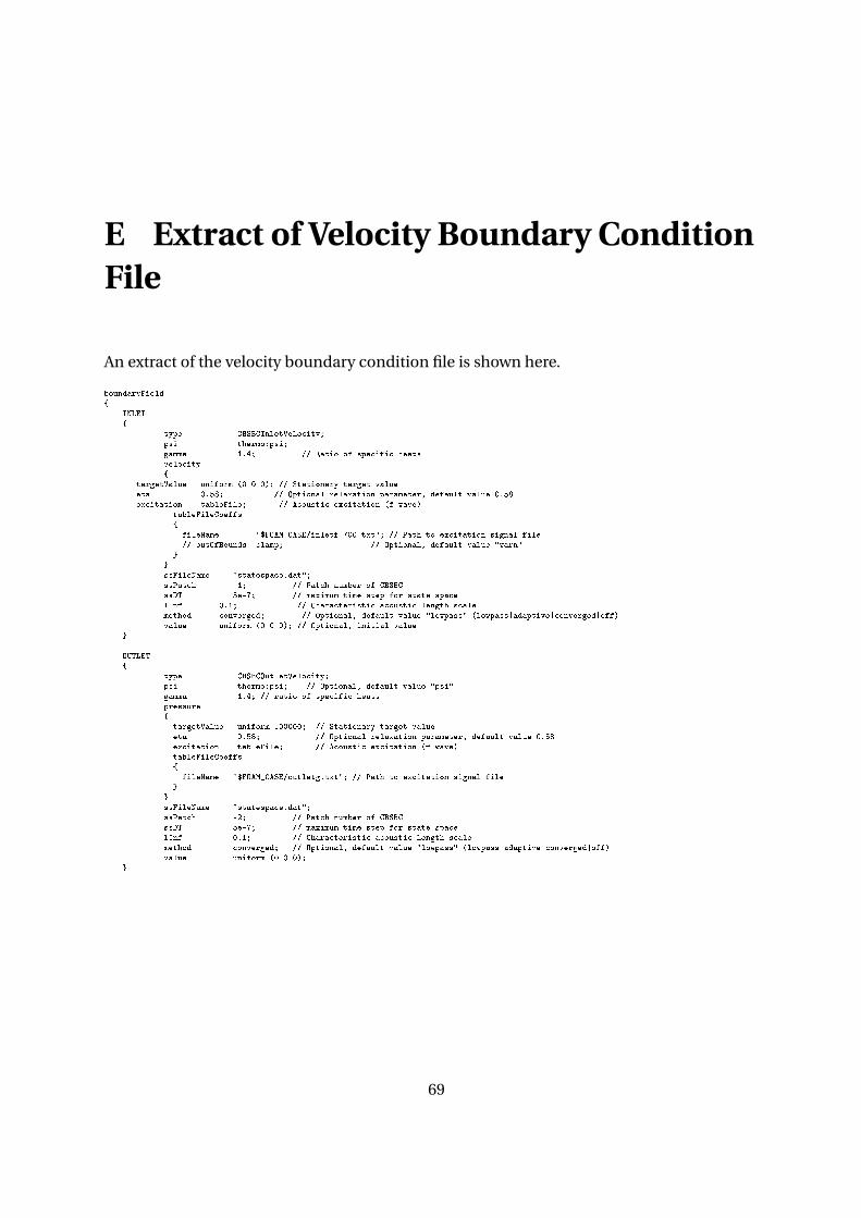
E Extract of Velocity Boundary ConditionFile
An extract of the velocity boundary condition file is shown here.
boundaryField{
INLET{
type CBSBCInletVelocity;psi thermo:psi;gamma 1.4; // Ratio of specific heatsvelocity{
targetValue uniform (0 0 0); // Stationary target valueeta 0.58; // Optional relaxation parameter, default value 0.58excitation tableFile; // Acoustic excitation (f wave)
tableFileCoeffs{
fileName "$FOAM_CASE/inletf_700.txt"; // Path to excitation signal file// outOfBounds clamp; // Optional, default value "warn"
}}ssFileName "statespace.dat";ssPatch -1; // Patch number of CBSBCssDT 5e-7; // maximum time step for state spacelInf 0.1; // Characteristic acoustic length scalemethod converged; // Optional, default value "lowpass" (lowpass|adaptive|converged|off)value uniform (0 0 0); // Optional, initial value
}
OUTLET{
type CBSBCOutletVelocity;psi thermo:psi; // Optional, default value "psi"gamma 1.4; // ratio of specific heatspressure{targetValue uniform 100000; // Stationary target valueeta 0.58; // Optional relaxation parameter, default value 0.58excitation tableFile; // Acoustic excitation (f wave)tableFileCoeffs{
fileName "$FOAM_CASE/outletg.txt"; // Path to excitation signal file}
}ssFileName "statespace.dat";ssPatch -2; // Patch number of CBSBCssDT 5e-7; // maximum time step for state spacelInf 0.1; // Characteristic acoustic length scalemethod converged; // Optional, default value "lowpass" (lowpass|adaptive|converged|off)value uniform (0 0 0);
}
69

F Matlab Code
The matlab code for calculating the f and g waves and the corresponding Rc value for theno-slip mean-flow case:
%Input of the wall distances vectorProbe_fid = fopen('~/postProcessing/probes0.022575/0/p', 'r');Probe_dataRaw = textscan(Probe_fid, '%*s%*s%f%f%f%f%f%f%f%f%f%f%f%f%f%f%f%f%f%f%f%f%f%f%f%f%f%f%f%f%f%f%f%f%f%f% \\f%f%f%f%f%f%f%f%f%f%f%f%f%f%f%f%f%f%f%f%f%f%f%f%f%f%f%f%f%f%f%f%f%f%f%f' ,...
2);Probe_data = cell2mat(Probe_dataRaw);distance = Probe_data(2,:)';distance = [0.005;distance(:,1)];fclose(Probe_fid);
%Input of pressure vector for every cellProbe_fid = fopen('~/postProcessing/probes0.029925/0/p', 'r');Probe_dataRaw = textscan(Probe_fid, '%f %f %f %f %f %f %f %f %f %f %f %f %f %f %f %f %f %f %f %f %f %f %f %f %f %f \\%f %f %f %f %f %f %f %f %f %f %f %f %f %f %f %f %f %f %f %f %f %f %f %f %f %f %f %f %f %f %f %f %f %f %f %f %f %f %f %f %f %f %f %f %f' ,...
'CommentStyle', '#');Probe_data = cell2mat(Probe_dataRaw);pWall = Probe_data;fclose(Probe_fid);
%Input of velocity vector for every cellProbe_fid = fopen('~/postProcessing/probes0.029925/0/U', 'r');Probe_dataRaw = textscan(Probe_fid, '%f (%f %f %f) (%f %f %f) (%f %f %f) (%f %f %f) (%f %f %f) (%f %f %f) (%f %f %f) \\(%f %f %f) (%f %f %f) (%f %f %f) (%f %f %f) (%f %f %f) (%f %f %f) (%f %f %f) (%f %f %f) (%f %f %f) (%f %f %f) (%f %f %f) \\(%f %f %f) (%f %f %f) (%f %f %f) (%f %f %f) (%f %f %f) (%f %f %f) (%f %f %f) (%f %f %f) (%f %f %f) (%f %f %f) (%f %f %f) \\(%f %f %f) (%f %f %f) (%f %f %f) (%f %f %f) (%f %f %f) (%f %f %f) (%f %f %f) (%f %f %f) (%f %f %f) (%f %f %f) (%f %f %f) \\(%f %f %f) (%f %f %f) (%f %f %f) (%f %f %f) (%f %f %f) (%f %f %f) (%f %f %f) (%f %f %f) (%f %f %f) (%f %f %f) (%f %f %f) \\(%f %f %f) (%f %f %f) (%f %f %f) (%f %f %f) (%f %f %f) (%f %f %f) (%f %f %f) (%f %f %f) (%f %f %f) (%f %f %f) (%f %f %f) \\(%f %f %f) (%f %f %f) (%f %f %f) (%f %f %f) (%f %f %f) (%f %f %f) (%f %f %f) (%f %f %f)' , ...
'CommentStyle', '#');Probe_data = cell2mat(Probe_dataRaw);UWall = Probe_data;fclose(Probe_fid);
%Declaration of the matrices/valuesdeltaT = 4286; %deltaT of the mean-value calculation; 3 time periods for F=700Hzl = length(UWall);s = size(pWall,2);rhoc = 407.5321184;
A_f = zeros(l,s);A_ff = zeros(deltaT+1,s);A_ff(:,1) = UWall(meanValue:(meanValue+deltaT),1);P2f = zeros(deltaT+1,s);P1f = zeros((deltaT+2)/2,s);A_g = zeros(l,s);A_gg = zeros(deltaT+1,71);A_gg(:,1) = UWall(meanValue:(meanValue+deltaT),1);P2g = zeros(deltaT+1,s);P1g = zeros((deltaT+2)/2,s);
%Declaration of matrices/values used for FFTt = 0.02:1e-6:0.024286;L = 4286;Fs = 1e6; %sampling frequencyT = 1/Fs; %period of samplef = Fs*(0:(L/2))/L; %frequency resolutionmax_A = zeros(s,3);
%Declaration of the matrice for the acoustic part of velocity/pressure%Start of the mean-value calculationUA = zeros(l,71);pA = zeros(l,71);meanValue = 95000;
%Calculating the acoustic fluctuation of pressure and velocity for every cell
70
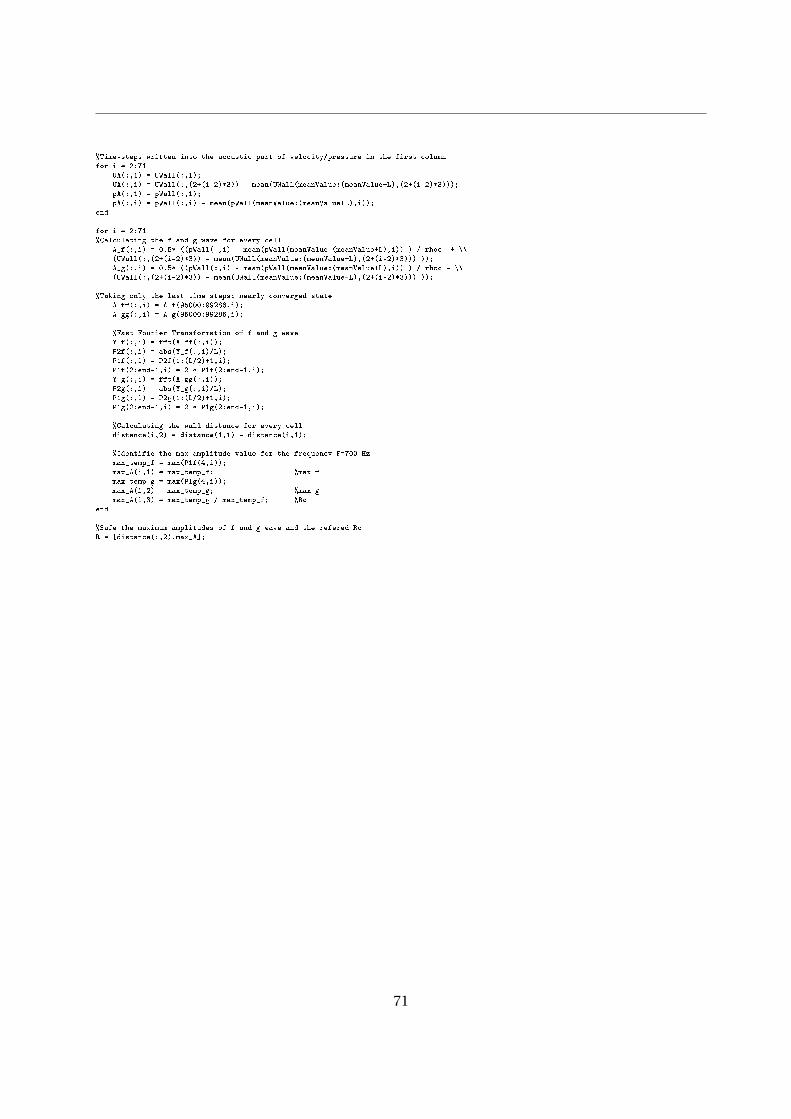
%Time-steps written into the acoustic part of velocity/pressure in the first columnfor i = 2:71
UA(:,1) = UWall(:,1);UA(:,i) = UWall(:,(2+(i-2)*3)) - mean(UWall(meanValue:(meanValue+L),(2+(i-2)*3)));pA(:,1) = pWall(:,1);pA(:,i) = pWall(:,i) - mean(pWall(meanValue:(meanValue+L),i));
end
for i = 2:71%Calculating the f and g wave for every cell
A_f(:,i) = 0.5* ((pWall(:,i) - mean(pWall(meanValue:(meanValue+L),i)) ) / rhoc + \\(UWall(:,(2+(i-2)*3)) - mean(UWall(meanValue:(meanValue+L),(2+(i-2)*3))) ));A_g(:,i) = 0.5* ((pWall(:,i) - mean(pWall(meanValue:(meanValue+L),i)) ) / rhoc - \\(UWall(:,(2+(i-2)*3)) - mean(UWall(meanValue:(meanValue+L),(2+(i-2)*3))) ));
%Taking only the last time steps; nearly converged stateA_ff(:,i) = A_f(95000:99286,i);A_gg(:,i) = A_g(95000:99286,i);
%Fast Fourier Transformation of f and g waveY_f(:,i) = fft(A_ff(:,i));P2f(:,i) = abs(Y_f(:,i)/L);P1f(:,i) = P2f(1:(L/2)+1,i);P1f(2:end-1,i) = 2 * P1f(2:end-1,i);Y_g(:,i) = fft(A_gg(:,i));P2g(:,i) = abs(Y_g(:,i)/L);P1g(:,i) = P2g(1:(L/2)+1,i);P1g(2:end-1,i) = 2 * P1g(2:end-1,i);
%Calculating the wall distance for every celldistance(i,2) = distance(1,1) - distance(i,1);
%Identifie the max amplitude value for the frequency F=700 Hzmax_temp_f = max(P1f(4,i));max_A(i,1) = max_temp_f; %max fmax_temp_g = max(P1g(4,i));max_A(i,2) = max_temp_g; %max gmax_A(i,3) = max_temp_g / max_temp_f; %Rc
end
%Safe the maximum amplitudes of f and g wave and the refered RcR = [distance(:,2),max_A];
71
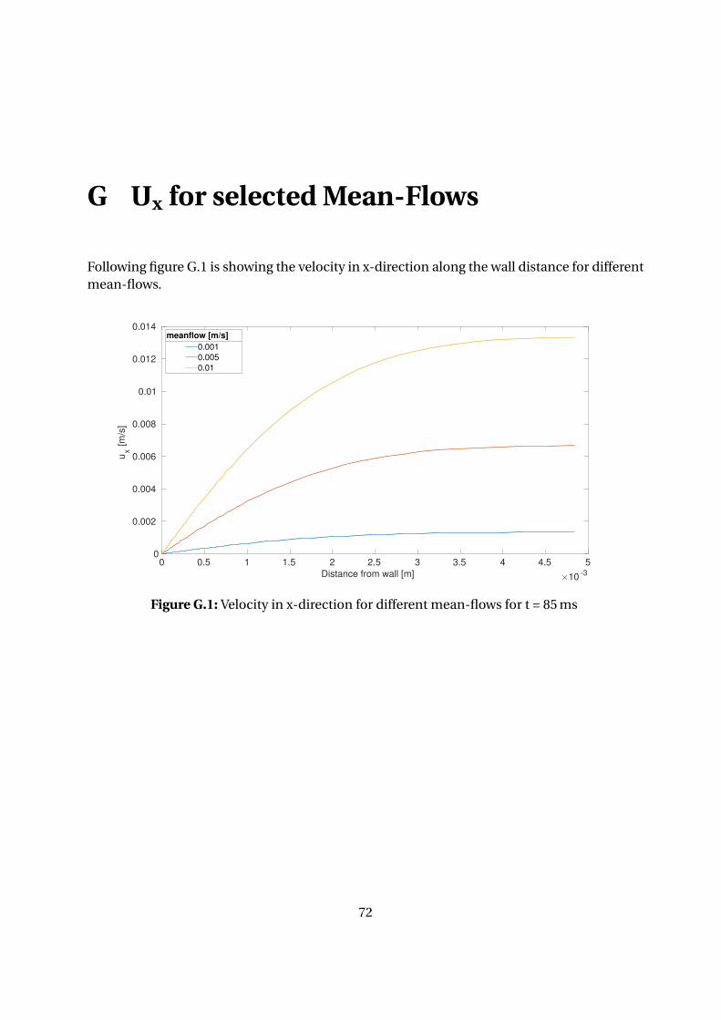
G Ux for selected Mean-Flows
Following figure G.1 is showing the velocity in x-direction along the wall distance for differentmean-flows.
0 0.5 1 1.5 2 2.5 3 3.5 4 4.5 5
Distance from wall [m] 10-3
0
0.002
0.004
0.006
0.008
0.01
0.012
0.014
ux [m
/s]
0.001
0.005
0.01
meanflow [m/s]
Figure G.1: Velocity in x-direction for different mean-flows for t = 85 ms
72

Bibliography
[1] Franz Durst. Grundlagen der Strömungsmechanik: eine Einführung in die Theorie derStrömung von Fluiden. Springer-Verlag, 2007.
[2] Klaus Ehrenfried. Strömungsakustik: Skript zur Vorlesung. Mensch-und-Buch-Verlag,2004.
[3] Kilian Heinrich Förner. Nonlinear Aeroacoustic Characterization of Resonators. PhD the-sis, Technische Universität München, 2017.
[4] B. Gschaider. Swak4foam [online: http:// openfoamwiki.net/index.php/contrib/swak4foam].
[5] Robert L Higdon. Absorbing boundary conditions for difference approximations to themultidimensional wave equation. Mathematics of computation, 47(176):437–459, 1986.
[6] Stefan Jaensch, Carlo Sovardi, and Wolfgang Polifke. On the robust, flexible and consis-tent implementation of time domain impedance boundary conditions for compressibleflow simulations. Journal of Computational Physics, 314:145–159, 2016.
[7] Heinz-Otto Kreiss. Initial boundary value problems for hyperbolic systems. Communi-cations on Pure and Applied Mathematics, 23(3):277–298, 1970.
[8] T.J. Poinsot and S.K. Lele. Boundary conditions for direct simulations of compressibleviscous flows. Journal of computational physics, 101(1):104–129, 1992.
[9] Wolfgang Polifke, Clifton Wall, and Parviz Moin. Partially reflecting and non-reflectingboundary conditions for simulation of compressible viscous flow. Journal of Computa-tional Physics, 213(1):437–449, 2006.
[10] Kevin W. Thompson. Time dependent boundary conditions for hyperbolic systems. Jour-nal of computational physics, 68(1):1–24, 1987.
[11] R Vilums. Implementation of transient robin boundary conditions in openfoam. InWorkshop Multiphysical Modelling in OpenFOAM, Riga, Latvia, pages 39–40, 2011.
[12] FA Williams. Combustion theory 2nd, 1985.
73