PHYSIK-DEPARTMENT

Structural changes in lamellar diblock copolymer thin films

during solvent vapor treatment

Dissertation

von Zhenyu Di

TECHNISCHE UNIVERSITÄT

MÜNCHEN

TECHNISCHE UNIVERSITAT MUNCHEN

Lehrstuhl fur Funktionelle MaterialienPhysik-Department E13

Structural changes inlamellar diblock copolymer thin films

during solvent vapor treatment

Zhenyu Di

Vollstandiger Abdruck der von der Fakultat fur Physik der Technischen Universitat Munchenzur Erlangung des akademischen Grades eines

Doktors der Naturwissenschaften (Dr. rer. nat.)

genehmigten Dissertation.

Vorsitzender: Univ.-Prof. Dr. Ralf Metzler

Prufer der Dissertation: 1. Univ.-Prof. Dr. Christine Papadakis

2. Univ.-Prof. Dr. Katharina Krischer

Die Dissertation wurde am 30.03.2010 bei der Technischen Universitat Muncheneingereicht und durch die Fakultat fur Physik am 27.04.2010 angenommen.

Abstract

This research work focuses on the structural changes in thin films of lamellar

poly(styrene-b-butadiene) diblock copolymer during solvent vapor treatment. Two

kinds of solvent were used in this work: cyclohexane and cyclohexanone. The

cyclohexane is slightly polybutadiene selective while cyclohexanone is slightly

polystyrene selective. Two vapor treatments were carried out using cyclohexane: one

was in saturated vapor atmosphere and the other was under stepwise-increasing vapor

pressure. For cyclohexanone, since its saturated vapor pressure is very low already,

only the vapor treatment in saturated vapor atmosphere was carried out.

To study the film inner structural changes during vapor treatment, in situ

grazing-incidence small angle X-ray scattering (GISAXS) measurements were

performed. The GISAXS offered a time resolution up to a few seconds thus the fast

structural changes was well followed. With the help of GISAXS measurements, the

lamellae and film swelling, the improvement of the long-range order and the phase

transition were observed. We attribute the observations to the change of the glass

transition temperature, the Flory-Huggins segment-segment interaction parameter

and/or the volume fraction of one block.

Contents 1 Introduction 1

1.1 Block copolymer thin films . . . . . . . . . . . . . . . . . . . . . . . . . . . . . . . 1

1.2 Vapor treatment . . . . . . . . . . . . . . . . . . . . . . . . . . . . . . . . . . . . . . . 3

2 Strategy of this work 5

3 Theory of block copolymer solvent blends 7

3.1 Flory-Huggins segment-segment interaction parameter . . . . . . . . . 7

3.1.1 Dry sample . . . . . . . . . . . . . . . . . . . . . . . . . . . . . . . . . . . . . . . 7

3.1.2 Polymer-solvent blend . . . . . . . . . . . . . . . . . . . . . . . . . . . . . . 10

3.2 Concentration dependence of Tg . . . . . . . . . . . . . . . . . . . . . . . . . . . 11

3.2.1 Tg of the polymer . . . . . . . . . . . . . . . . . . . . . . . . . . . . . . . . . . . 11

3.2.2 Tg of the solvent . . . . . . . . . . . . . . . . . . . . . . . . . . . . . . . . . . . 11

3.2.3 Tg of the polymer-solvent blend . . . . . . . . . . . . . . . . . . . . . . . 12

3.3 Selectivity of solvent . . . . . . . . . . . . . . . . . . . . . . . . . . . . . . . . . . . . . 13

4 Experimental 17

4.1 The samples . . . . . . . . . . . . . . . . . . . . . . . . . . . . . . . . . . . . . . . . . . . 17

4.2 White light interferometer . . . . . . . . . . . . . . . . . . . . . . . . . . . . . . . . . 18

4.2.1 Methods . . . . . . . . . . . . . . . . . . . . . . . . . . . . . . . . . . . . . . . . . 18

4.2.2 Setup . . . . . . . . . . . . . . . . . . . . . . . . . . . . . . . . . . . . . . . . . . . . 18

4.2.3 Data analysis . . . . . . . . . . . . . . . . . . . . . . . . . . . . . . . . . . . . . 19

4.3 X-ray reflectivity . . . . . . . . . . . . . . . . . . . . . . . . . . . . . . . . . . . . . . . . 20

4.3.1 Methods . . . . . . . . . . . . . . . . . . . . . . . . . . . . . . . . . . . . . . . . . 20

4.3.2 Setup . . . . . . . . . . . . . . . . . . . . . . . . . . . . . . . . . . . . . . . . . . . . 20

4.3.3 Data analysis . . . . . . . . . . . . . . . . . . . . . . . . . . . . . . . . . . . . . 21

4.4 GISAXS . . . . . . . . . . . . . . . . . . . . . . . . . . . . . . . . . . . . . . . . . . . . . . 21

4.4.1 Methods . . . . . . . . . . . . . . . . . . . . . . . . . . . . . . . . . . . . . . . . . 21

4.4.2 Setup . . . . . . . . . . . . . . . . . . . . . . . . . . . . . . . . . . . . . . . . . . . . 22

i

4.4.3 Data analysis . . . . . . . . . . . . . . . . . . . . . . . . . . . . . . . . . . . . . 24

4.4.3.1 Lamellar orientation . . . . . . . . . . . . . . . . . . . . . . . . . . 24

4.4.3.2 Two banches of scattering . . . . . . . . . . . . . . . . . . . . . 24

4.4.3.3 Fitting of the DBSs . . . . . . . . . . . . . . . . . . . . . . . . . . . 25

4.4.3.4 Scattering depth . . . . . . . . . . . . . . . . . . . . . . . . . . . . . 26

5 Vapor treatment with saturated CHX 27

5.1 Idea . . . . . . . . . . . . . . . . . . . . . . . . . . . . . . . . . . . . . . . . . . . . . . . . . 27

5.2 Experimental . . . . . . . . . . . . . . . . . . . . . . . . . . . . . . . . . . . . . . . . . . 27

5.3 Results . . . . . . . . . . . . . . . . . . . . . . . . . . . . . . . . . . . . . . . . . . . . . . . 28

5.3.1 Structure of the as-prepared film . . . . . . . . . . . . . . . . . . . . . . 28

5.3.1.1 X-ray reflectivity . . . . . . . . . . . . . . . . . . . . . . . . . . . . . 28

5.3.1.2 GISAXS . . . . . . . . . . . . . . . . . . . . . . . . . . . . . . . . . . . 29

5.3.2 Structure changes during vapor treatment . . . . . . . . . . . . . . 33

5.3.2.1 Lamellar thickness . . . . . . . . . . . . . . . . . . . . . . . . . . . 35

5.3.2.2 Film thickness . . . . . . . . . . . . . . . . . . . . . . . . . . . . . . 36

5.3.2.3 Domain size . . . . . . . . . . . . . . . . . . . . . . . . . . . . . . . . 37

5.3.3 Maximum film swelling . . . . . . . . . . . . . . . . . . . . . . . . . . . . . . 37

5.4 Discussion . . . . . . . . . . . . . . . . . . . . . . . . . . . . . . . . . . . . . . . . . . . . . 38

5.4.1 Decrease of the effective Tg . . . . . . . . . . . . . . . . . . . . . . . . . . 39

5.4.2 Decrease of eff . . . . . . . . . . . . . . . . . . . . . . . . . . . . . . . . . . . 39

5.4.3 Increase of the degree of coiling . . . . . . . . . . . . . . . . . . . . . . 40

5.4.4 Behavior of randomly oriented lamellae . . . . . . . . . . . . . . . . 42

5.5 Conclusion . . . . . . . . . . . . . . . . . . . . . . . . . . . . . . . . . . . . . . . . . . . . 42

6 Stepwise vapor treatment with CHX 45

6.1 Idea . . . . . . . . . . . . . . . . . . . . . . . . . . . . . . . . . . . . . . . . . . . . . . . . . 45

6.2 Experimental . . . . . . . . . . . . . . . . . . . . . . . . . . . . . . . . . . . . . . . . . . 45

6.3 Results and discussion

6.3.1 Structure of the as-prepared film . . . . . . . . . . . . . . . . . . . . . 47

ii

6.3.2 The first step of swelling . . . . . . . . . . . . . . . . . . . . . . . . . . . . . 49

6.3.2.1 Stable state . . . . . . . . . . . . . . . . . . . . . . . . . . . . . . . . 50

6.3.2.2 The transition process . . . . . . . . . . . . . . . . . . . . . . . . 52

6.3.2.3 Lamellae swelling . . . . . . . . . . . . . . . . . . . . . . . . . . . . 53

6.3.3 Further swelling . . . . . . . . . . . . . . . . . . . . . . . . . . . . . . . . . . . 56

6.3.3.1 Nonequilibrium . . . . . . . . . . . . . . . . . . . . . . . . . . . . . . 56

6.3.3.1.1 Results . . . . . . . . . . . . . . . . . . . . . . . . . . . . . . . . . 56

6.3.3.1.2 Discussion . . . . . . . . . . . . . . . . . . . . . . . . . . . . . . 57

6.3.3.2 Scalling law . . . . . . . . . . . . . . . . . . . . . . . . . . . . . . . . . 58

6.4 Conclusion . . . . . . . . . . . . . . . . . . . . . . . . . . . . . . . . . . . . . . . . . . . . 59

6.4.1 The first swelling-step . . . . . . . . . . . . . . . . . . . . . . . . . . . . . . 59

6.4.2 The other swelling-steps . . . . . . . . . . . . . . . . . . . . . . . . . . . . 60

7 Vapor treatment with saturated CHXO 63

7.1 Idea . . . . . . . . . . . . . . . . . . . . . . . . . . . . . . . . . . . . . . . . . . . . . . . . . 63

7.2 Setup . . . . . . . . . . . . . . . . . . . . . . . . . . . . . . . . . . . . . . . . . . . . . . . . 63

7.3 Results and discussion . . . . . . . . . . . . . . . . . . . . . . . . . . . . . . . . . . . 64

7.3.1 Structure of the as-prepared film . . . . . . . . . . . . . . . . . . . . . . 64

7.3.2 Structural changes in saturated CHXO . . . . . . . . . . . . . . . . . 66

7.3.2.1 Long-range order . . . . . . . . . . . . . . . . . . . . . . . . . . . . 67

7.3.2.2 Lamellar thickness . . . . . . . . . . . . . . . . . . . . . . . . . . . 68

7.3.2.3 Side maximum . . . . . . . . . . . . . . . . . . . . . . . . . . . . . . 68

7.3.2.4 Elongation and bending of DBSs . . . . . . . . . . . . . . . 70

7.3.2.5 Dewetting of the thin film . . . . . . . . . . . . . . . . . . . . . . 70

7.4 Conclusion . . . . . . . . . . . . . . . . . . . . . . . . . . . . . . . . . . . . . . . . . . . . 70

7.4.1 Fast process . . . . . . . . . . . . . . . . . . . . . . . . . . . . . . . . . . . . . 71

7.4.2 Slow process . . . . . . . . . . . . . . . . . . . . . . . . . . . . . . . . . . . . . 71

8 Summary 73

iii

iv

Chapter 1

Introduction

1.1 Block copolymer thin films

Block copolymers are macromolecules containing different species of monomers, which are

arranged in blocks. The monomers constituting the blocks (A and B) are in most cases

immiscible, thus a decrease in A-B segment-segment contacts reduces the system enthalpy H,

which motivates the micro-phase separation. However, the micro-phase separation decreases

the entropy. Therefore, the immiscibility of the different block must be big enough so that the

enthalpic factors can dominate the entropic factors. Thanks to Flory [1] and Huggins [2], the

immiscibility of the two blocks can be expressed by the product of N , where is Flory-

Huggins segment-segment interaction parameter and N is the overall degree of polymerization.

When 0N , the two blocks are immiscible but only when ODTNN , where ODT

represents order-to-disorder transition, the enthalpic factors can dominate the entropic factors

and the micro-phase separation is possible. Depending on N and the volume fraction of one

block, fA, the block copolymer shows various micro-phase behaviors as lamellae, gyroid,

cylinders or spheres (Figure 1.1).

Because of the ability to self-assemble into a rich variety of periodic patterns, which have repeat

distances typically in the range of 10 to 100 nm [3, 4], block copolymer thin films have the

potential for a number of nanotechnology applications. For example, Thurn-Albrecht et al. used

poly(styrene-b-methylmethacry) thin films to produce the templates for nano-wire arrays [5]. In

their system the volume fraction of styrene is 0.71, so that the copolymer self-assembles into

arrays of PMMA cylinders hexagonally packed in a PS matrix (Figure 1.2 A). Deep ultraviolet

exposure was performed afterwards to degrade the PMMA domains and simultaneously cross-

link the PS matrix such that the degraded PMMA can be removed by rinsing with acetic acid

(Figure 1.2 B). Electro-deposition is used to fill the nanopores with continuous metal nano-

wires (Figure 1.2 C). The nano-wire has a density in excess of wires per square

centimeter that point toward a route to ultrahigh-density storage media. Urbas et al. used

poly(styrene-b-isoprene) symmetric diblock copolymer-homopolymer blends as one-

111.9 10

1

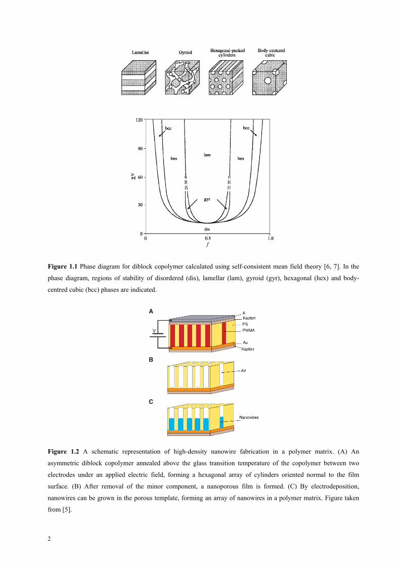
Figure 1.1 Phase diagram for diblock copolymer calculated using self-consistent mean field theory [6, 7]. In the

phase diagram, regions of stability of disordered (dis), lamellar (lam), gyroid (gyr), hexagonal (hex) and body-

centred cubic (bcc) phases are indicated.

Figure 1.2 A schematic representation of high-density nanowire fabrication in a polymer matrix. (A) An

asymmetric diblock copolymer annealed above the glass transition temperature of the copolymer between two

electrodes under an applied electric field, forming a hexagonal array of cylinders oriented normal to the film

surface. (B) After removal of the minor component, a nanoporous film is formed. (C) By electrodeposition,

nanowires can be grown in the porous template, forming an array of nanowires in a polymer matrix. Figure taken

from [5].

2

dimensionally periodic dielectric reflectors [8]. They cast-coated a 0.5 mm thin film from blend

of P(S-b-I) and homopolyisoprene. Polystyrene and polyisoprene self-assembled into lamellae

parallel to the film surface with a lamellar thickness of 130 nm. Thus only the light with a wave

length around 450 nm can be efficiently reflected. More examples of the applications of block

copolymer thin film can be listed e.g. molecular sieves [9], and sensors [10], solar cells [11] …

1.2 Vapor treatment

In many applications, there is a common requirement: long-range order of the nano-structure.

However, self-assembly doesn´t necessarily lead to long-range order. Only when the repulsion

between the different blocks is big enough and the block copolymer is in micro-phase

equilibrium, the long-range ordered micro-phase separation can be achieved. The former

condition can be fulfilled by choosing the block copolymer system properly. The latter is

achieved by thermal annealing or vapor treatment.

Thermal annealing is the most commonly used method, because it is straightforward and

efficient in many cases. By heating the block copolymer above the glass transition temperatures

of the blocks, the chain mobility increases, and thermodynamic equilibrium can be achieved

[12]. However, this process does not apply to all polymers. Some polymers have a Tg close to

their thermal degradation temperature, whereas others crosslink during annealing at high

temperature. For example, conductive polymers are normally hard and thus difficult to use

thermal annealing to achieve equilibrium.

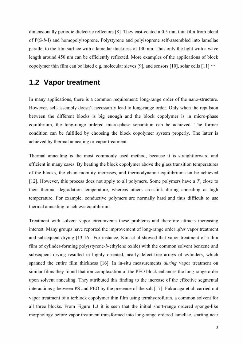
Treatment with solvent vapor circumvents these problems and therefore attracts increasing

interest. Many groups have reported the improvement of long-range order after vapor treatment

and subsequent drying [13-16]. For instance, Kim et al showed that vapor treatment of a thin

film of cylinder-forming poly(styrene-b-ethylene oxide) with the common solvent benzene and

subsequent drying resulted in highly oriented, nearly-defect-free arrays of cylinders, which

spanned the entire film thickness [16]. In in-situ measurements during vapor treatment on

similar films they found that ion complexation of the PEO block enhances the long-range order

upon solvent annealing. They attributed this finding to the increase of the effective segmental

interactions between PS and PEO by the presence of the salt [17]. Fukunaga et al. carried out

vapor treatment of a terblock copolymer thin film using tetrahydrofuran, a common solvent for

all three blocks. From Figure 1.3 it is seen that the initial short-range ordered sponge-like

morphology before vapor treatment transformed into long-range ordered lamellae, starting near

3

the air-polymer interface, which results in a multilayered structure throughout the film [18].

Albalak et al. studied the structural changes of poly(styrene-b-butadiene-b-styrene) triblock

copolymers after exposure to the vapor of hexane, methylethylketone and toluene, respectively.

They observed an improvement of the long-range order and a complex behavior of the repeat

distance as a function of vapor treatment time [19].

Figure 1.3 Cross-sectional TEM images showing the time

evolution of self-assembly in the thin SVT triblock terpolymer

film: as-prepared (a), after the THF vapor treatment for 5 s (b,

c). and 1 min (d). The black scale bar, common for the all

images, in the topmost figure represents 100 nm. The

embedding matrix, the substrate, and the triblock terpolymer

film are in the portion A, S, and P, respectively. PS, P2VP, and

PtBMA microdomains appear bright, dark, and gray,

respectively, in the TEM images. Dotted lines represent the

approximate position of the free surface in the respective

images. In (d), a dislocation core is indicated by D. (Figure

taken from [18])

However, most of the previous studies only showed that the vapor treatment have the capability

to improve the micro-phase separation of the block copolymer thin films. The underlying

molecular processes occurring during vapor treatment are still not well understood. For example,

it is unclear why the vapor treatment does not improve the long-range order in all systems [17].

It would be desirable to know which conditions – choice of solvent, vapor pressure, duration of

treatment time, conditions of drying etc. – are optimum for obtaining the desired structure.

Moreover, a detailed understanding of the processes during restructuring is desirable for the

optimization.

4

Chapter 2

Strategy of this work

The goal of this work is to study the mechanism and the underlying molecular processes

occurring in thin films of lamellar P(S-b-B) block copolymer during vapor treatment. We

investigate the influences of the solvent to the micro-phase separation: The phase diagram, the

long-range order and the structure dimension.

For this purpose, three in-situ, real-time grazing-incidence small-angle X-ray scattering

(GISAXS) experiments were carried out during vapor treatment. In the first two experiments,

cyclohexane (CHX) was used as solvent for vapor treatment (Chapter 5, Chapter 6), while in the

third experiment, cyclohexanone (CHXO) was used (Chapter 7). The CHX is slightly

polybutadiene (PB) selective while the CHXO is slightly polystyrene (PS) selective.

In Chapter 3, the theory of block copolymer-solvent blends will be discussed focusing on the

parameters which are most important during vapor treatment i.e the glass transition temperature,

Tg, the Flory-Huggins segment-segment interaction parameter, and the selectivity of the

solvent.

In Chapter 4, the experimental methods and setup are introduced including the sample

preparation, white light interferometer, X-ray reflectivity and GISAXS.

In Chapter 5, a block copolymer thin film with initially short-range ordered, randomly oriented

lamellae was exposed in saturated solvent vapor atmosphere. Drastic changes of the inner

structure were observed: (i) The long-range order of the lamellar micro-phase separation first

improved and then became worse and at last the sample became disordered. (ii) The lamellar

thickness of the of the parallel lamellae first increased quickly and then decrease slowly and at

last leveled off with a value slightly larger than that in the dry state. We related the changes to

the influence of the solvent vapor on Tg and N .

In Chapter 6, the vapor treatment conditions were improved with an additional possibility to

adjust the vapor pressure. The block copolymer thin film was exposed to a solvent vapor

atmosphere where the vapor pressure increased stepwise. In each vapor pressure/step, the thin

5

film was exposed for enough time until the sample was stable (time independent). Thus the

lamellar thickness of the parallel lamellae can be expressed only as a function of the volume

fraction of the polymer, , but independent of time. Moreover, stable states with improved long-

range order of the lamellar micro-phase separation were observed in some of the vapor

pressure/step.

In Chapter 7 the solvent for vapor treatment was changed from CHX to CHXO. The idea is that:

in the block copolymer, the PB is the soft block and PS is the rigid block. Thus the PS selective

CHXO could soften the sample better. Furthermore, CHXO has a lower glass transition

temperature than that of CHX, which would also benefit the softening. However, since the

vapor pressure of CHXO is very low, only vapor treat in saturated CHXO vapor was performed.

An improvement of the lamellar micro-phase separation and the transition of micro-phase were

observed.

In Chapter 8 a summary and conclusion of this work is drawn.

6

Chapter 3

Theory of block copolymer-solvent

blends

In this chapter, the parameters which are important for understanding the observations in this

work will be discussed. Each of them plays a key role during vapor treatment.

3.1 Flory-Huggins segment-segment interaction

parameter

3.1.1 Dry sample

In this section, the micro-phase separation of block copolymers will be discussed focused on the

Flory-Huggins segment-segment interaction parameter, , which is defined by [20]

1 1

2AB AB BBBk T

(3.2)

where ij denotes the contact energy between i and j segments and kB the Boltsmann constant.

Bk T represents the change in enthalpy when bringing, say, an A-segment from a pure A-

environment to a pure B-environment [21]. If is negative, mixing is favorable, this may be the

case with hydrogen bonding; if is positive, the interaction between different segments is

repulsive. The physical origin of the interaction between nonpolar monomers, such as the

polystyrene or polybutadiene monomers, is the van der Waals interaction, also termed

“dispersion forces” [22]. These forces arise from the fluctuating electric field created by the

electrons oscillating around the nucleus in an atom, which may polarize nearby atoms. The

resulting interaction between two equal atoms can be shown to be attractive [19]. Dispersion

forces are at the origin of the crystallization of noble gases, for instance. The total

intermolecular pair potential is obtained by adding the long-range attractive van-der-Waals-

7

potential ( ) and the repulsive hard-core potential, which is short-ranged ( ). The

simple picture valid for small spherical atoms has to be refined for anisotropic molecules, such

as polymer segments, which may align each other upon mixing.

61/ r 121/ r

To learn the micro-phase behavior, we will start with a simpler case, a polymer blend. The

micro-phase behavior of polymer blend can be described by the Flory-Huggins theory. Here we

consider a mixture of polymers A and B with a polymerization index NA and NB, respectively.

The volume fraction of component A in the blend is . The free energy of mixing is given by

mi 1 1ln 1 ln 1 1x

A B

F

kT N N

(3.1)

where k is the Boltzmann constant, T is the absolute temperature and is the Flory-Huggins

interaction parameter characterizing the effective interaction of monomers A and B. Figure 3.1

shows a composition dependence of the free energy of mixing for a symmetric polymer blend

(NA = NB = N) with the product 2.7N and the corresponding phase diagram. The binodal

line corresponds to the micro-phase boundary and for binary mixtures coincides with the

coexistence curve. The spinodal line separates the ordered region into the meta-stable region

and the unstable region. The lowest point on the spinodal curve corresponds to the critical point

( 1/c 2 ). The spinodal and binodal for any binary mixture meet at the critical point. For

below the critical one ( c ) the homogeneous mixture is stable at any composition. For higher

values of the , there is a miscibility gap between the two branches of the bimodal in Figure 3.1.

For any composition in a miscibility gap, the equilibrium state corresponds to two phases with

compositions ' and '' located on the two branches of the coexistence curve at the same value

of [23].

However, the Flory-Huggins theory can not perfectly describe the micro-phase separation of a

block copolymer. In this context, Bates and Fredrickson [3] have given a representative review

of the experimental and theoretical developments in block copolymer thermodynamics. In the

strong segregation limit, the experimental results show the various micro-phase equilibrium

morphologies depending on the volume fraction of the block components. Most of these

equilibrium morphologies (spherical, cylindrical and lamellar morphologies) are in close

agreement with theoretical predictions [24], based on the self-consistent-field theory proposed

by Helfand [25]. In order to investigate the ODT, Leibler [26] constructed a Landau expansion

8

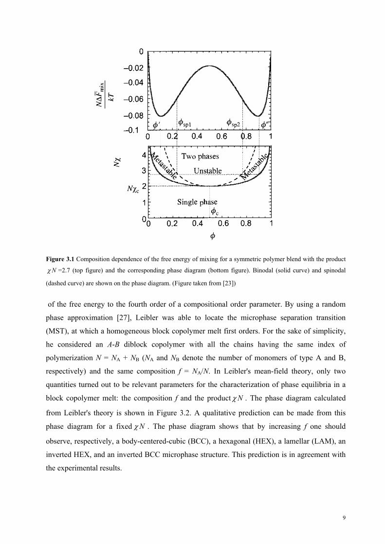
Figure 3.1 Composition dependence of the free energy of mixing for a symmetric polymer blend with the product

N =2.7 (top figure) and the corresponding phase diagram (bottom figure). Binodal (solid curve) and spinodal

(dashed curve) are shown on the phase diagram. (Figure taken from [23])

of the free energy to the fourth order of a compositional order parameter. By using a random

phase approximation [27], Leibler was able to locate the microphase separation transition

(MST), at which a homogeneous block copolymer melt first orders. For the sake of simplicity,

he considered an A-B diblock copolymer with all the chains having the same index of

polymerization N = NA + NB (NA and NB denote the number of monomers of type A and B,

respectively) and the same composition f = NA/N. In Leibler's mean-field theory, only two

quantities turned out to be relevant parameters for the characterization of phase equilibria in a

block copolymer melt: the composition f and the product N . The phase diagram calculated

from Leibler's theory is shown in Figure 3.2. A qualitative prediction can be made from this

phase diagram for a fixed N . The phase diagram shows that by increasing f one should

observe, respectively, a body-centered-cubic (BCC), a hexagonal (HEX), a lamellar (LAM), an

inverted HEX, and an inverted BCC microphase structure. This prediction is in agreement with

the experimental results.

9

Figure 3.2 Phase diagram calculated from Leibler’s mean-field theory for a diblock copolymer with all the chains

having the same index of polymerization N = NA + NB and the same composition f = NA/N. The critical point occurs

at f c= 0.5, . (Figure taken from [3]) 10.495c

N

The phase behavior of A-B diblock copolymers thus can be described in terms of the N, f and .

All three parameters are controllable during the synthesis by choice of monomers and by

stoichiometry but only and f are influenced by solvent uptake. When the solvent is

nonselective or close to nonselective, f will be constant during vapor treatment. So here, we will

only focus on .

3.1.2 Polymer solvent blend

In some applications or treatments, block copolymers may dissolve in solvent or blend with

solvent or homo-polymers. The vapor treatment is one example that the copolymer blend with

solvent. To study the mechanism of vapor treatment, it is essential to inspect the role of solvent

to the copolymer A-B interactions. It is useful to consider first the ideal case in which the

solvent/polymer parameters are equal for both blocks, SA SB . An important concept for

this system is the dilution approximation, which assumes that the only role of the solvent is to

screen the A-B interactions, and that the solvent density is uniform throughout the system. With

this approximation, the micro-phase diagram and domain size behavior for concentrated

solutions are the same as for neat copolymer, except that the AB is replaced by an effective

parameter [28],

eff AB (3.3)

10

where is the overall copolymer volume fraction. In thin film geometry, ,

where

/dry swollenfilm filmD D

dryfilmD and swollen

filmD are the film thickness in dry state and swollen state respectively.

The behavior of systems with slightly selective solvents is similar to that of the idealized,

perfectly nonselective solvent [29, 30]. The solvent is partially partitioned between subdomains,

but it is approximately uniform within each subdomain, and the variation between layers is

relatively small. Nonetheless, even a slight difference can be sufficient to eliminate the small

local maximum in each interphase, so that the solvent density decreases monotonically from

one subdomain to the other.

3.2 The concentration dependence of Tg

3.2.1 Tg of the polymer

Polymers are glass forming materials that can undergo a glass transition and form glassy solid.

When the glass transition temperature, Tg, is lower than the ambient temperature, the polymers

are soft and mobile thus they can rearrange themselves to a favored state. The Tg of most

polymers have been measured and can be found in literature. However, since Tg is molar mass

dependence, to obtain the accurate values, the Tg’s of our samples were measured by ourselves

by differential scanning calorimentry [31]. The Tg of the PS and PB domains in the present

copolymers are 76 °C and -89 °C, respectively.

3.2.2 Tg of the solvent

Due to the difficulty of finding a homogeneous set of experimental values for the solvents, Tg’s

of solvents used in this study were calculated from their melting temperatures according to a

first approximation relation [32]:

0.6 0.0003g mT T M w (3.4)

where Tm and Mw are the melting temperature and the molar mass, respectively. From the

calculation, the Tg’s of cyclohexane and cyclohexanone are 175 K and 162 K, respectively.

11

3.2.3 Tg of the polymer-solvent blend

When polymers are dissolved in or blend with solvent, the effective Tg’s are influenced

depending on the character of the solvent and the concentration. Usually a dilution decreases the

Tg of a polymer severely. Early measurements [32] indicated that solvents with lower Tg’s of

their own decreased the Tg of a polymer to a greater extent. This can be seen in Figure 3.3

where the compositional variation of the Tg of polystyrene in a number of solvent is shown.

Solutions of a polymer in solvents with Tg’s higher than its own will usually have a greater

value than that of the neat polymer [33].

Figure 3.3 The compositional variation of the glass transition temperature Tg of polystyrene in 12 different

solvents. ω1 is the weight fraction of solvent. (Figure taken from [32])

Kelley and Bueche developed a general expression for the variation of the glass transition

temperature with polymer-diluent concentration [34]

,p p g p s s g sg

p p s s

T TT ,

(3.5)

12

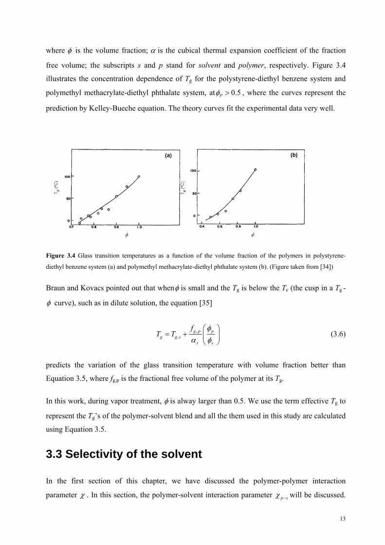
where is the volume fraction; is the cubical thermal expansion coefficient of the fraction

free volume; the subscripts s and p stand for solvent and polymer, respectively. Figure 3.4

illustrates the concentration dependence of Tg for the polystyrene-diethyl benzene system and

polymethyl methacrylate-diethyl phthalate system, at 0.5P , where the curves represent the

prediction by Kelley-Bueche equation. The theory curves fit the experimental data very well.

Figure 3.4 Glass transition temperatures as a function of the volume fraction of the polymers in polystyrene-

diethyl benzene system (a) and polymethyl methacrylate-diethyl phthalate system (b). (Figure taken from [34])

Braun and Kovacs pointed out that when is small and the Tg is below the Tc (the cusp in a Tg -

curve), such as in dilute solution, the equation [35]

,,

g p pg g s

s s

fT T

(3.6)

predicts the variation of the glass transition temperature with volume fraction better than

Equation 3.5, where fg,p is the fractional free volume of the polymer at its Tg.

In this work, during vapor treatment, is alway larger than 0.5. We use the term effective Tg to

represent the Tg’s of the polymer-solvent blend and all the them used in this study are calculated

using Equation 3.5.

3.3 Selectivity of the solvent

In the first section of this chapter, we have discussed the polymer-polymer interaction

parameter . In this section, the polymer-solvent interaction parameter p s will be discussed.

13

The miscibility of the solvent for different polymers is governed by p s . p s is modeled as the

sum of entropic and enthalpic components: [36]

p s H S (3.7)

where H is the enthalpic component and S is the entropic component. S is usually taken to be

a constant between 0.3 and 0.4 for nonpolar systems: 0.34S is often used, leading to [37]

20.34s

p s s p

V

RT (3.8)

where Vs is the molar volume of the solvent, R is the gas constant, T is the temperature,

s and p are the solubility parameters of the solvent and polymer, respectively. According to

Flory-Huggins theory, the polymer and solvent are completely miscible over the entire

composition range when 0.5p s . [37]

It was well known that p s is a function of T and for most systems follows:

bT a

T (3.9)

where a contains the enthalpic interactions and b contains the entropic effects of non-random

segment packing. The T dependence of is crucial during thermal annealing but not so

important during vapor treatment in constant temperature.

One of the most important things during vapor treatment is the concentration dependence

of p s . Though at first p s was considered to be independent of the concentration of the

polymer, subsequent experiments have shown the necessity of treating p s as a function of

composition [38, 39].

Based on the lattice theory [40], the following expression for the Flory-Huggins parameter was

deduced [41]:

2

2

1

1p s

(3.10)

14

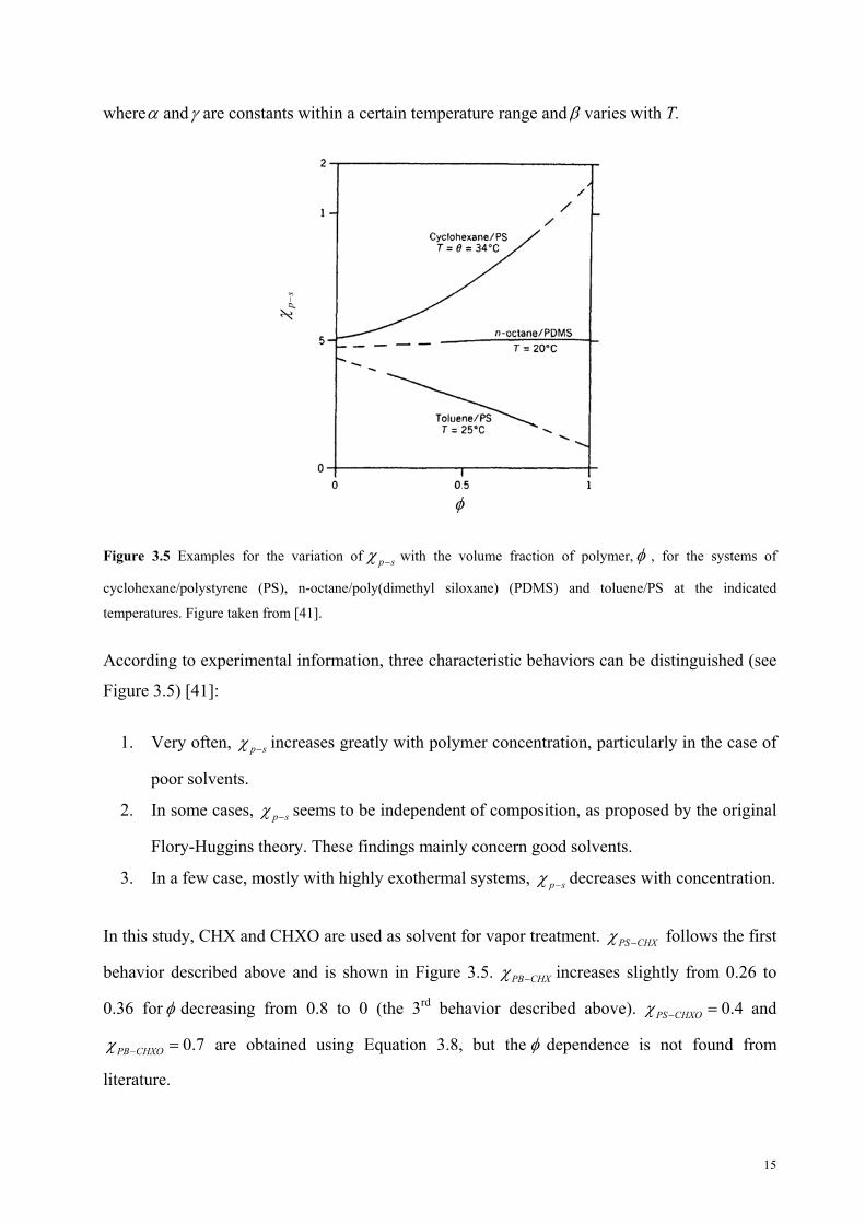
where and are constants within a certain temperature range and varies with T.

Figure 3.5 Examples for the variation of p s with the volume fraction of polymer, , for the systems of

cyclohexane/polystyrene (PS), n-octane/poly(dimethyl siloxane) (PDMS) and toluene/PS at the indicated

temperatures. Figure taken from [41].

According to experimental information, three characteristic behaviors can be distinguished (see

Figure 3.5) [41]:

1. Very often, p s increases greatly with polymer concentration, particularly in the case of

poor solvents.

2. In some cases, p s seems to be independent of composition, as proposed by the original

Flory-Huggins theory. These findings mainly concern good solvents.

3. In a few case, mostly with highly exothermal systems, p s decreases with concentration.

In this study, CHX and CHXO are used as solvent for vapor treatment. PS CHX follows the first

behavior described above and is shown in Figure 3.5. PB CHX increases slightly from 0.26 to

0.36 for decreasing from 0.8 to 0 (the 3rd behavior described above). 0.4CHXOPS and

0.7PB CHXO are obtained using Equation 3.8, but the dependence is not found from

literature.

15

16

Chapter 4

Experimental

4.1 The samples

Two kinds of poly(styrene-b-butadiene) (P(S-b-B)) diblock copolymers, namely SB12 and

SB4908, are used in this study. SB12 was synthesized by anionic polymerization [42]. Its molar

mass is 22.1 kg/mol, which corresponds to a degree of polymerization N = 374 and it has a

polydispersity index, PDI of 1.05 [31]. The PB volume fraction is 0.49 ± 0.01. In bulk, the

polymer forms lamellae with a lamellar thickness of 189 1 Å. The Flory-Huggins segment-

segment interaction parameter is = A/T + B with A = 21.6 2.1 K and B = -0.019 0.005 [31].

At room temperature, N =20, the sample is thus in the intermediate segregation regime [43].

The order-to-disorder transition temperature (TODT) is 181 ± 2 °C. The glass transition

temperatures of PS and PB in the present copolymer are Tg = 76°C and -89°C respectively, as

measured by differential scanning calorimetry [31].

SB4908 is a commercial product from Polymer Source Inc., Canada. Its molar mass is 28.0

kg/mol (15.0 kg and 13.0 kg for PS and PB respectively), which corresponds to a degree of

polymerization N = 474. It has the same PDI of 1.05 as SB12. The PB volume fraction is not

provided by the supplier and fPB = 0.51 is calculated from the molar masses of each block. Since

SB4908 is very similar to SB12 and depends only on the pair of monomers chosen, we

assume that the Flory-Huggins segment-segment interaction parameter,, is the same for both.

Thus, at room temperature, N =25, the sample is in the intermediate segregation regime [43].

To prepare thin films, the block copolymers were first dissolved in toluene then the polymer

solution was poured onto the Si substrates until these were completely wet. Films were spin-

coated at 3000 rpm for 30 s and stored in vacuum at room temperature or at 60 °C for one day

to remove the residual solvent. The Si substrates were cut from Si(100) wafers with a dimension

of 2 × 4 cm2 and cleaned by UV or acid bath. For the latter, the Si substrates were cleaned as

follows: sonication in dichloromethane at 35 °C for 15 min, water rinsing for 5 min, and then

soaking in the cleaning bath at 80 °C for 15 min. The cleaning solution was composed of 100

17

mL of 96% H2SO4, 35 mL of 35% H2O2, and 65 mL deionized water. The cleaned substrates

were further rinsed in deionized water for 10 min and finally spin-dried. At last the substrates

were rinsed and spin-dried with methonal and aceton chronologically to decrease the surface

energy.

4.2 White light interferometer

4.2.1 Methods

The white light interferometer “Filmetrics F20” (Filmetrics Inc., San Diego) is used to

measure the film thickness. The Filmetrics F20 can measure the thickness and optical

constants (n and k) of transparent and semi-transparent thin films. Measured films

must be optically smooth and between 10 nm and 50 µm thick. Since our block

copolymer thin films have a film thickness between 90 nm and 500 nm, it is ideal in our

case.

The basic idea behind the technique is to reflect a batch of light with different

wavelength from a flat surface or interface and to then measure the intensity of the light

reflected in the specular direction (reflected angle equal to incident angle). Based on

Fresnel equations, when light makes multiple reflections between two or more parallel

surfaces, the multiple beams of light generally interfere with each another, resulting in

net transmission and reflection amplitudes that depend on the light-wavelength [44].

Therefore the reflection spectrum shows a series of fringes of which the positions and

the amplitude are mainly dependent on the film thickness, surface roughness and

optical constants (n and k). By fitting with a model system containing layers of varying

refractive index/thickness, the thickness/refractive index values can be acquired.

4.2.2 Setup

The Filmetrics F20 is composed of a spectrophotometer (with light source), a set of

fiber-optic cables and a lens assembly (Figure 4.1). The lens assembly can be fixed on

the cover of the sample cell where a glass window allows the light to transmit. The

fiber-optic cable contains 7 fibers: a single detection fiber surrounded by 6 illumination

fibers. The measurement spot size is the intersection of the illuminated area with the

projected image of the detection fiber.

18

Figure 4.1 Setup configuration for the Filmetrics F20 (Figure taken from the operation manual)

4.2.3 Data analysis

The F20 is able to determine thin film characteristics by first carefully measuring the

amount of light reflected from the thin film over a range of wavelengths, and then

analyzing this data by comparing it to a series of calculated reflectance spectra using

the software “FILMeasure” (as shown in Figure 4.2). The P(S-b-B) thin film is set to be

homogeneous with the reflective index, n = 1.5. During the measurement, the film

thickness, d, and roughness, r, are fitted by the software.

Figure 4.2 An example of the FILMeasure software main window. The blue curve is from the

experimental data and the red curve is the fitting. (Figure taken from the operation manual)

19

4.3 X-ray reflectivity

4.3.1 Methods

Figure 4.3 Illustration of specular reflectivity.

X-ray reflectivity (XR) is a surface-sensitive analytical technique used in chemistry, physics,

and materials science to characterize surfaces, thin films and multilayer [45, 46]. The basic idea

behind the technique is to reflect a beam of x-rays from a flat surface and then measure the

intensity of x-rays reflected in the specular direction. For example, when X-rays impinge on a

flat material (Figure 4.3), the surface reflected beam and the thin film/substrate reflected beam

may interference. When the difference of the X-ray path lengths, L, fulfills Bragg’s law:

2 sinfilm iL D n (4.1)

where Dfilm is the film thickness, i is the incidence angle, is the wavelength and n = 1,2,3…,

the two reflected beams will be constructive and the Kiessig fringes are seen. Therefore the film

thickness can be deduced from the period of the Kiessig fringes. The roughness of the thin film

is deduced from the amplitudes of the fringes. When there are repeated sublayers within the thin

film, additional Bragg peaks are superposed on the Kiessig fringes. The thickness of the sub

layers can be deduced from Equation 4.1 with the Dfilm replaced by the sub layer thickness.

4.3.2 Setup

XR experiments were carried out at CHESS beamline D1 using the collimating slits,

goniometer and sample environment of the GISAXS experiments. The detector was an ion

chamber with an aperture of 50 mm height and 13 mm width mounted a few cm in front of the

CCD camera. The direct beam spilling over the sample surface at low angles was blocked by a

20

blade in front of the ion chamber. The advantage of using this GISAXS experiments sample

environment is obvious: the GISAXS measurement and the XR measurement can be combined

and be switched easily during the vapor treatment without touching the sample.

The XR measurements were only carried out for the experiment described in Chapter 5. The

measuring time was 1 second per point, and measuring the whole curve took ~10 min. The

electronic background of the detector was measured and subtracted from the data.

4.3.3 Data analysis

For fitting models of the scattering length density profiles, the software Parratt32 (HMI Berlin)

was used. Parratt32 is a program to calculate the optical reflectivity of neutrons or x-rays from

flat surfaces. The calculation is based on Parratt’s recursion scheme for stratified media [47].

In the fit, the Si substrate is set to be homogeneous with indefinite thickness. A SiOx thin layer

is on the top of the substrate. For lamellar thin film with short-range order, the main part of the

polymer film is set to be homogeneous, while for thin film with long-range order of parallel

lamellae, the main part of the polymer film is set to be repeating PS and PB layers. In both cases,

a top layer with a lower SLD stands at the surface. Such a layer may be attributed to the

inhomogeneity of the film thickness after preparation or to terrace formation in the upper

lamellar layer [48].

4.4 GISAXS

4.4.1 Methods

Grazing-incidence small-angle X-ray scattering (GISAXS) is a versatile tool for characterizing

nanoscale density correlations and/or the shape of nanoscopic objects at surfaces, at buried

interfaces, or in thin films [49-51]. As a hybrid technique, GISAXS combines concepts from

transmission small-angle X-ray scattering (SAXS) [52] and from grazing incidence diffraction

(GID) [46]. Applications range from the characterization of quantum dot arrays [53] and growth

instabilities formed during in-situ growth [54], as well as self-organized nanostructures in thin

films of block copolymers [55], silica mesophases [56], and nanoparticles [57]. In general,

GISAXS can be applied to characterize self-assembly and self-organization on the nanoscale in

thin films.

21

Similar to SAXS, GISAXS is using a reflection geometry but suited for thin films. In GISAXS,

the beam does not transmit through the sample but impinges under a grazing angle (< 1°) and

the reflected and scattered intensities are recorded with a 2D detector. Thus, big advantages of

GISAXS over SAXS are the high sensitivity to the surface structures and the improvement of

the resolution limit. Varying the distance between the sample and the detector, structures of 5

nm to 15 µm can be resolved by GISAXS. The scattering data are analyzed in a similar way as

done with SAXS. The basic experimental set-up is shown schematically in Figure 4.4. GISAXS

also shares elements of the scattering technique of diffuse reflectivity such as the Yoneda peak

at the critical angle of the sample, and the scattering theory, the so-called distorted wave Born

approximation (DWBA) [58-60].

In summary, there are two advantages of GISAXS over SAXS: one advantage is that GISAXS

gets rid of the background scattering from the substrate i.e. the X-ray does not need to traverse

the substrate. This is crucial in thin film geometry. The other big advantage is the improvement

of the resolution limit. In SAXS, the direct beam needs to be shielded on the detector to avoid

damage by the high intensity, which limits the access to very small values of the scattering

vector q, i.e, large structural length scales. GISAXS overcomes this problem by reflection,

because the direct beam is far from the interesting region on the detector and as a result, a better

resolution can be achieved as compared to a transmission experiment.

4.4.2 Setup

The GISAXS measurements were performed at two different beamlines. One is at beamline D1

at the Cornell High Energy Synchrotron Source (CHESS) at Cornell University in Ithaca, NY,

USA. The other was at beamline BW4 at the DORIS III at HASY LAB in the Deutsches

Elektronen-Synchrotron (DESY) in Hamburg, Germany. At both beamlines, the sample cell

was mounted horizontally on a goniometer and the X-rays hit the sample surface with an

incidence angle between 0.14° and 0.18°. A CCD camera behind the sample recorded the

scattering photons. The sample to detector distances were selected between 1.76 m and 1.97 m.

Exposure times were controlled by a fast shutter in the incident beam. The setup is shown

schematically in Figure 4.4.

Beamline D1 is located on a hard-bent dipole magnet of the CESR storage ring and uses a W:C

multilayer monochromator with about 1.5 percent band path providing 1012 photons per mm2

and sec at a photon energy of 8 keV. Two collimation slits and a guard slit condition the beam

22

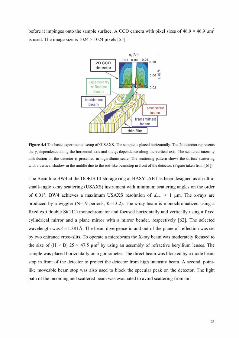
before it impinges onto the sample surface. A CCD camera with pixel sizes of 46.9 × 46.9 µm2

is used. The image size is 1024 × 1024 pixels [55].

Figure 4.4 The basic experimental setup of GISAXS. The sample is placed horizontally. The 2d detector represents

the qy-dependence along the horizontal axis and the qz-dependence along the vertical axis. The scattered intensity

distribution on the detector is presented in logarithmic scale. The scattering pattern shows the diffuse scattering

with a vertical shadow in the middle due to the rod-like beamstop in front of the detector. (Figure taken from [61])

The Beamline BW4 at the DORIS III storage ring at HASYLAB has been designed as an ultra-

small-angle x-ray scattering (USAXS) instrument with minimum scattering angles on the order

of 0.01°. BW4 achieves a maximum USAXS resolution of dmax < 1 µm. The x-rays are

produced by a wiggler (N=19 periods, K=13.2). The x-ray beam is monochromatized using a

fixed exit double Si(111) monochromator and focused horizontally and vertically using a fixed

cylindrical mirror and a plane mirror with a mirror bender, respectively [62]. The selected

wavelength was 1.381 Å. The beam divergence in and out of the plane of reflection was set

by two entrance cross-slits. To operate a microbeam the X-ray beam was moderately focused to

the size of (H × B) 25 × 47.5 µm2 by using an assembly of refractive beryllium lenses. The

sample was placed horizontally on a goniometer. The direct beam was blocked by a diode beam

stop in front of the detector to protect the detector from high intensity beam. A second, point-

like moveable beam stop was also used to block the specular peak on the detector. The light

path of the incoming and scattered beam was evacuated to avoid scattering from air.

23

4.4.3 Data analysis

4.4.3.1 Lamellar orientation

Figure 4.5 Schematic GISAXS images with the real images in the top-left corner for lamellar block copolymer thin

films with the lamellar orientation parallel to the film surface (a), perpendicular to the film surface (b) and having

mixed/random orientation (c). The names of the scattering peaks are indicated in each image.

Figure 4.5 shows the schematic GISAXS images and the real GISAXS images in the top-left

corner of each schematic image for lamellar block copolymer thin films. The inner structure of

thin film is indicated below each image. Different scattering patterns namely diffuse Bragg

sheets (DBS’s), diffuse Bragg rods (DBRs) or diffuse Debye-Scherrer rings (DDSR’s) are

observed for different lamellae orientations as shown in the figure.

4.4.3.2 Two branches of scattering

From Figure 4.6 it is seen that the DBS’s appear in pairs in each order. One branch of the

DBS’s comes from the direct beam (namely ‘M’ branch) and the other branch of the DBS’s

come from the reflected beam from the substrate (namely ‘P’ branch) [63]. For DBR’s, these

two branches overlap at:

2y perp

lam

qD

(4.2)

24

where is the lamellar thickness of the lamellae perpendicular to the film surface. For the

DBS’s the two branches separate at:

perplamD

2

2 22z iz cP iz cPpar

lam

mq k k k k

D

2

(4.3)

where kiz=k0sinαi and kcp= k0sinαcp with k0=2π/λ. αi is the incidence angle of the X-ray beam

with respect to the film surface. αcp is the critical angle of total external reflection of P(S-b-B),

which is a function of the wave length. is the lamellar thickness of the parallel lamellae.

The ‘p’ branch and ‘m’ branch correspond to the ‘Plus’ and ‘Minus’ sign in Equation 4.3,

respectively [63].

parlamD

Figure 4.6 Typical GISAXS image for lamellar block copolymer thin film with lamellar orientation dominantly

parallel to the film surface (left) and its intensity profile along qz axis (right). The red box in the GISAXS image

indicates the region of integration used for obtaining the intensity profile.

4.4.3.3 Fitting of the DBS’s

A program named Layers [64] was written according DWBA model [65] to fit the peak position

of the DBS’s. The Layers is designed for thin films with parallel A-B repeating layers. The

thickness of A and B-layer together with i can be fitted. Since in the program, the parallel

layers are assumed to be infinitely long and perfect, there is no intensity decay with increasing

qz. Therefore, it can only fit the peak position but not the peak heights/intensities.

25

4.4.3.4 Scattering depth

The penetration or information depth of the X-rays is controlled by i and f /qz. When i is

smaller than c (critical angle of the polymer), the penetration depth is less than 5 nm, which is

independent of f [66]. To investigate the inner structure of a thin film thick than 5 nm, the i

must be larger than c . However, in this case, the situation is qualitatively different. The upper

limit of the scattering length is then merely determined by photoelectric absorption and

therefore increases continuously with f [66].

In our study, the thin films are always thicker than 90 nm and 'i s are always larger than c .

Therefore, the scattering depth is a function of f (or qz), i.e. the low-qz scattering comes

mainly from the film surface while the high-qz scattering comes mainly from the film bottom.

26

Chapter 5

Vapor treatment with saturated CHX

5.1 Idea

Vapor treatment has been shown to be an effective way to anneal defects and increase the long-

range order of the nanostructure of block copolymers. Despite extensive studies of resulting

structures, the underlying molecular processes occurring during vapor treatment are still not

well understood. It would be desirable to know which conditions –vapor pressure, duration of

treatment time etc. – are optimum for obtaining the desired structure. Moreover, apart from

showing fundamentally interesting phenomena, a detailed understanding of the processes during

restructuring is needed for the optimization of annealing procedures and for design of sensors

for volatile solvents, for instance. In this work, we carried out GISAXS measurements during

vapor treatment with saturated CHX vapor. Using real-time, in-situ GISAXS, the swelling and

the rearrangement of the lamellae were followed with a time resolution of a few seconds, and

the underlying processes on the molecular level were revealed.

5.2 Experimental

The polymer used in this study is the block copolymer SB12 (see § 4.1). In-situ vapor treatment

with CHX was performed using the sample cell shown in Figure 5.1. Its volume amounts to

~110 ml. Up to 3 ml of solvent can be injected remotely through a long Teflon capillary into the

solvent reservoir at the bottom of the cell, i.e. ~2 cm below the sample. A time series was

initiated such that 2-3 initial GISAXS images were taken before injection, and the time series

continued during injection and subsequent solvent annealing. After 30 min, when the

experiment was finished, there was still solvent present in the cell, i.e. the vapor pressure was

close to saturation during the experiment.

A light bulb at the top of the cell heats the cell slightly and thus prevents condensation of

solvent vapor on the sample and on the Kapton windows. In order to avoid beam damage of the

polymer film, the sample was moved sideways after each exposure, such that a pristine spot was

27

illuminated in each measurement. A second scan of the same region was started after 19 min.

The results do not show any signs of beam damage from the first run. GISAXS images were

recorded every 15 s (10 s for measurement and 5 s for CCD read-out, data storage and change

of sample position) for the first 19 min and every 25 s (extra 10 s waiting time) afterwards.

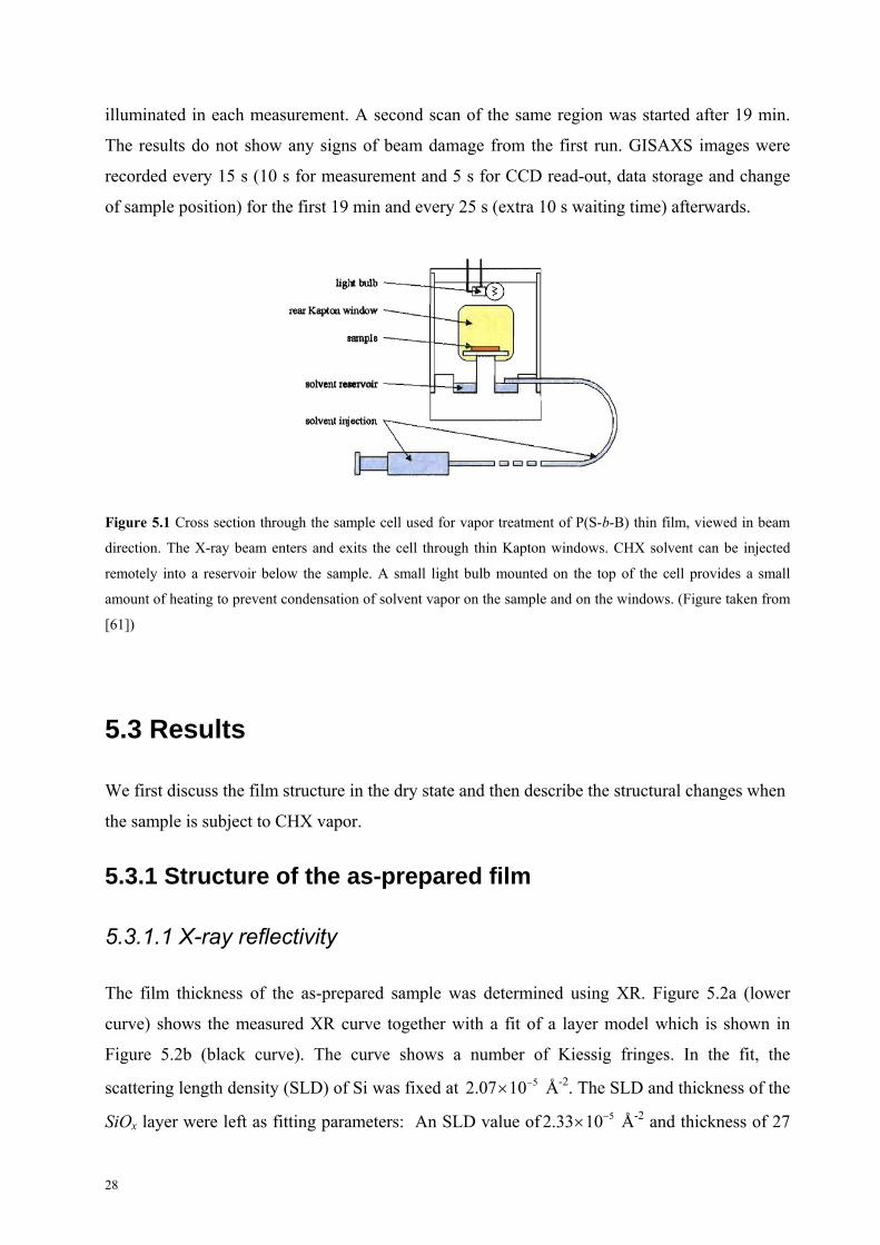
Figure 5.1 Cross section through the sample cell used for vapor treatment of P(S-b-B) thin film, viewed in beam

direction. The X-ray beam enters and exits the cell through thin Kapton windows. CHX solvent can be injected

remotely into a reservoir below the sample. A small light bulb mounted on the top of the cell provides a small

amount of heating to prevent condensation of solvent vapor on the sample and on the windows. (Figure taken from

[61])

5.3 Results

We first discuss the film structure in the dry state and then describe the structural changes when

the sample is subject to CHX vapor.

5.3.1 Structure of the as-prepared film

5.3.1.1 X-ray reflectivity

The film thickness of the as-prepared sample was determined using XR. Figure 5.2a (lower

curve) shows the measured XR curve together with a fit of a layer model which is shown in

Figure 5.2b (black curve). The curve shows a number of Kiessig fringes. In the fit, the

scattering length density (SLD) of Si was fixed at 52.07 10 Å-2. The SLD and thickness of the

SiOx layer were left as fitting parameters: An SLD value of 52.33 10 Å-2 and thickness of 27

28

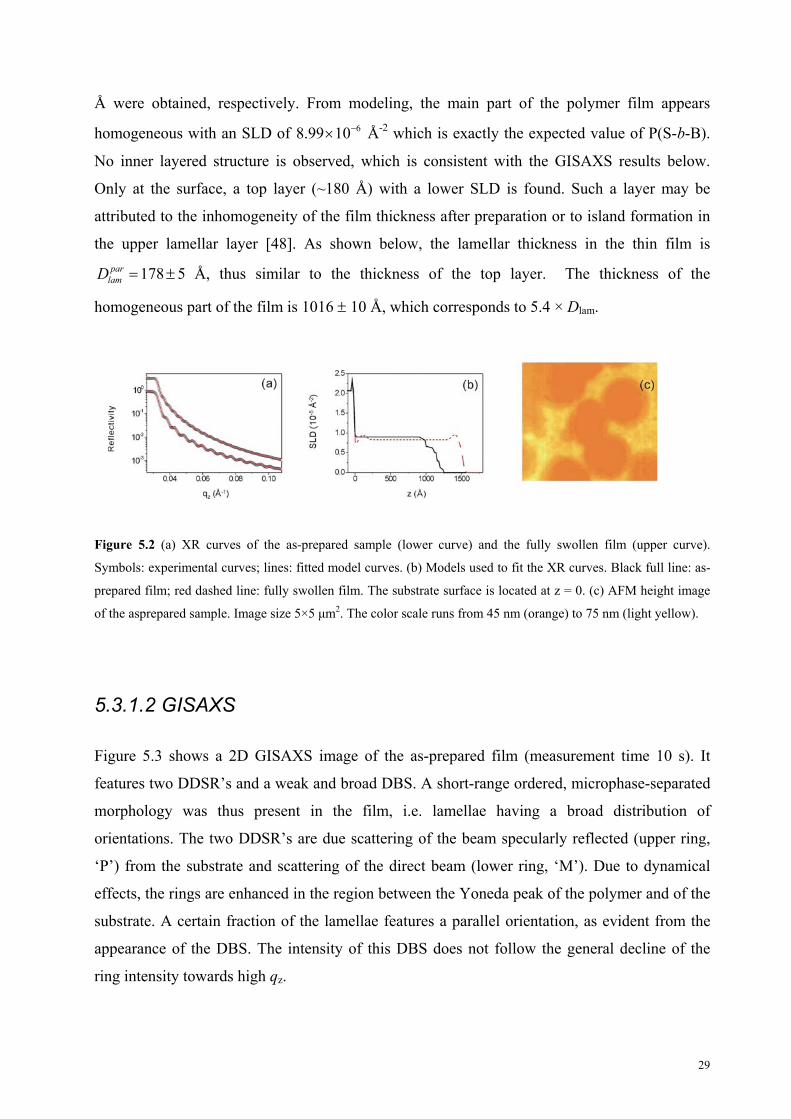
Å were obtained, respectively. From modeling, the main part of the polymer film appears

homogeneous with an SLD of 68.99 10 Å-2 which is exactly the expected value of P(S-b-B).

No inner layered structure is observed, which is consistent with the GISAXS results below.

Only at the surface, a top layer (~180 Å) with a lower SLD is found. Such a layer may be

attributed to the inhomogeneity of the film thickness after preparation or to island formation in

the upper lamellar layer [48]. As shown below, the lamellar thickness in the thin film is

Å, thus similar to the thickness of the top layer. The thickness of the

homogeneous part of the film is 1016 10 Å, which corresponds to 5.4 × Dlam.

178 5parlamD

Figure 5.2 (a) XR curves of the as-prepared sample (lower curve) and the fully swollen film (upper curve).

Symbols: experimental curves; lines: fitted model curves. (b) Models used to fit the XR curves. Black full line: as-

prepared film; red dashed line: fully swollen film. The substrate surface is located at z = 0. (c) AFM height image

of the asprepared sample. Image size 5×5 μm2. The color scale runs from 45 nm (orange) to 75 nm (light yellow).

5.3.1.2 GISAXS

Figure 5.3 shows a 2D GISAXS image of the as-prepared film (measurement time 10 s). It

features two DDSR’s and a weak and broad DBS. A short-range ordered, microphase-separated

morphology was thus present in the film, i.e. lamellae having a broad distribution of

orientations. The two DDSR’s are due scattering of the beam specularly reflected (upper ring,

‘P’) from the substrate and scattering of the direct beam (lower ring, ‘M’). Due to dynamical

effects, the rings are enhanced in the region between the Yoneda peak of the polymer and of the

substrate. A certain fraction of the lamellae features a parallel orientation, as evident from the

appearance of the DBS. The intensity of this DBS does not follow the general decline of the

ring intensity towards high qz.

29

Figure 5.3 2D GISAXS image of the as-prepared sample at αi = 0.18°. The measuring time was 10 s. The regions

of low intensity (white rectangles in the center) are due to the rod like beam-stop and the lead tape. Arrows mark

the positions expected for the Yoneda peaks of the polymer (YP) and the Si substrate (YS). The two ellipses

indicate the two diffuse Debye-Scherrer rings, centered on the direct beam and the specularly reflected

beam(marked “S”).M1 and P1 stand for the minus and the plus branch of the first-order DBS and DDSR (eq 1).

The inset shows a zoom of the black rectangle. The left magenta box indicates the range of integration for the

intensity profile in Figure 5.4.

We have previously observed that the P(S-b-B) diblock copolymer under study has a parallel

lamellar structure in thermal equilibrium on Si wafers cleaned by detergent solution, water and

toluene [65, 67]. In contrast, the present sample was spin-cast onto a UV treated Si wafer. We

conclude that the substrate properties and possibly details regarding the actual spin-coater used

have an influence on the degree of lamellar orientation.

From the present single 2D GISAXS image, the lamellar thickness cannot be determined with

high precision because the DBS is broadened along qz and because the specularly reflected

beam is shielded by lead tape. It becomes possible, though, using a series of GISAXS images

taken at several values of αi between 0.05° and 0.5° (Figure 5.4a-d). To precisely determine the

position of the specularly reflected beam (which is a direct way for the exact determination of

αi), the lead tape was removed, thus only shorter measuring times were possible, resulting in

less good statistics. For αi = 0.11°, only very weak scattering is observed in the Yoneda band

(Figure 4a). This incidence angle is below αcp, thus only scattering from a thin layer beneath the

film surface can be observed [68]. The absence of scattering indicates that close to the film

surface, no pronounced, surface-induced structure is present. The images with αi between αcP

and αcS and slightly above (Figure 5.4b, c) show the same features as the image shown in Figure

30

5.3. For αi significantly larger than αcS (Figure 5.4d), the diffuse scattering is very weak,

because the reflectivity of the film/substrate interface is low.

Figure 5.4 2D GISAXS images of the as-prepared sample at i = 0.11° (a), 0.14° (b), 0.19° (c) and 0.34° (d).

Measuring times were 0.3 s for (a-c) and 10 s for (d). The arrows indicate the position of specularly reflected beam.

The logarithmic intensity scale runs from 3 to 2000 cts for all images. (e) Resulting qz positions of the specularly

reflected beam (stars, marked S), the Yoneda peaks of the polymer (open triangles, Yp) and of the Si substrate

(open circles, YS) as well as the qz values of the DDSR’s (filled circles) as a function of kiz together with fits of

Equation 4.3 to the minus and the plus branch of the first order (marked M1 and P1, solid lines). The vertical

dashed line marks the resulting kcP. The arrow indicates the incidence angle used during vapor treatment.

Figure 5.5 Black thick line: Intensity profile

along qz through the DDSR of the as-prepared

sample at i = 0.18°. Red thin line: Fit of the

profile of a homogeneous, flat film, see text.

Ellipses were constructed to the rings of diffuse scattering, and the lengths of their half axes

along qz are given as a function of kiz (i.e. αi) together with the fitting curves (Equation 4.3) in

Figure 5.4e. The qz values of the specularly reflected beam and of the Yoneda peaks from the

polymer and the Si substrate are given as well. From the fits, we obta 5 Å, and

kcP = 0.0105 Å-1 (vertical dashed line) which corresponds to the mean value of kcP for a 50/50

vol/vol mixture of pure PS and pure PB. From the length of the qy half axes of the ellipses, the

in 178parlamD

31

average was found to be 188 ± 3 Å, i.e. the value is practically independent of αi. is

thus equal to the bulk value (189 1 Å). In contrast, is 6 % lower than in the bulk. This

effect has been previously observed by us [67]. The film thickness of the as-prepared sample

and the thickness during swelling could be determined from the period of oscillations and the

positions of the maxima in the intensity profiles along qz through the DDSR’s (Figures 5.3 and

5.5) as described in the Experimental Section. The positions of the maxima could be recovered

very well. However, whereas in the model, the amplitude of the oscillations between the

Yoneda peaks of the polymer film and the substrate are constant, the experimental curve decays

with increasing qz and shows less pronounced oscillations. We attribute this difference to the

high roughness of the film surface (see XR result above) and to the presence of internal

structure in the sample which is not included in the model. Fitting the position of the maxima,

we obtain a film thickness of 970 30 Å in the dry state (Figure 5.5). which agrees well with

the value found by XR (1016 10 Å). This fast method of film thickness determination from

the GISAXS images was applied during vapor treatment, where XR measurements would take

too long.

perplamD perp

lamD

parlamD

Figure 5.6 Sketch of the structure of the as-

prepared sample (a), the transient state (b) and the

final, disordered state (c). The different shades of

grey indicate the PS and PB parts of the lamellae.

For clarity, only a few lamellar domains are shown.

The substrate is marked by dashes.

We conclude that, in the dry state, the film consists of domains of lamellae with short-range

order and a wide distribution of orientations. A certain preference for the parallel lamellar

orientation is found, as expected. D is very similar to the bulk value, whereas D is 6 %

smaller than in the bulk. We summarize the structure of the as-prepared film in Figure 5.6a.

perplam

parlam

32

5.3.2 Structural changes during vapor treatment

Cyclohexane (CHX) was used as the solvent for vapor treatment. It is known to be a good

solvent for PB and a θ solvent for PS. It is thus selective for PB, i.e. PB CHX PS CHX .

Therefore, the volume fraction of CHX in PB is expected to be higher than in PS. Moreover,

PB CHX and PS CHX both depend on [69]. The dependence is much weaker for PB CHX than

for PS CHX : PB CHX increases slightly from 0.26 to 0.36 for decreasing from 0.8 to 0,

whereas PS CHX decreases from 0.92 to 0.51 in the same range. The values at 0 are

calculated from the solubility parameters [70] and are consistent with the dependence. This

means that during CHX vapor uptake, the selectivity of CHX varies. In the final state of

swelling, where 0.55 , the -values are 0.8PS CHX and 0.3HXPB C . For the

poly(Styrene-b-isoprene)/CHX system with 0.59CHXPS and 0.39PB CHX , an uneven

distribution with 0.71PS and 0.48PB was predicted (Figure 13a in Ref. 40). In our case,

the selectivity, i.e. the difference of -values is higher throughout the entire experiment, thus a

more uneven distribution is expected. The values of the volume fraction of CHX in the PS and

PB domains cannot, however, be calculated in a straightforward manner.

Upon injection of liquid CHX into the sample cell, drastic changes of the GISAXS images are

observed (Figure 5.7): (i) During the first ~7.5 min, the radii of the DDSR’s vary, while

intensities and the DBS’s are approximately unchanged. (ii) 7.5 min to 13.5 min after injection,

the DBS’s get more pronounced and sharper, whereas the intensities of the DDSR’s decrease

drastically. (iii) After 13.5 min, the intensity along the DDSR reappears and its intensity

becomes more evenly distributed. A transient state has thus been revealed. It is observed more

clearly in the intensity profiles through the DDSR’s and the DBS’s (Figure 5.8): (i) For times

shorter than 7.5 min, the profile through the DBS is flat (Figure 5.8a), and the profile through

the DDSR shows a flat and broad peak at qy = 0.0323 Å-1 (Figure 5.8b). We conclude that, in

this time regime, the microphase-separated structure stays short-ranged (Figure 5.6a). (ii)

Between 7.5 min and 13.5 min, both profiles display well-pronounced peaks. This indicates the

appearance of more long-ranged lamellar order (Figure 5.6b). (iii) For times longer than 13.5

min, the profile through the DDSR’s display a weak and broad peak reminiscent of the

33

Figure 5.7 GISAXS images of the film during treatment with saturated CHX vapor for the times given in the

figures. i = 0.18°. The logarithmic intensity scale runs from 30 to 600 cts for all images. The boxes in the image

of the dry state indicate the regions of integration used for obtaining the profiles along qz (Figure 5.8a) and along qy

(Figure 5.8b).

correlation peaks observed in the disordered state [26, 31, 43] and the DBS’s disappear (Figure

5.6c). We will discuss the transition to the disordered state below.

In the following, we will quantify the thicknesses of the differently oriented lamellae, and

and compare these to the changes in the film thickness.

parlamD

perplamD

34

Figure 5.8 Intensity profiles along qz, i.e. through the DBS (P1) (a) and along qy i.e. through the DDSR (P1) (b)

from the images in Figure 6 as a function of treatment time. Representative profiles from the three time regimes

marked 1-3 are shown in the inserts. The thick red lines mark the times 7.5 min and 15 min in (a) and 7.5 min and

13.5 min in (b), i.e. when the peaks appear and vanish.

5.3.2.1 Lamellar thickness

The lamellar thickness of the parallel lamellae, , is deduced from the qz position of the

DBS’s. These can directly be read off from the peaks in the intensity profiles (Figure 5.8a) for

vapor treatment times between 7.5 min and 13.5 min. For earlier and later times, however, the

DBS’s are too weak to be fitted properly, and we therefore use the qz intercept of the

constructed ellipse. Good agreement was found between the two methods. The resulting qz

positions were converted to values using Eq. 1. For the perpendicular oriented lamellae,

the positions of the peaks in the profiles shown in Figure 5.8b together with Eq. 2 were used to

determine . For simplicity, we use the term Dlam throughout, also in the disordered state

after 13.5 min, where the value rather corresponds to the size of the correlation hole [37].

During the initial 13.5 min, and show very different behavior as a function of

treatment time (Figure 5.9a): During the first 5.3 min, is unchanged at 188 Å. Then,

increases with a rate of 3.5 Å/min, i.e. by 1.9 %/min, and reaches 197 Å after 6.5 min.

Thereafter, the value stays constant. In contrast, the behavior of the parallel lamellae is more

complex: During the first 2 min, = 180 Å, i.e. it is smaller than . After 2 min,

increases with a rate of 9.5 Å/min, i.e. by 5.3 %/min, and reaches a plateau at 214 5 Å after 6

min. The rate of swelling is thus higher than for the perpendicular lamellae. Then,

decreases until it reaches 201 Å after 13.5 min. After this time, both values stay constant and

are very similar to each other.

parlamD

parlamD

palamD

perplamD

r

D

perplamD

perplamD perp

lamD

parlamD

parlamD

parlam

perplamD

35

Figure 5.9 (a) parlamD (filled circles) and perp

lamD (filled triangles) as a function of treatment time. The dashed line

marks the bulk lamellar thickness [31]. (b) Film thickness as a function of treatment time (open squares, left axis)

and the resulting volume fraction of P(S-b-B) in the swollen film (filled squares, right axis) as determined from

the period of the waveguide oscillations in the GISAXS images.

We conclude that both and change during treatment with CHX vapor. Perpendicular

lamellae are much more constrained laterally, and maybe this explains their slower thickness

increase. The two types of lamellae differ in behavior during the first 15 min but then reach the

same new equilibrium value. In the disordered state after 15 min, there is no more distinction

between the two directions. We now relate the swelling behavior of the lamellae to the changes

of the entire film, i.e. the overall solvent uptake.

parlamD perp

lamD

5.3.2.2 Film thickness

The film thickness as a function of vapor treatment time is determined from the period of the

oscillations in the DDSR. The resulting film thickness, filmD , stays constant at 970 Å during the

first 2 min (Figure 5.9b). Then, the film starts to swell at a rate of 42 Å/min, i.e. by 4.3 %/min,

until a new equilibrium value at 1780 Å is reached after 20 min. The rate of swelling is lower

than the one of the parallel lamellae, i.e., the behavior is non-affine. The final film thickness is

84% higher than in the dry state. The time-dependent volume fraction of polymer,

dryfilm filmD D , decreases from unity to 0.55 in the fully swollen state (Figure 5.9b).

36

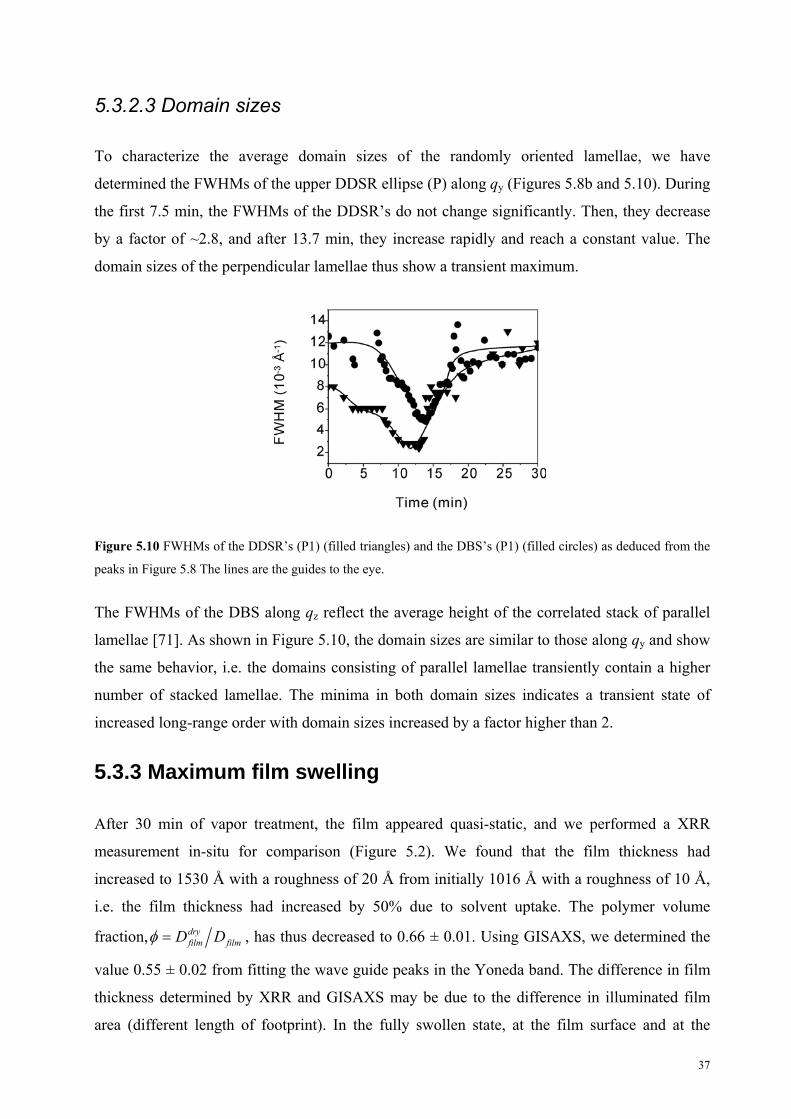
5.3.2.3 Domain sizes

To characterize the average domain sizes of the randomly oriented lamellae, we have

determined the FWHMs of the upper DDSR ellipse (P) along qy (Figures 5.8b and 5.10). During

the first 7.5 min, the FWHMs of the DDSR’s do not change significantly. Then, they decrease

by a factor of ~2.8, and after 13.7 min, they increase rapidly and reach a constant value. The

domain sizes of the perpendicular lamellae thus show a transient maximum.

Figure 5.10 FWHMs of the DDSR’s (P1) (filled triangles) and the DBS’s (P1) (filled circles) as deduced from the

peaks in Figure 5.8 The lines are the guides to the eye.

The FWHMs of the DBS along qz reflect the average height of the correlated stack of parallel

lamellae [71]. As shown in Figure 5.10, the domain sizes are similar to those along qy and show

the same behavior, i.e. the domains consisting of parallel lamellae transiently contain a higher

number of stacked lamellae. The minima in both domain sizes indicates a transient state of

increased long-range order with domain sizes increased by a factor higher than 2.

5.3.3 Maximum film swelling

After 30 min of vapor treatment, the film appeared quasi-static, and we performed a XRR

measurement in-situ for comparison (Figure 5.2). We found that the film thickness had

increased to 1530 Å with a roughness of 20 Å from initially 1016 Å with a roughness of 10 Å,

i.e. the film thickness had increased by 50% due to solvent uptake. The polymer volume

fraction, dryfilm filmD D , has thus decreased to 0.66 ± 0.01. Using GISAXS, we determined the

value 0.55 ± 0.02 from fitting the wave guide peaks in the Yoneda band. The difference in film

thickness determined by XRR and GISAXS may be due to the difference in illuminated film

area (different length of footprint). In the fully swollen state, at the film surface and at the

37

film/substrate interface, indications of layering are observed with PB/CHX being preferentially

adsorbed at both surfaces. The remainder of the film is homogeneous with an SLD of

Å-2 which is complies with the volume weighted average of PS, PB and CHX

( Å-2, Å-2 and

68.35 1069.60 10 68.35 10 67.56 10 Å-2 for PS, PB and the solvent respectively).

5.4 Discussion

Several interesting effects have been identified during swelling of the thin film with initially

mixed lamellar orientation upon treatment with cyclohexane, a slightly PB selective solvent: (i)

Vapor treatment improves the long-range order, the increased order, however, is lost again

resulting in a final disordered state. (ii) The swelling behavior of the parallel and the randomly

oriented lamellae is different: Whereas the behavior of is characterized by an overshoot of

19 % and a final value which is 12 % higher than the one in the dry state, increases after

an incubation time of 5 min to the same final value without an overshoot. (iii) Comparison of

and

parlamD

perplamD

parlamD Dfilm shows that additional parallel lamellae are formed. For instance, after 13 min of

treatment (just before the film disorders), filmD / = 7.4, which is significantly higher than in

the dry state (5.4). This behavior is consistent with our previous observations on a lamellar P(S-

b-B) film with initially parallel lamellae and treated with toluene.[71] (iv) The transient maxima

of the domain sizes of the domains consisting of parallel and perpendicular lamellae reflect the

transient state of improved long-range order before crossing the order-to-disorder transition. We

will discuss these observations considering the effects of the uptake of CHX on P(S-b-B).

parlamD

The uptake of CHX is expected to have several effects on the P(S-b-B) film: (i) The effective

glass transition temperature Tg of the polymer blocks is decreased, which is especially important

for the PS domain (the Tg of PB is far below room temperature). As the PS glass transition is

reached, the copolymer mobility increases, which enables large-scale structural rearrangements.

(ii) The effective Flory-Huggins segment-segment interaction parameter between the two

blocks, χeff, is reduced, thus the enthalpic penalty for the creation of additional lamellar

interfaces is decreased. (iii) In the presence of solvent, the copolymers assume more coiled

molecular conformations than in the dry state where they are stretched away from the

interface.[19, 71, 72] This implies an increased demand of interfacial area of each copolymer,

thus promoting the formation of additional lamellae. In the following, we will discuss the

resulting effect on the film structure.

38

5.4.1 Decrease of the effective Tg

Following the Equation 3.5, the glass transition temperature Tg of a PS/CHX mixture in bulk

varies with as

,

,(1 )

(1 )g P S C H X

C H X g C H X P S g P S

C H X P S

T TT ,

(5.1)

where is the cubical thermal expansion coefficient of the fractional free volume,

[73], 310CHX K 1 11.23 41.9 10PS K [70], and , 186g CHXT K [74]. To estimate the

variation of Tg, we assume for simplicity that CHX is equally distributed in PS and PB. This

assumption of equal distribution thus only holds strictly for the later stages when the difference

in χPS-CHX and χPB-CHX is small, whereas in the beginning of the treatment, CHX is slightly more

PB selective as discussed above. The resulting Tg,PS-CHX values during vapor treatment are given

as a function of treatment time in Figure 5.11a. Already after 3.5 min of vapor treatment, Tg,PS-

CHX falls below room temperature. We expect the true glass transition at slightly later time than

this estimate because CHX is not distributed evenly in the PS and PB domains, but in

equilibrium PB is enriched in CHX.

The strong increase of the copolymer mobility thus promotes the feasibility of structural

rearrangements after a few minutes of vapor treatment.

5.4.2 Decrease of χeff

The presence of solvent in the microphase-separated, lamellar morphology not only decreases

Tg but also screens the repulsive interaction between the PS and the PB domains. In the absence

of solvent, χN = 20, the diblock copolymer melt is thus in the intermediate-segregation regime

[43]. Starting from this low value, it is probable that χN reaches the value of 10.5 upon solvent

uptake, where the order-to-disorder transition (ODT) is expected. For a non-selective solvent,

χN of the copolymer is replaced by χeffN with eff [75]. Using this assumption in spite of

the slight selectivity of CHX, we find that χeffN of P(S-b-B) decreases with time as shown in

Figure 5.11b during treatment with CHX vapor. After a treatment time of ~20 min, χeffN has

decreased to 11.0, i.e. (χN)ODT is reached. Again, this time is only a crude estimate, because the

solvent distribution is presumably not equal in the PS and PB domain and because the exact

value of (χN)ODT may be higher than 10.5 for a low molar mass copolymer, as stated by

39

Figure 5.11 Effective Tg (a) and χeffN (b) as a function of treatment time. The horizontal dashed lines in (a) and (b)

indicate room temperature (25°C) and the order-to-disorder transition.

fluctuation theory [76]. However, it is striking that the ODT is reached significantly later than

the glass transition. We assign the vanishing of the DBS’s and DDSR’s after 13.5 and 15 min,

respectively, to the ODT of the copolymer in the presence of solvent.

The transient state of increased lamellar order which persists in the time range 7.5 min to 15

min is thus a result of the competition between the increased polymer mobility facilitating

structural rearrangements and the order-to-disorder transition due to screening of the repulsive

interaction between PS and PB. Conserving the structure of the vapor-swollen film, e.g. by

quick drying or chemical cross-linking, must be carried out during this transient state.

5.4.3 Increase of the degree of coiling

The behavior of thickness of the parallel lamellae – overshoot and leveling-off – resembles very

much the one observed in our previous study where the initial morphology was purely parallel

and a non-selective solvent, toluene, was used [71]. However, the kinetics is different: In

toluene vapor, the maximum of the overshoot was already reached after 3-4 min of treatment.

The overshoot was attributed to predominantly uniaxial swelling with an unchanged interfacial

area per chain in the first instant and the subsequent deswelling of the lamellae when the

copolymers adopt a more coiled molecular conformation. The latter process only becomes

40

possible when the polymers become mobile. It results in undulations of the lamellar interfaces

and the creation of additional lamellae to allow more interfacial area per chain.

In the present work, we were able to compare the behavior of the parallel lamellae

quantitatively to the mean-field predictions for the behavior of the lamellar thickness as

presented in Ref.[77].

Figure 5.12 as a function of parlamD (lower axis) in a double-logarithmic representation. The time of

vapor treatment is given on the top axis. The lines are fits of power laws, see text. The dashed line marks

the predicted behavior 1parlamD .

Figure 5.12 shows the dependence of onparlamD . During vapor treatment, decreases from 1 in

the dry state to ~0.55 in the fully swollen state. In spite of the scatter in the data, two limiting

regimes can be discerned: In the high-concentration regime (early times), an increase of

following is observed. The swelling is slightly slower than the uniaxial

swelling predicted by mean-field theory,

parlamD

0.76 0.11parlamD

1lamparD , for the case that the interfacial area per

chain is unchanged from the dry state [77]. The discrepancy may be due to the presence of

randomly oriented lamellae. However, this swelling only lasts until = 0.81 is reached, i.e.

after ~6 min, when levels off. The glass transition of PS is reached, and the polymer

becomes significantly more mobile, which enables the coiling of the copolymers and the

formation of additional lamellae. In the low-concentration regime for

parlamD

< 0.72, i.e. after ~8 min,

. The latter behavior is in agreement with the mean-field prediction 0.2parlamD 7 0.04 1/3par

lamD

(Ref.[77]) and is related to the higher degree of molecular coiling in the presence of solvent.

41

This coiling is only possible when the polymers are sufficiently mobile to move along and

across the lamellar interfaces.

5.4.4 Behavior of randomly oriented lamellae

The thickness of the perpendicular part of the randomly oriented lamellae stays constant during

the first ~5.5 min, presumably because of the strong lateral constraints. Only after this time, the

polymer is mobile enough for an increase of . Eventually, reaches the same value as

the , consistent with a new equilibrium state, the disordered state, as argued above, has

been reached at a polymer volume fraction of 0.55 in saturated CHX vapor. An ellipse was

found to match the DDSR’s well thoughout the vapor treatment. We thus conclude that the

lamellae with intermediate orientation follow a behavior intermediate between the parallel and

perpendicular ones.

perplamD perp

lamD

parlamD

5.5 Conclusion

Solvent vapor treatment offers an efficient route to control the structures in thin block

copolymer films, however, the mechanisms are complex. In this study, we report on the

structural changes of a lamellar film which features a distribution of lamellar orientations before

treatment. We observe that the orientation becomes more well-defined for a certain time, but

then the film becomes disordered. Additional parallel lamellae are created during the process,

which is consistent with our previous observation that the parallel orientation is the equilibrium

one [65, 67]. We relate the changes to the influence of solvent vapor on Tg, χN and the tendency

to increased molecular coiling in the presence of solvent.

The time scale of the structural changes (< 30 min) is much lower than what has been reported

in the literature for poly(styrene-b-methyl methacrylate) having a molar mass of 263 kg/mol

[14]. Structural changes have been reported to occur during 120 h of treatment. The reason may

be the higher molar mass of the polymer and that the driving force of this system is mainly the

change in surface energy by the solvent, whereas, in our case, the film is thicker and the

structural changes reflect rather the thermodynamics of the copolymer.

Using a thin film with several lamellae stacked allowed us to separate structural changes along

the lamellar normal and within the plane of the lamellar interface, because of the macroscopic

orientation of the lamellae along the film surface. Moreover, the vapor treatment of a thin film

42

enabled us to address the low solvent concentration regime which is difficult with bulk samples.

We were able to show that lamellar thin films of P(S-b-B) qualitatively follow the mean-field

predictions at very low solvent concentration, , whereas they quantitatively

follow the predictions at higher solvent concentration, .

0.76 0.11parlamD

0.2parlamD 7 0.04

However, in this study, changes with time so is not only a function of parlamD but also a

function of time. Therefore, the structure we observed probably doesn’t refer to the equilibrium

or stable state for each . To make it strict, in the next chapter, we carried out stepwise vapor

treatment and thus the is obtained as a function of parlamD and is independent of time.

43

44

Chapter 6

Stepwise vapor treatment

6.1 Idea

In the previous chapter, the vapor treatment was performed under saturated CHX atmosphere. A

transient state with improved long-range order was observed and the sample became disordered

at last. We attribute this phenomenon to the fact that the eff N at the final state is smaller

than . We suppose that under a proper vapor pressure, a stable state with improved long-

range order will appear in the solvent vapor atmosphere.

ODTN

Therefore, in this chapter, we started the vapor treatment with a much lower CHX vapor

pressure and wait until the sample structure was constant with time. Then the vapor pressure

was increased slightly, and again we waited until the sample structure was constant with time.

In this manner, the sample is stepwise swollen by all together 5 steps. We will see whether there

are stable states with improved long-range order in these steps/vapor pressures. Further more,

the lamellar thickness was obtained as a function of but independent with time. Thus the

condition of the mean-field theory is fulfilled more strictly.

6.2 Experimental

The polymer used in this study is the block copolymer SB12 (see § 4.1). In-situ GISAXS

measurement was performed at Beamline D1, CHESS. The beam was 0.1 mm high and 0.5 mm

wide. The wave length was 1.23 Å and the sample detector distance was 1760 mm. The

incidence angle used during vapor treatment was i = 0.14 °, which was larger than the critical

angle of the polymer (0.12°) but smaller than the critical angle of Si (0.176 °). Thus the inner

structure of the thin film can be determined with a time resolution of only a few seconds. The

sample cell used for in-situ stepwise vapor treatment is shown in Figure 6.1. It is similar to the

one used for saturated vapor treatment (Chapter 5) but with additional helium gas flow and a

white light interferometer. The helium flow was used to dilute the CHX vapor inside the cell.

The magnitude of the helium flow was controlled by an adjustable flow meter from 0 to 400

45

sccm (Standard Cubic Centimeters per Minute). A white light interferometer was fixed at the

top of the sample cell to measure the film thickness every 1 s through a glass window.

Figure 6.1 Sketch of the sample cell used for stepwise vapor treatment. The X-ray beam enters and exits the cell

through the thin kapton windows. CHX solvent can be injected remotely into a reservoir below the sample. A

helium flow, which can be adjusted from outside the hutch from 0 to 400 sccm, is connected to the sample cell to

dilute the solvent vapor pressure. A white light interferometer is fixed at the top of sample cell to measure the film

thickness every 1 s through a glass window.

A time series was initiated such that GISAXS images were taken continuously every 7 s with a

helium flow of 92 sccm. After 3 ~ 5 initial GISAXS images were taken, the CHX was injected

into the cell while keeping the same helium flow and the same GISAXS image taking rate. This

rate was decreased to 37 s per image after 5.5 min of the CHX’ injection because the changes in

the GISAXS images became slow. This lasted for another 22 min until the white light

interferometer showed a constant film thickness and the rearrangement of the polymer chains

have finished i.e. no further changes of the GISAXS images. Then the helium flow was

decreased to 70 sccm such that a higher CHX vapor pressure was reached. To catch the fast

dynamics, the GISAXS image taken rate was set back to 7 s per image for the first 5.8 min and

37 s per image afterwards. It lasted for 24 min until the film thickness became constant and no

changes were observable from the GISAXS images. Then the helium flow was further

decreased in steps to 44.5 sccm, 37 sccm and 31 sccm respectively. For each step, the GISAXS

images were taken every 7 s for the first few minutes and every 37 s afterwards. In each step

46

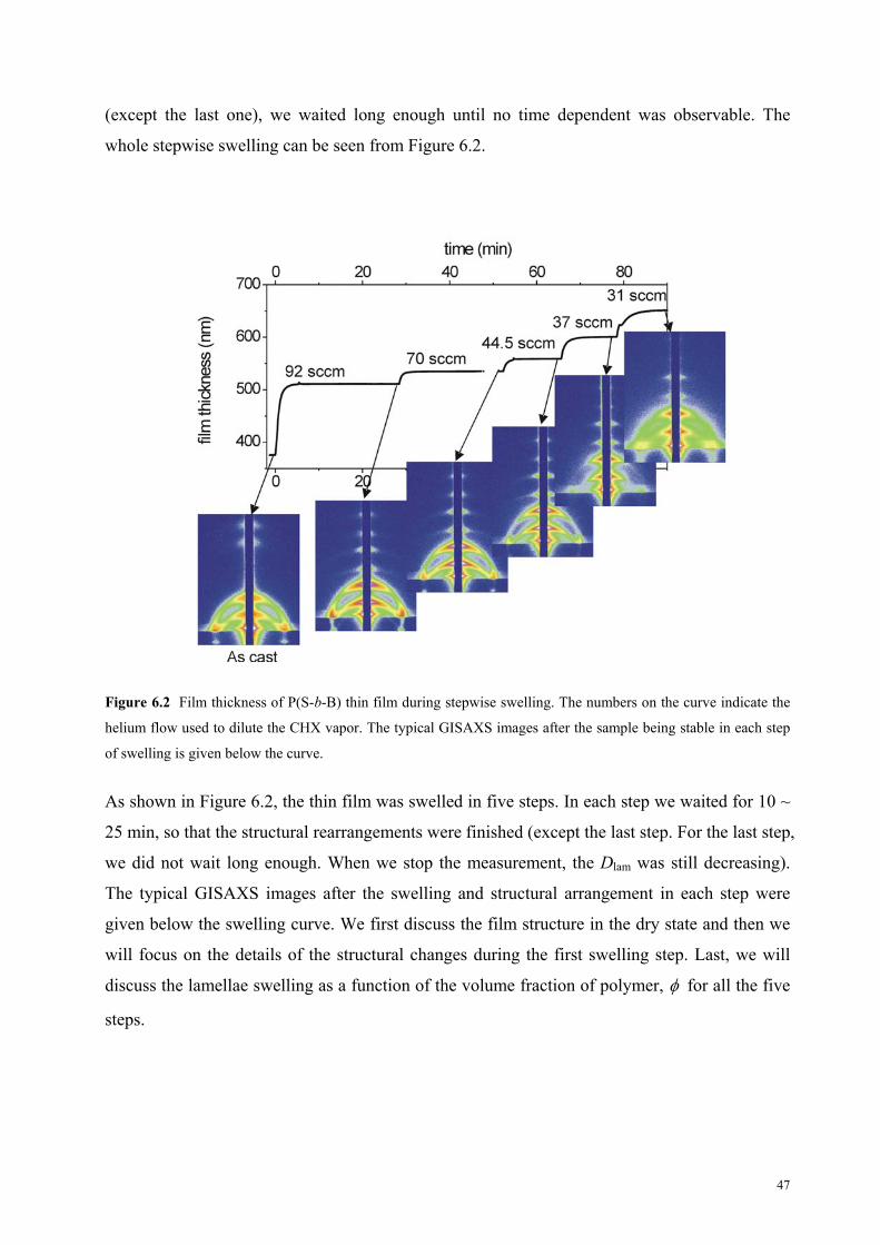
(except the last one), we waited long enough until no time dependent was observable. The

whole stepwise swelling can be seen from Figure 6.2.

Figure 6.2 Film thickness of P(S-b-B) thin film during stepwise swelling. The numbers on the curve indicate the

helium flow used to dilute the CHX vapor. The typical GISAXS images after the sample being stable in each step

of swelling is given below the curve.

As shown in Figure 6.2, the thin film was swelled in five steps. In each step we waited for 10 ~

25 min, so that the structural rearrangements were finished (except the last step. For the last step,

we did not wait long enough. When we stop the measurement, the Dlam was still decreasing).

The typical GISAXS images after the swelling and structural arrangement in each step were

given below the swelling curve. We first discuss the film structure in the dry state and then we

will focus on the details of the structural changes during the first swelling step. Last, we will

discuss the lamellae swelling as a function of the volume fraction of polymer, for all the five

steps.

47

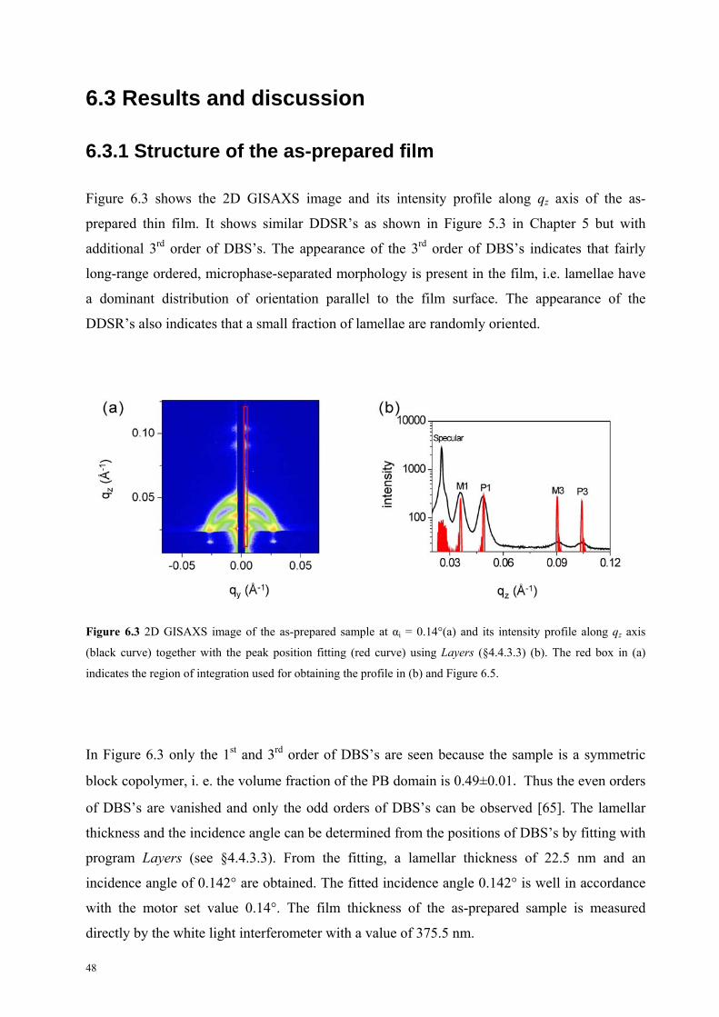
6.3 Results and discussion

6.3.1 Structure of the as-prepared film

Figure 6.3 shows the 2D GISAXS image and its intensity profile along qz axis of the as-

prepared thin film. It shows similar DDSR’s as shown in Figure 5.3 in Chapter 5 but with

additional 3rd order of DBS’s. The appearance of the 3rd order of DBS’s indicates that fairly

long-range ordered, microphase-separated morphology is present in the film, i.e. lamellae have

a dominant distribution of orientation parallel to the film surface. The appearance of the

DDSR’s also indicates that a small fraction of lamellae are randomly oriented.

Figure 6.3 2D GISAXS image of the as-prepared sample at αi = 0.14°(a) and its intensity profile along qz axis

(black curve) together with the peak position fitting (red curve) using Layers (§4.4.3.3) (b). The red box in (a)

indicates the region of integration used for obtaining the profile in (b) and Figure 6.5.

In Figure 6.3 only the 1st and 3rd order of DBS’s are seen because the sample is a symmetric

block copolymer, i. e. the volume fraction of the PB domain is 0.49±0.01. Thus the even orders

of DBS’s are vanished and only the odd orders of DBS’s can be observed [65]. The lamellar

thickness and the incidence angle can be determined from the positions of DBS’s by fitting with

program Layers (see §4.4.3.3). From the fitting, a lamellar thickness of 22.5 nm and an

incidence angle of 0.142° are obtained. The fitted incidence angle 0.142° is well in accordance

with the motor set value 0.14°. The film thickness of the as-prepared sample is measured

directly by the white light interferometer with a value of 375.5 nm.

48

We conclude that, in the dry state, the film consists of fairly long-range ordered lamellae with a

domain orientation parallel to the film surface. In contrast, in Chapter 5, the P(S-b-B) diblock

copolymer having a film thickness of ~ 100 nm shows a lamellar structure with a broad

distribution of lamellar orientations. The main reason is that the UV treated Si wafer is not

favorable for parallel lamellae orientation. Here we use the same substrate but the film is much

thicker (375 nm). The increase of the film thickness weakens the influence of the substrate so

that lamellae with a dominant distribution of orientation parallel to the film surface are observed.

6.3.2 The first step of swelling

After several initial GISAXS images were taken with the helium flow of 92 sccm, CHX solvent

was injected into the sample cell while keeping the helium flow at the same level. Drastic

changes of the GISAXS images were observed (Figure 6.4): (i) During the first ~3 min, the 3rd

order of DBS’s weakened and disappeared. (ii) New DBS’s in between the 1st and 3rd order of

DBS’s appeared from after ~40 s. (iii) The overall scattering intensity increased. (iv) The

GISAXS images became stable with 6 DBS’s after ~10 min.

Figure 6.4 GISAXS images of the film during treatment with diluted CHX vapor (the first step in Figure 6.2) for

the time given in the figures. The helium flow is 92 sccm. αi = 0.142°. The logarithmic intensity scale runs from 15

to 5000 cts for all images.

49

The observations are more clearly seen in the intensity profiles through the DBS’s (Figure 6.5):

At the very beginning (dry state), 4 Bragg peaks besides the specularly reflected peak can be

seen, 2 of 1st order, M1 and P1 and 2 of 3rd order, M3 and P3 (Figure 6.3b). When injecting

CHX, the peaks changed dramatically and in a complex manner for the first few minutes: M3,

P3 first weakened and then disappeared and then new peaks grew. After ~10 min, 6 peaks

Figure 6.5 Intensity profiles along qz, i.e. through the DBS’s from the GISAXS images (partially shown in Figure

6.4) as a function of treatment time: From the dry states until end of the first-step swelling (~30 min). The red

curve is corresponding to 40 second of vapor treatment.

besides the specularly reflected peak can be seen remaining unchanged with time. The whole

swelling process can thus be divided into two regimes i.e. the transition regime (the first few

minutes) and the final, stable state regime (after ~10 min). In the following we will discuss the

two regimes separately. Since in the transition regime, the DBS’s changed dramatically and in a

complex manner, we will start first with the more clear stable states.

6.3.2.1 Stable states

Six DBS’s were seen in the stable state (stabilized swollen state). To identify the DBS’s, the

intensity profiles were fitted with Layers. The fitting of the dry state intensity profile has been

done in Figure 6.3b very successfully. It is a good starting point for the new fitting. In Figure

50

6.6a we use the same fitting parameters as for the dry state except a slightly larger lamellar

thickness. With a lamellar thickness of 23.3 nm and an incidence angle of 0.142°, 4 peaks can

be well fitted. Thus the 1st order DBS’s M1 and P1 and the 3rd order DBS’s M3 and P3 are

indentified, whereas two peaks between the P1 and M3 can not be fitted. Previously, we have

mentioned that, for symmetric block copolymers, only the odd order of DBS’s can be seen. So

in the fitting we always set the thickness of PS layers exactly equal to that of the PB layers.

However, CHX is slightly PB selective. In the swollen state the PS and PB domains are not

symmetric any more. Therefore we set the thickness of PB layers slightly larger than that of PS

layers, i.e. the volume fraction of PB is 0.6. This way all the six peaks can be fitted with the

same lamellar thickness and incidence angle (Figure 6.6b). Therefore, all the six peaks are

indentified.

Figure 6.6 Intensity profile along qz from the last GISAXS image of Figure 6.4 together with the fittings assuming

that the block copolymer is symmetrical (a) or asymmetrical (b)

Each peak can also be fitted with a Gaussian function, thus the peak width is obtained. It is

interesting to compare the peak width with the one from the dry state. From table 6-1 we see

that after the sample has become stable in the first-step swelling, all the DBS’s become much

sharper than in the dry state.

Table 6-1 The FWHMs of the 1st and 3rd order peaks from Figure 6.3b and 6.6

M1 (Å-1) P1 (Å-1) M3 (Å-1) P3 (Å-1)

Dry state 0.0042 0.0039 0.0053 0.0059

Swollen state 0.0025 0.0029 0.0039 0.0036

51

We conclude that when the sample is stable in the first-step swelling, the lamellar thickness

increases from 22.5 nm to 23.3 nm, and the appearance of the 2nd order of DBS’s is consistent

with the slight selectivity of the CHX to PB. The sharper and more intensive DBS’s in swollen

state also indicate that the vapor annealing in the described conditions improves the lamellar

phase-separation i.e. increases long-range order.

6.3.2.2 The transition process

The transition process lasted for a few minutes from the start of the vapor treatment until the

stable state was reached. From the above study we have learned that in the dry state the 1st and

3rd order of DBS’s were seen but at the stable state not only the odd order but also the 2nd order

of DBS’s were seen. However in the transition regime the behavior of the DBS’s was very

complex. From Figure 6.5 we can see the 1st order DBS’s remained rather stable in this regime

with some position shift corresponding to the variation of the lamellar thickness. But the 3rd

order DBS’s disappeared shortly after the injection of the CHX solvent and appeared again ~40

s (red curve in Figure 6.5), but they only lasted for a few second and lost again. They appeared

again only when the stable state was reached. Meanwhile, the 2nd order DBS’s appeared around

40 s (M2) and around 3.3 min (P2) and remained with small position shifts.

Figure 6.7 Intensity profile along qz together with the fits using program Layers. For the fitting, 0.142i ,

volume fraction of PB, 0.58PBf (to get the even order), and the lamellar thickness, nm for (a) and

nm for (b).

28.5lamD

23.6lamD

Since many DBS’s appeared at 40 s, it is interesting to fit the intensity profile at this time.

However, unlike in the dry state or in the stable state, it is impossible to fit all the peaks in this

intensity profile with a single value of Dlam (Figure 6.7). When the positions of DBS’s at low-qz

52

are fitted, the ones at high-qz are dismatched (Figure 6.7a) and vice versa (Figure 6.7b). The

resulting Dlam from fitting the position of DBS’s at low and high-qz are 28.5 nm and 23.6 nm

respectively. Both values are larger than the one in the stable state. This complex Dlam behavior

will be further discussed in the next section. Now we concentrate on the dismatch of the fitting.

What causes the failure of the peak position fitting? It works successfully in the dry state and

the stable state. Nevertheless, it is clear that, the model used for the calculation cannot reflect

the real structure at this special swelling moment. One possible reason is that the lamellar

structure has changed to some other structure such as cylinder due to the increase of the fPB. All

of the previous calculations are based on lamellar structure. If the lamellar micro-phase

separation transformed to cylindrical micro-phase separation, the calculated peak position

cannot fit. However, from Figure 6.7a, besides the specularly reflected peak, the first 6

calculated peaks fit the experimental data. It is impossible that the sample consists of other

structure, otherwise it won’t fit so many peaks. Furthermore, if the micro-phase diagram has

transformed to cylinder, higher order of DBR’s should be seen due to regular lateral structure

[78]. The remained possible reason is that the film swelling is uneven i.e. the lamellar thickness

differs from the top to the bottom of the thin film. This explains the lamellar thickness (28.5 nm)

obtained from fitting the DBS’s in low-qz is larger than that in high-qz (23.6 nm). We learned

from §4.4.3.4 that the low-qz scattering comes more from the film surface while the high-qz

scattering comes more from the film bottom. It is reasonable that the lamellae at the surface of

the thin film swell more than that at the bottom at the beginning of vapor treatment. This

uneven swelling explains also the loss of the 3rd order DBS’s from ~40 s to ~5 min.

We conclude that in the transition state, an uneven swelling of the lamellae is observed. The

lamellae at the top of the thin film swell much faster than that at the bottom. The gradient of the

lamellar thickness breaks the 3rd order of the DBS’s in the time region from ~40 s to ~5 min.

6.3.2.3 Lamellae swelling

Peak position fittings were done for all curves in Figure 6.5. In dry state and stable states, all the

peaks are matched with one Dlam while for the curves in transition regime, two Dlam’s were

deduced and the Dlam for the lamellae at surface were used in Figure 6.8. The resulting lamellar

thicknesses are plotted as a function of time in Figure 6.8 (red dots) and four interesting

phenomena can be seen: (i) At the very beginning, the lamellar thickness increased very rapidly,

even faster than the film thickness (blue curve). (ii) A sharp overshot with a swelling of 35%

53

was seen. The overshot was much sharper than the case in the saturated vapor treatment

(Chapter 5). (iii) At 0.6 min, there was a change of the slope (pointed out by the black dashed

line in Figure 6.8). (iv) The film thickness leveled off earlier than the lamellar thickness.

Figure 6.8 The degree of lamellae swelling (red dots) and the degree of thin film swelling (blue curve) as a

function of vapor treatment time in the first swelling-step. The perpendicular black dashed line indicates the first

inflexion of the lamellae swelling

We would expect that at the very beginning of the swelling, the film thickness is proportional to

the lamellar thickness leading a same degree of swelling for both, i.e. in Figure 6.8, the red dots

fell on the blue curve at the very beginning (before the first kink). However, we can see from

Figure 6.8, it is not in this case. The lamellae swell faster than the whole film. To explain this

phenomenon we have to look back how we get the lamellar thickness. We obtained the lamellar

thickness by fitting the position of the DBS’s. However, because of the uneven swelling, we

cannot fit all the DBS’s at the beginning of the swelling. Therefore, we only fit the first order of

the DBS’s. As already discussed before, the lamellae near the surface contribute dominantly to

the first order DBS’s and they swell faster than the lamellae near the bottom. The film thickness

is proportional to the average lamellar thickness and the latter is smaller than the lamellar

thickness near/at the film surface.

The fast swelling of the lamellae lasted only a few minutes. Two kinks appeared, one at 0.6 min

(indicated by the dashed black line in Figure 6.8) and the other at 1.17 min (the highest point in

Figure 6.8). After the first one, the lamellae swelled much more slowly and after the second one,

the lamellae started to deswell. It is natural to assume that one of the kinks represents the glass

transition of PS. Considering that the rearrangement requires a certain time, especially when the

54

Tg of PS is not yet far below the ambient temperature. There must be a delay between the glass

transition of PS and the decrease of the lamellar thickness. Therefore the kink at 1.17 min (the

highest point) cannot be the transition point. However the kink at 0.6 min is a likely candidate:

After this turning point, the lamellar thickness still increases but with an obvious smaller speed

(Figure 6.8). This can better be discussed when Dlam is plotted as a function of ( Figure 6.9).

Figure 6.9 Dlam as a function of (lower axis) in a double-logarithmic representation. The time of vapour

treatment is given on the top axis. The lines are fits of power laws, see text.

Figure 6.9 shows the dependence of Dlam on . The two kinks can be better seen here. These

two kinks are at 0.85 and 0.77 respectively and marked tree regimes: In the high-

concentration region ( 0.85 ), an increase of Dlam following is observed. The

swelling is faster than the uniaxial swelling predicted by mean-field theory,

1.5 0.1lamD

D 1lam , for the

reason of uneven swelling at this time region. This swelling lasts until 0.85 , i.e. for ~ 0.6

min. Then the swelling speed decreased and an increase of Dlam following is

observed. Two possible reasons may explain this much slower swelling. One is the uneven

swelling ends at the first kink (

0.57 0.04 lamD

0.85 ) and the other is that the glass transition of PS is

reached here. The ending of uneven swelling is a gradual process and moreover from the

GISAXS images it is seen that the DBS’s at high-qz are very similar before and after

0.85

0.85

which points out the gradience of Dlam has no obvious change at this point. Therefore,

we conclude that the appearance of the first kink come from the glass transition of PS. Since at

the glass transition of PS is reached and we know from Kelley-Buecher’s equation

55

(Equation 3.5) that for pure PS the glass transition is reached at 0.93PS (volume fraction of

PS), we can then estimate the selectivity of the CHX in our sample. Let’s assume that the partial

of the CHX entering PS domain is x, the partial entering PB domain is (1-x); both volumes of

PS and PB are the same and equal to 0.5. The volume of CHX is then equal to 1-0.85=0.15. We

have:

0.50.93

0.15 0.5x

Resolving the above equation, we get 0.25x .Therefore, we conclude that approximately 25%

of CHX goes into PS block and the rest goes into the PB domain. It is compatile with the theory

predictions [29, 30].

The slow swelling ends at the second kink at 0.77 and the Dlam decreases with following

. In this low-concentration regime, the effective Tg of PS is significantly lower

than the ambient temperature and the polymer becomes significantly more mobile, which

enables a very fast rearrangement. However, the mean-field theory predicts a decrease of Dlam

following

5.28 0.00lamD

lamD 1/3 which is much smaller than in our case. This may due to the fact that the

copolymer is in a nonequilibrium state (highly stretched) before the deswelling. The theory

predicts the Dlam changes from one equilibrium state to another, instead of from a stretched state

to equilibrium state.

The film thickness is the product of the average lamellar thickness and the number of lamellae.

The decrease of Dlam together with the increase of Dfilm indicates the formation of additional

lamellar layers. The formation of new layers requires large rearrangement of the polymer.

During this process, of course, the long-range order of the lamellae will be perturbed and this is

observed by the loss of 3rd order DBS’s in Figure 6.5, between 2 and 4 min.

6.3.3 Further swelling

6.3.3.1 Nonequilibrium

6.3.3.1.1 Results

After the stable state of the first-swelling had been reached for more than 10 min, the helium

flow was decreased to 70 sccm and the second swelling-step began. Since the second step was

56

much smaller than the first one, no uneven swelling was observed. The fitting of the positions

of the DBS’s revealed that first increased and reached the maximum value of 23.8 nm in ~

30 seconds and then decreased to 23.3 nm. The decrease lasted roughly 2 min and leveled

off afterwards. Meanwhile, the

lamD

lamD

filmD increased from 511 nm to 530 nm for the first ~ 2 min and

then increased much slower and leveled off with a value of 535 nm.

The 3rd swelling-step started 23 min after the second swelling-step, with a helium flow of 44.5

sccm. The behavior of the was very similar as in the second step: first increased and

reached the maximum value in ~ 26 seconds and then decreased slightly and levels off.

lamD lamD

The 4th swelling-step started 13 min after the 3rd swelling-step, with a helium flow of 37 sccm.

Instead of first swelling, incubated for the first ~ 20 s and then decreased slightly and

leveled off.

lamD

The 5th swelling-step started 13 min after the 4th swelling-step with a helium flow of 31 sccm.

first increased and reached the maximum value of 23.1 nm in 14 seconds, then

keeped decreasing afterwards. The 5th swelling-step was measured for 10 min and the

lamD lamD

filmD leveled off at ~6.6 min while kept decreasing until the stop of the measurement. lamD

6.3.3.1.2 Discussion

The unexpected increase of the lamellar thickness points to a nonequilibrium state at the

beginning of each swelling step. The nonequilibrium is due to the delay of the rearrangement of

the polymer chains, i.e. the polymer needs time to establish equilibration. This phenomenon

helps us to estimate the time scale of the rearrangement of polymer. We conclude the polymer

needs a few tens of seconds to acquire new equilibration responding to the variation of . The

delay time may differ for different , i.e. the smaller responding to shorter delay.

Moreover, since the decrease of lamellar thickness almost stop at the same time as the stop of

film swelling, it implies that the delay of the rearrangement of the polymer occurs dominantly at

the beginning. The well-ordered lamellar structure acts as a big hindrance for rearrangement of

the polymer chains. The polymer chains have to struggle a lot before they can move through the

neighbor layers, but if the rearrangement starts, they can rearrange themselves much faster.

57

However, it is interesting that the lamellar thickness decreases more and longer at the 5th

swelling-step (The Dlam was still decreasing when we stopped the measurement). At this step,

the polymer chains have the highest mobility and should rearrange themselves fastest i.e.

reaches the equilibrium fastest. This raises a question: Do the stable states in the first 4

swelling-steps really reach the equilibrium? We will discuss it in the following session.

6.3.3.2 Scalling law

Figure 6.10 shows the change of as a function of lamD in a double-logarithmic representation

for the whole stepwise swelling. Four linear regions can be seen and in each region a linear

fitting is performed. The Dlam follows , , and

in the high-concentration region (

1.5lamD 0.1 0.57 0.04

lamD

0.85

5.28 0.00lamD

0.14 0.03lamD ), in 0.85 0.77 , in

0.77 0.73 and in the low-concentration region ( 0.73 ), respectively. The first 3 regions

( 0.73

0.73

) occurred in the first step of the swelling and had been discussed in §6.3.2. We

conclude that the equilibration is not reached in these regions. In the low-concentration region

( ), four black filled circles correspond the stable states under four different CHX vapor

pressures. In the stable states, the Dlam’s are constant with time. Together with the fact that the

sample is far above the glass transition temperature, i.e. the sample is very mobile, it is likely

that the sample is in the equilibrium. However, in this region, Dlam’s followed

and thus a question is raised. We know from the mean-field theory that in the low-concentration

region Dlam is expected to be proportional to

0.14lamD 0.03

1/3 (instead of 0.14 ) in equilibration. Further more,

the four stable states were reached in 3 or 4 minutes whereas in the 5th swelling-step, the stable

state was never reached even after 10 min. It is abnormal because the sample should reach

equilibration fastest in the 5th swelling-step. If in the 5th swelling-step the sample can not reach

the equilibrium in 10 min, it cannot reach the equilibrium in 3-4 min in the previous four

swelling-steps either. Therefore the 4 stable states cannot be equilibrium states. In low-

concentration region, the Dlam is expected to decrease following 1/3lamD . However, the

decrease of Dlam requires the formation of new lamellar layers i.e. large rearrangement. When

the sample is well ordered in lamellae, the polymer chains have to travel across existent

lamellae to form a new one. However it is impossible if the eff N OD

NT

lamD

. In this case, the

Dlam can not decrease freely, thus meta-stable states with larger following

58

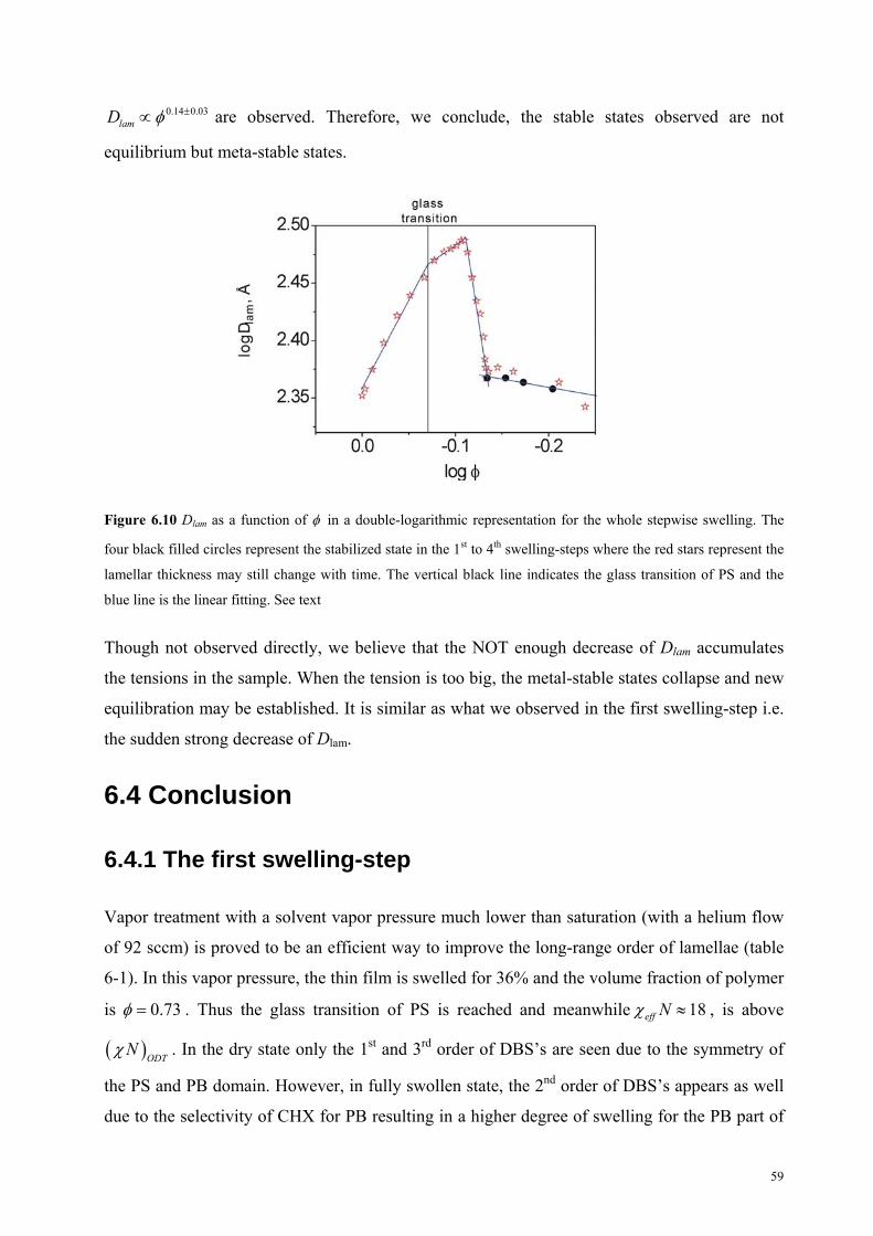
0.14 0.03lamD are observed. Therefore, we conclude, the stable states observed are not

equilibrium but meta-stable states.

Figure 6.10 Dlam as a function of in a double-logarithmic representation for the whole stepwise swelling. The

four black filled circles represent the stabilized state in the 1st to 4th swelling-steps where the red stars represent the

lamellar thickness may still change with time. The vertical black line indicates the glass transition of PS and the

blue line is the linear fitting. See text

Though not observed directly, we believe that the NOT enough decrease of Dlam accumulates

the tensions in the sample. When the tension is too big, the metal-stable states collapse and new

equilibration may be established. It is similar as what we observed in the first swelling-step i.e.

the sudden strong decrease of Dlam.

6.4 Conclusion

6.4.1 The first swelling-step

Vapor treatment with a solvent vapor pressure much lower than saturation (with a helium flow

of 92 sccm) is proved to be an efficient way to improve the long-range order of lamellae (table

6-1). In this vapor pressure, the thin film is swelled for 36% and the volume fraction of polymer

is 0.73 . Thus the glass transition of PS is reached and meanwhile 18eff N , is above

. In the dry state only the 1st and 3rd order of DBS’s are seen due to the symmetry of

the PS and PB domain. However, in fully swollen state, the 2nd order of DBS’s appears as well

due to the selectivity of CHX for PB resulting in a higher degree of swelling for the PB part of

ODTN

59

the lamellae. At the very beginning of the vapor treatment, an uneven swelling of the thin film

is observed, i.e. the lamellae at the film surface swell faster than those deep in the film. The

lamellar thicknesses obtained from the position of the 1st order DBS’s are given in Figure 6.8

together with the film thickness as a function of treatment time. Initially, Dlam increases rapidly

and even faster than the film thickness. This is due to the fact that mainly the upper (more

swollen) lamellae contribute to the average position of the 1st order DBS’s. The increase of Dlam

reflects that the uptake of solvent results mainly in swelling along the lamellar normal. After

~0.6 min of treatment, the swelling of the lamellae abruptly slows down. We attribute this

slowing down to the glass transition of the PS domain: After having taken up a sufficient

amount of CHX, PS goes from the glassy to the liquid state, and the block copolymers become

significantly more mobile. The two blocks can now assume more coiled molecular

conformations, which are entropically favored when solvent is present [72]. These more coiled

conformations result in an increased interfacial area per copolymer and in a lower lamellar

thickness than for pure uniaxial swelling along the film normal. After ~1.3 min, suddenly the

lamellae start to de-swell strongly. We have observed this effect before [71], and have attributed

it to the strongly coiled molecular conformations of the PS and the PB domain. The interfacial

demand is now so high that the copolymers cannot be accommodated at a certain lamellar

interface any longer. Therefore, additional lamellae are formed, and the blocks can relax to their

new (coiled) equilibrium conformation with a lower Dlam than in the as-prepared state.

Eventually, levels off after ~4 min of treatment, i.e. a new equilibrium state is reached.

From the kink of the lamellar thickness at 0.6 min, the selectivity of CHX in our sample is

estimated that ~25% of CHX goes into PS domain and the rest goes into the PB domain.

lamD

6.4.2 The other swelling-step

In the further swelling, at the beginning of each step, a transient state is observed. The transient

state is characterized by an overshoot of the lamellar thickness. Then the sample becomes stable

after a few minutes except the last step. Though the sample has passed the glass transition, the

overshoot of the lamellar thickness reveals that the polymer is still rearranging itself. This

rearrangement takes one or two minutes until the sample reaches a stable state. This gives us a

clue how fast the polymer can rearrange itself. More interesting, the lamellar thicknesses in the

stable states are much larger than predicted ones by the mean-field theory which implies that

even the stable states are not equilibrium states. We contribute it to the screening effect of the

already existent well-ordered lamellae, which hinder the travelling of polymer chains thus

60

hinder the formation of new lamellae. Therefore a meta-stable state with a more stretched chain

conformation is observed.

61

62

Chapter 7

Vapor treatment with saturated

cyclohexanone

7.1 Idea

We have discussed vapor treatment with slightly PB selective solvent CHX in saturated vapor

atmosphere in Chapter 5 and in stepwise-increasing vapor pressure atmosphere in Chapter 6.

However, as demonstrated previously, one of the most key effects of the solvent is to make the

PS domain soft and mobile. Therefore a PS selective solvent may benefit this purpose. In this

Chapter we will discuss vapor treatment with CHXO, which is PS selective and has a 13 k

lower Tg than that of CHX. Both of the properties help to soft the PS domain. Further more, the

vapor pressure of CHXO is very low (3.1 mmHg @21°C). It is only 1/25 of that of CHX.

Therefore, even with saturated CHXO vapor, there is no risk that too much solvent might enter

the thin film and lead to disorder.

7.2 Setup

The polymer used in this study is the commercial block copolymer SB4908 (see § 4.1). It is

spin-cased to an acid-bath cleaned Si substrate (see § 4.1). The in-situ vapor treatment was

performed in the beamline BW4, HASYLAB in DESY. The beam was 25 µm high and 48 µm

wide. The wave length was 1.381 Å and the sample detector distance was 1972 mm. The

incidence angle used during vapor treatment was I = 0.15 °, which is larger than the critical

angle of the polymer (0.12°) but smaller than the critical angle of Si (0.176 °). Thus the inner

structure of the thin film can be determined with a time resolution of only a few seconds. The

sample cell used for in-situ vapor treatment is the same as described in Chapter 6 (Figure 6.1).

However, since the CHXO is oil-like solvent, its saturated vapor pressure is very low, therefore

vapor treatment was performed only under saturated vapor atmosphere.

63

7.3 Result and discussion

We first discuss the film structure in the dry state and then describe the structural changes when

the sample is subject to CHX vapor.

7.3.1 Structure of the as-prepared film

The film thickness of the as-prepared thin film measured by the white light interferometer is

203 nm. Figure 7.1 shows a 2D GISAXS image of the as-prepared thin film (measurement time

5 min). It features two orders of DBS’s namely M1, P1 and M3, P3 respectively but no DBR’s.

A long-range ordered lamellar micro-phase morphology with the lamellar orientation parallel to

the film surface was thus present in the film.

Figure 7.1 2D GISAXS image of the as-prepared sample at αi = 0.15°. The measuring time was 5 min. The DBS’s

are marked by M1, P1, M3, P3 in the image, respectively. The red box indicates the range of integration for the

intensity profile in Figure 7.2. The blank region at qy = 0 comes from a point-like (the lower) and a rod-like (the

higher) beamstop.

We have observed in Chapter 5 that SB12, which is very similar as SB4908, has a short-range

ordered morphology with randomly oriented lamellae on Si substrate cleaned by UV treatment.

In contrast, the present sample was spin-cased onto a Si substrate which was first cleaned by

64

acid bath and then coated with methanol and acetone chronologically. The latter process is to

make the substrate hydrophobic. Thus the substrate is selective to PS. and benefit a parallel

lamellar orientation.

More details are observed from the intensity profile along qz axis and its peak position fittings

(Figure 7.2). First, not only the 1st and 3rd order of DBS’s but also weak 2nd order DBS’s were

observed. This is due to the asymmetry of the PS and PB domain (however not accordant with

the calculated value, fPB = 0.51); Second, as shown in the figure, it is impossible to fit all the

peak positions with one Dlam: When the peak positions of the 1st order DBS’s are fitted,

resulting in a Dlam of 22.2 nm, the 3rd order DBS’s are dismatched (Figure 7.2 a) and vice versa

resulting in a lamellar thickness of 21.4 nm (Figure 7.2 b). Therefore, we conclude that the

lamellar thickness for the as-prepared sample is not constant: the lamellae close to the surface

have a thickness of ~ 22.2 nm which is very similar as we observed in Chapter 6 (22.5 nm),

meanwhile the lamellae close to the substrate have a smaller thickness of ~ 21.4 nm. We

attribute the lamellar thickness decrease close to the substrate to the selectivity of the substrate

to PS. In detail, because of the attraction of the substrate to PS, the thickness of the PS layer

close to the substrate is smaller than that far away.

Figure 7.2 Intensity profile along qz axis of the 2D GISAXS image from Figure 7.1 together with the peak position

fittings using Layers. Since it is impossible to fit all the peak positions with one Dlam, the 1st order peaks are chose

to fit in (a) and the 3rd order peaks are chose to fit in (b). Two lamellar thicknesses of 22.2 nm and 21.4 nm are

acquired respectively. The intensity increase at qz > 0.089 Å-1 is due to the end of the rod-like beamstop.

We conclude that, in the dry state, the film consists of fairly long-range ordered lamellae with

an orientation parallel to the film surface; The lamellar thickness differs with depth: the

lamellae close to the substrate is smaller than that close to the film surface due to the attraction

of the substrate to the polymer.

65

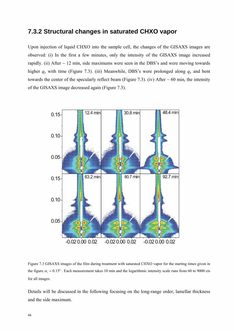
7.3.2 Structural changes in saturated CHXO vapor

Upon injection of liquid CHXO into the sample cell, the changes of the GISAXS images are

observed: (i) In the first a few minutes, only the intensity of the GISAXS image increased

rapidly. (ii) After ~ 12 min, side maximums were seen in the DBS’s and were moving towards

higher qy with time (Figure 7.3). (iii) Meanwhile, DBS’s were prolonged along qy and bent

towards the center of the specularly reflect beam (Figure 7.3). (iv) After ~ 60 min, the intensity

of the GISAXS image decreased again (Figure 7.3).

Figure 7.3 GISAXS images of the film during treatment with saturated CHXO vapor for the starting times given in

the figure. 0.15i . Each measurement takes 10 min and the logarithmic intensity scale runs from 60 to 9000 cts

for all images.

Details will be discussed in the following focusing on the long-range order, lamellar thickness

and the side maximum.

66

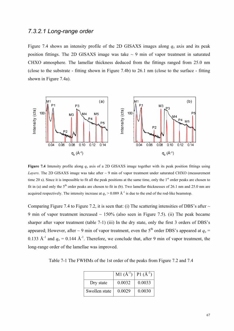
7.3.2.1 Long-range order

Figure 7.4 shows an intensity profile of the 2D GISAXS images along qz axis and its peak

position fittings. The 2D GISAXS image was take ~ 9 min of vapor treatment in saturated

CHXO atmosphere. The lamellar thickness deduced from the fittings ranged from 25.0 nm

(close to the substrate - fitting shown in Figure 7.4b) to 26.1 nm (close to the surface - fitting

shown in Figure 7.4a).

Figure 7.4 Intensity profile along qz axis of a 2D GISAXS image together with its peak position fittings using

Layers. The 2D GISAXS image was take after ~ 9 min of vapor treatment under saturated CHXO (measurement

time 20 s). Since it is impossible to fit all the peak positions at the same time, only the 1st order peaks are chosen to

fit in (a) and only the 5th order peaks are chosen to fit in (b). Two lamellar thicknesses of 26.1 nm and 25.0 nm are

acquired respectively. The intensity increase at qz > 0.089 Å-1 is due to the end of the rod-like beamstop.

Comparing Figure 7.4 to Figure 7.2, it is seen that: (i) The scattering intensities of DBS’s after ~

9 min of vapor treatment increased ~ 150% (also seen in Figure 7.5). (ii) The peak became

sharper after vapor treatment (table 7-1) (iii) In the dry state, only the first 3 orders of DBS’s

appeared; However, after ~ 9 min of vapor treatment, even the 5th order DBS’s appeared at qz =

0.133 Å-1 and qz = 0.144 Å-1. Therefore, we conclude that, after 9 min of vapor treatment, the

long-range order of the lamellae was improved.

Table 7-1 The FWHMs of the 1st order of the peaks from Figure 7.2 and 7.4

M1 (Å-1) P1 (Å-1)

Dry state 0.0032 0.0033

Swollen state 0.0029 0.0030

67

7.3.2.2 Lamellar thickness

Figure 7.5 Map of the 1st order DBS’s versus the vapor treatment time. The black line is the guider for the eyes.

The linear intensity scale runs from 10 to 200 cts.

After the CHXO was injected to the sample cell, the DBS’s shifted towards low-qz continuously.

A Map of the 1st order DBS’s (M1, P1) versus the vapor treatment time is shown in Figure 7.5.

The lamellar thicknesses were deduced from M1 and P1. The lamellae swelled from 22.2 nm in

the dry state (fitting curve shown in Figure 7.2 a) to 26.1 nm in swollen state (fitting curve

shown in Figure 7.4 a). The lamellar thickness leveled off after ~ 8 min and increased ~ 17%.

Afterwards, side maximum was observed in much longer time scale and we will discuss it in the

following section.

7.3.2.3 Side maximum

After ~ 12 min of vapor treatment, side maximums were seen in the DBS’s and moving towards

higher qy with time (Figure 7.3). The side maximums indicate the formation of lateral structure.

The length scale, D, of the lateral structure can be calculated using

68

2

y

Dq

D decreased from ~209 nm and leveled off at 106 nm after ~ 80 min of vapor treatment as

shown in Figure 7.6.

Figure 7.6 The lateral length scale D versus the vapor treatment time.

Figure 7.7 Schematics of the micro-phase transition. The yellow part represents the PS domain

and the blue part represents the PB domain.

As seen in Figure 7.3, the side maximums are intensive and superposed on DBS’s. it indicates

that the lateral structure is very regular inside each layer. Together with the fact that CHXO is

PS selective, we conclude that after ~ 12 min of vapor treatment in saturated CHXO atmosphere,

regular holes (PS) were formed in the PB domains and the number of holes increased with time

resulting a decrease of D (distance of neighbor holes) (Figure 7.6). Thus the lamellar micro-

phase separation transformed to perforated layer micro-phase separation (Figure 7.7).

69

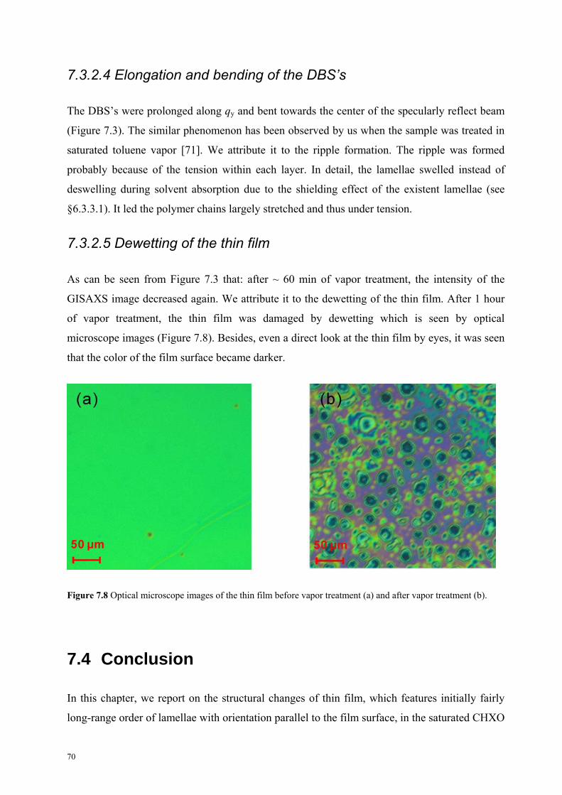
7.3.2.4 Elongation and bending of the DBS’s

ter of the specularly reflect beam

(Figure 7.3). The similar phenomenon has been observed by us when the sample was treated in

60 min of vapor treatment, the intensity of the

GISAXS image decreased again. We attribute it to the dewetting of the thin film. After 1 hour

The DBS’s were prolonged along qy and bent towards the cen

saturated toluene vapor [71]. We attribute it to the ripple formation. The ripple was formed

probably because of the tension within each layer. In detail, the lamellae swelled instead of

deswelling during solvent absorption due to the shielding effect of the existent lamellae (see

§6.3.3.1). It led the polymer chains largely stretched and thus under tension.

7.3.2.5 Dewetting of the thin film

As can be seen from Figure 7.3 that: after ~

of vapor treatment, the thin film was damaged by dewetting which is seen by optical

microscope images (Figure 7.8). Besides, even a direct look at the thin film by eyes, it was seen

that the color of the film surface became darker.

Figure 7.8 Optical microscope images of the thin film before vapor treatment (a) and after vapor treatment (b).

.4 Conclusion

he structural changes of thin film, which features initially fairly

long-range order of lamellae with orientation parallel to the film surface, in the saturated CHXO

7

In this chapter, we report on t

70

atmosphere. Two processes, namely fast process and slow process, were observed by in-situ

GISAXS measurement during this vapor treatment.

7.4.1 Fast process

The fast process took place roughly within the first 9 min. It is characterized by a strong

increase of the scattering intensity, sharper DBS’s and the appearance of 5th order DBS’s. All

ent, regular holes were formed in the PB domain. The density of

the holes increased with time. This can be seen from the decrease of the distance between

this observations point out that the long-range order of the lamellar micro-phase separation is

further improved. We attribute the efficient improvement of the long-range order to the special

properties of the CHXO, i.e. low Tg (162 K) and selective to the rigid PS domain. A detailed

analysis of the position of the DBS’s revealed that the lamellar thickness increased continuously

with the increase of the film thickness. We have learned in previous chapters that the lamellar

thickness should decrease with solvent absorption when the sample was in equilibrium. We

attribute the increase of the lamellar thickness to the screening effect of the existent well-

ordered lamellae (§6.3.3.1).

7.4.2 Slow process

After ~ 12 min of vapor treatm

neighbored holes. It revealed that the lamellar micro-phase separation has transformed to

perforated layer micro-phase separation. Meanwhile, because of the tension in the thin film,

ripple was formed and dewetting was observed.

71

72

Chapter 8

n the structural changes of lamellar P(S-b-B) thin films during vapor

Flory-Huggins segment-segment interaction parameter,

Summary

In this thesis, the focus is o

treatment. The effective eff , the

effective glass transition temperature, Tg and the volume fraction of one block, f, play an key

mer chains in the P(S-b-B) thin film are immobile and can not rearrange

themselves to the micro-phase equilibration. However, when the solvent enters the sample the

role for the structural rearrangement. Furthermore, the existent structure also influences further

structural changes.

The Tg of the PS domain is 76 °C which is higher than the room temperature. Thus in room

temperature the poly

effective Tg of PS decreases. The effective Tg of PS can be deduced from the Kelley-Bueche

equation (Equation 3.6). When the effective Tg of PS is lower than the ambient temperature, the

sample becomes soft and the polymer chains become mobile. Thus it is possible for the sample

to rearrange itself to the most favored state i.e. the micro-phase equilibrium. However, the

micro-phase equilibrium is controlled by several parameters. Among them, and f are the most

important two. Both of them are dependent. For nonselective (or close to nonselective)

solvents, f is constant and eff . Thus if too much solvent enters the polymer, resulting

eff ODT

of

in will be disordered N N , the equilibrium state. Therefore, there is a window

which is suitable for va ent.

During vapor treatment not only the long-range order but also the structure dimension is

inf uenced by solvent uptake. In our case,

por treatm

l is a function oflamD . When the effective Tg of PS is

still higher than ambient temperature, the polymer d they swell with the chains are immobile an

thin film, leading 1lamD . After enough solvent has entered the thin film and the effective Tg

of PS is lower than ambient temperature, the polymer chains become mobile and can rearrange

themselves to the equilibrium state. According to the mean-field theory, the 1/3Dlam .

1/3lamHowever, for the s ith initial long-range ordered para l lamellae,ample w lle D

n. W

, in ma

e attribute it

ny

cases, is not fulf could be r than the m ield predictioilled i.e. the lamD large ean-f

73

to the shielding effect of the existent lamellae. In detail, the decrease of lamD i.e. d

chain conformation, requires larger cross-section for each chain. To make fr part of the

polymer chains has to be thrown out off the layer. The thrown out chains accumulate and form

out chains from one layer and even more difficult for those chains to travel cross other layers to

accumulate and form new layers. Since the movement of polymer chains are largely shielded by

existent lamellae, the lamD can not decrease freely, thus a meta-stable state with larger lamD was

observed. Only when the lamD is far away from the equilibrium value and the tension for coiling

the chain is large enough, the meta-stable state will break. Subsequently, the rearrangement of

the polymer chains in a large scale take place and new equilibration can establish.

Furthermore, the selectivit the solvent plays an important role to the micro-phase separation

morphology. When CHXO is used as solvent for vapor treatment, since the fPS is then bigger

than fPB, after a prolonged treatment time, the lamellar micro-phase separation is tra

more coile

pace,

new lamellar layers. However, if the sample is in well-ordered lamellae, it is d ficult to thrown

nsf d to

perforated layer mi

ee s

if

y of

cro-phase separation.

orme

74

Bibliography

1. Flory, P.J., Thermodynami

1941. 9(8): p. 660.

cs of High Polymer Solutions. Journal of Chemical Physics,

2. Huggins, M.L., Solutions of Long Chain Compounds. Journal of Chemical Physics, 1941.

3. Bates, F.S. and G.H. Fredrickson, Block Copolymer Thermodynamics - Theory and

4. Hamley, I.W., The physics of block copolymers. Oxford science publications. 1998,

5. Thurn-Albrecht, T., et al., Ultrahigh-density nanowire arrays grown in self-assembled

6. Matsen, M. and M. Schick, Stable and unstable phases of a diblock copolymer melt.

7. Matsen, M. and F. Bates, Unifying weak-and strong-segregation block copolymer

8. Urbas, A., Y. Fink, and E.L. Thomas, One-dimensionally periodic dielectric reflectors

.

p. 1664-1670.

11. de Boer, B., et al., Supramolecular self-assembly and opto-electronic properties of

9(5): p. 440.

Experiment. Annual Review of Physical Chemistry, 1990. 41: p. 525-557.

Oxford ; New York: Oxford University Press. viii, 424 p.

diblock copolymer templates. Science, 2000. 290(5499): p. 2126-2129.

Physical Review Letters, 1994. 72(16): p. 2660-2663.

theories. Macromolecules, 1996. 29(4): p. 1091-1098.

from self-assembled block copolymer-homopolymer blends. Macromolecules, 1999

32(14): p. 4748-4750.

9. Jin, C.Z., et al., Synthesis, characterization and catalytic performance of Ti-containing

mesoporous molecular sieves assembled from titanosilicate precursors. Chemistry of

Materials, 2007. 19(7):

10. Jung, Y.S., et al., Nanowire Conductive Polymer Gas Sensor Patterned Using Self-

Assembled Block Copolymer Lithography. Nano Letters, 2008. 8(11): p. 3776-3780.

semiconducting block copolymers. Polymer, 2001. 42(21): p. 9097-9109.

75

12. Albalak, R.J., E.L. Thomas, and M.S. Capel, Thermal annealing of roll-cast triblock

copolymer films. Polymer, 1997. 38(15): p. 3819-3825.

er film

2004. 37(19): p. 7301-7307.

olvent

): p. 4406-4413.

7-1656.

21. Wasserman., E.H.a.R., Microdomain structure and the interface in block copolymers. In

ages 99-

125. Applied Science Publishers, London, 1982.

22.

23. Rubinstein, M. and R.H. Colby, Polymer physics. 2003, Oxford ; New York: Oxford

. 39-45.

13. Elbs, H., et al., Microdomain morphology of thin ABC triblock copolymer films.

Macromolecules, 1999. 32(4): p. 1204-1211.

14. Xuan, Y., et al., Morphology development of ultrathin symmetric diblock copolym

via solvent vapor treatment. Macromolecules,

15. Peng, J., et al., Morphologies in solvent-annealed thin films of symmetric diblock

copolymer. Journal of Chemical Physics, 2006. 125(6): p. -.

16. Kim, S.H., et al., Highly oriented and ordered arrays from block copolymers via s

evaporation. Advanced Materials, 2004. 16(3): p. 226-231.

17. Kim, S.H., et al., Salt complexation in block copolymer thin films. Macromolecules,

2006. 39(24): p. 8473-8479.

18. Fukunaga, K., et al., Self-assembly of a lamellar ABC triblock copolymer thin film.

Macromolecules, 2002. 35(11

19. Albalak, R.J., M.S. Capel, and E.L. Thomas, Solvent swelling of roll-cast triblock

copolymer films. Polymer, 1998. 39(8-9): p. 164

20. Bates, F., Polymer-polymer phase behavior. Science, 1991. 251(4996): p. 898.

I. Goodman, editor, Developments in Block Copolymers, volume 1, chapter 4, p

Israelachvili, J., Intermolecular and Structural Forces. 1985, Academic Press, London.

University Press. xi, 440 p.

24. Price, C. and I. Goodman, Developments in Block Copolymers. London: Applied

Science Publisher, 1982. 1: p

76

25. Helfand, E., Block copolymer theory. III. Statistical mechanics of the microdomain

structure. Macromolecules, 1975. 8(4

): p. 552-556.

es,

1970. 31(2-3): p. 235-238.

.

3412.

.

e Physique II, 1997. 7(12): p. 1829-1854.

es with

): p. 549-556.

am, 1965).

,

26. Leibler, L., Theory of Microphase Separation in Block Co-Polymers. Macromolecul

1980. 13(6): p. 1602-1617.

27. De Gennes, P., Theory of X-ray scattering by liquid macromolecules with heavy atom

labels. Journal de Physique,

28. Helfand, E. and Y. Tagami, Theory of Interface between Immiscible Polymers .2.

Journal of Chemical Physics, 1972. 56(7): p. 3592-3601

29. Banaszak, M. and M. Whitmore, Self-consistent theory of block copolymer blends:

Selective solvent. Macromolecules, 1992. 25(13): p. 3406-

30. Lodge, T.P., et al., Solvent distribution in weakly-ordered block copolymer solutions

Macromolecules, 1997. 30(20): p. 6139-6149.

31. Papadakis, C.M., et al., A small-angle scattering study of the bulk structure of a

symmetric diblock copolymer system. Journal D

32. Jenckel, E. and R. Heusch, Lowering the Freezing Temperature of Organic Glass

Solvents. Kolloid-Zeitschrift, 1953. 130: p. 89-105.

33. Plazek, D., C. Seoul, and C. Bero, Diluent Effects on Viscoelastic Behaviour. Journal of

Non-crystalline Solids, 1990. 131(2): p. 570-578.

34. Kelley, F. and F. Bueche, Viscosity and glass temperature relations for polymer-diluent

systems. Journal of Polymer Science, 1961. 50(154

35. Braun, G. and A.J. Kovacs, in Proc. Int. Conf. on Phys. Non-Crystalline Solids, Delft,

July, 1964, edited by J. A. Prins (North-Holland Pub. Co. Amsterd

36. Schuld, N. and B.A. Wolf, Polymer-Solvent Interaction Parameters. Polymer handbook

1999.

37. Grulke, E., Solubility parameter values. Polymer handbook, 1999. 4: p. 675-714.

77

38. Orwoll, R., The polymer¨Csolvent interaction parameter x. Rubber chemistry and

technology, 1977. 50: p. 451-79.

39. f solubility parameters and other cohesion parameters.

1983, Boca Raton, Fla.: CRC Press. 594 p.

40. quid phase separation in multicomponent

polymer systems. X. Concentration dependence of the pair-interaction parameter in the

41. andbook,

John Wiley & Sons, Inc, New York, 1999: p. 247-64.

42. olymerization under Inert

Atmosphere. Review of Scientific Instruments, 1995. 66(2): p. 1090-1095.

43. e in a diblock

copolymer system. Europhysics Letters, 1996. 36(4): p. 289-294.

44.

d systems. Physical review B, 1993.

47(23): p. 15896-15903.

46. Morrow, Elements of modern X-ray physics. 2001, New York:

Wiley. xi, 318 p.

47. e studies of solids by total reflection of x-rays. Physical Review, 1954.

95(2): p. 359-369.

48. Analysis of X-ray reflectivity curves of non-Gaussian surfaces. Thin

Solid Films, 1998. 323(1-2): p. 1-5.

49. ch, High-resolution X-ray scattering from thin films

and multilayers. Springer tracts in modern physics,. 1999, Berlin ; New York: Springer.

Barton, A.F.M., CRC handbook o

Koningsveld, R. and L. Kleintjens, Liquid-li

system cyclohexane-polystyrene. Macromolecules, 1971. 4(5): p. 637-641.

Schuld, N. and B. Wolf, Polymer-solvent interaction parameters. Polymer H

Ndoni, S., et al., Laboratory-Scale Setup for Anionic-P

Papadakis, C.M., et al., Identification of an intermediate-segregation regim

Hecht, E., Optics. 4th ed. Addison Wesley, 2002.

45. Holy, V., et al., X-ray reflection from rough layere

Als-Nielsen, J. and D. Mc

Parratt, L., Surfac

Vignaud, G., et al.,

Holý, V., U. Pietsch, and T. Baumba

xi, 256 p.

78

50. Dubcek, P., et al., GISAXS study of Cadmium Sulfide quantum dots GISAXS Sstudies of

shape and size of CdS nanocrystals formed in monocrystalline Si by ion

implantationobtained by ion implantation. NUCLEAR INSTRUMENTS & METHODS

IN PHYSICS RESEARCH SECTION B, 2003. 200: p. 138-141.

51. Revenant, C., et al., Quantitative analysis of grazing incidence small-angle x-ray

scattering: Pd/MgO (001) growth. Physical review B, 2004. 69(3): p. 35411.

52. Glatter, O. and O. Kratky, Small angle X-ray scattering. 1982: Academic Press London.

53. Metzger, T., et al., Shape, size, strain and correlations in quantum dot systems studied

by grazing incidence X-ray scattering methods. Thin Solid Films, 1998. 336(1-2): p. 1-8.

54. Renaud, G., et al., Real-time monitoring of growing nanoparticles. Science, 2003.

300(5624): p. 1416.

55. Smilgies, D.-M., et al., Characterization of Polymer Thin Films with Small-Angle X-ray

Scattering under Grazing Incidence (GISAXS). Synchrotron Radiation News, 2002.

15(No.5): p. 35-42.

56. Gibaud, A., et al., Evaporation-controlled self-assembly of silica surfactant mesophases.

J. Phys. Chem. B, 2003. 107(25): p. 6114-6118.

57. Saunders, A., et al., Columnar self-assembly of colloidal nanodisks. Nano Lett, 2006.

6(12): p. 2959-2963.

58. Sinha, S., et al., X-ray and neutron scattering from rough surfaces. Physical review B,

1988. 38(4): p. 2297-2311.

59. Rauscher, M., T. Salditt, and H. Spohn, Small-angle x-ray scattering under grazing

incidence: The cross section in the distorted-wave Born approximation. Physical review

B, 1995. 52(23): p. 16855-16863.

60. Lazzari, R., IsGISAXS: a program for grazing-incidence small-angle X-ray scattering

analysis of supported islands. Journal of Applied Crystallography, 2002. 35: p. 406-421.

61. From home page of Prof. Papadakis, C.M., http://www.e13.physik.tu-

muenchen.de/structpol/index.en.php.

79

62. Roth, S., et al., Small-angle options of the upgraded ultrasmall-angle x-ray scattering

beamline BW4 at HASYLAB. Review of Scientific Instruments, 2006. 77: p. 085106.

63. Busch, P., et al., Grazing-incidence small-angle X-ray scattering from thin polymer

films with lamellar structures-the scattering cross section in the distorted-wave Born

approximation. Journal of Applied Crystallography, 2006. 39: p. 433-442.

64. Layer, Written by Markus Rauscher. Max-Planck-Institute for Metals research, Stuttgart,

Germany.

65. Busch, P., et al., Inner structure of thin films of lamellar poly(styrene-b-butadiene)

diblock copolymers as revealed by grazing-incidence small-angle scattering.

Macromolecules, 2007. 40(3): p. 630-640.

66. Dosch, H., B. Batterman, and D. Wack, Depth-controlled grazing-incidence diffraction

of synchrotron x radiation. Physical review letters, 1986. 56(11): p. 1144-1147.

67. Busch, P., et al., Lamellar diblock copolymer thin films investigated by tapping mode

atomic force microscopy: Molar-mass dependence of surface ordering. Macromolecules,

2003. 36(23): p. 8717-8727.

68. Tolan, M., X-ray scattering from soft-matter thin films : materials science and basic

research. Springer tracts in modern physics ;. 1999, Berlin ; New York: Springer. viii,

197 p.

69. Krigbaum, W.R. and D.O. Geymer, Thermodynamics of Polymer Solutions - the

Polystyrene Cyclohexane System near the Flory Theta-Temperature. Journal of the

American Chemical Society, 1959. 81(8): p. 1859-1868.

70. Brandrup, J., E.H. Immergut, and E.A. Grulke, Polymer Handbook. 4th ed. 1999, New

York: Wiley.

71. Papadakis, C.M., et al., Structural Instabilities in Lamellar Diblock Copolymer Thin

Films During Solvent Vapor Uptake. Langmuir, 2008. 24(24): p. 13815-13818.

72. Shibayama, M., et al., Ordered Structure in Block Polymer-Solutions .3. Concentration-

Dependence of Microdomains in Non-Selective Solvents. Macromolecules, 1983. 16(9):

p. 1427-1433.

80

81

73. Marcus, Y., The properties of solvents. Wiley series in solution chemistry. 1998,

Chichester ; New York: Wiley. xiv, 239 p.

74. Prevosto, D., et al., Secondary dielectric relaxation in decahydroisoquinoline-

cyclohexane mixture. Journal of Non-Crystalline Solids, 2006. 352(42-49): p. 4685-4689.

75. Helfand, E. and Y. Tagami, Theory of Interface between Immiscible Polymers .2.

Journal of Chemical Physics, 1972. 56(7): p. 3592-3601.

76. Fredrickson, G.H. and E. Helfand, Fluctuation Effects in the Theory of Microphase

Separation in Block Copolymers. Journal of Chemical Physics, 1987. 87(1): p. 697-705.

77. Noolandi, J. and K.M. Hong, Theory of Inhomogeneous Polymers in Presence of Solvent.

Ferroelectrics, 1980. 30(1-4): p. 117-123.

78. Lee, B., et al., Structural analysis of block copolymer thin films with grazing incidence

small-angle X-ray scattering. Macromolecules, 2005. 38(10): p. 4311-4323.

Acknowledgement

I would like to express my deepest gratitude and appreciation to my supervisor Prof.

Dr. Christine M. Papadakis. She has led me into the fascinating research field of block

copolymers. I would not be able to finish this thesis without her patient guidance and

many useful discussions. Her valuable insight and continuous support both within and

beyond this thesis work always encourages me and helps me to reach my goals

I thank Prof. Dr. Peter Müller-Buschbaum, acting chair person of the Physik

Department E13, for his help, insight and advice.

I thank Prof. Katharina Krischer, my co-advisor, for valuable discussion and widening

of my knowledge.

My special thanks to Prof. Dorthe Posselt at IMFUFA, the Department of Science,

Systems and Models, Roskilde University, Denmark for her assistance, cooperation

and fruitful discussions during GISASX experiment.

I wish to acknowledge Dr. Detlef-M. Smilgies at the Cornell High Energy

Synchrotron Source (CHESS), Cornell University, Ithaca, New York and Dr. Stephan

V. Roth at the Hamburger Synchrotronstrahlungslabor (HASYLAB) for their

enormous help, assistance and fruitful discussions during the GISAXS experiments.

Many thanks go to all past and present E13 group members especially Dr. Peter Busch,

Dr. Charles Darko, Dr. Jan Perlich, Josseph Adelsberger, Alessandro Sepe, Tilo Hoppe,

Dr. Ezzeldin Metwalli Ali, Weinan Wang for their help and kindness.

I acknowledge to the Bavarian State Ministry of Sciences, Research and the Arts for

financial support through the International Graduate School “Materials Science of

Complex Interfaces (CompInt)”.