Zurich Open Repository andArchiveUniversity of ZurichMain LibraryStrickhofstrasse 39CH-8057 Zurichwww.zora.uzh.ch

Year: 2003

Brain electric fields, belief in the paranormal, and reading of emotion words

Gianotti, Lorena R R

Abstract: Die Arbeit umfasst zwei Experimente zu hirnelektrischen Korrelaten kognitiver und emo-tionaler Funktionen. (1) Glauben an paranormale Phänomene: 35-Kanal Ruhe-EEG (10 ‘Gläubige’, 13‘Skeptiker’) wurde mit ‘Low Resolution Electromagnetic Tomography’ (LORETA) analysiert (7 EEG-Frequenzbänder). LORETA zeigte Links-Verschiebung der Schwerpunkte aller Bänder bei Gläubigendurch erhöhte Aktivität links fronto-temporo-parietal. Die Affektive Haltung war im Selbst-Rating beiGläubigen weniger negativ als bei Skeptikern. Die EEG-Lateralisierung passt zur Valenz-Hypothese emo-tionaler Verarbeitung, die vorwiegend linkshemisphärische Aktivität bei positiver Emotion postuliert. (2)Zur Emotions-Verarbeitung wurden 21 Versuchspersonen emotional positive und negative Wörter gezeigtund dabei ‘Event-Related Potentials’ (ERPs) registriert. 13 Mikrozustände (Informations-Verarbeitungsschritte)wurden während der Darbietungszeit (450 ms) identifiziert. In 3 Mikrozuständen unterschieden sich dietopographischen ERP-Karten für positive und negative Wörter. LORETA zeigte erhöhte Aktivität imMikrozustand 4 (106-122 ms) für positive Wörter rechts anterior, für negative links zentral; im Mikrozu-stand 6 (138-166 ms) für positive Wörter links anterior, für negative links posterior; im Mikrozustand7 (166-198 ms) für positive Wörter rechts anterior, für negative rechts zentral. Zusammenfassend: dieExtraktion emotionalen Gehalts beginnt bereits 106 ms nach Stimulusbeginn, umfasst repetitiv drei sep-arate, kurze Verarbeitungsschritte, und erfolgt in diesen Schritten auf unterschiedliche Art, d.h. benutztunterschiedliche Hirnmechanismen zur Inkorporation der Unterscheidung positiv-negativ. The presentwork reports two experiments on brain electric correlates of cognitive and emotional functions. (1) Study-ing paranormal belief, 35-channel resting EEG (10 believers and 13 skeptics) was analyzed with ‘LowResolution Electromagnetic Tomography’ (LORETA) in seven frequency bands. LORETA gravity cen-ters of all bands shifted to the left in believers vs. sceptics, and showed that believers had stronger leftfronto-temporo-parietal activity than skeptics. Self-rating of affective attitude showed believers to beless negative than skeptics. The observed EEG lateralization agreed with the ‘valence hypothesis’ thatposits predominant left hemispheric processing for positive emotions. (2) Studying emotions, positiveand negative emotion words were presented to 21 subjects while ‘Event-Related Potentials’ (ERPs) wererecorded. During word presentation (450 ms), 13 microstates (steps of information processing) wereidentified. Three microstates showed different potential maps for positive vs. negative words; LORETAfunctional imaging showed stronger activity in microstate 4 (106-122 ms) for positive words right ante-rior, for negative words left central; in 6 (138-166 ms) for positive words left anterior, for negative wordsleft posterior; in 7 (166-198 ms), for positive words right anterior, for negative words right central. Inconclusion: during word processing, the extraction of emotion content starts as early as 106 ms afterstimulus onset; the brain identifies emotion content repeatedly in three separate, brief microstate epochs;and, this processing of emotion content in the three microstates involves different brain mechanisms torepresent the distinction positive vs. negative valence.

Posted at the Zurich Open Repository and Archive, University of ZurichZORA URL: https://doi.org/10.5167/uzh-163143

DissertationPublished Version

Originally published at:Gianotti, Lorena R R. Brain electric fields, belief in the paranormal, and reading of emotion words. 2003,University of Zurich, Faculty of Arts.

2

BRAIN ELECTRIC FIELDS,

BELIEF IN THE PARANORMAL, AND

READING OF EMOTION WORDS

Thesis presented to the Faculty of Arts

of the University of Zurich

for the degree of Doctor of Philosophy

by

Lorena R.R. Gianotti

of Stampa / GR

Accepted on the recommendation of Prof. Dr. phil. Inge Strauch

and Prof. Dr. med. Dr. h.c. Dietrich Lehmann

Zentralstelle der Studentenschaft, Zürich

2003

To Manuela and Ulrico, my parents

v

TABLE OF CONTENTS

SUMMARY ix ZUSAMMENFASSUNG xii GLOSSARY xv PART 1: THEORETICAL PART 1

Section 1. ELECTROPHYSIOLOGY AND HUMAN

INFORMATION PROCESSING 3 1.1. Brief Historical Introduction to the Study of the EEG 3 1.2. Electrophysiological Basis of the EEG 5

1.2.1. Spontaneous EEG 6 1.2.2. Event-Related Potentials 8

1.3. EEG and ERP Analysis: Methodological Considerations 9 1.4. Analysis of Scalp-Recorded EEG/ERP 12

1.4.1. Data Reduction in the Space Domain: Quantitative Descriptors of the Maps and Comparisons between Maps 13 1.4.2. Data Reduction in the Time Domain: Temporal Parsing of Map Series into Microstates 17

1.5. From the Scalp-Recorded EEG/ERP to Sources in the Head 19 1.5.1. Single Source Localization of Frequency Bands: The

FFT-Dipole-Approximation 20 1.5.2. Low Resolution Electromagnetic Tomography (LORETA):

EEG/ERP Functional Imaging 21 1.6. Other Brain Imaging Methods 23

1.6.1. PET and SPECT 23 1.6.2. fMRI 23 1.6.3. MEG 24 1.6.4. EEG and Other Brain Imaging Methods in Comparison 25 1.6.4.1. Advantaged and limitation of the EEG/ERP 25 1.6.4.2. EEG/ERP vs MEG, PET, SPECT, and fMRI 26

Section 2. BELIEF IN THE PARANORMAL 27

2.1. Paranormal Belief and the ‘Magical Ideation’ 28

vi

2.2. The ‘Magical Ideation Scale’ by Eckblad & Chapman 29 2.3. ‘Magical Ideation’ and Schizotypy 29 2.4. Paranormal Belief and Schizotypy 30 2.5. Paranormal Belief and Hemisphericity 31 2.6. Paranormal Belief and Affectivity 33 2.7. Concluding Remarks 37

Section 3. LANGUAGE PROCESSING IN NEUROSCIENCE 39

3.1. Localizing Language in the Brain 40 3.1.1. Human Lesions Study 41 3.1.2. Brain Imaging Studies 42

3.2. The Time Course of the Language Processing in the Brain 44 3.2.1. Psychological Experiments 44 3.2.2. Psychophysiological Experiments 45 3.2.3. ERP Studies and Brain Electric Correlates of Visually Presented Emotion Words 52

3.3. Concluding Remarks 55

Section 4. FUNCTIONAL ASYMMETRY IN THE PROCESSING OF

EMOTION 57

4.1. The Right-Hemisphere Hypothesis 57 4.2. The Valence-Hypothesis 58 4.3. Concluding Remarks 60

PART 2: EMPIRICAL PART 63

Section 5. SUBJECTS AND PROTOCOL OF THE EXPERIMENTS 65

5.1. Subjects 65 5.2. Protocol 65

Section 6. EXPERIMENT I: SPONTANEOUS EEG AND

PARANORMAL BELIEF 68

6.1. Introduction 68 6.2. Methods 69

6.2.1. Questionnaire 69 6.2.2. EEG Recording 70 6.2.3. EEG Pre-Processing 70

vii

6.2.4. EEG Analyses and Statistics 70 6.3. Results 73

6.3.1. Self-Report Measurements 73 6.3.2. EEG Results 73

6.4. Discussion 74

Section 7. EXPERIMENT II: EVENT-RELATED POTENTIALS

WHILE READING EMOTION WORD 79 7.1. Introduction 79 7.2. Methods 81

7.2.1. Stimulus Material and Procedure 81 7.2.2. ERP Recording: Stimulation and Recording Protocol 83 7.2.3. Post-Recording Judgment of Emotional Content 84 7.2.4. ERP Pre-Processing 85 7.2.5. ERP Analysis and Statistics 86 7.2.5.1. Map Landscape Descriptors 86 7.2.5.2. Microstate Analysis 86 7.3. Results 89

7.3.1. Judgment of Emotional Content 89 7.3.2. ERP Results 89

7.3.2.1. Descriptive Statistics of the ERP Map Series 89 7.3.2.2. Microstate Analysis 91

7.4. Discussion 95

Section 8. GENERAL DISCUSSION 104 REFERENCES 109 TABLES (1-4) 129 FIGURES (1-28) 135 APPENDICES (1-9) 165 CURRICULUM VITAE 178 OWN PUBLICATIONS 179 ACKNOWLEDGEMENTS 183

ix

SUMMARY The present work comprises two experiments on brain electric correlates

(mechanisms) of higher cognitive and emotional functions. The first study explored resting brain electric activity (EEG) of people differing in their belief in the paranormal. The second study explored information processing during the reading of emotion words in an Event-Related Potential (ERP) paradigm.

In the study on paranormal belief, 35-channel eyes-closed resting EEG from 10 believers and 13 skeptics was analyzed. The subjects were selected from 105 volunteers as extreme cases in their declared belief or disbelief in paranormal phenomena. Two analysis approaches were used: Topographic analysis of the scalp EEG potential map landscapes (2-20 Hz EEG frequency band), and Low Resolution Brain Electromagnetic Tomography (LORETA) in seven frequency bands. The scalp EEG field mean maps of believers compared to skeptics showed a significant counter-clockwise rotation of field orientation. LORETA gravity centers of all frequency bands showed a shift to the left in believers vs. skeptics, most prominently in the functionally excitatory beta2 band. LORETA functional imaging clarified that the left-shift in believers was due to stronger activity in left fronto-temporo-parietal areas. In self-rating of affective attitude (PANAS scales), our believers were less negative than our skeptics - a controversial issue in the literature. In sum, the observed EEG lateralization agreed with the ‘valence hypothesis’ that posits predominant left hemispheric processing for positive emotions.

On the other hand, the question arises why our EEG results disagreed with earlier reports of predominant right hemispheric activity in believers compared to skeptics. When the subjects rated the emotion content of presented words, believers gave more extreme judgments than skeptics, in the positive as well as in the negative direction. Some earlier studies had reported more, other less positive, affective attitude in believers than skeptics (see above). In the light of our emotion rating results, we propose a third hypothesis about paranormal belief, emotionality and hemisphericity: believers in the paranormal might be more strongly influenced by momentarily available information than skeptics; they might be more engaged in, or empathizing with, or aware of their surround. Their

x

hemisphericity, in agreement with the valence theory, accordingly would change as function of the setting.

The second experiment studied the processing of emotional content of visually presented words. Positive and negative emotion words (as rated in this and other studies) were presented for 450 msec each to 21 subjects while 35-channel ERPs were recorded. Microstate analysis was applied that segmented the grand-grandmean ERP map series (averaged across conditions and subjects) into the putative steps of information processing. During the word presentation, 13 microstates were identified. Three of these microstates showed different potential map landscapes for positive vs. negative words: microstate #4, 106-122 msec; #6, 138-166 msec; and #7, 166-198 msec post-stimulus onset. The differences included, for positive compared to negative emotions, a more counter-clockwise rotated ERP field axis in #4 and #6, but more clockwise rotation in #7. Scalp ERP amplitudes (in brackets: LORETA functional imaging) showed, in microstate #4, stronger activity for positive emotion right posterior (LORETA: right anterior), for negative emotion left central (LORETA: same); in #6 for positive emotion left anterior (LORETA: same), for negative emotion bilateral posterior (LORETA: left posterior); in #7, for positive emotion bilateral anterior (LORETA: right-predominant anterior), for negative emotion bilateral posterior (LORETA: right-predominant central). We note that different scalp localizations proof the existence of different intracerebral generators, but cannot directly indicate their localizations as it is possible with LORETA functional imaging, since brain electric generators possess orientations.

The ERP results let us conclude that (1) during word processing, extraction of emotion content starts as early as 106 msec after stimulus onset; (2) during word processing, the brain identifies emotion content repeatedly in three separate, brief microstate epochs; and (3) this processing of emotion content in the three microstates involves different brain mechanisms to represent the distinction positive vs. negative valence.

The results underline that word processing is a dynamic process, consisting of a rapid sequence of identifiable steps; even though the distinction ‘positive vs. negative emotion’ is done in three of these steps, their implementation in brain activity is different in all three, certainly not consistently following the valence hypothesis of lateralization. The results even suggest an anterior-posterior organization of brain mechanisms for valence distinction in some processing steps. We hypothesize that the

xi

repeated processing steps that distinguish words according to valence serve as primary categorizations that are followed by different, secondary categorizations in the three microstates. Further experimentation will have to clarify the involved secondary categories of words.

xii

ZUSAMMENFASSUNG

Die vorliegende Arbeit umfasst zwei Experimente zu den hirnelektrischen Korrelaten (Mechanismen) höherer kognitiver und emotionaler Funktionen. Das erste Experiment untersuchte das Ruhe-EEG bei Personen, die sich in ihrem Glauben an paranormale Phänomene unterscheiden. Das zweite Experiment untersuchte Ereignis-korrelierter Potentiale (Event-Related Potentials, ERPs) beim Lesen emotionaler Wörter.

Im ersten Experiment zum Glauben an paranormale Phänomene wurde von 10 ‘Gläubigen’ und 13 ‘Skeptikern’ ein 35-Kanal Ruhe-EEG während geschlossenen Augen analysiert. Die Personen waren als Extremfälle in Bezug auf Glauben oder Skepsis gegenüber paranormalen Phänomenen aus 105 Freiwilligen ausgewählt. Zwei verschiedene Analyse-Ansätze wurden benutzt: topographische Karten der Skalp-EEG-Felder (2-20 Hz EEG Frequenzband), und ‘Low Resolution Brain Electromagnetic Tomography’ (LORETA) in sieben EEG Frequenz-Bändern. Die Achse der gemittelten Skalp-EEG-Felder bei Gläubigen war verglichen mit Skeptikern signifikant im Gegenuhrzeigersinn rotiert. In LORETA-Analyse zeigten die Aktivitätsschwerpunkte aller Frequenzbänder bei Gläubigen eine Links-Verschiebung, am deutlichsten im funktionell exzitatorischen Beta2 Frequenzband. Funktionelles LORETA-Imaging zeigte, dass die Linksverschiebung auf erhöhte Aktivität in den links fronto-temporo-parietalen Arealen beruhte. In der Selbst-Beurteilung ihrer affektiven Haltung mittels PANAS-Skala erwiesen sich die Gläubigen als weniger negativ als die Skeptiker – in der Literatur ein kontroverses Thema. Unsere EEG-Lateralisierung steht somit in Einklang mit der Valenz-Hypothese emotionaler Verarbeitung, die eine hauptsächlich links-hemisphärische Verarbeitung positiver Emotionen postuliert.

Andererseits stellt sich die Frage, weshalb unsere EEG-Resultate im Widerspruch zu früheren Berichten stehen, welche eine hauptsächlich rechts-hemisphärische Aktivität bei Gläubigen fanden. Die Selbst-Beurteilung des emotionalen Gehalts angebotener Wörter zeigte bei unseren Gläubigen verglichen mit Skeptikern extremere Beurteilungen sowohl in positiver wie auch negativer Richtung. Manche frühere Studien hatten positivere, andere negativere, affektive Haltungen bei Gläubigen im Vergleich zu Skeptikern gefunden (siehe oben). Auf Grund der vorliegenden

xiii

Selbstbeurteilungs-Daten schlagen wir eine dritte Hypothese zum Glauben an Paranormales, Emotionalität und hemisphärische Lateralisierung vor: Gläubige werden womöglich stärker durch im jeweiligen Moment gegebene Informationen beeinflusst als Skeptiker. Sie könnten stärker ihrer Umgebung bewusst sein, daran teilhaben bzw. davon absorbiert sein. Abhängig von diesem ‘setting’, und in Übereinstimmung mit der Valenz-Theorie, wäre dann auch die hemisphärische Lateralisierung verschieden.

Das zweite Experiment untersuchte die Verarbeitung des emotionalen Gehalts visuell dargebotener Wörter im Gehirn. Emotional positive und negative Wörter (in dieser und anderern Studien beurteilt) wurden während je 450 msec 21 Versuchspersonen angeboten; dabei wurden ERPs in 35 Kanälen registiert. Mikrozustands-Analyse unterteilte die Grand-Grand-Mean ERPs (d.h. die ERPs gemittelt über Versuchsbedingungen und –personen) in einzelne Informationsverarbeitungsschritte. Dreizehn Mikrozustände wurden während der 450 msec-Angebotszeit identifiziert. Die topographischen Karten der Skalp-ERP-Felder von drei dieser Mikrozustände unterschieden sich für positive vs. negative Wörter: Mikrozustand #4, 106-122 msec; #6, 138-166 msec; und #7, 166-198 msec nach Stimulusbeginn. Im Vergleich zu negativen zeigte sich bei positiven Wörtern eine Rotation der ERP-Feldachse von Mikrozustand #4 und #6 im Gegenuhrzeigersinn, von Mikrozustand #7 dagegen im Uhrzeigersinn. Die Analyse der Skalp-ERP-Amplituden (in Klammern Resultate der LORETA-Analyse) zeigte folgende erhöhte Aktivitäten: im Mikrozustand #4 für positive Emotionen rechts posterior (LORETA: rechts anterior), für negative Emotionen links zentral (LORETA: dito); im Mikrozustand #6 für positive Emotionen links anterior (LORETA: dito), für negative Emotionen bilateral posterior (LORETA: links posterior); in Mikrozustand #7 für positive Emotionen bilateral anterior (LORETA: rechtslastig anterior), für negative Emotionen bilateral posterior (LORETA: rechtslastig zentral). Verschiedene Skalp-Lokalisationen beweisen die Existenz verschiedener Generatoren, können aber nicht wie LORETA-Imaging direkt zur Lokalisation dienen, da hirnelektrische Quellen gerichtet sind.

Die ERP-Resultate lassen folgende Schlüsse über die emotionale Verarbeitung von Wörtern zu: (1) die Extraktion emotionalen Gehalts beginnt bereits 106 msec nach Stimulusbeginn, (2) umfasst repetitiv drei separate, kurze Verarbeitungsschritte (Mikrozustände), und (3) erfolgt innerhalb dieser Schritte auf unterschiedliche Weisen, d.h. involviert

xiv

unterschiedliche Mechanismen im Gehirn um die Unterscheidung positiv-negative zu inkorporieren.

Die Befunde unterstreichen, dass Wortverarbeitung im Hirn ein dynamischer Prozess ist, der aus einer raschen Folge identifizierbarer Schritte besteht. Obzwar die Unterscheidung zwischen positiver und negativer Emotion in dreien dieser Schritte geschieht, ist ihre Sigantur als Hirnaktivität jeweils verschieden und folgt somit nicht der Valenz-Hypothese der Lateralisierung. Die Resultate weisen sogar auf eine anterior-posteriore Organisation der Hirnprozesse in bestimmten Schritten. Es wird vorgeschlagen, dass die repetitiven Verarbeitungsschritte, die Wörter nach emotionaler Valenz unterscheiden, als primäre Kategorisierung dienen, gefolgt von sekundären anderen Kategorisierungen in den drei Mikrozuständen. Diese hypothetisierten Kategorisierungen müssen in zukünftigen Untersuchungen geklärt werden.

xv

GLOSSARY BA = Brodmann Area EEG = Electroencephalogram ERP = Event-Related Potential FFT = Fast Fourier Transformation fMRI = functional Magnetic Resonance Imaging GFP = Global Field Power GMD = Global Map Dissimilarity LORETA = Low Resolution Brain Electromagnetic Tomography MRI = Magnetic Resonance Imaging PCA = Principle Component Analysis PET = Positron Emission Tomography TANOVA = Topographic Analysis of Variance

1

PART 1: THEORETICAL PART

3

1. ELECTROPHYSIOLOGY AND HUMAN INFORMATION PROCESSING

1.1. Brief Historical Introduction to the Study of the EEG

Being conscious seems to be effortless, but actually mental activity involves quite a bit of brain work: every thought, feeling, emotion or urge creates its own small rustle of activity - there will be a flashing discharge of neurons in many brain areas, followed by a local surges in blood flow and glucose consumption.

The idea of reading something out of such changes is old. In the 1870’s, the French surgeon Paul Broca put 6 thermometers on the heads of 12 colleagues, three on the left (on the anterior, temporal and occipital regions) and the other three symmetrically on the right side of the head. He measured the temperature under two different conditions: during resting and during reading. What he found was that after 10 min of reading, the temperature as measured by the 6 thermometers on the head had increased, i.e. changes in the mental activity of his colleagues changed the temperature on the scalp (Broca, 1877). Few years later, the Italian physiologist Angelo Mosso used a pressure pad (‘plethysmographic recording’) to measure increases of blood flow into an area of the brain of a peasant, who had a bone flap missing from the front of his skull (Mosso, 1881); he found that he could produce differences in the pressure simply by asking the man to multiply two numbers. Besides these works of Broca and Mosso there are other examples for those early attempts to read ‘brain’s changes’.

Attempts to decode the electrical activity of the brain started just as early. After the discovery of the biological current in 1791 by the Italian Luigi Galvani (1791), Carlo Matteucci (1838), another Italian scientist, professor of physics at the university ‘Normale’ in Pisa, recorded in 1838 voltage fluctuations from a muscle. At about the same time, Emil Heinrich Du Bois-Reymond (1848), professor of physiology at Berlin, recorded for the first time electric signals from a peripheral nerve.

In the 1870’s the British physiologist Richard Caton (1875) examined the brains of rabbits and monkeys to see whether the action potential that Du Bois-Reymond had found to accompany an impulse in peripheral nerve and in spinal cord could also be detected in the brain when impulses passed through it. Two non-polarizable electrodes were either applied to the surface of both hemispheres, or one on the cortex and the other on the skull. The currents were recorded with a sensitive galvanometer. He was looking for voltage changes with sensory stimulation, flashing lights into the eyes of his

4

laboratory animals, which indeed he found. He named these the ‘electric currents of the brain’ (Caton, 1875). This was the discovery of the ERP.

Sometime later, Adolf Beck (1890), a Polish physiologist, made the important observation that a current of variable strength is present at all times when any two points on the cortical surface of a rabbit are compared. This was the discovery of the ‘spontaneous’ activity of the brain.

Other scientists of this period, Fleischl von Marxow, Gotch and Horsley, and Danilewski, unaware of Caton’s studies, claimed priority for the discovery of brain potentials (Brazier, 1957). So what was known of brain potentials at the end of the nineteenth century was that (a) the brain had ‘spontaneous’ electrical activity, that (b) potential shifts of this spontaneous activity could be elicited by sensory stimulation and that (c) these evoked potentials could be recorded from the scalp (Brazier, 1957).

Hans Berger, a German psychiatrist at the University of Jena, started his work on brain electric activity with recordings from cats and dogs at the beginning of the twentieth century. Eventually, on July 6, 1924 Berger recorded for the first time voltage fluctuations from the skin overlying a bone defect in a 17 year old patient, who previously had been operated because of a brain tumor (Gloor, 1969). In the years following this first recording Berger recorded EEG from 38 others subjects. At the time of these early studies Berger already used the term ‘Elektrenkephalogramm’ in his diary, but for several years he still had doubts about the cerebral origin of the electrical oscillations he recorded from the scalp (Gloor, 1969). One of his first subjects was his young son, from whom he was able to record a fine 10 per second rhythm: the ‘alpha rhythm’ (Berger, 1929). In the 1929 he published his first communication: ‘Über das Elektrenkephalogramm des Menschen’ (Berger, 1929), but this had very little impact on the scientific world: it was either ignored or regarded with open incredulity. He remained lonely and isolated in his interests and even later, when others confirmed his findings, he was often criticized and not taken seriously. The year 1934 marked the end of Berger’s isolation, thanks to Adrian & Matthews’ publication (Adrian & Matthews, 1934). The outstanding contribution of Berger is not only that he demonstrated for the first time the electroencephalogram in man, but that he established its abnormality in pathological conditions affecting mental functions such as epileptic seizures and structural brain lesions (Gloor, 1969). In the course of these studies he was the first to propose a physiological model of attention and conscious

5

perception based on verifiable physiological observations (Adrian & Matthews, 1934).

In the following years, amplifiers became more and more efficient to record brain activity from the intact scalp. These ‘EEG machines’ seemed to have great promise: EEG is a non-invasive method, is relatively cheap and easy to use. However, there was a big problem, the EEG electrodes are unselective. They pick up everything and in the noise of activity it is difficult to differentiate between the background noise and the noise done by a specific reaction or an individual thought.

There was an important new aspect in the 1960s with the development of the averaging techniques for the detection of ‘evoked’ or ‘event related’ potential (EP or ERP). An ordinary EEG system would be used to record a subject doing a simple task that involved repetitive stimuli, such as listening to a tone or looking at an image, many dozens of times. Then, averaging the time epochs immediately after the stimuli, it became possible to filter out the background noise and just be left with the brain activity associated with the processing of the stimuli.

1.2. Electrophysiological Basis of the EEG

The basis for scalp EEG recordings are the field potentials originating in large neuronal populations. A single neuron does not produce enough electrical current to be measurable on the scalp. The major ‘generators’ for the EEG are post-synaptic potentials, generated by assemblies of cortical neurons, the pyramidal cells. The pyramidal cells are not randomly oriented in the cortical layers, but are arranged largely parallel to each other, perpendicular to the cortical surface. In order to produce a field strong enough to be recorded at some distance, the neurons must be have a certain geometry so that their individual electric fields sum up and do not cancel each other. Another basic condition for the measurement of a remote EEG is instantaneous synchronization of activity, i.e. the simultaneous occurrence of post-synaptic potentials of all pyramidal cells in a cluster. Additionally, the same type of post-synaptic potential, excitatory or inhibitory, advantageously should occur within the same cortical layer, for many pyramidal cells within a cluster. The indirect measurement of the post-synaptic potentials from the scalp with EEG electrodes is possible because the generators are surrounded by conductive media: the cerebrospinal fluid, the meninges, the skull and the scalp.

6

As already described in the previous section, in human brain electrophysiology, two broad classes of activation can be distinguished: (1) ‘spontaneous’ neural activity which constitutes the continuous brain activity, and (2) activity elicited by internal or external stimuli, the ‘event-related potentials’ (ERP) or ‘evoked potentials’ (EP). Conventionally, spontaneous EEG is used for quantifying the global, functional state of the brain, whereas ERP/EP studies aim at elucidating different brain mechanisms of information processing; the latter can assess sensory or cognitive processing while the subject is involved in perceptual or cognitive tasks.

1.2.1. Spontaneous EEG

The EEG permits the continuous recording of brain electric activity from the scalp. The EEG reflects the summed and synchronized activity of large neuronal ensembles. Its amplitude ranges between about 5 to 100 microVolts and its wave frequency conventionally covers a range between 0.5 and 40 Hz.

Classically, analysis methods for spontaneous EEG activity used transformations into the frequency domain, assessing spectral power and coherence. In the present study, we distinguish 7 frequency bands, following Herrmann et al.’s factorial analyses of EEG data (Herrmann et al., 1978). The authors studied EEG spectra from 480 recordings of 5 minutes each, obtained from 60 healthy male volunteers; spectral resolution was 0.5 Hz ; 57 frequency points between 1.5 and 30 Hz were analyzed.

Lowest frequencies, called delta, range from 1.5-6 Hz, followed by theta

ranging from 6.5-8 Hz. These slow frequencies are traditionally assumed to be associated with functional inhibition. In healthy adults, these low frequencies dominate the EEG during sleep. On the other hand, theta activity is also observed under the condition of ‘focused attention’ as the so-called frontal midline theta activity (e.g. Asada et al., 1999; Ishii et al., 1999). Some authors (Aftanas & Golocheikine, 2002; Hebert & Lehmann, 1977; Kjaer et al., 2002; Tebecis, 1975) found an increase of theta during meditation compared with a no-meditation condition. In general, an increase of slow wave activity in adults can be a sign of pathological processes, e.g. vascular diseases or tumors of the central nervous system, inflammation, dementia, head trauma, intoxication or coma. Slow waves have a particular relation to ontogenesis: during maturation and development, the dominant EEG frequency in an awake individual increases, from predominant delta-theta of

7

the newborn to predominating alpha in most young adults to predominance of faster activity in the healthy elderly.

In awake subjects one finds alpha activity in a state of relaxation, especially when the subjects are seated with closed eyes. In this situation, as soon as the eyes are opened, alpha activity disappears (so-called alpha ‘blocking’, or ‘desynchronization’). The same phenomenon occurs when subjects start to concentrate on a mental task, e.g. mental arithmetic. Two different alpha frequency bands were distinguished: alpha1 from 8.5-10 Hz and alpha2 from 10.5-12 Hz. Alpha desynchronization is a consequence of endogenous or exogenous processes, by task or by stimulation. Thus, it represents the brain electrical component of the classical orienting reaction of Pavlov (see e.g. Koukkou & Gianotti, in press; Koukkou-Lehmann, 1987).

In a state of active wakefulness, beta is the leading frequency band. Beta activity reflects functional excitation, intense mental activity. Nevertheless, some studies have shown that beta activity is decreased in response to movement: Pfurtscheller and collaborators showed a decrease of beta rhythms over sensorimotor areas following voluntary self-paced movement (Pfurtscheller, 1981), and in preparation for hand movement (Pfurtscheller et al., 1994). Cochin et al. (1998) showed the same phenomenon during the perception of motion. These results seem to contradict the well-known fact that beta activity reflects functional excitation.

Also in the beta band, subsets of frequencies were identified by the factorial analyses of Herrmann et al. (1978), but not in clinical observations: beta1 from 12.5-18 Hz, beta2 from 18.5-21 Hz, and beta3 from 21.5-30 Hz. As quoted, these band definitions are not based on arbitrary divisions; rather, they were objectively determined as result of the factorial EEG analyses.

A common, general observation is that large amplitudes occur with low EEG frequencies, while high EEG frequencies are associated with only small amplitudes, presumably since the underlying neuronal activity is desynchronized.

In addition to the 7 discussed frequency bands, there are high frequencies around 40 Hz, called gamma frequency, which have gained in interest in the last years because their probable relevance in the ‘binding problem’ and in brain mechanisms of conscious perception.

Brief Excursion on the ‘Binding Problem’

The ‘binding problem’ refers to the problem of how the unity of conscious perception is brought about in the brain by the distributed

8

activities of large numbers of single elements. How are the appropriate neurons linked together so that, for example, visual perception is integrated to form a unitary perceptual experience? What makes binding of special interest for consciousness research is the experiential unity of consciousness: in subjective perception, objects appear as unified percepts located in one unified perceptual world. For the solution of the binding problem, two different perspectives were proposed: a spatial solution perspective and a temporal solution perspective. Briefly, the perspective of the spatial solutions presupposes anatomical connections among visual neurons and focuses on an explanation of how these connections may be formed (see Gold, 1999 for a review of this issue). An alternative solution has been proposed by von der Malsburg & Schneider (1986), who argued that neurons might form functional groups by some form of temporal correlation. On this perspective, neurons are bound by synchronous electrophysiological activity rather than by means of direct anatomical connections. Gray et al. (1989) have early proposed that specifically, 40 Hz oscillations of activity of neurons are the means by which a form of temporal correlation is achieved. Crick & Koch (1990) made the putative binding property of 40 Hz oscillation the centerpiece of their sketch of a theory of visual consciousness. They proposed that binding by means of synchronous 40 Hz oscillations is not only the mechanism by which the visual system constructs a coherent percept but, in addition, that synchronous oscillation is a mechanism by which visual information finally results in conscious awareness.

1.2.2. Event-Related Potentials (ERPs)

The stimulus-dependent voltage variations in the EEG are called event-related potentials (ERP) or event-related responses. ERPs are the potential changes with which the brain reacts to a particular stimulus. However, when recorded from scalp electrodes, the event-related electric activity is embedded in the ‘spontaneous’, background electric activity that is not contingent on the stimulus. Using a technical language, the evoked activity might be called the ‘signal’ (with amplitude between about 0.1 and 15 microVolts) and the background activity might be called the ‘noise’. A low signal-to-noise ratio means that the evoked response may be masked or hidden by the background activity. Thus, in order to detect an evoked potential, it is indispensable to increase the signal-to-noise ratio. The solution is to diminish the amount of the noise, a goal achieved with

9

stimulus-contingent averaging (stimulus time-locked averaging). The rationale of this method is the following: Whereas the evoked potential present in an epoch is coherent with, or time-locked to, the evoking stimulus, the spontaneous electric activity is random in time-relation to the stimulus. Therefore, an algebraic summation of the stimuus-locked epochs containing both evoked and spontaneous activity over sufficient times causes a quasi cancellation of the spontaneous activity and, at the same time, a linear summation of the signal. Averaging of between 20 and 100 trials is usually sufficient to obtain a reasonable signal-to-noise ratio for ERPs. But it is clear that averaging of more trials will increase the signal-to-noise ratio.

ERPs can be displayed in the form of a voltage waveshape as a function of time. The characteristic waveshape which arises with the averaging procedure is constituted by several peaks and troughs, so-called ‘components’. Conventional ERP analysis typically is based on these ERP waveshapes, where the evoked activity is investigated in terms of peak latencies and amplitude. Peak latencies are the time point of the occurrence of the maximal negative or positive voltages measured after stimulus presentation. Amplitude is the strength of the voltage, usually measured in form of peak to peak amplitude or by measuring peaks against some ‘baseline’, for example a pre-stimulus baseline. The components are conventionally labeled according to their polarity, positive (P) or negative (N) relative to the reference electrode, as well as according to their latency of occurrence (e.g., P100 for a positive peak at approximately 100 ms after stimulus onset) or according to their sequence of occurrence (e.g., first P1, then P2, and then P3a, P3b, P3c, etc.); for more detailed reviews about ERP methodology see e.g. Duffy et al. (1989).

1.3. EEG and ERP Analysis: Methodological Considerations

While analyzing spontaneous EEG and ERPs, several fundamental issues need to be considered: (a) the reference site, (b) the baseline, (c) the overlapping components, and (d) the physiological interpretations.

(a) The reference site. For a given point on the scalp, information about EEG power and phase is ambiguous because the recorded waveshapes are dependent on the chosen reference. For a given ‘active’ elecrtrode, different reference electrodes give different, however equally correct EEG power spectra and ERP wave latencies and amplitudes (Lehmann, 1984; 1987). Since there is no possible physical proof for the electric inactivity of any reference site (Katznelson, 1981), it follows (Lehmann, 1984) that for any

10

single electrode location there are as many possible voltages as there are available reference electrode locations. Therefore, the choice of a reference will always remain a source of ambiguity and arbitrariness. For N electrodes on the scalp, at one moment in time, it is possible to record (N-1) voltages. This results in N*(N-1) possible waveshapes over time, which all have different forms but are correct. At the reference electrode, which by definition is set to electric zero, no voltages are recorded, and electrodes close to the reference electrode will tend to generally have lower waveshape amplitudes than electrodes that are further away from the reference electrode. The identification of a ‘component’ in a waveshape (latencies and/or amplitudes) of EEG and ERP will therefore always result in a large set of different, but nevertheless correct results for different references. This will ultimately lead to differences in the interpretation of the data if different references are used, which reduces the comparability and validity of the conclusions. The strategy of the ‘recomputation against the average reference’ is used to produce a privileged result. The average reference, from the point of view of physics is reasonable because one can assume that, for each moment in time, the sum of all electric charges on the scalp is zero, as each single generator in the brain must have positive and negative poles that are equally loaded. In terms of recording reference, this concept is implemented by defining the entire scalp area that has been recorded as electrically neutral. Thus, to compute the so-called average reference, for each moment in time the mean voltage of all electrodes is subtracted from the voltage at each electrode. Note that this procedure does not alter the potential difference between any pair of electrodes, i.e., the mapped, momentary potential landscape remains unchanged, only the ‘water level’ is changed. The average reference computation removes whatever spatial DC offset there is in the data.

The recording reference, wherever it was located, always records – by definition – a zero potential difference against itself. Therefore the voltage of the average reference potential at the reference site is always zero minus the mean voltage of all recorded electrode positions, including the zero potential difference at the reference site. In practice this means that the recording reference can be a part of the normal electrode array and be used for analysis like all other electrode sites.

(b) The baseline. In many ERP studies, the data are analyzed against a pre-stimulus baseline, which means that for each channel, the baseline is defined by the mean of a time period of EEG directly preceding the

11

presentation of the stimulus. However, the brain electric field preceding an event cannot be expected to be flat as it is unreasonable to assume that at this time, the brain is doing nothing, especially not if the subject is expecting and/or preparing for the perception and processing of a stimulus. Results obtained at a given time after the stimulus using pre-stimulus baseline correction therefore represent ‘the amount of change introduced by the event, not the absolute state’ (Brandeis & Lehmann, 1986). Comparable to the choice of reference in waveshape analysis, this introduces ambiguity as it is not possible any more to distinguish ERP differences that result from differences in processing from those that result from differences in preparation.

(c) The overlapping components. It might well be that a certain component of an ERP is not produced by one single process, but by several. This considerable overlap of independent components in the waveshape can be extricated with difficulty. Coles & Rugg (1997) give the following example: An ERP component with a latency of 200 ms latency might not only reflect the activity of one particular generator that is maximally active at that time, but the combined activity of two or more different generators, one maximally active just before, and the other just after 200 ms latency. Their fields could then summate to a maximum at 200 ms, without the possibility to distinguish them anymore. A possible solution is the substraction of two ERPs that are obtained under tow different conditions, where one condition affects only one of the components. The drawback of this method is that it needs a priori assumptions about the possibly participating different ERP components. Another often employed statistical approach to account for overlap of ERP components is Principal Component Analysis (PCA). This multivariate technique performs factorial analysis from the ERP waveshapes across electrodes, conditions or experimental groups so that a description of statistically independent ‘orthogonal factors’ is achieved, which can be displayed in their time course. In other words, PCA components are statistically independent contributions to the variance across waveshapes, and do not necessarily correspond with peaks or troughs. Main disadvantages of this approach are the possible difficulty to interpret the resulting factor loadings in relation to the sequence of peaks and troughs of the original waveshape and the information loss about latency variations between conditions. We have also to note that the accuracy of this technique has been questioned since simulation studies demonstrated misallocation of variance across components by PCA (Wood & McCarthy, 1984).

12

(d) The physiological interpretations. Conventional waveshape analysis had often advanced the assumption that the scalp location of differences of EEG and ERP waveshapes indicates the site of processing in the brain. This assumption is only true if the generators implementing the function under investigation were oriented perpendicular to the scalp surface. However, the cortical surface, which contains the pyramidal cells arranged perpendicular to the cortical surface, only in part is parallel to the scalp surface. Cortical surface is folded in intricate ways so that the generators cannot be assumed to be generally perpendicular to the outer surface of the brain. Moreover, the accomplishments of magnetoencephalographic (MEG) measurements, in which only generators tangentially oriented to the surface can be recorded, obviously contradicts this assumption.

1.4. Analysis of Scalp-Recorded EEG and ERP

EEG and ERP recordings consist of one value for each moment in time and for each recorded location. EEG/ERP data represent a two dimensional array, time vs. space, which is traditionally read out over time, as brain waveshapes. The resulting illustration contains as many waveshapes as recording electrodes. Another possible approach to read the data out of the two-dimensional array is the read out over space, as brain field maps.

The momentary brain electric field is given by the distribution of the electric potential on the scalp at a given time point. It is described uniquely by the voltages at all the electrode positions at one moment in time, using any of the electrodes as reference. To display measured brain electric fields, two-dimensional maps are constructed: The three-dimensional locations of the electrodes on the scalp are projected onto a two-dimensional surface in a schematic way where electrode positions are arranged in a rectangular grid pattern (see Fig. 1). Then, isopotential lines are drawn that connect the locations where equal potential values have been measured or, for the sake of better visualization, have been interpolated. The picture that is obtained by this procedure might be read in the same way as geographic maps, where ‘valleys’ represent areas of the scalp where lower potential values have been recorded and ‘mountains’ are areas where higher potential values have been recorded. For the necessary interpolation of voltages between electrode locations, linear interpolation should be used to prevent spatial aliasing. Brain electric field potential maps are also often displayed as color coded maps (see the present study); usually red colors code for scalp areas with positive potential different compared to the recording reference and blue

13

colors code for scalp areas with negative potential different compared to the recording reference. In Fig. 2, twenty-one channels of EEG are shown as waveshapes and as maps.

Since the topography of the mapped brain electric field reflects the relative differences in potential between the recording sites, it is not affected by the location of the reference. Changing the site of the recording reference will only influence the decision which one of the field lines is to be called the zero potential line. Thus, the spatial configuration of the field distribution, its ‘landscape’, remains invariant, only the labeling of the field lines changes. And using again the comparison with geographic maps: The topographical features remain identical when the electrical landscape is viewed from different points (references), similar to the constant relief of a geographical map where sea level is arbitrarily defined as zero level.

Mapping implies no data reduction. It actually requires an increase of data, since interpolated lines are more than the originally available points. Mapping is ‘just’ another way to display the recorded EEG signals. Because mapping of electrical brain activity in itself does not constitute data analysis, in order to compare activity patterns with conventional statistical methods, the data must be reduced to quantitative descriptors of potential maps. In the follows, the two possible approach for data reduction were described, the reduction in the space domain and the reduction in the time domain. Note that when the data are reduced in the time domain, the different quantitative descriptors which are discussed in the next section (1.4.1.) are used for statistical comparisons.

1.4.1. Data Reduction in the Space Domain: Quantitative Descriptors of

the Maps and Comparisons between Maps

The spatial configuration of the brain’s electric field on the scalp reflects the activities of neuronal populations. A change of the spatial configuration must have been caused by a change of the geometry of the neural activity in the brain, i.e., other neural elements must have become active. Conversely, however, similar spatial configurations may or may not have been generated by the same neural elements.

When the geometry of active neural elements is stable and only the amount of activity is changed, the topography of the brain electric field will remain unchanged and only the strength of the field will change.

The goal of an adequate analysis of brain electric field maps is to identify the activation of different neural generators under different

14

conditions. It is therefore essential that this analysis completely disconnects the spatial configuration of the field (‘landscape’) from its strength (‘hilliness’).

The Electric Gravity Center

The most simple and thereby most robust statement about a mapped electric field is the electric gravity center. It is an estimate of the mean location of all active, electric, intracerebral sources in two-dimensional space. With this descriptor, the momentary field configuration is expressed by only two parameters: a value for the location along the left-right axis and a value for the location along the anterior-posterior axis. The left-right and anterior-posterior coordinates can be plotted as a function of time (Fig. 3) and compared between two conditions or between two subject groups.

The Extreme Potential Values

A major feature of an electric field is its orientation. This is most simply assessed by the scalp field locations of the maximal and minimal field potential values; their potential difference is a measure of field strength (Lehmann, 1971). The positive extreme is the location of the electrode where the most positive voltage has been recorded, the negative extreme is the location of the electrode where the most negative voltage has been recorded. The choice of the reference electrode does not affect the locations of these two spatial descriptors because the most positive / negative voltage is a relative statement and does not depend on absolute values. Note that extremes can only be located at electrode positions correspondingly; the voltage between the two extreme potential values is independent of the chosen reference. As shown in the Fig. 3, the location of the extremes is described by the anterior-posterior and left-right coordinates of the schematic electrode array. Thus, extremes describe the topography of a map by two location parameters each. However, since more information is available about the mapped field configurations when one considers the values at all electrodes (‘area centroids’, below), the extracted extreme values will not be used in the present study.

The Maps’ Centroids of Positive and Negative Potential Areas

The locations of the centroids of positive and negative map areas (defined versus the average reference) assessed the field configuration with all available data. (‘Centroid’ has the same meaning as ‘gravity center’, but

15

in order to distinguish the measure from the global measure defined in the preceding paragraph, this terminology was chosen). As above for gravity centers, each centroid location is expressed by only two spatial parameters, an x (left-right) and a y (anterior-posterior) value. Other than in the case of the extremes, centroids can be located anywhere within the mapped electrode array, i.e., are not restricted to the electrode positions since they use the information at all electrodes (Lehmann, 1987; Wackemann et al., 1993). Compared to the extreme locations, centroid locations have a tendency to be nearer to the center of the field and are less likely to occur near the borders of the electrode array.

The left-right and anterior-posterior coordinates of the positive and negative centroid can be plotted as a function of time (Fig. 3) and compared between conditions or between subject groups.

Note that the average location between the location of the positive and the negative centroids is the electric gravity center.

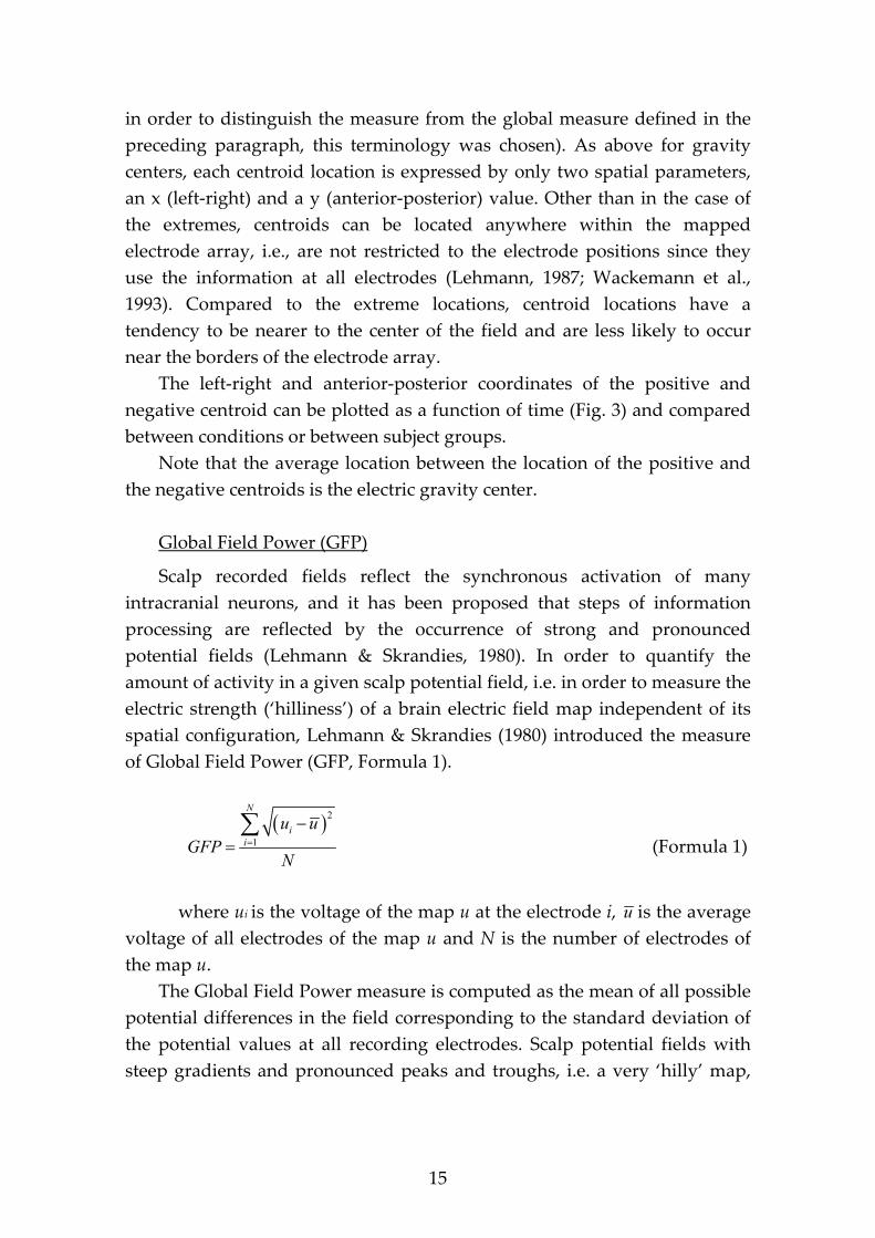
Global Field Power (GFP)

Scalp recorded fields reflect the synchronous activation of many intracranial neurons, and it has been proposed that steps of information processing are reflected by the occurrence of strong and pronounced potential fields (Lehmann & Skrandies, 1980). In order to quantify the amount of activity in a given scalp potential field, i.e. in order to measure the electric strength (‘hilliness’) of a brain electric field map independent of its spatial configuration, Lehmann & Skrandies (1980) introduced the measure of Global Field Power (GFP, Formula 1).

( )2

1

N

i

i

u u

GFPN

=

−=∑

(Formula 1)

where ui is the voltage of the map u at the electrode i, u is the average

voltage of all electrodes of the map u and N is the number of electrodes of the map u.

The Global Field Power measure is computed as the mean of all possible potential differences in the field corresponding to the standard deviation of the potential values at all recording electrodes. Scalp potential fields with steep gradients and pronounced peaks and troughs, i.e. a very ‘hilly’ map,

16

will result in high Global Field Power, while Global Field Power is low in electrical fields with only shallow gradients that have a ‘flat’ appearance.

This reference-free index quantifies the amount of activity in the analysed map and can be computed for each map, resulting in a single value at each time point, and these values can be plotted as a function of time (Fig. 4). Maps at times of maximal Global Field Power imply the optimal signal-to-noise ratios. High Global Field Power is typically associated with stable landscape configuration, while low Global Field Power is associated with changes in the landscape configurations.

Global Map Dissimilarity (GMD)

In order to compare the topographies of two maps independent from their strength and without prior feature extraction, Lehmann & Skrandies (1980) introduced the Global Map Dissimilarity (GMD, Formula 2) descriptor.

2

2 21

1 1

1

( ) ( )

N

i i

N Ni

i i

i i

u u v vGMD

N u u v v

N N

=

= =

− − = − − −

∑∑ ∑

(Formula 2)

where ui is the voltage of map u at the electrode i, vi is the voltage of map

v at the electrode i, u is the average voltage of all electrodes of map u, v is the average voltage of all electrodes of map v and N is the total number of electrodes.

This one-number statement about the global spatial configuration dissimilarity of two maps corresponds to the Global Field Power of the difference map. This letter method implies prior map normalization to unity Global Field Power in order to make it insensitive to differences in overall scaling and to assess landscape difference only.

Note that the Global Map Dissimilarity is 0 when two maps are equal, and that Global Map Dissimilarity maximally reaches 2.0 for the case where the two maps are identical in their topography but with inversed polarity. For the determination of start (end) points of microstates, the time moments of maximal Global Map Dissimilarity are used.

17

1.4.2. Data Reduction in the Time Domain: Temporal Parsing of Map Series into Microstates

Examining brain electric activity as a series of maps of the momentary potential distributions demonstrates that a given map configuration tends to persist for a certain time duration and than changes relatively quickly (in the millisecond time range) into a new configuration that stays stable again for a certain time (Lehmann & Skrandies, 1984; see Fig. 4). The transitions between one map configuration to the next one are not smooth, but tend to occur quickly, ‘stepwise’. The time segments of stable map configurations were suggested to reflect steps of information processing; they were called functional microstates of the brain (Lehmann, 1987; Michel et al., 1992a). The study of the distribution and the time course of the momentary brain electric field topography therefore offers a unique possibility to obtain insights into important features of the brain’s processing of information.

Changes in the spatial distribution of the electric signal, i.e. segment changes, and reflect changes of the functional state. On the other hand, the successive occurrence of microstates does not imply that brain information processing is strictly sequential: the underlying mechanism may be composed of any number of sequential or parallel physiological subprocesses (Lehmann, 1989). Following, it will be assumed that the distribution of active neuronal generators (without taking into account the intensity) characterizes uniquely the functional microstate of the brain (Lehmann, 1987). Due to the nonuniqueness of the electromagnetic inverse problem, it may occur that different source distributions produce exactly the same scalp field. However, changes in the scalp field are undoubtedly due to changes in the distribution of active sources.

The main goal of a time-oriented analysis is to identify onset and offset times of particular field configurations, i.e., to identify time epochs where the potential field distributions is in a quasi-stable state. Which are the parameters or the measurements that we have to take into account to define a ‘quasi-stable’ state, i.e. a microstate? Essentially, there are two main approaches to assign the maps to the different microstates: (a) a ‘sequential approach’ (e.g., Lehmann et al., 1987; Strick & Lehmann, 1993), and (b) a ‘global approach’ (Pascual-Marqui et al., 1995; Koenig et al., 1999).

(a) The Sequential Approach

The sequential approach compares a map with the following map, in a sequential way: Two methods are available in the identification of segments

18

which are defined by field characteristic, the ‘global map dissimilarity’ and the ‘spatial window’. The descriptor of the global map dissimilarity was already discussed in the section 1.4.1.

The second method available in the sequential identification of segments which are defined by field characteristic as ‘quasi-stable’ was proposed by Lehmann & Skrandies (1984). The segmentation was based on the following strategy: Two spatial windows were set up around the location of the extremes or centroids of the first map of the series. At the second time point, it was checked whether one of the descriptor (extremes or centroids) of this second map had left its spatial window. If this is the case, a new segment (a new microstate) was started and a new spatial window was set up. If this is not the case, the second map is considered belonging to the same segment and the next time point is then considered. Obviously in this approach, the size of the spatial window is of crucial importance for the identification of the segments and their length. The larger is the size of the spatial window, the longer will be the identified segment and the contrary. An often used strategy to determine the size of the spatial window is to use as size one or one half electrode distance. Strick & Lehmann (1993) introduced a boot-strap determination for window size, and Koenig & Lehmann (1996) introduced an elegant, ‘know all’ solution for this problem (see Koenig, 1995 and Koenig & Lehmann, 1996 for a detailed presentation of this solution).

(b) The Global Approach: Microstate Clustering Analysis

Different from the sequential approach, the global approach, a modification of the classical k-means clustering (Pascual-Marqui et al., 1995), is not primarily driven by the sequence of the maps. The global approach examines the entire data set at all time points simultaneously and assigns all analysed maps to a limited number of clusters (class mean maps).

The principle of clustering is reviewed in Fig. 5 (modified from Koenig et al., 1999), illustrating the clustering of a sequence of a 10 maps into 2 class mean maps. In a first step, 2 maps (so-called prototype map) are randomly selected between the 10 maps. In a second step, the similarity of the spatial configuration of each prototype map (let say, map A and B) with each of the 10 maps is computed using the squared correlation coefficient to omit the maps’ polarities. If map 1 is more similar to the prototype A compared to the prototype B, than map 1 is assigned to the prototype A. Contrary, if map 1 is more similar to the prototype B compared to the prototype A, than map 1 is assigned to the prototype B. The assignment to prototype A or B is done for

19

all 10 maps. When the assignment is completed, an update of the prototypes configuration is done, by averaging all maps assigned to prototype A and B, separately, disregarding map polarity. This procedure is repeated in a second and later runs until no further changes in the assignment occur. Eventually, the percentage of the variance of the data explained by the 2 class mean maps is determined. Explained variance might change depending on selected starting 2 prototypes. Therefore, to find the solution with the maximal explained variance, the entire procedure is repeated 20 times with newly randomly selected starting prototypes.

The complete procedure described above can be repeated aiming at different number of class mean maps. The optimal number of class mean maps is then determined by the minimum of the cross-validation index which considers both the number of used class mean maps and the percent variance explained by the class mean maps (Pascual-Marqui et al., 1995).

This procedure will be further illustrated in the section 7.2.5. by means of the data collected in the present investigation.

1.5. From the Scalp-Recorded EEG/ERP to the Sources in the Head

One aim of EEG/ERP recording is the identification of the active sources in the central nervous system. The underlying assumption is that information is processed in circumscribed brain areas, and that spontaneous activity patterns originate in specific structures of the brain. Thus, it is of interest to account for the scalp-recorded topography of electric activity in terms of anatomical localization of intracerebral, neuronal generators.

A severe complication for the realization of this aim is the problem of the so-called ‘inverse solution’, i.e. the impossibility to compute the location, orientation and strength of electric sources in a volume based on surface data if there is more than one generator source. Any given scalp distribution of brain electrical activity can be explained by an infinite number of intracranial neural source distributions. Obviously, at any moment in time there is a very large number of generators active in the brain. Thus, the inverse problem, the computation of source locations from surface voltages cannot be solved uniquely for brain electric data. The only way to solve this problem is to constrain the problem. In the following, two different solutions of the inverse solution problem are described.

The basis for the solutions is the fact that the surface electric field generated by one or several known sources in a volume can be calculated correctly. In other words, this so-called ‘forward solution’ is not ambiguous,

20

contrary to the inverse problem for more than one source. A model source dipole generator, the so-called ‘equivalent dipole’ has 6 parameters: 3 for location, 2 for orientation and one for strength.

1.5.1. Single Source Localization of Frequency Bands: The FFT-Dipole-

Approximation

The most simple constraint to the inverse problem of brain electric data is to assume a single dipole model generator source. Consider the case of an observed single momentary scalp field, of spontaneous or event-related brain electric activity. In order to find the putative single source, an iterative procedure is used. One computes the forward solutions, the scalp field distributions for very many single dipole models, using all possible locations and all possible orientations of the model source in the head. All computed scalp field distributions are compared to the actually observed scalp field. The computed field that best fits the observed field identifies the best-fitting single model source. It is worth pointing out that this single, best-fit model source is independent from the recording reference for the observed scalp field, and does not presuppose a scalp-orthogonal orientation of the source while explaining the measured electric field on the scalp.

Lehmann & Michel (1990) proposed a source modeling approach in the frequency domain for EEG multichannel time series, the ‘FFT-Dipole-Approximation’. Using multichannel brain electric field data, this method produces a potential distribution map for each frequency point of the Fourier transformation (FFT) by assuming a single phase angle. For each frequency point of the FFT, the cosine and sine FFT values of all electrodes are entered into a Nyquist diagram. A best fit-phase angle is computed as the first principal component of the data entries. All entries are projected onto this first principal component, and read out as a map. This map then is subjected to a conventional 3-dimensional model dipole source computation as described above. It is important that the location of one or several equivalent dipole generator models is not necessarily the location of the active neural elements. The computed model locations represents the location of the point of gravity of all neural activity.

Note that the location of the positive and negative extremes and the locations of the centroids of the positive and negative potential areas can be considered as projections of the positive and negative poles of an intracerebral single model dipole onto the scalp; seen from the scalp, the

21

single equivalent dipole model solution is located between the locations of the positive and negative potential area centroids.

1.5.2. Low Resolution Electromagnetic Tomography (LORETA): EEG/ERP

Functional Imaging

Information is processed in parallel distributed networks and long-range cooperation between different structures constitutes a basic feature of mechanisms of brain information processing (Singer, 1999). Due to this fact, neuronal activation is distributed over large areas of the central nervous system and its extension is unknown. Thus, Skrandies (2002, p. 14) warns that ‘the approach of single dipole solutions or the fit of a small number of dipoles to the data appears to be not appropriate when unknown source distributions shall be detected’. More realistic views of underlying mechanisms are approximated with methods that aim at the estimation of the most likely intracranial sources that may be distributed through an extended three-dimensional volume.

The first attempt in this direction was the ‘minimum norm solution’ by Hämäläinen & Ilmoniemi (1984). The disadvantage of this solution was that it would always produce activity maxima only at the outer cortex, close to the electrodes, i.e. it misplaces deep sources into shallow depth (Pascual-Marqui, 1999).

Low Resolution Electromagnetic Tomography (LORETA, Pascual-Marqui et al., 1994; Pascual-Marqui et al., 1999) is another method aiming to solve the so-called inverse solution problem and belongs to the family of instantaneous, 3D distributed, discrete, linear inverse methods.

Different from dipole models (see above), the LORETA method makes no assumption about the number of dipoles: LORETA directly computes the current distribution throughout the entire brain volume. But, as discussed above, some constrain is needed to find a solution to the inverse problem. LORETA assumes that the smoothest of all possible activity distributions is most plausible and to aimed at. This means that neighboring volume voxels should have maximally similar generator strength. This assumption is consistent with known electrophysiological data on neuronal activation: neighboring neuronal populations show highly correlated activity (Gray et al., 1989; Llinas, 1988; Silva et al., 1991). This is implemented by requiring that the electric activity at any given voxel must be as close as possible to the average activity of the neighboring voxels. The technical details of LORETA

22

are described in Pascual-Marqui et al. (1994) and Pascual-Marqui et al. (1999).

This computation of the smoothest of all possible three-dimensional current distributions results in a true tomography that, however, has a relatively low spatial resolution. Thus, LORETA solves the inverse problem without a priori-knowledge of the number of sources, but by applying the restriction of maximal smoothness of the solution considering the neighboring voxels. The result is the current density at each voxel as the linear, weighted sum of the scalp electric potentials (Pascual-Marqui, 1995; Pascual-Marqui et al., 1999; Pascual-Marqui et al., 1994). In the implementation of LORETA used in the present study, the relation to brain anatomy is established by using a 3-shell spherical head model matched to the atlas of the human brain (Talairach & Tournoux, 1988), available as a digitized MRI from the Brain Imaging Centre, Montral Neurologic Insititute. Registration between spherical and realistic head geometry uses EEG electrode coordinates reported by Towle et al. (1993), and the solution space is restricted to the grey matter of cortex and hippocampal regions, as determined by the corresponding digitized Probability Atlas available from the Brain Imaging Centre, Montral Neurologic Institute. A total of 2394 cortical voxels are produced by the version of the LORETA program used in the present study. Each voxel represents a cube of 7x7x7 mm. The advantage of using the Talairach head model is that it allows precise neuroanatomical localization in standardized coordinates. (Ideally, it would be best to use the exact head model for each subject from the individual MRI. In this case, the final step would be to cross-register the individual anatomy to the standard Talairach atlas.)

The LORETA images represent the electrical activity at each voxel as squared magnitude (i.e. power) of the computed current density.

LORETA is one of many proposed solutions for the ‘inverse problem’. Compared with other published EEG/MEG instantaneous, 3D, discrete, linear inverse solutions, for LORETA the advantage of correctly localizing deep sources has been claimed (Pascual-Marqui et al., 1994) whereas the other methods (e.g., minimum norm, weighted minimum norm, and weighted resolution optimization) allegedly find the solutions biased towards the EEG/MEG sensors. There are several studies validating LORETA, based on, e.g., correct localization of the auditory cortex (Anderer et al., 1998a; b), the visual cortex (Steger et al., 2001), epileptic foce related to MRI lesions (Worrell et al., 2000).

23

1.6. Other Brain Imaging Methods

In the last two decades, other brain imaging methods were developed and used to produce functional images of the brain. In this paragraph, a brief overview of these methods is given.

1.6.1. PET and SPECT

Cerebral blood flow (CBF) and metabolism are normally closely linked (Logothetis, 2002); hence, assessment of CBF may provide an indirect measure of neuronal activity.

In SPECT (single photon emission computed tomography), a radioactive tracer is applied that specifically interacts with brain tissue. Technetium-99m hexamethyl propyleneamine oxime (99Tc-HMPAO), which is taken up by tissue and then trapped, is commonly used. Radiation is detected by rotating gamma cameras, and, by a process of backprojection and tomographic reconstruction, an image of blood flow is obtained.

The idea of the functioning of PET (positron emission tomography) is simple. A fast-decaying radioactive tracer is injected into the bloodstream and then the brain is scanned while the person is immobilized. PET depends on the emission of positrons, the positively charged electrons released by certain isotopes upon their decay. In tissue, the positron unites with an electron, and the two particles convert their mass into radiation energy. It is this quick anti-particle annihilation that produces the gamma rays picked up by the system’s head-encircling detector ring. The gamma rays come in pairs which fly off in exactly opposite directions. By catching both, the scanner’s computers can draw a line running straight back through the original positron event in the brain. After a few million such readings, the scanner has an accurate, three-dimensional image of any metabolic hot spots in the brain. Several different positron emitters are available, but most work is done with oxygen-15, carbon-11, and fluorine-18.

With both SPECT and PET, it is possible to label ligands (ion or a neutral molecule which binds to a receptor to form a complex) for a variety of drugs and neuroreceptors, for example, the D2 receptor, the benzodiazepine receptor, and opiate receptors.

1.6.2. fMRI

The principle of fMRI (functional magnetic resonance imaging) is the examination of the physicochemical environment of the brain’s protons.

24

An object (proton) with a charge and velocity provokes a magnetic field adjacent to it. Because protons spin around their axis at random, the sum total of magnetization in an area of the brain is zero. On application of an external magnetic field, the particles and their charges align, just like the compass needle of a small compass in the earth’s magnetic field. In this artificially ordered state, the particles can then be probed by firing a tuned pulse of radio energy at them. Different kinds of atom resonate at different frequencies, so it is possible to measure with accuracy the concentration of various elements like iron, oxygen, of hydrogen. By taking these readings from many angles, just as with PET, a computer can be used to turn the information into a three-dimensional reconstruction.

1.6.3. MEG

A MEG (magnetoencephalogram) system is much like EEG in that it measures the magnet field activity of the brain. As was reviewed above, differences of scalp-recorded electric fields are due to postsynaptic potentials occurring on the cortical pyramidal neurons in the brain. These processes are caused by ionic current flows that also produce magnetic fields. These magnetic fields are extraordinarily weak, i.e. approximately 109 times weaker than the background magnetism produced by the earth. MEG has its own drawbacks that have hampered its introduction until the end of the 1960s (Cohen, 1968; 1970). It requires the use of SQUIDS (super-conducting quantum interference devices) as sensors. These electronic circuits use quantum effects to pick up the brain’s magnetic fields, but they only work when they are cooled to almost absolute zero in a bath of liquid helium. Finding ways of having something that cold almost touching a subject’s head is a challenge in itself.

Due to the common neuronal generators for EEG and MEG, both techniques provide information on the same brain processes. From a physics-theoretic point of view, it was initially thought that MEG had higher spatial resolution than EEG, because magnetic fields have the advantage that they pass through the tissues of the head without distortion. This was proven false in a study that objectively compared the spatial resolution of both methods (Pascual-Marqui & Biscay-Lirio, 1993), showing that MEG offers no advantages over EEG in terms of information on brain processes.

25

1.6.4. EEG and Other Brain Imaging Methods in Comparison

In this paragraph we first list the advantages and the limitations of the EEG/ERP. Secondly, we aim to compare the other brain imaging techniques described briefly above with EEG/ERP, starting with the advantages and ending by the drawbacks. Time resolution, space resolution as well as the invasiveness of the brain imaging methods described in this paragraph are summarized in the Fig. 6.

1.6.4.1. Advantaged and Limitation of EEG/ERP

The scalp recorded EEG/ERP technique is completely non-invasive, is low-cost, offers an extremely high sensitivity to changes in the internal (central nervous system) state, and has virtually unlimited time resolution (Ozaki & Lehmann, 2000).

The limitations of the EEG/ERP technique are: First, there is insufficient information in the EEG (recorded from the scalp) for a unique determination of the three-dimensional source distribution. This is the so-called ‘inverse solution problem’ (see section 1.5.). An approximate solution for the three-dimensional distribution modeling is the LORETA method (see section 1.5.2.), but still with a low spatial resolution.

The second disadvantage is the fact that the high sensitivity to all information arriving in the brain requires a careful experimental design that excludes as much as possible sensory input and internal states that are not part of the design. The high sensitivity leads also to the co-registration of non-cerebral electrical currents from the body or of the surround that are obviously not of interest in brain studies. These unwanted co-registrations are called artifacts. There are two categories of artifacts: internal and external. The internal artifacts are, for example, muscle movements, eyes movements, eyes blinks, or heart beat. The external artifacts are electrical sources, such as all electrical equipment used for the recording and for other purposes (e.g., elevators, paging systems). There are of course several strategies to avoid or at least to reduce artifacts. There are also ways to eliminate certain artifacts, e.g. eye movements, but EEG epochs that are still contamined with non-cerebral artifacts despite all efforts should be excluded from further analysis.

Another general limitation is that a large, but unknown amount of brain neural activity cannot be measured from the scalp. Some neuronal populations might not have sufficient synchronous activation to generate a measurable signal. Other neuronal populations, e.g. in thalamic nuclei,

26

presumably generate a closed electric field because of their non-parallel orientation; these neurons are arranged in such a way that it is likely that they cannot produce a measurable electrical signal on the scalp. It might therefore well be that several important neural processes cannot be detected using this technique.

1.6.4.2. EEG/ERP vs. MEG, PET, SPECT, and fMRI

MEG compared with EEG/ERP data are easier to measure in one respect: no electrodes need to be placed on the subject’s head. On the other hand, there is the restriction that the subject’s head has to be completely immobilized. This is problematic if one has to work with non-cooperative patients. The cost of the device is around 10 times higher than for EEG, and maintenance is very expensive. A third problematic aspect of the MEG technique is that neural generators that are oriented parallel to the scalp surface are very difficult to measure.

PET and SPECT are invasive techniques, since the tracers used to mark the CBF are radioactive. Another disadvantage compared with EEG/ERP is the relatively low time resolution, in the range of many seconds for PET and in the range of minutes for SPECT. On the other hand, the space resolution of these two techniques compared with the EEG/ERP is relatively high, 3-5 mm resolution for PET and 6-10 mm for SPECT. Both techniques are very expensive.

MRI machines are expensive. The space resolution is the highest available in brain imaging methods, at about 2 mm, but the time resolution of fMRI compared with EEG/ERP is again very low, with conventional strategies in the range of seconds; recent special, selective methods can reach a resolution of 150 msec.

In sum, the brain reacts with very high sensitivity to changes in the external and internal environment. Therefore, relevant brain processes for information processing must occur in a very short time range, in fractions of seconds. Scalp recorded brain electric activity appears to be a most appropriate and useful tool for studying human brain processes of perceptual and cognitive functions.

27

2. BELIEF IN THE PARANORMAL

Paranormal belief literally means ‘belief besides normal’ and is traditionally defined as belief in phenomena, which, if true, violate basic limiting principles of science (Broad, 1953). Irwin (1999) described parapsychology as the ‘scientific study of experiences which, if they are as they seem to be, are in principle outside the realm of human capabilities as presently conceived by conventional scientists. Thus parapsychological phenomena ostensibly indicate the operation of factors unknown to or unrecognized by orthodox science, popularly referred to as paranormal factors.’ (Irwin, 1999, p. 1). The paranormal phenomena include a range of phenomena such as ‘superstitious beliefs’ (e.g., black cats and breaking mirrors cause bad luck), ‘precognition’ (i.e., the apparent foreknowledge of as yet undetermined future events), ‘clairvoyance’ (i.e., the paranormal acquisition of any information directly from a physical source), ‘telepathy’ (i.e., the apparent ability to communicate information from one mind to another), ‘telekinesis’ (i.e., the apparent ability to influence the environment seemingly by intention or other mental activity alone), ‘communication with the dead’, ‘out-of-body experiences’, and a host of other such phenomena.

In our opinion, if we accept the definition of Broad (1953) a very interesting question arises: what about religiosity and the often related belief in the ‘supernatural’, i.e. belief in supernatural agents such as angels or demons, the present-day occurrence of miracles, the causal power of prayer? Should one make a distinction between the belief in the supernatural and the belief in paranormal phenomena?

Factor analytic studies (Grimmer & White, 1990; Haraldsson & Houtkooper, 1996; Johnston et al., 1995) have shown that one should differentiate between these two categories of beliefs; in fact these studies have indicated that certain individuals do make distinctions between supernatural phenomena and paranormal phenomena like ESP (extra-sensory perception, for instance clairvoyance), telekinesis, precognition, and so forth. The reason why people make such discriminations appears to depend on whether they have preexisting religious beliefs (Clarke, 1995). Prior beliefs may influence which phenomena are accepted as credible occurrences and which are treated with skepticism. Indeed, Christians may express disbelief about ESP or telekinesis but belief in guardian angels or miracles. Beck & Miller (2001) referred to this bias as ‘metaphysical chauvinism’, whereby one rejects certain quasi-empirical claims if they are

28

not consistent with one’s metaphysical assumptions, despite simultaneously holding beliefs that are equally unverifiable from an empirical point of view. Beck & Miller (2001) also contended that metaphysical chauvinism is shaped not only by prior religious belief but also by the life experiences of the individual.

For the present study we used the Mischo questionnaire (see APPENDIX 1, Mischo et al., 1993) for the pre-selection of our subjects. The 6 items included in the Mischo questionnaire asked about telepathy (e.g. ‘I had at least one telepathic experience with another person’), clairvoyance (‘I never had ay extrasensory perceptions’), and precognition (e.g. ‘I had at least one presentiment that came true and that I thought was not due to chance’). If we accept the distinction between belief in the supernatural and belief in the paranormal described above, then our ‘believers’, i.e. subjects scoring high on the Mischo questionnaire, believed in the existence of paranormal phenomena. Since we did not ask about supernatural belief, we cannot assume that (1) our ‘believers’ also believe in supernatural phenomena, and that (2) our ‘skeptics’, i.e. subjects scoring low on the Mischo questionnaire or, in other words, subjects who strongly disbelief in paranormal phenomena, do not believe in supernatural phenomena.

In sum, in this study we focused on the belief/skepticism in telepathy, clairvoyance and precognition. This is an argument to keep in mind when reading the many results found in the literature, because the populations investigated in other reports sometimes differ very much from the population investigated in the present study.

2.1. Paranormal Belief and ‘Magical Ideation’

Paranormal belief is closely linked to the ‘Magical Ideation’, which has been defined as ‘belief in forms of causation that by conventional standards are invalid’ (Eckblad & Chapman, 1983). As long as we agree on what the ‘conventional standards’ are, it is easy to provide examples of ‘Magical Ideation’. Most of us would probably not hesitate to consider dancing for rain to be based on invalid assumptions about causality. An especially notorious lack of agreement on the conventional standards of the laws of causation is found in the area of paranormal belief.

Brugger & Graves (1997) provided an extensive overview of findings from their own and independent studies showing that the link between ‘Magical Ideation’ and paranormal belief has been suggested by neuropsychological experiments. Measures of ‘Magical Ideation’ are found

29

to correlate positively with global paranormal belief and with belief in precognition, superstition, extraordinary life forms, and also in traditional religious concepts (Thalbourne, 1985; 1994; Thalbourne et al., 1995; Thalbourne & French, 1995; Tobacyk & Wilkinson, 1990; Williams & Irwin, 1991). The ‘Magical Ideation Scale’ by Eckblad & Chapman (1983), which is one of the scales administered in the present study, was previously shown to be significantly correlated with the Mischo questionnaire (Pizzagalli et al., 2001; Pizzagalli et al., 2000).

2.2. The ‘Magical Ideation Scale’ by Eckblad & Chapman

The ‘Magical Ideation’ scale is a 30-item true-false scale assessing the presence of hallucination-like experiences and delusion-like, paranormal beliefs. The complete scale is shown in APPENDIX 2. This scale was developed and evaluated during a 10 year longitudinal study initiated by the Chapman group. These authors aimed at producing DSM-based scales of current deviant functioning to identify young adults who may be psychosis-prone. After reassessing the original population (only 5% of subjects dropped out), the authors found that the originally high scorers on the ‘Magical Ideation’ scale, especially those who reported psychotic-like experiences of at least moderate deviance, exceeded control subjects on the later outbreak of psychosis, the number of psychotic relatives, and the severity of overall schizotypal symptoms (Kwapil et al., 1999).

2.3 ‘Magical Ideation’ and Schizotypy

Eckblad & Chapman (1983) considered ‘Magical Ideation’ as the best-documented indicator of positive symptoms of schizotypy. Lenzenweger (1994) showed that the ‘Magical Ideation Scale’ has good reliability and validity in assessing ‘schizotypy’ or psychosis-proneness in the normal population. Note that individuals identified as psychosis-prone will not necessarily decompensate in clinical psychosis, but show higher vulnerability for this. In the ‘Diagnostic and Statistical Manual of Mental Disorders’ (APA, 1994) ‘Magical Ideation’ is described as a key feature in schizotypal personality disorder and also in schizophrenia.

There are models which define ‘psychosis’ as a series of symptoms that are aligned along a continuum (Eysenck, 1952; Meehl, 1962). According to this idea, psychotic characteristics should no longer be the prerogative of the classically diagnosable psychotic patient, but form, instead, part of the array of psychological and biological features that characterize individual

30

variations between human beings. In the model of Meehl (1962) schizotypy represents the personality organization of a schizotaxic person. Meehl wrote: ‘If the interpersonal regime is favourable, and the schizotaxic person also has the good fortune to inherit a low anxiety readiness, physical vigor, general resistance to stress and the like, he will remain a well-compensated ‘normal’ schizotype, never manifesting symptoms of mental disease…Only a subset of schizotypic personalities decompensate into clinical schizophrenia’. (p. 830). Several studies showed the validity of Meehl’s model; in fact, they demonstrated that positive schizophrenic symptomatology (e.g. delusion- and hallucination-like phenomena) are present in non-psychotic subjects in the absence of manifest illness (Claridge & Broks, 1984; Thalbourne, 1994; Verdoux et al., 1998).

2.4. Paranormal Belief and Schizotypy

The relation between paranormal beliefs and schizotypal personality traits has been closely examined in recent years. Rust (1992) found atypical schizotypy scores, measured with the Rust Inventory of Schizotypal Cognitions (RISC) among members of occult sects. Relations between schizotypal traits and paranormal-related phenomena such as out-of-body experiences have been demonstrated by McCreery & Claridge (1995). Straube et al. (1998) found a close relation between schizotypal traits measured with the Schizotypal Personality Scale and paranormal beliefs measured with the Mischo questionnaire among adolescents. In another study done by the same group, the authors showed that in a large sample of 374 students anomalous experiences (self-reported paranormal abilities, experiences and beliefs) were closely related to schizotypal traits (Wolfradt et al., 1999).

Thus, the formation and the maintenance of paranormal beliefs appear important for understanding schizotypal ideation.

Studying people differing only in their declared belief in paranormal phenomena while being completely healthy, give us the opportunity to study some cognitive and emotional aspects that these people share with subjects with a diagnosis of schizotypal personality disorder. Moreover, the assumption that schizotypal subjects may have the inherent vulnerability to develop schizophrenia (Eckblad & Chapman, 1983; Kwapil et al., 1999) makes this population attractive to research into the issue of the prodrom of psychosis.

31

In the Experiment I, two are the aspects of paranormal belief that were discussed: paranormal belief and hemisphericity, and paranormal belief and emotionality. Therefore, in the next two sections, an overview of the literature about these two aspects is given.

2.5. Paranormal Belief and Hemisphericity

In neuropsychological studies, paranormal belief has often been reported to be related to a relative overactivation of the right hemisphere. A selection of the growing body of literature is reviewed here.

Leonhard & Brugger (1998) studied 40 right-handed men with a lateralized tachistoscopic lexical decision task. Subjects also completed the ‘Magical Ideation Scale’. The authors found that although the 20 subjects with Magical Ideation scores below the median displayed the expected right visual field/left hemisphere superiority in lexical decision accuracy, the 20 high scorers were equally proficient in both visual fields. Compared to the low scorers, they made significantly more correct decisions in the left visual field/right hemisphere. The results showed a reduced left hemisphere language dominance for believers in paranormal and the authors proposed that this dominance failure facilitates the emergence of paranormal ideas by way of right hemisphere associative processing characteristics, that is, coarse rather than focused semantic activation.

Pizzagalli et al. (2001) administered a lateralized semantic priming task to healthy subjects who were either strong believers or strong skeptics in paranormal phenomena. This paper reported stronger indirect (but not direct) semantic priming in believers than skeptics, an effect which was confined to the left visual field/right hemisphere stimulations. The authors interpreted their findings as (1) evidence for a specialization of the right hemisphere for the appreciation of specifically remote associations, and (2) as evidence for a relative overactivation of the right hemisphere for the believers.

Mohr et al. (2001b) studied 40 right-handed subjects (20 women and 20 men) in an olfactory detection experiment. Subjects were given the ‘Magical Ideation Scale’. The results illustrated that over both nostrils, subjects with high Magical Ideation scores showed elevated olfactory detection thresholds that subjects with low Magical Ideation scores. Moreover, in men but not in women, left-nostril acuity was inversely correlated to MI raw scores. The olfactory system, from the receptor in the nasal epithelium to cerebral olfactory regions, is mainly ipsilaterally connected. Therefore, the authors

32

suggested that the selective impairment of left-nostril performance is related to left functional abnormalities in believers in the paranormal. Interestingly, the reported olfactory detection impairments on the left side were also found in another study testing unmedicated patients with schizophrenia (Purdon & Flor-Henry, 2000).

Taylor et al. (2002) aimed to study right hemispatial inattention in believers and skeptics with an implicit line bisection task. They administered the ‘Magical Ideation Scale’, to 40 right-handed men who had copied and later recalled the Rey-Osterrieth complex figure. Implicit line bisection performances were defined as the bisecting lines of the complex figure’s large rectangle and were recorded for the copy and delay conditions. The results showed that Magical Ideation scores were significantly correlated with a leftward shift in bisections in the delay but not in the copy condition, indicating a significant relationship between the degree of right hemispatial inattention (i.e., a processing advantage of the right and disadvantage of the left hemisphere) and belief in the paranormal.

In a response commonality analysis of verbal fluency test, Duchêne et al. (1998) found that people with high scores on Magical Ideation scale generated more rare words than those with low scores. Since disinhibite semantic network activation in the right hemisphere may be responsible for the production of more rare than common associations, the authors interpreted their findings as an enhanced right hemispheric function in the group of the believers.

In a previous study done in our laboratory (Gianotti et al., 2001), believers and skeptics in paranormal phenomena were asked to produce single-word associations to preselected semantically related or unrelated word pairs. Response commonalities and association latencies for each association was calculated. The results showed that believers as compared to skeptics produced more rare associations, i.e. associations produced by only few subjects of the sample. Whereas idiosyncratic and common associations were comparably frequent within both groups of subjects. These findings indicate that believers have a facilitated capacity to see a relationship between words, and thus produce associations that are neither common nor absolutely unique. The authors interpreted the findings as due to enhanced right hemispheric contributions.

In another study of semantic association, Mohr et al. (2001a) investigated whether high Magical Ideation scorers would also perceive remote associations produced by independent subjects as being more closely related

33

than low Magical Ideation scorers. Two experiments were set up: In the first experiment, word pairs were constructed from a conventional categorical fluency task. The task was to judge the semantic distance between the two words. In the second experiment, the associations to word pairs from the study described above (Gianotti et al., 2001) were presented. Subjects had to judge the semantic distance of the association to the word pair. The results of both experiments showed that higher Magical Ideation scorers considered unrelated words as more closely associated than did lower Magical Ideation scorers. These findings indicate that for loosely associated word, high Magical Ideation scorers have a facilitated capacity to see a relationship between words that have been produced by independent subjects. Therefore, the authors suggested that an enhanced right hemispheric functions may not only be relevant for the production of remote associations (see study above by Gianotti et al., 2001) but also for the perception of remote association.

In a EEG study, Pizzagalli et al. (2000) investigated subjects who were either strong believers or strong skeptics in paranormal phenomena during resting EEG. The EEG data were subjected to the FFT-Dipole-Approximation (see section 1.5.1. for a description of the method) and the results showed that the source of the beta2 frequency band was more right located for subjects who strong belief in paranormal phenomena. The authors interpreted their findings as evidence for a relative overactivation of the right hemisphere for the believers.

2.6. Paranormal Belief and Affectivity

Affective aspects of belief in the paranormal were controversially discussed in the literature. Two major lines of discussion can be identified: (1) On the one hand there are authors describing believers in the paranormal being more positive in their affect compared with skeptics and (2) on the other hand there are studies showing the opposite, i.e. that believers are more negative in their affect.

(1) The first line of discussion links belief in the paranormal with positive affect and/or hedonic components. Brugger (1995) showed a significant negative correlation in 40 students between the belief in the paranormal, measured with the ‘Australian Shep-Goat Scale’ by Thalbourne & Delin (1993), and anhedonic personality traits, measured with the scales for physical and social anhedonia by Chapman et al. (1976). He interpreted the results as a hyperactivation of medial temporal lobe structures. Jaanus

34

(1990) described this negative correlation in a more general form, i.e. in regard to belief in general: ‘Disbelief is inherently allied to negation, unpleasure, and unreality just as belief is to affirmation, joy, and reality’. In 1988, Taylor & Brown (1988) published an article that challenged the notion that accurate perceptions of self and the world are essential for mental health. They argued instead that people’s perceptions in these domains are positively biased and that these positive illusions, especially the illusion to effect change in the environment and the future (a particularity of the paranormal belief), involve an enhanced ‘joie de vivre’ and promote psychological well-being. This model of mental health was further supported by empirical studies, summarized in another paper by Taylor & Brown (1994). Blackmore (1992) characterized the tenacious skeptic as somebody who needs lots of evidence before seeing or experiencing anything. Because of this enhanced ‘critical’ threshold, the skeptic on the one hand does not believe and on the other hand misses a lot of fun. Windholz & Diamant (1974) found that believers in ‚extraordinary phenomena’ scored higher, among other things, on the Hypomania scale of the MMPI.

(2) A different point of view links belief in the paranormal with negative affect and/or anhedonic components. The greatest number of experiments that investigated the relationship between negative affect and reported level of paranormal belief comes from Dudley’s group (Dudley, 1999; 2000; Dudley & Whisnand, 2000). In a first experiment, published in 1999, these authors followed the idea that belief in the paranormal may increase during periods of uncertainty, ambiguity or uncontrollability, resulting in negative emotions (Dudley, 1999). They tested the hypothesis that the level of superstitious belief, i.e. a typical phenomenon in paranormal belief, increases following exposure to uncontrollable situations. To accomplish this, 116 students were tested for their level of superstitious belief before and after attempting to solve an unsolvable problem. Participants were given a word puzzle to complete. The word puzzle consisted of 20 names of foreign countries and cities. Two list of word puzzle were constructed: a solvable and an unsolvable one. A random half of the participants received the solvable and the other half received the unsolvable puzzles. The results showed that the participant’s reported level of superstitious belief increased after exposure to the unsolvable problem, but decreased after exposure to the unsolvable problem. Thus, they showed that negative emotions, resulting when failure occurs, may induce the increase of superstitious beliefs. Already Keinan (1994) came to similar conclusions; he found that

35

during the Gulf War, residents living in high-stress areas, i.e. those more likely to be hit by a missile, reported higher levels of magical thinking than residents living in low-stress areas. In an even earlier study Malinowski (1954) described that Trobriand islanders’ superstitious ideas about success in fishing developed exclusively in waters with a very high uncertainty of success, which is in line with the idea that negative emotions enhance the belief in the paranormal.

Dudley tested in another experiment negative affect, measured with the negative scale of the PANAS questionnaire, and paranormal belief, measured with the revised Paranormal Belief Scale (PBS, (Tobacyk, 1988), depending on the questionnaire’s paper colour (Dudley, 2000). Both questionnaires were printed on paper that was either white, blue, or red. It was expected that blue would elicit negative emotions, red would elicit positive emotions, and white would be neutral. The participants that completed the two questionnaires printed on blue paper reported a significant higher level of negative affect and of paranormal belief compared with the participants that completed the questionnaires printed in either red or white. From the results of this experiment, Dudley concluded that negative affect influenced the level of paranormal belief. In a next experiment Dudley (2000), he focused on the question whether the opposite relationship also exists, i.e. does the priming of paranormal beliefs influence the affect? Three questionnaires were used for this study: PANAS, PBS, and Rotter’s locus of control scale (LOCS). A random third of the 90 participants completed the PANAS immediately following completion of the PBS; another third completed the PANAS immediately following completion of LOCS, and the final third of the participants completed only the PANAS. The results showed that the group that received the PBS prior to the PANAS, but not the groups that either received the LOCS or that received nothing prior to the PANAS, showed a higher negative affect score. These results indicated that exposure to the PBS may have induced negative emotions.

In a further experiment, Dudley & Whisnand (2000) tested the hypothesis of a positive relationship between paranormal belief and a depressive attributional style. They administered the PBS and the Attributional Style Questionnaire by Peterson et al. (1982) to 52 undergraduate students and they found a statistically weak correlation between paranormal belief and depressive attributional style. This last finding is also consistent with the general relationship between paranormal

36

belief and negative emotional states proposed by Dudley and colleagues. The authors discussed the proposed relationship in two ways: One possible explanation may have to do with a lack of critical thinking and information processing ability that occurs when in a negative emotional state. For example, studies have shown that during periods of high anxiety, working memory capacity is restricted (Darke, 1988; MacLeod & Donnellan, 1993). Dudley and colleagues concluded that this restriction may then impair cognitive ability, such as the critical evaluation of paranormal phenomena. However, this explanation does not adequately explain why negative affect would increase following exposure to the PBS. Another explanation of the link between negative affect and paranormal belief may be mood-congruent memory. According to mood-congruency, emotional states act as retrieval cues that evoke memories of events involving the same emotion (Willner & Neiva, 1986). Mood-congruency is a mechanism that may allow paranormal beliefs to be invoked in uncertain situations. Once these beliefs are recalled, they might then be used to rationalize failure, lowering the chances of the development of learned helplessness, depression, or other byproducts of negative emotional states. Dudley argued that in this way certain paranormal beliefs may serve an adaptive function.

In a previous study done in our laboratory, Pizzagalli et al. (2000) studied believers (n=19) and skeptics (n=18) preselected with the Mischo questionnaire (Mischo et al., 1993) for differences in the resting EEG and in their declared affectivity, using the trait form of the Positive and Negative Affect Scale (PANAS, Watson et al., 1988). The authors found that believers scored significantly higher on the negative affect scale compared to skeptics, i.e. believers showed more general negative affect than skeptics.

In a recent study, Beck & Miller (2001) tested 94 students for the effects of religiosity and negative affect on belief in the paranormal and supernatural. They found a significant positive correlation between experiences of negative affect over the preceding year and belief in the paranormal. Using a regression analysis they also found that negative affect during the preceding year predicted greater belief in the paranormal. According to their model, the authors interpreted the findings as follows: if a person is relatively content, happy, and free from negative affect, then he or she may feel little internal impetus to modify his or her current stance (skepticism or belief). Contrary, if negative affects increases over time, than the person may increase his or her belief in the paranormal. However, in our opinion, the study presents two major limitations: the authors should

37

examine the beliefs over time and in response not only to negative but also to positive life events.

2.7. Concluding Remarks

While the results of the many neuropsychological studies and the sole EEG study about ‘Paranormal Belief and Hemisphericity’ are in agreement, the results of the studies dealing with ‘Paranormal Belief and Affectivity’ are not.

There appear to be several, independent reasons for these latter divergent results: First, the samples investigated in many studies reviewed above are very different, since the inventories used to define the concept of ‘belief in the paranormal’ were dissimilar. Some measures devised by parapsychologists are purely sheep-goat scales, that is, they index no more than belief in extra-sensory perception (Thalbourne & Delin, 1993). Other instruments tap a greater range of parapsychological claims; for example, the Mischo questionnaire (Mischo et al., 1993) addresses belief in telepathy, precognition and clairvoyance. Beck & Miller (2001) recently mentioned this point and complained about the fact that researchers have frequently used the terms ‘paranormal’ and ‘supernatural’ interchangeably in the empirical literature. Roe & Morgan (2002) designed a study to assess whether the relationship between narcissistic personality and paranormal belief identified by Tobacyk & Mitchell (1987) earlier could be replicated with a general population and to see whether the effect could be found with a narrower definition of paranormal beliefs that focuses only on belief in psychic phenomena. 75 participants completed the Narcissistic Personality Inventory and two measures of paranormal belief, the Paranormal Belief Scale and the Australian Sheep-Goat Scale. There was no correlation between narcissism and Paranormal Belief Scale scores, but narcissism and Australian Sheep-Goat Scale scores were significantly positively correlated. Of the three subscales to the Australian Sheep-Goat measure, scores for narcissism correlated with belief in ESP and ‘telekinesis’ but not in ‘Life after death’. Thus, it seems that the concept of ‘belief in the paranormal’ contains many sub-concepts, which are not necessarily closely related with each other and which are not correlated in the same manner with other variables, for example with the positive or negative affect.

Because of this variation in the assessment of paranormal belief, caution should be exercised in accepting at face value any findings on the nature of such belief; that is, it is advisable to ask if ‘paranormal’ is being used by the

38

researcher in a limited parapsychological sense or instead is intended to signify a much broader domain of attitudes. The majority of empirical data in fact do relate to paranormal belief in its broadest sense. Thus, one should use a narrower definition of the concept ‘belief in the paranormal’ to target the studied aspects more exactly.

Irwin (1999) complained also about the fact that the discussion of the topic of paranormal belief tends to be in terms of ‘believers’ and ‘skeptics’. However, on the basis of a cluster analysis Irwin (1997) had identified a four-category typology; the respective subgroups of which may be described as traditional religious believers, New Agers, tentative believers, and skeptics.

Another reason for the diverging results described above may be the heterogeneity of the measured variable. Brugger (1995) examined the anhedonic personality traits, measured with the scales for physical and social anhedonia by Chapman et al. (1976). Taylor & Brown (1988, 1994) mentioned a ‘joie de vivre’ variable. Blackmore (1992) characterized the tenacious skeptics as somebody who misses a lot of fun. Windholz & Diamant (1974) used the Hypomania scale of the MMPI. Beck & Miller (2001) focused at negative affect (NA scale) during the year preceding the investigation. Pizzagalli et al. (2000) studied the subjects in their declared affectivity, using the trait form of the Positive and Negative Affect Scale (PANAS, Watson et al., 1988). The state form of the PANAS was used by Dudley (2000); Dudley and colleagues also measured the depressive attributional style (Dudley & Whisnand, 2000) and studied negative emotions in an indirect way, i.e. exposing subjects to unsolvable problems (Dudley, 1999).

For this review on belief in the paranormal and affectivity, we decided to use two broad categories, i.e. positive and negative affect, and we attempted to review the pertinent literature according to this classification. However, creating such a dichotomy, useful for an overview, in a certain perspective one necessarily has to sacrifice some factors that contain important informations as seen from other views.

39

3. LANGUAGE PROCESSING IN NEUROSCIENCE

In the second half of the 19th century, Broca (1861) and Wernicke (1874)

described two different lesions of the brain that produce different types of aphasia, i.e. the partial loss of language abilities. Since these early findings, many further patients have been described with circumscribed impairments of selective language abilities while other abilities were relatively spared. These dissociations have contributed considerably to today’s knowledge about the dimensions along which human language might be organized. It seems that three important dimensions of the brain’s lexical organization are (1) semantics, i.e. word meaning, (2) syntax (or grammar), i.e. sentence structure, and (3) phonology. Semantic categories can be of the type ‘abstract vs. concrete words’, ‘living things and food vs. inanimate objects’, ‘animals’, ‘countries’, ‘fruits’, ‘vegetables’, ‘positive vs. negative words’, and others. Grammatical categories can be of the type ‘nouns vs. verbs’, ‘content vs. function words’ and others. Phonological categories can be of the type ‘rhymed vs. non-rhymed words’. We have to note that this third dimension plays an important role in the processing of written language and not only in acoustic language processing.

Since the aim of the present study was to investigate the processing of emotionally loaded words, that were presented visually, we will concentrate on the literature dealing especially with the semantic dimension of language processing. Nevertheless, because of the interrelations of the issue a brief overview of the literature about the grammar and the phonologic dimensions will also be given.

Research on human language and word processing branched into two directions. One of these branches focused on neuroanatomy, namely, which areas of the brain are involved when language is perceived or produced. In recent years, more and more neuropsychological studies have been devoted to the investigation of networks of cortical mechanisms necessary for word processing, and psychophysiological studies have been investigating the brain areas that ‘light up’ when words are being produced or comprehended. The other branch focuses more on temporal properties of human language processing. These studies include both psychological and electrophysiological experiments. In psychological experiments, models of language processing are brought into relations with behavioral data such as reaction times or subjective reports when the subject could not unambiguously identify a presented stimulus. In electrophysiological

40

experiments, the momentary electrical state of the brain as a function of time is recorded while the subject is involved in language tasks and conclusions are drawn in terms of language-related sequential steps of information processing.

This second branch, the temporal characteristics of perceiving emotionally loaded words, is the core of the present investigation. This is why we will concentrate more on the literature concerned with the temporal properties of word processing rather than the literature concerned with the neuroanatomical correlates of word processing.

3.1. Localizing Language in the Brain

Traditionally, the issue of the neuroanatomy is analyzed from three different perspectives, (1) the localizationist’s, (2) the holistic’s and (3) the Hebbian’s perspective. (1) Localizationists would assume that small cortical areas are fully capable of performing complex cognitive operations. A localizationist would, for example, propose that an area of a few square centimeters of cortical surface is the locus of word comprehension (Wernicke, 1874) or the locus of word production (Broca, 1861). According to this view, the psychological process (word comprehension, or production) is restricted to one area, that is, no other areas are assumed to contribute to this specific process. Only during pathological conditions or during development may there be a shift of the process to another equally narrow area (Luria, 1973). (2) In contrast, a holistic approach would imply that the entire cortex exhibits equipotentiality with regard to all cognitive operations and that all cortical areas can contribute to sufficiently complex processes, such as those involved in language (for an overview, see Deacon, 1989). (3) The Hebbian model (Hebb, 1949) is in sharp contrast to both of these views. Cell assemblies with defined cortical topographies are assumed to form the neurobiological representations of cognitive elements such as words. This position is radically different from a localizationist approach, because it assumes that neurons in different cortical areas may be part of the same distributed functional networks. The Hebbian point of view is also different form the holistic’s view (that ‘everything is equally distributed’), because it implies that the representation of, for example, a word may involve cortical areas entirely different from those contributing to the representation of, say, an odor. Accordingly, the representation of a word would not be restricted to a small cortical locus, but would be distributed over well-defined areas, for example over Broca’s, Wernicke’s, and some other areas.

41

In our opinion, this third point of view seems to be the more appropriate when complex cognitive processes, like language processing, are discussed and analyzed. The often cited clinical case of Pineas Gage (described for instance in Damasio, 1999), would speak against a holistic approach. In fact, despite a very bad brain injury, the patient was still able to speak normally. Against a strict localizationist approach speaks the fact that high cognitive brain processes rely on many different processing activities that presumably run in parallel, so that it appears very improbable to assume that a circumscribed part of the brain is responsible for all processes.

3.1.1. Human Lesion Studies

As already briefly mentioned above, in 1861 Broca discovered that lesions in the posterior region of the frontal lobe of the left hemisphere produce a type of aphasia which today is called Broca aphasia or motor aphasia. It is best characterized by major word finding difficulties and disturbed syntactic structure of spontaneous speech, whereas understanding remains relatively unimpaired. Wernicke described in 1874 a different type of aphasia. His patients presented an overshooting language production often lacking in meaningful content but with a relatively intact syntactic structure while their understanding of language was strongly impaired. This latter type of language impairment is closely associated with lesions in the superior temporal gyrus of the left hemisphere.

The broadest type of semantic classes that were observed as dissociated in aphasic patients are of the type abstract vs. concrete. Warrington (1975) and Warrington & Shallice (1984) presented data of patients who had either selectively impaired or preserved abilities to correctly define concrete words compared with abstract words.

Another type of dissociation that has repeatedly been found is the distinction between inanimate objects and living things or foods. There have been reports of patients with selectively spared comprehension of living things and foods (Warrington & McCarthy, 1987) while other studies reported patients where this class was selectively imparired (e.g., Hillis & Caramazza, 1991; Warrington & Shallice, 1984).

There is also evidence for more fine-grained categorical impairments of semantic knowledge. For instance, a striking finding was made by McKenna & Warrington (1978) who described a patient with a selectively spared preservation of the semantic category ‘countries’.

42

Several studies reported on patients who presented with selective impairments of either nouns or verbs. Miceli et al. (1984) compared the speech of 5 patients with severe Broca aphasia, 5 patients with mild aphasia of the anomia type and 10 normals. They found that the patients with Broca aphasia had more difficulty producing verbs compared to nouns. Contrary, the anomic patients and the normals produced verbs better than nouns.

A similar study was carried out by Zingeser & Berndt (1990); they found relative impairments in single verb production in Broca patients and reversed patterns in anomic patients.

3.1.2. Brain Imaging Studies

Studies on language-related functions in normal subjects have been initiated using PET in attempts to localize the activation centers during the processing of aurally and visually presented words (Petersen et al., 1988). Petersen et al. (1990) have identified a center of visual word form (VWF), i.e., a cortical area in which words are specifically represented, in the left medial extrastriate cortex of the occipital lobe. They observed strong activation in this region when subjects viewed real words and pseudo-words that obey English spelling rules, but not when they viewed unreadable strings of letters and letter-like forms (false fonts). They also located the focus of semantic processing in the left inferior frontal cortex.

However, the activation of the medial extrastriate cortex in word processing was not reproduced in a subsequent PET study by Howard et al. (1992). They employed a task of reading words aloud, which was compared with a control of viewing false fonts and speaking a predetermined word. They did not observe significant activation in the medial occipital cortex under the reading condition. Instead, activation occurred in the left temporal area, which presumably belongs to the visual association cortex. The authors proposed that this area is the center of word recognition.

In the experiment by Price et al. (1994) who followed the paradigms of Petersen’s and of Howard’s experiments, activation of the medial occipital cortex was not observed under the conditions of reading words silently and aloud. They observed strong activation in the left temporal areas which has been suggested to mediate the phonological process, i.e., the process encoding visual form into phonology, and in the left inferior frontal cortex and the supplementary motor areas, presumed to mediate the semantic process for lexical decision.

43

In their experiments in subjects reading words or naming pictures silently and aloud, Bookheimer et al. (1995) observed activation in the medial extrastriate cortex under both conditions, suggesting that this area is not specialized for visual word processing. They also observed strong activation in the left inferior occipitotemporal cortex, anterior cingulated cortex, and left inferior frontal gyrus.

In their fMRI study, Pugh et al. (1996) have shown that the medial extrastriate cortex is more strongly activated with real words than with consonant strings, which is in general agreement with Petersen’s observation.

Vanderberghe et al. (1996) studied the functional anatomy of the semantic processing of words and of pictures by using PET. The results of the study showed a word-specific activation related to semantic tasks localized to the left superior temporal sulcus, left anterior middle temporal gyrus, and left inferior frontal sulcus.

Bauregard and colleagues (1997) investigated in a PET study 10 normal individuals, examining components of processing of passively viewed words. Subjects viewed blocks of random-letter strings or abstract, concrete, or emotional words (words with positive or negative emotional valence). All words (and to a lesser extent the random letters) produced robust activity in the left posterior temporal lobe, in addition to bilateral occipital activation. Furthermore, emotional words produced activation in orbital and midline frontal structures. Further activation in the left orbital frontal gyrus, the left inferior temporal gyrus, the left caudate nucleus, the anterior cingulate, and the cerebellum could be ascribed to the anticipatory state. The authors described this pattern of activity as suggesting that the occipital regions are recruited for visual-perceptual analysis of words, and the left temporal lobe represents the neural substrate for the orthographic lexicon. In addition, emotionally relevant material produces additional processing in limbic brain structures of the frontal lobes.

Across these studies, we find considerable inconsistency as to the existence of a visual area that may specifically be involved in word processing. The lack of agreement between the results of the different studies might in part be due to differences in methodology between the studies, differences in duration of stimulus presentations, differences in instructions to the subjects, or more in general, differences in the cognitive tasks. Nevertheless, even if the experimental task was very similar, often very different results appeared. In our opinion, a possible source of the

44

controversial results from similar experiments is the subtraction of the signals obtained in the task and control conditions. It is assumed that the cortical process occurring during the control condition is equally reproduced during the task condition, and the difference between task and control is the process that is inherently required in performing the task. The value remaining after subtraction of the signal measured during control from that during task thus is argued to be the task-related activity. However, the task-related and other unrelated processes might not be simply additive, but there might instead be some interaction (Bookheimer et al., 1995; Kuriki et al., 1998; Price et al., 1994). This non-linear effect would modify the conclusions drawn from the subtraction results.

In contrast to this, there is no need for subtraction of the control signals form the task signals in EEG or MEG measurements, because of the relatively high signal-to-noise ratio of the electromagnetic response of the brain. These EEG or MEG responses reflecting neural activity are distinctively detected, while other response-unrelated activity is diminished during the averaging over repeated task trials (see ERP procedure, section 1.2.2.).

In sum, only a certain number of the described brain areas should be finally accepted as related to semantic processing, the remainder probably reflecting the activity of other subsequent or auxiliary processes, such as attentional control, perceptual analyses, and so on.

As a conclusion from these lesions studies and brain imaging studies, it can be said that the both approaches are unable to provide information about the time course of the underlying processes, i.e. how the brain shifts from a state representing the physical appearance of the stimulus to a state that represents its meaning.

3.2. The Time Course of Language Processing in the Brain

3.2.1. Psychological Experiments

In order to investigate the time course of the brain’s language processing, many studies have been carried out in which the latencies of some kind of reaction to a language stimulus were studied. One of the most frequently used paradigms is the so-called lexical decision task. In this type of experiments, single words or non-words are presented to the subject in random order and the subject has to decide as fast as possible whether the presented stimulus was a word or a non-word. The most prominent effect that has been observed is an effect of word frequency; frequent words are

45

recognized faster than infrequent words. This effect may account for about 50% of the variance (Whaley, 1978) and it depends only on the individual familiarity of the stimuli.

Another frequently used paradigm is the priming experiment. In 1971, Meyer & Schvanefeldt (1971) found that in a lexical decision task experiment, a first stimulus (prime) accelerates the recognition of a following stimulus (target) if the two words are semantically related. This effect persists even if the subject is not able to consciously identify the prime (Marcel, 1983).

Posner & Snyder (1975) proposed a model that might account for these findings: The percept of a words leads to a spreading activation within the lexical long-term memory structures. This activation is narrowed down until one semantic field, representing the meaning of the perceived word, eventually reaches a threshold activation level and leads to conscious identification. The word frequency effect might be due to lowered threshold activity levels of the representations of frequently used words. Effects of priming could then be explained by a pre-activation through neighbouring semantic fields.

3.2.2. Psychophysiological Experiments

ERPs have frequently been used in the study of human language and have provided a series of electrophysiological signs of language processing.

The probably most classical experimental design used in language related semantic processing ERP studies is the so called ‘N400’ paradigm. It was first described by Kutas & Hillyard (1980) and has since often been repeated with various modifications and alterations (Kutas & Van Petten, 1988). In this paradigm, some of the last words of sequentially presented sentences are incongruous with the preceding context and violate the semantic expectations of the subject (for example: ‘I drink tee with dogs’). The percept of these incongruous sentence endings typically elicits a negative ERP component peaking at about 400 msec after the stimulus, with maximal amplitude at centroparietal sites. The N400 can be evoked not only by semantically incongruous sentence endings, but also in other related conditions, as for example when self-referential statements such as ‘my name is manuela’ are presented and subjectively false (Fischler et al., 1984). Components resembling the N400 have also been found in tasks where word series were presented without sentence structure, but where the critical

46

words were not semantically related with the previous words (Harbin et al., 1984).

In a clinical approach, Brandeis & Lehmann (1994) found that the N400 component systematically decreases in aphasic patients with increasing degree of language impairment.

Interestingly, although the N400 component has classically been considered as a specific-language-related component, several recent studies have shown N400-like effects in response to pictures (Holcomb & McPherson, 1994). Moreover, N400 presents its peak amplitude about 400 msec after stimulus onset, at a time that could be considered as too late for reading processes. Actually, Holcomb (1993) argued that the mechanism underlying the N400 is more probably a relatively late postlexical process than the process itself.

In the recent years, another visual-semantic related potential was discussed, the Recognition Potential (RP; Rudell, 1991; Rudell & Hua, 1997). The RP reaches its positive peak at about 200-250 msec after stimulus onset (Rudell, 1992). However, as Rudell & Hua (1997) also pointed out, the possibility cannot be ruled out that the processes reflected by the RP are related to orthographic analysis rather than semantic analysis. To test this hypothesis, Martin-Loeches et al. (1999) set up an experiment with ‘semantically correct words’ (SC), ‘nonwords with orthographic correct rules’ (OC) and ‘nonwords created with random letter’ (RL) as stimuli. EEG was recorded bipolarly with 2 electrodes placed on the inion and on Pz. The authors found a significant greater amplitude for RP component, ranging from 250 to 310 msec, after SC compared to OC or RL stimuli, confirming the hypothesis that RP is sensitive to the semantic level of reading analysis.

In a more recent study, Martin-Loeches et al. (2001) used a similar paradigm as described above with an additional differentiation in the stimulus classes: concrete vs. abstract words. EEG was recorded with 58 channels and recomputed against the average reference. The authors focused their attention on the RP component, ranging from 240 to 296 msec, and they found that RP showed smaller amplitude during abstract material processing than during the reading of concrete material. Moreover, abstract material also evoked a larger RP component than pseudowords or unpronounceable letter strings. In the same study, source analysis (BESA, Brain Electric Source Analysis Scherg, 1990) was applied: 2 sources were localized during the RP component on the left (one source) and right (one source) lingual gyri.

47

From the same laboratory comes the study of Hinojosa et al. (2000). They compared words, pictures, Chinese characters and control stimuli in a 58-channel ERP study. Only RP component was analyzed. The RP was identified for both words and pictures, being higher in the case of words. Chinese characters also produced a reduced RP. The results showed that the RP is an electrical brain response that is sensitive to common aspects of both words and pictures. These common aspects may be those related to the presence of semantic contents. This is true despite the existence of a RP to Chinese characters, a meaningless stimulus for the subjects. Meaningless stimuli have been shown to evoke a RP (see above). However, the amplitude of the RP to these meaningless stimuli was always significantly reduced as compared to semantic content stimuli, as has also been the case with the Chinese characters. Dipole analysis showed similar RP neural generators location for pictures and words, namely in the lingual gyrus.

In a later study, Hinojosa et al. (2001b) investigated the RP components evoked by words of two different semantic categories: animals and tools. As stimulus material, four different categories were used: semantically correct animal names, semantically correct tool names, orthographically correct nonwords, and random letters. 59-channel EEG was recorded and recomputed against average reference. The results could not greater RP component for semantically correct nouns (animal and tools) compared with nonwords and compared with random letters, but no distinctions were found when comparing the activity evoked by animals and that evoked by tools. The authors discussed the absence of topographical differences when comparing animals and tools, as evidence against a semantic system organize exclusively by category, in which animals and tools categories would be allotted to separate cerebral areas, as proposed by the domain-specific knowledge hypothesis (DSKH). DSKH assumes a modular perspective in which semantic knowledge is compartmentalized according to category.

West et al. (2001) investigated concrete vs. abstract words in a 13-channels ERP study. Waveshapes analysis was used. The results showed two endogenous ERP components that were modulated by tasks requiring higher-level cognitive processing of concrete and abstract words: the N400 (at about 400 to 500 msec after stimulus onset) and the N700 (at about 650-750 msec after stimulus onset) components.

Cohen et al. (2000) recorded 128-channel ERP (referenced to vertex and recomputed off-line against average reference) from 5 normal subjects. 80

48

real words and 80 non-words consisting of a random string of consonants were presented either to the right or to the left visual field. The ERP evoked by words compared to non-words showed topographical differences from 240 to 360 msec: the word stimuli elicited a prolonged left temporal negativity accompanied by a diffuse anterior positivity. The word/non-word difference at this latency showed the same topography whether the stimuli were presented in the LVF or the RVF. The authors concluded that the same topography suggested convergent processing within the left temporal lobe.

In 2001, Khateb et al. (2001) investigated the time course of the hemispheric involvement in the processing of semantic category information. 41-channel ERPs were recorded from 15 subjects during a categorisation task of sequentially presented word pairs. Subjects had to judge mentally after the appearance of the second word whether the words of a pair were semantically related (SR) or not (SU). A temporal segmentation of ERP map series into sequences of quasi-stable map configurations (microstates) revealed a total of seven microstates during the first 600 msec of the prentation of the second word. While the first 5 segments (appearing from 70 to 400 msec) showed different map configurations as a function of visual field, the last two segments which appeared between 400 and 600 msec differentiated SR from SU.

Posner & Pavese (1998) aimed to differentiate between lexical semantic (i.e., the processing of the meaning of the single word) and sentential semantic stimuli (i.e., the processing of relating a current word to other words within the same sentence). 12 subjects were analyzed with 128-channel ERPs (referenced to Cz and recomputed off-line to average reference) during two tasks: (1) a single lexical task, where subjects were asked to decide whether the word presented represented a natural or a manufactured object and (2) a single sentence task, where participants were instructed to decide whether the word presented fit the previously presented sentence or not. The two tasks conditions were compared and the results showed differences starting at 160 msec in the left frontal channels, with the lexical task condition showing a larger amplitude. The authors interpreted this larger amplitude as reflecting greater activation of the frontal area in the lexical task.

Brandeis & Lehmann (1986) recorded 16-channel ERPs to words and meaningless nonwords consisting of letter-like elements. All stimuli were shown in a subliminal viewing condition, i.e. masked to prevent recognition.

49

The authors found differences in the topography of the evoked brain electric fields between 296 and 416 msec after stimulus presentation.

Koenig et al. (1998) collected ERPs in 27 channels from 25 subjects who were presented with single, imagery-type and abstract-type words. The stimuli were presented centrally for 450 msec. 1020 msec during and after stimulus presentation were analyzed. The applied microstate analysis identified 3 segments, during which imagery-type and abstract-type words elicited significant different scalp map topographies: between 286 and 354 msec; between 550 and 606 msec and between 606 and 666 msec.

In an intracranial EEG study, Nobre et al. (1994) studied visual processing of words and word-like stimuli (letter-strings) by recording field potentials directly from the human inferior temporal lobe. The results showed that two discrete portions of the fusiform gyrus responded preferentially to letter-strings. A region of the posterior fusiform gyrus responded equally to words and non-words, and was unaffected by the semantic context in which words were presented. In contrast, a region of the anterior fusiform gyrus was sensitive to these stimulus dimensions.

Halgren et al. (1994) used intracranial recording in order to localize ERP generators of information-processing stages after word (and face; not discussed here) presentation. 33 patients with depth electrodes implanted in order to direct surgical treatment of drug-resistant epilepsy were analyzed. Depth recordings were obtained from sites in the occipital, temporal and parietal cortices and limbic system (amygdala, hippocampal formation and posterior cingulate gyrus). The patients did a declarative memory recognition task in which words were presented for 300 ms every 3 s. The authors discussed the successive ERP components that were found in the study as putative information-processing functions based on their cognitive correlates, as well as the functions and connections of their generating structures. The putative function of the N75-P105 component (in the results not visible in response to words, presumably because words were presented foveally) is a simple feature detection in primary visual cortex (V1 and V2, corresponding to Brodamnn Areas 17, 18). Visual-form encoding (in fusiform gyrus) or visual-phonemic encoding (in angular gyrus) may occur between 150 and 280 ms. During the N310, words may be multiply encoded for form and identity (inferotemporal), emotional (amygdala), recent declarative mnestic (hippocampal formation), and semantic (supramarginal and superior temporal sulcal supramodal cortices) characteristics. These multiple characteristics may be contextually integrated across

50

inferotemporal, supramodal association, and limbic cortices during the N430, with cognitive closure following in the P630.

As already mentioned in the section 3., a brief overview of the literature about the two other lexical dimensions of human language processing, i.e. lexical and phonological, will be given. Moreover, a couple of studies that compared the three dimensions will also be discussed in the following.

In a study set up by Federmeier et al. (2000), 26-channel ERP (referenced to left mastoid, and re-referenced off-line to the algebraic mean of left and right mastoids) were recorded from 22 subjects. Stimulus material consisted of 60 each of four types of target words: (i) word class-ambiguous items that can be used as either nouns or verbs, (ii) unambiguous nouns, (iii) unambiguous verbs, (iiii) pronounceable pseudowords. Target words appeared in two types of minimally contrastive sentence contex: (a) Noun-predicting contexts (e.g., ‘john wanted the…’) and (b) verb-predicting contexts (e.g., ‘john wanted to…’). The results showed that, (1) ambiguous items differed from unambiguous ones over frontal regions starting at 150 msec; (2) unambiguous verbs elicited a left-lateralized, anterior positivity by ca. 200 msec, though only when these items are used appropriately as verbs; and (3) pseudowords elicited increased central negativity from 250 to 450 msec (N400) relative to real words. These results support the notion that different neural networks implement the representation of nouns and of verbs. However, the results also make it clear that word class-ambiguous items constitute yet another class of lexical items with a distinct neural representation.

Koenig & Lehmann (1996) recorded 20-channel ERPs from 17 healthy subjects during the randomly presentation of nouns and verbs. Using a microstate segmentation analysis of the brain electric scalp maps, they found significant differences elicited by nouns vs. verbs in the second identified microstate, between 117 and 172 msec: noun-related scalp maps differed significantly from verb-related maps along the left-right axis.

Khateb et al. (1999) recorded 41-channels ERP (referenced to Cz and recomputed off-line against the average reference) from 14 subjects during a semantic and a phonological reading task. In the semantic task condition, semantically related word pairs vs. unrelated word pairs were presented. In the phonological task condition, rhymed words pairs vs. not rhymed words pairs were presented. It is important to note that identical words were used in both tasks. The results showed that semantic and phonological word processing start to differently activate the neuronal language network in the

51

brain 280 msec after stimulus onset and that the differences lasted for a brief period of 100 msec.

Does grammatical information become available before the words’ meaning (semantic), or vice-versa? Pulvermüller et al. (2001) addressed this question by investigating magnetic brain responses to words belonging to different grammatical and semantic categories. In a single-case study, using a 148-channel whole-head magnetometer, the ERP recording showed that 100 msec after stimulus onset, significantly stronger neuromagnetic responses were elicited by words with strong multimodal semantic associations than by other word material. Subsequent to this early difference related to word meaning, additional differences in MEG responses emerged for words from different grammatical categories (at about 125 msec). Together, these results suggest that word meaning can be reflected by early neuromagnetic brain responses and before the grammatical information about the word is encoded.

Takashima et al. (2001) recorded 6-channel ERP (from F3, F4, C3, C4, P3, and P4, referenced to the linked earlobes) from 14 healthy subjects and 13 patients with schizophrenia, while they silently read content (nouns, verbs) vs. function words (particles) separately. Only results from the healthy control group are discussed here. The authors confined the ERPs analysis to 2 components: the P200 (occurring at about 150-300 msec) and the N400. The results from the P200 component showed a larger response elicited by the content word class compared to the function word class. The authors interpreted this finding suggesting that greater resources might be used to identify the content words which were less frequent, more unusual and more complex compared to the function words which were often repeated during the experiment. No differences were found in the N400 component.

A similar experiment was set out up by Hinojosa et al. (2001a): the authors recorded 59-channel ERPs (referenced to the right mastoid, and recomputed off-line against the average reference) from 20 subjects while they silently read (a) animal names, (b) content words (only nouns), (c) function words, (d) pseudowords, and (e) random letters. Subjects were instructed to press a button as fast as possible every time they detected an animal name. The analysis was restricted to the RP potential, between 232 and 288 msec. The results showed that there were no significant differences when comparing the RP evoked by content and function words over the left hemisphere. However, over the right hemisphere this situation changed: the RP evoked by content words was significantly higher than the RP evoked by

52

function words. Thus, so concluded the authors, whereas the semantic processing of content words recruits brain areas of both hemispheres, the semantic processing of function words is left-lateralized.

3.2.3. ERP Studies and Brain Electric Correlates of Visually Presented

Emotion Words

A specific category of the semantic dimension of the brain’s lexical organization is the emotional content of words. The aim of the present study is to compare the brain electric activity evoked by emotionally positive and negative words. Therefore, a separate section in this overview about the literature on ‘word processing’ is devoted to previous studies that focused on the specific aspect of emotion.

Begleiter & Platz (1969) described cortical evoked potentials to affective word stimuli. The authors recorded ERPs from O2 (referenced to ear lobes). In addition to late effects occurring after about 365 msec, the results demonstrated the influence of affective meaning at component latencies between 95 and 170 msec.

Begleiter et al. (1979) recorded ERPs (from F3/4, C3/4, P3/4 referenced to linked ears) while subjects viewed for 20 msec the same set of words during two conditions, letter identification (attending to the structural content) and affective rating (attending to the connotative content of the words). Presenting only the results from the electrodes P3 and P4, significant amplitude differences to emotionally positive, negative and neutral words in the N1-P2 ERP component (140-200 msec) were reported during rating of the affective connotation; the positive words elicited the largest, the neutral the smallest amplitudes. No hemispheric differences were found in the processing of emotional or neutral words, although the N1-P2 component amplitudes were generally greater over P3 than P4.

Chapman (1979) and Chapman et al. (1980) selected words along Osgood’s semantic dimensions of evaluation (good-bad), potency (strong-weak) and activity (active-passive). Using semantic differential measures of meaning, Osgood’s work (e.g., Osgood, 1952) indicated that the connotative meaning of a word can be represented in a three-dimensional semantic space. ERPs were recorded (from one lead between Cz and Pz, referenced to linked earlobe) during word presentation (17 msec). Using Principal Component Analysis (PCA), the authors found ERP differences along each dimension, with the largest differences in the evaluation dimension: Positive

53

words evoked larger amplitudes than negative words in the range between 200 and 420 msec.

Kostandov & Arzumanov (1986) recorded 5-channel ERPs (from Cz, right and left ‘occipital’ leads, right and left ‘associative’ leads, i.e., middle of the distance between Pz and the mastoid; referenced to ipsilateral left and right mastoids) while a word pair was subliminally presented (15 msec) to the subjects, one word in each hemifield. The subjects (n=unknown) were all in a state of heavy emotional stress, since they had all committed offenses out of jealousy. There were three presentation conditions: A neutral word in the LVF and one in the RVF, a neutral word in the LVF and an emotional word (i.e., related to the subject’s conflict situation) in the RVF, and vice versa. Restricting their analysis to the P300 component, the authors found that the words elicited larger P300 amplitudes over the left hemisphere and specifically that emotional words evoked larger P300 amplitudes than the neutral ones over both hemispheres (at the vertex, the occipital and the associative leads). Therefore, the presentation of subliminal emotional words did not affect hemispheric asymmetry.

Vanderploeg et al. (1987) recorded the ERPs (from Fz, Pz, F7/8, and T5/6, referenced to linked earlobes) during the presentation and emotional rating of emotional words and face drawings as stimuli (neutral, positive and negative connotation). The authors failed to find influences of the emotional connotation of the words on ERP components, but effect of the face drawings.

The goal of the investigation of Naumann et al. (1992) was to assess whether cognitive and affective information processing functions of the same verbal material can be separated by means of the late positive complex of the ERP. In two studies, they recorded ERP (from Pz, Cz, and Pz, referenced to the left mastoid) while subjects viewed words for 125 msec in two distinct experimental conditions: Affective (i.e., judging the subjective emotional value of the stimulus) and cognitive (i.e., deciding the numbers of letters) condition. The analysis was restricted to the P300 (300-700 msec) and slow wave (700-1200 msec) components. They demonstrated that active, conscious evaluation of affective meaning of the stimuli elicited a long lasting shift (maximal over the frontal lead); this shift was independent of the emotional category (it was also present by neutral words) but was absent in the cognitive condition. Moreover, the P300 amplitudes were enhanced over the parietal lead when presenting emotional (i.e., both negative and positive) words compared to neutral ones, independent whether the task

54

was cognitive or affective. Therefore, the results showed a frontal slow potential effect caused by the emotional processing task and a parietal P300 effect due to the subjective affective meaning of the words.

Two previous studies done in our laboratory (Esslen, 1997; Pizzagalli, 1998) investigated the brain electric signature of emotionally negative, positive and neutral words by means of 27-channel ERP. Esslen (1997) presented the words in random sequences, centrally for 450 msec at intervals of 1800 msec. Pizzagalli (1998) presented the words in random sequence, for 100 msec in either the left visual field (=right hemisphere stimulation) or right visual field (=left hemisphere stimulation) at intervals of 2000 msec. Space-oriented microstate analysis (e.g., Lehmann, 1987; Lehmann & Skrandies, 1984) was employed to identify basic brain information processing steps. Esslen found significant differences (computed by Global Dissimilarity) between positive and negative words in three microstates: from 122 to 182 msec; from 182-230 msec; and from 230 to 294 msec. Pizzagalli found significant differences in a microstate lasting from 116 to 188 msec, and described the topographical differences between the two ERPs (emotionally positive and negative words) by means of map centroid locations.

Skrandies (1998) investigated words along the Osgood’s dimension of evaluation (good-bad), potency (strong-weak) and activity (active-passive) in German subjects. Thus, 6 semantic word classes, containing each 20 words, were used for an ERP study recorded with 30 EEG-channels. Words were presented centrally for 1000 msec. The evoked components were identified topographically at peak times of the Global Field Power curve (GFP). During the first identified component, ranging from 80 to 130 msec (mean latency of 108 msec) the ERP maps evoked by emotionally positive vs. negative words (i.e., dimension of evaluation) were significantly different in regard to centroid locations.

In a latter study, Skrandies & Chiu (2003) used the same paradigm of the previous study (‘semantic differential technique’) with Chinese adults. ERP were recorded with 32-channels. Evoked activity was computed for each semantic class. The evoked components were identified topographically at peak times of the Global Field Power curve (GFP). During the first identified component, ranging from 80 to 130 msec (mean latency of 108.2 msec for positive words and 105.0 msec for negative words) the results showed a significant effect of semantic meaning on the brain electric activity. With this replication study they could show that (1) the semantic dimensions are

55

similar in German and Chinese subjects, and that (2) significant differences in scalp topography between semantic classes are not restricted to late ‘cognitive’ components, but already brain activity in primary visual areas is affected by semantic meaning of verbal stimuli (positive vs. negative words).

3.3. Concluding Remarks

After this lengthy but nevertheless not exhaustive review of the literature about the issue of language, in particular about the time processing of words as detected in brain electric fields what can be concluded?

From the many studies presented and discussed above (for an overview, see Table 1) it appears that many EEG studies focused on pre-defined ERP components, which based on the literature available until today, conceive of semantic processing as a relatively ‘late’ event. Traditionally, the attention of the researchers was focused on the so-called N400 component. In recent years, many studies were published that focused on the RP (response potential) component, occurring at 250 msec after stimulus onset.

This approach precludes the possibility to examine earlier components, which in our opinion seem to be probable and expectable candidate in the search for brain mechanisms of language processing. Since it is known that visual information reaches the occipital visual cortex within around 30 msec (e.g., Cigánek, 1961), why should the brain wait until 200-400 msec later to analyze the semantic content of the arrived information? If one hypothesizes the information processing stream as a series of serial steps, then the time course described above could make sense. But, since most of the theories dealing with this issue refer to the presence of parallel information processing rather than serial information processing, it appears uneconomic to wait so long to get access to essentials information for our survival, such the meaning of the stimuli. It must be faster so that people can interact with their environment.

Evidence from intracranial recordings and from scalp ERP recordings also gives cause to expect that ‘early’ processing occurs considerably quicker than is commonly thought.

Halgren et al. (1994) used a declarative memory recognition task in a intracranial recording study, and showed that by about 75 msec, in BA 17, the recorded component distinguished between familiar and novel faces. In a similar study, Seeck et al. (1997) showed differential response to repeated and non-repeated faces in human intracranial and surface evoked potentials

56

as early as 50-90 msec post-stimulus. Similar values from intracranial recordings have been reported for visual motion input into area V5 of human cerebral cortex (ffytche et al., 1995).

Thorpe et al. (1996) have used some 4000 unique photographs, half of which contained an animal of some sort as target in a go/no-go task. They found a robust frontal negativity in the no-go trials which onset at just 150 msec. They contended that this represented a point in time before which the visual processing needed to achieve the complex neural computations required by their stimuli had taken place. This provided a time frame within which the human visual system must be able to process complex natural images. Curran et al. (2002) recorded ERPs during categorization and recognition tasks. The results revealed that the N1 component (156-200 msec) was sensitive to category membership. Hopf et al. (2002) found in a target discrimination task, that the N1 component (beginning within 150 msec of stimulus onset) discriminates between target and non target.

57

4. FUNCTIONAL ASYMMETRY IN THE PROCESSING OF EMOTION

The literature of brain physiology and emotion studies is dominated by

the discussion about hemispheric or preferences and differences in emotion processing. On one hand there is the hypothesis that emotion processing is generally a function of the right hemisphere (right-hemisphere hypothesis). On the other hand there is the so-called valence-hypothesis which implies left hemisphere dominance for positive emotions and right hemisphere dominance for negative emotions, regardless of processing mode, i.e. regardless of perception or expression of emotion and regardless of input channel.

4.1. The Right-Hemisphere Hypothesis

According to this theory it is exclusively the right hemisphere that is responsible for emotion processing. A selection of studies that support the right-hemisphere hypothesis is reviewed, even if the support is not always unambiguous.

Vanderploeg et al. (1987) visually presented words and faces of positive, negative, or neutral valence. They reported significant results in different ERP waveshapes (late positive components) only during the stimulation with faces. A greater slow-wave amplitude for emotional than for neutral faces was found over the right hemisphere.

In a study by Laurian et al. (1991) the subjects had to respond, by pressing a button, to pictures of emotional faces (positive and negative) that were mixed with neutral faces. When the subjects had to discriminate between emotional and neutral faces, the largest ERP amplitudes were observed over centro-parietal area with a maximum at C4, i.e., over right hemisphere, for the emotional faces.

Kayser et al. (1997) presented to their subjects 16 faces with dermatological diseases as negative emotional stimuli, and of the same 16 faces after healing or operation as neutral stimuli. The pictures were presented to the left or right visual hemifield. The results showed influence of emotional content in N200, early P300, late P300, and slow ERP waves. Asymmetries in emotional processing were restricted to N200 and early P300 with maximal effects over the right parietal region. The authors interpreted their results as confirmation for a right hemispheric superiority in emotion-related processing. Unfortunately, this used a confounding stimulus selection. As the authors themselves admitted, the deformed faces

58

were rated as negative, aversive, which does not represent emotion in general. Therefore, right hemisphere dominance in response to the emotional stimuli might actually have been responses to negative stimuli in this study.

Krolak-Salmon et al. (2001) used positive, negative and neutral faces as stimuli. They found differences in the ERPs between neutral and emotional faces. Topographic maps showed a specific right temporal activity related to all emotional expressions, lending strong support to the right-hemispheric hypothesis of right hemisphere dominance for emotional (face) processing.

4.2. The Valence-Hypothesis

Evidence for the valence-hypothesis first came from patient studies. Terzian & Ceccotto (1959) used the ‘Wada-Test’ to localize the speech areas in patients before neurosurgery. In this technique, barbiturates were injected in the arteria carotis of the patients, either in the right or in the left cervical’s side. The injection causes an ipsilateral ‘drop off’ of the hemisphere, so that the contralateral hemisphere can be better analyzed. The authors found that emotional reactions of the patients correlated with the side of the injection: narcotization of the right hemisphere caused anosognosia and maniacal reactions; narcotization of the left hemisphere caused a negative and depressive state.

Gainotti (1972) compared the emotional effects of lesions in the right hemisphere or in the left hemisphere: after a lesion in the right hemisphere, the patient showed indifference and inadequate euphoria. After a lesion in the left hemisphere, depressive reactions were present in the patient.

Bear & Fedio (1977) investigated patients with epilepsy in temporal lobe and found relative consistent differences in the emotional state of the patients, depending on the localization of the epileptical focus. If the focus was found in the right hemisphere, the emotional state of these patients was worse compared with patients with the focus of the epilepsy localized in the left hemisphere.

Later neuropsychological research has (e.g., Nelson et al., 1993) or has not (e.g., Gass & Lawhorn, 1991) confirmed these early observations (for reviews, see Borod, 1992 and Gainotti, 1989).

Main support for the valence-hypothesis comes in addition from several EEG studies. A selection is reviewed here.

Henriques & Davidson (1991) compared resting EEG alpha power between clinically depressed and normals, and observed a pattern of

59

increased right-sided frontal cortical activation in the depressed subjects. This finding was supplemented by a study of Allen et al. (1993), who compared resting alpha activity between subjects with bipolar seasonal affective disorder and normal controls. The authors reported on greater frontal right than left cortical activation in the depressed group.

A direct approach to investigate lateralized regional activation in emotionality is provided by several investigators who induced positive and negative emotion in normal subjects and simultaneously recorded multichannel EEG.

Tucker et al. (1981) induced a euphoric or depressive mood with verbal suggestions and then assessed regional alpha power. The authors reported that subjects showed relative right-sided cortical activation only over the frontal region after depressed mood was induced, compared with the euphoric mood condition.

This pattern of frontal asymmetry shift due to the induction of negative and positive emotion was also observed by Reeves et al. (1989), who recorded EEG while their subjects watched positive and negative scenes from television shows.

Davidson et al. (1990) presented positive and negative film clips while EEG was collected. The authors reported that the experience of disgust (indicating by corresponding facial signs) was associated with relative right-sided activation in anterior regions compared with the experience of happiness (also indicated by corresponding facial signs), whereas the experience of happiness was associated with relative left-sided anterior activation compared with disgust.

In addition to these observations obtained from adult subjects, Davidson & Fox (1982) and Davidson & Fox (1989) reported similar frontal asymmetry shifts due to the induction of positive and negative emotions in 10-months-old infants. In both studies, EEG was recorded while infants either viewed videotaped segments of an actress generating happy or sad facial expressions (Davidson & Fox, 1982), or infants were approached by their mother or a stranger (Davidson & Fox, 1989).

Pizzagalli et al. (1998) showed pictures of faces of psychiatric patients (from the ‘Szondi Test’). These faces are supposed to elicit a wide range of emotions and to force approach- as well as withdrawal-related emotional judgment. After EEG recording, subjects self-rated each face image on a scale from ‘liked’ to ‘disliked’. These ratings were used to dichotomize the face images into the affective evaluation categories of ‘liked’ and ‘disliked’ for

60

each subject and the subjects into the affective attitudes of ‘philanthropists’ and ‘misanthropists’ (depending on their mean rating across images). The electric gravity center for ‘disliked’ faces was located more to the right and somewhat more posterior than for ‘liked’ faces. Similar differences were found between ‘misanthropists’ (more right and more posterior) and ‘philanthropists’.

A third line of evidence supporting the valence-hypothesis emerged from investigations in which asymmetries of cortical activation have been assessed via resting EEG in normals, and used to predict affective trait-like behavior occurring subsequent to the recording of EEG.

Jacobs & Snyder (1996) recorded resting EEG from male subjects and reported on an association between relative right-sided frontal cortical activation and increased generalized negative affect, measured with the PANAS.

Tomarken et al. (1990) observed a significant relation between relative right-sided cortical activation and increased affective reactivity to negative film clips which was restricted to the frontal region.

Petruzzello & Landers (1994) reported on an association between increased relative right-sided cortical activation and increased trait anxiety in a sample of both sexes.

Pizzagalli et al. (1999a) investigated subjects with negative attitude vs. subjects with positive attitude (as assessed by self-rating of emotional faces) during resting EEG. The EEG data were subjected to the FFT-Dipole-Approximation (see section 1.5.1. for a description of the method) and the results showed that the source of the alpha and beta frequency bands were more right located for subjects with negative attitude.

4.3. Concluding Remarks

All in all taking together the results of the studies described above, there is a great deal of evidence from EEG studies supporting the valence-hypothesis. Nevertheless, these findings are contrasted by research reports of investigators who used similar approaches to induce emotion, but did not observe significant asymmetry shifts between positive and negative emotional states. Cole & Ray (1985) recorded EEG while subjects remembered or imagined pleasant of unpleasant events, or viewed positive or negative slides. No regional shifts of alpha asymmetry were recorded between the affective conditions. To similar results came Schellberg et al. (1993), who recorded EEG while subjects watched positive and negative film

61

clips. In addition, there is evidence of an association between regional asymmetry and emotion that is opposed to the valence-hypothesis. Tucker & Dawson (1984) asked students from an actor’s school, to remember personal experience to create emotional states of sexual arousal or depression while EEG was recorded. The results showed greater right-sided activation during sexual arousal than for the depressive state, which assumes a reverse asymmetry than expected by the valence-hypothesis.

63

PART 2: EMPIRICAL PART

65

5. SUBJECTS AND PROTOCOL OF THE EXPERIMENTS

5.1. Subjects

The subjects were recruited from the undergraduate students who attended the introductory psychology course of the winter semester 1999 at the University of Zurich. All 340 students were given a six-item questionnaire to fill in. The questionnaire assesses belief in and experience of paranormal phenomena (APPENDIX 1; Mischo et al., 1993; Pizzagalli et al., 2001; Pizzagalli et al., 2000; Schienle et al., 1996), mainly telepathy, precognition and general extrasensory perception. The items had to be scored on a 4-point scale. The possible scores ranged from 0 to 18, denoting strong skepticism (score=0) and strong belief in paranormal phenomena (score=18), respectively. Willingness to participate in a later study on neuropsychological and physiological aspects of belief in extrasensory perception was also asked. 188 of the 340 students returned the questionnaire, but only 146 students expressed their willingness to participate. Of these 146 questionnaires, 7 were not correctly filled out (not all the questions were answered). The students were additionally asked about their handedness, asked as a forced-choice alternative: right-handed or left-handed. Only right-handed subjects were selected. Another selection criterion was German or Swiss-German as native language. From the 139 completely filled questionnaires, 34 were rejected because of left handedness or/and because of foreign native language.

Drawing on the upper and lower extremes of the scale scores, 13 subject pairs matched for age and educational level were formed. However, three subjects of the upper extreme were eventually not willing to participate. Thus finally, 10 scoring in the upper extreme of the scale scores (believers; mean=17.2, S.D.=1.0; 6 women, 4 men) and 13 subjects scoring in the lower extreme (skeptics; mean=2.7, S.D.=1.8; 8 women, 5 men) participated in the study. None had any history of psychiatric or neurological disorders, or alcohol or drug abuse. The study had been approved by the local Ethics Committee. All subjects gave their written, informed consent and were paid 40 Swiss Francs for their participation.

5.2. Protocol

After arrival at the laboratory and before placing the electrodes, subjects were informed about the experimental design, but not about the specific aim of the study. The instruction included the information that the subjects were

66

going to see words on the PC screen while their EEG was recorded, and that they should keep the last one in mind and repeat it if a quotation mark followed the word. They were not told that the study aimed at differentiating EEG responses to words with different emotional load. During electrode placement, subjects completed the German version of the Handedness Inventory of Chapman & Chapman (1987; APPENDIX 3). The inventory contains 13 questions on which hand subjects prefer for a variety of manual activities (i.e., hand used to write). Subjects were asked to choose between one of the three possibilities: right hand, left hand or both hands.

Thirty-five electrodes were used for the recording, placed according to the 10/10 international system (Nuwer et al., 1998). The selected positions were Fp1/2, Fpz, AF3/4, F7/8, F3/4, Fz, FC5/6, FC1/2, T7/8, C3/4, Cz, CP5/6, CP1/2, P7/8, P3/4, Pz, PO3/4, O1/2, Oz, O9/O10. Horizontal and vertical eye movements were recorded with two electrodes at the outer left and right canthus and an electrode at the left infraorbital site. The placement of the electrodes is shown in Fig. 7.

After cleaning the scalp locations first with a Nihon Kohden skin preparation gel (SkinPure) and then with alcohol, Grass gold plated cup electrodes were attached with Grass EC2 Electrode Cream. Impedances were kept below 5 kΩ. Cz was used as recording reference. Filter settings were between 0.5 and 70 Hz. The signals were continuously with 250 samples per second/channel. Onset and offset of the stimuli generated TTL-pulses that were recorded simultaneously on the 64-channel EEG-acquisition system (hardware: M & I Ltd., Prague, Czech Republic; acquisition software: Easys221, Neuroscience Technology Research Ltd., Prague, Czech Republic).

After electrode attachment, subjects entered the sound, light, and electrically shielded EEG recording chamber and were seated in a comfortable chair. The experimenter in the adjacent recording room was in contact with the subject via an intercom, always open on the subject’s side. Subjects were told that the experiment consisted of EEG recordings, first during resting with open or closed eyes as requested by the experimenter (REST EEG), then during the viewing of words on the computer display with the task to repeat the last word shown if it was followed by a question mark. The latter recording was analyzed as event-related potentials (ERPs).

The resting EEG recording consisted of (1) 20 sec eyes open, (2) 40 sec eyes closed, (3) 20 sec eyes open, and (4) 40 sec eyes closed.

The ERP recording consisted of the presentation of 74 words with different emotional valence in eight runs (for detailed descriptions of the

67

stimulation material and protocol, see section 7.2.1.). During the recording of the ERP data, the subject placed the head into a forehead-chin rest so that the distance between subject’s eyes and the PC screen remained constant (100 cm) and head movements were minimized.

68

6. EXPERIMENT I: SPONTANEOUS EEG AND BELIEF IN THE

PARANORMAL

6.1. Introduction

Several studies demonstrated that positive schizophrenic symptomatology (e.g. delusion- and hallucination-like phenomena) are present in non-psychotic subjects (Claridge & Broks, 1984; Thalbourne, 1994; Verdoux et al., 1998). This observation led Meehl (1962) to the idea of psychosis as a continuum, i.e. that psychosis is defined as a series of symptoms that are aligned along a continuum from normal to pathologic. According to this idea, psychotic characteristics should no longer be the prerogative of the classically diagnosable psychotic patient. They exist, instead, as part of the array of psychological and biological features that characterize individual variations between human beings. This continuity model of psychosis offered more than the simple psychotic vs. non-psychotic dichotomy to describe human ‘psychotic’ behavior. If psychotic symptoms can be found not only in clinical but also in healthy populations, brain mechanisms underlying schizophrenia could be tested with healthy subjects possessing a psychotic thinking style, so called ‘schizotypal’ subjects. The advantage of this approach, the ‘psychometric high-risk paradigm’, is that brain processes underlying schizophrenia can be investigated in populations uncontaminated by confounding variables like hospitalization or medication.

Pathological peculiarities of ideation (odd beliefs or magical thinking, such a superstition, clairvoyance, belief in telepathy, ‘6th sense’) and unusual perceptual experiences are key features in schizophrenia and schizotypal personality disorder (APA, 1994) and have been linked to the positive dimension of SPD and schizophrenia, together with ‘ideas of reference’, ‘unusual experiences’, and ‘suspiciousness/paranoid ideation’ (Raine et al., 1994). Thus, the formation and maintenance of paranormal beliefs, i.e. the belief in supernatural or paranormal phenomena as, for instance, extrasensory perception and psychokinesis, appear important for the understanding of schizotypal ideation and for schizophrenia. Previous research demonstrated a link between paranormal belief and schizotypy as well as other schizophrenia-relevant features (Thalbourne, 1994; Tobacyk & Milford, 1983; for reviews, see Irwin, 1993 for the psychological perspective, and Brugger, 2001 for the neurobehavioral view).

69

In sum: Normal subjects, differing only in their declared belief in paranormal phenomena, give us the possibility to discover important aspects of the neurocognitive processes underlying the formation and maintenance of paranormal beliefs, which is a key feature in schizophrenia and in schizotypy.

The aim of the present experiment I was to elucidate the electrophysiological basis of the neurocognitive processes underlying belief in the paranormal.

The electrophysiological correlates of belief in paranormal phenomena were studied during task-free resting, in order to avoid potentially confounding effects of task execution and focusing of attention. To our knowledge, up to now only one study on paranormal belief was carried out with resting EEG. In this study by Pizzagalli et al., 2000, believers compared to skeptics showed a more right-located gravity center of the beta2 EEG frequency band (i.e., of excitatory activity of the brain). This result support the hypothesis of a relative overactivation of the right hemisphere in believers (Duchêne et al., 1998; Gianotti et al., 2001; Leonhard & Brugger, 1998; Mohr et al., 2001a; Mohr et al., 2001b; Pizzagalli et al., 2001; Taylor et al., 2002) compared to skeptics.

According to the many neuropsychological studies and to the only electrophysiological study, we hypothesize that believers are related with a relative overactivation of the right hemisphere, and thus, we expect a shift to the right of the gravity centers for the fast frequency bands.

6.2. Methods

6.2.1. Questionnaire

All subjects completed two questionnaires, the Magical Ideation Scale, the Positive and Negative Affect Scale.

The Magical Ideation Scale (MI) is a 30-item true-false scale developed by Eckblad & Chapman (1983). The questionnaire assesses the presence of hallucination-like experiences and delusion-like, paranormal beliefs. The scale has good reliability and validity in assessing ‘schizotypy’ or psychosis-proneness in the normal population (Lenzenweger, 1994). The complete scale is shown in the APPENDIX 2.

The Positive and Negative Affect Scale (PANAS; Watson et al., 1988; APPENDIX 4) contains 20 emotion descriptors; 10 of these assess positive affect (PA; e.g. enthusiastic, inspired), and 10 assess negative affect (NA; e.g. afraid, distressed). Subjects were asked to rate the items on a 5-point Likert-

70

type scale (1=very slightly or not al all, 5=extremely). In the trait form, subjects indicate how they feel ‘in general’ and not, like in the state form, at the moment of the examination. The PANAS scale was administered because it is known that affective dimensions of personality influence patterns of brain asymmetry (Pizzagalli et al., 1999a; Tomarken et al., 1992), and thus may represent a confounding variable in our experiment.

6.2.2. EEG Recording

The EEG was continuously recorded from 35 scalp locations as described in section 5.2., while the subjects were in two conditions: eyes open and eyes closed. Subjects were asked in succession to: close and then to open the eyes (20 sec), close the eyes (40 sec), open the eyes (20 sec) and close the eyes again (40 sec). The subjects were instructed to keep their regard steady on a mark on the wall of the dimly lit recording room.

6.2.3. EEG Pre-Processing

The EEG from the two 40-sec-eyes-closed conditions was reviewed off-line for artifacts (EOG, movements, muscle) examining successive epochs with a moving, non-overlapping window of 2048 msec. All artifact-free epochs were extracted for subsequent analyses. A total of 22.1 (S.D.=8.2) artifact-free epochs per subject were available, about equal for the two groups (believers: mean=23.5, S.D.=7.3; skeptics: mean=21.0, S.D.=9.2; t=0.72; df=22; ns). The channels O9 and O10 were omitted because of very frequent contamination with muscle artifacts in the majority of the subjects.

All epochs were digitally downsampled from the original 250 samples/sec to 128 samples/sec. All epochs were then shortened to 2000 msec.

6.2.4. EEG Analyses and Statistics

All available artifact-free epochs were subjected to two different analyses, (a) the topographic configuration of the scalp EEG, and (b) Low Resolution Electromagnetic Tomography (LORETA, in seven EEG frequency bands). The results were compared between believers and skeptics.

(a) Topographic Configuration of the Scalp EEG

The data epochs were digitally bandpassed between 2-20 Hz and recomputed against average reference (Lehmann & Skrandies, 1980) into

71

sequences of momentary maps of the brain electric field’s topographic configuration (landscape maps of potential distribution). Global Field Power was computed for each sample point. For optimal signal-to-noise ratio, only those momentary maps that occurred at time moments of maximal Global Field Power (Koenig et al., 1999; Lehmann et al., 1987; Strick & Lehmann, 1993; Wackemann et al., 1993) were used for further analysis. (The curve of Global Field Power that is computed from all simultaneously recorded EEG curves shows approximately twice the wave frequency of the original EEG). There was no difference between the number of the GFP maxima/sec, i.e. GFP waves/sec for believers and skeptics (believers: mean=21.0, S.D.=1.40; skeptics: mean=21.0, S.D.=1.1; t=0.12; df=22; ns), indicating that there was no group difference in unspecific arousal.

On the average, for each believer, 987 momentary maps and for each skeptic, 882 momentary maps were available. For each subject, all available maps were averaged in such a way that the average landscape structure was revealed while disregarding polarity. One can think of this procedure as the computation of an average map that shows a minimal sum of the standard deviations at all 33 electrodes. Minimal standard deviation at a given electrode for the average of say, 2 maps, can be found by comparing standard deviations of the average of the original maps and of the average where one member map was entered with inversed polarity. Thus, for many member maps, all possible combinations of polarity inverted of the member maps would have to be examined for minimal standard deviation. The averaging computation that was actually utilized was a Principle Component Analysis approach. The resulting average map across all momentary maps will be called model maps. For each subject, the model map (illustrated in Fig. 8) shows two areas of opposite potential polarity, in the picture arbitrarily labeled as red and blue for ease of visualization. Clearly, the average potential structure of the model maps in Fig. 8 showed, in all subjects, two areas of opposite potential polarity, one anterior and one posterior area, demarcated by a band of minimal values extending from left to right. Even though the areas of extreme values computationally represent opposite polarities, after the average computation, there is no more polarity assignment possible for these areas since the maps were averaged disregarding polarity.

For each subject, the location of the centroids of the anterior and posterior opposing polarity-areas of the model maps were determined, yielding location parameters on the left-right and anterior-posterior head

72

axes. Unpaired t-tests for statistical comparison between believers and skeptics were performed for the locations.

Additionally, the orientation of the scalp electric fields was assessed by the orientation of the line connecting the two centroid locations of the model maps. This orientation was measured as the angle, in counterclock-wise direction, between the left-right head axis and the line connecting the centroids of the two map areas of opposed polarity. Examination of the model maps (Fig. 8) showed that the angles of field orientation of all 23 subjects were within a narrow range, from 92 to 112 degrees for believers, and from 86 to 99 degrees for skeptics. Thus, using the angle values for statistics was justified, and these angle values were tested for group differences, using unpaired t-tests.

(b) LORETA

The data epochs were digitally filtered via Fourier Transformation (box car window) into the seven non-overlapping, independent frequency bands after Herrmann and colleagues (Herrmann et al., 1978; Kubicki et al., 1979): delta (1.5-6 Hz), theta (6.5-8 Hz), alpha1 (8.5-10 Hz), alpha2 (10.5-12 Hz), beta1 (12.5-18 Hz), beta2 (18.5-21 Hz), and beta3 (21.5-30 Hz). Separately for the seven frequency bands, LORETA (Pascual-Marqui et al., 1994) was used to compute, from the scalp-recorded electric potential distributions, the three-dimensional intracortical distribution of electric activity (current density in 2394 cortical voxels) produced by the neuronal generators. For each frequency band, these LORETA images of intracortical current density distributions were computed for each subject.

Gravity centers of the LORETA-computed intracerebral distributions of current density: To gain an overview of the basic characteristics of the three-dimensional distribution of intracortical current density, for each subject and for each frequency band, the mean location (the center of gravity) of the distributed current density on the three head dimensions was computed.

LORETA images of the intracerebral distributions of current density: For each frequency band, the LORETA images of current density distributions were averaged across subjects separately for believers and skeptics, and the differences between groups were examined. Statistical significance of the differences in the distributions between groups was assessed by voxel-by-voxel t-tests of the LORETA images, using the log-transformed power of current density and subject-wise normalization. The voxel-by-voxel P-values were corrected for multiple testing following Nichols & Holmes (2002).

73

6.3. Results

6.3.1. Self-Report Measurements

The two subject groups that were preselected according to their differential beliefs in paranormal phenomena differed in their Magical Ideation scores (believers: mean=17.4, S.D.=5.1; skeptics: mean=6.5, S.D.=3.5; t=6.29; df=21; P<0.00001), and in the scores of the Negative Affective Scale (NA) as assessed with the PANAS scale (believers: mean=17.0, S.D.=3.2; skeptics: mean=21.9, S.D.=6.3; t=-2.23; df=21; P<0.037). No difference was found in the scores of the Positive Affective Scale (PA; believers: mean=34.0; S.D.=5.4; skeptics: mean=34.5, S.D.=4.1; ns). Moreover, believers and skeptics did not differ in regard to age, educational level and handedness score (Chapman & Chapman, 1987), as listed in Table 2.

6.3.2. EEG Results

(a) Topographic Configuration of the Scalp EEG

The potential distribution structure of the subjects’ model maps in Fig. 8 was compared using the location of the centroids of the maps’ anterior and posterior areas of opposing polarity. The two subject groups (believers vs. skeptics) showed significant location differences on the left-right axis (see Fig. 9): for believers, the anterior centroid was located significantly more to the left (P=0.012), and the posterior centroid significantly more to the right (P=0.046) compared to skeptics. No difference was found in the location of the gravity center.

Reflecting the results above, the orientation of the brain electric scalp fields (insets in Fig. 8, and Fig. 9) of believers was significantly counter-clockwise rotated compared to skeptics (believers: mean angle=98.1, S.D.=5.8 degrees; skeptics: mean angle=92.3, S.D.=3.6 degrees; P=0.016).

(b) LORETA

Gravity centers of LORETA-computed intracerebral distributions of current density: The general geometry of the frequency band gravity centers was comparable to the source model locations reported in previous analyses of eyes-closed EEG recordings (Kondakor et al., 1997; Lehmann et al., 1993; Michel et al., 1992b; Pizzagalli et al., 1999a; Pizzagalli et al., 2000) with delta sources most anterior and alpha most posterior and most to the right.

Comparing the gravity center locations between believers and skeptics, believers had more left located gravity centers for all seven EEG frequency

74

bands; more anteriorly located gravity centers for all bands except delta and beta3; and more inferior located gravity centers for all bands except delta and beta2. Taking together the results in the seven, independent frequency bands, the locations on the left-right dimension of the head (Fig. 10) differed significantly between groups (binomial test: n=7, P=0.016), but there was no overall difference on the other two dimensions. Examining the band-wise location differences on the left-right axis that are illustrated in Fig. 10 with individual t-tests, the lowest P-value was found for the beta2 band (P=0.128), with the following location data: believers’ mean location =-1.03, S.D.=5.07; skeptics’ mean location=1.88, S.D.=3.74 (t=-1.59; df=21).

LORETA images of the intracerebral distributions of current density: For this beta2 frequency band, the LORETA images of the differences between groups are shown in Fig. 11. It is clear that at all depths, believers had stronger activity than skeptics in the left anterior cortical regions. However, the voxel-by-voxel t-tests when corrected for multiple testing did not reach significance, similar to the results in the other six frequency bands.

6.4. Discussion

The present Experiment I investigated the contribution of belief in the paranormal to a putative right-hemisphericity in normals.

From a large group of subjects, two subgroups had been selected that differed maximally in their declared belief or disbelief (skepticism) in paranormal phenomena, and the brain electric activity of these subjects was recorded during a resting, task-free condition.

Behaviour

The Magical Ideation Scale

Our behavioural data showed a significant difference between believers and skeptics in the ‘Magical Ideation Scale’: believers scored significantly higher than skeptics. This result is in line with previous results, showing a significant correlation between the ‘Magical Ideation Scale’ and the Mischo questionnaire (Pizzagalli et al., 2001; Pizzagalli et al., 2000). Thus, this study corroborates the recently closely examined positive correlation between paranormal beliefs and schizotypal personality traits (McCreery & Claridge, 1995; Rust, 1992; Straube et al., 1998; Wolfradt et al., 1999), confirming that the study of people differing only in their declared belief in paranormal phenomena while being completely healthy, give us the opportunity to

75

study some cognitive and emotional aspects that these people share with subjects with a diagnosis of schizotypal personality disorder.

The PANAS Scales

The behavioural results concerning the other administered questionnaire, the PANAS, were somehow surprising and very interesting for the present discussion about the contribution of belief in the paranormal to a putative right-hemisphericity in normals. The PANAS is a measurement of general affective trait of the subject. In our study, PANAS showed a less negative, general affective attitude for believers compared to skeptics.

This finding agrees with several other studies in the controversial literature, but is contrary to the other position in the literature. In fact, as to the emotionality of believers, two idiosyncratic points of view were discussed in the literature (for a detailed discussion, see section 2.6.). Studying emotionality and belief in the paranormal, Brugger (1995) found a negative significant correlation between paranormal belief and an anhedonic scale. This negative correlation was described in a more general form, i.e. in regard to belief in general, by Jaanus (1990, p. 8): ‘Disbelief is inherently allied to negation, unpleasure, and unreality just as belief is to affirmation, joy, and reality’. Taylor & Brown (1988; 1994) presented a summary of empirical studies showing that cognitive, positive illusions, especially the illusion to be able to effect changes in the environment and future, involve an enhanced ‘joie de vivre’. Blackmore (1992) characterized the tenacious skeptic as somebody who needs lots of evidence before seeing or experiencing anything. Because of this enhanced ‘critical’ threshold, the skeptic on the one hand does not believe and on the other hand misses a lot of fun.

Pizzagalli et al. (2000) reported that believers in the paranormal showed more negative, general affect compared to skeptics. Anhedonic components in subjects with schizotypal/paranormal ideation were reported in other studies (Beck & Miller, 2001; Chapman et al., 1994; Kwapil et al., 1999). Beck & Miller (2001) demonstrated that increased belief in the paranormal predicted reports on high negative affect. In four different experiments, Dudley and colleagues reported a relationship between negative affect and level of paranormal belief (Dudley, 1999; 2000; Dudley & Whisnand, 2000).

76

The EEG

Topographic Configuration of the Scalp EEG

The results of the topographic configuration of the scalp EEG showed that believers compared to skeptics showed a shift to the left of the anterior centroid and a shift to the right of the posterior centroid. The significantly different location of the centroids results in a more counter-clockwise rotated electric field for the believers compared to the skeptics. Although there are no directly comparable studies on field orientation and emotion during resting in the literature, scalp field rotations in relation to processing of newly arriving, emotional information had been reported. Skrandies (1998) reported in an ERP study an early (between 80-130 msec after stimulus presentation) difference in location of the positive and negative ERP centroids after the presentation of words with a positive valence compared with words with a negative valence. Thus, this specific time of information processing, a difference in the electric scalp field distribution to stimuli with positive or negative emotional valence is in agreement with the present data observed during spontaneous brain activity. Our believers, i.e. the group with a less negative emotional attitude in the PANAS rating compared with our skeptics, showed during resting a more counter-clockwise rotated electric field, reminiscent of Skrandies’ results after presentation of positive valence stimuli compared with negative ones in normals.

LORETA

Gravity Centers of LORETA Images

Contrary to our working hypothesis, in the present study, believers in the paranormal compared with skeptics showed a more left-located LORETA gravity center in the fast beta2 band that implements excitatory activity. This suggests a relative left-hemispheric dominance of brain activity in our believers. A previous study by Pizzagalli et al. (2000) had shown opposite results: believers compared to skeptics showed a more right-located dipole source model gravity center of the beta2 EEG frequency band. Taking Pizzagalli et al.’s results as hypothesis for confirmatory testing, reversed hemisphericity would have been indicated at a single-ended P-value of P=0.06 in our data. However, many neuropsychological studies (Duchêne & Brugger, 1998; Gianotti et al., 2001; Leonhard et al., 1998; Mohr et al., 2001a; Mohr et al., 2001b; Pizzagalli et al., 2001; Taylor et al., 2002) also

77

supported the right hemisphere-hypothesis of belief function. Further, if one widens the scope of this discussion on brain hemisphericity and believe to include available reports on religious experience in neurologically healthy subjects, a relevant study illustrates (Fig. 1 in Azari et al., 2001) a clear right-hemispheric predominance of PET-detected brain activity during religious experience in dorsolateral prefrontal (BA 9) and medial parietal cortex (BA 7).

The fact that there were no significant difference in the location of the gravity center between our believers and skeptics when analyzing the full-band topographic configuration of the scalp EEG seems to contradict the difference found for the LORETA gravity center of the beta2 band. In fact, in LORETA not only the significant beta2 band, but all bands showed more left located gravity centers for believers compared to skeptics, albeit not significant. However, these seemingly contradictory results can be explained by the following arguments: (1) A location shift of intracortical brain electric activity does not necessarily need to appear as a corresponding location shift when the same electric activity is recorded on the scalp, because, as discussed in section 1.5., electric generators have orientations, and therefore, one cannot conclude that scalp recorded potentials are generated by perpendicularly underlying sources; that implies that there is not a direct, unambiguous relationship between scalp recorded activity and intracortical generators. (2) The extreme reduction of the multichannel data to a single gravity center on the scalp is less likely to reflect differences than an approach that fully unfolds the available data into a larger result space such as LORETA. (3) In the implementation of LORETA used in the present study, the solution space is the cortical and hippocampal grey matter, thus possibly enhancing mildly lateralizing solutions.

LORETA Imaging of the Beta-2 Frequency Band

The LORETA images of the activity difference between believers and skeptics in the beta2 band clarified that the more left located gravity center for the believers was due to a relative stronger activation of the left hemisphere, especially in frontal, temporal and parietal areas.

Thus, our EEG results in the beta2 band contradict our hypothesized stronger right hemisphere activation in believers compared to skeptics. However, based on the well-known valence-hypothesis (discussed in section 4.2.) that predicts hemisphericity of brain activity as function of emotionality, our psychological results of the PANAS scales need to be taken

78

into account. In fact, according to the valence-hypothesis, the EEG results (shift of the gravity center in beta2 to the left for believers) were in line with the psychological results (less general negative affect).

In the sole EEG study on belief in the paranormal, Pizzagalli et al. (2000) found (1) a relative overactivation of right hemisphere in the believers, and (2) a more negative, general affective attitude of the believers. We found a reverse pattern of hemispheric activation as well as a reverse pattern of general affective attitude. The valence-hypothesis can account for the EEG and the psychological results of both studies.

In conclusion, in this present study, we demonstrated that considering the fairly uniform opinion on affective attitude and hemisphere (valence), and the controversial opinion on belief and affective attitude (discussed at the beginning of this section), it is evident that a clear hemisphericity cannot be expected for belief, since a possible confoundation with affectivity might be involved.

Nevertheless, an open and intriguing question remains: Why were our believers less negative in their general affective attitude, compared to reports of many other studies?

We will come back to this question in the General Discussion, after more results will have become available in the present Experiment II.

79

7. EXPERIMENT II: EVENT-RELATED POTENTIALS WHILE READING

EMOTION WORDS

7.1. Introduction

Reading subsumes a variety of brain processes that lead from visual letter identification to the comprehension of the content and context of the written word. Most psycholinguistic models distinguish at least three processes that are activated when reading common words: the grammatical, the phonological and the semantic encoding of the word. The emotional content of words belongs to the semantic realm. In the present investigation, in order to study the processing of emotion content we used emotionally loaded words as stimuli to investigate the time course of putative emotion(semantic)-related modulations of brain electric activity. Most of recent studies concerned with recordings of electromagnetic brain activity during language processing, especially during the encoding of semantic content, have centered on late components.

Discovering emotionally salient cues in the environment plays a fundamental role in evolutionary adaptation. To have survival values, monitoring of potentially salient cues with emotional valence (positive vs.

negative) should be rapid and appropriate (LeDoux, 1995). Human behavioral studies (Hansen & Hansen, 1988; Kunst-Wilson & Zajonc, 1980; Murphy & Zajonc, 1993; Öhman & Soares, 1994) have consistently demonstrated that emotional perception and judgment can take place outside the real of consciousness, i.e. pre-attentively, without effort and automatically. But when reviewing the psychological and electrophysiological literature on emotions, a discrepancy emerges. While behavioral studies have consistently demonstrated the emotions are extracted pre-attentively and influence subsequent perception, only few eletrophysiological studies have found correlates for these processes (Begleiter & Platz, 1969; Begleiter et al., 1979; Esslen, 1997; Pizzagalli, 1998; Pizzagalli et al., 2002; Pizzagalli et al., 1999b; Skrandies, 1998; Skrandies & Chiu, 2003). We have to note that most of these studies were done in our laboratory.

A major drawback of conventional ERP studies is the fact that they have concentrated on measuring latencies and amplitudes of components recorded at one or a few recording sites. Such analyses do not yield satisfying information as to which different cortical areas are activated in different task conditions. Delayed or prolonged activation of the same

80

cortical areas or slight variations of the strength of activity in one of several simultaneously active areas might lead to the development of ‘new’ components at certain electrode sites. Hence, any interpretations regarding differences of components with respect to neurophysiological generators in the brain are invalid when comparing ERP waveshapes of a few scalp locations. In addition, all the differences reported on characteristics of ERP waveshapes are reference-dependent, i.e. waveshapes, and thereby including latencies and amplitudes, change when the recording reference has changed, making comparisons of studies that used different reference locations impossible. If the aim of an ERP study is to show differences in the configuration of the active areas in the brain between conditions, spatial analysis of the electric potential distributions on the scalp (ERP mapping) is required. Only if the configuration of the electric potential distribution differs between conditions, then it is valid to assume that different generators have been active in the brain (Lehmann, 1987).

For this reason, multi-channel ERP recordings and reference-independent spatial analysis procedures have been used in the present investigation. The first step in this analysis procedure is to consider the ERP recordings as a series of instantaneous maps, i.e. as a millisecond-by-millisecond assessment of the brain electric field measured on the scalp. Inspection of these map series reveals that the topography of the field is not randomly varying over time, but that it tends to remain quasi-stable for certain time periods. These periods of stable map configuration are concatenated by very brief, rapid transition periods. This basic observation led to the concept of ‘functional microstates’ of brain functioning (Lehmann & Skrandies, 1980), where each period of stable map topography is conceptualized to reflect a certain functional process in the stream of information processing. Stimulus processing is thus reflected by a certain number of functional microstates, and when different processing is required, the type, the sequence and/or the duration of these microstates differ (e.g., Brandeis et al., 1995; Koenig et al., 1998).

In the present study we used the approach of microstates analysis as initial step in the analysis of the brain electric activity present when subjects read emotionally loaded words. Having parsed the stream of momentary potential distribution maps into a limited number of microstates, we explored whether or not the words of different emotional loads activated different functional brain processes, and, if yes, when these differences occurred after stimulus onset. More specifically, our aim was to study the

81

dynamics of the neuronal network that is involved in processing the emotional content of visually presented words. In view of previous ERP studies we hypothesized that (1) if different semantic categories, in our case emotional postivite vs. negative words, activate different processing in the word analysis, than these differences would be seen by changes in the repertoire of the functional microstates of the brain. Moreover, based on few earlier publications (Begleiter & Platz, 1969; Skrandies, 1998; Skrandies & Chiu, 2003) we hypothesized that (2) differences in the semantic analysis of the presented words occur very early after stimulus onset, namely around 100 msec.

7.2. Methods

7.2.1. Stimulus Material and Procedure

54 emotionally loaded (27 positive and 27 negative) and 20 emotionally neutral words were used for the ERP stimulation. The utilized list of 74 words was previously developed by Michaela Esslen and Thomas Koenig (Esslen, 1997), who kindly permitted us to use this stimulus material for our study. To obtain these emotionally neutral, positive and negative loaded word stimuli, a list of 116 words had been generated using dictionaries. 15 subjects judged each word for its emotional content on a 1-7 digital scale (1=emotionally very negative; 7=emotionally very positive). Making sure that the words did not differ in word length (between 3 and 6 letters and between 1 and 3 syllables), frequency of occurrence in German texts (Rosengren, 1977, list F), and visual-abstract meaning, 27 words were assigned to the negative, 27 to the positive and 20 to the neutral stimulus category class. The words are listed in APPENDIX 5 with their English translation.

The 74 words were used in two studies (Esslen, 1997; Pizzagalli, 1998), prior to the present experiment. After each of these two previous experiments, the subjects had to judge the emotional content of the presented words. These previous ratings of the emotional content of the words are listed in APPENDIX 6.

As mentioned above, words can vary on many scales (e.g. word length, frequency of occurrence, visual-abstract meaning) and therefore, there are various word properties that might affect brain processes. Behavioral studies in which response times and accuracies of responses were measured precisely have demonstrated that various properties of stimuli influence

82

information processing in the brain. Several of these results were paralleled by results in psychophysiological experiments (Pulvermüller, 1999).

Word Length

Reading the word ‘hippopotamus’ needs more time than reading the word ‘cat’: already this naïve observation that long words are more difficult to read than short ones is paralleled by the observation than words of different length elicit different electric responses as measured in the EEG, regardless of the modality of presentation, auditory (Woodward et al., 1990) or visual (Kaufman, 1994).

In order to eliminate this potentially confounding variable, Esslen and Koenig (Esslen, 1997) matched the words of the three stimulus classes according to the length of the words, measured by the parameter ‘number of letters’.

Using a 1-way ANOVA, differences in word length (measured by number of letters) between the three words classes were calculated. The 3 word classes did not differ in regard to word length, measured in letters (positive: mean=4.85, S.D.=0.77, negative: mean=4.96, S.D.=0.85, neutral: mean=4.95, S.D.=0.60; ns).

Nevertheless, according to the some studies (Pulvermüller, 1999) two other parameters were of basic importance when one studies the length of words, i.e. ‘number of syllables’ and ‘length of the displayed words measured in cm’. We decided to take these two additional parameters into account and the results of the two 1-way ANOVAs showed no differences between the three classes using the parameter ‘length of the displayed words measured in cm’ (positive: mean=6.55, S.D.=1.33, negative: mean=6.31, S.D.=1.17, neutral: mean=6.45, S.D.=1.23; ns); but a statistical trend was found using the parameter ‘number of syllables’ (positive: mean=1.56, S.D.=0.51, negative: mean=1.41, S.D.=0.50, neutral=1.75, S.D.=0.55; F2,71=2.53, P<0.1). Newman-Keuls post-hoc tests showed that the largest difference was between negative and neutral words (P=0.06). Contrary, no difference was found between positive and negative words.

The length of the displayed stimulus words as measured in cm, in number of letters and in number of syllables is reported in APPENDIX 7.

Frequency of Occurrence

A second important factor influencing behavioral and physiological responses to words is the frequency of occurrence, i.e. whether a word is

83

common or exceptional in spoken or written language. Word frequency is well known to have a strong influence on accuracies and response times in word processing (see, e.g. Bradley, 1978; Mohr, 1996) and on cortical potentials evoked by word presentation (Polich & Donchin, 1988; Rugg, 1990; Rugg & Doyle, 1992).

Analyzing spoken or written text, the frequency of words has been reported in several studies (for German: Rosengren, 1977; Ruoff, 1990).

Words in the three stimulus category classes were matched in regard to this potentially confounding variable. The 1-way ANOVA results demonstrated that no differences existed between the three classes in regard to the frequency of occurrence in German texts (Rosengren, 1977), (positive: mean=98.5, S.D.=85.0; negative: mean=71.2, S.D.=86.0; neutral: mean=90.1, S.D.=142.4; ns; see APPENDIX 8).

Visual vs. Abstract Meaning

The third important and potentially confounding variable that Esslen and Koenig decided to take into account when preparing the stimulus material is the visual-abstract meaning.

Koenig et al. (1998) demonstrated in an ERP-study, that imagery-type and abstract-type visually presented words elicited, in part, different microstates. Lehmann et al. (1998) recorded EEG, while randomly prompted reports of recall of spontaneous, conscious experiences were collected. These mentation reports were classified into visual imagery and abstract thoughts. These two types of reported experiences were associated with different microstates immediately preceding the prompts.

In order to ensure that this visual vs. abstract dimension of word meaning did not confound our results, the 15 subjects who rated the stimulus words for their emotional content, also rated the words for their visual vs. abstract meaning (1=abstract meaning; 7=visual meaning; see APPENDIX 8). The 1-way ANOVA results of the abstract vs. visual ratings showed no difference between the three word classes (positive: mean=5.07, S.D.=1.47, negative: mean=4.80, S.D.=0.98, neutral: mean=4.68, S.D.=1.81; ns).

7.2.2. ERP Recording: Stimulation and Recording Protocol

The instructions were verbally given to the subjects while the electrodes where mounted. Before the start of the recording, the subjects read the same instructions again on the display screen. The subjects were asked to fixate a cross (fixation point) in the middle of the PC screen until the stimulus word

84

appeared, and to read the word silently and carefully. However, in order to ensure that subjects were carrying out the task, they were told that sometimes, instead of a word, a question mark would appear on the screen; subjects were instructed to repeat loudly the last word that was presented before the question mark appeared. We decided to introduce this feature to keep the subject’s attention on a high level. In order to avoid artifacts as much as possible, caused for instance by manual responses or verbal responses, no other task was given. All subjects underwent a training session consisting of a presentation of 10 words.

Words, fixation point and question marks were displayed in black on a light grey background in the middle of the computer screen placed 100 cm from the subject’s eyes.

A PC with ERTS software (BeriSoft Cooperation, Frankfurt, Germany) was used for stimulus presentation.

Words were presented 8 times (runs) for a total of 596 (74 words X 8 runs) word presentation for each subject. The 8 runs were carried out, showing always different pseudo-random sequences of the 74 words. Each subject viewed new pseudo-random sequences of the words, prepared in advance using a random number generator (i.e., using the function ‘random’ implemented in Borland Delphi 4.0), with the constraint that a word of the same word class (negative, positive or neutral) not occur more than 2 times in sequence.

Words were presented for 450 msec in the middle of a PC screen at intervals of 2000 msec. Between two runs, there was a 1 minute interval. The experiment lasted ca. 27 min.

Section 5.2. described the general procedure for ERP recording including the electrode positions and amplification settings. The ERTS software (BeriSoft Cooperation, Frankfurt, Germany), used for stimulus presentation, showed simultaneously a stimulus on the screen viewed by the subject, and sent a signal to the ERP acquisition system (hardware: M & I Ltd., Prague; Software: Easys221, Neuroscience Technology Research Ltd., Prague, Czech Republic). Thus, each stimulus presentation was marked online with a tag from the acquisition system. Positive, negative and neutral word classes were marked with three different tags.

7.2.3. Post-Recording Judgment of Emotional Content

After the EEG recording, the subjects were asked to judge the emotional content of all words used in the ERP experiment on a 7-point scale from

85

‘very negative word’ (position ‘1’) and to ‘very positive word’ (position ‘7’). The middle of the scale, i.e. at the position ‘4’, was labeled ‘neutral word’. All 74 words were printed on two A4-size paper pages, randomly ordered in regard to emotional content. For each word, subjects had to mark the appropriate rating with a cross. Mean and S.D. of the judged emotional content was computed across subjects.

7.2.4. ERP Pre-Processing

Off line, the ERP recording epochs starting at onset of the word presentations to 512 msec later (=128 timeframes), thus covering the entire word presentation from onset to offset, were carefully inspected on a screen display for eye movements, muscle and other artifacts. Artifact epochs were omitted from further processing. The channels O9 and O10 were discarded completely because of very frequent contamination with muscle artifacts in the majority of the subjects.

The number of the artifact-free epochs finally available for analysis was compared between the three word classes using a repeated measure ANOVA, with Word Classes (positive, negative and neutral) as within subject factor. The repeated measure ANOVA revealed a significant factor effect (positive: mean=130.4, S.D.=43.1, negative: mean=129.1, S.D.=40.4, neutral: mean=94.0, S.D.=30.2; F2,71=126.55, P<0.0001). Newman-Keuls post-hoc tests showed that negative vs. neutral classes differed significantly (P<0.0001), as well as positive vs. neutral classes (P<0.0001). Contrary, no difference was found between positive and negative classes.

We decided to discard the neutral word class in the final analysis for two reasons: (1) the number of artifact-free epochs used for the ERP averaging of the neutral class was significantly smaller compared to the positive and negative classes (see above). (2) Because of the statistical trend found between number of syllables composing the neutral words compared with the number of syllables composing the negative words (see section 7.2.1.).

The ERP data of two subjects had to be omitted from further processing because of serious technical errors during recording that could not be repaired post-hoc so that 21 subjects were entered in the analysis of this Experiment II.

For each subject, the available ERP epochs were averaged separately for the emotionally positive and negative word classes. The averaged ERPs were digitally band passed between 2 and 20 Hz and recomputed against

86

average reference (Lehmann & Skrandies, 1980). In order to normalize the data across subjects and conditions, Global Field Power for each timeframe was set to 1. The mean of the resulting ERP map series across subjects was computed for the first 113 maps (= timeframes = 448 msec) during the stimulus presentation, separately for the two emotion classes. These two grandmean ERP map series are shown in Figs. 12 and 13, respectively.

7.2.5. ERP Analysis and Statistics

7.2.5.1. Map Landscape Descriptors

In order to obtain a general survey of the grandmean ERP map series before further analyses, the following parameters were extracted from each grandmean ERP map (n=113) and plotted as a function of time: Global Field Power, the location of the map gravity center, the locations of the two potential area centroids. As descriptive statistics, the parameters were tested between the two conditions (paired t-tests of positive vs. negative emotion words) for each timeframe.

7.2.5.2. Microstate Analysis

The two grandmean ERP map series for emotionally positive and for emotionally negative words shown in Figs. 12 and 13 were averaged into a grand-grandmean ERP map series (113 maps, Fig. 14). This grand-grandmean ERP map series was used for microstate parsing. A detailed description of the rationale and the utilized procedure of the clustering approach for microstate identification was given in section 1.4.2. and illustrated in Fig. 5. In short, a microstate is defined as a series of successive maps with quasi-stable potential landscape; in the present case of ERP maps, polarity plays a major role. First, however, the member maps were clustered while disregarding polarity (class mean maps). Then, the optimal number of class mean maps to account for the data set was determined, testing the entire range from 1 class mean map to 12 class mean maps. The minimal cross validation index was found for 7 (polarity disregarding) class mean maps, with a cross validation index = 0.065. These 7 identified class mean maps ‘A’-’G’ are shown with arbitrary polarity in Fig. 15.

Each of the 113 grand-grandmean ERP maps was assigned to the best-fitting class mean map of the 7 class mean maps disregarding polarity. The grand-grandmean map series was thereby parsed into 13 ‘microstates’ as shown in Fig. 16. Note that now, even though only 7 class mean maps sorted the data, some of the 13 microstates belong to the same class mean map but

87

with reversed polarity. Only class mean map ‘D’ resulted in 2 microstates of the same polarity (#4 and #10), in addition to 1 microstate of reversed polarity (#7). The microstates represent the putative, functional steps of the emotion word processing (see section 1.4.).

The start and end points of the microstates were set between the occurrence times of the neighbor maps that were assigned to different microstates.

TANOVA tests for Global Map Dissimilarity

For each of the identified 13 microstates, the contributing microstate maps evoked by the positive and by the negative emotion words for each subject were statistically tested for significance of global landscape difference, using the TANOVA procedure developed by R.D. Pascual-Marqui (Strick et al., 1998).

TANOVA employs the Global Map Dissimilarity (Lehmann & Skrandies, 1980) as a global measure of ‘landscape distance’ between two maps, and a statistical randomization procedure to establish the exact probability of the observed ‘distance’ (Pitman, 1937).

How does this procedure work? For each microstate, the ‘landscape distance’ between conditions (positive and negative emotion words) is given, in this case, by the Global Map Dissimilarity (GMD) between the mean map of positive emotion (P) and the mean map of negative emotion (N). Furthermore, the average is taken over all individual mean maps (21

subjects), for each condition separately (P,N) .

The probability distribution of the Global Map Dissimilarity under the

hypothesis of ‘no difference between conditions’ can be estimated by generating samples where the conditions, and not the subjects, are randomly shuffled. When this process is repeated a large number of times (M), the set of values:

( ) ( ) ( ) ( ){ }1 1 2 2 3 3 M MGMD P , N ,GMD P ,N ,GMD P ,N ,....k....,GMD P , N

gives the required probability distribution for ‘no difference between

conditions’. If ‘k’ denotes the position of the original (non-shuffled) ( )GMD P,N in the ascending-ordered list of all randomized dissimilarities,

then

88

P=1-k / (M+1) (Formula 3) gives the exact probability for the significant difference test. If the actual

dissimilarity ( )GMD P,N is so large that there is no random sample with

larger dissimilarity value, then the position of the actual dissimilarity in the list is at the very end (M+1), which gives P=0 corresponding to a very significant difference between conditions.

The microstates where TANOVA showed significant results, i.e., the microstates that showed statistically relevant, global differences between the microstate ERP maps elicited by emotionally positive and negative words (‘significant microstates’), were further assessed using (a) map landscape descriptors, (b) parametric mapping, and (c) LORETA functional imaging.

(a) Map Landscape Descriptors

In significant microstates, the location of the positive and negative potential area centroids where tested for the two conditions: positive vs. negative words, using multivariate analysis of variance (MANOVA) with emotion (positive vs. negative words) and centroid polarity (positive vs. negative electric area centroid) as repeated measures, and the centroid

locations on the left-right brain axis and on the anterior-posterior brain axis as dependent variables. In the case of a significant effect for emotion or a significant interaction between emotion and centroid polarity, for both dependent variables (the left-right and the anterior-posterior brain axes, 2-way repeated measure ANOVA’s (emotion X centroid polarity) were calculated as follow-up tests). Note that a main effect of emotion means that the averaged location between the positive and negative polarity area centroids (which is in fact the electric gravity center) is located differently for positive and negative words. Note also that differences or no differences between the locations of the positive and negative area centroids are of no interest for the analysis, but that they provide the possibility to identify the interesting interactions between centroid locations and word classes.

(b) Parametric Mapping

In post-hoc testing, for each significant microstate and each electrode, the difference between voltages for emotion positive and emotion negative words were evaluated using paired t-tests.

89

(c) LORETA Functional Imaging

Based on the rationale that a statistical significant difference between two scalp maps must have been caused by a difference in the three-dimensional distribution of the generating, active neurons, Low Resolution Electromagnetic Tomography (LORETA, Pascual-Marqui et al., 1999; Pascual-Marqui et al., 1994) was applied as a post-hoc tool to the significant microstates between emotionally positive and negative words. For each subject, LORETA cortical images (3D maps, 7 mm resolution, 2394 voxels, see section 1.5.2.) were computed from the microstate map, i.e. the potential distribution map averaged within the time segments defined by the microstate parsing, for the two conditions. For each of the significant microstates, voxel-by-voxel t-tests with non-linear correction for multiple testing (Nichols & Holmes, 2002) were calculated in order to assess the different spatial activation patterns of sources elicited by the positive and the negative word classes.

7.3. Results

7.3.1. Judgement of Emotional Content

The mean emotional rating of the words (mean and S.D. over subjects) is listed in APPENDIX 9. The emotional positive and negative words were judged, across subjects, as significantly different in a paired t-tests. (positive words: mean=6.07, S.D.=0.29; negative words: mean= 2.05, S.D.=0.34, df=19, P<0.0001).

The present ratings correlated very significantly with the three previous ratings of the same words by independent subject groups (‘first rating’: r=0.980, P<0.0001; Esslen (1997): r=0.984, P<0.0001; Pizzagalli (1998): r= 0.984, P<0.0001).

7.3.2. ERP Results

7.3.2.1. Descriptive Statistics of the ERP map series

The curves of the Global Field Power of the 113 ERP maps of the grandmean map series evoked by the positive and the negative words are shown in Fig. 17. The curve evoked by positive words shows a total of 6 peaks, whereas the curve evoked by negative words shows only 5 peaks; the very last, small peak of the positive emotion words is missing. In sum, the 2 curves showed a very high agreement (correlation coefficient r=0.96, df=111, P<0.0001). Maps at times of maximal Global Field Power imply an optimal

90

signal-to-noise ratio, and are typically associated with stable landscape configurations before and after the peak time. The first maximum occurred at 100 msec post-stimulus for both curves, the second maximum at 160 msec for the positive word condition and at 156 msec for the negative word condition. The later maxima showed smaller amplitudes and peaked at 232, 296, 376 and 428 msec post-stimulus for the positive words and at 228, 348, and 372 msec post-stimulus for the negative words.

Similarly, the trajectories of the map gravity centers (Fig. 18) and of the centroids of positive and negative potential areas (Figs. 19 and 20) of the grandmean maps showed very similar shapes on the anterior-posterior (A-P) as well as on the left-right (L-R) brain axis. All trajectory shapes correlated highly significantly between positive and negative emotion words at P<0.0001 (df=111). The correlation coefficients were: gravity center: A-P: 0.90, L-R: 0.83. Positive area centroid: A-P: 0.98, L-R: 0.80. Negative area centroid: A-P: 0.98, L-R: 0.72. Inspecting the gravity centers in Fig. 18, one notices that along the anterior-posterior axis (Fig. 18, part A), the locations were over posterior brain areas during the entire analysis epoch. The centroids for positive (Fig. 19) and negative (Fig. 20) potential areas showed the usual, general inversion of the trajectories waveshapes. For example, at around 100 msec, the positive centroid tended to a maximally posterior position whereas the negative centroid was maximally anterior, and at 180 msec, the opposite is observed.

Figs. 17-20 also indicate the time frames when differences at P<0.1 were observed in the comparison of data for positive and negative emotion words. These P-values are merely descriptive; they are not corrected for multiple testing. Obviously, there are quite a few briefer or more extended epochs during which uncorrected P-values of <0.1 occurred, at differing times on the seven time series in Figs. 17-20. The observed frame-by-frame differences in these seven time series of course describe various extracted features of a single sequence of brain states in two conditions. The present analysis takes a holistic approach to a comprehensive analysis, aiming at identifying the putative building blocks of emotion processing in terms of global brain temporal microstates. Accordingly, the described frame-by-frame differences in the seven extracted time series will not be examined further.

91

7.3.2.2. Microstate Analysis

The topography, latency and duration of the 13 microstates are described in the following, and are summarized in Fig. 21.

Microstate #1 (corresponding to class mean map A) starts at the begin of the analysis, i.e. at the onset of the stimulus presentation, and ends after 30 msec. The map shows a central positive polarity and a lateral negative polarity, against the average reference.

Microstate #2 (corresponding to class mean map B) starts at 30 msec and ends at 82 msec. It lasts 52 msec, and thus is the second longest of all 13 microstates. Its scalp topography shows a central, posterior negative polarity, surrounded by positive polarity areas.

Microstate #3 (corresponding to class mean map C) starts at 82 msec and ends at 106 msec, showing the typical P1 topography: positive polarity in the occipital area and negative polarity in the central and frontal regions. Microstate #3 corresponded to the ascending part of the Global Field Power peak at 100 msec, the P1 component (as seen in Fig. 16).

Microstate #4 (corresponding to class mean map D) starts at 106 msec and ends 16 msec later, at 122 msec. Simliar to #3, this microstate showed positive polarity over occipital regions that, different from #3, extended to central regions. Microstate #4 corresponded to the descending part of the Global Field Power peak of the P1 component (as seen in Fig. 16).

Microstate #5 (corresponding to class mean map E with inversed polarity) starts at 122 msec and lasts 16 msec, similar to the previous microstate. The topography of this microstate shows a posterior, negative polarity with an extension to electrode C3.

Microstate #6 (corresponding to class mean map C with inversed polarity) starts at 138 msec and ends at 166 msec, showing the typical topography of the conventional ‘N1 ERP component’ with occipital negativity, i.e., a reversed compared to the P1 topography (i.e., to microstate #3).

Microstate #7 (corresponding to class mean map D with inverse polarity) starts at 166 msec and ends at a198 msec. Also this microstate shows the reversed pattern similar to microstate #4.

Microstate #8 (corresponding to the class mean map E, with inverse polarity) starts at 198 msec and ends at 230 msec and shows again the curious topography that was described after the two P1 components, but with reversed pattern.

92

Microstate #9 (corresponding to class mean map F) starts at 230 msec and ends 44 msec later, at 274 msec. The positive polarity is posterior located and the negative polarity anterior, similar to class mean maps C and D, but with a more anterior located gravity center. The topography of this microstate appears here for the first time during the time line of the analyzed epoch.

Microstate #10 (corresponding to class mean map D) starts at 274 msec and ends at 318 msec. The topography and the polarity of this microstate is identical to that of microstate #4. However, it differs strongly in duration: microstate #10 is more than 3 times longer than microstate #4.

Microstate #11 (corresponding to class mean map G) starts at 318 msec and ends at 342 msec. The topography of this microstate shows a negative polarity in posterior and central areas and a positive polarity in anterior areas, with a brain axis rotated to the right.

Microstate #12 (corresponding to class mean map F with inversed polarity) is the longest microstate of the analyzed epoch, starting at 342 msec and ending at 410 msec, i.e. lasting for 68 msec. It corresponds to the third higher peak of the global field power curve, and its topography is the same as that of microstate #9, but with reversed polarity.

Microstate #13 (corresponding to class mean map G with inversed polarity) starts at 410 msec and ends at 448 msec, covering the final part of the analyzed epoch. The topography of this microstate is the same as the topography of the microstate #11, but with reversed polarity.

Fig. 16 demonstrates that the sequence of class mean maps C, D, E of the microstates #3, #4, #5 was repeated, but with inverted polarity and longer durations, as microstates #6, #7, #8.

The mean duration of all microstates was 34.5 msec (S.D.= 14.7). Global Topographical Comparison (TANOVA) of the 13 Microstates

The topography of the ERP microstate maps was compared between positive and negative emotion words using TANOVA. Significant, global topographical differences between positive and negative word-evoked ERPs were found in three microstates (Table 3); microstate #4, #6 and #7 yielded P-values of <0.001, <0.30 and <0.026, respectively. The grandmean ERP potential distribution maps for positive and for negative words during the three significantly different microstates are illustrated in Fig. 22.

93

(a) Comparing the Three Significant Microstates Between Word Classes with Surface Map Descriptors

MANOVA of the extracted map parameters (2 emotions x 2 centroid polarities, Table 4) showed no main effect for emotion. Computation of the main effect emotion implies collapsing of the values for the 2 centroid polarities. Since the mean location of the two area centroids is the location of the field center of gravity, the conclusion is that this latter, most reductive descriptor of the mapped fields did not differ significantly between emotions.

The more sophisticated descriptors of the mapped fields are the locations of potential area centroids. Fig. 23 shows these measurements for the three significant microstates. MANOVA (2 emotions x 2 centroid polarities, Table 4) for microstate #4 (106-122 msec) revealed a significant emotion X centroid polarity interaction (P<0.001). The follow-up, axis-separating ANOVA’s (2 emotions x 2 centroid polarities) showed, for the left-right axis, a significant (P<0.001) emotion X centroid polarity interaction: for words with positive valence, the positive centroid location was more to the right (P<0.002; observed in 17 of the 21 subjects) and the negative centroid location more to the left (P<0.002; observed in 18 of the 21 subjects) than for words of negative valence (Fig. 23).

For microstate #6 (138-166 msec), MANOVA (2 emotions x 2 centroid polarities, Table 4) showed a significant emotion X centroid polarity interaction (P<0.00001). Also in this case, the follow-up, axis-separating ANOVA’s (2 emotions x 2 centroid polarities) showed a significant emotion X centroid

polarity interaction along the left-right axis (P<0.037): words with positive valence were associated with a more left-located positive centroid (P<0.031; observed in 16 of the 21 subjects) than negative valence words (Fig. 23).

For microstate #7 (166-198 msec), MANOVA (2 emotions x 2 centroid polarities, Table 4) resulted in P<0.13 for the interaction emotion X centroid

polarity. Following up on this indication, the axis-separating ANOVA’s yielded a significant difference along the left-right axis (P<0.04): positive words were associated with a more left-located negative centroid (P<0.01; observed in 15 of 21 subjects) than negative valence words.

(b) Comparing the Three Significant Microstates between Word Classes

with Parametric Mapping

For each of the three significant microstates, maps were computed (Fig. 24) that show, at each electrode position, the statistical significance of the

94

absolute potential differences in the maps evoked by emotionally positive and negative words. As these tests are not corrected for multiple testing, the results in Fig. 24 are descriptive.

In Fig. 24, P-values are indicated at the 10% and 5% level. In the following description, reported locations were significant at P<0.05; if P<0.1, an asterisk (*) marks the reported location.

In microstate #4 (106-122 msec), the positive words showed stronger activity at right central-posterior areas (C4, T8, CP6, P4, P8, PO4), and negative words elicited significant stronger activity than positive words at left central lateral to frontal areas (Fp1, Fpz*, F7, FC5, FC1, T7, C3, Cz, CP1*).

In microstate #6 (138-166 msec), the positive words elicited stronger activity at anterior locations (Fp1*, Fpz*, AF3*, F7, Fz*, FC5, FC1, FC2*, FC6, C3*, Cz) and the negative words elicited stronger activity at five posterior locations (P7, P4, P8, O1, O2).

At the microstate #7 (166-198 msec), the positive words elicited stronger activity at the central anterior locations (FP1*, AF3, AF4*, F7, F3. Fz, F4, F8*, FC5, FC1, FC2, FC6, C3, Cz, C4*) and the negative words showed stronger activity at posterior locations (P7, P3, P4, P8*, PO3, PO4, O1, Oz*, O2).

(c) Comparing the Three Significant Microstates between Word Classes

with LORETA

As discussed in the earlier sections, the scalp distribution of the brain electric field does not offer direct conclusions about the intracerebral localization of the field-generating neuronal assemblies. As discussed, the present study applied LORETA, a particularly suitable, advanced method for 3-D-source estimations.

The LORETA functional images evoked by positive and negative words and computed for the three significant microstates were statistically compared using voxel-by-voxel t-statistics with non-linear corrections for multiple testing. The best 20% of the voxels showing an increase of activity during the presentation of emotionally positive words, as well as the best 20% of the voxels showing an increase of electrical activity during the presentation of emotionally negative words, are shown in Figs. 25-27, and are discussed in the following.

In microstate #4 (106-122 msec), the horizontal slices in Fig. 25 illustrate a trend (P=0.10) for a predominance of activity for emotionally positive than negative words in right inferior frontal gyrus (BA 47). The emotionally negative words showed stronger activation than positive words in left

95

superior temporal gyrus (BA 22), left insula (BA 13), left precentral gyrus (BA 44, 4, 6), and left superior parietal lobe (BA 7).

In microstate #6 (138-166 msec), emotionally positive words activated more than negative words (Fig. 26) the left superior temporal gyrus (BA 38, 9, 10), and left inferior frontal gyrus (BA 47). There was a predominance for activity generated by negative words in left middle temporal gyrus (BA 22), left superior temporal gyrus (BA 39), left precuneus (BA1 19), and in right frontal lobe (BA 6).

In microstate #7 (166-198 msec), a predominance of activity generated by emotionally positive words (Fig. 27) was found in right superior frontal gyrus (BA 11), and in the right middle frontal gyrus (BA 9, 8), in left middle frontal gyrus (BA 46), in left superior temporal gyrus (BA 29), and in left insula (BA 13). The difference in the right middle frontal gyrus reached a statistical significant difference (P=0.03). A predominance for activity produced by negative words, however, was found in the right uncus (BA 36, 38), in right parahippocampal gyrus (BA 35), in right precuneus (BA 19, 7), in left precentral gyrus (BA 44), and in the cingulate gyrus (BA 23).

7.4. Discussion

This study explored differences in electric brain activity using an event-related design when reading emotional words, i.e., words with different semantic content. In contrast to many earlier event-related potential studies, we utilized analysis techniques that aim to assess differences in the spatial configuration of the ERP scalp fields rather than to describe differences in the ERP potential waveshapes at individual electrode positions. In addition, the final analysis applied a comprehensive approach, microstate analysis, that reduces the stream of event-related brain activity into temporal epochs which reflect different modes or steps of brain activity and accordingly, different modes or steps of brain information processing. The underlying argument for this approach is the fact that different brain electric field configurations on the scalp must have been caused by neuronal activity of different neuronal assemblies in the brain. In our design, different scalp fields must have been produced by the different emotional load of the presented words.

In a further step of the analyses, the measured electric field maps were used for a computational estimation of the localization of the putative generators in specific brain areas. After a long history of single or multiple, intracerebral dipole source modeling that can only produce localizations of

96

mean tendencies, algorithms for source computations in full three-dimensional space have become available recently. LORETA, the method employed in the present our study is an original and most widely used strategy of this class (see also section 1.5.).

Thus, the interpretation of the results is based on the statistically significant differences, between the two emotion conditions, in the scalp-measured brain electric ERP fields, analyzed as steps of information processing, and referring them back to their intracerebral generators.

Judgement of Emotional Content

Our group of subjects judged the emotion content of the used stimulation words extremely similar to three other subject groups. The important conclusion is that commonly recognized, emotional content was measured in our study.

ERP results

Descriptive Statistics of the Mapped ERP Fields

As stated initially, the relevant analyses in this experiment was based on the microstate segmentation approach. However, the assessment of the ERP field configurations with more conventional strategies will be shortly discussed here in order to demonstrate the good agreement of the present data set with reported, comparable data sets in the literature, and to point to specific observations related to the theories of emotion processing by the brain.

The shapes of the present Global Field Power curves with their first maximum at 100/100 msec (for positive as well as for negative words, the second at 160/156 msec and the third at 232/228 msec were very similar to those of other visual evoked potential studies: for example, Skrandies (1998), in a similar experiment, studied visually evoked potential correlates of semantic meaning. Words were presented for 1000 msec each. The authors identified ERP components by means of the maxima of the Global Field Power curve. The first maximum peaked at 108 msec post-stimulus, the second maximum occurred after 160 msec and the third after 223 msec after stimulus onset. In a replication of this study with Chinese subjects, Skrandies & Chiu (2003) found the first maximum of the Global Field Power curve at 107 msec after stimulus onset, the second one at 170 msec. In this study, the authors reported findings only about the first two components. Vitacco et al. (2002) in a combined EEG/fMRI study presented words for 400

97

msec. They defined microstates by means of Global Field Power maxima and of Global Map Dissimilarity minima. No latencies for the maxima of Global Field Power were given, but our first Global Field Power maximum fell into the middle of their first microstate, and the our second maximum into the middle of their second microstate. In sum, our Global Field Power results were in good agreement with previous findings in word-evoked visual potential studies.

The electric gravity centers that are the most conservative, basic descriptors of the mapped ERP fields were located over posterior head areas during the whole analysis epoch. This is important in view of the utilized stimulus paradigm: since the words were presented visually, one indeed expects that the strongest cortical activity should occur in occipital areas; the observed posterior localization of the gravity centers supports this.

Incidentally, in view of the valence hypotheses of emotional processing we note that the gravity centers to positive compared to negative words showed a single epoch of significant left lateralization from 220 to 232 msec post-stimulus (Fig. 18B). We also note that during this epoch, both gravity centers were located over the right hemisphere, in agreement with the right-hemispheric hypothesis of emotional processing. Hence, this brief period agreed with both of the classical hypotheses.

Microstate analysis

This Experiment II studied the brain activity during the time periods when processing of emotional positive and negative words involved different neuronal networks in the brain. In our results, such differences first occurred as early as 106 msec after stimulus onset.

At first sight, considering the literature, early semantic effects in the order of 100 msec may come as a surprise since most electrophysiological experiments on language processing have reported much longer latencies (see sections 3.2.3. and 3.2.4.). On the other hand, it is clear that language processing must be a very rapid process. Rubin & Turano (1992) for eaxample showed that subjects are able to read and comprehend more than 300 words/min, corresponding to about 200 msec per word. This rate could be increased to more than 1000 words/min (corresponding to 17 words/sec) when words were presented in serial, visual presentation modus, i.e. when the text was presented sequentially, one word at at time at the same location in the visual field.

98

In general, conduction times and information processing in the brain are very fast, in fractions of seconds. For example, single channel evoked potentials to unstructured, intensive light flashes are known to produce the earliest, scalp-detectable components after 28 msec over occipital regions of the head (Cigánek, 1961). Recent high-density (128 electrodes) ERP mapping (Foxe & Simpson, 2002) confirmed this early latency of evoked activity over cortical areas at 30 msec after stimulus onset, somewhat later over other areas.

Basic, additional processing demands only little additional time. In intracranial recording studies in humans, Halgren et al. (1994) used a declarative memory recognition task, and showed that by about 75 msec, in BA 17, the recorded component distinguished between familiar and novel faces. Seeck et al. (1997) showed differential response to repeated and non-repeated faces in human intracranial and surface evoked potentials as early as 50-90 msec post-stimulus. Similar values from intracranial recordings have been reported for visual motion input into area V5 of human cerebral cortex (ffytche et al., 1995).

Generally, scalp ERP components with latencies in the order of 100 have been reported to reflect cortical perceptual processes. This was demonstrated by studies using dynamic random dot stereograms which are processed only after binocular fusion in the human visual cortex (Lehmann & Julesz, 1978; Skrandies, 1991; 1995). Components with latencies in the order of 100 msec have been also demonstrated to be sensitive to task relevance and stimulus type (Skrandies et al., 1984). Schendan et al. (1998) reported differences in ERPs to written words and to objects that began at 90 msec. Thorpe et al. (1996) used 4000 unique photographs, half of which portrayed animals as target, in a go/no-go task. They found a frontal negativity in the no-go trials at 150 msec post-stimulus. They contended that this represented a point in time before which the visual processing required by the stimuli was completed. Curran et al. (2002) recorded ERPs during categorization and recognition tasks. The results revealed that the N1 component (156-200 msec) was sensitive to category membership. Hopf et al. (2002) found in a target discrimination task that the N1 component (beginning within 150 msec of stimulus onset) discriminated between target and non-target. Pulvermüller et al. (2001) studied magnetic brain responses to words belonging to different grammatical and semantic categories. In a single-case study, using a 148-channel whole-head magnetometer, the ERP recording showed that 100 msec after stimulus onset, significantly stronger

99

neuromagnetic responses were elicited by words with strong multimodal semantic associations than by other word material.

Particularly early signs of brain distinction between different classes of incoming information are to be expected when recognition is involved. In the present study, since each word was presented eight times, the relevant memory trace for a given word was most probably already active when the same word stimulus arrived once more (active memory; Fuster, 1997); therefore, less time would have been necessary to handle the repeated stimuli. As we did not separate first and repeat presentations of the stimuli words in the ERP analysis, relatively short mean latencies are to be expected.

One may argue that not the semantic content of the words, in our specific case the emotional content, but an additional unknown property of the words may have been responsible for the early brain response to the two word classes. However, we demonstrated in section 7.2.1. that the words were carefully matched for important psycholinguistic variables, including word length (number of letters and number of syllables) and word frequency, which rules them out as possible confounds. In addition, the words’ concreteness cannot account for the differences, because all selected nouns were rated as equally concrete. Therefore, concreteness alone also would not allow distinction between the positive and the negative word classes.

In sum, it seems that the only variable accounting for the early difference in electrophysiological responses appears to be the emotional content of the two word classes.

Our latency results in the microstatste #4 are in line with other reports of very early differences between emotionally loaded words. Begleiter & Platz (1969) demonstrated the influence of affective meaning at ERP component latencies between 95 and 170 msec. This study was done with only one electrode pair (O2 referenced to ear lobes). In an ERP study with 30 channels, Skrandies (1998) found significant differences between positive and negative emotion words in a first ERP component from 80 to 130 msec (maximal amplitude of Global Field Power 108 msec). This result was replicated in a later study by Skrandies & Chiu (2003), where the ERPs showed first, significant differences between positive and negative emotion words again at 80 msec post-stimulus. In both studies (Skrandies, 1998; Skrandies & Chiu, 2003), the topography of the first discriminative component corresponded to the topography of our microstate #4 (so-called P1 component). Moreover, similar with our results, the positive potential

100

centroid (posterior located) of positive emotion words were more right compared to that of negative emotion words; the negative potential centroid (anterior located) of positive words was more left compared to that of negative words.

This very early valence-dependent emotional processing was also described in an ERP study by Pizzagalli et al. (1999b), where liked and disliked faces were hemifield-presented. The authors found that after stimulation of either hemisphere, personal affective judgments of face images significantly modulated ERP responses at an early microstate, covering 80-116 msec after right hemisphere stimulation, and 104-160 msec after left hemisphere stimulation. Esslen (2002) replicated this result in a ERP study where pictures of different emotional and neutral faces were presented. The results showed that significant difference began as early as 108 msec after stimulus onset in the condition of sadness.

Parametric Mapping showed that positive emotion words compared to negative emotion words elicited more activity in right-posterior areas, whereas negative emotion words compared to positive emotion words produced stronger activity over left central areas. Indeed, the scalp gravity centers (Fig. 18) for positive compared to negative emotion words were more right and more posterior located, but this difference did not reach significance.

The right-hemisphericity of the positive emotion words as well as the left-hemisphericity of the negative emotion words was supported by the intracortical LORETA functional images (Fig. 25) that showed a trend for more activity elicited by positive emotion words in the right inferior frontal gyrus, whereas negative emotion words displayed more activity in the left superior temporal gyrus , in the left insula, in the left precentral gyrus and in the left superior parietal lobe, altogether somewhat more posterior than positive words.

In sum, in microstate #4, the first identified step of valence-dependent information processing, Parametric Mapping and LORETA showed a comparable pattern of lateralization, but a pattern that is not in agreement with the valence-hypothesis that would have predicted the reversed lateralization.

Begleiter et al. (1979) found in an ERP study with 6 electrodes (F3/4, C3/4, P3/4) significant amplitude differences between ERPs evoked by emotionally positive, negative and neutral words during the N1-P2 ERP component (140-200 msec). This range corresponds to the latency of our

101

microstates #6 and #7 (138-166 and 166-198 msec, respectively). In a previous study in our laboratory, using microstate analysis, Esslen (1997) found significant differences between positive and negative words in a microstate between 122 and 182 msec after stimulus onset. The topography and the latency of this microstate are very similar to the topography and the latency of our microstates #6 and #7, showing the typical N1 topography with occipital negativity. In Esslen’s study, the global topographical descriptors were not further analyzed. In a later study also done in our laboratory, Pizzagalli (1998) found significant ERP differences between positive and negative emotion word in a microstate from 116 to 188 msec, and described the topographical differences between the two ERPs by means of centroid locations. The topography of this microstate corresponded to the topography of our microstates #6 and #7. Since Pizzagalli (1998) used a hemifield presentation paradigm, a direct comparison with our results of the differences in location of the potential area centroids between positive and negative words is not possible.

Parametric Mapping of microstates #6 and #7 showed that positive emotion words elicited stronger activity than negative emotion words over the anterior areas (left-predominant in #6), and the opposite was found over posterior areas. On the lateral dimension, in addition to the left-predominant scalp differences in #6, the involved scalp gravity centers in Fig. 18 consistently showed a left-lateralization for positive emotion words in both microstates, but without significance.

LORETA functional images reflected the results above on a descriptive level; they showed in both of these microstates that positive emotion words elicited more activity than negative words in frontal areas, with a left predominance in microstate #6 and a right predominance in microstate #7. Negative emotion words produced stronger activity than positive words in microstate #6 in posterior areas with some left accentuation; in microstate #7, negative words showed stronger activity than positive words mainly in central areas with right predominance.

Overviewing the distribution differences in these two significant microstates, we note that positive emotion-related activity tended to more anterior localizations than negative emotion activity. This shift to the anterior for positive emotion compared to negative emotions was also observed in other studies. Pizzagalli et al. (1998) reported a shift to the anterior in ERPs to emotionally positive (‘liked’) faces compared to ‘disliked’ faces. In another study Pizzagalli et al. (1999a), the gravity center of the

102

functional excitatory EEG beta2 frequency band was found more anterior in subjects with positive attitude, compared with subjects with negative attitude. In a EEG study where positive and negative emotions were induced under hypnosis, Lehmann et al. (1999) found that in the EEG beta2 band the brain electric source during suggested joy was more anterior compared to the source during suggested sadness.

It is interesting to note that the three previous studies that showed emotion processing differences in the time range of our microstates #6 and #7 (Begleiter et al., 1979; Esslen, 1997; Pizzagalli, 1998) dealt with a single component, N1, whereas our analysis differentiated this epoch into 2 microstates, even though of related map topographies. Thus, it seems that the present microstate analysis strategy was more sensitive than the approaches used in the previous studies.

Moreover, if one inspects carefully the curve of Global Field Power of the grand-grandmean (Fig. 16), three interesting considerations come to mind:

(1) In relation to the curve of Global Field Power, microstate #6 clearly covers the ascending part of its second peak, and microstate #7 with its somewhat different topography covers the descending part of this second peak.

(2) The same happened around the first Global Field Power peak at 100 msec post-stimulus and around the third peak at 230 msec post-stimulus: two different even though related microstates covered the ascending and the descending parts of the peaks, respectively.

(3) The sequence of microstates covering the ascending part, the descending part, as well as the following trough of the first peak is repeated with reversed polarity around the second peak of the Global Field Power curve.

In conclusion, our two initial hypotheses were supported by the present

ERP results. With this Experiment II we demonstrated that different semantic categories, in our case positive and negative emotion words, activated different neural populations in the brain during word processing, and that these differences were detected as changes in the functional microstates of the brain.

Moreover, the results demonstrated that the human brain differentiates between positive and negative stimuli earlier than traditionally thought. The present and other recent ERP results (Begleiter & Platz, 1969; Esslen, 2002;

103

Pizzagalli et al., 1999b; Skrandies, 1998; 2002) clearly challenge the traditional distinction between early exogenouos and late endogenous ERP responses, the former such as P1 considered as ‘manifestation of primitive sensory processes insensitive to psychological factors (Coles et al., 1991, p. 434-435), the latter considered as characterized by ‘the nature of the interaction between the subject and the event’ (Coles et al., 1991, p. 414). That latter definition would certainly apply also to our first significant microstate at 106-122 msec.

104

8. GENERAL DISCUSSION

Belief in the Paranormal and Affectivity

This section takes up the intriguing question that was triggered by the results of Experiment I, and formulated in section 6.4.: Why were our believers less negative in their general affective attitude than our skeptics?

As reviewed in section 2.6., two idiosyncratic lines of arguments about affective aspects of belief in the paranormal were controversially debated in the literature: (1) there are authors who described believers in the paranormal as being more positive in their affect than skeptics, and (2) there are others who reported the opposite, i.e. that believers are more negative in their affect.

A hint to a third solution can be found in two studies by Thalbourne et al. (Thalbourne & Delin, 1994; Thalbourne & French, 1995) who reported believers scored higher on a manic experience scale, but also scored higher on a depressive experience scale than skeptics; believers were more extreme on both scales.

Re-analysis (Fig. 28) of the subjective rating of the stimulus material (emotional words) of our Experiment II (section 7.2.1) in fact agreed with Thalbourne et al.’s reports. The believers rated the 27 negative words significantly more negative than the skeptics (believers: mean=1.98, S.D.=0.50; skeptics: mean=2.17, S.D.=0.47; t=-3.31; df=26; P<0.003), but also, the believers rated the 27 positive words significantly more positive than the skeptics (believers: mean=6.18, S.D.=0.52; skeptics: mean=5.90, S.D.=0.57; t=-4.38; df=26; P<0.0002). No difference was found when the subjects rated the neutral words (believers: mean= 4.04, S.D.=0.33; skeptics: mean=3.99, S.D.=0.21; t=0.98; df=19; ns). These behavioral results obviously demonstrate that believers, when confronted with positive emotional stimuli, react more positively than skeptics. But also, when believers are confronted with negative stimuli, they react more negatively than skeptics.

Based on these present data we propose a third, challenging line: believers in the paranormal might be more extreme in regard to emotionality than skeptics, in the positive as well as in the negative direction. The results would be accounted for by the assumption that there is a much stronger ability in believers than in skeptics to empathize with the emotional/affective influence of received information.

105

This hypothesis offers a pivoting point which accommodates the reviewed, two idiosyncratic lines of arguments about affective aspects of belief or disbelief in the paranormal.

Our hypothesis would not contradict the two different points of view (believers more positive in their affect vs. believers more negative in their affect). Contrary, the proposed hypothesis contains both points of view. The crucial aspect is that there is no uni-directional relationship in one or the other direction, i.e. that with stronger belief in the paranormal there is more positive (or more negative) emotionality.

If our hypothesis is true, what may have caused the present believers to be less negative in their reported affectivity, compared to other studies? It appears plausible that the differences in general affective attitude may have been produced by the setting of the experiment. As described by Lewin (1986), the attitude of the investigator is of considerable influence on the behavior and emotional attitude of the subjects. This attitude of the investigator, known as ‘investigator’s effect’, might reflect the investigator’s expectancy, but also, in a more general way, the investigator’s approach to the subject. Due to the hypothesized, much stronger ability of the believers to empathize with the emotional/affective influence of the surround, one can therefore speculate that the investigator’s effect could account for the reported differences in the emotionality of the two groups.

Brain Electric Microstates and Emotion Processing

A second issue that we would like to emphasize in this final section is the finding that during presentation of emotional words (Experiment II) three emotional valence-dependent microstates were identified. Thus, the processing of the information about the emotional content of the words was done in three successive steps. An important observation is that these three steps are different, as illustrated on the scalp by the locations of the potential area centroids and by the Parametric Mapping and as clarified with LORETA functional imaging. A second important observation is that not all three steps were directly successive. In fact, between microstate #4 and microstate #6, there is a step (microstate #5) which did not differentiate between emotional positive and negative words.

Summing up, during word processing, the brain extracted at three times information about the emotional content of the words. Why? A possible explanation could be that the variety of brain processes that are parallel involved in the processing of reading words (from visual letter identification

106

to the comprehension of the content and context of the written word) need at different latencies to encode the information about the emotional content of the words. We hypothesize that the repeated processing steps that distinguish words according to valence serve as primary categorizations that are followed by different, secondary categorizations in the three microstates. Further experimentation will have to clarify the involved secondary categories of words.

The present findings about ERP brain fields during emotion processing have identified valence-dependent activation of different brain areas at different times after stimulus onset. The discussed results made it obvious that nor simple, one-dimensional rules as to lateralization, anteriorization, or better, localization in general would hold for all times during which differentiation of valence was found to be reflected in the measured brain electric activity. Obviously, we are dealing with dynamic processes of high organizational complexity that unfold very rapidly over time and engage different brain areas and thereby set into motion different brain mechanisms. One-dimensional concepts such as lateralization or even hemisphericity cannot do justice to the quickly changing cooperativity of the participating, distributed neuronal network (Mesulam, 1990).

Brain Fields, Belief and Emotionality: Brain Electric Signatures of Information

This study did find brain electric signatures for affectivity and emotion valence, in an intricate way interrelated with personality, setting and time. It was discussed that in microstate #4, the emotional positive words showed a counter-clockwise rotation of the brain field orientation compared to the emotional negative words (Fig. 23). The same tendency was found in microstate #6; microstate #7, however, showed the opposite rotation tendency. Considering at present only the result of microstate #4, we observed a comparable rotation of the field orientation of spontaneous EEG in Experiment I between believers and skeptics, where the field orientation of the believers resembled the orientation of ERP microstate #4 fields to emotional positive words, and that of skeptics resembled that of the ERP fields to emotional negative words. The results in this microstate #4 are in line with the PANAS results, where believers showed less negative attitude than skeptics during resting. Studies on brain electric representation of other properties of treated informations come to mind that used related brain field assessment techniques:

107

In an ERP microstate study, Koenig et al. (1998) showed that the field orientation to words with visual meaning was more counter-clockwise rotated compared to the field orientations to words with abstract meaning. Related results were obtained in a resting EEG study during free associations (Lehmann et al., 1998). Prompted reports of recall of spontaneous, conscious experiences were collected. The mentation reports were classified into visual imagery and abstract thought. The microstates immediately preceding the prompts showed, for visual thought (compared to abstract imagery), a counter-clockwise rotation of the field axis. Considering this single dimension of more or less rotation of the field orientation, obviously, all conceivable informations should have a location on the available 360 degrees. Hence, only if the experimental question is constrained to the utmost (e.g., to 2 types of information) will it be expected that the different types of information can be distinguished on this single dimension. Independent distinctions of 2 or 3 characteristics in separate experiments could well work, as e.g. in the present study. The general, common conclusion is that the differentiation of a larger number of items will require the utilization of a larger-dimensional classification space. In our studies of brain electric fields for example the combination of gravity center locations, field orientation, LORETA localization, and, in the case of ERP paradigms, latency definitely is needed as shown. This catalogue likely will have to be much extended for real-life experimentation that wants to grasp the full width of possible human experience.

We would like to re-emphasize that our ERP field orientation differences cannot have been caused by differences of the stimulus words on the abstract-visual dimension, because the positive and negative emotion words were carefully matched in regard to this psycholinguistic variable of concreteness and abstractness.

One could think of a hierarchical system of information representation in orientation angles, recognizing for example, within emotion positive informations as well as within emotion negative informations subtypes that are of the visual imagery-type and of the abstract-type, reflected in turn by their specific deviations in field orientation.

However, as we saw, the crucial or the optimally discriminating measurement parameters for brain electric data and subjective percepts are not clear. For example, we saw that besides hemisphericity or lateralization, our data also showed tendencies in anterior-posterior brain functional organization for representation of emotions, and definitely a world of

108

complexity when intracortical localizations as function of time were examined. Of overarching interest in these considerations is the fact that, as stated at the beginning, a given feature such as the orientation of the ERP fields was not consistent over time, through the significant microstates: it even reversed itself in microstate #7 as opposed to #4 and #6. This should caution us to draw any generalizing rules from data constellations observed in single microstates during processing of some specific information: it is clear that we are only at a first, very modest beginning of work towards the establishment of a knowledge base that eventually might enable us to describe the psychophysiological building blocks or ‘atoms’ of human brain information processing in a dictionary that associates brain electric field characteristics with information processing steps and subjective experience.

109

REFERENCES

Adrian, E., and Matthews, B. (1934). The Berger rhythm. Potential changes from the occipital lobes in man. Brain, 57, 355-385.

Aftanas, L., and Golocheikine, S. (2002). Non-linear dynamic complexity of the human EEG during meditation. Neuroscience Letters, 330, 143-146.

Allen, J., Iacono, W., Depue, R., and Arbisi, P. (1993). Regional electroencephalographic asymmetries in bipolar seasonal affective disorder before and after exposure to bright light. Biological Psychiatry, 33, 642-646.

Anderer, P., Pascual-Marqui, R., Semlitsch, H., and Saletu, B. (1998a). Differential effects of normal aging on sources of standard N1, Target N1 and Target P300 auditory event-related potentials revealed by Low Resolution Electromagnetic Tomography (LORETA). Evoked Potentials-Electroencephalography & Clinical

Neurophysiology, 108, 160-174.

Anderer, P., Pascual-Marqui, R., Semlitsch, H., and Saletu, B. (1998b). Electrical sources of P300 event-related brain potentials revealed by Low Resolution Electromagnetic Tomography -1- Effects of normal aging. Neuropsychobiology, 37, 20-27.

Asada, H., Fukuda, Y., Tsunoda, S., Yamaguchi, M., and Tonoike, M. (1999). Frontal midline theta rhythms reflect alternative activation of prefrontal cortex and anterior cingulate cortex in humans. Neuroscience Letters, 274, 29-32.

American Psychiatric Association (1994). DSM-IV: Diagnostic and Statistical Manual of Mental Disorders. Washington, DC: The Association.

Azari, N., Nickel, J., Wunderlich, G., Niedeggen, M., Hefter, H., Tellmann, L., Herzog, H., Stoerig, P., Birnbacher, D., and Seitz, R. (2001). Neural correlates of religious experience. European Journal of Neuroscience, 13, 1649-1652.

Bear, D., and Fedio, P. (1977). Quantitative analysis of interictal behavior in temporal lobe epilepsy. Archives of Neurology, 34, 454-467.

Beck, A. (1890). Die Bestimmung der Localisation der Gehirn und Rückenmarksfunktionen vermittelt der elektrische Erscheinungen. Centralblatt

für Physiologie, 4, 473-476.

Beck, R., and Miller, J. (2001). Erosion of belief and disbelief: Effects of religiosity and negative affect on beliefs in the paranormal and supernatural. The Journal

of Social Psychology, 14, 277-287.

Begleiter, H., and Platz, H. (1969). Cortical evoked potentials to semantic stimuli. Psychophysiology, 6, 91-100.

110

Begleiter, H., Porjesz, B., and Garozzo, R. (1979). Visual evoked potentials and affective ratings of semantic stimuli. In H. Begleiter (Ed.), Evoked Brain

Potentials and Behavior. New York: Plenum Press, pp. 127-141.

Berger, H. (1929). Uber das Elektrenkephalogramm des Menschen. Archiv für

Psychiatrie und Nervenkrankheiten, 87, 527-570.

Blackmore, S. (1992). Psychich experiences: Psychic illusions. Skeptical Inquirer, 16, 367-376.

Bookheimer, S., Zeffiro, T., Blaxton, T., Gaillard, W., and Theodore, W. (1995). Regional cerebral blood flow during object naming and word reading. Human

Brain Mapping, 3, 93-106.

Borod, J. (1992). Interhemispheric and intrahemispheric control of emotion: A focus on unilateral brain damage. Journal of Consulting & Clinical Psychology, 60, 339-348.

Bradley, D. (1978). Computational distinction of vocabulary type, Massachusetts

Institute of Technology. Boston.

Brandeis, D., and Lehmann, D. (1986). Event-related potentials of the brain and cognitive processes: Approaches and applications. Neuropsychologia, 24, 151-168.

Brandeis, D., and Lehmann, D. (1994). ERP mapping: A tool for assessing language disorders? In H. Heinze, & G. Mangun (Eds.), Cognitive Electrophysiology. Boston: Birkhäuser.

Brandeis, D., Lehmann, D., Michel, C., and Mingrone, W. (1995). Mapping event-related brain potential microstates to sentences endings. Brain Topography, 8, 145-159.

Brazier, M. (1957). Rise of neurophysiology in the 19th century. Journal of

Neurophysiology, 20, 212-226.

Broad, C. (1953). The relevance of psychical research to philosophy. In J. Lidwig (Ed.), Philosophy and parapsychology. Buffalo: Prometheus, pp. 43-64.

Broca, P. (1861). Remarques sur le siège de la faculté du langage articulé, suivies d’une observatin d’aphemie (perte de la parole). Bulletin de la Société Anatomic

(Paris), 36, 330-357.

Broca, P. (1877). Sur la thermometrie cerebrale. Revue Scientifique, 13, 257-258.

Brugger, P. (1995). Magie und Hedonie. Genussfähigkeit, Assoiationsfreudigkeit und der Glaube ans Paranormale. Zeitschrift für Parapsychologie und Grenzgebiete

der Psychologie, 37, 234-241.

Brugger, P. (2001). From haunted brain to haunted science: A cognitive neuroscience view of paranormal and pseudoscientific thought. In J. Houran, & R. Lange (Eds.), Spirited Exchanges: Multidisciplinary Perspectives on Hauntings

and Poltergeists. Westport, CT: Greenhouse, pp. 195-213.

111

Brugger, P., and Graves, R. (1997). Testing vs. believing hypotheses: Magical ideation in the judgement of contingencies. Cognitive Neuropsychiatry, 2, 251-272.

Caton, R. (1875). The electric currents of the brain. British Medical Journal, 2, 278.

Chapman, L., and Chapman, J. (1987). The measurement of handedness. Brain

Cognition, 6, 175-183.

Chapman, L., Chapman, J., Kwapil, T., Eckblad, M., and Zinser, M. (1994). Putatively psychosis-prone subjects 10 years later. Journal of Abnormal

Psychology, 103, 171-183.

Chapman, L., Chapman, J., and Raulin, M. (1976). Scales for physical and social anhedonia. Journal of Abnormal Psychology, 85, 374-382.

Chapman, R. (1979). Connotative meaning and averaged evoked potentials. In H. Begleiter (Ed.), Evoked Brain Potentials and Behavior. New York: Plenum Press, pp. 171-196.

Chapman, R., Mccrary, J., Chapman, J., and Martin, J. (1980). Behavioral and neural analyses of connotative meaning: Word classes and rating scales. Brain &

Language, 11, 319-339.

Cigánek, L. (1961). Die Elektroencephalographische Lichtantwort der Menschlichen

Hirnrinde. Bratislava: Verlag der slovakischen Akademie der Wissenschaften.

Claridge, G., and Broks, P. (1984). Schizotypy and hemisphere Function-I. Theoretical considerations and the measurement of schizotypy. Personality &

Individual Differences, 5, 633-648.

Clarke, D. (1995). Experience and other reasons given for belief and disbelief in theparanormal and religious phenomena. Journal of the Society for Psychical

Research, 60, 371-384.

Cochin, S., Barthelemy, C., Lejeune, B., Roux, S., and Martineau, J. (1998). Perception of motion and qEEG activity in human adults. Electroencephalography & Clincal Neurophysiology, 107, 287-295.

Cohen, D. (1968). Magnetoencephalography: Evidence of magnetic fields produced by alpha-rhythm currents. Science, 161, 784-786.

Cohen, D. (1970). Detection of magnetic fields outside the human head produced by alpha rhythm currents. Electroencephalography & Clincal Neurophysiology, 28, 102.

Cohen, L., Dehaene, S., Naccache, L., Lehéricy, S., Dehaene-Lambertz, G., Hénaff, M.-A., and Michel, F. (2000). The visual word form area: Spatial and temporal characterization of an initial stage of reading in normal subjects and posterior split-brain patients. Brain, 123, 291-307.

Cole, H., and Ray, W. (1985). EEG correlates of emotional tasks related to attentional demands. International Journal of Psychophysiology, 3, 33-41.

112

Coles, M., Gratton, G., and Fabiani, M. (1991). Event-related brain potentials. In J. Cacioppo, & L. Tassinary (Eds.), Principles of Psychophysilogy: Physical, Social,

and Inferential Elements. Cambridge: Cambridge University Press, pp. 413-455.

Coles, M., and Rugg, M. (1997). Event related brain potentials: An introduction. In M. Rugg, & M. Coles (Eds.), Electrophysiology on Mind: Event-Related Brain

Potentials and Cognition. New York: Oxford University Press, pp. 1-26.

Crick, F., and Koch, C. (1990). Towards a neurobiological theory of consciousness. Seminars in Neurosciences, 2, 263-275.

Curran, T., Tanaka, J., and Weiskopf, D. (2002). An electrophysiological comparison of visual categorization and recognition memory. Cognitive, Affective &

Behavioral Neuroscience, 2, 1-18.

Damasio, A. (1999). The Feeling of What Happens: Body and Emotion in the Making of

Consciousness. New York: Harcourt, Brace & Company.

Darke, S. (1988). Anxiety and working memory capacity. Cognition & Emotion, 2, 145-154.

Davidson, R., Ekman, P., Saron, C., Senulis, J., and Friesen, W. (1990). Approach/withdrawal and cerebral asymmetry: Emotional expression and brain physiology, I. Journal of Personality & Social Psychology, 58, 330-341.

Davidson, R., and Fox, N. (1982). Asymmetrical brain activity discriminates between positive and negative affective stimuli in human infants. Science, 218, 1235-1237.

Davidson, R., and Fox, N. (1989). Frontal brain asymmetry predicts infant’s response to maternal separation. Journal of Abnormal Psychology, 98, 127-131.

Deacon, T. (1989). Holism and associationism in neuropsychology: An anatomical synthesis. In E. Perecman (Ed.), Integrating Theory and Practice in Clinical

Neuropsychology: Erlbaum.

Du Bois-Reymond, E. (1848). Untersuchungen über Thierische Elektricität. Berlin: Reimer.

Duchêne, A., Graves, R., and Brugger, P. (1998). Schizotypal thinking and associative procesing: A response commonality analysis of verbal fluency. Journal of Psychiatry & Neuroscience, 23, 56-60.

Dudley, R. (1999). The effect of supertitious belief on performance following an unsolvable problem. Personality & Individual Differences, 26, 1057-1064.

Dudley, R. (2000). The relationship between negative affect and paranormal belief. Personality & Individual Differences, 28, 315-321.

Dudley, R., and Whisnand, E. (2000). Paranormal belief and attributional style. Psychological Reports, 86, 863-864.

Duffy, F., Iyer, V., and Surwillo, W. (1989). Clinical Electroencepholography and

Topographic Brain Mapping. Technology and Practice. New York.

113

Eckblad, M., and Chapman, L. (1983). Magical Ideation as an indicator of schizotypy. Journal of Consulting & Clinical Psychology, 51, 215-225.

Esslen, M. (1997). Brain mapping funktioneller Hirnzustände beim Lesen emotional besetzter Wörter, Philosophischen Fakultät I. Zürich, Switzerland: Universität Zürich.

Esslen, M. (2002). Human Brain Imaging of Emotion and Language using Low Resolution Brain Electromagnetic Tomography, Faculty of Arts. Zurich: University of Zurich.

Eysenck, H. (1952). The Scientific Study of Personality. London: Routledge & Kegan Paul.

Federmeier, K., Segal, J., Lombrozo, T., and Kutas, M. (2000). Brain responses to nouns, verbs and class-ambiguous words in context. Brain, 123, 2552-2566.

Ffytche, D., Guy, C., and Zeki, S. (1995). The parallel visual motion inputs into areas V1 and V5 of the human cerebral cortex. Brain, 118, 1375-1394.

Fischler, I., Bloom, P., and Perry, N. (1984). Brain potentials during sentence verification: Late negativity and long term memory strength. Neuropsychologia, 22, 559-568.

Foxe, J., and Simpson, G. (2002). Flow of activation from V1 to frontal cortex in humans: A framework for defining ‘early’ visual processing. Experimental Brain

Research, 142, 139-150.

Fuster, J. (1997). Network memory. Trends in Neuroscience, 20, 451-459.

Gainotti, G. (1972). Emotional behavior and hemispheric side of the lesion. Cortex, 8, 41-55.

Gainotti, G. (1989). The Meaning of Emotional Disturbances Resulting from Unilateral Brain Damage. In G. Gainotti, & C. Caltagirone (Eds.), Emotions and

the Dual Brain. New York: Springer.

Galvani, L. (1791). De Viribus Electricitatis in Motu Musculari. Bologna: Commentarius.

Gass, C., and Lawhorn, L. (1991). Psychological adjustment following stroke: An MMPI study. Psychological Assessment, 3, 628-633.

Gianotti, L., Mohr, C., Pizzagalli, D., Lehmann, D., and Brugger, P. (2001). Associative processing and paranormal belief. Psychiatry & Clinical

Neurosciences, 55, 595-603.

Gloor, P. (1969). The work of Hans Berger. Electroencephalography & Clinical

Neurophysiology, 27, 649.

Gold, I. (1999). Does 40-Hz oscillation play a role in visual consciousness? Consciousness & Cognition, 8, 186-195.

114

Gray, C., König, P., Engel, A., and Singer, W. (1989). Oscillatory responses in cat visual cortex exhibit inter-columnar synchronization which reflects global stimulus properties. Nature, 338, 334-337.

Grimmer, M., and White, K. (1990). The structure of paranormal beliefs among Australian psychology students. The Journal of Psychology, 124, 357-370.

Halgren, E., Baudena, P., Heit, G., Clarke, J., and Marinkovic, K. (1994). Spatio-temporal stages in face and word processing. 1. Depth recorded potentials in the human occipital and parietal lobes. Journal of Physiology, 88, 1-50.

Hämäläinen, M., and Ilmoniemi, R. (1984). Interpreting measured magnetic fields of the brain: Estimates of current distributions: Helsinki University of Technology.

Hansen, C., and Hansen, R. (1988). Finding the face in the crowd: an anger superiority effect. Journal of Personality & Social Psychology, 54, 917-924.

Haraldsson, E., and Houtkooper, J. (1996). Traditional Christian beliefs, spiritualism, and the paranormal: An Icelandic-Amrican comparison. Intenational Journal for the Psychology of Religion, 6, 51-64.

Harbin, T., Marsh, G., and Harvey, M. (1984). Differences in the late components of the event-related potential due to age and to semantic and non-semantic tasks. Electroencephalography & Clincal Neurophysiology, 59, 489-496.

Hebb, D. (1949). The Organization of Behavior. A Neurophysiological Theory.: Wiley.

Hebert, R., and Lehmann, D. (1977). Theta bursts: an EEG pattern in normal subjects practicing the transcendental meditation technique. Electroencephalography & Clincal Neurophysiology, 42, 397-405.

Henriques, J., and Davidson, R. (1991). Left frontal hypoactivations in depression. Journal of Abnormal Psychology, 100, 535-545.

Herrmann, W., Fichte, K., and Kubicki, S. (1978). Mathematische Rationale für die klinischen EEG-Frequenzbänder. 1. Faktorenanalyse mit EEG-Powerspektralschätzungen zur Definition von Frequenzbändern. EEG-EMG

Zeitschrift für Elektroencephalographie Elektromyographie und Verwandte Gebiete, 9, 146-154.

Hillis, A., and Caramazza, A. (1991). Category-specific naming and comprehension impairement: A double dissociation. Brain, 114, 2081-2094.

Hinojosa, J., Martin-Loeches, M., Casado, P., Munoz, F., Carretie, L., Fernandez-Frias, C., and Pozo, M. (2001a). Semantic processing of open- and closed-class words: An event-related potentials study. Cognitive Brain Research, 11, 397-407.

Hinojosa, J., Martin-Loeches, M., Gomez-Jarabo, G., and Rubia, F. (2000). Common basal extrastriate areas for the semantic processing of words and pictures. Clinical Neurophysiology, 111, 552-560.

115

Hinojosa, J., Martin-Loeches, M., Munoz, F., Casado, P., Fernandez-Frias, C., and Pozo, M. (2001b). Electrophysiological evidence of a semantic system commonly accessed by animals and tools categories. Cognitive Brain Research, 12, 321-328.

Holcomb, P. (1993). Semantic priming and stimulus degradation: Implications for the role of the N400 in language processing. Psychophysiology, 30, 47-61.

Holcomb, P., and Mcpherson, W. (1994). Event-related brain potentials reflect semantic priming in an object decision task. Brain & Cognition, 24, 259-276.

Hopf, J., Vogel, E., Woodman, G., Heinze, H., and Luck, S. (2002). Localizing visual discrimination processes in time and space. Journal of Neurophysiology, 88, 2088-2095.

Howard, D., Patterson, K., Wise, R., Brown, W., Friston, K., Weiller, C., and Frackowiack, R. (1992). The cortical localization of the lexicons. Brain, 115, 1769-1782.

Irwin, H. (1993). Belief in the paranormal: A review of the empirical literature. Journal of the American Society for Psychical Research, 87, 1-39.

Irwin, H. (1997). An empirically derived typology of paranomal believers. European

Journal of Parapsychology, 13, 1-14.

Irwin, H. (1999). An Introduction to Parapsychology (Third edition ed.). Jefferson, NC: McFarland & Company.

Ishii, R., Shinosaki, K., Ukai, S., Inouye, T., Ishihara, T., Yoshimine, T., Hirabuki, N., Asada, H., Kihara, T., Robinson, S., and Takeda, M. (1999). Medial prefrontal cortex generates frontal midline theta rhythm. NeuroReport, 10, 675-679.

Jaanus, M. (1990). Inhibition, heautoscopy, movement in the Freudian and Lacanian body. Literature & Psychology, 36.

Jacobs, G., and Snyder, D. (1996). Frontal brain asymmetry predicts affective style in men. Behavioral Neuroscience, 110, 3-6.

Johnston, J., De Groot, H., and Spanos, N. (1995). The structure of paranormal belief: A factor-analytic investigation. Imagination, Cognition, & Personality, 14, 165-174.

Katznelson, R. (1981). EEG recording, electrode placement and aspects of generator localization. In P. Nunez (Ed.), Electric Fields of the Brain: The Neurophysics of

EEG. London: Oxford University Press, pp. 176-213.

Kaufman, L. (1994). Cognitin and Local Changes in Brain Oscillations. In C. Pantev, T. Elbert, & B. Luetkenhoener (Eds.), Oscillatory Event-Related Brain Dynamics: Plenum Press.

Kayser, J., Tenke, C., Nordby, H., Hammerborg, D., Hugdahl, K., and Erdmann, G. (1997). Event-related poential (ERP) asymmetries to emotional stiluli in a visual half-field paradigm. Psychophysiology, 34, 414-426.

116

Keinan, G. (1994). Effects of stress and tolerance of ambiguity on magical thinking. Journal of Personality & Social Psychology, 67, 48-55.

Khateb, A., Annoni, J.-M., Landis, T., Pegna, A., Custodi, M.-C., Fonteneau, E., Morand, S., and Michel, C. (1999). Spatio-temporal analysis of electric brain activity during semantic and phonological word processing. International

Journal of Psychophysiology, 32, 215-231.

Khateb, A., Michel, C., Pegna, A., Thut, G., Landis, T., and Annoni, J.-M. (2001). The time course of semantic category processing in the cerebral hemispheres: An electrophysiological study. Cognitive Brain Research, 10, 251-264.

Kjaer, T., Bertelsen, C., Piccini, P., Brooks, D., Alving, J., and Lou, H. (2002). Increased dopamine tone during meditation-induced change of consciousness. Brain Research. Cognitive Brain Research, 13, 255-259.

Koenig, T. (1995). Brain Electric Microstates and the Processing of Language: ETH Zurich, Switzerland.

Koenig, T., Kochi, K., and Lehmann, D. (1998). Event-related electric microstates of the brain differ between words with visual and abstract meaning. Electroencephalography & Clinical Neurophysiololgy, 106, 535-546.

Koenig, T., and Lehmann, D. (1996). Microstates in language-related brain potential maps show noun-verb differences. Brain & Language, 53, 169-182.

Koenig, T., Lehmann, D., Merlo, M., Kochi, K., Hell, D., and Koukkou, M. (1999). A deviant EEG brain microstate in acute, neuroleptic-naive schizophrenics at rest. European Archives of Psychiatry & Clinical Neuroscience, 249, 205-211.

Kondakor, I., Brandeis, D., Wackermann, J., Kochi, K., Koenig, T., Rei, E., Pascual-Marqui, R., Yagyu, R., and Lehmann, D. (1997). Multichannel EEG fields during and without visual input: Frequency domain model source locations and dimensional complexity. Neuroscience Letters, 226, 49-52.

Kostandov, E., and Arzumanov, Y. (1986). The influence of subliminal emotional words on functional hemispheric asymmetry. International Journal of

Psychophysiology, 4, 143-147.

Koukkou, M., and Gianotti, L. (in press). Plastiticy of the Brain’s Functions and the Genesis of the Intrapsychic Conflict. In P. Giampieri-Deutsch (Ed.), Psychoanalysis as an Empirical, Interdisciplinary Science.

Koukkou-Lehmann, M. (1987). Hirnmechanismen Normalen und Schizophrenen

Denkens. Berlin: Springer.

Krolak-Salmon, P., Fischer, C., Vighetto, A., and Mauguiere, P. (2001). Processing of facial emotional expression: spatio-temporal data as assessed by scalp event-related potentials. European Journal of Neuroscience, 13, 987-994.

Kubicki, S., Herrmann, W., Fichte, K., and Freund, G. (1979). Reflections on the topics: EEG frequency bands and regulation of vigilance. Pharmacopsychiatry, 12, 237-245.

117

Kunst-Wilson, W., and Zajonc, R. (1980). Affective discrimination of stimuli that cannot be recognized. Science, 207, 557-558.

Kuriki, S., Takeuchi, F., and Hirata, Y. (1998). Neural processing of words in the human extrastriate visual cortex. Cognitive Brain Research, 6, 193-203.

Kutas, M., and Hillyard, S. (1980). Reading senseless sentences: Brain potentials reflects semantic incongruity. Science, 207, 203-305.

Kutas, M., and Van Petten, C. (1988). Event-related brain potential studies of language. In J. Jennings, & M. Coles (Eds.), Advances in Psychophysiology. Greenwich: JAI Press, pp. 139-187.

Kwapil, T., Chapman, L., and Chapman, J. (1999). Validity and usefulness of the Wisconsin Manual for assessing psychotic-like experiences. Schizophrenia

Bulletin, 25, 363-375.

Laurian, S., Bader, M., Lanares, J., and Oros, L. (1991). Topography of event-related potentials elicited by visual emotional stimuli. International Journal of

Psychophysiology, 10, 231-238.

Ledoux, J. (1995). Emotion: Clues from the brain. Annual Review of Psychology, 46, 209-235.

Lehmann, D. (1971). Multichannel topography of human alpha EEG fields. Electroencepholography & Clinical Neurophysiology, 71, 439-449.

Lehmann, D. (1984). EEG assessment of brain activity: Spatial aspects, segmentation and imaging. International Journal of Psychophysiology, 1, 267-276.

Lehmann, D. (1987). Principles of Spatial Analysis. In A. Gevins, & A. Remond (Eds.), Handbook of Electroencephalography and Clinical Neurophysiology: Methods

of Analysis of Brain Electrical and Magnetic Signals. Amsterdsam: Elsevier, pp. 309-354.

Lehmann, D. (1989). Microstates of the brain in EEG and ERP mapping studies. In E. Basar, & T. Bullock (Eds.), Brain Dynamics. Heidelberg: Springer, pp. 72-83.

Lehmann, D., Henggeler, B., Koukkou, M., and Michel, C. (1993). Source localization of brain electric field frequency bands during conscious, spontaneous, visual imagery and abstract thought. Cognitive Brain Research, 1, 203-210.

Lehmann, D., and Julesz, B. (1978). Lateralized cortical potentials evoked in humans by dynamic random-dot stereograms. Vision Research, 18, 1265-1271.

Lehmann, D., Koenig, T., and Pizzagalli, D. (1999). Gedanken und Emotionen im elektrischen Feld des Hirns. In W. Machleidt, H. Haltenhof, & P. Garlipp (Eds.), Schizophrenie - eine affektive Erkrankung? Stuttgart: Schattauer, pp. 31-43.

Lehmann, D., and Michel, C. (1990). Intracerebral source localization for FFT power maps. Electroencepholography & Clinical Neurophysiology, 76, 271-276.

118

Lehmann, D., Ozaki, H., and Pal, I. (1987). EEG alpha map series: Brain micro-states by space-oriented adaptive segmentation. Electroencephalography &

Clinical Neurophysiology, 67, 271-288.

Lehmann, D., and Skrandies, W. (1980). Reference-free identification of components of checkerboard-evoked multichannel potential fields. Electroencephalography & Clinical Neurophysiology, 48, 609-621.

Lehmann, D., and Skrandies, W. (1984). Spatial analysis of evoked potentials in man. A review. Progress in Neurobiology, 23, 227-250.

Lehmann, D., Strik, W., Henggeler, B., Koenig, T., and Koukkou, M. (1998). Brain electric microstates and momentary conscious mind states as building blocks of spontaneous thinking: I. Visual imagery and abstract thoughts. International

Journal of Psychophysiology, 29, 1-11.

Lenzenweger, M. (1994). The psychometrich high-risk paradigm, perceptual aberrations, and schizotypy: An update. Schizophrenia Bullettin, 20, 121-135.

Leonhard, D., and Brugger, P. (1998). Creative, paranormal, and delusional thought: a consequence of right semantic activation? Neuropsychiatry,

Neuropsychology & Behavioral Neurology, 11, 177-183.

Lewin, M. (1986). Psychologische Forschung im Umriss. Berlin: Springer Verlag.

Llinas, R. (1988). The intrinsic electrophysiological properties of mammalian neurons: Insights into central nervous system function. Science, 242, 1654-1664.

Logothetis, N. (2002). The neural basis of the blood-oxygen-level-dependent functional magnetic resonance imaging signal. Philosophical Transactions:

Biological Sciences, 357, 1003-1037.

Luria, A. (1973). The Working Brain: Basic Books.

Macleod, C., and Donnellan, A. (1993). Individual differences in anxiety and the restriction of working memory capacity. Personality & Individual Differences, 15, 163-173.

Malinowski, B. (1954). Magic, Science, and Religion. Garden City, NY: Doubleday.

Marcel, A. (1983). Conscious and unconscious perception: Experiments of visual masking and word recognition. Cognitive Psychology, 15, 197-237.

Martin-Loeches, M., Hinojosa, J., Fernandez-Frias, C., and Rubia, F. (2001). Functional differences in the semantic processing of concrete and abstract words. Neuropsychologia, 39, 1086-1096.

Martin-Loeches, M., Hinojosa, J., Gomez-Jarabo, G., and Rubia, F. (1999). The recognition potential: An ERP index of lexical access. Brain & Language, 70, 364-384.

Matteucci, C. (1838). Sur le courant electrique de la grenouille. Annales de Chimique

et Physiologie, 68, 93-106.

119

Mccreery, C., and Claridge, G. (1995). Out-of-body experiences and personality. Journal of the Society for Psychical Research, 60, 129-148.

Mckenna, P., and Warrington, E. (1978). Category-specific naming preservation: A single case study. Journal of Neurology, Neurosurgery & Psychiatry, 41, 571-574.

Meehl, P. (1962). Schizotaxia, schizotypy, schizophrenia. American Psychologist, 17, 827-838.

Mesulam, M. (1990). Large-scale neurocognitive networks and distributed processing for attention, language and memory. Annales of Neurology, 28, 597-613.

Meyer, D., and Schvanefeldt, R. (1971). FAcilitation of recognizing pairs of words: Evidence of a dependence between retrieval operations. Journal of Experimental

Psychology, 90, 227-234.

Miceli, G., Silveri, M., Villa, G., and Caramazza, A. (1984). On the basis for the agrammatic’s difficulty in producing main verbs. Cortex, 20, 207-220.

Michel, C., Henggeler, B., and Lehmann, D. (1992a). 42-channel potential map series to visual contrast and stereo stimuli. International Journal of

Psychophysiology, 12, 133-145.

Michel, C., Lehmann, D., Henggeler, B., and Brandeis, D. (1992b). Localization of the sources of EEG delta, theta, alpha and beta frequency bands using the FFT dipole approximation. Electroencephalography & Clinical Neurophysiology, 82, 38-44.

Mischo, J., Boller, E., and Braun, G. (1993). Fragebogenuntersuchung zur Erfassung von

okkulten Glaubenshaltungen und Merkmalen schizotypischer Verarbeitung. Freiburg, Germany: Institut für Grenzgebiete der Psychologie.

Mohr, C., Graves, R., Gianotti, L., Pizzagalli, D., and Brugger, P. (2001a). Loose but normal: A semantic association study. Journal of Psycholinguistic Research, 30, 475-483.

Mohr, C., Röhrenbach, C., Laska, M., and Brugger, P. (2001b). Unilateral olfactory perception and magical ideation. Schizophrenia Research, 47, 255-264.

Mosso, A. (1881). Ueber der Kreislauf des Blutes in Menschlichen Gehirn. Leipzig: Verlag von Viet.

Murphy, S., and Zajonc, R. (1993). Affect, cognition, and awareness: affective priming with optimal and suboptimal stimulus exposures. Journal of Personality

& Social Psychology, 64, 723-739.

Naumann, E., Bartussek, D., Diedrich, O., and Laufer, M. (1992). Assessing cognitive and affective information processing functions of the brain by means of the late positive complex of the event-related potential. Journal of

Psychophysiology, 6, 285-298.

Nelson, L., Cicchetti, D., Satz, P., Stern, S., Sowa, M., Cohen, S., Mitrushina, M., and Van Gorp, W. (1993). Emotional sequelae of stroke. Neuropsychology, 7, 553-560.

120

Nichols, T., and Holmes, A. (2002). Nonparametric permutation tests for functional neuroimaging: A primer with examples. Human Brain Mapping, 15, 1-25.

Nobre, A., Allison, T., and Mccarthy, G. (1994). Word recognition in the human inferior temporal lobe. Nature, 372, 260-263.

Nuwer, M., Comi, G., Emerson, R., Fuglsang-Frederiksen, A., Guerit, J.-M., Hinrichs, H., Ikeda, A., Luccas, F., and Rappelsburger, P. (1998). IFCN standards for digital recording of clinical EEG. Electroencephalography & Clinical

Neurophysiology, 106, 259-261.

Öhman, A., and Soares, J. (1994). ‘Unconscious anxiety’: phobic responses to masked stimuli. Journal of Abnormal Psychology, 103, 231-40.

Osgood, C. (1952). The nature and measurements of meaning. Psychological Bulletin, 49, 197-237.

Ozaki, H., and Lehmann, D. (2000). EEG reconsidered: From neuroelectric signals to human conscious experience. Rinsho Shinkei Seirigaku (Japanese Journal of

Clinical Neurophysiology), 28, 15-17.

Pascual-Marqui, R. (1995). Source localization: Continuing discussion of the inverse problem. ISBET Newsletter, 6, 9-30.

Pascual-Marqui, R. (1999). Review of methods for solving the EEG inverse problem. International Journal of Bioelectromagnetism, 1, 75-86.

Pascual-Marqui, R., and Biscay-Lirio, R. (1993). Spatial resolution of neuronalgenerators based on EEG and MEG measurements. International

Journal of Neuroscience, 68, 93-105.

Pascual-Marqui, R., Lehmann, D., Koenig, T., Kochi, K., Merlo, M., Hell, D., and Koukkou, M. (1999). Functional imaging in acute, neuroleptic-naive, first-episode, productive schizophrenia. Psychiatry Research: Neuroimaging, 90, 169-179.

Pascual-Marqui, R., Michel, C., and Lehmann, D. (1994). Low resolution electromagnetic tomography: A new method for localizing electrical activity in the brain. International Journal of Psychophysiology, 7, 49-65.

Pascual-Marqui, R., Michel, C., and Lehmann, D. (1995). Segmentation of brain electric activity into microstates: Model estimation and validation. IEEE

Transactions on Biomedical Engineering, 42, 658-665.

Petersen, S., Fox, P., Posner, M., Mintun, M., and Raichle, M. (1988). Positron emission tomographic studies of the cortical anatomy of single-word processing. Nature, 331, 585-589.

Petersen, S., Fox, P., Snyder, A., and Raichle, M. (1990). Activation of extrastriate and frontal cortical areas by visual words and word-like stimuli. Science, 249, 1041-1044.

121

Peterson, C., Semmel, A., Von Baeyer, C., Abramson, L., Metalsky, G., and Seligman, M. (1982). The Attributional Style Questionnaire. Cognitive Therapy

and Research, 6, 287-299.

Petruzzello, S., and Landers, D. (1994). State anxiety reduction and exercise: Does hemispheric activatin reflect such changes? Medicine and Science in Sports and

Exercise, 26, 1028-1035.

Pfurtscheller, G. (1981). Central beta rhythm during sensorimotor activities in man. Electroencephalography & Clincal Neurophysiology, 51, 253-264.

Pfurtscheller, G., Pregenzer, M., and Neuper, C. (1994). Visualization of sensorimotor areas involved in preparation for hand movement based on classification of mu and central beta rhythms in single EEG trials in man. Neuroscience Letters, 181, 43-46.

Pitman, E.J.G. (1937). Significance tests which may be applied to samples from any populations. Journal of the Royal Statistical Society, 4, 119-130.

Pizzagalli, D. (1998). Face, Word, and Emotional Processing: Electrophysiological (EEG and ERP) studies on emotions with a focus on personality, Faculty of Arts (pp. 236). Zurich: University of Zurich.

Pizzagalli, D., Koenig, T., Regard, M., and Lehmann, D. (1998). Faces and emotions: Brain electric field sources during covert emotional processing. Neuropsychologia, 36, 323-332.

Pizzagalli, D., Koenig, T., Regard, M., and Lehmann, D. (1999a). Affective attitudes to face images associated with intracerebral EEG source location before face viewing. Cognitive Brain Research, 7, 371-377.

Pizzagalli, D., Lehmann, D., and Brugger, P. (2001). Lateralized direct and indirect semantic priming effects in subjects with paranormal experiences and beliefs. Psychopathology, 34, 75-80.

Pizzagalli, D., Lehmann, D., Gianotti, L., Koenig, T., Tanaka, H., Wackermann, J., and Brugger, P. (2000). Brain electric correlates of strong belief in paranormal phenomena: Intracerebral EEG source and regional complexity analyses. Psychiatry Research: Neuroimaging, 100, 139-154.

Pizzagalli, D., Lehmann, D., Hendrick, A., Regard, M., Pascual-Marqui, R., and Davidson, R. (2002). Affective judgements of faces modulate early activity (~160 ms) within the fusiform gyri. NeuroImage, 16, 663-677.

Pizzagalli, D., Regard, M., and Lehmann, D. (1999b). Rapid emotional face processing in the human right and left brain hemispheres: an ERP study. NeuroReport, 10, 2691-2698.

Polich, J., and Donchin, E. (1988). P300 and the word frequency effect. Electroencephalography & Clincal Neurophysiology, 70, 33-45.

122

Posner, M., and Pavese, A. (1998). Anatomy of word and sentence meaning. Proceeding of the National Academy of Sciences of the United States of America:

PNAS, 95, 899-905.

Posner, M., and Snyder, C. (1975). Attention and cognitive control. In R. Solso (Ed.), Information Processing and Cognition: The Loyola Symposium. Hillsdale NJ: Erlbaum, pp. 55-85.

Price, C., Wise, R., Watson, J., Patterson, K., Howard, D., and Frackowiak, R. (1994). Brain activity during reading. The effects of exposure duration and task. Brain, 117, 1255-1269.

Pugh, K., Shaywitz, B., Shaywitz, S., Constable, R., Skudlarski, P., Fullbright, R., Bronen, P., Shankweiler, P., Katz, L., Fletcher, J., and Gore, J. (1996). Cerebral organization of component processes in reading. Brain, 119, 1221-1238.

Pulvermüller, F. (1999). Words in the brain’s language. Behavioral & Brain Sciences, 22, 253-336.

Pulvermüller, F., Assadollahi, R., and Elbert, T. (2001). Neuromagnetic evidence for early semantic access in word recognition. European Journal of Neuroscience, 13, 201-205.

Purdon, S., and Flor-Henry, P. (2000). Asymmetrical olfactory acuity and neuroleptic treatment in schizophrenia. Schizophrenia Research, 44, 221-232.

Raine, A., Reynolds, C., Lencz, T., Scerbo, A., Triphon, N., and Kim, D. (1994). Cognitive-perceptual, interpersonal, and disorganized features of schizotypal personality. Schizophrenia Bulletin, 20, 191-201.

Reeves, B., Lang, A., Thorson, E., and Rothschild, M. (1989). Emotional televisin scenes and hemispheric specialization. Human Communication Research, 15, 493-508.

Roe, C., and Morgan, C. (2002). Narcissism and belief in the paranormal. Psychological Reports, 90, 405-411.

Rosengren, I. (1977). Frequenzwörterbuch der Deutschen Zeitungssprache. Köpenhamn: Villadsen & Christensen.

Rubin, G., and Turano, K. (1992). Reading without saccadic eye movements. Vision

Research, 32, 895-902.

Rudell, A. (1991). The recognition potential contrasted with the P300. International

Journal of Neuroscience, 60, 85-111.

Rudell, A. (1992). Rapid stream stimulation and the recognition potential. Electroencephalography & Clincal Neurophysiology, 83, 77-82.

Rudell, A., and Hua, J. (1997). The recognition potential, word difficulty, and individual reading ability: On using event-related potentials to study perception. Journal of Experimental Psychology: Human Perception and

Performance, 23, 1170-1195.

123

Rugg, M. (1990). Event-related potentials dissociate repetition effects of high- and low-frequency words. Memory & Cognition, 18.

Rugg, M., and Doyle, M. (1992). Event-related potentials and recognition memory for low- and high- frequency words. Journal of Cognitive Neuroscience, 4, 69-79.

Ruoff, A. (1990). Häufigkeitswörterbuch Gesprochener Sprache. Tübingen, Germany: Max Niemeyer.

Rust, J. (1992). Schizotypal thinking among members of occult sects. Social Behavior

& Personality, 20, 121-130.

Schellberg, D., Besthorn, C., Pfleger, W., and Gasser, T. (1993). Emotional activation and topographic EEG band power. Journal of Psychophysiology, 7, 24-33.

Schendan, H., Ganis, G., and Kutas, M. (1998). Neurophysiological evidence for visual perceptual categorization of words and faces within 150 ms. Psychophysiology, 35, 240-251.

Scherg, M. (1990). Fundamentals of dipole source potential analysis. In F. Grandori, M. Hoke, & G. Romani (Eds.), Auditory Evoked Magnetic Fields and Potentials.

Advances in Audiology. Basel: Karger, pp. 40-69.

Schienle, A., Vaitl, D., and Stark, R. (1996). Covariation bias and paranormal belief. Psychological Reports, 78, 291-305.

Seeck, M., Michel, C., Mainwaring, N., Cosgrove, R., Blume, H., Landis, T., and Schomer, D. (1997). Evidence for face recognition from human scalp and intracranial electrodes. NeuroReport, 8, 2749-2754.

Silva, L., Amitai, Y., and Connors, B. (1991). Intrinsic oscillations of neocortex generated by layer 5 pyramidal neurons. Science, 251, 432-435.

Singer, W. (1999). Neuronal synchrony: A versatile code for the definition of relations? Neuron, 24, 49-65.

Skrandies, W. (1991). Contrast and stereoscopic visual stimuli yield lateralized scalp potential fields associated with different neural generators. Electroencephalography & Clincal Neurophysiology, 78, 274-283.

Skrandies, W. (1995). Visual information processing: Topography of brain electrical activity. Biological Psychology, 40, 1-15.

Skrandies, W. (1998). Evoked potential correlates of semantic meaning. A brain mapping study. Cognitive Brain Research, 6, 173-183.

Skrandies, W. (2002). Electroencephalogram (EEG) Topography. In J. Hornak (Ed.), The Encyclopedia of Imaging Science and Technology. New York: John Wiley & Sons, pp. 198-210.

Skrandies, W., Chapman, R., Mccrary, J., and Chapman, J. (1984). Distribution of latent components related to information processing. Annales of the New York

Academy of Sciences, 425, 271-277.

124

Skrandies, W., and Chiu, M. (2003). Dimensions of affective semantic meaning - behavioral and evoked potential correlates in chinese subjects. Neuroscience

Letters, 341, 45-48.

Steger, J., Imhof, K., Denoth, J., Pascual-Marqui, R., Steinhausen, H., and Brandeis, D. (2001). Brain mapping of bilateral visual interactions in children. Psychophysiology, 38, 243-253.

Straube, E., Wolfradt, U., and Hellmeister, G. (1998). Klinisch-psychologisches Beschwerdespektrum und extreme Belief-Systeme bei Jugendlichen. Zeitschrift

für Klinische Psychologie, 27, 202-204.

Strick, W., Fallgatter, A., Brandeis, K., and Pascual-Marqui, R. (1998). Three-dimensional tomography of event related potential during response inhibition: Evidence for phasic frontal lobe activation. Electroencephalography & Clinical

Neurophysiology, 109, 406-413.

Strick, W., and Lehmann, D. (1993). Data-determined window size and space-oriented segmentation of spontaneous EEG map series. Electroencephalography

& Clinical Neurophysiology, 87, 169-174.

Takashima, A., Ohta, K., Matsushima, E., and Toru, M. (2001). The event-related potentials elicited by content and function words during the reading of sentences by patients with schizophrenia. Psychiatry & Clinical Neurosciences, 55, 611-618.

Talairach, J., and Tournoux, P. (1988). Co-Planar Stereotaxic Atlas of the Human Brain. Stuttgart: Thieme.

Taylor, K., Zäch, P., and Brugger, P. (2002). Why is magical ideation related to leftward deviation on an implicit line bisection task? Cortex, 38, 247-252.

Taylor, S., and Brown, J. (1988). Illusions and well-being: A social-psychological perspective on mental health. Psychological Bulletin, 103, 193-210.

Taylor, S., and Brown, J. (1994). Positive illusions and well-being revisited: Separating fact from fiction. Psychological Bulletin, 116, 21-27.

Tebecis, A. (1975). A controlled study of the EEG during transcendental meditation: Comparison with hypnosis. Folia Psychiatrica et Neurologica Japonica, 29, 305-313.

Terzian, H., and Ceccotto, X. (1959). Su un nuovo metodo per la determinazione e lo studio della dominanza emisferica. Giornale di Psichiatria e Neuropatologia, 87, 889.

Thalbourne, M. (1985). Are believers in psi more prone to schizophrenia? In R. White, & J. Solfvin (Eds.), Research in Parapsychology 1984. Metuchen, NJ: Scarecrow Press, pp. 85-88.

Thalbourne, M. (1994). Belief in the paranormal and its relationship to schizophrenia-relevant measures: A confirmatory study. British Journal of

Clinical Psychology, 33, 78-80.

125

Thalbourne, M., and Delin, P. (1993). A new instrument for measuring the sheep-goat variable: its psychometric properties and factor structure. Journal of the

Society for Psychical Research, 59, 172-186.

Thalbourne, M., and Delin, P. (1994). A common thread underlying belief in the paranormal, creative personality, mystical experience and psychopathology. Journal of Parapsychology, 58, 3-38.

Thalbourne, M., Dunbar, K., and Delin, P. (1995). An investigation into correlates of belief in the paranormal. Journal of the American Society for Psychical Research, 89, 215-231.

Thalbourne, M., and French, C. (1995). Paranormal belief, manic-depressiveness, and magical ideation: a replication. Personality and Individual Differences, 18, 291-292.

Thorpe, S., Fize, D., and Marlot, C. (1996). Speed of processing in the human visual system. Nature, 381, 520-522.

Tobacyk, J. (1988). A revised Paranormal Belief Scale. Louisiana: Louisiana Tech University.

Tobacyk, J., and Milford, G. (1983). Belief in paranormal phenomena: Assessment instrument development and implications for personality functioning. Journal

of Personality & Social Psychology, 44.

Tobacyk, J., and Mitchell, T. (1987). The out-of-body experience and personality adjustment. Journal of Nervous & Mental Disease, 175, 367-370.

Tobacyk, J., and Wilkinson, L. (1990). Magical thinking and paranormal beliefs. Journal of Social Behavior and Personality, 5, 255-264.

Tomarken, A., Davidson, R., and Henriques, J. (1990). Resting frontal brain asymmetry predicts affective response to films. Journal of Personality & Social

Psychology, 59, 791-801.

Tomarken, A., Davidson, R., Wheeler, R., and Doss, R. (1992). Individual differences in anterior brain symmetry and fundamental dimensions of emotion. Journal of Personality & Social Psychology, 62, 676-687.

Towle, V., Bolanos, J., Suarez, D., Tan, K., Grzeszczuk, R., Levin, D., Cakmun, R., Frank, S., and Spire, J. (1993). The spatial location of EEG electrodes: Locating the best-fitting sphere relative to cortical anatomy. Electroencepholography &

Clinical Neurophysiology, 86, 1-6.

Tucker, D., and Dawson, S. (1984). Asymmetric EEG changes as method actors generated emotions. Biological Psychology, 19, 63-75.

Tucker, D., Stenslie, C., Roth, R., and Shearer, S. (1981). Right frontal lobe activation and right hemisphere performance: Decrement during a depressed mood. Archives of General Psychiatry, 38, 169-174.

Vanderploeg, R., Brown, W., and Marsh, J. (1987). Judgments of emotion in words and faces: ERP correlates. International Journal of Psychophysiology, 5, 193-205.

126

Verdoux, H., Van Os, F., Maurice-Tison, S., Gay, B., Salamon, R., and Bourgeois, M. (1998). Is early adulthood a critical developmental stage for psychosis proneness? A survey of delusional ideation in normal subjects. Schizophrenia

Research, 29, 247-254.

Vitacco, D., Brandeis, D., Pascual-Marqui, R., and Martin, E. (2002). Correspondence of event-related potential tomography and functional magnetic resonance imaging during language processing. Human Brain

Mapping, 17, 4-12.

Von Der Malsburg, C., and Schneider, W. (1986). A neural cocktail-party processor. Biological Cybernetics, 54, 29-40.

Wackemann, J., Lehmann, D., Michel, C., and Strick, W. (1993). Adaptive segmentation of spontaneous EEG map series into spatially defined microstates. International Journal of Psychophysiology, 14, 269-283.

Warrington, E. (1975). The selective impairement of semantic memory. Quarterly

Journal of Experimental Psychology, 27, 635-657.

Warrington, E., and Mccarthy, R. (1987). Categories of knowledge: Further fractations and an attempted integration. Brain, 110, 1273-1296.

Warrington, E., and Shallice, T. (1984). Category specific semantic impairements. Brain, 107, 829-854.

Watson, D., Clark, L., and Tellegen, A. (1988). Development and validation of brief measures of positive and negative affect: The PANAS scales. Journal of

Personality & Social Psychology, 54, 1063-1070.

Wernicke, C. (1874). Der Aphasische Symptomenkomplex. Breslau, Poland: Cohn & Weigert.

Whaley, C. (1978). Word- nonword classification time. Journal of Verbal Learning and

Verbal Behavior, 17, 143-154.

Williams, L., and Irwin, H. (1991). A study of paranormal belief, magical ideation as an index of schizotypy and cognitive style. Personality & Individual

Differences, 12, 1339-1348.

Willner, P., and Neiva, J. (1986). Brief exposure to uncontrollable but not contrallable noise biases the retrieval of information from memory. British

Journal of Clinical Psychology, 25, 93-100.

Windholz, G., and Diamant, L. (1974). Some personality traits of believers in extraordinary phenomena. Bulletin of the Psychonomic Society, 3, 125-126.

Wolfradt, U., Oubaid, V., Straube, E., Bischoff, N., and Mischo, J. (1999). Thinking styles, schizotypal traits and anomalous experiences. Personality & Individual

Differences, 27, 821-830.

Wood, C., and Mccarthy, G. (1984). Principal component analysis of event-related potentials: Simulation studies demonstrate misallocation of variance across components. Electroencephalography & Clinical Neurophysiology, 59, 249-260.

127

Woodward, S., Owens, J., and Thompson, L. (1990). Word-to-word variation in ERP component latencies: Spoken words. Brain & Language, 38, 488-503.

Worrell, G., Lagerlund, T., Sharbrough, F., Brinkmann, B., Busacker, N., Cicora, K., and O’brien, T. (2000). Localization of the epileptic focus by Low-Resolution Electromagnetic Tomography in patients with a lesion demostrated by MRI. Brain Topography, 12, 273-282.

Zingeser, L., and Berndt, R. (1990). Retrieval of nouns and verbs in agrammatism and anomia. Brain & Language, 39, 14-32.

129

TABLES

130

Method Analysis

Time after stimulus onset (msec) First author Year

E M IR W M S P Only

SEMANTIC

Brandeis 1986 X X

Halgren 1994 X

Koenig 1998 X X

Posner 1998 X X

Kateb 1999 X X X

Martin-Loeches

1999 X X X RP

Cohen 2000 X X

Federmeier 2000 X X

West 2000 X X

Hinojosa 2001b X X RP

Martin-Loeches

2001 X X X RP

Pulvermüller 2001 X X

GRAMMAR

Koenig 1996 X X

Federmeier 2000 X X

Hinojosa 2001a X X RP

Pulvermüller 2001 X X

Takashima 2001 X X P2+N4

Table 1: Resume of the literature about the time course of language processing discussed

in the present study. First column: first author; second column: year; third column:

E=electric evoked potential, M=magnetic evoked potential, IR=intracranial recording;

fourth column: W=waveshape analysis; M=microstate analysis; S=source localization

analysis; P=principal component analysis; fifth column: analysis restricted to SW=slow

waves, RP=response potential, P2=P200, N4=N400, P3=P300; last column: bars indicate

the involved latencies. Note that only the first identified significant difference is indicated.

500400300200100

131

Method Analysis Time after stimulus

onset (msec) First author Year E M IR W M S P

Only

EMOTIONS

Begleiter 1969 X X

Begleiter 1979 X X

Chapman 1980 X X

Kostandov 1986 X X

Naumann 1992 X X P3+ SW

Esslen 1997 X X

Pizzagalli 1998 X X

Skrandies 1998 X X

Skrandies press X X

PHONOLOGY

Halgren 1994 X

SEMANTIC vs. PHONOLOGY

Khateb 2001 X X X

WORD vs. PICTURE

Schendan 1998 X X

Hinojosa 2000 X X RP

500400300200100

132

Believers Skeptics P-value

Paranormal belief score (a) 17.2±1.0 2.7±1.8 P<0.0001

Age (years) 21.7±1.3 23.6±3.9 ns

Educational level (years) 13.6±1.4 14.9±2.0 ns

Handedness score (b) 14.8±1,2 14.2±1.7 ns

Magical Ideation score (c) 17.4±5.1 6.5±3.5 P<0.0001

PANAS PA (d) 34.0±5.4 34.5±4.1 ns

PANAS NA (d) 17.0±3.2 21.9±6.3 P<0.05

(a) Six-item questionnaire assessing belief in and experience of paranormal phenomena (Mischo et al., 1993; possible range: 0-18; see APPENDIX 1) (b) Chapman & Chapman (1987; possible score: 13-39; APPENDIX 2) (c) Magical Ideation score (Eckblad & Chapman, 1983; possible score: 0-30, see APPENDIX 3) (d) Positive and Negative Affective Scale (PA: Positive Affect, possible score: 10-50; NA: Negative Affect, possible score: 10-50; trait form; Watson et al., 1988; see APPENDIX 4)

Table 2: Demographic and self-report data (mean ± S.D.) for believers (n=10) and

skeptics (n=13) in paranormal phenomena.

133

Microstate TANOVA

P-values

#1 0.909

#2 0.527

#3 0.422

#4 0.001*

#5 0.394

#6 0.030*

#7 0.026*

#8 0.498

#9 0.514

#10 0.468

#11 0.248

#12 0.908

#13 0.354

Table 3: Global topographical comparison of the scalp field distributions of the 13

microstates (#1-#13), and their P-values of the TANOVA analysis (emotional

positive vs. negative words).

134

Microstate (msec)

positive emotion words

negative emotion words

MANOVA

emotion (E) centroid (C)

2-way ANOVA

emotion (E) centroid (C)

axis Centroid mean location (S.D.) F-valuesa F-valuesb pos. neg. pos. neg.

L-R 5.36 (1.01)

4.76 (0.75)

5.00 (1.03)

5.06 (0.67) #4

(106-122) A-P 6.83 (1.19)

4.65 (1.68)

6.95 (1.16)

4.42 (1.36)

E: 0.45 E x C: 7.20**

E x C: L-R: 15.16** A-P: 1.50

L-R 5.14

(0.50) 4.89 (0.85)

5.33 (0.58)

4.77 (0.75) #6

(138-166) A-P 4.16 (1.04)

7.51 (0.75)

3.97 (0.79)

7.68 (0.50)

E: 0.74 E x C: 3.47**

E x C: L-R: 5.00** A-P: 1.81

L-R 4.76

(0.64) 4.98 (0.98)

4.66 (0.59)

5.19 (0.86) #7

(166-198) A-P 4.24 (1.31)

7.07 (1.08)

4.32 (1.28)

7.01 (1.06)

E: 0.94 E x C: 2.27*

E x C: L-R: 4.78** A-P: 0.54

Table 4: Mean locations (and S.D.; n=21 subjects) of spatial descriptors

characterizing microstates #4, #6, and #7, for emotional positive and negative

words. Locations of positive (pos.) and negative (neg.) potential area centroids given

by electrode positions along the left-right (L-R) and the anterior-posterior (A-P)

brain axis. For each microstate, MANOVA (2 emotions x 2 centroid polarity)

results are shown (aF(2,19); **=P<0.05; *=0.15<P<0.05). 2-way ANOVA results (2

emotions x 2 centroid polarity) for the two brain axes are reported (bF(1,20);

**=P<0.05). E=main effect emotion (positive; negative), E x C=interaction between

emotion and centroid polarity (positive, negative potential).

135

FIGURES

136

Fp2

AF3

Fp1 Fpz

AF4

F7 F3 FZ F4 F8

FC5 FC1 FC2 FC6

T7 C3 CZ C4 T8

CP5 CP1 CP2 CP6

P7 P3 PZ P4 P8

PO3 PO4

O1 OZ O2

Fp2

1 2 3 4 5 6 7 8 9

1

2

3

4

5

6

7

8

9

left right

anterior

posterior

Fig. 1: Schematic overview of the utilized 33 electrode positions (circles). The

electrode positions described in the ‘10/10 system’ (cf. Fig. 7) were projected into a

9 x 9 rectangular array (grey). The vertical and horizontal axes represent the

anterior-posterior and the left-right head axes, respectively. Using the vertical and

horizontal axes of the coordinate system, each electrode position is defined by 2

numbers. A head outline is shown as background of the rectangular grid pattern,

viewed from above, nose up, left ear left. The ‘10/10 system’ identifications of the

electrode are indicated: Fp=frontal pole; F=frontal; Z=‘zentral’, i.e. midline;

C=central; T=temporal; P=parietal; O=occipital.

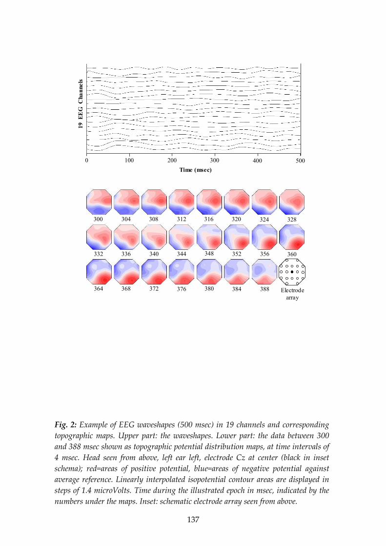
137

300 304 308 312 316 320 324 328

332 336 340 344 348 352 356 360

364 368 372 376 380 384 388 Electrode

array

0 100 200 300 400 500

Time (msec)

19 E

EG

C

ha

nn

els

Fig. 2: Example of EEG waveshapes (500 msec) in 19 channels and corresponding

topographic maps. Upper part: the waveshapes. Lower part: the data between 300

and 388 msec shown as topographic potential distribution maps, at time intervals of

4 msec. Head seen from above, left ear left, electrode Cz at center (black in inset

schema); red=areas of positive potential, blue=areas of negative potential against

average reference. Linearly interpolated isopotential contour areas are displayed in

steps of 1.4 microVolts. Time during the illustrated epoch in msec, indicated by the

numbers under the maps. Inset: schematic electrode array seen from above.

138

7

5

3

7A

left

-ri

gh

t

5

3

an

t -

post

B

5

1

9

left

-ri

ghtC

5

1

9

an

t -

post

D

5

0

10

left

-ri

gh

tE

500 msec3002001000 400

5

0

10

ant

-po

st

F

H

I

G

*

ex

trem

e p

ote

nti

als

po

ten

tia

l a

rea c

entr

oid

se

lect

ric

gra

vit

y c

en

ter

Fig. 3: Descriptions and descriptors of potentials maps. Vertical axes: numbers

indicate electrode positions as described in Fig. 1. A, B: Trajectories of the map

gravity center over time (x-axis) along the left-right (A) and anterior-posterior (B)

axis. C, D: Trajectories of the positive (red line) and negative (blue line) potential

area centroids over time (x-axis) along the left-right (C) and anterior-posterior (D)

axis. E, F: Trajectories of the maximal (red line) and minimal (blue line) potential

values over time (x-axis) along the left-right (E) and anterior-posterior (F) axis.

Maps on the right: an example of map descriptors extracted from the potential

distribution map at 140 msec (vertical line), shown with linearly interpolated

isopotential areas in steps of 1.4 microVolts; positive potential areas in red, negative

in blue, against average reference; darker hue=more extreme potential values. G:

asterisk symbol marks the location of the mapped scalp field’s electric gravity center.

H: positive and negative symbols mark the locations of the mapped scalp field’s

centroids for the positive and the negative potential areas. I: positive and negative

symbols mark the locations (electrode positions) of the mapped scalp field’s maximal

and minimal field potential values, i.e. of the positive and negative extreme

potentials. Note that locations of gravity center and centroids need not coincide

with electrode positions.

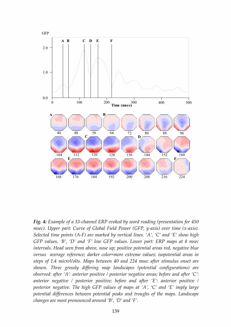
139

A B

C D

E F

40 48 56 64 72 80 88 96

104 112 120 128 136 144 152 160

168 176 184 192 200 208 216 224

0.0 32.0 64.0 96.0 128.0160.0192.0224.0256.0288.0320.0352.0384.0416.0448.0480.05120.0

0.00

0.40

0.80

1.20

1.60

2.00

2.40

0.0

1.0

2.0

GFP

A B C D E F

0 100 200 300 400 500Time (msec)

Fig. 4: Example of a 33-channel ERP evoked by word reading (presentation for 450

msec). Upper part: Curve of Global Field Power (GFP, y-axis) over time (x-axis).

Selected time points (A-F) are marked by vertical lines. ‘A’, ‘C’ and ‘E’ show high

GFP values, ‘B’, ‘D’ and ‘F’ low GFP values. Lower part: ERP maps at 8 msec

intervals. Head seen from above, nose up; positive potential areas red, negative blue

versus average reference; darker color=more extreme values; isopotential areas in

steps of 1.4 microVolts. Maps between 40 and 224 msec after stimulus onset are

shown. Three grossly differing map landscapes (potential configurations) are

observed: after ‘A’: anterior positive / posterior negative areas; before and after ‘C’:

anterior negative / posterior positive; before and after ‘E’: anterior positive /

posterior negative. The high GFP values of maps at ‘A’, ‘C’ and ‘E’ imply large

potential differences between potential peaks and troughs of the maps. Landscape

changes are most pronounced around ‘B’, ‘D’ and ‘F’.

140

Fig. 5 (modified from T. Koenig, 1999): Example of clustering a sequence of 10 momentary

maps into 2 class mean maps. First box: the maps (normalized potential maps with

equidistant contour lines; nose up, left ear left, blue areas = negative against average

reference). Two randomly selected, starting prototype maps are labeled A (black) and B

(white). Second box: first run; similarity of spatial configuration of each prototype map

with each of the 10 maps is computed using the squared correlation coefficient to omit the

maps’ polarities; the highest value determines the assignment, shown by black (similarity to

A) or white (similarity to B) symbols. Separately for each class, the prototype maps are

updated combining all assigned maps, by computing the first spatial principal component

of the maps and thereby maximizing the common variance while disregarding map polarity

(right: updated maps). Third box: this is repeated in the second and later runs until no

further changes in assignment occur, and thus 2 prototypes are established as 2 class mean

maps (final run, last box). Eventually, the percentage of the variance of the data explained

by the 2 class mean maps is determined. Explained variance might change depending on

selected starting prototype maps. To find the solution with maximal explained variance, the

entire procedure was repeated 20 times with newly randomly selected starting prototype

maps.

141

BBBBB

B

BBB

Ra

nd

om

Sele

cti

on

Sim

ilari

ty w

ith

T

yp

e A

& B

B BBBB

Ass

ign

men

t to

Ty

pe A

& BFir

st

Ru

nF

inal

Ru

nS

econ

d

Ru

n

Update

Update

(no more

change)

Update

Typ

e

Sim

ilari

ty w

ith

Ty

pe A

& B

Ass

ign

men

t to

Ty

pe A

& B

Sim

ilari

ty w

ith

Ty

pe A

& B

Ass

ign

men

t to

Ty

pe A

& B

high

low

high

low

high

low

A

B

A

B

A

B

A

A A A A A AA

A A A AA

A A A AA

A

B

A

B

A

B

Mat

eria

l

711 758 805 852 898 945 992 1039 1156 1195 msec

142

S

PA

TIA

L

RE

SO

LU

TIO

N

TEMPORAL RESOLUTION

EEG / MEG

5 cm

5 mm

1 mm

10 msec1 msec 100 msec 1 sec 10 sec 1 min

1 cm

PET

SPECT

fMRI

Fig. 6: Resolution in time and space of brain physiologic measurements: EEG, MEG,

fMRI, PET and SPECT. Time (horizontal), space (vertical); invasive methods (grey),

non-invasive methods (white).

143

Fp1 Fp2Fpz

AF3 AF4

F7F3 F4

F8

FC5 FC1 FC2 FC6

FZ

T7 C3 CZ C4 T8

CP5 CP1 CP2 CP6

P7P3 PZ P4

P8

PO3 PO4

O1 OZO2

O9 O10

Nasion

Inion

Lef

t p

rea

uri

cula

rp

oin

tR

igh

t prea

uricu

lar

po

int

Fp1 Fp2Fpz

AF3 AF4

F7F3 F4

F8

FC5 FC1 FC2 FC6

FZ

T7 C3 CZ C4 T8

CP5 CP1 CP2 CP6

P7P3 PZ P4

P8

PO3 PO4

O1 OZO2

O9 O10

Fp1 Fp2Fpz

AF3 AF4

F7F3 F4

F8

FC5 FC1 FC2 FC6

FZ

T7 C3 CZ C4 T8

CP5 CP1 CP2 CP6

P7P3 PZ P4

P8

PO3 PO4

O1 OZO2

O9 O10

Nasion

Inion

Lef

t p

rea

uri

cula

rp

oin

tR

igh

t prea

uricu

lar

po

int

Fig. 7: The ‘10/10 system’ (Nuwer et al., 1998) of electrode placement on the scalp.

The head is viewed from above, nose up, left ear left. The measurement technique is

based on standard landmarks of the skull. Namely, the nasion, inion, and the left

and right preauricular points. The first measurement is in the anterior-posterior

distance in the midline (via the vertex) from nasion to inion (=100%). Fpz is at

10%, Fz is at 30%, Cz at 50%, Pz at 70% and Oz at 90% of the nasion-inion

distance. Lateral measurements start at the left preauricular point through Cz

(vertex) to the right preauricular point. Marks are placed at 10% of this left-right

preauricular distance and labeled T7 (left) and T8 (right). Marks at additiomal 20%

are labeled C3 (left) and C4 (right). With these first 9 cardinal marks all other marks

are constructed. The circles with thick lines and with grey background correspond

to the 35 electrodes recorded in the present study (O9 and O10 were omitted from

analysis). The identification labels of all used electrodes are given. Fp=frontal pole;

F=frontal; Z=‘zentral’, i.e. midline; C=central; T=temporal; P=parietal; O=occipital.

Three additional electrodes (not shown in this schema) were used for the detection of

horizontal and vertical eye movements: Two electrodes at the outer left and right

canthus and an electrode at the left infraorbital site.

144

A

B

Fig. 8: Single model maps of the resting EEGs of the 10 believers (A) and 13

skeptics (B). Head seen from above, nose up, left ear left. Red and blue indicate map

areas of opposite polarity, deeper hue=higher potential values; note that the analysis

procedure omitted absolute polarity, thereby revealing the configuration of the

potential landscapes on the scalp. Dots and squares=locations of area centroids of

opposite potential, connected by a straight line that indicates the orientation of the

electric field of the model map. Open symbols for believers, filled for skeptics. Insets:

mean model maps across subjects of each group.

145

**

**4.6 5.0 5.4 5.8

3.0

5.0

7.0

9.0

**

Fig. 9: Locations of the anterior (ovals) and posterior (rectangles) located potential

centroids for the believers (open areas; n=10) and the skeptics (filled areas; n=13)

during resting EEG. The extensions of the ovals and rectangles indicate ± 1 S.E.

from the mean. The illustrated square area displays a narrow, rectangular area on

the scalp (i.e., the white rectangle in the inset head, top left) which was magnified in

the left-right direction in order to visualize the relevant left-right differences of the

centroid locations. Numbers along the axis indicate electrode positions: the

horizontal (left-right) axis covers electrode positions 4.6 to 5.6; the vertical axis

(anterior-posterior) positions 2.0 to 9.0. ** = P-values of P<0.05.

146

ANTERIOR

RIG

HT

LEFT

Delta

Beta3

Theta

Beta1

Alpha1

Alpha2

Beta2

POSTERIOR

LE

FT

Fig. 10: Mean locations of the LORETA gravity centers for skeptics (black squares;

n=10 and believers (open circles; n=13) for the seven independent EEG frequency

bands on the left-right and anterior-posterior head axes. Head seen from above, nose

up. The illustrated area displays a narrow, rectangular head area (i.e., the white

rectangle in the inset head, top left) which was magnified in the left-right direction

in order to visualize the relevant, lateral differences of the gravity center locations.

Tickmarks at distances of 5 mm on the anterior-posterior axis and of 1 mm on the

left-right axis; the vertical line through the display is the head midline.

147

A

B

Fig. 11: LORETA functional images of the difference in current density between

believers (n=10) minus skeptics (n=13) in the beta2 band. A: Red are voxels with

stronger activity in believers than skeptics; B: vice versa, stronger in skeptics than

believers. A and B: 15 axial brain slices in Talairach space, at 7 mm distance from

most inferior (z = -41 mm) to most superior (z = 57 mm), viewed from above. X axis

from left (L) to right (R); Y axis from posterior to anterior; Z axis from inferior to

superior. Structural anatomy is shown in gray scale.

148

0

8

16

2

4

32

4

0

48

56

6

4

72

80

88

96

104

11

2

1

20

1

28

136

144

152

16

0

1

68

176

18

4

1

92

2

00

2

08

216

22

4

23

2

2

40

248

256

264

272

28

0

28

8

2

96

304

31

2

3

20

3

28

3

36

3

44

352

360

368

376

38

4

3

92

4

00

408

416

424

432

440

448

mse

c

0

8

16

2

4

32

4

0

48

56

6

4

72

80

88

96

104

11

2

1

20

1

28

136

144

152

16

0

1

68

176

18

4

1

92

2

00

2

08

216

22

4

23

2

2

40

248

256

264

272

28

0

28

8

2

96

304

31

2

3

20

3

28

3

36

3

44

352

360

368

376

38

4

3

92

4

00

408

416

424

432

440

448

mse

c

0

8

16

2

4

32

4

0

48

56

6

4

72

80

88

96

104

11

2

1

20

1

28

136

144

152

16

0

1

68

176

18

4

1

92

2

00

2

08

216

22

4

23

2

2

40

248

256

264

272

28

0

28

8

2

96

304

31

2

3

20

3

28

3

36

3

44

352

360

368

376

38

4

3

92

4

00

408

416

424

432

440

448

mse

c

Fig

. 12

: G

ran

dmea

n (

over

21

subj

ects

) 33

-cha

nn

el E

RP

map

ser

ies

evok

ed b

y th

e pr

esen

tati

ons

(448

mse

c) o

f em

otio

nal

pos

itiv

e w

ords

.

Hea

d se

en f

rom

abo

ve,

nos

e u

p, l

eft

ear

left

; is

opot

enti

al c

onto

ur

area

s in

ste

ps o

f 1.

4 m

icro

Vol

ts.

Red

=are

as o

f po

siti

ve p

oten

tial

aga

inst

aver

age

refe

ren

ce;

blu

e=ar

eas

of n

egat

ive

pote

nti

al a

gain

st a

vera

ge r

efer

ence

. B

elow

eac

h m

ap,

the

nu

mbe

rs i

den

tify

lat

enci

es i

n m

illi

seco

nds

afte

r st

imu

lus

onse

t (t

ime

betw

een

su

cces

sive

map

s is

8 m

sec)

. T

hus,

eve

ry s

econ

d ti

mef

ram

e of

the

com

plet

e m

ap s

erie

s (1

13 t

ime

fram

es a

t

4 m

sec

inte

rval

) is

ill

ust

rate

d he

re.

149

0

8

16

2

4

32

4

0

48

56

6

4

72

80

88

96

104

11

2

1

20

1

28

136

144

152

16

0

1

68

176

18

4

1

92

2

00

2

08

216

22

4

23

2

2

40

248

256

264

272

28

0

28

8

2

96

30

4

3

12

320

328

336

344

352

360

368

376

38

4

392

40

0

4

08

4

16

4

24

4

32

440

448

mse

c

0

8

16

2

4

32

4

0

48

56

6

4

72

80

88

96

104

11

2

1

20

1

28

136

144

152

16

0

1

68

176

18

4

1

92

2

00

2

08

216

22

4

23

2

2

40

248

256

264

272

28

0

28

8

2

96

30

4

3

12

320

328

336

344

352

360

368

376

38

4

392

40

0

4

08

4

16

4

24

4

32

440

448

mse

c

0

8

16

2

4

32

4

0

48

56

6

4

72

80

88

96

104

11

2

1

20

1

28

136

144

152

16

0

1

68

176

18

4

1

92

2

00

2

08

216

22

4

23

2

2

40

248

256

264

272

28

0

28

8

2

96

30

4

3

12

320

328

336

344

352

360

368

376

38

4

392

40

0

4

08

4

16

4

24

4

32

440

448

mse

c

Fig

. 13

: G

ran

dmea

n (

over

21

subj

ects

) 33

-cha

nn

el E

RP

map

ser

ies

evok

ed b

y th

e pr

esen

tati

ons

(448

mse

c) o

f em

otio

nal

neg

ativ

e w

ords

.

Hea

d se

en f

rom

abo

ve,

nos

e u

p, l

eft

ear

left

; is

opot

enti

al c

onto

ur

area

s in

ste

ps o

f 1.

4 m

icro

Vol

ts.

Red

=are

as o

f po

siti

ve p

oten

tial

aga

inst

aver

age

refe

ren

ce;

blu

e=ar

eas

of n

egat

ive

pote

nti

al a

gain

st a

vera

ge r

efer

ence

. B

elow

eac

h m

ap,

the

nu

mbe

rs i

den

tify

lat

enci

es i

n m

illi

seco

nds

afte

r st

imu

lus

onse

t (t

ime

betw

een

su

cces

sive

map

s is

8 m

sec)

. T

hus,

eve

ry s

econ

d ti

mef

ram

e of

the

com

plet

e m

ap s

erie

s (1

13 t

ime

fram

es a

t

4 m

sec

inte

rval

) is

ill

ust

rate

d he

re.

150

0

8

16

2

4

32

4

0

48

56

6

4

72

80

88

96

104

11

2

1

20

128

136

144

152

16

0

1

68

176

18

4

1

92

2

00

2

08

21

6

2

24

232

24

0

2

48

2

56

264

272

28

0

28

8

2

96

304

31

2

3

20

3

28

3

36

3

44

352

360

368

376

38

4

3

92

4

00

408

416

424

432

440

448

mse

c

0

8

16

2

4

32

4

0

48

56

6

4

72

80

88

96

104

11

2

1

20

128

136

144

152

16

0

1

68

176

18

4

1

92

2

00

2

08

21

6

2

24

232

24

0

2

48

2

56

264

272

28

0

28

8

2

96

304

31

2

3

20

3

28

3

36

3

44

352

360

368

376

38

4

3

92

4

00

408

416

424

432

440

448

mse

c

Fig

. 14:

Gra

nd-

gran

dmea

n (

over

21

subj

ects

) 33

-cha

nn

el E

RP

map

ser

ies

evok

ed b

y th

e pr

esen

tati

ons

(448

mse

c) o

f em

otio

nal

ly p

osit

ive

and

neg

ativ

e w

ords

. H

ead

seen

fro

m a

bove

, n

ose

up,

lef

t ea

r le

ft;

isop

oten

tial

con

tou

r ar

eas

in s

teps

of

1.4

mic

roV

olts

. R

ed=a

reas

of

pos

itiv

e

pote

nti

al a

gain

st a

vera

ge r

efer

ence

; bl

ue=

area

s of

neg

ativ

e po

ten

tial

aga

inst

ave

rage

ref

eren

ce.

Bel

ow e

ach

map

, th

e n

um

bers

in

dica

te t

he

late

nci

es i

n m

illi

seco

nds

aft

er s

tim

ulu

s on

set

(tim

e be

twee

n s

ucc

essi

ve m

aps

is 8

mse

c).

Thu

s, e

very

sec

ond

tim

efra

me

of t

he c

ompl

ete

map

seri

es (

113

tim

e fr

ames

at

4 m

sec

inte

rval

) is

ill

ust

rate

d he

re.

151

A B C D E F G

Fig. 15: The scalp potential distribution map of the 7 class mean maps (A-G)

identified by the global microstate analysis of the grand-grandmean ERP map series

(n=113 timeframes) during visual word presentation. Head seen from above, nose

up, left ear left; isopotential contour areas in steps of 1.4 microVolts. Red and blue

colors identify areas of opposite polarity; note that these class mean maps identify

the spatial configuration of the potential distributions while disregarding polarity,

i.e., two identical maps of inverted polarity constitute a given class mean map.

“Original Polarity” is shown in this figure, i.e., red=positive, blue=negative.

152

Class Mean Maps

010

02

00

30

040

0

125

50

75

10

0

mse

c

fra

me

#

12

34

56

78

91

01

11

213

A B C D E F G

12

34

56

78

910

11

12

13

44

8

11

3

Fig

. 16

: T

he 1

3 m

icro

stat

es i

den

tifi

ed b

y th

e gl

obal

mic

rost

ate

anal

ysis

of

the

gran

d-gr

andm

ean

ER

P m

ap s

erie

s (n

=113

) du

rin

g vi

sual

wor

d pr

esen

tati

on.

Upp

er p

art:

Eac

h ti

mef

ram

e du

rin

g th

e 44

8 m

sec

of s

tim

ulu

s pr

esen

tati

on i

s as

sign

ed t

o on

e of

the

7 c

lass

mea

n m

aps

(A-G

) id

enti

fied

by

the

glob

al m

icro

stat

e an

alys

is a

s sh

own

in

Fig

. 13

wit

h th

e or

igin

al p

olar

ity

(bl

ack

diam

onds

) or

wit

h re

vers

ed p

olar

ity

(whi

te d

iam

onds

). F

or i

nst

ance

, m

icro

stat

es #

4, #

7 an

d #1

0 ar

e re

pres

ente

d by

th

e sa

me

clas

s m

ean

map

(D

). M

icro

stat

es #

4 an

d #1

0 ha

ve

the

sam

e po

lari

ty a

s sh

own

in

Fig

. 13,

whe

reas

mic

rost

ate

#7 h

as r

ever

sed

pola

rity

. On

e di

amon

d co

rres

pon

ds t

o 1

tim

efra

me;

the

nu

mbe

r of

con

secu

tive

tim

efra

mes

bel

ongi

ng

to t

he s

ame

clas

s m

ean

map

def

ines

the

du

rati

on o

f th

at m

icro

stat

e. T

he t

ime

betw

een

con

secu

tiv

e

tim

efra

mes

is

4 m

sec.

The

glo

bal

fiel

d po

wer

cu

rve

of t

he g

ran

d-gr

andm

ean

ER

P i

s sh

own

in

gre

y in

the

bac

kgro

un

d. L

ower

par

t: S

calp

pote

nti

al d

istr

ibu

tion

s of

the

13

mic

rost

ates

are

dis

play

ed.

For

fu

rthe

r ex

plan

atio

n o

f th

e m

ap d

ispl

ays

see

Fig

. 12.

153

0 100 200 300 400

1 25 50 75 100

msec

frame #

0

0.5

1.0G

FP

(m

icro

Vo

lts)

Fig. 17: Curves of Global Field Power (GFP, microVolts) over time (x-axis, msec) for

the grandmean ERP map series evoked by emotional positive (open diamonds) and

negative words (solid diamonds). The two series consist each of a total of 113 maps

(=frames).

154

4.5

5.5

0.00

0.10

0 100 200 300 400

1 25 50 75 100

msec

frame #

p-v

alu

es

left

-ri

gh

t

5

6

0.00

0.10

0 100 200 300 400 msecp-v

alu

es

an

t -

po

stA

B

Fig. 18: Trajectory of the locations of the electric gravity center over time (x-axis)

along the anterior-posterior (vertical, A) and left-right (vertical, B) axis, for the

grandmean ERP map series evoked by emotional positive (open triangles) and

negative words (solid triangles). The numbers along the y-axis represent electrode

positions according to the international ‘10/10 system’ as described in Fig. 1. On

the bottom of the figures, P-values (between 0.10 and 0.00) of t-tests comparing

locations for positive and negative emotion words are illustrated for each time frame.

155

4

5

6

0.00

0.10

0 100 200 300 400

1 25 50 75 100

msec

frame #

p-v

alu

es

left

-ri

ght

B

3

8

0.00

0.10

0 100 200 300 400 msecp-v

alu

es

ant

-post

A

4

5

6

7

Fig. 19: Trajectory of the locations of the positive potential area centroid over time

(x-axis) along the anterior-posterior (vertical, A) and left-right (vertical, B) axis, for

the grandmean ERP map series evoked by emotional positive (open circles) and

negative words (solid circles). The numbers along the y-axis represent electrode

positions according to the international ‘10/10 system’ as described in Fig. 1. On

the bottom of the figures, P-values (between 0.10 and 0.00) of t-tests comparing

locations for positive and negative emotion words are illustrated for each time

frame.

156

4

5

6

0.00

0.10

0 100 200 300 400

1 25 50 75 100

msec

frame #

p-v

alu

es

left

-ri

ght

B

3

8

0.00

0.10

0 100 200 300 400 msecp-v

alu

es

ant

-p

ost

A

4

5

6

7

Fig. 20: Trajectory of the locations of the negative potential area centroid over time

(x-axis) along the anterior-posterior (vertical, A) and left-right (vertical, B) axis, for

the grandmean ERP map series evoked by emotional positive (open rectangles) and

negative words (solid rectangles). The numbers along the y-axis represent electrode

positions according to the international ‘10/10 system’ as described in Fig. 1. On

the bottom of the figures, P-values (between 0.10 and 0.00) of t-tests comparing

locations for positive and negative emotion words are illustrated for each time

frame.

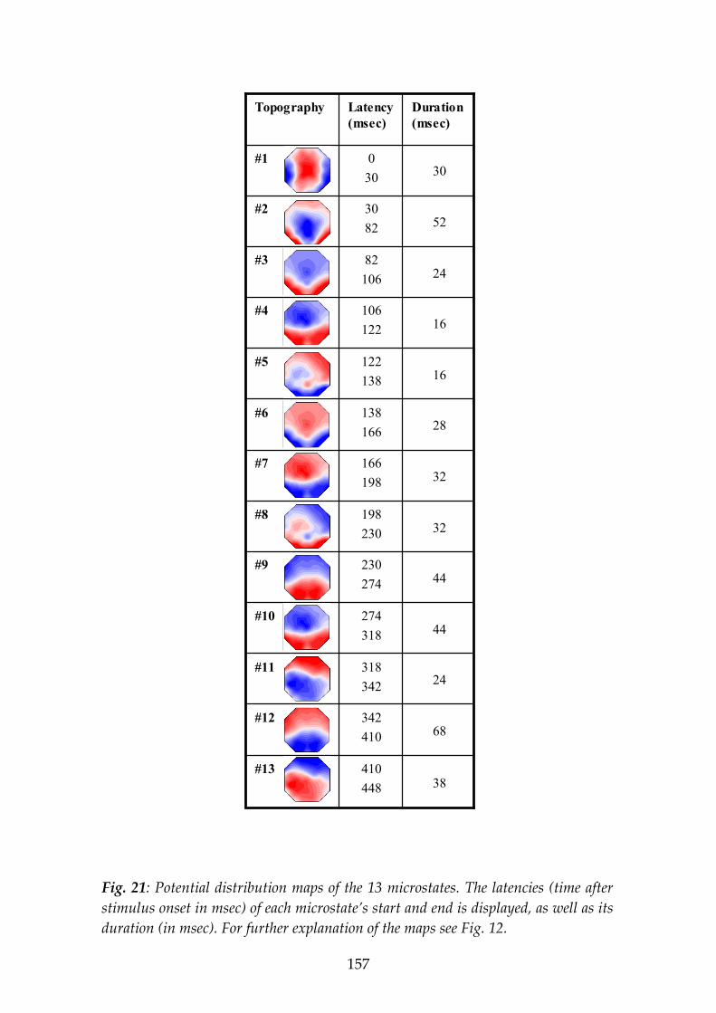
157

38410

448

#13

68342

410

#12

24318

342

#11

44274

318

#10

44230

274

#9

32198

230

#8

32166

198

#7

28138

166

#6

16122

138

#5

16106

122

#4

2482

106

#3

5230

82

#2

300

30

#1

Duration

(msec)

Latency

(msec)

Topography

Fig. 21: Potential distribution maps of the 13 microstates. The latencies (time after

stimulus onset in msec) of each microstate’s start and end is displayed, as well as its

duration (in msec). For further explanation of the maps see Fig. 12.

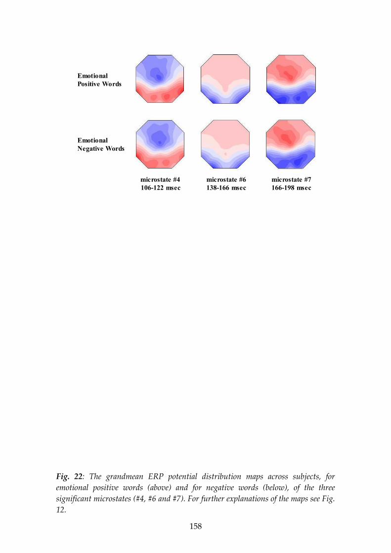
158

Emotional

Positive Words

Emotional

Negative Words

microstate #4

106-122 msec

microstate #6

138-166 msec

microstate #7

166-198 msec

Fig. 22: The grandmean ERP potential distribution maps across subjects, for

emotional positive words (above) and for negative words (below), of the three

significant microstates (#4, #6 and #7). For further explanations of the maps see Fig.

12.

159

microstate #4

106-122 msec

microstate #6

138-166 msec

microstate #7

166-198 msec

**

**

**

*4.6 4.8 5 5.2 5.43.8

4.8

5.8

6.8

7.8

Fig. 23: Mean location of the positive (circle) and negative (square) potential area

centroids in the three significant microstates. Head seen from above, nose up, left ear

left. Open symbols and filled symbols show the centroid locations for emotionally

positive and negative words, respectively. The numbers along the horizontal (left-

right) x-axis and the vertical (anterior-posterior) y-axis indicate electrode positions

of the 10-10 system as described in Fig. 1 (left=1, right=9; Cz=5; anterior=1;

posterior=9; Cz=5). Red double-headed arrows indicate statistically significant

differences of the centroid locations. **= P<0.01; *=0.01<P<0.05.

160

microstate #4

106-122 msec

microstate #6

138-166 msec

microstate #7

166-198 msec

Fp1 Fpz Fp2

AF3 AF4

F7 F3 FZ F4 F8

T7 C3 CZ C4 T8

P7 P3 PZ P4 P8

O1 OZ O2

PO3 PO4

FC5 FC1 FC2 FC6

CP5 CP1 CP2 CP6

Fig. 24: Electrode-by-electrode t-statistics between word classes in the three

significant microstates (#4, #6 and #7). Grandmean ERP potential distribution

maps evoked by positive and negative words were compared at each electrode. The

map on top shows the identification labels of the electrode positions. White circles

mark electrodes that show significant (thick line) or a trend (thin line) for more

activity evoked by positive compared to negative words. Grey circles correspond to

electrodes that show significant (thick line) or a trend (thin line) for more activity

evoked by negative compared to positive words.

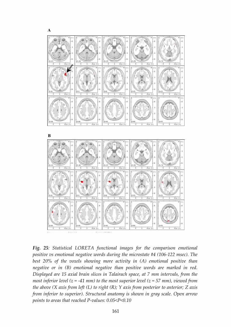
161

A

B

Fig. 25: Statistical LORETA functional images for the comparison emotional

positive vs emotional negative words during the microstate #4 (106-122 msec). The

best 20% of the voxels showing more activity in (A) emotional positive than

negative or in (B) emotional negative than positive words are marked in red.

Displayed are 15 axial brain slices in Talairach space, at 7 mm intervals, from the

most inferior level (z = -41 mm) to the most superior level (z = 57 mm), viewed from

the above (X axis from left (L) to right (R); Y axis from posterior to anterior; Z axis

from inferior to superior). Structural anatomy is shown in gray scale. Open arrow

points to areas that reached P-values: 0.05<P<0.10

162

B

A

Fig. 26: Statistical LORETA functional images for the comparison emotional

positive vs emotional negative words during the microstate #6 (138-166 msec). The

best 20% of the voxels showing more activity in (A) emotional positive than

negative or in (B) emotional negative than positive words are marked in red.

Displayed are 15 axial brain slices in Talairach space, at 7 mm intervals, from the

most inferior level (z = -41 mm) to the most superior level (z = 57 mm), viewed from

the above (X axis from left (L) to right (R); Y axis from posterior to anterior; Z axis

from inferior to superior). Structural anatomy is shown in gray scale.

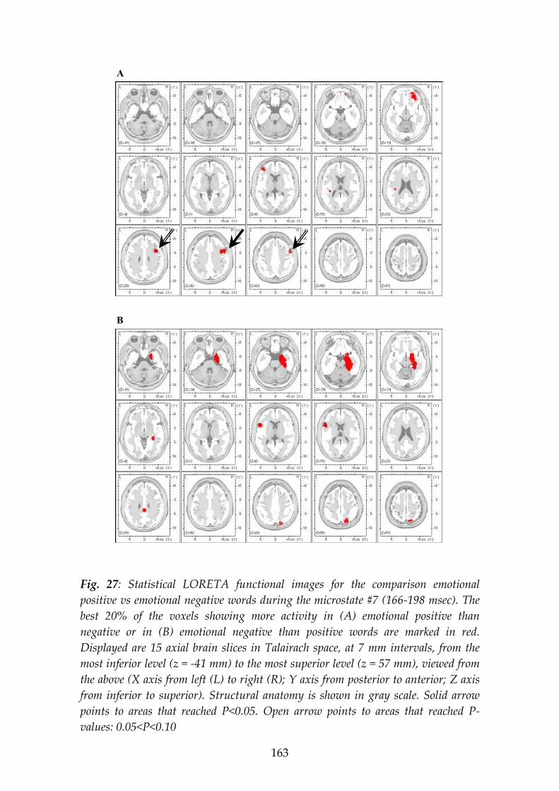
163

B

A

Fig. 27: Statistical LORETA functional images for the comparison emotional

positive vs emotional negative words during the microstate #7 (166-198 msec). The

best 20% of the voxels showing more activity in (A) emotional positive than

negative or in (B) emotional negative than positive words are marked in red.

Displayed are 15 axial brain slices in Talairach space, at 7 mm intervals, from the

most inferior level (z = -41 mm) to the most superior level (z = 57 mm), viewed from

the above (X axis from left (L) to right (R); Y axis from posterior to anterior; Z axis

from inferior to superior). Structural anatomy is shown in gray scale. Solid arrow

points to areas that reached P<0.05. Open arrow points to areas that reached P-

values: 0.05<P<0.10

164

1

2

3

4

5

6

7

negative

words

neutral

words

positive

words

P<0.01

P<0.001

“Very

positive word”

“Very

negative word”

“Neutral word”

Fig. 28: Rating of the emotional content of the three words classes. Horizontal axis:

words classes. Vertical axis: Mean (+1 S.E.) of the rating of the emotional content of

the 74 words on a 7-point scale, separately, for believers (n=10; white columns) and

skeptics (n=13; black columns). The rating scale was labeled on one extreme with:

“very negative word” (position 1) and on the other extreme: “very positive word”

(position 7). In the middle of the scale, i.e. at the position “4”, there was the label

“neutral word”.

165

APPENDICES

166

APPENDIX 1: Six-item questionnaire assessing belief in and experience of

paranormal phenomena (Mischo et al., 1993).

Tri

fft

kla

r

zu

Tri

fft

kla

r

nic

ht

zu

- Ich habe mindestens ein telepathisches Erlebnis zwischen mir und einem anderen Menschen gehabt.

� � � �

- Ich habe noch nie eine Aussersinnliche Wahrnehmung bei mir selbst erlebt. � � � �

- Ich hatte wenigstens einmal eine Vorahnung, die sich erfüllte und von der ich annahm, dass sie kein Zufall war.

� � � �

- Ich glaube, es gibt so etwas wie Gedankenübertragung.

� � � �

- Manche Träume weisen auf zukünftige Erlebnisse hin, von denen man vorher nichts wissen kann.

� � � �

- Ich hatte mindestens einen Traum, der sich auf die Zukunft bezog und sich so exakt erfüllte, dass ich glaube, dass das kein Zufall war.

�

�

� �

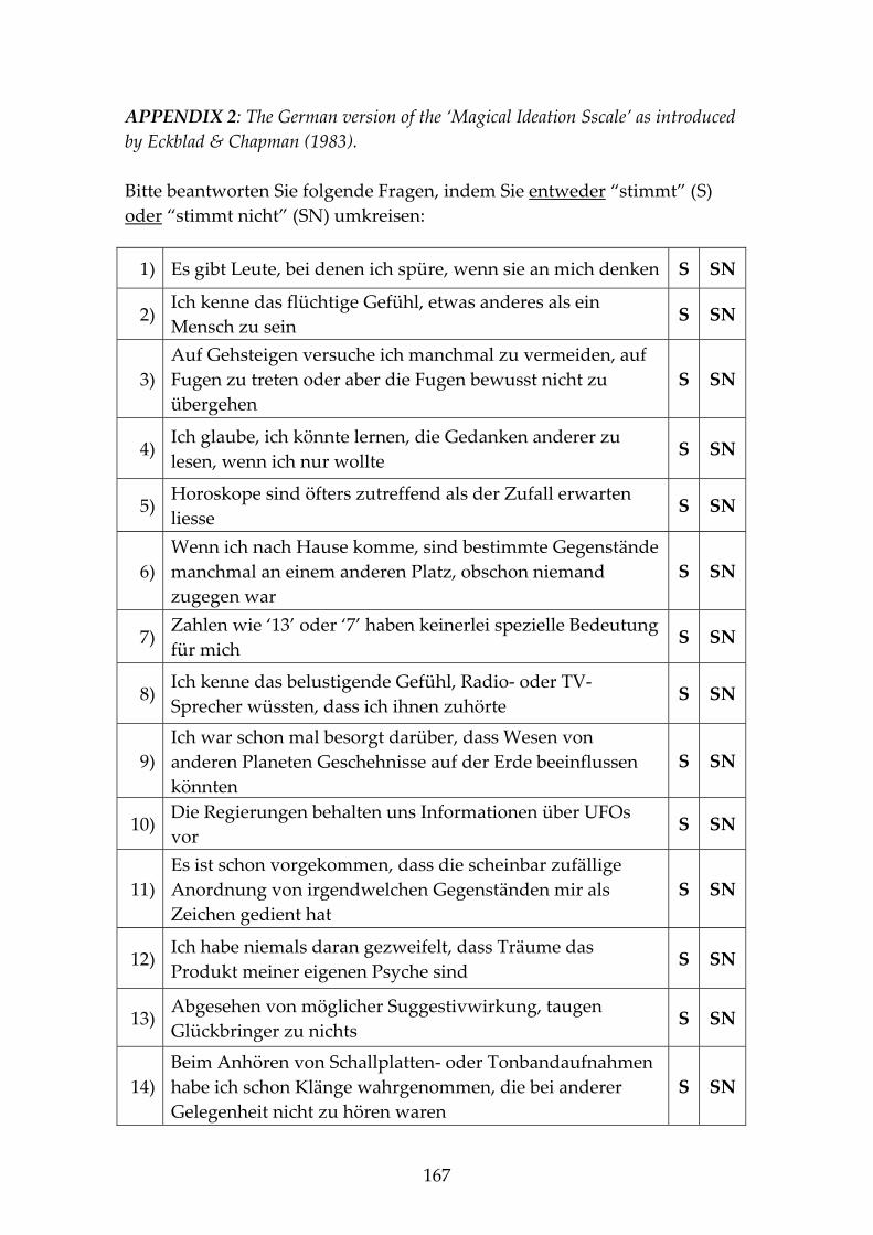
167

APPENDIX 2: The German version of the ‘Magical Ideation Sscale’ as introduced

by Eckblad & Chapman (1983).

Bitte beantworten Sie folgende Fragen, indem Sie entweder “stimmt” (S) oder “stimmt nicht” (SN) umkreisen:

1) Es gibt Leute, bei denen ich spüre, wenn sie an mich denken S SN

2) Ich kenne das flüchtige Gefühl, etwas anderes als ein Mensch zu sein

S SN

3) Auf Gehsteigen versuche ich manchmal zu vermeiden, auf Fugen zu treten oder aber die Fugen bewusst nicht zu übergehen

S SN

4) Ich glaube, ich könnte lernen, die Gedanken anderer zu lesen, wenn ich nur wollte

S SN

5) Horoskope sind öfters zutreffend als der Zufall erwarten liesse

S SN

6) Wenn ich nach Hause komme, sind bestimmte Gegenstände manchmal an einem anderen Platz, obschon niemand zugegen war

S SN

7) Zahlen wie ‘13’ oder ‘7’ haben keinerlei spezielle Bedeutung für mich

S SN

8) Ich kenne das belustigende Gefühl, Radio- oder TV-Sprecher wüssten, dass ich ihnen zuhörte

S SN

9) Ich war schon mal besorgt darüber, dass Wesen von anderen Planeten Geschehnisse auf der Erde beeinflussen könnten

S SN

10) Die Regierungen behalten uns Informationen über UFOs vor

S SN

11) Es ist schon vorgekommen, dass die scheinbar zufällige Anordnung von irgendwelchen Gegenständen mir als Zeichen gedient hat

S SN

12) Ich habe niemals daran gezweifelt, dass Träume das Produkt meiner eigenen Psyche sind

S SN

13) Abgesehen von möglicher Suggestivwirkung, taugen Glückbringer zu nichts

S SN

14) Beim Anhören von Schallplatten- oder Tonbandaufnahmen habe ich schon Klänge wahrgenommen, die bei anderer Gelegenheit nicht zu hören waren

S SN

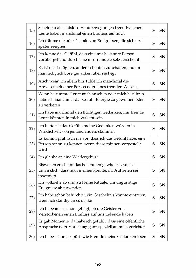
168

15) Scheinbar absichtslose Handbewegungen irgendwelcher Leute haben manchmal einen Einfluss auf mich

S SN

16) Ich träume nie oder fast nie von Ereignissen, die sich erst später ereignen

S SN

17) Ich kenne das Gefühl, dass eine mir bekannte Person vorübergehend durch eine mir fremde ersetzt erscheint

S SN

18) Es ist nicht möglich, anderen Leuten zu schaden, indem man lediglich böse gedanken über sie hegt

S SN

19) Auch wenn ich allein bin, fühle ich manchmal die Anwesenheit einer Person oder eines fremden Wesens

S SN

20) Wenn bestimmte Leute mich ansehen oder mich berühren, habe ich manchmal das Gefühl Energie zu gewinnen oder zu verlieren

S SN

21) Ich habe manchmal den flüchtigen Gedanken, mir fremde Leute könnten in mich verliebt sein

S SN

22) Ich hatte nie das Gefühl, meine Gedanken würden in Wirklichkeit von jemand anders stammen

S SN

23) Es kommt praktisch nie vor, dass ich das Gefühl habe, eine Person schon zu kennen, wenn diese mir neu vorgestellt wird

S SN

24) Ich glaube an eine Wiedergeburt S SN

25) Bisweilen erscheint das Benehmen gewisser Leute so unwirklich, dass man meinen könnte, ihr Auftreten sei inszeniert

S SN

26) Ich vollziehe ab und zu kleine Rituale, um ungünstige Ereignisse abzuwenden

S SN

27) Ich habe schon befürchtet, ein Geschehnis könnte eintreten, wenn ich ständig an es denke

S SN

28) Ich habe mich schon gefragt, ob die Geister von Verstorbenen einen Einfluss auf uns Lebende haben

S SN

29) Es gab Momente, da habe ich gefühlt, dass eine öffentliche Ansprache oder Vorlesung ganz speziell an mich gerichtet S SN

30) Ich habe schon gespürt, wie Fremde meine Gedanken lesen S SN

169

APPENDIX 3: The German version of the Handedness Inventory (Chapman &

Chapman, 1987).

Bitte geben Sie an, mit welcher Hand Sie für gewöhnlich folgende Tätigkeiten ausüben (Sie können mit ‘linke’, ‘rechte’ oder ‘beide Hände gleichermassen’ antworten). Mit welcher Hand (3Pte.) (1Pt.) (2Pte.) - zeichnen Sie? linke rechte beide - schreiben Sie? linke rechte beide - benutzen Sie einen Flaschenöffner? linke rechte beide - werfen Sie einen Schneeball? linke rechte beide - benutzen Sie einen Hammer? linke rechte beide - eine Zahnbürste? linke rechte beide - einen Schraubenzieher? linke rechte beide - einen Radiergummi? linke rechte beide - einen Tennisschläger? linke rechte beide - eine Schere? linke rechte beide - zünden Sie ein Streichholz an? linke rechte beide - rühren Sie mit einer Kelle? linke rechte beide - auf welcher Schulter ruht der Schläger beim Baseball / Hornussen etc.? linke rechte beide

Anzahl Punkte: ______ ______ ______

TOTAL: ===========

170

APPENDIX 4: The German version of the Positive and Negative Affect Scale

(PANAS; Watson et al., 1988).

Dieser Fragebogen enthält eine Reihe von Wörtern, die unterschiedliche Gefühle und Empfindungen beschreiben. Lesen Sie jedes Wort und tragen Sie dann in die Skala neben jedem Wort die Intensität ein. Sie haben die Möglichkeit, zwischen fünf Abstufungen zu wählen: 1. ganz wenig oder gar nicht 2. ein bisschen 3. einigermassen 4. erheblich 5. äusserst Geben Sie bitte an, wie Sie sich im allgemeinen fühlen. ganz wenig oder einiger- gar nicht ein bisschen massen erheblich äusserst

aktiv O---------------O---------------O---------------O---------------O

bekümmert O---------------O---------------O---------------O---------------O

interessiert O---------------O---------------O---------------O---------------O

freudig erregt O---------------O---------------O---------------O---------------O

verärgert O---------------O---------------O---------------O---------------O

stark O---------------O---------------O---------------O---------------O

schuldig O---------------O---------------O---------------O---------------O

erschrocken O---------------O---------------O---------------O---------------O

feindselig O---------------O---------------O---------------O---------------O

angeregt O---------------O---------------O---------------O---------------O

stolz O---------------O---------------O---------------O---------------O

gereizt O---------------O---------------O---------------O---------------O

begeistert O---------------O---------------O---------------O---------------O

beschämt O---------------O---------------O---------------O---------------O

wach O---------------O---------------O---------------O---------------O

nervös O---------------O---------------O---------------O---------------O

entschlossen O---------------O---------------O---------------O---------------O

aufmerksam O---------------O---------------O---------------O---------------O

durcheinander O---------------O---------------O---------------O---------------O

ängstlich O---------------O---------------O---------------O---------------O

171

APPENDIX 5: Complete list of the stimuli with English translation.

Positive words (n=27) Negative words (n=27) Neutral words (n=20)

German English German English German English

Freude joy Ärger irritation Bein leg Freund friend Angst angst Blatt sheet Friede peace Armut poverty Blech plate Glück luck Elend misery Ebene level Güte goodness Flucht flight Ecke corner Herz hearth Furcht fear Format format Idee idea Gift poison Forum forum Kuss kiss Grab tomb Gebiet field Lachen laugh Haft detention Kugel sphere Leben life Härte toughness Länge length Licht light Hass hate Pfeife pipe Liebe love Hunger hunger Phase phase Lust lust Kälte coldness Regel rule Musik music Klage plaint Rest balance Mutter mother Krieg war Sitte custom Nähe closeness Last encumbrance Umbau reconstruction Ofen oven Leiche cadaver Vieh livestock Rose rose Mord murder Wage balance Sinn sense Panik panic Woche week Sommer summer Sarg coffin Zitat quotation Sonne sun Schalg stroke Spass fun Stich sting Spiel game Strafe punishment Wald wood Streit dispute Wärme geat Tadel reproach Weite width Tod death Wonne delight Zwang compulsion

172

APPENDIX 6: Averaged data of the emotional content after the first rating, during

the creaton of the 3 lists of the word classes (preparation of the word list, word

selection and matching by Esslen & Koenig; see also Esslen, 1997), and after the 2

previous studies, which used the same words (Esslen, 1997; Pizzagalli, 1998).

Listing of the words used in the present investigation, divided according to the three

word classes (emotional positive words: left; emotional negative words: middle;

emotional neutral words: right). The rating was done on a 7-point scale. The scale

was labelled on an extreme with: ‘very negative word’ (position ‘1’) and on the other

extreme: ‘very positive word’ (position ‘7’). In the middle of the scale, i.e. by the

position ‘4’, there was the label ‘neutral word’. Means and standard deviations of

the rating are provided for each word and for each subjects group. On the bottom of

the table, the mean and standard deviation (across words) of the rating for each word

class and for each subjects group are listed.

Positive words (n=27) Negative words (n=27) Neutral words (n=20)

Firs

t rat

ing

Ess

len

Piz

zaga

lli

Firs

t rat

ing

Ess

len

Piz

zaga

lli

Firs

t rat

ing

Ess

len

Piz

zaga

lli

Freude 6.7 ±0.6

6.6 ±0.6

6.7 ±0.6

Ärger 2.5 ±1.1

2.3 ±1.0

2.2 ±0.7

Bein 4.3 ±0.8

4.3 ±1.1

4.4 ±0.9

Freund 6.6 ±0.5

6.5 ±0.7

6.7 ±0.5

Angst 2.2 ±0.9

1.7 ±1.1

2.1 ±0.9

Blatt 4.6 ±1.0

4.6 ±1.0

4.9 ±1.1

Friede 6.1 ±0.8

6.4 ±0.8

6.5 ±0.9

Armut 1.9 ±0.6

1.9 ±0.7

2.1 ±1.1

Blech 3.6 ±0.7

3.6 ±0.8

3.9 ±0.8

Glück 6.7 ±0.6

6.5 ±0.6

6.8 ±0.4

Elend 2.1 ±1.6

1.4 ±0.5

1.5 ±0.5

Ebene 4.3 ±0.9

4.3 ±0.7

4.8 ±0.9

Güte 5.5 ±1.1

5.2 ±1.1

5.9 ±1.0

Flucht 2.5 ±0.7

2.3 ±0.9

2.4 ±1.0

Ecke 3.9 ±0.6

3.7 ±0.8

3.4 ±0.9

Herz 5.9 ±1.1

6.0 ±0.9

6.0 ±1.1

Furcht 2.6 ±1.2

2.1 ±1.0

2.1 ±0.5

Format 4.1 ±0.3

3.8 ±0.5

3.9 ±0.7

Idee 6.1 ±1.0

5.7 ±1.1

5.9 ±0.9

Gift 2.0 ±1.2

2.2 ±1.0

1.7 ±0.9

Forum 4.3 ±0.5

4.0 ±0.4

4.2 ±0.7

Kuss 6.4 ±0.7

6.7 ±0.5

6.7 ±0.6

Grab 2.1 ±0.9

2.4 ±1.1

2.1 ±1.1

Gebiet 4.0 ±0.0

4.3 ±0.7

4.1 ±0.5

Lachen 6.3 ±1.0

6.6 ±0.7

6.5 ±0.5

Härte 2.5 ±0.7

2.8 ±1.2

2.4 ±1.1

Kugel 4.1 ±1.4

4.3 ±1.3

4.2 ±1.6

Leben 6.2 ±0.9

6.3 ±0.8

6.3 ±0.7

Haft 1.6 ±0.7

2.0 ±1.2

1.9 ±1.7

Länge 4.1 ±0.3

4.2 ±1.0

4.0 ±0.7

Licht 6.1 ±0.8

6.5 ±0.8

6.6 ±0.6

Hass 1.7 ±0.8

1.6 ±1.1

1.4 ±0.7

Pfeife 3.7 ±0.9

3.8 ±0.9

3.8 ±1.1

173

Liebe 6.8 ±0.4

6.8 ±0.5

6.7 ±0.6

Hunger 2.5 ±1.4

2.4 ±1.0

2.6 ±1.5

Phase 4.3 ±0.9

4.0 ±0.5

4.1 ±0.7

Lust 6.2 ±1.3

6.4 ±1.1

6.4 ±0.7

Kälte 2.4 ±0.7

2.6 ±1.4

3.3 ±1.5

Regel 3.9 ±1.2

3.6 ±0.8

3.3 ±0.8

Musik 6.1 ±0.8

6.5 ±0.6

6.6 ±0.6

Klage 2.6 ±0.7

2.9 ±0.9

2.4 ±0.8

Rest 3.6 ±0.8

3.5 ±0.6

3.6 ±0.7

Mutter 5.5 ±1.3

5.2 ±1.5

5.8 ±0.9

Krieg 1.2 ±0.4

1.3 ±0.8

1.1 ±0.3

Sitte 3.6 ±0.7

3.9 ±1.2

3.4 ±1.2

Nähe 5.7 ±0.8

5.4 ±0.8

5.5 ±1.0

Last 2.3 ±1.0

2.4 ±0.8

2.2 ±0.7

Umbau 4.2 ±1.3

4.0 ±0.8

4.2 ±1.3

Ofen 5.7 ±1.0

4.6 ±0.7

5.0 ±1.3

Leiche 1.8 ±0.9

1.7 ±0.9

1.5 ±1.0

Vieh 4.1 ±0.9

4.2 ±1.1

4.4 ±0.9

Rose 6.0 ±0.9

6.1 ±1.1

6.0 ±1.1

Mord 1.5 ±0.5

1.5 ±1.0

1.2 ±0.5

Wage 4.6 ±1.2

4.1 ±0.5

4.3 ±0.7

Sinn 6.0 ±1.0

5.3 ±1.2

5.4 ±1.0

Panik 1.2 ±0.6

1.6 ±0.8

1.4 ±0.6

Woche 4.1 ±0.3

4.1 ±0.2

4.1 ±1.6

Sommer 6.3 ±0.7

6.5 ±0.7

6.0 ±0.7

Sarg 2.2 ±1.5

2.2 ±1.2

1.6 ±0.9

Zitat 4.1 ±0.4

4.1 ±0.7

4.3 ±0.9

Sonne 6.3 ±0.7

6.6 ±0.7

6.8 ±0.4

Schlag 2.4 ±1.2

2.7 ±0.8

2.1 ±1.2

Spass 5.9 ±1.0

6.0 ±1.2

6.3 ±0.6

Stich 2.7 ±1.2

3.0 ±1.0

2.4 ±0.7

Spiel 5.9 ±0.8

5.7 ±0.8

6.0 ±0.7

Strafe 2.1 ±1.0

2.0 ±1.5

1.9 ±0.7

Wald 5.7 ±0.7

6.4 ±0.7

6.4 ±0.6

Streit 2.9 ±1.4

2.5 ±1.1

2.3 ±0.9

Wärme 6.2 ±0.8

6.4 ±0.7

6.3 ±0.9

Tadel 2.6 ±0.8

2.1 ±0.5

2.5 ±0.8

Weite 5.6 ±0.7

5.6 ±1.0

5.9 ±1.1

Tod 2.3 ±1.1

2.7 ±1.6

2.3 ±1.2

Wonne 5.9 ±0.9

6.2 ±1.1

6.1 ±0.9

Zwang 1.7 ±0.8

1.5 ±0.6

1.3 ±0.6

mean

±SD

6.1

±0.4

6.1

±0.6

6.2

±0.5

2.2

±0.5

2.1

±0.5

2.0

±0.5

4.1

±0.3

4.0

±0.3

4.1

±0.4

174

APPENDIX 7: Word length measured in number of syllables, number of letters and

in cm of the printed words. Listing of the words used in the present investigation,

divided according to the three word classes (emotional positive words: left; emotional

negative words: middle; emotional neutral words: right). On the bottom of the table,

the mean and standard deviation (across words) of the length for each word class.

Positive words (n=27) Negative words (n=27) Neutral words (n=20)

wor

d

sylla

bles

lett

ers

cm

wor

d

sylla

bles

lett

ers

cm

wor

d

sylla

bles

lett

ers

cm

Freude 2 6 8.1 Ärger 2 5 7.9 Bein 1 4 4.9 Freund 1 6 8.0 Angst 1 5 6.7 Blatt 1 5 5.0 Friede 2 6 7.2 Armut 2 5 7.1 Blech 1 5 6.3 Glück 1 5 6.6 Elend 2 6 6.4 Ebene 3 5 7.3 Güte 2 4 5.4 Flucht 1 6 7.1 Ecke 1 4 5.6 Herz 1 4 5.3 Furcht 1 6 7.9 Format 2 6 8.3 Idee 1 4 4.7 Gift 1 4 3.9 Forum 2 5 7.5 Kuss 1 4 5.5 Grab 1 4 5.7 Gebiet 2 6 7.1 Lachen 2 6 8.2 Haft 1 4 4.5 Kugel 2 5 6.4 Leben 2 5 6.9 Härte 2 5 6.1 Länge 2 5 7.0 Licht 1 5 5.4 Hass 1 4 5.6 Pfeife 2 6 6.1 Liebe 2 5 6.0 Hunger 2 6 8.5 Phase 2 5 7.0 Lust 1 4 4.7 Kälte 2 5 5.5 Regel 2 5 6.2 Musik 2 5 6.6 Klage 2 5 6.4 Rest 1 4 5.0 Mutter 2 6 7.2 Krieg 1 5 5.8 Sitte 2 5 5.0 Nähe 1 4 5.8 Last 1 4 4.7 Umbau 2 5 8.2 Ofen 2 4 5.4 Leiche 2 6 7.4 Vieh 1 4 4.9 Rose 2 4 5.7 Mord 1 4 6.8 Waage 2 5 8.0 Sinn 1 4 5.1 Panik 2 5 6.2 Woche 2 5 8.1 Sommer 2 6 10.0 Sarg 1 4 5.4 Zitat 2 5 5.0 Sonne 2 5 7.5 Schlag 1 6 7.9 Spass 1 5 7.2 Stich 1 5 5.7 Spiel 1 5 5.6 Strafe 2 6 6.8 Wald 1 4 5.8 Streit 1 6 6.0 Wärme 2 5 8.3 Tadel 2 5 6.2 Weite 2 5 6.5 Tod 1 3 4.5 Wonne 2 5 8.2 Zwang 1 5 7.7 mean 1.6 4.9 6.6 1.4 5 6.3 1.8 5 6.4 SD 0.5 0.8 1.3 0.5 0.9 1.2 0.6 0.6 1.2

175

APPENDIX 8: Frequency of occurrence in German texts (Rosengren, 1977) and

visual-abstract meaning. Listing of the words (n=74) used in the present

investigation, divided according to the three word classes (emotional positive words:

left; emotional negative words: middle; emotional neutral words: right). On the

bottom of the table, the mean and standard deviation (across words) of the frequency

of occurrence and visual-abstract meaning for each word class is given.

Positive words (n=27) Negative words (n=27) Neutral words (n=20)

wor

d

freq

uen

cy

visu

al v

s ab

stra

ct

wor

d

freq

uen

cy

visu

al v

s ab

stra

ct

wor

d

freq

uen

cy

visu

al v

s ab

stra

ct

Freude 108 5.0±1.7 Ärger 46 4.2±1.6 Bein 17 6.8±0.4 Freund 136 5.8±1.2 Angst 136 4.3±1.8 Blatt 102 6.4±1.3 Friede 12 3.1±1.6 Armut 32 4.7±2.0 Blech 9 6.1±1.0 Glück 97 3.8±1.6 Elend 23 4.7±1.6 Ebene 82 6.3±0.6 Güte 11 3.1±1.8 Flucht 81 5.4±0.9 Ecke 31 6.3±0.9 Herz 82 6.7±0.6 Furcht 85 3.6±1.8 Format 21 2.3±1.4 Idee 144 2.3±1.3 Gift 11 4.9±1.9 Forum 39 3.1±2.0 Kuss 2 6.7±1.5 Grab 23 6.6±0.6 Gebiet 459 4.5±1.6 Lachen 14 6.3±0.7 Haft 35 5.2±1.2 Kugel 11 6.7±0.6 Leben 215 4.1±1.3 Härte 37 4.1±1.8 Länge 39 3.8±2.1 Licht 158 6.1±0.8 Hass 38 3.7±1.9 Pfeife 5 6.7±0.8 Liebe 159 5.0±1.6 Hunger 27 4.6±1.7 Phase 138 2.1±1.3 Lust 51 5.2±1.7 Kälte 26 4.4±1.8 Regel 12 2.4±1.4 Musik 310 5.1±1.8 Klage 62 3.3±1.4 Rest 137 3.8±1.6 Mutter 124 6.4±0.8 Krieg 424 6.3±0.4 Sitte 15 1.8±0.9 Nähe 125 4.5±1.7 Last 69 5.2±1.4 Umbau 15 5.8±1.5 Ofen 3 6.8±0.5 Leiche 35 6.5±0.7 Vieh 8 5.9±1.6 Rose 9 6.9±0.3 Mord 54 5.0±1.8 Waage 28 6.4±1.0 Sinn 216 1.8±1.1 Panik 25 4.9±1.7 Woche 511 2.8±1.3 Sommer 192 6.1±1.5 Sarg 41 6.6±0.6 Zitat 14 3.3±1.8 Sonne 70 6.9±0.5 Schlag 55 5.1±1.8 Spass 41 4.1±1.7 Stich 20 5.3±1.8 Spiel 216 5.5±1.4 Strafe 53 4.2±1.6 Wald 99 6.9±0.3 Streit 163 4.9±1.3 Wärme 16 4.4±1.5 Tadel 10 3.1±1.9 Weite 44 4.9±1.8 Tod 230 5.6±1.6 Wonne 5 3.8±1.6 Zwang 82 3.3±1.7 mean±SD 98±83 5.1±1.5 71±86 4.8±1.0 85±143 4.7±1.8

176

APPENDIX 9: Averaged data of the emotional content rating after ERP recording.

Listing of the words used in the present investigation, divided according to the three

word classes (emotional positive words: left; emotional negative words: middle;

emotional neutral words: right). The rating was done on a 7-point scale. The scale

was labelled on an extreme with: ‘very negative word’ (position ‘1’) and on the other

extreme: ‘very positive word’ (position ‘7’). In the middle of the scale, i.e. by the

position ‘4’, there was the label ‘neutral word’. Means and standard deviations of

the rating are provided for each word. On the bottom of the table, the mean and

standard deviation (across words) of the rating for each word class are listed.

word mean SD word mean SD word mean SD

Freude 6.5 0.7 Äerger 2.3 1.0 Bein 4.1 0.4

Freund 6.4 0.7 Angst 2.1 1.1 Blatt 4.4 0.7

Friede 6.4 0.7 Armut 1.6 0.6 Blech 4.0 0.5

Glück 6.7 0.5 Elend 1.3 0.5 Ebene 4.4 0.7

Güte 6.3 0.7 Flucht 2.2 1.0 Ecke 4.1 0.3

Herz 5.7 1.1 Furcht 2.0 1.0 Format 3.9 0.3

Idee 5.6 0.8 Gift 2.1 1.0 Forum 3.8 0.7

Kuss 6.7 0.5 Grab 2.6 0.8 Gebiet 4.0 0.4

Lachen 5.6 1.5 Haft 2.0 1.0 Kugel 4.0 0.7

Leben 6.0 1.0 Härte 2.8 1.1 Länge 4.0 0.2

Licht 6.2 0.7 Hass 1.4 1.1 Pfeife 4.0 0.8

Liebe 6.9 0.3 Hunger 2.7 1.2 Phase 4.0 0.3

Lust 6.4 0.7 Kälte 2.2 0.7 Regel 3.5 0.7

Musik 6.4 0.8 Klage 2.5 0.9 Rest 3.9 0.5

Mutter 6.0 1.2 Krieg 1.3 0.5 Sitte 3.5 1.1

Nähe 5.7 0.9 Last 2.1 0.7 Umbau 4.0 0.9

Ofen 4.9 0.9 Leiche 2.2 1.1 Vieh 4.2 0.7

Rose 5.7 0.9 Mord 1.6 1.4 Waage 4.0 0.4

Sinn 5.4 1.3 Panik 1.4 0.5 Woche 4.0 0.2

Sommer 6.4 0.7 Sarg 2.5 1.0 Zitat 4.5 0.8

Sonne 6.7 0.7 Schlag 2.5 0.9

Spass 6.4 0.7 Stich 2.6 0.8

Spiel 5.0 0.9 Strafe 2.0 0.9

Wald 5.5 1.1 Streit 1.9 0.9

Wärme 6.0 0.7 Tadel 2.5 1.3

Weite 5.6 1.1 Tod 2.6 1.1

Wonne 5.9 0.9 Zwang 1.6 0.7

mean±SD 6.0±0.5 2.1±0.5 4.0±0.2

178

CURRICULUM VITAE

Lorena R.R. Gianotti

Born September 17, 1972 in Locarno/TI, Switzerland

Citizen of Zürich/ZH, Switzerland

1978-1983 Primary School, Minusio/TI, Switzerland

1983-1987 Secondary School, Ascona/TI, Switzerland

1987-1991 High Scholl (Liceo Collegio Papio), Ascona/TI, Switzerland

1991 High School Certificate, Type C (‘Maturità federale scientifica’)

1991-1998 Study of Psychology at the University of Zürich/ZH,

Switzerland

1st minor: Psychopathology (Prof. Chr. Scharfetter)

2nd minor: Neurophysiology (Prof. M.-C. Hepp)

1994-1997 Clinical assistant, Schlaflabor Fluntern (Dr. med. Bem Shmuel),

Zürich/ZH, Switzerland

1998 Master degree in Psychology (lic. phil. I)

1998-2003 Research assistant and

1999-2003 Ph.D. student at the KEY Institute for Brain-Mind research,

University Hospital of Psychiatry, Zürich/ZH, Switzerland

under the supervision of Prof. Dr. Dr. D. Lehmann

1998-2003 Research assistant at the Division of Geriatric Psychiatry (PD

Dr. med. U. Schreiter Gasser), University Hospital of

Psychiatry, Zürich/ZH, Switzerland

179

OWN PUBLICATIONS

PAPERS IN PEER REVIEWED JOURNALS

Gianotti, L.R.R., Mohr, C., Pizzagalli, D., Lehmann, D. and Brugger, P. (2001).

Associative information processing and paranormal belief. Psychiatry and

Clinical Neurosciences, 55, 595-603. Lehmann, D., Faber, P.L., Achermann, P., Jeanmonod, D., Gianotti, L.R.R. and

Pizzagalli, D. (2001). Brain sources of EEG gamma frequency during volitionally meditation-induced, altered states of consciousness, and experience of the self. Psychiatry Research: Neuroimaging, 108, 111-121.

Lehmann, D., Faber, P.L., Gianotti, L.R.R., Isotani, T. and Wohlgemuth, P. (2001).

Source locations of EEG frequency bands during hypnotic arm levitation: a pilot study. Contemporary Hypnosis, 18, 120-127. Erratum (author list): Contemporary

Hypnosis, 18, 220. Mohr, C., Graves, R.E., Gianotti, L., Pizzagalli, D. and Brugger, P. (2001). Loose but

normal: A semantic association study. Journal of Psycholinguistic Research, 30, 475-483.

Pizzagalli, D., Lehmann, D., Gianotti, L., Koenig, T., Tanaka, H., Wackermann, J.

and Brugger, P. (2000). Brain Electric Correlates of Extreme Attitudes towards Paranormal Phenomena: Intracerebral EEG Source and Regional Omega Complexity Analyses. Psychiatry Research: Neuroimaging, 100, 139-154.

Strelets, V., Faber, P.L., Golikova, J., Novototsky-Vlasov, V., Koenig, T., Gianotti,

L.R.R., Gruzelier, J.H. and Lehmann, D. (in press). Chronic schizophrenics with positive symptomatology have shortened EEG microstate durations. Clinical

Neurophysiology. PAPERS IN BOOKS

Faber, P.L., Lehmann, D. Achermann, P., Jeanmond, D. and Gianotti, L.R.R. (2000).

Brain sources of EEG gamma frequency differ between various meditation-induced, altered states of consciousness. Proceedings of The Parapsychological

Association 43rd Annual Convention, pp. 390-391.

180

Gianotti, L.R.R., Faber, P.L. and Lehmann, D. (2002). EEG source locations after guessed random events in believers and skeptics of paranormal phenomena. In: K. Yamazaki and K. Hirata (Eds.), Recent Advances in Human Brain Mapping. Amsterdam: Elsevier, pp. 439-442.

Koukkou. M. and Gianotti, L.R.R. (in press). Plasticity of the brain’s functions, and

the genesis of the intrapsychic conflict. In: P. Giampieri-Deutsch (Ed.), Psychoanalysis as an Empirical, Interdisciplinary Science.

ABSTRACTS IN JOURNALS

Faber, P., Gianotti, L., Achermann, P. and Lehmann, D. (2000). Different

meditation-induced, altered states of consciousness show different EEG source locations. Archives Suisses de Neurologie et de Psychiatrie, 151, 272.

Faber, P.L., Gianotti, L.R.R., Achermann, P., Jeanmonod, D. and Lehmann, D.

(2001). Brain sources of EEG gamma frequency distinguish different meditation-induced, altered states of consciousness. Brain Topography, 13, 315.

Faber, P.L, Lehmann, D., Pütz, P., Gianotti, L.R.R., Strauch, I. and Wackermann, J.

(2002). EEG source locations during ganzfeld, sleep onset and waking. Brain

Topography, 14, 349-350. Faber, P.L., Wohlgemuth, P., Gianotti, L.R.R. and Lehmann, D. (2001). Frequency

domain EEG source locations during arm levitation under hypnosis: A pilot study. Brain Topography, 13, 229.

Faber, P.L., Wohlgemuth, P., Gianotti, L.R.R. and Lehmann, D. (2002). EEG source

locations during voluntary and hypnotic arm levitation in a pilot study. Psychiatry Research: Neuroimaging, 114, 175.

Gianotti, L.R.R., Faber, P. and Lehmann, D. (2001) Brain electric activity in believers

and critics of paranormal phenomena after correctly or incorrectly guessed random events. Brain Topography, 13, 321.

Gianotti, L.R.R., Faber, P.L. and Lehmann, D. (2002). Event-related microstates

when reading emotionally positive, negative and neutral words. Brain

Topography, 14, 350. Gianotti, L.R.R., Faber, P.L. and Lehmann, D. (2002). EEG source locations after

guessed random events in believers and skeptics of paranormal phenomena. Brain Topography, 14, 257.

181

Gianotti, L.R.R., Faber, P.L. and Lehmann, D. (2002). Resting EEG microstates in Alzheimer patients before and after rivastigmine medication. Psychiatry

Research: Neuroimaging, 114, 178. Gianotti, L.R.R., Faber, P.L. and Lehmann, D. (2003). Differences and consistencies

for valence distinction in ERP microstates when reading emotionally positive and negative words. Brain Topography, 15, 269-270.

Gianotti, L.R.R., Faber, P.L. and Lehmann, D. (2003). Electrophysiological and

affective correlates of belief in the paranormal. Brain Topography, 15, 190. Gianotti, L.R.R., Faber, P.L., Pascual-Marqui, R.D., Kochi, K. and Lehmann, D.

(2003). Very early affect-modulated brain electric microstates (~100 msec) during word processing, and their functional tomography. NeuroImage, 19, 20.

Gianotti, L.R.R., Faber, P.L., Pascual-Marqui, R.D., Kochi, K. and Lehmann, D.

(2003). Lesen emotionaler Wörter und ERP-Mikrozustände: Drei Informations-Verarbeitungsschritte der ERP-Kartenserien unterscheiden positive von negativen Emotionen. Klinische Neurophysiologie, 3, A12.

Gianotti, L.R.R., Künig, G., Faber, P.L., Pascual-Marqui, R.D., Kochi, K., Lehmann,

D. and Schreiter Gasser, U. (in press). Effects of Rivastigmine medication in Alzheimer patients using frequency-domain dipole modeling and LORETA. Brain Topography.

Gianotti, L.R.R., Lehmann, D., Künig, G., Faber, P.L. and Schreiter Gasser U. (2003).

LORETA analysis of an EEG microstate class affected by rivastigmine in Alzheimer patients. Brain Topography, 15, 190.

Gianotti, L., Lehmann, D., Pascual-Marqui, R.D. and Schreiter Gasser, U. (2000).

Brain electric tomography (LORETA) in Alzheimer’s disease under rivastigmine medication. Archives Suisses de Neurologie et de Psychiatrie, 151, 272-273.

Gianotti, L.R.R., Lehmann, D., Pascual-Marqui, R.D. and Schreiter Gasser, U.

(2001). EEG intracerebral source locations, LORETA Brain Electric Tomography and MMSE in Alzheimer’s Disease. Brain Topography, 13, 231-232.

Gianotti, L.R.R., Lehmann, D., Pascual-Marqui, R.D. and Schreiter Gasser, U.

(2001). Alzheimer under rivastigmine: intracerebral EEG sources. The World

Journal of Biological Psychiatry, 2, 265. Gianotti, L., Lehmann, D., Pascual-Marqui, R.D. and Schreiter Gasser, U. (in press).

Alzheimer’s disease under rivastigmine medication: a functional study with Low Resolution Electromagnetic Tomography (LORETA). Klinische

Neurophysiologie.

182

Gianotti, L., Pizzagalli, D., Faber, P., Brugger, P. and Lehmann, D. (2000). Brain

electric tomography (LORETA) in healthy subjects who believe or disbelieve in paranormal phenomena. Archives Suisses de Neurologie et de Psychiatrie, 151, 271.

Isotani, T., Lehmann, D., Pascual-Marqui, R.D., Gianotti, L.R.R., Kochi, K.,

Wackermann, J., Saito, A. and Kinoshita, T. (2003). Ethanol effects on the spatial configuration of brain electric activity. Brain Topography, 15, 192.

Lehmann, D., Faber, P.L., Achermann, P., Jeanmonod, D., Gianotti, L.R.R. and

Pizzagalli, D. (2001). EEG gamma frequency brain sources differ between meditation-induced, altered states of consciousness. Brain Topography, 13, 239.

Lehmann, D., Faber, P.L., Galderisi, S., Gianotti, L.R.R., Hermann, W.M., Kinoshita,

T., Koukkou, M., Mucci, A., Saito, N., Wackermann, J., Winterer, G. and Koenig, T. (2003). Geänderte Verkettung der Spontan-EEG-Mikrozustände in akuter, unbehandelter Schizophrenie. Klinische Neurophysiologie, 3, A24.

Lehmann, D., Faber, P.L., Strelets, V., Gianotti, L.R.R., Novototsky-Vlasov, V.,

Gruzelier, J.H. and Koenig, T. (2003). EEG temporal wave frequency differs between topography-defined EEG microstates in subseconds. Brain Topography, 15, 194.

Lehmann, D., Faber, P.L., Strelets, V., Gianotti, L.R.R., Novototsky-Vlasov, V.,

Gruzelier, J.H. and Koenig, T. (2003). Subsecond EEG microstates with different topographies differ in EEG temporal wave frequency. Brain Topography, 15, 271.

Lehmann, D., Pizzagalli, D., Gianotti, L., Faber, P., Wackermann, J., Tanaka, H.,

Strauch, I. and Brugger, P. (2000). Brain electric states before correctly and before incorrectly guessed random events. Brain Topography, 12, 299.

Lehmann, D., Pizzagalli, D., Gianotti, L., Faber, P., Wackermann, J., Tanaka, H.,

Strauch, I. and Brugger, P. (2000). Brain electric correlates of precognition. International Journal of Psychophysiology, 35, 42.

Mohr, C., Gianotti, L., Pizzagalli, D., Lehmann, D. and Brugger, P. (2000). Magical

thinking and the judgment of semantic relations. European Journal of Neurosciece, 12, 239.

Strelets, V., Golikova, J., Novototsky-Vlasov, V., Gianotti, L.R.R., Faber, P.L. and

Lehmann, D. (2002). Shortened EEG microstate duration in schizophrenics with positive symptomatology. Psychiatry Research: Neuroimaging, 114, 19.

183

ACKNOWLEDGEMENTS This doctoral dissertation was realized under the direction of Prof. Dr. phil. Inge Strauch. I would like to express my thanks for her support of my work. I am most grateful to Prof. Dr. med. Dr. med. h.c. Dietrich Lehmann for encouraging me to work in the fascinating field of electrophysiology and to embark on the challenging adventure to work on this thesis. I am profoundly indebted to him for his continuous inspiration, suggestions and practical advices, as well as for his constructive criticism which fundamentally contributed to the successful completion of my thesis. The following colleagues and friends helped me in so many different ways, with fruitful discussions, with kindhearted encouragement: PD Dr. Peter Brugger, Dr. Michaela Esslen, lic. phil. Pascal Faber, Dr. Alex Gamma, Dr. Daria Knoch, Dr. Thomas Koenig, Prof. Dr. med. Martha Lehmann Koukkou, Dr. Christine Mohr, Dr. Roberto D. Pascual-Marqui and Dr. Diego Pizzagalli. The KEY Institute for Brain-Mind Research, Zurich had an important supportive role and I wish to express my gratitude to the Insitute’s president, Dr. med. Kieko Kochi. I would also like to express my thanks to the ‘Institut der Grenzgebiete der Psychologie und Psychohygiene’, Freiburg i.Br. (Germany) for the financial support. Zurich, November 2003 Lorena Gianotti