1

Generalized gradient approximation exchange energy functional with

correct asymptotic behavior of the corresponding potential

Javier Carmona-Espíndolaa,1

, José L. Gázqueza,b,2

, Alberto Velab, S. B. Trickey

c.

aDepartamento de Química, Universidad Autónoma Metropolitana-Iztapalapa, Av. San Rafael

Atlixco 186, México, D. F. 09340, México.

bDepartamento de Química, Centro de Investigación y de Estudios Avanzados, Av. Instituto

Politécnico Nacional 2508, México, D. F. 07360 México.

cQuantum Theory Project, Dept. of Physics and Dept. of Chemistry, P.O. Box 118435, University

of Florida, Gainesville, Florida 32611-8435, USA.

1E-mail: jcarmona_26@yahoo.com.mx

2E-mail: jlgm@xanum.uam.mx

Keywords: Density functional theory, exchange-correlation functional, exchange potential

asymptotic behavior, polarizabilities, hyperpolarizabilities

2

Abstract

A new non-empirical exchange energy functional of the generalized gradient approximation type

which gives an exchange potential with the correct asymptotic behavior is developed and explored.

In combination with the Perdew-Burke-Ernzerhof correlation energy functional, the new CAP-PBE

(CAP stands for correct asymptotic potential) exchange-correlation functional gives heats of

formation, ionization potentials, electron affinities, proton affinities, binding energies of weakly

interacting systems, barrier heights for hydrogen and non-hydrogen transfer reactions, bond

distances, and harmonic frequencies on standard test sets that are fully competitive with those

obtained from other GGA-type functionals that do not have the correct asymptotic exchange

potential behavior. Distinct from them, the new functional provides important improvements in

quantities dependent upon response functions, e.g., static and dynamic polarizabilities and

hyperpolarizabilities. CAP combined with the Lee-Yang-Parr correlation functional (CAP-LYP)

gives roughly equivalent results. Consideration of the computed dynamical polarizabilities in the

context of the broad spectrum of other properties considered tips the balance to the non-empirical

CAP-PBE combination. Intriguingly, these improvements arise primarily from improvements in the

highest occupied and lowest unoccupied molecular orbitals, and not from shifts in the associated

eigenvalues. Those eigenvalues do not change dramatically with respect to eigenvalues from other

GGA-type functionals that do not provide the correct asymptotic behavior of the potential.

Unexpected behavior of the potential at intermediate distances from the nucleus explains this

unexpected result and indicates a clear route for improvement.

3

I. Introduction

Density functional methods1 in the Kohn-Sham (KS) formulation

2 have become the most

common approach to electronic structure calculations of atoms, molecules, and solids.3-11

Though

present-day approximations to the exchange-correlation (XC) energy functional enable calculations

with rather reasonable computational effort even on large systems, the need continues for better

balanced descriptions of thermodynamic, structural, and response properties at each rung of the

Jacobs’ ladder12

above the local density approximation (LDA). Improved generalized gradient

approximations (GGAs) are particularly desirable,13-16

both because of the wide range of accessible

systems at near-minimal computational cost (since GGAs have no explicit orbital dependence) and

because a GGA usually is a foundational component of higher-rung functionals. A GGA exchange

(X) functional in general can be expressed as

[ ] ( ) [ ; ] ( ) [ , ; ]GGA LDA

x x x xE e F s d e s d r r r r r , (1)

where

1/3[ ; ] ( ) ,LDA

x xe A r r with 2 1/33(3 )

,4

xA

(2)

and

1 | ( ) |

( )2 ( ) ( )F

sk

rr

r r with 2 1/3( ) (3 ( ))Fk r r . (3)

The enhancement factor ( )xF s describes deviations from local homogeneous electron gas

(HEG) behavior. Typically it is expressed as an analytical function of s that depends on several

parameters. Empirical procedures set at least some parameters by minimizing the mean absolute

error in the calculated values of several properties relative to well-known test sets.17-27

Non-

empirical procedures fix the parameters by imposition of conditions known to be obeyed by the

exact XC energy functional.

The analytical forms of most current GGA X functionals are designed to satisfy constraints

related to the properties of Ex (and, sometimes, the canonical exchange-energy density) at small and

large s -values. At small s one has

4

2

0( ) 1 ...x s

F s s

, (4)

where may be fixed in various non-empirical ways. That diversity is an example of design

choices that occur in constraint-based functional development. The gradient expansion

approximation (GEA) yields28

10 / 81 0.1235GEA . In the Perdew-Burke-Ernzerhof functional

(PBE)15

, is fixed to cancel the second-order gradient contribution to the correlation energy in the

high density limit,15

so as to recover the LDA linear response behavior, which is known to be rather

good. With the Ma and Brueckner29

correlation energy result, one finds 0.2195PBE .

Alternatively, the asymptotic expansion of the semi-classical neutral atom yields a modified

gradient expansion approximation30

with 0.26MGEA . One also can fix so that the X energy for

the exact ground state density of the hydrogen atom cancels the spurious electron-electron Coulomb

repulsion for that density, thereby obtaining an X functional which is approximately one-electron

self-interaction free.31

The resulting value depends on the particular analytical form chosen for

( )xF s , together with the values of the other parameters present in it.

The enhancement factor behavior at large s also depends on the constraint used. For

example, to guarantee satisfaction of the Lieb-Oxford bound32,33

for all densities, that bound is

imposed locally in PBE X, that is, on the integrand of the RHS of eq. (1). Thus ( )PBE

xF s grows

monotonically from unity at 0s (to recover the HEG, as must all non-empirical functionals) to a

limiting value of 1.804 as s . In VMT34

, ( )VMT

xF s also grows to a maximum determined by the

local Lieb-Oxford bound, but then decreases back to unity as s , so as to recover the HEG

limit. The ( )xF s factors for PW91,35

VT8436

, and PBE-LS,37

all go to a local Lieb-Oxford bound

maximum, and then, as s , decrease to zero faster than 1/2s to fulfill the non-uniform density

scaling result.33

Exact satisfaction of that constraint would imply38-41

that the enhancement function

should decrease to zero proportionally to 1/2s . An empirical functional that also decreases to zero

faster than 1/2s was proposed by Lacks and Gordon,42

but its maximum is unrelated to the local

Lieb-Oxford bound.

5

Arguing from a different perspective, there have been other approximations, e.g. such as the

B88 functional,13

in which ( )xF s is designed to reproduce the asymptotic behavior of the

conventional (i.e. canonical) exact exchange energy density

( )

[ , ; ]2

x re s

r

rr , (5)

which for a GGA is equivalent to43

( ) / lnx sF s a s s

, (6)

where a is a constant. Despite this divergence in ( )xF s as s , the whole integrand of the first

equality in Eq. (1) tends to zero when r , so that the exchange energy is finite. Another

enhancement factor that also diverges for large s , but as 2/5s , is PW86,44

which follows from the

gradient expansion of the exchange hole with real space cutoffs. The relevance of this large s limit

has been analyzed by Murray, Lee, and Langreth.45

Broadly speaking, all these ( )xF s forms provide a reasonable description of properties that

depend on total energy differences, although there are important and subtle differences among

them. However, for finite systems, those approximate forms of ( )xF s give KS eigenvalues and

orbitals which have undesirable consequences for the calculation of response properties such as the

static and dynamic polarizabilities and hyperpolarizabilities. In particular, it long has been known

that the asymptotic behavior of the XC potential plays a fundamental role in the description of

excitation energies determined from time dependent density functional theory (TDDFT).46,47

Additionally, recently there has been discussion to the effect that accurate XC potentials are

essential for getting accurate energies.48

Thus, it seems worthwhile to incorporate constraints

specific to the X potential, because of its direct connection to the KS eigenvalues and orbitals.

The X potential,

[ ]

[ ; ]( )

xx

Ev

r

r , (7)

has two important properties which are related to the KS eigenvalues and orbitals, namely its

discontinuity with respect to particle number N 49-52

and its asymptotic behavior.53-55

No simple N-

6

independent GGA can mimic, by itself, the linear dependence of Etot on N that underlies the

derivative discontinuity (though there are prescriptions for adding such behavior56-60

), so we put the

issue aside. The asymptotic behavior of the X potential is

] 1

[ ;x rv

r

r . (8)

Most current GGA-type X functionals, e.g., PBE, VMT, VT84, PBE-LS, and many others, yield vx

that decays exponentially. Although the B88 X functional fulfills Eq. (5), its functional derivative

decays as 2/h r ( h is a constant related to the asymptotic behavior of ρ), because all the terms

with 1/ r behavior cancel. Since violation of Eq. (8) causes problems for response properties

dependent upon the KS eigenvalues and on the orbital behavior in distant regions, there have been

several attempts at direct construction of a GGA X potential with the correct asymptotic

behavior43,61-63

, Eq. (8). Such potentials certainly improve the description of response properties.

But their utility is severely limited by the fact that they are not the functional derivative of an X

energy functional, Eq. (7). The total energy obtained via such a potential therefore is not a

variational extremum and associated total energy differences are of questionable validity.

Additionally, recently it has been shown64

that the description of electronic excitations also is

severely limited when using XC potentials that are not the functional derivative of an XC energy

functional.

While there are higher-rung X functionals that yield an X potential with the correct

asymptotic behavior, those add dependence upon the Laplacian of the density 65-67

at minimum.

That adds computational complexity, hence cost. Similarly, incorporation of correct asymptotic

behavior through non-local procedures68-72

introduces a substantial increase in computational effort.

Thus, it seems worthwhile to attempt incorporation of correct asymptotic behavior in a non-

empirical GGA X functional. Here we present such a functional and show that it retains the quality

of calculated thermodynamic and kinetic properties associated with current GGA functionals while

improving the description of response properties.

After summarizing the formal development, we report validation of the new X functional via

the customary calculations on diverse data sets. We compare with results from several current GGA

functionals in the prediction of properties that depend on energy differences. Then we report results

7

for the new X functional for static and dynamic polarizabilities and hyperpolarizabilities and assess

the results.

II. Correct asymptotic potential (“CAP”) GGA exchange energy functional

The general expression for the GGA X potential in terms of the X energy density from the

first equality of Eq. (1) is

1/3

21/3

2

21/3 2

2

4[ ; ] ( )

3

4 1 ( ) 1 ( ) | ( ) | ( ) ( )

3 2 | ( ) | 2 | ( ) |

1 ( ) | ( ) | 4 ( ) ( )

(2 ) | ( ) | ( ) 3

( )

( )

GGA

x x x

xx

F F

xx

F

v A F

dFA s

k k ds

d FA

s

sk

s

r r

r r rr r

r r

r rr r

r r2

( )s

ds

. (9)

Observe that the gradient terms in the denominators cancel if the enhancement function behaves as

in Eq. (4) as 0s . This fact underscores the relevance of using GGA enhancement functions that

fulfill the limit given by Eq. (4).

Correct asymptotic behavior of the X potential depends upon the asymptotic behavior of the

density, namely73-75

0( ) r

rr r e

. (10)

From this Eq. (9) becomes

1/3 1/3

21/3 2

2

4 4 2[ ; ] ( ) ( ) ( ) ( )

3 3

1 ( ) ( )

3

GGA xx x x xr

xx

dFv A r F A r s r s r

r ds

d FA r s r

ds

r

(11)

An equivalent expression was derived by Engel and collaborators,76

who showed that if the

enhancement factor behaves as

8

Fx(s)

s®¥¾ ®¾¾ -

(3p 2 )1/3

Ax

s , (12)

then, since the reduced density gradient in that limit goes as

2 1/3

1( ) 1

2(3 ( ))rs r

r r

, (13)

one finds [substitute Eqs. (12) and (13) in (11)], that the leading term in the X potential decays

correctly, e.g. per Eq. (8).

The asymptotic behaviors of ( )xF s in Eqs. (12) and (6) obviously are incompatible which

follows from the equally obvious fact that a GGA functional cannot satisfy both Eqs. (8) and (5).

Note also that (12) is incompatible with the uniform scaling asymptotics,33

proportional to 1/2s .

However, Eq. (8) appears to be important for response functions whereas calculations show that the

values of the enhancement function when s only weakly influences the X energy37

[because

this region corresponds to very small ρ]. Our experience with the uniform scaling asymptotics34,36,37

shows that they do not strongly affect the results either (except indirectly as they influence the

small- s behavior because of a specific functional form for Fx). Therefore we enforce Eq. (8)

instead of those other constraints. This is a design choice which differs from our ones34,36,37

because

of different motivations. The key to such choices is to resolve which ones yield the most broadly

useful X functional, with clear insight as to the cause. One may be concerned that enforcement of

Eq. (8) leaves open the certainty of violation of the Lieb-Oxford bound for some arbitrary density.

However, were such a density to be be found, it seems plausible that it would be remote from the

neighborhood of ground-state densities, and the practical consequences of such a violation would be

negligible compared to the utilitarian simplicity of a GGA X functional. In the numerical studies

presented below, this speculation is confirmed. We, find no example of violation of the L-O bound

by the new functional we present next.77

In contrast, the gedanken density recently proposed by

Perdew and collaborators,41

which is far from the densities for real systems, was built so that any

enhancement function that takes values above 1.804 violates the global Lieb-Oxford bound. Thus,

enhancement functions that diverge when s , such as those that fulfill Eqs. (6) or (12), violate

the Lieb-Oxford bound for this gedanken density, as is shown in detail in the supplementary

9

material.77

Our results (as well as those with the B88 X functional) suggest that one may be

reasonably confident that such violations occur only in extreme situations.

To proceed we need a form of ( )xF s that reduces to Eq. (4) as 0s and to Eq. (12) as

s . Additionally, it seems prudent to select a form which is close to good current GGA

functionals on 0 3s , a region known to be important for the total energy78-80

. Thus, we propose

ln(1 )

( ) 11 ln(1 )

CAP

x

x

s sF s

A c s

. (14)

The superscript stands for “correct asymptotic potential”. Observe that a ln(1 )s dependence in Fx

has been discussed recently.81

The constant c is fixed to fulfill Eq. (12), 2 1/3/ (3 )c , and is

fixed from Eq. (4), leading to xA . As mentioned, may be fixed via several non-empirical

procedures, so one can test Eq. (14) with those different values, another design choice. For

convenience of computational implementation, the ingredients of CAP

xv are given in the Appendix.

We return to its detailed form below.

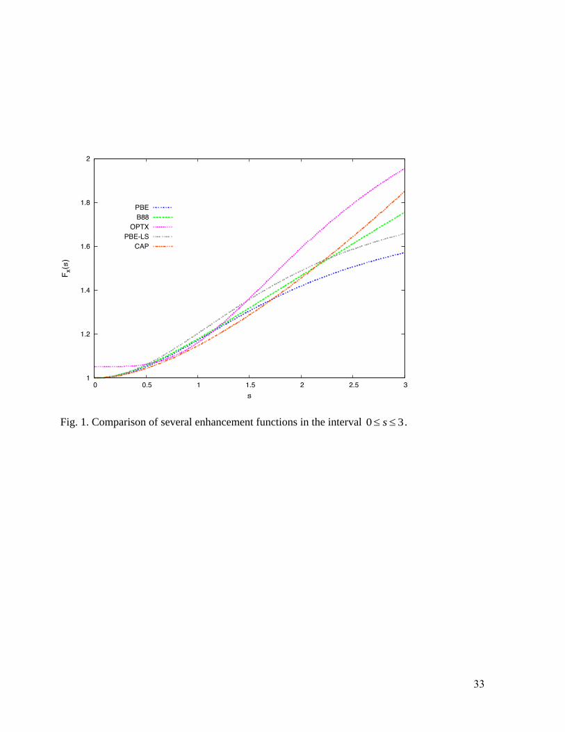
Fig. 1 shows the new X enhancement factor (Eq. (14)), on 0 3s , for xA fixed via

0.2195PBE . Fig. 1 also shows the B88,13

PBE,15

PBE-LS,37

and OPTX16

enhancement factors.

Observe that CAP

xF lies below all the others for s between 0 and about 1.7, after which they all

separate. The B88 form, as noted, was constructed to satisfy Eq. (5), leading to the divergence of

the form given by Eq. (6). Recall also the discussion above about large- s behaviors and satisfaction

of the local Lieb-Oxford bound for various functionals. Also note that the empirical parameters in

the OPTX functional are fixed to obtain the minimum error in the total Hartree-Fock energy of the

first eighteen atoms of the periodic table.

III. Results and discussion

With the objective of improving response properties without sacrificing the quality of

thermodynamic, structural, and kinetic properties obtained with current GGA functionals, we first

considered the consequences of different non-empirical values (recall discussion in Sect. I) and

10

associated xA values to determine which gives the best description of properties that

depend on energy differences. Thus, we did calculations of heats of formation using the G3/99 test

set17

(data for 223 molecules) with the values corresponding to the different non-empirical

values summarized in Sect. I. We used both the PBE15

or LYP14

correlation energy functionals.

The calculations used a developmental version of the program NWChem6.0.82

The protocol for

calculating heats of formation was as established in Ref. [83] and described previously.31

Mean

absolute error (MAE) results for the Def2-TZVPP basis set84

for the different combinations are

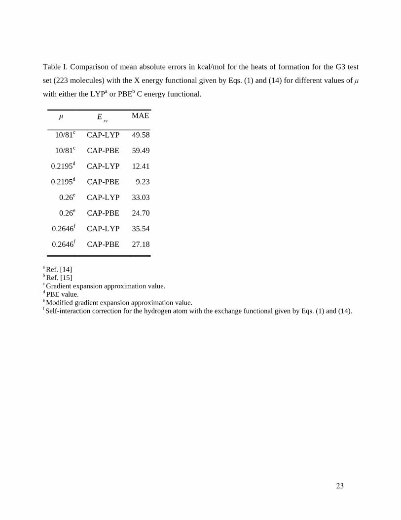
presented in Table I. One sees that the lowest MAE is obtained for from 0.2195PBE , in

combination with the PBE C functional. Next best is CAP X with LYP C for the same μ. Thus, all

subsequent calculations presented in this work were done with ( )CAP

xF s from Eq. (14), with

xA and 0.2195PBE . Recall that the PBE C functional used in Table I corresponds to the

Ma and Brueckner,15,29

value 0.066725 through the relationship 2 / 3 . It has become

common practice to use that relationship between and to fix the value of the latter when μ

different from 0.2195PBE is considered.31,85

We tried that with the PBE C functional and found

MAEs of 65.88 kcal/mol, 28.29 kcal/mol, and 31.21 kcal/mol for 10 / 81 0.1235GEA ,

0.26MGEA , and 0.2646SICH respectively. All those errors are worse than for the

0.066725 of the original PBE C energy.

Comparison calculations used the LDA 86,87

, PBE15

, BLYP,13,14

PBE-LS,37

and OLYP14,16

X

functionals. All calculations were done with the same developmental version of NWChem6.0 and

the same protocol for the heats of formation. Ionization potentials and electron affinities were

obtained for the IP13/319

(6 molecules) and EA13/325

(7 molecules) datasets, respectively. The

molecular calculations were done adiabatically according to the geometries reported in Ref. [88].

Proton affinities were calculated for the PA818,26

dataset (8 molecules). For the geometries of the

anions and neutral species MP2(full)/6-31G (2df,p) calculations were used.89

Binding energies of

weakly interacting systems were carried out for the HB6/04,21

CT7/04,21

DI6/04,21

WI7/05,22

and

PPS5/0522

datasets (31 systems). Ionization potentials, electron affinities, proton affinities and

binding energies were calculated with the 6-31++G(d,p) basis set. Barrier heights for forward and

backward transition states of 19 hydrogen and 19 non-hydrogen transfer reactions were done for the

HTBH38/0422-24,27

and the NHTBH38/0422-24,27

datasets, respectively. Bond distance calculations

11

were done for the T-96R20

dataset (96 molecules). Experimental bond distances for this analysis

were taken from Ref. [90]. Finally, harmonic frequencies were calculated for the T-82F20

dataset

(82 molecules), with experimental values from Refs. [90-92]. Barrier heights, bond distances, and

vibrational frequencies were calculated with the Def2-TZVPP basis set.

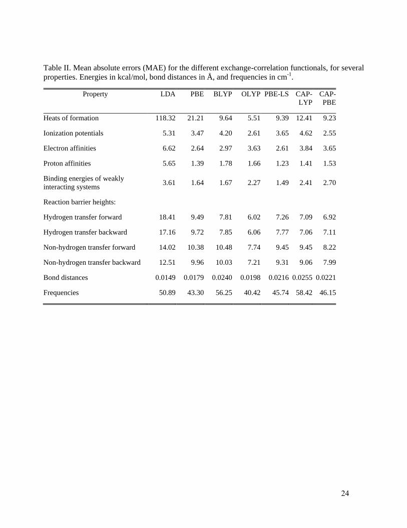
Table II shows the MAE results for those various property comparisons. Individual

deviations for each property are given in the Supplementary Material.77

Clearly CAP-PBE (i.e. CAP

X with PBE correlation C) provides a rather good description of all those properties and is fully

competitive with PBE-LS. Except for the heats of formation, it is fully competitive with OLYP,

which is known to be among the better empirical GGA functionals for thermodynamic, kinetic, and

structural properties. More significant, from the perspective of design choice, is the fact that the

CAP-PBE, PBE-LS, and OLYP enhancement factor functional forms are so qualitatively different.

The difference is particularly striking in the case of PBE-LS and CAP-PBE, which share the same C

functional. Their MAE outcomes are, in general, close to each other, despite opposite behaviors in

the large s limit (PBE-LS goes to zero exponentially while CAP diverges) and distinctly different

behaviors relative to PBE on 0 3s ; recall Fig. 1. The combination of CAP X with LYP C leads

to a somewhat similar description, though generally not as good as the combination with PBE C.

This is especially the case for heats of formation and forward and backward barrier heights of non-

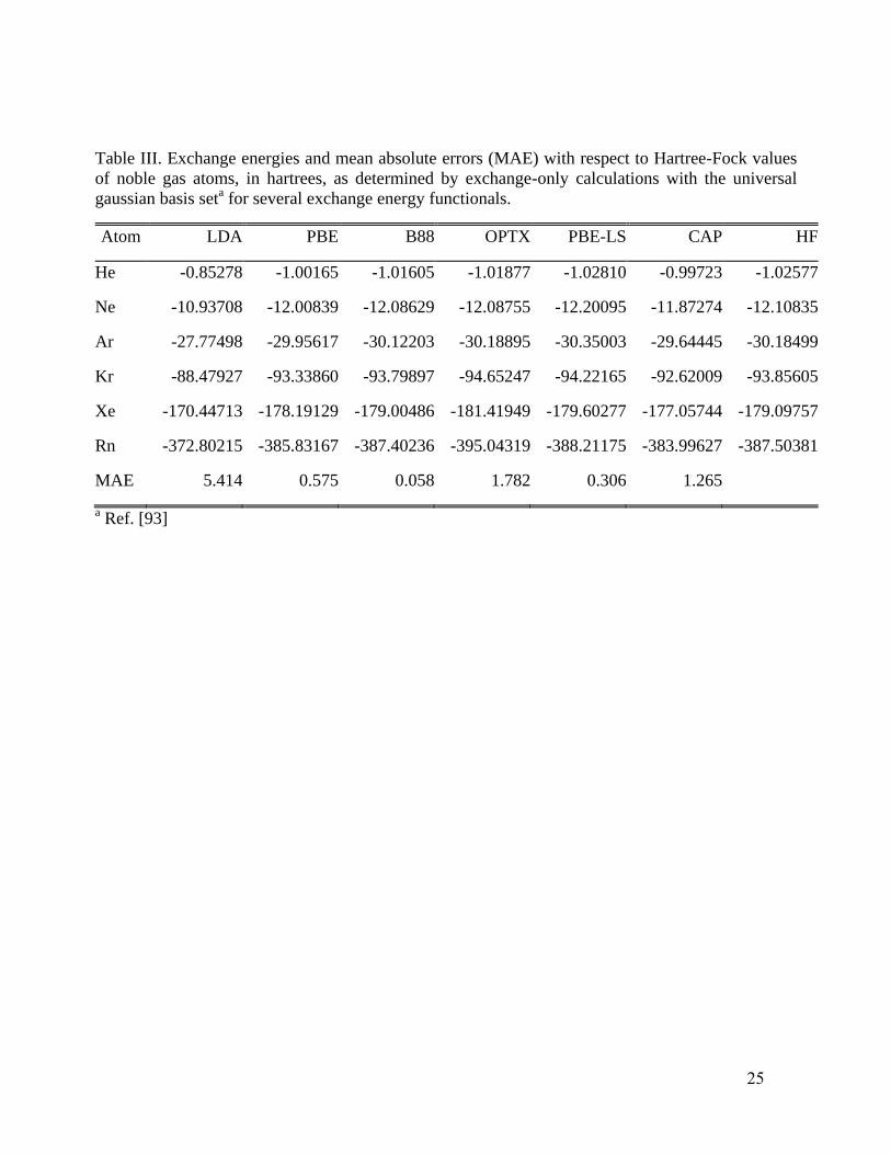
hydrogen transfer reactions. As an additional test of CAP

xF , we performed X-only calculations for

the noble gas atoms to compare CAP

xE values with those from LDA, PBE, B88, PBE-LS, and

OPTX, all referenced to the Hartree-Fock values. The calculations were done using the universal

gaussian basis set93

(UGBS) and the same developmental version of NWChem6.0. See Table III.

Unsurprisingly, B88, which was designed to reproduce HF X energies, is best on this test. PBE-LS,

which is approximately one-electron self-interaction free, is next best. CAP is better than OPTX

but has more than twice the MAE of PBE. These outcomes illustrate the general difficulty of

designing GGA XC functionals. Improvement on one figure of merit often leads to loss of accuracy

on another. Here the emphasis on the accuracy of the X potential has caused a loss of accuracy in

the X energy when compared to the atomic Hartree-Fock values.

For response properties, we calculated static and dynamic polarizabilities and

hyperpolarizabilities via TDDFT recently implemented in time-dependent auxiliary density

perturbation theory (TDADPT) form94-98

in the code deMon2k,pre-release version 4.2.2,99,100

. We

12

used the TZVP-FIP1 basis sets.101,102

TDADPT uses the expansion of the density as a linear

combination of Hermite Gaussian functions103,104

called the auxiliary density in deMon2k. We used

the GEN-A2* auxiliary function set105

for that expansion in all the response calculations. As a

technical matter, we followed the familiar procedure58,106-108

of evaluating the TDDFT kernel

xc xcf v and kernel derivative, 22

xc xc xcg f v in the adiabatic local density

approximation (ALDA). That is, the LDA functional derivatives were used rather than the CAP or

other GGA derivatives. The original rationale for that approximation was (and is) that the GGA

derivatives have complicated internal structure that tends to cause serious numerical instabilities.

These problems could be addressed in the future through the use of analytical rather than numerical

derivatives but at present they are a limitation. It is critical to note, however, that the previous

efforts to mend or repair the incorrect asymptotic potential in TDDFT, which we discussed at the

outset, also used the ALDA derivatives as well. Thus our first principles CAP

xv first must be tested

in the same context. To minimize numerical noise, the XC energy, potential, TDDFT kernel, and

kernel derivative were integrated numerically on the so-called reference grid109

in deMon2k. The

mean polarizabilities were calculated from the diagonal elements of the polarizability tensor

according to

1

( ) ( ) ( ) ( )3

xx yy zz . (15)

For the calculation of hyperpolarizabilities we employed the so-called EFISH (electric-field-

induced second-harmonic) orientation. The average hyperpolarizability was calculated from

3 1 2

1( ; , )

5zii izi iiz

i

, (16)

where i runs over x , y , and z . In all response calculations, experimental molecular structures

were employed.110-113

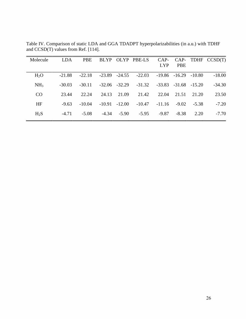
Table IV shows calculated static hyperpolarizabilities of five small molecules, including

both CCSD(T) and TDHF calculations.114

Although TDHF values often exhibit large deviations

from CCSD(T) results, they are presented for completeness. The overall trend from the table is that

either CAP-PBE or CAP-LYP is preferable, but a decisive choice between the two cannot be made

13

from those data alone. In H2O, the CAP-PBE hyperpolarizability is rather close to the CCSD(T)

value, while all other functionals give similar overestimates in absolute value relative to the

CCSD(T) result. For NH3, the CAP-LYP, BLYP, and OLYP results lie very close to the CCSD(T)

value, while the LDA, PBE, PBE-LS, and CAP-PBE values are underestimates (in magnitude). For

CO, all functionals perform similarly, with a modest advantage to BLYP, CAP-LYP, and LDA. For

HF, the CAP-PBE hyperpolarizability is notably closer to the CCSD(T) value, while all other

functionals overestimate the absolute value substantially. In H2S, both the CAP-PBE and CAP-LYP

values are close to that from CCSD(T), while all the other functionals give less negative values.

Table V presents static hyperpolarizabilities of methane analogs with comparisons to

available theoretical results. One sees that for CH3OH, LDA, PBE, PBE-LS, BLYP, and OLYP

static hyperpolarizabilities severely overestimate (absolute values) the published CCSD value115

by

at least 14 a.u. In contrast, CAP-LYP reduces the error substantially, and CAP-PBE essentially

eliminates the error. In CH3F, the signs of our hyperpolarizability results, using EFISH orientation,

differ from the published LDA result but not the published HF one.116

Comparison of absolute

values shows that our LDA, PBE, BLYP, and OLYP hyperpolarizabilities agree well with the LDA

result from Ref. [116]. Both the CAP-PBE and CAP-LYP values differ from all the rest, with CAP-

PBE and Hartree-Fock results116

being relatively close in value and with the same sign. For

CH3CN, CAP-PBE clearly is superior to all the other functionals relative to the CCSD(T)

value,116, whereas PBE, PBE-LS, and CAP-LYP values all are rather similar to the LDA result.116

For the remaining systems reported in Table V, reliable theoretical or experimental values are not

available and the one Hartree-Fock value117

does not seem reasonable in context. Overall, Table V

suggests a preference to CAP-PBE.

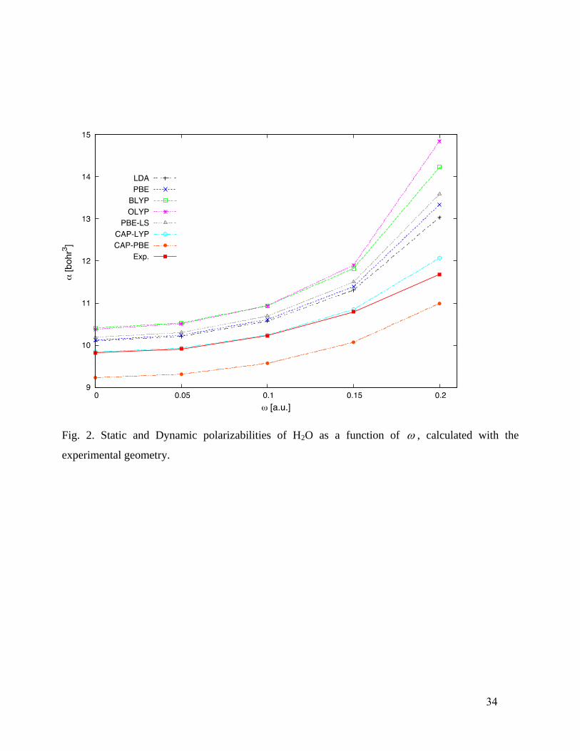
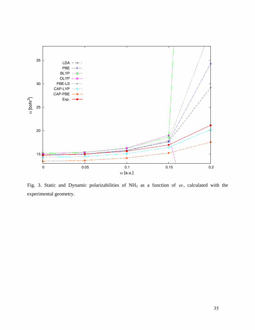
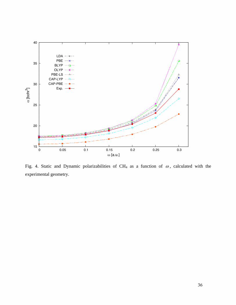
We proceed to the dynamic mean polarizabilities. Figs. 2 – 5 present results for H2O, NH3,

CH4, and benzene respectively, including experimental values. In all cases, the experimental

frequency ranges are considered. For comparison of the theoretical and experimental values, it is

important to bear thermal effects in mind. They are not included in the theoretical values. It is

known that thermal effects shift the theoretical values upward (by about 1 a.u.),118

a key interpretive

fact in assessing the dynamic mean polarizability results.

For H2O, Fig. 2 shows that the LDA, PBE, BLYP, OLYP, and PBE-LS functionals all

overestimate the polarizability, with a frequency dependence which is too strong, even over the

14

relatively small experimental range. Though the CAP-LYP values superficially agree with

experimental values, that is without thermal correction. Thermal corrections will lift the CAP-PBE

values closer to the experimental values, but move the CAP-LYP values above. For NH3 (Fig. 3)

and CH4 (Fig. 4), the only two functionals that give qualitatively correct frequency dependence are

CAP-PBE and CAP-LYP. Thus, thermally corrected CAP-PBE and CAP-LYP are expected to give

a rather satisfactory description.

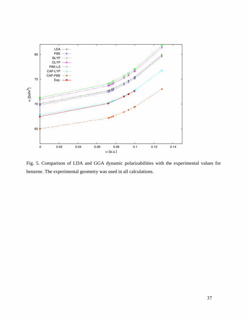
For benzene119

(Fig. 5) the frequency dependence generated by all the functionals is

essentially identical and close to that from experiment. However, all of the other functionals, LDA,

PBE, PBE-LS, BLYP, and OLYP, overestimate the experimental polarizabilities at least by 3 au

before thermal correction, which will worsen the error. The uncorrected CAP-LYP values lie almost

atop experiment but after correction will lie above, while CAP-PBE values will lie below or near

the experimental results.

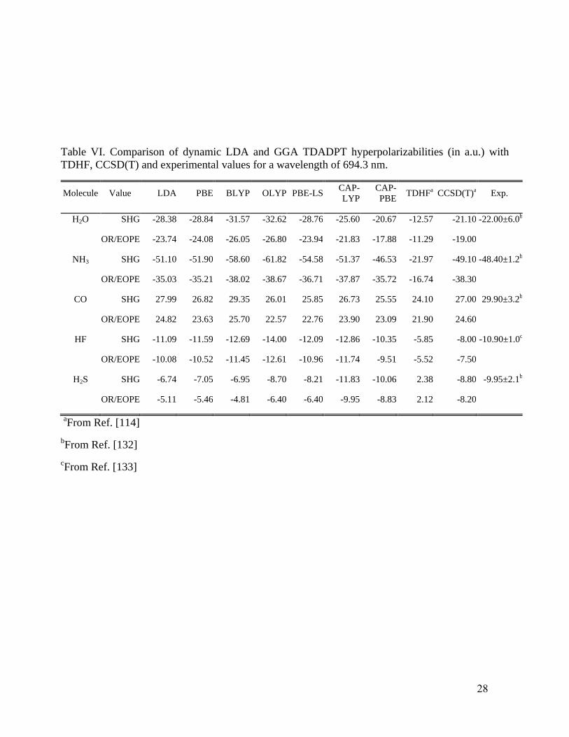
Table VI compares dynamic hyperpolarizabilities of the same five small molecules as in

Table IV with respect to values from CCSD(T) calculations and from experiment. All the

calculations are for the experimental wavelength, 694.3 nm.. For H2O, the CAP-PBE functional

gives values of second-harmonic generation SHG and OR (optical rectification)

hyperpolarizabilities that lie very close to the CCSD(T) results, while all other functionals

overestimate both in absolute value. In NH3, LDA, PBE, PBE-LS, BLYP, OLYP, and CAP-LYP

tend to overestimate the SHG absolute value relative to both CCSD(T) and to experiment, whereas

CAP-PBE lies rather close to the experimental value. The OR absolute values from all functionals

match well with CCSD(T). For CO, LDA, PBE, BLYP and CAP-LYP give SHG and OR

hyperpolarizabilities in good agreement with the reference values, but OLYP, PBE-LS, and CAP-

PBE modestly underestimate them. In the HF molecule, LDA, PBE, and CAP-PBE result agree

well with the SHG and OR references, whereas BLYP, OLYP, and CAP-LYP tend to somewhat

larger overestimated absolute values. For H2S, all functionals give good results. Again, one can see

that overall CAP-PBE is consistently closer to CCSD(T) and experimental results.

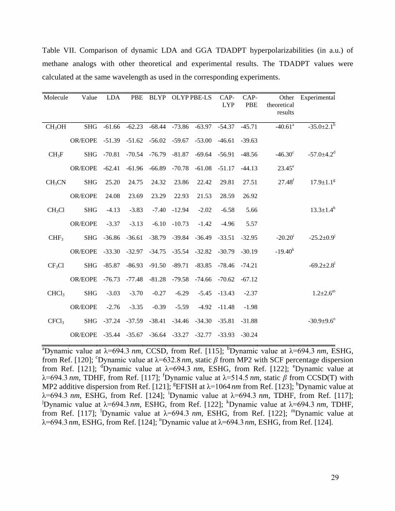
Table VII shows dynamic hyperpolarizabilities for the same methane analogs as were considered in

Table V. All LDA and GGA functional calculations for SHG were done at the same wavelength as

the corresponding experiments. In CH3OH, the SHG result for CAP-PBE is in good agreement with

respect to the CCSD115

and relatively close to the experimental value120

, whereas all the other

15

functionals overestimate the absolute values. Note that this overestimation is partially corrected by

CAP-LYP. For CH3F, for SHG, CAP-PBE gives a result very close to the MP2 hyperpolarizability

augmented with SCF dispersion.121

However, these values underestimate (in absolute value) the

experimental result.122

On the other hand, CAP-LYP agrees very well with experiment, while all the

other functionals yield overestimates (in absolute value). Nevertheless, in all cases the sign of the

hyperpolarizabilities is right, as also was presented in Table VI. For the SHG of CH3CN, CAP-PBE

is in a good agreement with respect to the CCSD(T) hyperpolarizability augmented with MP2

dispersion.121

In general, all functionals and MP2 give overestimates relative to the experimental

value.123

In the case of CH3Cl, for SHG, there is a sign inversion, with CAP-PBE giving one sign

versus the rest of the functionals giving the other. However, the experimental reference124

matches

well with the CAP-PBE value. For SHG in CHF3, all the functionals overestimate the absolute

value compared to the corresponding experiment,122

but once again CAP-PBE is closest to

experiment122

. In CF3Cl, CAP-LYP and CAP-PBE SHG values are very close to experiment, unlike

all the other functionals. For CHCl3, we find a large discrepancy between all functionals and the

experimental reference for SHG.124

However, we have not found theoretical results with which to

compare. All DFT SHG values for CFCl3 look similar, with CAP-PBE lying rather close to the

experimental value.124

In Table VII one can also see OR and EOPE (electro-optical Pockels effect)

values for the same systems, at the same wavelength of the SHG results. Unfortunately, in those

cases we have not found any reference results from highly correlated wavefunctions.

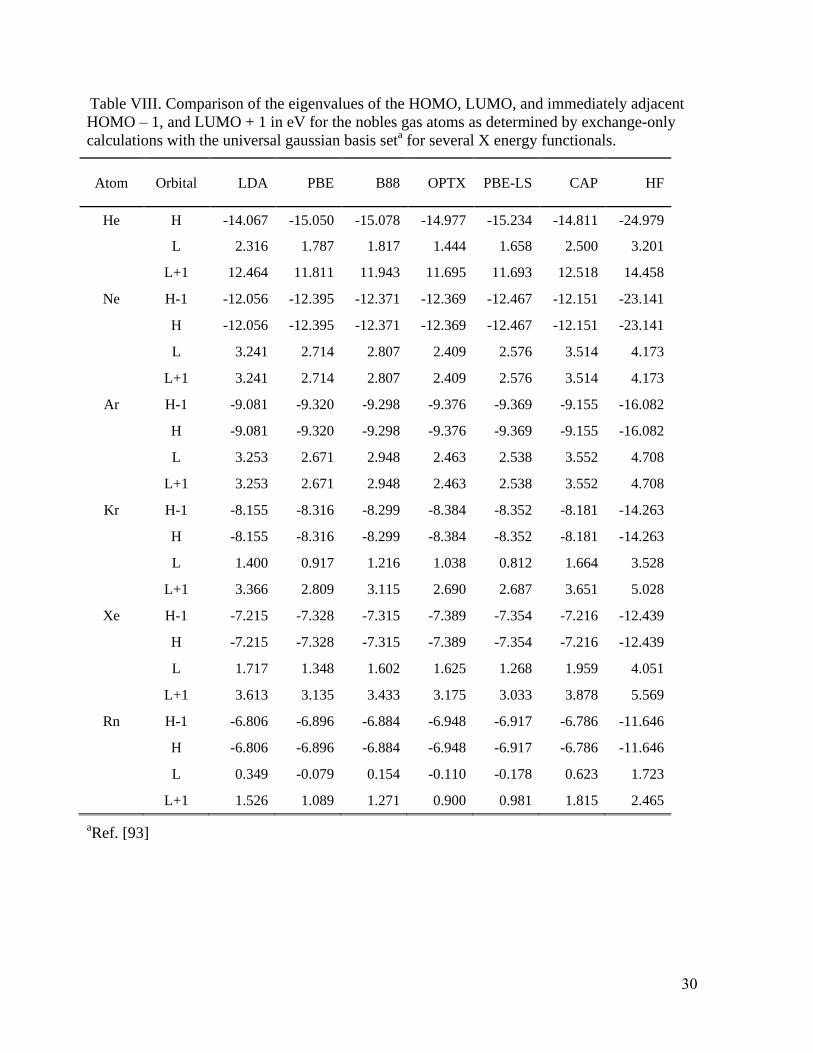
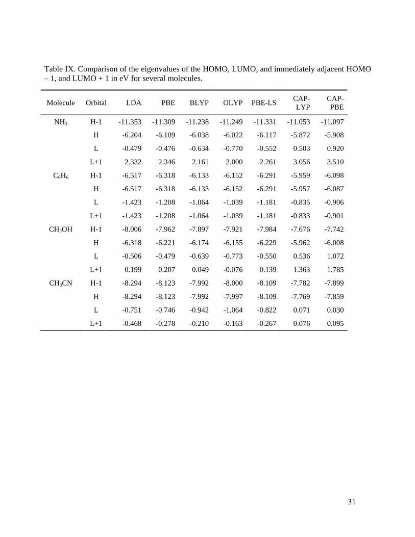
IV. Potential properties

The CAP functional, Eq. (14) provides as good or better results on most of the standard sets

as any other GGA and it does better on response properties than the others. Intriguingly, however,

it does not lead to major changes in the eigenvalues for the highest occupied molecular orbitals but

does affect the lowest unoccupied ones. Table VIII for the noble gas atoms and Table IX for some

molecules illustrates the point with HOMO, LUMO, and immediately adjacent (“HOMO – 1”,

“LUMO + 1”) eigenvalues for several systems and XC functionals. Note that for the Rn atom and

the NH3, CH3OH, and CH3CN molecules, the CAP potential gives a positive energy LUMO, in

contrast with the values from all the other functionals (Teale, De Proft and Tozer125

have reported

such behavior for a potential with the correct asymptotic behavior). Such positive energy states

16

cannot be bound states in a potential which vanishes as -1/r. Rather they occur because of the

confinement provided from the finite-sized L2 basis set

126, so detailed exploration is required,

especially in view of the good response property performance from CAP-PBE.

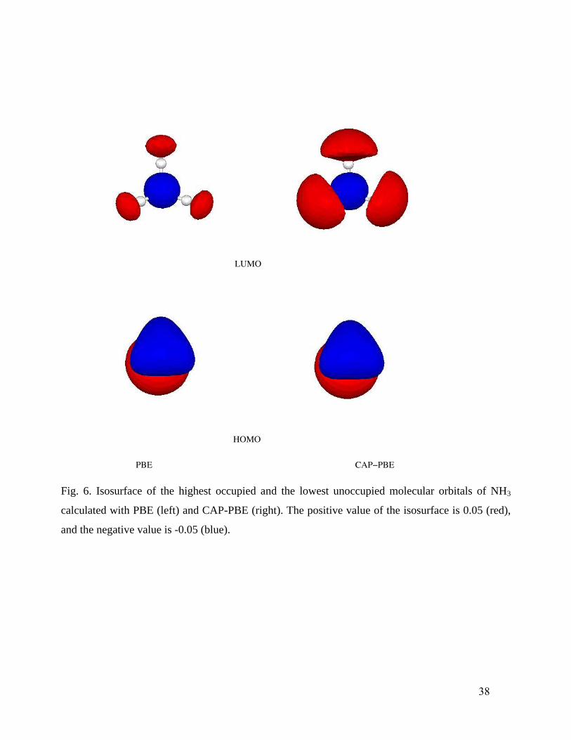
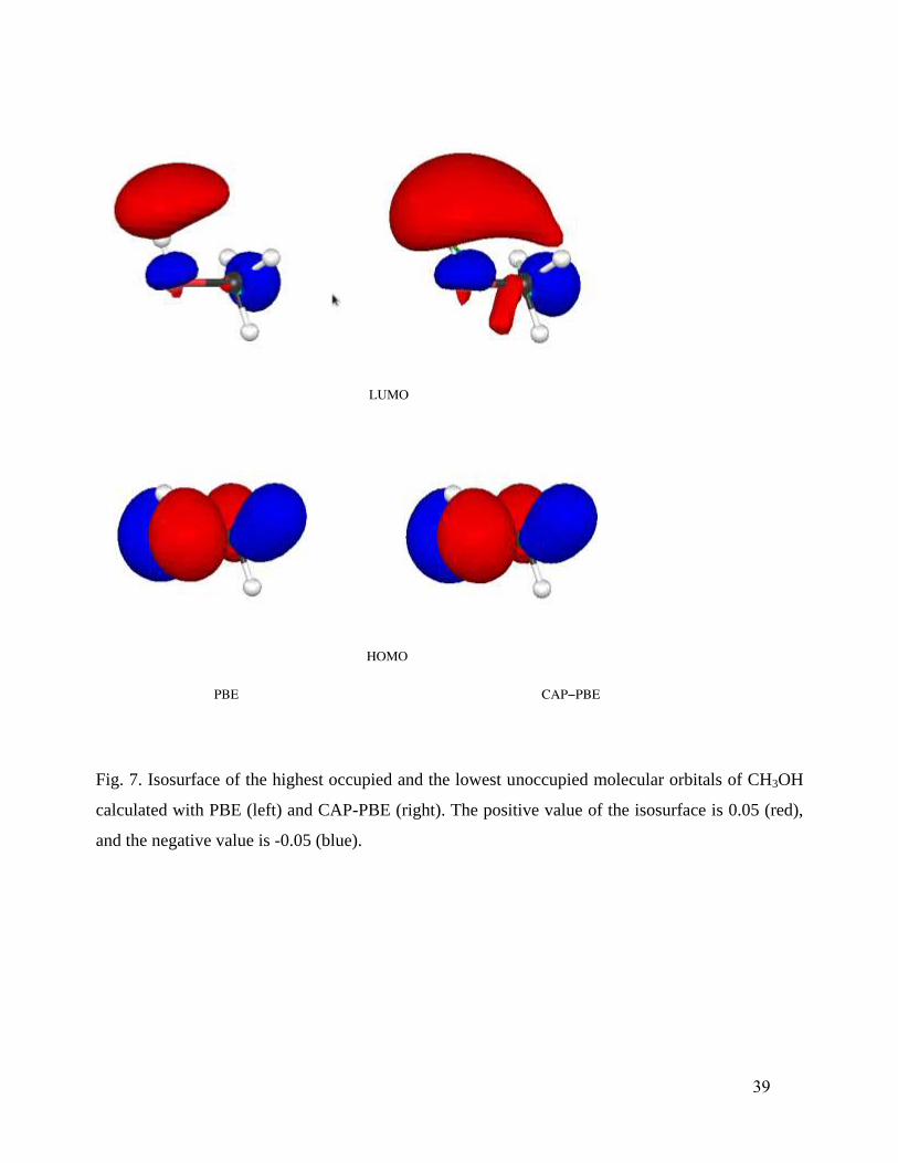
First we observe that, in going from other functionals to CAP, the HOMOs, and particularly

the LUMOs do show slight to large changes in several cases. For example, Fig. 6 shows the slight

shifts from PBE to CAP-PBE in the HOMO and LUMO of NH3, while Fig. 7 shows the

corresponding large changes in CH3OH. These changes in the orbitals seem to be primarily

responsible for the improvement observed in calculated response properties.

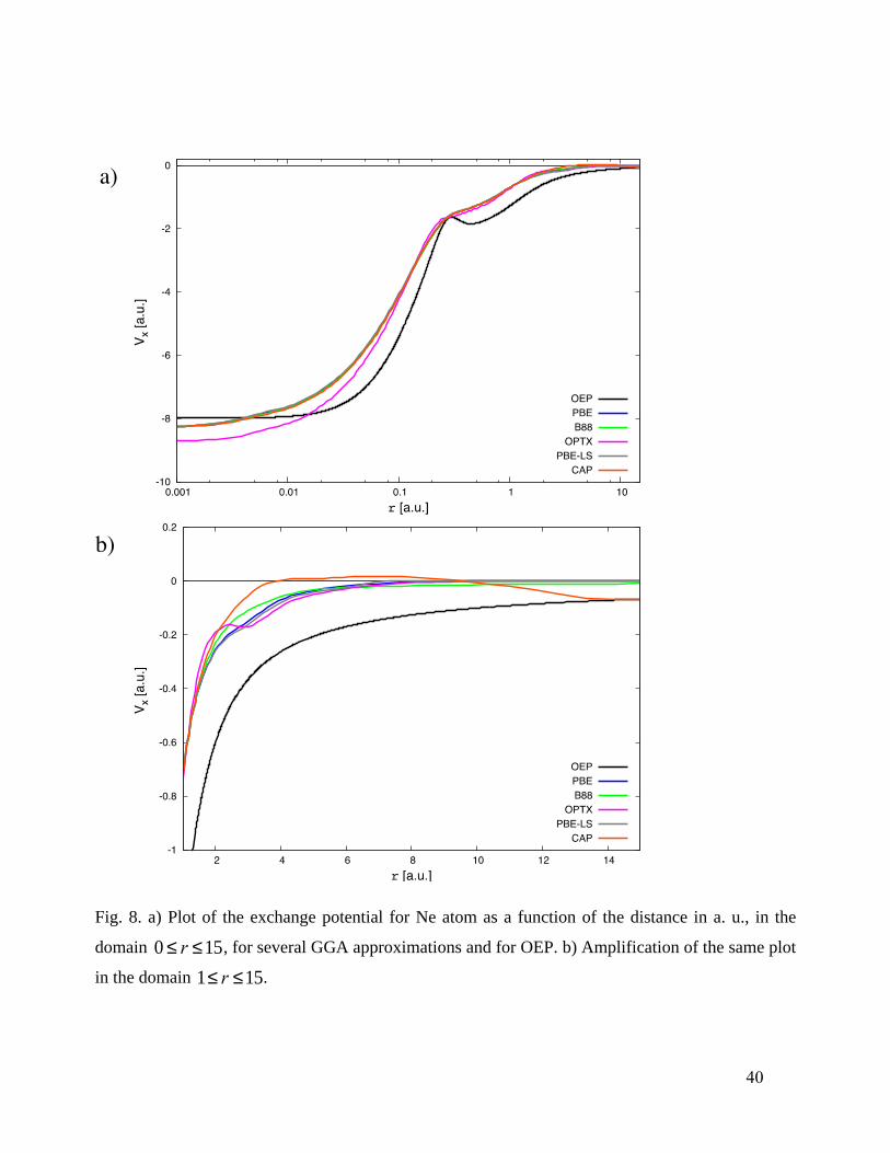
Obviously the orbital changes among X functionals reflect differences in the potentials they

generate. Keep in mind that CAP was constructed to fulfill constraints for 0s and r and to

provide a sensible, smooth connection between those limits. Fig. 8 provides comparison of CAP

xv

with other GGA X potentials and with the optimized effective potential (OEP), plot (a) corresponds

to the domain 0 £ r £15 au, and plot (b) corresponds to an amplification of the domain 1£ r £15

au. The OEP comes from the method of Talman and Shadwick127

and values obtained by Engel and

Vosko.128

All the potentials in Fig. 8 correspond to exchange-only calculations. What one sees is

that CAP

xv has unexpected behavior. In particular, it very closely resembles a standard GGA

potential in the HOMO energy range and below but it is substantially higher than a standard GGA

for larger r and even goes slightly positive. While that weakly positive region is unphysical, the

combination has the pragmatically valuable consequence that the HOMO energy stays roughly

fixed while the LUMO energy goes up, hence the LUMO orbital spreads out. This is not a direct

consequence of the asymptotic condition but instead is an indirect result which occurs because of

the interpolation between large and small s constraints.

That realization leads to a deeper insight. The Engel et al. constraint76

given in Eq. (12) is not

unique. It is a solution of the asymptotic differential equation for GGA

xF (Eq. 11), but not the only

one possible. In particular, Gill and Pople129

give the exact asymptotic behavior of the X

enhancement function for atomic H as 2/3(ln )s s . Thus not only is Eq. (12) not unique, it is

inconsistent with at least one critical case. Imposition of the Gill-Pople asymptotic behavior would

force a different interpolation to the 0s limit, a topic we leave to future work. Similarly we

17

leave for the future the exploration of potentials which go to a constant because of the derivative

discontinuity.56,125,130

V. Concluding remarks

The analysis performed in the previous section confirms that for thermodynamic, kinetic,

and structural properties the behavior of the enhancement function in the interval 0 3s is

crucial. Properties that depend on the response functions should depend upon the large s behavior

associated with the functional derivative that leads to the X potential with the correct asymptotic

behavior. But in practice that behavior can be mimicked in the context of an L2 basis set by a

potential which goes high enough, exactly as CAP

xv does.

The CAP X functional provides a description of properties that depend on total energy

differences superior to or competitive with other GGA X functionals with the additional benefit of

an improved description of properties that depend upon response functions as calculated via

TDDFT in the ALDA. Based on the broad spectrum of quantities treated well by a single

functional, we believe that the non-empirical CAP-PBE recommends itself as the best practical

general purpose GGA XC functional presently available. We now are working to remove the mid-

range positive behavior, improve the correlation functional, and to add features related to the

discontinuity of the exchange-correlation potential and the approximate satisfaction of the

ionization-potential theorem.131

Acknowledgments

We thank the Laboratorio de Supercómputo y Visualización of Universidad Autónoma

Metropolitana-Iztapalapa for the use of their facilities. We also thank Eberhard Engel and Erin

Johnson for providing us with OEP data for the Ne atom, and Jorge Garza for many useful

discussions. JCE was supported in part by Conacyt through a postdoctoral fellowship. JLG thanks

Conacyt for grants 128369 and 155698, and AV thanks Conacyt for grant 128369. SBT was

supported in part by the U.S Dept. of Energy grant DE-SC-0002139.

18

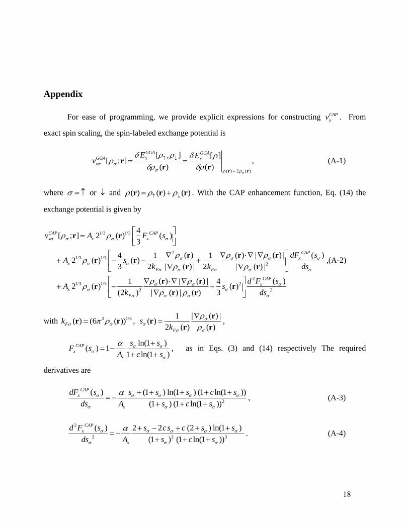
Appendix

For ease of programming, we provide explicit expressions for constructing CAP

xv . From

exact spin scaling, the spin-labeled exchange potential is

( ) 2 ( )

[ , ] [ ][ ; ]

( ) ( )

GGA GGAxGGA x

x

E Ev

r r

rr r

, (A-1)

where or and ( ) ( ) ( )

r r r . With the CAP enhancement function, Eq. (14) the

exchange potential is given by

1/3 1/3

21/3 1/3

2

1/3 1/3

2

4[ ; ] ( )

3

( ) ( ) | ( ) | )4 1 1 ( ) ( )

3 2 | ( ) | 2 | ( ) |

( ) | ( ) |1

2 (

( )(2 )

)

(

| ( ) | (

2

2

CAP CAP

x x x

CAP

xx

F F

x

F

v A F

dF sA s

k k ds

Ak

s

r r

r r rr r

r r

r rr

r r

22

2

)4(

)

()

3

CAP

xd F ss

ds

r

,(A-2)

with 2 1/3( ) (6 ( ))Fk r r , | ( ) |1

( )2 ( ) ( )F

sk

rr

r r,

ln(1 )

( ) 11 ln(1 )

CAP

x

x

s sF s

A c s

, as in Eqs. (3) and (14) respectively The required

derivatives are

2

) (1 ) ln(1 ) (1 ln(1 ))

(1 ) (1 ln(1 )

(

)

CAP

x

x

dF s s s s c s

ds A s c s

, (A-3)

2

2 2 3

) 2 2 (2 ) ln(1 )

(1 ) (1 ln(1 )

(

)

CAP

x

x

d F s s c s c s s

ds A s c s

. (A-4)

19

References

1. P. Hohenberg and W. Kohn, Phys. Rev. B 136, B864 (1964).

2. W. Kohn and L. J. Sham, Phys. Rev. 140, 1133 (1965).

3. R. G. Parr and W. T. Yang, Density-Functional Theory of Atoms and Molecules, (Oxford

University Press, New York, 1989).

4. R. M. Dreizler and E. K. U. Gross, Density Functional Theory, (Springer, Berlin, 1990).

5. J. P. Perdew and S. Kurth, in A Primer in Density Functional Theory, edited by C. Fiolhais, F.

Nogueira, and M. A. L. Marques (Springer, Berlin, 2003), p. 1.

6. J. P. Perdew, A. Ruzsinszky, J. M. Tao, V. N. Staroverov, G. E. Scuseria, and G. I. Csonka, J.

Chem. Phys. 123, 062201 (2005).

7. G. E. Scuseria and V. N. Staroverov, in Theory and Applications of Computational Chemistry:

The First Forty Years, edited by C. Dykstra, G. Frenking, K. S. Kim, and G. E. Scuseria (Elsevier,

Amsterdam, 2005), p. 669.

8. E. Engel and R. M. Dreizler, Density Functional Theory, (Springer-Verlag, Berlin, 2011).

9. A. J. Cohen, P. Mori-Sanchez, and W. T. Yang, Chem. Rev. 112, 289 (2012).

10. K. Burke, J. Chem. Phys. 136, 150901 (2012).

11. A. D. Becke, J. Chem. Phys. 140, 18A301 (2014).

12. J. P. Perdew and K. Schmidt, in Density Functional Theory and its Application to Materials,

edited by V. E. Van Doren, C. Van Alsenoy, and P. Geerlings (AIP, Melville, New York, 2001), p.

1.

13. A. D. Becke, Phys. Rev. A 38, 3098 (1988).

14. C. T. Lee, W. T. Yang, and R. G. Parr, Phys. Rev. B 37, 785 (1988).

15. J. P. Perdew, K. Burke, and M. Ernzerhof, Phys. Rev. Lett. 77, 3865 (1996); erratum 78, 1396

(1997).

16. N. C. Handy and A. J. Cohen, Mol. Phys. 99, 403 (2001).

17. L. A. Curtiss, K. Raghavachari, P. C. Redfern, and J. A. Pople, J. Chem. Phys. 112, 7374

(2000).

18. S. Parthiban and J. M. L. Martin, J. Chem. Phys. 114, 6014 (2001).

19. B. J. Lynch, Y. Zhao, and D. G. Truhlar, J. Phys. Chem. A 107, 1384 (2003).

20. V. N. Staroverov, G. E. Scuseria, J. M. Tao, and J. P. Perdew, J. Chem. Phys. 119, 12129

(2003).

21. Y. Zhao and D. G. Truhlar, J. Chem. Theory Comput. 1, 415 (2005).

22. Y. Zhao and D. G. Truhlar, J. Phys. Chem. A 109, 5656 (2005).

23. Y. Zhao, N. Gonzalez-Garcia, and D. G. Truhlar, J. Phys. Chem. A 109, 2012 (2005).

24. Y. Zhao, B. J. Lynch, and D. G. Truhlar, Phys. Chem. Chem. Phys. 7, 43 (2005).

25. Y. Zhao, N. E. Schultz, and D. G. Truhlar, J. Chem. Theory Comput. 2, 364 (2006).

26. Y. Zhao and D. G. Truhlar, J. Phys. Chem. A 110, 10478 (2006).

27. R. Peverati and D. G. Truhlar, arXiv:1212.0944v4 [physics.chem-ph] (2013).

28. P. R. Antoniewicz and L. Kleinman, Phys. Rev. B 31, 6779 (1985).

29. S. K. Ma and K. A. Brueckner, Phys. Rev. 165, 18 (1968).

30. L. A. Constantin, E. Fabiano, S. Laricchia, and F. Della Sala, Phys. Rev. Lett. 106, 186406

(2011).

31. J. M. del Campo, J. L. Gázquez, S. B. Trickey, and A. Vela, J. Chem. Phys. 136, 104108

(2012).

32. E. H. Lieb and S. Oxford, Int. J. Quantum Chem. 19, 427 (1981).

33. M. Levy and J. P. Perdew, Phys. Rev. B 48, 11638 (1993); erratum 55, 13321 (1997).

20

34. A. Vela, V. Medel, and S. B. Trickey, J. Chem. Phys. 130, 244103 (2009).

35. J. P. Perdew, in Electronic Structure of Solids '91, edited by P. Ziesche and H. Eschrig

(Akademie, Berlin, 1991), p. 11.

36. A. Vela, J. C. Pacheco-Kato, J. L. Gázquez, J. M. del Campo, and S. B. Trickey, J. Chem. Phys.

136, 144115 (2012).

37. J. L. Gázquez, J. M. del Campo, S. B. Trickey, R. J. Alvarez-Mendez, and A. Vela, in Concepts

and Methods in Modern Theoretical Chemistry, edited by S. K. Ghosh and P. K. Chattaraj (CRC

Press, Boca Raton, 2013), p. 295.

38. S. Kurth, J. Mol. Struc. (Theochem) 501, 189 (2000).

39. L. Pollack and J. P. Perdew, J. Phys.: Condens. Matter 12, 1239 (2000).

40. L. Chiodo, L. A. Constantin, E. Fabiano, and F. Della Sala, Phys. Rev. Lett. 108 (2012).

41. J. P. Perdew, A. Ruzsinszky, J. Sun, and K. Burke, J. Chem. Phys. 140, 18A533 (2014).

42. D. J. Lacks and R. G. Gordon, Phys. Rev. A 47, 4681 (1993).

43. R. van Leeuwen and E. J. Baerends, Phys. Rev. A 49, 2421 (1994).

44. J. P. Perdew and W. Yue, Phys. Rev. B 33, 8800 (1986).

45. E. D. Murray, K. Lee, and D. C. Langreth, J. Chem. Theory Comput. 5, 2754 (2009).

46. M. Petersilka, U. J. Gossmann, and E. K. U. Gross, Phys. Rev. Lett. 76, 1212 (1996).

47. M. E. Casida, in Recent Developments and Applications in Density Functional Theory, edited

by J. M. Seminario (Elsevier, Amsterdam, 1996), p. 391.

48. P. Bleiziffer, A. Hesselmann, C. J. Umrigar, and A. Görling, Phys. Rev. A 88, 042513 (2013).

49. J. P. Perdew and M. Levy, Phys. Rev. Lett. 51, 1884 (1983).

50. L. J. Sham and M. Schluter, Phys. Rev. Lett. 51, 1888 (1983).

51. J. P. Perdew, R. G. Parr, M. Levy, and J. L. Balduz, Phys. Rev. Lett. 49, 1691 (1982).

52. W. T. Yang, A. J. Cohen, and P. Mori-Sanchez, J. Chem. Phys. 136, 204111 (2012).

53. L. J. Sham, Phys. Rev. B 32, 3876 (1985).

54. C. O. Almbladh and U. vonBarth, Phys. Rev. B 31, 3231 (1985).

55. M. K. Harbola and V. Sahni, Phys. Rev. Lett. 62, 489 (1989).

56. D. J. Tozer and N. C. Handy, J. Chem. Phys. 109, 10180 (1998).

57. M. E. Casida and D. R. Salahub, J. Chem. Phys. 113, 8918 (2000).

58. M. Gruning, O. V. Gritsenko, S. J. A. van Gisbergen, and E. J. Baerends, J. Chem. Phys. 114,

652 (2001).

59. J. L. Gázquez, J. Garza, F. D. Hinojosa, and A. Vela, J. Chem. Phys. 126, 214105 (2007).

60. J. L. Gázquez, J. Garza, R. Vargas, and A. Vela, in Recent Developments in Physical Chemistry,

edited by E. Diaz-Herrera and E. Juaristi (2008), Vol. 979, p. 11.

61. A. Lembarki, F. Rogemond, and H. Chermette, Phys. Rev. A 52, 3704 (1995).

62. M. Gruning, O. V. Gritsenko, S. J. A. van Gisbergen, and E. J. Baerends, J. Chem. Phys. 116,

9591 (2002).

63. Q. Wu, P. W. Ayers, and W. T. Yang, J. Chem. Phys. 119, 2978 (2003).

64. A. Karolewski, R. Armiento, and S. Kummel, Phys. Rev. A 88, 052519 (2013).

65. M. Filatov and W. Thiel, Phys. Rev. A 57, 189 (1998).

66. P. Jemmer and P. J. Knowles, Phys. Rev. A 51, 3571 (1995).

67. E. Engel and S. H. Vosko, Phys. Rev. B 50, 10498 (1994).

68. J. Garza, J. A. Nichols, and D. A. Dixon, J. Chem. Phys. 112, 7880 (2000).

69. J. Garza, J. A. Nichols, and D. A. Dixon, J. Chem. Phys. 112, 1150 (2000).

70. N. Umezawa, Phys. Rev. A 74, 032505 (2006).

71. A. P. Gaiduk, D. Mizzi, and V. N. Staroverov, Phys. Rev. A 86, 052518 (2012).

72. A. P. Gaiduk, D. S. Firaha, and V. N. Staroverov, Phys. Rev. Lett. 108, 253005 (2012).

21

73. M. Hoffmann-Ostenhof and T. Hoffmann-Ostenhof, Phys. Rev. A 16, 1782 (1977).

74. Y. Tal, Phys. Rev. A 18, 1781 (1978).

75. M. Levy, J. P. Perdew, and V. Sahni, Phys. Rev. A 30, 2745 (1984).

76. E. Engel, J. A. Chevary, L. D. Macdonald, and S. H. Vosko, Z. Phys. D: At., Mol. Clusters 23, 7

(1992).

77. See Supplementary Material at [URL will be inserted by AIP].

78. A. Zupan, J. P. Perdew, K. Burke, and M. Causà, Int. J. Quantum Chem. 61, 835 (1997).

79. A. Zupan, K. Burke, M. Emzerhof, and J. P. Perdew, J. Chem. Phys. 106, 10184 (1997).

80. J. M. del Campo, J. L. Gázquez, R. J. Alvarez-Mendez, and A. Vela, Int. J. Quantum Chem.

112, 3594 (2012).

81. R. Armiento and S. Kummel, Phys. Rev. Lett. 111, 036402 (2013).

82. M. Valiev, E. J. Bylaska, N. Govind, K. Kowalski, T. P. Straatsma, H. J. J. Van Dam, D. Wang,

J. Nieplocha, E. Apra, T. L. Windus, and W. de Jong, Comput. Phys. Commun. 181, 1477 (2010).

83. L. A. Curtiss, K. Raghavachari, P. C. Redfern, and J. A. Pople, J. Chem. Phys. 106, 1063

(1997).

84. F. Weigend and R. Ahlrichs, Phys. Chem. Chem. Phys. 7, 3297 (2005).

85. E. Fabiano, L. A. Constantin, and F. Della Sala, J. Chem. Theory Comput. 7, 3548 (2011).

86. P. A. M. Dirac, Proc. Cambridge Philos. Soc. 26, 376 (1930).

87. S. H. Vosko, L. Wilk, and M. Nusair, Can. J. Phys. 58, 1200 (1980).

88. B. J. Lynch, Y. Zhao, and D. G. Truhlar, http://t1.chem.umn.edu/db/.

89. L. A. Curtis, P. C. Redfern, and K. Raghavachari, in Wiley Interdisciplinary Reviews:

Computational Molecular Science (Wiley, 2011), Vol. 1, p. 810.

90. CRC Handbook of Chemistry and Physics, 83rd ed, (CRC, Boca Raton, FL, 2002).

91. J. M. L. Martin, Chem. Phys. Lett. 303, 399 (1999).

92. K. P. Huber and G. Herzberg, Molecular Spectra and Molecular Structure IV. Constants of

Diatomic Molecules, (Van Nostrand, New York, 1979).

93. E. V. R. de Castro and F. E. Jorge, J. Chem. Phys. 108, 5225 (1998).

94. S. V. Shedge, J. Carmona-Espíndola, S. Pal, and A. M. Köster, J. Phys. Chem. A 114, 2357

(2010).

95. J. Carmona-Espíndola, R. Flores-Moreno, and A. M. Köster, J. Chem. Phys. 133, 084102

(2010).

96. J. Carmona-Espíndola, R. Flores-Moreno, and A. M. Köster, Int. J. Quantum Chem. 112, 3461

(2012).

97. P. Calaminici, J. Carmona-Espíndola, G. Geudtner, and A. M. Köster, Int. J. Quantum Chem.

112, 3252 (2012).

98. S. V. Shedge, S. Pal, and A. M. Köster, Chem. Phys. Lett. 552, 146 (2012).

99. A. M. Köster, G. Geudtner, P. Calaminici, M. E. Casida, V. D. Dominguez-Soria, R. Flores-

Moreno, G. U. Gamboa, A. Goursot, T. Heine, A. Ipatov, F. Janetzko, J. M. del Campo, J. U.

Reveles, A. Vela, B. Zuñiga-Gutierrez, and D. R. Salahub, deMon2k, Version 3, The deMon

Developers, Cinvestav, México (2011).

100. G. Geudtner, P. Calaminici, J. Carmona-Espíndola, J. M. del Campo, V. D. Dominguez-Soria,

R. Flores-Moreno, G. U. Gamboa, A. Goursot, A. M. Köster, J. U. Reveles, T. Mineva, J. M.

Vasquez-Perez, A. Vela, B. Zuñiga-Gutierrez, and D. R. Salahub, Wiley Interdisciplinary Reviews:

Computational Molecular Science 2, 548 (2012).

101. P. Calaminici, K. Jug, and A. M. Köster, J. Chem. Phys. 109, 7756 (1998).

102. P. Calaminici, K. Jug, A. M. Köster, V. E. Ingamells, and M. G. Papadopoulos, J. Chem. Phys.

112, 6301 (2000).

22

103. J. C. Boettger and S. B. Trickey, Phys. Rev. B 53, 3007 (1996).

104. A. M. Köster, J. Chem. Phys. 118, 9943 (2003).

105. P. Calaminici, F. Janetzko, A. M. Köster, R. Mejia-Olvera, and B. Zuniga-Gutierrez, J. Chem.

Phys. 126, 044108 (2007).

106. S. J. A. van Gisbergen, J. G. Snijders, and E. J. Baerends, J. Chem. Phys. 109, 10657 (1998).

107. M. Stener, G. Fronzoni, and M. de Simone, Chem. Phys. Lett. 373, 115 (2003).

108. M. Seth, G. Mazur, and T. Ziegler, Theoretical Chemistry Accounts 129, 331 (2011).

109. A. M. Köster, R. Flores-Moreno, and J. U. Reveles, J. Chem. Phys. 121, 681 (2004).

110. G. Herzberg, Electronic Spectra and Electronic Structure of Polyatomic Molecules, (Van

Nostrand Reinhold Company, New York, 1966).

111. J. H. Callomon, E. Hirota, K. Kuchitsu, W. J. Lafferty, A. G. Maki, and C. S. Pote, Landolt-

Bornstein: Group II, Atomic and Molecular Physics, Volume 7, Structure Data of Free Polyatomic

Molecules, (Springer-Verlag, Berlin, 1976).

112. K. Kuchitsu, Landolt-Bornstein: Group II, Molecules and Radicals, Volume 25, Structure

Data of Free Polyatomic Molecules, (Springer-Verlag, Berlin, 1999).

113. M. W. Chase, C. A. Davies, J. R. Downey, D. J. Frurip, R. A. McDonald, and A. N. Syverud,

in JANAF Thermochemical Tables, Third Edition, J. Phys. Chem. Ref. Vol. 14, Suppl. 1 (1985).

114. H. Sekino and R. J. Bartlett, J. Chem. Phys. 98, 3022 (1993).

115. A. S. Dutra, M. A. Castro, T. L. Fonseca, E. E. Fileti, and S. Canuto, J. Chem. Phys. 132,

034307 (2010).

116. A. M. Lee and S. M. Colwell, J. Chem. Phys. 101, 9704 (1994).

117. H. Sekino and R. J. Bartlett, J. Chem. Phys. 85, 976 (1986).

118. G. U. Gamboa, P. Calaminici, G. Geudtner, and A. M. Köster, J. Phys. Chem. A 112, 11969

(2008).

119. G. R. Alms, A. K. Burnham, and W. H. Flygare, J. Chem. Phys. 63, 3321 (1975).

120. G. Maroulis, Chem. Phys. Lett. 195, 85 (1992).

121. D. P. Shelton and J. E. Rice, Chem. Rev. 94, 3 (1994).

122. J. F. Ward and I. J. Bigio, Phys. Rev. A 11, 60 (1975).

123. P. Kaatz, E. A. Donley, and D. P. Shelton, J. Chem. Phys. 108, 849 (1998).

124. C. K. Miller and J. F. Ward, Phys. Rev. A 16, 1179 (1977).

125. A. M. Teale, F. De Proft, and D. J. Tozer, J. Chem. Phys. 129, 044110 (2008).

126. N. Rosch and S. B. Trickey, J. Chem. Phys. 106, 8940 (1997).

127. J. D. Talman and W. F. Shadwick, Phys. Rev. A 14, 36 (1976).

128. E. Engel and S. H. Vosko, Phys. Rev. A 47, 2800 (1993).

129. P. M. W. Gill and J. A. Pople, Phys. Rev. A 47, 2383 (1993).

130. D. J. Tozer, Phys. Rev. A 56, 2726 (1997).

131. J. P. Perdew and M. Levy, Phys. Rev. B 56, 16021 (1997).

132. J. F. Ward and C. K. Miller, Phys. Rev. A 19, 826 (1979).

133. J. W. Dudley and J. F. Ward, J. Chem. Phys. 82, 4673 (1985).

23

Table I. Comparison of mean absolute errors in kcal/mol for the heats of formation for the G3 test

set (223 molecules) with the X energy functional given by Eqs. (1) and (14) for different values of μ

with either the LYPa or PBE

b C energy functional.

μ E xc

MAE

10/81c CAP-LYP 49.58

10/81c CAP-PBE 59.49

0.2195d CAP-LYP 12.41

0.2195d CAP-PBE 9.23

0.26e CAP-LYP 33.03

0.26e CAP-PBE 24.70

0.2646f CAP-LYP 35.54

0.2646f CAP-PBE 27.18

a Ref. [14]

b Ref. [15] c Gradient expansion approximation value. d PBE value. e Modified gradient expansion approximation value. f Self-interaction correction for the hydrogen atom with the exchange functional given by Eqs. (1) and (14).

24

Table II. Mean absolute errors (MAE) for the different exchange-correlation functionals, for several

properties. Energies in kcal/mol, bond distances in Å, and frequencies in cm-1

.

Property LDA PBE BLYP OLYP PBE-LS CAP-

LYP

CAP-

PBE

Heats of formation 118.32 21.21 9.64 5.51 9.39 12.41 9.23

Ionization potentials 5.31 3.47 4.20 2.61 3.65 4.62 2.55

Electron affinities 6.62 2.64 2.97 3.63 2.61 3.84 3.65

Proton affinities 5.65 1.39 1.78 1.66 1.23 1.41 1.53

Binding energies of weakly

interacting systems 3.61 1.64 1.67 2.27 1.49 2.41 2.70

Reaction barrier heights:

Hydrogen transfer forward 18.41 9.49 7.81 6.02 7.26 7.09 6.92

Hydrogen transfer backward 17.16 9.72 7.85 6.06 7.77 7.06 7.11

Non-hydrogen transfer forward 14.02 10.38 10.48 7.74 9.45 9.45 8.22

Non-hydrogen transfer backward 12.51 9.96 10.03 7.21 9.31 9.06 7.99

Bond distances 0.0149 0.0179 0.0240 0.0198 0.0216 0.0255 0.0221

Frequencies 50.89 43.30 56.25 40.42 45.74 58.42 46.15

25

Table III. Exchange energies and mean absolute errors (MAE) with respect to Hartree-Fock values

of noble gas atoms, in hartrees, as determined by exchange-only calculations with the universal

gaussian basis seta for several exchange energy functionals.

Atom LDA PBE B88 OPTX PBE-LS CAP HF

He -0.85278 -1.00165 -1.01605 -1.01877 -1.02810 -0.99723 -1.02577

Ne -10.93708 -12.00839 -12.08629 -12.08755 -12.20095 -11.87274 -12.10835

Ar -27.77498 -29.95617 -30.12203 -30.18895 -30.35003 -29.64445 -30.18499

Kr -88.47927 -93.33860 -93.79897 -94.65247 -94.22165 -92.62009 -93.85605

Xe -170.44713 -178.19129 -179.00486 -181.41949 -179.60277 -177.05744 -179.09757

Rn -372.80215 -385.83167 -387.40236 -395.04319 -388.21175 -383.99627 -387.50381

MAE 5.414 0.575 0.058 1.782 0.306 1.265

a Ref. [93]

26

Table IV. Comparison of static LDA and GGA TDADPT hyperpolarizabilities (in a.u.) with TDHF

and CCSD(T) values from Ref. [114].

Molecule LDA PBE BLYP OLYP PBE-LS CAP-

LYP

CAP-

PBE

TDHF CCSD(T)

H2O -21.88 -22.18 -23.89 -24.55 -22.03 -19.86 -16.29 -10.80 -18.00

NH3 -30.03 -30.11 -32.06 -32.29 -31.32 -33.83 -31.68 -15.20 -34.30

CO 23.44 22.24 24.13 21.09 21.42 22.04 21.51 21.20 23.50

HF -9.63 -10.04 -10.91 -12.00 -10.47 -11.16 -9.02 -5.38 -7.20

H2S -4.71 -5.08 -4.34 -5.90 -5.95 -9.87 -8.38 2.20 -7.70

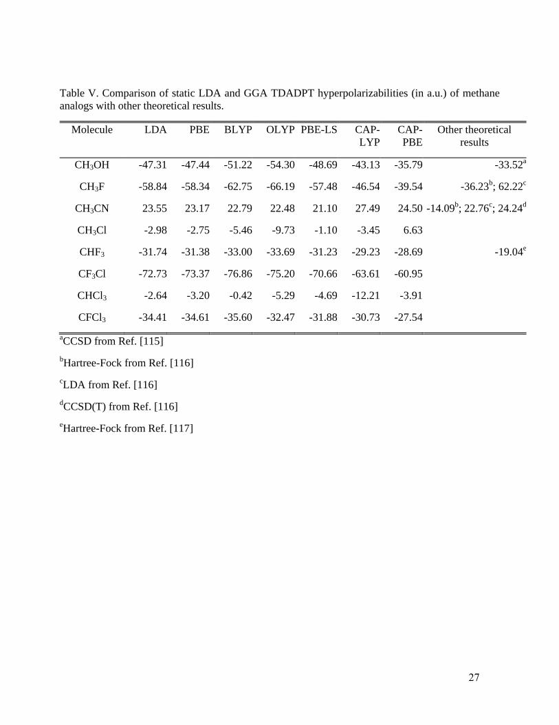
27

Table V. Comparison of static LDA and GGA TDADPT hyperpolarizabilities (in a.u.) of methane

analogs with other theoretical results.

Molecule LDA PBE BLYP OLYP PBE-LS CAP-

LYP

CAP-

PBE

Other theoretical

results

CH3OH -47.31 -47.44 -51.22 -54.30 -48.69 -43.13 -35.79 -33.52a

CH3F -58.84 -58.34 -62.75 -66.19 -57.48 -46.54 -39.54 -36.23b; 62.22

c

CH3CN 23.55 23.17 22.79 22.48 21.10 27.49 24.50 -14.09b; 22.76

c; 24.24

d

CH3Cl -2.98 -2.75 -5.46 -9.73 -1.10 -3.45 6.63

CHF3 -31.74 -31.38 -33.00 -33.69 -31.23 -29.23 -28.69 -19.04e

CF3Cl -72.73 -73.37 -76.86 -75.20 -70.66 -63.61 -60.95

CHCl3 -2.64 -3.20 -0.42 -5.29 -4.69 -12.21 -3.91

CFCl3 -34.41 -34.61 -35.60 -32.47 -31.88 -30.73 -27.54

aCCSD from Ref. [115]

bHartree-Fock from Ref. [116]

cLDA from Ref. [116]

dCCSD(T) from Ref. [116]

eHartree-Fock from Ref. [117]

28

Table VI. Comparison of dynamic LDA and GGA TDADPT hyperpolarizabilities (in a.u.) with

TDHF, CCSD(T) and experimental values for a wavelength of 694.3 nm.

Molecule Value LDA PBE BLYP OLYP PBE-LS CAP-

LYP

CAP-

PBE TDHFa CCSD(T)a Exp.

H2O SHG -28.38 -28.84 -31.57 -32.62 -28.76 -25.60 -20.67 -12.57 -21.10 -22.00±6.0b

OR/EOPE -23.74 -24.08 -26.05 -26.80 -23.94 -21.83 -17.88 -11.29 -19.00

NH3 SHG -51.10 -51.90 -58.60 -61.82 -54.58 -51.37 -46.53 -21.97 -49.10 -48.40±1.2b

OR/EOPE -35.03 -35.21 -38.02 -38.67 -36.71 -37.87 -35.72 -16.74 -38.30

CO SHG 27.99 26.82 29.35 26.01 25.85 26.73 25.55 24.10 27.00 29.90±3.2b

OR/EOPE 24.82 23.63 25.70 22.57 22.76 23.90 23.09 21.90 24.60

HF SHG -11.09 -11.59 -12.69 -14.00 -12.09 -12.86 -10.35 -5.85 -8.00 -10.90±1.0c

OR/EOPE -10.08 -10.52 -11.45 -12.61 -10.96 -11.74 -9.51 -5.52 -7.50

H2S SHG -6.74 -7.05 -6.95 -8.70 -8.21 -11.83 -10.06 2.38 -8.80 -9.95±2.1b

OR/EOPE -5.11 -5.46 -4.81 -6.40 -6.40 -9.95 -8.83 2.12 -8.20

aFrom Ref. [114]

bFrom Ref. [132]

cFrom Ref. [133]

29

Table VII. Comparison of dynamic LDA and GGA TDADPT hyperpolarizabilities (in a.u.) of

methane analogs with other theoretical and experimental results. The TDADPT values were

calculated at the same wavelength as used in the corresponding experiments.

Molecule Value LDA PBE BLYP OLYP PBE-LS CAP-

LYP

CAP-

PBE

Other

theoretical

results

Experimental

CH3OH SHG -61.66 -62.23 -68.44 -73.86 -63.97 -54.37 -45.71 -40.61a -35.0±2.1b

OR/EOPE -51.39 -51.62 -56.02 -59.67 -53.00 -46.61 -39.63

CH3F SHG -70.81 -70.54 -76.79 -81.87 -69.64 -56.91 -48.56 -46.30c -57.0±4.2d

OR/EOPE -62.41 -61.96 -66.89 -70.78 -61.08 -51.17 -44.13 23.45e

CH3CN SHG 25.20 24.75 24.32 23.86 22.42 29.81 27.51 27.48f 17.9±1.1g

OR/EOPE 24.08 23.69 23.29 22.93 21.53 28.59 26.92

CH3Cl SHG -4.13 -3.83 -7.40 -12.94 -2.02 -6.58 5.66 13.3±1.4h

OR/EOPE -3.37 -3.13 -6.10 -10.73 -1.42 -4.96 5.57

CHF3 SHG -36.86 -36.61 -38.79 -39.84 -36.49 -33.51 -32.95 -20.20i -25.2±0.9j

OR/EOPE -33.30 -32.97 -34.75 -35.54 -32.82 -30.79 -30.19 -19.40k

CF3Cl SHG -85.87 -86.93 -91.50 -89.71 -83.85 -78.46 -74.21 -69.2±2.8l

OR/EOPE -76.73 -77.48 -81.28 -79.58 -74.66 -70.62 -67.12

CHCl3 SHG -3.03 -3.70 -0.27 -6.29 -5.45 -13.43 -2.37 1.2±2.6m

OR/EOPE -2.76 -3.35 -0.39 -5.59 -4.92 -11.48 -1.98

CFCl3 SHG -37.24 -37.59 -38.41 -34.46 -34.30 -35.81 -31.88 -30.9±9.6n

OR/EOPE -35.44 -35.67 -36.64 -33.27 -32.77 -33.93 -30.24

aDynamic value at λ=694.3 nm, CCSD, from Ref. [115];

bDynamic value at λ=694.3 nm, ESHG,

from Ref. [120]; cDynamic value at λ=632.8 nm, static β from MP2 with SCF percentage dispersion

from Ref. [121]; dDynamic value at λ=694.3 nm, ESHG, from Ref. [122];

eDynamic value at

λ=694.3 nm, TDHF, from Ref. [117]; fDynamic value at λ=514.5 nm, static β from CCSD(T) with

MP2 additive dispersion from Ref. [121]; gEFISH at λ=1064 nm from Ref. [123];

hDynamic value at

λ=694.3 nm, ESHG, from Ref. [124]; iDynamic value at λ=694.3 nm, TDHF, from Ref. [117];

jDynamic value at λ=694.3 nm, ESHG, from Ref. [122];

kDynamic value at λ=694.3 nm, TDHF,

from Ref. [117]; lDynamic value at λ=694.3 nm, ESHG, from Ref. [122];

mDynamic value at

λ=694.3 nm, ESHG, from Ref. [124]; nDynamic value at λ=694.3 nm, ESHG, from Ref. [124].

30

Table VIII. Comparison of the eigenvalues of the HOMO, LUMO, and immediately adjacent

HOMO – 1, and LUMO + 1 in eV for the nobles gas atoms as determined by exchange-only

calculations with the universal gaussian basis seta for several X energy functionals.

Atom Orbital LDA PBE B88 OPTX PBE-LS CAP HF

He H -14.067 -15.050 -15.078 -14.977 -15.234 -14.811 -24.979

L 2.316 1.787 1.817 1.444 1.658 2.500 3.201

L+1 12.464 11.811 11.943 11.695 11.693 12.518 14.458

Ne H-1 -12.056 -12.395 -12.371 -12.369 -12.467 -12.151 -23.141

H -12.056 -12.395 -12.371 -12.369 -12.467 -12.151 -23.141

L 3.241 2.714 2.807 2.409 2.576 3.514 4.173

L+1 3.241 2.714 2.807 2.409 2.576 3.514 4.173

Ar H-1 -9.081 -9.320 -9.298 -9.376 -9.369 -9.155 -16.082

H -9.081 -9.320 -9.298 -9.376 -9.369 -9.155 -16.082

L 3.253 2.671 2.948 2.463 2.538 3.552 4.708

L+1 3.253 2.671 2.948 2.463 2.538 3.552 4.708

Kr H-1 -8.155 -8.316 -8.299 -8.384 -8.352 -8.181 -14.263

H -8.155 -8.316 -8.299 -8.384 -8.352 -8.181 -14.263

L 1.400 0.917 1.216 1.038 0.812 1.664 3.528

L+1 3.366 2.809 3.115 2.690 2.687 3.651 5.028

Xe H-1 -7.215 -7.328 -7.315 -7.389 -7.354 -7.216 -12.439

H -7.215 -7.328 -7.315 -7.389 -7.354 -7.216 -12.439

L 1.717 1.348 1.602 1.625 1.268 1.959 4.051

L+1 3.613 3.135 3.433 3.175 3.033 3.878 5.569

Rn H-1 -6.806 -6.896 -6.884 -6.948 -6.917 -6.786 -11.646

H -6.806 -6.896 -6.884 -6.948 -6.917 -6.786 -11.646

L 0.349 -0.079 0.154 -0.110 -0.178 0.623 1.723

L+1 1.526 1.089 1.271 0.900 0.981 1.815 2.465

aRef. [93]

31

Table IX. Comparison of the eigenvalues of the HOMO, LUMO, and immediately adjacent HOMO

– 1, and LUMO + 1 in eV for several molecules.

Molecule Orbital LDA PBE BLYP OLYP PBE-LS CAP-

LYP

CAP-

PBE

NH3 H-1 -11.353 -11.309 -11.238 -11.249 -11.331 -11.053 -11.097

H -6.204 -6.109 -6.038 -6.022 -6.117 -5.872 -5.908

L -0.479 -0.476 -0.634 -0.770 -0.552 0.503 0.920

L+1 2.332 2.346 2.161 2.000 2.261 3.056 3.510

C6H6 H-1 -6.517 -6.318 -6.133 -6.152 -6.291 -5.959 -6.098

H -6.517 -6.318 -6.133 -6.152 -6.291 -5.957 -6.087

L -1.423 -1.208 -1.064 -1.039 -1.181 -0.835 -0.906

L+1 -1.423 -1.208 -1.064 -1.039 -1.181 -0.833 -0.901

CH3OH H-1 -8.006 -7.962 -7.897 -7.921 -7.984 -7.676 -7.742

H -6.318 -6.221 -6.174 -6.155 -6.229 -5.962 -6.008

L -0.506 -0.479 -0.639 -0.773 -0.550 0.536 1.072

L+1 0.199 0.207 0.049 -0.076 0.139 1.363 1.785

CH3CN H-1 -8.294 -8.123 -7.992 -8.000 -8.109 -7.782 -7.899

H -8.294 -8.123 -7.992 -7.997 -8.109 -7.769 -7.859

L -0.751 -0.746 -0.942 -1.064 -0.822 0.071 0.030

L+1 -0.468 -0.278 -0.210 -0.163 -0.267 0.076 0.095

32

Figure Captions

Fig. 1. Comparison of several enhancement functions in the interval 0 3s .

Fig. 2. Static and Dynamic polarizabilities of H2O as a function of , calculated with the

experimental geometry.

Fig. 3. Static and Dynamic polarizabilities of NH3 as a function of , calculated with the

experimental geometry.

Fig. 4. Static and Dynamic polarizabilities of CH4 as a function of , calculated with the

experimental geometry.

Fig. 5. Comparison of LDA and GGA dynamic polarizabilities with the experimental values for

benzene. The experimental geometry was used in all calculations.

Fig. 6. Isosurface of the highest occupied and the lowest unoccupied molecular orbitals of NH3

calculated with PBE (left) and CAP-PBE (right). The positive value of the isosurface is 0.05 (red),

and the negative value is -0.05 (blue).

Fig. 7. Isosurface of the highest occupied and the lowest unoccupied molecular orbitals of CH3OH

calculated with PBE (left) and CAP-PBE (right). The positive value of the isosurface is 0.05 (red),

and the negative value is -0.05 (blue).

Fig. 8. a) Plot of the exchange potential for Ne atom as a function of the distance in a. u., in the

domain 0 £ r £15, for several GGA approximations and for OEP. b) Amplification of the same plot

in the domain 1£ r £15.

33

Fig. 1. Comparison of several enhancement functions in the interval 0 3s .

34

Fig. 2. Static and Dynamic polarizabilities of H2O as a function of , calculated with the

experimental geometry.

35

Fig. 3. Static and Dynamic polarizabilities of NH3 as a function of , calculated with the

experimental geometry.

36

Fig. 4. Static and Dynamic polarizabilities of CH4 as a function of , calculated with the

experimental geometry.

37

Fig. 5. Comparison of LDA and GGA dynamic polarizabilities with the experimental values for

benzene. The experimental geometry was used in all calculations.

38

Fig. 6. Isosurface of the highest occupied and the lowest unoccupied molecular orbitals of NH3

calculated with PBE (left) and CAP-PBE (right). The positive value of the isosurface is 0.05 (red),

and the negative value is -0.05 (blue).

39

Fig. 7. Isosurface of the highest occupied and the lowest unoccupied molecular orbitals of CH3OH

calculated with PBE (left) and CAP-PBE (right). The positive value of the isosurface is 0.05 (red),

and the negative value is -0.05 (blue).

40

Fig. 8. a) Plot of the exchange potential for Ne atom as a function of the distance in a. u., in the

domain 0 £ r £15, for several GGA approximations and for OEP. b) Amplification of the same plot

in the domain 1£ r £15.