


Sprachen
Seiten
Rechtliche


Human State Computing
–
Employing different feature sources of non-intrusive biosignals
for pattern recognition based automatic state recognition
within occupational fields of application
Inaugural-Dissertation
zur Erlangung des akademischen Grades eines
Dr. rer. nat.
durch die Fakultät für Human- und Sozialwissenschaften der
Bergischen Universität Wuppertal
vorgelegt von
Tom Schoss (geb. Laufenberg)
Erkrath
Juni 2014
Erstgutachter und Betreuer: Prof. Dr. Jarek Krajewski
Zweitgutachter: Prof. Dr. Ralph Radach

Dies ist eine von der Fakultät für Human- und Sozialwissenschaften
der Bergischen Universität Wuppertal angenommene Dissertation
Die Dissertation kann wie folgt zitiert werden:
urn:nbn:de:hbz:468-20160708-111611-3[http://nbn-resolving.de/urn/resolver.pl?urn=urn%3Anbn%3Ade%3Ahbz%3A468-20160708-111611-3]

Human State Computing iii
DANKSAGUNG
Diese Arbeit wäre ohne die Mithilfe einiger Menschen nicht möglich gewesen, sodass
ich ein paar Worte des Dankes verlieren möchte.
Besonderer Dank geht an Prof. Dr. Jarek Krajewski, der mein akademisches Fortkom-
men seit dem Hauptstudium fördert und sich trotz aller deadlines immer Zeit für mei-
ne Anliegen genommen hat. Ohne seine Ideen und Vorschläge wäre diese Arbeit nur
halb so gut.
Des Weiteren möchte ich mich bei Sebastian Schnieder, M. Sc. bedanken, der in allen
Belangen stets als Ansprechpartner diente und bei allen Projekten auch in organisatori-
schen Fragen immer den Durchblick bewahrt hat.
Außerdem möchte ich mich bei allen Mitarbeitern, SHKs und sonstigen fleißigen Hel-
fern der Arbeitsgruppe der Experimentellen Wirtschaftspsychologie für die geopferte
Zeit und Mühe bedanken, ohne die ich wohl heute noch an der Datensammlung sitzen
würde.
Zuletzt möchte ich mich bei meiner Familie bedanken, insb. meiner Mutter Hilde, mei-
nen Schwiegereltern Brigitte und Niels-Peter, meinem Schwager Sven und meinen
Schwiegeromas Elsbeth und Irmgard, die mir auf dem manchmal beschwerlichen und
entbehrungsreichen Weg immer Mut zugesprochen und für reichlich Ablenkung ge-
sorgt haben, sodass ich diese Zeit gut überstehen konnte.
Immer an meiner Seite ist und war meine Frau Jenny, ohne deren Rückhalt, Verständ-
nis und Liebe ich nicht zu dem glücklichen Menschen geworden wäre, der ich heute
bin. Da jeglicher Versuch scheitern muss, meinen Dank hierfür mit Worten zu be-
schreiben, widme ich ihr als kleines Zeichen meiner Dankbarkeit diese Arbeit.
Danke!

All our dreams can come true,
if we have the courage to pursue them.
(Walt Disney)
Für Jenny

Human State Computing v
SUMMARY
The aim of the present thesis is to outline, how psychology in general and occupa-
tional psychology in particular can benefit from automatic biosignal analysis. Progress
in this field within the last decade bears chances to widen the horizon of commonly
employed statistics and use an interdisciplinary approach to gain new insights of typi-
cal occupational issues with the help of human state computing.
Advances within psychological methodology are necessary, because recent ap-
proaches are neither sufficient to measure relevant human states in a suitable way nor
show feasibility regarding every day usage. Hence, a way of obtaining more conven-
ient assessments is presented. This thesis demonstrates how the assessment of leader-
ship relevant states, fatigue and stress based on voice, mouse and head movement is
facilitated with natural data gathered while acting in typical tasks. Advantageous is,
that measurements take place during work automatically with the help of non-
intrusive devices resulting in a minimally resource consuming way of testing.
Obtaining proper features of recordings is assigned a key factor for state compu-
ting. Hence, the theoretical focus is set on the derivation of suitable features. The novel-
ty of the presented approach lies within its generalizability. It is demonstrated, how
features from several sources can be transferred to both different human states and
biosignals. For that purpose, nonlinear dynamics as well as Wavelet based and signal-
specific features have been extracted in addition to commonly examined temporal and
spectral features and functionals in order to generate optimized prediction models.
Results prove a wide ranged feasibility of the approach starting to close the gap re-
sulting from drawbacks of current methods. Nonetheless, it is still only the beginning
of emancipating promising statistical methods in today’s psychology with possibilities
reaching far beyond occupational matters.
Future work mainly consists of improving data corpora, prediction algorithms and
adapting features to several signals as well as states for optimal results. Moreover,
long-time validations within companies were helpful to further prove the added value
of human state computing to recent approaches.

vi Human State Computing
TABLE OF CONTENT
1 INTRODUCTION ......................................................................................................... 1
1.1 Necessity of Biosignal Analysis in Occupational State Prediction
1.1.1 Questionnaires and Interviews
1.1.2 Simulations
1.1.3 Psychophysiological Measurements
1.2 Theoretical Aspects of Biosignal Processing
1.2.1 Linking User States and Biosignals
1.2.2 Biosignal Data Design and Measurements
1.2.3 User States and Motor Behavior
1.3 Employed Biosignals
1.3.1 Voice
1.3.2 Mouse Movement
1.3.3 Head Movement
2 STEPS OF BIOSIGNAL ANALYSIS .............................................................................. 77
2.1 Data Generation
2.2 Feature Extraction
2.2.1 Common Features
2.2.2 Wavelet Features
2.2.3 Nonlinear Dynamic Features
2.2.4 Signal-Specific Features
2.3 Feature Selection
2.4 Prediction Model Generation
2.5 Evaluation
2.6 Summary of Methodological Approach and Hypotheses
3 FIELD OF APPLICATION I – VOICE BASED LEADERSHIP ANALYSIS ...................... 157
3.1 Leadership Analysis: Relevance and Empirical Findings
3.2 Data Generation
3.3 Cross-Dimensional Results
3.4 Dimensional Analysis

Human State Computing vii
3.4.1 Visionarity
3.4.2 Inspiration
3.4.3 Integrity
3.4.4 Determination
3.4.5 Performance Orientation
3.4.6 Team Integration
3.4.7 Diplomacy
3.4.8 Non-Maliciousness
3.4.9 Overall Factor
3.5 Discussion
4 FIELD OF APPLICATION II – MOUSE MOVEMENT BASED FATIGUE DETECTION . 229
4.1 Fatigue Detection: Relevance and Empirical Findings
4.2 Data Generation
4.3 Results
4.4 Discussion
5 FIELD OF APPLICATION III – HEAD MOVEMENT BASED STRESS ASSESSMENT ... 249
5.1 Stress Measurement: Relevance and Empirical Findings
5.2 Data Generation
5.3 Results
5.4 Discussion
6 GENERAL DISCUSSION .......................................................................................... 278
REFERENCES .................................................................................................................. 287
LIST OF FIGURES ............................................................................................................ 339
LIST OF TABLES ............................................................................................................. 345
LIST OF EQUATIONS ...................................................................................................... 349
APPENDIX ..................................................................................................................... 351


Human State Computing 1
1 INTRODUCTION
Psychology has had an effect on occupational matters for clearly more than a cen-
tury by now since first scientists like Taylor, Weber, Hawthorne and many more start-
ed to optimize work and work environments in the early 1900s after first bigger facto-
ries and assembly lines had been established (see Lück, 2004, for an overview). Reach-
ing from rather anthropological questions like images of humanity influencing the way
tasks and workgroups are organized over medical concerns evolving large efforts in
ergonomics and work-related diseases up to mathematical issues in forecasting of stock
market prices, psychology has always looked for new spheres of activity. Considering
the precedent examples, one may wonder why psychology interferes in all of these
disciplines instead of leaving them to the designated specialists. The truth might be
that the core competency of psychology and by association the relevance for those
manifold fields of application is to gather clean data within suitable test designs in or-
der to examine distinct hypotheses about human-centered not directly visible or meas-
urable constructs with sound evaluation methods.
Within the last decades, methods of occupational psychology were mainly shaped
by survey and observation techniques (Bungard, Holling, & Schultz-Gambard, 1996;
Sonntag, Frieling, & Stegmaier, 2012; Sinclair, Wang, & Tetrick, 2013), while physiolog-
ical approaches were rather treated marginally. Although work on the current core
area of psychological methods still remains valid and important, it is of crucial interest
for the future to keep pace with recent developments in data analysis techniques in
order to improve results and strengthen the impact of psychology in contemporary
problems and questions. To fulfill this need, it seems a good way to follow an interdis-
ciplinary approach and benefit from implementing latest technologies for psychologi-
cal purposes.
Having this background in mind, the purpose of the presented work is to demon-
strate how modern achievements in the field of biosignal processing and pattern
recognition methods can contribute to and expand the prevailing methodology of oc-
cupational psychology. For this matter, the results of three at first glance quite different
fields of application are depicted based on the same methodological background in

2 1. Introduction
order to prove its wide-ranging feasibility. The focus is hereby set on a novel approach
which combines the same just slightly modified unique range of feature sources for all
analyzed different kinds of signals and human states. The main achievement of the
present study is to lay the foundation for contemporary technology within the meth-
odology of occupational psychology using the technological progress and its ad-
vantages in situations where common methods are stuck. In a time, where both em-
ployers and employees have to adapt to increasing complexity and dynamic environ-
ments, it is shown that utilizing advances of neighboring disciplines may be a key fac-
tor for solving recent and future challenges. For these reasons, the present thesis gives
a wide overview over possibilities of biosignal based pattern recognition methods to
allow a proper assessment of its value for relevant fields of research.
Structure of this Thesis. After completing this section with a framework of methods,
the aim of this introductory chapter is to give an overview of recent occupational re-
search methods including their drawbacks that have to be faced on a global level
(chapter 1.1), followed by theoretical aspects of biosignal processing (chapter 1.2) and a
closer look at the employed biosignals of the presented fieldwork (chapter 1.3) in order
to give clear indications, why biosignal measurements are supposed to be beneficial for
occupational psychology. Afterwards, a more in-depth description of biosignal analy-
sis steps with a focus on feature extraction is presented to provide a comprehensive
summary of the introduced method (chapter 2). After these theoretical issues are treat-
ed, the displayed approach is adapted to three different biosignals and fields of appli-
cations which are voice based leadership analysis (chapter 3), mouse movement based
fatigue detection (chapter 4) and head movement based stress assessment (chapter 5).
This thesis is closed by a discussion integrating the results in an overall context (chap-
ter 6).
Framework. For a better understanding of the methodological framework in the con-
text of occupational psychology, the following deliberations deal with basic tasks of
research and show, which fields are supposed to be affected by topics discussed in this
thesis. Generally, occupational psychology pursues to optimize both companies’ suc-
cess and employees’ wellbeing by analyzing and optimizing the interaction of tasks,
people and the work environment as can be derived from definitions of work (Hoyos,
Human State Computing 3
1974, p. 24), organizational (von R,osenstiel, 2007, p. 5), personnel (Schuler, 2006, p. 4)
and occupational psychology (Hollway, 2005, p. 6, citing Rodger, 1970s; British Psycho-
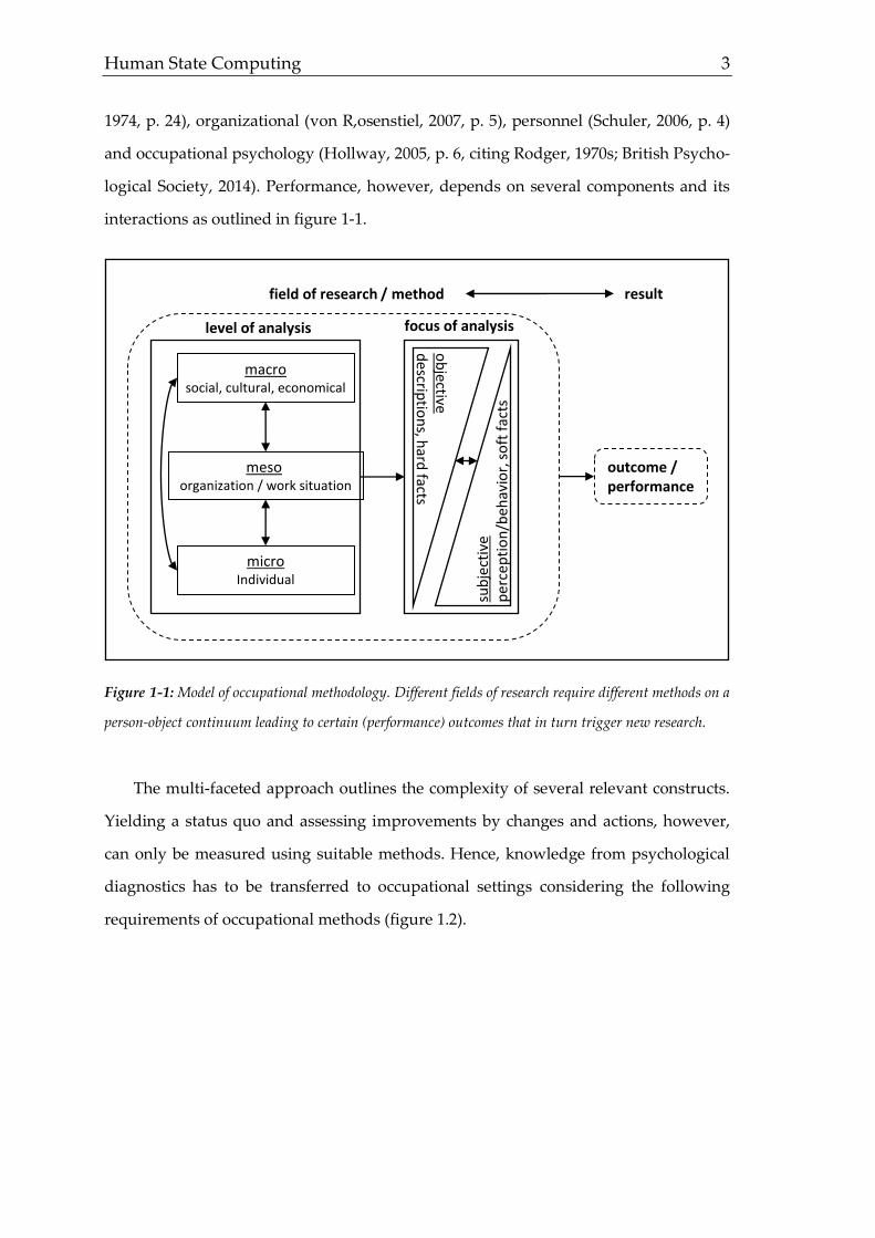
logical Society, 2014). Performance, however, depends on several components and its
interactions as outlined in figure 1-1.
Figure 1-1: Model of occupational methodology. Different fields of research require different methods on a
person-object continuum leading to certain (performance) outcomes that in turn trigger new research.
The multi-faceted approach outlines the complexity of several relevant constructs.
Yielding a status quo and assessing improvements by changes and actions, however,
can only be measured using suitable methods. Hence, knowledge from psychological
diagnostics has to be transferred to occupational settings considering the following
requirements of occupational methods (figure 1.2).
macrosocial, cultural, economical
level of analysis
outcome / performance
mesoorganization / work situation
microIndividual
focus of analysis
field of research / method result
sub
ject
ive
per
cep
tio
n/b
ehav
ior,
so
ft f
acts
ob
jectived
escriptio
ns, h
ardfacts
4 1. Introduction
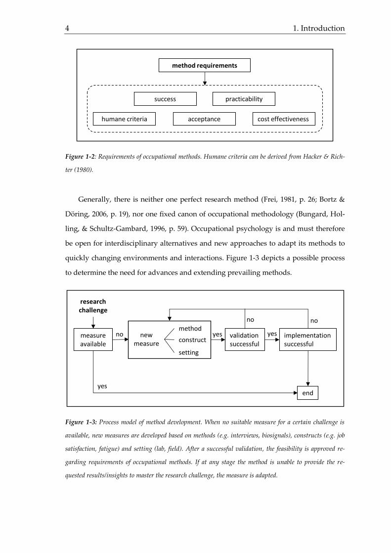
Figure 1-2: Requirements of occupational methods. Humane criteria can be derived from Hacker & Rich-
ter (1980).
Generally, there is neither one perfect research method (Frei, 1981, p. 26; Bortz &
Döring, 2006, p. 19), nor one fixed canon of occupational methodology (Bungard, Hol-
ling, & Schultz-Gambard, 1996, p. 59). Occupational psychology is and must therefore
be open for interdisciplinary alternatives and new approaches to adapt its methods to
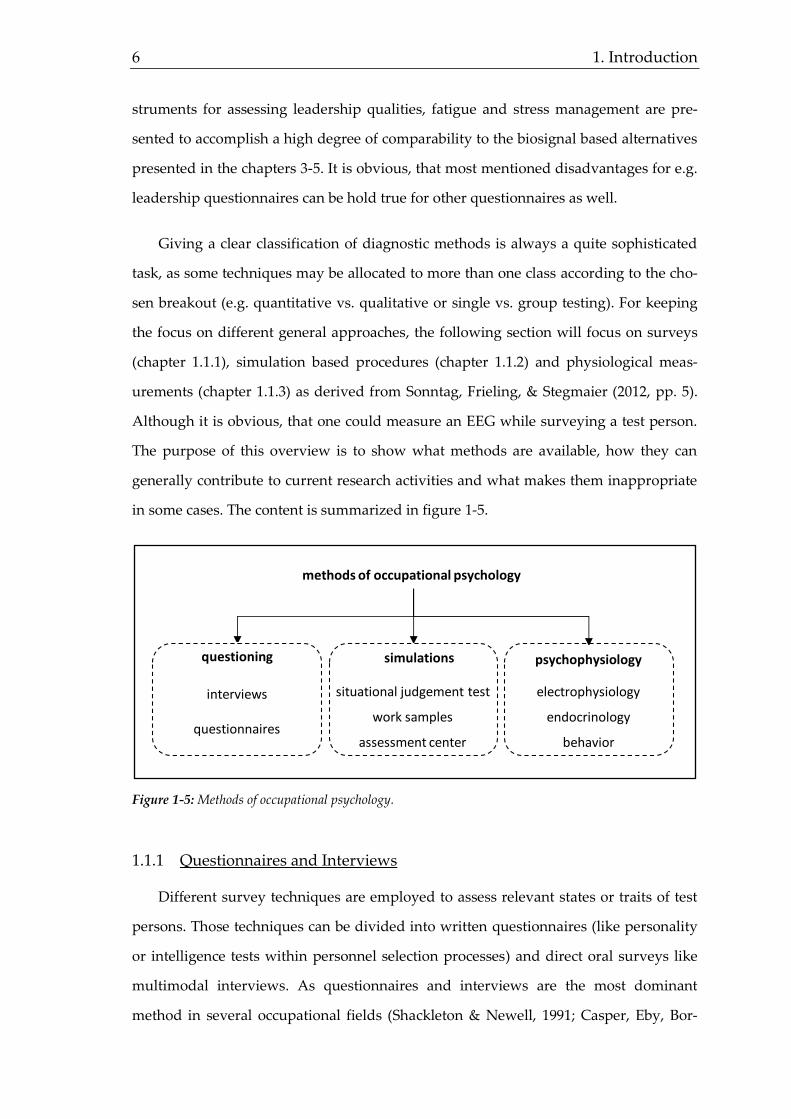
quickly changing environments and interactions. Figure 1-3 depicts a possible process
to determine the need for advances and extending prevailing methods.
Figure 1-3: Process model of method development. When no suitable measure for a certain challenge is
available, new measures are developed based on methods (e.g. interviews, biosignals), constructs (e.g. job
satisfaction, fatigue) and setting (lab, field). After a successful validation, the feasibility is approved re-
garding requirements of occupational methods. If at any stage the method is unable to provide the re-
quested results/insights to master the research challenge, the measure is adapted.
cost effectiveness
success
acceptance
practicability
humane criteria
method requirements
implementationsuccessful
researchchallenge
measure available
endyes
validationsuccessful
new measure
method
setting
constructno
no no
yesyes

Human State Computing 5
Following Moser (2007), methodology has five main functions ranging from data
generation to derived recommendations for action (figure 1-4). Suitable new approach-
es should therefore match these requirements and enhance prevailing practices or fill
in gaps. As it is outlined in this thesis, biosignal analysis is such a suitable candidate
allowing new perspectives and ways of measurement in currently stuck fields of appli-
cation, especially regarding practical usage.
Figure 1-4: Analysis scope of occupational methods. Derived from Moser (2007).
1.1 Necessity of Biosignal Analysis in Occupational State Prediction
New techniques need not necessarily to be better than established old ones. None-
theless, the following section outlines that common occupational methodology lacks of
quality in some issues that might be compensated by techniques presented later in this
thesis. As the human being as well as the interaction with his surroundings get more
and more into the focus of the economy (visible e.g. by increasing HRM spends as
shown by Towers Watson, 2012), employer offers for health-related programs (Claxton
et al., 2013) or international research on training offers (Hansson, 2007), the demand for
valid measurement methods in multifarious and wide fields like human resource man-
agement (HRM), customer satisfaction or product performance increases likewise. Ex-
hausting all different measurement techniques of among others personnel or organiza-
tional psychology is not appropriate for this thesis as it is supposed to outline general
problems of the common methodology. Instead, examples of employed measuring in-
analysis scope
description, explanation, prediction and change measurement
testing of causal, regressive and path -analytic relations
identifcation and analysis of problems
statistical and contentual evaluation of actions
recommendation for interventions on individual and work -related level
6 1. Introduction
struments for assessing leadership qualities, fatigue and stress management are pre-
sented to accomplish a high degree of comparability to the biosignal based alternatives
presented in the chapters 3-5. It is obvious, that most mentioned disadvantages for e.g.
leadership questionnaires can be hold true for other questionnaires as well.
Giving a clear classification of diagnostic methods is always a quite sophisticated
task, as some techniques may be allocated to more than one class according to the cho-
sen breakout (e.g. quantitative vs. qualitative or single vs. group testing). For keeping
the focus on different general approaches, the following section will focus on surveys
(chapter 1.1.1), simulation based procedures (chapter 1.1.2) and physiological meas-
urements (chapter 1.1.3) as derived from Sonntag, Frieling, & Stegmaier (2012, pp. 5).
Although it is obvious, that one could measure an EEG while surveying a test person.
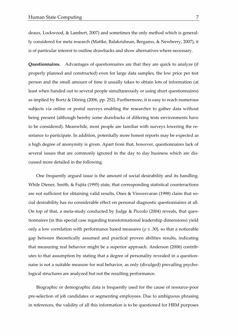
The purpose of this overview is to show what methods are available, how they can
generally contribute to current research activities and what makes them inappropriate
in some cases. The content is summarized in figure 1-5.
Figure 1-5: Methods of occupational psychology.
1.1.1 Questionnaires and Interviews
Different survey techniques are employed to assess relevant states or traits of test
persons. Those techniques can be divided into written questionnaires (like personality
or intelligence tests within personnel selection processes) and direct oral surveys like
multimodal interviews. As questionnaires and interviews are the most dominant
method in several occupational fields (Shackleton & Newell, 1991; Casper, Eby, Bor-
methods of occupational psychology
interviews
questionnaires
questioning
situational judgement test
work samples
assessment center
simulations psychophysiology
electrophysiology
endocrinology
behavior
Human State Computing 7
deaux, Lockwood, & Lambert, 2007) and sometimes the only method which is general-
ly considered for meta research (Mattke, Balakrishnan, Bergamo, & Newberry, 2007), it
is of particular interest to outline drawbacks and show alternatives where necessary.
Questionnaires. Advantages of questionnaires are that they are quick to analyze (if
properly planned and constructed) even for large data samples, the low price per test
person and the small amount of time it usually takes to obtain lots of information (at
least when handed out to several people simultaneously or using short questionnaires)
as implied by Bortz & Döring (2006, pp. 252). Furthermore, it is easy to reach numerous
subjects via online or postal surveys enabling the researcher to gather data without
being present (although hereby some drawbacks of differing tests environments have
to be considered). Meanwhile, most people are familiar with surveys lowering the re-
sistance to participate. In addition, potentially more honest reports may be expected as
a high degree of anonymity is given. Apart from that, however, questionnaires lack of
several issues that are commonly ignored in the day to day business which are dis-
cussed more detailed in the following.
One frequently argued issue is the amount of social desirability and its handling.
While Diener, Smith, & Fujita (1995) state, that corresponding statistical counteractions
are not sufficient for obtaining valid results, Ones & Viswesvaran (1998) claim that so-
cial desirability has no considerable effect on personal diagnostic questionnaires at all.
On top of that, a meta-study conducted by Judge & Piccolo (2004) reveals, that ques-
tionnaires (in this special case regarding transformational leadership dimensions) yield
only a low correlation with performance based measures (ρ ≤ .30), so that a noticeable
gap between theoretically assumed and practical proven abilities results, indicating
that measuring real behavior might be a superior approach. Anderson (2006) contrib-
utes to that assumption by stating that a degree of personality revealed in a question-
naire is not a suitable measure for real behavior, as only (divulged) prevailing psycho-
logical structures are analyzed but not the resulting performance.
Biographic or demographic data is frequently used for the cause of resource-poor
pre-selection of job candidates or segmenting employees. Due to ambiguous phrasing
in references, the validity of all this information is to be questioned for HRM purposes

8 1. Introduction
(Weuster, 1994). Usability of demographic indications is strongly based on the formula-
tion of questions, as many people e.g. miscalculate their income or mix up own beliefs
with behavior. Choi & Pak (2005) reviewed numerous health surveys and identified 48
typical questionnaire biases based on suboptimal phrasing. For these reasons it is not
astonishing that the prediction of job success works out only at a correlation level of
about r = .26 (Schuler & Marcus, 2006).
In the context of market research, the demand of and research on psychological
profiles of users is steadily growing (Goel & Sarkar, 2002; Kang, Lee, & Donohoe, 2002;
Gao et al., 2013) since many companies do not have available a sharp image of their
customers, especially within the e-commerce (Wu, Zhao & Zhang, 2008). Therefore,
questionnaires contain more frequently questions regarding psychological attributes of
the user beside demographic information. Yet, answers are supposed to be biased by
social desirability or simply dishonesty, so that only a low validity can be assumed as
mentioned above. Hence, it would be more suitable to find ways of gaining psycholog-
ical user insights without having to rely on users’ honesty.
On the one hand, intelligence and attention tests are less open to influence from so-
cial desirability, as in situations like personnel selection the vast majority of applicants
will perform best possible to increase their chances of getting a job or a certain position.
On the other hand, there are only a few fields of application showing a suitable coher-
ence with intelligence like the WIE (von Aster, Neubauer, & Horn, 2006), given a corre-
lation e.g. between leadership performance and intelligence tests of about r = .27 fol-
lowing Judge, Colbert, & Ilies, 2004. The qualification of rail riders as an example for
several other monotonous jobs depends on an ability to keep focused over a long time
with rare stimulus input. For this reason, it is suitable to use attention tests like the vig-
ilance tests as can be found within the TAP (“Testbatterie zur Aufmerksamkeitsprü-
fung”, Zimmermann & Fimm, 2002) or the d2-R (Brickenkamp, Schmidt-Atzert, &
Liepmann, 2010), where the test results show higher correlations with relevant
measures of about r = .40 Büttner & Schmidt-Atzert, 2004, p. 95). Contrary, intelligence
tests often take several hours and frequently measure criteria-unrelated dimensions.
For both kinds of performance tests can be hold true that they are quite expensive and
(from an occupational view) only useful in HRM contexts. Although online versions of

Human State Computing 9
many tests exist, marketing-relevant dimensions like joy of use on a website or with a
certain product are easier and more suitable obtained by natural measuring and auto-
matic assessment of comments. For those domains biosignals come into play. Figure
1.6 summarizes some main drawbacks of questionnaires.
Figure 1-6: Overview of questionnaire pitfalls.
Interviews. As a part of direct surveying, interviews are frequently used. As it turned
out quite early, that most unstructured interviews are of no or only little predictive
usage (Scott, 1915), other kinds of interviews have evolved. The multimodal job inter-
view (Schuler, 1992), e.g., structures questions about biography, self-display and situa-
tional behavior. This kind of structured interview appears to be one of the best predic-
tors for job success (ρ = .51, following Schmidt & Hunter, 1998). Since especially situa-
tional questions get closer to a kind of natural behavior measuring, it is only logical to
follow the approach of elaborating more sophisticated natural behavior measures as
the biosignal analysis does.
Another way of interviewing in occupational fields of application is realized by fo-
cus groups (see e.g. Morgan, 1988; Kitzinger, 1995; Kruger & Casey, 2008) with the aim
of evaluating products, brands or similar. Within focus groups, participants with spe-
cial demographic or other backgrounds evaluate a product within group discussions
and simulated tasks like finding or using certain features of a website. This approach
might not base on a representative sample, but potentially reveals relevant insights
eva
luat
ion
issu
es
com
pil
ing
& c
on
du
ctio
n
interpret open comments
hardly generate hypotheses
random/dishonest answers(esp. online surveys)
missing values (manual tests)
mistakes in manual data transfer
inappropriate statistical tests
inappropriate scales
bad phrasing
technical issues (online surveys)
time issues with long surveys
low flexibility
privacy issues (e.g. company surveys)
10 1. Introduction
about features users miss or like and what competitors do better. Gaining these in-
sights is quite expensive per person compared to simple questionnaires, but neverthe-
less popular. Companies could save lots of money, if biosignals of users were tracked
while browsing a website or using another kind of product and matching biosignal
parameters with certain product features, so that at some points oral comments be-
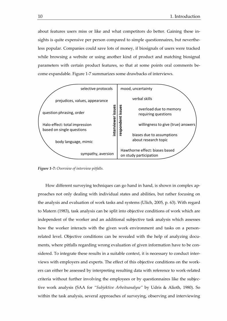
come expandable. Figure 1-7 summarizes some drawbacks of interviews.
Figure 1-7: Overview of interview pitfalls.
How different surveying techniques can go hand in hand, is shown in complex ap-
proaches not only dealing with individual states and abilities, but rather focusing on
the analysis and evaluation of work tasks and systems (Ulich, 2005, p. 63). With regard
to Matern (1983), task analysis can be split into objective conditions of work which are
independent of the worker and an additional subjective task analysis which assesses
how the worker interacts with the given work environment and tasks on a person-
related level. Objective conditions can be revealed with the help of analyzing docu-
ments, where pitfalls regarding wrong evaluation of given information have to be con-
sidered. To integrate these results in a suitable context, it is necessary to conduct inter-
views with employers and experts. The effect of this objective conditions on the work-
ers can either be assessed by interpreting resulting data with reference to work-related
criteria without further involving the employees or by questionnaires like the subjec-
tive work analysis (SAA for “Subjektive Arbeitsanalyse” by Udris & Alioth, 1980). So
within the task analysis, several approaches of surveying, observing and interviewing
resp
on
den
tis
sues
inte
rvie
wer
issu
es
mood, uncertainty
verbal skills
overload due to memory requiring questions
willingness to give (true) answers
biases due to assumptionsabout research topic
Hawthorne effect: biases based on study participation
prejudices, values, appearance
selective protocols
question phrasing, order
Halo-effect: total impression based on single questions
body language, mimic
sympathy, aversion

Human State Computing 11
are combined. The next passage deals with another kind of evaluation stronger focus-
ing on observations of possibly real work performance and behavior.
1.1.2 Simulations
As soon as real situations are imitated and transferred to a test situation, one can
allocate this kind of test to simulative techniques. The main advantage of those tech-
niques is the possibility to observe relevant dimensions directly in (almost) real situa-
tions. Contrary, the main disadvantages are more requirements, costs and time per
testing (Hunter & Hunter, 1984; Riggio, Mayes, & Schleicher, 2003). Frequently, the
presented methods are allocated to observations, but as from a certain view also inter-
views or questionnaires can be interpreted as a (performance) observation, the term
simulation is employed to more suitable capture the peculiarity of these methods. For a
quick overview, situational judgement tests, work samples and assessment center are
described.
Situational Judgement Test. Starting with a hybrid of interview/questionnaire and
simulation, situational judgement tests (SJTs) can be quoted. Following Ployhart (2006),
the aim of SJTs is to assess the choice (or ranking) of actions by applicants in relevant
situations. Depending on the way information is presented (face-to-face, questionnaire)
and responses are expected (e.g. verbally or actually executing the task), the degree of
practice varies. Nonetheless, this kind of assessing reaches an at least mediocre predic-
tive validity of .26 < r < .34 to job performance (McDaniel, Morgeson, Finnegan, Cam-
pion, & Braverman, 2001) and considerable values for other predictors (Clevenger, Pe-
reira, Wiechmann, Schmitt, & Harvey, 2001). Advantageous are little socio-
demographic issues (Weekley, Ployhart, & Harold, 2004) and a high acceptance by ap-
plicants as well as its feasibility for all hierarchic levels (Ployhart, 2006). Obvious
drawbacks are e.g. both social desirability (choosing options that appear best, although
the real behavior would differ) and actual performance skills if actions only have to be
chosen but are not executed. As Ployhart (2006) further notes, SJTs give only rare in-
formation about what constructs are measured, what however should be addressed on
a theoretical level for all measurement approaches.

12 1. Introduction
Work Samples. Transferring SJTs in a more practical context, it is quite intuitive to
use work samples for assessing the performance of a candidate on relevant tasks. As
“work sample” appears to be quite a generic term, a definition of Ployhart (2006) is
employed describing work samples as “presenting applicants with a set of tasks or
exercises that are nearly identical to those performed on the job”. Although this general
definition is in line with others (Gatewood & Field, 2001; Guion, 1998; Roth, Bobko, &
McFarland, 2005) advert in their meta-study to an important differentiation of work
samples as a measurement technique on the one hand and actual performance tests in
e.g. internships on the other hand following suggestions by Guion (1998). Within the
mentioned meta-study, several drawbacks of a much-noticed work by Hunter &
Hunter (1984) are outlined leading to a decrease of the correlation with supervisory
assessments as job performance measure of r = .54 to .26 < r < .33 on new data. Table 1-1
states some pros and cons of work samples adapted from Ployhart (2006).
Table 1-1: Advantages and disadvantages of work samples.
advantage disadvantage
high validity (Hunter & Hunter, 1984; Reilly
& Warech, 1994; Terpstra, Kethley, & Foley,
& Limpaphayom, 2000)
resource consuming wrt time and cost (Calli-
nan & Robertson, 2002)
low social/cultural impact (Schmitt & Mills,
2001; Cascio, 2003)
poor long-term validity (Siegel & Bergman,
1975; Robertson & Kandola, 1982)
low adverse impact (Callinan & Robertson,
2000)
determining scores / prohibiting diversity
(Kandola & Fullerton, 1994)
high acceptance by applicants (Hattrup &
Schmitt, 1990)

Human State Computing 13
Given these characteristics of work samples, there are still relevant sources of vari-
ation for this kind of testing. Callman & Robertson (2002) therefore state some dimen-
sions allowing contrasts between different work samples. These dimensions are given
in the following list:
Bandwidth: covered spectrum of relevant job tasks
Fidelity: matching of the actual task (e.g. hands-on task vs. description)
Specifity: continuum of testing general skills vs. job-specific tasks
Experience: degree of required knowledge for executing the work sample
Presentation/response mode: delivery of information and response channel
Due to these manifold sources of variance it is not surprising that the pre-
dictive power can be narrowed down to each of these characteristics. Nonethe-
less, general mentioned advantages and disadvantages apply for work samples
in general.
Assessment Center. When combining more or less natural situations for work sam-
ples, the result can be an assessment center. Within personnel selection and develop-
ment, the assessment center is the most important representative of simulated ap-
proaches. Commonly, all participants are observed by experienced observers regarding
predefined dimensions (Fisseni & Preusser, 2007). It is necessary to align all observers,
as only observable behavior may be taken into consideration for decision making. As
the possible development potential of participants is ignored and not only trained ob-
servers evaluate the participants’ behavior, the prediction power of assessment centers
differs widely, also because shown behavior need not necessarily to be representative
for the day to day performance (Sackett, Zedeck, & Fogli, 1988) and sometimes deci-
sions are not only based on the ratings. Following Nerdinger, Blickle, & Schaper (2008,
p. 251), a prediction average of about ρ = .37 can be assumed. Despite that rather medi-
um correlation, the proximity to reality as well as the transparency contribute to a high
acceptance by employees and employers, especially when a personal feedback is of-
fered afterwards (Kanning, 2011). These reasons imply again, that decision makers in

14 1. Introduction
occupational contexts are open to natural measures, whereby biosignal based ap-
proaches may be quite easily implemented in corresponding fields of application.
1.1.3 Psychophysiological Measurements
Although some psychophysiological measures are presented within chapter 1.3
and introductory parts of chapters 3 to 5, a short overview of different psychophysio-
logical approaches is given here. As outlined in figure 1-5, psychophysiological
measures can be divided into electrical, endocrinological and behavioral measures.
Without going into detail about how all measurements are conducted exactly, the fol-
lowing passages are used to stress drawbacks of these approaches requiring different
ways of obtaining comparable data.
Electrophysiology. As it will be further depicted later on, electrophysiological meas-
urements make use of the fact that muscles as well as neuronal activity in general pro-
duce measurable electrical currents (Schmidt & Walach, 2000; Day, 2002; Teplan, 2002).
Hence, electrophysiological approaches can be divided into gaining insights into neu-
ronal activity (e.g. EEG) and muscle-related activity (e.g. EMG, EOG, ECG). Further-
more, conductivity based on perspiration is employed for EDA measurements. Because
the tracked changes of electrical currents are very small (uV to small μV for EDA fol-
lowing Basmajan & De Luca, 1985) and are commonly derived from electrodes placed
not directly on the neural pathway or the muscle but on the skin, measures are quite
sensitive to outer conditions. However, the general approach is always to put at least
one electrode on the (ideally cleansed and shaved) skin and quantify the electric activi-
ty. In case of EEGs where no superficial measurement is possible and recognizable
changes are very small, a reference electrode has to be used in a neutral position to
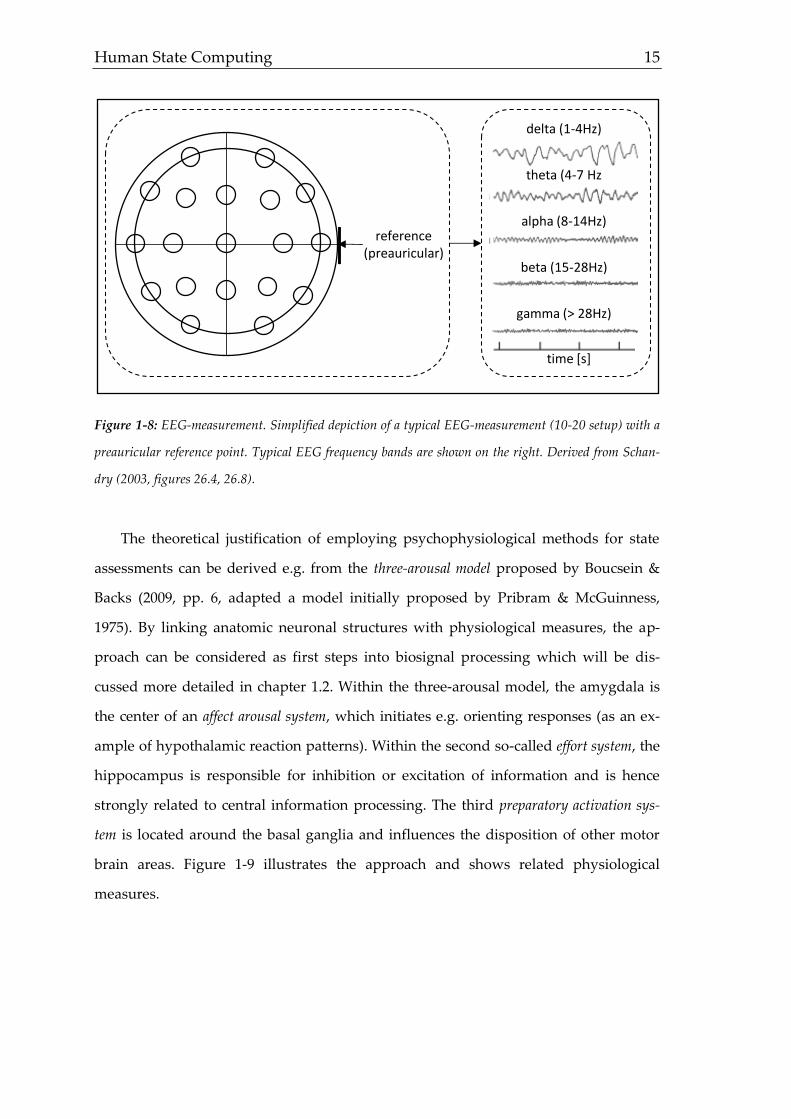
assess the general level (figure 1-8).
Human State Computing 15
Figure 1-8: EEG-measurement. Simplified depiction of a typical EEG-measurement (10-20 setup) with a
preauricular reference point. Typical EEG frequency bands are shown on the right. Derived from Schan-
dry (2003, figures 26.4, 26.8).
The theoretical justification of employing psychophysiological methods for state
assessments can be derived e.g. from the three-arousal model proposed by Boucsein &
Backs (2009, pp. 6, adapted a model initially proposed by Pribram & McGuinness,
1975). By linking anatomic neuronal structures with physiological measures, the ap-
proach can be considered as first steps into biosignal processing which will be dis-
cussed more detailed in chapter 1.2. Within the three-arousal model, the amygdala is
the center of an affect arousal system, which initiates e.g. orienting responses (as an ex-
ample of hypothalamic reaction patterns). Within the second so-called effort system, the
hippocampus is responsible for inhibition or excitation of information and is hence
strongly related to central information processing. The third preparatory activation sys-
tem is located around the basal ganglia and influences the disposition of other motor
brain areas. Figure 1-9 illustrates the approach and shows related physiological
measures.
reference(preauricular)
beta (15-28Hz)
alpha (8-14Hz)
theta (4-7 Hz
delta (1-4Hz)
time [s]
gamma (> 28Hz)

16 1. Introduction
Figure 1-9: three-arousal model. Different neuronal structures are mainly involved in the three arousal
types depicted on the left. Each arousal type therefore leads to certain physiological changes. Adapted
from Boucsein & Backs (2009, figure 1.1).
So although described psychophysiological measures allow reasonable measure-
ments of states, most commonly employed procedures take a considerable amount of
time already for the preparation. Nonetheless, electrophysiological changes can be seen
as the origin of biosignal measurement and are therefore heavily employed in many
fields of application like e.g. tracking EDA while feeling anxious or testing products
(Boucsein, 1992; 2008). Even EEG-measurements (Chanel, Kronegg, Granjean, & Pun,
2006; Golz, Sommer, Holzbrecher, & Schnupp, 2007; Hoenig, Batliner, & Noeth, 2007;
Murugappan, Rizon, Nagarajan, & Yaacob, 2007) are used in manifold ways. For an
extensive overview of common psychophysiological fields of research and outcomes
see Boucsein & Backs (2000, pp. 9). Despite the value of these measurements as a
ground truth (e.g. EEG signals for recognizing sleep stages following Shimada, Shiina,
& Saito, 2000; Brown, Johnson, & Milavetz, 2013), repetitive or even daily/hourly usage
in occupational contexts is not feasible neither regarding time efforts nor costs
(Boucsein & Backs, 2000, p. 22). In the end it is for this reason futile to have alternative
state measurement methods, if the application in relevant situations is not viable. Simi-
lar issues also apply for endocrinological analysis presented in the following.
Endocrinology. Endocrinological measures have been employed quite often in the
last decades. Examples are cortisol-based stress measurements (Burke, Davis, Otte, &
Mohr, 2005; Krajewski, Sauerland, & Wieland, 2010), melatonin tracking in night shift
arousal type neuronal structure physiological measure
affect arousal system
effort system
preparatoryactivation system basal ganglia
hippocampus
amygdala
neu
ron
al in
pu
t
neu
ron
al o
utp
ut
phasic HR changes EDA+
EEG α-HRV-
tonic HR changes

Human State Computing 17
work (Sharkey & Eastman, 2002; Crowley, Lee, Tseng, Fogg, & Eastman, 2003) or rela-
tion of testosterone and leadership (Anderson & Summers, 2007). Hormone levels are
commonly derived from blood or saliva samples taken in relevant situations being af-
terwards analyzed in a medicinal lab. Although the preparation time for taking the
samples is much shorter than for electrophysiological measures, data are usually avail-
able within a few days (or within some hours assuming a quick connect to a lab). Ob-
viously, it is again of minor usage to know that an employee’s cortisol level indicate
he/she might have been too stressed two days ago, as e.g. the lunch break behavior
cannot be changed retrospectively (Krajewski, Wieland, & Sauerland, 2010). So this
kind of measurement can only contribute to a general evaluation of state levels over
longer time periods. Despite the added value of obtaining reliable and valid data, this
procedure is hence only suitable for single testing or maybe in the course of a project,
but not feasible for every day usage.
Behavior. Without anticipating the more detailed presentation of behavior based bi-
osignals employed in this thesis within chapter 1.3, the general approach of using re-
cording methods analyzing behavioral data in a broader sense is shortly introduced
here. When speaking about behavioral data, all sources can be considered allowing
non-obtrusive recordings. The difference to methods mentioned before is, that the rela-
tion of recording device and target measure need not necessarily be one-to-one.
Webcams with included microphone e.g. can cover a wide variety of different behav-
ioral data sources like mimic or facial expression (Stoiber, Aubault, Seguler, & Breton,
2010; Zeng, Pantic, Roisman, & Huang, 2009; Stoiber, Aubult, Seguier, & Breton, 2010;
Kamberi, 2012), and body language (Horling, Datcu, & Rothkrantz, 2008) as well as
pupillography (Lüdtke, Wilhelm, Adler, Schaeffel, & Wilhelm, 1998; Morad, Lemberg,
Yofe, & Dagan, 2000), voice analysis (Schuller, Rigoll, & Lang, 2003; Krajewski, Batlin-
er, & Golz, 2009) and even heart rate estimates employing videoplethysmography (Al-
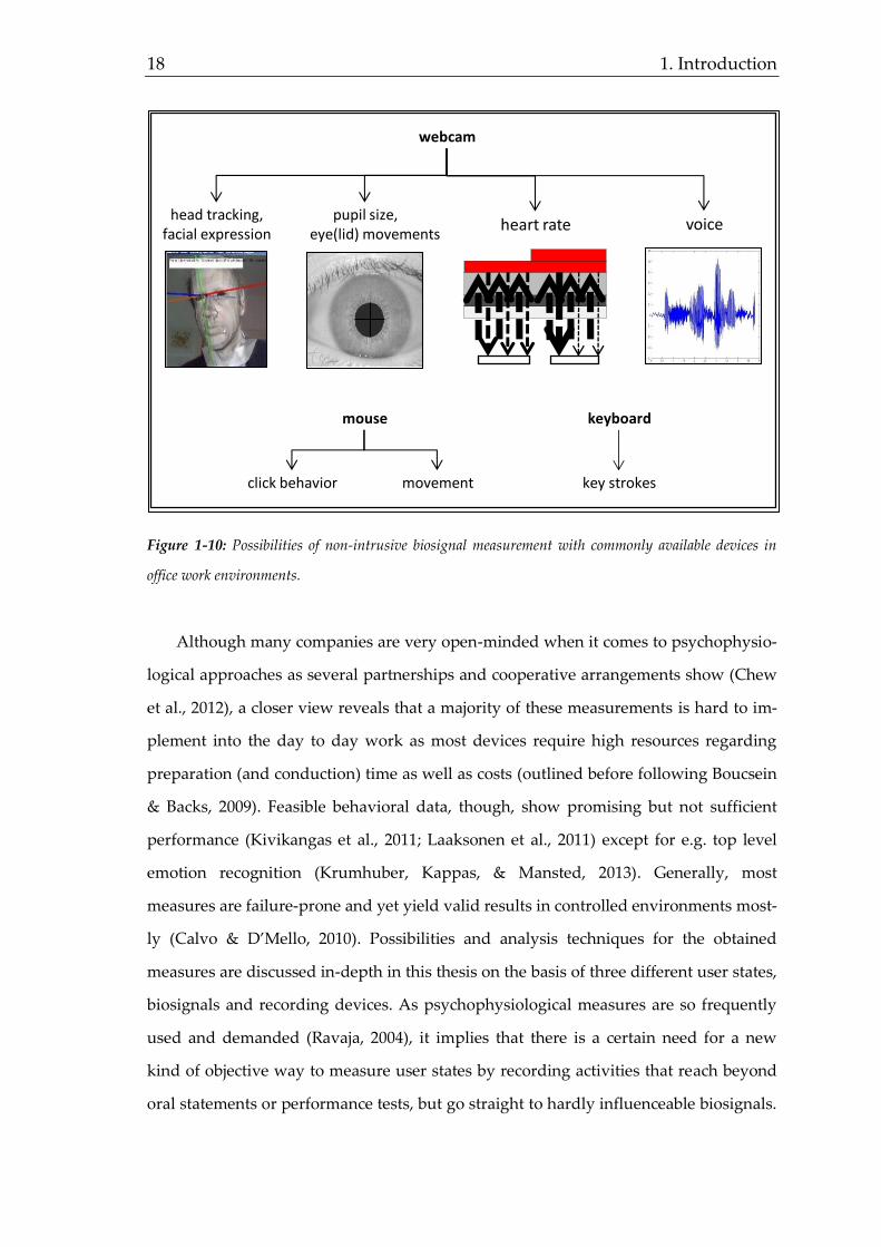
len, 2007; Shelley, 2007) For a first impression, figure 1-10 summarizes different sources
and recording devices simply employable for desk work in a non-intrusive way.
18 1. Introduction
Figure 1-10: Possibilities of non-intrusive biosignal measurement with commonly available devices in
office work environments.
Although many companies are very open-minded when it comes to psychophysio-
logical approaches as several partnerships and cooperative arrangements show (Chew
et al., 2012), a closer view reveals that a majority of these measurements is hard to im-
plement into the day to day work as most devices require high resources regarding
preparation (and conduction) time as well as costs (outlined before following Boucsein
& Backs, 2009). Feasible behavioral data, though, show promising but not sufficient
performance (Kivikangas et al., 2011; Laaksonen et al., 2011) except for e.g. top level
emotion recognition (Krumhuber, Kappas, & Mansted, 2013). Generally, most
measures are failure-prone and yet yield valid results in controlled environments most-
ly (Calvo & D’Mello, 2010). Possibilities and analysis techniques for the obtained
measures are discussed in-depth in this thesis on the basis of three different user states,
biosignals and recording devices. As psychophysiological measures are so frequently
used and demanded (Ravaja, 2004), it implies that there is a certain need for a new
kind of objective way to measure user states by recording activities that reach beyond
oral statements or performance tests, but go straight to hardly influenceable biosignals.
pupil size, eye(lid) movements
head tracking,facial expression
heart rate
mouse
voice
webcam
click behavior movement
keyboard
key strokes

Human State Computing 19
To close this chapter, table 1-2 summarizes the mentioned psychophysiological
measures and their fields of application.
Table 1-2: Advantages and disadvantages of psychophysiological measurements.
measure advantages disadvantages
electrophysiology high validity/theoretical linking,
good temporal resolution
resource consuming wrt time and
costs, intrusive/invasive
endocrinology high validity/theoretical linking, ,
objective
low time resolution, intru-
sive/invasive, limited fields of
application
behavior non-intrusive, flexible so far often low validity
1.2 Theoretical Aspects of Biosignal Processing
When speaking of biosignal processing, it seems to be a good idea starting with a
definition and historical backgrounds of biosignals. Commonly, biosignals are em-
ployed in medicinal contexts and refer to bioelectric signals like EEG, ECG or EMG as
mentioned in chapter 1.1.3. First bioelectrical signals were studied since Galvani (1791,
cited by Piccolino, 1998) discovered electricity in frog legs. Kaniusas (2012) gives a
broader definition by sketching biosignals “as a description of a physiological phe-
nomenon” (p. 1) including even visual body inspection. Another focus is given by the
DIN 44300, where biosignals are defined as “information springing from physical or
chemical actions of the human body”. This definition stronger emphasizes an (at least
theoretical) objective possibility of measuring. For the purpose of human state compu-
ting in this thesis, biosignals may be defined as all signals based on automatically and non-
intrusively recordable human behavior. In this sense, behavior can be seen as any kind of
“actions or reactions of a person […] in response to external or internal stimuli” (Farlex
Inc., 2013) also covering physiological output. In line with the Oxford dictionary, that
definition may be expanded to animals as well. But as animals are not included in the
presented studies, the biosignal definition shall be narrowed down to human behavior.
It has already been mentioned that human states are supposed to be assessed and
predicted with the help of biosignals. Hence, the definitional task of this chapter also
covers a clear statement of what is meant when speaking about analyzing states in this
20 1. Introduction
context. Within the psychology of personality there are numerous approaches to define
personality characteristics (Herrmann, 1991, p. 25; Pervin, 1996, p. 414; Hobmair, 1997,
p. 3; Fiedler, 2000, p. 417; Gerrig & Zimbardo, 2008, p. 504; Asendorpf, 2009, p. 2). One
popular and easily transferable definition is given by McCrae & Costa (1990, p.3) in the
widely known five-factor model describing traits as “dimensions of individual differ-
ences in tendencies to show consistent patterns of thoughts, feelings and actions […]
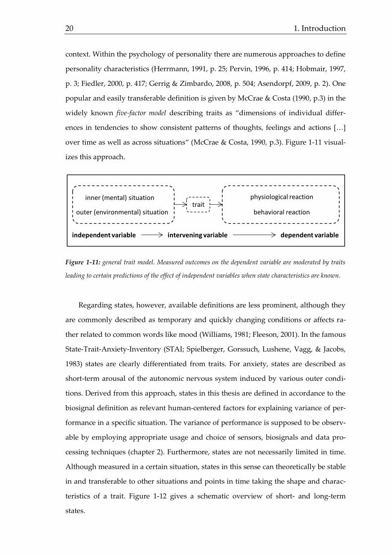
over time as well as across situations“ (McCrae & Costa, 1990, p.3). Figure 1-11 visual-
izes this approach.
Figure 1-11: general trait model. Measured outcomes on the dependent variable are moderated by traits
leading to certain predictions of the effect of independent variables when state characteristics are known.
Regarding states, however, available definitions are less prominent, although they
are commonly described as temporary and quickly changing conditions or affects ra-
ther related to common words like mood (Williams, 1981; Fleeson, 2001). In the famous
State-Trait-Anxiety-Inventory (STAI; Spielberger, Gorssuch, Lushene, Vagg, & Jacobs,
1983) states are clearly differentiated from traits. For anxiety, states are described as
short-term arousal of the autonomic nervous system induced by various outer condi-
tions. Derived from this approach, states in this thesis are defined in accordance to the
biosignal definition as relevant human-centered factors for explaining variance of per-
formance in a specific situation. The variance of performance is supposed to be observ-
able by employing appropriate usage and choice of sensors, biosignals and data pro-
cessing techniques (chapter 2). Furthermore, states are not necessarily limited in time.
Although measured in a certain situation, states in this sense can theoretically be stable
in and transferable to other situations and points in time taking the shape and charac-
teristics of a trait. Figure 1-12 gives a schematic overview of short- and long-term
states.
independent variable
trait
intervening variable dependent variable
inner (mental) situation
outer (environmental) situation
physiological reaction
behavioral reaction

Human State Computing 21
Figure 1-12: Schematic concept of temporal consistency of state levels. Height and width of boxes indi-
cates possible differences in duration and onset/volatility.
As the figure above outlines, some evaluated states aim to show long-term validity
(since e. g. leadership-based states should not only apply within the hiring process),
while other states like fatigue or emotions are supposed to change quicker, whereby
the prompt detection of changes is a challenging task.
Before going more into detail about biosignal-based research, the growing popu-
larity of biosignal analysis is worth to mention. Publications increased massively over
the last decades. Figure 1-13 shows, that springing from engineering and medicine,
publications employing or regarding biosignals multiplied their impact in psychology.
Compared to about 4 publications around 1980, almost 150 peer-reviewed articles by
searching for “biosignal” can be retrieved from the database of psycinfo for the last
decade.
du
rati
on
of
con
sist
ent
stat
e le
vel
onset / volatility
leadership
fatigueshort term stress
emotions
long term stress

22 1. Introduction
Figure 1-13: Increase of publications with keywords "biosignal" or "affective computing" in decades
starting in 1975 based on psycinfo (Apr 2014).
By analyzing biosignals for state recognition, the wide field of affective computing
has to be considered (Picard, 2000; Tao & Tan, 2005; Lemmens, de Haan, Van Galen, &
Meulenbroek, 2007). Although affective computing mainly focuses on analyzing emo-
tions and responding appropriately within human computer interactions (Tao & Tan,
2005), the methodological background can be transferred easily to other human states
like fatigue or leadership relevant dimensions as undertaken in this thesis. The inter-
face of cognitive and psychological sciences as well as informatics allows the develop-
ment of measuring tools commonly referred to as sensors (Picard, 1995) for various bi-
osignals (preferably non-intrusively recorded ones). Despite the wide variability of
sensors for manifold fields of application, their general usage is always the same: Con-
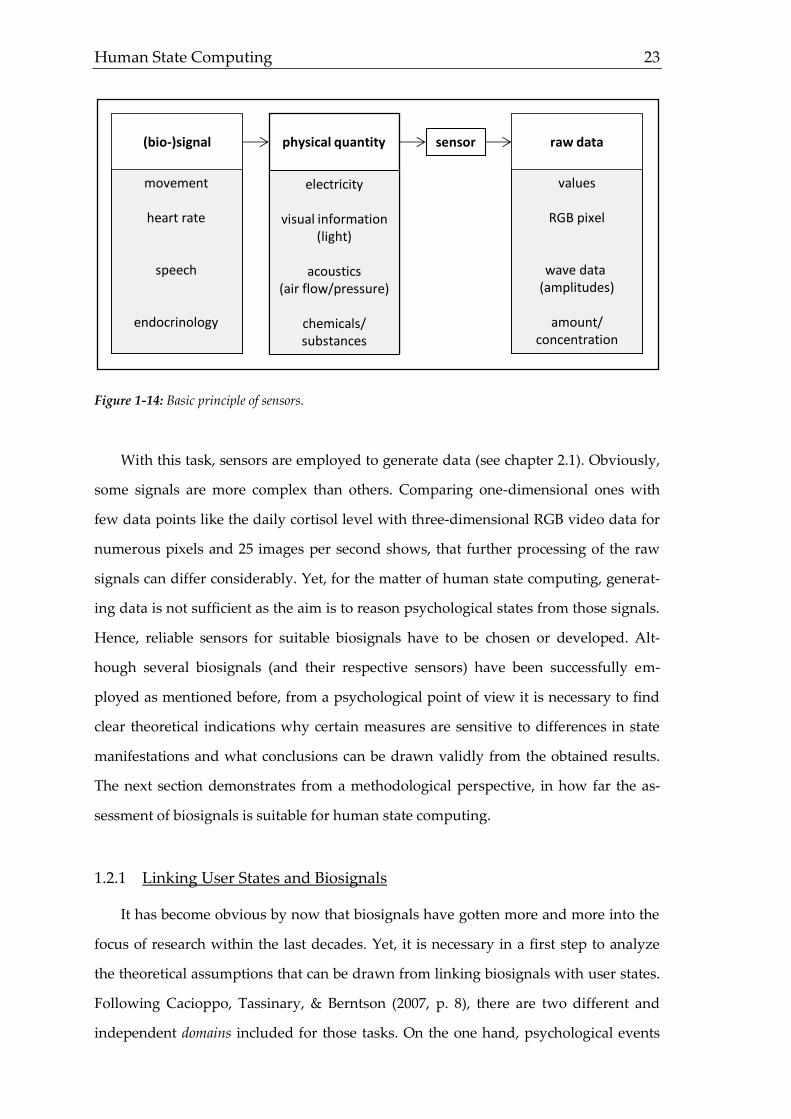
verting a physical quantity to a readable signal (figure 1-14).
1975-1984 1985-1994 1995-2004 2005-20140
50
100
150
decade
nu
mb
er o
f p
ub
licat
ion
s
Human State Computing 23
Figure 1-14: Basic principle of sensors.
With this task, sensors are employed to generate data (see chapter 2.1). Obviously,
some signals are more complex than others. Comparing one-dimensional ones with
few data points like the daily cortisol level with three-dimensional RGB video data for
numerous pixels and 25 images per second shows, that further processing of the raw
signals can differ considerably. Yet, for the matter of human state computing, generat-
ing data is not sufficient as the aim is to reason psychological states from those signals.
Hence, reliable sensors for suitable biosignals have to be chosen or developed. Alt-
hough several biosignals (and their respective sensors) have been successfully em-
ployed as mentioned before, from a psychological point of view it is necessary to find
clear theoretical indications why certain measures are sensitive to differences in state
manifestations and what conclusions can be drawn validly from the obtained results.
The next section demonstrates from a methodological perspective, in how far the as-
sessment of biosignals is suitable for human state computing.
1.2.1 Linking User States and Biosignals
It has become obvious by now that biosignals have gotten more and more into the
focus of research within the last decades. Yet, it is necessary in a first step to analyze
the theoretical assumptions that can be drawn from linking biosignals with user states.
Following Cacioppo, Tassinary, & Berntson (2007, p. 8), there are two different and
independent domains included for those tasks. On the one hand, psychological events
sensor(bio-)signal
movement
heart rate
speech
endocrinology
physical quantity
electricity
visual information (light)
acoustics (air flow/pressure)
chemicals/substances
raw data
values
RGB pixel
wave data (amplitudes)
amount/concentration
24 1. Introduction
of a set ψ are described as a kind of conceptual variables covering (brain) functions and
states with unexplained behavior being the target variable of a study. On the other
hand, in order to get an idea about how these functions work and behave in different
situations, a physiological set Φ containing physical and hence directly measurable
variables is determined to obtain an anchor for drawing conclusions regarding ψ.
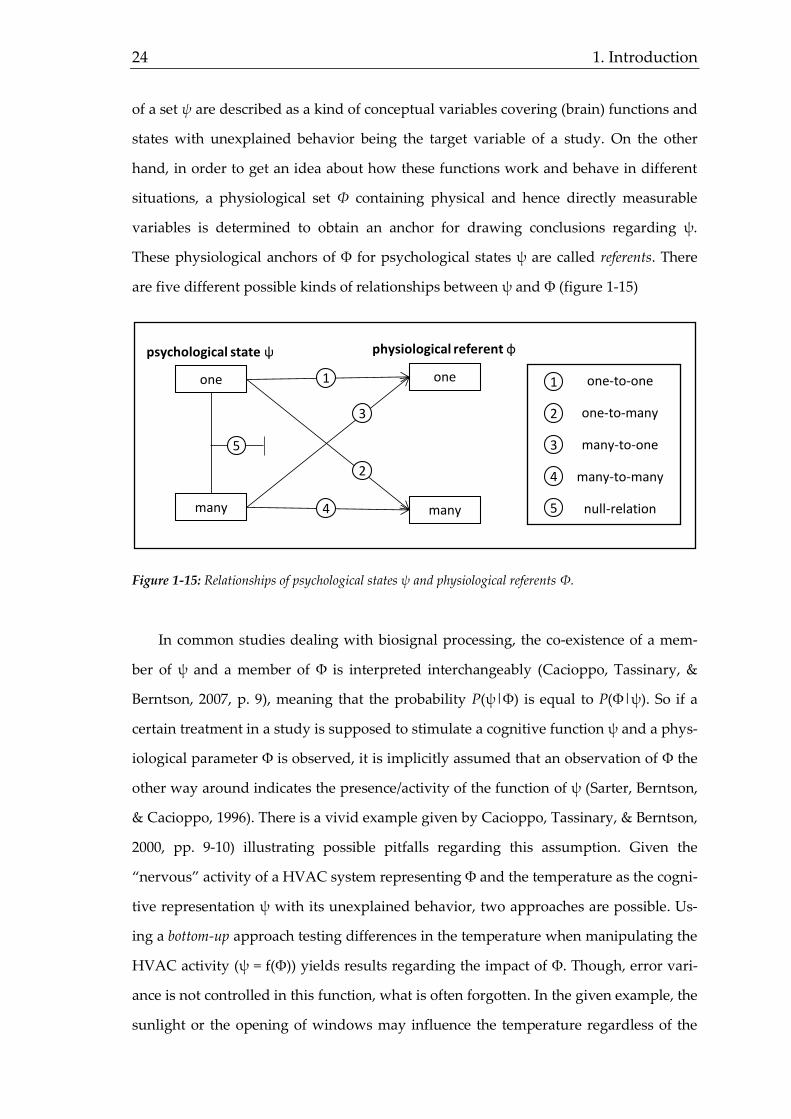
These physiological anchors of Φ for psychological states ψ are called referents. There
are five different possible kinds of relationships between ψ and Φ (figure 1-15)
Figure 1-15: Relationships of psychological states ψ and physiological referents Φ.
In common studies dealing with biosignal processing, the co-existence of a mem-
ber of ψ and a member of Φ is interpreted interchangeably (Cacioppo, Tassinary, &
Berntson, 2007, p. 9), meaning that the probability P(ψ|Φ) is equal to P(Φ|ψ). So if a
certain treatment in a study is supposed to stimulate a cognitive function ψ and a phys-
iological parameter Φ is observed, it is implicitly assumed that an observation of Φ the
other way around indicates the presence/activity of the function of ψ (Sarter, Berntson,
& Cacioppo, 1996). There is a vivid example given by Cacioppo, Tassinary, & Berntson,
2000, pp. 9-10) illustrating possible pitfalls regarding this assumption. Given the
“nervous” activity of a HVAC system representing Φ and the temperature as the cogni-
tive representation ψ with its unexplained behavior, two approaches are possible. Us-
ing a bottom-up approach testing differences in the temperature when manipulating the
HVAC activity (ψ = f(Φ)) yields results regarding the impact of Φ. Though, error vari-
ance is not controlled in this function, what is often forgotten. In the given example, the
sunlight or the opening of windows may influence the temperature regardless of the
psychological state ψ physiological referent φ
one
many
one
many
2
3
4
5
1 1 one-to-one
one-to-many
many-to-one
many-to-many
2
3
4
5 null-relation

Human State Computing 25
HVAC activity, so P(ψ|Φ) < 1. Nonetheless, in the case of constant sunlight and closed
windows, still a (theoretically) perfect relation of P(ψ|Φ) = 1 is measured, although the
HVAC is neither the only one nor a perfect referent for predicting the temperature. Of
course, with P(ψ|Φ) > 0, the HVAC still has to be considered a predictor. This pitfall
describes, that a top-down approach assuming Φ = f(ψ) or P(Φ|ψ) needs not necessarily
equal P(ψ|Φ). In the given example, the activity of the HVAC must not necessarily be
explained equally by the temperature. Near a window, the temperature still varies for
different outside air temperatures, even if the HVAC is active. Hence, a measurement
indicating that P(Φ|ψ) = 0 does not necessarily prove Φ cannot be a predictor of ψ.
Cacioppo et al. transfers this insight to fMRI studies, where inactive regions on an im-
age do not have to be unrelated to an examined state ψ, although this is the prevalent
interpretation. Regarding the five mentioned relationships in figure 1-15, the dominant
approach to assume symmetric relationships between Φ and ψ is only valid for (1) and
(3). Hence, it is of utter importance to keep these possible relationships in mind when
analyzing biosignal data. Replicating studies should occasionally also include small
changes of the setting making sure that – spoken in terms of fMRI images – inactive
regions (or non-correlating features) are not generally discarded for the wrong reason
and the importance of high correlating features is not overestimated.
Psychophysiological Categories. To clarify the extent of (external) validity, it seems
useful to distinguish not only possible relationships, but also situational aspects. Nar-
rowing down the focus to one psychological parameter ψ allows deriving a 2x2-
dimensional matrix as suggested by Cacioppo, Tassinary, & Berntson (2007, pp. 10),
with one dimension covering the relationship (one-to-one vs. many-to-one) and the
other one giving ideas about the generalizability (context-dependent vs. context-free)
as depicted in figure 1-16. By excluding a third dimension giving information about the
causal relationship (Φ causing ψ, ψ causing Φ, or a third variable causing both), a better
comprehension is ensured, although the relevance of this information must be kept in
mind.

26 1. Introduction
Figure 1-16: System of psychophysiological inferences.
Each of the four fields yields different suggestions for a validity assessment. Psy-
chological Outcomes can be found in a many-to-one and context-dependent relationship,
where in a given situation (possibly) several elements of ψ covary with one physiologi-
cal referent Φ. Beside the physiological pattern based on psychological state changes,
no other validating inference is possible. Knowing that state changes lead to a certain
physiological output does not allow inferring that the physiological output vice versa
indicates the presence of the psychological state, only its absence. This is, because other
variables causing the same physiological output are usually unknown, so it is not clear
whether the physiological pattern is based on the presence of the analyzed psychologi-
cal state or any other variable. However, it is known that the physiological pattern oc-
curs for the psychological state, so an observed absence of this pattern merely predicts
the absence of the psychological state (at least, if no third variable blurs the physiologi-
cal measurement for any reason, what is no logical problem anyway). Another ap-
proach of explaining limitations of psychological outcomes is to assume asymmetric a
priori probabilities like P(Φ) > P(ψ). In this case, the presence of ψ is overestimated
when employing Φ as an evidence for the presence of ψ. For theoretical models,
though, outcomes are totally sufficient to assess the model fitness. Commonly, psycho-
physiological experiments start with outcomes, as only one setting is initially tested
and hence it is not clear to what degree the results are context-free. Sometimes, other
variables are measured in addition and hereby controlled afterwards with ANCOVAs,
partial regressions and other procedures trying to change the many-to-one relationship
into a one-to-one relationship. Although these attempts improve valid inferences, it is
context-dependent
context-independent
invariantsconcomitants
man
y-to
-on
e
markersoutcomes
on
e-to
-on
e
Human State Computing 27
hardly possible to ensure all confounders are controlled. In the end (after several re-
search cycles), outcomes are likely to turn out as one of the other categories. This is,
however, no methodological problem, as all conclusions drawn from outcomes apply
for other categories, too.
As the general way of proving and assessing the validity of different categories has
been described within the psychological outcomes, other categories can be approached
a little bit shorter. Psychological markers represent a one-to-one and context-depending
relationship between ψ and Φ. Hence, a theoretically symmetric interaction is assumed
meaning that not only the absence, but also the presence of ψ is indicated by Φ and the
other way around within a predefined situation. Since such relationships are likely to
occur in natural connections or artificially induced situations only, markers reveal
backgrounds regarding the nature of states and physiological measures. Qualifying an
element of Φ as a marker, though, requires firstly, that Φ not only reliably predicts the
absence, but also the presence of ψ, secondly, that Φ is unrelated to any other element
of ψ and thirdly, the specific situation is defined.
Now differences between many-to-one and one-to-one content-dependent infer-
ring have been presented. Both other categories deal with content-independent validity
assumptions. Psychophysiological concomitants are established when in a many-to-one
relationship the context of research does not influence the relationship between ψ and
Φ. In that case, neither changing the stimulus (e.g. visual vs. acoustic material) nor
changing the environment (e.g. testing in silence against noisy surrounding) has an
effect on the result. Tranel, Fowles, & Damasio (1985) showed based on skin conduct-
ance responses (SCR) that familiarity leading to higher SCR under different conditions
can be ruled out as a concomitant relationship, because future studies revealed higher
SCR also for unfamiliar stimuli under different conditions. Similar to psychological
markers, increased SCR (Φ) is still valid as a predictor for either absence or presence of
familiarity (ψ), as Φ always occurs for ψ and vice versa. Though, it is not valid to infer
a certain strength or direction of the relationship, especially when a priori probabilities
are not controlled or unknown.

28 1. Introduction
The last and most desirable category is represented by psychophysiological invariants
with a symmetric and content-independent one-to-one relationship of ψ and Φ. Due to
these characteristics, P(Φ) = P(ψ) or P(ψ|Φ) = P(Φ|ψ) = 0 meaning neither Φ nor ψ oc-
curs when the other one does not. This ideal category is unfortunately more frequently
assumed than proven (Stevens, 1951, p. 20, cited by Cacioppo, Tassinary, & Berntson,
2007, p. 14). Although research should demonstrate an ambition to gather data sup-
porting invariant relationships, it must be kept in mind that – as outlined – also other
categories lead to several relevant and valid conclusions (Donchin, 1982). It is rather of
crucial importance to be aware of valid interpretations of findings as well as view and
test relationships from several angles, since all results from psychological outcomes to
invariants contribute to the general state of knowledge and help building best possible
performing prediction models in all fields of application. Probability characteristics
and hence valid inferences of all psychophysiological categories are summarized in
table 1-3.
Table 1-3: Probability characteristics of psychophysiological categories.
category probability
assumption inference
invariant P(Φ) = P(ψ) Φ never occurs without ψ and vice versa
outcome P(Φ|s) > P(ψ|s)
Φ also occurs for other ψ in several situa-
tions, so only absence of ψ can be deter-
mined in predefined situations, not presence
concomitant P(Φ) < P(ψ)
Φ always occurs for ψ and vice versa, but Φ
covaries with other ψ as well. Hence, ab-
sence and presence is determined, but not
strength of ψ
marker P(Φ|s) = P(ψ|s) Φ never occurs without ψ in a predefined
situation and vice versa
1.2.2 Biosignal Data Design and Measurements
When generating physiological data with the help of a suitable sensor, different
measure types and study designs can be distinguished comparable to common psycho-
logical research approaches. The following specifications regarding the analyzed
measures always have to be considered for a successful data processing with relevant
and valid outcomes.
Human State Computing 29
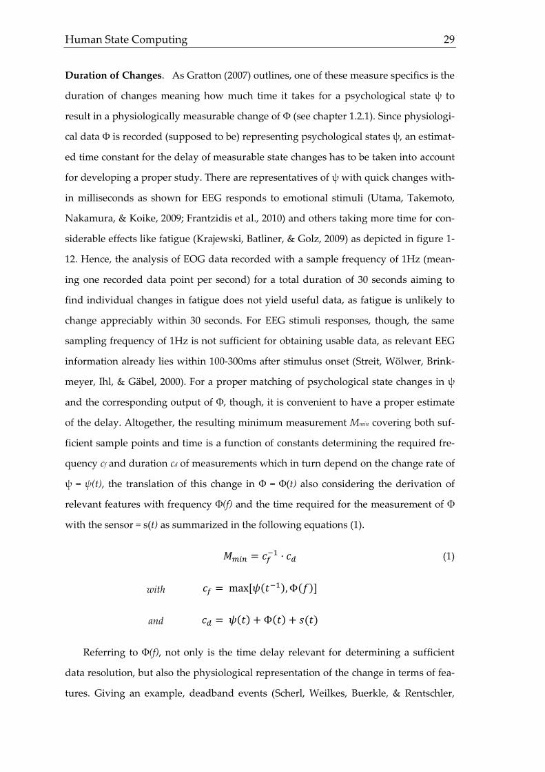
Duration of Changes. As Gratton (2007) outlines, one of these measure specifics is the
duration of changes meaning how much time it takes for a psychological state ψ to
result in a physiologically measurable change of Φ (see chapter 1.2.1). Since physiologi-
cal data Φ is recorded (supposed to be) representing psychological states ψ, an estimat-
ed time constant for the delay of measurable state changes has to be taken into account
for developing a proper study. There are representatives of ψ with quick changes with-
in milliseconds as shown for EEG responds to emotional stimuli (Utama, Takemoto,
Nakamura, & Koike, 2009; Frantzidis et al., 2010) and others taking more time for con-
siderable effects like fatigue (Krajewski, Batliner, & Golz, 2009) as depicted in figure 1-
12. Hence, the analysis of EOG data recorded with a sample frequency of 1Hz (mean-
ing one recorded data point per second) for a total duration of 30 seconds aiming to
find individual changes in fatigue does not yield useful data, as fatigue is unlikely to
change appreciably within 30 seconds. For EEG stimuli responses, though, the same
sampling frequency of 1Hz is not sufficient for obtaining usable data, as relevant EEG
information already lies within 100-300ms after stimulus onset (Streit, Wölwer, Brink-
meyer, Ihl, & Gäbel, 2000). For a proper matching of psychological state changes in ψ
and the corresponding output of Φ, though, it is convenient to have a proper estimate
of the delay. Altogether, the resulting minimum measurement Mmin covering both suf-
ficient sample points and time is a function of constants determining the required fre-
quency cf and duration cd of measurements which in turn depend on the change rate of
ψ = ψ(t), the translation of this change in Φ = Φ(t) also considering the derivation of
relevant features with frequency Φ(f) and the time required for the measurement of Φ
with the sensor = s(t) as summarized in the following equations (1).
with
and
𝑀𝑚𝑖𝑛 = 𝑐𝑓−1 · 𝑐𝑑
𝑐𝑓 = max [𝜓(𝑡−1), Φ(𝑓)]
𝑐𝑑 = 𝜓(𝑡) + Φ(𝑡) + 𝑠(𝑡)
(1)
Referring to Φ(f), not only is the time delay relevant for determining a sufficient
data resolution, but also the physiological representation of the change in terms of fea-
tures. Giving an example, deadband events (Scherl, Weilkes, Buerkle, & Rentschler,

30 1. Introduction
2007; Sgambati, 2012) in the context of steering behavior based driver sleepiness detec-
tion respond to the previously as slowly changing described state fatigue. The event
itself consists of two main stages: absent steering wheel activity followed by quick and
overly correction behavior (see figure 1-17).
Figure 1-17: Deadband event. Reduced micro corrections (phase 1) followed by heavy corrections (phase
2) and common steering activity (phase 3).
As the time axis of figure 1-17 reveals, relevant aspects for defining a deadband
event are only visible within a short amount of time. For this reason, the sensor must
allow a suitable sampling frequency to cover these fast changes of Φ, although fatigue
as a state of ψ shows a comparably slow change rate (see also Gratton, 2007).
Similar to the deadband events, recordings of the heart rate also contain most use-
ful information at those times when the heart is beating (corresponding to a deadband
event), while data points in between are negligible as (almost) no activity is observable.
When relevant information is only obtainable at specific times, Gratton (2007) induces
the term discrete measures. Contrary, biosignals like speech or pupillography often do
not offer cyclic events of particular interest, wherefore they are called continuous for
those applications. The relevance of the distinction between discrete and continuous
measures is given by the different handling and valid inferences. While continuous
measures allow a good temporal assessment of the course of ψ, discrete measures are
1 2 3 4 5-1
0
1
time [s]
stee
rin
g an
gle
(no
rmal
ized
)phase 1 phase 2 phase 3

Human State Computing 31
limited to their natural sampling rate of relevant information windows. Better resolu-
tions can only be achieved by a more complex “pooling […] across trials” (Gratton,
2007, p. 840). For gaining insights into drawing relevant information from cyclic
events, Jennings, van der Molen, Somsen, & Ridderinkhof (1991) present a technique
for the analysis of changes of the cardiac interbeat interval. All measures employed for
the conducted studies in this thesis, though, are continuous and hence contain possibly
relevant information at all times.
Indirect Measurement. Having a look at the time delay function already implies that
biosignal analysis is commonly not capable of measuring psychological states directly.
In the former passages, though, a mostly linear relationship between ψ and Φ has been
implicitly assumed, although directions of valid inferences are questioned. But when
thinking further about relationships, where the presence of Φ does not necessarily pre-
dict the presence of ψ and vice versa, there must be some intervening variables or am-
biguity in the relationship. When expecting linearity, a measurement of state Φ = MΦ
for a state ψ is simplified defined by a function based on the constant of proportionali-
ty k ≠ 0 and the time delay constant tc (equation 2).
Φ = 𝑘 · ψ + 𝑡𝑐 (2)
In the given equation, the psychological state ψ leads to a particular reaction of Φ
with a time delay tc. While dependencies of the time delay and the required minimum
measurement Mmin already have been explained, the more interesting interaction is that
one describing the effect of ψ on Φ represented by k. Taking fatigue as an example
again, an increase results in longer periods of eye closure (Ji, Zhu, & Lan, 2004; Vural et
al., 2007). So k describes the relationship between fatigue and eye closure (like the du-
ration of eye closure in regard of the degree of fatigue), while tc represents the time it
commonly takes until the response of Φ (eye closure) is recorded by the sensor. Occa-
sionally, k not only depends on ψ and Φ, but also on third variables endangering line-
arity. For example, Gratton (2007) states that differences in cardiovascular health modi-
fies the neuronal reaction resulting in measurable changes of the blood flow, whereby
the assessment of older subjects leads to different results (also of k) than those of

32 1. Introduction
younger ones. Eventually, using the same k for young and old subjects leads to high
prediction errors caused by the confounding variable age.
As stated in chapter 1.2.1, a solution of this problem is sometimes sought by con-
trolling possible confounders. Nonetheless, even a best possible control does not im-
prove the prediction, if the relationship simply is not linear. Some transformations (e.g.
logarithmic functions) which can be used to adapt k allow converting nonlinear to line-
ar relationships. For more complex nonlinear relationships (see chapter 2.2.3), some-
times it is advantageous to discard linearity and use other statistics for assessment and
prediction (Gratton, p. 839). The only problematic relation is a non-monotonous one,
where a certain measurement MΦ indicates different state levels of ψ as illustrated in
figure 1-18.
Figure 1-18: Nonlinear relationships. Left: relationship can be linearized by logarithmic function. Right:
Different levels of ψ are indicated by the same value of Φ.
When analyzing single features derived from Φ (chapter 2.2), the underlying rela-
tionship has to be kept in mind before deducing allegedly valid conclusions. The ad-
vantage of pattern recognition based methods, though, lies within the combination of
several features using information of several relationships to obtain distinct predictions
also for complex interactions and relations (Burges, 1998) as required in the schemati-
cally case shown on the right side of figure 1-18. One last theoretical issue of biosignal
processing is now discussed, before those biosignals employed for the presented stud-
ies are presented.
0 10
1
= 4 ^
0 10
1
= ^ 2

Human State Computing 33
Ground Truth. In addition to the presented assumptions regarding the relationships
of psychological states and physiological quantities, a frequently forgotten issue is the
ground truth of a psychological state. The common definition has given a theoretical
perspective. While physiological conditions Φ are often easily measured with a suitable
sensor, a psychological state ground truth or baseline is more difficult to assess. Measur-
ing EMGs of a relaxed muscle can easily be differentiated from the same muscle while
moving and a baseline is easily found. For the assessment of psychological user states
ψ, though, on the one hand it is important to have a baseline for statistical comparison,
but on the other hand the experimental induction of e.g. an emotional baseline is very
difficult, as subjects cannot be considered to feel nothing (else) even if a pretest is pos-
sible. Furthermore, not only primarily relevant states ought to be controlled but also all
other states (fatigue, stress, confidence, etc.) having a clear one- or many-to-one rela-
tionship have to be considered what is hardly possible in practice. When speaking
about testing, it is a question of study design, whether a between subject or a repeated
measurement is preferred. Jennings & Gianaros (2007, p. 814) give a good example by
showing that the same mean difference leads to higher values for t in a t-test (see table
1-4).
Table 1-4: Comparison of repeated and between subject design.
A B C tbetween twithin
pre-test 3 4 5 .4 20.0
post-test 3.2 4.3 5.1
Due to the much smaller standard error se for the repeated measurement (se = .01
compared to se = .52 for the between subject design), the same mean difference leads to
higher significances for repeated measurements. Due to this increased sensitivity, bi-
osignal analysis often prefers repeated measurements.
In addition, many applications for analyzing user states are supposed to not ana-
lyze an average value for groups but for individuals as a diagnostic test. Since thresh-
olds are easier to define intra-individually (see Bakerman, 2005, for a comparison), ac-
curate measures in terms of sensitivity and specificity can be facilitated using individ-
34 1. Introduction
ual baselines of a state ψ. Unfortunately, determining a baseline is not always possible
(Tkalčič, Odić, & Košir, 2013), especially in the context of recording natural behavior as
the best source (see chapter 2.1.1) of externally valid data (Douglas-Cowie, Cowie, &
Schröder, 2005), where data is gathered in free environments with no possibility of
manipulation and hence baseline measurements. Burkhardt, Paeschke, Rolfes, Sendl-
meier, & Weiss (2005) argue for this reason, that for a better controlled experimental
setup also acted data are to be tolerated despite the mentioned disadvantages. While in
the context of basic emotions acted data sometimes may indeed imitate natural behav-
ior properly, the acting challenge gets more and more difficult for complex states like
leadership dimensions, wherefore natural data are chosen for research described in
chapter 3.
These deliberations make clear, that the ideal composition of biosignal data results
from natural data in a mostly controlled environment with a distinct baseline meas-
urement. To obtain these baselines, sometimes physiologically measures of Φ like EEG
or similar spoil natural behavior and are hence not applicable, even if a controlled en-
vironment is given. Furthermore, for some complex states like leadership dimensions
no particularly suitable physiological value is known by now. So in these cases, it is
necessary to draw on both observer and subject ratings for gaining a ground truth,
whereby additional observer ratings increase the reliability (Schnieder, Krajewski,
Esch, Baluch, & Wilhelm, 2012). When mapping self and observer ratings on the same
scale, they can even be treated like repeated measurements for a better estimation of
quality criteria (Ingre et al., 2006).
Generalizability Theory. When speaking about quality criteria, the reliability as an
important measure is typically based on the classical test theory (CTT, see Spearman
1904; 2010; Novick, 1966) or item response theory (IRT or sometimes referred to as Latent
Trait Analysis LTA, see Lazarsfeld & Henry, 1968; Hambleton, Swaminathan, & Rogers,
1991, for an overview). In its basic form, the CTT assumes that an observed score X
consists of a true score t and a random error e, so that the outcome of a measurement is
mainly based on the subject’s ability (state level respectively) that varies for the same
level by the summand e (equation 3).
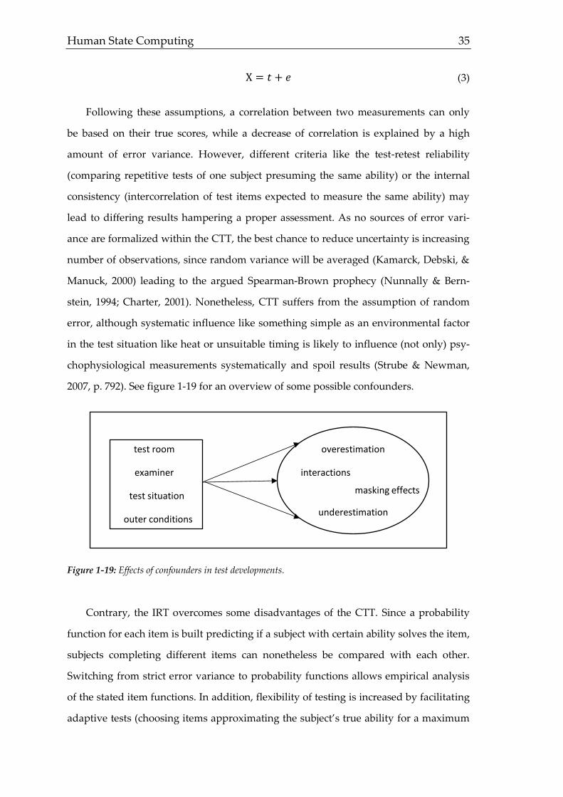
Human State Computing 35
X = 𝑡 + 𝑒 (3)
Following these assumptions, a correlation between two measurements can only
be based on their true scores, while a decrease of correlation is explained by a high
amount of error variance. However, different criteria like the test-retest reliability
(comparing repetitive tests of one subject presuming the same ability) or the internal
consistency (intercorrelation of test items expected to measure the same ability) may
lead to differing results hampering a proper assessment. As no sources of error vari-
ance are formalized within the CTT, the best chance to reduce uncertainty is increasing
number of observations, since random variance will be averaged (Kamarck, Debski, &
Manuck, 2000) leading to the argued Spearman-Brown prophecy (Nunnally & Bern-
stein, 1994; Charter, 2001). Nonetheless, CTT suffers from the assumption of random
error, although systematic influence like something simple as an environmental factor
in the test situation like heat or unsuitable timing is likely to influence (not only) psy-
chophysiological measurements systematically and spoil results (Strube & Newman,
2007, p. 792). See figure 1-19 for an overview of some possible confounders.
Figure 1-19: Effects of confounders in test developments.
Contrary, the IRT overcomes some disadvantages of the CTT. Since a probability
function for each item is built predicting if a subject with certain ability solves the item,
subjects completing different items can nonetheless be compared with each other.
Switching from strict error variance to probability functions allows empirical analysis
of the stated item functions. In addition, flexibility of testing is increased by facilitating
adaptive tests (choosing items approximating the subject’s true ability for a maximum
masking effects
underestimation
overestimation
interactions
test room
examiner
test situation
outer conditions
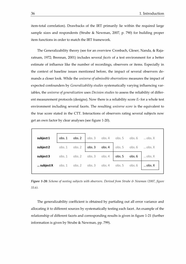
36 1. Introduction
item-total correlation). Drawbacks of the IRT primarily lie within the required large
sample sizes and respondents (Strube & Newman, 2007, p. 790) for building proper
item functions in order to match the IRT framework.
The Generalizability theory (see for an overview Cronbach, Gleser, Nanda, & Raja-
ratnam, 1972; Brennan, 2001) includes several facets of a test environment for a better
estimate of influence like the number of recordings, observers or items. Especially in
the context of baseline issues mentioned before, the impact of several observers de-
mands a closer look. While the universe of admissible observations measures the impact of
expected confounders by Generalizability studies systematically varying influencing var-
iables, the universe of generalization uses Decision studies to assess the reliability of differ-
ent measurement protocols (designs). Now there is a reliability score EΡ for a whole test
environment including several facets. The resulting universe score is the equivalent to
the true score stated in the CTT. Interactions of observers rating several subjects now
get an own factor by clear analyses (see figure 1-20).
Figure 1-20: Scheme of nesting subjects with observers. Derived from Strube & Newman (2007, figure
33.6).
The generalizability coefficient is obtained by partialing out all error variance and
allocating it to different sources by systematically testing each facet. An example of the
relationship of different facets and corresponding results is given in figure 1-21 (further
information is given by Strube & Newman, pp. 799).
subject 1 obs. 1 obs. 2 obs. 3 obs. 4 obs. 5 obs. 6 … obs. X
subject 2 obs. 1 obs. 2 obs. 3 obs. 4 obs. 5 obs. 6 … obs. X
subject 3 obs. 1 obs. 2 obs. 3 obs. 4 obs. 5 obs. 6 … obs. X
… subject X obs. 1 obs. 2 obs. 3 obs. 4 obs. 5 obs. 6 … obs. X

Human State Computing 37
Figure 1-21: G-study example. Fictive raw data are on the left side with computed error score in the top
right corner. Systematic decrease of the standard error for increased number of observers or observations
(days) is illustrated in the bottom right corner. Data and figures are derived from Strobe & Newman
(2007, figures 33.11, 33.12, 33.20).
In this way, the reliability score is determined distinctly depending among others
on the study design and the number of facets and levels (Strobe & Newman, 2007).
Although this approach is commonly not reported in biosignal based studies, it should
be kept in mind that several facets like the number of observers and the study design
in general have an impact on the accuracy of a model predicting user states and should
hence be considered in interpretations as well.
After theoretical and methodological backgrounds of biosignal research regarding
user states have been explained, a further clarification of physiological interactions
with human states have to be addressed for gaining insights into the specific structures
being responsible for the observable dependencies of Φ and ψ. Hence, an overview of
the general motor behavior with respect to state changes is provided in the following
chapter.
1 2 3 4 5 6 7 8 9 10
12345678910
1.0
0.5
0.1
num observernum days
var source
varcomp
% totalvar
person p 180 40
obs. o 25 6
day d 15 3
p,o 40 9
p,d 75 17
o,d 10 2
p,o,d 105 23
𝐸𝑝2 =
𝜎𝑝2
𝜎𝑝2 +
𝜎𝑝 ,𝑜2
𝑛𝑜+
𝜎𝑝 ,𝑑2
𝑛𝑑+
𝜎𝑝 ,𝑜 ,𝑑2
𝑛𝑜 𝑛𝑑
=180
180 +402
+754
+1052 · 4
std
. err
or

38 1. Introduction
1.2.3 User States and Motor Behavior
As this thesis analyzes perceptible motoric biosignals (in a broader sense), explana-
tions mainly cover the effect of different state levels on motor behavior. Though, it is
without more ado possible to transfer these assumptions to common electric biosignals,
too. As motor behavior is a very complex task with many structures involved and
strong interactions (Kelly & Strick, 2003), an approach is chosen to describe relevant
impacts on motor behavior after giving a broad overview of anatomical structures as
well as their physiological interactions to obtain a multifarious linkage of user states
and employed biosignals. By this approach, a clear picture is drawn from different per-
spectives to prove a sufficient theoretical basis for empirical research. For a broad
overview of relevant stages in voluntary movement, the hierarchic model of voluntary
movement by Kawato, Furukuwa, & Suzuki (1987) is considered. As figure 1-22 shows,
voluntary movement is initially based on a goal of movement (like grasping a glass of
water). This abstract goal has to be translated to a concrete plan by choosing one of the
commonly indefinite trajectories to reach the glass (trajectory determination). The select-
ed spatial coordinates of the trajectory now must result in body coordinates (including
involved muscles, angles of joints, etc.) based on spatial information (transformation of
coordinates). Finally, the reinterpreted motor command must be executed and evaluated
(generation of motor program). Naturally, the stages can also be adapted to different
kinds of movement like speech production. Hereby, spatial information is represented
by required control and modification of the airflow as well as involved structures for
articulation.
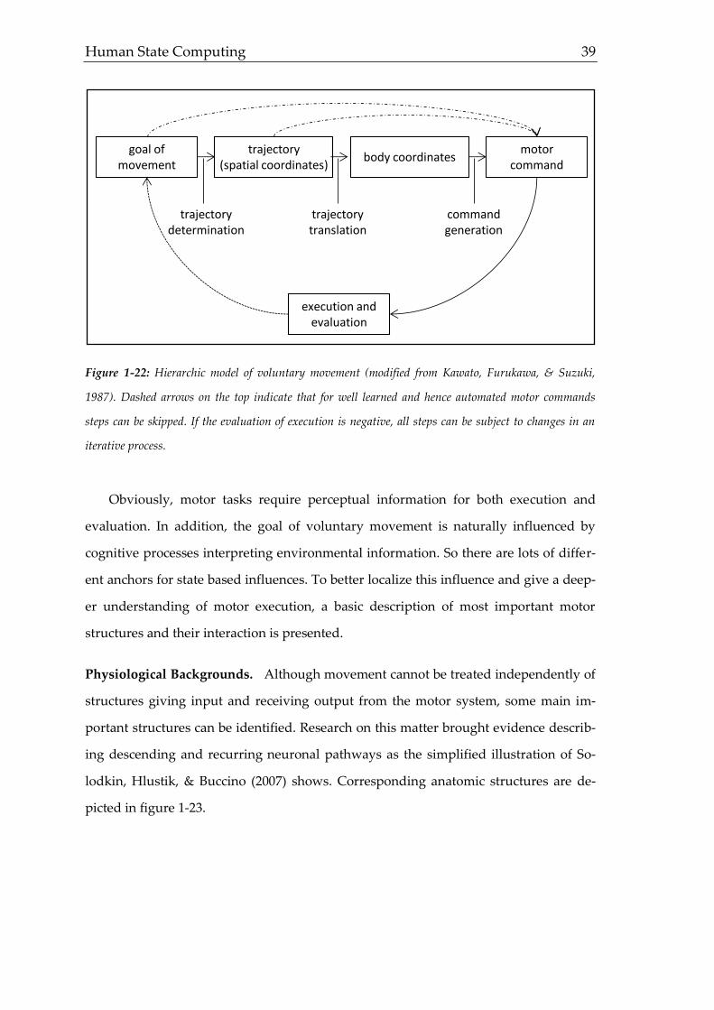
Human State Computing 39
Figure 1-22: Hierarchic model of voluntary movement (modified from Kawato, Furukawa, & Suzuki,
1987). Dashed arrows on the top indicate that for well learned and hence automated motor commands
steps can be skipped. If the evaluation of execution is negative, all steps can be subject to changes in an
iterative process.
Obviously, motor tasks require perceptual information for both execution and
evaluation. In addition, the goal of voluntary movement is naturally influenced by
cognitive processes interpreting environmental information. So there are lots of differ-
ent anchors for state based influences. To better localize this influence and give a deep-
er understanding of motor execution, a basic description of most important motor
structures and their interaction is presented.
Physiological Backgrounds. Although movement cannot be treated independently of
structures giving input and receiving output from the motor system, some main im-
portant structures can be identified. Research on this matter brought evidence describ-
ing descending and recurring neuronal pathways as the simplified illustration of So-
lodkin, Hlustik, & Buccino (2007) shows. Corresponding anatomic structures are de-
picted in figure 1-23.
goal of movement
trajectory (spatial coordinates)
body coordinates
execution and evaluation
motor command
trajectory translation
trajectory determination
command generation
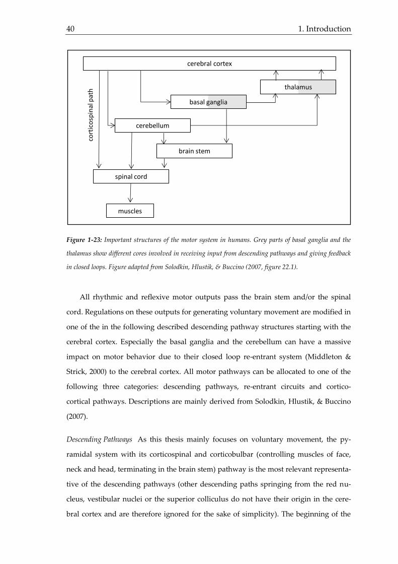
40 1. Introduction
Figure 1-23: Important structures of the motor system in humans. Grey parts of basal ganglia and the
thalamus show different cores involved in receiving input from descending pathways and giving feedback
in closed loops. Figure adapted from Solodkin, Hlustik, & Buccino (2007, figure 22.1).
All rhythmic and reflexive motor outputs pass the brain stem and/or the spinal
cord. Regulations on these outputs for generating voluntary movement are modified in
one of the in the following described descending pathway structures starting with the
cerebral cortex. Especially the basal ganglia and the cerebellum can have a massive
impact on motor behavior due to their closed loop re-entrant system (Middleton &
Strick, 2000) to the cerebral cortex. All motor pathways can be allocated to one of the
following three categories: descending pathways, re-entrant circuits and cortico-
cortical pathways. Descriptions are mainly derived from Solodkin, Hlustik, & Buccino
(2007).
Descending Pathways As this thesis mainly focuses on voluntary movement, the py-
ramidal system with its corticospinal and corticobulbar (controlling muscles of face,
neck and head, terminating in the brain stem) pathway is the most relevant representa-
tive of the descending pathways (other descending paths springing from the red nu-
cleus, vestibular nuclei or the superior colliculus do not have their origin in the cere-
bral cortex and are therefore ignored for the sake of simplicity). The beginning of the
cerebral cortex
basal ganglia
thalamus
cerebellum
brain stem
spinal cord
muscles
cort
ico
spin
al p
ath

Human State Computing 41
corticospinal pathway spreads over several cortical areas like the primary motor and
sensory cortices, premotor regions and the anterior cingulated motor area (Pinel, 2006)
highlighted in figure 1-24.
Figure 1-24: Relevant motor structures (excerpt). While the corticospinal pathway descends from motor
cortices, relevant perceptual information is gathered from sources described in the figure. The anterior
cingulaed motor area is on the inside and is hence not visible. Derived from Pinel (2006, figure 8.2).
The lateral corticospinal pathway runs on the contralateral side leading to contrala-
teral deficits of injuries for distal muscles like the hand relevant for mouse movements
and terminates in different regions of the spinal cord. Contrary, the medially descend-
ing pathway being responsible for proximal muscles (mainly upper arms and legs)
runs ipsilateral.
Re-entrant Circuits. While the former mentioned descending pathways rather deter-
mine the execution of an actual movement, re-entrant circuits primarily modify move-
ments and interact with other motor circuits. There are two structures being presented
in the following together building the extrapyramidal system (which has to be differen-
tiated from the corticospinal pyramidal system). In addition, the cerebellum with its
primary motor cortex
premotor cortex
somatosensoric cortex
supplementary motor area
posterior parietal association cortex
visual cortex
cerebellum
auditory cortex
frontal eye field

42 1. Introduction
anatomy similar to the cerebral cortex receives manifold afferent input from different
cortical and subcortical regions playing a relevant role also for reflex control involved
in posture and eye movements (Peterson, Baker, Goldberg, & Banovetz, 1988). Regard-
ing voluntary movement, though, important inputs are received from motor and sen-
sory cortical regions what enables the cerebellum to supervise fine motor behavior via
the loop through the ventral lateral nucleus of the thalamus already depicted in figure
1-23. Furthermore, the basal ganglia (in a strict sense) consisting of two main structures
(caudate and lentiform nuclei) have an impact primarily on motor control. The lenti-
form nucleus can be further separated in the putamen and the pallidum. Yet, putamen
and pallidum are also connected to the caudate nucleus. Due to the morphological ob-
vious connection via gray matter and the neighborly embryonic growth of the caudate
nucleus and the putamen, they are grouped as striatum. There are two pathways being
differentiated in a direct one leading back to the motor cortex running through the in-
ternal part of the putamen and ventral thalamic parts (independent of the cerebellar
pathway) and an indirect one. The indirect path leads through structures being allocat-
ed to the basal ganglia in a broader sense, in particular the substantia nigra (pars com-
pacta and pars reticularis) and the subthalamic nucleus. Information makes its way
from the putamen to the external pallidum further to the subthalamic nucleus being
redirected to the internal pallidum and the substantia nigra pars reticularis terminating
back in the motor cortex after running through the ventrolateral thalamus. All these
quite complex relationships are simplified in figure 1-25.

Human State Computing 43
Figure 1-25: Simplified scheme of motor re-entrant circuits. Bold black arrows indicate excitation, grey
dashed arrows inhibition. Adapted from Solodkin, Hlustik, & Buccino (2007, figure 22.9).
Beside the importance of the basal ganglia for motor control, Middleton & Strick
(1994) also proposed effects on cognitive functions due to strong efferences leading to
prefrontal cortical regions being e.g. related to stress reactions underlining a linkage of
pure motor behavior and cognitive activities.
Cortico-cortical Pathways. The last and most important part of motor behavior for vol-
untary movement is represented by the cortico-cortical pathways. Until the late 1980s,
the cortical motor system was supposed to mainly consist of the primary motor cortex,
the premotor cortex and the supplementary cortex, whereas the letter ones were
rather connected to motor planning and the primary motor cortex to motor execution.
New studies (mostly based on monkeys), however, postulate more complex relation-
ships. As it is not the intention of this thesis to depict an exhausting explanation of cor-
tical complexity, only a neuronal circuit of grasping objects is presented to give at least
an example of cortical interaction necessary for actually simple tasks applying for mo-
tor behavior like mouse movements. Starting with a certain structure within the pre-
motor cortex (F5 in monkeys), motor representations for several distinct tasks like
cerebral cortex
putamensubst. nigra
pars compacta
pallidum pars externa
sub-thalamic nuclei
pallidum pars interna
substantia nigra
ventro-lateralthalamic nucleus

44 1. Introduction
grasping food with the hand and the mouse have been found. Further differentiation is
even possible, as the identification of neurons responding to different kinds of grasp-
ing (e.g. approaching thumb and index finger against thumb and other fingers) leading
to the assumption of a vocabulary for different motor actions. Neurons in this context
can be separated into mirror and canonical neurons. Mirror neurons are not only active
when executing/planning a specified motor task, but also when someone else is ob-
served executing the same kind of task. Hence, a linkage to the sensory system is indi-
cated. Canonical neurons have their activity for planning and executing a certain task
in common with mirror neurons, but do not show activation for observing somebody
else. Instead, they are activated by objects being the target of specific motor tasks, e.g. a
pen or a piece of food that is possibly grasped. Hence, connections not only to the sen-
sory system but also to memory-related regions of the brain were found explaining
strong efferences to the parietal lobe.
Due to this strong differentiation of motor neurons paired with complex interac-
tions with several brain structures not primarily considered motor-related, central pat-
tern generators (CPGs) have been proposed, where this complex system is organized
hierarchically (Grillner & Wallen, 1985; Wiesendanger & Wise, 1992) with several quite
autonomic subsystems being responsible for modulating and executing tasks based on
general commands with regard to sensory feedback. This allows a better usage of high-
er order resources, as the foremost challenge then consists of giving the general com-
mand only without caring for the details being modified in hierarchically lower struc-
tures. Indeed, research on this topic trying to isolating CPGs from other influences
(with pharmacological help or studying vertebras with dissected connections of spinal
cord and higher regions) gives promising evidence on this matter.
These findings are relevant for biosignal analysis, as research has shown that not
only rhythmic and reflexive behavior, but also complex motor tasks (like swimming or
speaking) underlie relatively autonomous processes. The advantage of these almost
automatic processes for biosignal analysis results from the insight that observed bigger
changes in commonly little varying behavior can be traced back quite well to different
state levels. As CPGs receive not only input from descending motor pathways but also
sensory structures and are influenced by endocrinological conditions as well, it is obvi-

Human State Computing 45
ous that both complex motor tasks (consisting of several CPGs) like speaking as well as
simple ones (like mouse movements) are open to influence regarding different state
levels. CPGs in general are depicted in figure 1-26.
Figure 1-26: Basic scheme of CPGs. A simple/automized motor plan is controlled via a CPG structure
adapting its efferent output based on sensory feedback.
Impact Perspectives. After having given some anatomical backgrounds of motor be-
havior in general, a clear linkage to the impact of different state levels on the presented
stages of motor execution (figure 1-22) must be depicted in order to compile theoreti-
cally reasoned hypotheses on observed biosignals for different state levels. For this
reason, theories of motor control and skill acquisition are introduced. Following Mech-
ling & Munzert (2003), motor control theories can be allocated to one of the following
approaches:
1. Information processing theories: Motor actions are stored as generally fixed con-
cepts or patterns with adaptable variables allowing situation-specific modifica-
tions of motor behavior. Examples are generalized motor programs (GMP;
Schmidt, 1985; Lai & Shea, 1998) program oriented models like the already
mentioned central pattern generators (CPG) or closed-loop control theories
(Adams, 1971). Measurable impact of states is expected to be due to a changed
choice of motor patterns and/or different modification of variables.
motor command(„walk“)
left leg
right leg
CPG
sensory feedback
sensory feedback

46 1. Introduction
2. Behavioral theories: Motor behavior or behavior in general always takes place in
a system of persons, environments and tasks. In this context, actions are execut-
ed to improve the status quo. Narrowing the approach down to single motor
task executions, available motor units are employed and combined to reach a
certain goal. With the help of feedback loops it is evaluated whether the target-
ed reference value is reached. Examples are the TOTE-model (Miller, Galanter
& Pribram, 1960) or the action theory (Nitsch & Hackfort, 1999). Measurable
impact of states is expected due to changed reference values and overriding
goals.
3. Dynamic system theories: Motor actions are a product of self-organized and po-
tentially chaotic interactions between different involved structures. For predict-
ing or characterizing movement, though, it is sufficient to know the manifesta-
tion of low level descriptors covering variables like environment, task or indi-
vidual (e.g. state) characteristics, while high level patterns (intrinsic dynamics)
are commonly stable. Examples are the synergetic approach (Haken, 2012), the
Dynamic Pattern Theory (Zanone & Kelso, 1997) or Differential Learning
(Schöllhorn, 1999). Measurable impact of states is expected due to changes of
the mentioned low level descriptors.
All of the mentioned theories draw different conclusions regarding motor acquisi-
tion and execution. Although this thesis rather focuses on already learnt and automat-
ed tasks (like speaking or moving a mouse), (motor) tasks always contain a certain de-
gree of novelty, because two situations are never the same (even if the setting is identi-
cal, the experience differs). Hence, in the following both motor acquisition and control
is further analyzed.
Motor Skill Acquisition. There are several theories dealing with motor skill acquisition
as it is summarized at the end of this chapter. Following Fitts (1964; Fitts & Posner,
1967), however, motor skill acquisition mainly passes cognitive, associative and auton-
omous stages as depicted in figure 1-27.

Human State Computing 47
Figure 1-27: Fitts’s stages in the acquisition of motor skills.
In the cognitive phase, people are aware of what they want to do, but do not pos-
sess skilled motor plans to execute an action properly. In the associative phase, this
missing plan is built by modifying all necessary movements until a satisfying matching
between actual and desired outcome of a movement is reached. In the autonomous
phase, repetitive and similarly executed actions require less attention leading to an
automated completion of a motor task with only little variations. Especially this little
(but always present) amount of variation in automated motor skills allows biosignal
analysis to step in, as distinct measurable deviations in the execution of automated
motor tasks can be ascribed to state changes without being blurred by a high random
variability. Hence, it makes sense to analyze rather automated motor behavior as done
in the studies presented in chapters 3-5. Schmidt & Lee (2005; 2011) extended motor
skill acquisition by inducing the terms open-loop environments for slow actions that al-
low constant feedback while the movement is executed and closed loop environments
(conceptually similar to the CPGs mentioned before) for quicker actions requiring an
automated motor plan that is executed and not evaluated before the action is finished
(figure 1-28).
cognitive phase associative phase autonomous phase
AUTOMATISM
CONSCIOUSNESS

48 1. Introduction
Figure 1-28: Schematic comparison of open- and closed-loop environments. While in open-loop environ-
ments interference is possible during the execution due to constant feedback, within the faster closed-loop
environments feedback is not given before the execution is finished.
Spoken in these terms, mouse and head movement as well as speaking commonly
takes place in closed loop environments. Several studies (e.g. Ackermann & Cianciolo,
2000; Doyon & Benali, 2005; Calvo-Merino, Glaser, Grézes, Passingham, & Haggard,
2005) emphasized the involvement of cognitive processes in motor skill acquisition and
execution from either psychological or neurobiological perspectives. Physiologically,
the execution of a motor task starts with the perception and interpretation of the envi-
ronment leading to the plan for a motor activity in the motor cortex which is executed
based on the regularities of the reafference principle (Holst & Mittelstaedt, 1950; de-
tailed description of involved structures already given in this chapter). Most other
models of motor learning also focus on training and perfection like the described Fitts-
Posner-Model. For a general overview of relevant models, see table 1-5. Further infor-
mation can be derived from e.g. Birklbauer (2012).
motor plan
execution
feedback
OPEN-LOOP ENVIRONMENT
motor plan execution
feedback
CLOSED-LOOP ENVIRONMENT

Human State Computing 49
Table 1-5: Overview of motor skill acquisition models.
model type examples
stage models Daugs & Blischke (Acquisition and Optimization)
Fitts-Posner (cognitive, associative, autonomous phase)
Glencross (feedback dependency followed by motor programs)
Hotz (learning, refraining, deepening)
Lehnertz (acquisition principles and application principles)
Loosch (3 stages),
Meinel & Schnabel (gross skills, fine skills, stabilization and variability)
Pöhlmann (acquisition and perfection)
Roth (3 stages)
hierarchic model Jackson; Gesell & McGraw (top-down information processing, where
higher structures inhibit influence of subsequent structures)
scheme theories Attneave; Bartlett; Head; Schmidt (movement as mental representa-
tions)
Motor Execution. Usually, the execution of a well learned motor task is successful apart
from the ubiquitous variability mentioned before. Yet, there seem to be some points for
influence. Although people acquire and perfect motor skills frequently to a certain ex-
tent, most people already experienced athletes failing on apparently easy tasks or can-
didates stumbling in a job interview, although the athlete performed well on the same
task numerous times before and the candidate is not affected all of a sudden by some
kind of speech disorder. Hence, certain human state changes based on environmental
and/or intra-individual conditions must be responsible for those kinds of incidents.
Theoretical descriptions of state based variables are presented in the next paragraphs.
Starting with the well-known Yerkes-Dodson-Law dealing with cognitive abilities
for different levels of arousal, it is not difficult to imagine that there are not only ideal
state levels for cognitive, but also for motor tasks (Oxendine, 1970; Deviterne, Gau-
chard, Jamet, Vancon, & Perrin, 2005). It has to be considered that most primarily mo-
tor tasks presented in this thesis require cognitive work as well as described before.
The Yerkes-Dodson-Law postulates that best performance is shown within medium
levels of activation, so it is likely to observe that the characteristic of many user states
affects the users’ abilities (figure 1-29).

50 1. Introduction
Figure 1-29: Relation of performance and state level/arousal following the Yerkes-Dodson-Law. Ideal
performance is reached for a medium arousal.
Regarding the exemplary failing athlete mentioned before, the Yerkes-Dodson-
Law explains poor performance with either too low or too high arousal (making no
effort in performing well or being stressed by trying too hard). Although some criti-
cism came up regarding the method underlying the Yerkes-Dodson-Law, especially
regarding different types of arousal like anxiety and emotions (Sonstroem & Bernardo,
1982; Imlay, Carda, Stanbrough, Dreiling, & O’Connor, 1995; LeUnes & Nation, 1996),
or its underlying theoretical assumptions respectively (Neiss, 1988), several future
studies (Bregman & McAllister, 1982; Watters; Martin, & Schreter, 1997; Calabrese,
2008) adapting the law to different conditions (Teigen, 1994) have proven its wide-
ranged feasibility. While it is hence to expect, that predictions of the Yerkes-Dodson-
Law not always fully apply, literature gives clear indication that different kinds of
arousal based on emotions, fatigue, anxiety, stress and other states affect measurable
behavioral changes. Additionally, the cognitive perspective is not the only one sup-
porting the link between user states and biosignals.
Another perspective of task execution is given by Masters (1992) in his studies ad-
dressing the Implicit Learning approach postulating certain predictions regarding devi-
ating performance in well trained sports activities. The key finding was that the success
of motor actions (like golfing in his initial study) decreases, if a commonly automatical-
state level / arousal
per
form
ance
ideal
too relaxed
too nervous

Human State Computing 51
ly executed task is consciously dissected under pressure in order to perform best pos-
sible. Interfering in such processes leads to worse results (figure 1-30).
Figure 1-30: Study design of Masters's golf study (2007). Stress induction had a higher (negative) im-
pact for explicit learners.
In his study, Masters compared two groups learning how to putt (golf sports) as
can be derived from figure 1-30. One group learned with a prevailing technique con-
sisting of practical training and providing lots of explicit knowledge about what factors
influence the putting success. Within the other group, theoretical knowledge was kept
to minimum leading to rather implicit knowledge meaning that test persons are able to
putt properly, but are not totally aware of how they do it exactly. Exemplary, the act of
keeping balance when biking can be considered. Somebody who is able to use a bike
does not think about the correct angle of the handlebars or how he has to shift his
weight in order to avoid falling down when putting more weight on one side while
pedaling and is hardly aware of these factors. Under stress (induced by certain benefits
for good performance), though, having and rethinking explicit knowledge led to worse
performance. Despite some methodological issues in measuring implicit learning
(DeKeyser, 2008), the results were replicated in future studies (Liao & Masters, 2001;
Fine & Jäger, 2013). Obviously, sometimes thinking too much about actions reduces
skills.
Regarding motor variability, several approaches exist trying to make use of una-
voidable variance that even occurs when attempting to do a simple task twice. Beyond
the common variability of motor task execution for different tasks that has already
been mentioned, Riley & Turvey (2002) made an attempt to distinguish sources of this
variability with the help of nonlinear dynamic features (see chapter 2.2.3 for further
implicit learning
explicit learning
equal performance
stress induction
≈stable results
worse results

52 1. Introduction
explanation). As a key finding, it was shown that variability was a good predictor for
several disorders and state changes. Similar outcomes based on emotional changes
induced by pictures have been reported (Coombes, Janelle, & Duley, 2005; Coombes,
Kelly, Cauraugh, & Janelle, 2008) revealing that emotionally relevant stimuli lead to
increased force in motor actions. Following Winston, Gottfried, Killner, & Doran
(2005), pictures with stimulating valence extremes arouse the amygdala, which in turn
interfere with motor circuits including the basal ganglia leading to increased motor
cortex excitability (Haber, 2003) as shown in figure 1-31 as extension of figure 1-23.
Figure 1-31: Integration of the amygdala in the feedback loop of cortex, basal ganglia and the thalamus.
Grey shadows depict different localization of afferent input and efferent output.
From a physiological point of view it has to be taken into account that different
levels of stress or fatigue go along with endocrinological changes Stratakis & Chrousos,
1995; Hillhouse & Grammatopoulos, 2006) in line with the Yerkes-Dodson-Law impli-
cations. By way of illustration, stress causes an activation of the sympathetic nervous
system (Chrousos & Gold, 1992; Black, 1994; Staal, 2004) leading among others to a
higher muscle tense, blood pressure and pulse as well as the release of hormones like
adrenaline and cortisol (Aldwin, 2007, p. 25; more detailed description is given in chap-
ter 5.1). All of these changes (at least from a certain extent) result in a decrease of fine
and complex motor skill performance (Murphy & Woolfolk, 1987; Petruzzello,
Landers, Hatfield, Kubitz, & Salazar, 1991; Muller, Hardy & Tattersall, 2005; Kolove-
lonis, Goudas, & Dermitzaki, 2011), preventing automated motor plans to act as usual
respectively intervene in closed loops. With reference to the initially presented hierar-
chic model of voluntary movement by Kawato, Furukuwa, & Suzuki (1987), described
models of motor skill acquisition and execution can be linked to the assumed stages of
voluntary movements. Table 1-6 gives an overview of relations.
cerebral cortex
basal ganglia
thalamus
amygdala

Human State Computing 53
Table 1-6: Relations of voluntary movement and theoretically reasoned state influence on motor control.
movement step influence
trajectory
determination
Following behavioral motor control theories, cognitive (state-based)
processes can influence the perceived status quo leading to different
intentions/planned actions. Also dynamic system theories support this
assumption
trajectory
translation
Following implicit learning, states can modify or interfere in trajectory
translations (which might be even skipped for usually already auto-
mated tasks)
command
generation
Following analyses of motor variability, command generation and its
execution is strongly influenced by state levels. Also the Yerkes-
Dodson-Law support this assumption
Biosignal Applicability. It has been outlined now that there are several different an-
gles all indicating a theoretical and empiric linkage of human states and motor-related
biosignals. Transferring these findings to biosignals leads to concrete hypotheses for
changes under different state conditions. All employed biosignals have their automatic
and usually implicit usage in common. Nobody usually considers the exact position of
his tongue and the airflow one has to generate before speaking a word, the computer
mouse is used without consciously estimating the required distance and angle before
moving and natural head movements take place without noticing. Hence, regularities
described by Masters’s (1992) implicit knowledge behavior (comparable to closed-loop
movements described before) apply. When in a stressful situation like a job interview,
candidates could try to rethink and build explicit knowledge about how to appear
most suitable for the desired position including how to speak or how to show a proper
body language, a decrease of the performance can be assumed (relating to findings of
Spalding & Hardin, 1999, where explicit self-esteem was a better predictor of self-
handicapping than implicit self-esteem). Although variance in the degree of perfor-
mance changes is likely explained by the degree subjects are affected by different state
levels, it is to assume that state-based differences in motor behavior occur potentially
allowing the derivation of underlying regularities. In summary, there is clear indica-
tion from several points of view, that non-intrusive recordable biosignals are affected
by different state expressions in a predictable manner. For proving this assumption,
several studies have been conducted focusing on different biosignals illustrating meas-

54 1. Introduction
urements of those changes on a physical level. Examples of the employed biosignals for
studies described in this thesis are presented in the following section (chapter 1.3).
1.3 Employed Biosignals
As this work aims at proving the feasibility of pattern recognition based biosignal
analysis in manifold fields of (occupational) application, three different sources of bi-
osignals are employed for assessing user states like leadership qualities, fatigue and
stress. To give a brief introduction about using voice, mouse and head movement sig-
nals for automatic state analysis, some peculiarities of physiological backgrounds as
well as fields of application are described in the following passages for all biosignals
employed in the studies described within the chapters 3-5.
1.3.1 Voice
An almost non-intrusive as well as preparation-free and maintenance-free analysis
tool is the microphone. Employees are used to headsets or similar hardware due to
telephone conferences or presentations, so that a quite natural way of measuring may
be assumed (Krajewski, Sauerland, Sommer, & Golz, 2011). Also audio recordings via
webcam are possible providing data of sufficient quality in several settings. While most
studies use the term “speech”, within this thesis the term “voice” is employed, as
speech implicitly covers language-specific characteristics like words/semantic, gram-
mar or syntax (Moats, 2000) and hence includes non-physical phenomena (in a strict
view) being ignored in most voice-based analyses as with this thesis to allow a more
general view. Physiological backgrounds and state-of-the-art knowledge about speech
and voice measurements will be explained further in the next section.
Physiological Backgrounds. Due to the relevance and complexity of speech produc-
tion for the presented studies, involved structures must be described. In general, the
corticobulbar pathway springing from the primary motor cortex and terminating in
motor neurons of the brain stem is responsible for face, head and neck movements
(Barnes, 2013, p. 179). For speech production, structures responsible for respiration
(Subramanian, Balnave, & Holstege, 2008), phonation by controlling lower structures

Human State Computing 55
like glottis, larynx and pharynx (Edmondon & Esling, 2006) and articulation based on
higher structures like peri-oral muscles and the tongue (Kim, Ura, Kashino, & Gomi,
2011) must be considered. The innervation and control of the respiratory system is
mainly realized by the aquaeductual Gray (Subramanian et al., 2008), further leading to
the pulmonary plexus nerve with branches of the vagus nerve (CN X) and sympathetic
trunks of the fourth thoracic ganglia (Drake, Vogel, & Mitchell, 2010, p. 46). For phona-
tion, especially the cranial division of the accessory nerve (CN XI) is important (Wil-
son-Pauwels, 2010, pp. 209). Peri-oral muscles like the lips as well as the tongue are
mainly innerved by maxillary and mandibular parts of the tripartite trigeminal nerve
(CN V). By including altogether three out of twelve cranial nerves, the complexity of
speech production is emphasized. Figure 1-32 gives a very simplified overview of re-
lated structures and functions.
Figure 1-32: Simplified innervation of functions required for speech.
The high amount of employed muscles for speech production gives lots of possibil-
ities for measurable state based influence. Foundation of those measurements is the
unconscious influence of speech production by the autonomous nervous system
(Pierre-Yves, 2003), which is not surprising as e.g. the respiration is directly innerved
by sympathetic nerves as outlined before. For a further understanding of involved and
iinfluencable structures, figure 1-33 illustrates the vocal tract.
speech
phonationrespiration articulation
pulmonary plexus nerve (vagus CN X) / symp. trunk
cranial division of accessorious (CN XI)
tongue: hypoglossus (CN XII) lips: trigeminus (CN V)

56 1. Introduction
Figure 1-33: Speech-relevant structures of the vocal tract. Adapted from Hess (2002).
Following figure 1-33, the airflow evolving from the lunges is excited by the vocal
chords leading to a source signal (phonation). In the remaining resonance chamber
(vocal tract) the source signal is modified allowing a discrimination of speech sounds
(articulation). In figure 1-34, a technical representation of the vocal tract is depicted.
Figure 1-34: Technical representation of the vocal tract. The airflow generated by the lungs (respiration)
is stimulated (phonation) before reaching mouth and/or nasal cavity (articulation). Adapted from Krajew-
ski (2007, figure 3).
Having a closer look at speech production theories, following Krajewski (2007, pp.
39) it can be differentiated between stage models without any recurrent interaction of
subsequent steps and activation spreading allowing interactions of involved structures.
Considering stages proposed by Levelt, Roelofs, & Meyer (1999), at the beginning of
Mundraum
Rachenraum (Pharynx)
Nasenraum
Gaumen
Lippen
Zunge
Unterkiefer Velum
Stimmbänder, Stimmritze (Glottis)
mouth cavitynasal cavity
palatal
lips
tongue
pharynx
velum
vocal chords,glottis
mandible
larynx
glottis trachea
lungs
nose
mouthpharynx
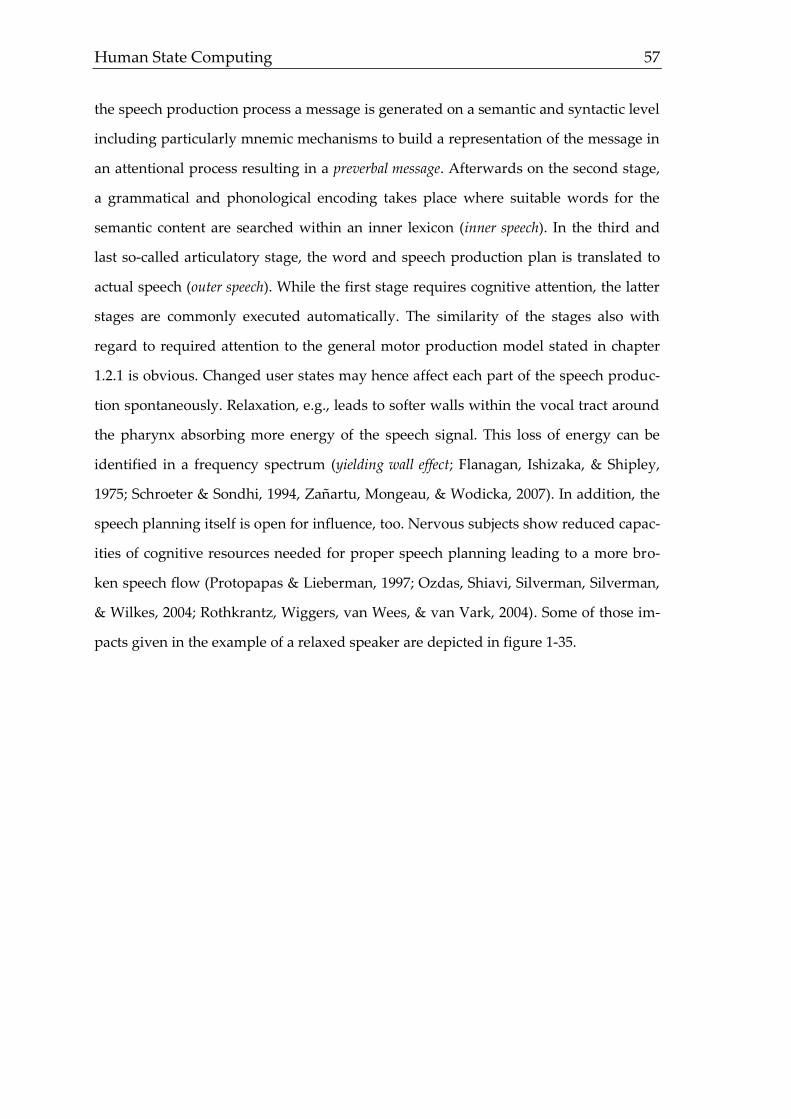
Human State Computing 57
the speech production process a message is generated on a semantic and syntactic level
including particularly mnemic mechanisms to build a representation of the message in
an attentional process resulting in a preverbal message. Afterwards on the second stage,
a grammatical and phonological encoding takes place where suitable words for the
semantic content are searched within an inner lexicon (inner speech). In the third and
last so-called articulatory stage, the word and speech production plan is translated to
actual speech (outer speech). While the first stage requires cognitive attention, the latter
stages are commonly executed automatically. The similarity of the stages also with
regard to required attention to the general motor production model stated in chapter
1.2.1 is obvious. Changed user states may hence affect each part of the speech produc-
tion spontaneously. Relaxation, e.g., leads to softer walls within the vocal tract around
the pharynx absorbing more energy of the speech signal. This loss of energy can be
identified in a frequency spectrum (yielding wall effect; Flanagan, Ishizaka, & Shipley,
1975; Schroeter & Sondhi, 1994, Zañartu, Mongeau, & Wodicka, 2007). In addition, the
speech planning itself is open for influence, too. Nervous subjects show reduced capac-
ities of cognitive resources needed for proper speech planning leading to a more bro-
ken speech flow (Protopapas & Lieberman, 1997; Ozdas, Shiavi, Silverman, Silverman,
& Wilkes, 2004; Rothkrantz, Wiggers, van Wees, & van Vark, 2004). Some of those im-
pacts given in the example of a relaxed speaker are depicted in figure 1-35.

58 1. Introduction
Figure 1-35: Examples of measurable impacts on speech.
It is shown therefore, that (considering also impacts on automatic motor execution
described in chapter 1.2) speech planning and production is sensitive for different lev-
els of human states going along with general assumptions mentioned in chapter 1.2. As
voice is a heavily researched biosignal for manifold fields of application, the following
passage deals with corresponding research.
Research on Voice. Although primarily employed within the Speech Emotion Recog-
nition (SER), Human-Computer-Interaction (HCI) and Call Centers (Burkhadrt, van
Ballegooy, Englet, & Huber, 2005; Burkhardt, Ajmera, Englert, Stegmann, & Burleson,
2006; Devillers & Vidrascu, 2006; Steidl, 2009; Batliner et al., 2011), other areas of appli-
cation are opened up like leadership or self-confidence since the 1970s (Scherer, Lon-
don, & Wolf, 1973; Streeter, Krauss, Geller, Olson, & Apple, 1977; Maclachlan, Czepiel,
& LaBarbera, 1979) and fatigue (Claghorn, Mathew, Weinman, & Hruska, 1981; Murry
& Bone, 1989). While early studies rather focus on (by humans) perceptible voice
changes, the progress in computer technologies and the linked improve of computation
capacities of personal computers enables scientists to extract a variety of features
(chapter 2.2), that need not to be linked directly to sensations of human perception.
Those numerous features combined with suitable pattern recognition methods allow
relaxed pharynx (yielding wall effect)
lower velum (open nasal cavity)
reduced heat emission (change of airflow)
reduced tension and stiffness of glottis
regular and slow respiration upright pose (no shortened vocal tract)
frequent smiling and lip spreading
no trembling, shaking of voice due reduced fine
motor skills
regular speech planning
relaxed-open-mouth-display (van Hooff, 1972, p. 217)

Human State Computing 59
an automatic and decent assessment of human states. Regarding self-confidence, short
response latencies (Kimble & Seidel, 1991; Boltz, 2005), certain courses of frequency
(Hecht & LaFrance, 1995, Chen, Gussenhoven, & Tietveld, 2004; Hecht) and Power
Spectral Density (PSD) of some frequency bandwidths (Keßel & Krajewski, 2010) are
some features that facilitate good assessments. Successful implementations of state
recognition with modern techniques by workgroups around the author and others
apart from SER also cover sleepiness (Greeley, Friets, Wilson, Raghaven, Picone, &
Berg, 2006; Dhupati, Kar, Rajaguru, & Routray, 2010; Krajewski et al., 2010), depression
(Schnieder, Laufenberg, & Krajewski), blood alcohol level (Schiel & Heinrich, 2009;
Schuller et al., 2014) and leadership assessment (Laufenberg, Krajewski, & Rathert,
2011). Schuller et al. (2013) further segregate voice research in short, medium and long
term states finding examples for implementations of among others sociodemographic
descriptives like height, weight, age, gender, group/ethnicity, relationships in interac-
tions, uncertainty, deception or frustration. Table 1-7 gives an overview of state-related
voice changes on a general level.
Table 1-7: Empirical results on state-based voice changes for the dimensions activation, valence and
potency. Adapted from Laukka, Juslin, & Bresin, (2005).
dimension voice changes
activation high average of F0, high variability of F0, high maximum of F0, high
average of intensity, high variability of intensity, high average of F1,
low bandwidth of F1, precise articulation, low bandwidth of F3, high
energy of higher frequencies, increased speech rate, less pauses, de-
creased voice onset
positive valence low average of F0, high variability of F0, low average of intensity, low
variability of intensity, low average of F1, slurred articulation, low
bandwidth of F2, low energy of high frequencies, increased speech rate,
increased voice onset
potency high variability of F0, high average of intensity, high variability of in-
tensity, high average of F1, low bandwidth of F1, precise articulation,
low average of F3, low bandwidth of F3, high energy of high frequen-
cies, decreased speech rate, decreased voice onsets
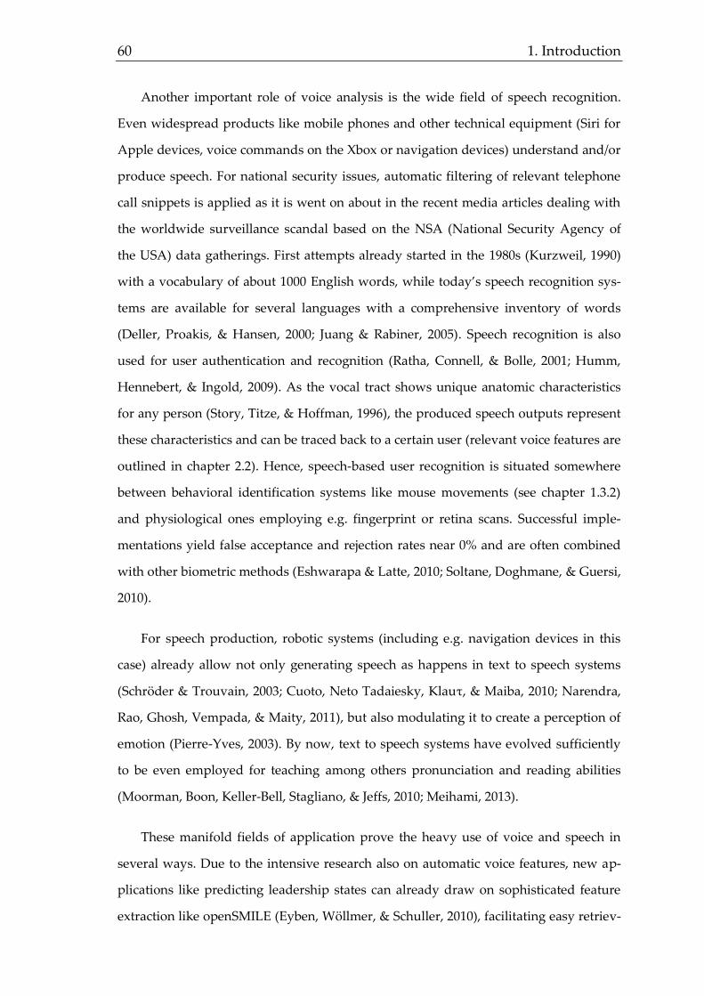
60 1. Introduction
Another important role of voice analysis is the wide field of speech recognition.
Even widespread products like mobile phones and other technical equipment (Siri for
Apple devices, voice commands on the Xbox or navigation devices) understand and/or
produce speech. For national security issues, automatic filtering of relevant telephone
call snippets is applied as it is went on about in the recent media articles dealing with
the worldwide surveillance scandal based on the NSA (National Security Agency of
the USA) data gatherings. First attempts already started in the 1980s (Kurzweil, 1990)
with a vocabulary of about 1000 English words, while today’s speech recognition sys-
tems are available for several languages with a comprehensive inventory of words
(Deller, Proakis, & Hansen, 2000; Juang & Rabiner, 2005). Speech recognition is also
used for user authentication and recognition (Ratha, Connell, & Bolle, 2001; Humm,
Hennebert, & Ingold, 2009). As the vocal tract shows unique anatomic characteristics
for any person (Story, Titze, & Hoffman, 1996), the produced speech outputs represent
these characteristics and can be traced back to a certain user (relevant voice features are
outlined in chapter 2.2). Hence, speech-based user recognition is situated somewhere
between behavioral identification systems like mouse movements (see chapter 1.3.2)
and physiological ones employing e.g. fingerprint or retina scans. Successful imple-
mentations yield false acceptance and rejection rates near 0% and are often combined
with other biometric methods (Eshwarapa & Latte, 2010; Soltane, Doghmane, & Guersi,
2010).
For speech production, robotic systems (including e.g. navigation devices in this
case) already allow not only generating speech as happens in text to speech systems
(Schröder & Trouvain, 2003; Cuoto, Neto Tadaiesky, Klauτ, & Maiba, 2010; Narendra,
Rao, Ghosh, Vempada, & Maity, 2011), but also modulating it to create a perception of
emotion (Pierre-Yves, 2003). By now, text to speech systems have evolved sufficiently
to be even employed for teaching among others pronunciation and reading abilities
(Moorman, Boon, Keller-Bell, Stagliano, & Jeffs, 2010; Meihami, 2013).
These manifold fields of application prove the heavy use of voice and speech in
several ways. Due to the intensive research also on automatic voice features, new ap-
plications like predicting leadership states can already draw on sophisticated feature
extraction like openSMILE (Eyben, Wöllmer, & Schuller, 2010), facilitating easy retriev-
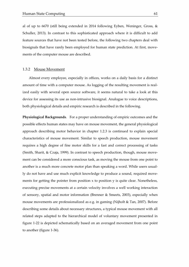
Human State Computing 61
al of up to 6670 (still being extended in 2014 following Eyben, Weninger, Gross, &
Schuller, 2013). In contrast to this sophisticated approach where it is difficult to add
feature sources that have not been tested before, the following two chapters deal with
biosignals that have rarely been employed for human state prediction. At first, move-
ments of the computer mouse are described.
1.3.2 Mouse Movement
Almost every employee, especially in offices, works on a daily basis for a distinct
amount of time with a computer mouse. As logging of the resulting movement is real-
ized easily with several open source software, it seems natural to take a look at this
device for assessing its use as non-intrusive biosignal. Analogue to voice descriptions,
both physiological details and empiric research is described in the following.
Physiological Backgrounds. For a proper understanding of empiric outcomes and the
possible effects human states may have on mouse movement, the general physiological
approach describing motor behavior in chapter 1.2.3 is continued to explain special
characteristics of mouse movement. Similar to speech production, mouse movement
requires a high degree of fine motor skills for a fast and correct processing of tasks
(Smith, Sharit, & Czaja, 1999). In contrast to speech production, though, mouse move-
ment can be considered a more conscious task, as moving the mouse from one point to
another is a much more concrete motor plan than speaking a word. While users usual-
ly do not have and use much explicit knowledge to produce a sound, required move-
ments for getting the pointer from position x to position y is quite clear. Nonetheless,
executing precise movements at a certain velocity involves a well working interaction
of sensory, spatial and motor information (Brenner & Smeets, 2003), especially when
mouse movements are professionalized as e.g. in gaming (Nijholt & Tan, 2007). Before
describing some details about necessary structures, a typical mouse movement with all
related steps adapted to the hierarchical model of voluntary movement presented in
figure 1-22 is depicted schematically based on an averaged movement from one point
to another (figure 1-36).
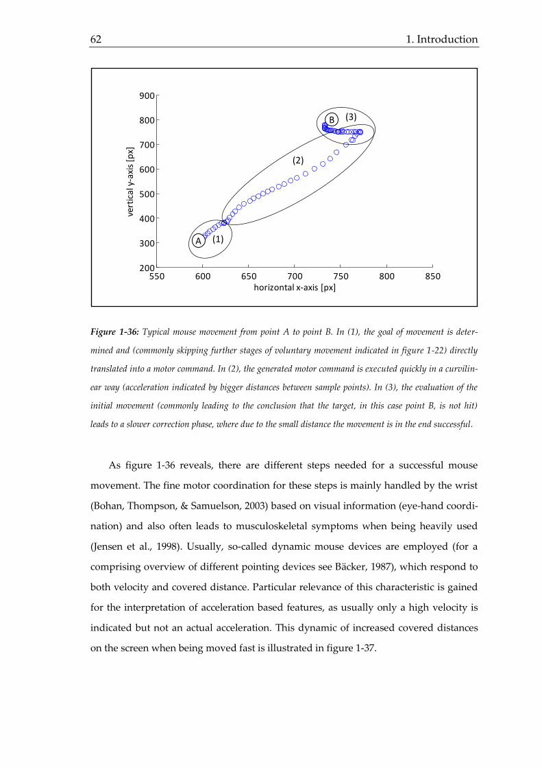
62 1. Introduction
Figure 1-36: Typical mouse movement from point A to point B. In (1), the goal of movement is deter-
mined and (commonly skipping further stages of voluntary movement indicated in figure 1-22) directly
translated into a motor command. In (2), the generated motor command is executed quickly in a curvilin-
ear way (acceleration indicated by bigger distances between sample points). In (3), the evaluation of the
initial movement (commonly leading to the conclusion that the target, in this case point B, is not hit)
leads to a slower correction phase, where due to the small distance the movement is in the end successful.
As figure 1-36 reveals, there are different steps needed for a successful mouse
movement. The fine motor coordination for these steps is mainly handled by the wrist
(Bohan, Thompson, & Samuelson, 2003) based on visual information (eye-hand coordi-
nation) and also often leads to musculoskeletal symptoms when being heavily used
(Jensen et al., 1998). Usually, so-called dynamic mouse devices are employed (for a
comprising overview of different pointing devices see Bäcker, 1987), which respond to
both velocity and covered distance. Particular relevance of this characteristic is gained
for the interpretation of acceleration based features, as usually only a high velocity is
indicated but not an actual acceleration. This dynamic of increased covered distances
on the screen when being moved fast is illustrated in figure 1-37.
550 600 650 700 750 800 850200
300
400
500
600
700
800
900
horizontal x-axis [px]
vert
ical
y-a
xis
[px]
(1)A
B (3)
(2)
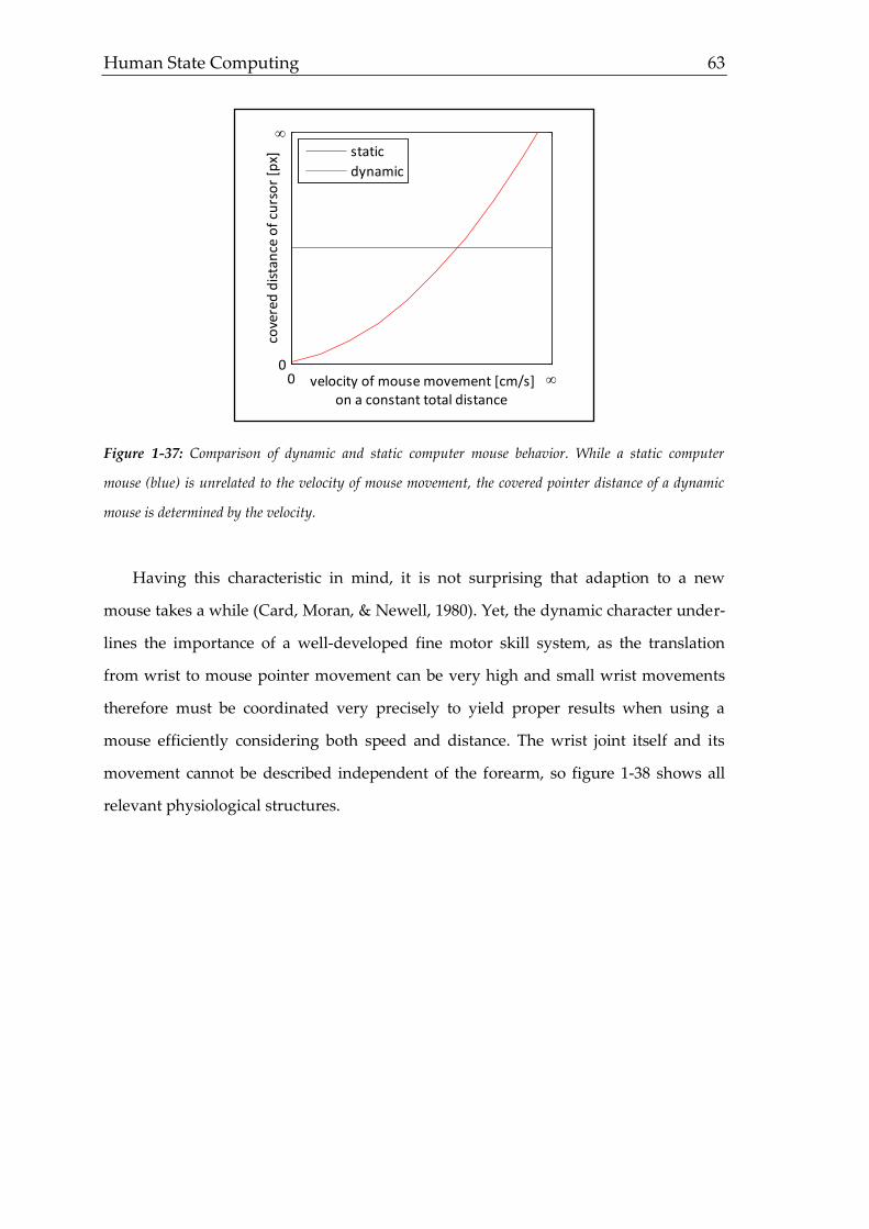
Human State Computing 63
Figure 1-37: Comparison of dynamic and static computer mouse behavior. While a static computer
mouse (blue) is unrelated to the velocity of mouse movement, the covered pointer distance of a dynamic
mouse is determined by the velocity.
Having this characteristic in mind, it is not surprising that adaption to a new
mouse takes a while (Card, Moran, & Newell, 1980). Yet, the dynamic character under-
lines the importance of a well-developed fine motor skill system, as the translation
from wrist to mouse pointer movement can be very high and small wrist movements
therefore must be coordinated very precisely to yield proper results when using a
mouse efficiently considering both speed and distance. The wrist joint itself and its
movement cannot be described independent of the forearm, so figure 1-38 shows all
relevant physiological structures.
velocity of mouse movement [cm/s]on a constant total distance
cove
red
dis
tan
ce o
f cu
rso
r [p
x]
0 0
static
dynamic

64 1. Introduction
Figure 1-38: Simplified innervation of wrist and hands. Nerves springing from the brachial plexus are
responsible for innervation of wrist and fingers (information derived from Trepel, 2004, pp. 37).
The ellipsoid wrist joint itself allows movements along two axes, whereby parallel
movement in both axes is possible (Trepel, 2004, pp. 37). With regard to mouse move-
ment, horizontal movements (moving the cursor from left to right and vice versa; x-
axis) and vertical movements (moving the cursor from top to bottom and vice versa; y-
axis) can be differentiated by extension and deeviation (figure 1-39). Wrist movements
along the z-axis (turning the wrist by pronation and supplination) are provided by the
elbow and are hence not listed, as they are not relevant for mouse applications.
spin
al c
ord
BACK OF HAND
bra
chia
l ple
xus
ulnar nerve
medial nerve
PALM
brach
ial plexu
s
radial nerve
ulna
radius
proximal wrist
distal wrist
carpu
s
ulna
radius
proximal wrist
distal wrist
carp
us

Human State Computing 65
Figure 1-39: Wrist joint movements. Moving the mouse cursor on the horizontal x-axis is realized by
ulnar (left) and radial (right) deviation (assuming right-handed users). Vertical cursor movements on the
y-axis are realized by different degrees of wrist extension coordinated with flexion of the fingers. Bigger
movements can also be the result of moving the whole arm with a fixed wrist.
The innervation of all relevant muscles for wrist, fingers and arm is delivered by
the median, radial and ulnar nerve springing from the brachial plexus (cervical verte-
bra C5 to thorical vertebra Th1) which in turn is innerved by the spinal cord (Trepel,
2004, pp. 37) as shown on figure 1-38. Miall, Imamizu, & Miyauchi (2000) especially
stress the important influence of the cerebellum for eye-hand coordinated tasks in this
context. Although movement along the x-axis is limited to about 30° (neutral zero
method following Ryf & Weymann, 1995), it is responsible for the major part of hori-
zontal mouse movement, while vertical movement results from coordinated activities
of extension of the wrist joint and flexion of the fingers.
Research on Mouse Movement. As it has been outlined by now which structures of
the body are employed for mouse movements, the following section comprises empiric
and theoretical findings on mouse movement. Simple “point and touch” actions were
already analyzed by Fitts (1954). Although he started in his studies with point and
touch tasks in order to find a formula describing the required time for completing the
task, the setting can and has been easily transferred to “point and mouse click” or other
high extension
low extension
radial deviation
ulnar deviation
x-axis y-axis
66 1. Introduction
tasks (Kabbash & Buxton, 1995; Accot & Zhai, 1997; Soukoreff & MacKenzie, 2004; Wu,
Yang, & Honda, 2010). Although several formula exist based on Fitts’s original find-
ings (Drewes, 2010) the most prominent version of MacKenzie (1992; 1995) is chosen to
describe variables predicting the required time T to execute the task (equation 4).
𝑇 = 𝑎 + 𝑏 · log2 (1 +𝐷
𝑊) (4)
Time T is given by the device-specific and empirically generated variables a (delay
of the device starting), b (acceleration and movement changes) as well as the distance D
between starting point to the target of the center and the target size W (since a test per-
son is allowed to click anywhere on a target). D/W is also referred to as the index of
difficulty, as a task is the more difficult to fulfill in a certain amount of time, the bigger
the distance and the smaller the target is. The stability and precision of this prediction
reaches unusual high correlation rates of r = .95 (McKenzie, 1992). With McKenzie’s
Shannon formula (1992) shown above, it is also possible to assess two-dimensional
tasks, although Fitts (1954) previously only analyzed unidimensional movements. For
biosignal based state recognition, Fitts’s law gives evidence to the assumption that dif-
ferent state levels might be sensitive to speed changes as indicated in chapter 1-2-3.
Due to the high stability (also confirmed by e.g. Murata, 1999; Accot & Zhai, 2003), dif-
ferences in the required time of executing a mouse movement are likely to be ascribed
to state changes like increased fatigue.
Research regarding mouse movements also heavily focused on indicating eye
movements in order to replace artificial and costly settings with eye tracking equip-
ment (Chen, Anderson, & Son, 2001) in different fields of application like getting in-
sights about the perception of web designs (Arroyo, Selker, & Wei, 2006) or usabil-
ity/joy of use (Atterer, Wnuk, & Schmidt, 2006). Due to insufficiently performing at-
tempts to replace eye tracking with the computer mouse, the development of new al-
gorithms has decreased within the last years. Since especially receptive activities like
reading or getting an overview of a website are mainly done by eye movements only,
the insufficient relation is not surprising keeping in mind, that mouse movement is a
rather productive task mostly leading to some kind of click activity.
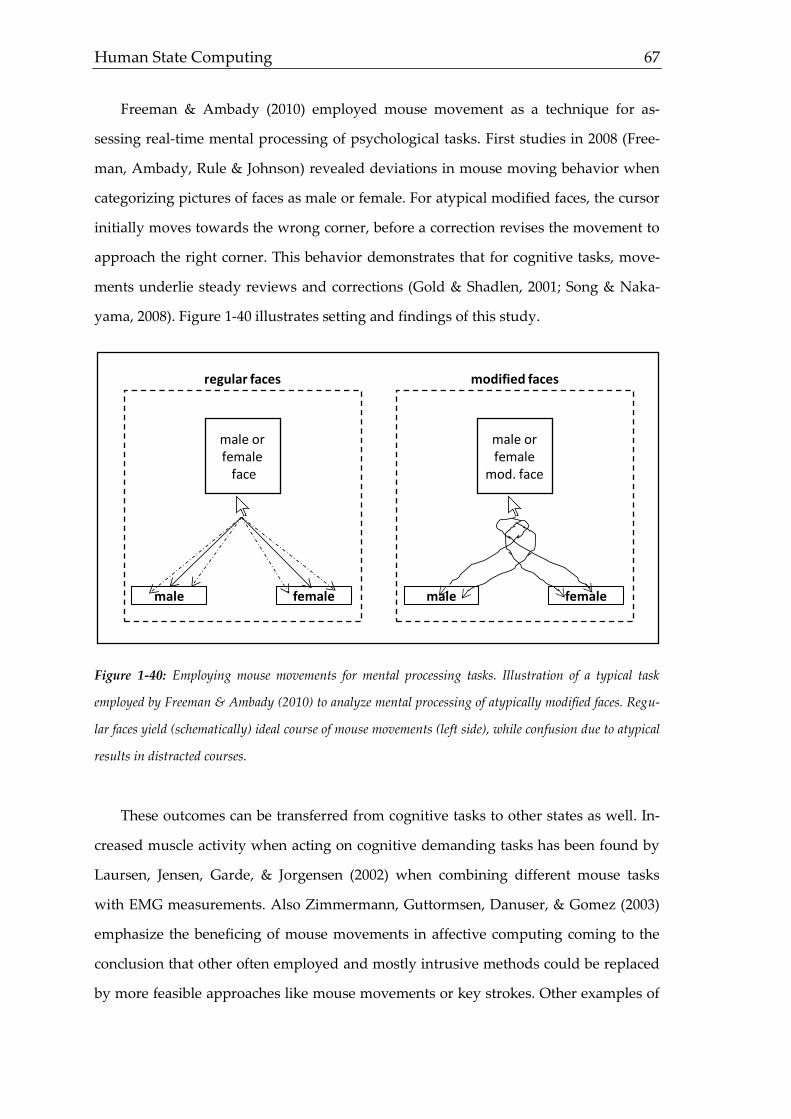
Human State Computing 67
Freeman & Ambady (2010) employed mouse movement as a technique for as-
sessing real-time mental processing of psychological tasks. First studies in 2008 (Free-
man, Ambady, Rule & Johnson) revealed deviations in mouse moving behavior when
categorizing pictures of faces as male or female. For atypical modified faces, the cursor
initially moves towards the wrong corner, before a correction revises the movement to
approach the right corner. This behavior demonstrates that for cognitive tasks, move-
ments underlie steady reviews and corrections (Gold & Shadlen, 2001; Song & Naka-
yama, 2008). Figure 1-40 illustrates setting and findings of this study.
Figure 1-40: Employing mouse movements for mental processing tasks. Illustration of a typical task
employed by Freeman & Ambady (2010) to analyze mental processing of atypically modified faces. Regu-
lar faces yield (schematically) ideal course of mouse movements (left side), while confusion due to atypical
results in distracted courses.
These outcomes can be transferred from cognitive tasks to other states as well. In-
creased muscle activity when acting on cognitive demanding tasks has been found by
Laursen, Jensen, Garde, & Jorgensen (2002) when combining different mouse tasks
with EMG measurements. Also Zimmermann, Guttormsen, Danuser, & Gomez (2003)
emphasize the beneficing of mouse movements in affective computing coming to the
conclusion that other often employed and mostly intrusive methods could be replaced
by more feasible approaches like mouse movements or key strokes. Other examples of
regular faces modified faces
male female
male or female
face
male female
male or female
mod. face

68 1. Introduction
application and research are among others diagnostics of fine motor skills and motor
control (Sandfeld & Jensen, 2005)
Another field of application for mouse movement is the user recognition for un-
locking computers. Biometric approaches commonly distinguish between physiologi-
cal ones, which base on retina, face or fingerprint recognition, and behavioral ones be-
ing realized by analyzing keystrokes or mouse movements (Everitt, & McOwan, 2003).
Physiological recognition methods gained some attention of research (Gupta, Ravi,
Raghunathan, & Jha, 2005; Mallauran, Dugelay, Perronnin, & Garcia, 2005), though
they lack of feasibility by requiring special equipment. Due to increasing problems
with passwords (Ross, Jackson, Miyake, Boneh, & Mitchell, 2005; Zhang, Monrose, &
Reiter, 2010), feasible and resource-saving methods are very welcome. In the past
years, though, successful implementations of mouse movement based user recognition
have been presented (Weiss, Ramapanicker, Shah, Noble, & Immohr, 2007; Zheng,
Paloski, & Wang, 2012). Generated features are based on angles, direction, curvature
distance, speed and click behavior (more information about mouse movement based
features is described in chapter 2.2.4). Although the recognition rate correlates highly
with the user actions (and is hence only usable to a certain extent, as the authentication
must not take much time), false rejection rates of 1% for 15 clicks and a false acceptance
rate of 3% for 25 clicks show, that mouse movement behavior obviously brings up in-
ter-individual differences. Hence, it is not far-fetched to presume also intra-individual
dependencies of current state levels as described in first attempts by Ark, Dryer, & Lu
(1999) or Zimmermann, Guttormsen, Danuser, & Gomez (2003).
As outlined, mouse movement has been employed in various fields of application.
However, there has not been drawn much attention on other states than emotions.
Nonetheless, employed features for describing trajectories of mouse movements can be
transferred to other state computing tasks as well. To complete the presentation of all
biosignals employed in this thesis, the following section deals with head movements.
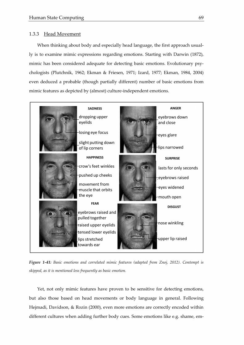
Human State Computing 69
1.3.3 Head Movement
When thinking about body and especially head language, the first approach usual-
ly is to examine mimic expressions regarding emotions. Starting with Darwin (1872),
mimic has been considered adequate for detecting basic emotions. Evolutionary psy-
chologists (Plutchnik, 1962; Ekman & Friesen, 1971; Izard, 1977; Ekman, 1984, 2004)
even deduced a probable (though partially different) number of basic emotions from
mimic features as depicted by (almost) culture-independent emotions.
Figure 1-41: Basic emotions and correlated mimic features (adapted from Znoj, 2012). Contempt is
skipped, as it is mentioned less frequently as basic emotion.
Yet, not only mimic features have proven to be sensitive for detecting emotions,
but also those based on head movements or body language in general. Following
Hejmadi, Davidson, & Rozin (2000), even more emotions are correctly encoded within
different cultures when adding further body cues. Some emotions like e.g. shame, em-
dropping upper eyelids
losing eye focus
SADNESS
slight putting down of lip corners
ANGER
eyebrows down and close
eyes glare
lips narrowed
DISGUST
HAPPINESS
FEAR
SURPRISE
nose winkling
upper lip raised
crow‘s feet winkles
pushed up cheeks
movement from muscle that orbits the eye
eyebrows raised and pulled together
raised upper eyelids
tensed lower eyelids
lips stretched towards ear
lasts for only seconds
eyebrows raised
eyes widened
mouth open
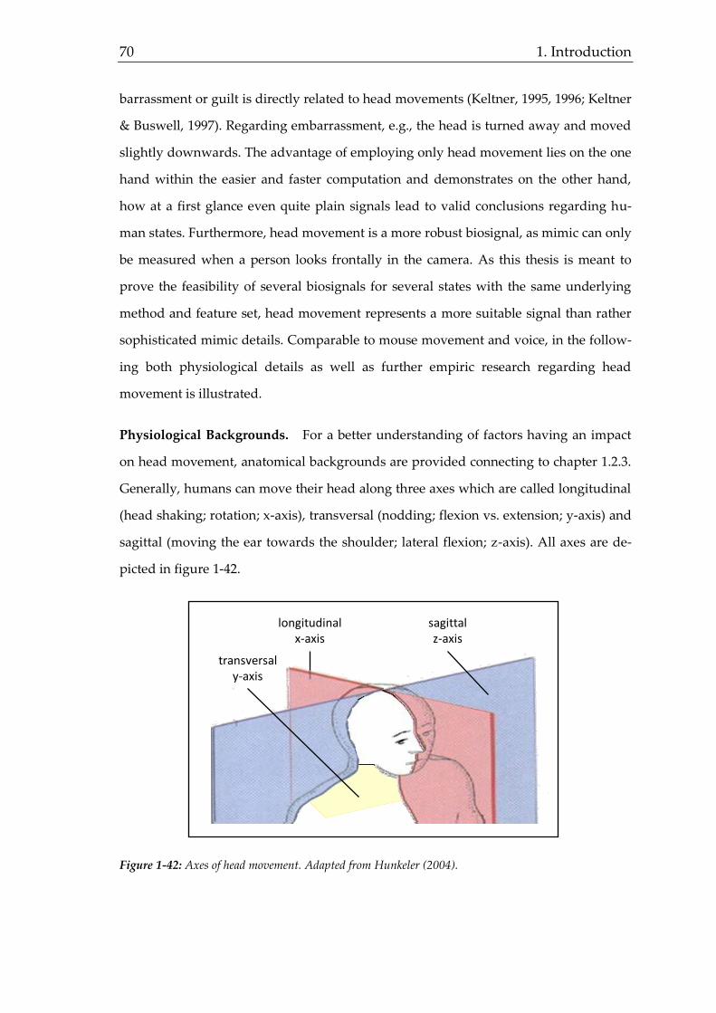
70 1. Introduction
barrassment or guilt is directly related to head movements (Keltner, 1995, 1996; Keltner
& Buswell, 1997). Regarding embarrassment, e.g., the head is turned away and moved
slightly downwards. The advantage of employing only head movement lies on the one
hand within the easier and faster computation and demonstrates on the other hand,
how at a first glance even quite plain signals lead to valid conclusions regarding hu-
man states. Furthermore, head movement is a more robust biosignal, as mimic can only
be measured when a person looks frontally in the camera. As this thesis is meant to
prove the feasibility of several biosignals for several states with the same underlying
method and feature set, head movement represents a more suitable signal than rather
sophisticated mimic details. Comparable to mouse movement and voice, in the follow-
ing both physiological details as well as further empiric research regarding head
movement is illustrated.
Physiological Backgrounds. For a better understanding of factors having an impact
on head movement, anatomical backgrounds are provided connecting to chapter 1.2.3.
Generally, humans can move their head along three axes which are called longitudinal
(head shaking; rotation; x-axis), transversal (nodding; flexion vs. extension; y-axis) and
sagittal (moving the ear towards the shoulder; lateral flexion; z-axis). All axes are de-
picted in figure 1-42.
Figure 1-42: Axes of head movement. Adapted from Hunkeler (2004).
longitudinalx-axis
transversaly-axis
sagittalz-axis
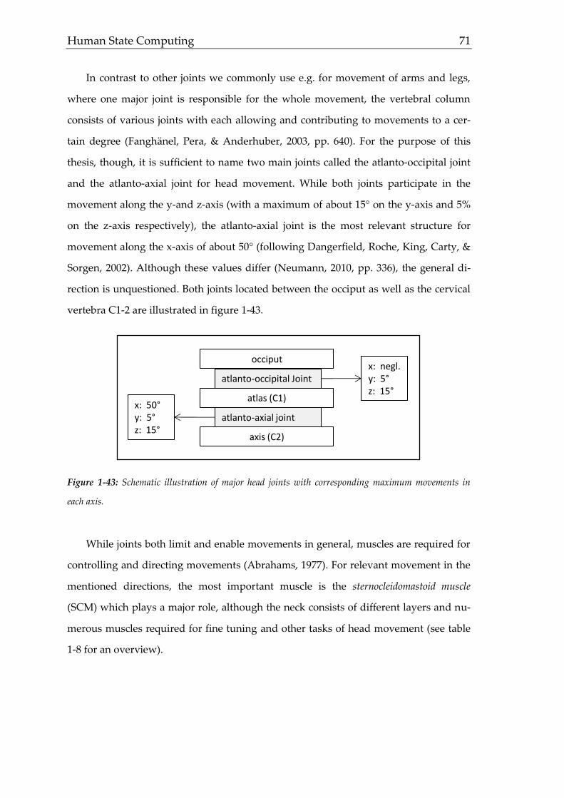
Human State Computing 71
In contrast to other joints we commonly use e.g. for movement of arms and legs,
where one major joint is responsible for the whole movement, the vertebral column
consists of various joints with each allowing and contributing to movements to a cer-
tain degree (Fanghänel, Pera, & Anderhuber, 2003, pp. 640). For the purpose of this
thesis, though, it is sufficient to name two main joints called the atlanto-occipital joint
and the atlanto-axial joint for head movement. While both joints participate in the
movement along the y-and z-axis (with a maximum of about 15° on the y-axis and 5%
on the z-axis respectively), the atlanto-axial joint is the most relevant structure for
movement along the x-axis of about 50° (following Dangerfield, Roche, King, Carty, &
Sorgen, 2002). Although these values differ (Neumann, 2010, pp. 336), the general di-
rection is unquestioned. Both joints located between the occiput as well as the cervical
vertebra C1-2 are illustrated in figure 1-43.
Figure 1-43: Schematic illustration of major head joints with corresponding maximum movements in
each axis.
While joints both limit and enable movements in general, muscles are required for
controlling and directing movements (Abrahams, 1977). For relevant movement in the
mentioned directions, the most important muscle is the sternocleidomastoid muscle
(SCM) which plays a major role, although the neck consists of different layers and nu-
merous muscles required for fine tuning and other tasks of head movement (see table
1-8 for an overview).
occiput
axis (C2)
atlanto-occipital Joint
atlas (C1)
atlanto-axial jointx: 50°y: 5°z: 15°
x: negl.y: 5°z: 15°

72 1. Introduction
Table 1-8: Overview of most relevant muscles for head movement. Adapted from McCaw (2009).
muscle origin insertion axes
sternonucleidomastoid manubrium of sternum and
mediale clavicle
Mastoid process of
temporal bone
x, y, z
semispinalis (capitis,
cervicis, thoracis)
transverse process of cervical
and thorical vertebrae
occipital bone, cervical
and thoracic vertebrae
x
splenius capitis spinous process of cervical
and thoracic vertebrae
mastoid process, oc-
cipital bone
x, z
longissimus capitis transverse process of vertebrae mastoid process x, z
Most muscles are paired being symmetrically ordered in the neck facilitating
movements along the y-axis when working together and movement along the x- and z-
axis when used individually (Neumann, 2010, pp. 336). The SCM is anchored with two
heads on both origin and insertion. It springs from the sternum (medial part) and the
clavicle (lateral part) leading to the temporal and occipital bone. It is innerved by the
accessory nerve (CN XI). Referring to figure 1-23, the accessory nerve obtains its input
in the spinal cord before innerving the SCM and is connected to the mentioned reaffer-
ent circuits. Other muscles in the neck are innerved by the tectospinal tract (Neumann,
2010, pp. 336) as depicted in figure 1-44.
Figure 1-44: Overview of head and neck muscles highlighting the sternocleidomastoid muscle (SCM).
Illustrations printed with permission of Tim Taylor (based on Taylor, 2012).

Human State Computing 73
Research on Head Movement. Analogously to speech production and mouse move-
ment, it has been outlined that due to their common parts in their nerval pathways
state level based effects are likely observable from a physiologic point of view. In sev-
eral experiments (Ekman & Friesen, 1973; Wells & Petty, 1980; Buller, Burgoon, White,
& Ebesu, 1994; Lance & Marsella, 2007; Gunes & Pantic, 2010), manually or automati-
cally generated features of head movement have been employed successfully for state
predictions. This is no surprising fact as the regularities mentioned in chapter 1.2.3
apply for head movement, too.
Besides emotions, though, other kinds of human states are obviously related to
head movement. Sleepiness is such a state. Similar to mouse movement, experiments
have determined more and extremer head movement for sleep deprived test persons
(van den Berg, 2006). Forward and backward movement as well as movement to the
left and right is not found to be indicative of fatigue, but analysis over time shows that
the increase of velocity differs for rested people. Furthermore, EEG and heart rate vari-
ability show a high correlation with rested head movement.
In linguistics, research focusing on audiovisual prosody reveals that head and
body movement is of crucial importance to speech understanding (Krahmer & Swerts,
2009), as in typical conversations people do not only hear, but also see each other face
to face and therefore probably use any cues based on movement (Clark & Krych, 2004),
which is carried to extremes for lip movement in the well-known McGurk effect
(McGurk & MacDonald, 1976).
Moreover, already early analysis of head movement in speech interactions lead to
the conclusion, that an assessment of the recent stress level is also possible (Hadar,
Steiner, Grant, & Rose, 1983) and that the outcome of a job interview is correlated with
differences in head movement of applicants (Forbes & Jackson, 1980). More recent
studies focusing on persuasion (Brinol & Petty, 2011) and impression management
reveal the importance of head management in interviews. Yet, not only the appeal of a
person is affected by head movement, but also the conveyed message, as it is possible
to emphasize particular words or phrases of a message by well-chosen movements
(House, Beskow, & Granström, 2001). Additionally, perceptions like friendliness or

74 1. Introduction
attractiveness show differences regarding head movement (Bente, Feist, & Elder, 1996).
Medicinal studies strengthen this relationship by emphasizing stress-based worsening
of involuntary (and therefore hardly possible to fake) movement like head tremor
(Jankovic & Stanley, 1980).
With the progress of biosignal processing capabilities, the assessment of mimic and
head features got automatized by software like FaceReader by Noldus Information
Technology (van Kuilenburg, Wiering, & den Uyl, 2005) or the sophisticated high
speed object recognition engine (SHORE) by the Fraunhofer IIS Institute (Ruf &
Küblbeck, 2011) which is employed for video data analysis within this thesis. As de-
tecting a head from video data and logging movement appears to be more sophisticat-
ed than recording voice or mouse movement, a brief introduction about head move-
ment detection is given. First real-time approaches back in 2001 by Viola & Jones were
not exclusively meant to detect heads or faces, but objects in general. The basic ques-
tion is, what features a head or object offers that allow recognizing it from a certain
conglomeration of pixels in an image (or quickly changing images as happening in a
video). The basic idea is to analyze rectangular parts of the image (typically of size
24x24px) in order to find contrasts between adjacent rectangles of an image and em-
ploy machine learning algorithms with proper training data afterwards to match found
shapes with those ones being known from the training data as a head. The clue is to
employ poorly performing but quickly working classifiers to separate an object like a
head from its background and use afterwards better performing classifiers to deter-
mine whether the identified object is indeed a head (see chapter 2.4 for an introduction
to prediction modeling using classifiers). The process is depicted in figure 1-45.
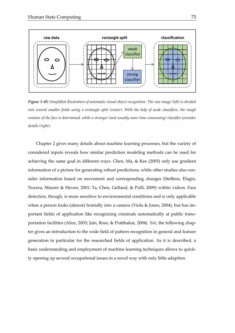
Human State Computing 75
Figure 1-45: Simplified illustration of automatic visual object recognition. The raw image (left) is divided
into several smaller fields using a rectangle split (center). With the help of weak classifiers, the rough
contour of the face is determined, while a stronger (and usually more time consuming) classifier provides
details (right).
Chapter 2 gives many details about machine learning processes, but the variety of
considered inputs reveals how similar prediction modeling methods can be used for
achieving the same goal in different ways. Chen, Ma, & Kee (2005) only use gradient
information of a picture for generating robust predictions, while other studies also con-
sider information based on movement and corresponding changes (Steffens, Elagin,
Nocera, Maurer & Heven, 2001; Ta, Chen, Gelfand, & Pulli, 2009) within videos. Face
detection, though, is more sensitive to environmental conditions and is only applicable
when a person looks (almost) frontally into a camera (Viola & Jones, 2004), but has im-
portant fields of application like recognizing criminals automatically at public trans-
portation facilities (Alice, 2003; Jain, Ross, & Prabhakar, 2004). Yet, the following chap-
ter gives an introduction to the wide field of pattern recognition in general and feature
generation in particular for the researched fields of application. As it is described, a
basic understanding and employment of machine learning techniques allows to quick-
ly opening up several occupational issues in a novel way with only little adaption.
strong classifier
weak classifier
raw data rectangle split classification


Human State Computing 77
2 STEPS OF BIOSIGNAL ANALYSIS
From a theoretical point of view, there is a huge difference between gathering data
by those widely employed typically psychological means mentioned in chapter 1.1 and
gaining insights by biosignal analysis. When developing a questionnaire or testing two
hypotheses against each other in a common study, researchers follow a certain theory
driven approach (Chen & Rossi, 1980) predicting what will probably happen if the theo-
ry’s statements were correct. In the case of deviating results (no matter if this is in
terms of a different number of underlying factors or insignificant results), the theory is
abandoned and modified, before a new test is run. If the theory works within this trial
and error procedure, it is quite a convenient path to choose, because researchers have a
clear idea about why e.g. people behave the way they do under a certain treatment.
Lewin (1952, p. 169) summarizes this advantage with the words “there’s nothing more
practical than a good theory”.
The major disadvantage of this approach, however, lies within the case of rejected
hypotheses, because they result in a necessity to (repetitively) change or adapt state-
ments, until quantitative data are sufficient to support the theory. It can be a long way
there and all it reveals is knowledge about several possibilities about what does not
work. Although this means a gain of insights as well, considering the time it takes to
publish findings in scientific journals, progress is certainly slowed down by always
only testing and reporting one hypothesis at a time and building theories over and
over again that in the end do (for many iterations) not work.
Biosignal analysis chooses a different approach. The primary question is based on
a comparably vague theoretical understanding, what empiric data propose and only in
a second step, how the findings may be put into some kind of most appropriate theory.
With the underlying rationale, that something what simply works and is proven mani-
fold by empiric data cannot be considered wrong, even if researchers struggle building
a theory explaining the data, the way of testing and building hypotheses seems in-
versed. Although, especially from a psychological perspective, just testing impromptu
cannot embody the desired way of research, a data driven approach (e.g. Ren, Patrick,
Efron, Hodgins, & Rehg, 2005; Kiff, Nepp, Kiff, & Albrecht, 2007) becomes superior in
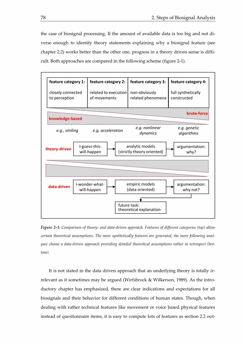
78 2. Steps of Biosignal Analysis
the case of biosignal processing. If the amount of available data is too big and not di-
verse enough to identify theory statements explaining why a biosignal feature (see
chapter 2.2) works better than the other one, progress in a theory driven sense is diffi-
cult. Both approaches are compared in the following scheme (figure 2-1).
Figure 2-1: Comparison of theory- and data-driven approach. Features of different categories (top) allow
certain theoretical assumptions. The more synthetically features are generated, the more following anal-
yses choose a data-driven approach providing detailed theoretical assumptions rather in retrospect (bot-
tom).
It is not stated in the data driven approach that an underlying theory is totally ir-
relevant as it sometimes may be argued (Wirfsbrock & Wilkerson, 1989). As the intro-
ductory chapter has emphasized, there are clear indications and expectations for all
biosignals and their behavior for different conditions of human states. Though, when
dealing with rather technical features like movement or voice based physical features
instead of questionnaire items, it is easy to compute lots of features as section 2.2 out-
knowledge-based
feature category 1:
closely connectedto perception
feature category 2:
related to executionof movements
e.g., smiling e.g. acceleratione.g. nonlinear
dynamics
feature category 3:
non-obviously related phenomena
feature category 4:
full synthetically constructed
e.g. genetic algorithms
brute-force
I-wonder-what-will-happen
I-guess-this-will-happen
analytic models (strictly theory oriented)
future task: theoretical explanation
empiric models (data oriented)
argumentation: why?
argumentation: why not?
theory-driven
data-driven
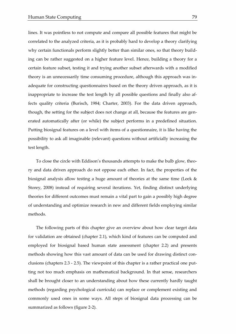
Human State Computing 79
lines. It was pointless to not compute and compare all possible features that might be
correlated to the analyzed criteria, as it is probably hard to develop a theory clarifying
why certain functionals perform slightly better than similar ones, so that theory build-
ing can be rather suggested on a higher feature level. Hence, building a theory for a
certain feature subset, testing it and trying another subset afterwards with a modified
theory is an unnecessarily time consuming procedure, although this approach was in-
adequate for constructing questionnaires based on the theory driven approach, as it is
inappropriate to increase the test length by all possible questions and finally also af-
fects quality criteria (Burisch, 1984; Charter, 2003). For the data driven approach,
though, the setting for the subject does not change at all, because the features are gen-
erated automatically after (or while) the subject performs in a predefined situation.
Putting biosignal features on a level with items of a questionnaire, it is like having the
possibility to ask all imaginable (relevant) questions without artificially increasing the
test length.
To close the circle with Eddison’s thousands attempts to make the bulb glow, theo-
ry and data driven approach do not oppose each other. In fact, the properties of the
biosignal analysis allow testing a huge amount of theories at the same time (Leek &
Storey, 2008) instead of requiring several iterations. Yet, finding distinct underlying
theories for different outcomes must remain a vital part to gain a possibly high degree
of understanding and optimize research in new and different fields employing similar
methods.
The following parts of this chapter give an overview about how clear target data
for validation are obtained (chapter 2.1), which kind of features can be computed and
employed for biosignal based human state assessment (chapter 2.2) and presents
methods showing how this vast amount of data can be used for drawing distinct con-
clusions (chapters 2.3 - 2.5). The viewpoint of this chapter is a rather practical one put-
ting not too much emphasis on mathematical background. In that sense, researchers
shall be brought closer to an understanding about how these currently hardly taught
methods (regarding psychological curricula) can replace or complement existing and
commonly used ones in some ways. All steps of biosignal data processing can be
summarized as follows (figure 2-2).

80 2. Steps of Biosignal Analysis
Figure 2-2: Overview of biosignal analysis steps. Within the generation process (top), clean data are
obtained for the following feature extraction (center).Afterwards, the generated features are taken to a
supervised machine learning process (bottom) combining feature selection, prediction model generation
and evaluation.
2.1 Data Generation
Regardless of existence or non-existence of prediction models, one can only yield
valid results with proper data following the GIGO-principle (Garbage In, Garbage Out
as often used in informatics and in the context of meta-analysis; Glass, McGaw, &
Smith, 1981, pp. 217; Hunter & Schmidt, 1990). If a data basis, or usually referred to as
corpus, is supposed to be established, a representative amount of data is required
(Wright, Kim, & Perry, 2010). On the one hand, it has to be chosen as so often between
data generation
cleansed data
total feature set
subset selection
raw data data cleansingreference /
validation data
feature extraction
feature source algorithms
total feature set
feature selection prediction modeling evaluation
feature subset oftrain data
+validation data
prediction modelmatch predicted
data with validation
apply model on test data
supervised machine learning
test next feature subset
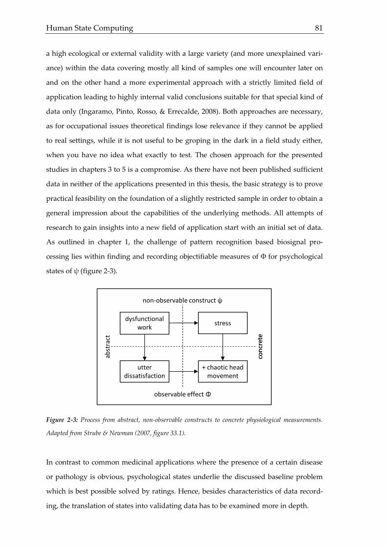
Human State Computing 81
a high ecological or external validity with a large variety (and more unexplained vari-
ance) within the data covering mostly all kind of samples one will encounter later on
and on the other hand a more experimental approach with a strictly limited field of
application leading to highly internal valid conclusions suitable for that special kind of
data only (Ingaramo, Pinto, Rosso, & Errecalde, 2008). Both approaches are necessary,
as for occupational issues theoretical findings lose relevance if they cannot be applied
to real settings, while it is not useful to be groping in the dark in a field study either,
when you have no idea what exactly to test. The chosen approach for the presented
studies in chapters 3 to 5 is a compromise. As there have not been published sufficient
data in neither of the applications presented in this thesis, the basic strategy is to prove
practical feasibility on the foundation of a slightly restricted sample in order to obtain a
general impression about the capabilities of the underlying methods. All attempts of
research to gain insights into a new field of application start with an initial set of data.
As outlined in chapter 1, the challenge of pattern recognition based biosignal pro-
cessing lies within finding and recording objectifiable measures of Φ for psychological
states of ψ (figure 2-3).
Figure 2-3: Process from abstract, non-observable constructs to concrete physiological measurements.
Adapted from Strube & Newman (2007, figure 33.1).
In contrast to common medicinal applications where the presence of a certain disease
or pathology is obvious, psychological states underlie the discussed baseline problem
which is best possible solved by ratings. Hence, besides characteristics of data record-
ing, the translation of states into validating data has to be examined more in depth.
non-observable construct ψ
observable effect Φ
abst
ract
con
cret
e
dysfunctional work
stress
utter dissatisfaction
+ chaotic head movement
con
cret
e

82 2. Steps of Biosignal Analysis
Human State Labeling. Following Cowie & Cornelius (2003), there are two different
types of labeling (or frequently referred to as rating) user states. On the one hand, there
is a cause-oriented approach labeling differences in states directly. Yet, figure 2-3 ex-
plains that the state itself is usually not visible and therefore allows no cause-oriented
labeling. On the other hand, when having to rely on indirect, observable representa-
tions of a state, an effect-oriented approach is chosen. For this type of labeling, the origi-
nally subjective impression of an observer is used for validation, or differently put, the
effect of the current state level on the observer. Thus, invisible changes of the state level
stay unnoticed possibly leading to a decrease of validity. However, it should be taken
into consideration that for some fields of application unnoticeable or unobservable
differences in a subject’s behavior are not at all supposed to yield different labels, re-
gardless of the actual state level. In occupational or political environments, e.g., the
shown behavior or respectively the effect on the audience is much more important at a
first glance than the true score of tension when providing a speech (Cronin, 2008). So
sometimes the perception of a state level seems to gain higher importance than the un-
derlying state itself, especially when no self-report is available for determining a prop-
er baseline. Nonetheless, ratings should always attempt to allow an assessment of the
cause and not primarily on the effects. Otherwise, instead of measuring the desired
state, rather an intervening variable (like e.g. the ability for stress coping) is assessed
and (referring to chapter 1.2.1) the reach of valid inferences is poor. The superior ap-
proach for the described interaction is to quantify both the psychological true state
score and the intervening variable if possible. This little scenario already emphasizes,
how important it is to optimize labels by averaging several impressions and defining
rating criteria.
Now there are different possibilities to label user states. Category labels are the most
common one where verbal descriptions are employed to describe a state (Cowie &
Cornelius, 2003). Using different words for different states seems self-evident, but has
certain drawbacks. In the case of emotions, e.g., there is a huge number of emotional
labels (558 following Averill, 1975). Of course, employing such a set of categories for
describing each recorded sample cannot yield reliable results, since it would over-
charge each observer no matter how well trained. But there is another issue even when

Human State Computing 83
reducing categories to basic emotions (Plutchnik, 1962; Ekman & Friesen, 1971; Izard,
1977; as outlined in chapter 1.3.3). States (including emotions) are not as dominantly
prevailing as words imply. Usually a mixture of several states is present, so categories
must not only suffice regarding different states but also their intensity leading again to
a non-manageable amount of categories (Abrillian, Devillers, Buisine, & Martin, 2005)
as shown in figure 2-4.
Figure 2-4: Emotional category labels. Adapted from Scherer (2001).
The two axes of figure 2-4 and the quite randomly scattered categories reveal that
even such a quantity of words is not enough to represent different levels of a state sys-
tematically. For this reason, it seems superior to define a set of verbal anchors and rate
them on an appropriate scale allowing a coexistence of different states with different
impatient
desperate
sleepy
solemn
content
pleased
aroused
lusting
conceited
triumphant
self-confident
joyous
POSITIVE NEGATIVE
ACTIVE
PASSIVE
interestedexpectant
passionate
excited
light-hearted
amused
determined
ambituous
impressed
confident
hopeful
relaexed
longingattentive
friendlypolite
peaceful
empathicreverent
conscientious
serious
doubtful
sad
boredhesitant
embarrased
melancholic
languid
worried
apathetic
feel guilty
ashamed
wavering
dissatisfied
disappointed
sad
depressed
miserable
bored
jealous
tense
alarmed
hostile
enviousafraid
annoyed
angry
distressed
disgusted
bitter
insulteddistrustful
suspiscious
frustrated

84 2. Steps of Biosignal Analysis
levels. Such an approach is realized by dimensional labeling proposed e.g. in the Cir-
cumplex Emotion Model by Russell (1980), suggesting the two dimensions arousal and
valence as depicted in figure 2-5.
Figure 2-5: Simplified Circumplex Emotion Model. Adapted from Russell (1980).
In the context of Speech Emotion Recognition (SER), Sun & Moore II (2012) com-
pared category and dimensional labeling coming to the conclusion that acted data is
well assessed regarding categories by raters and that contrary to minor problems iden-
tifying the correct emotional expression, the evaluation of the intended affective space
is very successful. Due to the mentioned difficulties with category labels, best matching
dimensional labels are employed allowing a free scaling of subjects’ state perception.
Nonetheless, a proper alignment and training of all observers is inevitable to yield reli-
able ratings (Reid, 1982). After pointing out how data for validation are retrieved, dif-
ferent sources and preparation of recordings are to be discussed as well.
Data Sources. After the decision about the application of the results is made, it is im-
portant from what source data are gathered and by what means. To avoid noise in the
data, high quality equipment is preferable especially for building a corpus. Technical
specifications of the employed equipment is provided within the respective chapters.
UNPLEASANT PLEASANT
ACTIVATION
DEACTIVATION
upset
stressed
nervous
tense
happy
elated
excited
tense
calm
relaxed
serene
contented
fatigued
lethargic
depressed
sad

Human State Computing 85
Following Devillers, Martin, Cowie, Douglas-Cowie, & Batliner (2006), data
sources can be divided into four parts: (1) Acted data are easily gathered and multi-
plied, as commonly only a few actors are consulted as test persons producing an al-
most unlimited amount of data. This approach is detrimental to a practical use as the
resulting corpus will vastly depend on those few speakers. So it can be argued, wheth-
er the data are only applicable for the actors afterwards what was of minor use for the
academic and occupational society. Furthermore, empirical findings (Batliner, Fischer,
Huber, Spilker, & Nöth, 2000) indicate a poor transferability from acted to real emo-
tions (and therefore probably examined states like sleepiness or self-confidence). Non-
acted data can be retrieved from (2) induced, (3) application-oriented and (4) natural
situations. Induced states evoke natural behavior in a standardized setting, what in-
creases objectivity and validity. Unfortunately, e.g. the evaluated leadership dimen-
sions are quite difficult to induce, so that it is not always possible to draw on induced
data. Sleepiness, though, can be easily induced (Dinges & Kribbs, 1991) Application-
oriented data usually stem from certain contexts like sales talks or customer services.
Most companies acquire those data, but regrettably do not grant scientific institutions
access. In a variety of cases it is therefore inevitable to gather real interactions from
natural sources. Unrelated to certain applications, natural data comprise all useful data
that was not intentionally recorded for scientific purposes, but made available to the
public (commonly via internet). It is in the nature of this source, that data quality dif-
fers and noise is increased, so that a careful selection and processing is necessary to
yield workable outputs (Devillers et al., 2006). Furthermore, public data commonly
lack of the possibility to determine a baseline via self-reports. However, also self-
reports must be employed and surveyed carefully (Schwarz, 1999) to have a beneficial
effect on the state prediction.
Data Cleansing. High data quality is of crucial importance for building decent corpo-
ra and related prediction models (Klein & Rossin, 1999). Whenever there is no possibil-
ity to objectively and physically measure user states for validating biosignal data cor-
pora (what is usually the case as states of ψ are never directly visible), mentioned de-
tails of user state labeling ensure that ratings as the base for prediction models are of
high quality. Yet, not only all data employed for validation must be clean, but also in-
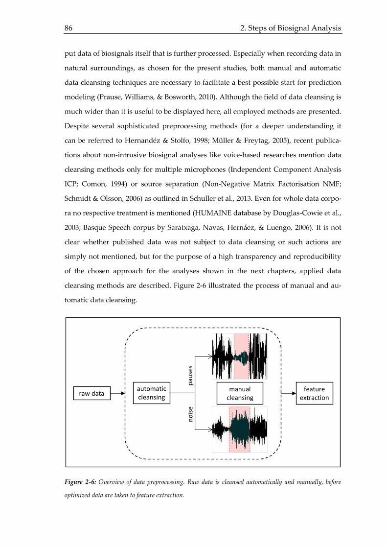
86 2. Steps of Biosignal Analysis
put data of biosignals itself that is further processed. Especially when recording data in
natural surroundings, as chosen for the present studies, both manual and automatic
data cleansing techniques are necessary to facilitate a best possible start for prediction
modeling (Prause, Williams, & Bosworth, 2010). Although the field of data cleansing is
much wider than it is useful to be displayed here, all employed methods are presented.
Despite several sophisticated preprocessing methods (for a deeper understanding it
can be referred to Hernandéz & Stolfo, 1998; Müller & Freytag, 2005), recent publica-
tions about non-intrusive biosignal analyses like voice-based researches mention data
cleansing methods only for multiple microphones (Independent Component Analysis
ICP; Comon, 1994) or source separation (Non-Negative Matrix Factorisation NMF;
Schmidt & Olsson, 2006) as outlined in Schuller et al., 2013. Even for whole data corpo-
ra no respective treatment is mentioned (HUMAINE database by Douglas-Cowie et al.,
2003; Basque Speech corpus by Saratxaga, Navas, Hernáez, & Luengo, 2006). It is not
clear whether published data was not subject to data cleansing or such actions are
simply not mentioned, but for the purpose of a high transparency and reproducibility
of the chosen approach for the analyses shown in the next chapters, applied data
cleansing methods are described. Figure 2-6 illustrated the process of manual and au-
tomatic data cleansing.
Figure 2-6: Overview of data preprocessing. Raw data is cleansed automatically and manually, before
optimized data are taken to feature extraction.
raw data
pau
ses
no
ise
automatic cleansing
feature extraction
manual cleansing

Human State Computing 87
Automatic Cleansing. Some undesirable characteristics of the recorded data require
automatic cleansing methods (Rahm & Do, 2000). Particularly natural data frequently
contain irrelevant pauses reducing the amount of valuable parts. Taking the fact into
account that commonly samples of (approximately) the same length are chosen for
gaining high comparability, it is obvious that a pause of ten seconds in a 30 second
sample is not expedient. Hence, after doing some deliberations and research for deter-
mining a limit for pauses, data quality is optimized by automatic pause deletion. How-
ever, not all desired parts might be removed by this automatic method, so that a man-
ual check is appropriate. For more sophisticated cleansing requirements mostly rele-
vant to less robust recording techniques like EEG and others, filters and artifacts are to
consider (Ramoser, Muller-Gerking, & Pfurtscheller, 2000). In applications where rele-
vant frequencies of a signal are known beforehand, all other contained frequencies can
and should be discarded. The superior approach is to exclude irrelevant data as early
as possible to reduce interactions like peak shifts in the signal (Gratton, 2007, p. 484)
employing analogue high- and low-pass filters (filtering respective frequencies) when
recording samples (in electronics this is implemented via resistors; see RC filters fol-
lowing Adams, 1979, for further details). One tangible realization of an analogue audio
low-pass filter is to implement a physical barrier in the recording device reflecting high
frequencies for excluding them. Digital filters using mathematical operations to ex-
clude unwanted parts of the signal are another possibility to smooth the signal (for an
overview of digital filters see Antoniou, 1993).
For voice data reported in chapter 3, high frequencies are ruled out from further
analysis by choosing a respectively low sampling frequency. With an outlook on the
next chapter is has to be kept in mind, though, that filtering with the aim of feature
extraction is to be separated from data cleansing. The last mentioned aspect of auto-
matic data cleansing is the issue of artifacts describing specific noise occurrences. Ex-
amples of artifacts with kind of individual fingerprints are coughing or eye blinking in
voice or EOG studies. Such events can overlie the true signal and therefore blur anal-
yses. The identification of such events is hence very important, especially for regularly
occurring artifacts like blinking. As this is not always possible by automatic means, a
manual quality check is necessary.

88 2. Steps of Biosignal Analysis
Manual Cleansing. One technically easy but most time consuming way to delete defi-
cient parts of the signal is to cut and modify them manually (Saranummi, Korhonen,
van Gils, & Kari, 1997). When thinking about biosignal data samples recorded in natu-
ral surroundings, there is always noise in the signal that has to be separated from the
signal parts. Noise in this case is a general term comprising all facets of irrelevant in-
formation of recorded data. Examples can be either background noise due to bad re-
cording or in the case of voice laughter of the audience, coughing or other sounds that
are not supposed to be related to ψ (Semmler, 2004, pp. 7). So before recorded data are
taken to analysis, it is recommended to have a look at all data again and cut noisy
parts. Especially for building new corpora this step is of vital importance, as new pre-
diction algorithms must not be sensitive for not state-related phenomena. Afterwards,
when employing a prediction algorithm in practice, noise is irrelevant to a certain de-
gree (if not blurring the whole sample), since no signal features (or their corresponding
pattern) are implemented in the algorithm and hence will not yield biased results.
When assessing a data corpus, it is necessary to have criteria at hand allowing a
comparison of quality. Although depending on the granularity manifold criteria are
imaginable, a good start seems to be an overview derived from Schuller (2006). The
stated criteria will also be employed for the evaluation of presented data corpora in
this thesis (table 2-1).
Table 2-1: Relevant criteria to assess the quality of a data corpus. Adapted from Schuller (2006).
corpus criterion description
validity anchor As prediction models are based on the validating ratings, it must be
ensured the quality of this anchor is possibly high. This can be
achieved by e.g. obtaining both self and observer reports as well as
employing physiological and behavioral measures
perception test To make sure rating a state using a certain input is possible, it is
necessary to train raters and see, if a satisfactory agreement is
achieved on unambiguous samples
class adaption For different fields of application, a different number of classes may
be suitable. Hence it is necessary to build corpora and prediction
models with regard to the required classes
ideal setting Especially for building an initial version of a corpus, it is necessary
to avoid any kind of confounders as good as possible. Where this is
not applicable, considered confounders should at least be con-
trolled to measure the impact

Human State Computing 89
repeatability Corpora do not only consist of data. It is equally important to give
exact details about how data were derived to allow a proper as-
sessment and facilitate repeated measurements to enhance and
extend existing corpora
diversity Although it is necessary to start building a corpus in a low-noise
environment, it is necessary with regard to practical applications to
adapt corpora and prediction models to (various) places of action
rating distribution Especially for small corpora it is advantageous to yield equal dis-
tributed ratings over all classes to ensure proper training sets for all
classes. For bigger data corpora, however, it can be argued whether
a representative a priori probability should influence the prediction
or not
availability When a data corpus of satisfactory quality is established, it should
be tested within various situations and possibly also by different
persons. Hence, it is inevitable to share corpora in order to further
perfect it.
Generally, all mentioned aspects of this chapter so far should be considered when
designing a corpus and instead of building several new corpora, sometimes trying or
enlarging existing ones is the better approach for comparing prediction results as it is
common use in biosignal analysis (Schuller, Steidl, Batliner, Schiel, & Krajewski, 2011).
After relevant aspects of building validation and recording data for establishing a
proper corpus have been outlined by now, it is necessary to process the obtained data
for building prediction models. One of this thesis’s core issues is to demonstrate, that
several kinds of features are applicable for manifold biosignals. Hence, the main focus
of the steps of biosignal processing lies on the following chapter explaining how rele-
vant characteristics are retrieved from the corpus data.
2.2 Feature Extraction
After all raw data has been gathered, automatically extractable features are needed
to find patterns that can be matched with the labeled raw data. So the question is, what
features can be derived from the usually one-dimensional input vector. There are lots
of different techniques and sources for features for different purposes. An overview is
shown in table 2-2.

90 2. Steps of Biosignal Analysis
Table 2-2: Overview of feature sources.
feature source success source (examples)
raw series data + Mierswa (2005)
time domain ++ Tkach, Huan, & Kuiken (2010)
spectral domain +++ Reynolds, 2002
nonlinear dynamics/chaos +++ Krajewski, Schnieder, Sommer, Batliner &
Schuller (2012)
genetic/evolutionary features + Pierre-Yves (2003)
feature normalization ++ Viiki, Bye, & Laurila (1998)
wavelet features +++ Modic, Lindberg, & Petek (2003)
In order to compute the numerous feature set, it makes sense to draw back on
quality proofed software instead of reinventing the wheel over and over again. Except
for the signal-specific features, features are computed by Praat (Boersma & Weenink,
2010), openSMILE (Eyben, Wöllmer, & Schuller, 2010) and Matlab (employing the
openTSTOOL toolbox by Merkwirth, Parlitz, Wedekind, Engster, & Lauterborn, 2009,
as well as the Wavelet toolbox) contributing to a five-digit total feature set.
There are manifold arrangements of features, e.g. differentiation of time and fre-
quency (Reynolds, 2002; Tkach, Huan & Kuiken, 2010) or regarding voice features clas-
ses like prosody, spectral/articulation and voice quality (Krajewski, 2007; Steidl, 2009).
As this thesis (also) focuses on mostly ignored methods of feature computation, a part-
ly novel distribution of features has been chosen. First, features suitable for all three
source signals are presented containing common (time domain and spectral) features
(chapter 2.2.1), wavelet features (chapter 2.2.2) and nonlinear dynamic features (chap-
ter 2.2.3). Afterwards, signal-specific features are displayed (chapter 2.4). For all fea-
tures, functionals are computed as described in table 2-3 to boost the total number of
features with regard to the data-driven approach and make sure the ideal facets of each
general feature are retrieved.

Human State Computing 91
Table 2-3: Overview of functionals.
functional number description
range 1 range
maxPos / minPos 2 position (x-axis) of global minimum/maximum
min / max meandist 2 mean distance to global minimum/maximum (y-axis)
LRCx / QRCx 5 linear / quadratic regression coefficients
rel regr errA/Q 2 linear / quadratic relative regression error
abs REA/Q 2 absolute linear / quadratic regression error
abs/quadr/geom mean 3 absolute / quadratic / geometric mean
mean 1 arithmetic mean
stddev / var 2 standard deviation / variance
skewness 1 skewness
kurtosis 1 kurtosis
quartx / Percx 5 25/50/75% quartile / 95%/98%-percentile
iqrx-y 3 inter quartiles ranges
ZCR 1 Zero Crossing Rate
num peaks 1 number of peaks (extrema)
mean peak dist 1 arithmetic mean of peak distances (x-axis)
peak mean 1 arithmetic mean of peaks (y-axis extrema)
peakmean meandist 1 arithmetic mean of mean peak distance
nz_a/abs/qmean 3 normalized arithmetic / absolute / quadratic mean
nnz mean 1 number of normalized mean ≠ 0
Δ / ΔΔ derivation 3·39 = 117
2.2.1 Common Features
No matter what kind of signal is recorded, its first representation is in the time
domain. Therefore, the first and unlike smaller part of the introduction of common
features deals with time-based features, while the second part shows how signals can
be transferred to the frequency domain (spectral features).
Time Domain. When having a closer look at e.g. a voice sample, it is easy to compre-
hend that the resulting signal consists of a sequence of amplitudes (voice) or distances
(movement) as elucidated in figure 2-7.

92 2. Steps of Biosignal Analysis
Figure 2-7: Zoom on wave form of a voice sample.
The Zero Crossing Rate (ZCR) expresses, how often a signal crosses the zero ampli-
tude. Beside its suitability for a first estimation of a fundamental frequency (Kedem,
1986), it is possible to assess how noisy a signal is (Tzanetakis, 2002). Although the
ZCR is hardly related to any user states, it gives information about the data quality and
is therefore a valuable measure that should be analyzed. Sometimes it is used as a func-
tional as well.
As it is later described, signals can be interpreted as a composition of waves,
whereas it is not always applicable to use the observed amplitude as a suitable meas-
ure. Instead it is recommended to use the Energy as measure, as it is proportional to the
logarithmized sum of the quotient of squared amplitudes n and the number of all am-
plitudes N. The resulting value corresponds to the logarithmized RMS-amplitude (root
mean square), as shown in the following formula (equation 5).
𝐸 = log √∑ 𝑛2
𝑁 (5)
time [s] time [s]
time [s]time [s]
amp
litu
de
(no
rmal
ized
)
amp
litu
de
(no
rmal
ized
)
amp
litu
de
(no
rmal
ized
)am
plit
ud
e (n
orm
aliz
ed)
0
0 0
01 0.3
0.1 0.02-1
1
11
1
-1
-1-1
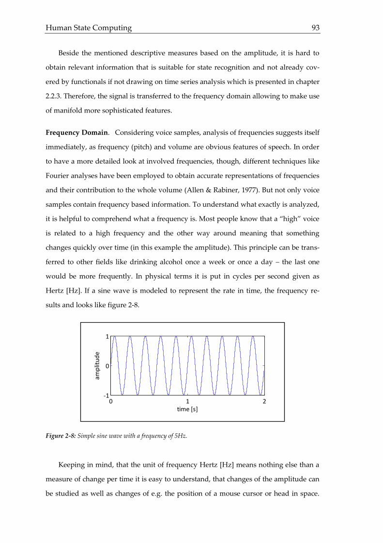
Human State Computing 93
Beside the mentioned descriptive measures based on the amplitude, it is hard to
obtain relevant information that is suitable for state recognition and not already cov-
ered by functionals if not drawing on time series analysis which is presented in chapter
2.2.3. Therefore, the signal is transferred to the frequency domain allowing to make use
of manifold more sophisticated features.
Frequency Domain. Considering voice samples, analysis of frequencies suggests itself
immediately, as frequency (pitch) and volume are obvious features of speech. In order
to have a more detailed look at involved frequencies, though, different techniques like
Fourier analyses have been employed to obtain accurate representations of frequencies
and their contribution to the whole volume (Allen & Rabiner, 1977). But not only voice
samples contain frequency based information. To understand what exactly is analyzed,
it is helpful to comprehend what a frequency is. Most people know that a “high” voice
is related to a high frequency and the other way around meaning that something
changes quickly over time (in this example the amplitude). This principle can be trans-
ferred to other fields like drinking alcohol once a week or once a day – the last one
would be more frequently. In physical terms it is put in cycles per second given as
Hertz [Hz]. If a sine wave is modeled to represent the rate in time, the frequency re-
sults and looks like figure 2-8.
Figure 2-8: Simple sine wave with a frequency of 5Hz.
Keeping in mind, that the unit of frequency Hertz [Hz] means nothing else than a
measure of change per time it is easy to understand, that changes of the amplitude can
be studied as well as changes of e.g. the position of a mouse cursor or head in space.
0 1 2-1
0
1
time [s]
amp
litu
de

94 2. Steps of Biosignal Analysis
Against this background it is not surprising that the same feature set (with small adap-
tations) may be employed for various and rather diverse data sources next to signal-
specific features. Although there are several other possibilities to transform a signal
(Gamage & Blumen, 1993) than using the Fourier transformation, it is the basis of most
commonly used transformations in this as well as almost every other study in this field
of research (Deller, Proakis, & Hanseon, 2000). In order to transfer a signal from time to
frequency domain, the original source data is represented by overlaying sine functions
and multiplication of its amplitude. Assuming a constant signal with three overlaying
frequencies, the following figure results (figure 2-9).
Figure 2-9: Composing a signal (right) based on signals with three different frequencies (left).
Now a constant signal as mentioned in the example before can be reconstructed.
When transforming the illustrated signal in the frequency domain, all three employed
frequencies should appear again. As figure 1-10 shows, the peaks are located correctly.
0 1 2-1
0
1
time [s]
amp
litu
de
0 1 2-1
0
1
time [s]
amp
litu
de
0 1 2-1
0
1
time [s]
amp
litu
de
0 1 2-1
0
1
time [s]
amp
litu
de
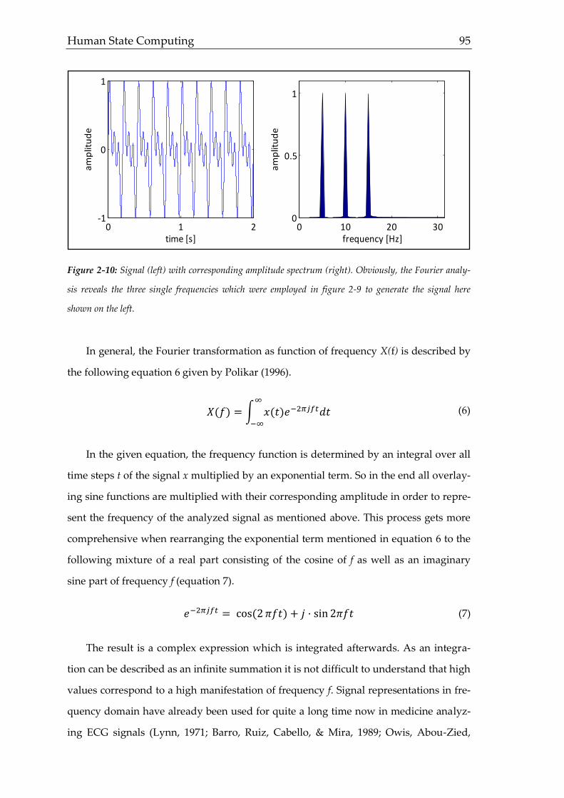
Human State Computing 95
Figure 2-10: Signal (left) with corresponding amplitude spectrum (right). Obviously, the Fourier analy-
sis reveals the three single frequencies which were employed in figure 2-9 to generate the signal here
shown on the left.
In general, the Fourier transformation as function of frequency X(f) is described by
the following equation 6 given by Polikar (1996).
𝑋(𝑓) = ∫ 𝑥(𝑡)𝑒−2𝜋𝑗𝑓𝑡𝑑𝑡
∞
−∞
(6)
In the given equation, the frequency function is determined by an integral over all
time steps t of the signal x multiplied by an exponential term. So in the end all overlay-
ing sine functions are multiplied with their corresponding amplitude in order to repre-
sent the frequency of the analyzed signal as mentioned above. This process gets more
comprehensive when rearranging the exponential term mentioned in equation 6 to the
following mixture of a real part consisting of the cosine of f as well as an imaginary
sine part of frequency f (equation 7).
𝑒−2𝜋𝑗𝑓𝑡 = cos(2 𝜋𝑓𝑡) + 𝑗 · sin 2𝜋𝑓𝑡 (7)
The result is a complex expression which is integrated afterwards. As an integra-
tion can be described as an infinite summation it is not difficult to understand that high
values correspond to a high manifestation of frequency f. Signal representations in fre-
quency domain have already been used for quite a long time now in medicine analyz-
ing ECG signals (Lynn, 1971; Barro, Ruiz, Cabello, & Mira, 1989; Owis, Abou-Zied,
0 1 2-1
0
1
time [s]
am
plit
ud
e
0 10 20 300
0.5
1
frequency [Hz]
am
plit
ud
e
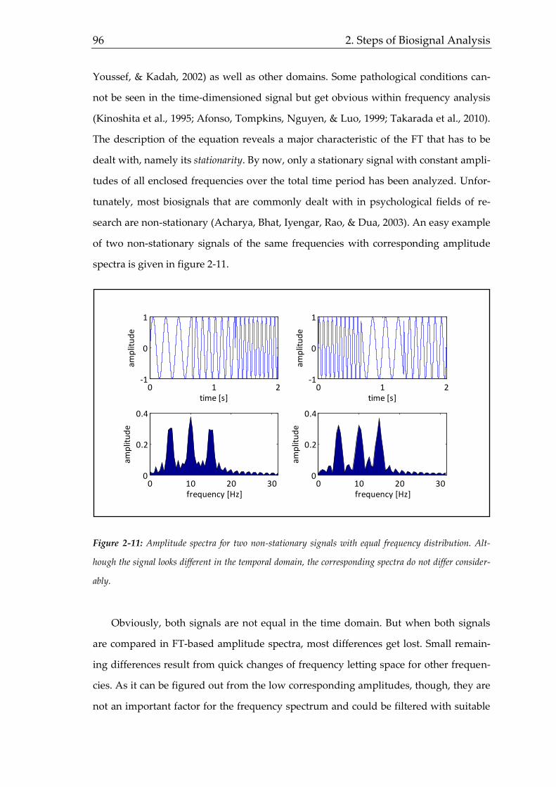
96 2. Steps of Biosignal Analysis
Youssef, & Kadah, 2002) as well as other domains. Some pathological conditions can-
not be seen in the time-dimensioned signal but get obvious within frequency analysis
(Kinoshita et al., 1995; Afonso, Tompkins, Nguyen, & Luo, 1999; Takarada et al., 2010).
The description of the equation reveals a major characteristic of the FT that has to be
dealt with, namely its stationarity. By now, only a stationary signal with constant ampli-
tudes of all enclosed frequencies over the total time period has been analyzed. Unfor-
tunately, most biosignals that are commonly dealt with in psychological fields of re-
search are non-stationary (Acharya, Bhat, Iyengar, Rao, & Dua, 2003). An easy example
of two non-stationary signals of the same frequencies with corresponding amplitude
spectra is given in figure 2-11.
Figure 2-11: Amplitude spectra for two non-stationary signals with equal frequency distribution. Alt-
hough the signal looks different in the temporal domain, the corresponding spectra do not differ consider-
ably.
Obviously, both signals are not equal in the time domain. But when both signals
are compared in FT-based amplitude spectra, most differences get lost. Small remain-
ing differences result from quick changes of frequency letting space for other frequen-
cies. As it can be figured out from the low corresponding amplitudes, though, they are
not an important factor for the frequency spectrum and could be filtered with suitable
0 1 2-1
0
1
time [s]
amp
litu
de
0 1 2-1
0
1
time [s]
amp
litu
de
0 10 20 300
0.2
0.4
frequency [Hz]
amp
litu
de
0 10 20 300
0.2
0.4
frequency [Hz]
amp
litu
de

Human State Computing 97
techniques. This comparison illustrates that the time domain representation (top of
figure 2-11) reveals no real information about the contained frequencies, while the fre-
quency domain (bottom of figure2-11) in contrary gives no information about the time.
So when a signal is transformed to the frequency domain, time data get lost. This prop-
erty can be derived from equation 6. Since the frequency function is computed over all
times of the signal there is no temporal information left after transforming. The integra-
tion reaches from minus infinity to plus infinity meaning that no matter where in the
signal (within the time domain) the frequency occurs, it contributes to the overall inte-
grated value for that frequency.
The issue of not optimizing information about time and frequency at once is dealt
with in the Heisenberg uncertainty principle (Gröchening, 2001, gives a comprising
overview) stating that one dimension is lost the stronger the focus or resolution of the
other one is. This principle is depicted in figure 2-12.
Figure 2-12: Visualized principle of the Heisenberg uncertainty principle regarding frequency and time
resolution. While all squares cover the same area, time and frequency resolution differs. Adapted from
Polikar (1996).
time
freq
uen
cy

98 2. Steps of Biosignal Analysis
All rectangles shown in figure 2-12 have the same surface area. Small values for
rectangle heights indicate a good frequency resolution, while small rectangle widths
represent a good time resolution. Following the implications of Heisenberg’s state-
ments reveals, that always a compromise between frequency and time resolution has to
be found and optimized based on the underlying analysis. For this reason, a possibility
has to be found in order to on the one hand analyze non-stationary signals and on the
other hand lose as less information as possible. One welcome method to overcome sta-
tionarity issues is to split the signal into several small windows or blocks. The resulting
n analysis blocks of length M (for voice signals presented in this study M equals 25ms
allowing a theoretical frequency minimum of 40Hz, so that one oscillation takes 25ms)
are supposed to be roughly stationary. Of course, the size of M has to be adapted for
each type of signal corresponding to relevant frequencies (Kawahara, Masuda-Katsuse,
& de Cheveigné, 1999). The approach of dividing the non-stationary source signal into
small rather stationary analysis blocks is known as the short time Fourier transformation
(STFT). Especially the center of a block promises to be constant while the margins may
be blurry, because they might contain residual information of the previous block
(Leakage effect; Stankovic, 1994; Huang et al., 1998). Hence, it is helpful to emphasize
the center by a window function like the Hamming window (Enochson & Otnes, 1968)
given by the following formula and reduce the amplitudes at the margin to hereby
reduce their influence on the frequency spectrum (equation 8).
𝜔(n) = 0.54 + 0.46 · cos (
2𝜋𝑛
𝑀) (8)
There are several other windowing functions, but the Hamming window has prov-
en to yield good results and is mostly used in biosignal contexts (Bimbot et al., 2004).
Table 2-4 provides a comparison of different window functions.
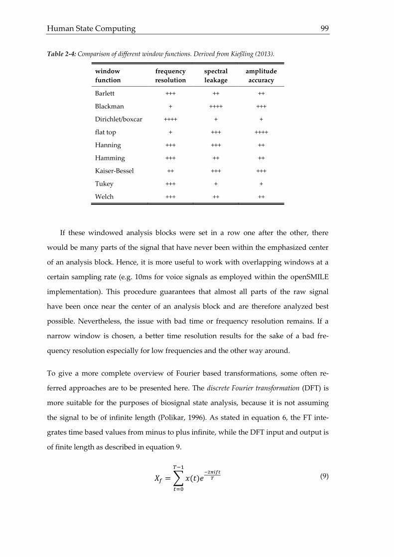
Human State Computing 99
Table 2-4: Comparison of different window functions. Derived from Kießling (2013).
window
function
frequency
resolution
spectral
leakage
amplitude
accuracy
Barlett +++ ++ ++
Blackman + ++++ +++
Dirichlet/boxcar ++++ + +
flat top + +++ ++++
Hanning +++ +++ ++
Hamming +++ ++ ++
Kaiser-Bessel ++ +++ +++
Tukey +++ + +
Welch +++ ++ ++
If these windowed analysis blocks were set in a row one after the other, there
would be many parts of the signal that have never been within the emphasized center
of an analysis block. Hence, it is more useful to work with overlapping windows at a
certain sampling rate (e.g. 10ms for voice signals as employed within the openSMILE
implementation). This procedure guarantees that almost all parts of the raw signal
have been once near the center of an analysis block and are therefore analyzed best
possible. Nevertheless, the issue with bad time or frequency resolution remains. If a
narrow window is chosen, a better time resolution results for the sake of a bad fre-
quency resolution especially for low frequencies and the other way around.
To give a more complete overview of Fourier based transformations, some often re-
ferred approaches are to be presented here. The discrete Fourier transformation (DFT) is
more suitable for the purposes of biosignal state analysis, because it is not assuming
the signal to be of infinite length (Polikar, 1996). As stated in equation 6, the FT inte-
grates time based values from minus to plus infinite, while the DFT input and output is
of finite length as described in equation 9.
𝑋𝑓 = ∑ 𝑥(𝑡)𝑒
−2𝜋𝑖𝑓𝑡
𝑇
𝑇−1
𝑡=0
(9)

100 2. Steps of Biosignal Analysis
All issues mentioned for the FT can be hold true for the DFT as well, as in the end
nothing changes about the fact that still the whole signal is analyzed to sum up the
impact of each frequency Xf. Besides the DFT, there have been made efforts to acceler-
ate computations of the frequency domain. On the one hand, there is the fast Fourier
transformation (FFT) introduced most successfully by Cooley & Tukey (1965), although
first FFT methods were published already in the early 19th century (Stankovic,
Stankovic, Egiazarian, & Yaroslavsky, 2004). A necessary assumption for the FFT algo-
rithm is, that the number of sampling points (T in equation 9) is a power of two (T = 2n).
In this case, the proposed divide and conquer algorithm reduces the computational
effort (equation 10).
𝑂(𝑇2) → 𝑂(𝑇 · log(𝑇)) (10)
Another possibility is to employ a discrete cosine transformation (DCT) which was
first presented by Ahmed, Natarjan, & Rao (1974). The DCT is heavily used for audio
and video compression (Le Gall, 1991) due to its well-fitting representation of image
and audio signals with minimal redundancy and hence smaller file sizes. As the name
already reveals, in contrast to the (D)FT cosine functions are calculated to represent the
signal. Depending on how the signal is supposed to extend, there are slightly different
algorithms for computing. The most often employed approach is called DCT-II given
in equation 11.
𝑋𝑓 = ∑ 𝑥(𝑡) · 𝑒−2𝜋𝑖 (
𝑓𝜋
𝑇(𝑡 +
1
2))
𝑇−1
𝑡=0
(11)
For voice based state analysis the DCT is often preferred to other Fourier transfor-
mations, because data can be processed more quickly. Furthermore the highly informa-
tive low frequency part (0.1 - 1kHz) is a little bit better represented due to a better reso-
lution (Gazor & Zhang, 2003).
Another popular derivative of the spectrum is described with the fantasy word
Cepstrum, where the first part of “spectrum” is reversed (for an overview see Deller,
Proakis, & Hansen, 2000, pp. 352). This kind of renaming is necessary to separate
cepstrum frequency analysis (also named quefrency analysis) from the common fre-

Human State Computing 101
quency analysis, as the cepstrum is nothing else than a spectrum of the spectrum. It is
computed by an inverse DFT of the logarithmized spectrum. There exist several slight-
ly different ways of computing like taking the inverse FT instead of the DCT. Im-
portant to notice, though, is their application within biosignal based state analysis, as
the impact of frequency cepstrum coefficients grew over the last decades (Atal, 2005).
As the following formula shows (equation 12), the initial multiplication of source fre-
quency and amplitude is transformed to an addition allowing to separate the source
signal and the way it is manipulated by a filter like the vocal tract (complex cepstrum
introduced by Oppenheimer, 1965).
𝐶(𝑋) = 𝐹𝑇(log(𝐹𝑇(𝑋) + 2𝜋𝑗𝑚) (12)
After generating the cepstrum, coefficients are required containing distinct infor-
mation about certain frequencies (as described above, they are named quefrencies, but
for the sake of understandability they will be described using the primary frequencies
they are derived from). Following an example by Polikar (1996), employing a linear
distribution of commonly used 256 frequency bands leads to a representation of the
spectrum. These 256 frequency bands are further compressed using triangular filters
(similar to the window functions mentioned above) and afterwards decorrelated by a
DCT eliminating redundant information leading to twelve linear frequency cepstrum
coefficients (LFCC). On top of that, the zeroth LFCC obtaining information about the
summed up average energy of every frequency band (Zheng, Zhang, & Song, 2001), is
included in the common feature set. Now all relevant transformations springing from
the FT have been presented. Based on the resulting frequency spectrum there are sev-
eral commonly employed features that will be described now.
The spectral roll-off indicates, up to which frequency α [%] of the spectrum have
summed up (Eyben, Wollmer, & Schuller, 2009). For the analyzed signals, the roll-off
for α = [25, 50, 75, 90] have been computed. The formula is given in equation 13.
∑ 𝑀𝑡(𝑛)
𝑅
𝑛=1
=𝛼
100∑ 𝑀𝑡(𝑛)
𝑁
𝑛=1
(13)

102 2. Steps of Biosignal Analysis
The Centroid strongly corresponds to the roll-off for α = 50. By weighting all magni-
tudes Mt[n] with their allocated frequency n, the central frequency of the spectrum is
computed as depicted in equation 14 (Eyben, Wollmer, & Schuller, 2009).
𝐶𝑡 =
∑ 𝑀𝑡(𝑛) · 𝑛𝑁𝑛=1
∑ 𝑀𝑡𝑁𝑛=1 (𝑛)
(14)
The spectral Flux normalizes the spectrum based on its magnitude. By comparing
successive analysis windows t, the degree of changes within the changes can be evalu-
ated. This information is helpful to assess how stationary the analysis windows of
length M are revealing hereby the accuracy of the frequency analysis by the STFT.
Other values for t are worth taken into consideration as well. The equation of the spec-
tral flux is given in equation 15 (Eyben, Wollmer, & Schuller, 2009).
𝐹𝑡 = ∑(𝑁𝑡(𝑛) − 𝑁𝑛−1(𝑛))
𝑁
𝑛=1
(15)
The last described measures are extreme values (minima and maxima). They show
up in a frequency spectrum at peaks (maxima) and low values. It is important to dis-
tinguish these features from the mentioned functionals (table 2-3) giving extreme val-
ues for the course of each feature. So in contrast to functionals, extreme values as a fea-
ture depict the minimum and maximum obtained frequency exceeding a certain
threshold. An overview of all computed feature groups within the common feature set
is shown in table 2-5 followed by a presentation of wavelet features (chapter 2.2.2).

Human State Computing 103
Table 2-5: Overview of commonly computed features based on openSMILE. It is to mention that MagLin
features are discarded for the conducted analyses in chapters 3-5. F0 and its envelope are omitted in this
table due to their particular importance for voice.
feature count abbreviation
energy 1 energy
f0 1 f0
f0 envelope 1 f0_env
LFC coefficients 13 LFCCx
magnitude F-bandwidths 5 fbandx-y
magnitude LFC coefficients 26 maglinx-y
peaks (minima, maxima) 2 min/max
spectral centroid 1 centroid
spectral flux 1 flux
spectral roll-off 4 roll-off
voice probability 1 voiceprob
zero crossing rate 1 ZCR
total 57
2.2.2 Wavelet Features
Following the disadvantages of the already presented Fourier based transfor-
mations, another way of obtaining frequency information of a time based signal has
evolved within the last decades. Although the continuous or discrete wavelet transfor-
mation (CWT/DWT) cannot overcome the limitations described by Heisenberg’s uncer-
tainty principle, it allows a best possible resolution of both frequency and time
(Polikar, 1996). For this reason, it has not stayed unnoticed within different fields of
signal analysis like voice (e.g. Walker & Foo, 2003; van Pham, 2008) or steering wheel
analysis (Krajewski et al., 2010). It can be argued whether it is important to know
where a certain frequency (almost) exactly occurs, as the STFT with its overlapping
windows already allows quite a detailed analysis. One example, though, are latencies
(kind of neuronal reaction times) in EEGs, where a very small delay or the amplitude
of a peak gives relevant information about its nature (Uberall, Renner, Edl, Parzinger,
& Wenzel, 1996) as depicted in figure 2-13.

104 2. Steps of Biosignal Analysis
Figure 2-13: Time delay in Event-related potentials (ERPs) for the P300 reaction in insulin dependent
group vs. control group. Adapted from Uberall et al. (1996).
The bottleneck of the STFT is the fixed window size. If the range of relevant fre-
quencies is high as for voice samples, the window size M must be at least long enough
to contain a whole oscillation of the lowest frequency (depending on the window func-
tion accordingly longer). For higher frequencies, the time resolution decreases auto-
matically. How the WT yields an optimal time-frequency representation is explained in
the following part as well as derived features for pattern recognition based state analy-
sis.
Describing the STFT’s bottleneck already reveals an approach for optimizing both
frequency and time resolution. If one window length M is not sufficient for all frequen-
cies, it is only a small step to choose different values for M for different frequencies.
This way of analysis is called multi resolution analysis (MRA; Mallat, 1989). Taking a
voice sample as an example for biosignals, it is obvious, that lower frequencies like the
fundamental frequency are constant for a longer time than higher frequencies changing
rapidly (figure 2-14).
0 100 200 300 400 500 600
latency (ms)
control group
experimental group
0
5
10
1
5
0
5
10
15
amp
litu
de
(µV
)
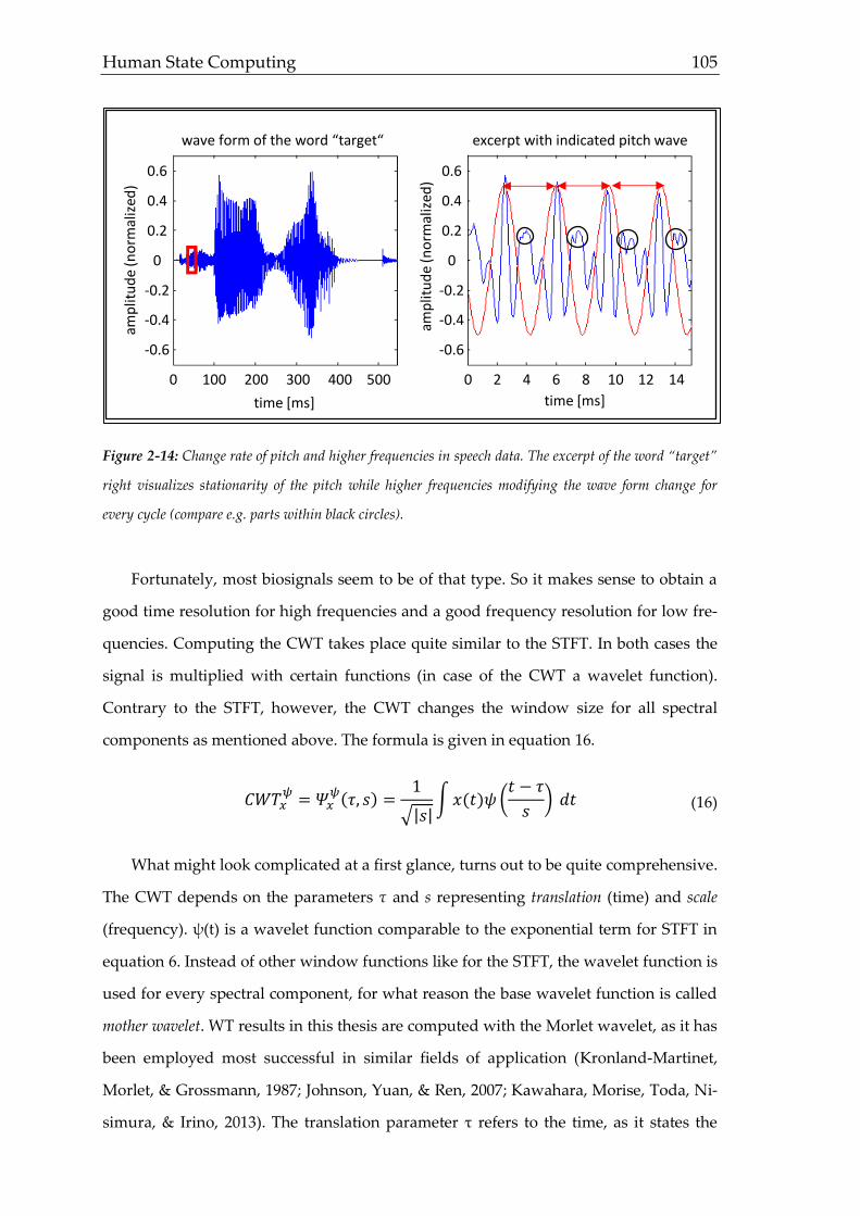
Human State Computing 105
Figure 2-14: Change rate of pitch and higher frequencies in speech data. The excerpt of the word “target”
right visualizes stationarity of the pitch while higher frequencies modifying the wave form change for
every cycle (compare e.g. parts within black circles).
Fortunately, most biosignals seem to be of that type. So it makes sense to obtain a
good time resolution for high frequencies and a good frequency resolution for low fre-
quencies. Computing the CWT takes place quite similar to the STFT. In both cases the
signal is multiplied with certain functions (in case of the CWT a wavelet function).
Contrary to the STFT, however, the CWT changes the window size for all spectral
components as mentioned above. The formula is given in equation 16.
𝐶𝑊𝑇𝑥𝜓
= 𝛹𝑥𝜓(𝜏, 𝑠) =
1
√|𝑠|∫ 𝑥(𝑡)𝜓 (
𝑡 − 𝜏
𝑠) 𝑑𝑡 (16)
What might look complicated at a first glance, turns out to be quite comprehensive.
The CWT depends on the parameters τ and s representing translation (time) and scale
(frequency). ψ(t) is a wavelet function comparable to the exponential term for STFT in
equation 6. Instead of other window functions like for the STFT, the wavelet function is
used for every spectral component, for what reason the base wavelet function is called
mother wavelet. WT results in this thesis are computed with the Morlet wavelet, as it has
been employed most successful in similar fields of application (Kronland-Martinet,
Morlet, & Grossmann, 1987; Johnson, Yuan, & Ren, 2007; Kawahara, Morise, Toda, Ni-
simura, & Irino, 2013). The translation parameter τ refers to the time, as it states the
wave form of the word “target“ excerpt with indicated pitch wave
time [ms]
0 2 4 6 8 10 12 140 100 200 300 400 500
time [ms]
amp
litu
de
(no
rmal
ized
)
amp
litu
de
(no
rmal
ized
)
0.6
0.4
0.2
0
-0.2
-0.4
-0.6
0.6
0.4
0.2
0
-0.2
-0.4
-0.6
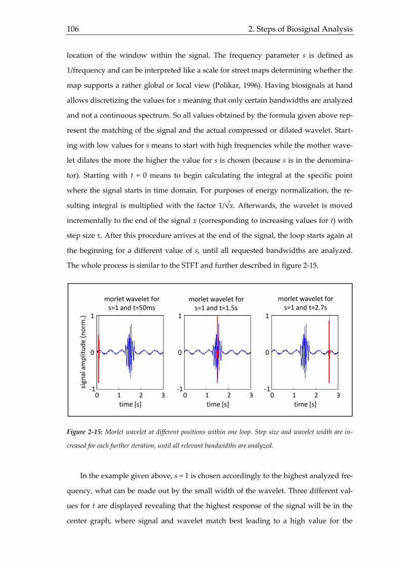
106 2. Steps of Biosignal Analysis
location of the window within the signal. The frequency parameter s is defined as
1/frequency and can be interpreted like a scale for street maps determining whether the
map supports a rather global or local view (Polikar, 1996). Having biosignals at hand
allows discretizing the values for s meaning that only certain bandwidths are analyzed
and not a continuous spectrum. So all values obtained by the formula given above rep-
resent the matching of the signal and the actual compressed or dilated wavelet. Start-
ing with low values for s means to start with high frequencies while the mother wave-
let dilates the more the higher the value for s is chosen (because s is in the denomina-
tor). Starting with t = 0 means to begin calculating the integral at the specific point
where the signal starts in time domain. For purposes of energy normalization, the re-
sulting integral is multiplied with the factor 1/√𝑠. Afterwards, the wavelet is moved
incrementally to the end of the signal x (corresponding to increasing values for t) with
step size τ. After this procedure arrives at the end of the signal, the loop starts again at
the beginning for a different value of s, until all requested bandwidths are analyzed.
The whole process is similar to the STFT and further described in figure 2-15.
Figure 2-15: Morlet wavelet at different positions within one loop. Step size and wavelet width are in-
creased for each further iteration, until all relevant bandwidths are analyzed.
In the example given above, s = 1 is chosen accordingly to the highest analyzed fre-
quency, what can be made out by the small width of the wavelet. Three different val-
ues for t are displayed revealing that the highest response of the signal will be in the
center graph, where signal and wavelet match best leading to a high value for the
morlet wavelet for s=1 and t=1.5s
morlet wavelet for s=1 and t=50ms
morlet wavelet for s=1 and t=2.7s
time [s]time [s]time [s]time [s] time [s] time [s]
sign
al a
mp
litu
de
(no
rm.)
0 1 2 3
1
0
-10 1 2 3 0 1 2 3
1
0
-1
1
0
-1
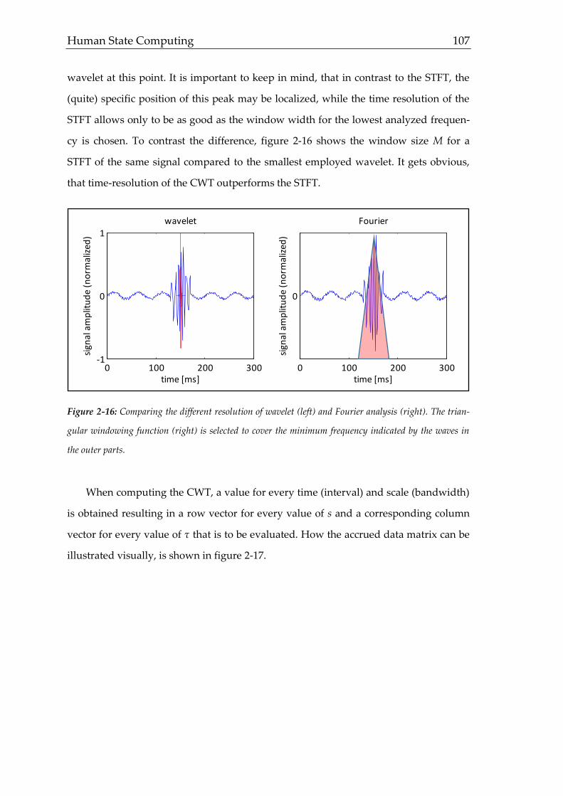
Human State Computing 107
wavelet at this point. It is important to keep in mind, that in contrast to the STFT, the
(quite) specific position of this peak may be localized, while the time resolution of the
STFT allows only to be as good as the window width for the lowest analyzed frequen-
cy is chosen. To contrast the difference, figure 2-16 shows the window size M for a
STFT of the same signal compared to the smallest employed wavelet. It gets obvious,
that time-resolution of the CWT outperforms the STFT.
Figure 2-16: Comparing the different resolution of wavelet (left) and Fourier analysis (right). The trian-
gular windowing function (right) is selected to cover the minimum frequency indicated by the waves in
the outer parts.
When computing the CWT, a value for every time (interval) and scale (bandwidth)
is obtained resulting in a row vector for every value of s and a corresponding column
vector for every value of τ that is to be evaluated. How the accrued data matrix can be
illustrated visually, is shown in figure 2-17.
0 100 200 300-1
0
1
time [ms]
sign
al a
mp
litu
de
(no
rmal
ized
)
wavelet
0 100 200 300
0
time [ms]
sign
al a
mp
litu
de
(no
rmal
ized
)
Fourier
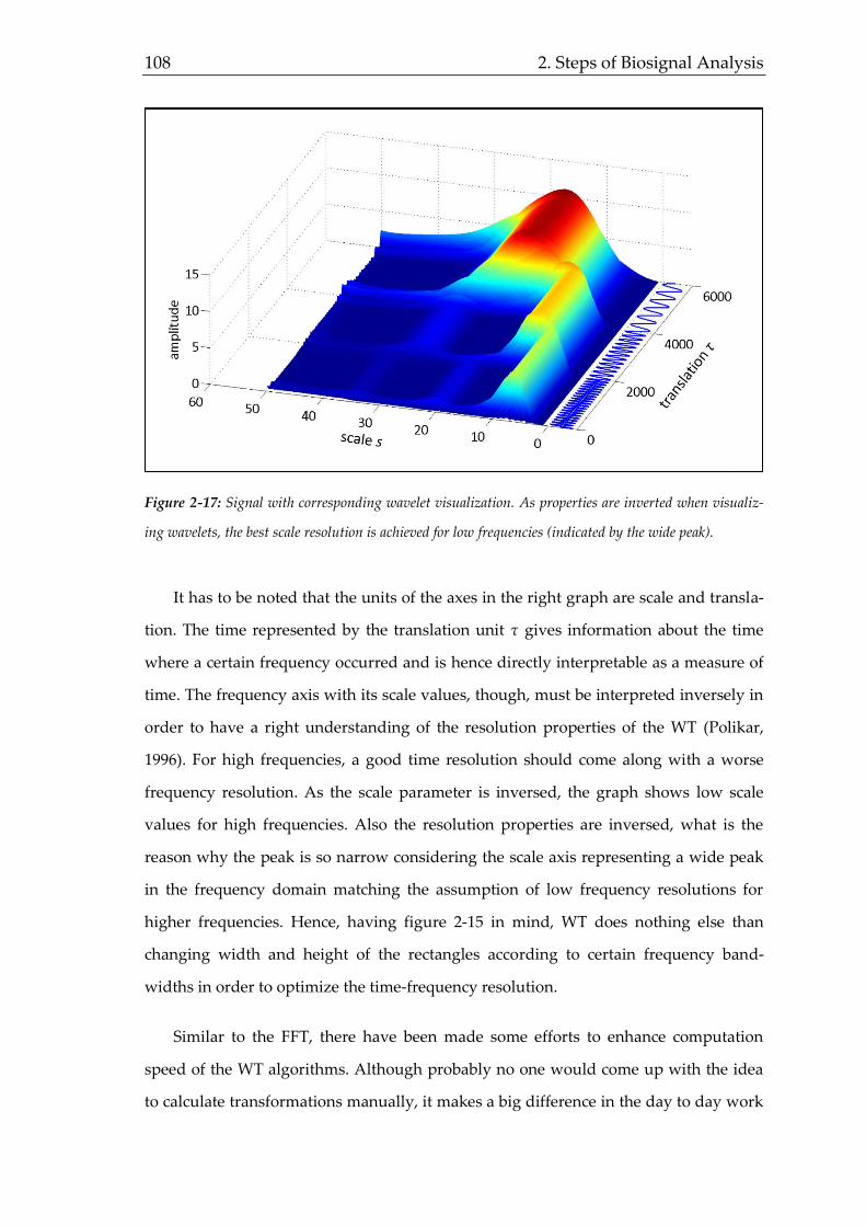
108 2. Steps of Biosignal Analysis
Figure 2-17: Signal with corresponding wavelet visualization. As properties are inverted when visualiz-
ing wavelets, the best scale resolution is achieved for low frequencies (indicated by the wide peak).
It has to be noted that the units of the axes in the right graph are scale and transla-
tion. The time represented by the translation unit τ gives information about the time
where a certain frequency occurred and is hence directly interpretable as a measure of
time. The frequency axis with its scale values, though, must be interpreted inversely in
order to have a right understanding of the resolution properties of the WT (Polikar,
1996). For high frequencies, a good time resolution should come along with a worse
frequency resolution. As the scale parameter is inversed, the graph shows low scale
values for high frequencies. Also the resolution properties are inversed, what is the
reason why the peak is so narrow considering the scale axis representing a wide peak
in the frequency domain matching the assumption of low frequency resolutions for
higher frequencies. Hence, having figure 2-15 in mind, WT does nothing else than
changing width and height of the rectangles according to certain frequency band-
widths in order to optimize the time-frequency resolution.
Similar to the FFT, there have been made some efforts to enhance computation
speed of the WT algorithms. Although probably no one would come up with the idea
to calculate transformations manually, it makes a big difference in the day to day work

Human State Computing 109
if a computation takes ten minutes or ten hours. Additionally, a continuous spectrum
with infinite values can only be theoretically computed. One approach to overcome
this issue has already been mentioned by discretizing the signal instead of taking a
continuous spectrum. According to the Nyquist-Shannon sampling theorem (although
it is argued to whom the sampling theorem can be traced back to, for first ideas it may
be referred to Nyquist, 1928), the sampling rate may be decreased for lower frequencies
with f1 > f2 as described in equation 17.
𝑁2 =
𝑓2
𝑓1𝑁1 (17)
That simple adaption of the sampling rate already decreases computation time no-
ticeably (Unser, 2000). It has to be mentioned at this stage, that further reduction of the
sampling rate is possible in the case of omitting the possibility of a signal synthesis
(reversing the function like an FT in order to rebuild the original data based on wavelet
coefficients). As (wavelet) syntheses of the source data are of higher importance for e.g.
data compression, but not for biosignal state analysis, syntheses techniques and their
mathematical background will not be provided in this thesis. Discretizing the CWT
usually follows a logarithmic rule (Polikar, 1996). Hence, the infinite points of (starting
with) the scale axis become finite with commonly 2n points. The higher the scale gets
(meaning a decrease of frequency), the lower the number of computed samples gets, as
the values for τ decrease by a factor 2 for each increase of the scale by the same factor.
That is, how mathematically put the reduction of the sampling rate for lower frequen-
cies takes place.
Much quicker and hence employed for the data analyzed in this thesis is the dis-
crete wavelet transformation (DWT; see for a first implementation Haar, 1910). Hence, the
last section of the wavelet features introduction is supposed to explain the algorithm
and underlying principle of this approach. As discretizing the CWT only leads to a
sampled type of the CWT called wavelet series (WS), coefficients contain a high amount
of redundant information. The development of the DWT reaches back to subband cod-
ing presented by Crochiere, Weber & Flanagan (1976) when they tried to decompose
speech signals. The approach of the DWT is similar to the CWT. Plainly put, the raw

110 2. Steps of Biosignal Analysis
data are filtered meaning they are split into small pieces regarding time and frequency.
Depending on how many filters are used respectively how small the step size for scale
und translation parameters are chosen, the resolution changes. This filtering can be
achieved by changing the sampling rate as already described earlier in another context.
Reducing the sampling rate, e.g., not only reduces the computation time, but also re-
duces the possibly captured bandwidth as well simultaneously. Figure 2-18 illustrates,
why higher frequencies are omitted when the sampling rate decreases.
Figure 2-18: Relation of sampling rate and frequency. As indicated by the red squares, the applied sam-
pling rate (indicated by grey squares) is not sufficient for the increased frequency in the second half of the
signal. Available sample points cannot detect the additional oscillations (missing sampling points are
plotted red).
Commonly, values for s and τ are obtained from the continuous spectrum by ex-
ponential terms with base j = 2 starting with s0 = 2 and t0 = 1 resulting in the coefficients
s = 2j and τ = k·s or τ = k*2j. The factor k for the τ parameter draws back on the fact that
a certain base vector function k is needed to transform the time domain values t into
the translation information τ. Values of the discrete biosignal x are denoted with x(n).
Following Polikar (1996), the signal is split by several highpass filters H and lowpass
filters G leading to coefficients hx and gx by employing the following formulas (equa-
tion 18).
0 0.5 1 1.5 2-1
0
1
time [s]
amp
litu
de
(no
rmal
ized
)
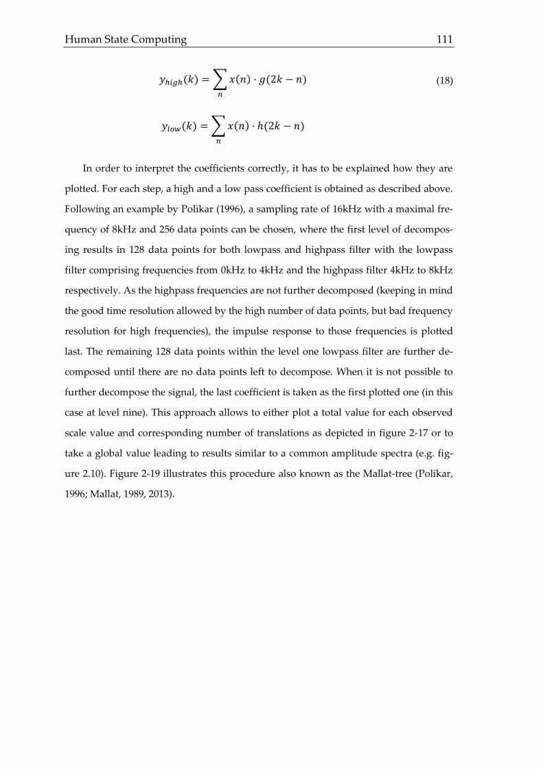
Human State Computing 111
𝑦ℎ𝑖𝑔ℎ(𝑘) = ∑ 𝑥(𝑛) · 𝑔(2𝑘 − 𝑛)
𝑛
𝑦𝑙𝑜𝑤(𝑘) = ∑ 𝑥(𝑛) · ℎ(2𝑘 − 𝑛)
𝑛
(18)
In order to interpret the coefficients correctly, it has to be explained how they are
plotted. For each step, a high and a low pass coefficient is obtained as described above.
Following an example by Polikar (1996), a sampling rate of 16kHz with a maximal fre-
quency of 8kHz and 256 data points can be chosen, where the first level of decompos-
ing results in 128 data points for both lowpass and highpass filter with the lowpass
filter comprising frequencies from 0kHz to 4kHz and the highpass filter 4kHz to 8kHz
respectively. As the highpass frequencies are not further decomposed (keeping in mind
the good time resolution allowed by the high number of data points, but bad frequency
resolution for high frequencies), the impulse response to those frequencies is plotted
last. The remaining 128 data points within the level one lowpass filter are further de-
composed until there are no data points left to decompose. When it is not possible to
further decompose the signal, the last coefficient is taken as the first plotted one (in this
case at level nine). This approach allows to either plot a total value for each observed
scale value and corresponding number of translations as depicted in figure 2-17 or to
take a global value leading to results similar to a common amplitude spectra (e.g. fig-
ure 2.10). Figure 2-19 illustrates this procedure also known as the Mallat-tree (Polikar,
1996; Mallat, 1989, 2013).
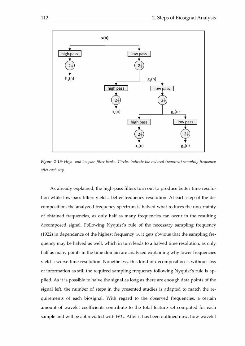
112 2. Steps of Biosignal Analysis
Figure 2-19: High- and lowpass filter banks. Circles indicate the reduced (required) sampling frequency
after each step.
As already explained, the high-pass filters turn out to produce better time resolu-
tion while low-pass filters yield a better frequency resolution. At each step of the de-
composition, the analyzed frequency spectrum is halved what reduces the uncertainty
of obtained frequencies, as only half as many frequencies can occur in the resulting
decomposed signal. Following Nyquist’s rule of the necessary sampling frequency
(1922) in dependence of the highest frequency ω, it gets obvious that the sampling fre-
quency may be halved as well, which in turn leads to a halved time resolution, as only
half as many points in the time domain are analyzed explaining why lower frequencies
yield a worse time resolution. Nonetheless, this kind of decomposition is without loss
of information as still the required sampling frequency following Nyquist’s rule is ap-
plied. As it is possible to halve the signal as long as there are enough data points of the
signal left, the number of steps in the presented studies is adapted to match the re-
quirements of each biosignal. With regard to the observed frequencies, a certain
amount of wavelet coefficients contribute to the total feature set computed for each
sample and will be abbreviated with WTx. After it has been outlined now, how wavelet
x(n)
high pass low pass
low passhigh pass
low passhigh pass
2 2
2 2
22
h1(n)
h2(n)
h3(n) g3(n)
g1(n)
g2(n)
Human State Computing 113
features can be computed and how they differ from common features, the following
chapter introduces nonlinear dynamics.
2.2.3 Nonlinear Dynamic Features
All features mentioned so far base on the assumption of some kind of linear func-
tional and predictable relationship between features and user states. Regarding motor
behavior, though, a considerable amount of studies (Beek, Peper, & Stegemann, 1995;
Shelhammer, 1998; Jiang & Zhang, 2002; Cavanaugh, Guskiewicz, & Sterigou, 2005;
Stergiou & Decker, 2011; 5 more) emphasize, that (deterministic) chaotic systems are
particularly suitable for describing observable variance that may be due to different
state manifestations. Without plotting too many details, the basic principle behind cha-
otic assumptions is, that dynamical systems are majorly affected by smallest changes of
initial conditions (like differences in user states). In contrast to common equations,
where little varying values usually lead to only little varying results, Lorenz (1956,
1963) found out when analyzing weather data, that a simple rounding of one data
point was sufficient to change the outcome dramatically. This effect, commonly re-
ferred to as the butterfly effect (Lorenz, 2000; Hilborn, 2004), can be used for compu-
ting mathematical models taking this special behavior into account.
Within the last decades, some studies regarding emotional speech (Cairns & Han-
sen, 1994; Kwon, Chan. Hao, & Lee, 2003) as well as health-related issues (Zhang &
Yiang, 2008) employed nonlinear dynamic features with promising outcomes. In the
case of fatigue assessment from voice samples, a successful implementation of nonline-
ar dynamic features has been undertaken by a workgroup around the author (Krajew-
ski, et al, 2010). Therefore, a short description based on the abstract follows to further
demonstrate, how nonlinear dynamics can be adapted to biosignals. Afterwards, find-
ings regarding motor behavior are depicted, before a short explanation of all employed
nonlinear dynamic features closes this chapter.
When analyzing voice samples, not only changes of muscle behavior are to be ob-
served, but also differences in the airflow generated by exhaling air for the aim of
speaking. An important aspect in the vocal tract regarding different user states influ-

114 2. Steps of Biosignal Analysis
encing speech production is especially the generation of nonlinear aerodynamic phe-
nomena including non-laminar flow, flow separation in various regions, generation
and propagation of vortices and formation of jets rather than well-behaved laminar
flow (Teager & Teager, 1989; Thomas 1986; Kaiser, 1983). The collapse of laminar flow
arises at high reynolds number stating the relationship of inertial and viscous forces or,
differently put, the degree of sensitivity of the flow for turbulences and is defined as
the quotient given by the product of density 𝜌, mean velocity of the fluid 𝜐 and dis-
tance d divided by the dynamic viscosity 𝜂 as depicted in equation 19.
𝑅𝑒 =
𝜌 · 𝜐 · 𝑑
𝜂 (19)
Due to the relevant length and subsonic speed of air flow in the vocal tract, this
number is very large, indicating that the air flow can be expected to be turbulent. The
air jet flowing through the vocal tract during speech production includes convoluted
paths of rapidly varying velocity, which are highly unstable and oscillate between its
walls, attaching or detaching itself, and thereby changing the effective cross-sectional
areas and air masses. Several issues are responsible for the generation of these nonline-
ar effects: The vocal folds behave as a vibrating valve, disrupting the constant airflow
from the lungs and forming it into regular puffs of air. Modeling approaches which
have their origin in fluid dynamics coupled with the elastodynamics of a deformable
solid understand this phonation process as nonlinear oscillation: dynamical forcing
from the lungs provides the energy needed to overcome dissipation in the vocal fold
tissue and vocal tract air. The vocal folds themselves are modeled as elastic tissue with
nonlinear stress-strain relationship. These nonlinear stretching qualities of the vocal
folds are based on larynx muscles and cartilage which produces nonlinear behavior.
Furthermore, vocal tract and the vocal folds are coupled when the glottis is open re-
sulting in significant changes in formant characteristics between open and closed glot-
tis cycles. The movement of the vocal folds themselves is modeled by a lumped two
mass system connected by springs again with nonlinear coupling. These nonlinear
phenomena produce turbulent flow while the air jet may be modulated either by the
vibration of the walls or by the generated vortices. Several methods based on chaotic
dynamics and fractal theory have been suggested to describe these aerodynamic turbu-

Human State Computing 115
lence related phenomena of the speech production system (Maragos, Kaiser, & Quatie-
ri, 1993; Dimitridis & Maragos, 2003; MacLaughlin & Maragos, 2007) including the
modeling of the geometrical structures in turbulence (spatial structure, energy cascade)
utilizing fractals and multifractals (Maragos, 1991; Adeyemi & Boudreaux-Bartels,
1997; Ashkenazy, 1999], nonlinear oscillator models (Quatieri & Hofstetter, 1990;
Townshend, 1990; Kubin, 1996), and state-space reconstruction. This state-space recon-
struction is done utilizing the embedding theorem which reconstructs a multidimen-
sional attractor by embedding the scalar signal into a phase space. The embedding al-
lows us to reconstruct the geometrical structure of the original attractor of the system
which formed the observed speech signal. Moreover, it helps us to discover the degree
of determinism of an apparently random signal, e.g. by applying measures like Lya-
punov exponents.
However, no empirical research has been done to examine the turbulence effects in
speech signals regarding leadership relevant states, although previous work (Krajew-
ski, Batliner, & Wieland, 2009; Krajewski et al., 2011) has demonstrated the feasibility
for fatigue detection. Previous work associating changes in voice with leadership abili-
ties (Krajewski, Batliner, & Golz, 2009; has generally focused only on features derived
from speech emotion recognition (Batliner, Seppi, Steidl, & Schuller, 2010), whereas
nonlinear dynamics based speech features have received no attention. Thus, it seems
only logical to take corresponding features to further analysis and follow the novelty
approach of the present study by combining those features with other mentioned fea-
ture sets. Nonetheless, nonlinear dynamics are not only suitable for the evaluation of
voice samples. In the field of motor behavior, more studies have been conducted with
promising results as described before.
Already Bernstein (1967) shaped the dynamic of motor behavior with the phrase
“repetition without repetition” meaning that two (consecutive) executions of the same
action will never be exactly the same. It is to reason, whether the deviation is due to
random error (as outlined within Generalized Motor Programs mentioned analyzed by
Schmidt, 1985; Lai & Shea, 1998; Summers & Anson, 2009, as mentioned in chapter
1.2.3) or chaotic nature. The latter explanation gives an onset for explaining motor var-
iance with the help of nonlinear dynamic features. Some studies have already taken

116 2. Steps of Biosignal Analysis
those capabilities into account when analyzing the nature of pathologic (Cignetti, Ster-
giou, & Decker, 2012; Harbourne & Stergiou, 2009) and/or usual movement (van Em-
merik, Rosenstein, McDermott, & Hamill, 2004) or robotics (Nakanishi & Schaal, 2004).
Outcomes of these studies reveal, that movement variability is well explained by chaot-
ic systems. Especially the possibility to identify pathologic features of a movement
gives reason to detect varying patterns for different user states. Although fatigue or
stress cannot be considered as pathology firstly, it seems likely to observe different
motor behavior also for different manifestations of user states. The following features
were employed for all fields of application with slight modifications based on the
Matlab openTSTOOL box and own scripts.
AMIF. The auto-mutual information function AMIF represents a measure of shared
information between two random variables taken from the same signal. In contrast to
the autocorrelation function, AMIF also considers nonlinear correlations meaning that
also higher order dependencies are analyzed (see figure 2-20) .
Figure 2-20: Comparison of linear and nonlinear correlations.
As random variables, different parts of the input signal with certain time lags τ in an
interval [0 τmax] are employed revealing any kind of periodicity in the signal. Results for
all values of τ are computed as given in equation 20 by the joint probability distribu-
tion function p(x,y) with y = x+τ and the respective marginal probabilities p(x) and
p(y).
0 5 100
5
10
x
y
5 100
5
10
x
y

Human State Computing 117
𝐼(𝑋, 𝑌) = ∑ ∑ 𝑝(𝑥, 𝑦) · log (
𝑝(𝑥, 𝑦)
𝑝(𝑥) · 𝑝(𝑦))
𝑦∈𝑌𝑥∈𝑋
(20)
Boxcounting. When dealing with chaotic systems, dimensionality is not limited to
integers anymore meaning that objects may take on any values describing its dimen-
sion. For a proper understanding, it is to state that a dimension can be defined as the
number of degrees of freedom in a space (Itzkov, 2009). In the case of a three-
dimensional space, it is possible to move in the directions forward/backward, left/right
or up and down. Following Freistetter (2010), fractal dimensions are approachable by
analyzing superimpositions. Imagining a simple line with dimension D = 1 and a
length of one meter, it can be questioned how many squares N of a certain edge length
L are required to cover it. The roughly correct mathematical answer is given in equa-
tion 21.
𝑁 ~
1
𝐿𝐷 (21)
Referring to the one-dimensional line, 10 squares with L = 0.1m are required to
cover the line (10 = 1/0.11). Reducing L by factor 2 doubles the number of squares. Go-
ing one step further by assuming a square (with an edge length of one meter), the re-
duction of L by a factor 2 results in a factor 2D = 22 = 4 more squares to cover the area.
However, superimposition can be realized by other geometric objects like circles or
triangles as well. Taking the equilateral Sierpinski-triangle (Barlow & Perkins, 1988,
citing Sierpinski, 1912) into account, it is possible to produce a fractal object. Simply
connect the center of each side and the triangle is divided into four equal smaller trian-
gles (figure 2-21).
Figure 2-21: Sierpinski triangle. Adapted from Wilhelm (2007).

118 2. Steps of Biosignal Analysis
Repeating this process infinitely would still be insufficient for covering the whole
area of the initial triangle. The remaining area is neither a simple perimeter line nor is it
defined by disjunctive points; it is something different (Freistetter, 2010). Applying the
formula for boxcounting dimensions (equation 22)
𝐷 = lim
𝑒→0
log (𝑁(𝜀))
log ( 1
𝜀)
(22)
for a grid width ε and N(ε) the number of covered boxes results in a dimensionality D
of about 1.59 or log(3)/log(2). Similar effects are generated analyzing the Koch-Curve,
where a simple line is manipulated systematically, until the resulting object is more
than just a line (figure 2-22).
Figure 2-22: Koch-curve. Adapted from Wilhelm (2007).
While the perimeter line of this object is infinite for infinite iterations of the pro-
cess, the area is not (it is 9/5 for an initial length 1). Although natural objects are never
fractal dimensioned, comparable effects of self-similarity can be observed for roma-
nesco broccoli, e.g., or when trying to measure the length of a coastline and zooming
progressively in to measure as detailed as possible (Freistetter, 2010). In the end, box
counting does nothing else than assessing, how many nonempty boxes are to count in
order to cover a certain object (like a coastline) lying on an evenly-spaced grid at a cer-
tain scale. In the openTSTOOL box, Segdgewick’s Ternary Search Tree algorithm (see
Bentley & Sedgewick, 1997, for a search and sort task) is implemented for a fast compu-
tation. As input, an N-by-D matrix containing the data points as well as a number of

Human State Computing 119
partitions describing the grid are required. Adapting the input matrix to the employed
biosignal data, the N-by-D matrix takes the shape of the N-by-1 matrix, as both wave
form and movement data are one-dimensional. Several different partitions are tested
for gaining insights at different scale levels.
Information and Correlation Dimension. Taken into consideration that the box-
counting method primarily differentiates between empty and nonempty boxes (Theil-
er, 1990), the Rényi-dimension (see Bromiley, Thacker, & Bouhova-Thacker, 2004, for
an overview) computation for assessing dimensionality analyzes how much of a box is
covered. The normalized area is integrated over all boxes and exponentiated with the
power q. While the result for q = 0 equals the common fractal dimension based on box-
counting as mentioned above, the result for q = 1 is called the information dimension,
while q = 2 represents the correlation dimension, which are both computed within the
openTSTOOL box in the way given in equation 23.
𝐷𝑞 = lim
𝜖→0
log (∑ 𝜇(𝐵𝑖𝑖 )𝑞)
(1 − 𝑞) · log (𝜀) (23)
Minimum Embedding Dimension. Time series analysis often takes place by finding
parameters to reconstruct the phase space which is a kind of the timeless space consist-
ing of all conditions of a system (trajectory). Closed subsets of this trajectory represent-
ed by several data points are called attractor. The aim is to find a model that rebuilds
the topological neighborhood or dimension of data points. As states of systems change
in time, the trajectory describes the time evolution or the dynamic of a system (Kennel,
Brown, & Abarbanel, 1992). Different systems appear to have different phase space
portraits, whereby the underlying nature of the system (e.g. periodic or chaotic) can be
described (figure 2-23). Basic assumption of phase space reconstruction is, that in a
deterministic system the state at time tx contains all necessary information to predict
future system states for tx+n. For chaotic dynamical systems, though, the phase space
and underlying mathematical functions are unknown. Hence, the best approach is to
build prediction models based on several observations of the system’s behavior in or-
der to approximate a most fitting model (Kennel, Brown, & Abarbanel, 1992).
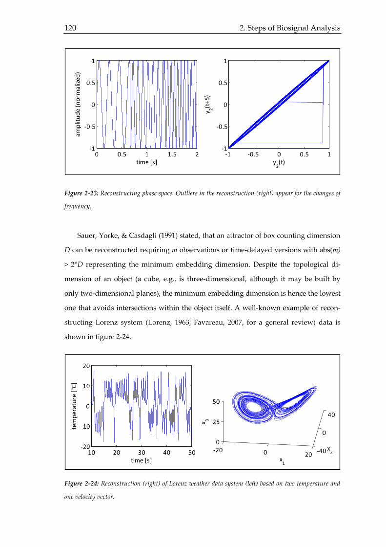
120 2. Steps of Biosignal Analysis
Figure 2-23: Reconstructing phase space. Outliers in the reconstruction (right) appear for the changes of
frequency.
Sauer, Yorke, & Casdagli (1991) stated, that an attractor of box counting dimension
D can be reconstructed requiring m observations or time-delayed versions with abs(m)
> 2*D representing the minimum embedding dimension. Despite the topological di-
mension of an object (a cube, e.g., is three-dimensional, although it may be built by
only two-dimensional planes), the minimum embedding dimension is hence the lowest
one that avoids intersections within the object itself. A well-known example of recon-
structing Lorenz system (Lorenz, 1963; Favareau, 2007, for a general review) data is
shown in figure 2-24.
Figure 2-24: Reconstruction (right) of Lorenz weather data system (left) based on two temperature and
one velocity vector.
0 0.5 1 1.5 2-1
-0.5
0
0.5
1
time [s]
amp
litu
de
(no
rmal
ized
)
-1 -0.5 0 0.5 1-1
-0.5
0
0.5
1
y2(t)
y 2(t
+5)
10 20 30 40 50-20
-10
0
10
20
time [s]
tem
per
atu
re [
°C]
200-20
40
0
-40
0
25
50
x2
x1
x 3

Human State Computing 121
One critical factor of efficient reconstructing is the time delay. Although recon-
struction is possible with any time delay (following Sauer et al., 1991), it turned out
that time delays with minimal autocorrelation (or even better auto-mutual information
function AMIF) yield best results. For computations within this thesis, the cao algo-
rithm (Cao, 1997) is employed within the openTSTOOL box requiring a number of data
points as well as the number of computed nearest neighbors leading to a notation like
cao10-2 for a 10-point data vector and two computed nearest neighbors. Figure 2-24 fur-
thermore indicates, that attractor contours are similar, but not identical (Krajewski et
al., 2010). The resulting differences can be measured using trajectory descriptors like
the angle between consecutive trajectory parts, distance to the attractor centroid as well
as the leg length of the trajectory. All these features are implemented in the nonlinear
dynamic feature set.
Largest Lyapunov Exponent. Within the process of phase space reconstruction, it has
already been described that the aim has to be to retain initial neighborhoods of data
points. When predicting states of a data point for several points in time (representing
the dynamic), the increase or decrease of the distance between predicted and true val-
ues for several points in time is a measure for the stability of a dynamic system (see
Rosenstein, Collins, & de Luca, 1993 for overview and implementation). Based on pre-
diction error and time, the largest lyapunov exponent is computed. Although there is a
lyapunov exponent for each dimension, commonly only the largest exponent is ana-
lyzed, as it contains all necessary information of the other exponents. While a positive
large lyapunov exponent indicates a chaotic system, a negative one is returned for a
fixed point. An exponent of zero usually represents periodic signals. The algorithm
integrated in the openTSTOOL box is based on Wolf, Swift, Swinney, & Vastano (1985)
computing the i-th Lyapunov exponent λi based on the length of the ellipsoidal princi-
pal axis pi(t) and shown in equation 24.
𝜆𝑖 = lim
𝑡→∞
1
𝑡log2
𝑝𝑡(𝑡)
𝑝𝑖(0) (24)

122 2. Steps of Biosignal Analysis
After all relevant backgrounds on nonlinear dynamic feature computation have
been described, table 2-6 gives an overview of all retrieved features. More details about
feature specifics are given within each field of application.
Table 2-6: Overview of employed NLD features.
feature number abbreviation
attractor trajectory (angle, distance to
attractor centroid, length of leg) 3
traj_angle, traj_centdist,
traj_leglen
auto mutual information function 9 AMIFD,τ
boxcounting dimension 3 boxcounting
minimum embedding dimension (cao) 3 caoD
correlation dimension 1 corrdim
information dimension 1 infodim-y
large lyapunov exponent 1 large-lyap
total 21
With the depiction of nonlinear dynamic features, all universally usable feature
sources are described. Although the aim of this thesis is to show that small adaptations
of these universal feature sources are sufficient for (almost) all fields of application, a
comparison to signal-specific features is necessary to prove this assumption. For this
reason, the following chapter deals with features being specific for the employed bi-
osignals.
2.2.4 Signal-Specific Features
When thinking about state prediction using a certain biosignal, characteristics of
the particular biosignals are elaborated to derive corresponding features. With regard
to the employed biosignals voice as well as head and mouse movement, the most im-
portant specific features are described in the following.
Voice. One of the most evolved analyses among the employed biosignals are done
regarding voice features. Within the common feature set, a large variety of frequency
related features is displayed relating directly to voice changes. Some frequencies are
more important than others, though, which is why certain adjustments on analyzed

Human State Computing 123
frequencies contribute to a good prediction performance (Hermansky, 1990; Kawahara,
Masuda-Katsuse, & de Cheveigné, 1999). An overview of voice sensitive features is
given in the following figure 2-25.
Figure 2-25: Overview of voice-specific features.
Although some of the features accounting to the depicted categories have already
been described within the common feature section, some particularly relevant features
for voice analyses will be presented here. Regarding prosody, features are relevant that
can be allocated to the speech melody. The most prominent representative of these
measures is the perceived pitch level or fundamental frequency (F0). Further, features for
volume or speech rate are employed for voice based state assessment.
F0. Within a frequency spectrum, the fundamental frequency appears as the lowest
frequency with the highest energy. There are manifold ways how to compute it auto-
matically (Gerhard, 2003). In the present case, the openSMILE implementation based
on both auto-correlation function and cepstra is used.
pitch(f0)
sonority(e.g. MFCC)
shakiness(e.g. jitter)
aspirate(e.g. closure)
voice qualityprosody
pressure(intensity)
frequency decompositionusing Fourier analysis
sound pressure over time trembling(rapid changes in e.g. pitch)
sonority(e.g. MFCC)
sonority(e.g. MFCC)
articulation
VOICE
sonority(e.g. MFCC)
tone softness(e.g. formant)
sonority(e.g. MFCC)
tone softness (e.g. formant)
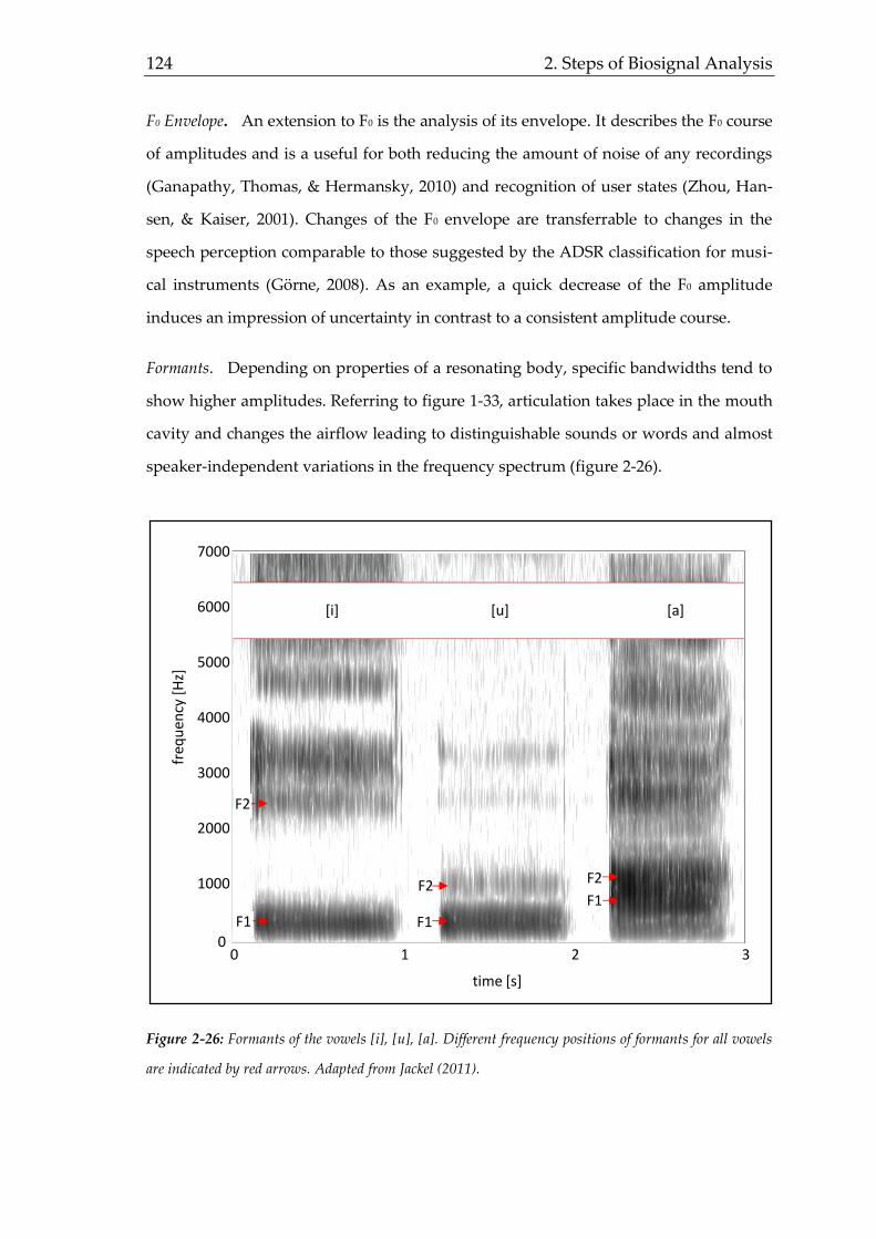
124 2. Steps of Biosignal Analysis
F0 Envelope. An extension to F0 is the analysis of its envelope. It describes the F0 course
of amplitudes and is a useful for both reducing the amount of noise of any recordings
(Ganapathy, Thomas, & Hermansky, 2010) and recognition of user states (Zhou, Han-
sen, & Kaiser, 2001). Changes of the F0 envelope are transferrable to changes in the
speech perception comparable to those suggested by the ADSR classification for musi-
cal instruments (Görne, 2008). As an example, a quick decrease of the F0 amplitude
induces an impression of uncertainty in contrast to a consistent amplitude course.
Formants. Depending on properties of a resonating body, specific bandwidths tend to
show higher amplitudes. Referring to figure 1-33, articulation takes place in the mouth
cavity and changes the airflow leading to distinguishable sounds or words and almost
speaker-independent variations in the frequency spectrum (figure 2-26).
Figure 2-26: Formants of the vowels [i], [u], [a]. Different frequency positions of formants for all vowels
are indicated by red arrows. Adapted from Jackel (2011).
0 31 2
time [s]
0
1000
2000
3000
4000
5000
6000
7000
[i] [u] [a]
F1
F2
F1
F2
F1
F2
freq
uen
cy [
Hz]

Human State Computing 125
While the first two formants are an indicator of the tongue position (Cherif,
Bouafif, & Dabbabi, 2001) the following two formants match perceptions of nasality.
Originally employed for speech recognition tasks due to their generally speaker-
independence (Itakura, 1975; Welling & Ney, 1998), some studies (Williams & Stevens,
2005; Ververidis & Kotropoulos, 2006; Krajewski, Batliner, & Golz, 2009; El Ayadi,
Kamel, & Karray, 2011) examining different speech state recognition tasks have proven
their feasibility in other contexts as well.
Voice Probability. The speech rate has already been mentioned as a relevant factor for
voice based state recognition. One snippet of the speech rate can be the proportion of
words and pauses referring to the probability that a person speaks at a random mo-
ment. Gaussian mixture models (GMM) can be used to differentiate between both con-
ditions for each speech segment. Another approach is to split segments by their vol-
ume (Tüske, Mihajlik, Tobler, & Fegyó, 2005).
Frequency Bands. As it does not appear to be sensible to examine each frequency sepa-
rately as done for the fundamental frequency, the magnitude of certain frequency
bandwidths is taken to further analysis (also considering resolution issues mentioned
before). Linear distributions of bandwidths covering the whole frequency range are not
to recommend, since a majority of information lies within the lower frequencies (see
chapter 2.2.1). Hence, openSMILE introduces five frequency bandwidths from 0Hz
reaching to 9123Hz, where the first 3 bands focus on frequencies up to 650Hz.
Mel-Cepstrum. Regularities applying for frequency analyses turn out to be relevant for
cepstral analyses, too. Chapter 2.2.1 already introduced linear cepstra, but especially
for voice samples, a different scaling is more reasonable. The perceptual Mel scale, first
introduced by Stevens, Volkman, & Newman (1937) takes into account that the percep-
tion of sound distances (in terms of pitch) is nonlinear. The higher the frequency is, the
higher the difference between the pitch of two sounds must be in order to be perceived
as equally distant compared to lower frequencies. Equation 25 shows how linear fre-
quency values f are concerted to values of the Mel scale m and vice versa.

126 2. Steps of Biosignal Analysis
𝑀 = 2595 · 𝑙𝑔 (1 +𝑓
700)
(25)
𝐹 = 700 (10𝑚
2595 − 1)
As the MFCCs are computed as described for the LFCCs (only differing in the non-
linear approach), no repetitive derivation is given here. openSMILE includes the mag-
nitude of the first 25 mel frequency bands as well as the first MFCCs resulting from
decorrelation (MFCC1-12) eliminating inappropriately high frequencies from further
analysis. In addition, the zeroth MFCC0 is computed similar to LFCC0. Although the
MFCC0 is often discarded for speech recognition tasks, it is of major importance for
speech enhancements and the perceptual quality (Boucheon & De Leon, 2008).
Jitter/Shimmer. As part of speech quality features, jitter and shimmer are sensitive
measures especially to stress related phenomena (Protopapas & Lieberman, 1997; Oz-
das, Shiavi, Silverman, Silverman, & Wilkes, 2005; Li et al., 2007). It is general
knowledge that nervous people are prone to have a kind of shaky voice. This percep-
tion can be reproduced by frequency analyses as well. There are two different ways
how a voice can be trembling. On the one hand, F0 can change rapidly within a certain
bandwidth (jitter), while on the other hand, the amplitude can be subject to cycle-to-
cycle variations (shimmer). Although jitter has its origin in telecommunication systems,
where a high jitter indicates problems in transmitting a steady signal, both measures
are easily adapted to speech features. A good overview of different ways of computing
is provided by Farrús, Hernando, & Ejarque (2007). For human state analysis within
this thesis, the common implementation of Praat’s algorithms (Boersma & Weenink,
2010) has been chosen.
Now all voice-specific features have been presented. As mouse and head movement
are in high conformity with each other, the first presented features apply for both bi-
osignals. Afterwards, some more specific features are presented.
Movement. Both head and mouse movement appear to be a bit simpler kind of bi-
osignal. On the one hand, this assumption might apply, because typically employed
specific movement features are based on a 2-dimensional (mouse) or 3-dimensional

Human State Computing 127
(head) movement. On the other hand, this chapter has already proven the possibility of
treating movement based features like voice features, as in the end a speech sample’s
wave form does not look that different from plotting normalized movement, although
frequency analyses is not as obvious as it is for voice analysis. When thinking of
movement, speed and acceleration are common descriptors. Speed v is computed by
analyzing the change of position (meaning the distance d) with reference to time t so
that v = d/t. In turn, the distance for two points p and q in an n-dimensional space is
calculated using the Euclidian distance as shown in equation 26.
𝑑(𝑝, 𝑞) = √∑(𝑝𝑖 − 𝑞𝑖)2
𝑛
𝑖=1
(26)
For the whole sample, the distance d in units of pixel [px] of all m subsequent data
points has to be summed up leading to a total distance dtotal in pixel [px] as given in
equation 27.
𝑑𝑡𝑜𝑡𝑎𝑙 = √∑ 𝑑(𝑝, 𝑞)
𝑚
𝑗=1
(27)
Keeping formula v = d/t in mind, t is still missing. Depending on the sampling rate
or sampling frequency fs (being fs = 10Hz meaning 10 data points per second for both
head and mouse movement), elapsed time t in seconds [s] can be calculated based on
the number of considered data points p as equation 28 shows.
𝑡 =𝑝
𝑓𝑠 (28)
In the end, speed v results in units of [px/s] and gives an indication about how fast
the mouse or head is moved during recording. Speed, however, reveals no information
about the style of movement behavior, but only how much distance is covered over
time within the sample. The acceleration a as a derivation of speed, though, indicates
whether the movement is rather continuous or jumpy. Figure 2-27 depicts how equal
values for speed v can be a realization for different amounts of variation in accelera-

128 2. Steps of Biosignal Analysis
tion. Regarding mouse movement, however, characteristic of the dynamic computer
mouse described in chapter 1.3.2 have to be considered.
Figure 2-27: Comparison of two different movement patterns. Both lines cover the same distance in the
same time and hence move with the same speed in total. Comparing the acceleration, though, leads to the
depicted difference.
Additionally, mouse movement generates information about the clicking behavior.
For that reason it is possible to compute not only overall values, but use a finer resolu-
tion and analyze click to click period and behavior as well as clicking duration, which
is possibly affected by states like fatigue (Komandur, Johnson, & Storch, 2008). In a
standardized task as employed and described in chapter 4, the total amount of time
needed for completing the task may allow a fatigue assessment, too and is hence in-
cluded in the feature set. Furthermore, click to click analysis allows to analyze devia-
tions from the “racing line” in terms of a zero crossing rate (count of switching from
above to below the racing line) as well as the difference between covered distance and
minimal distance between two points. Both features are illustrated in figure 2-28.
0 5 100
50
100
time [s]
cove
red
dis
tan
ce [
%]
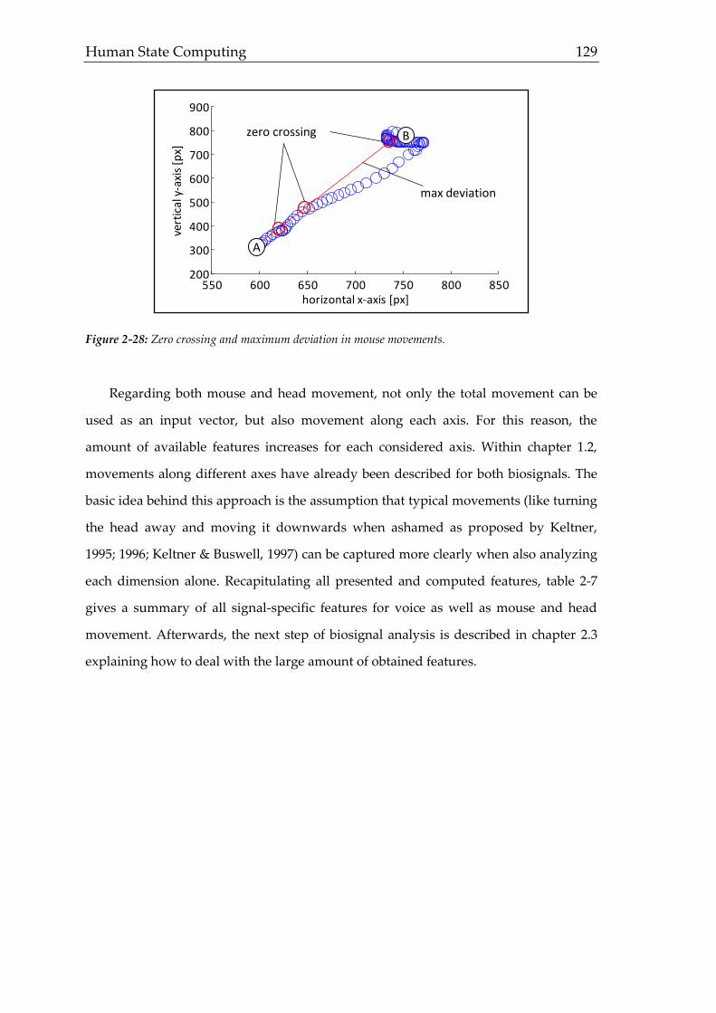
Human State Computing 129
Figure 2-28: Zero crossing and maximum deviation in mouse movements.
Regarding both mouse and head movement, not only the total movement can be
used as an input vector, but also movement along each axis. For this reason, the
amount of available features increases for each considered axis. Within chapter 1.2,
movements along different axes have already been described for both biosignals. The
basic idea behind this approach is the assumption that typical movements (like turning
the head away and moving it downwards when ashamed as proposed by Keltner,
1995; 1996; Keltner & Buswell, 1997) can be captured more clearly when also analyzing
each dimension alone. Recapitulating all presented and computed features, table 2-7
gives a summary of all signal-specific features for voice as well as mouse and head
movement. Afterwards, the next step of biosignal analysis is described in chapter 2.3
explaining how to deal with the large amount of obtained features.
550 600 650 700 750 800 850200
300
400
500
600
700
800
900
horizontal x-axis [px]
vert
ical
y-a
xis
[px]
B
A
max deviation
zero crossing

130 2. Steps of Biosignal Analysis
Table 2-7: Overview of signal-specific features.
feature number abbreviation
Fundamental and harmonic frequencies 5 Fx
F0 envelope 1 F0_env
formantx 5 Formantx
jitter, shimmer 2 jitter, shimmer
Mel Frequency Cepstrum Coefficients 13 MFCC0-12
voice probability 1 voiceprob
total voice-specific features 27
movement descriptors
(acceleration, speed) 2 acc, speed
click behavior (duration, frequency) 2 click_dur, click_freq
point-to-point analysis (covered distance,
maximum deviation, zero crossing) 3
p2p_covdist,
p2p_maxdev, p2p_zcr
total mouse-specific features 7
movement descriptors
(acceleration, speed) 2 acc, speed
total signal-specific features 36
2.3 Feature Selection
The descriptions in this chapter have already shown that feature selection is some-
times closely linked to prediction models. As there are several methods available
commonly used within the field of biosignal analysis, those that were implemented in
the presented studies will be shown in this chapter.
The basic idea behind feature selection is on the one hand a reduction of computa-
tional efforts and on the other hand gaining highly informative feature sets that allow
to be integrated in a theoretical framework. Chapter 1 has already given several hints
about how certain feature could behave with regard to particular user states, whereby
despite the data driven approach, a validation of distinct hypothesis is possible. Fur-
thermore, facing issues with overfitting (Harrell, Lee, & Mark, 1996; more on this mat-
ter is discussed in chapter 2.5) are reduced with a small proportion of features in rela-
tion to the sample size. In the case of equal numbers of features and samples, a predic-
tion algorithm is likely to “remember” each vector as an example for a certain output

Human State Computing 131
and hence gives perfect results for train samples, but performs poorly on test samples
(Hsu, Chang, & Lin, 2003).
Hence, the best solution is a small but robust feature set with high performance for
both known and unknown samples (Hitten & Frank, 2005). Feature selection in general
has become a very wide field of research by now. Yet, this thesis rather focuses on fea-
ture extraction, wherefore at this place only some popular methods achieving this goal
in different ways are presented in the following. For a more detailed view of different
techniques and their development, other sources are more appropriate (Liu & Motoda,
1998; Saeys, Inza, & Larranaga, 2007; Hua, Tembe, & Dougherty, 2009). For an over-
view of feature selection tasks see figure 2-29.
Figure 2-29: Overview of feature selection purposes. Although within some transformation techniques
new features are generated, this property is skipped in this overview as it is not always a distinct selection
process.
In general, procedures reducing the dimensionality of the initial feature space can
be distributed in filter and wrapper approaches (Guyon & Elisseeff, 2003). Furthermore,
feature transformation techniques can be mentioned in this field (Kusiak, 2001). Within
filter-based approaches, performance criteria like correlation, distance or error
measures are applied for every single feature based on the training set. With regard to
the achieved performance, features can be ordered. The selection can now be conduct-
ed either using a fixed number of features (taking the best pre-defined number of fea-
tures) or defining a certain threshold (take only features that perform better than a pre-
defined criterion).
avoid overfittingreduce computational
effortstest hypotheses
feature selection

132 2. Steps of Biosignal Analysis
For wrapper-based selections, the performance of feature subsets is computed al-
ready employing a classification algorithm. The general idea is to test all feature sub-
sets following a certain rule (heuristic) or randomly within the selection process and
test the feature subset performance based on all designated prediction algorithm.
Hence, it is obvious that the feature selection in this case does not only depend on the
features, but also on the chosen classifier. Considering the commonly huge amount of
features and hence numerous subset possibilities, it is usually not possible to test all
subsets, so the computational effort depends on the employed selection parameter.
Feature transformations do not directly make use of the feature expressions, but
modify the input data by setting them in a certain relationship (e.g. factoring based on
similarity). Afterwards, e.g. averaged factors can be employed as features to build pre-
diction models. Hereby, though, for every prediction task of a test set it is necessary to
rebuild the factor expression based on all (relevant) extracted features. Depending on
the aggregation of transformed features, the possibility of deriving useful theoretical
assumptions can vary. The shortly described general feature subset selection ap-
proaches are depicted in table 2-8. Examples as well as advantages and disadvantages
been added for a better overview.
Table 2-8: Overview of feature selection methods. Adapted from Krajewski (2007, p. 100).
selection method example evaluation
filter-based
subset selection
density, smoothness, entropy,
salience
correlation, information gain
ratio, t-test value
+
-
quick, intuitive
redundant, no learning
wrapper-based
subset selection
brute-force, heuristic (feed for-
ward, backward elimination,
sequential forward floating
search, genetic selection
+
-
avoids redundancy, includes
learning algorithm
time consuming, potentially
finds only local maxima
feature
transformation
PCA methods, nonlinear auto-
associative network, independ-
ent component analysis (ICA),
multidimensional scaling
(MDS), sammon map, enhanced
lipschitz embedding, linear
discriminant analysis (LDA
following Chen & Yang, 2004)
+
-
potentially stronger theoreti-
cal focus, can produce im-
proved features
not always reduces number
of necessarily extracted fea-
tures (Kraiss, 2003; Golz et
al., 2007), time consuming
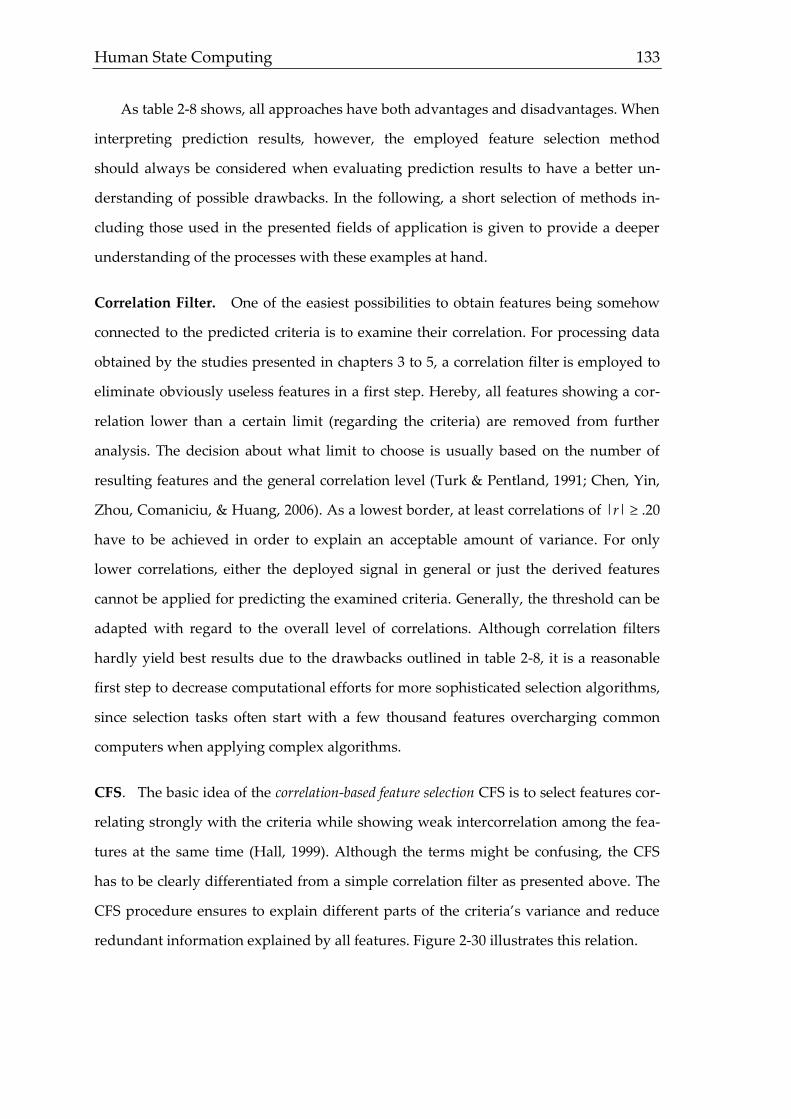
Human State Computing 133
As table 2-8 shows, all approaches have both advantages and disadvantages. When
interpreting prediction results, however, the employed feature selection method
should always be considered when evaluating prediction results to have a better un-
derstanding of possible drawbacks. In the following, a short selection of methods in-
cluding those used in the presented fields of application is given to provide a deeper
understanding of the processes with these examples at hand.
Correlation Filter. One of the easiest possibilities to obtain features being somehow
connected to the predicted criteria is to examine their correlation. For processing data
obtained by the studies presented in chapters 3 to 5, a correlation filter is employed to
eliminate obviously useless features in a first step. Hereby, all features showing a cor-
relation lower than a certain limit (regarding the criteria) are removed from further
analysis. The decision about what limit to choose is usually based on the number of
resulting features and the general correlation level (Turk & Pentland, 1991; Chen, Yin,
Zhou, Comaniciu, & Huang, 2006). As a lowest border, at least correlations of |r| ≥ .20
have to be achieved in order to explain an acceptable amount of variance. For only
lower correlations, either the deployed signal in general or just the derived features
cannot be applied for predicting the examined criteria. Generally, the threshold can be
adapted with regard to the overall level of correlations. Although correlation filters
hardly yield best results due to the drawbacks outlined in table 2-8, it is a reasonable
first step to decrease computational efforts for more sophisticated selection algorithms,
since selection tasks often start with a few thousand features overcharging common
computers when applying complex algorithms.
CFS. The basic idea of the correlation-based feature selection CFS is to select features cor-
relating strongly with the criteria while showing weak intercorrelation among the fea-
tures at the same time (Hall, 1999). Although the terms might be confusing, the CFS
has to be clearly differentiated from a simple correlation filter as presented above. The
CFS procedure ensures to explain different parts of the criteria’s variance and reduce
redundant information explained by all features. Figure 2-30 illustrates this relation.
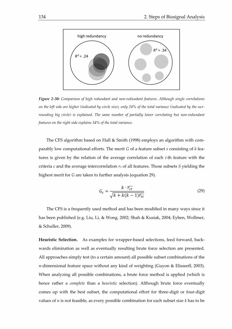
134 2. Steps of Biosignal Analysis
Figure 2-30: Comparison of high redundant and non-redundant features. Although single correlations
on the left side are higher (indicated by circle size), only 24% of the total variance (indicated by the sur-
rounding big circle) is explained. The same number of partially lower correlating but non-redundant
features on the right side explains 34% of the total variance.
The CFS algorithm based on Hall & Smith (1998) employs an algorithm with com-
parably low computational efforts. The merit G of a feature subset s consisting of k fea-
tures is given by the relation of the average correlation of each i-th feature with the
criteria c and the average intercorrelation rii of all features. Those subsets S yielding the
highest merit for G are taken to further analysis (equation 29).
𝐺𝑠 =
𝑘 · 𝑟𝑐𝑡
√𝑘 + 𝑘(𝑘 − 1)𝑟𝑡𝑡 (29)
The CFS is a frequently used method and has been modified in many ways since it
has been published (e.g. Liu, Li, & Wong, 2002; Shah & Kusiak, 2004; Eyben, Wollmer,
& Schuller, 2009).
Heuristic Selection. As examples for wrapper-based selections, feed forward, back-
wards elimination as well as eventually resulting brute force selection are presented.
All approaches simply test (to a certain amount) all possible subset combinations of the
n-dimensional feature space without any kind of weighting (Guyon & Elisseeff, 2003).
When analyzing all possible combinations, a brute force method is applied (which is
hence rather a complete than a heuristic selection). Although brute force eventually
comes up with the best subset, the computational effort for three-digit or four-digit
values of n is not feasible, as every possible combination for each subset size k has to be
high redundancy
R² = .24
no redundancy
R² = .34

Human State Computing 135
tested. Feed forward algorithms start with comparing all single features and increasing
k as long as the increase yields better performance in terms of the chosen evaluation
measure (see chapter 2.5). Different adjustments are possible like considering only
more features, when the enhancement is significant, testing additional cycles, also if
one cycle of increasing k does not show better results, or defining a minimum and/or
maximum for k. Feed forward selections allowing to increase k until it equals n led to
the same results as a brute force algorithm did. Backward elimination, though, is the
direct opposite of the feed forward selection. The backward elimination starts with the
full feature space of k = n and reduces k as long as removing features from the subset
does not yield worse results compared to the bigger subset with the same possible
modifications as mentioned before. The common approach is illustrated in table 2-9.
Table 2-9: characteristics of heuristic feature selection in comparison to brute force.
feed
forward
backward
elimination
brute
force
number of features in
the course of iteration ↑ ↓ irrelevant
termination
condition
addition does not
improve prediction
reduction worsens
prediction /
Genetic Selection. As the name already reveals, genetic selection algorithms are
modeled on biological principles and were first introduced by Holland (1975). Contra-
ry to the heuristic selection, this wrapper-based approach follows no heuristic and is
hence considered a random wrapper (Yang & Honavar, 1998). Based on the whole
sample set as the parent generation, new individuals (or feature subsets) are built
based on crossover and mutation techniques. Crossover means that successful subsets
(meaning those with a high prediction power) of a parent feature space are exchanged
with another strand (feature subset) building the genetic information (feature space) of
a new generation. Mutation changes features of a new individual in a random process
leading to on the one hand unpredictable results, but induces new information on the
other hand (Schuller, Arsić, Wallhoff, Lang, & Rigoll, 2005). This new generation con-
tains much information from each parent and is further analyzed. So by chance, after a
few generations (the exact number has to be tested and adjusted based on computa-
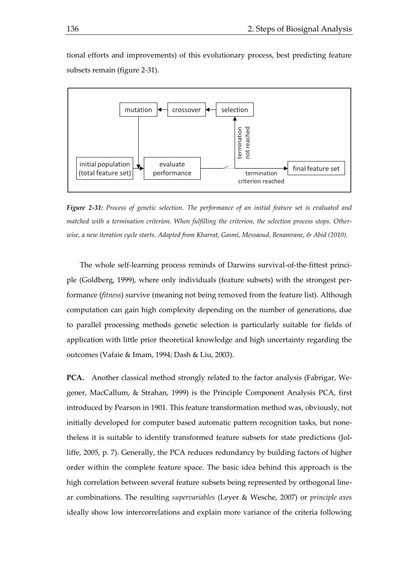
136 2. Steps of Biosignal Analysis
tional efforts and improvements) of this evolutionary process, best predicting feature
subsets remain (figure 2-31).
Figure 2-31: Process of genetic selection. The performance of an initial feature set is evaluated and
matched with a termination criterion. When fulfilling the criterion, the selection process stops. Other-
wise, a new iteration cycle starts. Adapted from Kharrat, Gasmi, Messaoud, Benamrane, & Abid (2010).
The whole self-learning process reminds of Darwins survival-of-the-fittest princi-
ple (Goldberg, 1999), where only individuals (feature subsets) with the strongest per-
formance (fitness) survive (meaning not being removed from the feature list). Although
computation can gain high complexity depending on the number of generations, due
to parallel processing methods genetic selection is particularly suitable for fields of
application with little prior theoretical knowledge and high uncertainty regarding the
outcomes (Vafaie & Imam, 1994; Dash & Liu, 2003).
PCA. Another classical method strongly related to the factor analysis (Fabrigar, We-
gener, MacCallum, & Strahan, 1999) is the Principle Component Analysis PCA, first
introduced by Pearson in 1901. This feature transformation method was, obviously, not
initially developed for computer based automatic pattern recognition tasks, but none-
theless it is suitable to identify transformed feature subsets for state predictions (Jol-
liffe, 2005, p. 7). Generally, the PCA reduces redundancy by building factors of higher
order within the complete feature space. The basic idea behind this approach is the
high correlation between several feature subsets being represented by orthogonal line-
ar combinations. The resulting supervariables (Leyer & Wesche, 2007) or principle axes
ideally show low intercorrelations and explain more variance of the criteria following
initial population(total feature set)
evaluate performance termination
criterion reached
final feature set
selectioncrossovermutation
term
inat
ion
no
t re
ach
ed
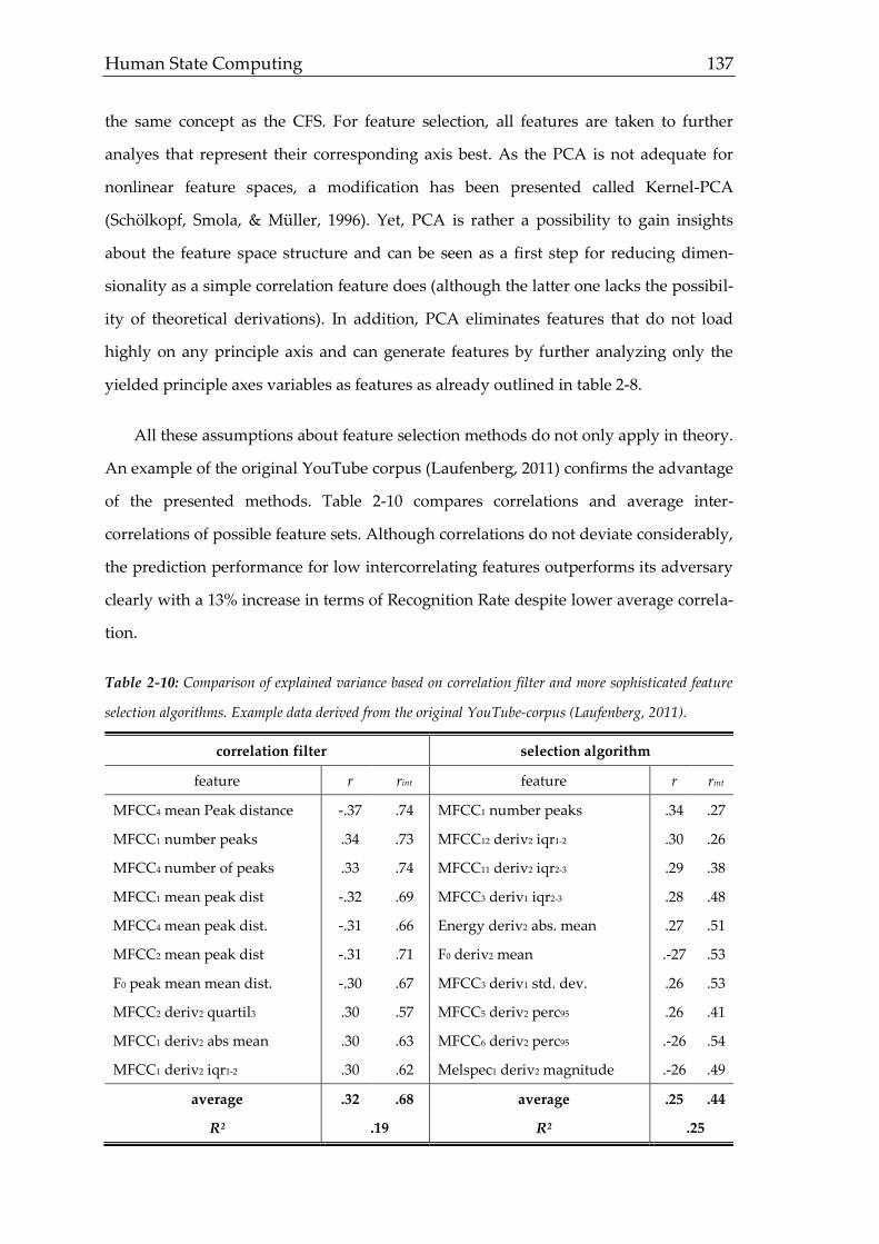
Human State Computing 137
the same concept as the CFS. For feature selection, all features are taken to further
analyes that represent their corresponding axis best. As the PCA is not adequate for
nonlinear feature spaces, a modification has been presented called Kernel-PCA
(Schölkopf, Smola, & Müller, 1996). Yet, PCA is rather a possibility to gain insights
about the feature space structure and can be seen as a first step for reducing dimen-
sionality as a simple correlation feature does (although the latter one lacks the possibil-
ity of theoretical derivations). In addition, PCA eliminates features that do not load
highly on any principle axis and can generate features by further analyzing only the
yielded principle axes variables as features as already outlined in table 2-8.
All these assumptions about feature selection methods do not only apply in theory.
An example of the original YouTube corpus (Laufenberg, 2011) confirms the advantage
of the presented methods. Table 2-10 compares correlations and average inter-
correlations of possible feature sets. Although correlations do not deviate considerably,
the prediction performance for low intercorrelating features outperforms its adversary
clearly with a 13% increase in terms of Recognition Rate despite lower average correla-
tion.
Table 2-10: Comparison of explained variance based on correlation filter and more sophisticated feature
selection algorithms. Example data derived from the original YouTube-corpus (Laufenberg, 2011).
correlation filter selection algorithm
feature r rint feature r rint
MFCC4 mean Peak distance -.37 .74 MFCC1 number peaks .34 .27
MFCC1 number peaks .34 .73 MFCC12 deriv2 iqr1-2 .30 .26
MFCC4 number of peaks .33 .74 MFCC11 deriv2 iqr2-3 .29 .38
MFCC1 mean peak dist -.32 .69 MFCC3 deriv1 iqr2-3 .28 .48
MFCC4 mean peak dist. -.31 .66 Energy deriv2 abs. mean .27 .51
MFCC2 mean peak dist -.31 .71 F0 deriv2 mean .-27 .53
F0 peak mean mean dist. -.30 .67 MFCC3 deriv1 std. dev. .26 .53
MFCC2 deriv2 quartil3 .30 .57 MFCC5 deriv2 perc95 .26 .41
MFCC1 deriv2 abs mean .30 .63 MFCC6 deriv2 perc95 .-26 .54
MFCC1 deriv2 iqr1-2 .30 .62 Melspec1 deriv2 magnitude .-26 .49
average .32 .68 average .25 .44
R² .19 R² .25

138 2. Steps of Biosignal Analysis
Results suggest that selection algorithms improve performance by identifying a
better differentiating feature set even when the general level of correlations is rather
mediocre. Figure 2-2 has already shown that (most) selection algorithms cannot be ana-
lyzed without any knowledge of the employed method for generating the prediction
algorithm. It has further been pointed out, that feature selection always seeks the “best
performing” feature subset. As no performance can be measured without prediction
modeling, it gets obvious that both domains are closely linked to and affect each other.
This is e.g. the case, if a feature selection algorithm suggests different feature subsets
when evaluating the performance with different prediction algorithms. Hence, both
selection and prediction algorithms have always to be chosen thoroughly and tested
against each other for gaining optimal outcomes. Specifics of prediction model genera-
tion are introduced in the following chapter.
2.4 Prediction Model Generation
Considering the huge data vectors remaining for all recordings even after feature
selection, it gets obvious that prediction modeling somehow has to handle these multi-
dimensional data and find patterns between different state levels. Based on examples
of possibly all relevant state levels (train set), an algorithm has to be developed to match the
feature expressions with the data labels (true score) in order to assess unlabeled data (test set)
later on. This general process is depicted in figure 2-32.
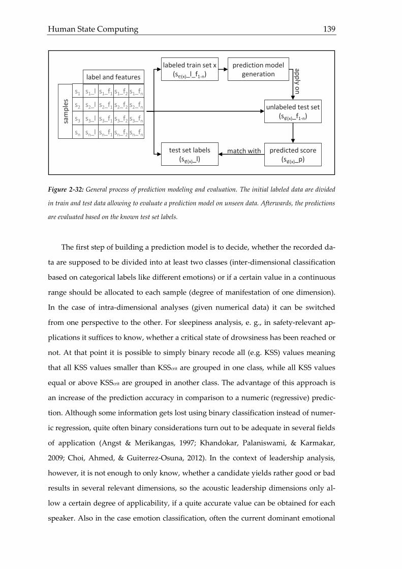
Human State Computing 139
Figure 2-32: General process of prediction modeling and evaluation. The initial labeled data are divided
in train and test data allowing to evaluate a prediction model on unseen data. Afterwards, the predictions
are evaluated based on the known test set labels.
The first step of building a prediction model is to decide, whether the recorded da-
ta are supposed to be divided into at least two classes (inter-dimensional classification
based on categorical labels like different emotions) or if a certain value in a continuous
range should be allocated to each sample (degree of manifestation of one dimension).
In the case of intra-dimensional analyses (given numerical data) it can be switched
from one perspective to the other. For sleepiness analysis, e. g., in safety-relevant ap-
plications it suffices to know, whether a critical state of drowsiness has been reached or
not. At that point it is possible to simply binary recode all (e.g. KSS) values meaning
that all KSS values smaller than KSScrit are grouped in one class, while all KSS values
equal or above KSScrit are grouped in another class. The advantage of this approach is
an increase of the prediction accuracy in comparison to a numeric (regressive) predic-
tion. Although some information gets lost using binary classification instead of numer-
ic regression, quite often binary considerations turn out to be adequate in several fields
of application (Angst & Merikangas, 1997; Khandokar, Palaniswami, & Karmakar,
2009; Choi, Ahmed, & Guiterrez-Osuna, 2012). In the context of leadership analysis,
however, it is not enough to only know, whether a candidate yields rather good or bad
results in several relevant dimensions, so the acoustic leadership dimensions only al-
low a certain degree of applicability, if a quite accurate value can be obtained for each
speaker. Also in the case emotion classification, often the current dominant emotional
sam
ple
s
s1
s2
s3
sn
label and features
s1_l
s2_l
s3_l
sn_l
s1_f1
s2_f1
s3_f1
sn_f1
s1_f2
s2_f2
s3_f2
sn_f2
s1_fn
s2_fn
s3_fn
sn_fn
prediction modelgeneration
predicted score(s∉(x)_p)
test set labels(s∉(x)_l)
unlabeled test set(s∉(x)_f1-n)
app
ly on
match with
labeled train set x(s∈(x)_l_f1-n)

140 2. Steps of Biosignal Analysis
state is required for proper applications and not only knowledge about, whether a sub-
ject is e.g. happy or not (Kim & André, 2008; Steidl, 2009). For these reasons, the predic-
tion algorithm always should be chosen with regard to the targeted application.
After it has now been clarified how sample data are grouped (or not), it is neces-
sary to present the differences between all employed classifiers and regressive ap-
proaches. Hence, the next part deals with a more detailed description of Support Vec-
tor Machines (SVM), artificial neuronal networks (ANN), k nearest neighbor (kNN,
linear discriminance analysis (LDA), and regression modeling. Although the wide field
of classifiers is hereby not exhausted, it is considered a sufficient selection to guarantee
a first estimate of the prediction potential.
SVM. One of the most heavily employed classifier is the Support Vector Machine
(SVM, Vapnik, 1982). It belongs to the so-called large margin classifiers meaning that
two neighbored points of different classes are separated by a possibly large margin.
The coordinates of all classes are employed as supportive vectors. With the help of the
Kernel trick it is possible to compute a hyperplane in a high-dimensional space leading
to a better separability of classes that are difficult to separate linearly in the original
dimensioned space. This advantage even allows allocating samples to classes that are
usually not linearly separable (Abe, 2010) as the simple example in figure 2-33 illus-
trates.
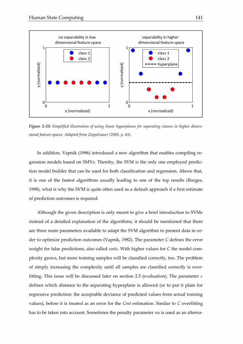
Human State Computing 141
Figure 2-33: Simplified illustration of using linear hyperplanes for separating classes in higher dimen-
sional feature spaces. Adapted from Zeppelzauer (2005, p. 43).
In addition, Vapnik (1996) introduced a new algorithm that enables compiling re-
gression models based on SMVs. Thereby, the SVM is the only one employed predic-
tion model builder that can be used for both classification and regression. Above that,
it is one of the fastest algorithms usually leading to one of the top results (Burges,
1998), what is why the SVM is quite often used as a default approach if a first estimate
of prediction outcomes is required.
Although the given description is only meant to give a brief introduction to SVMs
instead of a detailed explanation of the algorithms, it should be mentioned that there
are three main parameters available to adapt the SVM algorithm to present data in or-
der to optimize prediction outcomes (Vapnik, 1982). The parameter C defines the error
weight for false predictions, also called costs. With higher values for C the model com-
plexity grows, but more training samples will be classified correctly, too. The problem
of simply increasing the complexity until all samples are classified correctly is over-
fitting. This issue will be discussed later on section 2.5 (evaluation). The parameter ε
defines which distance to the separating hyperplane is allowed (or to put it plain for
regressive prediction: the acceptable deviance of predicted values from actual training
values), before it is treated as an error for the Cost estimation. Similar to C overfitting
has to be taken into account. Sometimes the penalty parameter nu is used as an alterna-
0 10
1
x (normalized)
y (n
orm
aliz
ed)
no separability in low dimensional feature space
class 1
class 2
0 10
1
x (normalized)
y (n
orm
aliz
ed)
separability in higher dimensional feature space
class 1
class 2
hyperplane

142 2. Steps of Biosignal Analysis
tive to ε. At last the parameter γ is introduced as an influence factor for the hyper-
plane’s shape. Increasing values require a higher number of support vectors and hence
slow down the computation. Furthermore, there are a lot of different Kernel functions
to choose. A general introduction to SVMs is provided by Burges (1998). For the data
presented in the result sections of chapters 3 to 5, a default linear Kernel function was
employed.
LDA. A typical example for linear classification is the linear discriminant analysis
(LDA) which was primarily introduced by Fisher (1936). It is closely related to the PCA
(Principal component analysis), but has another objective. The approach of the LDA is
to choose coefficients of a linear combination in a way that maximizes the probability
of correct allocations to previously given classes (Maximum-Likelihood-Method) by
determining a best fitting hyperplane or threshold respectively, while the PCA algo-
rithm aims at minimizing the mean squared error (MSE) of the prediction of all sam-
ples. As sometimes relations are not linear but e.g. quadratic, the quadratic discriminant
analysis (QDA) may be employed for certain samples using accordingly quadratic in-
stead of linear functions to separate classes. In the case of numeric instead of category
class labels, the function is transformed to a (multiple) linear regression analysis. As
there is no other distinctive difference between linear classification by LDA and regres-
sion modeling using linear regression, the latter one is not explained any further.
ANN. Artificial neural networks (ANN) were introduced by McCulloch & Pitts (1943).
In its most simple form, the ANN represents a kind of linear classification, where fea-
tures are weighted according to a best possible classification outcome. The more com-
plex the neural network is constructed, though, the less it is possible to predict or educ-
ible its behavior becomes. The basic idea behind neural networks is to develop a kind
of intelligent and autodidactic model that is supposed to kind of represent the way
neutrons interact in a brain. Accordingly, the approach is to take several simple units
(neurons) that process data simultaneously and interact by activating or enhancing (or
weight higher) those connections leading to desired results (Crone, 2010). This way of
modelling can be found in brains as well where frequently activated connections be-
tween neurons grow stronger, while those who tend to be less or not at all activated
anymore degenerate. Obviously, weights for all features are not adjusted by a kind of

Human State Computing 143
maximum likelihood estimation, but on learning. To give an easy example based on
Rosenblatt (1958), a perceptron with each one input and output layer is imagined. As
input in the stage of learning, each vector of the training set is allocated to a certain
neuron along with all known outputs (classes). In a next step, all neurons of the input
layer handle their information about the class over to the output layer. In that way, the
output layer receives information about patterns that go along with certain classifica-
tions in order to weight the information of all neurons in the input layer. So connec-
tions of neurons that often “fire” simultaneously will be enhanced. Unseen data within
the stage of testing are now classified based on the learning experience with the train-
ing set. Depending on the pattern the neurons feed forward to the output vector, it can
be decided which class matches the given pattern best. All neurons of the perceptron
are commonly referred to as knots, while its connections are called edges. The most im-
portant information the neural network provides is the weight of all edges. They repre-
sent a kind of memory of the neural net.
The structure of ANNs can be arbitrarily complex, but it’s the most deciding factor
for the performance of a neural net. As an example a one layer perceptron can be used.
It is only sufficient for predicting continuous values, as the output can only discrimi-
nate between exceeding or coming below a certain threshold. Each neuron, though, can
receive input of several sources (features) and weight information, so that the number
of input neurons does not necessarily have to match the number of input vectors (fea-
tures). Within multi layer perceptrons (MLP) a so-called hidden layer is located between
input and output layer. The behavior of hidden layers is unpredictable as they process
data not only to the output layer (forward propagation), but also to the input layer (back-
ward propagation) as outlined by Rumelhart, Hinton, & Williams (1986). Hereby, classi-
fication errors are assumed to be based on the original weights passed by the input
layer, so that based on the outcomes weights of the input layers can be adapted. The
general structure of a neuronal net is illustrated in figure 2-34.

144 2. Steps of Biosignal Analysis
Figure 2-34: ANN architecture and facilitated separability of the feature space. Adapted from van den
Ruhren (2006).
ANNs are frequently employed classifiers (Mukkamala, Janoski, & Sung, 2000; Fa-
sel & Luettin, 2003; Stuhlsatz et al., 2011), but their computation takes (depending on
the structure) longer than e.g. SVM algorithms. Nevertheless, resulting models are less
complex, but especially when dealing with hidden layers, it is difficult to draw any
conclusions about data relations of the input data.
kNN. With k nearest neighbors, a non-parametric classifier is introduced meaning
that not the whole distribution of different classes of the input data are modeled (Alt-
man, 1992). Hence, each input vector is analyzed individually as an example for its
corresponding class based on the input data. Therefore, it is theoretically not necessary
to train this classifier, although generalizability may get lost (overfitting). The k in kNN
represents the number of neighbors that is taken into account for classification. Com-
monly, only small values for k are chosen (Jerritta, Murugappan, Nagarajan, & Wa,
2011). With a 1NN-classifier for example, only the distance to the next neighbor is max-
imized (what usually proves to be sufficient). The distance, however, can be computed
in different ways. Presented data in this thesis were classified by using the Euclidian
two layersthree layers
(one hidden layer)four layers
(two hidden layers)
AN
N a
rch
itec
ture
linear separability convex polygons arbitrary planes
sep
arat
ion
of
feat
ure
sp
ace

Human State Computing 145
distance (equation 25). When new samples shall be classified, the area that surrounds
each data point of the training set based on its distance to the next point is considered
as decider for a class. So the new input vector is located in space and allocated to the
class corresponding to the nearest data point of the training data set as depicted in fig-
ure 2-35.
Figure 2-35: k nearest neighbor classification. All samples are indicated by the small "x" with the sur-
rounding area which is allocated to the respective sample. New feature vectors are classified depending on
they are located in white or grey areas.
Ensembles. As it has already been illustrated within the feature extraction section
(chapter 2.2), it is possible to combine several features as an input for pattern recogni-
tion models. Similar approaches may be chosen for classifiers as well and are called
ensembles. There are different kinds of combining different classifiers like stacking
(Wolpert, 1992), where different models are computed for train and test data leading to
an average overall model (similar to cross-validation as depicted in chapter 2.5). Bag-
ging (Breiman, 1994) or bootstrap aggregating repeats model building for partially
identical m training sets based on the total training set and combines the outputs for
each set. Boosting (Freund & Schapire, 1997) meta-algorithms take misclassified sam-
ples of a classification model as input for another classifier. Afterwards samples, that
provide patterns typically misclassified by the first model are supposed to be better
matched by another model. Figure 2-36 shows an example.
x
y
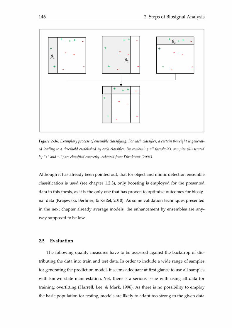
146 2. Steps of Biosignal Analysis
Figure 2-36: Exemplary process of ensemble classifying. For each classifier, a certain β-weight is generat-
ed leading to a threshold established by each classifier. By combining all thresholds, samples (illustrated
by “+” and “-“) are classified correctly. Adapted from Fürnkranz (2004).
Although it has already been pointed out, that for object and mimic detection ensemble
classification is used (see chapter 1.2.3), only boosting is employed for the presented
data in this thesis, as it is the only one that has proven to optimize outcomes for biosig-
nal data (Krajewski, Berliner, & Keßel, 2010). As some validation techniques presented
in the next chapter already average models, the enhancement by ensembles are any-
way supposed to be low.
2.5 Evaluation
The following quality measures have to be assessed against the backdrop of dis-
tributing the data into train and test data. In order to include a wide range of samples
for generating the prediction model, it seems adequate at first glance to use all samples
with known state manifestation. Yet, there is a serious issue with using all data for
training: overfitting (Harrell, Lee, & Mark, 1996). As there is no possibility to employ
the basic population for testing, models are likely to adapt too strong to the given data
β1
+
+
+ + + -
-
--
-
+
β2
+
+
+ + -
-
--
-
β3
+
+
+ + + -
-
--
-
+
+
+ + + -
-
--
-
β1

Human State Computing 147
leading to worse predictions for unseen samples. Albeit, the aim of generating predic-
tion models is to compute a generalizable algorithm that best possibly assesses new
data. From this perspective the approach is quite comparable to developing question-
naires or other measurement tools. The given sample is always only a (hopefully repre-
sentative) basis that is supposed to represent characteristics of the population. Ques-
tionnaires are e.g. developed in due consideration of reliability and validity measure-
ments. Overfitting matches to a certain degree a high level of internal validity, as it is
only a suitable measure for a snippet (in this case the particular sample) of the total
picture. Reliability of questionnaires is inter alia evaluated by employing the split half
method dividing a task into two pieces with the expectations to obtain (almost) identi-
cal results regarding a certain criteria for both parts. The same principle can be trans-
ferred to biosignal prediction model evaluation in many ways. On the one hand, all
evaluated samples could be split into two pieces indicating how long certain behavior
has to be recorded in order to result in similar results. This approach e.g. led to the
conclusion that 30 seconds samples are sufficient for assessing leadership dimensions
in voice samples, although the original corpus was compiled using 60 second samples.
On the other hand, and that is more important regarding overfitting, a prediction mod-
el based on one representative half of the total sample set is supposed to predict state
manifestations of the other half equally good. If quality measures for the first predic-
tion show better values than for the unseen half, the model will not be capable of as-
sessing new data properly, as it obviously relies on particular features being only sensi-
tive for the given train set.
By the same token, there is no use in reducing the train set disproportionally, be-
cause underfitting (Backhaus, Erichson, Plinke, & Weiber, 2011, pp. 55) is not helpful
either. Underfitting means, that the train data set is too small to contain a sufficient
amount of relevant features and their variation regarding different state manifesta-
tions. Obviously, underfitted data result in a poor overall performance, as inappropri-
ate models can neither predict given nor unseen data. Though, poor performance can
also be indicative of a general lacking relation between the biosignal (or the extracted
features) and the analyzed state. By increasing the number of samples, underfitting
should vanish and results improve noticeably, while for a missing relation no relevant
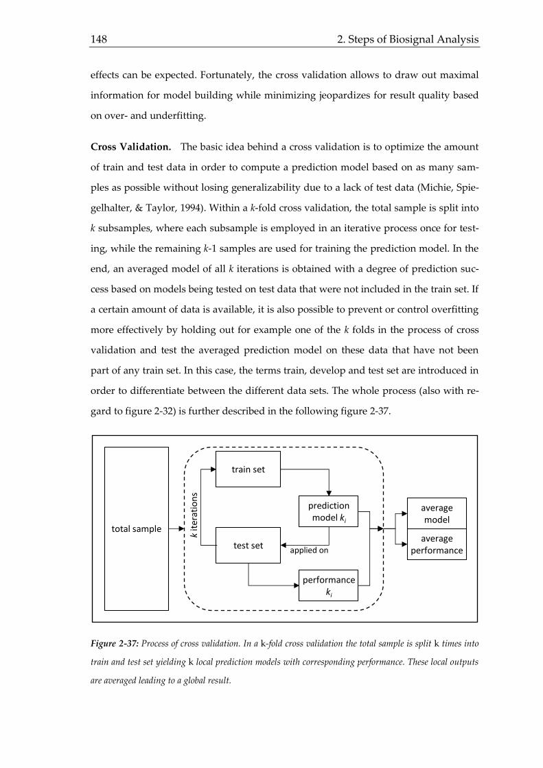
148 2. Steps of Biosignal Analysis
effects can be expected. Fortunately, the cross validation allows to draw out maximal
information for model building while minimizing jeopardizes for result quality based
on over- and underfitting.
Cross Validation. The basic idea behind a cross validation is to optimize the amount
of train and test data in order to compute a prediction model based on as many sam-
ples as possible without losing generalizability due to a lack of test data (Michie, Spie-
gelhalter, & Taylor, 1994). Within a k-fold cross validation, the total sample is split into
k subsamples, where each subsample is employed in an iterative process once for test-
ing, while the remaining k-1 samples are used for training the prediction model. In the
end, an averaged model of all k iterations is obtained with a degree of prediction suc-
cess based on models being tested on test data that were not included in the train set. If
a certain amount of data is available, it is also possible to prevent or control overfitting
more effectively by holding out for example one of the k folds in the process of cross
validation and test the averaged prediction model on these data that have not been
part of any train set. In this case, the terms train, develop and test set are introduced in
order to differentiate between the different data sets. The whole process (also with re-
gard to figure 2-32) is further described in the following figure 2-37.
Figure 2-37: Process of cross validation. In a k-fold cross validation the total sample is split k times into
train and test set yielding k local prediction models with corresponding performance. These local outputs
are averaged leading to a global result.
total sample
train set
test set
kit
erat
ion
s
prediction model ki
applied on
performance ki
average performance
average model
Human State Computing 149
There are two further issues to be considered. On the one hand, a suitable value for
k has to be chosen. For very small values, the computation time is lower, as only fewer
models have to be built and evaluated. Though, overfitting is not prevented optimally
with only a small number of iterations. The other way around it is possible to employ
the widely distributed leave-one-sample-out (LOSO) approach. As its name already
reveals, k equals the total number n of samples, so that train data consist of n-1 sam-
ples, while the resulting prediction model is tested on one single sample. This process
performs well in avoiding overfitting, but requires lots of computation time (especially
for high values of n when combined with a feature selection algorithm). Following
Steidl (2009), results do not vary considerably when using more than k=3 folds. How-
ever, this analysis comprises only speech samples, so a common compromise with k =
10 (McLachlan, Do, & Ambroise, 2004) qualifies as a best approach for balancing com-
putational requirements and overfitting.
On the other hand, the second issue to keep in mind is the compilation or selection
of the samples being grouped together in different folds. At first glance, the easiest way
to draw representative samples is to conduct a random selection for each fold. The
drawback of a random selection is that not all folds might be representative in terms of
matching the distribution of state manifestation. For instance, a fold consisting of pri-
marily highly charismatic assessed samples is likely to result in a totally different pre-
diction model than a fold containing mostly non-charismatic samples. To overcome
this issue, a stratified selection produces randomly representative subgroups meaning
that class proportions are kept (almost) constant in each fold. As a matter of course that
makes only sense if representative samples are gathered. Otherwise, a prediction mod-
el would erroneously tend to allocate samples to the biggest classes, even if it cannot be
supposed to be the biggest one in the population. Assuming a prediction model has
been generated, there are measures needed to assess the prediction success. The fol-
lowing section shows the most important and relevant quality criteria.
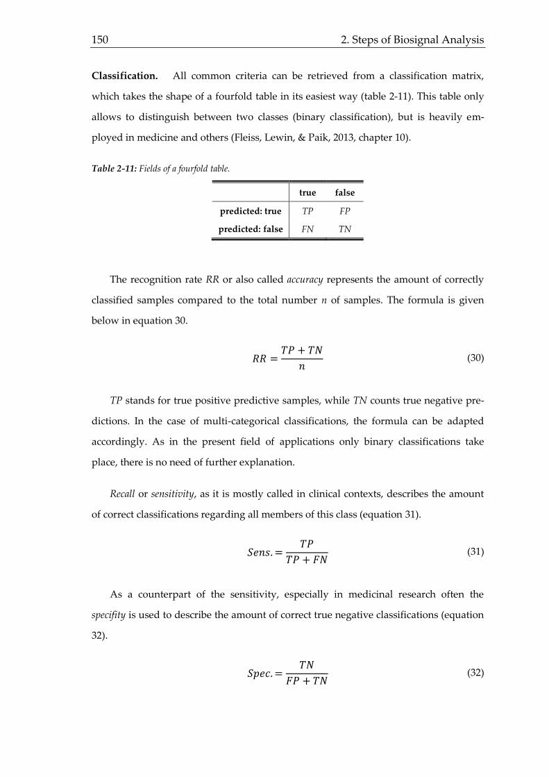
150 2. Steps of Biosignal Analysis
Classification. All common criteria can be retrieved from a classification matrix,
which takes the shape of a fourfold table in its easiest way (table 2-11). This table only
allows to distinguish between two classes (binary classification), but is heavily em-
ployed in medicine and others (Fleiss, Lewin, & Paik, 2013, chapter 10).
Table 2-11: Fields of a fourfold table.
true false
predicted: true TP FP
predicted: false FN TN
The recognition rate RR or also called accuracy represents the amount of correctly
classified samples compared to the total number n of samples. The formula is given
below in equation 30.
𝑅𝑅 =𝑇𝑃 + 𝑇𝑁
𝑛 (30)
TP stands for true positive predictive samples, while TN counts true negative pre-
dictions. In the case of multi-categorical classifications, the formula can be adapted
accordingly. As in the present field of applications only binary classifications take
place, there is no need of further explanation.
Recall or sensitivity, as it is mostly called in clinical contexts, describes the amount
of correct classifications regarding all members of this class (equation 31).
𝑆𝑒𝑛𝑠. =𝑇𝑃
𝑇𝑃 + 𝐹𝑁 (31)
As a counterpart of the sensitivity, especially in medicinal research often the
specifity is used to describe the amount of correct true negative classifications (equation
32).
𝑆𝑝𝑒𝑐. =𝑇𝑁
𝐹𝑃 + 𝑇𝑁 (32)

Human State Computing 151
Contrary, the precision or positive predictive value (PPV) shows the proportion of cor-
rect positive predictions against all positive predictions as shown in equation 33 (anal-
ogously, a negative predictive value NPV can be computed).
𝑃𝑃𝑉 =𝑇𝑃
𝑇𝑃 + 𝐹𝑃 (33)
As a last measure for classifications, the F value is presented, which depends on
both precision and recall as well as a weighting variable 𝛽 (equation 34).
𝐹𝛽 =
(1 + 𝛽) · (𝑝𝑟𝑒𝑐 · 𝑟𝑒𝑐𝑎𝑙𝑙)
(𝑝𝑟𝑒𝑐 · 𝑟𝑒𝑐𝑎𝑙𝑙) (34)
For 𝛽 = 1, F is written F1 and corresponds to the harmonic mean of precision and
recall and is employed in this thesis as a summarizing indicator for both criteria. Be-
sides this commonly employed value for 𝛽, sometimes F2 and F0.5 are used.
Regression. As soon as samples are supposed to be assigned to continual values, all
above mentioned criteria are not feasible. Continuous measurements become inevita-
ble, when the aim is not a distinction between different classes, but to assess to which
degree a certain state applies. In this case it is a common approach to use well known
criteria from regression analyses.
The vast majority of regression analyses are reported using the correlation coeffi-
cient r as a measure of the linear relationship between two random variables (for pat-
tern recognition these variables represent the distribution of true and predicted val-
ues). By rearranging the equation of r it is possible to calculate the amount of explained
variance. The corresponding measure is the determination coefficient (equation 35).
𝑟𝑥𝑦 =
𝐶𝑜𝑣(𝑥, 𝑦)
√𝑉𝑎𝑟(𝑥) · 𝑉𝑎𝑟(𝑦) (35)
𝑅2 = 𝑟𝑥𝑦2
The root mean square error (RMSE) expresses the predictive deviation as the root of
squared differences of true and predicted values (equation 36). Eventually, the normal-
152 2. Steps of Biosignal Analysis
ized form is used (NRMSE). As this measure indicates errors, low values result in the
case of a good matching.
𝑅𝑀𝑆𝐸 =
∑ √(𝑡𝑟𝑢𝑒𝑖 − 𝑝𝑟𝑒𝑑𝑖)2𝑁𝑖=1
𝑁 (36)
Furthermore, absolute and relative error are computed. The absolute error is ob-
tained by taking the arithmetic mean of the differences of the absolute predicted scores
and the true scores. The relative error sets this error in relation to the used scale, so the
absolute error is divided by the scale range.
Rater. In order to assess the data input quality, it is of crucial importance to know
how well the assessments of the observers match. Especially for quite subjective di-
mensions as analyzed within the voice based leadership skill evaluation, it is some-
times hard to assign a clear value to a sample, so even experienced raters will deviate
in their results. Yet, these results represent the data base for prediction modeling.
When prediction results turn out to be lower than expected, it is not necessarily true to
deduce a missing relation between biosignal and state from these results. If the input
data (ratings) are ambiguous, it is impossible to overcome this drawback by prediction
modeling. Hence, the rater agreement gives a clear indication how to interpret predic-
tion results by setting certain ranges for the success of prediction.
Within the field of speech emotion recognition, sometimes it is useful to weight rat-
ing deviations (Steidl, 2009). The reason is, that a confusion of for instance “anger” and
“rage“ is not as bad as a confusion between “anger” and “happy”. Yet, in the case of
intradimensional classifications (high vs. low), there is no need to distinguish differing
ratings.
Cohen’s κ is a well known measure for categorical data. It compares the actual
match with a random one being calculated by the a priori probability of an allocation
to a certain class. This approach ensures that a high level of agreement within high
frequency classes is not having too much impact on the overall rater agreement evalua-
tion. In the present case, though, interval scaled data of 10 raters has to be examined, so
that an extension of the algorithm becomes necessary. Krippendorff’s α (Krippendorff,

Human State Computing 153
2004; 2013, pp. 221, for a historic overview of usage), gives such an extension, which
also handles missing values and different scale levels, sizes of the data set as well as
number of classes and raters. Similar to Cohens κ, actual agreement is compared to a
random one. In contrast to Cohen’s κ, though, the ratio of actual Deviation (D0) and
randomly expected deviation (DE) is subtracted from 1, where both values are comput-
ed in regard of their scale level and number of raters (equation 37).
𝛼 = 1 −𝐷0
𝐷𝐸 (37)
Beside Krippendorff’s α, there is another measurement for rater agreement, namely
the inter-rater-correlation (irc). The interpretation of this measure has to be done care-
fully, though, as correlations do not include rater tendencies. Yielding a perfect correla-
tion of r = 1 does not necessarily indicate a perfect matching or agreement, but only an
equal slope. Considering an extreme case on a five point scale, one rater could assess
all samples with an average of �� = 2, while another rater comes to an average of �� = 4
with a standard deviation for both of s = 1. When splitting the data into two classes
(high vs. low), no sample is allocated to the same group by both raters, although the
inter-rater-correlation shows a perfect relationship. Although the probability of such an
event is very low, especially for experienced raters, the intra class correlation (ICC, being
different from item characteristic curves) is usually a preferred measure, as it handles
this disadvantage by building a common distribution for all raters (Wirtz & Caspar,
2002; Fleiss & Cohen, 1973). Summarized, the ICC coefficient is computed by compar-
ing the variance Varin within all n samples with the variance Varrater of all k raters as well
as the remaining error variance Varerr. The best possible ICC value is reached, when a
high class variance goes along with a low rater variance. Depending on several factors
(number of raters, aggregation of raters, missing values, randomized selection of
raters), slightly different formulas exist (Shrout & Fleiss, 1979). In the present case, the
ICC is computed as follows (equation 38).
𝐼𝐶𝐶 =𝑉𝑎𝑟𝑖𝑛 − 𝑉𝑎𝑟𝑒𝑟𝑟
𝑉𝑎𝑟𝑖𝑛 + (𝑘 − 1) · 𝑉𝑎𝑟𝑒𝑟𝑟 +𝑘(𝑉𝑎𝑟𝑜𝑏𝑠−𝑉𝑎𝑟𝑒𝑟𝑟)
𝑛
(38)

154 2. Steps of Biosignal Analysis
Now all necessary basics have been presented to understand and interpret the re-
sults of the analyzed fields of application. After a concise summary of the methodical
approach (chapter 2.6), a study analyzing leadership states based on voice recordings is
presented (chapter 3).
2.6 Summary of Methodological Approach and Hypotheses
With a focus on different sources of biosignal feature sets, this chapter has given a
theoretical overview of pattern recognition based human state prediction. Starting with
the importance of both clear recording and validation data generation, four different
sources of feature sets are presented. Common Features include the recent default ap-
proach with both time and frequency domain features, whereas the latter ones make
use of Fourier transformations. Wavelet features are positioned in the frequency domain
as well, but allow an efficient way of optimizing both time and frequency resolution
without changing the size of analysis blocks. Hence, additional information is sup-
posed to be created especially for the course of frequencies, where the chosen block
size within the Fourier transformations is not ideal. Nonlinear dynamic features analyze
the raw data and employ chaotic-deterministic logic on the time-domain signal to
compute a different kind of feature set including predictability and the amount of ran-
dom variation in the data. Due to the different perspective of nonlinear dynamic fea-
tures, they likely contribute value to the prediction. Signal-specific features are meant to
depict special characteristics of the biosignals (in this case head and mouse movement
as well as voice) like clicking behavior or Mel-scaled voice representations. In order to
both allow a proper building of theories based on the most relevant features for each
state on the one hand and minimize the computational efforts in building prediction
models on the other hand, the number of considered features is first reduced by a cor-
relation filter and afterwards adjusted via a fast forward feature selection algorithm.
For obtaining the ideal feature set and the final prediction algorithm, several classifier
and regression algorithms are chosen like Support Vector Machines, Random Forests, k
Nearest Neighbor and multiple regression analysis. In the end, common quality criteria
explained in the evaluation section are applied to assess the success of the generated
prediction models.

Human State Computing 155
Chapter 1, however, already outlined several theoretical links of human states and
recordable non-intrusive biosignals. Despite the empiric approach of biosignal analysis
(contrasted to theory-driven approaches at the beginning of chapter 2), empirical data
generation should always be based on distinct assumptions allowing a proper evalua-
tion of the outcomes. Hence, the following general hypotheses are to be examined and
discussed for the presented fields of application:
H1: Each considered state goes along with significant correlations of features
and validating data
H2: The recognition rate RR of generated prediction algorithms for all states is above
guessing probability for binary classification
H3: The combination of all feature sources yields better prediction results than
each feature itself does
H4: The rater agreement behaves inversely proportional to the complexity of
skills
H5: There is a considerable (due to low sample size not necessarily significant)
correlation of rater agreement and recognition rate RR
With these five general hypotheses, most important interactions of biosignal analy-
sis steps are covered allowing an assessment of the overall applicability of this meth-
odological approach (with a focus on different feature sets) for occupational fields of
research, what can be considered the major target of this thesis. Besides these general
hypotheses being discussed in the closing chapter, state and signal-specific hypotheses
are to be examined for each of the conducted studies which will therefore be dealt with
in the respective chapters.


Human State Computing 157
3 FIELD OF APPLICATION I – VOICE BASED LEADERSHIP ANALYSIS
After the general framework of currently available methods and characteristics of
biosignal based analyses have been described, it is time to transfer the methodological
approach to different settings. One widely researched and occupationally relevant state
is leadership with its many facets. Although leadership states are not supposed to
change quickly (see figure 1-12), current methods fail to prove convincing validity,
although being (partially) both cost and time intensive.
3.1 Leadership Analysis: Relevance and Empirical Findings
After an introduction to the relevance and underlying theory of leadership analy-
sis, the five steps mentioned in section 2 will now be employed for a voice based lead-
ership analysis. To give a wide overview of the relevance of improved leadership anal-
ysis, the following part contains some general information about why a focus has to be
set on new measurement techniques. Most information provided also applies for
mouse and head movement analysis and will therefore not be repeated in these chap-
ters again. Before basics of recent leadership dimensions and their assessment are out-
lined, it is important to make clear, how leadership affects important occupational fac-
tors like absenteeism and labor turnover.
Sick Days. Absenteeism represents interference for both employer and employee.
Employers must somehow manage to compensate (unforeseen) missing manpower
and financial loss, while the employee lacks of health, is therefore restricted in his
wellbeing and might have to cope with lower income (based on the length of illness).
In an evaluation of the situation, the BDP (“Berufsverband Deutscher Psychologin-
nen und Psychologen”, 2008, p. 8) revealed, that about 420.5 million sick days led to a
loss of production of €37.8bn in line with a loss regarding the gross value added of
€66.5bn in Germany. Although the total number of sick days decreased from 2000 to
2005, the situation worsened again at least until 2011 with a growth rate of about 20%.
Considering psychological indications of sick days, the growth rate has increased even
stronger. Figure 3-1 depicts absolute and relative changes from 2000 to 2010.
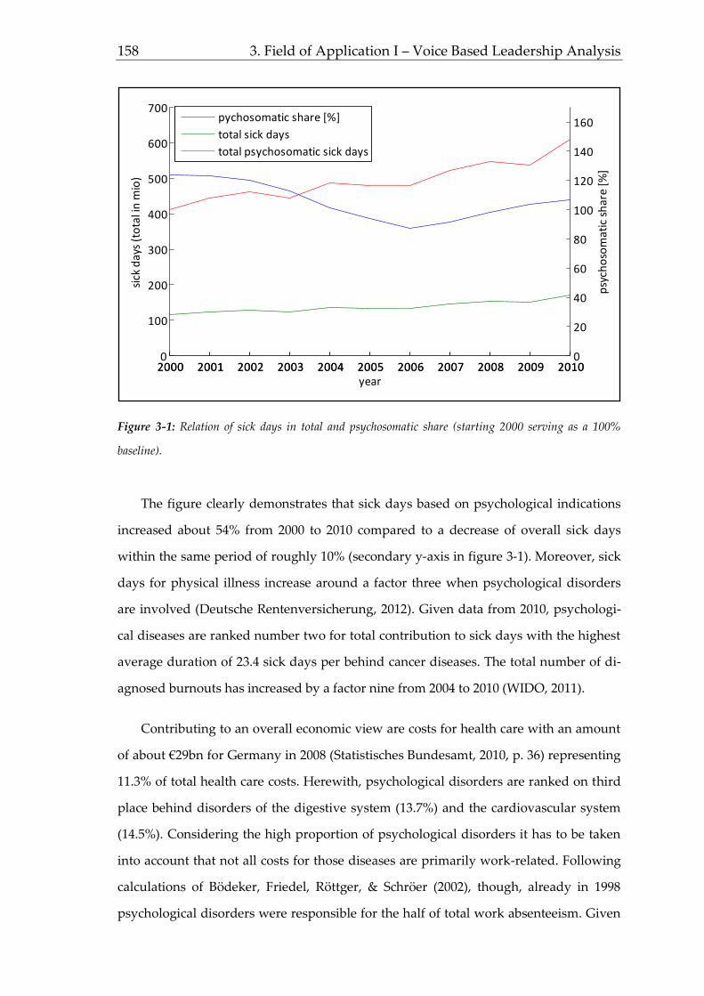
158 3. Field of Application I – Voice Based Leadership Analysis
Figure 3-1: Relation of sick days in total and psychosomatic share (starting 2000 serving as a 100%
baseline).
The figure clearly demonstrates that sick days based on psychological indications
increased about 54% from 2000 to 2010 compared to a decrease of overall sick days
within the same period of roughly 10% (secondary y-axis in figure 3-1). Moreover, sick
days for physical illness increase around a factor three when psychological disorders
are involved (Deutsche Rentenversicherung, 2012). Given data from 2010, psychologi-
cal diseases are ranked number two for total contribution to sick days with the highest
average duration of 23.4 sick days per behind cancer diseases. The total number of di-
agnosed burnouts has increased by a factor nine from 2004 to 2010 (WIDO, 2011).
Contributing to an overall economic view are costs for health care with an amount
of about €29bn for Germany in 2008 (Statistisches Bundesamt, 2010, p. 36) representing
11.3% of total health care costs. Herewith, psychological disorders are ranked on third
place behind disorders of the digestive system (13.7%) and the cardiovascular system
(14.5%). Considering the high proportion of psychological disorders it has to be taken
into account that not all costs for those diseases are primarily work-related. Following
calculations of Bödeker, Friedel, Röttger, & Schröer (2002), though, already in 1998
psychological disorders were responsible for the half of total work absenteeism. Given
3.1_1 sick days
2000 2001 2002 2003 2004 2005 2006 2007 2008 2009 20100
100
200
300
400
500
600
700
sick
day
s (t
ota
l in
mio
)
year
2000 2001 2002 2003 2004 2005 2006 2007 2008 2009 20100
20
40
60
80
100
120
140
160
psy
cho
som
atic
sh
are
[%]
pychosomatic share [%]
total sick days
total psychosomatic sick days

Human State Computing 159
a growth rate of more than 50% since then, the share has increased by today notably.
Reasons for these increases might be the unpredictability of the job market as well as
higher time and performance pressure (Frieling & Gösel, 2003). Furthermore, the com-
plexity of tasks combined with minor possibilities to self-manage may stronger influ-
ence the development of psychological diseases as well as increased working hours
and the expectation to be reachable all day trough mobile devices (Frieling et al., 2004).
Following implications of a blue ribbon commission (Hans-Böckler-Stiftung 2004,
p. 30), these changes lead to an “intensification of work and an increase of uncertainty,
anxieties, distrust and helplessness among the employees”. Plus, indirect effects of
psychological afflictions have to be considered, as there are severe relations between
e.g. stress perception (Lundberg, et al., 1994; Frauendorf, Caffier, Kaul, & Wawr-
zinoszek, 1995), monotony, too little time for breaks (Maintz, Ullsperger, Junghanns, &
Ertel, 2000), perception of autonomy (Melin, Lundberg, Suderling, & Granqvist, 1999),
approval (Peter, Geissler, & Siegrist, 1998) and musculoskeletal disorders (being the
most frequent reason for absenteeism), the digestive system, abilities to recover and
labor turnover rate.
These results clearly indicate a demand for action for improved job design and
structuring. All mentioned relations can after all be hold true on a globally basis as
well. A generalized report of the World Health Organization (WHO, 2001) predicts that
in 2020 depression will be the most treated disease in all developed countries. In order
to prevent such a dramatic increase, there are several actions taken related to work-
place health promotion.
Actions. Especially the rapid and over-average increase of (work-related) psychologi-
cal diseases shows that workplace health promotion has to be taken seriously. Com-
monly, individual-related and organizational/conditional interventions can be distin-
guished (Busch & Steinmetz, 2002). In the field of individual-related interventions
modifications of the personal behavior are heavily employed. As examples back train-
ing, more efficient use of work breaks (Krajewski & Wieland, 2004; Krajewski, Wieland
& Sauerland, 2010) and stress coping.

160 3. Field of Application I – Voice Based Leadership Analysis
Although all of these interventions foster useful skills, the cause of dysfunctional
strains is not worked at, but only the ability to handle with the consequences based on
difficult working conditions. From that angle it appears to be not astonishing, that in-
dividual-related actions usually show rather short term effects (Lenhardt, Elkeles, &
Rosenbrock, 1997). To provide a reason for this mechanism, a simple example helps to
illustrate the circumstances. Often, musculoskeletal diseases have their origin in wrong
postures, independent of whether the work is rather physical or one sit on a badly ar-
ranged chair at a too low desk in an office. Employees in an auto repair shop some-
times have to work several hours a day overhead leading to tensions in neck and
shoulders. An individual-based action would be back training to better the tensions.
Although this action might help a little bit, it would be more useful to fashion the work
in a way, where the employee is not forced to work overhead all day. Since following
DIN EN ISO 10075, the task is supposed to be adapted to the individual and not the
other way around, or at least to employ those workers with different tasks that allow
them to carry out dysfunctional tasks only at a smaller amount of time in the sense of a
job rotation. The last two mentioned actions (adapting or rotating tasks) are allocated
to organizational/conditional interventions, which stronger implement contextual is-
sues in taken actions, therefore rather asking for “under which circumstances” a job
has to be carried out instead of “who” has to do something or “what” has to be done.
The effectiveness of these occupational influences can be derived from Degener
(2004). It is demonstrated, that high manifestations of factors corresponding to the job
design like a sense of purpose for the bigger picture (contrary to production line-like
executing of independent little tasks), challenges and qualifying potential, variety of
tasks, ample scope and participation as well as (also herewith resulting) traits like mo-
tivation, team-oriented behavior and perceived leadership correlate in a range of .72 < r
< .80 with measures of success like gains, revenue and net product. Contrary, there is a
high negative correlation with criteria like sickness absence rate and labor turnover for
those factors in a range of -.74 > r > -.82. How subjective perception of outer conditions
can be diagnosed, is described by Ulich (2005, pp. 94).
Leadership. Having a closer look at definitions of leadership, it gets obvious, that
leadership has an essential impact on the factors mentioned before. Von Rosenstiel

Human State Computing 161
(1993) defines leadership as a “direct, intended and aim-related influence by holders of
supervising positions on employees”. It is not to deny that also leadership underlies
organizational conditions, but at least methods like job rotation are certainly possible
to be applied by leaders in order to reduce dysfunctional stresses and strains. The pre-
sented increase of work-related disorders, however, reveals clearly that leaders do not
sufficiently make use of their opportunity in designing jobs. It is hence to question,
which behaviors or traits lead to successful working conditions and how correspond-
ing states can be measured in a feasible way.
Within the historical course of leadership research, some frequent cited aspects and
dimensions of leadership have evolved like the extent of participation (Vroom &
Yetton, 1973), concern for people or production (as a two-dimensional construct by
Blake & Mouton, 1964 in their Managerial grid model) as well as transactional and
transformational leadership (Bass, 1985). Especially transformational leadership gained
importance over the last decades. The aim of transformational leadership is for the
leader to act as a role model by satisfying and awakening higher intellectual and inspi-
rational needs. Employees are supposed to enhance their efforts to reach a certain, val-
ued goal instead of just executing tasks. As the GLOBE-study (Global Leadership and
Organizational Behavior Effectiveness; House, Hanges, Javidan, Dorfman, & Gupta,
2004) can be considered the first approach to assess leadership dimensions on a
worldwide level, it seems like a good start to derive first voice based predicted leader-
ship relevant states from these endeavors. The goal of the GLOBE study is to achieve a
selection of situational and cultural flexible core values for successful leadership
grounded on assumptions of the implicit leadership theory (ILT; see Dorfman, Hanges,
& Brodbeck, 2004, for an overview) being widely considered the leading cross-cultural
leadership approach (Dickson, Den Hartog, & Mitchelson, 2003). Within this study, six
culturally endorsed implicit leadership theories (CLT) with specific sub-dimensions are
analyzed. An overview of all dimensions is given in the following table 3-1. Dimen-
sions considered in this thesis are highlighted in bold letters.

162 3. Field of Application I – Voice Based Leadership Analysis
Table 3-1: CLT-dimensions following the GLOBE study. Globally positive evaluated dimensions are
bold.
CLT sub-dimensions
charismatic
charisma 1: visionarity
charisma2: inspiration
charisma 3: self-sacrifice
integrity
determination
performance orientation
team orientation
team 1: cooperation
team 2: team integration
diplomacy
maliciousness (inverse)
administrative skills
self-protective
egocentric
statusorientation
conflict behavior
face-saving
process orientation
participating autocracy (inverse)
not participating (inverse)
employer orientation modesty
human orientiation
autonomous autonomy
As mentioned before, the GLOBE dimensions may differ due to cultural and situa-
tional issues. However, high performance in charismatic-value based as well as team
oriented leadership dimensions is globally desirable. On a sub-dimensional level, this
applies particularly to the highlighted dimensions visionarity, inspiration, integrity,
determination, performance orientation, team integration, diplomacy and non-
maliciousness (Dorfman, Hanges, & Brodbeck, 2004). To shorten definitional work
within the dimensional analysis, the following table 3-2 gives an overview of keywords
describing each employed dimension.

Human State Computing 163
Table 3-2: Description of global culturally endorsed leadership dimensions. Derived from Quaquebeke &
Brodbeck (2008).
dimension leader descriptors
visionarity inspires feelings, opinions, values; motivates to work hard; is
future oriented and follows plans
inspiration general positive attitude; motivating, reliable and trustful; ener-
getic and transfers his energy to others; encouraging; moral per-
son
integrity reliable; trustworthy; sticks to own words
determination decisive; handles ambiguity of information; clear and straight
forward thinking
performance orientation seeks perfection; wants to continuously improve all facets of
work; expects outstanding performance from him-/herself and
the team
team integration connects people and establishes proper work environment; in-
formed also about informal details helping to improve interac-
tion
diplomacy good negotiator; convincing
non-maliciousness reliable, smart, intelligent, focus on positive things
Recent Measurements. Giving a proper classification of personal diagnostics is diffi-
cult insofar, as many approaches can be allocated to several measurements already
described in chapter 1. For leadership assessments, though, interviews/questionnaires
and simulations cover the most important. To avoid unnecessary repetition of already
described drawbacks and pitfalls, the presentation of recent measurements is short-
ened.
Personality tests like the Multifactor Leadership Questionnaire (MLQ; Bass & Avolio,
1997) are a default measurement within the process of personnel selection. Yet, a prob-
lem of all those tests is the extent of social desirability and its control. While Diener,
Smith, & Fujita (1995) consider statistical counteractions insufficient, Ones &
Viswesveran (1998) deny a general impact of social desirability on leadership diagnos-
tics at all. Furthermore, following a meta-study by Judge & Piccolo (2004), the relation
of questionnaire based transformational leadership assessments with future perfor-
mance evaluations is quite low (ρ ≤ .30) stating an dissatisfactory validity. Anderson
(2006) argues, that the personality itself does not directly determine the behavior or the
164 3. Field of Application I – Voice Based Leadership Analysis
performance respectively. Hence, a better predictor might be an approach that
measures the behavior instead of the personality, where voice based assessments jump
in. Other performance tests giving scores for intelligence or vigilance are hardly to ef-
fect in a positive way intentionally, but those dimensions are not really relevant for
leadership performance and hence show only low correlations of r = .27 following
Judge, Colbert, & Ilies (2004). In addition, these questionnaires or tests often take sev-
eral hours and are for this reason much more resource consuming in comparison to
biosignal based assessments. Often employed biographic questionnaires do neither
allow an evaluation of the actual performance, as the ambiguous information given in
e.g. reference letters are hard to interpret (Weuster, 1994). The correlation with predic-
tion success is as a consequence low with r = .26 (Schuler & Marcus, 2006). As a best
technique for interviewing, the multimodal interview with its standardized process
and different kinds of questions at least yields a predictive validity of ρ = .51 (Schmidt
& Hunter, 1998).
Due to these insufficient results, approaches simulating real tasks have evolved in
order to observe natural behavior. As a most prominent representative, the assessment
center has to be mentioned. Within possibly different but real tasks, experienced ob-
server try to assess the candidates’ behavior regarding several relevant dimensions
(Fisseni & Preusser, 2007). Although the predictive success is generally influenced by a
representative choice of tasks, neither the candidates’ behavior nor the tasks are really
natural (Sackett, Zedeck, & Fogli, 1988). Despite its averaged low correlation with later
on observed performance of r = .37, the assessment center is at least highly accepted
due to its immediate feedback and transparency (Nerdinger, Blickle, & Schaper, 2008,
p. 251). Other already presented approaches like SJTs and other simulations show no
satisfying performance as well. For justifying the amount of spent time and costs of
each method, though, the validity has to be improved. Alternatively to the above men-
tioned approaches, details regarding a study focusing on voice based leadership as-
sessment are depicted in the following to illustrate a physiological alternative comple-
menting the recent research canon.
Human State Computing 165
3.2 Data Generation
In order to present relevant details of the data and feature generation process, this
part gives information about the most important facts. Following the steps of biosignal
analysis, hence study design, ratings and feature extraction is described.
Design. The original YouTube corpus (Wenninger, Krajewski, Batliner, & Schuller,
2012) was initially presented by the author as ALA-corpus (Laufenberg, 2011) and con-
sists of 409 recordings (two samples included in Laufenberg, 2011, were removed due
to quality issues), each one minute long, from 143 speeches available on YouTube (143
male executives within the age range of about 20–75 years, M = 51.14, SD = 12.13). The
new version presented in this thesis is an extended one considering the gained insight,
that a time amount of about 30 seconds is sufficient for the raters to assess all dimen-
sions. 1022 cut recordings result with a duration of 30 seconds each based on 176
speeches. The following description of the data generation is derived from Wenninger,
Krajewski, Batliner, & Schuller (2012) where the author contributed main parts to the
description. All new recordings as well as the further split old samples were assessed
by the same trained persons that participated in the initial version.
For speeches where either the exact date or the speaker’s day of birth could not be
allocated (n = 45), age was estimated and the mean value of all annotators taken to
analyses. Train, Develop and Test data reveal no significant differences in the speakers'
age. Moreover, the speakers' age was not related to any perceived leadership dimen-
sion and could therefore not be considered as relevant confounding factor.
As this study chooses an approach to assess perceived leadership states based on
voice characteristics, the sample selection focused on real leaders in order to achieve a
high resolution within the upper range of ability. Hence, all samples of the original
YouTube-corpus were only taken from subjects who can be accounted to leaders. Func-
tions of all speakers may be summarized as follows: the vast majority (83.7% or 855
samples) was taken from top executives of global players (mostly derived from Forbes
Global 2000 list in 2011). Remaining 167 samples are composed of leaders of Non-
Profit-Organizations (75), entrepreneurs (52), university professors (34) and one foot-
ball team captain (6) as shown in table 3-3.

166 3. Field of Application I – Voice Based Leadership Analysis
Table 3-3: Data sources of speeches.
category absolute samples relative share [%]
executives Forbes 2000 855 83.66
executives Non-Profit-Organizations 75 7.34
entrepreneurs 52 5.09
university professors 34 3.32
sport team captain 6 0.59
Speeches were derived from public presentations like introducing new products
(720 or 70.45%), outlining future prospects (181 or 17.71%) or summarizing recent de-
velopments (93 or 9.10%). The remaining 28 samples (2.74%) were obtained by record-
ing interviews or speeches about latest events as well as presentations of professors at
university. Although Pennebaker & Lay (2002) have shown that next to stable speaker
characteristics different speech settings and authorships of a speech affect linguistic
features, we did not explicitly control for these confounders, since this current study
only aims to assess the subjective impression of leadership. In contrast to invariant per-
sonality traits, variant perceived leadership states should not be masked by these un-
controlled confounders.
In order to obtain a nearly equal amount of data per speaker, not more than six re-
cordings per speech were extracted. These recordings are subsequently referred to as
tracks. The speech signal was recorded with different microphones and qualities, main-
ly with a 16 kHz sampling rate. The recordings took place in lecture-rooms under vary-
ing levels of noise and reverberation (microphone-to-mouth distance > 0.3 m). None of
the speeches was scripted (respectively read from a teleprompter or similar). Regard-
ing data cleansing, all recordings are cleaned manually from artifacts and automatical-
ly from general noise.
Ratings. The corpus was annotated by 10 raters (Ph.D. and Master Students in Psy-
chology, five males, five females) aged between 23 and 58 years (mean 36.9). Gender
effects were controlled by Krippendorff’s α and significance testing, but no differences
showed up. All raters had been formally trained to apply a Likert scale on a standard-
ized set of judging criteria and are experienced both in leadership research and rating
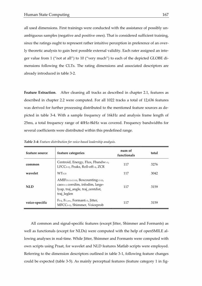
Human State Computing 167
all used dimensions. First trainings were conducted with the assistance of possibly un-
ambiguous samples (negative and positive ones). That is considered sufficient training,
since the ratings ought to represent rather intuitive perception in preference of an over-
ly theoretic analysis to gain best possible external validity. Each rater assigned an inte-
ger value from 1 (“not at all”) to 10 (“very much”) to each of the depicted GLOBE di-
mensions following the CLTs. The rating dimensions and associated descriptors are
already introduced in table 3-2.
Feature Extraction. After cleaning all tracks as described in chapter 2.1, features as
described in chapter 2.2 were computed. For all 1022 tracks a total of 12,636 features
was derived for further processing distributed to the mentioned feature sources as de-
picted in table 3-4. With a sample frequency of 16kHz and analysis frame length of
25ms, a total frequency range of 40Hz-8kHz was covered. Frequency bandwidths for
several coefficients were distributed within this predefined range.
Table 3-4: Feature distribution for voice-based leadership analysis.
feature source feature categories num of
functionals total
common Centroid, Energy, Flux, Fbandw1-5,
LFCC0-12, Peaks, Roll-off1-4, ZCR 117 3276
wavelet WT0-25 117 3042
NLD
AMIFD1-3;τ1:5:10, Boxcounting1:5:10,
caoD1-3, corrdim, infodim, large-
lyap, traj_angle, traj_centdist,
traj_leglen
117 3159
voice-specific F0-4, F0_env, Formant1-5, Jitter,
MFCC0-12, Shimmer, Voiceprob 117 3159
All common and signal-specific features (except Jitter, Shimmer and Formants) as
well as functionals (except for NLDs) were computed with the help of openSMILE al-
lowing analyses in real-time. While Jitter, Shimmer and Formants were computed with
own scripts using Praat, for wavelet and NLD features Matlab scripts were employed.
Referring to the dimension descriptors outlined in table 3-1, following feature changes
could be expected (table 3-5). As mainly perceptual features (feature category 1 in fig-

168 3. Field of Application I – Voice Based Leadership Analysis
ure 2-1) allow best derivation of hypothesis, they are more frequently used for distinct
expected changes (contrary to rather abstract features).
Table 3-5: Expected perceptual voice changes for analyzed leadership states.
expected feature changes
visionarity higher frequency and energy variability to propose visions; more re-
laxed voice and hence less influenced by yielding wall effect);
inspiration in comparison to visionarity less variability; more tensed and evenly
voice to rather capture the energetic aspect
integrity evenly voice; lower frequency bandwidth (minimum, maximum peaks);
higher predictability (less outliers in phase space reconstruction)
determination general high energy with less variation; increased share of high frequen-
cies (yielding wall effect
performance similar to determination with increased frequency range and general
intensity
team-integration
more relaxed and sociable leading to lower amplitudes for higher fre-
quencies (decreased yielding wall effect); more variable and adaptive
speaking
diplomacy controlled and deliberate with less variation leading to lower frequency
range and higher predictability (NLD phase space reconstruction)
non-maliciousness soft and evenly voice, also more relaxed leading to a stronger share of
lower frequencies and less variation
Prediction Process. After all features were extracted, feature selection, prediction
model generation and evaluation are done within one combining script using the open-
source software RapidMiner. For feature selection, a feed forward algorithm is chosen
checking if an extension of the feature set yields a significant better recognition rate
(error rate α = .20). Adding features to the feature set is stopped, when within two cy-
cles (extending the feature set by two additional features) no improvement is observa-
ble. For obtaining recognition rates in turn, all classifiers presented in chapter 2.4 are
employed, so it is checked in each cycle whether one of the employed classifiers yields
better results or not. For each classifier, however, the recognition rate is assessed with-
in a 10% hold out cross validation meaning that in an iterative process 90% of the data
are used for training the classifier, while the remaining 10% serve as test data deter-
mining the recognition rate. So summarized, for each feature set size all possible fea-
ture combinations are tested with different classifiers within a cross validation to ob-

Human State Computing 169
tain the ideal feature set size and respective classifier (details on the general process of
building prediction models based on extracted features are introduced in the chapters
2.3 to 2.5).
3.3 Cross-Dimensional Results
In this section, an overview for all dimensions and important steps of biosignal
analysis is given. Global results over all leadership dimensions allow a proper assess-
ment of the overall success of voice based prediction and the feasibility for practical
applications. In addition, a first conclusion about the benefit of all feature sources is
possible.
Rater. Reliable ratings are the foundation for all biosignal based validations as a basis
for prediction modeling. Commonly, biosignal analysis rather focuses on distinct states
which can be measured accurately by physical or at least physiological methods. Non-
intrusive approaches are then supposed to replace resource consuming sensors. For
such complex states like leadership performance and its underlying dimensions,
though, there is no device available offering direct quantization for e.g. inspiration or
diplomacy. Personality questionnaires sometimes give some indications, but they can
hardly capture a current impression, but more mindset-related information. Due to this
fact and other drawbacks mentioned in chapter 1, the best way of getting an idea of the
generated impression of a speaker is to ask an experienced audience. Nonetheless, it is
in the nature of those assessments that ratings vary more than a physical measurement
does. Table 3-6 shows the averaged interrater correlation irc of all ten observers.
Table 3-6: average interrater correlation (irc) for voice-based leadership assessment.
rater R1 R2 R3 R4 R5 R6 R7 R8 R9 R10 total avg.
avg. irc .59 .63 .62 .48 .57 .68 .67 .61 .59 .51 .60
The results reveal that all observers rate on a comparable level and scatter around
irc = 60. Contrasting these results to other studies with leadership ratings (assessment
center; job performance rating), the raters seem to assess the speech samples consistent-

170 3. Field of Application I – Voice Based Leadership Analysis
ly regarding this difficult task (Arthur, Day, McNelly, & Edens, 2003; Heidemeier &
Moser, 2008). Other measures confirm the indications based on rater intercorrelation.
Computing Krippendorff’s α and ICC results in α = .35 und ICC = .41. Especially when
matching these values with the initial YouTube-corpus, a considerable improvement
has been reached by further training and extending the data corpus.
Ratings. For building successful data corpora, it is necessary that the proportions of
ratings represent externally valid quotas. For performance based measurements, a dis-
tribution matching the Gaussian normal curve can be assumed with the majority of
samples gathering around the center and smaller proportions for either particular good
or bad performances. As in stratified sampling proportions of the total sample are kept
constant, biased samples led to biased prediction models increasing the probability for
globally fewer cases. Hence, the distribution of ratings gives information about the
representativity of a corpus. Although it cannot be foreclosed completely, that an ex-
pectation matching distribution is still based on a biased sample, defining a narrow
performance corridor as happened for the YouTube corpus rather focusing on high
performers of global players can be considered sufficient regarding the reached sample
size. For wider assessments, sample sizes as applied for validating e.g. intelligence
questionnaires seems desirable. In the original YouTube-corpus, however, a slightly
bias in favor of well performing samples was observed. Hence, the corpus was extend-
ed by probably worse but experienced performers to counterbalance this issue. The
range R of the averaged ratings is 8.8 (ratingmax = 9.9 – ratingmin = 1.1) and covers 97.78%
of the available scale. This is a proper indication for a good overall usage of the scale,
as the average is taken from 10 raters. Referring to the desirable bell curve distribution
mentioned before, the results seem promising, too. Figure 3-2 matches the theoretically
expected outcome with a histogram of the obtained ratings based on all eight assessed
leadership states.
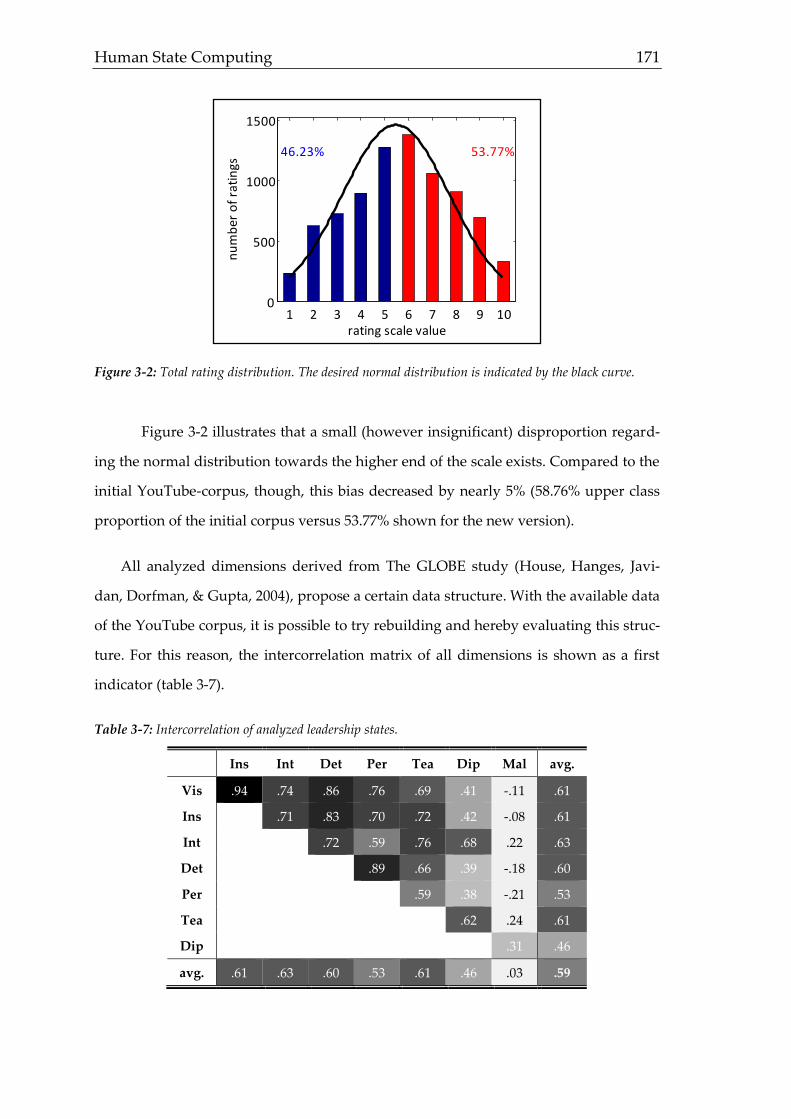
Human State Computing 171
Figure 3-2: Total rating distribution. The desired normal distribution is indicated by the black curve.
Figure 3-2 illustrates that a small (however insignificant) disproportion regard-
ing the normal distribution towards the higher end of the scale exists. Compared to the
initial YouTube-corpus, though, this bias decreased by nearly 5% (58.76% upper class
proportion of the initial corpus versus 53.77% shown for the new version).
All analyzed dimensions derived from The GLOBE study (House, Hanges, Javi-
dan, Dorfman, & Gupta, 2004), propose a certain data structure. With the available data
of the YouTube corpus, it is possible to try rebuilding and hereby evaluating this struc-
ture. For this reason, the intercorrelation matrix of all dimensions is shown as a first
indicator (table 3-7).
Table 3-7: Intercorrelation of analyzed leadership states.
Ins Int Det Per Tea Dip Mal avg.
Vis .94 .74 .86 .76 .69 .41 -.11 .61
Ins .71 .83 .70 .72 .42 -.08 .61
Int .72 .59 .76 .68 .22 .63
Det .89 .66 .39 -.18 .60
Per .59 .38 -.21 .53
Tea .62 .24 .61
Dip .31 .46
avg. .61 .63 .60 .53 .61 .46 .03 .59
1 2 3 4 5 6 7 8 9 100
500
1000
1500
rating scale value
nu
mb
er o
f ra
tin
gs
46.23% 53.77%

172 3. Field of Application I – Voice Based Leadership Analysis
The presented values show substantial relations between most dimensions except
non-maliciousness. When having a look at the charismatic dimensions visionarity and
inspiration, an expected high correlation shows up (r ≥ .90). Similar high correlations
exist regarding other dimensions belonging to the same higher level dimension. The
second super-ordinate dimension team orientation consisting of the analyzed dimen-
sions diplomacy and non-maliciousness show an unexpected correlation drop. To vis-
ualize the interdependencies of all dimensions, multidimensional scaling (MDS) is em-
ployed to transform the higher dimensional space into a two-dimensional overview
(figure 3-3).
Figure 3-3: Spatial localization of leadership states after MDS analysis. Different font sizes indicate
different averaged strength of prediction quality within a causal dominance analysis (CDA). States are
clustered by two separating lines.
The MDS yields a close spatial proximity of integrity, team integration and diplo-
macy as well as a strong agglomeration of charismatic dimensions. Determination and
performance orientation build another separate unit. With this result, all dimensions
except non-maliciousness behave in an expected way based on the GLOBE findings
(House, Hanges, Javidan, Dorfman, & Gupta, 2004). Within the figure, not only spatial
performance orientation
determination
visionarity
inspiration
team integration
integritydiplomacy
non-maliciousness
x
y
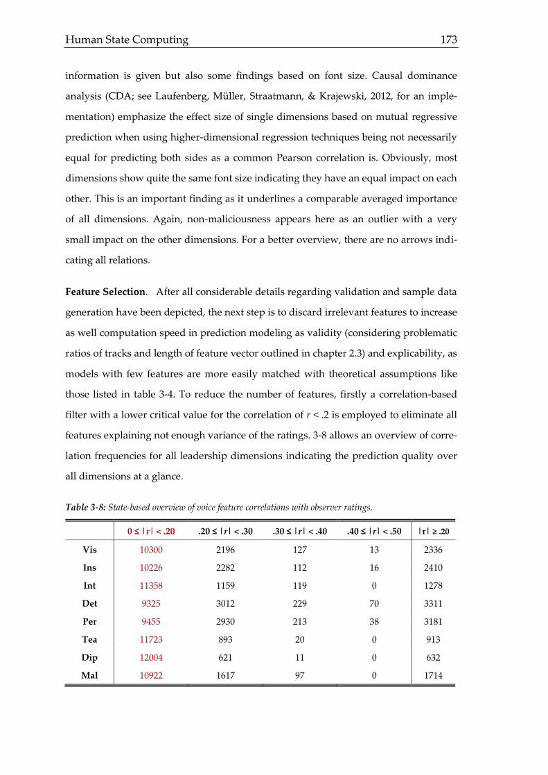
Human State Computing 173
information is given but also some findings based on font size. Causal dominance
analysis (CDA; see Laufenberg, Müller, Straatmann, & Krajewski, 2012, for an imple-
mentation) emphasize the effect size of single dimensions based on mutual regressive
prediction when using higher-dimensional regression techniques being not necessarily
equal for predicting both sides as a common Pearson correlation is. Obviously, most
dimensions show quite the same font size indicating they have an equal impact on each
other. This is an important finding as it underlines a comparable averaged importance
of all dimensions. Again, non-maliciousness appears here as an outlier with a very
small impact on the other dimensions. For a better overview, there are no arrows indi-
cating all relations.
Feature Selection. After all considerable details regarding validation and sample data
generation have been depicted, the next step is to discard irrelevant features to increase
as well computation speed in prediction modeling as validity (considering problematic
ratios of tracks and length of feature vector outlined in chapter 2.3) and explicability, as
models with few features are more easily matched with theoretical assumptions like
those listed in table 3-4. To reduce the number of features, firstly a correlation-based
filter with a lower critical value for the correlation of r < .2 is employed to eliminate all
features explaining not enough variance of the ratings. 3-8 allows an overview of corre-
lation frequencies for all leadership dimensions indicating the prediction quality over
all dimensions at a glance.
Table 3-8: State-based overview of voice feature correlations with observer ratings.
0 ≤ |r| < .20 .20 ≤ |r| < .30 .30 ≤ |r| < .40 .40 ≤ |r| < .50 |r| ≥ .20
Vis 10300 2196 127 13 2336
Ins 10226 2282 112 16 2410
Int 11358 1159 119 0 1278
Det 9325 3012 229 70 3311
Per 9455 2930 213 38 3181
Tea 11723 893 20 0 913
Dip 12004 621 11 0 632
Mal 10922 1617 97 0 1714

174 3. Field of Application I – Voice Based Leadership Analysis
Interpreting all correlations of at least |r| = .30 as low, r =.50 as medium and r > .70
as high, a feature proportion of 1.15% reaches a low to medium correlation exceeding
the minimum correlation filter criterion. For pattern recognition based predictions,
though, features are combined in order to yield better results than single features do.
Hence, the expected prediction success is higher than the single correlations imply,
especially for less related features as ensured by the chosen different feature sources.
The overview detects big differences between several leadership dimensions. While
ratings of determination and performance orientation turn out to match the computed
features best with more than 3,000 features remaining after the correlation filter with
top features of almost |r| = .50, visionarity and inspiration share second position with
roughly 2,500 features followed by integrity and non-maliciousness with more than
1,000 features. Considering the three digit number of remaining features for team inte-
gration and diplomacy, ratings seem to be represented worse by the generated feature
sets. Further information about selected features for each dimension is given in the
respective chapters below.
Prediction Modeling. After (respectively while) selecting a reasonable amount of data
with methods described in chapter 2.3, different prediction models for classification
and regression are employed to find a best possible prediction algorithm. As the focus
of this thesis is set on the different employed feature sources and their prediction suc-
cess, a comparison of all sources is useful. As detailed results for all single leadership
dimensions regarding each feature source are given in the respective chapters, an aver-
aged summary in table 3-9 demonstrates the performance of the generated feature
sources for binary classification and regression over all dimensions.
Table 3-9: Prediction quality of each feature source.
feature source Recognition Rate (%) correlation r
common features 61.62 .40
wavelet features 55.18 .38
nonlinear dynamics 52.68 .34
voice-specific features 62.46 .41
combined 67.67 .45
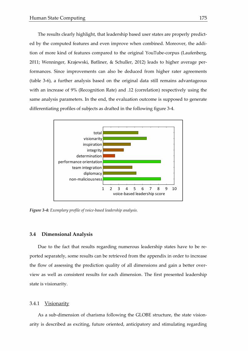
Human State Computing 175
The results clearly highlight, that leadership based user states are properly predict-
ed by the computed features and even improve when combined. Moreover, the addi-
tion of more kind of features compared to the original YouTube-corpus (Laufenberg,
2011; Wenninger, Krajewski, Batliner, & Schuller, 2012) leads to higher average per-
formances. Since improvements can also be deduced from higher rater agreements
(table 3-6), a further analysis based on the original data still remains advantageous
with an increase of 9% (Recognition Rate) and .12 (correlation) respectively using the
same analysis parameters. In the end, the evaluation outcome is supposed to generate
differentiating profiles of subjects as drafted in the following figure 3-4.
Figure 3-4: Exemplary profile of voice-based leadership analysis.
3.4 Dimensional Analysis
Due to the fact that results regarding numerous leadership states have to be re-
ported separately, some results can be retrieved from the appendix in order to increase
the flow of assessing the prediction quality of all dimensions and gain a better over-
view as well as consistent results for each dimension. The first presented leadership
state is visionarity.
3.4.1 Visionarity
As a sub-dimension of charisma following the GLOBE structure, the state vision-
arity is described as exciting, future oriented, anticipatory and stimulating regarding
1 2 3 4 5 6 7 8 9 10
non-maliciousness
diplomacy
team integration
performance orientation
determination
integrity
inspiration
visionarity
total
voice-based leadership score

176 3. Field of Application I – Voice Based Leadership Analysis
emotions, opinions, values and behavior (outlined in table 3-2). In order to give a broad
overview of all findings regarding visionarity, first measurements for rater agreement
are depicted, as it allows assessing the data quality for visionarity in general. After-
wards, feature selection, classification and regression results are shown for each feature
source followed by an ideal feature set based on all computed features allowing an
assessment about the added value new and specific features contribute to prediction
results.
Ratings. As a basis for speech-based visionarity prediction, the rater agreement is
assessed by means of intercorrelation (table 3-10), Krippendorff’s α and ICC.
Table 3-10: Averaged rater-agreement for visionarity.
R1 R2 R3 R4 R5 R6 R7 R8 R9 R10 avg.
.59 .48 .56 .61 .55 .54 .59 .54 .62 .60 .58
The average correlation of all raters scatters around r = .58 without significant out-
liers. Krippendorff’s α and ICC result in slightly lower values (α = .54, ICC = .49). Obvi-
ously, rater assessments show a mediocre performance. Class proportions for classifi-
cation and regression are shown in figure 3-5.
Figure 3-5: Rating distribution for visionarity.
The range R of all averaged ratings is 9.7(max) – 1.1(min) = 8.6 and comprises 95.56% of
the scale. Ratings appear to be normally distributed with no noteworthy tendency to-
wards the upper range of the scale as in the initial version of the YouTube corpus.
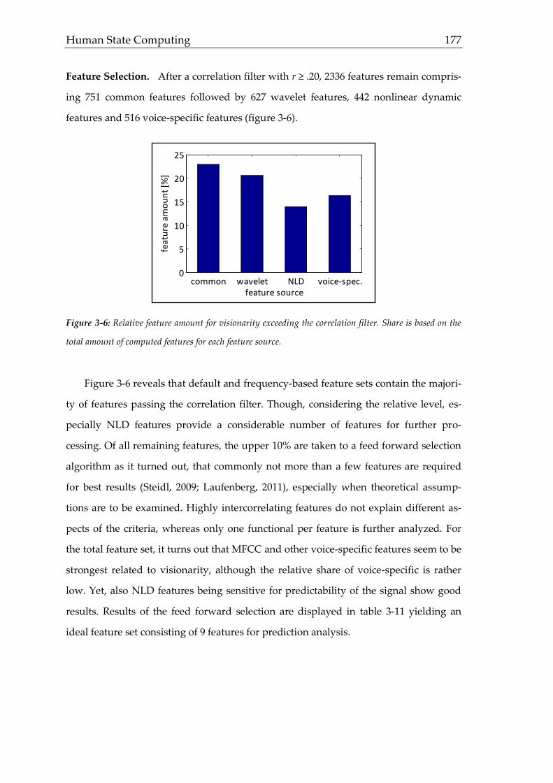
Human State Computing 177
Feature Selection. After a correlation filter with r ≥ .20, 2336 features remain compris-
ing 751 common features followed by 627 wavelet features, 442 nonlinear dynamic
features and 516 voice-specific features (figure 3-6).
Figure 3-6: Relative feature amount for visionarity exceeding the correlation filter. Share is based on the
total amount of computed features for each feature source.
Figure 3-6 reveals that default and frequency-based feature sets contain the majori-
ty of features passing the correlation filter. Though, considering the relative level, es-
pecially NLD features provide a considerable number of features for further pro-
cessing. Of all remaining features, the upper 10% are taken to a feed forward selection
algorithm as it turned out, that commonly not more than a few features are required
for best results (Steidl, 2009; Laufenberg, 2011), especially when theoretical assump-
tions are to be examined. Highly intercorrelating features do not explain different as-
pects of the criteria, whereas only one functional per feature is further analyzed. For
the total feature set, it turns out that MFCC and other voice-specific features seem to be
strongest related to visionarity, although the relative share of voice-specific is rather
low. Yet, also NLD features being sensitive for predictability of the signal show good
results. Results of the feed forward selection are displayed in table 3-11 yielding an
ideal feature set consisting of 9 features for prediction analysis.
common wavelet NLD voice-spec.0
5
10
15
20
25fe
atu
re a
mo
un
t [%
]
feature source

178 3. Field of Application I – Voice Based Leadership Analysis
Table 3-11: Remaining feature set for visionarity after feed forward selection.
feature r feature source
MFCC4 mean peak distance -.46 voice-specific
f0 deriv1 mean -.43 voice-specific
MFCC2 linreg -.40 voice-specific
voice prob regr. error .38 voice-specific
cao1,3 mean .38 NLD
WT3 quad regr error .37 wavelet
WT4 .37 wavelet
roll-off1 deriv2 min -.35 common
traj_angle deriv2 mean .33 NLD
average |r| .38
In the case of voice analysis, common and specific features are in various cases
hardly to distinguish on a theoretical basis. For this reason, it is not surprising that only
two common features are selected for the final input vector, as common and voice-
specific features often show a high degree of intercorrelation decreasing the likelihood
of considering all of them. On feature level, it is shown that particularly small mean
peak distances of the MFCC4 are correlated with high visionarity. With the negative
correlation of the voice probability regression error a more dynamic way of speaking is
emphasized, as high errors in the prediction of voiced and unvoiced segments correlate
with high visionarity. Differences between high and low manifestations of visionarity
are visualized exemplarily by wave form, frequency spectrum and phase space recon-
struction indicating general changes for visionarity (figure 3-7). As it turns out, vision-
arity is indeed correlated to higher variability in terms of intensity (derivable from the
wave form and phase reconstruction), whereas the frequency spectrum indicates an
increased share of higher frequencies typical for a higher yielding wall effect, so that
visionarity seems to be rather related with a hard than a soft voice .

Human State Computing 179
Figure 3-7: Visualized general differences for visionarity. Top row: wave form, center row: frequency
spectrum, bottom row: phase space reconstruction with d =2, τ=5.
After selecting the best feature sets, the output of their respective prediction mod-
els can be analyzed. As mentioned earlier, commonly prediction models are already
employed for feature selection, which is why both steps cannot be separated as it
commonly seems to be when presenting results step by step. Nonetheless, the follow-
ing passage contains all noteworthy classification results.
Classification. As the scope of this thesis is rather the applicability of different feature
sources, detailed information about the modification of classifiers is omitted for a bet-
ter overview. Competition, however, can be referred to as a first impression about pre-
diction model optimization. For this reason, the following table 3-12 gives information
about classification results based on separate and combined feature sources for opti-
mized classifiers employing the respective default algorithm of RapidMiner.
0 10 20 30-1
0
1
high visionarity
time [s]
no
rm. a
mp
l.
0 10 20 30-1
0
1
low visionarity
time [s]
no
rm. a
mp
l.
time [s]
fre
q [
Hz]
0 10 20 300
2000
4000
time [s]
fre
q [
Hz]
0 10 20 300
2000
4000
-0.2 -0.1 0 0.1 0.2-0.2
0
0.2
y2(t)
y 2(t
+5
)
-0.2 -0.1 0 0.1 0.2-0.2
0
0.2
y2(t)
y 2(t
+5
)

180 3. Field of Application I – Voice Based Leadership Analysis
Table 3-12: Classification results for visionarity.
feature source classifier RR (%) F1 (%) Sens. (%) Spec. (%)
common SVM 64.14 66.03 65.42 66.55
wavelet ANN 57.43 59.87 58.68 61.44
NLD ANN 53.02 50.78 53.43 47.90
voice spec. SVM 65.02 67.50 70.45 64.40
combined SVM 70.00 70.79 67.66 75.23
Applying for all quality measures, the support vector machine leads to best results,
what is quite a typical finding for voice analysis (Schuller et al., 2013). Far more inter-
esting than the best classifier, however, is to see how the different feature sources be-
have, as the novelty of the presented work regarding voice analysis lies within the
combination of several different feature extraction approaches. Although NLD features
yield lower prediction results than the other sets which are quite ahead, it turns out
that a combination of all feature sources is the most successful approach. When NLDs
are omitted, values for all quality measures decrease by about 4.26% revealing their
relevant contribution to the overall performance.
Regression. Analogous to the classification results, values regarding regression anal-
ysis are depicted in the following table. As especially for leadership states it is not suf-
ficient in practical use to only differentiate between good and bad performance, it has
to be analyzed how well exact values are predicted by the features computed. Em-
ployed algorithms are linear and quadratic regression as well as regressive SVM with
corresponding quality measures. Results are presented in table 3-13.
Table 3-13: Regression results for visionarity.
feature source classifier r R² RMSE rel. err. abs. err.
common LReg 0.43 0.18 0.96 9.06% 0.82
wavelet SVM 0.41 0.17 1.24 12.14% 1.09
NLD SVM 0.37 0.14 0.75 7.42% 0.67
voice spec. LReg 0.44 0.19 1.25 12.21% 1.10
combined LReg 0.49 0.24 1.38 13.80% 1.24

Human State Computing 181
The presented values show that a proper level of regressive prediction succeeds.
Based on the employed 10 points scale, predicted values deviate about 1.26 points av-
eraged around the assumed true score allowing a much better assessment than a sim-
ple binary classification does. In the following figure 3-8, a scatter plot (based on a rep-
resentative data excerpt) described the predictive power of the combined regression
feature model.
Figure 3-8: Predicted and true visionarity scores based on regression modeling.
For closing the voice based analysis of visionarity it can be summarized that based
on a mediocre rater agreement, a decent prediction power is achieved with the em-
ployed features. As another sub-dimension of charisma, inspiration results and a first
interpretation is given in the following chapter.
3.4.2 Inspiration
Analogously to visionarity, first measurements for rater agreement are depicted,
followed by feature selection, classification and regression results for each feature
source and outcomes for an ideal feature set based on all computed features. As it can
be derived from table 3-2 (description of all leadership states) inspiration is supposed
to be high for positive, motivating, dynamic or encouraging leaders. Going a level
deeper inspiration is separated from visionarity by rather covering daily leadership
behavior and human-centered criteria. However, similar findings to visionarity can be
expected due to the high intercorrelation of both states depicted in table 3-7.
1 2 3 4 5 6 7 8 9 10123456789
10
true score
pre
dic
ted
sco
re
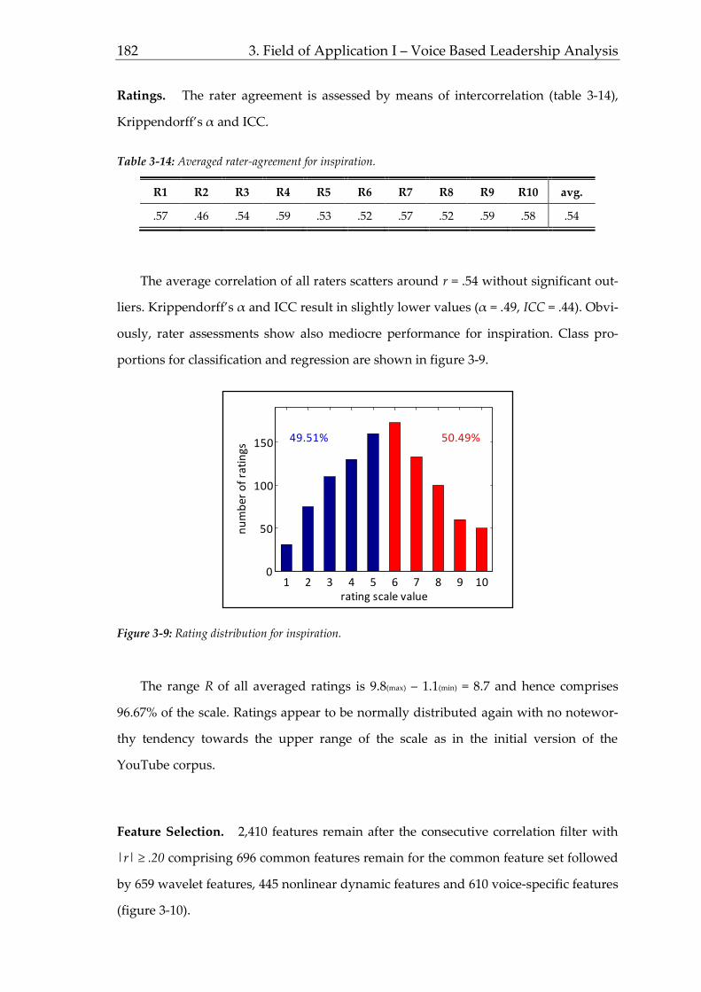
182 3. Field of Application I – Voice Based Leadership Analysis
Ratings. The rater agreement is assessed by means of intercorrelation (table 3-14),
Krippendorff’s α and ICC.
Table 3-14: Averaged rater-agreement for inspiration.
R1 R2 R3 R4 R5 R6 R7 R8 R9 R10 avg.
.57 .46 .54 .59 .53 .52 .57 .52 .59 .58 .54
The average correlation of all raters scatters around r = .54 without significant out-
liers. Krippendorff’s α and ICC result in slightly lower values (α = .49, ICC = .44). Obvi-
ously, rater assessments show also mediocre performance for inspiration. Class pro-
portions for classification and regression are shown in figure 3-9.
Figure 3-9: Rating distribution for inspiration.
The range R of all averaged ratings is 9.8(max) – 1.1(min) = 8.7 and hence comprises
96.67% of the scale. Ratings appear to be normally distributed again with no notewor-
thy tendency towards the upper range of the scale as in the initial version of the
YouTube corpus.
Feature Selection. 2,410 features remain after the consecutive correlation filter with
|r| ≥ .20 comprising 696 common features remain for the common feature set followed
by 659 wavelet features, 445 nonlinear dynamic features and 610 voice-specific features
(figure 3-10).
1 2 3 4 5 6 7 8 9 100
50
100
150
rating scale value
nu
mb
er o
f ra
tin
gs
49.51% 50.49%

Human State Computing 183
Figure 3-10: Relative feature amount for inspiration exceeding the correlation filter. Share is based on the
total amount of computed features for each feature source.
Figure 3-10 illustrates similar outcomes comparing visionarity to inspiration with
high values for default, wavelet and speech-specific features. As these sets are all close-
ly related especially for voice, this result is not surprising. NLD features, however,
provide useful features as well. Of all remaining features, the upper 10% (regarding
|r|) are taken to a feed forward selection algorithm allowing quicker computations and
better hypothesis testing leading to the following ideal prediction feature set consisting
of 9 features (table 3-15).
Table 3-15: Remaining feature set for inspiration after feed forward selection.
feature r feature source
MFCC3 mean peak distance -.44 voice-specific
f0 deriv1 stdev -.44 voice-specific
energy stdev .41 voice-specific
voice prob regr. error .37 voice-specific
WT4 .37 NLD
WT4 quad regr error .36 wavelet
cao1,3 quadr regr err. .35 wavelet
traj_leglen deriv1 mean .35 common
roll-off1 deriv1 max -.32 NLD
average |r| .37
common wavelet NLD voice-spec.0
5
10
15
20
25
feat
ure
am
ou
nt
[%]
feature source

184 3. Field of Application I – Voice Based Leadership Analysis
Despite some changes of the functionals and the addition of an intensity-based fea-
ture indicating that variation of the sound pressure is related to a high level of inspira-
tion, the visionarity feature set is matched. The high correlation of the energy standard
deviation emphasizes a more variable and dynamic speaker (in terms of loudness) to
be perceived as an inspiring leader. Classification and regression results are given after
a visualization of samples for high and low inspiration (figure 3-11).
Figure 3-11: Visualized general differences for inspiration. Top row: wave form, center row: frequency
spectrum, bottom row: phase space reconstruction with d =2, τ=5.
Classification. Since features and correlations do not vary considerably from those
presented for visionarity, also prediction outcomes are supposed to be closely related.
The stated results in table 3-16 are again derived by employing default algorithms of
RapidMiner.
0 10 20 30-1
0
1
high inspiration
time [s]
no
rm. a
mp
l.
0 10 20 30-1
0
1
low inspiration
time [s]
no
rm. a
mp
l.
time [s]
fre
q [
Hz]
0 10 20 300
2000
4000
time [s]
fre
q [
Hz]
0 10 20 300
2000
4000
-0.2 -0.1 0 0.1 0.2-0.2
0
0.2
y2(t)
y 2(t
+5
)
-0.2 -0.1 0 0.1 0.2-0.2
0
0.2
y2(t)
y 2(t
+5
)

Human State Computing 185
Table 3-16: Classification results for inspiration.
feature source classifier RR (%) F1 (%) Sens. (%) Spec. (%)
common SVM 63.22 60.81 60.71 60.89
wavelet SVM 56.61 55.28 54.74 55.97
NLD ANN 52.26 52.54 54.00 50.71
voice spec. SVM 64.09 66.83 68.93 64.99
combined SVM 69.56 71.79 74.34 69.07
In contrast to visionarity, also for wavelet features the SVM performs best. Both
common and wavelet feature show more consistent results regarding the employed
quality measures, while the combined feature shows differences in sensitivity and
specifity of about 5%. The combination of all feature sources yields the highest results.
When omitting the chosen NLD feature of the top feature set, performance decrease by
averaged 5.79% over all measures highlighting an existing impact of NLD features on
inspiration.
Regression. Visionarity results already implied there is a proper linear relation of
voice based features and leadership states. Table 3-17 summarizes the results for inspi-
ration.
Table 3-17: Regression results for inspiration.
feature source classifier r R² RMSE rel. err. abs. err.
common LReg .41 .17 1.19 11.83% 1.06
wavelet SVM .39 .15 0.88 8.20% 0.74
NLD SVM .35 .13 0.92 8.52% 0.77
voice spec. LReg .42 .18 0.99 9.54% 0.86
combined LReg .47 .22 1.31 7.99% 0.72
Combined regression succeeds with a performance of r = .47 and and a relative er-
ror of about 8% indicating that the rater perception regarding inspiration varies 0.72
scale points around the initial rating. This can be considered a good representation of
the rater perception. Room for improvement, however, is shown in the following scat-
terplot (figure 3-12) contrasting predicted and true scores.

186 3. Field of Application I – Voice Based Leadership Analysis
Figure 3-12: Predicted and true inspiration scores based on regression modeling.
Summarizing voice based prediction of inspiration leads to the conclusion that
based on a high correlation of visionarity and inspiration comparable results are ob-
tained allowing a proper assessment of the given ratings. Results for regarding integri-
ty as another leadership relevant state are displayed within the following chapter.
3.4.3 Integrity
After some widespread charisma states have been presented, the focus is narrowed
down to closer defined states starting with integrity. Following table 3-2, leaders with
high integrity are reliable, stick to what they do and show consistency of words and
behavior. Although this kind of trust-related state commonly has to be earned over
time, an attempt is made to capture a first impression by voice-based analyses. Analo-
gously to the other presented states, first measurements for rater agreement are depict-
ed, followed by feature selection, classification and regression results.
Ratings. As a basis for speech-based integrity prediction, the rater agreement is as-
sessed by means of intercorrelation (table 3-18), Krippendorff’s α and ICC.
Table 3-18: Averaged rater-agreement for integrity.
R1 R2 R3 R4 R5 R6 R7 R8 R9 R10 avg.
.49 .40 .47 .51 .46 .45 .49 .45 .52 .50 .48
1 2 3 4 5 6 7 8 9 10123456789
10
true scorep
red
icte
d s
core
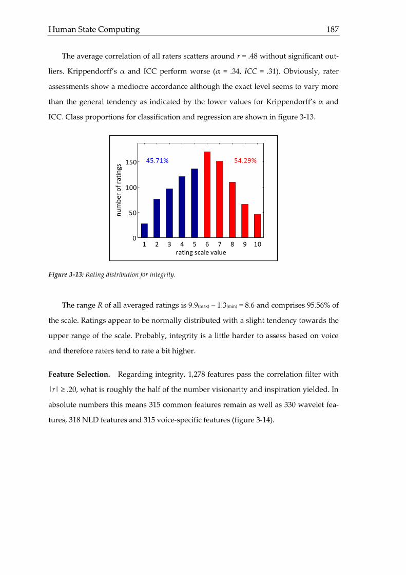
Human State Computing 187
The average correlation of all raters scatters around r = .48 without significant out-
liers. Krippendorff’s α and ICC perform worse (α = .34, ICC = .31). Obviously, rater
assessments show a mediocre accordance although the exact level seems to vary more
than the general tendency as indicated by the lower values for Krippendorff’s α and
ICC. Class proportions for classification and regression are shown in figure 3-13.
Figure 3-13: Rating distribution for integrity.
The range R of all averaged ratings is 9.9(max) – 1.3(min) = 8.6 and comprises 95.56% of
the scale. Ratings appear to be normally distributed with a slight tendency towards the
upper range of the scale. Probably, integrity is a little harder to assess based on voice
and therefore raters tend to rate a bit higher.
Feature Selection. Regarding integrity, 1,278 features pass the correlation filter with
|r| ≥ .20, what is roughly the half of the number visionarity and inspiration yielded. In
absolute numbers this means 315 common features remain as well as 330 wavelet fea-
tures, 318 NLD features and 315 voice-specific features (figure 3-14).
1 2 3 4 5 6 7 8 9 100
50
100
150
rating scale value
nu
mb
er o
f ra
tin
gs
45.71% 54.29%

188 3. Field of Application I – Voice Based Leadership Analysis
Figure 3-14: Relative feature amount for integrity exceeding the correlation filter. Share is based on the
total amount of computed features for each feature source.
Although the general picture does not change in comparison to the other so far
presented states, it should be pointed out that while the number of common, wavelet
and voice-specific decreases by around 50%, the amount of remaining NLD features
shows a more constant level of more than 70% compared to inspiration. This finding
could be seen as an indicator for the higher robustness of NLD features. After taking
the upper 10% of all feature sets to the consecutive feed forward selection, the follow-
ing ideal prediction feature set consisting of eight features is obtained (table 3-19).
Table 3-19: Remaining feature set for integrity after feed forward selection.
feature r feature source
MFCC1 num peaks -.32 voice-specific
MFCC4 mean peak distance .29 voice-specific
traj_leg angle stdev -.26 NLD
traj_leg length mean .24 NLD
WT12 lin regr err -.24 wavelet
jitter mean -.23 voice-specific
f0 deriv1 stdev -.23 common
roll-off2 deriv2 median .21 common
average |r| .25
common wavelet NLD voice-spec.0
5
10
15
feat
ure
am
ou
nt
[%]
feature source
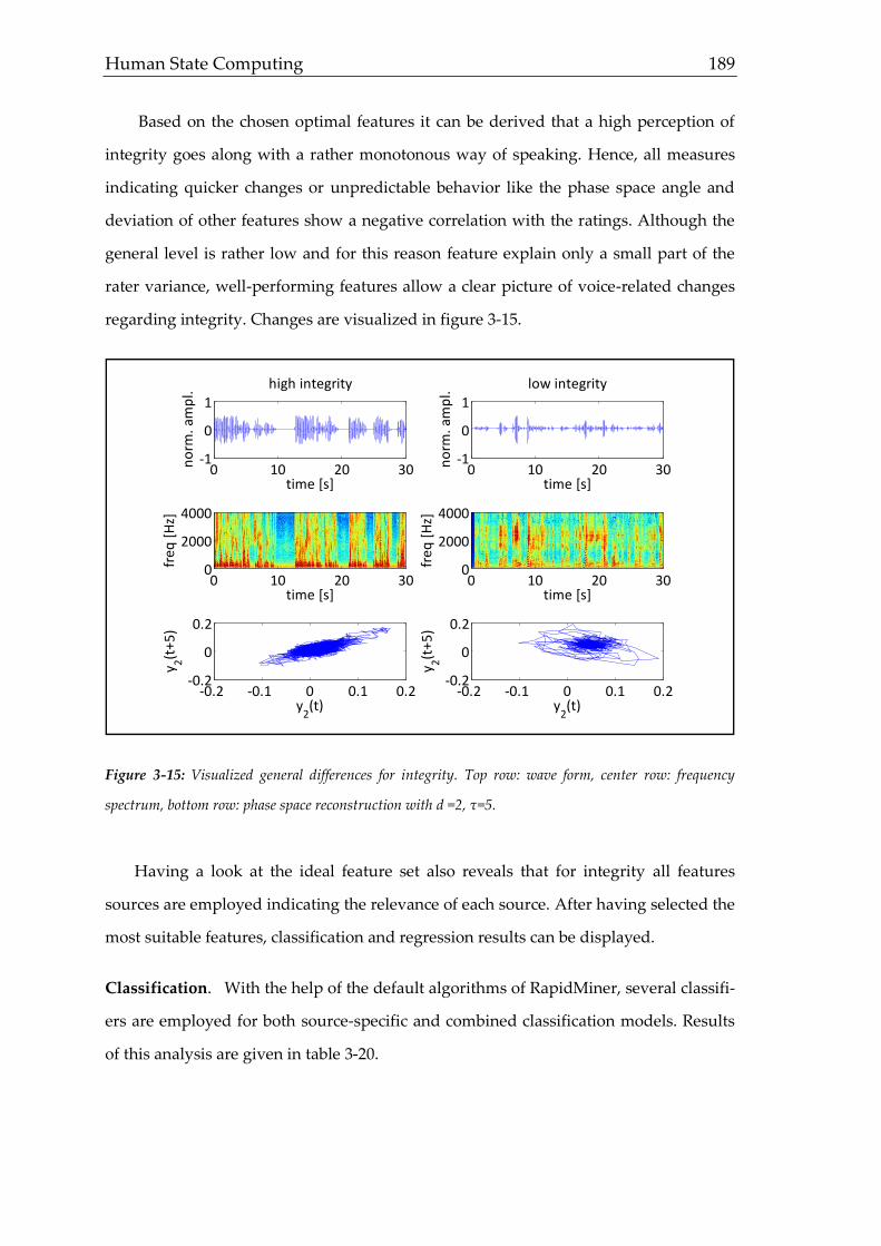
Human State Computing 189
Based on the chosen optimal features it can be derived that a high perception of
integrity goes along with a rather monotonous way of speaking. Hence, all measures
indicating quicker changes or unpredictable behavior like the phase space angle and
deviation of other features show a negative correlation with the ratings. Although the
general level is rather low and for this reason feature explain only a small part of the
rater variance, well-performing features allow a clear picture of voice-related changes
regarding integrity. Changes are visualized in figure 3-15.
Figure 3-15: Visualized general differences for integrity. Top row: wave form, center row: frequency
spectrum, bottom row: phase space reconstruction with d =2, τ=5.
Having a look at the ideal feature set also reveals that for integrity all features
sources are employed indicating the relevance of each source. After having selected the
most suitable features, classification and regression results can be displayed.
Classification. With the help of the default algorithms of RapidMiner, several classifi-
ers are employed for both source-specific and combined classification models. Results
of this analysis are given in table 3-20.
0 10 20 30-1
0
1
high integrity
time [s]
no
rm. a
mp
l.
0 10 20 30-1
0
1
low integrity
time [s]
no
rm. a
mp
l.
time [s]
fre
q [
Hz]
0 10 20 300
2000
4000
time [s]
fre
q [
Hz]
0 10 20 300
2000
4000
-0.2 -0.1 0 0.1 0.2-0.2
0
0.2
y2(t)
y 2(t
+5
)
-0.2 -0.1 0 0.1 0.2-0.2
0
0.2
y2(t)
y 2(t
+5
)
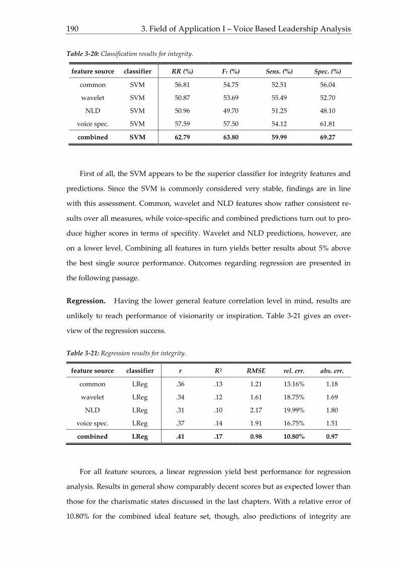
190 3. Field of Application I – Voice Based Leadership Analysis
Table 3-20: Classification results for integrity.
feature source classifier RR (%) F1 (%) Sens. (%) Spec. (%)
common SVM 56.81 54.75 52.51 56.04
wavelet SVM 50.87 53.69 55.49 52.70
NLD SVM 50.96 49.70 51.25 48.10
voice spec. SVM 57.59 57.50 54.12 61.81
combined SVM 62.79 63.80 59.99 69.27
First of all, the SVM appears to be the superior classifier for integrity features and
predictions. Since the SVM is commonly considered very stable, findings are in line
with this assessment. Common, wavelet and NLD features show rather consistent re-
sults over all measures, while voice-specific and combined predictions turn out to pro-
duce higher scores in terms of specifity. Wavelet and NLD predictions, however, are
on a lower level. Combining all features in turn yields better results about 5% above
the best single source performance. Outcomes regarding regression are presented in
the following passage.
Regression. Having the lower general feature correlation level in mind, results are
unlikely to reach performance of visionarity or inspiration. Table 3-21 gives an over-
view of the regression success.
Table 3-21: Regression results for integrity.
feature source classifier r R² RMSE rel. err. abs. err.
common LReg .36 .13 1.21 13.16% 1.18
wavelet LReg .34 .12 1.61 18.75% 1.69
NLD LReg .31 .10 2.17 19.99% 1.80
voice spec. LReg .37 .14 1.91 16.75% 1.51
combined LReg .41 .17 0.98 10.80% 0.97
For all feature sources, a linear regression yield best performance for regression
analysis. Results in general show comparably decent scores but as expected lower than
those for the charismatic states discussed in the last chapters. With a relative error of
10.80% for the combined ideal feature set, though, also predictions of integrity are
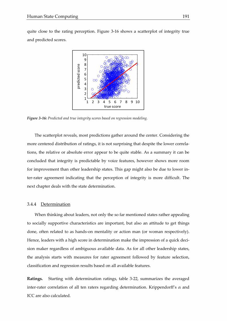
Human State Computing 191
quite close to the rating perception. Figure 3-16 shows a scatterplot of integrity true
and predicted scores.
Figure 3-16: Predicted and true integrity scores based on regression modeling.
The scatterplot reveals, most predictions gather around the center. Considering the
more centered distribution of ratings, it is not surprising that despite the lower correla-
tions, the relative or absolute error appear to be quite stable. As a summary it can be
concluded that integrity is predictable by voice features, however shows more room
for improvement than other leadership states. This gap might also be due to lower in-
ter-rater agreement indicating that the perception of integrity is more difficult. The
next chapter deals with the state determination.
3.4.4 Determination
When thinking about leaders, not only the so far mentioned states rather appealing
to socially supportive characteristics are important, but also an attitude to get things
done, often related to as hands-on mentality or action man (or woman respectively).
Hence, leaders with a high score in determination make the impression of a quick deci-
sion maker regardless of ambiguous available data. As for all other leadership states,
the analysis starts with measures for rater agreement followed by feature selection,
classification and regression results based on all available features.
Ratings. Starting with determination ratings, table 3-22, summarizes the averaged
inter-rater correlation of all ten raters regarding determination. Krippendorff’s α and
ICC are also calculated.
1 2 3 4 5 6 7 8 9 10123456789
10
true score
pre
dic
ted
sco
re
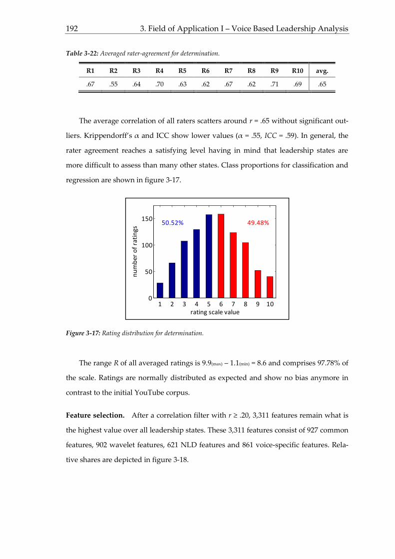
192 3. Field of Application I – Voice Based Leadership Analysis
Table 3-22: Averaged rater-agreement for determination.
R1 R2 R3 R4 R5 R6 R7 R8 R9 R10 avg.
.67 .55 .64 .70 .63 .62 .67 .62 .71 .69 .65
The average correlation of all raters scatters around r = .65 without significant out-
liers. Krippendorff’s α and ICC show lower values (α = .55, ICC = .59). In general, the
rater agreement reaches a satisfying level having in mind that leadership states are
more difficult to assess than many other states. Class proportions for classification and
regression are shown in figure 3-17.
Figure 3-17: Rating distribution for determination.
The range R of all averaged ratings is 9.9(max) – 1.1(min) = 8.6 and comprises 97.78% of
the scale. Ratings are normally distributed as expected and show no bias anymore in
contrast to the initial YouTube corpus.
Feature selection. After a correlation filter with r ≥ .20, 3,311 features remain what is
the highest value over all leadership states. These 3,311 features consist of 927 common
features, 902 wavelet features, 621 NLD features and 861 voice-specific features. Rela-
tive shares are depicted in figure 3-18.
1 2 3 4 5 6 7 8 9 100
50
100
150
rating scale value
nu
mb
er o
f ra
tin
gs
50.52% 49.48%
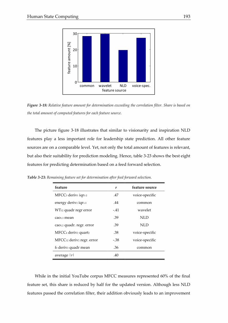
Human State Computing 193
Figure 3-18: Relative feature amount for determination exceeding the correlation filter. Share is based on
the total amount of computed features for each feature source.
The picture figure 3-18 illustrates that similar to visionarity and inspiration NLD
features play a less important role for leadership state prediction. All other feature
sources are on a comparable level. Yet, not only the total amount of features is relevant,
but also their suitability for prediction modeling. Hence, table 3-23 shows the best eight
features for predicting determination based on a feed forward selection.
Table 3-23: Remaining feature set for determination after feed forward selection.
feature r feature source
MFCC3 deriv1 iqr1-2 .47 voice-specific
energy deriv2 iqr1-3 .44 common
WT12 quadr regr error -.41 wavelet
cao1,3 mean .39 NLD
cao1,2 quadr. regr. error .39 NLD
MFCC4 deriv2 quart2 .38 voice-specific
MFCC12 deriv2 regr. error -.38 voice-specific
f0 deriv2 quadr mean .36 common
average |r| .40
While in the initial YouTube corpus MFCC measures represented 60% of the final
feature set, this share is reduced by half for the updated version. Although less NLD
features passed the correlation filter, their addition obviously leads to an improvement
common wavelet NLD voice-spec.0
10
20
30
feat
ure
am
ou
nt
[%]
feature source
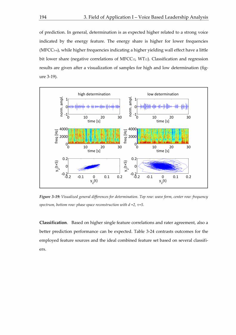
194 3. Field of Application I – Voice Based Leadership Analysis
of prediction. In general, determination is as expected higher related to a strong voice
indicated by the energy feature. The energy share is higher for lower frequencies
(MFCC3+4), while higher frequencies indicating a higher yielding wall effect have a little
bit lower share (negative correlations of MFCC12, WT12). Classification and regression
results are given after a visualization of samples for high and low determination (fig-
ure 3-19).
Figure 3-19: Visualized general differences for determination. Top row: wave form, center row: frequency
spectrum, bottom row: phase space reconstruction with d =2, τ=5.
Classification. Based on higher single feature correlations and rater agreement, also a
better prediction performance can be expected. Table 3-24 contrasts outcomes for the
employed feature sources and the ideal combined feature set based on several classifi-
ers.
0 10 20 30-1
0
1
high determination
time [s]
no
rm. a
mp
l.
0 10 20 30-1
0
1
low determination
time [s]
no
rm. a
mp
l.
time [s]
fre
q [
Hz]
0 10 20 300
2000
4000
time [s]
fre
q [
Hz]
0 10 20 300
2000
4000
-0.2 -0.1 0 0.1 0.2-0.2
0
0.2
y2(t)
y 2(t
+5
)
-0.2 -0.1 0 0.1 0.2-0.2
0
0.2
y2(t)
y 2(t
+5
)

Human State Computing 195
Table 3-24: Classification results for determination.
feature source classifier RR (%) F1 (%) Sens. (%) Spec. (%)
common SVM 72.39 70.24 70.22 70.25
wavelet RF 64.82 64.35 68.94 59.43
NLD ANN 59.83 62.33 60.73 63.87
voice spec. SVM 73.38 75.13 75.98 74.69
combined SVM 79.31 81.76 79.00 84.07
Also for determination, SVM turns out to be the preferred classifier for the given
combined feature set. Although results do not vary considerably, regarding wavelet
features the random forest classifier performed best. While predictions for voice-
specific and common features do hardly vary for all performance measures the com-
bined prediction yields highest values for specifity when maximizing the recognition
rate as primary target for classification. With nearly 80%, a proper performance on the
binary differentiation task is achieved. Regression results follow within the next pas-
sage.
Regression. With single correlations of nearly .50, the optimized regression model is
supposed to yield better results, although already the previously presented states re-
vealed that models seem to struggle improving regression results by combining several
features. Table 3-25 gives results for determination.
Table 3-25: Regression results for determination.
feature source classifier r R² RMSE rel. err. abs. err.
common LReg .49 .24 1.06 10.50% 0.95
wavelet SVM .47 .22 1.21 9.44% 0.85
NLD SVM .42 .18 1.15 9.91% 0.89
voice spec. SVM .50 .25 1.14 8.82% 0.79
combined LReg .56 .31 0.94 7.01% 0.63
With a lowest relative error of about 7%, predictions seem to nearly perfectly
match the true ratings. Having a look at the correlation or R² respectively shows, how-
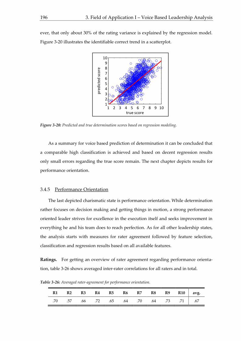
196 3. Field of Application I – Voice Based Leadership Analysis
ever, that only about 30% of the rating variance is explained by the regression model.
Figure 3-20 illustrates the identifiable correct trend in a scatterplot.
Figure 3-20: Predicted and true determination scores based on regression modeling.
As a summary for voice based prediction of determination it can be concluded that
a comparable high classification is achieved and based on decent regression results
only small errors regarding the true score remain. The next chapter depicts results for
performance orientation.
3.4.5 Performance Orientation
The last depicted charismatic state is performance orientation. While determination
rather focuses on decision making and getting things in motion, a strong performance
oriented leader strives for excellence in the execution itself and seeks improvement in
everything he and his team does to reach perfection. As for all other leadership states,
the analysis starts with measures for rater agreement followed by feature selection,
classification and regression results based on all available features.
Ratings. For getting an overview of rater agreement regarding performance orienta-
tion, table 3-26 shows averaged inter-rater correlations for all raters and in total.
Table 3-26: Averaged rater-agreement for performance orientation.
R1 R2 R3 R4 R5 R6 R7 R8 R9 R10 avg.
.70 .57 .66 .72 .65 .64 .70 .64 .73 .71 .67
1 2 3 4 5 6 7 8 9 10123456789
10
true score
pre
dic
ted
sco
re
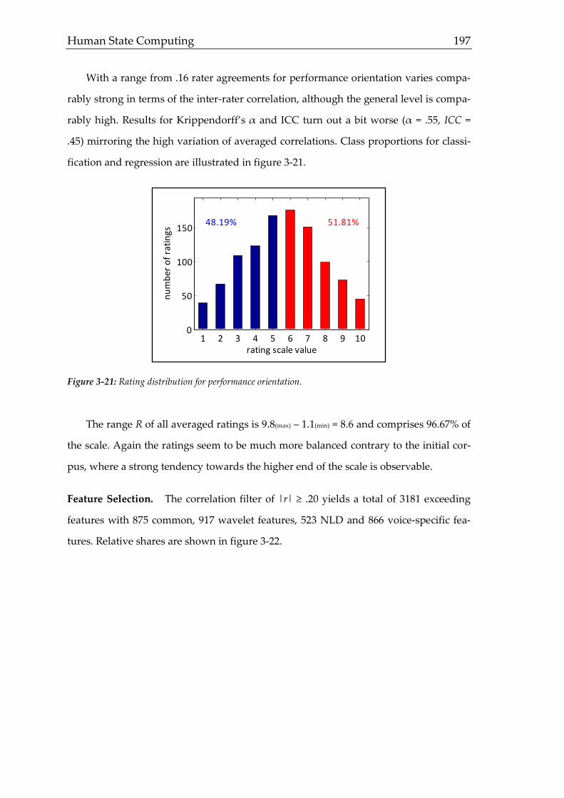
Human State Computing 197
With a range from .16 rater agreements for performance orientation varies compa-
rably strong in terms of the inter-rater correlation, although the general level is compa-
rably high. Results for Krippendorff’s α and ICC turn out a bit worse (α = .55, ICC =
.45) mirroring the high variation of averaged correlations. Class proportions for classi-
fication and regression are illustrated in figure 3-21.
Figure 3-21: Rating distribution for performance orientation.
The range R of all averaged ratings is 9.8(max) – 1.1(min) = 8.6 and comprises 96.67% of
the scale. Again the ratings seem to be much more balanced contrary to the initial cor-
pus, where a strong tendency towards the higher end of the scale is observable.
Feature Selection. The correlation filter of |r| ≥ .20 yields a total of 3181 exceeding
features with 875 common, 917 wavelet features, 523 NLD and 866 voice-specific fea-
tures. Relative shares are shown in figure 3-22.
1 2 3 4 5 6 7 8 9 100
50
100
150
rating scale value
nu
mb
er o
f ra
tin
gs
48.19% 51.81%

198 3. Field of Application I – Voice Based Leadership Analysis
Figure 3-22: Relative feature amount for performance orientation exceeding the correlation filter. Share is
based on the total amount of computed features for each feature source.
The presented figure shows an even distribution of common, wavelet and voice-
specific features, while the share of NLD features is a little bit less than half of the other
sources. After employing the feed forward selection algorithm, the following eight fea-
tures are chosen for best prediction of performance orientation (table 3-27).
Table 3-27: Remaining feature set for performance orientation after feed forward selection.
feature r feature source
energy deriv2 quartil3 .49 common
MFCC12 deriv2 quadr regr error .46 voice-specific
WT11 lin regr error .43 wavelet
WT14 deriv2 stdev .41 wavelet
traj_angle mean .41 NLD
MFCC0 quart3 .40 voice-specific
MFCC1 deriv1 iqr1-3 .40 voice-specific
flux stdev .38 common
average |r| .41
Features sensitive for performance orientation show a slightly different picture com-
pared to e.g. integrity. In line with the assumptions presented in table 3-5, performance
orientation shows higher correlations with features representing variability and more
powerful speaking not only in terms of energy but also regarding the spectrum of fre-
common wavelet NLD voice-spec.0
10
20
30
feat
ure
am
ou
nt
[%]
feature source
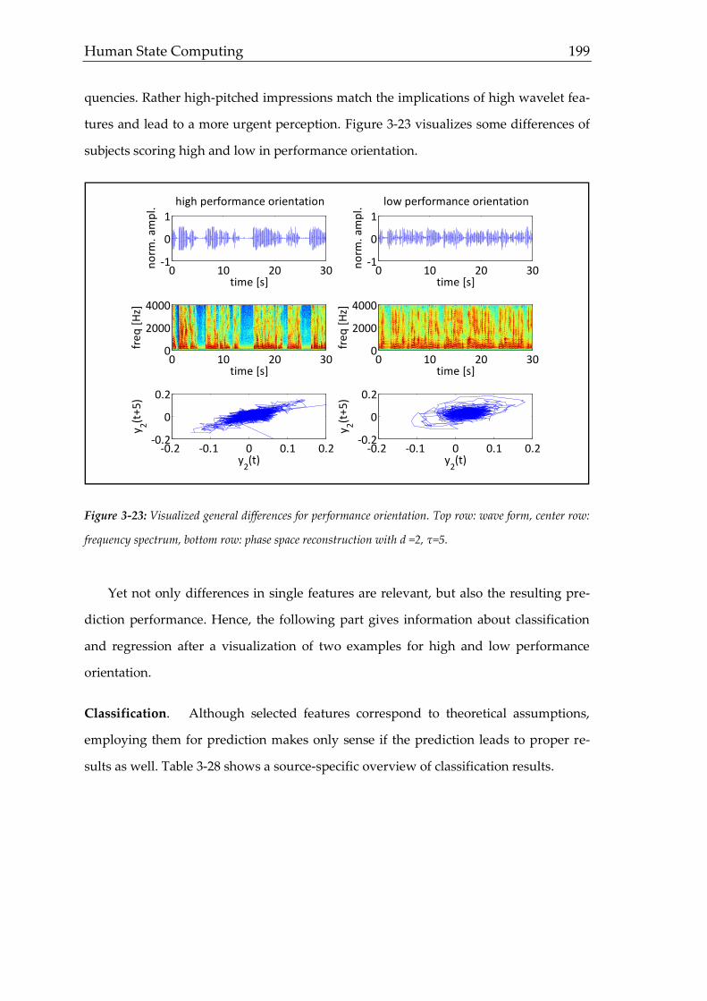
Human State Computing 199
quencies. Rather high-pitched impressions match the implications of high wavelet fea-
tures and lead to a more urgent perception. Figure 3-23 visualizes some differences of
subjects scoring high and low in performance orientation.
Figure 3-23: Visualized general differences for performance orientation. Top row: wave form, center row:
frequency spectrum, bottom row: phase space reconstruction with d =2, τ=5.
Yet not only differences in single features are relevant, but also the resulting pre-
diction performance. Hence, the following part gives information about classification
and regression after a visualization of two examples for high and low performance
orientation.
Classification. Although selected features correspond to theoretical assumptions,
employing them for prediction makes only sense if the prediction leads to proper re-
sults as well. Table 3-28 shows a source-specific overview of classification results.
0 10 20 30-1
0
1
high performance orientation
time [s]
no
rm. a
mp
l.
0 10 20 30-1
0
1
low performance orientation
time [s]
no
rm. a
mp
l.time [s]
fre
q [
Hz]
0 10 20 300
2000
4000
time [s]
fre
q [
Hz]
0 10 20 300
2000
4000
-0.2 -0.1 0 0.1 0.2-0.2
0
0.2
y2(t)
y 2(t
+5
)
-0.2 -0.1 0 0.1 0.2-0.2
0
0.2
y2(t)
y 2(t
+5
)

200 3. Field of Application I – Voice Based Leadership Analysis
Table 3-28: Classification results for performance orientation.
feature source classifier RR (%) F1 (%) Sens. (%) Spec. (%)
common SVM 69.64 70.57 73.08 68.91
wavelet SVM 62.35 59.57 57.12 62.74
NLD SVM 57.56 59.65 59.71 59.61
voice spec. SVM 70.59 73.19 75.18 71.15
combined SVM 76.54 77.07 80.98 74.47
Obviously, SVM is the best classifier for the given data set achieving a maximum
recognition rate of RR = 76.54% what is about 20% better than the NLD-based predic-
tion. Nonetheless, removing the chosen NLD feature from the combined prediction
reduces the averaged performance by 2.7%, so its usage is reasonable. Contrary to most
other leadership states, however, sensitivity yields best outcomes when optimizing the
prediction algorithm with regard to the recognition rate. Regression results are shown
in the next passage.
Regression. With maximum single feature correlating almost .50 with performance
orientation, the regression results are likely better. Table 3-29 provides an overview of
regression results.
Table 3-29: Regression results for performance orientation.
feature source classifier r R² RMSE rel. err. abs. err.
common LReg .51 .26 1.21 9.52% 0.86
wavelet SVM .49 .24 1.09 10.72% 0.96
NLD SVM .44 .19 1.01 10.30% 0.93
voice spec. LReg .52 .27 1.12 9.09% 0.82
combined LReg .58 .34 1.27 7.63% 0.69
With a maximum R² of .34 for the combined feature set, a considerable amount of
the ratings is explained by the voice based features. Small error values contribute to the
suitability of voice features for the assessment of performance orientation. Figure 3-24
gives a visual impression of the regression performance.
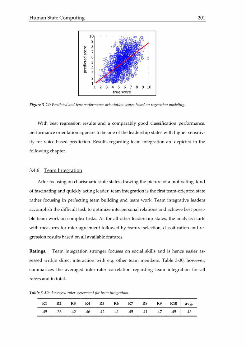
Human State Computing 201
Figure 3-24: Predicted and true performance orientation scores based on regression modeling.
With best regression results and a comparably good classification performance,
performance orientation appears to be one of the leadership states with higher sensitiv-
ity for voice based prediction. Results regarding team integration are depicted in the
following chapter.
3.4.6 Team Integration
After focusing on charismatic state states drawing the picture of a motivating, kind
of fascinating and quickly acting leader, team integration is the first team-oriented state
rather focusing in perfecting team building and team work. Team integrative leaders
accomplish the difficult task to optimize interpersonal relations and achieve best possi-
ble team work on complex tasks. As for all other leadership states, the analysis starts
with measures for rater agreement followed by feature selection, classification and re-
gression results based on all available features.
Ratings. Team integration stronger focuses on social skills and is hence easier as-
sessed within direct interaction with e.g. other team members. Table 3-30, however,
summarizes the averaged inter-rater correlation regarding team integration for all
raters and in total.
Table 3-30: Averaged rater-agreement for team integration.
R1 R2 R3 R4 R5 R6 R7 R8 R9 R10 avg.
.45 .36 .42 .46 .42 .41 .45 .41 .47 .45 .43
1 2 3 4 5 6 7 8 9 10123456789
10
true score
pre
dic
ted
sco
re

202 3. Field of Application I – Voice Based Leadership Analysis
In general, inter-rater correlations show a consistent level varying around r = .43
without any outliers. Krippendorff’s α and ICC result in lower values (α = .34, ICC =
.29) indicating that the general level differs stronger than the general tendency of rat-
ings. Class proportions for classification and regression are shown in figure 3-25.
Figure 3-25: Rating distribution for team integration.
The range R of all averaged ratings is 9.9(max) – 1.2(min) = 8.6 and comprises 96.67% of
the scale. However, ratings appear to show a small tendency towards the upper end of
the scale, although the disproportion is quite small with 2.33% or 24 tracks respective-
ly. As figure 3-25 shows, there is a noticeable small amount of ratings close to the lower
end of the scale probably influencing regression outcomes.
Feature Selection. When employing a correlation filter with features r ≥ .20, a total
amount of 913 features remain consisting of 237 common features followed by 213
wavelet, 263 NLD and 200 voice-specific features (figure 3-26).
1 2 3 4 5 6 7 8 9 100
50
100
150
200
rating scale value
nu
mb
er o
f ra
tin
gs47.67% 52.33%

Human State Computing 203
Figure 3-26: Relative feature amount for team integration exceeding the correlation filter. Share is based
on the total amount of computed features for each feature source.
Comparing the relative feature amount it gets obvious that similar to integrity,
NLD features increase the share while other feature sources show comparably worse
results. Table 3-31 gives the corresponding optimal feature set for prediction consisting
of seven features.
Table 3-31: Remaining feature set for team integration after feed forward selection.
feature r feature source
energy deriv1 mean .28 common
traj_angle deriv2 stdev .25 NLD
largelyap deriv2 mean .22 NLD
traj_leglen .20 NLD
MFCC5 deriv2 quadr. mean .20 voice-specific
WT3 .19 wavelet
MFCC2 deriv1 perc95 .19 voice-specific
average |r| .22
NLD features contribute considerably to the chosen feature set. Although the gen-
eral level of correlations is rather low, NLD features show more stable results. Contra-
ry, common features seem hardly useful for voice based prediction of team integration.
Similar to other leadership states, MFCC features are required for good prediction.
With regard to the expected outcomes, the energy based feature corresponds to a ra-
common wavelet NLD voice-spec.0
2
4
6
8
10
feat
ure
am
ou
nt
[%]
feature source
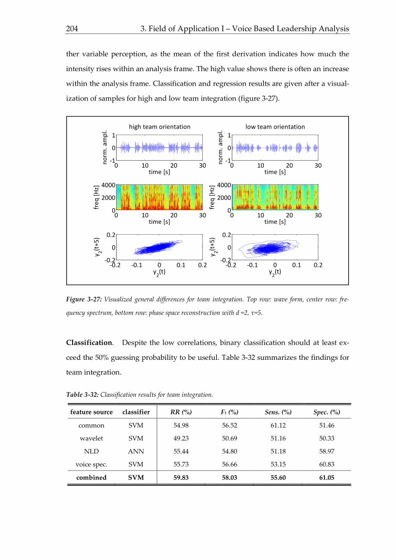
204 3. Field of Application I – Voice Based Leadership Analysis
ther variable perception, as the mean of the first derivation indicates how much the
intensity rises within an analysis frame. The high value shows there is often an increase
within the analysis frame. Classification and regression results are given after a visual-
ization of samples for high and low team integration (figure 3-27).
Figure 3-27: Visualized general differences for team integration. Top row: wave form, center row: fre-
quency spectrum, bottom row: phase space reconstruction with d =2, τ=5.
Classification. Despite the low correlations, binary classification should at least ex-
ceed the 50% guessing probability to be useful. Table 3-32 summarizes the findings for
team integration.
Table 3-32: Classification results for team integration.
feature source classifier RR (%) F1 (%) Sens. (%) Spec. (%)
common SVM 54.98 56.52 61.12 51.46
wavelet SVM 49.23 50.69 51.16 50.33
NLD ANN 55.44 54.80 51.18 58.97
voice spec. SVM 55.73 56.66 53.15 60.83
combined SVM 59.83 58.03 55.60 61.05
0 10 20 30-1
0
1
high team orientation
time [s]
no
rm. a
mp
l.
0 10 20 30-1
0
1
low team orientation
time [s]
no
rm. a
mp
l.time [s]
fre
q [
Hz]
0 10 20 300
2000
4000
time [s]
fre
q [
Hz]
0 10 20 300
2000
4000
-0.2 -0.1 0 0.1 0.2-0.2
0
0.2
y2(t)
y 2(t
+5
)
-0.2 -0.1 0 0.1 0.2-0.2
0
0.2
y2(t)
y 2(t
+5
)
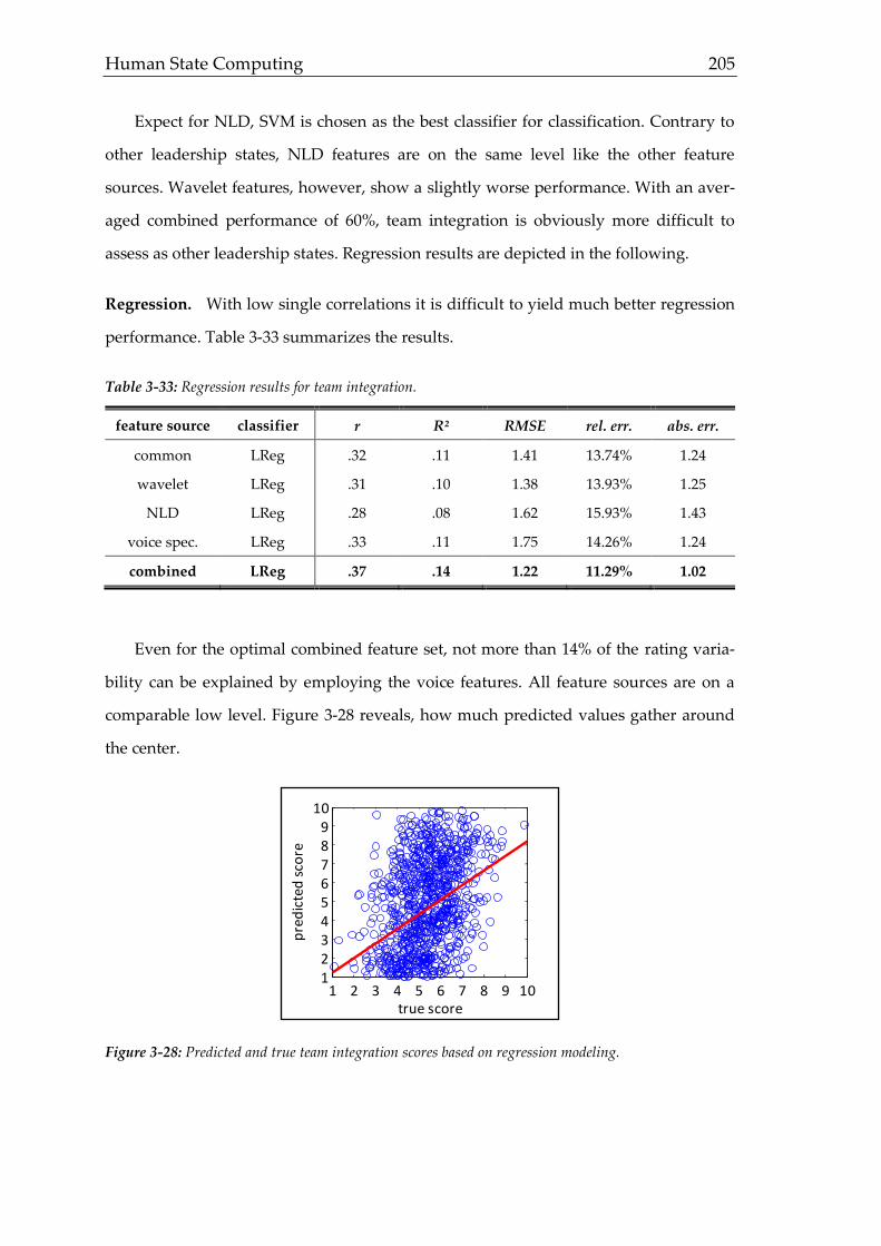
Human State Computing 205
Expect for NLD, SVM is chosen as the best classifier for classification. Contrary to
other leadership states, NLD features are on the same level like the other feature
sources. Wavelet features, however, show a slightly worse performance. With an aver-
aged combined performance of 60%, team integration is obviously more difficult to
assess as other leadership states. Regression results are depicted in the following.
Regression. With low single correlations it is difficult to yield much better regression
performance. Table 3-33 summarizes the results.
Table 3-33: Regression results for team integration.
feature source classifier r R² RMSE rel. err. abs. err.
common LReg .32 .11 1.41 13.74% 1.24
wavelet LReg .31 .10 1.38 13.93% 1.25
NLD LReg .28 .08 1.62 15.93% 1.43
voice spec. LReg .33 .11 1.75 14.26% 1.24
combined LReg .37 .14 1.22 11.29% 1.02
Even for the optimal combined feature set, not more than 14% of the rating varia-
bility can be explained by employing the voice features. All feature sources are on a
comparable low level. Figure 3-28 reveals, how much predicted values gather around
the center.
Figure 3-28: Predicted and true team integration scores based on regression modeling.
1 2 3 4 5 6 7 8 9 10123456789
10
true score
pre
dic
ted
sco
re

206 3. Field of Application I – Voice Based Leadership Analysis
All in all, team integration seems to be difficult to assess by voice features. Alt-
hough classification results achieve predictions for binary differentiation above guess-
ing probability, the more relevant regression performs insufficiently. The next team
orienting leadership state is diplomacy.
3.4.7 Diplomacy
When leading a team, it is not only important to create an ideal environment for
the team, but also to represent it and negotiate with other stakeholders and members of
(e.g.) the managing board. Hence, diplomacy is an important skill to reach satisfying
agreements with both team members and other departments. High scores in diploma-
cy, therefore, characterize a person as a well performing negotiator. As for all other
leadership states, the analysis starts with measures for rater agreement followed by
feature selection, classification and regression results based on all available features.
Ratings. Similar to team integration, diplomacy is a state which is probably better
observable within social interaction instead of holding presentations. Nonetheless, as
an important CLT dimension it is necessary to integrate this state in the voice-based
leadership prediction. Table 3-34 contains results of the inter-rater correlation.
Table 3-34: Averaged rater-agreement for diplomacy.
R1 R2 R3 R4 R5 R6 R7 R8 R9 R10 avg.
.40 .32 .38 .41 .37 .36 .40 .36 .42 .40 .38
With a total average inter-rater correlation of r = .38, a rather poor agreement is
reached (yet on a stable level ranging from .36 to .42). Also Krippendorff’s α and ICC
show dissatisfactory results (α = .24, ICC = .29). Obviously, diplomacy is more difficult
to assess than other leadership states. Class proportions for classification and regres-
sion are given in figure 3-29.
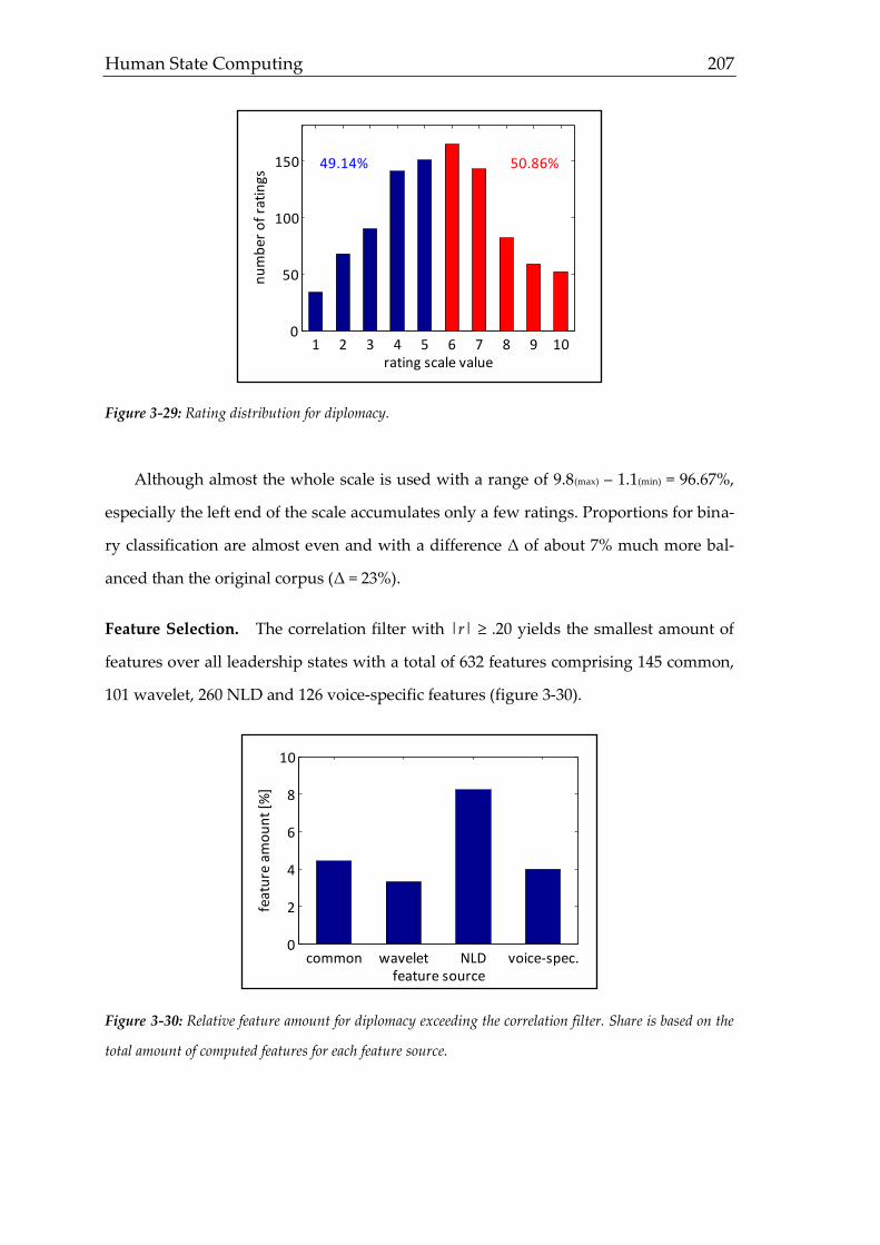
Human State Computing 207
Figure 3-29: Rating distribution for diplomacy.
Although almost the whole scale is used with a range of 9.8(max) – 1.1(min) = 96.67%,
especially the left end of the scale accumulates only a few ratings. Proportions for bina-
ry classification are almost even and with a difference Δ of about 7% much more bal-
anced than the original corpus (Δ = 23%).
Feature Selection. The correlation filter with |r| ≥ .20 yields the smallest amount of
features over all leadership states with a total of 632 features comprising 145 common,
101 wavelet, 260 NLD and 126 voice-specific features (figure 3-30).
Figure 3-30: Relative feature amount for diplomacy exceeding the correlation filter. Share is based on the
total amount of computed features for each feature source.
1 2 3 4 5 6 7 8 9 100
50
100
150
rating scale value
nu
mb
er o
f ra
tin
gs
49.14% 50.86%
common wavelet NLD voice-spec.0
2
4
6
8
10
feat
ure
am
ou
nt
[%]
feature source

208 3. Field of Application I – Voice Based Leadership Analysis
The most noteworthy aspect of figure 3-30 is the comparable high relative share of
NLD features. While the total number of features passing the correlation filter adds up
to only about 20% of the number resulting for determination, NLD features are again
much more stable and shows an equal relative share, whereas for better assessable
states the relative share was only the half of other feature sources. Table 3-35 depicts
the ideal feature set selected by a feed forward algorithm choosing six features for di-
plomacy prediction.
Table 3-35: Remaining feature set for diplomacy after feed forward selection.
feature r feature source
f0 mean peak dist .24 common
traj_len deriv1 median .21 NLD
largelyap -.18 NLD
roll-off50 stdev -.16 voice-specific
ZCR deriv1 perc95 -.16 common
MFCC12 deriv2 mean .15 voice-specific
average |r| .18
Having a glance at the average correlation of |r| = .18 for the ideal feature set, it is
obvious that only a small part of the rating variance can be explained by the features
and hence matching the outcomes with hypothesis has to be treated carefully. None-
theless, chosen features are in accordance with expected voice changes (at least regard-
ing the perceivable changes). As a diplomatic voice is supposed to be rather controlled
and deliberate, it makes sense that a bigger distance between F0 peaks (meaning less
bursts in terms of the pitch) correlate positively with diplomacy. On the contrary, fea-
tures indicating higher variance in terms of frequency like the spectral Roll-off or the
ZCR show a negative correlation. Classification and regression results are given after a
visualization of samples for high and low diplomacy (figure 3-31).

Human State Computing 209
Figure 3-31: Visualized general differences for diplomacy. Top row: wave form, center row: frequency
spectrum, bottom row: phase space reconstruction with d =2, τ=5.
Classification. Based on the low general correlation level, it is difficult to yield high
classification performance even for a binary classification. Table 3-36, though, depicts
results achieved by classifiers employing the stated ideal feature set for diplomacy.
Table 3-36: Classification results for diplomacy.
feature source classifier RR (%) F1 (%) Sens. (%) Spec. (%)
common SVM 53.14 54.38 57.79 51.14
wavelet SVM 47.59 44.78 42.32 46.21
NLD RF 53.93 52.59 55.73 50.30
voice spec. SVM 53.87 51.15 48.58 54.77
combined SVM 58.98 55.58 59.88 52.78
While wavelet features do not exceed the guessing probability of 50%, at least the
combined feature set with a Recognition Rate approaching the 60% shows sufficient
results to outperform guessing. As to expect based on the missing wavelet features in
the feature set, predictions based on only wavelet features result in worst classification.
0 10 20 30-1
0
1
high diplomacy
time [s]
no
rm. a
mp
l.
0 10 20 30-1
0
1
low diplomacy
time [s]
no
rm. a
mp
l.
time [s]
fre
q [
Hz]
0 10 20 300
2000
4000
time [s]
fre
q [
Hz]
0 10 20 300
2000
4000
-0.2 -0.1 0 0.1 0.2-0.2
0
0.2
y2(t)
y 2(t
+5
)
-0.2 -0.1 0 0.1 0.2-0.2
0
0.2
y2(t)
y 2(t
+5
)

210 3. Field of Application I – Voice Based Leadership Analysis
Regarding the chosen classifier, RF yields best results for NLD features, but in general
the SVM appears to be favorable again.
Regression. Already the low single correlations reveal that only a small part of the
rating variance can be explained. Regression results are depicted in table 3-37.
Table 3-37: Regression results for diplomacy.
feature source classifier r R² RMSE rel. err. abs. err.
common LReg .29 .08 1.75 17.00% 1.53
wavelet SVM .28 .08 1.60 15.66% 1.41
NLD SVM .25 .06 1.75 17.23% 1.55
voice spec. LReg .30 .09 1.90 18.73% 1.69
combined LReg .33 .11 1.85 14.22% 1.28
While the explained variance hardly exceeds 10% for the combined feature set, also
other error measures show dissatisfactory results. Although most ratings gather
around the center, there is still a considerable error indicating that even within a small-
er bandwidth of ratings predicted scores show high deviations. This big amount of
random variance within the predicted scores is illustrated in figure 3-32.
Figure 3-32: Predicted and true diplomacy scores based on regression modeling.
It can be summarized, that based on low rater agreements only a comparably small
amount of features is found that generally exceeds the correlation filter. Although cho-
sen features for the ideal feature set are in line with expected perceivable voice chang-
es, the total amount of explained variance is too low for a proper assessment.
1 2 3 4 5 6 7 8 9 10123456789
10
true score
pre
dic
ted
sco
re

Human State Computing 211
3.4.8 Non-Maliciousness
As the last leadership state, non-maliciousness is discussed. Following the multi-
dimensional scaling within the across-dimensional results (chapter 3.3) the impact of
this state on the other ones is rather poor. Nonetheless, it is one of the generally en-
dorsed leadership attributes and is hence analyzed. Persons scoring high in this state
tend to be smart and fast learning leaders considering employees as many-faceted hu-
man beings with several interests. Being a reliable and integrating person, non-
malicious leaders keep an eye on personal needs and care for a good work-life-balance
in line with the strong belief that satisfied employees perform better, especially in the
long run. As for all other leadership states, the analysis starts with measures for rater
agreement followed by feature selection, classification and regression results based on
all available features.
Ratings. Although non-maliciousness does not correlate high with other leadership
states, the rater agreement needs not to be necessarily low. Table 3-38 summarizes the
averaged inter-rater correlation.
Table 3-38: Averaged rater-agreement for non-maliciousness.
R1 R2 R3 R4 R5 R6 R7 R8 R9 R10 avg.
.51 .41 .48 .52 .47 .46 .51 .46 .53 .51 .49
In comparison to all other stated leadership states, the inter-rater correlation indi-
cates a moderate agreement. This conclusion is further supported by mediocre results
for Krippendorff’s α and the ICC (α = .44, ICC = .41). Class proportions for classification
and regression are shown in figure 3-33.
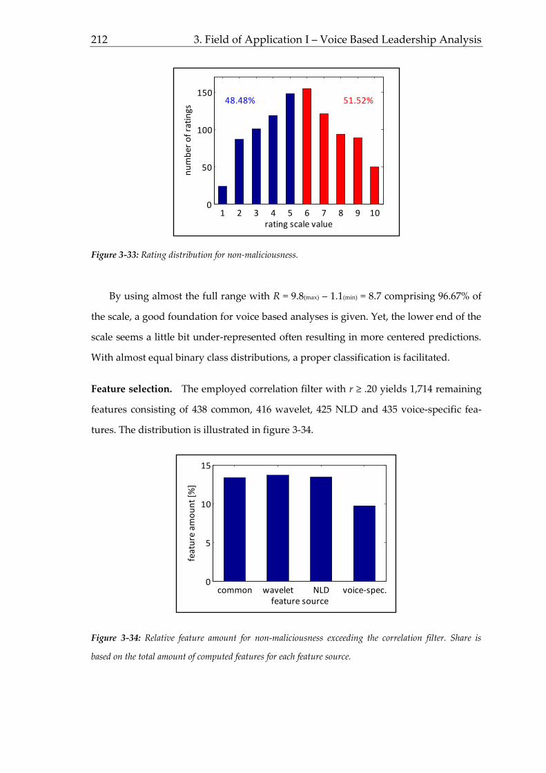
212 3. Field of Application I – Voice Based Leadership Analysis
Figure 3-33: Rating distribution for non-maliciousness.
By using almost the full range with R = 9.8(max) – 1.1(min) = 8.7 comprising 96.67% of
the scale, a good foundation for voice based analyses is given. Yet, the lower end of the
scale seems a little bit under-represented often resulting in more centered predictions.
With almost equal binary class distributions, a proper classification is facilitated.
Feature selection. The employed correlation filter with r ≥ .20 yields 1,714 remaining
features consisting of 438 common, 416 wavelet, 425 NLD and 435 voice-specific fea-
tures. The distribution is illustrated in figure 3-34.
Figure 3-34: Relative feature amount for non-maliciousness exceeding the correlation filter. Share is
based on the total amount of computed features for each feature source.
1 2 3 4 5 6 7 8 9 100
50
100
150
rating scale value
nu
mb
er o
f ra
tin
gs
48.48% 51.52%
common wavelet NLD voice-spec.0
5
10
15
feat
ure
am
ou
nt
[%]
feature source

Human State Computing 213
The feature distribution is a little bit different to what is shown for most other
states with rather good results. While still frequency based features reach a high share,
NLD features outperforms voice-specific a little bit. Table 3-39 depicts the selected fea-
tures for optimal feature selection
Table 3-39: Remaining feature set for non-maliciousness after feed forward selection.
feature r feature source
f0 iqr2-3 -.33 common
voiceprob deriv1 perc95 -.30 common
MFCC2 quadr regr error -.27 voice-specific
WT3 lin regr error -.25 wavelet
cao1,2 stdev -.25 NLD
MFCC4 mean peak dist .24 voice-specific
traj_angel length stdev -.24 NLD
average |r| .27
Having the description of non-maliciousness in mind, persons scoring high in this
state are considered sympathetic. The proposed voice changes stated in table 3-5 indi-
cate that a rather soft and monotonous voice is expected. Looking at the chosen fea-
tures reveals a proper matching of this assumption. The negative correlation of the f0
inter quartile range, e.g., describes that f0 does not change noticeably for speaker being
perceived non-malicious. Also e.g. the positive correlation of the mean peak distance of
a MFCC is a clear indicator for a soft voice with little variation. Classification and re-
gression results are given after a visualization of samples for high and low non-
maliciousness (figure 3-35).

214 3. Field of Application I – Voice Based Leadership Analysis
Figure 3-35: Visualized general differences for non-maliciousness. Top row: wave form, center row: fre-
quency spectrum, bottom row: phase space reconstruction with d =2, τ=5.
Classification. With an average correlation of |r| = .27 for the ideal feature set, only
mediocre prediction performance can be expected. Classification results for non-
maliciousness are presented in table 3-40.
Table 3-40: Classification results for non-maliciousness.
feature source classifier RR (%) F1 (%) Sens. (%) Spec. (%)
common SVM 58.64 60.58 59.08 62.57
wavelet SVM 52.51 53.68 50.64 56.83
NLD SVM 48.47 47.37 44.89 51.10
voice spec. SVM 59.44 62.14 63.31 61.47
combined SVM 64.77 61.21 60.94 61.46
Predictions of single feature sources differ by about 11% with a minimum recogni-
tion rate of 48.47% for NLD features and 59.44% for voice-specific features. When op-
timizing predictions with regard to the recognition rate, specifity increases most. Com-
bined features, though, yield the highest recognition rate of 64.77% making use of all
0 10 20 30-1
0
1
high non-maliciousness
time [s]n
orm
. am
pl.
0 10 20 30-1
0
1
low non-maliciousness
time [s]
no
rm. a
mp
l.
time [s]
fre
q [
Hz]
0 10 20 300
2000
4000
time [s]
fre
q [
Hz]
0 10 20 300
2000
4000
-0.2 -0.1 0 0.1 0.2-0.2
0
0.2
y2(t)
y 2(t
+5
)
-0.2 -0.1 0 0.1 0.2-0.2
0
0.2
y2(t)
y 2(t
+5
)
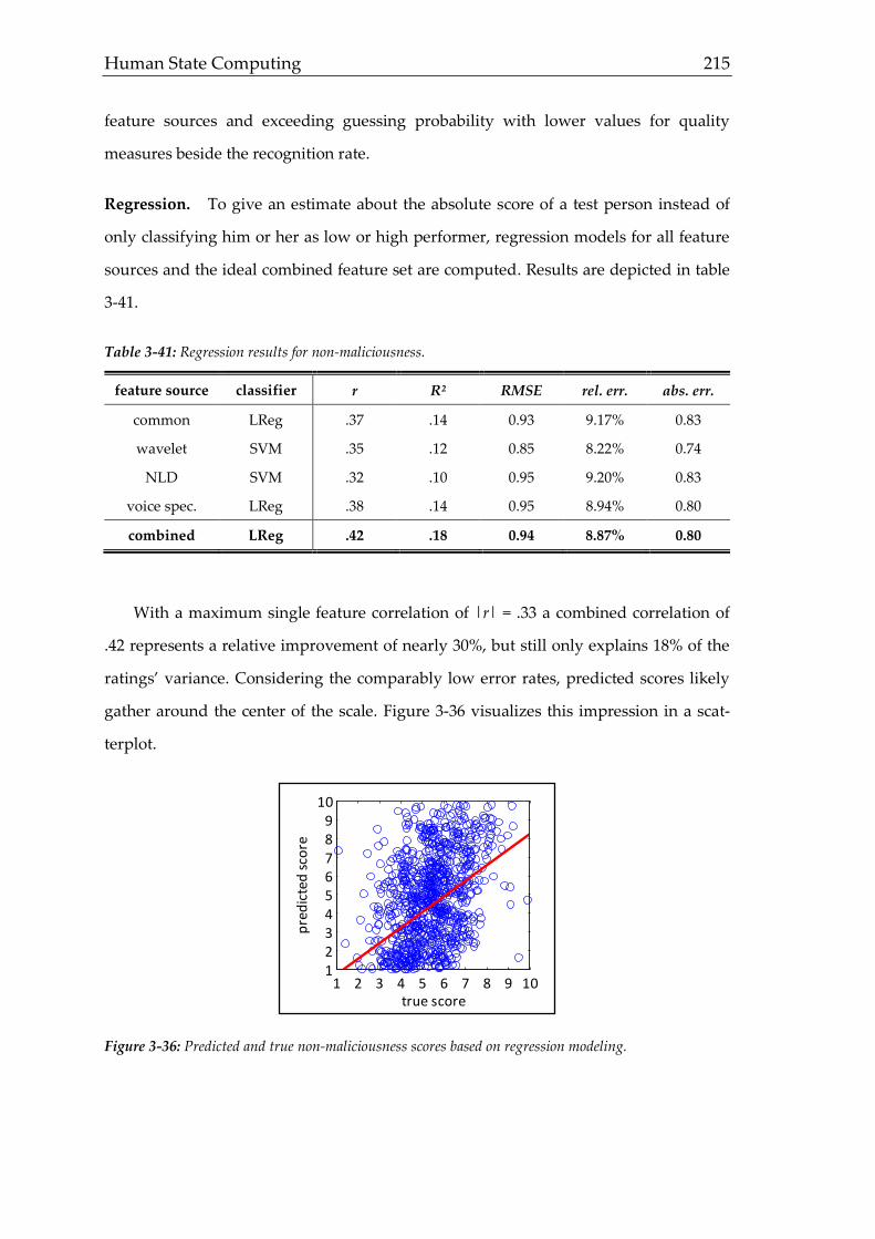
Human State Computing 215
feature sources and exceeding guessing probability with lower values for quality
measures beside the recognition rate.
Regression. To give an estimate about the absolute score of a test person instead of
only classifying him or her as low or high performer, regression models for all feature
sources and the ideal combined feature set are computed. Results are depicted in table
3-41.
Table 3-41: Regression results for non-maliciousness.
feature source classifier r R² RMSE rel. err. abs. err.
common LReg .37 .14 0.93 9.17% 0.83
wavelet SVM .35 .12 0.85 8.22% 0.74
NLD SVM .32 .10 0.95 9.20% 0.83
voice spec. LReg .38 .14 0.95 8.94% 0.80
combined LReg .42 .18 0.94 8.87% 0.80
With a maximum single feature correlation of |r| = .33 a combined correlation of
.42 represents a relative improvement of nearly 30%, but still only explains 18% of the
ratings’ variance. Considering the comparably low error rates, predicted scores likely
gather around the center of the scale. Figure 3-36 visualizes this impression in a scat-
terplot.
Figure 3-36: Predicted and true non-maliciousness scores based on regression modeling.
1 2 3 4 5 6 7 8 9 10123456789
10
true score
pre
dic
ted
sco
re
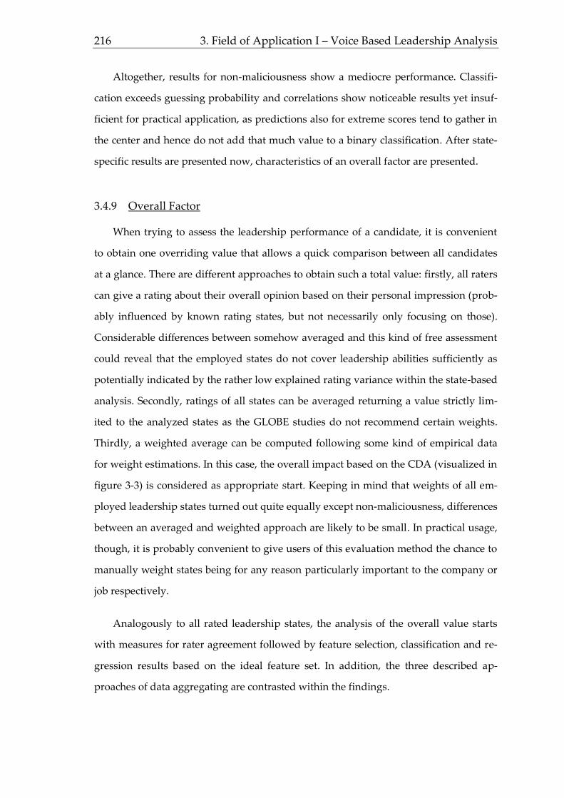
216 3. Field of Application I – Voice Based Leadership Analysis
Altogether, results for non-maliciousness show a mediocre performance. Classifi-
cation exceeds guessing probability and correlations show noticeable results yet insuf-
ficient for practical application, as predictions also for extreme scores tend to gather in
the center and hence do not add that much value to a binary classification. After state-
specific results are presented now, characteristics of an overall factor are presented.
3.4.9 Overall Factor
When trying to assess the leadership performance of a candidate, it is convenient
to obtain one overriding value that allows a quick comparison between all candidates
at a glance. There are different approaches to obtain such a total value: firstly, all raters
can give a rating about their overall opinion based on their personal impression (prob-
ably influenced by known rating states, but not necessarily only focusing on those).
Considerable differences between somehow averaged and this kind of free assessment
could reveal that the employed states do not cover leadership abilities sufficiently as
potentially indicated by the rather low explained rating variance within the state-based
analysis. Secondly, ratings of all states can be averaged returning a value strictly lim-
ited to the analyzed states as the GLOBE studies do not recommend certain weights.
Thirdly, a weighted average can be computed following some kind of empirical data
for weight estimations. In this case, the overall impact based on the CDA (visualized in
figure 3-3) is considered as appropriate start. Keeping in mind that weights of all em-
ployed leadership states turned out quite equally except non-maliciousness, differences
between an averaged and weighted approach are likely to be small. In practical usage,
though, it is probably convenient to give users of this evaluation method the chance to
manually weight states being for any reason particularly important to the company or
job respectively.
Analogously to all rated leadership states, the analysis of the overall value starts
with measures for rater agreement followed by feature selection, classification and re-
gression results based on the ideal feature set. In addition, the three described ap-
proaches of data aggregating are contrasted within the findings.
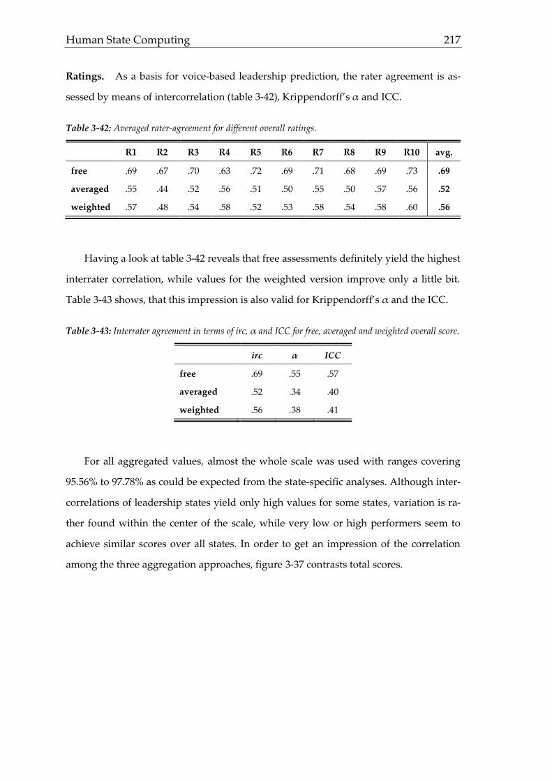
Human State Computing 217
Ratings. As a basis for voice-based leadership prediction, the rater agreement is as-
sessed by means of intercorrelation (table 3-42), Krippendorff’s α and ICC.
Table 3-42: Averaged rater-agreement for different overall ratings.
R1 R2 R3 R4 R5 R6 R7 R8 R9 R10 avg.
free .69 .67 .70 .63 .72 .69 .71 .68 .69 .73 .69
averaged .55 .44 .52 .56 .51 .50 .55 .50 .57 .56 .52
weighted .57 .48 .54 .58 .52 .53 .58 .54 .58 .60 .56
Having a look at table 3-42 reveals that free assessments definitely yield the highest
interrater correlation, while values for the weighted version improve only a little bit.
Table 3-43 shows, that this impression is also valid for Krippendorff’s α and the ICC.
Table 3-43: Interrater agreement in terms of irc, α and ICC for free, averaged and weighted overall score.
irc α ICC
free .69 .55 .57
averaged .52 .34 .40
weighted .56 .38 .41
For all aggregated values, almost the whole scale was used with ranges covering
95.56% to 97.78% as could be expected from the state-specific analyses. Although inter-
correlations of leadership states yield only high values for some states, variation is ra-
ther found within the center of the scale, while very low or high performers seem to
achieve similar scores over all states. In order to get an impression of the correlation
among the three aggregation approaches, figure 3-37 contrasts total scores.

218 3. Field of Application I – Voice Based Leadership Analysis
Figure 3-37: Intercorrelation of different leadership overall score approaches. Higher correlation/lower
variability results for averaged and weighted score (left hand figure), while free scores differ stronger
(right hand figure),
Figure 3-37 illustrates that the correlation between all three approaches is quite
high, whereas the correlation between averaged and weighted scores based on the
CDA is higher (r = 0.93, left side), while most variance is due to free scores (right side
with an averaged correlation of r = .76). Differences within the feature selection are
described hereafter.
Feature selection. Although ratings have shown some differences among the different
aggregations, some features turn out suitable for all overall score feature sets. In the
following table 3-44, all relevant features are given along with the respective correla-
tion.
wei
ghte
d s
core
wei
ghte
d s
core
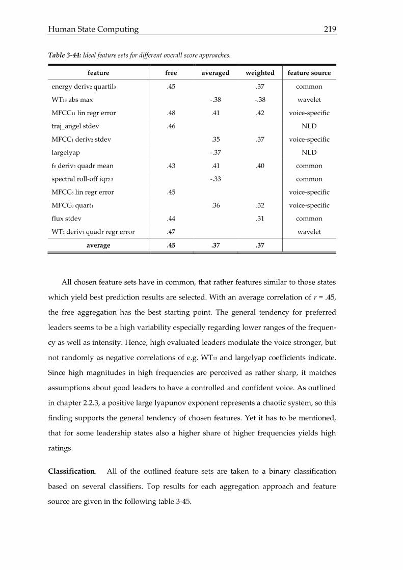
Human State Computing 219
Table 3-44: Ideal feature sets for different overall score approaches.
feature free averaged weighted feature source
energy deriv2 quartil3 .45 .37 common
WT13 abs max -.38 -.38 wavelet
MFCC11 lin regr error .48 .41 .42 voice-specific
traj_angel stdev .46 NLD
MFCC1 deriv2 stdev .35 .37 voice-specific
largelyap -.37 NLD
f0 deriv2 quadr mean .43 .41 .40 common
spectral roll-off iqr2-3 -.33 common
MFCC8 lin regr error .45 voice-specific
MFCC0 quart1 .36 .32 voice-specific
flux stdev .44 .31 common
WT2 deriv1 quadr regr error .47 wavelet
average .45 .37 .37
All chosen feature sets have in common, that rather features similar to those states
which yield best prediction results are selected. With an average correlation of r = .45,
the free aggregation has the best starting point. The general tendency for preferred
leaders seems to be a high variability especially regarding lower ranges of the frequen-
cy as well as intensity. Hence, high evaluated leaders modulate the voice stronger, but
not randomly as negative correlations of e.g. WT13 and largelyap coefficients indicate.
Since high magnitudes in high frequencies are perceived as rather sharp, it matches
assumptions about good leaders to have a controlled and confident voice. As outlined
in chapter 2.2.3, a positive large lyapunov exponent represents a chaotic system, so this
finding supports the general tendency of chosen features. Yet it has to be mentioned,
that for some leadership states also a higher share of higher frequencies yields high
ratings.
Classification. All of the outlined feature sets are taken to a binary classification
based on several classifiers. Top results for each aggregation approach and feature
source are given in the following table 3-45.
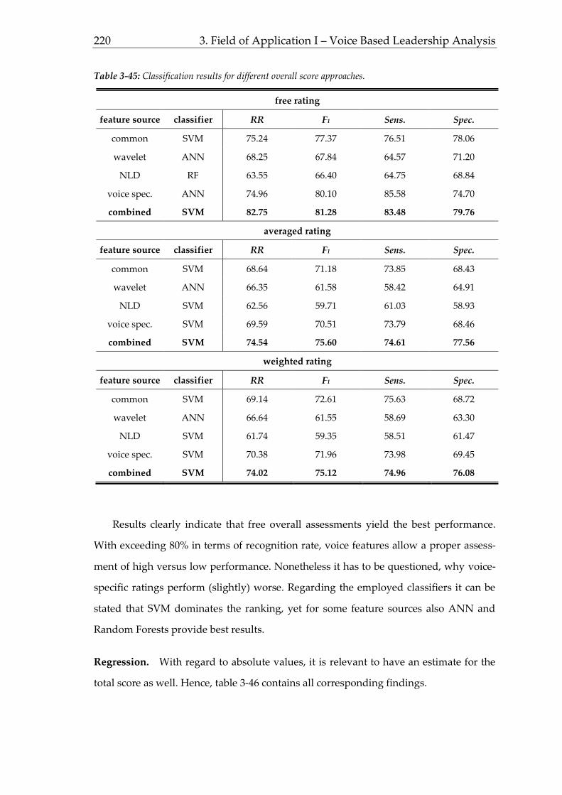
220 3. Field of Application I – Voice Based Leadership Analysis
Table 3-45: Classification results for different overall score approaches.
free rating
feature source classifier RR F1 Sens. Spec.
common SVM 75.24 77.37 76.51 78.06
wavelet ANN 68.25 67.84 64.57 71.20
NLD RF 63.55 66.40 64.75 68.84
voice spec. ANN 74.96 80.10 85.58 74.70
combined SVM 82.75 81.28 83.48 79.76
averaged rating
feature source classifier RR F1 Sens. Spec.
common SVM 68.64 71.18 73.85 68.43
wavelet ANN 66.35 61.58 58.42 64.91
NLD SVM 62.56 59.71 61.03 58.93
voice spec. SVM 69.59 70.51 73.79 68.46
combined SVM 74.54 75.60 74.61 77.56
weighted rating
feature source classifier RR F1 Sens. Spec.
common SVM 69.14 72.61 75.63 68.72
wavelet ANN 66.64 61.55 58.69 63.30
NLD SVM 61.74 59.35 58.51 61.47
voice spec. SVM 70.38 71.96 73.98 69.45
combined SVM 74.02 75.12 74.96 76.08
Results clearly indicate that free overall assessments yield the best performance.
With exceeding 80% in terms of recognition rate, voice features allow a proper assess-
ment of high versus low performance. Nonetheless it has to be questioned, why voice-
specific ratings perform (slightly) worse. Regarding the employed classifiers it can be
stated that SVM dominates the ranking, yet for some feature sources also ANN and
Random Forests provide best results.
Regression. With regard to absolute values, it is relevant to have an estimate for the
total score as well. Hence, table 3-46 contains all corresponding findings.

Human State Computing 221
Table 3-46: Regression results for different overall score approaches.
free rating
feature source classifier r R² RMSE rel. err. abs. err.
common LReg .51* .26 .75 9.67% 0.87
wavelet LReg .53* .28 .66 8.16% 0.73
NLD SVM .53* .28 .61 9.39% 0.85
voice spec. LReg .54* .29 .75 8.67% 0.78
combined LReg .60* .36 .66 7.61% 0.68
averaged rating
feature source classifier RR R² RMSE rel. err. abs. err.
common LReg .48* .23 .75 11.64% 1.05
wavelet LReg .47* .22 .66 10.54% 0.95
NLD SVM .43* .18 .61 13.27% 1.19
voice spec. LReg .51* .26 .75 9.61% 0.86
combined LReg .53* .28 .66 9.01% 0.81
weighted rating
feature source classifier RR R² RMSE rel. err. abs. err.
common LReg .48* .23 .74 11.07% 1.00
wavelet LReg .49* .24 .68 10.69% 0.96
NLD LReg .44* .19 .59 12.95% 1.17
voice spec. LReg .51* .26 .65 10.68% 0.96
combined LReg .54* .29 .63 9.16% 0.82
Analyzing the given regression results leads to the conclusion that with 36% ex-
plained variance for the free ratings the best value compared to all single states is
reached. Relative values over all aggregation approaches are quite low and hence al-
low a first estimate of the true score. In the following chapter, a short summary of all
findings comes along with a general discussion of all findings with regard to the stated
general and voice-specific hypotheses.
222 3. Field of Application I – Voice Based Leadership Analysis
3.5 Discussion
Considering the initial presentation of currently available leadership measures
yielding correlation with the actual leadership performance of about r ≤ .50 it is unde-
niable there is a need to enhance selection and training of leaders. Whether voice based
analysis can contribute to better measurement solutions or not, is assessed within this
chapter with regard to stated hypotheses and steps of biosignal processing.
Data Generation. In order to provide sufficient data for a leadership speech corpus,
176 speeches of different speakers are taken from online sources like YouTube. From
each speech, up to six tracks with a length of 30 seconds are taken to further analyses to
prevent biases based on long speeches. For yielding comparable data, each track is
preprocessed both manually and automatically to ensure only relevant information is
given within each track. As a possibly high consistency of data is desirable, the setting
of all speeches was quite equal, as only kind of presentations are chosen, whereas envi-
ronments with a stronger emphasis on interaction are omitted. Without anticipating
later discussions, results show, however, that some states seem to be quite difficult to
assess within the chosen context. Additionally, the scope of research is narrowed down
to male (probably) rather high performers giving the clear suggestion to extend this
scope to a broader sample in the future. Yet, advantageous of the chosen kind of data
acquisition is that firstly, speeches in natural surroundings are retrieved with the pos-
sibility to get real data, as acted data appear to be unsuitable (beside general issues) for
such complex states like the employed ones. Secondly, it is comparably easy to obtain a
large amount of data. On the contrary, it is discussed within the introductory chapter
that best validating data draw on both self and observer reports. Ratings of the subject,
however, cannot be used for this kind of data gathering technique. Hence, the quality
of validating data must be questioned in general.
For obtaining ratings, ten experienced raters were employed to give a qualified av-
eraged perception. Table 3-47 summarizes the rater agreement over all leadership
states and overall assessments.

Human State Computing 223
Table 3-47: Summary of interrater agreement. Columns for averaged and weighted overall scores are
excluded from the computation of total averages (last column).
Vis Ins Int Det Per Tea Dip Mal free avg wei total
icr .69 .67 .70 .63 .72 .69 .71 .68 .69 .52 .56 .66
α .55 .44 .52 .56 .51 .50 .55 .50 .55 .34 .38 .52
ICC .57 .48 .54 .58 .52 .53 .58 .54 .57 .40 .41 .55
The average rater agreement shows proper scores regarding correlation (r = .66) as
well as Krippendorff’s α (.52) and ICC (.55). Considering the extremely difficult task to
rate such complex states as required for leadership analyses, the agreement is satisfac-
tory. Though, it is obvious that despite the high experience of the raters it is difficult to
yield a higher level of agreement when assessing leadership states. As for the em-
ployed ratings only the sound is evaluated, it is indisputable that also other factors like
body language and mimic can contribute to leadership relevant states. All relevant
facets of data generation are summarized and evaluated regarding the data corpus
criteria stated in chapter 2.1 within the following table 3-48.
Table 3-48: Evaluation of voice corpus quality.
corpus criterion voice adaptation
validity anchor With the given natural source, no employment of self-reports was
possible. The general level of rater agreement heavily depends on
the respective state, but is all in all not satisfactory. Hence, methods
to improve ratings should be introduced in order to provide a bet-
ter foundation for prediction modeling. However, the complexity of
analyzed states having almost no physiological anchors must not be
ignored when interpreting the validity of ratings
perception test Previously to the assessments, raters were trained with unambigu-
ous samples leading to a comparably high agreement and hence a
general positive evaluation of the general possibility to rate leader-
ship states based on voice samples. Also video and other assess-
ments could be considered. Yet, recorded samples appeared to be
more difficult to assess than the test samples
class adaption Binary classes and continuous scores have been employed to allow
assessments from both sides. Although it can be questioned wheth-
er binary classifications are useful for leadership assessments, the
chosen approach should work for the general proof of method fea-
sibility

224 3. Field of Application I – Voice Based Leadership Analysis
ideal setting Although samples were preferably chosen from comparable set-
tings, the sample acquisition approach does not allow determining
a certain setting. So from this perspective a not ideal base for estab-
lishing a data corpus is given, although the advantage of the data
lies within its closeness to reality
repeatability Setting, hardware and software as well as the subjects and further
data operations are sufficiently described to repeat measurements
or systematically modify conditions in controlled settings
diversity For the initial stage of voice based leadership prediction, no interac-
tions with other states or demographics are analyzed. Yet, this can
be suggested for later stages of this approach
rating distribution The total sample wit over 1,000 tracks and more than 100 speakers
can be considered sufficient regarding representativity. As expected
from a representative corpus, data gather normally distributed
around the center. Yet, especially for states with lower rater agree-
ment, this tendency is too distinct for yielding proper classifications
availability Sharing recorded data to cooperate on building a bigger corpus
could be considered the next step of acoustic leadership assess-
ments. As the cooperation of Krajewski et al (2011) shows, first at-
tempts to spread the corpus have been made.
Although table 3-48 outlines some major drawbacks of the obtained data corpus, it
is still an improvement compared to the initial one. So the corpus extensions as well as
the reduced time amount per track and the expanded rating scale obviously already
have had a positive effect on the generated validating data.
Feature Extraction. With a focus on feature extraction, it is of crucial importance to
analyze whether the extraction for different sources is successful and in a later stage
leads to improved prediction results. As outlined in table 3-4, altogether 12,636 features
(compared to 6,670 within the initial corpus) are extracted for each of the 1,022 tracks.
For all feature sources except wavelet features, tracks are cut into overlapping analysis
windows with duration of 25ms allowing the computation of manifold functionals.
Window length for wavelet features is adapted according to frequency levels to best
possibly optimize time and frequency resolution. Altogether, a frequency bandwidth of
40Hz to 8kHz is analyzed. Computations are realized with different software like
openSMILE and own scripts based on Praat and Matlab.
Feature Selection. Correlative relations of ratings and features are on a mediocre lev-
el. Yet, the employed feed forward selection algorithm identified several useful fea-

Human State Computing 225
tures integrating all different feature sources supporting the hypothesis that all feature
sources can contribute to the prediction success. Features were added to each ideal
feature set, if the addition of a feature led to a significant of the recognition rate in-
crease (error α = .20) within two iteration cycles. Averaged and maximum single fea-
ture correlations for all analyzed leadership states are given in the following table 3-49.
Table 3-49: Maximum and averaged feature correlations for all leadership state-specific optimal feature
sets including different approaches of overall factors.
Vis Ins Int Det Per Tea Dip Mal free avg wei total
|r| max .46 .44 .32 .47 .49 .28 .24 .33 .48 .42 .41 .39
|r| avg .38 .37 .25 .40 .41 .22 .18 .27 .45 .37 .37 .33
Compared to the initial corpus version, selected features generally show higher
variability and lower intercorrelation establishing a better fundament for successful
predictions. Regarding other stated hypotheses, most expected acoustic perceptions
match features being sensitive for the respective leadership state. Fortunately, these
findings allow a theoretical linkage of empirically generated knowledge and theoreti-
cally derived assumptions as described in chapter 1.3.1 as well as in table 3-5. Regard-
ing the size of ideal feature sets, sizes of seven to nine features are chosen for ideal
prediction. With such small feature sets, very short computation times can be achieved
allowing real-time assessments.
Prediction Modeling. States representing several leadership relevant dimensions
have been analyzed. Within the cross-dimensional results it has already been outlined,
that relations between all states mirror outcomes of the underlying GLOBE study
(House, Hanges, Javidan, Dorfman, & Gupta, 2004) with some minor exceptions. Fur-
thermore, results are stable for both the initial and extended corpus version. Table 3-50
summarizes the classification and regression outcomes for all leadership states.
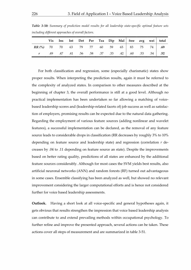
226 3. Field of Application I – Voice Based Leadership Analysis
Table 3-50: Summary of prediction model results for all leadership state-specific optimal feature sets
including different approaches of overall factors.
Vis Ins Int Det Per Tea Dip Mal free avg wei total
RR (%) 70 70 63 79 77 60 59 65 83 75 74 .69
r .49 .47 .41 .56 .58 .37 .33 .42 .60 .53 .54 .52
For both classification and regression, some (especially charismatic) states show
proper results. When interpreting the prediction results, again it must be referred to
the complexity of analyzed states. In comparison to other measures described at the
beginning of chapter 3, the overall performance is still at a good level. Although no
practical implementation has been undertaken so far allowing a matching of voice-
based leadership scores and (leadership-related facets of) job success as well as satisfac-
tion of employers, promising results can be expected due to the natural data gathering.
Regarding the employment of various feature sources (adding nonlinear and wavelet
features), a successful implementation can be declared, as the removal of any feature
source leads to considerable drops in classification (RR decreases by roughly 3% to 10%
depending on feature source and leadership state) and regression (correlation r de-
creases by .04 to .11 depending on feature source an state). Despite the improvements
based on better rating quality, predictions of all states are enhanced by the additional
feature sources considerably. Although for most cases the SVM yields best results, also
artificial neuronal networks (ANN) and random forests (RF) turned out advantageous
in some cases. Ensemble classifying has been analyzed as well, but showed no relevant
improvement considering the larger computational efforts and is hence not considered
further for voice based leadership assessments.
Outlook. Having a short look at all voice-specific and general hypotheses again, it
gets obvious that results strengthen the impression that voice based leadership analysis
can contribute to and extend prevailing methods within occupational psychology. To
further refine and improve the presented approach, several actions can be taken. These
actions cover all steps of measurement and are summarized in table 3-51.

Human State Computing 227
Table 3-51: Summary of future work for voice-based leadership analysis.
biosignal step suggestion
data generation improving validating data, extending scope of research to other
target groups, adapt setting state-specifically
feature extraction extending features (especially NLD), further adapt features to voice
phenomena
feature selection employing brute force for finalization, test other selection algo-
rithms
prediction modeling adjusting classifier parameters, further ensemble classifying
After having outlined the applicability of voice-based biosignal state analysis for
leadership assessment, the approach has to be adapted and transferred to other fields
of application to prove its wide-ranged feasibility. For this reason, mouse-movement
based fatigue detection is presented in the following chapter.


Human State Computing 229
4 FIELD OF APPLICATION II – MOUSE MOVEMENT BASED FATIGUE
DETECTION
After a complex mixture of states leading to an overall assessment of leadership
has been described in the last chapter, it is time to transfer the methodological ap-
proach to different settings. One widely researched and occupationally relevant state is
fatigue. Contrary to (probably) enduring states described in chapter 3, levels of fatigue
change quicker, wherefore fatigue detection requires adapted measurements with a
method suitable for every day usage. This chapter outlines corresponding research and
demonstrates the feasibility of a mouse-based biosignal measurement approach.
4.1 Fatigue Detection: Relevance and Empirical Findings
Within the relevance of leadership diagnostics (chapter 3.1) already several find-
ings have been presented underlining the importance of (mental) health and proper
work conditions. These facts also apply for sleepiness, as it is a proper predictor for
work accidents (Wright & McGowen, 2001; Melamed & Oksenberg, 2002) and is related
to mental diseases like burnouts for longer periods of sleep deprivation (Åkerstedt,
Kecklund, & Gillberg, 2007). While sleep-related diseases are more useful to be meas-
ured regularly in a long term with a low importance of the actual moment of meas-
urement, (work) accidents based on drowsiness, micro sleep or sleepiness can be re-
duced when any kind of alert interferes in the right moment. In the case of driving a
car, Rimini-Doering, Manstetten, Altmüller, Ladstätter, & Mahler (2001) hence pro-
posed, that growing complexity in today’s traffic paired with drowsiness and higher
work load lead to a considerable amount of severe car accidents. Similar relations have
been reported by other authors (Risser & Ware, 1999; Moller, Kayumov, Bulmash, Ni-
han, & Shapiro. 2006; Boyle, Tippin, Paul, & Rizzo, 2008; Golz, Sommer, Trutschel, Si-
rois, & Edwards, 2010; Forsman, Vila, Short, Mott, & van Dongen, 2013). These results
are easily transferable to other means of transportation like aircrafts (Borghini, Astolfi,
Vecchiato, Mattia, & Babiloni, 2012) or trains (Iridiastadi & Ikatrinasari, 2012).

230 4. Field of Application II – Mouse Movement Based Fatigue Detection
But not only (traffic) accidents are a subject of sleepiness detection, also the quality
of work e.g. in an office is influenced by adverse states of sleepiness. There is clear evi-
dence available, that sleepiness affects several cognitive abilities (Dinges, & Kribbs,
1991; Tassi, Pellerin, Moessinger Eschenlauer, & Muzet, 2000; Bratzke, Rolke, Ulrich &,
Peters, 2007). Furthermore, some authors state a relation between sleepiness and typi-
cally work-related factors like motivation and job satisfaction (Baldwin, Griffith, Nieto
et al., 2001; Dababneh, Swanson, & Shell, 2001; Engle-Friedman et al., 2003). Due to
these relevant findings, it is not surprising that lots of techniques have emerged to de-
tect sleepiness in various situations.
Recent Measurements. The first approach for most kinds of measurement have al-
ways been ratings based on observations, as people use their own perception as a
measurement tool for several issues all the day. Yet, without proper training and defi-
nitions what exactly to observe, ratings by observers always risk to be biased (Pod-
sakoff, MacKenzie, Lee, & Podsakoff, 2003). When using explicit features allowing an
objectification of what distinct behavior is assessed and employing a certain number of
raters, averaged observations are less influenced by interindividual differences in per-
ception (Muttray, Hagenmeyer, Unold, du Prel, & Geißler, 2007). As such observation
criteria are easier to define for states like sleepiness than for complex ones like de-
scribed for leadership states, high values for rater agreements can be expected.
Lots of observation based rating methods have shown up during the last decades.
Dealing with driver sleepiness, the Wierwille Rating Skala (WRS; Wierwille & Ellsworth,
1994) uses observable and well described features based on eyelid movement as well as
mimic and gestures like attempts of self-activation and divides sleepiness into four
stages, whereas the last one comprises micro sleep episodes. Decreasing frequency of
blinking paired with longer durations of winking as well as more comfortable sitting
position and flagging facial movement are key indicators for sleepiness in this test. Yet,
the range of only four sleepiness values seems too low for some fields of application.
With the HFC Müdigkeitsskala 2.0 (Kolrep, Rimini-Döring, Oehme, Jürgensohn, & Alt-
müller, 2005), nine stages reaching from awake to sleep are distinguished based on
nine indicators. In contrast to the WRS, though, different manifestations of each feature
are not clearly linked with the different states of sleepiness. Therefore, observers have

Human State Computing 231
to make up their own opinion based on the presence or degree of all nine indicators.
Combining the wider scale of the HFC scale with the detailed feature descriptions ad
stage allocations of the WRS leads to the TUBSS (TU Berlin Schläfrigkeitsskala; Dit-
trich, Brandenburg, & Thüring, 2009). TUBSS ratings choose a two step approach by
using the WRS video ratings first (resulting in a value reaching from one to four) fol-
lowed by tendency evaluations regarding adjacent stages. When there is a tendency
observable, interstage values are allotted leading in total to eight stages reaching from
not tired to micro sleep. Another WRS-based approach is the Observer Rating of Drowsi-
ness Protocol (ORD; Wiegand, McClafferty, McDonald, & Hanowski, 2009). Similar to
other scales, the ORD employs behavioral aspects and mannerisms for an assessment
of effects on the autonomic nervous system (Schnieder, Krajewski, Esch, Baluch, &
Wilhelm, 2012). As a last observer based evaluation, the widely used Karolinksa Sleepi-
ness Scale (KSS; Åkerstedt & Gillberg, 1990) is presented. It has proven decent correla-
tions with sophisticated physiological sleepiness measures like EEG (r = .56 following
Kaida et al., 2006) and reflects situational sensitive subjectively experienced states
within the last ten minutes (Shahid, Wilkinson, Marcu, & Shapiro, 2012). Employed in
experimental settings and combined with observer ratings, the KSS can be considered
an almost non-intrusive, fine ground truth estimate (Schnieder et al., 2012) and is hence
used for validation in the presented study. Scale values are described in table 4-1.
Table 4-1: KSS scale values and corresponding descriptions.
KSS value description
1 extremely alert
2 very alert
3 alert
4 rather alert
5 neither alert nor sleepy
6 some signs of sleepiness
7 sleepy, no effort to stay awake
8 sleepy, some efforts to stay awake
9 very sleepy, great effort to stay awake, fighting sleep
10 asleep

232 4. Field of Application II – Mouse Movement Based Fatigue Detection
While all mentioned scales lead to high interrater reliabilities of .75 < r < .95 (except
the subjective KSS, where no inter-rater reliability can be measured), there are signifi-
cant differences between observers (Dittrich, Brandenburg, & Thüring, 2009; Wiegand,
McClafferty, McDonald, & Hanowski, 2009). Despite a high retest reliability for WRS,
HFC and TUBSS (rtt > .9), all three scales except the TUBSS show significant mean dif-
ferences after one week.
When having a look at the indicators analyzed in the observer based ratings, it is
not surprising to find many descriptions focusing on movement in general and mimic
or respectively eye movement in particular. Physiological techniques allowing a re-
placement of observers with accurate sensors make further fatigue assessments availa-
ble. Starting with the most prominent representative for medicinal sleepiness research,
EEG waves have been differentiated to separate levels of vigilance (Torsvall & Åker-
stedt, 1987; Berka et al., 2007). In addition, the measurement of eye or pupil movements
(EOG, EMG, pupillography) ranks among the best gold standards for sleepiness detec-
tion (Ji, Zhu, & Lan, 2004; Canisius &Penzel, 2007).
Ratings as well as physiological measurements, however, lack of the possibility to
interfere in critical situations as video analyses or EEG measurements are time consum-
ing (regarding both preparation and evaluation) and hence not applicable in e.g. driv-
ing situations. For this reason, drivers’ sleepiness has been successfully detected by
means like steering behavior (Thiffault & Bergeron, 2003; Krajewski, Sommer,
Trutschel, Edwards, & Golz, 2009) or voice (Stemple, Stanley, & Lee, 1995; Krajewski &
Kröger, 2007). Also camera-related indicators like the videoplethysmography (measur-
ing heart rate based on video data) or thermographic devices have been employed
(Niedermeyer, 1999; Byeon et al., 2006; Park, Oh, & Han, 2009).
Yet, especially for assessing sleepiness while working, not only the objective, but
also the subjective perception of sleepiness is important for efficient working (Åker-
stedt & Gillberg, 1990). As the KSS is a both prominent and subjective approach, it is
employed (as mentioned above combined with observer ratings) as an indicator for
sleepiness. Due to several privacy issues, the use of cameras or other devices in an of-
fice is critical. Hence, an approach has to be found possibly using already present

Human State Computing 233
equipment, what is why the computer mouse is a suitable device for that field of appli-
cation. Several findings regarding reduced psychomotility, hand-eye coordination and
motor irregularities for fatigue probands (Dinges & Kribbs, 1991; Dawsoon & Reid,
1997; Tassi und Muzet, 2000; Jennings, Monk, & v. d. Molen, 2003; Nilsson et al., 2005)
strengthen this assumption. Table 4-2 summarizes pros and cons of several fatigue
measurement approaches.
Table 4-2: Evaluation of fatigue measurements. SEL = self-reports, COG = cognitive approaches, PHY =
physiological approaches, EYE = eye and pupil-related approaches, BRA = behavioral rating approaches,
BSY = behavioral device-supported object recognition approaches, LAT = sleep-latency based approaches,
ACO = acoustic approaches. Derived from Krajewski (2007, p. 23).
criteria SEL COG PHY EYE BRA BSY LAT ACO
validity o o + + o o + o
required resources
time + + - + + + - +
staff + + - o - + - +
costs + + - - + - - +
intrusiveness
adaption + - o + + + + o
calibration + o o o + o - +
measurement o - - + + + - +
suitable for
real-time monitoring - - o + - + + +
When thinking about hypotheses regarding mouse movement based changes for
different states of fatigue, several assumptions can be taken into account. Table 4-3
summarizes the assumed impact of fatigue on mouse movement.
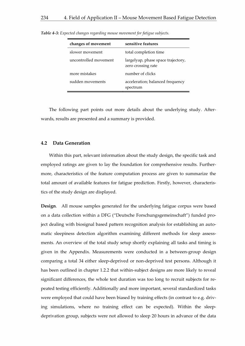
234 4. Field of Application II – Mouse Movement Based Fatigue Detection
Table 4-3: Expected changes regarding mouse movement for fatigue subjects.
changes of movement sensitive features
slower movement total completion time
uncontrolled movement largelyap, phase space trajectory,
zero crossing rate
more mistakes number of clicks
sudden movements acceleration; balanced frequency
spectrum
The following part points out more details about the underlying study. After-
wards, results are presented and a summary is provided.
4.2 Data Generation
Within this part, relevant information about the study design, the specific task and
employed ratings are given to lay the foundation for comprehensive results. Further-
more, characteristics of the feature computation process are given to summarize the
total amount of available features for fatigue prediction. Firstly, however, characteris-
tics of the study design are displayed.
Design. All mouse samples generated for the underlying fatigue corpus were based
on a data collection within a DFG (“Deutsche Forschungsgemeinschaft”) funded pro-
ject dealing with biosignal based pattern recognition analysis for establishing an auto-
matic sleepiness detection algorithm examining different methods for sleep assess-
ments. An overview of the total study setup shortly explaining all tasks and timing is
given in the Appendix. Measurements were conducted in a between-group design
comparing a total 34 either sleep-deprived or non-deprived test persons. Although it
has been outlined in chapter 1.2.2 that within-subject designs are more likely to reveal
significant differences, the whole test duration was too long to recruit subjects for re-
peated testing efficiently. Additionally and more important, several standardized tasks
were employed that could have been biased by training effects (in contrast to e.g. driv-
ing simulations, where no training effect can be expected). Within the sleep-
deprivation group, subjects were not allowed to sleep 20 hours in advance of the data
Human State Computing 235
recording (as for the whole testing process a time period of four hours was scheduled,
test persons did not sleep for about 24h in total). To ensure participants did not sleep
within the predefined time frame, emails were automatically sent in a randomized time
interval (hourly in average) containing simple questions (like “what is the capitol of
Germany” or computations like “what is 3+4+1”) that had to be answered within five
minutes after the email was sent and received. Although the aim of the approach was
to develop a measurement tool on individual level, a sleep-deprived group was used to
make sure there was sufficient variability within the ratings that can be explained by
mouse movement based features. All measurements were conducted in the morning at
9am to avoid an influence of daytime. Furthermore, sleep-related psychosomatic indi-
cators were controlled like sleep quality, depression and medication in order to use
only data not biased by these confounders. The subjects were aged between 18-59
years, M = 26.46, SD = 7.51 and consisted mainly of students (n = 23) and graduates (n =
8). The remaining n = 3 subjects graduated from high school and were full-time em-
ployees. Gender was equally distributed among the subjects (17 male, 17 female). Alto-
gether, 112 minutes of mouse recording were generated with an average of three
minutes and 13 seconds per person per session (SD = 33 seconds). All subjects were
incented with either €20 or certificates of attendance (“Versuchspersonenstunden”) as a
necessary condition to finish studies.
Task. As this study aimed to examine the value of mouse-based sleepiness assess-
ments in typical office tasks while working with a computer, subjects had to rebuild a
predefined simple Powerpoint slide (figure 4-1). The task was explained in detail on
the screen before and all subjects had the opportunity to ask for help, although no sub-
ject made use of that for this office task. All recordings took place in an office at the
Wuppertal University representing a suitable replacement of a common office envi-
ronment (figure 4-1). Only little technical equipment for other measurements reduced
the ordinariness, what potentially caused little behavioral changes. For a first attempt
to find a relationship between different biosignal feature sources and fatigue within
mouse movements, though, the effects of these confounders are probably negligible.

236 4. Field of Application II – Mouse Movement Based Fatigue Detection
Figure 4-1: Experimental setup (left) and PowerPoint slide (right) that had to be compiled by the subjects
within the office mouse task.
Although it was ensured all subjects were familiar with Microsoft PowerPoint due
to their job-related background (including university activities), experience with simi-
lar task might differ. Hence, the task difficulty was assessed by each subject yielding no
considerable differences. Furthermore, lacking experience with the software can be
supposed to rather affect features like total time of task completion (searching for the
suitable function), total number of clicks (corrections) and duration of inter-click inter-
vals (looking for where to click next). The movement itself when the target is clear
should not be affected, though, allowing a proper subject independent evaluation. Ac-
cordingly, analyses of the click to click behavior revealed only sleepiness but not indi-
vidual related effects, meaning the click behavior of similar fatigue (or awake) subjects
does not show considerable differences.
Ratings. The corpus was annotated by the same raters mentioned in chapter 3. Gen-
der effects were again controlled by Krippendorff’s α and significance testing, but no
differences could be found. All raters had been previously trained to apply the KSS
scale on subjects with the help of videos. In addition, the study setting allowed to also
obtain self reports which were surveyed before the task started. Matching self and ob-
server ratings further improves the basis for fatigue prediction as outlined in the intro-
ductory chapter.
Feature Extraction. In contrast to voice recordings, where data are generated with a
very high sampling rate (like 16kHz as used for leadership state prediction), mouse
Human State Computing 237
recording software commonly allows only recordings with a sampling rate of 100Hz
meaning that the position of the mouse cursor is tracked every 10ms. Hence, the high-
est observable frequency is 50Hz following the Nyquist-Shannon sampling theorem
described in chapter 2.2.1. With an average task duration of 193s, it does not make
sense to analyze frequencies lower than 0.1Hz at the same time. Considering this
heavily reduced frequency bandwidth, it is not useful to employ the same amount of
coefficients and ranges presented for voice analysis. In detail, the number all LFC and
wavelet coefficients was decreased from 24 to 6. To further reduce computational ef-
forts, the window size was adapted to the decreased frequency bandwidth as well.
While for voice analysis, overlapping frames of 25ms were employed covering a lowest
frequency of 40Hz, a window size of 100ms was chosen for all coefficients in the fre-
quency interval [10 50], 1s in the interval [1 9] and 10s in the interval [0.1 0.9]. Wavelet
features, though, adapt the frame size according to the analyzed frequency anyway
and are hence not in that way subject to changes of window sizes. Contributing to the
total feature set, though, is the possibility to analyze three data series based on changes
on the x-axes (movement from left to right and vice versa), the y-axes (movement from
top to bottom and vice versa) as well as the total distance s based on the Euclidian
point-to-point distance. As movement on the y-axis is a little bit more complex due to
the involvement of more muscles (stronger involvement of fingers, while movement
along the x-axis is primarily conducted with fixed fingers and movements in the wrist
and/or shoulder only), it is potentially easier affected by fatigue. The total computed
feature set comprising 22,464 features for all samples is depicted in the following table
4-4.

238 4. Field of Application II – Mouse Movement Based Fatigue Detection
Table 4-4: Source-specific overview of computed mouse movement features.
feature source feature categories num of
functionals total
common Centroid, Energy, Flux, Fbandw1-4,
LFCC0-6, Peaks, Roll-off1-4, ZCR [s,x,y] * 117 7722
wavelet WTs0-s6 [s,x,y] * 117 2457
NLD AMIFD1-3;τ1:5:10, Boxcounting1:5:10,
caoD1-3, corrdim, infodim, large-
lyap, traj_angle, traj_centdist,
traj_leglen
[s,x,y] * 117 9828
mouse-specific acc, click_dur, click_freq,
p2p_covdist, p2p_maxdist,
p2p_zcr, speed
[s,x,y] * 117 2457
Table 4-4 illustrates, that despite the reduced frequency range, the total feature set
almost doubles compared to voice analyses. This is due to the fact that with s, x and y
three different raw time series are analyzed and hence the total amount of features
grows. The benefits of this approach as well as other relevant findings are depicted in
the following chapter.
4.3 Results
Similar to the presentation of voice based analysis, results are given in the order of
biosignal analysis steps starting with an analysis of ratings followed by single feature
results and finally performance of prediction performance.
Ratings. As a basis for mouse movement based fatigue prediction, the rater agree-
ment is assessed by means of intercorrelation (table 4-5), Krippendorff’s α and ICC.
Table 4-5: Interrater correlation for fatigue.
R1 R2 R3 R4 R5 R6 R7 R8 R9 R10 avg.
.71 .74 .66 .79 .81 .73 .75 .74 .78 .69 .74
The average correlation of all raters scatters around r = .74 without significant out-
liers on an average level. For single correlations, however, R1 and R2 show a signifi-
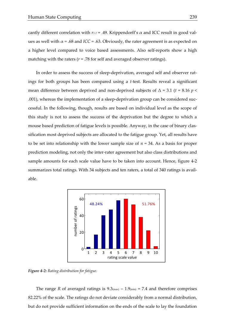
Human State Computing 239
cantly different correlation with r1-2 = .49. Krippendorff’s α and ICC result in good val-
ues as well with α = .68 and ICC = .63. Obviously, the rater agreement is as expected on
a higher level compared to voice based assessments. Also self-reports show a high
matching with the raters (r = .78 for self and averaged observer ratings).
In order to assess the success of sleep-deprivation, averaged self and observer rat-
ings for both groups has been compared using a t-test. Results reveal a significant
mean difference between deprived and non-deprived subjects of Δ = 3.1 (t = 8.16 p <
.001), whereas the implementation of a sleep-deprivation group can be considered suc-
cessful. In the following, though, results are based on individual level as the scope of
this study is not to assess the success of the deprivation but the degree to which a
mouse based prediction of fatigue levels is possible. Anyway, in the case of binary clas-
sification most deprived subjects are allocated to the fatigue group. Yet, all results have
to be set into relationship with the lower sample size of n = 34. As a basis for proper
prediction modeling, not only the inter-rater agreement but also class distributions and
sample amounts for each scale value have to be taken into account. Hence, figure 4-2
summarizes total ratings. With 34 subjects and ten raters, a total of 340 ratings is avail-
able.
Figure 4-2: Rating distribution for fatigue.
The range R of averaged ratings is 9.3(max) – 1.9(min) = 7.4 and therefore comprises
82.22% of the scale. The ratings do not deviate considerably from a normal distribution,
but do not provide sufficient information on the ends of the scale to lay the foundation
1 2 3 4 5 6 7 8 9 100
20
40
60
rating scale value
nu
mb
er o
f ra
tin
gs
48.24% 51.76%

240 4. Field of Application II – Mouse Movement Based Fatigue Detection
for a fatigue corpus. As this study tries to demonstrate the general applicability of the
mouse movement approach, though, variation seems adequate to give a first estima-
tion.
Feature Selection. Due to the high amount of features in general and promising single
features, the correlation filter threshold was increased by .05 to r ≥ .30 to reduce com-
putational efforts for features that are quite unlikely to be included to the final feature
set. After cropping the features with regard to the given filter criterion, 580 features
remain for the common feature set followed by 216 wavelet features, 1130 nonlinear
dynamic features and 325 mouse-specific features. The relative distribution is given in
figure 4-3.
Figure 4-3: Relative feature amount for fatigue exceeding the correlation filter. Share is based on the total
amount of computed features for each feature source.
The basic finding of this figure is, that all feature subsets yield suitable and compa-
rably high correlations with the fatigue KSS scores which are supposed to be predicted.
As with s, x and y different dimensions or time series are analyzed, table 4-6 gives an
overview of the averaged correlation passing the filter
Table 4-6: Comparison of movement dimension features exceeding the given correlation filter threshold.
dimension s x y
average |r| .41 .35 .38
common wavelet NLD mouse-spec.0
5
10
15
feat
ure
am
ou
nt
[%]
feature source

Human State Computing 241
Table 4-6 shows that the total covered distance s yields highest average correla-
tions, while results for x and y are in line with the assumption that movement
along the y-axes are sometimes more complex and hence more open for influ-
ence by state changes like fatigue. However, the significant differences between
all dimensions show a very small effect size of rΔ = .03, so that a theoretically de-
rived explanation must be treated carefully. After taking the upper 10% of all feature
sets to the consecutive feed forward selection, the following ideal prediction feature set
consisting of eight features is obtained (table 4-7).
Table 4-7: Remaining feature set for fatigue after feed forward selection.
feature r feature source
click_freq -.42 mouse specific
p2p_maxdev .40 mouse specific
s ZCR .39 common
p2p_covdist .38 common
y WT3 deriv2 stdev -.36 wavelet
s largelyap -.35 NLD
s f0 stdev -.34 common
s traj_angle deriv2 lin regr error .33 NLD
average |r| .37
Based on the chosen optimal features certain characteristics of fatigue mouse
movement can be stated. Starting with the click frequency it is shown that the average
time between two clicks increases for fatigue subjects. Following indications of mouse-
specific features, also the maximum deviation from the direct line between leads to a
more fatigue impression. The higher variance of the click to click behavior is also em-
phasized by the Zero Crossing Rate showing that fatigue subjects struggle following
the shortest way from one point to another. This impression is supported by the find-
ing that the total number of clicks required for fulfilling the task also increases for fa-
tigue subjects demonstrating that not only motor but also cognitive activity is affected
by this state change. Regarding involved frequencies fatigue subjects show a rather
monotonous but more chaotic movement pattern, as alert subjects yield high frequency
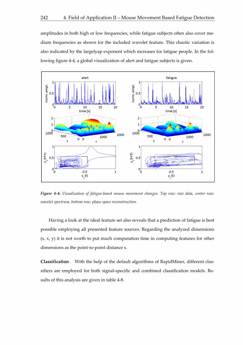
242 4. Field of Application II – Mouse Movement Based Fatigue Detection
amplitudes in both high or low frequencies, while fatigue subjects often also cover me-
dium frequencies as shown for the included wavelet feature. This chaotic variation is
also indicated by the largelyap exponent which increases for fatigue people. In the fol-
lowing figure 4-4, a global visualization of alert and fatigue subjects is given.
Figure 4-4: Visualization of fatigue-based mouse movement changes. Top row: raw data, center row:
wavelet spectrum, bottom row: phase space reconstruction.
Having a look at the ideal feature set also reveals that a prediction of fatigue is best
possible employing all presented feature sources. Regarding the analyzed dimensions
(s, x, y) it is not worth to put much computation time in computing features for other
dimensions as the point-to-point distance s.
Classification . With the help of the default algorithms of RapidMiner, different clas-
sifiers are employed for both signal-specific and combined classification models. Re-
sults of this analysis are given in table 4-8.
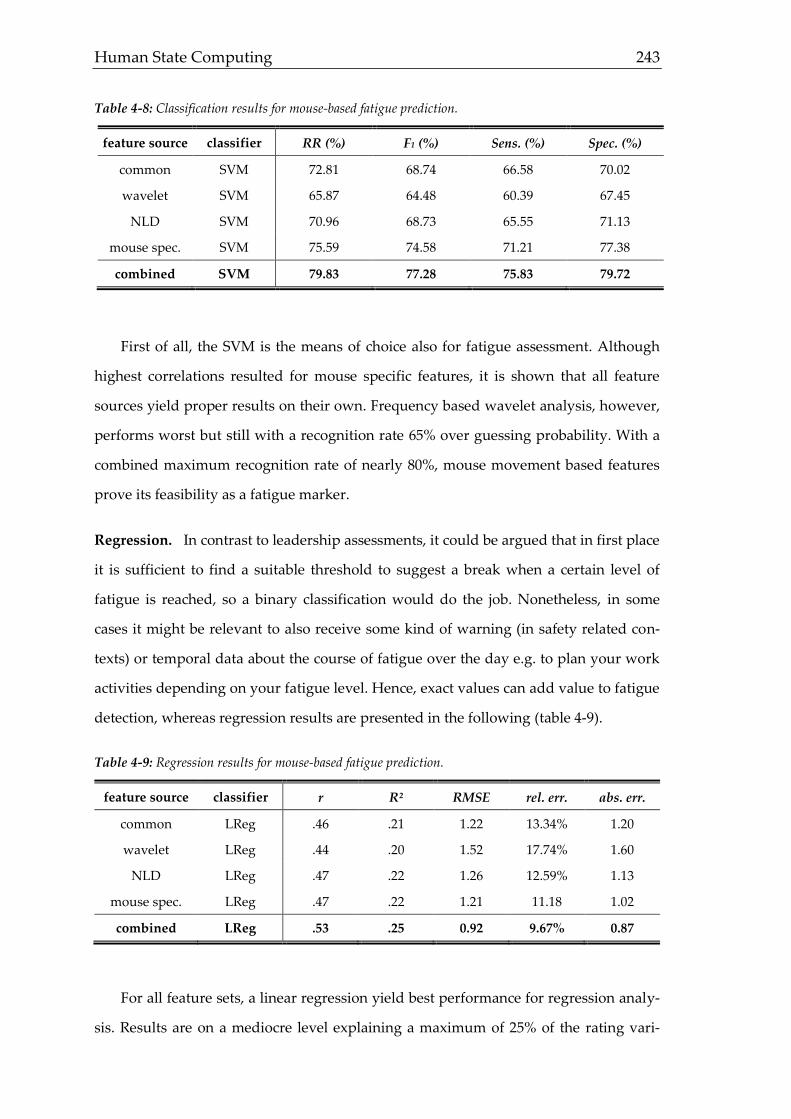
Human State Computing 243
Table 4-8: Classification results for mouse-based fatigue prediction.
feature source classifier RR (%) F1 (%) Sens. (%) Spec. (%)
common SVM 72.81 68.74 66.58 70.02
wavelet SVM 65.87 64.48 60.39 67.45
NLD SVM 70.96 68.73 65.55 71.13
mouse spec. SVM 75.59 74.58 71.21 77.38
combined SVM 79.83 77.28 75.83 79.72
First of all, the SVM is the means of choice also for fatigue assessment. Although
highest correlations resulted for mouse specific features, it is shown that all feature
sources yield proper results on their own. Frequency based wavelet analysis, however,
performs worst but still with a recognition rate 65% over guessing probability. With a
combined maximum recognition rate of nearly 80%, mouse movement based features
prove its feasibility as a fatigue marker.
Regression. In contrast to leadership assessments, it could be argued that in first place
it is sufficient to find a suitable threshold to suggest a break when a certain level of
fatigue is reached, so a binary classification would do the job. Nonetheless, in some
cases it might be relevant to also receive some kind of warning (in safety related con-
texts) or temporal data about the course of fatigue over the day e.g. to plan your work
activities depending on your fatigue level. Hence, exact values can add value to fatigue
detection, whereas regression results are presented in the following (table 4-9).
Table 4-9: Regression results for mouse-based fatigue prediction.
feature source classifier r R² RMSE rel. err. abs. err.
common LReg .46 .21 1.22 13.34% 1.20
wavelet LReg .44 .20 1.52 17.74% 1.60
NLD LReg .47 .22 1.26 12.59% 1.13
mouse spec. LReg .47 .22 1.21 11.18 1.02
combined LReg .53 .25 0.92 9.67% 0.87
For all feature sets, a linear regression yield best performance for regression analy-
sis. Results are on a mediocre level explaining a maximum of 25% of the rating vari-

244 4. Field of Application II – Mouse Movement Based Fatigue Detection
ance for the combined feature set. In terms of the KSS scale, an assessment differs in
average by almost 1 level from the assumed true score. Considering the few ratings at
the end of the scale, though, the low error values are likely due to a stronger tendency
towards the center. All in all, results strengthen a feasible linkage of mouse movement
to fatigue levels. The description of this study is closed by a summary of all findings.
4.4 Discussion
Relevant fatigue measurements presented in chapter 4.1 revealed that assessments
are not only required in safety related contexts, but also in typical office environments.
Momentarily available methods, however, lack of feasibility, although a better fatigue
measurement can contribute to more efficient and healthier work. Within this chapter,
all stated general and mouse-specific hypotheses are discussed following steps of bi-
osignal processing.
Data Generation. In order to allow an estimation of mouse based fatigue detection, a
data corpus with 34 sleep-deprived and non-deprived subjects and 109 minutes of re-
cording was established. Recordings were taken in the morning within the course of
multiple fatigue-related measurements. Mouse measurements were conducted while
executing a typical office task (compiling a PowerPoint presentation slide). Data were
automatically and manually preprocessed to ensure a satisfactory and comparable
quality. Although the task itself is quite natural, a drawback is the total conduction
time for all mouse-unrelated tasks within this study. Furthermore, some features like
the total completion time cannot be implemented in every-day application easily. Alt-
hough obviously (in this context) critical features are not selected for the ideal feature
set, it has to be questioned how well e.g. inter click intervals predict fatigue in other
tasks, as compiling presentation slides might be a typical, but definitely not the only
task for employees. In how far it is necessary to adapt algorithms can only be shown
within field studies. Beside these practical deliberations the generally low amount of
data has to be considered just allows assessing a general possibility to employ mouse
based features for fatigue prediction in office environments. For a final algorithm,
though, the data corpus has to be extended massively to reach a general validity.

Human State Computing 245
Regarding the ratings, it can be noted that due to the fatigue induction by sleep-
deprivation a certain degree of variance is achieved. Nonetheless, both self and observ-
er ratings miss examples for the ends of the employed KSS scale building a suboptimal
basis for prediction modeling. Otherwise, the rater agreement yields sufficient results
with an averaged interrater correlation of rirc = .74 as well as Krippendorff’s α and ICC
on a similar level. Although rating fatigue is assumed to be easier than the more com-
plex leadership states, values are satisfactory. To give a summary of the established
data corpus, all initially mentioned criteria are analyzed (table 4-10).
Table 4-10: Evaluation of the mouse movement data corpus.
corpus criterion mouse movement adaptation
validity anchor Self and observer reports were employed. Combination with physi-
ological measures could improve the validity. Unambiguity due to
mediocre rater agreement is questionable. Employing acted data
cannot be recommended for sleep
perception test Previously to the assessments, raters were trained with unambigu-
ous samples leading to a very high agreement and hence a positive
evaluation of the general possibility to visually rate fatigue. Yet,
recorded samples appeared to be more difficult to assess, although
the rater agreement can be considered satisfactory
class adaption Binary classes and continuous scores have been employed to allow
assessments from both sides. Relevant number of classes could be
adapted application-specifically, but should work for the general
proof of method feasibility
ideal setting Environment was chosen possibly realistic, yet the circumstance of
being recorded with manifold sensors as well as the sleep-
deprivation decrease the setting quality
repeatability Setting, hardware and software as well as the subjects and further
data operations are sufficiently described to repeat measurements
or systematically modify conditions
diversity For the initial stage of mouse movement based fatigue prediction,
no interactions with other states or demographics are analyzed. Yet,
this can be suggested for later stages of this approach
rating distribution The low total sample size does not allow sufficient training data for
ends of the scale. Although it can be argued whether prediction
models should base on representative samples or equally distribut-
ed data, with the given distribution no generally valid model can be
established
availability Sharing recorded data to cooperate on building a bigger corpus is
not supposed to be targeted before a proper and more realistic set-
ting is chosen. At this stage, only the general applicability of the
chosen approach is demonstrated

246 4. Field of Application II – Mouse Movement Based Fatigue Detection
Considering the chosen approach in this thesis, an important step towards a prop-
er corpus has been made. Nonetheless, table 4-10 also reveals many things to improve
before a practical feasibility is given.
Feature Extraction. With a focus on feature extraction, it is of crucial importance to
analyze whether the extraction for different sources is successful and in a later stage
leads to improved prediction results. As outlined in table 4-4, altogether 22,464 features
are extracted for each of the 34 mouse recordings. Due to the much lower covered fre-
quency range from 0.1Hz-50Hz compared to 40Hz-8kHz in voice analysis, the length of
analysis frames was adapted. For frequency based features (except wavelet features),
three different window sizes were employed to on the one hand obtain a sufficient
number of windows for computing functionals and on the one hand cover potentially
relevant very low frequencies <1Hz. While recordings of mouse movement is done
with the help of the free software MouseLogger with a sampling frequency of 100Hz,
features are generated as described before with adapted scripts from openSMILE, Praat
and Matlab.
Feature Selection. Correlative relations of ratings and features are on a mediocre lev-
el. Yet, the employed feed forward selection algorithm identified several useful fea-
tures integrating all different feature sources supporting the hypothesis that all feature
sources can contribute to the prediction success. Although the general impact of signal-
specific features is a little bit higher than for voice analysis, especially NLD features
performed on a comparably high level (table 4-3). Within the selection process, features
were added to the ideal feature set, if the addition of a feature leads to a significant (α =
.10) increase of the recognition rate within two iteration cycles. In the end, an ideal fea-
ture set consisting of eight features was selected for prediction modeling. Most of the
features match previously stated hypotheses proving also a theoretical linking of
mouse movement and fatigue. In general, features illustrate that fatigue subjects show
less determinant mouse movements with more required clicks, bigger deviation from
the direct way and more chaotic movements with a rather stepwise approaching of the
target.
Human State Computing 247
Prediction Modeling. It has already been outlined that in contrast to voice analysis,
sometimes binary classifications can be sufficient in many situations for a practical us-
age, e.g. when an employee just gets noticed when his or her mouse movement pattern
indicates that it would make sense to do a break if possible. Having a look at the classi-
fication results with a optimal recognition rate of nearly 80%, it cannot be denied there
is a considerable connection between mouse movement and fatigue. Although it is dif-
ficult or yet impossible to find studies to compare with, 80% seems like a good starting
point to further optimize the approach. Also the employment of different feature
sources is reasonable as the removal of one source leads to a decrease in terms of
recognition rate between 7% and 8%. Focusing on the technical side, SVMs (again)
turned out to be the superior classifier for mouse movement. Although other classifier
show good results as well, SVM is the best choice also keeping the computational effort
in mind. Ensemble classifying has been analyzed as well, but showed no relevant im-
provement (RR +3%) considering the larger computational efforts and hence cannot be
suggested unconditionally.
Regarding regression outcomes, it can be stated that with a total explained vari-
ance of 25% there is still much room for improvement. The biggest problem for regres-
sion, however, is the high tendency towards the center of the scale increasing the prob-
ability of a medium predicted score dramatically. Although the absolute/relative error
is quite low, the corpus obviously requires major extensions to yield sufficient training
data at the end of the scales. For building the regression model, linear regression out-
performed SVM and quadratic regression. Nonetheless, it still makes sense to test other
algorithms as well, as the corpus requires major changes to be used for fatigue predic-
tion on a continuous scale.
Outlook. Having a short look at all mouse-specific and general hypotheses, results
strengthen the impression that mouse based fatigue analysis can contribute to and ex-
tend prevailing methods within occupational psychology. As there are no real alterna-
tives available at the moment to measure fatigue in an office environment in a feasible
way, it can be suggested to follow this approach to further refine and improve the pre-
sented approach, several actions can be taken. These actions cover all steps of meas-
urement and are summarized in table 4-11.

248 4. Field of Application II – Mouse Movement Based Fatigue Detection
Table 4-11: Future work for mouse-movement based fatigue prediction.
biosignal step suggestion
data generation heavily extending the corpus (especially at ends of the scales), widen
scope of research to other target groups, adapt and test other settings,
combine with other biosignals (e.g. video-based analysis)
feature extraction extending features (especially NLD and mouse-specific), further adapt
features to mouse phenomena
feature selection employing brute force for finalization, test other selection algorithms
prediction modeling adjusting classifier parameters, further ensemble classifying for revised
corpora
After having outlined the applicability of mouse-based biosignal state analysis for
leadership assessment, the general method is also transferred to both different biosig-
nal and state. The following field of application focuses on head movement based
stress assessment.

Human State Computing 249
5 FIELD OF APPLICATION III – HEAD MOVEMENT BASED STRESS
ASSESSMENT
To further prove the wide-ranged feasibility of a non-intrusive biosignal based
measurement approach for different occupationally relevant states, a third and last
study is described making the attempt to predict stress based on head movements.
Although there might be other biosignals at first glance seeming to have more in com-
mon with stress, this chapter demonstrates the usability of head movements also in the
field of stress research allowing non-intrusive measurements with the help of cheap
and often already available sensors as is the case for webcams. Before the analysis is
presented, however, a short overview of relevant theoretical aspects and empiric re-
search regarding stress is depicted.
5.1 Stress Measurement: Relevance and Empirical Findings
The term “stress” is frequently used in everyday life. Everybody seems to naturally
know what stress is and how it feels to be stressed. To allow valid inferences from re-
search data regarding a certain state, though, it is of major importance to clarify what is
expected from rater and self-reports when assessing a state. Hence, as a theoretical in-
troduction to head movement based stress prediction, information about the employed
stress definition as well as fields of research and measurement techniques is provided.
Definition. For defining a state or psychological construct in general, it is always a
good start to see how the term is used so far. Regarding stress, there is a general
agreement that an interaction of the environment and a person potentially leads to a
stress reaction (figure 5-1).

250 5. Field of Application III – Head Movement Based Stress Assessment
Figure 5-1: General stress model. Stressors cause a stress response which has an effect on psychological,
physiological and behavioral level. Derived from Aldwin (2007).
Beyond these very basic assumptions, different opinions evolved over the decades.
Selye (1950; 1956) as one of the initiators of stress research proposed a reactional model
with a strict focus on physiological outcomes (e.g. increased heart rate, release of
adrenaline and noradrenaline, muscle tone) summarized as General Adaption Syn-
drom (GAS). Furthermore, it has to be taken into account there are not only negative
but also positive variations of stress reported when distinguishing distress and eustress
(Selye, 1956). As Selye’s reactional model focuses on physiological reactions and was
only proven in animals, Holmes & Rahe (1967) even attempted to allocate fixed stress
scores to several events within a stimulus-oriented stress theory rather focusing on the
impact of stimuli (table 5-1).
environment person
stimulus response
stressorstress
response
psychological
physiological
behavioral

Human State Computing 251
Table 5-1: Top ten of Holmes & Rahe's stress scale (1967).
rank incident life change units
1 death of spouse 100
2 divorce 73
3 marital separation 65
4 imprisonment 63
5 death of close relative 63
6 personal injury/illness 53
7 marriage 50
8 dismissal from work 47
9 marital reconciliation 45
10 retirement 45
Following this model, it is commonly distinguished between outer conditions like
unemployment or time pressure called stressors and corresponding inner conditions
referred to as strain as the corresponding state (Pearlin & Schooler, 1978). Bodenmann
& Gmelch (2009, p. 619) differentiate the following stressors:
Social stressors
Physical stressors
Ecological stressors
Economical stressors
Job-related stressors
Monotony stressors
Adding health stressors, it gets obvious that manifold circumstances in life possi-
bly induce stress. One big drawback of both mentioned approaches, though, is the rig-
id relation of stressors and strain allowing (theoretically) no differences on the one
hand in the physiological reaction independent of the stressor (reactional model), while
on the other hand the kind of physiological response is only determined by the stress-
or, with the same outcome when exposed to the same stressor (stimulus-oriented mod-

252 5. Field of Application III – Head Movement Based Stress Assessment
el). These inflexible models ignore the vital role of cognition for the perceived level of
stress (or from this angle better called strain).
So what is meant when talking about stress? Within the cognitive-transactional stress
theory proposed by Lazarus (Lazarus & Launier, 1978), an interaction of stressors, cog-
nition and physiological output is assumed defining (psychological) stress as the “par-
ticular relationship between the person and the environment that is appraised by the
person as taxing or exceeding his or her resources and endangering his or her well-
being” (Lazarus & Folkman 1984, p. 19). The cognitive processes as the centerpiece of
the theory are divided into the following three parts and are further illustrated in fig-
ure 5-2.
Within the primary appraisal, a situation is considered stressful, non-stressful
or irrelevant. Stressful situations in turn can be divided into threat (possible
impairment), challenge (future and rather positive event) and harm/loss (al-
ready occurred impairment) .
When a situation is assessed (potentially) stressful, within the second ap-
praisal available resources helping to overcome the situation are evaluated
to avoid a harm/loss
After performing a counteraction, the situation is reappraised lead. When the
issue remains unsolved and stressful, stress reactions continue
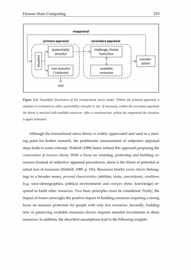
Human State Computing 253
Figure 5-2: Simplified illustration of the transactional stress model. Within the primary appraisal, a
situation is evaluated as either (potentially) stressful or not. If necessary, within the secondary appraisal
the threat is matched with available resources. After a counteraction, within the reappraisal the situation
is again evaluated.
Although the transactional stress theory is widely appreciated and used as a start-
ing point for further research, the problematic measurement of subjective appraisal
steps leads to some criticism. Hobfoll (1989) hence refined this approach proposing the
conservation of resource theory. With a focus on retaining, protecting and building re-
sources (instead of subjective appraisal procedures), stress is the threat of potential or
actual loss of resources (Hobfoll, 1989, p. 516). Resources hereby cover objects (belong-
ings in a broader sense), personal characteristics (abilities, traits, convictions), conditions
(e.g. socio-demographics, political environment) and energies (time, knowledge) re-
quired to build other resources. Two basic principles must be considered: Firstly, the
impact of losses outweighs the positive impact of building resources requiring a strong
focus on resource protection for people with only few resources. Secondly, building
new or preserving available resources always requires stressful investments in these
resources. In addition, the described assumptions lead to the following insights:
situ
atio
n
(potentially) stressful
counter-action
challenge, threat,harm/loss
available resources
non-stressful / irrelevant
end
primary appraisal secondary appraisal
reappraisal

254 5. Field of Application III – Head Movement Based Stress Assessment
1) Having only few resources available increases the probability of a loss leading
to a further increased loss probability (loss spiral)
2) Having many resources available increases the probability of building new
ones (spiral of profit)
Following Knoll, Scholz & Rieckmann (2005), Hobfoll’s conservation of resource
theory is appreciated as a useful extension of the transactional stress theory. Having
the integrative interdisciplinary approach of this thesis in mind and referring to chap-
ter 1.2, both physiological and psychological concepts rather represent two sides of the
same coin, as the psychological state ψ is represented by physiological differences in φ
allowing a proper biosignal based assessment of states. Therefore, stress can be derived
from both Lazarus and Hobfoll as an activation of the nervous system based on a perceived
mismatch between the sufficiency of available resources and expected or present threats. This
definition is chosen for handling several circumstances. Firstly, stress is seen as a phys-
iological (and hence quite objectively measureable) reaction. Secondly, it is assumed
that stress can result from both inner and outer conditions, whereas no according dif-
ferentiation is implemented. Thirdly, to include cognitive processes, the perception of a
situation is supposed to be more important than actual givens. Fourthly, stress can also
result from scenarios that need not necessarily come true. So the main conflict respon-
sible for creating the physiological response identified as stress is the perception (of a
person), that one is not able to handle a situation leading to negative consequences
when unsolved, what can also be transferred to difficulties of affiliated persons (Ald-
win, 2007, p. 32). Hence, stress is always negative in this definition, while positive ver-
sions like the mentioned eustress or first appraisal challenges are not considered a part
of stress (but rather as euphoria, joy or the like). Expected neurophysiological respons-
es cover therefore those ones being linked with an activation of the peripheral nervous
system with symptoms depicted in table 5-2.

Human State Computing 255
Table 5-2: behavioral and physiological stress responses. Adapted from Aldwin (2007, p.25).
behavioral stress reaction physiological stress reaction
increased arousal and alertness oxygen and nutrients directed to the CNS
and stressed body sites
increased cognition, vigilance and focused
attention
altered cardiovascular tone, increased blood
pressure and heart rate
euphoria/dysphoria increased respiratory rate
increased analgesia increased gluconeogenesis and lipolysis
increased body temperature detoxification from toxic products
suppression of appetite and feeding behavior inhibition of growth and reproduction
containment of the stress response containment of the inflammatory/immune
response
So when rating a person, raters are supposed to follow e.g. the visible body cues
described in table 5-2. Suitable and recordable biosignals are those in line with the
physiological response reaching from more or less invasive signals like using endo-
crinological markers to non-intrusively recordable biosignals like motor behavior in
general or head movement in particular.
Empirical Findings. As outlined before, stress has been subject to many different
fields of research. Chapter 3 already indicated the impact of burnout on our working
society. Stress, especially over a longer time period (based on lack of time referring to
resources mentioned before or abilities leading to fear of failures), is considered one of
the main predictors of burnout and is hence heavily researched (see for an overview
e.g. Maslach & Leiter, 1997; Schaufeli & Baker, 2004). This also applies for related psy-
chological diseases like depression (Hammon, 2005) and anxiety assessment (Depres-
sion Anxiety Stress Scales DASS by Crawford & Henry, 2003). Another mediate effect
of long term stress on both mental and physical health are changes of the immune sys-
tem. Following a much-noticed meta-study of Segerstrom & Miller (2004), chronic
stressors suppress both cellular and humoral immune responses, while short- and me-
dium-term stressors (only) affect subunits of the immune system. Hence, it can be con-
cluded from a physiological view that stress, especially in a long run, leads to several
serious psychosomatic problems (see the simplified illustration in the following figure
5-3.

256 5. Field of Application III – Head Movement Based Stress Assessment
Figure 5-3: standard psychoneuroimmunology model of stress and health. Adapted from Aldwin (2007,
p. 18).
Further research on physiological responses to stress (Hagemann, 2009) showed
that not only quickly decomposed hormones like adrenaline and noradrenaline (level
is reduced to 50% in about three to five minutes) are released, but also cortisol which is
decomposed to 50% in about 90 minutes. High cortisol levels in turn are associated in
the long run with several psychosomatic diseases as mentioned above. In addition to
long-term stress-related diseases, critical events like participating in war or mourning a
severe loss can lead to acute stress disorders (ICD F43.0; or post-traumatic stress disor-
ders ICD F43.1, as can be further derived from Dilling, Momour, & Schmidt, 1991) also
in a short-term.
Narrowing the focus a little bit down to occupationally relevant aspects of day-to-
day work, not only diseases but also the quality of work is of crucial importance. Start-
ing with findings reported by Motowidio, Packard, & Manning (1986) analyzing the
impact of stressors and self- as well as observer based stress levels on social, emotional
and cognitive skills, revealed significant correlations for all analyzed aspects of the job
performance. Other empiric studies evaluating the daily work of nurses strengthen
these outcomes (e.g. AbuAlRub, 2004; Applebaum, Fowler, Fiedler, Osinubi, & Robson,
2010 focusing on environmental givens). However, research on job performance does
not only focus on nurses. Following a meta-study by Fried, Shirom, Gilboa, & Cooper
(2008) analyzing 113 independent samples with more than 22,000 subjects, direct and
indirect effects of stress on job-relevant factors like fluctuation and performance were
stressnegative
affect
health outcomes
immune system change
neuroendocrine change

Human State Computing 257
found. Since stress has a certain effect on job satisfaction, also the widely minded rela-
tionship of job satisfaction and performance can be considered. Judge, Thoresen, Bono,
& Patton (2001) give a broad overview of this field of research analyzing different ef-
fects. The following figure 5-4 is derived from their work now including stress as a
variable.
Figure 5-4: relational models of stress and job performance. Although the list does not cover all imagina-
ble relations, most important general types are provided. Adapted from Judge, Thoresen, Bono, & Patton
(2001).
Now general stress diseases and relations to broad occupational constructs have
been discussed. Going one step further and considering not only long-term or health-
related phenomena, also effects on task execution are to consider as wrong decisions or
data due to stress are of vital economical interest. Already in chapter 1.2 the Yerkes-
Dodson-Law has been described postulating that too low or high arousal causes
model 1
model 2
model 3
model 4
model 5
model 6
model 7
stress job performance
stress job performance
stress job performance
stress job performance
stress job performance
stress job performance
stress job performance
C
C
C

258 5. Field of Application III – Head Movement Based Stress Assessment
suboptimal performance. Having defined stress (partly) as a certain kind of arousal
possibly induced by circumstances endangering resources by both too low (e.g. bore-
dom, monotony) or too high (e.g. time pressure, losses) arousal, best performance can
be expected for environments where resources can be built or are at least not threat-
ened. Within their attentional control theory (ACT), Eysenck, Derakshan, Santos, &
Calvo, 2007) propose that anxiety (caused by stressful situations) leads to a reduction
of attentional control (inhibition) and a shifting of cognitive resources to threatening
stimuli (so when finishing an important presentation under time pressure, less atten-
tion is paid on the presentation itself, while resources are shifted to the threatening
event of being unable to finish in time or in a broader sense to fail). The quality of per-
formance is therefore only satisfactory, if compensatory resources are available to
counteract and e.g. increase processing resources, so that still sufficient attention is
paid on the relevant task (see figure 5-5).
Figure 5-5: Performance based on the interaction of inhibition/shifting and compensatory resources fol-
lowing the ACT model. Performance is determined by the success of compensatory resources.
Having this theoretical approach in mind, it is not surprising that several studies
report a decrease of performance for both cognitive (Fiedler, 1995; Linden, Keijsers,
Eling, & Schaijk, 2005; Beilock, 2008) and manual tasks (Mese, Kok, Lewis, & Wyon,
1984; Birch, Juul-Kristensen, Jensen. Finsen, & Christensen, 2000; Lundberg, 2005),
which are not observable the same way for persons with supposed high coping re-
sources Fogarty et al., 1999; LePine, Podsakoff, & LePine, 2005; Darr & Johns, 2008; ).
As head movement based stress is supposed to extend currently available stress meas-
urement, the next part focuses on how stress is assessed so far.
stressful situation
inhibition / shifting
compensatory resources –
per
form
ance
+

Human State Computing 259
Recent Measurements. Stress as a construct is theoretically complex and on the one
hand depends on several factors (like stressors and coping abilities), while on the other
hand temporal issues (short-term measurement for predicting distinct task-related per-
formance versus long-term measurements evaluating the risk of psychosomatic diseas-
es) have to be considered. Adding both the level of interest (e.g. company, department,
individual) and the environment (e.g. office, manual work, indoor, outdoor) manifold
different measurements have emerged leading to a complexity of required tools. Since
head movement based stress detection rather focuses on short-term assessment in the
first place and is supposed to complement recent approaches being hardly applicable
in every day work, no detailed analysis of all aspects is necessary at this place. None-
theless, prominent representatives covering different facets of stress measurement are
outlined in the following.
Questionnaires. For most constructs and states, psychological research comes up with a
variety of questionnaires (sometimes including data acquisition via interviews) what
applies also for measuring stress. Within this wide field, the following approaches can
be differentiated (Ulich, pp. 63):
condition-related (assessing the work task)
semi-objective (also covering e.g. subjective stress perception)
individual-related (subjective statements regarding different dimensions)
Although the above mentioned distribution of tests is not only suitable for stress-
related measurements, but also for other fields of research, a few questionnaires focus-
ing on the work environment, tasks und subjective perception are outlined. Condition-
related questionnaires like the TBS (Hacker, Fritsche, Richter, & Iwanowa, 2003), VERA
with the allocated RHIA (Leitner et al., 1993) give a detailed description about objec-
tively identifiable details of a task. Taking the VERA questionnaire (German acronym
for a procedure to identify job tasks requiring coping resources) as an example, five
different regulatory aspects of job tasks are depicted as there are opening new fields of
activity, coordination of plural fields of activity, planning, subgoals, planning actions
and sensomotoric regulation. After assessing the job environment (e.g. required educa-

260 5. Field of Application III – Head Movement Based Stress Assessment
tion, work hours per week, work space, variety of tasks), common task outcomes, work
equipment and used information are gathered. In a last step, coping requirements are
determined by a question algorithm leading to a final classification for the job. Even
this brief description elucidates the quite high amount of time required for retrieving
all relevant information about the job, before a final assessment can take place. Hence,
a short-term evaluation is not facilitated, although it allows a good comparison of dif-
ferent departments or companies.
Giving an example for semi-objective questionnaires, the SynBA-GA (Synthetic
stress and work analysis for computer-oriented jobs by Wieland-Eckelmann,
Saßmannshausen, Rose, & Schwarz, 1999, focusing on employees mainly sitting in
front of a screen) is to mention. In addition to the objectively determinable job re-
quirements mainly analyzed with methods like the RHIA, also the subjective effect of
the job conditions (tasks, environment, etc.) is taken into account. Key elements of a job
(e.g. completeness of job task, scope for decision making and acting, avoidance of cop-
ing limitations, adequate performance targets, cooperation and social interaction) are
measured on three levels (individual, organizational, interactional) to allow distinct
recommendations of actions for suboptimal tasks.
By presenting the SALSA (salutogenetic subjective work analysis by Riman &
Udris, 1997), also subjective approaches are covered. Following Antonovsky’s corre-
sponding theoretical concept (1997), the SALSA focuses on conditions that maintain
and recover resources. Comprising 60 items allocated to 17 scales and five key factors
(job characteristics, workload, environmental factors, organizational and social re-
sources), it is quite a quick test allowing comparisons with provided reference data.
Ratings. Although questionnaires are of proper use when strategic in-depth insights
are required, it is hardly possible to employ such a measurement technique for gaining
a momentarily assessment of the actual stress level. Even daily event measures like the
Daily Life Experience Checklist (DLE, Stone & Neale, 1982), the Daily Stress Inventory
(DSI, Brantley & Jones, 1993), or the Hassle Scale (DeLongis, Folkman, & Lazarus, 1988)
only provide information about potentially stressful events. Hence, questionnaires are
not suitable for obtaining validating data for biosignal based state predictions. Short

Human State Computing 261
ratings bringing down the (self-)perception down to a single value, underlie the com-
mon rating drawbacks already mentioned in chapter 1. Nonetheless, self- and observer
reports are the only possibility to give a sufficiently quick and flexible estimation. As
there is to the author’s knowledge no stress-scale available comparably to mentioned
sleepiness scales (e.g. KSS) in chapter 4, proprietary scales for self- and observer re-
ports have to be developed. While it lasts out to just rate a recent stress level for stress
reports, observers have more time due to recording for deciding on a stress level. Fol-
lowing Rapee & Lim (1992), specific items (e.g. voice shaking, hands trembling) are
more effective than global ones (e.g. confident appearance). Hence, all ratings are
based on a short list of questions covering expected physiological changes for stressed
participants following indications mentioned above (more details are given within the
description of data generation in chapter 5.2).
Physiological Measures. When looking for a baseline, physiological measurements are
frequently used for several states as depicted in the last chapters. Also regarding stress,
some prominent measures have evolved and are commonly used as a reference. It has
already been outlined, that endocrinological changes like the cortisol or adrenaline
concentration can give a baseline for stress assessment (Fox, Dwyer, & Ganster, 1993;
Burke, Davis, Otte, & Mohr, 2055; Krajewski, Sauerland, & Wieland, 2011). Other so-
matic symptoms going alone with stress reactions like increased heart rate or blood
pressure (Lazarus, Speisman, & Mordkoff, 1963; McCraty, Atkinson, Tiller, Rein, &
Watkins, 1995; Vrijkotte, van Doornen, & de Geus, 2003), flat and accelerated respira-
tion (Aldwin, 2007, p. 23), perspiration (Masaoka, Onaka, Shimizu, Sakurai, & Homma,
2007, using e.g. EDA), trembling/shaking of voice or hands (Kendall, Flannery-
Schroeder, & Panichelli-Mindel, 1997) or (video-based) behavioral assessments (Giv-
ens, 2006; Preußners, 2006) have also been observed frequently. All of those approaches
not using non-intrusive biosignal measurement techniques lack of feasibility issues
mentioned in chapter 1.1.3, as taking blood or saliva samples is not useful for everyday
usage and takes quite a long time for getting results. Also blood pressure or heart rate
based measurements are hard to employ free of interference in a working environment
(if not established via videoplethysmography). In the same way, observer-based meth-
ods also cannot overcome mentioned drawbacks.
262 5. Field of Application III – Head Movement Based Stress Assessment
For all these reasons, it can be concluded that there are hardly methods available
for situation-specific stress level assessment. Hence, in the following details of a study
are presented to give an overview of stress assessments based on head movement.
5.2 Data Generation
Within this part, relevant information about the study design, the specific task,
employed ratings and data processing are given to lay the foundation for comprehen-
sive results. Furthermore, characteristics of the feature computation process are given
to summarize the total amount of available features for fatigue prediction. Firstly,
however, characteristics of the study design are displayed.
Design. All video samples generated for the underlying stress corpus were based on a
data collection within a university office. Measurements were taken for a total of 36
students (M = 25.13, SD = 4.36, equal gender distribution) simulating a job interview for
a student assistant position in the department. All subjects agreed to be recorded for
academic purposes via video camera. The interview duration was approximately 30
minutes. Altogether, a total of 980 minutes of cleansed recording resulted after prepro-
cessing. To make sure no other state-related confounders biased the results, fatigue
levels and medication were controlled via a KSS scale and a short question regarding
medication after the interview, but no significant differences for KSS scales or consid-
erable medications could be found. Although social desirability/honesty has to be con-
sidered in such a situation, also a general assessment of the body language and behav-
ior led to no exclusion of subjects.
Task. As this study aimed to examine the value of head movement based stress as-
sessments in a typical occupational situation, stress was induced by conducting a simu-
lated job interview for a research assistant position. To increase the stress level, the
interview was conducted in English. Although there was no English native speaker,
English skills deviated and hence further led to more variance within the experienced
stress level. The task in general was not explained to the subjects before, so they only
knew they would be recorded while simulating a job interview. All recordings took
place in an office at the Wuppertal University representing a suitable replacement of a

Human State Computing 263
common office. Apart from the employed video camera located at height of head in
opposite of the subjects, no equipment or other surroundings could be identified as
confounders. Although the presence of a video camera is supposed to be disturbing,
for the sake of stress assessments the setting was only problematic in case head move-
ments differed systematically for recording situations, but this is quite unlikely espe-
cially with regard to the length of the interview. To keep interviews comparable, a
timeline with discussion topics was compiled to make sure all recordings were taken
under the same conditions. For conducting possibly natural interviews, however, the
timeline given in table 5-3 was only used as a reference to structure the interview, but
should also allow little deviation in case the interview got stuck otherwise.
Table 5-3: Timeline for simulated online interviews.
time [min] topic
0-5 introduction of the applicant
5-15 discussion of relevant skills
(methods, literature research, writing and social skills)
15-25 case study: how to conduct a study analyzing fatigue-
based voice changes
25-30 closing; general comments
Ratings. The corpus was annotated by the same raters mentioned in the previous
fields of application. Gender effects were again controlled by Krippendorff’s α and
significance testing, but no differences could be found for the interviewees. All raters
had been previously trained to apply a scale from one to ten for stress assessments
with the help of videos. For increasing the rater agreement, the presence of the follow-
ing criteria was summed up to yield a total value (table 5-4) containing observable
stress indicators as outlined in chapter 5.1.
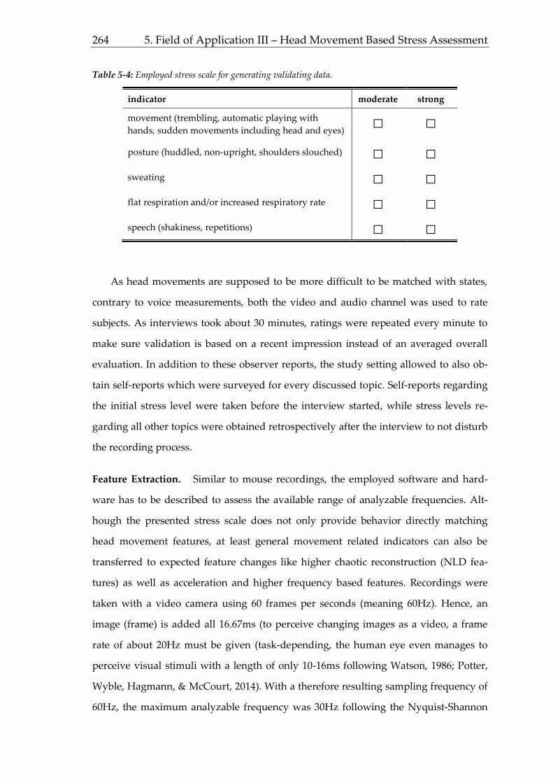
264 5. Field of Application III – Head Movement Based Stress Assessment
Table 5-4: Employed stress scale for generating validating data.
indicator moderate strong
movement (trembling, automatic playing with
hands, sudden movements including head and eyes) □ □
posture (huddled, non-upright, shoulders slouched) □ □
sweating □ □
flat respiration and/or increased respiratory rate □ □
speech (shakiness, repetitions) □ □
As head movements are supposed to be more difficult to be matched with states,
contrary to voice measurements, both the video and audio channel was used to rate
subjects. As interviews took about 30 minutes, ratings were repeated every minute to
make sure validation is based on a recent impression instead of an averaged overall
evaluation. In addition to these observer reports, the study setting allowed to also ob-
tain self-reports which were surveyed for every discussed topic. Self-reports regarding
the initial stress level were taken before the interview started, while stress levels re-
garding all other topics were obtained retrospectively after the interview to not disturb
the recording process.
Feature Extraction. Similar to mouse recordings, the employed software and hard-
ware has to be described to assess the available range of analyzable frequencies. Alt-
hough the presented stress scale does not only provide behavior directly matching
head movement features, at least general movement related indicators can also be
transferred to expected feature changes like higher chaotic reconstruction (NLD fea-
tures) as well as acceleration and higher frequency based features. Recordings were
taken with a video camera using 60 frames per seconds (meaning 60Hz). Hence, an
image (frame) is added all 16.67ms (to perceive changing images as a video, a frame
rate of about 20Hz must be given (task-depending, the human eye even manages to
perceive visual stimuli with a length of only 10-16ms following Watson, 1986; Potter,
Wyble, Hagmann, & McCourt, 2014). With a therefore resulting sampling frequency of
60Hz, the maximum analyzable frequency was 30Hz following the Nyquist-Shannon
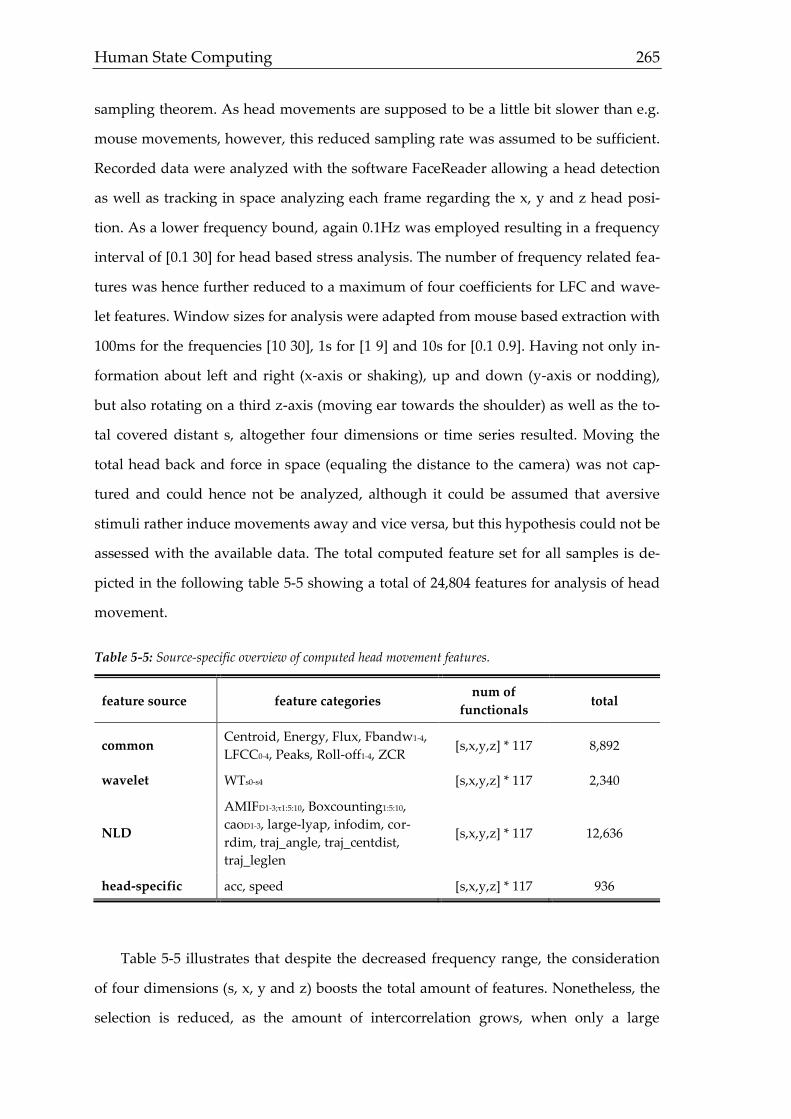
Human State Computing 265
sampling theorem. As head movements are supposed to be a little bit slower than e.g.
mouse movements, however, this reduced sampling rate was assumed to be sufficient.
Recorded data were analyzed with the software FaceReader allowing a head detection
as well as tracking in space analyzing each frame regarding the x, y and z head posi-
tion. As a lower frequency bound, again 0.1Hz was employed resulting in a frequency
interval of [0.1 30] for head based stress analysis. The number of frequency related fea-
tures was hence further reduced to a maximum of four coefficients for LFC and wave-
let features. Window sizes for analysis were adapted from mouse based extraction with
100ms for the frequencies [10 30], 1s for [1 9] and 10s for [0.1 0.9]. Having not only in-
formation about left and right (x-axis or shaking), up and down (y-axis or nodding),
but also rotating on a third z-axis (moving ear towards the shoulder) as well as the to-
tal covered distant s, altogether four dimensions or time series resulted. Moving the
total head back and force in space (equaling the distance to the camera) was not cap-
tured and could hence not be analyzed, although it could be assumed that aversive
stimuli rather induce movements away and vice versa, but this hypothesis could not be
assessed with the available data. The total computed feature set for all samples is de-
picted in the following table 5-5 showing a total of 24,804 features for analysis of head
movement.
Table 5-5: Source-specific overview of computed head movement features.
feature source feature categories num of
functionals total
common Centroid, Energy, Flux, Fbandw1-4,
LFCC0-4, Peaks, Roll-off1-4, ZCR [s,x,y,z] * 117 8,892
wavelet WTs0-s4 [s,x,y,z] * 117 2,340
NLD
AMIFD1-3;τ1:5:10, Boxcounting1:5:10,
caoD1-3, large-lyap, infodim, cor-
rdim, traj_angle, traj_centdist,
traj_leglen
[s,x,y,z] * 117 12,636
head-specific acc, speed [s,x,y,z] * 117 936
Table 5-5 illustrates that despite the decreased frequency range, the consideration
of four dimensions (s, x, y and z) boosts the total amount of features. Nonetheless, the
selection is reduced, as the amount of intercorrelation grows, when only a large

266 5. Field of Application III – Head Movement Based Stress Assessment
amount of functionals is computed for only a few main features. The benefits of this
approach as well as other relevant findings, however, are depicted in the following
chapter.
5.3 Results
Also for head movement analysis, results are given in the order of biosignal analy-
sis steps starting with an analysis of ratings followed by single feature results and fi-
nally performance of prediction performance.
Ratings. As a basis for head movement based prediction of a recent stress level, the
rater agreement is assessed by means of intercorrelation (table 5-6), Krippendorff’s α
and ICC.
Table 5-6: Interrater correlation for stress.
R1 R2 R3 R4 R5 R6 R7 R8 R9 R10 avg.
.62 .55 .57 .56 .54 .62 .67 .52 .61 .53 .58
The average correlations of all raters scatter around r = .58 without significant out-
liers on an average level. For single correlations, some outliers appear with a maximum
range of rirc_min = .43 to rirc_max = .75. Krippendorff’s α and ICC result in mediocre values
as well with α = .42 and ICC = .39. Obviously, the rater agreement is as expected on a
lower level than fatigue assessments, as despite some training it can be considered a
difficult task to assess a stress level from video and hence body language/mimic. Re-
garding self-reports, though, a matching shows values being in line with other inter-
rater correlations. To illustrate the course of perceived and observed stress during the
interview, figure 5-6 gives a comparison.
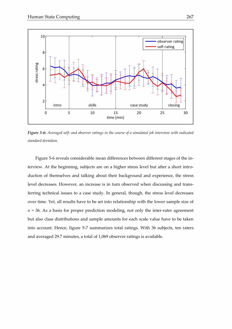
Human State Computing 267
Figure 5-6: Averaged self- and observer ratings in the course of a simulated job interview with indicated
standard deviation.
Figure 5-6 reveals considerable mean differences between different stages of the in-
terview. At the beginning, subjects are on a higher stress level but after a short intro-
duction of themselves and talking about their background and experience, the stress
level decreases. However, an increase is in turn observed when discussing and trans-
ferring technical issues to a case study. In general, though, the stress level decreases
over time. Yet, all results have to be set into relationship with the lower sample size of
n = 36. As a basis for proper prediction modeling, not only the inter-rater agreement
but also class distributions and sample amounts for each scale value have to be taken
into account. Hence, figure 5-7 summarizes total ratings. With 36 subjects, ten raters
and averaged 29.7 minutes, a total of 1,069 observer ratings is available.
0 5 10 15 20 25 30
2
4
6
8
10
time [min]
stre
ss r
atin
g
intro skills case study closing
observer rating
self-rating
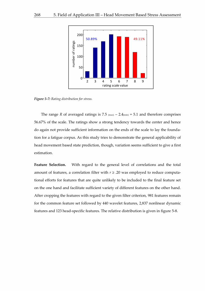
268 5. Field of Application III – Head Movement Based Stress Assessment
Figure 5-7: Rating distribution for stress.
The range R of averaged ratings is 7.5 (max) – 2.4(min) = 5.1 and therefore comprises
56.67% of the scale. The ratings show a strong tendency towards the center and hence
do again not provide sufficient information on the ends of the scale to lay the founda-
tion for a fatigue corpus. As this study tries to demonstrate the general applicability of
head movement based state prediction, though, variation seems sufficient to give a first
estimation.
Feature Selection. With regard to the general level of correlations and the total
amount of features, a correlation filter with r ≥ .20 was employed to reduce computa-
tional efforts for features that are quite unlikely to be included to the final feature set
on the one hand and facilitate sufficient variety of different features on the other hand.
After cropping the features with regard to the given filter criterion, 981 features remain
for the common feature set followed by 440 wavelet features, 2,837 nonlinear dynamic
features and 123 head-specific features. The relative distribution is given in figure 5-8.
2 3 4 5 6 7 8 90
50
100
150
200
rating scale value
nu
mb
er o
f ra
tin
gs
50.89% 49.11%
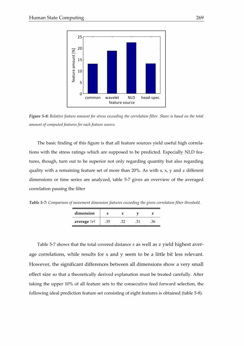
Human State Computing 269
Figure 5-8: Relative feature amount for stress exceeding the correlation filter. Share is based on the total
amount of computed features for each feature source.
The basic finding of this figure is that all feature sources yield useful high correla-
tions with the stress ratings which are supposed to be predicted. Especially NLD fea-
tures, though, turn out to be superior not only regarding quantity but also regarding
quality with a remaining feature set of more than 20%. As with s, x, y and z different
dimensions or time series are analyzed, table 5-7 gives an overview of the averaged
correlation passing the filter
Table 5-7: Comparison of movement dimension features exceeding the given correlation filter threshold.
dimension s x y z
average |r| .35 .32 .31 .36
Table 5-7 shows that the total covered distance s as well as z yield highest aver-
age correlations, while results for x and y seem to be a little bit less relevant.
However, the significant differences between all dimensions show a very small
effect size so that a theoretically derived explanation must be treated carefully. After
taking the upper 10% of all feature sets to the consecutive feed forward selection, the
following ideal prediction feature set consisting of eight features is obtained (table 5-8).
common wavelet NLD head-spec.0
5
10
15
20
25
feat
ure
am
ou
nt
[%]
feature source

270 5. Field of Application III – Head Movement Based Stress Assessment
Table 5-8: Remaining feature set for stress after feed forward selection.
feature r feature source
z acc mean peak dist -.39 head specific
s largelyap deriv1 stdev .38 NLD
s speed median .37 head specific
s WT2 deriv1 mean peak dist .35 wavelet
y ZCR stdev .34 common
s traj_angle deriv1 quadr regr error -.33 NLD
y max lin regr error -.31 common
average |r| .35
Based on the chosen optimal features certain characteristics of head movement un-
der stress can be stated. Starting with the chosen top feature, as expected a high varia-
bility in terms of peaks yields a stressful perception meaning that people more fre-
quently move their head noticeably along the z-axis, so the other way around high dis-
tances (in the temporal domain) between peaks in the z-axis acceleration is perceived
less stressed. Further matching previous assumption is the fact that moving the head
downwards (nodding or respectively keeping the head below the baseline) regarding
the y-axis leads to a more stressful perception. Although it’s unlikely within a common
conversation that people lift their head permanently, the covered total integral none-
theless correlates considerably with the stress ratings. High zero crossing rate for
stressed subjects strengthen this impression, as a frequent zero crossing could be inter-
preted as a steady reminder to keep the head looking straight ahead and hence correct-
ing the head position. Rather random or chaotic movements further characterize
stressed head movements. With regard to the frequency domain, however, only one
wavelet feature is included in the final set. Yet, some frequency related features turned
out to be useful for visualizing differences in stressed head movement. For this reason,
the following figure 5-9 contrast findings for stressed and (rather) relaxed subjects.

Human State Computing 271
Figure 5-9: Visualization of stress-based head movement changes. Top row: raw data, center row: wavelet
spectrum, bottom row: phase space reconstruction.
Having a look at the ideal feature set also reveals that a prediction of stress is best
possible employing all presented feature sources. Regarding the analyzed dimensions
(s, x, y, z) features derived from movements along the x-axis are not included in the
ideal feature set. Nonetheless, contrary to mouse movement potential differences espe-
cially for the z-axis can be stated. With regard to figure 5-9, it is shown that the general
amount of head movements decreases for stressed subjects (lower amplitudes in top
row) with corresponding lower amplitudes in the wavelet spectrum (center row), but
with considerable peaks for high frequencies strengthening the impression of rather
sudden movements. The phase space reconstruction also highlights the more chaotic
nature of stressful head movement by slightly higher deviations within the trajectory
figure.
Classification. With the help of the default algorithms of RapidMiner, different classi-
fiers are employed for both signal-specific and combined classification models. Results
of this analysis are given in table 5-9.
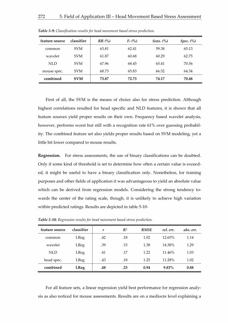
272 5. Field of Application III – Head Movement Based Stress Assessment
Table 5-9: Classification results for head movement based stress prediction.
feature source classifier RR (%) F1 (%) Sens. (%) Spec. (%)
common SVM 63.81 62.41 59.38 65.13
wavelet SVM 61.87 60.68 60.29 62.75
NLD SVM 67.96 68.45 65.41 70.56
mouse spec. SVM 68.73 65.83 66.52 64.34
combined SVM 73.87 72.73 74.17 70.48
First of all, the SVM is the means of choice also for stress prediction. Although
highest correlations resulted for head specific and NLD features, it is shown that all
feature sources yield proper results on their own. Frequency based wavelet analysis,
however, performs worst but still with a recognition rate 61% over guessing probabil-
ity. The combined feature set also yields proper results based on SVM modeling, yet a
little bit lower compared to mouse results.
Regression. For stress assessments, the use of binary classifications can be doubted.
Only if some kind of threshold is set to determine how often a certain value is exceed-
ed, it might be useful to have a binary classification only. Nonetheless, for training
purposes and other fields of application it was advantageous to yield an absolute value
which can be derived from regression models. Considering the strong tendency to-
wards the center of the rating scale, though, it is unlikely to achieve high variation
within predicted ratings. Results are depicted in table 5-10-
Table 5-10: Regression results for head movement based stress prediction.
feature source classifier r R² RMSE rel. err. abs. err.
common LReg .42 .18 1.02 12.65% 1.14
wavelet LReg .39 .15 1.38 14.38% 1.29
NLD LReg .41 .17 1.22 11.46% 1.03
head spec. LReg .43 .18 1.25 11.28% 1.02
combined LReg .48 .23 0.94 9.83% 0.88
For all feature sets, a linear regression yield best performance for regression analy-
sis as also noticed for mouse assessments. Results are on a mediocre level explaining a

Human State Computing 273
maximum of 23% of the rating variance for the combined feature set. In terms of the
employed rating scale, an assessment differs in average by almost one scale point from
the assumed true score. Considering the few ratings at the end of the scale, though, the
low error values are likely due to a stronger tendency towards the center. This also
explains, why relative and absolute errors are smaller compared to mouse predictions,
although the general performance level is lower. All in all, results nonetheless indicate
a linkage of head movement to stress levels. The description of this study is closed by a
discussion of all findings.
5.4 Discussion
While this chapter reports a summarized overview of main findings regarding
head movement, within the discussion (chapter 6) all results are integrated in a higher
context. At the beginning of describing this study and its backgrounds, it has been
shown that momentarily available methods lack of feasibility for everyday usage, alt-
hough a better knowledge of stress levels can contribute to a more healthy work design
and improve personal skills in training environments. In the following, general and
head movement specific hypotheses are discussed with regard to the steps of biosignal
processing.
Data Generation. In order to allow an estimation of head movement based stress as-
sessment, a data corpus with 36 subjects conducting a simulated job interview held in
English with an targeted length of 30 minutes was established comprising 980 minutes
of recordings by the help of a video camera recording with 60Hz. Data were automati-
cally and manually preprocessed to ensure a satisfactory and comparable quality. Alt-
hough the situation itself is quite typical, a drawback is that stress would have been
induced more realistically within real job interviews. Furthermore, it has to be ques-
tioned whether a webcam could be employed in an office due to privacy issues, alt-
hough it should be possible for recruiting matters. Also the low sample size has to be
considered, as results might depend on the subjects, yet in total a quite high number of
recordings is obtained. For a final algorithm, though, the data corpus has to be extend-

274 5. Field of Application III – Head Movement Based Stress Assessment
ed massively to reach a general validity. To assess the quality of the derived data cor-
pus, again Schuller’s criteria (2006) are adapted to give a better overview (table 5-11).
5-11: Evaluation of the head movement data corpus.
corpus criterion head movement adaptation
validity anchor Self and observer reports were employed. Combination with physi-
ological measures could improve validity. Unambiguity due to
mediocre rater agreement questionable
perception test Previously to the assessments, rater were trained with unambigu-
ous samples. Yet, recorded samples appeared to be more difficult to
assess (closer to real applications, but more difficult for initial pre-
diction modeling)
class adaption Binary classes and continuous scores have been employed to allow
assessments from both sides. Relevant number of classes should be
adapted application-specifically
ideal setting Environment was chosen possibly realistic. Nonetheless the pres-
ence of the video camera could bias natural behavior. Furthermore,
interviews were only simulated and hence are potentially not rep-
resentative
repeatability Setting, hardware and software as well as the subjects and further
data operations are sufficiently described to repeat measurements
or systematically modify conditions
diversity For the initial stage of head movement based stress prediction, no
interactions with other states or demographics are analyzed. Yet,
this can be suggested for later stages of this approach
rating distribution The low total sample size does not allow sufficient training data for
ends of the scale. Although it can be argued whether prediction
models should base on representative samples or equally distribut-
ed data, with the given distribution no generally valid model can be
established
availability Sharing recorded data to cooperate on building a bigger corpus is
not supposed to be targeted before a proper and more realistic set-
ting is chosen. At this stage, only the general applicability of the
chosen approach is demonstrated
Feature Extraction. With a focus on feature extraction, it is of crucial importance to
analyze whether the extraction for different sources is successful and in a later stage
leads to improved prediction results. As outlined in table 5-5, altogether 24,804 features
are extracted for each of the 36 head movement recordings. Due to the much lower
covered frequency range from 0.1Hz-30Hz compared to 40Hz-8kHz in voice analysis,
the length of analysis frames was adapted. For frequency based features (except wave-
Human State Computing 275
let features), three different window sizes were employed to on the one hand obtain a
sufficient number of windows for computing functionals and on the one hand cover
potentially relevant very low frequencies <1Hz. While recordings of mouse movement
is done with a video camera using a frame rate of 60Hz (meaning 60 images per sec-
ond), head position of the resulting frames is retrieved by the software FaceReader. All
features based on these outputs are generated as described before with adapted scripts
from openSMILE, Praat and Matlab.
Feature Selection. Correlative relations of ratings and features are on a mediocre level
(yet lower compared to mouse results). However, the employed feed forward selection
algorithm identified several useful features integrating all different feature sources
supporting the hypothesis that all feature sources can contribute to the prediction suc-
cess (as summarized in appendix B omitting feature sources leads to a decrease of
recognition rate of 3% to 10%). Although the general impact of signal-specific features
is a little bit higher than for voice analysis, especially NLD features performed on a
comparably high level similar to mouse assessments (figure 5-8). Within the selection
process, features were added to the ideal feature set, if the addition of a feature leads to
a significant increase of the recognition rate (α = .20) within two iteration cycles. In the
end, an ideal feature set consisting of seven features was selected for prediction model-
ing. Most of the features match previously stated hypotheses proving also a theoretical
linking of head movement and stress. Having a look at the ideal features reveals that
stress in head movements is indicated by rather short, sudden and quick movements
with lower predictability. This also matches assumptions based on physiological
arousal caused by stress, so that the data-driven outcomes can be linked with physio-
logical assumptions.
Prediction Modeling. It has already been outlined that in contrast to voice analysis,
sometimes binary classifications can be sufficient, although an adaption of scale levels
seems useful in some fields of application, while binary scores rather can be used in
terms of frequency of exceeding this threshold. Having a look at the classification re-
sults with an optimal recognition rate of nearly 74%, it cannot be denied there is a con-
siderable yet improvable connection between mouse movement and fatigue. Although
it is difficult or yet impossible to find studies to compare with, 74% seems like a good

276 5. Field of Application III – Head Movement Based Stress Assessment
starting point to further optimize the approach. Also the employment of different fea-
ture sources is reasonable as the removal of one source leads to a decrease in terms of
recognition rate between 4% and 8%. Focusing on the technical side, SVMs (again)
turned out to be the superior classifier for mouse movement. Although other classifiers
show good results as well, the SVM is the best choice also keeping the computational
effort in mind. Ensemble classifying has been analyzed as well, but showed no relevant
improvement (RR +2%) considering the larger computational efforts and hence cannot
be suggested unconditionally.
Regarding regression outcomes, it can be stated that with a total explained vari-
ance of 22% there is still much room for improvement. The biggest problem for regres-
sion, however, is the very high tendency towards the center of the scale increasing the
probability of a medium predicted score dramatically again strengthening Schuller’s
(2006) suggestion to possibly use equally distributed ratings which however has to
deal with the base rate fallacy. Although the absolute/relative error is quite low, the
corpus obviously requires major extensions to yield sufficient training data at the end
of the scales. For building the regression model, linear regression outperformed SVM
and quadratic regression. Nonetheless, it still makes sense to test other algorithms as
well, as the corpus requires major changes to be used for fatigue prediction on a con-
tinuous scale.
Outlook. Having a short look at all head movement specific and general hypotheses,
results strengthen the impression that head movement based stress analysis can con-
tribute to and extend prevailing methods within occupational psychology. As there are
no real alternatives available at the moment to measure stress in an office environment
in a feasible way, it can be suggested to follow this approach. Only the combination of
other non-intrusively recordable biosignals like voice, mimic and similar sources head
toward the same direction. To further refine and improve the presented approach, sev-
eral actions can be taken. These actions cover all steps of measurement and are summa-
rized in table 5-12.

Human State Computing 277
Table 5-12: Future work for head movement based stress prediction.
biosignal step suggestion
data generation Heavily extending the corpus (especially at ends of the scales), widen
scope of research to other target groups, adapt and test other settings,
combine with other biosignals (e.g. video-based analysis), choose real
situations
feature extraction Extending features (especially NLD and mouse-specific), further adapt
features to head movement phenomena
feature selection Employing brute force for finalization, test other selection algorithms
prediction modeling Adjusting classifier parameters, further ensemble classifying for re-
vised corpora
By having outlined the applicability of head movement based stress analysis, three
fields of application with different biosignals and states already prove the feasibility.
To close this thesis, the final chapter discusses the general presented approach and
gives on outlook on future perspectives.

Human State Computing 278
6 GENERAL DISCUSSION
Within this closing chapter, at first hypotheses outlined in chapter 2.6 are exam-
ined followed by a detailed discussion of all relevant aspects of biosignal processing
employed in the presented fields of application. The last section of this thesis addresses
future work, challenges and possibilities of the presented methodological approach in
the context of modern occupational psychology.
Hypotheses. In chapter 2.6, five different hypotheses were stated which are to exam-
ine within the following passage. Generally, all hypotheses are not to reject with regard
to the obtained analysis results. The rating of each state could be allocated to signifi-
cantly correlating features (h1) as expected. Given the huge number of features, howev-
er, it is not surprising that significant correlations for several features were reached in
the first place. Though, a closer look at the correlations reveals that not only high levels
of significance, but also considerable high values were found for manifold states and
features. With top features reaching correlations of almost |r| = .50, about 25% of the
state-based rating variance could be explained by only one feature proofing a close
connection between biosignal and state. From a theoretical point of view, the analyzed
relations clearly can be classified as many-to-many relationship (chapter 1.2.1), as sev-
eral features were employed for several biosignals. Because of the empirical or data-
centric approach (outlined in the introduction of chapter 2), it is not enough to just
identify sufficiently high correlations, but also theoretical assumptions have to be
matched. Fortunately, with respect to the theoretical suitability of the presented meth-
odological approach, especially features supposed to be sensitive for physiological
changes described in chapter 1 showed strong correlations with state ratings. Reasona-
ble alterations of biosignals as e.g. stated in table 3-5 turned out to match noticeable
parts of resulting ideal feature sets. Hence, both practical usage and theoretical linking
is possible to a sufficient degree.
Going a step further than only analyzing single feature results, the performance of
ideal feature sets has to be assessed. Following h2, pattern recognition based prediction
algorithms must yield recognition rates of more than at least 50% for binary tasks in

Human State Computing 279
order to overcome the guessing probability and therefore add value. Although all re-
sults succeeded regarding this minimum prediction criterion, it is not sufficient for
proving practical applicability. All leadership predictions, though, exceed the guessing
probability by around 9-29%, while fatigue (RR = 79.83%) and stress assessments (RR =
73.87%) also succeeded in yielding proper classification results. Considering the lim-
ited approach in optimizing prediction models and partially low sample sizes with
insufficient data for high and low state manifestations, it can be concluded that results
appear promising for further research.
When further analyzing the prediction success, h3 is of utter importance for the
main focus of this thesis. In chapter 2.2, four different kinds of feature sources were
presented with the implication that the current approach to employ only one of these
sets results in worse predictions than making use of all sets. With regard to all dis-
cussed fields of application, analyses clearly demonstrate that despite some state-
specific superior sets the combination of all (theoretically reasoned) available features
led to best results. Hence, the implementation of several feature sources is to recom-
mend for future studies.
In chapter 1.2.1 and chapter 2.1 the relevance of proper ratings was discussed and
its effect on prediction outcomes. Although all raters were experienced and tried to
align on ratings for possibly unambiguous samples before rating all samples individu-
ally, such complex states like the employed leadership states are likely to evoke deviat-
ing ratings. The approach of classifying the complexity of a state is difficult and the
attempt made in figure 1-12 might not be the answer to everything, but nonetheless
outcomes correspond to the proposed hypothesis h4 with lower averaged interrater
correlations for leadership states compared to fatigue or stress. However, these inter-
correlations must also be interpreted in the light of the setup, as e.g. team integration is
probably easier assessed within group tasks than by listening to presentations. As out-
lined in chapter 1.1, also other currently employed research methods fail in making
good predictions for relevant states, so only fieldwork can show, if biosignal based
measures outperform recent approaches or can at least compete and hereby add re-
source-poor alternatives to the canon of available methods.

280 6. General Discussion
The assumptions regarding h4 directly lead to implications being the reason for
proposing h5. Interrater agreement as the basis for validating biosignal based meas-
urement approaches must be consistent to identify sensitive data patterns for state lev-
el predictions. Considering the rated ten states (eight leadership dimensions plus fa-
tigue and stress), the sample size is too low for final conclusions. Yet, a correlation of
r = .79 (p = .01) is clearly in favor of h5 proposing that disagreement in rater agreement
goes along with worse prediction performance, although the correlation was probably
moderated by the sensibility of generated features. All general hypotheses are com-
mented in summary in table 6-1.
Table 6-1: Summary of general hypotheses.
hypotheses comment
H1: significant feature correlations
for each state
not to reject; for all states significant features have been
found with maximum correlating features of |r| = .49
H2: recognition rate above
guessing probability
not to reject; recognition rate for all states is in the range
of 59% < RR < 80%
H3: combination of feature sources
yields better results
not to reject; for all states the combining feature sets leads
to an improvement of up to 8%
H4: inverse relation of complexity
of skills and rater agreement
not to reject; despite the objectively difficult evaluation of
state complexity, a general tendency has been implied
H5: noticeable correlation of rater
agreement and recognition rate
not to reject; with a correlation of r = 79 derived from all
states, a considerable relation is obvious
After all hypotheses have been discussed shortly now, not only outcomes of this study
are relevant, but also limitations and future work derived from the presented theoreti-
cal assumptions and empirical findings. Hence, some steps of biosignal processing are
questioned in the following section followed by an outlook of future challenges.
Data Generation. Without proper validation and recording data, no useful building
of prediction models is possible. Hence, the obtained generated data are discussed in
this section. For all ratings of state levels, experienced raters were employed to allow a
best possible matching of different ratings. As already examined in h4, complex states
were more difficult to assess. Results like proposed by Biadsy, Hirschberg, Rosenberg,
& Dakka (2007) add to this assumption by yielding rater agreements of κ < .30 for other
(possibly even a bit less) complex states like kindness, trust and enthusiasm based on

Human State Computing 281
acoustic and lexical ratings. Nonetheless, comparing the evaluation of leadership states
of the initial YouTube-corpus (Laufenberg, 2011; Weninger, Krajewski, Batliner &
Schuller, 2012) and the revised version presented in this thesis leads to the conclusion
that changing rating scales, enhancing corpus data and adapting length of samples can
have a beneficial effect on rater agreement. While there are to the authors knowledge
no other comparable biosignal-based reference data available for leadership ratings,
searching for fatigue and stress ratings yield a higher amount of reported ratings, yet
not necessarily for biosignal based assessments. Wierwille & Ellsworth (1994) proposed
an interrater agreement of ric = .81 for driver drowsiness assessments, which is compa-
rable to the ric = .74 found for KSS-based assessments in this thesis. Following
Pinderhughes, Dodge, Bates, Pettit, & Zelli (2000) stating an interrater agreement of ric
= .70 within stress-diagnostic interviews, the reached stress agreement for simulated
job interviews with an interrater correlation of irc = .58 also seems sound. Rater agree-
ment yielded for all samples can thus compete with similar research proving the prac-
ticability of ratings for biosignal based measuring approaches in various occupational
fields of application. Unfortunately, self-assessments are missing for all leadership
states due to the chosen natural source of data gathering. Furthermore, only in the case
of voice-based leadership assessment, the sample size is considered sufficient for build-
ing a proper data corpus. Referring to the baseline issue mentioned in chapter 1.2.2,
generating validation data based on both self and observer ratings is favorable, but for
the aim of proving a many-faceted general feasibility, this drawback does not reduce
the validity of statements considerably. Recording data were gathered both in rather
experimental settings (mouse movement, simulative interviews) and from online
available sources (voice). Although data quality varies especially for the YouTube-
corpus, the aim to employ non-intrusive sensors for gathering data in relevant situa-
tions is achieved, as after manual and automatic cleansing no samples had to be dis-
carded. Hence, all used sensors and biosignals are not vulnerable to failures and robust
enough for practical usage.
Feature Extraction. Within this thesis, the advantage of a combination of both com-
mon and rarely employed feature sources is investigated. While publications dealing
with voice introduce numerous features for a long time now (as represented by speech

282 6. General Discussion
software like e.g. Praat or openSMILE), other reported biosignal publications rather
focus on signal-specific features and functionals (Pusara & Brodley, 2004; Huang,
White, & Dumais, 2010; Shelton, Adams, Leflore, & Dozier, 2013; Sun, Paredes & Cun-
ny, 2014). Searches for corresponding analysis software for these fields of application
(not surprisingly) yields no proper results, which is why available software and/or file
formats of recorded data have to be adapted (like converting head and mouse logging
files to WAVE format for enabling the usage of openSMILE and Praat). Results of this
thesis clearly indicate not only the advantage of employing several feature sources, but
strengthen also the approach of a consistent feature computation for data obtained by
different sensors, biosignals, states and environments. This finding allows (when fur-
ther proven) classing non-intrusive biosignal processing with other common occupa-
tional research methods, since the presented approach is obviously not limited to sin-
gle applications, but is easily transferred to several relevant environments without
noteworthy adaptations. Even enlargements of the generated feature space are imagi-
nable, as e.g. NLDs cannot only be used as features but also as functionals. With in-
creasing capabilities of computers, it is possible to examine the benefit of more and
more features at once yielding better prediction models. With regard to the chosen
segmentation of features in common, wavelet, NLD and signal-specific features,
though, it should be emphasized that in general it seems more useful to use the much
more frequently used separation of time and frequency domain features to avoid issues
in distributing features to one or another feature source. As this thesis however aims to
underline different possibilities and approaches for generating features which are usu-
ally not combined, the chosen segmentation is considered more appropriate in this
special case.
Prediction Modeling. Although optimizing classifiers and regression techniques is
not the main aspect of this thesis, outcomes are still important to assess the general
applicability of the whole method to appraise whether results can contribute to and
complement recent measurement approaches or not. Considering (rather quickly)
changing states like fatigue or stress, where there are hardly alternatives to measure
momentarily state levels non-intrusively, all predictions above guessing probability are
a step in the right direction. In the case of more trait-like states like leadership skills

Human State Computing 283
which are not supposed to change appreciably on a daily or even hourly level in gen-
eral, biosignal-based measurements compete to sophisticated and in-depth analyzed
questionnaires, simulations and other measurements discussed in chapter 1.1. In this
matter, results at least imply general possibilities to improve predictions of other
measures, because several leadership dimensions show high prediction performance
(RRDet = 78.89%). Despite the fact that prediction performance of ratings and biosignal
features cannot be equated with predictions of biosignal-based prediction algorithms
and leadership job performance, results absolutely suggest moving to the next level by
conducting field studies aiming at the described relationship to assess the practical
benefit. With regard to the present thesis, the contribution to current research can be
summarized as follows in table 6-2.
Table 6-2: Added value of the presented work for the occupational methodology.
scope added value
general as recently most employed occupational research approaches lack of practical
applicability for many states in many fields of application, the presented ap-
proach shows an alternative to easily assess a large variety of states non-
intrusively. With the chosen data driven method, careful interpretations lead to
meaningful hypothesis and backgrounds of states with the capability of quickly
assessing several hypotheses
data
generation
different ways of gathering data have been employed. While natural data are
used for leadership states, stress and fatigue provide the suggested mixture of
self-reports and observer ratings. With regard to stress ratings, a short stress
scale has been introduced giving the chance of closing a gap in the literature.
Furthermore, definitional work on states, biosignals and stress better captures
the situational aspect of biosignal based state analysis
feature
extraction
the focus of this thesis is set on feature extraction. With a unique feature set
derived from several sources with the help of different software, the presented
approach combines all major sources which are commonly rather used separate-
ly. With the conversion of head and mouse movement data to the WAVE for-
mat, it is possible to use the extensive openSMILE feature extraction tool for
several sensors. The main advantage is that it is hereby no longer necessary to
compile specific features for each recording tool (sensor) output, but to employ
one single instrument which enables more researchers to set foot in this field of
research and helps to facilitate wide-ranged studies
prediction
modeling
results of prediction models clearly highlight the feasibility of the illustrated
approach for manifold fields of application. While the way prediction modeling
has been conducted in this thesis matches state-of-the-art procedures without
adding further value in the first place, the employment for several occupational-
ly relevant states and the presentation of the framework possibly contributes to
an easier access to this approach for a wider scientific audience

284 6. General Discussion
Outlook. Some statements proposed within the discussion already indicated the di-
rection of future work. Regarding methodological aspects of the presented studies,
several improvements are to follow aiming at an improvement of prediction perfor-
mance and quality of validation data. Starting points are especially extending data cor-
pora, enhancing validating data by obtaining self-ratings (if applicable) and optimizing
classifiers as well as regression techniques. Joachims (2006) e.g. has shown some inter-
esting adaptations of SVM parameters leading to increased prediction results that must
not be ignored. Employing a revised data processing procedure, the promising results
have to be further confirmed both in real settings and other fields of application for
several sensors, biosignals, states and environments to draw a clear picture about most
useful fields of application. Within this process, the approach to combine different fea-
ture sources has to be promoted and expanded to employ different biosignals and/or
sensors at the same time for one or more states at once. Figure 6-1 contrasts both main-
ly used current and recommended approach.
Figure 6-1: Current and recommended approach of employing biosignal-based measurements. In the
current approach (top), single states often are assessed by single biosignals with signal-specific features.
Better results might be achieved by combining different states and signals, though (bottom).
state 1
state 2
state n
biosignal 1
biosignal 2
biosignal n
signal-specific features 1
signal-specific features 2
signal-specific features n
separatedpredictionmodeling
current approach
state 1state 2
…state n
biosignal 1biosignal 2
…biosignal n
all (adapted) available feature sources
combined predictionmodeling
recommended approach
... ... ...

Human State Computing 285
Referring to figure 1-10, commonly available sensors already allow recording a
large number of biosignals which could be analyzed simultaneously. Combined with
the logging of posturographic information as well as other biosignals, the whole work-
place in an office (also imaginable for other workplaces) can be transformed into a non-
intrusive real-time measurement tool for various states optimizing the employees’ per-
formance by identifying daytimes of highest performance and best ways and times to
do breaks and hereby structure the workday. Although it must be dealt with some is-
sues like privacy and costs for restructuring, the implementation needs at least not to
be limited by a lack of technical solutions. Naturally, such an outlook contours only a
conceivable vision of applications. However, visions are important to find a suitable
direction for research – and stronger considering methods presented in this thesis may
be contributing to the next steps of setting up occupational psychology to face and
overcome recent and future challenges.


Human State Computing 287
REFERENCES
Abe, S. (2010). Support Vector Machines for Pattern Recognition. London: Springer.
Abrahams, V. C. (1977). The physiology of neck muscles; their role in head movement
and maintenance of posture. Canadian Journal of Physiology and Pharmacology,
55(3), 332-338.
Abrilian, S., Devillers, L., Buisine, S., & Martin, J. C. (2005). EmoTV1: Annotation of
real-life emotions for the specification of multimodal affective interfaces. HCI
International 2005.
AbuAlRub, R. F. (2004). Job stress, job performance, and social support among hospital
nurses. Journal of nursing scholarship, 36(1), 73-78.
Accot, J., & Zhai, S. (1997). Beyond Fitts' law: models for trajectory-based HCI tasks.
Proceedings of the ACM SIGCHI Conference on Human factors in computing systems,
295-302).
Accot, J., & Zhai, S. (2003). Refining Fitts' law models for bivariate pointing. In
Proceedings of the SIGCHI conference on Human factors in computing systems, 193-
200.
Ackerman, P. L., & Cianciolo, A. T. (2000). Cognitive, perceptual speed, and
psychomotor determinants of individual differences during skill acquisition.
Journal of Experimental Psychology: Applied, 6, 259-290.
Adams, J. A. (1971). A closed-loop theory of motor learning. Journal of motor behavior,
3(2), 111-150.
Adams, R. W. (1979, May). Filtering in the log domain. In Audio Engineering Society
Convention, 63, np.
Adeyemi, O., & Boudreaux-Bartels, F. G. (1997). Improved accuracy in the singularity
spectrum of multifractal chaotic time series. IN Proceedings of the IEEE ICASSP-
97 Conference, np.
Afonso, V. X., Tompkins, W. J., Nguyen, T. Q., & Luo, S. (1999). ECG beat detection
using filter banks. In IEEE Transactions on Biomedical Engineering, 46(2), 192-202.
Ahmed, N., T. Natarajan, & Rao K. N. (1974). On image processing and a discrete
cosine transform. In IEEE Transactions on Computers C-23, 1, 90-93.
Aldwin, C. M. (2007). Stress, coping, and development: An integrative perspective.
Guilford Press.
Åkerstedt, T., Kecklund, G., & Gillberg, M. (2007). Sleep and sleepiness in relation to
stress and displaced work hours. Physiology & behavior, 92(1), 250-255.

288 References
Åkerstedt, T., & Gillberg, M. (1990). Subjective and objective sleepiness in the active
individual. International Journal of Neuroscience, 52(1-2), 29-37.
Aldwin, C. M. (2007). Stress, coping, and development: An integrative perspective.
New York: Guilford Press.
Alice, I. (2003). Biometric recognition: Security and privacy concerns. In Proceedings of
the IEEE on Security & Privacy 2003, 32-38.
Allen, J. (2007). Photoplethysmography and its application in clinical physiological
measurement. Physiological measurement, 28(3), R1.
Allen, J. B., & Rabiner, L. (1977). A unified approach to short-time Fourier analysis and
synthesis. In Proceedings of the IEEE, 65(11), 1558-1564.
Altman, N. S. (1992). An introduction to kernel and nearest-neighbor nonparametric
regression. The American Statistician, 46(3), 175–185.
Andersen, J. (2006). Leadership, personality and effectiveness. Journal of Socio-
Economics, 35(6), 1078-1091.
Anderson, W. D. & Summers, A. H. (2007). Neuroendocrine Mechanisms, Stress
Coping Strategies, and Social Dominance: Comparative Lessons about
Leadership Potential. The ANNALS of the American Academy of Political and Social
Science, 614(1), 102-130.
Angst, J., & Merikangas, K. (1997). The depressive spectrum: diagnostic classification
and course. Journal of affective disorders, 45(1), 31-40.
Antoniou, A. (1993). Digital Filters: Analysis, Design, and Applications, New York:
McGraw-Hill.
Antonovsky, A. (1997): Salutogenese. Zur Entmystifizierung der Gesundheit. Deutsche
Herausgabe von Alexa Franke. Tübingen: dgvt.
Applebaum, D., Fowler, S., Fiedler, N., Osinubi, O., & Robson, M. (2010). The Impact of
Environmental Factors on Nursing Stress , Job Satisfaction, and Turnover
Intention. Journal of Nursing Administration, 40(7/8), 323-328.
Ark, W. S., Dryer, D. C., & Lu, D. J. (1999). The Emotion Mouse. In Human Computer
Interactions, 1, 818-823.
Arroyo, E., Selker, T., & Wei, W. (2006). Usability tool for analysis of web designs using
mouse tracks. In CHI'06 Extended Abstracts on Human Factors in Computing
Systems, 484-489.
Arthur, W., Day, E. A., McNelly, T. L., & Edens, P. S. (2003). A meta-analysis of the
criterion-related validity of assessment center dimensions. Personnel Psychology,
56(1), 125-153.

Human State Computing 289
Asendorpf, J. B. (2009). Personality: Traits and situations. In P. J. Corr, & G. Matthews
(Eds.), The Cambridge handbook of personality psychology (pp. 43-53). Cambridge:
Cambridge University Press.
Ashkenazy, Y. (1999). The use of generalized information dimension in measuring
fractal dimension of time series. Physica A, 271(3-4), 427–447.
Atal, B. S. (2005). Effectiveness of linear prediction characteristics of the speech wave
for automatic speaker identification and verification. Journal of the Acoustical
Society of America, 55(6), 1304-1312.
Atterer, R., Wnuk, M., & Schmidt, A. (2006). Knowing the user's every move: user
activity tracking for website usability evaluation and implicit interaction. In
Proceedings of the 15th international conference on World Wide Web, 203-212.
Averill, R. R. (1975). A semantic atlas of emotional concepts. Journal of Southern
African Studies: Catalog of Selected Documents in Psychology, 5, 330.
Bäcker, R. M. (1987). Models of Computer User and Usage. Readings in Human-
Computer Interaction, 175.
Backhaus, K., Erichson, B., Plinke, W., & Weiber, R. (2011). Multivariate
Analysemethoden. Eine anwendungsorientierte Einführung (13th edition.). Berlin:
Springer.
Bakeman, R. (2005). Recommended effect size statistics for repeated measures designs.
Behavior research methods, 37(3), 379-384.
Peterson, B. W., Baker, J. F., Goldberg, J., & Banovetz, J. (1988). Dynamic and kinematic
properties of the vestibulocollic and cervicocollic reflexes in the cat. Progress in
brain research, 76, 163-172.
Baldwin, C. M., Griffith, K. A., Nieto, F. J., O'Connor, G. T., Walsleben, J. A., & Redline,
S. (2001). The association of sleep-disordered breathing and sleep symptoms
with quality of life in the Sleep Heart Health Study. Sleep, 24(1), 96-105.
Barlow, M. T. & Perkins, E. A. (1988). Brownian Motion on the Sierpinski Gasket.
Probability Theory and Related Fields, 79, 543-623.
Barro, S., Ruiz, R., Cabello, D., & Mira, J. (1989). Algorithmic sequential decision-
making in the frequency domain for life threatening ventricular arrhythmias
and imitative artefacts: a diagnostic system. Journal of biomedical engineering,
11(4), 320-328.
Basmajian J. V., De Luca, CJ (1985) Muscles Alive: Their function revealed by
electromyography. Baltimore: Williams & Wilkens.
Barnes, J. (2013). Essential Biological Psychology. Los Aangeles: Sage.

290 References
Bass, B. M. (1985). Leadership and performance beyoond expectations. New York: Free
Press.
Bass, B. M., & Avolio, B. J. (1997). Full range leadership development: Manual for the
multifactor leadership questionnaire. California: Mindgarden.
Batliner, A., Fischer, K., Huber, R., Spilker, J., & Nöth, E. (2000). Desperately seeking
emotions: Actors, wizards, and human beings. In ISCA Workshop on Speech and
Emotion: A Conceptual Framework for Research, np.
Batliner, S. Steidl, B. Schuller, D. Seppi, T. Vogt, J. Wagner, L. Devillers, L.
Vidrascu, V. Aharonson, L. Kessous, & N. Ami (2011). Whodunnit - Searching
for the Most Important Feature Types Signalling Emotion-Related User States in
Speech. Computer Speech and Language (CSL), Special Issue.
Batliner, A., Steidl, S., Seppi, D., & Schuller, B. (2010). Segmenting into adequate units
for automatic recognition of emotion-related episodes: a speech-based
approach. Advances in Human-Computer Interaction, 2010, 3-6.
Beek, P. J., Peper, C. E., & Stegeman, D. F. (1995). Dynamical models of movement
coordination. Human Movement Science, 14(4), 573-608.
Beilock, S. L. (2008). Math performance in stressful situations. Current Directions in
Psychological Science, 17(5), 339-343.
Bente, G., Feist, A., & Elder, S. (1996). Person perception effects of computer-simulated
male and female head movement. Journal of Nonverbal Behavior, 20(4), 213-228.
Bentley, J. L., & Sedgewick, R. (1997). Fast algorithms for sorting and searching strings.
In Proceedings of the eighth annual ACM-SIAM symposium on Discrete algorithms,
360-369.
Berka, C., Levendowski, D. J., Lumicao, M. N., Yau, A., Davis, G., Zivkovic, V. T., &
Craven, P. L. (2007). EEG correlates of task engagement and mental workload in
vigilance, learning, and memory tasks. Aviation, space, and environmental
medicine, 78(Supplement 1), B231-B244.
Bernstein, N. A. (1967). The Co-ordination and Regulation of Movements. Oxford:
Pergamon Press.
Berufsverband deutscher Psychologinnen und Psychologen (2008). Psychische
Gesundheit am Arbeitsplatz. Berlin: BDP.
Biadsy, F., Hirschberg, J., Rosenberg, A., & Dakka, W. (2007). Comparing American
and Palestinian Perceptions of Charisma Using Acoustic-Prosodic and Lexical
Analysis. In INTERSPEECH 2007, 2221-2224.

Human State Computing 291
Bimbot, F., Bonastre, J. F., Fredouille, C., Gravier, G., Magrin-Chagnolleau, I., Meignier,
S., & Reynolds, D. A. (2004). A tutorial on text-independent speaker
verification. EURASIP journal on applied signal processing, 2004, 430-451.
Birch, L., Juul-Kristensen, B., Jensen, C., Finsen, L., & Christensen, H. (2000). Acute
response to precision, time pressure and mental demand during simulated
computer work. Scandinavian journal of work, environment & health, 26(4), 299-
305.
Birklbauer, J. Modelle der Motorik (2nd edition). Aachen: Mayer & Meyer.
Black, P. H. (1994). Central nervous system-immune system interactions: psychoneuro-
endocrinology of stress and its immune consequences. Antimicrobial agents and
chemotherapy, 38(1), 1-6.
Blake, R. R., & Mouton, J. S. (1964). The Managerial Grid: The Key to Leadership Excellence.
Houston: Gulf Publishing.
Bödeker, W., Friedel, H., Röttger, C., & Schröer, A. (2002). Kosten arbeitsbedingter
Erkrankungen. Schriftenreihe der Bundesanstalt für Arbeitsschutz und
Arbeitsmedizin - Forschung - FB 946. Berlin: Bundesanstalt für Arbeitsschutz
und Arbeitsmedizin.
Bodenmann, G., & Gmelch, D. P. S. (2009). Stressbewältigung. In S. Schneider, &
Margraf, J. (Eds.). Lehrbuch der Verhaltenstherapie (pp. 617-629). Heidelberg:
Springer.
Boersma, P., & Weenink, D. (2010). Praat: doing phonetics by computer (Version
5.1.05). Computer software [03 Jun 2010].
Bohan, M., Thompson, S. G., & Samuelson, P. J. (2003). Kinematic analysis of mouse
cursor positioning as a function of movement scale and joint set. In Proceedings
of the International Conference on Industrial Engineering–Theory, Applications and
Practice, 442-447.
Boltz, M. (2005). Temporal Dimensions of Conversation Interaction: The Role of
Response latencies and pauses in social impression formation. Journal of
Language and Social Psychology, 24, 103-138.
Borghini, G., Astolfi, L., Vecchiato, G., Mattia, D., & Babiloni, F. (2012). Measuring
neurophysiological signals in aircraft pilots and car drivers for the assessment
of mental workload, fatigue and drowsiness. Neuroscience & Biobehavioral
Reviews. doi: 10.1016/j.neubiorev.2014.05.008.
Bortz, J. & Döring, N. (2006). Forschungsmethoden und Evaluation für Human- und Sozial-
wissenschaftler (4th edition). Heidelberg: Springer.

292 References
Boucheron, L. E., & De Leon, P. L. (2008, September). On the inversion of mel-
frequency cepstral coefficients for speech enhancement applications. In
International Conference on Signals and Electronic Systems, 2008. ICSES'08, 485-488.
Boucsein, W. (1992). Electrodermal Activity. New York: Plenum Press.
Boucsein, W., & Backs, R. W. (2000). Engineering psychophysiology as a discipline:
Historical and theoretical aspects. In R. W. Backs, & W. Boucsein (Eds.),
Engineering Psychophysiology Issues and Applications (pp. 3-30). Mahwah:
Lawrence Erlbaum.
Boyle, L. N., Tippin, J., Paul, A., & Rizzo, M. (2008). Driver performance in the
moments surrounding a microsleep. Transportation Research Part F: Traffic
Psychology and Behaviour, 11(2), 126-136.
Bratzke, D., Rolke, B., Ulrich, R., & Peters, M. (2007). Centralslowing during the night:
researcharticle, Psychological Science , 18(5), 456-461.
Bregman, N. J., & McAllister, H. A. (1982). Motivation and Skin Temperature
Biofeedback: Yerkes‐Dodson Revisited. Psychophysiology, 19(3), 282-285.
Breiman, L. (1996). Bagging Predictors. Machine Learning, 24, 123-140.
Brennan, R. L. (2001). Generalizability theory. New York: Springer.
Brenner, E., & Smeets, J. B. (2003). Fast corrections of movements with a computer
mouse. Spatial vision, 16(3-4), 365-376.
Brickenkamp, R., Schmidt-Atzert, L., & Liepmann, D. (2010). Test d2 - Aufmerksamkeits-
Belastungs-Test. Göttingen: Hogrefe.
Briñol, P., & Petty, R. E. (2003). Overt head movements and persuasion: a self-
validation analysis. Journal of personality and social psychology, 84(6), 1123.
British Psychological Society (2014). Welcome to the Division of Occupational Psychology's
DOP) website. Retrieved from http://dop.bps.org.uk [24 April 2014].
Bromiley, P. A., Thacker, N., & Bouhova-Thacker, E. (2004). Shannon entropy, Renyi
entropy, and information. Statistics and Information Series (2004-004). Retrieved
from http://www.tina-vision.net [11 Feb 2014].
Brown, T., Johnson, R., & Milavetz, G. (2013). Identifying periods of drowsy driving
using EEG. Annals of advances in automotive medicine, 57, 99-105.
Burges, C. J. (1998). A tutorial on support vector machines for pattern recognition. Data
mining and knowledge discovery, 2(2), 121-167.
Buller, D., Burgoon, J., White, C., & Ebesu, A. (1994). Interpersonal deception: Vii.
Behavioural profiles of falsification, equivocation and concealment. Journal of
Language and Social Psychology, 13(5), 366–395.

Human State Computing 293
Bungard, W., Holling, H. & Schultz-Gambard, J. (1996). Methoden der Arbeits- und.
Organisationspsychologie. Weinheim: PVU
Burges, C. J. (1998). A tutorial on support vector machines for pattern recognition. Data
mining and knowledge discovery, 2(2), 121-167.
Burisch, M. (1984). You don't always get what you pay for: Measuring depression with
short and simple versus long and sophisticated scales. Journal of Research in
Personality, 18(1), 81-98.
Burke, H. M., Davis, M. C., Otte, C., & Mohr, D. C. (2005). Depression and cortisol
responses to psychological stress: a meta-analysis. Psychoneuroendocrinology,
30(9), 846-856.
Burkhardt, F., Ajmera, J., Englert, R., Stegmann, J., & Burleson, W. (2006). Detecting
anger in automated voice portal dialogs. In Proceedings of INTERSPEECH’2006,
1147-1150.
Burkhardt, F., Paeschke, A., Rolfes, M., Sendlmeier, W. F., & Weiss, B. (2005). A
database of German emotional speech. Interspeech, 5, 1517-1520.
Burkhart, F., Ballegooy, v. M., Englet, R., & Huber, R. (2005). An emotion aware voice
portal. In Proceedings of Electronic Speech Signal Processing ESSP, 373-380.
Busch, C., & Seinmetz, B. (2002). Stressmanagement und Führungskräfte.
Gruppendynamik und Organisationsberatung, 33(4), 385-401.
Büttner, G. & Schmidt-Atzert, L. (2004). Diagnostik von Konzentration und
Aufmerksamkeit. Göttingen: Hogrefe.
Byeon, M. K., Han, S. W., Min, H. K., Wo, Y. S., Park, Y. B., & Huh, W. (2006). A study
of HRV analysis to detect drowsiness states of drivers. In Proceedings of the 24th
IASTED international conference on Biomedical engineering, 153-155.
Cacioppo, J. T., Tassinary, L. G., & Berntson, G. G. (Eds.)(2007). The Handbook of
Psychophysiology (3rd edition). Cambridge: Cambridge University Press.
Cairns, D. A., & Hansen, J. H. (1994). Nonlinear analysis and classification of speech
under stressed conditions. The Journal of the Acoustical Society of America, 96(6),
3392-3400.
Calabrese, E. J. (2008). Converging concepts: adaptive response, preconditioning, and
the Yerkes–Dodson Law are manifestations of hormesis. Ageing research reviews,
7(1), 8-20.
Callinan, M., & Robertson, I. T. (2002). Work Sample Testing. International Journal of
Selection and Assessment, 8(4). 248-260.

294 References
Calvo, R. A., & D'Mello, S. (2010). Affect detection: An interdisciplinary review of
models, methods, and their applications. IEEE Transactions on Affective
Computing, 1(1), 18-37.
Calvo-Merino, B., Glaser, D. E., Grèzes, J., Passingham, R. E., & Haggard, P. (2005).
Action observation and acquired motor skills: an FMRI study with expert
dancers. Cerebral cortex, 15(8), 1243-1249.
Canisius, S., & Penzel, T. (2007). Vigilance monitoring–review and practical aspects.
Biomedizinische Technik, 52(1), 77-82.
Cao, L. (1997). Practical method for determining the minimum embedding dimension
of a scalar time series., Physica D, 110, 43-50.
Card, S. K., Moran, T. P., & Newell, A. (1980). The Keystroke-Level Model for User
Performance Time with Interactive Systems. Readings in Human-Computer
Interaction, 192-195.
Cascio, W. F. 2003. Changes in Workers, Work, and Organizations. In I. B. Weiner, R. J.
Nelson, & S. Mizumori (eds.) Handbook of Psychology Three: Behavioral
Neuroscience (2nd edition)(pp. 399–422). New York: Wiley and Sons.
Casper, W. J., Eby, L. T., Bordeaux, C., Lockwood, A., & Lamert, D. (2007). A review of
research methods in IO/OB work-family research. Journal of Applied Psychology,
92(1), 28-43.
Cavanaugh, J. T., Guskiewicz, K. M., & Stergiou, N. (2005). A nonlinear dynamic
approach for evaluating postural control. Sports Medicine, 35(11), 935-950.
Chanel, G., Kronegg, J., Granjean, D., & Pun, T. (2006). Emotion assessment: arousal
evaluation using EEG’s and peripheral physiological signals. In Proceedings
International Workshop on Multimedia Content Representation, Classification and
Security, 530-537.
Charter, R. A. (2001). It is time to bury the Spearman-Brown “prophecy” formula for
some common applications. Educational and psychological measurement, 61(4),
690-696.
Charter, R. A. (2003). A breakdown of reliability coefficients by test type and reliability
method, and the clinical implications of low reliability. The Journal of general
psychology, 130(3), 290-304.
Chen, M. C., Anderson, J. R., & Sohn, M. H. (2001). What can a mouse cursor tell us
more?: correlation of eye/mouse movements on web browsing. In CHI'01
extended abstracts on Human factors in computing systems, 281-282.
Chen, A., Gussenhoven, C., & Tietveld, T. (2004). Language-Specificty in the Perception
of Paralinguistic Intonational Meaning. Language and Speech, 47, 311-349.

Human State Computing 295
Chen, M., Ma, G., & Kee, S. C. (2005). Multi-view Human Head Detection in Static
Images. In Teaching Academy of Visual Arts, 100-103.
Chen, H. T., & Rossi, P. H. (1980). The multi-goal, theory-driven approach to
evaluation: A model linking basic and applied social science. Social forces, 59(1),
106-122.
Chen, S., & Yang, X. (2004). Alternative linear discriminant classifier. Pattern
Recognition, 37(7), 1545-1547.
Chen, T., Yin, W., Zhou, X. S., Comaniciu, D., & Huang, T. S. (2006). Total variation
models for variable lighting face recognition. IEEE Transactions on Pattern
Analysis and Machine Intelligence, 28(9), 1519-1524.
Chew, S. W., Lucey, P., Lucey, S., Saragih, J., Cohn, J. F., Matthews, I., & Sridharan, S.
(2012). In the pursuit of effective affective computing: The relationship between
features and registration. IEEE Transactions on Systems, Man, and Cybernetics,
Part B: Cybernetics, 42(4), 1006-1016.
Cherif, A., Bouafif, L., & Dabbabi, T. (2001). Pitch detection and formant analysis of
Arabic speech processing. Applied Acoustics, 62(10), 1129-1140.
Choi, J., Ahmed, B., & Gutierrez-Osuna, R. (2012). Development and evaluation of an
ambulatory stress monitor based on wearable sensors. IEEE Transactions on
Information Technology in Biomedicine, 16(2), 279-286.
Choi, B. C. K. & Pak, A. W. P. (2005). A Catalog of Biases in Questionnaires. Preventing
Chronic Disease, 2(1). A13.
Chrousos, G. P., & Gold, P. W. (1992). The concepts of stress and stress system
disorders: overview of physical and behavioral homeostasis. Journal of the
American Medical Association, 267(9), 1244-1252.
Cignetti, F., Decker, L. M., & Stergiou, N. (2012). Sensitivity of the Wolf’s and
Rosenstein’s algorithms to evaluate local dynamic stability from small gait data
sets. Annals of biomedical engineering, 40(5), 1122-1130.
Claghorn, J. L., Mathew, R. J., Weinman, M. L., & Hruska, N. (1981). Daytime
sleepiness in depression. The Journal of clinical psychiatry, 42(9), 342-343.
Clark, H. & Krych, M. (2004). Speaking while monitoring addressees for
understanding. Journal of Memory and Language, 50, 62–81.
Claxton, G., Rae, M., Panchal, N., Damico, A., Whitmore, H., Bostick, N., & Kenward
(2013), K. (2013). Health Benefits In 2013: Moderate Premium Increases In
Employer-Sponsored Plans. Health Affairs, 32(9), 1667-1676.

296 References
Clevenger, J., Pereira, G. M., Wiechmann, D., Schmitt, N., & Harvey, V. S. 2001.
Incremental validity of situational judgment tests. Journal of Applied Psychology,
86, 410-417.
Comon, P. (1994). Independent Component Analysis: a new concept? Signal Processing,
36(3), 287–314.
Cooley, J., & Tukey, J. (1965). An algorithm for machine calculation of complex fourier
series. Mathematics of Computation (19), 297-301.
Coombes, S. A., Gamble, K. M., Cauraugh, J. H., & Janelle, C. M. (2008). Emotional
states alter force control during a feedback occluded motor task. Emotion, 8(1),
104-109.
Coombes, S. A., Janelle, C. M., & Duley, A. R. (2005). Emotion and motor control:
Movement attributes following affective picture processing. Journal of motor
behavior, 37(6), 425-436.
Cowie, E., & Cornelius, R. R. (2003). Describing the emotional states that are expressed
in speech. Speech communication, 40(1-2),5-32.
Couto, I., Neto, N., Tadaiesky, V., Klautau, A., & Maia, R. (2010). An open source
HMM-based text-to-speech system for Brazilian Portuguese. In 7th international
telecommunications symposium, np.
Crawford, J. R., & Henry, J. D. (2003). The Depression Anxiety Stress Scales (DASS):
Normative data and latent structure in a large non‐clinical sample. British
Journal of Clinical Psychology, 42(2), 111-131.
Crochiere, R. E., Webber, S. A., & Flanagan, J. L. (1976). Digital Coding of Speech in
Sub‐bands. Bell System Technical Journal, 55(8), 1069-1085.
Cronbach, L. J., Gleser, G. C., Nanda, H., & Rajaratnam, N. (1972). The dependability of
behavioral measurements: Theory of generalizability of scores and profiles.
New York: Wiley.
Crone, S. (2010). Neuronale Netze zur Prognose und Disposition im Handel.
Wiesbaden: GWV.
Cronin, T. E. (2008). “All the world's a stage…” acting and the art of political
leadership. The Leadership Quarterly, 19(4), 459-468.
Crowley, S. J., Lee, C., Tseng, C. Y., Fogg, L. F., & Eastman, C. I. (2003). Combinations
of bright light, scheduled dark, sunglasses, and melatonin to facilitate circadian
entrainment to night shift work. Journal of Biological Rhythms, 18(6), 513-523.
Dababneh, A. J., Swanson, N., & Shell, R. L. (2001). Impact of added rest breaks on the
productivity and well being of workers. Ergonomics, 44(2), 164-174.

Human State Computing 297
Dangerfield, P. H., Roche, C. J., King, S. E., Carty, H. M., & Dorgan, J. C. (2002).
Rotation of the atlantico-axial joint, investigated using CT and MRI. Studies in
health technology and informatics, 336-339.
Darwin, C. R. (1872). The expression of the emotions in man and animals. London: John
Murray. Transcribed for John van Wyhe 2002, corrections 2003, 2006. Proofread
and corrected by Sue Asscher, 2008. Retrieved from http://darwin-
online.org.uk/content/frameset?pageseq=1&itemID=F1142&viewtype=text [23
Feb 2014].
Darr, W., & Johns, G. (2008). Work strain, health, and absenteeism: a meta-analysis.
Journal of occupational health psychology, 13(4), 293.
Dash, M., & Liu, H. (2003). Consistency-based search in feature selection. Artificial
intelligence, 151(1), 155-176.
Dawson, D., & Reid, K. (1997). Fatigue, alcohol and performance impairment. Nature,
388(6639), 235-235.
Day, S. (2002). Important factors in surface EMG measurement. Calgary: Bortech
Biomedical Ltd.
Degener, M. (2004). Unternehmenserfolg und soziale Verantwortung.
Unternehmenskultur und Human Resource Management und deren Einfluss
auf den ökonomischen Erfolg und das subjektive Erleben der Beschäftigten.
Frankfurt/Main: Peter Lang.
DeKeyser, R. (2008). Implicit and Explicit Learning. In C. J. Doughty, & M. H. Long
(eds.), The Handbook of Second Language Acquisition (chapter 11). Oxford:
Blackwell Publishing Ltd.
Deller, J. R., Proakis, J. G., & Hansen, J. H. (2000). Discrete-time processing of speech
signals. New York: Macmillan Publishing Company.
DeLongis, A., Folkman, S., & Lazarus, R. S. (1988). The impact of daily stress on health
and mood: Psychological and social resources as mediators. Journal of
Personality and Social Psychology, 54, 486-495.
Devillers, L., & Vidrascu, V. (2006). Real-life emotion detection with lexical and
paralinguistic cues on Human-Human call center dialogs. Proceedings of
INTERSPEECH 2006, np.
Devillers, L., Martin, J., Cowie, R., Douglas-Cowie, E., & Batliner, A. (2006).
Proceedings of the workshop wp09 “corpora for research on emotion and
affect". Satellite workshop of Irec 2006, np.
Deutsche Rentenversicherung (2012). Positionspapier der Deutschen
Rentenversicherung zur Bedeutung psychischer Erkrankungen in der

298 References
Rehabilitation und bei Erwerbsminderung. Retrieved from
http://www.deutsche-rentenversicherung
.de/cae/servlet/contentblob/339288/publicationFile/64601/pospap_psych_Erkrankung.p
df [29 May 2014].
Deviterne, D., Gauchard, G. C., Jamet, M., Vançon, G., & Perrin, P. P. (2005). Added
cognitive load through rotary auditory stimulation can improve the quality of
postural control in the elderly. Brain research bulletin, 64(6), 487-492.
Dhupati, L. S., Kar, S., Rajaguru, A., & Routray, A. (2010). A novel drowsiness
detection scheme based on speech analysis with validation using simultaneous
EEG recordings. In IEEE Conference on Automation Science and Engineering
CASE'10, 917-921.
Dickson, M. W., den Hartog, D. N., & Mitchelson, J. K. (2003). Research on leadership
in a cross-cultural context: Making progress, and raising new questions. The
leadership quarterly, 14(6), 729-768.
Diener, E., Smith, H., & Fujita, F. (1995). The personality structure of affect. Journal of
Personality and Social Psychology, 69, 130-141.
Dilling, H., Mombour, & W., Schmidt, M. H. (Eds.)(1991). Internationale Klassifikation
psychischer Storungen: ICD-10, Kapitel V (F), klinisch-diagnostische Leitlinien
(9th edition). Bern: Huber
Dimitriadis, D. & Maragos, P. (2003) Robust energy demodulation based on continuous
models with application to speech recognition. In Proceedings of Eurospeech
Conference 2003, np.
Dinges, D.F. & Kribbs, N. (1991). Performing while sleepy: effects of experimentally
induced sleepiness. In T.H.Monk (Ed.), Sleep, Sleepiness and Performance (pp. 97-
128). Chichester: Wiley & Sons.
DIN 44300-1:1988-11. Information processing - Concepts - General terms. Berlin: Beuth.
DIN EN ISO 10075-3:2004-12: Ergonomische Grundlagen bezüglich psychischer
Arbeitsbe-lastung. Berlin: Beuth.
Dittrich, E., Brandenburg, S., & Thüring, M. (2009). Beobachtungsbasierte Erfassung
von Müdigkeit im Kfz–die TUBS-Skala. Der Mensch im Mittelpunkt technischer
Systeme, 8, 123-128.
Donchin, E. (1982). The relevance of dissociations and the irrelevance of
dissociationism: A reply to Schwartz and Pritchard. Psychophysiology, 19, 457–
463.
Dorfman, P. W., Hanges, P. J., & Brodbeck, F. C. (2004). Leadership and cultural
variation. In R. J. House, P. Hanges, M. Javidan, P. Dorfman, & V. Gupta (Eds.),

Human State Computing 299
Culture, leadership, and organizations: The GLOBE study of 62 societies (pp. 669-
719). Thousand Oaks: Sage.
Douglas-Cowie, E., Cowie, R., & Schröder, M. (2000). A new emotion database:
considerations, sources and scope. In ISCA Tutorial and Research Workshop
(ITRW) on Speech and Emotion, np.
Doyon, J., & Benali, H. (2005). Reorganization and plasticity in the adult brain during
learning of motor skills. Current opinion in neurobiology, 15(2), 161-167.
Drake, R. L., Vogl, A. W., & Mitchell, A. W. M. (2010). Gray’s Anatomy for Students (2nd
edition). Philadelphia: Curchill Livingston/Elsevier.
Drewes, H. (2010). Only one Fitts' law formula please!. In CHI'10 Extended Abstracts on
Human Factors in Computing Systems, 2813-2822.
Edmondson, J. A., & Esling, J. H. (2005). The valves of the throat and their functioning
in tone, vocal register, and stress: laryngoscopic case studies. Phonology, 23(2),
157–191.
Ekman, P. (1984). Expression and the nature of emotion. In K. Scherer and P. Ekman
(Eds.), Approaches to emotion (pp. 319-343). Hillsdale: Lawrence Erlbaum.
Ekman, P. (2004). Gefühle lesen – Wie Sie Emotionen erkennen und richtig
interpretieren. München: Spektrum Akademischer Verlag.
Ekman, P., & Friesen, W. V. (1967). Head and body cues in the judgment of emotion: A
reformulation. Perceptual and motor skills, 24(3), 711-724.
Ekman, P, & Friesen, W. (1971). Constants across cultures in the face and emotion.
Journal of Personality and Social Psychology, 17(2). 124–129.
El Ayadi, M., Kamel, M. S., & Karray, F. (2011). Survey on speech emotion recognition:
Features, classification schemes, and databases. Pattern Recognition, 44(3), 572-
587.
Engle‐Friedman, M., Riela, S., Golan, R., Ventuneac, A. M., Davis, C. M., Jefferson, A.
D., & Major, D. (2003). The effect of sleep loss on next day effort. Journal of sleep
research, 12(2), 113-124.
Eshwarappa, M. N., & Latte, M. V. (2010). Bimodal biometric person authentication
system using speech and signature features. International Journal of Biometrics
and Bioinformatics, 4(4), 147.
Everitt, R. A., & McOwan, P. W. (2003). Java-based internet biometric authentication
system. IEEE Transactions on Pattern Analysis and Machine Intelligence, 25(9),
1166-1172.

300 References
Eyben, F., Weninger, F., Gross, F., & Schuller, B. (2013). Recent developments in
openSMILE, the munich open-source multimedia feature extractor. In
Proceedings of the 21st ACM international conference on Multimedia, 835-838.
Eyben, F., Wöllmer, M., & Schuller, B. (2010). Opensmile: the munich versatile and fast
open-source audio feature extractor. In Proceedings of the international conference
on Multimedia, 1459-1462.
Eysenck, M. W., Derakshan, N., Santors, R., & Calvo, M. G. (2007). Anxiety and
Cognitive Performance: Attentional Control Theory. Emotions, 7(2), 336-353.
Fabrigar, L. R., Wegener, D. T., MacCallum, R. C., & Strahan, E. J. (1999). Evaluating
the use of exploratory factor analysis in psychological research. Psychological
methods, 4(3), 272-277.
Fanghänel, J., Pera, F., & Anderhuber, F. (Eds.)(2003). Waldeyer Anatomie des Menschen
(17th edition). Berlin: de Gruyter.
Farlex Inc. (2013). Biosignal. Retrieved from http://encyclopedia.thefreedictionary.com/
biosignal [30 Nov 2013].
Farrús, M., Hernando, J., & Ejarque, P. (2007). Jitter and shimmer measurements for
speaker recognition. In Proceedings of Interspeech 2007, 778-781.
Fasel, B., & Luettin, J. (2003). Automatic facial expression analysis: a survey. Pattern
Recognition, 36(1), 259-275.
Favareau, D. (2007). The evolutionary history of biosemiotics. In Introduction to
biosemiotics, 1-68.
Fiedler, P. (2000). Integrative Psychotherapie bei Persönlichkeitsstörungen. Göttigen:
Hogrefe.
Fiedler, F. E. (1995). Cognitive resources and leadership performance. Applied
Psychology, 44(1), 5-28.
Fine, A. B., & Florian Jaeger, T. (2013). Evidence for implicit learning in syntactic
comprehension. Cognitive Science, 37(3), 578-591.
Fisher, R. (1936). The use of multiple measurements in taxonomic problems. Annals
Eugenics, 7, 179-188.
Fisseni, H.-J., & Preusser, I. (2007). Assessment Center. Eine Einführung in Theorie und
Praxis. Göttingen: Hogrefe.
Fitts, P. M. (1964). Perceptual-motor skills learning. In A.W. Melton (ed.), Categories of
human learning (pp. 243-285). New York: Academic Press.
Fitts, P. M., & Posner, M. I. (1967). Human Performance. Belmont: Brooks Cole.

Human State Computing 301
Flanagan, J. L., Ishizaka, K., & Shipley, K. L. (1975). Synthesis of speech from a dynamic
model of the vocal cords and vocal tract. Bell System Technical Journal, 54(3), 485-
506.
Fleeson, W. (2001). Toward a structure-and process-integrated view of personality:
Traits as density distributions of states. Journal of personality and social
Psychology, 80(6), 1011-1017.
Fleiss, J. L., & Cohen, J. (1973). The equivalence of weighted kappa and the intraclass
correlation coefficient as measures of reliability. Educational and Psychological
Measurement, 33, 613-619.
Fleiss, J. L., Levin, B., & Paik, M. C. (2013). Statistical methods for rates and proportions.
Hoboken: John Wiley & Sons.
Forbes, R. J., & Jackson, P. R. (1980). Nonverbal behaviour and the outcome of selection
interviews. Journal of Occupational Psychology, 53(1), 65-72.
Forsman, P. M., Vila, B. J., Short, R. A., Mott, C. G., & Van Dongen, H. (2013). Efficient
driver drowsiness detection at moderate levels of drowsiness. Accident Analysis
& Prevention, 50, 341-350.
Fox, M. L., Dwyer, D. J., & Ganster, D. C. (1993). Effects of stressful job demands and
control on physiological and attitudinal outcomes in a hospital setting. Academy
of Management Journal, 36(2), 289-318.
Frantzidis, C. A., Bratsas, C., Papadelis, C. L., Konstantinidis, E., Pappas, C., &
Bamidis, P. D. (2010). Toward emotion aware computing: an integrated
approach using multichannel neurophysiological recordings and affective
visual stimuli. IEEE Transactions on Information Technology in Biomedicine, 14(3),
589-597.
Frauendorf, H., Caffier, G., Kaul, G., & Wawrzinoszek, M. (1995).
Modellunteruschungen zur Erfassung und Bewertung der Wirkung
kombinierter physischer und psychischer Belastungen auf Funktionen des
Herz-Kreislauf-Systems. In: Schriftenreihe der Bundesanstalt für Arbeitsmedizin und
Arbeitsschutz Bf HK 051. Bremerhaven: Wirtschaftsverlag NW.
Freeman, J. B., & Ambady, N. (2010). MouseTracker: Software for studying real-time
mental processing using a computer mouse-tracking method. Behavior Research
Methods, 42(1), 226-241.
Freeman, J. B., Ambady, N., Rule, N. O., & Johnson, K. L. (2008). Will a category cue
attract you? Motor output reveals dynamic competition across person construal.
Journal of Experimental Psychology: General, 137(4), 673.

302 References
Frei, F. (1981). Psychologische Arbeitsanalyse – eine Einführung zum Thema. In F. Frei
& E. Ulich (eds.), Beiträge zur psychologischen Arbeitsanalyse (pp. 11-36). Schriften
zur Arbeitspsychologie 31. Bern: Huber
Freistetter, F. (2000). Fractal Dimensions as Chaos Indicators. Celestial Mechanics and
Dynamical Astronomy, 78, 211-225.
Freund, Y., & Schapire, R. E. (1997). A desicion-theoretic generalization of on-line
learning and an application to boosting. Journal of Computer and System Sciences,
55, 119-139.
Fried, Y., Shirom, A., Gilboa, S., & Cooper, C. L. (2008). The mediating effects of job
satisfaction and propensity to leave on role stress-job performance
relationships: Combining meta-analysis and structural equation modeling.
International Journal of Stress Management, 15(4), 305.
Frieling, E., & workgroup (2004). Wandel der Arbeitswelt. Handlungsbedarf und
Maßnahmen zur Förderung der betrieblichen Gesundheitspolitik. In
Bertelsmann-Stiftung & Hans-Böckler-Stiftung (Eds.), Zukunftsfähige betriebliche
Gesundheitspolitik. Ergebnisse der Arbeitsgruppen. Gütersloh: Bertelsmann
Stiftung.
Frieling, E., & Gösel, C. (2003). Gesundheitspolitik - Wo besteht in der deutsschen
Wirtschaft besonderer Handlungsbedarf? In Bertelsmann-Stiftung, & Hans-
Böckler-Stiftung (Eds.), Expertise für die Expertenkommission "Betriebliche
Gesundheitspolitik". Kassel: Bertelsmann.
Fürnkranz, J. (2004). Ensemble classifiers. Vorlesung Maschinelles Lernen und Data
Mining, WS 04/05. TU Darmstadt.
Ganapathy, S., Thomas, S., & Hermansky, H. (2010). Temporal envelope compensation
for robust phoneme recognition using modulation spectrum. Journal of the
Acoustic Society of America, 128(6), 3769-3780.
Gamage, N., & Blumen, W. (1993). Comparative analysis of low-level cold fronts:
wavelet, Fourier, and empirical orthogonal function decompositions. Monthly
weather review, 121(10), 2867-2878.
Gao, R., Hao, B., Bai, S., Li, L., Li, A., & Zhu, T. (2013). Improving user profile with
personality traits predicted from social media content. RecSys’13 Proceedings of
the 7th ACM conference on Recommender systems, 355-358.
Gatewood, R. D. & Fields, H. S. (2001). Human resource selection (5th ed.). New York:
Harcourt.
Gazor, S., & Zhang, W. (2003). Speech probability distribution. IEEE Signal Processing
Letters, 10(7), 204-207.

Human State Computing 303
Gerrig, R. J., & Zimbardo, P. G. (2008). Psychologie (18th edition). München: Pearson-
Studium.
Gerhard, D. (2003). Pitch Extraction and Fundamental Frequency: History and Current
Techniques. Technical Report. University of Regina, Department of Computer
Science, Regina, Canada.
Givens, D. B. (2006). The nonverbal dictionary of gestures, signs & body language cues.
Spokane: Center for Nonverbal Studies Press. Retrieved from
http://cdn.preterhuman.net/texts/other/Body%20Language.pdf [12 Mar 2014].
Glass, G. V., McGaw, B. & Smith, M. L. (1981). Meta-Analysis in Social Research. Beverly
Hills: Sage.
Goel, M., & Sarkar, S. (2002). Web Site Personalization Using User Profile Information.
Adaptive Hypermedia and Adaptive Web-Based Systems. Lecture Notes in
Computer Science, 2347, 510-513.
Gold, J. I. & Shadlen, M. N. (2001). Neural computations that underlie decisions about
sensory stimuli. Trends in Cognitive Sciences, 5(1), 10-16.
Goldberg, D. E. (1989). Genetic Algorithms in Search, Optimization & Machine Learning.
Reading: Addison-Wesley Publishing.
Golz, M., Sommer, D., Holzbrecher, M., & Schnupp, T. (2007). Detection and Prediction
of Driver’s Microsleep Events. In RS4C (Ed.), Proceedings of the 14th International
Conference Road Safety on Four Continents, np.
Golz, M., Sommer, D., Schnupp, T., Holzbrecher, M. & Mandie, D. P. (2007). Detection
of microsleep events data reduction or data fusion? Monitoring sleep and
sleepiness with new sensors within medical and industrial applications,
SENSATION IP 2nd International Conference, np.
Golz, M., Sommer, D., Trutschel, U., Sirois, B., & Edwards, D. (2010). Evaluation of
fatigue monitoring technologies. Somnologie-Schlafforschung und Schlafmedizin,
14(3), 187-199.
Görne, T. (2008). Tontechnik (2nd ed.). München: Hanser.
Gratton, G. (2007). Biosignal Processing. In: J. T. Cacioppo, L. G. Tassinary, & G. G.
Berntson, (Eds.), Handbook of Psychophysiology (pp. 834-858). Camridge:
Cambridge University Press.
Greeley, H. P., Friets, E., Wilson, J. P., Raghavan, S., Picone, J., & Berg, J. (2006).
Detecting fatigue from voice using speech recognition. In IEEE International
Symposium on Signal Processing and Information Technology 2006, 567-571.
Grillner, S., & Wallen, P. (1985). Central pattern generators for locomotion, with special
reference to vertebrates. Annual review of neuroscience, 8(1), 233-261.

304 References
Gröchenig, K. (2001). Foundations of time-frequency analysis. Heidelberg: Springer.
Guion, R. M. (1998). Assessment measurement and prediction for personnel decisions.
Mahwah: Erlbaum.
Gunes, H., & Pantic, M. (2010). Automatic, dimensional and continuous emotion
recognition. International Journal of Synthetic Emotions, 1(1), 68-99.
Gupta, P., Ravi, S., Raghunathan, A., & Jha, N. K. (2005). Efficient fingerprint-based
user authentication for embedded systems. In Proceedings of the 42nd Design
Automation Conference 2005, 244-247.
Guyon, I., & Elisseeff, A. (2003). An introduction to variable and feature selection. The
Journal of Machine Learning Research, 3, 1157-1182.
Haar, Alfréd (1910), Zur Theorie der orthogonalen Funktionensysteme. Mathematische
Annalen, 69(3), 331–371.
Haber, S. N. (2003). The primate basal ganglia: Parallel and integrative networks.
Journal of Chemical Neuroanatomy, 26, 317–330.
Hacker, W., Fritsche, B., Richter, P., & Iwanowa, A. (2003). Tätigkeitsbewertungssystem
TBS: Verfahren zur Analyse, Bewertung und Gestaltungvon Arbeitstätigkeiten.
Zürich: vdf
Hadar, U., Steiner, T. J., Grant, E. C., & Rose, F. C. (1983). Head movement correlates of
juncture and stress at sentence level. Language and Speech, 26(2), 117-129.
Hagemann, W. (2009): Burnout bei Lehrern. Ursachen, Hilfen, Therapien. München:
Beck.
Hall, M. A. (1999). Correlation-based feature selection for machine learning. Dissertation.
University of Waikato.
Hall, M. A., & Smith, L. A. (1998). Practical feature subset selection for machine
learning. In Australian Computer Science Conference 1998, 181-191.
Hambleton, R. K., Swaminathan, H., & Rogers, H. J. (1991). Fundamentals of item
response theory. Newbury Park: Sage.
Hammon, C. (2005). Stress and depression. Annual Review of Clinical Psychology, 1, 293-
319.
Hans-Böckler-Stiftung (Hrsg.)(2004). Zukunftsfähige betriebliche Gesundheitspolitik.
Vorschläge der Expertenkommission. Gütersloh: Bertelsmann.
Haken, H. (2012). Principles of brain functioning: A synergetic approach to brain
activity, behavior and cognition. Heidelberg: Springer.

Human State Computing 305
Hansson, (2007). Company-based determinants of training and the impact of training
on company performance: Results from an international HRM survey. Personnel
Review, 36(2). 311-331.
Harbourne, R. T., & Stergiou, N. (2009). Movement variability and the use of nonlinear
tools: principles to guide physical therapist practice. Physical therapy, 89(3), 267-
282.
Harrell, F. E., Lee, K. L., & Mark, D. B. (1996). Tutorial in biostatistics multivariable
prognostic models: issues in developing models, evaluating assumptions and
adequacy, and measuring and reducing errors. Statistics in medicine, 15, 361-387.
Hattrup, K., & Schmitt, N. (1990). Prediction of trades apprentices' performance on job
sample criteria. Personnel Psychology, 43(3), 453-466.
Hecht, M., & LaFrance, M. (1995). How (Fast) Can I Help You? Tone of Voice and
Telephone Operator Efficiency in Interactions. Journal of Applied Social
Psychology, 25, 2086-2098.
Heidemeier, H., & Moser, K. (2008). Self-Other Agreement in Job Performance Ratings:
A Meta-Analytic Test of a Process Model. LASER discussion papers, 17, 54 pages.
Hejmadi, A., Davidson, R. J., & Rozin, P. (2000). Exploring Hindu Indian emotion
expressions: Evidence for accurate recognition by Americans and Indians.
Psycholological Science, 11(3), 183-187.
Hermansky, H. (1990). Perceptual linear predictive (PLP) analysis of speech. Journal of
the Acoustical Society of America, 87(4), 1738-1752.
Hernández, M. A., & Stolfo, S. J. (1998). Real-world data is dirty: Data cleansing and
the merge/purge problem. Data mining and knowledge discovery, 2(1), 9-37.
Hess, W. (2002). Deskriptive Phonetik. Lehrskript Grundlagen der Phonetik. Institut für
Kommunikationswissenschaften der Universität Bonn.
Herrmann, T. (1991). Lehrbuch der empirischen Persönlichkeitsforschung. Göttingen:
Hogrefe.
Hilborn, R. C. (2004). Sea gulls, butterflies, and grasshoppers: A brief history of the
butterfly effect in nonlinear dynamics. American Journal of Physics, 72(4), 425-427.
Hillhouse, E. W., & Grammatopoulos, D. K. (2006). The molecular mechanisms
underlying the regulation of the biological activity of corticotropin-releasing
hormone receptors: implications for physiology and pathophysiology. Endocrine
reviews, 27(3), 260-286.
Hirschberg, J. B., Biadsy, F., Rosenberg, A., & Dakka, W. (2007). Comparing American
and Palestinian Perceptions of Charisma Using Acoustic-Prosodic and Lexical
Analysis. In Interspeech 2007, 2221-2224.

306 References
Hobfoll, S. E. (1989): Conservation of resources: A new attempt at conceptualizing
stress. In: American Psychologist, 44, 513–524.
Hobmair. (1997). Psychologie. Köln: Stam.
Hoenig, F., Batliner, A., & Noeth, E. (2007). Fast Recursive Data-driven Multi-
resolution Feature Extraction for Physiological Signal Classification. In J.
Hornegger (Ed.), 3rd Russian-Bavarian Conference on Bio-medical Engineering (pp.
47-52). Erlangen: Frauen-hofer.
Holland, J. H. (1975). Adaptation in Natural and Artificial Systems: An Introductory
Analysis with Applications to Biology, Control and Artificial Intelligence
(Complex Adaptive Systems). Cambridge, MIT-Press.
Hollway, (2005). Work psychology and organizational behavior. Managing the
individual at work. London: Sage.
Holmes, T. H., & Rahe, R. H. (1967). The Social Readjustment Rating Scale. Journal of
Psychosomatic Research, 11(2), 213-218.
Holst, E. & Mittelstaedt, H. (1950). Das Reafferenzprinzip: Wechselwirkungen
zwischen Zentralnervensystem und Peripherie. Naturwissenschaft, 37, 464-476.
Horling, R., Datcu, D., & Rothkrantz, L. (2008). Emotional Recognition using Brain
Activity. In ACM International Conference Proceedings 2008, 374-375.
House, D., Beskow, J., & Granström, B. (2001). Timing and interaction of visual cues for
prominence in audiovisual speech perception. In Interspeech 2001, 387-390.
House, R., Hanges, P., Javidan, M., Dorfman, P., & Gupta, V. (2004). Culture, Leadership
and Organizations. The GLOBE-Study of 62 Societies. Thousand Oaks: Sage.
Hoyos, C. G. (1974). Arbeitspsychologie. Stuttgart: Kohlhammer.
Hsu, C. W., Chang, C. C., & Lin, C. J. (2003). A practical guide to support vector
classification. Department of Computer Science of the National Taiwan
University. Retrieved from
https://www.cs.sfu.ca/people/Faculty/teaching/726/spring11/svmguide.pdf [21
Apr 2014].
Hua, J., Tembe, W. D., & Dougherty, E. R. (2009). Performance of feature-selection
methods in the classification of high-dimension data. Pattern Recognition, 42(3),
409-424.
Huang, N. E., Shen, Z., Long, S. R., Wu, M. C., Shih, H. H., Zheng, Q., & Liu, H. H.
(1998). The empirical mode decomposition and the Hilbert spectrum for
nonlinear and non-stationary time series analysis. Proceedings of the Royal Society
of London. Series A: Mathematical, Physical and Engineering Sciences, 454(1971),
903-995.

Human State Computing 307
Huang, J., White, R. W., & Dumais, S. (2011). No clicks, no problem: using cursor
movements to understand and improve search. In Proceedings of the SIGCHI
Conference on Human Factors in Computing Systems, 1225-1234.
Humm, A., Hennebert, J., & Ingold, R. (2009). Combined handwriting and speech
modalities for user authentication. IEEE Transactions on Systems and Humans
Part A , 39(1), 25-35.
Hunkeler, M. (2004). Cours d’anatomie/physiologie 2004-2005. Lecture of the Université de
Neuchâtel. Retrieved from
http://www2.unine.ch/repository/default/content/sites/cep/files/shared/docume
nts/anatomie_squelette_et_muscle_membres_superieurs.pdf [08 Feb 2014].
Hunter, John E. & Frank L. Schmidt (1994), Correcting for Sources of Artifical Variation
Across Studies, In Harris Cooper & Larry V. Hedges (Hrsg.), The Handbook of
Research Synthesis, New York: Russell Sage Foundation, S. 323-336.
Hunter, J. E., & Hunter, R. F. (1984). Validity and utility of alternative predictors of job
performance. Psychological bulletin, 96(1), 72.
Imlay, G. J., Carda, R. D., Stanbrough, M. E., Dreiling, A. M., & O'Connor, P. J. (1995).
Anxiety and athletic performance: A test of Zone of Optimal Function Theory.
International Journal of Sport Psychology, 26, 295-306.
Iridiastadi, H., & Ikatrinasari, Z. F. (2012). Indonesian railway accidents–utilizing
Human Factors Analysis and Classification System in determining potential
contributing factors. Work: A Journal of Prevention, Assessment and Rehabilitation,
41, 4246-4249.
Ingaramo, D., Pinto, D., Rosso, P., & Errecalde, M. (2008). Evaluation of internal
validity measures in short-text corpora. In Computational Linguistics and
Intelligent Text Processing 2008, 555-567.
Ingre, M., ÅKerstedt, T., Peters, B., Anund, A., Kecklund, G., & Pickles, A. (2006).
Subjective sleepiness and accident risk avoiding the ecological fallacy. Journal of
sleep research, 15(2), 142-148.
Itakura, F. (1975). Minimum prediction residual principle applied to speech
recognition. IEEE Transactions on Acoustics, Speech and Signal Processing, 23(1),
67-72.
Itzkov, Mikhail (2009). Tensor Algebra and Tensor Analysis for Engineers: With
Applications to Continuum Mechanics. Heidelberg: Springer.
Izard, C.E. (1977). Human emotions. New York: Plenum Press.

308 References
Jackel, M. (2011). Hören. Vorlesung Medientechnik. Universität Koblenz-Landau, SS
2011. Retrieved from http://mtech.uni-koblenz.de/MT2011/material/10-2011-
Hoeren.pdf [29 Sep 2013].
Jain, A. K., Ross, A., & Prabhakar, S. (2004). An introduction to biometric recognition.
IEEE Transactions on Circuits and Systems for Video Technology, 14(1), 4-20.
Jankovic, J., & Stanley, F. (1980). Physiologic and Pathologic TremorsDiagnosis,
Mechanism, and Management. Annals of internal medicine, 93(3), 460-465.
Jennings, J. R., & Gianaros, P. J. (2007). Methodology. In: J. T. Cacioppo, L. G.
Tassinary, & G. G. Berntson, (Eds.), Handbook of Psychophysiology (pp. 812-833).
Cambridge: Cambridge University Press.
Jennings, J. R., Monk, T. H., & van der Molen, M. W. (2003). Sleep deprivation
influences some but not all processes of supervisory attention. Psychological
Science, 14, 473-479.
Jennings, J. R., van der Molen, M. W., Somsen, R. J., & Ridderinkhof, K. R. (1991).
Graphical and statistical techniques for cardiac cycle time (phase) dependent
changes in interbeat interval. Psychophysiology, 28(5), 596–606.
Jensen, C., Borg, V., Finsen, L., Hansen, K., Juul-Kristensen, B., & Christensen, H.
(1998). Job demands, muscle activity and musculoskeletal symptoms in relation
to work with the computer mouse. Scandinavian Journal of Work Environment and
Health, 24, 418-424.
Jerritta, S., Murugappan, M., Nagarajan, R., & Wan, K. (2011). Physiological signals
based human emotion Recognition: a review. In Signal Processing and its
Applications (CSPA), 2011 IEEE 7th International Colloquium on, 410-415.
Ji, Q., Zhu, Z., & Lan, P. (2004). Real-time nonintrusive monitoring and prediction of
driver fatigue. IEEE Transactions on Vehicular Technology, 53(4), 1052-1068.
Jiang, J. J., & Zhang, Y. (2002). Nonlinear dynamic analysis of speech from pathological
subjects. Electronics Letters, 38(6), 294-295.
Joachims, T. (2006). Training linear SVMs in linear time. In Proceedings of the 12th
ACM SIGKDD international conference on Knowledge discovery and data
mining, 217-226.
Johnson, T., Yuan, X., & Ren, Y. (2007). Speech signal enhancement through adaptive
wavelet tresholding. Speech communication, 49(2), 123-133.
Jolliffe, I. (2005). Principal component analysis. Hoboken: John Wiley & Sons.
Juang, B. H., & Rabiner, L. R. (2005). Automatic speech recognition–A brief history of
the technology development. Encyclopedia of Language and Linguistics, Elsevier, 1-
24.

Human State Computing 309
Judge, T. A., Colbert, A., & Ilies, R. (2004). Intelligence and leadership: A quantitative
review and test of theoretical propositions. Journal of Applied Psychology, 89(3),
542-552.
Judge, T. A., & Piccolo, R. (2004). Transformational and transactional leadership: A
meta-analytic test of their relative validity. Journal of Applied Psychology, 89, 755-
768.
Judge, T. A., Thoresen, C. J., Bono, J. E., & Patton, G. K. (2001). The job satisfaction–job
performance relationship: A qualitative and quantitative review. Psychological
bulletin, 127(3), 376.
Kabbash, P., & Buxton, W. A. (1995). The “prince” technique: Fitts' law and selection
using area cursors. In Proceedings of the SIGCHI conference on Human factors in
computing systems, 273-279.
Kaida, K., Takahashi, M., Åkerstedt, T., Nakata, A., Otsuka, Y., Haratani, T., &
Fukasawa, K. (2006). Validation of the Karolinska sleepiness scale against
performance and EEG variables. Clinical Neurophysiology, 117(7), 1574-1581.
Kaiser, J.F. (1983) Some observations on vocal tract operation from a fluid flow point of
view. In I. R. Titze & R. C. Scherer (eds.), Vocal Fold Physiology: Biomechanics,
Acoustics and Phonatory Control (pp. 358–386). Denver: Denver Center for
Performing Arts.
Kamarck, T. W., Debski, T. T., & Manuck, S. B. (2000). Enhancing the laboratory-to-life
generalizability of cardiovascular reactivity using multiple occasions of
measurement. Psychophysiology, 37, 533–542.
Kamberi, S. (2012). A Cross-Case Analysis of Possible Facial Emotion Extraction
Methods that Could Be Used in Second Life. Journal of Virtual Worlds Research,
5(3), np.
Kandola, R., & Fullerton, J. (1994). Managing the Mosiac: Diversity in Action. London:
IPD
Kang, K. C., Lee, J., & Donohoe, P. (2002). Feature-Oriented Product Line Engineering.
IEEE Software, 19(4). 58-65.
Kaniusus, E. (2012). Biomedical Signals and Sensors I. Linking Physiological
Phenomena and BioSignals. Heidelberg: Springer.
Kanning, U. P. (2011). Akzeptanz von Assessment Center-Übungen bei AC-
Teilnehmern. Wirtschaftspsychologie, 13(2), 89-101.
Kawahara, H., Masuda-Katsuse, I., & de Cheveigné, A. (1999). Restructuring speech
representations using a pitch-adaptive time–frequency smoothing and an

310 References
instantaneous-frequency-based F0 extraction: Possible role of a repetitive
structure in sounds. Speech communication, 27(3), 187-207.
Kawahara, H., Morise, M., Toda, T., Nisimura, R., & Irino, T. (2013). Beyond
bandlimited sampling of speech spectral envelope imposed by harmonic
structure of voiced sounds. In Interspeech 2013, 34-38.
Kawato, M., Furukawa, K., & Suzuki, R. (1987). A hierarchical neural-network model
for control and learning of voluntary movement. Biological cybernetics, 57(3),
169-185.
Kedem, B. (1986). Spectral analysis and discrimination by zero-crossings. IEEE
Proceedings, 74, 1477-1493.
Kelly, R. M & Strick, P. L. (2003). Cerebellar loops with motor cortex and prefrontal
cortex of a nonhuman primate. Journal of Neuroscience, 23, 8432-8444.
Keltner, D. (1995). Signs of appeasement: Evidence for the distinct displays of
embarrassment, amusement, and shame. Journal of Personality and Social
Psychology, 68(3), 441-454.
Keltner, D. (1996). Evidence for the distinctness of embarrassment, shame, and guilt: A
study of recalled antecedents and facial expressions of emotion. Cognition &
Emotion, 10(2), 155-172.
Keltner, D., & Buswell, B. N. (1997). Embarrassment: its distinct form and appeasement
functions. Psychological Bulletin, 122, 250.
Kendall, P. C., Flannery-Schroeder, E., Panichelli-Mindel, S. M., Southam-Gerow, M.,
Henin, A., & Warman, M. (1997). Therapy for youths with anxiety disorders: A
second randomized clincal trial. Journal of consulting and clinical psychology,
65(3), 366.
Kennel, M. B., Brown, R., & Abarbanel, H. D. (1992). Determining embedding
dimension for phase-space reconstruction using a geometrical construction.
Physical review A, 45(6), 3403.
Keßel, S., & Krajewski, J. (2009). Stimmakustische Erfassung von charismatischer
Führung unter besonderer Berücksichtigung von Selbstsicherheit und
Enthusiasmus. In 13. Symposium Arbeitsmedizin und Arbeitswissenschaft für
Nachwuchswissenschaftler - Beiträge des Wuppertaler ASER-Instituts, 45-55.
Khandoker, A. H., Palaniswami, M., & Karmakar, C. K. (2009). Support vector
machines for automated recognition of obstructive sleep apnea syndrome from
ECG recordings. IEEE Transactions on Information Technology in Biomedicine,
13(1), 37-48.

Human State Computing 311
Kharrat, A., Gasmi, K., Messaoud, M. B., Benamrane, N., & Abid, M. (2010). A Hybrid
Approach for Automatic Classification of Brain MRI Using Genetic Algorithm
and Support Vector Machine. Leonardo Journal of Sciences, 17, 71-82.
Kießling, T. (2013). Application Note 14: Understanding FFT Windows. Lecture basic
studies in physics of Würzburg University. Retrieved from
http://www.physik.uni-wuerzburg.de/~praktiku/Anleitung/Fremde/
ANO14.pdf [08 May 2014].
Kim, J., & André, E. (2008). Emotion recognition based on physiological changes in
music listening. IEEE Transactions on Pattern Analysis and Machine Intelligence,
30(12), 2067-2083.
Kim, K., Ura, T., Kashino, M., & Gomi, H. (2009). A perioral dynamic model for
investigating human speech articulation. Multibody System Dynamics, 26(2), 107-
134.
Kimble, C., & Seidel, S. (1991). Vocal Signs of Confidence. Journal of Nonverbal Behavior,
15, 99-105.
Kinoshita, O., Fontaine, G., Rosas, F., Elias, J., Iwa, T., Tonet, J., & Frank, R. (1995).
Time-and frequency-domain analyses of the signal-averaged ECG in patients
with arrhythmogenic right ventricular dysplasia. Circulation, 91(3), 715-721.
Kipp, M., Neff, M., Kipp, K. H., & Albrecht, I. (2007, January). Towards natural gesture
synthesis: Evaluating gesture units in a data-driven approach to gesture
synthesis. In Intelligent Virtual Agents, 15-28.
Kitzinger, J. (1995). Qualitative Research: Introducing focus groups. British Medical
Journal, 311, 299-302.
Kivikangas, J. M., Chanel, G., Cowley, B., Ekman, I., Salminen, M., Järvelä, S., & Ravaja,
N. (2011). A review of the use of psychophysiological methods in game
research. Journal of Gaming & Virtual Worlds, 3(3), 181-199.
Klein, B. D., & Rossin, D. F. (1999). Data quality in neural network models: effect of
error rate and magnitude of error on predictive accuracy. Omega, 27(5), 569-582.
Knoll, N., Scholz, U., Rieckmann, N. (2005). Einführung in die Gesundheitspsychologie.
München: Reinhardt.
Kolovelonis, A., Goudas, M., & Dermitzaki, I. (2011). The effects of instructional and
motivational self-talk on students’ motor task performance in physical
education. Psychology of Sport and Exercise, 12(2), 153-158.
Kolrep, H., Rimini-Döring, M., Oehme, A., Jürgensohn, T., & Altmüller, T. (2005). Wie
sieht „müde“ aus? Entwicklung und Validierung einer Skala zur
Müdigkeitsbewertung von Kraftfahrern. In L. Urbas, & C. Steffens (eds.), 6.

312 References
Berliner Werkstatt Mensch-Maschine-Systeme, Zustandserkennung und
Systemgestaltung. Fortschrittsberichte VDI, 22(22)(pp. 65-70). Düsseldorf: VDI.
Komandur, S., Johnson, P. W., & Storch, R. L. (2008). Relation between mouse button
click duration and muscle contraction time. In Engineering in Medicine and
Biology Society, 2008. EMBS 2008. 30th Annual International Conference of the IEEE,
2299-2301.
Kraiss, K.-F. (2003). Skript zur Vorlesung Mensch-Maschine-Systeme II. Lehrstuhl für
Technische Informatik, RWTH Aachen.
Krajewski, J. (2007). Acoustic Sleepiness Analysis – Stimmbasierte akustische
Schläfrigkeitsdetektion mittels machine learning Mustererkennungsverfahren.
Dissertation. Bergische Universität Wuppertal.
Krajewski, J., Batliner, A., & Golz, M. (2009). Acoustic sleepiness detection: Framework
and validation of a speech-adapted pattern recognition approach. Behavior
Research Methods, 41(3), 795-804.
Krajewski, J., Batliner, A., & Wieland, R. (2009). Multiple classifier applied on
predicting microsleep from speech. In ICPR (Ed.), 19th Conference on Pattern
Recognition, 4 pages, np.
Krajewski, J., Batliner, A., & Keßel, S. (2010). Comparing Multiple Classifiers for
Speech-Based Detection of Self-Confidence - A Pilot Study. International
Conference on Pattern Recognition, 20, 4 pages, np.
Krajewski, J., Golz, M., Schnieder, S., Schnupp, T., Heinze, C., & Sommer, D. (2010).
Detecting Fatigue from Steering Behaviour Applying Continuous Wavelet
Transform. Proceedings Measuring Behaviour, 7, 326-329.
Krajewski, J., & Kröger, B. J. (2007). Using prosodic and spectral characteristics for
sleepiness detection. In INTERSPEECH 2007, 1841-1844).
Krajewski, J., Sauerland, M., Sommer, D., & Golz, M. (2011). Phonetisch-akustische
Schläfrigkeitsdetektion. Somnologie-Schlafforschung und Schlafmedizin, 15(1), 24-
31.
Krajewski, J., Sauerland, M., & Wieland, R. (2010). Relaxation-induced cortisol changes
within lunch breaks: An experimental longitudinal worksite field study. Journal
of Occupational and Organizational Psychology, 1, 1-14.
Krajewski, J., Schnieder, S., Sommer, D., Batliner, A., & Schuller, B. (2012). Applying
multiple classifiers and non-linear dynamics features for detecting sleepiness
from speech. Neurocomputing, 84, 65-75.
Krajewski, J., Sommer, D., Schnupp, T., Laufenberg, T., Heinze, C., & Golz, M. (2010).
Applying nonlinear dynamics features for speech-based fatigue detection.
Proceedings Measuring Behaviour, 7, 322-325.

Human State Computing 313
Krajewski, J., Sommer, D., Trutschel, U., Edwards, D., & Golz, M. (2009). Steering
wheel behavior based estimation of fatigue. In Proceedings of the Fifth
International Driving Symposium on Human Factors in Driver Assessment, Training
and Vehicle Design, 118-124.
Krajewski, J., & Wieland, R. (2004). SilentRoom – Über die Optimierung des
Regenerationspotentials von Arbeitspausen zu nachhaltiger Work-Life Balance.
Dokumentation des Wirtschaftspsychologie Kongresses in Hamburg, np.
Krajewski, J., Wieland, R., & Sauerland, M. (2010). Regulating strain states by using the
recovery potential of lunch breaks. Journal of occupational health psychology, 15(2),
131.
Krahmer, E., & Swerts, M. (Eds.)(2009). Audiovisual prosody (special issue). Language
and Speech, 52(2-3), 129-386.
Krippendorff, K. (2004). Reliability in Content Analysis: Some Common
Misconceptions and Recommendations. Human Communication Research, 30(3),
411-433.
Krippendorff, K. (2013). Content analysis: An Introduction to Its Methodology (3rd edition).
Thousand Oaks: Sage
Kronland-Martinet, R., Morlet, J., & Grossmann, A. (1987). Analysis of sound patterns
through wavelet. International Journal of Pattern Recognition and Artifical
Intelligence, 1(2), 273-302.
Kruger, & Casey, (2008). Focusgroups: A Practical Guide for Applied Research.
Thousand Oaks: Sage.
Krumhuber, E. G., Kappas, A., & Manstead, A. S. (2013). Effects of dynamic aspects of
facial expressions: a review. Emotion Review, 5(1), 41-46.
Kubin, G (1996). Synthesis and Coding of ContinuousSpeech with the Nonlinear
Oscillator Model. In Proceedings of the International Conference on Acoustics, Speech
and Signal Processing 1996, 1, 267.
Kurzweil, R. (1990). The Age of Intelligent Machines. Cambridge: MIT Press.
Kusiak, A. (2001). Feature transformation methods in data mining. IEEE Transactions
on Electronics Packaging Manufacturing, 24(3), 214-221.
Kwon, O. W., Chan, K., Hao, J., & Lee, T. W. (2003). Emotion recognition by speech
signals. In EUROSPEECH 2003, 125-128.
Laaksonen, S., Falco, A., Salminen, M., Aula, P., Ravaja, N., & Ainamo, A. (2011).
Reputation as emotional experiences-the use of psychophysiological measurements in
corporate reputation research. Working Paper. Retrieved from

314 References
http://reputationproject.files.wordpress.com/2011/08/nordmedia2011-paper-
laaksonen-al-final.pdf [Dec 18 2013].
Lai, Q., & Shea, C. H.(1998). Generalizedmotor program (GMP) learning: Effects of
reduced frequency of knowledge of results and practice variability. Journal of
Motor Behavior 30, 51-59.
Lance, B., & Marsella, S. C. (2007). Emotionally expressive head and body movement
during gaze shifts. In Intelligent virtual agents, 72-85.
Laufenberg, T., Müller, K., Straatmann, T, & Krajewski, J. (2012). Validierung der
Kausal-Dominanz-Analyse (CDA) über empirische und simulierte
Zeitreihendaten. In 48. Kongress der Deutschen Gesellschaft für Psychologie 2012,
np.
Laufenberg, T., Krajewski, J., Rathert, M. (2011). Automatisierte stimmphonetische
Detektion eines Assessment Center Bausteins. 7. Tagung der Fachgruppe AOW
2011, np.
Laukka, P., Juslin P. N. & Bresin, R. (2005). A dimensional approach to vocal
expression of emotion. Cognition and Emotion, 19, 633-653.
Laursen, B., Jensen, B. R., Garde, A. H., & Jorgensen, A. H. (2002). Effect of mental and
physical demands on muscular activity during the use of a computer mouse
and a keyboard. Scandinavian Journal of Work Environment and Health, 28(4), 215-
221.
Lazarsfeld, P. F., & Henry, N. W. (1968). Latent structure analysis. Houghton, Mifflin.
Lazarus, R. S., & Folkman, S. (1984). Stress: Appraisal and Coping, New York: Springer.
Lazarus, R. S., & Launier, R. (1978). Stress-related transactions between person and
environment. In Perspectives in interactional psychology, 287-327.
Lazarus, R. S., Speisman, J. C., & Mordkoff, A. M. (1963). The relationship between
autonomic indicators of psychological stress: Heart rate and skin conductance.
Psychosomatic Medicine, 25(1), 19-30.
Leek, J. T., & Storey, J. D. (2008). A general framework for multiple testing dependence.
Proceedings of the National Academy of Sciences, 105(48), 18718-18723.
Le Gall, D. (1991). MPEG: A video compression standard for multimedia applications.
Communications of the ACM, 34(4), 46-58
Leitner, K., Lüders, E., Greiner, B., Ducki, A., Niedermeier, R. & Volpert, W. (1993).
Analyse psychischer Anforderungen und Belastungen in der Büroarbeit: Das
RHIA/VERA-Büro-Verfahren. Handbuch, Manual und Antwortblätter.
Göttingen: Hogrefe.

Human State Computing 315
Lemmens, P. M. C., De Haan, A., Van Galen, G. P., & Meluenbroek, R. G. J. (2007).
Stimulus-response compatibility and affective computing: A review. Theoretical
Issues in Ergonomics Science, 8(6), 583-600.
Lenhardt, U., Elkeles, T., & Rosenbrock, R. (1997). Betriebsproblem Rückenschmerz:
Eine gesundheitswissenschaftliche Bestandsaufnahme zu Verursachung,
Verbreitung und Verhütung. Weinheim: Juventa.
LePine, J. A., Podsakoff, N. P., & LePine, M. A. (2005). A meta-analytic test of the
challenge stressor–hindrance stressor framework: An explanation for
inconsistent relationships among stressors and performance. Academy of
Management Journal, 48(5), 764-775.
LeUnes, R. & Nation, J. R., (1996). Sport Psychoology: An Introduction (2nd edition).
Chicago: Nelson Hall.
Levelt, W. J. M., Roelofs, A. & Meyer, A. S. (1999). A theory of lexical access in speech
production. Behavioral and Brain Sciences, 22, 1-75.
Lewin, K. (1952). Field theory in social science: Selected theoretical papers by Kurt
Lewin. London: Tavistock
Leyer, I., & Wesche, K. (2007). Multivariate Statistik in der Önkologie. Heidelberg:
Springer.
Li, X., Tao, J., Johnson, M. T., Soltis, J., Savage, A., Leong, K. M., & Newman, J. D.
(2007). Stress and emotion classification using jitter and shimmer features. In
IEEE International Conference on Acoustics, Speech and Signal Processing ICASSP
2007 (Vol. 4, 1071-1081.
Liao, C. M., & Masters, R. S. (2001). Analogy learning: A means to implicit motor
learning. Journal of sports sciences, 19(5), 307-319.
Linden, D. V. D., Keijsers, G. P., Eling, P., & Schaijk, R. V. (2005). Work stress and
attentional difficulties: An initial study on burnout and cognitive failures. Work
& Stress, 19(1), 23-36.
Liu, H., Li, J., & Wong, L. (2002). A comparative study on feature selection and
classification methods using gene expression profiles and proteomic patterns.
Genome Informatics Series, 13, 51-60.
Liu, H., & Motoda, H. (1998). Feature selection for knowledge discovery and data
mining. Heidelberg: Springer
Loren D. Enochson, & Robert K. Otnes (1968). Programming and Analysis for Digital Time
Series Data. Washington: US Department of Defense.

316 References
Lorenz, E. N. (1956). Empirical orthogonal functions and statistical weather prediction.
Scientific Report No. 1: Statistical Forecasting Project. Cambridge: MIT
Department of Meteorology.
Lorenz, E. N. (1963). Deterministic nonperiodic flow. Journal of the atmospheric sciences,
20(2), 130-141.
Lorenz, E. (2000). 7. The Butterfly Effect. The chaos avant-garde: Memories of the early
days of chaos theory, 39, 91.
Lück , H. E. (2004). Geschichte der Organisationspsychologie. In: H. Schuler (Ed.),
Organi-sationspsychologie 1 – Grundlagen und Personalpsychologie.
Enzyklopädie der Psychologie D/III/3 (pp. 17-72).
Lüdtke, H., Wilhelm, B., Adler, M., Schaeffel, F., & Wilhelm, H. (1998). Mathematical
procedures in data recording and processing of pupillary fatigue waves. Vision
research, 38(19), 2889-2896.
Lundberg, U. (2005). Stress hormones in health and illness: the roles of work and
gender. Psychoneuroendocrinology, 30(10), 1017-1021.
Lundberg, U., Kadefors, R., Belin, B., Palmerud, G., Hassmen, P., & Engström, M.
(1994). Psychophysiological stress and EMG activity of the trapezius muscle.
International Journal of Behavioral Medicine 1, 354-370.
Lynn, P. A. (1971). Recursive digital filters for biological signals. Medical and Biological
Engineering, 9(1), 37-43.
MacKenzie, I. S. (1992). Fitts' law as a research and design tool in human-computer
interaction. Human-computer interaction, 7(1), 91-139
MacKenzie, I. S. (1995). Movement time prediction in human-computer interfaces. In R.
M. Baecker, W. A. S. Buxton, J. Grudin, & S. Greenberg (Eds.), Readings in
human-computer interaction (2nd edition)(pp. 483-493). Los Altos: Kaufmann.
[reprint of MacKenzie, 1992].
Maclachlan, J., Czepiel, J., & LaBarbera, P. (1979). Implementation of response latency
measures. Journal of Marketing Research, 16, 573-577.
Mallat, S. G. (1989). A theory for multiresolution signal decomposition: the wavelet
representation. IEEE Transactions on Pattern Analysis and Machine Intelligence,
11(7), 674-693.
Mallat, S. G. (2013). Filter banks for enhancing signals using oversampled subband
transforms. U.S. Patent Nr. 8,620,979.
Maintz, G., Ullsperger, P., Junghanns, G., & Ertel, M. (2000). Psychische
Arbeitsbelastung und Prävention von Muskel-Skeletterkrankungen. In:
Landesschutz für Arbeitsschutz und Arbeitsmedizin (Ed.), Gemeinsam gegen

Human State Computing 317
Muskel- und Skeletterkrankungen. Multiplikatoren-Kolloquium (pp. 52-57). Potsdam:
Landesinstitut für Arbeitsschutz und Arbeitsmedizin.
Mallauran, C., Dugelay, J. L., Perronnin, F., & Garcia, C. (2005). Online face detection
and user authentication. In Proceedings of the 13th annual ACM international
conference on Multimedia, 219-220.
Maragos, P. (1991) Fractal aspects of speech signals: Dimension and interpolation. In
Proceedings of the International Conference on Acoustics, Speech and Signal
Processing ICASSP 1991, 417-420.
Maragos, P, Kaiser, J. F., & Quatieri, T. F. (1993). Energy separation in signal
modulations with application to speech analysis. IEEE Transactions on Signal
Processing, 41(10), 3024–3051.
Masaoka, Y., Onaka, Y., Shimizu, Y., Sakurai, S., & Homma, I. (2007). State anxiety
dependent on perspiration during mental stress and deep inspiration. The
journal of physiological sciences, 57(2), 121-126.
Maslach, C., & Leiter, M. P. (2008). The truth about burnout: How organizations cause
personal stress and what to do about it. Hoboken: Wiley & Sons.
Masters, R.S.W. (1992). Knowledge, knerves and know-how: The role of explicit versus
implicit knowledge in the breakdown of a complex motor skill under pressure.
British Journal of Psychology, 83, 343-358
Matern, B. (1983). Psychologische Arbeitsanalyse. In: W. Hacker (Ed.), Spezielle Arbeits-
und Ingenieurpsychologie (3rd edition). Berlin: VEB Deutscher Verlag der
Wissenschaften.
Mattke, S., Balakrishnan, A., Bergamo, G., & Newberry, S. J. (2007). A Review of
Methods to MEasure Health-related Productivity Loss. American Journal of
Managed Care, 13, 211-217.
McCaw, S. T (2009). Muscular movements of the head (at the cervical spine /neck) and
of the torso (thoracic and lumbar spine/upper, middle, and lower back): flexion,
extension, lateral flexion, rotation. Retrieved from
http://www.castonline.ilstu.edu/mccaw/KNR181/Master%20Lists/Master%20M
uscle%20List.pdf [23 Mar 2014].
McCrae, R. R., & Costa, P. T. (1990). Personality in adulthood. New York: Guilford.
McCraty, R., Atkinson, M., Tiller, W. A., Rein, G., & Watkins, A. D. (1995). The effects
of emotions on short-term power spectrum analysis of heart rate variability. The
American journal of cardiology, 76(14), 1089-1093.
McCulloch, W., & Pitts, W. (1943). A logical calculus of the ideas immanent in nervous
activity. Bulletin of Mathematical Biophysics, 5, 115-133.

318 References
McDaniel, M. A., Morgeson, F. P., Finnegan, E. B., Campion, M. A., & Braverman, E. P.
2001. Use of situational judgment tests to predict job performance: A
clarification of the literature. Journal of Applied Psychology, 80, 730-740.
McGurk, H., & MacDonald, J. (1976). Hearing lips and seeing voices. Nature, 264, 746 –
748.
McLachlan, G. J., Do, K., & Ambroise, C. (2004). Analyzing microarray gene expression
data. Hoboken, New Jersey: Wiley.
McLaughlin, J. S. & Maragos, P. (2007). Nonlinear methods for speech analysis and
synthesis. In S. Marshall, & G. Sicuranza (Eds.), Advances in nonlinear signal and
image processing (pp. 103-140). New York: Hindawi.
Mechling, H., & Munzert, M. J. (Eds.)(2003): Handbuch Bewegungswissenschaft -
Bewegungslehre. Schorndorf: Hofmann.
Meese, G. B., Kok, R., Lewis, M. I., & Wyon, D. P. (1984). A laboratory study of the
effects of moderate thermal stress on the performance of factory workers.
Ergonomics, 27(1), 19-43.
Meihami, H. (2013). Text-To-Speech Software: a New Perspective in Learning and
Teaching Word Stress, Word Intonation, Pitch Contour, and Fluency of English
Reading. International Letters of Social and Humanistic Sciences, 8, 24-33.
Melamed, S. & Oksenberg, A. (2002). Excessive daytime sleepiness and risk of
occupational injuries in non-shift daytime workers. Sleep, 25, 315-322.
Melin, B., Lundberg, U., Suderling, J., & Granqvist, M. (1999). Psychological and
physiological stress reaction of male and female assembly workers: a
comparison between two different forms of work organization. Journal of
Organizational Behavior, 20, 47-61.
Merkwirth, C., Parlitz, U., Wedekind, I., Engster, D., & Lauterborn, W. (2009).
OpenTSTOOL User Manual. Göttingen: Drittes Physikalisches Institut der
Universität Göttingen.
Miall, R. C., Imamizu, H., & Miyauchi, S. (2000). Activation of the cerebellum in co-
ordinated eye and hand tracking movements: an fMRI study. Experimental Brain
Research, 135(1), 22-33.
Michie, D., Spiegelhalter, D. J., & Taylor, C. C. (Eds.)(1994). Machine learning, neural and
statistical classification. Herts: Ellis Horwood.
Middleton, F. A. & Strick, P. L. (1994). Anatomical evidence for cerebellar and basal
ganglia involvement in higher cognitive function. Science, 266(5184), 458–461.
Middleton, F. A., & Strick, P. L. (2000). Basal ganglia and cerebellar loops: motor and
cognitive circuits. Brain Research Reviews, 31(2), 236-250.

Human State Computing 319
Mierswa, I. (2005). Automatic feature extraction from large time series. In C. Weihs, &
W. Gaul (Eds.), Classification—the Ubiquitous Challenge (pp. 600-607). Berlin:
Springer
Miller, G. A., Galanter, E., & Pribram, K. A. (1960). Plans and the structure of behavior.
New York: Holt, Rhinehart, & Winston.
Moats, L. C. (2000). Speech to print: Language essentials for teachers. Baltimore:
Brookes.
Modic, R., Lindberg, B., & Petek, B. (2003). Comparative wavelet and mfcc speech
recognition experiments on the slovenian and english speechdat2. In ISCA
tutorial and research workshop on non-linear speech processing 2003, np.
Moller, H. J., Kayumov, L., Bulmash, E. L., Nhan, J., & Shapiro, C. M. (2006). Simulator
performance, microsleep episodes, and subjective sleepiness: normative data
using convergent methodologies to assess driver drowsiness. Journal of
psychosomatic research, 61(3), 335-342.
Moorman, A., Boon, R. T., Keller-Bell, Y., Stagliano, C., & Jeffs, T. (2010). Effects of text-
to-speech software on the reading rate and comprehension skills of high school
students with specific learning disabilities. Learning Disabilities: A
Multidisciplinary Journal, 16(1), 41-49.
Morgan, (1998). Focus groups as qualitative research: Qualitative research methods
series 16. Thousand Oaks: Sage.
Morad, Y., Lemberg, H., Yofe, N., & Dagan, Y. (2000). Pupillography as an objective
indicator of fatigue. Current eye research, 21(1), 535-542.
Moser, K. (2007). Planung und Durchführung organisationspsychologischer Untersu-
chungen. In H. Schuler (ed.). Lehrbuch Organisationspsychologie (pp. 89-120).
Stuttgart: Huber.
Motowidio, S. J., Packard, J. S., & Manning, M. R. (1986). Occupational stress: Its causes
and consequences for job performance. Journal of Applied Psychology, 71(4), 618-
629.
Mukkamala, S., Janoski, G., & Sung, A. (2002). Intrusion detection using neural
networks and support vector machines. In Proceedings of the 2002 International
Joint Conference on Neural Networks IJCNN'02, 2, 1702-1707.
Mullen, R., Hardy, L., & Tattersall, A. (2005). The effects of anxiety on motor
performance: A test of the conscious processing hypothesis. Journal of Sport &
Exercise Psychology, 27(2), 212-225.
Müller, H., & Freytag, J. C. (2005). Problems, methods, and challenges in comprehensive data
cleansing. Berlin: HUB department of computer sciences.

320 References
Murata, A. (1999). Extending effective target width in Fitts' law to a two-dimensional
pointing task. International journal of human-computer interaction, 11(2), 137-152.
Murphy, S. M., & Woolfolk, R. L. (1987). The effects of cognitive interventions on
competitive anxiety and performance on a fine motor skill accuracy task.
International Journal of Sport Psychology, 18, 152-166.^
Murry, T., & Bone, R. C. (1989). Acoustic characteristics of speech following
uvulopalatopharyngoplasty. The Laryngoscope, 99(12), 1217-1219.
Murugappan, M., Rizon, M., Nagarajan, R., & Yaacob, S. (2007). EEG feature extraction
for classifying emotion using FCM and FKM. International Journal of Computers,
1(2), 21-25.
Muttray, A., Hagenmeyer, L., Unold, B., du Prel, J. B., & Geißler, B. (2007).
Videoanalyse der Schläfrigkeit von Fahrern - eine Pilotstudie. Arbeitsmedizin,
Sozialmedizin, Umweltmedizin, 42, 184-185.
Nakanishi, J., & Schaal, S. (2004). Feedback error learning and nonlinear adaptive
control. Neural Networks, 17(10), 1453-1465.
Neiss, R. (1988). Reconceptualizing arousal: Psychobiological states in motor
performance. Psychological Bulletin, 103(3), 345-366.
Nerdinger, F., Blickle, G., & Schaper, N. (2008). Arbeits- und Organisationspsychologie.
Heidelberg: Springer Medizin-Verlag.
Neumann, D. A. (2010). Kinesiology of the Musculoskeletal System. Foundations for
Rehabilitation (2nd edition). St. Louis: Mosby.
Niedermeyer, E. (1999). A concept of consciousness. The Italian Journal of Neurological
Sciences, 20(1), 7-15.
Nijholt, A., & Tan, D. (2007). Playing with your brain: brain-computer interfaces and
games. In Proceedings of the international conference on Advances in computer
entertainment technology, 305-306.
Nilsson, J. P., Söderström, M., Karlsson, A. U., Lekander, M., Åkerstedt, T., Lindroth,
N. E., & Axelsson, J. (2005). Less effective executive functioning after one night's
sleep deprivation. Journal of sleep research, 14(1), 1-6.
Nitsch, J. R. & Hackfort, D. (1999). Stress in Schule und Hochschule – eine
handlungspsy-chologische Funktionsanalyse. In J. R. Nitsch (Ed.), Stress,
Theorien, Untersuchungen, Maßnahmen (pp. 263-311). Bern: Huber.
Novick, M. R. (1966). The axioms and principal results of classical test theory. Journal of
Mathematical Psychology, 3(1), 1-18.
Nunnally, J. C, & Bernstein, I. H. (1994). Psychometric theory (3rd edition). New York:
McGraw-Hill.

Human State Computing 321
Nyquist, H. (1928). Certain topics in telegraph transmission theory. American Institute of
Electrical Engineers, Transactions of the, 47(2), 617-644.
Ones, D., & Viswesvaran, C. (1998). The effects of social desirability and faking on
personality and integrity assessment for personnel selection. Human
Performance, 11, 245-269.
Oppenheim, A. V. (1965). Superposition in a class of nonlinear systems. Dissertation.
Cambridge: Electronic Research Laboratories of the MIT.
Owis, M. I., Abou-Zied, A. H., Youssef, A., & Kadah, Y. M. (2002). Study of features
based on nonlinear dynamical modeling in ECG arrhythmia detection and
classification. IEEE Transactions on Biomedical Engineering, 49(7), 733-736.
Oxendine, J. B. (1970). Emotional arousal and motor performance. Quest, 13(1), 23-32.
Ozdas, A., Shiavi, R. G., Silverman, S. E., Silverman, M. K., & Wilkes, D. M. (2004).
Investigation of vocal jitter and glottal flow spectrum as possible cues for
depression and near-term suicidal risk. IEEE Transactions on Biomedical
Engineering, 51(9), 1530-1540.
Park, H., Oh, S., & Hahn, M. (2009). Drowsy driving detection based on human pulse
wave by photoplethysmography signal processing. In Proceedings of the 3rd
International Universal Communication Symposium, 89-92.
Pearlin, L. I., & Schooler, C. (1978). The structure of coping. Journal of health and social
behavior, 19(1), 2-21.
Pearson, K. (1901). On lines and planes of closest fit to a system of points in space. The
London, Edinburgh, and Dublin Philosophical Magazine and Journal of Science, 6(2),
559-572.
Pennebaker, J. W., & Lay, T. C. (2002). Language use and personality during crises:
Analyses of Mayor Rudolph Giuliani's press conferences. Journal of Research in
Personality, 36(3), 271-282.
Pervin L. A. (1996). The science of personality. New York: Wiley.
Peter, R., Geissler, H., & Siegrist, J. (1998). Associations of affort-reward imbalance at
work and reported symptoms in different groups of male and female public
transport workers. Stress medicine, 14, 175-182.
Petruzzello, S. J., Landers, D. M., Hatfield, B. D., Kubitz, K. A., & Salazar, W. (1991). A
meta-analysis on the anxiety-reducing effects of acute and chronic exercise.
Sports medicine, 11(3), 143-182.
Picard, R. W. (1995). Affective Computing. Cambridge: MIT Technical Report #321.
Picard, R. W. (2000). Affective computing. Cambridge: MIT press.

322 References
Piccolino, M. (1998). Animal electricity and the birth of electrophysiology: the legacy of
Luigi Galvani. Brain research bulletin, 46(5), 381-407.
Pierre-Yves, O. (2003). The production and recognition of emotions in speech: features
and algorithms. International Journal of Human-Computer Studies, 59, 157-183.
Pinderhughes, E. E., Dodge, K. A., Bates, J. E., Pettit, G. S., & Zelli, A. (2000). Discipline
responses: influences of parents' socioeconomic status, ethnicity, beliefs about
parenting, stress, and cognitive-emotional processes. Journal of family psychology,
14(3), 380.
Pinel, J. P. J. (2006). Biopsychology (6th edition). Boston: Pearson Allyn and Bacon.
Ployhart, R. E. (2006). Staffing in the 21st century: New challenges and strategic
opportunities. Journal of Management, 32(6), 868-897.
Plutchnik, R. (1962). The Emotions: Facts, Theories and a New Model. New York: Random
House.
Podsakoff, P. M., MacKenzie, S. B., Lee, J. Y., & Podsakoff, N. P. (2003). Common
method biases in behavioral research: a critical review of the literature and
recommended remedies. Journal of applied psychology, 88(5), 879.
Polikar, R. (1996). The Wavelet Tutorial. Retrieved from
http://person.hst.aau.dk/enk/ST8/wavelet_tutotial.pdf [13 Jan 2013].
Potter, M. C., Wyble, B., Hagmann, C. E., & McCourt, E. S. (2013). Detecting meaning in
RSVP at 13 ms per picture. Attention, Perception, & Psychophysics, 76, 270-279.
Pusara, M., & Brodley, C. E. (2004). User re-authentication via mouse movements. In
Proceedings of the 2004 ACM workshop on Visualization and data mining for
computer security, 1-8.
Prause, N., Williams, K., & Bosworth, K. (2010). Wavelet denoising of vaginal pulse
amplitude. Psychophysiology, 47(2), 393-401.
Preußners, D. (2006). Körpersprache verstehen und bewusst einsetzen. Sicheres
Auftreten für Ingenieure im Vertrieb: So machen Sie Ihre Kompetenz für den
Kunden sichtbar, Heidelberg: Springer.
Pribram, K. H. & McGuinness, D. (1975). Arousal, Activation, and Effort in the Control
of Attention. Psychological Review, 82(2), 116-149
Protopapas, A., & Lieberman, P. (1997). Fundamental frequency of phonation and
perceived emotional stress. The Journal of the Acoustical Society of America, 101(4),
2267-2277.
Quatieri, T. F., & Hofstetter, E. M. (1990). Short-time signal representation by nonlinear
difference equations. In Proceedings of the international conference on acoustics,
speech and signal processing ICASSP'90, 3, 1551-1554.

Human State Computing 323
Rahm, E., & Do, H. H. (2000). Data cleaning: Problems and current approaches. IEEE
Data Engineering Bulletin, 23(4), 3-13.
Rajendra Acharya, U., Subbanna Bhat, P., Iyengar, S. S., Rao, A., & Dua, S. (2003).
Classification of heart rate data using artificial neural network and fuzzy
equivalence relation. Pattern Recognition, 36(1), 61-68.
Ramoser, H., Muller-Gerking, J., & Pfurtscheller, G. (2000). Optimal spatial filtering of
single trial EEG during imagined hand movement. IEEE Transactions on
Rehabilitation Engineering, 8(4), 441-446.
Rapee, R. M., & Lim, L. (1992). Discrepancy between self- and observer ratings of
performance in social phobics. Journal of Abnormal Psychology, 101(4), 728-731.
Ratha, N. K., Connell, J. H., & Bolle, R. M. (2001). Enhancing security and privacy in
biometrics-based authentication systems. IBM systems Journal, 40(3), 614-634.
Ravaja, N. (2004). Contributions of psychophysiology to media research: Review and
recommendations. Media Psychology, 6(2), 193-235.
Reid, J. B. (1982). Observer training in naturalistic research. New Directions for
Methodology of Social & Behavioral Science, 14, 37-50.
Reilly, R. R., & Warech, M. A. (1994). The validity and fairness of alternatives to
cognitive tests. In L. C. Wing, & B. R. Gifford (eds.), Policy issues in employment
testing (pp. 131-224). Heidelberg: Springer.
Ren, L., Patrick, A., Efros, A. A., Hodgins, J. K., & Rehg, J. M. (2005). A data-driven
approach to quantifying natural human motion. In ACM Transactions on
Graphics TOG, 24(3), 1090-1097).
Reynolds, D. A. (2002). An overview of automatic speaker recognitionn. In International
Conference on Acoustics, Speech, and Signal Processing ICASSP'2002, 4072-4075.
Riggio, R. E., Mayes, B. T., & Schleicher, D. J. (2003). Using assessment center methods
for measuring undergraduate business student outcomes. Journal of Management
Inquiry, 12(1), 68-78.
Riley, M. A., & Turvey, M. T. (2002). Variability and determinism in motor behavior.
Journal of motor behavior, 34(2), 99-125.
Rimann, M., & Udris, I. (1997). Subjektive arbeitsanalyse: Der Fragebogen SALSA. In
O. Ulich & O. Strohm (Eds.), Unternehmen arbeitspsychologisch bewerten. Zürich:
vdf Hochschulverlag.
Rimini-Doering, M., Manstetten, D., Altmueller, T., Ladstaetter, U., & Mahler, M.
(2001). Monitoring driver drowsiness and stress in a driving simulator. In First
International Driving Symposium on Human Factors in Driver Assessment, Training
and Vehicle Design, 58-63.

324 References
Risser, M. R., Ware, J. C., & Freeman, F. G. (2000). Driving simulation with EEG
monitoring in normal and obstructive sleep apnea patients. Sleep: Journal of Sleep
Research & Sleep Medicine, 23(3), 393-398.
Robertson, L. T., & Kandola, R. S. (1982). Work sample tests: Validity, adverse impact
and application reaction. Journal of Occupational Psychology, 55, 171,183.
Rosenblatt, F. (1958). The perceptron: a probabilistic model for information storage and
organization in the brain. Psychological Review, 65, 386-408.
Rosenstein, M. T., Collins, J. J., & De Luca, C. J. (1993). A practical method for
calculating largest Lyapunov exponents from small data sets. Physica D:
Nonlinear Phenomena, 65(1), 117-134.
Ross, B., Jackson, C., Miyake, N., Boneh, D., & Mitchell, J. C. (2005). Stronger password
authentication using browser extensions. In Proceedings of the 14th Usenix
Security Symposium, 31, np.
Roth, P. L., Bobko, P., & McFarland, L. A. (2005). A meta-analysis on work sample test
validity: updating and integrating some classic literature. Personnel Psychology,
58(4). 1009-1037.
Rothkrantz, L. J., Wiggers, P., van Wees, J. W. A., & van Vark, R. J. (2004). Voice stress
analysis. In Text, Speech and Dialogue, 449-456.
Ruf, T., Ernst, A., & Küblbeck, C. (2011). Face detection with the sophisticated high-
speed object recognition engine (SHORE). In Microelectronic Systems, 243-252.
Rumelhart, D. E., Hinton, G. E., & Williams, R. J. (1986). Learning representations by
back-propagating errors. Nature, 323, 533-536.
Russell, J. (1980). A circumplex model of affect. Journal of Personality and Social
Psychology, 39, 1161-1178.
Ryf, C., & Weymann, A. (1995). The neutral zero method—a principle of measuring
joint function. Injury, 26, 1-11.
Sackett, P., Zedeck, S., & Fogli, L. (1988). Relations between measures of typical and
maximum job performance. Journal of Applied Psychology, 73, 482-486.
Saeys, Y., Inza, I., & Larrañaga, P. (2007). A review of feature selection techniques in
bioinformatics. bioinformatics, 23(19), 2507-2517.
Sandfeld, J., & Jensen, B. R. (2005). Effect of computer mouse gain and visual demand
on mouse clicking performance and muscle activation in a young and elderly
group of experienced computer users. Applied ergonomics, 36(5), 547-555.
Saranummi, N., Korhonen, I., Van Gils, M., & Kari, A. (1997). Framework for biosignal
interpretation in intensive care and anesthesia. Methods of information in
medicine, 36, 340-344.

Human State Computing 325
Saratxaga, I., Navas, E., Hernáez, I., & Luengo, I. (2006). Designing and recording an
emotional speech database for corpus based synthesis in Basque. In Proceedings
of the fifth international conference on Language Resources and Evaluation LREC,
2126-2129.
Sarter, M., Berntson, G. G., & Cacioppo, J. T. (1996). Brain imaging and cognitive
neuroscience: Towards strong inference in attributing function to structure.
American Psychologist, 51, 13–21.
Sauer, T., Yorke, J. A., Casdagli, M. (1991). Embedology. Journal of Statistical Physics, 65,
579-616.
Schaufeli, W. B. & Bakker, A. B. (2004). Job demands, job resources, and their
relationship with burnout and engagement: a multi-sample study. Journal of
Organizational Behavior, 25(3), 293-315.
Scherer, K. R., (2001). Emotions. In M. Hewstone, & W. Stroebe (Eds.), Introduction to
Socal Psychology: A European perspective (pp. 151-191). Blackwell: Oxford.
Scherer, K., London, H., & Wolf, J. (1973). The Voice of Confidence: Paralinguistic Cues
and Audience Evaluation. Journal of Research in Personality, 7, 31-44.
Scherl, M., Weilkes, M., Buerkle, L., & Rentschler, T. (2005). Steering control low-
maintenance system with a modified control characteristic when turning. Patent no.
WO 2007051671 A1.
Schiel, F., & Heinrich, C. (2009). Laying the foundation for in-car alcohol detection by
speech. In Proceedings of Interspeech 2009, 983-986.
Schmidt, R. A. (1985). The search for invariance in skilled movement behavior. Research
Quarterly for Exercise and Sport, 56, 188–200.
Schmidt, F. L., & Hunter, J. (1998). The validity and utility of selection methods in
personnel psychology: Practical and theoretical implications of 85 years of
research findings. Psychological Bulletin, 124, 437-454.
Schmidt, R. A.; Lee, T. D. (2005). Motor control and learning: a behavioral emphasis.
Champaign: Human Kinetics.
Schmidt, S., & Walach, H. (2000). Electrodermal activity (EDA) - State-of-the-art
measurements and techniques for parapsychological purposes. Journal of
Parapsychology, 64(2), 139-163.
Schmitt, N., & Mills, A. E. (2001). Traditional tests and job simulations: minority and
majority performance and test validities. Journal of Applied Psychology, 86(3), 451.
Schnieder, S., Laufenberg, T., & Krajewski, J. (2011). Detecting Depression from
Phonetic Voice Characteristics. In K. Bittrich, S. Blankenberger, & J. Lukas

326 References
(Eds.), Beiträge zur 53. Tagung experimentell arbeitender Psychologen - TeaP 2011 (p.
158). Lengerich: Pabst Science Publishers.
Schnieder, S., Krajewski J., Esch, T., Baluch, B. & Wilhelm, B. (2012). Nur valide oder
auch akkurat? Provisorische Bestimmung der Messgenauigkeit des
pupillographischen Schläfrigkeitstests mithilfe von Selbst- und Fremdratings.
Somnology, Sleep Research and Sleep Medicine, 1, 1-15.
Schölkopf, B., Smola, A., & Müller, K. (1996). Nonlinear Component Analysis as a
Kernel Eigenvalue Problem. Neural Computation, 10(5), 1299-1319.
Schöllhorn, W.I. (1999). Individualität - ein vernachlässigter Parameter? Leistungssport,
29, 5-12.
Schröder, M., & Trouvain, J. (2003). The German text-to-speech synthesis system
MARY: A tool for research, development and teaching. International Journal of
Speech Technology, 6(4), 365-377.
Schroeter, J., & Sondhi, M. M. (1994). Techniques for estimating vocal-tract shapes from
the speech signal. IEEE Transactions on Speech and Audio Processing, 2(1), 133-150.
Schuler, H. (1992). Das multimodale Eintsellungsinterview. Diagnostica, 38, 281-300.
Schuler, H., & Marcus, B. (2006). Biografieorientierte Verfahren der Personalauswahl.
In H. Schuler (Ed.), Lehrbuch der Personalpsychologie (2nd edition)(pp. 189-229).
Göttingen: Hogrefe.
Schuller, B. (2006). Automatische Emotionserkennung aus sprachlicher und manueller
Interaktion. Dissertation. München: Technische Universität München.
Schuller, B., Arsić, D., Wallhoff, F., Lang, M., & Rigoll, G. (2005). Bioanalog Acoustic
Emotion Recognition by Genetic Feature Generation Based on Low-Level-
Decriptors. In EUROCON 2005, 1292-1295.
Schuller, B., Rigoll, G., & Lang, M. (2003). Hidden Markov model-based speech
emotion recognition. In IEEE International Conference on Acoustics, Speech, and
Signal Processing ICASSP'03, 2, II-1.
Schuller, B., Steidl, S., Batliner, A., Burkhardt, F., Devillers, L., Müller, C., &
Narayanan, S. (2013). Paralinguistics in speech and language—state-of-the-art
and the challenge. Computer Speech & Language, 27(1), 4-39.
Schuller, B., Steidl, S., Batliner, A., Schiel, F., & Krajewski, J. (2011). The INTERSPEECH
2011 Speaker State Challenge. In INTERSPEECH 2011, 3201-3204.
Schuller, B., Steidl, S., Batliner, A., Schiel, F., Krajewski, J., Weninger, F., & Eyben, F.
(2014). Medium-term speaker states—A review on intoxication, sleepiness and
the first challenge. Computer Speech & Language, 28(2), 346-374.

Human State Computing 327
Schwarz, N. (1999). Self-reports: how the questions shape the answers. American
psychologist, 54(2), 93.
Scott, W. (1915). Scientific selection of salesmen. Advertising and Selling Magazine, 5, 5-6.
Segerstrom, S. C. & Miller, G. E. (2004). Psychological Stress and the Human Immune
System: A Meta-Analytic Study of 30 Years of Inquiry. Psychological Bulletin,
130(4), 601-630.
Selye, H. (1950). Forty years of stress research:Principal remaining problems and
misconceptions. Canadian Medicinal Association Journal, 115, 53–55.
Selye, H. (1956). The stress of life. New York: McGraw-Hill.
Semmlow, J. L. (2004). Biosignal and medical image processing. Boca-Raton: CRC.
Sgambati, F. (2012). Driver Drowsiness Detection. In SAE International World Congress
2012, np.
Shackleton, V. & Newell, S. (2011). Management Selection: A comparative survey of
methods used in top British and Friends companies. Journal of Occupational
Psychology, 64(1), 23-36.
Shelley, K. H. (2007). Photoplethysmography: beyond the calculation of arterial oxygen
saturation and heart rate. Anesthesia & Analgesia, 105(6), 31-36.
Siegel, A. I., & Bergman, B. A. (1975). A job learning approach to performance
prediction. Personel Psychology, 28, 325-329.
Sinclair, R. R., Wang, M. & Tetrick, L. E. (Eds.)(2013). Research Methods in
Occupational Health Psychology: Measurement, Design and Data Analysis.
New York: Routledge.
Shah, S. C., & Kusiak, A. (2004). Data mining and genetic algorithm based gene/SNP
selection. Artificial intelligence in medicine, 31(3), 183-196.
Shahid, A., Wilkinson, K., & Marcu, S. (Eds.)(2012). STOP, THAT and One Hundred
Other Sleep Scales. Heidelberg: Springer.
Sharkey, K. M., & Eastman, C. I. (2002). Melatonin phase shifts human circadian
rhythms in a placebo-controlled simulated night-work study. American journal
of physiology. Regulatory, integrative and comparative physiology, 282(2), R454.
Shelhamer, M. (1998). Nonlinear dynamic systems evaluation ofrhythmic'eye
movements (Optokinetic Nystagmus). Journal of neuroscience methods, 83(1), 45-
56.
Shelton, J., Adams, J., Leflore, D., & Dozier, G. (2013). Mouse tracking, behavioral
biometrics, and GEFE. In 2013 Procesedings of the IEEE Southeastcon, 1-6.

328 References
Shimada, T., Shiina, T., & Saito, Y. (2000). Detection of characteristic waves of sleep
EEG by neural network analysis. IEEE Transactions on Biomedical Engineering,
47(3), 369-379.
Shrout, P. E., & Fleiss, J. L. (1979). Intraclass correlation: Uses in assessing rater
reliability. Psychological Bulletin, 86, 420-428.
Sinclair, R. R., Wang, M., & Tetrick, L. E. (Eds.)(2012). Research Methods in
Occupational Health Psychology: Measurement, Design, and Data Analysis.
Florence: Routledge.
Smith, M. W., Sharit, J., & Czaja, S. J. (1999). Aging, motor control, and the performance
of computer mouse tasks. Human Factors: The Journal of the Human Factors and
Ergonomics Society, 41(3), 389-396.
Solodkin, A., Hlustik, P., & Buccino, G. (2007). The Anatomy and Physiology of the
Motor System in Humas. In J. T. Cacioppo, L. G. Tassinary, & G. G. Berntson,
(Eds.). Handbook of Psychophysiology (pp. 507-539). Camridge: Cambridge
University Press.
Soltane, M., Doghmane, N., & Guersi, N. (2010). Face and Speech Based Multi-Modal
Biometric Authentication. International Journal of Advanced Science & Technology,
21, 41-56.
Song, J.-H. & Nakayama, K. (2008). Target selection in visual search as revealed by
movement trajectories. Vision Research, 48, 853-861.
Sonntag, K., Frieling, E. & Stegmaier, R. (2012). Lehrbuch Arbeitspsychologie (3rd edition).
Stuttgart: Huber.
Sonstroem, R. & Bernardo, P. (1982). Intraindividual pregame state anxiety and
basketball performance: A re-examination of the inverted-U curve. Journal of
Sport Psychology, 4, 235-245.
Soukoreff, R. W., & MacKenzie, I. S. (2004). Towards a standard for pointing device
evaluation, perspectives on 27 years of Fitts’ law research in HCI. International
Journal of Human-Computer Studies, 61(6), 751-789.
Spalding, L. R., & Hardin, C. D. (1999). Unconscious unease and self-handicapping:
Behavioral consequences of individual differences in implicit and explicit self-
esteem. Psychological Science, 10(6), 535-539.
Spearman, C. (2010). The proof and measurement of association between two things.
International journal of epidemiology, 39(5), 1137-1150.
Spielberger, C. D., Gorssuch, R. L., Lushene, P. R., Vagg, P. R., & Jacobs, G. A. (1983).
Manual for the State-Trait Anxiety Inventory. Palo Alto: Consulting Psychologists
Press.

Human State Computing 329
Staal, M. A. (2004). Stress, cognition, and human performance: A literature review and
conceptual framework. NASA technical memorandum 212824.
Stankovic, L. J. (1994). A method for time-frequency analysis. IEEE Transactions on
Signal Processing, 42(1), 225-229.
Stankovic, R. S., Stankovic, M. S., Egiazarian, K., & Yaroslavsky, L. P. (2004). Remarks
on history of FFT and related algorithms. In Proceedings of The 2004 International
TICSP Workshop on Spectral Methods and Multirate Signal Processing SMMSP'04,
np.
Statistisches Bundesamt. (2010). Gesundheit Krankheitskosten. Wiesbaden: Statistisches
Bundesamt.
Steffens, J. B., Elagin, E. V., Nocera, L. P. A., Maurer, T., & Neven, H. (2001). U.S. Patent
No. 6,301,370. Washington: U.S. Patent and Trademark Office.
Steidl, S. (2009). Automtic Classification of Emotion-Related User States in Spontanous
Children's Speech. Dissertation. Universität Erlangen-Nürnberg, Technische
Fakultät, Erlangen.
Stemple, J. C., Stanley, J., & Lee, L. (1995). Objective measures of voice production in
normal subjects following prolonged voice use. Journal of Voice, 9(2), 127-133.
Stevens, S. S., Volkman, J. & Newman, E. B. (1937). A Scale for the Measurement of the
Psychological Magnitude of Pitch. Journal of the Acoustical Society, 8, 185-190.
Stoiber, N., Aubault, O., Seguier, R., & Breton, G. (2010). The mimic game: real-time
recognition and imitation of emotional facial expressions. In ACM SIGGRAPH
2010 Talks, 38.
Stone, A. A., & Neale, J. M. (1982). Development of a methodology for assessing daily
experiences. In A. Baum & J. E. Singer (Eds.), Advances in Environmental
Psychology: Environment and health, 4 (pp. 49-83). Hillsdale: Lawrence Erlbaum.
Story, B. H., Titze, I. R., & Hoffman, E. A. (1996). Vocal tract area functions from
magnetic resonance imaging. The Journal of the Acoustical Society of America,
100(1), 537-554.
Stratakis, C. A., & Chrousos, G. P. (1995). Neuroendocrinology and pathophysiology of
the stress system. Annals of the New York Academy of Sciences, 771(1), 1-18.
Streeter, L., Krauss, R., Geller, V., Olson, C., & Apple, W. (1977). Pitch changes during
attempted deception. Journal of Personality and Social Psychology, 35, 345-350.
Streit, M., Wölwer, W., Brinkmeyer, J., Ihl, R., & Gaebel, W. (2000). Electrophysiological
correlates of emotional and structural face processing in humans. Neuroscience
Letters, 278(1), 13-16.

330 References
Strube, J. M., & Newman, L. C. (2007). Psychometrics. In: J. T. Cacioppo, L. G.
Tassinary, & G. G. Berntson, (Eds.). The Handbook of Psychophysiology (3rd
edition)(pp. 789-811). Camridge: Cambridge University Press.
Stuhlsatz, A., Meyer, C., Eyben, F., ZieIke, T., Meier, G., & Schuller, B. (2011). Deep
neural networks for acoustic emotion recognition: raising the benchmarks. In
IEEE International Conference on Acoustics, Speech and Signal Processing
ICASSP'10, 5688-5691.
Subramanian, H. H., Balnave, R. J., & Holstege, G. (2008). The Midbrain
Periaquaeductal Gray Control of Respiration. Journal of Neuroscience, 28(47),
12274-12283.
Summers, J. J. & Anson, J. G. (2009). Current status of the motor program: Revisited.
Human Movement Sciences, 28, 566-577.
Sun, R., & Moore II, E. (2012). Empirical Study of Dimensional and Categorical
Emotion Descriptors in Emotional Speech Perception. In FLAIRS Conference, np.
Sun, D., Paredes, P., & Canny, J. (2014). MouStress: detecting stress from mouse
motion. In Proceedings of the 32nd annual ACM conference on Human factors in
computing systems, 61-70.
Ta, D. N., Chen, W. C., Gelfand, N., & Pulli, K. (2009). Surftrac: Efficient tracking and
continuous object recognition using local feature descriptors. In IEEE Conference
on Computer Vision and Pattern Recognition CVPR'09, 2937-2944.
Takarada, S., Imanishi, T., Liu, Y., Ikejima, H., Tsujioka, H., Kuroi, A., & Akasaka, T.
(2010). Advantage of next‐generation frequency‐domain optical coherence
tomography compared with conventional time‐domain system in the
assessment of coronary lesion. Catheterization and Cardiovascular Interventions,
75(2), 202-206.
Tao, J., & Tan, T. (2005). Affective computing: A review. In Affective computing and
intelligent interaction: Lecture Notes in Computer Science, 3784, 981-995.
Tassi, P., & Muzet, A. (2000). Sleep inertia. Sleep Medicine Reviews, 4(4), 341-353.
Tassi, P., Pellerin, N., Moessinger, M., Eschenlauer, R., & Muzet, A. (2000). Variation of
visual detection over the 24-hour period in humans. Chronobiology international,
17(6), 795-805.
Taylor, T. (2012). Muscles of the Head and Neck. Retrieved from
http://www.innerbody.com [07 May 2014]. Copyright by InnerBody.com,
HowToMedia, Inc.
Teager, H. M., & Teager, S. M. (1989). Evidence for nonlinear sound production
mechanisms in the vocal tract. In W. J. Hardcastle, & A. Marchal (Eds.), Speech

Human State Computing 331
Production and Speech Modelling. NATO Advanced Study Institute Series D, 55 (pp.
241–261). France: Bonas.
Teigen, K. H. (1994). Yerkes-Dodson: A law for all seasons. Theory & Psychology, 4(4),
525-547.
Teplan, M. (2002). Fundamentals of EEG measurement. Measurement science review, 2(2),
1-11.
Terpstra, D. E., Kethley, R. B., Foley, R. T., & Limpaphayom, W. T. (2000). The nature of
litigation surrounding five screening devices. Public Personnel Management,
29(1), 43-54.
Theiler, J. (1990). Estimating fractal dimension. Journal of the Optical Soceity of America A,
7(6), 1055-1073.
Thiffault, P., & Bergeron, J. (2003). Monotony of road environment and driver fatigue: a
simulator study. Accident Analysis & Prevention, 35(3), 381-391.
Thomas, T. J. (1986). A finite element model of fluid flow in the vocal tract. Computer
Speech & Language, 1, 131–151.
Tkach, D., Huang, H., & Kuiken, T. A. (2010). Research study of stability of time-
domain features for electromyographic pattern recognition. Journal of
Neuroengineering and Rehabilitation, 7, 21. doi:10.1186/1743-0003-7-21.
Tkalčič, M., Odić, A., & Košir, A. (2013). The impact of weak ground truth and facial
expressiveness on affect detection accuracy from time-continuous videos of
facial expressions. Information Sciences, 249, 13-23.
Torsvall, L., & Åkerstedt, T. (1987). Sleepiness on the job: continuously measured EEG
changes in train drivers. Electroencephalography and clinical Neurophysiology,
66(6), 502-511.
Towers Watson (2012). HR Service Delivery and Technology Survey Report.
Retrieved from: http://www.towerswatson.com/en-US/Insights/IC-Types/
Survey-Research-Results [08 Jan 2014].2012/08/2012-HR-Service-Delivery-and-
Technology-Survey-Report [24 Apr 2014].
Townshend, B. (1990). Nonlinear prediction of speech signals. Proceedings of the IEEE
Internationl Conference on Acoustics, Speech and Signal Processing ICASS'90,
np.
Tranel, D., Fowles, D. C., & Damasio, A. R. (1985). Electrodermal discrimination of
familiar and unfamiliar faces: A methodology. Psychophysiology, 22, 403–408.
Martin Trepel: Neuroanatomie. Struktur und Funktion (3rd edition). München: Urban &
Fischer.

332 References
Turk, M., & Pentland, A. (1991). Eigenfaces for recognition. Journal of cognitive
neuroscience, 3(1), 71-86.
Tüske, Z., Mihajlik, P., Tobler, Z., & Fegyó, T. (2005). Robust Voice Activity Detection
Based on the Entropy of Noise-Suppressed Spectrum. INTERSPEECH 2005, 245-
248.
Tzanetakis, G. (2002). Manipulation, Analysis and Retrieval Systems for Audio Signals.
Princeton: University Press.
Uberall, M. A., Renner, C., Edl, S., Parzinger, E., & Wenzel, D. (1996). VEP and ERP
abnormalities in children and adolescents with prepubertal onset of insulin-
dependent diabetes mellitus. Neuropediatrics, 27(2), 88-93.
Udris, I. & Alioth, A. (1980). Fragebogen zur subjektiven Arbeitsanalyse (SAA). In E.
Martin, I. Udris, U. Ackermann, & K. Oegerli (eds.), Monotonie in der Industrie
(pp. 61-68; 204-227). Schriften zur Arbeitspsychologie, 29. Bern: Huber.
Ulich, E. (2005). Arbeitspsychologie (6th edition). Zürich: vdf Hochschulverlag AG.
Unser, M. (2000). Sampling-50 years after Shannon. Proceedings of the IEEE, 88(4), 569-
587.
Utama, N. P., Takemoto, A., Nakamura, K., & Koike, Y. (2009). Single-trial EEG data to
classify type and intensity of facial emotion from P100 and N170.
In International Joint Conference on Neural Networks IJCNN'09, 3156-3163.
Vafaie, H., & Imam, I. F. (1994). Feature selection methods: genetic algorithms vs.
greedy-like search. In Proceedings of International Conference on Fuzzy and
Intelligent Control Systems, np.
Van den Berg, J. (2006). Sleepiness and head movements. Industrial health, 44(4), 564-
576.
Van den Ruhren, S. (2006). Kurzfristprognosen von Verkehrszuständen auf Basis von
Verfahren der Mustererkennung und von dynamischen Routensuch- und
Umlegungsverfahren. Dissertation. RWTH Aachen.
Van Emmerik, R. E., Rosenstein, M. T., McDermott, W. J., & Hamill, J. (2004). A
Nonlinear Dynamics Approach to Human Movement. Journal of Applied
Biomechanics, 20(4), 396-420.
Van Hooff, J. A. R. A. M. (1972). A comparative approach to the phylogeny of laughter
and smiling. In R. A. Hinde (Ed.), Nonverbal communication (pp. 209-237).
Cambridge: Cambridge University Press.
Van Kuilenburg, H., Wiering., M, Den Uyl, M J. (2005). A Model Based Method for
Automatic Facial Expression Recognition. Proceedings of the 16th European
Conference on Machine Learning 2005, 194-205.

Human State Computing 333
Van Pham, T. (2008). Wavelet Analysis For Robust Speech Processing and
Applications. Saarbrücken: VDM.
Van Quaquebeke, N., & Brodbeck, F. C. (2008). Entwicklung und erste Validierung
zweier Instrumente zur Erfassung von Führungskräfte-Kategorisierung im
deutschsprachigen Raum. Zeitschrift für Arbeits-und Organisationspsychologie
A&O, 52(2), 70-80.
Vapnik, V. (1982). Estimation of Dependences Based on Empirical Data. Heidelberg:
Springer.
Ververidis, D., & Kotropoulos, C. (2006). Emotional speech recognition: Resources,
features, and methods. Speech communication, 48(9), 1162-1181.
Viikki, O., Bye, D., & Laurila, K. (1998). A recursive feature vector normalization
approach for robust speech recognition in noise. In, 1998. Proceedings of the 1998
IEEE International Conference on Acoustics, Speech and Signal Processing, 2, 733-736.
Viola, P., & Jones, M. J. (2001). Robust real-time face detection. International journal of
computer vision, 57(2), 137-154.
Viola, P., & Jones, M. J. (2004). Robust real-time face detection. International journal of
computer vision, 57(2), 137-154.
Von Aster, M., Neubauer, A. & Horn, R. (2006). Wechsler Intelligenztest für Erwachsene
(WIE). Manual. Frankfurt am Main: Harcourt Test Services.
Von Rosenstiel, L. (1993). Kommunikation und Führung in Arbeitsgruppen. In H.
Schuler, Lehrbuch Organisationspsychologie (pp. 321-351). Bern: Huber.
Von Rosenstiel, L. (2007): Grundlagen der Organisationspsychologie (6th edition). Stuttgart:
Schäffer-Poeschel.
Vrijkotte, T. G., van Doornen, L. J., & de Geus, E. J. (2000). Effects of work stress on
ambulatory blood pressure, heart rate, and heart rate variability. Hypertension,
35(4), 880-886.
Vroom, V. H., & Yetton, W. (1973). Leadership and Decision-making. Pittsburgh:
University Press.
Vural, E., Cetin, M., Ercil, A., Littlewort, G., Bartlett, M., & Movellan, J. (2007). Drowsy
driver detection through facial movement analysis. In Internationl Conference on
Computer Vision: Workshop on Human Computer Interaction, np.
Walker, S. L., & Foo, S. Y. (2003). Optimal Wavelets for Speech Signal Representations.
Journal of Systemics, Cybernetics and Informatics, 1(4), 217-223.

334 References
Watson, A. B. (1986). Temporal sensitivity. In K. R. Boff, L. Kaufmann, & J. P. Thomas
(eds.), Handbook of perception and human performance (chapter 6). New York:
Wiley.
Watters, P. A., Martin, F., & Schreter, Z. (1997). Caffeine and cognitive performance:
The nonlinear Yerkes–Dodson law. Human Psychopharmacology: Clinical and
Experimental, 12(3), 249-257.
Weekley, J. A., Ployhart, R. E., & Harold, C. M. 2004. Personality and situational
judgment tests across applicant and incumbent contexts: An examination of
validity, measurement, and subgroup differences. Human Performance, 17, 433-
461.
Weiss, A., Ramapanicker, A., Shah, P., Noble, S., & Immohr, L. (2007). Mouse
movements biometric identification: A feasibility study. In Proceedings of the
Student/Faculty Research Day CSIS'07, np.
Welling, L., & Ney, H. (1998). Formant estimation for speech recognition. Speech and
Audio Processing, IEEE Transactions on, 6(1), 36-48.
Wells, G. L., & Petty, R. E. (1980). The effects of over head movements on persuasion:
Compatibility and incompatibility of responses. Basic and Applied Social
Psychology, 1(3), 219-230.
Weninger, F., Krajewski, J., Batliner, A., & Schuller, B. (2012). The voice of leadership:
models and performances of automatic analysis in online speeches. IEEE
Transactions on Affective Computing, 3(4), 496-508.
Weuster, A. (1994). Personalauswahl und Personalbeurteilung mit Arbeitszeugnissen.
Stuttgart: Verlag für Angewandte Psychologie.
WIDO (2010). Burnout auf dem Vormarsch. Pressemitteilung des Wissenschaftlichen
Instituts der AOK (WIDO). Retrieved from
http://www.wido.de/fileadmin/wido/downloads/pdf_pressemitteilungen/wido
_pra_pm_krstd_0411.pdf [29 Mar 2013].
Wiegand, D. M., McClafferty, J., McDonald, S. E., & Hanowski, R. J. (2009). Development
and evaluation of a naturalistic Observer Rating of Drowsiness protocol. Blacksburg:
National Surface Transportation Safety Center for Excellence.
Wieland-Eckelmann, R., Saßmannshausen, A., Rose, M. & Schwarz, R. (1999).
Synthetische Beanspruchungs- und Arbeitsanalyse (SYNBA-GA). In H. Dunckel
(ed.), Handbuch psychologischer Arbeitsanalyseverfahren. Zürich: ETH.
Wierwille, W. W., & Ellsworth, L. A. (1994). Evaluation of driver drowsiness by trained
raters. Accident Analysis & Prevention, 26(5), 571-581.

Human State Computing 335
Wiesendanger, M., & Wise, S. P. (1992). Current issues concerning the functional
organization of motor cortical areas in nonhuman primates. Advances in
Neurology, 57, 117–134.
Wilhelm, R. (2007). Fraktale und Lindenmayer-Systeme. Zusammenfassung des Vortrages.
Proseminar Grundlagen der theoretischen Informatik. Berlin: Freie Universität
Berlin.
Williams, D. G. (1981). Personality and mood: State-trait relationships. Personality and
Individual Differences, 2(4), 303-309.
Williams, C. E., & Stevens, K. N. (2005). Emotions and speech: Some acoustical
correlates. The Journal of the Acoustical Society of America, 52(4B), 1238-1250.
Wilson-Pauwels, L. (2010). Cranial nerves: function and dysfunction. Shelton: People's
Medical Pubishing House.
Winston, J. S., Gottfried, J. A., Kilner, J. M., & Dolan, R. J. (2005). Integrated neural
representations of odor intensity and affective valence in human amygdala.
Journal of Neuroscience, 25, 8903–8907.
Wirfs-Brock, R., & Wilkerson, B. (1989). Object-oriented design: a responsibility-driven
approach. In ACM SIGPLAN Notices, 24(10), 71-75.
Wirtz, M., & Caspar, F. (2002). Methoden zur Bestimmung und Verbesserung der
Zuverlässigkeit von Einschätzungen mittels Kategoriensystemen und
Ratingskalen. Göttingen: Hogrefe.
Witten, I. H., & Frank, E. (2005). Data Mining: Practical machine learning tools and
techniques. Burlington: Morgan Kaufmann.
Wolf, A., Swift, J. B., Swinney, H. L., & Vastano, J. A. (1985). Determining Lyapunov
exponents from a time series. Physica D, 16, 285.
Wolpert, D. H. (1992). Stacked Generalization. Neural Networks, 5, 241-258.
World Health Organization. (2001). The World health report 2001. Mental health. new
understanding. new hope. Genf: WHO Library.
Wright, H. K., Kim, M., & Perry, D. E. (2010). Validity concerns in software engineering
research. In Proceedings of the FSE/SDP workshop on Future of software engineering
research, 411-414.
Wright, N. & McGown, A. (2001). Vigilance on the civil flight deck: incidence of
sleepiness and sleep during long-haul flights and associated changes in
physiological parameters. Ergonomics, 44, 82-106.
Wu, J., Yang, J., & Honda, T. (2010). Fitts’ law holds for pointing movements under
conditions of restricted visual feedback. Human movement science, 29(6), 882-892.

336 References
Wu, D., Zhao, D., & Zhang, X. (2008). An Adaptive User Profile Based on Memory
Model. In 9th International Conference on Web-Age Information Management
WAIM'08, 461-468
Yang, J., & Honavar, V. (1998). Feature subset selection using a genetic algorithm. IEEE
Intelligent Systems, 13(2), 44-49.
Yerkes, R. M. & Dodson, J. D. (1908): The relation of strength of stimulus to rapidity of
habit-formation. Journal of Comparative Neurology and Psychology, 18, 459-482.
Zañartu, M., Mongeau, L., & Wodicka, G. R. (2007). Influence of acoustic loading on an
effective single mass model of the vocal folds. The Journal of the Acoustical Society
of America, 121(2), 1119-1129.
Zanone, P. G., & Kelso, J. S. (1997). Coordination dynamics of learning and transfer:
collective and component levels. Journal of Experimental Psychology: Human
Perception and Performance, 23(5), 1454.
Zeppelzauer, M. (2005). Discrimination and Retrieval of Animal Sounds. Magisterarbeit.
Wien: TU Wien, Softwaretechnik und interaktive Systeme.
Zeng, Z., Pantic, M., Roisman, G. I., & Huang, T. S. (2009). A survey of affect
recognition methods: Audio, visual, and spontaneous expressions. IEEE
Transactions on Pattern Analysis and Machine Intelligence, 31(1), 39-58.
Zhang, Y., & Jiang, J. J. (2008). Acoustic analyses of sustained and running voices from
patients with laryngeal pathologies. Journal of Voice, 22(1), 1-9.
Zhang, Y., Monrose, F., & Reiter, M. K. (2010). The security of modern password
expiration: an algorithmic framework and empirical analysis. In Proceedings of
the 17th ACM conference on Computer and communications security, 176-186.
Zheng, N., Paloski, A., & Wang, H. (2011). An efficient user verification system via
mouse movements. In Proceedings of the 18th ACM conference on Computer and
communications security,139-150.
Zheng, F., Zhang, G., & Song, Z. J. (2001). Comparison of Different Implementations of
MFCC. Journal of Computer Science & Technology, 16(6), 582-589.
Zhou, G., Hansen, J. H., & Kaiser, J. F. (2001). Nonlinear Features Based Classification
of Speech Und Stress. IEEE Transactions an Speech and Audio Processing, 9(3), 201-
216.
Zimmermann, P., Guttormsen, S., Danuser, B., & Gomez, P. (2003). Affective
computing – a rationale for measuring mood with mouse and keyboard.
International journal of occupational safety and ergonomics, 9(4), 539-551.

Human State Computing 337
Zimmermann, P., & Fimm, B. (2002). A test battery for attentional performance. In M.
Leclercq & P. Zimmermann (Eds.), Applied Neuropsychology of Attention: Theory,
Diagnosis and Rehabilitation (pp. 110 - 151): Florence: Psychology Press.
Znoj, H. (2012). Gefühlte Wirklichkeit: Über den Umgang mit Emotionen in der
Psychotherapie. In Fortbildungstagung der Weiterbildung Psychotherapie:
Emotionen in der Psychotherapie, np


Human State Computing 339
LIST OF FIGURES
Figure 1-1: Model of occupational methodology .................................................................. 3
Figure 1-2: Requirements of occupational methods ............................................................. 4
Figure 1-3: Process model of method development .............................................................. 4
Figure 1-4: Analysis scope of occupational methods . .......................................................... 5
Figure 1-5: Methods of occupational psychology ................................................................. 6
Figure 1-6: Overview of questionnaire pitfalls ...................................................................... 9
Figure 1-7: Overview of interview pitfalls ........................................................................... 10
Figure 1-8: Simplified depiction of a typical EEG-measurement . .................................... 15
Figure 1-9: three-arousal model ............................................................................................ 16
Figure 1-10: Possibilities of non-intrusive biosignal measurements ................................ 18
Figure 1-11: general trait model ............................................................................................ 20
Figure 1-12: Schematic concept of temporal consistency of state levels .......................... 21
Figure 1-13: Increase of biosignal-related publications ...................................................... 22
Figure 1-14: Basic principle of sensors. ................................................................................. 23
Figure 1-15: Relationships of psychological states and physiological referents. ............ 24
Figure 1-16: System of psychophysiological inferences. .................................................... 26
Figure 1-17: Deadband event ................................................................................................. 30
Figure 1-18: Nonlinear relationships .................................................................................... 32
Figure 1-19: Effects of confounders in test developments. ................................................. 35
Figure 1-20: Scheme of nesting subjects with observers ..................................................... 36
Figure 1-21: G-study example ................................................................................................ 37
Figure 1-22: Hierarchic model of voluntary movement ..................................................... 39
Figure 1-23: Important structures of the motor system in humans .................................. 40
Figure 1-24: Relevant motor structures (excerpt) ................................................................ 41
Figure 1-25: Simplified scheme of motor re-entrant circuits.............................................. 43

340 List of Figures
Figure 1-26: Basic scheme of CPGs ........................................................................................ 45
Figure 1-27: Fitts’s stages in the acquisition of motor skills ............................................... 47
Figure 1-28: Schematic comparison of open- and closed-loop environments ................. 48
Figure 1-29: Relation of performance and state level/arousal ............................................ 50
Figure 1-30: Study design of Masters's golf study (2007) .................................................. 51
Figure 1-31: Integration of the amygdala in the neuronal feedback loop ....................... 52
Figure 1-32: Simplified innervation of functions required for speech .............................. 55
Figure 1-33: Speech-relevant structures of the vocal tract .................................................. 56
Figure 1-34: Technical representation of the vocal tract . ................................................... 56
Figure 1-35: Examples of measurable impacts on speech .................................................. 58
Figure 1-36: Typical mouse movement from point A to point B ....................................... 62
Figure 1-37: Comparison of dynamic and static computer mouse behavior ................... 63
Figure 1-38: Simplified innervation of wrist and hands ..................................................... 64
Figure 1-39: Wrist joint movements ....................................................................................... 65
Figure 1-40: Employing mouse movements for mental processing tasks ........................ 67
Figure 1-41: Basic emotions and correlated mimic features ............................................... 69
Figure 1-42: Axes of head movement ................................................................................... 70
Figure 1-43: Schematic illustration of major head joints ..................................................... 71
Figure 1-44: Overview of head and neck muscles .............................................................. 72
Figure 1-45: Simplified illustration of automatic visual object recognition ..................... 75
Figure 2-1: Comparison of theory- and data-driven approach .......................................... 78
Figure 2-2: Overview of biosignal analysis steps................................................................. 80
Figure 2-3: Process from abstract to concrete constructs .................................................... 81
Figure 2-4: Emotional category labels ................................................................................... 83
Figure 2-5: Simplified Circumplex Emotion Model ........................................................... 84
Figure 2-6: Overview of data preprocessing ....................................................................... 86
Figure 2-7: Zoom on wave form of a voice sample ............................................................. 92
Human State Computing 341
Figure 2-8: Simple sine wave with a frequency of 5Hz ...................................................... 93
Figure 2-9: Composing a signal (right) with three different frequencies ......................... 94
Figure 2-10: Signal with corresponding amplitude spectrum .......................................... 95
Figure 2-11: Amplitude spectra for two non-stationary signals ........................................ 96
Figure 2-12: Visualized principle of the Heisenberg uncertainty principle ..................... 97
Figure 2-13: Time delay in Event-related potentials ......................................................... 104
Figure 2-14: Change rate of pitch and higher frequencies in speech data. .................... 105
Figure 2-15: Morlet wavelet at different positions within one loop ............................... 106
Figure 2-16: Comparing resolution of wavelet and Fourier analysis ............................. 107
Figure 2-17: Signal with corresponding wavelet visualization ....................................... 108
Figure 2-18: Relation of sampling rate and frequency ...................................................... 110
Figure 2-19: High- and lowpass filter banks ...................................................................... 112
Figure 2-20: Comparison of linear and nonlinear correlations ........................................ 116
Figure 2-21: Sierpinski triangle ............................................................................................ 117
Figure 2-22: Koch-curve ........................................................................................................ 118
Figure 2-23: Reconstructing phase space ........................................................................... 120
Figure 2-24: Reconstruction of Lorenz weather data system ........................................... 120
Figure 2-25: Overview of voice-specific features ............................................................... 123
Figure 2-26: Formants of the vowels [i], [u], [a] ................................................................ 124
Figure 2-27: Comparison of two different movement patterns . ..................................... 128
Figure 2-28: Zero crossing and maximum deviation in mouse movements ................. 129
Figure 2-29: Overview of feature selection purposes ....................................................... 131
Figure 2-30: Comparison of high redundant and non-redundant features .................. 134
Figure 2-31: Process of genetic selection ............................................................................ 136
Figure 2-32: General process of prediction modeling and evaluation .......................... 139
Figure 2-33: Simplified illustration of using linear hyperplanes ..................................... 141

342 List of Figures
Figure 2-34: ANN architecture and facilitated separability ............................................. 144
Figure 2-35: k nearest neighbor classification ................................................................... 145
Figure 2-36: Exemplary process of ensemble classifying.................................................. 146
Figure 2-37: Process of cross-validation ............................................................................. 148
Figure 3-1: Relation of sick days in total and psychosomatic share ................................ 158
Figure 3-2: Total rating distribution ................................................................................... 171
Figure 3-3: Spatial localization of leadership states after MDS analysis ....................... 172
Figure 3-4: Exemplary profile of voice-based leadership analysis .................................. 175
Figure 3-5: Rating distribution for visionarity ................................................................... 176
Figure 3-6: Relative feature amount for visionarity .......................................................... 177
Figure 3-7: Visualized general differences for visionarity................................................ 179
Figure 3-8: Predicted and true visionarity scores ............................................................. 181
Figure 3-9: Rating distribution for inspiration .................................................................. 182
Figure 3-10: Relative feature amount for inspiration ....................................................... 183
Figure 3-11: Visualized general differences for inspiration ............................................ 184
Figure 3-12: Predicted and true inspiration scores ............................................................ 186
Figure 3-13: Rating distribution for integrity. .................................................................... 187
Figure 3-14: Relative feature amount for integrity ............................................................ 188
Figure 3-15: Visualized general differences for integrity ................................................. 189
Figure 3-16: Predicted and true integrity scores ................................................................ 191
Figure 3-17: Rating distribution for determination .......................................................... 192
Figure 3-18: Relative feature amount for determination ................................................. 193
Figure 3-19: Visualized general differences for determination ...................................... 194
Figure 3-20: Predicted and true determination .................................................................. 196
Figure 3-21: Rating distribution for performance orientation. ........................................ 197
Figure 3-22: Relative feature amount for performance orientation ............................... 198
Figure 3-23: Visualized general differences for performance orientation ...................... 199

Human State Computing 343
Figure 3-24: Predicted and true performance orientation scores .................................... 201
Figure 3-25: Rating distribution for team integration. ...................................................... 202
Figure 3-26: Relative feature amount for team integration ............................................. 203
Figure 3-27: Visualized general differences for team integration .................................. 204
Figure 3-28: Predicted and true team integration scores .................................................. 205
Figure 3-29: Rating distribution for diplomacy ................................................................. 207
Figure 3-30: Relative feature amount for diplomacy ........................................................ 207
Figure 3-31: Visualized general differences for diplomacy ............................................. 209
Figure 3-32: Predicted and true diplomacy scores ............................................................ 210
Figure 3-33: Rating distribution for non-maliciousness. .................................................. 212
Figure 3-34: Relative feature amount for non-maliciousness .......................................... 212
Figure 3-35: Visualized general differences for non-maliciousness ............................... 214
Figure 3-36: Predicted and true non-maliciousness scores .............................................. 215
Figure 3-37: Intercorrelation of leadership overall score approaches ............................ 218
Figure 4-1: Experimental setup and PowerPoint slide ..................................................... 236
Figure 4-2: Rating distribution for fatigue .......................................................................... 239
Figure 4-3: Relative feature amount for fatigue ................................................................ 240
Figure 4-4: Visualization of fatigue-based mouse movement changes ......................... 242
Figure 5-1: General stress model.......................................................................................... 250
Figure 5-2: Simplified illustration of the transactional stress model ............................. 253
Figure 5-3: standard psychoneuroimmunology model of stress and health ................. 256
Figure 5-4: relational models of stress and job performance ........................................... 257
Figure 5-5: Performance based on principles of the ACT model ................................... 258
Figure 5-6: Averaged self- and observer ratings ............................................................... 267
Figure 5-7: Rating distribution for stress ............................................................................ 268
Figure 5-8: Relative feature amount for stress exceeding correlation filter .................. 269

344 List of Figures
Figure 5-9: Visualization of stress-based head movement changes ................................ 271
Figure 6-1: Current and recommended approach of biosignal measurements. ............ 284

Human State Computing 345
LIST OF TABLES
Table 1-1: Advantages and disadvantages of work samples. ........................................... 12
Table 1-2: Advantages and disadvantages of physiological measurements ................... 19
Table 1-3: Probability characteristics of psychophysiological categories ........................ 28
Table 1-4: Comparison of repeated and between subject design ...................................... 33
Table 1-5: Overview of motor skill acquisition models ..................................................... 49
Table 1-6: Theoretically reasoned state influence on motor control ................................. 53
Table 1-7: Empirical results on state-based voice changes ................................................ 59
Table 1-8: Overview of most relevant muscles for head movement ............................... 72
Table 2-1: Relevant criteria to assess the quality of a data corpus .................................... 88
Table 2-2: Overview of feature sources. ............................................................................... 90
Table 2-3: Overview of functionals. ...................................................................................... 91
Table 2-4: Comparison of different window functions ...................................................... 99
Table 2-5: Overview of maximum employed common features .................................... 103
Table 2-6: Overview of employed NLD features .............................................................. 122
Table 2-7: Overview of signal-specific features . ............................................................... 130
Table 2-8: Overview of feature selection methods ........................................................... 132
Table 2-9: characteristics of heuristic feature selection .................................................... 135
Table 2-10: Comparison of correlation filters and sophisticated selection ................... 137
Table 2-11: Fields of a fourfold table . ................................................................................. 150
Table 3-1: CLT-dimensions following the GLOBE study ................................................ 162
Table 3-2: Description of global culturally endorsed leadership dimensions. ............. 163
Table 3-3: Data sources of speeches .................................................................................... 166
Table 3-4: Feature distribution for voice-based leadership analysis . ............................ 167
Table 3-5: Expected perceptual voice changes for analyzed leadership states ............. 168
Table 3-6: interrater correlation (irc) for voice-based leadership assessment ............... 169

346 List of Tables
Table 3-7: Intercorrelation of analyzed leadership states ................................................. 171
Table 3-8: overview of voice feature correlations with observer ratings ....................... 173
Table 3-9: Prediction quality of each feature source . ....................................................... 174
Table 3-10: Averaged rater-agreement for visionarity ..................................................... 176
Table 3-11: Remaining feature set for visionarity after feature selection. ...................... 178
Table 3-12: Classification results for visionarity ................................................................ 180
Table 3-13: Regression results for visionarity . .................................................................. 180
Table 3-14: Averaged rater-agreement for inspiration . ................................................... 182
Table 3-15: Remaining feature set for inspiration after feature selection ..................... 183
Table 3-16: Classification results for inspiration ............................................................... 185
Table 3-17: Regression results for inspiration .................................................................... 185
Table 3-18: Averaged rater-agreement for integrity ......................................................... 186
Table 3-19: Remaining feature set for integrity after feature selection ......................... 188
Table 3-20: Classification results for integrity ................................................................... 190
Table 3-21: Regression results for integrity ........................................................................ 190
Table 3-22: Averaged rater-agreement for determination .............................................. 192
Table 3-23: Remaining feature set for determination after feature selection................. 193
Table 3-24: Classification results for determination.......................................................... 195
Table 3-25: Regression results for determination . ............................................................ 195
Table 3-26: Averaged rater-agreement for performance orientation ............................. 196
Table 3-27: Feature set for performance orientation after feature selection. ................. 198
Table 3-28: Classification results for performance orientation ........................................ 200
Table 3-29: Regression results for performance orientation . .......................................... 200
Table 3-30: Averaged rater-agreement for team integration .......................................... 201
Table 3-31: Feature set for team integration after feature selection ................................ 203
Table 3-32: Classification results for team integration ..................................................... 204
Table 3-33: Regression results for team integration .......................................................... 205

Human State Computing 347
Table 3-34: Averaged rater-agreement for diplomacy ..................................................... 206
Table 3-35: Remaining feature set for diplomacy after feature selection....................... 208
Table 3-36: Classification results for diplomacy................................................................ 209
Table 3-37: Regression results for diplomacy .................................................................... 210
Table 3-38: Averaged rater-agreement for non-maliciousness ....................................... 211
Table 3-39: Feature set for non-maliciousness after feature selection . .......................... 213
Table 3-40: Classification results for non-maliciousness .................................................. 214
Table 3-41: Regression results for non-maliciousness ..................................................... 215
Table 3-42: Averaged rater-agreement for different overall ratings .............................. 217
Table 3-43: Interrater agreement in terms of irc, α and ICC ............................................ 217
Table 3-44: Ideal feature sets for different overall score approaches ............................ 219
Table 3-45: Classification results for different overall score approaches ...................... 220
Table 3-46: Regression results for different overall score approaches .......................... 221
Table 3-47: Summary of interrater agreement . ................................................................. 223
Table 3-48: Evaluation of voice corpus quality ................................................................. 223
Table 3-49: Maximum and averaged feature correlations for leadership ...................... 225
Table 3-50: Summary of prediction model results for leadership .................................. 226
Table 3-51: Summary of future work for voice-based leadership analysis ................... 227
Table 4-1: KSS scale values and corresponding descriptions . ........................................ 231
Table 4-2: Evaluation of fatigue measurements ................................................................ 233
Table 4-3: expected changes regarding mouse movement for fatigue ........................... 234
Table 4-4: Source-specific overview of computed mouse movement features. ............ 238
Table 4-5: Interrater correlation for fatigue. ....................................................................... 238
Table 4-6: Comparison of movement dimension features .............................................. 240
Table 4-7: Remaining feature set for fatigue after feed forward selection .................... 241
Table 4-8: Classification results for mouse-based fatigue prediction ............................. 243

348 List of Tables
Table 4-9: Regression results for mouse-based fatigue prediction . ............................... 243
Table 4-10: Evaluation of the mouse movement data corpus .......................................... 245
Table 4-11: Future work for mouse-movement based fatigue prediction .................... 248
Table 5-1: Top ten of Holmes & Rahe's stress scale (1967) ............................................... 251
Table 5-2: behavioral and physiological stress responses ................................................ 255
Table 5-3: Timeline for simulated online interviews ....................................................... 263
Table 5-4: Employed stress scale for generating validating data .................................... 264
Table 5-5: Source-specific overview of computed head movement features ................ 265
Table 5-6: Interrater correlation for stress .......................................................................... 266
Table 5-7: Comparison of movement dimension features .............................................. 269
Table 5-8: Remaining feature set for stress after feed forward selection ...................... 270
Table 5-9: Classification results for head movement based stress prediction .............. 272
Table 5-10: Regression results for head movement based stress prediction ................ 272
Table 5-11: Future work for head movement based stress prediction .......................... 277
Table 6-1: Summary of general hypotheses. ..................................................................... 280
Table 6-2: Added value of this thesis .................................................................................. 283

Human State Computing 349
LIST OF EQUATIONS
Equation 1: required frequency and duration of measurements ...................................... 29
Equation 2: expected relation for linear measurements with ............................................ 31
Equation 3: Score as a function of true score and error following the CTT .................... 35
Equation 4: Fitts’s formula after MacKenzie (1992; 1995) .................................................. 66
Equation 5: Energy of a frequency ........................................................................................ 92
Equation 6: Fourier transformation (FT) .............................................................................. 95
Equation 7: Splitting the Fourier transformation in real and imaginary parts ............... 95
Equation 8: Hamming window function ............................................................................. 98
Equation 9: Discrete Fourier transformation (DFT) ............................................................ 99
Equation 10: Reduced sample points for the Fourier transformation (FT) ................... 100
Equation 11: DCT-II formula ............................................................................................... 100
Equation 12: Complex cepstrum ......................................................................................... 101
Equation 13: Spectral roll-off ................................................................................................ 101
Equation 14: Spectral centroid ............................................................................................. 102
Equation 15: Spectral Flux .................................................................................................... 102
Equation 16: Continuous wavelet transformation (CWT) ............................................... 105
Equation 17: Nyquist-Shannon sampling theorem ........................................................... 109
Equation 18: high- and lowpass filtering ........................................................................... 111
Equation 19: Sensitivity of a flow for turbulences ............................................................ 114
Equation 20: auto-mutual information function (AMIF) ................................................. 117
Equation 21: Determining number of required squares for boxcounting ..................... 117
Equation 22: Determining dimensionality by boxcounting ............................................ 118
Equation 23: Information and correlation dimension ...................................................... 119
Equation 24: Large Lyapunov exponent ............................................................................ 121
Equation 25: Mel-scale transformation ............................................................................... 126

350 List of Equations
Equation 26: Euclidian distance ........................................................................................... 127
Equation 27: Total distance based on Euclidian distance ............................................... 127
Equation 28: Elapsed time based on data points and sampling frequency ................... 127
Equation 29: Correlation-based filter selection algorithm (CFS)..................................... 134
Equation 30: Recognition rate (RR) ..................................................................................... 150
Equation 31: Sensitivity ......................................................................................................... 150
Equation 32: Specifity ............................................................................................................ 151
Equation 33: Positive predicted value (PPV) ..................................................................... 151
Equation 34: F-measure ......................................................................................................... 151
Equation 35: Correlation and determination coefficient .................................................. 152
Equation 36: Root mean squared error (RMSE) ................................................................. 153
Equation 37: Krippendorff’s α ............................................................................................. 153

Human State Computing 351
APPENDIX
A: AVERAGED AGGREGATED FEATURE CORRELATIONS BY STATE ......................... 352
B: ADDED VALUE OF EACH FEATURE SOURCE BY STATE ........................................ 370
C: SLEDS EXPERIMENTAL SETUP ............................................................................. 371

352 Appendix A: Averaged Aggregated Feature Correlations by State
A: Averaged Aggregated Feature Correlations by State
As this thesis generally focuses on the added value of numerous features derived
from different feature sources, it is useful to also display averaged correlations of all
features for all analyzed states. While the total number of raw features with more than
30,000 distinct features would burst the limits of a thesis, an approach is chosen to ag-
gregate all features over all functionals. Although the employed functionals can hence
have an effect on the averaged correlation of a feature, general tendencies should none-
theless be revealed.
Table A-1: Averaged aggregated feature correlations for visionarity.
COMMON FEATURES
feature avg. |r| feature avg. |r| feature avg. |r|
Centroid .01 LFCC_2 .07 LFCC_12 .03
Energy .07 LFCC_3 .09 Minimum .12
Flux .13 LFCC_4 .05 Maximum .07
Fbandw_1 .06 LFCC_5 .14 Roll-off_1 .16
Fbandw_2 .05 LFCC_6 .17 Roll-off_2 .10
Fbandw_3 .14 LFCC_7 .06 Roll-off_3 .10
Fbandw_4 .12 LFCC_8 .15 Roll-off_4 .18
Fbandw_5 .12 LFCC_9 .03 ZCR .11
LFCC_0 .13 LFCC_10 .15
LFCC_1 .01 LFCC_11 .17
WAVELET FEATURES
feature avg. |r| feature avg. |r| feature avg. |r|
WT_0 .07 WT_9 .14 WT_18 .05
WT_1 .09 WT_10 .07 WT_19 .08
WT_2 .19 WT_11 .12 WT_20 .02
WT_3 .01 WT_12 .16 WT_21 .05
WT_4 .19 WT_13 .00 WT_22 .05
WT_5 .04 WT_14 .02 WT_23 .07
WT_6 .13 WT_15 .19 WT_24 .03
WT_7 .11 WT_16 .13 WT_25 .10
WT_8 .12 WT_17 .12
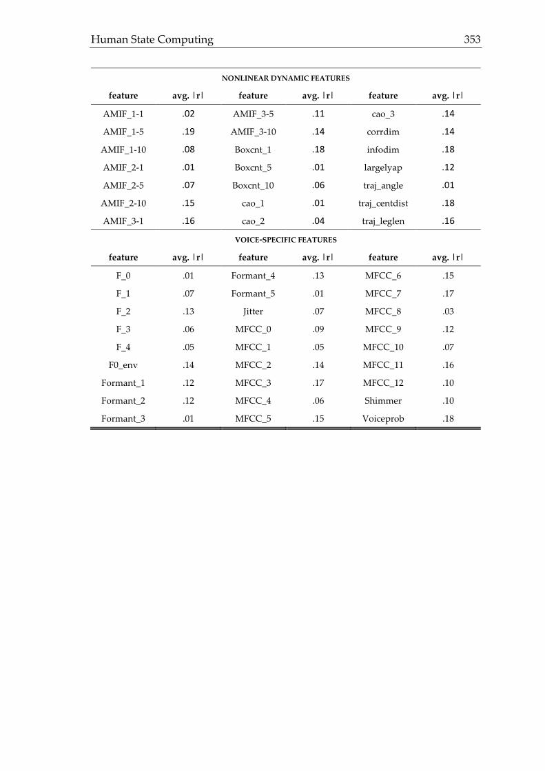
Human State Computing 353
NONLINEAR DYNAMIC FEATURES
feature avg. |r| feature avg. |r| feature avg. |r|
AMIF_1-1 .02 AMIF_3-5 .11 cao_3 .14
AMIF_1-5 .19 AMIF_3-10 .14 corrdim .14
AMIF_1-10 .08 Boxcnt_1 .18 infodim .18
AMIF_2-1 .01 Boxcnt_5 .01 largelyap .12
AMIF_2-5 .07 Boxcnt_10 .06 traj_angle .01
AMIF_2-10 .15 cao_1 .01 traj_centdist .18
AMIF_3-1 .16 cao_2 .04 traj_leglen .16
VOICE-SPECIFIC FEATURES
feature avg. |r| feature avg. |r| feature avg. |r|
F_0 .01 Formant_4 .13 MFCC_6 .15
F_1 .07 Formant_5 .01 MFCC_7 .17
F_2 .13 Jitter .07 MFCC_8 .03
F_3 .06 MFCC_0 .09 MFCC_9 .12
F_4 .05 MFCC_1 .05 MFCC_10 .07
F0_env .14 MFCC_2 .14 MFCC_11 .16
Formant_1 .12 MFCC_3 .17 MFCC_12 .10
Formant_2 .12 MFCC_4 .06 Shimmer .10
Formant_3 .01 MFCC_5 .15 Voiceprob .18

354 Appendix A: Averaged Aggregated Feature Correlations by State
Table A-2: Averaged aggregated feature correlations for inspiration.
COMMON FEATURES
feature avg. |r| feature avg. |r| feature avg. |r|
Centroid .01 LFCC_2 .17 LFCC_12 .10
Energy .09 LFCC_3 .19 Minimum .15
Flux .13 LFCC_4 .13 Maximum .08
Fbandw_1 .10 LFCC_5 .04 Roll-off_1 .19
Fbandw_2 .07 LFCC_6 .13 Roll-off_2 .20
Fbandw_3 .19 LFCC_7 .01 Roll-off_3 .17
Fbandw_4 .17 LFCC_8 .08 Roll-off_4 .19
Fbandw_5 .17 LFCC_9 .13 ZCR .14
LFCC_0 .07 LFCC_10 .17
LFCC_1 .12 LFCC_11 .16
WAVELET FEATURES
feature avg. |r| feature avg. |r| feature avg. |r|
WT_0 .08 WT_9 .18 WT_18 .02
WT_1 .09 WT_10 .09 WT_19 .08
WT_2 .05 WT_11 .04 WT_20 .06
WT_3 .16 WT_12 .18 WT_21 .14
WT_4 .18 WT_13 .15 WT_22 .06
WT_5 .18 WT_14 .18 WT_23 .18
WT_6 .11 WT_15 .06 WT_24 .17
WT_7 .12 WT_16 .13 WT_25 .08
WT_8 .03 WT_17 .13
NONLINEAR DYNAMIC FEATURES
feature avg. |r| feature avg. |r| feature avg. |r|
AMIF_1-1 .10 AMIF_3-5 .14 cao_3 .02
AMIF_1-5 .14 AMIF_3-10 .18 corrdim .16
AMIF_1-10 .17 Boxcnt_1 .14 infodim .06
AMIF_2-1 .12 Boxcnt_5 .00 largelyap .05
AMIF_2-5 .11 Boxcnt_10 .13 traj_angle .07
AMIF_2-10 .07 cao_1 .09 traj_centdist .08
AMIF_3-1 .09 cao_2 .09 traj_leglen .11
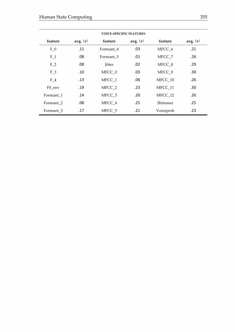
Human State Computing 355
VOICE-SPECIFIC FEATURES
feature avg. |r| feature avg. |r| feature avg. |r|
F_0 .11 Formant_4 .03 MFCC_6 .21
F_1 .08 Formant_5 .01 MFCC_7 .26
F_2 .08 Jitter .02 MFCC_8 .29
F_3 .10 MFCC_0 .03 MFCC_9 .30
F_4 .13 MFCC_1 .06 MFCC_10 .26
F0_env .19 MFCC_2 .23 MFCC_11 .30
Formant_1 .14 MFCC_3 .20 MFCC_12 .26
Formant_2 .08 MFCC_4 .25 Shimmer .25
Formant_3 .17 MFCC_5 .21 Voiceprob .23
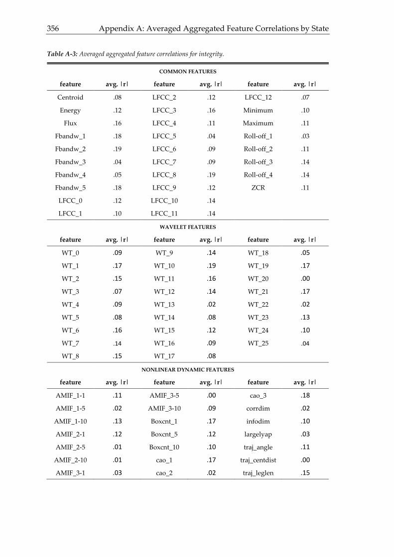
356 Appendix A: Averaged Aggregated Feature Correlations by State
Table A-3: Averaged aggregated feature correlations for integrity.
COMMON FEATURES
feature avg. |r| feature avg. |r| feature avg. |r|
Centroid .08 LFCC_2 .12 LFCC_12 .07
Energy .12 LFCC_3 .16 Minimum .10
Flux .16 LFCC_4 .11 Maximum .11
Fbandw_1 .18 LFCC_5 .04 Roll-off_1 .03
Fbandw_2 .19 LFCC_6 .09 Roll-off_2 .11
Fbandw_3 .04 LFCC_7 .09 Roll-off_3 .14
Fbandw_4 .05 LFCC_8 .19 Roll-off_4 .14
Fbandw_5 .18 LFCC_9 .12 ZCR .11
LFCC_0 .12 LFCC_10 .14
LFCC_1 .10 LFCC_11 .14
WAVELET FEATURES
feature avg. |r| feature avg. |r| feature avg. |r|
WT_0 .09 WT_9 .14 WT_18 .05
WT_1 .17 WT_10 .19 WT_19 .17
WT_2 .15 WT_11 .16 WT_20 .00
WT_3 .07 WT_12 .14 WT_21 .17
WT_4 .09 WT_13 .02 WT_22 .02
WT_5 .08 WT_14 .08 WT_23 .13
WT_6 .16 WT_15 .12 WT_24 .10
WT_7 .14 WT_16 .09 WT_25 .04
WT_8 .15 WT_17 .08
NONLINEAR DYNAMIC FEATURES
feature avg. |r| feature avg. |r| feature avg. |r|
AMIF_1-1 .11 AMIF_3-5 .00 cao_3 .18
AMIF_1-5 .02 AMIF_3-10 .09 corrdim .02
AMIF_1-10 .13 Boxcnt_1 .17 infodim .10
AMIF_2-1 .12 Boxcnt_5 .12 largelyap .03
AMIF_2-5 .01 Boxcnt_10 .10 traj_angle .11
AMIF_2-10 .01 cao_1 .17 traj_centdist .00
AMIF_3-1 .03 cao_2 .02 traj_leglen .15

Human State Computing 357
VOICE-SPECIFIC FEATURES
feature avg. |r| feature avg. |r| feature avg. |r|
F_0 .17 Formant_4 .02 MFCC_6 .09
F_1 .18 Formant_5 .13 MFCC_7 .17
F_2 .20 Jitter .10 MFCC_8 .11
F_3 .10 MFCC_0 .03 MFCC_9 .11
F_4 .05 MFCC_1 .19 MFCC_10 .14
F0_env .02 MFCC_2 .12 MFCC_11 .24
Formant_1 .10 MFCC_3 .09 MFCC_12 .22
Formant_2 .12 MFCC_4 .19 Shimmer .26
Formant_3 .15 MFCC_5 .13 Voiceprob .29
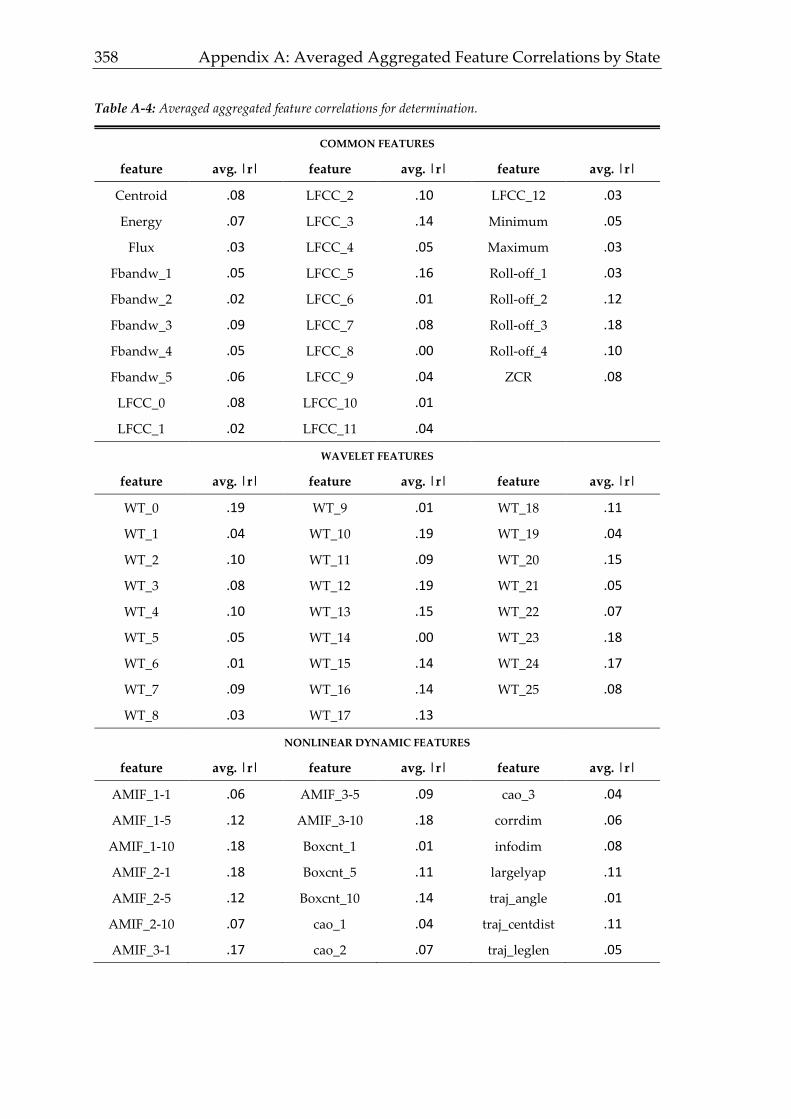
358 Appendix A: Averaged Aggregated Feature Correlations by State
Table A-4: Averaged aggregated feature correlations for determination.
COMMON FEATURES
feature avg. |r| feature avg. |r| feature avg. |r|
Centroid .08 LFCC_2 .10 LFCC_12 .03
Energy .07 LFCC_3 .14 Minimum .05
Flux .03 LFCC_4 .05 Maximum .03
Fbandw_1 .05 LFCC_5 .16 Roll-off_1 .03
Fbandw_2 .02 LFCC_6 .01 Roll-off_2 .12
Fbandw_3 .09 LFCC_7 .08 Roll-off_3 .18
Fbandw_4 .05 LFCC_8 .00 Roll-off_4 .10
Fbandw_5 .06 LFCC_9 .04 ZCR .08
LFCC_0 .08 LFCC_10 .01
LFCC_1 .02 LFCC_11 .04
WAVELET FEATURES
feature avg. |r| feature avg. |r| feature avg. |r|
WT_0 .19 WT_9 .01 WT_18 .11
WT_1 .04 WT_10 .19 WT_19 .04
WT_2 .10 WT_11 .09 WT_20 .15
WT_3 .08 WT_12 .19 WT_21 .05
WT_4 .10 WT_13 .15 WT_22 .07
WT_5 .05 WT_14 .00 WT_23 .18
WT_6 .01 WT_15 .14 WT_24 .17
WT_7 .09 WT_16 .14 WT_25 .08
WT_8 .03 WT_17 .13
NONLINEAR DYNAMIC FEATURES
feature avg. |r| feature avg. |r| feature avg. |r|
AMIF_1-1 .06 AMIF_3-5 .09 cao_3 .04
AMIF_1-5 .12 AMIF_3-10 .18 corrdim .06
AMIF_1-10 .18 Boxcnt_1 .01 infodim .08
AMIF_2-1 .18 Boxcnt_5 .11 largelyap .11
AMIF_2-5 .12 Boxcnt_10 .14 traj_angle .01
AMIF_2-10 .07 cao_1 .04 traj_centdist .11
AMIF_3-1 .17 cao_2 .07 traj_leglen .05

Human State Computing 359
VOICE-SPECIFIC FEATURES
feature avg. |r| feature avg. |r| feature avg. |r|
F_0 .05 Formant_4 .22 MFCC_6 .28
F_1 .05 Formant_5 .20 MFCC_7 .28
F_2 .03 Jitter .23 MFCC_8 .26
F_3 .19 MFCC_0 .27 MFCC_9 .27
F_4 .19 MFCC_1 .26 MFCC_10 .26
F0_env .28 MFCC_2 .25 MFCC_11 .21
Formant_1 .27 MFCC_3 .24 MFCC_12 .25
Formant_2 .22 MFCC_4 .23 Shimmer .23
Formant_3 .24 MFCC_5 .25 Voiceprob .21

360 Appendix A: Averaged Aggregated Feature Correlations by State
Table A-5: Averaged aggregated feature correlations for performance orientation.
COMMON FEATURES
feature avg. |r| feature avg. |r| feature avg. |r|
Centroid .11 LFCC_2 .09 LFCC_12 .01
Energy .06 LFCC_3 .12 Minimum .20
Flux .19 LFCC_4 .14 Maximum .06
Fbandw_1 .18 LFCC_5 .14 Roll-off_1 .12
Fbandw_2 .08 LFCC_6 .13 Roll-off_2 .19
Fbandw_3 .00 LFCC_7 .15 Roll-off_3 .04
Fbandw_4 .13 LFCC_8 .07 Roll-off_4 .04
Fbandw_5 .17 LFCC_9 .12 ZCR .07
LFCC_0 .19 LFCC_10 .11
LFCC_1 .01 LFCC_11 .02
WAVELET FEATURES
feature avg. |r| feature avg. |r| feature avg. |r|
WT_0 .07 WT_9 .02 WT_18 .10
WT_1 .19 WT_10 .12 WT_19 .13
WT_2 .08 WT_11 .00 WT_20 .04
WT_3 .05 WT_12 .11 WT_21 .17
WT_4 .03 WT_13 .16 WT_22 .19
WT_5 .08 WT_14 .05 WT_23 .17
WT_6 .07 WT_15 .09 WT_24 .10
WT_7 .03 WT_16 .11 WT_25 .06
WT_8 .09 WT_17 .01
NONLINEAR DYNAMIC FEATURES
feature avg. |r| feature avg. |r| feature avg. |r|
AMIF_1-1 .15 AMIF_3-5 .05 cao_3 .16
AMIF_1-5 .05 AMIF_3-10 .17 corrdim .08
AMIF_1-10 .19 Boxcnt_1 .18 infodim .20
AMIF_2-1 .12 Boxcnt_5 .14 largelyap .02
AMIF_2-5 .12 Boxcnt_10 .15 traj_angle .06
AMIF_2-10 .03 cao_1 .05 traj_centdist .10
AMIF_3-1 .02 cao_2 .12 traj_leglen .01

Human State Computing 361
VOICE-SPECIFIC FEATURES
feature avg. |r| feature avg. |r| feature avg. |r|
F_0 .15 Formant_4 .21 MFCC_6 .29
F_1 .11 Formant_5 .21 MFCC_7 .26
F_2 .11 Jitter .23 MFCC_8 .23
F_3 .17 MFCC_0 .25 MFCC_9 .21
F_4 .17 MFCC_1 .30 MFCC_10 .28
F0_env .16 MFCC_2 .27 MFCC_11 .26
Formant_1 .06 MFCC_3 .23 MFCC_12 .29
Formant_2 .25 MFCC_4 .23 Shimmer .21
Formant_3 .28 MFCC_5 .29 Voiceprob .26

362 Appendix A: Averaged Aggregated Feature Correlations by State
Table A-6: Averaged aggregated feature correlations for team integration.
COMMON FEATURES
feature avg. |r| feature avg. |r| feature avg. |r|
Centroid .04 LFCC_2 .01 LFCC_12 .07
Energy .06 LFCC_3 .01 Minimum .13
Flux .03 LFCC_4 .16 Maximum .19
Fbandw_1 .13 LFCC_5 .09 Roll-off_1 .02
Fbandw_2 .11 LFCC_6 .08 Roll-off_2 .12
Fbandw_3 .03 LFCC_7 .16 Roll-off_3 .08
Fbandw_4 .03 LFCC_8 .07 Roll-off_4 .13
Fbandw_5 .10 LFCC_9 .11 ZCR .11
LFCC_0 .18 LFCC_10 .14
LFCC_1 .11 LFCC_11 .17
WAVELET FEATURES
feature avg. |r| feature avg. |r| feature avg. |r|
WT_0 .06 WT_9 .08 WT_18 .09
WT_1 .05 WT_10 .15 WT_19 .15
WT_2 .15 WT_11 .10 WT_20 .01
WT_3 .20 WT_12 .16 WT_21 .19
WT_4 .04 WT_13 .07 WT_22 .15
WT_5 .16 WT_14 .01 WT_23 .11
WT_6 .04 WT_15 .12 WT_24 .04
WT_7 .20 WT_16 .18 WT_25 .10
WT_8 .16 WT_17 .04
NONLINEAR DYNAMIC FEATURES
feature avg. |r| feature avg. |r| feature avg. |r|
AMIF_1-1 .10 AMIF_3-5 .10 cao_3 .19
AMIF_1-5 .20 AMIF_3-10 .05 corrdim .11
AMIF_1-10 .17 Boxcnt_1 .08 infodim .19
AMIF_2-1 .19 Boxcnt_5 .14 largelyap .02
AMIF_2-5 .14 Boxcnt_10 .11 traj_angle .01
AMIF_2-10 .08 cao_1 .15 traj_centdist .06
AMIF_3-1 .19 cao_2 .20 traj_leglen .12
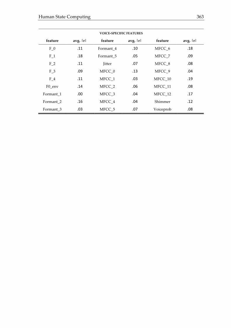
Human State Computing 363
VOICE-SPECIFIC FEATURES
feature avg. |r| feature avg. |r| feature avg. |r|
F_0 .11 Formant_4 .10 MFCC_6 .18
F_1 .18 Formant_5 .05 MFCC_7 .09
F_2 .11 Jitter .07 MFCC_8 .08
F_3 .09 MFCC_0 .13 MFCC_9 .04
F_4 .11 MFCC_1 .03 MFCC_10 .19
F0_env .14 MFCC_2 .06 MFCC_11 .08
Formant_1 .00 MFCC_3 .04 MFCC_12 .17
Formant_2 .16 MFCC_4 .04 Shimmer .12
Formant_3 .03 MFCC_5 .07 Voiceprob .08

364 Appendix A: Averaged Aggregated Feature Correlations by State
Table A-7: Averaged aggregated feature correlations for diplomacy.
COMMON FEATURES
feature avg. |r| feature avg. |r| feature avg. |r|
Centroid .12 LFCC_2 .04 LFCC_12 .03
Energy .18 LFCC_3 .02 Minimum .08
Flux .14 LFCC_4 .09 Maximum .15
Fbandw_1 .08 LFCC_5 .00 Roll-off_1 .07
Fbandw_2 .15 LFCC_6 .18 Roll-off_2 .16
Fbandw_3 .19 LFCC_7 .13 Roll-off_3 .09
Fbandw_4 .11 LFCC_8 .00 Roll-off_4 .16
Fbandw_5 .11 LFCC_9 .01 ZCR .09
LFCC_0 .06 LFCC_10 .04
LFCC_1 .01 LFCC_11 .09
WAVELET FEATURES
feature avg. |r| feature avg. |r| feature avg. |r|
WT_0 .09 WT_9 .10 WT_18 .03
WT_1 .01 WT_10 .04 WT_19 .14
WT_2 .01 WT_11 .05 WT_20 .12
WT_3 .02 WT_12 .11 WT_21 .09
WT_4 .12 WT_13 .15 WT_22 .18
WT_5 .05 WT_14 .07 WT_23 .08
WT_6 .17 WT_15 .09 WT_24 .04
WT_7 .17 WT_16 .13 WT_25 .13
WT_8 .19 WT_17 .18
NONLINEAR DYNAMIC FEATURES
feature avg. |r| feature avg. |r| feature avg. |r|
AMIF_1-1 .12 AMIF_3-5 .00 cao_3 .04
AMIF_1-5 .07 AMIF_3-10 .12 corrdim .09
AMIF_1-10 .16 Boxcnt_1 .02 infodim .19
AMIF_2-1 .20 Boxcnt_5 .08 largelyap .02
AMIF_2-5 .20 Boxcnt_10 .18 traj_angle .09
AMIF_2-10 .03 cao_1 .11 traj_centdist .17
AMIF_3-1 .05 cao_2 .07 traj_leglen .01
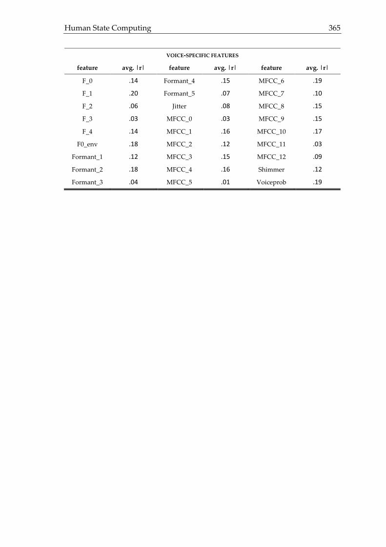
Human State Computing 365
VOICE-SPECIFIC FEATURES
feature avg. |r| feature avg. |r| feature avg. |r|
F_0 .14 Formant_4 .15 MFCC_6 .19
F_1 .20 Formant_5 .07 MFCC_7 .10
F_2 .06 Jitter .08 MFCC_8 .15
F_3 .03 MFCC_0 .03 MFCC_9 .15
F_4 .14 MFCC_1 .16 MFCC_10 .17
F0_env .18 MFCC_2 .12 MFCC_11 .03
Formant_1 .12 MFCC_3 .15 MFCC_12 .09
Formant_2 .18 MFCC_4 .16 Shimmer .12
Formant_3 .04 MFCC_5 .01 Voiceprob .19

366 Appendix A: Averaged Aggregated Feature Correlations by State
Table A-8: Averaged aggregated feature correlations for non-maliciousness.
COMMON FEATURES
feature avg. |r| feature avg. |r| feature avg. |r|
Centroid .08 LFCC_2 .08 LFCC_12 .14
Energy .01 LFCC_3 .12 Minimum .16
Flux .15 LFCC_4 .03 Maximum .17
Fbandw_1 .03 LFCC_5 .04 Roll-off_1 .06
Fbandw_2 .03 LFCC_6 .02 Roll-off_2 .06
Fbandw_3 .12 LFCC_7 .06 Roll-off_3 .10
Fbandw_4 .05 LFCC_8 .15 Roll-off_4 .07
Fbandw_5 .06 LFCC_9 .05 ZCR .9
LFCC_0 .08 LFCC_10 .12
LFCC_1 .08 LFCC_11 .15
WAVELET FEATURES
feature avg. |r| feature avg. |r| feature avg. |r|
WT_0 .17 WT_9 .20 WT_18 .20
WT_1 .16 WT_10 .15 WT_19 .19
WT_2 .11 WT_11 .20 WT_20 .08
WT_3 .05 WT_12 .05 WT_21 .07
WT_4 .14 WT_13 .11 WT_22 .11
WT_5 .05 WT_14 .01 WT_23 .04
WT_6 .09 WT_15 .15 WT_24 .04
WT_7 .08 WT_16 .12 WT_25
WT_8 .11 WT_17 .17
NONLINEAR DYNAMIC FEATURES
feature avg. |r| feature avg. |r| feature avg. |r|
AMIF_1-1 .02 AMIF_3-5 .19 cao_3 .15
AMIF_1-5 .15 AMIF_3-10 .18 corrdim .03
AMIF_1-10 .15 Boxcnt_1 .07 infodim .16
AMIF_2-1 .11 Boxcnt_5 .11 largelyap .01
AMIF_2-5 .07 Boxcnt_10 .07 traj_angle .08
AMIF_2-10 .17 cao_1 .12 traj_centdist .15
AMIF_3-1 .11 cao_2 .16 traj_leglen .16

Human State Computing 367
VOICE-SPECIFIC FEATURES
feature avg. |r| feature avg. |r| feature avg. |r|
F_0 .07 Formant_4 .01 MFCC_6 .04
F_1 .15 Formant_5 .12 MFCC_7 .08
F_2 .18 Jitter .03 MFCC_8 .07
F_3 .05 MFCC_0 .17 MFCC_9 .05
F_4 .03 MFCC_1 .03 MFCC_10 .19
F0_env .05 MFCC_2 .10 MFCC_11 .14
Formant_1 .07 MFCC_3 .20 MFCC_12 .19
Formant_2 .06 MFCC_4 .07 Shimmer .09
Formant_3 .19 MFCC_5 .01 Voiceprob .19
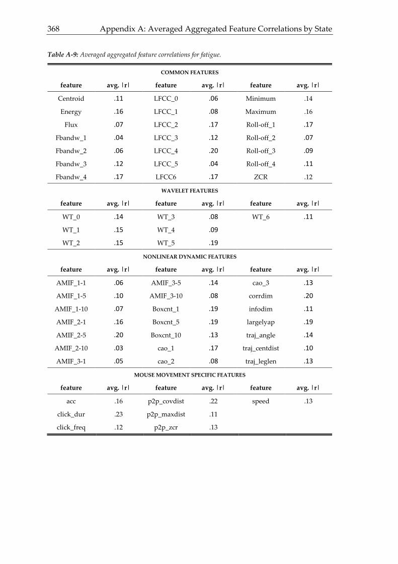
368 Appendix A: Averaged Aggregated Feature Correlations by State
Table A-9: Averaged aggregated feature correlations for fatigue.
COMMON FEATURES
feature avg. |r| feature avg. |r| feature avg. |r|
Centroid .11 LFCC_0 .06 Minimum .14
Energy .16 LFCC_1 .08 Maximum .16
Flux .07 LFCC_2 .17 Roll-off_1 .17
Fbandw_1 .04 LFCC_3 .12 Roll-off_2 .07
Fbandw_2 .06 LFCC_4 .20 Roll-off_3 .09
Fbandw_3 .12 LFCC_5 .04 Roll-off_4 .11
Fbandw_4 .17 LFCC6 .17 ZCR .12
WAVELET FEATURES
feature avg. |r| feature avg. |r| feature avg. |r|
WT_0 .14 WT_3 .08 WT_6 .11
WT_1 .15 WT_4 .09
WT_2 .15 WT_5 .19
NONLINEAR DYNAMIC FEATURES
feature avg. |r| feature avg. |r| feature avg. |r|
AMIF_1-1 .06 AMIF_3-5 .14 cao_3 .13
AMIF_1-5 .10 AMIF_3-10 .08 corrdim .20
AMIF_1-10 .07 Boxcnt_1 .19 infodim .11
AMIF_2-1 .16 Boxcnt_5 .19 largelyap .19
AMIF_2-5 .20 Boxcnt_10 .13 traj_angle .14
AMIF_2-10 .03 cao_1 .17 traj_centdist .10
AMIF_3-1 .05 cao_2 .08 traj_leglen .13
MOUSE MOVEMENT SPECIFIC FEATURES
feature avg. |r| feature avg. |r| feature avg. |r|
acc .16 p2p_covdist .22 speed .13
click_dur .23 p2p_maxdist .11
click_freq .12 p2p_zcr .13

Human State Computing 369
Table A-10: Averaged aggregated feature correlations for stress.
COMMON FEATURES
feature avg. |r| feature avg. |r| feature avg. |r|
Centroid .18 LFCC_0 .17 Roll-off_1 .09
Energy .09 LFCC_1 .01 Roll-off_2 .11
Flux .15 LFCC_2 .09 Roll-off_3 .16
Fbandw_1 .12 LFCC_3 .07 Roll-off_4 .14
Fbandw_2 .16 LFCC_4 .13 ZCR .12
Fbandw_3 .02 Minimum .09
Fbandw_4 .20 Maximum .13
WAVELET FEATURES
feature avg. |r| feature avg. |r| feature avg. |r|
WT_0 .17 WT_2 .04 WT_4 .19
WT_1 .01 WT_3 .09
NONLINEAR DYNAMIC FEATURES
feature avg. |r| feature avg. |r| feature avg. |r|
acc .02 speed .11
HEAD MOVEMENT SPECIFIC FEATURES
feature avg. |r| feature avg. |r| feature avg. |r|
acc .01 speed .15
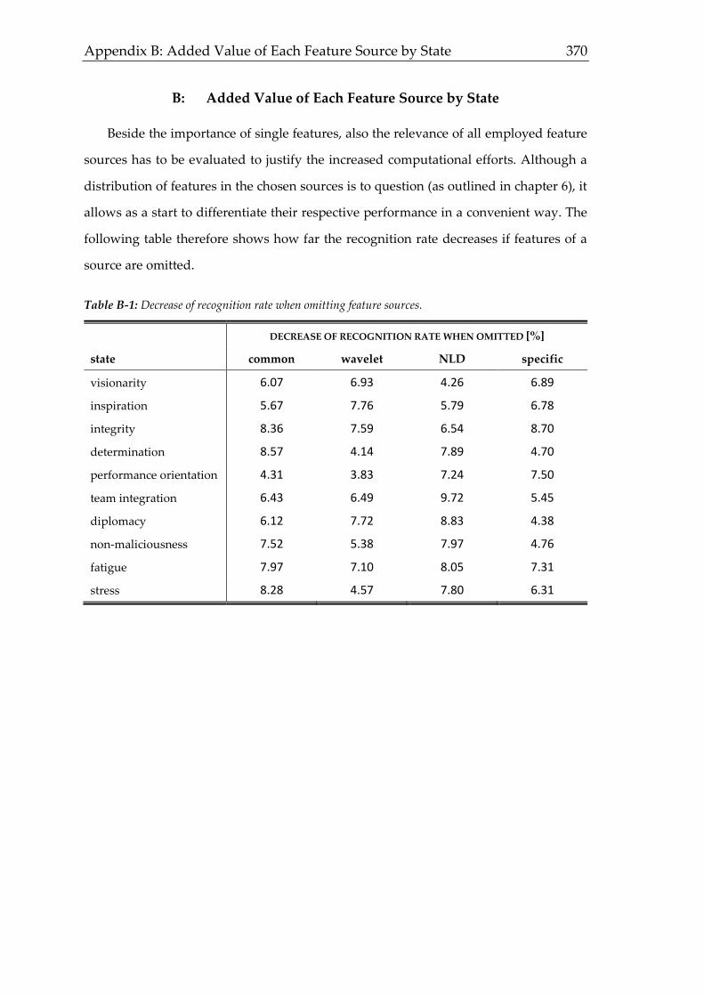
Appendix B: Added Value of Each Feature Source by State 370
B: Added Value of Each Feature Source by State
Beside the importance of single features, also the relevance of all employed feature
sources has to be evaluated to justify the increased computational efforts. Although a
distribution of features in the chosen sources is to question (as outlined in chapter 6), it
allows as a start to differentiate their respective performance in a convenient way. The
following table therefore shows how far the recognition rate decreases if features of a
source are omitted.
Table B-1: Decrease of recognition rate when omitting feature sources.
DECREASE OF RECOGNITION RATE WHEN OMITTED [%]
state common wavelet NLD specific
visionarity 6.07 6.93 4.26 6.89
inspiration 5.67 7.76 5.79 6.78
integrity 8.36 7.59 6.54 8.70
determination 8.57 4.14 7.89 4.70
performance orientation 4.31 3.83 7.24 7.50
team integration 6.43 6.49 9.72 5.45
diplomacy 6.12 7.72 8.83 4.38
non-maliciousness 7.52 5.38 7.97 4.76
fatigue 7.97 7.10 8.05 7.31
stress 8.28 4.57 7.80 6.31

Human State Computing 371
C: SLEDS Experimental Setup
Within chapter 4.2 it has been outlined that not only mouse movement data were
gathered within the described experimental setup. To give an overview of other
measures and tasks that were employed, table C-1 gives a detailed timeline all subjects
had to follow (organized by the examiner).
Table C-1: Timeline and tasks of the SLEDS study.
est. time setup
00:00 – 00:10 welcoming, introduction, consent form
00:10 – 00:25 technical check
(heart rate belt, posturography cap, hemodynamometer, thermography cam,
webcam, audio recording)
00:25 – 00:30 single question statements for different states
(fatigue, interested, contented, strain, sadness, bugged, cheerful, boredom,
activity level, stressed, uncomfortable)
00:30 – 00:40 description and verbal evaluation of pictures and videos
(content, basic emotions)
00:40 – 00:45 single question statements for different states
00:45 – 00:55 description and verbal evaluation of pictures and videos
(content, basic emotions)
00:55 – 01:00 single question statements for different states
01:00 – 01:10 description and verbal evaluation of pictures and videos
(content, basic emotions)
01:10 – 01:15 single question statements for different states
01:15 – 01:20 wreckage task (sort importance of items after wreckage)
01:20 – 01:25 measuring blood pressure
01:25 – 01:30 single question statements for different states
01:30 – 01:35 posturography task
01:35 – 01:40 single question statements for different states
01:40 – 02:00 experimental mouse tasks
(clicking on randomly distributed numbers in right order; clicking on
squares as fast as possible after appearance; clicking on red square within
several other shapes; follow instructions regarding website browsing, maze
track)
02:00 – 02:05 real-life mouse task: recreate PowerPoint slide
02:05 – 02:10 single question statements for different states
02:10 – 02:15 voice tasks: answering questions regarding information displayed on web-
site; use speech-based smart home system
02:15 – 02:25 description and verbal evaluation of pictures and videos

372 Appendix C: SLEDS Experimental Setup
(content, basic emotions)
02:25 – 02:30 single question statements for different states
02:30 – 02:40 reading pre-defined short stories; tell personal childhood stories; speak
vowel [a] for 10 seconds; sing a short song
02:40 – 02:45 single question statements for different states
02:45 – 02:55 description and verbal evaluation of pictures and videos
(content, basic emotions)
02:55 – 03:00 flight controller task: answer pilot requests with pre-defined instructions
03:00 – 03:05 single question statements for different states
03:05 – 03:15 description and verbal evaluation of pictures and videos
(content, basic emotions)
03:15 – 03:20 single question statements for different states
03:20 – 03:25 human driver task: help inexperienced driver with instructions while watch-
ing a driving simulation
03:25 – 03:30 single question statements for different states
03:30 – 03:45 take care of technical equipment; dismiss
Top Related