


Sprachen
Seiten
Rechtliche


Simulation Environment for Development of Unmanned Helicopter
Automatic Take-off and Landing on Ship Deck
Antonio Vitale1 Davide Bianco1 Gianluca Corraro1 Angelo Martone1 Federico Corraro1
Alfredo Giuliano2 Adriano Arcadipane2 1On-boar Systems and ATM Department, CIRA - Italian Aerospace Research Centre, Capua (CE), Italy, {a.vitale,
d.bianco, g.corraro, a.martone, f.corraro}@cira.it 2Electrical and Avionics Systems Department, Finmeccanica - Helicopter Division, Cascina Costa (VA), Italy,
{Alfredo.Giuliano, Adriano.Arcadipane}@finmeccanica.com
AbstractHelicopter take-off and landing operations on ship
carrier are very hazardous and training intensive.
Guidance, Navigation and Control algorithms can help
pilots to face these tasks by significantly reducing the
workload and improving safety level. Anyway, the
design and verification of such algorithms require the
availability of suitable simulation environments that
shall be a trade-off between simplicity and accuracy.
This paper presents the simulation models developed to
support the design, pre-flight verification and validation
of helicopter trajectory generation and tracking
algorithms for automated take-off and landing on a
frigate deck. The process for generation and testing of
the code to be integrated into the real-time Software-In-
the-Loop simulator is also described. Such fast time and
real-time simulation environments contributed to reduce
algorithms design time, risks and costs, by limiting the
required flight test activities. Take-off and landing
algorithms developed by using the proposed simulation
environments were successfully demonstrated in flight.
Keywords: GNC, helicopter, sensor, ship, turbulence
1 Introduction
Vertical take-off and landing operations of aerial vehicle
on ship’s deck enhance mission capabilities for military
and civilian users. Anyway, these operations are the
most dangerous flight phases for helicopters (Padfield,
1998; Lee, 2005). Indeed, a pilot have to deal with an
invisible ship air wake, poor visible cueing and a landing
spot which is heaving, rolling, pitching and yawing. At
the same time the pilot shall also monitor vehicle’s
structural, aerodynamic and control limits. Moreover,
operations take place in close proximity to the
superstructure of the ship, that means there is little
margin for error and the consequences of a significant
loss of positional accuracy by the pilot can be severe.
The availability of Guidance Navigation and Control
(GNC) algorithms for automatic operations can help
pilots to face these tasks by significantly reducing
operator workload, improving safety level and flight
handling qualities. To develop these algorithms, suitable
simulation environments are essential in order to reduce
the flight test time and cost and to establish safe
operating envelopes. The simulation tools shall be able
to model all the relevant phenomena, such as helicopter
flight dynamics (including on board sensors and
actuators), the motion of the ship for the given sea state,
the influence on the helicopter of the ship air wake and
of the environment in general.
It is worth to note that modelling and simulation of
each of the above listed phenomena is not a trivial task.
Indeed, the simulation of the helicopter flight behavior
includes kinematics, dynamics and aerodynamics of its
subsystems (main rotor, fuselage, empennage, tail rotor,
power plant, primary flight control system, on board
sensors).
The vehicle’s equations of motion, even if presented
in several textbooks (Padfield, 1996; Johnson, 1994),
are differential high order, nonlinear, coupled, and
contain a large number of parameters, which often
cannot be directly measured (Tishler et al., 2006). On
the other hand, simplified models, which are able to
catch the relevant dynamics, are typically required for
GNC design purpose (Lee, 2005), to enhance physical
understanding and lower the computational load. To this
aim, linear parametrized models have been widely used
(Tishler et al., 2006), but they are inadequate for
accurate simulation of the vehicle dynamics when state
variables significantly deviate from the linearization
point (Gavrilets, 2006). Therefore, a suitable trade-off
between model complexity and simulation accuracy
shall be performed.
Another relevant topic concerns ship motion, which
is an important issue for helicopter deck operations. For
helicopter GNC algorithms design and analysis purpose,
ship motion is usually represented through linear models
or simplified nonlinear models with benign
nonlinearities to capture the essential behavior of the
vessel (Li, 2009). Ship motion can also be modelled
using pre-computed or measured time histories (Carico
et al., 2003). In any case, the ship model shall take into
account the effect of the environment, and, in particular,
EUROSIM 2016 & SIMS 2016
228DOI: 10.3384/ecp17142228 Proceedings of the 9th EUROSIM & the 57th SIMSSeptember 12th-16th, 2016, Oulu, Finland

of the sea waves (Perez, 2005), which lead an
undesirable low frequency disturbance into the motion
of the vessel.
Finally yet importantly, the ship produces an air
wake, which affects the helicopter dynamics. Indeed,
ship air wake contains large velocity gradients and area
of turbulence, generated by complex mechanisms of
vortex dynamics near the ship deck, which greatly
impair controllability of the flying vehicle and require
additional control efforts to avoid accidents and to
compensate abrupt changes in thrust level. Several
accurate and complex CFD models of ship air wake are
proposed in the literature (Kääriä, 2012), but CFD
simulations produce a large amount of data and their use
for GNC design and real time testing is usually
unfeasible (Lee, 2005).
Stochastic turbulence models have been also
proposed to represent the air wake with reasonable
accuracy (Lee, 2005; Yang et al., 2009). These models
may provide some insight into the effects of the air wake
that are typically enough relevant for real-time
simulations and flight control systems design.
It is also worth to note that, with reference to all the
discussed models, a suitable code generation procedure
and testing methodology shall be defined, in order to
generate reliable real-time simulation models,
applicable for GNC algorithms verification and
performance assessment.
This paper presents the simulation environment
developed by the Italian Aerospace Research Centre and
Finmeccanica in order to support the design and
verification of algorithms for helicopter trajectory
generation and tracking, during an automated take-off
and landing on a frigate deck. Matlab/Simulink was
used for implementing such simulation environment,
which constitutes an alternative to the already existing
Finmeccanica GNC validation environment.
The proposed models, although simplified, are able
to take into account the main effects of the sea’s
disturbance on the ship motion and of the ship air wake
on the helicopter trajectory. Concerning the helicopter
vehicle dynamics, its model emulates the relevant
closed loop performance of the vehicle and includes
operating envelope limitations through a model for
aerodynamic forces and thrust computation, whose
parameters are identified from experimental data.
The paper also includes some fast time simulation
results compared to experimental data, demonstrating
that the proposed simulation environment is accurate
enough for GNC algorithms design.
Finally, some models of the above mentioned
simulation environment were also integrated into the
detailed Software-in-the-Loop Simulator of
Finmeccanica, to perform real-time verification and
validation of the whole Flight Management System (FMS). Therefore, a real-time automatic code
generation process has been defined and implemented,
in order to keep consistency between the simulation
environment used for design, and the one used for final
software verification. The paper briefly describes such
generation process, which allowed producing reliable
software code, compliant to DO-178C standard and
Finmeccanica own implementation rules.
The proposed fast time simulation environment
dramatically reduced the algorithms design time, risks
and costs, by limiting the required flight test activities.
The take-off and landing algorithms developed by
using the simulation environment described in this paper
were successfully demonstrated in flight, by means of a
full-size optionally piloted helicopter: the Finmeccanica
SW-4 SOLO.
2 Simulation Models
The model based design process of a Guidance
Navigation and Control system requires the
development of simulation models with different
complexity level, to be used in the various development
phases, as shown in Figure 1.
The present section describes the mathematical
models integrated into the simulation environment that
was employed to design the helicopter trajectory
generation and tracking algorithms for automated take-
off and landing on a frigate deck. Figure 2 shows the
functional architecture of such environment.
Figure 1. GNC Technology Development Cycle.
Figure 2. Simulation Environment functional
architecture.
FMS
AUTOPILOT HELICOPTER
ATMOSPHERE
SHIP
SENSORS
EUROSIM 2016 & SIMS 2016
229DOI: 10.3384/ecp17142228 Proceedings of the 9th EUROSIM & the 57th SIMSSeptember 12th-16th, 2016, Oulu, Finland

The blue blocks represent the simulation models, scope
of this paper, whereas the red blocks are the GNC
algorithms. The following sub-sections describe in
detail each blue block.
2.1 Helicopter Model
Trajectory generation and tracking algorithms typically
require the knowledge of vehicle’s position and velocity
only. Therefore, for the design and preliminary
verification of such algorithms, it is sufficient and cost
effective to model only the closed loop attitude dynamic
response of the vehicle coupled with the high-level
modes of the autopilot system. With this approach, a
rigid body with three degrees of freedom, subject to
external forces, and the rotational dynamic response of
the vehicle to the autopilot commands represent the
helicopter dynamics.
While this modelling approach is widely used in
fixed-wing aircraft for guidance algorithms design, it is
quite unusual for helicopters, because it does not take
into account the coupled dynamics of the rotor
flexibility with the helicopter rigid flight mechanics
(Tishler et al., 2006).
Key original contribution of this paper is the
development of a mixed empirical and physical
formulation of the equations, so that the resulting
simulation model includes only the low frequency
effects of the neglected helicopter dynamics. As
demonstrated by the comparisons with flight data
reported in this paper, this allows obtaining enough
accurate simulation results during the quasi-static
manoeuvers of take-off and landing, while still taking
into account the disturbance effects of wind and ship air
wake.
The model assumes flat and fixed Earth, with
constant gravity acceleration, and quasi-stationary
variation of the vehicle mass (only due to fuel
consumption).
The model’s commands are the reference attitude and
collective, while wind velocity (VW) is the disturbance
input.
The actual attitude (φH, ϑ H, ψ H) and collective (δcoll)
of the vehicle, used in (1) for computation of forces, are
modelled by unitary gain second order filters applied to
the commands provided as input to the helicopter model.
Such filtered Euler angles and collective and their rates
are also saturated to account for actuator velocity
limitations and some inner autopilot protection
functions. Overall, the linear filters and related
saturations model the closed loop performance of the
inner autopilot modes. The parameters of both these
filters and saturations are scheduled with respect to
airspeed and they were identified by analyzing flight
data gathered in specific manoeuvers.
The outputs are the helicopter position, velocity, load factors, actual attitude and angular rates.
The following equations of motion of the vehicle
centre of mass (CoM), in North-East-Down (NED)
inertial reference frame (McCormick, 1995), compute
such outputs:
WcollHHH V,δ,ψ, ,FV m (1)
HH VP (2)
wh (3)
where V is the inertial velocity vector, VH and w are its
horizontal (included into the North-East plane) and
vertical components (positive down), respectively; PH is
the horizontal position and h the altitude of the vehicle
CoM; m is the helicopter mass and F is the resultant
force vector acting on the vehicle.
The force vector F is composed by gravitational force
W (constant, and directed along the down axis of the
NED reference frame), aerodynamic force FA and
propulsive force T.
The computation of aerodynamic and thrust forces is
first performed in the vehicle body reference frame, and
then it is rotated in NED reference frame. The
aerodynamic forces in body axes ( B
AiF ) are as follows:
j
, ,jijdyn
B
Ai cSqF (4)
WW
2 VVVV T
TASV (5)
2ρ5.0 TASdyn Vq (6)
TASTAS uwtg 1α (7)
TASTAS Vv1sinβ (8)
where qdyn is the dynamic pressure, ρ is the air density,
VTAS ≡ (TASTASTAS wvu ,, ) is the helicopter true airspeed,
Sj is the reference aerodynamic surface of the j-th
aerodynamic component (that is, fuselage, vertical and
horizontal stabilizers) and ci,j the corresponding
aerodynamic non-dimensional coefficient, which
depends on the angle of attack α and sideslip angle β.
Tabled functions express the aerodynamic coefficients
using data extrapolated from flight experiments.
It is worthy to note that the aerodynamic angles α and
β are not defined when the helicopter airspeed is null,
for example in hover condition with null wind speed. In
this case, the aerodynamic forces are negligible and the
aerodynamic angles are not computed.
The propulsive force is evaluated by using the
following semi-empirical linear model (Gavrilets,
2003):
wVz+Vz=T TASwTAScoll collδ (9)
The parameter zcoll is a gain between the thrust and the
collective command δcoll in level flight trim conditions.
It is scheduled as a function of the forward speed of the
aircraft with respect to air, and its values were identified
applying a best-fit procedure of the rotor thrust data in
EUROSIM 2016 & SIMS 2016
230DOI: 10.3384/ecp17142228 Proceedings of the 9th EUROSIM & the 57th SIMSSeptember 12th-16th, 2016, Oulu, Finland

different flight conditions provided by the helicopter
manufacturer.
The parameter zw relates the thrust to the vertical
speed. Although an analytical relation exists to express
these parameters as function of vehicle characteristics
(Gavrilets, 2003), in the present work, zw was computed
by fitting experimental data in climb and descent flight,
and it is expressed as fraction of zcoll.
The thrust vector is assumed to point in the opposite
direction of the body Z-axis. This hypothesis allows
reproducing in simulation the trim values of pitch angle
experimented in flight by the vehicle in level flight
conditions.
2.2 Atmosphere Model
This model is in charge to reproduce the environmental
conditions, in which the helicopter flies, that can
influence the vehicle behaviour.
The model includes computation of atmospheric
parameters (air density and temperature, static and
dynamic pressure), wind velocity (wind shear, wind
gust, atmospheric turbulence), and ship air wake
experimented by the helicopter, based on its current
position and velocity. International Standard
Atmosphere (McCormick, 1995), von Karman model
(von Karman, 1948) and standard wind model (MIL-F-
8785C, 1991) are used for atmospheric parameters,
turbulence and wind shear and gust, respectively.
Another element of originality included in this paper
concerns the simplified ship air wake model, which is
implemented as a stochastic phenomenon through a
parameter modification of the von Karman turbulence
model (von Karman, 1948).
In this model, independent white noise processes are
suitably filtered to yield the desired forms of output
power spectral density. The transfer functions (Xug, Xvg,
Xwg) of these linear filters in the Laplace domain are:
sVL
VL
=sX
TASu
TASuu
ug
1
12σ
(10)
221
3212σ
sVL
sVLVL
=sX
TASv
TASvTASvv
vg
(11)
221
3212σ
sVL
sVLVL
=sX
TASw
TASwTASww
wg
(12)
where σu, σv, σw and Lu, Lv, Lw are gains and scale
factors, respectively, to be tuned through the analysis of
CFD or experimental (wind tunnel or flight test) data.
Anyway, due to the unavailability of these data, such
model parameters and their dependencies from
helicopter state variables were determined through
literature analysis and physical considerations.
The scale factors are set proportional to the
characteristic lengths of the ship super-structure, which
generates the wake. Since the effects of the wake on
helicopter depend also from ship-helicopter relative
position, the filters gains varied linearly with the ratio
between ship speed and the square of the helicopter-ship
distance.
Moreover, to take into account the local effect of the
air ship wake disturbance and its dependence on wind
direction, the wake’s perturbation is only active within
a limited size parallelepiped, which is oriented parallel
to the wind speed and has width equal to the section of
the super-structure orthogonal to the wind direction,
length equal to three times the superstructure’s section
parallel to the wind direction, and height equal to three
times the superstructure’s height.
2.3 Ship Model
The ship translational motion is represented through
kinematic relations, for the computation of undisturbed
centre of mass position and velocity, plus an additive
stochastic model, which simulates the sea wave
disturbance on the ship. The applied equations for
nominal position and velocity computation are:
TyxNo aa 0V (13)
(14)
where ax and ay are the commanded horizontal
acceleration of the ship; VNo ≡ (uNo, vNo, wNo) and PNo ≡
(xNo, yNo, hNo) are nominal velocity and position in NED
reference frame, respectively. The actual position PN ≡
(uN, vN, wN) and velocity VN ≡ (xN, yN, hN) are calculated
by adding the sea disturbance η ≡ (ηx, ηy, ηz) to nominal
values:
η0V T
NoNoN vu (15)
ηPP NoN (16)
The attitude equations are defined independently as
follows:
ψ
θ
0
0
0
N
N
N
η
η
η
ψ
θ
ψ
θ
(17)
It is assumed that the ship does not steer when helicopter
is close, therefore its Euler angles (φN, θN, ψN) only
depend on their initial values and on the sea disturbance
(ηφ, ηθ, ηψ).
The stochastic variables introduced in (16) and (17)
for representing the sea disturbance are generated using
the same equations. A mean velocity VS and
displacement DS produced by the disturbance is
associated to each variable. VS and DS depend on ship
speed and sea state, and are provided by look up tables,
which collect experimental data. The sea disturbance is periodic and it pulsation ω is
given by (Holthuijsen, 2017)
TNoNoNoNo wvu P
EUROSIM 2016 & SIMS 2016
231DOI: 10.3384/ecp17142228 Proceedings of the 9th EUROSIM & the 57th SIMSSeptember 12th-16th, 2016, Oulu, Finland
SS DVπ2ω (18)
The time evolution of the generic component of the sea
disturbance ηi is then evaluated as follows
tAt i ii ωsinη (19)
The gain Ai is a random variable with Rayleigh
distribution, whose parameters depend on sea state and
ship speed and are provided by a look up table based on
experimental observations. During a simulation, the
gain Ai is updated at the end of each wave period (that
is, each DS / VS seconds) by performing a new random
draw.
2.4 Sensor Model
Two kinds of sensors are available on-board the
helicopter and are included into the simulation
environment: a standard navigation suite (composed of
an inertial navigation system and an air data system) and
a differential GPS, with centimetric precision, denoted
as Precision Positioning System (PPS) and needed for
accurate relative navigation during take-off and landing
operations.
Each measurement (M) is computed starting from its
simulated true value ( M ) taken from the models of the
helicopter, the ship or the atmosphere.
For what concerns the inertial navigation sensor, each
true variable to be measured is filtered and sampled.
Then it is corrupted by introducing a scale factor
deviation (CSF), a bias (ebias), white noise (ewhite) and an
additive magnetic declination error (edec), which is zero
for all the measurements but the helicopter heading:
decwhitebiasSF eeeMCM (20)
The air data measurements are generated through the
relation:
whitebias eeMM (21)
Concerning the GPS sensor, it is simulated corrupting
the true measurements with bias, white noise and
diluition of precision error (eDOP):
DOPwhitebias eeeMM (22)
All the additive errors in (20), (21) and (22) are
stochastic and derived from the specification data sheet
of the real sensor.
In the GPS model, these errors depend on the
configuration of the sensor, which can work in SPS
(Standard Positioning Service), DGPS (Differential
GPS) and RTK (Real Time Kinematic) mode. The
model also allows injecting a failure which degrades the
precision of the sensor from RTK mode (also denoted as
Precision Positioning System) to SPS mode.
3 Code Generation and Verification
As said, some of the developed models (e.g. ship, ship
air wake and GPS sensor) were automatically software
coded after the implementation in Matlab/Simulink, in
order to allow their integration into the Finmeccanica
real-time Software-In-the-Loop (SIL) simulator, which
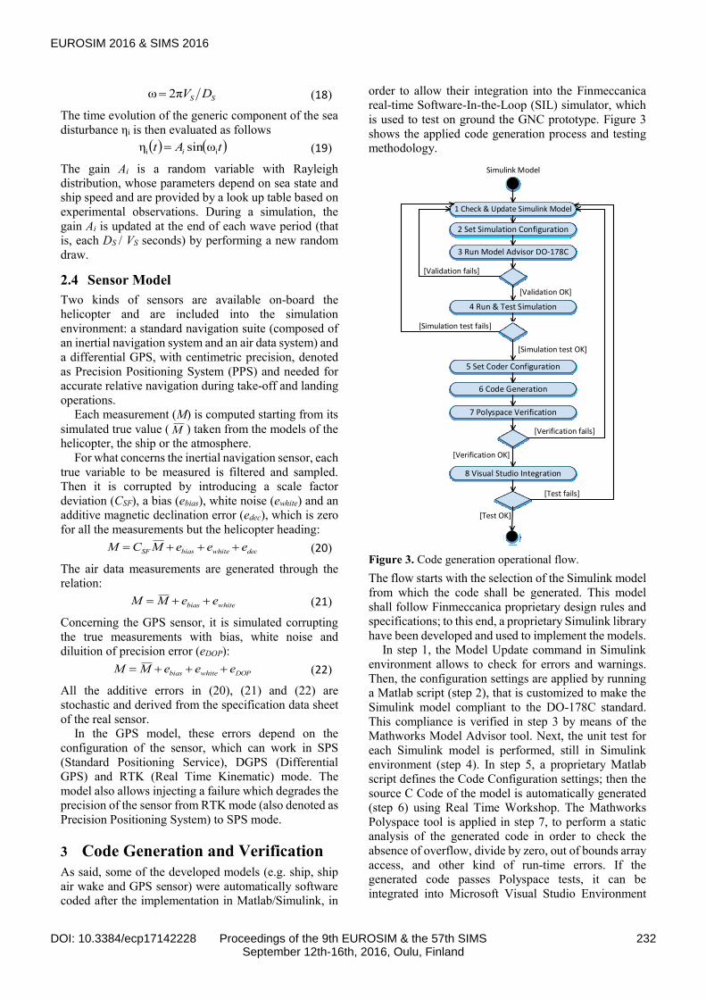
is used to test on ground the GNC prototype. Figure 3
shows the applied code generation process and testing
methodology.
1 Check & Update Simulink Model
2 Set Simulation Configuration
3 Run Model Advisor DO-178C
[Simulation test fails]
4 Run & Test Simulation
5 Set Coder Configuration
[Validation fails]
6 Code Generation
7 Polyspace Verification
8 Visual Studio Integration
[Verification fails]
[Test fails]
[Test OK]
[Verification OK]
[Simulation test OK]
[Validation OK]
Simulink Model
Figure 3. Code generation operational flow.
The flow starts with the selection of the Simulink model
from which the code shall be generated. This model
shall follow Finmeccanica proprietary design rules and
specifications; to this end, a proprietary Simulink library
have been developed and used to implement the models.
In step 1, the Model Update command in Simulink
environment allows to check for errors and warnings.
Then, the configuration settings are applied by running
a Matlab script (step 2), that is customized to make the
Simulink model compliant to the DO-178C standard.
This compliance is verified in step 3 by means of the
Mathworks Model Advisor tool. Next, the unit test for
each Simulink model is performed, still in Simulink
environment (step 4). In step 5, a proprietary Matlab
script defines the Code Configuration settings; then the
source C Code of the model is automatically generated
(step 6) using Real Time Workshop. The Mathworks
Polyspace tool is applied in step 7, to perform a static
analysis of the generated code in order to check the
absence of overflow, divide by zero, out of bounds array
access, and other kind of run-time errors. If the generated code passes Polyspace tests, it can be
integrated into Microsoft Visual Studio Environment
EUROSIM 2016 & SIMS 2016
232DOI: 10.3384/ecp17142228 Proceedings of the 9th EUROSIM & the 57th SIMSSeptember 12th-16th, 2016, Oulu, Finland

(step 8) to be tested with the same test vectors used in
Step 4. Finally, the test outputs of step 4 and step 8 are
compared, in order to check the correctness of the
generated code.
After that, the model code can be integrated into the
final detailed simulation model, being sure that it
performs exactly as the simulation environment used for
design.
4 Simulation Results
The principal phenomena that influenced the design of
the trajectories and tuning of the tracking algorithm for
automatic take-off and landing are the wake
phenomenon near the ship, the PPS availability along
the trajectory, the disturbance of the sea waves on the
ship deck motion and the performance and dynamic
behavior of the helicopter.
The validity of the proposed helicopter model for
GNC algorithm design can be demonstrated by Figure 4
where comparison of flight data versus simulation data
is reported for attitude.
The differences that can be noted have negligible
effects on the algorithm design and preliminary testing,
as the helicopter low frequency behavior is almost
accurately predicted. Similar results hold for
acceleration, not reported here for the sake of brevity.
Moreover, Figure 5 compares the collective
deflections in trim condition at 650ft altitude computed
by using the model with a validation data set provided
by Finmeccanica: the model reproduces quite well the
vehicle behavior, confirming the validity of the
proposed helicopter thrust model.
Figure 4. Comparison between simulated and
experimental attitudes.
Figure 5. Comparison between simulated collective
deflections in trim condition and validation data.
Figure 6. Schematic representation of the landing
trajectory.
The other main simulated effects on a sample automatic
landing trajectory are also presented below.
The designed landing trajectory, schematically
shown in Figure 6, is structured in three phases. In the
Proximity phase the helicopter is almost aligned with
the ship direction at a desired speed in order to follow
properly the descending path to the first relative
hovering way point (Approach phase). In the Final
phase, after the operator acknowledgment, the
helicopter moves to the second relative hovering
waypoint (P2HOVER) and finally lands on the ship deck.
The modelled action of the air wake on the helicopter
vertical acceleration, during the automatic landing
manoeuvers, is shown in Figure 7.
It is worth to note, in the second graph, how the effect
of the air wake is null until the helicopter enters in a
proper area (near P1HOVER). As said, such area depends
on the ship super-structure and wind direction (which in
the test is aligned with the ship speed). When the ground
operator gives the acknowledge command, the relative
distance between the ship and the helicopter decreases
while the wake effect increases. The same happens as
the relative altitude decreases in the last manoeuver for
deck landing.
Figure 7. Air wake effect on the helicopter vertical
acceleration.
Figure 8 presents the effect of the sea waves on the ship.
It refers to Type 23 frigate at two different speeds for
see state level six.
2100 2105 2110 2115 2120 2125 2130 2135
0
5
10
Ro
ll a
ng
le
(de
g)
TIME (S)
2030 2040 2050 2060 2070 2080 2090 2100 2110 2120
-2
0
2
4
Pitch
an
gle
(de
g)
TIME (S)
810 820 830 840 850 860 870 880
100
120
140
TIME (s)
Ya
w a
ng
le(d
eg
)
Flight Data Model Command to AP
0 5 10 15 20 25 30 35 40
6
8
10
12
Forward Speed (kts)
Colle
ctive
(deg)
Validation dataset
Model
EUROSIM 2016 & SIMS 2016
233DOI: 10.3384/ecp17142228 Proceedings of the 9th EUROSIM & the 57th SIMSSeptember 12th-16th, 2016, Oulu, Finland
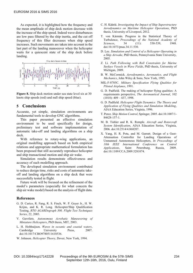
As expected, it is highlighted how the frequency and
the mean amplitude of ship deck motion decrease with
the increase of the ship speed. Indeed wave disturbances
are low pass filtered by the ship inertia, and the cut off
frequency of this filter decreases when ship speed
increases. Such movements are taken into account in the
last part of the landing manoeuver when the helicopter
waits for a quiescent state of the ship deck before
landing.
Figure 8. Ship deck motion under sea state level six at 30
knots ship speeds (red) and null ship speed (blue).
5 Conclusions
Accurate, yet simple, simulation environments are
fundamental tools to develop GNC algorithms.
This paper presented an effective simulation
environment to be used specifically for design,
preliminary test and software implementation of
automatic take-off and landing algorithms on a ship
deck.
With reference to rotary-wing applications, an
original modelling approach based on both empirical
relations and appropriate mathematical formulation has
been proposed that still accurately reproduce helicopter
and ship transactional motion and ship air wake.
Simulation results demonstrate effectiveness and
accuracy of such modelling approach.
The developed simulation environment contributed
to reduce design time, risks and costs of automatic take-
off and landing algorithms on a ship deck that were
successfully tested in flight.
Future work will be focused on the refinement of the
model’s parameters (especially for what concern the
ship air wake model) based on the analysis of flight data.
References
G. D. Carico, R. Fang, R. S. Finch, W. P. Geyer Jr., H. W.
Krijns, and K. R. Long. Helicopter/Ship Qualification
Testing, RTO AGARDograph 300, Flight Test Techniques
Series, 22, 2003.
V. Gavrilets. Autonomous Acrobatic Maneuvering of
Miniature Helicopters, PhD thesis, MIT, 2003.
L. H. Holthuijsen. Waves in oceanic and coastal waters,
Cambridge University Press, 2007.
doi:10.1017/CBO9780511618536.
W. Johnson. Helicopter Theory, Dover, New York, 1994.
C. H. Kääriä. Investigating the Impact of Ship Superstructure
Aerodynamics on Maritime Helicopter Operations, PhD
thesis, University of Liverpool, 2012.
T. von Kármán. Progress in the Statistical Theory of
Turbulence, Proceedings of the National Academy of
Sciences, 34 (11): 530-539, 1948.
doi:10.1073/pnas.34.11.530.
D. Lee. Simulation and Control of a Helicopter Operating in
a Ship Airwake, PhD thesis, Pennsylvania State University,
2005.
Z. Li. Path Following with Roll Constraints for Marine
Surface Vessels in Wave Fields, PhD thesis, University of
Michigan, 2009.
B. W. McCormick. Aerodynamics, Aeronautics, and Flight
Mechanics, John Wiley & Sons, New York, 1995.
MIL-F-8785C. Military Specification Flying Qualities for
Piloted Airplanes, 1991.
G. D. Padfield. The making of helicopter flying qualities: A
requirements perspective, The Aeronautical Journal, 102
(1018): 409 – 437, 1998.
G. D. Padfield. Helicopter Flight Dynamics: The Theory and
Application of Flying Qualities and Simulation Modeling,
AIAA Education Series, Virginia, 1996.
T. Perez. Ship Motion Control, Springer, 2005. doi:10.1007/1-
84628-157-1.
M. B. Tishler and R. K. Remple. Aircraft and Rotorcraft
System Identification, AIAA Education Series, Virginia,
2006. doi:10.2514/4.868207.
X. Yang, H. R. Pota, and M. Garratt. Design of a Gust-
Attenuation Controller for Landing Operations of
Unmanned Autonomous Helicopters, In Proceedings of
18th IEEE International Conference on Control
Applications, Saint Petersburg, Russia, 2009.
doi:10.1109/CCA.2009.5281074.
EUROSIM 2016 & SIMS 2016
234DOI: 10.3384/ecp17142228 Proceedings of the 9th EUROSIM & the 57th SIMSSeptember 12th-16th, 2016, Oulu, Finland
Top Related