Time-declining risk-adjusted social discount rates for transport infrastructure planning

by Kathrin Goldmann

Institute of Transport Economics Münster Working Paper No. 22 April 2017

© Westfälische Wilhelms-Universität (WWU), Institute of Transport Economics, 2017 Address Institut für Verkehrswissenschaft Am Stadtgraben 9 D 48143 Münster, Germany Telephone +49 251 83-22 99 0 Fax +49 251 83-28 39 5 E-Mail verkehrswissenschaft@uni-muenster.de Website http://www.iv-muenster.de All rights reserved. Any reproduction, publication and reprint in the form of a different publication, whether printed or produced electronically, in whole or in part, is permitted only with the explicit written authorisation of the Westfälische Wilhelms-Universität, Institute of Transport Economics, or the author(s). The views expressed in this paper do not necessarily reflect those of the Institute of Transport Economics or the WWU. The Working Paper Series seeks to disseminate economic research work by the WWU, Institute of Transport Economics staff and visitors. Papers by researchers not affiliated with the WWU Institute of Transport Economics may also be considered for publication to the extent that they have been presented at research seminars/workshops organised by the institute. The working papers published in the Series constitute work in progress circulated to stimulate discussion and critical comments. Views expressed represent exclusively the authors' own opinions. The Series is managed by the Director of the Institute of Transport Economics.

Time-declining risk-adjusted social discount rates for transport infrastructure planning

By KATHRIN GOLDMANN*

I. Introduction

In economics literature, there is consensus that the choice of discount rate has an enormous impact on the appraisal results of public investment projects. There is a vast literature on methods of how to discount future costs and benefits of public projects and how risk should be priced. This variety of methods translates into national guidelines in which social discount rates (SDRs) are very heterogeneous and range between 0.3% and 11% (Harrison, 2010). The natural candidate for a risk-free discount rate derived from market rates is the government bond rate of AAA-rated countries, as it represents the governments financing costs. Using the government bond rate without a separate assessment of the risk properties of transport projects, however, also implies that risk in investment projects often remains unconsidered. If this is

This paper proposes a social discount rate for transport infrastructure project evaluation in Germany that accounts for production efficiency, systematic traffic demand risk, as well as increasing uncertainty in the long-run. The systematic risk in infrastructure planning is measured by the sensitivity of transport volume towards GDP using cointegration analysis. In contrast to the only existing application of this model in transport economics, in this paper the systematic risk for freight transport projects is substantially higher than for passenger transport projects. Due to different systematic risk patterns, the discount rates for freight and passenger transport projects should differ as well, with the former being equal to approximately 3.5% and declining to 2.7% after 50 years, and the latter ranging between 2.0% and the risk-free rate of 1.3%. This paper focuses especially on the econometric challenges of the CAPM-like estimation of systematic risk in public transport infrastructure project assessment and is at the same time the first application to German data. JEL: H43; R42

* Kathrin Goldmann: Westfälische Wilhelms-Universität, Institut für Verkehrswissenschaft, Am Stadtgraben 9, 48143 Münster, Germany, kathrin.goldmann@uni-muenster.de. Acknowledgements: The author would like to thank three anonymous referees, Gernot Sieg, David Ennen, Thorsten Heilker, Inga Molenda and Julia Rothbauer for helpful comments. This version: April 26, 2017. The final publication is available at Springer via http://dx.doi.org/10.1007/s11116-017-9780-4

INSTITUTE OF TRANSPORT ECONOMICS MÜNSTER WORKING PAPER NO. 22 2

done deliberately, it will often be justified on the basis that the project risk is spread over a large number of tax payers and the proportion of risk of single projects each tax payer has to bear is relatively low (Arrow and Lind, 1970). This might be justified, as long as the project risks are idiosyncratic and can be pooled by the government (Little and Mirrlees, 1974; Ewijk and Tang, 2003). In transport infrastructure projects, the benefits are in general positively correlated with national income and this systematic risk cannot be reduced by diversification (Little and Mirrlees, 1974). Hence, ignoring the systematic risk of a project causes evaluation mistakes that may lead to allocative inefficiencies of public resources.

In this paper I estimate the systematic risk of transport projects by the relationship between transport demand and GDP for different modes of transportation using cointegration techniques. The information for the social planner of these results is twofold: First, they give information about the degree of systematic risk in projects and therefore their contribution to consumption smoothing of households. Second, they provide insights for the optimal timing of the investment decision. Projects whose performance depends strongly on the overall economic activity should for example not be completed in times of economic downturns.

Using this information, this paper provides input on how to determine country-specific risk-adjusted discount rates for transport project assessment. It provides new insights on how to empirically estimate the model for risk-adjusted long-term discount rates proposed by Weitzman (2012, 2013) paying special attention to the time series properties of the employed data. The approach uses the opportunity costs of capital adjusted for systematic, but not for project specific risk. The results suggest that systematic traffic demand risk differs significantly between freight and passenger transport projects and therefore different discount rates should be used. These discount rates can easily be implemented in national guidelines and would ensure, that every social planner accounts for risk in transport projects in the same way.

The remainder of this paper is structured as follows. The next section gives an overview of the existing literature on risk-adjusted social discount rates. The third section describes the underlying economic model and defines the parameter (γ) that determines the systematic risk in real project assessment. The forth section consists of the empirical estimation of γ. The fifth section derives values of risk-free and equity discount rates from market interest rates. Combining γ and the interest rates from the previous section in the discount rate formula based on the linear decomposition of risk factors, yields the risk-adjusted SDR for the specific risk-properties inherent in German transport projects, depending on the transport mode. The final section contains the main conclusions.

II. Risk-adjustment of the social discount rate When analyzing the risk-adjustment of discount rates, it is necessary to differentiate between uncertainty regarding the economic environment in general, the uncertainty about a project’s future costs and benefits as well as their relation to other income accruing to households. The first aspect can be accounted for with the variance of macroeconomic variables, the second aspect relates to the variance of project returns and the third to the covariance between project returns and the economic development in general.

Uncertainty about the economic environment becomes especially relevant if project life span is long and may even involve different generations. There is agreement in literature on

SOCIAL DISCOUNT RATE FOR TRANSPORT INFRASTRUKTURE PLANNING

3

the fact that when the economic environment is uncertain, the discount rate should decrease for projects exceeding time horizons of 40 to 50 years (Weitzman, 1998; Weitzman, 2001; Gollier et al. (2008); Arrow et al., 2014; Gollier, 2016).

The concept of a time-declining SDR in Cost-Benefit-Analysis (CBA) was introduced by Weitzman (1998). The model focuses on discounting the distant future, where even the discount rate itself is uncertain. Weitzman (1998) proposes a certainty-equivalent discount rate that declines continuously over time to the lowest possible rate. He states that in order to obtain the relevant discount rate at a point in time, the discount factors and not the discount rates should be averaged (Weitzman, 1998). An example is given by Hepburn et al. (2009), who demonstrate that an SDR which is equally likely to be 2% or 10% will yield the following certainty-equivalent discount rate schedule of − !

! ln!! !

!!.!"! + !! !

!!.!"! demonstrating that the discount factors need to be averaged, since they are the relevant shadow prices under uncertainty. The resulting discount rate declines from 6% in t = 1 to 2.7% in t = 100 and will eventually approach 2% when time goes to infinity. Gollier et al. (2008) illustrate that the more uncertain the future interest rate, the faster the certainty-equivalent discount rate will approach the low-scenario rate. An intuitive explanation is given by the precautionary motive of saving. It makes agents save more in safe assets to ensure a certain level of future consumption the more uncertain they perceive the future economic environment (Gollier, 2015). In recent work, Gollier (2016) shows that when future consumption is positively correlated with future spot interest rates, the discount rate for discounting safe future costs and benefits is even lower than proposed by Weitzman (2001). The concept of time-declining discount rates has been adopted by some national authorities for public policy evaluation. 1

In large and diversified portfolios, as can be assumed for the government’s project portfolio, the variance of project returns can be neglected at the aggregate level, since those project specific risks can be neutralised by diversification. For this reason the variance in transport project returns is not discussed any further.

The risk specifically addressed in this paper is the fraction of risk imposed by projects on households that cannot be diversified. That is inherent in projects that have uncertain future benefits which are correlated with economic growth. For these projects the discount rate should include a risk premium to account for this systematic risk (Harrison, 2010; Gollier, 2011). A standard model for evaluating such risks of financial assets is the Capital Asset Pricing Model (CAPM) (Sharpe, 1964; Lintner, 1965; Mossin, 1966).

As the CAPM is a static model and only includes wealth in the form of corporate stocks, the Consumption CAPM (CCAPM) has been developed to overcome these shortfalls (Merton, 1973; Breeden, 1979). However, when putting plausible values for risk aversion and respective standard deviations into the model variables, the CCAPM will yield excessively high values for the risk-free rate and values for the equity premium that are too low to correspond with actual observable rates. These discrepancies are referred to as the risk-free rate and equity premium puzzle (Mehra and Prescott, 1985).

Weitzman (2012, 2013) has developed an approach for assessing the risk of public projects. It is based on consumption-based asset pricing with respect to thicker tails of the consumption distribution in order to resolve the equity-premium and risk-free rate puzzle. In a model for CBA he divides project benefits into those that are independent of the overall 1 See e.g. HM Treasury 2011; Lebègue 2005.

INSTITUTE OF TRANSPORT ECONOMICS MÜNSTER WORKING PAPER NO. 22 4

economic activity and those that are correlated with it. The aspects of the Weitzman-Model that are relevant for this analysis are described in more detail in the next chapter.

The basic issue is how to empirically match the broader concept of the CCAPM and the specific risk patterns of the transport sector. It seems intuitive that the more the net benefit of a specific project is correlated with the remainder of the economy, the less it provides a hedge for households against poor states of the economy (Little and Mirrlees, 1974; Hultkrantz et al., 2014). These are times of relatively low economic activity, which result in low consumption. For this reason, the covariance between the project return and the aggregate growth rate of consumption or GDP can serve as a measure of systematic risk and is therefore used in literature. (Dixit and Williamson, 1989; Ewijk and Tang, 2003; Krüger, 2012).

The benefits of public transport infrastructure projects like reductions in travel time, increase in safety, increase in travel time reliability, noise and pollution reduction usually depend on traffic demand and the main uncertainty is whether traffic demand is sufficient to cover the investment and maintenance costs (Krüger, 2012). In empirical studies, traffic demand is often approximated with traffic volume (Ramanathan, 2001; Krüger, 2012; Hultkrantz et al., 2014).

Krüger (2012) uses a wavelet variance analysis and estimates the correlation between GDP fluctuations and traffic demand growth for Sweden, for various time scales. He obtains a stronger correlation of rail freight transport with overall economic activity (0.48-0.63) than with road transport (0.03-0.49). Moreover, he obtains substantially higher values for freight transport than for passenger transport, and concludes that investment in infrastructure for freight transport is more risky than in infrastructure for passenger transport. He points out that these results might be useful for determining the SDR, but leaves the implementation for future research.

Hultkrantz et al. (2014) provide a direct empirical application of the Weitzman-Model, which is related to the one used in this paper. They use cointegration techniques to analyse the long-run relationship between transport demand and GDP for Sweden. The employed time series for rail passenger, rail freight, road passenger, road freight transport and GDP are transformed to obtain correlation coefficients. The bivariate level data correlation coefficients of each transport time series with GDP are, with values around 0.9, very high. In contrast to Krüger (2012) the coefficients do not differ systematically between freight and passenger transport. They use the coefficients to specify the degree of systematic risk in the respective transport sector and include the estimated γ-coefficients in the time-declining discount rate schedule for CBA, as proposed by Weitzman (2012, 2013). Since the high degree of systematic risk places considerable weight on the equity discount rate, Hultkrantz et al. (2014), who use a risk-free rate of 2.0% and an equity discount rate of 6.5%, estimate SDRs between 5% and 6%, depending on the transport mode, which decline only marginally over the assumed investment horizon of approximately 80 years.

III. Decomposition and discounting of project benefits

The underlying model of this paper for risk-adjusted discount rates for cost-benefit analysis has been developed by Weitzman (2012, 2013). It is based on a linear decomposition of real project benefits at time t (!!) into those that evolve independently (!!!) and benefits that are correlated with the overall economic activity (!!!) (Weitzman, 2013)

SOCIAL DISCOUNT RATE FOR TRANSPORT INFRASTRUKTURE PLANNING

5

!! = !!! + !!! . (1)

Weitzman assumes that !!! is proportional to !! and !!! is proportional to !!, with the variable !! representing an idiosyncratic component like e.g. the payoff of merit goods and !! representing systemwide shocks in the aggregate economy (Weitzman, 2013). He defines the parameter reflecting the non-diversifiable systematic risk as !, which is the proportion of benefits, which move proportionally with overall economic activity:

!! ≡ !!!

!! 1− !! = !!

!

!!. (2)

Applying these considerations to the discount rate (!!), it seems plausible that the proportion of benefits that is independent of developments in the uncertain macro economy is discounted with a risk-free rate (!!). Individual projects may be risky, but in the aggregate in a large diversified portfolio, idiosyncratic risks can be diversified and need not be accounted for with an equity premium. Benefits that move proportionally to macroeconomic developments contain systematic risk, which can be assessed by an equity discount rate (!!) containing a risk premium (Weitzman, 2013). The model only includes systematic risk in the framework of cost-benefit analysis

! !! !!!!∙! = ! !!! ∙ !!!!∙! + ! !!! ∙ !!!!∙! . (3)

Substituting the expected benefits with the shares of systematic and project-specific benefits derived above, one obtains the following equation:

!!!!∙! = 1− !! ∙ !!!!∙! + !! ∙ !!!!∙! . (4)

Taking into account the assumption of constant proportions of risk, the discount rate can be defined as

!! = − !! ln 1− ! ∙ !!!!∙! + ! ∙ !!!!∙! . (5)

The Weitzman-Model conceptualizes the project benefits similar to the CAPM and one obtains a single parameter !, which quantifies the degree of systematic risk. This parameter is, however, defined differently to the CAPM as a proportion. The framework does not directly derive an equation that can be estimated with real data. The specification of ! and the required time series transformations are therefore presented in the appendix.

IV. Empirical estimation of ! for Germany

To determine !, the relationship between the systematic risk component (!!∗) and the project benefits (!!∗) can be estimated by a simple regression equation.2

!!∗ = 1− ! + ! ∙ !!∗ + !! (6)

For the empirical analysis, it is necessary to identify a time series, which can approximate the project benefits, since project payoffs are rarely measurable on a regular basis (Weitzman, 2012). For transport infrastructure projects, Hultkrantz et al. (2014) find, that a large share of transport project benefits emerges from improvements in travel time duration and travel time 2 Variables !!∗ and !!∗ and the evolution of the regression equation are described in appendix B. Notice that the

relation does not necessarily need to be linear.

INSTITUTE OF TRANSPORT ECONOMICS MÜNSTER WORKING PAPER NO. 22 6

reliability, as well as traffic safety. The realization of these benefits strongly depends on the extent the infrastructure is actually used, that is traffic demand. In empirical studies, traffic demand is usually approximated with transport volume (TV), measured in tonnes multiplied by distance for freight transport (tkm) and passengers multiplied by distance for passenger transport (pkm) (Krüger, 2012; Hultkrantz et al., 2014). As a broad concept for risk in the overall economy, !"# is often used in the empirical literature on this topic (Dixit and Williamson, 1989; Ewijk and Tang, 2003; Krüger, 2012; Hultkrantz et al., 2014).

If !!∗ is replaced by !"!, !!∗ by !"#! and 1− ! represents the constant (!), the regression equation for this set of variables has the following form:

!"! = ! + ! ∙ !"#! + !!. (7)

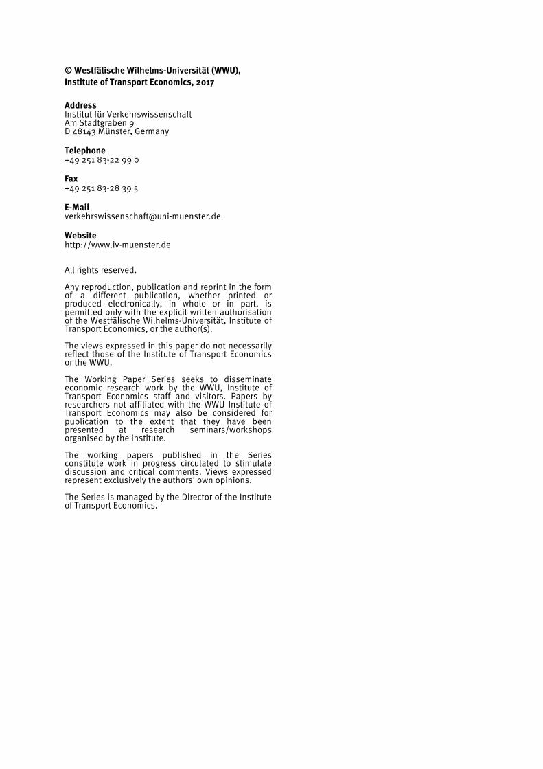
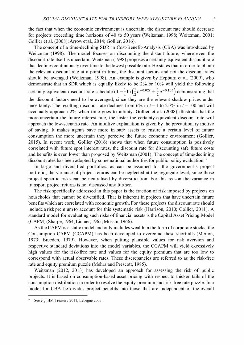
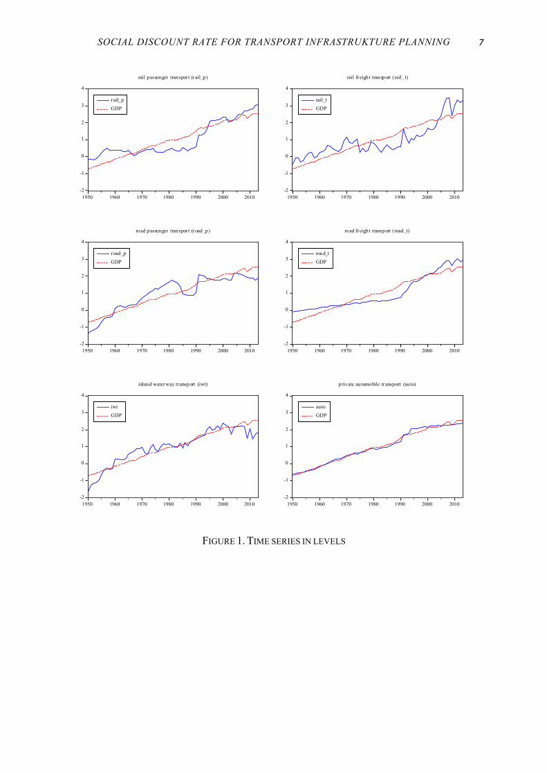
The analysis differentiates between six transport modes that are most relevant for German transport infrastructure planning. Included time series for !" are (roadp, roadt, railp, railt, iwt, auto).3 Compared to Hultkrantz et al. (2014), the analysis is extended by iwt and auto as those transport modes are very relevant for Germany and they use infrastructure, which requires huge amounts of public investment. !"# is employed in each of the six equations.4 All time series range from 1950 to 2013 and were available on an annual basis. Figures 1 and 2 show the transportation time series with GDP.

From the visual inspection, all time series seem to follow either a random walk with drift or a deterministic trend. The relevant specifications of the Augmented Dickey Fuller test (ADF-test) indicate that all variables except iwt follow a random walk with drift (Dickey and Fuller, 1979). However, the ADF-Test is biased towards non-rejection of the null hypothesis of a unit root in the presence of structural breaks. For this reason, the Zivot and Andrews test has been employed to identify the properties of the time series (Zivot and Andrews, 1992).5 On the basis of these results and logical reasoning, all time series are assumed to be I(1).

3 All transport time series are taken from the annual publication "Verkehr in Zahlen" published by the Ministry for

Transport and Digital Infrastructure. A more detailed description of the time series can be found in appendix A.4 The GDP time series is taken from the Bundesbank database.5 The results of the Zivot and Andrews-Test are presented in Table C.1 in the appendix.

SOCIAL DISCOUNT RATE FOR TRANSPORT INFRASTRUKTURE PLANNING

7

FIGURE 1. TIME SERIES IN LEVELS

-2

-1

0

1

2

3

4

1950 1960 1970 1980 1990 2000 2010

rail_pGDP

rail passenger transpor t (rail_p)

-2

-1

0

1

2

3

4

1950 1960 1970 1980 1990 2000 2010

rail_tGDP

rail freight transport ( rail_t)

-2

-1

0

1

2

3

4

1950 1960 1970 1980 1990 2000 2010

road_pGDP

road passenger transpor t (road_p)

-2

-1

0

1

2

3

4

1950 1960 1970 1980 1990 2000 2010

roa d_tGDP

road freight transport ( road_t)

-2

-1

0

1

2

3

4

1950 1960 1970 1980 1990 2000 2010

iwtGDP

inland waterway transport (iwt)

-2

-1

0

1

2

3

4

1950 1960 1970 1980 1990 2000 2010

autoGDP

private automobile tr ansport (auto)

INSTITUTE OF TRANSPORT ECONOMICS MÜNSTER WORKING PAPER NO. 22 8

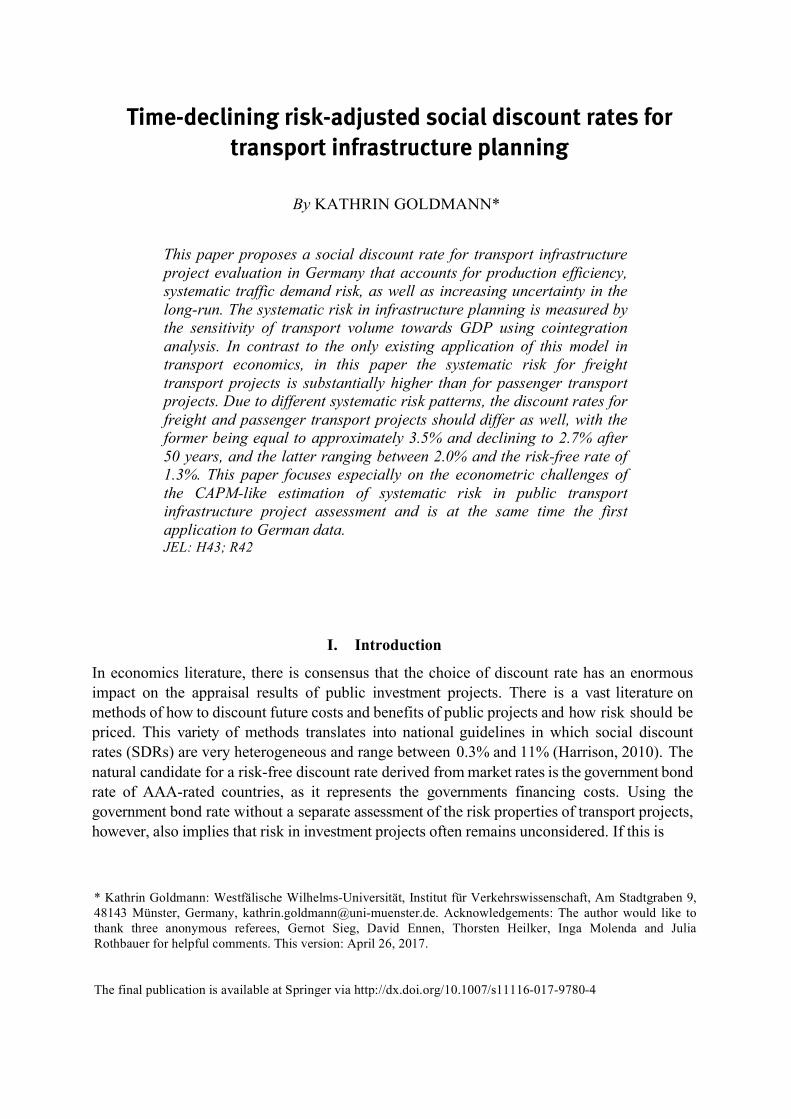
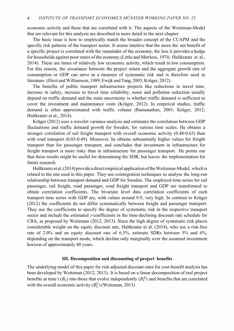
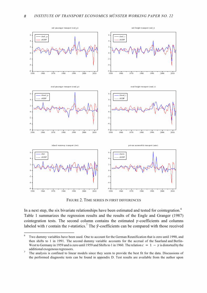
FIGURE 2. TIME SERIES IN FIRST DIFFERENCES

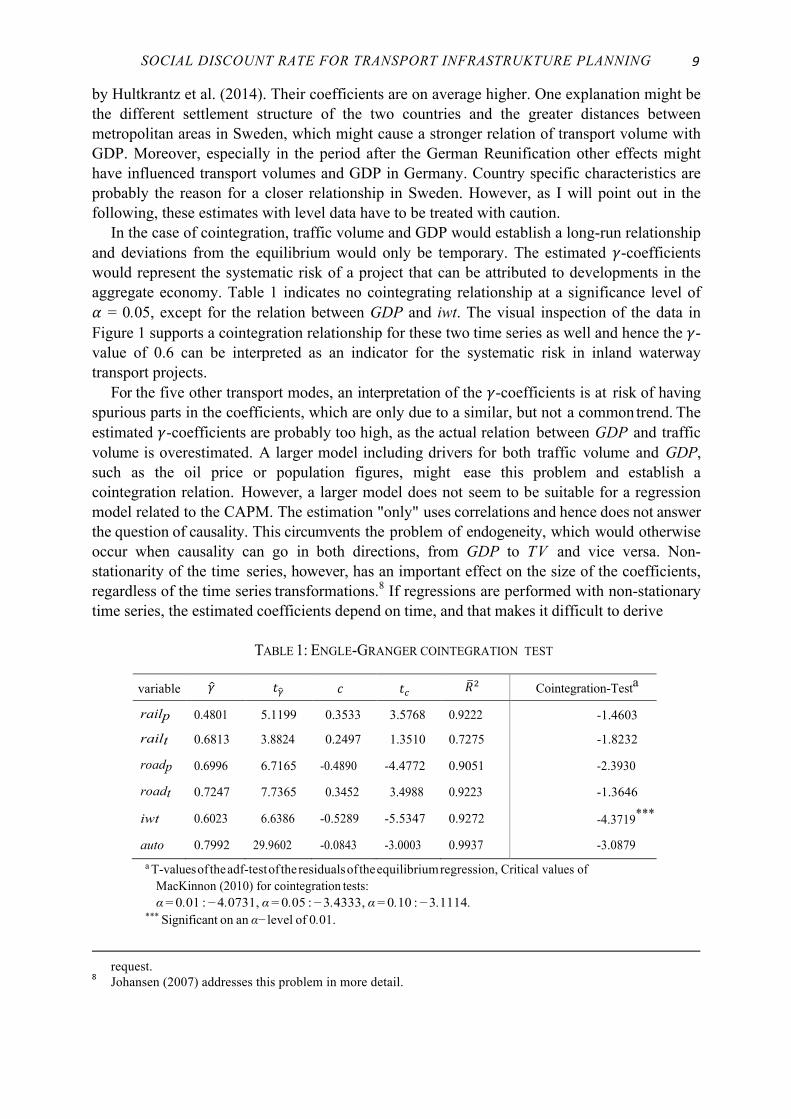
In a next step, the six bivariate relationships have been estimated and tested for cointegration.6 Table 1 summarizes the regression results and the results of the Engle and Granger (1987) cointegration tests. The second column contains the estimated !-coefficients and columns labeled with t contain the t-statistics.7 The !-coefficients can be compared with those received 6 Two dummy variables have been used. Oneto account for the German Reunification that is zero until 1990, and

then shifts to 1 in 1991. The second dummy variable accounts for the accrual of the Saarland and Berlin-West to Germany in 1959 and is zero until 1959 and Shifts to 1 in 1960. The relation ! = 1 − ! is distorted by the additional exogenous regressors.

7 The analysis is confined to linear models since they seem to provide the best fit for the data. Discussions of the performed diagnostic tests can be found in appendix D. Test results are available from the author upon

-6

-4

-2

0

2

4

6

1950 1960 1970 1980 1990 2000 2010

drail_pdGDP

rail passenger transpor t (rail_p)

-6

-4

-2

0

2

4

6

1950 1960 1970 1980 1990 2000 2010

drail_tdGDP

rail f reight tr ansport ( rail_t)

-6

-4

-2

0

2

4

6

1950 1960 1970 1980 1990 2000 2010

droa d_pdGDP

road passenger transpor t (road_p)

-6

-4

-2

0

2

4

6

1950 1960 1970 1980 1990 2000 2010

droad_tdGDP

road f reight tra nsport ( road_t)

-6

-4

-2

0

2

4

6

1950 1960 1970 1980 1990 2000 2010

diwtdGDP

inland waterway transport (iwt)

-6

-4

-2

0

2

4

6

1950 1960 1970 1980 1990 2000 2010

dautodGDP

private automobile transport ( auto)

SOCIAL DISCOUNT RATE FOR TRANSPORT INFRASTRUKTURE PLANNING

9

by Hultkrantz et al. (2014). Their coefficients are on average higher. One explanation might be the different settlement structure of the two countries and the greater distances between metropolitan areas in Sweden, which might cause a stronger relation of transport volume with GDP. Moreover, especially in the period after the German Reunification other effects might have influenced transport volumes and GDP in Germany. Country specific characteristics are probably the reason for a closer relationship in Sweden. However, as I will point out in the following, these estimates with level data have to be treated with caution.

In the case of cointegration, traffic volume and GDP would establish a long-run relationship and deviations from the equilibrium would only be temporary. The estimated !-coefficients would represent the systematic risk of a project that can be attributed to developments in the aggregate economy. Table 1 indicates no cointegrating relationship at a significance level of ! = 0.05, except for the relation between GDP and iwt. The visual inspection of the data in Figure 1 supports a cointegration relationship for these two time series as well and hence the !-value of 0.6 can be interpreted as an indicator for the systematic risk in inland waterway transport projects.

For the five other transport modes, an interpretation of the !-coefficients is at risk of having spurious parts in the coefficients, which are only due to a similar, but not a common trend. The estimated !-coefficients are probably too high, as the actual relation between GDP and traffic volume is overestimated. A larger model including drivers for both traffic volume and GDP, such as the oil price or population figures, might ease this problem and establish a cointegration relation. However, a larger model does not seem to be suitable for a regression model related to the CAPM. The estimation "only" uses correlations and hence does not answer the question of causality. This circumvents the problem of endogeneity, which would otherwise occur when causality can go in both directions, from GDP to TV and vice versa. Non-stationarity of the time series, however, has an important effect on the size of the coefficients, regardless of the time series transformations.8 If regressions are performed with non-stationary time series, the estimated coefficients depend on time, and that makes it difficult to derive

TABLE 1: ENGLE-GRANGER COINTEGRATION TEST

variable ! !! ! !! !! Cointegration-Testa

railp 0.4801 5.1199 0.3533 3.5768 0.9222 -1.4603

railt 0.6813 3.8824 0.2497 1.3510 0.7275 -1.8232

roadp 0.6996 6.7165 -0.4890 -4.4772 0.9051 -2.3930

roadt 0.7247 7.7365 0.3452 3.4988 0.9223 -1.3646

iwt 0.6023 6.6386 -0.5289 -5.5347 0.9272 -4.3719***

auto 0.7992 29.9602 -0.0843 -3.0003 0.9937 -3.0879 a T-values of the adf-test of the residuals of the equilibrium regression, Critical values of

MacKinnon (2010) for cointegration tests: α = 0.01 : −4.0731, α = 0.05 : −3.4333, α = 0.10 : −3.1114.

*** Significant on an α−level of 0.01.

request.

8 Johansen (2007) addresses this problem in more detail.

INSTITUTE OF TRANSPORT ECONOMICS MÜNSTER WORKING PAPER NO. 22 10

generally valid results. Moreover, when comparing this model to estimations of the CAPM-model for financial data, asset returns are used, which are more likely to be stationary processes than the underlying performance indices.

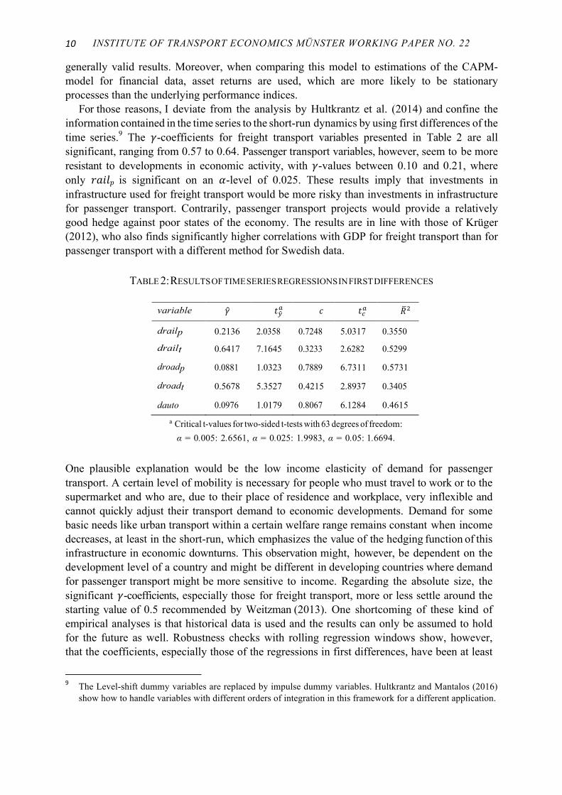
For those reasons, I deviate from the analysis by Hultkrantz et al. (2014) and confine the information contained in the time series to the short-run dynamics by using first differences of the time series.9 The !-coefficients for freight transport variables presented in Table 2 are all significant, ranging from 0.57 to 0.64. Passenger transport variables, however, seem to be more resistant to developments in economic activity, with !-values between 0.10 and 0.21, where only !"#$! is significant on an !-level of 0.025. These results imply that investments in infrastructure used for freight transport would be more risky than investments in infrastructure for passenger transport. Contrarily, passenger transport projects would provide a relatively good hedge against poor states of the economy. The results are in line with those of Krüger (2012), who also finds significantly higher correlations with GDP for freight transport than for passenger transport with a different method for Swedish data.

TABLE 2: RESULTS OF TIME SERIES REGRESSIONS IN FIRST DIFFERENCES

variable !!! !!! !!!! !!! !!!!

drailp 0.2136 2.0358 0.7248 5.0317 0.3550

drailt 0.6417 7.1645 0.3233 2.6282 0.5299

droadp 0.0881 1.0323 0.7889 6.7311 0.5731

droadt 0.5678 5.3527 0.4215 2.8937 0.3405

dauto 0.0976 1.0179 0.8067 6.1284 0.4615

a Critical t-values for two-sided t-tests with 63 degrees of freedom: α = 0.005: 2.6561, α = 0.025: 1.9983, α = 0.05: 1.6694.

One plausible explanation would be the low income elasticity of demand for passenger transport. A certain level of mobility is necessary for people who must travel to work or to the supermarket and who are, due to their place of residence and workplace, very inflexible and cannot quickly adjust their transport demand to economic developments. Demand for some basic needs like urban transport within a certain welfare range remains constant when income decreases, at least in the short-run, which emphasizes the value of the hedging function of this infrastructure in economic downturns. This observation might, however, be dependent on the development level of a country and might be different in developing countries where demand for passenger transport might be more sensitive to income. Regarding the absolute size, the significant !-coefficients, especially those for freight transport, more or less settle around the starting value of 0.5 recommended by Weitzman (2013). One shortcoming of these kind of empirical analyses is that historical data is used and the results can only be assumed to hold for the future as well. Robustness checks with rolling regression windows show, however, that the coefficients, especially those of the regressions in first differences, have been at least

9 The Level-shift dummy variables are replaced by impulse dummy variables. Hultkrantz and Mantalos (2016)

show how to handle variables with different orders of integration in this framework for a different application.

SOCIAL DISCOUNT RATE FOR TRANSPORT INFRASTRUKTURE PLANNING

11

relatively stable over the sample period. If the analysis is confined to the period after the German Reunification, the regressions deliver very similar results with the coefficients of freight transport variables being substantially higher than those of passenger transport variables as well. For this reason, the coefficients seem to be a good guess that can be made by historical data.

V. Interest rates, taxes and risk-adjusted discount rates

To calculate the risk-adjusted discount rate of equation (5), I identify values for the risk-free and the equity rate of return in this section. There is agreement in literature on the selection of the risk-free rate. Since the default risk of AAA-rated countries is close to zero, the return on government bonds is generally chosen as the risk-free rate. When using market rates of return, the selected time horizon of historical data, or the assumptions for the interest rate forecasts have a significant impact on the level of the interest rate. In this paper, historical data for German Government Bonds with a maturity between 15 to 30 years is used. In the last eight years, the average nominal return was 3.3%.10 Using a shorter time span puts too much weight on the very low interest rates in recent years, which were probably the result of the quantitative easing activities of the European Central Bank. A longer time span would implicitly support the unlikely assumption that the economy will revert to those high interest rate levels of past decades. Hence, the right balance between those two rates seems to be found when averaging the interest rates over the last eight years. This is assumed to be a reasonable guess of long-term future interest rates. The equity rate of interest can be calculated by average stock returns. In the same time horizon of eight years, the average nominal return in Germany was 7.5%.11

In perfect markets, the interest rate for displaced consumption would equal the interest rate for displaced investment. In the presence of taxes, however, these rates can differ significantly. The social opportunity costs of capital will be the weighted average of the pre-tax and the after-tax rates of return and the costs of funding from abroad (Boardman et al., 2014). The German government has committed itself to maintaining a balanced budget. Hence it seems reasonable to assume, that investments in infrastructure will be tax financed or financed by the heavy vehicle toll or rail charges.12 For this reason the effects of government borrowing are not discussed further in this paper.

To determine the relevance of different taxes, the question of who bears the tax and toll burden has to be answered in advance. For the extra costs of the road charge, Einbock (2007) found for Austria, that a large share is passed on to clients in the form of increasing prices of final products. If one assumes a similar pass-through of financing costs for Germany, it would be reasonable to assume, that approximately 90 % of the costs are born by consumers. Due to the market power of the Deutsche Bahn, a similar pass through can be assumed for rail charges. Regarding taxes, the split between investment and consumption seems to be similar to the toll, since most of the tax revenue is borne by consumers.13 To keep the analysis simple, both the

10 The data has been taken from the Bundesbank press releases on Government bond yields.11 The time series has been taken from the Bundesbank-Database, DAX Performance-Index (BBK01.WU3141).12 Other financing sources are not taken into account as they only account for a small share. 13 Calculation based on the table of tax revenues in 2014 from the German Federal Ministry of Finance. It has

been taken into account that taxes paid by enterprises are often passed on to consumers, who therefore bear the tax burden. Boardman (2014) receives very similar results for the US, where the majority of government projects is tax

INSTITUTE OF TRANSPORT ECONOMICS MÜNSTER WORKING PAPER NO. 22 12

toll and the taxes for financing transport infrastructure investments are assumed to be borne completely by consumers. This is of course a simplifying assumption, but a more detailed analysis on this topic is beyond the scope of this paper and would not change the results significantly.

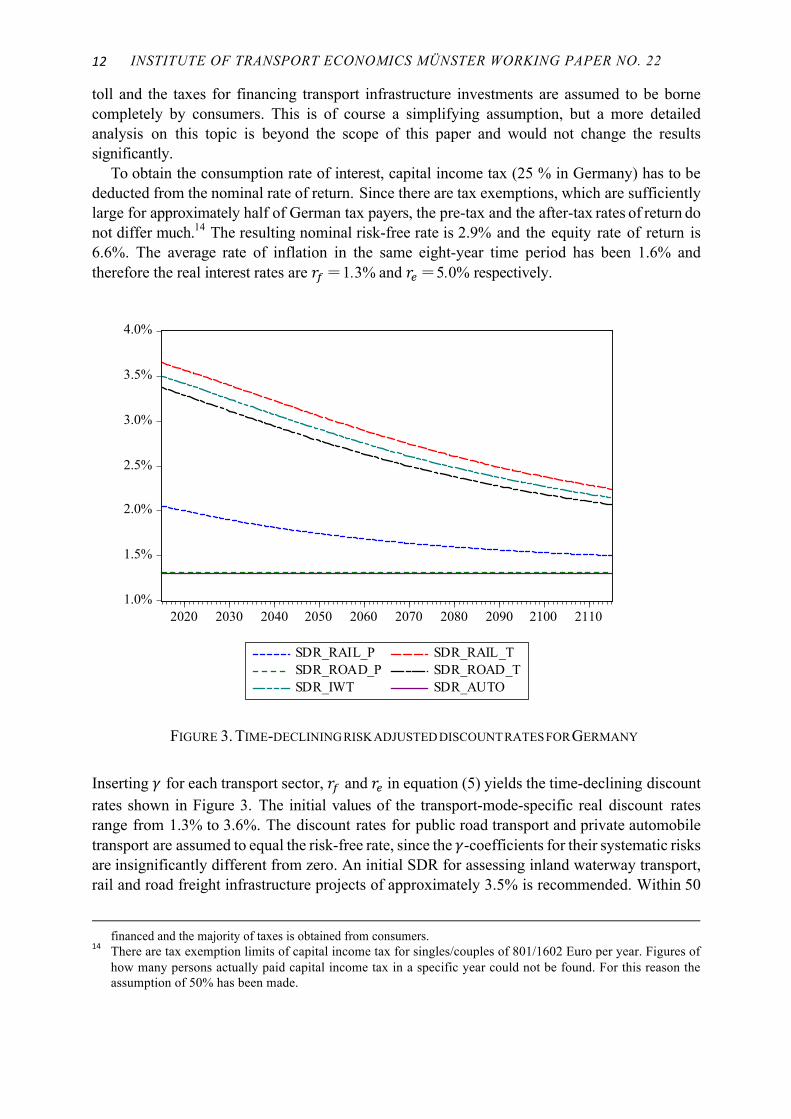
To obtain the consumption rate of interest, capital income tax (25 % in Germany) has to be deducted from the nominal rate of return. Since there are tax exemptions, which are sufficiently large for approximately half of German tax payers, the pre-tax and the after-tax rates of return do not differ much.14 The resulting nominal risk-free rate is 2.9% and the equity rate of return is 6.6%. The average rate of inflation in the same eight-year time period has been 1.6% and therefore the real interest rates are !! = 1.3% and !! = 5.0% respectively.

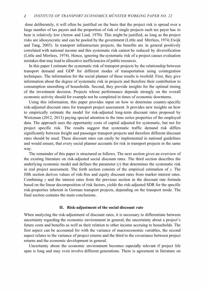
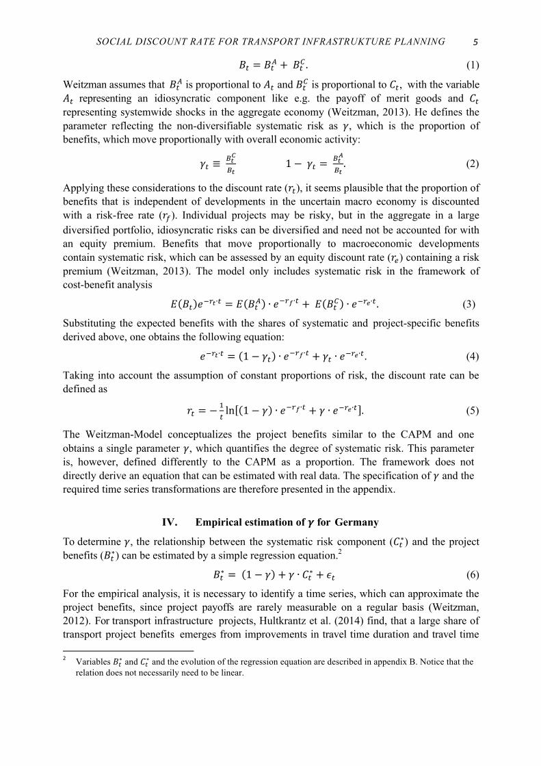
FIGURE 3. TIME-DECLINING RISK ADJUSTED DISCOUNT RATES FOR GERMANY

Inserting ! for each transport sector, !! and !! in equation (5) yields the time-declining discount rates shown in Figure 3. The initial values of the transport-mode-specific real discount rates range from 1.3% to 3.6%. The discount rates for public road transport and private automobile transport are assumed to equal the risk-free rate, since the !-coefficients for their systematic risks are insignificantly different from zero. An initial SDR for assessing inland waterway transport, rail and road freight infrastructure projects of approximately 3.5% is recommended. Within 50

financed and the majority of taxes is obtained from consumers.

14 There are tax exemption limits of capital income tax for singles/couples of 801/1602 Euro per year. Figures of how many persons actually paid capital income tax in a specific year could not be found. For this reason the assumption of 50% has been made.

1.0%

1.5%

2.0%

2.5%

3.0%

3.5%

4.0%

2020 2030 2040 2050 2060 2070 2080 2090 2100 2110

SDR_RAIL_P SDR_RAIL_TSDR_ROAD_P SDR_ROAD_TSDR_IWT SDR_AUTO

SOCIAL DISCOUNT RATE FOR TRANSPORT INFRASTRUKTURE PLANNING

13

years, the rate for freight infrastructure declines to approximately 2.7%. Due to a small positive correlation with GDP, rail passenger transport projects should be discounted with 2.0%. Accordingly, the government should accept these lower rates of return for passenger transport projects, as those projects comprise less systematic risk than freight transport projects and therefore turned out to contribute to consumption smoothing of private households. Projects that partially make up for income losses in economic downturns are more beneficial for society than others.

VI. Conclusions

Given that taxpayers want the government to invest their money in a diversified portfolio, so as to gain stable returns that do not vary much with economic activity, risk, which cannot be diversified in the government’s project portfolio, should not be ignored in public project assessment. For this reason, the systematic risk inherent in transport projects should be priced in order to obtain socially optimal evaluation results.

In this paper Weitzman’s (2012, 2013) risk-adjusted discount rate model has been estimated, for which the discount rate is a weighted average of the discount factors of the risk-free and the equity rates of return. The weight for return on equity is determined by a coefficient representing the systematic traffic demand risk. The results are obtained by regressions of the transport time series with GDP, with particular regard to the time series properties. The demand for freight transport seems more sensitive to economic fluctuations than the demand for passenger transport. This alone is already a useful insight for the composition of the government’s project portfolio. Moreover, while the timing of completion does not seem to influence the performance of passenger transport infrastructure projects, freight transport infrastructure projects should not be completed in economic downturns.

The risk-free and equity rates of return have been determined by opportunity costs of taking the money out of the private sector by taxes and tolls. Translated into the discount rate, the results imply that the SDRs for freight transport projects should be higher than for passenger transport projects and should approximately equal 3.5%, declining to 2.7% after 50 years. The SDRs for passenger transport projects should range between the risk-free rate of 1.3% and 2.0%. The results furthermore show, that risk-adjustment of discount rates does not necessarily lead to excessively high SDRs.

Using discount rates that are corrected for systematic risk will lead to investment decisions in favor of projects that have low sensitivity with regard to GDP and for this reason contribute to consumption smoothing of economic entities. They account for production efficiency in the short-run and the declining term structure ensures that long-run impacts are not ignored. In practice, the majority of transport projects is used for both passenger and freight transport and hence two of the derived SDRs might be relevant for one project. As in cost-benefit analyses it can be distinguished between benefits accruing to each group of users, the appropriate SDR can be chosen for each benefit stream.

The estimated discount rates can easily be implemented in project evaluation and an incorporation into evaluation guidelines would ensure that social planners use the same methodology to account for systematic risk in transport projects.

Future research should consider a time-varying !-coefficient, since ! need not be stable over time. Moreover, Gollier (2016) proposed a different term structure of long-term SDRs that might be integrated into risk-adjusted SDRs.

INSTITUTE OF TRANSPORT ECONOMICS MÜNSTER WORKING PAPER NO. 22 14

REFERENCES

Arrow, K. J., M. L. Cropper, C. Gollier, B. Groom, G. M. Heal, R. G. Newell, W. D. Nordhaus, R. S. Pindyck, W. A. Pizer, P. R. Portney, T. Sterner, R. S. J. Tol and M. L. Weitzman (2014): ‘Should governments use a declining discount rate in project analysis?’ Review of Environmental Economics and Policy, 8(2):145–163.

Arrow, K. J. and R. C. Lind (1970): ‘Uncertainty and the evaluation of public investment decisions’ The American Economic Review, 60(3):364–378.

Boardman, A. E., D. H. Greenberg, A. R. Vining D. L. and Weimer (2014): ‘Cost- Benefit Analysis’, Boston, 4. edition.

Breeden, D. T. (1979): ‘Intertemporal asset pricing model with stochastic consumption and investment opportunities’, Journal of Financial Economics, 7:265–296.

Dickey, D. A. and W. A. Fuller (1979): ‘Distribution of the Estimators for Autoregressive Time Series with a Unit Root’, Journal of the American Statistical Association, 74(366):427-431.

Dixit, A. and A. Williamson (1989): ‘Risk-adjusted rates of return for project appraisal’, Worldbank.

Durbin, J. and G. S. Watson (1950): ‘Testing for Serial Correlation in Least Squares Regression: I’, Biometrika, 37, 3/4 (Dec., 1950): 409-428.

Durbin, J. and G. S. Watson (1951): ‘Testing for Serial Correlation in Least Squares Regression: II’, Biometrika, 38, 1/2 (Jun., 1951): 159-177.

Einbock, M. (2007): ‘Die fahrleistungsabhängige LKW-Maut - Konsequenzen für Un- ternehmen am Beispiel Österreichs’, Deutscher Universitäts-Verlag, 1 edition.

Engle, R. F. and C. W. J. Granger (1987): ‘Co-integration and error correction: Repre- sentation, estimation, and testing’, Econometrica, 55(2): 251–276.

Ewijk, C. and P. J. G. Tang (2003): ‘How to price the risk of public investment?’, De Economist, 151(3): 317–328.

Gollier, C. (2011): ‘On the underestimation of the precautionary effect in discounting’, CESIFO Working Paper, 3536.

Gollier, C. (2015): ‘Evaluation of long-dated assets: The role of parameter uncertainty’, TSE Working Paper, 12-361.

Gollier, C. (2016): ‘Gamma discounters are short-terminst’, Journal of Public Economics, 142: 83-90.

Gollier, C., P. Koundouri and T. Pantelidis (2008): ‘Declining discount rates: Economic justifications and implications for long-run policy’, Economic Policy, 23(56):757–795.

SOCIAL DISCOUNT RATE FOR TRANSPORT INFRASTRUKTURE PLANNING

15

Harrison, M. (2010): ‘Valuing the future: The social discount rate in cost-benefit analysis’, Australian Government Productitity Commission.

Hepburn, C., P. Koundouri, E. Panopoulou and T. Pantelidis (2009): ‘Social discounting under uncertainty: A cross-country comarison’, Journal of Environmental Economics and Management, 57:140–150.

HM Treasury (2011): ‘The green book - appraisal and evaluation in central government’, Technical report, HM Treasury.

Hultkrantz, L., Krüger, N., and P. Mantalos. (2014): ‘Risk-adjusted long term social rates of discount for transportation infrastructure investment’, Research in Transportation Economics, 47:70–81.

Hultkrantz, L. and P. Mantalos (2016): Hedging with Trees: Tail-Hedged Discounting Long-Term Forestry Returns, Örebro University working paper.

Jarque, C. M. and A. K. Bera (1980): ‘Efficient tests for normality, homoskedasticity and serial independence of regression residuals’, Economic Letters, 6 (1980), 255-259.

Johansen, S. (2007): ‘Correlation, regression, and cointegration of nonstationary economic time series’, Discussion Papers Department of Economics, University of Copenhagen, 7(25).

Krüger, N. A. (2012): ‘Estimating traffic demand risk - a multiscale analysis’, Trans- portation Research Part A, 46:1741–1751.

Lebègue, D. (2005): ‘Révision du taux d’actualisation des investissements publics’, Technical report, Commisariat Général du Plan.

Lintner, J. (1965): ‘The valuation of risk assets and the selection of risky investments in stock portfolios and capital budgets’, The Review of Economics and Statistics, 47(1):13–37.

Little, I. M. D. and J. A. Mirrlees (1974): ‘Project appraisal and planning for developing countries’, London.

MacKinnon, J. G. (2010): ‘Critical values for cointegration tests’, Queen’s Economics Department Working Paper No. 1227.

Mehra, R. and E. C. Prescott (1985): ‘The equity premium puzzle - a puzzle’, Journal of Monetary Economics, 15:145–161.

Merton, R. C. (1973): ‘An intertemporal capital asset pricing model’, Econometrica, 41(5):867–887.

Mossin, J. (1966): ‘Equilibrium in a capital asset market’, Econometrica, 34(4):768–783.

Newey, W. K. and K. D. West (1987): ‘A Simple, Positive Semi-Definite Heteroskedasticity and Autocorrelation Consistent Covariance Matrix’, Econometrica, 55 (3), 703-708.

INSTITUTE OF TRANSPORT ECONOMICS MÜNSTER WORKING PAPER NO. 22 16

Ramanathan, R. (2001): ‘The long-run behaviour of transport performance in India: a cointegration approach’, Transportation Research Part A, 35: 309-320.

Sharpe, W. F. (1964): ‘Capital asset prices: A theory of market equilibrium under conditions for risk’, The Journal of Finance, 19(3):425–442.

Weitzman, M. L. (1998): ‘Why the far-distant future should be discounted at its lowest possible rate’, Journal on environmental economics and management, 36:201–208.

Weitzman, M. L. (2001): ‘Gamma discounting’, The American Economic Review, 91(1):260–271.

Weitzman, M. L. (2012): ‘Rare disasters, tail-hedged investments, and risk-adjusted discount rates’, NBER Working paper series, 18496.

Weitzman, M. L. (2013): ‘Tail-hedge discounting and the social costs of carbon’, Journal of Economic Literature, 51(3):873–882.

Zivot, E. and D. W. K. Andrews (1992): ‘Further evidence on the great crash, the oil-price shock, and the unit-root hypothesis’. Journal of Business and Economic Statistics, 10(3):251–270.

SOCIAL DISCOUNT RATE FOR TRANSPORT INFRASTRUKTURE PLANNING

17

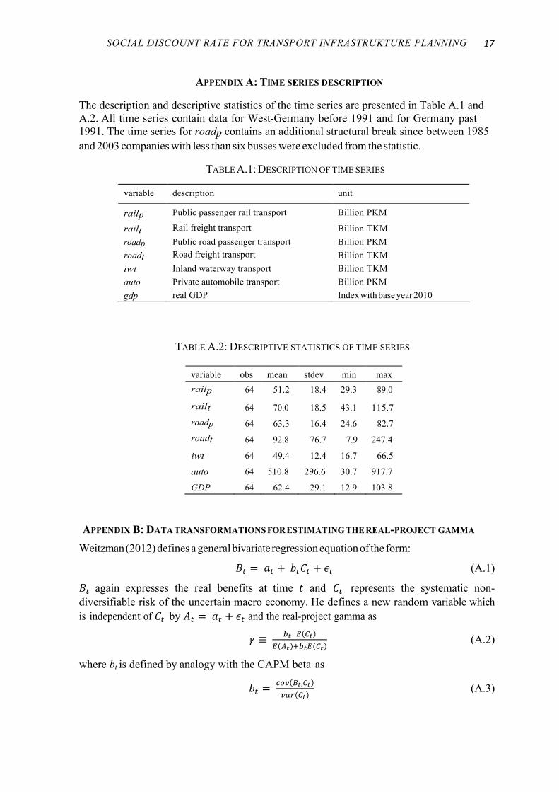
APPENDIX A: TIME SERIES DESCRIPTION The description and descriptive statistics of the time series are presented in Table A.1 and A.2. All time series contain data for West-Germany before 1991 and for Germany past 1991. The time series for roadp contains an additional structural break since between 1985 and 2003 companies with less than six busses were excluded from the statistic.

TABLE A.1: DESCRIPTION OF TIME SERIES

variable description unit

railp Public passenger rail transport Billion PKM

railt Rail freight transport Billion TKM roadp Public road passenger transport Billion PKM roadt Road freight transport Billion TKM iwt Inland waterway transport Billion TKM auto Private automobile transport Billion PKM gdp real GDP Index with base year 2010

TABLE A.2: DESCRIPTIVE STATISTICS OF TIME SERIES

variable obs mean stdev min max railp 64 51.2 18.4 29.3 89.0

railt 64 70.0 18.5 43.1 115.7 roadp 64 63.3 16.4 24.6 82.7 roadt 64 92.8 76.7 7.9 247.4

iwt 64 49.4 12.4 16.7 66.5

auto 64 510.8 296.6 30.7 917.7

GDP 64 62.4 29.1 12.9 103.8

APPENDIX B: DATA TRANSFORMATIONS FOR ESTIMATING THE REAL-PROJECT GAMMA

Weitzman (2012) defines a general bivariate regression equation of the form:

!! = !! + !!!! + !! (A.1)

!! again expresses the real benefits at time ! and !! represents the systematic non- diversifiable risk of the uncertain macro economy. He defines a new random variable which is independent of !! by !! = !! + !! and the real-project gamma as

! ≡ !! ! !!! !! !!!! !!

(A.2)

where bt is defined by analogy with the CAPM beta as

!! = !"# !!,!!!"# !!

(A.3)

INSTITUTE OF TRANSPORT ECONOMICS MÜNSTER WORKING PAPER NO. 22 18

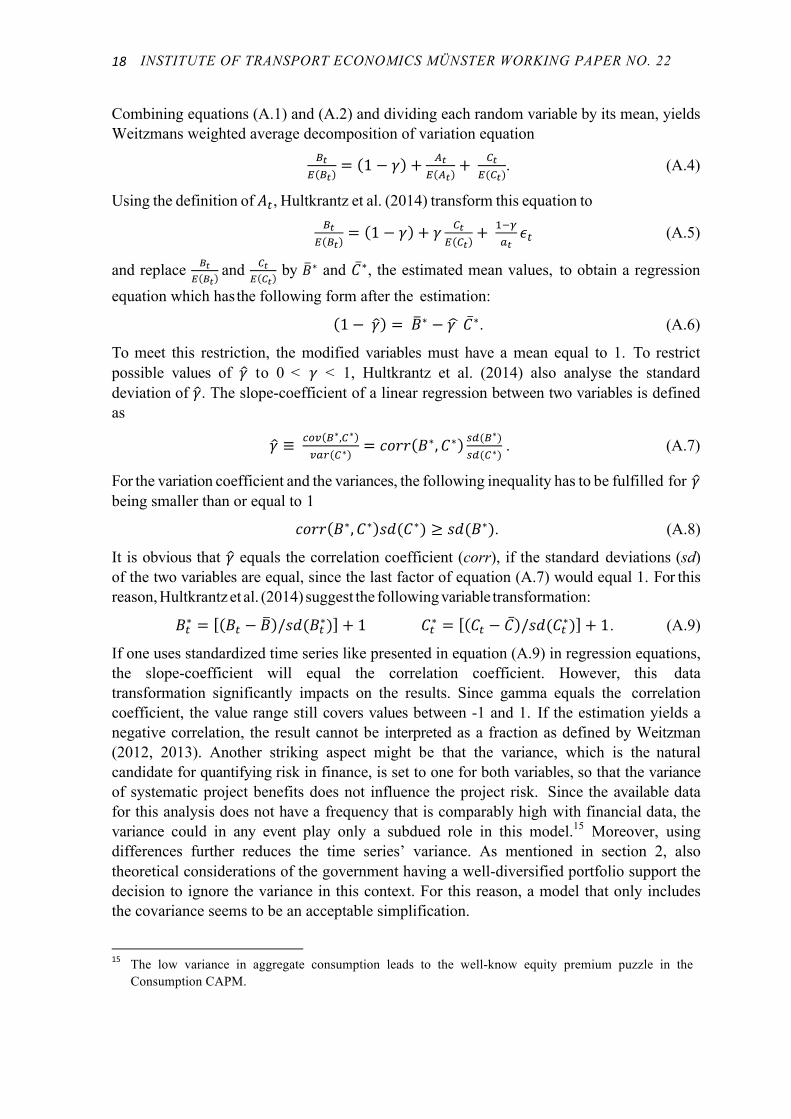
Combining equations (A.1) and (A.2) and dividing each random variable by its mean, yields Weitzmans weighted average decomposition of variation equation

!!! !!

= 1− ! + !!! !!

+ !!!(!!)

. (A.4)

Using the definition of !!, Hultkrantz et al. (2014) transform this equation to !!

! !!= 1− ! + ! !!

! !!+ !!!!! !! (A.5)

and replace !!! !!

and !!! !!

by !∗ and !∗, the estimated mean values, to obtain a regression equation which has the following form after the estimation:

1− ! = !∗ − ! !∗. (A.6)

To meet this restriction, the modified variables must have a mean equal to 1. To restrict possible values of ! to 0 < ! < 1, Hultkrantz et al. (2014) also analyse the standard deviation of !. The slope-coefficient of a linear regression between two variables is defined as

! ≡ !"# !∗,!∗!"# !∗ = !"## !∗,!∗ !"(!∗)

!"(!∗) . (A.7)

For the variation coefficient and the variances, the following inequality has to be fulfilled for ! being smaller than or equal to 1

!"## !∗,!∗ !"(!∗) ≥ !"(!∗). (A.8)

It is obvious that ! equals the correlation coefficient (corr), if the standard deviations (sd) of the two variables are equal, since the last factor of equation (A.7) would equal 1. For this reason, Hultkrantz et al. (2014) suggest the following variable transformation:

!!∗ = !! − ! /!"(!!∗) + 1 !!∗ = !! − ! /!"(!!∗) + 1 . (A.9)

If one uses standardized time series like presented in equation (A.9) in regression equations, the slope-coefficient will equal the correlation coefficient. However, this data transformation significantly impacts on the results. Since gamma equals the correlation coefficient, the value range still covers values between -1 and 1. If the estimation yields a negative correlation, the result cannot be interpreted as a fraction as defined by Weitzman (2012, 2013). Another striking aspect might be that the variance, which is the natural candidate for quantifying risk in finance, is set to one for both variables, so that the variance of systematic project benefits does not influence the project risk. Since the available data for this analysis does not have a frequency that is comparably high with financial data, the variance could in any event play only a subdued role in this model.15 Moreover, using differences further reduces the time series’ variance. As mentioned in section 2, also theoretical considerations of the government having a well-diversified portfolio support the decision to ignore the variance in this context. For this reason, a model that only includes the covariance seems to be an acceptable simplification.

15 The low variance in aggregate consumption leads to the well-know equity premium puzzle in the

Consumption CAPM.

SOCIAL DISCOUNT RATE FOR TRANSPORT INFRASTRUKTURE PLANNING

19

For the empirical analysis, regression equation (A.6) has been rearranged with the following form prior to estimation:

!!∗ = 1− ! + !!!∗ + !! . (A.10)

APPENDIX C: ZIVOT AND ANDREWS UNIT ROOT TEST

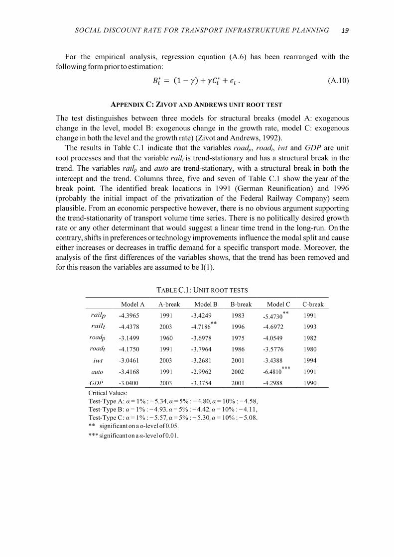
The test distinguishes between three models for structural breaks (model A: exogenous change in the level, model B: exogenous change in the growth rate, model C: exogenous change in both the level and the growth rate) (Zivot and Andrews, 1992).

The results in Table C.1 indicate that the variables roadp, roadt, iwt and GDP are unit root processes and that the variable railt is trend-stationary and has a structural break in the trend. The variables railp and auto are trend-stationary, with a structural break in both the intercept and the trend. Columns three, five and seven of Table C.1 show the year of the break point. The identified break locations in 1991 (German Reunification) and 1996 (probably the initial impact of the privatization of the Federal Railway Company) seem plausible. From an economic perspective however, there is no obvious argument supporting the trend-stationarity of transport volume time series. There is no politically desired growth rate or any other determinant that would suggest a linear time trend in the long-run. On the contrary, shifts in preferences or technology improvements influence the modal split and cause either increases or decreases in traffic demand for a specific transport mode. Moreover, the analysis of the first differences of the variables shows, that the trend has been removed and for this reason the variables are assumed to be I(1).

TABLE C.1: UNIT ROOT TESTS

Model A A-break Model B B-break Model C C-break railp -4.3965 1991 -3.4249 1983 -5.4730** 1991 railt -4.4378 2003 -4.7186** 1996 -4.6972 1993

roadp -3.1499 1960 -3.6978 1975 -4.0549 1982 roadt -4.1750 1991 -3.7964 1986 -3.5776 1980

iwt -3.0461 2003 -3.2681 2001 -3.4388 1994

auto -3.4168 1991 -2.9962 2002 -6.4810*** 1991

GDP -3.0400 2003 -3.3754 2001 -4.2988 1990 Critical Values: Test-Type A: α = 1% : −5.34, α = 5% : −4.80, α = 10% : −4.58, Test-Type B: α = 1% : −4.93, α = 5% : −4.42, α = 10% : −4.11, Test-Type C: α = 1% : −5.57, α = 5% : −5.30, α = 10% : −5.08. ** significant on a α-level of 0.05. *** significant on a α-level of 0.01.

INSTITUTE OF TRANSPORT ECONOMICS MÜNSTER WORKING PAPER NO. 22 20

APPENDIX D: DISCUSSION OF DIAGNOSTIC TESTS

To ensure that the t-statistics are valid, the residuals of the regressions need to be normally distributed. Visual inspection of histograms and the Jarque-Bera test (Jarque and Bera, 1980) results reveal that this is the case for all equations except for the relation between !"#$ and !"#$!_!. Due to the sample size, it can be assumed that the t-statistics are valid for this equation, as well.

Regression equations of the level data show positive first order autocorrelation. Values of the Durbin-Watson (Durbin and Watson, 1950, 1951) test are close to zero for all equations except for !"#-!"#. Apart from autocorrelation, this test can also indicate cointegration by a value equal to or higher than the R2. If there is a cointegration relation between the variables at all, then it can be found in between these two variables. That supports the results of the Engle-Granger test. There are different ways to ease autocorrelation. However, when keeping the model similar to a standard CAPM estimation, it cannot be eased by adding more explanatory variables or by dynamic modeling. A different functional form has been discussed but can be rejected on the basis of special developments in the past due to the German Reunification. As the impact of autocorrelation and heteroskedasticity leads to unbiased but inefficient estimates with the true standard errors exceeding the ordinary White standard errors, regressions can be corrected with Newey-West standard errors (Newey and West, 1987). These standard errors, however, do not change the inference on the significant gamma coefficients reported in table 1 and 2.

Westfälische Wilhelms-Universität Münster, Institute of Transport Economics, Working Paper Series 12 “Specific Investments and Ownership Structures in Railways - An Experimental

Analysis“ by Thomas Ehrmann/ Karl-Hans Hartwig/ Torsten Marner/ Hendrik Schmale, 2009

13 „Größenvorteile im deutschen ÖSPV - Eine empirische Analyse“

by Karl-Hans Hartwig/ Raimund Scheffler, 2009 14 „Measuring Efficiency of German Public Bus Transport“

by Raimund Scheffler/ Karl-Hans Hartwig/ Robert Malina, July 2010 15 „Market Power of Hub Airports: The Role of Lock-in Effects and Downstream

Competition“ by Florian Allroggen/ Robert Malina, July 2010

16 “Studentische Automobilnutzung - mangels Alternativen?“

by Daniel Krimphoff/ Peter Pollmeier, November 2011 17 „Ein Ansatz zur Verteilung der Bestellerentgelte im SPNV“

by Karl-Hans Hartwig/ Peter Pollmeier, September 2012 18 “Residential Parking in Vibrant City Districts”

by Inga Molenda and Gernot Sieg, September 2013 19 “Are commercial ceilings adequate for the regulation of

commercial overload on free-to-air TV channels?” by Julia Rothbauer and Gernot Sieg, September 2013

20 “Welfare Effects of Subsidizing a Dead-End Network of Less Polluting Vehicles“ by Antje-Mareike Dietrich and Gernot Sieg, October 2013

21 “Costs and benefits of a bicycle helmet law for Germany” by Gernot Sieg, March 2014

22 “Time-declining risk-adjusted social discount rates for transport infrastructure

planning” by Kathrin Goldmann, April 2017

For a complete list of Working Papers published by Westfälische Wilhelms-Universität Münster, Institute of Transport Economics, please visit the website (http://www.iv-muenster.de)