3D Modelling and Reconstruction of Peripheral Arteries · DISSERTATION 3D Modelling and...
124
DISSERTATION 3D Modelling and Reconstruction of Peripheral Arteries ausgef¨ uhrt zum Zwecke der Erlangung des akademischen Grades eines Doktors der technischen Wissenschaften unter Anleitung von Ao.Univ.Prof. Dipl.-Ing. Dr.techn. Eduard Gr¨ oller Institut f¨ ur Computergraphik und Algorithmen eingereicht an der Technischen Universit¨ at Wien, Fakult¨ at f¨ ur Informatik von Alexandra La Cruz Matrikelnummer: 0426667 Fickeystrasse 6/20 1110 Wien, ¨ Osterreich geboren am 03.09.1971 in Caracas, Venezuela Wien, im J¨ anner 2006
-
Upload
duongxuyen -
Category
Documents
-
view
219 -
download
0
Transcript of 3D Modelling and Reconstruction of Peripheral Arteries · DISSERTATION 3D Modelling and...
D I S S E R T A T I O N
3D Modelling and Reconstruction ofPeripheral Arteries
ausgefuhrtzum Zwecke der Erlangung des akademischen Grades
eines Doktors der technischen Wissenschaften
unter Anleitung vonAo.Univ.Prof. Dipl.-Ing. Dr.techn. Eduard Groller
Institut fur Computergraphik und Algorithmen
eingereichtan der Technischen Universitat Wien,
Fakultat fur Informatik
vonAlexandra La Cruz
Matrikelnummer: 0426667Fickeystrasse 6/20
1110 Wien, Osterreichgeboren am 03.09.1971in Caracas, Venezuela
Wien, im Janner 2006
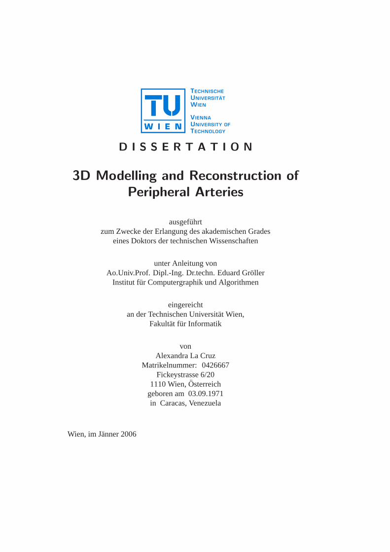
Alexandra La Cruz
3D Modelling and Reconstruction ofPeripheral Arteries
(PhD Thesis)
Institute of Computer Graphics and AlgorithmsVienna University of Technology, Austria
http://www.cg.tuwien.ac.at/research/vis/angiovis/

A mis padres Juan de Mata y Chelaa mis hermanos Juan Carlos, Wilmer, Felix, Carolay y Roso
a mis sobrinos Gabi y Carlitos,Eduardito,
Valeria y Valentina,Dilso, Dilma, Dany y Daniel,
a mi familia, en especial a Laya, Dilcia, Mirian, Nayipsi yNayibi
a mis amigos,y por sobre todas las cosas a DIOS.
ACKNOWLEDGEMENTS
I would like to thank all the people who made this work possible. Primarily,I would like to express my gratitude towards my supervisor, Master EduardGroller, who always encouraged me to continue working, and never give up,allowing me to finish my work, and my thesis in Vienna.
To all the co-workers in the AngioVis project (Dominik Fleischmann,Milos Sramek, Matus Straka, Arnold Kochl, and Rudiger Schernthaner) Itruly benefitted from every fruitful and interesting scientific discussion inall of the AngioVis meetings. Special acknowledge to Dominik, for all ofhis encouragement to continue working, his comments were always verygood motivation for my work.
I would also like to thank all the members (Tom, Armin, Katja, Jirı,Adriana, Soren, Ivan, Matej, Stefan, Ernesto) of the Visualization Group inthe Institute of Computer Graphics and Algorithms of the Vienna Universityof Technology, for the chocolates and their excellent support and friendship.I would like to thank the secretaries of the Institute; Anita and Andrea, with-out their assistance with the legal documents and German support my stayin Vienna would have been difficult beyond what words can express. Spe-cial thanks to the people of the Rendering and Virtual Reality group for theirtime and conversations in the Institute, especially Alessandro and Werner.
Words cannot express my undying gratefulness to my family who fromVenezuela always supported and trusted me. Especially to my parents (Juande Mata and Chela), my brothers (Juan Carlos, Wilmer, Cheo and Roso),and my sister (Carolay). Without their support and confidence I would havenot been able to finish this work.
To John Puentes, for sending to me that email, I never would havethought that email would be the beginning of a new adventure in my life.Katja Buhler, without that successful interview in Venezuela it would nothave been possible for me to be accepted to the Institute to pursue my PhD.To Armin Kanitsar for his trust and confidence in my abilities to completemy studies.
I would like to thank all my friends in Vienna. First of all, to SylviaLaya, who supported me from the beginning, because of her friendship
and support I was able to call Vienna ’home’ outside my true home. Tothe Spanish cell group (Santa, Sergio, Liz, Ramona, Jorge, Dennys, Gori,Raquel, Elizabeth, Vele and others), the open cell group (especially to Mar-got, Gabi, Yu-Chen, Cumari, Sheila, Olga, Sabine, Yudith, Asther, Heidi)and the people from VCC (specially to Pastor Tom and Candi, Uschi, Chapa,Elli, Nishanta, and hundreds of other VCC members) for their spiritual sup-port and friendship that made my stay in Vienna a joyful experience. ToNariana, for her support, and English correction.
To all my friends out of Vienna who, that in some way, always gave methe right comment in the right moment, especially to Sara Wong, FranciscoNg, Ricardo Bravo, Monica Huerta and Francisco Azuage (the Powers). Ialso would like to express special thankfulness to Marianella Santiago forsome of the figures in this thesis, invaluable support, friendship, and forsuch an exceptional, sportive, and joyful time I could share with her duringher visit to Vienna.
I express my undying gratitude to GOD for being with me all the timeand for his great grace I have always received from him.
To Anna Rosa Cambas for her support, who through the LateinamerikaInstitut made it possible part of the financing required in the last year tofinish my PhD study. Thank also to Prof. Lammer and the Department ofAngiography and Interventional Radiology at the General Hospital of Vi-enna (AKH - Allgemeines Krankenhaus), who also provided part of financialsupport.
The work presented in this thesis has been mainly funded by the An-gioVis project. The AngioVis project was supported by the FWF (Fondszur Forderung der Wissenschaftlichen Forschung - Austrian Science Fund)grant No. P15217.
ii
ABSTRACT
A model is a simplified representation of an object. The modeling stagecould be described as shaping individual objects that are later used in thescene. For many years scientists are trying to create an appropriate model ofthe blood vessels. It looks quite intuitive to believe that a blood vessel can bemodeled as a tubular object, and this is true, but the problems appear whenyou want to create an accurate model that can deal with the wide variabilityof shapes of diseased blood vessels. From the medical point of view it isquite important to identify, not just the center of the vessel lumen but alsothe center of the vessel, particularly in the presences of some anomalies,which is the case diseased blood vessels.
An accurate estimation of vessel parameters is a prerequisite for auto-mated visualization and analysis of healthy and diseased blood vessels. Webelieve that a model-based technique is the most suitable one for parameter-izing blood vessels. The main focus of this work is to present a new strategyto parameterize diseased blood vessels of the lower extremity arteries.
The first part presents an evaluation of different methods for approxi-mating the centerline of the vessel in a phantom simulating the peripheralarteries. Six algorithms were used to determine the centerline of a syntheticperipheral arterial vessel. They are based on: ray casting using thresholdsand a maximum gradient-like stop criterion, pixel-motion estimation be-tween successive images called block matching, center of gravity and shapebased segmentation. The Randomized Hough Transform and ellipse fittinghave been used as shape based segmentation techniques. Since in the syn-thetic data set the centerline is known, an estimation of the error can becalculated in order to determine the accuracy achieved by a given method.
The second part describes an estimation of the dimensions of lower ex-tremity arteries, imaged by computed tomography. The vessel is modeledusing an elliptical or cylindrical structure with specific dimensions, orien-tation and CT attenuation values. The model separates two homogeneousregions: Its inner side represents a region of density for vessels, and its outerside a region for background. Taking into account the point spread functionof a CT scanner, which is modeled using a Gaussian kernel, in order to
smooth the vessel boundary in the model. An optimization process is usedto find the best model that fits with the data input. The method providescenter location, diameter and orientation of the vessel as well as blood andbackground mean density values.
The third part presents the result of a clinical evaluation of our meth-ods, as a prerequisite step for being used in clinical environment. To per-form this evaluation, twenty cases from available patient data were selectedand classified as ’mildly diseased’ and ’severely diseased’ datasets. Manualidentification was used as our reference standard. We compared the modelfitting method against a standard method, which is currently used in theclinical environment. In general, the mean distance error for every methodwas within the inter-operator variability. However, the non-linear model fit-ting technique based on a cylindrical model shows always a better centerapproximation in most of the cases, ’mildly diseased’ as well as ’severelydiseased’ cases. Clinically, the non-linear model fitting technique is morerobust and presented a better estimation in most of the cases. Nevertheless,the radiologists and clinical experts have the last word with respect to theuse of this technique in clinical environment.
iv

KURZFASSUNG
Ein Modell ist eine vereinfachte Reprasentationsform eines Objekts. DieModellbildung kann als Formen von individuellen Objekte bezeichnet wer-den, die spater in der Szene Verwendung finden. Seit vielen Jahren ver-suchen Wissenschaftler ein geeignetes Modell fur die Blutgefaße zu finden.Auf den ersten Blick scheint hierfur ein tubulares Modell am Bestengeeignet zu sein, allerdings erweist sich dabei eine prazise Berucksichti-gung der vielfaltigen Gefaßpathologien als problematisch. Aus medizinis-cher Sicht ist nicht nur der Mittelpunkt eines Gefaßlumens, sondern auchder Mittelpunkt des Gefaßes selbst relevant. Dies trifft vor allem bei auftre-tenden Anomalien, wie zum Beispiel bei pathologischen Blutgefaßen, zu.
Eine prazise Berechnung von Gefaßparametern ist eine Grundvoraus-setzung fur automatisierte Visualisierung und Analyse von sowohl gesun-den wie auch erkrankten Blutgefaßen. Wir sind davon uberzeugt, dass sicheine modell-basierte Technik am Besten fur die Parametrierung von Blut-gefaßen eignet. Ziel dieser Arbeit ist die Vorstellung einer neuen Tech-nik zur Berechnung von Parametern erkrankter Blutgefaße der unteren Ex-tremitaten.
Der erste Teil beschreibt den Vergleich verschiedener Methoden zurApproximation der Mittellinie eines Gefaßes in einem Phantom der pe-ripheren Arterien. Sechs verschiedene Algorithmen wurden zur Berech-nung der Mittellinie einer synthetischen peripheren Arterie verwendet. Dieevaluierten Methoden basieren auf folgenden Verfahren: Raycasting, beidem das Abbruchkriterium entweder schwellwertbasiert oder auf dem max-imalen Gradienten basiert ist; Block-Matching, bei dem die Pixelbewegungin aufeinander folgenden Bildern geschatzt wird und schwerpunkt- oderformbasierte Segmentierung. Fur die formbasierte Segmentierung wurdesowohl die randomisierte Hough-Transformation als auch Ellipsen-Fittingverwendet. Da in dem synthetischen Datensatz die Mittellinie bekannt ist,kann die Genauigkeit der Verfahren berechnet werden.
Der zweite Teil beschreibt die Einschatzung der Abmessungen derBeinarterien, die mittels Computertomographie aufgenommen wurden. Das
Blutgefaß wird durch ein elliptisches oder zylindrisches Modell mit bes-timmten Abmessungen, bestimmter Ausrichtung und einer bestimmtenDichte (CT-Schwachungswerte) beschrieben. Das Modell separiert zweihomogene Regionen: Im Inneren des Modells befindet sich eine Re-gion mit der Dichte eines Gefaßes, außerhalb befindet sich der Hinter-grund. Um die Punktbildfunktion des CT-Scanners zu modellieren, wurdeein Gauß Filter verwendet, der zu einer Verschmierung der Gefaßgrenzenfuhrt. Ein Optimierungsvorgang dient zur Auffindung des Modells, dassich am besten mit den Eingangsdaten deckt. Die Methode bestimmt Mit-telpunkt, Durchmesser, Orientierung und die durchschnittliche Dichte desBlutgefaßes, sowie die durchschnittliche Dichte des Hintergrundes.
Der dritte Teil prasentiert die Ergebnisse einer klinschen Evaluation un-serer Methoden, eine Grundvoraussetzung fur den klinischen Einsatz. Furdiese Evaluation wurden 20 Falle aus den vorhandenen Patientendaten aus-gewahlt und nach Schweregrad der Erkrankung in zwei Gruppen klassi-fiziert. Manuelle Identifikation diente als Referenzstandard. Wir verglichendie Model-Fitting-Methode mit einer Standard-Methode, die derzeit imklinischen Einsatz ist. Im Allgemeinen war der durschnittliche Abstands-fehler fur beide Methoden innerhalb der Variabilitat zwischen den einzelnenmanuellen Identifikationen. Jedoch erzielte die nicht-lineare Model-Fitting-Technik basierend auf einem zylindrischen Modell in den meisten Falleneine bessere Annaherung an die Mittellinie, sowohl in den leicht wie auchin den schwer erkrankten Fallen. Die nicht-lineare Model-Fitting-Technikist robuster und ergab eine bessere Beurteilung der meisten Falle. Nicht-destoweniger haben die Radiologen und die klinischen Experten das letzteWort im Hirblick auf den Einsatz dieser Technik im klinischen Umfeld.
vi
CONTENTS
1 Introduction 11.1 Lower Extremity Arterial Tree . . . . . . . . . . . . . . . . 11.2 Peripheral Arterial Occlusive Disease . . . . . . . . . . . . 21.3 Medical Imaging Used For Peripheral Vessel Investigation . 6
1.3.1 Angiography . . . . . . . . . . . . . . . . . . . . . 71.3.2 Doppler Ultrasound . . . . . . . . . . . . . . . . . . 81.3.3 Magnetic Resonance Imaging . . . . . . . . . . . . 91.3.4 Compute Tomography Angiography . . . . . . . . . 9
1.4 CTA of Peripheral Arterial Occlusive Disease . . . . . . . . 101.5 Visualization of PAOD in CTA datasets . . . . . . . . . . . 14
1.5.1 Curved Planar Reformation . . . . . . . . . . . . . 151.5.2 VesselGlyph . . . . . . . . . . . . . . . . . . . . . 161.5.3 Convolution Surface . . . . . . . . . . . . . . . . . 16
1.6 Discussion . . . . . . . . . . . . . . . . . . . . . . . . . . . 191.7 Thesis Contents . . . . . . . . . . . . . . . . . . . . . . . . 20
2 Model Based Segmentation Techniques 232.1 Introduction . . . . . . . . . . . . . . . . . . . . . . . . . . 232.2 Deformable Models . . . . . . . . . . . . . . . . . . . . . . 25
2.2.1 Snakes . . . . . . . . . . . . . . . . . . . . . . . . 262.2.2 Level-sets . . . . . . . . . . . . . . . . . . . . . . . 262.2.3 Probabilistic Snakes . . . . . . . . . . . . . . . . . 26
2.3 Multi-scale Methods . . . . . . . . . . . . . . . . . . . . . 272.4 Geometry Based Segmentation . . . . . . . . . . . . . . . . 28
2.4.1 Geometry Based Segmentation Combined with aDeformable Model Approach . . . . . . . . . . . . 29
2.4.2 Geometry Based Segmentation Combined with aMulti-scale Approach . . . . . . . . . . . . . . . . . 30
vii
CONTENTS CONTENTS
2.5 Model Fitting . . . . . . . . . . . . . . . . . . . . . . . . . 302.6 Hybrid Segmentation . . . . . . . . . . . . . . . . . . . . . 312.7 Discussion . . . . . . . . . . . . . . . . . . . . . . . . . . . 33
3 Centerline Approximations of Blood Vessels 353.1 Introduction . . . . . . . . . . . . . . . . . . . . . . . . . . 353.2 Centerline Approximation Methods . . . . . . . . . . . . . 36
3.2.1 Ray Casting . . . . . . . . . . . . . . . . . . . . . . 373.2.2 Block Matching . . . . . . . . . . . . . . . . . . . . 383.2.3 Center Of Gravity . . . . . . . . . . . . . . . . . . 393.2.4 Ellipse Fitting . . . . . . . . . . . . . . . . . . . . . 393.2.5 Randomized Hough Transform . . . . . . . . . . . . 40
3.3 Evaluation . . . . . . . . . . . . . . . . . . . . . . . . . . . 423.4 Discussion . . . . . . . . . . . . . . . . . . . . . . . . . . . 443.5 Improvements . . . . . . . . . . . . . . . . . . . . . . . . . 463.6 Conclusion . . . . . . . . . . . . . . . . . . . . . . . . . . 46
4 Vessel Model Fitting 514.1 Introduction . . . . . . . . . . . . . . . . . . . . . . . . . . 514.2 Motivation . . . . . . . . . . . . . . . . . . . . . . . . . . . 524.3 Non-Linear Model Fitting . . . . . . . . . . . . . . . . . . . 52
4.3.1 Elliptical Cross-section Model of a Vessel . . . . . . 554.3.2 Cylindrical 3D Model of a Vessel . . . . . . . . . . 554.3.3 Levenberg-Marquardt Method . . . . . . . . . . . . 56
4.4 Results . . . . . . . . . . . . . . . . . . . . . . . . . . . . . 594.5 Conclusion . . . . . . . . . . . . . . . . . . . . . . . . . . 63
5 Clinical Evaluation of a Non-linear Model Fitting Technique 685.1 Introduction . . . . . . . . . . . . . . . . . . . . . . . . . . 685.2 Materials and Methods . . . . . . . . . . . . . . . . . . . . 69
5.2.1 Vessel Segments . . . . . . . . . . . . . . . . . . . 695.2.2 Reference Standard Centerlines . . . . . . . . . . . 715.2.3 Automated Centerline Extraction . . . . . . . . . . 73
5.3 Distance Error Estimation Measures . . . . . . . . . . . . . 745.4 Statistical Analysis used for Evaluation . . . . . . . . . . . 765.5 Evaluation Results . . . . . . . . . . . . . . . . . . . . . . 76
5.5.1 Evaluation of Operator Variability . . . . . . . . . . 775.5.2 Evaluation of Automatic Methods . . . . . . . . . . 79
viii

CONTENTS CONTENTS
5.6 Conclusion . . . . . . . . . . . . . . . . . . . . . . . . . . 85
6 Summary and Conclusions 88
References 100
A Curriculum Vitae 101
ix
LIST OF FIGURES
1.1 Illustrative example of the peripheral arterial tree [77]. . . . 31.2 Illustration and schematic drawing of atherosclerotic plaque
with luminal narrowing. This image is courtesy of MedlinePlus and A.D.A.M. a Health Illustrated Encyclopedia on-line [56] . . . . . . . . . . . . . . . . . . . . . . . . . . . . 4
1.3 Maximum intensity projection image of a patient data withleft calf claudication. Bones were removed for the purposeof better visualization of arterial vessels. Note the occlusionof the left superficial femoral artery. Several small collateralvessels fill the arteries distal to the occluded segment (imagecourtesy of Justus Roos from Stanford University MedicalCenter:[email protected]) . . . . . . . . . . . . . . 5
1.4 (a) The first X-rays image obtained by Rontgen in Decem-ber 1895 and (b) the first angiogram image obtained by Mr.Haschek and Dr. Lindenthal in January 1896. . . . . . . . . 6
1.5 Illustrative example of a non-calcified plaque (vessel cross-section view). . . . . . . . . . . . . . . . . . . . . . . . . . 12
1.6 Illustrative example of a calcified plaque (vessel cross-section view), closer to bone (a), far away from bone (b). . . 13
1.7 Topogram image of a PAOD dataset with a dark bold line(blue) in the place of the manually segmented left leg vesseland the voxel density values along the vessel together withthe average values of density from the 3x3 surroundings ofthe center-path [17] . . . . . . . . . . . . . . . . . . . . . . 13
1.8 CPR example. (a) First the center path is estimated, definingstarting (crosses at the top) and endpoints (cross at bottom).In (b) a coronar CPR (left) and sagittal CPR (right) from thedata set in (a) [36] . . . . . . . . . . . . . . . . . . . . . . . 15
x
LIST OF FIGURES LIST OF FIGURES
1.9 VesselGlyph examples: (a) CPR + DVR, (b) foreground-cleft in DVR with occlusion lines, (c) Thick-Slab rendering(DVR), (d) tubular rendering (DVR) [75] . . . . . . . . . . 17
1.10 Visualization of cerebral vasculature imaged by MRI usinga convolution surface [59] . . . . . . . . . . . . . . . . . . 18
1.11 Close-up images of a vessel tree example, comparing iso-surface rendering (left) with a more refined rendering tech-nique (middle, details in [59]) and convolution surface ren-dering (right) [59] . . . . . . . . . . . . . . . . . . . . . . 19
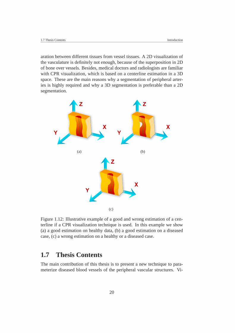
1.12 Illustrative example of a good and wrong estimation of acenterline if a CPR visualization technique is used. In thisexample we show (a) a good estimation on healthy data, (b)a good estimation on a diseased case, (c) a wrong estimationon a healthy or a diseased case. . . . . . . . . . . . . . . . . 20
2.1 Intensity profiles of 2D slices of a thin vessel in the pelvis(left), the iliac artery of the pelvis (middle), and the aorta(right) in 3D MR images [88]. . . . . . . . . . . . . . . . . 31
2.2 Segmentation results of applying the cylindrical model toarteries of the pelvis (left and middle) as well as to coronaryarteries and the aorta (right) [88]. . . . . . . . . . . . . . . . 32
3.1 Example of the ray casting method . . . . . . . . . . . . . . 383.2 Ellipse Approximation. (a) Estimation of the line where the
ellipse center should pass. (b) Estimation of the ellipse center. 423.3 Maximum Intensity Projection of the synthetic data. . . . . . 433.4 Distance error graphs of the center estimated by the (a)
RCT, (b) RCMG, (c) CoG, (d) BM, (e) EF, and (f) RHTmethod . . . . . . . . . . . . . . . . . . . . . . . . . . . . 47
3.5 Diameter estimated by the (a) RCT, (b) RCMG, (c) EF, and(d) RHT method . . . . . . . . . . . . . . . . . . . . . . . . 48
xi
LIST OF FIGURES LIST OF FIGURES
3.6 From left to right rotating CPR with 45, 135, 225 and 315degrees. From top to bottom centerline detected with RCT,RCMG, and CoG. This data corresponds to a femoral witha diameter between 2mm and 4mm, and present calcifica-tions and bifurcations. Brighter objects correspond to bonestructures. For this data the best approximation center indifferent rotations of the CPR is exhibited by the RCMGmethod. . . . . . . . . . . . . . . . . . . . . . . . . . . . . 49
3.7 From left to right rotating CPR with 45, 135, 225 and 315degrees. From top to bottom centerline detected with BM,EF, and RHT. This data corresponds to a femoral with adiameter between 2mm and 4mm, and present calcifica-tions and bifurcations. Brighter objects correspond to bonestructures. This is without consider bifurcations, and corre-sponds to the CoG method. For this sample the best resultis exhibited by the EF method. . . . . . . . . . . . . . . . . 50
4.1 MIP image (left) of a clinical peripheral CTA dataset ob-tained from a patient with advanced peripheral arterial dis-ease with superimposed tree of vessel-centerlines. Theencircled areas indicate vessel regions, where automatedcenterline calculations failed due to excessive disease andvessel calcifications, and thus required manual placementof center points by a radiologist, to achieve the resultingCurved Planar Reformation (right). . . . . . . . . . . . . . . 53
4.2 erfc function . . . . . . . . . . . . . . . . . . . . . . . . . . 544.3 (a) Cylinder along the z-axis rotated with angles α and
β around the x-axis and y-axis respectively. (b) Ellipticalcross section along the z-axis of the rotated cylinder . . . . . 57
4.4 Illustrative example of a cylindrical model . . . . . . . . . . 584.5 Result on synthetic data. Left, MIP image of the synthetic
data, followed by elliptical cross-section model fitted alongthe vessel path, and finally a parameterized vessel by cylin-drical model fitting . . . . . . . . . . . . . . . . . . . . . . 60
4.6 Result of fitting to a vessel with a partial occlusion . . . . . 614.7 Result of fitting to a vessel with calcifications . . . . . . . . 62
xii
LIST OF FIGURES LIST OF FIGURES
4.8 MIP images with superimposed centerline generated by (a)the RCT technique and (b) the cylindrical model fitting.Note, that patient images are shown as if viewed from thefront of the patient. The right femoral artery is thus on theleft side of the image. . . . . . . . . . . . . . . . . . . . . . 64
4.9 CPR images of the right femoral artery from the samedataset as Figure 4.8, viewed from three different angles(−90o [as if viewed from the right side of the patient], 0o
[viewed from the front of the patient], and 45o [as if viewedfrom an oblique left standpoint relative to the patient]), withsuperimposed center-paths. Images in panel (a) were cre-ated from the RCT centerline approximation. Images inpanel (b) were created with the cylindrical 3D model fitting. 65
4.10 CPR images of the left femoral artery from the same datasetas Figure 4.8, viewed from three different angles (−90o [asif viewed from the right side of the patient], 0o [viewedfrom the front of the patient], and 45o [as if viewed froman oblique left standpoint relative to the patient]), with su-perimposed center-paths. Images in panel (a) were createdfrom the RCT centerline approximation. Images in panel(b) were created with cylindrical model fitting. Note theimproved course of the centerline in (b) in this example ofcomplex attenuation of the diseased blood vessel, caused byresidual lumen, hypodense (non-calcified) plaque, and hy-perdense calcified plaque. . . . . . . . . . . . . . . . . . . . 67
5.1 Maximum intensity projection image of a full patient data(left). The bone was removed manually for better vesselvisualization. These images show the two arterial segmentswe are using in this work for evaluation, the iliac (top-right)and femoro-popliteal (bottom-right) arteries. . . . . . . . . . 70
5.2 Example of a manual centerline (a) and its correspondingCPR image for validation. As an example, CPR views with20o (a) and −64o (b) of rotation [viewed from the front ofthe patient] are shown. The user can rotate the CPR viewand visualize any angle of rotation. . . . . . . . . . . . . . . 72
5.3 Example that illustrates a common segment part extractionfor two centered paths. . . . . . . . . . . . . . . . . . . . . 74
xiii
LIST OF FIGURES LIST OF FIGURES
5.4 The DTW technique, in (a) two curves for comparison, (c)the warping path, and (b) the optimal sequence aligned be-tween these curves [38]. . . . . . . . . . . . . . . . . . . . 76
5.5 Intra-operator (a) and inter-operator (b) variability. Theseplots correspond to an iliac arterial segment of a ’severelydiseased’ case. In (b) we can only appreciate the variabil-ity inter-operator, which is quite wide. 12 combinations ofdistance error graphs between operators (3 operators, everyone made two manual editing of centerlines) are plotted in(b). . . . . . . . . . . . . . . . . . . . . . . . . . . . . . . . 80
5.6 A case of inter-operator variability. Three manual cen-terlines are drawn [with different colors (orange, red andblue)]. Every centerline corresponds to a manual segmenta-tion from a different operator. The plot shows the variabil-ity between them. Two remarkable peaks correspond to thearea pointed it out in image 1. . . . . . . . . . . . . . . . . 81
5.7 Comparison between automatic methods vs average path ofmanual segmentations from three expert operators. The dataset corresponds with the femoro-popliteal artery segmentof ’mildly diseased’ (a) and ’severely diseased’ (c) cases,as well as the iliac artery segment of ’mildly diseased’ (b)and ’severely diseased’ (d) cases, respectively. The meandistance between operator (inter-operator) for every patientwas plotted as a reference (black boxes). . . . . . . . . . . . 84
5.8 Comparison of the M3D method vs the RCT method. Im-ages were captured for three consecutive cross-sections. (a)(b), (c) show a result produced by the RCT method, and (d),(e), (f) show a result produced by the M3D method. Fig-ures (a), (b), (c), (d) are produced by a wrong estimation ofinitial parameters. . . . . . . . . . . . . . . . . . . . . . . . 86
xiv
LIST OF TABLES
1.1 Relative diameter of the main group of arteries of the pe-ripheral vasculature . . . . . . . . . . . . . . . . . . . . . . 2
1.2 Summary of advantages and disadvantages of different im-age modalities used for the evaluation of peripheral arterialocclusive disease. . . . . . . . . . . . . . . . . . . . . . . . 11
3.1 Comparison of the evaluated methods. . . . . . . . . . . . . 443.2 Execution times in seconds for each evaluated method. . . . 46
4.1 Advantages and limitations using the non-linear vesselmodel fitting . . . . . . . . . . . . . . . . . . . . . . . . . . 63
5.1 Intra- and inter-operator variability shows significant differ-ences between groups of patients with a probability p fromthe Student t-test analysis. The mean and maximum of thedistances are also compared in this table. . . . . . . . . . . . 78
5.2 Table of significant difference between groups M2D, M3Dand RCT per patient. Mean and maximum distance errorbetween centerlines estimated by the automated methods(RCT, M2D, and M3D) and the average path of six read-ings. . . . . . . . . . . . . . . . . . . . . . . . . . . . . . . 82
5.3 This table shows the percentage of cases whose mean andmaximum distance error from every method is within theinter-operator variability. . . . . . . . . . . . . . . . . . . . 83
xv
CHAPTER 1
INTRODUCTION
Peripheral arterial occlusive disease (PAOD) of the lower extremities is ahighly prevalent disorder. Although PAOD is not a frequent primary causeof mortality, this disease is a significant cause of morbidity and an adverseprognostic indicator among the elderly [86] (about 30% at age 60 andabove). Catheter-based techniques are considered to be the ”gold standard”for diagnosis and treatment of PAOD. However, because of their invasivenature, these techniques inherently have some complications. On the otherhand, non-invasive diagnostic techniques are high operator dependent andrequire a time consuming examination.
This chapter introduces the reader to the peripheral vessel investigationfield. First, a description of the peripheral vasculature and its main functionis presented. Then, the vascular diseases that can affect the normal bloodflow through the peripheral arteries are described. Different image modal-ities have been already used as a radiological evaluation of peripheral vas-cular disease. A comparative table of the different modalities is presented.Furthermore, we point out the major motivation why we focus our investi-gation on datasets from computed tomography angiography for peripheralvessel investigation. Finally, three of the most recent vessel visualizationtechniques that are applied to the blood vessels are addressed.
1.1 Lower Extremity Arterial TreeThe main function of the lower extremity arterial tree is to supply oxygen tothe muscles and other tissues of the legs and feet. The ’root’ of the periph-eral arterial tree is the abdominal aorta (the main artery of the body). Thebilateral common iliac arteries divide into the internal iliac artery (which
1
1.2 Peripheral Arterial Occlusive Disease Introduction
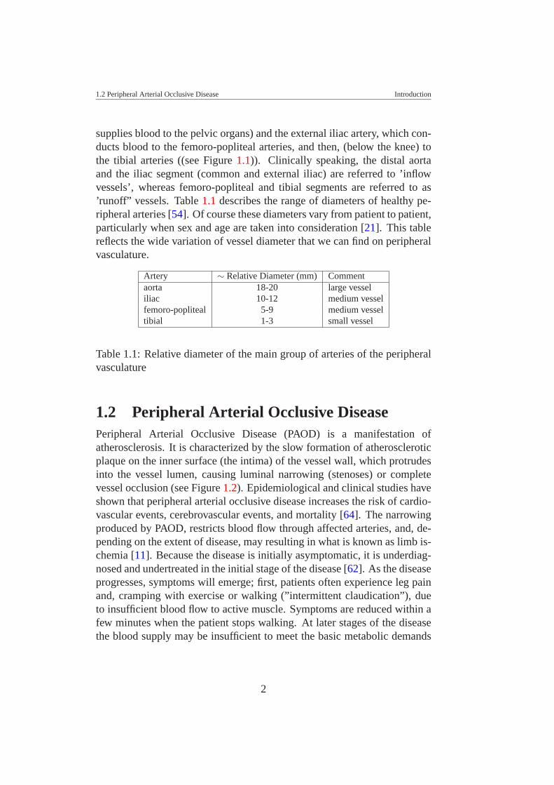
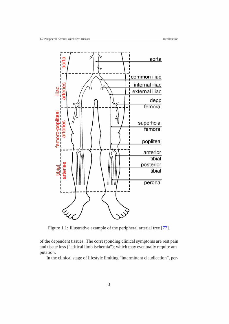
supplies blood to the pelvic organs) and the external iliac artery, which con-ducts blood to the femoro-popliteal arteries, and then, (below the knee) tothe tibial arteries ((see Figure 1.1)). Clinically speaking, the distal aortaand the iliac segment (common and external iliac) are referred to ’inflowvessels’, whereas femoro-popliteal and tibial segments are referred to as’runoff” vessels. Table 1.1 describes the range of diameters of healthy pe-ripheral arteries [54]. Of course these diameters vary from patient to patient,particularly when sex and age are taken into consideration [21]. This tablereflects the wide variation of vessel diameter that we can find on peripheralvasculature.
Artery ∼ Relative Diameter (mm) Commentaorta 18-20 large vesseliliac 10-12 medium vesselfemoro-popliteal 5-9 medium vesseltibial 1-3 small vessel
Table 1.1: Relative diameter of the main group of arteries of the peripheralvasculature
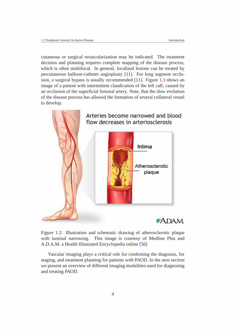
1.2 Peripheral Arterial Occlusive DiseasePeripheral Arterial Occlusive Disease (PAOD) is a manifestation ofatherosclerosis. It is characterized by the slow formation of atheroscleroticplaque on the inner surface (the intima) of the vessel wall, which protrudesinto the vessel lumen, causing luminal narrowing (stenoses) or completevessel occlusion (see Figure 1.2). Epidemiological and clinical studies haveshown that peripheral arterial occlusive disease increases the risk of cardio-vascular events, cerebrovascular events, and mortality [64]. The narrowingproduced by PAOD, restricts blood flow through affected arteries, and, de-pending on the extent of disease, may resulting in what is known as limb is-chemia [11]. Because the disease is initially asymptomatic, it is underdiag-nosed and undertreated in the initial stage of the disease [62]. As the diseaseprogresses, symptoms will emerge; first, patients often experience leg painand, cramping with exercise or walking (”intermittent claudication”), dueto insufficient blood flow to active muscle. Symptoms are reduced within afew minutes when the patient stops walking. At later stages of the diseasethe blood supply may be insufficient to meet the basic metabolic demands
2
1.2 Peripheral Arterial Occlusive Disease Introduction
Figure 1.1: Illustrative example of the peripheral arterial tree [77].
of the dependent tissues. The corresponding clinical symptoms are rest painand tissue loss (”critical limb ischemia”); which may eventually require am-putation.
In the clinical stage of lifestyle limiting ”intermittent claudication”, per-
3
1.2 Peripheral Arterial Occlusive Disease Introduction
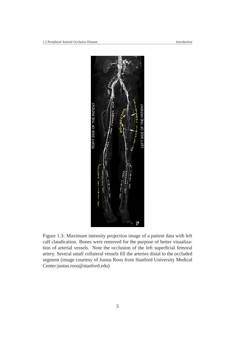
cutaneous or surgical revascularization may be indicated. The treatmentdecision and planning requires complete mapping of the disease process,which is often multifocal. In general, localized lesions can be treated bypercutaneous balloon-catheter angioplasty [11]. For long segment occlu-sion, a surgical bypass is usually recommended [11]. Figure 1.3 shows animage of a patient with intermittent claudication of the left calf, caused byan occlusion of the superficial femoral artery. Note, that the slow evolutionof the disease process has allowed the formation of several collateral vesselto develop.
Figure 1.2: Illustration and schematic drawing of atherosclerotic plaquewith luminal narrowing. This image is courtesy of Medline Plus andA.D.A.M. a Health Illustrated Encyclopedia online [56]
Vascular imaging plays a critical role for confirming the diagnosis, forstaging, and treatment planning for patients with PAOD. In the next sectionwe present an overview of different imaging modalities used for diagnosingand treating PAOD.
4
1.2 Peripheral Arterial Occlusive Disease Introduction
Figure 1.3: Maximum intensity projection image of a patient data with leftcalf claudication. Bones were removed for the purpose of better visualiza-tion of arterial vessels. Note the occlusion of the left superficial femoralartery. Several small collateral vessels fill the arteries distal to the occludedsegment (image courtesy of Justus Roos from Stanford University MedicalCenter:[email protected])
5
1.3 Medical Imaging Used For Peripheral Vessel Investigation Introduction
1.3 Medical Imaging Used For Peripheral Ves-sel Investigation
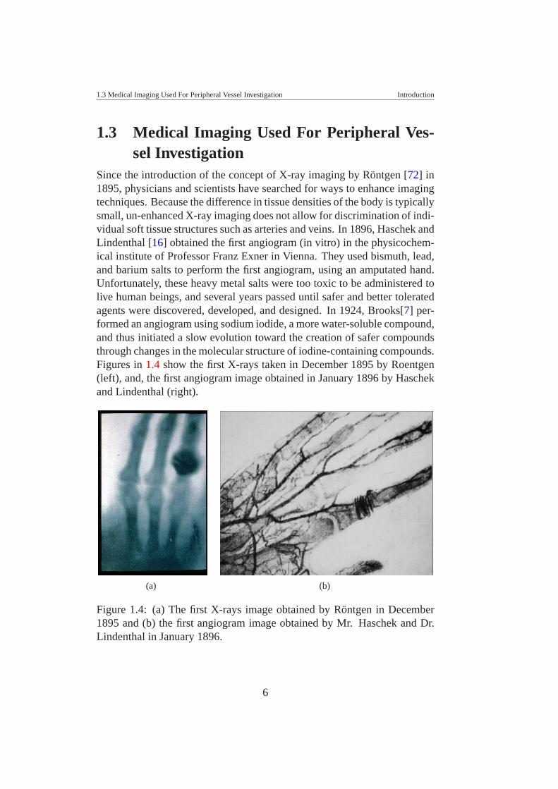
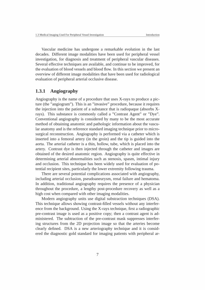
Since the introduction of the concept of X-ray imaging by Rontgen [72] in1895, physicians and scientists have searched for ways to enhance imagingtechniques. Because the difference in tissue densities of the body is typicallysmall, un-enhanced X-ray imaging does not allow for discrimination of indi-vidual soft tissue structures such as arteries and veins. In 1896, Haschek andLindenthal [16] obtained the first angiogram (in vitro) in the physicochem-ical institute of Professor Franz Exner in Vienna. They used bismuth, lead,and barium salts to perform the first angiogram, using an amputated hand.Unfortunately, these heavy metal salts were too toxic to be administered tolive human beings, and several years passed until safer and better toleratedagents were discovered, developed, and designed. In 1924, Brooks[7] per-formed an angiogram using sodium iodide, a more water-soluble compound,and thus initiated a slow evolution toward the creation of safer compoundsthrough changes in the molecular structure of iodine-containing compounds.Figures in 1.4 show the first X-rays taken in December 1895 by Roentgen(left), and, the first angiogram image obtained in January 1896 by Haschekand Lindenthal (right).
(a) (b)
Figure 1.4: (a) The first X-rays image obtained by Rontgen in December1895 and (b) the first angiogram image obtained by Mr. Haschek and Dr.Lindenthal in January 1896.
6
1.3 Medical Imaging Used For Peripheral Vessel Investigation Introduction
Vascular medicine has undergone a remarkable evolution in the lastdecades. Different image modalities have been used for peripheral vesselinvestigation, for diagnosis and treatment of peripheral vascular diseases.Several effective techniques are available, and continue to be improved, forthe evaluation of blood vessels and blood flow. In this section we present anoverview of different image modalities that have been used for radiologicalevaluation of peripheral arterial occlusive disease.
1.3.1 Angiography
Angiography is the name of a procedure that uses X-rays to produce a pic-ture (the ”angiogram”). This is an ”invasive” procedure, because it requiresthe injection into the patient of a substance that is radiopaque (absorbs X-rays). This substance is commonly called a ”Contrast Agent” or ”Dye”.Conventional angiography is considered by many to be the most accuratemethod of obtaining anatomic and pathologic information about the vascu-lar anatomy and is the reference standard imaging technique prior to micro-surgical reconstruction. Angiography is performed via a catheter which isinserted into a femoral artery (in the groin) and the tip is guided into theaorta. The arterial catheter is a thin, hollow, tube, which is placed into theartery. Contrast dye is then injected through the catheter and images areobtained of the desired anatomic region. Angiography is quite effective indetermining arterial abnormalities such as stenosis, spasm, intimal injuryand occlusion. This technique has been widely used for evaluation of po-tential recipient sites, particularly the lower extremity following trauma.
There are several potential complications associated with angiography,including arterial occlusion, pseudoaneurysm, renal failure and hematoma.In addition, traditional angiography requires the presence of a physicianthroughout the procedure, a lengthy post-procedure recovery as well as ahigh cost when compared with other imaging modalities.
Modern angiography units use digital substraction techniques (DSA).This technique allows showing contrast-filled vessels without any interfer-ence from the background. Using the X-rays technique, first a radiographicpre-contrast image is used as a positive copy; then a contrast agent is ad-ministered. The subtraction of the pre-contrast mask suppresses interfer-ing structures from the 2D projection image so that the arteries becomeclearly defined. DSA is a new arteriography technique and it is consid-ered the diagnostic gold standard for imaging patients with peripheral ar-
7
1.3 Medical Imaging Used For Peripheral Vessel Investigation Introduction
terial disease [29]. However, it is associated with a small but definite riskof complications. First, there are procedure-related complications, such ashematoma, vascular dissection, infection, etc. Second, it takes time to re-cover after such an invasive procedure. DSA is also a very costly procedure,and inconvenient for the patients. Thus, there is a considerable demand fora non-invasive technique to replace DSA.
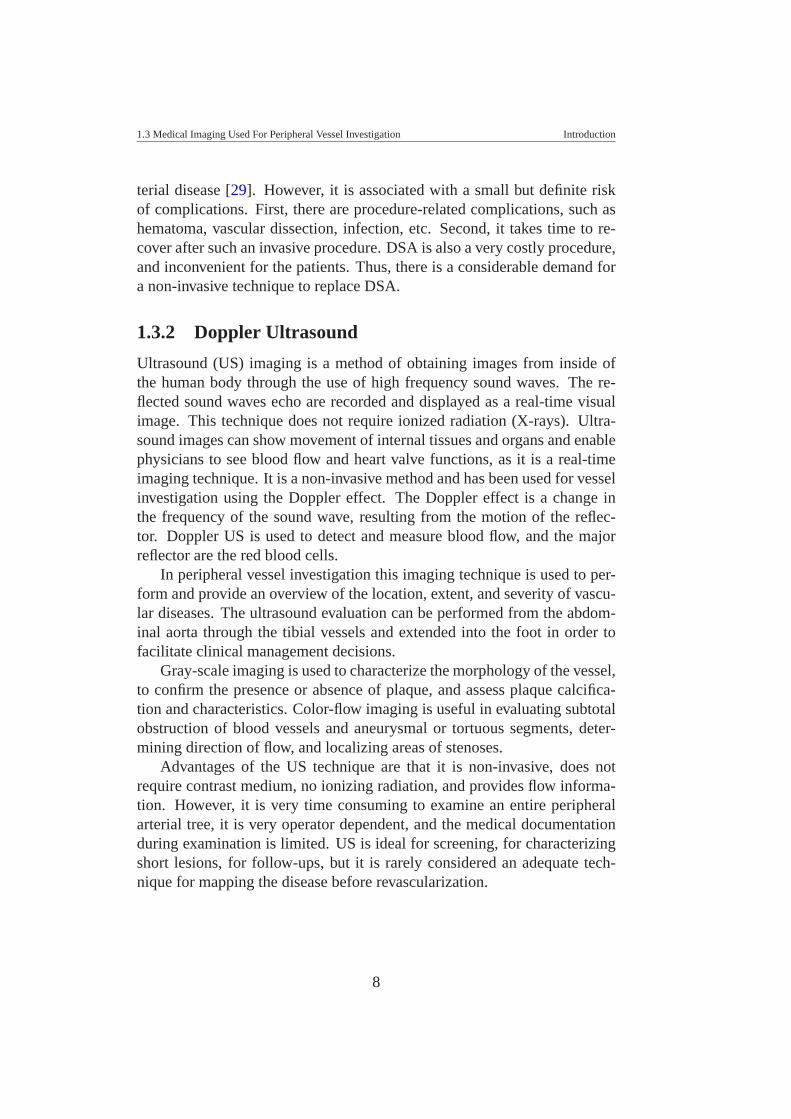
1.3.2 Doppler Ultrasound
Ultrasound (US) imaging is a method of obtaining images from inside ofthe human body through the use of high frequency sound waves. The re-flected sound waves echo are recorded and displayed as a real-time visualimage. This technique does not require ionized radiation (X-rays). Ultra-sound images can show movement of internal tissues and organs and enablephysicians to see blood flow and heart valve functions, as it is a real-timeimaging technique. It is a non-invasive method and has been used for vesselinvestigation using the Doppler effect. The Doppler effect is a change inthe frequency of the sound wave, resulting from the motion of the reflec-tor. Doppler US is used to detect and measure blood flow, and the majorreflector are the red blood cells.
In peripheral vessel investigation this imaging technique is used to per-form and provide an overview of the location, extent, and severity of vascu-lar diseases. The ultrasound evaluation can be performed from the abdom-inal aorta through the tibial vessels and extended into the foot in order tofacilitate clinical management decisions.
Gray-scale imaging is used to characterize the morphology of the vessel,to confirm the presence or absence of plaque, and assess plaque calcifica-tion and characteristics. Color-flow imaging is useful in evaluating subtotalobstruction of blood vessels and aneurysmal or tortuous segments, deter-mining direction of flow, and localizing areas of stenoses.
Advantages of the US technique are that it is non-invasive, does notrequire contrast medium, no ionizing radiation, and provides flow informa-tion. However, it is very time consuming to examine an entire peripheralarterial tree, it is very operator dependent, and the medical documentationduring examination is limited. US is ideal for screening, for characterizingshort lesions, for follow-ups, but it is rarely considered an adequate tech-nique for mapping the disease before revascularization.
8
1.3 Medical Imaging Used For Peripheral Vessel Investigation Introduction
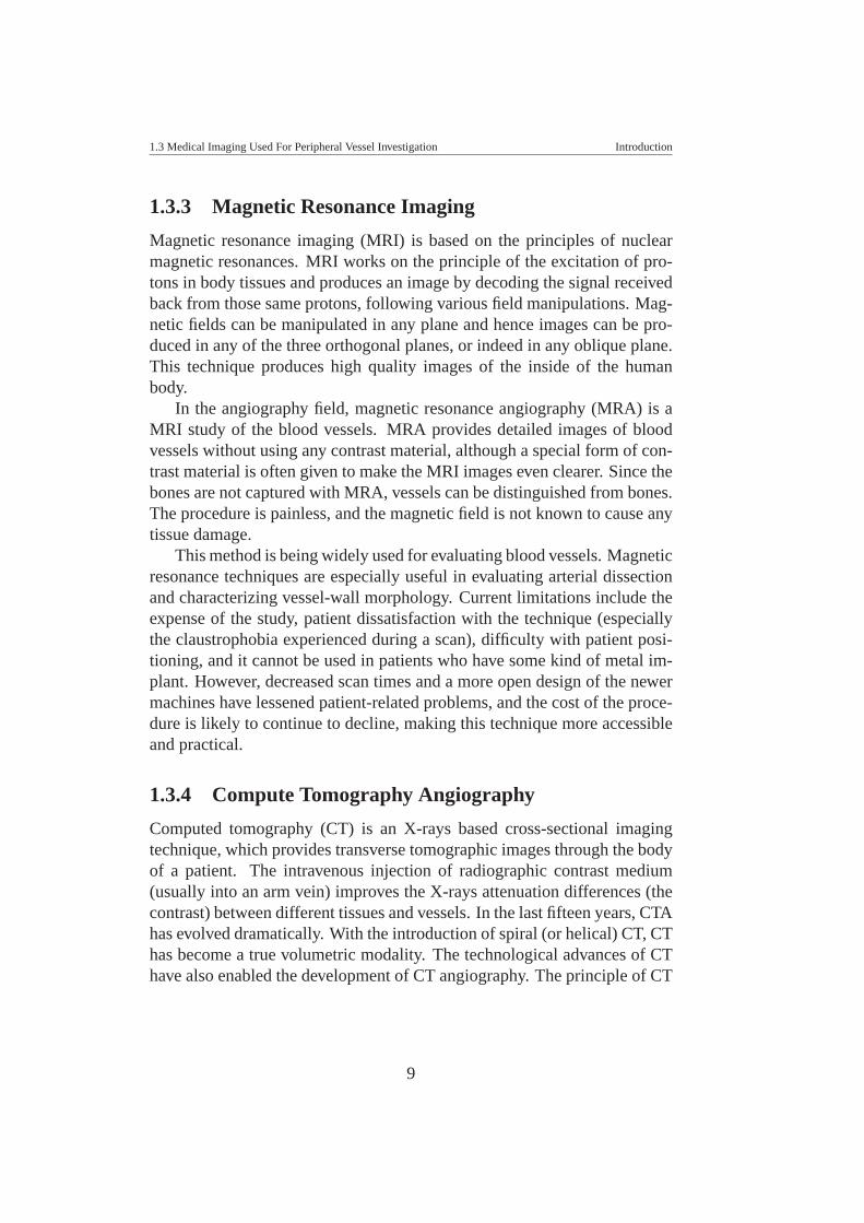
1.3.3 Magnetic Resonance Imaging
Magnetic resonance imaging (MRI) is based on the principles of nuclearmagnetic resonances. MRI works on the principle of the excitation of pro-tons in body tissues and produces an image by decoding the signal receivedback from those same protons, following various field manipulations. Mag-netic fields can be manipulated in any plane and hence images can be pro-duced in any of the three orthogonal planes, or indeed in any oblique plane.This technique produces high quality images of the inside of the humanbody.
In the angiography field, magnetic resonance angiography (MRA) is aMRI study of the blood vessels. MRA provides detailed images of bloodvessels without using any contrast material, although a special form of con-trast material is often given to make the MRI images even clearer. Since thebones are not captured with MRA, vessels can be distinguished from bones.The procedure is painless, and the magnetic field is not known to cause anytissue damage.
This method is being widely used for evaluating blood vessels. Magneticresonance techniques are especially useful in evaluating arterial dissectionand characterizing vessel-wall morphology. Current limitations include theexpense of the study, patient dissatisfaction with the technique (especiallythe claustrophobia experienced during a scan), difficulty with patient posi-tioning, and it cannot be used in patients who have some kind of metal im-plant. However, decreased scan times and a more open design of the newermachines have lessened patient-related problems, and the cost of the proce-dure is likely to continue to decline, making this technique more accessibleand practical.
1.3.4 Compute Tomography Angiography
Computed tomography (CT) is an X-rays based cross-sectional imagingtechnique, which provides transverse tomographic images through the bodyof a patient. The intravenous injection of radiographic contrast medium(usually into an arm vein) improves the X-rays attenuation differences (thecontrast) between different tissues and vessels. In the last fifteen years, CTAhas evolved dramatically. With the introduction of spiral (or helical) CT, CThas become a true volumetric modality. The technological advances of CThave also enabled the development of CT angiography. The principle of CT
9
1.4 CTA of Peripheral Arterial Occlusive Disease Introduction
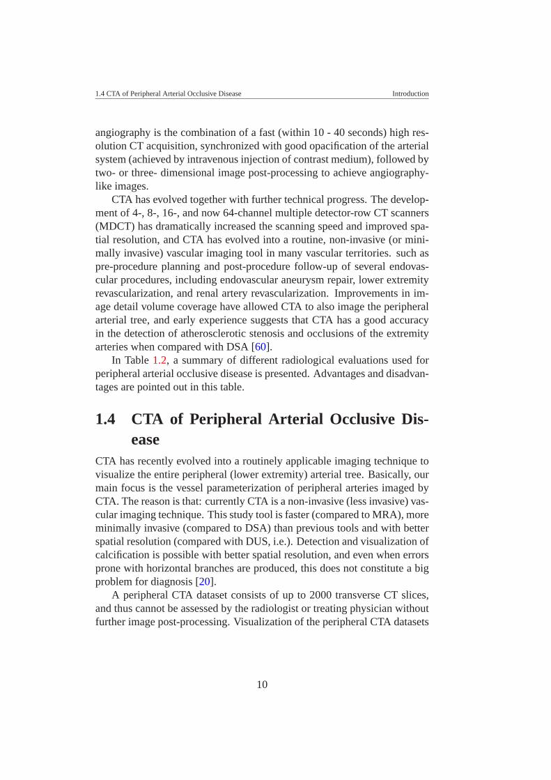
angiography is the combination of a fast (within 10 - 40 seconds) high res-olution CT acquisition, synchronized with good opacification of the arterialsystem (achieved by intravenous injection of contrast medium), followed bytwo- or three- dimensional image post-processing to achieve angiography-like images.
CTA has evolved together with further technical progress. The develop-ment of 4-, 8-, 16-, and now 64-channel multiple detector-row CT scanners(MDCT) has dramatically increased the scanning speed and improved spa-tial resolution, and CTA has evolved into a routine, non-invasive (or mini-mally invasive) vascular imaging tool in many vascular territories. such aspre-procedure planning and post-procedure follow-up of several endovas-cular procedures, including endovascular aneurysm repair, lower extremityrevascularization, and renal artery revascularization. Improvements in im-age detail volume coverage have allowed CTA to also image the peripheralarterial tree, and early experience suggests that CTA has a good accuracyin the detection of atherosclerotic stenosis and occlusions of the extremityarteries when compared with DSA [60].
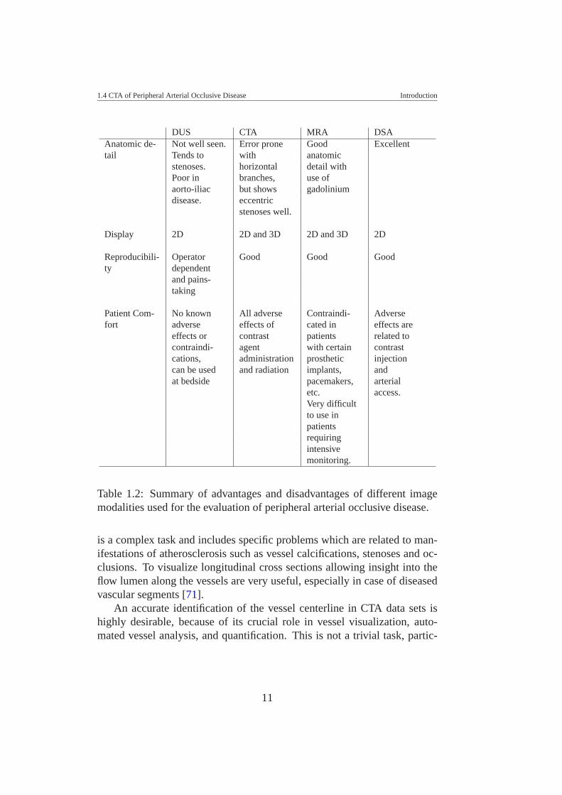
In Table 1.2, a summary of different radiological evaluations used forperipheral arterial occlusive disease is presented. Advantages and disadvan-tages are pointed out in this table.
1.4 CTA of Peripheral Arterial Occlusive Dis-ease
CTA has recently evolved into a routinely applicable imaging technique tovisualize the entire peripheral (lower extremity) arterial tree. Basically, ourmain focus is the vessel parameterization of peripheral arteries imaged byCTA. The reason is that: currently CTA is a non-invasive (less invasive) vas-cular imaging technique. This study tool is faster (compared to MRA), moreminimally invasive (compared to DSA) than previous tools and with betterspatial resolution (compared with DUS, i.e.). Detection and visualization ofcalcification is possible with better spatial resolution, and even when errorsprone with horizontal branches are produced, this does not constitute a bigproblem for diagnosis [20].
A peripheral CTA dataset consists of up to 2000 transverse CT slices,and thus cannot be assessed by the radiologist or treating physician withoutfurther image post-processing. Visualization of the peripheral CTA datasets
10
1.4 CTA of Peripheral Arterial Occlusive Disease Introduction
DUS CTA MRA DSAAnatomic de- Not well seen. Error prone Good Excellenttail Tends to with anatomic
stenoses. horizontal detail withPoor in branches, use ofaorto-iliac but shows gadoliniumdisease. eccentric
stenoses well.
Display 2D 2D and 3D 2D and 3D 2D
Reproducibili- Operator Good Good Goodty dependent
and pains-taking
Patient Com- No known All adverse Contraindi- Adversefort adverse effects of cated in effects are
effects or contrast patients related tocontraindi- agent with certain contrastcations, administration prosthetic injectioncan be used and radiation implants, andat bedside pacemakers, arterial
etc. access.Very difficultto use inpatientsrequiringintensivemonitoring.
Table 1.2: Summary of advantages and disadvantages of different imagemodalities used for the evaluation of peripheral arterial occlusive disease.
is a complex task and includes specific problems which are related to man-ifestations of atherosclerosis such as vessel calcifications, stenoses and oc-clusions. To visualize longitudinal cross sections allowing insight into theflow lumen along the vessels are very useful, especially in case of diseasedvascular segments [71].
An accurate identification of the vessel centerline in CTA data sets ishighly desirable, because of its crucial role in vessel visualization, auto-mated vessel analysis, and quantification. This is not a trivial task, partic-
11
1.4 CTA of Peripheral Arterial Occlusive Disease Introduction
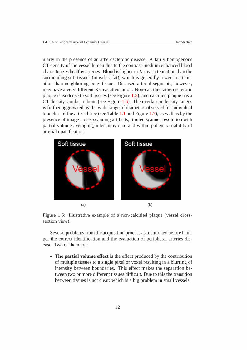
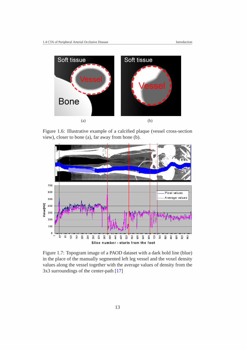
ularly in the presence of an atherosclerotic disease. A fairly homogenousCT density of the vessel lumen due to the contrast-medium enhanced bloodcharacterizes healthy arteries. Blood is higher in X-rays attenuation than thesurrounding soft tissues (muscles, fat), which is generally lower in attenu-ation than neighboring bony tissue. Diseased arterial segments, however,may have a very different X-rays attenuation. Non-calcified atheroscleroticplaque is isodense to soft tissues (see Figure 1.5), and calcified plaque has aCT density similar to bone (see Figure 1.6). The overlap in density rangesis further aggravated by the wide range of diameters observed for individualbranches of the arterial tree (see Table 1.1 and Figure 1.7), as well as by thepresence of image noise, scanning artifacts, limited scanner resolution withpartial volume averaging, inter-individual and within-patient variability ofarterial opacification.
(a) (b)
Figure 1.5: Illustrative example of a non-calcified plaque (vessel cross-section view).
Several problems from the acquisition process as mentioned before ham-per the correct identification and the evaluation of peripheral arteries dis-ease. Two of them are:
• The partial volume effect is the effect produced by the contributionof multiple tissues to a single pixel or voxel resulting in a blurring ofintensity between boundaries. This effect makes the separation be-tween two or more different tissues difficult. Due to this the transitionbetween tissues is not clear; which is a big problem in small vessels.
12
1.4 CTA of Peripheral Arterial Occlusive Disease Introduction
(a) (b)
Figure 1.6: Illustrative example of a calcified plaque (vessel cross-sectionview), closer to bone (a), far away from bone (b).
Figure 1.7: Topogram image of a PAOD dataset with a dark bold line (blue)in the place of the manually segmented left leg vessel and the voxel densityvalues along the vessel together with the average values of density from the3x3 surroundings of the center-path [17]
13
1.5 Visualization of PAOD in CTA datasets Introduction
• Contrast agent administration. The contrast agent is more of a con-cern with the protocol followed by radiologists [73]. Poor injection ofcontrast agent produces images with a non-clear distinction betweensoft tissues and blood vessels. The poor administration of the contrastagent, added to the partial volume effect constitute a big challenge forthe underlying detection of diseased blood vessels, and even healthyvessels with small diameters [22].
1.5 Visualization of PAOD in CTA datasetsSeveral visualization techniques have been already used for blood vesselvisualization. The most known are; direct volume rendering (DVR), maxi-mum intensity projection (MIP), iso-surface display, etc.
• DVR is a visualization technique that allows the whole volume datasetto be displayed. With DVR, it is possible to visualize all structuresanatomically correct, but for large datasets this is time consuming.DVR depends on a transfer function definition, which allows the iden-tification and classification of different tissues along the viewing ray.In some cases this is a challenge because it is highly dependent on thedataset.
• MIP displays the highest intensity value of all voxels along the corre-sponding viewing ray. In this case, all structures with higher intensityvalues are displayed in front, hiding lower intensity structures. There-fore, the bones are always in front of the vessels.
• Iso-surface display produces surfaces in the domain of the scalarquantity, which has the same value, the so-called isosurface value.There are different methods to generate the surfaces from a discreteset of data points. All methods use interpolation to construct a contin-uous function. The correctness of the generated surfaces depends onhow well the constructed continuous function matches the underlyingcontinuous function representing the discrete data set. The most usedmethod is the marching cube algorithm [70].
We present in this section the most recent and novel visualization tech-niques that have been presented to the scientific community for vessel visu-alization, some of them have been applied for peripheral vessels.
14
1.5 Visualization of PAOD in CTA datasets Introduction
1.5.1 Curved Planar Reformation
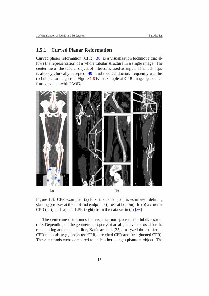
Curved planer reformation (CPR) [36] is a visualization technique that al-lows the representation of a whole tubular structure in a single image. Thecenterline of the tubular object of interest is used as input. This techniqueis already clinically accepted [40], and medical doctors frequently use thistechnique for diagnosis. Figure 1.8 is an example of CPR images generatedfrom a patient with PAOD.
(a) (b)
Figure 1.8: CPR example. (a) First the center path is estimated, definingstarting (crosses at the top) and endpoints (cross at bottom). In (b) a coronarCPR (left) and sagittal CPR (right) from the data set in (a) [36]
The centerline determines the visualization space of the tubular struc-ture. Depending on the geometric property of an aligned vector used for there-sampling and the centerline, Kanitsar et al. [35], analyzed three differentCPR methods (e.g., projected CPR, stretched CPR and straightened CPR).These methods were compared to each other using a phantom object. The
15
1.5 Visualization of PAOD in CTA datasets Introduction
comparison evaluated spatial perception, isometry, and possible occlusions.The straightened CPR is preferable in many applications. Due to the factthat the surrounding tissue may be distorted in the image, it might be dif-ficult to immediately recognize which portions of a vessel tree are actuallydisplayed. Thus, Kanitsar et al. [35] defined three CPR enhancements thatovercome this problem (more details in [35]). These CPR enhancementsare; multipath CPR, rotated CPR and thick CPR. The multipath CPR allowsthe visualization of multiple vessels in one image without the overlappingof other tissues (e.g., bone). The rotated CPR allows rotating the projectionof any CPR method. The thick CPR reduces sampling artifacts, achieving abetter projection of small vessels and removing false stenoses.
1.5.2 VesselGlyph
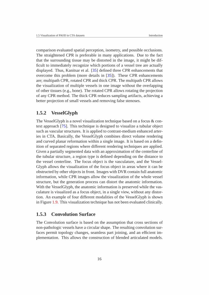
The VesselGlyph is a novel visualization technique based on a focus & con-text approach [75]. This technique is designed to visualize a tubular objectsuch as vascular structures. It is applied to contrast-medium enhanced arter-ies in CTA. Basically, the VesselGlyph combines direct volume renderingand curved planar reformation within a single image. It is based on a defin-ition of separated regions where different rendering techniques are applied.Given a partially segmented data with an approximation of the centerline ofthe tubular structure, a region type is defined depending on the distance tothe vessel centerline. The focus object is the vasculature, and the Vessel-Glyph allows the visualization of the focus object in areas where it can beobstructed by other objects in front. Images with DVR contain full anatomicinformation, while CPR images allow the visualization of the whole vesselstructure, but the generation process can distort the anatomic information.With the VesselGlyph, the anatomic information is preserved while the vas-culature is visualized as a focus object, in a single view, without any distor-tion. An example of four different modalities of the VesselGlyph is shownin Figure 1.9. This visualization technique has not been evaluated clinically.
1.5.3 Convolution Surface
The Convolution surface is based on the assumption that cross sections ofnon-pathologic vessels have a circular shape. The resulting convolution sur-faces permit topology changes, seamless part joining, and an efficient im-plementation. This allows the construction of blended articulated models.
16
1.5 Visualization of PAOD in CTA datasets Introduction
(a) (b)
(c) (d)
Figure 1.9: VesselGlyph examples: (a) CPR + DVR, (b) foreground-cleftin DVR with occlusion lines, (c) Thick-Slab rendering (DVR), (d) tubularrendering (DVR) [75]
17
1.5 Visualization of PAOD in CTA datasets Introduction
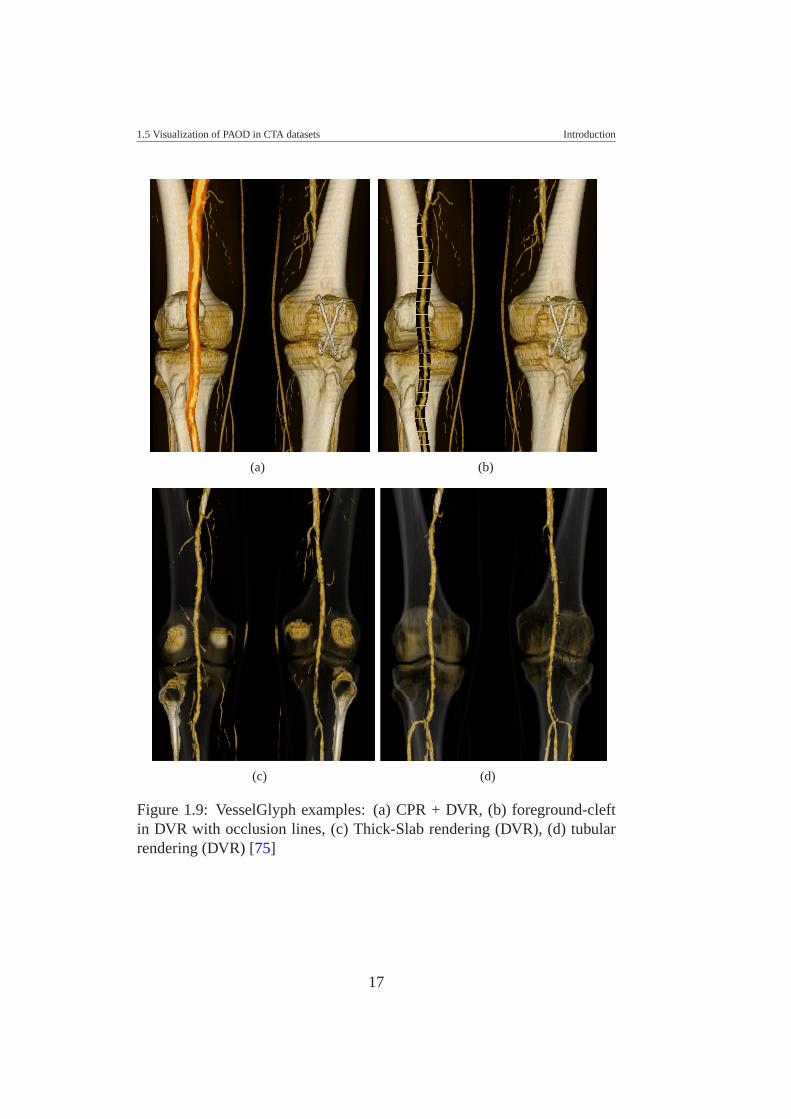
The convolution surface for vessel tree visualization was explored and im-plemented by Oeltze and Preim [58, 59]. First, the vessel skeleton mustbe defined and an initial estimation of its diameter should be used as in-put. Then, the tubular object is defined by the convolution of the skeletonwith a three-dimensional Gaussian filter. This technique is independent ofthe modality used for 3D imaging (e.g., MRI or CTA). An example of acerebral vasculature imaged by MRI is shown in Figure 1.10.
Figure 1.10: Visualization of cerebral vasculature imaged by MRI using aconvolution surface [59]
The convolution surface visualization technique defines a model ade-quately for visualizing vascular tree structures. However, this method as-sumes a circular cross-section of blood vessels, it is based on an initial esti-mation of the skeleton and diameter estimation of the vascular tree structure.As we described, in Section 1.4, we found that with diseased blood vessels,assuming just circular cross-sections is insufficient, due to the irregularityof shape of the diseased blood vessels. The intensity image distribution ofdiseased blood vessel is also non-uniform.
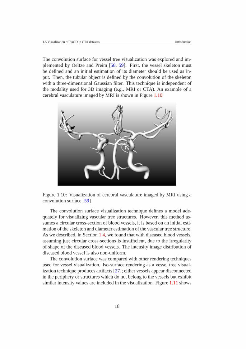
The convolution surface was compared with other rendering techniquesused for vessel visualization. Iso-surface rendering as a vessel tree visual-ization technique produces artifacts [27]; either vessels appear disconnectedin the periphery or structures which do not belong to the vessels but exhibitsimilar intensity values are included in the visualization. Figure 1.11 shows
18
1.6 Discussion Introduction
an example of comparing the convolution surface with other rendering tech-nique including iso-surfacing.
Figure 1.11: Close-up images of a vessel tree example, comparing iso-surface rendering (left) with a more refined rendering technique (middle,details in [59]) and convolution surface rendering (right) [59]
1.6 DiscussionIn general, the visualization techniques presented in the previous sectionsassume an initial estimation of the centerline and diameter of the tubularstructure. Peripheral vasculature consists of large and tiny vessel diame-ters, and patients with PAOD may have an irregular variability of the vesselshape. A wrong estimation of a centerline may produce wrong visualiza-tion results (e.g., using CPR), and then, the so-called pseudo-stenoses mayappear. An illustrative example is shown on Figure 1.12. This may involveinteractive intervention, which is time consuming.
On the other hand, peripheral vascular investigation (where the averagescan length is between 110 cm and 130 cm[20]) and analysis in any imagemodality, require the analysis of large datasets (i.e., a CTA dataset may con-sist of 2000 2D slices). Which is very time consuming for radiologist with-out any semi-automatic or automatic segmentation algorithm that allowsthem identify accurately and more precisely the localization and quantifica-tion of any vascular anomaly, without wasting of time. For theses reasons,a accurate segmentation is highly required and necessary. Furthermore, theperipheral CTA has been gradually more used in clinical practice for PAODdiagnosis and posterior following treatment. Additionally, with the evolu-tion of CT-scanner technology, high resolution imaging of the peripheralvasculature has become routinely possible. However, the density overlap-ping of different tissues is a major difficulty for segmentation and clear sep-
19
1.7 Thesis Contents Introduction
aration between different tissues from vessel tissues. A 2D visualization ofthe vasculature is definitely not enough, because of the superposition in 2Dof bone over vessels. Besides, medical doctors and radiologists are familiarwith CPR visualization, which is based on a centerline estimation in a 3Dspace. These are the main reasons why a segmentation of peripheral arter-ies is highly required and why a 3D segmentation is preferable than a 2Dsegmentation.
(a) (b)
(c)
Figure 1.12: Illustrative example of a good and wrong estimation of a cen-terline if a CPR visualization technique is used. In this example we show(a) a good estimation on healthy data, (b) a good estimation on a diseasedcase, (c) a wrong estimation on a healthy or a diseased case.
1.7 Thesis ContentsThe main contribution of this thesis is to present a new technique to para-meterize diseased blood vessels of the peripheral vascular structures. Vi-
20
1.7 Thesis Contents Introduction
sualization of tubular structures such as blood vessels is quite ”easy” whenthe blood vessel is healthy, problems appear when the vessel presents anyanomaly due to the presence of some vascular disease.
This thesis presents an investigative result for blood vessel segmenta-tion, with the focus on diseased blood vessels of peripheral arteries imagedby CTA. Medical doctors are more interested in being able to visualize andquantify vascular diseases than having just nice images. For them it is quiteimportant to identify the center and surround area close to the vessel center.The vessel center is not defined only by the center of the lumen (which isthe area where the flow goes through in the vasculature structure), but alsoby the calcified and occluded part of the vessel. In this case we have ex-perienced that it is a challenge to find a simple segmentation technique thattakes into account such variability. Due to this fact and the knowledge basedon that, vessels conserve a tubular structure, even in the presence of calci-fications and occlusions. We believe a model-based technique is the mostsuitable approach for showing a better or even more accurate segmentation.In this direction we present in chapter two a review of different model basedtechniques already applied to vessel segmentation and visualization. In thisreview we included the last 20 years of investigation in this area, giving thereader a good reference frame.
As we could see in the section before, most of the blood vessel visualiza-tion techniques require an accurate estimation of the centerline of the vessel.Most of them are based on an initial centerline approximation. At the begin-ning of our research we were more interested in the improvement of the cen-terline estimation than an actual centering technique used on a daily clinicalbasis. Therefore, we start with an evaluation of different centerline tech-niques that were worked on. Thus, chapter three presents an evaluation ofdifferent methods for approximating the centerline of a vessel in a phantomsimulating the peripheral arteries. Six algorithms were used to determine thecenterline of a synthetic peripheral arterial vessel. They are based on: raycasting using thresholds, maximum gradient-like stop criterion, pixel mo-tion estimation between successive images called block matching, center ofgravity, and shape based segmentation. The Randomized Hough Transformand ellipse fitting have been used as shape based segmentation techniques.Since in the synthetic data set the centerline is known, an estimation of theerror can be calculated in order to determine the accuracy achieved by agiven method. Mostly these methods work on a cross-section of the vesselfrom an initial vessel path tracked but not centered. Unfortunately, in this
21
1.7 Thesis Contents Introduction
investigation we did not find any relevant improvement for accuracy in thecenterline estimation, due to the wide variability of blood vessels in patientswith PAOD. However, this allowed us to conclude that it might be signifi-cant if a three dimensional space is taken into account when evaluating anideal profile of blood vessels. In this direction we designed a new strategyfor a blood vessel parameterization. This strategy is presented in Chapterfour.
Chapter four describes an estimation of the dimensions of lower extrem-ity arteries, imaged by computed tomography. The vessel is modelled usingan elliptical or cylindrical structure with specific dimensions, orientation,and blood vessel density. The model separates two homogeneous regions:Its inner side represents a region of density for vessels, and its outer sidea region for background. Taking into account the point spread function ofa CT scanner, a function is modelled with a Gaussian kernel, in order tosmooth the vessel boundary in the model. Thus, a new strategy for vesselparameter estimation is presented in this chapter. It stems from the vesselmodel and the model parameter optimization by a nonlinear optimizationprocedure, i.e., the Levenberg-Marquardt technique. The method providescenter location, diameter and orientation of the vessel, as well as blood, andbackground mean density values.
We considered it quite important that medical doctors were involved inthe development of every new approach designed to help them for diagno-sis. For this reason a clinical evaluation of every new technology is crucialbefore it can be used in a clinical environment. Therefore, Chapter fivepresents a clinical evaluation of the method described in Chapter four as afirst step to introduce this technique in a clinical environment. Twenty casesfrom available patient data were pre-selected and separated into ’minimaldiseased’ and ’severe diseased’ vessels. Manual identification were used asour gold standard. We compared the model fitting method against a standardmethod, which is presently used in the clinical environment.
22
CHAPTER 2
MODEL BASED SEGMENTATION
TECHNIQUES
Part of this chapter is based on the following publication:
Buhler K., Felkel P., and La Cruz A.: Geometric Methods for Vessel Visu-alization and Quantification - A Survey. Geometric Modelling for ScientificVisualization. G. Brunnett, B. Hammann, H. Muller, and L. Linsen, (eds),Kluwer Academic Publishers. pp 399-420. 2004.
2.1 IntroductionIn medical imaging, segmentation is the process of classifying and separat-ing different tissues. It is a prerequisite for quantification of morphologicaldisease manifestation, for volume visualization and modeling of individualobjects, for chirurgical operation planning and simulation (e.g., using virtualendoscopy).
We found that recently, two relevant works in this area were presented tothe scientific community. In both of them, the authors presented an overviewof different segmentation and visualization techniques designed for identi-fying and modeling vessels and tube-like structures. Buhler et al. [8] presenta survey and discussion of different geometric techniques applied to vesselvisualization and geometric model generation. Kirbas et al. [39], classi-fied several segmentation methods according to the technique that was used.They point out that there is no single segmentation method that allows theextracting of the vasculature across different medical imaging modalities
23
2.1 Introduction Model Based Segmentation Techniques
(e.g., MRA, CTA, US, etc.), and not even across different vascular anatomicterritories. Some methods use threshold values, or an explicit vessel modelto extract contours. Other techniques require image processing (dependingon the data, quality, noise, artifacts, etc.), a priori segmentation, or post-processing.
A general segmentation technique is based on the intensity level. Thistechnique relies on the assumption that the blood vessels have a differentintensity level than soft tissue or bone. This is due to the absorption and/oremission property of the object being imaged by any modality, which is dif-ferent for blood, muscle, bone, air, fat, etc. Based on this fact it is possibleto classify different objects according to the thresholds of intensity leveldefined for every tissue. Nevertheless, due to many factors (e.g., noise,partial volume effect, artifacts, etc.) this approach is not enough for an ac-curate segmentation. Thus, an immediate improvement is using a techniquethat allows an adaptive local thresholding [31], or using a statistic shapemodel [12, 13]. The region growing technique [5, 8, 39], which can be seenas an extension of a thresholding technique is based on a classification ofpixels (voxels) that fulfill certain constrains defined previously. From an ini-tial pixel (voxel), the neighborhood is analyzed and added to the region if itsatisfies a decision rule. Normally the decision rule is defined using thresh-old values, the gradient operator, and/or spatial proximity. This methodassumes that discontinuities are not possible between objects. The grow-ing criteria should be sufficient to face local image variations. Due to thevariations in image intensities and noise, region growing can result in holesand over-segmentation. An improvement to this method includes mathe-matical morphology [74], which may avoid holes and remove the connec-tivity between different tissues. This technique has been used for blood ves-sel segmentation in combination with other techniques as a post-processingstep [63].
As mention in the previous chapter, our main focus is the segmenta-tion of blood vessels imaged by CTA. The vessel lumen of healthy vesselsin CTA datasets is characterized by a fairly homogenous CT density. Ondiseased blood vessels it is a challenge to identify the center of the vessel,due to the characteristics of non-calcified and calcified plaque, as it wasdescribed in a previous chapter. Therefore, it is not surprising that densityand gradient information alone is insufficient to accurately extract the cen-terlines of a diseased arterial tree. The overlap in density ranges is furtheraggravated by the wide range of diameters observed for individual branches
24
2.2 Deformable Models Model Based Segmentation Techniques
of the arterial tree, as well as by the presence of image noise, scanning arti-facts, limited scanner resolution with partial volume averaging, and finally,inter-individual and within-patient variability of arterial opacification. Forthis reason, we believe that a model-based technique is more suitable for theproblem we are dealing with in our investigation.
Classical model based segmentation algorithms [8, 39] applied to vesselextraction are based on fitting circular, elliptical or cylindrical geometricmodels to the data, assuming a tubular shape. Such techniques combinethresholds with gradient information [87] or derivative estimation [42, 43,44] in order to approximate the vessel boundary. Then, this initial boundaryestimation is fitted to a geometrical model (e.g., circular or elliptical cross-section or cylindrical structure).
This chapter contains an overview of the most recent works related tomodel based segmentation techniques applied to blood vessels. We presenta list of the most important model based segmentation techniques that weconsidered and which have been used in the last two decades. Various re-search has been already done in this area. However, an accurate vessel seg-mentation and visualization continues to be an open problem. Most of therecent works have been motivated to provide more confidence and fastertechniques.
2.2 Deformable ModelsThe deformable model approach is described in more detail as a geometricmodel used for blood vessel segmentation and visualization by Buhler [8].Kirbas et al. [39], also classified it as a model based approach.
Deformable models [53] appear to be one of the most promising seg-mentation techniques. This approach is powerful and widely used for seg-mentation and geometric model generation in 2D and 3D data [8], and it canbe used for any modality [39]. These techniques are based on a minimiza-tion process of an energy function. This energy function involves internaland external forces. The internal forces allow smoothness of the contourand the external forces move the deformable structure towards the edges ofthe underlying data. Depending on the definition of the energy function, thedeformable model inflates or shrinks towards the object. Normally, the en-ergy function involves the gradient information or derivative values aroundthe deformable object.
Depending on the parameterization used for the model and the definition
25
2.2 Deformable Models Model Based Segmentation Techniques
of the energy function, in the literature [8] three more common deformablemodels are found. They are: the snakes or active contours, level-sets, andprobabilistic snakes.
2.2.1 Snakes
The snake approach uses a parameterized curve which evolves over time.This technique has been applied in many areas of medical segmentation.Gong et al. [26] define a deformable super-ellipse for prostate segmentation.Hernandez et al. [28] use this approach for three-dimensional segmentationof brain aneurysms in CTA. Lorigo et al. [49] present a deformable modelbased on active contours for segmentation of brain vasculature. The maingoal of the snake is to minimize a weighted sum of influences from variousenergy forces. Conventionally, this parametric model usually relies on a setof basis functions. Depending on the shape of the object it may require are-parameterization that is heuristically or interactively controlled [85]. Anew generation of deformable models was designed to avoid such problems,which is the well-known level-set approach [61].
2.2.2 Level-sets
A level-set is based on an implicit model to represent surface shapes. Thisapproach is topologically flexible and can split and join as necessary in thedeformation process [53], without a re-parameterization [85].
The level-set approach has been widely used for vascular segmenta-tion [8] in general, aortic aneurysm segmentation [48, 76], and centerlinedetection of colon CT data [15]. Wang et al. [83] used this approach as anexperimental result to segment a case of lower extremity occlusive diseases.
2.2.3 Probabilistic Snakes
Another way to define an energy function in a deformable model approach isusing statistic information. This approach is called the probabilistic snake.A probabilistic shape model generally assumes that image features are ran-dom variables with shape dependence on probability distributions [52]. Thisapproach searches the probability of an image of a given model, using aBayesian framework. Pujol et al. [68] applied this approach for segmenta-tion of intravascular features of coronary arteries imaged by US.
26
2.3 Multi-scale Methods Model Based Segmentation Techniques
Yim et al. [90, 91, 92] present a deformable model for reconstructing thevessel surface of a carotid artery. The deformable model is based on a cylin-drical coordinate system of curvilinear axes [92]. The model consists of amesh, where vertices are evenly spaced in the axial and in the circumferen-tial directions. In this mesh the vertices deform only in the radial directionand their position is described by their radial location. The method allowsfor curves in the vessel axis, variability in the vessel diameter, and variabil-ity in cross sectional shape. Internal and external forces produce the defor-mation. The internal forces push the vertices to minimize discontinuities inthe radial location between adjacent vertices. The external forces push thevertices towards peaks in the gradient magnitude images. In this approachit is possible that adjacent radial meshes intersect each other. In this case awarping process is used to solve this problem (more details in [92]). Here,the axes are selected manually. Later on, Yim et al. [91] present an improve-ment of the location of the vessel axes by a skeletonisation technique. Thisskeletonisation technique is based on the ordered region-growing algorithm(ORG). The ORG represents the image as an acyclic graph, which can bereduced to a skeleton by specifying starting and ending point. This mayconstruct paths, which are not part of the vessel. A pruning process solvesthis error. This pruning process is based upon branch lengths. Brancheswithout a minimal length are removed.
Feng et al. [18] present a 3D geometric deformable model for tubularstructure segmentation. Based on internal and external forces, Feng et al.introduced a new energy term which incorporates the information of thespatial relationship between tubular branches. The results were shown onlywith experimental data [18].
2.3 Multi-scale MethodsMulti-scale methods are based on the extraction of large structures at low-resolution images and fine structures at high-resolution images. Multi-scalemethods [44] as well as deformable models have been used more recentlyfor blood vessel segmentation. In fact, Whitaker et al. [85] point out that thecombination of the level-set method with a multi-scale approach allows themodel to start on a coarse grid and progress on finer grids until a solutionis reached. This reduces computation time and controls the relative impor-tance of differently sized structures in the model. A similar combination oflevel-set and multi-scale approaches was used by Boldak et al. [6].
27
2.4 Geometry Based Segmentation Model Based Segmentation Techniques
The multi-scale approach uses the Hessian matrix, which contains thesecond derivatives of the data. This method is based on the fact that thesmallest Eigen value of the Hessian matrix is close to zero at the centerof tubular structures, and the other two Eigen values are high and close toequal, assuming a circular cross-section.
Krissian et al. [42, 43, 44] presented a new approach to segment vesselsof 3D angiography data of the brain using the multi-scale technique.
Frangi et al. [25] introduce a multi-scale vessel enhancement ap-proach applied to segment and analyze the vasculature on cardiac im-ages. Frangi [23, 24, 25] worked in his PhD thesis on the applicationof a three-dimension model for vascular and cardiac images based on amulti-scale method for vessel enhancement. Many other authors have usedthis approach to model geometric flows of cerebral vasculature imaged byMRI [78].
Joshi et al. [32, 33] present a Bayesian multi-scale three-dimensionaldeformable template approaches based on a medial representation for thesegmentation and shape characterization of anatomical objects in medicalimagery. Via the construction of templates, information about the geometryand shape of the anatomical objects under study should be given, before-hand. Defining probabilistic transformations on these templates pursues theanatomical variability. The multi-scale deformable template is based onthe medial axis representation of objects proposed by Blum [4]. This tech-nique was applied for the automatic extraction and analysis of the shapeof anatomical objects from brain and abdomen, imaged by MRI and CTrespectively.
2.4 Geometry Based SegmentationGeometry based segmentation is based on a parametric model, which de-fines a tubular model. This tubular model with elliptical or cylindricalcross-section has been applied on 2D and 3D datasets. Mostly this approachis combined with a deformable model or a multi-scale approach. Given aparametric model of a tubular object (e.g., generalized cylinder) and usingthe deformable model approach it can be deformed to get the most appro-priate model. On the other hand, using the properties of the Hessian matrixand the medialness approach [25] a cylindrical model can be extracted. Me-dialness or core is defined in terms of convolution kernels at many positionsand scales (in scale space), with scales, i.e., kernel widths, that are a signif-
28
2.4 Geometry Based Segmentation Model Based Segmentation Techniques
icant fraction of the radial width of a tubular object. Basically a medialnessfunction measure the degree of belonging to the medial axis of the object.
2.4.1 Geometry Based Segmentation Combined with aDeformable Model Approach
Boldak et al. [5, 6] proposed a segmentation of three-dimensional vesselsimaged by CTA using geometrical moments, assuming that segments can beconsidered as tube-like structures. A 3D geometrical moment-based methodis used to localize the center of the vessel and its local direction, by usinga local approximation by a cylinder. This ideal cylinder separates two ho-mogeneous regions. The area inside the cylinder (the vessel) is defined witha higher intensity level and the area outside (background) with a lower in-tensity. Filtering ideally smoothes the transition between both regions. Thisapproach uses several adaptive controls that allow dealing with pathologicalpatterns such as dense and scattered calcifications. The disadvantage of thismethod is that it allows an underestimation of the diameter for better track-ing in a defined window size. It makes a compromise to avoid includingother structures in the window, like: bones, distinct vessels, highly curvedvessel parts, etc. This window size can be adjusted by applying an adaptivecontrol. This is performed by means of an exponential weighting of the cur-rent and previous vessel diameter values in order to avoid window size oscil-lations. Using a heuristic approach to handle calcifications and stenoses, thealgorithm removes calcifications using a region growing approach, allowingalso the removal of vessel tissues, and this introduce slight changes of thevessel shape. The advantage with this heuristic rule is that it also removesbones that appear closer to the vessel. Then, the level set approach [6] isused in order to refine the segmentation process allowing improvement ofthe delineation accuracy of contours and calcifications. This approach hasbeen applied to segmentation of the lower limb vessels.
Baun et al. [3] presented a method for 3D surface modelling of the cere-bral vasculature of 3D medical images using active contours. In this workBaun et al. used the generalized cylinder to represent the active contour.The generalized cylinder allows the modelling of an elongated tubular ob-ject with cylindrical or elliptical cross section. In this case it is necessary toreach a global minimum in order to minimize the energy function used bythe active contour. This global minimum is reached using dynamic program-ming for energy minimization. The energy function defines an internal and
29
2.5 Model Fitting Model Based Segmentation Techniques
external force. The external force is based on the gradient, stopping the con-tour when an edge is reached, which is defined by the highest gradient value.The internal forces model the rigid and tension of the object, which allowa bending behavior and prevent clustering of neighbor points on the axes.The initial forces also include a radius constraint, which is used to minimizethe differences of radiuses in a same vessel segment defined between bifur-cation points. In this case, the basic idea of using dynamic programming isto treat the minimization as a path-planning problem of finding the optimalpath between multiple paths at multiple decision states. Each transition be-tween the points on the spine, and between the different radiuses, is equal toa transition in the decision stage. Each decision stage contains informationof the previous stage, reducing the complexity problem considerably. Thiswork presented encouraging results on CTA and MRA datasets applied forsegmentation of cerebral vasculature.
2.4.2 Geometry Based Segmentation Combined with aMulti-scale Approach
Aylward et al. [1] map image intensity to height. This is based on the factthat a 3D image can be viewed as a 3D surface in 4D space, and a 2D imagecan be viewed as a 3D surface, with peaks in areas of height intensity. Itis assumed that tubular objects generally appear brighter than background,and the centerline follows a ridgeline. The segmentation technique is usedin combination with a multi-scale approach that allows the extraction of atubular model using the properties of the Hessian matrix and the medialnessapproach [25]. As we said before the medialness functions measure at agiven point the degree of belonging to the medial axis of the object. Further-more, the multiscale medial axis can be defined by applying the medialnessfunction at multiple scales. Aylward et al. [1] illustrate the capabilities of themethod for medical applications that involve a variety of tubular structuresin clinical data of different organs, patients, and image modalities.
2.5 Model FittingA model fitting is a segmentation method that typically tries to fit a simplegeometric shape, such as an ellipse or curve to the locations of extracted im-ages features in an image [65]. A more general approach, in this direction,is to fit a spline or surface [65] to different features. Huang et al. [30] used
30
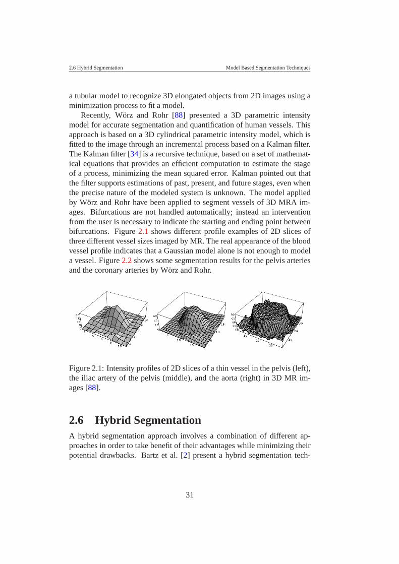
2.6 Hybrid Segmentation Model Based Segmentation Techniques
a tubular model to recognize 3D elongated objects from 2D images using aminimization process to fit a model.
Recently, Worz and Rohr [88] presented a 3D parametric intensitymodel for accurate segmentation and quantification of human vessels. Thisapproach is based on a 3D cylindrical parametric intensity model, which isfitted to the image through an incremental process based on a Kalman filter.The Kalman filter [34] is a recursive technique, based on a set of mathemat-ical equations that provides an efficient computation to estimate the stageof a process, minimizing the mean squared error. Kalman pointed out thatthe filter supports estimations of past, present, and future stages, even whenthe precise nature of the modeled system is unknown. The model appliedby Worz and Rohr have been applied to segment vessels of 3D MRA im-ages. Bifurcations are not handled automatically; instead an interventionfrom the user is necessary to indicate the starting and ending point betweenbifurcations. Figure 2.1 shows different profile examples of 2D slices ofthree different vessel sizes imaged by MR. The real appearance of the bloodvessel profile indicates that a Gaussian model alone is not enough to modela vessel. Figure 2.2 shows some segmentation results for the pelvis arteriesand the coronary arteries by Worz and Rohr.
Figure 2.1: Intensity profiles of 2D slices of a thin vessel in the pelvis (left),the iliac artery of the pelvis (middle), and the aorta (right) in 3D MR im-ages [88].
2.6 Hybrid SegmentationA hybrid segmentation approach involves a combination of different ap-proaches in order to take benefit of their advantages while minimizing theirpotential drawbacks. Bartz et al. [2] present a hybrid segmentation tech-
31
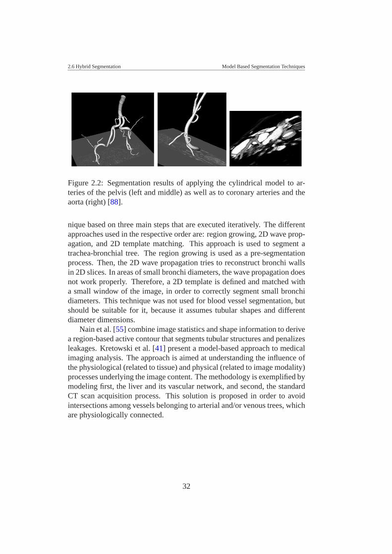
2.6 Hybrid Segmentation Model Based Segmentation Techniques
Figure 2.2: Segmentation results of applying the cylindrical model to ar-teries of the pelvis (left and middle) as well as to coronary arteries and theaorta (right) [88].
nique based on three main steps that are executed iteratively. The differentapproaches used in the respective order are: region growing, 2D wave prop-agation, and 2D template matching. This approach is used to segment atrachea-bronchial tree. The region growing is used as a pre-segmentationprocess. Then, the 2D wave propagation tries to reconstruct bronchi wallsin 2D slices. In areas of small bronchi diameters, the wave propagation doesnot work properly. Therefore, a 2D template is defined and matched witha small window of the image, in order to correctly segment small bronchidiameters. This technique was not used for blood vessel segmentation, butshould be suitable for it, because it assumes tubular shapes and differentdiameter dimensions.
Nain et al. [55] combine image statistics and shape information to derivea region-based active contour that segments tubular structures and penalizesleakages. Kretowski et al. [41] present a model-based approach to medicalimaging analysis. The approach is aimed at understanding the influence ofthe physiological (related to tissue) and physical (related to image modality)processes underlying the image content. The methodology is exemplified bymodeling first, the liver and its vascular network, and second, the standardCT scan acquisition process. This solution is proposed in order to avoidintersections among vessels belonging to arterial and/or venous trees, whichare physiologically connected.
32
2.7 Discussion Model Based Segmentation Techniques
2.7 DiscussionAll algorithms and techniques presented in this chapter have been designed,used, or are suitable for blood vessel segmentation. In general intensity-based approaches are not sufficiently powerful for being applied to PAODpatients. This is mainly because of the intensity overlap between bloodvessels and bone tissues in CTA data. An additional challenge is that thepartial volume effect has a high influence in areas where a bone is close tovessel tissues, making the separation between these tissues more difficult.The choice of a threshold level is quite subjective and highly depending onthe data set. Using intensity-based approaches alone to deform a model forvascular segmentation often results in leakages in areas where the imageinformation is ambiguous.
Deformable models are strongly dependent on the initialization and thedata. It may be difficult to define the stopping criteria to be used during thedeformation process. A trade off between freedom of deformation, perfor-mance, and accuracy of the extracted model should be defined beforehand.Interactive control may be required in the deformation process or for there-parameterization of the model. However, a higher level of precision mayinvolve a more time consuming process.
On the other hand, multi-scale approaches allow the enhancement ofvessel structures. In the case of a CTA dataset, we may have the risk ofenhancing the bones more than the vessel [17]. Furthermore, this approachis based on the properties of the Hessian matrix, which contains secondderivatives. This may not work properly on a vessel with tiny diameter.
Our experimental results on synthetic and real clinical data [45] suggestthat even the gradient information and derivatives are not sufficient to accu-rately extract the centerlines of peripheral arteries. This is due to the over-lapping of density ranges between vascular and non-vascular structures, thevariability in opacification between patients and from aorta to pedal vessels,image noise, and partial volume averaging.
In general all authors who presented a review or a survey of differentsegmentation techniques of medical images in general or blood vessels,agree that future research in the segmentation of medical images shouldstrive towards improving the accuracy, precision, and computational speedof segmentation methods, as well as reducing the amount of manual inter-action. But the most important focus should be on the design of a clinicallyapplicable method. It is unlikely that automated segmentation will ever re-
33

2.7 Discussion Model Based Segmentation Techniques
place medical doctors, but it will likely become a crucial element of ana-lyzing medical images. In computer integrated surgery the visualization ofanatomy is a critical component [65].
34
CHAPTER 3
CENTERLINE APPROXIMATIONS
OF BLOOD VESSELS
This chapter is based on the following publications:
La Cruz A.: Accuracy Evaluation of Different Centerline Approximationsof Blood Vessels. Data Visualization 2004, Eurographics/IEEE TCVG,Visualization Symposium Proceedings. In cooperation with ACM SIG-GRAPH. Konstanz, Germany, May 2004. pp. 115-120.
La Cruz A., Straka M., Kochl A., Sramek M., Groller E., and Fleis-chmann D.: Accuracy of Automated Centerline Approximation Algorithmsfor Lower Extremity Vessels in a CTA Phantom. Electronic Poster in ECR2004, Austria. March. Supplement 2, Volume 14, ECR. pp. 524.
La Cruz A.: Accuracy Evaluation of Different Centerline Approximationsof Blood Vessels. Technical Report TR-186-2-03-12, Institute of ComputerGraphics and Algorithms, Vienna University of Technology. December2003.
3.1 IntroductionThe vessel centerline is widely used for 3D reconstruction and modelling ofvessel structures. It has been used as a basis for several vessel segmenta-tion techniques [39], and as starting point for a geometric model definitionof vascular structures [8]. The skeletonization of a vascular structure is a
35
3.2 Centerline Approximation Methods Centerline Approximations of Blood Vessels
method widely used for centerline detection [67]. Several methods basedon the skeletonization use thresholds and object connectivity [57], distancefield calculation [67], and mathematical morphology based on dilation, ero-sion, opening and closing operators [79]. These approaches have been ap-plied on different image modalities (e.g., MRI, CTA) and vascular struc-tures. Many of them have been applied on a specific part of the vessel struc-ture, for example, cerebrovascular structures [67], coronary arteries frombiplane angiograms [10] or the aorta [87]. These techniques and methodshave not been applied to the centerline detection of peripheral vessels, wherethe level of intensity decreases from top to bottom, from aorta to pedal (tib-ial and fibular arteries). For peripheral arteries, an accurate detection of thecenterline is very difficult, specifically where the diameter can be betweenonly two to four voxels. The partial volume effect also makes the correctidentification of small vessels (e.g. tibial and fibular arteries) difficult.
In this chapter, an accuracy evaluation of six techniques for approximat-ing the vessel centerline in peripheral arteries is presented. They are basedon: ray casting using thresholds, maximum gradient-like stop criterion,pixel motion estimation between successive images called block matching,center of gravity, and shape based segmentation. The Randomized HoughTransform and ellipse fitting have been used as shape based segmentationtechniques. This chapter has the following structure. Section 3.2 describeseach method which has been evaluated. Section 3.3 presents the evaluationand the results. Finally, Section 3.6 presents the conclusions.
3.2 Centerline Approximation MethodsStarting from an initial path of the vessel, six different techniques to approx-imate the vessel centerline have been used in order to evaluate accuracy andquality. The initial path is estimated using the vessel tracking technique de-veloped by Kanitsar et al. [36]. This technique consists of finding the pathwith the minimum cost. The cost is defined by a cost function which de-pends on a value associated to the density for vessels vs other tissues, theLaplacian filter, and the gradient magnitude between two adjacent voxelsalong the path.
The path generated by vessel tracking is, with high probability, insidethe vessel structure and is taken as basis to apply the different centerlineapproximation methods. Along this path, a perpendicular cross-section isestimated for each point. Each center approximation technique presented in
36
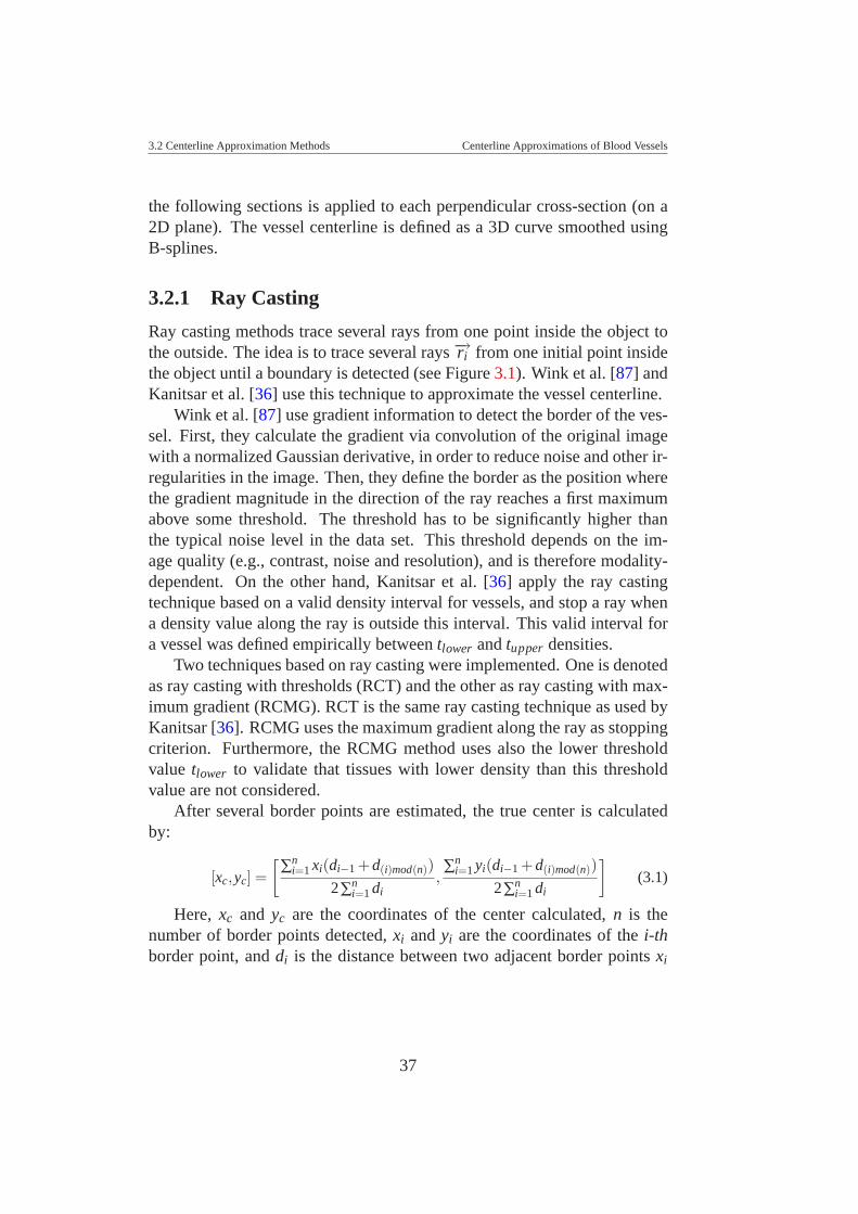
3.2 Centerline Approximation Methods Centerline Approximations of Blood Vessels
the following sections is applied to each perpendicular cross-section (on a2D plane). The vessel centerline is defined as a 3D curve smoothed usingB-splines.
3.2.1 Ray Casting
Ray casting methods trace several rays from one point inside the object tothe outside. The idea is to trace several rays −→ri from one initial point insidethe object until a boundary is detected (see Figure 3.1). Wink et al. [87] andKanitsar et al. [36] use this technique to approximate the vessel centerline.
Wink et al. [87] use gradient information to detect the border of the ves-sel. First, they calculate the gradient via convolution of the original imagewith a normalized Gaussian derivative, in order to reduce noise and other ir-regularities in the image. Then, they define the border as the position wherethe gradient magnitude in the direction of the ray reaches a first maximumabove some threshold. The threshold has to be significantly higher thanthe typical noise level in the data set. This threshold depends on the im-age quality (e.g., contrast, noise and resolution), and is therefore modality-dependent. On the other hand, Kanitsar et al. [36] apply the ray castingtechnique based on a valid density interval for vessels, and stop a ray whena density value along the ray is outside this interval. This valid interval fora vessel was defined empirically between tlower and tupper densities.
Two techniques based on ray casting were implemented. One is denotedas ray casting with thresholds (RCT) and the other as ray casting with max-imum gradient (RCMG). RCT is the same ray casting technique as used byKanitsar [36]. RCMG uses the maximum gradient along the ray as stoppingcriterion. Furthermore, the RCMG method uses also the lower thresholdvalue tlower to validate that tissues with lower density than this thresholdvalue are not considered.
After several border points are estimated, the true center is calculatedby:
[xc,yc] =[
∑ni=1 xi(di−1 +d(i)mod(n))
2∑ni=1 di
,∑n
i=1 yi(di−1 +d(i)mod(n))2∑n
i=1 di
](3.1)
Here, xc and yc are the coordinates of the center calculated, n is thenumber of border points detected, xi and yi are the coordinates of the i-thborder point, and di is the distance between two adjacent border points xi
37
3.2 Centerline Approximation Methods Centerline Approximations of Blood Vessels
Figure 3.1: Example of the ray casting method
and xi+1. The function mod is used due to the circular connection betweensuccessive border points.
3.2.2 Block Matching
The Block Matching (BM) technique is used for motion estimation betweensuccessive frames in video compression. More details are described in [14].We assume that two 2D images are related by a simple shift determined byxd and yd . These values are estimated by minimizing the magnitude of thedifference between shifted states of the two images as:
[xd,yd] = minx′d ,y′d ∑i, j
[f2D(i+ x′d, j + y′d,1)− f2D(i, j,0)
]2, (3.2)
where x′d and y′d are the displacements of pixels in image space. Then, thenew center would be:
[xc,yc] = [x′c + xd,y′c + yd] (3.3)
where x′c and y′c are the initial center location of the vessel cross-section.This method is applied incrementally for pairs of successive cross-
sections of the initial vessel path. It looks for the best matching between twovessel cross-sections by applying a shift on the original cross-section. Theconsecutive cross-section is shifted to several new positions and matchedwith the previous cross-section. The best match result is selected as centerof the vessel in consecutive cross-sections.
38
3.2 Centerline Approximation Methods Centerline Approximations of Blood Vessels
3.2.3 Center Of Gravity
The weighted center of gravity (CoG) has been used widely for estimationof object centers in gray level images with sub-pixel precision [81]. Thecenter of gravity can be defined as the equilibrium point where the entireweight of the object is concentrated. For a 2D gray level image the centerof gravity is defined in [81] as:
[xc,yc] =(
∑x,y∈Ω xw(x,y)∑x,y∈Ω w(x,y)
,∑x,y∈Ω yw(x,y)∑x,y∈Ω w(x,y)
), (3.4)
where Ω defines the area containing pixels that belong to the vessel. w(x,y)is the weight for each coordinate in the Ω space, and can be defined as:
w(x,y) = f2D(x,y)−m (3.5)
and,
m = minx,y∈Ω( f2D(x,y)) (3.6)
The function f2D(x,y) corresponds to the density value of a pixel (x,y)in the perpendicular 2D cross-section.
The threshold values tlower and tupper defined for the RCT technique,were used also in this method to determine those points which belong withhigh probability to the blood vessel. Considering only those pixels whosedensity value are between those lower and upper threshold values.
3.2.4 Ellipse Fitting
Blood vessels have a tubular structure, which can be defined by a set ofelliptical shapes along its axis. Therefore, an approximation of the center-line of the vessel can be estimated as the center of an elliptical shape movedalong its axis. This technique is denoted as ellipse fitting (EF). Starting fromthe initial path obtained via vessel tracking, the Canny edge detector [9] isapplied in order to get a set of points around the vessel boundary. Then,these points are approximated with an ellipse using the Lagrange multipliertechnique. The problem can be described as:
Given:
• A set of 2D Points P = {xi}ni=1, where xi = (xi,yi)
39
3.2 Centerline Approximation Methods Centerline Approximations of Blood Vessels
• A curve C(a) characterized by the vector a. Where C(a) ={x|F(a,x) = 0}, in our case F(a,x) is the representation of generalconic curves which is given by:
F(a,xi) = ax2i +bxiyi + cy2
i +dxi + eyi + f
=[x2
i ,xiyi,y2i ,xi,yi,1
][a,b,c,d,e, f ]T , (3.7)
with a = [a,b,c,d,e, f ] and xi = [x2i ,xiyi,y2
i ,xi,yi,1]
• A distance metric δ (C(a),x) as a measure of the distance from a pointx to the curve C(a), which is defined by F(a,xi)2.
The problem consists of minimizing the sum of squared algebraic dis-tances ∑n
i=1 F(a,xi)2 that fit an ellipse. For ellipse they must satisfyb2 − 4ac < 0. After this optimization problem is solved [19], the ellipsecenter and axis can be extracted using Equation (3.7).
3.2.5 Randomized Hough Transform
The randomized Hough Transform (RHT) technique introduced by Xu etal. [89] consists of randomly selecting a subset of points from an image andfitting a parameterized curve to them.
First, the Canny edge detector is applied [9] in order to get a binaryedge image. Then, parametric ellipses are extracted using the technique de-fined by MacLaughlin [50]. He describes a method to accelerate the ellipsedetection in an image using the RHT. This technique consists of randomlyselecting three points (P1, P2, P3) from the binary edge image, and definingthe ellipse that passes through these points (see Figure 3.2). For each pointPi the tangent to the curve is estimated, selecting a neighborhood aroundthis point and finding the line of best least-squares fitting to the curve inthis neighborhood. The mid point m between P1 and P2 is calculated, andconnected with the intersection point t between the tangents of these points(see Figure 3.2(a)). The possible center of the ellipse will lie in the line de-fined by −→tm. The process is repeated with the points P2 and P3, which definea second line. The intersection of these two lines will be the center of theellipse.
40
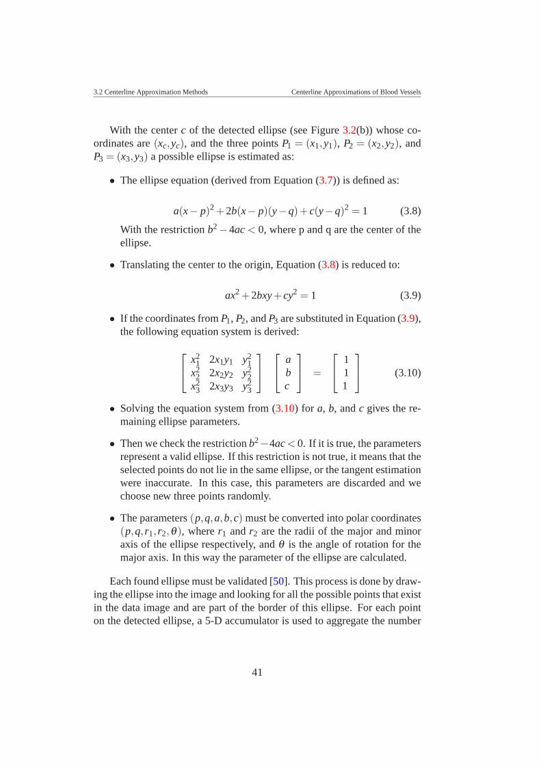
3.2 Centerline Approximation Methods Centerline Approximations of Blood Vessels
With the center c of the detected ellipse (see Figure 3.2(b)) whose co-ordinates are (xc,yc), and the three points P1 = (x1,y1), P2 = (x2,y2), andP3 = (x3,y3) a possible ellipse is estimated as:
• The ellipse equation (derived from Equation (3.7)) is defined as:
a(x− p)2 +2b(x− p)(y−q)+ c(y−q)2 = 1 (3.8)
With the restriction b2 −4ac < 0, where p and q are the center of theellipse.
• Translating the center to the origin, Equation (3.8) is reduced to:
ax2 +2bxy+ cy2 = 1 (3.9)
• If the coordinates from P1, P2, and P3 are substituted in Equation (3.9),the following equation system is derived:
⎡⎣ x2
1 2x1y1 y21
x22 2x2y2 y2
2x2
3 2x3y3 y23
⎤⎦
⎡⎣ a
bc
⎤⎦ =
⎡⎣ 1
11
⎤⎦ (3.10)
• Solving the equation system from (3.10) for a, b, and c gives the re-maining ellipse parameters.
• Then we check the restriction b2−4ac < 0. If it is true, the parametersrepresent a valid ellipse. If this restriction is not true, it means that theselected points do not lie in the same ellipse, or the tangent estimationwere inaccurate. In this case, this parameters are discarded and wechoose new three points randomly.
• The parameters (p,q,a,b,c) must be converted into polar coordinates(p,q,r1,r2,θ), where r1 and r2 are the radii of the major and minoraxis of the ellipse respectively, and θ is the angle of rotation for themajor axis. In this way the parameter of the ellipse are calculated.
Each found ellipse must be validated [50]. This process is done by draw-ing the ellipse into the image and looking for all the possible points that existin the data image and are part of the border of this ellipse. For each pointon the detected ellipse, a 5-D accumulator is used to aggregate the number
41
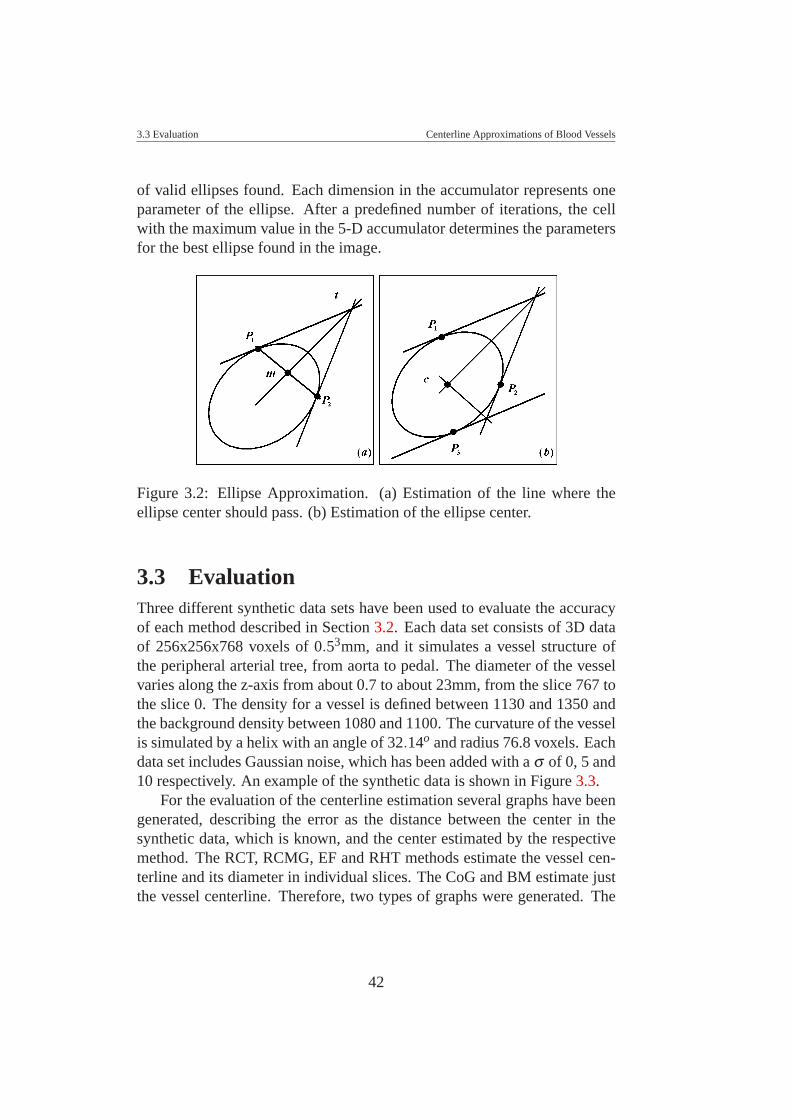
3.3 Evaluation Centerline Approximations of Blood Vessels
of valid ellipses found. Each dimension in the accumulator represents oneparameter of the ellipse. After a predefined number of iterations, the cellwith the maximum value in the 5-D accumulator determines the parametersfor the best ellipse found in the image.
Figure 3.2: Ellipse Approximation. (a) Estimation of the line where theellipse center should pass. (b) Estimation of the ellipse center.
3.3 EvaluationThree different synthetic data sets have been used to evaluate the accuracyof each method described in Section 3.2. Each data set consists of 3D dataof 256x256x768 voxels of 0.53mm, and it simulates a vessel structure ofthe peripheral arterial tree, from aorta to pedal. The diameter of the vesselvaries along the z-axis from about 0.7 to about 23mm, from the slice 767 tothe slice 0. The density for a vessel is defined between 1130 and 1350 andthe background density between 1080 and 1100. The curvature of the vesselis simulated by a helix with an angle of 32.14o and radius 76.8 voxels. Eachdata set includes Gaussian noise, which has been added with a σ of 0, 5 and10 respectively. An example of the synthetic data is shown in Figure 3.3.
For the evaluation of the centerline estimation several graphs have beengenerated, describing the error as the distance between the center in thesynthetic data, which is known, and the center estimated by the respectivemethod. The RCT, RCMG, EF and RHT methods estimate the vessel cen-terline and its diameter in individual slices. The CoG and BM estimate justthe vessel centerline. Therefore, two types of graphs were generated. The
42
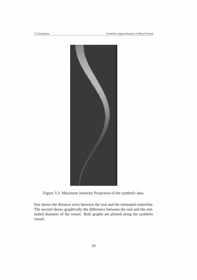
3.3 Evaluation Centerline Approximations of Blood Vessels
Figure 3.3: Maximum Intensity Projection of the synthetic data.
first shows the distance error between the real and the estimated centerline.The second shows graphically the difference between the real and the esti-mated diameter of the vessel. Both graphs are plotted along the syntheticvessel.
43
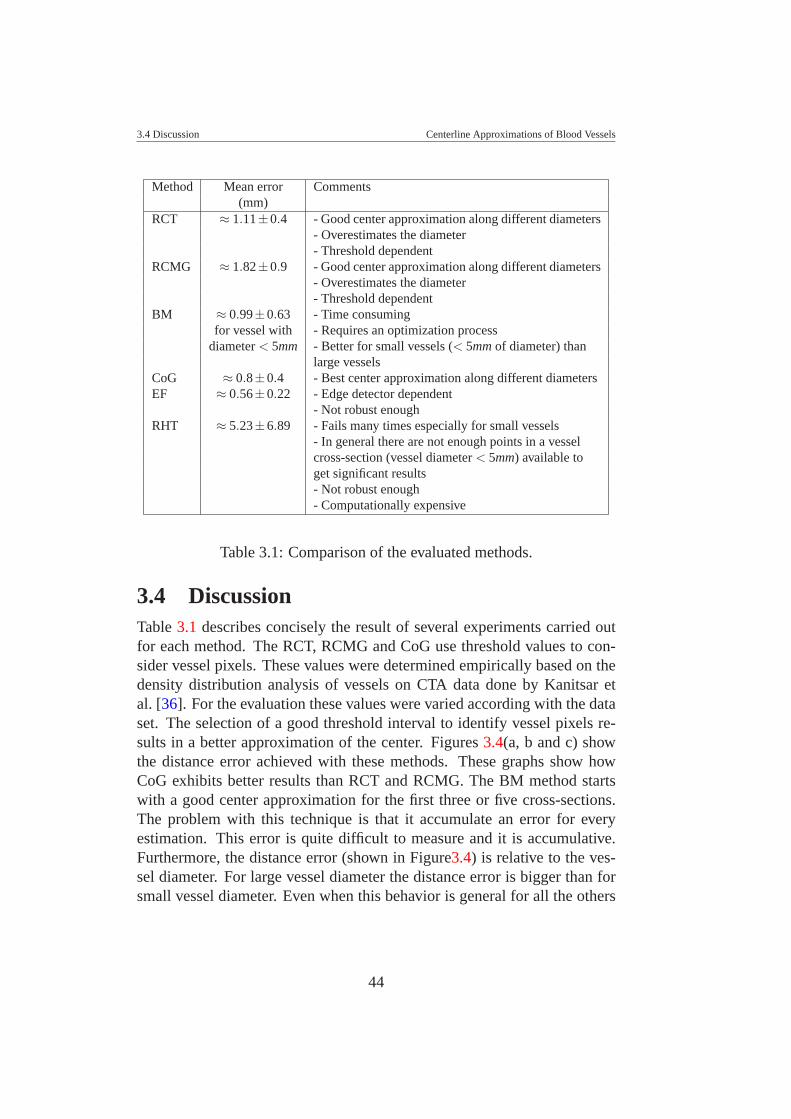
3.4 Discussion Centerline Approximations of Blood Vessels
Method Mean error Comments(mm)
RCT ≈ 1.11±0.4 - Good center approximation along different diameters- Overestimates the diameter- Threshold dependent
RCMG ≈ 1.82±0.9 - Good center approximation along different diameters- Overestimates the diameter- Threshold dependent
BM ≈ 0.99±0.63 - Time consumingfor vessel with - Requires an optimization process
diameter < 5mm - Better for small vessels (< 5mm of diameter) thanlarge vessels
CoG ≈ 0.8±0.4 - Best center approximation along different diametersEF ≈ 0.56±0.22 - Edge detector dependent
- Not robust enoughRHT ≈ 5.23±6.89 - Fails many times especially for small vessels
- In general there are not enough points in a vesselcross-section (vessel diameter < 5mm) available toget significant results- Not robust enough- Computationally expensive
Table 3.1: Comparison of the evaluated methods.
3.4 DiscussionTable 3.1 describes concisely the result of several experiments carried outfor each method. The RCT, RCMG and CoG use threshold values to con-sider vessel pixels. These values were determined empirically based on thedensity distribution analysis of vessels on CTA data done by Kanitsar etal. [36]. For the evaluation these values were varied according with the dataset. The selection of a good threshold interval to identify vessel pixels re-sults in a better approximation of the center. Figures 3.4(a, b and c) showthe distance error achieved with these methods. These graphs show howCoG exhibits better results than RCT and RCMG. The BM method startswith a good center approximation for the first three or five cross-sections.The problem with this technique is that it accumulate an error for everyestimation. This error is quite difficult to measure and it is accumulative.Furthermore, the distance error (shown in Figure3.4) is relative to the ves-sel diameter. For large vessel diameter the distance error is bigger than forsmall vessel diameter. Even when this behavior is general for all the others
44
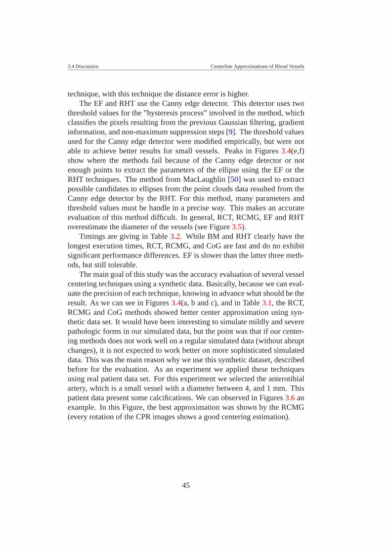
3.4 Discussion Centerline Approximations of Blood Vessels
technique, with this technique the distance error is higher.The EF and RHT use the Canny edge detector. This detector uses two
threshold values for the ”hysteresis process” involved in the method, whichclassifies the pixels resulting from the previous Gaussian filtering, gradientinformation, and non-maximum suppression steps [9]. The threshold valuesused for the Canny edge detector were modified empirically, but were notable to achieve better results for small vessels. Peaks in Figures 3.4(e,f)show where the methods fail because of the Canny edge detector or notenough points to extract the parameters of the ellipse using the EF or theRHT techniques. The method from MacLaughlin [50] was used to extractpossible candidates to ellipses from the point clouds data resulted from theCanny edge detector by the RHT. For this method, many parameters andthreshold values must be handle in a precise way. This makes an accurateevaluation of this method difficult. In general, RCT, RCMG, EF and RHToverestimate the diameter of the vessels (see Figure 3.5).
Timings are giving in Table 3.2. While BM and RHT clearly have thelongest execution times, RCT, RCMG, and CoG are fast and do no exhibitsignificant performance differences. EF is slower than the latter three meth-ods, but still tolerable.
The main goal of this study was the accuracy evaluation of several vesselcentering techniques using a synthetic data. Basically, because we can eval-uate the precision of each technique, knowing in advance what should be theresult. As we can see in Figures 3.4(a, b and c), and in Table 3.1, the RCT,RCMG and CoG methods showed better center approximation using syn-thetic data set. It would have been interesting to simulate mildly and severepathologic forms in our simulated data, but the point was that if our center-ing methods does not work well on a regular simulated data (without abruptchanges), it is not expected to work better on more sophisticated simulateddata. This was the main reason why we use this synthetic dataset, describedbefore for the evaluation. As an experiment we applied these techniquesusing real patient data set. For this experiment we selected the anterotibialartery, which is a small vessel with a diameter between 4, and 1 mm. Thispatient data present some calcifications. We can observed in Figures 3.6 anexample. In this Figure, the best approximation was shown by the RCMG(every rotation of the CPR images shows a good centering estimation).
45
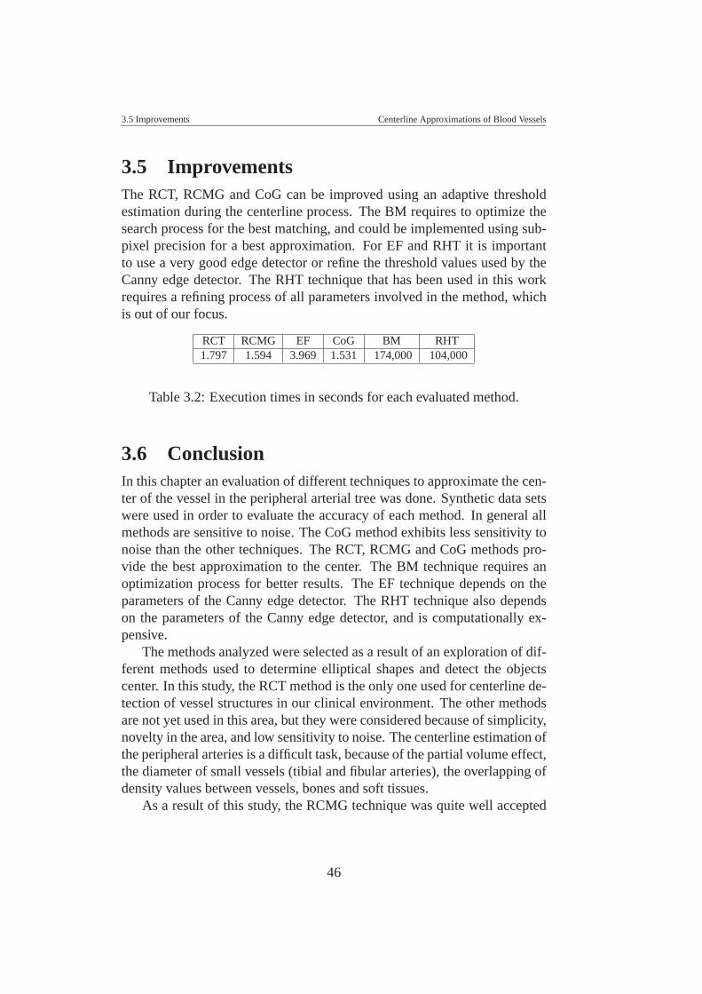
3.5 Improvements Centerline Approximations of Blood Vessels
3.5 ImprovementsThe RCT, RCMG and CoG can be improved using an adaptive thresholdestimation during the centerline process. The BM requires to optimize thesearch process for the best matching, and could be implemented using sub-pixel precision for a best approximation. For EF and RHT it is importantto use a very good edge detector or refine the threshold values used by theCanny edge detector. The RHT technique that has been used in this workrequires a refining process of all parameters involved in the method, whichis out of our focus.
RCT RCMG EF CoG BM RHT1.797 1.594 3.969 1.531 174,000 104,000
Table 3.2: Execution times in seconds for each evaluated method.
3.6 ConclusionIn this chapter an evaluation of different techniques to approximate the cen-ter of the vessel in the peripheral arterial tree was done. Synthetic data setswere used in order to evaluate the accuracy of each method. In general allmethods are sensitive to noise. The CoG method exhibits less sensitivity tonoise than the other techniques. The RCT, RCMG and CoG methods pro-vide the best approximation to the center. The BM technique requires anoptimization process for better results. The EF technique depends on theparameters of the Canny edge detector. The RHT technique also dependson the parameters of the Canny edge detector, and is computationally ex-pensive.
The methods analyzed were selected as a result of an exploration of dif-ferent methods used to determine elliptical shapes and detect the objectscenter. In this study, the RCT method is the only one used for centerline de-tection of vessel structures in our clinical environment. The other methodsare not yet used in this area, but they were considered because of simplicity,novelty in the area, and low sensitivity to noise. The centerline estimation ofthe peripheral arteries is a difficult task, because of the partial volume effect,the diameter of small vessels (tibial and fibular arteries), the overlapping ofdensity values between vessels, bones and soft tissues.
As a result of this study, the RCMG technique was quite well accepted
46
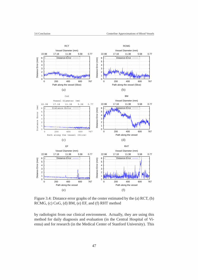
3.6 Conclusion Centerline Approximations of Blood Vessels
0
1
2
3
4
5
6
767 600 400 200 0
0.77 5.58 11.38 17.18 22.98
Dis
tanc
e E
rror
(m
m)
Path along the vessel (Slice)
RCT
Vessel Diameter (mm)
Distance-Error
(a)
0
1
2
3
4
5
6
767 600 400 200 0
0.77 5.58 11.38 17.18 22.98
Dis
tanc
e E
rror
(m
m)
Path along the vessel (Slice)
RCMG
Vessel Diameter (mm)
Distance-Error
(b)
0
1
2
3
4
5
6
767 600 400 200 0
0.77 5.58 11.38 17.18 22.98
Distance Error (mm)
Path along the vessel (Slice)
CoG
Vessel Diameter (mm)
Distance-Error
(c)
0
1
2
3
4
5
6
767 600 400 200 0
0.77 5.58 11.38 17.18 22.98
Dis
tanc
e E
rror
(m
m)
Path along the vessel
BM
Vessel Diameter (mm)
Distance-Error
(d)
0
1
2
3
4
5
6
767 600 400 200 0
0.77 5.58 11.38 17.18 22.98
Dis
tanc
e E
rror
(m
m)
Path along the vessel
EF
Vessel Diameter (mm)
Distance-Error
(e)
0
1
2
3
4
5
6
767 600 400 200 0
0.77 5.58 11.38 17.18 22.98
Dis
tanc
e E
rror
(m
m)
Path along the vessel
RHT
Vessel Diameter (mm)
Distance-Error
(f)
Figure 3.4: Distance error graphs of the center estimated by the (a) RCT, (b)RCMG, (c) CoG, (d) BM, (e) EF, and (f) RHT method
by radiologist from our clinical environment. Actually, they are using thismethod for daily diagnosis and evaluation (in the Central Hospital of Vi-enna) and for research (in the Medical Center of Stanford University). This
47
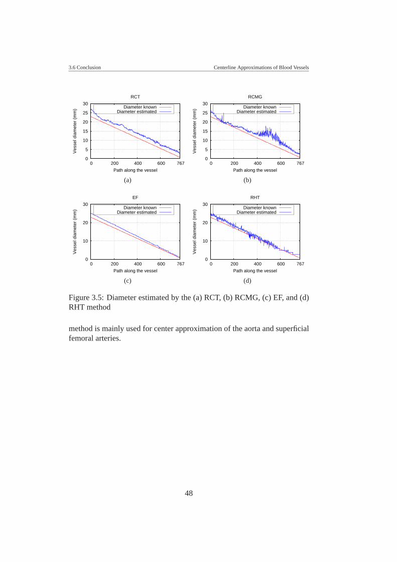
3.6 Conclusion Centerline Approximations of Blood Vessels
0
5
10
15
20
25
30
767 600 400 200 0
Ves
sel d
iam
eter
(m
m)
Path along the vessel
RCT
Diameter knownDiameter estimated
(a)
0
5
10
15
20
25
30
767 600 400 200 0
Ves
sel d
iam
eter
(m
m)
Path along the vessel
RCMG
Diameter knownDiameter estimated
(b)
0
10
20
30
767 600 400 200 0
Ves
sel d
iam
eter
(m
m)
Path along the vessel
EF
Diameter knownDiameter estimated
(c)
0
10
20
30
767 600 400 200 0
Ves
sel d
iam
eter
(m
m)
Path along the vessel
RHT
Diameter knownDiameter estimated
(d)
Figure 3.5: Diameter estimated by the (a) RCT, (b) RCMG, (c) EF, and (d)RHT method
method is mainly used for center approximation of the aorta and superficialfemoral arteries.
48
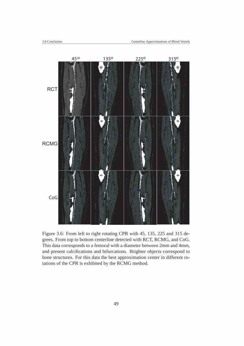
3.6 Conclusion Centerline Approximations of Blood Vessels
45o 135o 225o 315o
RCT
RCMG
CoG
Figure 3.6: From left to right rotating CPR with 45, 135, 225 and 315 de-grees. From top to bottom centerline detected with RCT, RCMG, and CoG.This data corresponds to a femoral with a diameter between 2mm and 4mm,and present calcifications and bifurcations. Brighter objects correspond tobone structures. For this data the best approximation center in different ro-tations of the CPR is exhibited by the RCMG method.
49
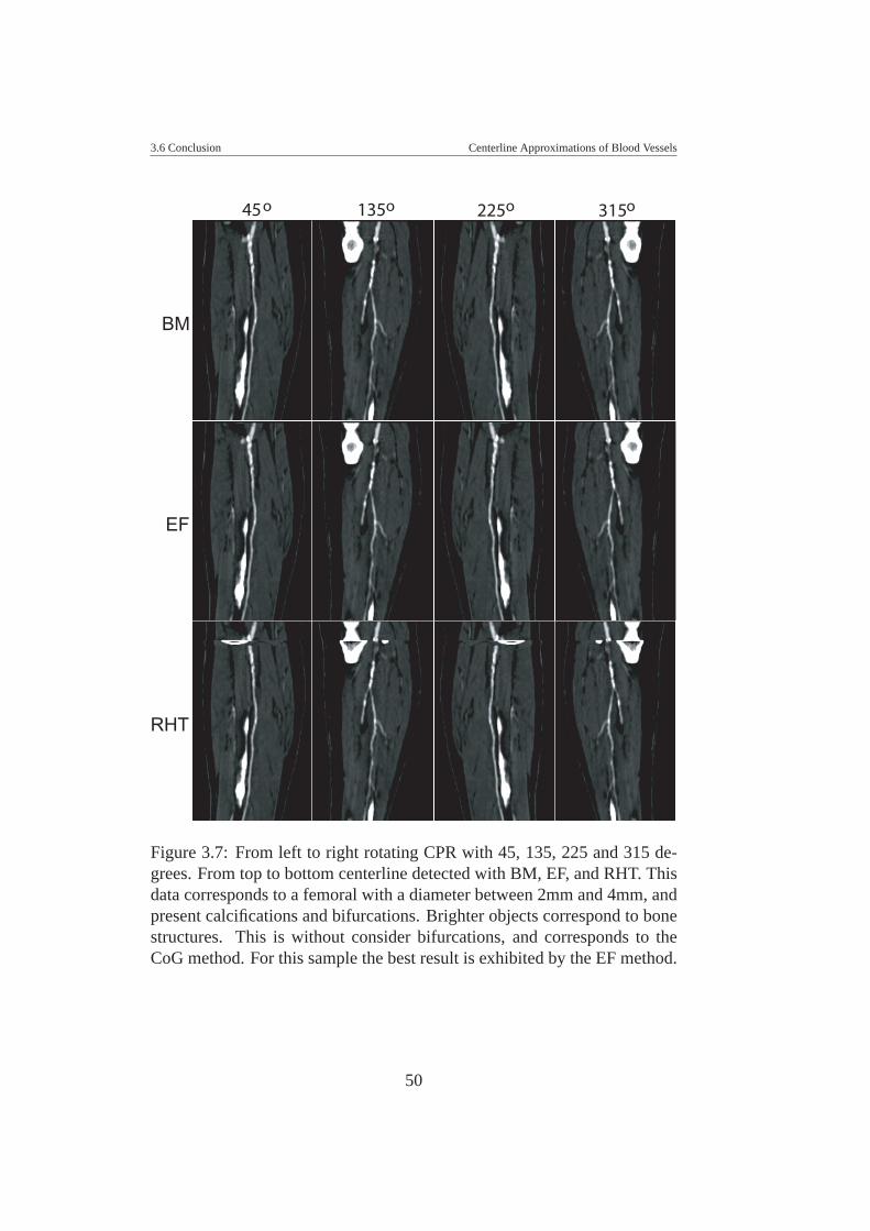
3.6 Conclusion Centerline Approximations of Blood Vessels
BM
RHT
EF
45o 135o 225o 315o
Figure 3.7: From left to right rotating CPR with 45, 135, 225 and 315 de-grees. From top to bottom centerline detected with BM, EF, and RHT. Thisdata corresponds to a femoral with a diameter between 2mm and 4mm, andpresent calcifications and bifurcations. Brighter objects correspond to bonestructures. This is without consider bifurcations, and corresponds to theCoG method. For this sample the best result is exhibited by the EF method.
50
CHAPTER 4
VESSEL MODEL FITTING
This chapter is based on the following publications:
La Cruz A., Straka M., Kochl A., Sramek M., Groller E., Fleischmann D.:Non-linear Model Fitting to Parameterize Diseased Blood Vessels. In pro-ceedings of IEEE Visualization 2004, Austin, USA. 10-15 October. pp. 393-400.
La Cruz A., Straka M., Kochl A., Sramek M., Groller E., Fleischmann D.:Non-linear Model Fitting to Parameterize Diseased Blood Vessels. Tech-nical Report TR-186-2-04-05, Institute of Computer Graphics and Algo-rithms, Vienna University of Technology. May 2004.
4.1 IntroductionThe most characteristic feature of an artery (healthy or diseased) is its cylin-drical or tubular shape. A cylindrical or tubular shape can be modeled aselliptical or circular cross-sections along its medial axis, and can then befitted to a candidate vascular structure. As a result of the estimated vesseldiameter and density, a more robust extraction of the vessel centerline is ex-pected, even in the presence of atherosclerotic disease. We are particularlyinterested in finding a model that best fits the data concerning tubular shapeand mean density value.
In this chapter, we present two new strategies to estimate vessel parame-ters from an initial vessel model using a non-linear minimization process.The first strategy attempts to fit an elliptical cross-section model to the ves-
51
4.2 Motivation Vessel Model Fitting
sel. The second strategy uses a 3D cylindrical model of the vessel to fit itto the data. This approach was presented to the visualization community in2004 [46], and this chapter is based mainly on this publication.
This chapter is divided into five sections. Section 4.2 describes the mainmotivation of this work and the importance of extracting a better parameter-ization of diseased blood vessels. Section 4.3 presents the non-linear modelfitting technique using an elliptical cross-section (in 2D) and a cylindricalshape (in 3D). In Section 4.4 we present and discuss our results and finally,in Section 4.5 draw the conclusions of this work.
4.2 MotivationAutomatic segmentation and accurate centerline identification of diseasedarteries certainly is a challenge. We are currently using a density and gradi-ent based vessel tracking and centering technique to process clinical casesof patients with PAOD [37]. In patients with extensive disease, substantialexpert user interaction and manual corrections are necessary to bridge thesegments where standard segmentation fails. Figure 4.1 is an illustrationof extensively diseased vessel territories where expert user interaction wasrequired to generate images of adequate diagnostic quality. In this case, atechnique capable of identifying the vessel by its cylindrical or tubular shapemight have produced a similar or better result in determining the centerline.This would improve the visualization technique actually used in the clini-cal environment, which is mostly Curved Planar Reformation (CPR) and itsextensions [37].
4.3 Non-Linear Model FittingIn this chapter, we present two different vessel models. An elliptical modelin 2D (M2D) and a cylindrical model in 3D (M3D). Each model has a setof unknown parameters, which are estimated by minimization of a χ2-basedmerit function. Both methods require an initial estimation of the parameters.They can either be obtained from the initial path defined by vessel tracking,or from the previous slices, which requires only an initial seed point.
We represent the vessel by a 2D (ellipse in a slice) or 3D (cylinder)implicit model f . The CT-scanner, due to finite dimensions of its detectors,blurs the data, which leads to partial volume effects (PVE) [82]. This can bemodeled by a non ideal point spread function (PSF) of the scanner, which we
52
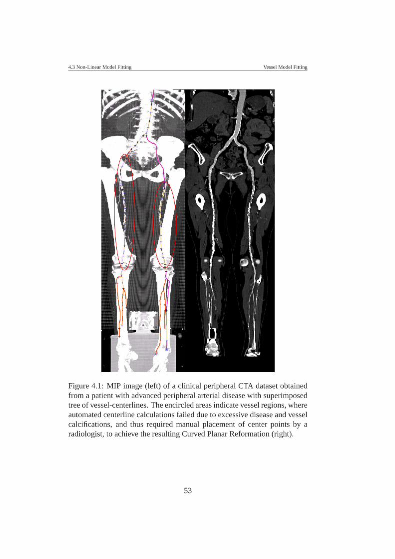
4.3 Non-Linear Model Fitting Vessel Model Fitting
Figure 4.1: MIP image (left) of a clinical peripheral CTA dataset obtainedfrom a patient with advanced peripheral arterial disease with superimposedtree of vessel-centerlines. The encircled areas indicate vessel regions, whereautomated centerline calculations failed due to excessive disease and vesselcalcifications, and thus required manual placement of center points by aradiologist, to achieve the resulting Curved Planar Reformation (right).
53
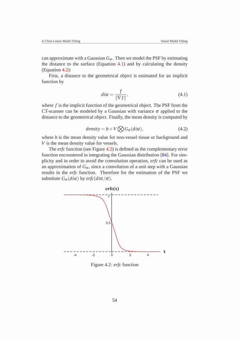
4.3 Non-Linear Model Fitting Vessel Model Fitting
can approximate with a Gaussian Gσ . Then we model the PSF by estimatingthe distance to the surface (Equation 4.1) and by calculating the density(Equation 4.2):
First, a distance to the geometrical object is estimated for an implicitfunction by
dist =f
‖∇ f‖ , (4.1)
where f is the implicit function of the geometrical object. The PSF from theCT-scanner can be modeled by a Gaussian with variance σ applied to thedistance to the geometrical object. Finally, the mean density is computed by
density = b+V⊗
Gσ (dist), (4.2)
where b is the mean density value for non-vessel tissue or background andV is the mean density value for vessels.
The erfc function (see Figure 4.2) is defined as the complementary errorfunction encountered in integrating the Gaussian distribution [84]. For sim-plicity and in order to avoid the convolution operation, erfc can be used asan approximation of Gσ , since a convolution of a unit step with a Gaussianresults in the erfc function. Therefore for the estimation of the PSF wesubstitute Gσ (dist) by erfc(dist/σ).
1
0
0.5
2 4
x
erfc(x)
-2-4
Figure 4.2: erfc function
54
4.3 Non-Linear Model Fitting Vessel Model Fitting
4.3.1 Elliptical Cross-section Model of a Vessel
An elliptical cross-section of a vessel is modeled using the following para-meters:
• Center of the ellipse, given by (x0,y0)
• Radius dimensions, given by (rx,ry)
• Rotation angle, given by α
• Gaussian filter with parameter σ to model the PSF from the CT-scanner using the erfc function
• Mean density value V for a vessel structure
• Mean density value b for background
For a general ellipse with a rotation parameter α , its implicit function isgiven by:
f (x,y) =[(x− x0)cos(α)− (y− y0)sin(α)]2
r2x
+
[(x− x0)sin(α)+(y− y0)cos(α)]2
r2y
−1 (4.3)
4.3.2 Cylindrical 3D Model of a Vessel
The cylindrical 3D model is created using the following parameters:
• Center of the cylinder, given by (x0,y0,z0)
• Radius dimensions of the cross-section for the cylinder, given by(rx,ry)
• Rotation angles around the x and y axes, given by α and β
• Gaussian filter with parameter σ to model the PSF from the CT-scanner using the erfc function
• Mean density value V for a vessel structure
55
4.3 Non-Linear Model Fitting Vessel Model Fitting
• Mean density value b for background
We assume a cylinder along the z-axis rotated with respect to the xaxis by α , and with respect to the y axis by β . The cylinder is centeredat (x0,y0,z0) (see Figure 4.3). A general elliptic cylinder can be modeled bythe implicit function as given by Equation (4.4):
f (x,y,z) =[(x− x0)cos(β )+(y− y0)sin(α)sin(β )+(z− z0)cos(α)sin(β )]2
r2x
+
[(y− y0)cos(α)− (z− z0)sin(α)]2
r2y
−1 (4.4)
Figure 4.4 illustrates the data generated by a cylindrical 3D model. Wecreate a set of slices with elliptical cross-sections along the z-axis. Thismodel is modulated by its parameters until it fits the data.
4.3.3 Levenberg-Marquardt Method
The Levenberg-Marquardt method [47, 51] is a nonlinear minimizationtechnique. This technique can be used to fit a model to data when it dependsnonlinearly on a set of M unknown parameters ak, k = 1,2, ...,M. The ideaof the Levenberg-Marquardt algorithm is to minimize a merit function χ2
and iteratively determine the best fitting parameters by minimization. Themerit function measures the agreement between the model and the givendata. In a fitting process, the parameters of the model are adjusted to achievea minimum in the merit function. The process is repeated while χ2 de-creases and is stopped when a change in the parameters changes χ2 by anamount << 1, which is not considered statistically significant any more.
Let us assume that we are fitting N data points (xi,yi) i = 1, ...,N, toa model f (x;a) that has M adjustable parameters ak. The model predictsa functional relationship between the measured independent and dependentvariables.
y = f (x;a) (4.5)
The idea is to minimize the merit function χ2 given by:
χ2(a) =N
∑i=1
[yi − f (xi;a)
σi
]2
(4.6)
56
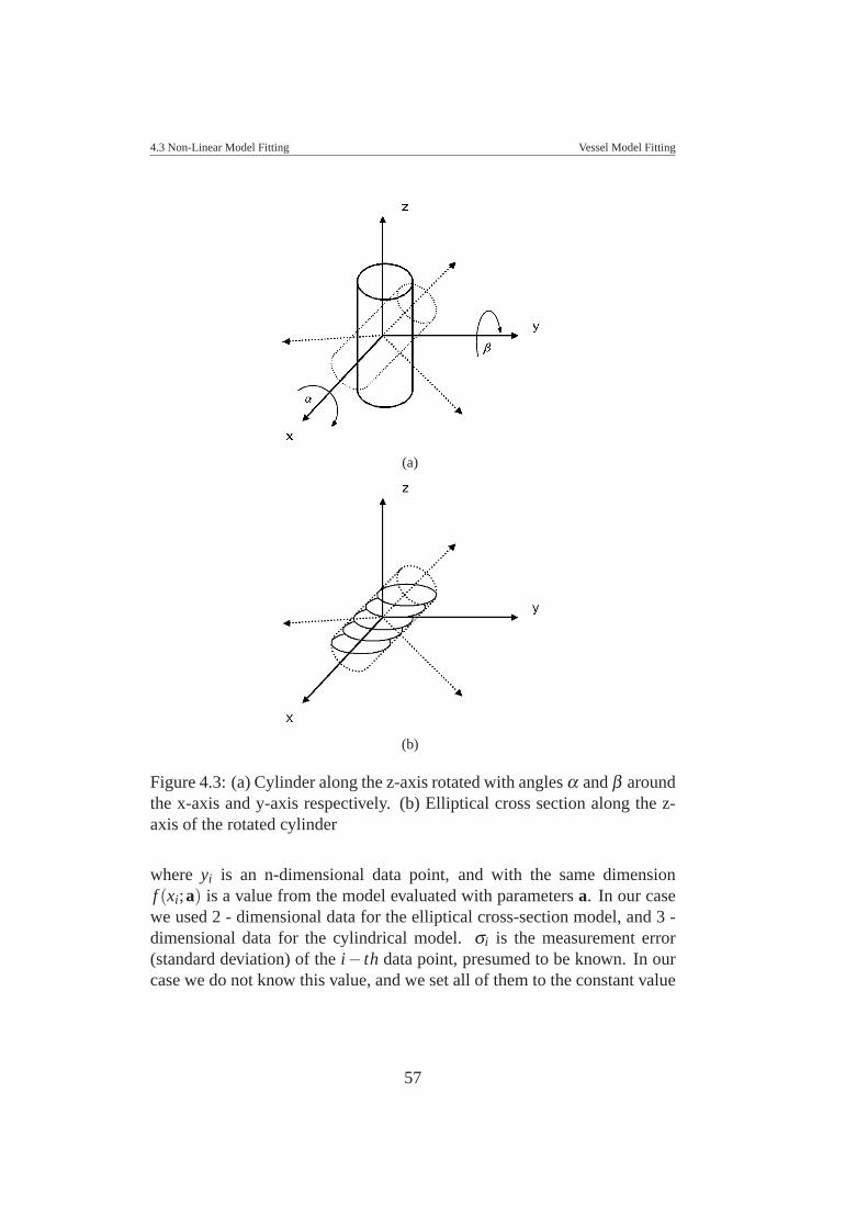
4.3 Non-Linear Model Fitting Vessel Model Fitting
(a)
(b)
Figure 4.3: (a) Cylinder along the z-axis rotated with angles α and β aroundthe x-axis and y-axis respectively. (b) Elliptical cross section along the z-axis of the rotated cylinder
where yi is an n-dimensional data point, and with the same dimensionf (xi;a) is a value from the model evaluated with parameters a. In our casewe used 2 - dimensional data for the elliptical cross-section model, and 3 -dimensional data for the cylindrical model. σi is the measurement error(standard deviation) of the i− th data point, presumed to be known. In ourcase we do not know this value, and we set all of them to the constant value
57
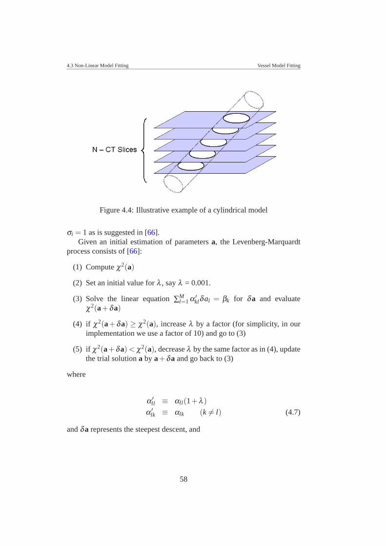
4.3 Non-Linear Model Fitting Vessel Model Fitting
Figure 4.4: Illustrative example of a cylindrical model
σi = 1 as is suggested in [66].Given an initial estimation of parameters a, the Levenberg-Marquardt
process consists of [66]:
(1) Compute χ2(a)
(2) Set an initial value for λ , say λ = 0.001.
(3) Solve the linear equation ∑Ml=1 α ′
klδal = βk for δa and evaluateχ2(a+δa)
(4) if χ2(a+δa) ≥ χ2(a), increase λ by a factor (for simplicity, in ourimplementation we use a factor of 10) and go to (3)
(5) if χ2(a+δa) < χ2(a), decrease λ by the same factor as in (4), updatethe trial solution a by a+δa and go back to (3)
where
α ′ll ≡ αll(1+λ )
α ′lk ≡ αlk (k = l) (4.7)
and δa represents the steepest descent, and
58
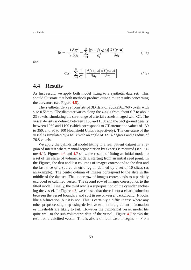
4.4 Results Vessel Model Fitting
βk = −12
δ χ2
δak=
N
∑i=1
[yi − f (xi;a)]σ2
i
∂ f (xi;a)∂ak
(4.8)
and
αkl =N
∑i=1
1
σ2i
[∂ f (xi;a)
∂ai
∂ f (xk;a)∂al
](4.9)
4.4 ResultsAs first result, we apply both model fitting to a synthetic data set. Thisshould illustrate that both methods produce quite similar results concerningthe curvature (see Figure 4.5).
The synthetic data set consists of 3D data of 256x256x768 voxels withsize 0.53mm. The diameter varies along the z-axis from about 0.7 to about23 voxels, simulating the size-range of arterial vessels imaged with CT. Thevessel density is defined between 1130 and 1350 and the background densitybetween 1080 and 1100 (which corresponds to CT attenuation values of 130to 350, and 80 to 100 Hounsfield Units, respectively). The curvature of thevessel is simulated by a helix with an angle of 32.14 degrees and a radius of76.8 voxels.
We apply the cylindrical model fitting to a real patient dataset in a re-gion of interest where manual segmentation by experts is required (see Fig-ure 4.1). Figures 4.6 and 4.7 show the results of fitting an initial model toa set of ten slices of volumetric data, starting from an initial seed point. Inthe Figures, the first and last columns of images correspond to the first andthe last slice of a sub-volumetric region defined by a set of 10 slices (asan example). The center column of images correspond to the slice in themiddle of the dataset. The upper row of images corresponds to a partiallyoccluded or calcified vessel. The second row of images corresponds to thefitted model. Finally, the third row is a superposition of the cylinder enclos-ing the vessel. In Figure 4.6, we can see that there is not a clear distinctionbetween the vessel boundary and soft tissue or vessel background. It lookslike a bifurcation, but it is not. This is certainly a difficult case where anyother preprocessing step using derivative estimation, gradient informationor thresholds are likely to fail. However the cylindrical vessel model fitsquite well to the sub-volumetric data of the vessel. Figure 4.7 shows theresult on a calcified vessel. This is also a difficult case to segment. From
59
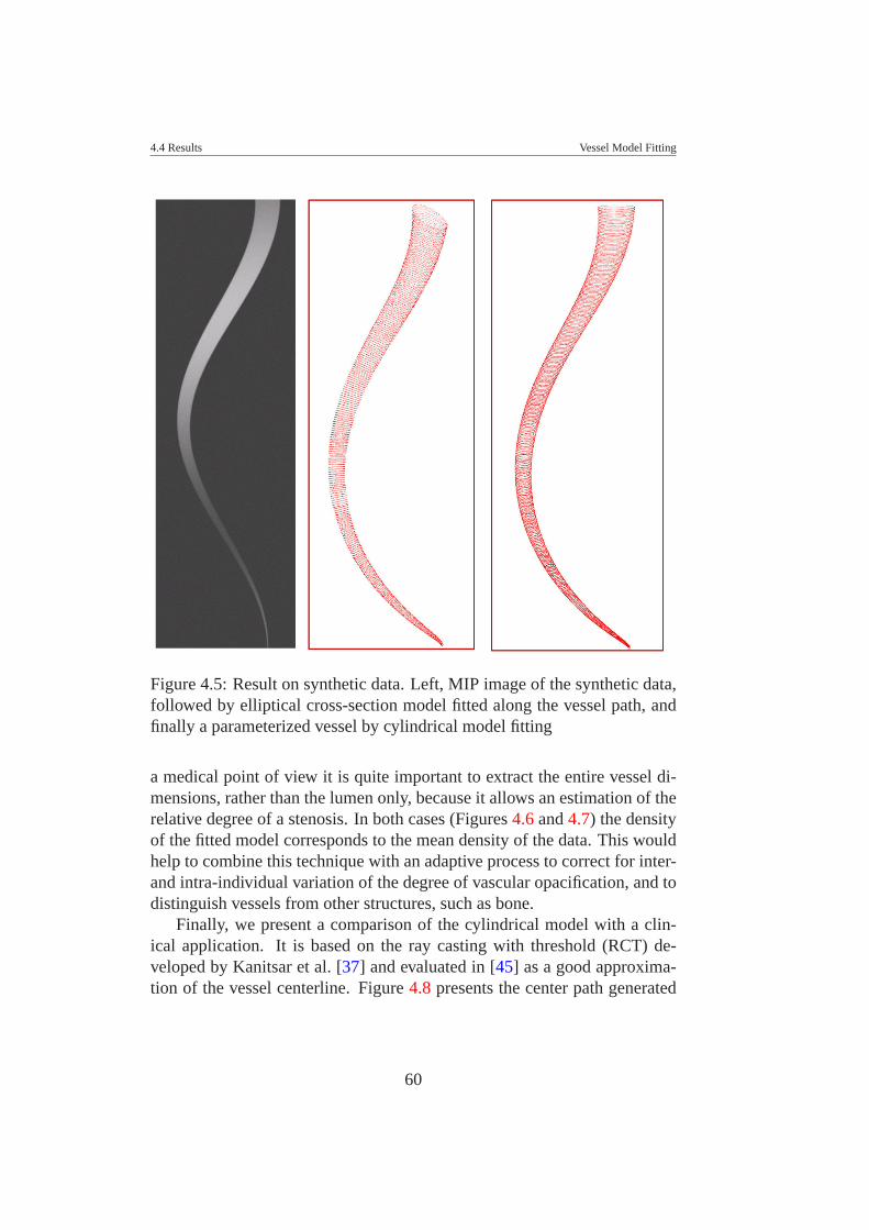
4.4 Results Vessel Model Fitting
Figure 4.5: Result on synthetic data. Left, MIP image of the synthetic data,followed by elliptical cross-section model fitted along the vessel path, andfinally a parameterized vessel by cylindrical model fitting
a medical point of view it is quite important to extract the entire vessel di-mensions, rather than the lumen only, because it allows an estimation of therelative degree of a stenosis. In both cases (Figures 4.6 and 4.7) the densityof the fitted model corresponds to the mean density of the data. This wouldhelp to combine this technique with an adaptive process to correct for inter-and intra-individual variation of the degree of vascular opacification, and todistinguish vessels from other structures, such as bone.
Finally, we present a comparison of the cylindrical model with a clin-ical application. It is based on the ray casting with threshold (RCT) de-veloped by Kanitsar et al. [37] and evaluated in [45] as a good approxima-tion of the vessel centerline. Figure 4.8 presents the center path generated
60
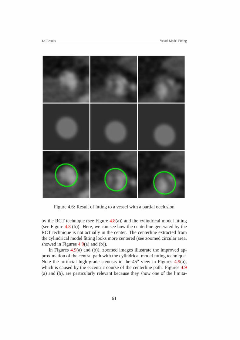
4.4 Results Vessel Model Fitting
Figure 4.6: Result of fitting to a vessel with a partial occlusion
by the RCT technique (see Figure 4.8(a)) and the cylindrical model fitting(see Figure 4.8 (b)). Here, we can see how the centerline generated by theRCT technique is not actually in the center. The centerline extracted fromthe cylindrical model fitting looks more centered (see zoomed circular area,showed in Figures 4.9(a) and (b)).
In Figures 4.9(a) and (b)), zoomed images illustrate the improved ap-proximation of the central path with the cylindrical model fitting technique.Note the artificial high-grade stenosis in the 45o view in Figures 4.9(a),which is caused by the eccentric course of the centerline path. Figures 4.9(a) and (b), are particularly relevant because they show one of the limita-
61
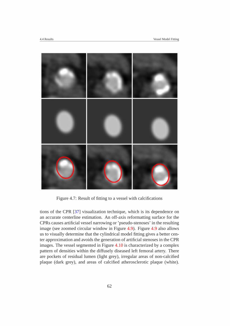
4.4 Results Vessel Model Fitting
Figure 4.7: Result of fitting to a vessel with calcifications
tions of the CPR [37] visualization technique, which is its dependence onan accurate centerline estimation. An off-axis reformatting surface for theCPRs causes artificial vessel narrowing or ’pseudo-stenoses’ in the resultingimage (see zoomed circular window in Figure 4.9). Figure 4.9 also allowsus to visually determine that the cylindrical model fitting gives a better cen-ter approximation and avoids the generation of artificial stenoses in the CPRimages. The vessel segmented in Figure 4.10 is characterized by a complexpattern of densities within the diffusely diseased left femoral artery. Thereare pockets of residual lumen (light grey), irregular areas of non-calcifiedplaque (dark grey), and areas of calcified atherosclerotic plaque (white).
62
4.5 Conclusion Vessel Model Fitting
The centerlines and CPR images from the cylindrical model fitting are moreaccurate than the RCT based results, and compare favorably to those basedon expert user interactions.
Concerning the performance, for a dataset of 512x512x224 voxels, theprocess took about 210 seconds, that means 0.9 seconds per slice. Table 4.1summarizes the advantages and limitations using non-linear model fitting.
Advantages Limitations- It does not use density and any opera- - Requires a definition of initial parame-tor estimation such as gradients or de- ters close to the data. This s done onlyrivatives. for the first slice, the following estima-- It does not require preprocessecing tions are based on previous slices.steps. - It does not work on bifurcations.- It produces very good results on di- - Performance (∼ 0.9 sec/slice).seased vessels.
Table 4.1: Advantages and limitations using the non-linear vessel modelfitting
4.5 ConclusionThis chapter describes a strategy to parameterize a vascular structure froma vessel model by a non-linear fitting process. The Levenberg-Marquardtmethod is used as a non-linear minimization process, which allows to extractoptimal parameters from a model that best fits the data.
In this chapter, we present a segmentation solution for visualization andanalysis purposes in cases where classical segmentation methods based onboundary detection often fail. Diseased vessels show a wide variability ofdensity values, which is a challenge because calcifications appear as bonesand partial occlusion or soft plaque appear as soft tissue. This makes itdifficult to detect the vessel boundaries. The cylindrical 3D model fittingrequires neither a preprocessing step nor any operator estimation, such as,gradients, derivatives, etc.
Results were evaluated just in a qualitative way instead of using also aquantitative analysis. For these reason, a clinical evaluation is required inorder to present a quantitative comparison with the second best centeringtechnique we evaluated in previous chapter. This is the concerning to thenext chapter, where we present a clinical evaluation of the non-linear model
63
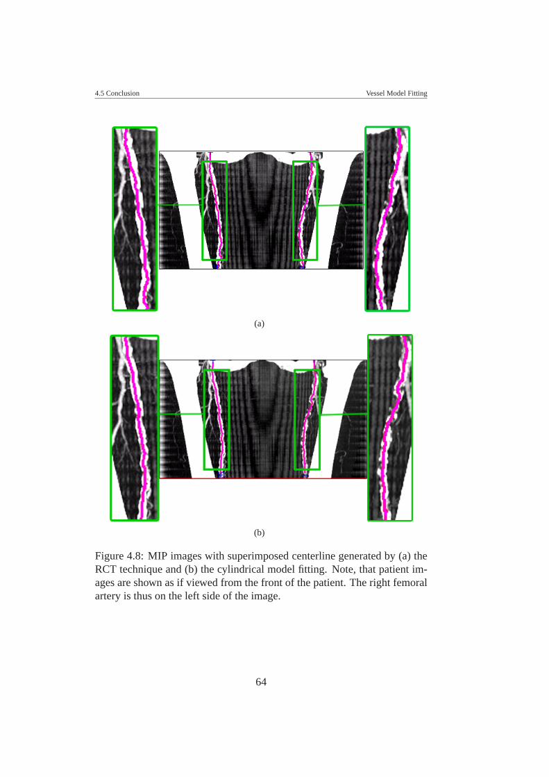
4.5 Conclusion Vessel Model Fitting
(a)
(b)
Figure 4.8: MIP images with superimposed centerline generated by (a) theRCT technique and (b) the cylindrical model fitting. Note, that patient im-ages are shown as if viewed from the front of the patient. The right femoralartery is thus on the left side of the image.
64
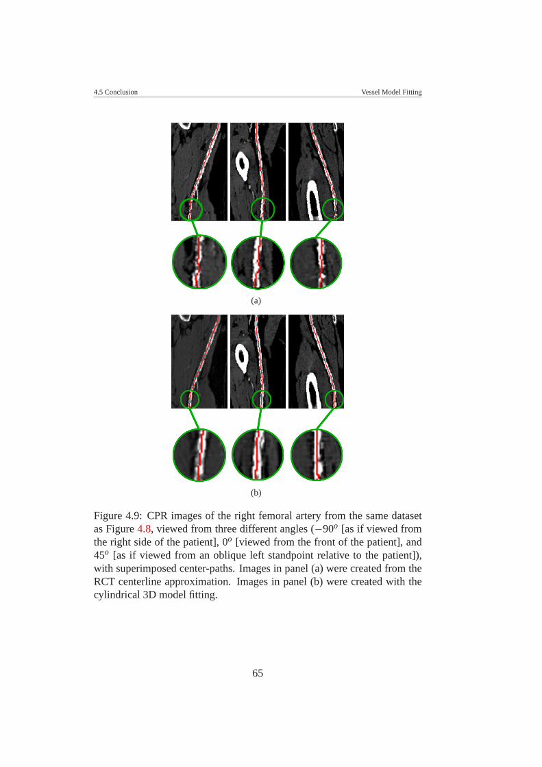
4.5 Conclusion Vessel Model Fitting
(a)
(b)
Figure 4.9: CPR images of the right femoral artery from the same datasetas Figure 4.8, viewed from three different angles (−90o [as if viewed fromthe right side of the patient], 0o [viewed from the front of the patient], and45o [as if viewed from an oblique left standpoint relative to the patient]),with superimposed center-paths. Images in panel (a) were created from theRCT centerline approximation. Images in panel (b) were created with thecylindrical 3D model fitting.
65

4.5 Conclusion Vessel Model Fitting
fitting technique compared to a centering approximation technique actuallyused in a clinical environment for daily patient evaluation.
The cylindrical model fitting can be considered as initial step to imple-ment an automatic segmentation of vascular structures. Future work shouldaddress the following issues: performance, handling of vessel bifurcations,and inclusion of further anatomical knowledge.
66
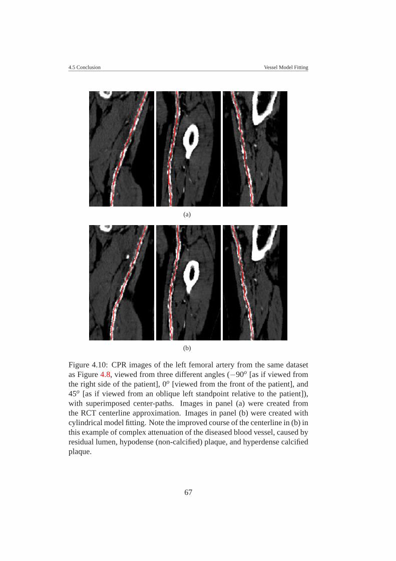
4.5 Conclusion Vessel Model Fitting
(a)
(b)
Figure 4.10: CPR images of the left femoral artery from the same datasetas Figure 4.8, viewed from three different angles (−90o [as if viewed fromthe right side of the patient], 0o [viewed from the front of the patient], and45o [as if viewed from an oblique left standpoint relative to the patient]),with superimposed center-paths. Images in panel (a) were created fromthe RCT centerline approximation. Images in panel (b) were created withcylindrical model fitting. Note the improved course of the centerline in (b) inthis example of complex attenuation of the diseased blood vessel, caused byresidual lumen, hypodense (non-calcified) plaque, and hyperdense calcifiedplaque.
67
CHAPTER 5
CLINICAL EVALUATION OF A
NON-LINEAR MODEL FITTING
TECHNIQUE
5.1 IntroductionAutomated and semi-automated centerline extraction techniques have beensuccessfully employed in the past with excellent results in normal or min-imally diseased vascular segments. But these semi-automatic techniques,which rely on density properties in the data, tend to fail in significantly dis-eased vascular segments. In these cases the density ranges differ substan-tially from normally perfused vessels and overlap widely with neighboringnon-vascular structures such as soft tissues and bone. Newer algorithmshave been investigated and seem to further increase the accuracy of center-line estimations. Among them, a frequently integrated method is the raycasting with threshold technique (RCT) [35]. The RCT technique was eval-uated and compared against other centering methods (see Chapter three).This technique shows a better approximation on synthetic data sets. TheRCT technique is based on threshold values and gradient estimation by trac-ing rays from the vessel center to the vessel border. In the previous chapter(Chapter four), we presented a new approach of an automated centerline ex-traction that uses a non-linear fitting process [46]. The preliminary resultswere very promising, but thorough evaluation needs to be executed beforeputting the proposed technique to clinical usage. The crucial step is there-fore validation and comparison of the proposed technique for a potentialclinical application. The task of a comprehensive validation is rather diffi-
68
5.2 Materials and Methods Clinical Evaluation of a Non-linear Model Fitting Technique
cult in clinical datasets. A major obstacle is the lack of an objective goldstandard. Furthermore, the situation is intricate because of anatomical vari-ability of diseased vessels, the presence of image noise, motion artifacts,metallic implants (i.e. intravascular stents) and possible poor opacificationin ”real life” data sets. The accuracy of a segmentation algorithm is mostcommonly evaluated by comparison with a manual segmentation, as thereis no true gold standard. Ideally, all methods should be evaluated for perfor-mance on data from a realistic phantoms or cadaver studies, but this is notpractical given the wide spectrum clinical disease manifestations.
Thus, the expert manual segmentation is compared with the output ofthe centering method. The main purpose of the study presented in thisChapter, is to present an evaluation of three automatic centerline extrac-tion techniques compared to manually derived centerlines from three expertoperators in order to evaluate each algorithm for precision and robustness inreal peripheral CT-angiography datasets. One of these techniques is actuallyused in daily clinical routine, which is the ray casting with threshold tech-nique (RCT). This technique is described in detail in Chapter three. Theother two techniques are based on non-linear model fitting, already pre-sented in the previous chapter (Chapter four). They are: the elliptical modelin 2D (M2D) and the cylindrical model in 3D (M3D). We are interesting ina comparison of these non-linear techniques using clinical datasets. First, inSection 5.2, we describe the methodology used for the evaluation. In Sec-tion 5.3 we explain how the distances between centerlines are estimated. InSection 5.5 we present results and finally in Sections 5.6 the conclusions forthis chapter are presented.
5.2 Materials and Methods
5.2.1 Vessel Segments
Twenty CT angiography data sets of the lower extremities were identifiedby an expert. Ten of these datasets focused on the iliac vessels and tenon the femoro-popliteal arterial segments. Figure 5.1 shows an exampledataset of peripheral vasculature and the anatomical area of the iliac andfemoro-popliteal segments, respectively. Datasets within every group ofdata (femoro-popliteal and iliac), they were categorized into five ’mildly dis-eased’ and five ’severely diseased’ segments per group, respectively. Thusa total of five ’minimal diseased’ and five ’severely diseased’ iliac arter-
69
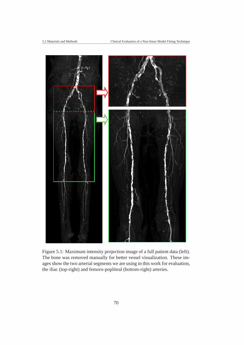
5.2 Materials and Methods Clinical Evaluation of a Non-linear Model Fitting Technique
Figure 5.1: Maximum intensity projection image of a full patient data (left).The bone was removed manually for better vessel visualization. These im-ages show the two arterial segments we are using in this work for evaluation,the iliac (top-right) and femoro-popliteal (bottom-right) arteries.
70
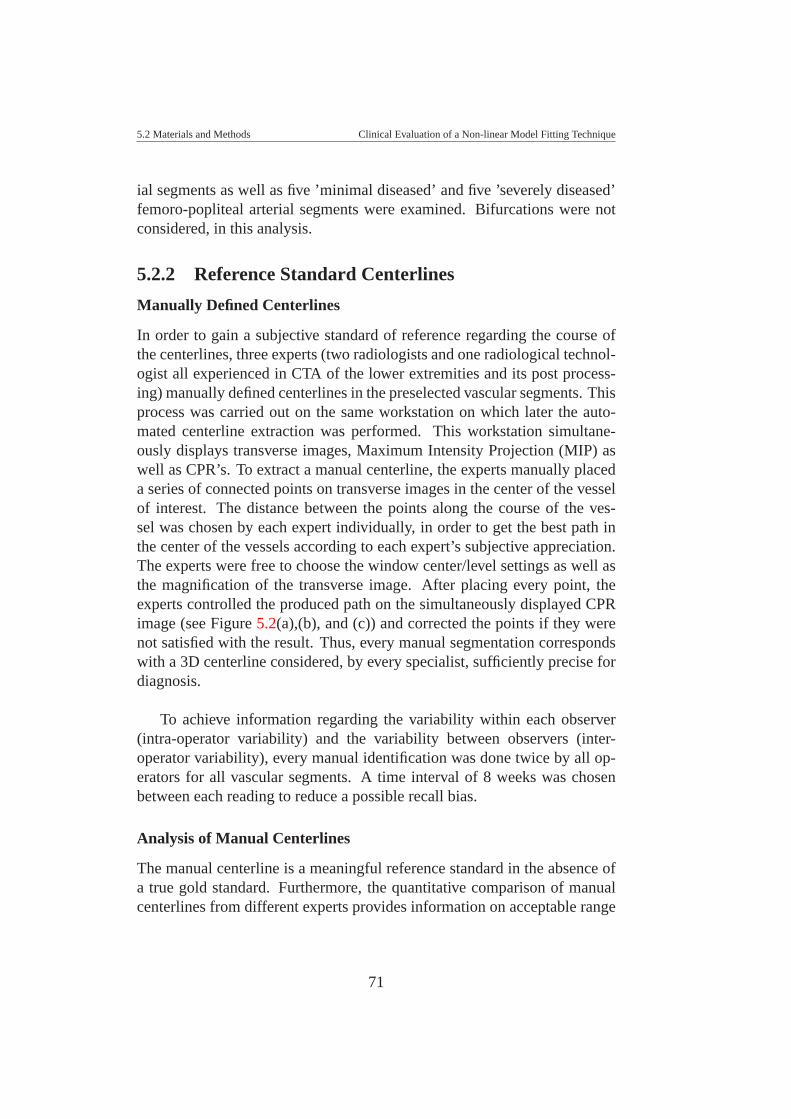
5.2 Materials and Methods Clinical Evaluation of a Non-linear Model Fitting Technique
ial segments as well as five ’minimal diseased’ and five ’severely diseased’femoro-popliteal arterial segments were examined. Bifurcations were notconsidered, in this analysis.
5.2.2 Reference Standard Centerlines
Manually Defined Centerlines
In order to gain a subjective standard of reference regarding the course ofthe centerlines, three experts (two radiologists and one radiological technol-ogist all experienced in CTA of the lower extremities and its post process-ing) manually defined centerlines in the preselected vascular segments. Thisprocess was carried out on the same workstation on which later the auto-mated centerline extraction was performed. This workstation simultane-ously displays transverse images, Maximum Intensity Projection (MIP) aswell as CPR’s. To extract a manual centerline, the experts manually placeda series of connected points on transverse images in the center of the vesselof interest. The distance between the points along the course of the ves-sel was chosen by each expert individually, in order to get the best path inthe center of the vessels according to each expert’s subjective appreciation.The experts were free to choose the window center/level settings as well asthe magnification of the transverse image. After placing every point, theexperts controlled the produced path on the simultaneously displayed CPRimage (see Figure 5.2(a),(b), and (c)) and corrected the points if they werenot satisfied with the result. Thus, every manual segmentation correspondswith a 3D centerline considered, by every specialist, sufficiently precise fordiagnosis.
To achieve information regarding the variability within each observer(intra-operator variability) and the variability between observers (inter-operator variability), every manual identification was done twice by all op-erators for all vascular segments. A time interval of 8 weeks was chosenbetween each reading to reduce a possible recall bias.
Analysis of Manual Centerlines
The manual centerline is a meaningful reference standard in the absence ofa true gold standard. Furthermore, the quantitative comparison of manualcenterlines from different experts provides information on acceptable range
71
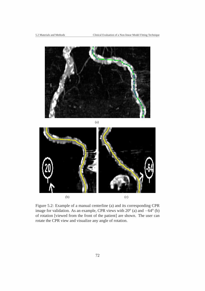
5.2 Materials and Methods Clinical Evaluation of a Non-linear Model Fitting Technique
(a)
(b) (c)
Figure 5.2: Example of a manual centerline (a) and its corresponding CPRimage for validation. As an example, CPR views with 20o (a) and −64o (b)of rotation [viewed from the front of the patient] are shown. The user canrotate the CPR view and visualize any angle of rotation.
72
5.2 Materials and Methods Clinical Evaluation of a Non-linear Model Fitting Technique
of precision that is desired (as a goal) for every automatic centering tech-nique.
The acceptable range of precision is estimated by analyzing the intra-operator and inter-operator variability. The analysis was done as follows:the centering paths from the operators were compared to each other in orderto evaluate the inter-operator and intra-operator variability. The way how wecompared these centerlines is described in details in Section 5.3. The eval-uation is carried out by comparing distances between manual centerlines.The result is used as a reference of an acceptable range of precision for ana-lyzing how far the centerlines are estimated by the automated methods fromthe reference standard, which is the manual centering.
5.2.3 Automated Centerline Extraction
We used three centerline techniques already described in Chapters three andfour. The first is the ray casting with threshold technique (RCT), which wasevaluated against five others techniques (see Chapter three), and resulted asone of the most accurate technique. However, our experience has shownthat this technique is not optimal enough and requires, in diseased datasets,a difficult tuning process, which makes it a tedious work for radiologistsand technologists. The second and third technique are the non-linear modelfitting with two modalities, two-dimensional (M2D) and three-dimensionalmodality (M3D) (see Chapter four for details).
Evaluation of the automatically extracted centerlines
To evaluate the quality of automatically extracted centerlines, they need tobe compared to the reference standard. The comparison process first needsto find correspondences between identified center-points and then measuredifferences (see Section 5.3). As a result, we get information about the meanand the maximum difference between the reference standard and the auto-matically extracted centerlines. This process is executed for all three auto-matic techniques (RCT, M2D, M3D) and mutual comparison is provided toget insight on the quality of the individual techniques.
73
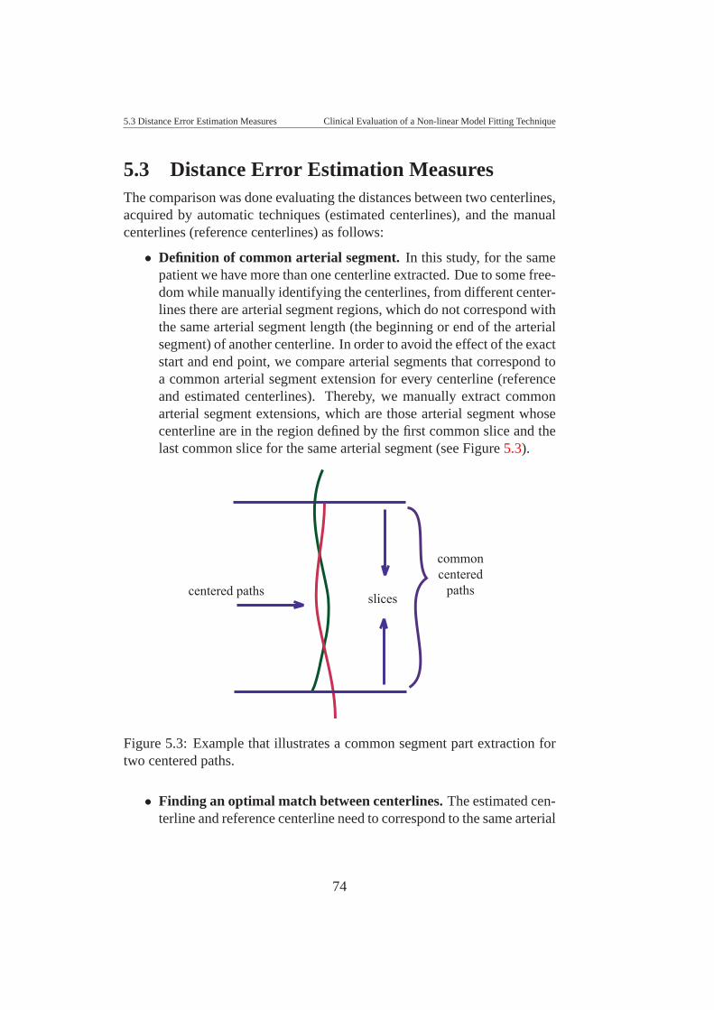
5.3 Distance Error Estimation Measures Clinical Evaluation of a Non-linear Model Fitting Technique
5.3 Distance Error Estimation MeasuresThe comparison was done evaluating the distances between two centerlines,acquired by automatic techniques (estimated centerlines), and the manualcenterlines (reference centerlines) as follows:
• Definition of common arterial segment. In this study, for the samepatient we have more than one centerline extracted. Due to some free-dom while manually identifying the centerlines, from different center-lines there are arterial segment regions, which do not correspond withthe same arterial segment length (the beginning or end of the arterialsegment) of another centerline. In order to avoid the effect of the exactstart and end point, we compare arterial segments that correspond toa common arterial segment extension for every centerline (referenceand estimated centerlines). Thereby, we manually extract commonarterial segment extensions, which are those arterial segment whosecenterline are in the region defined by the first common slice and thelast common slice for the same arterial segment (see Figure 5.3).
slicescentered paths
commoncentered
paths
Figure 5.3: Example that illustrates a common segment part extraction fortwo centered paths.
• Finding an optimal match between centerlines. The estimated cen-terline and reference centerline need to correspond to the same arterial
74
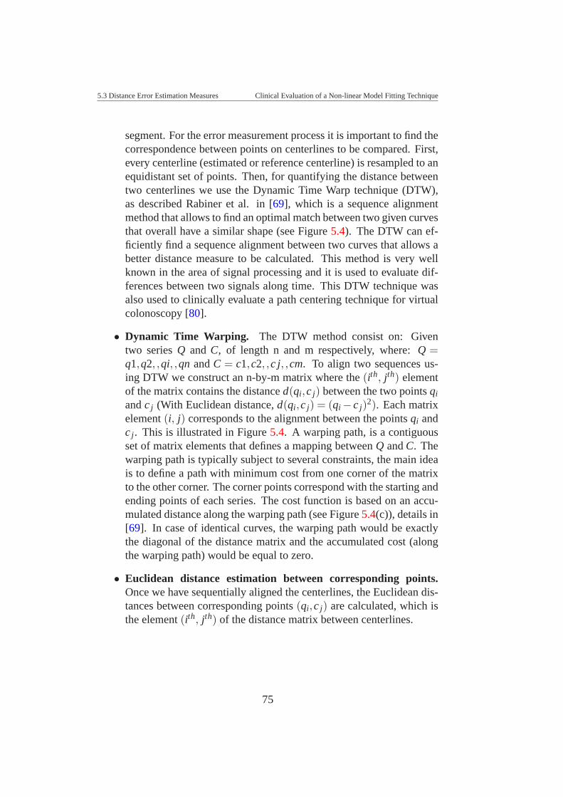
5.3 Distance Error Estimation Measures Clinical Evaluation of a Non-linear Model Fitting Technique
segment. For the error measurement process it is important to find thecorrespondence between points on centerlines to be compared. First,every centerline (estimated or reference centerline) is resampled to anequidistant set of points. Then, for quantifying the distance betweentwo centerlines we use the Dynamic Time Warp technique (DTW),as described Rabiner et al. in [69], which is a sequence alignmentmethod that allows to find an optimal match between two given curvesthat overall have a similar shape (see Figure 5.4). The DTW can ef-ficiently find a sequence alignment between two curves that allows abetter distance measure to be calculated. This method is very wellknown in the area of signal processing and it is used to evaluate dif-ferences between two signals along time. This DTW technique wasalso used to clinically evaluate a path centering technique for virtualcolonoscopy [80].
• Dynamic Time Warping. The DTW method consist on: Giventwo series Q and C, of length n and m respectively, where: Q =q1,q2, ,qi, ,qn and C = c1,c2, ,c j, ,cm. To align two sequences us-ing DTW we construct an n-by-m matrix where the (ith, jth) elementof the matrix contains the distance d(qi,c j) between the two points qi
and c j (With Euclidean distance, d(qi,c j) = (qi − c j)2). Each matrixelement (i, j) corresponds to the alignment between the points qi andc j. This is illustrated in Figure 5.4. A warping path, is a contiguousset of matrix elements that defines a mapping between Q and C. Thewarping path is typically subject to several constraints, the main ideais to define a path with minimum cost from one corner of the matrixto the other corner. The corner points correspond with the starting andending points of each series. The cost function is based on an accu-mulated distance along the warping path (see Figure 5.4(c)), details in[69]. In case of identical curves, the warping path would be exactlythe diagonal of the distance matrix and the accumulated cost (alongthe warping path) would be equal to zero.
• Euclidean distance estimation between corresponding points.Once we have sequentially aligned the centerlines, the Euclidean dis-tances between corresponding points (qi,c j) are calculated, which isthe element (ith, jth) of the distance matrix between centerlines.
75
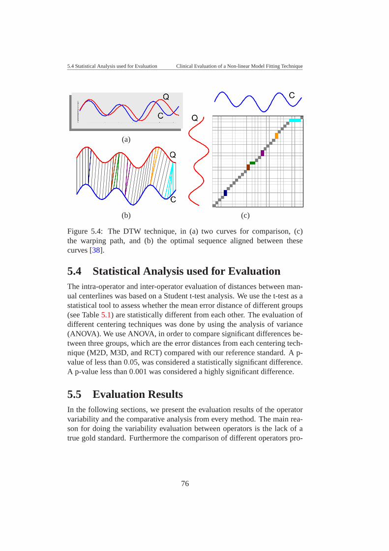
5.4 Statistical Analysis used for Evaluation Clinical Evaluation of a Non-linear Model Fitting Technique
(a)
(b) (c)
Figure 5.4: The DTW technique, in (a) two curves for comparison, (c)the warping path, and (b) the optimal sequence aligned between thesecurves [38].
5.4 Statistical Analysis used for EvaluationThe intra-operator and inter-operator evaluation of distances between man-ual centerlines was based on a Student t-test analysis. We use the t-test as astatistical tool to assess whether the mean error distance of different groups(see Table 5.1) are statistically different from each other. The evaluation ofdifferent centering techniques was done by using the analysis of variance(ANOVA). We use ANOVA, in order to compare significant differences be-tween three groups, which are the error distances from each centering tech-nique (M2D, M3D, and RCT) compared with our reference standard. A p-value of less than 0.05, was considered a statistically significant difference.A p-value less than 0.001 was considered a highly significant difference.
5.5 Evaluation ResultsIn the following sections, we present the evaluation results of the operatorvariability and the comparative analysis from every method. The main rea-son for doing the variability evaluation between operators is the lack of atrue gold standard. Furthermore the comparison of different operators pro-
76
5.5 Evaluation Results Clinical Evaluation of a Non-linear Model Fitting Technique
vides information of the required level of precision.
5.5.1 Evaluation of Operator Variability
Quantitative Analysis
We have four sets of vessel segments, two sets of femoro-popliteal artery,and two sets of the iliac artery, categorized by ’mildly diseased’ and’severely diseased’ groups, respectively. We have two kinds of measure-ments for every group. They are the distance error variability within eachoperator (intra-operator) and the distance error variability between operators(inter-operator).
The result (see Table 5.1) shows a significant difference (p = 0.01) be-tween intra- and inter-operator variability. The intra-operator error distance(1.0 mm) was significantly smaller (p < 0.05) than inter-operator error dis-tance (1.2 mm), which is not surprising. Then, we considered it is im-portant to evaluate independent groups separately. The intra-operator andinter-operator measurements were ordered into separated groups (iliac andfemoro-popliteal segments), in order to evaluate the variability separatelyon different arterial segments, and in both cases we found:
• A significant difference (p < 0.05) between femoro-popliteal and il-iac arterial segment groups. The operator error distance for femoro-popliteal segments was significantly smaller (0.9 mm and 1.0 mm)than iliac segments (1.2 mm and 1.4 mm), corresponding with theintra- and inter-operator variability, respectively.
• No significant difference were identified between ’mildly diseased’and ’severely diseased’ cases for expert operators.
Considering theses findings and evaluating the mean values from eachgroup, we conclude that the variability is more significant if we considerthe artery segment (femoro-popliteal and iliac) than the state of the patient(’mildly diseased’ and ’severely diseased’). For this reason we also made aseparate analysis of separated groups of the femoro-popliteal and the iliaccases, and we found:
• For the femoral cases: It was observed a very high significant differ-ence (p < 0.001) between ’mildly diseased’ (0.8 mm) and ’severely
77
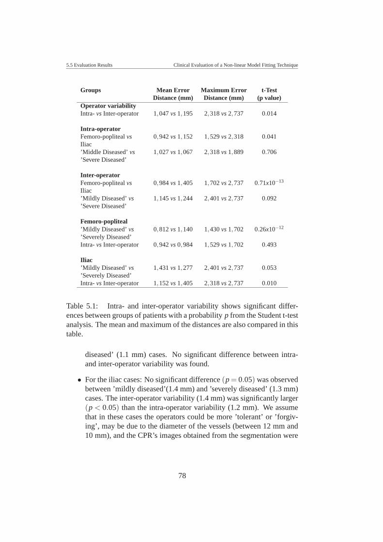
5.5 Evaluation Results Clinical Evaluation of a Non-linear Model Fitting Technique
Groups Mean Error Maximum Error t-TestDistance (mm) Distance (mm) (p value)
Operator variabilityIntra- vs Inter-operator 1,047 vs 1,195 2,318 vs 2,737 0.014
Intra-operatorFemoro-popliteal vs 0,942 vs 1,152 1,529 vs 2,318 0.041Iliac’Middle Diseased’ vs 1,027 vs 1,067 2,318 vs 1,889 0.706’Severe Diseased’
Inter-operatorFemoro-popliteal vs 0,984 vs 1,405 1,702 vs 2,737 0.71x10⁻¹³
Iliac’Mildly Diseased’ vs 1,145 vs 1,244 2,401 vs 2,737 0.092’Severe Diseased’
Femoro-popliteal’Mildly Diseased’ vs 0,812 vs 1,140 1,430 vs 1,702 0.26x10⁻¹²
’Severely Diseased’Intra- vs Inter-operator 0,942 vs 0,984 1,529 vs 1,702 0.493
Iliac’Mildly Diseased’ vs 1,431 vs 1,277 2,401 vs 2,737 0.053’Severely Diseased’Intra- vs Inter-operator 1,152 vs 1,405 2,318 vs 2,737 0.010
Table 5.1: Intra- and inter-operator variability shows significant differ-ences between groups of patients with a probability p from the Student t-testanalysis. The mean and maximum of the distances are also compared in thistable.
diseased’ (1.1 mm) cases. No significant difference between intra-and inter-operator variability was found.
• For the iliac cases: No significant difference (p = 0.05) was observedbetween ’mildly diseased’(1.4 mm) and ’severely diseased’ (1.3 mm)cases. The inter-operator variability (1.4 mm) was significantly larger(p < 0.05) than the intra-operator variability (1.2 mm). We assumethat in these cases the operators could be more ’tolerant’ or ’forgiv-ing’, may be due to the diameter of the vessels (between 12 mm and10 mm), and the CPR’s images obtained from the segmentation were
78
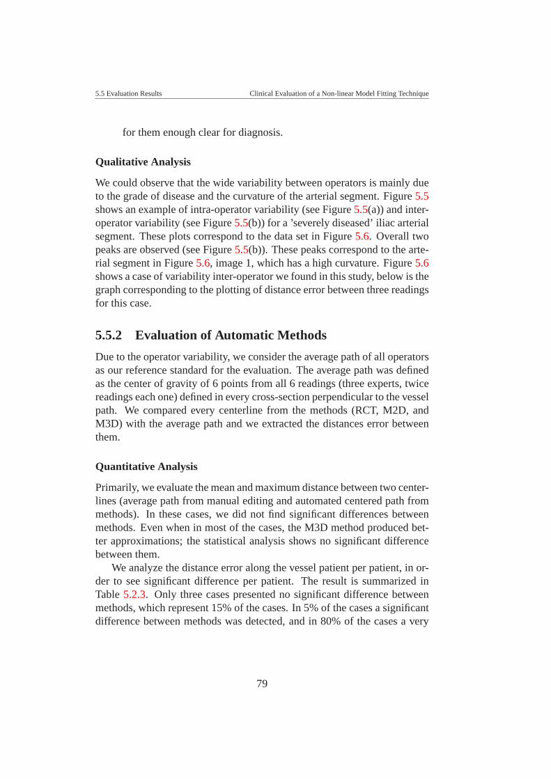
5.5 Evaluation Results Clinical Evaluation of a Non-linear Model Fitting Technique
for them enough clear for diagnosis.
Qualitative Analysis
We could observe that the wide variability between operators is mainly dueto the grade of disease and the curvature of the arterial segment. Figure 5.5shows an example of intra-operator variability (see Figure 5.5(a)) and inter-operator variability (see Figure 5.5(b)) for a ’severely diseased’ iliac arterialsegment. These plots correspond to the data set in Figure 5.6. Overall twopeaks are observed (see Figure 5.5(b)). These peaks correspond to the arte-rial segment in Figure 5.6, image 1, which has a high curvature. Figure 5.6shows a case of variability inter-operator we found in this study, below is thegraph corresponding to the plotting of distance error between three readingsfor this case.
5.5.2 Evaluation of Automatic Methods
Due to the operator variability, we consider the average path of all operatorsas our reference standard for the evaluation. The average path was definedas the center of gravity of 6 points from all 6 readings (three experts, twicereadings each one) defined in every cross-section perpendicular to the vesselpath. We compared every centerline from the methods (RCT, M2D, andM3D) with the average path and we extracted the distances error betweenthem.
Quantitative Analysis
Primarily, we evaluate the mean and maximum distance between two center-lines (average path from manual editing and automated centered path frommethods). In these cases, we did not find significant differences betweenmethods. Even when in most of the cases, the M3D method produced bet-ter approximations; the statistical analysis shows no significant differencebetween them.
We analyze the distance error along the vessel patient per patient, in or-der to see significant difference per patient. The result is summarized inTable 5.2.3. Only three cases presented no significant difference betweenmethods, which represent 15% of the cases. In 5% of the cases a significantdifference between methods was detected, and in 80% of the cases a very
79
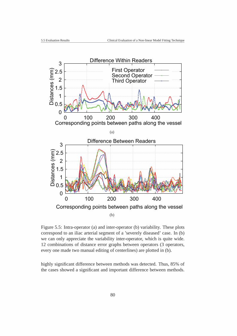
5.5 Evaluation Results Clinical Evaluation of a Non-linear Model Fitting Technique
3 2.5
2 1.5
1 0.5
0 400 300 200 100 0
Dis
tanc
es (m
m)
Corresponding points between paths along the vessel
Difference Within Readers
First OperatorSecond OperatorThird Operator
(a)
3 2.5
2 1.5
1 0.5
0 400 300 200 100 0
Dis
tanc
es (m
m)
Corresponding points between paths along the vessel
Difference Between Readers
(b)
Figure 5.5: Intra-operator (a) and inter-operator (b) variability. These plotscorrespond to an iliac arterial segment of a ’severely diseased’ case. In (b)we can only appreciate the variability inter-operator, which is quite wide.12 combinations of distance error graphs between operators (3 operators,every one made two manual editing of centerlines) are plotted in (b).
highly significant difference between methods was detected. Thus, 85% ofthe cases showed a significant and important difference between methods.
80
5.5 Evaluation Results Clinical Evaluation of a Non-linear Model Fitting Technique
~2.5 & 2.7 mm~2.2 mm
3 2.5
2 1.5
1 0.5
0 400 300 200 100 0
Dis
tanc
es (m
m)
Corresponding points between paths along the vessel
Difference Between Readers
Reader 1 vs Reader 2Reader 1 vs Reader 3Reader 2 vs Reader 3
Figure 5.6: A case of inter-operator variability. Three manual centerlinesare drawn [with different colors (orange, red and blue)]. Every centerlinecorresponds to a manual segmentation from a different operator. The plotshows the variability between them. Two remarkable peaks correspond tothe area pointed it out in image 1.
81
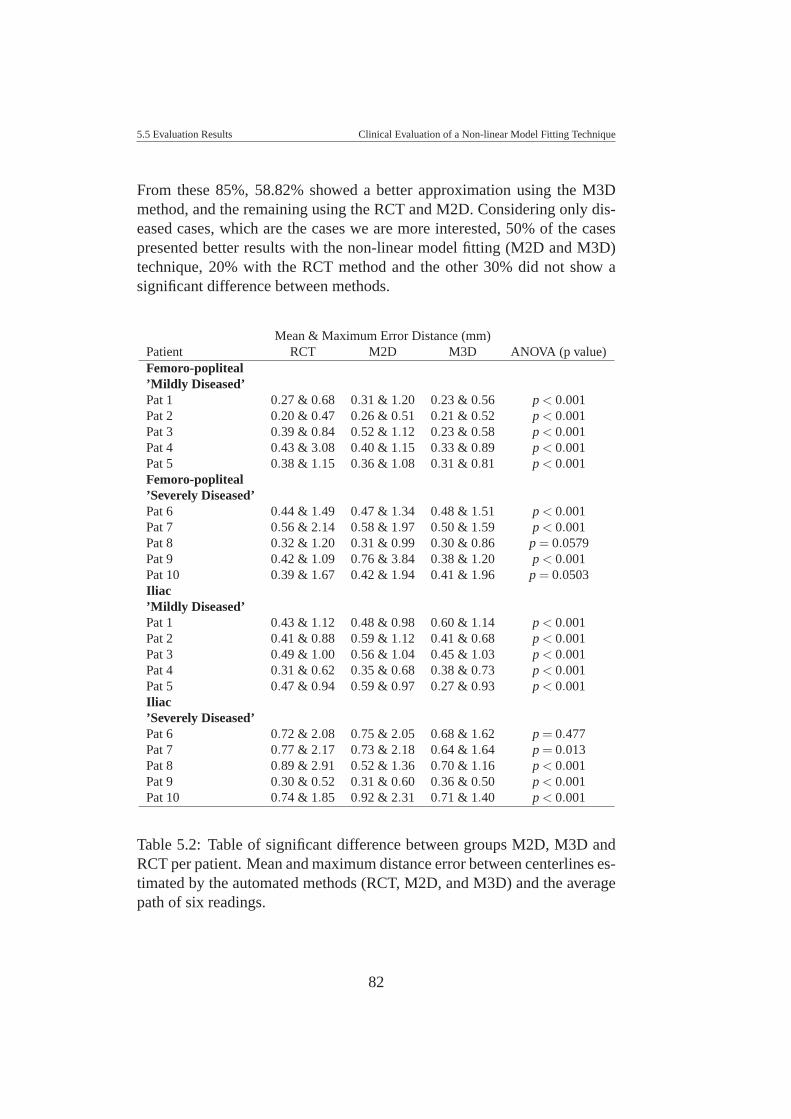
5.5 Evaluation Results Clinical Evaluation of a Non-linear Model Fitting Technique
From these 85%, 58.82% showed a better approximation using the M3Dmethod, and the remaining using the RCT and M2D. Considering only dis-eased cases, which are the cases we are more interested, 50% of the casespresented better results with the non-linear model fitting (M2D and M3D)technique, 20% with the RCT method and the other 30% did not show asignificant difference between methods.
Mean & Maximum Error Distance (mm)Patient RCT M2D M3D ANOVA (p value)Femoro-popliteal’Mildly Diseased’Pat 1 0.27 & 0.68 0.31 & 1.20 0.23 & 0.56 p < 0.001Pat 2 0.20 & 0.47 0.26 & 0.51 0.21 & 0.52 p < 0.001Pat 3 0.39 & 0.84 0.52 & 1.12 0.23 & 0.58 p < 0.001Pat 4 0.43 & 3.08 0.40 & 1.15 0.33 & 0.89 p < 0.001Pat 5 0.38 & 1.15 0.36 & 1.08 0.31 & 0.81 p < 0.001Femoro-popliteal’Severely Diseased’Pat 6 0.44 & 1.49 0.47 & 1.34 0.48 & 1.51 p < 0.001Pat 7 0.56 & 2.14 0.58 & 1.97 0.50 & 1.59 p < 0.001Pat 8 0.32 & 1.20 0.31 & 0.99 0.30 & 0.86 p = 0.0579Pat 9 0.42 & 1.09 0.76 & 3.84 0.38 & 1.20 p < 0.001Pat 10 0.39 & 1.67 0.42 & 1.94 0.41 & 1.96 p = 0.0503Iliac’Mildly Diseased’Pat 1 0.43 & 1.12 0.48 & 0.98 0.60 & 1.14 p < 0.001Pat 2 0.41 & 0.88 0.59 & 1.12 0.41 & 0.68 p < 0.001Pat 3 0.49 & 1.00 0.56 & 1.04 0.45 & 1.03 p < 0.001Pat 4 0.31 & 0.62 0.35 & 0.68 0.38 & 0.73 p < 0.001Pat 5 0.47 & 0.94 0.59 & 0.97 0.27 & 0.93 p < 0.001Iliac’Severely Diseased’Pat 6 0.72 & 2.08 0.75 & 2.05 0.68 & 1.62 p = 0.477Pat 7 0.77 & 2.17 0.73 & 2.18 0.64 & 1.64 p = 0.013Pat 8 0.89 & 2.91 0.52 & 1.36 0.70 & 1.16 p < 0.001Pat 9 0.30 & 0.52 0.31 & 0.60 0.36 & 0.50 p < 0.001Pat 10 0.74 & 1.85 0.92 & 2.31 0.71 & 1.40 p < 0.001
Table 5.2: Table of significant difference between groups M2D, M3D andRCT per patient. Mean and maximum distance error between centerlines es-timated by the automated methods (RCT, M2D, and M3D) and the averagepath of six readings.
82
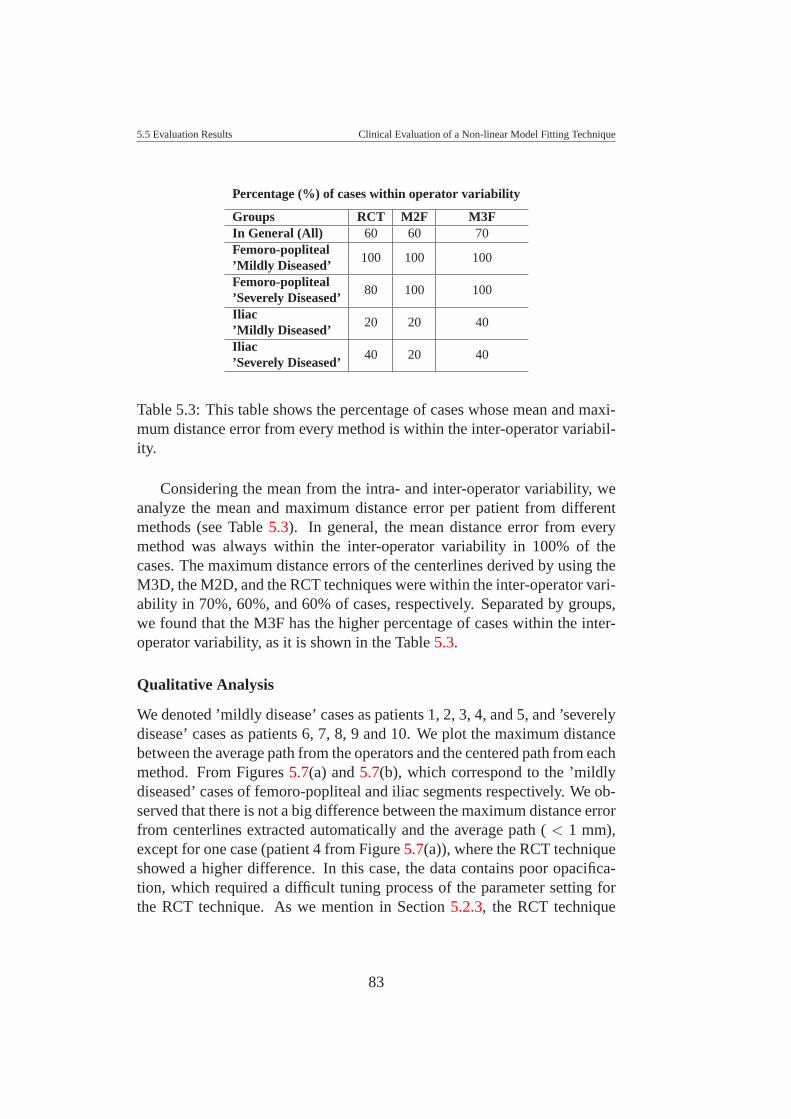
5.5 Evaluation Results Clinical Evaluation of a Non-linear Model Fitting Technique
Percentage (%) of cases within operator variability
Groups RCT M2F M3FIn General (All) 60 60 70Femoro-popliteal
100 100 100’Mildly Diseased’Femoro-popliteal
80 100 100’Severely Diseased’Iliac
20 20 40’Mildly Diseased’Iliac
40 20 40’Severely Diseased’
Table 5.3: This table shows the percentage of cases whose mean and maxi-mum distance error from every method is within the inter-operator variabil-ity.
Considering the mean from the intra- and inter-operator variability, weanalyze the mean and maximum distance error per patient from differentmethods (see Table 5.3). In general, the mean distance error from everymethod was always within the inter-operator variability in 100% of thecases. The maximum distance errors of the centerlines derived by using theM3D, the M2D, and the RCT techniques were within the inter-operator vari-ability in 70%, 60%, and 60% of cases, respectively. Separated by groups,we found that the M3F has the higher percentage of cases within the inter-operator variability, as it is shown in the Table 5.3.
Qualitative Analysis
We denoted ’mildly disease’ cases as patients 1, 2, 3, 4, and 5, and ’severelydisease’ cases as patients 6, 7, 8, 9 and 10. We plot the maximum distancebetween the average path from the operators and the centered path from eachmethod. From Figures 5.7(a) and 5.7(b), which correspond to the ’mildlydiseased’ cases of femoro-popliteal and iliac segments respectively. We ob-served that there is not a big difference between the maximum distance errorfrom centerlines extracted automatically and the average path ( < 1 mm),except for one case (patient 4 from Figure 5.7(a)), where the RCT techniqueshowed a higher difference. In this case, the data contains poor opacifica-tion, which required a difficult tuning process of the parameter setting forthe RCT technique. As we mention in Section 5.2.3, the RCT technique
83
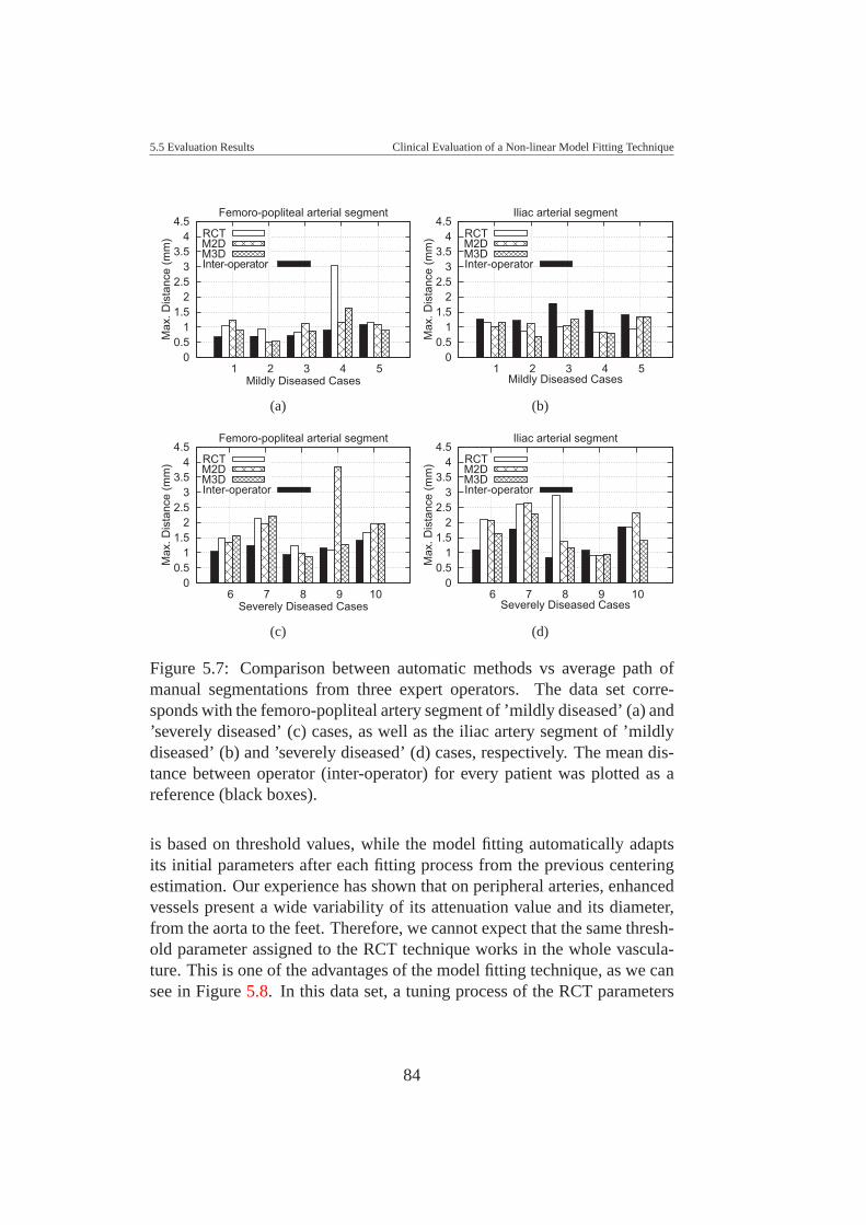
5.5 Evaluation Results Clinical Evaluation of a Non-linear Model Fitting Technique
0 0.5
1 1.5
2 2.5
3 3.5
4 4.5
5 4 3 2 1
Max
. Dis
tanc
e (m
m)
Mildly Diseased Cases
Femoro-popliteal arterial segment
RCTM2DM3DInter-operator
(a)
0 0.5
1 1.5
2 2.5
3 3.5
4 4.5
5 4 3 2 1
Max
. Dis
tanc
e (m
m)
Mildly Diseased Cases
Iliac arterial segment
RCTM2DM3DInter-operator
(b)
0 0.5
1 1.5
2 2.5
3 3.5
4 4.5
10 9 8 7 6
Max
. Dis
tanc
e (m
m)
Severely Diseased Cases
Femoro-popliteal arterial segment
RCTM2DM3DInter-operator
(c)
0 0.5
1 1.5
2 2.5
3 3.5
4 4.5
10 9 8 7 6
Max
. Dis
tanc
e (m
m)
Severely Diseased Cases
Iliac arterial segment
RCTM2DM3DInter-operator
(d)
Figure 5.7: Comparison between automatic methods vs average path ofmanual segmentations from three expert operators. The data set corre-sponds with the femoro-popliteal artery segment of ’mildly diseased’ (a) and’severely diseased’ (c) cases, as well as the iliac artery segment of ’mildlydiseased’ (b) and ’severely diseased’ (d) cases, respectively. The mean dis-tance between operator (inter-operator) for every patient was plotted as areference (black boxes).
is based on threshold values, while the model fitting automatically adaptsits initial parameters after each fitting process from the previous centeringestimation. Our experience has shown that on peripheral arteries, enhancedvessels present a wide variability of its attenuation value and its diameter,from the aorta to the feet. Therefore, we cannot expect that the same thresh-old parameter assigned to the RCT technique works in the whole vascula-ture. This is one of the advantages of the model fitting technique, as we cansee in Figure 5.8. In this data set, a tuning process of the RCT parameters
84
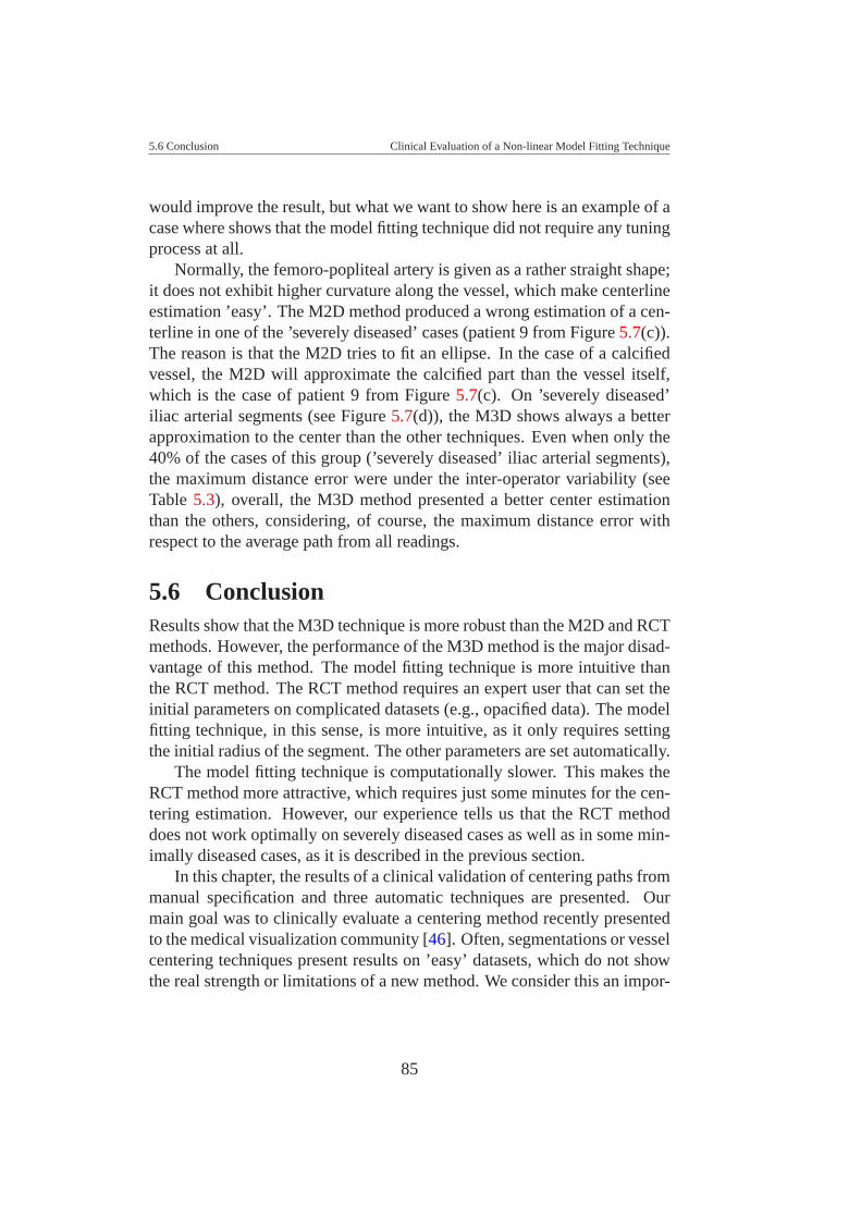
5.6 Conclusion Clinical Evaluation of a Non-linear Model Fitting Technique
would improve the result, but what we want to show here is an example of acase where shows that the model fitting technique did not require any tuningprocess at all.
Normally, the femoro-popliteal artery is given as a rather straight shape;it does not exhibit higher curvature along the vessel, which make centerlineestimation ’easy’. The M2D method produced a wrong estimation of a cen-terline in one of the ’severely diseased’ cases (patient 9 from Figure 5.7(c)).The reason is that the M2D tries to fit an ellipse. In the case of a calcifiedvessel, the M2D will approximate the calcified part than the vessel itself,which is the case of patient 9 from Figure 5.7(c). On ’severely diseased’iliac arterial segments (see Figure 5.7(d)), the M3D shows always a betterapproximation to the center than the other techniques. Even when only the40% of the cases of this group (’severely diseased’ iliac arterial segments),the maximum distance error were under the inter-operator variability (seeTable 5.3), overall, the M3D method presented a better center estimationthan the others, considering, of course, the maximum distance error withrespect to the average path from all readings.
5.6 ConclusionResults show that the M3D technique is more robust than the M2D and RCTmethods. However, the performance of the M3D method is the major disad-vantage of this method. The model fitting technique is more intuitive thanthe RCT method. The RCT method requires an expert user that can set theinitial parameters on complicated datasets (e.g., opacified data). The modelfitting technique, in this sense, is more intuitive, as it only requires settingthe initial radius of the segment. The other parameters are set automatically.
The model fitting technique is computationally slower. This makes theRCT method more attractive, which requires just some minutes for the cen-tering estimation. However, our experience tells us that the RCT methoddoes not work optimally on severely diseased cases as well as in some min-imally diseased cases, as it is described in the previous section.
In this chapter, the results of a clinical validation of centering paths frommanual specification and three automatic techniques are presented. Ourmain goal was to clinically evaluate a centering method recently presentedto the medical visualization community [46]. Often, segmentations or vesselcentering techniques present results on ’easy’ datasets, which do not showthe real strength or limitations of a new method. We consider this an impor-
85
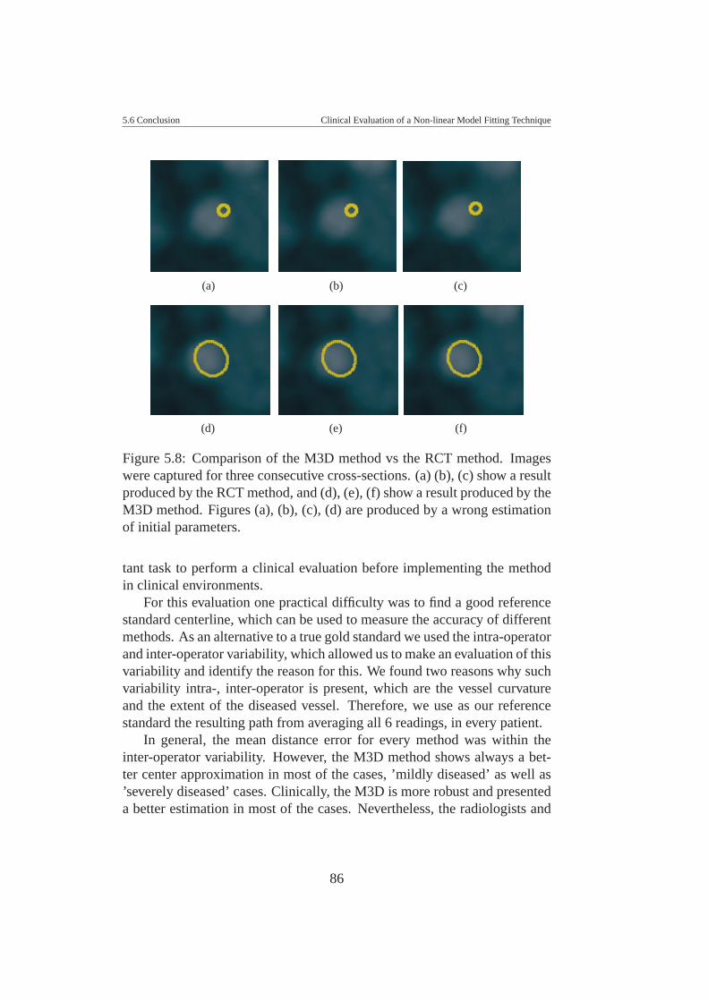
5.6 Conclusion Clinical Evaluation of a Non-linear Model Fitting Technique
(a) (b) (c)
(d) (e) (f)
Figure 5.8: Comparison of the M3D method vs the RCT method. Imageswere captured for three consecutive cross-sections. (a) (b), (c) show a resultproduced by the RCT method, and (d), (e), (f) show a result produced by theM3D method. Figures (a), (b), (c), (d) are produced by a wrong estimationof initial parameters.
tant task to perform a clinical evaluation before implementing the methodin clinical environments.
For this evaluation one practical difficulty was to find a good referencestandard centerline, which can be used to measure the accuracy of differentmethods. As an alternative to a true gold standard we used the intra-operatorand inter-operator variability, which allowed us to make an evaluation of thisvariability and identify the reason for this. We found two reasons why suchvariability intra-, inter-operator is present, which are the vessel curvatureand the extent of the diseased vessel. Therefore, we use as our referencestandard the resulting path from averaging all 6 readings, in every patient.
In general, the mean distance error for every method was within theinter-operator variability. However, the M3D method shows always a bet-ter center approximation in most of the cases, ’mildly diseased’ as well as’severely diseased’ cases. Clinically, the M3D is more robust and presenteda better estimation in most of the cases. Nevertheless, the radiologists and
86

5.6 Conclusion Clinical Evaluation of a Non-linear Model Fitting Technique
clinical experts have the last word with respect to the use of this techniquein clinical environment. Overall, the model fitting technique presented bet-ter results, but also require of the improvement of performance. The ideaof using a model based segmentation on this kind of vessels, with highervariability of appearance, due to the diameter, opacification and level of dis-eased, is the most suitable way to determine the centerline along the vessel.
87
CHAPTER 6
SUMMARY AND CONCLUSIONS
An accuracy estimation of the centerline for blood vessels is a pre-requisitefor different visualization techniques. This thesis is divided in three parts:
The first part is addressed to improve a current centerline segmentationused for daily clinical evaluation and diagnosis of peripheral arterial occlu-sive diseases. The ray casting technique (RCT) is investigated, which isthe standard semi-automatic method actually used in a clinical environmentin the central hospital of Vienna. The RCT technique is based on thresh-old values defined to identify the vessel boundary once a vessel trackingprocess has approximated a vessel path. This technique has several limita-tions to detect the boundary of diseased blood vessels. This is due to thehigh variability that diseased blood vessels may show concerning the den-sity distribution of non-calcified and calcified plaques, and concerning thediameter from aorta to pedal arteries. Some improvements to the RCT wereimplemented that allowed to deal with calcified vessels whose location isfar away from bones. They use the maximum gradient information alongrays defined by the RCT method to detect the vessel boundary. However, onvessels with partial occlusion (non-calcified plaque) this method has somedifficulties to properly identify the centerline.
We implemented and investigated different centering techniques. All ofthem were evaluated using a phantom simulating the density and diameterof peripheral arteries. Because the center of the vessel in the synthetic datais known an accuracy evaluation of different centering techniques could bedone. These centering techniques are: the RCT, the improved RCT usinga maximum gradient like stop criterion (RCMG), pixel motion estimationbetween successive images called block matching (BM), center of gravity(CoG), the Randomized Hough Transform (RHT), and ellipse fitting (EF).
88
Summary and Conclusions
The last two techniques have been used as shape based segmentation tech-niques. Results show that the RCT and RCMG were the most accuratemethods.
In the second part we implemented a new parameterization technique fordiseased blood vessels, which takes 3D spatial information into account fora best parameterization. This technique is based on a non-linear optimiza-tion process, which estimates the center, diameter, and mean density valuesfor blood vessel and surrounding area or background. The method requiresan initial estimation of a cylindrical (in 3D) or elliptical model (in 2D). Anon-linear optimization process is used to find the 2D or the 3D model thatbest fits the data (M2D and M3D, respectively). This technique can be usedas a semi-automatic or automatic technique; hence it does not require aninitial estimation of a vessel path. The Levenberg-Marquardt method wasused as a non-linear minimization process, which allows extracting optimalparameters from a model that best fits the data.
In the third part we proceeded with the clinical evaluation of our method.Results showed that the cylindrical model fitting method (M3D) is more ro-bust than the elliptical model fitting (M2D) and the RCT method. The majordisadvantage of the model fitting technique is the performance. However,it works very well on diseased blood vessels where the previous methodmay fail. The model fitting method can be used for the centering of local-ized parts when other techniques fail and one gains performance on healthyblood vessels, which do not require such a sophisticated algorithm.
The main contribution of this investigation is the implementation of asegmentation solution for visualization and analysis purposes in cases whereclassical segmentation methods based on boundary detection often fail. Dis-eased vessels show a wide variability of density values, which is a challengebecause calcifications appear as bones and partial occlusion or soft plaquesappear as soft tissues. This makes it difficult to detect the vessel boundaries.The cylindrical 3D model (M3D) fitting requires neither a pre-processingstep nor any operator estimation, such as, gradient, derivative, etc.
The cylindrical model fitting can be considered as initial step to im-plement an automatic segmentation of diseased vascular structures. Futurework should address the following issues: performance, handling of vesselbifurcations, and inclusion of further anatomical knowledge.
89
BIBLIOGRAPHY
[1] S.R. Aylward and E. Bullitt. Initialization, Noise, Singularities, andScale in Height Ridge Traversal for Tubular Object Centerline Extrac-tion. IEEE Transactions on Medical Imaging, 21(2):61–75, February2002. 30
[2] D. Bartz, D. Mayer, J. Fischer, S. Ley, A. del Rio, S. Thust, C.P.Heussel, H.-U. Kauczor, and W. Strasser. Hybrid Segmentation andExploration of the Human Lungs. In IEEE Visualization 2003, pages177–184, October 2003. 31
[3] T. Baun, J.J. Flaaris, M. Volden, J. Haase, O.V. Larsen, and L.R. Os-tergaard. Surface Modeling of Blood Vessels Based on 3D MedicalImages. In International Federation for Medical & Biological Engi-neering, IFMBE, IX Mediterranean Conference on Medical and Bio-logical Engineering and Computing, Medicon 2001, pages 969–973.Magjarevic,R., Tonkovic,S., Bilas,V. and Lackovic,I. (eds.). Zagreb:Faculty of Electrical Engineering and Computing, University of Za-greb, June 2001. 29
[4] H. Blum. A Transformation for Extracting New Descriptors of Shape.In W. Whaten-Dunn, editor, Symposium Models for the Perception ofSpeech and Visual Form, pages 362–380. MIT Press, 1967. 28
[5] C. Boldak, Y. Rolland, and C. Toumoulin. An Improved Model-Based Vessel Tracking Algorithm with Application to Computed To-mography Angiography. Biocybernetics and Biomedical Engineering,23:41–63, 2003. 24, 29
[6] C. Boldak, C. Toumoulin, and J. L. Coatrieux. 3D Segmentation andCharacterization of Lower Limb Vessels in Multi-Slice Computed To-
90
BIBLIOGRAPHY BIBLIOGRAPHY
mography. 25th Annual International Conference of the IEEE EMBS,pages 580–583, September 2003. 27, 29
[7] B. Brooks. Intra-arterial Injection of Sodium Iodide. Journal of theAmerican Medical Association, 82:1016–1019, 1924. 6
[8] K. Buhler, P. Felkel, and A. La Cruz. Geometric Methods for VesselVisualization and Quantification - A Survey, pages 399–420. G. Brun-net, B. Hamann and H. Muller and L. Linsen (eds.). Kluwer Academic,2003. 23, 24, 25, 26, 35
[9] J. Canny. A Computational Approach to Edge Detection. IEEE Trans-actions Pattern Analysis Machine Intelligence, 8(6):679–698, 1986.39, 40, 45
[10] J. L. Coatrieux, J. Rong, and R. Collarec. A Framework for AutomaticAnalysis of the Dynamic Behavior of Coronary Angiograms. Interna-tional Journal Cardiac Imaging, 8:1–10, 1992. 36
[11] J. D. Coffman and R. T. Eberhardt. Peripheral Arterial Disease: Di-agnosis and Treatment. Humana Press Inc., 2003. 2, 4
[12] T. F. Cootes, A. Hill, C. J. Taylor, and J. Haslam. The Use of ActiveShape Models for Locating Structures in Medical Images. In H.H.Barrett and A.F. Gmitro, editors, 13th International Conference on In-formation Processing in Medical Imaging, pages 33–47, 1993. 24
[13] T.F. Cootes, D. Cooper, C.J. Taylor, and J. Graham. Active ShapeModels - Their Training and Application. Computer Vision and ImageUnderstanding, 61(1):38–59, January 1995. 24
[14] C. Q. Davis, Z. Z. Karu, and D. M. Freeman. Equivalence of SubpixelMotion Estimators Based on Optical Flow and Block Matching. InInternational Symposium Computer Vision, pages 7–12, 1995. 38
[15] T. Deschamps and L.D. Cohen. Fast Extraction of Tubular and Tree3D Surfaces with Front Propagation Methods. In 16th InternationalConference on Pattern Recognition, ICPR’02., pages 731–734, August2002. 26
91
BIBLIOGRAPHY BIBLIOGRAPHY
[16] O. Lindenthal E. Haschek. A Contribution to the Practical use of Pho-tography According to Roentgen. Wien Chir Wochenschr, 9:63–64,1896. 6
[17] P. Felkel, R. Wegenkittl, and A. Kanitsar. Vessel Tracking in PeripheralCTA Datasets - An Overview. In Spring Conference on ComputerGraphics, pages 232–239, April 2001. x, 13, 33
[18] J. Feng, H. S. Horace, and H. C. Shuk. A 3D Geometric DeformableModel for Tubular Structure Segmentation. In Multimedia ModellingConference (MMM’04), pages 174–180, January 2004. 27
[19] A. Fitzgibbon and R. Fisher. A Buyer’s Guide to Conic Fitting. InBritish Machine Vision Conference, pages 513–522, 1995. 40
[20] D. Fleischmann, R.L. Hallet, and G.D. Rubin. CT Angiography of Pe-ripheral Arterial Disease. Journal of Vascular Intervention Radiology,17(1):3–26, January 2006. 10, 19
[21] D. Fleischmann, T. J. Hastie, F. C. Dannegger, D. S. Paik, M. Tillich,C. K. Zarins, and G. D. Rubin. Quantitative Determination of Age-Related Geometric Changes in the Normal Abdominal Aorta. Journalof Vascular Surgery, 33(1):97–105, May 2001. 2
[22] D. Fleischmann and G.D. Rubin. Quantification of Intravenously Ad-ministered Contrast Medium Transit Through the Peripheral Arter-ies: Implications for CT Angiography. Radiology, 236(3):1076–1082,September 2005. 14
[23] A. Frangi. Three-Dimensional Model-Based Analysis of Vascular andCardiac Images. PhD thesis, University Medical Center Utrecht, TheNetherlands, 2001. 28
[24] A.F. Frangi, W.J. Niessen, R.M. Hoogeveen, T. van Walsum, andM.A. Viergever. Model-Based Quantization of 3-D Magnetic Reso-nance Angiographic Images. IEEE Transactions on Medical Imaging,18(10):946–956, October 1999. 28
[25] A.F. Frangi, W.J. Niessen, K.L. Vincken, and M.A. Viergever. Multi-scale Vessel Enhancement Filtering. In Medical Image Computing andComputer-Assisted Intervention - MICCAI, pages 130–137. Springer,1998. 28, 30
92
BIBLIOGRAPHY BIBLIOGRAPHY
[26] L. Gong, S.D. Pathak, D.R. Haynor, P.S. Cho, and Y. Kim. Paramet-ric Shape Modeling Using Deformable Superellipses for Prostate Seg-mentation. IEEE Transactions on Medical Imaging, 23(3):304–349,March 2004. 26
[27] H.K. Hahn, B. Preim, D. Selle, and H.O. Peitgen. Visualization andInteraction Techniques for the Exploration of Vascular Structures. InIEEE Visualization 2001, pages 395–578, October 2001. 18
[28] M. Hernandez, A.F. Frangi, and R. Barrena. Pre-clinical Evaluation ofImplicit Deformable Models for Three-Dimensional Segmentation ofBrain Aneurysms from CTA Images. In SPIE Medical Imaging, ImageProcessing, volume 5032, pages 1264–74, 2003. 26
[29] C.-F. Ho, M.-H. Wu, H.-M. Wu, C.-Y. Chang, M. C.-M. Chen, andT.-Y. Chou. Comparison of Auto-moving Table Contrast-enhanced3-D MRA and Iodinated Contrast-enhanced DSA for Evaluating theLower-extremity Arteries. Journal of the Chinese Medical Associa-tion, 67(10):511–520, 2004. 8
[30] Q. Huang and C. Stockman. Generalized Tube Model: Recognizing3D Elongated Objects from 2D Intensity Images. In IEEE Conferenceon Computer Vision and Pattern Recognition, New York, pages 104–109, June 1993. 30
[31] X. Jiang and D. Mojon. Adaptive Local Thresholding by Verification-Based Multithreshold probing with Application to Vessel Detection inRetinal Images. IEEE Transaction on Patter Analysis and MachineIntelligence, 25(1):131–137, 2003. 24
[32] S. Joshi, S. Pizer, P. Fletcher, P. Yushkevich, A. Thall, and J. Mar-ron. Multiscale Deformable Model Segmentation and Statistical ShapeAnalysis using Medial Descriptions. In IEEE Transactions on MedicalImaging, pages 538–550, 2002. 28
[33] S.C. Joshi, S.M. Pizer, P.T. Fletcher, A. Thall, and G. Tracton. Multi-scale 3-D Deformable Model Segmentation Based on Medial Descrip-tion. In International Conference on Information Processing in Med-ical Imaging, IPMI, pages 64–77, London, UK, 2001. Springer-Verlag.28
93
BIBLIOGRAPHY BIBLIOGRAPHY
[34] R.E. Kalman. A New Approach to Linear Filtering and PredictionProblems. Transaction of the ASME - Journal of Basic Engineering,pages 35–45, March 1960. 31
[35] A. Kanitsar, D. Fleischmann, R. Wegenkittl, P. Felkel, and M. E.Groller. CPR - Curved Planar Reformation. In IEEE Visualization2002, pages 37–44, October 2002. 15, 16, 68
[36] A. Kanitsar, R. Wegenkittl, P. Felkel, D. Fleischmann, D. Sandner,and E. Groller. Computed Tomography Angiography: A Case Studyof Peripheral Vessel Investigation. In IEEE Visualization, pages 477–480, October 2001. x, 15, 36, 37, 44
[37] A. Kanitsar, R. Wegenkittl, P. Felkel, D. Fleischmann, D. Sandner,and E. Groller. Computed Tomography Angiography: A Case Studyof Peripheral Vessel Investigation. In IEEE Visualization 2001, pages477–480, October 2001. 52, 60, 62
[38] E. Keogh. Exact Indexing of Dynamic Time Warping. In 28th Inter-national Conference on Very Large Data Bases, Proceedings, pages406–417. Endowment Inc., August 2002. xiv, 76
[39] C. Kirbas and F.K.H Quek. A Review of Vessel Extraction Techniquesand Algorithms. ACM Computing Surveys (CSUR) archive, 36:81–121, June 2004. 23, 24, 25, 35
[40] A. Kochl, A. Kanitsar, F. Lomoschitz, E. Groller, and D. Fleischmann.Comprehensive Assessment of Peripheral Arteries using Multi-pathCurved Planar Reformation of CTA Datasets. In European RadiologyConference - ECR, Vienna, volume 13, pages 268–269, 2003. 15
[41] M. Kretowski, Y. Rolland, J. Bezy-Wendling, and J.-L. Coatrieux.Physiologically Based Modeling of 3-D Vascular Networks andCT Scan Angiography. IEEE Transactions on Medical Imaging,22(2):248–257, February 2000. 32
[42] K. Krissian, G. Malandain, and N. Ayache. Model Based MultiscaleDetection and Reconstruction of 3D Vessels. Technical Report 3442,INRIA Sophia Antipolis, June 1998. 25, 28
94
BIBLIOGRAPHY BIBLIOGRAPHY
[43] K. Krissian, G. Malandain, N. Ayache, R. Vaillant, and Y. Trousset.Model-Based Multiscale Detection of 3D Vessels. In IEEE Conferenceon Computer Vision and Pattern Recognition, pages 722–727, SantaBarbara, June 1998. 25, 28
[44] K. Krissian, G. Malandain, N. Ayache, R. Vaillant, and Y. Trousset.Model Based Detection of Tubular Structures in 3D Images. ComputerVision and Image Understanding, 80(2):130–171, November 2000.25, 27, 28
[45] A. La Cruz. Accuracy Evaluation of Different Centerline Approxima-tions of Blood Vessels. In Data Visualization 2004, Visualization Sym-posium, pages 115–120. EUROGRAPHICS/IEEE TCVG, May 2004.33, 60
[46] A. La Cruz, M. Straka, A. Kochl, M. Sramek, E. Groller, and D. Fleis-chmann. Non-linear Model Fitting to Parameterize Diseased BloodVessels. In IEEE Visualization 2004, pages 393–400, October 2004.52, 68, 85
[47] K. Levenberg. A Method for the Solution of Certain Nonlinear Prob-lems in Least Squares. Quart. Application Mathematic, 2:164–168,1944. 56
[48] S. Loncaric, M. Subasic, and E. Sorantin. 3-D Deformable Model forAortic Aneurysm Segmentation from CT Images. In Annual EMBSInternational Conference, pages 398–401, Chicago IL., July 2000. 26
[49] L.M. Lorigo, O. Faugeras, W.E.L. Grimson, R. Keriven, R. Kikinis,A. Nabavi, and C.-F. Westin. Codimension-Two Geodesic Active Con-tours for the Segmentation of Tubular Structures. In IEEE Conferenceon Computer Vision and Pattern Recognition, pages 444–451, June2000. 26
[50] R.A. MacLaughlin. Randomized Hough Transform: Improved EllipseDetection with Comparison. In Pattern Recognition Letters, pages299–305, 1998. 40, 41, 45
[51] D. W. Marquardt. An Algorithm for Least-Squares Estimation of Non-linear Parameters. Journal of the Society for Industrial and AppliedMathematics, 11:431–441, 1963. 56
95
BIBLIOGRAPHY BIBLIOGRAPHY
[52] J.S. Marques and A.J. Abrantes. A Class of Probabilistic Shape Mod-els. In IEEE Conference on Computer Vision and Pattern Recognition,pages 1054–1059, June 1999. 26
[53] T. McInerney and D. Terzopoulos. Topology Adaptive DeformableSurfaces for Medical Image Volume Segmentation. IEEE Transac-tions on Medical Imaging, 18(10):840–850, 1999. 25, 26
[54] T.B. Moller and E. Reif. Normal Findings in CT and MRI. ThemeMedical Publishers. Medical Publications, 2000. 2
[55] D. Nain, A. Yezzi, and G. Turk. Vessel Segmentation Using a ShapeDriven Flow. In Medical Image Computing and Computer-AssistedIntervention - MICCAI, pages 51–59. Springer, September 2004. 32
[56] National Library of Medicine web site. Medline Plus.Medical Encyclopedia. Arteriosclerosis of the extremities.http://www.nlm.nih.gov/medlineplus/encyclopedia.html, 2005.x, 4
[57] N. Niki, Y. Kawata, H. Sato, and T. Kumazaki. 3D Imaging of BloodVessels using X-ray Rotational Angiographic System. In MedicalImaging Conference, pages 1873–1877. IEEE, 1993. 36
[58] S. Oeltze and B. Preim. Visualization of Anatomic Tree Structureswith Convolution Surfaces. In Data Visualization 2004, VisualizationSymposium, pages 311–320. EUROGRAPHICS/IEEE TCVG, May2004. 18
[59] S. Oeltze and B. Preim. Visualization of Vascular Structures: Method,Validation and Evaluation. IEEE Transactions on Medical Imaging,24(4):540–548, April 2005. xi, 18, 19
[60] A. Ofer, S.S. Nitecki, and S. Linn. Multidetector CT Angiographyof Peripheral Vascular Disease: A Prospective Comparison with In-traarterial Digital Substraction Angiography. AJR Am R Roentgenol,180:719–724, 2003. 10
[61] S. Osher and J.A. Sethian. Fronts Propagating with Curvature-Dependent Speed: Algorithms Based on Hamilton-Jacobi Formula-tions. Journal of Computational Physics, pages 12–49, 1988. 26
96
BIBLIOGRAPHY BIBLIOGRAPHY
[62] K. Ouriel. Endovascular Techniques in the Treatment of Acute LimbIschemia: Thrombolytic Agents, Trials, and Percutaneous MechanicalThrombectomy Techniques. In Seminar Vascular Surgery, volume 16,pages 270–279, 2003. 2
[63] M.E. Martınez P., A.D. Hughes, A.V. Stanton, S.A. Thom, N. Chap-man, A.A. Bharath, and K.H. Parker. Geometrical and MorphologicalAnalysis of Vascular Branches from fundus Retinal Images. In Med-ical Image Computing and Computer-Assisted Intervention - MICCAI,pages 756–765. Springer, October 2000. 24
[64] P. Paredos, M. Golob, and M. Jensterle. Interrelationship Between Pe-ripheral Arterial Occlusive Disease, Carotid Atherosclerosis and FlowMediated Dilation of the Brachial Artery. International Angiology,March 2003. 22(1):83-7. 2
[65] D.L. Pham, C. Xu, and J.L. Prince. A Survey of Current Methods inMedical Image Segmentation. In Annual Review of Biomedical Engi-neering, volume 2, pages 315–337. Annual Reviews, 2000. 30, 34
[66] W. Press and W. Vettering B. Flannery, S. Teukolsky. Numerical Re-ceipes in C. Cambridge University press, Cambridge, 1992. 58
[67] A. Puig. Cerebral Blood Vessels Modelling. Technical Report LSI-98-21-R, Universidad Politecnica de Catalunya, 1998. 36
[68] O. Pujol and P. Radeva. Texture Segmentation by Statistic DeformableModels. International Journal of Image and Graphics, 4(3):433–452,July 2004. 26
[69] L.R. Rabiner, A.E. Rosenberg, and S.E. Levinson. ConsiderationsIn Dynamic Time Warping Algorithms For Discrete Word Recogni-tion. IEEE Transactions On Acoustics, Speech and Signal Processing,ASSP-26(6), December 1978. 75
[70] D.A. Rajon and W.E. Bolch. Marching Cube Algorithm: Review andTrilinear Interpolation Adaptation for Image-Based Dosimetric Mod-els. Computerized Medical Imaging and Graphics, 27(5):411–435,2003. 14
97
BIBLIOGRAPHY BIBLIOGRAPHY
[71] R. Raman, S. Napel, C.F. Beaulieua, E.S. Bain, R.B. Jeffrey, and G.D.Rubin. Automated Generation of Curved Planar Reformations fromVolume Data: Method and Evaluation. Radiology, 223(1):275–280,2002. 11
[72] W.C. Rontgen. Uber eine nue Art von Strahlen [On a new kind of rays].In Sitzungsberichte der Wrzburger Phys-Med Ges. [Physical-MedicalSociety of Wurzburg], pages 132–141, 1895. 6
[73] G.D. Rubin and D. Fleischmann. CT Angiography of the Lower Ex-tremities. The Use of Contrast in CT Angiography Applications. On-line supplement to Applied Radiology, pages 45–51, July 2004. 14
[74] J. Serra. Image Analysis and Mathematical Morphology. AcademicPress, London, 1982. 24
[75] M. Straka, M. Cervenansky. A. La Cruz, A. Kochl, M. Sramek,E. Groller, and D. Fleischmann. The VesselGlyph: Focus & ContextVisualization in CT-Angiography. In IEEE Visualization 2004, pages385–392, October 2004. xi, 16, 17
[76] M. Subasic, S. Loncaric, and E. Sorantin. 3D Image Analysis of Ab-dominal Aortic Aneurysm. In SPIE Medical Imaging, Image Process-ing, volume 4684, pages 1681–1689, November 2002. 26
[77] E. Sueyoshi, I. Sakamoto, Y. Matsuoka, Y. Ogawa, H. Hayashi,R. Hashmi, and K. Hayashi. Aorto-iliac and Lower Extremity Arter-ies: Comparison of Three-dimensional Dynamic Contrast-enhancedSubtraction MR Angiography and Conventional Angiography. Radi-ology, 210(3):683–688, March 1999. x, 3
[78] J.S Suri, K. Liu, S. Singh, and S. Laxminarayan. Automatic LocalEffect of Window/Level on 3D Scale-Space Ellipsoidal Filtering onRun-off-arteries from White Blood Magnetic Resonance Angiography.In 16th International Conference on Pattern Recognition, pages 899–902. IEEE, August 2002. 28
[79] T. Tozaki, Y. Kawata, N. Niki, H. Ohmatsu, and N. Moriyama. AnApproach for Detecting Blood Vessel Diseases from Cone-beam CTImages. In IEEE Nuclear Science Symposium and Medical ImagingConference, pages 1470–1474, 1995. 36
98
BIBLIOGRAPHY BIBLIOGRAPHY
[80] R. Truyen, T. Deschamps, and L.D. Cohen. Clinical Evaluation of anAutomatic Path tracker for Virtual Colonoscopy. In Medical ImageComputing and Computer-Assisted Intervention - MICCAI. Springer,October 2001. 75
[81] H.C van Assen, M. Egmont-Petersen, and J.H.C. Reiber. AccurateObject Localization in Gray Level Images Using the Center of Grav-ity Measure; Accuracy Versus Precision. IEEE Transaction ImagingProcessing, 11(12):1379–1384, December 2002. 39
[82] M. Sramek and A. Kaufman. Object Voxelization by Filtering. In IEEESymposium on Volume Visualization, pages 111–118. North Carolina,1998. 52
[83] K.C. Wang, R.W. Dutton, and C.A. Taylor. Improving GeometricModel Construction for Blood Flow Modeling. Engineering in Medi-cine and Biology Magazine, 18(6):33–39, Nov-Dec 1996. 26
[84] E. Weisstein. CRC Concise Encyclopedia of Mathematics. Boca Ra-ton, FL: CRC Press, 1998. 54
[85] R.T. Whitaker and D.E. Breen. Level-Set Models for the Deformationof Solid Objects. In Proceedings of Implicit Surfaces ’98, Eurograph-ics/Siggraph, June 1998. 26, 27
[86] M.H. Wholey and J.A. Smith. Newer Atherectomy and Reperfu-sion Devices for the Peripheral Circulation. Radiology: Diagnosis-Imaging-Intervention, pages 1–12, 1991. 1
[87] O. Wink, W.J. Niessen, and M.A. Viergever. Fast Delineation and Vi-sualization in 3D Angiographic Images. IEEE Transactions on Med-ical Imaging, 19(4):337–346, 2000. 25, 36, 37
[88] S. Worz and K. Rohr. A New 3D Parametric Intensity Model for Ac-curate Segmentation and Quantification of Human Vessels. In Med-ical Image Computing and Computer-Assisted Intervention - MICCAI.Springer, September 2004. xi, 31, 32
[89] L. Xu, E. Oja, and P. Kultanen. A New Curve Detection Method:Randomized Hough Transform (RHT). In Pattern Recognition Letters,pages 331–338, 1990. 40
99
BIBLIOGRAPHY BIBLIOGRAPHY
[90] P.J. Yim, J.R. Cebral, R. Mullick, H. Marcos, and P.L. Choyke.Vessel Surface Reconstruction With a Tubular Deformable Model.IEEE Transactions on Medical Imaging, 20(12):1411–1421, Decem-ber 2001. 27
[91] P.J. Yim, P.L. Choyke, J.R. Cebral, and R.M. Summers. Gray-ScaleSkeletonization of Small Vessels in Magnetic Resonance Angiogra-phy. IEEE Transactions on Medical Imaging, 19(6):568–576, June2000. 27
[92] P.J. Yim, R. Mullick, R.M. Summers, H. Marcos, J.R. Cebral,R. Lohner, and P.L. Choyke. Measurement of Stenosis from Mag-netic Resonance Angiography using Vessel Skeletons. In SPIE Med-ical Imaging, pages 3978–26. SPIE, 2000. 27
100
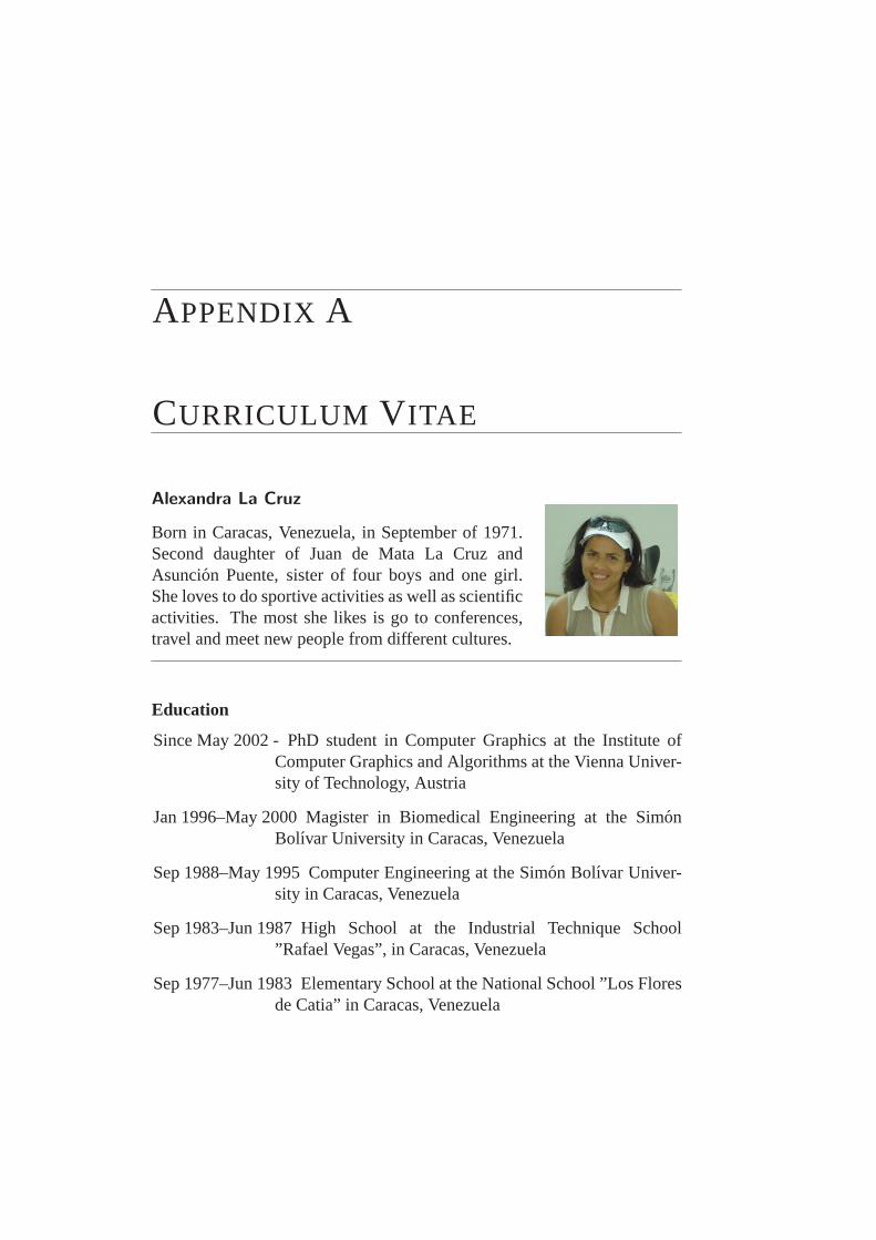
APPENDIX A
CURRICULUM VITAE
Alexandra La Cruz
Born in Caracas, Venezuela, in September of 1971.Second daughter of Juan de Mata La Cruz andAsuncion Puente, sister of four boys and one girl.She loves to do sportive activities as well as scientificactivities. The most she likes is go to conferences,travel and meet new people from different cultures.
Education
Since May 2002 - PhD student in Computer Graphics at the Institute ofComputer Graphics and Algorithms at the Vienna Univer-sity of Technology, Austria
Jan 1996–May 2000 Magister in Biomedical Engineering at the SimonBolıvar University in Caracas, Venezuela
Sep 1988–May 1995 Computer Engineering at the Simon Bolıvar Univer-sity in Caracas, Venezuela
Sep 1983–Jun 1987 High School at the Industrial Technique School”Rafael Vegas”, in Caracas, Venezuela
Sep 1977–Jun 1983 Elementary School at the National School ”Los Floresde Catia” in Caracas, Venezuela
Curriculum Vitae
Summary of Qualifications
• Research experience in the field of medical image processing, com-puter graphics, modeling, simulation and biomedical data analysis.
• Teaching experience in post-graduate level course ”Image Process-ing”.
• Teaching experience in graduate level course ”Programming in C++”.
• Clinical and research experience in medical image processing (Com-puted Tomography, Coronary Angiography)
Awards, Scholarship
• Scholarship of the Universidad Simon Bolıvar 1988-1993.
• ORINOQUIA AWARD to the Applied Investigation. Period 1995-1996. ANIA: A tool for ANgiographic Image Analysis and study.Caracas, Venezuela.
• Excellence AWARD MARAVEN. Academic year 1996. SimonBolıvar University, Caracas, Venezuela.
• Mention Honorific by the theses work done for obtaining the Diplomaof Computer Engineering. Feb 1995. Simon Bolıvar University, Cara-cas, Venezuela.
• Scholarship of the Lateinamerika Institute, October 2004 until July2005.
• Scholarship of the Lateinamerika Institute since October 2005.
• Third place of Eurographics 2005 Medical Prize, for ”The Angio-Vis ToolBox”. Authors: Matus Straka, Milos Sramek, AlexandraLa Cruz, Eduard Groller Arnold Kochl and Dominik Fleischmann.Competition to acknowledge the contribution that computer graphicsis playing in the medical field, organized by the Eurographics Asso-ciation.
102
Curriculum Vitae
Related Short Courses
• Fourth IEEE-EMBS International Summer School on BiomedicalImaging. June 17- 24, 2000, Ile de Berder, Bretagne, France. Co-Chairs: Christian Roux, Jean-Louis Coatrieux.
• Course on Medical Imaging. Bio-engineering and Applied Bio-physic Group. Simon Bolıvar University. Caracas, Venezuela. 1995
Professional Experience
Jun 2004–Aug 2004 Research Assistant at the University of Medicine ofVienna, AUSTRIA
May 2002–May 2004 Research Assistant at the Institute of ComputerGraphics and Algorithms, Vienna University of Technol-ogy, Vienna, Austria
May 1998–Abr 2002 Project Manager at Hipercom, System Department
Jan 1996–Dec 1997 Teaching Assistant at the Simon Bolıvar Univer-sity, Computer and Technology Department, Caracas,Venezuela
Jan 1995–Dec 1996 Research Assistant at Simon Bolıvar University, Re-search and Development Department
Feb 1994–Dec 1995 Research Assistant at Bio-engineering and AppliedBio-physic Group, Simon Bolıvar University, Caracas,Venezuela
Publication List
LS12004 La Cruz A., Straka M., Kochl A., Sramek M., Groller E.,Fleischmann D.: Non-linear Model Fitting to Parameter-ize Diseased Blood Vessels. In proceedings of IEEE Visu-alization 2004, Austin, USA. 10-15 October. pp. 393-400.
SCL2004 Straka M., Cervenansky M., La Cruz A., KochlA., Sramek M., Groller E., Fleischmann D.: TheVesselGlyph: Focus & Context Visualization in CT-Angiography. In proceedings of IEEE Visualization 2004,Austin, USA. 10-15 October. pp. 385-392.
103
Curriculum Vitae
ALC2004 La Cruz A.: Accuracy Evaluation of Different Center-line Approximations of Blood Vessels. Data Visualiza-tion 2004, Eurographics/IEEE TCVG, Visualization Sym-posium Proceedings. In cooperation with ACM SIG-GRAPH. Konstanz, Germany, May 2004. pp. 115-120.
LS22004 La Cruz A., Straka M., Kochl A., Sramek M., Groller E.,and Fleischmann D.: Accuracy of Automated CenterlineApproximation Algorithms for Lower Extremity Vesselsin a CTA Phantom. Electronic Poster in ECR 2004, Aus-tria. March. Supplement 2, Volume 14, ECR. pp. 524.
AL12004 La Cruz A., Straka M., Kochl A., Sramek M., GrollerE., Fleischmann D.: Non-linear Model Fitting to Parame-terize Diseased Blood Vessels. Technical Report TR-186-2-04-05, Institute of Computer Graphics and Algorithms,Vienna University of Technology. May 2004.
AL12003 La Cruz A.: Accuracy Evaluation of Different Center-line Approximations of Blood Vessels. Technical ReportTR-186-2-03-12, Institute of Computer Graphics and Al-gorithms, Vienna University of Technology. December2003.
BFL2003 Buhler K., Felkel P., and La Cruz A.: Geometric Meth-ods for Vessel Visualization and Quantification - A Sur-vey. Geometric Modelling for Scientific Visualization. G.Brunnett, B. Hammann, H. Muller, and L. Linsen, editors.Springer. 2003. pp. 399-421.
SL12003 Straka M., La Cruz A., Kochl A., Sramek M., Groller, E.,Fleischmann D.: Bone Segmentation in CT-AngiographyData Using a Probabilistic Atlas. In proceedings of VMV2003. November Munich, Germany. pp. 505-512.
SL22003 M. Straka, La Cruz A., Kochl A., Sramek M., GrollerE., Fleischmann D.: 3D Watershed Transform Combinedwith a Probabilistic Atlas for Medical Image Segmenta-tion. Journal of Medical Informatics and Technologies,Vol.6. November 2003, pp IT-69-IT-78.
104
Curriculum Vitae
NGG2000 Ng, F., Garcia, I., Gomis, P., La Cruz, A., Passariello, G.,Mora, F. Bayesian hierarchical model with wavelet trans-form coefficients of the ECG in obstructive sleep apneascreening; Computers in Cardiology 2000 , 24-27 Septem-ber. pp. 275-278.
LW11998 La Cruz A., Windyga P., Bevilacqua G., Mora F., Pas-sariello G.: Angiographic Image Analysis and Study ToolANIA: First Application. Devices, Circuits and Systems,1998. Proceedings of the 1998 Second IEEE InternationalCaracas Conference, 2-4 March. pp. 282-284.
LW21997 La Cruz A., Windyga P., Bevilacqua G., Garreau M.,Coatrieux J.L.: Analytic Description of the EstimatedVentricular Surface from Coronary Arteries. Engineeringin Medicine and Biology society, 1997. Proceedings of the19th Annual International Conference of the IEEE, Vol-ume 2, 30 October - 2 November. pp. 845-847.
LLR1997 La Cruz A., Lecuna M., Rodrıguez N., Windyga P.,Bevilacqua G.: Utilidad de la Rectificacion de Imagenesen el Problema de la Reconstruccion Tridimensional(3D) de Arterias Coronarias a partir de Imagenes An-giograficas Biplano. Avances Recientes en Bioinge-nierıa, Investigacion y Tecnologıa Aplicada, 1997, So-ciedad Venezolana de Metodos Numericos en Ingenierıa,Editores: Barrios V., Montilla G., Cerrolaza M., Valencia,Venezuela. pp. 29-36.
LDW1997 La Cruz A., Dibe M., Windyga P., Bevilacqua G.: De-scripcion Analıtica de la Superficie Ventricular Estimadaa partir de las Arterias Coronarias. Avances Recientesen Bioingenierıa, Investigacion y Tecnologıa Aplicada,1997, Sociedad Venezolana de Metodos Numericos en In-genierıa, Editores: Barrios V., Montilla G., Cerrolaza M.,Valencia-Venezuela. pp. 23-28.
LM11995 La Cruz A., Morinelli G., Windyga P., Bevilacqua G.,Silva J.: ANIA, A Tool for Angiographic Image Analysis
105
Curriculum Vitae
and Study. In proceedings of Annual Conference of En-gineering in Medicine and Biology Society, 1995. IEEE.Volume 1, 20-23 September. pp. 381-382.
LM21995 La Cruz A., Morinelli G., Windyga P.: ANIA, Her-ramienta para el Analisis de Imagenes Angiograficas.Acta Cientıfica Venezolana, 1995, XLV Convencion An-ual de ASOVAC, Caracas, Venezuela. pp. 238.
HobbysSportive activities in general, Volleyball, Biking, Climbing, Inline Skating,Swimming, Skiing, Cinema, Dance, Travel, Music, Dive lovely.
Language KnowledgeSpanish: native / English: fluently / German: fair / French: fair
Vienna, January 27, 2006
106