A Fast Rotating Bose-Einstein Condensate on a Disc

Diplomarbeitzur Erlangung des akademischen Grades

Mag. rer. nat.an der

Fakultat fur Physikder Universitat Wien

Autor: Florian PinskerMatrikel-Nummer: 0404721Studienrichtung: 411 PhysikBetreuer: O. Univ. Prof. Dr. Jakob Yngvason

Wien, Dezember 2009

1

2

1 Zusammenfassung/Abstract

In der vorliegenden Arbeit studieren wir ein schnell rotierendes Bose-Einstein Kondensat auf einerScheibe im Grenzwert starker Wechselwirkung (Thomas-Fermi Limes) mithilfe der 2D Gross-Pitaevskii(GP) Theorie. Wir bestimmen sowohl eine untere als auch eine obere Schranke zur Energie eines solchenBose Gases mit Dirichlet Randbedingung. Ein Beweis dieser Schranken unter Neumann Randbedin-gungen wurde zuerst in den Arbeiten [CY], [CDY] gefuhrt. Unser Beitrag besteht unter anderemdarin, diese Betrachtungen durch einen zusatzlichen Faktor in der Versuchswellenfunktion auf den Fallvon Dirichlet Randbedingungen zu erweitern. Dabei zeigen wir methodisch analog zu [CDY], dass ineinem bestimmten Bereich der Drehgeschwindigkeit keine zusatzlichen Beitrage zur fuhrenden und derdarauffolgenden Ordnung zur oberen Schranke der GP Energie aufkommen. Des Weiteren finden wirunter Verwendung einer Variationsgleichung, die mit einem weiteren GP Funktional assoziert ist, dass eseine additive Zerlegung des GP Energiefunktionals gibt. Dies fuhrt zu der getrennten Betrachtung vonzwei verschiedenen Funktionalen. Das eine berucksichtigt den Beitrag zur Energie durch die Wirbel imKondensat und das andere den Beitrag des Profiles des Bose-Einstein Kondesates. Diese Methode liefertim Prinzip bessere Schranken als die vorherige.

In this work we study a rapidly rotating Bose-Einstein condensate on a disc in the strong cou-pling (Thomas-Fermi) limit in the 2D Gross-Pitaevskii (GP) framework. We establish upper and lowerbounds to the energy of the Bose Gas under Dirichlet boundary conditions. The case of Neumannboundary conditions has already been considered in [CY] and [CDY]. In the present work theseconsiderations are extended by including an additional factor in the trial function for the upper boundto ensure Dirichlet boundary conditions. We show explicitly that this does not effect the contributionto the leading and subleading order of the GP energy in a certain regime of the rotational velocity.Moreover, by using a variational equation associated with the minimizer of an auxiliary GP functionalan additive decoupling of the GP energy functional is achieved. This leads us to consider two functionalsseperately, one accounting for the contribution of the vortices and the other for the density profile of theBose-Einstein condensate. This method leads in principle to better bounds than the previous approach.

3

Contents

1 Zusammenfassung/Abstract 2

2 Introduction 42.1 Historical Overview . . . . . . . . . . . . . . . . . . . . . . . . . . . . . . . . . . . . . . . . 4

3 Mathematical Framework and Methods 43.1 Hamiltonian . . . . . . . . . . . . . . . . . . . . . . . . . . . . . . . . . . . . . . . . . . . . 4

3.1.1 Two-Particle Scattering Length a . . . . . . . . . . . . . . . . . . . . . . . . . . . . 53.2 Bose-Einstein Condensation . . . . . . . . . . . . . . . . . . . . . . . . . . . . . . . . . . . 53.3 The Gross-Pitaevskii Framework . . . . . . . . . . . . . . . . . . . . . . . . . . . . . . . . 6

3.3.1 Complete BEC in the GP Limes . . . . . . . . . . . . . . . . . . . . . . . . . . . . 73.4 GP Energy in 2D and its Correspondence to the Many Body Problem . . . . . . . . . . . 83.5 A Rapidly Rotating Bose Gas on a Disc . . . . . . . . . . . . . . . . . . . . . . . . . . . . 9

3.5.1 Spherical Symmetry and the Emergence of Vortices . . . . . . . . . . . . . . . . . 11

4 Main Results 12

5 Energy Asymptotics with Dirichlet Boundary Condition 145.1 Energy Upper Bound . . . . . . . . . . . . . . . . . . . . . . . . . . . . . . . . . . . . . . . 145.2 Energy Lower Bound and Asymptotics . . . . . . . . . . . . . . . . . . . . . . . . . . . . . 19

6 A Refined Method to Determine the Energy 216.1 Additive Decoupling of the Energy . . . . . . . . . . . . . . . . . . . . . . . . . . . . . . . 216.2 Estimates on EGP . . . . . . . . . . . . . . . . . . . . . . . . . . . . . . . . . . . . . . . . 216.3 Analysis of the Minimizer g . . . . . . . . . . . . . . . . . . . . . . . . . . . . . . . . . . . 246.4 Upper Bound to the Vortex Functional Fg[u] . . . . . . . . . . . . . . . . . . . . . . . . . 346.5 Energy Lower Bound . . . . . . . . . . . . . . . . . . . . . . . . . . . . . . . . . . . . . . . 37

6.5.1 Separation of the Energy . . . . . . . . . . . . . . . . . . . . . . . . . . . . . . . . 376.5.2 Lower Bound to the Ginzburg-Landau (GL) Type Functional Eg[u] . . . . . . . . . 37

7 Conclusions 39

A The TF Energy and Density 40

B Further Analysis of the Minimizer 40

C Acknowlegdments 41

4

2 Introduction

2.1 Historical Overview

In 1924 S.N. Bose derived Planck’s formula for the spectral distribution of the energy of photons in acavity by using a new way of counting the possible states that differed from classical Boltzmann statistics[Bo]. Einstein [E] realized that the method of Bose could also be used in the quantum theory of anideal gas of material particles. Moreover, he discovered in the same work that in thermal equilibriumat sufficiently low temperature (depending on the density) a macroscopic number of particles of the gasoccupied the ground state. We now refer to this phenomenom as Bose-Einstein condensation (BEC), butin those years it was more a mathematical feature than an experimentally proven fact. Shortly afterwardsthe formalism of quantum mechanics was developed, and the statistics of particles were implemented inthe symmetry properties of the many-particle wave function: Symmetric wave functions decribe bosonswith integer spin and antisymmetric fermions with half-integer spin. This distinction implies that onlybosons reach a common single state. Liquid Helium (4He) was suggested first to be a candidate forthe realization of a BE condensate, but the situation has not yet be clarified rigorously, because thestrong interaction between the helium atoms has to be taken into account. Bogoliubov [Bog] analyzedsystematically a weakly interacting Bose gas at T = 0K and derived through an ingenious approximationto the Hamiltonian (written in terms of creation and annihilation operators) the energy of the groundstate and of excitations by quasiparticles.

An experimental breakthrough was achieved by Cornell and Wieman [CW] and a short time later in thesame year with a different approach (a novel trap) by the Ketterle [K1] group. Both groups experimentallyrealized BEC, the first with rubidium and the latter with a sodium isotope and a three orders of magnitudelarger number of Bose-condensed atoms. A wide variety of experimental setups followed, carried outworldwide by different scientists, and BE condensates became and still are an important area in research[K2]. Extensive theoretical studies have also been performed. For these the Gross-Pitaevskii (GP)framework has been very important. The GP equation, a nonlinear (cubic) Schrodinger equation, has theadvantage to be less complex compared to the many particle Schrodinger equation. The monograph [A]and the review article [F] describe extensively the mathematical modelling of the Bose-Einstein condensateand in particular the GP theory for different traps and its connection to recent experiments. As universeof discourse many investigations have the effect of rotation on the formation of BE condensates. Indeed,these condensates respond to rotation with a wide range of phenomena, such as the appearance ofquantized vortices in a particular shape and their arrangement. Experimentally, quantized vortices in BEcondensates where realized in 1999 for example by the Cornell and Wiemann group [CW2]. On the otherhand a mathematically rigorous proof of the asymptotical exactness of the GP description of the Bosegas with repulsive interaction was derived by Lieb, Seiringer and Yngvason [LSY], [LS1] and additionallythe existence of 100% BEC [LS1], [LS2]. It was shown in [SchY] that a 2D GP functional also reproducesthe energy of the many body problem with strong confinement in one direction or for highly elongatedtraps.

3 Mathematical Framework and Methods

3.1 Hamiltonian

As starting point we consider a Hamiltonian for N interacting particles acting on bosonic wave functions,i.e., on the symmetric part of a Hilbert space L2(R3N , d~x1, . . . d~xN ),

H =N∑i=1

H(i)0 +

∑1≤i<j≤N

v(|~xi − ~xj |), (3.1)

5

where v is a spherically symmetric, positive two-particle interaction, which decreases faster than |~x|−3 atinfinity, and H0 is a one particle Hamiltonian. We use units in which ~ = 2m = 1, where m denotes themass of a single particle. Since we are interested in identical bosons in a rotating trap, we consider theone-particle quantum mechanical Hamiltonian in a rotating reference frame of the form

H0 = −∆− ~L · ~Ω + V (~x) (3.2)

acting on the one-particle Hilbert space L2(R3, d~x). H(i)0 denotes the corresponding operator for the

particle i. Here ~Ω denotes the rotational velocity, V (~x) the trapping potential, ~x the position operatorand ~L = −i~x × ~∇ its angular momentum operator. We choose ~Ω = Ω~ez and by introducing the vectorpotential ~A = 1

2Ω(~ez × ~x), where ~ez is the unit vector in z-direction, we are able to write (3.1) as

H =N∑i=1

(i~∇j + ~A(~xj)

)2

+ V (~xj)−14

Ω2x2j

+

∑1≤j<k≤N

v(|~xj − ~xk|) (3.3)

with the distance from the rotational axis r ≡ |~ez × ~x|. In the rotating frame the vector potential ~A canbe seen as the Coriolis part of this Hamiltonian and −Ω2r2/4 contributes the centrifugal force. In orderto confine the condensate we require for the trapping potential V (~x) : R3 → R

V (~x) ≥ Ω2x2/4 (3.4)

as x ≡ |~x| → ∞. The simplest way to fulfill this condition is to assume V (λ~x) = λsV (~x) for λ > 0 withs > 2.

We denote the ground state energy of (3.1) by EQM and the corresponding many-particle wave functionΨ0. The particle density of the ground state is defined by

ρQM(~x) ≡ N∫|Ψ0(~x, ~X)|2d~x2 · · · d~xN (3.5)

with the notation ~X ≡ (~x2, . . . , ~xN ).

3.1.1 Two-Particle Scattering Length a

The scattering length a is defined by means of the zero scattering Schrodinger equation

(−2∆ + v(x))ψ = 0 (3.6)

with the boundary condition ψ(~x)→ 1 as |~x| → ∞. If the potential has finite range R0, then the solutionsatisfies for |~x| > R0

ψ(~x) = 1− a

|~x|(3.7)

which defines a. We also note that if v1 has scattering length 1, then va(~x) = a−2v1(~x/a) has scatteringlength a.

3.2 Bose-Einstein Condensation

We now define the term ‘Bose-Einstein condensation’ using the notion of second quantization: First weintroduce creation- and annihilation operators a(ϕ)∗ and a(ϕ) for a one-particle state ϕ. Let 〈·〉 denotesome many-particle state. Then the expectation value for the occupation number of ϕ in the state 〈·〉 isgiven by

Nϕ = 〈a(ϕ)∗a(ϕ)〉 (3.8)

6

and the total particle number is given by

N =∑i

〈a(ψi)∗a(ψi)〉, (3.9)

where ψi is a complete orthonormal basis of the one-particle Hilbert space L2(R3, d~r).

Definition 3.1 (Bose-Einstein Condensation in a State ϕ [OP])There is a c > 0 such that

Nϕ/N ≥ c (3.10)

for all large N .

In this sense we have macroscopic occupation of a single-particle state. If there is a unique macroscopicϕ we may describe a BE condensate by this single complex-valued wave function. It is then referred toas the wave function of the condensate.

The concept of BEC can also be formulated in terms of the one-particle density matrix

γ(~x, ~x′) = 〈a(~x)∗a(~x′)〉. (3.11)

Here BEC means that this density matrix has at least one eigenvalue which is O(N).

3.3 The Gross-Pitaevskii Framework

Theoretical investigations of dilute Bose gases at low temperatures are usually carried out within Gross-Pitaevskii theory [G], [P]. Its connection with the quantum mechanical many body problem was estab-lished rigorously in [LSY] for nonrotating gases and in [LS2] for the rotating case. In the GP theory weconsider an energy functional [DGP] of complex-valued wave functions φ(~x) with ~x ∈ R3. It is given by

EGP[φ] = 〈φ|H0|φ〉+ 4πa/N∫

R3|φ(~x)|4d~x. (3.12)

The GP energy EGP is defined as the infimum of EGP[φ] over all φ under the mass constraint ‖φ‖22 = N .This infimum is indeed a minimum, i.e., there exists a φGP with

EGP ≡ inf‖φ‖2=N

EGP[φ] = EGP[φGP]. (3.13)

The GP energy fulfills the scaling relation

EGPN,a = NEGP

1,Na. (3.14)

The minimizer φGP is in general not unique in the rotating case [LS1], but every minimizer satisfies avariational equation, the so called GP equation,

(−i~∇+ ~A(~x))2φ(~x) + V (~x)φ(~x) + 8πa|φ(~x)|2φ(~x) = µGPφ. (3.15)

Here µGP is the chemical potential given by

µGP = dEGP(N, 1)/dN = EGP(N, 1)/N + (4πa/N)∫

R3|φGP(~x)|4d~x. (3.16)

The GP density is defined asρGPN,a(~x) ≡ |φGP(~x)|2 (3.17)

7

and satisfies the scaling relationρGPN,a(~x) = NρGP

1,Na(~x). (3.18)

We define the coupling constant g asg ≡ aN. (3.19)

Next, we define the so-called GP limit, in which the GP energy EGP becomes equivalent to EQM.

Definition 3.2 (The GP Limit)As N → ∞ we fix the external trapping potential V and simultaneously let the interparticle potential vbe scaled with N , such that a is related to N by the condition

Na = g fixed. (3.20)

More precisely, v(~x) = a2v1(~x/a), where v1 is fixed with scattering length 1, and a = g/N .

The mean GP density ρGP is defined by

ρGP ≡ 1N

∫|ρGPN,a(~x)|2d~x. (3.21)

Per definition a ∼ N−1. Inserting (3.18) into (3.21) yields a3ρGP ∼ N−2, i.e., we consider dilute systemsin the GP limit,

a3ρGP 1. (3.22)

The ground state energy EQM of (3.1) is a function of the confining potential V , the interaction potentialv and N . As in [S1] we introduce for V and v1 fixed with v fulfilling above scaling relations the notationEQM(N, a). It turns out that in the GP limit the minimum of the GP functional EGP correctly de-scribes the ground state energy of a trapped, non-rotating and rotating Bose gas with repulsive two-bodyinteraction [LSY], [LS2], whereby in the latter case Ω is fixed.

Theorem 3.1 (In the GP Limit the QM Ground State Energy is EGP)If N →∞ with g fixed, then

limN→∞

EQM(N, a)N

= EGP(1, g). (3.23)

For a non-rotating gas (~Ω = 0) it is proven that in the GP limit the GP density ρGP converges to ρQM

in the weak L1 sense [LSY]. In a rotating system the possibility of rotational symmetry breaking andensuring nonuniqueness of the GP minimizer has to be taken into account. Furthermore, the absolutemany-body ground state is in general not the same as the bosonic ground state Ψ0.

3.3.1 Complete BEC in the GP Limes

An important fact derived in [LS1] and [LS2] is that there is complete BEC in the GP limit. In particular,when we consider a non-rotating gas, the wave function of the condensate is the unique minimizer of theGP functional φGP.

Theorem 3.2 (BEC in the GP Limit, Nonrotating Case)For each fixed g

limN→∞

1Nγ(~x, ~x′) = φGP(~x)φGP(~x′) (3.24)

converges in the sense that tr | 1N γ − P

GP| → 0 where PGP ≡ |φGP〉〈φGP|.

8

There is actually more to explain about the BE condensation of a rotating Bose gas [LS2]: Let anapproximate ground state be defined as a sequence of bosonic N -particle density matrices γN for whichlimN→∞N−1 trHγN = EGP(1, g). We denote the reduced density matrix to γN as γ(1)

N . This matrixis a positive trace class operator on the one-particle Hilbert space L2(R3) and in the following it isnormalized to Trγ(1)

N = 1. Now, by applying the Banach-Alaoglu Theorem (see for example [LL]) Lieband Seiringer find that any sequence γ(1)

N has a subsequence that converges to a γ in weak-* topology,i.e., limN→∞ TrAγ(1)

N = TrAγ for every compact operator A. Additionaly, one can show that Trγ =limN→∞TrγN = 1. As a consequence we have limN→∞ Tr|γ(1)

N − γ| = 0. In fact, considering onlypositive operators, weak-* convergence together with convergence of the trace implies convergence intrace norm.

Let us now define the set of all γ’s that are limit points of one-particle density matrices of approximateground states. That is,

Γ =γ : there is a sequence γN , lim

N→∞

1N

trHγN = EGP(1, g = Na), limN→∞

γ(1)N = γ

. (3.25)

The convergence of γ(1)N → γ can either mean weak-* convergence or norm convergence. In particular

norm convergence implies that tr γ = 1 for all γ ∈ Γ.

Theorem 3.3 (BEC in the GP Limit for Rotating Bose Gases)The set γ of one-particle density matrices of approximate ground states, as defined in (3.25), has thefollowing properties.

1. Γ is a compact and convex subset of the set of all trace class operators.

2. Let Γext ⊂ Γ denote the set of extreme points in Γ. (An element γ ∈ Γ is extreme if γ cannot bewritten as γ = aγ1 +(1−a)γ2 with γ1,2 ∈ Γ, γ1 6= γ2 and 0 < a < 1.) We have Γext = |φGP〉〈φGP| :EGP[φGP] = EGP(g), i.e., the extreme points in Γ are given by the rank-one projections onto GPminimizers

3. For each γ ∈ Γ, there is a positive (regular Borel) measure dµγ , supported in Γext, with∫Γext

dµγ(φGP) = 1, such that

γ =∫

Γext

dµγ(φGP)|φGP〉〈φGP|, (3.26)

where the integral is understood in the weak sense. That is, every γ ∈ Γ is a convex combination ofrank-one projetions onto GP minimizers.

By assuming the trapping potential to be slightly asymmetric, a minimizer in which to condensate mightbe distinguished (and it is expected that Γext then contains only one element), such that one has completeBEC.

3.4 GP Energy in 2D and its Correspondence to the Many Body Problem

We now restrict our consideration to a 2D domain. It is applicable if one considers strong confinementof the condensate in one direction. A rigorous proof of the crossover from the Hamiltonian (3.1) withoutrotation (~Ω = 0) to the GP energy in 2D has been achieved in [SchY]. We explain their setting andthe main theorem shortly: The particles are strongly confined in z-direction. We introduce the notation(~r, z) = ~x ∈ R3, with ~r ∈ R2 and z ∈ R. Further on, we consider trapping potentials of the form

VL,h(~x) = VL(~r) + V ⊥h (z) =1L2V (L−1~r) +

1h2V ⊥(h−1z) (3.27)

9

with V and V ⊥ fixed and consider h and L as parameter. Additionally, v has the parameter a. It isassumed that V (x) and V ⊥(z) are locally bounded and V (x), V ⊥(z)→∞ as |x|, |z| → ∞. So, the groundstate energy of (3.1) for ~Ω = 0 has the scaling property

EQM(N,h, a, L) =1L2EQM(N,h/L, a/L, 1). (3.28)

In contrast to the GP limes we have considered before the ratio h/L is not fixed, but tends to zero. Wedenote the ground state energy of −d2/dz2 +V ⊥(z) by e⊥ and the normalized ground state wave functionas s(z).

We now turn to the two-dimensional GP functional defined analogously as in 3D, but we consider thedomain of the wave functions to be R2. Additionally the coupling parameter is given by

g2D = | ln(ρa22D)|−1. (3.29)

For simplicity we mean in the following g2D but write g. We define the mean density ρ as

ρNg =1N

∫|ϕGPNg |4d~r (3.30)

where ϕGP(~r)Ng is a minimizer of the 2D GP functional. The 2D scattering length is defined by

a2D = h exp

(−(∫

s(z)4dz

)−1

h/2a

). (3.31)

The GP energy per particle in 2D is defined as

EGP2D (N,L, g)/N = inf

EGP

2D [ϕ],∫|ϕ(~x)|2d2~x = 1

=

1L2EGP

2D (1, 1, Ng), (3.32)

where the last step points out the scaling of V ⊥ and the GP minimizer.

Theorem 3.4 (From 3D to 2D, Ground State Energy)Let N →∞ and at the same time h/L→ 0 and a/h→ 0 in such a way that h2ρg2D → 0 (with g2D givenby (3.29) ). Then

limEQM(N,L, h, a)−Nh−2e⊥

EGP2D (N,L, g)

= 1. (3.33)

The meaning of h2ρg → 0 is that the ground state energy h−2e⊥ associated with the confining potential inthe z−direction is much larger than the energy ρg. This is the so-called condition of strong confinement.

Remark: In our proof we consider a rapidly rotating Bose gas in 2D. We assume that (3.33) is trueeven for Ω → ∞ and g2D → ∞ (possibly with some additional constraint on diluteness), although thisstill remains to be proved rigorously.

3.5 A Rapidly Rotating Bose Gas on a Disc

Now, we consider a 2D GP functional of wave functions on a disc of finite radius and center at the origin.We write the 2D coupling parameter as g2D = 1/ε2 and consider a regime of ‘rapid rotation’ by whichwe mean

| log ε| Ω 1ε2| log ε|

(3.34)

with ε→ 0. We assume the rotational axis to be perpendicular to the disc and to be located at its center.Moreover, the confining potential V (~r) is assumed to be zero inside a finite radius R and infinite beyond,

10

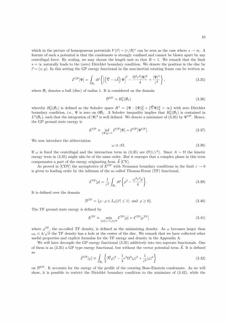
which in the picture of homogeneous potentials V (~r) ∼ (r/R)s can be seen as the case where s→∞. Afeature of such a potential is that the condensate is strongly confined and cannot be blown apart by anycentrifugal force. By scaling, we may choose the length unit so that R = 1. We remark that the limits =∞ naturally leads to the (zero) Dirichlet boundary condition. We denote the position in the disc by~r = (x, y). In this setting the GP energy functional in the non-inertial rotating frame can be written as

EGP[Ψ] =∫B1

d~r

∣∣∣(~∇− i ~A)Ψ∣∣∣2 − Ω2r2|Ψ|2

4+|Ψ|4

ε2

, (3.35)

where B1 denotes a ball (disc) of radius 1. It is considered on the domain

DGP = H10 (B1) (3.36)

whereby H10 (B1) is defined as the Sobolev space H1 = Ψ : ‖Ψ‖22 + ‖~∇Ψ‖22 < ∞ with zero Dirichlet

boundary condition, i.e., Ψ is zero on ∂B1. A Sobolev inequality implies that H10 (B1) is contained in

L4(B1), such that the integration of |Ψ|4 is well defined. We denote a minimizer of (3.35) by ΨGP. Hence,the GP ground state energy is

EGP ≡ inf‖Ψ‖2=1

EGP[Ψ] = EGP[ΨGP]. (3.37)

We now introduce the abbreviationω ≡ εΩ. (3.38)

If ω is fixed the centrifugal and the interaction term in (3.35) are O(1/ε2). Since A ∼ Ω the kineticenergy term in (3.35) might also be of the same order. But it emerges that a complex phase in this termcompensates a part of the energy originating from ~A [CY].

As proved in [CDY] the asymptotics of EGP with Neumann boundary conditions in the limit ε → 0is given to leading order by the infimum of the so called Thomas-Fermi (TF) functional,

ETF[ρ] =1ε2

∫B1

d~r

ρ2 − ω2r2ρ

4

. (3.39)

It is defined over the domain

DTF = ρ : ρ ∈ L2(|~r| ≤ 1) and ρ ≥ 0. (3.40)

The TF ground state energy is defined by

ETF ≡ min‖ρ‖1=1,ρ≥0

ETF[ρ] = ETF[ρTF] (3.41)

where ρTF, the so-called TF density, is defined as the minimizing density. As ω becomes larger thanωh ≡ 4/

√π the TF density has a hole at the center of the disc. We remark that we have collected other

useful properties and explicit formulas for the TF energy and density in the Appendix A.We will later decouple the GP energy functional (3.35) additively into two seperate functionals. One

of them is as (3.35) a GP type energy functional, but without the vector potential term ~A. It is definedas

EGP[ϕ] ≡∫B1

|~∇ϕ|2 − 1

4r2Ω2|ϕ|2 +

1ε2|ϕ|4

(3.42)

on DGP. It accounts for the energy of the profile of the rotating Bose-Einstein condensate. As we willshow, it is possible to restrict the Dirichlet boundary condition to the minimizer of (3.42), while the

11

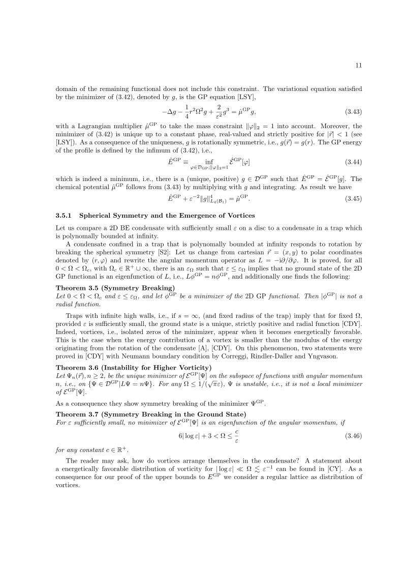
domain of the remaining functional does not include this constraint. The variational equation satisfiedby the minimizer of (3.42), denoted by g, is the GP equation [LSY],

−∆g − 14r2Ω2g +

2ε2g3 = µGPg, (3.43)

with a Lagrangian multiplier µGP to take the mass constraint ‖ϕ‖2 = 1 into account. Moreover, theminimizer of (3.42) is unique up to a constant phase, real-valued and strictly positive for |~r| < 1 (see[LSY]). As a consequence of the uniqueness, g is rotationally symmetric, i.e., g(~r) = g(r). The GP energyof the profile is defined by the infimum of (3.42), i.e.,

EGP ≡ infϕ∈DGP;‖ϕ‖2=1

EGP[ϕ] (3.44)

which is indeed a minimum, i.e., there is a (unique, positive) g ∈ DGP such that EGP = EGP[g]. Thechemical potential µGP follows from (3.43) by multiplying with g and integrating. As result we have

EGP + ε−2‖g‖4L4(B1) = µGP. (3.45)

3.5.1 Spherical Symmetry and the Emergence of Vortices

Let us compare a 2D BE condensate with sufficiently small ε on a disc to a condensate in a trap whichis polynomally bounded at infinity.

A condensate confined in a trap that is polynomally bounded at infinity responds to rotation bybreaking the spherical symmetry [S2]: Let us change from cartesian ~r = (x, y) to polar coordinatesdenoted by (r, ϕ) and rewrite the angular momentum operator as L = −i∂/∂ϕ. It is proved, for all0 < Ω < Ωc, with Ωc ∈ R+ ∪∞, there is an εΩ such that ε ≤ εΩ implies that no ground state of the 2DGP functional is an eigenfunction of L, i.e., LφGP = nφGP, and additionally one finds the following:

Theorem 3.5 (Symmetry Breaking)Let 0 < Ω < Ωc and ε ≤ εΩ, and let φGP be a minimizer of the 2D GP functional. Then |φGP| is not aradial function.

Traps with infinite high walls, i.e., if s = ∞, (and fixed radius of the trap) imply that for fixed Ω,provided ε is sufficiently small, the ground state is a unique, strictly positive and radial function [CDY].Indeed, vortices, i.e., isolated zeros of the minimizer, appear when it becomes energetically favorable.This is the case when the energy contribution of a vortex is smaller than the modulus of the energyoriginating from the rotation of the condensate [A], [CDY]. On this phenomenon, two statements wereproved in [CDY] with Neumann boundary condition by Correggi, Rindler-Daller and Yngvason.

Theorem 3.6 (Instability for Higher Vorticity)Let Ψn(~r), n ≥ 2, be the unique minimizer of EGP[Ψ] on the subspace of functions with angular momentumn, i.e., on Ψ ∈ DGP|LΨ = nΨ. For any Ω ≤ 1/(

√πε), Ψ is unstable, i.e., it is not a local minimizer

of EGP[Ψ].

As a consequence they show symmetry breaking of the minimizer ΨGP.

Theorem 3.7 (Symmetry Breaking in the Ground State)For ε sufficiently small, no minimizer of EGP[Ψ] is an eigenfunction of the angular momentum, if

6| log ε|+ 3 < Ω ≤ c

ε(3.46)

for any constant c ∈ R+.

The reader may ask, how do vortices arrange themselves in the condensate? A statement abouta energetically favorable distribution of vorticity for | log ε| Ω . ε−1 can be found in [CY]. As aconsequence for our proof of the upper bounds to EGP we consider a regular lattice as distribution ofvortices.

12

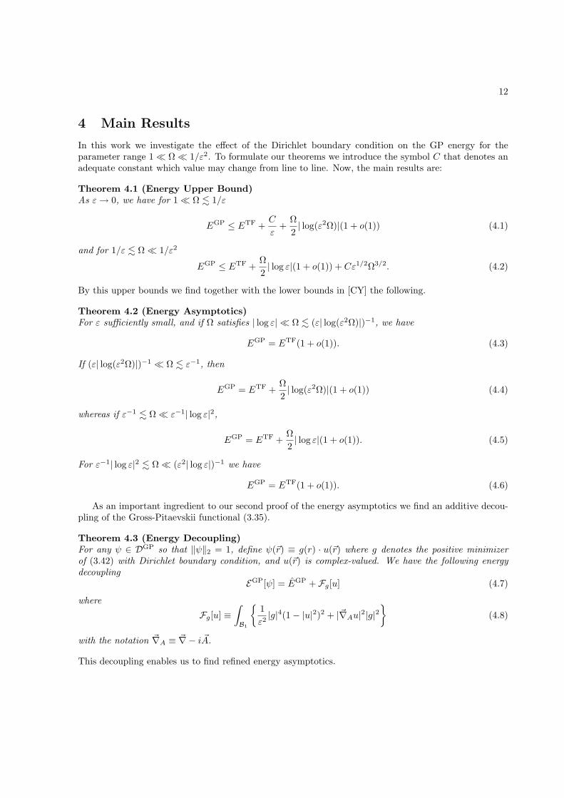
4 Main Results

In this work we investigate the effect of the Dirichlet boundary condition on the GP energy for theparameter range 1 Ω 1/ε2. To formulate our theorems we introduce the symbol C that denotes anadequate constant which value may change from line to line. Now, the main results are:

Theorem 4.1 (Energy Upper Bound)As ε→ 0, we have for 1 Ω . 1/ε

EGP ≤ ETF +C

ε+

Ω2| log(ε2Ω)|(1 + o(1)) (4.1)

and for 1/ε . Ω 1/ε2

EGP ≤ ETF +Ω2| log ε|(1 + o(1)) + Cε1/2Ω3/2. (4.2)

By this upper bounds we find together with the lower bounds in [CY] the following.

Theorem 4.2 (Energy Asymptotics)For ε sufficiently small, and if Ω satisfies | log ε| Ω . (ε| log(ε2Ω)|)−1, we have

EGP = ETF(1 + o(1)). (4.3)

If (ε| log(ε2Ω)|)−1 Ω . ε−1, then

EGP = ETF +Ω2| log(ε2Ω)|(1 + o(1)) (4.4)

whereas if ε−1 . Ω ε−1| log ε|2,

EGP = ETF +Ω2| log ε|(1 + o(1)). (4.5)

For ε−1| log ε|2 . Ω (ε2| log ε|)−1 we have

EGP = ETF(1 + o(1)). (4.6)

As an important ingredient to our second proof of the energy asymptotics we find an additive decou-pling of the Gross-Pitaevskii functional (3.35).

Theorem 4.3 (Energy Decoupling)For any ψ ∈ DGP so that ‖ψ‖2 = 1, define ψ(~r) ≡ g(r) · u(~r) where g denotes the positive minimizerof (3.42) with Dirichlet boundary condition, and u(~r) is complex-valued. We have the following energydecoupling

EGP[ψ] = EGP + Fg[u] (4.7)

where

Fg[u] ≡∫B1

1ε2|g|4(1− |u|2)2 + |~∇Au|2|g|2

(4.8)

with the notation ~∇A ≡ ~∇− i ~A.

This decoupling enables us to find refined energy asymptotics.

13

Theorem 4.4 (Refined Energy Asymptotics)For ε sufficiently small, and if Ω satisfies | log ε| Ω . 1/ε we have

EGP = EGP +Ω2| log(ε2Ω)|(1 + o(1)), (4.9)

and for 1/ε . Ω (ε2| log ε|)−1

EGP = EGP +Ω2| log ε|(1 + o(1)). (4.10)

We remark that EGP is computable, since its minimizer solves an ordinary second order differentialequation. Starting from (4.7) we reproduce the upper bounds (4.1) and (4.2), and also the energyasymptotics (4.3), (4.4), (4.5) and (4.6).

14

5 Energy Asymptotics with Dirichlet Boundary Condition

It is our aim to examine the effect of the Dirichlet boundary condition. In particular we will prove inthis section that for sufficiently rapid rotation it has no effect on the first and second order contributionto the asymptotic expansion of EGP.

5.1 Energy Upper Bound

We start with the proof of Theorem 4.1.Proof: Imposing the Dirichlet boundary condition to the domain of the GP functional (3.35) means

requiring the wave function to be zero at the boundary of the disc ∂B1. To fulfill this requirement weextend the trial function of [CY] (equation 4.1) by a cut-off function which is zero at the boundary.Hence, we choose as ansatz a wave function of the form

Ψ(~r) ≡ c√ρ(~r)ξ(~r)g(~r)d(~r). (5.1)

Here c denotes the normalization constant, ρ a regularization of the density ρTF(~r), ξ(~r) a functionvanishing linearly at each vortex, i.e., at the singularities of the phase function g(~r), and d(~r) is afunction that takes care of the Dirichlet boundary condition. The latter is defined by

d(~r) ≡

1 ~r ∈ B1\I(1/δ) (1− r)) ~r ∈ I

(5.2)

with a parameter 1 δ > 0 and I is given by

I ≡ r|1− δ ≤ r ≤ 1.

The area of the annulus I is

A = 2πδ(

1− δ

2

). (5.3)

As in [CY] we decompose the disc B1 into cells Qi whose centers ~ri ∈ B1 are arranged in a regularlattice denoted by L. The lattice constant l is choosen so that each cells area is

|Qi| = 2πΩ, (5.4)

i.e.,l = CΩ−1/2 (5.5)

and the total number of lattice points inside B1 is given by

N =Ω2

(1 +O(Ω−1/2)). (5.6)

The number of lattice points in I is given by

NI = O(Ωδ). (5.7)

If ω = εΩ is large the area of supp ρTF is O(ω)−1 and the number of lattice points on the support of ρTF

is of the order

N ′ = O(

1ε

). (5.8)

15

Since C ' R2 the position vector ~r = (x, y) ∈ R2 can be written as a complex number ζ = x + iy ∈ C.So, we define the phase factor g as

g(~r) ≡∏ζi∈L

ζ − ζi|ζ − ζi|

. (5.9)

To get rid of the singularities of the phase factor g at the lattice points, we define the function

ξ(~r) ≡

1 if |ζ − ζi| > t for all it−1|ζ − ζi| if |ζ − ζi| ≤ t

(5.10)

where t is a variational parameter, which fulfills minε, (ε/Ω)1/2 ≤ t Ω−1/2 and will be fixed later.To justify the estimates on t we refer to the heuristics in [CY]. The function ξ(~r) generates discs Bit ofradius t with center at the lattice points ~ri ∈ L, where ξ vanishes, but is equal 1 in the complement tothose discs.

In the case where Ω ≤ ωh/ε, we set the density ρ to be equal to the TF density ρTF. If we considerω > ωh the density ρTF vanishes inside a hole of radius Rh = 1− Cω−1, but is abruptly increasing in rfor Rh < r (see (A.4)). Hence, the kinetic energy originating from the term

√ρTF is infinite. Therefore

it is necessary to regularize ρTF near the boundary of the hole. But it is also important that the densityremains similar to ρTF . Thus, if ω > ωh we define as in [CY], equation 4.9,

ρ(r) ≡

0 if r ≤ RhρTF(Rh + Ω−1)Ω2(r −Rh)2 if Rh ≤ r ≤ Rh + Ω−1

ρTF(r) otherwise(5.11)

Notice that the only difference to ρTF is that it is equal to ρTF(Rh + Ω−1)Ω2(r − Rh)2 inside Rh ≤r ≤ Rh + Ω−1, i.e., from the radius of the hole Rh the regularized density increases quadratically in anannulus of thickness ∼ Ω−1 with increasing distance from the hole. This construction guarantees a finitekinetic energy. By (A.4) we find that

ρTF(Rh + Ω−1) = O(ε2Ω) (5.12)

and so one hasρ(r) = ρTF(r) +O(ε2Ω) (5.13)

inside B1. Note that by assumption ε2Ω = o(1).Now, we calculate some useful estimates. Both functions, d2 and ξ2, are smaller than or equal to 1.

Thus, we haved2ξ2 ≥ 1− (1− ξ2)− (1− d2). (5.14)

By the explicit formula for the TF density (A.2) one gets ρTF ≤ C(ω + 1). Also recall that the numberof lattice points in support of ρTF is (5.8). Combining these facts together with (5.14), (5.13) we find∫

B1

ρξ2d2 ≥∫B1

ρ−∫∪iBti

ρ(1− ξ2)−∫Iρ(1− d2) ≥ 1− C(Ωt2)− C(ω + 1)δ. (5.15)

Thus, by the normalization condition ‖Ψ‖2 = 1 we get for the constant the estimate

c2 ≤ 1 + CΩt2 + C(ω + 1)δ. (5.16)

Since ρ, ξ, d are real-valued functions, d ≤ 1 and g is a phase factor, Cauchy-Schwarz inequality yields∣∣∣(~∇− i ~A) (√ρξgd)

∣∣∣2 = |~∇(√ρξd)g + i(gξ

√ρd~∇φ− ~Ad

√ρξg)|2 =

= |~∇(√ρξd)|2 + |dξ√ρ(~∇φ− ~A)|2 ≤

≤ 3(|~∇(ξ)|2ρ+ |~∇(

√ρ)|2ξ2 + |~∇(d)|2ρξ2

)+ |ξ√ρ(~∇− i ~A)g|2. (5.17)

16

Integration of (5.17) gives the contribution to the kinetic energy. The corresponding estimate for the firstterm on the right hand side in (5.17) is the same as in [CY]

‖√ρ~∇(ξ)‖22 ≤ CΩ. (5.18)

Also for the second term we may use the corresponding estimate in [CY], which is given by

||ξ∇(√ρ)||22 ≤

∫B1

|ξ|2 14|∇ρ|2

ρ≤ CΩ(ε2Ω) + C(ε2Ω)Ω| log ε|. (5.19)

Since (~∇(d))2 = 1/δ2 for all r ∈ I and zero inside B1−δ we find together with ρ ≤ ρTF(1) ≤ C(ω+ 1) theestimate

‖~∇(d)√

(ρ)ξ‖22 ≤∫B1

|~∇(d)|2ρ =1δ2

∫Iρ ' 1

δ2

∫ 1

1−δrρ ≤ C

δ(ω + 1). (5.20)

Putting the above estimates together we obtain for the difference between the GP and the TF functionalthe bound

EGP[Ψ]− ETF[|Ψ|2] = c2∫B1

|(~∇− i ~A

)(√ρξgd)|2

≤(1 + CΩt2 + C(ω + 1)δ

) ∫B1

ρξ2|(~∇− i ~A

)g|2+

+(1 + CΩt2 + C(ω + 1)δ

)(CΩ + C(ε2Ω)Ω| log ε|+ C(εΩ + 1)

δ

). (5.21)

We now claim an upper bound for the kinetic energy of the vortices.

Proposition 5.1 (Vortex Kinetic Energy)If ε→ 0 and 1 Ω 1/ε2, then∫

B1

ρξ2|(~∇− i ~A

)g|2 ≤ 1

2Ω| log(t2Ω)|+ CΩ + CΩ(ε2Ω)1/2| log(t2Ω)|. (5.22)

Proof: We apply an upper bound to the kinetic energy term proved in [CY], where they use anelectrostatic analogy. For completeness we repeat shortly their arguments: First we recall the definitionof g(~r), which can be written as a phase factor,

g(~r) =∏i

ζ − ζi|ζ − ζi|

= exp (iφ(~r)) (5.23)

with the phase function defined byφ(~r) =

∑i

arg(ζ − ζi). (5.24)

The phase function is a harmonic function. Its conjugate harmonic function is

χ(~r) =∑i

log |~r − ~ri|. (5.25)

Thus, we find the holomorphic function

χ+ iφ =∑i

log(ζ − ζi) ≡ φ. (5.26)

17

Now, by the fact that|(~∇− i ~A)g|2 = |(~∇φ− ~A)|2 (5.27)

and by the Cauchy-Riemann equations we obtain the identity

|~∇φ− ~A|2 = |~∇φ−A~er|2. (5.28)

We now define the ’electric field’~E(~r) ≡ ~∇φ(~r)−A(r)~er. (5.29)

In [CY] the first term is interpreted as the electric field generated by fixed point charges located at thepositions of the vortices. The second term A(r)~er is considered as the field originating from a uniformcharge density with the magnitude Ω/2π = |Qi|−1. A variable transformation maps the lattice of cellsonto a lattice with side length O(1). A static electric field is determined by a potential, originating froma charge distribution. Thus they consider the multipole expansion of this potential, which simplifies asa consequence of the neutrality of the charge distribution and the symmetry of the unit cell. Then,each other cell Qi is generated by translations and scaling starting from the first cell. This implies anestimate of the electric field in a cell generated by the other cells and together with the simple bound~Ei(~r) ≤ |~r − ~ri|−1 for any ~r ∈ Qi,

| ~E(~r)|2 ≤ | ~Ei(~r)|2 + const.(Ω1/2|~r − ~ri|−1 + Ω). (5.30)

A short calculation then gives∫B1

d~rρTF(~r)ξ(~r)2| ~E(~r)|2 ≤(

1 +O((t2Ω)1/2))∑

i ~r∈Qisup ρTF(~r)

(π| log(t2Ω)|+O(1)

). (5.31)

It then remains to estimate the Riemann approximation error.

R ≡ |Q0|∑i ~r∈Qi

ρTF(~r)−∫B1

d~rρTF(~r) ≤ |Q0|∑i

sup~r∈Qi

ρTF(~r)− inf~r∈Qi

ρTF(~r)

(5.32)

By noting that ‖dρTF/dr‖∞ ≤ C(εΩ)2 and the number of cells Qi that intersect ρTF is bounded byCε−1(1 + Ω−1/2) and the fact that the lattice constant is l = Ω−1/2 it follows

R ≤ CΩ−1 · Ω−1/2(εΩ)2 · ε−1(1 + Ω−1/2). (5.33)

Thus, (5.31) is bounded by(1 +O((t2Ω)1/2)

)(1 +R)

(π| log(t2Ω)|+O(1)

)≤

≤ 12

Ω| log(t2Ω)|+ CΩ + CΩ(ε2Ω)1/2| log(t2Ω)|. (5.34)

2

Inserting (5.22) and (5.16) in (5.21) yields

EGP[Ψ]− ETF[|Ψ|2] ≤(1 + CΩt2 + C(ω + 1)δ

)(12

Ω| log(t2Ω)|+ CΩ(ε2Ω)1/2| log(t2Ω)|+ CΩ + C(ε2Ω)Ω| log ε|+ C(εΩ + 1)δ

). (5.35)

18

Now, we calculate an estimate for the difference between ETF[|Ψ|2] and ETF = ETF[ρTF]. We considerboth terms of this functional separately. Since ξ2ρ ≤ ρTF and by inserting the normalization constant(5.16) it follows that the first term on the right hand side of (3.39) can be estimated by

ε−2

∫B1

d~r|Ψ|4 = ε−2

∫B1

d~r(c2ξ2d2ρ)2 ≤

≤ 1 + Ct2Ω + C(ω + 1)δε2

∫B1

d~r(ρTF)2 = ε−2

∫B1

d~r(ρTF)2 + remainder. (5.36)

By ρTF ≤ C(εΩ + 1) and∫ρTF = 1 we obtain as upper bound to the second term in (5.36)

Ct2Ω + C(ω + 1)δε2

∫B1

d~r(ρTF)2 ≤ C(t2Ωε2

(εΩ + 1))

+ C

((εΩ + 1)2 δ

ε2

). (5.37)

This remainder has to be small compared to Ω| log(t2Ω)|. By a conversion of the second term in (3.39)we find by partial integration and using the normalization of Ψ the following identity.

−Ω2

4

∫B1

d~rr2|Ψ|2 = −πΩ2

2+ πΩ2

∫ 1

0

drrΦ(r) (5.38)

withΦ(r) =

∫ r

0

dr′r′|Ψ(r′)|2. (5.39)

Analogously, we obtain

−Ω2

4

∫B1

d~rr2ρTF = −πΩ2

2+ πΩ2

∫ 1

0

drrΦTF(r) (5.40)

withΦTF(r) =

∫ r

0

dr′r′ρTF(r′). (5.41)

By the definition of the regularized density (5.11) and using the normalization constant (5.16) we find

Φ(r) ≤ ΦTF(r) + Ct2Ω + C(ω + 1)δ. (5.42)

The area of support of Φ and ΦTF is smaller than C(εΩ + 1)−1, which yields

Ω2

∫ 1

0

dr

ΦTF(r)− Φ(r)≤ CΩ2 · (t2Ω(εΩ + 1)−1 + δ). (5.43)

Putting together (5.35), (5.37) and (5.43), one gets for the difference between GP energy and TF energy

EGP − ETF ≤(1 + CΩt2 + C(ω + 1)δ

)(12

Ω| log(t2Ω)|+ CΩ(ε2Ω)1/2| log(t2Ω)|+ CΩ + C(ε2Ω)Ω| log ε|+ C(εΩ + 1)δ

)+

+ CΩ2 · (t2Ω(εΩ + 1)−1 + δ) + C

(t2Ωε2

(εΩ + 1))

+ C

((εΩ + 1)2 δ

ε2

). (5.44)

It now remains to determine the parameters t and δ by minimizing the right hand side of (5.44). Wedistinguish two different regimes of rotation. At first we consider the regime 1 Ω . 1/ε where wechoose t = ε, which implies that CΩ(εΩ)2 ≤ CΩ (see (5.43)), because in this regime εΩ is bounded.By this choice also the contribution due to t of the remainder (5.37) is small compared to Ω| log(t2Ω)|.

19

Minimizing in terms of δ yields δ ' ε. This implies that (5.43) is O(Ω), but the second term in (5.37)partly exceeds Ω| log(t2Ω)|. Thus we have proved the estimate

EGP ≤ ETF +12

Ω| log(ε2Ω)|+ CΩ +C

δ(1 + CΩε) ≤ ETF +

C

ε+

12

Ω| log(ε2Ω)|+ CΩ. (5.45)

Next, we consider the regime 1/ε . Ω 1/ε2. Here we choose t2 = ε/Ω, which as above implies thesmallness of the remainder (5.37) and the abberation originating from the centrifugal contribution (5.43)compared to 1

2Ω| log ε|. Analogously, minimizing (5.44) in terms of δ yields δ '√ε/Ω. Thus, the upper

bound to the Gross-Pitaevskii energy in this regime is

EGP ≤ ETF +12

Ω| log ε|+ Cε1/2Ω3/2 + CΩ + CΩ(ε2Ω)1/2| log ε|. (5.46)

2

Let us now turn to the lower bound to the GP energy with Dirichlet boundary condition. Therebywe find some energy asymptotics.

5.2 Energy Lower Bound and Asymptotics

The energy of the GP functional (3.35) with Neumann boundary conditions is always smaller than theenergy under the constraint of Dirichlet boundary conditions. Since lower bounds for the same problemwith Neumann boundary conditions were achieved in [CY], we can apply their results.

Theorem 5.1 (Energy Lower Bound with Neumann Boundary Conditions [CY])As ε→ 0, we have for | log ε| Ω . 1/ε

EGP ≥ ETF +Ω| log(ε2Ω)|

2(1− o(1)) (5.47)

and for 1/ε . Ω (ε2| log ε|)−1

EGP ≥ ETF +Ω| log ε|

2(1− o(1)). (5.48)

By recalling (4.1) we find that our method of imposing Dirichlet boundary conditions provides anupper bound that includes a term C/ε for | log ε| Ω . 1/ε, which partly exceeds Ω| log(ε2Ω)|. Thelower bound with Neumann boundary conditions does not include such a term (5.47). Therefore theselower and upper bounds are not sufficient to reproduce for all Ω in the considered domain a second orderexpansion of the energy, but a leading order expansion,

EGP = ETF(1 + o(1)), (5.49)

in the regime where C/ε & Ω| log(ε2Ω)|. If, however, Ω satisfies (ε| log(ε2Ω)|)−1 Ω . ε−1, we have

EGP = ETF +Ω2| log(ε2Ω)|(1 + o(1)). (5.50)

On the other hand, if we consider the upper bound for ε−1 . Ω ε−2 (4.2), we are able to find asecond order expansion in the regime where Cε1/2Ω3/2 is much smaller than Ω| log ε|, which is the casefor all Ω satisfying ε−1 . Ω ε−1| log ε|2. Then we have

EGP = ETF +Ω2| log ε|(1 + o(1)). (5.51)

20

For all Ω satisfying 1/(ε2| log ε|) Ω & ε−1| log ε|2 the term originating from the Dirichlet boundarycondition, Cε1/2Ω3/2, is the second order contribution in our upper bound for the GP energy (4.2) insteadof Ω/2| log ε|, and therefore the lower bound (5.48) is not sufficient to argue a second order expansion,but we find

EGP = ETF(1 + o(1)). (5.52)

21

6 A Refined Method to Determine the Energy

This chapter is devoted to refine the methods for a new proof of the energy asymptotics to (3.35).The basic idea is a decoupling of this GP energy functional, which seperates the energy contributionthat originates from the occurence of vortices from the contribution of the profile of the Bose-Einsteincondensate. After the decoupling both functionals are estimated seperately. Furthermore, we reproducethe energy asymptotics achieved in the previous chapter. Indeed, this method leads in principle to betterbounds than the previous one.

6.1 Additive Decoupling of the Energy

In this section we use the notation ‖ · ‖p as well as ‖ · ‖Lp(D). The first symbol means ‖ · ‖p = ‖ · ‖Lp(B1),while the other points out the restriction to a set D ⊆ B1. Let us now start by proving the additiveenergy decoupling (4.7).

Proof: We assume ϕ(~r) > 0 for |~r| < 1. Then we can write any ψ ∈ DGP as ψ = ϕ · u with ucomplex-valued. Because of the identity∫

|~∇ψ|2 = −∫|u|2ϕ∆ϕ+

∫ϕ2|~∇u|2 (6.1)

the kinetic energy term of the GP functional (3.35) can be written as∫|~∇Aψ|2 =

∫|~∇ψ|2 + i

∫~Aψ∗~∇ψ − i

∫~Aψ~∇ψ∗ +

∫| ~A|2|ψ|2 =

= −∫|u|2ϕ∆ϕ−

∫ϕ2|~∇u|2 +

∫ iψ∗ ~Aϕ~∇u− iψϕ ~A~∇u∗

+∫| ~A|2|ψ|2 =

= −∫|u|2ϕ∆ϕ+

∫ϕ2|~∇Au|2. (6.2)

By taking (6.2) into account we rewrite the GP functional (3.35) and get

EGP[ψ] =∫B1

−|u|2ϕ∆ϕ+ ϕ2|~∇Au|2 −

14r2Ω2|ϕu|2 +

1ε2|ϕu|4

. (6.3)

Now, by taking ϕ = g, where g is the (positive) minimizer of (3.43), we may use the GP equation (3.43),together with (3.45) and obtain

EGP[ψ] =∫B1

|u|2|g|2

(14r2Ω2 − 2

ε2|g|2 + µGP

)+ |g|2|~∇Au|2 −

14r2Ω2|gu|2 +

1ε2|gu|4

=

= EGP +∫B1

|g|2|~∇Au|2 +

1ε2|g|4|(1− |u|2)|2

≡ EGP + Fg[u], (6.4)

where we additionally used the mass constraint ‖ψ‖2 = 1.

2

We continue our investigation with lower and upper bounds to EGP.

6.2 Estimates on EGP

The minimum of the functional EGP[ϕ] is regarded as the energy of the condensate without the contribu-tion of vortices, i.e., the energy of the profile (including the constraint of Dirichlet boundary condition).We begin this section with a simple lower bound to the energy and then state the upper bound.

22

Proposition 6.1 (Lower Bound to EGP)A simple lower bound is given by

EGP ≥ ETF. (6.5)

Proof: The statement (6.5) trivially follows by omitting the positive kinetic energy term and thedefinition of the TF ground state energy.

EGP[ϕ] =∫B1

|~∇ϕ|2 +∫B1

−1

4r2Ω2|ϕ|2 +

1ε2|ϕ|4

≥ ETF[|ϕ|2] ≥ ETF (6.6)

2

Proposition 6.2 (Upper Bound to EGP)For ε→ 0 and 1 Ω . 1/ε we have

EGP ≤ ETF (1 +O(ε)) (6.7)

and for 1/ε . Ω 1/ε2

EGP ≤ ETF(

1 +O(√

ε/Ω)

+O(ε2| log ε|

)). (6.8)

We see, our trial function with Dirichlet boundary condition still implies ETF as leading order contributionin the energy expansion of EGP, exactly as for Neumann boundary conditions in [CDY]. However, thesubsequent order may include the kinetic energy originating from the decrease of density of the Bose-Einstein condensate close to the boundary. Indeed, in our energy upper bound this decrease is representedby the leading relative error. For 1/ε . Ω 1/ε2 the subleading relative error is a consequence of theincreasing of the density. In contrast, for slower rotation some additional terms exceeding the term ofthe increasing of the density are discovered.

Proof: To prove the upper bound to the energy functional (3.42) we test this functional with a wavefunction of the form

ϕ(~r) = c√ρ(~r)d(~r) (6.9)

where c is the normalization constant and ρ(~r) the regularized TF density (5.11). The factor d(~r) imposesthe Dirichlet boundary condition, which is defined by (5.2).

By ρTF ≤ C(ω + 1), the fact that ρ = ρTF + O(ε2Ω) and the definition of the regularized density(5.11) we obtain

1/c2 =∫B1

ρd2 =∫B1

ρ−∫Iρ(1− d2) ≥ 1− ε2 − C(ω + 1)δ. (6.10)

Hence, the normalization constant satisfies

c2 ≤ 1 + C(ω + 1)δ. (6.11)

We estimate the integrand of the kinetic energy contribution in (3.42) by Cauchy-Schwarz inequality,

c2|(~∇√ρd)|2 ≤ 2c2(d2|(~∇√ρ)|2 + ρ|(~∇d)|2

). (6.12)

Now, consider the integral of the first term on the right hand side of (6.12) over B1 for ω > ωh. Thedefinition of the regularized density yields

‖d∇√ρ||22 ≤∫B1

14|∇ρ|2

ρ≤∫r<Rh+Ω−1

14|∇ρ|2

ρ+∫r≥Rh+Ω−1

14|∇ρTF|2

ρTF. (6.13)

23

By (5.11) and (5.13) the first term of (6.13) is bounded by C(ε2Ω) ·Ω. Using the explicit formular of ρTF

we obtain analogously to [CY] ∫r≥Rh+Ω−1

14|∇ρTF|2

ρTF≤ C(ε2Ω)Ω| log ε|. (6.14)

The integral of the second term in (6.12) can be estimated by applying ρ = ρTF + O(ε2Ω) and ρTF ≤C(ω + 1),

‖~∇(d)√

(ρ)‖22 =∫B1

|~∇(d)|2ρ =1δ2

∫Iρ =

C

δ2

∫ 1

1−δrρdr ≤ C

δ(ω + 1). (6.15)

Alltogether we obtain as upper bound to the kinetic energy term of (3.42)∫|~r|≤1

|~∇ϕ|2 ≤ (1 + C(ω + 1)δ)(C

δ(ω + 1) + C(ε2Ω)Ω| log ε|

). (6.16)

To complete our proof it remains to estimate the difference between ETF[ρTF] = ETF and ETF[ϕ2]. Bothterms of the Thomas-Fermi energy functional (3.39) will be considered seperately. At first we considerthe nonlinear interaction term. Using (6.11) and d2ρ ≤ ρTF we find

ε−2

∫B1

d~r|ϕ|4 = ε−2

∫B1

d~r(c2d2ρ)2 ≤

≤ 1 + C(ω + 1)δε2

∫B1

d~r(ρTF)2 = ε−2

∫B1

d~r(ρTF)2 + remainder. (6.17)

If we now use the normalization of ρTF and ρTF ≤ C(εΩ + 1) we get

remainder ≤ C(

(εΩ + 1)2 δ

ε2

). (6.18)

By a conversion of the term of the centrifugal contribution given by partial integration and using thenormalization of ϕ we have

−Ω2

4

∫B1

d~rr2|ϕ|2 = −πΩ2

2+ πΩ2

∫ 1

0

drrΦ(r), (6.19)

withΦ(r) =

∫ r

0

dr′r′|ϕ(r′)|2. (6.20)

Analoguosly one gets

−Ω2

4

∫B1

d~rr2ρTF = −πΩ2

2+ πΩ2

∫ 1

0

drrΦTF(r), (6.21)

withΦ(r) =

∫ r

0

dr′r′ρTF(r′). (6.22)

By the definition of the regularized density (5.11) and using the normalization constant (6.11) we have

Φ(r) ≤ ΦTF(r) + C(ω + 1)δ. (6.23)

The area of support of Φ and ΦTF has an upper bound C(εΩ + 1)−1, thus

Ω2

∫ 1

0

dr

ΦTF(r)− Φ(r)≤ CΩ2δ. (6.24)

24

Putting together (6.24) and (6.18) we obtain

ETF[ϕ2]− ETF[ρTF] ≤ C(

(εΩ + 1)2 δ

ε2

)+ CΩ2δ. (6.25)

We now summarize our findings in

EGP ≤ ETF + (1 + C(ω + 1)δ)(C

δ(ω + 1) + C(ε2Ω)Ω| log ε|

)+ C(εΩ + 1)2 δ

ε2, (6.26)

and minimize in terms of δ in two different regimes of rotational velocity. In 1 Ω . 1/ε we obtainδ ' ε/

√ε2] log ε|+ 1 + 2δ and choose δ = ε. And if we consider 1/ε . Ω 1/ε2 we find a different δ

and choose δ =√ε/Ω. Both choices satisfy δ 1. Inserting each δ in (6.26) yields the results.

2

6.3 Analysis of the Minimizer g

We now prove some useful statements about the minimizer g, i.e., the unique, positive solution of (3.43).Recall that the uniqueness of g implies spherical symmetry.

Lemma 6.1 (The Minimizer Achieves a Maximum at a Unique Radius)The minimizer g(r) has only one maximum.

Proof: We remark that in [CRY] they argue similarily, but consider Neumann boundary conditions. Werewrite (3.42) by a variable transformation r2 → s and therefore consider g2 as a function of s, such thatthe functional EGP[g] is

π

∫ 1

0

s|~∇g|2 − Ω2

4sg2 +

1ε2g4

ds. (6.27)

The mass constraint in the new coordinates is∫ 1

0

g2ds = 1/π. (6.28)

First, we note that the variational equation

−∆g − Ω2r2

4g +

2ε2g3 = µGPg (6.29)

implies that g is not constant on any open interval (otherwise g = 0 that contradicts the mass constraint‖g‖22 = 1). Thus, if g(r) had more than one local maximum, it would have a minimum at some s = s2 with0 < s2 < 1, on the right of a maximum at a position s = s1, i.e., s1 < s2. Now, for 0 < ε < g2(s1)−g2(s2)we consider the set Iε = s < s2 : g2(s1) − ε ≤ g2(s) ≤ g2(s1). Since g2 is continuous, F (ε) ≡

∫Iε g

2

is strictly positive and F (ε) → 0 for ε → 0. Likewise, for a κ > 0 we consider Jκ = s > s1 : g2(s2) ≤g2(s) ≤ g2(s2) + κ. So, the function G(κ) ≡

∫Jκg2 has the same properties as F . These properties

imply that there exist ε, κ > 0 such that g2(s2) + κ < g2(s1)− ε with F (ε) = G(κ). Let us define a newfunction g2 with the same mass constraint as g2, i.e., (6.28), by

g2(s) =

g(s1)2 − ε if s ∈ Iεg(s2)2 + κ if s ∈ Jκg(s)2 otherwise

(6.30)

25

The mass constraint is unchanged because what we subtract from g2 in Iε equals what we add to g2 inJκ, or rather F (ε) = G(κ). Now, we consider the three terms in (6.27) seperately. The kinetic energy ofg2 vanishes in the intervalls Iε and Jκ, but doesn’t differ from g2 elsewhere. Therefore it is smaller thanthe kinetic energy by g2. The potential term for g2 is strictly smaller than for g2 because −s is strictlydecreasing and the value of g2 on Iε is larger than on Jκ. By the definition of g2, mass is rearrangedfrom Iε to Jκ, where the density is lower, such that

∫g4 <

∫g4. Thus, the functional evaluated for g2 is

strictly smaller on B1. This contradicts the assumption that g2 is a minimizer. Hence, the minimizer ghas no local minimum aside from the boundary points s = 0 and s = 1.

2

Lemma 6.2 (Upper Bound for the Minimizer g)If g is a positive function, which satisfies the GP equation (3.43), we have

‖g‖2∞ ≤(µGP + Ω2/4

)ε2

2. (6.31)

Proof: By the fact that −∆g ≥ 0 at the maximum of the positive function g, which we say is locatedat r = R, and (3.43) we obtain the inequality

0 ≤ 14R2Ω2 − 2

ε2g2(R) + µGP, (6.32)

which proves our statement.

2

Proposition 6.3 (L2 Estimates for g)As ε→ 0, for any Ω with 1 Ω . 1/ε we have

‖g2 − ρTF‖2 = O(√ε)

(6.33)

and for 1/ε . Ω 1/ε2

‖g2 − ρTF‖2 = O(√

ε(εΩ)3/2

). (6.34)

Proof: The structure of the proof is similar as in [CRY]. We start the argumentation with the factthat in the regime 1/ε . Ω the TF density is the positive part of some explicit function (A.5). So, bythe definition of the TF functional and the upper bound for EGP we find the estimate∫

B1

d~r(g2 − ρTF)2 = ‖g‖44 + ‖ρTF‖22 − 2∫B1

d~rg2ρTF ≤ ‖g‖44 + ‖ρTF‖22 − ε2µTF − ε2Ω2

∫B1

d~rr2g2

= ε2(ETF[|g|2]− ETF

)≤ ε2

(EGP − ETF

)≤ Cε2

(ε1/2Ω3/2

)(6.35)

for any Ω satisfying 1/ε . Ω 1/ε2. By an analogue calculation the estimate for 1 Ω . 1/ε isachieved.

2

Lemma 6.3 (Upper Bound for g2)For ε→ 0, if Ω satisfies 1 Ω . 1/ε, we have

‖g‖2∞ ≤ ρTF(1)(

1 + Cε1/2)

(6.36)

and, if Ω satisfies 1/ε . Ω 1/ε2, we have

‖g‖2∞ ≤ ρTF(1)(1 + o(1)). (6.37)

26

Proof: The arguments in the proof for 1 Ω . 1/ε are similar to those given in [CY]. As aconsequence of (6.33), Cauchy-Schwarz inequality and the trivial bound ‖ρTF‖22 ≤ ‖ρTF‖∞ = ρTF(1) wefind

‖g2‖22 − ‖ρTF‖22 = 2∫B1

d~rρTF(g2 − ρTF) +∫B1

d~r(g2 − ρTF)2 ≤ C(ρTF(1)ε

)1/2. (6.38)

Thus, we get an estimate for the difference of the TF and GP chemical potential by additionally insertingthe upper bound for EGP,

ε2(µGP − µTF) = ε2(EGP − ETF

)+ ‖g2‖22 − ‖ρTF‖22 ≤ C

(ρTF(1)ε

)1/2. (6.39)

Inserting the variational equation of g (3.43) in

−12

∆g2 ≤ −g∆g (6.40)

together with the explicit formulas for µTF and ρTF yields

− 12

∆g2 ≤(ε2µGP +

ω2

4− 2g2

)g2

ε2≤(ε2(µGP − µTF) + 2(ρTF(1)− g2)

) g2

ε2≤

≤ 2((

1 + Cε1/2)ρTF(1)− g2

) g2

ε2. (6.41)

Since −∆g2 ≥ 0 at the maximum of g2 we obtain the first result.As above we now find for 1/ε . Ω 1/ε2 by composing (6.34), Cauchy-Schwarz inequality and the

bound ‖ρTF‖22 ≤ ‖ρTF‖∞ = ρTF(1) the estimate

‖g2‖22 − ‖ρTF‖22 = 2∫B1

d~rρTF(g2 − ρTF) +∫B1

d~r(g2 − ρTF)2 ≤

≤ ρTF(1)1/2O(ε1/2(εΩ)3/4

)≤ ρTF(1)1/2O

(ε1/2(εΩ)3/4

). (6.42)

Therefore, we have

ε2(µGP − µTF) = ε2(EGP − ETF

)+ ‖g2‖22 − ‖ρTF‖22 ≤ ρTF(1)1/2O

(ε1/2(εΩ)3/4

), (6.43)

which by (A.6) implies

µGP ≤ µTF + Cε−1/4Ω5/4 =33

Ω√πε− Ω2

4+ Cε−1/4Ω5/4. (6.44)

Now we use (6.31), which yields the result.

2

Let us prove a lower bound to the maximum of g, which we will use afterwards in the proof of thelower bound on the position of the maximum.

Proposition 6.4 (Lower Bound for sup g2)For small enough ε, and if Ω satisfies 1/ε . Ω 1/ε2, we have

‖g‖2∞ ≥13εΩ√π− Cε7/4Ω5/4. (6.45)

27

Proof: By Cauchy-Schwarz inequality and (6.34) we find

‖ρTF‖22 − ‖g2‖22 = 2∫B1

d~rρTF(ρTF − g2) +∫B1

d~r(ρTF − g2)2 ≤

≤ ρTF(1)1/2O(ε1/2(εΩ)3/4

)≤ O

(ε1/2(εΩ)5/4

). (6.46)

Composing (6.46) with the equation for the chemical potential µGP = EGP + ε−2‖g‖44, the correspondingformula for µTF and (A.1) together with (A.6) yields

1ε2g2(R) ≥ 1

ε2‖g‖44 = µGP − EGP = µTF −ETF + ε−2‖g‖44 − ε−2‖ρTF‖22 ≥

13

Ω√πε−Cε−1/4Ω5/4, (6.47)

and thus we have proved the lower bound.

2

Proposition 6.5 (Lower Bound for the Radius of the Maximum of g)R denotes the unique radius where the minimizer g attains its maximum. For ε → 0, and Ω satisfying1/ε . Ω 1/ε2, we have

R2 ≥ 1− 13ωhω− C

√ε

Ω. (6.48)

Proof: We consider any Ω such that 1/ε . Ω 1/ε2. We estimate the position of the maximum Rby composing (3.43), the fact that −∆g ≥ 0 at the maximum and µGP = EGP + ε−2‖g‖44, which gives

R2 ≥ 4Ω2

(2ε2g2(R)− EGP − ε−2‖g‖44

). (6.49)

Now, by (6.8) and the explicit formula for the TF energy, i.e., (A.1), we have

EGP ≤ ETF + Cε1/2Ω3/2 = −Ω2

4

(1− 8

3√πω

)+ Cε1/2Ω3/2. (6.50)

Putting together (6.49) and (6.50) results in

R2 ≥ 1 +4

Ω2

(2ε2g2(R)− 2Ω

3√πε− Cε1/2Ω3/2 − ε−2‖g‖44.

). (6.51)

Inserting (6.45) and (6.47) into (6.51) concludes the proof.

2

If the rotational velocity is Ω > ωh/ε, the TF density vanishes on a disc centered at the origin, whichwe refer to as the hole. Its radius is given by (A.3). We now argue that the minimizer g is at least smallin L2-sense within this area.

Proposition 6.6 (L2 Estimate for g Inside the Hole)As ε→ 0, for Ω satisfying 1/ε . Ω 1/ε2, we have

‖g‖2L2(BRh ) = O(√ε). (6.52)

28

Proof: Our proof is similar to that in [CRY]. We consider Ω such that 1/ε . Ω 1/ε2. Now, we findby the definition (3.42) and the upper bound for EGP∫

B1

|~∇g|2 ≤ ETF − ETF[g2] + Cε1/2Ω3/2. (6.53)

Since the kinetic energy is positive we obtain

ETF[g2] ≤ ETF + Cε1/2Ω3/2. (6.54)

Observe that for any density ρ normalized to 1 in L1(B1\BRh), one has∫B1\BRh

d~rε−2ρ2 − Ω2r2ρ

≥ ETF. (6.55)

Hence, setting U ≡ g2 and denoting by ‖U‖ the norm in L1(B1\BRh), we obtain

ETF[g2] ≥ ETF‖U‖+1ε2

(1− 1‖U‖

)∫B1\BRh

d~rU2 − Ω2R2h(1− ‖U‖) ≥

≥ ETF‖U‖ − ‖U‖(1− ‖U‖)πε2(1−R2

h)− Ω2R2

h(1− ‖U‖) (6.56)

by Cauchy-Schwarz inequality. Using the explicit formula for ETF and R2h = 1−ωh/ω together with the

energy bound from above one thus obtains

Ω2√πε

[‖U‖2 − 7

3‖U‖+

43

]≤ Cε1/2Ω3/2 if 1/ε . Ω ε−2. (6.57)

Therfore, we have

‖U‖2 − 73‖U‖+

43≤ Cε3/2Ω1/2 C

√ε, (6.58)

which implies that ‖U‖ 1−C√ε. The statement of the proposition is a consequence of ‖U‖L2(B1) = 1

.

2

Moreover, we now improve the L2 estimate to the minimizer in a particular subset of the hole to apointwise estimate of exponential smallness.

Proposition 6.7 (Exponential Smallness of the Minimizer g)There exists a constant 0 < C <∞, such that, for any ~r ∈ T , whereby

T ≡ ~r ∈ B1 : r ≤ Rh − ε, (6.59)

the minimizer g satisfies for 1/ε . Ω ≤ 1/ε4/3 the pointwise bound

g(r)2 ≤ Cω exp

r2 − 1√ε| log ε|

, (6.60)

and for 1/ε4/3 < Ω ≤ 1/ε7/4

g(r)2 ≤ Cω exp

r2 − 1ε5/6| log ε|

, (6.61)

and if 1/ε7/4 < Ω 1/ε2

g(r)2 ≤ Cω exp

r2 − 1ε5/4| log ε|

. (6.62)

29

Proof: Since the argumention is analogue in all proofs we just explain the proof of (6.60). We remarkthat this proof is similar to that in [CRY]. We start by using the inequality

−12

∆U ≤ −g∆g (6.63)

together with the variational equation (3.43) and the fact that

µGP − µTF ≤ Cε−1/4Ω5/4 (6.64)

and obtain similar to (6.41) the estimate

−12

∆U ≤ 2ε2

[ω2

4(r2 −R2

h) + Cε7/4Ω5/4 − 2U]U. (6.65)

Let us consider all r for which r ≤ Rh − ε. So, we have

ε2Ω2(−2Rhε+ ε2)4

+ Cε7/4Ω5/4 ≤ −Rhε3Ω2

2(1− o(1)) ≤ − ε

2| log ε|(6.66)

and therefore−1

2∆U +

1ε| log ε|

U ≤ 0. (6.67)

Consider the function

W (r) = exp

r2 − 1√ε| log ε|

, (6.68)

which satisfies for any r ≤ 1

−∆W + (ε| log ε|)−1W = W (r)(− 4r2

ε| log ε|2− 2√

ε| log ε|+

1ε| log ε|

)≥ 0. (6.69)

If we multiply W by g(R)2 we obtain a supersolution to the solution of (6.67), i.e.,

g(r)2 ≤ g(R)2W (r), (6.70)

for any r ≤ Rh − ε. The fact g(R)2 ≤ Cω yields the result.

2

For technical reasons we now define a set where we subsequently find a pointwise estimate to g(r) interms of ρTF. Moreover, we consider another set, on which a bound from below to the vortex functionalFg[u] will be proved later.

Definition 6.1 (Sets of Points Inside the Radius of the Maximum R)R denotes the unique radius where the minimizer g attains its maximum and Rh is the inner radius atwhich the TF density vanishes. So, we define the set

D ≡ ~r ∈ BR : ρTF ≥ Cω/| log ε| (6.71)

andDs ≡ ~r ∈ BR : ρTF ≥ Cω/| log τ | (6.72)

withτ ≡ ε2Ω| log ε| 1. (6.73)

30

For ~r ∈ Ds we haveρTF(~r) ≥ ω| log τ |−1 ≥ ω| log ε|−1 (6.74)

since τ ε2| log ε|2, in the regime | log ε| Ω 1/(ε2| log ε|), so that

0 ≥ log τ ≥ log(ε2| log ε|2) ≥ C log ε. (6.75)

We remark that D is, due to the position of the maximum R and the definition of Rh, not empty in theregime where 1/ε . Ω. The same is true for 1/ε & Ω, as the fact that g2(R) achieves only one maximumtogether with the exponential smallness of g inside T and the mass constraint implies R ≥ C > 0.

Proposition 6.8 (Pointwise Estimate for g(r)2)If Ω satisfies 1 Ω . 1/ε as ε→ 0, then for any ~r ∈ D we have

|g(r)2 − ρTF(r)| ≤ Cε1/2 (6.76)

and if 1/ε . Ω 1/ε2, then for any ~r ∈ D we have

|g(r)2 − ρTF(r)| ≤ Cε1/4ρTF(r). (6.77)

Proof: We point out the analysis of the case 1/ε . Ω 1/ε2 as comparable arguments are used inour proof of (6.76). Note that our argumentation is similar to that in [AAB]. We start by rewriting theGP equation (3.43) for the minimizer g as

−∆g =2ε2

[ρ(r)− |g|2

]g (6.78)

and thereby define the density

ρ(r) ≡ ε2

2

(r2Ω2

4+ µGP

). (6.79)

Except of the chemical potential the above density coincides with the TF density ρTF, see (A.5). By theestimate to the difference between the chemical potentials (6.43) one finds

‖ρ− ρTF‖∞ = Cε7/4Ω5/4. (6.80)

Thus, using the definition of the set D, yields

ρ(r) ≥ ρTF(r)(1− o(1)) ≥ Cω/| log ε|. (6.81)

We now find the pointwise estimate by providing suitable super- and subsolutions to (6.78) inside a localinterval r ∈ [r0 − κ, r0 + κ] where R + κ < r0 < R − κ with 1 κ ≥ 0 and R denoting the inner radiusof D. The supersolution has the form

W (r) =√ρ(r0 + κ) coth

[coth−1

(√ρ(R)

ρ(r0 + κ)

)+κ2 − |r − r0|2

3κε

√2ρ(r0 + κ)

]. (6.82)

In [AS] it was indeed shown that

−∆W ≥ 2ε2

(ρ(r0 + κ)−W 2

)W ≥ 2

ε2

(ρ(r)−W 2

)W, (6.83)

31

for any r ∈ [r0 − κ, r0 + κ], because ρ is increasing in r. At the boundary of the interval the functioncoincides with the density ρ, i.e, W (r0 − κ) = W (r0 + κ) =

√ρ(R), which by combining −∆g(R) ≥ 0

and (6.78) is larger than g. Hence, by the maximum principle

g(r0) ≤W (r0) ≤√ρ(r0 + κ) coth

[ κ3ε

√2ρ(r0 + κ)

]≤

≤√ρ(r0) (1 + Cκ)

(1 + C exp

−2κ

3ε

√2ρ(r0 + κ)

), (6.84)

where we assumed that the argument in coth goes to ∞,

κ

ε

√ρ(r0 + κ) ≥ κ

ε

√ω/| log ε| 1. (6.85)

Simultaneously the first factor in (6.84) has to be o(1). We choose κ = ε1/2, such that

g(r) ≤√ρ(r)

(1 + Cε1/2

), (6.86)

for any R + κ < r < R − κ. Since ρ and g are monotonous regarding r one can extend the estimate toD. For example we take a closer look on the extension to the inner radius of D. For any r ∈ [R, R + κ]we have

g(r) ≤ g(R+ κ) ≤√ρ(R+ κ)

(1 + Cε1/2

). (6.87)

By above estimate (6.84), √ρ(R+ κ) ≤

√ρ(R) (1 + Cκ) . (6.88)

So, we conclude that the remainder on the extended domain is the same order. The same arguments holdtrue for the extension to the outer boundary of D, which closes our proof of the upper bound.

In order to find a lower bound, we fix some r0 in the intervall R+κ ≤ r0 ≤ R−κ. Consider equation(6.78) on the set r0 − κ ≤ r ≤ r0 + κ. Since ρ is an increasing function and g is positive,

−∆g ≥ 2ε2

[ρ(r0 − κ)− |g|2

]g. (6.89)

We find a subsolution to (6.78) by imposing a Dirichlet boundary condition to the same problem on theboundary ∂BR: Remark that g achieves its maximum on ∂BR, which is O(ω). In [B] it was proven thatthere is only one positive function h satisfying

−∆h = 1/ε2[1− h2]h in Ωh = 0 on ∂Ω

(6.90)

as ε → 0 and it is stated that h ≤ 1. In particular, if we consider the domain Ω = BR, it follows fromthe uniqueness of the positive solution h, that it is radially symmetric. In [Ser] it was proven that thereis a lower bound to h, namely

1− C exp−dist(r, ∂Ω)

2ε

≤ h. (6.91)

Hence, we deduct for Ω = BR1− C exp

−R

2 − r2

2ε

≤ h(r) ≤ 1. (6.92)

If we now define

h(r) ≡√ρ(r0)h

(r − r0

κ

)(6.93)

32

andε ≡ ε

κ√

2ρTF(r0), (6.94)

then for any ~r ∈ B(r0 − κ, r0 + κ) the function h solves

−∆h =2ε2

[ρ(r0 − κ)− h2

]h, (6.95)

with Dirichlet conditions at the boundary r = r0±κ. Therefore, h is a subsolution for the problem (6.78),so that by the maximum principle g(r) ≥ h(r) and in particular

g(r0) ≥ h(r0) ≥√ρ(r0)

[1− C exp

(−R

2

2ε

)](6.96)

for any R+ κ ≤ r0 ≤ R− κ. Interchanging R2 ≥ 1−C/ω by 1 in (6.96) only changes the constant. Notethat in order to have ε = o(1) the parameter κ has to fulfill the following condition: Since in the regimeof our interest we have ρTF ≤ CεΩ and by the definition (6.94) we find

κ√ε

Ω. (6.97)

To extend the domain of the lower bound (6.96) to any ~r ∈ D we use the definition of the density ρ, i.e.,(6.79), the monotonicity of ρ as well as g and (6.81). Thus, we get

ρ(r0 + κ)− ρ(r0) ≤ Cε2Ω2κ ≤ CεΩ| log ε|κρ(r0). (6.98)

Note, the coefficient of ρ(r0) is o(1) ifκ εΩ| log ε|. (6.99)

To satisfy both conditions on κ, i.e., (6.97) and (6.99), we choose κ = (ε/Ω)1/2| log ε|γ with γ > 0 andtherefore find the pointwise lower bound for all ~r ∈ D

g(r) ≥√ρ(r)(1− Cε1/2| log ε|1+γ). (6.100)

Alltogether we obtain for the regime 1/ε . Ω 1/ε2 the estimate

ρ(r)(

1−O(ε1/2| log ε|1+γ))≤ g(r)2 ≤ ρ(r)

(1 +O(ε1/2| log ε|1+γ)

)(6.101)

for any ~r ∈ D.Finally we apply the lower bound for ρ, i.e, (6.80) and its abberation from the TF density (6.81),

which concludes our proof.

2

Important for the observation of the subleading order effects originating from the zero Dirichletboundary condition to the energy expansion is the set of points beyond the maximum of the minimizerg.

Definition 6.2 (Set of Points Outside the Radius R)R denotes the unique radius where the minimizer g attains its maximum. So, we define the set

C ≡ B1\BR. (6.102)

33

Let us now introduce the notation (D∪C)c for the complement to the set D∪C, where the minimizeris expected to be small.

Proposition 6.9 (L2 Estimate for g on (D ∪ C)c)If 1/ε . Ω 1/ε2 we have

‖g‖2L2((D∪C)c) ≤C

| log ε|2. (6.103)

Proof: By the definition of (6.71), (D ∪ C)c is the set of points for which

r2 < R2h + C(ω| log ε|)−1. (6.104)

By the monotonicity of g and the pointwise estimate (6.77) its supremum on (D ∪ C)c is bounded by

‖g‖2L∞((D∪C)c) ≤ ρTF(√Rh + C(ω| log ε|)−1)

(1 + Cε1/4

). (6.105)

Thus, we have ∫(D∪C)c\BRh

g2 ≤ C

| log ε|2. (6.106)

Since ‖g(r)‖2L2(BRh ) = O(ε1/2) (see (6.52)) the result follows.

2

We now compare ρTF and g2 on C. This leads to an improved lower bound to the radius where theminimizer attains its maximum.

Lemma 6.4 (Estimate for ρTF on C)As ε→ 0 and if Ω satisfies 1 Ω . 1/ε we have∣∣‖ρTF − g‖L1(C)

∣∣ ≤ O(ε1/2) (6.107)

and if 1/ε . Ω 1/ε2 we have ∣∣‖ρTF − g‖L1(C)∣∣ ≤ O (| log ε|−1

). (6.108)

Proof: Since both proofs follow the same strategy we only prove 1/ε . Ω 1/ε2. Note that theargumentation is symmetric in g2 and ρTF. By the norm ‖g‖22 = 1 = ‖ρTF‖1 and the fact that (6.77) onD we obtain∫

C(ρTF − g2) =

∫D

(g2 − ρTF) +∫

(D∪C)c(g2 − ρTF) = O(ε1/4) +

∫(D∪C)c

(g2 − ρTF). (6.109)

It remains to argue that the second term is smaller than Cε1/4. Inside BRh we already achieved theestimate (6.52) and additionally ρTF vanishes. By (6.103) and the explicit formula for ρTF we have∣∣∣∣∣

∫(D∪C)c\BRh

(g2 − ρTF)

∣∣∣∣∣ ≤ C

| log ε|, (6.110)

and thus, ∣∣∣∣∣∫

(D∪C)c(g2 − ρTF)

∣∣∣∣∣ ≤ C

| log ε|. (6.111)

By inserting (6.111) in (6.109) the result follows.

34

2

Proposition 6.10 (Refined Estimate for the Radius R)If Ω satisfies 1 Ω . 1/ε we have

R2 = 1±O(ε−3/2Ω−2

)(6.112)

and if 1/ε . Ω 1/ε2 we haveR2 = 1±O

(| log ε|−1ω−2

). (6.113)

Proof: For the sake of brevity we only consider the case 1/ε . Ω 1/ε2. On the set C, startingfrom ρTF(R)(1 + o(1)) = g2(R) the minimizer g2 is monotonously decreasing while ρTF is quadraticallyincreasing in r. Therefore, by (6.108) we have∣∣∣∣∫

C

ω2

8(r2 −R2

h)−∫C

ω2

8(R2 −R2

h)(1 + Cε1/2| log ε|)∣∣∣∣ ≤ ‖ρTF − g‖2L2(C) ≤ O

(| log ε|−1

)(6.114)

which implies ∣∣∣∣∫C

ω2

8(r2 −R2)

∣∣∣∣ ≤ O (| log ε|−1). (6.115)

Performing the integration in (6.115) yields

R2 = 1±O(| log ε|−1ω−2

)(6.116)

which proves our statement. But note that of course R < 1.

2

Corollary 6.1 (L1 Estimate for ρTF on C)If Ω satisfies 1 Ω 1/ε2 we have

‖ρTF‖L1(C) ≤ o(1). (6.117)

Proof: The definition (A.2) together with (6.112) and (6.113) yields the result.

2

We remark that by (6.107) and (6.108) the same as in (6.117) holds true for g2.

6.4 Upper Bound to the Vortex Functional Fg[u]

This section is devoted to estimate from above the functional Fg[u], which includes the energy originatingfrom the occurence of vortices.

Proposition 6.11 (Upper Bound to the Vortex Functional)For ε→ 0 and 1 Ω . 1/ε we have

Fg[u] ≤ 12

Ω| log(ε2Ω)|(1 + o(1)), (6.118)

and for 1/ε . Ω 1/ε2,

Fg[u] ≤ 12

Ω| log ε|(1 + o(1)). (6.119)

35

Proof: As trial function we take a wave function of the form

u = ξv (6.120)

where v is the new symbol for the phase function defined as (5.9) and ξ is the function defined by (5.10),which vanishes at the singularities of v. Remark that the trial function has no factor originating from theDirichlet boundary condition, since this constraint already has been accounted by the minimizer of EGP

and the product of both functions again fulfills that it is zero at ∂B1, i.e., the trial function for (3.35)satisfies Dirichlet boundary conditions.

We start with the upper bound to the vortex kinetic energy term in (4.8).

Proposition 6.12 (Vortex Kinetic Energy)For ε→ 0 and Ω in 1 Ω 1/ε2 we have∫

B1

|g|2|(~∇− i ~A)vξ|2 ≤ 12

Ω| log(t2Ω)|(1 + o(1)), (6.121)

with minε, (εΩ)1/2 ≤ t Ω−1/2.

Proof: Corresponding to [CY] we transform the integrand by introducing the electrostatic analogymentioned in the proof of (5.22). By the facts that v is a phase factor and ξ is real-valued we obtain∫

B1

|g|2|(~∇− i ~A)vξ|2 =∫|ζ−ζi|≤t

g2|~∇(ξ)v|2 +∫B1

g2|iξ ~∇(v)− i ~Aξv|2 =

=∫|ζ−ζi|≤t

g2|~∇ξ|2 +∫B1

g2|ξ ~E|2. (6.122)

We turn to the first term in (6.122). Recall that |~∇ξ| = t−1 inside each vortex disc Bit and zero inthe complement. By inserting the estimate g2(R) ≤ ρTF(1)(1 + o(1)) inside D ∪ C, which holds for1 Ω 1/ε2, we obtain for the first term in (6.122) the estimate

‖g~∇ξ‖22 ≤ C/t2∑i

∫Bit∩(D∪C)

ρTF(1)(1 + o(1)) + C/t2∑i

∫Bit∩(D∪C)c

g2 (6.123)

The second term in (6.123) by the exponential smallness of g inside T and the fact that the number ofvortices in the remaining domain is smaller than Cε−1 together with g2 ≤ Cω bounded by CΩ. Let us nowconsider the first term in (6.123). By the number of vortices in the support of ρTF, i.e., N ′ = CΩ/(1+ω),and ρTF ≤ C(ω + 1) we find

C/t2∑i

∫Bit∩(D∪C)

d~rρTF(1)(1 + o(1)) ≤ CΩ(1 + ω)−1 · t2 · t−2 · (ω + 1) (1 + o(1)) = CΩ. (6.124)

In the following we restrict our analysis to all Ω such that 1/ε . Ω 1/ε2 holds, since similar argumentsextend the proof to the remaining parameter regime. Note that we now estimate the ’electrostatic term’from above by similar arguments as in the previous section, but additionally use that the ratio g2/ρTF(r)inside C and D is smaller than 1 + o(1). The value of the upper bound for the ratio is justified by (6.77)

36

and the fact that ρTF is an increasing function in r while g2 is decreasing inside C.∫(D∪C)c

d~rg2(r)ξ2(r)| ~E(~r)|2 +∫C∪D

d~rg2

ρTF(r) · ρTF(r)ξ2(r)| ~E(~r)|2 ≤

≤∫

(D∪C)cd~rg2(r)ξ2(r)| ~E(~r)|2 +

∫B1

d~rρTF(r)ξ2(r)| ~E(~r)|2 · (1 + o(1)) ≤

≤∫

(D∪C)cd~rg2(r)ξ2(r)| ~E(~r)|2+

+(

1 +O((t2Ω)1/2))∑

i

sup~r∈Qi

ρTF(~r)(π| log(t2Ω)|+O(1)

)· (1 + o(1)) (6.125)

Let us start estimating the first part in (6.125). By the exponential smallness of g2 inside T and g2(R) =O(ω) together with the definition of the domain and (5.30) we find∫

(D∪C)cd~rg2(r)ξ2(r)| ~E(~r)|2 ≤

∫(D∪C)c\T

d~rg2(r)ξ2(r)| ~E(~r)|2 + o(1) ≤ O(Ω). (6.126)

The remaining term in (6.125) is estimated as in (5.22), but for the complete argumentation we refer tothe paper [CY].

2

We continue our proof of the upper bound to (4.8) by estimating the remaining term. At first, let usconsider Ω such that 1 Ω . 1/ε. Using ‖g‖2∞ ≤ Cω and the total number of vortices N = O(Ω) yields

1ε2

∑i

∫Bitg4

(1−

(rt

)2)2

≤ Ct2

ε2· ‖g‖4∞ · Ω =

Ct2

ε2Ω. (6.127)

To finish our proof for 1 Ω . 1/ε we set t = ε. Inserting (6.127) and the estimate for the kinetic energy(6.121) in the definition of Fg[u] yields our result. If Ω satisfies 1/ε . Ω 1/ε2, we follow a differentstrategy. We split the integration area B1 of the remaining term in (4.8) into two seperate domains, D∪Cand (D∪C)c. So we can use that in the former the ratio g2/ρTF(r) is smaller than 1 + o(1). Now, by thefact ‖ρTF‖∞ ≤ Cω we find for the part corresponding to D ∪ C,

∑i

1ε2

∫Bit∩(D∪C)

(ρTF)2

(1−

(rt

)2)2

(1+o(1)) ≤∑i

Cω

ε2|Qi| sup

~r∈QiρTF(ri)

∫Bit

(1−

(rt

)2)2

(1+o(1)) ≤

≤∑i

Ct2Ωε|Qi| sup

~r∈QiρTF(ri)(1 + o(1)) ≤ Ct2Ω

ε(1 + o(1)), (6.128)

where we used the normalization of ρTF and that the Riemann approximation error R is o(1), i.e., (5.33),in the last line. Since g is exponential small inside T it remains to consider the contribution originatingfrom (D ∪ C)c\T . By using that the number of lattice points inside this area is smaller than O(ε−1)together with ‖g‖2∞ ≤ Cω we obtain

1ε2

∑i

∫Bit∩((D∪C)c\T )

g4

(1−

(rt

)2)2

≤ CΩ2

εt2. (6.129)

Now, choosing t2 = ε/Ω yields the result.

2

37

6.5 Energy Lower Bound

6.5.1 Separation of the Energy

As a main step of our proof of the lower bound to EGP we use that by (4.7) for any ψ ∈ H10 (B1) = DGP

with ‖ψ‖2 = 1 the ansatz ψ = gu decouples (3.35) additively into the minimum of a GP type functional(3.42) and (4.8), i.e.,

EGP[ψ] = EGP +∫B1

1ε2|g|4(1− |u|2)2 + |~∇Au|2|g|2

. (6.130)

Now, for technical reasons we restrict our consideration of the integral in (6.130) to the domain Ds. Thiscan be done, because of the positivity of the integral kernel. Let us now consider the function

u(~r) ≡ ΨGP(~r)g−1(r) (6.131)

such that by (6.130) together with the restriction of the integration domain to Ds we have

EGP ≥ EGP +∫Ds

1ε2|g|4(1− |u|2)2 + |~∇Au|2|g|2

≡ EGP + Eg[u]. (6.132)

We remark that we already proved a trivial lower bound to EGP by neglecting the kinetic energy con-tribution, which leads to ETF (6.5). However, as the minimizer g satisfies an ordinary second orderdifferential equation with Dirichlet boundary condition, one may calculate EGP numerically.

6.5.2 Lower Bound to the Ginzburg-Landau (GL) Type Functional Eg[u]

We begin by stating the lower bound of the functional Eg[u], which of course is also a lower bound toFg[u].

Proposition 6.13 (Lower Bound to the Vortex Functional)Let u be defined by ΨGP = u · g. If Ω satisfies | log ε| Ω 1/(ε2| log ε|) we find for ε→ 0

Fg[u] ≥ Eg[u] ≥ Ω| log γ|2

(1− o(1)), (6.133)

where γ ≡ min[ε, ε2Ω].

Proof: Note that many arguments we may use are analogous to [CY]. Indeed, the difference to theirsetting at this point is the definition of the domain Ds, which takes care of the fact that we are consideringDirichlet boundary conditions, and Eg[u] includes the minimizer g2 instead of ρTF.

The energy functional Eg[u] as well as Fg[u] is a weighted Ginzburg-Landau (GL) type functional,where the Lebesgue measure is replaced by g2(r)d~r. But there are two more differences that distiguishFg[u] from the usual GL setting:

• The internal magnetic field ~A is fixed.

• The coupling parameter is g2(~r)ε−2, i.e., it depends on the minimizer g2(~r) at each position.

To handle the dependence of the coupling parameter on the position, we decompose the disc B1 intosmall cells arranged on the square regular lattice defined by

L ≡~ri = (ml, nl),m, n ∈ Z|Qi ⊂ Ds

(6.134)

38

where Qi is the cell centered at the position ~ri. We also apply the lattice constant from [CY], i.e.,√| log ε|

Ω l min

[1,

1ω| log τ |

]. (6.135)

Both conditions, (6.73) and (6.135), are consistent, since by multiplying (6.135) with ω and assumingthat ω ≥ | log τ |−1 we find √

τ ωl | log τ |−1, (6.136)

which can be satisfied, since by definition we have τ 1. In contrast to the smaller cells in the proof forthe upper bound, each cell Qi is now expected to carry a large number of vortices. Now, by the lowerbound for the outer radius of Ds and the definition of the inner radius we find for the width of Ds

R2 − R2 ≥ C/ω. (6.137)

By comparing (6.135) with (6.137) we find that l is much smaller, which is useful for extracting the TFprofile.

Using the decomposition of Ds into cells, the pointwise estimate g2(r) ≥ ρTF(r)(1− o(1)) on Ds ⊆ Dand the fact that ρTF(r) ≥ ρTF(ri)(1−O(lω| log τ |)), which follows from the explicit formula of ρTF andthe lattice size, yields

Eg[u] =∫Dsd~r|g|2

ε−2|g|2(1− |u|2)2 + |u|2

≥

≥∑~ri∈L

∫Qi|g|2

ε−2|g|2(1− |u|2)2 + |~∇Au|2

≥

≥ (1− o(1))∑~ri∈L

ρTF(ri)E(i)[u] (6.138)

withE(i)[u] ≡

∫Qi

ε−2ρTF(r)(1− |u|2)2 + |~∇Au|2

. (6.139)

Correggi and Yngvason [CY] already have achieved a lower bound to E(i)[u], so we simply state the resultand refer to their proof.

Proposition 6.14 (Lower Bound inside Cells)For any Ω satisfying | log ε| Ω (ε2| log ε|)−1 and ε sufficiently small, it is possible to find l in sucha way that (6.135) is fulfilled and

E(i)[u] ≥ Ωl2| log γ|2

(1− o(1)), (6.140)

where γ ≡ min[ε, ε2Ω].

Inserting (6.140) in (6.138) yields

Eg[u] ≥∑~ri∈L

ρTF(ri)Ωl2| log γ|

2(1− o(1)). (6.141)

By the replacement of the Riemann sum by the integral analogously to [CY] (section 5, inequality (5.37))together with the fact that the contribution to the normalization of ρTF on the area beyond R is negligible(6.117), i.e., ∫

CρTF(r) = o(1), (6.142)

39

we obtain

Eg[u] ≥ Ω| log γ|2

(1− o(1)), (6.143)

with γ ≡ min[ε, ε2Ω], which proves our statement.

2

7 Conclusions

Within the 2D GP framework we have proved upper and applied lower bounds to the GP energy of arapidly rotating Bose-Einstein condensate on a disc with zero Dirichlet boundary condition. By thatwe could argue that the first order contribution to the energy is the TF energy. In a particular regimewe evaluated exactly the subleading contribution due to the occurence of vortices, and found that EGP

equals to the second order the energy with Neumann boundaries. By a different approach we could deriveupper and lower bounds similar to those in the previous section, but we have now included the kineticenergy of the condensate.

40

A The TF Energy and Density

The TF ground state energy is explicitly given by

ε2ETF =

1π −

ω2

8 −πω4

768 ω ≤ ωh−ω

2

4

(1− 8

3√πω

)ω > ωh

(A.1)

Also the unique minimizer can be calculated explicitly. The result is

ρTF =

1π + ω2

16 −ω2

8 (1− r2) ω ≤ ωh[ω

2√π− ω2

8 (1− r2)]

+ω > ωh

(A.2)

As a consequence of the centrifugal force in the parameter regime ω > ωh ≡ 4/√π the density ρTF

responds by creating a hole centered at the origin. Indeed, ρTF = 0 on a disc with radius Rh defined by

Rh ≡

√1− 4√

πεΩ. (A.3)

In this parameter regime of Ω one then may rewrite the TF minimizer in terms of Rh as

ρTF(~r) =ω2

8[r2 −R2

h

]+, (A.4)

where [t]+ = t, if t ≥ 0 and 0 otherwise. We can also express the TF density by

ρTF(~r) =12[ε2µTF + ω2r2

]+, (A.5)

where µTF is a Lagrangian multiplier determined by the constraint ‖ρTF‖1 = 1. It is given by

µTF =

2πε2 −

Ω2

8 ω ≤ ωh−Ω2

4

[1− 4√

πω

]ω > ωh

(A.6)

Multiplying (A.5) with ρTF and integrating yields

µTF = ETF + ε−2‖ρTF‖22. (A.7)

B Further Analysis of the Minimizer

Since we have refined our statement on the radius of the maximum in (6.113) and (6.112) we straightfor-wardly find the first order expansion of the maximum of the minimizer.

Corollary B.1 (First Order Expansion of the Maximum of g)If 1 Ω 1/ε2 as ε→ 0 we have

‖g‖2∞ = ρTF(1)(1 + o(1)). (B.1)

Proof: Inserting R, i.e., (6.113) and (6.112), in (6.77) yields the statement.

2

41

Proposition B.1 (Upper Bound for the Gradient of g)As ε→ 0 for Ω satisfying 1/ε . Ω 1/ε2 we have

‖~∇g‖L∞(D) ≤ Cε1/4| log ε|Ω‖g‖L∞(D). (B.2)

Proof: We use the same strategy as in the corresponding proof of [CRY]. By rewriting the variationalequation satisfied by the minimizer g, i.e., (3.43), in polar coordinates and using g = g(r) we find

−g′′ − 1rg′ =

2ε2

(ρ− g2

)g. (B.3)

Now, taking the L∞(D) norm of the equation (B.3) yields

‖g′′‖L∞(D) ≤ C‖r−1g′‖L∞(D) +2ε2‖[ρ(r)− g2(r)

]g(r)‖L∞(D) ≤

≤ C‖g′‖L∞(D) + Cε1/2| log ε|1+γΩ2‖g‖L∞(D), (B.4)

where we used the pointwise estimate (6.101) with γ > 0 and ρ ≤ Cω2. By composing the Gagliardo-Nirenberg inequality [N] and (B.4) we obtain

‖g′‖L∞(D) ≤ C‖g′′‖1/2L∞(D)‖g‖

1/2L∞(D) + C‖g‖L∞(D) ≤

≤(C‖g′‖L∞(D) + Cε1/2| log ε|1+γΩ2‖g‖L∞(D)

)1/2

‖g‖1/2L∞(D), (B.5)

which implies with γ = 1‖g′‖L∞(D) ≤ Cε1/4| log ε|Ω‖g‖L∞(D). (B.6)

2

C Acknowlegdments

I would like to thank Prof. J. Yngvason for offering me such an interesting question, his support andmany helpful suggestions. Moreover, I would like to thank my parents for their financial support. Andof course many thanks to my girlfriend and friends.

42

References

[A] Aftalion A. (2006)Vortices in Bose-Einstein Condensates. 1st ed., Birkhauser, Boston, MA.

[AAB] Aftalion A., Alama S., Bronsard L. (2005) Giant Vortex and the Breakdown of Strong Pinning ina Rotating Bose-Einstein Condensate. Arch. Rational Mech. Anal. 178, 247-286.

[AS] Andre N., Shafrir I., (1998) Minimization of a Ginzburg-Landau Type Functional with NonvanishingDirichlet Boundary Condition. Calc. Var. Partial Differential Equations 7, 191-217.

[Bog] Bogoliubov N.N. (1947) On the Theory of Superfluidity. Izv. Akad. Nauk USSR, 11, 77.

[Bo] Bose S.N. (1924) Plancks Gesetz und Lichtquantenhypothese. Z. f. Physik 26, 178-181.

[B] Brezis H., Oswald L. (1986) Remarks on Sublinear Elliptic Equations. Nonlinear Analysis, 10, 55-64.

[CRY] Correggi M., Rougerie N., Yngvason J. (2010) Giant Vortex. in prep.

[CDY] Correggi M., Rindler-Daller, T., Yngvason, J. (2007) Rapidly Rotating Bose-Einstein condensatesin Strongly Anharmonic Traps. J. Math. Phys. 48, 042104, 30pp.

[CW] Anderson M.H., Ensher J.R., Matthews M.R., Wieman C.E., Cornell E.A. (1995) Observation ofBose-Einstein Condensation in a Dilute Atomic Vapor. Science 269, 198-201.

[CW2] Anderson M.H., Matthews M.R., Haljan P.C., Hall D.S., Wieman C.E., Cornell E.A. (1999)Vortices in a Bose-Einstein Condensate Phys. Rev. Lett. 83, 2498-2501.

[CY] Correggi M., Yngvason J., (2008) Energy and Vorticity in fast Rotating Bose-Einstein Condensates.J. Phys. A.: Theor. 41, 445002, 19pp.

[DGP] Dalfovo F, Giorgini S, Pitaevskii L. P., Stringari S. (1999) Theory of Bose-Einstein Condensationin Trapped Gases. Rev. Mod. Phys., 71, 463-512.

[E] Einstein A. (1924) Quantentheorie des einatomigen Idealen Gases. Sitzungsbericht der PreussischenAkademie der Wissenschaften, Physikalisch-Mathematische Klasse 261- 267.

[F] Fetter A. L. (2009) Rotating trapped Bose-Einstein Condensates. Rev. Mod. Phys., 81, 647, 45pp.

[G] Gross E.P. (1961) Structure of a Quantized Vortex in Boson Systems. Nuovo Cimento 20, 454−466.

[LS1] Lieb E. H., Seiringer R. (2002) Proof of Bose-Einstein Condensation for Dilute Trapped Gases.Phys. Rev. Lett. 88, 170409, 4pp.

[LS2] Lieb E.H., Seiringer R. (2006) Derivation of the Gross-Pitaevskii Equation for Rotating Bose Gases.Math. Physics, 264, 505-537.

[LSY] Lieb E.H., Seiringer R., Solovej J.P., Yngvason J. (2000) Bosons in a Trap: A Rigorous Derivationof the Gross-Pitaevskii Energy Functional. Phys. Rev A, 61, 043602, 13pp.

[LSSY] Lieb E.H., Seiringer R., Solovej J.P., Yngvason J. (2001) The Mathematics of the Bose Gas andits Condensation. Oberwolfach Seminars, 34. Birkhauser, Basel, 184pp.

[LL] Lieb E.H., Loss M. (2001) Analysis. 2nd edition, Amer. Math. Soc., RI.

[N] Nirenberg L. (1966) An Extended Interpolation Inequality. Ann. Scuola Norm. Sup. Pisa, 20, 733-727.

[OP] Onsager L., Penrose O. (1956) Bose-Einstein Condensation and Liquid Helium Phys. Rev., 104,576-584.

43

[P] Pitaevskii L. P. (1961) Vortex Lines in an imperfect Bose Gas. Sov. Phys. JETP. 13, 451-454.

[S1] Seiringer R. (1999) Interacting Bose Gases in External Potentials. Diplomarbeit, Universitat Wien.

[S2] Seiringer R. (2002) Gross-Pitaevskii Theory of the Rotating Bose Gas. Math. Physics 229, 491-509.

[Ser] Serfaty S. (2001) On a Model of Rotating Superfluids. ESAIM: Control Optim. Calc. Var. 6, 201-238.

[K1] Davis K.B., Mewes, M.O., Andrews M.R., van Druten N.J., Durfee, D.S., Kurn, D.M., Ketterle W.(1995) Bose-Einstein Condensation in a Gas of Sodium Atoms. Phys. Rev. Lett. 75 (22), 3969-3973.

[K2] Ketterle W. (2002) Nobel Lecture: When Atoms behave as Waves: Bose-Einstein Condensation andthe Atom Laser. Rev. Mod. Phys. , 74, 1131-1151.

[SchY] Schnee K., Yngvason J. (2006) Bosons in Disc-Shaped Traps: From 3D to 2D. Commun. Math.Physics, 269, 659-691.

44

Curriculum Vitae

Florian Pinsker, geboren am 1. Mai 1984 in Tubingen, Deutschland, als Kind von Doris undWilhelm Pinsker.

1990-1994: Besuch der Volksschule Bendagasse, Wien

1994-1998: Besuch der Unterstufe des GRG Wenzgasse, Wien

1998-2003: Besuch der hoheren technischen Lehranstalt (Abteilung, Maschinen- und Anlagentech-nik), Modling

2003-2004: Absolvierung des Zivildienstes

ab 2004 Physikstudium an der Universitat, Wien