A Metric for Covariance Matrices∗

Wolfgang Förstner, Boudewijn MoonenInstitut für Photogrammetrie, Universität Bonn

Nussallee 15, D-53115 Bonn, e-mail: wf|bm@ipb.uni-bonn.de

Diese Sätze führen dahin, die Theorie der krummen Flächen aus einem neuen Gesichtspunktzu betrachten, wo sich der Untersuchung ein weites noch ganz unangebautes Feld öffnet. . . so begreift man, dass zweierlei wesentlich verschiedene Relationen zu unterscheiden sind,theils nemlich solche, die eine bestimmte Form der Fläche im Raume voraussetzen, theilssolche, welche von den verschiedenen Formen . . . unabhängig sind. Die letzteren sind es,wovon hier die Rede ist . . .man sieht aber leicht, dass eben dahin die Betrachtung der aufder Fläche construirten Figuren, . . . , die Verbindung der Punkte durch kürzeste Linien∗]u.dgl. gehört. Alle solche Untersuchungen müssen davon ausgehen, dass die Natur derkrummen Fläche an sich durch den Ausdruck eines unbestimmten Linearelements in derForm

√(Edp2 + 2Fdpdq +Gdq2) gegeben ist . . .

Carl Friedrich Gauss

Abstract

The paper presents a metric for positive definite covariance matrices. It is a natural expressioninvolving traces and joint eigenvalues of the matrices. It is shown to be the distance coming froma canonical invariant Riemannian metric on the space Sym+(n,R) of real symmetric positivedefinite matrices

In contrast to known measures, collected e. g. in Grafarend 1972, the metric is invariantunder affine transformations and inversion. It can be used for evaluating covariance matrices orfor optimization of measurement designs.

Keywords: Covariance matrices, metric, Lie groups, Riemannian manifolds, exponential map-ping, symmetric spaces

1 Background

The optimization of geodetic networks is a classical problem that has gained large attention inthe 70s.

1972 E. W. Grafarend put together the current knowledge of network design, datum transfor-mations and artificial covariance matrices using covariance functions in his classical monograph[5]; see also [6]. One critical part was the development of a suitable measure for comparingtwo covariance matrices. Grafarend listed a dozen measures. Assuming a completely isotropicnetwork, represented by a unit matrix as covariance matrix, the measures depended on theeigenvalues of the covariance matrix.∗Quo vadis geodesia ...?, Festschrift for Erik W. Grafarend on the occasion of his 60th birthday, Eds..: F.

Krumm, V. S. Schwarze, TR Dept. of Geodesy and Geoinformatics, Stuttgart University, 1999∗]emphasized by the authors

113

1983, 11 years later, at the Aalborg workshop on ’Survey Control Networks’ Schmidt [13] usedthese measures for finding optimal networks. The visualization of the error ellipses for a singlepoint, leading to the same deviation from an ideal covariance structure revealed deficiencies ofthese measures, as e. g. the trace of the eigenvalues of the covariance matrix as quality measurewould allow a totally flat error ellipse to be as good as a circular ellipse, more even, as good asthe flat error ellipse rotated by 900.

Based on an information theoretic point of view, where the information of a Gaussian variableincreases with lnσ2, the first author guessed the squared sum d2 =

∑i ln

2 λi of the logarithmsof the eigenvalues to be a better measure, as deviations in both directions would be punishedthe same amount if measured in percent, i. e. relative to the given variances. He formulated theconjecture that the distance measure d would be a metric. Only in case d would be a metric,comparing two covariance matrices A and B with covariance matrix C would allow to state oneof the two to be better than the other. Extensive simulations by K. Ballein [2] substantiated thisconjecture as no case was found where the triangle inequality was violated.

1995, 12 years later, taking up the problem within image processing, the first author provedthe validity of the conjecture for 2× 2-matrices [3]. For this case the measure already had beenproposed by V. V. Kavrajski [8] for evaluating the isotropy of map projections. However, theproof could not be generalized to higher dimensions. Using classical results from linear algebraand differential geometry the second author proved the distance d to be a metric for generalpositive definite symmetric matrices. An extended proof can be found in [11].

This paper states the problem and presents the two proofs for 2 × 2-matrices and for thegeneral case. Giving two proofs for n = 2 may be justified by the two very different approachesto the problem.

2 Motivation

Comparing covariance matrices is a basic task in mensuration design. The idea, going backto Baarda 1973 [1] is to compare the variances of arbitrary functions f = eTx on one handdetermined with a given covariance matrix C and on the other hand determined with a referenceor criterion matrix H.

One requirement would be the variance σ2(C)f of f when calculated with C to be always

smaller than the variance σ2(H)f of f when calculated with H. This means:

eTCe ≤ eTHe for all e 6= 0

or the Raleigh ratio

0 ≤ λ(e) = eTCe

eTHe≤ 1 for all e 6= 0.

The maximum λ from 1/2∂λ(e)/∂e = 0↔ λHe−Ce = (λH−C)e = 0 results in the maximumeigenvalue λmax(CH−1) from the generalized eigenvalue problem

|λH−C| = 0 , (1)

Observe that λeTHe − eTCe = eT (λH −C)e = 0 for e 6= 0 only is fulfilled if (1) holds. Theeigenvalues of (1) are non-negative if the two matrices are positive semidefinite.

This suggests the eigenvalues of CH−1 to capture the difference in form of C and H com-pletely.

The requirement λmax ≤ 1 can be visualized by stating that the (error) ellipsoid xTC−1x = clies completely within the (error) ellipsoid xTH−1x = c.

114

The statistical interpretation of the ellipses results from the assumption, motivated by theprinciple of maximum entropy, that the stochastical variables are normally distributed, thushaving density:

p(x) =1√

(2π)n detΣe−

12xT Σ−1x

with covariance matrix Σ. Isolines of constant density are ellipses with semiaxes proportional tothe square roots of the eigenvalues of Σ. The ratio

λmax = maxe

σ2(C)f

σ2(H)f

thus gives the worst case for the ratio of the variances when calculated with the covariances Cand H respectively.

Instead of requiring the worst precision to be better than a specification one also could requirethe covariance matrix C to be closest to H in some sense. Let us for a moment assume H = I.Simple examples for measuring the difference in form of C compared to I are the trace

trC =n∑

i=1

λi(C) (2)

or the determinant

detC =n∏

i=1

λi(C) . (3)

These classical measures are invariant with respect to rotations (2) or affine transformations(3) of the coordinate system. Visualizing covariance matrices of equal trace or determinantcan use the eigenvalues. Restricting to n = 2 in a 2D-coordinate system (λ1, λ2) covariancematrices of equal trace tr(C) = ctr are characterized by the straight line λ1 = ctr − λ2 orσ21 = ctr − σ22 . Covariance matrices of equal determinant det(C) = cdet are determined by thehyperbola λ1 = cdet/λ2 or σ21 = cdet/σ

22 . Obviously in both cases covariance matrices with very

flat form of the corresponding error ellipse eTCe = c are allowed. E. g., if one requires ctr = 2then the pair (0.02, 1.98) with a ratio of semiaxes

√1.98/0.02 = 7 is evaluated as being similar

to the unit circle. The determinant measure is even more unfavourable. When requiring cdet = 1even a pair (0.02, 50.0) with ratio of semiaxes 50 is called similar to the unit circle.

However, it would be desirable that the similarity between two covariance matrices reflects thedeviation in variance in both directions according to the ratio of the variances. Thus deviationsin variance by a factor f should be evaluated equally as a deviation by a factor 1/f , of coursea factor f = 1 indicating no difference. Thus other measures capturing the anisotropy, such as(1− λ1)2 + (1− λ2)2, not being invariant to inversion, cannot be used.

The conditions can be fulfilled by using the sum of the squared logarithms of the eigenvalues.Thus we propose the distance measure

d(A,B) =

√√√√ n∑i=1

ln2 λi(A,B) (4)

between symmetric positive definite matrices A and B, with the eigenvalues λi(A,B) from|λA −B| = 0. The logarithm guarantees, that deviations are measured as factors, whereas thesquaring guarantees factors f and 1/f being evaluated equally. Summing squares is done in closeresemblance with the Euclidean metric.

This note wants to discuss the properties of d:

115

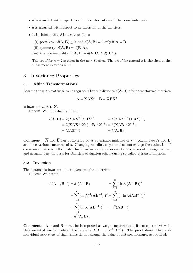
• d is invariant with respect to affine transformations of the coordinate system.

• d is invariant with respect to an inversion of the matrices.

• It is claimed that d is a metric. Thus

(i) positivity: d(A,B) ≥ 0, and d(A,B) = 0 only if A = B.

(ii) symmetry: d(A,B) = d(B,A),

(iii) triangle inequality: d(A,B) + d(A,C) ≥ d(B,C).

The proof for n = 2 is given in the next Section. The proof for general n is sketched in thesubsequent Sections 4 – 6.

3 Invariance Properties

3.1 Affine Transformations

Assume the n×n matrix X to be regular. Then the distance d(A,B) of the transformed matrices

A = XAXT B = XBXT

is invariant w. r. t. X.Proof: We immediately obtain:

λ(A,B) = λ(XAXT ,XBXT ) = λ(XAXT (XBXT )−1)

= λ(XAXT (XT )−1B−1X−1) = λ(XAB−1X−1)

= λ(AB−1) = λ(A,B) .

Comment: A and B can be interpreted as covariance matrices of y = Xx in case A and Bare the covariance matrices of x. Changing coordinate system does not change the evaluation ofcovariance matrices. Obviously, this invariance only relies on the properties of the eigenvalues,and actually was the basis for Baarda’s evaluation scheme using so-called S-transformations.

3.2 Inversion

The distance is invariant under inversion of the matrices.Proof: We obtain

d2(A−1,B−1) = d2(A−1B) =n∑

i=1

(lnλi(A

−1B))2

=n∑

i=1

(ln[λ−1i (AB−1)]

)2=

n∑i=1

(− lnλi(AB−1)

)2=

n∑i=1

(lnλi(AB−1)

)2= d2(AB−1)

= d2(A,B) .

Comment: A−1 and B−1 can be interpreted as weight matrices of x if one chooses σ2o = 1.Here essential use is made of the property λ(A) = λ−1(A−1). The proof shows, that alsoindividual inversions of eigenvalues do not change the value of distance measure, as required.

116

3.3 d is a Distance Measure

We show that d is a distance measure, thus the first two criteria for a metric hold in general.

ad 1 d ≥ 0 is trivial from the definition of d, keeping in mind, that the eigenvalues all arepositive. Proof of d = 0↔ A = B:

← : If A = B then d = 0.Proof: From λ(AB−1) = λ(I) follows λi = 1 for all i, thus d = 0.

→ : If d = 0 then A = B.Proof: From d = 0 follows λi(AB−1) = 1 for all i, thus AB−1 = I from whichA = B follows.

ad 2 As (AB−1)−1 = BA−1 symmetry follows from the inversion invariance.

3.4 Triangle Inequality

For d providing a metric on the symmetric positive definite matrices the triangle inequality musthold.

Assume three n× n matrices with the following structure:

• The first matrix is the unit matrix:A = I .

• The second matrix is a diagonal matrix with entries ebi thus

B = Diag(ebi) .

• The third matrix is a general matrix with eigenvalues eci and modal matrix R, thus

C = RDiag(eci)RT .

This setup can be chosen without loss of generality, as A and B can be orthogonalized simulta-neously [4].

The triangle inequality can be written in the following form and reveals three terms

s.= d(A,B) + d(A,C)− d(B,C) = dc + db − da ≥ 0 . (5)

The idea of the proof is the following:

(i) We first use the fact that db and dc are independent on the rotation R.

s(R) = dc + db − da(R) .

(ii) In case R = I then the correctness of (5) results from the triangle inequality in Rn. Thiseven holds for any permutation P (i) of the indices i of the eigenvalues λi of BC−1. Thereexists a permutation Pmax for which da is maximum, thus s(R) is a minimum.

(iii) We then want to show, and this is the crucial part, that any rotation R 6= I leads to adecrease of da(R), thus to an increase of s(R) keeping the triangle inequality to hold.

117

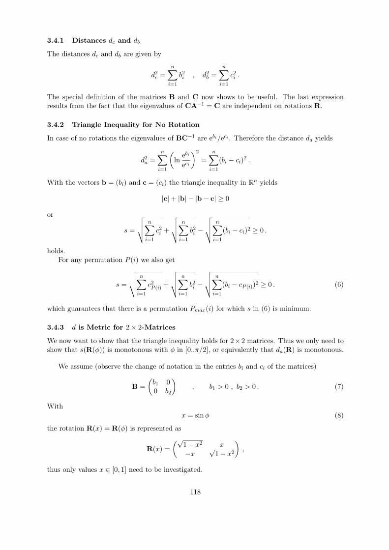
3.4.1 Distances dc and db

The distances dc and db are given by

d2c =n∑

i=1

b2i , d2b =n∑

i=1

c2i .

The special definition of the matrices B and C now shows to be useful. The last expressionresults from the fact that the eigenvalues of CA−1 = C are independent on rotations R.

3.4.2 Triangle Inequality for No Rotation

In case of no rotations the eigenvalues of BC−1 are ebi/eci . Therefore the distance da yields

d2a =n∑

i=1

(ln

ebi

eci

)2

=n∑

i=1

(bi − ci)2 .

With the vectors b = (bi) and c = (ci) the triangle inequality in Rn yields

|c|+ |b| − |b− c| ≥ 0

or

s =

√√√√ n∑i=1

c2i +

√√√√ n∑i=1

b2i −

√√√√ n∑i=1

(bi − ci)2 ≥ 0 .

holds.For any permutation P (i) we also get

s =

√√√√ n∑i=1

c2P (i) +

√√√√ n∑i=1

b2i −

√√√√ n∑i=1

(bi − cP (i))2 ≥ 0 . (6)

which guarantees that there is a permutation Pmax(i) for which s in (6) is minimum.

3.4.3 d is Metric for 2× 2-Matrices

We now want to show that the triangle inequality holds for 2×2 matrices. Thus we only need toshow that s(R(φ)) is monotonous with φ in [0..π/2], or equivalently that da(R) is monotonous.

We assume (observe the change of notation in the entries bi and ci of the matrices)

B =

(b1 00 b2

), b1 > 0 , b2 > 0 . (7)

Withx = sinφ (8)

the rotation R(x) = R(φ) is represented as

R(x) =

(√1− x2 x

−x√1− x2

),

thus only values x ∈ [0, 1] need to be investigated.

118

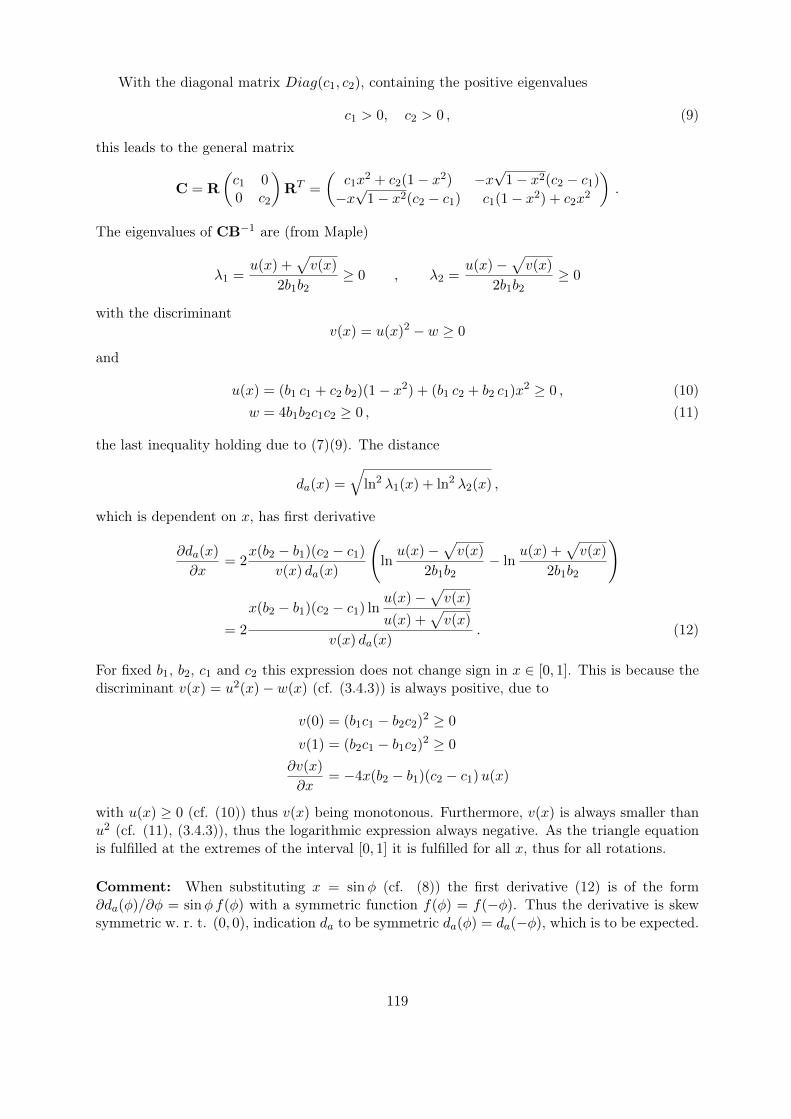
With the diagonal matrix Diag(c1, c2), containing the positive eigenvalues

c1 > 0, c2 > 0 , (9)

this leads to the general matrix

C = R

(c1 00 c2

)RT =

(c1x

2 + c2(1− x2) −x√1− x2(c2 − c1)

−x√1− x2(c2 − c1) c1(1− x2) + c2x

2

).

The eigenvalues of CB−1 are (from Maple)

λ1 =u(x) +

√v(x)

2b1b2≥ 0 , λ2 =

u(x)−√v(x)

2b1b2≥ 0

with the discriminantv(x) = u(x)2 − w ≥ 0

and

u(x) = (b1 c1 + c2 b2)(1− x2) + (b1 c2 + b2 c1)x2 ≥ 0 , (10)

w = 4b1b2c1c2 ≥ 0 , (11)

the last inequality holding due to (7)(9). The distance

da(x) =

√ln2 λ1(x) + ln2 λ2(x) ,

which is dependent on x, has first derivative

∂da(x)

∂x= 2

x(b2 − b1)(c2 − c1)v(x) da(x)

(lnu(x)−

√v(x)

2b1b2− ln

u(x) +√v(x)

2b1b2

)

= 2

x(b2 − b1)(c2 − c1) lnu(x)−

√v(x)

u(x) +√v(x)

v(x) da(x). (12)

For fixed b1, b2, c1 and c2 this expression does not change sign in x ∈ [0, 1]. This is because thediscriminant v(x) = u2(x)− w(x) (cf. (3.4.3)) is always positive, due to

v(0) = (b1c1 − b2c2)2 ≥ 0

v(1) = (b2c1 − b1c2)2 ≥ 0

∂v(x)

∂x= −4x(b2 − b1)(c2 − c1)u(x)

with u(x) ≥ 0 (cf. (10)) thus v(x) being monotonous. Furthermore, v(x) is always smaller thanu2 (cf. (11), (3.4.3)), thus the logarithmic expression always negative. As the triangle equationis fulfilled at the extremes of the interval [0, 1] it is fulfilled for all x, thus for all rotations.

Comment: When substituting x = sinφ (cf. (8)) the first derivative (12) is of the form∂da(φ)/∂φ = sinφ f(φ) with a symmetric function f(φ) = f(−φ). Thus the derivative is skewsymmetric w. r. t. (0, 0), indication da to be symmetric da(φ) = da(−φ), which is to be expected.

119

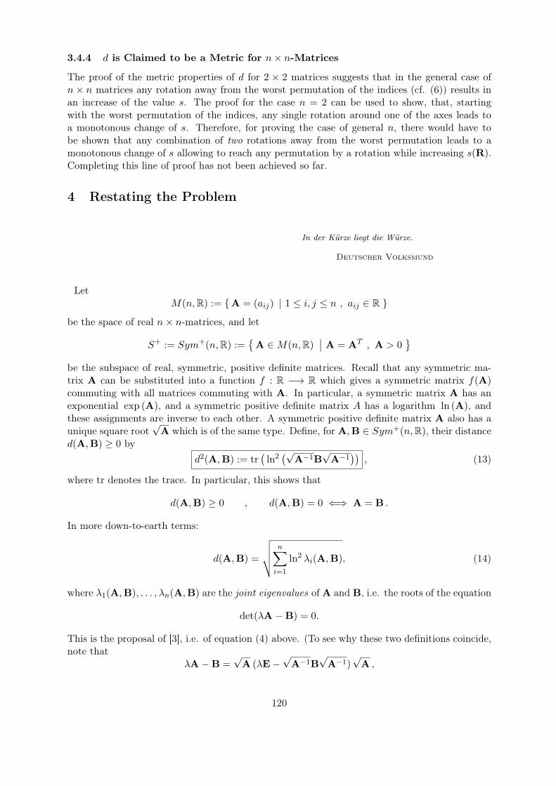
3.4.4 d is Claimed to be a Metric for n× n-Matrices

The proof of the metric properties of d for 2 × 2 matrices suggests that in the general case ofn× n matrices any rotation away from the worst permutation of the indices (cf. (6)) results inan increase of the value s. The proof for the case n = 2 can be used to show, that, startingwith the worst permutation of the indices, any single rotation around one of the axes leads toa monotonous change of s. Therefore, for proving the case of general n, there would have tobe shown that any combination of two rotations away from the worst permutation leads to amonotonous change of s allowing to reach any permutation by a rotation while increasing s(R).Completing this line of proof has not been achieved so far.

4 Restating the Problem

In der Kürze liegt die Würze.

Deutscher Volksmund

LetM(n,R) := {A = (aij) | 1 ≤ i, j ≤ n , aij ∈ R }

be the space of real n× n-matrices, and let

S+ := Sym+(n,R) :={

A ∈M(n,R)∣∣ A = AT , A > 0

}be the subspace of real, symmetric, positive definite matrices. Recall that any symmetric ma-trix A can be substituted into a function f : R −→ R which gives a symmetric matrix f(A)commuting with all matrices commuting with A. In particular, a symmetric matrix A has anexponential exp (A), and a symmetric positive definite matrix A has a logarithm ln (A), andthese assignments are inverse to each other. A symmetric positive definite matrix A also has aunique square root

√A which is of the same type. Define, for A,B ∈ Sym+(n,R), their distance

d(A,B) ≥ 0 byd2(A,B) := tr

(ln2(√

A−1B√

A−1))

, (13)

where tr denotes the trace. In particular, this shows that

d(A,B) ≥ 0 , d(A,B) = 0 ⇐⇒ A = B .

In more down-to-earth terms:

d(A,B) =

√√√√ n∑i=1

ln2 λi(A,B), (14)

where λ1(A,B), . . . , λn(A,B) are the joint eigenvalues of A and B, i.e. the roots of the equation

det(λA−B) = 0.

This is the proposal of [3], i.e. of equation (4) above. (To see why these two definitions coincide,note that

λA−B =√

A (λE−√

A−1B√

A−1)√

A ,

120

so that the joint eigenvalues λi(A,B) are just the eigenvalues of the real symmetric positivedefinite matrix

√A−1B

√A−1; in particular, they are positive real numbers and so the definition

(14) makes sense.) The equation (14) shows that d is invariant under congruence transformationswith X ∈ GL(n,R), where GL(n,R) is the group of regular linear transformations of Rn:

∀X ∈ GL(n,R) : d(A,B) = d(XAXT ,XBXT ) (15)

(since det (λA−B) and det(X(λA−B)XT

)have the same roots); this is not easily seen from

definition (13). It also shows that

d(A,B) = d(B,A) , d(A,B) = d(A−1,B−1).

5 The results

One then has

Theorem 1. The map d defines a distance on the space Sym+(n,R), i.e there holds

(i) Positivity: d(A,B) ≥ 0, and d(A,B) = 0 ⇐⇒ A = B

(ii) Symmetry: d(A,B) = d(B,A)

(iii) Triangle inequality: d(A,C) ≤ d(A,B) + d(B,C)

for all A,B,C ∈ Sym+(n,R). Moreover, d has the following invariances:

(iv) It is invariant under congruence transformations, i.e.

d(A,B) = d(XAXT ,XBXT )

for all A,B ∈ Sym+(n,R), X ∈ GL(n,R)

(v) It is invariant under inversion, i.e.

d(A,B) = d(A−1,B−1)

for all A,B ∈ Sym+(n,R)

The same conclusions hold for the space SSym(n,R) of real symmetric positive definite matricesof determinant one, when one replaces the general linear group GL(n,R) with the special lineargroup SL(n,R), the n×n–matrices of determinant one, and the space of real symmetric matricesSym(n,R) with the space Sym0(n,R) of real symmetric traceless matrices.

Remark 1. We use here the terminology “distance” in contrast to the standard terminology“metric” in order to avoid confusion with the notion of “Riemannian metric”, which is going toplay a rôle soon.

The case n = 2 is already interesting; see Remark 2 below.All the properties except property (iv), the triangle inequality, are more or less obvious from

the definition (see above), but the triangle inequality is not. In fact, the theorem will be theconsequence of a more general theorem as follows.

The most important geometric way distances arise is as associated distances to Riemannianmetrics on manifolds; the Riemannian metric, as an infinitesimal description of length is usedto define the length of paths by integration, and the distance between two points then arises asthe greatest lower bound on the length of paths joining the two points. More precisely, if M

121

is a differentiable manifold (in what follows, “differentiable” will always mean “infinitely manytimes differentiable”, i.e. of class C∞), a Riemannian metric is the assignment to any p ∈ Mof a Euclidean scalar product 〈− |−〉p in the tangent space TpM depending differentiably on p.Technically, it is a differentiable positive definite section of the second symmetric power S2T ∗Mof the cotangent bundle, or a positive definite symmetric 2-tensor. In classical terms, it is givenin local coordinates (U, x) as the “square of the line element” or “first fundamental form”

ds2 = gij(x)dxidxj (16)

(Einstein summation convention: repeated lower and upper indices are summed over). Herethe gij are differentiable functions (the metric coefficients) subjected to the transformation rule

gij(x) = gkl(y(x))∂yk

∂xi∂yl

∂xj.

A differentiable manifold together with a Riemannian metric is called a Riemannian manifold.Given a piecewise differentiable path c : [a, b] −→M in M , its length L [c] is defined to be

L [c] :=

∫ b

a‖c(t)‖c(t) dt ,

where for X ∈ TpM we have ‖X‖p :=√〈X |X〉p, the Euclidean norm associated to the scalar

product in TpM given by the Riemannian metric. In local coordinates

L [c] =

∫ b

a

√gij(c(t)) ci(t)cj(t) dt .

Given p, q ∈M , the distance d(p, q) associated to a given Riemannian metric then is defined tobe

d(p, q) := infcL [c] , (17)

the infimum running over all piecewise differentiable paths c joining p to q. This defines indeeda distance:

Proposition. The distance defined by (17) on a connected Riemannian manifold is a metric inthe sense of metric spaces, i.e. defines a map d :M ×M −→ R satisfying

(i) d(p, q) ≥ 0, d(p, q) = 0 ⇐⇒ p = q

(ii) d(p, q) = d(q, p)

(iii) d(p, r) ≤ d(p, q) + d(q, r) .

An indication of proof will be given in the next section.So the central issue here is the fact that a Riemannian metric is the differential substrate

of a distance and, in turn, defines a distance by integration. This is the most important wayof constructing distances, which is the fundamental discovery of Gauß and Riemann. In ourcase, this paradigm is realized in the following way.

The space Sym+(n,R) is a differentiable manifold of dimension n(n+1)/2, more specifically,it is an open cone in the vector space

Sym(n,R) :={

A ∈M(n,R)∣∣ A = AT

}

122

of all real symmetric n× n-matrices. Thus the tangent space TASym+(n,R) to Sym+(n,R) at

a point A ∈ Sym+(n,R) is just given as

TASym+(n,R) = Sym(n,R).

The tangent space TASSym+(n,R) to SSym(n,R) at a point A ∈ SSym(n,R) is just given as

TASSym(n,R) = Sym0(n,R) := {X ∈ Sym(n,R) | tr (X) = 0 } ,

the space of traceless symmetric matrices.Now note that there is a natural action of GL(n,R) on S+, namely, as already referred to

above, by congruence transformations: X ∈ GL(n,R) acts via A 7→ XAXT . If one regards A asthe matrix corresponding to a bilinear form with respect to a given basis, this action representsa change of basis. This action is transitive, and the isotropy subgroup at E ∈ S+ is just theorthogonal group O(n):{

X ∈ GL(n,R)∣∣ XEXT = E

}={

X ∈ GL(n,R)∣∣ XXT = E

}= O(n),

and so S+ can be identified with the homogeneous space GL(n,R)/O(n) upon which GL(n,R)acts by left translations (its geometric significance being that its points parametrize the possiblescalar products in Rn) †] .

In general, a homogeneous space is a differentiable manifold with a transitive action of a Liegroup G, whence it has a representation as a quotient M = G/H with H a closed subgroup ofG. The most natural Riemannian metrics in this case are then those for which the group G actsby isometries, or, in other words, which are invariant under the action of G; e.g. the classicalgeometries – the Euclidean, the elliptic, and the hyperbolic geometry – arise in this manner.Looking out for these metrics, Theorem 1 will be a consequence of the following theorem :

Theorem 2. (i) The Riemannian metrics g on Sym+(n,R) invariant under congruencetransformations with matrices X ∈ GL(n,R) are in one-to-one-correspondence with positivedefinite quadratic forms Q on TESym

+(n,R) = Sym(n,R) invariant under conjugationwith orthogonal matrices, the correspondence being given by

gA(X,Y) = B(√

A−1X√

A−1,√

A−1Y√

A−1) ,

where A ∈ Sym+(n,R), X,Y ∈ Sym(n,R) = TASym+(n,R), and B is the symmetric

positive bilinear form corresponding to Q

(ii) The corresponding distance dQ is invariant under congruence transformations and inver-sion, i.e. satisfies

dQ(A,B) = dQ(XAXT ,XBXT )

anddQ(A,B) = dQ(A

−1,B−1)

for all A,B ∈ Sym+(n,R), X ∈ GL(n,R), and is given by

d2Q(A,B) =1

4Q(ln(√

A−1B√

A−1)). (18)

†]A concrete map p : G −→ S+ achieving this identification is given by p(A) := AAT ; it is surjective andsatisfies p(XA) = Xp(A)XT . The fact that p is an identification map is then equivalent to the polar decomposi-tion: any regular matrix can be uniquely written as the product of a positive definite symmetric matrix and anorthogonal matrix. This generalizes the representation z = reiϕ of a nonzero complex number z.

123

(iii) In particular, the distance in Theorem 1 is given by the invariant Riemannian metriccorresponding to the canonical non–degenerate bilinear form ‡]

∀X,Y ∈M(n,R) : B(X,Y) := 4 tr (XY)

on M(n,R), restricted to Sym(n,R) = TESym(n,R)+, i.e. to the quadratic form

∀X ∈ Sym(n,R) : Q(X) := 4 tr(X2)

on Sym(n,R). As a Riemannian metric it is, in classical notation,

ds2 = 4 tr((√

X−1 dX√

X−1)2)

= 4 tr((

X−1 dX)2) (19)

where X = (Xij) is the matrix of the natural coordinates on Sym+(n,R) and dX = (dXij)is a matrix of differentials.

The same conclusions hold for the space SSym(n,R) of real symmetric positive definite ma-trices of determinant one, when one replaces the general linear group GL(n,R) with the speciallinear group SL(n,R), the n × n–matrices of determinant one, and the space of real symmetricmatrices Sym(n,R) with the space Sym0(n,R) of real symmetric traceless matrices.

Remark 2. Although the expression (19) appears to be explicit in the coordinates, it seemsto be of no use for analyzing the properties of the corresponding Riemannian metric, since theoperations of inverting, squaring, and taking the trace gives, in the general case, untractableexpressions. In particular, it apparently is of no help in deriving the expression (14) for theassociated distance by direct elementary means.

There is, however, one interesting case where it can be checked to give a very classicalexpression; this is the case n = 2. In this case, one has

SSym+(2,R) ={ (

x yy z

) ∣∣∣∣ x, y, z ∈ R , xz − y2 = 1 , x > 0

}a hyperboloid in 3-space. This is classically known as a candidate for a model of the hyperbolicplane.In fact, in this case, one may show by explicit computation that the metric (19) restricts tothe classical hyperbolic metric, and that the corresponding distance just gives one of the classicalformulas for the hyperbolic distance. For details, see [11].

Of course, the next question is which invariant metrics there are. Also this question can beanswered:

Addendum. (i) The positive definite quadratic forms Q on Sym(n,R) invariant under con-jugation with orthogonal matrices are of the form

Q(X) = α tr(X2)+ β

(tr (X)

)2, α > 0, β > −α

n

(ii) The positive definite quadratic forms Q on Sym0(n,R) invariant under conjugation withorthogonal matrices are unique up to a positive scalar and hence of the form

Q(X) = α tr(X2), α > 0.

In particular, the Riemannian metric (19) corresponds to the case α = 1, β = 0. Since fromthe point of this classification all these metrics stand on an equal footing, it would be interestingto know by which naturality requirements this choice can be singled out.‡]the famous Cartan-Killing-form of Lie group theory

124

6 The proofs

To put this result into proper perspective and to cut a long story short, let us very brieflysummarize why Theorem 2, and consequently Theorem 1, are true. First, however, we indicatea proof of the Proposition above, since it is on this Proposition that our approach to the triangleequality for the distance defined by (14) is based.

The fact that d(p, q) ≥ 0 and the symmetry of d are immediate from the definitions. Thereremains to show d(p, q) = 0 =⇒ p = q and the triangle inequality.

For given p ∈ M , choose a coordinate neighbourhood U ∼= Rn around p such that p corre-sponds to 0 ∈ Rn. We then have the expression (16) for the given metric in U . Moreover, wehave in U the standard Euclidean metric

ds2E := δijdxidxj =

n∑i=1

(dxi)2 .

Let ‖−‖ denote the norm belonging to the given Riemannian metric in U and |−| the normgiven by the standard Euclidean metric. For r > 0 let

B(p; r) := {x ∈ Rn | |x| ≤ r }

be the standard closed ball with radius r around p = 0, and

S(p; r) := {x ∈ Rn | |x| = r }

its boundary, the sphere of radius r around p ∈ Rn.As a continuous function U × Rn −→ R the norm ‖−‖ takes its minimum m > 0 and its

maximum M > 0 on the compact set B(p; 1)× S(p; 1). It follows that we have

∀ q ∈ B(p; 1) , X ∈ Rn : m|X| ≤ ‖X‖q ≤M |X|

by homogeneity of the norm, and so by integrating and taking the infimum

∀ q ∈ B(p; 1) : mdE(p, q) ≤ d(p, q) ≤MdE(p, q) (20)

where dE(p, q) = |q − p| is the Euclidean distance. If q 6∈ B(p; 1), then any path c joining p toq meets the boundary S(p; 1) in some point r, from which follows L [c] ≥ L [c′] ≥ d(p, r) ≥ m– where c′ denotes the part of c joining p to r for the first time, say – whence d(p, q) ≥ m. Inother words, if d(p, q) < m we have q ∈ B(p; 1), where we can apply (20). If now d(p, q) = 0,then surely d(p, q) < m, and then by (20) mdE(p, q) ≤ d(p, q) = 0, whence dE(p, q) = 0, whichimplies p = q.

For the triangle inequality, let c be a path joining p to q and d a path joining q to r. Let c∗dbe the composite path joining p to r. Then L [c ∗ d] = L [c] + L [d]. Taking the infimum on theleft hand side over all paths joining p to r gives d(p, r) ≤ L [c] + L [d]. Taking on the right handside first the infimum over all paths joining p to q and subsequently over all the paths joining qto r then gives d(p, r) ≤ d(p, q) + d(q, r), which is the triangle inequality.

Remark 3. In particular, (20) shows that the metric topology induced by the distance d on aconnected Riemannian manifold coincides with the given manifold topology.

Now to the proof of Theorem 2. Recall the terminology of [10], Chapter X: Let G be a Liegroup with Lie algebra g, H ⊆ G a closed Lie subgroup corresponding to the Lie subalgebrah ⊆ g. Let M be the homogeneous space M = G/H. Then G operates as a symmetry group onM by left translations. M has the distinguished point o = eH = H corresponding to the coset

125

of the unit element e ∈ G with tangent space ToM = g/h. This homogeneous space is calledreductive if g splits as a direct vector space sum g = h ⊕ m for a linear subspace m ⊆ g suchthat m is invariant under the adjoint action Ad : H −→ GL(g). Then canonically ToM = m.In our situation, G = GL(n,R), H = O(n). Then g = M(n,R), the full n × n-matrices, andh = Asym(n,R), the antisymmetric matrices. As is well known,

M(n,R) = Asym(n,R)⊕ Sym(n,R) ,

since any matrix X splits into the sum of its antisymmetric and symmetric part via

X =X −XT

2+X +XT

2.

The adjoint action of O ∈ O(n) on M(n,R) is given by X 7→ OXO−1 = OXOT and clearlypreserves Sym(n,R). So Sym+(n,R) is a reductive homogeneous space.

We now have the following facts from the general theory:a) On a reductive homogeneous space there is a distinguished connection invariant under the

action of G, called the natural torsion free connection in [10]. It is uniquely characterized by thefollowing properties ([10], Chapter X, Theorem 2.10)

– It is G–invariant

– Its geodesics through o ∈ M are the orbits of o under the one-parameter subgroups of G,i.e. of the form t 7→ exp(tX) · o for some X ∈ g, where exp : g −→ G is the exponentialmapping of Lie group theory

– It is torsion free

In particular, with this connectionM becomes an affine locally symmetric space, i.e. the geodesicsymmetries at a point of M given by inflection in the geodesics locally preserve the connection(loc. cit Chapter XI, Theorem 1.1). If M is simply connected, M is even an affine symmetricspace, i.e. the geodesic symmetries extend to globally defined transformations of M preservingthe connection (loc. cit., Chapter XI, Theorem 1.2). By homogeneity, these are determined bythe geodesic symmetry s at o. In our case M = Sym+(n,R), M is even contractible, hencesimply connected, and so with the natural torsion free connection an affine symmetric space.We have o = E, the n × n unit matrix. For G = GL(n,R), the exponential mapping of Liegroup theory is given by the “naive matrix exponential” eX =

∑∞k=0 t

kXk/k!. So the geodesicsare t 7→ exp (tX)E exp (tX)T = e2tX, where X ∈ Sym(n,R), and s is given by s(X) = X−1.

b) The Riemannian metrics g on M invariant under the action of G are in one-to-one-corres-pondence with positive definite quadratic forms Q on m invariant under the adjoint action of H(loc. cit, Chapter X, Corollary 3.2), the correspondence being given by

∀X ∈ ToM = m : go(X,X) = Q(X) .

This is intuitively obvious, since we can translate o to any point of M by operating on it withan element g ∈ G.

c) All G-invariant Riemannian metrics on M (there may be none) have the natural torsionfree connection as their Levi-Cività connection (loc. cit, Chapter XI, Theorem 3.3). In particular,such a metric makesM into a Riemannian (locally) symmetric space, i.e. the geodesic symmetriesare isometries, and the exponential map of Riemannian Geometry at o, Expo : ToM = m −→Mis given by the exponential map of Lie group theory for G:

∀X ∈ m : Expo(tX) = exp (tX) · o .

126

Collecting these results, we now can come to terms with formula (4). First we see thatPart (i) of Theorem 2 is a standard result in the theory of homogeneous spaces. Furthermore,S+, being a Riemannian symmetric space with the metric (19), is complete (loc. cit, ChapterXI, Theorem 6.4), the exponential mapping ExpE of Riemannian geometry is related to theexponential mapping exp : S −→ S+, S = TES

+ from Lie theory and the matrix exponential eX

via ExpE(X) = exp(2X) = e2X and is a diffeomorphism §] .Having reached this point, here is the showdown. Since, by general theory, the Riemannian

exponential mapping is a radial isometry, we get for the square of the distance dQ:

d2Q(A,B) = d2Q(E,√

A−1B√

A−1)

since dQ is invariant under congruences by (15) ,

= Q(1

2exp−1(

√A−1B

√A−1))

since ExpE is a radial isometry ,

=1

4Q(ln(

√A−1B

√A−1)) ,

and this is just equation (18). In particular, from this one directly reads off that the distance isinvariant under inversion, as claimed. Of course, the invariances in question are for the particularcase corresponding to (14) read off easily from the classical form (19) of the Riemannian metric.On the other hand, we see that the invariance under inversion comes from the structural factsthat S+ is a symmetric space, and that the geodesic symmetry at E, which on general groundsmust be an isometry, is just given by matrix inversion (see a) above).

One should add that these arguments are general and pertain to the situation of a symmetricspace of the non–compact type; for this, see [11].

The representation of the orthogonal group O(n) on the symmetric matrices by conjugationis not irreducible, but decomposes as

Sym(n,R) = Sym0(n,R)⊕ d(n,R), (21)

where d(n,R) are the scalar diagonal matrices. It is easy to see that both summands are invariantunder conjugation with orthogonal matrices, and it can be shown that both parts are irreduciblerepresentations of O(n). From this it is standard to derive the Addendum. In the geometricframework of symmetric spaces, this describes the decomposition of the holonomy representationand correspondingly the canonical de Rham–decomposition

Sym+(n,R) ∼= SSym(n,R)× R+

of the symmetric space Sym(n,R) into irreducible factors. This is a direct product of Riemannianmanifolds, i.e. the metric on the product is just the product of the metrics on the individualfactors, that is given by the Pythagorean description. Thus it suffices to classify the invariantmetrics on the individual factors, which accounts for the Addendum.

Thus, it transpires that the theorems above follow from the basics of Lie group theory andDifferential Geometry and so should be clear to the experts. The main results upon which it isbased appeared originally in the literature in [12]. All in all, it follows in a quite straightforward§]The fact that the naive matrix exponential is a diffeomorphism, whence S+ is complete, can be seen by

elementary means in the case under consideration. The main point is that it coincides with the exponentialmapping coming from Riemannian Geometry (up to scaling with a factor of 2).

127

manner from the albeit rather elaborated machinery of modern Differential Geometry and thetheory of symmetric spaces. In conclusion, it might therefore be still interesting to give a moreelementary derivation of the result, as was done above in the case n = 2.

As a general reference for Differential Geometry and the theory of symmetric spaces I recom-mend [9], [10] (which, however, make quite a terse reading). A detailed exposition [11] coveringall the necessary prerequisites is under construction; the purpose of this paper is to introduce thenon–experts to all the basic notions of Differential Geometry and to expand the brief argumentsjust sketched.

References

[1] Baarda, W. (1973): S-Transformations and Criterion Matrices, Band 5 der Reihe 1. Nether-lands Geodetic Commission, 1973.

[2] Ballein, K., 1985, Untersuchung der Dreiecksungleichung beim Vergleich von Kovarianz-matrizen, persönliche Mitteilung, 1985

[3] Förstner, W., A Metric for Comparing Symmetric Positive Definite Matrices, Note, August1995

[4] Fukunaga, K., Introduction to Statistical Pattern Recognition, Academic Press, 1972

[5] Grafarend, E. W. (1972): Genauigkeitsmasse geodätischer Netze. DGK A 73, BayerischeAkademie der Wissenschaften, München, 1972.

[6] Grafarend, E. W. (1974): Optimization of geodetic networks. Bolletino di geodesia eScienze Affini, 33:351–406, 1974.

[7] Grafarend, E. W. and Niermann, A. (1994): Beste echte Zylinderabbildungen, Kar-tographische Nachrichten, 3:103–107, 1984.

[8] Kavrajski, V. V., Ausgewählte Werke, Bd. I: Allgemeine Theorie der kartographischenAbbildungen, Bd. 2. Kegel- und Zylinderabbildungen (russ.), GVSMP, Moskau, 1958, zitiertin [7]

[9] Kobayashi, S. & Nomizu, K., Foundations of Differential Geometry, Vol. I, IntersciencePublishers 1963

[10] Kobayashi, S. & Nomizu, K., Foundations of Differential Geometry, Vol. II, IntersciencePublishers 1969

[11] Moonen, B, Notes on Differential Geometry,ftp://ftp.uni-bonn.cd/pub/staff/moonen/symmc.ps.gz

[12] Nomizu, K., Invariant affine connections on homogeneous spaces, Amer. J. Math, 76(1954), 33-65

[13] Schmitt, G. (1983): Optimization of Control Networks – State of the Art. In: Borre, K.;Welsch, W. M. (Eds.), Proc. Survey Control Networks, pages 373–380, Aalborg UniversityCentre, 1983.

128