econstor www.econstor.eu

Der Open-Access-Publikationsserver der ZBW – Leibniz-Informationszentrum WirtschaftThe Open Access Publication Server of the ZBW – Leibniz Information Centre for Economics

Standard-Nutzungsbedingungen:

Die Dokumente auf EconStor dürfen zu eigenen wissenschaftlichenZwecken und zum Privatgebrauch gespeichert und kopiert werden.

Sie dürfen die Dokumente nicht für öffentliche oder kommerzielleZwecke vervielfältigen, öffentlich ausstellen, öffentlich zugänglichmachen, vertreiben oder anderweitig nutzen.

Sofern die Verfasser die Dokumente unter Open-Content-Lizenzen(insbesondere CC-Lizenzen) zur Verfügung gestellt haben sollten,gelten abweichend von diesen Nutzungsbedingungen die in der dortgenannten Lizenz gewährten Nutzungsrechte.

Terms of use:

Documents in EconStor may be saved and copied for yourpersonal and scholarly purposes.

You are not to copy documents for public or commercialpurposes, to exhibit the documents publicly, to make thempublicly available on the internet, or to distribute or otherwiseuse the documents in public.

If the documents have been made available under an OpenContent Licence (especially Creative Commons Licences), youmay exercise further usage rights as specified in the indicatedlicence.

zbw Leibniz-Informationszentrum WirtschaftLeibniz Information Centre for Economics

Hayo, Bernd; Neumeier, Florian

Working Paper

Political leaders' socioeconomic background andfiscal performance in Germany

Joint discussion paper series in economics, No. 41-2011

Provided in Cooperation with:Faculty of Business Administration and Economics, University ofMarburg

Suggested Citation: Hayo, Bernd; Neumeier, Florian (2011) : Political leaders' socioeconomicbackground and fiscal performance in Germany, Joint discussion paper series in economics,No. 41-2011

This Version is available at:http://hdl.handle.net/10419/56585

Joint Discussion Paper

Series in Economics by the Universities of

Aachen · Gießen · Göttingen Kassel · Marburg · Siegen

ISSN 1867-3678

No. 41-2011

Bernd Hayo and Florian Neumeier

Political Leaders’ Socioeconomic Background and Fiscal Performance in Germany

This paper can be downloaded from http://www.uni-marburg.de/fb02/makro/forschung/magkspapers/index_html%28magks%29

Coordination: Bernd Hayo • Philipps-University Marburg

Faculty of Business Administration and Economics • Universitätsstraße 24, D-35032 Marburg Tel: +49-6421-2823091, Fax: +49-6421-2823088, e-mail: hayo@wiwi.uni-marburg.de

1

Political Leaders’ Socioeconomic Background and Fiscal

Performance in Germany*

Bernd Hayo and Florian Neumeier

Philipps-University Marburg

This version: 7 October 2011

Corresponding author: Bernd Hayo Faculty of Business Administration and Economics Philipps-University Marburg D-35032 Marburg Germany Phone: +49–6421–2823091 Email: hayo@wiwi.uni-marburg.de

* Thanks to Edith Neuenkirch, Matthias Neuenkirch, Britta Niehof, and Matthias Uhl for their helpful comments on earlier versions of the paper. The usual disclaimer applies.

2

Political Leaders’ Socioeconomic Background and Fiscal

Performance in Germany

Abstract

This paper investigates whether the socioeconomic status of the head of government helps

explain fiscal performance. Applying sociological research that attributes differences in

people’s ways of thinking and acting to their relative standing within society, we test whether

the social status of German prime ministers can help explain differences in fiscal performance

among the German Laender. Our empirical findings show that the tenures of prime ministers

from a poorer socioeconomic background are associated with higher levels of public spending

and debt financing.

JEL: E61, E62, H11, H72

Keywords: Leadership, socioeconomic status, fiscal policy, public spending, public deficit.

3

1. Introduction

Explaining variations in government size and public debt accumulation is an important issue

for political economists, and one in which the motives of relevant political actors are thought

to play a decisive role. The literature typically assumes that political decision-making is

driven by one of three motivations. First, politicians behave in a purely opportunistic manner.

For instance, political budget cycle (PBC) theorists argue that public spending and debt

financing are connected to the legislation cycle (e.g., Rogoff and Sibert, 1988; Alesina et al.,

1992; Persson and Tabellini, 1997):1 to enhance their re-election prospects, politicians are

expected to raise the level of public expenditure and debt financing in pre-election and

election years, while fiscal consolidation is expected to occur in the aftermath of an election.2

A second branch of the literature views politicians as purely benevolent. Political actors

design fiscal policy to optimise some sort of social welfare function. A well-known example

is Barro’s (1979) tax-smoothing hypothesis, in which it is assumed that governments choose

tax rates with the aim of minimising the excess burden of taxation. As a consequence, the

accumulation of public debt is expected to be linked to the business cycle, since governments

are assumed to incur deficits during recessions and surpluses during booms (Alesina and

Perotti, 1994).

Finally, there are political economists who link political performance to partisan ideology

(see, e.g., Hibbs, 1977; Buchanan and Wagner, 1977). A common assumption in this body of

literature is that the tenures of left-wing governments are associated with higher levels of

public spending and debt financing than are the tenures of right-wing governments (e.g., Blais

et al., 1993; Cusack, 1997).

However, empirical analyses cast serious doubt on all three approaches, since findings from

different studies are often contradictory and the explanatory power of the employed covariates

is low. In the case of PBC theory, for example, Shi and Svensson (2006) find robust evidence

for PBCs in fiscal deficits for developing countries, but not for developed countries. Brender

and Drazen (2005) provide similar results based on a differentiation between new and

established democracies: PBCs are found in the former only.

Results from the two other strands are, at best, mixed, too. With respect to the partisan

hypothesis, there is some evidence from OECD countries that tenures of left-wing 1 Originally, the theory of political business cycles was formulated in a Phillips curve context. See Nordhaus (1975) and MacRae (1977). 2 These implications depend on the assumption that voters are either myopic, i.e., they overestimate the benefit of current public spending and underestimate the costs of future taxes (Alesina and Perotti, 1994), or have imperfect information regarding the competence of the incumbent government and the costs of publicly provided goods (Rogoff and Sibert, 1988; Rogoff, 1990). See Alesina and Perotti (1994) and Eslava (2006) for a summary.

4

governments are indeed associated with a rise in public expenditures (e.g., de Haan and

Sturm, 1994, 1997; Cusack, 1997), but the conclusion that leftist incumbents accumulate

higher public debt is made less than solid by the experience of many Western European

countries between 1960–1990.

Finally, the tax-smoothing approach is not in line with observations on the development of

public budgets in many OECD countries during the 1970s and 1980s (Roubini and Sachs,

1989; Alesina and Perotti, 1994). In particular, the absence of fiscal adjustments in some

OECD countries after the recession of 1973–1974 and differences in the accumulation of

public debt in the following decades cannot be convincingly explained by a tax-smoothing

motive.

So, what is driving the fiscal decisions of political actors? In this paper, we argue that a

broader social science perspective may provide some important insights. Sociologists

emphasise the strong connection between an individual’s socioeconomic background—

especially factors that determine an individual’s relative position within a society, called

status—and preferences, attitudes, and habits.3

Choosing the German Laender as the object of analysis has two advantages: first, they are

highly homogeneous regarding politics, culture, demography, and institutional as well as

constitutional frameworks, which limits the number of control variables required and

minimises potential biases due to endogeneity problems. Second, the Laender are

constitutionally endowed with a high degree of fiscal authority regarding budgetary matters.

There is a considerable amount of political

economics literature suggesting that factors related to individuals’ status—such as occupation,

income, and education—help explain differences in policy preferences and decision

behaviour, but typically these variables are employed in a more or less ad hoc fashion. To the

best of our knowledge, there is no empirical work that links theoretical research on status to

the fiscal behaviour of leaders. We fill this gap by investigating the impact that a political

actor’s family status has on his or her fiscal preferences. To this end, we utilise observations

on the leaders, the prime ministers (Ministerpräsidenten), of the fiscally partially autonomous

states making up the Federal Republic of Germany, the Laender (Bundesländer). We

concentrate on the social status of the German Laenders’ prime ministers and study its

influence on the level of public expenditures as well as debt financing.

These advantages have made the German Laender a popular venue for research into the

motivations of incumbent governments. However, neither the PBC theorem (Berger and

Holler, 2007; Schneider, 2010), the tax-smoothing approach (Seitz, 2000), nor the partisan 3 In fact, this belief is the motivation of a huge body of sociological research analysing the social structure of society.

5

hypothesis (Seitz, 2000; Galli and Rossi, 2002; Jochimsen and Nuscheler, 2010; Schneider,

2010) are supported by empirical findings from this work. In contrast to these studies, we find

robust empirical support for our social-science-based approach to explaining political decision

making.

In the next section of this paper, we discuss related literature. In Section 3, we take a brief

look at the German system of fiscal federalism and its political landscape. Then, in Section 4,

we introduce the concept of status, provide empirical measures for it, and identify

transmission channels that link a person’s status to his or her preferences public expenditure

and debt financing. In Section 5, we conduct some preliminary analyses proving the accuracy

of our conclusions drawn in Section 4. Section 6 presents the results of our main analysis, in

which we investigate the influence of German prime ministers’ socioeconomic backgrounds

on the fiscal performances of the German Laender. Section 7 concludes.

2. Related Literature

By focussing on how the head of government influences economic outcomes, this paper

contributes to an expanding branch of the literature. Starting with the work of Jones and

Olken (2005), researchers have become increasingly concerned with the question of whether

political leaders exert an impact on economic performance. Jones and Olken (2005) provide

evidence that leaders do influence the rate of economic growth in their country. They compare

GDP growth rates before and after exogenous leader changes (i.e., leader transitions caused

by natural death of the incumbent) and find significant differences. Brender and Drazen

(2009) use the same approach to test whether political leaders affect the composition of

government expenditures, finding significant effects in the long run. A major drawback of

both studies is that they assume the relevant competences to be randomly distributed across

political leaders and it is thus unclear in what specific characteristics leaders differ.

Other researchers attempt to overcome this shortcoming by focussing on the

sociodemographics of leaders, e.g., age, tenure, education, and professional background, but

with limited success.4

4 Individual characteristics are also used as explanatory variables for committee decisions. For instance, focussing on members of monetary policy committees rather than heads of government, Göhlmann and Vaubel (2007) investigate the impact of education and occupation histories of 391 central bankers from 10 European countries on inflation outcomes.

For instance, Hayo and Voigt (2011) study determinants of

constitutional change, particularly movements from the status quo toward more

parliamentarism or presidentialism, in a large sample of countries. They find that these

changes are influenced by specific characteristics of political leaders.

6

Besley et al. (2009) identify leaders’ educational attainment and experience as relevant to

differences in GDP growth. More precisely, they find that the more educated the leader

(differentiating between non-graduate education, graduate education, and college education)

and the longer the stay in office, the higher the country’s economic growth.

Dreher et al. (2009) focus on the effect of different fields of education and occupation on

economic reforms, measured as changes in the Economic Freedom Index. They are primarily

interested in the effect of leaders’ economic and entrepreneurial backgrounds and expect that

economists, as well as entrepreneurs, should be more likely to liberalise the economy. The

authors account for different educational and occupational backgrounds by including dummy

variables and find evidence that supports their hypothesis. However, among the occupation

dummies, there are three additional effects (for scientists other than economists, military

personnel, and life-long politicians) that have a positive sign, but the authors conduct no

further tests to compare these groups. Moreover, Dreher et al.’s (2009) findings are not robust

to varying specifications, especially to the inclusion of a lagged dependent variable and

additional controls.

Mikosch (2009) employs the same dataset in an attempt to explain differences in public

deficits. According to his results, tenures of former economists, white-collar workers, and

blue-collar workers are associated with significantly higher deficits than tenures of leaders

who have been politicians most of their working life. However, this finding is counterintuitive

and actually contradicts the author’s hypothesis that economists should reduce public debts.

A problem with these studies is that the theoretical link between, say, certain educational and

occupational backgrounds and economic performance remains vague. The authors refer to

some sort of socialisation or, rather, ‘professional indoctrination’, which economists in

particular are presumed to experience. However, experimental studies show that the

differences between economists and other people with respect to ways of thinking and acting

can at least partially be ascribed to a selection effect (for a recent summary on experimental

findings, see Goossens and Méon, 2010). Moreover, sociological research reveals that

educational and occupational choices themselves depend on the social environment, in

particular family status (e.g., Bourdieu, 1984). Hence, instead of focussing on specific fields

of education and work, we look at leaders’ family status, i.e., parental status and the status of

positions prime ministers held before entering office. Our novel approach to the analysis of

leaders’ influence is motivated by manifold empirical findings linking individual status to

motives and patterns of behaviour. Thus, our measures of status are those frequently

employed in the social sciences. In our empirical analysis, we find strong evidence that a

7

prime minister’s socioeconomic background matters in terms of the incumbent government’s

fiscal performance: the higher a prime minister’s status, the lower the public expenditures and

debt financing.

3. Fiscal Federalism and Political Landscape in Germany

The German federal system consists of three parliamentary governmental levels, each with its

own fiscal competences and responsibilities as specified by the German Constitution, the

Grundgesetz: federal level, state level, and local level.5 At the state level, there were 11

Laender before German Unification in 1990; 16 afterward.6

The competences assigned to the German Laender are extensive and mainly defined in

Articles 71–74 of the Grundgesetz. As Schneider (2010) states, these policy areas are

potentially attractive for political manipulation as they include—among others—social

security, public safety, education, cultural affairs, administration, and health.

Three out of the 16 are so-called

city-states (Berlin, Bremen, and Hamburg), which combine competences assigned to the state

and the local level.

There are currently five major political parties in Germany: the conservative Christian

Democratic Party (CDU) and its sister party the Christian Socialist Party (CSU), the Social

Democratic Party (SPD), the Green Party (Bündnis 90/Die Grünen), the Liberal Democratic

Party (FDP), and the Left-Wing Party (Die Linke).7

Since the political system of the German Laender is parliamentary, the question may arise as

to whether German prime ministers even can exert an influence on fiscal policy. De jure they

can, for at least two reasons. First, the prime minister appoints the cabinet ministers and

therefore can to some extent ensure that the members of government back his or her preferred

policy. Second, the prime minister has guideline competences (Richtlinienkompetenz),

meaning that he or she has the authority to issue directives to the ministers.

Governments at the state level are led by

either CDU/CSU or SPD. During the period we study, some of the states in our sample have

one-party governments, others are governed by some form of coalition government (mainly

made up of two parties), majority governments, or minority governments.

5 For a more detailed overview of the German fiscal federalism, see, e.g., Seitz (2000) and Jochimsen and Nuscheler (2010). 6 The 11 Laender making up the former Federal Republic of Germany are Baden-Wuerttemberg, Bavaria, West Berlin, Bremen, Hamburg, Hesse, Lower Saxony, North Rhine Westphalia, Rhineland-Palatinate, Saarland, and Schleswig-Holstein. The additional five states are Brandenburg, Mecklenburg-Vorpomerania, Thuringia, Saxony, and Saxony-Anhalt. Before unification, Berlin was divided into West and East Berlin. They merged into the new state Berlin in 1990. 7 The latter was founded in 2007 as a fusion of two parties: the Employment and Social Justice Party (WASG, founded in 2004) and the Party of Democratic Socialism (PDS, founded in 1989). Due to their substantive similarities, we do not differentiate between these three parties in our study.

8

Some hints of a de facto association between fiscal performance and prime minister

transitions can be found in Figures A1 and A2 of the Appendix, which present movements in

public spending and net public borrowing, respectively, within the Old German Laender

between 1985–2009. To filter out symmetric business cycle effects, we calculated deviations

from the contemporary means across the Laender. The marks along the single series indicate

changes of prime minister. We observe a remarkable extent of cross-Laender variation with

respect to fiscal performance. Moreover, leader transitions tend to be followed by changes in

the (relative) level of public expenditures and debt financing. It is noteworthy that leader

transitions do not necessarily coincide with changes in the governing party. In fact, only in 14

out of 38 cases did the incumbent prime minister have to leave office because he had not been

re-elected. Hence, we need to carefully distinguish between leader and party effects.

4. The Status Concept and its Measurement

In this section, we clarify the concept of status, discuss its implications for motives and

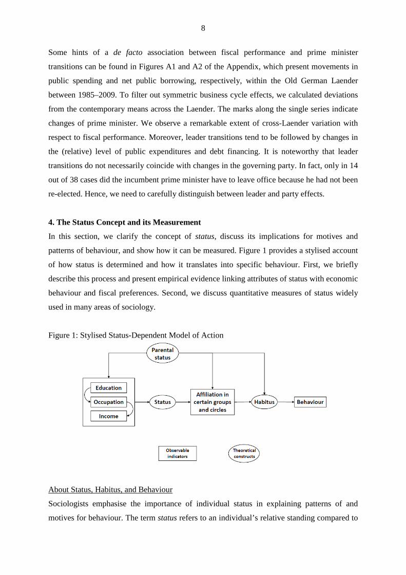
patterns of behaviour, and show how it can be measured. Figure 1 provides a stylised account

of how status is determined and how it translates into specific behaviour. First, we briefly

describe this process and present empirical evidence linking attributes of status with economic

behaviour and fiscal preferences. Second, we discuss quantitative measures of status widely

used in many areas of sociology.

Figure 1: Stylised Status-Dependent Model of Action

About Status, Habitus, and Behaviour

Sociologists emphasise the importance of individual status in explaining patterns of and

motives for behaviour. The term status refers to an individual’s relative standing compared to

9

other members of society. It is determined by the individual’s endowment with certain

resources and attributes considered valuable by society, such as occupation, education,

income, and prestige. Sociological research describes numerous examples of status-related

behavioural patterns: the way people speak and dress, lifestyles, taste, consumption choices,

leisure activities, political attitudes, and so on.8

The connection between status and behaviour is thought to be mediated by habitus. Habitus is

defined as ‘a system of lasting, transposable dispositions which, integrating past experiences,

functions at every moment as a matrix of perceptions, appreciations, and actions’ (Bourdieu

and Wacquant, 1992: 18). In other words, the way people think and act is believed to be

guided by a set of inclinations that individuals acquire over the life time, especially during

adolescence (e.g., Crossley, 2001; Pickel, 2005).

Since nearly all personal experience occurs in structured social contexts (e.g., Berger and

Luckmann, 1966; Bourdieu, 1984; Giddens, 1984; Bourdieu and Wacquant, 1992), the social

environment plays a decisive role in the development of an individual’s habitus. Of particular

importance are so-called agents of socialisation, such as the family, peer groups, and

educational institutions, as well as any other community or association with which an

individual is affiliated. These agents filter the information an individual receives and provide

him or her with—or, as some sociologists would say, condition the individual to9

First, people of similar standing usually face similar life conditions, economic and cultural

constraints, and pass through similar careers or trajectories, which is why they share certain

perceptions and have similar experiences.

—

predisposed interpretations, meanings, appraisals, and patterns of behaviour, manifested in

(formal and informal) rules, codes of conduct, common ends, beliefs, ideals, etc. (Berger and

Luckmann, 1966). Since the personal habitus is an individual representation of these social

structures, it derives from a more general ‘social habitus’. In status-conscious societies, there

are at least two reasons why we should expect that social habitus appears to exhibit status-

specific characteristics.

10

Since the history of the individual is never anything other than a certain specification of the collective history of his class or group, each individual system of dispositions may be seen as a structural variant of all other group or class habitus, expressing the difference between trajectories and positions inside or outside the class. ‘Personal style’, the particular stamp marking all products of the

8 A particularly influential study in this field is Bourdieu (1984). 9 This conditioning is done by the application of a complex system of social rewards and punishments, for example, approval/disapproval, esteem/contempt, or inclusion/exclusion. For a depiction in the context of a case study in an English township, see Elias and Scotson (1965). 10 Analogue argumentations can be found, for instance, in Bourdieu (1984), Breen (1997), Sørensen (2000), and Goldthorpe (2002).

10

same habitus, whether practices or works, is never more than a deviation in relation to the style of a period or class […]. (Bourdieu, 1977: 86; o.e.)

The second reason stresses the impact that personal status has on both the quality and quantity

of social affiliation. On the one hand, high-status people are typically endowed with more

prestige (Treiman, 1977), authority (Erikson and Goldthorpe, 1992), and power (Weber,

1946), inducing feelings of superiority (or inferiority, on the part of lower-status people),

leading to resentment as well as social rivalry between ranks. On the other hand, a person’s

status defines the range of his or her social environment by increasing the intensity and

likelihood of social interaction between people of similar standing. For instance, access to

certain communities, associations, and institutions is usually limited to people sharing certain

attributes related to status, e.g., to those in certain occupations or holding specific educational

degrees, and even friendships and partnerships are primarily established between persons of

equal rank (Blossfeld and Timm, 2003). Thus, status discrepancies within a society constitute

a stratification system that sets boundaries between people of different standing, ties the

formation as well as the reproduction of the habitus to these borders, and provides the basis

for people’s social identity (Goldthorpe, 2002).11

Based on this line of reasoning, we expect that politicians’ decisions will reflect the status-

specific habitus of the social environment in which they were socialised. More specifically,

according to the literature, there should be status-related differences regarding (i) time

preferences and (ii) attitudes toward government size and welfare state.

As a consequence, we observe ‘strong ties’,

emotional proximity, and solidarity between people of similar standing (Bourdieu, 1984).

i. Differing time preferences: Empirical studies conducted at the household level show

that lower levels of education and income are associated with a higher propensity to

consume (e.g., Carroll and Kimball, 1996; Börsch-Supan and Essig, 2005) and lower

debt aversion (Livingstone and Lunt, 1992; Lea et al., 1993, 1995), indicating a

stronger preference for current consumption or even a greater than usual prevalence of

myopic decision-making among individuals of low status (Angeletos et al., 2001).12

11 In this respect, a decisive aspect is that that the borders attributed to status discrepancies are hardly permeable. Studies such as the famous ‘Programme for International Student Assessment’ (PISA) conducted by the OECD, for example, reveal that the educational engagement of children is strongly influenced by the level of parental education (for Germany, see Prenzel et al., 2007). The same is true with respect to parental influence on the choice of occupation. Thus, we often observe little intergenerational mobility across different social strata (e.g., Breen and Goldthorpe, 2001; Büchner and Gerlitz, 2005).

In

their model, Becker and Mulligan (1997) provide an explanation for this relationship

12 Further support for this conjecture is found in psychological and health studies showing that obesity, the use of tobacco and alcohol, drug addiction, etc.—which are commonly regarded as perfect examples of myopic decision-making—are much more prevalent among members of lower social classes. See Bradley and Corwyn (2002) for a review.

11

by determining individuals’ time preferences endogenously. Both the level of

education and the level of income enhance consumption patience by distracting

people’s attention from their present situation and promoting a greater consideration of

future needs.13

ii. Differing attitudes toward the welfare state: Survey data indicate that individual

support of a large government sector and a high degree of redistribution is negatively

correlated not only with personal income and education (Corneo and Grüner, 2002;

Alesina and La Ferrara, 2005), but also with family income during childhood and

father’s education (Alesina and Giuliano, 2009). One interpretation of this finding is

that the perceived value of publicly provided services depends on status: since persons

with low status are more vulnerable to undesirable life events, such as unemployment

and financial distress (McLeod and Kessler, 1990), they experience the benefits of

public services more intensely and are more likely to be benefitted by them. In

contrast, people of higher social status rarely need to rely on the social safety net. This

conclusion is supported by Breen (1997), who argues that the modern welfare state is

one of the most important institutions in reducing the high degree of uncertainty faced

particularly by persons of low status.

In this regard, Ainslie (1992: 57) states that ‘living mostly for the

present is our normal state of functioning, and that consistent behavior is sometimes

acquired, to a greater or lesser extent, as a skill’.

Applying these arguments to the German Laender’s prime ministers suggests that those with

relatively lower status will be characterised by a lesser degree of consumption patience and a

greater emphasis on the uncertainty reducing aspects of government activity and the welfare

state. Thus, based on this reasoning, our research hypothesis is that due to a status-specific

habitus, we expect prime ministers characterised by high status to bring about lower public

expenditures and less reliance on debt financing.

An empirical indicator for status is derived in the next section.

Measuring Status

Determinants of an individual’s relative standing are studied in the sociological subdiscipline 13 In the case of education, they claim that ‘schooling focuses students’ attention on the future. Schooling can communicate images of the situations and difficulties of adult life, which are the future of childhood and adolescence. In addition, through repeated practice at problem solving, schooling helps children learn the art of scenario simulation. Thus educated people should be more productive at reducing the remoteness of future pleasures’ (Becker and Mulligan, 1997: 735–736). With respect to income, they state that financial distress increases the desire for current income and, citing Irving Fisher, ‘blinds a person to the needs of the future’ (Becker and Mulligan, 1997: 732).

12

‘stratification research’. Here, status is regarded as an attribute of a social position, not of an

individual in persona. Ranking of people is seen as a necessity of social life, since it provides

individuals with an incentive to meet the requirements of a respective position.

As a functioning mechanism a society must somehow distribute its members in social positions and induce them to perform the duties of these positions. It must thus concern itself with motivation at two different levels: to instill in the proper individuals the desire to fill certain positions, and, once in these positions, the desire to perform the duties attached to them. (Davis and Moore, 1945: 242)

Accordingly, an individual’s status depends on the functional importance of the social

position occupied. In modern societies, the position regarded as most relevant for an

individual’s standing is occupation. Factors influencing the functional importance of a

specific occupation are its endowment with certain resources and its association with valuable

attributes. The most important indicators here are the required level of (formal) education,

income, and prestige (Bourdieu, 1986; Bourdieu and Wacquant, 1992; Ganzeboom et al.,

1992).

An important aspect of moving toward an empirical analysis is the operationalisation of status

as a theoretical concept. There are, in general, two types of indicators measuring status:

subjective and objective.

Based on survey data, indicators relying on subjective measures usually evaluate the prestige

connected with different occupations. A widely used index is the Standard International

Occupational Prestige Scale (SIOPS) by Treiman (1977). Objective indicators focus on the

level of income and education associated with a certain occupation. A frequently applied

index is the International Socio-Economic Index of Occupational Status (ISEI) introduced by

Ganzeboom et al. (1992). This index is constructed by combining information on the average

level of education and average income in different occupations.

Despite their differences, both indices provide a continuous measure of occupational status

ranging from 0 to 100. However, in the subsequent analysis, we divide each index score by

100 to facilitate interpretation by avoiding very small coefficients. Both ISEI and SIOPS are

based on the International Standard Classification of Occupations (ISCO-68) of the

International Labour Organization (ILO, 1969), which makes them directly comparable.

Although these indices are constructed based on international data, they are included in

prominent nationwide surveys, such as the German Socio-Economic Panel (SOEP), the

German General Social Survey (GGSS/ALLBUS), or the German version of the Programme

for International Student Assessment (PISA) studies, and appear to perform well in empirical

applications to Germany (Büchner and Gerlitz, 2005). Table 1 illustrates ISEI and SIOPS

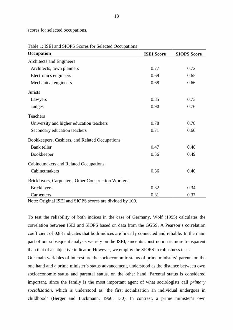
13

scores for selected occupations.

Table 1: ISEI and SIOPS Scores for Selected Occupations Occupation ISEI Score SIOPS Score Architects and Engineers

Architects, town planners 0.77 0.72 Electronics engineers 0.69 0.65 Mechanical engineers 0.68 0.66

Jurists Lawyers 0.85 0.73 Judges 0.90 0.76

Teachers University and higher education teachers 0.78 0.78 Secondary education teachers 0.71 0.60

Bookkeepers, Cashiers, and Related Occupations Bank teller 0.47 0.48 Bookkeeper 0.56 0.49

Cabinetmakers and Related Occupations Cabinetmakers 0.36 0.40

Bricklayers, Carpenters, Other Construction Workers Bricklayers 0.32 0.34 Carpenters 0.31 0.37

Note: Original ISEI and SIOPS scores are divided by 100.

To test the reliability of both indices in the case of Germany, Wolf (1995) calculates the

correlation between ISEI and SIOPS based on data from the GGSS. A Pearson’s correlation

coefficient of 0.88 indicates that both indices are linearly connected and reliable. In the main

part of our subsequent analysis we rely on the ISEI, since its construction is more transparent

than that of a subjective indicator. However, we employ the SIOPS in robustness tests.

Our main variables of interest are the socioeconomic status of prime ministers’ parents on the

one hand and a prime minister’s status advancement, understood as the distance between own

socioeconomic status and parental status, on the other hand. Parental status is considered

important, since the family is the most important agent of what sociologists call primary

socialisation, which is understood as ‘the first socialisation an individual undergoes in

childhood’ (Berger and Luckmann, 1966: 130). In contrast, a prime minister’s own

14

occupational status defines his or her social environment after adolescence and hence affects

secondary socialisation. However, since primary socialisation is regarded as ‘the most

important one for an individual, and that the basic structure of all secondary socialization has

to resemble that of primary socialization’ (Berger and Luckmann, 1966: 131), we expect own

occupational status to be important only in case of a discrepancy with parental status.14

5. Preliminary analysis: Do time and fiscal preferences depend on status?

Our research hypothesis is that German state governments led by prime ministers

characterised by high family status spend less and accumulate fewer debts. This hypothesis

relies on the assumption that an individual’s status determines his or her i) degree of

consumption patience or myopia and ii) preferences for the size of the government sector.

The extant literature provides evidence that preferences for government size and patience are

linked to single components of personal as well as parental status, i.e., education and income

(cf. Section 4) but, to the best of our knowledge, there is no political economy study

employing the status measures introduced above. Hence, in this section, we perform some

preliminary analyses employing German survey data in order to demonstrate the accuracy of

our core assumption. Our data source is the German General Social Survey

(GGSS/ALLBUS), which has been conducted every two years since 1980. In every survey

wave, about 2,800–3,500 representatively chosen respondents are interviewed.

We capture the degree of impatience or myopia, respectively, with answers to the following

question, which was part of the GGSS questionnaire in 1984, 1994, 2000, and 2004:15

What about your personal pension provision or provision for incapacity or illness? Do you feel you are─

(1) adequately provided for, (2) not adequately provided for, (3) or have you not thought about that yet?

We believe that a respondent who chooses either answer (2) or (3) can be regarded as

impatient or myopic. Thus, we create a binary variable by assigning the value 1 to answer (1)

and the value 0 to answers (2) and (3), pool the data from each single survey wave, and run a

binary choice (probit) regression, employing respondents’ parental status (indicated by the

14 This point of view is quite different from the one employed by the few economic applications of the status concept. In those, only an individual’s contemporary or future personal status is supposed to influence decision-making. Status is seen as steering individual behaviour because it is viewed as a substitute for pecuniary incentives, i.e., status concerns are represented directly in an individual’s utility function. See Fershtman et al. (1996) for a summary. 15 Descriptive statistics for this item can be found in Table A1 of the Appendix.

15

socioeconomic status of a respondent’s father) and status advancement as defined in Section 4

as explanatory variables.16

- A time dummy for each survey wave (reference: first wave).

We control for the following factors:

- Respondents’ self-placement on a left/right scale capturing ideological affiliation. The

scale ranges from 1 (left) to 10 (right).

- Dummies for respondents’ employment status, differentiating between employees

(including self-employed; reference group), students, retirees, unemployed, and other

jobless persons.

- A dummy for members of employees’ associations as membership may indicate

identification with the working class.

- Respondents’ age and a dummy for female respondents.

- A dummy for respondents living in East Germany, since the New Laender made up the

former socialistic German Democratic Republic (GDR).

The GGSS reports ISEI (SIOPS) scores for each respondent, the respondent’s father, and the

respondent’s spouse from 2000 (1980) onward. Hence, when utilising ISEI scores, we lose all

observations from survey waves conducted before 2000. Therefore, we also employ SIOPS

scores to test the robustness of our results.

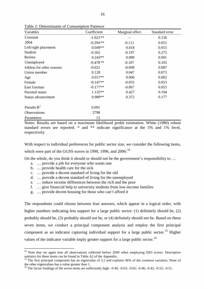
Table 2 reports the results of the probit specification.17

Focussing on our variables of main interest, we find that they are significantly different from

zero at the 1% level. The prevalence of myopia is lower the higher both parental status and

status advancement, which is well in line with our expectations. Both effects appear to be

substantial: a hike in parental status (status advancement) by 0.5—which roughly corresponds

to the distance between tradesmen and academic professions—increases the probability of

being provided for by about 21 (18.5) percentage points (pp).

The first column shows the

coefficients of the maximum likelihood estimation for the underlying continuous latent

variable model. In our case, the latent variable may be interpreted as the individual degree of

consumption patience. The second column shows the corresponding marginal effects, which

are calculated based on the sample averages.

16 Here, the variable status advancement equals the difference between the parental status score and the status score of the head of the household the respondent lives in, whereas the latter score is calculated as follows: first, we consider the status score of the respondent and the respondent’s spouse. Then, we assign the larger of the two numbers to the respondent. 17 Alternatively, we employ an ordered probit model and a multinomial model. Our results remain robust and are available on request.

16

Table 2: Determinants of Consumption Patience Variables Coefficient Marginal effect Standard error Constant -1.023 ** – 0.156 2004 -0.294 ** -0.111 0.051 Left/right placement 0.049 ** 0.018 0.015 Student -0.502 -0.197 0.275 Retiree 0.243 ** 0.089 0.091 Unemployed -0.478 ** -0.187 0.105 Jobless for other reasons -0.021 -0.008 0.087 Union member 0.128 0.047 0.073 Age 0.017 ** 0.006 0.002 Female -0.147 ** -0.055 0.053 East German -0.177 ** -0.067 0.055 Parental status 1.135 ** 0.427 0.194 Status advancement 0.989 ** 0.372 0.177 Pseudo-R2 0.091 Observations 2798 Parameters 13 Notes: Results are based on a maximum likelihood probit estimation. White (1980) robust standard errors are reported. * and ** indicate significance at the 5% and 1% level, respectively.

With respect to individual preferences for public sector size, we consider the following items,

which were part of the GGSS waves in 1990, 1996, and 2006:18

On the whole, do you think it should or should not be the government’s responsibility to …

a. … provide a job for everyone who wants one b. … provide health care for the sick c. … provide a decent standard of living for the old d. … provide a decent standard of living for the unemployed e. … reduce income differences between the rich and the poor f. … give financial help to university students from low-income families g. … provide decent housing for those who can’t afford it

The respondents could choose between four answers, which appear in a logical order, with

higher numbers indicating less support for a large public sector: (1) definitely should be, (2)

probably should be, (3) probably should not be, or (4) definitely should not be. Based on these

seven items, we conduct a principal component analysis and employ the first principal

component as an indicator capturing individual support for a large public sector.19 Higher

values of the indicator variable imply greater support for a large public sector.20

18 Note that we again lose all observations collected before 2000 when employing ISEI scores. Descriptive statistics for these items can be found in Table A2 of the Appendix.

19 The first principal component has an eigenvalue of 3.2 and explains 46% of the common variation. None of the other eigenvalues has a value greater than 1. 20 The factor loadings of the seven items are sufficiently high: -0.40; -0.63; -0.65; -0.46; -0.42; -0.52; -0.51.

17

Table 3 shows the results of an OLS regression with the principal component as the

endogenous variable, employing the same exogenous variables as before. The first column

contains the coefficients calculated based on the original units of measurement. The second

column reports standardised coefficients (beta coefficients), which facilitate interpretation of

the effects and permit conclusions about the relative importance of the single covariates.

Concentrating yet again on our variables of interest, we find that both parental status and

status advancement are significant at the 1% level and with signs in accordance with our

prior. The poorer an individual’s socioeconomic background, the greater his or her support for

a large government sector. The beta coefficients reveal that the impact of our status measures

is considerable as they have the largest standardised effects (in absolute terms): a hike in

parental status or status advancement by one standard deviation decreases the fiscal

preference indicator by about 0.17 standard deviations.

Table 3: Determinants of Preferences for Public Sector Size Variables Coefficient Beta coefficient Standard error Constant 0.662 – 0.156 Left/right placement -0.146 ** -0.149 0.039 Student 0.216 0.011 0.770 Retiree 0.210 0.053 0.235 Unemployed 0.410 0.062 0.272 Jobless for other reasons 0.622 * 0.099 0.260 Union member 0.363 * 0.087 0.164 Age 0.011 0.097 0.006 Female 0.110 0.031 0.144 East German 0.573 ** 0.157 0.149 Parental status -1.899 ** -0.165 0.509 Status advancement -1.518 ** -0.171 0.392 R2 0.131 Observations 597 Parameters 12 Notes: Results are based on an OLS estimation. * and ** indicate significance at the 5% and 1% level, respectively.

To check the robustness of our results, we employ the SIOPS scores as status measures

instead of the ISEI. This procedure has the advantage that SIOPS scores have been kept since

the first wave of the GGSS, so the number of observations in each specification increases

considerably. We find that our results are not only extremely robust, but even more

significant, reflecting the larger sample size.21

21 Results available on request.

18

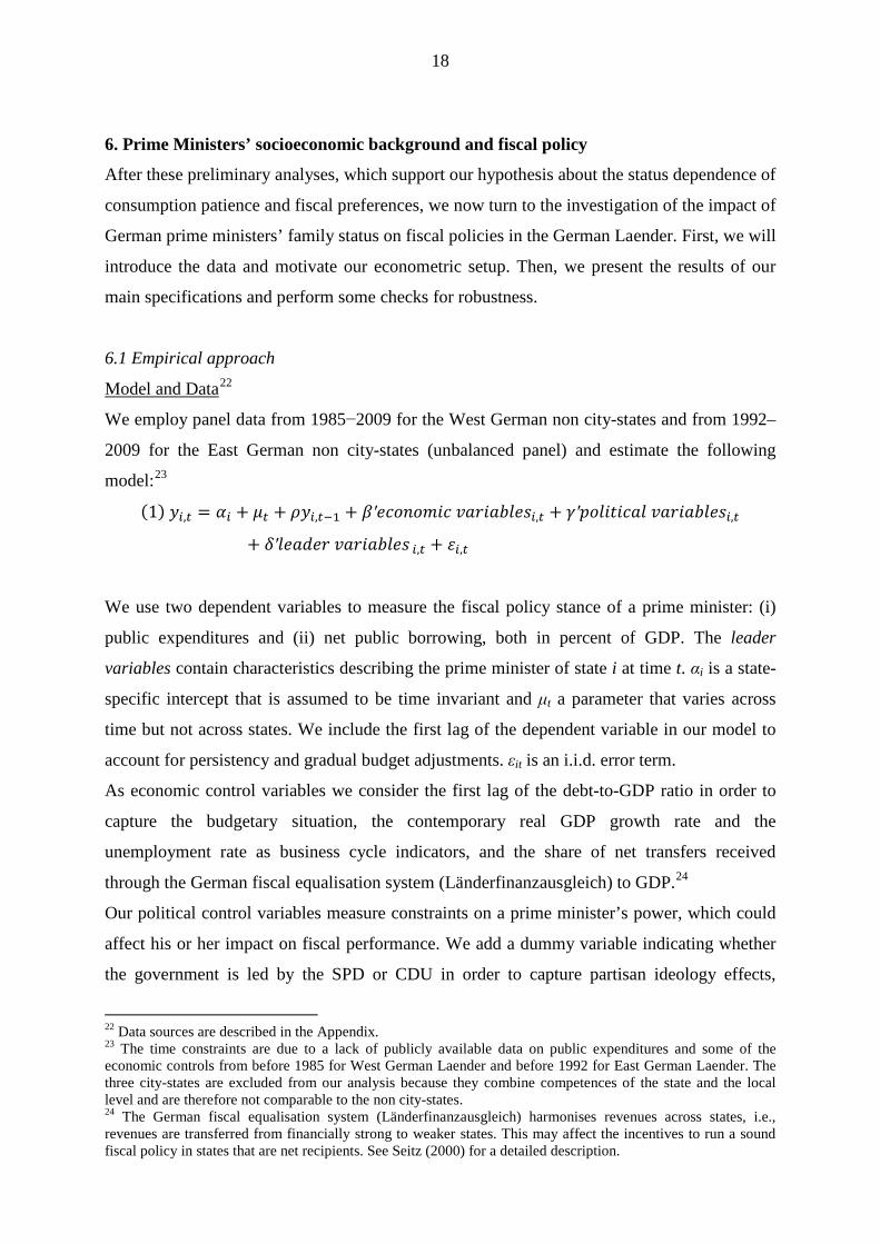
6. Prime Ministers’ socioeconomic background and fiscal policy

After these preliminary analyses, which support our hypothesis about the status dependence of

consumption patience and fiscal preferences, we now turn to the investigation of the impact of

German prime ministers’ family status on fiscal policies in the German Laender. First, we will

introduce the data and motivate our econometric setup. Then, we present the results of our

main specifications and perform some checks for robustness.

6.1 Empirical approach

Model and Data22

We employ panel data from 1985−2009 for the West German non city-states and from 1992–

2009 for the East German non city-states (unbalanced panel) and estimate the following

model:

23

(1) 𝑦𝑖,𝑡 = 𝛼𝑖 + 𝜇𝑡 + 𝜌𝑦𝑖,𝑡−1 + 𝛽′𝑒𝑐𝑜𝑛𝑜𝑚𝑖𝑐 𝑣𝑎𝑟𝑖𝑎𝑏𝑙𝑒𝑠𝑖,𝑡 + 𝛾′𝑝𝑜𝑙𝑖𝑡𝑖𝑐𝑎𝑙 𝑣𝑎𝑟𝑖𝑎𝑏𝑙𝑒𝑠𝑖,𝑡+ 𝛿′𝑙𝑒𝑎𝑑𝑒𝑟 𝑣𝑎𝑟𝑖𝑎𝑏𝑙𝑒𝑠 𝑖,𝑡 + 𝜀𝑖,𝑡

We use two dependent variables to measure the fiscal policy stance of a prime minister: (i)

public expenditures and (ii) net public borrowing, both in percent of GDP. The leader

variables contain characteristics describing the prime minister of state i at time t. αi is a state-

specific intercept that is assumed to be time invariant and μt a parameter that varies across

time but not across states. We include the first lag of the dependent variable in our model to

account for persistency and gradual budget adjustments. εit is an i.i.d. error term.

As economic control variables we consider the first lag of the debt-to-GDP ratio in order to

capture the budgetary situation, the contemporary real GDP growth rate and the

unemployment rate as business cycle indicators, and the share of net transfers received

through the German fiscal equalisation system (Länderfinanzausgleich) to GDP.24

Our political control variables measure constraints on a prime minister’s power, which could

affect his or her impact on fiscal performance. We add a dummy variable indicating whether

the government is led by the SPD or CDU in order to capture partisan ideology effects,

22 Data sources are described in the Appendix. 23 The time constraints are due to a lack of publicly available data on public expenditures and some of the economic controls from before 1985 for West German Laender and before 1992 for East German Laender. The three city-states are excluded from our analysis because they combine competences of the state and the local level and are therefore not comparable to the non city-states. 24 The German fiscal equalisation system (Länderfinanzausgleich) harmonises revenues across states, i.e., revenues are transferred from financially strong to weaker states. This may affect the incentives to run a sound fiscal policy in states that are net recipients. See Seitz (2000) for a detailed description.

19

dummies for coalition governments and minority governments to account for effects of

political dispersion or conflicts of interest,25

Our main variables of interest among the leader characteristics are the socioeconomic status

of prime ministers’ parents and change in their own status. Following the literature and adding

additional controls, we include as further characteristics:

and dummies for pre-election and election years

to control for political budget cycles. Further, we control for the share of votes the prime

minister’s party received in the last election. This variable indicates the strength of the

incumbent governing party. Finally, we include a dummy that indicates whether the minister

of finance is from the same party as the prime minister, since the finance minister has

significant authority regarding preparation of the public budget. We expect that a finance

minister from the same party is more likely to back the prime minister’s political course

(Jochimsen and Nuscheler, 2010).

- A prime minister’s age and number of years in office, thus capturing experience.

- A dummy for prime ministers who have been members in employees’ associations, since

membership may serve as an indicator of an individual’s habitus, i.e., indicate that he or

she is prone to implementing policies benefitting a certain group in society.

- A dummy for prime ministers of states in which they did not formerly reside. We believe

this variable to be an indicator for how strongly a leader is attached to the state he or she

governs.

- A dummy for years in which a new prime minister comes into power to capture transition

effects.26

Econometric Methodology

We estimate Equation (1) with a two-way fixed-effects model, allowing for the state- and

time-specific effects to be correlated with the other covariates. A Hausman test reveals that

the results of the fixed-effects approach differ significantly from those of a random-effects

approach or a pooled OLS model, supporting our empirical specification. The lagged

dependent variable correlates with the error term, which causes the least squares dummy

variable (LSDV) estimator of the autoregressive coefficient ρ to be biased downward (Judson

and Owen, 1997), while the bias in the coefficients of the exogenous regressors tends to be

positive but much smaller (in absolute terms). Moreover, the bias becomes negligible for

25 As Edin and Ohlsson (1991) and de Haan and Sturm (1994, 1997) state, the measurement of political dispersion by a single ordinal variable, as employed by Roubini and Sachs (1989), is not recommended, since this imposes a strong restriction on its effect. 26 Transition years imply coding problems, since we can only take into account one prime minister each year. In these cases, we decided to include the prime minister who held the office for the larger part of the year.

20

growing T.

An alternative to LSDV estimation is a GMM approach, as suggested by Arellano and Bond

(1991). However, GMM estimators suffer from poor finite sample properties for small N and

tend to underestimate the coefficients of the exogenous regressors (Kiviet, 1995).

Taking into consideration the advantages and disadvantages of both estimation techniques, we

rely on the LSDV estimator in the main part of our analysis and apply GMM as part of our

robustness tests. Other robustness checks investigate whether our results differ across the

West and East German states, different government constellations, and when including

additional control variables.

6.2 Results

Main specifications

Results of the regressions explaining public spending in the German Laender are presented in

Table 4. In a first step, we estimate a general model containing all the theory-relevant

covariates described in Subsection 6.1. Then, we eliminate insignificant regressors by

applying a consistent general-to-specific approach (Hendry, 2000) so as to enhance estimation

efficiency.

We find that the coefficient of the lagged debt-to-GDP ratio is significantly negative at the 1%

level. Hence, Laender with a poor budgetary situation reduce their expenditures. This suggests

that the political process does react to the debt situation in a state, but not strongly. In the

short run, a 1 percentage point (pp) increase in the previous period’s debt-to-GDP ratio

reduces government expenditures in relation to GDP by 0.06 pp. The long-run multiplier is

0.3, which is still quite modest.

The real GDP growth rate also exerts a significantly negative impact, indicating that state

governments engage in counter-cyclical fiscal policy. However, given the short-term nature of

stabilisation, the effect is small: a 1 pp reduction in GDP growth triggers an adjustment of 0.1

pp in the expenditure-to-GDP ratio; the long-run effect is about 0.5. Transfers received

through the fiscal equalisation scheme in relation to GDP show a positive coefficient, but the

individual effect is not significantly different from zero.27

Among the political covariates, three out of seven variables survive the model reduction. The

dummies for minority governments and ministers of finance who are not from the same party

as the prime minister have the expected positive signs, meaning that the greater the dispersion

of power within a government, the higher the level of public spending. The former variable is

27 Note that we cannot exclude this variable from the model without violating the testing-down restriction.

21

individually insignificant; the latter has a substantial impact—a finance minister from a

different party causes an increase in the expenditure-to-GDP ratio of over 0.45 pp in the short

run. In the long run, this effect grows to over 2 pp. The vote share of the prime minister’s

party also reveals a positive impact on expenditures, but the economic effect is almost

negligible.

Table 4: Results for Public Expenditures Over GDP (in %)

Variables General Model Reduced Model Coefficient Stand. error Coefficient Stand. error

Publ. expend./GDP (-1) 0.750 ** 0.054 0.794 ** 0.046

Economic variables Debt-to-GDP-ratio (-1) -0.061 ** 0.018 -0.059 ** 0.017 GDP growth -0.083 ** 0.027 -0.094 ** 0.025 Unemployment rate 0.038 0.029 Transfers/GDP 0.303 0.211 0.337 0.219

Political variables SPD-led government -0.178 0.102 Coalition 0.215 0.128 Minority government 0.674 * 0.318 0.427 0.234 Vote share gov. party 0.035 * 0.014 0.018 * 0.008 Pre-election year 0.070 0.065 Election year -0.002 0.058 MoF from different party 0.411 * 0.194 0.458 * 0.189

Leader variables PM change -0.018 0.077 Outside PM 0.081 0.150 Union member -0.043 0.083 Age -0.002 0.006 Years in office -0.003 0.010 Parental status -1.448 ** 0.424 -1.021 ** 0.385 Status advancement -1.481 ** 0.494 -1.116 * 0.456

R2 (without state and time fixed effects) 0.899 0.894 Observations 277 277 Parameters 55 45 Testing-down restriction Chi2 (10) = 17.0562 Notes: Results are based on a least squares dummy variable (LSDV) estimation. The models include cross-section and time fixed effects. Panel robust standard errors are reported. * and ** indicate significance at the 5% and 1% level, respectively.

Regarding leader characteristics, we find that parental status and status advancement are the

only variables remaining in the reduced model. They show the expected signs and are

22

significant at the 1% and 5% level, respectively. Tenures of prime ministers who worked in

academic professions before taking up politics (average ISEI score about 0.85) are associated

with a public expenditure quota that is on average 0.55 pp less than that during tenures of

prime ministers who were formerly tradesmen (average ISEI score about 0.35), keeping

parental status constant. The influence of parental status is only slightly smaller in magnitude:

the difference between prime ministers whose parents hold academic professions compared to

those whose parents are tradesmen is about 0.5 pp. Other leader characteristics exert no

significant influence on public spending. In the long run, the expenditure-to-GDP ratio of

Laender with prime ministers who formerly were tradesmen is 2.7pp lower than it is in

Laender with prime ministers who previously held an academic post. The parental status

effect multiplier is about 2.5, but the difference between the coefficients of the two status

variables is not statistically significant.28

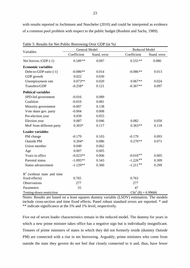
Table 5 presents the results for net public borrowing over GDP. The coefficients of the

general model including all covariates are shown on the left-hand side; the results for the

reduced model are shown on the right-hand side. With respect to the economic covariates, we

observe a counter-cyclical movement of net borrowings, just like in the case of public

expenditures, but whereas public spending responds to GDP growth, net borrowing reacts to

the unemployment rate. This makes sense, since a rise in unemployment leads to a decrease in

public revenues and, thus, raises the current deficit even if the level of expenditures is held

constant. The economic impact of unemployment on the deficit-to-GDP ratio is small, though.

After a 1 pp increase in the unemployment rate, the ratio decreases by only 0.07 pp in the

short run and by about 0.15 pp in the long run. The coefficient of the lagged debt-to-GDP-

ratio is negative also, which indicates that states tend to reduce deficits when they have a high

level of debt. Yet, again, the adjustment effect is small, a decline of less than 0.1 (0.2) pp in

the short (long) run. Unlike in the case of public spending, we find a negative effect of

received transfers, which suggests that such transfers are a substitute for deficit spending. A 1

pp increase in transfers lowers the deficit-to-GDP ratio by 0.4 pp and the long-run multiplier

is 0.8.

Thus, the impact of status is not only statistically

significant with theory-consistent signs but also economically substantial.

Regarding political controls, we find that the election year dummy has a positive sign,

indicating evidence of a political budget cycle in public deficits, but it is not individually

significant. The dummy for finance ministers from other parties is positive, which is in line

28 The p-value for a corresponding Chi2-test with the null hypothesis ‘coefficients are equal’ is 0.57.

23

with results reported in Jochimsen and Nuscheler (2010) and could be interpreted as evidence

of a common pool problem with respect to the public budget (Roubini and Sachs, 1989).

Table 5: Results for Net Public Borrowing Over GDP (in %)

Variables General Model Reduced Model Coefficient Stand. error Coefficient Stand. error

Net borrow./GDP (-1) 0.549 ** 0.097 0.555 ** 0.080

Economic variables Debt-to-GDP-ratio (-1) -0.086 ** 0.014 -0.086 ** 0.013 GDP growth 0.022 0.030 Unemployment rate 0.073 ** 0.020 0.067 ** 0.024 Transfers/GDP -0.258 * 0.121 -0.367 ** 0.097

Political variables SPD-led government -0.016 0.089 Coalition -0.019 0.081 Minority government -0.007 0.138 Vote share gov. party -0.004 0.008 Pre-election year 0.039 0.055 Election year 0.087 0.046 0.082 0.050 MoF from different party 0.303 * 0.117 0.363 ** 0.118

Leader variables PM change -0.179 0.103 -0.179 0.093 Outside PM 0.204 * 0.086 0.270 ** 0.071 Union member 0.049 0.062 Age 0.007 0.005 Years in office -0.023 ** 0.006 -0.018 ** 0.005 Parental status -1.095 ** 0.343 -1.226 ** 0.309 Status advancement -1.129 ** 0.360 -1.211 ** 0.299

R2 (without state and time fixed effects) 0.765 0.763 Observations 277 277 Parameters 55 47 Testing-down restriction Chi2 (8) = 6.99666 Notes: Results are based on a least squares dummy variable (LSDV) estimation. The models include cross-section and time fixed effects. Panel robust standard errors are reported. * and ** indicate significance at the 5% and 1% level, respectively.

Five out of seven leader characteristics remain in the reduced model. The dummy for years in

which a new prime minister takes office has a negative sign but is individually insignificant.

Tenures of prime ministers of states in which they did not formerly reside (dummy Outside

PM) are connected with a rise in net borrowing. Arguably, prime ministers who come from

outside the state they govern do not feel that closely connected to it and, thus, have fewer

24

incentives to conduct sustainable fiscal policy and are more prone to myopic decision-making.

The deficit-to-GDP ratio is about 0.3 pp higher in the case of an outside prime minister, with a

long-run multiplier of 0.6. We also find that the longer a prime minister stays in office, the

smaller is net borrowing over GDP. We interpret this result as reflecting increasing

competence during incumbency: the more experienced a prime minister, the easier it is for

him or her to keep the budget in balance. In addition, staying in office for a long time may

deepen attachment to the governed state. The effect is fairly modest, though. Staying in office

for a second term lowers the deficit-to-GDP ratio by 0.07 pp.

As in the case of public spending, a prime minister’s parental status and own status

advancement play an important role in explaining variations in fiscal performance: the higher

the parental status or own status advancement, the lower the inclination toward deficit

spending. Both effects are significant at the 1% level and their coefficients are of a similar

magnitude as in the case of public spending, which implies that, on average, every additional

Euro of public expenditure by a prime minister of low status is deficit financed. Comparing

again tradesman and academic profession parental background, prime ministers from the

latter have a 0.6 pp lower deficit in the short run and a 1.4 pp lower deficit in the long run.

Similar effects apply in the case of status advancement and the coefficients of the two status

variables are not significantly different.29

Checks for Robustness

To check the robustness of our results and glean further insight, we conduct several

experiments. First, we test whether our results are affected by the estimation method. We re-

estimate Equation (1) using a GMM approach to account for the fact that the lagged

dependent variable is correlated with the error term. We apply one-step GMM estimation and

use up to five valid lags of the dependent variable as instruments.30

29 The p-value for a corresponding Chi2-test with the null hypothesis ‘coefficients are equal’ is 0.92.

The results for public

spending and debt financing are presented in the Appendix, Table A3. In line with findings

from simulation studies, most coefficients and standard errors decrease in the GMM

approach, but in our case the differences are typically rather small. The biggest difference can

be found in the model for public spending and the coefficients for parental status and status

advancement. However, both variables are now significant at the 1% level and the long-run

30 The number of lags is restricted for two reasons. First, standard econometric software is not able to invert the matrix of instruments when using all valid lags to define moment conditions (as suggested by Arellano and Bond, 1991), as the computational requirements increase substantially. Second, simulation studies show that there is a tradeoff when increasing the number of lags: together with efficiency, the finite sample bias of the GMM estimates also increases (Judson and Owen, 1997). With respect to our variables of main interest, we find no significant changes when varying the number of lags used as instruments, employing from 1 up to 10 lags.

25

multipliers remain basically constant, so that even in this case our conclusions do not change

notably.

Second, we check whether our results differ across the Old and New Laender. Since the New

Laender made up the former socialist German Democratic Republic (GDR), there could be

status-specific differences between them and the Old Laender. We address this problem by

including two dummy variables: D1 takes the value 1 for West German Laender and 0 for East

German Laender; D2 the other way around. Then, we let these dummies interact with the

political controls and leader characteristics and estimate the following equation:31

(2) 𝑦𝑖,𝑡 = 𝛼𝑖 + 𝜇𝑡 + 𝜌𝑦𝑖,𝑡−1 + 𝛽′𝑒𝑐𝑜𝑛𝑜𝑚𝑖𝑐 𝑣𝑎𝑟𝑖𝑎𝑏𝑙𝑒𝑠𝑖,𝑡 + �𝛾𝑘′ 𝐷𝑘𝑝𝑜𝑙𝑖𝑡𝑖𝑐𝑎𝑙 𝑣𝑎𝑟𝑖𝑎𝑏𝑙𝑒𝑠𝑖,𝑡𝑘

+ �𝛿𝑘′ 𝐷𝑘𝑙𝑒𝑎𝑑𝑒𝑟 𝑣𝑎𝑟𝑖𝑎𝑏𝑙𝑒𝑠𝑖,𝑡𝑘

+ 𝜀𝑖,𝑡

The results for both public expenditure and debt financing are presented in Table A4 of the

Appendix. We find that our variables of main interest exert a statistically significant influence

in both subpanels, and that this influence is greater in the East German states than it is in the

West German ones.32

An interesting result is that a prime minister’s experience (measured as years in office) has a

statistically significant effect only in the New Laender. The longer an East German prime

minister stays in power, the lower the public spending and debt financing in his or her state,

which supports our proposition that experience enhances competence. The five New Laender

suffered a lack in infrastructure and continue to lag behind the Old Laender in per-capita GDP

and income, making the economic conditions in those states far more challenging; hence,

competence might be even more valuable in the New Laender.

The coefficient of parental status is more than two times larger in case

of public spending and more than four times larger in case of net borrowing within the New

Laender. The coefficient of status advancement is three times the magnitude in the case of

public spending and seven times in the case of net borrowing.

There are several differences between East and West German states when it comes to the

political controls. Within the New Laender, tenures of SPD-led governments are associated

with a decline in public expenditure and net borrowing, whereas coalitions tend to increase

31 Alternatively, we could have estimated two balanced subpanels: one for the Old Laender and one for the New Laender. We decided to estimate a nested model for two reasons: (i) it increases the number of observations and hence enhances efficiency and (ii) it allows performing statistical tests across Old and New Laender. 32 Note that a Chi-squared test reveals that parental status and status advancement are jointly significant within the East German Laender at the 1% level. Hence, the individual insignificance of both coefficients is due to collinearity.

26

public spending and debt financing. Minority governments exert a significantly positive

influence only on public spending.

In a third robustness check, we examine the effect of including additional control variables.

First, we control for different partisan compositions of the government, following Seitz

(2000), Galli and Rossi (2002), Berger and Holler (2007), Schneider (2010), and Jochimsen

and Nuscheler (2010). Dummies for each composition that occurred during our sample period

replace the dummies for SPD-led governments and coalition governments. The output is

presented in Table A5 of the Appendix and reveals that the results for the economic indicators

and leader characteristics hardly change. We are also concerned about the problem of

spurious causation due to omitted variables. It could be argued that our findings regarding the

impact of a prime minister’s socioeconomic background are driven by the socioeconomic

conditions of the electorate. We examined this possibility by including real disposable income

per head in our regressions. We also controlled for several demographic factors, i.e.,

population growth as well as the share of population aged less than 25 years and more than 65

years, since these groups typically benefit overproportionally from the public provision of

goods. However, since none of these factors reveals a significant impact on the endogenous

variables or changes our results, we do not report these estimates (they are available upon

request).

Finally, we check whether choice of status index affects our findings. As mentioned in

Section 4, there are essentially two ways of measuring an individual’s status: objective

indicators (e.g., ISEI) or subjective indicators (e.g., SIOPS). We replace the ISEI scores with

the SIOPS scores and re-estimate Equation (1). As can be seen in Table A6 of the Appendix,

use of the other index hardly changes the results: the coefficients of parental status and status

advancement become a little larger and are still significant at the 1% level.

7. Conclusion

‘Classical’ theories in political economy that view politicians’ motives as decisive in fiscal

performance often reveal little explanatory power in empirical research. Neither opportunism,

nor benevolence, nor partisan ideology satisfactorily explain politicians’ decision-making. In

light of this, some economics researchers have begun focussing on politicians’ backgrounds

instead, taking into account age, experience, or certain educational and occupational

characteristics. However, yet again the results are ambiguous and not particularly robust.

In contrast, an important strand in sociological research argues that the way people think and

act is steered by a set of socially constituted schemes that depend on an individual’s status—

27

i.e., his or her relative standing within society. Evidence from household and survey data as

well as our own empirical investigations employing the German General Social Survey

indicate that individual status or factors related to it (such as educational attainment and

income) might help explain differences in how leaders conduct fiscal policy.

In our novel empirical analysis, we test whether a head of government’s family status has an

impact on the incumbent government’s fiscal performance. We focus on the German Laender,

as they are characterised by a high degree of political and institutional homogeneity and their

prime ministers’ are empowered with extensive fiscal competences.

Our extremely robust and theory-consistent findings reveal that a prime minister’s family

status—operationalised by parental status and own status advancement—influences fiscal

performance in a statistically significant and economically relevant way. The higher a prime

minister’s parental status and own status advancement, the lower are the incumbent

government’s public spending and debt financing in relation to GDP. For example, tenures of

prime ministers who worked in academic professions before taking up politics are associated

with a public expenditure quota that is on average 0.55 percentage points less than that of

tenures of prime ministers who were formerly tradesmen. The influence of parental status is

only slightly smaller in magnitude. In the long run, the expenditure-to-GDP ratio of Laender

with prime ministers who formerly worked as tradesmen is 2.7 percentage points lower than

that of Laender having prime ministers who formerly held an academic post. The parental

status effect multiplier is about 2.5. In the case of net public borrowing over GDP, prime

ministers with an academic history have a 0.6 percentage points lower deficit in the short run

and a 1.4 percentage points lower deficit in the long run. Similar effects are found for the case

of parental status.

In the theoretical part of our paper, we emphasise that individual preferences and patterns of

behaviour reflect status-specific dispositions. However, it is not only aggregate public

spending, but also preferences regarding the composition of the public budget, that might

depend on individual status. In this regard, effects of social rivalry may be important, e.g.,

with respect to the share of public expenditure on policies such as social security or education.

Therefore, an interesting task for future research would be an investigation of the influence of

the head of government’s status on single items of public expenditure.

28

Appendix:

Data Sources

Economic Controls

Data on public expenditures, real GDP growth, unemployment rate, per-capita income, and

the demography of population for each German state are from the Federal Statistical Office

(Statistisches Bundesamt). Data on public debts, net public borrowing, and transfers between

the Laender within the fiscal equalisation system are from the Federal Ministry of Finance.

Political Controls

Data on election dates, vote shares, and government composition are taken from the

homepages of the German Laender and the State Returning Officers (Landeswahlleiter), as is

historical information on the party affiliation of the ministers of finance.

Leader Characteristics

Information on prime ministers is from various sources. Years in which a new prime minister

took office are identified using the homepages of the German Laender and the State Returning

Officers.

Information on prime ministers’ dates of birth, places of residence, occupational histories, and

whether they have been union members is from the Munzinger Online biography and the

public record offices of the German Laender. Both provide brief biographies of public figures,

especially politicians. In a few cases we also rely on information provided on personal

homepages of (former) prime ministers. The variable age refers to a prime minister’s age at

the end of the year.

The variable parental status measures the occupational status score of prime ministers’

parents. To construct this variable, we coded the occupations of prime ministers’ parents

according to the ISCO-68 and then applied the ISEI and SIOPS scores. When both parents

were working or when a parent held more than one occupation during his or her career, we

decided to employ the highest ISEI and SIOPS score. In cases where a prime minister was

entirely raised by one parent only (due to divorce or death of the other parent), we decided to

take only the status score of that parent into account. Further, we do not differentiate between

biological and stepparents.

For the variable status advancement we focus on the positions prime ministers held before

their political career, which we defined as first membership in a party executive committee or

ministry. In cases where prime ministers engaged in more than one occupation during their

career, we chose the occupation with the highest ISEI and SIOPS score.

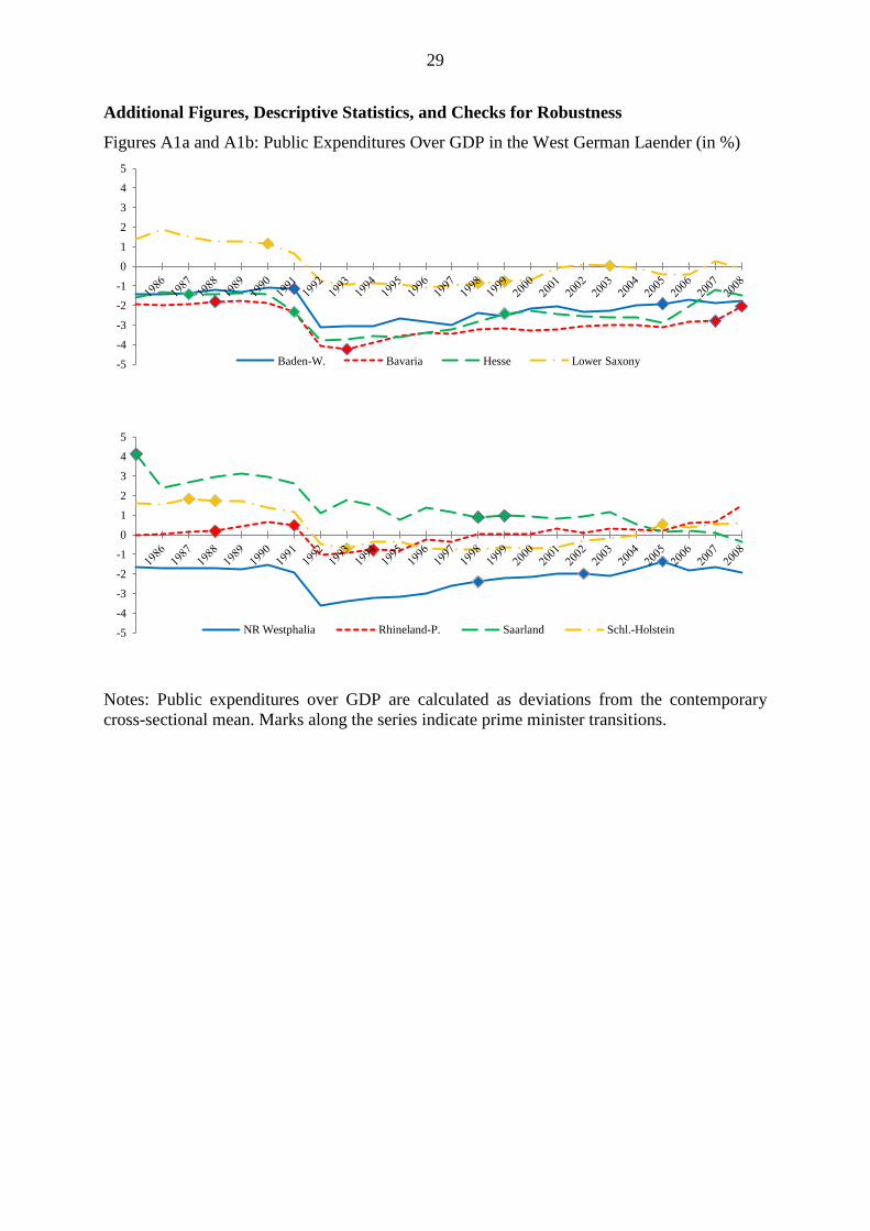
29

Additional Figures, Descriptive Statistics, and Checks for Robustness

Figures A1a and A1b: Public Expenditures Over GDP in the West German Laender (in %)

Notes: Public expenditures over GDP are calculated as deviations from the contemporary cross-sectional mean. Marks along the series indicate prime minister transitions.

-5

-4

-3

-2

-1

0

1

2

3

4

5

Baden-W. Bavaria Hesse Lower Saxony

-5

-4

-3

-2

-1

0

1

2

3

4

5

NR Westphalia Rhineland-P. Saarland Schl.-Holstein

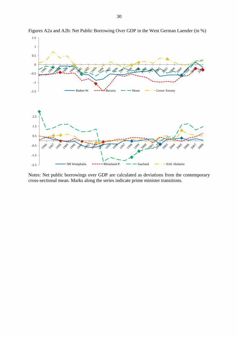
30

Figures A2a and A2b: Net Public Borrowing Over GDP in the West German Laender (in %)

Notes: Net public borrowings over GDP are calculated as deviations from the contemporary cross-sectional mean. Marks along the series indicate prime minister transitions.

-1.5

-1

-0.5

0

0.5

1

1.5

Baden-W. Bavaria Hesse Lower Saxony

-2.5

-1.5

-0.5

0.5

1.5

2.5

NR Westphalia Rhineland-P. Saarland Schl.-Holstein

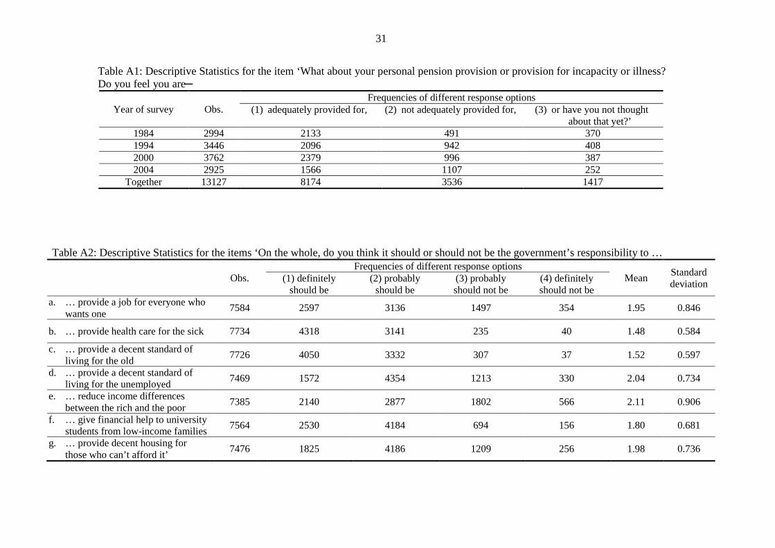
31

Table A1: Descriptive Statistics for the item ‘What about your personal pension provision or provision for incapacity or illness? Do you feel you are─

Year of survey Obs. Frequencies of different response options

(1) adequately provided for, (2) not adequately provided for, (3) or have you not thought about that yet?’

1984 2994 2133 491 370 1994 3446 2096 942 408 2000 3762 2379 996 387 2004 2925 1566 1107 252

Together 13127 8174 3536 1417

Table A2: Descriptive Statistics for the items ‘On the whole, do you think it should or should not be the government’s responsibility to …

Obs. Frequencies of different response options

Mean Standard deviation (1) definitely

should be (2) probably

should be (3) probably should not be

(4) definitely should not be

a. … provide a job for everyone who wants one 7584 2597 3136 1497 354 1.95 0.846

b. … provide health care for the sick 7734 4318 3141 235 40 1.48 0.584

c. … provide a decent standard of living for the old 7726 4050 3332 307 37 1.52 0.597

d. … provide a decent standard of living for the unemployed 7469 1572 4354 1213 330 2.04 0.734

e. … reduce income differences between the rich and the poor 7385 2140 2877 1802 566 2.11 0.906

f. … give financial help to university students from low-income families 7564 2530 4184 694 156 1.80 0.681

g. … provide decent housing for those who can’t afford it’ 7476 1825 4186 1209 256 1.98 0.736

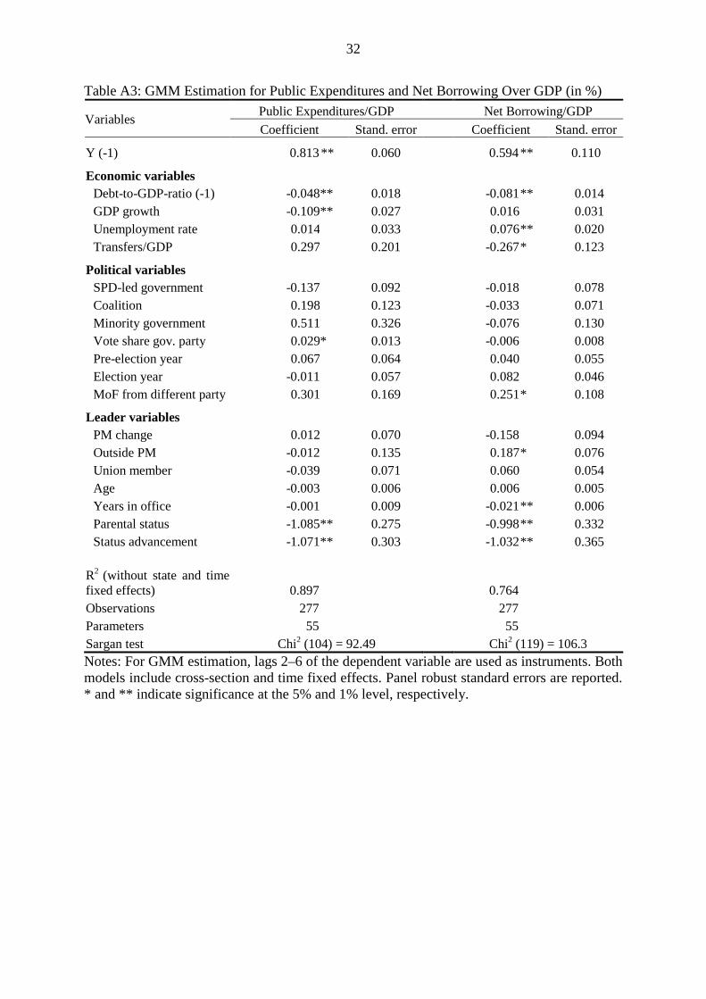
32

Table A3: GMM Estimation for Public Expenditures and Net Borrowing Over GDP (in %)

Variables Public Expenditures/GDP Net Borrowing/GDP Coefficient Stand. error Coefficient Stand. error

Y (-1) 0.813 ** 0.060 0.594 ** 0.110

Economic variables Debt-to-GDP-ratio (-1) -0.048 ** 0.018 -0.081 ** 0.014 GDP growth -0.109 ** 0.027 0.016 0.031 Unemployment rate 0.014 0.033 0.076 ** 0.020 Transfers/GDP 0.297 0.201 -0.267 * 0.123

Political variables SPD-led government -0.137 0.092 -0.018 0.078 Coalition 0.198 0.123 -0.033 0.071 Minority government 0.511 0.326 -0.076 0.130 Vote share gov. party 0.029 * 0.013 -0.006 0.008 Pre-election year 0.067 0.064 0.040 0.055 Election year -0.011 0.057 0.082 0.046 MoF from different party 0.301 0.169 0.251 * 0.108

Leader variables PM change 0.012 0.070 -0.158 0.094 Outside PM -0.012 0.135 0.187 * 0.076 Union member -0.039 0.071 0.060 0.054 Age -0.003 0.006 0.006 0.005 Years in office -0.001 0.009 -0.021 ** 0.006 Parental status -1.085 ** 0.275 -0.998 ** 0.332 Status advancement -1.071 ** 0.303 -1.032 ** 0.365

R2 (without state and time fixed effects) 0.897 0.764 Observations 277 277 Parameters 55 55 Sargan test Chi2 (104) = 92.49 Chi2 (119) = 106.3 Notes: For GMM estimation, lags 2–6 of the dependent variable are used as instruments. Both models include cross-section and time fixed effects. Panel robust standard errors are reported. * and ** indicate significance at the 5% and 1% level, respectively.

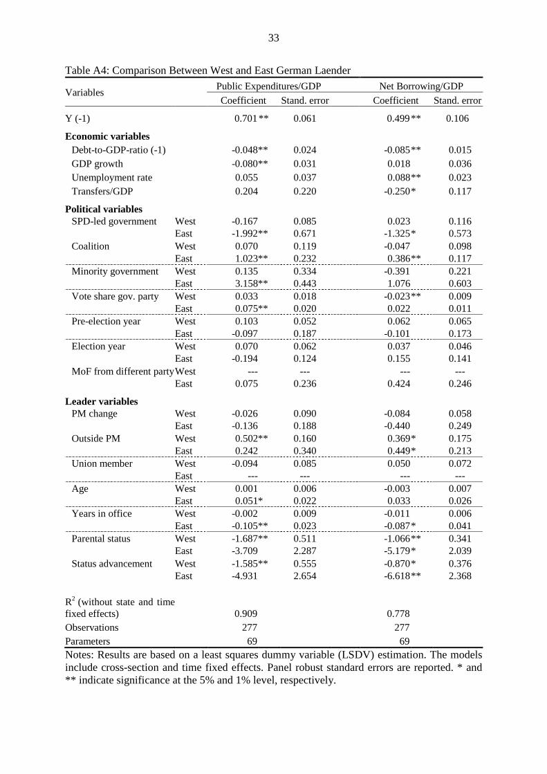
33

Table A4: Comparison Between West and East German Laender

Variables Public Expenditures/GDP Net Borrowing/GDP Coefficient Stand. error Coefficient Stand. error

Y (-1) 0.701 ** 0.061 0.499 ** 0.106

Economic variables Debt-to-GDP-ratio (-1) -0.048 ** 0.024 -0.085 ** 0.015 GDP growth -0.080 ** 0.031 0.018 0.036 Unemployment rate 0.055 0.037 0.088 ** 0.023 Transfers/GDP 0.204 0.220 -0.250 * 0.117

Political variables SPD-led government West -0.167 0.085 0.023 0.116

East -1.992 ** 0.671 -1.325 * 0.573 Coalition West 0.070 0.119 -0.047 0.098

East 1.023 ** 0.232 0.386 ** 0.117 Minority government West 0.135 0.334 -0.391 0.221

East 3.158 ** 0.443 1.076 0.603 Vote share gov. party West 0.033 0.018 -0.023 ** 0.009

East 0.075 ** 0.020 0.022 0.011 Pre-election year West 0.103 0.052 0.062 0.065

East -0.097 0.187 -0.101 0.173 Election year West 0.070 0.062 0.037 0.046

East -0.194 0.124 0.155 0.141 MoF from different party West --- --- --- ---

East 0.075 0.236 0.424 0.246

Leader variables PM change West -0.026 0.090 -0.084 0.058

East -0.136 0.188 -0.440 0.249 Outside PM West 0.502 ** 0.160 0.369 * 0.175

East 0.242 0.340 0.449 * 0.213 Union member West -0.094 0.085 0.050 0.072

East --- --- --- --- Age West 0.001 0.006 -0.003 0.007

East 0.051 * 0.022 0.033 0.026 Years in office West -0.002 0.009 -0.011 0.006

East -0.105 ** 0.023 -0.087 * 0.041 Parental status West -1.687 ** 0.511 -1.066 ** 0.341

East -3.709 2.287 -5.179 * 2.039 Status advancement West -1.585 ** 0.555 -0.870 * 0.376

East -4.931 2.654 -6.618 ** 2.368 R2 (without state and time fixed effects)

0.909 0.778

Observations 277 277 Parameters 69 69 Notes: Results are based on a least squares dummy variable (LSDV) estimation. The models include cross-section and time fixed effects. Panel robust standard errors are reported. * and ** indicate significance at the 5% and 1% level, respectively.

34

Table A5: Controlling for Different Government Compositions

Variables Public Expenditures/GDP Net Borrowing/GDP Coefficient Stand. error Coefficient Stand. error

Y (-1) 0.723 ** 0.054 0.520 ** 0.117

Economic variables Debt-to-GDP-ratio (-1) -0.056 ** 0.018 -0.081 ** 0.013 GDP growth -0.074 ** 0.028 0.022 0.034 Unemployment rate 0.040 0.038 0.074 ** 0.027 Transfers/GDP 0.304 0.222 -0.193 0.116

Political variables CDU Reference Reference CDU/SPD 0.341 0.181 -0.091 0.135 CDU/FDP 0.313 * 0.138 0.022 0.093 SPD -0.090 0.112 -0.095 0.101 SPD/CDU -0.166 0.337 -0.083 0.226 SPD/GREEN 0.089 0.157 -0.044 0.127 SPD/LEFT 0.053 0.234 -0.035 0.155 SPD/FDP -0.107 0.155 -0.155 0.164 SPD/FDP/GREEN 0.526 0.408 0.766 * 0.295 Minority government 0.723 * 0.279 0.022 0.145 Vote share gov. party 0.034 * 0.016 -0.001 0.010 Pre-election year 0.074 0.066 0.032 0.055 Election year -0.008 0.059 0.078 0.049 MoF from different party 0.355 0.223 0.301 * 0.136

Leader variables PM change 0.000 0.076 -0.160 0.106 Outside PM 0.187 0.125 0.330 ** 0.097 Union member 0.009 0.148 0.089 0.097 Age -0.005 0.007 0.003 0.005 Years in office -0.002 0.010 -0.021 ** 0.006 Parental status -1.316 * 0.505 -1.106 ** 0.327 Status advancement -1.417 * 0.551 -1.096 ** 0.355

R2 (without state and time fixed effects) 0.901 0.770 Observations 277 277 Parameters 61 61 Notes: Results are based on a least squares dummy variable (LSDV) estimation. The models include cross-section and time fixed effects. Panel robust standard errors are reported. * and ** indicate significance at the 5% and 1% level, respectively.

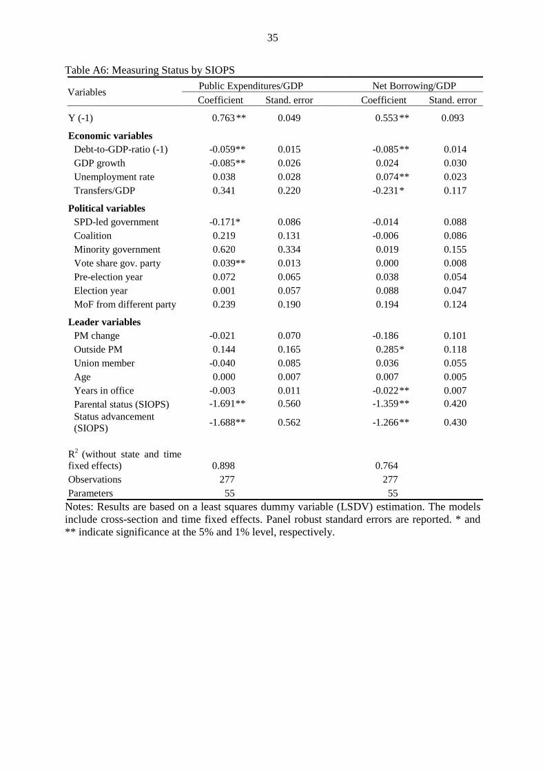
35

Table A6: Measuring Status by SIOPS

Variables Public Expenditures/GDP Net Borrowing/GDP Coefficient Stand. error Coefficient Stand. error

Y (-1) 0.763 ** 0.049 0.553 ** 0.093

Economic variables Debt-to-GDP-ratio (-1) -0.059 ** 0.015 -0.085 ** 0.014 GDP growth -0.085 ** 0.026 0.024 0.030 Unemployment rate 0.038 0.028 0.074 ** 0.023 Transfers/GDP 0.341 0.220 -0.231 * 0.117

Political variables SPD-led government -0.171 * 0.086 -0.014 0.088 Coalition 0.219 0.131 -0.006 0.086 Minority government 0.620 0.334 0.019 0.155 Vote share gov. party 0.039 ** 0.013 0.000 0.008 Pre-election year 0.072 0.065 0.038 0.054 Election year 0.001 0.057 0.088 0.047 MoF from different party 0.239 0.190 0.194 0.124

Leader variables PM change -0.021 0.070 -0.186 0.101 Outside PM 0.144 0.165 0.285 * 0.118 Union member -0.040 0.085 0.036 0.055 Age 0.000 0.007 0.007 0.005 Years in office -0.003 0.011 -0.022 ** 0.007 Parental status (SIOPS) -1.691 ** 0.560 -1.359 ** 0.420 Status advancement (SIOPS) -1.688 ** 0.562 -1.266 ** 0.430

R2 (without state and time fixed effects) 0.898 0.764 Observations 277 277 Parameters 55 55

Notes: Results are based on a least squares dummy variable (LSDV) estimation. The models include cross-section and time fixed effects. Panel robust standard errors are reported. * and ** indicate significance at the 5% and 1% level, respectively.

36

References Ainslie, G. (1992), Picoeconomis, Cambridge: Cambridge University Press. Alesina, A., Cohen, G. D., and Roubini, N. (1992), Macroeconomic policy and elections in

OECD democracies, Economics and Politics 4, 1–30. Alesina, A. and Giuliano, P. (2009), Preferences for redistribution, IZA Discussion Paper

4056. Alesina, A. and La Ferrara, E. (2005), Preferences for redistribution in the land of

opportunities, Journal of Public Economics 89, 897–931. Alesina, A. and Perotti, R. (1994), The political economy of budget deficits, NBER Working

Paper 4637. Angeletos, G.-M., Laibson, D., Repetto, A., Tobacman, J., and Weinberg, S. (2001), The

hyperbolic consumption model: Calibration, simulation, and empirical evaluation, Journal of Economic Perspectives 15, 47–68.

Arellano, M. and Bond, S. (1991), Some tests of specification for panel data: Monte Carlo evidence and an application to employment equations, Review of Economic Studies 58, 277–297.

Barro, R. (1979), On the determination of public debt, Journal of Political Economy 87, 940–971.

Becker, G. S. and Mulligan, C. B. (1997), The endogenous determination of time preference, Quarterly Journal of Economics 112, 729–758.

Berger, P. L. and Luckmann, T. (1966), The social construction of reality: A treatise in the sociology of knowledge, New York: Anchor Books.

Berger, H. and Holler, A. (2007), What determines fiscal policy? Evidence from German states, CESifo Working Paper 2062.

Besley, T., Montalvo, J. G., and Reynal-Querol, M. (2009), Do educated leaders matter? Working paper downloaded from: http://www.econ.upf.edu/~reynal/delm_December_3.pdf.

Blais, A., Blake, D., and Dion, S. (1993), Do parties make a difference? Parties and the size of government in liberal democracies, American Journal of Political Science 37, 40–62.

Blossfeld, H.-P. and Timm, A. (2003), Who marries whom? Educational systems as marriage markets in modern societies, Dordrecht: Kluwer Academic Publishers.

Börsch-Supan, A. H. and Essig, L. (2005), Household saving in Germany: Results of the first SAVE study, in: D. A. Wise (ed.), Analyses in the economics of aging, Chicago: University of Chicago Press.

Bourdieu, P. (1977), Outline of a theory of practice, Cambridge: Cambridge University Press. Bourdieu, P. (1984), Distinction: A social critique of the judgement of taste, Cambridge:

Harvard University Press. Bourdieu, P. (1986), The forms of capital, in: N. W. Biggart (ed.), Readings in economic

sociology, Oxford: Blackwell Publishers Ltd. Bourdieu, P. and Wacquant, L. J. D. (1992), An invitation to reflexive sociology, Chicago:

University of Chicago Press. Bradley, R. H. and Corwyn, R. F. (2002), Socioeconomic status and child development,

Annual Review of Psychology 53, 371–399. Breen, R. (1997), Risk, recommodification and stratification, Sociology 31, 473–489.

37

Breen, R. and Goldthorpe, J. H. (2001), Class, mobility and merit: The experience of two British birth cohorts, European Sociological Review 17, 81–101.

Brender, A., and Drazen, A. (2005), Political budget cycles in new versus established democracies. Journal of Monetary Economics 52, 1271–1295.

Brender, A. and Drazen, A. (2009), Do leaders affect government spending priorities? NBER Working Paper 15368.

Buchanan, J. and Wagner, R. (1977), Democracy in deficit, New York: Academic Press. Büchner, C. and Gerlitz, J.-Y. (2005), Influences on socio-economic status in Germany:

Reproduction of social structure or modes of individual acting? SOEP Working Paper, Berlin: DIW.

Carroll, C. D. and Kimball, M. S. (1996), On the concavity of the consumption function, Econometrica 64, 981–992.

Corneo, G. and Grüner, H. P. (2002), Individual preferences for political redistribution, Journal of Public Economics 83, 83–107.

Crossley, N. (2001), The phenomenological habitus and its construction, Theory and Society 30, 81–120.

Cusack, T. (1997), Partisan politics and public finance: Changes in public spending in the industrialized democracies 1955–1989, Public Choice 91, 375–395.

Davis, K. and Moore, W. E. (1945), Some principles of stratification, American Sociological Review 10, 242–249.

De Haan, J. and Sturm, J.-E. (1994), Political and institutional determinants of fiscal policy in the European Community, Public Choice 80, 157–172.

De Haan, J. and Sturm, J.-E. (1997), Political and economic determinants of OECD budget deficits and government expenditure: A reinvestigation, European Journal of Political Economy 13, 739–750.

Dreher, A., Lamla, M. J., Lein, S. M., and Somogyi, F. (2009), The impact of political leaders’ profession and education on reforms, Journal of Comparative Economics 37, 169–193.

Edin, P. and Ohlsson, H. (1991), Political determinants of budget deficits: Coalition effects versus minority effects, European Economic Review 35, 1597–1603.

Elias, N. and Scotson, J. L. (1965), The established and the outsiders. A sociological enquiry into community problems, London: Frank Cass & Co.

Erikson, R. and Goldthorpe, J. H. (1992), The constant flux: A study of class mobility in industrial societies, Oxford: Clarendon.

Eslava, M. (2006), The political economy of fiscal policy: Survey, Inter-American Development Bank Working Paper 583.

Fershtman, C., Murphy, K. M., and Weiss, Y. (1996), Social status, education, and growth, Journal of Political Economy 104, 108–132.

Galli, E. and Rossi, S. (2002), Political budget cycles: The case of the Western German Länder, Public Choice 110, 283–303.

Ganzeboom, H. B. G., De Graaf, P. M., and Treiman, D. J. (1992), A standard international socio-economic index of occupational status, Social Science Research 21, 1–56.

Giddens, A. (1984), The constitution of society: Outline of the theory of structuration, Cambridge: Polity Press.

Göhlmann, S. and Vaubel, R. (2007), The educational and professional background of central bankers and its effect on inflation: An empirical analysis, European Economic Review 51, 925–941.

38

Goldthorpe, J. H. (2002), Globalisation and social class, West European Politics 25, 1–28. Goossens, A. and Méon, P. G. (2010), ‘This is an economist’s argument!’ The impact of

studying economics, and other disciplines, on the belief that voluntary transactions make everyone better off, paper presented at the Silvaplana Workshop in Political Economy in Pontresina.

Hayo, B. and Voigt, S. (2011), Endogenous constitutions: Politics and politicians matter, economic outcomes don’t, Journal of Economic Behavior and Organization, forthcoming.

Hendry, D. F. (2000), Econometrics: Alchemy or science? Essays in econometric methodology, New Edition, Oxford: Oxford University Press.

Hibbs, D. A. (1977), Political parties and macroeconomic policy, American Political Science Review 23, 1467–1488.

ILO (1969), International standard classification of occupations, Geneva: International Labour Organization.

Jochimsen, B. and Nuscheler, R. (2010), The political economy of the German Länder deficits: Weak governments meet strong finance ministers, Applied Economics, forthcoming.

Jones, B. F. and Olken, B. A. (2005), Do leaders matter? National leadership and growth since World War II, Quarterly Journal of Economics 120, 835–864.

Judson, R. A. and Owen, A. L. (1997), Estimating dynamic panel data models: A practical guide for macroeconomists, Finance and Economics Discussion Series, Washington: Federal Reserve Board.

Kiviet, J. F. (1995), On bias, inconsistency, and efficiency of various estimators in dynamic panel data models, Journal of Econometrics 68, 53–78.

Lea, S. E. G., Webley, P., and Levine, R. M. (1993), The economic psychology of consumer debt, Journal of Economic Psychology 14, 85–119.

Lea, S. E. G., Webley, P., and Walker, C. M. (1995), Psychological factors in consumer debt: Money management, economic socialization, and credit use, Journal of Economic Psychology 16, 681–701.

Livingstone, S. M. and Lunt, P. K. (1992), Predicting personal debt and debt repayment: Psychological, social and economic determinants, Journal of Economic Psychology 13, 111–134.

MacRae, C. D. (1977), A political model of the business cycle, Journal of Political Economy 85, 239–263.

McLeod, J. D. and Kessler, R. C. (1990), Socioeconomic status differences in vulnerability to undesirable life events, Journal of Health and Social Behavior 31, 162–172.

Mikosch, H. F. (2009), Individuals vs. institutions. The impact of political leaders’ education and profession on public deficits, ETH Zurich, mimeo.

Nordhaus, W. D. (1975), The political business cycle, Review of Economic Studies 42, 169–190.

Pickel, A. (2005), The habitus process. A biopsychological conception, Journal for the Theory of Social Behaviour 35, 437–461.

Prenzel, M., Artelt, C., Baumert, J., Blum, W., Hammann, M., Klieme, E., and Pekrun, R. (eds.) (2007), PISA 2006. Die Ergebnisse der dritten internationalen Vergleichsstudie, Münster: Waxmann.

Rogoff, K. (1990), Equilibrium political budget cycles, American Economic Review 80, 21–36.

39

Rogoff, K. and Sibert, A. (1988), Elections and macroeconomic policy cycles, Review of Economic Studies 55, 1–16.

Roubini, N. and Sachs, J. (1989), Political and economic determinants of budget deficits in the industrial democracies, European Economic Review 33, 903–938.

Schneider, C. J. (2010), Fighting with one hand tied behind the back: Political budget cycles in the West German states, Public Choice 142, 125–150.

Seitz, H. (2000), Fiscal policy, deficits, and politics of subnational government. The case of the German Länder. Public Choice 102, 183–218.

Shi, M. and Svensson, J. (2006), Political business cycles: Do they differ across countries and why? Journal of Public Economics 90, 1367–1389.

Sørensen, A. B. (2000), Toward a sounder basis for class analysis, American Journal of Sociology 105, 1523–1558.

Treiman, D. J. (1977), Occupational prestige in comparative perspective, New York: Academic Press.

Weber, M. (1946), Class, status and power, in: H. H. Gerth and C. W. Mills (eds.), From Max Weber: Essays in sociology, New York: Oxford University Press.

White, H. (1980), A heteroskedasticity-consistent covariance matrix estimator and a direct test for heteroskedasticity, Econometrica 48, 817–838.

Wolf, C. (1995), Sozio-ökonomischer Status und berufliches Prestige: Ein kleines Kompendium sozialwissenschaftlicher Skalen auf Basis der beruflichen Stellung und Tätigkeit, ZUMA-Nachrichten 37, 102–136.