
Advanced photometric studies of Gamma-ray Burst...
127
Transcript of Advanced photometric studies of Gamma-ray Burst...
TECHNISCHE UNIVERSITÄT
MÜNCHEN
Max-Planck-Institut für extraterrestrische Physik
Advanced Photometric Studies of
Gamma-ray Burst Afterglows
Thomas Christian Krühler
Vollständiger Abdruck der von der Fakultät für Physik der Technischen
Universität München zur Erlangung des akademischen Grades eines
Doktors der Naturwissenschaften
genehmigten Dissertation.
Vorsitzender: Univ.-Prof. Dr. A. J. Buras
Prüfer der Dissertation: 1. Priv.-Doz. Dr. J. Greiner
2. Univ.-Prof. Dr. F. von Feilitzsch
Die Dissertation wurde am 10.09.2009 bei der Technischen Universität München
eingereicht und durch die Fakultät für Physik am 17.11.2009 angenommen.


Abstract
Gamma-ray Bursts (GRBs) are cosmic, stellar explosions, that emit a typical amount of energy of
1051 erg in γ-rays on short time scales of 0.1 to 100 seconds. This energy is released via shocks
in ultra-relativistic jets and makes GRBs the most luminous objects in the Universe after the
Big Bang. The prompt emission in γ-rays is followed by a longer-lasting afterglow, which can be
detected in all wavelengths ranges from radio, optical, to X- and γ-rays up to several days after
the explosion. The large energy release and high luminosity of GRBs and their afterglows make
them ideal probes for studies of the early Universe and the cosmic evolution.
This PhD thesis describes the basic principles and scientic applications of a new measurement
technique designed for detailed studies of GRB afterglows. The Gamma-Ray Burst Optical/Near-
infrared Detector (GROND), built and operated by the Max-Planck-Institut für extraterrestrische
Physik in collaboration with the Thüringer Landessternwarte, is a seven-channel imager, capa-
ble of simultaneous observations in seven broad-band lters in the optical and the near-infrared
wavelength regime (380 nm−2400 nm). GROND is mounted at the 2.2 m MPG/ESO telescope
at LaSilla observatory, Chile, fully operational since spring 2007 and dedicated to GRB afterglow
studies.
GROND's main goal is a fast determination of the photometric redshift of GRBs via the drop-
out technique. Absorption of photons on neutral hydrogen leads to a characteristic edge in the
spectral energy distribution of GRB afterglows. At redshifts larger than z ∼ 3, this Lyman-α
edge at wavelength λα(z) = 121.6 nm(1 + z) is well within GROND's sensitivity limits and can
be used to rapidly measure the distance scale to the GRB. Multi-band photometry thus obtains
the information which is crucial for a ne-tuned setting of spectroscopic follow-up observations to
enable detailed studies of high-redshift afterglows.
The GROND measurements are unique in the eld of optical/near-infrared astronomy and pro-
vide new insights into GRB physics and cosmology. The afterglows of the two most distant GRBs
to date, GRB 080913 and GRB 090423, for example, were both observed with GROND. The latter
is located at a redshift of z = 8.3, which corresponds to a light-travel time of 13.04 Gyr or an age of
the universe of 620 Myr, and is hence the most distant object ever detected to date. Furthermore,
GROND measured the distance scale to the most energetic GRB so far, GRB 080916C. A redshift
determination is the most crucial step to connect the extreme characteristics of these explosions
to cosmology and unied theories of quantum gravity.
The structure of this thesis can be summarized as follows: The rst chapter introduces to the
basic concepts and scientic background of GRB physics. Afterwards, instrumental details about
GROND, as well as its unique observations are presented. This part contains information about
the modus operandi, and the software tools developed for data reduction and analysis. Together
with data obtained in dierent spectral regimes, in particular at X-ray energies, the GROND data
constitutes a multi-wavelength data set, which allows detailed studies of GRB afterglow physics.
Chapter 3, 4 and 5 demonstrate scientic applications of this data on the basis of observations
obtained for the afterglows of GRBs 070802, 071031 and 080710.
3
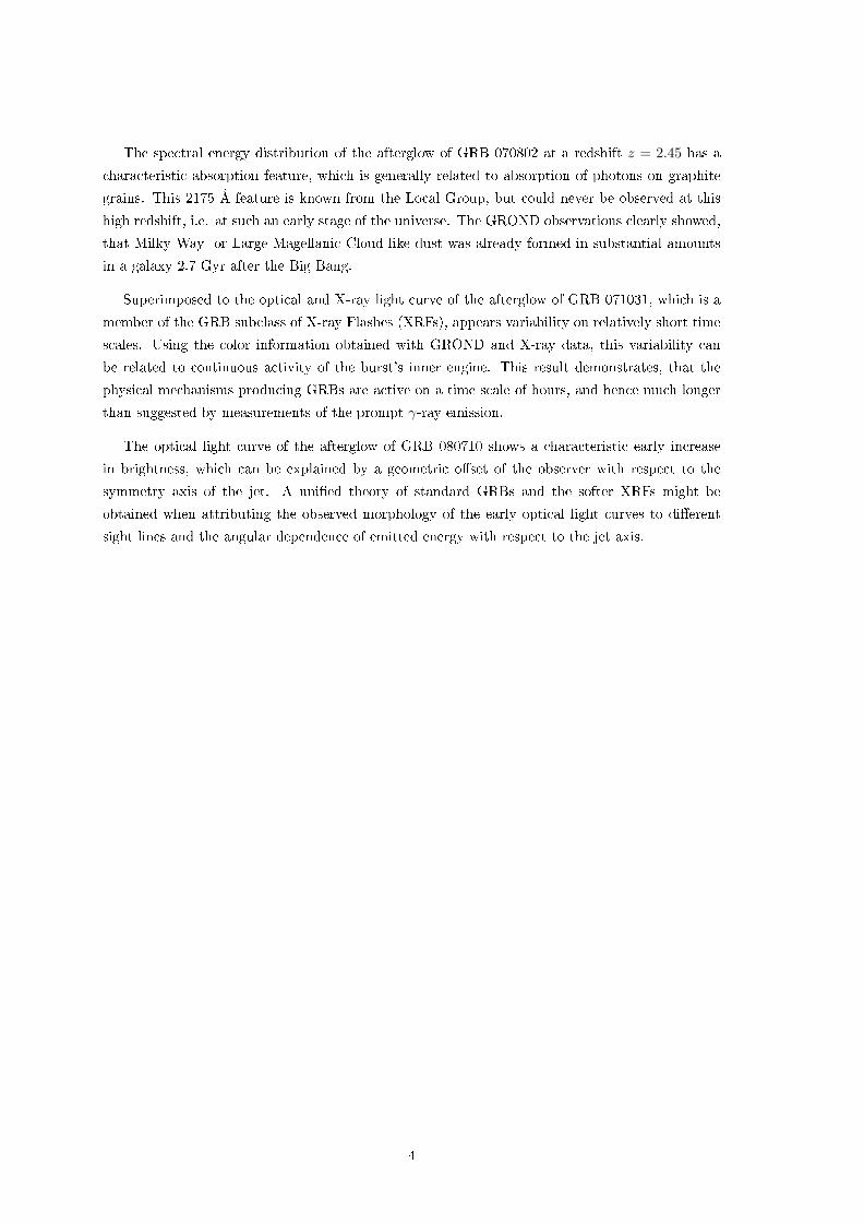
The spectral energy distribution of the afterglow of GRB 070802 at a redshift z = 2.45 has a
characteristic absorption feature, which is generally related to absorption of photons on graphite
grains. This 2175 Å feature is known from the Local Group, but could never be observed at this
high redshift, i.e. at such an early stage of the universe. The GROND observations clearly showed,
that Milky Way- or Large Magellanic Cloud-like dust was already formed in substantial amounts
in a galaxy 2.7 Gyr after the Big Bang.
Superimposed to the optical and X-ray light curve of the afterglow of GRB 071031, which is a
member of the GRB subclass of X-ray Flashes (XRFs), appears variability on relatively short time
scales. Using the color information obtained with GROND and X-ray data, this variability can
be related to continuous activity of the burst's inner engine. This result demonstrates, that the
physical mechanisms producing GRBs are active on a time scale of hours, and hence much longer
than suggested by measurements of the prompt γ-ray emission.
The optical light curve of the afterglow of GRB 080710 shows a characteristic early increase
in brightness, which can be explained by a geometric oset of the observer with respect to the
symmetry axis of the jet. A unied theory of standard GRBs and the softer XRFs might be
obtained when attributing the observed morphology of the early optical light curves to dierent
sight lines and the angular dependence of emitted energy with respect to the jet axis.
4
Zusammenfassung
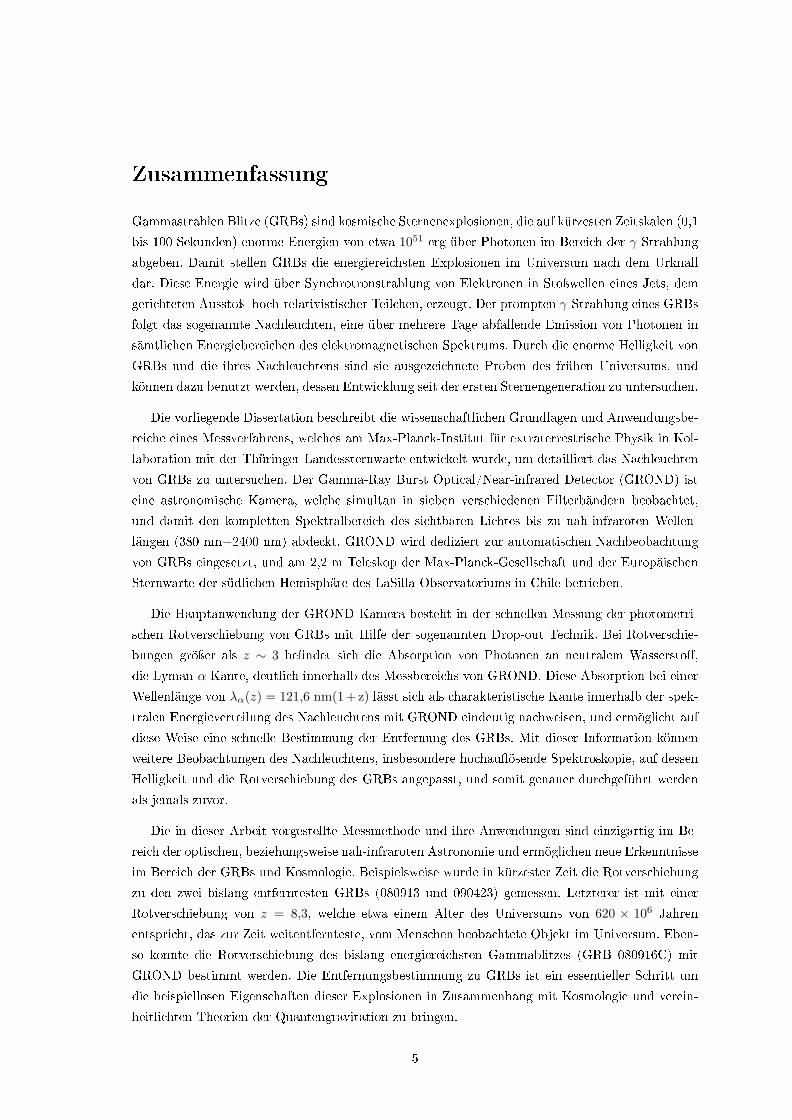
Gammastrahlen Blitze (GRBs) sind kosmische Sternenexplosionen, die auf kürzesten Zeitskalen (0,1
bis 100 Sekunden) enorme Energien von etwa 1051 erg über Photonen im Bereich der γ-Strahlung
abgeben. Damit stellen GRBs die energiereichsten Explosionen im Universum nach dem Urknall
dar. Diese Energie wird über Synchrotronstrahlung von Elektronen in Stoÿwellen eines Jets, dem
gerichteten Ausstoÿ hoch-relativistischer Teilchen, erzeugt. Der prompten γ-Strahlung eines GRBs
folgt das sogenannte Nachleuchten, eine über mehrere Tage abfallende Emission von Photonen in
sämtlichen Energiebereichen des elektromagnetischen Spektrums. Durch die enorme Helligkeit von
GRBs und die ihres Nachleuchtens sind sie ausgezeichnete Proben des frühen Universums, und
können dazu benutzt werden, dessen Entwicklung seit der ersten Sternengeneration zu untersuchen.
Die vorliegende Dissertation beschreibt die wissenschaftlichen Grundlagen und Anwendungsbe-
reiche eines Messverfahrens, welches am Max-Planck-Institut für extraterrestrische Physik in Kol-
laboration mit der Thüringer Landessternwarte entwickelt wurde, um detailliert das Nachleuchten
von GRBs zu untersuchen. Der Gamma-Ray Burst Optical/Near-infrared Detector (GROND) ist
eine astronomische Kamera, welche simultan in sieben verschiedenen Filterbändern beobachtet,
und damit den kompletten Spektralbereich des sichtbaren Lichtes bis zu nah-infraroten Wellen-
längen (380 nm−2400 nm) abdeckt. GROND wird dediziert zur automatischen Nachbeobachtung
von GRBs eingesetzt, und am 2,2 m Teleskop der Max-Planck-Gesellschaft und der Europäischen
Sternwarte der südlichen Hemisphäre des LaSilla Observatoriums in Chile betrieben.
Die Hauptanwendung der GROND Kamera besteht in der schnellen Messung der photometri-
schen Rotverschiebung von GRBs mit Hilfe der sogenannten Drop-out Technik. Bei Rotverschie-
bungen gröÿer als z ∼ 3 bendet sich die Absorption von Photonen an neutralem Wassersto,
die Lyman-α Kante, deutlich innerhalb des Messbereichs von GROND. Diese Absorption bei einer
Wellenlänge von λα(z) = 121,6 nm(1 + z) lässt sich als charakteristische Kante innerhalb der spek-
tralen Energieverteilung des Nachleuchtens mit GROND eindeutig nachweisen, und ermöglicht auf
diese Weise eine schnelle Bestimmung der Entfernung des GRBs. Mit dieser Information können
weitere Beobachtungen des Nachleuchtens, insbesondere hochauösende Spektroskopie, auf dessen
Helligkeit und die Rotverschiebung des GRBs angepasst, und somit genauer durchgeführt werden
als jemals zuvor.
Die in dieser Arbeit vorgestellte Messmethode und ihre Anwendungen sind einzigartig im Be-
reich der optischen, beziehungsweise nah-infraroten Astronomie und ermöglichen neue Erkenntnisse
im Bereich der GRBs und Kosmologie. Beispielsweise wurde in kürzester Zeit die Rotverschiebung
zu den zwei bislang entferntesten GRBs (080913 und 090423) gemessen. Letzterer ist mit einer
Rotverschiebung von z = 8,3, welche etwa einem Alter des Universums von 620 × 106 Jahren
entspricht, das zur Zeit weitentfernteste, vom Menschen beobachtete Objekt im Universum. Eben-
so konnte die Rotverschiebung des bislang energiereichsten Gammablitzes (GRB 080916C) mit
GROND bestimmt werden. Die Entfernungsbestimmung zu GRBs ist ein essentieller Schritt um
die beispiellosen Eigenschaften dieser Explosionen in Zusammenhang mit Kosmologie und verein-
heitlichten Theorien der Quantengravitation zu bringen.
5
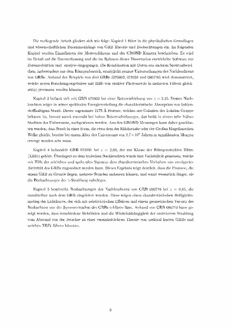
Die vorliegende Arbeit gliedert sich wie folgt: Kapitel 1 führt in die physikalischen Grundlagen
und wissenschaftlichen Zusammenhänge von GRB Theorie und Beobachtungen ein. Im folgenden
Kapitel werden Einzelheiten des Messverfahrens und der GROND Kamera beschrieben. Es wird
im Detail auf die Datenerfassung und die im Rahmen dieser Dissertation entwickelte Software zur
Datenreduktion und -analyse eingegangen. Die Kombination mit Daten aus anderen Spektralberei-
chen, insbesondere aus dem Röntgenbereich, ermöglicht genaue Untersuchungen des Nachleuchtens
von GRBs. Anhand der Beispiele von drei GRBs (070802, 071031 und 080710) wird demonstriert,
welche neuen Forschungsergebnisse mit Hilfe von exakter Photometrie in mehreren Filtern gleich-
zeitig gewonnen werden können.
Kapitel 3 befasst sich mit GRB 070802 bei einer Rotverschiebung von z = 2,45. Dessen Nach-
leuchten zeigte in seiner spektralen Energieverteilung die charakteristische Absorption von kohlen-
stohaltigem Staub. Dieses sogenannte 2175 Å Feature, welches aus Galaxien der Lokalen Gruppe
bekannt ist, konnte somit erstmals bei hohen Rotverschiebungen, das heiÿt in einem sehr frühen
Stadium des Universums, nachgewiesen werden. Aus den GROND Messungen kann daher geschlos-
sen werden, dass Staub in einer Form, die etwa dem der Milchstraÿe oder der Groÿen Magellanschen
Wolke gleicht, bereits bei einem Alter des Universums von 2,7×10⁹ Jahren in signikanten Mengen
erzeugt worden sein muss.
Kapitel 4 behandelt GRB 071031 bei z = 2,69, der zur Klasse der Röntgenstrahlen Blitze
(XRFs) gehört. Überlagert zu dem typischen Nachleuchten wurde hier Variabilität gemessen, welche
mit Hilfe der zeitlichen und spektralen Signatur dem charakteristischen Verhalten von verzögerter
Aktivität des GRBs zugeordnet werden kann. Dieses Ergebnis zeigt deutlich, dass die Prozesse, die
einem GRB zu Grunde liegen, mehrere Stunden andauern können, und somit wesentlich länger, als
die Beobachtungen der γ-Strahlung nahelegen.
Kapitel 5 beschreibt Beobachtungen des Nachleuchtens von GRB 080710 bei z = 0,85, die
unmittelbar nach dem GRB eingeleitet wurden. Diese zeigen einen charakteristischen Helligkeits-
anstieg der Lichtkurve, der sich mit relativistischen Eekten und einem geometrischen Versatz des
Beobachters von der Symmetrieachse des GRBs erklären lässt. Anhand von GRB 080710 kann ge-
zeigt werden, dass verschiedene Sichtlinien und die Winkelabhängigkeit der emittierten Strahlung
vom Abstand von der Jetachse zu einer vereinheitlichten Theorie von spektral harten GRBs und
weichen XRFs führen könnten.
6
Contents
1 Introduction to Gamma-ray Bursts 1
1.1 The Fireball Scenario . . . . . . . . . . . . . . . . . . . . . . . . . . . . . . . . . . 2
1.1.1 The Prompt Phase . . . . . . . . . . . . . . . . . . . . . . . . . . . . . . . . 2
1.1.2 The Afterglow . . . . . . . . . . . . . . . . . . . . . . . . . . . . . . . . . . 7
1.1.3 Jets and Jet Structure . . . . . . . . . . . . . . . . . . . . . . . . . . . . . . 11
1.2 Swift and the Afterglow Era . . . . . . . . . . . . . . . . . . . . . . . . . . . . . . . 13
1.2.1 A Generic X-ray Afterglow Light Curve . . . . . . . . . . . . . . . . . . . . 15
1.2.2 The Early Optical Afterglow . . . . . . . . . . . . . . . . . . . . . . . . . . 19
1.2.3 Chromatic Breaks . . . . . . . . . . . . . . . . . . . . . . . . . . . . . . . . 21
1.3 Progenitor Models . . . . . . . . . . . . . . . . . . . . . . . . . . . . . . . . . . . . 23
1.3.1 The Collapsar Model . . . . . . . . . . . . . . . . . . . . . . . . . . . . . . . 24
1.3.2 The Merger Scenario . . . . . . . . . . . . . . . . . . . . . . . . . . . . . . . 26
1.4 GRBs as Tools . . . . . . . . . . . . . . . . . . . . . . . . . . . . . . . . . . . . . . 27
2 The GROND Instrument 31
2.1 Filter System . . . . . . . . . . . . . . . . . . . . . . . . . . . . . . . . . . . . . . . 33
2.2 GROND Observation Scheme . . . . . . . . . . . . . . . . . . . . . . . . . . . . . . 34
2.3 Reduction Software . . . . . . . . . . . . . . . . . . . . . . . . . . . . . . . . . . . . 34
2.3.1 Reduction, Dithering and Sky Subtraction . . . . . . . . . . . . . . . . . . . 36
2.3.2 Astrometry and Photometry . . . . . . . . . . . . . . . . . . . . . . . . . . 36
2.3.3 Photmetric Accuracy . . . . . . . . . . . . . . . . . . . . . . . . . . . . . . . 37
2.4 Light Curve Fitting . . . . . . . . . . . . . . . . . . . . . . . . . . . . . . . . . . . . 37
7
2.5 Spectral Energy Distribution Modelling . . . . . . . . . . . . . . . . . . . . . . . . 40
2.5.1 Photometric Redshifts with GROND . . . . . . . . . . . . . . . . . . . . . . 42
2.5.2 Simulating the Spectral Energy Distribution of GRB Afterglows . . . . . . 43
2.5.3 Redshift Accuracy . . . . . . . . . . . . . . . . . . . . . . . . . . . . . . . . 46
3 The 2175 Å Dust Feature in GRB 070802 51
3.1 Introduction . . . . . . . . . . . . . . . . . . . . . . . . . . . . . . . . . . . . . . . . 51
3.2 Observations . . . . . . . . . . . . . . . . . . . . . . . . . . . . . . . . . . . . . . . 52
3.2.1 Swift Observations . . . . . . . . . . . . . . . . . . . . . . . . . . . . . . . . 52
3.2.2 GROND Optical and Near-infrared Observations . . . . . . . . . . . . . . . 53
3.3 Analysis . . . . . . . . . . . . . . . . . . . . . . . . . . . . . . . . . . . . . . . . . . 55
3.3.1 The Early Light Curve of the Afterglow of GRB 070802 . . . . . . . . . . . 55
3.3.2 The Spectral Energy Distribution . . . . . . . . . . . . . . . . . . . . . . . . 59
3.4 Conclusions . . . . . . . . . . . . . . . . . . . . . . . . . . . . . . . . . . . . . . . . 63
4 Optical Flares in the Afterglow of XRF 071031 67
4.1 Introduction . . . . . . . . . . . . . . . . . . . . . . . . . . . . . . . . . . . . . . . . 67
4.2 Observations . . . . . . . . . . . . . . . . . . . . . . . . . . . . . . . . . . . . . . . 68
4.2.1 Swift . . . . . . . . . . . . . . . . . . . . . . . . . . . . . . . . . . . . . . . . 68
4.2.2 GROND . . . . . . . . . . . . . . . . . . . . . . . . . . . . . . . . . . . . . . 70
4.3 Analysis . . . . . . . . . . . . . . . . . . . . . . . . . . . . . . . . . . . . . . . . . . 72
4.3.1 The Optical/NIR Light Curve . . . . . . . . . . . . . . . . . . . . . . . . . . 72
4.3.2 The X-ray Afterglow Light Curve . . . . . . . . . . . . . . . . . . . . . . . . 74
4.3.3 The Bumps . . . . . . . . . . . . . . . . . . . . . . . . . . . . . . . . . . . . 76
4.3.4 Spectral Evolution . . . . . . . . . . . . . . . . . . . . . . . . . . . . . . . . 79
4.4 Discussion . . . . . . . . . . . . . . . . . . . . . . . . . . . . . . . . . . . . . . . . . 82
4.4.1 The Likely Cause of the Flares . . . . . . . . . . . . . . . . . . . . . . . . . 82
4.4.2 Paucity of Detection of Correlated Early Optical Bumps and X-ray Flares . 85
4.5 Conclusions . . . . . . . . . . . . . . . . . . . . . . . . . . . . . . . . . . . . . . . . 85
8

5 The O-axis GRB 080710 89
5.1 Introduction . . . . . . . . . . . . . . . . . . . . . . . . . . . . . . . . . . . . . . . . 89
5.2 Observations . . . . . . . . . . . . . . . . . . . . . . . . . . . . . . . . . . . . . . . 90
5.3 Results . . . . . . . . . . . . . . . . . . . . . . . . . . . . . . . . . . . . . . . . . . . 93
5.3.1 Afterglow Light Curve . . . . . . . . . . . . . . . . . . . . . . . . . . . . . . 93
5.3.2 Broad-band Spectrum . . . . . . . . . . . . . . . . . . . . . . . . . . . . . . 93
5.4 Discussion . . . . . . . . . . . . . . . . . . . . . . . . . . . . . . . . . . . . . . . . . 95
5.4.1 On-axis Jet in its Pre-deceleration Phase . . . . . . . . . . . . . . . . . . . 96
5.4.2 Jet Seen O-axis . . . . . . . . . . . . . . . . . . . . . . . . . . . . . . . . . 97
5.5 Conclusions . . . . . . . . . . . . . . . . . . . . . . . . . . . . . . . . . . . . . . . . 98
6 Summary and Outlook 103
9

10
Chapter 1
A Short Introduction to Gamma-ray
Burst Physics and Observations
Only very few other subjects in astronomy have shown a comparable evolution in the recent past
as the eld of Gamma-ray Burst (GRB) science. First detected in the late sixties as mysterious,
brief ashes of γ-rays, it has been demonstrated by now that a GRB is a violent, extragalactic,
stellar explosion followed by a longer-lasting afterglow. The class of GRBs and their afterglows
thus comprehends the most energetic, luminous and distant events in all energy ranges from the
radio band to γ-rays detected by mankind at redshifts from z = 0.0085 (Galama et al., 1998) up
to z = 8.3 (Tanvir et al., 2009; Salvaterra et al., 2009).
Apart from their intrinsic record-breaking properties, which make GRBs ideal tools for studies
of the early Universe, their physical nature is still hardly understood. While there is strong evidence
that long GRBs with a typical duration of T90 ∼> 2 s are related to the collapse of super-massive,
fast-rotating Wolf-Rayet stars, the progenitors of short-duration (T90 ∼< 2 s) GRBs remain to be
identied. Other open questions include what governs the burst's central engine, the microphysical
conditions in the ejecta, the amount of beaming and jet structure and whether the prompt emission
properties can be used to turn GRBs into standard candles. The latter would enable direct tests
of cosmology out to redshift of 8 and above.
The discovery of GRBs, which triggered a large number of space and ground-based follow-up
programs was made in 1967 by the Vela satellites, that monitored the compliance of the nuclear
test treaty, and published in 1973 (Klebesadel et al., 1973). At that time, space astronomy was
just beginning to play an important role in science, and it took until 1991 to launch a mission
designated for high-energy astronomy and GRB physics. The Compton Gamma-Ray Observatory
(CGRO) hosted four instruments sensitive to photons from 30 keV to 30 GeV, where the Burst
And Transient Source Experiment (BATSE) was specically designed for GRB prompt emission
studies. Until its deorbit in 2000, BATSE detected over 2700 GRBs, and obtained the bulk of
information about the prompt emission characteristics available to date. In 2009, two major
satellite missions are in orbit to study the afterglow (Swift, since 2004, Gehrels et al., 2004) and
1

Chapter 1. Introduction to Gamma-ray Bursts 1.1. The Fireball Scenario
prompt phase (Fermi). Launched in 2008, the two instruments onboard Fermi, the GRB Monitor
(GBM, Meegan et al., 2009) and the Large Area Telescope (LAT, Atwood et al., 2009) with
their combined sensitivity over 7.5 decades of energy from 8 keV to 300 GeV open a new eld of
physics regarding prompt emission properties (see Fig 1.1 and Abdo et al., 2009a,b). In addition,
several other space missions have GRBs as one of their primary science drivers (e.g., the Italian
satellite "Astro-rivelatore Gamma a Immagini Leggero" (AGILE), the International Gamma-Ray
Astrophysics Laboratory (INTEGRAL) or Suzaku).
In addition to the space observatories, a large number of ground-based projects aim on gathering
information about the afterglow. Most crucial is the determination of the distance scale to the
GRB, i.e. a redshift measurement with atomic absorption lines via optical spectroscopy, typically
performed with telescopes of the 8 m class. But also smaller-sized, robotic telescopes play an
important role, especially with respect to the early phase of the GRB. As the very early afterglow,
or the optical emission related to the prompt phase, can be extremely bright, small telescopes with
aperture sizes in the range of 15 to 80 cm are able to obtain valuable data during the rst stages of
the explosion. Although limited to the brighter end of the afterglow distribution, the rapid response
and slewing capabilities of order few ten seconds provide information which is not accessible by
other means. Located in between in detection eciency and response time is the growing number
of instruments dedicated to and specialized on afterglow studies mounted on telescopes of the
2 m class. With somewhat longer slew times, but greatly enhanced sensitivity as compared to
small robotic telescopes, these instruments are able to provide a complete and unbiased sample of
afterglows, and the trigger information for 8 m class telescopes, as brightness of the optical transient
and redshift estimates. Pioneering in this eld is the Gamma-Ray Burst Optical/Near-infrared
Detector (GROND, Greiner et al., 2008), a seven-channel imager in the optical and near-infrared
regime mounted at the 2.2 m MPG/ESO telescope at LaSilla observatory, Chile. Noteworthy are
also the projects which study the low-energy afterglow, in particular in the radio and sub-millimeter
band, and studies of the host galaxy properties with large aperture ground-based telescopes and
the Hubble Space Telescope (HST) in the optical/near-infrared and the Spitzer Space Telescope in
the mid-infrared. Only a combination of data obtained with satellites and ground-based follow-up,
is able to provide a complete picture of the event, followed from start to nish.
1.1 The Fireball Scenario
1.1.1 The Prompt Phase
First studies of the γ-ray phenomenology with BATSE data showed, that GRBs are distributed
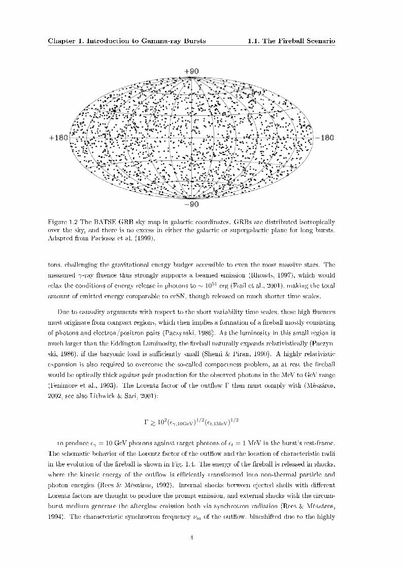
isotropically over the sky (Meegan et al., 1992; Fishman et al., 1994; Paciesas et al., 1999), strongly
supporting cosmological distances (see Fig. 1.2, also Section 1.4). According to their duration
distribution, which is roughly bimodial, GRBs can be divided into two populations (Kouveliotou
et al., 1993): Long (T90 ∼> 2 s) versus short (T90 ∼< 2 s) bursts. Their photon spectra as a function of
energy N(E), are non-thermal (see Fig 1.1), and typically well described with the empirical Band
function (Band et al., 1993) of two power laws with low- and high-energy photon index α ∼ −1 and
2
Chapter 1. Introduction to Gamma-ray Bursts 1.1. The Fireball Scenario
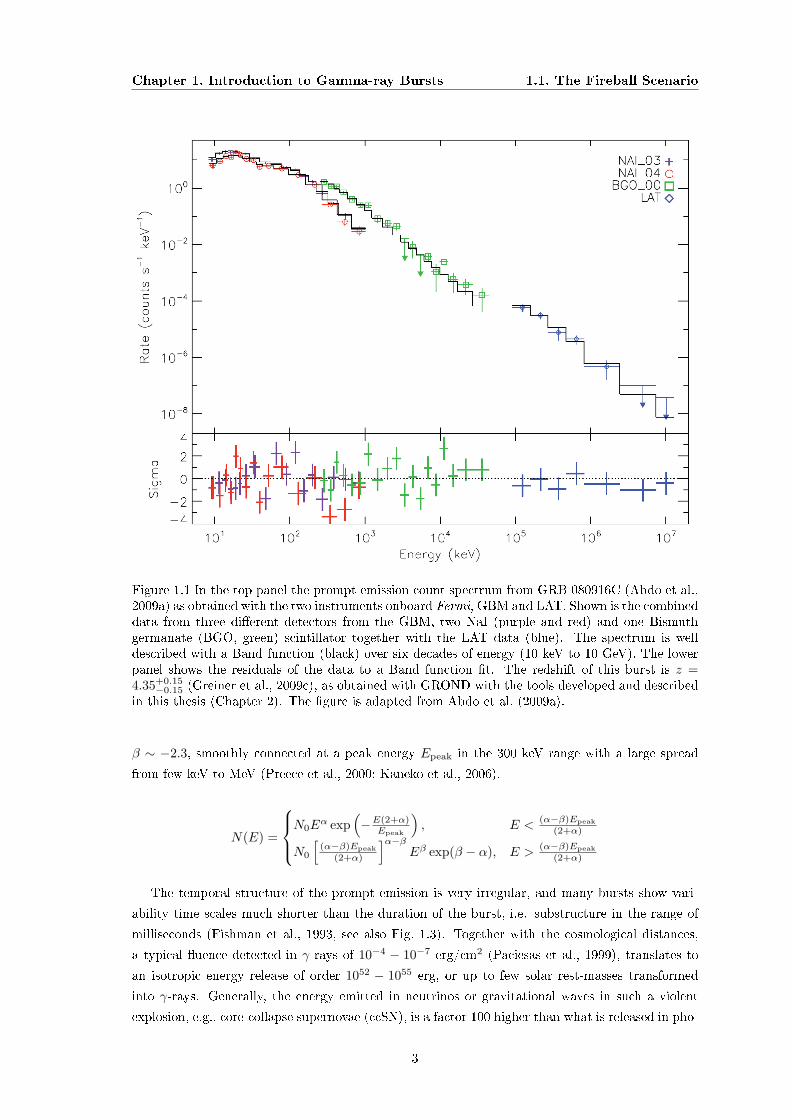
Figure 1.1 In the top panel the prompt emission count spectrum from GRB 080916C (Abdo et al.,2009a) as obtained with the two instruments onboard Fermi, GBM and LAT. Shown is the combineddata from three dierent detectors from the GBM, two NaI (purple and red) and one Bismuthgermanate (BGO, green) scintillator together with the LAT data (blue). The spectrum is welldescribed with a Band function (black) over six decades of energy (10 keV to 10 GeV). The lowerpanel shows the residuals of the data to a Band function t. The redshift of this burst is z =4.35+0.15
−0.15 (Greiner et al., 2009c), as obtained with GROND with the tools developed and describedin this thesis (Chapter 2). The gure is adapted from Abdo et al. (2009a).
β ∼ −2.3, smoothly connected at a peak energy Epeak in the 300 keV range with a large spread
from few keV to MeV (Preece et al., 2000; Kaneko et al., 2006).
N(E) =
N0E
α exp(−E(2+α)
Epeak
), E <
(α−β)Epeak(2+α)
N0
[(α−β)Epeak
(2+α)
]α−βEβ exp(β − α), E >
(α−β)Epeak(2+α)
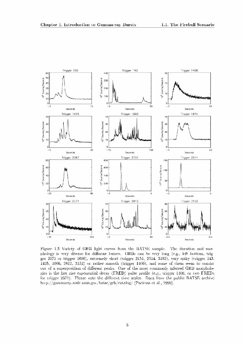
The temporal structure of the prompt emission is very irregular, and many bursts show vari-
ability time scales much shorter than the duration of the burst, i.e. substructure in the range of
milliseconds (Fishman et al., 1993, see also Fig. 1.3). Together with the cosmological distances,
a typical uence detected in γ-rays of 10−4 − 10−7 erg/cm2 (Paciesas et al., 1999), translates to
an isotropic energy release of order 1052 − 1055 erg, or up to few solar rest-masses transformed
into γ-rays. Generally, the energy emitted in neutrinos or gravitational waves in such a violent
explosion, e.g., core-collapse supernovae (ccSN), is a factor 100 higher than what is released in pho-
3
Chapter 1. Introduction to Gamma-ray Bursts 1.1. The Fireball Scenario
Figure 1.2 The BATSE GRB sky map in galactic coordinates. GRBs are distributed isotropicallyover the sky, and there is no excess in either the galactic or supergalactic plane for long bursts.Adapted from Paciesas et al. (1999).
tons, challenging the gravitational energy budget accessible to even the most massive stars. The
measured γ-ray uence thus strongly supports a beamed emission (Rhoads, 1997), which would
relax the conditions of energy release in photons to ∼ 1051 erg (Frail et al., 2001), making the total
amount of emitted energy comparable to ccSN, though released on much shorter time scales.
Due to causality arguments with respect to the short variability time scales, these high uences
must originate from compact regions, which then implies a formation of a reball mostly consisting
of photons and electron/positron pairs (Paczynski, 1986). As the luminosity in this small region is
much larger than the Eddington Luminosity, the reball naturally expands relativistically (Paczyn-
ski, 1986), if the baryonic load is suciently small (Shemi & Piran, 1990). A highly relativistic
expansion is also required to overcome the so-called compactness problem, as at rest the reball
would be optically thick against pair production for the observed photons in the MeV to GeV range
(Fenimore et al., 1993). The Lorentz factor of the outow Γ then must comply with (Mészáros,
2002, see also Lithwick & Sari, 2001):
Γ ∼> 102(εγ,10GeV)1/2(εt,1MeV)1/2
to produce εγ = 10 GeV photons against target photons of εt = 1 MeV in the burst's rest-frame.
The schematic behavior of the Lorentz factor of the outow and the location of characteristic radii
in the evolution of the reball is shown in Fig. 1.4. The energy of the reball is released in shocks,
where the kinetic energy of the outow is eciently transformed into non-thermal particle and
photon energies (Rees & Mészáros, 1992). Internal shocks between ejected shells with dierent
Lorentz factors are thought to produce the prompt emission, and external shocks with the circum-
burst medium generate the afterglow emission both via synchrotron radiation (Rees & Mészáros,
1994). The characteristic synchrotron frequency νm of the outow, blueshifted due to the highly
4
Chapter 1. Introduction to Gamma-ray Bursts 1.1. The Fireball Scenario
Figure 1.3 Variety of GRB light curves from the BATSE sample. The duration and mor-phology is very diverse for dierent bursts. GRBs can be very long (e.g., left bottom, trig-ger 2571 or trigger 1606), extremely short (trigger 2151, 2514, 3152), very spiky (trigger 143,1425, 1606, 2812, 3152) or rather smooth (trigger 1406), and some of them seem to consistout of a superposition of dierent peaks. One of the most commonly inferred GRB morpholo-gies is the fast rise exponential decay (FRED) pulse prole (e.g., trigger 1406, or two FREDsfor trigger 2571). Please note the dierent time scales. Data from the public BATSE archivehttp://gammaray.msfc.nasa.gov/batse/grb/catalog/ (Paciesas et al., 1999).
5

Chapter 1. Introduction to Gamma-ray Bursts 1.1. The Fireball Scenario
relativistic motion into the observers frame is then dependent on the strength of the magnetic eld
B, and the Lorentz factors of the shocked relativistic electrons γe and of the emitting material Γ:
νm ∼ qeB/(2πmec)γ2eΓ
with the charge qe and mass me of the electron. The emitted power P in the ejecta's co-moving
rest-frame Prest or observers frame Pobs by a single electron with γe, assuming no signicant energy
losses due to cooling, can be calculated accordingly:
Prest = (4/3)σT cUBγ2e
Pobs = Γ2(4/3)σT cUBγ2e
with the Thomson cross section σT and the magnetic eld energy density UB = B2/8π = εBe.
Here, εB is the ratio of magnetic energy to the total energy density e dissipated in the shock.
Typically, the energy- or velocity distribution of particles in the shock N(γ) is described as a
power law above a certain minimal Lorentz factor γm (e.g., Sari et al., 1998),
N(γ) ∝ γ−p
with the spectral index p > 2, to keep the total integrated energy nite. Initially, γm is equal
for protons and electrons, and the energy ratio carried by electrons versus protons is ∼ me/mp.
Collisionless shocks via chaotic electric and magnetic elds, however, can redistribute the energy
between protons and electrons, a process which is usually described by the fraction of energy εewhich goes into electrons (Mészáros, 2006). Furthermore, only a fraction of all shocked electrons
ξe will be accelerated above γm (Bykov & Mészáros, 1996). By integrating over the initial velocity
distribution N(γ) ∝ γ−p one obtains the minimal Lorentz factor of the electron population:
γm ∼ g(p)(εe/ξe)(mp/me)Γ
where g(p) = (p − 2)/(p − 1). The theoretical synchrotron spectrum Fν(ν) is then a broken
power law with Fν ∝ ν1/3 at ν < νm and Fν ∝ ν−(p−1)/2 for ν > νm (Rybicki & Lightman, 1979).
The power-law shape and the spectral indices below and above νm are roughly compatible with
the observations over a large energy range (see Fig. 1.1) and thus support the energy dissipation
in shocks via synchrotron radiation.
This reball and its synchrotron radiation due to shocks are the main characteristics and the
only observables of the progenitor, and the emission from the remnant remains hidden as it is
dominated by the much brighter internal and external shocks. Hence, direct observations of the
central engine are practically unfeasible, independent of the optical thickness of the outow.
Alternatively to the reball origin of the prompt GRB emission, several models have been pro-
6
Chapter 1. Introduction to Gamma-ray Bursts 1.1. The Fireball Scenario
posed which invoke dierent speculative radiation scenarios. The most plausible ones consider the
prompt emission from highly magnetized or Poynting ux dominated outows via the dissipation
of eld energy or magnetic reconnection (e.g., Mészáros et al., 1994; Usov, 1994; Drenkhahn &
Spruit, 2002). Magnetic reconnection would lead to particle acceleration, and in the case of a slow
energy dissipation the environment would be optically thin for the synchrotron radiation of the ac-
celerated particles in the presence of the magnetic eld of the outow (Spruit & Drenkhahn, 2004).
A magnetic eld would thus provide the particle acceleration and energy dissipation mechanisms
via synchrotron radiation to produce prompt γ-rays, followed by a standard external shock and
the afterglow (see Section 1.1.2).
Other alternative models consider non-uid, ultra-relativistic ejecta in the form of "cannonballs"
in a supernova explosion (e.g., Dar & de Rújula, 2004). These bullets, which have about the mass
of the Earth, produce prompt γ-ray emission by inverse Compton scattering of supernova light,
and the afterglow by thermal bremsstrahlung and synchrotron radiation of accelerated electrons
of the ambient medium (Dado et al., 2002). However, several unresolved issues remain in the
cannonball model, for example the mechanism of coherent bullet formation and discrete nature of
the ejecta. The latter is particularly controversial, as most high-energy astrophysical phenomena
(e.g., the jets of Active Galactic Nuclei) are probably related to uid or plasma outows (Mészáros,
2006). Despite the lack of conclusive alternatives to the reball model, also the standard models
remain largely phenomenological and the radiation mechanism of the prompt emission, the role of
magnetic elds and the microphysics of shocked particle acceleration stays the subject of discussion
(Mészáros, 2006).
1.1.2 The Afterglow
As soon as the reball ejecta expand into the circumburst medium, inevitably external shocks start
to develop. The interaction of the ultra-relativistic shells and the external medium then gives rise
to afterglow emission from radio to X-ray energies, rst detected for GRB 970228 (van Paradijs
et al., 1997; Vietri, 1997; Wijers et al., 1997; Frontera et al., 1998). The emission from external
shocks is dependent on the amount of material which has been swept up by the shock-wave and
reaches maximum luminosity at the typical deceleration radius rdec and observed time tdec (Rees
& Mészáros, 1992; Mészáros & Rees, 1993):
rdec ∼ (3E0/(4πnextmpc2Γ2
0))1/3
tdec ∼ rdec/(2cΓ20)
with the isotropic equivalent energy released in γ-rays E0, the external matter density next
and the proton mass mp. At that point the Lorentz factor of the outow Γdec is expected to be
half of the initial Lorentz factor of the bulk of the emission Γ0 (Panaitescu & Kumar, 2000). The
dependency of the Lorentz factor on the radius is schematically shown in Fig. 1.4. An analytical
calculation including the eciency of the radiative energy transfer η and the cosmological redshift
z, yields (Sari & Piran, 1999):
7

Chapter 1. Introduction to Gamma-ray Bursts 1.1. The Fireball Scenario
Figure 1.4 Schematic behavior of the jet's Lorentz factor Γ and nominal location of dierent radii.rs is the saturation radius where the reball is not accelerated anymore, rph the photospheric radius,where the Thompson optical depth τ is unity, ris the dissipation radius for internal shocks, wheretwo shells with dierent velocities typically catch up with each other producing the prompt emis-sion, and res = rdec the external shock radius, where the circumburst medium starts to ecientlydecelerate the ejecta which produces the afterglow. Both radial and velocity scale are logarithmicand γth, γ, X, O and R indicate the location of thermal γ-ray production at the photosphere, orγ-ray, X-ray, optical and radio photon emission via synchrotron radiation. From Mészáros (2006).
Γdec =(
3E0(1 + z)3
32πnextmpc5ηtdec
)1/8
Measurements of the peak emission of the afterglow external shock can thus provide direct
information about the conditions in the outow, in particular the initial bulk Lorentz factor, the
deceleration radius and the isotropic equivalent baryonic loading of the reball Mfb = E0/(Γ0c2)
(Molinari et al., 2007).
The emission from the external shock is again synchrotron radiation with a peak frequency
νm, similarly proportional to the Lorentz factor of the ejecta, the electrons in the shock and the
co-moving magnetic eld as in the prompt phase (Mészáros & Rees, 1993). The particle and energy
density (N/V and E/V , respectively) behind the forward shock propagating through a uniform
and cold medium is given by the Blandford-McKee solution (Blandford & McKee, 1976), i.e. at
rst order N/V (t) = 4Γ(t)next and E/V (t) = 4Γ(t)2nextmpc2 (Piran, 1999). Under the assumption
that the dominant emission process is forward shock emission, the entire spectrum of the afterglow
can be calculated selfconsistently (Mészáros & Rees, 1997).
Above a critical Lorentz factor γc, the electrons loose signicant amount of their energy due to
8

Chapter 1. Introduction to Gamma-ray Bursts 1.1. The Fireball Scenario
cooling. γc is described by the time scale t it takes for an electron with γe > γc to cool down to γc(Sari et al., 1998).
γc =6πmec
σTΓB2t
The resulting theoretical afterglow spectrum is a three fold broken power law with spectral
breaks at νa, the synchrotron self absorption, νm and νc, the cooling frequency (Sari et al., 1998;
Granot & Sari, 2002a) and a maximum luminosity at Fν,max. The part of the spectrum below νm is
the low-frequency tail of the synchrotron radiation and independent on the electron spectral index
p, i.e. Fν ∝ ν1/3 (Katz, 1994). The high energy part above νc is described by the electrons with
Lorentz factors greater than γc, which cool rapidly and emit practically all their energy at their
synchrotron frequency. Following Sari et al. (1998), the afterglow spectrum is Fν ∝ ν−p/2 in this
regime, which gives direct observational access to the energy index of the electrons from the high
energy spectral slope. Assuming that a constant fraction of the shock energy goes into electrons
and the magnetic eld, the shock wave is then fully dened by next, E0, the energy index of the
electrons in the shock p, and the eciency factors of the magnetic eld εB , of the electrons εe, the
fraction of accelerated electrons ξe associated with the inter stellar material (ISM), the dependence
of Γ on the radius r and the redshift z (Zhang & Mészáros, 2004). The time dependence of νa, νc,
and νm in the adiabatic case (Γ ∝ r−3/2) is then given by (Zhang & Mészáros, 2004):
νm(t) = (6× 10¹⁵)(1 + z)1/2g(p)2(εe/ξe)2ε1/2B E
1/20,52t
−3/2d [Hz]
νc(t) = (9× 10¹²)(1 + z)−1/2ε−3/2B n−1
1 E−1/20,52 t
−1/2d [Hz]
νa(t) = (2× 10⁹)(1 + z)−1(εe/ξe)−1ε1/5B n
3/51 E
1/50,52 [Hz]
with E0,52 = E0 in units of 1052 erg, n in 1 cm−3 and t in days.
The order of νm and νc denes two cases: the slow cooling (νm < νc) and fast cooling (νm > νc)
case as shown in Fig. 1.5.
The normalization Fν,max is obtained by the ux integral over all radiating electrons, which
is only a function of the turbulent magnetic eld B in the shock, i.e. εB , and not of the other
microphysical parameters εe, ξe and p (Wijers & Galama, 1999; Zhang & Mészáros, 2004):
Fν,max = 20(1 + z)ε1/2B n1/2E52D−2L,28 [mJy]
where DL,28 is the luminosity distance in units of 1028 cm.
A characteristic set of equations then relates the spectral index β, where Fν(ν) = ν−β , to the
temporal decay index of the light curve α, with Fν(t) = t−α. These closure relations depend
on the type of circumburst medium, typically described with an index s, where next ∝ n−s0 ,
most commonly s = 0 for an homogeneous ISM-like circumburst medium, or s = 2 for a wind
type environment. Furthermore, they dier between the spectral regime of slow or fast cooling
9

Chapter 1. Introduction to Gamma-ray Bursts 1.1. The Fireball Scenario
Figure 1.5 Schematic behavior of the dierent afterglow synchrotron spectra in the fast and slowcooling case. As the ejecta slow down, the characteristic frequencies move to lower energies. Asthe cooling frequency moves faster νc ∝ t−3/2 with respect to νm ∝ t−1/2, the afterglow is expectedto go through a transition from fast to slow cooling regime at t0. From Sari et al. (1998).
10

Chapter 1. Introduction to Gamma-ray Bursts 1.1. The Fireball Scenario
and the location of the observed frequency, the electron index p and a possible energy injection
(e.g., Mészáros & Rees, 1997; Sari & Piran, 1999; Dai & Cheng, 2001; Zhang & Mészáros, 2004;
Panaitescu, 2005; Zhang et al., 2006; Panaitescu et al., 2006b). Assuming the most simple condition
of an ISM-like circumburst environment in the slow cooling case with p ≥ 2 and no energy injection,
the closure relation for νm < ν < νc or νc < ν is α = 3β/2 or α = (3β − 1)/2, respectively. By
measuring the spectral and temporal index, the reball model can thus be tested straight forwardly
by observations, and the late (t > 104−5 s) afterglow generally was in good agreement with the
expectations. With increasing temporal and spectral information of the afterglow after the advent
of the Swift mission, however, more and more data about the early (t < 104−5 s) and late afterglow
phase became available, raising questions about the validity and signicance of the most simple
reball scenarios (see Section 1.2).
1.1.3 Jets and Jet Structure
Beamed emission from GRBs is already suggested by energetic considerations that GRBs must be
related to an energy reservoir accessible to massive stars. If the outow is collimated in a cone
of half opening angle θjet the evolution is similar to the spherical case, given that the relativistic
beaming 1/Γ is smaller than θjet and the observer is located face on to the jet (Mészáros et al.,
1993). The light cone is then constrained to a region within the jet and disconnected from outer
areas. As soon as the jet has decelerated to 1/Γ ∼ θjet, more energy is emitted in directions
outside the central cone, and the jet starts to expand laterally with the co-moving speed of sound
(Mészáros, 2006). This results in a characteristic steepening of the light curve of the afterglow
with a change in the temporal index ∆α ∼ 3/4 (Mészáros & Rees, 1999) if the sideways expansion
is negligible, or a nal decay with α = p when including the lateral spreading (Rhoads, 1999).
These jet breaks are a pure geometrical eect, and thus truly achromatic by denition. One of the
earliest detections of a jet break in a number of broad-band lters is shown in Fig. 1.6.
From the time tjet where the break in the light curve occurs, the half opening angle of the jet
can be calculated, depending on the redshift and circumburst prole (Sari et al., 1999; Bloom et al.,
2003):
θISMjet ≈ 0.099
(tjet[s]1 + z
)3/8
·(η0.2n1
E0,53
)1/8
θwindjet ≈ 0.075
(tjet[s]1 + z
)1/4
·(η0.2A∗E0,53
)1/4
where the burst characteristics have been normalized to typical values, e.g., E0 to 1053 erg, n
to 1 cm−3, and A∗ is the normalized wind density with A = Mw/4πvw = 5× 10¹¹A∗g cm−1. Here
Mw is the mass-loss rate of the progenitor in its nal stage of stellar evolution and vw the wind
velocity with reference values of Mw = 1× 10⁻⁵Myr−1 and vw = 1000 km/s, characteristic for a
Wolf-Rayet star (Chevalier & Li, 2000).
With the knowledge of the jets opening angle, the beaming-corrected energy release in γ-rays
11

Chapter 1. Introduction to Gamma-ray Bursts 1.1. The Fireball Scenario
Figure 1.6 Multi-color light curve of the afterglow of GRB 990510 in four dierent photometriclters (B, V , R and I). The light curve is described by a characteristic smooth turnover fromshallow to steep decay. This break in the light curve is generally related to the collimation of theejecta and happens when the relativistic beaming is of the order of the jet half opening angle. FromStanek et al. (1999).
Eγ is then:
Eγ = fbE0
where fb is the beaming factor fb = (1 − cos θjet). After correcting for the apparent beaming,
the energy released in γ-rays by GRBs clusters at around Eγ ≈ 1051 erg, as shown in Fig 1.7 (Frail
et al., 2001; Bloom et al., 2003). There is however, evidence for sub- and super-energetic bursts,
with emitted beaming corrected energies signicantly below or above 1051 erg, so the use of GRBs
as direct standard candles is strongly questioned.
The apparently beamed emission of GRBs raises the question of the jet structure, i.e. the
lateral energy distribution around the jets symmetry axis. Dierent jet congurations have been
proposed, including the most popular uniform jet, where the energy distribution ε(θ) is described
by a simple top hat. Frequently used is also the universal structured jet model, where ε(θ) is
characterized by a power law with index k, i.e. ε(θ) = εc(θ/θc)−k outside of a uniform core with
angle θc (e.g., Lipunov et al., 2001). The jet structure of both models is schematically shown in
Fig. 1.8. A more physical jet structure was introduced in Zhang & Mészáros (2002b) and Kumar &
Granot (2003), where the angular prole of the jet is Gaussian shaped. In addition to these models
of single jets, the combination of two components (e.g., Pedersen et al., 1998; Peng et al., 2005)
has been used to explain the increasing diversity in optical afterglows. Here, the superposition of
a narrowly collimated fast jet, and a broad jet with lower velocities can produce a broad type of
afterglow light-curve morphologies. Further motivation for this model is provided by numerical
12

Chapter 1. Introduction to Gamma-ray Bursts 1.2. Swift and the Afterglow Era
Figure 1.7 Clustering of the beaming-corrected energy release in γ-ray photons. After correctingthe emitted energy for the jetted emission, there seems to appear a clustering around 1051 erg.There is however, evidence for sub- and super-energetic bursts in the recent years. Thus, GRBsare most probably not connected to a constant energy reservoir, which might have been deducedfrom earlier and limited samples. From Bloom et al. (2003).
simulations, which show evidence for a slower component around a hydrodynamically driven jet,
that originates from compact objects (Ramirez-Ruiz et al., 2002; Vlahakis et al., 2003; Zhang et al.,
2003b).
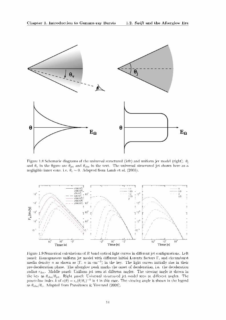
Although the morphology of the afterglow light curve is in principle a robust diagnostics for
the jet structure (see Fig. 1.9), denite conclusions about the angular distribution of energy in the
jet is not yet reached (e.g., Rossi et al., 2002). A part of the problem is related to the quality and
quantity of obtained optical light curves, which are not well sampled in either time or frequency
domain, and of inferior photometric accuracy. The lack of high quality data makes a comparison or
discrimination between dierent jet structures so far inconclusive. Additional evidence about the jet
structure can be obtained from polarization measurements (e.g., Wijers et al., 1999; Greiner et al.,
2003a; Rossi et al., 2004). However, as in the case of light-curve modelling, previous measurements
are not yet fully conclusive.
1.2 Swift and the Afterglow Era
After the launch of Swift in 2004, with its rapid slewing capabilities and two narrow eld follow-up
instruments, the X-ray- (XRT, Burrows et al., 2005b) and Ultraviolet/Optical Telescope (UVOT,
Roming et al., 2005), observations of the early afterglow in the X-ray and ultraviolet/optical energy
band were feasible for the rst time in larger numbers of around 100 per year. One of the most
surprising discoveries was the variety of features in the X-ray light curve. While previously, X-ray
observations started earliest at 10 ks after the trigger, the fast Swift response now gives a complete
description of the events starting as early as 100 s after the burst.
13
Chapter 1. Introduction to Gamma-ray Bursts 1.2. Swift and the Afterglow Era
Figure 1.8 Schematic diagrams of the universal structured (left) and uniform jet model (right). θj
and θv in the gure are θjet and θobs in the text. The universal structured jet shown here as anegligible inner cone, i.e. θc ∼ 0. Adapted from Lamb et al. (2005).
Figure 1.9 Numerical calculations of R-band optical light curves in dierent jet congurations. Leftpanel: Homogeneous uniform jet model with dierent initial Lorentz factors Γ, and circumburstmedia density n as shown as (Γ, n in cm−3) in the key. The light curves initially rise in theirpre-deceleration phase. The afterglow peak marks the onset of deceleration, i.e. the decelerationradius rdec. Middle panel: Uniform jet seen at dierent angles. The viewing angle is shown inthe key as θobs/θjet. Right panel: Universal structured jet model seen at dierent angles. Thepower-law index k of ε(θ) = εc(θ/θc)−k is 4 in this case. The viewing angle is shown in the legendas θobs/θc. Adapted from Panaitescu & Vestrand (2008).
14

Chapter 1. Introduction to Gamma-ray Bursts 1.2. Swift and the Afterglow Era
Figure 1.10 The canonical X-ray light curve in the Swift era. The very early X-ray data usuallyconnect smoothly to the prompt emission. This is followed by a characteristic steep decline, relatedto high latitude emission. Afterwards there is a transition to a much shallower decline, or evenplateau phase, which is followed by two breaks: rst to the typical power-law decline of afterglowemission, and eventually a jet break. Superimposed onto all components X-ray ares can appear.Time scales are indicative, and not all features are present in all bursts. Dashed lines indicatesections which are only observed in a smaller fraction of afterglows. For physical processes shapingthe X-ray light curve please see text. Adapted from Zhang et al. (2006).
1.2.1 A Generic X-ray Afterglow Light Curve
Already very early samples of Swift X-ray light curves showed, that there was evidence for a generic
scheme underlying all X-ray afterglows (Nousek et al., 2006). Though not all features are observed
in every burst, a single X-ray afterglow light curve can be described within the framework shown
in Fig. 1.10. In detail, there is a very early stage which usually connects smoothly to the prompt
emission (O'Brien et al., 2006), followed by a characteristic steep - at - steep evolution. Finally,
there is a late break in the light curve which is generally related to the jet break. It must be noted
though, that the fraction of detections of achromatic late breaks consistent with a jet break is much
lower than previously expected. Whether this apparent lack of jet breaks is the result of a larger
redshift and beaming (on average, Swift detects fainter bursts at higher redshifts than previous
missions) or the jet break in the X-ray band is masked by an additional emission component (e.g.,
ares, inverse Compton emission, separate jet component) is still a matter of debate (Sato et al.,
2007; Ghisellini et al., 2007; Genet et al., 2007; Racusin et al., 2009). Superimposed to all epochs
appear in roughly 50% of all cases X-ray ares which can be as energetic as the prompt phase itself
(Falcone et al., 2006).
This generic scheme puts strong constraints on the physical concepts of the light curve and its
implications about the central engine. The dierent stages in this generic light curve are discussed
in detail below.
15

Chapter 1. Introduction to Gamma-ray Bursts 1.2. Swift and the Afterglow Era
The Steep Decay
According to the standard reball model (see Section 1.1), the prompt phase and the afterglow
are emitted by internal and external shocks, and are thus spatially separated. In the very early
phase, the emission from the prompt phase still dominates over the afterglow. A steep decay is
expected due to the time delay of t = (1 + z)(r/c)(θ2/2) between the photons emitted along the
line of sight and at an angle θ (e.g., Dermer, 2004). Hence, even after the energy dissipation in
the prompt phase stops, there is a maximum delay of order tmax = (1 + z)(r/c)(θ2jet/2), assuming
that the observers line of sight is not far o the jet symmetry axis. The temporal and spectral
dependence of the ux density Fν for high latitude emission can be expressed using the co-moving
surface brightness L′ν′ (Zhang et al., 2006), where ν′ is the co-moving frequency of the shocked
electrons. Transforming into the observers frame, using the Doppler factor D = 1/(Γ(1−v cos θ/c))
with the velocity of the outow v, and thus D ∼ 2/Γθ2 as long as the relativistic beaming is much
larger than θ, yields (Zhang et al., 2006):
Fν ∝ L′ν′D2 ∝ ν−βD2+β
Together with the dependence of the time delay on the emitting angle t ∝ θ2 ∝ D−1, this
becomes Fν ∝ L′ν′D2 ∝ ν−βt−2−β . Hence, the temporal decline index is α = 2 + β (Kumar
& Piran, 2000). This relation is a characteristic for high-latitude emission and was shown to
adequately describe samples of X-ray afterglows, where the steep decay is observed (Nousek et al.,
2006; O'Brien et al., 2006). Therefore, the steep decay can be considered as the tail end of the
prompt emission, and further is implicit proof that GRBs are beamed and that afterglow and
prompt photons arise from dierent emission sites. Not all bursts, however, satisfy the earlier
constraint. As the measured power-law index is strongly dependent on the choice of the reference
time T0, which is usually set to the trigger time, i.e. the start of the γ-ray emission, there is
another degree of freedom which can be adapted to t the relation for high-latitude emission. In
fact, Liang et al. (2006) nd, that the vast majority of steep tails can be accounted for with high-
latitude emission if T0 is set to the time of the last pulse of the burst, which is physically reasonable
as this last pulse would largely dominate any tail emission.
The Shallow Decay Phase
The tail end of the prompt emission is usually followed by a plateau phase, with a decline index
of order α ∼ −0.5 which is too shallow for the expectations from the standard model (α ∼ −1.2).
Additional evidence that the shallow decay phase is physically dierent from the early steep decline
is provided by spectral evolution. Typically the spectrum hardens during the steep - shallow
transition. Hence, the shallow phase is usually considered as the rst part of the light curve where
the afterglow dominates. However, as the decline index is too shallow to be accounted for in the
original form of the reball model, there needs to be some sort of additional energy which is injected
into the forward shock-wave during this epoch (Nousek et al., 2006).
The most popular mechanism of energy injection is the so-called refreshed shock scenario,
16

Chapter 1. Introduction to Gamma-ray Bursts 1.2. Swift and the Afterglow Era
where later or slower shells catch up with the decelerating shock. These refreshed shocks might be
produced by a long-lived engine, with reduced activity at later times, or a simultaneous ejection of
shells with a distribution of Lorentz factors (Zhang et al., 2006). In the rst case the activity of the
central engine L(t) can be described with a power-law dependence with time, i.e. L(t) = L0(t/tb)−q,
with a luminosity of the central engine L0 at tb and a typical value of q ∼ 1/2. A longer lasting
central engine is generally related to late accretion onto a central black hole (MacFadyen et al.,
2001) or the spin down of a millisecond pulsar (Dai & Lu, 1998). The second case is described
by a spread of Lorentz factors of the initial ejected mass. The dependency of amount of ejected
mass M on its Lorentz factor is often described with a power law of index s, i.e. M ∝ Γ−s (Rees
& Mészáros, 1998). Slower shells progressively pile up onto the decelerating shock-wave, which
mimics the eect of a late central engine activity. Hence q is somewhat degenerate to s, and for
q = 0.5, s = 2.6 would produce similar eects on the light curve (Zhang et al., 2006).
An alternative way of energy injection, independent on the physics of the central engine, is
given by a delayed energy transfer into the forward shock. As it takes time to sweep up enough
matter for an ecient deceleration of the ejecta, the time scale from the prompt phase to the
Blandford-McKee deceleration phase can be as long as several 103 seconds (Kobayashi & Zhang,
2007). The shallow decay phase may thus simply represent the time scale of energy transfer to the
circumburst medium.
Other mechanisms of producing the shallow decay phase mostly relate to the jet structure. In
both, an o-beam or two-component jet model, the shallow decay phase can be explained as a
combination of the late tail of the steep decay phase and a delayed rise of the afterglow. In an
o-axis scenario, the delayed onset is caused by a rising afterglow emission as more and more of
the relativistically beamed jet enters the observer's sight line. In a two-component jet model, the
rise is produced by a late deceleration of the lower Γ, broad jet. Hence, both scenarios result in
an increasing afterglow emission at early times and consequentially in the shallow decay phase as
a superposition of high latitude and increasing afterglow emission.
After the cessation of the energy injection into the forward shock, the afterglow follows what
was known earlier and expected from the reball model: a generic power-law decline eventually
followed by a jet break. The discovery of the shallow decay phase however, was unexpected and
provides a strong challenge to existing theories. Similar statements can be used for X-ray ares,
which appear erratic superimposed onto around 50% of all X-ray afterglow light curves during its
entire evolution.
X-ray Flares
Observationally, X-ray ares appear on both, short and long bursts, with a ux increase which can
be as large as a factor of 500 on time scales of 100 s (Chincarini et al., 2007, see also Fig. 1.11).
The rise and decay index are very steep, and depending on the time of reference can reach values
of 7 and above. After the end of the are, the ux level drops to the extrapolation of the previ-
ously established afterglow decline. Furthermore, ares show strong spectral hard-to-soft evolution
throughout rise and decay, suggesting a dierent emission than the generic forward shock afterglow
17

Chapter 1. Introduction to Gamma-ray Bursts 1.2. Swift and the Afterglow Era
Figure 1.11 The remarkable light curve of the X-ray afterglow of GRB 050502B as the most dramaticexample of X-ray aring activity. Within few hundred seconds, the X-ray ux increases about afactor of 500, and drops back to the initial niveau ∼ 400 s later. In addition to the rst early are,which peaks at 700 s, there is evidence for late aring at around 80 ks.
(Falcone et al., 2007). One of the most dramatic examples is the are of GRB 050502B (Fig. 1.11),
where the are contains more energy than the prompt emission itself (e.g., Burrows et al., 2005a;
Falcone et al., 2006).
Previously, dierent models have been invoked to explain variability in an afterglow light curve.
These models include inhomogeneities in the circumburst medium or the angular distribution
of energy in the forward shock (patchy shells) or late energy injection, but all have diculties
explaining the strong variability of ares on short time scales (Ioka et al., 2005). In addition, they
cannot account for the strong spectral evolution which is observed in all ares where a detailed
spectral analysis is possible. The X-ray spectrum hardens during ares, and is no longer well
tted by a simple power law as typical for afterglow emission. In fact, a are spectrum is better
represented using a Band function peaking in the few keV energy range, and together with the
highly variable light curve much more resembles what is observed during the prompt phase, but at
lower energies (Butler & Kocevski, 2007; Krühler et al., 2009).
Given the above observational constraints, and the phenomenological similarity to the prompt
phase, it is very likely that the X-rays ares are caused by similar processes as the prompt phase,
i.e. late central engine activity (e.g., Falcone et al., 2006). This might result in either a late ejection
of discrete shells with varying Γ, and their collision produces the X-ray ares, or late injection of
energy from Poynting ux dominated outows, where the dissipation of the magnetic elds causes
the observed emission (Zhang et al., 2006).
The fact that ares appear on both, long and short duration bursts hints on a physical origin
18

Chapter 1. Introduction to Gamma-ray Bursts 1.2. Swift and the Afterglow Era
related to a common stage of the dierent progenitors (see Section 1.3). In both cases, the initial
source of energy is the infall of matter from an accretion disk onto a newly formed compact object.
Due to gravitational instabilities, the accretion disk might fragment, in particular at the outer
regions of the disk (Perna et al., 2006). These fragments would be accreted onto the black hole on
longer time scales up to days, providing new fuel to the central engine. The energy output which
is observed in forms of X-ray ares is then dominated by the mass supply and the accretion rate.
For further discussion about X-ray ares and their optical counterparts, see Chapter 4.
1.2.2 The Early Optical Afterglow
In contrast to the evidence of a generic X-ray afterglow light curve, the evolution of optical after-
glows shows large diversity during its early phase. This may be partly the result of an observational
bias. While the XRT detects an afterglow for essentially all GRBs, the eciency of UVOT and
ground-based, small aperture sized, robotic telescopes limits the information that can be obtained
for the early optical afterglow to around 1/3 of all detected GRBs (Roming et al., 2009).
Theoretically, the early optical afterglow is thought to be a superposition of the reverse shock
(RS) traveling into the ejecta and the forward shock (FS) propagating into the circumburst medium
(e.g., Zhang et al., 2003a). While the FS is expected to be long-lasting and the source of the late
afterglow emission, the RS is thought to be brief, and appearing around the typical deceleration
time. A RS can be easily identied in the light curve as it should produce a characteristic signature
of a bright optical ash declining with Fν(t) ∝ t−2 (Nakar & Piran, 2004).
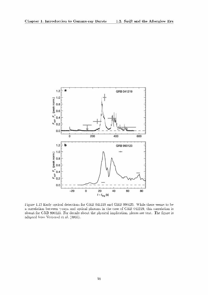
Probably the best studied examples of early afterglows are GRBs 990123 (Akerlof et al., 1999),
041219A (Vestrand et al., 2005; Blake et al., 2005) and 080319B (Racusin et al., 2008; Bloom et al.,
2009). While there seems to be a correlation between prompt γ-rays and early optical photons for
GRB 041219A, and the optical ash is interpreted as the low energy tail of the Band function from
the prompt emission, this correlation is absent for GRB 990123 (see Fig. 1.12). Its optical ash
is rather interpreted as the signature of a reverse shock component. The extremely bright optical
afterglow of GRB 080319B nally showed both components before the generic afterglow forward
shock: correlated optical and γ-ray emission and a reverse shock contribution. It must be noted
though, that in this case the optical emission is magnitudes brighter than expected from a simple
extrapolation of the γ-ray spectrum. Dierent types of emission mechanisms must be responsible
for the dierent photons, where physically reasonable ones are synchrotron emission for the optical
bands, and synchrotron self-Compton for the prompt γ-rays (Racusin et al., 2008), but see Piran
et al. (2009).
However, only a minor fraction of all well-localized bursts show either of the two eects (Roming
et al., 2006). While the spectral shape of the prompt emission and its extrapolation to the op-
tical bands naturally provide a convincing argument for the (non)-detection of correlated optical
emission, it is not immediately clear why some bursts do have prominent reverse shocks while the
majority does not (Roming et al., 2006).
The relative luminosities in the optical band between FS and RS is given by the degree of
magnetization of the outow, the relative energies between the two components and whether the
19
Chapter 1. Introduction to Gamma-ray Bursts 1.2. Swift and the Afterglow Era
Figure 1.12 Early optical detections for GRB 041219 and GRB 990123. While there seems to bea correlation between γ-rays and optical photons in the case of GRB 041219, this correlation isabsent for GRB 990123. For details about the physical implication, please see text. The gure isadapted from Vestrand et al. (2005).
20

Chapter 1. Introduction to Gamma-ray Bursts 1.2. Swift and the Afterglow Era
RS is relativistic or Newtonian. In particular, only when the RS is highly relativistic, most of the
emission is released in the optical bands. If the conditions are such, that the RS is only mildly
relativistic or Newtonian, the typical emission frequency shifts towards, but not reaching the radio
band (Nakar & Piran, 2004). Furthermore, the RS might be completely absent if the ejecta are
totally or not at all magnetized (Zhang & Kobayashi, 2005). Consequently, the specic conditions
in the ejecta, which are dependent on the exact type of progenitor, are expected to populate a
large region of dierent physical properties and only in the minor fraction the degree of baryon
loading, circumburst medium density and magnetization supports the formation of a prominent RS
emitting in the optical wavelength range. Only in these cases, the luminosity released in the RS is
compatible to the FS and fast-slewing, small robotic telescopes are able to detect a characteristic
RS signature in the optical afterglow light curve.
1.2.3 Chromatic Breaks
The previously discussed breaks due to the angular distribution of the shock wave's kinetic energy
(Section 1.1.3) and the cessation of an energy injection episode (Section 1.2.1) are achromatic by
denition, and their signature should appear in all energy bands. However, with the extended
coverage with X-ray and optical data in the Swift era, a signicant fraction of bursts has light-
curve breaks which are either only present in one band or not simultaneous as shown in Fig. 1.13.
These chromatic breaks are in strong contrast to the expectations for an energy injection or jet
break (Panaitescu et al., 2006a).
Furthermore, these breaks lack spectral evolution in the X-ray band, suggesting that the passage
of the cooling frequency νc is not responsible for these kind of light-curve morphologies. In order
to account for chromatic breaks dierent new models have been proposed, which either imply
severe modications of the standard model, or completely abandon the idea that the afterglow is
caused by a forward shock propagating into the circumburst media. In the earlier case, a chromatic
break requires a temporal evolution of the microphysical parameters εB and εe (Panaitescu, 2006).
There is however, no obvious physical reason for varying conditions in the shock-wave, which
might indicate that in the case of chromatic breaks the afterglow emission in the optical bands
and X-rays arise from dierent outows or regions in the ejecta (Panaitescu et al., 2006a). A more
controversial explanation has been proposed by Genet et al. (2007), where the X-ray afterglow
has an additional reverse shock contribution even at late times, which does not strongly aect
the optical bands. This implies that the energy must only be transferred to a very small electron
population. Under very specic conditions, in particular a very low Γ of the material which is
ejected at late stages of central engine activity, the X-ray afterglow might be explained by a long
lasting reverse shock component. There is, however, still no consensus, how to interpret chromatic
breaks and all proposed models need further investigation in the light of an increasing sample of
well monitored multi-wavelength afterglow light curves.
21

Chapter 1. Introduction to Gamma-ray Bursts 1.2. Swift and the Afterglow Era
Figure 1.13 A sample of Swift bursts with chromatic breaks. Shown are X-ray data in black andR band optical data in open circles. The data are tted by a single or broken power law (dashedand solid lines). The apparent break is either absent in one of the X-ray or optical bands, or notsimultaneous. Adapted from Panaitescu et al. (2006a).
22

Chapter 1. Introduction to Gamma-ray Bursts 1.3. Progenitor Models
Figure 1.14 Illustration of the two most popular GRB progenitor models and the internal - externalshock scenario. The formation of a GRB could begin either with the merger of two neutron starsor with the collapse of a fast rotating massive star. While the earlier scenario is thought to resultin a short GRB, there is rm evidence that long GRBs are caused by the latter one. Both of theseevents create a black hole with a rotating disk of material around it. The black hole - accretiondisk system launches a highly relativistic jet along the polar axis of the system. Internal shocksbetween shells of dierent velocity produce the GRB, and external shocks with the circumburstmedium the afterglow. Adapted from Gehrels et al. (2007).
1.3 Progenitor Models
As discussed in the previous section, a physically reasonable progenitor model must be able to
account for a huge energy release in photons of 1050 − 1052 erg on very short time scales, beamed
emission with opening angles of 1 to 20 and ultra-relativistic outows with Γ0 > 100. This
all strongly suggests the role of newborn compact objects with high angular momentum and an
accretion disk as central engine. One of the key questions is then, how to form these accretion
systems from stars or binaries at the end of their lifetime. A schematic view of the two most
popular progenitor models for long and short bursts is shown in Fig. 1.14 and discussed below.
23
Chapter 1. Introduction to Gamma-ray Bursts 1.3. Progenitor Models
1.3.1 The Collapsar Model
A collapsar is dened as a very massive, fast-rotating Wolf-Rayet star, which iron core collapses
directly to a black hole at the nal stage of its stellar evolution (Woosley, 1993). The accretion
disk formed around the newborn black hole has typical masses of several tenths of a solar mass,
and is fed by the collapse of the outer regions of the progenitor star on time scales of several ten to
hundred seconds. A reball is created by neutrino annihilation above the polar axes, just providing
the right amount of energy necessary for GRBs (Woosley, 1993). One crucial stage in the evolution
of the progenitor is the loss of its hydrogen and possibly helium envelope due to stellar winds
(MacFadyen & Woosley, 1999), which strongly relates the collapsar model to type Ic supernova
explosions. A fast rotation is also necessary to achieve a matter free region along the polar axis,
which then supports the formation of a jet and an expanding blastwave (e.g., Fryer et al., 1999).
The jet is focused by density and pressure gradients, and naturally maintains a collimation of the
order of 10 in these simulations (MacFadyen & Woosley, 1999).
Further simulations (e.g., Aloy et al., 2000; MacFadyen et al., 2001; Zhang et al., 2003b, 2004),
studied the subsequent evolution after the jet is formed and its breakout through the stellar at-
mosphere (Fig. 1.15). These simulations predict a further collimation and sporadic decelerations
and mixing of the ow along its edges with the stationary stellar material. These variations in
the baryonic load lead to dierent velocities in dierent regions of the jet - a crucial condition to
form internal shocks. Furthermore, a small amount of material is signicantly decelerated because
of friction and escapes at large angles. The observed morphology and energetics of GRBs are
thus strongly dependent on the viewing angle of the observer. Hence, these simulations support a
universal model, where the observed spread in GRB prompt emission spectra, i.e. a varying Epeak
of the Band function between several keV to MeV, can be attributed to dierent osets of the
observer with respect to the jet's symmetry axis.
By now, there is strong observational evidence through observations of optical spectra which
links long GRBs to the death of massive stars. One of the most convincing ones is the GRB-
Supernova (SN) connection. In the error box of GRB 980425 (Galama et al., 1998), simultaneous
within a day, a nearby SN was located (SN1998bw), which had remarkable brightness. Although
the chance coincidence was very low (∼ 10−4), the missing afterglow signature and extremely
low energy emitted in γ-rays of order 1048 erg raised questions whether this might not be a very
unusual type of GRB. The textbook example, which unambiguously connected GRBs to type Ic
SNe was GRB 030329, i.e. SN 2003dh (Hjorth et al., 2003; Stanek et al., 2003) at a redshift of
z = 0.1685 (Greiner et al., 2003b). Here, the typical afterglow spectrum of a power-law continuum
evolves towards a spectrum very similar to SN1998bw as the relative brightness of afterglow and
SN component vary. This provided direct spectroscopic evidence of an emerging SN at later
times. Further evidence supporting the collapsar model comes from light-curve modelling of a
larger sample of pre-Swift afterglows. The signature of an underlying SN is clearly detected in the
afterglow of nearby (z<0.7) GRBs as an extra emission component at later times, superimposed
to the typical afterglow power-law decay (Zeh et al., 2004).
However, diculties remain, especially in the light of the two recent GRBs 060505 and 060614
(Fynbo et al., 2006; Gal-Yam et al., 2006; Gehrels et al., 2006; McBreen et al., 2008). Located
24

Chapter 1. Introduction to Gamma-ray Bursts 1.3. Progenitor Models
Figure 1.15 Propagation of the jet in the local rest-frame through the stellar atmosphere. Screen-shots of numerical calculation in the collapsar model at 2 s and 7 s after the jet is formed areshown. In the left image only the central region of the star with a radius y = 0.8 × 1010 cm isshown. From Zhang et al. (2003b).
25

Chapter 1. Introduction to Gamma-ray Bursts 1.3. Progenitor Models
at redshift 0.089 and 0.125, their underlying SN signature would have been detected if present
at similar level as observed for previous GRBs. Deep optical observations suggest that the SN
component for these bursts must have been several hundred times fainter than SN1998bw, and
fainter than any type Ic SN ever observed (Richardson et al., 2006). These two bursts represent a
signicant fraction of nearby (z < 0.2) Swift GRBs, so that the total fraction of supernova-faint
bursts is also expected to be substantial. The luminosity of a SN is related to the amount of
synthesized radioactive 56Ni, which needs to be smaller than 1/100 M for the SN non-detections
in GRBs 060505 and 060614.
A possible explanation for a missing or very sub luminous SN might be the failed supernovae
scenario (Woosley, 1993), where the black hole is not formed directly after the collapse, but only
delayed due to fall-back onto the proto-compact object (Fryer et al., 2006). In this case the SN
would produce a much lesser amount of 56Ni and its light curve is no longer dominated by its
radioactive decay, but rather by the energy deposited in the SN shock. These calculations suggest,
that a fall-back GRB might be responsible for the apparent lack of associated SNe in some GRBs
(Fryer et al., 2007).
1.3.2 The Merger Scenario
While there is strong evidence linking long bursts to the death of massive stars and the collapsar
model, the situation is somewhat dierent for short bursts. Typically short bursts are less energetic,
nearby (z ∼< 1) and their afterglows are orders of magnitudes fainter than for long bursts (e.g.,
Fox et al., 2005; Levan et al., 2006; Nakar, 2007). A direct spectroscopic measurement of the
redshift of a short burst afterglow is thus observationally very dicult, and redshifts for short
bursts are generally obtained via host galaxy associations. Contrary to the hosts of long bursts,
which are most commonly blue, star-forming, small galaxies (e.g., Le Floc'h et al., 2003; Savaglio
et al., 2009), the morphology of short duration burst hosts is diverse (e.g., Berger et al., 2007;
Berger, 2009). A signicant fraction of these hosts are evolved elliptical galaxies with old stellar
populations. Therefore, the most frequently discussed model for the progenitor of short bursts is
a merger of two compact objects, either a neutron star - neutron star or neutron star - black hole
binary, schematically shown in Fig 1.14. This model is supported by the lack of SN features in the
light curves of short burst afterglows. Similar to the collapsar model, a spinning black hole with
an accretion disk is also formed in a binary merger, representing a large reservoir of gravitational
energy. Naturally, there is a distinct baryon free region along the spin axis of the merging binary.
However, the small number of well sampled afterglow light curves and the observational bias in the
host galaxies towards brighter, and thus more nearby hosts, makes a distinct identication of the
progenitor types for short bursts impossible at the current stage. Although binary mergers have
the potential of explaining the short burst phenomenon, more data is needed to securely associate
short bursts with mergers. One interesting possibility might be the detection of gravitational waves
contemporaneous with a short burst. Berger et al. (2007), for example, estimated the detection
rate of the signature of a binary merger for the upcoming generation of gravitational wave detectors
to 2-6 per year.
26

Chapter 1. Introduction to Gamma-ray Bursts 1.4. GRBs as Tools
Figure 1.16 Photometric (8.06+0.21−0.28) and spectroscopic (8.26+0.07
−0.08) redshift of GRB 090423. Thephotometric data has been obtained by GROND, VLT/HAWKI and the Gemini South telescope,analyzed and modeled by the tools described in Chapter 2. The inset shows the spectroscopic ob-servations performed with ISAAC at the VLT, fully consistent with the photometric data. Adaptedfrom Tanvir et al. (2009).
1.4 GRBs as Tools
Two recent discoveries of GRBs at very high redshift, GRB 080913 at redshift 6.7 (Greiner et al.,
2009b) and GRB 090423 at redshift 8.3 (see Fig. 1.16, and also Tanvir et al. (2009)), clearly
demonstrate the potential of GRBs as cosmological probes (see also Chapters 2 and 3). Theoreti-
cally, Swift is able to detect GRBs at redshift of 10 and beyond (see Fig. 1.17), which given only
modest brightness can be followed up and detected by state of the art instruments as GROND (see
Fig. 1.16, Chapter 2, also Greiner et al. (2009b)).
Although the direct cosmological use of GRBs as standard candles (e.g., Ghirlanda et al., 2004;
Firmani et al., 2005), analog to SN Ia explosions is still highly debated (e.g., Nakar & Piran, 2005;
Butler et al., 2007), the enormous energy release and brightness of the afterglow, which can outshine
even the brightest quasar by a factor of 105 at a similar redshift, makes GRBs ideal light sources
to study the very early Universe (Bromm & Loeb, 2002). In the very most pragmatic way, GRBs
are considered just as a source of radiation, which is then used to investigate the metal enrichment
of the Universe and the epoch of reionization (Lamb & Reichart, 2000; Loeb & Barkana, 2001).
Furthermore, using the association of GRBs with the death of massive stars, the star formation
history of the Universe can be directly constrained out to very high redshifts as shown in Fig. 1.18
(Yüksel et al., 2008). Although number statistics are still low, GRBs already provide signicant
constraints on the star formation rate (SFR) at redshifts above z ∼ 6, a region which is not easily
accessible with other sources so far. The SFR rate as derived with GRBs can exceed the critical
27

Chapter 1. Introduction to Gamma-ray Bursts 1.4. GRBs as Tools
Figure 1.17 The luminosity - redshift distribution of 119 Swift bursts determined by Butler et al.(2007). The shaded region approximates an eective threshold for detections with the Burst AlertTelescope (BAT) onboard Swift, and clearly shows that the somewhat brighter bursts can bedetected by BAT to redshifts of above 9. Demarcated in grey boxes are the GRB sub sample usedto estimate the cosmic star formation rate in Fig. 1.18. Adapted from Kistler et al. (2009).
Figure 1.18 The cosmic star formation rate density ρ∗ in solar mass per year and volume as derivedwith GRBs and other methods in dependence on the redshift (lower x axis) and the age of theUniverse (upper x axis) assuming concordance cosmology. After correcting for evolutionary eects,straight forward number counts of GRBs can be used to measure the SFR. Shown are the datacompiled in Hopkins & Beacom (2006) in grey light circles, Lyman Break Galaxies (LBG) fromBouwens et al. (2008) in blue triangles, and Lyman-α emitters (LAE) from Ota et al. (2008). Indashed lines the critical SFR ρc which is needed to balance recombination. ρc is depending on theclumpiness C of the intergalactic medium (IGM) and the escape fraction of photons in their hostgalaxy fesc. Adapted from Kistler et al. (2009).
28

Chapter 1. Introduction to Gamma-ray Bursts 1.4. GRBs as Tools
SFR ρc which is needed to balance the recombination of ionized Hydrogen even at redshift above
8. Thus, it seems plausible that the level of star formation was high enough even at this very early
times to reionize the Universe (Kistler et al., 2009).
Apart from their intrinsic brightness, GRBs have several advantages over Quasars as probes
of the early Universe. As the source of the explosion is stellar, GRBs do not disturb or ionize
the intergalactic medium (IGM). After the afterglow had faded, the host galaxies of high-redshift
GRBs can be observed in their characteristic physical state. GRBs thus serve as signposts of the
very rst or even proto galaxies, which will be observationally accessible to the upcoming telescopes
of the 30-40 m class or the James Webb Space Telescope, the successor of HST.
In addition, their spectrum is a very simple power law, making fast photometric redshifts reli-
able, and a detailed, unambiguous investigation of hydrogen and metal absorption in their spectra
possible. However, the transient nature of GRBs and their afterglows require rapid identication
and follow-up observations, preferentially within the rst hours post burst. It is from primary im-
portance to measure the spectral energy distribution of the afterglow in the near-infrared regime,
as any optical follow-up is determined to miss the afterglow of GRBs above redshifts of z ∼ 7.
29

Chapter 1. Introduction to Gamma-ray Bursts 1.4. GRBs as Tools
30
Chapter 2
The GROND Instrument
The primary goal of the Gamma-Ray Burst Optical/Near-infrared Detector (GROND, Greiner
et al., 2007b, 2008) is to identify GRB afterglows and measure their photometric redshift as rapid
after the trigger as possible. Therefore, the instrument is designed for simultaneous imaging in
7 dierent photometric bands: four optical CCDs in lters g′r′i′z′ and three near-infrared (NIR)
detectors in JHKS . These lters cover the wavelength range from 380 nm to 2400 nm, and GROND
can thus identify GRB afterglows up to z ∼ 20 and measure their redshifts in a range from z ∼ 3
to z ∼ 13. A schematic view of the optical layout is shown in Fig. 2.1.
GROND was designed and built by the Max-Planck-Institut für extraterrestrische Physik (MPE)
in collaboration with the Thüringer Landessternwarte Tautenburg (TLS) and is permanently
mounted at the 2.2 m MPG/ESO Ritchey-Cretien telescope at LaSilla observatory, Chile and
operational since spring 2007. A movable mirror (M3) reects light coming from the telescope's
primary (M1) and secondary (M2) mirror towards the GROND vessel in a Coudé-like focus. Both
the instrument and the telescope are controlled semi-robotically, which yields a typical reaction
time of 200− 400 s to GRB triggers. Most of the delay is due to the limited slewing speed of the
conventional telescope and dome. The medium-sized aperture of the telescope and relatively fast
response is crucial for an eective observation of GRB afterglows. A typical afterglow fades by ≈ 3
magnitudes during its rst 10 minutes after the trigger, and another 3 magnitudes in the following
two hours. The unique optical design with NIR coverage, medium-sized telescope aperture and
rapid response yields unprecedented detection eciency for GRB afterglows. If the visibility of the
optical transient associated with a GRB is such, that GROND can observe within 10 minutes, an
afterglow is detected with a probability in the high 90% region (cp. other robotic telescopes in the
∼ 30 − 80% region e.g., Roming et al., 2009; Cenko et al., 2009; Ryko et al., 2009; Klotz et al.,
2009), or in 62% of all ∼ 100 bursts observed with GROND until June 2009. These numbers are
signicantly higher than any GRB follow up program has reported so far. A subset of GROND
afterglow light curves is shown in Fig. 2.2.
Utilizing the high detection rate of the early afterglow observations, its now possible for the
rst time to address open questions in GRB physics with a sample which is unbiased in intrinsic
brightness, extinction and redshift. A complete sample will allow to probe the rates of highly
31
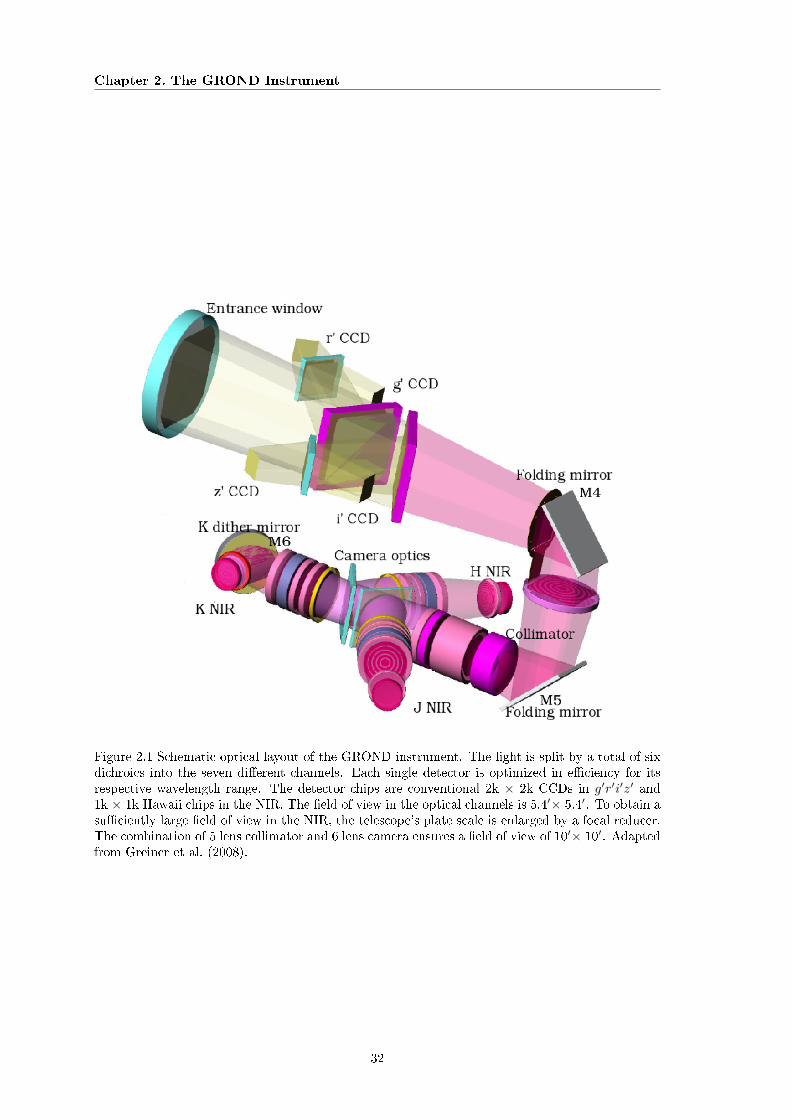
Chapter 2. The GROND Instrument
Figure 2.1 Schematic optical layout of the GROND instrument. The light is split by a total of sixdichroics into the seven dierent channels. Each single detector is optimized in eciency for itsrespective wavelength range. The detector chips are conventional 2k × 2k CCDs in g′r′i′z′ and1k × 1k Hawaii chips in the NIR. The eld of view in the optical channels is 5.4′× 5.4′. To obtain asuciently large eld of view in the NIR, the telescope's plate scale is enlarged by a focal reducer.The combination of 5 lens collimator and 6 lens camera ensures a eld of view of 10′× 10′. Adaptedfrom Greiner et al. (2008).
32

Chapter 2. The GROND Instrument 2.1. Filter System
Figure 2.2 Subset of r′-band light curves of GRB afterglows as observed with GROND. For caseswhere the redshift was z ≥ 5 (GRBs 080913 and 090423) the J-band light curve is shown. Thissample clearly shows the variety and variability of early afterglow light curves. While conventionalinstruments provide spectral information only on a longer time scale due to lter cycling, GRONDmeasures the spectral energy distribution (SED) in a broad range at each point of each singlelight curve. Eects of a changing spectrum or intrinsic extinction can thus be measured with highcondence, independent on the light curve morphology.
extincted, highly redshifted and intrinsically faint GRB afterglows, eventually reaching stringent
conclusion about the nature of so-called dark bursts (Groot et al., 1998), where the ratio of X-ray
to optical ux indicates a suppression of the optical afterglow.
Because of its simultaneous imaging, GROND has the key advantage that it obtains information
about the spectral energy distribution at each point during the evolution of the afterglow. In
particular in the early stages of optical afterglows, eects of a changing spectrum or a highly
variable light curve can be unambiguously disentangled, which has been proven to be crucial in
the interpretation of the light curves of, e.g., GRB 071031 (Krühler et al., 2009) or GRB 080129
(Greiner et al., 2009a).
2.1 Filter System
GROND uses dichroics, which transmit the lower- and reect the higher-energy photons to split
the incoming light into its seven channels. To dene the nal shape of the total response curve of
each wavelength band in GROND, there is also an additional lter which cuts o regions of high
sky background in the NIR and reduces spurious reections from the backside of the dichroics.
Additional optical components in the instrument/telescope system are the aluminum coated M1
and M2 of the 2.2 m telescope, GROND's silver coated M3, M4, M5 and M6 (see Fig. 2.1) and the
33

Chapter 2. The GROND Instrument 2.2. GROND Observation Scheme
focal reduction system in the NIR. Together with the transmission of the entrance window and the
quantum eciency of the detectors, these dene the GROND lter bands as shown in Fig. 2.3. The
reection and transmission of all optical components was measured at their operating temperature
of 80 K inside the GROND vessel, yielding highly accurate response curves down to systematic
errors of typically 2− 4%. A more detailed description of the lter curves including characteristic
lter parameters is given in Krühler (2006).
2.2 GROND Observation Scheme
The bright and variable NIR sky background limits the individual exposure times in the NIR
to around 10 s. Hence, a dithering pattern on the sky must be performed for an ecient sky
subtraction. These ditherings should be faster than the typical time scale of sky variation which
is of the order of several minutes for J , H and KS . A typical GROND observation thus consists
of several observation blocks, each with four, six or eight telescope pointings. These pointings are
oset by roughly 10 arcseconds and contain one or several images in the g′r′i′z′ channels with
a typical integration time between 30 s and six minutes, and a series of 10 s exposures in the
NIR. In addition, there is a KS-band dither mirror, which performs internal dithering in the KS
band to ensure an appropriate dither pattern for this band. The exposures in g′r′i′z′JHKS are
synchronized, so that no band sits idle with as little overhead as possible. The detailed GROND
observation scheme is described in Krühler (2006).
2.3 Reduction Software
The mechanical and optical design of a multi-channel imager operating in the optical and NIR
regime requires sophisticated observation scheduling and requires an advanced layout of the auto-
mated data reduction scheme. In particular, the GROND Pipeline (GP) must be able to deal with
both, optical data and NIR frames. The whole code is implemented in python1, utilizing pyraf 2,
a wrapper for the standard software for astronomical image processing, the Image Reduction and
Analysis Facility (IRAF, Tody, 1993). In addition, the object oriented python language provides
the substructure and possibility to utilize spawned processes and fork dierent tasks to child pro-
cesses within a single framework. Consequentially, a complete reduction of GROND raw data until
nal photometry products can be handled in a single program. For a technical description of the
GP concepts and basics, see Küpcü-Yolda³ (2006). Based on the existing pipeline layout, a user
friendly and stable code for data reduction has been developed in the context of this thesis, which
is described in detail below.
1http://www.python.org/2http://www.stsci.edu/resources/software_hardware/pyraf
34

Chapter 2. The GROND Instrument 2.3. Reduction Software
Figure 2.3 Eciency of the GROND instrument at the 2.2 m telescope: Top panel: telescope andGROND-internal mirrors. Panels 2 and 3 from top: transmission of the dichroics and the NIRlens systems. Panel 4: Transmission of the lters. Panel 5: Detector quantum eciencies. Bottompanel: Total eciency in each of the seven GROND bands. All losses are included, except theobstruction of M1 by M2. Except for the telescope (M1, M2) data, all curves represent measureddata at their operating temperatures, i.e. all transmission values for the lenses, dichroic and anti-reection coatings refer to 80 K.
35

Chapter 2. The GROND Instrument 2.3. Reduction Software
2.3.1 Reduction, Dithering and Sky Subtraction
Although the reduction code is customized and optimized to GROND data, the complete software
layout aims on being as generic as feasible, which makes the program also suitable for imaging data
from dierent telescope/instrument combinations. A set of photometric data can thus be analyzed
consistently in a single software framework. Starting from raw frames, as they are produced by the
instrument, the data-reduction pipeline performs the following tasks which are split into dierent
modules.
preprocess module: This module performs the necessary steps to extract the single-band image
from the raw data. In particular, all four CCD frames come stacked into one multi-extension
ts image, while the NIR data from three 1k x 1k detectors are stored in a single 1k x 3k ts
image with a single header.
reduction module: After initial pre- and overscan clipping and bias correction, the image is
atelded with the most recent master at. A defringing step is applied when necessary, but
only long exposures (∼> 3 min) suer from detectable fringing in the z′ band. NIR data are
corrected for the odd/even eect of the Hawaii chips. Optional, there can be a background
estimation using either a one-dimensional line-by-line t, or a two-dimensional plane t. In
particular, if the sky conditions or brightness are changing on a time scale faster than the
observations, this step is necessary to obtain adequate results.
stacking module: The individual 10 s NIR images, which are obtained on the same position of
the sky in the NIR channels are combined to obtain a higher signal-to-noise ratio.
distortion correction module: The stacked images are corrected for the image distortion
which is a result of the focal reducer in the NIR channels. The theoretical image distor-
tion depending on the location of the object in the focal plane and the dithering position has
been calculated, stored in a database and is applied onto the image.
dithering module: The sky background estimation and shift-and-add of frames which have been
obtained on dierent telescope dither positions can be done using either IRAF or jitter3, a
compilation of NIR data reduction algorithms from the European Southern Observatory
(ESO). The oset search is performed using cross-correlation techniques, which are very reli-
able and result in sub-pixel accuracy of the image registration. To enhance the computation
speed an initial guess of the image shift depending on the dither pattern can be provided.
2.3.2 Astrometry and Photometry
The nal product of the previous steps, a single image for a single observation block per band
is then pushed to the astrometry and photometry task. After source detection, an astrometric
solution is derived against automatically parsed USNO-B1 (Monet et al., 2003) and Two Micron
All Sky Survey (2MASS, Skrutskie et al., 2006) catalogs or the Sloan Digital Sky Survey (SDSS,
Adelman-McCarthy et al., 2008), if available. The full width half maximum (FWHM) of the
3http://www.eso.org/projects/dfs/papers/jitter99/
36

Chapter 2. The GROND Instrument 2.4. Light Curve Fitting
stellar point spread function (PSF) is derived for each image in each band separately by sextractor
(Bertin & Arnouts, 1996). Final products of a successful analysis include aperture and PSF tting
photometry from daophot (Stetson, 1987) of all detected eld sources, auxiliary photometry from
sextractor, calibrated magnitudes against the downloaded catalogs, and the accuracy of the absolute
photometry and of the astrometric solution. The brightness of an object is measured in magnitudes
(mag) in the AB system (Oke & Gunn, 1983), where the AB magnitude is related to the respective
ux density Fν via (e.g., Fukugita et al., 1996):
Fν [µJy] = 10(23.9−magAB)/2.5
2.3.3 Photmetric Accuracy
The native GROND photometric system is based on the SDSS g′r′i′z′ and 2MASS JHKS lters.
In most cases, however, the burst eld is not covered by the SDSS, which is a photometric and
spectroscopic survey of the northern sky. In that case, secondary eld stars are calibrated against
the primary equatorial SDSS standards, or a nearby SDSS eld under photometric conditions.
As the lter bands are nearly identical to the Sloan and 2MASS lters, the absolute photometric
accuracy reachable with GROND is in the range of 0.03 mag for g′r′i′z′ and 0.05 mag for JHKS .
Typical limiting magnitudes in the AB system for a 1 h exposure at zenith, and seeing 1" at new
moon are 25.0 (g′), 25.0(r′), 24.3 (i′), 24.0 (z′), 22.9 (J), 22.4 (H) and 21.8 (KS).
The limiting magnitudes of the NIR channels are strongly dependent on the NIR sky back-
ground, which shows large seasonal variations depending on temperature, humidity and sky con-
ditions. Under a bright NIR sky, the JHKS limiting magnitudes can be up to 1.5 mag higher. A
detailed description of the photometric calibration will be given in Clemens (2009, in preparation).
2.4 Light Curve Fitting
One key information about GRB afterglows that can be obtained by continuous monitoring is
the dependence of the ux density on time, i.e. Fν(t), as shown in Fig. 2.2. Consistent with the
expectations from theory (see Section 1.1) and observed in a large sample of light curves (Zeh et al.,
2006), the late optical afterglow is typically well described with two power-law segments, smoothly
connected at a break time tbreak and a possible constant host or SN contribution. However, the
early afterglow can be highly variable, with early rising components and chromatic ares (see
Fig. 2.2 and Chapters 3, 4 and 5). A crucial task is then to model the diversity of early afterglows,
which makes it possible to draw conclusions about the GRBs inner engine and the nature of the
afterglow, in particular the conditions in the ejecta, the geometry of the outow and the circumburst
medium. Therefore, the constraints on a multi-color light-curve tting program can be summarized
as follows:
Multi Dimensionality: The program should be able to combine various input data obtained in
dierent energy ranges from radio over optical/NIR to X-ray. In particular a typical GROND
37

Chapter 2. The GROND Instrument 2.4. Light Curve Fitting
afterglow light curve consists of 7 dierent energy bands from 380 nm to 2400 nm (0.5 eV to
3.2 eV). In most cases this information is complemented with X-ray data in the 0.3 keV to
10 keV range. Best possible constraints from the available data can only be obtained when
analyzing the entire data set simultaneously.
Parameter Handling: Model parameters must be able to be frozen, thawed and constrained to
specic ranges with upper and/or lower limits.
Model Denition and User Interface: User dened models should be easy to code, and easy
to implement for further extension of the light-curve tting program. The user interface must
be easy to learn and (re-)run, and scriptable for automated analysis.
Error Estimation: The code should automatically perform a reliable estimate of the errors at-
tributed to the best-t parameters.
Speed: The software should be able to obtain results and reliable errors on a typical personal
computer in less than a minute, even for large data sets (> 2000 unique measurements) and
complex models (> 20 free parameters).
Open Source: The program must not be based on commercial packages which require a license
or purchase.
From particular importance is a thorough error analysis, so that observational parameters can
be condentially compared with expectations from theory. The light-curve tting program which
was designed and developed as part of this thesis is based on the python interface4 to the root5
framework (Brun & Rademakers, 1997), which has proven to be stable and reliable in numerous
application, preferentially in particle physics, but also astrophysics. Given the stability and re-
liability of the root substructure and an easy readable and expandable code and user interface
in python, the program then complies with all predened constraints. In particular, it is able to
account for a simultaneous t with an unlimited set of input data. Each lter band (e.g., the
GROND g′r′i′z′JHKS ) and/or energy range (optical + X-ray) is linked via shared parameters,
while a subset of parameters is exclusively accessible to a subset of the specic input data. The
earlier typically include power-law slopes and break times, while the latter describe the overall ux
normalization and/or the color change of the afterglow in ares, or in the host dominated regime.
All parameters can be tied, thawed, frozen or linked according to the specic needs of the user.
Technically, this is performed via a virtual multi-dimensional t, where the shared parameters
represent the rst, and all unique parameters the higher dimensions of the t.
As predened empirical model functions a number of equations, describing a typical afterglow
light curve have been pre-coded. These include (amongst others):
Single Power Law (PL)
Fν(t) = F0 · (t/t0)−α(+H)
4http://www.scipy.org/PyRoot5http://www.root.cern.ch
38
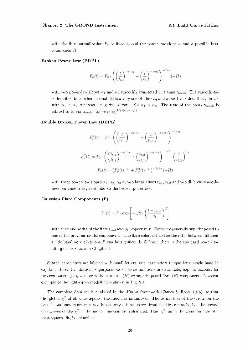
Chapter 2. The GROND Instrument 2.4. Light Curve Fitting
with the ux normalization F0 at xed t0 and the power-law slope α and a possible host
component H.
Broken Power Law (BRPL)
Fν(t) = F0 ·
((t
tb
)−s·α1
+(t
tb
)−s·α2)−1/s
(+H)
with two power-law slopes α1 and α2 smoothly connected at a time tbreak. The smoothness
is described by s, where a small |s| is a very smooth break, and a positive s describes a break
with α1 < α2, whereas a negative s stands for α1 > α2. The time of the break tbreak is
related to tb via tbreak=tb(−α1/α2)1/(s(α1−α2))
Double Broken Power Law (DBPL)
F 1ν (t) = F0 ·
((t
tb,1
)−s1·α1
+(
t
tb,1
)−s1·α2)−1/s1
F 2ν (t) = F0 ·
((tb,2tb,1
)−s1·α1
+(tb,2tb,1
)−s1·α2)−1/s1 (
t
tb,2
)α3
Fν(t) =(F 1ν (t)−s2 + F 2
ν (t)−s2)−1/s2 (+H)
with three power-law slopes α1, α2, α3 at two break times tb,1, tb,2 and two dierent smooth-
ness parameters s1, s2 similar to the broken power law.
Gaussian Flare Components (F)
Fν(t) = F · exp
[−1/2 ·
(t− tmid
σt
)2]
with time and width of the are tmid and σt respectively. Flares are generally superimposed to
one of the previous model components. The are color, dened as the ratio between dierent
single band normalizations F can be signicantly dierent than in the standard power-law
afterglow as shown in Chapter 4.
Shared parameters are labeled with small letters, and parameters unique for a single band in
capital letters. In addition, superpositions of these functions are available, e.g., to account for
two-component jets, with or without a host (H) or superimposed are (F ) component. A recent
example of the light-curve modelling is shown in Fig. 2.4.
The complete data set is analyzed in the Minuit framework (James & Roos, 1975), so that
the global χ2 of all data against the model is minimized. The estimation of the errors on the
best-t parameters are returned in two ways. First, errors from the Hesse-matrix, i.e. the second
derivatives of the χ2 of the model function are calculated. Here χ2, as in the common case of a
least-squares t, is dened as:
39

Chapter 2. The GROND Instrument 2.5. Spectral Energy Distribution Modelling
χ2(ξ) =n∑i=1
(f(xi, ξ)− ei)2
σ2i
where ξ is the vector of the free t parameters and ei are the individual measurements with
uncertainties σi. These are symmetric 1σ errors and take all parameter correlations but not the
non-linearities into account. The Hesse-matrix analysis thus results in symmetric errors and in
an appropriate error estimation as long as the χ2(ξ)-function can be approximated as a quadratic
function in the local minimum of the parameter space. If the problem is highly non-linear, this
procedure will signicantly underestimate the errors, and hence a second run of error estimation
is performed by default. Here, the algorithm to estimate the parameter error is dened such, that
the parameter is varied and the t function is subsequently minimized with respect to all other
variable parameters. Hence, the value of the t parameter where the ∆χ2 represents a 1σ error
is obtained numerically with respect to the minimum of all other free parameters. The resulting
errors are then generally asymmetric and relatively expensive to calculate, but return a reliable
estimate on the parameter errors in all cases.
Finally it must be noted, that even the most sophisticated error analysis strongly relies on a
correct determination of the errors attributed to the experiment. While the t and the best-t
parameters may still be physically reasonable in the case of under- or overestimated measurement
errors, the error bars on the t parameters are certainly not. Special care must thus be taken to
account for all statistic and systematic errors in the measurement, and a correct error propagation.
2.5 Spectral Energy Distribution Modelling
Apart from the light-curve information, GROND obtains the spectral energy distribution of the
afterglow, i.e. information on Fν(ν) over a large frequency domain. The typical afterglow spectrum
is a simple power law which is modied by dust and gas along the sight line towards the GRB. From
special interest here is the dust attenuation law, and the absorption of light by neutral hydrogen
in the GRB environment bluewards of Lyman-α (Ly-α) at 121.6(1 + z) nm in the observers frame.
The host of GRBs and the circumburst environment is generally gas rich, and thus has a very
high neutral hydrogen column density of NH ∼ 1021cm−2 and above. Systems with logNH ≥ 20.2
are named Damped Lyman-α Absorbers (DLAs). The afterglow ux is further suppressed by
intervening absorbers at redshifts between the bursts and the observer, the so called Lyman-α
forest. By modelling the eects of dust and gas along the sight line towards the afterglow, the
redshift of the burst, as well as the dust content in its immediate environment can be studied
(e.g., Fig. 2.5, or Chapter 3). Above redshifts of z ∼ 3, the Ly-α edge is well within GROND's
sensitivity limits and results in a redshift dependent absorption at the blue side of the afterglow
spectrum. Details on the specic software used, the physical eects of gas and dust absorption,
and photometric redshifts and their accuracy are given in the following sections.
40
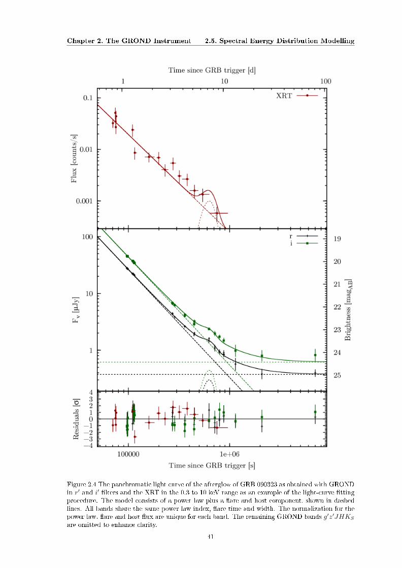
Chapter 2. The GROND Instrument 2.5. Spectral Energy Distribution Modelling
Figure 2.4 The panchromatic light curve of the afterglow of GRB 090323 as obtained with GRONDin r′ and i′ lters and the XRT in the 0.3 to 10 keV range as an example of the light-curve ttingprocedure. The model consists of a power law plus a are and host component, shown in dashedlines. All bands share the same power-law index, are time and width. The normalization for thepower law, are and host ux are unique for each band. The remaining GROND bands g′z′JHKS
are omitted to enhance clarity.
41

Chapter 2. The GROND Instrument 2.5. Spectral Energy Distribution Modelling
Figure 2.5 GROND photometric redshift of 6.44±0.30 for GRB 080913. The inset shows theafterglow spectrum obtained with FORS at the VLT, which resulted in a redshift measurementof z = 6.7 via spectroscopy, fully consistent with the GROND photo-z. The upper panel showsGROND images in the dierent lters. The afterglow is clearly detected in J and redder, very faintin z′, whereas the i′ band and bluer only yield upper limits. Adapted from Greiner et al. (2009b).
2.5.1 Photometric Redshifts with GROND
The software used for the measurement of the photometric redshift (photo-z) of GRBs and the
amount of dust in their environment is based on the publicly available hyperZ code (Bolzonella
et al., 2000). In addition to the existing treatment of the Lyman-α absorption according to Madau
(1995) and default reddening templates from local galaxies, the code is complemented by several
additions to t it to the need of GRB science. In particular, power-law spectral templates with the
possibility to constrain the spectral index and an additional reddening law according to Maiolino
et al. (2004) were added. The program also includes the measured total GROND lter response,
including all components in the optical pathway from the primary mirror of the telescope to the
quantum eciency of the detectors (Fig. 2.3). Special care was taken for a correct treatment of
the lter curves: The total eciency curve is calculated from its single components measured at
their operating temperature inside the GROND vessel. The latter are actively controlled by a set
of ten heaters and control loops, to ensure constant conditions during all observations.
Typical results are similar to the standard outputs of the original hyperZ version, including the
photometric redshift, error bars or contours of the three main parameters redshift, spectral index
and intrinsic reddening at arbitrary condence levels and the statistical probability associated with
the derived redshifts and secondary solutions if existent.
42

Chapter 2. The GROND Instrument 2.5. Spectral Energy Distribution Modelling
2.5.2 Simulating the Spectral Energy Distribution of GRB Afterglows
To test for the accuracy of the photometric redshift measurement with GROND, a sample of GRB
afterglow spectra was simulated. The continuum spectrum of an afterglow in the optical/NIR
range is a power law:
Fν(λ) = F0(λ/λ0)−β
where F0 is the normalization at λ0 = 1000 nm. F0 was chosen to be in the range of a standard
afterglow as observed with GROND and shown in Fig. 2.2. The brightness of the afterglow and the
observing conditions dene the signal-to-noise ratio of the measurement and the image quality. The
average accuracy for GROND with standard absolute ux calibration is 0.04 mag in g′r′i′z′ and
0.06 mag in JHKS lters. These values were chosen as the minimum errors, where additionally a
statistical error proportional to F0 was added quadratically. The latter one is typically dominating
in the range of faint bursts with an r′-band magnitude of 25 to 23.5 mag.
The Eect of Intrinsic Extinction
To model the eect of intrinsic reddening due to dust in the circumburst medium or the host
galaxy, dierent dust attenuation laws η(λ) = Aλ(λ)/AV as shown in Fig. 2.6 were used. AV is
the dust extinction in the V band, typically centered at 550 nm. The optical thickness τ in the
rest-frame of the host is then:
τdust(λ) = 0.92AV η(λ)
so that the model spectrum is reddened via:
Fν(λ) = F0(λ/λ0)−β exp[−τdust(λ/(1 + z))]
The dust extinction laws of Milky Way (MW), Small and Large Magellanic Cloud (SMC, LMC)
are parameterized according to Pei (1992). They strongly dier in their absolute UV absorption,
which is decreasing in strength from SMC, over LMC to MW. The most prominent extinction fea-
tures in the local extinction curves is the 2175 Å bump, which is generally attributed to absorption
by graphite grains. While the feature is highly signicant in MW and LMC models, it is absent in
the SMC dust attenuation law (Fig. 2.6).
However, there is no physical reason to assume that the extinction law in the environment of a
GRB from the early Universe necessarily has to comply with what is known from local galaxies. In
particular, the dust content, constitution, element abundances and grain sizes can be signicantly
dierent and thus the specic intrinsic extinction. Therefore, a more generic approach is used to
obtain a broader range of reasonable dust extinction laws by utilizing the Drude model proposed
in Li et al. (2008) and Liang & Li (2009).
43
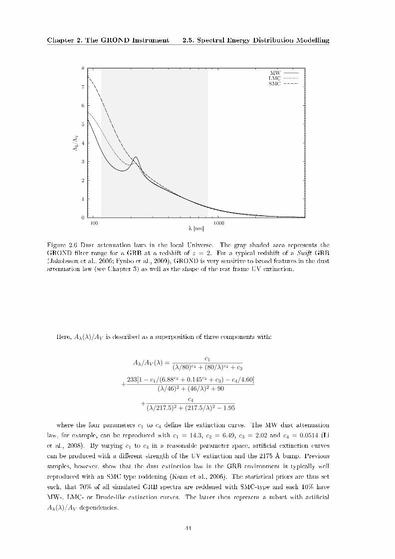
Chapter 2. The GROND Instrument 2.5. Spectral Energy Distribution Modelling
Figure 2.6 Dust attenuation laws in the local Universe. The gray shaded area represents theGROND lter range for a GRB at a redshift of z = 2. For a typical redshift of a Swift GRB(Jakobsson et al., 2006; Fynbo et al., 2009), GROND is very sensitive to broad features in the dustattenuation law (see Chapter 3) as well as the shape of the rest-frame UV extinction.
Here, Aλ(λ)/AV is described as a superposition of three components with:
Aλ/AV (λ) =c1
(λ/80)c2 + (80/λ)c2 + c3
+233[1− c1/(6.88c2 + 0.145c2 + c3)− c4/4.60]
(λ/46)2 + (46/λ)2 + 90
+c4
(λ/217.5)2 + (217.5/λ)2 − 1.95
where the four parameters c1 to c4 dene the extinction curve. The MW dust attenuation
law, for example, can be reproduced with c1 = 14.3, c2 = 6.49, c3 = 2.02 and c4 = 0.0514 (Li
et al., 2008). By varying c1 to c4 in a reasonable parameter space, articial extinction curves
can be produced with a dierent strength of the UV extinction and the 2175 Å bump. Previous
samples, however, show that the dust extinction law in the GRB environment is typically well
reproduced with an SMC-type reddening (Kann et al., 2006). The statistical priors are thus set
such, that 70% of all simulated GRB spectra are reddened with SMC-type and each 10% have
MW-, LMC- or Drude-like extinction curves. The latter then represent a subset with articial
Aλ(λ)/AV dependencies.
44

Chapter 2. The GROND Instrument 2.5. Spectral Energy Distribution Modelling
Eects of Damped Lyman-α Systems
A large number of optical afterglow spectra show the clear presence of a Damped Lyman-α Absorber
(DLA) (e.g., Watson et al., 2006). To quantify the eects of strong neutral hydrogen absorption
associated with the GRB, the standard approach of DLA modelling (e.g., Vreeswijk et al., 2004)
is used. Following the description of Totani et al. (2006) and references therein, the optical depth
τDLA of the DLA is dened as:
τDLA(νobs) = NHIσα[νobs(1 + zDLA)]
where σα is the Ly-α cross section with
σα(ν) =3λ2
αfαΛcl,α
8πΛα(ν/να)4
4π2(ν − να)2 + Λ2α(ν/να)6/4
fα=0.4162 is the absorption oscillator strength and Λα is the damping constant of the Ly-α
resonance with Λα = 3(gl/gu)fαΛcl,α. The g-factors are the statistical weights of the rst and
second electronic niveau of hydrogen, and thus gl = 1 and gu = 3. The classical damping constant
Λcl,α is given as Λcl,α = 8(πqe)2/(3mecλ2α) with the mass and charge of the electron me and qe and
the wavelength λα = 121.6 nm of the Ly-α transition. The redshift of the DLA zDLA is always set
to the redshift of the burst in the following.
The reddened afterglow spectrum together with the eects of a DLA at the burst's redshift
then becomes:
Fν(λ) = F0(λ/λ0)−β exp[−τdust(λ/(1 + z))] exp[−τDLA(λ/(1 + z))]
Absorption lines due to metals in the GRB environment are omitted, as their eect on the
integrated magnitude in broad-band lters as the GROND g′r′i′z′JHKS is negligible.
Eective Lyman-α Forest Opacity
Bluewards of the DLA centered at the redshifted λα, i.e. at 121.6(1+z) nm in the observers frame,
the afterglow ux is further suppressed by the Lyα forest: intervening absorbers between the burst
site and the observer. To model the eect of the Ly-α forest, the average opacity depending on
the redshift is calculated. According to Faucher-Giguère et al. (2008), the eective optical depth
τeff of the Ly-α forest, can be described as:
τeff = 1.8 · 10−3(1 + z)3.92
To compute the wavelength-averaged attenuation of the afterglow continuum due to line blanken-
ing (Madau, 1995), averaged over dierent sight lines, the observed ux decits 〈DA〉 between Ly-α
45
Chapter 2. The GROND Instrument 2.5. Spectral Energy Distribution Modelling
and Ly-β in the GRB rest-frame is calculated according to:
〈DA〉 = 1−∆λα−β∫ λα(1+z)
λβ(1+z)
exp[−τeff ]dλobs
and similarly for Ly-β, Ly-γ and Ly-δ and higher orders, e.g., for Ly-β:
〈DB〉 = 1−∆λβ−γ∫ λβ(1+z)
λγ(1+z)
exp[−τβeff ]dλobs
The most prominent contribution however, is Ly-α, and including higher order hydrogen ab-
sorption does not signicantly change the average eective Ly-α forest opacity. To account for
dierent measurements, measurement errors and specic sight lines, the observed ux decits are
allowed to vary according to the errors given in Faucher-Giguère et al. (2008). In particular, it is
taken into account that the uncertainty is increasing with redshift. Consequently, the afterglow
spectrum becomes:
Fν(λ) = 〈DA〉F0(λ/λ0)−β exp[−τdust(λ/(1 + z))] exp[−τDLA(λ/(1 + z))]
for λβ(1 + z) < λobs < λα(1 + z) and similar for 〈DB〉 and higher order absorptions. Below the
Lyman limit of ∼ 90.7(1 + z) nm, the observed ux is fully attenuated by the circumburst neutral
hydrogen, and hence Fν(λ) = 0. Fig. 2.7 shows examples of ideal afterglow spectra in dependency
of the relevant parameters.
Synthetic AB magnitudes of the afterglow spectrum in the dierent lters i are then derived
via:
magiAB = −2.5 log
∫Fν(λ)Ti(λ)dλ∫
Ti(λ)dλ+ 23.9 mag
where T (λ) are the specic lter curves shown in Fig. 2.3. These magnitudes are then varied
according to an associated error, which depends on the lter and overall normalization of the spec-
trum F0, where F0 was initially chosen to be in a reasonable range of previously observed GROND
GRB afterglows. If the integrated ux over the bandpass is lower than the typical sensitivity limit
of a one hour GROND exposure, the obtained magnitudes are converted into upper limits.
2.5.3 Redshift Accuracy
To investigate how accurate photometry can reproduce the redshift of a GRB, a mock set of ∼ 1500
GRB spectra was simulated using the procedure described in Section 2.5.2. The properties of the
simulations are shown in Fig. 2.8. Several priors have been set, to eciently sample the region of
specic interest. These priors are chosen such, that they resemble the information known about
GRB afterglow spectra, and probe a parameter space which is accessible to the GROND instrument.
46

Chapter 2. The GROND Instrument 2.5. Spectral Energy Distribution Modelling
Figure 2.7 Simulated GROND SEDs for dierent input parameters. From top left to right bottom:redshift z = 3, 4, 5, 6, 7 and 8, extinction AV = 0.6, 0.4, 0.3, 0.0, 0.2, 0,1, log(NH) = 24, 23, 22,21, 20, 19 and power-law index β = 0.2, 0.4, 0.6, 0.8, 1.0 and 1.2. Filled circles mark simulateddetections, while open triangles upper limits. The vertical error bars on the measurement is afunction of magnitude with respect to GROND's sensitivity. The horizontal error bars mark the50% range of maximum throughput for each lter. The colored areas represent the ux transmissionin the individual lters. Note the dierent extinction laws (i.e. a MW-type extinction with a2175 Å feature in the upper left panel), and the blue leak of the H and KS lters.
47
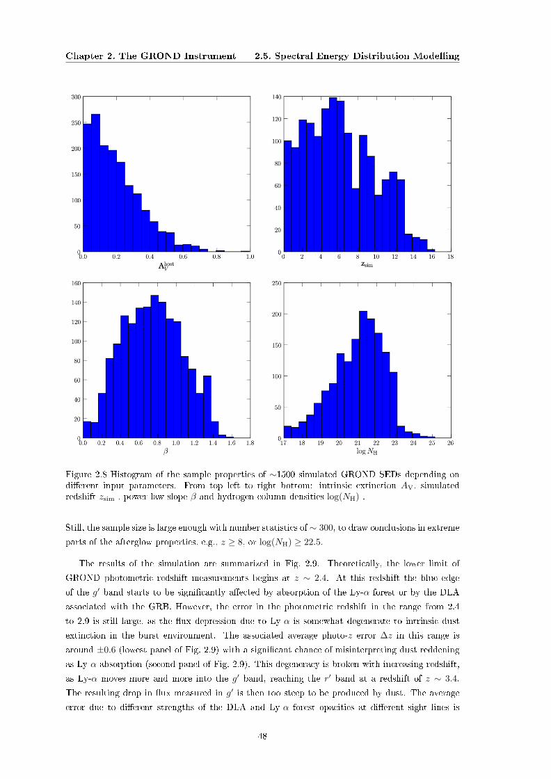
Chapter 2. The GROND Instrument 2.5. Spectral Energy Distribution Modelling
Figure 2.8 Histogram of the sample properties of ∼1500 simulated GROND SEDs depending ondierent input parameters. From top left to right bottom: intrinsic extinction AV, simulatedredshift zsim , power-law slope β and hydrogen column densities log(NH) .
Still, the sample size is large enough with number statistics of ∼ 300, to draw conclusions in extreme
parts of the afterglow properties, e.g., z ≥ 8, or log(NH) ≥ 22.5.
The results of the simulation are summarized in Fig. 2.9. Theoretically, the lower limit of
GROND photometric redshift measurements begins at z ∼ 2.4. At this redshift the blue edge
of the g′ band starts to be signicantly aected by absorption of the Ly-α forest or by the DLA
associated with the GRB. However, the error in the photometric redshift in the range from 2.4
to 2.9 is still large, as the ux depression due to Ly-α is somewhat degenerate to intrinsic dust
extinction in the burst environment. The associated average photo-z error ∆z in this range is
around ±0.6 (lowest panel of Fig. 2.9) with a signicant chance of misinterpreting dust reddening
as Ly-α absorption (second panel of Fig. 2.9). This degeneracy is broken with increasing redshift,
as Ly-α moves more and more into the g′ band, reaching the r′ band at a redshift of z ∼ 3.4.
The resulting drop in ux measured in g′ is then too steep to be produced by dust. The average
error due to dierent strengths of the DLA and Ly-α forest opacities at dierent sight lines is
48
Chapter 2. The GROND Instrument 2.5. Spectral Energy Distribution Modelling
±0.4 in this range. Larger errors are only obtained with a very high DLA hydrogen column with
log(NH) ≥ 23 or signicant dust (AV ≥ 0.5). With further increasing redshift above ∼ 3.4, Ly-α is
in the r′ band, with signicant ux being still detected bluewards due to the transmissivity of the
Ly-α forest. Consequently, two bands then show ux lower than the extrapolation of the power
law, which results in a very accurate and robust redshift estimate with an average error ∆z = ±0.2,
with negligible chance of misidentication (see Fig. 2.7). At redshifts above 7, Ly−α is redwards of
973 nm, and only very little or no ux reaches the reddest optical band z′. As the spacing between
z′ and J is relatively large, the photometric redshift is rather loosely constrained, increasing from
∆z ∼ 0.2 at z = 6.5 to ∆z ∼ 0.8 at a redshift of 8.2. In this region, the ux decrease in J could be
mimicked by some amount of intrinsic extinction and a lower redshift down to around 7. Above
a redshift of z ∼ 9.5, where bursts are expected to be relatively faint the transmitted ux in J is
on average below the GROND sensitivity limit. With detections in only H and KS , the problem
is totally degenerate between the spectral power-law slope β and redshift, and only constraints
on the power-law index from the previously measured range or from the X-ray spectrum allow a
photometric redshift determination. Consequentially, the typical photo-z error reaches ∆z = ±2 at redshifts of 11 and above. The upper limit for a reliable photo-z estimate for GROND is
z ∼ 13.5.
49

Chapter 2. The GROND Instrument 2.5. Spectral Energy Distribution Modelling
Figure 2.9 Results of the simulation of GRB afterglow spectra and photometric redshift measure-ment. From top to bottom: Photometric redshift zphot, absolute dierence ∆z = zphot − zsim,relative dierence ∆z/(1 + z) and total, i.e. quadratically added systematic and statistical error∆zsys+stat versus simulated, i.e. input redshift zsim
50

Chapter 3
The 2175 Å Dust Feature in a
Gamma-ray Burst at Redshift 2.45 1
ABSTRACT
We present optical and near-infrared photometry of the afterglow of the long Gamma-ray Burst
GRB 070802 at redshift 2.45 obtained with the ESO/MPI 2.2 m telescope equipped with the
multi-channel imager GROND. Follow-up observations in g′r′i′z′ and JHKS bands started at
∼ 17 minutes and extended up to 28 hr post burst. We nd an increase in the brightness of the
afterglow at early times, which can be explained by the superposition of reverse and forward shock
(FS) emission or the onset of the afterglow FS. In addition, we detect a strong broad absorption
feature in the i′ band, which we interpret as extinction from the redshifted 2175 Å bump in the
GRB host galaxy. This is one of the rst and clearest detections of the 2175 Å feature at high
redshift. It is strong evidence for a carbon rich environment, indicating that Milky Way- or Large
Magellanic Cloud- like dust was already formed in substantial amounts in a galaxy at z = 2.45.
3.1 Introduction
Gamma-ray Bursts (GRBs) are intense extragalactic ashes of γ-rays with durations between
several tenths to hundreds of seconds (e.g. Fishman et al., 1994; Mészáros, 2006). They cluster
in two dierent categories of duration and spectral hardness: short-hard bursts versus long-soft
bursts (Kouveliotou et al., 1993). GRBs are followed by longer lasting afterglows in radio to X-rays
(e.g. Katz, 1994; Mészáros & Rees, 1997; Zhang, 2007). The enormous energy release in γ-rays
is unaected by dust or gas absorption, so GRBs are detectable out to very high redshifts (e.g.
Lamb & Reichart, 2000; Kawai et al., 2006). These characteristics make GRBs potential tools
to constrain the history of star formation (Bromm & Loeb, 2002) and chemical evolution in the
universe (Savaglio, 2006; Fynbo et al., 2006; Berger et al., 2006).1T. Krühler, A. Küpcü Yolda³, J. Greiner, C. Clemens, S. McBreen N. Primak, S. Savaglio, A. Yolda³, G. P.
Szokoly and S. Klose (2008), Astrophysical Journal, 685, 376
51
Chapter 3. The 2175 Å Dust Feature in GRB 070802 3.2. Observations
The GRB-SN connection (e.g. Zeh et al., 2004; Woosley & Bloom, 2006) strongly supports the
association of long GRBs with the core-collapse of very massive stars, and therefore with regions
of high-mass star formation in the host galaxies (Paczynski, 1998). High-mass star-forming regions
show signatures of signicant dust and gas absorption in ultra-violet and optical spectra of bright
GRB afterglows (Savaglio, 2006; Berger et al., 2006; Fynbo et al., 2007). In fact, a large number of
bursts do not show optical afterglows despite rapid and deep optical follow-up observations (e.g.
Stratta et al., 2004; Rol et al., 2005). Natural explanations for "optically dark bursts" (Groot et al.,
1998) include dust extinction in the host galaxy (e.g. Fynbo et al., 2001; Klose et al., 2003) and
high redshift (e.g. Groot et al., 1998), both eciently suppressing any ux in the observed optical
bands (Roming et al., 2006). Several bursts with moderate dust absorption have been detected
(e.g. Kann et al., 2006), which may represent only the lower end of the host extinction distribution
(Schady et al., 2007). The detection of signicant reddening in a host is strongly instrumentally
biased due to the lack of rapid near-infrared follow-up observations with large-aperture telescopes.
In particular, one of the biggest shortcomings of all multi-color monitoring of afterglows so far was
the lack of a simultaneous coverage of the optical to near-infrared (NIR) bands.
The Gamma-Ray Burst Optical/Near-infrared Detector (GROND) is a seven-channel imager
primarily designed for fast follow-up observations of GRB afterglows (Greiner et al., 2007b, 2008).
It enables the detection and identication of GRB afterglows in a broad wavelength range (380-
2400 nm). Due to the use of dichroic beam splitters it is capable of simultaneous imaging in seven
bands, g′r′i′z′ (similar to the Sloan system) and JHKS . GROND has been mounted on the 2.2 m
ESO/MPI telescope on LaSilla/Chile since April 2007. The instrument is operated robotically and
is capable of monitoring the light curve of the transient starting from a minimum of a few minutes
after burst alert. The eld of view of the instrument is 10′ × 10′ in the NIR and 5.4′ × 5.4′ for
the optical bands (Greiner et al., 2008). The fast response, medium-sized telescope aperture, NIR
capabilities, and unique optical design makes GROND an ideal tool for follow-up observations of
GRBs.
Here we report on rst GROND follow-up observations of GRB 070802 (Section 3.2) and derive
constraints on the GRB ejecta and its circumburst properties (Section 3.3).
3.2 Observations
3.2.1 Swift Observations
The BAT (Burst Alert Telescope) instrument (Barthelmy et al., 2005) onboard the Swift satellite
(Gehrels et al., 2004) triggered on the long-soft GRB 070802 at T0 = 07 : 07 : 25 UTC and
immediately slewed to the burst (Barthelmy et al., 2007). The BAT light curve shows a single
peak starting at T0 + 5 s and ending at T0 + 50 s. There is evidence at the 3σ level for a precursor
at T0 − 150 s (Cummings et al., 2007). The T90 for GRB 070802 is 16.1± 1.0 s and the uence in
the 15-150 keV band is (2.8± 0.5)× 10−7 erg cm−2 (Cummings et al., 2007).
The X-Ray Telescope (XRT; Burrows et al., 2005b) began follow-up observations of the burst
52

Chapter 3. The 2175 Å Dust Feature in GRB 070802 3.2. Observations
eld 138 s after the trigger and detected an uncatalogued fading X-ray source at a position of
R.A.(J2000.0)=02h 27min 35s.76, decl.(J2000.0)=-55 31′ 38.′′4 with a rened 90% coincidence
error of 2.′′1 (Mangano et al., 2007). The XRT light curve decays with a slope of α ∼ −2 until
T0 + 500 s and then remains at until ∼ 4 ks. Afterwards the light curve decays with a power-law
index of ∼ −1 until it fades below the XRT sensitivity limits (Mangano et al., 2007). No bright
ares are detected in the XRT light curve.
The third instrument onboard Swift, the Ultra-Violet Optical Telescope (UVOT, Roming et al.,
2005) started observations at T0 + 100 s and did not nd any transient sources inside the XRT
error circle down to 19.5 mag (u lter), 21.3 mag (b lter) and 21.2 mag (uvw2 lter) (Immler
et al., 2007).
3.2.2 GROND Optical and Near-infrared Observations
GROND responded to the Swift GRB alert and initiated automated observations on the 2007 Au-
gust 2 at 07:24:09 UTC, starting 7 minutes 16 s after the Swift trigger and 16 minutes 44 s after the
onset of the burst. A predened sequence of exposures with successively increasing exposure times
were executed, acquiring images in all seven photometric bands simultaneously. The observations
continued for two nights, after which the afterglow had faded below the GROND sensitivity limits.
A variable point source in the NIR bands (Greiner et al., 2007a) inside the Swift XRT error circle
was identied by the GROND data reduction pipeline (Küpcü-Yolda³ et al., 2008). The transient
is shown in Fig. 3.1 and its absolute position is calculated to be R.A.(J2000.0)=02h 27m 35.68s,
decl.(2000.0)=-55 31′ 38.9′′ with an uncertainty of 0.3′′ compared to 2MASS reference eld stars.
The afterglow was also observed and detected by the Magellan telescope at Las Campanas Obser-
vatory (LCO, Berger & Murphy, 2007) and the Very Large Telescope (VLT), the latter yielding a
spectroscopic redshift of z = 2.45 (Prochaska et al., 2007).
In total, 2036 NIR images with an integration time of 10 s each and 56 CCD optical frames
were obtained with GROND. The CCD integration times scaled with the brightness of the transient
from 45 s at early times to 10 minutes when the source had faded. Sky conditions were clear with
a mean seeing around 1.2′′. All GROND data were obtained at airmasses between 1.35 and 1.12.
Optical and NIR image reduction and photometry was performed using standard IRAF tasks
(Tody, 1993). A general model for the point-spread function (PSF) of each image was constructed
using bright eld stars and tted to the afterglow. In addition, aperture photometry was carried
out, and the results were consistent with the reported PSF photometry. Photometric calibration
was performed relative to secondary standards in the GRB eld. During photometric conditions,
two spectrophotometric standard stars, SA114-750 and SA114-656, both primary Sloan standards
(Smith et al., 2002), were observed with GROND. Observations of the GRB eld followed within
4 minutes. The magnitudes of SA114-750 and SA114-656 were transformed to the GROND lter
system using their spectra and the GROND lter curves (Greiner et al., 2008). The obtained
zeropoints were corrected for atmospheric extinction dierences and used to calibrate stars in the
GRB eld, shown in Fig. 3.1. The apparent magnitudes of the afterglow were measured with
respect to the secondary standards reported in Table 3.1.
53

Chapter 3. The 2175 Å Dust Feature in GRB 070802 3.2. Observations
Figure 3.1 NIR afterglow of GRB 070802 in the J band at t = 3.4±0.3 ks post burst, including theSwift XRT error circle. Only a ∼3′ × 2.5′ segment of the original 10′ × 10′ image is shown. TheGROND NIR images have a pixel scale of 0.′′6/px each. The image is a combination of 48 stacked10 s exposures and also shows the secondary standards used for calibration, marked as A, B, C, Dand E.
54
Chapter 3. The 2175 Å Dust Feature in GRB 070802 3.3. Analysis
Vega magnitudes have been transformed to the AB system using transformation factors for
the GROND lter system as δg′ = 0.01 mag, δr′ = 0.15 mag, δi′ = 0.39 mag, δz′ = 0.52 mag,
δJ = 0.91 mag, δH = 1.38 mag and δKS = 1.80 mag. All reported afterglow magnitudes are
corrected for Galactic foreground reddening (EB−V = 0.026 mag, Schlegel et al., 1998). Assuming
RV = 3.1 for the Milky Way, this leads to AK = 0.01 mag, AH = 0.02 mag, AJ = 0.03 mag,
Az = 0.04 mag, Ai = 0.05 mag, Ar = 0.07 mag and Ag = 0.10 mag for the GROND lter bands.
The afterglow is detected in all seven GROND bands, however, it was too dim to construct a
light-curve with reasonable time resolution in the lter bands g′ and i′. The light-curves obtained
in the r′z′JHKS bands are presented in Fig. 3.2. The light-curve behavior is dominated by an early
rise in brightness, after which it declines with a bump superimposed onto the overall decay. The
observed variations occur in all ve GROND bands, and the generic light-curve shape is achromatic
within the measurement uncertainties.
3.3 Analysis
3.3.1 The Early Light Curve of the Afterglow of GRB 070802
According to the reball model (e.g. Wijers et al., 1997; Sari & Piran, 1999; Piran, 2005; Mészáros,
2006), GRBs produce their prompt emission in γ-rays from internal shocks of an ultra-relativistic
outow from a compact source and long-wavelength afterglows from the interaction of the ejecta
with the circumburst medium. After the prompt internal shock phase, the optical afterglow light
curve is composed of a superposition of two dierent emission components: the reverse shock (RS)
propagating into the ejecta and the forward shock (FS) traveling into the surrounding medium
(Zhang et al., 2003a). Rapid optical observations of the early transition phase between prompt and
afterglow emission can constrain the nature of the outow (Nakar & Piran, 2004). While baryonic
ejecta are expected to produce an optical ash, that can be associated with a RS, a Poynting ux
dominated afterglow should preferentially show the FS emission. The hydrodynamical calculations
from the reball model have succeeded in describing the generic afterglow of GRBs from several
minutes to days post burst. However, the majority of bursts do not show bright optical ashes
and apparently lack a strong RS emission component (Roming et al., 2006). This fact provides
observational support that the strength of the optical emission from the RS may be weaker than
previously calculated (Beloborodov, 2005).
A baryonic shell expanding into a homogeneous medium is fully described by the shell isotropic
equivalent energy E, its width ∆, the initial Lorentz factor Γ0 and the ISM density n (Nakar
& Piran, 2004). In the thick shell case, the initial Lorentz factor is large, and the swept up
circumburst medium decelerates the ejecta eciently (Kobayashi & Sari, 2000). Here, the RS
becomes relativistic in the rest frame of the unshocked ejecta. The critical Lorentz factor Γcdiscriminating between the relativistic thick (Γ0 > Γc) and Newtonian thin shell (Γ0 < Γc) cases
55
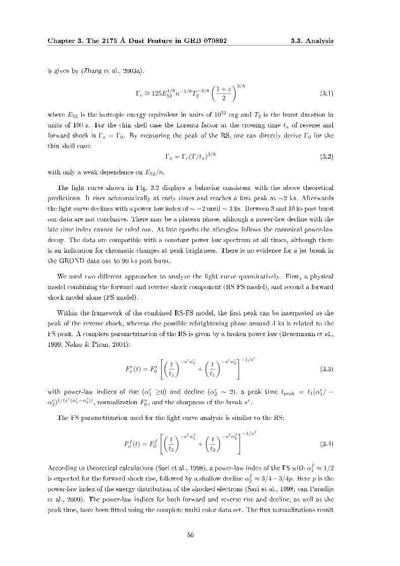
Chapter 3. The 2175 Å Dust Feature in GRB 070802 3.3. Analysis
is given by (Zhang et al., 2003a).
Γc ∼= 125E1/852 n−1/8T
−3/82
(1 + z
2
)3/8
(3.1)
where E52 is the isotropic energy equivalent in units of 1052 erg and T2 is the burst duration in
units of 100 s. For the thin shell case the Lorentz factor at the crossing time tx of reverse and
forward shock is Γx = Γ0. By measuring the peak of the RS, one can directly derive Γ0 for the
thin shell case:
Γx = Γc(T/tx)3/8 (3.2)
with only a weak dependence on E52/n.
The light curve shown in Fig. 3.2 displays a behavior consistent with the above theoretical
predictions. It rises achromatically at early times and reaches a rst peak at ∼2 ks. Afterwards
the light curve declines with a power-law index of ∼ −2 until ∼ 3 ks. Between 3 and 10 ks post burst
our data are not conclusive. There may be a plateau phase, although a power-law decline with the
late time index cannot be ruled out. At late epochs the afterglow follows the canonical power-law
decay. The data are compatible with a constant power-law spectrum at all times, although there
is an indication for chromatic changes at peak brightness. There is no evidence for a jet break in
the GROND data out to 90 ks post burst.
We used two dierent approaches to analyze the light curve quantitatively. First, a physical
model combining the forward and reverse shock component (RS-FS model), and second a forward
shock model alone (FS model).
Within the framework of the combined RS-FS model, the rst peak can be interpreted as the
peak of the reverse shock, whereas the possible rebrightening phase around 4 ks is related to the
FS peak. A complete parametrization of the RS is given by a broken power law (Beuermann et al.,
1999; Nakar & Piran, 2004):
F rν (t) = F r0
[(t
t1
)−srαr1+(t
t1
)−srαr2]−1/sr
(3.3)
with power-law indices of rise (αr1 ≥0) and decline (αr2 ∼ 2), a peak time tpeak = t1(αr1/ −αr2)1/(sr(αr1−α
r2)), normalization F r0 , and the sharpness of the break sr.
The FS parametrization used for the light curve analysis is similar to the RS:
F fν (t) = F f0
[(t
t2
)−sfαf1+(t
t2
)−sfαf2]−1/sf
(3.4)
According to theoretical calculations (Sari et al., 1998), a power-law index of the FS with αf1 ≈ 1/2
is expected for the forward shock rise, followed by a shallow decline αf2 ≈ 3/4−3/4p. Here p is the
power-law index of the energy distribution of the shocked electrons (Sari et al., 1998; van Paradijs
et al., 2000). The power-law indices for both forward and reverse rise and decline, as well as the
peak time, have been tted using the complete multi-color data set. The ux normalizations result
56

Chapter 3. The 2175 Å Dust Feature in GRB 070802 3.3. Analysis
Figure 3.2 X-ray and optical/NIR light curve of the afterglow GRB 070802. The X-ray light curvein the upper panel was obtained from the Swift XRT light-curve repository (Evans et al., 2007).The afterglow light curve in the GROND bands r′, z′, J , H and KS is shown in the lower panel.In the g′ and i′ bands the afterglow was too dim to construct a light curve. Also shown are thebest-t models in dotted lines for the RS plus FS model and in dashed-dotted lines for the FSmodel. The simple model of an exclusive FS emission cannot explain the light-curve shape aroundpeak brightness and requires an extra emission component superimposed to the overall rise anddecay.
57

Chapter 3. The 2175 Å Dust Feature in GRB 070802 3.3. Analysis
from single-band ts. The result of the combined t of the RS and FS are consistent with the
expected power-law decline of the RS with a power-law index ∼ −2 (Tables 3.2 and 3.3).
To constrain the RS/FS t, the sharpness parameter of the power-law transition (sr) and the
time of the putative FS (t2) had to be xed to 2.5 and 4.5 ks, respectively. However, this aects
mainly the late time properties of the afterglow, whereas our analysis is concentrated on the early
epoch dominated by the rise of the light curve. Specically, the peak of the light curve is unaected
by the xed parameters.
We also t the data with the FS broken power law alone. In this case the early rise of the
afterglow is interpreted as the onset of the afterglow. The single FS component t is consistent
with a power-law rise index ∼ 3, as expected for an ISM prole and results in t parameters as
reported in Tables 3.2 and 3.3. This simple model alone cannot explain the steep decay of the
initial peak. A further emission component at ∼ 2.5 ks superimposed on the overall power-law
rise and decay is required to explain the observed light curve features. Rebrightening episodes and
variabilities in the optical afterglow light curve have been observed in a number of previous burst,
e.g. GRB 021004 (e.g. Fox et al., 2003), GRB 030329 (e.g. Lipkin et al., 2004), GRB 050502A
(Guidorzi et al., 2005), GRB 061126 (Perley et al., 2008b) and GRB 070125 (Updike et al., 2008).
Possible explanations include inhomogeneities in the density prole of the circumburst medium
(e.g. Wang & Loeb, 2000; Lazzati et al., 2002), in the angular distribution of the outow (i.e.
the patchy shell model, Kumar & Piran 2000) or late energy injection by refreshed shocks (e.g.
Rees & Mészáros, 1998). Nakar & Granot (2007) nd that sharp rebrightenings in the optical
light curve are very unlikely to be caused by density jumps in general and favor the refreshed
shock (GRB 030329) or patchy shell model (GRB 021004). Points in the afterglow light curve of
GRB 070802 which are attributed to the superimposed component at ∼ 2.5 ks have been excluded
from the generic light curve t of the exclusive FS model.
The peak times of both parametrizations can then be used to constrain the initial conditions
in the ejecta. Due to the lack of sucient time resolution between 3 and 10 ks, the two models
cannot be clearly discriminated.
Within the interpretation of the early brightening of the afterglow of GRB 070802 as the RS,
a wind-shaped circumburst medium and Poynting ux dominated models are implicitly ruled out.
In both cases a RS would not cause a t−2 decay and it is very unlikely to be imitated by other
phenomena (Nakar & Piran, 2004).
Although the prole of the light curve of the optical/NIR afterglow shows evidence for a reverse
shock in an ISM circumburst medium, there is still a problem with its timing relative to the
burst. The putative RS peak at ∼ 2 ks is highly delayed with respect to the duration of the burst
(16.4 ± 1.0 s), which is possible for a very thin shell only. As a consequence, the initial Lorentz
factor of the outow, which is estimated to be Γ0 ≈ 40(E52/n)1/8, is quite small compared to the
expected distribution of the Lorentz factors above 100 (Piran, 2000) and previous bursts (Molinari
et al., 2007; Pe'er et al., 2007; Ferrero et al., 2009). A possible solution within the context of the
RS scenario would be an extremely low density environment.
Alternatively, the initial increase in brightness might be related to the onset of the forward shock
58
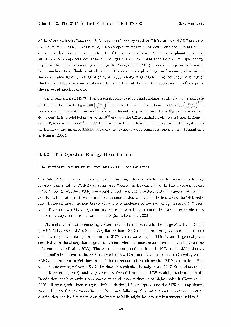
Chapter 3. The 2175 Å Dust Feature in GRB 070802 3.3. Analysis
of the afterglow itself (Panaitescu & Kumar, 2000), as suggested for GRB 060418 and GRB 060607A
(Molinari et al., 2007). In this case, a RS component might be hidden under the dominating FS
emission or have occurred even before the GROND observations. A possible explanation for the
superimposed component occurring at the light curve peak would then be e.g. multiple energy
injections by refreshed shocks (e.g. de Ugarte Postigo et al., 2005) or dense clumps in the circum-
burst medium (e.g. Guidorzi et al., 2005). Flares and rebrightenings are frequently observed in
X-ray afterglow light curves (O'Brien et al., 2006; Zhang et al., 2006). The fact that the length of
the are (∼ 1200 s) is compatible with the start time of the are (∼ 1800 s post burst) supports
the refreshed shock scenario.
Using Sari & Piran (1999), Panaitescu & Kumar (2000), and Molinari et al. (2007), we estimate
Γ0 for the ISM case to Γ0 ≈ 160(E53η0.2n
)1/8
, and for the wind shaped case to Γ0 ≈ 80(
E53η0.2A∗
)1/4
,
both more in line with previous bursts and theoretical predictions. Here E53 is the isotropic-
equivalent energy released in γ-rays in 1053 erg, η0.2 the 0.2 normalized radiative transfer eciency,
n the ISM density in cm−3 and A∗ the normalized wind density. The steep rise of the light curve
with a power-law index of 3.56±0.36 favors the homogeneous circumburst environment (Panaitescu
& Kumar, 2000).
3.3.2 The Spectral Energy Distribution
The Intrinsic Extinction in Previous GRB Host Galaxies
The GRB/SN connection hints strongly at the progenitors of GRBs, which are supposedly very
massive, fast rotating Wolf-Rayet stars (e.g. Woosley & Bloom, 2006). In this collapsar model
(MacFadyen & Woosley, 1999) one would expect long GRBs preferentially in regions with a high
star formation rate (SFR) with signicant amount of dust and gas in the host along the GRB sight
line. However, most previous bursts show only a moderate or low reddening (Galama & Wijers,
2001; Kann et al., 2006, 2008), contrary to the observed high column densities of heavy elements
and strong depletion of refractory elements (Savaglio & Fall, 2004) .
The main feature discriminating between the extinction curves in the Large Magellanic Cloud
(LMC), Milky Way (MW), Small Magellanic Cloud (SMC), and starburst galaxies is the presence
and intensity of an absorption feature at 2175 Å rest-wavelength. This feature is generally as-
sociated with the absorption of graphite grains, whose abundance and sizes changes between the
dierent models (Draine, 2003). The feature is most prominent from the MW to the LMC, whereas
it is practically absent in the SMC (Cardelli et al., 1989) and starburst galaxies (Calzetti, 2001).
SMC and starburst models have a much larger amount of far ultraviolet (FUV) extinction. Pre-
vious bursts strongly favored SMC like dust host galaxies (Schady et al., 2007; Stamatikos et al.,
2007; Kann et al., 2008), and only for a very few of them does a MW model provide a better t.
In addition, the host extinction shows a trend of lower extinction at higher redshift (Kann et al.,
2006). However, with increasing redshift, both the FUV absorption and the 2175 Å bump signi-
cantly decrease the detection eciency for optical follow-up observations, so the present extinction
distribution and its dependence on the bursts redshift might be strongly instrumentally biased.
59

Chapter 3. The 2175 Å Dust Feature in GRB 070802 3.3. Analysis
The SED of the Afterglow of GRB 070802
In the present analysis we used MW-, LMC- and SMC-like extinction models (Seaton, 1979; Fitz-
patrick & Massa, 1986; Fitzpatrick, 1986; Prevot et al., 1984) as templates to t our multi-band
data. All of the GROND optical and NIR data were obtained simultaneously at the time epoch
between 1.5 and 3.6 ks post burst. As the generic shape of the early light curve is achromatic, we
can exclude large eects from an evolving spectrum. The data were t by a power law and extinc-
tion templates from the LMC, SMC, and MW in hyperZ (Bolzonella et al., 2000). The amount of
dust, power-law slope and normalization were free parameters in the t. The redshift was xed to
the spectroscopic redshift of 2.45 obtained by the VLT (Prochaska et al., 2007).
The GROND SED is shown in Fig. 3.3 and was well t by the LMC (reduced χ2 = 0.67 for 4
d.o.f) and the MW (reduced χ2 = 1.96 for 4 d.o.f.) extinction models, while the t was considerably
worse for SMC-like extinction (reduced χ2 = 4.57 for 4 d.o.f.). The large χ2 dierence between
LMC and MWmodels is mostly due to the g′ band magnitude, where the error in the GROND data
is relatively large. The dust extinction in the GRB host in the best t model is AhostV = 0.9±0.3 mag
for MW and AhostV = 1.8 ± 0.3 mag for LMC models. We caution that these values are derived
using local extinction curves for a galaxy at a redshift of 2.45. The extinction curve and thus the
amount of dust reddening could be signicantly dierent. In addition, intervening absorbers could
contribute to the observed dust extinction, which is only resolved by the spectrum (Fynbo et al.,
2007).
We detect a strong absorption feature in the GROND i′ band. GROND i′ is slightly narrower
than the SDSS i′ band and is located at 7630±537 Å. The 2175 Å bump at redshift 2.45 (i.e. at
∼ 7500 Å in the observers frame) provides the ideal and obvious candidate for this broad absorption
feature. The 2175 Å bump is the dominating spectral signature of dust in the interstellar medium
(ISM) in the Milky Way and is often attributed to small graphite grains processed by star formation
(Gordon et al., 1997; Draine, 2003; Duley & Lazarev, 2004). However, the nature of the bump is
not totally clear. Its strength varies along dierent sight lines in the Milky Way (Cardelli et al.,
1989). Dierent size distributions or dierent chemical compositions could be the origin of this
variation (Natta & Panagia, 1984).
At high redshift, the search for the 2175 Å feature has always been very dicult. It was never
clearly detected in single objects, for instance, in damped Ly-α systems (DLAs) along quasar
(QSO) sight lines. The presence of the bump was excluded from a composite spectrum of 37 Ca II
and Mg II absorbers from Sloan Digital Sky Survey (SDSS) QSOs (Wild et al., 2006), but detected
in a combined spectrum of 18 galaxies at 1 ≤ z ≤ 1.5 with intermediate-age stellar populations
(Noll et al., 2007). Further detections outside the Local Group have been suggested e.g. for
GRB 050802 (Schady et al., 2007) at z = 1.71 (Fynbo et al., 2005) and a galaxy at z = 0.83 (Motta
et al., 2002). Despite the presence of strong metal absorption (Savaglio & Fall, 2004; Berger et al.,
2006; Fynbo et al., 2006) and the depletion of refractory elements (Savaglio, 2006) it has not been
detected in spectra of previous bursts. The afterglow of GRB 070802 shows the clearest presence
of the 2175 Å dust feature at a high redshift so far, where it is detected with GROND broad-band
photometry and VLT spectroscopy as shown in Fig. 5 in Fynbo et al. (2007) and Eliasdottir et al.
(in preparation).
60

Chapter 3. The 2175 Å Dust Feature in GRB 070802 3.3. Analysis
Figure 3.3 Spectral Energy Distribution of the afterglow of GRB 070802 in the GROND lterbands. The data were obtained simultaneously in all colors between T0 + 1.5 ks and T0 + 3.6 kspost burst. The shape of the SED can be well reproduced by LMC and MW extinction models. Abroad extinction feature is detected in the GROND i′ band at 7630 Å central wavelength, whichwe relate to the 2175 Å dust feature in the host at redshift 2.45. Depending on the used model,the best t extinction varies between Ahost
V = 0.9 mag (MW) and 1.8 mag (LMC).
61

Chapter 3. The 2175 Å Dust Feature in GRB 070802 3.3. Analysis
We can estimate the column density of dierent metals along the sight line for GRB 070802,
following the approach described in Savaglio (2006). The AhostV is directly proportional to the
dust column density. The dust column density is also proportional to the total metal column
density. For instance, in a galaxy with MW- or LMC-like visual extinction, AhostV = 0.5 mag
or 0.4 mag is expected for a column density of oxygen of log(NO) = 17.7 or 17.1, respectively.
Assuming a constant dust-to-metals ratio, our AhostV = 0.9 mag for MW or 1.8 mag for LMC gives
log(NO) = 18.0 and 17.8. This is the oxygen column density in gas form, i.e. assuming that the
amount of oxygen locked into dust grains is marginal. In the Galactic ISM, oxygen in dust grains
is negligible, but is up to about 40% in the cool gas (Savage & Sembach, 1996). If we assume this
kind of dust depletion, then the total oxygen column density is log(NO) = 18.4 or 18.2, for MW
or LMC, respectively. Using the standard nomenclature for hydrogen absorption at X-ray energies
and assuming solar metallicity, we conclude that the column density of hydrogen log(NH) is about
21.7 or 21.5, for MW or LMC dust, respectively.
Combined Optical/NIR and X-ray Analysis
The XRT spectrum including all data from 150 s to 405 ks post burst with a total exposure time
of 56 ks is compatible with an absorbed power law with a photon index Γ = 2.1 ± 0.3 (reduced
χ2 = 0.7 for 15 d.o.f.). The foreground hydrogen column density was frozen at the Galactic value of
3×1020 cm−2 (Dickey & Lockman, 1990). The best t for NH at z = 2.45 is 1.60+1.20−1.10×1022 cm−2,
which corresponds to a total gas plus dust oxygen column density of NO = 7.2+5.4−5.0 × 1018 cm−2.
Given the large uncertainties, this is consistent with the values estimated in the previous section.
The GROND optical/NIR and XRT X-ray data can be t together to constrain the broadband
afterglow spectrum. We t the data using a power law with absorption in the X-ray regime and
extinction in the optical/NIR regime using the XSPEC package (Arnaud, 1996). Unfortunately,
there is no simultaneous early coverage by XRT and GROND, as there is a gap in the XRT coverage
of GRB070802 from 911 s to 4.2 ks (Fig. 3.2). Therefore XRT data from 460 s to 5 ks with a total
exposure time of 1.3 ks and GROND data from 1.5 to 3.6 ks after trigger were selected for the joint
t. These intervals were chosen because they are the closest in time while the source is still bright
and do not include the steep decay in the early XRT light curve, see Fig. 3.2 and Immler et al.
(2007).
The XRT spectrum alone from 460 s to 5 ks post burst is compatible with the total spectrum
with a power-law photon index of 1.9±0.4, although NH is no longer well constrained due to poorer
statistics.
The combined GROND and XRT SED from 2.2 µm KS to ∼4 keV was t by a single power law
with reddening EB−V and NH Galactic foreground values from Schlegel et al. (1998) and Dickey &
Lockman (1990) (0.026 and 3× 1020 cm−2, respectively) and by extinction in the host at z = 2.45.
There were insucient statistics above 4 keV in the XRT band to extend the t to higher energies.
The optical/NIR data were modelled using the zdust XSPEC model, where the extinction in the
host is obtained using MW, LMC and SMC reddening laws with values of RV of 3.08, 3.18 and
2.93 respectively, where AV = EB−V × RV (Pei, 1992). As shown in Fig. 3.3, the GROND data
62

Chapter 3. The 2175 Å Dust Feature in GRB 070802 3.4. Conclusions
alone is well described by MW and LMC models. The additional absorption in the soft X-ray band
was modelled by an absorbing column at z = 2.45.
In the broadband ts we are mainly interested in the power-law index between the GROND
and XRT bands. The combined optical/NIR and X-ray data are well described by a single power
law with a photon index of 1.91± 0.04 (reduced χ2 of 1.36 for 12 d.o.f.) using the MW extinction
model with EB−V of 0.35 ± 0.04. The NH at z = 2.45 is not well constrained by the t. Similar
values of the power-law index and EB−V are achieved using the LMC and SMC extinction curves.
The results of the zdust and single power-law models are presented in Table 3.4 with the MW
yielding the best t.
To test for a cooling break, a broken power law with extinction and soft X-ray absorption was
also t to the data. Here the high energy photon index Γ2 was linked to Γ1 via Γ2 = Γ1 + 0.5
as expected in the reball model. The value of the break energy was constrained to lie between
the optical and X-ray bands and the best t photon indices for the low and high energies were
Γ1 = 1.61± 0.05 and Γ2 = 2.11 respectively. The reduced χ2 for this t is 1.47 for 11 d.o.f for the
MW extinction curve, 2.40 for 11 d.o.f for LMC and 3.5 for 11 d.o.f for SMC. The t parameters
EB−V and the low energy power-law index are presented in Table 3.4.
The broadband model without a break provides a better t to the data, however the dierence
in the reduced χ2 parameters of the ts is not conclusive. The single power law implies that the
cooling break is redwards the GROND bands at this time, which would be surprisingly early after
the explosion. We caution that the GROND and XRT data are not simultaneous.
We also t a late time SED using the XRT data 50 to 196 ks post burst with the GROND
data obtained in the JHKS band from 86 to 96 ks. The best t model has a power-law slope of
2.0± 0.2, so the data are still compatible with the early time single power-law model, but we are
not able to distinguish between a single and broken power-law t. We do not nd evidence for a
cooling break between the NIR and X-ray data.
3.4 Conclusions
The optical/NIR afterglow light curve of GRB 070802 can be explained using two models: a
combined reverse - forward shock model, and a single forward shock model with a superimposed
emission component at peak brightness. Due to the fact that the afterglow peak is heavily delayed
compared to the duration of the burst, it is very likely that the increase in brightness in the early
light curve is related to the onset of the afterglow as proposed for GRB 060418 and GRB 060607A
(Molinari et al., 2007). Using an analogue analysis for GRB 070802, we derive an initial bulk
Lorentz factor in the jet of around Γ0 ≈ 160(E53η0.2n
)1/8
for an ISM environment. The steep rise
of the early light curve favors an homogeneous over a wind-shaped circumburst medium. The
ground-based observations of the optical/NIR afterglow of GRB 070802 were fast enough to detect
an early brightening of the afterglow. Further rapid follow-up campaigns may establish whether
this rapid rise is a generic feature of GRB afterglow light curves.
63

Chapter 3. The 2175 Å Dust Feature in GRB 070802 3.4. Conclusions
Table 3.1. Secondary standards in the GRB eld in the GROND lter bands used during thecalibration
Identier g′ r′ i′ z′ J H KSmag mag mag mag mag mag mag
A 22.42 ± 0.05 20.71 ± 0.04 19.26 ± 0.04 18.50 ± 0.04 16.98 ± 0.06 16.55 ± 0.06 16.09 ± 0.08B 16.33 ± 0.07 15.89 ± 0.03 15.78 ± 0.03 15.65 ± 0.03 14.81 ± 0.05 14.59 ± 0.05 14.42 ± 0.06C 15.47 ± 0.05 14.98 ± 0.03 14.86 ± 0.03 14.72 ± 0.03 13.87 ± 0.05 13.61 ± 0.05 13.43 ± 0.06D 20.07 ± 0.06 18.76 ± 0.04 18.23 ± 0.04 17.92 ± 0.04 16.72 ± 0.07 16.19 ± 0.07 15.74 ± 0.09E 15.70 ± 0.05 14.62 ± 0.03 14.17 ± 0.03 13.87 ± 0.03 12.71 ± 0.05 12.61 ± 0.05 11.99 ± 0.06
Table 3.2. Parameters of the generic light curve t to the r′z′JHK band
Model αr1 αr2 αf1 αf2 t1 [s] sf
RS rise index RS decline index FS rise index FS decline index Break sharpness
Combined RS + FS 3.16 ± 0.33 -2.66 ± 0.96 3.12 ± 1.49 -0.63 ± 0.14 2181 ± 107 3.15 ± 2.16Single FS 3.56 ± 0.36 -0.68 ± 0.04 1830 ± 51.9 2.48 ± 0.72
A broadband t of GROND and XRT data is compatible with a single power-law spectrum with
photon index 1.91±0.04, suggesting the cooling break being redwards of the GROND bands at the
start of the observations at ∼1.2 ks post burst. The late-time photon index from NIR to X-rays
is still comparable with the early time power law, indicating no time evolution of the spectrum
during our observations.
The observed SED from g′ to theKS band can be well reproduced with LMC and MW extinction
models. A broadband absorption feature in the GROND i′ band with a central wavelength of
7630 Å is unquestionably required to explain the observed SED. The redshifted 2175 Å feature in
the host galaxy of the burst at z = 2.45 known from MW and LMC extinction models provides
the ideal candidate. Depending on the model the best t extinction ranges from AhostV = 0.9 mag
for MW-like dust absorption to AhostV = 1.8 mag for LMC dust. The amount of extinction is
signicantly larger than estimated for previous bursts (Kann et al., 2006; Schady et al., 2007; Kann
et al., 2008). Pre-Swift bursts have shown a correlation of decreasing extinction with increasing
redshift (Kann et al., 2008). However, there might be a strong instrumental bias, as fast and
simultaneous optical-to-NIR follow-up observations for a large GRB sample are missing. The
GROND instrument, with its unique optical and NIR capabilities, is a powerful tool which might
remove this bias. GRB 070802 was the rst burst for GROND occurring during nighttime and
revealed signicant amount of dust in its host galaxy, indicating that at least a good fraction of
the UVOT dark burst is due to intrinsic extinction in the GRB host galaxy. Future observations
will help to quantify the amount of highly extinguished bursts and may help to solve the mystery
of dark bursts.
64

Chapter 3. The 2175 Å Dust Feature in GRB 070802 3.4. Conclusions
Table 3.3. Parameters of the individual ts to the r′z′JHK bands.
Model Parameter r′ z′ J H KS
Combined RS + FS F 0r [µJ] 14.7 ± 0.7 30.9 ± 1.6 102 ± 2.5 163 ± 3.1 365 ± 11.0
Combined RS + FS F 0f [µJ] 4.3 ± 0.7 9.7 ± 1.0 33.1 ± 1.6 46.5 ± 2.1 135 ± 10.9
Combined RS + FS reduced χ2/d.o.f. 0.64/5 0.98/7 1.80/18 1.10/15 1.53/18
Single FS F 0f [µJ] 10.2 ± 0.6 21.8 ± 0.9 70.6 ± 1.0 104 ± 2.0 278 ± 7.6
Single FS reduced χ2/d.o.f. 0.62/3 0.66/5 0.98/7 0.67/7 0.80/7
Table 3.4. Broad band spectral ts to the GROND and XRT data using XSPEC.
Extinction Model Power law E(B-V) Photon Index χ2/d.o.f
MW Single 0.35±0.04 1.91±0.04 1.36/12MW Broken 0.41±0.04 1.61±0.05 1.47/11LMC Single 0.35±0.04 1.92±0.03 2.13/12LMC Broken 0.39±0.04 1.61±0.05 2.40/11
SMC Single 0.34+0.04−0.03 1.90+0.03
−0.04 3.2/12
SMC Broken 0.34+0.04−0.02 1.61±0.03 3.5/11
65

Chapter 3. The 2175 Å Dust Feature in GRB 070802 3.4. Conclusions
66

Chapter 4
Correlated Optical and X-ray Flares
in the Afterglow of XRF 071031 1
ABSTRACT
We present a densely sampled early light curve of the optical/near-infrared (NIR) afterglow
of the X-ray Flash (XRF) 071031 at z = 2.692. Simultaneous and continuous observations in
seven photometric bands from g′ to KS with GROND at the 2.2 m MPI/ESO telescope on LaSilla
were performed between 4 minutes and 7 hours after the burst. The light curve consists of 547
individual points which allows us to study the early evolution of the optical transient associated
with XRF 071031 in great detail. The optical/NIR light curve is dominated by an early increase in
brightness which can be attributed to the apparent onset of the forward shock emission. There are
several bumps which are superimposed onto the overall rise and decay. Signicant aring is also
visible in the Swift X-Ray Telescope (XRT) light curve from early to late times. The availability
of high-quality, broadband data enables detailed studies of the connection between the X-ray and
optical/NIR afterglow and its color evolution during the rst night post burst. We nd evidence of
spectral hardening in the optical bands contemporaneous with the emergence of the bumps from
an underlying afterglow component. The bumps in the optical/NIR light curve can be associated
with ares in the X-ray regime suggesting late central engine activity as the common origin.
4.1 Introduction
Major progress in the understanding of the X-ray and optical afterglow light curves of Gamma-ray
Bursts (GRBs) and the softer X-ray Flashes (XRFs) has been made since the launch of the Swift
satellite (Gehrels et al., 2004) and the rapid follow-up data provided by the X-Ray Telescope (XRT,
Burrows et al., 2005b) and Ultra-Violet Optical Telescope (UVOT, Roming et al., 2005). However,
access to the longer wavelength afterglow is still somewhat limited to the brighter half of all detected1T. Krühler, J. Greiner, S. McBreen, S. Klose, A. Rossi, P. Afonso, C. Clemens, R. Filgas, A. Küpcü Yolda³, G.
P. Szokoly and A. Yolda³ (2009), Astrophysical Journal, 697, 758
67
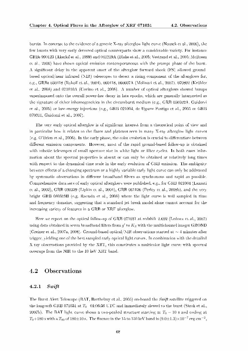
Chapter 4. Optical Flares in the Afterglow of XRF 071031 4.2. Observations
bursts. In contrast to the evidence of a generic X-ray afterglow light curve (Nousek et al., 2006), the
few bursts with very early detected optical counterparts show a considerable variety. For instance
GRBs 990123 (Akerlof et al., 1999) and 041219A (Blake et al., 2005; Vestrand et al., 2005; McBreen
et al., 2006) have shown optical emission contemporaneous with the prompt phase of the burst.
A signicant delay in the apparent onset of the afterglow forward shock (FS) allowed ground-
based optical/near infrared (NIR) telescopes to detect a rising component of the afterglows for,
e.g., GRBs 030418 (Ryko et al., 2004), 060418, 060607A (Molinari et al., 2007), 070802 (Krühler
et al., 2008) and 071010A (Covino et al., 2008). A number of optical afterglows showed bumps
superimposed onto the overall power-law decay in late epochs, which are generally interpreted as
the signature of either inhomogeneities in the circumburst medium (e.g., GRB 050502A, Guidorzi
et al., 2005) or late energy injections (e.g., GRB 021004, de Ugarte Postigo et al., 2005 or GRB
070311, Guidorzi et al., 2007).
The very early optical afterglow is of signicant interest from a theoretical point of view and
in particular how it relates to the ares and plateaus seen in many X-ray afterglow light curves
(e.g. O'Brien et al., 2006). In the early phase, the color evolution is crucial to dierentiate between
dierent emission components. However, most of the rapid ground-based follow-up is obtained
with robotic telescopes of small aperture size in white light or lter cycles. In both cases infor-
mation about the spectral properties is absent or can only be obtained at relatively long times
with respect to the dynamical time scale in the early evolution of GRB emission. The ambiguity
between eects of a changing spectrum or a highly variable early light curve can only be addressed
by systematic observations in dierent broadband lters as synchronous and rapid as possible.
Comprehensive data sets of early optical afterglows were published, e.g., for GRB 021004 (Lazzati
et al., 2002), GRB 030329 (Lipkin et al., 2004), GRB 061126 (Perley et al., 2008b), and the very
bright GRB 080319B (e.g. Racusin et al., 2008) where the light curve is well sampled in time
and frequency domains, suggesting that a standard jet break model alone cannot account for the
increasing variety of features in a GRB or XRF afterglow.
Here we report on the optical follow-up of GRB 071031 at redshift 2.692 (Ledoux et al., 2007)
using data obtained in seven broadband lters from g′ toKS with the multichannel imager GROND
(Greiner et al., 2007a, 2008). Ground-based optical/NIR observations started at ∼ 4 minutes after
trigger, yielding one of the best sampled early optical light curves. In combination with the detailed
X-ray observations provided by the XRT, this constitutes a multicolor light curve with spectral
coverage from the NIR to the 10 keV XRT band.
4.2 Observations
4.2.1 Swift
The Burst Alert Telescope (BAT, Barthelmy et al., 2005) on-board the Swift satellite triggered on
the long-soft GRB 071031 at T0=01:06:36 UTC and immediately slewed to the burst (Stroh et al.,
2007b). The BAT light curve shows a two-peaked structure starting at T0 − 10 s and ending at
T0+180 s with a T90 of 180±10 s. The uence in the 15 to 150 keV band is (9.0±1.3)×10−7 erg cm−2,
68

Chapter 4. Optical Flares in the Afterglow of XRF 071031 4.2. Observations
Figure 4.1 Swift XRT light curve of the X-ray afterglow of XRF 071031 obtained from the XRTlight curve repository (Evans et al., 2007)
with a uence ratio of 1.34 between the BAT 25-50 and 50-100 keV bands (Stamatikos et al., 2007).
This is remarkably soft compared to conventional GRBs and qualies GRB 071031 as an XRF
according to the working denition of Sakamoto et al. (2008). The BAT spectrum of the rst peak
is well described with a single power law with a photon index of 2.26 ± 0.30 (χ2 = 28.83 for 36
degrees of freedom (d.o.f.)). This is well outside the normal range for the low energy index α but
similar to the spectral index β above the break energy for a Band function (Band et al., 1993;
Preece et al., 2000). The peak energy of the prompt emission spectrum must then be close to or
below the BAT lower energy range of around 30 keV (see also McGlynn et al., 2005; Stamatikos
et al., 2007). Therefore, GRB 071031 is designated as XRF 071031 hereafter.
The XRT began follow-up observations of the burst eld 103 s after the trigger and detected
an uncatalogued fading X-ray source at a position of R.A.(J2000)=00h 25m 37s.4, decl.(J2000)=-
58 03′ 33′′ with a rened 90% condence error circle of 2.′′0 radius (Stroh et al., 2007a). The
early XRT light curve is dominated by signicant amount of aring with bright ares at around
120, 150, 200, 250 and 450 s. Also the late X-ray data exhibit rebrightenings at 5.5, 20 and 55
ks superimposed onto the overall power-law decay. The complete XRT light curve is shown in
Fig. 4.1.
The X-ray spectra were obtained with the xrtpipeline tool using the latest calibration frames
from the Swift CALDB and standard parameters. The spectra were tted with the XSPEC package
(Arnaud, 1996) and a foreground hydrogen column density at the Galactic value of NH = 1.2 ×1020 cm−2 (Kalberla et al., 2005).
69

Chapter 4. Optical Flares in the Afterglow of XRF 071031 4.2. Observations
The third instrument on-board Swift, UVOT started observations at T0 + 114 s and found a
transient source inside the XRT error circle in the white, v- and b-band lters. The UVOT data
show an increase in the brightness of the afterglow of around 0.5 mag in the rst few hundred
seconds (Breeveld & Stroh, 2007).
4.2.2 GROND
GROND responded to the Swift GRB alert and initiated automated observations that started at
01:10:21 UTC, 3 minutes 45 s after the burst and continued until local Sunrise at 08:55:51 UTC. A
predened sequence of observations with successively increasing exposure times was executed and
images were acquired in all seven photometric bands simultaneously. In total 84 individual frames
in each g′r′i′z′ and 1510 images of 10 s exposures in JHKS were obtained during the rst night
at airmasses between 1.1 and 2.4. The integration time of the CCD optical images scaled from 45
to 360 s according to the brightness of the optical afterglow. A variable point source was detected
in all bands (Krühler et al., 2007) by the automated GROND pipeline (Küpcü-Yolda³ et al., 2008)
and its absolute position is measured to R.A.(J2000)=00h 25m 37s.24, decl.(J2000)=58 03′ 33.′′6
compared to USNO-B reference eld stars (Monet et al., 2003) with an astrometric uncertainty
of 0.′′3. Photometry and spectroscopy of the afterglow was also obtained by telescopes at Cerro
Tololo Inter-American Observatory (CTIO Haislip et al., 2007; Cobb, 2007) and the Very Large
Telescope (VLT), the latter yielding an UVES and FORS spectroscopic redshift of 2.692 (Ledoux
et al., 2007; Fox et al., 2008).
Photometric calibration was performed relative to the magnitudes of 10 secondary standards
in the eld of XRF 071031, shown in Fig. 4.2 and Tab. 4.1. During photometric conditions,
three spectrophotometric standard stars, SA114-750, SA114-656, and SA95-42, all primary Sloan
standards (Smith et al., 2002), were observed with GROND. Observations of the GRB eld followed
within a few minutes. The magnitudes of the Sloan standards were transformed to the GROND
lter system using their spectra and the GROND lter curves (Greiner et al., 2008). The obtained
zeropoints were corrected for atmospheric extinction dierences and used to calibrate the stars
in the GRB eld. An independent absolute calibration was obtained with respect to magnitudes
of the SDSS and 2MASS stars within the standard elds obtained from the SDSS data release
6 (Adelman-McCarthy et al., 2008) and the 2MASS catalog (Skrutskie et al., 2006) with results
consistent with the standard star calibration at the 0.03 mag level.
Optical and NIR image reduction and photometry were performed using standard IRAF tasks
(Tody, 1993). For each frame a model of the point spread function (PSF) was constructed us-
ing brighter eld stars, and tted to the afterglow. The relatively large seeing between 2′′ and
3′′ together with the pixel scale of 0.′′16 for g′r′i′z′ and 0.′′60 for JHKS resulted in an excellent
spatial sampling of the PSF with statistical t errors of the order of 0.2 % for g′r′i′z′ and 0.5 % for
JHKS . For consistency, we also performed standard aperture photometry with compatible results
with respect to the reported PSF photometry. All data were corrected for a Galactic foreground
reddening of EB−V = 0.012 mag in the direction of the burst (Schlegel et al., 1998).
The stacking of individual images was done twice for dierent purposes. First, all available
70

Chapter 4. Optical Flares in the Afterglow of XRF 071031 4.2. Observations
Figure 4.2 GROND r′ band image showing the afterglow of XRF 071031 and the XRT error circle.The secondary standards used for calibration are labeled 1 to 10 and listed in Tab .4.1. The lowerleft corner shows a zoom in to the afterglow position.
71
Chapter 4. Optical Flares in the Afterglow of XRF 071031 4.3. Analysis
data were used and individual frames were stacked until a statistical error in the PSF t of around
0.1 mag was obtained. This resulted in 75 frames in each g′r′i′ , 51 in z′, 118 in J , and 76 in
each H and KS , yielding the multiwavelength light curve shown in Fig. 4.3. Second, only NIR
data simultaneous to the optical integrations were selected, excluding the frames which were taken
during the g′r′i′z′ CCD read out. The resulting NIR image stacks were used to derive the optical
to NIR spectral energy distribution (SED).
4.3 Analysis
4.3.1 The Optical/NIR Light Curve
The multicolor light curve of XRF 071031 is complex and not described by smoothly connected
power laws alone (Fig. 4.3). Evident in all colors is the initial increase in brightness up to ∼ 1 ks,
which smoothly turns over to a generic power-law decline with superimposed variations. In order
to study small-scale irregularities at the highest possible signal-to-noise, a white-light curve was
derived by combining all g′r′i′z′ CCD data (Fig. 4.4, upper panel), which are exactly synchronous
by hardware setup. The NIR bands are excluded from this process due to the intrinsically larger
photometric error which would serve only to increase the uncertainties in the summed data.
In order to better visualize the afterglow light curve, it is also presented dierentiated in its
native log− log scale, i.e. δ(log(Fν))/δ(log(t)), which directly represents the local power-law decay
index α(t) (Fig. 4.4, lower panel). On a log− log scale, the rst derivative of a power law is
a constant, so for a smoothly connected power-law rise and decay, one would expect a positive
constant at early, turning into a negative at later times. Changes in the power-law index and
deviations from the decay are clearly visible in this representation.
Without imposing an a priori model of the afterglow, Fig. 4.4 convincingly demonstrates that
the overall trend of the light curve is well described by two smoothly connected power laws as
introduced in Beuermann et al. (1999). In both panels of Fig. 4.4, however, the deviations from
a Beuermann-like power-law rise and decay are clearly apparent. There are two features, which
require either a superimposed component or a dierent parameterization of the intrinsic afterglow.
The rst and most obvious is the additional emission component in regions A,B,C,D shown in
the upper panel of Fig. 4.4. This extra emission requires features intrinsic to the source or its
environment to produce the observed ux excess with respect to the power law. The second is the
steepening of the power-law decline after a rebrightening from region I over II to III in the lower
panel of Fig. 4.4. However, there is so much variability within the light curve that the underlying
afterglow cannot be established with high certainty.
The early rising component in the optical bands might be related to the deceleration of the FS
by the circumburst medium, which happens when the swept up medium eciently decelerate the
ejecta. From the time of the light curve peak, the initial bulk Lorentz factor of the outow Γ0 can
be constrained. Using the formalism outlined by Sari & Piran (1999), Panaitescu & Kumar (2000),
and Molinari et al. (2007), Γ0 is estimated to ≈ 90(
E53η0.2A∗
)1/4
in a wind shaped circumburst
72
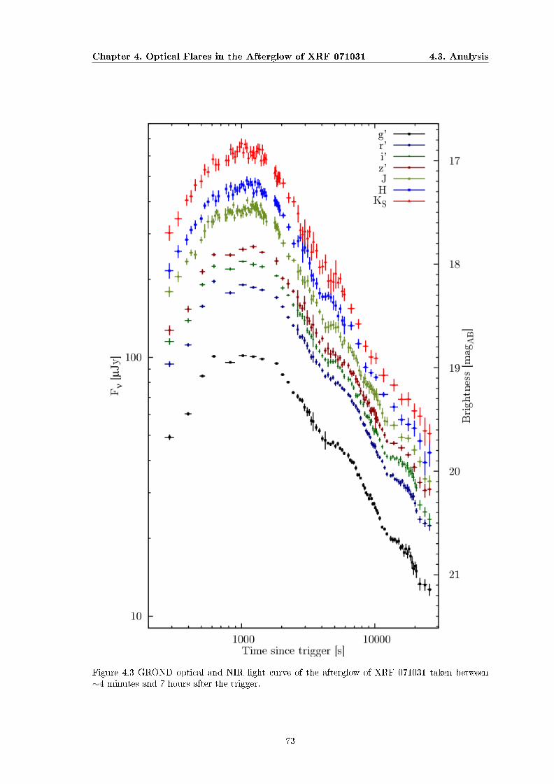
Chapter 4. Optical Flares in the Afterglow of XRF 071031 4.3. Analysis
Figure 4.3 GROND optical and NIR light curve of the afterglow of XRF 071031 taken between∼4 minutes and 7 hours after the trigger.
73
Chapter 4. Optical Flares in the Afterglow of XRF 071031 4.3. Analysis
medium and to ≈ 200(E53η0.2n
)1/8
for an ISM type environment, with a weak dependence on the
uncertain parameters A∗ being the normalized wind density, E53 the isotropic-equivalent energy
released in γ-rays in 1053 erg, η0.2 the radiative transfer eciency normalized to 0.2 and n the ISM
density in cm−3. The slow rise with a power law index of ∼0.7 suggests a wind like environment,
which would only be consistent with the closure relations for a very hard electron index (Dai &
Cheng, 2001) of p ∼1.6 and νc < ν using the spectral and temporal slopes in the late afterglow
light curve αX,o ∼ 1 and βX = 0.8 ± 0.1. The classical closure relations (e.g. Zhang & Mészáros,
2004), however, would favor an ISM environment in the slow cooling case with νm < ν < νc and a
more canonical value of p ∼ 2.6.
Alternatively, the initial rise could be the result of a structured outow seen o-axis (e.g.
Panaitescu et al., 1998). In the case of previous fast and slowly rising afterglow light curves,
Panaitescu & Vestrand (2008) nd an anticorrelation of peak ux in the R band Fν,R and peak time
tp. K-correcting the afterglow to z = 2 to match the previous sample, we nd that the optical/NIR
light curve of XRF 071031 ts very well into this anticorrelation. In this interpretation, the slow
rise would hint on a smooth angular structure of the outow (Panaitescu & Vestrand, 2008).
Chromaticity around peak brightness was tested by comparing the optical/NIR SED before
and after the total maximum. Apart from changes in the spectral index which can be attributed
to the emergence of the bumps (see Sec. 4.3.4 and Fig. 4.7), there is no evidence for a change in
the spectrum before and after the light curve peak. The time of the light curve maximum is not
correlated with energy and all bands peak at a similar time within the measurement uncertainties.
Such evolution would be expected if the main peak was caused by cooling of the ejecta after
the prompt emission resulting in the shift of the characteristic synchrotron frequency νm into the
optical bands (e.g. Ziaeepour et al., 2008). In addition, a moving νm through the optical bands is
expected to cause a strong change from a positive to negative spectral index (e.g. Sari et al., 1998;
Granot & Sari, 2002b). Neither eect is observed.
After correcting for Galactic foreground extinction, the SED from g′ to KS was t with a power
law and dust reddening templates in the host at z=2.692. Using extinction templates from the
Milky Way (MW), Large (LMC) and Small Magellanic Cloud (SMC) and supernovae-induced dust
(Pei, 1992; Maiolino et al., 2004; Stratta et al., 2007) no signatures of dust extinction in the GRB
host are evident down to 1σ condence limits of AhostV < 0.06 mag (MW), Ahost
V < 0.07 mag (LMC),
AhostV < 0.05 mag (SMC and SNe induced). Therefore, the eect of dust reddening is considered as
negligible in the following analysis. The deviation from a power-law SED in the GROND g′ band
is consistent with Lyman-α absorption in the GRB host at z = 2.692.
4.3.2 The X-ray Afterglow Light Curve
In addition to the variable and densely sampled light curve in the GROND lter bands, the X-
ray afterglow is bright and well covered by XRT observations. Similar to what is seen in the
optical bands, the X-ray data show strong variability, and the underlying afterglow is poorly
constrained. After excluding the very early data, where there are no GROND observations (t−T0 <
300 s), we tted the remaining data using a similar procedure as used for the optical bands with a
74
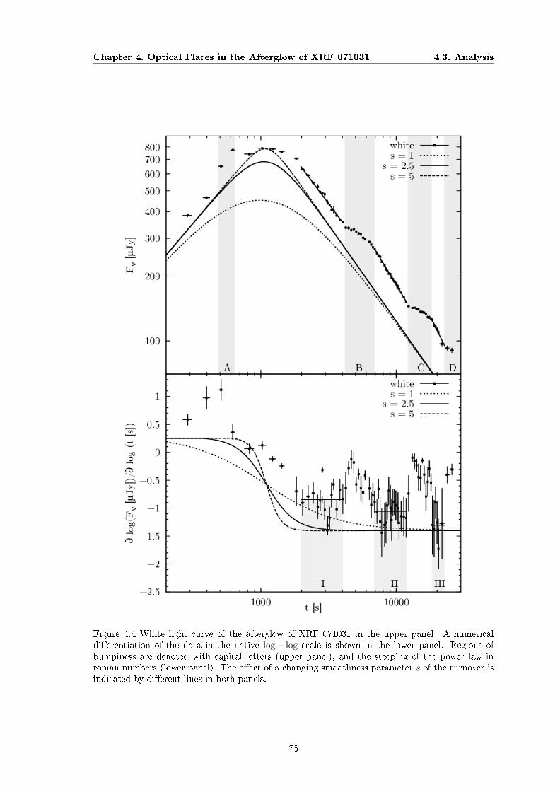
Chapter 4. Optical Flares in the Afterglow of XRF 071031 4.3. Analysis
Figure 4.4 White light curve of the afterglow of XRF 071031 in the upper panel. A numericaldierentiation of the data in the native log− log scale is shown in the lower panel. Regions ofbumpiness are denoted with capital letters (upper panel), and the steeping of the power law inroman numbers (lower panel). The eect of a changing smoothness parameter s of the turnover isindicated by dierent lines in both panels.
75

Chapter 4. Optical Flares in the Afterglow of XRF 071031 4.3. Analysis
combination of a smoothly connected power laws. Remarkably, the obtained late power-law index
αX = 0.99±0.12 is compatible with the best t from the GROND data αo = 0.97±0.06, providing
additional evidence that the applied model tting traces the underlying power-law decay of the
afterglow reasonably well. The XRT light curve and the residuals to the power-law ts are shown
in Fig. 4.5. After aring episodes, the XRT light curve drops back to the power law, consistent
with the rebrightenings observed in previous GRBs or XRFs (e.g. Burrows et al., 2005a; Romano
et al., 2006b). All XRT light curve data have been obtained from the Swift XRT light curve online
repository (Evans et al., 2007).
4.3.3 The Bumps
Both X-ray and optical/NIR data show signicant variations from the typical power-law proles at
very early times. While this is observed in nearly 50% of all X-ray afterglows (e.g. Nousek et al.,
2006), this is rarely seen so early in an optical light curve starting ∼400 s after the trigger.
We tted the combined white light data with a canonical afterglow rise and decay with super-
imposed Gaussian proles to account for the variations in the light curve. While this may not be
the true physical model, it provides a good t to the data, and represents the morphology of the
bumps with adequate accuracy. For the very early optical data, where the time sampling of the
light curve is naturally sparse, we used a cubic spline interpolation with equally spaced nodes in
the native log− log scale of the afterglow to constrain the t. The data suggest the existence of
three major and three small bumps: The three brighter ones, π1 to π3, which peak at 0.6, 6 and
18 ks, and three fainter ones, ξ1 to ξ3, all shown in the lower panel of Fig. 4.6. The rst faint bump
is only indicated by one data point and the last peak is not sampled by the observations due to the
break of dawn. The t shown in Fig. 4.6 has a χ2red = 1.05 with 52 d.o.f.. The best t parameters
are presented in Tab. 4.2.
The typical time scale of variation for the optical bumps is 〈∆T/T 〉 = 0.35± 0.13, where ∆T is
calculated as the full width half maximum of the Gaussian, and have a relative ux increase with
respect to the underlying afterglow of 〈∆F/F 〉 = 0.29 ± 0.18. All bumps, which are reasonably
sampled by our observations, have a change in the slope δα between 0.5 and 0.9, which can be
directly deduced from the lower panel of Fig. 4.4.
Due to the faintness of the source, the late X-ray afterglow light curve is not equally well
sampled as the optical and a detailed analysis is not possible in late epochs. There is, however,
evidence for three X-ray ares φ1 to φ3 between 350 and 25000 s with synchronous optical coverage.
To derive the morphology of the ares in the XRT light curve, we use a similar approach as for
the optical bands for a direct comparison: an underlying continuum tted with power laws and
superimposed Gaussians to account for the evident ux excess which yields a reduced χ2red of 1.15
for 154 degrees of freedom. The best t is shown in Fig. 4.5 and the corresponding parameters are
reported in Tab. 4.3.
The X-ray ares are much stronger 〈∆F/F 〉 = 1.28 ± 0.28 with respect to the underlying
afterglow than the optical bumps. Comparing against a statistical sample of previous X-ray ares
(Chincarini et al., 2007) shows that the ares observed in XRF 071031 populate a similar phase-
76

Chapter 4. Optical Flares in the Afterglow of XRF 071031 4.3. Analysis
Figure 4.5 XRT light curve of the afterglow of XRF 071031 in the time domain simultaneous tothe GROND data (top panel). The middle panel shows the residuals to the smoothly connectedpower-law t, as well as their modeling using Gaussians. The residuals of the rst are have beenscaled by 1/500. The bottom panel shows the hardness ratio of the 1.5-10 vs. 0.3-1.5 keV band.
77

Chapter 4. Optical Flares in the Afterglow of XRF 071031 4.3. Analysis
Figure 4.6 White light curve of the afterglow of XRF 071031 (upper panel, shown are the data andthe cubic spline interpolation with equally spaced nodes in log(t)). The data were tted using thesum of a smoothly connected power law for the canonical afterglow (dashed line) and Gaussianproles to account for the evident ux excess (solid line). The lower panel shows the residuals tothe smoothly connected power law, as well their modeling by six Gaussians.
78
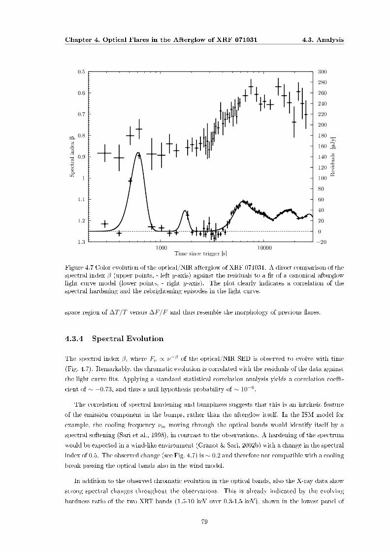
Chapter 4. Optical Flares in the Afterglow of XRF 071031 4.3. Analysis
Figure 4.7 Color evolution of the optical/NIR afterglow of XRF 071031. A direct comparison of thespectral index β (upper points, - left y-axis) against the residuals to a t of a canonical afterglowlight curve model (lower points, - right y-axis). The plot clearly indicates a correlation of thespectral hardening and the rebrightening episodes in the light curve.
space region of ∆T/T versus ∆F/F and thus resemble the morphology of previous ares.
4.3.4 Spectral Evolution
The spectral index β, where Fν ∝ ν−β of the optical/NIR SED is observed to evolve with time
(Fig. 4.7). Remarkably, the chromatic evolution is correlated with the residuals of the data against
the light curve ts. Applying a standard statistical correlation analysis yields a correlation coe-
cient of ∼ −0.73, and thus a null hypothesis probability of ∼ 10−6.
The correlation of spectral hardening and bumpiness suggests that this is an intrinsic feature
of the emission component in the bumps, rather than the afterglow itself. In the ISM model for
example, the cooling frequency νm moving through the optical bands would identify itself by a
spectral softening (Sari et al., 1998), in contrast to the observations. A hardening of the spectrum
would be expected in a wind-like environment (Granot & Sari, 2002b) with a change in the spectral
index of 0.5. The observed change (see Fig. 4.7) is ∼ 0.2 and therefore not compatible with a cooling
break passing the optical bands also in the wind model.
In addition to the observed chromatic evolution in the optical bands, also the X-ray data show
strong spectral changes throughout the observations. This is already indicated by the evolving
hardness ratio of the two XRT bands (1.5-10 keV over 0.3-1.5 keV), shown in the lowest panel of
79
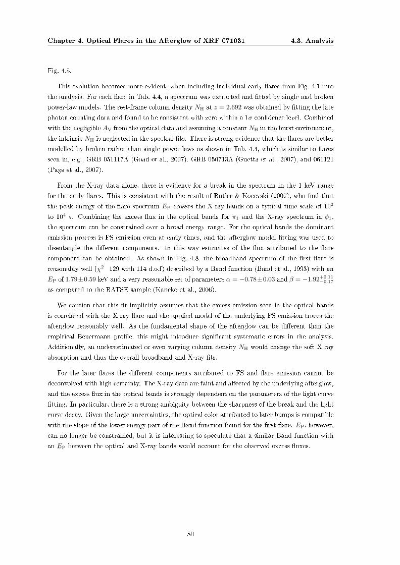
Chapter 4. Optical Flares in the Afterglow of XRF 071031 4.3. Analysis
Fig. 4.5.
This evolution becomes more evident, when including individual early ares from Fig. 4.1 into
the analysis. For each are in Tab. 4.4, a spectrum was extracted and tted by single and broken
power-law models. The rest-frame column density NH at z = 2.692 was obtained by tting the late
photon counting data and found to be consistent with zero within a 1σ condence level. Combined
with the negligible AV from the optical data and assuming a constant NH in the burst environment,
the intrinsic NH is neglected in the spectral ts. There is strong evidence that the ares are better
modelled by broken rather than single power laws as shown in Tab. 4.4, which is similar to ares
seen in, e.g., GRB 051117A (Goad et al., 2007), GRB 050713A (Guetta et al., 2007), and 061121
(Page et al., 2007).
From the X-ray data alone, there is evidence for a break in the spectrum in the 1 keV range
for the early ares. This is consistent with the result of Butler & Kocevski (2007), who nd that
the peak energy of the are spectrum EP crosses the X-ray bands on a typical time scale of 102
to 104 s. Combining the excess ux in the optical bands for π1 and the X-ray spectrum in φ1,
the spectrum can be constrained over a broad energy range. For the optical bands the dominant
emission process is FS emission even at early times, and the afterglow model tting was used to
disentangle the dierent components. In this way estimates of the ux attributed to the are
component can be obtained. As shown in Fig. 4.8, the broadband spectrum of the rst are is
reasonably well (χ2=129 with 114 d.o.f) described by a Band function (Band et al., 1993) with an
EP of 1.79±0.59 keV and a very reasonable set of parameters α = −0.78±0.03 and β = −1.92+0.11−0.17
as compared to the BATSE sample (Kaneko et al., 2006).
We caution that this t implicitly assumes that the excess emission seen in the optical bands
is correlated with the X-ray are and the applied model of the underlying FS emission traces the
afterglow reasonably well. As the fundamental shape of the afterglow can be dierent than the
empirical Beuermann prole, this might introduce signicant systematic errors in the analysis.
Additionally, an underestimated or even varying column density NH would change the soft X-ray
absorption and thus the overall broadband and X-ray ts.
For the later ares the dierent components attributed to FS and are emission cannot be
deconvolved with high certainty. The X-ray data are faint and aected by the underlying afterglow,
and the excess ux in the optical bands is strongly dependent on the parameters of the light curve
tting. In particular, there is a strong ambiguity between the sharpness of the break and the light
curve decay. Given the large uncertainties, the optical color attributed to later bumps is compatible
with the slope of the lower energy part of the Band function found for the rst are. EP, however,
can no longer be constrained, but it is interesting to speculate that a similar Band function with
an EP between the optical and X-ray bands would account for the observed excess uxes.
80

Chapter 4. Optical Flares in the Afterglow of XRF 071031 4.3. Analysis
Figure 4.8 Broadband spectrum of the rst are π1 with simultaneous optical and X-ray coverage.The data are tted by a Band function with EP = 1.79 ± 0.59 keV, α = −0.78 ± 0.03, andβ = −1.92+0.11
−0.17.
81

Chapter 4. Optical Flares in the Afterglow of XRF 071031 4.4. Discussion
4.4 Discussion
4.4.1 The Likely Cause of the Flares
Previously, bumps or ares in optical afterglow light curves have been reproduced using either a
superimposed reverse shock component for early ares, inhomogeneities in the circumburst medium
(e.g. Wang & Loeb, 2000), or the angular distribution of the energy in the jet (patchy shell model;
e.g. Kumar & Piran, 2000) or late energy injection by refreshed shocks (e.g. Rees & Mészáros,
1998) for later ares. However, a clear discrimination in the individual previous cases was not
possible due to the lack of simultaneous coverage in broad wavelength ranges.
Although we cannot completely rule out a reverse shock component for the rst bump, it seems
likely that it is produced by the same mechanism as the later ones. After subtracting the rising
power law, the decline of the rst bump can be tted with a power law of index ∼ −7. This
would be surprisingly fast for a reverse shock, which is expected to decline with ∼ t−2 in the
basic reball model (e.g. Nakar & Piran, 2004) and not faster than ∼ t−3 for more complicated
models (Kobayashi & Sari, 2000). The fact that the morphology is comparable to the later bumps
additionally hints on a common origin. Therefore, we try to account for all bumps with as few
assumptions as possible, thus searching for a phenomenological explanation for all bumps observed.
Recently, Nakar & Granot (2007) found that density jumps in the circumburst medium cannot
account for the majority of uctuations previously observed in GRB afterglow light curves. Only
large contrasts in the circumburst medium density are able to produce bumps with a change in
the temporal power-law decay index δα ≈1 in the light curve with a long transition time, which
scales linearly with contrast. Thus, signatures of inhomogeneities in the circumburst medium in
the optical light curve are expected to be smoother to what is observed.
A jet with inhomogeneities in the angular energy distribution produces episodic bumps when
the cone of a relativistically beamed patch enters the eld of the view of the observer (Zhang et al.,
2006). Similar to refreshed shocks, these patches inject additional energy into the blastwave, the
afterglow emission is boosted to a higher level and resumes the same power-law index as before
the bump (Zhang & Mészáros, 2002b). A characteristic for rebrightenings due to patchy shells
or refreshed shocks consequentially is a step like afterglow light curve. Given the steepening of
the power law post bump (Fig. 4.4), this scenario seems inconsistent with the bumps observed in
XRF 071031. We note, however, that the refreshed shock scenario can produce rebrightenings on
relatively short time scales under certain conditions, where the light curve drops back to the initial
decay (e.g. Guidorzi et al., 2007).
Although the morphology of the light curve and optical bumps in the GROND data might be
explained within the framework of variable external density or energy dissipation in the FS, both
the spectral evolution and the correlation with the X-ray data argue for an independent origin and
a second emission component. A hardening of the spectral index for ares in an optical light curve
is not unprecedented (Greiner et al., 2009a), and suggests a dierent emission than the generic
afterglow FS. In addition, the rst pronounced bump in the optical light curve is already observed
during the rise of the afterglow at 600 s, when the apparent onset of the FS just started.
82

Chapter 4. Optical Flares in the Afterglow of XRF 071031 4.4. Discussion
If all previously observed X-ray ares are due to the same physical process, it is very likely
that they do not originate from external shocks that give rise to the afterglow emission, but from
late time internal shocks (e.g. Burrows et al., 2005a; Zhang et al., 2006; Chincarini et al., 2007;
Butler & Kocevski, 2007). Thus, X-ray ares seem to be produced by a similar mechanism as the
prompt γ-rays, which are also caused by internal shocks in the standard model (Rees & Mészáros,
1992). Detailed analysis for GRB 050820A (Vestrand et al., 2006) showed that the optical emission
contemporaneous with the prompt phase can be explained as the superposition of forward shock and
emission correlated with the γ-rays. Similarly for XRF 071031, after subtracting the dominating
FS in the optical bands, the are spectrum from NIR to X-rays is well described with a Band
function.
Remarkably, the optical bumps show features which have been previously observed in X-ray
ares: a hardening of their spectra (e.g. Burrows et al., 2005a; Butler & Kocevski, 2007; Falcone
et al., 2007; Goad et al., 2007) and a correlation of the duration with the time where the bump
occurs, i.e. a roughly constant ∆T/T (Chincarini et al., 2007; Kocevski et al., 2007). They are,
however, less pronounced than typical X-ray ares. Temporal analysis of the early data shows that
the optical bump peaks signicantly later than the X-ray are. A hard to soft evolution of EP
which is found in the majority of all bright ares where a detailed spectral analysis is possible (e.g.
Burrows et al., 2005a; Romano et al., 2006a; Perri et al., 2007; Falcone et al., 2007) provides a
natural explanation for the time dierence between the are in the X-ray and optical wavelength
range. Spectral lags and a broadening towards lower energies have been observed in a number of
previous X-ray ares and the prompt emission (e.g. Norris et al., 1996; Romano et al., 2006b; Perri
et al., 2007).
Based on the light curve tting, the observed peak of the early optical are is delayed by
τ ∼ 130 s compared to the X-rays, which corresponds to 35 s in the bursts rest frame. As the
temporal coverage of the optical light curve is sparse in the early time frame, this delay is strongly
dependent on the assumed functional form of the afterglow and are morphology, but in any case it
is signicantly longer than what is typically observed as spectral lags in the prompt phase. Typical
values for prompt lags range from slightly negative (i.e. soft preceding hard bands) to several
seconds for long lag GRBs (e.g. Norris et al., 2000; Gehrels et al., 2006; McBreen et al., 2008; Foley
et al., 2008). The observed time dierence in the case of XRF 071031, however, is based on entirely
dierent energy ranges. In particular, the dierence between hard and soft energy bands is around
a factor of 103 for X-rays versus optical, while it is ∼ 10 for BAT channels.
Combining bump morphology, color evolution, broadband spectrum and the temporal connec-
tion to the X-ray data as shown in Fig. 4.9, the most likely origin of the bumps in the optical/NIR
light curve of XRF 071031 is the same as in the X-rays, namely the soft tail of emission correlated
with late internal shocks.
83
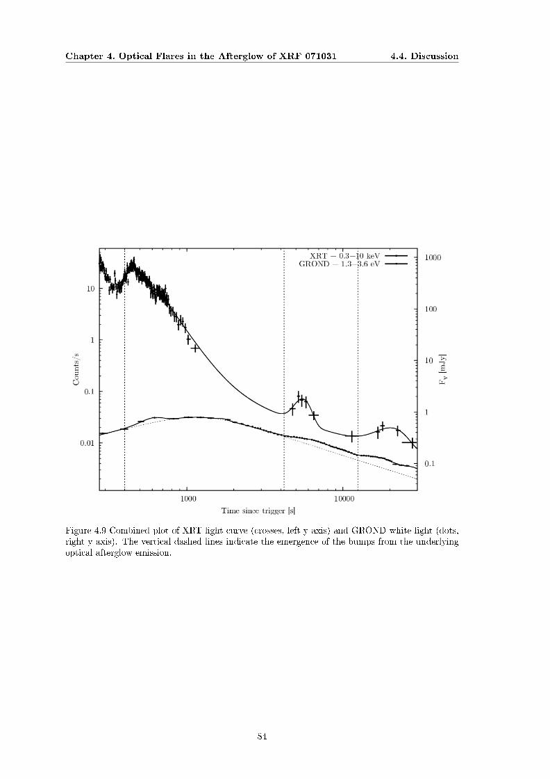
Chapter 4. Optical Flares in the Afterglow of XRF 071031 4.4. Discussion
Figure 4.9 Combined plot of XRT light curve (crosses, left y axis) and GROND white light (dots,right y axis). The vertical dashed lines indicate the emergence of the bumps from the underlyingoptical afterglow emission.
84
Chapter 4. Optical Flares in the Afterglow of XRF 071031 4.5. Conclusions
4.4.2 Paucity of Detection of Correlated Early Optical Bumps and X-ray
Flares
While a number of bursts have shown considerable variability in the optical bands during X-ray
ares (e.g. Pandey et al., 2006; Boër et al., 2006; Page et al., 2007; Malesani et al., 2007), the
early optical light curve is generally not as strongly aected as the X-rays by aring episodes.
The UVOT and ground-based robotic telescopes with their fast response provide a good sample
of optical observations simultaneous with the XRT light curve. If the rst optical bump and the
rst X-ray are in XRF 071031 are correlated as suggested by the data, the signature of a typical
X-ray are in the optical light curve can be approximated with the ratio of absolute optical to
X-ray peak ux obtained for XRF 071031.
GRB 060607A for example, showed signicant X-ray aring very early in the X-ray light curve
with only marginally correlated optical emission (Ziaeepour et al., 2008). However, the afterglow
was very bright, reaching ∼ 14.3 mag in the r band (Nysewander et al., 2007). If the are was
described with a similar spectrum as in XRF 071031, the expected optical counterpart of the
brightest X-ray are is estimated to have a peak amplitude of ∼ 200 µJy and could only be
resolved with continuous photometric monitoring with a precision of at least 0.03 mag. Thus, if
the emission in the ares is not strong enough with respect to the FS, a bright afterglow can easily
outshine are signatures in the optical bands even for very bright X-ray ares. In fact, GRB 061121
(Page et al., 2007) had simultaneous coverage with BAT, XRT and UVOT of the prompt emission
with a peak ux density in the X-rays of ∼ 15 mJy. Page et al. (2007) nd that most of the ux
is emitted in the γ-ray and X-ray bands, while the UVOT data only showed a relatively small
increase in brightness.
4.5 Conclusions
The detailed light curve and spectral evolution of the afterglow of XRF 071031 showed several
remarkable features. The most salient one is the achromatic early rise in brightness, resulting in a
peak of the optical/NIR light curve at around 1 ks. The achromatic turnover from rise to decay
suggests the apparent onset of the FS as its origin, due to either the increase in radiating electrons
in the pre-deceleration phase or a structured outow seen o axis. In the latter case the increase
in brightness is caused by the deceleration of the shock, so that the relativistically beamed cone
widens and gradually enters the sight line of the observer.
Superimposed onto the afterglow continuum emission are bumps which have a harder SED and
appear in similar epochs in the optical/NIR as well as in the X-ray bands. Based on the GROND
data collected for XRF 071031, we conclude that the variation in the light curve are most probably
the optical counterparts of X-ray ares, and therefore directly connect variability in an optical light
curve with the emergence of X-ray ares. Although emission from external shocks or a combination
of dierent eects cannot be completely ruled out, an internal origin seems to nicely account for
the majority of observations: the light curve shape and in particular the morphology of the bumps,
the spectral hardening in the optical SED, the observed decrease in EP from the prompt emission
85

Chapter 4. Optical Flares in the Afterglow of XRF 071031 4.5. Conclusions
Table 4.1. Secondary standards in the GRB eld in the GROND lter bands from 1 to 10
Ra/Dec g′ r′ i′ z′ J H KSDeg [J2000] mag mag mag mag mag mag mag
6.4098/-58.0831 15.44 ± 0.02 14.55 ± 0.02 14.28 ± 0.02 14.13 ± 0.02 13.09 ± 0.04 12.55 ± 0.04 12.50 ± 0.066.4186/-58.0723 16.32 ± 0.02 15.73 ± 0.02 15.54 ± 0.02 15.43 ± 0.02 14.46 ± 0.04 14.07 ± 0.04 14.00 ± 0.066.3933/-58.0662 17.84 ± 0.03 17.32 ± 0.03 17.18 ± 0.03 17.10 ± 0.03 16.18 ± 0.04 15.94 ± 0.06 15.65 ± 0.076.3672/-58.0536 20.71 ± 0.05 19.33 ± 0.03 18.53 ± 0.03 18.13 ± 0.03 16.86 ± 0.05 16.41 ± 0.07 16.28 ± 0.086.4579/-58.0492 20.03 ± 0.04 18.90 ± 0.03 18.49 ± 0.03 18.31 ± 0.03 17.07 ± 0.05 16.68 ± 0.07 16.45 ± 0.086.3663/-58.0782 20.09 ± 0.04 18.62 ± 0.03 17.60 ± 0.03 17.13 ± 0.03 15.80 ± 0.04 15.30 ± 0.05 14.92 ± 0.066.3751/-58.0631 21.26 ± 0.05 20.13 ± 0.04 19.72 ± 0.04 19.52 ± 0.04 18.29 ± 0.07 17.87 ± 0.08 17.79 ± 0.106.4021/-58.0496 22.72 ± 0.10 20.85 ± 0.05 20.06 ± 0.05 19.65 ± 0.05 17.94 ± 0.06 17.35 ± 0.07 16.11 ± 0.086.4117/-58.0575 22.49 ± 0.08 21.21 ± 0.06 20.76 ± 0.06 20.51 ± 0.07 18.56 ± 0.07 17.78 ± 0.08 16.86 ± 0.106.4375/-58.0485 21.28 ± 0.05 20.77 ± 0.05 20.61 ± 0.05 20.59 ± 0.07 19.29 ± 0.09 18.91 ± 0.10 17.98 ± 0.15
Table 4.2. Parametrization of the excess ux in the GROND bands using Gaussians
Bump Tmid [s] ∆T/2 [s] Amplitude [µJy] ∆T/Tmid ∆F/F
π1 587 ± 12 84 ± 18 149 ± 5 0.29 ± 0.06 0.24 ± 0.01ξ1 1726 ± 6 130 ± 4 39 ± 5 0.15 ± 0.01 0.06 ± 0.01π2 6302 ± 156 1648 ± 136 60 ± 5 0.52 ± 0.05 0.26 ± 0.02ξ2 9439 ± 377 1461 ± 254 29 ± 4 0.31 ± 0.06 0.18 ± 0.02π3 16505 ± 135 4013 ± 263 43 ± 2 0.49 ± 0.03 0.46 ± 0.02ξ3 28000 5000 32 ± 4 0.36 0.55 ± 0.03
to the ares, and the broadband are spectrum from NIR to X-rays. The spectral similarities to
the prompt phase strengthen the picture of X-rays ares as later and softer examples of the prompt
emission due to internal shocks. This connection provides additional evidence that inner engine
activity may last or be revived on a time scale of hours or days at least for some bursts.
Table 4.3. Parametrization of the excess ux in the X-ray bands using Gaussians
Bump Tmid [s] ∆T/2 [s] Amplitude [Counts/s] ∆T/Tmid ∆F/F
φ1 459 ± 2 42 ± 2 14.5 ± 0.8 0.18 ± 0.01 1.36 ± 0.07φ2 5528± 85 604 ± 114 0.047 ± 0.01 0.22 ± 0.04 1.20 ± 0.20φ3 20507 ± 952 4557 ± 1088 0.012 ± 0.002 0.44 ± 0.10 1.28 ± 0.13
86

Chapter 4. Optical Flares in the Afterglow of XRF 071031 4.5. Conclusions
Table 4.4. Spectral ts to the XRT ares using XSPEC.
Flare Times [s] Model Photon Index 1 Break energy [keV] Photon Index 2 χ2/dof
1 137 - 150 Single 1.23+0.05−0.05 - - 323/131
1 137 - 150 Double 0.72+0.09−0.09 1.84+0.17
−0.36 1.85+0.12−0.19 157/129
2 189 - 217 Single 1.72+0.09−0.05 - - 180/85
2 189 - 217 Double 1.14+0.14−0.15 1.26+0.16
−0.13 2.20+0.13−0.11 89/83
3 236 - 284 Single 1.87+0.05−0.05 - - 146/74
3 236 - 284 Double 1.23+0.19−0.18 1.07+0.16
−0.12 2.39+0.17−0.14 67/72
4 (Φ1) 396 - 547 Single 1.64+0.04−0.04 - - 172/110
4 (Φ1) 396 - 547 Double 1.26+0.19−0.32 0.98+0.22
−0.20 1.88+0.08−0.08 120/108
87

Chapter 4. Optical Flares in the Afterglow of XRF 071031 4.5. Conclusions
88

Chapter 5
The Bright Optical/NIR Afterglow
of the Faint GRB 080710 - Evidence
of a Jet Viewed O-axis 1
ABSTRACT
We investigate the optical/near-infrared light curve of the afterglow of GRB 080710 in the
context of rising afterglows. Optical and near-infrared photometry was performed using the seven
channel imager GROND and the Tautenburg Schmidt telescope. X-ray data were provided by the
X-ray Telescope onboard the Swift satellite. We construct an empirical light curve model using
the available broadband data, which is well-sampled in the time and frequency domains. The
optical/NIR light curve of the afterglow of GRB 080710 is dominated by an initial increase in
brightness, which smoothly turns over into a shallow power law decay. At around 10 ks post-burst,
there is an achromatic break from shallow to steeper decline in the afterglow light curve with a
change in the power law index of ∆α ∼ 0.9. The initially rising achromatic light curve of the
afterglow of GRB 080710 can be accounted for with a model of a burst viewed o-axis or a single
jet in its pre-deceleration phase and in an on-axis geometry. A unied picture of the afterglow
light curve and prompt emission properties can be obtained with an o-axis geometry, suggesting
that late and shallow rising optical light curves of GRB afterglows might be produced by geometric
eects.
5.1 Introduction
The launch of the Swift satellite (Gehrels et al., 2004) in 2004 opened a new eld of gamma-ray
burst (GRB) afterglow physics. With its precise localization by the Burst Alert Telescope (BAT;1T. Krühler, J. Greiner, P. Afonso, D. Burlon, C.Clemens, R. Filgas, D.A. Kann, S. Klose, A. Küpcü Yolda³, S.
McBreen, F. Olivares, A. Rau, A. Rossi, S. Schulze, G. P. Szokoly, A. Updike and A. Yolda³ (2009), A&A, accepted,arXiv:0908.2250
89

Chapter 5. The O-axis GRB 080710 5.2. Observations
Barthelmy et al., 2005), rapid slewing capabilities and early follow-up with two instruments in the
X-ray and ultraviolet/optical regime, studies of the early afterglow phase were possible for the rst
time with larger sample statistics of around 50 per year.
Long GRBs are generally classied according to the spectral properties of their prompt emission.
While conventional GRBs (CGRBs) have the peak energy of their observed spectrum in the 300 keV
range (Preece et al., 2000), the spectrum of X-ray rich bursts (XRRs) and X-ray ashes (XRFs) peak
at signicantly lower energies, typically around 50 keV for XRRs or 10 keV for XRFs respectively
(e.g., Heise et al., 2001; Kippen et al., 2003). The spectral and temporal properties (e.g., Sakamoto
et al., 2005) and their afterglows similar to those of CGRBs provide strong evidence, however, that
XRRs/XRFs represent a softer region of a continuous GRB distribution (e.g., Lamb et al., 2005;
Sakamoto et al., 2008).
A unied picture of the subclasses of GRBs can be obtained by attributing the observed dif-
ferences in their peak energy to the same objects being observed at dierent angles with respect
to the symmetry axis of the GRB jet (e.g., Yamazaki et al., 2002). The kinetic energy in the jet
per solid angle ε is usually parametrized as a top hat (e.g., Rhoads, 1999; Woods & Loeb, 1999),
Gaussian (Zhang & Mészáros, 2002a), power-law structured outow with ε ∝ (θ/θjet)−q (Mészáros
et al., 1998), or a top hat with lower energetic wings. The resulting shape of the afterglow light
curve then depends on the viewing angle and jet structure (e.g., Rossi et al., 2002).
In an inhomogeneous or structured jet model, the initial bulk Lorentz factor as well as the
specic deceleration time and radius are dependent on the distance to the symmetry axis of the
jet (Kumar & Granot, 2003). Hence, a geometric oset in the observer's line of sight from the
jet's symmetry axis will have a distinct signature in the optical light curve (e.g., Granot & Kumar,
2003). Because of the relativistic beaming of the decelerating ejecta, an observer located o-axis to
the central jet will see a rising optical afterglow light curve at early times (e.g., Panaitescu et al.,
1998; Granot & Sari, 2002b). The steepness of the rise would then be characteristic of the o-axis
angle and the jet structure: the farther the observer is located from the central emitting cone or
the faster the energy per solid angle decreases outside the jet, the shallower is the observed rise
in a structured jet model (Panaitescu & Vestrand, 2008). A rest-frame peak energy Erestpeak of the
spectrum of the prompt phase consistent with an XRF would thus correspond to a shallow rise or
early plateau phase of the afterglow. With decreasing o-axis angle, both Erestpeak and the optical
afterglow rise index will increase to resemble those of XRRs and steeper rising early afterglow light
curves.
5.2 Observations
At T0=07:13:10 UT on 10 July 2008, Swift triggered and located GRB 080710, but did not slew
immediately to the burst (Sbarufatti et al., 2008). Because of an observing constraint, observations
with the two narrow eld instruments, the X-ray- (XRT; Burrows et al., 2005b) and UV/Optical
Telescope (UVOT; Roming et al., 2005) started 0.87 h and 0.89 h after the trigger (Landsman
& Sbarufatti, 2008). The burst had a relatively smooth fast rise - exponential decay temporal
90
Chapter 5. The O-axis GRB 080710 5.2. Observations
structure with T90 = 120 ± 17 s in the 15-350 keV band and weak indication of a precursor 120 s
before the main peak (Tueller et al., 2008). Above 100 keV, the burst was only marginally detected
by BAT and its spectrum is well described with a single power law of index −1.47 ± 0.23 and a
total uence in the 15-150 keV range of (1.4±0.2)×10−6 erg/cm2 (Tueller et al., 2008). Using the
spectral slope from the BAT data, and following Sakamoto et al. (2009), the peak energy of the
prompt emission spectrum can be constrained to be 110+340−60 keV, including the uncertainties in the
BAT power law slope. The uence ratio of GRB 080710 between the two BAT bands 25-50 keV
and 50-100 keV is S(25-50 keV)/S(50-100 keV) = 0.70 ± 0.15, and the burst thus qualies as a
CGRB in the observer's frame, with errors ranging to a uence ratio similar to those of XRRs
when applying the working denition of Sakamoto et al. (2008).
Assuming a spectral shape of a Band function (Band et al., 1993) with a peak energy of around
110 keV and a high energy index of −2.5, standard ΛCDM cosmology (ΩM = 0.27, ΩΛ = 0.73,
H0 = 71 (km/s)/Mpc) and a redshift z of 0.845 (Perley et al., 2008a; Fynbo et al., 2009), we derive
a bolometric (1 keV to 10 MeV) energy release for GRB 080710 of logEγ,iso[erg] = 51.75 with a rest-
frame peak energy of Erestpeak ∼ 200 keV. Peak energies of the observed prompt spectrum of 50 keV,
300 keV, or 500 keV result in log Eγ,iso[erg] ≈ 51.70, 51.94, or 52.14, respectively. Compared
to a sample of previous bursts of known redshift (e.g., Amati et al., 2008), these estimates place
GRB 080710 at the lower energy end of GRBs, with an inferred bolometric energy release of
around 103 times less than the extremely energetic GRB 080916C (Abdo et al., 2009a; Greiner
et al., 2009c). Hence, a low Erestpeak in the 50-200 keV range is also supported by the Amati relation
(Amati et al., 2002), and is consistent with the most reliable estimate derived using the BAT
spectral slope. Given the low redshift and prompt emission properties of GRB 080710, it thus
seems very likely that Erestpeak is in a range that is typically associated with a XRR in the GRB rest
frame (100-300 keV, Sakamoto et al., 2008), although a hard burst cannot be completely excluded
by the observations.
GROND (Greiner et al., 2008) at the 2.2 mMPI/ESO telescope at LaSilla observatory responded
to the Swift trigger and initiated automated observations, which started 384 s after the burst.
During the rst two hours, only the g′r′i′z′ CCDs of GROND were operating. Observations in
all seven colors g′r′i′z′JHKS simultaneously started 1.98 h later and continued until the start of
the local nautical twilight at 10:27 UT. Afterwards, GROND switched to a NIR-only mode, where
only imaging in JHKS was performed. TLS imaging was obtained between 00:09 UT and 01:43
UT on 11 July 2008 in lters BV R and I (Schulze et al., 2008). In addition, GROND imaged the
eld of GRB 080710, both 3 and 4 days after the burst.
The XRT light curve was downloaded from the XRT light-curve repository (Evans et al., 2007),
and spectra were obtained with the xrtpipeline tool using the latest calibration frames from
the Swift CALDB and standard parameters. The spectra were tted using the XSPEC package
(Arnaud, 1996) with a foreground hydrogen column density at the Galactic value of NH = 4.1 ×1020 cm−2 (Kalberla et al., 2005). Optical/NIR data (see Tables 5.1 and 5.2) were reduced using
standard IRAF tasks (Tody, 1993) similar to the procedure outlined in Krühler et al. (2008).
91
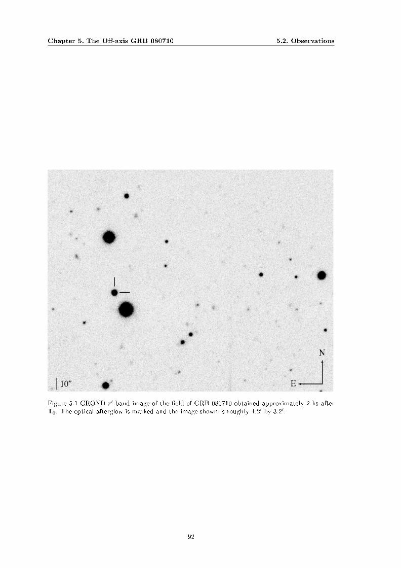
Chapter 5. The O-axis GRB 080710 5.2. Observations
Figure 5.1 GROND r′ band image of the eld of GRB 080710 obtained approximately 2 ks afterT0. The optical afterglow is marked and the image shown is roughly 4.2′ by 3.2′.
92
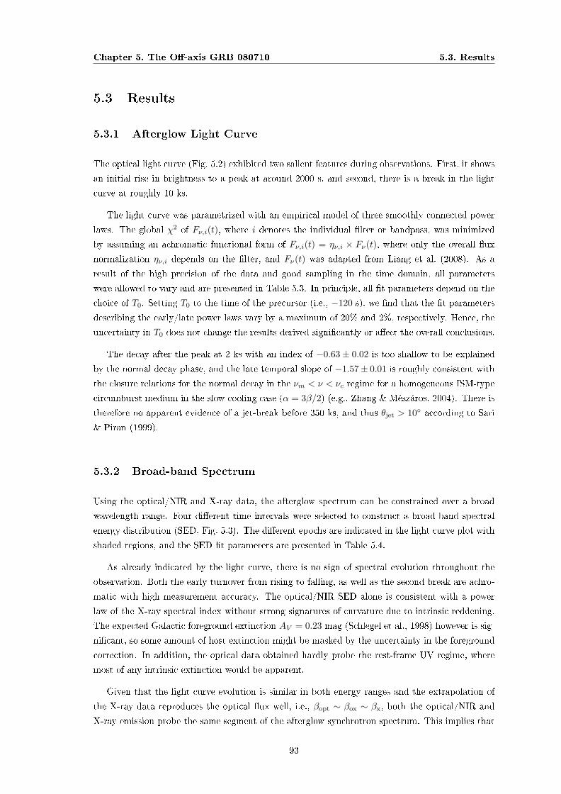
Chapter 5. The O-axis GRB 080710 5.3. Results
5.3 Results
5.3.1 Afterglow Light Curve
The optical light curve (Fig. 5.2) exhibited two salient features during observations. First, it shows
an initial rise in brightness to a peak at around 2000 s, and second, there is a break in the light
curve at roughly 10 ks.
The light curve was parametrized with an empirical model of three smoothly connected power
laws. The global χ2 of Fν,i(t), where i denotes the individual lter or bandpass, was minimized
by assuming an achromatic functional form of Fν,i(t) = ην,i × Fν(t), where only the overall ux
normalization ην,i depends on the lter, and Fν(t) was adapted from Liang et al. (2008). As a
result of the high precision of the data and good sampling in the time domain, all parameters
were allowed to vary and are presented in Table 5.3. In principle, all t parameters depend on the
choice of T0. Setting T0 to the time of the precursor (i.e., −120 s), we nd that the t parameters
describing the early/late power laws vary by a maximum of 20% and 2%, respectively. Hence, the
uncertainty in T0 does not change the results derived signicantly or aect the overall conclusions.
The decay after the peak at 2 ks with an index of −0.63± 0.02 is too shallow to be explained
by the normal decay phase, and the late temporal slope of −1.57± 0.01 is roughly consistent with
the closure relations for the normal decay in the νm < ν < νc regime for a homogeneous ISM-type
circumburst medium in the slow cooling case (α = 3β/2) (e.g., Zhang & Mészáros, 2004). There is
therefore no apparent evidence of a jet-break before 350 ks, and thus θjet > 10 according to Sari
& Piran (1999).
5.3.2 Broad-band Spectrum
Using the optical/NIR and X-ray data, the afterglow spectrum can be constrained over a broad
wavelength range. Four dierent time intervals were selected to construct a broad-band spectral
energy distribution (SED, Fig. 5.3). The dierent epochs are indicated in the light curve plot with
shaded regions, and the SED t parameters are presented in Table 5.4.
As already indicated by the light curve, there is no sign of spectral evolution throughout the
observation. Both the early turnover from rising to falling, as well as the second break are achro-
matic with high measurement accuracy. The optical/NIR SED alone is consistent with a power
law of the X-ray spectral index without strong signatures of curvature due to intrinsic reddening.
The expected Galactic foreground extinction AV = 0.23 mag (Schlegel et al., 1998) however is sig-
nicant, so some amount of host extinction might be masked by the uncertainty in the foreground
correction. In addition, the optical data obtained hardly probe the rest-frame UV regime, where
most of any intrinsic extinction would be apparent.
Given that the light curve evolution is similar in both energy ranges and the extrapolation of
the X-ray data reproduces the optical ux well, i.e., βopt ∼ βox ∼ βx, both the optical/NIR and
X-ray emission probe the same segment of the afterglow synchrotron spectrum. This implies that
93
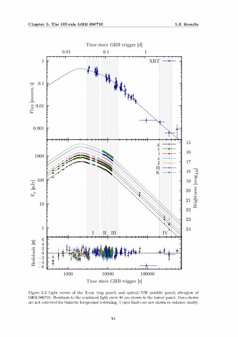
Chapter 5. The O-axis GRB 080710 5.3. Results
Figure 5.2 Light curves of the X-ray (top panel) and optical/NIR (middle panel) afterglow ofGRB 080710. Residuals to the combined light curve t are shown in the lowest panel. Data shownare not corrected for Galactic foreground reddening. Upper limits are not shown to enhance clarity.
94

Chapter 5. The O-axis GRB 080710 5.4. Discussion
Figure 5.3 Broad-band spectral energy distribution from XRT and GROND at dierent epochs(upper panel). The data were tted with a power-law, modied by a Galactic and intrinsic hydrogencolumn. The best t power law is shown in dotted lines, the best t model including the soft X-rayabsorption in solid lines. In the lower panel the residuals of the data to the best t model.
the X-ray and optical data are above the typical synchrotron frequency νm and in the spectral
regime of max(νm, νc) < νopt < νX , or νm < νopt < νX < νc, where the latter is consistent with
a reball model in a homogeneous ISM and slow cooling case. The spectral index of the electron
distribution p would then be p = 2β = 2.00±0.02 or 2β+ 1 = 3.00±0.02, respectively. Given that
not all bursts are consistent with the closure relations in the basic reball scenario (e.g., Evans
et al., 2008), we consider both cases in the following. Consequentially, the expected break in the
synchrotron afterglow spectrum at the cooling frequency νc could be below the optical at the start
of the observations 6 minutes after the burst, or, assuming νm < ν < νc, above the X-rays for the
entire observational period.
5.4 Discussion
A number of previous bursts have shown a rising optical afterglow at early times, e.g., GRBs 060418,
060607A (Molinari et al., 2007) amongst others (e.g., Krühler et al., 2008; Ferrero et al., 2009;
Greiner et al., 2009a; Oates et al., 2009; Ryko et al., 2009; Klotz et al., 2009). Similar to the
X-ray Flash 071031 (Krühler et al., 2009), the optical SED does not show signicant evolution
during the rise, and all bands peak at the same time.
95

Chapter 5. The O-axis GRB 080710 5.4. Discussion
An achromatic rising component is generally related to either the onset of the reball forward
shock (e.g., Sari & Piran, 1999) seen face-on, or to an outow seen o-axis (e.g., Panaitescu et al.,
1998). In the rst case, the apparent increase in brightness is caused by the increasing number
of radiating electrons. The time of the light curve peak at T0 + 2 ks is much later than the
end of signicant γ-ray emission (T0 + 40 s), so the afterglow can be described in the thin shell
approximation. The jet is then expected to produce a rising early light curve with a peak when the
swept-up circumburst medium starts to decelerate the ejecta eciently. Depending on the prole
of the circumburst medium, the rise has indices of ∼ 2 (νc < νopt) or 3 (νc > νopt) in an ISM,
or ∼ 0.5 in an wind-like environment (Panaitescu & Vestrand, 2008). Given that the majority of
bursts prefer a circumburst medium with an ISM prole, and the late afterglow decline is consistent
with this, we thus consider only the ISM, thin shell case in the following.
In the o-axis case, the peak is a geometric eect: as the shock decelerates, the relativistically
beamed emission cone widens and gradually enters the sight line of the observer. The light curve
morphology is then dependent on the jet structure and o-axis angle θobs, and reaches a maximum
when Γ ∼ (θobs− θc)−1, where θc is the angle of an uniform cone around the symmetry axis of the
jet.
There is no evidence of chromatic evolution, which would be the case if the peak was caused
by a νm moving through the optical bands, or dust destruction, and none of these processes can
produce the early achromatic rise. In addition, there is also no sign of a reverse shock, which is
expected to decline with a temporal index of −1.75 for p = 2, or −2.5 for p = 3. The latter,
however, might be masked by a dominating forward shock, or have happened before the start of
the GROND observations.
5.4.1 On-axis Jet in its Pre-deceleration Phase
If the light-curve peak was caused by a jet in its pre-deceleration phase, conclusions about the
motion of the ultra-relativistic outow from the central engine can be drawn. Using the time
of the absolute light curve maximum tmax ≈ 2 ks, logEγ,iso[erg] = 51.70 − 52.14 and following
Molinari et al. (2007), we nd initial Lorentz factors of the bulk outow of around ΓISM0 ≈ 90−100
(Γwind0 ≈ 30 − 40). This is at the very low end of the theoretically expected velocity of the
outow to produce γ-rays (e.g., Piran, 2005), and together with the divergence in the measured
(1.1) and expected (∼ 2 − 3) rise index, makes the scenario of a single on-axis decelerating jet
appears somewhat contrived. In addition, a small population of afterglows shows a very late peak
or long plateau (e.g., XRF 030723 (Fynbo et al., 2004) or GRB 060614 (Della Valle et al., 2006)),
where the derived Lorentz-factor in an on-axis conguration from the optical afterglow peak are
uncomfortably small. Furthermore, all previously observed rise indices have a broad distribution
(e.g. Panaitescu & Vestrand (2008); Oates et al. (2009); Ryko et al. (2009); Klotz et al. (2009)
and references therein) from early plateau to very fast rising curves, and they do not cluster around
the expected t2−3. Consequently, it seems plausible that at least some rising afterglows are not
caused by the onset of the afterglow, but rather by a geometrical oset of the observer's sight line
with respect to the jet's symmetry axis.
96

Chapter 5. The O-axis GRB 080710 5.4. Discussion
5.4.2 Jet Seen O-axis
In contrast to the model of an on-axis jet in its pre-deceleration phase, an o-axis scenario is able
to account for a broad range of observed rise indices. The peak time and rise index then relates to
the o-axis angle or jet structure and could therefore describe a wide diversity of early afterglows
in a single framework (Panaitescu & Vestrand, 2008).
If the energy in the jet outer wings decreases rapidly, the early emission of the line-of-sight
ejecta is negligible compared to the central part, and the jet structure can be approximated by
a homogeneous top-hat, where the burst energetics can be used to constrain the oset angle.
Following Granot & Sari (2002b), a homogeneous jet with a half opening angle θjet and a Lorentz
factor Γ seen o-axis at an angle θobs will appear less energetic by a factor of b6, where b = Γ (θobs−θjet). Assuming a mean value of logEγ,iso[erg] = 53 and, hence adopting b6 ∼<10 for GRB 080710,
it follows that θobs − θjet ∼< 3/Γ100. If viewed on-axis, Epeak would then be b2Eobspeak ≈ 300 keV.
However, the jet geometry need not necessarily be a simple top-hat. In a realistic jet model,
the jet viewed o-axis is inhomogeneous, has a top-hat structure with wings of lower energy, or
is Gaussian shaped (e.g. Zhang et al., 2003b; Eichler & Granot, 2006). In addition, some bursts
show evidence that their jet structure consists of two jets (Berger et al., 2003; Granot et al., 2006;
Racusin et al., 2008). In this two-component jet model, a narrow, fast jet produces the prompt
γ-rays and early afterglow, and a slow wide jet dominates the late afterglow emission (Peng et al.,
2005).
In these cases, the resulting afterglow light curve in an o-axis geometry is a superposition of
two dierent components: the emission from the ejecta with lower Lorentz-factors, which typically
dominates at late times, and the relativistic spreading of the decelerating jet around the symmetry
axis. The relative energies, jet structure, and oset angle then dene the light-curve morphology.
In particular, the delayed onset of the broad jet emission in its pre-deceleration phase might be
responsible for the shallow decay observed after the peak. Remarkably, the light curve is equally well
(χ2 = 485 for 425 d.o.f) reproduced by using the sum of the afterglow of two jets, where the narrow
one is viewed slightly o-axis (Fig. 5.4). Hence, the shallow decay phase could be the result of the
superposition of the narrow-jet afterglow and the rise of the broad jet with Γ0 ∼ 50, θjet > 10 in its
pre-deceleration phase. After the emergence of the broad jet afterglow, it subsequently dominates
the light curve morphology (Fig. 5.4). The two-component model thus provides a phenomenological
explanation of the shallow decay phase by attributing the shallow slope to the increasing energy
dissipation in the pre-deceleration phase of the broader jet in a specic jet conguration. The
opening angle of the narrow jet can be constrained from the light-curve tting to around 2 − 4,
but its evolution is masked by the brighter broad jet at later times (Fig. 5.4). An alternative, jet
geometry independent mechanism of energy injection during a decay phase that is shallower than
expected, is the refreshed shock scenario (e.g. Rees & Mészáros, 1998; Zhang et al., 2006). A long
lived central engine or a simultaneous ejection of shells with a distribution of Lorentz factors could
cause the continuous energy injection required for a shallow decay (e.g. Nousek et al., 2006).
An o-axis viewing angle in a two-component or structured jet model with an energy injection
can thus provide a consistent picture for the light-curve morphology and the relatively low estimates
97

Chapter 5. The O-axis GRB 080710 5.5. Conclusions
Figure 5.4 Tentative two-component t for GRB 080710 as the superposition of the afterglow oftwo jets with νm < νopt < νX < νc and p∼3 for both components. The narrow jet is viewed slightlyo-axis and produces a shallow rise as its emission spreads during deceleration due to relativisticbeaming eects. The broad jet is viewed on-axis with Γ0 ∼ 50, θjet > 10 and has the expectedsteep rise during its pre-deceleration phase. Shown is the GROND r′ band data, all other bandsare omitted to enhance clarity.
of Eγ, iso and Erestpeak of the prompt emission of GRB 080710. In an o-axis scenario, a lower Erest
peak
of the prompt emission spectrum would correspond to a later and fainter afterglow maximum,
since both are caused by geometric eects. We caution that the spectral properties of BAT bursts
are generally not well constrained, and GRB 080710 is no exception in this respect. The BAT
data, however, indicate a mildly soft event, which could be associated with a XRR in the burst
rest-frame, consistent with the o-axis interpretation of the optical light curve in a unied model.
5.5 Conclusions
The broad-band light curve of the afterglow of GRB 080710 shows two salient features, both
achromatic with high precision: an early rise in its brightness, peaking at ∼ 2 ks, and a turnover
from a shallow to steep decline at ∼ 10 ks. The early rise could be caused by a jet in its pre-
deceleration phase, or a viewing angle outside the central cone. The latter scenario is naturally
able to explain a late-rising afterglow for a soft and weak burst due to a viewing angle oset with
respect to the symmetry axis of the jet. An o-axis scenario provides a consistent description
of the properties of GRB 080710, and can additionally account for a broad range of rise indices.
98

Chapter 5. The O-axis GRB 080710 5.5. Conclusions
Consequently, some of the rising afterglow light curves, especially late and shallow ones, might not
represent the same class of afterglows that rise because of increasing emission in the pre-deceleration
phase, but rather provide evidence of an o-axis location of the observer. The achromatic early
increase in brightness observed in the mildly soft GRB 080710 is too shallow to be accounted
for with the onset of the afterglow, but signicantly steeper than observed in the XRFs 071031
(Krühler et al., 2009) and 080330 (Guidorzi et al., 2009). This might already reect a common
dependence of both Erestpeak, and the rise index of the early optical light curve, on the o-axis angle
in an unied model: the softer the prompt emission, the more o-axis, and the shallower the rise.
This interpretation remains to be tested by the study of a larger sample of early afterglows with
well constrained energetics and light curves of the prompt emission from combined Swift/BAT and
Fermi/GBM detections, whether and how the structure of an early rise in the optical afterglow
is related to prompt emission properties, and in particular, the rest frame Erestpeak and Eγ,iso. A
possible correlation would then shed light on the nature of the early afterglow rise, the shallow
decay segment, and the jet structure in general.
99

Chapter 5. The O-axis GRB 080710 5.5. Conclusions
Table 5.1. griz photometric data
Tmid − T0 Exposure Filter Brightness(a) Brightness(a) Brightness(a) Brightness(a)
[ks] [s] mag(bc)AB mag
(bc)AB mag
(bc)AB mag
(bc)AB
g′ r′ i′ z′
0.4169 66 g′r′i′z′ 18.619 ± 0.028 18.175 ± 0.026 17.899 ± 0.026 17.673 ± 0.0280.5745 35 g′r′i′z′ 18.162 ± 0.024 17.724 ± 0.018 17.478 ± 0.018 17.200 ± 0.0190.7457 115 g′r′i′z′ 17.815 ± 0.016 17.381 ± 0.010 17.162 ± 0.015 16.909 ± 0.0160.9334 35 g′r′i′z′ 17.509 ± 0.013 17.086 ± 0.009 16.875 ± 0.011 16.604 ± 0.0161.0726 71 g′r′i′z′ 17.385 ± 0.008 16.961 ± 0.006 16.711 ± 0.009 16.474 ± 0.0111.1977 35 g′r′i′z′ 17.300 ± 0.008 16.865 ± 0.006 16.637 ± 0.008 16.381 ± 0.0091.3423 35 g′r′i′z′ 17.163 ± 0.007 16.773 ± 0.006 16.523 ± 0.007 16.274 ± 0.0081.4556 35 g′r′i′z′ 17.118 ± 0.007 16.701 ± 0.005 16.442 ± 0.007 16.215 ± 0.0071.5595 35 g′r′i′z′ 17.075 ± 0.007 16.668 ± 0.005 16.425 ± 0.007 16.169 ± 0.0071.6767 35 g′r′i′z′ 17.044 ± 0.006 16.596 ± 0.005 16.354 ± 0.007 16.112 ± 0.0071.7947 35 g′r′i′z′ 17.020 ± 0.006 16.595 ± 0.005 16.334 ± 0.007 16.095 ± 0.0081.8996 35 g′r′i′z′ 17.003 ± 0.006 16.573 ± 0.005 16.326 ± 0.007 16.089 ± 0.0072.0065 35 g′r′i′z′ 17.003 ± 0.006 16.593 ± 0.005 16.343 ± 0.006 16.094 ± 0.0062.1892 115 g′r′i′z′ 16.976 ± 0.005 16.552 ± 0.004 16.312 ± 0.004 16.070 ± 0.0052.3835 115 g′r′i′z′ 16.995 ± 0.005 16.553 ± 0.004 16.315 ± 0.004 16.078 ± 0.0052.5359 35 g′r′i′z′ 17.007 ± 0.006 16.597 ± 0.004 16.363 ± 0.007 16.121 ± 0.0062.6421 35 g′r′i′z′ 17.042 ± 0.006 16.617 ± 0.005 16.386 ± 0.007 16.136 ± 0.0072.7614 35 g′r′i′z′ 17.044 ± 0.006 16.617 ± 0.005 16.387 ± 0.006 16.147 ± 0.0072.8323 35 g′r′i′z′ 17.061 ± 0.006 16.635 ± 0.005 16.401 ± 0.007 16.159 ± 0.0072.9105 35 g′r′i′z′ 17.074 ± 0.006 16.652 ± 0.005 16.409 ± 0.007 16.176 ± 0.0072.9854 35 g′r′i′z′ 17.103 ± 0.006 16.692 ± 0.005 16.453 ± 0.007 16.219 ± 0.0073.0564 35 g′r′i′z′ 17.110 ± 0.006 16.696 ± 0.005 16.463 ± 0.007 16.236 ± 0.0073.1276 35 g′r′i′z′ 17.125 ± 0.007 16.718 ± 0.005 16.483 ± 0.007 16.248 ± 0.0083.1962 35 g′r′i′z′ 17.151 ± 0.006 16.724 ± 0.005 16.492 ± 0.007 16.261 ± 0.0083.3151 35 g′r′i′z′ 17.164 ± 0.006 16.744 ± 0.005 16.513 ± 0.007 16.273 ± 0.0083.4059 35 g′r′i′z′ 17.181 ± 0.007 16.771 ± 0.005 16.554 ± 0.008 16.309 ± 0.0074.1611 115 g′r′i′z′ 17.273 ± 0.005 16.869 ± 0.004 16.643 ± 0.005 16.418 ± 0.0064.4496 115 g′r′i′z′ 17.315 ± 0.005 16.911 ± 0.004 16.689 ± 0.005 16.452 ± 0.0064.6632 115 g′r′i′z′ 17.341 ± 0.005 16.944 ± 0.004 16.716 ± 0.005 16.488 ± 0.0065.6014 115 g′r′i′z′ 17.456 ± 0.005 17.067 ± 0.004 16.830 ± 0.005 16.601 ± 0.0065.8030 115 g′r′i′z′ 17.501 ± 0.006 17.094 ± 0.004 16.881 ± 0.006 16.637 ± 0.0066.0290 115 g′r′i′z′ 17.529 ± 0.005 17.140 ± 0.004 16.910 ± 0.006 16.675 ± 0.0066.2166 115 g′r′i′z′ 17.556 ± 0.006 17.163 ± 0.004 16.941 ± 0.005 16.700 ± 0.0066.5862 115 g′r′i′z′ 17.591 ± 0.006 17.197 ± 0.004 16.977 ± 0.006 16.746 ± 0.0066.7883 115 g′r′i′z′ 17.598 ± 0.006 17.219 ± 0.004 16.984 ± 0.006 16.757 ± 0.0066.9845 115 g′r′i′z′ 17.643 ± 0.006 17.254 ± 0.004 17.028 ± 0.006 16.788 ± 0.0077.2804 115 g′r′i′z′ 17.689 ± 0.006 17.300 ± 0.004 17.073 ± 0.006 16.839 ± 0.0077.4691 115 g′r′i′z′ 17.713 ± 0.006 17.323 ± 0.004 17.087 ± 0.006 16.853 ± 0.0067.6567 115 g′r′i′z′ 17.760 ± 0.005 17.342 ± 0.004 17.101 ± 0.004 16.902 ± 0.0067.8462 115 g′r′i′z′ 17.769 ± 0.005 17.355 ± 0.004 17.130 ± 0.005 16.918 ± 0.0068.0363 115 g′r′i′z′ 17.779 ± 0.004 17.371 ± 0.004 17.150 ± 0.005 16.918 ± 0.0068.2434 115 g′r′i′z′ 17.786 ± 0.006 17.397 ± 0.004 17.170 ± 0.007 16.928 ± 0.0078.4312 115 g′r′i′z′ 17.812 ± 0.005 17.423 ± 0.004 17.197 ± 0.005 16.989 ± 0.0078.6219 115 g′r′i′z′ 17.826 ± 0.004 17.432 ± 0.004 17.226 ± 0.004 17.005 ± 0.0068.8119 115 g′r′i′z′ 17.836 ± 0.006 17.461 ± 0.005 17.247 ± 0.005 17.010 ± 0.0069.0840 115 g′r′i′z′ 17.875 ± 0.006 17.498 ± 0.005 17.274 ± 0.008 17.043 ± 0.0109.2723 115 g′r′i′z′ 17.898 ± 0.006 17.527 ± 0.004 17.304 ± 0.006 17.086 ± 0.0079.4591 115 g′r′i′z′ 17.929 ± 0.005 17.534 ± 0.004 17.324 ± 0.006 17.123 ± 0.0089.6457 115 g′r′i′z′ 17.960 ± 0.005 17.570 ± 0.004 17.333 ± 0.005 17.116 ± 0.0069.8478 115 g′r′i′z′ 17.989 ± 0.006 17.599 ± 0.005 17.366 ± 0.007 17.132 ± 0.00810.037 115 g′r′i′z′ 18.013 ± 0.005 17.619 ± 0.004 17.401 ± 0.005 17.180 ± 0.00610.227 115 g′r′i′z′ 18.025 ± 0.005 17.636 ± 0.004 17.419 ± 0.005 17.206 ± 0.00710.420 115 g′r′i′z′ 18.046 ± 0.006 17.646 ± 0.005 17.408 ± 0.004 17.187 ± 0.008
100
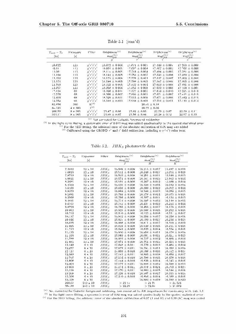
Chapter 5. The O-axis GRB 080710 5.5. Conclusions
Table 5.1 (cont'd)
Tmid − T0 Exposure Filter Brightness(a) Brightness(a) Brightness(a) Brightness(a)
[ks] [s] mag(bc)AB mag
(bc)AB mag
(bc)AB mag
(bc)AB
g′ r′ i′ z′
10.622 115 g′r′i′z′ 18.072 ± 0.006 17.674 ± 0.005 17.446 ± 0.007 17.203 ± 0.00810.811 115 g′r′i′z′ 18.091 ± 0.005 17.692 ± 0.004 17.467 ± 0.005 17.266 ± 0.00611.001 115 g′r′i′z′ 18.114 ± 0.005 17.718 ± 0.004 17.494 ± 0.005 17.281 ± 0.00611.194 115 g′r′i′z′ 18.142 ± 0.005 17.753 ± 0.007 17.523 ± 0.006 17.289 ± 0.00611.333 115 g′r′i′z′ 18.175 ± 0.006 17.776 ± 0.004 17.547 ± 0.007 17.302 ± 0.00811.574 115 g′r′i′z′ 18.199 ± 0.005 17.798 ± 0.005 17.567 ± 0.008 17.365 ± 0.00611.763 115 g′r′i′z′ 18.222 ± 0.005 17.822 ± 0.004 17.613 ± 0.008 17.391 ± 0.00611.957 115 g′r′i′z′ 18.258 ± 0.006 17.855 ± 0.009 17.633 ± 0.008 17.400 ± 0.00712.134 66 g′r′i′z′ 18.268 ± 0.011 17.877 ± 0.007 17.656 ± 0.010 17.395 ± 0.01012.270 66 g′r′i′z′ 18.300 ± 0.007 17.895 ± 0.005 17.671 ± 0.007 17.415 ± 0.01012.410 66 g′r′i′z′ 18.320 ± 0.011 17.915 ± 0.006 17.671 ± 0.009 17.462 ± 0.01012.552 66 g′r′i′z′ 18.348 ± 0.013 17.948 ± 0.008 17.714 ± 0.011 17.443 ± 0.013
62.856 300 R(d) 20.49 ± 0.18
64.523 4 x 300 I(d) 20.23 ± 0.09266.59 8 x 365 g′r′i′z′ 23.47 ± 0.06 23.02 ± 0.05 22.79 ± 0.07 22.59 ± 0.11353.11 8 x 365 g′r′i′z′ 24.09 ± 0.07 23.56 ± 0.06 23.28 ± 0.12 22.97 ± 0.15
(a) Not corrected for Galactic foreground reddening(b) In the light curve tting, a systematic error of 0.012 mag was added quadratically to the quoted statistical error
(c) For the SED tting, the aditional error of the absolute calibration of 0.05 mag was added(d) Calibrated using the GROND r′ and i′ eld calibration, including a (r′-i′) color term
Table 5.2. JHKS photometric data
Tmid − T0 Exposure Filter Brightness(a) Brightness(a) Brightness(a)
[ks] [s] mag(bc)AB mag
(bc)AB mag
(bc)AB
J H K
7.4943 12 x 10 JHKS 16.506 ± 0.009 16.215 ± 0.017 15.887 ± 0.0197.6818 12 x 10 JHKS 16.541 ± 0.008 16.240 ± 0.017 15.954 ± 0.0197.8710 12 x 10 JHKS 16.533 ± 0.008 16.251 ± 0.011 15.940 ± 0.0138.0611 12 x 10 JHKS 16.571 ± 0.008 16.264 ± 0.013 15.962 ± 0.0148.2685 12 x 10 JHKS 16.591 ± 0.009 16.267 ± 0.012 15.968 ± 0.0148.4560 12 x 10 JHKS 16.638 ± 0.008 16.329 ± 0.015 16.042 ± 0.0168.6469 12 x 10 JHKS 16.638 ± 0.008 16.309 ± 0.012 16.052 ± 0.0148.8370 12 x 10 JHKS 16.664 ± 0.009 16.346 ± 0.013 16.058 ± 0.0159.1091 12 x 10 JHKS 16.703 ± 0.009 16.378 ± 0.014 16.075 ± 0.0169.2966 12 x 10 JHKS 16.706 ± 0.008 16.397 ± 0.011 16.135 ± 0.0139.4841 12 x 10 JHKS 16.714 ± 0.008 16.397 ± 0.013 16.140 ± 0.0159.6707 12 x 10 JHKS 16.745 ± 0.009 16.437 ± 0.012 16.215 ± 0.0149.8729 12 x 10 JHKS 16.765 ± 0.009 16.455 ± 0.017 16.175 ± 0.01810.062 12 x 10 JHKS 16.825 ± 0.009 16.508 ± 0.015 16.252 ± 0.01610.252 12 x 10 JHKS 16.810 ± 0.008 16.533 ± 0.016 16.231 ± 0.01710.447 12 x 10 JHKS 16.842 ± 0.008 16.556 ± 0.017 16.258 ± 0.01810.646 12 x 10 JHKS 16.857 ± 0.009 16.599 ± 0.017 16.236 ± 0.01810.835 12 x 10 JHKS 16.908 ± 0.008 16.611 ± 0.017 16.310 ± 0.01911.025 12 x 10 JHKS 16.916 ± 0.008 16.620 ± 0.015 16.321 ± 0.01611.213 12 x 10 JHKS 16.949 ± 0.009 16.629 ± 0.014 16.334 ± 0.01611.415 12 x 10 JHKS 16.950 ± 0.009 16.658 ± 0.014 16.370 ± 0.01611.598 12 x 10 JHKS 16.989 ± 0.009 16.684 ± 0.011 16.411 ± 0.01311.788 12 x 10 JHKS 16.993 ± 0.008 16.737 ± 0.012 16.405 ± 0.01411.983 12 x 10 JHKS 17.071 ± 0.009 16.751 ± 0.013 16.414 ± 0.01512.140 6 x 10 JHKS 17.048 ± 0.011 16.770 ± 0.013 16.465 ± 0.01412.277 6 x 10 JHKS 17.079 ± 0.011 16.794 ± 0.014 16.453 ± 0.01612.417 6 x 10 JHKS 17.099 ± 0.010 16.788 ± 0.016 16.512 ± 0.01712.560 6 x 10 JHKS 17.141 ± 0.011 16.805 ± 0.016 16.458 ± 0.01712.707 6 x 10 JHKS 17.154 ± 0.010 16.796 ± 0.015 16.478 ± 0.01612.806 6 x 10 JHKS 17.144 ± 0.010 16.820 ± 0.014 16.543 ± 0.01612.904 6 x 10 JHKS 17.177 ± 0.011 16.808 ± 0.012 16.500 ± 0.01413.003 6 x 10 JHKS 17.174 ± 0.011 16.878 ± 0.024 16.553 ± 0.02513.116 6 x 10 JHKS 17.170 ± 0.011 16.863 ± 0.015 16.544 ± 0.01613.209 6 x 10 JHKS 17.226 ± 0.010 16.887 ± 0.017 16.555 ± 0.01813.308 6 x 10 JHKS 17.210 ± 0.010 16.856 ± 0.014 16.569 ± 0.01613.408 6 x 10 JHKS - - - 16.883 ± 0.019 16.593 ± 0.020269.07 240 x 10 JHKS > 22.47 > 21.97 > 21.224354.88 240 x 10 JHKS > 22.29 > 22.04 > 21.082
(a) Not corrected for Galactic foreground reddening, but converted to AB magnitudes for consistency with Tab. 5.1(b) In the light curve tting, a systematic error of 0.02 mag was added quadratically to the quoted statistical error
(c) For the SED tting, the aditional error of the absolute calibration of 0.07 (J and H) and 0.09 (K) mag was added
101

Chapter 5. The O-axis GRB 080710 5.5. Conclusions
Table 5.3. Light curve ts
Bands Fν(t) α(a)r s1 tb,1 [s] α
(a)d,1 s2 tb,2 [s] α
(a)d,2 χ2/d.o.f
g′ TPL(b) 1.20 ± 0.11 2.2 ± 0.5 1775 ± 62 -0.64 ± 0.04 7.2 ± 1.7 9665 ± 170 -1.58 ± 0.01 58 / 59
r′ TPL(b) 1.11 ± 0.07 2.6 ± 0.4 1816 ± 39 -0.65 ± 0.03 6.7 ± 1.3 9767 ± 157 -1.55 ± 0.01 49 / 60
i′ TPL(b) 1.10 ± 0.05 3.1 ± 0.5 1836 ± 37 -0.63 ± 0.03 5.5 ± 1.2 9752 ± 185 -1.56 ± 0.02 52 / 60
z′ TPL(b) 1.10 ± 0.06 3.4 ± 0.5 1835 ± 34 -0.60 ± 0.04 4.2 ± 1.0 9795 ± 268 -1.56 ± 0.03 61 / 59
JHK DPL(c) -0.53 ± 0.15 5.7 ± 1.7 9542 ± 527 -1.57 ± 0.15 84 / 99
g′-K TPL(b) 1.11 ± 0.03 2.9 ± 0.2 1829 ± 19 -0.63 ± 0.02 5.7 ± 0.5 9763 ± 83 -1.57 ± 0.01 425 / 362
XRT-K TPL(b) 1.11 ± 0.03 2.9 ± 0.2 1829 ± 19 -0.63 ± 0.02 5.7 ± 0.5 9759 ± 82 -1.57 ± 0.01 488 / 428
(a) Power law indices α of the segmented light curve, which are connected via breaks with smoothness s at break times tb(b) Smoothly connected triple power law(c) Smoothly connected double power law
Table 5.4. SED ts
Epoch Spectral index β N(a)H [1022cm2] χ2/d.o.f
I 1.00 ± 0.01 0.19 ± 0.09 36 / 36II 0.99 ± 0.01 0.17 ± 0.10 15 / 15
III 1.01 ± 0.01 0.13 +0.15−0.13 18 / 19
IV 1.01 ± 0.01 0.53 +1.30−0.53 0.3 / 3
(a) Intrisic hydrogen column desity, in excess of the frozen Galactic foreground of NH=4.1×1020 cm−2
102

Chapter 6
Summary and Outlook
While this thesis set up the framework of data reduction, analysis and science tools for GROND
observations and focused on the analysis of individual afterglows, there remains a lot to be studied
in GRB afterglow physics. The next steps will include a combination of all GROND observed
afterglows to a homogeneous sample. Using the properties of this sample, which yields unprece-
dented number statistics as well as coverage in time and frequency domain, many open question in
GRB physics can be addressed in a systematic way: the nature of optically dark or sub-luminous
afterglows, the average amount of dust extinction, the typical dust attenuation law in GRB host
galaxies and details about the optical afterglow light curve morphology are just few examples. To-
gether with the large sample of XRT light curves, furthermore the correlation between the X-ray
and optical afterglow can be studied, providing new insights into afterglow physics. This com-
bined data set might be able to answer, what is the dust-to-gas ratio in the burst environment
and its host galaxy, where are the achromatic jet breaks or how common are chromatic breaks,
how exactly does the early optical afterglow evolve as compared to the X-rays, and is the standard
reball model able to account for a large set of well sampled afterglows in both, the X-ray and
optical regime, or are the previous modications to the reball model just further complications of
a fundamentally decient model ?
In addition we are just beginning to utilize GRBs as probes of the early universe. After 5 years
of Swift operation, there is now a growing number of ground-based instruments available dedicated
to and specialized on afterglow observations. Because of its unprecedented spectral coverage and
sensitivity, GROND is able to detect the majority of afterglows of GRBs to redshifts of 10 and
above. GROND can thus systematically provide a rapid trigger on extremely distant events for
spectroscopy on 8 m class telescopes. The detection of two ultra high-z GRBs within the last 9
months (GRB 080913, GRB 090423), both exceeding the redshift of the most distant GRB so far,
and the latter clearly exceeding the distance to the most distant object known to date, demonstrate
the potential of GRBs to investigate the very early Universe, and possibly even the rst generation
of stars. Although number statistics are still low, rst cosmological applications already provide
information about the dark ages of the Universe, which is not accessible by other means except
GRBs.
103

Chapter 6. Summary and Outlook
Figure 6.1 The most distant spectroscopically conrmed object in the universe so far: GRB 090423at redshift 8.3 as obtained with GROND on 23.04.2009
A new eld of GRB science has opened with the launch of the Fermi satellite. Combined
with the distance information obtained with ground-based telescopes, the high energy photons
detected by GBM and LAT will give strong constraints on the prompt γ-ray spectrum and emission
mechanisms, the energy scale of quantum gravity and the extragalactic background light. 40 years
after the discovery of GRBs there are now two missions in orbit, focusing on afterglow (Swift)
and prompt phase (Fermi), whereas previously the focus was on one or the other. Combining the
information obtained with these satellites with ground-based follow-up observations, will provide
more information of the physical concepts in GRB astronomy than ever before. This data set will
result in a better understanding of GRB physics and the evolution of the early Universe within a
time scale of a few years.
104

Bibliography
Abdo, A. A. et al. 2009a, Science, 323, 1688
. 2009b, Nature, submitted, arXiv:0908.1832
Adelman-McCarthy, J. K. et al. 2008, ApJS, 175, 297
Akerlof, C. et al. 1999, Nature, 398, 400
Aloy, M. A., Müller, E., Ibáñez, J. M., Martí, J. M., & MacFadyen, A. 2000, ApJ, 531, L119
Amati, L., Guidorzi, C., Frontera, F., Della Valle, M., Finelli, F., Landi, R., & Montanari, E. 2008,
MNRAS, 391, 577
Amati, L. et al. 2002, A&A, 390, 81
Arnaud, K. A. 1996, in ASPC Ser., Vol. 101, Astronomical Data Analysis Software and Systems
V, ed. G. H. Jacoby & J. Barnes, 17
Atwood, W. B. et al. 2009, ApJ, 697, 1071
Band, D. et al. 1993, ApJ, 413, 281
Barthelmy, S. D. et al. 2005, Space Science Reviews, 120, 143
. 2007, GRB Coordinates Network, 6692
Beloborodov, A. M. 2005, ApJ, 618, L13
Berger, E. 2009, ApJ, 690, 231
Berger, E. & Murphy, D. 2007, GRB Coordinates Network, 6695
Berger, E., Penprase, B. E., Cenko, S. B., Kulkarni, S. R., Fox, D. B., Steidel, C. C., & Reddy,
N. A. 2006, ApJ, 642, 979
Berger, E. et al. 2003, Nature, 426, 154
. 2007, ApJ, 664, 1000
Bertin, E. & Arnouts, S. 1996, A&AS, 117, 393
Beuermann, K. et al. 1999, A&A, 352, L26
Blake, C. H. et al. 2005, Nature, 435, 181
105

BIBLIOGRAPHY BIBLIOGRAPHY
Blandford, R. D. & McKee, C. F. 1976, Physics of Fluids, 19, 1130
Bloom, J. S., Frail, D. A., & Kulkarni, S. R. 2003, ApJ, 594, 674
Bloom, J. S. et al. 2009, ApJ, 691, 723
Boër, M., Atteia, J. L., Damerdji, Y., Gendre, B., Klotz, A., & Stratta, G. 2006, ApJ, 638, L71
Bolzonella, M., Miralles, J.-M., & Pelló, R. 2000, A&A, 363, 476
Bouwens, R. J., Illingworth, G. D., Franx, M., & Ford, H. 2008, ApJ, 686, 230
Breeveld, A. A. & Stroh, M. 2007, GRB Coordinates Network, 7028
Bromm, V. & Loeb, A. 2002, ApJ, 575, 111
Brun, R. & Rademakers, F. 1997, Nucl. Instrum. Meth., A389, 81
Burrows, D. N. et al. 2005a, Science, 309, 1833
. 2005b, Space Science Reviews, 120, 165
Butler, N. R. & Kocevski, D. 2007, ApJ, 663, 407
Butler, N. R., Kocevski, D., Bloom, J. S., & Curtis, J. L. 2007, ApJ, 671, 656
Bykov, A. M. & Mészáros, P. 1996, ApJ, 461, L37
Calzetti, D. 2001, PASP, 113, 1449
Cardelli, J. A., Clayton, G. C., & Mathis, J. S. 1989, ApJ, 345, 245
Cenko, S. B. et al. 2009, ApJ, 693, 1484
Chevalier, R. A. & Li, Z.-Y. 2000, ApJ, 536, 195
Chincarini, G. et al. 2007, ApJ, 671, 1903
Clemens, C. 2009, PhD thesis, TU München / Max-Planck-Institut für extraterrestrische Physik
Cobb, B. E. 2007, GRB Coordinates Network, 7024
Covino, S. et al. 2008, MNRAS, 388, 347
Cummings, J. et al. 2007, GRB Coordinates Network, 6699
Dado, S., Dar, A., & De Rújula, A. 2002, A&A, 388, 1079
Dai, Z. G. & Cheng, K. S. 2001, ApJ, 558, L109
Dai, Z. G. & Lu, T. 1998, A&A, 333, L87
Dar, A. & de Rújula, A. 2004, Phys. Rep., 405, 203
de Ugarte Postigo, A. et al. 2005, A&A, 443, 841
Della Valle, M. et al. 2006, Nature, 444, 1050
106

BIBLIOGRAPHY BIBLIOGRAPHY
Dermer, C. D. 2004, ApJ, 614, 284
Dickey, J. M. & Lockman, F. J. 1990, ARA&A, 28, 215
Draine, B. T. 2003, ARA&A, 41, 241
Drenkhahn, G. & Spruit, H. C. 2002, A&A, 391, 1141
Duley, W. W. & Lazarev, S. 2004, ApJ, 612, L33
Eichler, D. & Granot, J. 2006, ApJ, 641, L5
Evans, P. A. et al. 2007, A&A, 469, 379
. 2008, ArXiv:0812.3662
Falcone, A. D. et al. 2006, ApJ, 641, 1010
. 2007, ApJ, 671, 1921
Faucher-Giguère, C.-A., Prochaska, J. X., Lidz, A., Hernquist, L., & Zaldarriaga, M. 2008, ApJ,
681, 831
Fenimore, E. E., Epstein, R. I., & Ho, C. 1993, A&AS, 97, 59
Ferrero, P. et al. 2009, A&A, 497, 729
Firmani, C., Ghisellini, G., Ghirlanda, G., & Avila-Reese, V. 2005, MNRAS, 360, L1
Fishman, G. J. et al. 1993, A&AS, 97, 17
. 1994, ApJS, 92, 229
Fitzpatrick, E. L. 1986, AJ, 92, 1068
Fitzpatrick, E. L. & Massa, D. 1986, ApJ, 307, 286
Foley, S., McGlynn, S., Hanlon, L., McBreen, S., & McBreen, B. 2008, A&A, 484, 143
Fox, A. J., Ledoux, C., Vreeswijk, P. M., Smette, A., & Jaunsen, A. O. 2008, A&A, 491, 189
Fox, D. B. et al. 2005, Nature, 437, 845
Fox, D. W. et al. 2003, Nature, 422, 284
Frail, D. A. et al. 2001, ApJ, 562, L55
Frontera, F. et al. 1998, A&A, 334, L69
Fryer, C. L., Hungerford, A. L., & Young, P. A. 2007, ApJ, 662, L55
Fryer, C. L., Woosley, S. E., & Hartmann, D. H. 1999, ApJ, 526, 152
Fryer, C. L., Young, P. A., & Hungerford, A. L. 2006, ApJ, 650, 1028
Fukugita, M., Ichikawa, T., Gunn, J. E., Doi, M., Shimasaku, K., & Schneider, D. P. 1996, AJ,
111, 1748
107

BIBLIOGRAPHY BIBLIOGRAPHY
Fynbo, J. P. U. et al. 2001, A&A, 373, 796
. 2004, ApJ, 609, 962
. 2005, GRB Coordinates Network, 3749
. 2006, A&A, 451, L47
. 2007, ESO Messenger, 130, 43
. 2009, ArXiv:0907.3449
Gal-Yam, A. et al. 2006, Nature, 444, 1053
Galama, T. J. & Wijers, R. A. M. J. 2001, ApJ, 549, L209
Galama, T. J. et al. 1998, Nature, 395, 670
Gehrels, N., Piro, L., & Leonard, P. J. T. 2007, Scientic American Reports, 17, 34
Gehrels, N. et al. 2004, ApJ, 611, 1005
. 2006, Nature, 444, 1044
Genet, F., Daigne, F., & Mochkovitch, R. 2007, MNRAS, 381, 732
Ghirlanda, G., Ghisellini, G., Lazzati, D., & Firmani, C. 2004, ApJ, 613, L13
Ghisellini, G., Ghirlanda, G., Nava, L., & Firmani, C. 2007, ApJ, 658, L75
Goad, M. R. et al. 2007, A&A, 468, 103
Gordon, K. D., Calzetti, D., & Witt, A. N. 1997, ApJ, 487, 625
Granot, J., Königl, A., & Piran, T. 2006, MNRAS, 370, 1946
Granot, J. & Kumar, P. 2003, ApJ, 591, 1086
Granot, J. & Sari, R. 2002a, ApJ, 568, 820
. 2002b, ApJ, 568, 820
Greiner, J. et al. 2003a, Nature, 426, 157
. 2003b, GRB Coordinates Network, 2020
. 2007a, GRB Coordinates Network, 6694
. 2007b, ESO Messenger, 130, 12
. 2008, PASP, 120, 405
. 2009a, ApJ, 693, 1912
. 2009b, ApJ, 693, 1610
. 2009c, A&A, 498, 89
108
BIBLIOGRAPHY BIBLIOGRAPHY
Groot, P. J. et al. 1998, ApJ, 493, L27
Guetta, D. et al. 2007, A&A, 461, 95
Guidorzi, C. et al. 2005, ApJ, 630, L121
. 2007, A&A, 474, 793
. 2009, A&A, 499, 439
Haislip, J. et al. 2007, GRB Coordinates Network, 7022
Heise, J., in't Zand, J., Kippen, R. M., &Woods, P. M. 2001, in Gamma-ray Bursts in the Afterglow
Era, ed. E. Costa, F. Frontera, & J. Hjorth, 16
Hjorth, J. et al. 2003, Nature, 423, 847
Hopkins, A. M. & Beacom, J. F. 2006, ApJ, 651, 142
Immler, S., Mangano, V., Kuin, N. P. M., & Cummings, J. 2007, GCN Report, 78
Ioka, K., Kobayashi, S., & Zhang, B. 2005, ApJ, 631, 429
Jakobsson, P. et al. 2006, A&A, 447, 897
James, F. & Roos, M. 1975, Comput. Phys. Commun., 10, 343
Kalberla, P. M. W., Burton, W. B., Hartmann, D., Arnal, E. M., Bajaja, E., Morras, R., & Pöppel,
W. G. L. 2005, A&A, 440, 775
Kaneko, Y., Preece, R. D., Briggs, M. S., Paciesas, W. S., Meegan, C. A., & Band, D. L. 2006,
ApJS, 166, 298
Kann, D. A., Klose, S., & Zeh, A. 2006, ApJ, 641, 993
Kann, D. A. et al. 2008, ApJ, submitted
Katz, J. I. 1994, ApJ, 432, L107
Kawai, N. et al. 2006, Nature, 440, 184
Kippen, R. M., Woods, P. M., Heise, J., in't Zand, J. J. M., Briggs, M. S., & Preece, R. D. 2003,
in AIPC, Vol. 662, Gamma-Ray Burst and Afterglow Astronomy 2001, ed. G. R. Ricker & R. K.
Vanderspek, 244
Kistler, M. D., Yuksel, H., Beacom, J. F., Hopkins, A. M., & Wyithe, J. S. B. 2009, ArXiv e-prints
Klebesadel, R. W., Strong, I. B., & Olson, R. A. 1973, ApJ, 182, L85
Klose, S. et al. 2003, ApJ, 592, 1025
Klotz, A., Boër, M., Atteia, J. L., & Gendre, B. 2009, AJ, 137, 4100
Kobayashi, S. & Sari, R. 2000, ApJ, 542, 819
Kobayashi, S. & Zhang, B. 2007, ApJ, 655, 973
109
BIBLIOGRAPHY BIBLIOGRAPHY
Kocevski, D., Butler, N., & Bloom, J. S. 2007, ApJ, 667, 1024
Kouveliotou, C., Meegan, C. A., Fishman, G. J., Bhat, N. P., Briggs, M. S., Koshut, T. M.,
Paciesas, W. S., & Pendleton, G. N. 1993, ApJ, 413, L101
Krühler, T. 2006, Master's thesis, TU München / Max-Planck-Institut für extraterrestrische Physik
Krühler, T., Greiner, J., Afonso, P., Küpcü-Yolda³, A., Yolda³, A., & Szokoly, G. P. 2007, GRB
Coordinates Network, 7021
Krühler, T. et al. 2008, ApJ, 685, 376
. 2009, ApJ, 697, 758
Kumar, P. & Granot, J. 2003, ApJ, 591, 1075
Kumar, P. & Piran, T. 2000, ApJ, 535, 152
Küpcü-Yolda³, A. 2006, PhD thesis, TU München / Max-Planck-Institut für extraterrestrische
Physik
Küpcü-Yolda³, A., Krühler, T., Greiner, J., Yolda³, A., Clemens, C., Szokoly, G., Primak, N., &
Klose, S. 2008, in AIPC Ser., Vol. 1000, AIPC Ser., ed. M. Galassi, D. Palmer, & E. Fenimore,
227
Lamb, D. Q., Donaghy, T. Q., & Graziani, C. 2005, ApJ, 620, 355
Lamb, D. Q. & Reichart, D. E. 2000, ApJ, 536, 1
Landsman, W. B. & Sbarufatti, B. 2008, GCN, 7965
Lazzati, D., Rossi, E., Covino, S., Ghisellini, G., & Malesani, D. 2002, A&A, 396, L5
Le Floc'h, E. et al. 2003, A&A, 400, 499
Ledoux, C., Jakobsson, P., Jaunsen, A. O., Thöne, C. C., Vreeswijk, P. M., Malesani, D., Fynbo,
J. P. U., & Hjorth, J. 2007, GRB Coordinates Network, 7023
Levan, A. J. et al. 2006, ApJ, 648, L9
Li, A., Liang, S. L., Kann, D. A., Wei, D. M., Klose, S., & Wang, Y. J. 2008, ApJ, 685, 1046
Liang, E.-W., Racusin, J. L., Zhang, B., Zhang, B.-B., & Burrows, D. N. 2008, ApJ, 675, 528
Liang, E. W. et al. 2006, ApJ, 646, 351
Liang, S. L. & Li, A. 2009, ApJ, 690, L56
Lipkin, Y. M. et al. 2004, ApJ, 606, 381
Lipunov, V. M., Postnov, K. A., & Prokhorov, M. E. 2001, Astronomy Reports, 45, 236
Lithwick, Y. & Sari, R. 2001, ApJ, 555, 540
Loeb, A. & Barkana, R. 2001, ARA&A, 39, 19
110

BIBLIOGRAPHY BIBLIOGRAPHY
MacFadyen, A. I. & Woosley, S. E. 1999, ApJ, 524, 262
MacFadyen, A. I., Woosley, S. E., & Heger, A. 2001, ApJ, 550, 410
Madau, P. 1995, ApJ, 441, 18
Maiolino, R., Schneider, R., Oliva, E., Bianchi, S., Ferrara, A., Mannucci, F., Pedani, M., & Roca
Sogorb, M. 2004, Nature, 431, 533
Malesani, D. et al. 2007, A&A, 473, 77
Mangano, V., Sbarufatti, B., La Parola, V., Troja, E., Evans, P., & Immler, S. 2007, GRB Coor-
dinates Network, 6702
McBreen, S., Hanlon, L., McGlynn, S., McBreen, B., Foley, S., Preece, R., von Kienlin, A., &
Williams, O. R. 2006, A&A, 455, 433
McBreen, S. et al. 2008, ApJ, 677, L85
McGlynn, S. et al. 2005, Nuovo Cimento C, 28, 481
Meegan, C. et al. 2009, ArXiv e-prints
Meegan, C. A., Fishman, G. J., Wilson, R. B., Horack, J. M., Brock, M. N., Paciesas, W. S.,
Pendleton, G. N., & Kouveliotou, C. 1992, Nature, 355, 143
Mészáros, P. 2002, ARA&A, 40, 137
. 2006, Rep. Prog. Phys., 69, 2259
Mészáros, P., Laguna, P., & Rees, M. J. 1993, ApJ, 415, 181
Mészáros, P. & Rees, M. J. 1993, ApJ, 405, 278
. 1997, ApJ, 476, 232
. 1999, MNRAS, 306, L39
Mészáros, P., Rees, M. J., & Papathanassiou, H. 1994, ApJ, 432, 181
Mészáros, P., Rees, M. J., & Wijers, R. A. M. J. 1998, ApJ, 499, 301
Molinari, E. et al. 2007, A&A, 469, L13
Monet, D. G. et al. 2003, AJ, 125, 984
Motta, V. et al. 2002, ApJ, 574, 719
Nakar, E. 2007, Phys. Rep., 442, 166
Nakar, E. & Granot, J. 2007, MNRAS, 380, 1744
Nakar, E. & Piran, T. 2004, MNRAS, 353, 647
. 2005, MNRAS, 360, L73
111

BIBLIOGRAPHY BIBLIOGRAPHY
Natta, A. & Panagia, N. 1984, ApJ, 287, 228
Noll, S., Pierini, D., Pannella, M., & Savaglio, S. 2007, in ASPC Ser., Vol. 380, Deepest Astronom-
ical Surveys, ed. J. Afonso, H. C. Ferguson, B. Mobasher, & R. Norris, p. 461
Norris, J. P., Marani, G. F., & Bonnell, J. T. 2000, ApJ, 534, 248
Norris, J. P., Nemiro, R. J., Bonnell, J. T., Scargle, J. D., Kouveliotou, C., Paciesas, W. S.,
Meegan, C. A., & Fishman, G. J. 1996, ApJ, 459, 393
Nousek, J. A. et al. 2006, ApJ, 642, 389
Nysewander, M., Reichart, D. E., Crain, J. A., Foster, A., Haislip, J., Ivarsen, K., Lacluyze, A., &
Trotter, A. 2007, arXiv: 0708.3444
Oates, S. R. et al. 2009, MNRAS, 395, 490
O'Brien, P. T. et al. 2006, ApJ, 647, 1213
Oke, J. B. & Gunn, J. E. 1983, ApJ, 266, 713
Ota, K. et al. 2008, ApJ, 677, 12
Paciesas, W. S. et al. 1999, ApJS, 122, 465
Paczynski, B. 1986, ApJ, 308, L43
. 1998, ApJ, 494, L45
Page, K. L. et al. 2007, ApJ, 663, 1125
Panaitescu, A. 2005, MNRAS, 363, 1409
. 2006, Nuovo Cimento B Serie, 121, 1099
Panaitescu, A. & Kumar, P. 2000, ApJ, 543, 66
Panaitescu, A., Mészáros, P., Burrows, D., Nousek, J., Gehrels, N., O'Brien, P., & Willingale, R.
2006a, MNRAS, 369, 2059
Panaitescu, A., Mészáros, P., Gehrels, N., Burrows, D., & Nousek, J. 2006b, MNRAS, 366, 1357
Panaitescu, A., Mészáros, P., & Rees, M. J. 1998, ApJ, 503, 314
Panaitescu, A. & Vestrand, W. T. 2008, MNRAS, 387, 497
Pandey, S. B. et al. 2006, A&A, 460, 415
Pedersen, H. et al. 1998, ApJ, 496, 311
Pe'er, A., Ryde, F., Wijers, R. A. M. J., Mészáros, P., & Rees, M. J. 2007, ApJ, 664, L1
Pei, Y. C. 1992, ApJ, 395, 130
Peng, F., Königl, A., & Granot, J. 2005, ApJ, 626, 966
112

BIBLIOGRAPHY BIBLIOGRAPHY
Perley, D. A., Chornock, R., & Bloom, J. S. 2008a, GCN, 7962
Perley, D. A. et al. 2008b, ApJ, 672, 449
Perna, R., Armitage, P. J., & Zhang, B. 2006, ApJ, 636, L29
Perri, M. et al. 2007, A&A, 471, 83
Piran, T. 1999, Phys. Rep., 314, 575
. 2000, Phys. Rep., 333, 529
. 2005, Reviews of Modern Physics, 76, 1143
Piran, T., Sari, R., & Zou, Y.-C. 2009, MNRAS, 393, 1107
Preece, R. D., Briggs, M. S., Mallozzi, R. S., Pendleton, G. N., Paciesas, W. S., & Band, D. L.
2000, ApJS, 126, 19
Prevot, M. L., Lequeux, J., Prevot, L., Maurice, E., & Rocca-Volmerange, B. 1984, A&A, 132, 389
Prochaska, J. X., Thöne, C. C., Malesani, D., Fynbo, J. P. U., & Vreeswijk, P. M. 2007, GRB
Coordinates Network, 6698
Racusin, J. L., Liang, E. W., Burrows, D. N., Falcone, A., Sakamoto, T., Zhang, B. B., Zhang, B.,
Evans, P., & Osborne, J. 2009, ApJ, 698, 43
Racusin, J. L. et al. 2008, Nature, 455, 183
Ramirez-Ruiz, E., Celotti, A., & Rees, M. J. 2002, MNRAS, 337, 1349
Rees, M. J. & Mészáros, P. 1992, MNRAS, 258, 41P
. 1994, ApJ, 430, L93
. 1998, ApJ, 496, L1
Rhoads, J. E. 1997, ApJ, 487, L1
. 1999, ApJ, 525, 737
Richardson, D., Branch, D., & Baron, E. 2006, AJ, 131, 2233
Rol, E., Wijers, R. A. M. J., Kouveliotou, C., Kaper, L., & Kaneko, Y. 2005, ApJ, 624, 868
Romano, P. et al. 2006a, A&A, 456, 917
. 2006b, A&A, 450, 59
Roming, P. W. A. et al. 2005, Space Science Reviews, 120, 95
. 2006, ApJ, 652, 1416
. 2009, ApJ, 690, 163
Rossi, E., Lazzati, D., & Rees, M. J. 2002, MNRAS, 332, 945
113

BIBLIOGRAPHY BIBLIOGRAPHY
Rossi, E. M., Lazzati, D., Salmonson, J. D., & Ghisellini, G. 2004, MNRAS, 354, 86
Rybicki, G. B. & Lightman, A. P. 1979, Radiative processes in astrophysics
Ryko, E. S. et al. 2004, ApJ, 601, 1013
. 2009, ArXiv: 0904.0261
Sakamoto, T. et al. 2005, ApJ, 629, 311
. 2008, ApJ, 697, 570
. 2009, ApJ, 693, 922
Salvaterra, R. et al. 2009, ArXiv:0906.1578
Sari, R. & Piran, T. 1999, ApJ, 520, 641
Sari, R., Piran, T., & Halpern, J. P. 1999, ApJ, 519, L17
Sari, R., Piran, T., & Narayan, R. 1998, ApJ, 497, L17
Sato, G. et al. 2007, ApJ, 657, 359
Savage, B. D. & Sembach, K. R. 1996, ARA&A, 34, 279
Savaglio, S. 2006, New Journal of Physics, 8, 195
Savaglio, S. & Fall, S. M. 2004, ApJ, 614, 293
Savaglio, S., Glazebrook, K., & LeBorgne, D. 2009, ApJ, 691, 182
Sbarufatti, B., Baumgartner, W. H., Evans, P. A., Guidorzi, C., Hoversten, E. A., La Parola, V.,
Mangano, V., Markwardt, C. B., Page, K. L., Romano, P., & Ukwatta, T. N. 2008, GCN, 7957
Schady, P. et al. 2007, MNRAS, 377, 273
Schlegel, D. J., Finkbeiner, D. P., & Davis, M. 1998, ApJ, 500, 525
Schulze, S., Kann, D. A., Rossi, A., Gonsalves, E., Hoegner, C., & Stecklum, B. 2008, GCN, 7972
Seaton, M. J. 1979, MNRAS, 187, 73P
Shemi, A. & Piran, T. 1990, ApJ, 365, L55
Skrutskie, M. F. et al. 2006, AJ, 131, 1163
Smith, J. A. et al. 2002, AJ, 123, 2121
Spruit, H. C. & Drenkhahn, G. D. 2004, in ASPC Ser., Vol. 312, ASPC Ser., ed. M. Feroci,
F. Frontera, N. Masetti, & L. Piro, 357
Stamatikos, M. et al. 2007, GRB Coordinates Network, 7029
Stanek, K. Z., Garnavich, P. M., Kaluzny, J., Pych, W., & Thompson, I. 1999, ApJ, 522, L39
Stanek, K. Z. et al. 2003, ApJ, 591, L17
114

BIBLIOGRAPHY BIBLIOGRAPHY
Stetson, P. B. 1987, PASP, 99, 191
Stratta, G., Fiore, F., Antonelli, L. A., Piro, L., & De Pasquale, M. 2004, ApJ, 608, 846
Stratta, G., Maiolino, R., Fiore, F., & D'Elia, V. 2007, ApJ, 661, L9
Stroh, M. C., Falcone, A., & Racusin, J. L. 2007a, GRB Coordinates Network, 7027
Stroh, M. C. et al. 2007b, GRB Coordinates Network, 7020
Tanvir, N. R. et al. 2009, Nature, accepted, ArXiv:0906.1577
Tody, D. 1993, in ASPC Ser., Vol. 52, Astronomical Data Analysis Software and Systems II, ed.
R. J. Hanisch, R. J. V. Brissenden, & J. Barnes, 173
Totani, T., Kawai, N., Kosugi, G., Aoki, K., Yamada, T., Iye, M., Ohta, K., & Hattori, T. 2006,
PASJ, 58, 485
Tueller, J. et al. 2008, GCN, 7969
Updike, A. C. et al. 2008, ApJ, 685, 361
Usov, V. V. 1994, MNRAS, 267, 1035
van Paradijs, J., Kouveliotou, C., & Wijers, R. A. M. J. 2000, ARA&A, 38, 379
van Paradijs, J. et al. 1997, Nature, 386, 686
Vestrand, W. T. et al. 2005, Nature, 435, 178
. 2006, Nature, 442, 172
Vietri, M. 1997, ApJ, 488, L105
Vlahakis, N., Peng, F., & Königl, A. 2003, ApJ, 594, L23
Vreeswijk, P. M. et al. 2004, A&A, 419, 927
Wang, X. & Loeb, A. 2000, ApJ, 535, 788
Watson, D. et al. 2006, ApJ, 652, 1011
Wijers, R. A. M. J. & Galama, T. J. 1999, ApJ, 523, 177
Wijers, R. A. M. J., Rees, M. J., & Mészáros, P. 1997, MNRAS, 288, L51
Wijers, R. A. M. J. et al. 1999, ApJ, 523, L33
Wild, V., Hewett, P. C., & Pettini, M. 2006, MNRAS, 367, 211
Woods, E. & Loeb, A. 1999, ApJ, 523, 187
Woosley, S. E. 1993, ApJ, 405, 273
Woosley, S. E. & Bloom, J. S. 2006, ARA&A, 44, 507
Yamazaki, R., Ioka, K., & Nakamura, T. 2002, ApJ, 571, L31
115

BIBLIOGRAPHY BIBLIOGRAPHY
Yüksel, H., Kistler, M. D., Beacom, J. F., & Hopkins, A. M. 2008, ApJ, 683, L5
Zeh, A., Klose, S., & Hartmann, D. H. 2004, ApJ, 609, 952
Zeh, A., Klose, S., & Kann, D. A. 2006, ApJ, 637, 889
Zhang, B. 2007, Chinese Journal of Astronomy and Astrophysics, 7, 1
Zhang, B., Fan, Y. Z., Dyks, J., Kobayashi, S., Mészáros, P., Burrows, D. N., Nousek, J. A., &
Gehrels, N. 2006, ApJ, 642, 354
Zhang, B. & Kobayashi, S. 2005, ApJ, 628, 315
Zhang, B., Kobayashi, S., & Mészáros, P. 2003a, ApJ, 595, 950
Zhang, B. & Mészáros, P. 2002a, ApJ, 571, 876
. 2002b, ApJ, 566, 712
. 2004, International Journal of Modern Physics A, 19, 2385
Zhang, W., Woosley, S. E., & Heger, A. 2004, ApJ, 608, 365
Zhang, W., Woosley, S. E., & MacFadyen, A. I. 2003b, ApJ, 586, 356
Ziaeepour, H. et al. 2008, MNRAS, 385, 453
116

Danksagung
Ich bedanke mich sehr herzlich bei allen Personen, die diese Arbeit maÿgeblich beeinusst, gefördert
und ermöglicht haben: Ganz besonders bei meinem Betreuer und GROND PI Jochen und bei
allen Mitgliedern des GROND Teams. Herzlichen Dank Abdullah, Adria, Andrea, Aybüke, Benni,
Clemi, Felipe, Fritz, Gyula, Heinz, Paulo, Robert, Martin, Matthias, Natalia, Sebastian, Stefan,
Sylvio, Uwe und Walter. Desweiteren danke ich allen, die mir auÿer den eben Genannten mit
Rat und Tat bei der Arbeit geholfen haben: Andreas, Alex, Arne, Elisabetta, Sheila und Sandra.
Ich bedanke mich auÿerdem beim "Cluster of Excellence for Fundamental Physics: Origin and
Structure of the Universe", beim MPE, und insbesondere bei allen Mitgliedern und dem früheren
Leiter der Hochenergieastrophysik Günther Hasinger. Grosser Dank gebührt auch der Belegschaft
des LaSilla Observatoriums fürs Kochen, Putzen, Waschen, Fuÿball spielen und nicht zuletzt für
die Unterstützung beim Beobachten.
Zum Schluss bedanke ich mich noch ganz besonders bei meinen Eltern und Schwestern Susanne
und Andrea, für ihre andauernde Unterstützung, Zusprache, Zuneigung und Geduld bei jedwedem
Problem. Ihr seid die beste Familie die man sich wünschen kann. Und zu allerletzt bedanke ich
mich bei der Person, ohne die nichts so schön wäre, wie es ist: Danke, Sabine!
117