Alpine Groundwater Investigations of an Alluvial Aquifer · Professur für Hydrologie Fakultät...

Professur für HydrologieFakultät für Umwelt und Natürliche Ressourcen

der Albert-Ludwigs-Universität Freiburg i.Br.

Andreas Lange

Alpine Groundwater

-

Investigations of an Alluvial Aquifer

Masterarbeit unter Leitung von Prof. Dr. Markus WeilerFreiburg i.Br., März 2015

Professur für HydrologieFakultät für Umwelt und Natürliche Ressourcen

der Albert-Ludwigs-Universität Freiburg i.Br.

Andreas Lange

Alpine Groundwater

-

Investigations of an Alluvial Aquifer

Referent: Prof. Dr. Markus WeilerKorreferentin: Prof. Dr. Jan Seibert

Wissenschaftliche Betreuung: Dr. Philipp Schneider

Masterarbeit unter Leitung von Prof. Dr. Markus WeilerFreiburg i.Br., März 2015

Contents i

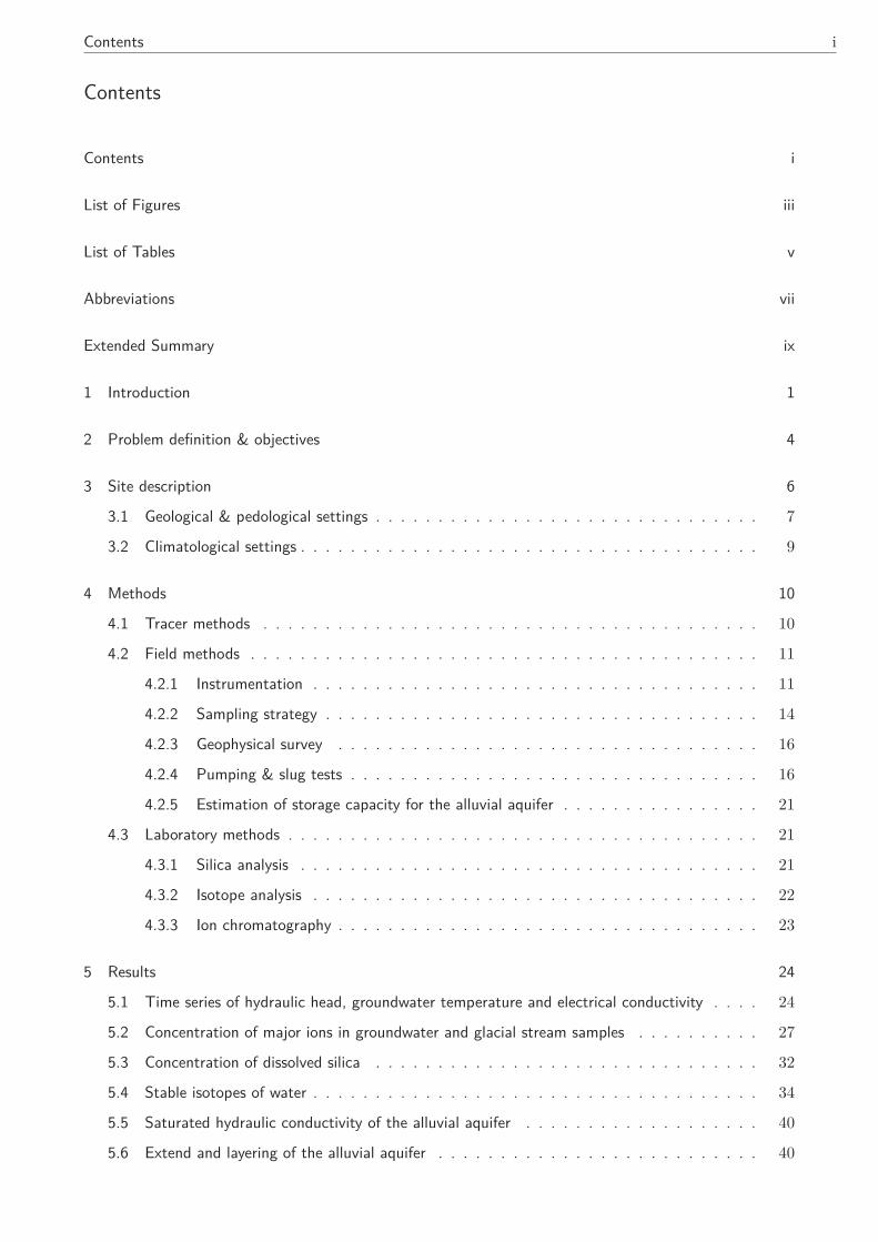
Contents

Contents i

List of Figures iii

List of Tables v

Abbreviations vii

Extended Summary ix

1 Introduction 1

2 Problem definition & objectives 4

3 Site description 6

3.1 Geological & pedological settings . . . . . . . . . . . . . . . . . . . . . . . . . . . . . . . 7

3.2 Climatological settings . . . . . . . . . . . . . . . . . . . . . . . . . . . . . . . . . . . . . 9

4 Methods 10

4.1 Tracer methods . . . . . . . . . . . . . . . . . . . . . . . . . . . . . . . . . . . . . . . . 10

4.2 Field methods . . . . . . . . . . . . . . . . . . . . . . . . . . . . . . . . . . . . . . . . . 11

4.2.1 Instrumentation . . . . . . . . . . . . . . . . . . . . . . . . . . . . . . . . . . . . 11

4.2.2 Sampling strategy . . . . . . . . . . . . . . . . . . . . . . . . . . . . . . . . . . . 14

4.2.3 Geophysical survey . . . . . . . . . . . . . . . . . . . . . . . . . . . . . . . . . . 16

4.2.4 Pumping & slug tests . . . . . . . . . . . . . . . . . . . . . . . . . . . . . . . . . 16

4.2.5 Estimation of storage capacity for the alluvial aquifer . . . . . . . . . . . . . . . . 21

4.3 Laboratory methods . . . . . . . . . . . . . . . . . . . . . . . . . . . . . . . . . . . . . . 21

4.3.1 Silica analysis . . . . . . . . . . . . . . . . . . . . . . . . . . . . . . . . . . . . . 21

4.3.2 Isotope analysis . . . . . . . . . . . . . . . . . . . . . . . . . . . . . . . . . . . . 22

4.3.3 Ion chromatography . . . . . . . . . . . . . . . . . . . . . . . . . . . . . . . . . . 23

5 Results 24

5.1 Time series of hydraulic head, groundwater temperature and electrical conductivity . . . . 24

5.2 Concentration of major ions in groundwater and glacial stream samples . . . . . . . . . . 27

5.3 Concentration of dissolved silica . . . . . . . . . . . . . . . . . . . . . . . . . . . . . . . 32

5.4 Stable isotopes of water . . . . . . . . . . . . . . . . . . . . . . . . . . . . . . . . . . . . 34

5.5 Saturated hydraulic conductivity of the alluvial aquifer . . . . . . . . . . . . . . . . . . . 40

5.6 Extend and layering of the alluvial aquifer . . . . . . . . . . . . . . . . . . . . . . . . . . 40

ii Contents

5.7 Estimated storage capacity for the alluvial aquifer . . . . . . . . . . . . . . . . . . . . . . 42

6 Discussion 43

6.1 Characteristics of the alluvial aquifer . . . . . . . . . . . . . . . . . . . . . . . . . . . . . 43

6.2 Seasonal storage dynamics . . . . . . . . . . . . . . . . . . . . . . . . . . . . . . . . . . 43

6.3 Hydrochemistry . . . . . . . . . . . . . . . . . . . . . . . . . . . . . . . . . . . . . . . . 48

6.4 Relevance of alluvial aquifers for alpine watershed . . . . . . . . . . . . . . . . . . . . . . 49

7 Conclusion 52

7.1 Findings . . . . . . . . . . . . . . . . . . . . . . . . . . . . . . . . . . . . . . . . . . . . 52

7.2 Reflection . . . . . . . . . . . . . . . . . . . . . . . . . . . . . . . . . . . . . . . . . . . 52

References 58

Acknowledgment 59

List of Figures iii

List of Figures

1.1 Altitudinal distribution of runoff-, precipitation- & groundwater gauges in Switzerland com-

pared to hypsography . . . . . . . . . . . . . . . . . . . . . . . . . . . . . . . . . . . . . 2

2.1 Motivation: Results of pilot study (07/2012 - 10/2012) . . . . . . . . . . . . . . . . . . . 4

3.1 Location & catchment area of test site in the Urseren Valley (Canton Uri, Switzerland) . . 6

3.2 Photo of the test site . . . . . . . . . . . . . . . . . . . . . . . . . . . . . . . . . . . . . 7

3.3 Geology for the Furka test site . . . . . . . . . . . . . . . . . . . . . . . . . . . . . . . . 8

3.4 Predicted porous aquifers based on slope for the Furka test site . . . . . . . . . . . . . . . 8

3.5 Mean daily air temperature (Ta) for Tiefenbach floodplain 06/2013 - 11/2014 . . . . . . . 9

4.1 Dimension & filtering of the different monitoring wells and mini-piezometers . . . . . . . . 12

4.2 Location of the monitoring wells & the gauging stations at the test site . . . . . . . . . . 14

4.3 Location & orientation of ERT transects 2012 & 2014 . . . . . . . . . . . . . . . . . . . 16

4.4 Location of slug- and infiltration tests . . . . . . . . . . . . . . . . . . . . . . . . . . . . 17

4.5 Guelph-Permeameter . . . . . . . . . . . . . . . . . . . . . . . . . . . . . . . . . . . . . 18

4.6 Materials for pumping tests . . . . . . . . . . . . . . . . . . . . . . . . . . . . . . . . . . 20

5.1 Time series of hydraulic head (HH), groundwater temperature (TGW ) and electrical con-

ductivity (EC) at 3 different monitoring wells (06/2013 - 10/2014) . . . . . . . . . . . . . 24

5.2 Meltwater lake during snowmelt 2012 . . . . . . . . . . . . . . . . . . . . . . . . . . . . 25

5.3 Time series of monitoring wells compared to the glacial stream (06/2013 - 10/2014) . . . 26

5.4 Correlation between electrical conductivity (EC) & hydraulic head (HH) . . . . . . . . . . 27

5.5 Correlation between electrical conductivity (EC) & major ions at monitoring well GW1 . . 28

5.6 Correlation between electrical conductivity (EC) & major ions at monitoring well GW2 . . 29

5.7 Correlation between electrical conductivity (EC) & hydraulic head (HH) at monitoring well

GW2 divided in summer & winter time . . . . . . . . . . . . . . . . . . . . . . . . . . . . 30

5.8 Correlation between hydraulic head (HH) & groundwater temperature (TGW ) at monitoring

well GW2 divided in summer & winter time . . . . . . . . . . . . . . . . . . . . . . . . . 31

5.9 Range of silica concentration in samples of different water types . . . . . . . . . . . . . . 32

5.10 Evolution of dissolved silica and DE during sampling campaign from 28.08. - 05.09.14 for

monitoring wells GW1 & GW2 . . . . . . . . . . . . . . . . . . . . . . . . . . . . . . . . 33

5.11 Range of oxygen-18 (δ18O) for different water types of test site . . . . . . . . . . . . . . 34

5.12 Range of deuterium excess (DE) for different water types of test site . . . . . . . . . . . . 35

5.13 Relation between deuterium (δ2H) and oxygen-18 (δ18O) of different water types at the

test site (2013 - 2014) . . . . . . . . . . . . . . . . . . . . . . . . . . . . . . . . . . . . 36

5.14 Relation between deuterium excess (DE) and oxygen-18 (δ18O) of different water types at

the test site (2013 - 2014) . . . . . . . . . . . . . . . . . . . . . . . . . . . . . . . . . . 36

iv List of Figures

5.15 Evolution of oxygen-18 (18O) during sampling campaigns 2013 for monitoring wells GW1

& GW2 . . . . . . . . . . . . . . . . . . . . . . . . . . . . . . . . . . . . . . . . . . . . 37

5.16 Evolution of oxygen-18 (18O) during sampling campaigns 2014 for monitoring wells GW1

& GW2 . . . . . . . . . . . . . . . . . . . . . . . . . . . . . . . . . . . . . . . . . . . . 38

5.17 Different isotopic composition at monitoring well GW1 & GW2 . . . . . . . . . . . . . . . 39

5.18 Results of geophysical survey from October 2012 . . . . . . . . . . . . . . . . . . . . . . 41

5.19 Results of geophysical survey from October 2014 . . . . . . . . . . . . . . . . . . . . . . 41

6.1 Seasonal storage dynamics of the alluvial aquifer . . . . . . . . . . . . . . . . . . . . . . . 44

6.2 Schematic representation of the effect of changing porosity with depth on outflow behavior

of the alluvial aquifer . . . . . . . . . . . . . . . . . . . . . . . . . . . . . . . . . . . . . 46

6.3 Schema of reservoirs, processes & regulators for alpine alluvial aquifers . . . . . . . . . . . 47

6.4 Schematic graph showing different water storages in alpine region and their corresponding

time scales . . . . . . . . . . . . . . . . . . . . . . . . . . . . . . . . . . . . . . . . . . . 51

List of Tables v

List of Tables

1.1 Hydrological relevance of the Alps for the major European rivers . . . . . . . . . . . . . . 1

3.1 Climatological settings of the test site . . . . . . . . . . . . . . . . . . . . . . . . . . . . 9

4.1 Properties of the different monitoring wells, mini-piezometers & gauge stations. . . . . . . 13

4.2 Sampling campaigns with automated water samplers on monitoring wells GW1 & GW2 . . 15

5.1 Results from ion chromatography for the soil sample next to monitoring well GW1 . . . . 29

5.2 Mean δ18O and DE values for all monitoring wells . . . . . . . . . . . . . . . . . . . . . . 39

5.3 Saturated hydraulic conductivity at the test site . . . . . . . . . . . . . . . . . . . . . . . 40

5.4 Estimated water storage volume of the alluvial aquifer . . . . . . . . . . . . . . . . . . . . 42

6.1 Estimated groundwater level decrease for providing low flow in different time scales . . . . 50

Abbreviations vii

Abbreviations

Symbol Unit Description

BF Base flow

CTD sensor Sensor for conductivity, temperature & depth (pressure)

DE Deuterium excess

EC mS/cm Electrical conductivity

ERT Electrical resistivity tomography

GIUZ Departement of Geography, University of Zürich

GL m a.s.l. Ground level

GMWL Global meteoric water line

GW Groundwater

HDPE High density polyethylene

HH m Hydraulic head

Ksat m/s Saturated hydraulic conductivity

LIA Little Ice Age (End 1850)

LMWL Local meteoric water line

MAAT ◦C Mean annual air temperature

MDAT ◦C Mean daily air temperature

MWL Melt water lake (Exfiltration of GW in snowcover)

PTFE Polytetrafluorethylene

r2 Correlation coefficient

SLF WSL Institute of Snow and Avalanche Research SLF

SOF Saturated overland flow

SWE mm Snow water equivalent

Ta ◦C Air temperature

TGW ◦C Groundwater temperature

TW ◦C Water temperature

TOW Top of well

VSMOW Vienna standard mean ocean water

WPW Water-level proportional water sampler2H δ VSMOV Deuterium18O δ VSMOV Oxygen-18

Extended Summary ix

Extended Summary

Groundwater recharge, storage dynamics and groundwater quality were investigated for an alpine allu-

vial aquifer in the catchment of the Tiefenbach in Central Swiss Alps. The aquifer is a sediment-filled

overdeeping formed by the Tiefengletscher during the Little Ice Age. Geophysical measurements indi-

cate an aquifer geometry of 140 x 160 m with a depth up to 20 m. Water level, water temperature and

electrical conductivity were measured continuously at several monitoring wells. The aquifer shows a

constant, nearly linear decrease during the winter month. During the snowmelt, the aquifer becomes

completely filled indicating the snowmelt as the dominating recharge source. The groundwater even

exfiltrates into the snowpack. Summer month show frequent fluctuations in water level. Rising water

level into the unsaturated zone affects high variability in hydrochemistry. Furthermore two different

flow systems with different recharges within the aquifer could be detected. Groundwater temperatures

show a strong increase up to 10 ◦C immediately after the aquifer becomes snow free due to the shallow

soils and the strong radiation input.

Keywords

alpine groundwater, water storage, alluvial aquifer, groundwater recharge, groundwater quality, ground-

water quantity

Zusammenfassung

Im Einzugsgebiet des Tiefenbaches in den Schweizer Zentralalpen wurde ein alluvialer Aquifer hin-

sichtlich Grundwasserneubildung, Speicherdynamiken und Grundwasserqualität untersucht. Der Grund-

wasserspeicher ist eine mit Sedimenten gefüllte Geländeübertiefung, die durch den Tiefengletscher

während der letzen kleinen Eiszeit entstanden ist. Die Ausdehnung des Aquifers konnte mittels geo-

physikalischer Untersuchungen auf etwa 140 x 160 m und einer Tiefe von 20 m bestimmt werden.

An mehreren Beobachtungsbrunnen wurden der Wasserstand, die Wassertemperatur sowie die elek-

trische Leitfähigkeit kontinuirlich gemessen. Während der Wintermonate zeigte der Aquifer eine kon-

stante, nahezu lineare Abnahme im Wasserstand. Im Verlauf der Schneeschmelze wurde der Aquifer

wieder komplett aufgefüllt. Dies deutet daraufhin, dass die Schneeschmelze den größten Anteil zur

Grundwasserneubildung beiträgt. Der Grundwasserspiegel steigt sogar bis in die noch vorhandene

Schneedecke an. Während der Sommermonate konnten sehr variable Grundwasserstände festgestellt

werden. Ein Anstieg des Wasserspiegels in die ungesättigte Zone scheint Auswirkungen auf die Hydro-

chemie zu haben. Desweiteren konnten zwei verschiedene Fließsysteme identifiziert werden. Aufgrund

der geringmächtigen Böden und dem direkten Strahlungeinfluss stieg die Grundwassertemperatur so-

fort nach der Schneeschmelze auf bis zu 10 ◦C an.

1 Introduction 1

1 Introduction

Mountains are often called the world’s natural "water towers", as they play an important role in the

water cycle. Especially alpine regions, such as the European Alps, contribute overproportionately

high runoff (Viviroli et al. 2003, Viviroli & Weingartner 2004). The European Alps also form the

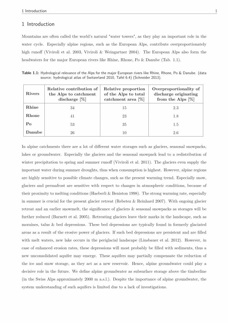
headwaters for the major European rivers like Rhine, Rhone, Po & Danube (Tab. 1.1).

Table 1.1: Hydrological relevance of the Alps for the major European rivers like Rhine, Rhone, Po & Danube. (datasource: hydrological atlas of Switzerland 2010, Tafel 6.4) (Schneider 2013).

RiversRelative contribution ofthe Alps to catchment

discharge [%]

Relative proportionof the Alps to totalcatchment area [%]

Overproportionality ofdischarge originating

from the Alps [%]

Rhine 34 15 2.3

Rhone 41 23 1.8

Po 53 35 1.5

Danube 26 10 2.6

In alpine catchments there are a lot of different water storages such as glaciers, seasonal snowpacks,

lakes or groundwater. Especially the glaciers and the seasonal snowpack lead to a redistribution of

winter precipitation to spring and summer runoff (Viviroli et al. 2011). The glaciers even supply the

important water during summer droughts, thus when consumption is highest. However, alpine regions

are highly sensitive to possible climate changes, such as the present warming trend. Especially snow,

glaciers and permafrost are sensitive with respect to changes in atmospheric conditions, because of

their proximity to melting conditions (Haeberli & Beniston 1998). The strong warming rate, especially

in summer is crucial for the present glacier retreat (Rebetez & Reinhard 2007). With ongoing glacier

retreat and an earlier snowmelt, the significance of glaciers & seasonal snowpacks as storages will be

further reduced (Barnett et al. 2005). Retreating glaciers leave their marks in the landscape, such as

moraines, talus & bed depressions. These bed depressions are typically found in formerly glaciated

areas as a result of the erosive power of glaciers. If such bed depressions are persistent and are filled

with melt waters, new lake occurs in the periglacial landscape (Linsbauer et al. 2012). However, in

case of enhanced erosion rates, these depressions will most probably be filled with sediments, thus a

new unconsolidated aquifer may emerge. These aquifers may partially compensate the reduction of

the ice and snow storage, as they act as a new reservoir. Hence, alpine groundwater could play a

decisive role in the future. We define alpine groundwater as subsurface storage above the timberline

(in the Swiss Alps approximately 2000 m a.s.l.). Despite the importance of alpine groundwater, the

system understanding of such aquifers is limited due to a lack of investigations.

2 1 Introduction

Most studies are focused on a single aspect of the hydrological cycle, such as glacier mass balance

or snow accumulation and melt (Hood & Hayashi 2015). Moreover, only 3 % of the hydrogeological

publications have a direct link to the alpine region and only a few of them are focusing on alpine hydro-

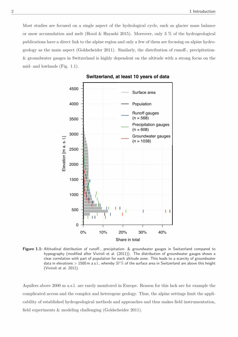
geology as the main aspect (Goldscheider 2011). Similarly, the distribution of runoff-, precipitation-

& groundwater gauges in Switzerland is highly dependent on the altitude with a strong focus on the

mid- and lowlands (Fig. 1.1).

0% 10% 20% 30% 40%

0

500

1000

1500

2000

2500

3000

3500

4000

4500

Share in total

Ele

vatio

n [m

a. s

. l.]

Surface area

Population

Runoff gauges(n = 568)

Precipitation gauges(n = 608)

Groundwater gauges(n = 1038)

Switzerland, at least 10 years of data

Figure 1.1: Altitudinal distribution of runoff-, precipitation- & groundwater gauges in Switzerland compared tohypsography (modified after Viviroli et al. (2011)). The distribution of groundwater gauges shows aclear correlation with part of population for each altitude zone. This leads to a scarcity of groundwaterdata in elevations > 1500 m a.s.l., whereby 37 % of the surface area in Switzerland are above this height(Viviroli et al. 2011).

Aquifers above 2000 m a.s.l. are rarely monitored in Europe. Reason for this lack are for example the

complicated access and the complex and heterogene geology. Thus, the alpine settings limit the appli-

cability of established hydrogeological methods and approaches and thus makes field instrumentation,

field experiments & modeling challenging (Goldscheider 2011).

1 Introduction 3

In addition, a long and cold winter season challenges instrumentation and limits time for field ex-

periments. In alpine regions, recent unconsolidated sediments are typically coarse and poorly sorted

(e.g. talus, moraines & alluvial deposits). The coarser sediments and the steep slopes also led to the

assumption that the water storage capacity in alpine regions is negligible (Clow et al. 2003). Ground-

water recharge and seasonal storage of aquifers in alpine terrain is typically neglected in hydrological

models (Schneider 2013). As already mentioned above, the retreat of the glaciers can induce new

groundwater reservoirs. These storages can be moraines, talus or alluvial aquifers. Clow et al. (2003)

found that for an alpine watershed in the Rocky Mountains, talus fields can contribute more than 75 %

to streamflow during the fall and winter base flow period. Talus slopes are the primary groundwater

storage at that site, having a maximum storage capacity approximately equal to that of total annual

discharge from the catchment. Hood & Hayashi (2015) found similar groundwater storage capacities

for an alpine watershed in British Columbia, Canada. McClymont et al. (2010) studied an alpine

meadow-talus complex, getting annual recharge from snowmelt and rainfall which is several times

higher than the storage capacity. Roy & Hayashi (2008) found, that talus fields and moraines which

are in contact with lake shores affect substantial the groundwater exchange with the lakes. The hydro-

logical importance of an alpine alluvial aquifer for flood-buffering and storage is highlighted in Lauber

et al. (2014). Ofterdinger et al. (2004) investigated deep groundwater in fractured granite, sampling

groundwater in the Bedretto Tunnel, which goes through the granite body of the western Gotthard

Massif. They found, that accumulated winter precipitation and glacial meltwater may contribute sig-

nificantly to recharge of deep groundwater. Due to the scarcity of field studies and their data from

alpine groundwater reservoirs, it is challenging to integrate these reservoirs into hydrological models

(Tague & Grant 2009). Roy & Hayashi (2009) found multiple distinctive groundwater flow systems

within a single moraine-talus field. Thus, it is maybe necessary to use more complex structures within

hydrological models. Magnusson et al. (2012) investigated stream-groundwater interactions on the ad-

jacent glacier forefield of Dammagletscher. They determined daily fluctuations in groundwater levels

as well as slowly declines over the season. A diffusion model was used to describe the groundwater

fluctuations, but the result highlights, that further work is needed to improve the calibration for such

heterogeneous field sites like glacier forefields.

All these studies highlight, that alpine groundwater reservoirs may affect significantly the waterbalance

of alpine watersheds. It becomes also evident, that the groundwater storages are highly heterogeneous.

Therefore, the implication of alpine groundwater reservoirs in hydrological models is considerably more

challenging than for most of the lowlands. To our knowledge, none of these studies measured contin-

uously groundwater level fluctuations as well as the electrical conductivity for an alpine groundwater

reservoir throughout the winter season. Thus, to improve the understanding of processes and impacts

of climate change on alpine water resources, more detailed studies are needed.

4 2 Problem definition & objectives

2 Problem definition & objectives

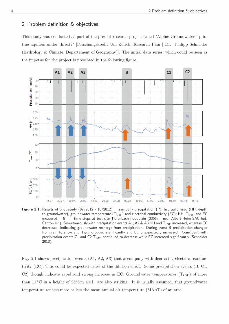
This study was conducted as part of the present research project called "Alpine Groundwater - pris-

tine aquifers under threat?" [Forschungskredit Uni Zürich, Research Plan | Dr. Philipp Schneider

(Hydrology & Climate, Departement of Geography)]. The initial data series, which could be seen as

the impetus for the project is presented in the following figure.

A1 C1 C2 A2 A3 B

Figure 2.1: Results of pilot study (07/2012 - 10/2012): mean daily precipitation (P), hydraulic head (HH, depthto groundwater), groundwater temperature (TGW ) and electrical conductivity (EC); HH, TGW and ECmeasured in 5 min time steps at test site Tiefenbach floodplain (2365 m, near Albert-Heim SAC hut,Canton Uri). Simultaneously with precipitation events A1, A2 & A3 HH and TGW increased, whereas ECdecreased, indicating groundwater recharge from precipitation. During event B precipitation changedfrom rain to snow and TGW dropped significantly and EC unexpectedly increased. Coincident withprecipitation events C1 and C2 TGW continued to decrease while EC increased significantly (Schneider2013).

Fig. 2.1 shows precipitation events (A1, A2, A3) that accompany with decreasing electrical conduc-

tivity (EC). This could be expected cause of the dilution effect. Some precipitation events (B, C1,

C2) though indicate rapid and strong increase in EC. Groundwater temperatures (TGW ) of more

than 11 ◦C in a height of 2365 m a.s.l. are also striking. It is usually assumed, that groundwater

temperature reflects more or less the mean annual air temperature (MAAT) of an area.

2 Problem definition & objectives 5

Because of the sparse instrumentation of these remote areas, this project can be seen as a first pilot

study of alpine porous aquifer observations. The aim of the project is to get a better understanding

and conceptualization of processes and reservoirs in alpine terrain to predict the impact of a melting

cryosphere on alpine water quality and quantity (Schneider 2013).

The main questions of this thesis are:

1. How do snowmelt, glacial stream and summer precipitation contribute to groundwater recharge?

2. Does the water level fluctuations affect the high variations in electrical conductivity?

3. What is the reason for such high groundwater temperatures?

4. Is it possible, that alpine porous aquifers may compensate the reduction of the glacier contribution

to low flows in alpine watersheds?

6 3 Site description

3 Site description

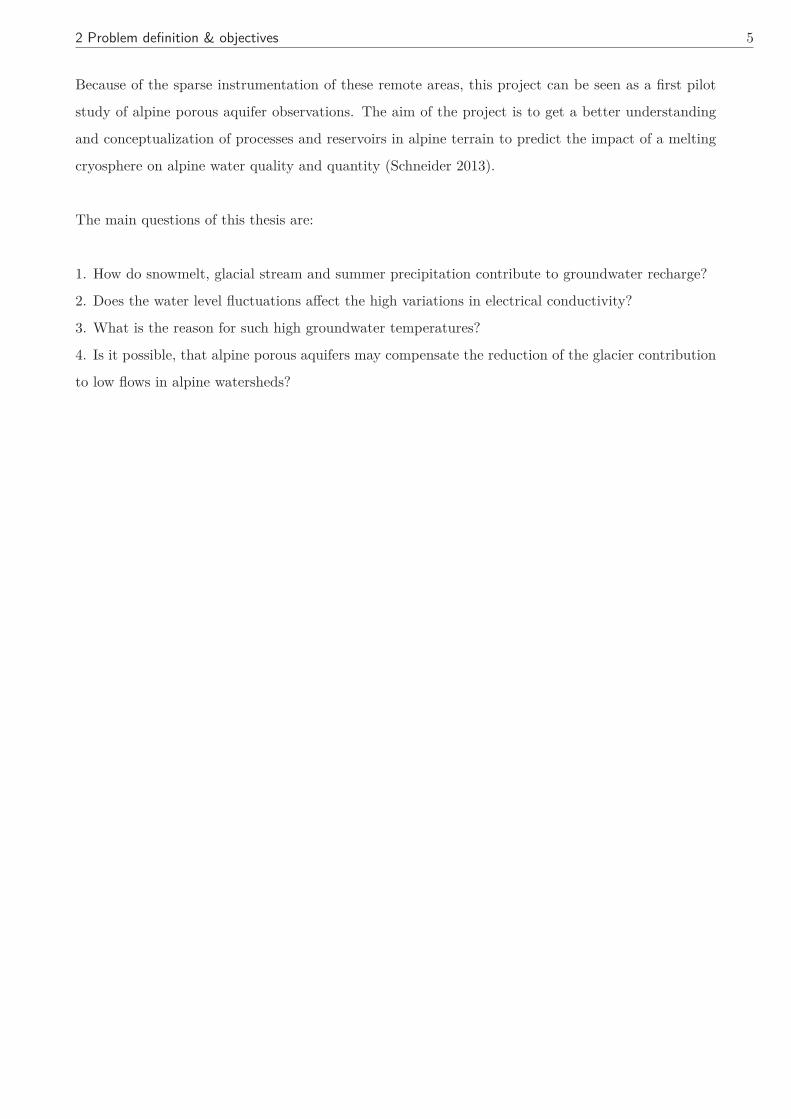
The study catchment is located near the Furka pass road in the upper Urseren Valley (Canton Uri)

in the Central Swiss Alps (Fig. 3.1).

2.17 km2

6.3 km2

674000

674000

675000

675000

676000

676000

677000

677000

678000

678000

679000

679000

680000

680000

1610

00

1610

00

1620

00

1620

00

1630

00

1630

00

1640

00

1640

00

1650

00

1650

00

Tiefenbach 2363m

Tiefenbach 2120m7.34 km2

Lochbergbach

Figure 3.1: Location of test site in the Urseren Valley (Canton Uri, Switzerland) (left corner) and the catchmentarea (6.3 km2) of the test site (red colored). The black circle shows the test site and the correspondingcatchment outlet (2362.44 m a.s.l.) is symbolized with a red point. The catchment area is bordering thecatchment of Lochbergbach in east, Dammagletscher in north and Rhonegletscher in west (Schneider &Lange (2014)).

The catchment area is about 6.3 km2, with altitudes ranging from 2365 to 3586 m a.s.l. (Galenstock).

The catchment area borders the catchment of Lochbergbach in east, Dammagletscher in north and

Rhonegletscher in west. The present-day ice cover is about 40 %, whereby the Tiefengletscher has

retreated continuously since the Little Ice Age (LIA) in 1850 (Moll 2012). Its meltwater is collected by

the Tiefenbach, which drains into the Furkareuss, a tributary of the Reuss river. At the catchment we

focused on a sediment-filled depression formed during the LIA at 2365 m a.s.l., about 1 km downstream

of the glacier snout (black circle in Fig. 3.1). This sediment-filled depression constitute an alluvial

aquifer, where still active deposition through the glacial stream is ongoing. The results from a first

geophysical survey in 2012 with electrical resistivity tomography (ERT) show, that this alluvial aquifer

is about 20 m deep, 140 wide and 160 long. The alpine terrain is dominated by glacial moraine and

alluvial deposits, talus and exposed bedrock (see Fig. 3.2).


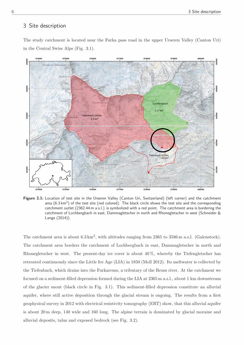
Figure 3.2: Photo of the test site. The photo is taken from end moraine of the LIA facing to north-west. The flood-plain with our instrumentation is visible on the right site. In the background there is the Tiefengletscherand the Galenstock (3586 m a.s.l.), which is the highest point in the catchment. The glacial streamflows through the center of the image. (photo: Schneider, 2013)

This photo shows the terrain of test site. In the foreground you can see part of the end moraine from

the LIA. On the right side you can see the floodplain with some of the instrumentation. The glacial

stream flows through the center of the image, originating at the Tiefengletscher, which can be seen at

the background.

3.1 Geological & pedological settings

The study catchment is situated on the crystalline Aar massif. The dominating rock type is the Central

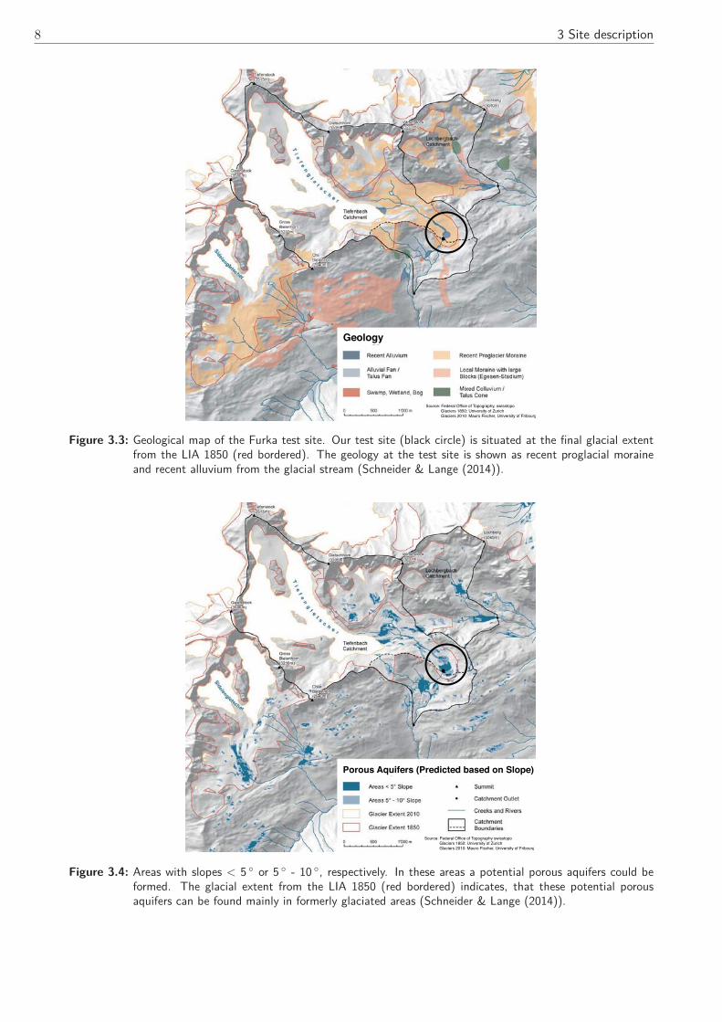
Aar Granite (Hosein et al. 2004). Fig. 3.3 represents the geology of the test site. The floodplain is

characterized through alluvial depositions (still present). Due to the height about 2000 m and the

sparse vegetation, the soils are very thin. According to the World Reference Base for Soil Resources

(WRB 2006) the soils at Tiefenbach floodplain could be classified as Hyperskeletic Leptosols. Fig. 3.4

highlights areas with slopes < 5 ◦ respectively 5 ◦ - 10 ◦. It can be noticed, that areas with slopes <

5 % can be often detected in formerly glaciated areas. These aquifers are mostly sediment filled bed

depressions. These depressions are a result of the erosive power of glaciers (Linsbauer et al. 2012).

8 3 Site description

Source: Federal Office of Topography, swisstopo Glaciers 1850: University of Zurich Glaciers 2010: Mauro Fischer, University of Fribourg

Geology

Figure 3.3: Geological map of the Furka test site. Our test site (black circle) is situated at the final glacial extentfrom the LIA 1850 (red bordered). The geology at the test site is shown as recent proglacial moraineand recent alluvium from the glacial stream (Schneider & Lange (2014)).

Source: Federal Office of Topography swisstopo Glaciers 1850: University of Zurich Glaciers 2010: Mauro Fischer, University of Fribourg

Porous Aquifers (Predicted based on Slope)

Figure 3.4: Areas with slopes < 5 ◦ or 5 ◦ - 10 ◦, respectively. In these areas a potential porous aquifers could beformed. The glacial extent from the LIA 1850 (red bordered) indicates, that these potential porousaquifers can be found mainly in formerly glaciated areas (Schneider & Lange (2014)).


3.2 Climatological settings

According to the Hydrological Atlas of Switzerland (2010), the mean annual precipitation amount for

the period 1951 - 1980 is about 2800 - 3200 mm, whereas the mean annual evaporation is about 200 -

300 mm. The flow-regime can be regarded as a-glacio-nival. The floodplain is typically covered with

snow for around 7 - 8 months of the year.

−16

−12

−8

−4

0

4

8

12

16

Jun Jul Aug Sep Okt Nov Dez Jan Feb Mrz Apr Mai Jun Jul Aug Sep Okt Nov Dez

T a [°

C]

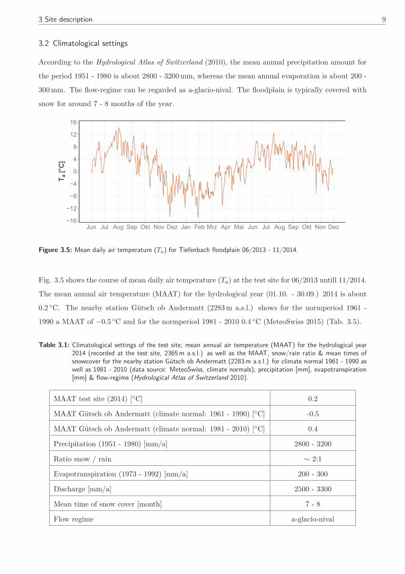
Figure 3.5: Mean daily air temperature (Ta) for Tiefenbach floodplain 06/2013 - 11/2014.

Fig. 3.5 shows the course of mean daily air temperature (Ta) at the test site for 06/2013 untill 11/2014.

The mean annual air temperature (MAAT) for the hydrological year (01.10. - 30.09.) 2014 is about

0.2 ◦C. The nearby station Gütsch ob Andermatt (2283 m a.s.l.) shows for the normperiod 1961 -

1990 a MAAT of −0.5 ◦C and for the normperiod 1981 - 2010 0.4 ◦C (MeteoSwiss 2015) (Tab. 3.5).

Table 3.1: Climatological settings of the test site; mean annual air temperature (MAAT) for the hydrological year2014 (recorded at the test site, 2365 m a.s.l.) as well as the MAAT, snow/rain ratio & mean times ofsnowcover for the nearby station Gütsch ob Andermatt (2283 m a.s.l.) for climate normal 1961 - 1990 aswell as 1981 - 2010 (data source: MeteoSwiss, climate normals); precipitation [mm], evapotranspiration[mm] & flow-regime (Hydrological Atlas of Switzerland 2010).

MAAT test site (2014) [◦C] 0.2

MAAT Gütsch ob Andermatt (climate normal: 1961 - 1990) [◦C] -0.5

MAAT Gütsch ob Andermatt (climate normal: 1981 - 2010) [◦C] 0.4

Precipitation (1951 - 1980) [mm/a] 2800 - 3200

Ratio snow / rain ∼ 2:1

Evapotranspiration (1973 - 1992) [mm/a] 200 - 300

Discharge [mm/a] 2500 - 3300

Mean time of snow cover [month] 7 - 8

Flow regime a-glacio-nival

10 4 Methods

4 Methods

4.1 Tracer methods

Different major ions, silica as well as the stable isotopes of water oxygen-18 (18O) and deuterium (2H)

were used as tracers. These methods will be presented in the following section.

Major ions

Major ions are, as well as silica, often used as a geochemical tracer. They are primarily used to

determine the fraction of water flowing along different subsurface flow paths (Kalbus et al. 2006). In

this study, major ions were used to identify the reason for the high fluctuations in EC.

Silica

Dissolved silicic acid is a often used geogenic tracer in hydrology. Based on this it is possible to

estimate the origin and resistance time of water. During silicate weathering silicic acid gets constantly

free and will be solved in the water. The longer water is in contact with the rock, the higher the

concentration of dissolved silicic acid. With the analysis of silica it is also possible to define melt- or

event water from the base flow, because silica occurs in precipitation only in very small concentrations

(Wels et al. 1991, Kienzler 2001).

Stable isotopes

In hydrology the stable isotopes of water, deuterium (2H) and oxygen-18 (18O), play a decisive role.

Since they are a natural part of the water molecule, they can be regarded as an ideal hydrological tracer

(Moser et al. 1980, Leibundgut & Seibert 2011). The different atomic mass and physical properties of

the different isotopes causes an isotopic fractionation during physical processes, such as evaporation,

condensation and freezing. That means, that the isotopic ratio changes over time of the process. By

measuring the isotope ratios 18O / 16O and 2H / 1H it is possible to draw conclusions on the origin

and age or residence time of the water. Another important parameter in addition to the 18O and 2H

values is the deuterium excess (DE). It represents the ratio of the two stable isotopes to each other.

Comparing global isotope samples with each other, it is evident that 18O and 2H are in a certain ratio

to each other. If you plot 18O against 2H, then all the values plot approximately on a straight line,

called Global Meteoric Water Line (GMWL). According to Craig (1961), the relation between 18O

and 2H can be described as follows:

δD = 8 · δ18O + 10 (1)

4 Methods 11

Due to local climatic conditions, e.g. high evaporation rates, and the different origins of the precip-

itation, a deviation from the GMWL can occur. This deviated line is called Local Meteoric Water

Line (LMWL). Furthermore, it is possible to detect different effects based on the global distribution

of the isotope ratios (Kendall & McDonnell 1998). The preferred condensation of heavier isotopes

leads to a progressing depletion of the heavy isotopes during a precipitation event. The precipitation

thus will become isotopic lighter with increasing duration of the precipitation event (amount effect).

The higher the temperature, the isotopic heavier the precipitation. This is not only important during

condensation - i.e. the precipitation event itself - but also during the evaporation. Humid air masses

that come from lower latitudes are in fact of that isotopic heavier than those formed at higher lati-

tudes. In addition to the temperature, the humidity at the point of origin plays a decisive role as well

(Jouzel & Merlivat 1984) (temperature/latitude effect). Additionally, increasing altitude lead to a

depletion of the heavy isotopes, because they condense first (altitude effect). This could be explained

by the cooling of the rising air masses and with increasing precipitation amount upwards. Therefrom

it represents a combination of amount and temperature effect. Schürch et al. (2003) found an average

decrease of 18O in precipitation for the Swiss Alps of about 0.2 � / 100 m. According to the amount

and altitude effect it is possible to describe the continental effect. The humid air masses formed over

the oceans are first depleted of heavy isotopes in the course of their journey across the continental

landmass. Thus, the precipitation with increasing distance to the source is isotopic lighter (Kendall

& McDonnell 1998, Moser et al. 1980). Since the isotopic composition of the water differs around the

world, a reference standard, called VSMOW (Vienna Standard Mean Ocean Water) was introduced.

The VSMOW is based on a mixture of several ocean samples and thus represents a uniform reference

against which waters of different composition can be compared.

4.2 Field methods

4.2.1 Instrumentation

Water level, water temperature and electrical conductivity (EC) were measured at seven ground-

water monitoring wells (15 min interval) and three discharge stations (5 min interval) using online

CTD-sensors (conductivity, temperature, depth) from HT-Hydrotechnik GmbH (HT). These sensors

measured electrical conductivity (accuracy < 1 %), water temperature (accuracy < 1 ◦C) and pressure

(accuracy < 0.05 %). The wells consisted partly of HDPE, some of stainless steel and one older one of

steel, extending to depths between 0 to 1 m and 2 to 3 m (Fig. 4.1). The sites for the monitoring wells

GW1, GW2 & GW3 were selected in such a way that they build an hydrological triangle (see Fig.

4.2). GW2 is located in a depression (2365.05 m a.s.l.), which can easily be distinguished based on the

vegetation, because it is saturated almost the whole summer period. In contrast, GW1 is located on

a small rise (2365.7 m a.s.l.).

12 4 Methods

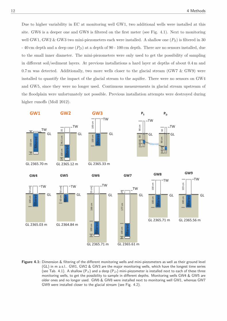
Due to higher variability in EC at monitoring well GW1, two additional wells were installed at this

site. GW6 is a deeper one and GW8 is filtered on the first meter (see Fig. 4.1). Next to monitoring

well GW1, GW2 & GW3 two mini-piezometers each were installed. A shallow one (PS) is filtered in 30

- 40 cm depth and a deep one (PD) at a depth of 90 - 100 cm depth. There are no sensors installed, due

to the small inner diameter. The mini-piezometers were only used to get the possibility of sampling

in different soil/sediment layers. At previous installations a hard layer at depths of about 0.4 m and

0.7 m was detected. Additionally, two more wells closer to the glacial stream (GW7 & GW9) were

installed to quantify the impact of the glacial stream to the aquifer. There were no sensors on GW4

and GW5, since they were no longer used. Continuous measurements in glacial stream upstream of

the floodplain were unfortunately not possible. Previous installation attempts were destroyed during

higher runoffs (Moll 2012).

filte

red

GL TW 8

150

cm

10

801

GL 2365.70 m

GW1

filte

red

GL

35

100

cm

20 02

TW

d96

.5 c

m

GL 2365.12 m

GW2

filte

red GL

100

cm

100

cm

TW

GL 2365.33 m

GW3

GL

55 c

m

100

cm

10

m01

TW

166

cm

filte

red

GL 2365.71 m

GW6

GL

23

100

cm

3

TW

177

cm

filte

red

GL 2365.61 m

GW7

filte

red GL

100

cm

100

cm

TW

GL 2365.71 m

GW8

GL 2365.56 m

GW9

filte

red GL

103

cm

100

cm

TW

GL 90

cm

30

TW

10

10

GL

90 c

m

30 TW

10 1

0 1

PS PD

filtered ff

00

d

10

filte

red GL

50 c

m

100

cm

m TW

GL 2365.03 m

GW4

filte

r GL

50 c

m

50 c

m

m TW

GL 2364.84 m

GW5

Figure 4.1: Dimension & filtering of the different monitoring wells and mini-piezometers as well as their ground level(GL) in m a.s.l.. GW1, GW2 & GW3 are the major monitoring wells, which have the longest time series(see Tab. 4.1). A shallow (PS) and a deep (PD) mini-piezometer is installed next to each of these threemonitoring wells, to get the possibility to sample in different depths. Monitoring wells GW4 & GW5 areolder ones and no longer used. GW6 & GW8 were installed next to monitoring well GW1, whereas GW7GW9 were installed closer to the glacial stream (see Fig. 4.2).

4 Methods 13

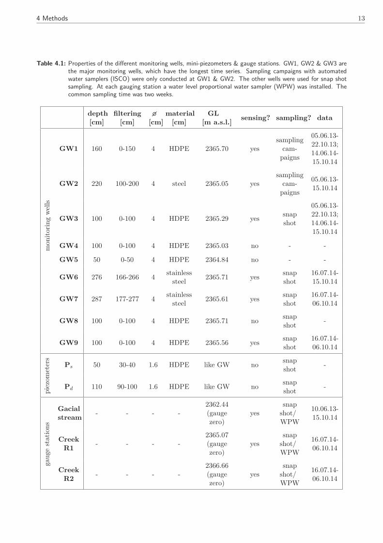
Table 4.1: Properties of the different monitoring wells, mini-piezometers & gauge stations. GW1, GW2 & GW3 arethe major monitoring wells, which have the longest time series. Sampling campaigns with automatedwater samplers (ISCO) were only conducted at GW1 & GW2. The other wells were used for snap shotsampling. At each gauging station a water level proportional water sampler (WPW) was installed. Thecommon sampling time was two weeks.

depth[cm]

filtering[cm]

�[cm]

material[cm]

GL[m a.s.l.] sensing? sampling? data

mon

itor

ing

wel

ls

GW1 160 0-150 4 HDPE 2365.70 yessampling

cam-paigns

05.06.13-22.10.13;14.06.14-15.10.14

GW2 220 100-200 4 steel 2365.05 yessampling

cam-paigns

05.06.13-15.10.14

GW3 100 0-100 4 HDPE 2365.29 yes snapshot

05.06.13-22.10.13;14.06.14-15.10.14

GW4 100 0-100 4 HDPE 2365.03 no - -

GW5 50 0-50 4 HDPE 2364.84 no - -

GW6 276 166-266 4 stainlesssteel 2365.71 yes snap

shot16.07.14-15.10.14

GW7 287 177-277 4 stainlesssteel 2365.61 yes snap

shot16.07.14-06.10.14

GW8 100 0-100 4 HDPE 2365.71 no snapshot -

GW9 100 0-100 4 HDPE 2365.56 yes snapshot

16.07.14-06.10.14

piez

omet

ers

Ps 50 30-40 1.6 HDPE like GW no snapshot -

Pd 110 90-100 1.6 HDPE like GW no snapshot -

gaug

est

atio

ns

Gacialstream - - - -

2362.44(gaugezero)

yessnap

shot/WPW

10.06.13-15.10.14

CreekR1 - - - -

2365.07(gaugezero)

yessnap

shot/WPW

16.07.14-06.10.14

CreekR2 - - - -

2366.66(gaugezero)

yessnap

shot/WPW

16.07.14-06.10.14

14 4 Methods

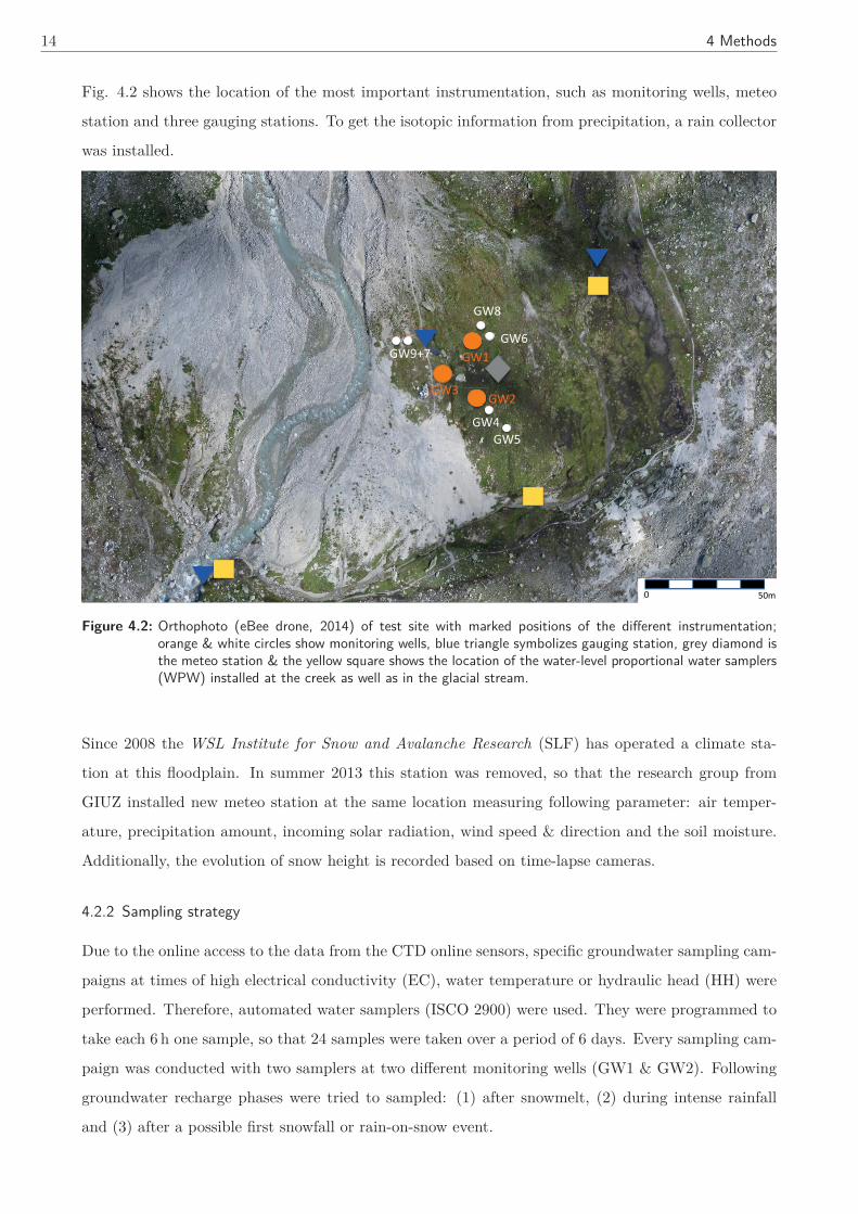
Fig. 4.2 shows the location of the most important instrumentation, such as monitoring wells, meteo

station and three gauging stations. To get the isotopic information from precipitation, a rain collector

was installed.

Figure 4.2: Orthophoto (eBee drone, 2014) of test site with marked positions of the different instrumentation;orange & white circles show monitoring wells, blue triangle symbolizes gauging station, grey diamond isthe meteo station & the yellow square shows the location of the water-level proportional water samplers(WPW) installed at the creek as well as in the glacial stream.

Since 2008 the WSL Institute for Snow and Avalanche Research (SLF) has operated a climate sta-

tion at this floodplain. In summer 2013 this station was removed, so that the research group from

GIUZ installed new meteo station at the same location measuring following parameter: air temper-

ature, precipitation amount, incoming solar radiation, wind speed & direction and the soil moisture.

Additionally, the evolution of snow height is recorded based on time-lapse cameras.

4.2.2 Sampling strategy

Due to the online access to the data from the CTD online sensors, specific groundwater sampling cam-

paigns at times of high electrical conductivity (EC), water temperature or hydraulic head (HH) were

performed. Therefore, automated water samplers (ISCO 2900) were used. They were programmed to

take each 6 h one sample, so that 24 samples were taken over a period of 6 days. Every sampling cam-

paign was conducted with two samplers at two different monitoring wells (GW1 & GW2). Following

groundwater recharge phases were tried to sampled: (1) after snowmelt, (2) during intense rainfall

and (3) after a possible first snowfall or rain-on-snow event.

4 Methods 15

Furthermore, manual groundwater, snow and glacial stream samples were collected. Wells were

pumped dry using a vacuum pump prior to sampling. In addition to the event & continuous sampling,

a snap-shot manual sampling every mid-august was conducted since 2012. Precipitation samples were

taken with a rain collector installed on the floodplain, which emptied approximately every two weeks.

Additionally, the hut warden of the Albert-Heim hut took a sample if the precipitation was more than

20 mm/d. To measure the isotopic and hydrochemical signal in the glacial stream and the small creeks

which goes through the floodplain, a water-level proportional water sampler (WPW) was installed at

each gauging station. These samplers use the law of Hagen-Poiseuille, where a capillary (or a valve)

controls the sampling aliquot per time by regulating the air flux out of a submersed plastic (HDPE)

sampling container (Schneider et al. (in prep.)). This allows us to take water-level proportional sam-

ples over a period of 2 weeks. An overview of all the campaigns with an automatic water sampler is

presented in Tab. 4.2.

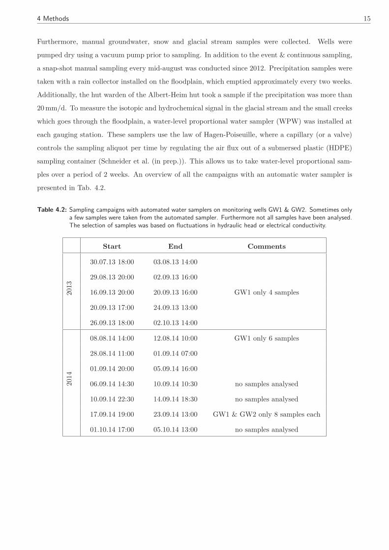
Table 4.2: Sampling campaigns with automated water samplers on monitoring wells GW1 & GW2. Sometimes onlya few samples were taken from the automated sampler. Furthermore not all samples have been analysed.The selection of samples was based on fluctuations in hydraulic head or electrical conductivity.

Start End Comments

2013

30.07.13 18:00 03.08.13 14:00

29.08.13 20:00 02.09.13 16:00

16.09.13 20:00 20.09.13 16:00 GW1 only 4 samples

20.09.13 17:00 24.09.13 13:00

26.09.13 18:00 02.10.13 14:00

2014

08.08.14 14:00 12.08.14 10:00 GW1 only 6 samples

28.08.14 11:00 01.09.14 07:00

01.09.14 20:00 05.09.14 16:00

06.09.14 14:30 10.09.14 10:30 no samples analysed


17.09.14 19:00 23.09.14 13:00 GW1 & GW2 only 8 samples each


16 4 Methods

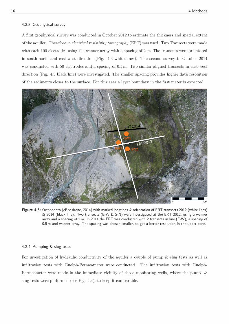
4.2.3 Geophysical survey

A first geophysical survey was conducted in October 2012 to estimate the thickness and spatial extent

of the aquifer. Therefore, a electrical resistivity tomography (ERT) was used. Two Transects were made

with each 100 electrodes using the wenner array with a spacing of 2 m. The transects were orientated

in south-north and east-west direction (Fig. 4.3 white lines). The second survey in October 2014

was conducted with 50 electrodes and a spacing of 0.5 m. Two similar aligned transects in east-west

direction (Fig. 4.3 black line) were investigated. The smaller spacing provides higher data resolution

of the sediments closer to the surface. For this area a layer boundary in the first meter is expected.

Figure 4.3: Orthophoto (eBee drone, 2014) with marked locations & orientation of ERT transects 2012 (white lines)& 2014 (black line). Two transects (E-W & S-N) were investigated at the ERT 2012, using a wennerarray and a spacing of 2 m. In 2014 the ERT was conducted with 2 transects in line (E-W), a spacing of0.5 m and wenner array. The spacing was chosen smaller, to get a better resolution in the upper zone.

4.2.4 Pumping & slug tests

For investigation of hydraulic conductivity of the aquifer a couple of pump & slug tests as well as

infiltration tests with Guelph-Permeameter were conducted. The infiltration tests with Guelph-

Permeameter were made in the immediate vicinity of those monitoring wells, where the pump- &

slug tests were performed (see Fig. 4.4), to keep it comparable.

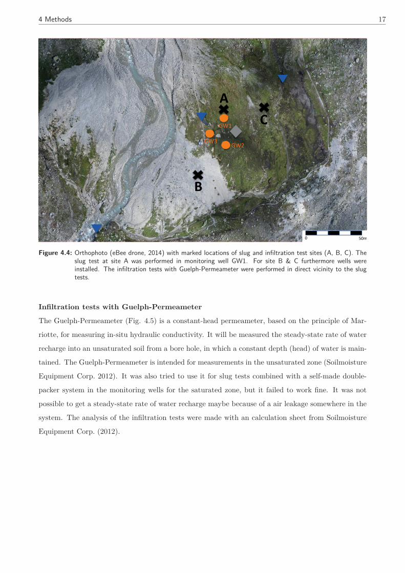
4 Methods 17

Figure 4.4: Orthophoto (eBee drone, 2014) with marked locations of slug and infiltration test sites (A, B, C). Theslug test at site A was performed in monitoring well GW1. For site B & C furthermore wells wereinstalled. The infiltration tests with Guelph-Permeameter were performed in direct vicinity to the slugtests.

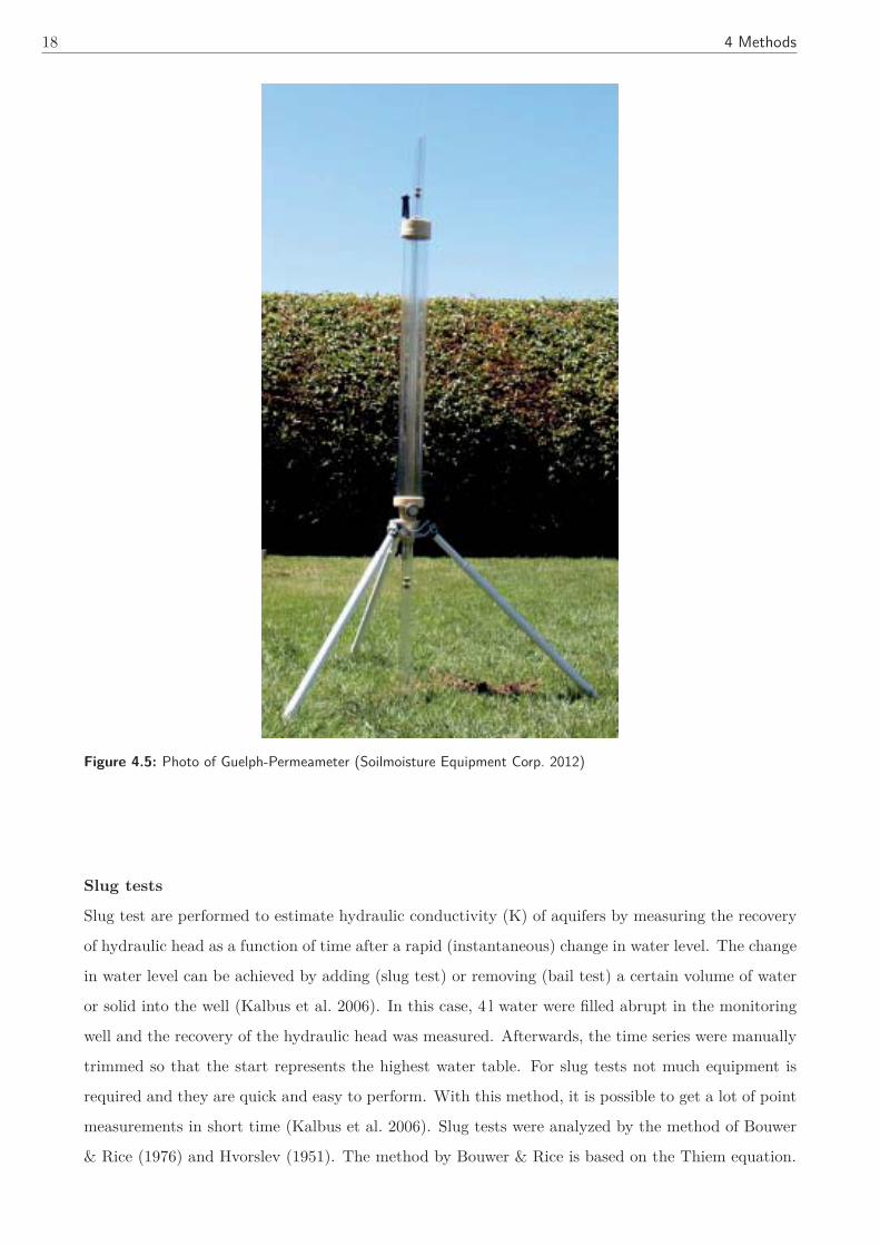
Infiltration tests with Guelph-Permeameter

The Guelph-Permeameter (Fig. 4.5) is a constant-head permeameter, based on the principle of Mar-

riotte, for measuring in-situ hydraulic conductivity. It will be measured the steady-state rate of water

recharge into an unsaturated soil from a bore hole, in which a constant depth (head) of water is main-

tained. The Guelph-Permeameter is intended for measurements in the unsaturated zone (Soilmoisture

Equipment Corp. 2012). It was also tried to use it for slug tests combined with a self-made double-

packer system in the monitoring wells for the saturated zone, but it failed to work fine. It was not

possible to get a steady-state rate of water recharge maybe because of a air leakage somewhere in the

system. The analysis of the infiltration tests were made with an calculation sheet from Soilmoisture

Equipment Corp. (2012).

18 4 Methods

Figure 4.5: Photo of Guelph-Permeameter (Soilmoisture Equipment Corp. 2012)

Slug tests

Slug test are performed to estimate hydraulic conductivity (K) of aquifers by measuring the recovery

of hydraulic head as a function of time after a rapid (instantaneous) change in water level. The change

in water level can be achieved by adding (slug test) or removing (bail test) a certain volume of water

or solid into the well (Kalbus et al. 2006). In this case, 4 l water were filled abrupt in the monitoring

well and the recovery of the hydraulic head was measured. Afterwards, the time series were manually

trimmed so that the start represents the highest water table. For slug tests not much equipment is

required and they are quick and easy to perform. With this method, it is possible to get a lot of point

measurements in short time (Kalbus et al. 2006). Slug tests were analyzed by the method of Bouwer

& Rice (1976) and Hvorslev (1951). The method by Bouwer & Rice is based on the Thiem equation.

4 Methods 19

Q = 2 · π · K · Le · y

ln(Rerw

)(2)

Q: volume rate of flow into well [m3/s]K : hydraulic conductivity of aquifer around well [m/s]Le: length of well screen [m]y: vertical section between water level inside level and static water table outside [m]Re: effective radial distance over which y is dissipated [m]rw: radial distance of undisturbed portion of aquifer from centerline [m]

where

K =rc

2 · ln(Rerw

)2 · Le

· 1t

· ln · y0yt

(3)

rc: radius of the casing [m]t: Time [s]

with

ln(Re

rw) = [

1.1ln(Lw

rw)

+CLerw

]−1 (4)

LW : section of well under water table [m]

Due to the relative small diameter of the monitoring wells, it wasn’t possible to abruptly pour all

of the water. This problem resulted in a big discrepancy in the analysis by Bouwer & Rice method,

because the input volume of water plays a role. This means, that a lot of the water gets lost before

the trimmed time series starts. With an adapted water volume, calculated based on water level and

diameter of well, the analysis works fine. Because of this discrepancy, Ksat was additionally calculated

with Hvorslev’s method (Eq. 5).

Ksat =rc

2 · ln(Lerw

)2 · Le · t37

(5)

Ksat: saturated hydraulic conductivity [m/s]rc : radius of well casing [m]Le: length of well screen [m]rw: radius of well screen [m]t37: time, when water level rises or falls 37% of initial HH [s]

20 4 Methods

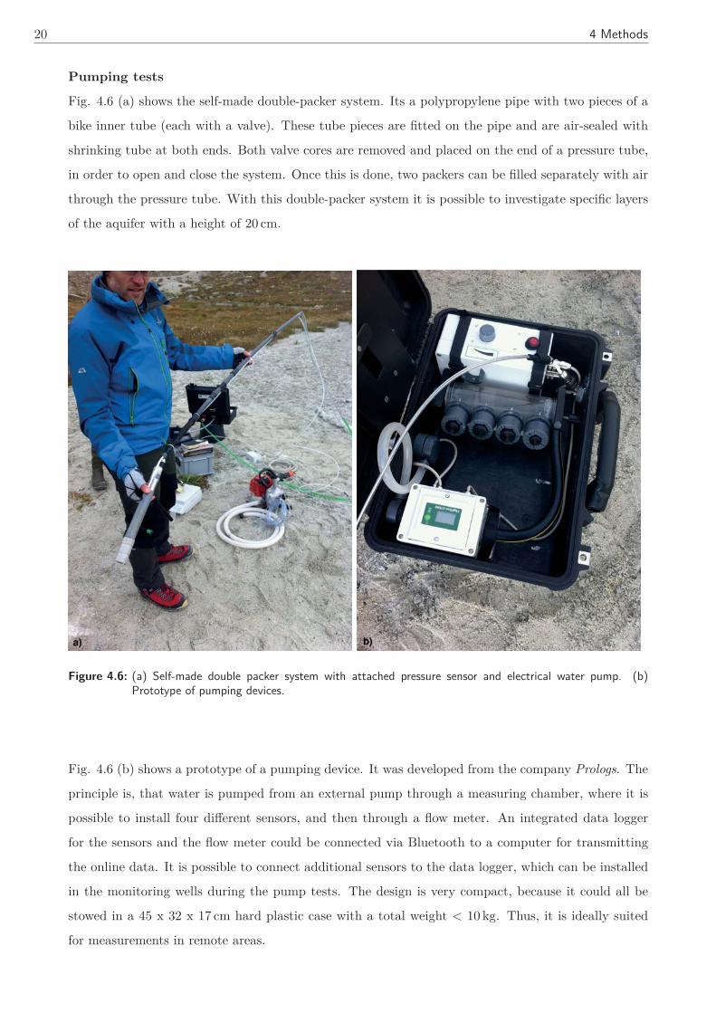
Pumping tests

Fig. 4.6 (a) shows the self-made double-packer system. Its a polypropylene pipe with two pieces of a

bike inner tube (each with a valve). These tube pieces are fitted on the pipe and are air-sealed with

shrinking tube at both ends. Both valve cores are removed and placed on the end of a pressure tube,

in order to open and close the system. Once this is done, two packers can be filled separately with air

through the pressure tube. With this double-packer system it is possible to investigate specific layers

of the aquifer with a height of 20 cm.

Figure 4.6: (a) Self-made double packer system with attached pressure sensor and electrical water pump. (b)Prototype of pumping devices.

Fig. 4.6 (b) shows a prototype of a pumping device. It was developed from the company Prologs. The

principle is, that water is pumped from an external pump through a measuring chamber, where it is

possible to install four different sensors, and then through a flow meter. An integrated data logger

for the sensors and the flow meter could be connected via Bluetooth to a computer for transmitting

the online data. It is possible to connect additional sensors to the data logger, which can be installed

in the monitoring wells during the pump tests. The design is very compact, because it could all be

stowed in a 45 x 32 x 17 cm hard plastic case with a total weight < 10 kg. Thus, it is ideally suited

for measurements in remote areas.

4 Methods 21

4.2.5 Estimation of storage capacity for the alluvial aquifer

The same method like Clow et al. (2003) and Hood & Hayashi (2015) (Eq. 6) was used for estimating

the storage capacity of the aquifer and the changes during the winter outflow.

Vs = A · d · nd (6)

Vs: storage capacity of aquifer [m3]A : areal extent [m2]d: depth of aquifer [m]nd: porosity [-]

The aquifer should be divided in an active and a passive part, since not the entire aquifer could drain

into the glacial stream due to different absolute elevations. As active aquifer, the part which drained

to the glacial stream was defined, thus above gauge zero at the catchment outlet (2362.44 m a.s.l.).

Only groundwater from the active part of the aquifer can contribute to the runoff of the glacial stream,

following this definition. The passive aquifer is accordingly below 2362.44 m a.s.l. Deeper groundwater

may be able to percolate through fissures in fractured crystalline rock.

4.3 Laboratory methods

4.3.1 Silica analysis

The silica analysis was performed using photometric measurements, according to the method described

in DIN38405-D21 (1990). Therefore, a spectrometer (Specord 40 from Analytik-Jena) was used. Sam-

ples for silica analysis are stored in low density polyethylene bottles, because glass bottles could falsify

the results due to possible dilution of silicon from the glass. Before analysis, the samples were filtered

with 0.45 μm cellulose-acetate filters, because suspended solids could impact the measurement. To

minimize potential errors, measuring was made twice. The results were averaged. If the difference was

bigger than 0.01 mg/L, the sample were measured a second time. The principle of silica measurement

is based on the fact that the dissolved silicic acid by the addition of ascorbic acid and ammonium

molybdate tetrahydrate forms a blue complex, which can be measured by a spectrometer. Because

phosphorous also affect to build this complex, these ions have to be masked selective by adding tartaric

acid.

H4SiO4 + 12H2MoO4(polymer) → H4Si(MO3O10)4 + 12H2O (7)

The formed color complex has an extinction maximum in the range of 815 nm. The calibration of the

photometer was made with 6 standards in range from 0.2 to 2 mg/L, as well as a "blind"-standard

with 0 mg/L. A new calibration was made for each measuring series. The determination coefficient r2

for each calibration was r2 = 1.0.

22 4 Methods

4.3.2 Isotope analysis

Samples for isotope analysis were taken separately in 20 ml glass bottles. To prevent evaporation,

which would influence the result, it is essential to keep the samples airproof (Kendall & McDonnell

1998). The samples were filtered with 0.45 μm PTFE filters and pipetted in 1.5 ml vials for the laser

spectrometer. They were stored in the fridge at 5 - 7 ◦C until analysis. The analysis was conducted

with a laser spectrometer Picarro L2130-i (cavity rind-down spectroscopy). As reference standard was

used an inhouse standard, which is calibrated against VSMOV. The laser spectrometer measures the

isotope ratio in relation to a given standard, because it‘s much easier and more precise to measure the

relative or absolute difference between two samples than their absolute 2H or 18O content (Dansgaard

1964).

δ =Rsample − Rstandard

Rstandard· 103 � (8)

Rsample: isotopic ratio of the sampleRstandard : isotopic ratio of the given standardRD or R18O: D or 18O - isotopic ratio of the sample

R18O =[H2

18O][H2

16O](9)

RD =[HD16O][H2

16O](10)

The VSMOW - values are:

R18O = 2.0052 · 10−3 (11)

R2H = 1.5575 · 10−4 (12)

(Kendall & McDonnell 1998)

The analytical uncertainty for this method and devices of 2H and 18O measurements is ± 0.6 � and

± 0.16 �, respectively. The error for DE results from the errors of the two isotopes. According to

Froehlich et al. (2002), the error is calculated as follows:

u(d) =√

(uδ2H)2 + 8 · (uδ18O)2 ∼ ± 0.75 � (13)

4 Methods 23

4.3.3 Ion chromatography

The major cations and anions were measured using ion chromatography (761 Compact IC, Metrohm)

that is hosted at the lab of environmental science at the ETH Zürich. The Precision is about <

2 % for concentrations of 1 - 200 mg/L. Water samples for ion chromatography were filtered with

0.45 μm Nylon-filter and stored in polyethylene bottles. Nylon-filters were used due to previous test

measurements, where these filters show the lowest contamination. For the analysis of the cations it is

necessary to acidify the samples with HCl, for example. Thus, it is necessary to take a second volume

from the sample, because HCl would falsify the result for anion Cl−. This means, that normally every

sample would be measured twice. However, only measurements with acidified samples were conducted,

because the sample volume is sometimes minimal and the fact that the alternative would have been

twice as expensive. Consequently, the results for Cl− could not be used. One soil sample (taken on

20.02.2015) from the upper soil layer in the near of monitoring well GW1 was also analysed. Three

different preparations have been analysed. For the first two preparations 50 g soil was mixed with

100 ml deionised water, shaken for 3 h and afterwards filtered. Afterwards a third preparation was

made with 50 g soil and 100 ml deionised water.

24 5 Results

5 Results

5.1 Time series of hydraulic head, groundwater temperature and electrical conductivity

50

40

30

20

10

0

P [m

m/d

]

P

GW1

GW2

GW3

Ta

−1.0

−0.5

0.0

0.5

1.0

HH

[m]

−15

−10

−5

0

5

10

15

Ta

, TG

W [°

C]

0.00

0.05

0.10

0.15

0.20

0.25

EC

[mS

/cm

]

01.06. 01.08. 01.10. 01.12. 01.02. 01.04. 01.06. 01.08. 01.10.2013 2014

P

snow accumulation: SWE 940 mm

Figure 5.1: Mean daily precipitation (P) & mean daily air temperature (Ta); Hydraulic head (HH, depth to ground-water), groundwater temperature (TGW ) and electrical conductivity (EC) at 3 different monitoring wellsGW1 - 3; GW1 is 1.5 m fully filtered (GL = 2365.7 m a.s.l.), GW2 partly filtered from 1 to 2 m depth(GL = 2365.05 m a.s.l.) & GW3 is 1 m fully filtered (GL = 2365.3 m a.s.l.) see Fig. 4.1; Samplingcampaigns at GW1 & GW2 with automated water samplers are highlighted in grey; HH, TGW and ECare measured in 15 min time steps with CTD online Sensors from HT.

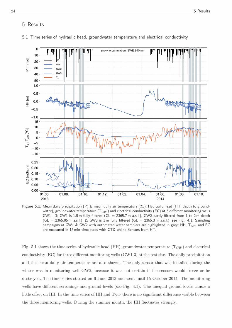
Fig. 5.1 shows the time series of hydraulic head (HH), groundwater temperature (TGW ) and electrical

conductivity (EC) for three different monitoring wells (GW1-3) at the test site. The daily precipitation

and the mean daily air temperature are also shown. The only sensor that was installed during the

winter was in monitoring well GW2, because it was not certain if the sensors would freeze or be

destroyed. The time series started on 6 June 2013 and went until 15 October 2014. The monitoring

wells have different screenings and ground levels (see Fig. 4.1). The unequal ground levels causes a

little offset on HH. In the time series of HH and TGW there is no significant difference visible between

the three monitoring wells. During the summer month, the HH fluctuates strongly.

5 Results 25

Most of them are coincided with precipitation events. During winter, a constant decrease in HH as

well as in TGW for GW2 were detected. EC shows no significant changes during the winter except one

abrupt increase from 0.05 to 0.10 mS/cm (24.03.2014) followed by slow decrease up to 0.025 mS/cm.

This peak in EC accompanied a very moderate increase in HH. Prior to this, the mean daily air

temperature rises temporary up to about 2.5 ◦C. At the beginning of April, the HH increases clearly

from about -0.8 m to +0.6 m. A positive HH means that the groundwater extends into the snow cover,

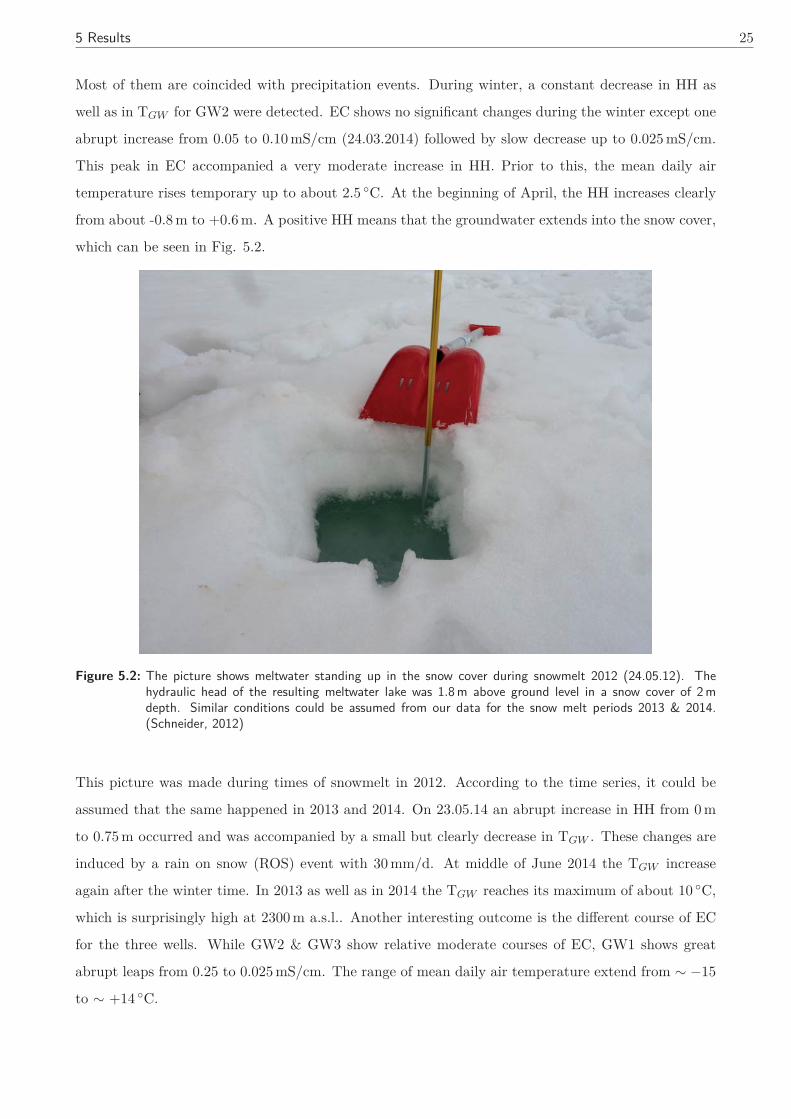
which can be seen in Fig. 5.2.

Figure 5.2: The picture shows meltwater standing up in the snow cover during snowmelt 2012 (24.05.12). Thehydraulic head of the resulting meltwater lake was 1.8 m above ground level in a snow cover of 2 mdepth. Similar conditions could be assumed from our data for the snow melt periods 2013 & 2014.(Schneider, 2012)

This picture was made during times of snowmelt in 2012. According to the time series, it could be

assumed that the same happened in 2013 and 2014. On 23.05.14 an abrupt increase in HH from 0 m

to 0.75 m occurred and was accompanied by a small but clearly decrease in TGW . These changes are

induced by a rain on snow (ROS) event with 30 mm/d. At middle of June 2014 the TGW increase

again after the winter time. In 2013 as well as in 2014 the TGW reaches its maximum of about 10 ◦C,

which is surprisingly high at 2300 m a.s.l.. Another interesting outcome is the different course of EC

for the three wells. While GW2 & GW3 show relative moderate courses of EC, GW1 shows great

abrupt leaps from 0.25 to 0.025 mS/cm. The range of mean daily air temperature extend from ∼ −15

to ∼ +14 ◦C.

26 5 Results

Q [

mm

/h]

0123456

6050403020100

P [

mm

/d]

P

G -2365

G W1

G W2

T a

-1.0

-0.5

0.0

0.5

1.0

HH

[m

]

-15

-10

-5

0

5

10

15

Ta ,

TW

, T

GW

[°C

]

0.00

0.05

0.10

0.15

0.20

0.25

EC

[m

S/c

m]

01.06. 01.08. 01.10. 01.12. 01.02. 01.04. 01.06. 01.08. 01.10.

2013 2014


ice: no data

2013 2014

Figure 5.3: Mean daily precipitation (P) & mean daily air temperature (Ta), runoff from glacial stream [mm/d],hydraulic head (HH, depth to groundwater), groundwater temperature (TGW ) and electrical conductivity(EC) from 2 different monitoring wells as well as hydraulic head (water level above gauge zero), watertemperature (TW ) and electrical conductivity (EC) from glacial stream; HH, TGW and EC measured in15 min time steps at monitoring wells GW1 & GW2; GW1 is 1.5 m fully filtered (GL = 2365.7 m a.s.l.)& GW2 partly filtered from 1 to 2 m depth (GL = 2365.05 m a.s.l.) see Fig. 4.1; Sampling campaignswith automated water samplers are highlighted in grey; HH, TW and EC measured in 5 min time stepsat glacial stream; data from glacial stream and monitoring wells are aggregated to hourly values; runoffis calculated by p/q - ratio, validated for medium and high flows with salt and uranin dilution; notvalidated for low flows.

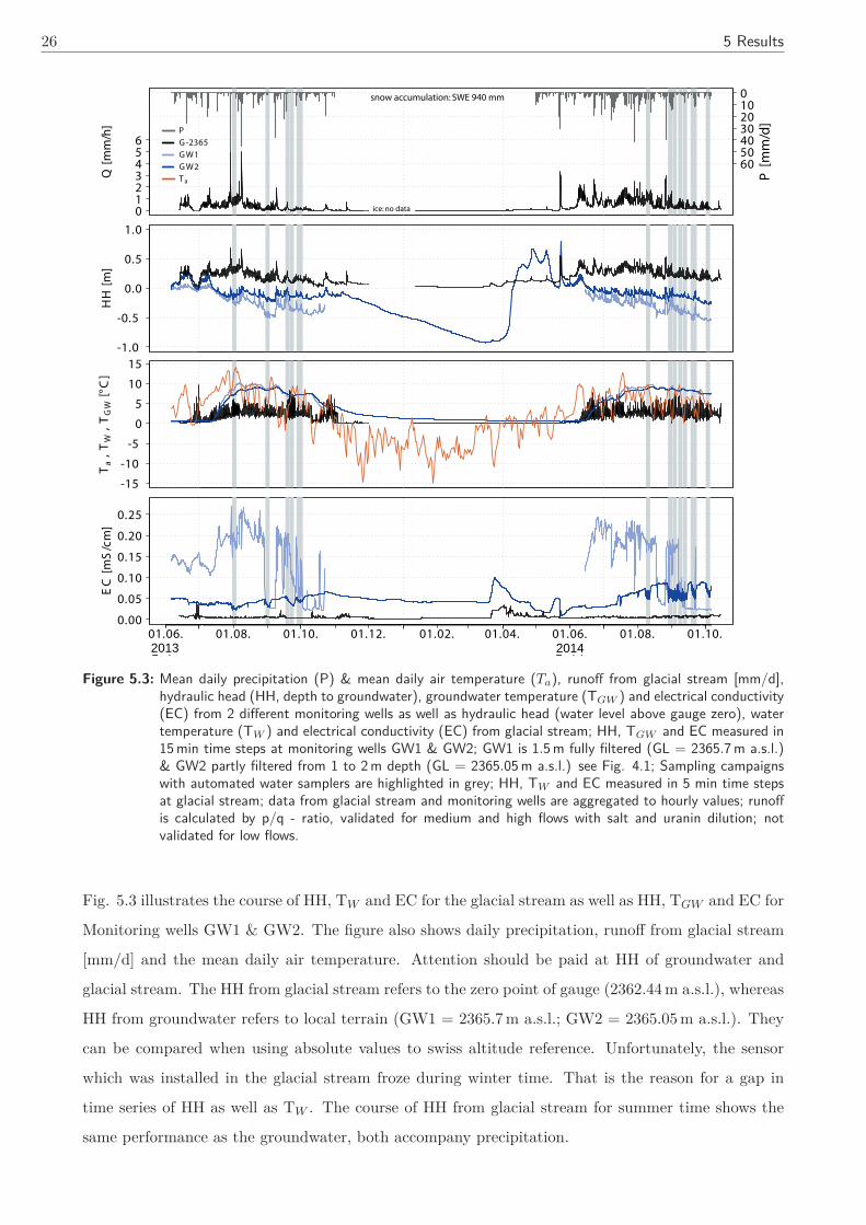
Fig. 5.3 illustrates the course of HH, TW and EC for the glacial stream as well as HH, TGW and EC for

Monitoring wells GW1 & GW2. The figure also shows daily precipitation, runoff from glacial stream

[mm/d] and the mean daily air temperature. Attention should be paid at HH of groundwater and

glacial stream. The HH from glacial stream refers to the zero point of gauge (2362.44 m a.s.l.), whereas

HH from groundwater refers to local terrain (GW1 = 2365.7 m a.s.l.; GW2 = 2365.05 m a.s.l.). They

can be compared when using absolute values to swiss altitude reference. Unfortunately, the sensor

which was installed in the glacial stream froze during winter time. That is the reason for a gap in

time series of HH as well as TW . The course of HH from glacial stream for summer time shows the

same performance as the groundwater, both accompany precipitation.

5 Results 27

As anticipated, the EC from glacial stream is throughout lower, than those from groundwater. Even

the behavior of the EC curve differs, unlike the behavior of HH. Only at the end of March 2014 was

a signal in EC of the glacial stream and GW2 detectable.

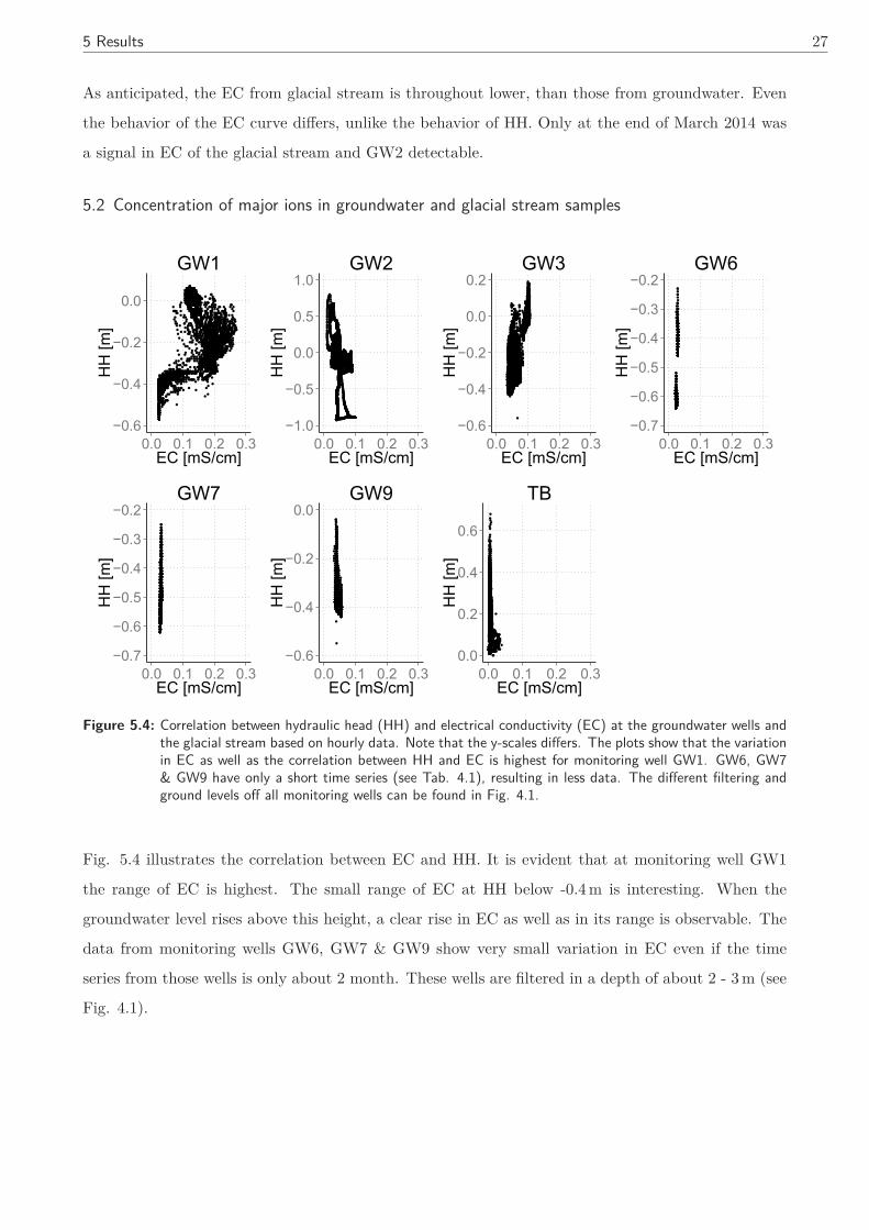
5.2 Concentration of major ions in groundwater and glacial stream samples

●●●●●●●●●●●●●●●●●●●●●●●●●●●●●●●●●●●●●●●●●●●●●●●●●●●●●●●●●●●●●●●●●●●●●●●●●●●●●●●●●●●●●●●●●●●●●●●●●●●●●●●●●●●●●●●●●●●●●●●●●●●●●●

●●●●●●●●●●●●●●●●●●●●●

●●●●●●●●●●●●●●●●●●●●●●●●●●●●●●●●●●●●●●●●●●●●●●

●●●●●●●●●●●●●●●●●●●●●●●●●●●●●●●●●●●●●●●●●●●●●●●●●●●●●●●●●●●●●●●●●●●●●●●●●●●●●●●●

●●●●●●●●●●●●●●●●●●●●●●●●●●●●●●●●●●●●●●●●●●●●●●●●●●●●●●●●

●●●●●●●●●●●●●●●●●●●●●●●●●●●●●●●●●●●●●●●●●●●●●●●●●●●●●●●●

●●●●●●●●●●●●●●●●●●●●●●●●●●●●●●●●●●●●●●●●●●●●●●●●●●●●

●●●●●●●●●●●●●●●●●●●●●●●●●●●●●●●●●●●●●●●●●●●●●●●●●●●●●●●●●●●●●●●●●●●●●●●●●●●●●●●●●●●●●●●●●●●●●●●●●●●●●●●●●●●●●●●●●●●●●●●●●●●●●●●●●●●●●●●●●●●●●●●●●●●●●●●●●●●●

●●●●●●●●

●●●●●●●●●●●●●●●●●●●●●●●

●●●●●●●●●●●●●●

●●●●●●●●●●●●

●●●●●●●●●●●●●●●●●●●●●●●●●●●●●●●●●●●●●●●●●●●●●●●●●●●●●●●●●●

●●●●●●●●●●●●●●●●●●●●●●●●●●●●●●●●●●●●●●●●●●●●●●●●

●●●●●●●●●●●●●●●●●●●●●●●●●●●●●●●●●●●●●●●●●●●●●●●●●●●●●●●●●●●●●●●●●●●●●●●●●●●●●●

●●●●●●●●●●●●●●●●●●●●●●●●●●●●●●●●●●●●●●●●●●●●●●●●●●●●●●●●●●●●●●●●●●●●●●●●●●●●●●●●●●●●●●●●●●●●●●●●●●●●●●●●●●●

●●●●●●●●●●●●●●●●●●●●●●●●●●●●●●●●●●●●●●●●●●●●●●

●

●●●●●●●●●●

●●●●●

●

●

●●●●●●●●●●●●●●●●●●●●●●●●●●●●●●●●●●●●

●●●●●●●●●●●●●

●●●●●●●●●●●●

●●●●●●●●●●●●●●●●●●●●●●●●●●●●●●●●●●●●●●●●●●●●●●●●●●●●●●●●●●●●●●●●●●●●●●●●●●●●●●●●

●

●●●●●●●●●●●●●●●●●●●●●●●●●●●●●●●●●●●●●●●●●●●●●●●●●●●●●●●●●●●●●●

●●●●●●●●●●●●●●●●●●●●●●●●●●●●●

●

●●●●●●●●●●●●●●●●●●●●●●●●●●●●●●●●●●●●●●

●●●

●●●

●●●●●

●●

●●●●

●●●●●●●●

●●●●●●●●●●●

●● ●●

●●●●●●●●●●●●●●●●

●●●●

●

●●●

●

●●●●

●●●●

●●●●

●●●

●●●●

●

●●●

●

●●●●

●●●●

●●●

●●

●●

●●

●●●

●●●

●

●●●●

●●●●

●●●●

●●●

●

●●●

●

●

●●●●●●●

●●●●●●●●●●●●●●●●●●●●●●●●●●●●●●●●●●●●●●●●●●

●

●●●

●●

●●●

●●●●●●

●●●●●●

●

●●●●●●●●

●●●

●●●●●●●●●●●●●●●●

●●●

●●

●●●

●●

●●

●●●●●

●●●

●●●●

●●●

●●●

●●●

●●●●●●●●●

●●●●●●●●●●●●●●

●●●●●●●●●●●●●●●●●●●●●●●●●●

●●●●●●●●●●●●●●●●●●●●●●●●

●●●●●●●●●●●●●●●●●●●●●

●●●●●●●●●●●●●●●●●●●●●●

●●●●●●●●●●●●●●●●●●●●●●●●●●●●●●●●

●●●●●●●●●●●●●●●●●●●●

●●●●●●●●●●●●●●●●●●●●

●●●●●●●●●●●●●●●●●●●●●●●●●●●●

●●●●●●●●●●●●●

●●●●●●●●●●●●●●●●●

●●●●●●●●

●

●●

●

●●●

●●

●●●●●●●●●

●●●●●●●●●●

●●●●●●●●●●●●●●●●●●●●●●●●●●●●●●●●●●●●●●●●●●●●●●

●●●●●●●●●●●●●●●●●●●

●

● ●

●●●●●●●●●

●●●●

●●●●●●

●

●●

●●

●

●●●

●●●

●●

●●●●●●●●

●●●●●●●●●●●●●●●●●●●●●●●●●●

●●●●●●●●●●●●●●●●●●●●●●

●

●●

●●●●●●●●●●●●●●●●

●●●●●

●

●●●●

●●●●

●●●●●●●●

●●●●●●●●●●●

●

●●●

●

●●●

●

●●●

●

●●●

●

●●●

●

●●●

●

●●●

●

●●●

●

●●●

●

●●●

●

●●●

●

●●●

●

●●●

●

●●●

●

●●●

●

●●●

●

●●●

●

●●●

●

●●●

●

●●●

●

●●●

●

●●●

●

●●●

●

●●●●●●●●●●●●●●●●●●●●●●●●●●●●●●●●●●●●●●●●●●●●●●●●●●●●●●●●●●●●●●●●●●●●●●●●●●●●●●●●●●●●●●●●●●●●●●●●●●●●●●●●●●●●●●●●●●●●●●●●●●●●●●●●●

●

●

●● ● ●

●●●●●

●

● ●●

●●

●●●

●

●

●●●●

●●●●●●●

●●

●●

●●●

●●●●●●●●

●●●●●●●●

●●●●●●●

●

●

●

●●●●●●●●●●●●●●

●●●●

●●●●●

●●

●●●●●●●●●●●●●●

●●●●

●

●●●●●●●●●●●●●

●●●●●●●●●●

●●●●

●●●●●●●●●●●●●●●●●●●●●

●●●●●●●●●●●●●●●

●●●●●●●

●●●●

●

● ●●

●●●

●●●●

●●●●●

●●●

●●●●

●●

●●●

●●

● ●●●●●

●●●

●●●●●●●●●●●●●●●●●●●●

●

●

●

●●●

●●●●

●

●●

●●

●●●●●

●●

●●●●●●●●●●●●●●

●●●●●●●●

●●●●●●●●●●●●●●●

●

●●●

●

●●●

●

●●●

●

●●●

●

●●●

●

●●●

●

●●●

●

●●●

●

●●●

●

●●●

●

●●●

●

●●●

●

●●●

●

●●●

●

●●●

●

●●●

●●●●

●

●●●

●

●●●

●

●●●

●

●●●

●

●●●

●

●●●

●

●●●

●

●●●●●●

●

●●●●●●●●

●●●●●●●●●●●

●●●●●●●●●●●●●●

●

●●

●●

●●●●●●●●●●●

●●●●●

●●●●●●●●

●●●

●●●●●●●

●●●●●●●●●●

●●●●●

●●●

●●●●●●●●●

●●●●●

●●●●●●●●

●●●●●●●●●●●●

●

● ● ●●

●●●●

●●●●●●●

●●●●●●●

●●

●●●●●

●

●●

●●

●●●

●●

●●

●●●

●●●●

●●●●●

●●●●

●●●●●●●●●●●●●

●●●●●●●●●●●●●●●●●●●●●●●●●●●●●●●●●●●●●●●●●●●●●●●●●●●●●●●●●●●●●●●●●●●●●●●●●● ●

●●●●●

●●●

●●●●●●●●●●●●●●●●●●●●●●●●●●●●●●●●●●●●●●●●●●●●●●●●●●●●●●●●●●●●●●●●●●●●●●●●●●●●●●●●●●●●●●●●●●●●●●●●●●●●●●●●●●●●●●●●●●●●●●●●●●●●●●●●●●●●●●●●●●●●●●●●●●●●●●●●●●●●●●●●●●●●●●●●

●●●●●●●●●●●●●●●●

●●●●●●●●●●●●●●●●●

●●●●●●●●●●●●●●●●●●●●●●●●●●●●●●●●●●●●●●●●●●●●●●●●●●●●●●●●●●●●●●

●●●

●●

●●●●●

●●●

●●

●●●●

●●●●●

●●●●●●●●●●

●●●●●●●●●●●●●●●●●●●●●●●●●●●●●●●●●●●●●●●●●●●●●●●●●●●●●●●●●●●●●●●●●●

●●

● ●●●●●●●●

●●●●●●●

● ●●●●

●●●●●●●●●●●●●●●●●●●●●●●●●●●●●●●●●●●●●●●●●●●●●●●●●●●●●●●●●●●●●●●●●●●●●●●●●

●

●●

●●●●●●●●●●●●●●●●●●●●●●

●●●

●●●●●●●●●●●●●●●●●●●●●

●●●

●●●●●●●●●●●●●●●●●●●●●●●●●●●●●●●●●●●●●●

●●●●●●●●●●●●●●●●●●●●●●

●●●●●●●●

●

●

●

●●●●

●●●●●●●●

●●●●●●

●

●●

●●●

●●

●

●●●●●●●●●●●●●●●●●●●●●●●●●●●●●●●●●●●●●●●●●●●●●●●●●●●●●●●●●●●●●●●●●●●

●●●●●●●●●●

●●●●●●●●●●●●●●●●

●

●●

●●●●

●●●●●●●●●●●●●●●●

●●●●●●●●●

●●●

●●●●●●

●●●●●●

●●●●

●●●●●●●●●

●

●●●●●●●●●●●●●●●●●●●

●●●●●●●●●●●●●●●●●●●●●●●●●●●

●

●●●●●●●●

●

●●●

●●●●●●●

●●●●●●●●●●●●●●●●●●●●●●●●●●●●●●●●●●●●●●●●●●●

●●●●●●●●●●●●●●●●●●●●●●●●●●●●●●●●●●●●●●●●●●●●●●●

●●●●●●●●●●●

●●●●●●●●●●●●●●●●●●

●

●●●●●●

●●

●●

●●

●●●●

●●●●●●●●●●●●●●

●●●●●●●●●●●●●●●●●●●●●●●●●

●●●●●●●●●●●●●●●●●●●●

●●●●

●●●

●●●●●●●●●

●●●●●●●●●●●●●●●●●●

●●●

●●●●●●●●●●●●●●●●●●●●●

●

●●●●●

●●●●●●●●●●●●●●●●●●●●●●●●

●●●●●●●●●●●●●●●●●●●●●●●

●●●●●●●●●●●●●●●●●●●●●●●●

●●●●●●●●●●●●●●●●●●●●●●●●●●●●●●●●●●●●●●●●●●●●●●●●●●●●●●●●●●●●●

●●●●●●●●

●

●

●●●●●●●●●●●●●●●●●●●●●●●●●●●

●

●

●

●

●●

●●

●●●

●●●●●●●●

●●●●●

●●●●●

●

●

●

●●

●●

●●

●●●●●●●●●●●●

●●●●●●●●●●●●●●●●●●●●●●●●●●●●

●●●●

●

●

●●●●●

●●●●●●

●●●●●●●●

●●●●●●●●●●●●●●●●●●●●●●●●●●●●●●

●

●●

●●●

●

●●●●●●●

●●●●●

●●●●●●

●●●●●●●●●●●●●●●●

●●●●●●●●●●●●●●●

●

●

●●●

●

●

●●

●●●●●

●●●●

●

●●●

●●●● ●

●●●●●●●●●●●

●●●●●●●●●●

●●●●●●●●●●●●●●●●●●●●●●●●●●●●●●●●●●●●●●●●●●●●

●●

●●●●●●●●●●

●●

●●

●●

●●

●●●

●●●●●

●●●

●

●

●●

●

●●

●●

●●●●●●●●●●●●●●●●●●●●●●●●●●●●●●●●●●●●●

●

●●●●●●●●●●●●●●●●●

●●●●●●●●●●●●●●●●●●●●●●●●●●●●●●●●●●●●●●●●●●●●●●●●●●●●●●●●●●●●●●●●●●●●●●●●

●●●●●●●

●

●

●

●●●●●●●●

●●

●●●●●●●●●

●●●●●●●●●●●●●●●●●●●●●●●●●●●●

●●●●●●

●●●●●●●●●●●●●●●●●●●●●●●●

●●●●●●●●●●●●●●

●●●●●●●●●●●●

●

●

●

●

●●

●●

●●●●●●●●●●●●●●●●●●●●●●●●●●●●●

●●●●●●●●●●●

●●●●●●●●●●●●●

●●●

●●●●●●●●●●●●●●●●●●●●●●●●●●●●●●●

●●●●●●●

●●●●●●●●●●●●●●●●●●

●●●

●

●

●●●●●●●●

●●●●●●●●●●●●●●●●●●●●●●●●●●●●●●●●●●●●●●●●●

●●●●●●●●●●●●●

●●●●●●●●●●●●●●●●●●●●●●●●●●●●●●●

●●●●●●●●●●●●●●●●●●●●●●●●●●●●●●●●●●●●●●●●●●●●●●●●●●●●●●●●●●●●●●●●●●●●●●●●●●●●●●●●●●●●●●●●●●●

●

●

●

●●●●●●

●●●

●●●

●●●●

●● ●

●●●●●●●

●●●●●●●●●●●●●●●●●●●●●●●

●

●

●

●

●

●●

●●●●

●●●●●●●●●●●●●●●●●

●●●●●●●

●

●

●

●

●

●●●

●●●

●●

●●●●●●●

●●●●●●●●●

●●●●●●

●●●●●●●●●

●

●

●

●

●●

●●●●●

●●●●

●●●●●●

●

●

●● ●

●

●●

●

●

●●●

●

●●●

●

●●●

●

●●●

●

●●●

●

●●●

●

●●●

●

●●●

●

●●●

●

●●●

●

●●●

●

●●●

●

●●●

●

●●●

●

●●●

●

●●●

●

●●●

●

●●●

●

●●●

●

●●●

●

●●●

●

●●●●●●●●●●●●●●●●●●●●●●

●●●●

●

●

●●●

●

●●●

●

●●●

●

●●●

●

●●●

●

●●●

●

●●●

●

●●●

●

●●●

●

●●●

●

●●●

●

●●●

●

●●●

●

●●●

●

●●●

●

●●●

●

●●●

●

●●●

●

● ●●

●

●●●

●

●●●

●

●●●

●

●●●

●

●●●●●●●●●●●

●●●●●●●●●●●●●●●●●●●●●●●●●●●

●●●●●●●●●

●●

●●

●●

●●●●●●

●●●●

●●●●●●●●●●●●●●●●●●●●●●●●●●●●●●●●●●●●●●●●●●●●●●●●●●●●●●●●●●●●●●●●●●●●●●

●●●●●●●●●●●●●●●●●●●●●●●●●●●●●●●●●●●●●●●●●●●●●●●●●●●●●●●●●●●●●●●●●●●●

●

●●●

●

●●●

●

●●●

●

●●●

●

●●●

●

●●●

●

●●●

●

●●●

●

●●●

●

●●●

●

●●●

●

●●●

●

●●●

●

●●●

●

●●●

●

●●●

●

●●●

●

●●●

●

●●●

●

●

●

●●

●●●

●

●

●

●

●

●●●

●

●●●

●●●●●●●●●●●●●●●●●●●●●●●●●●●●●●●●●●●●●●●●●●●●●●●●●●●●●●●●●●●●●●●●●●●●●●●●●●●●●●●●●●●●●●●●●●●●●●●●●●●●●●●●●●●●●●●●●●●●●●●●●●●●●●●●●●●●●●●●●●●●●●●●●●●●●●●●●●●●●●●●●●●●●●●●●●●●●●●●●●●●●●●●●●●●●●●●●●●●●●●●●●●●●●●●●●●●●●●●●●●●●●●●●●●●●●●●●●●●●●●●●●●●●●●●●●●●●●●●●●●●●●●●●●●●●●●●●●●●●●●●●●●●●●●●●●●●●●●●●●●●●●●●●●●●●●●●●●●●●●●●●●●●●●●●●●

−0.6

−0.4

−0.2

0.0

0.0 0.1 0.2 0.3EC [mS/cm]

HH

[m]

GW1

●●●●●●●●●●●●●●●●●●●●●●●●●●●●●●●●●●●●●●●●●●●●●●●●●●●●●●●●●●●●●●●●●●●●●●●●●●●●●●●●●●●●●●●●●●●●●●●●●●●●●●●●●●●●●●●●●●●●●●●●●●●●●●●●●●●●●●●●●●●●●●●●●●●●●●●●●●●●●●●●●●●●●●●●●●●●●●●●●●●●●●●●●●●●●●●●●●●●●●●●●●●●●●●●●●●●●●●●●●●●●●●●●●●●●●●●●●●●●●●●●●●●●●●●●●●●●●●●●●●●●●●●●●●●●●●●●●●●●●●●●●●●●●●●●●●●●●●●●●●●●●●●●●●●●●●●●●●●●●●●●●●●●●●●●●●●●●●●●●●●●●●●●●●●●●●●●●●●●●●●●●●●●●●●●●●●●●●●

●●●●●●●●●●●●●●●●●●●●●●●●●●●●●●●●●●●●●●●●●●●●●●●●●●●●●●●●●●●●●●●●●●●●●●●●●●●●●●●●●●●●●●●●●●●●●●●●●●●●●●●●●●●●●●●●●●●●●●●●●●●●●●●●●●●●●●●●●●●●●●●●●●●●●●●●●●●●●●●●●●●●●●●●●●●●●●●●●●●●●●●●●●●●●●●●●●●●●●●●●●●●●●●●●●●●●●●●●●●●●●●●●●●●●●●●●●●●●●●●●●●●●●●●●●●●●●●●●●●●●●●●●●●●●●●●●●●●●●●●●●●●●●●●●●●●●●●●●●●●●●●●●●●●●●●●●●●●●●●●●●●●●●●●●●●●●●●●●●●●●●●●●●●●●●●●●●●●●●●●●●●●●●●●●●●●●●●●●●●●●●●●●●●●●●●●●●●●●●●●●●●●●●●●●●●●●●●●●●●●●●●●●●●●●●●●●●●●●●●●●●●●●●●●●●●●●●●●●●●●●●●●●●●●●●●●●●●●●●●●●●●●●●●●●●●●●●●●●●●●●●●●●●●●●●●●●●●●●●●●●●●●●●●●●●●●●●●●●●●●●●●●●●●●●●●●●●●●●●●●●●●●●●●●●●●●●●●●●●●●●●●●●●●●●●●●●●●●●●●●●●●●●●●●●●●●●●●●●●●●●●●●●●●●●●●●●●●●●●●●●●●●●●●●●●●●●●●●●●●●●●●●●●●●●●●●●●●●●●●●●●●●●●●●●●●●●●●●●●●●●●●●●●●●●●●●●●●●●●●●●●●●●●●●●●●●●●●●●●●●●●●●●●●●●●●●●●●●●●●●●●●●●●●●●●

●●●●●●●●●●●●●●●●●●●●●●●●●●●●●●●●●●●●●●●●●●●●●●●●●●●●●●●●●●●●●●●●●●●●●●●●●●●●●●●●●●●●●●●●●●●●●●●●●●●●●●●●●●●●●●●●●●●●●●●●●●●●●●●●●●●

●●●●●●●●●●●●●●●●●●●●●●●●●●●●●●●●●●●●

●●●●

●

●●●●●●●

●

●●●

●

●●●

●

●●●

●

●●●

●

●●●

●

●●●

●

●●●

●●●●●●●●●●●●●●●●●●●●●●●●●●●●●●●●●●●●●●●●●●●●●●●●●●●●●●●●●●●●●●●●●●●●●●●●●●●●●●●●●●●●●●●●●●●●●●●●●●●●●●●●●●●

●

●●●●●●●●●●●●●●●●●●●●

●●●●●●●●●●●●●●●●●●●●●●●●●●●●●●●●●●●●●●●●●●●●●●●●●●●●●●●●●●●●●●●●●●●●●●●●●●●●●●●●●●●●●●●●●●●●●●●●●●●●●●●●●●●●●●●●●●●●●●●●●●●●●●●●●●●●●●●●●●●●●●●●●●●●●●●●●●●●●●●●●●●●●●●●●●●●●●●●●●●●●●●●●●●●●●●●●●●●●●●●●●●●●●●●●●●●●●●●●●●●●●●●●●●●●●●●●●●●●●●●●●●●●●●●●●●●●●●●●●●●●●●●●●●●●●●●●●●●●●●●●●●●●●●●●●●●●●●●●●●●●●●●●●●●●●●●●●●●●●●●●●●●●●●●●●●●●●●●●●●●●●●●●●●●●●●●●●●●●●●●●●●●●●●●●●●●●●●●●●●●●●●●●●●●●●●●●●●●●●●●●●●●●●●●●●●●●●●●●●●●●●●●●●●●●●●●●●●●●●●●●●●●●●●●●●●●●●●●●●●●●●●●●●●●●●●●●●●●●●●●●●●●●●●●●●●●●●●●●●●●●●●●●●●●●●●●●●●●●●●●●●●●●●●●●●

●●●●●●●●●●●●●●●●●●●●●●●●●●

●●●●●●●●●●●●●●●●●●●●●●●●●●●●●●●●●●●●●●●●●●●●●●●●●●●●●●●●●●●●●●●●●●●●●●●●●●●●●●●●●●●●●●●●●●●●●●●●●●●●●●●●●●●●●●●●●●●●●●●●●●●●●●●●●●●●●●●●●●●●●●●●●●●●●●●●●●●●●●●●●●●●●●●●

●●●●●●●●●●●●●●●●●●●●●●●●●●●●●●●●●●●●●●●●●●●●●●●●●●●●●●●●●●●●●●●●●●●●●●●●●●●●●●●●●●●●●●●●●●●●●●●●●●●●●●●●●●●●●●●●●●●●●●●●●●●●●●●●●●●●●●●●●●●●●●●●●●●●●●●●●●●●●●●●●●●●●●●●●●●●●●●●●●●●●●●●●●●●●●●●●●●●●●●●●●●●●●●●●●●●●●●●●●●●●●●●●●●●●●●●●●●●●●●●●●●●●●●●●●●●●●●●●●●●●●●●●●●●●●●●●●●●●●●●●●●●●●●●●●●●●●●●●●●●●●●●●●●●●●●●●●●●●●●●●●●●●●●●●●●●●●●●●●●●●●●●●●●●●●●●●●

●

●●●●●●●●●●●●●●●●●●●●●●●●●●●●●●●●●●●●●●●●●●●●●●●●●●●●●●●●●●●●●●●●●●●●●●●●●●●●●●●●●●●●●●●●●●●●●●●●●●●●●●●●●●●●●●●●●●●●●●●●●●●●●●●●●●●●●●●●●●●●●●●●●●●●●●●●●●●●●●●●●●●●●●●●●●●●●●●●●●●●●●●●●●●●●●●●●●●●●●●●●●●●●●●●●●●●●●●●●●●●●●●●●

●●●●●●●●●●●●●●●●●●●●●●●●●●●●●●●

●●●●●●●●●●●●●●●●●●●●●●●●●●●●●●●●●●●●●●●●●●●●●●●●●●●●●●●●●●●●●●●●●●●●●●●●●●●●●●●●●●●●●●●●●●●●●●●●●●●●●●●●●●●●●●●●●●●●●●●●●●●●●●●●●●●●●●●●●●●●●●●●●●●●●●●●●●●●●●●●●●●●●●●●●●●●●●●●●●●●●●●●●●●●●●●●●●●●●●●●●●●●●●●●●●●●●●●●●●●●●●●●●●●●●●●●●●●●●●●●●●●●●●●●●●●●●●●●●●●●●●●●●●●●●●●●●●●●●●●●●●●●●●●●●●●●●●●●●●●●●●●●●●●●●●●●●●●●●●●●●●●●●●●●●●●●●●●●●●●●●●●●●●●●●●●●●●●●●●●●●●●●●●●●●●●●●●●●●●●●●●●●●●●●●●●●●●●●●●●●●●●●●●●●●●●●●●●●●●●●●●●●●●●●●●●●●●●●●●●●●●●●●●●●●●●●●●●●●●●●●●●●●●●●●●●●●●●●●●●●●●●●●●●●●●●●●●●●●●●●●●●●●●●●●●●●●●●●●●●●●●●●●●●●●●●●●●●●●●●●●●●●●●●●●●●●●●●●●●●●●●●●●●●●●●●●●●●●●●●●●●●●●●●●●●●●●●●●●●●●●●●●●●●●●●●●●●●●●●●●●●●●●●●●●●●●●●●●●●●●●●●●●●●●●●●●●●●●●●●●●●●●●●●●●●●●●●●

●●●●●●●●●●●●●●●●●●●●●●●●●●●●●●●●●●●●●●●●●●●●●●●●●●●●●●●●●●●●●●●●●●●●●●●●●●●●●●●●●●●●●●●●●●●●●●●●●●●●●●●●●●●●●●●●●●●●●●●●●●●●●●●●●●●●●●●●●●●●●●●●●●●●●●●●●●●●●●●●●●●●●●●●●●●●●●●●●●●●●●●●●●●●●●●●●●●●●●●●●●●●●●●●●●●●●●●●●●●●●●●●●●●●●●●●●●●●●●●●●●●●●●●●●●●●●●●●●●●●●●●●●●●●●●●●●●●●●●●●●●●●●●●●●●●●●●●●●●●●●●●●●●●●●●●●●●●●●●●●●●●●●●●●●●●●●●●●●●●●●●●●●●●●●●●●●●●●●●●●●●●●●●●●●●●●●●●●●●●●●●●●●●●●●●●●●●●●●●●●●●●●●●●●●●●●●●●●●●●●●●●●●●●●●●●●●●●●●●●●●●●●●●●●●●●●●●●●●●●●●●●●●●●●●●●●●●●●●●●●●●●●●●●●●●●●●●●●●●●●●●●●●●●●●●●●●●●●●●●●●●●●●●●●●●●●●●●●●●●●●●●●●●●●●●●●●●●●●●●●●●●●●●●●●●●●●●●●●●●●●●●●●●●●●●●●●●●●●●●●●●●●●●●●●●●●●●●●●●●●●●●●●●●●●●●●●●●●●●●●●●●●●●●●●●●●●●●●●●●●●●●●●●●●●●●●●●●●●●●●●●●●●●●●●●●●●●●●●●●●●●●●●●●●●●●●●●●●●●●●●●●●●●●●●●●●●●●●●●●●●●●●●●●●●●●●●●●●●●●●●●●●●●●●●●●●●●●●●●●●●●●●●●●●●●●●●●●●●●●●●●●●●●●●●●●●●●●●●●●●●●●●●●●●●●●●●●●●●●●●●●●●●●●●●●●●●●●●●●●●●●●●●●●●●●●●●●●●●●●●●●●●●●●●●●●●●●●●●●●●●●●●●●●●●●●●●●●●●●●●●●●●●●●●●●●●●●●●●●●●●●●●●●●●●●●●●●●●●●●●●●●●●●●●●●●●●●●●●●●●●●●●●●●●●●●●●●●●●●●●●●●●●●●●●●●●●●●●●●●●●●●●●●●●●●●●●●●●●●●●●●●●●●●●●●●●●●●●●●●●●●●●●●●●●●●●●●●●●●●●●●●●●●●●●●●●●●●●●●●●●●●●●●●●●●●●●●●●●●●●●●●●●●●●●●●●●●●●●●●●●●●●●●●●●●●●●●●●●●●●●●●●●●●●●●●●●●●●●●●●●●●●●●●●●●●●●●●●●●●●●●●●●●●●●●●●●●●●●●●●●●●●●●●●●●●●●●●●●●●●●●●●●●●●●●●●●●●●●●●●●●●●●●●●●●●●●●●●●●●●●●●●●●●●●●●●●●●●●●●●●●●●●●●●●●●●●●●●●●●●●●●●●●●●●●●●●●●●●●●●●●●●●●●●●●●●●●●●●●●●●●●●●●●●●●●●●●●●●●●●●●●●●●●●●●●●●●●●●●●●●●●●●●●●●●●●●●●●●●●●●●●●●●●●●●●●●●●●●●●●●●●●●●●●●●●●●●●●●●●●●●●●●●●●●●●●●●●●●●●●●●●●●●●●●●●●●●●●●●●●●●●●●●●●●●●●●●●●●●●●●●●●●●●●●●●●●●●●●●●●●●●●●●●●●●●●●●●●●●●●●●●●●●●●●●●●●●●●●●●●●●●●●●●●●●●●●●●●●●●●●●●●●●●●●●●●●●●●●●●●●●●●●●●●●●●●●●●●●●●●●●●●●●●●●●●●●●●●●●●●●●●●●●●●●●●●●●●●●●●●●●●●●●●●●●●●●●●●●●●●●●●●●●●●●●●●●●●●●●●●●●●●●●●●●●●●●●●●●●●●●●●●●●●●●●●●●●●●●●●●●●●●●●●●●●●●●●●●●●●●●●●●●●●●●●●●●●●●●●●●●●●●●●●●●●●●●●●●●●●●●●●●●●●●●●●●●●●●●●●●●●●●●●●●●●●●●●●●●●●●●●●●●●●●●●●●●●●●●●●●●●●●●●●●●●●●●●●●●●●●●●●●●●●●●●●●●●●●●●●●●●●●●●●●●●●●●●●●●●●●●●●●●●●●●●●●●●●●●●●●●●●●●●●●●●●●●●●●●●●●●●●●●●●●●●●●●●●●●●●●●●●●●●●●●●●●●●●●●●●●●●●●●●●●●●●●●●●●●●●●●●●●●●●●●●●●●●●●●●●●●●●●●●●●●●●●●●●●●●●●●●●●●●●●●●●●●●●●●●●●●●●●●●●●●●●●●●●●●●●●●●●●●●●●●●●●●●●●●●●●●●●●●●●●●●●●●●●●●●●●●●●●●●●●●●●●●●●●●●●●●●●●●●●●●●●●●●●●●●●●●●●●●●●●●●●●●●●●●●●●●●●●●●●●●●●●●●●●●●●●●●●●●●●●●●●●●●●●●●●●●●●●●●●●●●●●●●●●●●●●●●●●●●●●●●●●●●●●●●●●●●●●●●●●●●●●●●●●●●●●●●●●●●●●●●●●●●●●●●●●●●●●●●●●●●●●●●●●●●●●●●●●●●●●●●●●●●●●●●●●●●●●●●●●●●●●●●●●●●●●●●●●●●●●●●●●●●●●●●●●●●●●●●●●●●●●●●●●●●●●●●●●●●●●●●●●●●●●●●●●●●●●●●●●●●●●●●●●●●●●●●●●●●●●●●●●●●●●●●●●●●●●●●●●●●●●●●●●●●●●●●●●●●●●●●●●●●●●●●●●●●●●●●●●●●●●●●●●●●●●●●●●●●●●●●●●●●●●●●●●●●●●●●●●●●●●●●●●●●●●●●●●●●●●●●●●●●●●●●●●●●●●●●●●●●●●●●●●●●●●●●●●●●●●●●●●●●●●●●●●●●●●●●●●●●●●●●●●●●●●●●●●●●●●●●●●●●●●●●●●●●●●●●●●●●●●●●●●●●●●●●●●●●●●●●●●●●●●●●●●●●●●●●●●●●●●●●●●●●●●●●●●●●●●●●●●●●●●●●●●●●●●●●●●●●●●●●●●●●●●●●●●●●●●●●●●●●●●●●●●●●●●●●●●●●●●●●●●●●●●●●●●●●●●●●●●●●●●●●●●●●●●●●●●●●●●●●●●●●●●●●●●●●●●●●●●●●●●●●●●●●●●●●●●●●●●●●●●●●●●●●●●●●●●●●●●●●●●●●●●●●●●●●●●●●●●●●●●●●●●●●●●●●●●●●●●●●●●●●●●●●●●●●●●●●●●●●●●●●●●●●●●●●●●●●●●●●●●●●●●●●●●●●●●●●●●●●●●●●●●●●●●●●●●●●●●●●●●●●●●●●●●●●●●●●●●●●●●●●●●●●●●●●●●●●●●●●●●●●●●●●●●●●●●●●●●●●●●●●●●●●●●●●●●●●●●●●●●●●●●●●●●●●●●●●●●●●●●●●●●●●●●●●●●●●●●●●●●●●●●●●●●●●●●●●●●●●●●●●●●●●●●●●●●●●●●●●●●●●●●●●●●●●●●●●●●●●●●●●●●●●●●●●●●●●●●●●●●●●●●●●●●●●●●●●●●●●●●●●●●●●●●●●●●●●●●●●●●●●●●●●●●●●●●●●●●●●●●●●●●●●●●●●●●●●●●●●●●●●●●●●●●●●●●●●●●●●●●●●●●●●●●●●●●●●●●●●●●●●●●●●●●●●●●●●●●●●●●●●●●●●●●●●●●●●●●●●●●●●●●●●●●●●

●●●●●●●●●●●●●●●●●●●●●●●●●●●●●●●●●●●●●●●●●●●●●●●●●●●●●●●●●●●●●●●●●●●●●●●●●●●●●●●●●●●●●●●●●●●●●●●●●●●●●●●●●●●●●●●●●●●●●●●●●●●●●●●●●●●●●●●●●●●●●●●●●●●●●●●●●●●●●●●●●●●●●●●●●●●●●●●●●●●●●●●●●●●●●●●●●●●●●●●●●●●●●●●●●●●●●●●●●●●●●●●●●●●●●●●●●●●●●●●●●●●●●●●●●●●●●●●●●●●●●●●●●●●●●●●●●●●●●●●●●●●●●●●●●●●●●●●●●●●●●●●●●●●●●●●●●●●●●●●●●●●●●●●●●●●●●●●●●●●●●●●●●●●●●●●●●●●●●●●●●●●●●●●●●●●●●●●●●●●●●●●●●●●●●●●●●●●●●●●●●●●●●●●●●●●●●●●●●●●●●●●●●●●●●●●●●●●●●●●●●●●●●●●●●●●●●●●●●●●●●●●●●●●●●●●●●●●●●●●●●●●●●●●●●●●●●●●●●●●●●●●●●●●●●●●●●●●●●●●●●●●●●●●●●●●●●●●●●●●●●●●●●●●●●●●●●●●●●●●●●●●●●●●●●●●●●●●●●●●●●●●●●●●●●●●●●●●●●●●●●●●●●●●●●●●●●●●●●●●●●●●●●●●●●●●●●●●●●●●●●●●●●●●●●●●●●●●●●●●●●●●●●●●●●●●●●●●●●●●●●●●●●●●●●●●●●●●●●●●●●●●●●●●●●●●●●●●●●●●●●●●●●●●●●●●●●●●●●●●●●●●●●●●●●●●●●●●●●●●●●●●●●●●●●●●●●●●●●●●●●●●●●●●●●●●●●●●●●●●●●●●●●●●●●●●●●●●●●●●●●●●●●●●●●●●●●●●●●●●●●●●●●●●●●●●●●●●●●●●●●●●●

●●●●●●●●●●●●●●●●●●●●●●●●●●●●●●●●●●●●●●●●●●●●●●●●●●●●●●●●●●●●●●●●●●●●●●●●●●●●●●●●●●●●●●●●●●●●●●●●●●●●●●●●●●●●●●●●●●●●●●●●●●●●●●●●●●●●●●●●●●●●●●●●●●●●●●●●●●●●●●●●●●●●●●●●●●●●●●●●●●●●●●●●●●●●●●●●●●●●●●●●●●●●●●●●●●●●●●●●●●●●●●●●●●●●●●●●●●●●●●●●●●●●●●●●●●●●●●●●●●●●●●●●●●●●●●●●●●●

●●●●●●●●●●●●●●●●●●●●●●●●●●●●●●●●●●●●●●●●●●●●●●●●●●●●●●●●●●●●●●●●●●●●●●●●●●●●●●●●●●●●●●●●●●●●●●●●●●●●●●●●●●●●●●●●●●●●●●●●●●●●●●●●●●●●●●●●●●●●●●●●●●●●●●●●●●●●●●●●●●●●●●●●●●●●●●●●●●●●●●●●●●●●●●●●●●●●●●●●●●●●●●●●●●●●●●●●●●●●●●●●●●●●●●●●●●●●●●●●●●●●●●●●●●●●●●●●●●●●●●●●●●●●●●●●●●●●●●●●●●●●●●●●●●●●●●●●●●●●●●●●●●●●●●●●●●●●●●●●●●●●●●●●●●●●●●●●●●●●●●●●●

●●●●●●●●●●●●●●●●●●●●●●●

●

●

●●●●●●●●●●●●●●●●●●●●●●●●●●●●●●

●●●●●●●●●●●●●●●●●●●●●●●●●●●●●●●●●●●●●●●●●●●●●●●●●●●●●●●●●●●●●●●●●●●●●●●●●●●●●●●●●●●●●●●●●●●●●●●●●●●●●●●●●●●●●●●●●●●●●●●●●●●●●●●●●●

●●●●●●●●●●●●●●●●●●●●●●●●●●●●●●●●●●●●●●●●●●●●●●●●●●●●●●●●●●●●●●●●●●●●●●●●●●●●●●●●●●●●●●●●●●●●●●●●●●●●●●●●●●●●●●●●●●●●●●●●●●●●●●●●●●●●●●●●●●●●●●●●●●●●●●●●●●●●●●●●●●●●●●●●●●●●●●●●●●●●●●●●●●●●●●●●●●●●●●●●●●●●●●●●●●●●●●●●●●●●●●●●●●●●●●●●●●●●●●●●●●●●●●●●●●●●●●●●●●●●●●●●●●●●●●●●●●●●●●●●●●●●●●●●●●●●●●●●●●●●●●●●●●●●●●●●●●●●●●●●●●●●●●●●●●●●●●●●●●●●●●●●●●●●●●●●●●●●●●●●●●●●●●●●●●●●●●●●●●●●●●●●●●●●●●●●●●●●●●●●●●●●●●●●●●●●●●●●●●●●●●●●●●●●●●●●●●●●●●●●●●●●●●●●●●●●●●●●

●●●●●●●●●●●●●●●●●●●●●●●●●●●●●●●●●●●●●●●●●●●●●●●●●●●●●●●●●●●●●●●●●●●●●●●●●●●●●●●●●●●●●●●●●●●●●●●●●●●●●●●●●●●●●●●●●●●●●●●●●●●●●●●●●●●●●●●●●●●●●●●●●●●●●●●●●●●●●●●●●●●●●●●●●●●●●●●●●●●●●●●●●●●●●●●●●●●●●●●●●●●●●●●●●●●●●●●●●●●●●●●●●●●●●●●●●●●●●●●●●●●●●●●●●●●●●●●●●●●●●●●●●●●●●●●●●●●●●●●●●●●●●●●●●●●●●●●●●●●●●●●●●●●●●●●●●●●●●●●●●●●●●●●●●●●●●●●●●●●●●●●●●●●●●●●●●●●●●●●●●●●●●●●●●●●●●●●●●●●●●●●●●●●●●●●●●●●●●●●●●●●●●●●●●●●●●●●●●●●●●●●●●●●●●●●●●●●●●●●●●●●●●●●●●●●●●●●●●●●●●●●●●●●●●●●●●●●●●●●●●●●●●●●●●●●●●●●●●●●●●●●●●●●●●●●●●●●●●●●●●●●●●●●●●●●●●●●●●●●●●●●●●●●●●●●●●●●●●●●●●●●●●●●●●●●●●●●●●●●●●●●●●●●●●●●●●●●●●●●●●●●●●●●●●●●●●●●●●●●●●●●●●●●●

●●●●●●●●●●●●●●●●●●●●●●●●●●●●●●●●●●●●●●●●●●●●●●●●●●●●●●●●●●●●●●●●●●●●●●●●●●●●●●●●●●●●●●●●●●●●●●●●●●●●●●●●●●●●●●●●●●●●●●●●●●●●●●●●●●●●●●●●●●●●●●●●●●●●●●●●●●●●●●●●●●●●●●●●●●●●●●●●●●●●●●●●●●●●●●●●●●●●●●●●●●●●●●●●●●●●●●●●●●●●●●●●●●●●●●●●●●●●●●●●●●●●●●●●●●

●●●●●●●●●●●●●●●●●●●●●●●●●●●●●●●●●●●●●●●●●●●●●●●●●●●●●●●●●●●●●●●●●●●●●●●●●●●●●●●●●●●●●●●●●●●●●●●●●●●●●●●●●●●●●●●●●●●●●●●●●●●●●●●●●●●●●●●●●●●●●●●●●●●●●●●●●●●●●●●●●●●●●●●●●●●●●●●●●●●●●●●●●●●●●●●●●●●●●●●●●●●●●●●●●●●●●●●●●●●●●●●●●●●●●●●●●●●●●●●●●●●●●●●●●●●●●●●●●●●●●●●●●●●●●●●●●●●●●●●●●●●●●●●●●●●●●●●●●●●●●●●●●●●●●●●●●●●●●●●●●●●●●●●●●●●●●●●●●●●●●●●●●●●●●●●●●●●●●●●●●●●●●●●●●●●●●

●● ●●●●●●●● ●●●●●●●●●●●●

●●●●●●●●●●●● ●●●● ●●●●●●●● ●●●●●●●●●●●●●●●●●●●●●●●● ●●●●●●●●●●●●●●●● ●●●●●●●●●●●●●●●●●●●●●●●●●●●●●●●●●●●●●●●●●●●●●●●●●●●●●●●●●●●●●●●●●●●●●●●●●●●●●●●●●●●●●●●●●●●●●●●●●●●●●●●●●●●●●●●●●●●●●●●●●●●●●●●●●●●●●●●●●●●●●●●●●●●● ●●●●●●●●●●●●●●●●●●●●●●●●●●●●●●●●●●●●●●●●●●●●●●●●●●●●●●●●●●●●●●●●●●●●●●●●●●●●●●●●●●●●●●●●●●●●●●●●●●●●●●●●●●●●●●●●●●●●●●●●●●●●●●●●●●●●●●●●●●●●●●●●●●●●●●●●●●●●●●●●●●●●●●●●●●●●●●●●●●●●●●●●●●●●●●●●●●●●●●●●●●●●●●●●●●●●●●●●●●●●●●●●●●●●●●●●●●

●

● ●●●● ●●●● ●●●●●●●●● ●●●● ●●●● ●●●●●●●●●●●●●●●●●●

●●●●●●●●●●●●●●●●●●●●●●●●●●●●●

●●●●

●●●●

●●●

●●●●

●●●●

●● ●●●●●●●●●

●●●●●●●●●●●●● ●●●● ●●●● ●●●● ●●●●●●●● ●●●●●●●● ●●●● ●●●● ●●●●●●●● ●●●●●●●● ●●●● ●●●●●●●● ●●●●● ●●● ●●●●●●●●●●●

●●●●●●●●●●●●●●●●●●●●●●●●●●●●●● ●●●● ●●●● ●●●● ●●●● ●●●● ●●●● ●●●● ●●●● ●●●● ●●●● ●●●● ●●●● ●●●● ●●●● ●●●● ●●●● ●●●● ●●●● ●●●●●●●●●●●● ●●●●●●●●●●●●●●●● ●●●● ●●●●●●●● ●●●● ●●●● ●●●●●●●●●●●●●●●●●●●●●●●● ●●●●●●●●●●●● ●●●●●●●●●●●●●●●● ●●●●●●●●●●●● ●●●●●●●●●●●●●●●●●●●●●●●●●●●●●●●

●●●●●●●●●●●●●●●●●●●●●●●●●●●●●●●●●●●●●●●●●●●●●●●●●●●●●●●●●●●●●●●●●●●●●● ●●●● ●●●● ●●●● ●●●● ●●●● ●●●● ●●●●●●●●●●●●●●●●●●●●●●●●●●●●●●●●●●●●●●●●●●●●●●●●●●●●●●●●●●●●●●●●●●●●●●●●●●●●●●●●●●●●●●●●●●●●●●●●●●●●●●●●●●●●●●●●●●●●●●●●●

●●●●●●●●●●●●●●●●●●●●●●●●●●●●●●●●●●●●●●●●●●●●●●●●●●●●●●●●●●●●●●●●●●●●●●●●●●●●●●●●●●●●●●●●●●●●●●●●●●●●●●●●●●●●●●●●●●●●●●●●●●●●●●●●●●●●●●●●●●●●●●●●●●●●●●●●●●●●●●●●●●●●●●●●●●●●●●●●●●●●●●●●●●●●●●●●●●●●●●●●●●●●●●●●●●●●●●●●●●●●●●●●●●●●●●●●●●●●●●●●●●●●●●●●●●●●●●●●●●●●●●●●●●

●●●●●●●●●●●●●●

−1.0

−0.5

0.0

0.5

1.0

0.0 0.1 0.2 0.3EC [mS/cm]

HH

[m]

GW2

●●●●●●●●●●●●●●●●●●●●●●●●●●●●●●●●●●●●●●●●●●●●●●●●●●●●●●●●●●●●●●●●●●●●●●●●●●●●●●●●●●●●●●●●●●●●●●●●●●●●●●●●●●●●●●●●●●●●●●●●●●●●●●●●●●●●●●●●●●●●●●●●●●●●●●●●●●●●●●●●●●●●●●●●●●●●●●●●●●●●●●●●●●●●●●●●●●●●●●●●●●●●●●●●●●●●●●●●●●●●●●●●●●●●●●●●●●●●●●●●●●●●●●●●●●●●●●●●●

●●●●●●●●●●●●●●●●●●●●●●●●

●●●●●●●●●●●●●●●●●●●●●●●●●●●●●●●●●●●●●●●●●●●●●●●●●●●●●●●●●●●●●●●●●●●●●

●

●●●●●●●●●●●●●●●●●●●●●●●●●●●●●●●●●●●●●●●●●●●●●●●●●●●●●●●●●●●●●●●●●●●●●●●●●●●●●●●●●●●●●●●●●●●●●●●●●●●●●●●●●●●●●●●●●●●●●●●●●●●●●●●●●●●●●●●●●●●●●●●●●●●●●●●●●●●●●●●●●●●●●●●●●●●●●●●●●●●●●●●●●●●●●●●●●●●●●●●●●●●●●●●●●●●●●●●●●●●●●●●●●●●●●●●●●●●●●●●●●●●●●●●●●●●●●●●●●●●●●●●●●

●●●●●●●●●●●●●●●●●●●●●●●

●●●●●●●●●●●●●●●●●●●●●●●●●●●●●●●●●●●●●●●●●●●●●●●●●●●●●●●●●●●●●●●●●●●●●●●●●●●●●●●●●●●●●●●●●●●●●●●●●

●●●●●●●●●●●●●●●●●●●●●●●●●●●●●●●●●●●●●●●●●●●●●●●●●●●●

●●●●●●●●●●●●●●●●●●●●

●●●●●●●●●●●●●●●●●●●●●●●●●●●

●●●●●●●●●●●●●●●●●●●●●●●●●●●●●●●●●●●●●●●●●●●●●●●●●●●●●●●●●●●●●●●●●●●●●●●●●●●●●●●●●●●●●●●●●●●●●●●

●●●●●●●●●●●●●●●●●●●●●●●●●●●●●●●●●●●●●●●●●●●●●●●●●●●●●●●●●

●●●●●●●●●●

●●●●●●

●

●

●●●●●●●●●●●●●●●●●●●●●●●●●●●●●●●●●●●●●

●●●●●●●●●●●●●●●●●●●●●●●●●●●●●●●●●●●●●●●●●●●●●●●●●●●●●●●●●●●●●●●●●●●●●●●●●●●●●●●●●●●●●●●●●●●●●●●●●

●●●●●●●

●

●●●●●●●●●●●●●●●●●●●●●●●●●●●●●●●●●●●●●●●●●●●●●●●●●●●●●●●●●●●●●●●●●●●●●●●●●●●●●●●●●●●●●●●●●●●●

●

●●●●●●●●●●●●●●●●●●●●●●●●●●●●●●●●●●●●●

●

●●●●●●●●●●●●

●●●●

●●●●●●●●

●●●●●●●●●

●●●●●

●●●●●●●●●●●●●●●

●

●●●

●●●●●●●●●●●●●●●●●●●●●●●●●●●●●●●●●●●●●●●●●●●●●●●●●●●●●●●●●●●●●●●●●●●●●●●●●●

●

●

●●●●●●●●●●●●●●●●●●●●●●●●●●●●●●●●●●●●●●●●●●●●●●●●●

●

●

●●●●●●●●●●●●●●●●●●●

●

●●●●●●●●

●●●

●●●●●

●●●●●●

●

●●●●

●●●

●●●●●

●●●●●●●●●●●●●●●●●●●

●●●●●●●●●●●●●●●

●●●●●●●●●●●●●●●●●●●●●●●●●●●●●●●●●●●●●●●●●●●●●●●●●●●●●●●●●●●●●●●●●●●●

●●●●●●●●●●●●●●●●●

●

●●●●●●●●●●●●●●●

●●●●●●●●●●●●●●●●●●●●●●●●●●●●●●●●●●●●●●●●●●●●●●●●●●●●●●●●●●●●●●●●●●●●●●●●●●●●●●●●●●●●●●●●●●●●●●●●●●●●●●●●●●●●●●●●●●●●●●●

●●●●●●●●●●●●●●●●●

●●

●●●

●●●

●●●●●●●●●●●●●●●●●●●●●●●●●●●●●

●●●●●●●●●●●●●●●●●●●●●●●●●●●●●●●●●●

●●●●●●●●●●●●●●●●●●●●●●●●●●●●●●

●

●●●●●●●●●●●●●●●●●●●●

●

●

●●●●●●●●●●●●●

●●●

●●●●●●●●●●

●●●●●●●●●●●●●●●●●●●●●

●●●●●●

●●●●●●●●●●●●●●●●

●

●

●●●

●

●●●●●●●●●●●●●●●●●●●●●●●

●

●●●●●●●●●●●●●●●●●●●●●●●●●●●●●●●●●●●●●●●●●●●●●●●●●●●●●●●●●●●●●●●●●●●●●●●●●●●●

●●●●●●●●●●●●●●●●●●●●●●●●●●●●●●●●●●●●●●●●●●●●●●●●●●●●●●●●●●●●●●●●●●●●●●●●●●●●●●●●●●●●●●●●●●●●●●●●●●●●●●●●●●●●●●●●●●●●●●●●●●●●●●●●●●●●●●●●●●●●●●●●●●●●●●●●●●●●●●●●●●●●●●●

●

●

●

●●●●●●●●

●●●●●●●

●●●●●●●●●●●●●●●●●●●●●●●●●●●●●●●●●●●●●●●●●●●●●●●

●

●●●●●●●●●●●●●●●●●●●●●●●●●●

●●●●●●●●●●●●●

●

●●●●

●●●●

●●●●●●●●●●●●●●●●●●●●●●●●●●●●●●●●●●●●●●●●●●●●●●●●●●●●●

●●●●●●●●●●●●●●●●●

●

●

●●●●●●●●●●●●●●●●●●●●●

●

●●●●●●●●●●●●●●●●●●●●●●●●●●●●●●●●●●●●

●●●●●●●●●●●●●●

●●●●●

●

●●●●●●●●●●●●●●●●●●●●●●●●●●●●●●●●●●●●●●●●●●●●●●●●●●●●●●●●●●●●●●●●●●●●●●●●●●●●●●●●●●●●●●●●●●●●●●●●●●●●●●●●●●●●●●●●●●●●●●●●●●●●●●●●●●●●●●

●●●●●●●●●●●●●●●●●●●●●●●●●●●●●●●●●●●●●●●●●●

●

●●●●●●●●●●●●

●●●●●●●●●●●●●●●●

●●●●●●●●●●●●●●●●●●●●●●●●●●●●●●●●●●●●●

●●●●●●●●●●●

●●●●●●●●●●●●●●

●●●●●●●●●●●●●●●●

●●●●●●●●●

●●●●●●

●●●●●●●

●●●

●●●●●●●●●●●●●●●●●●●●●●●●●●●●●●●●●●●●●●●●●●●●●●●●●●●●●●●●●●●●●●●●●●●●●●●●●●●●●●●●●●●●●●●●●●●●●●●●●●

●

●●●●●●●●

●●●●●●●●●●●●●●●●●●●●●●●●●●●●●●●●●●●●●●●●●●●●●●●●●●●●●●●●●●●●●●●●●●●●●●●●●●●●●●●●●●●●●●●●●●●●●●●●●●●●●●●●●●●●●●

●●●●●●●●●●●●●●●●●●●

●●●●●●●●●●●●●●●●●●●●●●●●●●●●●●●●●●●●●●●●●●●●●●●●●●●●●●●●●●●●●●●●●●●●●●●●●●●●●●●●●●●●●●●●●●●●●●●●●●●●●●●●●●●●●●●●●●●●●●●●●●●●●●●●●●●●●●●●●●●●●●●●●●●●●●●●●●●●●●●●●●●●●●●●●●●●●●●●●●●●●●●●●●●●●●●●●●●●●●●●●●●●●●●●●●●●●●●●●●●●●●●●●●●●●●●●●●●●●●●●●

●●●●●●●●●●●●●●●●●●●●●●●●●●●●●●●●●●●●●●●●●●●●●●●●●●●●●●●●●●●●●●●●●●●●●●●●●●●●●●●●●●●●●●●

●●●●●●●●●●●●●●●●●●●●●●●●

●●●

●●●●●●●●●●●●●●●●●●●●●●

●●●

●●●●●●●●●●●●●●●●●●●●●●●●●●●●●●●●●●●●●●●●●●●●●●●●●●●●●●●●●●●●●●●●●●●●

●

●

●●●●●●●●●●●●●●●●●●●

●

●●●●

●●●●●●●●●●●●●●●●●●●●●●●●●

●●●●●●●●●●●●●●●●●●●●●●●

●●●●●●●●●●●●●●●●●●●●●●●●●●●●●●●●●●●●●●●●●●●●●●●●

●

●

●●●●●●●●●●●●●●●●●●●●●

●●●●●●●●●

●

●●●●●●●●●●●●●●●●●●●●●●●●●●●●●●●●

●●●●●●●●●●●●●●●●●●●●●●●●●●●●●●●●●●●●●●●●●●●

●●●●●●●●

●●●●●●●●●●●●●●●●●●●●●●●●●●●●●●●●●●●●●●●●●●●●●●●●●●●●●●

●●●●●●●

●●●●●●●●●●●●●●●●●●●●●●●●●●●●●●●●●●●●●●●●

●

●●●●●●●●●●

●●●●●●●●●●●●●●●●●●

●

●●●●●●●●●●●●●●●●●●●●●●●●●●●●●●●●●●●●●●●●●●●●●●●●●●●●●●●●●●●●●●●●●●●●●●●●●●●●●●●

●●●●●●●●●●●●●●●●●●●●●●●●●●●●●●●●

●

●●●●●●●●●●●●●●●●●●●●●●

●●●●●

●●●●●●●●●●

●●●●●●●●

●●●●●●

●

●●●●●●●●●●●●●●●●●●●●●●●●●●●●●●●●●●●●●●●●●●●●●●●●●●●●●●●●●●●●●

●●●●●●●●●●●●●●●●●●●●●●●●●●●●●●●●●●●●●●●●●●●●●●●●●●●●●●●

●

●●●●●●●●●●●●●●●

●●●●●●●●●●●●

●

●●●●●●●●●●●●●●●●●●●●●●●●●●●●●●●●●●●●●●●●●●●●●●●●●●●●●●●●●●●●●●●●●●●●●●●●●●●●●●●●●

●

●●●●●●●●●●●●●●●●●●●●●●●●●●●●●●●●●●●●●●●●

●●●●●●●●

●●

●●●●●●●●●●●●●●●●●●●●●●●●●●●●●●●●●●●●●●●●●●●●●●●●●●●●●●●●

●

●

●●●●●●●●●●●●●●●●

●●●●●●●●●●●●●●●●●●●●●●●●●●●●●●●

●

●●●●●●●●●●●●●●●●●●●●●●●●●●●●●●●●●●●●●

●●●●●

●●●●●●●●●●●●

●

●●●●●

●●●

●●

●●●●●●●●

●

●●●●●●●●●●●●●●●●●●●●●●●●●●●●●●●●●●●●●●●●●●●●●

●

●●●●●●●●●●●●●●●●●

●●●●●●●●●●●●●●●●●●●●●●●●●●●●●●●●●●

●

●

●●●●●●●●●●●●●●●●●

●

●●●●●●●●●●●●●●●●●●●●●●●●

●

●

●●●●●●●●●

●●●●

●●●●●●●●

●●●●●●●●●●●●●●●●●●●●●●●●●●●●●●●●

●

●

●●●●●●●●●●●●●

●●●●●●●●●●●●●●●●●●●●●●●●●●●●●●●●●●●●●

●

●●●●●

●●●

●

●●●●●●●●●●●●●●●●●●●●●●●●●●●●●●●●●●●●●●●●●●●●●●●●●●●

●●●●●●●●●●●●●●●●●●●●●●●●●●●●●●●●●●●●●●●●●●●●●●●●●●●●●●●●●●●●●●●

●●●●

●

●●●●●●●●●●●●●●●●●●●●●●●●●●●●●●●●●●●●●●●●●●●●●●●●●●●●●●●●●●

●●●●●●●●●●●●●●●●●●●●●●●●●●●●●●●●●●●●●●●●●●●●●●●●●●●●●●●●●●●●●●●●●●●●●●●●●●●

●●●●●●●●●●●●●●●●●●●●●●●●●●●●●●●●●●●●●●●●●

●●●●●

●

●

●●●●●●●●●●●●●●●●●●●●●●

●●●●●●●●

●●●●●●●●●●●●●●●●●●●●●●●●●●●●●●●●●●●●●●●●●●●●●●●●●●●●●●●

●●

●

●

●●●●●●●●●●●●●●●●●●●●●●●●●●●●●●●●●●●●●●●●●●

●

●

●●●●●●●●●●●●●●●●●●●●●●●●●●●●●●●●●●●●●●●●●●●●●●●●●●●●●●●●●●●●●●●●●●●●●●●●●●●●●●●●●●●●●●●●●●●●●●●●●●●●●●●●●●●●●●●●●●●●●●

●●●●●●●●●●●●●●●●●●●●●●●●●●●●●●●●●●●●●●●●●●●●●●●●●●●●●●●●●●●●●●●●●●●●●●●●●●●●●●●●●●●●●●●●●●●●●

●●●●●●●●●●●●●●●●●●●●●●●●●●●●●●●●●●●●●●●●●●●●●●●●●●●●●●●

●

●●●●●●●●●●●●●

●●●●●●●●●●●●●●●●●●●●●●●●●●●●●●●●●●●●●●●●●●●●●●●●●●●●●●●●●●●●●●●●●●●●●●●●●●●●●●●●●●●●

●

●●●●●●●●●●●●●●●●●●●●●●●●●●●●●●●●●●●●●●●●●●●●●●●●●●●●●●●●●●●●●●●●●●●●●●●●●●●●●●●●●●●●●●●●●●●●●●●●●●●●●●●●●●●●●●●●●●●●●

●●●●●●●●●●●●

●●●●●●●●●

●

●

●●●●●●●●●●●●●●●●●●●●●●●●●●●●●●●●●●●●●●●●●●●●●●●●●●●●●●●●●●●●●●●●●●●●●●●●●●●●●

●●

●●●●●●●●●●●●●●●●●●●●●●●●●●●●●●●●●●●●●●●●●●●●●●●●●●●●●●●●●●●●●●●●●●●●●●●●●●●●●●●●●●●●●●●●●●●●●●●●●●●●●●●●●●●●●●●●●●●●●●●●●●●●●●●●●●●●

●●●●●●●●●●●●●●●●●●●●●●●●●●●●●●●●●●●●●●●●●●●●●●●●●●●●●●●●●●●●●●●●●●●●●●●●●●●●●●●●●●●●●●●●●●●●●●●●●●●●●●●●●●●●

●●●●●●●●●●●●●●●●●●●●●

●●●●●●●●●●●●●●

−0.6

−0.4

−0.2

0.0

0.2

0.0 0.1 0.2 0.3EC [mS/cm]

HH

[m]

GW3

●

●●●●●●●●●●●●●●●●●●●●●●●●●●●●●●●●●●●●●●●●●●●●●●●●●●●●●●●●●●●●●●●●●●●●●●

●

●

●●●●●●●●●●●●●●●●●●●●●●●●●●

●

●

●

●

●

●●●

●●●●●●●●●●●●●●●

●●●●●●●●

●

●

●●●●●●●●●●●●●●●●●●●●●●●●●●●●●●●●●●●●●●●●●●●●●●●●●

●

●

●

●●

●●●●●●●●●●●●●●●●●●●●●●●●●●●●●●●●●●●●●●●●●●●●●●●

●

●●

●●●●●●●●●●●●●●●●●●●●●●●●●●●●●●●●●●●●●●●●●●●●●●●●●●●●●

●

●

●●●

●

●

●

●

●●●●●

●●●●

●

●●●●●●●●●●●●●●●●●●●●●●●●●●●●●●●

●●●●●●●●●●●●●●●●●●●●●●●●●●●●●●●●●●●●●

●●●●●●●●●●●●●●●●●●

●●●●●●●●●●●●●●●●●●●●●●●●●●●●●●●●●●●●●●●●●●●●●●●●●●●●●●●●●●●●●●●●●●●●●●●●●●●●●●●●●●●●●●●●●●●●●●●●●●●●●●●●●●●●●●●●●●●●●●●●●●

●●●●●●●●●●●●●●●●●●●●●●●●●●●●●●●●●●●●●●●●●●●●●●●●●●●●●●●●●●●●●●●●●●●●●●●●●●●●●●●●●●●●●●●●●●●●●●●●●●●●●●●●●●●●●●●●●●●●●●●●●●●●●●●●●●●●●●●●●●●●●●●

−0.7

−0.6

−0.5

−0.4

−0.3

−0.2

0.0 0.1 0.2 0.3EC [mS/cm]

HH

[m]

GW6

●●●●●●●●●●●●●●●●●●●●●●●●●●●●●●●●●●●●●●●●●●●●●●●●●●●●●●●●●●●●●●●●●●

●

●

●●●●●●●●●●●●●●●●●●●●●●●●●

●

●

●●●●

●

●

●●●●●●●●●

●●●

●●●●

●●●●●●●

●

●●●●●●●●●●●●●●●●●●●●●●●●●●●●●●●●●●●●●●●●●●●●●●●●●●●

●

●●●●

●

●●●●●●●●●●●●●●●●●●●●●●●●●●●●●●●●●●●●●●●●●●●●●

●

●●

●●●●●●●

●●●●●●●●●●●●●●●●●●●●●●●●●●●●●●●●●●●●●●●●●●●●●●

●

●

●

●●

●●

●

●

●

●●●●●

●●●

●●●

●

●●●●●●●●●●●●●●●●●●●●●●●●●●●●

●

●●●●●●●●●●●●●●●●●●●●●●●●●●●●●●●●●●●●●●●●●●

●●●●●●●●●●●

●

●

●●

●●

●●●

●●

●●●

●●●●●

●

●

●

●●

●

●●●●●●●●●●●●●●●●●●●●●●●●●●●●●●●●●●●●●●●●

●

●●●●●

●●●●●●●●●●●

●

●

●

●●●●●●●●●●●●●●●●●●●●●●●●●●●●●●●●●

●

●●●●●●●●●●●●●●●●●●

●●●●●●●●●●●●●●●●●●●●●●●●

●

●

●●●

●●●●●●

●

●

●

●●●

●●●●●●

●●●●●●●●●●●●●●●●●●●●●●●●●●●●●●●●●

●

●●●●●●●●●●●●●●●●●●●●●●●●●●●●●●●●●●●●●●●●●●●●●●●●●●

●

●

●●●●

●●

●

●

●●●●●●●●●●●●

●●●●●●●●●●●●●●●●●●●●●●●●●●●●●●●●●●●●●●●

●

●●●●●●●●●●●

●●

●●●

●●●●●●●●●●●●●●●●●●●●●●●●●●●●●●●●●●●●●●●●●●●●●●●●●●●

●

●●●●●●●●●●●●●●

●●●●●●●●●●●●●●●●●●●●●●●●●●●●●●●●●●●●●●●●●●

●

●●●●●●●●●●●●●●●●●●●●●●●●●●●●●●●●●●●●●●●●●●●●●●●●●●●●●●●●●●●●●●●●●●●●●●●●●●●

●●●●●●●●●●●●●●●●●●●●●●●●●●●●●●●●●●●●●●●●●●●●●●●

●

●

●

●

●●

●●

●●

●●●

●●●

●●●●●●●●

●●●●●●●

●●●●●●●●●●●●●●●●●●●●●●●●●●●●●●●●●●●●●●●●●●●●●●●●●●●●●●●

●●

●

●

●

●●●●●●

●●●●●●●●●●●●●●●●●●●●●●●●●●●●●●●●●●●

●

●

●

●

●●●●●●●●●●●●●●●●●

●

●●●●

●●

●●●●●●●●●●●●●●●●●●●●●●●●●●●●●●●●●●●●●●●●●●●●●●●●●●●●●●●●●●●●●●●●●●●●●●●●●●●●●●●●●●●●●●●●●●●●

●●●●●●●●●●●●●●●●●●●●●●●●●●●●●●●●●●●●●●●●●●●●●●●●●●●●●●●●●●●●●●●●●●●●●●●●

●●●●●●●●●●●●●●●●●●●●●●

●●●●●●●●●●●●●●●●●●●●●●●●●

●●●●●●●●●●●●●●●●●●●●●●●●●●●●●

●

●●●●●●●●●●●●●

●

●●●●●●●●●●●●●●●●●●●●●●●●●●●●●●●●●●●●●●●●●●●●●●●●●●●●●●●●●●●●●●●●●●●●●●●●●●●●●●●●●●●

●

●

●●●●●●●●●●●●●●●●●●●●●●●●●●●●●●●●●●●●●●●●●●●●●●●●●●●●●●●●●●●●●●●●●●●●●●●●●●●●●●●●●●●●●●●●●●●●●●●●●●●●●●●●●●●●●●●●●●●●

●

●●●●●●●●●●●

●●●●●●●●●●

●

●●●●●●

●●●●●●

●

●●●●●●●●●●●●●●●●●●●●●●●●●●●●●●●●●●●●●●●●●●●●●●●●●●●●●●●●●●●●●

●●●●●●●●●●●●●●●●●●●●●●●●●●●●●●●●●●●●●●●●●●●●●●●●●●●●●●●●●●●●●●●●●●●●●●●●●●●●●●●●●●●●●●●●●●●●●●●●●●●●●●●●●●●●●●●●●●●●●●●●●●●●●●●●●●●●●●●●●

●

●●●●●●●●●●●●●●●●●●●●●●●

●

●●●●●●●●●●●●●●●●●●●●●●●●●●●●●●●●●●●●●●●●●●●●●●●●●●●●●●●●●●●●●●●●●●●●●●●●●●●●●

●●

●●●●

●●●●●●●●●●●●●●●●●●●●●

●●●●●●●●●●●●●●

−0.7

−0.6

−0.5

−0.4

−0.3

−0.2

0.0 0.1 0.2 0.3EC [mS/cm]

HH

[m]

GW7

●●●●●●●●●●●●●●●●●●●●●●●●●●●●●●●●●●

●

●●●●●●●●●●●●●●●●●●●●●●●●●●●●●●●●●●●●●●●●●●●●●●●●●●●●●●●●●●●●●●●●●●

●●

●●●●●●●●

●●●●●●●●

●●●●●●●●●●●●●●●●●●●●●●●●●●●●●

●●●●●●●●

●

●

●

●

●

●

●

●●●●●

●

●

●●●

●●●●●●●

●●

●●●●

●

●●●●

●●●●●●●●●●●●●●●●●●●●

●

●

●

●●●●●●●●●●●●●●●●●●●●●●●●●●●●

●●

●

●

●●

●●●●●

●●●

●●●●●●●●●●●●●●●●●●●●●●●●●●●●●●●

●

●

●

●

●●●●●●●●●●●●●●●●●

●

●●●●●

●●

●●

●●●●●●●●●●●●●●●●●●●●●●●●●●●●●●●●●●●●●●●●●●●●●●●●●●●●●●●●●●●●●●●●●●●●●●●●●●●●●●●●●●●●●●●●●●

●

●●●●●●●●●●●●●●●●●●●●●●●●●●●●●●●●●●●●●●●●●●●●●●●●●●●●●●●●●●●●●●●●●●●●●●

●●●●●●●●●●●●●●●●●●●●●

●

●●●●●●●●●●●●●●●●●●●●●●●●●●

●●●●●●●●●●●●●●●●●●●●●●●●●●●●

●

●

●●

●●●●●●●●●●●●

●●●●●●●●●●●●●●●●●●●●●●●●●●●●●●●●●●●●●●●●●●●●●●●●●●●●●●●●●●●●●●●●●●●●●●●●●●●●●●●●●●●

●

●

●●●●●●●●●●●●●●●●●●●●●●●●●●●●●●●●●●●●●●●●●●●●●●●●●●●●●●●●●●●●●●●●●●●●●●●●●●●●●●●●●●●●●●●●●●●●●●●●●●●●●●●●●●●●●●●●●●●

●

●

●●●

●●●●●●●●

●●●●●●●●●

●

●

●●

●●●●

●●●●●●

●

●

●●●●●●●●●●●●●●●●●●●●●●●●●●●●●●●●●●●●●●●●●●●●●●●●●●●●●●●●●●●

●●●

●●●

●●●●●●●●●●●●●●●●●●●●●●●●●●●●●●●●●●●●●●●●●●●●●●●●●●●●●●●●●●●●●●●●●●●●●●●●●●●●●●●●●●●●●●●●●●●●●●●●●●●●●●●●●●●●●●●●●●●●●●●●●●●●●●●●●●●●●

●

●

●●●●●●●●●●●●●●●●●●●●●●

●

●●●●●●●●●●●●●●●●●●●●●●●●●●●●●●●●●●●●●●●●●●●●●●●●●●●●●●●●●●●●●●●●●●●●●●●●●●●●●

●●

●●●

●

●●●●●●●●●●●●●●●●●●●●●●●●●●●●●●●●●●

−0.6

−0.4

−0.2

0.0

0.0 0.1 0.2 0.3EC [mS/cm]

HH

[m]

GW9

●●●●●●●●●●●●●●●●●●●●●●●●●●

●

●

●●

●

●

●

●●●●●●●●●●●●●●●●●●●●●●●●●●●●●●●●●●●●●●●●●●●●●●●●●●●●●●●●●●●●●●●●●●●●●●●●●●●●●●

●

●●●●●●●●●●●●●●●●●●●●●

●

●

●

●●●●●●●●●●●●●●●●●●●●

●●●●●●●●●●●●●●●●●●●●●●●●●

●

●●●●●●●●●●●●●●●●●●●●●●●●●●●●●●●●●●●●●●●●●●●●●●●●●●●●●●●●●●●●●●●●●●●●●●●●●●●●●●●●●●●●●●●●●●●●●●●●●●●●●●●●●●●●●●●●●●●●●●●●●●●●●●●●●●●●●●●●●●

●●●●●●●●●●●●●●●

●●●●●●●●●●●●●●●●●●●●

●●●●●●

●●●●●●●●●●●●●●●●●●

●●●●●

●●●●● ●

●●●●●

●●●●●●●●●●●●●●●

●●●●●●●●●●●●●●●●●●●●●●●●●●●●●●●●●●●●●●●●●●●●●●●●●●●●●●●●●●●●●●●●●●●●●●●●●●●●●●●●●●●●●●●●●●●●●●●●●●●●●●●●●●●●●●●●●●●●●●●●●●●●●●●●●●●●●●●●●●●●●●●●●●●●●●●●

●●●●●●●●●●●●●●●●●●●●

●●

●●●●●●●●●●●●●

●●●●●●●●●●●●●●●●

●

●

●●●●●●●●

●

●●

●●●●

●●●●●●●●●●●●●●●●●●●●●●●●●●●●

●●●●●●●●●●●●●●●●●●●●●●●●●●●●●●●●●●●●●●●●●●●●●●●●●●●●●●●●●●●●●●●●●●●●●●●●●●●●●●●●●●●●●●●●●●●●●●●●●●●●●●●●●●●●●●●●●●●●●

●●

●●●●●●●●●●●●●●●●●●●●●●●●●●●●●●

●●●●●●●●●●●●●●●●●●●●●●●●●●●●●●●●●●●●●●●●●●●●●●●●●●●●●●●●●●●●●●●●●●●●●●●●●●●●●●●●●●●●●●●●●●●●●●●●●●●●●●●●●●●●●●●●●

●●●●●●●●●●●●●●●●●●●●●●●●●●●●●●●●●●●●●●●●●●●●●●●●●●●●●●●●●●●●●●●●●●●●●●●●●

●●●●●●●●●●●●●●●●●●●●●●●●●●●●●●●●●●●●●●●●●●●●●●●

●●●●●●●●●●●●●●●●●●●

●

●●●●●●●●●●●●●●●●●●

●

●●

●

●

●

●●

●

●

●●

●●

●

●

●●●●●●●●●●●●●●●●●●●●●●●●●●●●●●●●●●●●

●●●●●●●

●●●●●●●●●●●●●●●●●●●●●●●●●●●●●●●●●●●●●●●●●●●●●●●●●●●●●●●●●●●●●●●●●●●●●●●●●●●●●●●●●●●●●●●●●●●●●●●●●●●●●●●●●●●●●●●●●●●

●●●●●●●●●

●

●

●

●

●●●●●●●●●●●●●●●●●

●●●●●●●●●●●●●●●●●●●●●●●●●●●●●●●●●●●●

●

●

●●●

●

●●

●

●●

●●●●●

●●●●●●●●●●●●●●●●

●●●●●●●●●●●●●●●●●●●●●●●●●●●●●●●●●●●●●●●●●●●●●●●

●●●●●●●●●●●●●●●●●●●●●●

●

●

●

●●●

●●●●●●●●●●●●●●●●●●●

●●

●●●●●●●●●●●●●●●●●●●●●●●●●●●●●●●●●●●●●●●●●●●●●

●

●

●●●●●●●●●●●●●●●●●●●●●●

●●●●●●●●●●●●●●●●●●●●●●●●●

●

●●●●●●●●●●●●●●●●●●●●●

●●●●●●●●●●●●●●●●●●●●●●●●●●●●●●●●●●●●●●●

●●●●●●●●●●●

●●

●●●●●●●●●●●●●●●●●●●●●

●

●

●●●●●●●●●●●●●●●●●●●●●●

●

●

●

●●●●●●●●●●●●●●●●●●●●●●

●

●

●●●●●●●●●●●●●●●●●●●●●●●●●●

●

●●●●●

●●●●●●●●●●●●●●●●●●●●●●●●●●●●●●●●●●●●●●●●●●●●●●●●●●●●●●●●●●●●●●●●●●●●●●●●●●●●●●●●●●●●●●●●●●●●●●●●●●●●●●●●●●●●●●●●●

●●●●●●●●●●●●●●●●●●●●●

●●●●●●●●●●●●●●●●●●●●●●●●

●

●●●●●●●●●●●●●●●●●●●●●

●

●

●●●●●●●●●●●●●●●●●●●●●●●●●

●●●●●●●●●●●●●●●●●●●●●●

●

●

●

●●●●●

●●●●●●●●●●●●●●●●

●

●

●●●●●●●●●●●●●●●●●●●●●

●

●

●

●●●●

●●●●●●●●●●●●●●●●●●●

●

●●●●●●●●●●●●●●●●●●●●●●●●●●●●●●●●●●

●

●●●●●●●●●●●

●

●●●●●

●●●●

●

●

●●

●

●●●●●●●●●●●●●●●●●●●●●●●●●●●●●●●●●●

●●●●●●●●●●●●●●●●●●●●●●●●

●●●●●●●●●●●●

●●●●●●●●●●●●●●●●●●●●●●●●●●●●●●●●●●●●●●●●●●●●●●●●●●●●●●●●●●●●●●●●●●●●●●●●●●●●●●●●●●●●●●●

●

●●●●●●●●●●●●●●●●●●●●●●

●

●●●●●●●●●●●●●●●●●●●●●●●●●●●●●●●●●●●●●

●●●●●●●●●●●●●●●●●●●●●●●●●●●●●●●●●●●●●●●●●●●●●●●●●●●●●●●●●●●●●●●●●●●●●●●●●●●●●●●●●●●●●●●●●●●●●●●●●●●●●●●●●●●●●●●●●●●●●●●●●●●●●●●●●●●●●●●●●●●●●●●●●●●●●●●●●●●

●●●●●●●●●●●●●●●●●●●●●●●●●●●●●●●●●●●●●●●●●

●●●●●●●●●●●●●●●●●●●●●●●●●●●●●●●●●●●●●●●●●●●●●●●●●●●●●

●

●●●●●●●●●●●●●●●●●●●●●●●●●●●●●●●●●●●●●●●●●●●●●●●●●

●●●●●●●●●●●●●●●●●●●●●●●●●●●●●●●●●●●●●●●●●●●●●●

●●●●●●●●●●●●●●●●●●●●●●●●●

●●●●●●●●●●●●●●●●●●●●●●●●

●●●●●●●●●●●●●●●●●●●●●

●●●●●●●●●●●●●●●●●●●●●●●●●●●●●●●●●●●●●●●●●●●●●●●●●

●

●●●●●●●●●●●●●●●●●●●●●●●

●●●●●●●●●●●●●●●●●●●●●●●●●●●

●●●●●●●●●●●●●●●●●●●●●●●●●

●●●

●●●●●●●●●●●●●●●● ●●●●●●●●

●●●●●●●●●●

●

●●●●●●●●●●●●●●●●●●●●●●●●●●●●●●●●●●●●●●●●●●●●●●●●●●●●●●●●●●●●●●●●●●●●●●●●●●●●●●●●●●●●●●●●●●●●●●●●●●●●●●●●●

●●●●●●●●●●●●

●●●●●●●●●●●●●●●●●●●●●●●●●●●●●●●●●●●●●●●●●●●●●●●●●●●●●●●●●●●●●●●●●●●●●●●●●●●●●●●●●●●●●●●●●●●●●●●●●●●●●●●●●●●●

●

●●●●●●●●●●●●●●●●●●●●●●●●●●●●●●●●●●●●●●●●●●●●●●●●●●●●●●●●●●●●●●●●●●●●●●●●●●●●●●●●●●●●●●●●●●

●●●●●●●●●●●●●●●●●●●●●●●●●●●●●●●●●●●●●●●●●●●●●●●●●●●●●●●●●●●●●●●●●●●●●●●●●●●●●●●●●●●●●●●●●●●●●●●●●●●●●●●●●●●●●●●●●●●●●●●●●●●●●●●●●●●●●●●●●●●●●●●●●●●●●●●●●●●●●●●●●●

●●●●●●●●●●●●●●●●●●●●●●●●●●●●●●●●●●●●●●●●●●●●●●●

●●●●●●●●●●

●●●●●●●●●●●●●●●●●●●●●●●●●

●●●●●●●●●●●●●●●●●●●●●●●●●●●●●●●●●●●●●●●●●●●●●●●●●●●●●●●●●●●●●●●●●●●●●●●●●●●●●●●●●●●●●●●●●●●●●●●●●●●●●●●●●●●●●●●●●●●●●●●●●●●●●●●●●●●●●●

●

●

●●●●●

●●●●●●●●●●●●●●●●●●●●●●●●●●●●●●●●●●●●●●●●●●●●●●●●●●●●●●●●●●●●●●●●●●●●●●●●●●●●●●●●●●●●●●●●●●●●●●●●●●●●●●●●●●●●●●●●●●●●●●●●●●●●●●●●●●●●●●●●●●●●●●●●●●●●●●●●●●●●●●●●●●●●●●●●●●●●●●●●●●●●●●●●●●●●●●●●●●●●●●●●●●●●●●●●●●●●●●●●●●●●●●●●●●●●●●●●●●●●●●●●●●●●●●●●●●●●●●●●●●●●●●●●●●●●●●●●●●●●●●●●●●●●●●●●●●●●●●●●●●●●●●●●●●●●●●●●●●●●●●●●●●●●●●●●●●●●●●●●●●●●●●●●●●●●●●●●●●●●●●●●●●●●●●●●●●●●●●●●●●●●●●●●●●●●●●●●●●●●●●●●●●●●●●●

●●●●●●●●●●●●●●●●●●●●●●●●●●●●●●●●●●●●●●●●●●●●●●●●●●●●●●●●●●●●●●●●●●●●●●●●●●●●●●●●●●●●●●●●●●●●●●●●●●●●●●●●●●●●●●●●●●●●●●●●●●●●●●●●●●●●●●●●●●●●●●●●●●●●●●●●●●●●●●●●●●●●●●●●●●●●●●●●●●●●●●●●●●●●●●●●●●●●●●●●●●●●●●●●●●●●●●●●●●●●●●●●●●●●●●●●●●●●●●●●●●●●●●●●●●●●●●●●●●●●●●●●●●●●●●●●●●●●●●●●●●●●●●●●●●●●●●●●●●●●●●●●●●●●●●●●●●●●●●●●●●●●●●●●●●●●●●●●●●●●●●●●●●●●●●●●●●●●●●●●●●●●●●●●●●●●●●●●●●●●●●●●●●●●●●●●●●●●●●●●●●●●●●●●●●●●●●●●●●●●●●●●●●●●●●●●●●●●●●●●●●●●●●●●●●●●●●●●●●●●●●●●●●●●●●●●●●●●●●●●●●●●●●●●●●●●●●●●●●●●●●●●●●●●●●●●●●●●●●●●●●●●●●●●●●●●●●●●●●●●●●●●●●●●●●●●●●●●●●●●●●●●●●●●●●●●●●●●●●●●●●●●●●●●●●●●●●●●●●●●●●●●●●●●●●●●●●●●●●●●●●●●●●●●●●●●●●●●●●●●●●●●●●●●●●●●●●●●●●●●●●●●●●●●●●●●●●●●●●●●●●●●●●●●●●●●●●●●●●●●●●●●●●●●●●●●●●●●●●●●●●●●●●●●●●●●●●●●●●●●●●●●●●●●●●●●●●●●●●●●●●●●●●●●●●●●●●●●●●●●●●●●●●●●●●●●●●●●●●●●●●●●●●●●●●●●●●●●●●●●●●●●●●●●●●●●●●●●●●●●●●●●●●●●●●●●●●●●●●●●●●●●●●●●●●●●●●●●●●●●●●●●●●●●●●●●●●●●●●●●●●●●●●●●●●●●●●●●●●●●●●●●●●●●●●●●●●●●●●●●●●●●●●●●●●●●●●●●●●●●●●●●●●●●●●●●●●●●●●●●●●●●●●●●●●●●●●●●●●●●●●●●●●●●●●●●●●●●●●●●●●●●●●●●●●●●●●●●●●●●●●●●●●●●●●●●●●●●●●●●●●●●●●●●●●●●●●●●●●●●●●●●●●●●●●●●●●●●●●●●●●●●●●●●●●●●●●●●●●●●●●●●●●●●●●●●●●●●●●●●●●●●●●●●●●●●●●●●●●●●●●●●●●●●●●●●●●●●●●●●●●●●●●●●●●●●●●●●●●●●●●●●●●●●●●●●●●●●●●●●●●●●●●●●●●●●●●●●●●●●●●●●●●●●●●●●●●●●●●●●●●●●●●●●●●●●●●●●●●●●●●●●●●●●●●●●●●●●●●●●●●●●●●●●●●●●●●●●●●●●●●●●●●●●●●●●●●●●●●●●●●●●●●●●●●●●●●●●●●●●●●●●●●●●●●●●●●●●●●●●●●●●●●●●●●●●●●●●●●●●●●●●●●●●●●●●●●●●●●●●●●●●●●●●●●●●●●●●●●●●●●●●●●●●●●●●●●●●●●●●●●●●●●●●●●●●●●●●●●●●●●●●●●●●●●●●●●●●●●●●●●●●●●●●●●●●●●●●●●●●●●●●●●●●●●●●●●●●●●●●●●●●●●●●●●●●●●●●●●●●●●●●●●●●●●●●●●●●●●●●●●●●●●●●●●●●●●●●●●●●●●●●●●●●●●●●●●●●●●●●●●●●●●●●●●●●●●●●●●●●●●●●●●●●●●●●●●

●●●●●●●●●●●●●●●●●●●●●●●●●●●●●●●●●●●●●●●●●●●●●●

●●●●●●●●●●●●●●●●●●●●●●●●●●●●●●●●●●●●●●●●●●●●●●●●●●●●●●●●●●●●●●●●●●●●●●●●●●●●●●●●●●●●●●●●●●●●●●●●●●●●●●●●●●●●●●●●●●●●●●●●●●●●●●●●●●●●●●●●●●●●●●●●●●●●●●●●●●●●●●●●●●●●●●●●●●●●●●●●●●●●●●●●●●●

●●●●●●●●●●●●●●●●●●●●●●●●●●●●●●●●●●●●●●●●●●●●●●●●●●●●●●●●●●●●●●●●●●●●●●●●●●●●●●●●●●●●●●●●●●●●●●●

●●●●●●●●●●●●●●●●●●●●●●●●●●●●●●●●●●●●●●●●●●●●●●●●●●●●●●●●●●●●●●●●●●●●●●●●●●●●●●●●●●●●●●●●●●●●●●● ●●●●●●●●●●●●●●●●●●●●●●●●●●●●●●●●●●●●●●●●●●●●●●●●●●●●●●●●●●●●●●●●●●●●●●●●●

●●●●●●●●●●●●●●●●●●●●●●●●●●●●●●●●●●●●●●●●●●●●●●●●●●●●●●●●●●●●●●●●●●●●●●●●●●●●●●●●●●●●●●●●●●●●●●●●●●●●●●●●●●●●●●●●●●●●●●●●●●●●●●●●●●●●●●●●●●●●●●●●●●●●●●●●●●●●●●●●●●●●●●●●●●●●●●●●●●●●●●●●●●●●●●●●●●●●●●●●●●●

●●●●●●●●●●●●●●●●●●●●●●●●●●●●●●●●●●●●●●●●●●●●●●●●●●●●●●●●●●●●●●●●●●●●●●●●●●●●●●●●●●●●●●●●●●●●●●●●●●●●●●●●●●●●●

●●●●●●●●●●●●●●●●●●●●●●●●●●●●●●●●●●●●●●●●●●●●●●●●●●●●●●●●●●●●●●●●●●●●●●●●●●●●●●●●●●●●●●●●●●●●●●●●●●●●●●●●●●●●●●●●●●●●●●●●●●●●●●●●●●●●●●●●●●●●●●●●●●●●●●●●●●●●●●●●●●●●●●●●●●●●●●●●●●●●●●●●●●●●●●●●●●●●●●●●●●●●●●●●●●●●●●●●●●●●●●●●●●●●●●●●●●●●●●●●●●●●●●●●●●●●●●●●●●●●●●●●●●●●●●●●●●●●●●●●●●●●●●●●●●●●●●●●●●●●●●●●●●●●●●●●●●●●●●●●●●●●●●●●●●●●●●●●●●●●●●●●●●●●●●●●●●●●●●●●●●●●●●●●●●●●●●●●●●●●●●●●●●●●●●●●●●●●●●●●●●●●●●●●●●●●●●●●●●●●●●●●●●●●●●●●●●●●●●●●●●●●●●●●●●●●●●●●●●●●●●●●●●●●●●●●●●●●●●●●●●●●●●●●●●●●●●●●●●●●●●●●●●●●●●●●●●●●●●●●●●●●●●●●●●●●●●●●●●●●●●●●●●●●●●●●●●●●●●●●●●●●●●●●●●●●●●●●●●●●●●●●●●●●●●●●●●●●●●●●●●●●●●●●●●●●●●●●●●●●●●●●●●●●●●●●●●●●●●●●●●●●●●●●●●●●●●●●●●●●●●●●●●●●●●●

●●

●

●●●●●●●

●

●

●●

●●●●●●

●●●●●●●●●●●

●

●

●●●●●●●●●●●●●●●●●●●●●●●●●●●●●●●●●●●●●●●●●●●●●●●●●●●●●●●●●●●●●●●●●●●●●●●●●●●●●●●●●●●●●●●●●●●●●●●●●●●●●●●●●●●●●●●●●●●●●●●●●●●●●●●●●●●●●●●●●●●●●●●●●●●●●●●●●●●●●●●●●●●●●●●●●●●●●●●●●●●●●●●●●●●●●●●●●●●●●●●●●●●●●●●●●●●●●●●●●●●●●●●●●●●●●●●●●●●●●●●●●●●●●●●●●●●●●●●●●●●●●●●●●●●●●●●●●●●●●●●

●●●●●●●●●●●●●●●●●●●●●●●●●●●●●●●●●●●●●●●●●●●●●●●●●●●●●●●●●●●●●●●●●●●●●●●

●●●

●●●●●●●●●●●●●●●●●

●

●●●●●●●●●●●●●●●●●●●●●●●●

●●●●●●●●●●●●●●●●●●●●●●●●●●

●●●●●●●●●●●●●●●●●●●●●●●●●●●●●●●●●●●●●●●●●●●●●●●●●●●●●●●●●●●●●●●●●●●●●●

●●

●

●●●●●●●●●●●●●●●●●●●●●●●●●●●●●●●●●●●●●●●●●●●●●●●●●●●●●●●●●●●●●●●●●●●●●●●●●●●●●●●●●●●●●●●●●●●●●●●●●●●●●●●●●●●●●●●●●●●●●●●●●●●●●●●●●●●●●●●●●●●●●●●●●●●●●●●●●●●●●●●●●●●●●●●●●●●●●●●●●●●●●●●●●●●●

●

●

●●●●●●●●●●●●●●●●●●●●●●●●●●●●

●

●

●

●●●●●

●●

●●●●●●●●●●●●●●●●●

●●●●●●●●●●●●●●●●●●●●●●●●●●●●●●●●●●●●●●●●●●●●●●●●●●●●●●●●●●●●●●●●●●●●●●●●●●●●●●●●●●●●●●●●●●●●●●●●●●●●●●●●●●●●●●●●●●●●●●●●●●●●●●●●●●●●●●●●●●●●●●●●●●●●●●●●●●●●●●●●●●●●●●●●●●●●●●●●●●●●●●●●●●●●●●●●●●●●●●●●●●●●●●●●●●●

●●●●●●●●●●●●●●●●●●●●

●

●●●●●●●●●●●●●●●●●●●●●●

●●●●●●●●●●●●●●●●●●●●●●●●●●●●●●●●●●●●●●●●●●●●●●●●●●●●●●●●●●●●●●●●●●●●●●●●●●●●●●●●●●●●●●●●●●●●●●●●●●●●●●●●●●●●●●●●●●●●●●●●●●●●●●●●●●●●●●●●●●●●●●●●●●●●●●●●●●●●●●●●●●●●●●●●●●●●●●●●●●●●●●●●●●●●●●●●●●●●●●●●●●●●●●●●●●●●●●●●●●●

●●●●●●●●●●●●●●●●●●●●●

●●●●●●●●●●●●●●●●●●●●●●●●●●●●●●●●●●●●●●●●●●●●●●●●

●●

●●●●●●●●●●●●●●●●●●●●

●

●●●

●●●●●●●●●●●●●●●●●●●●

●●

●●●●●●●●●●●●●●●●●●●●●●●●

●

●●●●●●●

●

●●●●●●●●●●●●●●●●●●●●●●●●●●●

●●

●●●●●●●●●●●●●●●●●●●●●●●●●●●

●

●●●●●●●●

●●●●●●●●●●●●●●●●●●●●●●●●●●●●●●●●●●●●●●●●●●●

●

●●●●●●●●●●●●●●●●●●●●●●●●

●

●●●●●●●●●●●●●●●●●●●●●●●●●●●●●●●●●●●●●●●●●●●●●●●●●●●●

●●●●●●●●●●●●●●●●●●●

●●●●●●●●●●●

●

●●●●●

●

●●●

●●●●●●●●●●●●●●●●●●●●●●●●●●●●●

●●

●●●●●●●●●●●●●●●●●●●●●

●●●●●●●●

●●●●●●●●●●●●●●●●●●●

●●●●●●●●●●●●●●●●

●●●●●●●●●

●●●●●●●●●

●

●

●

●

●●●●●●●●●●●●●●●●●●●●●●●●●●●●●●

●

●●●●●●●●●●●

●

●

●●●●●●●●●●●

●●●●●●●●●●●●●●●●●●●●●●●●

●

●●●●●

●●●●●●●●●●●●●●●●●

●●●●●●●●●●●●●●●●●●●●●●●●

●●●●●●●●●●●

●

●

●●

●

●●●●●●●●

●●●●●●●●●●●●●●●●●●●●●●●●●●●●●●●●●●●●●●●●●●●●

●●

●●●●●●●●●●●●●●●●●●●●●●●●●●

●

●

●●●●●

●●●●●●●●●●●●●●●

●

●

●

●

●●

●●●●●●●●●●●●●●●●●●●●●●

●

●●●●●●●●●●●●●●●●●●●●●●●●●●●●●●●●●●●●●●●●●●●●●●●●●●●●●●●●●●●●●●●●●●●●●●●

●

●

●●●●●

●●●●●●●●●●●●●●●●

●

●

●

●●●●●

●

●●●●●●●●●●●●●●●

●

●

●●●●●●●●●●●●●●●●●●●●●●●●

●

●●●●●

●●●●●●●●●●●●●●●●●●●

●

●●●

●

●●●●●●●●●●●●●●●●

●

●

●●●●●

●

●

●●●●●●●●●●●●●●●●●●●●●●●●●●●●●●●●●●●●●●●●●●●●●●●●●●●●●●●●●●●●●●●●●●●●●●●●●●●●●●●●●

●

●

●●

●●

●●●●

●

●●

●

●●●●●●●●●●●●●●●●

●●●●●●●●●●●●●●●●●●●●●●●●

●

●

●

●●●●

●

●●●●●●●●●●●●●●●●

●

●

●

●●●●●●●●●●●●●●●●●●●●●●●●●●●●●●●●●●●●●●●●●●●●●●

●

●●●●●●●

●

●

●●●●●●●●●●●●●●●●●●●●●●●●●●●●●●●●●●●●●●●●●●●●●●●●●●●●●●●●●●●●●●

●

●●●●●●●●●●●●●●●●●●●●●●●●

●●●●●●●●●●●●●●●●●●●●●●●●●●●●●●●●●●●●●●●●●●●●●●●

●

●●●●●●●●●●●●●●●●●●●●●●●

●

●

●

●●●●

●●●●●●●●●●●●●●●●●●

●

●●●●●●●●●●●●●●●●●●●●

●

●●●

●●●●●●●●●●●●●●●●●●●●●●

●

●

●●●●●●●●●●●●●●●●●●●●●

●

●

●●●●●●●●●●●●●●●●●●●●●●●●●●●●●●●●●●●●●●●●●●●●●●●●

●

●

●●●●

●●●●●●●●●●●●●●●●●

●

●

●●●●●

●●●●●●●●●●●●●●●●

●

●●●●●●●●●●

●

●●

●

●●●●●●●●●

●●●●●●●●●●●●●●●●●●●●●●●●●●

●●●●●●●●●●●●●●●●●●●●●●●●●●●●●●●●●●●●●●●●●●●●●●●●

●●●●●●●●●●●●●●●●●●●●●●●●

●

●●●●●●●●●●●●●●●●●●●●●●●●

●●●●●●●

●●●●●●●●●●●●●●●●●●●●●●●●●●●●●●●●●●●●●●●●●●●●●●●●●●●●●●●●●●●●●●●●●●●●●●●●●●●●●●●●●●●●●●●●●●●●●●●●●●●●●●●●●●●●●●●●

●

●●●●●●●●●●●●●●●●●●●●●●

●

●●●●●●

●●●●●●●●●●●●●●●●

●

●

●

●●●●●●

●●●●●●●●●●●●●●●●

●

●

●●●●●

●●●●●●●●●●●●●●●●●●●●●●●●●●●●●●●●●●●●●●●●●●

●

●

●●●●●●●●●●●●●●●●●●●●●

●

●●●●●

●●●●●●●●●●●●●●●●●●

●

●

●●●●●

●●●●●●●●●●●●●●●●●●

●

●●●●●●●●●●●●●●●●●●●●●●●●●●●●●●●●●●●●●●●●●●●●●●●●

0.0

0.2

0.4

0.6

0.0 0.1 0.2 0.3EC [mS/cm]

HH

[m]

TB

Figure 5.4: Correlation between hydraulic head (HH) and electrical conductivity (EC) at the groundwater wells andthe glacial stream based on hourly data. Note that the y-scales differs. The plots show that the variationin EC as well as the correlation between HH and EC is highest for monitoring well GW1. GW6, GW7& GW9 have only a short time series (see Tab. 4.1), resulting in less data. The different filtering andground levels off all monitoring wells can be found in Fig. 4.1.

Fig. 5.4 illustrates the correlation between EC and HH. It is evident that at monitoring well GW1

the range of EC is highest. The small range of EC at HH below -0.4 m is interesting. When the

groundwater level rises above this height, a clear rise in EC as well as in its range is observable. The

data from monitoring wells GW6, GW7 & GW9 show very small variation in EC even if the time

series from those wells is only about 2 month. These wells are filtered in a depth of about 2 - 3 m (see

Fig. 4.1).

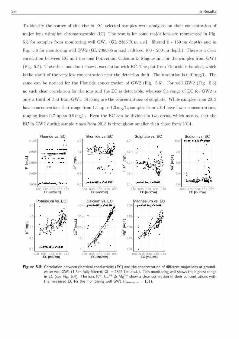
28 5 Results

To identify the source of this rise in EC, selected samples were analysed on their concentration of

major ions using ion chromatography (IC). The results for some major ions are represented in Fig.

5.5 for samples from monitoring well GW1 (GL 2365.70 m a.s.l.; filtered 0 - 150 cm depth) and in

Fig. 5.6 for monitoring well GW2 (GL 2365.06 m a.s.l.; filtered 100 - 200 cm depth). There is a clear

correlation between EC and the ions Potassium, Calcium & Magnesium for the samples from GW1

(Fig. 5.5). The other ions don’t show a correlation with EC. The plot from Flouride is banded, which

is the result of the very low concentration near the detection limit. The resolution is 0.01 mg/L. The

same can be noticed for the Flouride concentration of GW2 (Fig. 5.6). For well GW2 (Fig. 5.6)

no such clear correlation for the ions and the EC is detectable, whereas the range of EC for GW2 is

only a third of that from GW1. Striking are the concentrations of sulphate. While samples from 2013

have concentrations that range from 1.1 up to 1.3 mg/L, samples from 2014 have lower concentrations,

ranging from 0.7 up to 0.9 mg/L. Even the EC can be divided in two areas, which means, that the

EC in GW2 during sample times from 2013 is throughout smaller than those from 2014.

●

●●

●

●

●

●

●●

●

●

●

●

●

●

●●●●●●

●

●●●●●● ●●●●● ●

●●●●●

●●

●

●●●● ● ●●

●●

●

●●●

●●

●

●

●●

●●

●

●●

● ●

●

● ●

●

●●

●

●

●

● ●

● ●

●

● ● ●

●

●●●●

●

●●●●●●●●●●●●●●

●● ● ●●●●

●

●

y = 0.061 + 0.065 ⋅ x, r2 = 0.113y = 0.061 + 0.065 ⋅ x, r2 = 0.113y = 0.061 + 0.065 ⋅ x, r2 = 0.113y = 0.061 + 0.065 ⋅ x, r2 = 0.113y = 0.061 + 0.065 ⋅ x, r2 = 0.113y = 0.061 + 0.065 ⋅ x, r2 = 0.113y = 0.061 + 0.065 ⋅ x, r2 = 0.113y = 0.061 + 0.065 ⋅ x, r2 = 0.113y = 0.061 + 0.065 ⋅ x, r2 = 0.113y = 0.061 + 0.065 ⋅ x, r2 = 0.113y = 0.061 + 0.065 ⋅ x, r2 = 0.113y = 0.061 + 0.065 ⋅ x, r2 = 0.113y = 0.061 + 0.065 ⋅ x, r2 = 0.113y = 0.061 + 0.065 ⋅ x, r2 = 0.113y = 0.061 + 0.065 ⋅ x, r2 = 0.113y = 0.061 + 0.065 ⋅ x, r2 = 0.113y = 0.061 + 0.065 ⋅ x, r2 = 0.113y = 0.061 + 0.065 ⋅ x, r2 = 0.113y = 0.061 + 0.065 ⋅ x, r2 = 0.113y = 0.061 + 0.065 ⋅ x, r2 = 0.113y = 0.061 + 0.065 ⋅ x, r2 = 0.113y = 0.061 + 0.065 ⋅ x, r2 = 0.113y = 0.061 + 0.065 ⋅ x, r2 = 0.113y = 0.061 + 0.065 ⋅ x, r2 = 0.113y = 0.061 + 0.065 ⋅ x, r2 = 0.113y = 0.061 + 0.065 ⋅ x, r2 = 0.113y = 0.061 + 0.065 ⋅ x, r2 = 0.113y = 0.061 + 0.065 ⋅ x, r2 = 0.113y = 0.061 + 0.065 ⋅ x, r2 = 0.113y = 0.061 + 0.065 ⋅ x, r2 = 0.113y = 0.061 + 0.065 ⋅ x, r2 = 0.113y = 0.061 + 0.065 ⋅ x, r2 = 0.113y = 0.061 + 0.065 ⋅ x, r2 = 0.113y = 0.061 + 0.065 ⋅ x, r2 = 0.113y = 0.061 + 0.065 ⋅ x, r2 = 0.113y = 0.061 + 0.065 ⋅ x, r2 = 0.113y = 0.061 + 0.065 ⋅ x, r2 = 0.113y = 0.061 + 0.065 ⋅ x, r2 = 0.113y = 0.061 + 0.065 ⋅ x, r2 = 0.113y = 0.061 + 0.065 ⋅ x, r2 = 0.113y = 0.061 + 0.065 ⋅ x, r2 = 0.113y = 0.061 + 0.065 ⋅ x, r2 = 0.113y = 0.061 + 0.065 ⋅ x, r2 = 0.113y = 0.061 + 0.065 ⋅ x, r2 = 0.113y = 0.061 + 0.065 ⋅ x, r2 = 0.113y = 0.061 + 0.065 ⋅ x, r2 = 0.113y = 0.061 + 0.065 ⋅ x, r2 = 0.113y = 0.061 + 0.065 ⋅ x, r2 = 0.113y = 0.061 + 0.065 ⋅ x, r2 = 0.113y = 0.061 + 0.065 ⋅ x, r2 = 0.113y = 0.061 + 0.065 ⋅ x, r2 = 0.113y = 0.061 + 0.065 ⋅ x, r2 = 0.113y = 0.061 + 0.065 ⋅ x, r2 = 0.113y = 0.061 + 0.065 ⋅ x, r2 = 0.113y = 0.061 + 0.065 ⋅ x, r2 = 0.113y = 0.061 + 0.065 ⋅ x, r2 = 0.113y = 0.061 + 0.065 ⋅ x, r2 = 0.113y = 0.061 + 0.065 ⋅ x, r2 = 0.113y = 0.061 + 0.065 ⋅ x, r2 = 0.113y = 0.061 + 0.065 ⋅ x, r2 = 0.113y = 0.061 + 0.065 ⋅ x, r2 = 0.113y = 0.061 + 0.065 ⋅ x, r2 = 0.113y = 0.061 + 0.065 ⋅ x, r2 = 0.113y = 0.061 + 0.065 ⋅ x, r2 = 0.113y = 0.061 + 0.065 ⋅ x, r2 = 0.113y = 0.061 + 0.065 ⋅ x, r2 = 0.113y = 0.061 + 0.065 ⋅ x, r2 = 0.113y = 0.061 + 0.065 ⋅ x, r2 = 0.113y = 0.061 + 0.065 ⋅ x, r2 = 0.113y = 0.061 + 0.065 ⋅ x, r2 = 0.113y = 0.061 + 0.065 ⋅ x, r2 = 0.113y = 0.061 + 0.065 ⋅ x, r2 = 0.113y = 0.061 + 0.065 ⋅ x, r2 = 0.113y = 0.061 + 0.065 ⋅ x, r2 = 0.113y = 0.061 + 0.065 ⋅ x, r2 = 0.113y = 0.061 + 0.065 ⋅ x, r2 = 0.113y = 0.061 + 0.065 ⋅ x, r2 = 0.113y = 0.061 + 0.065 ⋅ x, r2 = 0.113y = 0.061 + 0.065 ⋅ x, r2 = 0.113y = 0.061 + 0.065 ⋅ x, r2 = 0.113y = 0.061 + 0.065 ⋅ x, r2 = 0.113y = 0.061 + 0.065 ⋅ x, r2 = 0.113y = 0.061 + 0.065 ⋅ x, r2 = 0.113y = 0.061 + 0.065 ⋅ x, r2 = 0.113y = 0.061 + 0.065 ⋅ x, r2 = 0.113y = 0.061 + 0.065 ⋅ x, r2 = 0.113y = 0.061 + 0.065 ⋅ x, r2 = 0.113y = 0.061 + 0.065 ⋅ x, r2 = 0.113y = 0.061 + 0.065 ⋅ x, r2 = 0.113y = 0.061 + 0.065 ⋅ x, r2 = 0.113y = 0.061 + 0.065 ⋅ x, r2 = 0.113y = 0.061 + 0.065 ⋅ x, r2 = 0.113y = 0.061 + 0.065 ⋅ x, r2 = 0.113y = 0.061 + 0.065 ⋅ x, r2 = 0.113y = 0.061 + 0.065 ⋅ x, r2 = 0.113y = 0.061 + 0.065 ⋅ x, r2 = 0.113y = 0.061 + 0.065 ⋅ x, r2 = 0.113y = 0.061 + 0.065 ⋅ x, r2 = 0.113y = 0.061 + 0.065 ⋅ x, r2 = 0.113y = 0.061 + 0.065 ⋅ x, r2 = 0.113y = 0.061 + 0.065 ⋅ x, r2 = 0.113y = 0.061 + 0.065 ⋅ x, r2 = 0.113y = 0.061 + 0.065 ⋅ x, r2 = 0.113y = 0.061 + 0.065 ⋅ x, r2 = 0.113y = 0.061 + 0.065 ⋅ x, r2 = 0.113y = 0.061 + 0.065 ⋅ x, r2 = 0.113y = 0.061 + 0.065 ⋅ x, r2 = 0.113y = 0.061 + 0.065 ⋅ x, r2 = 0.113y = 0.061 + 0.065 ⋅ x, r2 = 0.113y = 0.061 + 0.065 ⋅ x, r2 = 0.113y = 0.061 + 0.065 ⋅ x, r2 = 0.113y = 0.061 + 0.065 ⋅ x, r2 = 0.113y = 0.061 + 0.065 ⋅ x, r2 = 0.113y = 0.061 + 0.065 ⋅ x, r2 = 0.1130.000

0.025

0.050

0.075

0.100

0.00 0.05 0.10 0.15 0.20EC [mS/cm]

F− [m

g/L]

Fluoride vs. EC

●

●

●

●

●

●

●●

●

●

●

●

●

●

●

●●

●

●

●

●●

●●

●

●

●●

●

●

●

●●

●

●●

●●

●

●

●

●

●

●

●

●●

●

●●●

●

●●

●●

●●

●

●

●

●

●●

●

●●

●

●

●

●

●

●

●

●

●●

●●

●

●

●● ●

●●

●

●

●●

●●

●

●●●

●●

●●●●

●●

●

●● ●

●

●

●

●

●

●


0.5

1.0

1.5

2.0

0.00 0.05 0.10 0.15 0.20EC [mS/cm]

Br−

[mg/

L]

Bromide vs. EC

●

●

●

●●

●●

●

●

●●●

●

●●

●

●

●

●●●●

●●

●

●

●●

●●●

●●

●

●●

●●

●

●●

●●●●

● ●●

●●

●●

●

●●●●

●

●●

●

●●

●●

●●●

●

●

●

●

●

●●●

●●

●

●

●

●

●

●●

●

●●●●

●●●●●●●●●●●

●●●●

●

● ● ●●

●

●

●

●

y = 1 − 1.2 ⋅ x, r2 = 0.0467y = 1 − 1.2 ⋅ x, r2 = 0.0467y = 1 − 1.2 ⋅ x, r2 = 0.0467y = 1 − 1.2 ⋅ x, r2 = 0.0467y = 1 − 1.2 ⋅ x, r2 = 0.0467y = 1 − 1.2 ⋅ x, r2 = 0.0467y = 1 − 1.2 ⋅ x, r2 = 0.0467y = 1 − 1.2 ⋅ x, r2 = 0.0467y = 1 − 1.2 ⋅ x, r2 = 0.0467y = 1 − 1.2 ⋅ x, r2 = 0.0467y = 1 − 1.2 ⋅ x, r2 = 0.0467y = 1 − 1.2 ⋅ x, r2 = 0.0467y = 1 − 1.2 ⋅ x, r2 = 0.0467y = 1 − 1.2 ⋅ x, r2 = 0.0467y = 1 − 1.2 ⋅ x, r2 = 0.0467y = 1 − 1.2 ⋅ x, r2 = 0.0467y = 1 − 1.2 ⋅ x, r2 = 0.0467y = 1 − 1.2 ⋅ x, r2 = 0.0467y = 1 − 1.2 ⋅ x, r2 = 0.0467y = 1 − 1.2 ⋅ x, r2 = 0.0467y = 1 − 1.2 ⋅ x, r2 = 0.0467y = 1 − 1.2 ⋅ x, r2 = 0.0467y = 1 − 1.2 ⋅ x, r2 = 0.0467y = 1 − 1.2 ⋅ x, r2 = 0.0467y = 1 − 1.2 ⋅ x, r2 = 0.0467y = 1 − 1.2 ⋅ x, r2 = 0.0467y = 1 − 1.2 ⋅ x, r2 = 0.0467y = 1 − 1.2 ⋅ x, r2 = 0.0467y = 1 − 1.2 ⋅ x, r2 = 0.0467y = 1 − 1.2 ⋅ x, r2 = 0.0467y = 1 − 1.2 ⋅ x, r2 = 0.0467y = 1 − 1.2 ⋅ x, r2 = 0.0467y = 1 − 1.2 ⋅ x, r2 = 0.0467y = 1 − 1.2 ⋅ x, r2 = 0.0467y = 1 − 1.2 ⋅ x, r2 = 0.0467y = 1 − 1.2 ⋅ x, r2 = 0.0467y = 1 − 1.2 ⋅ x, r2 = 0.0467y = 1 − 1.2 ⋅ x, r2 = 0.0467y = 1 − 1.2 ⋅ x, r2 = 0.0467y = 1 − 1.2 ⋅ x, r2 = 0.0467y = 1 − 1.2 ⋅ x, r2 = 0.0467y = 1 − 1.2 ⋅ x, r2 = 0.0467y = 1 − 1.2 ⋅ x, r2 = 0.0467y = 1 − 1.2 ⋅ x, r2 = 0.0467y = 1 − 1.2 ⋅ x, r2 = 0.0467y = 1 − 1.2 ⋅ x, r2 = 0.0467y = 1 − 1.2 ⋅ x, r2 = 0.0467y = 1 − 1.2 ⋅ x, r2 = 0.0467y = 1 − 1.2 ⋅ x, r2 = 0.0467y = 1 − 1.2 ⋅ x, r2 = 0.0467y = 1 − 1.2 ⋅ x, r2 = 0.0467y = 1 − 1.2 ⋅ x, r2 = 0.0467y = 1 − 1.2 ⋅ x, r2 = 0.0467y = 1 − 1.2 ⋅ x, r2 = 0.0467y = 1 − 1.2 ⋅ x, r2 = 0.0467y = 1 − 1.2 ⋅ x, r2 = 0.0467y = 1 − 1.2 ⋅ x, r2 = 0.0467y = 1 − 1.2 ⋅ x, r2 = 0.0467y = 1 − 1.2 ⋅ x, r2 = 0.0467y = 1 − 1.2 ⋅ x, r2 = 0.0467y = 1 − 1.2 ⋅ x, r2 = 0.0467y = 1 − 1.2 ⋅ x, r2 = 0.0467y = 1 − 1.2 ⋅ x, r2 = 0.0467y = 1 − 1.2 ⋅ x, r2 = 0.0467y = 1 − 1.2 ⋅ x, r2 = 0.0467y = 1 − 1.2 ⋅ x, r2 = 0.0467y = 1 − 1.2 ⋅ x, r2 = 0.0467y = 1 − 1.2 ⋅ x, r2 = 0.0467y = 1 − 1.2 ⋅ x, r2 = 0.0467y = 1 − 1.2 ⋅ x, r2 = 0.0467y = 1 − 1.2 ⋅ x, r2 = 0.0467y = 1 − 1.2 ⋅ x, r2 = 0.0467y = 1 − 1.2 ⋅ x, r2 = 0.0467y = 1 − 1.2 ⋅ x, r2 = 0.0467y = 1 − 1.2 ⋅ x, r2 = 0.0467y = 1 − 1.2 ⋅ x, r2 = 0.0467y = 1 − 1.2 ⋅ x, r2 = 0.0467y = 1 − 1.2 ⋅ x, r2 = 0.0467y = 1 − 1.2 ⋅ x, r2 = 0.0467y = 1 − 1.2 ⋅ x, r2 = 0.0467y = 1 − 1.2 ⋅ x, r2 = 0.0467y = 1 − 1.2 ⋅ x, r2 = 0.0467y = 1 − 1.2 ⋅ x, r2 = 0.0467y = 1 − 1.2 ⋅ x, r2 = 0.0467y = 1 − 1.2 ⋅ x, r2 = 0.0467y = 1 − 1.2 ⋅ x, r2 = 0.0467y = 1 − 1.2 ⋅ x, r2 = 0.0467y = 1 − 1.2 ⋅ x, r2 = 0.0467y = 1 − 1.2 ⋅ x, r2 = 0.0467y = 1 − 1.2 ⋅ x, r2 = 0.0467y = 1 − 1.2 ⋅ x, r2 = 0.0467y = 1 − 1.2 ⋅ x, r2 = 0.0467y = 1 − 1.2 ⋅ x, r2 = 0.0467y = 1 − 1.2 ⋅ x, r2 = 0.0467y = 1 − 1.2 ⋅ x, r2 = 0.0467y = 1 − 1.2 ⋅ x, r2 = 0.0467y = 1 − 1.2 ⋅ x, r2 = 0.0467y = 1 − 1.2 ⋅ x, r2 = 0.0467y = 1 − 1.2 ⋅ x, r2 = 0.0467y = 1 − 1.2 ⋅ x, r2 = 0.0467y = 1 − 1.2 ⋅ x, r2 = 0.0467y = 1 − 1.2 ⋅ x, r2 = 0.0467y = 1 − 1.2 ⋅ x, r2 = 0.0467y = 1 − 1.2 ⋅ x, r2 = 0.0467y = 1 − 1.2 ⋅ x, r2 = 0.0467y = 1 − 1.2 ⋅ x, r2 = 0.0467y = 1 − 1.2 ⋅ x, r2 = 0.0467y = 1 − 1.2 ⋅ x, r2 = 0.0467y = 1 − 1.2 ⋅ x, r2 = 0.0467y = 1 − 1.2 ⋅ x, r2 = 0.0467y = 1 − 1.2 ⋅ x, r2 = 0.0467y = 1 − 1.2 ⋅ x, r2 = 0.0467y = 1 − 1.2 ⋅ x, r2 = 0.0467y = 1 − 1.2 ⋅ x, r2 = 0.04670.0

0.5

1.0

1.5

2.0

0.00 0.05 0.10 0.15 0.20EC [mS/cm]

SO

42− [m

g/L]

Sulphate vs. EC

●

●●

●●●●●●●

●●●●●●●

●●●●●●●●

●●● ●●●●

●

●

●●

●●●

●●● ●●●● ●●●

●●●

●●●●● ●

●

●

●

●

●●●

●● ●

●

●

●

●●●

●●●●

●

●

●

●

●

●●

●

●●●●●●●●●●

●●●●●●●●●●● ● ●●

●

●

●●

y = 0.64 + 4.5 ⋅ x, r2 = 0.0301y = 0.64 + 4.5 ⋅ x, r2 = 0.0301y = 0.64 + 4.5 ⋅ x, r2 = 0.0301y = 0.64 + 4.5 ⋅ x, r2 = 0.0301y = 0.64 + 4.5 ⋅ x, r2 = 0.0301y = 0.64 + 4.5 ⋅ x, r2 = 0.0301y = 0.64 + 4.5 ⋅ x, r2 = 0.0301y = 0.64 + 4.5 ⋅ x, r2 = 0.0301y = 0.64 + 4.5 ⋅ x, r2 = 0.0301y = 0.64 + 4.5 ⋅ x, r2 = 0.0301y = 0.64 + 4.5 ⋅ x, r2 = 0.0301y = 0.64 + 4.5 ⋅ x, r2 = 0.0301y = 0.64 + 4.5 ⋅ x, r2 = 0.0301y = 0.64 + 4.5 ⋅ x, r2 = 0.0301y = 0.64 + 4.5 ⋅ x, r2 = 0.0301y = 0.64 + 4.5 ⋅ x, r2 = 0.0301y = 0.64 + 4.5 ⋅ x, r2 = 0.0301y = 0.64 + 4.5 ⋅ x, r2 = 0.0301y = 0.64 + 4.5 ⋅ x, r2 = 0.0301y = 0.64 + 4.5 ⋅ x, r2 = 0.0301y = 0.64 + 4.5 ⋅ x, r2 = 0.0301y = 0.64 + 4.5 ⋅ x, r2 = 0.0301y = 0.64 + 4.5 ⋅ x, r2 = 0.0301y = 0.64 + 4.5 ⋅ x, r2 = 0.0301y = 0.64 + 4.5 ⋅ x, r2 = 0.0301y = 0.64 + 4.5 ⋅ x, r2 = 0.0301y = 0.64 + 4.5 ⋅ x, r2 = 0.0301y = 0.64 + 4.5 ⋅ x, r2 = 0.0301y = 0.64 + 4.5 ⋅ x, r2 = 0.0301y = 0.64 + 4.5 ⋅ x, r2 = 0.0301y = 0.64 + 4.5 ⋅ x, r2 = 0.0301y = 0.64 + 4.5 ⋅ x, r2 = 0.0301y = 0.64 + 4.5 ⋅ x, r2 = 0.0301y = 0.64 + 4.5 ⋅ x, r2 = 0.0301y = 0.64 + 4.5 ⋅ x, r2 = 0.0301y = 0.64 + 4.5 ⋅ x, r2 = 0.0301y = 0.64 + 4.5 ⋅ x, r2 = 0.0301y = 0.64 + 4.5 ⋅ x, r2 = 0.0301y = 0.64 + 4.5 ⋅ x, r2 = 0.0301y = 0.64 + 4.5 ⋅ x, r2 = 0.0301y = 0.64 + 4.5 ⋅ x, r2 = 0.0301y = 0.64 + 4.5 ⋅ x, r2 = 0.0301y = 0.64 + 4.5 ⋅ x, r2 = 0.0301y = 0.64 + 4.5 ⋅ x, r2 = 0.0301y = 0.64 + 4.5 ⋅ x, r2 = 0.0301y = 0.64 + 4.5 ⋅ x, r2 = 0.0301y = 0.64 + 4.5 ⋅ x, r2 = 0.0301y = 0.64 + 4.5 ⋅ x, r2 = 0.0301y = 0.64 + 4.5 ⋅ x, r2 = 0.0301y = 0.64 + 4.5 ⋅ x, r2 = 0.0301y = 0.64 + 4.5 ⋅ x, r2 = 0.0301y = 0.64 + 4.5 ⋅ x, r2 = 0.0301y = 0.64 + 4.5 ⋅ x, r2 = 0.0301y = 0.64 + 4.5 ⋅ x, r2 = 0.0301y = 0.64 + 4.5 ⋅ x, r2 = 0.0301y = 0.64 + 4.5 ⋅ x, r2 = 0.0301y = 0.64 + 4.5 ⋅ x, r2 = 0.0301y = 0.64 + 4.5 ⋅ x, r2 = 0.0301y = 0.64 + 4.5 ⋅ x, r2 = 0.0301y = 0.64 + 4.5 ⋅ x, r2 = 0.0301y = 0.64 + 4.5 ⋅ x, r2 = 0.0301y = 0.64 + 4.5 ⋅ x, r2 = 0.0301y = 0.64 + 4.5 ⋅ x, r2 = 0.0301y = 0.64 + 4.5 ⋅ x, r2 = 0.0301y = 0.64 + 4.5 ⋅ x, r2 = 0.0301y = 0.64 + 4.5 ⋅ x, r2 = 0.0301y = 0.64 + 4.5 ⋅ x, r2 = 0.0301y = 0.64 + 4.5 ⋅ x, r2 = 0.0301y = 0.64 + 4.5 ⋅ x, r2 = 0.0301y = 0.64 + 4.5 ⋅ x, r2 = 0.0301y = 0.64 + 4.5 ⋅ x, r2 = 0.0301y = 0.64 + 4.5 ⋅ x, r2 = 0.0301y = 0.64 + 4.5 ⋅ x, r2 = 0.0301y = 0.64 + 4.5 ⋅ x, r2 = 0.0301y = 0.64 + 4.5 ⋅ x, r2 = 0.0301y = 0.64 + 4.5 ⋅ x, r2 = 0.0301y = 0.64 + 4.5 ⋅ x, r2 = 0.0301y = 0.64 + 4.5 ⋅ x, r2 = 0.0301y = 0.64 + 4.5 ⋅ x, r2 = 0.0301y = 0.64 + 4.5 ⋅ x, r2 = 0.0301y = 0.64 + 4.5 ⋅ x, r2 = 0.0301y = 0.64 + 4.5 ⋅ x, r2 = 0.0301y = 0.64 + 4.5 ⋅ x, r2 = 0.0301y = 0.64 + 4.5 ⋅ x, r2 = 0.0301y = 0.64 + 4.5 ⋅ x, r2 = 0.0301y = 0.64 + 4.5 ⋅ x, r2 = 0.0301y = 0.64 + 4.5 ⋅ x, r2 = 0.0301y = 0.64 + 4.5 ⋅ x, r2 = 0.0301y = 0.64 + 4.5 ⋅ x, r2 = 0.0301y = 0.64 + 4.5 ⋅ x, r2 = 0.0301y = 0.64 + 4.5 ⋅ x, r2 = 0.0301y = 0.64 + 4.5 ⋅ x, r2 = 0.0301y = 0.64 + 4.5 ⋅ x, r2 = 0.0301y = 0.64 + 4.5 ⋅ x, r2 = 0.0301y = 0.64 + 4.5 ⋅ x, r2 = 0.0301y = 0.64 + 4.5 ⋅ x, r2 = 0.0301y = 0.64 + 4.5 ⋅ x, r2 = 0.0301y = 0.64 + 4.5 ⋅ x, r2 = 0.0301y = 0.64 + 4.5 ⋅ x, r2 = 0.0301y = 0.64 + 4.5 ⋅ x, r2 = 0.0301y = 0.64 + 4.5 ⋅ x, r2 = 0.0301y = 0.64 + 4.5 ⋅ x, r2 = 0.0301y = 0.64 + 4.5 ⋅ x, r2 = 0.0301y = 0.64 + 4.5 ⋅ x, r2 = 0.0301y = 0.64 + 4.5 ⋅ x, r2 = 0.0301y = 0.64 + 4.5 ⋅ x, r2 = 0.0301y = 0.64 + 4.5 ⋅ x, r2 = 0.0301y = 0.64 + 4.5 ⋅ x, r2 = 0.0301y = 0.64 + 4.5 ⋅ x, r2 = 0.0301y = 0.64 + 4.5 ⋅ x, r2 = 0.0301y = 0.64 + 4.5 ⋅ x, r2 = 0.0301y = 0.64 + 4.5 ⋅ x, r2 = 0.0301y = 0.64 + 4.5 ⋅ x, r2 = 0.0301y = 0.64 + 4.5 ⋅ x, r2 = 0.0301

0.0

2.5

5.0

7.5

10.0

0.00 0.05 0.10 0.15 0.20EC [mS/cm]

Na+ [m

g/L]

Sodium vs. EC

● ●●

●

●

●

●

●

●

●●

●

●

●

●●

●

●

●

●

●

●

●

●●

●

●

●

●

●

●

●

●

●

●

●

●

●

●

●

●

●

●

●

●

●

●

●

●

●

●

●

●

●

●

●●

●●

●

●

●

●

●

●

●

●

●

● ●

●●

●

●

●

●

●

●

●

●

● ●●●

●

●

●

●

●●

●

●●

●

●

●●

●

●●●

●

●●

●

●

●

●●

●

●

●

●

●


0.5

1.0

1.5

2.0

0.00 0.05 0.10 0.15 0.20EC [mS/cm]

K+ [m

g/L]

Potassium vs. EC

●

●

●●●●●

●●

●

●●●

●●

●

●●●

●●●

●●●●

●●●●

●

●●

●

●

●●

●

●

●

●●

●●

●

●●

●

●

●●●

●

●

●●

●

●●●

●

●

●

●●●

●●

●●

●●

●●●

●●

●●

●

●

●

●

●

●

●●

●●●

●●●●

●●●●●●

●●

●●

●

●● ● ●

●

●

●

●

●

y = −3.6 + 197 ⋅ x, r2 = 0.774y = −3.6 + 197 ⋅ x, r2 = 0.774y = −3.6 + 197 ⋅ x, r2 = 0.774y = −3.6 + 197 ⋅ x, r2 = 0.774y = −3.6 + 197 ⋅ x, r2 = 0.774y = −3.6 + 197 ⋅ x, r2 = 0.774y = −3.6 + 197 ⋅ x, r2 = 0.774y = −3.6 + 197 ⋅ x, r2 = 0.774y = −3.6 + 197 ⋅ x, r2 = 0.774y = −3.6 + 197 ⋅ x, r2 = 0.774y = −3.6 + 197 ⋅ x, r2 = 0.774y = −3.6 + 197 ⋅ x, r2 = 0.774y = −3.6 + 197 ⋅ x, r2 = 0.774y = −3.6 + 197 ⋅ x, r2 = 0.774y = −3.6 + 197 ⋅ x, r2 = 0.774y = −3.6 + 197 ⋅ x, r2 = 0.774y = −3.6 + 197 ⋅ x, r2 = 0.774y = −3.6 + 197 ⋅ x, r2 = 0.774y = −3.6 + 197 ⋅ x, r2 = 0.774y = −3.6 + 197 ⋅ x, r2 = 0.774y = −3.6 + 197 ⋅ x, r2 = 0.774y = −3.6 + 197 ⋅ x, r2 = 0.774y = −3.6 + 197 ⋅ x, r2 = 0.774y = −3.6 + 197 ⋅ x, r2 = 0.774y = −3.6 + 197 ⋅ x, r2 = 0.774y = −3.6 + 197 ⋅ x, r2 = 0.774y = −3.6 + 197 ⋅ x, r2 = 0.774y = −3.6 + 197 ⋅ x, r2 = 0.774y = −3.6 + 197 ⋅ x, r2 = 0.774y = −3.6 + 197 ⋅ x, r2 = 0.774y = −3.6 + 197 ⋅ x, r2 = 0.774y = −3.6 + 197 ⋅ x, r2 = 0.774y = −3.6 + 197 ⋅ x, r2 = 0.774y = −3.6 + 197 ⋅ x, r2 = 0.774y = −3.6 + 197 ⋅ x, r2 = 0.774y = −3.6 + 197 ⋅ x, r2 = 0.774y = −3.6 + 197 ⋅ x, r2 = 0.774y = −3.6 + 197 ⋅ x, r2 = 0.774y = −3.6 + 197 ⋅ x, r2 = 0.774y = −3.6 + 197 ⋅ x, r2 = 0.774y = −3.6 + 197 ⋅ x, r2 = 0.774y = −3.6 + 197 ⋅ x, r2 = 0.774y = −3.6 + 197 ⋅ x, r2 = 0.774y = −3.6 + 197 ⋅ x, r2 = 0.774y = −3.6 + 197 ⋅ x, r2 = 0.774y = −3.6 + 197 ⋅ x, r2 = 0.774y = −3.6 + 197 ⋅ x, r2 = 0.774y = −3.6 + 197 ⋅ x, r2 = 0.774y = −3.6 + 197 ⋅ x, r2 = 0.774y = −3.6 + 197 ⋅ x, r2 = 0.774y = −3.6 + 197 ⋅ x, r2 = 0.774y = −3.6 + 197 ⋅ x, r2 = 0.774y = −3.6 + 197 ⋅ x, r2 = 0.774y = −3.6 + 197 ⋅ x, r2 = 0.774y = −3.6 + 197 ⋅ x, r2 = 0.774y = −3.6 + 197 ⋅ x, r2 = 0.774y = −3.6 + 197 ⋅ x, r2 = 0.774y = −3.6 + 197 ⋅ x, r2 = 0.774y = −3.6 + 197 ⋅ x, r2 = 0.774y = −3.6 + 197 ⋅ x, r2 = 0.774y = −3.6 + 197 ⋅ x, r2 = 0.774y = −3.6 + 197 ⋅ x, r2 = 0.774y = −3.6 + 197 ⋅ x, r2 = 0.774y = −3.6 + 197 ⋅ x, r2 = 0.774y = −3.6 + 197 ⋅ x, r2 = 0.774y = −3.6 + 197 ⋅ x, r2 = 0.774y = −3.6 + 197 ⋅ x, r2 = 0.774y = −3.6 + 197 ⋅ x, r2 = 0.774y = −3.6 + 197 ⋅ x, r2 = 0.774y = −3.6 + 197 ⋅ x, r2 = 0.774y = −3.6 + 197 ⋅ x, r2 = 0.774y = −3.6 + 197 ⋅ x, r2 = 0.774y = −3.6 + 197 ⋅ x, r2 = 0.774y = −3.6 + 197 ⋅ x, r2 = 0.774y = −3.6 + 197 ⋅ x, r2 = 0.774y = −3.6 + 197 ⋅ x, r2 = 0.774y = −3.6 + 197 ⋅ x, r2 = 0.774y = −3.6 + 197 ⋅ x, r2 = 0.774y = −3.6 + 197 ⋅ x, r2 = 0.774y = −3.6 + 197 ⋅ x, r2 = 0.774y = −3.6 + 197 ⋅ x, r2 = 0.774y = −3.6 + 197 ⋅ x, r2 = 0.774y = −3.6 + 197 ⋅ x, r2 = 0.774y = −3.6 + 197 ⋅ x, r2 = 0.774y = −3.6 + 197 ⋅ x, r2 = 0.774y = −3.6 + 197 ⋅ x, r2 = 0.774y = −3.6 + 197 ⋅ x, r2 = 0.774y = −3.6 + 197 ⋅ x, r2 = 0.774y = −3.6 + 197 ⋅ x, r2 = 0.774y = −3.6 + 197 ⋅ x, r2 = 0.774y = −3.6 + 197 ⋅ x, r2 = 0.774y = −3.6 + 197 ⋅ x, r2 = 0.774y = −3.6 + 197 ⋅ x, r2 = 0.774y = −3.6 + 197 ⋅ x, r2 = 0.774y = −3.6 + 197 ⋅ x, r2 = 0.774y = −3.6 + 197 ⋅ x, r2 = 0.774y = −3.6 + 197 ⋅ x, r2 = 0.774y = −3.6 + 197 ⋅ x, r2 = 0.774y = −3.6 + 197 ⋅ x, r2 = 0.774y = −3.6 + 197 ⋅ x, r2 = 0.774y = −3.6 + 197 ⋅ x, r2 = 0.774y = −3.6 + 197 ⋅ x, r2 = 0.774y = −3.6 + 197 ⋅ x, r2 = 0.774y = −3.6 + 197 ⋅ x, r2 = 0.774y = −3.6 + 197 ⋅ x, r2 = 0.774y = −3.6 + 197 ⋅ x, r2 = 0.774y = −3.6 + 197 ⋅ x, r2 = 0.774y = −3.6 + 197 ⋅ x, r2 = 0.774y = −3.6 + 197 ⋅ x, r2 = 0.774y = −3.6 + 197 ⋅ x, r2 = 0.774y = −3.6 + 197 ⋅ x, r2 = 0.774y = −3.6 + 197 ⋅ x, r2 = 0.774y = −3.6 + 197 ⋅ x, r2 = 0.774y = −3.6 + 197 ⋅ x, r2 = 0.774

0

10

20

30

40

0.00 0.05 0.10 0.15 0.20EC [mS/cm]

Ca2+

[mg/

L]

Calcium vs. EC

●

●

●

●●●

●●

●

●

●●

●

●

●

●

●

●●

●

●

●

●

●●

●

●● ●

●

●

●

●

●

●●

●

●

●

●●

●

●

●

●

●

●

●

●●

●

●

●

●●

●

●

●

●

●

●

●●

●●

●

●●

●

●

●

●

●

●

●

●

●

●●

●

●

●

● ●

●

●

●

●

●

●

●●

●

●

●

●

●●

●

●

●

●

●

●●

●

●

●

●●

●

●

●

●

y = 0.2 + 2.6 ⋅ x, r2 = 0.634y = 0.2 + 2.6 ⋅ x, r2 = 0.634y = 0.2 + 2.6 ⋅ x, r2 = 0.634y = 0.2 + 2.6 ⋅ x, r2 = 0.634y = 0.2 + 2.6 ⋅ x, r2 = 0.634y = 0.2 + 2.6 ⋅ x, r2 = 0.634y = 0.2 + 2.6 ⋅ x, r2 = 0.634y = 0.2 + 2.6 ⋅ x, r2 = 0.634y = 0.2 + 2.6 ⋅ x, r2 = 0.634y = 0.2 + 2.6 ⋅ x, r2 = 0.634y = 0.2 + 2.6 ⋅ x, r2 = 0.634y = 0.2 + 2.6 ⋅ x, r2 = 0.634y = 0.2 + 2.6 ⋅ x, r2 = 0.634y = 0.2 + 2.6 ⋅ x, r2 = 0.634y = 0.2 + 2.6 ⋅ x, r2 = 0.634y = 0.2 + 2.6 ⋅ x, r2 = 0.634y = 0.2 + 2.6 ⋅ x, r2 = 0.634y = 0.2 + 2.6 ⋅ x, r2 = 0.634y = 0.2 + 2.6 ⋅ x, r2 = 0.634y = 0.2 + 2.6 ⋅ x, r2 = 0.634y = 0.2 + 2.6 ⋅ x, r2 = 0.634y = 0.2 + 2.6 ⋅ x, r2 = 0.634y = 0.2 + 2.6 ⋅ x, r2 = 0.634y = 0.2 + 2.6 ⋅ x, r2 = 0.634y = 0.2 + 2.6 ⋅ x, r2 = 0.634y = 0.2 + 2.6 ⋅ x, r2 = 0.634y = 0.2 + 2.6 ⋅ x, r2 = 0.634y = 0.2 + 2.6 ⋅ x, r2 = 0.634y = 0.2 + 2.6 ⋅ x, r2 = 0.634y = 0.2 + 2.6 ⋅ x, r2 = 0.634y = 0.2 + 2.6 ⋅ x, r2 = 0.634y = 0.2 + 2.6 ⋅ x, r2 = 0.634y = 0.2 + 2.6 ⋅ x, r2 = 0.634y = 0.2 + 2.6 ⋅ x, r2 = 0.634y = 0.2 + 2.6 ⋅ x, r2 = 0.634y = 0.2 + 2.6 ⋅ x, r2 = 0.634y = 0.2 + 2.6 ⋅ x, r2 = 0.634y = 0.2 + 2.6 ⋅ x, r2 = 0.634y = 0.2 + 2.6 ⋅ x, r2 = 0.634y = 0.2 + 2.6 ⋅ x, r2 = 0.634y = 0.2 + 2.6 ⋅ x, r2 = 0.634y = 0.2 + 2.6 ⋅ x, r2 = 0.634y = 0.2 + 2.6 ⋅ x, r2 = 0.634y = 0.2 + 2.6 ⋅ x, r2 = 0.634y = 0.2 + 2.6 ⋅ x, r2 = 0.634y = 0.2 + 2.6 ⋅ x, r2 = 0.634y = 0.2 + 2.6 ⋅ x, r2 = 0.634y = 0.2 + 2.6 ⋅ x, r2 = 0.634y = 0.2 + 2.6 ⋅ x, r2 = 0.634y = 0.2 + 2.6 ⋅ x, r2 = 0.634y = 0.2 + 2.6 ⋅ x, r2 = 0.634y = 0.2 + 2.6 ⋅ x, r2 = 0.634y = 0.2 + 2.6 ⋅ x, r2 = 0.634y = 0.2 + 2.6 ⋅ x, r2 = 0.634y = 0.2 + 2.6 ⋅ x, r2 = 0.634y = 0.2 + 2.6 ⋅ x, r2 = 0.634y = 0.2 + 2.6 ⋅ x, r2 = 0.634y = 0.2 + 2.6 ⋅ x, r2 = 0.634y = 0.2 + 2.6 ⋅ x, r2 = 0.634y = 0.2 + 2.6 ⋅ x, r2 = 0.634y = 0.2 + 2.6 ⋅ x, r2 = 0.634y = 0.2 + 2.6 ⋅ x, r2 = 0.634y = 0.2 + 2.6 ⋅ x, r2 = 0.634y = 0.2 + 2.6 ⋅ x, r2 = 0.634y = 0.2 + 2.6 ⋅ x, r2 = 0.634y = 0.2 + 2.6 ⋅ x, r2 = 0.634y = 0.2 + 2.6 ⋅ x, r2 = 0.634y = 0.2 + 2.6 ⋅ x, r2 = 0.634y = 0.2 + 2.6 ⋅ x, r2 = 0.634y = 0.2 + 2.6 ⋅ x, r2 = 0.634y = 0.2 + 2.6 ⋅ x, r2 = 0.634y = 0.2 + 2.6 ⋅ x, r2 = 0.634y = 0.2 + 2.6 ⋅ x, r2 = 0.634y = 0.2 + 2.6 ⋅ x, r2 = 0.634y = 0.2 + 2.6 ⋅ x, r2 = 0.634y = 0.2 + 2.6 ⋅ x, r2 = 0.634y = 0.2 + 2.6 ⋅ x, r2 = 0.634y = 0.2 + 2.6 ⋅ x, r2 = 0.634y = 0.2 + 2.6 ⋅ x, r2 = 0.634y = 0.2 + 2.6 ⋅ x, r2 = 0.634y = 0.2 + 2.6 ⋅ x, r2 = 0.634y = 0.2 + 2.6 ⋅ x, r2 = 0.634y = 0.2 + 2.6 ⋅ x, r2 = 0.634y = 0.2 + 2.6 ⋅ x, r2 = 0.634y = 0.2 + 2.6 ⋅ x, r2 = 0.634y = 0.2 + 2.6 ⋅ x, r2 = 0.634y = 0.2 + 2.6 ⋅ x, r2 = 0.634y = 0.2 + 2.6 ⋅ x, r2 = 0.634y = 0.2 + 2.6 ⋅ x, r2 = 0.634y = 0.2 + 2.6 ⋅ x, r2 = 0.634y = 0.2 + 2.6 ⋅ x, r2 = 0.634y = 0.2 + 2.6 ⋅ x, r2 = 0.634y = 0.2 + 2.6 ⋅ x, r2 = 0.634y = 0.2 + 2.6 ⋅ x, r2 = 0.634y = 0.2 + 2.6 ⋅ x, r2 = 0.634y = 0.2 + 2.6 ⋅ x, r2 = 0.634y = 0.2 + 2.6 ⋅ x, r2 = 0.634y = 0.2 + 2.6 ⋅ x, r2 = 0.634y = 0.2 + 2.6 ⋅ x, r2 = 0.634y = 0.2 + 2.6 ⋅ x, r2 = 0.634y = 0.2 + 2.6 ⋅ x, r2 = 0.634y = 0.2 + 2.6 ⋅ x, r2 = 0.634y = 0.2 + 2.6 ⋅ x, r2 = 0.634y = 0.2 + 2.6 ⋅ x, r2 = 0.634y = 0.2 + 2.6 ⋅ x, r2 = 0.634y = 0.2 + 2.6 ⋅ x, r2 = 0.634y = 0.2 + 2.6 ⋅ x, r2 = 0.634y = 0.2 + 2.6 ⋅ x, r2 = 0.634y = 0.2 + 2.6 ⋅ x, r2 = 0.634y = 0.2 + 2.6 ⋅ x, r2 = 0.634y = 0.2 + 2.6 ⋅ x, r2 = 0.634y = 0.2 + 2.6 ⋅ x, r2 = 0.634y = 0.2 + 2.6 ⋅ x, r2 = 0.634y = 0.2 + 2.6 ⋅ x, r2 = 0.634

0.00

0.25

0.50

0.75

1.00

0.00 0.05 0.10 0.15 0.20EC [mS/cm]

Mg2+

[mg/

L]

Magnesium vs. EC

Figure 5.5: Correlation between electrical conductivity (EC) and the concentration of different major ions at ground-water well GW1 (1.5 m fully filtered; GL = 2365.7 m a.s.l.). This monitoring well shows the highest rangein EC (see Fig. 5.4). The ions K+, Ca2+ & Mg2+ show a clear correlation in their concentrations withthe measured EC for the monitoring well GW1 (nsamples = 151).

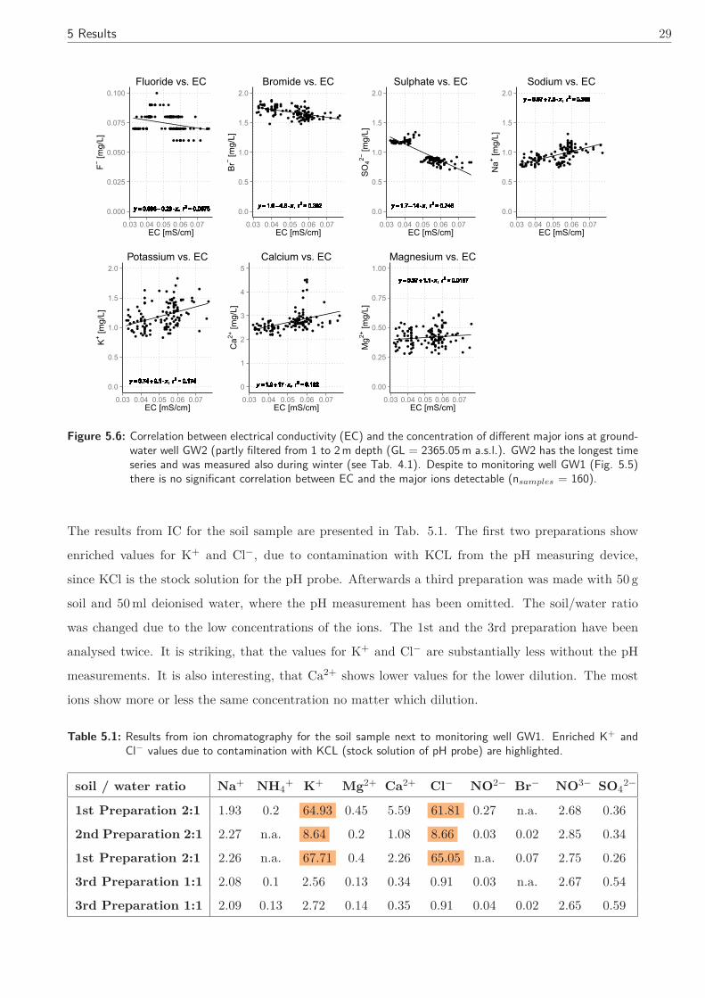
5 Results 29

●●●●

●●

●●●●

●

●●●●●●

●

●●●●●●

●

●

●●

●

●●

●●●

●

●●●●

●

●

●

●●●

●

●● ●●

●

●●● ●● ●●●● ●●

●

● ●● ●●●●●●

●

●●●●● ●●● ●

●●

●

●●

●●

●●●

●

●●

●

●●●● ●●●●● ●● ●●●● ●●●●

●

●● ●● ● ● ● ●●

y = 0.086 − 0.23 ⋅ x, r2 = 0.0875y = 0.086 − 0.23 ⋅ x, r2 = 0.0875y = 0.086 − 0.23 ⋅ x, r2 = 0.0875y = 0.086 − 0.23 ⋅ x, r2 = 0.0875y = 0.086 − 0.23 ⋅ x, r2 = 0.0875y = 0.086 − 0.23 ⋅ x, r2 = 0.0875y = 0.086 − 0.23 ⋅ x, r2 = 0.0875y = 0.086 − 0.23 ⋅ x, r2 = 0.0875y = 0.086 − 0.23 ⋅ x, r2 = 0.0875y = 0.086 − 0.23 ⋅ x, r2 = 0.0875y = 0.086 − 0.23 ⋅ x, r2 = 0.0875y = 0.086 − 0.23 ⋅ x, r2 = 0.0875y = 0.086 − 0.23 ⋅ x, r2 = 0.0875y = 0.086 − 0.23 ⋅ x, r2 = 0.0875y = 0.086 − 0.23 ⋅ x, r2 = 0.0875y = 0.086 − 0.23 ⋅ x, r2 = 0.0875y = 0.086 − 0.23 ⋅ x, r2 = 0.0875y = 0.086 − 0.23 ⋅ x, r2 = 0.0875y = 0.086 − 0.23 ⋅ x, r2 = 0.0875y = 0.086 − 0.23 ⋅ x, r2 = 0.0875y = 0.086 − 0.23 ⋅ x, r2 = 0.0875y = 0.086 − 0.23 ⋅ x, r2 = 0.0875y = 0.086 − 0.23 ⋅ x, r2 = 0.0875y = 0.086 − 0.23 ⋅ x, r2 = 0.0875y = 0.086 − 0.23 ⋅ x, r2 = 0.0875y = 0.086 − 0.23 ⋅ x, r2 = 0.0875y = 0.086 − 0.23 ⋅ x, r2 = 0.0875y = 0.086 − 0.23 ⋅ x, r2 = 0.0875y = 0.086 − 0.23 ⋅ x, r2 = 0.0875y = 0.086 − 0.23 ⋅ x, r2 = 0.0875y = 0.086 − 0.23 ⋅ x, r2 = 0.0875y = 0.086 − 0.23 ⋅ x, r2 = 0.0875y = 0.086 − 0.23 ⋅ x, r2 = 0.0875y = 0.086 − 0.23 ⋅ x, r2 = 0.0875y = 0.086 − 0.23 ⋅ x, r2 = 0.0875y = 0.086 − 0.23 ⋅ x, r2 = 0.0875y = 0.086 − 0.23 ⋅ x, r2 = 0.0875y = 0.086 − 0.23 ⋅ x, r2 = 0.0875y = 0.086 − 0.23 ⋅ x, r2 = 0.0875y = 0.086 − 0.23 ⋅ x, r2 = 0.0875y = 0.086 − 0.23 ⋅ x, r2 = 0.0875y = 0.086 − 0.23 ⋅ x, r2 = 0.0875y = 0.086 − 0.23 ⋅ x, r2 = 0.0875y = 0.086 − 0.23 ⋅ x, r2 = 0.0875y = 0.086 − 0.23 ⋅ x, r2 = 0.0875y = 0.086 − 0.23 ⋅ x, r2 = 0.0875y = 0.086 − 0.23 ⋅ x, r2 = 0.0875y = 0.086 − 0.23 ⋅ x, r2 = 0.0875y = 0.086 − 0.23 ⋅ x, r2 = 0.0875y = 0.086 − 0.23 ⋅ x, r2 = 0.0875y = 0.086 − 0.23 ⋅ x, r2 = 0.0875y = 0.086 − 0.23 ⋅ x, r2 = 0.0875y = 0.086 − 0.23 ⋅ x, r2 = 0.0875y = 0.086 − 0.23 ⋅ x, r2 = 0.0875y = 0.086 − 0.23 ⋅ x, r2 = 0.0875y = 0.086 − 0.23 ⋅ x, r2 = 0.0875y = 0.086 − 0.23 ⋅ x, r2 = 0.0875y = 0.086 − 0.23 ⋅ x, r2 = 0.0875y = 0.086 − 0.23 ⋅ x, r2 = 0.0875y = 0.086 − 0.23 ⋅ x, r2 = 0.0875y = 0.086 − 0.23 ⋅ x, r2 = 0.0875y = 0.086 − 0.23 ⋅ x, r2 = 0.0875y = 0.086 − 0.23 ⋅ x, r2 = 0.0875y = 0.086 − 0.23 ⋅ x, r2 = 0.0875y = 0.086 − 0.23 ⋅ x, r2 = 0.0875y = 0.086 − 0.23 ⋅ x, r2 = 0.0875y = 0.086 − 0.23 ⋅ x, r2 = 0.0875y = 0.086 − 0.23 ⋅ x, r2 = 0.0875y = 0.086 − 0.23 ⋅ x, r2 = 0.0875y = 0.086 − 0.23 ⋅ x, r2 = 0.0875y = 0.086 − 0.23 ⋅ x, r2 = 0.0875y = 0.086 − 0.23 ⋅ x, r2 = 0.0875y = 0.086 − 0.23 ⋅ x, r2 = 0.0875y = 0.086 − 0.23 ⋅ x, r2 = 0.0875y = 0.086 − 0.23 ⋅ x, r2 = 0.0875y = 0.086 − 0.23 ⋅ x, r2 = 0.0875y = 0.086 − 0.23 ⋅ x, r2 = 0.0875y = 0.086 − 0.23 ⋅ x, r2 = 0.0875y = 0.086 − 0.23 ⋅ x, r2 = 0.0875y = 0.086 − 0.23 ⋅ x, r2 = 0.0875y = 0.086 − 0.23 ⋅ x, r2 = 0.0875y = 0.086 − 0.23 ⋅ x, r2 = 0.0875y = 0.086 − 0.23 ⋅ x, r2 = 0.0875y = 0.086 − 0.23 ⋅ x, r2 = 0.0875y = 0.086 − 0.23 ⋅ x, r2 = 0.0875y = 0.086 − 0.23 ⋅ x, r2 = 0.0875y = 0.086 − 0.23 ⋅ x, r2 = 0.0875y = 0.086 − 0.23 ⋅ x, r2 = 0.0875y = 0.086 − 0.23 ⋅ x, r2 = 0.0875y = 0.086 − 0.23 ⋅ x, r2 = 0.0875y = 0.086 − 0.23 ⋅ x, r2 = 0.0875y = 0.086 − 0.23 ⋅ x, r2 = 0.0875y = 0.086 − 0.23 ⋅ x, r2 = 0.0875y = 0.086 − 0.23 ⋅ x, r2 = 0.0875y = 0.086 − 0.23 ⋅ x, r2 = 0.0875y = 0.086 − 0.23 ⋅ x, r2 = 0.0875y = 0.086 − 0.23 ⋅ x, r2 = 0.0875y = 0.086 − 0.23 ⋅ x, r2 = 0.0875y = 0.086 − 0.23 ⋅ x, r2 = 0.0875y = 0.086 − 0.23 ⋅ x, r2 = 0.0875y = 0.086 − 0.23 ⋅ x, r2 = 0.0875y = 0.086 − 0.23 ⋅ x, r2 = 0.0875y = 0.086 − 0.23 ⋅ x, r2 = 0.0875y = 0.086 − 0.23 ⋅ x, r2 = 0.0875y = 0.086 − 0.23 ⋅ x, r2 = 0.0875y = 0.086 − 0.23 ⋅ x, r2 = 0.0875y = 0.086 − 0.23 ⋅ x, r2 = 0.0875y = 0.086 − 0.23 ⋅ x, r2 = 0.0875y = 0.086 − 0.23 ⋅ x, r2 = 0.0875y = 0.086 − 0.23 ⋅ x, r2 = 0.0875y = 0.086 − 0.23 ⋅ x, r2 = 0.0875y = 0.086 − 0.23 ⋅ x, r2 = 0.0875y = 0.086 − 0.23 ⋅ x, r2 = 0.0875y = 0.086 − 0.23 ⋅ x, r2 = 0.0875y = 0.086 − 0.23 ⋅ x, r2 = 0.0875y = 0.086 − 0.23 ⋅ x, r2 = 0.0875y = 0.086 − 0.23 ⋅ x, r2 = 0.0875y = 0.086 − 0.23 ⋅ x, r2 = 0.0875y = 0.086 − 0.23 ⋅ x, r2 = 0.0875y = 0.086 − 0.23 ⋅ x, r2 = 0.0875y = 0.086 − 0.23 ⋅ x, r2 = 0.0875y = 0.086 − 0.23 ⋅ x, r2 = 0.0875y = 0.086 − 0.23 ⋅ x, r2 = 0.0875y = 0.086 − 0.23 ⋅ x, r2 = 0.0875y = 0.086 − 0.23 ⋅ x, r2 = 0.08750.000

0.025

0.050

0.075

0.100

0.03 0.04 0.05 0.06 0.07EC [mS/cm]

F− [m

g/L]

Fluoride vs. EC

●●

●

●

●

●

●●●●●

●●●●●●

●

●

●

●●●

●●●

●

●

●●●●

●

●●

●●

●●

●●

●●●●●●●

●●

●●●● ●

●●

●●●

●●

●

●

●●

●●●

●

●

●

●●

●●

●●

●●

●

●●●

●

●●

●●●

●●

●●

●

●●●●

●

●

●

●

●● ●●

●●

●●●

●●

●

●●● ●

●● ● ● ●

●

y = 1.9 − 4.8 ⋅ x, r2 = 0.302y = 1.9 − 4.8 ⋅ x, r2 = 0.302y = 1.9 − 4.8 ⋅ x, r2 = 0.302y = 1.9 − 4.8 ⋅ x, r2 = 0.302y = 1.9 − 4.8 ⋅ x, r2 = 0.302y = 1.9 − 4.8 ⋅ x, r2 = 0.302y = 1.9 − 4.8 ⋅ x, r2 = 0.302y = 1.9 − 4.8 ⋅ x, r2 = 0.302y = 1.9 − 4.8 ⋅ x, r2 = 0.302y = 1.9 − 4.8 ⋅ x, r2 = 0.302y = 1.9 − 4.8 ⋅ x, r2 = 0.302y = 1.9 − 4.8 ⋅ x, r2 = 0.302y = 1.9 − 4.8 ⋅ x, r2 = 0.302y = 1.9 − 4.8 ⋅ x, r2 = 0.302y = 1.9 − 4.8 ⋅ x, r2 = 0.302y = 1.9 − 4.8 ⋅ x, r2 = 0.302y = 1.9 − 4.8 ⋅ x, r2 = 0.302y = 1.9 − 4.8 ⋅ x, r2 = 0.302y = 1.9 − 4.8 ⋅ x, r2 = 0.302y = 1.9 − 4.8 ⋅ x, r2 = 0.302y = 1.9 − 4.8 ⋅ x, r2 = 0.302y = 1.9 − 4.8 ⋅ x, r2 = 0.302y = 1.9 − 4.8 ⋅ x, r2 = 0.302y = 1.9 − 4.8 ⋅ x, r2 = 0.302y = 1.9 − 4.8 ⋅ x, r2 = 0.302y = 1.9 − 4.8 ⋅ x, r2 = 0.302y = 1.9 − 4.8 ⋅ x, r2 = 0.302y = 1.9 − 4.8 ⋅ x, r2 = 0.302y = 1.9 − 4.8 ⋅ x, r2 = 0.302y = 1.9 − 4.8 ⋅ x, r2 = 0.302y = 1.9 − 4.8 ⋅ x, r2 = 0.302y = 1.9 − 4.8 ⋅ x, r2 = 0.302y = 1.9 − 4.8 ⋅ x, r2 = 0.302y = 1.9 − 4.8 ⋅ x, r2 = 0.302y = 1.9 − 4.8 ⋅ x, r2 = 0.302y = 1.9 − 4.8 ⋅ x, r2 = 0.302y = 1.9 − 4.8 ⋅ x, r2 = 0.302y = 1.9 − 4.8 ⋅ x, r2 = 0.302y = 1.9 − 4.8 ⋅ x, r2 = 0.302y = 1.9 − 4.8 ⋅ x, r2 = 0.302y = 1.9 − 4.8 ⋅ x, r2 = 0.302y = 1.9 − 4.8 ⋅ x, r2 = 0.302y = 1.9 − 4.8 ⋅ x, r2 = 0.302y = 1.9 − 4.8 ⋅ x, r2 = 0.302y = 1.9 − 4.8 ⋅ x, r2 = 0.302y = 1.9 − 4.8 ⋅ x, r2 = 0.302y = 1.9 − 4.8 ⋅ x, r2 = 0.302y = 1.9 − 4.8 ⋅ x, r2 = 0.302y = 1.9 − 4.8 ⋅ x, r2 = 0.302y = 1.9 − 4.8 ⋅ x, r2 = 0.302y = 1.9 − 4.8 ⋅ x, r2 = 0.302y = 1.9 − 4.8 ⋅ x, r2 = 0.302y = 1.9 − 4.8 ⋅ x, r2 = 0.302y = 1.9 − 4.8 ⋅ x, r2 = 0.302y = 1.9 − 4.8 ⋅ x, r2 = 0.302y = 1.9 − 4.8 ⋅ x, r2 = 0.302y = 1.9 − 4.8 ⋅ x, r2 = 0.302y = 1.9 − 4.8 ⋅ x, r2 = 0.302y = 1.9 − 4.8 ⋅ x, r2 = 0.302y = 1.9 − 4.8 ⋅ x, r2 = 0.302y = 1.9 − 4.8 ⋅ x, r2 = 0.302y = 1.9 − 4.8 ⋅ x, r2 = 0.302y = 1.9 − 4.8 ⋅ x, r2 = 0.302y = 1.9 − 4.8 ⋅ x, r2 = 0.302y = 1.9 − 4.8 ⋅ x, r2 = 0.302y = 1.9 − 4.8 ⋅ x, r2 = 0.302y = 1.9 − 4.8 ⋅ x, r2 = 0.302y = 1.9 − 4.8 ⋅ x, r2 = 0.302y = 1.9 − 4.8 ⋅ x, r2 = 0.302y = 1.9 − 4.8 ⋅ x, r2 = 0.302y = 1.9 − 4.8 ⋅ x, r2 = 0.302y = 1.9 − 4.8 ⋅ x, r2 = 0.302y = 1.9 − 4.8 ⋅ x, r2 = 0.302y = 1.9 − 4.8 ⋅ x, r2 = 0.302y = 1.9 − 4.8 ⋅ x, r2 = 0.302y = 1.9 − 4.8 ⋅ x, r2 = 0.302y = 1.9 − 4.8 ⋅ x, r2 = 0.302y = 1.9 − 4.8 ⋅ x, r2 = 0.302y = 1.9 − 4.8 ⋅ x, r2 = 0.302y = 1.9 − 4.8 ⋅ x, r2 = 0.302y = 1.9 − 4.8 ⋅ x, r2 = 0.302y = 1.9 − 4.8 ⋅ x, r2 = 0.302y = 1.9 − 4.8 ⋅ x, r2 = 0.302y = 1.9 − 4.8 ⋅ x, r2 = 0.302y = 1.9 − 4.8 ⋅ x, r2 = 0.302y = 1.9 − 4.8 ⋅ x, r2 = 0.302y = 1.9 − 4.8 ⋅ x, r2 = 0.302y = 1.9 − 4.8 ⋅ x, r2 = 0.302y = 1.9 − 4.8 ⋅ x, r2 = 0.302y = 1.9 − 4.8 ⋅ x, r2 = 0.302y = 1.9 − 4.8 ⋅ x, r2 = 0.302y = 1.9 − 4.8 ⋅ x, r2 = 0.302y = 1.9 − 4.8 ⋅ x, r2 = 0.302y = 1.9 − 4.8 ⋅ x, r2 = 0.302y = 1.9 − 4.8 ⋅ x, r2 = 0.302y = 1.9 − 4.8 ⋅ x, r2 = 0.302y = 1.9 − 4.8 ⋅ x, r2 = 0.302y = 1.9 − 4.8 ⋅ x, r2 = 0.302y = 1.9 − 4.8 ⋅ x, r2 = 0.302y = 1.9 − 4.8 ⋅ x, r2 = 0.302y = 1.9 − 4.8 ⋅ x, r2 = 0.302y = 1.9 − 4.8 ⋅ x, r2 = 0.302y = 1.9 − 4.8 ⋅ x, r2 = 0.302y = 1.9 − 4.8 ⋅ x, r2 = 0.302y = 1.9 − 4.8 ⋅ x, r2 = 0.302y = 1.9 − 4.8 ⋅ x, r2 = 0.302y = 1.9 − 4.8 ⋅ x, r2 = 0.302y = 1.9 − 4.8 ⋅ x, r2 = 0.302y = 1.9 − 4.8 ⋅ x, r2 = 0.302y = 1.9 − 4.8 ⋅ x, r2 = 0.302y = 1.9 − 4.8 ⋅ x, r2 = 0.302y = 1.9 − 4.8 ⋅ x, r2 = 0.302y = 1.9 − 4.8 ⋅ x, r2 = 0.302y = 1.9 − 4.8 ⋅ x, r2 = 0.302y = 1.9 − 4.8 ⋅ x, r2 = 0.302y = 1.9 − 4.8 ⋅ x, r2 = 0.302y = 1.9 − 4.8 ⋅ x, r2 = 0.302y = 1.9 − 4.8 ⋅ x, r2 = 0.302y = 1.9 − 4.8 ⋅ x, r2 = 0.302y = 1.9 − 4.8 ⋅ x, r2 = 0.302y = 1.9 − 4.8 ⋅ x, r2 = 0.302y = 1.9 − 4.8 ⋅ x, r2 = 0.302y = 1.9 − 4.8 ⋅ x, r2 = 0.302y = 1.9 − 4.8 ⋅ x, r2 = 0.302y = 1.9 − 4.8 ⋅ x, r2 = 0.3020.0

0.5

1.0

1.5

2.0

0.03 0.04 0.05 0.06 0.07EC [mS/cm]

Br−

[mg/

L]

Bromide vs. EC

●●●●●●●●●●●●●●

●●

●●●

●●●●●

●●

●●●

●●●

●●●●●●●

●

●●●●●●●●

●●● ●●● ●●●●●● ●●●● ●● ●●●●●●

●●●●

●● ●●● ●

●● ●●●●●●●●●●●

●●●●● ●●●●● ●● ●●●● ●●●● ●●

● ●●

● ●● ●●

y = 1.7 − 14 ⋅ x, r2 = 0.746y = 1.7 − 14 ⋅ x, r2 = 0.746y = 1.7 − 14 ⋅ x, r2 = 0.746y = 1.7 − 14 ⋅ x, r2 = 0.746y = 1.7 − 14 ⋅ x, r2 = 0.746y = 1.7 − 14 ⋅ x, r2 = 0.746y = 1.7 − 14 ⋅ x, r2 = 0.746y = 1.7 − 14 ⋅ x, r2 = 0.746y = 1.7 − 14 ⋅ x, r2 = 0.746y = 1.7 − 14 ⋅ x, r2 = 0.746y = 1.7 − 14 ⋅ x, r2 = 0.746y = 1.7 − 14 ⋅ x, r2 = 0.746y = 1.7 − 14 ⋅ x, r2 = 0.746y = 1.7 − 14 ⋅ x, r2 = 0.746y = 1.7 − 14 ⋅ x, r2 = 0.746y = 1.7 − 14 ⋅ x, r2 = 0.746y = 1.7 − 14 ⋅ x, r2 = 0.746y = 1.7 − 14 ⋅ x, r2 = 0.746y = 1.7 − 14 ⋅ x, r2 = 0.746y = 1.7 − 14 ⋅ x, r2 = 0.746y = 1.7 − 14 ⋅ x, r2 = 0.746y = 1.7 − 14 ⋅ x, r2 = 0.746y = 1.7 − 14 ⋅ x, r2 = 0.746y = 1.7 − 14 ⋅ x, r2 = 0.746y = 1.7 − 14 ⋅ x, r2 = 0.746y = 1.7 − 14 ⋅ x, r2 = 0.746y = 1.7 − 14 ⋅ x, r2 = 0.746y = 1.7 − 14 ⋅ x, r2 = 0.746y = 1.7 − 14 ⋅ x, r2 = 0.746y = 1.7 − 14 ⋅ x, r2 = 0.746y = 1.7 − 14 ⋅ x, r2 = 0.746y = 1.7 − 14 ⋅ x, r2 = 0.746y = 1.7 − 14 ⋅ x, r2 = 0.746y = 1.7 − 14 ⋅ x, r2 = 0.746y = 1.7 − 14 ⋅ x, r2 = 0.746y = 1.7 − 14 ⋅ x, r2 = 0.746y = 1.7 − 14 ⋅ x, r2 = 0.746y = 1.7 − 14 ⋅ x, r2 = 0.746y = 1.7 − 14 ⋅ x, r2 = 0.746y = 1.7 − 14 ⋅ x, r2 = 0.746y = 1.7 − 14 ⋅ x, r2 = 0.746y = 1.7 − 14 ⋅ x, r2 = 0.746y = 1.7 − 14 ⋅ x, r2 = 0.746y = 1.7 − 14 ⋅ x, r2 = 0.746y = 1.7 − 14 ⋅ x, r2 = 0.746y = 1.7 − 14 ⋅ x, r2 = 0.746y = 1.7 − 14 ⋅ x, r2 = 0.746y = 1.7 − 14 ⋅ x, r2 = 0.746y = 1.7 − 14 ⋅ x, r2 = 0.746y = 1.7 − 14 ⋅ x, r2 = 0.746y = 1.7 − 14 ⋅ x, r2 = 0.746y = 1.7 − 14 ⋅ x, r2 = 0.746y = 1.7 − 14 ⋅ x, r2 = 0.746y = 1.7 − 14 ⋅ x, r2 = 0.746y = 1.7 − 14 ⋅ x, r2 = 0.746y = 1.7 − 14 ⋅ x, r2 = 0.746y = 1.7 − 14 ⋅ x, r2 = 0.746y = 1.7 − 14 ⋅ x, r2 = 0.746y = 1.7 − 14 ⋅ x, r2 = 0.746y = 1.7 − 14 ⋅ x, r2 = 0.746y = 1.7 − 14 ⋅ x, r2 = 0.746y = 1.7 − 14 ⋅ x, r2 = 0.746y = 1.7 − 14 ⋅ x, r2 = 0.746y = 1.7 − 14 ⋅ x, r2 = 0.746y = 1.7 − 14 ⋅ x, r2 = 0.746y = 1.7 − 14 ⋅ x, r2 = 0.746y = 1.7 − 14 ⋅ x, r2 = 0.746y = 1.7 − 14 ⋅ x, r2 = 0.746y = 1.7 − 14 ⋅ x, r2 = 0.746y = 1.7 − 14 ⋅ x, r2 = 0.746y = 1.7 − 14 ⋅ x, r2 = 0.746y = 1.7 − 14 ⋅ x, r2 = 0.746y = 1.7 − 14 ⋅ x, r2 = 0.746y = 1.7 − 14 ⋅ x, r2 = 0.746y = 1.7 − 14 ⋅ x, r2 = 0.746y = 1.7 − 14 ⋅ x, r2 = 0.746y = 1.7 − 14 ⋅ x, r2 = 0.746y = 1.7 − 14 ⋅ x, r2 = 0.746y = 1.7 − 14 ⋅ x, r2 = 0.746y = 1.7 − 14 ⋅ x, r2 = 0.746y = 1.7 − 14 ⋅ x, r2 = 0.746y = 1.7 − 14 ⋅ x, r2 = 0.746y = 1.7 − 14 ⋅ x, r2 = 0.746y = 1.7 − 14 ⋅ x, r2 = 0.746y = 1.7 − 14 ⋅ x, r2 = 0.746y = 1.7 − 14 ⋅ x, r2 = 0.746y = 1.7 − 14 ⋅ x, r2 = 0.746y = 1.7 − 14 ⋅ x, r2 = 0.746y = 1.7 − 14 ⋅ x, r2 = 0.746y = 1.7 − 14 ⋅ x, r2 = 0.746y = 1.7 − 14 ⋅ x, r2 = 0.746y = 1.7 − 14 ⋅ x, r2 = 0.746y = 1.7 − 14 ⋅ x, r2 = 0.746y = 1.7 − 14 ⋅ x, r2 = 0.746y = 1.7 − 14 ⋅ x, r2 = 0.746y = 1.7 − 14 ⋅ x, r2 = 0.746y = 1.7 − 14 ⋅ x, r2 = 0.746y = 1.7 − 14 ⋅ x, r2 = 0.746y = 1.7 − 14 ⋅ x, r2 = 0.746y = 1.7 − 14 ⋅ x, r2 = 0.746y = 1.7 − 14 ⋅ x, r2 = 0.746y = 1.7 − 14 ⋅ x, r2 = 0.746y = 1.7 − 14 ⋅ x, r2 = 0.746y = 1.7 − 14 ⋅ x, r2 = 0.746y = 1.7 − 14 ⋅ x, r2 = 0.746y = 1.7 − 14 ⋅ x, r2 = 0.746y = 1.7 − 14 ⋅ x, r2 = 0.746y = 1.7 − 14 ⋅ x, r2 = 0.746y = 1.7 − 14 ⋅ x, r2 = 0.746y = 1.7 − 14 ⋅ x, r2 = 0.746y = 1.7 − 14 ⋅ x, r2 = 0.746y = 1.7 − 14 ⋅ x, r2 = 0.746y = 1.7 − 14 ⋅ x, r2 = 0.746y = 1.7 − 14 ⋅ x, r2 = 0.746y = 1.7 − 14 ⋅ x, r2 = 0.746y = 1.7 − 14 ⋅ x, r2 = 0.746y = 1.7 − 14 ⋅ x, r2 = 0.746y = 1.7 − 14 ⋅ x, r2 = 0.746y = 1.7 − 14 ⋅ x, r2 = 0.746y = 1.7 − 14 ⋅ x, r2 = 0.746y = 1.7 − 14 ⋅ x, r2 = 0.746y = 1.7 − 14 ⋅ x, r2 = 0.746y = 1.7 − 14 ⋅ x, r2 = 0.746y = 1.7 − 14 ⋅ x, r2 = 0.746y = 1.7 − 14 ⋅ x, r2 = 0.7460.0

0.5

1.0

1.5

2.0

0.03 0.04 0.05 0.06 0.07EC [mS/cm]

SO

42− [m

g/L]

Sulphate vs. EC

●

●

●●●

●●●

●

●●●●

●●●

●

●●

●

●

●●●

●

●

●●●●●●

●●●

●

●

●

●●

●

●●●●●●

●●●● ●●

●●

●●

●●

●

●●●

●●● ●

●

●●●●

●●

●●

●

● ●●

●

●

●●

●●

●

●●

●

●

●●●

●

●

●●

●●

●

●

●●

● ●●

●

●●

● ●●

●

●

●

●

●●●

● ● ●●

●

y = 0.57 + 7.5 ⋅ x, r2 = 0.386y = 0.57 + 7.5 ⋅ x, r2 = 0.386y = 0.57 + 7.5 ⋅ x, r2 = 0.386y = 0.57 + 7.5 ⋅ x, r2 = 0.386y = 0.57 + 7.5 ⋅ x, r2 = 0.386y = 0.57 + 7.5 ⋅ x, r2 = 0.386y = 0.57 + 7.5 ⋅ x, r2 = 0.386y = 0.57 + 7.5 ⋅ x, r2 = 0.386y = 0.57 + 7.5 ⋅ x, r2 = 0.386y = 0.57 + 7.5 ⋅ x, r2 = 0.386y = 0.57 + 7.5 ⋅ x, r2 = 0.386y = 0.57 + 7.5 ⋅ x, r2 = 0.386y = 0.57 + 7.5 ⋅ x, r2 = 0.386y = 0.57 + 7.5 ⋅ x, r2 = 0.386y = 0.57 + 7.5 ⋅ x, r2 = 0.386y = 0.57 + 7.5 ⋅ x, r2 = 0.386y = 0.57 + 7.5 ⋅ x, r2 = 0.386y = 0.57 + 7.5 ⋅ x, r2 = 0.386y = 0.57 + 7.5 ⋅ x, r2 = 0.386y = 0.57 + 7.5 ⋅ x, r2 = 0.386y = 0.57 + 7.5 ⋅ x, r2 = 0.386y = 0.57 + 7.5 ⋅ x, r2 = 0.386y = 0.57 + 7.5 ⋅ x, r2 = 0.386y = 0.57 + 7.5 ⋅ x, r2 = 0.386y = 0.57 + 7.5 ⋅ x, r2 = 0.386y = 0.57 + 7.5 ⋅ x, r2 = 0.386y = 0.57 + 7.5 ⋅ x, r2 = 0.386y = 0.57 + 7.5 ⋅ x, r2 = 0.386y = 0.57 + 7.5 ⋅ x, r2 = 0.386y = 0.57 + 7.5 ⋅ x, r2 = 0.386y = 0.57 + 7.5 ⋅ x, r2 = 0.386y = 0.57 + 7.5 ⋅ x, r2 = 0.386y = 0.57 + 7.5 ⋅ x, r2 = 0.386y = 0.57 + 7.5 ⋅ x, r2 = 0.386y = 0.57 + 7.5 ⋅ x, r2 = 0.386y = 0.57 + 7.5 ⋅ x, r2 = 0.386y = 0.57 + 7.5 ⋅ x, r2 = 0.386y = 0.57 + 7.5 ⋅ x, r2 = 0.386y = 0.57 + 7.5 ⋅ x, r2 = 0.386y = 0.57 + 7.5 ⋅ x, r2 = 0.386y = 0.57 + 7.5 ⋅ x, r2 = 0.386y = 0.57 + 7.5 ⋅ x, r2 = 0.386y = 0.57 + 7.5 ⋅ x, r2 = 0.386y = 0.57 + 7.5 ⋅ x, r2 = 0.386y = 0.57 + 7.5 ⋅ x, r2 = 0.386y = 0.57 + 7.5 ⋅ x, r2 = 0.386y = 0.57 + 7.5 ⋅ x, r2 = 0.386y = 0.57 + 7.5 ⋅ x, r2 = 0.386y = 0.57 + 7.5 ⋅ x, r2 = 0.386y = 0.57 + 7.5 ⋅ x, r2 = 0.386y = 0.57 + 7.5 ⋅ x, r2 = 0.386y = 0.57 + 7.5 ⋅ x, r2 = 0.386y = 0.57 + 7.5 ⋅ x, r2 = 0.386y = 0.57 + 7.5 ⋅ x, r2 = 0.386y = 0.57 + 7.5 ⋅ x, r2 = 0.386y = 0.57 + 7.5 ⋅ x, r2 = 0.386y = 0.57 + 7.5 ⋅ x, r2 = 0.386y = 0.57 + 7.5 ⋅ x, r2 = 0.386y = 0.57 + 7.5 ⋅ x, r2 = 0.386y = 0.57 + 7.5 ⋅ x, r2 = 0.386y = 0.57 + 7.5 ⋅ x, r2 = 0.386y = 0.57 + 7.5 ⋅ x, r2 = 0.386y = 0.57 + 7.5 ⋅ x, r2 = 0.386y = 0.57 + 7.5 ⋅ x, r2 = 0.386y = 0.57 + 7.5 ⋅ x, r2 = 0.386y = 0.57 + 7.5 ⋅ x, r2 = 0.386y = 0.57 + 7.5 ⋅ x, r2 = 0.386y = 0.57 + 7.5 ⋅ x, r2 = 0.386y = 0.57 + 7.5 ⋅ x, r2 = 0.386y = 0.57 + 7.5 ⋅ x, r2 = 0.386y = 0.57 + 7.5 ⋅ x, r2 = 0.386y = 0.57 + 7.5 ⋅ x, r2 = 0.386y = 0.57 + 7.5 ⋅ x, r2 = 0.386y = 0.57 + 7.5 ⋅ x, r2 = 0.386y = 0.57 + 7.5 ⋅ x, r2 = 0.386y = 0.57 + 7.5 ⋅ x, r2 = 0.386y = 0.57 + 7.5 ⋅ x, r2 = 0.386y = 0.57 + 7.5 ⋅ x, r2 = 0.386y = 0.57 + 7.5 ⋅ x, r2 = 0.386y = 0.57 + 7.5 ⋅ x, r2 = 0.386y = 0.57 + 7.5 ⋅ x, r2 = 0.386y = 0.57 + 7.5 ⋅ x, r2 = 0.386y = 0.57 + 7.5 ⋅ x, r2 = 0.386y = 0.57 + 7.5 ⋅ x, r2 = 0.386y = 0.57 + 7.5 ⋅ x, r2 = 0.386y = 0.57 + 7.5 ⋅ x, r2 = 0.386y = 0.57 + 7.5 ⋅ x, r2 = 0.386y = 0.57 + 7.5 ⋅ x, r2 = 0.386y = 0.57 + 7.5 ⋅ x, r2 = 0.386y = 0.57 + 7.5 ⋅ x, r2 = 0.386y = 0.57 + 7.5 ⋅ x, r2 = 0.386y = 0.57 + 7.5 ⋅ x, r2 = 0.386y = 0.57 + 7.5 ⋅ x, r2 = 0.386y = 0.57 + 7.5 ⋅ x, r2 = 0.386y = 0.57 + 7.5 ⋅ x, r2 = 0.386y = 0.57 + 7.5 ⋅ x, r2 = 0.386y = 0.57 + 7.5 ⋅ x, r2 = 0.386y = 0.57 + 7.5 ⋅ x, r2 = 0.386y = 0.57 + 7.5 ⋅ x, r2 = 0.386y = 0.57 + 7.5 ⋅ x, r2 = 0.386y = 0.57 + 7.5 ⋅ x, r2 = 0.386y = 0.57 + 7.5 ⋅ x, r2 = 0.386y = 0.57 + 7.5 ⋅ x, r2 = 0.386y = 0.57 + 7.5 ⋅ x, r2 = 0.386y = 0.57 + 7.5 ⋅ x, r2 = 0.386y = 0.57 + 7.5 ⋅ x, r2 = 0.386y = 0.57 + 7.5 ⋅ x, r2 = 0.386y = 0.57 + 7.5 ⋅ x, r2 = 0.386y = 0.57 + 7.5 ⋅ x, r2 = 0.386y = 0.57 + 7.5 ⋅ x, r2 = 0.386y = 0.57 + 7.5 ⋅ x, r2 = 0.386y = 0.57 + 7.5 ⋅ x, r2 = 0.386y = 0.57 + 7.5 ⋅ x, r2 = 0.386y = 0.57 + 7.5 ⋅ x, r2 = 0.386y = 0.57 + 7.5 ⋅ x, r2 = 0.386y = 0.57 + 7.5 ⋅ x, r2 = 0.386y = 0.57 + 7.5 ⋅ x, r2 = 0.386y = 0.57 + 7.5 ⋅ x, r2 = 0.386y = 0.57 + 7.5 ⋅ x, r2 = 0.386y = 0.57 + 7.5 ⋅ x, r2 = 0.386y = 0.57 + 7.5 ⋅ x, r2 = 0.386y = 0.57 + 7.5 ⋅ x, r2 = 0.386y = 0.57 + 7.5 ⋅ x, r2 = 0.386y = 0.57 + 7.5 ⋅ x, r2 = 0.386y = 0.57 + 7.5 ⋅ x, r2 = 0.386

0.0

0.5

1.0

1.5

2.0

0.03 0.04 0.05 0.06 0.07EC [mS/cm]

Na+ [m

g/L]

Sodium vs. EC

●

●

●

●

●

●

●

●

●

●

●●

●

●●●

●

●

●●

●

●

●

● ●

●

●●

●●●

●

●

●●

●

●

●●

●●

●

●

●

●●

●

●

●

●

●

●

●●

●

●●

●

●

●●

●

●

●

●

●

●●●●

●●

●

●

●

●●●●

●

●

●

●

●

●

●

●

●

●

●

●●●

●

●●

●

●

●

●

●

●

●

●

●●

●

●

●

●

●●●●

●●

●

●

●

●●

●

●

●

y = 0.74 + 9.1 ⋅ x, r2 = 0.174y = 0.74 + 9.1 ⋅ x, r2 = 0.174y = 0.74 + 9.1 ⋅ x, r2 = 0.174y = 0.74 + 9.1 ⋅ x, r2 = 0.174y = 0.74 + 9.1 ⋅ x, r2 = 0.174y = 0.74 + 9.1 ⋅ x, r2 = 0.174y = 0.74 + 9.1 ⋅ x, r2 = 0.174y = 0.74 + 9.1 ⋅ x, r2 = 0.174y = 0.74 + 9.1 ⋅ x, r2 = 0.174y = 0.74 + 9.1 ⋅ x, r2 = 0.174y = 0.74 + 9.1 ⋅ x, r2 = 0.174y = 0.74 + 9.1 ⋅ x, r2 = 0.174y = 0.74 + 9.1 ⋅ x, r2 = 0.174y = 0.74 + 9.1 ⋅ x, r2 = 0.174y = 0.74 + 9.1 ⋅ x, r2 = 0.174y = 0.74 + 9.1 ⋅ x, r2 = 0.174y = 0.74 + 9.1 ⋅ x, r2 = 0.174y = 0.74 + 9.1 ⋅ x, r2 = 0.174y = 0.74 + 9.1 ⋅ x, r2 = 0.174y = 0.74 + 9.1 ⋅ x, r2 = 0.174y = 0.74 + 9.1 ⋅ x, r2 = 0.174y = 0.74 + 9.1 ⋅ x, r2 = 0.174y = 0.74 + 9.1 ⋅ x, r2 = 0.174y = 0.74 + 9.1 ⋅ x, r2 = 0.174y = 0.74 + 9.1 ⋅ x, r2 = 0.174y = 0.74 + 9.1 ⋅ x, r2 = 0.174y = 0.74 + 9.1 ⋅ x, r2 = 0.174y = 0.74 + 9.1 ⋅ x, r2 = 0.174y = 0.74 + 9.1 ⋅ x, r2 = 0.174y = 0.74 + 9.1 ⋅ x, r2 = 0.174y = 0.74 + 9.1 ⋅ x, r2 = 0.174y = 0.74 + 9.1 ⋅ x, r2 = 0.174y = 0.74 + 9.1 ⋅ x, r2 = 0.174y = 0.74 + 9.1 ⋅ x, r2 = 0.174y = 0.74 + 9.1 ⋅ x, r2 = 0.174y = 0.74 + 9.1 ⋅ x, r2 = 0.174y = 0.74 + 9.1 ⋅ x, r2 = 0.174y = 0.74 + 9.1 ⋅ x, r2 = 0.174y = 0.74 + 9.1 ⋅ x, r2 = 0.174y = 0.74 + 9.1 ⋅ x, r2 = 0.174y = 0.74 + 9.1 ⋅ x, r2 = 0.174y = 0.74 + 9.1 ⋅ x, r2 = 0.174y = 0.74 + 9.1 ⋅ x, r2 = 0.174y = 0.74 + 9.1 ⋅ x, r2 = 0.174y = 0.74 + 9.1 ⋅ x, r2 = 0.174y = 0.74 + 9.1 ⋅ x, r2 = 0.174y = 0.74 + 9.1 ⋅ x, r2 = 0.174y = 0.74 + 9.1 ⋅ x, r2 = 0.174y = 0.74 + 9.1 ⋅ x, r2 = 0.174y = 0.74 + 9.1 ⋅ x, r2 = 0.174y = 0.74 + 9.1 ⋅ x, r2 = 0.174y = 0.74 + 9.1 ⋅ x, r2 = 0.174y = 0.74 + 9.1 ⋅ x, r2 = 0.174y = 0.74 + 9.1 ⋅ x, r2 = 0.174y = 0.74 + 9.1 ⋅ x, r2 = 0.174y = 0.74 + 9.1 ⋅ x, r2 = 0.174y = 0.74 + 9.1 ⋅ x, r2 = 0.174y = 0.74 + 9.1 ⋅ x, r2 = 0.174y = 0.74 + 9.1 ⋅ x, r2 = 0.174y = 0.74 + 9.1 ⋅ x, r2 = 0.174y = 0.74 + 9.1 ⋅ x, r2 = 0.174y = 0.74 + 9.1 ⋅ x, r2 = 0.174y = 0.74 + 9.1 ⋅ x, r2 = 0.174y = 0.74 + 9.1 ⋅ x, r2 = 0.174y = 0.74 + 9.1 ⋅ x, r2 = 0.174y = 0.74 + 9.1 ⋅ x, r2 = 0.174y = 0.74 + 9.1 ⋅ x, r2 = 0.174y = 0.74 + 9.1 ⋅ x, r2 = 0.174y = 0.74 + 9.1 ⋅ x, r2 = 0.174y = 0.74 + 9.1 ⋅ x, r2 = 0.174y = 0.74 + 9.1 ⋅ x, r2 = 0.174y = 0.74 + 9.1 ⋅ x, r2 = 0.174y = 0.74 + 9.1 ⋅ x, r2 = 0.174y = 0.74 + 9.1 ⋅ x, r2 = 0.174y = 0.74 + 9.1 ⋅ x, r2 = 0.174y = 0.74 + 9.1 ⋅ x, r2 = 0.174y = 0.74 + 9.1 ⋅ x, r2 = 0.174y = 0.74 + 9.1 ⋅ x, r2 = 0.174y = 0.74 + 9.1 ⋅ x, r2 = 0.174y = 0.74 + 9.1 ⋅ x, r2 = 0.174y = 0.74 + 9.1 ⋅ x, r2 = 0.174y = 0.74 + 9.1 ⋅ x, r2 = 0.174y = 0.74 + 9.1 ⋅ x, r2 = 0.174y = 0.74 + 9.1 ⋅ x, r2 = 0.174y = 0.74 + 9.1 ⋅ x, r2 = 0.174y = 0.74 + 9.1 ⋅ x, r2 = 0.174y = 0.74 + 9.1 ⋅ x, r2 = 0.174y = 0.74 + 9.1 ⋅ x, r2 = 0.174y = 0.74 + 9.1 ⋅ x, r2 = 0.174y = 0.74 + 9.1 ⋅ x, r2 = 0.174y = 0.74 + 9.1 ⋅ x, r2 = 0.174y = 0.74 + 9.1 ⋅ x, r2 = 0.174y = 0.74 + 9.1 ⋅ x, r2 = 0.174y = 0.74 + 9.1 ⋅ x, r2 = 0.174y = 0.74 + 9.1 ⋅ x, r2 = 0.174y = 0.74 + 9.1 ⋅ x, r2 = 0.174y = 0.74 + 9.1 ⋅ x, r2 = 0.174y = 0.74 + 9.1 ⋅ x, r2 = 0.174y = 0.74 + 9.1 ⋅ x, r2 = 0.174y = 0.74 + 9.1 ⋅ x, r2 = 0.174y = 0.74 + 9.1 ⋅ x, r2 = 0.174y = 0.74 + 9.1 ⋅ x, r2 = 0.174y = 0.74 + 9.1 ⋅ x, r2 = 0.174y = 0.74 + 9.1 ⋅ x, r2 = 0.174y = 0.74 + 9.1 ⋅ x, r2 = 0.174y = 0.74 + 9.1 ⋅ x, r2 = 0.174y = 0.74 + 9.1 ⋅ x, r2 = 0.174y = 0.74 + 9.1 ⋅ x, r2 = 0.174y = 0.74 + 9.1 ⋅ x, r2 = 0.174y = 0.74 + 9.1 ⋅ x, r2 = 0.174y = 0.74 + 9.1 ⋅ x, r2 = 0.174y = 0.74 + 9.1 ⋅ x, r2 = 0.174y = 0.74 + 9.1 ⋅ x, r2 = 0.174y = 0.74 + 9.1 ⋅ x, r2 = 0.174y = 0.74 + 9.1 ⋅ x, r2 = 0.174y = 0.74 + 9.1 ⋅ x, r2 = 0.174y = 0.74 + 9.1 ⋅ x, r2 = 0.174y = 0.74 + 9.1 ⋅ x, r2 = 0.174y = 0.74 + 9.1 ⋅ x, r2 = 0.174y = 0.74 + 9.1 ⋅ x, r2 = 0.174y = 0.74 + 9.1 ⋅ x, r2 = 0.174y = 0.74 + 9.1 ⋅ x, r2 = 0.174y = 0.74 + 9.1 ⋅ x, r2 = 0.174y = 0.74 + 9.1 ⋅ x, r2 = 0.174y = 0.74 + 9.1 ⋅ x, r2 = 0.1740.0

0.5

1.0

1.5

2.0

0.03 0.04 0.05 0.06 0.07EC [mS/cm]

K+ [m

g/L]

Potassium vs. EC

●

●

●●●

●●●●

●

●

●

●●

●●

●

●

●

●●●●●

●

●

●●

●●●●

●

●●●●●

●●

●

●

●●●●●● ●●

●●●

● ●

● ●●

●●

●●

●● ●●

●

●

●●●

●

●●●

●

●

●

●●● ●

●

●

●●

●

●

●

●

●●

●

●

●

●

●

●

●

●

●

●

●●

●

●

●

●

●

●

●●

●

●

●

●

●

●

●

●

●●

● ●

●

y = 1.9 + 17 ⋅ x, r2 = 0.182y = 1.9 + 17 ⋅ x, r2 = 0.182y = 1.9 + 17 ⋅ x, r2 = 0.182y = 1.9 + 17 ⋅ x, r2 = 0.182y = 1.9 + 17 ⋅ x, r2 = 0.182y = 1.9 + 17 ⋅ x, r2 = 0.182y = 1.9 + 17 ⋅ x, r2 = 0.182y = 1.9 + 17 ⋅ x, r2 = 0.182y = 1.9 + 17 ⋅ x, r2 = 0.182y = 1.9 + 17 ⋅ x, r2 = 0.182y = 1.9 + 17 ⋅ x, r2 = 0.182y = 1.9 + 17 ⋅ x, r2 = 0.182y = 1.9 + 17 ⋅ x, r2 = 0.182y = 1.9 + 17 ⋅ x, r2 = 0.182y = 1.9 + 17 ⋅ x, r2 = 0.182y = 1.9 + 17 ⋅ x, r2 = 0.182y = 1.9 + 17 ⋅ x, r2 = 0.182y = 1.9 + 17 ⋅ x, r2 = 0.182y = 1.9 + 17 ⋅ x, r2 = 0.182y = 1.9 + 17 ⋅ x, r2 = 0.182y = 1.9 + 17 ⋅ x, r2 = 0.182y = 1.9 + 17 ⋅ x, r2 = 0.182y = 1.9 + 17 ⋅ x, r2 = 0.182y = 1.9 + 17 ⋅ x, r2 = 0.182y = 1.9 + 17 ⋅ x, r2 = 0.182y = 1.9 + 17 ⋅ x, r2 = 0.182y = 1.9 + 17 ⋅ x, r2 = 0.182y = 1.9 + 17 ⋅ x, r2 = 0.182y = 1.9 + 17 ⋅ x, r2 = 0.182y = 1.9 + 17 ⋅ x, r2 = 0.182y = 1.9 + 17 ⋅ x, r2 = 0.182y = 1.9 + 17 ⋅ x, r2 = 0.182y = 1.9 + 17 ⋅ x, r2 = 0.182y = 1.9 + 17 ⋅ x, r2 = 0.182y = 1.9 + 17 ⋅ x, r2 = 0.182y = 1.9 + 17 ⋅ x, r2 = 0.182y = 1.9 + 17 ⋅ x, r2 = 0.182y = 1.9 + 17 ⋅ x, r2 = 0.182y = 1.9 + 17 ⋅ x, r2 = 0.182y = 1.9 + 17 ⋅ x, r2 = 0.182y = 1.9 + 17 ⋅ x, r2 = 0.182y = 1.9 + 17 ⋅ x, r2 = 0.182y = 1.9 + 17 ⋅ x, r2 = 0.182y = 1.9 + 17 ⋅ x, r2 = 0.182y = 1.9 + 17 ⋅ x, r2 = 0.182y = 1.9 + 17 ⋅ x, r2 = 0.182y = 1.9 + 17 ⋅ x, r2 = 0.182y = 1.9 + 17 ⋅ x, r2 = 0.182y = 1.9 + 17 ⋅ x, r2 = 0.182y = 1.9 + 17 ⋅ x, r2 = 0.182y = 1.9 + 17 ⋅ x, r2 = 0.182y = 1.9 + 17 ⋅ x, r2 = 0.182y = 1.9 + 17 ⋅ x, r2 = 0.182y = 1.9 + 17 ⋅ x, r2 = 0.182y = 1.9 + 17 ⋅ x, r2 = 0.182y = 1.9 + 17 ⋅ x, r2 = 0.182y = 1.9 + 17 ⋅ x, r2 = 0.182y = 1.9 + 17 ⋅ x, r2 = 0.182y = 1.9 + 17 ⋅ x, r2 = 0.182y = 1.9 + 17 ⋅ x, r2 = 0.182y = 1.9 + 17 ⋅ x, r2 = 0.182y = 1.9 + 17 ⋅ x, r2 = 0.182y = 1.9 + 17 ⋅ x, r2 = 0.182y = 1.9 + 17 ⋅ x, r2 = 0.182y = 1.9 + 17 ⋅ x, r2 = 0.182y = 1.9 + 17 ⋅ x, r2 = 0.182y = 1.9 + 17 ⋅ x, r2 = 0.182y = 1.9 + 17 ⋅ x, r2 = 0.182y = 1.9 + 17 ⋅ x, r2 = 0.182y = 1.9 + 17 ⋅ x, r2 = 0.182y = 1.9 + 17 ⋅ x, r2 = 0.182y = 1.9 + 17 ⋅ x, r2 = 0.182y = 1.9 + 17 ⋅ x, r2 = 0.182y = 1.9 + 17 ⋅ x, r2 = 0.182y = 1.9 + 17 ⋅ x, r2 = 0.182y = 1.9 + 17 ⋅ x, r2 = 0.182y = 1.9 + 17 ⋅ x, r2 = 0.182y = 1.9 + 17 ⋅ x, r2 = 0.182y = 1.9 + 17 ⋅ x, r2 = 0.182y = 1.9 + 17 ⋅ x, r2 = 0.182y = 1.9 + 17 ⋅ x, r2 = 0.182y = 1.9 + 17 ⋅ x, r2 = 0.182y = 1.9 + 17 ⋅ x, r2 = 0.182y = 1.9 + 17 ⋅ x, r2 = 0.182y = 1.9 + 17 ⋅ x, r2 = 0.182y = 1.9 + 17 ⋅ x, r2 = 0.182y = 1.9 + 17 ⋅ x, r2 = 0.182y = 1.9 + 17 ⋅ x, r2 = 0.182y = 1.9 + 17 ⋅ x, r2 = 0.182y = 1.9 + 17 ⋅ x, r2 = 0.182y = 1.9 + 17 ⋅ x, r2 = 0.182y = 1.9 + 17 ⋅ x, r2 = 0.182y = 1.9 + 17 ⋅ x, r2 = 0.182y = 1.9 + 17 ⋅ x, r2 = 0.182y = 1.9 + 17 ⋅ x, r2 = 0.182y = 1.9 + 17 ⋅ x, r2 = 0.182y = 1.9 + 17 ⋅ x, r2 = 0.182y = 1.9 + 17 ⋅ x, r2 = 0.182y = 1.9 + 17 ⋅ x, r2 = 0.182y = 1.9 + 17 ⋅ x, r2 = 0.182y = 1.9 + 17 ⋅ x, r2 = 0.182y = 1.9 + 17 ⋅ x, r2 = 0.182y = 1.9 + 17 ⋅ x, r2 = 0.182y = 1.9 + 17 ⋅ x, r2 = 0.182y = 1.9 + 17 ⋅ x, r2 = 0.182y = 1.9 + 17 ⋅ x, r2 = 0.182y = 1.9 + 17 ⋅ x, r2 = 0.182y = 1.9 + 17 ⋅ x, r2 = 0.182y = 1.9 + 17 ⋅ x, r2 = 0.182y = 1.9 + 17 ⋅ x, r2 = 0.182y = 1.9 + 17 ⋅ x, r2 = 0.182y = 1.9 + 17 ⋅ x, r2 = 0.182y = 1.9 + 17 ⋅ x, r2 = 0.182y = 1.9 + 17 ⋅ x, r2 = 0.182y = 1.9 + 17 ⋅ x, r2 = 0.182y = 1.9 + 17 ⋅ x, r2 = 0.182y = 1.9 + 17 ⋅ x, r2 = 0.182y = 1.9 + 17 ⋅ x, r2 = 0.182y = 1.9 + 17 ⋅ x, r2 = 0.182y = 1.9 + 17 ⋅ x, r2 = 0.182y = 1.9 + 17 ⋅ x, r2 = 0.182y = 1.9 + 17 ⋅ x, r2 = 0.182y = 1.9 + 17 ⋅ x, r2 = 0.182y = 1.9 + 17 ⋅ x, r2 = 0.182y = 1.9 + 17 ⋅ x, r2 = 0.1820

1

2

3

4

5

0.03 0.04 0.05 0.06 0.07EC [mS/cm]

Ca2+

[mg/

L]

Calcium vs. EC

●

●

●

●

●

●

●

●

●

●

●

●

●●

●

●

●

●

●

●●

●

●

● ●●

●

●

●

●

●●

●

●

●

●

●

●●

●

●

●

●

●

●●

●

●

●

● ●●

●

●●

●●

●●

●

●●

● ●●

●●

●

●

●●

●●

●

●●

●●

●

● ●

●

●

●

●

●

●

●

●

●

●

●

●

●●

●

●

●

●

●●●●

●●

●

●

●

●

●

●

●

●●●

●

●

●

●

●

●

●

●

●

y = 0.37 + 1.1 ⋅ x, r2 = 0.0157y = 0.37 + 1.1 ⋅ x, r2 = 0.0157y = 0.37 + 1.1 ⋅ x, r2 = 0.0157y = 0.37 + 1.1 ⋅ x, r2 = 0.0157y = 0.37 + 1.1 ⋅ x, r2 = 0.0157y = 0.37 + 1.1 ⋅ x, r2 = 0.0157y = 0.37 + 1.1 ⋅ x, r2 = 0.0157y = 0.37 + 1.1 ⋅ x, r2 = 0.0157y = 0.37 + 1.1 ⋅ x, r2 = 0.0157y = 0.37 + 1.1 ⋅ x, r2 = 0.0157y = 0.37 + 1.1 ⋅ x, r2 = 0.0157y = 0.37 + 1.1 ⋅ x, r2 = 0.0157y = 0.37 + 1.1 ⋅ x, r2 = 0.0157y = 0.37 + 1.1 ⋅ x, r2 = 0.0157y = 0.37 + 1.1 ⋅ x, r2 = 0.0157y = 0.37 + 1.1 ⋅ x, r2 = 0.0157y = 0.37 + 1.1 ⋅ x, r2 = 0.0157y = 0.37 + 1.1 ⋅ x, r2 = 0.0157y = 0.37 + 1.1 ⋅ x, r2 = 0.0157y = 0.37 + 1.1 ⋅ x, r2 = 0.0157y = 0.37 + 1.1 ⋅ x, r2 = 0.0157y = 0.37 + 1.1 ⋅ x, r2 = 0.0157y = 0.37 + 1.1 ⋅ x, r2 = 0.0157y = 0.37 + 1.1 ⋅ x, r2 = 0.0157y = 0.37 + 1.1 ⋅ x, r2 = 0.0157y = 0.37 + 1.1 ⋅ x, r2 = 0.0157y = 0.37 + 1.1 ⋅ x, r2 = 0.0157y = 0.37 + 1.1 ⋅ x, r2 = 0.0157y = 0.37 + 1.1 ⋅ x, r2 = 0.0157y = 0.37 + 1.1 ⋅ x, r2 = 0.0157y = 0.37 + 1.1 ⋅ x, r2 = 0.0157y = 0.37 + 1.1 ⋅ x, r2 = 0.0157y = 0.37 + 1.1 ⋅ x, r2 = 0.0157y = 0.37 + 1.1 ⋅ x, r2 = 0.0157y = 0.37 + 1.1 ⋅ x, r2 = 0.0157y = 0.37 + 1.1 ⋅ x, r2 = 0.0157y = 0.37 + 1.1 ⋅ x, r2 = 0.0157y = 0.37 + 1.1 ⋅ x, r2 = 0.0157y = 0.37 + 1.1 ⋅ x, r2 = 0.0157y = 0.37 + 1.1 ⋅ x, r2 = 0.0157y = 0.37 + 1.1 ⋅ x, r2 = 0.0157y = 0.37 + 1.1 ⋅ x, r2 = 0.0157y = 0.37 + 1.1 ⋅ x, r2 = 0.0157y = 0.37 + 1.1 ⋅ x, r2 = 0.0157y = 0.37 + 1.1 ⋅ x, r2 = 0.0157y = 0.37 + 1.1 ⋅ x, r2 = 0.0157y = 0.37 + 1.1 ⋅ x, r2 = 0.0157y = 0.37 + 1.1 ⋅ x, r2 = 0.0157y = 0.37 + 1.1 ⋅ x, r2 = 0.0157y = 0.37 + 1.1 ⋅ x, r2 = 0.0157y = 0.37 + 1.1 ⋅ x, r2 = 0.0157y = 0.37 + 1.1 ⋅ x, r2 = 0.0157y = 0.37 + 1.1 ⋅ x, r2 = 0.0157y = 0.37 + 1.1 ⋅ x, r2 = 0.0157y = 0.37 + 1.1 ⋅ x, r2 = 0.0157y = 0.37 + 1.1 ⋅ x, r2 = 0.0157y = 0.37 + 1.1 ⋅ x, r2 = 0.0157y = 0.37 + 1.1 ⋅ x, r2 = 0.0157y = 0.37 + 1.1 ⋅ x, r2 = 0.0157y = 0.37 + 1.1 ⋅ x, r2 = 0.0157y = 0.37 + 1.1 ⋅ x, r2 = 0.0157y = 0.37 + 1.1 ⋅ x, r2 = 0.0157y = 0.37 + 1.1 ⋅ x, r2 = 0.0157y = 0.37 + 1.1 ⋅ x, r2 = 0.0157y = 0.37 + 1.1 ⋅ x, r2 = 0.0157y = 0.37 + 1.1 ⋅ x, r2 = 0.0157y = 0.37 + 1.1 ⋅ x, r2 = 0.0157y = 0.37 + 1.1 ⋅ x, r2 = 0.0157y = 0.37 + 1.1 ⋅ x, r2 = 0.0157y = 0.37 + 1.1 ⋅ x, r2 = 0.0157y = 0.37 + 1.1 ⋅ x, r2 = 0.0157y = 0.37 + 1.1 ⋅ x, r2 = 0.0157y = 0.37 + 1.1 ⋅ x, r2 = 0.0157y = 0.37 + 1.1 ⋅ x, r2 = 0.0157y = 0.37 + 1.1 ⋅ x, r2 = 0.0157y = 0.37 + 1.1 ⋅ x, r2 = 0.0157y = 0.37 + 1.1 ⋅ x, r2 = 0.0157y = 0.37 + 1.1 ⋅ x, r2 = 0.0157y = 0.37 + 1.1 ⋅ x, r2 = 0.0157y = 0.37 + 1.1 ⋅ x, r2 = 0.0157y = 0.37 + 1.1 ⋅ x, r2 = 0.0157y = 0.37 + 1.1 ⋅ x, r2 = 0.0157y = 0.37 + 1.1 ⋅ x, r2 = 0.0157y = 0.37 + 1.1 ⋅ x, r2 = 0.0157y = 0.37 + 1.1 ⋅ x, r2 = 0.0157y = 0.37 + 1.1 ⋅ x, r2 = 0.0157y = 0.37 + 1.1 ⋅ x, r2 = 0.0157y = 0.37 + 1.1 ⋅ x, r2 = 0.0157y = 0.37 + 1.1 ⋅ x, r2 = 0.0157y = 0.37 + 1.1 ⋅ x, r2 = 0.0157y = 0.37 + 1.1 ⋅ x, r2 = 0.0157y = 0.37 + 1.1 ⋅ x, r2 = 0.0157y = 0.37 + 1.1 ⋅ x, r2 = 0.0157y = 0.37 + 1.1 ⋅ x, r2 = 0.0157y = 0.37 + 1.1 ⋅ x, r2 = 0.0157y = 0.37 + 1.1 ⋅ x, r2 = 0.0157y = 0.37 + 1.1 ⋅ x, r2 = 0.0157y = 0.37 + 1.1 ⋅ x, r2 = 0.0157y = 0.37 + 1.1 ⋅ x, r2 = 0.0157y = 0.37 + 1.1 ⋅ x, r2 = 0.0157y = 0.37 + 1.1 ⋅ x, r2 = 0.0157y = 0.37 + 1.1 ⋅ x, r2 = 0.0157y = 0.37 + 1.1 ⋅ x, r2 = 0.0157y = 0.37 + 1.1 ⋅ x, r2 = 0.0157y = 0.37 + 1.1 ⋅ x, r2 = 0.0157y = 0.37 + 1.1 ⋅ x, r2 = 0.0157y = 0.37 + 1.1 ⋅ x, r2 = 0.0157y = 0.37 + 1.1 ⋅ x, r2 = 0.0157y = 0.37 + 1.1 ⋅ x, r2 = 0.0157y = 0.37 + 1.1 ⋅ x, r2 = 0.0157y = 0.37 + 1.1 ⋅ x, r2 = 0.0157y = 0.37 + 1.1 ⋅ x, r2 = 0.0157y = 0.37 + 1.1 ⋅ x, r2 = 0.0157y = 0.37 + 1.1 ⋅ x, r2 = 0.0157y = 0.37 + 1.1 ⋅ x, r2 = 0.0157y = 0.37 + 1.1 ⋅ x, r2 = 0.0157y = 0.37 + 1.1 ⋅ x, r2 = 0.0157y = 0.37 + 1.1 ⋅ x, r2 = 0.0157y = 0.37 + 1.1 ⋅ x, r2 = 0.0157y = 0.37 + 1.1 ⋅ x, r2 = 0.0157y = 0.37 + 1.1 ⋅ x, r2 = 0.0157y = 0.37 + 1.1 ⋅ x, r2 = 0.0157y = 0.37 + 1.1 ⋅ x, r2 = 0.0157y = 0.37 + 1.1 ⋅ x, r2 = 0.0157y = 0.37 + 1.1 ⋅ x, r2 = 0.0157

0.00

0.25

0.50

0.75

1.00

0.03 0.04 0.05 0.06 0.07EC [mS/cm]

Mg2+

[mg/

L]

Magnesium vs. EC

Figure 5.6: Correlation between electrical conductivity (EC) and the concentration of different major ions at ground-water well GW2 (partly filtered from 1 to 2 m depth (GL = 2365.05 m a.s.l.). GW2 has the longest timeseries and was measured also during winter (see Tab. 4.1). Despite to monitoring well GW1 (Fig. 5.5)there is no significant correlation between EC and the major ions detectable (nsamples = 160).

The results from IC for the soil sample are presented in Tab. 5.1. The first two preparations show

enriched values for K+ and Cl−, due to contamination with KCL from the pH measuring device,

since KCl is the stock solution for the pH probe. Afterwards a third preparation was made with 50 g

soil and 50 ml deionised water, where the pH measurement has been omitted. The soil/water ratio

was changed due to the low concentrations of the ions. The 1st and the 3rd preparation have been

analysed twice. It is striking, that the values for K+ and Cl− are substantially less without the pH

measurements. It is also interesting, that Ca2+ shows lower values for the lower dilution. The most

ions show more or less the same concentration no matter which dilution.

Table 5.1: Results from ion chromatography for the soil sample next to monitoring well GW1. Enriched K+ andCl− values due to contamination with KCL (stock solution of pH probe) are highlighted.

soil / water ratio Na+ NH4+ K+ Mg2+ Ca2+ Cl− NO2− Br− NO3− SO42−

1st Preparation 2:1 1.93 0.2 64.93 0.45 5.59 61.81 0.27 n.a. 2.68 0.36

2nd Preparation 2:1 2.27 n.a. 8.64 0.2 1.08 8.66 0.03 0.02 2.85 0.34

1st Preparation 2:1 2.26 n.a. 67.71 0.4 2.26 65.05 n.a. 0.07 2.75 0.26

3rd Preparation 1:1 2.08 0.1 2.56 0.13 0.34 0.91 0.03 n.a. 2.67 0.54

3rd Preparation 1:1 2.09 0.13 2.72 0.14 0.35 0.91 0.04 0.02 2.65 0.59

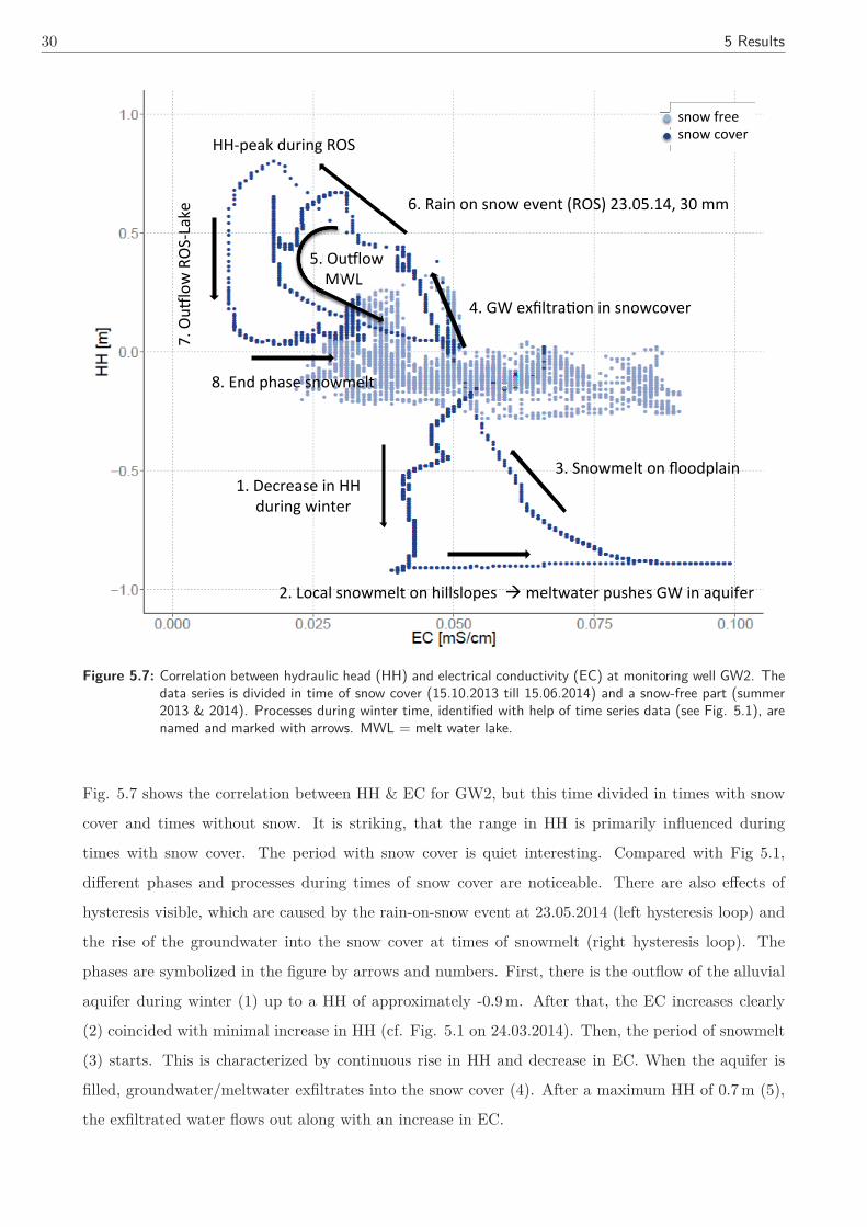
30 5 Results

Figure 5.7: Correlation between hydraulic head (HH) and electrical conductivity (EC) at monitoring well GW2. Thedata series is divided in time of snow cover (15.10.2013 till 15.06.2014) and a snow-free part (summer2013 & 2014). Processes during winter time, identified with help of time series data (see Fig. 5.1), arenamed and marked with arrows. MWL = melt water lake.

Fig. 5.7 shows the correlation between HH & EC for GW2, but this time divided in times with snow

cover and times without snow. It is striking, that the range in HH is primarily influenced during

times with snow cover. The period with snow cover is quiet interesting. Compared with Fig 5.1,

different phases and processes during times of snow cover are noticeable. There are also effects of

hysteresis visible, which are caused by the rain-on-snow event at 23.05.2014 (left hysteresis loop) and

the rise of the groundwater into the snow cover at times of snowmelt (right hysteresis loop). The

phases are symbolized in the figure by arrows and numbers. First, there is the outflow of the alluvial

aquifer during winter (1) up to a HH of approximately -0.9 m. After that, the EC increases clearly

(2) coincided with minimal increase in HH (cf. Fig. 5.1 on 24.03.2014). Then, the period of snowmelt

(3) starts. This is characterized by continuous rise in HH and decrease in EC. When the aquifer is

filled, groundwater/meltwater exfiltrates into the snow cover (4). After a maximum HH of 0.7 m (5),

the exfiltrated water flows out along with an increase in EC.

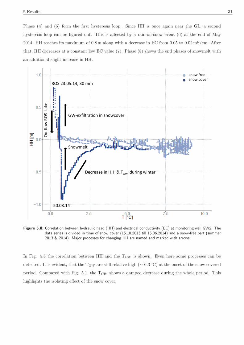
5 Results 31

Phase (4) and (5) form the first hysteresis loop. Since HH is once again near the GL, a second

hysteresis loop can be figured out. This is affected by a rain-on-snow event (6) at the end of May

2014. HH reaches its maximum of 0.8 m along with a decrease in EC from 0.05 to 0.02 mS/cm. After

that, HH decreases at a constant low EC value (7). Phase (8) shows the end phases of snowmelt with

an additional slight increase in HH.

Figure 5.8: Correlation between hydraulic head (HH) and electrical conductivity (EC) at monitoring well GW2. Thedata series is divided in time of snow cover (15.10.2013 till 15.06.2014) and a snow-free part (summer2013 & 2014). Major processes for changing HH are named and marked with arrows.

In Fig. 5.8 the correlation between HH and the TGW is shown. Even here some processes can be

detected. It is evident, that the TGW are still relative high (∼ 6.3 ◦C) at the onset of the snow covered

period. Compared with Fig. 5.1, the TGW shows a damped decrease during the whole period. This

highlights the isolating effect of the snow cover.

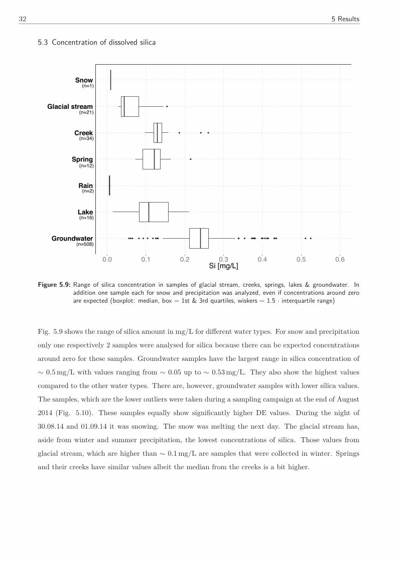
32 5 Results

5.3 Concentration of dissolved silica

Groundwater

Lake

Rain

Spring

Creek

Glacial stream

Snow

0.0 0.1 0.2 0.3 0.4 0.5 0.6Si [mg/L]

(n=1)

(n=21)

(n=34)

(n=12)

(n=2)

(n=16)

(n=508)

Figure 5.9: Range of silica concentration in samples of glacial stream, creeks, springs, lakes & groundwater. Inaddition one sample each for snow and precipitation was analyzed, even if concentrations around zeroare expected (boxplot: median, box = 1st & 3rd quartiles, wiskers = 1.5 · interquartile range)

Fig. 5.9 shows the range of silica amount in mg/L for different water types. For snow and precipitation

only one respectively 2 samples were analysed for silica because there can be expected concentrations

around zero for these samples. Groundwater samples have the largest range in silica concentration of

∼ 0.5 mg/L with values ranging from ∼ 0.05 up to ∼ 0.53 mg/L. They also show the highest values

compared to the other water types. There are, however, groundwater samples with lower silica values.

The samples, which are the lower outliers were taken during a sampling campaign at the end of August

2014 (Fig. 5.10). These samples equally show significantly higher DE values. During the night of

30.08.14 and 01.09.14 it was snowing. The snow was melting the next day. The glacial stream has,

aside from winter and summer precipitation, the lowest concentrations of silica. Those values from

glacial stream, which are higher than ∼ 0.1 mg/L are samples that were collected in winter. Springs

and their creeks have similar values albeit the median from the creeks is a bit higher.

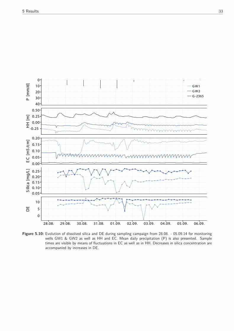
5 Results 33

0

10

20

30

40

P [

mm

/d]

-0.25

0.00

0.25

0.50

HH

[m

]

G W1

G W2

G -2365

0.00

0.05

0.10

0.15

0.20

EC

[m

S/c

m]

●

●

●

●

●

●

●

● ●

● ●

● ●●

●

●

●

●

●

●

●

●●

●

●

●

●

● ●

●

●

●

●

●

●

●

●

●●

● ●

●

●

●●

●

●

●

●

● ●

●

●

●

●

● ●

●

●

● ●

● ●

●●

●

●

● ●

●●

● ●

●

●

●

●

●

●

●

●

●

●

● ●

● ●

●

●

● ●

●

●

●

●

●

●

●

0.05

0.10

0.15

0.20

0.25

Sili

ca [

mg

/L]

●

●

●

●

●

●

●

● ●

● ●

● ●

● ●

●

●

●

●

●

●

●

●●

●

●

●

●

●

●

●

●

●

● ●

● ●

●

●

● ●

●

●● ●

●

●

●

●

●

●

●

●

●

●

●●

● ●

● ●

●

●

● ●

●

●

●

●

● ●

●

●

●

●

● ●

●

●

●

●

●

●

● ●

● ●

●

●

● ●

●

●

●

●

● ●

●

0

5

10

28.08. 29.08. 30.08. 31.08. 01.09. 02.09. 03.09. 04.09. 05.09. 06.09.

DE

Figure 5.10: Evolution of dissolved silica and DE during sampling campaign from 28.08. - 05.09.14 for monitoringwells GW1 & GW2 as well as HH and EC. Mean daily precipitation (P) is also presented. Sampletimes are visible by means of fluctuations in EC as well as in HH. Decreases in silica concentration areaccompanied by increases in DE.

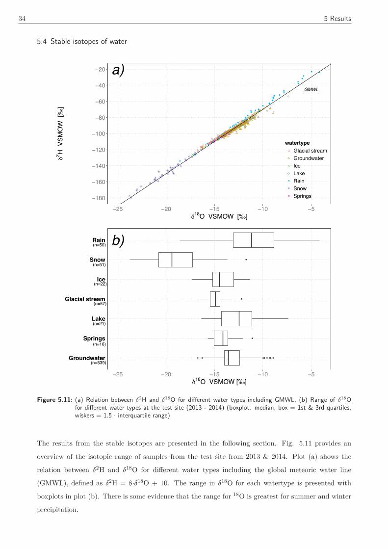
34 5 Results

5.4 Stable isotopes of water

GMWL

a)

−180

−160

−140

−120

−100

−80

−60

−40

−20

−25 −20 −15 −10 −5δ18O VSMOW [‰]

δ2 H V

SM

OW

[‰

]

watertypeGlacial streamGroundwaterIceLakeRainSnowSprings

b)

Groundwater

Springs

Lake

Glacial stream

Ice

Snow

Rain

−25 −20 −15 −10 −5δ18O VSMOW [‰]

(n=50)

(n=51)

(n=22)

(n=57)

(n=21)

(n=16)

(n=539)

Figure 5.11: (a) Relation between δ2H and δ18O for different water types including GMWL. (b) Range of δ18Ofor different water types at the test site (2013 - 2014) (boxplot: median, box = 1st & 3rd quartiles,wiskers = 1.5 · interquartile range)

The results from the stable isotopes are presented in the following section. Fig. 5.11 provides an

overview of the isotopic range of samples from the test site from 2013 & 2014. Plot (a) shows the

relation between δ2H and δ18O for different water types including the global meteoric water line

(GMWL), defined as δ2H = 8·δ18O + 10. The range in δ18O for each watertype is presented with

boxplots in plot (b). There is some evidence that the range for 18O is greatest for summer and winter

precipitation.

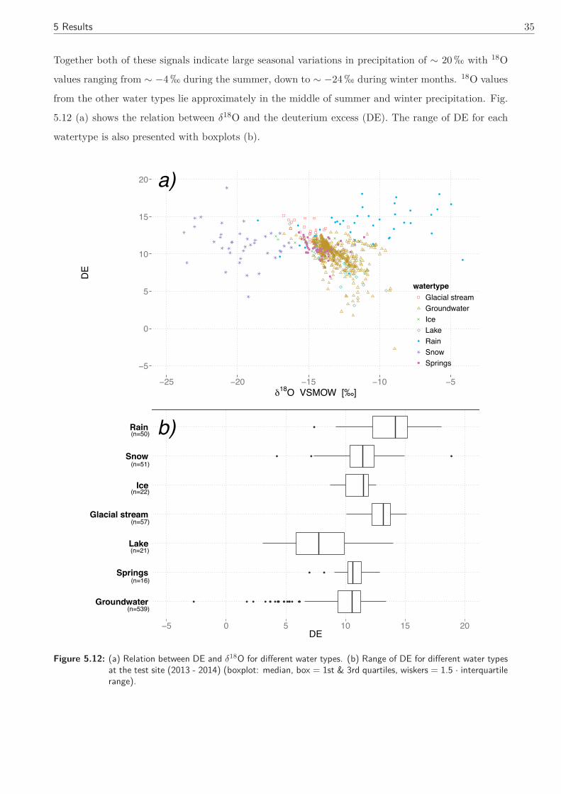
5 Results 35

Together both of these signals indicate large seasonal variations in precipitation of ∼ 20 � with 18O

values ranging from ∼ −4 � during the summer, down to ∼ −24 � during winter months. 18O values

from the other water types lie approximately in the middle of summer and winter precipitation. Fig.

5.12 (a) shows the relation between δ18O and the deuterium excess (DE). The range of DE for each

watertype is also presented with boxplots (b).

a)

−5

0

5

10

15

20

−25 −20 −15 −10 −5δ18O VSMOW [‰]

DE

watertypeGlacial streamGroundwaterIceLakeRainSnowSprings

b)

Groundwater

Springs

Lake

Glacial stream

Ice

Snow

Rain

−5 0 5 10 15 20DE

(n=22)

(n=51)

(n=50)

(n=57)

(n=21)

(n=16)

(n=539)

Figure 5.12: (a) Relation between DE and δ18O for different water types. (b) Range of DE for different water typesat the test site (2013 - 2014) (boxplot: median, box = 1st & 3rd quartiles, wiskers = 1.5 · interquartilerange).

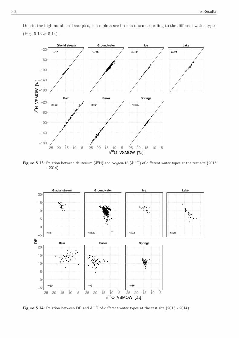
36 5 Results

Due to the high number of samples, these plots are broken down according to the different water types

(Fig. 5.13 & 5.14).

Glacial stream Groundwater Ice Lake

Rain Snow Springs

−180

−140

−100

−60

−20

−180

−140

−100

−60

−20

−25 −20 −15 −10 −5 −25 −20 −15 −10 −5 −25 −20 −15 −10 −5δ18O VSMOW [‰]

δ2 H V

SM

OW

[‰

]

n=57 n=539 n=22 n=21

n=50 n=51 n=539

Figure 5.13: Relation between deuterium (δ2H) and oxygen-18 (δ18O) of different water types at the test site (2013- 2014).

Glacial stream Groundwater Ice Lake

Rain Snow Springs

−5

0

5

10

15

20

−5

0

5

10

15

20

−25 −20 −15 −10 −5 −25 −20 −15 −10 −5 −25 −20 −15 −10 −5δ18O VSMOW [‰]

DE

n=57 n=539 n=22 n=21

n=50 n=51 n=16

Figure 5.14: Relation between DE and δ18O of different water types at the test site (2013 - 2014).

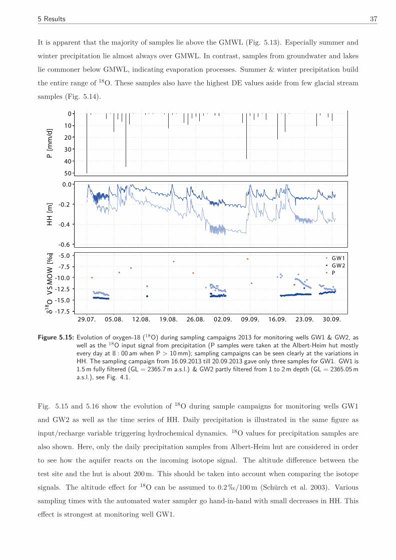
5 Results 37

It is apparent that the majority of samples lie above the GMWL (Fig. 5.13). Especially summer and

winter precipitation lie almost always over GMWL. In contrast, samples from groundwater and lakes

lie commoner below GMWL, indicating evaporation processes. Summer & winter precipitation build

the entire range of 18O. These samples also have the highest DE values aside from few glacial stream

samples (Fig. 5.14).

0

10

20

30

40

50

P [

mm

/d]

-0.6

-0.4

-0.2

0.0

HH

[m

]

●●●●●●●●●●●●●●●●●●●●●●●●●●●●●●●●●●●●●●●●●●●●●●●●●●●●●●●●●●●●●●●●●●●●● ●

●

●

●

●

●

●

●

●

●●●●●●●●●●●●●●●●●●●●●●●●●●●●●●●●●●●●●●●

●●●●●●

●●●●●●●●●●●●●● ●●●●●●●●●●●●●●●●●●

●●●●●●●●●●●●●●●●●●●●●●●●●●●●●●●●●●●

●●

●●●●●●●●●●●●●●●●●●●● ●●●●●●●●●●●●●●●●●●●●●●●●●●●●●●●●●●●●

●●●●●●●●●●●●●●●●●●●●●●●●●●●●●●●

●●●●●●●●●●●●●●●●

●●●●●●●●●●●●●●●●●●●●●

●●●●●●●●●●●

●●●

●●

●●●

●●

●

●

●

●●●●●●●●●●●●●

●●●●●●●●●●

●●●●●●●●●●●●●●●●●●●●●●

●

●●●

●●●●

●●●●●●●●●

●●

●●●●●●●●●●●●●●●●●●

●●

●●●●

●●

●●●●●●●●●●●●

●●●●●●●●●●

●●●●●●●●●●●●●●●●●●

●●●●●●

●

●

●

●

●

●

●●●

-17.5

-15.0

-12.5

-10.0

-7.5

-5.0

29.07. 05.08. 12.08. 19.08. 26.08. 02.09. 09.09. 16.09. 23.09. 30.09.

δ18O

V

SM

OW

[‰

]

●

●

●

G W1G W2P

Figure 5.15: Evolution of oxygen-18 (18O) during sampling campaigns 2013 for monitoring wells GW1 & GW2, aswell as the 18O input signal from precipitation (P samples were taken at the Albert-Heim hut mostlyevery day at 8 : 00 am when P > 10 mm); sampling campaigns can be seen clearly at the variations inHH. The sampling campaign from 16.09.2013 till 20.09.2013 gave only three samples for GW1. GW1 is1.5 m fully filtered (GL = 2365.7 m a.s.l.) & GW2 partly filtered from 1 to 2 m depth (GL = 2365.05 ma.s.l.), see Fig. 4.1.

Fig. 5.15 and 5.16 show the evolution of 18O during sample campaigns for monitoring wells GW1

and GW2 as well as the time series of HH. Daily precipitation is illustrated in the same figure as

input/recharge variable triggering hydrochemical dynamics. 18O values for precipitation samples are

also shown. Here, only the daily precipitation samples from Albert-Heim hut are considered in order

to see how the aquifer reacts on the incoming isotope signal. The altitude difference between the

test site and the hut is about 200 m. This should be taken into account when comparing the isotope

signals. The altitude effect for 18O can be assumed to 0.2 �/100 m (Schürch et al. 2003). Various

sampling times with the automated water sampler go hand-in-hand with small decreases in HH. This

effect is strongest at monitoring well GW1.

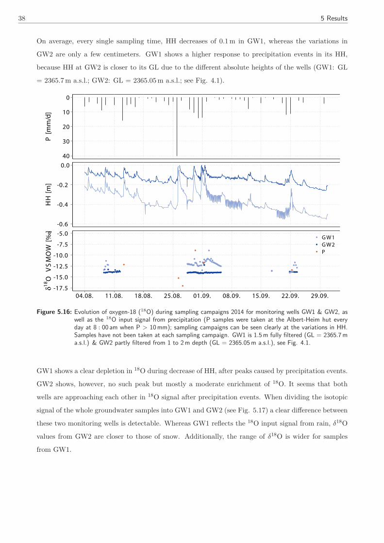
38 5 Results

On average, every single sampling time, HH decreases of 0.1 m in GW1, whereas the variations in

GW2 are only a few centimeters. GW1 shows a higher response to precipitation events in its HH,

because HH at GW2 is closer to its GL due to the different absolute heights of the wells (GW1: GL

= 2365.7 m a.s.l.; GW2: GL = 2365.05 m a.s.l.; see Fig. 4.1).

0

10

20

30

40

P [

mm

/d]

-0.6

-0.4

-0.2

0.0

HH

[m

]

●●

●

●●●●●●●

●●●●●●●●●●●

●●●

●●●●●

●●●●●●●●●●●●●●●●●●●●●●●●●●●●●●●●●●●●●●●●●●●●●●●●●●

●●●

●●●●●●●●●●●●●●●●●●●●●●●●●●●●●●●●●●●●●●●●●●●●●●●●●●●●●●●●●●●●●●●●

●●

●●

●●

●●●●●●●●●●●●●●●●●●●●●●●●

●●

●●●●●●●●●●●●●●

●●

●●●●

●●

●●●●●●

●●●

●●●●●●

●●●●●●

●●

●●●●●●

●●●●●●●●●●●●●●●●●●●●●●●●●●●●

●●●●●●●●●●●●

●●

●●

●●

●●

●

●

●

●

●

●

-17.5

-15.0

-12.5

-10.0

-7.5

-5.0

04.08. 11.08. 18.08. 25.08. 01.09. 08.09. 15.09. 22.09. 29.09.

δ18O

V

SM

OW

[‰

]

●

●

●

G W1G W2P

Figure 5.16: Evolution of oxygen-18 (18O) during sampling campaigns 2014 for monitoring wells GW1 & GW2, aswell as the 18O input signal from precipitation (P samples were taken at the Albert-Heim hut everyday at 8 : 00 am when P > 10 mm); sampling campaigns can be seen clearly at the variations in HH.Samples have not been taken at each sampling campaign. GW1 is 1.5 m fully filtered (GL = 2365.7 ma.s.l.) & GW2 partly filtered from 1 to 2 m depth (GL = 2365.05 m a.s.l.), see Fig. 4.1.

GW1 shows a clear depletion in 18O during decrease of HH, after peaks caused by precipitation events.

GW2 shows, however, no such peak but mostly a moderate enrichment of 18O. It seems that both

wells are approaching each other in 18O signal after precipitation events. When dividing the isotopic

signal of the whole groundwater samples into GW1 and GW2 (see Fig. 5.17) a clear difference between

these two monitoring wells is detectable. Whereas GW1 reflects the 18O input signal from rain, δ18O

values from GW2 are closer to those of snow. Additionally, the range of δ18O is wider for samples

from GW1.

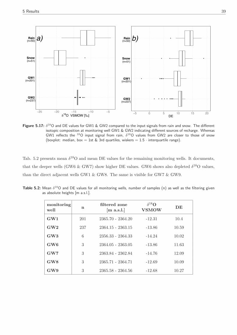
5 Results 39

a)

GW2

GW1

Snow

Rain

−25 −20 −15 −10 −5δ18O VSMOW [‰]

b)

GW2

GW1

Snow

Rain

−5 0 5 10 15 20DE

(n=50)

(n=51)

(n=201)

(n=237) (n=237)

(n=201)

(n=51)

(n=50)

Figure 5.17: δ18O and DE values for GW1 & GW2 compared to the input signals from rain and snow. The differentisotopic composition at monitoring well GW1 & GW2 indicating different sources of recharge. WhereasGW1 reflects the 18O input signal from rain, δ18O values from GW2 are closer to those of snow(boxplot: median, box = 1st & 3rd quartiles, wiskers = 1.5 · interquartile range).

Tab. 5.2 presents mean δ18O and mean DE values for the remaining monitoring wells. It documents,

that the deeper wells (GW6 & GW7) show higher DE values. GW6 shows also depleted δ18O values,

than the direct adjacent wells GW1 & GW8. The same is visible for GW7 & GW9.

Table 5.2: Mean δ18O and DE values for all monitoring wells, number of samples (n) as well as the filtering givenas absolute heights [m a.s.l.].

monitoringwell n filtered zone

[m a.s.l.]δ18O

VSMOW DE

GW1 201 2365.70 - 2364.20 -12.31 10.4

GW2 237 2364.15 - 2363.15 -13.86 10.59

GW3 6 2356.33 - 2364.33 -14.24 10.02

GW6 3 2364.05 - 2363.05 -13.86 11.63

GW7 3 2363.84 - 2362.84 -14.76 12.09

GW8 3 2365.71 - 2364.71 -12.69 10.09

GW9 3 2365.58 - 2364.56 -12.68 10.27

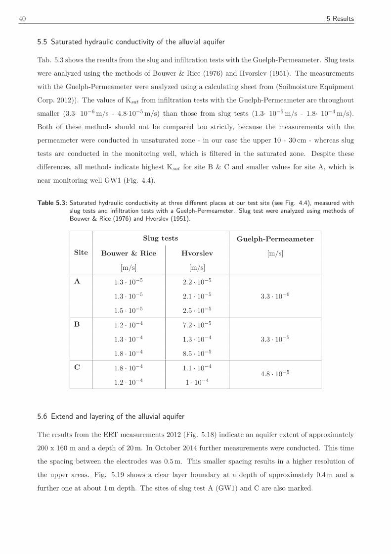
40 5 Results

5.5 Saturated hydraulic conductivity of the alluvial aquifer

Tab. 5.3 shows the results from the slug and infiltration tests with the Guelph-Permeameter. Slug tests

were analyzed using the methods of Bouwer & Rice (1976) and Hvorslev (1951). The measurements

with the Guelph-Permeameter were analyzed using a calculating sheet from (Soilmoisture Equipment

Corp. 2012)). The values of Ksat from infiltration tests with the Guelph-Permeameter are throughout

smaller (3.3· 10−6 m/s - 4.8·10−5 m/s) than those from slug tests (1.3· 10−5 m/s - 1.8· 10−4 m/s).

Both of these methods should not be compared too strictly, because the measurements with the

permeameter were conducted in unsaturated zone - in our case the upper 10 - 30 cm - whereas slug

tests are conducted in the monitoring well, which is filtered in the saturated zone. Despite these

differences, all methods indicate highest Ksat for site B & C and smaller values for site A, which is

near monitoring well GW1 (Fig. 4.4).

Table 5.3: Saturated hydraulic conductivity at three different places at our test site (see Fig. 4.4), measured withslug tests and infiltration tests with a Guelph-Permeameter. Slug test were analyzed using methods ofBouwer & Rice (1976) and Hvorslev (1951).

Slug tests Guelph-Permeameter

Site Bouwer & Rice Hvorslev [m/s]

[m/s] [m/s]

A 1.3 · 10−5 2.2 · 10−5

1.3 · 10−5 2.1 · 10−5 3.3 · 10−6

1.5 · 10−5 2.5 · 10−5

B 1.2 · 10−4 7.2 · 10−5

1.3 · 10−4 1.3 · 10−4 3.3 · 10−5

1.8 · 10−4 8.5 · 10−5

C 1.8 · 10−4 1.1 · 10−44.8 · 10−5

1.2 · 10−4 1 · 10−4

5.6 Extend and layering of the alluvial aquifer

The results from the ERT measurements 2012 (Fig. 5.18) indicate an aquifer extent of approximately

200 x 160 m and a depth of 20 m. In October 2014 further measurements were conducted. This time

the spacing between the electrodes was 0.5 m. This smaller spacing results in a higher resolution of

the upper areas. Fig. 5.19 shows a clear layer boundary at a depth of approximately 0.4 m and a

further one at about 1 m depth. The sites of slug test A (GW1) and C are also marked.

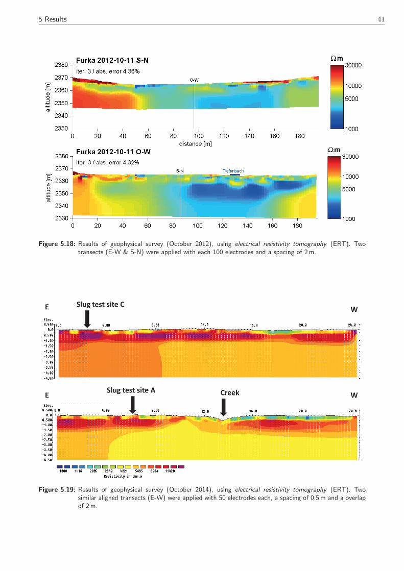
5 Results 41

Figure 5.18: Results of geophysical survey (October 2012), using electrical resistivity tomography (ERT). Twotransects (E-W & S-N) were applied with each 100 electrodes and a spacing of 2 m.

Slug test site C

Slug test site A Creek

E

E

W

W

Figure 5.19: Results of geophysical survey (October 2014), using electrical resistivity tomography (ERT). Twosimilar aligned transects (E-W) were applied with 50 electrodes each, a spacing of 0.5 m and a overlapof 2 m.

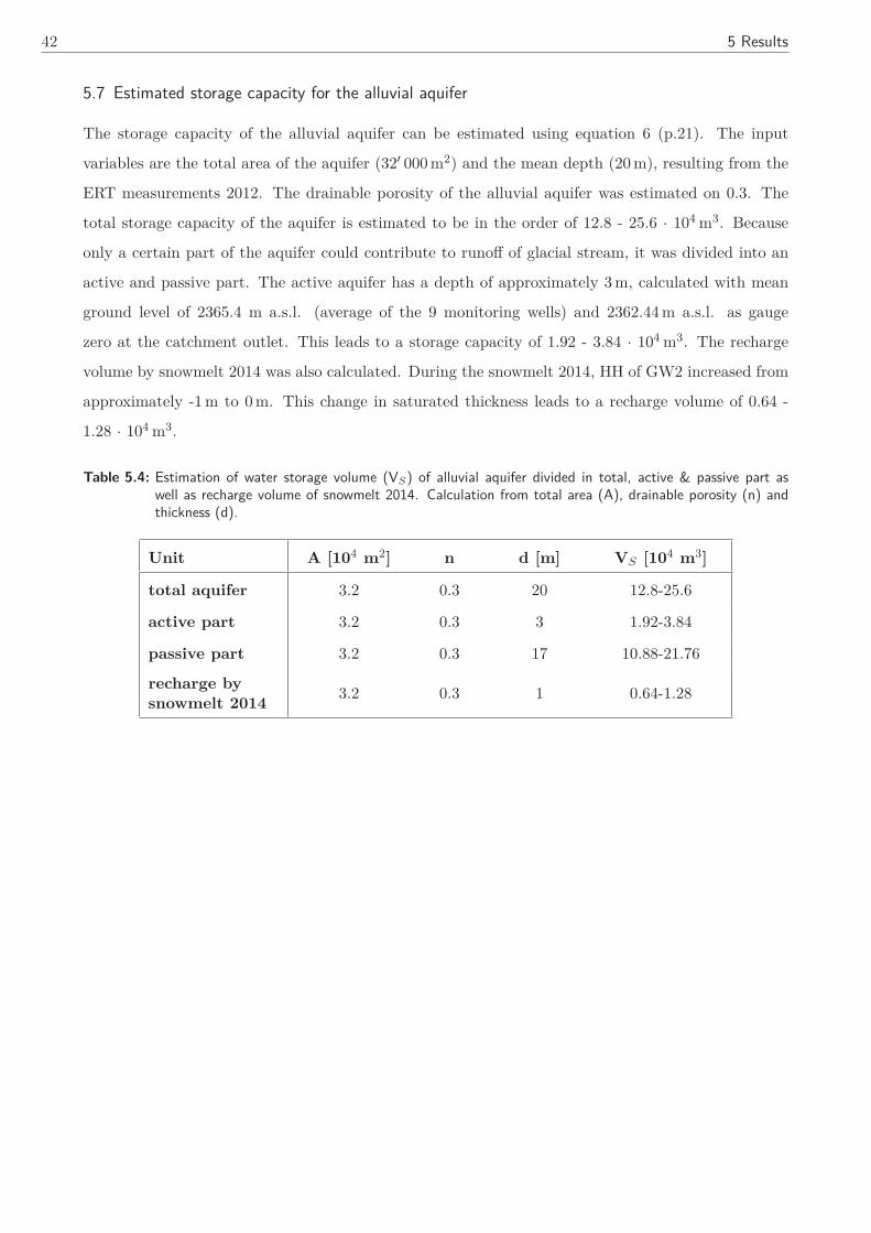
42 5 Results

5.7 Estimated storage capacity for the alluvial aquifer

The storage capacity of the alluvial aquifer can be estimated using equation 6 (p.21). The input

variables are the total area of the aquifer (32′ 000 m2) and the mean depth (20 m), resulting from the

ERT measurements 2012. The drainable porosity of the alluvial aquifer was estimated on 0.3. The

total storage capacity of the aquifer is estimated to be in the order of 12.8 - 25.6 · 104 m3. Because

only a certain part of the aquifer could contribute to runoff of glacial stream, it was divided into an

active and passive part. The active aquifer has a depth of approximately 3 m, calculated with mean

ground level of 2365.4 m a.s.l. (average of the 9 monitoring wells) and 2362.44 m a.s.l. as gauge

zero at the catchment outlet. This leads to a storage capacity of 1.92 - 3.84 · 104 m3. The recharge

volume by snowmelt 2014 was also calculated. During the snowmelt 2014, HH of GW2 increased from

approximately -1 m to 0 m. This change in saturated thickness leads to a recharge volume of 0.64 -

1.28 · 104 m3.

Table 5.4: Estimation of water storage volume (VS) of alluvial aquifer divided in total, active & passive part aswell as recharge volume of snowmelt 2014. Calculation from total area (A), drainable porosity (n) andthickness (d).

Unit A [104 m2] n d [m] VS [104 m3]

total aquifer 3.2 0.3 20 12.8-25.6

active part 3.2 0.3 3 1.92-3.84

passive part 3.2 0.3 17 10.88-21.76

recharge bysnowmelt 2014 3.2 0.3 1 0.64-1.28

6 Discussion 43

6 Discussion

6.1 Characteristics of the alluvial aquifer

Values for saturated hydraulic conductivity (Ksat) of the periglacial floodplain measured with slug

tests ranged from 1.3 · 10−5 m/s near monitoring well GW1 to 1.8 · 10−4 m/s near the glacial stream.

These values are similar to those measured from Magnusson et al. (2012) for a glacier forefield of the

adjacent Dammagletscher and Clow et al. (2003) for an alpine aquifer in Loch Vale, Rocky Mountains.

Furthermore, Cooper et al. (2002) found similar values for Ksat in moraine and fluvio-glacial sediments

in a floodplain in front of the glacier Finsterwalderbreen, Svalbard. Averaged Ksat are roughly similar

for site B (1.4 · 10−4 m/s (Bower & Rice), 9.7 · 10−5 m/s (Hvorslev)) & site C (1.5 · 10−4 m/s (Bower

& Rice), 1.1 · 10−4 m/s (Hvorslev)). These sites show also higher values than site A (1.4 · 10−5 m/s

(Bower & Rice), 2.3 · 10−5 m/s (Hvorslev)), which is in the vicinity of monitoring well GW1. For

site B the highest values were expected. This site is most influenced by glacial stream cause of the

deeper ground level (GL) (about 0.6 m deeper than site A; see Fig. 4.1, p.12). Hence, it is often

flooded when runoff from glacial stream increases and the stream will deposit a lot of sediments

there. This sedimentation area could be seen well on the orthophoto (Fig. 4.4, p.17). Ksat measured

with infiltration test by Guelph-Permeameter are throughout smaller than those measured with slug-

tests. Both of these methods should not be compared too strictly, because the measurements with

Permeameter are conducted in unsaturated zone, in our case the upper 10 - 30 cm, whereas slug tests

were conducted in the monitoring well, which was filtered in the saturated zone.

6.2 Seasonal storage dynamics

Based on the time series from Fig. 5.1 (p.24) conclusions can be drawn about the storage dynamics

of this alluvial aquifer. The course of the year can be divided into three different parts: (1) summer,

(2) winter & (3) snowmelt. These phases are highlighted in the following figure (Fig. 6.1). First one

is the part of summer time without snow cover (white). It is characterized by fluctuations in HH

coincident with different precipitation events. This causes also fluctuations in EC. The start of the

summer period can be explicit detected by rising TGW . During snow covered time TGW is about 0 ◦C.

Remarkable is TGW of about 10 ◦C in a height of 2365 m a.s.l. Similar TGW for alpine groundwater

can also be found in (Clow et al. 2003, Ward et al. 1999). Generally, TGW approximately reflects the

mean annual air temperature (MAAT) at the area. The MAAT for a comparable station (Gütsch ob

Andermatt, 2283 m a.s.l.) for the norm period 1981 - 2010 is 0.4 ◦C (MeteoSwiss 2015). One reason

for such high TGW is, that the soils are relatively thin. Furthermore there are no plants or trees which

provide shade resulting in direct radiation input. After snowmelt there is a lot of rotten gras on the

alluvial plain. Its dark color, combined with long days and strong radiation input during this times

could also support such abrupt increase in TGW .

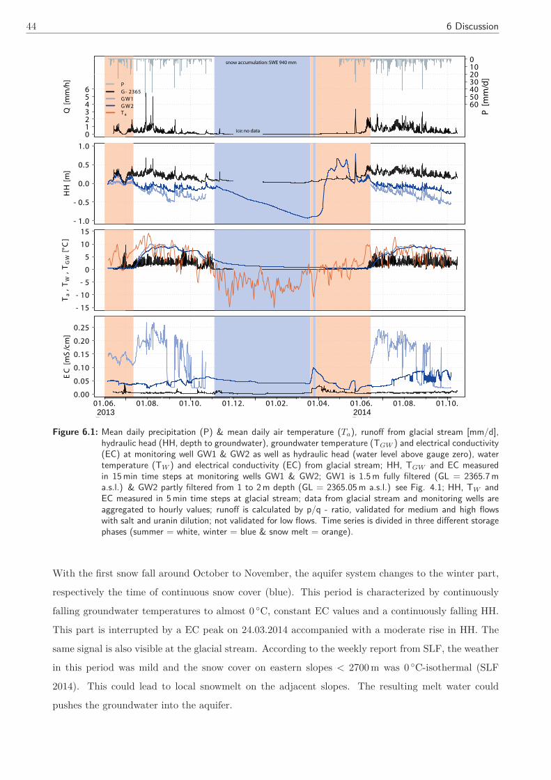
44 6 Discussion

Q [

mm

/h]

0123456

6050403020100

P [

mm

/d]

PG - 2365G W1G W2T a

- 1.0

- 0.5

0.0

0.5

1.0

HH

[m

]

- 15

- 10

- 5

0

5

10

15

Ta ,

TW

, T

GW

[°C

]

0.00

0.05

0.10

0.15

0.20

0.25

EC

[m

S/c

m]

01.06. 01.08. 01.10. 01.12. 01.02. 01.04. 01.06. 01.08. 01.10.

2013 2014


ice: no data

2013 2014

Figure 6.1: Mean daily precipitation (P) & mean daily air temperature (Ta), runoff from glacial stream [mm/d],hydraulic head (HH, depth to groundwater), groundwater temperature (TGW ) and electrical conductivity(EC) at monitoring well GW1 & GW2 as well as hydraulic head (water level above gauge zero), watertemperature (TW ) and electrical conductivity (EC) from glacial stream; HH, TGW and EC measuredin 15 min time steps at monitoring wells GW1 & GW2; GW1 is 1.5 m fully filtered (GL = 2365.7 ma.s.l.) & GW2 partly filtered from 1 to 2 m depth (GL = 2365.05 m a.s.l.) see Fig. 4.1; HH, TW andEC measured in 5 min time steps at glacial stream; data from glacial stream and monitoring wells areaggregated to hourly values; runoff is calculated by p/q - ratio, validated for medium and high flowswith salt and uranin dilution; not validated for low flows. Time series is divided in three different storagephases (summer = white, winter = blue & snow melt = orange).

With the first snow fall around October to November, the aquifer system changes to the winter part,

respectively the time of continuous snow cover (blue). This period is characterized by continuously

falling groundwater temperatures to almost 0 ◦C, constant EC values and a continuously falling HH.

This part is interrupted by a EC peak on 24.03.2014 accompanied with a moderate rise in HH. The

same signal is also visible at the glacial stream. According to the weekly report from SLF, the weather

in this period was mild and the snow cover on eastern slopes < 2700 m was 0 ◦C-isothermal (SLF

2014). This could lead to local snowmelt on the adjacent slopes. The resulting melt water could

pushes the groundwater into the aquifer.

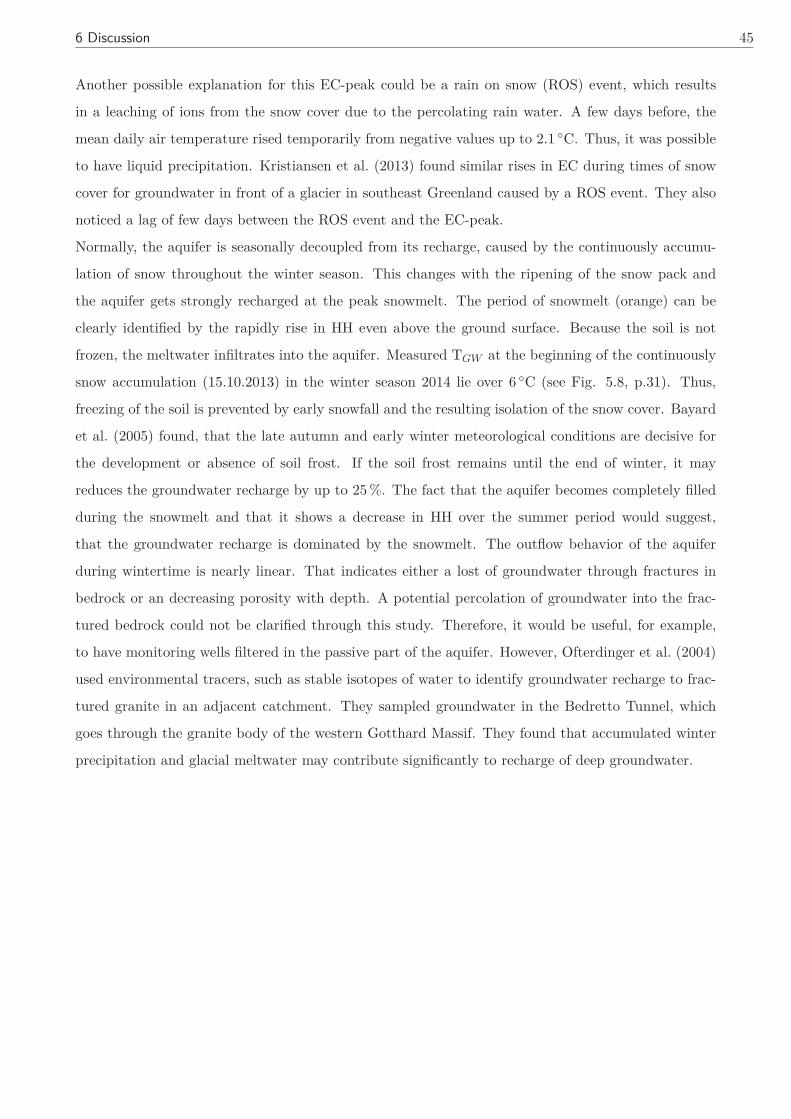
6 Discussion 45

Another possible explanation for this EC-peak could be a rain on snow (ROS) event, which results

in a leaching of ions from the snow cover due to the percolating rain water. A few days before, the

mean daily air temperature rised temporarily from negative values up to 2.1 ◦C. Thus, it was possible

to have liquid precipitation. Kristiansen et al. (2013) found similar rises in EC during times of snow

cover for groundwater in front of a glacier in southeast Greenland caused by a ROS event. They also

noticed a lag of few days between the ROS event and the EC-peak.

Normally, the aquifer is seasonally decoupled from its recharge, caused by the continuously accumu-

lation of snow throughout the winter season. This changes with the ripening of the snow pack and

the aquifer gets strongly recharged at the peak snowmelt. The period of snowmelt (orange) can be

clearly identified by the rapidly rise in HH even above the ground surface. Because the soil is not

frozen, the meltwater infiltrates into the aquifer. Measured TGW at the beginning of the continuously

snow accumulation (15.10.2013) in the winter season 2014 lie over 6 ◦C (see Fig. 5.8, p.31). Thus,

freezing of the soil is prevented by early snowfall and the resulting isolation of the snow cover. Bayard

et al. (2005) found, that the late autumn and early winter meteorological conditions are decisive for

the development or absence of soil frost. If the soil frost remains until the end of winter, it may

reduces the groundwater recharge by up to 25 %. The fact that the aquifer becomes completely filled

during the snowmelt and that it shows a decrease in HH over the summer period would suggest,

that the groundwater recharge is dominated by the snowmelt. The outflow behavior of the aquifer

during wintertime is nearly linear. That indicates either a lost of groundwater through fractures in

bedrock or an decreasing porosity with depth. A potential percolation of groundwater into the frac-

tured bedrock could not be clarified through this study. Therefore, it would be useful, for example,

to have monitoring wells filtered in the passive part of the aquifer. However, Ofterdinger et al. (2004)

used environmental tracers, such as stable isotopes of water to identify groundwater recharge to frac-

tured granite in an adjacent catchment. They sampled groundwater in the Bedretto Tunnel, which

goes through the granite body of the western Gotthard Massif. They found that accumulated winter

precipitation and glacial meltwater may contribute significantly to recharge of deep groundwater.

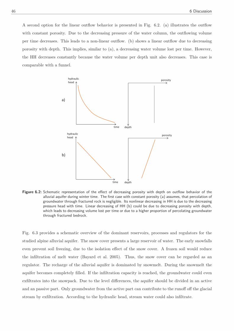
46 6 Discussion

A second option for the linear outflow behavior is presented in Fig. 6.2. (a) illustrates the outflow

with constant porosity. Due to the decreasing pressure of the water column, the outflowing volume

per time decreases. This leads to a non-linear outflow. (b) shows a linear outflow due to decreasing

porosity with depth. This implies, similar to (a), a decreasing water volume lost per time. However,

the HH decreases constantly because the water volume per depth unit also decreases. This case is

comparable with a funnel.

time

hydraulic head

porosity

depth

time

hydraulic head

porosity

depth

a)

b)

Figure 6.2: Schematic representation of the effect of decreasing porosity with depth on outflow behavior of thealluvial aquifer during winter time. The first case with constant porosity (a) assumes, that percolation ofgroundwater through fractured rock is negligible. Its nonlinear decreasing in HH is due to the decreasingpressure head with time. Linear decreasing of HH (b) could be due to decreasing porosity with depth,which leads to decreasing volume lost per time or due to a higher proportion of percolating groundwaterthrough fractured bedrock.

Fig. 6.3 provides a schematic overview of the dominant reservoirs, processes and regulators for the

studied alpine alluvial aquifer. The snow cover presents a large reservoir of water. The early snowfalls

even prevent soil freezing, due to the isolation effect of the snow cover. A frozen soil would reduce

the infiltration of melt water (Bayard et al. 2005). Thus, the snow cover can be regarded as an

regulator. The recharge of the alluvial aquifer is dominated by snowmelt. During the snowmelt the

aquifer becomes completely filled. If the infiltration capacity is reached, the groundwater could even

exfiltrates into the snowpack. Due to the level differences, the aquifer should be divided in an active

and an passive part. Only groundwater from the active part can contribute to the runoff off the glacial

stream by exfiltration. According to the hydraulic head, stream water could also infiltrate.

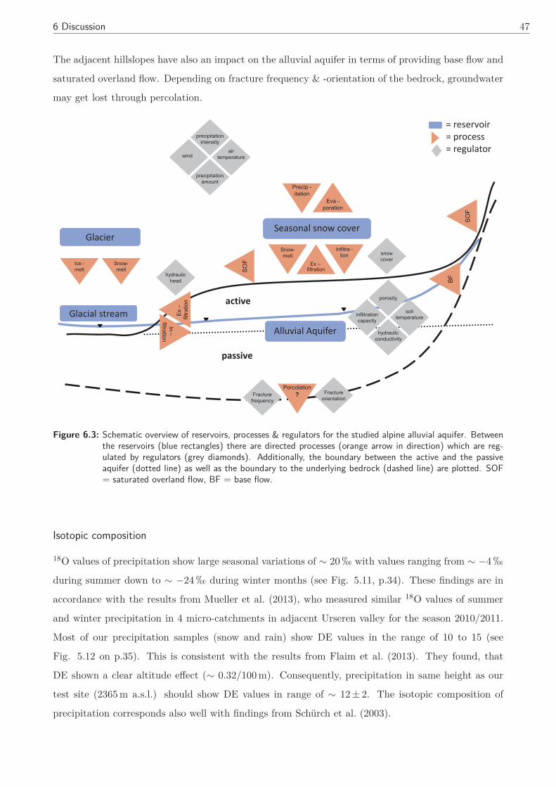
6 Discussion 47

The adjacent hillslopes have also an impact on the alluvial aquifer in terms of providing base flow and

saturated overland flow. Depending on fracture frequency & -orientation of the bedrock, groundwater

may get lost through percolation.

Seasonal snow cover

Glacial stream

SOF Ice -

melt Snow- melt

Snow- melt

Eva - poration

Precip - itation

air temperature

precipitation

intensity

wind

precipitation

amount

Glacier

hydraulic head

snow cover

Infiltra -tion

Ex – filtration

soil temperature infiltration

capacity

hydraulic conductivity

porosity

Ex –

fil

tratio

n

In – filtration Fracture

orientation

Percolation ?

Alluvial Aquifer

SOF

BF

active

passive

= reservoir = process = regulator

Fracture frequency

Figure 6.3: Schematic overview of reservoirs, processes & regulators for the studied alpine alluvial aquifer. Betweenthe reservoirs (blue rectangles) there are directed processes (orange arrow in direction) which are reg-ulated by regulators (grey diamonds). Additionally, the boundary between the active and the passiveaquifer (dotted line) as well as the boundary to the underlying bedrock (dashed line) are plotted. SOF= saturated overland flow, BF = base flow.

Isotopic composition

18O values of precipitation show large seasonal variations of ∼ 20 � with values ranging from ∼ −4 �during summer down to ∼ −24 � during winter months (see Fig. 5.11, p.34). These findings are in

accordance with the results from Mueller et al. (2013), who measured similar 18O values of summer

and winter precipitation in 4 micro-catchments in adjacent Urseren valley for the season 2010/2011.

Most of our precipitation samples (snow and rain) show DE values in the range of 10 to 15 (see

Fig. 5.12 on p.35). This is consistent with the results from Flaim et al. (2013). They found, that

DE shown a clear altitude effect (∼ 0.32/100 m). Consequently, precipitation in same height as our

test site (2365 m a.s.l.) should show DE values in range of ∼ 12 ± 2. The isotopic composition of

precipitation corresponds also well with findings from Schürch et al. (2003).

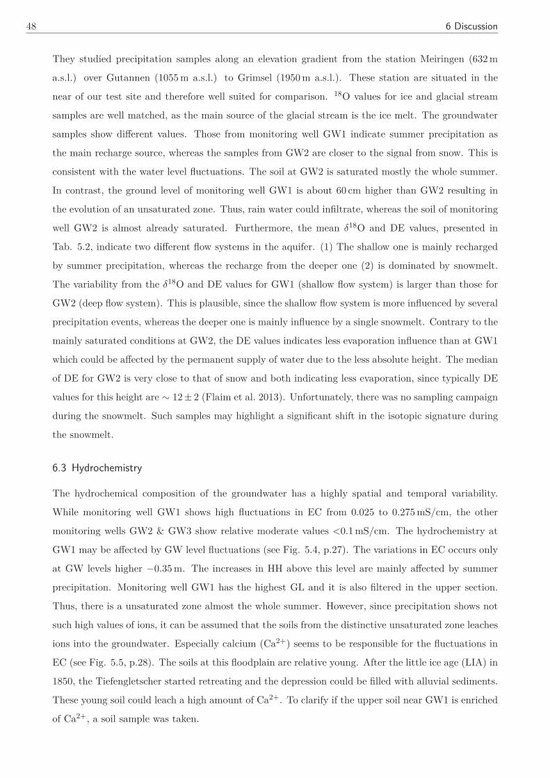
48 6 Discussion

They studied precipitation samples along an elevation gradient from the station Meiringen (632 m

a.s.l.) over Gutannen (1055 m a.s.l.) to Grimsel (1950 m a.s.l.). These station are situated in the

near of our test site and therefore well suited for comparison. 18O values for ice and glacial stream

samples are well matched, as the main source of the glacial stream is the ice melt. The groundwater

samples show different values. Those from monitoring well GW1 indicate summer precipitation as

the main recharge source, whereas the samples from GW2 are closer to the signal from snow. This is

consistent with the water level fluctuations. The soil at GW2 is saturated mostly the whole summer.

In contrast, the ground level of monitoring well GW1 is about 60 cm higher than GW2 resulting in

the evolution of an unsaturated zone. Thus, rain water could infiltrate, whereas the soil of monitoring

well GW2 is almost already saturated. Furthermore, the mean δ18O and DE values, presented in

Tab. 5.2, indicate two different flow systems in the aquifer. (1) The shallow one is mainly recharged

by summer precipitation, whereas the recharge from the deeper one (2) is dominated by snowmelt.

The variability from the δ18O and DE values for GW1 (shallow flow system) is larger than those for

GW2 (deep flow system). This is plausible, since the shallow flow system is more influenced by several

precipitation events, whereas the deeper one is mainly influence by a single snowmelt. Contrary to the

mainly saturated conditions at GW2, the DE values indicates less evaporation influence than at GW1

which could be affected by the permanent supply of water due to the less absolute height. The median

of DE for GW2 is very close to that of snow and both indicating less evaporation, since typically DE

values for this height are ∼ 12 ± 2 (Flaim et al. 2013). Unfortunately, there was no sampling campaign

during the snowmelt. Such samples may highlight a significant shift in the isotopic signature during

the snowmelt.

6.3 Hydrochemistry

The hydrochemical composition of the groundwater has a highly spatial and temporal variability.

While monitoring well GW1 shows high fluctuations in EC from 0.025 to 0.275 mS/cm, the other

monitoring wells GW2 & GW3 show relative moderate values <0.1 mS/cm. The hydrochemistry at

GW1 may be affected by GW level fluctuations (see Fig. 5.4, p.27). The variations in EC occurs only

at GW levels higher −0.35 m. The increases in HH above this level are mainly affected by summer

precipitation. Monitoring well GW1 has the highest GL and it is also filtered in the upper section.

Thus, there is a unsaturated zone almost the whole summer. However, since precipitation shows not

such high values of ions, it can be assumed that the soils from the distinctive unsaturated zone leaches

ions into the groundwater. Especially calcium (Ca2+) seems to be responsible for the fluctuations in

EC (see Fig. 5.5, p.28). The soils at this floodplain are relative young. After the little ice age (LIA) in

1850, the Tiefengletscher started retreating and the depression could be filled with alluvial sediments.

These young soil could leach a high amount of Ca2+. To clarify if the upper soil near GW1 is enriched

of Ca2+, a soil sample was taken.

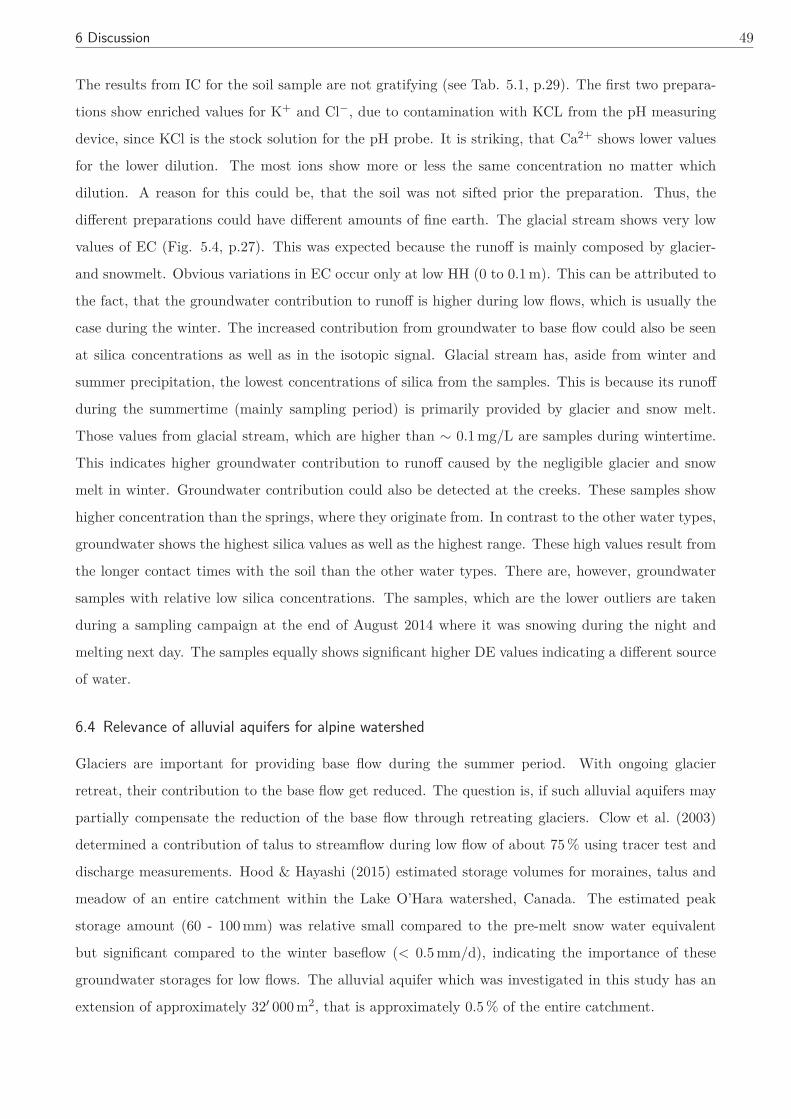
6 Discussion 49

The results from IC for the soil sample are not gratifying (see Tab. 5.1, p.29). The first two prepara-

tions show enriched values for K+ and Cl−, due to contamination with KCL from the pH measuring

device, since KCl is the stock solution for the pH probe. It is striking, that Ca2+ shows lower values

for the lower dilution. The most ions show more or less the same concentration no matter which

dilution. A reason for this could be, that the soil was not sifted prior the preparation. Thus, the

different preparations could have different amounts of fine earth. The glacial stream shows very low

values of EC (Fig. 5.4, p.27). This was expected because the runoff is mainly composed by glacier-

and snowmelt. Obvious variations in EC occur only at low HH (0 to 0.1 m). This can be attributed to

the fact, that the groundwater contribution to runoff is higher during low flows, which is usually the

case during the winter. The increased contribution from groundwater to base flow could also be seen

at silica concentrations as well as in the isotopic signal. Glacial stream has, aside from winter and

summer precipitation, the lowest concentrations of silica from the samples. This is because its runoff

during the summertime (mainly sampling period) is primarily provided by glacier and snow melt.

Those values from glacial stream, which are higher than ∼ 0.1 mg/L are samples during wintertime.

This indicates higher groundwater contribution to runoff caused by the negligible glacier and snow

melt in winter. Groundwater contribution could also be detected at the creeks. These samples show

higher concentration than the springs, where they originate from. In contrast to the other water types,

groundwater shows the highest silica values as well as the highest range. These high values result from

the longer contact times with the soil than the other water types. There are, however, groundwater

samples with relative low silica concentrations. The samples, which are the lower outliers are taken

during a sampling campaign at the end of August 2014 where it was snowing during the night and

melting next day. The samples equally shows significant higher DE values indicating a different source

of water.

6.4 Relevance of alluvial aquifers for alpine watershed

Glaciers are important for providing base flow during the summer period. With ongoing glacier

retreat, their contribution to the base flow get reduced. The question is, if such alluvial aquifers may

partially compensate the reduction of the base flow through retreating glaciers. Clow et al. (2003)

determined a contribution of talus to streamflow during low flow of about 75 % using tracer test and

discharge measurements. Hood & Hayashi (2015) estimated storage volumes for moraines, talus and

meadow of an entire catchment within the Lake O’Hara watershed, Canada. The estimated peak

storage amount (60 - 100 mm) was relative small compared to the pre-melt snow water equivalent

but significant compared to the winter baseflow (< 0.5 mm/d), indicating the importance of these

groundwater storages for low flows. The alluvial aquifer which was investigated in this study has an

extension of approximately 32′ 000 m2, that is approximately 0.5 % of the entire catchment.

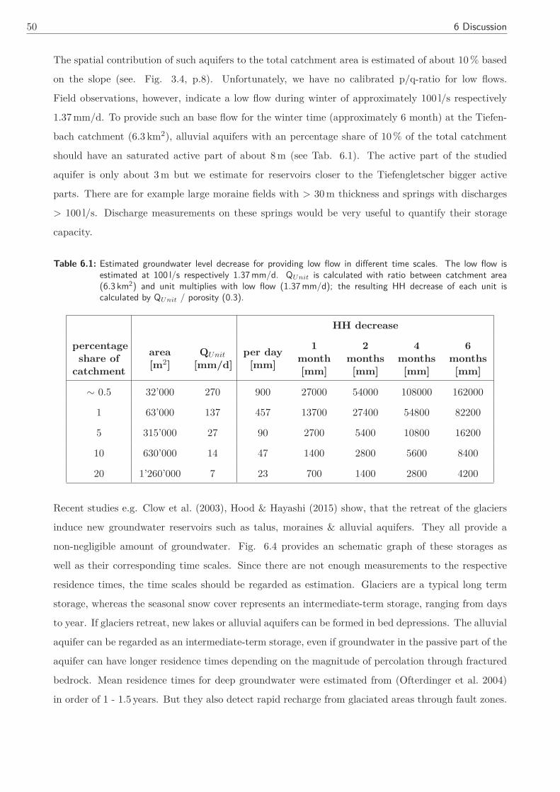
50 6 Discussion

The spatial contribution of such aquifers to the total catchment area is estimated of about 10 % based

on the slope (see. Fig. 3.4, p.8). Unfortunately, we have no calibrated p/q-ratio for low flows.

Field observations, however, indicate a low flow during winter of approximately 100 l/s respectively

1.37 mm/d. To provide such an base flow for the winter time (approximately 6 month) at the Tiefen-

bach catchment (6.3 km2), alluvial aquifers with an percentage share of 10 % of the total catchment

should have an saturated active part of about 8 m (see Tab. 6.1). The active part of the studied

aquifer is only about 3 m but we estimate for reservoirs closer to the Tiefengletscher bigger active

parts. There are for example large moraine fields with > 30 m thickness and springs with discharges

> 100 l/s. Discharge measurements on these springs would be very useful to quantify their storage

capacity.

Table 6.1: Estimated groundwater level decrease for providing low flow in different time scales. The low flow isestimated at 100 l/s respectively 1.37 mm/d. QUnit is calculated with ratio between catchment area(6.3 km2) and unit multiplies with low flow (1.37 mm/d); the resulting HH decrease of each unit iscalculated by QUnit / porosity (0.3).

HH decrease

percentageshare of

catchment

area[m2]

QUnit

[mm/d]per day

[mm]

1month[mm]

2months

[mm]

4months

[mm]

6months

[mm]

∼ 0.5 32’000 270 900 27000 54000 108000 162000

1 63’000 137 457 13700 27400 54800 82200

5 315’000 27 90 2700 5400 10800 16200

10 630’000 14 47 1400 2800 5600 8400

20 1’260’000 7 23 700 1400 2800 4200

Recent studies e.g. Clow et al. (2003), Hood & Hayashi (2015) show, that the retreat of the glaciers

induce new groundwater reservoirs such as talus, moraines & alluvial aquifers. They all provide a

non-negligible amount of groundwater. Fig. 6.4 provides an schematic graph of these storages as

well as their corresponding time scales. Since there are not enough measurements to the respective

residence times, the time scales should be regarded as estimation. Glaciers are a typical long term

storage, whereas the seasonal snow cover represents an intermediate-term storage, ranging from days

to year. If glaciers retreat, new lakes or alluvial aquifers can be formed in bed depressions. The alluvial

aquifer can be regarded as an intermediate-term storage, even if groundwater in the passive part of the

aquifer can have longer residence times depending on the magnitude of percolation through fractured

bedrock. Mean residence times for deep groundwater were estimated from (Ofterdinger et al. 2004)

in order of 1 - 1.5 years. But they also detect rapid recharge from glaciated areas through fault zones.

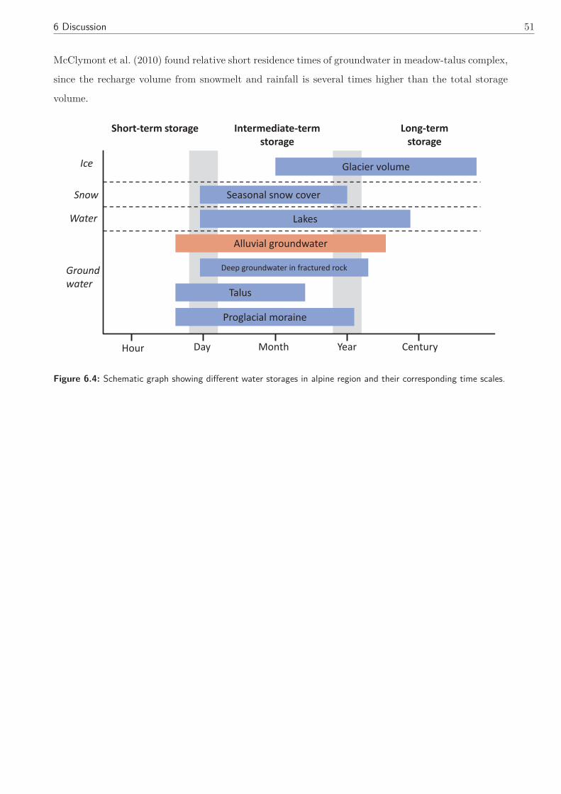
6 Discussion 51

McClymont et al. (2010) found relative short residence times of groundwater in meadow-talus complex,

since the recharge volume from snowmelt and rainfall is several times higher than the total storage

volume.

Short-term storage Intermediate-term storage

Long-term storage

Hour Day Month Year Century

Ice

Snow

Groundwater

Glacier volume

Deep groundwater in fractured rock

Seasonal snow cover

Talus

Alluvial groundwater

Proglacial moraine

Lakes Water

Figure 6.4: Schematic graph showing different water storages in alpine region and their corresponding time scales.

52 7 Conclusion

7 Conclusion

7.1 Findings

The study shows, that the groundwater recharge of the alluvial aquifer is mainly dominated by the

snowmelt. During the snowmelt, the aquifer get completely filled and the groundwater even exfiltrates

into the snowpack. The groundwater levels are very variable during the short summer period due to

different precipitation events. Especially monitoring well GW1 reacts strongly on precipitation events,

because there is a extended unsaturated zone. It is conceivable that such unsaturated zones may have

a large buffering capacity for intense rainfalls. There are, however, sites with lower ground levels, such

as GW2, which are almost the whole summer period saturated. Another difference between GW1 and

GW2 is the hydrochemistry. GW1 shows large variations in the electrical conductivity (EC) whereas

the variations at GW2 are relative moderate. The results from ion chromatography indicate, that EC is

mainly affected by leaching of ions from the unsaturated soil. Especially Ca2+ shows a high correlation

with EC, as it is representative for such young soils. Relative high groundwater temperatures (TGW )

of about 10 ◦C could be detected, which is a result of thin soils and direct radiation input through

missing vegetation. That means, that the assumption that the TGW reflects approximately (± 1 ◦C)

the mean annual air temperature doesn’t apply. These high TGW may also accelerate the weathering

rates. Such aquifers may provide low flows during winter or summer droughts, since they can store

huge amounts of water. It depends on the thickness of the active part of the aquifer and the quantity

respectively size of the aquifer. Here, only one alluvial aquifer was investigated. But additional

groundwater level measurements on adjacent Lochbergbach & Wittenwasserenreus within this project

suggest similar storage dynamics. In these two catchments also large flat sedimentation areas can be

found, which is typical for formerly glaciated areas. Considering the world wide glacier retreat, it will

be an important aim to investigate alternative water storages such as alluvial aquifers.

7.2 Reflection

This work can provide useful information for future field campaigns. The results from hydrochemistry

show, that such an aquifer is highly heterogene. It depends on where monitoring wells are installed

and if the filtering reaches into the saturated or unsaturated zone. It has been found practicable to

create an image of the water level prior to the installation of the monitoring wells for example with

the help of mini-piezometers. They are much easier to install and can be quickly removed. During the

installation of the mini-piezometers with a hammer, hard layers could maybe detected. In this study,

the assumption of a layer shift in about −0.4 m could be confirmed by conducting electrical resistance

tomography (ERT). The ERT is a useful tool to estimate the extension and depth as well as different

layers in the aquifer. To estimate the amount of groundwater contribution to the glacial stream, it

would be useful to install gauge stations upstream and downstream the aquifer.

7 Conclusion 53

For investigating possibly percolation of groundwater into fractured bedrock, deeper monitoring wells

which are filtered in the passive part of the aquifer are required. Thus, it would be possible to estimate

residence times for example. Unfortunately, the conducted pumping tests were not successful. The

distance of 2 m between the pumping and the observations wells was to large to see a distinctive

difference in the hydraulic head (HH) on the observation well. Furthermore, pumping tests need a lot

of time and materials which makes it challenging to conduct in alpine terrain. Slug test are therefore

easier to conduct in such environments. It is possible to make several slug test a day, which would

be more representative in such heterogeneous aquifers. The results show, that the period around the

snowmelt affects the largest variations in HH, TGW and EC. Thus, it would be interesting to conduct

sampling campaigns prior, during and after the snowmelt. The large variations in EC at GW1 are

mainly affected by Ca2+. A distinctively rise in EC was detectable, when the water level rises above

−0.4 m. The result of the ion chromatography of a soil sample was not gratifying. Three different

preparations show significant differences which was probably due to the fact, that the soil was not

sifted prior the preparation. For the future, it would be better to take samples below and above a

layering. The best time for taking soil samples is probably the late autumn, when the water level

is lowest. The CTD-online sensors proved to be very helpful. Having the actual data, it is possible

to react quickly on events. Thus, it is possible to conduct specific sampling campaigns at times of

high EC, TGW or HH. Another great advantage is, that it is immediately visible if a sensor fails.

With such sensors, it is also possible to equip several test sites without having to check or read out

all sensors frequently. Additionally, the installation of time-lapse camera is very useful. With the

camera it is possible to record the snow accumulation and the photos can provide useful information

to interpret the data, for example fresh snow or flooding by the glacial stream. As the access to the

alpine terrains is mostly difficult it is not easy to equip a huge number of aquifers. The study shows,

that the measurements on a single monitoring well (GW2) during the whole course of the year can

provide a lot of information about the storage dynamics. Thus, it might be useful to focus on selected

aquifers with more detailed measurements and additionally equip a higher number of aquifers with

just one sensored monitoring well.

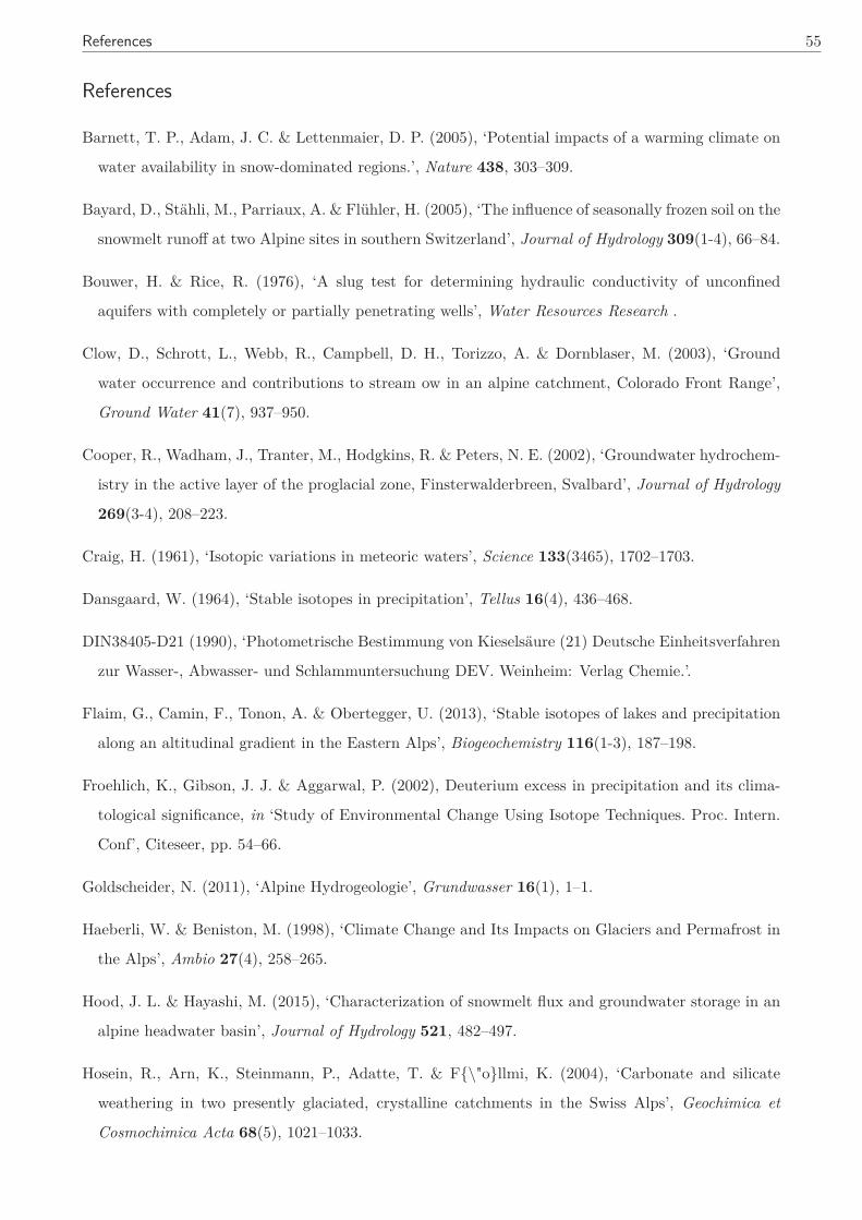
References 55

References

Barnett, T. P., Adam, J. C. & Lettenmaier, D. P. (2005), ‘Potential impacts of a warming climate on

water availability in snow-dominated regions.’, Nature 438, 303–309.

Bayard, D., Stähli, M., Parriaux, A. & Flühler, H. (2005), ‘The influence of seasonally frozen soil on the

snowmelt runoff at two Alpine sites in southern Switzerland’, Journal of Hydrology 309(1-4), 66–84.

Bouwer, H. & Rice, R. (1976), ‘A slug test for determining hydraulic conductivity of unconfined

aquifers with completely or partially penetrating wells’, Water Resources Research .

Clow, D., Schrott, L., Webb, R., Campbell, D. H., Torizzo, A. & Dornblaser, M. (2003), ‘Ground

water occurrence and contributions to stream ow in an alpine catchment, Colorado Front Range’,

Ground Water 41(7), 937–950.

Cooper, R., Wadham, J., Tranter, M., Hodgkins, R. & Peters, N. E. (2002), ‘Groundwater hydrochem-

istry in the active layer of the proglacial zone, Finsterwalderbreen, Svalbard’, Journal of Hydrology

269(3-4), 208–223.

Craig, H. (1961), ‘Isotopic variations in meteoric waters’, Science 133(3465), 1702–1703.

Dansgaard, W. (1964), ‘Stable isotopes in precipitation’, Tellus 16(4), 436–468.

DIN38405-D21 (1990), ‘Photometrische Bestimmung von Kieselsäure (21) Deutsche Einheitsverfahren

zur Wasser-, Abwasser- und Schlammuntersuchung DEV. Weinheim: Verlag Chemie.’.

Flaim, G., Camin, F., Tonon, A. & Obertegger, U. (2013), ‘Stable isotopes of lakes and precipitation

along an altitudinal gradient in the Eastern Alps’, Biogeochemistry 116(1-3), 187–198.

Froehlich, K., Gibson, J. J. & Aggarwal, P. (2002), Deuterium excess in precipitation and its clima-

tological significance, in ‘Study of Environmental Change Using Isotope Techniques. Proc. Intern.

Conf’, Citeseer, pp. 54–66.

Goldscheider, N. (2011), ‘Alpine Hydrogeologie’, Grundwasser 16(1), 1–1.

Haeberli, W. & Beniston, M. (1998), ‘Climate Change and Its Impacts on Glaciers and Permafrost in

the Alps’, Ambio 27(4), 258–265.

Hood, J. L. & Hayashi, M. (2015), ‘Characterization of snowmelt flux and groundwater storage in an

alpine headwater basin’, Journal of Hydrology 521, 482–497.

Hosein, R., Arn, K., Steinmann, P., Adatte, T. & F{\"o}llmi, K. (2004), ‘Carbonate and silicate

weathering in two presently glaciated, crystalline catchments in the Swiss Alps’, Geochimica et

Cosmochimica Acta 68(5), 1021–1033.

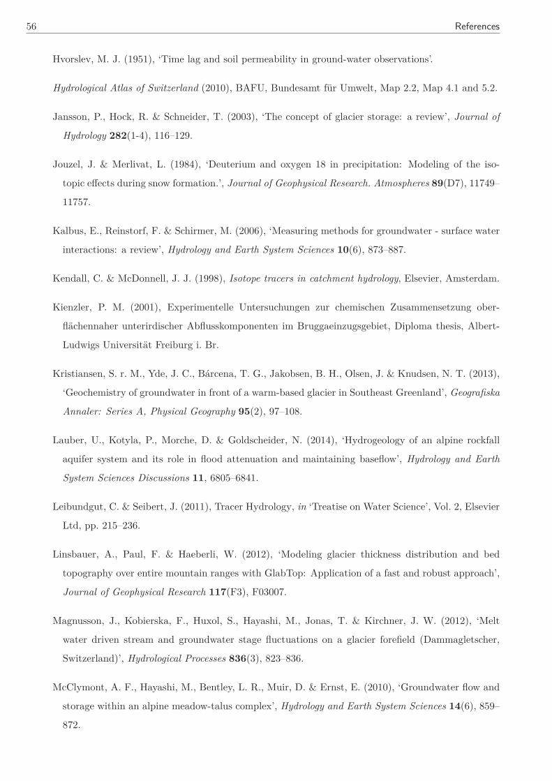
56 References

Hvorslev, M. J. (1951), ‘Time lag and soil permeability in ground-water observations’.

Hydrological Atlas of Switzerland (2010), BAFU, Bundesamt für Umwelt, Map 2.2, Map 4.1 and 5.2.

Jansson, P., Hock, R. & Schneider, T. (2003), ‘The concept of glacier storage: a review’, Journal of

Hydrology 282(1-4), 116–129.

Jouzel, J. & Merlivat, L. (1984), ‘Deuterium and oxygen 18 in precipitation: Modeling of the iso-

topic effects during snow formation.’, Journal of Geophysical Research. Atmospheres 89(D7), 11749–

11757.

Kalbus, E., Reinstorf, F. & Schirmer, M. (2006), ‘Measuring methods for groundwater - surface water

interactions: a review’, Hydrology and Earth System Sciences 10(6), 873–887.

Kendall, C. & McDonnell, J. J. (1998), Isotope tracers in catchment hydrology, Elsevier, Amsterdam.

Kienzler, P. M. (2001), Experimentelle Untersuchungen zur chemischen Zusammensetzung ober-

flächennaher unterirdischer Abflusskomponenten im Bruggaeinzugsgebiet, Diploma thesis, Albert-

Ludwigs Universität Freiburg i. Br.

Kristiansen, S. r. M., Yde, J. C., Bárcena, T. G., Jakobsen, B. H., Olsen, J. & Knudsen, N. T. (2013),

‘Geochemistry of groundwater in front of a warm-based glacier in Southeast Greenland’, Geografiska

Annaler: Series A, Physical Geography 95(2), 97–108.

Lauber, U., Kotyla, P., Morche, D. & Goldscheider, N. (2014), ‘Hydrogeology of an alpine rockfall

aquifer system and its role in flood attenuation and maintaining baseflow’, Hydrology and Earth

System Sciences Discussions 11, 6805–6841.

Leibundgut, C. & Seibert, J. (2011), Tracer Hydrology, in ‘Treatise on Water Science’, Vol. 2, Elsevier

Ltd, pp. 215–236.

Linsbauer, A., Paul, F. & Haeberli, W. (2012), ‘Modeling glacier thickness distribution and bed

topography over entire mountain ranges with GlabTop: Application of a fast and robust approach’,

Journal of Geophysical Research 117(F3), F03007.

Magnusson, J., Kobierska, F., Huxol, S., Hayashi, M., Jonas, T. & Kirchner, J. W. (2012), ‘Melt

water driven stream and groundwater stage fluctuations on a glacier forefield (Dammagletscher,

Switzerland)’, Hydrological Processes 836(3), 823–836.

McClymont, A. F., Hayashi, M., Bentley, L. R., Muir, D. & Ernst, E. (2010), ‘Groundwater flow and

storage within an alpine meadow-talus complex’, Hydrology and Earth System Sciences 14(6), 859–

872.

References 57

MeteoSwiss (2015), Climate normals for station Gütsch ob Andermatt, last accessed on 15.03.2015.

URL: http://www.meteoschweiz.admin.ch/home/klima/vergangenheit/klimanormwerte

/klimadiagramme-und-normwerte-pro-station.html?region=Tabelle

Moll, A. (2012), Vergangenheits- und Gegenwartsanalyse , Eisradarmessungen zum Stand 2011 sowie

Modellierungen einer zukünftigen möglichen Gletscherentwicklung Zusammenfassung, PhD thesis,

University of Zürich.

Moser, H., Rauert, W. & Behrens, H. M. (1980), Isotopenmethoden in der Hydrologie, Borntraeger,

Berlin, Stuttgart.

Mueller, M. H., Weingartner, R. & Alewell, C. (2013), ‘Importance of vegetation, topography and flow

paths for water transit times of base flow in alpine headwater catchments’, Hydrology and Earth

System Sciences 17(2012), 1661–1679.

Ofterdinger, U. S., Balderer, W., Loew, S. & Renard, P. (2004), ‘Environmental isotopes as indicators

for ground water recharge to fractured granite.’, Ground water 42(6-7), 868–79.

Rebetez, M. & Reinhard, M. (2007), ‘Monthly air temperature trends in Switzerland 1901–2000 and

1975–2004’, Theoretical and Applied Climatology 91(1-4), 27–34.

Roy, J. W. & Hayashi, M. (2008), ‘Groundwater exchange with two small alpine lakes in the Canadian

Rockies’, Hydrological Processes 22, 2838–2846.

Roy, J. W. & Hayashi, M. (2009), ‘Multiple , distinct groundwater flow systems of a single moraine –

talus feature in an alpine watershed’, Journal of Hydrology 373(1-2), 139–150.

Schneider, P. (2013), ‘Alpine Groundwater - Pristine Aquifers under Threat?’, Forschungskredit Uni

Zürich, Research Plan pp. 1–7.

Schneider, P. & Lange, A. (2014), ‘Alpine Groundwater - Pristine Aquifers under Threat?’, AGU

Poster .

Schneider, P., Lange, A. & Doppler, T. ((in prep.)), ‘Development and Evaluation of a water-level

proportional water sampler’, in preparation .

Schürch, M., Kozel, R., Schotterer, U. & Tripet, J.-P. (2003), ‘Observation of isotopes in the water

cycle - the Swiss National Network (NISOT)’, Environmental Geology 45(1), 1–11.

SLF (2014), SLF Weekly report (21.03.-27.03.2014), last accessed on 15.03.2015.

URL: http://www.slf.ch/schneeinfo/wochenbericht/2013-14/0321/index_DE

Soilmoisture Equipment Corp. (2012), ‘Operating instructions for Guelph Permeameter’, pp. 1–60.

58 References

Tague, C. & Grant, G. E. (2009), ‘Groundwater dynamics mediate low-flow response to global warming

in snow-dominated alpine regions’, Water Resources Research 45(7), 1–12.

Viviroli, D., Archer, D. R., Buytaert, W., Fowler, H. J., Greenwood, G. B., Hamlet, A. F. & Huang,

Y. (2011), ‘Climate change and mountain water resources : overview and recommendations for

research , management and policy’, pp. 471–504.

Viviroli, D. & Weingartner, R. (2004), ‘The hydrological significance of mountains: from regional to

global scale’, Hydrology and Earth System Sciences 8(6), 1017–1030.

Viviroli, D., Weingartner, R. & Messerli, B. (2003), ‘Assessing the Hydrological Significance of the

World’s Mountains’, Mountain Research and Development 23(1), 32–40.

Ward, J. V., Malard, F., Tockner, K. & Uehlinger, U. (1999), ‘Influence of ground water on sur-

face water conditions in a glacial flood plain of the Swiss Alps’, Hydrological Processes 13(April

1998), 277–293.

Wels, C., Cornett, R. J., Lazerte, B. D., Nuclear, C. R., River, C. & Branch, W. R. (1991), ‘Hydrograph

separation: a comparison of geochemical and isotopic tracers’, Journal of Hydrology 122(1), 253–

274.

WRB (2006), ‘World reference base for soil resources 2006’, World Soil Resources Reports 103.

Acknowledgment 59

Acknowledgment

I would like to thank the following people for their support during the thesis and the studies:

First of all my supervisor Dr. Philipp Schneider for supervision of my thesis, a lot of inspiring discus-

sions, many ideas, suggestions as well as practical support.

Prof. Dr. Markus Weiler and Prof. Dr. Jan Seibert for being my consultants.

I am grateful for all help and support during the field & laboratory work during this thesis.

Special thanks to the two hut wardens of Albert-Heim hut, Roman Felber and Marco Traxel, for col-

lecting the precipitation samples and the delicious meals after long field days. Thanks to Marcus and

Ronnie for their support in the field. Many thanks also to Benjamin Fischer and Barbara Herbstritt

for doing the isotope analysis and Lucien Biolley from ETH Zürich for conducting the ion chromatog-

raphy. Furthermore, I want to thank Sandra Röthlisberger for her assistance in the laboratory and

Emil Blattmann for the support during the construction of the double-packer system. For the analysis

of the ERT-measurements I would like to say thanks to Christin Hilbich.

Moreover, I want to thank my parents who made it possible for me to study.

I owe my deepest gratitude to Franzi who supported me when ever she can.

Ehrenwörtliche Erklärung:

Hiermit erkläre ich, dass die Arbeit selbständig und nur unter Verwendung der angegebenen Hilfs-

mittel angefertigt wurde.

Freiburg im Breisgau, 31. März 2015

Unterschrift

Alpine Groundwater Investigations of an Alluvial Aquifer · Professur für Hydrologie Fakultät...

Documents

Transcript of Alpine Groundwater Investigations of an Alluvial Aquifer · Professur für Hydrologie Fakultät...