Alternative acceleration sensors from...

„Alternative acceleration sensors from polymers“

Von der Fakultät für Maschinenwesen der Rheinisch-Westfälischen Technischen

Hochschule Aachen zur Erlangung des akademischen Grades eines Doktors der

Ingenieurwissenschaften genehmigte Dissertation

vorgelegt von

Ji Li

Berichter: Universitätsprofessor Dr. rer. nat. Werner Karl Schomburg

Universitätsprofessor Dr.-Ing. Robert Schmitt

Universitätsprofessor Dr. rer. nat. Wilfried Mokwa

Tag der mündlichen Prüfung: 28. September 2012

Diese Dissertation ist auf den Internetseiten der Hochschulbibliothek online verfügbar.

i

Kurzfassung

Üblicherweise werden mikrotechnisch hergestellte Beschleunigungssensoren aus Silizium gefertigt. Die Siliziumtechnik hat zwei deutliche Vorteile: Einerseits kann der mechanische Teil des Sensors mit der Elektronik für die Signalverarbeitung integriert werden und andererseits können die Abmessungen des Sensors bis in den Bereich von Mikrometern reduziert werden. Heutzutage wird allerdings auch Elektronik in Polymersubstrate integriert. Das heißt, dass in Zukunft Elektronik in Systeme aus Kunststoff integriert werden könnte. Deshalb wird im Rahmen dieser Dissertation untersucht, ob Beschleunigungssensoren auch aus Polymer hergestellt werden kön-nen. Es wird erwartet, dass die Herstellung von Mikrosystemen aus Kunststoff noch ökonomischer ist als aus Silizium.

Weil Polymere zum Kriechen neigen und ihre Eigenschaften sehr von der Temperatur abhängig sind, erscheinen Kunststoffkomponenten ungeeignet als funktionale Teile eines Sensors. Deshalb werden in dieser Arbeit zwei Methoden vorgeschlagen, um diese Nachteile zu vermeiden: einerseits können thermische Effekte werden anstelle einer seismischen Masse eingesetzt werden und andererseits kann die Abhängigkeit von den mechanischen Eigenschaften des Sensors durch eine Rückkopplung wesentlich begrenzt werden.

Für den thermischen Ansatz wurden zwei Entwürfe, ein Anemometer und ein Kalori-meter, durch Mikrofräsen und andere mikrotechnische Verfahren hergestellt und untersucht. Verglichen mit dem Anemometer zeichnet sich das Kalorimeter aus durch drei wesentliche Vorteile wie höhere Empfindlichkeit, eine lineare Kennlinie und die Möglichkeit, die Richtung zu erkennen. Dadurch ist das Kalorimeter eine gute Wahl für einen alternativen Beschleunigungssensor. In den Experimenten wurde mit dem Kalorimeter eine Empfindlichkeit von 0,5 V/(m/s²) erreicht, wenn der Heizer mit 0,2 W betrieben wurde.

Die Rückkopplung wurde mit den drei Antriebsarten kapazitiv, thermo-pneumatisch und elektromagnetisch untersucht. Es zeigte sich, dass die Rückkopplung über kapazitive und thermo-pneumatische Kräfte nur theoretisch geeignet war, aber wegen der zur Verfügung stehenden Ausrüstung konnte kein funktionierender Sensor reali-siert werden. Die magnetische Rückkopplung funktionierte auch im Experiment. Dafür wurde die Beschleunigung durch die elektromagnetische Kraft einer Spule im Feld von Permanentmagneten kompensiert und der elektrische Spulenstrom, der dafür notwenig war, war das Maß für die Beschleunigung.

Sowohl mikrotechnische als auch mechanische Fertigungsprozesse wie Sputtern, Fotolithografie und Ultraschallheißprägen wurden für die Herstellung des magnetisch rückgekoppelten Beschleunigungssensors verwendet. Er wurde montiert aus einer Polyimidmembran mit Goldleiterbahnen, die durch Fotolithografie und Ätzen entstan-den, einem Rahmen, der durch Ultraschallheißprägen erzeugt wurde, und Perma-nentmagneten, die am Rahmen befestigt wurden. Außer den Leiterbahnen und den Permanentmagneten werden alle Komponenten aus Polymeren auf einem flachen Substrat hergestellt und dann wird der Rahmen geknickt, um die gewünschte

ii

dreidimensionale Struktur zu erhalten. In den Messungen wurde eine Empfindlichkeit von 0,46 V/(m/s²) erreicht und die Empfindlichkeit auf Querbeschleunigungen betrug weniger als 3 %.

iii

Abstract

Usually micro machined acceleration sensors are silicon-based. There are two con-spicuous advantages of employing silicon technology: firstly, the mechanical element of the sensor can be integrated with the electronics required for signal processing; secondly, silicon-based micromachining technologies are capable of reducing the size of a sensor device to the micrometer. Nowadays, integrating electronics into polymer substrates has been realized, which means that polymer devices in future could be integrated with electronics as well. Therefore, the feasibility of fabricating acceleration sensors from polymer is investigated in this dissertation. The fabrication of micro systems from polymer is expected to be even more economic than from silicon.

Since polymers tend to creep and their properties are a strong function of temperature, polymer components appear to be not suitable functional elements in a sensor. Accordingly, two methods were proposed to avoid this disadvantage: on the one hand, the principles of thermal flow sensors can be adopted to design acceleration sensors, which apply thermal components instead of a proof mass and a suspending system as the sensing elements; on the other hand, applying a closed feedback loop ba-lancing the inertial force such, that the dependence on mechanical properties and temperature of the sensing element is limited significantly.

For the thermal method, two designs, an anemometer and a calorimeter, were inves-tigated and fabricated by micro milling and micromachining. Compared with the ane-mometric design, the calorimetric sensor has three outstanding advantages, such as higher sensitivity, a linear characteristic curve and direction sensing capability, which make it a good choice for an alternative acceleration sensor. In the experiments, the calorimeter achieved a sensitivity of 0.5 V/(m/s2) when the power of the heater is 0.2 W.

For the closed loop method three types of driving modes, capacitive, thermo-pneu-matic, and electromagnetic, were proposed and tested. In the research, the capacitive and thermo-pneumatic modes showed only theoretical feasibility, but no working sample could be realized due to the available equipments. The magnetic mode successfully fulfilled its function. In this case the acceleration is balanced by an electromagnetic force of a coil in the field of permanent magnets and the electrical current necessary for balancing is a measure of the acceleration.

Both micromachining and mechanical manufacturing processes, such as sputtering, photolithography, and ultrasonic hot embossing were employed in the fabrication of the magnetic closed loop acceleration sensor. The sensor was assembled from a polyimide membrane with conductor paths from gold patterned by photolithography and etching, a frame manufactured by ultrasonic hot embossing, and permanent magnets fixed to the frame. Except the conductor path and permanent magnets all components are made of polymers on a planar substrate, and then the frame is kinked forming the desired three-dimensional structure. In tests, a sensitivity of 0.46 V/(m/s²) was achieve, and the cross axis sensitivity error was less than 3 %.

iv

Contents

Kurzfassung i

Abstract iii

Contents iv

Chapter 1 Introduction to micro acceleration sensors 1

1.1 Overview 1

1.2 Fundamental principles 1

1.3 State of micro acceleration sensors 3 1.3.1 Open loop micro accelerometer 3 1.3.2 Closed loop micro accelerometer 5

1.4 Developing trends of micro accelerometers 6

Chapter 2 Thermal acceleration sensors without proof mass 9

2.1 Introduction 9

2.2 Anemometric accelerometer 9 2.2.1 Design 10 2.2.2 Calculation 11 2.2.3 Fabrication 15 2.2.4 Experimental results 16

2.3 Calorimetric accelerometer 17 2.3.1 Design of calorimetric accelerometer 17 2.3.2 Calculation of calorimetric accelerometer 17 2.3.3 Fabrication of calorimetric accelerometer 25 2.3.4 Experimental results of calorimetric accelerometers 25

2.4 Conclusions 28

Chapter 3 Closed loop acceleration sensors: capacitive drive 31

3.1 Introduction 31

3.2 Design and principle 31

3.3 Calculation and discussion 33

3.4 Fabrication and experiment 38

3.5 Conclusions 41

v

Chapter 4 Closed loop acceleration sensors: thermo-pneumatic drive 43

4.1 Introduction 43

4.2 Design and principle 43


4.4 Fabrication and experiments 57

4.5 Conclusions 62

Chapter 5 Closed loop acceleration sensors: magnetic force drive Principle and argumentation 65

5.1 Introduction 65

5.2 Design 65


5.4 Fabrication 76

5.5 Experiments 78

5.6 Conclusions 80

Chapter 6 Closed loop acceleration sensors: magnetic force drive Fabrication and experiments 81

6.1 Introduction 81

6.2 Design 82

6.3 Fabrication 84

6.4 Experiments 89

6.5 Discussion 93

6.6 Conclusions 94

Chapter 7 97

Conclusions 97

References 101

Curriculum Vitae 105

1

Chapter 1

Introduction to micro acceleration sensors

1.1 Overview

Acceleration sensors are designed to convert linear acceleration along one or multiple axes into a measurable electrical signal. With micromachining technologies, such as deposition, photolithography, and etching, the size of a sensor can be miniaturized to a few millimeters. Nowadays almost all acceleration sensors are fabricated by micro technique.

The application of acceleration sensors covers a broad area. They are used in auto-motive applications to activate the safety system, including air bags and vehicle sta-bility systems; in numerous consumer applications, such as optical image stabilizers of digital cameras, anti-vibration systems of hard discs and three-dimensional com-puter mousses; in industrial applications, for example, vibration monitoring of robotics and machines.

Obviously, micro machined acceleration sensors are a great market with huge com-mercial potential. Micro accelerometers have been the second largest sales volume after pressure sensors [1.1]. Therefore, micro machined acceleration sensors have been the subject of intensive research for the last three decades since Roylance et al. reported the first micro machined accelerometer in 1979 [1.7].

This chapter will introduce the fundamental principles and the state of micro accele-ration sensors. Moreover, advantages and disadvantages of conventional micro ac-celerometers will be summarized and discussed. Then, new developing trends in this field are introduced.

1.2 Fundamental principles

Most existing micro accelerometers share a similar mechanical sensing element, which consists of a proof mass attached to a fixed frame by one or more spring elements. Fig. 1.1 shows a simple lumped element model of such a structure. In this figure, k is the effective spring constant of the spring element and D is the damping factor.

If the sensor is accelerated by a, there is a displacement of the proof mass from its idle position caused by the inertial force FI, and the acceleration of the proof mass Fa is proportional to the 2nd derivative of its displacement x. Moreover, an elastic force FB is generated due to the deflection of the spring, and a damping force Fd acts on the movable part of the sensor, which is assumed being proportional to its velocity. The

2

behaviour of the system can be described by:

I a d BF F F F= + + (1.1)

2

2

d x dxa m m D k xdt dt

⇒ = + + (1.2)

When there is acting a constant or slow varying acceleration, the deflection x of the seismic mass is constant and its deriva-tives are zero. Therefore, Eq. (1.2) can be changed as:

a m k x= (1.3)

With Eq. (1.3), the characteristic curve is described by:

k xam

= (1.4)

The dynamic behavior of the system can be analyzed by using the Laplace transform to Eq. (1.2). This way, the function can be transformed from time domain to frequency domain [1.3]:

( ) -st

-0

F s f (t) e dt L f (t)∞

= =∫ (1.5)

where s = σ + jω is a complex variable with a positive real part σ and ω a positive constant. The lower integration limit -0 means that a possibly occurring discontinuity in f (t) at t = 0 is included into the integration.

There are also two useful rules, the linearity rule and differentiation, which can be employed in the transformation of a differential equation [1.3]:

( ) ( )( ) ( ) ( )1 1 2 2 1 1 2 2L a f t a f t a F s a F s+ = + (1.6)

( ) ( ) ( ) ( )-st

0

d f (t)L 0 f 0 s f t e dt f 0 s L f t d t

∞

−

= − − + = − − +∫ (1.7)

( ) ( )2

22

t 0

d f (t) d f (t)L s L f t s f 0d t d t

= −

= − − − (1.8)

At initial state (t = 0), the displacement and the velocity of the seismic mass are zero. Accordingly, Eq. (1.2) can be transformed as:

Fig. 1.1: Simple lumped element model of acceleration sensor with a proof mass.

m

Damper

Springk

D

a

x

m

Damper

Springk

D

a

x

3

( ) ( ) ( ) ( )2Bm A s m s X s D s X s k X s= + + (1.9)

With Eq. (1.9) a second-order transfer function of the system from the acceleration to the displacement of the mass is obtained:

( ) ( )( ) 2 2 2r

r

X s 1 1H s D k ωA s s s s s ωm m Q

= = =+ + + +

(1.10)

where ωr , Q are the resonance frequency and the quality factor, respectively, which can be defined as follows:

rkωm

= (1.11)

rω mQD

= (1.12)

Inserting Eq. (1.3) into Eq. (1.11) yields:

2r

axω

= (1.13)

where x is the displacement of the proof mass, which shows the magnitude of the sensitivity of an undamped acceleration sensor. According to Eq. (1.13), x is inversely proportional to the square of its resonant frequency, which illustrates the trade-off between bandwidth and sensitivity. In conclusion, a high resonant frequency permits acceleration measurement over a wider range of frequency, whereas a low frequency gives better sensitivity.

1.3 State of micro acceleration sensors

Many different types of micro accelerometers, such as capacitive, piezoresistive and piezoelectric ones, have been designed and reported in the literatures [1.4-1.6]. However, based on the utilized system methodologies, a micro accelerometer can be generally divided into two categories: open loop or closed loop system, which will be introduced in the following section, respectively.

1.3.1 Open loop micro accelerometer

Generally, if the output signal is a measure of change in piezoresistance, or capaci-tance, or other, as a result of the displacement of the proof mass from its rest position caused by the inertial force, and directly used as the output signal of the accelero-meter, this is called an open loop accelerometer. For the accuracy and stability of measuring, the original signal from the sensing element usually should be amplified,

4

compensated, filtered and then output as an analog or digital signal, as conceptually shown in Fig. 1.2.

Fig. 1.2: Schematic view of open loop accelerometer [1.2].

A typical micro machined open loop accelerometer (Roylance 1979) is shown in Fig. 1.3 [1.7]. A cantilever beam with proof mass on its free end is fabricated from a silicon wafer by a bulk micro machining process. The wafer is bonded between two glass wafers to form a sealing chamber used as protection and damping. A piezoresistor is integrated in the root of the suspension beam. When the sensor is accelerated, there will be a resistance change in the piezoresistor due to bending of the suspension beam.

Fig. 1.3: Schematic drawing of piezoresistive accelerometer (Roylance 1979) [1.7].

According to the description in the previous paragraph, open loop accelerometers have the advantages of a very simple structure and also uncomplicated electronic circuit to detect the deflection of the sensing element. That means that such type of a sensor can be fabricated by common micromachining processes, and thus the cost can be low in large-scale production. Moreover, an open loop sensor is an inherently stable system independent on any feedback signal.

However, Eq. (1.13) shows that there is a trade-off between bandwidth and sensitivity of open loop accelerometers. It determines that wide measuring range and high sen-sitivity can not be achieved simultaneously. Therefore, compromises need to be made

Output signalProof mass

displacement

Sensing elementSignal processing

circuit

Output signalProof mass

displacement

Sensing elementSignal processing

circuit

5

based on practical applications. Additionally, the dynamics of a mechanical sensing element is crucial to the performance of the sensor. According to Eq. (1.11), the weight of the proof mass m and the elastic coefficient k determine the resonance fre-quency ωr, and thus the displacement of the proof mass as a measure of acceleration. The mass is usually subject to considerable manufacturing tolerances. The elastic coefficient k is not only affected by manufacturing technology, but also interfered by working conditions, such as temperature and humidity. Thus, the output signal may be unstable and unrepeatable due to the fabrication process and working environment. Besides this, a larger proof mass deflection may cause nonlinear effects related to squeeze film damping (damping coefficient increases with the deflection of proof mass and also with the frequency of movement of the proof mass) and the mecha-nical suspension system. Fortunately, all of these disadvantages can be relieved sig-nificantly by using a feedback loop to make the proof mass stay nearly still.

1.3.2 Closed loop micro accelerometer

Closed loop accelerometers apply a position measurement circuit to detect the de-flection of a proof mass, and its output signal, together with a suitable controller, which can be used to move the proof mass back to its idle position via a force feedback. The driving signal of the actuator is used as a measure of acceleration. Acceleration sen-sors working with this principle are also called force balanced acceleration sensor [1.2].

For closed loop acceleration sensors, the resonance frequency is a function of closed loop gain multiplied by the moment of inertia of the proof mass [1.8]. Thus, the resonance frequency can mainly be determined by the control system. It is possible to achieve high sensitivity in a large measuring range (bandwidth). Besides, this type of sensor has two other advantages: first, the deflection of the proof mass is reduced considerably. Therefore, nonlinear effects from squeeze film damping and the mechanical suspension system are diminished considerably. Second, due to the tiny displacement of the proof mass, the influence to the mechanical characters from manufacturing tolerance and working environment is suppressed significantly.

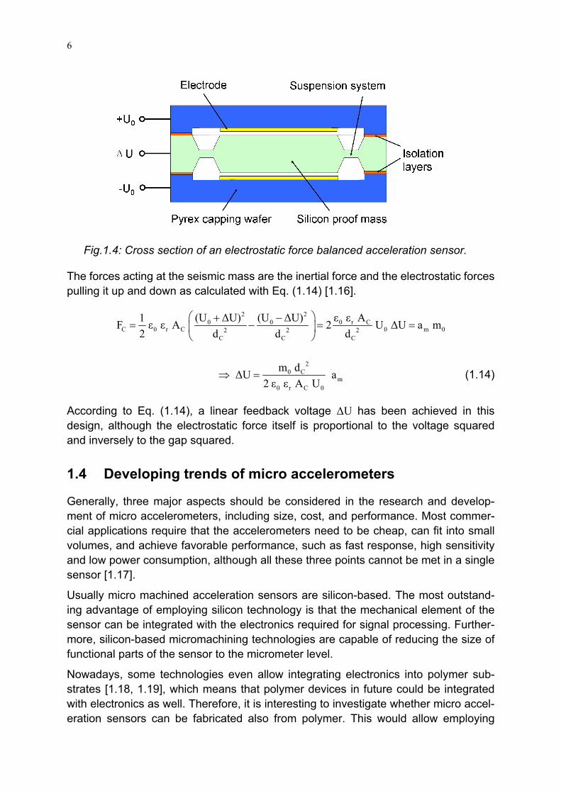
Due to these advantages force balanced acceleration sensors gradually became popular in research of accelerometers [1.9 - 1.15]. There are several possible actua-tion mechanisms to keep the proof mass at its idle position, such as electrostatic [1.11] and magnetic [1.15]. Electrostatic forces are the most commonly used type. Fig. 1.4 shows the principal of capacitive closed loop accelerometers. In this figure two capacitors are used as both position detector and force balancing actuator. When there is no acceleration, the proof mass is put to ground potential and it is attracted both to the upper and the lower electrode by the same electrostatic force. Therefore, it stays in its idle position. When there is some acceleration, the voltage at the seismic mass is adapted such that it is held at its idle position and this voltage is used as a measure of acceleration.

6

Fig.1.4: Cross section of an electrostatic force balanced acceleration sensor.

The forces acting at the seismic mass are the inertial force and the electrostatic forces pulling it up and down as calculated with Eq. (1.14) [1.16].

2 2

0 0 0 r CC 0 r C 0 m 02 2 2

C C C

(U ΔU) (U ΔU) ε ε A1F ε ε A 2 U ΔU a m2 d d d

⎛ ⎞+ −= − = =⎜ ⎟

⎝ ⎠

2

0 Cm

0 r C 0

m dΔU a2 ε ε A U

⇒ = (1.14)

According to Eq. (1.14), a linear feedback voltage ΔU has been achieved in this design, although the electrostatic force itself is proportional to the voltage squared and inversely to the gap squared.

1.4 Developing trends of micro accelerometers

Generally, three major aspects should be considered in the research and develop-ment of micro accelerometers, including size, cost, and performance. Most commer-cial applications require that the accelerometers need to be cheap, can fit into small volumes, and achieve favorable performance, such as fast response, high sensitivity and low power consumption, although all these three points cannot be met in a single sensor [1.17].

Usually micro machined acceleration sensors are silicon-based. The most outstand-ing advantage of employing silicon technology is that the mechanical element of the sensor can be integrated with the electronics required for signal processing. Further-more, silicon-based micromachining technologies are capable of reducing the size of functional parts of the sensor to the micrometer level.

Nowadays, some technologies even allow integrating electronics into polymer sub-strates [1.18, 1.19], which means that polymer devices in future could be integrated with electronics as well. Therefore, it is interesting to investigate whether micro accel-eration sensors can be fabricated also from polymer. This would allow employing

7

cheaper polymer and more economic fabrication processes for such sensor applica-tions.

Since polymers tend to creep and their properties are a strong function of temperature, polymer components appear to be no good functional elements in a sensor. However, there are two methods to avoid this disadvantage: firstly, the principles of thermal flow sensors can be adopted to design acceleration sensors, which apply thermal compo-nents instead of proof mass and suspending system as the sensing elements. Thus, there is no free-standing structure inside of the sensor, which eliminates the nonlinear effects due to the squeeze film damping and the mechanical suspension system. Secondly, use a closed feedback loop to balance against the inertial force. Therefore, the dependence on mechanical properties and temperature of the sensing element will be limited significantly.

Alternative schemes of acceleration sensors from polymer based on the two principles mentioned above will be discussed in the following chapters.

9

Chapter 2

Thermal acceleration sensors without proof mass

2.1 Introduction

Generally, conventional acceleration sensors measure the displacement of a proof mass, whose performances mainly depend on the mechanical sensing elements, in-cluding proof mass and suspending structure. However, larger deflection or deforma-tion of the suspending structure may cause nonlinear effects. Besides this, a moving seismic mass results in friction and squeeze film damping. Even damage of the sensor can occur during very high acceleration [2.1].

Recently, a new concept of thermal accelerometer has been proposed and developed in many publications [2.2-2.5]. In these new designs, thermal elements, including heaters and thermometers, are applied instead of mechanical elements, which avoid the disadvantages due to the free-standing structures. The principle of these sensors is as follows: a suspended heater generates a symmetric thermal distribution along the axis of acceleration. When the sensor is accelerated, the thermal distribution becomes asymmetric, which can be measured by thermometers suspending on both sides of the heater [2.6]. However, the distribution asymmetry in a sealed chamber due to the acceleration is determined by dissipation. Therefore, the temperature dif-ference between two thermometers is quite small, which limits the sensitivity of the sensor.

In the work reported here, the principles of thermal flow sensors are adopted to in-crease the sensitivity of thermal accelerometers. A circulation path and two air cells are applied to produce a circulation flow inside the sensor. Due to the convection between air flow and sensing elements, the temperature changes can be enlarged significantly.

In this chapter, two new designs, anemometric and calorimetric accelerometers, will be proposed and introduced. A calculation will be presented for the comprehension of the sensing principle and design optimization. Manufacturing processes and experi-mental results will also be presented and discussed.

2.2 Anemometric accelerometer

Hot-wire anemometers are widely used in measuring the velocity of flows. This tech-nique is based on King’s law which describes the relationship between the velocity of flow and the temperature change of a hot wire. Based on this principle, an anemo-metric accelerometer was designed, whose structure, fabrication process and mea-

10

surement results will be presented in the follow paragraphs.

2.2.1 Design

Fig. 2.1 shows the structure of the anemometric accelerometer. There are two air cells which are connected by a tube with length L and a heater wire crossing. The cross section of the tube is square with side length W. Another tube links the two air cells as a circulation loop, whose cross-section area should be much larger than that of the tube with the heater, so that the friction in the circulation loop can be ignored. Both cells and tubes are filled with air and sealed completely.

Fig. 2.1: Schematic drawing of the anemometric accelerometer.

The operational principle of this anemometric accelerometer is explained by Fig. 2.2. Without acceleration, the heat is transferred symmetrically to the air and housing around the heater, and the temperature of the heater keeps a certain value. When the sensor is accelerated with an acceleration a, the air in the heated tube gets a velocity v because it has a smaller density than the rest of the air. Then the temperature of the heater will vary because of the convection, which directly affects its resistance. Therefore, the resistance change of the heater can be used as a measure of accelera-tion.

Fig. 2.2: Operational principle of anemometric accelerometer.

11

2.2.2 Calculation

The air sealed inside the sensor is similar to the liquid in a connecting vessel shown in Fig. 2.3. The pressures P1 and P2 loading on both sides of the bottom surface (red) can be expressed by Eq. (2.1).

1 2P P ρ g h= = (2.1)

where ρ and h are the density and height of water, and g is the gravity of the earth. In equilibrium state, P1 and P2 are equal to each other, and there is no movement of water. Consequently, the heights of water in both vessels are the same. As in Eq. 2.1, the pressure on the bottom surface is determined by the liquid height h and density ρ.

The theory of connecting vessel can also be used to explain the working principle of thermal accelerometers. The air around the heater is warmed up, which leads to a density difference between hot and cold air. When the sensor is accelerated by a, there is a pressure difference described by Eq. (2.2).

c h c hΔP P P ρ a l ρ a l Δρ a l= − = − = (2.2)

where Pc and Ph are the pressures of cold and hot air. l, ρc, ρh are the length and densities of cold and hot air, respectively. Δρ is the density difference between cold and hot air.

It is assumed that there is a cube of air around the heater which is heated up. The in-terrelationship between pressure P, volume V, temperature T, and the number n of mols of an ideal gas is described by the ideal gas law (R is the gas constant = 8.314 J / (mol K)):

P V n R T= (2.3)

The volume of the heated air is much smaller than the total air volume so that the pressure is approximately constant. Then the change Δρ of density can be expressed as follows:

0 1

1 0

ρ T=ρ T

(2.4)

00 1 0

1

TΔρ = ρ ρ = ρ 1T

⎛ ⎞− −⎜ ⎟

⎝ ⎠ (2.5)

Fig. 2.3: Schematic of connecting vessel.

h

P1 P2

h

P1 P2

12

where ρ0, ρ1, T0, T1 are the volume, density and temperature of the air around the heater before and after heating, respectively.

The pressure difference ΔP overcomes the friction in the tube and drives a circulation flow inside the sensor. The flow velocity v can be calculated by Hagen-Poiseuille equation as follows [2.7]:

2

h

F

D1v ΔP32 η L

= − (2.6)

where Dh is the hydraulic diameter, LF is the length of the tube, and η is the dynamical viscosity of the air in the tube. The definition of the hydraulic diameter Dh is [2.7]:

Fh

w

4AD =U

(2.7)

where AF is the area of the cross-section and Uw is the circumference of the tube in contact to the moving air.

Inserting Eqs. (2.2) and (2.7) into Eq. (2.6) yields:

2

F2

F w

Δρ l A1v a2 η L U

= − (2.8)

According to Eq. (2.8), the velocity of the flow due to external acceleration is deter-mined by the dimensions of the tube, including length of the tube LF and hydraulic diameter Dh, and the power of the heater, which influences the effective length of the heated air l and density difference Δρ. For higher sensitivity, the flow velocity should be as large as possible. Therefore, the dimensions of the tube should be designed such that the ratio of Dh

2/LF gets large and the power of the heater also needs to be large.

When the air flow driven by external acceleration travels across the heater, the tem-perature of the heater will be decreased due to convection. The relationship between heater power per unit area taken away by convection QC and temperature difference ΔΤ between heater and environment can be expressed by King’s law, as follows:

FC F

R

ρ vQ λ TL η

= − Δ (2.9)

where λF is the thermal conductivity of the fluid, ρF is the density of the air, LR is the distance between heater and the front side of the substrate facing the flow (cf. Fig. 2.4), and η is the dynamical viscosity.

The thermal flow to the tube wall QW is estimated by Fourier’s law as:

13

S SW F F

K K

2 A 4 AQ = λ T = λ Td d2

Δ Δ (2.10)

where dK and AS are the height of the tube and the surface area of the wire, respec-tively.

The electrical power of the heater is equal to the sum of three terms: first, the energy loss due to convection which can be calculated by King’s law; second, the heat conduction of the tube wall; third, the heat absorbed by the heater itself due to its heat capacity, which can be described as [2.7]:

SF hel F S F D

R K

4 Aρ v dTP λ A ΔT λ ΔT CL η d dt

− − = (2.11)

where Pel, CD and Th are the electrical power, the heat capacity of the heater, and the temperature of heater, respectively.

When electric power is applied to the heater, the heater itself needs to be heated up first, and after a certain time the temperature of the wire will be constant (dT/dt = 0). Therefore, no more heat is consumed to warm up the heater, and the power of the heater is majorly consumed by the other two energy flows. If the sensor is not accele-rated and the fluid is not moving, there is no energy loss due to convection and all the power of the heater is conducted to the side wall. This way, the original temperature of the heater can be obtained:

el Kh 0

F S

P dT T4 λ A

= + (2.12)

where T0 is the environment temperature. The temperature of the heated air around the heater Ta is approximated as an average of the temperature of the heater and the environment.

h 0a

T TT2+

= (2.13)

When the sensor is accelerated, the temperature of the heater Th could be expressed by the following equation [2.7]:

Kh 0

FF

R K

QT Tρ v 4λL η d

= +⎛ ⎞

+⎜ ⎟⎝ ⎠

(2.14)

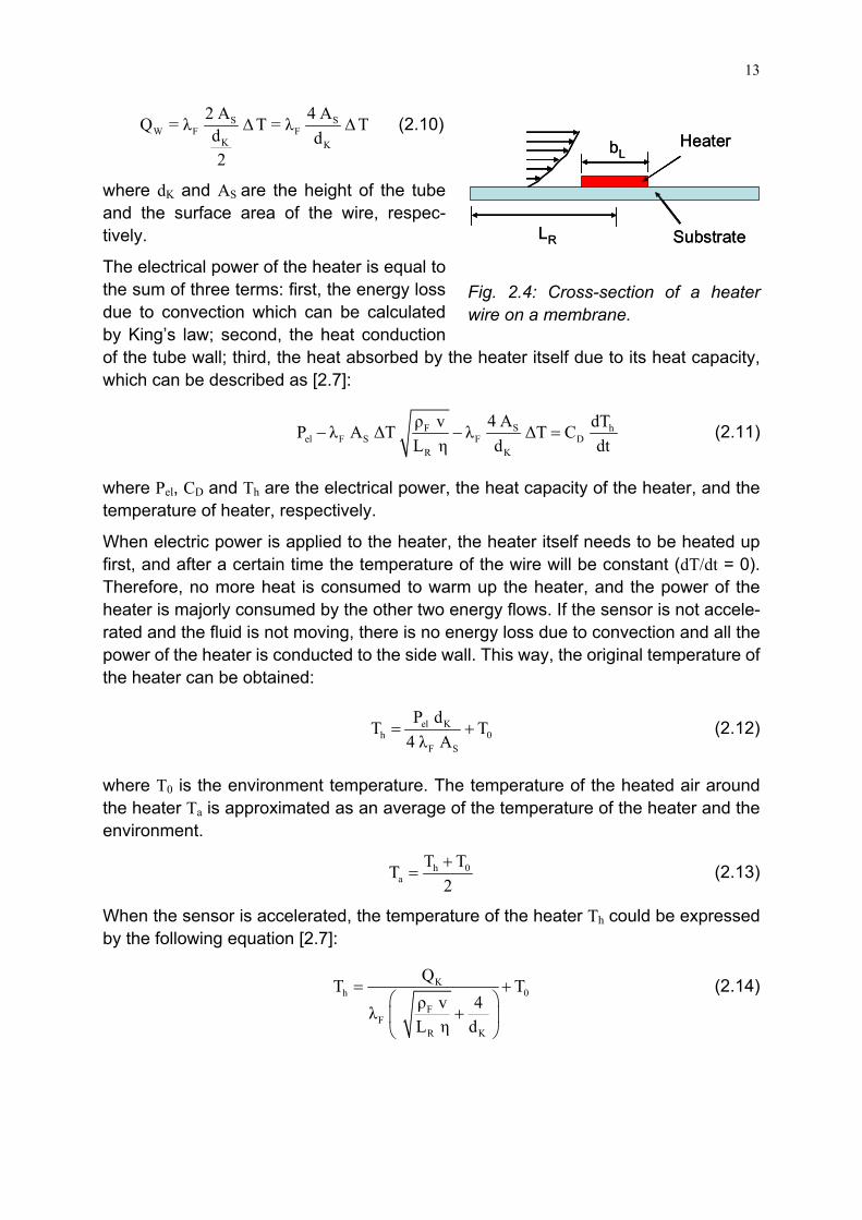
Fig. 2.4: Cross-section of a heater wire on a membrane.

LR

bL

Substrate

Heater

LR

bL

Substrate

Heater

14

where Qk is the power per unit area of the heater. For high sensitivity and a large output signal the heat loss due to flow convection should be comparable to that flowing into the side walls. Therefore, a small LR and large height of the air tube dK are necessary according to Eq. (2.14).

If a gold wire with the radius RB of 25 μm and the resistance of 9 mΩ is used as the heater and the length LF, the width W, and the height dK of the tube are 1 mm, 0.75 mm and 1.5 mm, respectively, the power per unit area QK and the surface area AS of the heater can be calculated as 1.9 W/cm2

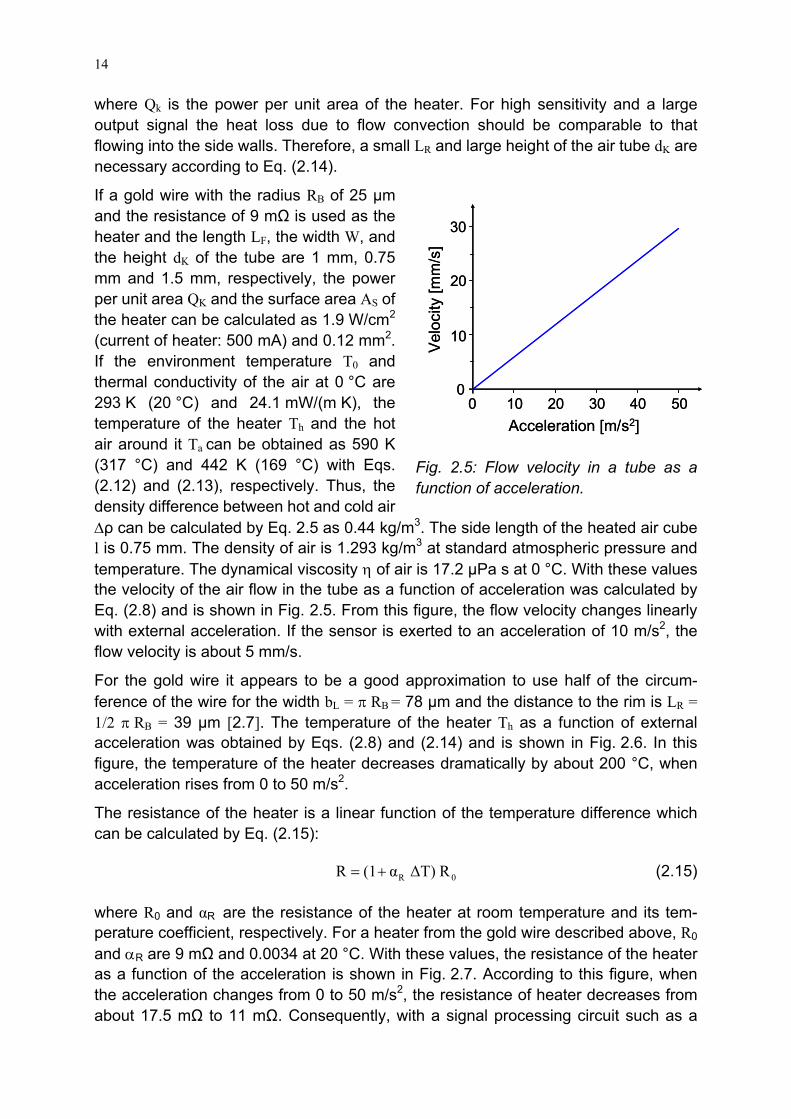
(current of heater: 500 mA) and 0.12 mm2. If the environment temperature T0 and thermal conductivity of the air at 0 °C are 293 K (20 °C) and 24.1 mW/(m K), the temperature of the heater Th and the hot air around it Ta can be obtained as 590 K (317 °C) and 442 K (169 °C) with Eqs. (2.12) and (2.13), respectively. Thus, the density difference between hot and cold air Δρ can be calculated by Eq. 2.5 as 0.44 kg/m3. The side length of the heated air cube l is 0.75 mm. The density of air is 1.293 kg/m3 at standard atmospheric pressure and temperature. The dynamical viscosity η of air is 17.2 µPa s at 0 °C. With these values the velocity of the air flow in the tube as a function of acceleration was calculated by Eq. (2.8) and is shown in Fig. 2.5. From this figure, the flow velocity changes linearly with external acceleration. If the sensor is exerted to an acceleration of 10 m/s2, the flow velocity is about 5 mm/s.

For the gold wire it appears to be a good approximation to use half of the circum-ference of the wire for the width bL = π RB = 78 μm and the distance to the rim is LR = 1/2 π RB = 39 μm [2.7]. The temperature of the heater Th as a function of external acceleration was obtained by Eqs. (2.8) and (2.14) and is shown in Fig. 2.6. In this figure, the temperature of the heater decreases dramatically by about 200 °C, when acceleration rises from 0 to 50 m/s2.

The resistance of the heater is a linear function of the temperature difference which can be calculated by Eq. (2.15):

R 0R (1 α ΔT) R= + (2.15)

where R0 and αR are the resistance of the heater at room temperature and its tem-perature coefficient, respectively. For a heater from the gold wire described above, R0

and αR are 9 mΩ and 0.0034 at 20 °C. With these values, the resistance of the heater as a function of the acceleration is shown in Fig. 2.7. According to this figure, when the acceleration changes from 0 to 50 m/s2, the resistance of heater decreases from about 17.5 mΩ to 11 mΩ. Consequently, with a signal processing circuit such as a

Fig. 2.5: Flow velocity in a tube as a function of acceleration.

0

10

20

30

0 30 40 502010Acceleration [m/s2]

Vel

ocity

[mm

/s]

0

10

20

30

0 30 40 502010Acceleration [m/s2]

Vel

ocity

[mm

/s]

15

bridge, an amplifier, and a filter the resistance change of the heater can be used as a measure of acceleration.

Fig. 2.6: Temperature of the heater as a function of the acceleration.

Fig. 2.7: Resistance of the heater as a function of the acceleration.

2.2.3 Fabrication

Two prototypes of anemometric accelerometers were made by different fabrication technologies. The first (prototype 1) was made by traditional mechanical manufac-turing technology, which used a gold wire as the heater. For prototype 2, the heater was made by sputtering and photolithography on a polymer substrate.

Fig 2.8 shows the details of prototype 1. In this figure, the housing and the cover of the sensor were made by micro milling on a PMMA plate with the thickness of 5 mm. The coil heater was made of a gold wire (diameter: 50 µm), and mounted into a special designed channel in the housing by double-compound glue (UHU). Another gold wire, which is the same as the heater, was also installed in the sensor as a calibration resistor for temperature compensation.

Fig. 2.8: Anemometric acceleration sen-sor with a gold wire as heater.

Fig. 2.9: Anemometric acceleration sen-sor with a sputtered heater.

8

12

16

20

0 10 20 30 40 50Acceleration [m/s2]

Res

ista

nce

[mΩ

]

8

12

16

20

0 10 20 30 40 50Acceleration [m/s2]

Res

ista

nce

[mΩ

]

0 10 20 30 40 500

200

300

100

Acceleration [m/s2]

Tem

pera

ture

of h

eate

r [°C

]

0 10 20 30 40 500

200

300

100

Acceleration [m/s2]

Tem

pera

ture

of h

eate

r [°C

]

16

Prototype 2 is shown in Fig. 2.9. The heater is made of a sputtered polyimide (PI) foil by photolithography and etching. The steps of the process are shown in Fig. 2.10. Firstly, a gold layer, approximately 220 nm in thickness, was sputtered on a polyimide foil (thickness: 25 µm) (Fig. 2.10.1). After that, a layer of photo-resist (AZ 4526) was spin-coated on the gold layer (Fig. 2.10.2). Then the photo-resist was exposed with a mask fabricated by micro milling and spray painting, shown in Fig. 2.11, by UV light, and developed by a developer (AZ 826 MIF) (Fig. 2.10.3). Following that, the exposed gold was etched by king water (Fig. 2.10.4). At last, the remained photo-resist was dissolved by a remover (AZ 100) (Fig. 2.10.5). With these processes, the pattern on the mask was transferred to the gold layer.

Fig. 2.10: Fabrication process of sput-tered heater.

Fig. 2.11: Photolithography mask made by micro milling and spray painting.

Compared with the coil heater the sputtered heater has three advantages: first of all, it can be fabricated in large batches, which decreases the cost significantly. Secondly, the size of the heater can be reduced to millimeter level by decreasing the minimum line width of the pattern on the mask, so that the total volume of the sensor can be reduced. Thirdly, heating efficiency is enhanced obviously due to the larger resistance and contacting area.

2.2.4 Experimental results

Both prototypes 1 and 2 were tilted in the gravity of the earth and shaken by hand in the experiments. Unfortunately, there was no useful signal measured from them, even when the current of the heaters were increased to about 0.2 A. Therefore, the conclusion was drawn that the sensitivity of the anemometric acceleration sensor needs to be enhanced. Thus, the power supplied by the heater should be raised to drive larger flow in the tube, which requires a bulky heater. However, a bulky heater has a larger heat capacity which decreases the sensitivity of the sensor. Accordingly, the best way to solve this problem is to employ an independent heater and thermometer making a calorimeter.

17

2.3 Calorimetric accelerometer

Calorimeters are another kind of widely applied flow sensors. The basic principle of calorimeters is quite similar as anemometers. The major difference is that the output signal does not depend on the resistance change of the heater caused by convection, but on the temperature difference between two thermometers installed on both sides of the heater. In this section, the design, fabrication process, and experimental results of calorimetric accelerometers are presented.

2.3.1 Design of calorimetric accelerometer

The structure of the calorimetric acceleration sensor is shown in Fig. 2.12. A heater is placed inside a heating chamber, which is connected to two symmetrical air cells by a couple of tubes. In a large heating chamber a high power heater is used to drive an air flow when the acceleration is applied. Meanwhile, the heat flowing to the side walls is decreased significantly, because the chamber walls are farer from the heater than for the anemometer discussed above. Two wires are suspended on both sides of the heater across the tubes serving as thermometers. A larger tube connecting the two air cells directly is used as a circulation path.

Fig. 2.12: Structure of calorimetric acceleration sensor.

The heater in the heating chamber generates a symmetric thermal profile along the tube, which can be detected by the two thermometers. Without acceleration both thermometers have the same temperature. When the acceleration is applied, the thermal profile becomes asymmetric due to a circulation flow inside the sensor. Therefore, there is a temperature difference between the two thermometers which can be used as a measure of acceleration.

2.3.2 Calculation of calorimetric accelerometer

The temperature distribution of the heater can be described by a differential equation given by Lammerink et al. [2.8]. The structure of the flow tube is shown in Fig. 2.13.

Circulation path Thermometer

Air cell HeaterHeating chamber

Tube

Thermometer HeaterTube

Heating Chamber

Circulation path Thermometer


TubeCirculation path Thermometer


Tube


Heating Chamber


Heating Chamber

18

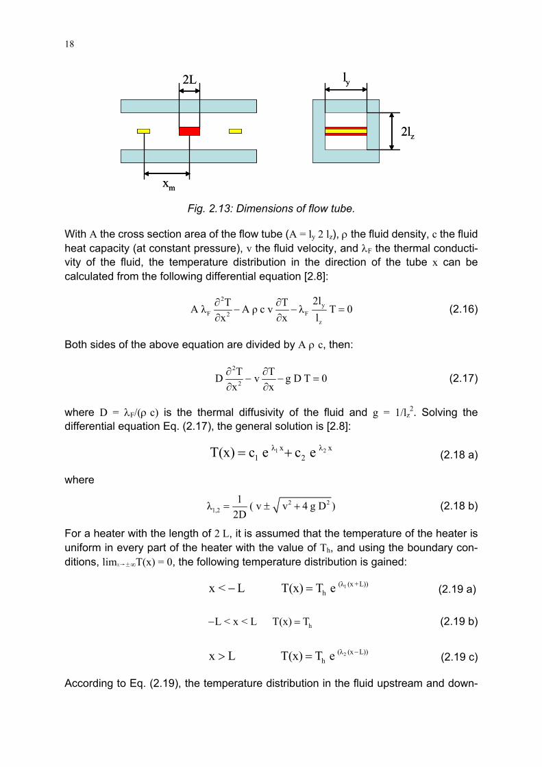
Fig. 2.13: Dimensions of flow tube.

With A the cross section area of the flow tube (A = ly 2 lz), ρ the fluid density, c the fluid heat capacity (at constant pressure), v the fluid velocity, and λF the thermal conducti-vity of the fluid, the temperature distribution in the direction of the tube x can be calculated from the following differential equation [2.8]:

2

yF F2

z

2lT TA λ A ρ c v λ T 0x x l

∂ ∂− − =

∂ ∂ (2.16)

Both sides of the above equation are divided by A ρ c, then:

2

2

T TD v g D T 0x x

∂ ∂− − =

∂ ∂ (2.17)

where D = λF/(ρ c) is the thermal diffusivity of the fluid and g = 1/lz2. Solving the

differential equation Eq. (2.17), the general solution is [2.8]:

1 2λ x λ x1 2T(x) c e c e= + (2.18 a)

where

2 21,2

1λ ( v v 4 g D )2D

= ± + (2.18 b)

For a heater with the length of 2 L, it is assumed that the temperature of the heater is uniform in every part of the heater with the value of Th, and using the boundary con-ditions, limx→±∞T(x) = 0, the following temperature distribution is gained:

1(λ (x +L))hx < L T(x) T e− = (2.19 a)

hL < x < L T(x) T− = (2.19 b)

2(λ (x L))hx L T(x) T e −> = (2.19 c)

According to Eq. (2.19), the temperature distribution in the fluid upstream and down-

2L

xm

ly

2lz

2L

xm

ly

2lz

19

stream is an index function of the position on the x axis, and the eigenvalues λ1 and λ2

are determined by the flow velocity v, which means the temperature distribution depends on the flow velocity. For better understanding of the temperature distribution, the temperature of the heater Th needs to be determined.

The electrical power of the heater P is equal to the sum of three parts: first, the heat conducted to the tube wall above and below the heater; second, the heat injected in the upstream and downstream of the fluid stream at the heater edges; third, the heat absorbed by the heater itself due to its heat capacity. If the heating time is long enough, the temperature of the heater will be constant, and no more energy is consumed by the heater itself. Therefore, the following equation can be gained:

w u dP = Φ + Φ + Φ (2.20)

where Φw, Φu, and Φd are the heat conducted to the side wall, upstream and down-stream of the fluid flow, respectively.

The heat flowing to the side wall can be described by Eq. (2.10):

sw F h

z

2 A= λ T l

Φ (2.21)

where As is the surface area of the heater. Using linearization of Eq. (2.19 a) in the vicinity of the left edge of the heater (x = – L) yields:

( )h 1

x L

dT xT(x) x T λ Δx

dx= −

Δ = Δ = (2.22)

Inserting Eq. (2.22) into Eq. (2.10) yields the heat injected to the upstream of the fluid flow:

u F F 1 hΔTλ A λ A λ TΔx

Φ = = (2.23)

Similarly, the heat injected to the downstream of the fluid flow can be expressed as:

d F F 2 hΔTλ A λ A λ TΔx

Φ = = − (2.24)

Taking Eqs. (2.21), (2.23) and (2.24) into Eq. (2.20), the temperature of the heater can be obtained as:

yh F

F 1 2 z

2lPT G λG 2 L A λ (λ λ ) l

= =+ −

(2.25)

For the calorimetric accelerometer shown in Fig. 2.12, the length ly and the width 2 L of the heater are 7 mm and 3.8 mm, respectively. Moreover, the height of the tube 2 lz and the thermal conductivity of air are 3 mm and 24.1 mW/(m K), respectively. If the

20

power of the heater is 0.2 W and there is no air flow inside the tube, the temperature of the heater is calculated by Eq. (2.25) to be 145 °C.

According to Fig. 2.12 the cross section of the heating chamber is much larger than the one of the connecting tube between the heating chamber and the air cell. Therefore, the flow resistance is majorly due to the connecting tube. If the dimensions of the connecting tube are 0.75 mm, 0.75 mm, and 1.5 mm as the length, width, and height, respectively, and the dynamical viscosity η of air is 17.2 µPa s at 0 °C, the flow velocity of air due to external acceleration was obt-ained with Eqs. (2.5), (2.8), (2.13) and (2.25) and is shown in Fig. 2.14. When the external acceleration is 10 m/s2 and 20 m/s2, the corresponding flow velocity is 11 mm/s and 23 mm/s, respectively. The density of air is 1.293 kg/m3 at standard atmospheric pressure and temperature, and the heat capacity of air is 1030 J/(kg K). With these values the temperature distribution for three different flow velocities (0 mm/s, 11 mm/s, and 23 mm/s) was calculated by Eq. (2.19) and shown in Fig. 2.15.

Fig. 2.15: Temperature distribution of the heater as a function of the position x at three different flow velocities.

Fig. 2.14: Flow velocity in a tube as a function of acceleration.

0 4 8 12 16 20

5

10

15

20

0

Acceleration [m/s2]Ve

loci

ty [m

m/s

]

25

0 4 8 12 16 20

5

10

15

20

0

Acceleration [m/s2]Ve

loci

ty [m

m/s

]

25

21

With Eq. (2.19) the temperatures at the two thermometers upstream (at x = xm) and downstream (at x = −xm), and the temperature difference ΔT are given by

2 m(λ (x L))d hT T e −= (2.26 a)

1 m(λ ( x +L))u hT T e −= (2.26 b)

( )2 m 1 m(λ (x L)) (λ ( x +L))d u hT T T T e e− −Δ = − = − (2.26 c)

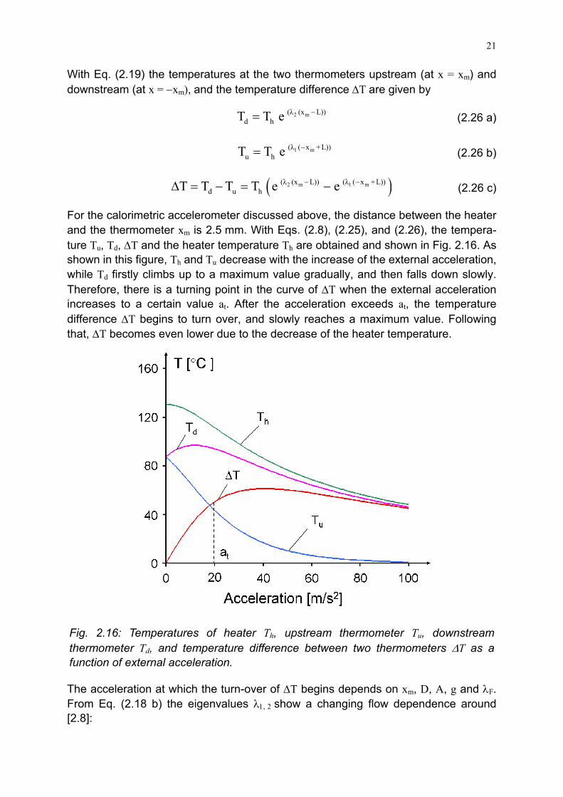
For the calorimetric accelerometer discussed above, the distance between the heater and the thermometer xm is 2.5 mm. With Eqs. (2.8), (2.25), and (2.26), the tempera-ture Tu, Td, ΔT and the heater temperature Th are obtained and shown in Fig. 2.16. As shown in this figure, Th and Tu decrease with the increase of the external acceleration, while Td firstly climbs up to a maximum value gradually, and then falls down slowly. Therefore, there is a turning point in the curve of ΔT when the external acceleration increases to a certain value at. After the acceleration exceeds at, the temperature difference ΔT begins to turn over, and slowly reaches a maximum value. Following that, ΔT becomes even lower due to the decrease of the heater temperature.

Fig. 2.16: Temperatures of heater Th, upstream thermometer Tu, downstream thermometer Td, and temperature difference between two thermometers ΔT as a function of external acceleration.

The acceleration at which the turn-over of ΔT begins depends on xm, D, A, g and λF. From Eq. (2.18 b) the eigenvalues λ1, 2 show a changing flow dependence around [2.8]:

22

2 2v 4 g D= (2.27)

The flow velocity in Eq. (2.27) is called turn-over flow velocity vt [2.8]:

tz

2 Dvl

= (2.28)

Therefore, the external acceleration at corresponding to the turn-over velocity vt can be obtained by inserting Eq. (2.8) into Eq. (2.28):

2

F wt 2

z F

4 D η L Ual Δρ l A

= (2.29)

For the calorimetric acceleration sensor discussed in Fig. 2.16, the turn-over acceleration at calculated with Eq. (2.29) is 21 m/s2. When the external acceleration is less than the turn-over acceleration at, the temperature difference ΔT can be regarded as a linear function of external acceleration. Therefore, the turn-over acceleration is a key parameter for the calorimetric accelerometer which determines the measuring range of the sensor.

In the linear range, the sensitivity S at a = 0 can be approximately defined as the derivative of ΔT with respect to a. With Eqs. (2.8), (2.25), and (2.26 c), the sensitivity S can be obtained as follows (assuming L = 0):

m z

2( x /l )F m

2F y F wa = 0

P Δρ l A xT T v 1S ea v a 8 λ l η L U D

−∂ Δ ∂ Δ ∂= = =

∂ ∂ ∂ (2.30)

Fig. 2.17: Sensitivity S as a function of the distance between the heater and the thermometer xm.

23

According to Eq. (2.30), the sensitivity of a calorimetric accelerometer depends on the power of the heater, the dimensions of the tube, and the properties of the fluid. If the fluid is air and the power of the heater is 0.2 W, the sensitivity S as a function of xm is shown in Fig. 2.17. In this figure the sensitivity S reaches the maximum value when the distance between heater and thermometer xm is equal to half of the tube’s height lz = 1.5 mm.

With Eq. (2.30), a linear characteristic curve of the calorimetric accelerometer is given as:

m z

2( x /l )F m

2F y F w

P Δρ l A x1T S a e a8 λ l η L U D

−Δ = = (2.31)

The sensor characteristics are strongly affected by the thermal diffusivity of the fluid inside the sensor. According to Eqs. (2.18 b) and (2.25) it is obvious that the tem-perature distribution is controlled by the ratio of the flow velocity and the thermal diffusivity v/D. If a liquid like water, with the thermal conductivity, the density, and the heat capacity of 0.58 W/m K, 4.2×103 J/kg K, and 103 kg/m3, respectively, is employed in the sensor and the power of the heater is 2 W, the temperature difference ΔT as a function of a and the sensitivity S as a function of xm between the heater and the thermometer are shown in Figs. (2.18) and (2.19), respectively.

Fig. 2.18: Temperature difference ΔT as a function of a of the calorimetric accelera-tion sensors with different fluids.

Fig. 2.19: Sensitivity S as a function xm of the calorimetric acceleration sensors with different fluids.

Due to the little thermal diffusivity of water the temperature difference ΔT caused by external acceleration is much smaller than the one of the sensor with air as the fluid, although the power of the heater is increased by 10 times (cf. Fig. 2.18). According to Fig. 2.19, the sensor with water flow has a much lower sensitivity than the one with air flow, and its maximum sensitivity is only 1/50 of the one of air flow calorimeter. However, the turn-over acceleration of the sensor with water flow calculated by Eq. (2.30) is 416 m/s2, which means it has a much wider measuring range. Therefore, for

24

measuring small acceleration the sensor with air flow has higher sensitivity and lower power consumption, and the sensor employing water flow is suitable for measuring large acceleration.

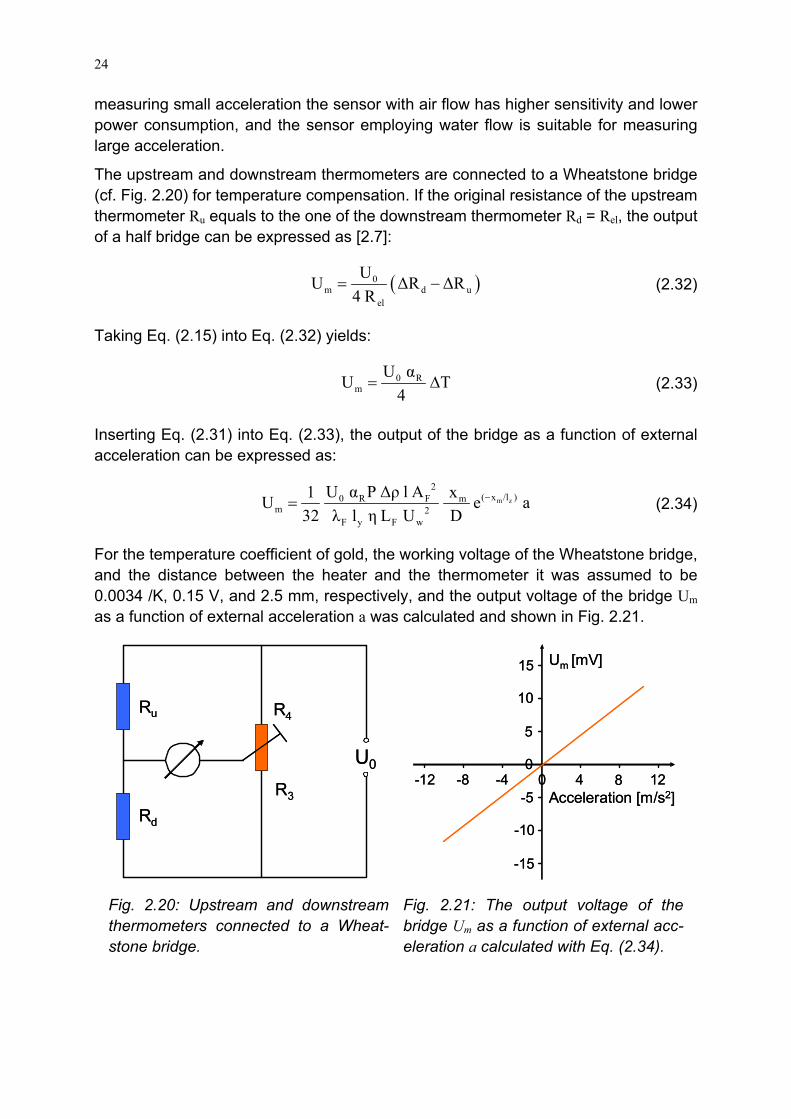
The upstream and downstream thermometers are connected to a Wheatstone bridge (cf. Fig. 2.20) for temperature compensation. If the original resistance of the upstream thermometer Ru equals to the one of the downstream thermometer Rd = Rel, the output of a half bridge can be expressed as [2.7]:

( )0m d u

el

UU ΔR ΔR4 R

= − (2.32)

Taking Eq. (2.15) into Eq. (2.32) yields:

0 Rm

U αU T4

= Δ (2.33)

Inserting Eq. (2.31) into Eq. (2.33), the output of the bridge as a function of external acceleration can be expressed as:

m z

2( x /l )0 R F m

m 2F y F w

U α P Δρ l A x1U e a32 λ l η L U D

−= (2.34)

For the temperature coefficient of gold, the working voltage of the Wheatstone bridge, and the distance between the heater and the thermometer it was assumed to be 0.0034 /K, 0.15 V, and 2.5 mm, respectively, and the output voltage of the bridge Um as a function of external acceleration a was calculated and shown in Fig. 2.21.

Fig. 2.20: Upstream and downstream thermometers connected to a Wheat-stone bridge.

Fig. 2.21: The output voltage of the bridge Um as a function of external acc-eleration a calculated with Eq. (2.34).

U0

Ru

Rd

R4

R3

U0

Ru

Rd

R4

R3 -5

-10

-15

5

10

15

0-4 4 8 12-8-12 0

Um [mV]

Acceleration [m/s2]-5

-10

-15

5

10

15

0-4 4 8 12-8-12 0

Um [mV]

Acceleration [m/s2]

25

2.3.3 Fabrication of calorimetric accelerometer

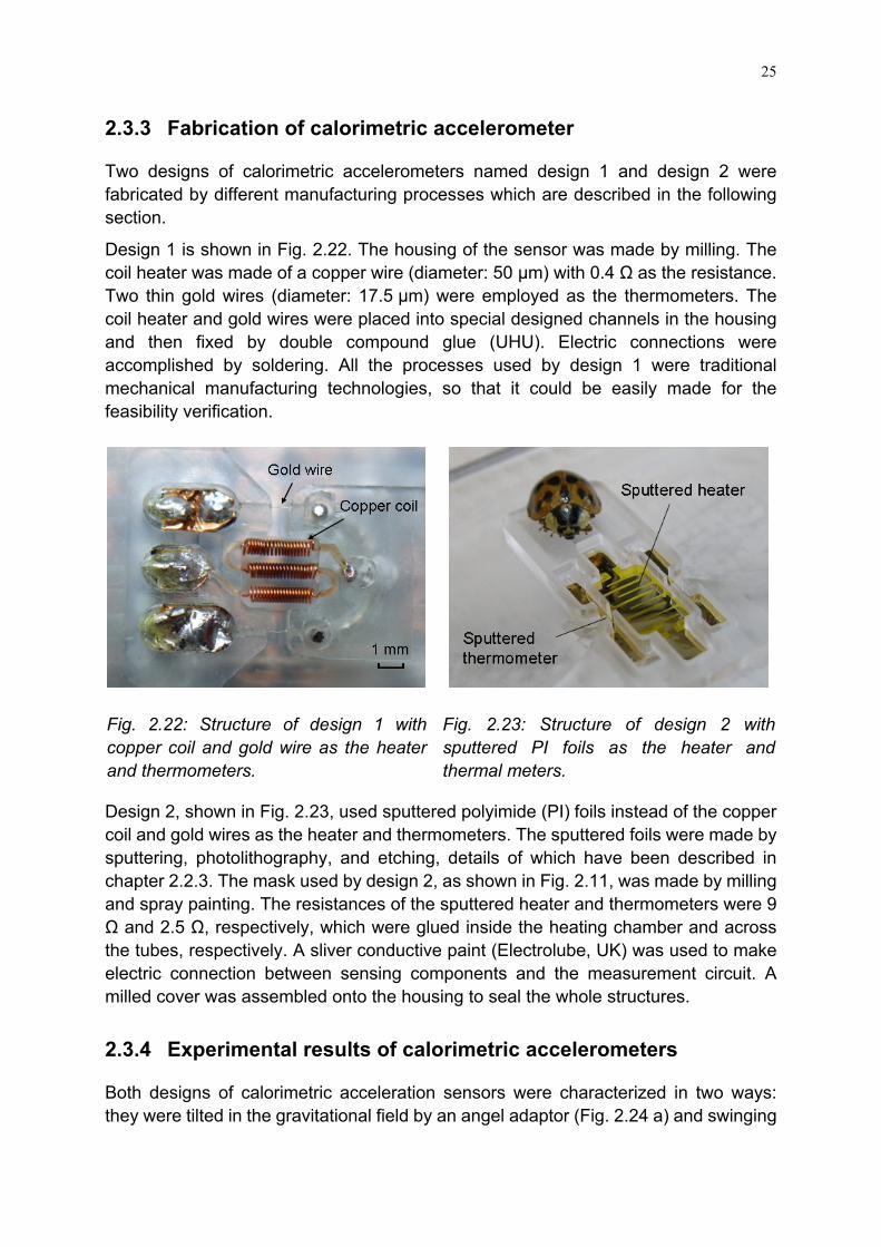
Two designs of calorimetric accelerometers named design 1 and design 2 were fabricated by different manufacturing processes which are described in the following section.

Design 1 is shown in Fig. 2.22. The housing of the sensor was made by milling. The coil heater was made of a copper wire (diameter: 50 μm) with 0.4 Ω as the resistance. Two thin gold wires (diameter: 17.5 μm) were employed as the thermometers. The coil heater and gold wires were placed into special designed channels in the housing and then fixed by double compound glue (UHU). Electric connections were accomplished by soldering. All the processes used by design 1 were traditional mechanical manufacturing technologies, so that it could be easily made for the feasibility verification.

Fig. 2.22: Structure of design 1 with copper coil and gold wire as the heater and thermometers.

Fig. 2.23: Structure of design 2 with sputtered PI foils as the heater and thermal meters.

Design 2, shown in Fig. 2.23, used sputtered polyimide (PI) foils instead of the copper coil and gold wires as the heater and thermometers. The sputtered foils were made by sputtering, photolithography, and etching, details of which have been described in chapter 2.2.3. The mask used by design 2, as shown in Fig. 2.11, was made by milling and spray painting. The resistances of the sputtered heater and thermometers were 9 Ω and 2.5 Ω, respectively, which were glued inside the heating chamber and across the tubes, respectively. A sliver conductive paint (Electrolube, UK) was used to make electric connection between sensing components and the measurement circuit. A milled cover was assembled onto the housing to seal the whole structures.

2.3.4 Experimental results of calorimetric accelerometers

Both designs of calorimetric acceleration sensors were characterized in two ways: they were tilted in the gravitational field by an angel adaptor (Fig. 2.24 a) and swinging

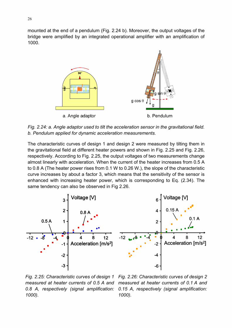
26

mounted at the end of a pendulum (Fig. 2.24 b). Moreover, the output voltages of the bridge were amplified by an integrated operational amplifier with an amplification of 1000.

Fig. 2.24: a. Angle adaptor used to tilt the acceleration sensor in the gravitational field. b. Pendulum applied for dynamic acceleration measurements.

The characteristic curves of design 1 and design 2 were measured by tilting them in the gravitational field at different heater powers and shown in Fig. 2.25 and Fig. 2.26, respectively. According to Fig. 2.25, the output voltages of two measurements change almost linearly with acceleration. When the current of the heater increases from 0.5 A to 0.8 A (The heater power rises from 0.1 W to 0.26 W.), the slope of the characteristic curve increases by about a factor 3, which means that the sensitivity of the sensor is enhanced with increasing heater power, which is corresponding to Eq. (2.34). The same tendency can also be observed in Fig 2.26.

Fig. 2.25: Characteristic curves of design 1 measured at heater currents of 0.5 A and 0.8 A, respectively (signal amplification: 1000).

Fig. 2.26: Characteristic curves of design 2 measured at heater currents of 0.1 A and 0.15 A, respectively (signal amplification: 1000).

0-4 4-8 8 12

-4

-2

0

2

4

6

-12

-6

Acceleration [m/s2]

Voltage [V]

0.15 A

0.1 A

0-4 4-8 8 12

-4

-2

0

2

4

6

-12

-6

Acceleration [m/s2]

Voltage [V]

0.15 A

0.1 A

-12 8 1240-8 -4

-3

-2

-1

0

1

2 0.8 A

0.5 A

Acceleration [m/s2]

Voltage [V]3

-12 8 1240-8 -4

-3

-2

-1

0

1

2 0.8 A

0.5 A

Acceleration [m/s2]

Voltage [V]3

8 1240-8 -4

-3

-2

-1

0

1

2 0.8 A

0.5 A

Acceleration [m/s2]

Voltage [V]3

27

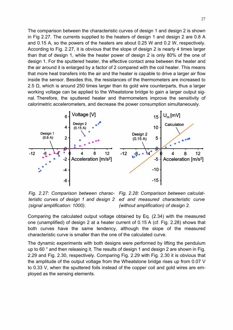
The comparison between the characteristic curves of design 1 and design 2 is shown in Fig 2.27. The currents supplied to the heaters of design 1 and design 2 are 0.8 A and 0.15 A, so the powers of the heaters are about 0.25 W and 0.2 W, respectively. According to Fig. 2.27, it is obvious that the slope of design 2 is nearly 4 times larger than that of design 1, while the heater power of design 2 is only 80% of the one of design 1. For the sputtered heater, the effective contact area between the heater and the air around it is enlarged by a factor of 2 compared with the coil heater. This means that more heat transfers into the air and the heater is capable to drive a larger air flow inside the sensor. Besides this, the resistances of the thermometers are increased to 2.5 Ω, which is around 250 times larger than its gold wire counterparts, thus a larger working voltage can be applied to the Wheatstone bridge to gain a larger output sig-nal. Therefore, the sputtered heater and thermometers improve the sensitivity of calorimetric accelerometers, and decrease the power consumption simultaneously.

Fig. 2.27: Comparison between charac-teristic curves of design 1 and design 2 (signal amplification: 1000).

Fig. 2.28: Comparison between calculat-ed and measured characteristic curve (without amplification) of design 2.

Comparing the calculated output voltage obtained by Eq. (2.34) with the measured one (unamplified) of design 2 at a heater current of 0.15 A (cf. Fig. 2.28) shows that both curves have the same tendency, although the slope of the measured characteristic curve is smaller than the one of the calculated curve.

The dynamic experiments with both designs were performed by lifting the pendulum up to 60 ° and then releasing it. The results of design 1 and design 2 are shown in Fig. 2.29 and Fig. 2.30, respectively. Comparing Fig. 2.29 with Fig. 2.30 it is obvious that the amplitude of the output voltage from the Wheatstone bridge rises up from 0.07 V to 0.33 V, when the sputtered foils instead of the copper coil and gold wires are em-ployed as the sensing elements.

Design 1 (0.8 A)

0-4 4-8 8 12

-4

-2

0

2

4

6

-12

-6

Acceleration [m/s2]

Voltage [V]

Design 2(0.15 A)

Design 1 (0.8 A)

0-4 4-8 8 12

-4

-2

0

2

4

6

-12

-6

Acceleration [m/s2]

Voltage [V]

Design 2(0.15 A)

-5

-10

-15

5

10

15

0-4 4 8 12-8-12 0

Um [mV]

Acceleration [m/s2]

Design 2(0.15 A)

Calculation

-5

-10

-15

5

10

15

0-4 4 8 12-8-12 0

Um [mV]

Acceleration [m/s2]

Design 2(0.15 A)

Calculation

28

Fig. 2.29: Output signal of design 1 when it is swinging with the pendulum.

Fig. 2.30: Output signal of design 2 when it is swing with pendulum.

2.4 Conclusions

The principles of anemometer and calorimeter have been proven to be feasible for measuring acceleration. Four prototypes of anemometric and calorimetric accelera-tion sensors have been fabricated by both mechanical manufacturing technology and micromachining processes. For the anemometers, due to their low sensitivity there

29

was no useful output signal measured in the experiments. To enhance the sensitivity, calorimetric acceleration sensors with independent heater and thermometers were developed. In experiments the calorimetric sensors successfully measured both static and dynamic acceleration. The output voltages were a linear function of the accelera-tion, which is corresponding to the theoretical calculation. In further research, it would be interesting to make the sensing elements including the heater and the thermo-meters with a custom-made mask. Due to the smaller line width of the patterns on this mask the dimension of the sensing elements can be reduced significantly such, that the total size of the sensor will be miniaturized. Furthermore, the housing of the sensor could be fabricated by ultrasonic hot embossing, which is capable to simplify the manufacturing process and decrease the cost.

31

Chapter 3

Closed loop acceleration sensors: capacitive drive

3.1 Introduction

For open loop acceleration sensors, there is a trade-off between bandwidth and sensitivity (cf. Chapter 1.2), which means that wide measuring range and high sensi-tivity can not be achieved simultaneously. Moreover, the deflection of mechanical sensing elements may cause nonlinear effects, and mechanical properties of free-standing structures could also affect the performance of a sensor.

To overcome these drawbacks, closed loop sensors adopting a feedback loop have been developed to enlarge the measuring range (bandwidth) at high sensitivity and keep the seismic mass at its idle position (cf. Chapter 1.3.2). The feedback signal is used as a measure of acceleration. This way, the characteristic curve of the sensor is not a function of the elastic properties of a movable micro structure. Sensing elements from polymer tend to creep and to change their behavior with temperature. Therefore, closed loop designs are favorable when a sensor shall be made of polymer.

There are several driving methods holding the seismic mass of a closed loop accele-ration sensor at its idle position. In the frame of this work, capacitive force, ther-mo-pneumatic and magnetic forces were tested as balancing force in closed loop acceleration sensors, which will be introduced in chapter 3, chapter 4, and chapter 5, respectively.

Capacitive force is a prevalent driving force in closed loop system configuration. A notable example of an inertial sensing system utilizing force rebalancing is Analog Devices, Inc. ADXL50, which is a lateral 50 g accelerometer [3.1, 3.2]. Capacitive force is independent of temperature, which means that sensors employing the capacitive force have the potential to be not cross-sensitive to temperature changes. Besides this, short response time can also be achieved by capacitive balancing forces. This chapter will discuss the feasibility of an acceleration sensor employing capacitive forces to balance a liquid seismic mass at its idle position.

3.2 Design and principle

Fig. 3.1 shows the schematic drawing of a closed loop accelerometer driven by capa-citive force which employs a liquid seismic mass. A droplet of a dielectric liquid is placed in the center of a micro tube. The material of the tube is chosen such that the droplet is repelled by capillary forces and does not permeate into small cavities which are due to the surface roughness of the tube walls. Therefore, the friction in the tube is

32

minimized and the liquid can easily be moved by acceleration of the entire device. There are two triangular electrodes on the roof and an oblong electrode on the bottom of the tube. The triangular electrodes form two capacitors with the oblong electrode. The voltages +U0 and –U0 are applied to the two triangular electrodes, respectively. The oblong counter electrode initially is connected to grounding.

Fig. 3.1: Schematic drawing of the closed loop accelerometer driven by capacitive force. Left: bird’s eye view; right: cross-section.

In the idle state when the droplet is in the center between the triangular electrodes, it is attracted to both sides by the same capacitive force. Therefore, the liquid stays in this position. If the sensor is accelerated by a, there will be a tiny movement of the di-electric liquid in opposite direction, which will cause a capacitance difference between the two capacitors. This capacitance difference shall be detected by a measurement circuit. Then, a control voltage ΔU will be applied at the oblong electrode by a feed-back circuit. As a result, there will be a difference of the capacitive force ΔFC,l which draws the dielectric liquid back to its idle position. The voltage necessary to hold the droplet in the idle position is a measure of the acceleration of the sensor.

Fig. 3.2: Modified designs of closed loop accelerometer driven by capacitive force. Bird’s eye (a) and cross-sectional view of the accelerometer with capacitive (b) and resistive (c) position detector.

However, a control loop, which detects the tiny position change of the seismic liquid and then applies a control voltage immediately, is difficult to achieve if a sole pair of electrodes is used as position detector and force actuator simultaneously. Therefore, an independent position sensing element seems to be a better choice. Two modified

33

designs are demonstrated in Fig. 3.2.

These two designs, named design 1 and design 2, respectively, are quite similar. As shown in Fig. 3.2 (a), both designs still use the triangular capacitors to control the liquid in the tube as described before. Additionally, in these two designs four pairs of electrodes are added at both sides of the tube and combined to a Wheatstone bridge as a position sensor. The difference of these two designs is that in design 1 shown in Fig. 3.2 (b) the dielectric liquid is employed as a seismic liquid, while that of design 2 shown in Fig. 3.2 (c) is conductive. Therefore, the position sensor of design 1 is capacitive, and that of design 2 is resistive. Due to the electric character of the seismic liquid, a layer of isolating material should be coated on the surface of the two triangular electrodes in design 2.

3.3 Calculation and discussion

Capacitive forces transform a voltage directly into a movement. A plate capacitor consists of two electrodes mounted at a certain distance. When the electrodes are charged, they are attracted to each other due to the electrostatic Coulomb force. There are several kinds of capacitive forces distinguished by the way of movement which is generated by the capacitive force. They all can be calculated from the potential energy WC stored in the capacitor which is a function of the voltage U and the capacity Cel [3.3]:

2C el

1W C U2

= (3.1)

Here Cel is the electrical capacity which is a function of the absolute ε0 and the relative εr permittivity of the material between the electrodes, the area AC, and the distance dC between the electrodes:

2C Cel 0 r C 0 r

C C

A A1C ε ε W ε ε Ud 2 d

= ⇒ = (3.2)

The force is the derivative of the potential energy with respect to the deflection, in general. If the bearing of the movable electrode allows a movement in lateral direction only, the capacitive force FC,l needs to be calculated from the derivative with respect to the overlapping length of the electrodes and the area is expressed as the product of overlapping length x and width bC of the electrodes (cf. Fig. 3.3):

2C CC,l 0 r

C

W b1F = ε ε Ux 2 d

∂=

∂ (3.3)

Fig. 3.3: Lateral capacitive force [3.3].

34

This lateral capacitive force is not a func-tion of the position of the electrode. Thus, the force is constant until it vanishes when the electrodes are overlapping completely.

The lateral capacitive force can be in-creased if the movable electrode is not a rigid body but an electrically conductive liquid as schematically shown in Fig. 3.4 (a). Since one of the electrodes is the conductive liquid now, the distance of the electrodes is reduced in this case to the thickness dI of an insulating layer on the electrode and the relative permittivity is the one of that layer. For this calculation it is neglected that the part of the capacitor not filled with liquid is also contributing a bit to the total stored energy, reducing the force a little bit. The lateral capacitive force on a conductive liquid can be calculated by Eq. (3.4).

2C CC,l 0 r,i

I


∂=

∂ (3.4)

where εr,i is the relative permittivity of the insulating layer.

If the liquid or a rigid body between two electrodes is dielectric, there is a capacitive force attracting it into the capacitor (cf. Fig. 3.4 (b)). This is due to atoms or molecules in the material acting as electrical dipoles which align to the electrical field in the capacitor and are attracted this way. This effect is a function of the relative permittivity of the material. The capacitor can be considered consisting of two parts filled with different dielectrics. Therefore, the potential energy stored in the capacitor is calculat-ed as the sum of the energies of both parts:

2 2C C CC 0 r,l 0 r,2

C C

b x b (L x)1 1W ε ε U ε ε U2 d 2 d

−= + (3.5)

Calculating the derivative with respect to x yields the force [3.3]:

2C CC,l 0 r,1 r,2

C

W b1F = ε U (ε ε )x 2 d

∂= −

∂ (3.6)

Note that this capacitive force may also become repulsive (negative) when the relative permittivity of the second material is larger than that of the first one. In such a case, the material with the smaller permittivity is ejected from the capacitor. When εr,1, the permittivity of dielectric 1 is much larger than εr,2, the permittivity of dielectric 2, the

Fig. 3.4: Lateral capacitive force on (a) a conductive liquid and (b) a dielectric one [3.3].

35

capacitive force on dielectric 2 is negligible compared to that on dielectric 1. Therefore, Eq. (3.6) can be simplified as follows:

2C CC,l 0 r,1

C


∂=

∂ (3.7)

Details of the triangular capacitor used in the sensor are shown in Fig. 3.5. According to the figure, base length and width of the triangular electrode are L and h, respectively. Assuming the permittivity of the dielectric liquid is much larger than that of air, the capacitance due to air can be ignored. Therefore, the effective electrode area, which is approximately shown by a red shade in Fig. 3.5, can be calculated as follows:

21 hA x2 L

= (3.8)

where x is the length of the red shade of the triangular electrode corresponding to the po-sition of the liquid.

For design 1, the potential energy stored in one control capacitor is expressed by inserting Eq. (3.8) into Eq. (3.2):

2 2 20 r 0 r

1 A 1 hW ε ε U ε ε x U2 d 4 L d

= = (3.9)


20 r

W 1 hF ε ε x Ux 2 L d

∂= =

∂ (3.10)

From Eq. (3.10), we can see that the capacitive force of a single control capacitor changes linearly with the position x of the droplet.

If the sensor is accelerated by a, the inertial force FI can be expressed by:

I 0F a m 2 a ρ L h d= = (3.11)

where ρ, L0, and d are the density of dielectric liquid, half of the length of the droplet, and distance between upper and bottom electrodes, respectively.

Fig. 3.5: Coordinate graph of one of the capacitor used in the sensor.

36

Fig. 3.6: Cross-section of accelerated sensor (design 1) applied on working voltage and control voltage.

Fig. 3.7: Control voltage ΔU (design 1) as a function of acceleration at different work-ing voltages and dimensions of triangular electrodes when ethyl alcohol is used as the dielectric.

According to Fig. 3.6, when design 1 is accelerated, there should be a control voltage applied on the bottom electrode to generate a difference of capacitive forces, which balances the inertial force of the dielectric liquid and holds the liquid at its idle position. This difference of the capacitive forces between the two capacitors can be calculated as follows:

( ) ( ) ( ) ( )[ ]2000

200002

1 UΔUwLUΔUwLdL

hεεxWFΔ r +−−−+=

∂∂

= (3.12)

where w0 is the displacement of the droplet. When the droplet is held at the center position, w0 equals 0:

( ) ( )[ ] UΔUdLhL

εεUΔUUΔUdLhL

εεFΔ rr 00

02

02

00

0 221

−=+−−= (3.13)

With Eq. (3.11) and Eq. (3.13), the control voltage ΔU can be expressed by:

2

0 0 r

ρ L dU aU ε ε

Δ = (3.14)

From Eq. (3.14) it is obvious that the control voltage ΔU of design 1 is only determined by length of the triangular electrode L, distance between upper and bottom electrodes d, and working voltage U0, when the dielectric liquid and acceleration a are given. Fig. 3.7 demonstrates that ΔU calculated by Eq. (3.14) changes as a function of acceleration for different dimensions of the triangular electrodes and working voltages when ethyl alcohol is employed as liquid in the sensor. The density and relative

37

permittivity of ethyl alcohol are 800 kg/m3 and 25, respectively. According to this figure, ΔU changes linearly with acceleration, and yet should not exceed the working voltage U0, or the pair of control capacitors will lose its function. The sensitivity of design 1 can be enhanced by lengthening triangular electrodes, increasing the distance between upper and bottom electrodes and decreasing working voltage. Nevertheless, high sensitivity also causes the decrement of measurable acceleration range of the sensor. Therefore, a compromise needs to be made between sensitivity and measurable acceleration range. Furthermore, both control voltage ΔU and working voltage U0

should be restricted in an acceptable range, since large voltage will be a challenge to fabrication and operation of the sensor.

For design 2, the capacitive force can be calculated by Eq. (3.4). Therefore, the control voltage ΔU is modified as:

L I

0 0 r, i

ρ L d dU aU ε ε

Δ = (3.15)

Fig. 3.8: Control voltage ΔU (design 2) as a function of acceleration for different thickness of isolating layer dI when water is used as conductive liquid.

Fig. 3.9: Comparison of control voltages of design 1 and design 2 as function of acceleration.

where dL, dI and εr,i are the height of conductive liquid, thickness and relative permitti-vity of the isolating layer, respectively. According to Eq. (3.15), besides the length of the triangular electrode L, height of conductive liquid dL, and working voltage U0 which determine the control voltage of design 1, ΔU of design 2 also depends on the thick-ness of the isolating layer dI and the relative permittivity of the isolating material εr,i, when the acceleration a is applied. The relative permittivity of the isolating layer is assumed to be 3, since the relative permittivity of most polymers is in the range of 1 to 5, and water with the density of 1000 kg/m3 is used as conductive liquid. With these values, ΔU as a function of acceleration for different thicknesses of the isolating layer dI can be calculated by Eq. (3.15) and is shown in Fig. 3.8.

38

Fig. 3.9 shows a comparison between the control voltages of the two designs. From Fig. 3.9, when the height of tube, the length of liquid, and the working voltage are the same, the control voltage of design 2 is larger than that of design 1 at the same acce-leration. However, the measurable acceleration range of the design 1 is two times larger than that of design 2. Furthermore, the coating of the isolating layer in design 2 makes the fabricating process more complex. Therefore, the design using a dielectric liquid appears to be a better choice.

3.4 Fabrication and experiment

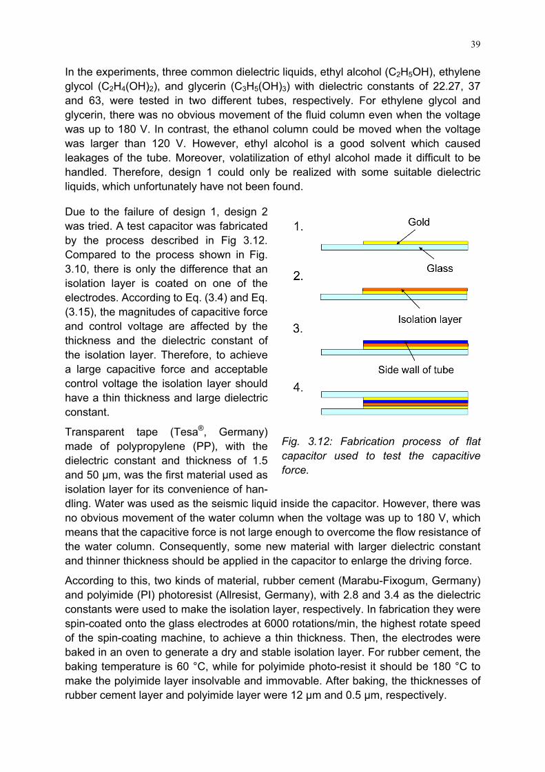
Due to the larger measurable range and simple fabrication process, design 1 was developed prior. For the first try, the driving capability of the capacitive force should be tested. Hence, a flat capacitor with a tube between electrodes was made. The fabric-ation process is demonstrated in Fig. 3.10. First, a layer of gold was sputtered on the surface of a glass slide. Then, two pieces of a thin foil were glued onto the gold layer to be the side walls of the tube. At last, another glass slide with a gold layer was put as a cover onto the thin foils. Two ways to make the sealed tube were investigated: one is gluing two pieces of thin glass between the couple of gold electrodes with molten wax; and the other was placing two hot melt adhesive fibers parallel between the gold electrodes and heating the adhesive fibers to cohere the electrodes. Samples manufactured by both methods are shown in Fig. 3.11. The cross-section dimensions of the two tubes are 5 mm × 0.06 mm (cf. Fig. 3.11 a) and 1 mm × 0.1 mm (cf. Fig. 3.11 b), respectively.

Fig. 3.11: Fabrication process of flat capacitor used to test the capacitive force.


39

In the experiments, three common dielectric liquids, ethyl alcohol (C2H5OH), ethylene glycol (C2H4(OH)2), and glycerin (C3H5(OH)3) with dielectric constants of 22.27, 37 and 63, were tested in two different tubes, respectively. For ethylene glycol and glycerin, there was no obvious movement of the fluid column even when the voltage was up to 180 V. In contrast, the ethanol column could be moved when the voltage was larger than 120 V. However, ethyl alcohol is a good solvent which caused leakages of the tube. Moreover, volatilization of ethyl alcohol made it difficult to be handled. Therefore, design 1 could only be realized with some suitable dielectric liquids, which unfortunately have not been found.

Due to the failure of design 1, design 2 was tried. A test capacitor was fabricated by the process described in Fig 3.12. Compared to the process shown in Fig. 3.10, there is only the difference that an isolation layer is coated on one of the electrodes. According to Eq. (3.4) and Eq. (3.15), the magnitudes of capacitive force and control voltage are affected by the thickness and the dielectric constant of the isolation layer. Therefore, to achieve a large capacitive force and acceptable control voltage the isolation layer should have a thin thickness and large dielectric constant.

Transparent tape (Tesa®, Germany) made of polypropylene (PP), with the dielectric constant and thickness of 1.5 and 50 μm, was the first material used as isolation layer for its convenience of han-dling. Water was used as the seismic liquid inside the capacitor. However, there was no obvious movement of the water column when the voltage was up to 180 V, which means that the capacitive force is not large enough to overcome the flow resistance of the water column. Consequently, some new material with larger dielectric constant and thinner thickness should be applied in the capacitor to enlarge the driving force.

According to this, two kinds of material, rubber cement (Marabu-Fixogum, Germany) and polyimide (PI) photoresist (Allresist, Germany), with 2.8 and 3.4 as the dielectric constants were used to make the isolation layer, respectively. In fabrication they were spin-coated onto the glass electrodes at 6000 rotations/min, the highest rotate speed of the spin-coating machine, to achieve a thin thickness. Then, the electrodes were baked in an oven to generate a dry and stable isolation layer. For rubber cement, the baking temperature is 60 °C, while for polyimide photo-resist it should be 180 °C to make the polyimide layer insolvable and immovable. After baking, the thicknesses of rubber cement layer and polyimide layer were 12 µm and 0.5 µm, respectively.


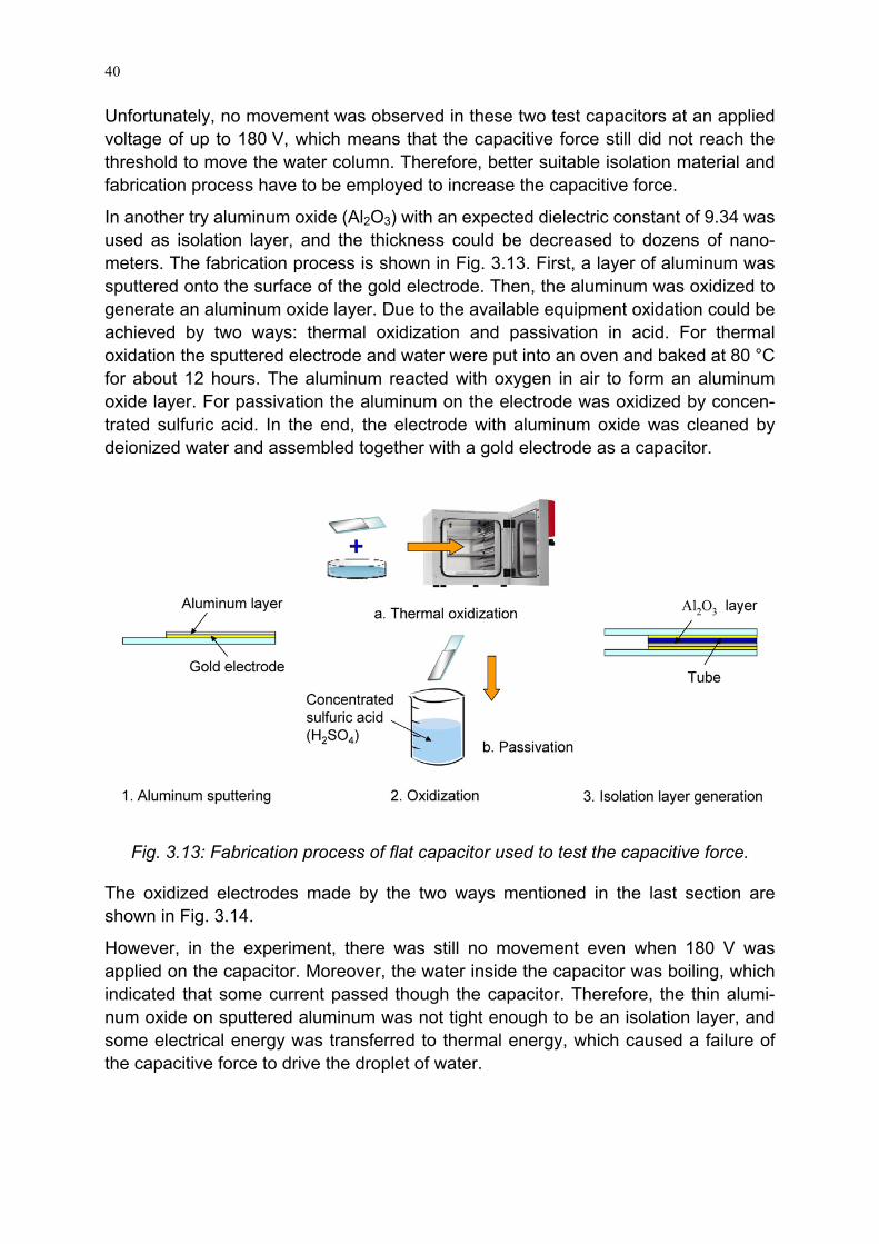
40

Unfortunately, no movement was observed in these two test capacitors at an applied voltage of up to 180 V, which means that the capacitive force still did not reach the threshold to move the water column. Therefore, better suitable isolation material and fabrication process have to be employed to increase the capacitive force.

In another try aluminum oxide (Al2O3) with an expected dielectric constant of 9.34 was used as isolation layer, and the thickness could be decreased to dozens of nano-meters. The fabrication process is shown in Fig. 3.13. First, a layer of aluminum was sputtered onto the surface of the gold electrode. Then, the aluminum was oxidized to generate an aluminum oxide layer. Due to the available equipment oxidation could be achieved by two ways: thermal oxidization and passivation in acid. For thermal oxidation the sputtered electrode and water were put into an oven and baked at 80 °C for about 12 hours. The aluminum reacted with oxygen in air to form an aluminum oxide layer. For passivation the aluminum on the electrode was oxidized by concen-trated sulfuric acid. In the end, the electrode with aluminum oxide was cleaned by deionized water and assembled together with a gold electrode as a capacitor.


The oxidized electrodes made by the two ways mentioned in the last section are shown in Fig. 3.14.

However, in the experiment, there was still no movement even when 180 V was applied on the capacitor. Moreover, the water inside the capacitor was boiling, which indicated that some current passed though the capacitor. Therefore, the thin alumi-num oxide on sputtered aluminum was not tight enough to be an isolation layer, and some electrical energy was transferred to thermal energy, which caused a failure of the capacitive force to drive the droplet of water.

41

Fig. 3.14: Oxidized electrodes made by thermal oxidization (a) and passivation (b).

According to the experiment result, design 2 also could not be realized due to a process problem. The key point of such a design is to make a compact thin isolation layer on the electrode of the capacitor, which can supply a sufficient capacitive force at an acceptable control voltage.

3.5 Conclusions

Theoretically, the principle of a closed loop acceleration sensor driven by capacitive force appears to be feasible. Two different designs (design 1 and design 2) were proposed and discussed. However, due to the available equipment it was not possible to build a working accelerometer of this type. It appears to be promising to investigate these concepts in a laboratory with better equipment.

43

Chapter 4

Closed loop acceleration sensors: thermo-pneumatic drive

4.1 Introduction

Closed loop sensors adopting a feedback loop are capable to enlarge the measuring range (bandwidth) at high sensitivity and keep the seismic mass at its idle position (cf. Chapter 1.4) compared to their open loop counterparts. Closed loop acceleration sensors from silicon driven by capacitive force have already been commercially available [4.1]. However, in the framework of this thesis it was not possible to build a working accelerometer of this type from polymer due to the available equipment. The main problem is that the capacitive forces in the prototypes were not large enough to overcome the flow resistance of the liquid column, i.e. the liquid column could not be held in its idle position when the acceleration was exerted on the sensor. Hence, the thermo-pneumatic force was employed as the balancing force for its larger force generated, although it consumes more power than the capacitive method.

A thermo-pneumatic drive can provide an actuation force on the order of hundreds of milli newtons or even higher [4.2]. Thermo-pneumatic drives are widely used in micro systems such as micro pumps [4.3] and micro valves [4.4]. Normally, the actuation mechanism can be realized by electrical heating of gas or liquid sealed inside of a cavity. When the temperature of the gas or liquid rises, its pressure increases, thus exerting a driving force on objects. This chapter discusses the feasibility of an acceleration sensor using thermo-pneumatic forces to restrict a seismic mass at its idle position.

Fig. 4.1: Closed loop accelerometer driven by the thermo-pneumatic force using a pair of capacitors as position detector. Left: bird view; right: cross section.

4.2 Design and principle

Two types of closed loop accelerometers driven by thermo-pneumatic forces (named

Heater Capacitor

Liquid Heating chamber

Heater Capacitor

Liquid Heating chamber

44

design 1 and design 2) are shown in Fig. 4.1 and Fig. 4.2, respectively.

In design 1 there is a droplet of a dielectric liquid in the center of a tube used as a seismic mass. Two pairs of electrodes are placed at the outside of the walls of the tube as a position detector. At each end of the tube, there is a chamber with a heater inside producing a thermo-pneumatic force on the liquid seismic mass. When there is no acceleration on the sensor, the powers of both heaters are the same, thus there is no pressure difference between the two heating chambers and the liquid column stays still. If the sensor is accelerated by a, there will be a tiny movement of the liquid column caused by the inertial force in the opposite direction, which can be detected by the two capacitors. The capacitive signal controls a power difference between the two heaters, which results in a temperature difference and a pressure difference between the two heating chambers. This pressure difference moves the liquid column back to its idle position. The feedback current signal is a measure of the acceleration.

Fig. 4.2: Closed loop accelerometer driven by a thermo-pneumatic force using a dia-phragm with strain gauges as position detector. Left: bird view; right: cross section.

In design 2 a diaphragm with strain gauges on its upper surface and a seismic mass is fixed in the centre of the sensor by a clamper. There are two chambers with heaters on top and below the membrane which are used to generate an air pressure keeping the membrane in central position. Between the heating chambers and the clamper, two o-rings are added to ensure the sealing of both heating chambers. When an acc-eleration a is acting on the sensor, there is a deflection of the diaphragm which results in an output signal of the strain gauges on the diaphragm. This output signal controls the current through each heater such, that the membrane is brought back to its idle position by the thermo-pneumatic force. The current change of the heater is a measure of the magnitude and direction of the acceleration.


The physical model of both design 1 and design 2 can be simplified as shown in Fig. 4.3. When the sensor is still, the pressures of the two heating chambers F1 and F2 are

HeaterStrain gauge

O-ring

Clamper

Seismic massPI diaphragm

HeaterStrain gauge

O-ring

Clamper

Seismic massPI diaphragm

45

equal. If the sensor is accelerated by a, there is a force FI applied to the seismic mass in the opposite direction if the housing of the sensor is chosen to be the reference:

IF a m= (4.1)

where m is the weight of the seismic mass. In static state the inertial force should be ba-lanced by a pressure difference between the two heating chambers to keep the seismic mass in its idle position:

( )I 1 2 1 2F F F Δp S p p S= − = = − (4.2)

where S is the cross-section area of the tube in design 1 or the area of the diaphragm in design 2.

The interrelationship between pressure p, volume V, temperature T, and the number of moles n of an ideal gas is described by the ideal gas equation (R = 8.314 J / (mol K) is the ideal gas constant):

p V = n R T (4.3)

Thus the pressure difference Δp is:

1 2 a1 a 2n RΔp p p (T T )V

= − = − (4.4)

where Τa1 and Τa2 are the average temperatures of the air in upper and lower heating chambers.

If all power of the heater is transferred to thermal energy of the air inside the heating chambers and there is no energy absorption of the housing, the temperature of the inner side of the heating chamber is equal to room temperature T0. The temperature of the air in the heating chamber can be estimated as the average of the room tem-perature T0 and the temperature of heating coil Th. According to Fourier's law, the temperature of heating coil Th and the air Ta can approximately be described as:

h 0P hT Tλ A

= + (4.5)

h 0a 0

T T 1 P hT T2 2 λ A+

= = + (4.6)

where P, h, λ, and A are the power of heater, height of heating chamber, thermal conductivity of air, and surface area of the heater, respectively.

If the power change of the heater is caused by a controlled current and the resistance change of the heater is ignorable compared to its original value, the temperature

Fig. 4.3: Physical model of closed loop acceleration sensor driven by thermo-pneumatic force.

m

a

F1F2

FI

mm

a

F1F2

FI

46

changes of upper and lower heating chambers, Τa1 and Τa2, can be calculated by Eq. (4.6):

2a1 0 0

1 hT (I ΔI) R'2 λ A

= + + Τ (4.7)

2a 2 0 0

1 hT (I ΔI) R' T2 λ A

= − + (4.8)

where I0, ΔI and R’ are the initial current, the current change of the heater, and the original resistance of the heater, respectively.

Eq. (4.4), Eq. (4.7), and Eq. (4.8) are inserted into Eq. (4.2):

0

λ A m VΔI a4 R n S I R' h

= (4.9)

Fig. 4.4: Feedback current ΔI as a func-tion of the acceleration a at different ini-tial working currents I0.

Fig. 4.5: Left: structure of capacitive posi-tion detector; right: physical model.

According to Eq. (4.9), the feedback current ΔI is a linear function of acceleration a. In our design air with the thermal conductivity of 24.1 mW/(m K) and a coil made of copper wire with diameter and length of 50 μm and 510 mm are employed as thermo-pneumatic medium and heater in the heating chamber, respectively. The original resistance R’ of the heater is 4.4 Ω. The weight of proof mass m, cross-section area S, height h and volume of heating chamber V are 0.05 g, 126.6 mm2, 4 mm, and 506 mm3, respectively. With all these values, the feedback current ΔI as a function of the acceleration at different initial working currents I0 is shown in Fig. 4.4.

For design 1 two capacitors connected to a bridge were used as position detector of the seismic mass. The structure and simplified physical model of the capacitors are demonstrated in Fig. 4.5. According to this figure, two electrodes are installed on both

47

sides of the tube, and the dielectric liquid flows inside the tube as the seismic mass. This structure can be described by an electrical equivalent circuit of a series con-nection of three capacitors: C1, C2 and C3. The total capacitance CT can be calculated as:

1 2T

1 2

1 2 3

C C1C 1 1 1 C 2 CC C C

= =++ +

(4.10)

The capacitance of a flat capacitor can be expressed as:

0 rε ε SCd

= (4.11)

where ε0 and εr are the permittivity of vacuum and relative permittivity of dielectric material, respectively. S and d are the area of the electrodes and the distance between them, respectively.


0 r1 r21 2T

1 2 r2 1 r1 2

ε ε ε SC CCC 2 C 2 ε d ε d

= =+ +

(4.12)

where εr1 and εr2 are the relative permittivity of the side wall and the dielectric liquid, respectively. d1 and d2 are the thickness of the side wall and the width of the tube, respectively.

As shown in Fig. 4.5, the area S of the electrode is equal to the lateral area of the dielectric liquid column inside the capacitor and can be calculated by:

S h x= (4.13)

where h and x are the width of the electrode glued onto the side wall and the length of the dielectric liquid column inside the capacitor, respectively.

Inserting Eq. (4.13) into Eq. (4.12) yields the capacitance CT as a function of the length of the dielectric liquid column inside the capacitor x:

0 r1 r2T

r2 1 r1 2

ε ε ε hC x2 ε d ε d

=+

(4.14)

Two capacitors are connected to a bridge circuit as a position detector. The bridge needs to be supplied with an alternating voltage (AC, e.g. sine function with amplitude U0) and the output is also an AC voltage (with amplitude Um). If a half bridge is employed (cf. Fig. 4.6), the output voltage of the bridge is calculated with:

48

0 r1 r2

m r2 1 r1 2m 0 0 0

0 r1 r2el

r2 1 r1 2

ε ε ε h xC 2 ε d ε d1 1 1 xU U U Uε ε ε h2 C 2 2 xx

2 ε d ε d

ΔΔ + Δ

= = =

+

(4.15)

Fig. 4.6: Two capacitors connected to a half bridge as position detector.

Fig. 4.7: Characteristic curve of the ca-pacitive position detector.

It is assumed that the amplitude of supply voltage U0 and initial length of dielectric liquid column inside the capacitor x are 5 V and 2.5 mm, respectively. The charac-teristic curve of the capacitive position detector described in Eq. (4.15) is shown in Fig. 4.7. Apparently the sensitivity of the position detector increases with decreasing initial length.

The displacement of the liquid column Δx can be estimated as a product of the velo-city of the liquid column v inside a capillary driven by a pressure difference Δp and the time period Δt:

Δx v Δt= (4.16)

The velocity v of the liquid column as a function of the pressure difference Δp is given by the following equation [4.5]:

2

F F2 2

F h F h F

η L η L 2 Δpv 32 32ρ D ρ D ρ

⎛ ⎞= − + −⎜ ⎟

⎝ ⎠ (4.17)

where Dh, η, ρF, and LF are the hydraulic diameter of the capillary, the dynamic viscosity, the density, and the wetting length of the flow. The pressure difference Δp is caused by external acceleration and can be calculated by Eqs. (4.1) and (4.2). The definition of the hydraulic diameter is:

Fh

w

4 ADU

= (4.18)

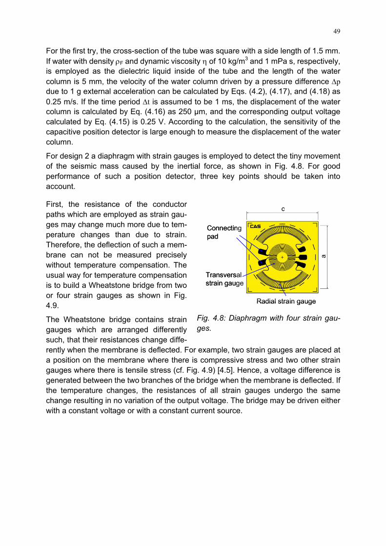
49

For the first try, the cross-section of the tube was square with a side length of 1.5 mm. If water with density ρF and dynamic viscosity η of 10 kg/m3 and 1 mPa s, respectively, is employed as the dielectric liquid inside of the tube and the length of the water column is 5 mm, the velocity of the water column driven by a pressure difference Δp due to 1 g external acceleration can be calculated by Eqs. (4.2), (4.17), and (4.18) as 0.25 m/s. If the time period Δt is assumed to be 1 ms, the displacement of the water column is calculated by Eq. (4.16) as 250 μm, and the corresponding output voltage calculated by Eq. (4.15) is 0.25 V. According to the calculation, the sensitivity of the capacitive position detector is large enough to measure the displacement of the water column.

For design 2 a diaphragm with strain gauges is employed to detect the tiny movement of the seismic mass caused by the inertial force, as shown in Fig. 4.8. For good performance of such a position detector, three key points should be taken into account.

First, the resistance of the conductor paths which are employed as strain gau-ges may change much more due to tem-perature changes than due to strain. Therefore, the deflection of such a mem-brane can not be measured precisely without temperature compensation. The usual way for temperature compensation is to build a Wheatstone bridge from two or four strain gauges as shown in Fig. 4.9.

The Wheatstone bridge contains strain gauges which are arranged differently such, that their resistances change diffe-rently when the membrane is deflected. For example, two strain gauges are placed at a position on the membrane where there is compressive stress and two other strain gauges where there is tensile stress (cf. Fig. 4.9) [4.5]. Hence, a voltage difference is generated between the two branches of the bridge when the membrane is deflected. If the temperature changes, the resistances of all strain gauges undergo the same change resulting in no variation of the output voltage. The bridge may be driven either with a constant voltage or with a constant current source.

Fig. 4.8: Diaphragm with four strain gau-ges.

Connectingpad

Radial strain gauge

Transversal strain gauge

Connectingpad

Radial strain gauge


50

Fig. 4.9: Wheatstone bridge. Left: a half bridge; Right: a full bridge.

The Wheatstone bridge with four strain gauges shown on the right of Fig. 4.9 is called a full bridge, while the one with two strain gauges in the left is a half bridge. The output of the bridge Um is given by [4.5]:

32m 0 0

1 2 3 4

RRU U UR R R R

= −+ +

(4.19)

If the bridge works as a half bridge, the output voltage due to resistance change of R1 and R2 can be calculated as [4.5]:

( ) ( )

2 1 1 2m 1 2 02 2

1 2 1 2 1 2

R ΔR R ΔRU UU R R UR R R R R R

⎛ ⎞−∂ ∂= Δ + Δ = +⎜ ⎟

⎜ ⎟∂ ∂ + +⎝ ⎠ (4.20)

If R1 equals R2 = Rel, the above equation results in:

( )0m 2 1

el

UU ΔR ΔR4 R

= − (4.21)

For a full bridge the output voltage can be expressed as:

( ) ( ) ( ) ( )

m 1 2 3 41 2 3 4

4 3 3 42 1 1 202 2 2 2

1 2 1 2 3 4 3 4

U U U UU R R R RR R R R

R ΔR R ΔRR ΔR R ΔR UR R R R R R R R

∂ ∂ ∂ ∂= Δ + Δ + Δ + Δ

∂ ∂ ∂ ∂

⎛ ⎞−−= + − −⎜ ⎟

⎜ ⎟+ + + +⎝ ⎠

(4.22)

If R1= R2 = R3 = R4 = Rel and resistance change ΔR1 = ΔR3, ΔR2 = ΔR4, Eq. (4.22) can be simplified to:

( ) ( ) ( )0 0m 2 4 1 3 2 1

el el

U UU ΔR ΔR ΔR ΔR ΔR ΔR4 R 2 R

= + − + = −⎡ ⎤⎣ ⎦ (4.23)

51

According to the equations above, on the one hand, the advantage of a half bridge is that small deviations of the resistances which occur during fabrication can be adapted with the potentiometer easily and that more area is available to achieve a sufficiently large resistance with a metal conductor path [4.5]. On the other hand, the output of a full bridge is two times larger than that of a half bridge and modern fabrication technologies allow balancing the bridge during the fabrication process [4.5].

Secondly, a strain gauge should have a sufficiently large resistance. The Wheatstone bridge must be driven with a comparatively large voltage (several volts) providing a suitable output (some milli volts). This would cause a huge electrical current through the strain gauge if its resistance is not large enough, and large current results in warming up the membrane and changing its deflection. Furthermore, the heating may also be asymmetrically over the membrane and cause a change of the output voltage. Therefore, the current needs to be limited.

Thirdly, the strain gauges need to be placed at suitable positions and orientations on the membrane which show the largest resistance changes for strain gauges to maxi-mize the output voltage of a Wheatstone bridge.

In the sensor the deflection of the circular membrane caused by inertial force is ba-lanced by the thermo-pneumatic force. If the response time of the thermo-pneumatic force is short enough, the deflection is restricted to the near of its idle position and is smaller than its thickness. Therefore, the diaphragm can be regarded as a thick membrane. It is assumed that the strain gauges are so thin and weak that they do not hinder the deflection of the membrane and that their lateral strain is the same as the strain of the membrane without a strain gauge at that position.

Based on these assumptions, ΔRel, R and ΔRel, T, the resistance changes of radial and transversal strain gauges on the surface of a thick circular membrane, can be ex-pressed as follows [4.5]:

( ) ( )( )2 2 2el,R el,R M M2

M M

3 ΔpΔR R 1 ν R ν 1 2 ν r4 E d

= − − + (4.24)

( ) ( )( )2 2 2el,T el,T M M2

M M

3 ΔpΔR R 1 ν R ν 1 2 ν r4 E d

= − + − (4.25)

where Rel,R and Rel,T are the electrical resistances of radial and tangential strain gauges, respectively. RM, dM, νM, and EM are the radius, thickness, Poisson’s ratio, and Young’s modulus of the membrane, respectively. ν is Poisson’s ratio of the conductor paths, and Δp is the pressure difference over the membrane.

The resistance changes of radial and transversal strain gauges are also a function of membrane deflection w0 generated by pressure drop. Therefore, it appears to be expedient to write Eqs. (4.24) and (4.25) as a function of deflection. The relationship between pressure difference Δp and membrane deflection w0 can be expressed as [4.5]:

52

22

M 0 0M M M02 2 2 2 2

M M M M M

4 d w wd E E4 64Δp σR 3 R 1 ν 105 R 1 ν

⎛ ⎞= + +⎜ ⎟− −⎝ ⎠

(4.26)

The first, second, and third term in the parenthesis of Eq. (4.26) describe the effects of bending moments, residual stress, and stress due to straining, respectively. For a circular thick membrane without residual stress, the second and third term in Eq. (4.26) can be ignored. Inserting the first term of Eq. (4.26) into Eqs. (4.24) and (4.25) yields:

( )( )2 2M 0el,R el,R M4

M

d wΔR 4 R R ν 1 2 ν rR

= − + (4.27)

( )( )2 2M 0el,T el,T M4

M

d wΔR 4 R R ν 1 2 ν rR

= + − (4.28)

According to Eqs. (4.27) and (4.28), the resistance change of strain gauges are a linear function of membrane deflection and no function of Young’s modulus and Poisson’s ratio of the membrane material.

The pressure drop Δp caused by the inertial force can approximately be calculated as:

IF a mΔpS S

= = (4.29)

where m and S are the weight of the seismic mass and the area of the diaphragm, respectively.

A polyimide diaphragm with steel strain gauges (N2A-06-S046R-350, Vishay cf. Fig. 4.8) with a Young’s modulus EM and Poisson’s ratio νM of 2.5 GPa (at 23 °C) and 0.34 was applied in design 2. The radius RM and the thickness dM of the diaphragm were 6.35 mm and 25 μm, respectively. The Poisson’s ratio of steel is 0.3. The seismic mass was made of lead and installed in the center of the diaphragm, and due to the limited area in the center of the membrane, the maximum seismic mass is about 50 mg. If 10 m/s² acceleration exerts on the sensor, the pressure drop Δp is about 4 Pa. Taking all these values into Eqs. (4.24) and (4.25), the relative resistance changes of radial and tangential conductor paths are shown in Fig. 4.10. According to this figure, the resistance of tangential strain gauges is rising everywhere on the membrane when it is bulged by the pressure difference. This effect increases by approximately a factor of 2.3 from the center to the rim of the membrane. Radial strain gauges gain an increase of their resistance at the

Fig. 4.10: Relative resistance change of strain gauges on a polyimide membrane.

53

center and a decrease at the rim of the membrane. The largest resistance change is the drop of a radial strain gauge at the rim.

Strain gauges need to be arranged on the membrane such that their resistance changes differ as much as possible achieving the largest possible output voltage of the Wheatstone bridge. From Fig. 4.10 it seems to be attractive to place both radial and tangential strain gauges near the rim of the membrane, since their difference of resistance changes is most there.

However, as mentioned above, the resistance of strain gauges should be sufficiently large to restrict the power consumption and heating of the membrane. Therefore, the strain gauges must be comparatively long and occupy a considerably large area of a small membrane, and there may be not enough space for both radial and tangential conductor paths at the rim. Due to this, a usual alternative way is to design radial strain gauges at the rim and tangential ones next to them toward the membrane center [4.5].

In this case, there are four strain gauges on the circular diaphragm. Two radial strain gauges are arranged near the rim of the membrane, and the other two tangential ones are placed in the center of the membrane. This way, the Wheatstone bridge made of the strain gauges works as a full bridge, and its output voltage due to pressure drop can be obtained by inserting Eqs. (4.24) and (4.25) into Eq. (4.23):

( ) ( ) ( )( )2 2 20m M t r2

M M

U Δp3U 1 ν 1 2ν r 1 2ν r8 E d

= − − + + (4.30)

where rt and rr are the effective distance of tangential and radial strain gauges, re-spectively, from the center of the membrane.

The output voltage of the full bridge can also be calculated as a function of membrane deflection w0 by inserting Eqs. (4.27) and (4.28) into Eq. (4.23):

( ) ( )( )2 20 M 0m t r4

M

2 U d wU 1 2ν r 1 2ν rR

= − + + (4.31)

Eq. (4.31) shows that the output voltage is a linear function of membrane defection and no function of Young’s modulus, Poisson’s ratio, and residual stress. Each com-bination of pressure and membrane properties yielding a certain deflection will result in the same output voltage.

Normally the diaphragm with strain gauges in design 2 should work like a thick membrane, which means that the deflection of the diaphragm is smaller than its thickness. If there is a long time delay of the feedback balancing force, the inertial force due to external acceleration can not be balanced immediately, which may deflect the diaphragm exceeding its thickness, and then the diaphragm need to be considered as a thin membrane.

For a thin membrane, the resistance changes of radial and transversal strain gauges on the surface should be expressed as follows [4.5]:

54

( )2 2

0el,R el,R 2 2

M M

w2 rΔR R 2 ν 1 ν3 R R

⎛ ⎞= + −⎜ ⎟

⎝ ⎠ (4.32)

( )2 2

0el,T el,T 2 2

M M

w2 rΔR R 2 ν 1 ν3 R R

⎛ ⎞= − +⎜ ⎟

⎝ ⎠ (4.33)

For the diaphragm discussed in Fig. 4.10, if the deflection w0 is assumed to be 50 μm larger than its thickness, the relative resistance changes of radial and tangen-tial strain gauges are shown in Fig 4.11. Comparing Fig. 4.10 and Fig. 4.11, it is obvious that the resistance of a radial strain gauge at the rim of a thick mem-brane becomes smaller with increasing deflection but it becomes larger when the deflection is larger than membrane thick-ness. For a transversal strain gauge the situation is similar but with the opposite trend as a function of increasing deflec-tion. Therefore, there is a certain range of deflections around the thickness of the membrane where the characteristic curve of the output signal of strain gauges is ambiguous.

Inserting Eqs. (4.32) and (4.33) into Eq. (4.23) yields the output voltage of strain gauges on a thin membrane (full bridge) as a function of membrane deflection:

( ) ( )( )2

2 20 0m t r4

M

U w1U 1 ν r 1 ν r3 R

= − + + − (4.34)

Eq. (4.34) is derived from the straining of the neutral fiber of a membrane and does not take its bending into account [4.5]. If a membrane is thin, straining at its surface is mainly due to straining of its neutral fiber and not due to bending which results from a difference in the strain on its upper and lower side. Eq. (4.34) is also an approximation of the bridge output obtained for a thick membrane when the strain gauges are not placed at the surface of the membrane but at its neutral fiber. This is only an approxi-mation because Eq. (4.34) assumes a parabola for the deflection form of the mem-brane and the real deflection form is the square of a parabola [4.5].

Eq. (4.31) is based only on the bending of the membrane and not on the straining of its neutral fiber [4.5]. When a membrane is thick (deflected less than its thickness) Eq. (4.31) is a good approximation, because straining of the neutral fiber is small when the deflection is less than membrane thickness. In general, straining at the surface of

Fig. 4.11: Relative resistance change of radial and tangential strain gauges on a thin polyimide membrane.

2

-2

-4

6

62 4

Radial conductor path

Tangential conductor path

r [mm]

el

el

ΔRR

[10-5]

0

4

2

-2

-4

6

62 4

Radial conductor path

Tangential conductor path

r [mm]

el

el

ΔRR

[10-5]

0

4

55

a membrane is due to both straining of its neutral fiber and bending. As a conse-quence, the real output of the bridge is the sum of Eq. (4.31) and Eq. (4.34):

( ) ( )( ) ( ) ( )( )2 2 2 20 0 0m M t r t r4

M

U w wU 2 d 1 2 ν r 1 2 ν r 1 ν r 1 ν rR 3

⎡ ⎤= − + + − − + +⎢ ⎥⎣ ⎦ (4.35)

In Fig. 4.12 there are shown the bridge output voltages calculated with Eqs. (4.31), (4.34), and (4.35). The radius of membrane RM, the supply voltage of the bridge, and Poisson’ ratio of the steel strain gauge are 5 V, 6.35 mm, and 0.3, respectively. The effective distance of tangential and radial strain gauges from the center of the membrane, rt and rr, are assumed to be 1.45 mm and 5.1 mm, respectively.

According to this figure, the bridge output voltage due to bending (orange curve) changes linearly with membrane deflection, while the bridge output voltage due to the straining of the neutral fiber as a function of membrane deflection is a parabola (green curve). Thus, the real output of the bridge is the sum of the two curves, and is shown as the blue curve. It is obvious that there is a turning of the real output of the bridge when the membrane is bulged up larger than its thickness (25 μm).

Fig. 4.12: The bridge output voltages cal-culated with Eqs. (4.31), (4.34), and (4.35) as a function of membrane deflection.

Fig. 4.13: The bridge output voltages cal-culated with Eqs. (4.26), (4.31), (4.34), and (4.35) as a function of pressure drop.

The relationship between pressure difference Δp and membrane deflection w0 can be described by Eq. (4.26). If there is no residual stress in the membrane (σ0 = 0), the bridge output voltages as a function of pressure drop over the membrane calculated with Eqs. (4.26), (4.31), (4.34), and (4.35) is shown in Fig. 4.13. The turning of the real bridge output voltage happens at the pressure drop of about 16 Pa.

Actually, the residual stress in the membrane is hard to be avoided in practical applications. Thus, in our analysis the effect due to residual stress needs to be taken into account. The influence of residual stress can be characterized by the critical stress σk of the membrane occurring where the slope of the function at the origin is

56

zero. Therefore the critical stress at which the transition takes place can be calculated from the zero of the derivative of Eq. 4.26 [4.5]:

0

2 2M M M M M

0 k2 2 2 2 20 M M M M Mw 0

4 d d E d Ep 4 40 σw R 3 R 1 ν 3 R 1 ν

σ=

⎛ ⎞∂Δ= = + ⇒ = −⎜ ⎟∂ − −⎝ ⎠

(4.36)

For the membrane studied in Fig. 4.12, the critical stress σk is about 58 kPa and the interrelationship between the pressure drop over a circular membrane and its center deflection for different residual stresses can be demonstrated in Fig. 4.14.

Fig. 4.14: Pressure drop over a circular membrane as a function of its center de-flection for different residual stresses.

Fig. 4.15: Real output voltage of the bri-dge as a function of pressure drop for different residual stresses.

When the residual stress is larger (more tensile) than the critical stress, the membrane is flat and does not deflect without a pressure drop. A membrane with smaller (more compressive) becomes bistable. According to the blue curve in Fig 4.14, when the residual stress σ0 equals to -1.9 MPa, in a certain pressure range there are two stable states for the membrane: it may buckle up (positive deflection) or buckle down (negative deflection). When there is no pressure drop over the membrane and it is buckling down, it will deflect downward approximately 210 μm. If the pressure is then rised, the downward deflection becomes increasingly smaller until at app-roximately -120 μm the membrane snaps over to the opposite side, following the dashed arrow and arriving at an upward deflection of approximately 240 μm. Reversely, from bulking up state the pressure can be decreased to about -380 Pa before the membrane snaps back to a downward deflection. The curve between the two points where the membrane is snapping over cannot be reached by adjusting the pressure difference over the membrane to a certain value. Therefore, the bistability of a membrane results in a snapping over of the real output voltage of the bridge. The real output voltage of the bridge as a function of pressure drop for different residual stress, which is described by Eqs. (4.26) and (4.35), and shown in Fig. 4.15.

57

4.4 Fabrication and experiments

A prototype of design 1 (prototype 1) was made as shown in Fig. 4.16. The housing including two chambers and a tube was made of a PMMA plate by a milling machine, and the heater was fabricated by sputtering and photolithography (cf. Chapter 2.2.3). The tube has the length, width and height of 15 mm, 1.5 mm, and 1.5 mm, respec-tively. The volume of the heating chamber is approximately 42 mm3. Copper tapes are glued onto both sides of the tube as electrodes. Water was injected into the tube as the seismic mass by a syringe.

In tests the capacitive position detector did not work as expected, because the water inside of the tube divided into small droplets and did not keep together as a column, especially when the sensor was subject to a large acceleration. This problem is due to the comparatively large dimensions of the tube and the hydrophilic PMMA surface. There-fore, two improvements were made to pro-totype 1.

First, the width of the tube was reduced from 1.5 mm to 0.5 mm to increase the capillary effect, which makes the water join together. Following the decrease of the tube width, the displacement of the water column in 1 ms due to 1 g external acceleration declines from 250 μm to 74 μm as calculated by Eqs. (4.16), (4.17) and (4.18), and the co-rresponding output voltage of the bridge decreases from 0.25 V to 74 mV. Although the output signal decreases by approximately a factor 3, it is still large enough for measuring and controlling the feedback force. Secondly, a special coating was smeared onto the inner surface of the tube, such that the droplet was repelled by capillary forces and did not permeate into small cavities due to surface roughness of the tube walls. This way, the contact surface between water and PMMA was changed to be hydrophobic, and the friction in the tube was minimized and the liquid could easily be moved by external acceleration.

Fig. 4.16: Prototype 1 with sputtered heaters and wide tube.

0.5 mm

1.5 mm

Sputtered heater Copper tape

PMMA housingConnecting wire

0.5 mm

1.5 mm

Sputtered heater Copper tape

PMMA housingConnecting wire

58

Fig. 4.17: Water droplets on different coatings.

An experiment was made to choose a suitable coating material. Five hydrophobic materials, such as silicon oil, multi oil, car wax, candle wax and teflon, were sprayed or brushed separately on a polymer substrate. A droplet of water was placed on the surface of each coating as shown in Fig. 4.17. From the figure it is clear that silicon oil, wax and telfon coating have obvious hydrophobic effects compared to the naked polymer surface. The polymer plate was tilted in the gravitational field to let the water droplets flow down on the surfaces. In several repeated experiments it could be concluded that candle wax has the minimum friction due to the largest falling velocity of the droplet. Therefore, melted candle wax was brushed on the inner side of the tube as hydrophobic layer.

With these improvements, an optimized prototype of design 1 (prototype 2) was made as shown in Fig. 4.18. In prototype 2, silver conduct paint was smeared on the outer surface of the tube as electrodes to eliminate the thickness of adhesive on metal electrodes, and copper coil heaters were employed instead of sputtered heaters due to their larger power, which may shorten the response time.

Fig. 4.18: Prototype 2 of design 1 with copper coil heaters and narrow tube. Left: details of the heating chambers and the tube; right: front view of prototype 2.

b. Silicon oila. Without

d. Car wax e. Candle wax f. Sprayed Teflon g. Brushed Teflon

c. Multi-oilb. Silicon oila. Without

d. Car wax e. Candle wax f. Sprayed Teflon g. Brushed Teflon

c. Multi-oil

Heater Tube

Electrode

CoverHeater Tube

Electrode

Cover

59

Due to the small cross-section and hydrophobic inner surface of the tube the water inside the tube joined together as a column. Unfortunately, there was no useful output signal from the capacitive position detector, which means the displacement of the water column was too small to be measured. Besides the inertia moment of the water column and the friction of the side walls considered in Eq. (4.17), there was still an adhesive force between the water column and the surface, which increases the flow resistance of the tube. Therefore, the inertial force could not overcome the flow resis-tance and move the water column.

Since prototype 2 did not work, for prototype 3 a circular diaphragm with strain gauges (N2A-06-S046R-350, Vishay, cf. Fig. 4.8) was fixed in the centre of the sensor by a clamper (cf. Fig. 4.19). Two heating chambers (cf. Fig. 4.20) with the radius and height of 6.35 mm and 4 mm, respectively, were made of a PMMA plate by milling and fixed above and below the membrane. Inside each chamber seven serial connected coils made of copper wire (50 μm in diameter) with a resistance of 4.4 Ω were install-ed to generate a thermo-pneumatic force keeping the membrane in its idle position. Between heating chambers and the clamper, two o-rings were added to ensure seal-ing of the whole sensor. All these components were assembled as shown in Fig. 4.21.

Fig. 4.19: Diaphragm with four strain gau-ges installed to a clamper.

Fig. 4.20: Heating chamber with seven serial connected coils.

Fig. 4.21: Assembling photo of prototype 3.

PI membrane

Strain gauge

PI membrane

Strain gauge

PMMA housing

Copper coil heater

PMMA housing

Copper coil heater

60

Prototype 3 was characterized by tilting in gravitation. Unfortunately, prototype 3 did not work as expected. There were two major problems resulting in the failure of the sensor. Firstly, a time delay of the feedback thermo-pneumatic force was found in the experiments. Therefore, it is hard to apply precise feedback currents to the upper and below heaters manually. Secondly, there was compressive residential stress in the diaphragm caused by installing, which was hard to be avoided. The diaphragm be-came bistable. Thus, the output voltage of the bridge did not change with acceleration monotonously, and could not properly measure the displacement of the seismic mass. These two problems will be analyzed in details in the following paragraphs.

For a practical force balanced sensor, the feedback current should drive a thermo-pneumatic balancing force as fast as possible. If a current goes through the heater, the coil and the air around it need to be heated up first before there is any thermo-pneumatic reaction. Therefore, there is a time delay between external acceleration and feedback balancing force, which can be described as follows:

a a h h dc ΔT c ΔT ΔP t+ = (4.37)

where ca and ch are the heat capacity of the heater and the air, respectively. ΔTa and ΔTh are the temperature change of the heating coil and the air, respectively. ΔP is the power change of the heater, and td is defined as the time delay.

Inserting Eqs. (4.5), (4.6) and (4.7) into Eq. (4.37) yields:

a h

d

1 c c h2t

λ A

⎛ ⎞+⎜ ⎟⎝ ⎠= (4.38)

In prototype 3, the heat capacity of heater and air are 3.46×10-3 J/K and 6.63×10-4 J/K, respectively. The thermal conductivity of the air λ is equal to 24.1 mW/(m K) and the surface area A of the heater is 10-9 m2. With these values the time delay td can be calculated by Eq. (4.38) as 7.9 s. Although Eq. (4.38) is only a rough estimation, it reveals an un-negligible time delay of the balancing force in prototype 3. According to this equation, td can be reduced by decreasing the height of heating chamber or employing a heater with larger contact area and smaller heat capacity.

The output of the bridge on the membrane of prototype 3 was measured as a function of the pressure difference. As shown in Fig. 4.22, an empty chamber connected with a syringe and a pressure sensor was employed instead of the chamber with the heater. The output signals from strain gauges and pressure sensor were measured by an oscilloscope and shown in Fig. 4.23.

61

Fig. 4.22: Method of experiment for testing the output of strain gauges on a diaphragm as a function of pressure difference.

Firstly, the piston of the syringe was pressed to increase the air pressure of the chamber from 100 kPa to about 130 kPa (from A to B in Fig. 4.23), and then the piston was pulled back reducing the pressure from 130 kPa to 70 kPa (from B to E in Fig. 4.23). At last, the piston was moved back to its original position (from E to F in Fig. 4.23). According to Fig. 4.23 the output of the pressure sensor (blue) is a sine curve, and the output of the strain gauges (pink) shows no regularity and symmetry.

Fig. 4.23: The output signals from the pressure sensor (blue) and strain gauges (pink) changing with time.

For better understanding the bridge output of Fig. 4.23 was redrawn as a function of the pressure difference over the membrane shown in Fig. 4.24.

Pressuresensor

Heater

Strain gauge

Syringe

Oscilloscope

Pressuresensor

Heater

Strain gauge

Syringe

Oscilloscope

0 5 10 2015 25 3530 40

0.1

0.2

0.3

-0.1

-0.2

-0.3

0 0

Time [s]

Out

put o

f stra

in g

auge

s [m

V]

-10

-20

-30

10

20

30

Pres

sure

diff

eren

ce [k

Pa]

A

B

E

CD F

0 5 10 2015 25 3530 40

0.1

0.2

0.3

-0.1

-0.2

-0.3

0 0

Time [s]

Out

put o

f stra

in g

auge

s [m

V]

-10

-20

-30

10

20

30

Pres

sure

diff

eren

ce [k

Pa]

A

B

E

CD F

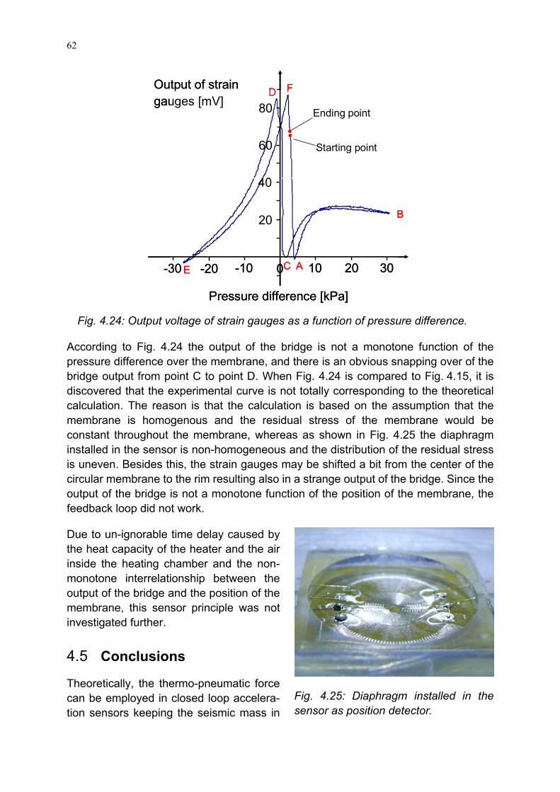
62

Fig. 4.24: Output voltage of strain gauges as a function of pressure difference.

According to Fig. 4.24 the output of the bridge is not a monotone function of the pressure difference over the membrane, and there is an obvious snapping over of the bridge output from point C to point D. When Fig. 4.24 is compared to Fig. 4.15, it is discovered that the experimental curve is not totally corresponding to the theoretical calculation. The reason is that the calculation is based on the assumption that the membrane is homogenous and the residual stress of the membrane would be constant throughout the membrane, whereas as shown in Fig. 4.25 the diaphragm installed in the sensor is non-homogeneous and the distribution of the residual stress is uneven. Besides this, the strain gauges may be shifted a bit from the center of the circular membrane to the rim resulting also in a strange output of the bridge. Since the output of the bridge is not a monotone function of the position of the membrane, the feedback loop did not work.

Due to un-ignorable time delay caused by the heat capacity of the heater and the air inside the heating chamber and the non-monotone interrelationship between the output of the bridge and the position of the membrane, this sensor principle was not investigated further.

4.5 Conclusions

Theoretically, the thermo-pneumatic force can be employed in closed loop accelera-tion sensors keeping the seismic mass in

Fig. 4.25: Diaphragm installed in the sensor as position detector.

-10-20 3020100-30

20

40

60

80

Output of strain gauges [mV]

Pressure difference [kPa]

Starting point

Ending point

A

B

C

D

E

F

-10-20 3020100-30

20

40

60

80

Output of strain gauges [mV]

Pressure difference [kPa]

Starting point

Ending point

A

B

C

D

E

F

63

its idle position. Two different designs (design 1 and design 2) were proposed and discussed, and three different prototypes were fabricated and tested. In the test the thermo-pneumatic force was large enough to move the seismic mass. However, no prototype could realize accurate and stable measurements of acceleration. For design 1, there is no useful control signal gained from the capacitive position detector due to its low sensitivity. For design 2 the delay of the balancing force was calculated to be too large for a suitable feedback, and the output of the bridge is not a monotone function of the position of the membrane. These two problems could not be solved temporarily with the available equipment. If the sensitivity of the capacitive position detector could be improved in design 1, or the response time of the balancing force could be shortened in design 2, there is still the chance that this type of acceleration sensor could work.

65

Chapter 5

Closed loop acceleration sensors: magnetic force drive

Principle and argumentation

5.1 Introduction

A closed loop acceleration sensor driven by capacitive force and thermal-pneumatic force have been discussed in chapter 3 and chapter 4, respectively. Both of them seem to be feasible theoretically, but due to the available equipment it was not possible to build working accelerometers of these types. For the capacitive method, the main problem is that the capacitive force was not large enough to overcome the flow resistance of the water column such that it could not keep the liquid column at its idle position when the sensor was exerted to acceleration. For the thermo-pneumatic method the long time delay of the thermal balancing force and the non-monotone interrelationship between the bridge output and the displacement of the seismic mass prevented building a working sensor.

Some closed loop accelerometers employ electromagnetic force as balancing force [5.1-5.3]. If a current-carrying wire is placed within a magnetic field, an electro-magnetic force (Lorentz force) will occur in a direction perpendicular to the current and magnetic field. Electromagnetic force can be controlled precisely, because its magni-tude is proportional to the current, the wire’s length, and the magnetic field. Moreover, there is nearly no time delay of the electromagnetic force when the current is applied to the wire. With these benefits the electromagnetic force appears to be a good choice for a closed loop acceleration sensor. Novel closed loop acceleration sensors driven by electromagnetic force with strain gauges as position detector are discussed and presented in this chapter.

5.2 Design

The feasibility of three designs was investigated. Design 1 (cf. Fig. 5.1) can be consi-dered a direct modification of prototype 3 with thermo-pneumatic balancing force (cf. Chapter 4.4). The only difference is that an electromagnetic coil is employed below the diaphragm as a force actuator instead of the heaters. A diaphragm with strain gauges was employed in the middle of the sensor to measure the position change of the seismic mass. An annular permanent magnet was glued onto a piston. One side of the piston was fixed to the center of the diaphragm, and the other free end was put inside the electromagnetic coil. An upper chamber with a through hole was mounted on the diaphragm for sealing and pressure balancing. When the sensor is accelerated

66

by a, there is an output signal of the strain gauges due to the deflection of the dia-phragm, which controls the current through the electromagnetic coil such, that a magnetic force is applied onto the piston moving the membrane back to its idle position. The feedback current through the coil is a measure of the acceleration.

Fig. 5.1: Schematic drawing of design 1 with a strain gauge diaphragm and a copper coil.

Fig. 5.2: Schematic drawing of design 2 with cantilever beam and sputtered coil.

As shown in Fig. 5.2, design 2 employs a cantilever beam as sensing element. Two strain gauges are glued on the upper and lower side of the beam near its fixing point, and a sputtered coil is installed on the free end of the beam. Two permanent magnets are fixed to the housing providing a mag-netic field. When the sensor is accelerated, the tiny bending of the beam caused by inertial force is detected by the strain gau-ges. The output signal of the strain gauges controls a feedback current through the electromagnetic coil pulling the beam back to its initial position.

Design 3 adopts double cantilever beams to support a seismic mass with an electro-magnetic coil. This way, the tiny displace-ment of the seismic mass caused by the inertial force is perpendicular to the mag-netic field. Moreover, two pairs of perman-ent magnets are placed attractively on the upper and lower side of the coil.


In design 1, a diaphragm with strain gauges is used as a position detector. The mechanical and electrical characters of a diaphragm have been introduced in chapter

Fig. 5.3: Schematic drawing of design 3 with double cantilever beams and sput-tered coil.

Permanentmagnet

Electromagnetic coil

Strain gaugeDiaphragm

Piston

Permanentmagnet


Strain gaugeDiaphragm

Piston

Permanent magnet


Cantilever beam

Strain gauge

N

N

Permanent magnet


Cantilever beam

Strain gauge

N

N

NS

S

N

Strain gauge

Cantilever beam Electromagneticcoil

Permanent magnet

NSNSNS

S

N

S

N

Strain gauge

Cantilever beam Electromagneticcoil

Permanent magnet

67

4.3.

In design 2 and design 3, cantilever beams with strain gauges are employed as sens-ing elements. Compared with the diaphragm structure a cantilever beam has two advantages. On the one hand, residual stress in a diaphragm is hard to control and it is affected by temperature and the assembling process. If a beam is fixed at one end only, there is no residual stress affecting the behavior of such a beam. On the other hand, as discussed in chapter 4.3, the overload on the diaphragm may result in an error output of strain gauges. For the beam structure two strain gauges on top and below of the beam were connected together with a potentiometer such, that they became a Wheatstone bridge detecting the bending. This way, the monotone output of the Wheatstone bridge changing with deflection can be realized more easily com-pared to the membrane structure.

If the sensor is accelerated, there is a transversal deflection of the cantilever beam due to the inertial force which is schematically shown in Fig. 5.4. The deflection x of a beam with length LB, width bB, thickness dB, and Young’s modulus EB as a function of the force acting at its free end is given by the following equation [5.4]:

2

BB

Fx y (3 L y)6 E I

= − (5.1)

where y is the coordinate in the direction of the non-deflected beam describing the distance from a deflecting point on the cantilever beam to the anchor; w is the deflection of the beam at the position y from its undeflected position; LB is the distance from the support of the cantilever to the point at which the load is applied; F is the force exerted by the load; EB is Young’s modulus of the beam; I is the area moment of inertia of the beam.

Fig. 5.4: Beam geometry of the acceleration sensor and its side view.

For a rectangular beam as shown in Fig. 5.4 the area moment of inertia I can be calculated by [5.4]:

3

B B1I b d

12= (5.2)

where bB and dB are the width and thickness of the beam, respectively. The corres-

Permanent magnetCantilever beam

Strain gauge y

LB

Fx

Rectangular

dB

bB

Permanent magnetCantilever beam

Strain gauge y

LB

Fx

Rectangular

dB

bB

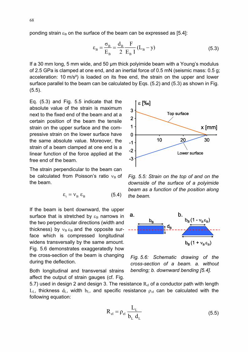
68

ponding strain εΒ on the surface of the beam can be expressed as [5.4]:

B BB B

B B

σ d Fε (L y)E 2 E I

= = − (5.3)

If a 30 mm long, 5 mm wide, and 50 μm thick polyimide beam with a Young’s modulus of 2.5 GPa is clamped at one end, and an inertial force of 0.5 mN (seismic mass: 0.5 g; acceleration: 10 m/s²) is loaded on its free end, the strain on the upper and lower surface parallel to the beam can be calculated by Eqs. (5.2) and (5.3) as shown in Fig. (5.5).

Eq. (5.3) and Fig. 5.5 indicate that the absolute value of the strain is maximum next to the fixed end of the beam and at a certain position of the beam the tensile strain on the upper surface and the com-pressive strain on the lower surface have the same absolute value. Moreover, the strain of a beam clamped at one end is a linear function of the force applied at the free end of the beam.

The strain perpendicular to the beam can be calculated from Poisson’s ratio νB of the beam.

t B Bε ν ε= (5.4)

If the beam is bent downward, the upper surface that is stretched by εB narrows in the two perpendicular directions (width and thickness) by νB εB and the opposite sur-face which is compressed longitudinal widens transversally by the same amount. Fig. 5.6 demonstrates exaggeratedly how the cross-section of the beam is changing during the deflection.

Both longitudinal and transversal strains affect the output of strain gauges (cf. Fig. 5.7) used in design 2 and design 3. The resistance Rel of a conductor path with length LL, thickness dL, width bL, and specific resistance ρel can be calculated with the following equation:

L

el elL L

LR ρb d

= (5.5)

Fig. 5.5: Strain on the top of and on the downside of the surface of a polyimide beam as a function of the position along the beam.

Fig. 5.6: Schematic drawing of the cross-section of a beam. a. without bending; b. downward bending [5.4].

0-1

-2

-3

1

23

10 20 30

ε [‰]

x [mm]

Top surface

Lower surface

0-1

-2

-3

1

23

10 20 30

ε [‰]

x [mm]

Top surface

Lower surface

a. b.bB

dB

bB (1 + νΒ εΒ)

bB (1 - νΒ εΒ)a. b.

bBdB

bB (1 + νΒ εΒ)

bB (1 - νΒ εΒ)

69

For a metal conductor path, the change of the specific resistance ρel with respect to the strain is comparatively small and usually neglected in calculations, and the geomet-rical change and temperature effect are the dominant factors influencing the resistance of the metal paths. The specific resistance is nearly a linear function of temperature which is described by the temperature coefficient αΤ. If this conductor path is strained in the direction of its length by ΔLL = LL εL, width by ΔbL = bL εb, and thickness ΔdL = dL εd, respectively, the resistance change ΔRel is according to the changes in geometry and temperature [5.4]:

( )

el el el elel L L L

L L L

el L b d el T

R R R RΔR ΔL Δb Δd ΔTL b d T

R ε ε ε R α ΔT

∂ ∂ ∂ ∂= + + +

∂ ∂ ∂ ∂

= − − + (5.6)

According to Eq. (5.6) the resistance of a conductor path may change much more due to temperature changes than due to strain. Therefore, in design 2 and design 3 two strain gauges are used and connected to a Wheatstone bridge for temperature compensation such that only resistance change with respect to geometry need to be taken into account.

The resistance change ΔRel of a strain gauge with Poisson’s ratio ν on a substrate with longitudinal εl and transversal strain εt is composed of terms which describe the effect of the strain gauge to become longer and wider by straining and by getting thinner perpendicular to each of these strain directions [5.4]:

( ) ( ) ( )el el l l t t el l tΔR R ε ν ε ε ν ε R ε 1 ν ε 1 ν= + − + = + − −⎡ ⎤⎣ ⎦ (5.7)

It is assumed that the strain gauges are so thin that they do not hinder the bending and straining of the beam. This assumption is not correct in most cases, but it eases the calculation a lot and the mechanical effect of the strain gauges just diminishes the resistance change measured in reality and does not cause principally different results. Therefore, the resistance change of metal strain gauges longitudinal ΔRel,l and trans-versal ΔRel,t to the beam can be calculated with Eq. (5.7) [5.4].

( )el,lB B B

el,l

ΔRε 1 ν ν 1 ν

R⎡ ⎤= + + −⎣ ⎦ (5.8)

Fig. 5.7: Strain gauge used in design 2 and design 3.

70

( )el,tB B B

el,t

ΔRε 1 ν ν 1 ν

R⎡ ⎤= + − −⎣ ⎦ (5.9)

Fig. 5.8 shows the resistance changes of longitudinal and transversal strain gauges on the upper surface of a beam discussed in Fig. 5.5, which are calculated by Eq. (5.8) and (5.9), respectively. It is obvious that the resistance change of a strain gauge longitudinal to the beam is a bit larger than that of a transversal one. Ac-cordingly, there are two methods to ar-range the stain gauges (cf. Fig. 5.9): (1) two longitudinal strain gauges are fixed on upper and lower surfaces of the beam; (2) two strain gauges, longitudinal and transversal, are placed on the same sur-face of the beam next to each other.

Fig. 5.9: Two methods of strain gauge arrangement on a beam.

According to Fig. 5.8 and Fig. 5.9, method 1 can achieve larger resistance difference between the two strain gauges than method 2, and then get a larger output signal at the same deflection of the beam. However, it does not enter into the calculations that the strain gauges stiffen the beam where the measurement is to be performed. As a consequence, method 1 may also result in smaller output signals.

For method 1 two strain gauges are fixed onto the upper and lower surface of the beam symmetrically, thus there is no difference of mechanical behavior when the beam is deflected upwards or downwards. Compared with method 1, method 2 is more convenient for fabrication, because the two strain gauges together with the

Fig. 5.8: Resistance change of strain gauges longitudinal and transversal to the beam.

0

-2

2

10 20 30

[‰]

x [mm]

Longitudinal strain gauge


4

-4

el

el

ΔRR

0

-2

2

10 20 30

[‰]

x [mm]



4

-4

el

el

ΔRR

Cross section

Bird view

Method 1 Method 2




Cross section

Bird view

Method 1 Method 2




71

electromagnetic coil can be patterned on the beam by sputtering and photolithography, simultaneously. Both methods were investigated as described in the next section.

If two strain gauges on a beam are connected to a Wheatstone bridge as shown in Fig. 4.9 (left), the output of the bridge can be calculated by Eq. (4.19).

If two strain gauges with R1 = R2 = Rel are arranged on a beam as for method 1 and the resistance changes are ΔR1 = -ΔR2 = ΔR. Thus the Eq. (4.19) results in:

m 01 ΔRU U2 R

= (5.10)

ΔR/R corresponds to the bending strain which can be calculated by Eq. (5.8). Inserting Eq. (5.8) into Eq. (5.10) yields:

( )m 0 B B B 01 ΔR 1U U ε 1 ν ν 1 ν U2 R 2

= = + + −⎡ ⎤⎣ ⎦ (5.11)

If the length of the beam is much larger than the one of the strain gauge and the strain gauges are fixed near the anchor area of the beam, the output of the bridge as a function of the deflection can be estimated by inserting Eqs. (5.1) and (5.3) into Eq, (5.11):

( )Bm B B 02

B

d3U 1 ν ν 1 ν U x4 L

= + + −⎡ ⎤⎣ ⎦ (5.12)

According to Eq. (5.12), the output voltage of the Wheatstone bridge changes linearly with the deflection of the beam, which is favorable for detecting the position of the seismic mass.

The working principle of the closed loop acceleration sensor driven by an electro-magnetic force is demonstrated in Fig. 5.10. When there is no acceleration, the seismic mass stands still. If the sensor is accelerated by a, the strain gauges detect the displacement of the seismic mass caused by the inertial force FI, and then control an electromagnetic force Fm to pull the seismic mass back to its idle position. Except these two forces, there are also the spring force of the sensing elements FB due to its deflection, the damping acting on the movable part of the sensor Fd (as-sumed being proportional to its velocity) and the acceleration of the seismic mass Fa (proportional to the 2nd derivative of its displacement x. The behaviour of the system can be described by:

Fig. 5.10: Working principle of closed loop acceleration sensor driven by ele-ctromagnetic force.

ma

FI Fm

Fd

FB

x

ma

FI Fm

Fd

FB

x

72

I a d B mF F F F F= + + + (5.13)

2

B m2

d x dxa m m D k x k xdt dt

⇒ = + + + (5.14)

where D, x, and m are the damping constant, the displacement and the seismic mass, respectively. kB and km are defined as mechanical spring constant of the sensing elements (the diaphragm in design 1 and the beams in designs 2 and 3) and magnetic spring constant of the electromagnetic force.

For design 1, the spring force FB of the diaphragm due to deflection x can be estimat-ed as the deflection of a membrane fixed at the rim and loaded transversally at its center [5.4]:

( )3

M MB B4 2

M M

16 d EF Δp S x :k x3 R 1 ν

= = =− (5.15)

where RM, dM, νM, and EM are the radius, thickness, Poisson’s ratio, and Young’s modulus of the diaphragm, respectively. Δp and S are the pressure difference over the diaphragm and its area.

For design 2 the spring force FB of the beam can be described as the deflection of a beam fixed at one end and loaded transversally at the other end:

B

B B3B

3 E IF x :k xL

= = (5.16)

In the above equation EB, I, and LB are denoting Young’s modulus, area momentum of inertia, and length of the beam, respectively.

For design 3, the spring force FB can be calculated in a similar way as for design 2. The only difference is that two beams are employed, thus the total spring force is the sum of the spring forces of both beams:

B

B B3B

3 E IF 2 x :k xL

= = (5.17)

In design 1 and design 2, the permanent magnet and the electromagnetic coil can be approximately regarded as two nearby magnetized surfaces. Therefore, the magnetic force Fm of these designs can be roughly calculated with the following equation [5.5]:

P E m

m0

B B AF2 μ

= (5.18)

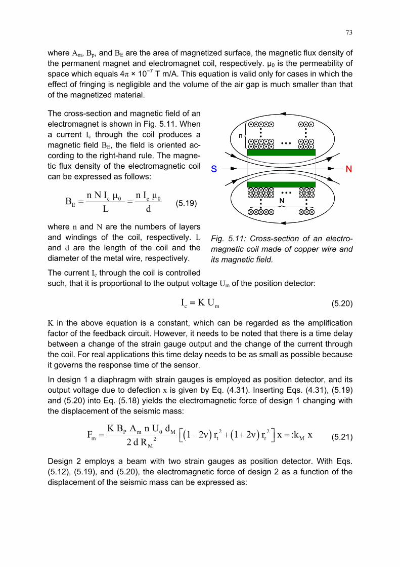
73

where Am, Bp, and BE are the area of magnetized surface, the magnetic flux density of the permanent magnet and electromagnet coil, respectively. μ0 is the permeability of space which equals 4π × 10−7 T m/A. This equation is valid only for cases in which the effect of fringing is negligible and the volume of the air gap is much smaller than that of the magnetized material.

The cross-section and magnetic field of an electromagnet is shown in Fig. 5.11. When a current Ic through the coil produces a magnetic field BE, the field is oriented ac-cording to the right-hand rule. The magne-tic flux density of the electromagnetic coil can be expressed as follows:

c 0 c 0E

n N I μ n I μBL d

= = (5.19)

where n and N are the numbers of layers and windings of the coil, respectively. L and d are the length of the coil and the diameter of the metal wire, respectively.

The current Ic through the coil is controlled such, that it is proportional to the output voltage Um of the position detector:

c mI K U= (5.20)

K in the above equation is a constant, which can be regarded as the amplification factor of the feedback circuit. However, it needs to be noted that there is a time delay between a change of the strain gauge output and the change of the current through the coil. For real applications this time delay needs to be as small as possible because it governs the response time of the sensor.

In design 1 a diaphragm with strain gauges is employed as position detector, and its output voltage due to defection x is given by Eq. (4.31). Inserting Eqs. (4.31), (5.19) and (5.20) into Eq. (5.18) yields the electromagnetic force of design 1 changing with the displacement of the seismic mass:

( ) ( )2 2P m 0 Mm t r M2

M

K B A n U dF 1 2ν r 1 2ν r x :k x2 d R

⎡ ⎤= − + + =⎣ ⎦ (5.21)

Design 2 employs a beam with two strain gauges as position detector. With Eqs. (5.12), (5.19), and (5.20), the electromagnetic force of design 2 as a function of the displacement of the seismic mass can be expressed as:

Fig. 5.11: Cross-section of an electro-magnetic coil made of copper wire and its magnetic field.

N

n

NS

N

n

NS

74

( )P m Bm B B 0 M2

B

3 K B A n dF 1 ν ν 1 ν U x :k x8 d L

= + + − =⎡ ⎤⎣ ⎦ (5.22)

The electromagnetic force Fm of design 3 equals the product of electrical current Ic, magnetic field B, and the effective length L of the coil. The effective length L can be estimated as half of the total length of the coil, since only half of the conductor paths are perpendicular to the direction of acceleration and contribute to the magnetic force.

m cF I B L= (5.23)

As shown in Fig (5.3), a pair of beams is employed to support a seismic mass with an electromagnetic coil, and two strain gauges are mounted on the outer surfaces of the beams. If the displacement of the seismic mass is small, the output of the strain gauges can also be described by Eq. (5.12). Inserting Eqs. (5.12) and (5.20) into Eq. (5.23), the electromagnetic force of design 3 changing with the displacement of the seismic mass can be obtained by:

( )Bm B B 0 M2

B

3 K B L dF 1 ν ν 1 ν U x :k x4 L

= + + − =⎡ ⎤⎣ ⎦ (5.24)

As discussed above, the electromagnetic force Fm and the spring force of the sensing elements FB can be expressed as a linear function of the displacement of seismic mass x. In practical application the electromagnetic force FM should be much larger than the spring force FB, such that the changes of the mechanical characters, e.g., due to creep of the polymer beam, show only a minor effect on the characteristic curve of the sensor. The relationship between the electromagnetic force Fm and the spring force of the sensing elements FB can be described by [5.1]:

M m

B B

F kGF k

= = (5.25)

where G is the feedback gain of the closed loop system. According to Eq. (5.25), the magnetic spring constant km needs to be larger than the mechanical spring constant kB to make the spring force FB negligible, which can be achieved by a large amplifica-tion factor K.

Design 3 for example employs two 60 mm long, 8 mm wide, and 150 µm thick poly-vinyl chloride (PVC) beams with a Young’s modulus of 3 GPa and the mechanical spring constant kB calculated by Eq. (5.17) is 0.19 N/m. It is assumed that the supply voltage U0, the magnetic flux density of the permanent magnet B, the effective length of the coil, Poisson’s ratio of the PVC beam νB, and conductor path (steel) ν are 5 V, 1.35 T, 100 mm, 0.42, and 0.3, respectively, the magnetic constant is equal to 0.034 N/m times amplification factor K. If K is estimated to be on the order of 100, km is on the order of 3.4 N/m. Therefore, the magnetic spring constant is approximately 18 times larger than the mechanical one, and the effect due to the mechanical characte-

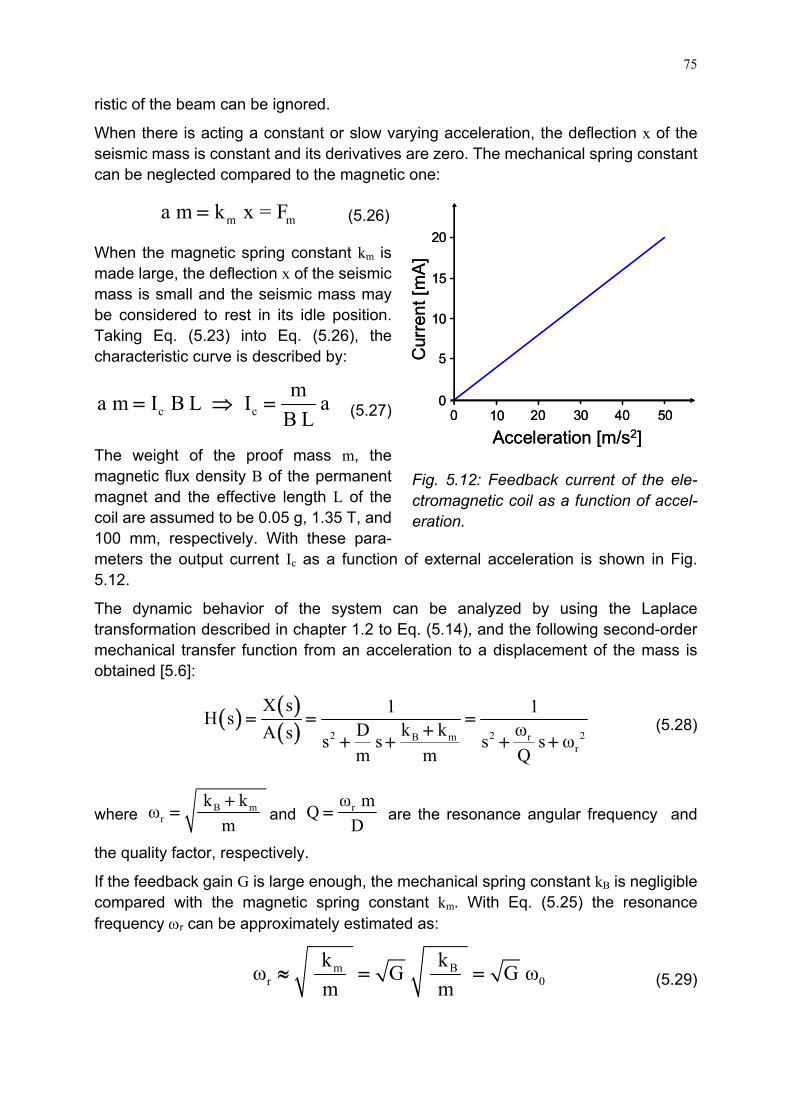
75

ristic of the beam can be ignored.

When there is acting a constant or slow varying acceleration, the deflection x of the seismic mass is constant and its derivatives are zero. The mechanical spring constant can be neglected compared to the magnetic one:

m ma m k x = F= (5.26)

When the magnetic spring constant km is made large, the deflection x of the seismic mass is small and the seismic mass may be considered to rest in its idle position. Taking Eq. (5.23) into Eq. (5.26), the characteristic curve is described by:

c cma m I B L I a

B L= ⇒ = (5.27)

The weight of the proof mass m, the magnetic flux density B of the permanent magnet and the effective length L of the coil are assumed to be 0.05 g, 1.35 T, and 100 mm, respectively. With these para-meters the output current Ic as a function of external acceleration is shown in Fig. 5.12.

The dynamic behavior of the system can be analyzed by using the Laplace transformation described in chapter 1.2 to Eq. (5.14), and the following second-order mechanical transfer function from an acceleration to a displacement of the mass is obtained [5.6]:

( ) ( )( ) 2 2 2B m r

r

X s 1 1H s k k ωDA s s s s s ωm m Q

= = =+

+ + + + (5.28)

where B mr

k kωm+

= and rω mQD

= are the resonance angular frequency and

the quality factor, respectively.

If the feedback gain G is large enough, the mechanical spring constant kB is negligible compared with the magnetic spring constant km. With Eq. (5.25) the resonance frequency ωr can be approximately estimated as:

m B

r 0k kω G G ωm m

≈ = = (5.29)

Fig. 5.12: Feedback current of the ele-ctromagnetic coil as a function of accel-eration.

0 10 20 30 40 50

Acceleration [m/s2]

0

5

10

15

20

Cur

rent

[mA

]0 10 20 30 40 50

Acceleration [m/s2]

0

5

10

15

20

Cur

rent

[mA

]

76

where ω0 is the resonant frequency of an open loop acceleration sensor. According to Eq. (5.29), compared to an open loop acceleration sensor, the useful bandwidth of a force balanced sensor is increased by a factor equal to the square root of the feed-back gain, thus the trade-off between sensitivity and bandwidth can be relieved significantly [5.6, 5.7].

5.4 Fabrication

In design 1 (Fig. 5.1) a diaphragm with strain gauges (N2A-06-S046R-350, Vishay, Germany) was fixed in the center of the sensor by a clamper (cf. Fig. 5.14). Four strain gauges from steel on the membrane were connected to build a full Wheatstone bridge. A ring permanent magnet (R-06-02-02-G, Supermagnete, Germany) was glued to a piston made of polyvinylidene fluoride (PVDF) by turning. One end of the piston was glued to the center of the diaphragm and the other side was inserted into an electromagnetic coil mounted to a chamber below. The electromagnetic coil with 10 windings and 12 mm in length was made of a copper wire, 300 µm in thickness, and its resistance was about 2 Ω. An upper chamber was mounted on top of the diaphragm to seal the sensor. The upper and lower chambers with a radius of 6.35 mm were made from a polymethylmethacrylate (PMMA) plate by a milling machine. The assembled sensor is shown in Fig. 5.14.

Fig. 5.13: A diaphragm with strain gau-ges fixed into a clamper.

Fig. 5.14: Closed loop acceleration sen-sor driven by electromagnetic force with a copper-wire coil.

For design 2 (Fig. 5.2) two ways were tried to manufacture the beam sensing element. On the one hand, a polyvinyl chloride (PVC) foil was cut out to make a beam 75 mm, 10 mm, and 150 µm, in length, width, and thickness, respectively. Two strain gauges (N2A06-S108N-10C, Vishay, Germany) were glued on the upper and lower surfaces of the beam. An electromagnetic coil made by sputtering and photolithography was glued on the free end of the beam (cf. Fig. 5.15).

77

Fig. 5.15: Closed loop acceleration sen-sor driven by electromagnetic force with a PVC beam and sputtered coil.

Fig. 5.16: Polyimide beam with sputter-ed coil and strain gauges.

On the other hand, a polyimide foil with conductor paths was used as a cantilever beam as shown in Fig. 5.16. It was made by multiple-layer photolithography and etching technology, which are demonstrated in Fig. 5.17. Firstly, a gold layer, approx-imately 220 nm in thickness, was sputtered on the surface of a 25 µm thick polyimide foil (cf. Fig. 5.17(1)), and patterned by photolithography and etching with King water generating the coil and strain gauges (cf. Fig. 5.17(2)). After that, a layer of polyimide photo-resist (SX AR-P5000/82.7) was spin-coated on the gold layer for isolation (cf. Fig. 5.17(3)), exposed with a second mask, and developed to generate connection windows (cf. Fig. 5.17(4)). Then, the whole structure was baked in an oven at 180 °C to make the PI layer insoluble. At last, a second gold layer was sputtered (cf. Fig. 5.17(5)) and patterned to fabricate a jumper path of the coil and two strain gauges (cf. Fig. 5.17(6)). The PI foil was cut out as shown in Fig. 5.16, and used as the sensing element. Two ring mag-nets (R-10-04-05-G, Supermagnete, Ger-many) were placed repellently above and beneath the electromagnetic coil to sup-ply the magnetic field.

Design 3 (cf. Fig. 3.3) employed double beams made of a PVC foil as sensing element with the length, width, and thick-ness of 60 mm mm, 8 mm, and 150 µm, respectively. Near by their anchor area two strain gauges were glued on the outer sides of both beams. A square PVC foil with a sputtered coil was glued on the top of the two beams as seismic mass. Two pairs of permanent magnets (W-05-N50-G, Supermagnete, Germany) were

Fig. 5.17: Fabrication process of coil and strain gauges on a PI foil.

(1)

(2)

(3)

(4)

(5)

(6)

Polyimide foil

Gold layer

Polyimide photo-resist

Gold

(1)

(2)

(3)

(4)

(5)

(6)

Polyimide foil

Gold layer

Polyimide photo-resist

Gold

78

placed attractively above and beneath the seismic mass by a holder made of an iron bar. The sensor is shown in Fig. 5.18.

Fig. 5.18: Closed loop acceleration sensor driven by electromagnetic force with double beams.

5.5 Experiments

To test the feasibility of the closed loop acceleration sensor driven by electromagnetic force, design 1 was mounted to a rotary holder and tilted in the gravitational field. For the first try, the feedback current was applied manually. When the angle of the sensor was changed in gravity, there was an output voltage of the strain gauges on the diaphragm. Then, a current was applied through the electromagnetic coil manually to balance the deflection of the diaph-ragm till there was zero output of the bridge. The characteristic curve of the sensor is shown in Fig. 5.19.

According to this figure the feedback current changes linearly with external ac-celeration as expected. However, des-ign 1 was not investigated more because the bulky electromagnetic coil made by hand makes the manufacturing of the sensor very complex.

Design 2 employs a cantilever beam with strain gauges and an electromagnetic coil. As mentioned in the last section, these components were fabricated by sputtering, photolithography and etching. Two permanent magnets providing the magnetic field were glued into the two chambers in the housing above and beneath the coil.

Fig. 5.19: Characteristic curve of design 1 tilted in the gravitational field of the earth.

0.1

0

0.2

-0.1

-0.2

-3 3 6 9 12-6-9-12

Current [A]

Acceleration [m/s2]

0.1

0

0.2

-0.1

-0.2

-3 3 6 9 12-6-9-12

Current [A]

Acceleration [m/s2]

79

Design 2 was tilted in the gravitational field in the same way as design 1. However, it was hard holding the beam at the idle position. This problem was probably caused by a non-uniform magnetic flux. As shown in Fig. 5.20, two permanent magnets were placed repulsively, thus the magnetic flied lines are only in the plane of the coil when it is in the center between the magnets. The magnetic force becomes smaller when the beam is deflected. Therefore, it is difficult to supply an accurate feedback current holding the seismic mass in its idle position.

Fig. 5.20: Schematic drawing of the nonuniform magnetic flux in design 2.

Fig. 5.21: Schematic drawing of per-manent magnets and coil in design 3.

To get a stable electromagnetic force, the magnetic flux should be uniform in the dis-placement area of the seismic mass. Thus, in design 3 the permanent magnets were placed attractive to each other as shown in Fig. 5.21. This way, homogeneous mag-netic flux across the coil was achieved.

Design 3 was characterized by tilting in the gravitational field. As shown in Fig. 5.22, when the acceleration was chang-ed from 0 m/s2 to 10 m/s2, the feedback current increased linearly by about 60 mA. There is nearly no difference be-tween two measurements. Due to the large resistance of the sputtered electro-magnetic coil (273 Ω) its power con-sumption at the acceleration of 10 m/s2 is 0.85 W, which is 10 times larger than the one of design 1 (cf. Fig. 5.19). How-ever, the structure of design 3 is much simpler and can be realized by micro machining processes.

Fig. 5.22: Characteristic curve of design 3 tilted in the gravitational field of the earth.

F

F’

N

N

F

F’

N

N

S

N

F1 F2

S

N S

N

F1 F2

S

N

Acceleration [m/s2]Cur

rent

[mA]

Second measurement

First measurement

0

20

40

-20

-40

0 2 4 6 8 10


rent

[mA]

Second measurement

First measurement

0

20

40

-20

-40

0 2 4 6 8 10


rent

[mA]

Second measurement

First measurement

0

20

40

-20

-40

0 2 4 6 8 10

80

5.6 Conclusions

The principle of closed loop acceleration sensors driven by magnetic force has been investigated. Three different designs were fabricated and tested. According to the experimental results, design 1 and design 3 could realize stable acceleration mea-surements. Compared to design 1, design 3 has some prominent advantages, e.g. a simple structure, process compatibility, and high stability. Accordingly, it is interesting to fabricate an accelerometer of design 3 and characterize this accelerometer in different ways, for example, static and dynamic modes. Furthermore, a feedback circuit should be made to achieve automatic control. The details of the fabrication and experimental results are presented and discussed in the next chapter.

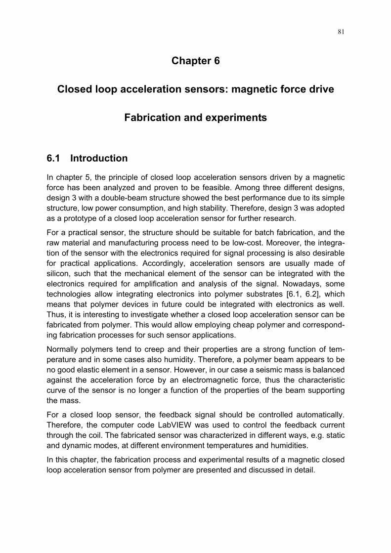
81

Chapter 6

Closed loop acceleration sensors: magnetic force drive

Fabrication and experiments

6.1 Introduction

In chapter 5, the principle of closed loop acceleration sensors driven by a magnetic force has been analyzed and proven to be feasible. Among three different designs, design 3 with a double-beam structure showed the best performance due to its simple structure, low power consumption, and high stability. Therefore, design 3 was adopted as a prototype of a closed loop acceleration sensor for further research.

For a practical sensor, the structure should be suitable for batch fabrication, and the raw material and manufacturing process need to be low-cost. Moreover, the integra-tion of the sensor with the electronics required for signal processing is also desirable for practical applications. Accordingly, acceleration sensors are usually made of silicon, such that the mechanical element of the sensor can be integrated with the electronics required for amplification and analysis of the signal. Nowadays, some technologies allow integrating electronics into polymer substrates [6.1, 6.2], which means that polymer devices in future could be integrated with electronics as well. Thus, it is interesting to investigate whether a closed loop acceleration sensor can be fabricated from polymer. This would allow employing cheap polymer and correspond-ing fabrication processes for such sensor applications.

Normally polymers tend to creep and their properties are a strong function of tem-perature and in some cases also humidity. Therefore, a polymer beam appears to be no good elastic element in a sensor. However, in our case a seismic mass is balanced against the acceleration force by an electromagnetic force, thus the characteristic curve of the sensor is no longer a function of the properties of the beam supporting the mass.

For a closed loop sensor, the feedback signal should be controlled automatically. Therefore, the computer code LabVIEW was used to control the feedback current through the coil. The fabricated sensor was characterized in different ways, e.g. static and dynamic modes, at different environment temperatures and humidities.

In this chapter, the fabrication process and experimental results of a magnetic closed loop acceleration sensor from polymer are presented and discussed in detail.

82

6.2 Design

As shown in Fig. 5.18, design 3 employs double cantilever beams to support a seismic mass with a coil. A pair of strain gauges is glued near the fixing points of the beams, and two pairs of permanent magnets are placed attractively on upper and lower sides of the coil. The processes of making such a sensor are quite complicated. Firstly, two polyvinyl chloride (PVC) beams were cut out and fixed to a polymethyl-methacrylate (PMMA) base. Then another square PVC foil was installed to the free ends of the double beams as a seismic mass. After that, a sputtered coil and two strain gauges were glued onto the outer surfaces of the double beams and the square seismic mass, respectively. Lastly, a magnet holder made of an iron bar was em-ployed to support the permanent magnets above and beneath the coil. There are too many steps and hand works in this fabrication process, which is not suitable for mass production. Therefore, the structure and the process were improved to be compatible with common micro machining processes and mechanical manufacturing techno-logies.

Fig. 6.1 shows an improved design of the magnetic acceleration sensor schematically. A rigid frame from the polymer polyvinylidenefluoride (PVDF) carries 8 pairs of per-manent magnets. Between the magnet pairs there is a polyimide (PI) foil with con-ductor paths from gold. The conductor paths form an electromagnetic coil in the field of the magnets. On the lower surface of the foil, under the coil, there is glued an aluminum plate stiffening the foil.

Fig. 6.1: Schematic view of the magnetic acceleration sensor. Left: front view; right: side view.

Tongues on the left and the right of the foil are bent down and fixed at the substrate. Near the fixation point of the tongues there are strain gauges from gold which are combined to a Wheatstone bridge detecting the position of the seismic mass. A base and clampers from polymethylmethacrylate (PMMA) are used to fix the frame and provide electronic connection.

83

The operational principle of the sensor is illustrated in Fig. 6.2. When the sensor is accelerated, the proof mass tends to be displaced relative to the case, and the tongues of the foil are bent. This deformation is detected by the strain gauges which are combined with external resistors to a half bridge. The output signal of the bridge is amplified and, after suitable processing by the computer code LabVIEW, is controlling a feedback circuit driving the coil on the foil such that the foil is pulled back to its idle position. The driving voltage of the coil is a measure of the acceleration.

Fig. 6.2: Operational principle of the magnetic force balanced acceleration sensor.

The behavior of such a sensor has been discussed in chapter 5.3, which is described by Eq. (5.14), Eq. (5.17), and Eq. (5.24). In this case, two 12.5 mm long, 4.2 mm wide, and 50 μm thick polyimide (PI) tongues with a Young’s modulus of 8 GPa were em-ployed as cantilever beams, the mechanical spring constant kB was calculated by Eq. (5.17) as 1.1 N/m. If the supply voltage U0, the magnetic flux density of the permanent magnet B, the effective length of the coil L, Poisson’s ratio of the PI beam νB and the gold conductor path ν are 1.56 V, 1.35 T, 124 mm, 0.42, and 0.34, respectively, the magnetic constant calculated by Eq. (5.24) is equal to 0.1 N/m times the amplification factor K. If K is set to be on the order of 100, km is on the order of 10 N/m. Therefore, the magnetic spring constant is approximately 10 times larger than the mechanical one, and the effect of the mechanical characteristic of the tongues can be ignored. Accordingly, when there is acting a constant acceleration, the characteristic curve is given by Eq. (5.27):

c cma m I B L I a

B L= ⇒ = (5.27)

84

If the seismic mass is estimated to be the weight of the square PI foil and the alu-minum plate (0.09 g), the feedback current through the coil as a function of external acceleration can be calculated in Eq. 5.27 as shown in Fig. 6.3. It shows that the current through the coil which is approxi-mately proportional to the voltage drop over the coil is a linear function of acc-eleration. Besides this, the characteristic curve in a first order approximation is not a function of the properties of the movable parts of the sensor such as Young’s mo-dulus, Poisson’s ratio, length, width, and thickness of the tongues etc. Therefore, geometrical changes caused by the creep of polymers affect the sensor only little.

6.3 Fabrication

In fabrication it is favorable that all the components can be made by planar micro machining processes and mechanical manufacturing, and then assembled in a simple way to generate the desired three-dimension structure. Due to the available equip-ments the magnetic acceleration sensor was fabricated by sputtering, photolitho-graphy, ultrasonic hot embossing, and micro milling [6.3].

According to Fig. 6.2, the core com-ponent of the sensor is a polyimide foil with a coil, strain gauges, and conductive paths. It was made by multiple-layer photolithography and etching. The whole process can be divided into three major steps, which are demonstrated in Fig. 6.4.

In the first step, the electromagnetic coil and its conductor paths were fabricated on a polyimide (PI) foil. In the beginning, a gold layer, approximately 220 nm in thickness, was sputtered onto a 50 µm thick polyimide foil. A positive photoresist (AZ 4562) was spin-coated on the gold layer at 4000 rotations/min generating a 6 µm thick film. Then, the sample was baked in an oven at 60 °C for 45 min

Fig. 6.3: Feedback current through the coil as a function of acceleration.

Fig. 6.4: Fabrication process of the PI foil with coil and strain gauges.

85

drying the photoresist film. After that, the photoresist film was exposed with mask 1 (cf. Fig. 6.5) for 3.5 minutes by UV light, and developed by a developer (AZ 826 MIF) for 12 minutes. Following that, the exposed gold was etched by king water. At last, the remained photo-resist was dissolved by a remover (AZ 100). With these processes, the pattern on mask 1 was transferred to the gold layer.

Fig. 6.5: Masks used in multiple-layer photolithography.

Fig. 6.6: Sputtering process employed to make gold conductor paths.

For sputtering, as shown in Fig. 6.6, an argon plasma is generated in a vacuum cham-ber. The argon ions (Ar+) impact toward the cathode (target) and sputter the target material. The target atoms hit the substrate surface and condense as a film. Normally it is favorable that the target atoms are accelerated to a high velocity attaching well to the substrate surface and generating a compact film. However, the intense hitting

86

produces a high temperature on the substrate. To resist the high temperature a polyimide foil was chosen for the substrate because it withstands temperatures of up to 450 °C. Moreover, the sputtering power was limited to 250 W, and a water cooling system was employed to decrease the temperature of the anode. Nevertheless, there was still deformation of the PI foil probably caused by overheating. By observing the whole sputtering process through a glass window in the chamber, it was found that the foil bulged and the bulged part had no contact with the anode. Accordingly, a layer of thermal joint compound (type 120, Wakefield) was added between the anode and the PI foil. This way, a flat PI foil with gold pattern was obtained.

After the first gold layer was patterned, a thin polyimide layer was produced on it as isolation layer. Polyimide photoresist (SX AR-P5000/82.7) was spin-coated on the patterned gold layer at 1000 rotations per minute to make a thin film with a thickness of 1.6 µm. The sample was prebaked at 85 °C for 30 minutes, and then exposed by mask 2 (cf. Fig. 6.5) with UV light for 3 minutes. The PI photoresist was developed by a developer (AR300-47) for 8 minutes to release connection windows. Following that, the whole structure was baked in an oven at 180 °C to make the PI layer an insoluble isolating layer.

In step 2 the rotational speed of spin-coating of PI photoresist is the key point which determines the thickness and insu-lation effect of the film. If the rotational speed was too slow, the thickness of the film was not un-uniform, which affected the electric connection between the two gold layers through the windows. When the speed was too large, there was no closed insulation film covering the gold layer, thus short cuts occurred between the two gold layers. By several tests, the spin-coating speed was set to 1000 r/min, which en-sured the homogeneity and the insulation of the PI isolation film.

In the last step a second gold layer was sputtered and patterned by mask 3 (cf. Fig. 6.5) as described in step 1 to become a jumper path of the coil and two strain gauges on the PI insulation layer. The PI foil was cut out as shown in Fig. 6.7, containing the coil in the center and two tongues on opposite sides.

The fabrication processes of the three masks used in photolithography are demon-strated in Fig. 6.8. Firstly, the patterns of conductor paths were milled onto a PMMA plate by milling machine (Kosy 3, Germany). Then, a layer of black paint was sprayed on to the milled surface. After the paint was dry, a thin surface layer of PMMA was milled to expose the patterns of conductor paths. Due to the limit of our milling machine, it was not possible to generate conductor paths for strain gauges and the coil with a width of less than 100 µm.

Fig. 6.7: Polyimide foil with coil, strain gauges, and conductive paths.

87

Fig. 6.8: Fabrication process of masks.

The frame and the magnet holder were fabricated by ultrasonic hot embossing [6.4]. The whole process can be distinguished into five phases [6.5]: the pre-process, the force build up, the transient phase, the cooling phase and the demolding phase (cf. Fig. 6.9).

Fig. 6.9: Five phases of ultrasonic hot embossing.

In the pre-process stage (cf. Fig. 6.9 (A)), polymer films are placed between the horn and the metal tool. The horn moves down and touches the polymer films between the horn and the tool. After that, the horn presses the polymer film, and the pressure force grows up to a certain trigger value which starts the ultrasonic vibrations (cf. Fig. 6.9 (B)). Then, heat is generated as a result of the friction between the film surfaces and the intermolecular friction inside the films. The temperature of the polymer increases until the glass transition temperature (Tg) is reached. Energy dissipation is generated at polymer parts contacting the pattern on the tool. Therefore, a thin molten polymer layer is generated next to protruding structures on the tool. The force slightly drops in this phase because the polymer is softening. The melting polymer adapts to the metal

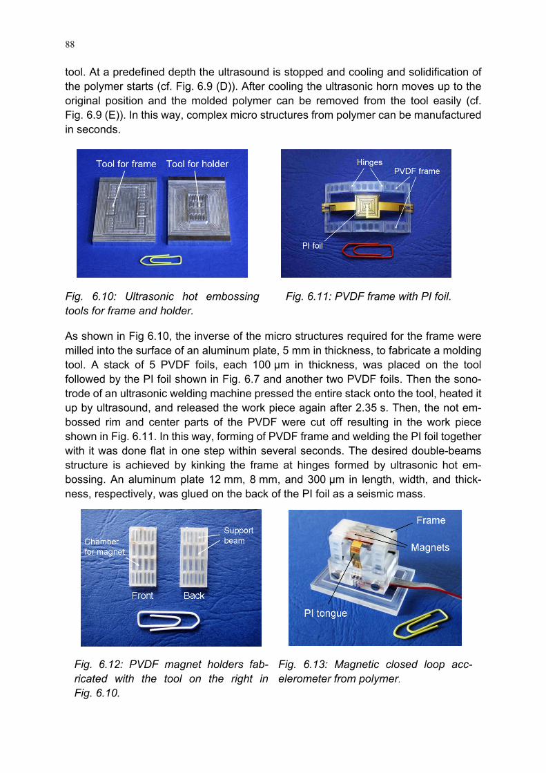
88

tool. At a predefined depth the ultrasound is stopped and cooling and solidification of the polymer starts (cf. Fig. 6.9 (D)). After cooling the ultrasonic horn moves up to the original position and the molded polymer can be removed from the tool easily (cf. Fig. 6.9 (E)). In this way, complex micro structures from polymer can be manufactured in seconds.

As shown in Fig 6.10, the inverse of the micro structures required for the frame were milled into the surface of an aluminum plate, 5 mm in thickness, to fabricate a molding tool. A stack of 5 PVDF foils, each 100 µm in thickness, was placed on the tool followed by the PI foil shown in Fig. 6.7 and another two PVDF foils. Then the sono-trode of an ultrasonic welding machine pressed the entire stack onto the tool, heated it up by ultrasound, and released the work piece again after 2.35 s. Then, the not em-bossed rim and center parts of the PVDF were cut off resulting in the work piece shown in Fig. 6.11. In this way, forming of PVDF frame and welding the PI foil together with it was done flat in one step within several seconds. The desired double-beams structure is achieved by kinking the frame at hinges formed by ultrasonic hot em-bossing. An aluminum plate 12 mm, 8 mm, and 300 µm in length, width, and thick-ness, respectively, was glued on the back of the PI foil as a seismic mass.

Fig. 6.12: PVDF magnet holders fab-ricated with the tool on the right in Fig. 6.10.

Fig. 6.13: Magnetic closed loop acc-elerometer from polymer.

Fig. 6.10: Ultrasonic hot embossing tools for frame and holder.

Fig. 6.11: PVDF frame with PI foil.

89

Similarly two magnet holders were fabricated of PVDF foils by ultrasonic hot embossing and the finished samples are shown in Fig 6.12. There are 8 chambers for permanent magnets, and 16 support beams keeping the magnet holder flat.

As shown in Fig. 6.14, 8 pairs of permanent magnets (Q-05-1.5-01-N from Supermag-nete, Germany) were glued attractively posi-tioned into the magnet holders. Then, the two holders were glued on upper and bottom surfaces of the PVDF frame to generate a uniform magnetic field across the coil on the PI foil. The PVDF frame was kinked at the hinges forming the desired three-dimen-sional suspending structure and fixed to the base by two clampers with four screws. At the development stage base and clampers were made by milling, but in mass production injection molding would be more efficient. In each clamper there were three copper tapes which provided the electric contact between gold pads on the PI foil and wires soldered to the tapes. The assembled magnetic closed loop acceleration sensor is shown in Fig. 6.13.

Fig. 6.15: Analog amplification circuit for strain gauges.

6.4 Experiments

The resistances of the strain gauges on the PI tongues were measured to be 129 Ω and 98 Ω, respectively. An analog circuit was designed to amplify the tiny output signal from the strain gauges (cf. Fig. 6.15).

Fig. 6.14: Assembling photo of the acceleration sensor.

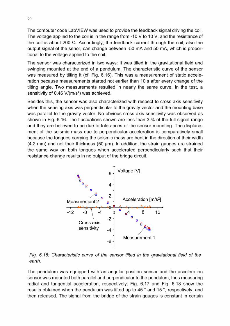
90

The computer code LabVIEW was used to provide the feedback signal driving the coil. The voltage applied to the coil is in the range from -10 V to 10 V, and the resistance of the coil is about 200 Ω. Accordingly, the feedback current through the coil, also the output signal of the senor, can change between -50 mA and 50 mA, which is propor-tional to the voltage applied to the coil.

The sensor was characterized in two ways: It was tilted in the gravitational field and swinging mounted at the end of a pendulum. The characteristic curve of the sensor was measured by tilting it (cf. Fig. 6.16). This was a measurement of static accele-ration because measurements started not earlier than 10 s after every change of the tilting angle. Two measurements resulted in nearly the same curve. In the test, a sensitivity of 0.46 V/(m/s²) was achieved.

Besides this, the sensor was also characterized with respect to cross axis sensitivity when the sensing axis was perpendicular to the gravity vector and the mounting base was parallel to the gravity vector. No obvious cross axis sensitivity was observed as shown in Fig. 6.16. The fluctuations shown are less than 3 % of the full signal range and they are believed to be due to tolerances of the sensor mounting. The displace-ment of the seismic mass due to perpendicular acceleration is comparatively small because the tongues carrying the seismic mass are bent in the direction of their width (4.2 mm) and not their thickness (50 µm). In addition, the strain gauges are strained the same way on both tongues when accelerated perpendicularly such that their resistance change results in no output of the bridge circuit.

Fig. 6.16: Characteristic curve of the sensor tilted in the gravitational field of the earth.

The pendulum was equipped with an angular position sensor and the acceleration sensor was mounted both parallel and perpendicular to the pendulum, thus measuring radial and tangential acceleration, respectively. Fig. 6.17 and Fig. 6.18 show the results obtained when the pendulum was lifted up to 45 ° and 15 °, respectively, and then released. The signal from the bridge of the strain gauges is constant in certain

91

limits because the coil pulls the seismic mass back into its idle position while position and acceleration are changing.

Fig. 6.17: Signal from the bridge containing the strain gauges, position of the pen-dulum, and voltage supplied to the coil when the acceleration sensor is measuring in tangential direction.

Fig. 6.18: Signal from the bridge containing the strain gauges, position of the pen-dulum, and voltage supplied to the coil when the acceleration sensor is measuring in radial direction.

92

The time shift between accelerometer and the position sensor found in the data shown in Fig. 6.17 and Fig. 6.18 is about 250 ms. This is probably caused by the feedback loop realized by a computer code and not by an analog circuit. The computer needs about 5.3 ms to calculate a changed feedback signal. This is a function of both, code and computer capability. Several feedback steps are required to adapt to a changed acceleration. It is expected that a much quicker response time can be achieved with a suitable analog circuit. Measurements of the response time are not reasonable before an analog feedback circuit is available.

The sensor was also tilted and tested in the gravitational field at different temperature and different relative humidity to check the stability. As shown in Fig. 6.19 and Fig. 6.20, temperature changes caused an obvious zero point drift of the characteristic curve, while the drift due to humidity change seems to be much smaller. Therefore, temperature fluctuations of the environment are the major interference to the per-formance of the sensor. The problem is possibly caused by the fabrication processes. If the thicknesses would be the same everywhere, the expansions of the polymer due to temperature or humidity change do not change the position of the seismic mass significantly. Only a small move perpendicular to the magnets has to be expected. A local difference of the thickness of the polyimide foil and the gold layer on the two tongues, however, would result in a lateral move of the seismic mass and cause a shift of the characteristic curve.

Fig. 6.19: Characteristic curves of the sensor tilted in the gravitational field of the earth at 35 °C and 55 °C. The relative humidity was kept at 55 %.

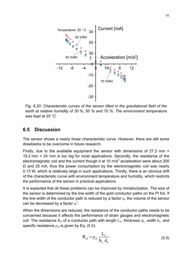
93

Fig. 6.20: Characteristic curves of the sensor tilted in the gravitational field of the earth at relative humidity of 30 %, 50 % and 70 %. The environment temperature was kept at 25 °C.

6.5 Discussion

The sensor shows a nearly linear characteristic curve. However, there are still some drawbacks to be overcome in future research.

Firstly, due to the available equipment the sensor with dimensions of 27.2 mm × 19.2 mm × 24 mm is too big for most applications. Secondly, the resistance of the electromagnetic coil and the current though it at 10 m/s2 acceleration were about 200 Ω and 25 mA, thus the power consumption by the electromagnetic coil was nearly 0.13 W, which is relatively large in such applications. Thirdly, there is an obvious drift of the characteristic curve with environment temperature and humidity, which restricts the performance of the sensor in practical applications.

It is expected that all these problems can be improved by miniaturization. The size of the sensor is determined by the line width of the gold conductor paths on the PI foil. If the line width of the conductor path is reduced by a factor sf, the volume of the sensor can be decreased by a factor sf

3.

When the dimensions are reduced, the resistance of the conductor paths needs to be concerned because it affects the performance of strain gauges and electromagnetic coil. The resistance Rel of a conductor path with length LL, thickness dL, width bL, and specific resistance ρel is given by Eq. (5.5):

L

el elL L

LR ρb d

= (5.5)

94

In miniaturization the length and width of the conductor paths are reduced by the same factor sf, and the thickness of the gold layer cannot be reduced significantly any more because no homogeneous thickness can be generated with our equipment for thinner layers. For strain gauges, a large resistance is required because, on the one hand, a comparatively high voltage (on the order of 5 V) needs to be applied to achieve a large output voltage, and, on the other hand, the current through the strain gauges needs to be small to avoid local heating which changes the resistance and may cause bending of the tongues. Therefore, the thickness of the gold layer should remain the same to maintain the resistance of the strain gauges. Although the power of the stain gauge is not changed, the volume heated by strain gauges is reduced, which may result in an enhanced temperature.

As shown in Fig. 6.18 and Fig. 6.19, the current through the strain gauges is 7.5 mA while the current through the coil is on the order of several 10 mA. Therefore, more heat is generated at the coil and the heat development there needs to be considered carefully. The seismic mass would shrink proportional to sf

3 when the length is reduced by a factor sf. According to Eq. 5.27, the current through the coil would reduce with the square of the factor sf. The electrical power is reduced with the 2nd power of the current and the 4th power of sf. If the power is absorbed mainly by the seismic mass, it results in a linear reduction of power density. Heat dissipation can be approximately estimated by Eq. (4.6) as:

c 0P hT Tλ A

= + (4.5)

where P, h, λ, and A are the power of coil, effective distance between coil and case, thermal conductivity of air, and surface area of the coil, respectively. T0 and Tc are the temperature of the case and electromagnetic coil, respectively. If the room tem-perature is ignorable compared with the temperature of the coil, the temperature of the coil would reduce with the factor sf

3, when the dimensions are reduced by a factor sf. Therefore, the power and the coil temperature both could be decreased sign-ificantly.

Due to dimension reduction, the mismatch in fabrication process may also be decreased. For example, the local difference of the thickness of the polyimide foil and the gold layer on the two tongues in macro dimensions is probably larger than the one in micro scale. Therefore, it could improve the performance of the sensor at different environment temperatures and humidities.

All in all, it appears to be interesting to fabricate a smaller version of the sensor and to investigate whether better performance can be achieved.

6.6 Conclusions

A magnetic closed loop acceleration sensor from polymer was built and tested. This shows that even inertial sensors can be fabricated from polymers if the design is

95

adapted to the special needs of this material class. In this case the acceleration was balanced by the magnetic force of a coil in the field of permanent magnets and the electrical current necessary for balancing is a measure of the acceleration. It would be desirable to obtain a characteristic curve which is more linear and not a function of temperature. Therefore, more investigations are required to find out whether sensors from polymer are a potential option for the future.

Balancing the acceleration and thus preventing large movements of the seismic mass has the advantage that the mechanical properties and dimensions of the polymer carrying the coil do not affect the characteristic curve of the sensor if only static mea-surements are carried out. The influence of material properties on dynamic measure-ments still needs to be investigated.

Ultrasonic hot embossing was employed for fabricating the sensor from a stack of polymer foils allowing easy fabrication of the sensing element. Other polymer fabrication processes such as injection molding and hot embossing could also be suitable for sensor fabrication. It appears to be possible that in future developments even the control electronics could be integrated into polymer sensors [6.1, 6.2]. It would be interesting to investigate whether other kinds of sensors such as pressure sensors can also be fabricated from polymer.

97

Chapter 7

Conclusions

Alternative acceleration sensors from polymer, open loop and closed loop, were successfully fabricated and tested as presented in this dissertation. This shows that inertial sensors can be manufactured from polymer.

Due to the creep and temperature sensitive mechanical properties polymer compo-nents appear to be not suitable functional elements in a sensor. However, with an appropriate design which is adapted to the special character of this material class the drawbacks mentioned above can be overcome. This way, cheaper polymers and more economic fabrication processes can be employed for such sensor applications.

Two methods were proposed to realize alternative acceleration sensors from polymer: firstly, the principles of thermal flow sensors were adopted to the design of accelera-tion sensors applying thermal components instead of a proof mass and a suspending system as the sensing element; secondly, applying a feedback loop balancing the inertial force such, that the dependence on mechanical properties and temperature of the sensing element are limited significantly.

For the thermal method two designs, an anemometer and a calorimeter, were fabri-cated by micro milling and micromachining. Both designs employ a heater inside a tube. Without acceleration, the heat is transferred symmetrically to the air and housing around the heater, and the temperature of the heater keeps a certain value. When the sensor is accelerated with an acceleration a, the heated air gets a velocity v due to buoyancy. Then the temperature of the heater and the heat distribution will vary be-cause of the convection. In an anemometer the resistances of the heaters were measured, but there was no useful signal gained from them, even when the current of the heaters were increased to about 0.2 A. The sensitivity of such a sensor can not be enhanced easily, since there is a compromise between heater power and its heat capacity. According to the calculation, the sensitivity could be improved by raising the power of the heater, which requires a bulky heater to resist a larger working current. However, the larger heat capacity of a bulky heater decreases the sensitivity of the sensor. Accordingly, the anemometer was modified to become a calorimeter by employing an independent heater and thermometers.

In a calorimeter thermometers are installed on both sides of the heater. This way, the change of heat distribution caused by external acceleration can be detected by the two thermometers. Compared with the anemometer, the calorimeter has three ad-vantages: higher sensitivity, linear characteristic curve, and direction sensing capa-bility. With sputtering and photolithography the sensing element, such as heater and thermometers, were fabricated on a polyimide foil. With the sputtered sensing ele-ments, the connecting area between the heater and the surrounding air was expand-

98

ed generating a faster air flow and the resistances of the thermometers were also increased allowing a larger voltage supplied to the Wheatstone bridge. This way, the sensitivity was enhanced. In the experiments the calorimeter with sputtered elements could achieve a sensitivity of 0.5 V/(m/s2) at a heater power of 0.2 W, while the one of the calorimeter employing metal wire elements was only 0.22 V/(m/s2) at a power of 0.26 W. The characteristic curves of the sensors were linear corresponding to the theoretical calculation. Therefore, the calorimeter appears to be a good choice for an alternative acceleration sensor. In further research it would be interesting to make the sensing elements, including the heater and the thermometers, with a custom-made mask. Due to the smaller line width of the patterns on this mask the dimension of the sensing elements can be reduced significantly such, that the total size of the sensor will be miniaturized. Moreover, the housing of the sensor can be fabricated by ultra-sonic hot embossing, which is capable to simplify the manufacturing process and de-crease the cost.

For the closed loop method, three types of driving modes, capacitive, thermo-pneu-matic, and electromagnetic were proposed and tested. In capacitive mode instead of a common cantilever suspending structure a droplet of liquid was employed as proof mass inside a tube. The displacement of the liquid droplet should be balanced by a capacitive force. Unfortunately, due to the available equipments it was not possible to supply a capacitive force which was sufficient to move the liquid droplet at an acceptable control voltage.

To achieve a larger balancing force the thermo-pneumatic force was employed to keep the proof mass in its idle position. Two different designs employing different proof masses and position detectors were proposed and fabricated. For the design with a liquid droplet as proof mass and a capacitive position detector, no useful position signal could be gained from the capacitive position detector due to its low sensitivity, although the thermo-pneumatic force was large enough to move the liquid droplet in the tube. For the other design, a diaphragm with strain gauges dividing two heating chambers was used as a position detector, which shows higher sensitivity to the tiny displacement of the proof mass glued in the centre of the diaphragm. However, the time delay of the balancing force was too long for a suitable feedback, and the output of the strain gauges was not a monotone function of the position of the membrane. Consequently, no prototype of a thermo-pneumatic mode could be realiz-ed providing accurate and stable measurements of acceleration.

In the case of the electromagnetic driving mode, the acceleration is balanced by the electromagnetic force of a coil in the field of permanent magnets and the electrical current necessary for balancing is a measure of the acceleration. Double cantilever beams supporting a seismic mass with an electromagnetic coil successfully fulfilled its function in the experiments. Then, the prototype was fabricated by micro machining processes and mechanical manufacturing technology. The core component of the sensor, a polyimide foil with a coil, strain gauges, and a conductive path, was made by multiple-layer photolithography and etching. The frame and magnet holders were fab-ricated by ultrasonic hot embossing. This way, complex micro structures from polymer

99

are manufactured in seconds. In the experiments the computer code LabVIEW was providing the feedback signal driving the coil, and the sensor was characterized in two ways: it was tilted in the gravitational field and swinging mounted at the end of a pendulum. In the test a sensitivity of 0.46 V/(m/s²) was achieved and the cross axis sensitivity error was less than 3 %.

The calorimeter and the electromagnetically force balanced accelerometer were suc-cessfully fabricated from polymer. Both types have the potential of miniaturization, which could be achieved by employing custom-made masks with narrower line width in photolithography decreasing the dimensions of their sensing elements. Following the size shrinkage the sensitivity is expected to be enhanced at much lower power consumption and the disturbance due to environment change, e.g. temperature and humidity fluctuations, might be relieved. Moreover, with electronics integrated into polymer substrates the alternative acceleration sensor from polymer sensors in future could be integrated with electronics as well as silicon-based devices.

101

References

Chapter 1

[1.1] N. Yazdi, F. Ayazi and K. Najafi, Micormachined Inertial Sensors, Proceedings of the IEEE, 1998, 86, 1640 - 1659.

[1.2] S. Beeby, G. Ensell, M. Kraft, and N. White, MEMS Mechanical Sensors, Artech House (2004), p. 177, ISBN 1-58053-536-4.

[1.3] D. Abel, “Automatic control for master course students”, lecture notes, 8th edition, p. 47 - 52.

[1.4] F. Rudolf, A. Jornod, J. Bergqvist and H. Leuthold, Precison Accelerometers with µg Resolution, Sensors and Actuators A, 1990, 21-23, 297 - 302.

[1.5] H. Seidel, et al., A Piezoresistive Accelerometer with Monolithically Integrated CMOS Circuitry, Proc. Eurosensors IX and Transducers’91, Stockholm, Sweden, 1995, 597 - 600.

[1.6] Y. Nemirovsky, A. Nemirovsky, P. Muralt, and N. Setter, Design of a Novel Thin-Film Piezoelectric Accelerometer, Sensors and Actuators A, 1996, 56, 239 - 249.

[1.7] L. M. Roylance and J. B. Angell, A Batch-Fabricated Silicon Accelerometer, IEEE Trans. Electron Devices, 1979, ED-26, 1911 - 1917.

[1.8] M. Elwenspoek and R. Wiegerink, “Mechanical Microsensors”, Springer-Verlag (2001), p. 143, ISBN 3-540-67582-5.

[1.9] F. Goodenough, Airbags Boom when IC Accelerometer Sees 50 g, Electron. Design, 1991, 45 - 47.

[1.10] S. J. Sherman, W. K. Tsang, T. A. Core, R. S. Payne, D. E. Quinn, K. H.-L. Chau, J. A. Farash, and S. K. Baum, A Low Cost Monolithic Accelerometer; Product/Technology Update, Technical Digest IEEE, Electron Devices Meeting 1992, 501 - 504.

[1.11] W. Henrion, M. Ip, S. Terry, and H. Jerman, Wide Dynamic Range Direct Digital Accelerometer, IEEE Solid-State Sensor and Actuator Workshop, Hilton Head, SC, 1990, 153 - 157.

[1.12] Y. De Coulon, T. Smith, J. Hermann, and M. Chevroulet, Design and Test of a Precision Servoaccelerometer with Digital Output, 7th Intl. Conf. Solid-State Sensors and Actuators (Transducer ’93), Yokohama, Japan, 1993, 832 - 835.

[1.13] T. Smith, et al., Electro-Mechanical Sigma-Delta Converter for Acceleration Measurements, IEEE International Solid-State Circuits Conference, San Francisco, CA, 1994, 160 - 161.

[1.14] C. Lu, M. Lemkin, and B. Boser, A Monolithic Surface-Micromachined Accele-rometer with Digital Output, IEEE J. Solid-State Circuits, 1995, 30(12), 1367 - 1373.

[1.15] E. Abbaspour-Sania, R. Huanga, and C. Y. Kwok, A linear electromagnetic accelerometer, Sensors and Actuators A, 1994, 44, 103 - 109.

[1.16] W. K. Schomburg, “Introduction to Microsystem Design”, Springer RWTHedi-tion (2011), p. 306, ISBN 978-3-642-19488-7.

102

[1.17] P. L. Bergstrom, M. L. Trombley, and G. G. Li, “The handbook of MEMS (2nd editon): MEMS Applications, Chapter 2 Inertial Sensors”, Tayler and Francis (2006) p. 2-2, ISBN 0-8493-9139-3.

[1.18] F. J. Touwslager, N. P. Willard, and D. M. Leeuw, I-line Lithography of Poly-(3,4-ethylenedioxythiophene) Electrodes and Application in All-polymer Integ-rated Circuits, Appl. Phys. Let., 2002, 81, 4556 - 4558.

[1.19] P. Khuntontong, T. Blaser, and W. K. Schomburg, Fabrication of Molded Interconnection Devices by Ultrasonic Hot Embossing on Thin Polymer Films, IEEE Transactions on Electronics Packaging Manufacturing, 2009, 32, 152 - 156.

Chapter 2

[2.1] S. Beeby, G. Ensell, M. Kraft, and N. White, “MEMS Mechanical Sensors”, Artech House (2004) p. 177, ISBN 1-58053-536-4.

[2.2] V. Milanovic, E. Bowen, M. E. Zaghloul, N. H. Tea, J. S. Suehle, B. Payne, and M. Gaitan, Micromachined Convective Accelerometers in Standard Integrated Circuits Technology, Appl . Phys. Lett., 2000, 76(4), 508 - 510.

[2.3] A. M. Leung, J. Jones, E. Czyzewska, J. Chen, and B. Woods, Micromachined Accelerometer Based on Convection Heat Transfer, MEMS, 1998, 98, 627 - 630.

[2.4] X. B. Luo, Y. J. Yang, F. Zheng, Z. X. Li, and Z. Y. Guo, An Optimized Micromachined Convective Accelerometer with No Proof Mass, J. Micromech. Microeng., 2001,11, 504 - 508.

[2.5] F. Mailly, A. Giani, S. Martine, R. Bonnot, P. Temple-Boyer, and A. Boyer, Micromachined Thermal Accelerometer, Sensors and Actuators A, 2003, 103 (3), 359 - 363.

[2.6] F. Mailly, A. Giani, and A. Boyer, “MEMS/NEMS Handbook Techniques and Applications v.4. Sensors and Actuators in MEMS/NEMS, Chapter 2 Micromachined Thermal Accelerometer without Proof Mass”, Springer Science+Bussiness Media, Inc (2006), ISBN10 0-387-24520-0.

[2.7] W. K. Schomburg, “Introduction to Microsystem Design”, Springer RWTH-edition (2011), ISBN 978-3-642-19488-7.

[2.8] T. S. Lammerink, N. R. Tas, M. Elwenspoek, and J. H. Fluitman, Micro-Liquid flow sensor, Sensors and Actruators A, 1993, 37(38), 45 - 50.

Chapter 3

[3.1] F. Goodenough, Airbags boom when IC Accelerometer Sees 50 g, Electron. Design, 1991, 45-47.

[3.2] S. J. Sherman, W. K. Tsang, T. A. Core, R. S. Payne, D. E. Quinn, K. H. -L. Chau, J. A. Farash, and S. K. Baum, A Low Cost Monolithic Accelerometer; Product/Technology Update, Technical Digest IEEE, International Electron Devices Meeting, New York, 1992, 501 - 504.

103

[3.3] W. K. Schomburg, “Introduction to Microsystem Design”, Springer RWTHedi-tion (2011), p. 131, ISBN 978-3-642-19488-7.

Chapter 4

[4.1] F. Goodenough, Airbags Boom when IC Accelerometer Sees 50 g, Electron. Design, 1991, 45-47.

[4.2] N. Maluf and K. Willams, “An Introduction to Microelectromechanical Systems Engineering”, Artech House, Inc. (2004), p. 84, ISBN 1-58053-590-9.

[4.3] B. Bustgens, W. Bacher, W. Menz, and W. K. Schomburg, Micropump Manu-factured by Thermoplastic Molding, IEEE Workshop on Micro Electro Mechanical Systems, Oiso, Japan, 1994, 18 - 21.

[4.4] U.S. Patents 4,824,073, April 25, 1989 and 4,966,646, October 30, 1990. [4.5] W. K. Schomburg, “Introduction to Microsystem Design”, Springer RWTH-

edition (2011), ISBN 978-3-642-19488-7.

Chapter 5

[5.1] J. H. van Nierop, A Low-cost Linear Accelerometer, J. Phys. E: Sci. Instrum, 1981,14, 880 - 882.

[5.2] E. Abbaspour-Sani, R. S. Huang, and C. Y. Kwok, A Novel Electromagnetic Accelerometer, IEEE Electron Device Letters, 1994, 15, 272 - 273.

[5.3] E. Abbaspour-Sani, R. S. Huang, and C. Y. Kwok, A Linear Electomagnetic Accelerometer, Sensors and Actuators A, 1994, 44, 103 - 109.

[5.4] W. K. Schomburg, “Introduction to Microsystem Design”, Springer RWTH-edition (2011), ISBN 978-3-642-19488-7.

[5.5] http://en.wikipedia.org, entry: electromagnet. [5.6] M. Elwenspoek and R. Wiegerink, “Mechanical Microsensors”, (Springer-

Verlag), 1st edition, (2001), p. 133, 143, ISBN 3-540- 67582-5. [5.7] S. Beeby, G. Ensell, M. Kraft, and N. White, “MEMS Mechanical Sensors”,

(Artech House), 2004, p. 177, ISBN 1-58053-536-4.

Chapter 6

[6.1] F. J. Touwslager, N. P. Willard, and D. M. Leeuw, “I-line Lithography of Poly-(3,4-ethylenedioxythiophene) Electrodes and Application in All-polymer Integrated Circuits, Appl. Phys. Let., 2002, 81, 4556 - 4558.

[6.2] P. Khuntontong, T. Blaser, and W. K. Schomburg, Fabrication of Molded Inter-connection Devices by Ultrasonic Hot Embossing on Thin Polymer Films, IEEE Transactions on Electronics Packaging Manufacturing, 2009, 32, 152 - 156.

[6.3] J. Li and W. K. Schomburg, Magnetic Accelerometer from Polymer, Eurosen-sors XXV, Athens, Greece, Proc., 2011.

[6.4] P. Khuntontong, T. Blaser, and W. K. Schomburg, Ultrasonic Micro Hot Em-bossing of Thermoplastic Polymers, Proc. 24th Annual Meeting of the Polymer Processing Society, Salerno, Italy, 2008, 2, 364.

104

[6.5] P. Khuntontong, Fabrication of Polymer Micro Devices by Ultrasonic Hot Em-bossing, PhD Dissertation at KEmikro RWTH Aachen, 2008, 13 - 14.

105

Curriculum Vitae

Personal Details

Name: Ji Li

Date of Birth: May 16th, 1983

Nationality: China

Education Background

2008-2012 Doctor of Engineering at Konstrukton und Entwicklung von Microsystemen (KEmikro), RWTH Aachen University, Germany.

2006-2009 Master of Engineering, Southeast University, Nanjing, China.

2001-2005 Bachelor of Engineering, Southeast University, Nanjing, China.

1998-2001 Jinling High School, Nanjing, China.

Work Experience

08.2005-07.2006 Volunteer Teacher, The First Middle School of Zhungeer, Inner Mongolia, China.

Award

2008-2012 Awarded Full Scholarship by China Scholarship Council (CSC) for Doctor of Engineering in Design and Development of Microsystems at KEmikro, RWTH Aachen University, Germany.

Alternative acceleration sensors from...

Documents

Transcript of Alternative acceleration sensors from...