An Improved Dislocation Density Based Work Hardening...
101
An Improved Dislocation Density Based Work Hardening Model for Al-Alloys Von der Fakult¨at f¨ ur Georessourcen und Materialtechnik der Rheinisch-Westf¨alischen Technischen Hochschule Aachen zur Erlangung des akademischen Grades eines Doktors der Ingenieurwissenschaften genehmigte Dissertation vorgelegt von Master of Science Gurla V.S.S. Prasad aus Indien Berichter: PD Dr. rer.nat. Volker Mohles Univ.-Prof.Dr.rer.nat. G¨ unter Gottstein Tag der m¨ undlichen Pr¨ ufung: 16. Februar 2007 Diese Dissertation ist auf den Internetseiten der Hochschulbibliothek online verf¨ ugbar
Transcript of An Improved Dislocation Density Based Work Hardening...

An Improved DislocationDensity Based Work Hardening
Model for Al-Alloys
Von der Fakultat fur Georessourcen und Materialtechnik
der Rheinisch-Westfalischen Technischen Hochschule Aachen
zur Erlangung des akademischen Grades eines
Doktors der Ingenieurwissenschaften
genehmigte Dissertation
vorgelegt von Master of Science
Gurla V.S.S. Prasad
aus Indien
Berichter: PD Dr. rer.nat. Volker Mohles
Univ.-Prof.Dr.rer.nat. Gunter Gottstein
Tag der mundlichen Prufung: 16. Februar 2007
Diese Dissertation ist auf den Internetseiten der Hochschulbibliothek online
verfugbar
Acknowledgements
I thank my research supervisor Prof. rer nat Gunter Gottstein for his guid-
ance and encouragement during the project. I am deeply indebted to PD
Dr.rer.nat. Volker Mohles for his invaluable guidance, friendly nature and
immense help especially in picking up some key concepts which will help me
now and in my future academic career.
I would also like to thank Sheila Bhaumik and Talal Al Samman for their
help in conducting the experiments. I thank David Beckers for helping me
in the metallography lab and Thomas Burlet for setting up the equipments
in the mechanical testing lab. I would like to thank Mr. Matthias Loeck
and Sergej Laiko for their help in setting up my computer and periodically
helping me solve some problems related to computations.
I would also like to thank my friends, Hanne linckens, Arndt Ziemons, Luis
Barrales, Bashir Ahmed, Mahesh Dogga, Dirk Kirch, Prantik Mukherjee,
Syed Badirujjaman, Satyam Suwas, Esra Erdem and all other members of
the institute for making my stay at IMM a memorable one.

Dedicated to
My Master, my Mother, my wife Kalpana and my sweet daugh-
ter Swarna

Zusammenfassung
Das Anliegen der aktuellen Arbeit ist die Entwicklung eines einheitlichen
Verfestigungsmodells zur Vorhersage des Fliessverhaltens von Aluminium
und seinen Legierungen. Ein besonderer Vorteil des Modells, welcher in der
aktuellen Arbeit dargelegt wird, ist, dass der Output des Modells direkt
als Input fur anschliessende Erholungs- und Rekristallationsmodelle genutzt
werden kann. In Verbindung mit FEM-Codes kann das Modell dazu benutzt
werden, komplexe Umformsimulationen wie das Walzen auszufuhren. Das
gegenwartige Modell ist ideal zur Einbindung in Gesamtprozessmodellierun-
gen.
Bei dem Modell handelt es sich um ein statistisches, auf
Versetzungsdichte basiertes Verfestigungsmodell, das auf unserem heutigen
Verstandnis der Mikrostruktur basiert. Alle statistischen Modelle wie das
derzeitige machen Gebrauch von einem oder mehreren Anpassungsparame-
tern. Ein genaues einheitliches Verfestigungsmodell sollte in der Lage sein,
Fliesskurven uber einen grossen Bereich an Verformungsbedingungen bei
Benutzung des selben Satzes von Anpassungsparametern zu beschreiben.
Gegenwartig gibt es eine Reihe von Verfestigungsmodellen, die das Fliessver-
halten von Aluminium und seinen Legierungen beschreiben konnen. Jedoch
sind diese Modelle fast immer auf sehr enge Temperaturbereiche beschrankt.
In der aktuellen Arbeit bemuhen wir uns, ein vereinheitlichtes Verfestigungsmod-
ell zu liefern, um das plastische Fliessverhalten von Aluminium (99% Rein-
heit) uber einen grossen Bereich an Temperaturen und Dehnraten zu beschreiben.
iii
Das Konzept des aktuellen Modells basiert auf dem 3IVM (3
Interne Variablen Modell)[1]. Das 3IVM wurde hauptsachlich entwickelt fur
den Hochtemperatur Bereich. Wie in Kapitel 3 gezeigt wird, macht das 3IVM
hervorragende Anpassungen bei Beschrankung auf den Hochtemperaturbere-
ich. Bei niedrigen Temperaturen, oder wenn ein breiter Temperaturbere-
ich betrachtet wird, ist die Qualitat der Anpassungen jedoch nicht ausre-
ichend. Bei niedrigen Temperaturen ist die Anwendbarkeit des 3IVM also
sehr beschrankt. Das 3IVM betrachtet Stufenversetzungen und entsprechend
nur Versetzungsklettern als moglichen Erholungsmechanismus. Jedoch kann
Quergleiten der dominierende Erholungsprozess sein, besonders bei niedrigen
Temperaturen. Ein weiterer Mangel des Modells ist die Vernachlassigung der
Wechselwirkung beweglicher Versetzungen mit unbeweglichen Versetzungen.
Unter Berucksichtigung dieser Mangel entwickelten wir ein
verbessertes 3-Interne-Variablen-Modell, genannt 3IVM+ (mit einem + Ze-
ichen zur Hervorhebung der Verbesserungen). Unser Modell macht die An-
nahme einer zellularen Mikrostruktur [2] und betrachtet entsprechend drei
interne Zustandsgrossen, ahnlich dem 3IVM. Das 3IVM+ verwendet eine
neuartige kinetische Zustandsgleichung, um die Spannung zu ermitteln, die
gebraucht wird, um die jeweilige Verformungsgeschwindigkeit zu erreichen.
Gegenuber dem 3IVM wurden verschiedene neue Reaktionen individueller
Versetzungen und deren Effekte auf die verschiedenen Versetzungspopulatio-
nen berucksichtigt. Dieses Modell wird in Kapitel 4 vorgestellt.
Um die Modelle zu validieren, wurden Stauchversuche mit
fast reinem Aluminium (99,9% Reinheit) uber einen weiten Bereich von
Temperaturen und Dehnraten durchgefuhrt. Diese experimentellen Ergeb-
nisse werden in jedem Fall mit den Modellanpassungen verglichen, um die
Qualitat der Modelle zu beurteilen. Wie viele statistische, auf Versetzungs-
iv

dichte basierende Modelle macht 3IVM+ Gebrauch von mehreren Anpas-
sungsparametern, deren genauer Wert nicht bekannt ist. Deshalb ist diesen
Parametern ein physikalisch sinnvoller Wertebereich vorgegeben. Eine Op-
timierungstechnik wird angewendet, um die Parameterwerte zu ermitteln,
die die Summe der Differenzen zwischen experimentellen und simulierten
Fliesskurven minimieren. Mit dem gleichen Satz von Anpassungsparametern
erfassen wir das komplette Fliessfeld fur einen Bereich an Temperaturen und
Dehnraten.
Das originale 3IVM erreicht gute Anpassungen, wenn wir
uns auf enge Temperaturbereiche beschranken. Die Anpassungen dieses
Modells sind besonders gut bei hohen Temperaturen. Bei relativ niedrigen
Temperaturen ist das Modell jedoch nicht ausreichend. Wenn ein grosser
Bereich von Temperaturen gewahlt wird, erreicht das Modell keine brauch-
baren Anpassungen. Hingegen erzeugt das 3IVM+ erfolgreich Fliesskurven
nicht nur bei hohen und niedrigen Temperaturen separat, sondern auch uber
einen weiten Bereich von Verformungsbedingungen.
Die Arbeit ist folgendermassen aufgebaut. Die verschiede-
nen in der Literatur verfugbaren Verfestigungsmodelle und ihre speziellen
Eigenheiten und Beschrankungen werden im Literaturuberblick, Kapitel 1,
behandelt. Anschliessend werden wir die experimentellen Ergebnisse, die
Simulationsmethodik und die Optimierungstechnik in Kapitel 2 diskutieren.
Anschliessend werden das 3IVM und das 3IVM+ jeweils in Kapitel 3 und
Kapitel 4 gesondert behandelt. Schliesslich werden wir in Kapitel 5 einen
Ausblick geben.
v

Abstract
The objective of the present work is to develop a unified work hardening
model to predict the flow behaviour of aluminium and its alloys. A particular
advantage of the model presented in the present work is that the output
from the model can directly be used as input for subsequent recovery and
recrystallisation models. This model in conjunction with FEM codes can be
used to model the complex metal forming operations like rolling. The present
model is ideal to be included in a through process model.
The present model is a statistical dislocation density based
work hardening model based on our contemporary understanding of the mi-
crostrucature. All the statistical models like the present one make use of
one or more fit parameters. A truly unified work hardening model should be
able to fit flow curves over a complete deformation conditions range using
the same set of fitting parameters. There are many work hardening models
available today for modeling the flow behaviour of Aluminium and its alloys.
However, these models almost always restrict themselves to very narrow tem-
perature ranges. In the present work we endevour to provide a unified work
hardening model, to describe the plastic flow behaviour of aluminium (99.9%
purity) over a wide range of temperatures and strain rates.
The concepts in the present models are inspired from the
3IVM (3 internal variables model) [1]. The 3IVM was developed mainly for
the high temperature range. As will be demonstrated in chapter 3 the 3IVM
makes excellent fits when confined to a high temperature range. At low tem-
vi
peratures or when a wide temperature range is considered the fits are not
satisfactory. It has limited capability at low temperatures. The 3IVM consid-
ers edge dislocations, and hence only dislocation climb as a possible recovery
mechanism. However, cross slip can be the ruling recovery process especially
at low temperatures. Another shortcoming of the model is the neglection of
the interaction of mobile dislocations with immobile dislocations.
Keeping these deficiencies in mind, we developed an im-
proved 3 internal variables model called the 3IVM+ (with a + sign indicating
an improved version). Our model makes an inherent assumption of a cellular
microstructure [2], hence consider 3 internal state variables similar to the
3IVM. The 3IVM+ introduces a novel kinetic equation of state to calculate
the total stress needed to accommodate a particular strain rate. Various
new reactions of individual dislocations and hence their effect on the various
dislocation populations is considered as compared to the 3IVM. This model
will be presented in chapter 4.
To validate the models, compression tests were performed
on rather pure aluminium (99.9% purity) over a wide range of temperatures
and strain rates. These experimental results were compared to the model
fits in each case to judge the ability of the models. Like many statistical
dislocation density based models, our model also makes use of many fitting
parameters whose exact values are not known. Hence, these fitting parame-
ters are given a physically viable range of values. An optimisation technique
is used to determine the values of these parameters that minimise the sum of
the differences between the experimental and simulated flow curves. For the
same set of optimising parameters, we fit the complete flow field for a range
of temperatures and strain rates.
The original 3IVM makes good fits when we confine our-
vii

selves to a narrow temperature range. The fits from this model are especially
good at high temperatures. At relatively low temperatures the model is un-
satisfactory. When a wide range of temperatures is choosen, the model fails
to make reasonable fits. The 3IVM+ on the other hand successfully fits the
flow curves not only at high and low temperatures separately but also over
a wide range of deformation conditions.
The thesis is organised as follows. The various work harden-
ing models available in the literature and their salient features and limitations
will be discussed in the literature survey, chapter 1. We will then discuss the
experimental results along with the simulation methodology and optimisa-
tion technique in chapter 2. Subsequently the 3IVM and 3IVM+ will be
discussed separately in chapter 3 and chapter 4 respectively. Finally we will
conclude the thesis in Outlook (chapter 5).
viii

Contents
1 Literature Review 1
1.1 Earlier Theories . . . . . . . . . . . . . . . . . . . . . . . . . . 1
1.2 Statistical Dislocation Density Based Models . . . . . . . . . . 2
1.2.1 The One Parameter Model . . . . . . . . . . . . . . . . 2
1.2.2 Multi Parameter Models - Concept . . . . . . . . . . . 3
1.2.3 Model by Prinz and Argon . . . . . . . . . . . . . . . . 4
1.2.4 Model by Estrin . . . . . . . . . . . . . . . . . . . . . . 5
1.2.5 Microstructural Metal Plasticity Model - E. Nes . . . . 7
1.2.6 Model by Nix . . . . . . . . . . . . . . . . . . . . . . . 8
1.2.7 3 Internal Variables Model (3IVM) - Roters et. al . . . 11
1.2.8 4 Internal Variables Model - Roters and Karhausen . . 14
1.3 Empirical Models . . . . . . . . . . . . . . . . . . . . . . . . . 15
1.4 Dislocation Dynamics Models . . . . . . . . . . . . . . . . . . 17
1.5 Summary . . . . . . . . . . . . . . . . . . . . . . . . . . . . . 18
2 Experimental Results and Simulation Technique 19
2.1 Experimental Procedure and Results . . . . . . . . . . . . . . 19
2.2 Simulation Method and Optimization . . . . . . . . . . . . . . 22
ix
3 Three Internal Variables Model (3IVM) 27
3.1 Kinetic Equation Of State . . . . . . . . . . . . . . . . . . . . 28
3.2 Structure Evolution Equations . . . . . . . . . . . . . . . . . . 29
3.2.1 Mobile Dislocation Density . . . . . . . . . . . . . . . . 29
3.2.2 Immobile Dislocation Density in the cell interiors . . . 31
3.2.3 Immobile Dislocation Density in the cell walls . . . . . 32
3.2.4 Results and Evaluation . . . . . . . . . . . . . . . . . . 33
3.3 Conclusion . . . . . . . . . . . . . . . . . . . . . . . . . . . . . 36
4 Improved Three Internal Variables Model (3IVM+) 41
4.1 Kinetic Equation Of State . . . . . . . . . . . . . . . . . . . . 42
4.2 Structure Evolution Equations . . . . . . . . . . . . . . . . . . 46
4.3 Results and Evaluation . . . . . . . . . . . . . . . . . . . . . . 56
4.4 Conclusion . . . . . . . . . . . . . . . . . . . . . . . . . . . . . 61
5 Summary and Outlook 65
x
List of Figures
1.1 Sketch of cell wall and matrix structure . . . . . . . . . . . . . 4
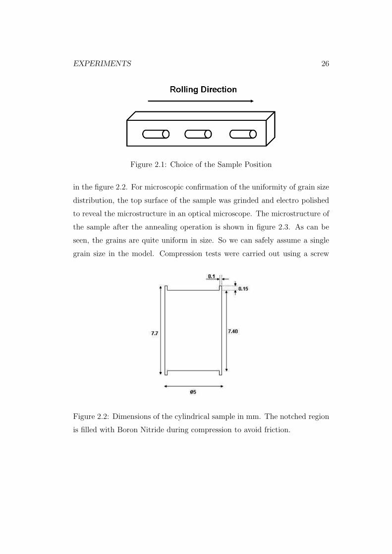
2.1 Choice of the Sample Position . . . . . . . . . . . . . . . . . . 20
2.2 Dimensions of the cylindrical sample in mm. The notched
region is filled with Boron Nitride during compression to avoid
friction. . . . . . . . . . . . . . . . . . . . . . . . . . . . . . . 20
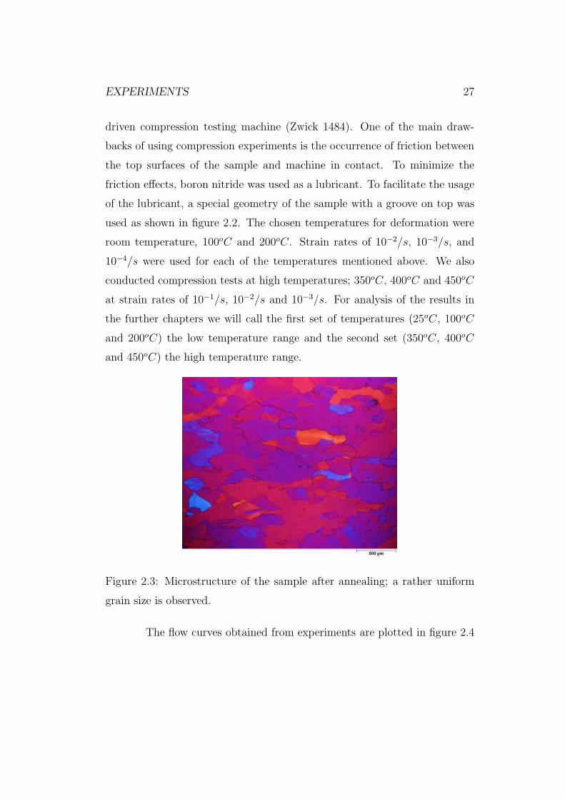
2.3 Microstructure of the sample after annealing; a rather uniform
grain size is observed. . . . . . . . . . . . . . . . . . . . . . . . 21
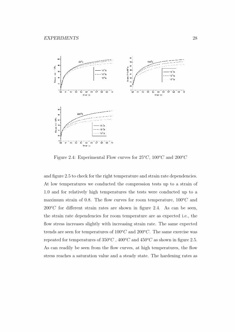
2.4 Experimental Flow curves for 25oC, 100oC and 200oC . . . . . 22
2.5 Experimental Flow curves for 350oC, 400oC and 450oC . . . . 23
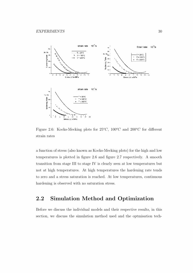
2.6 Kocks-Mecking plots for 25oC, 100oC and 200oC for different
strain rates . . . . . . . . . . . . . . . . . . . . . . . . . . . . 23
2.7 Kocks-Mecking plots for 350oC, 400oC and 450oC for different
strain rates . . . . . . . . . . . . . . . . . . . . . . . . . . . . 24
2.8 Flow chart describing the simulation method . . . . . . . . . . 25
3.1 3IVM Optimized Flow curves for 350oC, 400oC and 450oC
and strain rates of 10−1/s, 10−2/s and 10−3/s . . . . . . . . . 34
3.2 Evolution of Dislocation Densities at 350oC and strain rate of
10−1/s . . . . . . . . . . . . . . . . . . . . . . . . . . . . . . . 35
xi

3.3 3IVM Optimized Flow curves for 25oC, 100oC and 200oC and
strain rates of 10−2/s, 10−3/s and 10−4/s . . . . . . . . . . . . 37
3.4 Evolution of Dislocation Densities at 25oC and strain rate of
10−2/s . . . . . . . . . . . . . . . . . . . . . . . . . . . . . . . 38
3.5 3IVM Optimized Flow curves for 25oC, 100oC, 350oC, 400oC
and strain rates of 10−2/s and 10−3/s . . . . . . . . . . . . . . 39
4.1 Relation between force profile, F(y), of obstacles and ∆G: (a)
Square shaped obstacle as in equation 4.4 (b) Parabolic shaped
obstacle as in equations 4.6 and 4.7 . . . . . . . . . . . . . . . 44
4.2 Schematic showing the dependency of the production of mobile
dislocations on the slip length of the dislocation which in turn
depends on the cell size . . . . . . . . . . . . . . . . . . . . . . 50
4.3 The dislocation length produced during bow out is lost instan-
taneously by overcoming the particles . . . . . . . . . . . . . . 50
4.4 Schematic showing of one possible clearing effect; dislocation
(2) and (3) are in dipole configuration. The mobile dislocation
(1) can annihilate with dislocation (2) and hence make the
dislocation (3) mobile. . . . . . . . . . . . . . . . . . . . . . . 52
4.5 Simulated Stress Strain curves for T = 25oC, 100oC and 200oC
; (a), (b) and (c) ǫ = 10−2/s, (d), (e) and (f) 10−3/s and (g),
(h) and (i) 10−4/s . . . . . . . . . . . . . . . . . . . . . . . . . 57
4.6 Dislocation density evolution for T = 100oC and ǫ = 10−2/s
; (a) Mobile dislocation density (b) Immobile dislocation den-
sity in the cell interiors (c) Immobile dislocation density in the
cell walls (d) Total dislocation density. . . . . . . . . . . . . . 58
xii
4.7 Simulated Stress Strain curves for T = 350oC, 400oC and
450oC; (a), (b) and (c) ǫ = 10−1/s (d), (e) and (f) 10−2/s,
(g), (h) and (i) 10−3/s . . . . . . . . . . . . . . . . . . . . . . 59
4.8 Dislocation density evolution for T = 350oC and ǫ = 10−2/s;
(a) Mobile dislocation density (b) Immobile dislocation den-
sity in the cell interiors (c) Immobile dislocation density in the
cell walls (d) Total dislocation density. . . . . . . . . . . . . . 60
4.9 Simulated Stress Strain curves for T = 25oC,100oC, 350oC,
400oC ; (a), (b), (c) and (d) ǫ = 10−2/s, (e), (f), (g) and (h)
10−3/s . . . . . . . . . . . . . . . . . . . . . . . . . . . . . . . 62
4.10 Dislocation Density evolution at 100oC and a strain rate of
10−2/s ; (a) Mobile dislocation density (b) Immobile dislo-
cation density in the cell interiors (c) Immobile dislocation
density in the cell walls (d) Total dislocation density . . . . . 63
xiii

Chapter 1
Literature Review
Our present work makes use of the existing theories and experimentally ob-
served microstructural information to model work hardening. There are
many ways to model work hardening, each one of them has its own advan-
tages and disadvantages. We will list some of the most important approaches
and their salient features below. Some of the existing work hardening models
have been reviewed recently [4,6]. Before we describe the various models, we
will review some of the earlier work hardening theories.
1.1 Earlier Theories
It is well established that flow curves at relatively low temperatures can
be distinguished into various stages of work hardening. Stage I, also called
the easy glide stage, is associated with the the glide of dislocations over long
distances without hindrance by other dislocations. Stage II is associated with
a linear hardening rate and is only slightly temperature dependent. Stage
III begins as soon as the flow curve deviates from linearity. The process
1
LITERATURE REVIEW 2
controlling the hardening rate during this state is generally believed to be
cross slip of screw dislocations. stage V [7] which are have been observed.
The theories on the initiation of stage III date back to the 1950’s.
Seeger and coworkers [8–10] had postulated a pileup model to explain the
occurrence of cross slip. They postulate that when the pileup stresses of the
dislocations is high enough, cross slip occurs. They also predict an expo-
nential variation of τIII (stress where stage III initiates) with temperature.
This theory was contradicted by another one by Friedel [11]. Friedel’s theory
doesn’t require pileup of dislocations for cross slip to occur. They describe
cross slip as a thermally activated process and requires the formation of
constriction by pinching of partial dislocations. Based on their theory they
predict a linear variation of τIII with temperature.
Another prominent theory emerged later by Kuhlmann-Wilsdorf [12,
13], called the mesh length theory, states that the gliding dislocations arrange
into stress screened low energy structures and the flow stress is the stress
needed to generate new glide dislocations. It makes extensive use of the
principle of similitude i.e., once nature has selected a particular geometry,
increasing stress will cause that structure to remain similar to itself but shrink
in scale such that l = 1/τ . In the following section we will consider select
work hardening models starting with the one parameter model by Kocks.
LITERATURE REVIEW 3
1.2 Statistical Dislocation Density Based Mod-
els
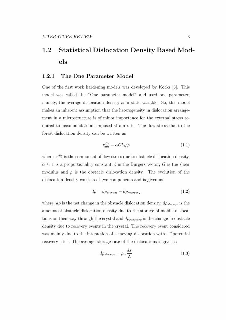
1.2.1 The One Parameter Model
One of the first work hardening models was developed by Kocks [3]. This
model was called the ”One parameter model” and used one parameter,
namely, the average dislocation density as a state variable. So, this model
makes an inherent assumption that the heterogeneity in dislocation arrange-
ment in a microstructure is of minor importance for the external stress re-
quired to accommodate an imposed strain rate. The flow stress due to the
forest dislocation density can be written as
τdisath = αGb
√ρ (1.1)
where, τdisath is the component of flow stress due to obstacle dislocation density,
α ≈ 1 is a proportionality constant, b is the Burgers vector, G is the shear
modulus and ρ is the obstacle dislocation density. The evolution of the
dislocation density consists of two components and is given as
dρ = dρstorage − dρrecovery (1.2)
where, dρ is the net change in the obstacle dislocation density, dρstorage is the
amount of obstacle dislocation density due to the storage of mobile disloca-
tions on their way through the crystal and dρrecovery is the change in obstacle
density due to recovery events in the crystal. The recovery event considered
was mainly due to the interaction of a moving dislocation with a ”potential
recovery site”. The average storage rate of the dislocations is given as
dρstorage = ρmdx
Λ(1.3)

LITERATURE REVIEW 4
where, ρm is a certain fraction of the total dislocation density which is stored
in the crystal after moving a distance dx. Λ is the mean free path of the
dislocation. This mean free path is determined by a statistical process and
is proportional to the mean spacing of the obstacle dislocations, Λ = β/√
ρ.
The recovery rate in equation 1.2 is given as
dρrecovery =LR
bρ (1.4)
where, LR is the average length of the dislocation getting annihilated at a
potential recovery site. Kocks and Mecking presented a novel way of depict-
ing the stress-strain curves namely, by plotting the work hardening rate (Θ)
against stress (σ); where the work hardening coefficient is given as
θ =δσ
δǫ
∣∣∣∣ǫ,T
(1.5)
This plot is very commonly refered to as the ”Kocks-Mecking” plot. In
Collaboration between Kocks and Mecking [5,14–16], Estrin and Mecking [17]
and Follansbee and Kocks [18], this model through the years has undergone
many changes and has evolved into what is called the ”Mechanical Threshold
Model” (MTS model) [19].
1.2.2 Multi Parameter Models - Concept
Apart from the One Parameter Model described above, most of the later at-
tempts for the development of a unified plasticity model are multi-parameter
models that consider more than one state variable to describe the microstruc-
ture. The one Parameter Model was followed by a different class of models
called the two phase composite models which described the microstructure
to consist of ”soft regions” (cell interiors with low dislocation density) and
”hard regions” (cell walls with high dislocation density), in agreement with
LITERATURE REVIEW 5
the direct observations of internal stress [2, 20, 21] and with observations of
creep an-elasticity [21]. All the multi parameter models existent today not
only differ from each other in the choice of state variables and underlying pro-
cesses considered for dislocation storage and recovery, but also in the number
of state variables. We will list some of the models which are based on the
multi-parameter description of the microstructure and describe briefly the
salient features of the models.
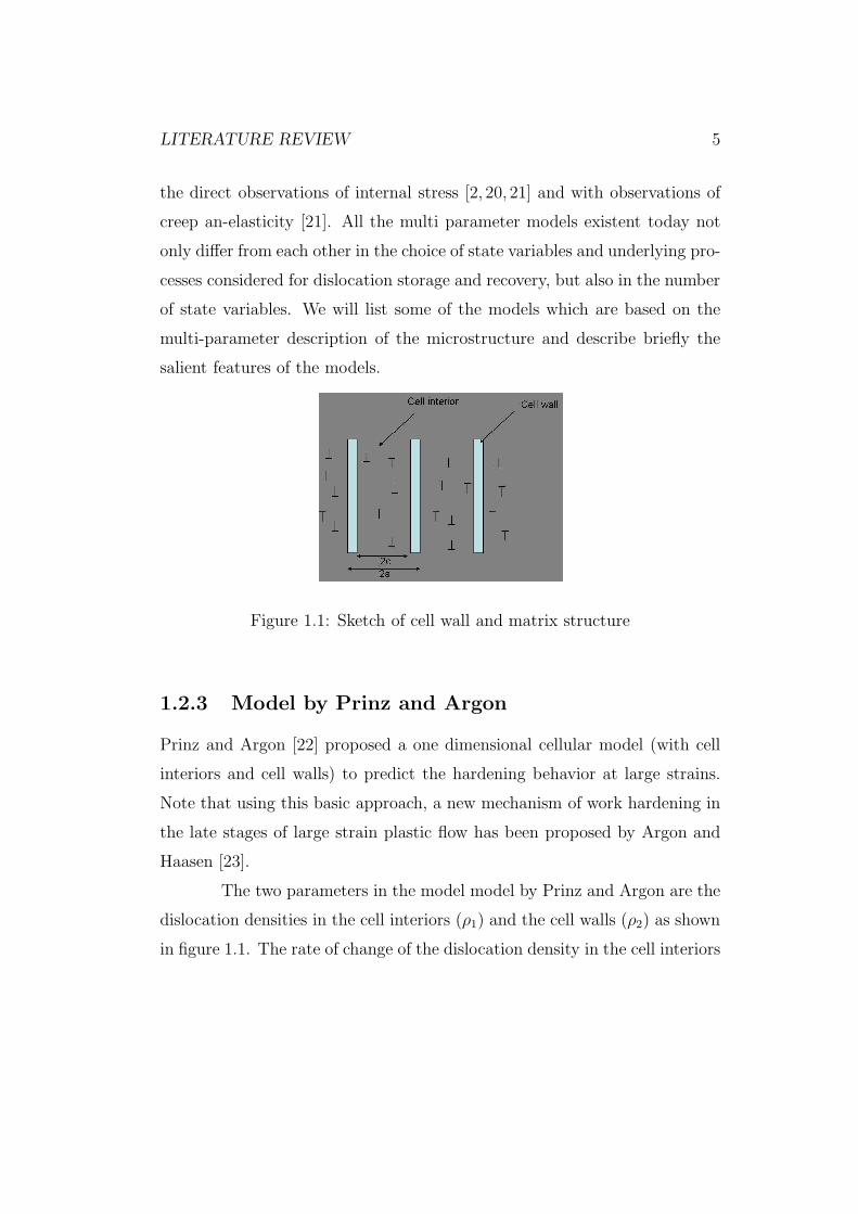
Figure 1.1: Sketch of cell wall and matrix structure
1.2.3 Model by Prinz and Argon
Prinz and Argon [22] proposed a one dimensional cellular model (with cell
interiors and cell walls) to predict the hardening behavior at large strains.
Note that using this basic approach, a new mechanism of work hardening in
the late stages of large strain plastic flow has been proposed by Argon and
Haasen [23].
The two parameters in the model model by Prinz and Argon are the
dislocation densities in the cell interiors (ρ1) and the cell walls (ρ2) as shown
in figure 1.1. The rate of change of the dislocation density in the cell interiors

LITERATURE REVIEW 6
in this case is given as
dρ1
dγ=
dρ+
1
dγ+
dρ−1
dγ(1.6)
=
(2πα
bK2
)
ρ1/2
1 − La
K2bρ1 (1.7)
Where, α ≈ 0.5, γ is the shear rate, K is a constant determining the mean
spacing of the regions in the obstacle network that are impenetrable to dis-
locations, La is the eliminated line length of the dislocation when glide dis-
locations sweep through a certain volume in the crystal. The first term in
the above equation, is the rate of increase of the dislocation density in the
cell interiors due to the storage of dislocation loops which interact with the
impenetrable dislocation forests as postulated by Kocks [24]. The second
term corresponds to the recovery event due to the annihilation of a moving
dislocation, when it encounters a metastable cluster (eg. stored loop or a
partially pinned dipole) that can be annihilated when the pinning constraint
is removed. For a detailed description of the variables in the above equation,
see [22].
The rate of change of the dislocation density in the cell walls is given
asdρ2
dγ=
√
2
3
(a
h
1
b
)
x1/2ρ1/2
1 − 2
γKiρ
y2 (1.8)
where, a is the radius of the cells as shown in figure 1.1, h is the cell wall thick-
ness, x is the ratio of the mobile dislocations to the total dislocation density
and y = 2 for lattice diffusion and y = 3 for core diffusion (K2 and K3 are
different expressions for lattice diffusion and core diffusion respectively) [22].
Although the authors use the above model only in an intermediate
temperature range to compare with the experimental results of Lloyd et.
al [25] for pure aluminum, they claim that by determining the constants

LITERATURE REVIEW 7
appropriately the low temperature behavior can also be predicted with their
model.
1.2.4 Model by Estrin
Another classic model was developed by Estrin et.al [26]. It is a multi param-
eter model based on a cellular microstructure to describe the work hardening
stages (including stage IV) in large strain deformations. They attempt to
combine within a single model a dislocation theory-based approach with a
solid-mechanics treatment taking into account the real topology of the dislo-
cation structure. They consider it essential to take into account the variation
of cell wall volume fraction [27, 29] during deformation. As dislocation glide
is rate and temperature sensitive, they write the equations relating the shear
stress and resolved shear strain rate as
τ rw + τ i
w = τ 0
w
(γr
w
γ0
) 1
m
(1.9)
τ rc + τ i
c = τ 0
c
(γr
c
γ0
) 1
m
. (1.10)
Here, 1/m is the strain rate sensitivity index, τ rw and τ r
c are the resolved
stresses in the walls and interiors respectively, τ iw and τ i
c are the internal
stresses in the walls and interiors respectively, γ0 is the reference shear strain,
while the quantities τ 0w and τ 0
c express the glide resistance in the cell walls
and cell interiors at absolute zero temperature. The latter are given as
τ 0
w = αGb√
ρw (1.11)
τ 0
c = αGb√
ρc (1.12)
where ρw and ρc are the dislocation densities in the cell walls and
cell interiors respectively.

LITERATURE REVIEW 8
For the evolution of the dislocation structure during deformation, it
is assumed that dislocation generation takes place only in the cell walls by
Frank-Read sources. Dislocation annihilation is considered both in the cell
interiors and cell walls. Calculating the number of ”operative” Frank-Read
sources on the surface of the cell walls, they obtain the rate of dislocation
emission by these ”operative” sources into the cell interiors, which is given
as
(ρc)+ = α∗ 2
3√
3
√ρw
bγw (1.13)
where, α∗ is a factor taking into account that not every dislocation source is
operative. Assuming that a fraction β∗ of the dislocations which are within
a distance vcdt from the cell walls will become part of the walls, the loss of
the cell interior dislocations as they move and join the walls is expressed as
(ρc)−walls = β∗ 4γc
bd√
1 − f(1.14)
Where, f is the volume fraction of the cell walls. They consider cross-slip as
the process of dynamic recovery. The loss rate of the cell interior dislocations
due to cross-slip in their case is given as
(ρc)−cs = −k0
(γc
γ0
)−1
n
γcρc (1.15)
where, k0 is a constant and n is a parameter which is inversely proportional
to temperature.
Apart from the gain of the dislocation density in the cell walls due
to the loss of the cell interior dislocations as described in equation 1.14,
the generation of dislocations in the cell walls due to operative Frank-Read
sources is given as
(ρw)+FR =2β∗γc(1 − f)
√ρw
fb√
3(1.16)
LITERATURE REVIEW 9
Recovery in the walls due to cross-slip is treated in a similar way as equa-
tion 1.15. From the experimental values of the change in the volume fraction
(f) of cell walls [27] they derive a function for the variation in the volume
fraction of cell walls with the resolved shear strain described as
f = f∞ + (f0 − f∞)exp
(−γr
γr
)
(1.17)
where, f0 is the peak value of f , f∞ is its saturation value at large strains
and the quantity γr describes the rate of decrease of f .
Their model is tested for the case of torsion deformation of pure
polycrystalline copper at room temperature. A good agreement is found
between the experimental hardening rates results and simulated hardening
rates for all hardening stages, including stage V. The authors also considered
the effect of the evolution of the deformation texture (considering evolving
Taylor factor) as obtained from texture simulations. A comparison of the dis-
location densities from the model is also made with the experimental results.
Other temperatures were not considered as their main aim was to predict the
hardening rate especially for the late stages of deformations (stage IV and V).
1.2.5 Microstructural Metal Plasticity Model - E. Nes
Another recent composite structure based model is the M¯
icrostructural M¯
etal
P¯lasticity (MMP) model developed by Nes et al. [4, 30–34]. The choice of
the state variables in this model are novel. This model is again a multi-
parameter model based on the assumption of a cellular microstructure and
considers the cell size (δ), the dislocation density in the cell interiors (ρi) and
the boundary. Though all models differ in the choice of the state variables
and the description of the microstructure in terms of the state variables,

LITERATURE REVIEW 10
there is agreement that the stress (τ) needed to move a dislocation through an
obstacle environment should consist of a thermal component and an athermal
component. In the MMP model this stress is given as
τ = τt + τa (1.18)
τ = τt + τp + α1Gb√
ρi + α2Gb(1/δ + 1/D) (1.19)
where, τt is the strain rate and temperature dependent short range stress
(stress needed to overcome the local obstacles) and τa is the rate and tem-
perature independent long range stress (also called the passing stress), τp is
the stress needed to overcome the non deformable particles, on the way of
the moving dislocations, G is the shear modulus, b the Burgers vector of the
dislocation, α1 and α2 are constants, δ is the sub grain size, D is the average
grain size and ρi is the dislocation density in the cell interiors. The average
velocity v of the dislocations in this case is given as
v = laBtνDexp
(
− Ut
kT
)
2sinh
(τtVt
kT
)
(1.20)
where, la is the travel distance between obstacles, Ut is the activation en-
ergy for glide, Vt is the activation volume, νD is the Debye frequency, Bt
is a constant, k is the Boltzmann constant and T is the temperature. By
substituting equation 1.20 into the Orowan equation, which relates the shear
rate (γ) with the mobile dislocation density (ρm),
γ = ρmbv (1.21)
the thermal component of the flow stress (τt) is calculated.
The structure evolution equations in the MMP model are given as
LITERATURE REVIEW 11
below.
dρi
dγ=
1
1 + f(qb)
2
bLeff− ρivi
γ(1.22)
dδ
dγ= −2δ2ρi
κ0φ
SL2
Leff+
bvδ
γ(1.23)
dφ
dγ= f(ρi, δ, φ) (1.24)
For a detailed description of these equations and the model concepts, see [4].
The model is tested in the relatively high temperature range of 200oC to
550oC with various strain rates. The model predictions agree well with ex-
periments.
1.2.6 Model by Nix
All the above mentioned models don’t distinguish between edge and screw
dislocations. There have been attempts to treat the edge and screw dislo-
cation densities as separate state variables [35, 36] and hence consider both
cross-slip and climb as the essential recovery mechanisms.
Nix et al. [21] in an attempt to predict the work hardening stages
beyond stage III, developed a composite structure based model with a dis-
tinction between edge and screw dislocations. The main idea behind the
partitioning was to use diffusion controlled climb as the rate controlling mech-
anism at high temperatures and to use cross-slip of screw dislocations as the
rate controlling recovery mechanism at low temperatures. Their model has
two internal state variables, namely, the edge dislocation density (present
only in the cell walls) and the screw dislocation density (present only in the
cell interiors). The screw dislocations are allowed to glide, multiply, cross-
slip and annihilate inside the cell interiors. The recovery events the authors

LITERATURE REVIEW 12
consider are the climb of edge dislocations in the cell walls and the cross-
slip of screw dislocations in the cell interiors. However these two recovery
mechanisms are coupled in a way that neither of them can act independently.
According to Nix et al., this coupling is one of the most important factors to
be able to get reasonable hardening rates. Another model by the present au-
thors namely 6IVM [36] explicitly considered edge and screw dislocations as
separate variables. The results from 6IVM support the conclusion of Nix et
al. that the screw dislocation and edge dislocation reaction must be coupled
enough to get reasonable hardening rates.
The kinetics of plastic flow in both in the cell interiors and cell walls
in this model are described as
γi = γ0
(
exp
(−∆F
kT
)){
exp
(∆F
kT
τi
τi
)
− 1
}
(1.25)
where, i = C, W stands for the cell interiors or cell walls respectively. τi is
the strength of a particular region (cell interiors or cell walls) related to the
dislocation density through the Taylor equation, τi is the stress in the interiors
or walls. ∆F is the strength of the dislocation obstacles and is taken to be,
∆F = c1Gb3 (c1 is arbitrarily chosen as 0.5). The pre-exponential constant
is given as 1012(τi/G)2. The processes that occur in the cell interiors are
coupled with those in the cell walls through the mechanics of the composite
structure. For this they assume the total strain rate, composed of the plastic
and elastic strain rates to be the same in each region.
γ = γC +τC
G= γW +
τW
G(1.26)
where, γC and γW represent the plastic shear strain rates in the cell interiors
and cell walls respectively, while the second term in the above equation repre-
sents the elastic strain rate in that region. An overall mechanical equilibrium

LITERATURE REVIEW 13
condition is also assumed which is represented as
τ =LC
LC + LWτC +
LW
LC + LWτW (1.27)
where, LC and LW represent the thickness of the cell interiors and cell walls
respectively.
The hardening rate due to dislocation storage in the cell interiors is
given as(
dτC
dγC
)+
=G
2ΛC√
ρC
(1.28)
where ΛC is the mean spacing of the dislocations and is taken as λC =
100ρ−1/2
C . According to the authors, the choice of the factor 100, produces
realistic strain hardening rates. Therefore the rate of strain hardening in the
cell interiors takes the expression(
dτC
dγC
)+
=G
200(1.29)
The dynamic recovery in the cell interiors is due to the cross-slip and an-
nihilation of screw dislocations of opposite sign. The net loss rate due to
dynamic recovery is given as(
dτC
dγC
)−= −10
b
wν0
G
γC
(
exp−Wcs
kT
){
exp
(τCbαWcs
kTGb
)
− 1
}
(1.30)
where, α is a constant fit parameter, w ≈ 100b is the length of the recovery
site where cross-slip can occur, ν0 is the attempt frequency for cross-slip, Wcs
is the activation energy for cross-slip.
Therefore the final structure evolution equations in the cell interiors
can be summarized as
dτC
dγC=
(dτC
dγC
)+
+
(dτC
dγC
)−(1.31)
=G
200− 10
b
wν0
ν0
γC
exp
(−Wcs
kT
){
exp
(τCbA
kT
)
− 1
}
(1.32)
LITERATURE REVIEW 14
As indicated above when screw dislocations move, they deposit edge dislo-
cations in the cell walls. This hardening contribution is given as
(dτW
dγC
)
= − Gb
2√
ρW
dρW
dγC(1.33)
Recovery in the cell walls is assumed to occur by diffusion controlled climb
and annihilation of edge dislocations of opposite sign. Hence the recovery
rate in this case is given as
(dτW
dγC
)−=
Gb
2√
ρW
dρW
dt
1
γC
(1.34)
Therefore the final structure evolution equation in full form, in the
cell walls is written as,
dτW
dγC
=
(dτW
dγC
)+
+
(dτW
dγC
)−(1.35)
=bG2
LW τW
− 1
2G
(τW
G
)3Gb
kTDL
1
γC
(1.36)
The authors of the above model used it to predict stress-strain curves
for pure nickel at various temperatures. Their simulations show good agree-
ment with experiments. It is worth noting that the parameter ∆F in equa-
tion 1.25 is not a constant but assumed to increase with temperature. They
also confirm from their calculations that climb is the rate controlling reaction
for recovery at high temperatures and annihilation of screw dislocation by
cross-slip controls the recovery mechanism at low temperatures. Their model
predictions are also compared with torsion experiments on Ni-Co alloys. In
their study they predict flow curves at both low and high temperatures but
only separately.

LITERATURE REVIEW 15
1.2.7 3 Internal Variables Model (3IVM) - Roters et.
al
Roters et al. [1] developed a novel 3 internal variables model. Our present
models have a basic structure similar to the 3IVM. Since its inception, there
have been numerous developments to this model and they have been applied
to predict the flow behavior of various commercial aluminum alloys [49, 50].
The original 3IVM has been coupled with FEM codes to predict complex
forming operations like rolling [47,48]. It has also been coupled with texture
models and recrystallization models in an attempt to develop a ”through
process model” [45,46]. We will describe some salient features of this model
briefly. For more detailed description, refer to chapter 3.
The 3IVM is another composite structure based model which relies
on on 3 internal state variables, namely 3 dislocation densities; the mobile
dislocation density (ρm), the immobile dislocation density in the cell interiors
(ρi) and the immobile dislocation density in the cell walls (ρw). The mobile
dislocations move to accommodate the imposed strain rate and on their way
interact with other dislocations. There is no distinction between edge and
screw dislocations and the ruling recovery mechanism in this model is due
to the climb of immobile edge dislocations. A variant of this model to in-
clude both screw and edge dislocation densities has also been developed by
Karhausen et. al [35] (see 1.2.8) and Gottstein et. al [36].
In the 3IVM, the kinetic equation of state which calculates the ex-
ternal stress required to accommodate an imposed strain rate is the Orowan
equation.
γ = ǫM = ρmbv (1.37)
where, γ is the shear rate, M is the Taylor factor and v is the average velocity
LITERATURE REVIEW 16
of the mobile dislocations. If we assume jerky motion of the dislocation, i.e.,
the dislocations would glide long distances and wait in front of the obsta-
cles to overcome them by thermal activation, then the average velocity of a
dislocation is written as
v = λν0exp
(−Q
kT
)
sinh
(τeffV
kT
)
(1.38)
By substituting equation 1.38 into equation 1.37 the effective stress can be
calculated. As the mean spacing of obstacles is different in the cell interiors
and cell walls (depending on the respective dislocation densities), two effec-
tive stress values are obtained, one for the cell interiors and the other for the
cell walls. The total shear stress is calculated by adding the above calculated
short range stresses to the long range passing stress of the dislocations.
τx = τeffx+ αGb
√ρx (1.39)
where, x = i, w and α is a geometrical constant and G the shear modulus.
The total external stress required to accommodate the imposed strain rate
is then calculated by weighting the stress in the cell interiors and cell walls
by the corresponding volume fractions of the cell walls (fw) and cell interiors
(fi).
σext = M(fiτi + fwτw) (1.40)
In the above equation, M is the average Taylor factor to take into account
the orientations in the polycrystalline materials.
For predicting the complete stress-strain curve, like all other mod-
els described above, a set of structure evolution equations for each class of
dislocation density are developed which have a common form given as
ρx = ρx+ + ρx
− (1.41)

LITERATURE REVIEW 17
where, the index x = m, i, w for mobile, cell interiors and cell walls respec-
tively.
The production of mobile dislocations, which is calculated by ex-
tending the Orowan equation on a larger time scale is given as
ǫ = ˙ρ+mbLeff
1
M(1.42)
where, Leff is the effective length that a dislocation will travel before it
is immobilized by any of the obstacles on its way through the crystal. It
is noteworthy that Roters [44] has also introduced a novel concept for the
calculation of the mobile dislocation density. Two approaches were tried in
this respect,
1. Keeping the mobile dislocation density constant
2. Obtaining the value of the mobile dislocation density by minimizing
the plastic work rate
When applied to a single stress strain curve both concepts give about equal
results when the constant dislocation density is chosen close to the aver-
age mobile dislocation density obtained by the minimization process. When
applied to a set of stress strain curves, it was seen that the average value
of mobile dislocation density obtained by the minimization process showed
significant variations. As a consequence the second concept shows a higher
strain rate sensitivity than the first one. They conclude that the stress-strain
curve predictions along with their strain rate change tests indicate that the
second method of minimizing the plastic work rate results in a more realistic
form of the stress strain curves.
In the 3IVM, the evolution of each class of dislocation densities are
obtained by considering the probability for a particular dislocation reaction
LITERATURE REVIEW 18
to take place. The loss of mobile dislocation density is assumed to occur due
to three reactions, namely, annihilation, lock formation and dipole formation.
Hence, the total loss rate of the mobile dislocation density is given as
ρ−m = ρ−
m(annihilation) + ρ−m(lock) + ρ−
m(dipole) (1.43)
The details of the parameters used in the above equation can be found in
[1].
The net rate of change of immobile dislocation density in the cell
interiors is given as
ρi = ρ+
i (lock) + ρ−i (climb) (1.44)
The third class of dislocation density, the dislocation density in the cell walls
(ρw), undergoes the same processes as in the cell interiors with one additional
reaction. It is assumed that all the dipoles that are formed in the cell interiors
are instantly swept into the walls by mobile dislocations. Hence the rate of
gain of the wall dislocation density due to this reaction is equal to the number
of mobile dislocations lost due to the formation of dislocation dipoles.
The detailed description of the model concepts with results and anal-
ysis is presented in chapter 3.
1.2.8 4 Internal Variables Model - Roters and Karhausen
Roters and Karhausen considered 4 internal state variables in their model,
namely, the immobile edge and screw dislocation densities in the cell interiors
(ρei and ρsi) and the immobile edge and screw dislocation densities in the
cell walls (ρew and ρsw). The calculation of the external stress is completely
analogous to the procedure as described in [1] with the exception that the
new state variables are now included in the equations. Considering the screw

LITERATURE REVIEW 19
dislocation densities, the shear stress is calculated as
τx = kT
(
c1
√ρex + ρsx +
c2
Leff
)
asinh
[
c3γ
(√ρex + ρsx +
1
Leff
)
exp
(Qglide
kT
)]
+ c4
√ρex + ρsx
(1.45)
where the subscript x denotes either w for cell walls or i for cell interiors, c1 to
c4 are constants and Leff is the effective spacing of precipitates and all other
symbols have their usual meaning. The total external stress is calculated in
a similar way as in [1] and is weighted by the respective volume fractions.
σ = M (fwτw + (1 − fw)τi) (1.46)
where, M is the average Taylor factor and fw is the volume fraction of the cell
walls. The evolution of the edge dislocation densities is treated in a similar
way as the 3IVM with the consideration of pipe diffusion in addition to bulk
diffusion for the climb and annihilation of the immobile edge dislocations.
With this new modification the evolution equations for the edge dislocations
can be summarized as
ρew =
(
c3 +c6
τext
)
γ −[
c7exp
(−Qbulk
kT
)
+ c8exp
(−Qcore
kT
)
ρew
]τw
kνρ2
ew
(1.47)
ρei = c5γ −[
c7exp
(−Qbulk
kT
)
+ c8exp
(−Qcore
kT
)
ρei
]τi
kTρ2
ei (1.48)
For an explanation of the constants used in the above equations see [35].
Like the equations above, the evolution equations for the screw dislocation
densities also have production and reduction terms. Considering cross-slip
as the main recovery mechanism for screw dislocations, the rate equations
read as
ρsw =
(−Qcross
kT
)
γ − c11
τw
kTexp
(−Qcross
kT
)
ρ2
sw (1.49)
ρsi = c9γ − c11
τi
kTexp
(−Qcross
kT
)
ρ2
si (1.50)

LITERATURE REVIEW 20
The authors use the model to predict the behavior of aluminum
alloys during multi-stand hot rolling with a view accurately describing the
flow stress, dependent on strain rate, temperature and forming history.
As described in this section there are numerous models available
which in some cases vastly differ from each other and still allow for accurate
descriptions of the flow stress. Apart from studying the stages of work hard-
ening and predicting the stress-strain curves of metals and alloys, two phase
models of cells and cell walls have also been used, to study the constant strain
rate and creep tests [37], to model plastic composites [38] and also to model
persistent slip bands in fatigued materials [39].
1.3 Empirical Models
This class of models describe the flow stress in terms of power laws as a
function of strain with many empirical constants. As compared to the statis-
tical dislocation density based models that we discussed in the last section,
these models have little physics in them and the constants usually cannot
be related to any physical process or phenomenon. In spite of this inher-
ent disadvantage, these models are extensively used in FEM codes to model
plasticity as they require low computational resources and provide excellent
fits for any given deformation condition. But these models don’t have any
predictive power beyond the experimental data range. In what follows, we
will discuss some of these approaches briefly. One of the simple approaches
is the Holloman equation which describes the flow stress as a simple power
law in strain given as
σ = kǫmH (1.51)

LITERATURE REVIEW 21
where, k and mH are fitting parameters. Ludwig made a minor change in
the above equation to take into consideration the yield stress of the material.
σ = σ0 + kǫmL (1.52)
If the dependency of the constants on the temperature and strain rate is
defined then the complete flow field can be described.
Voce [40] for the first time postulated the existence of a saturation
stress at large strain and a need to be able to predict it at large strains. He
expressed the stress as
σ = σs + (σ0 − σs)exp
(−ǫ
k
)
(1.53)
where k is a constant and σs is the saturation stress.
A more complex model was developed by Chaboche et al. [41]. It is
a micro-mechanical model and like other models, makes use of state variables
and also defines the evolution of the state variables but the constants used
in the model are purely fit parameters and don’t relate to any specific mech-
anism of microstructural evolution. The definition of the one-dimensional
form of the model is given by:
ǫvp =
⟨ |σ − a| − k
Z
⟩n
︸ ︷︷ ︸
sgn(σ − a) (1.54)
a = a1 + a2 (1.55)
ai = Hiǫvp − Diaip for i=1,2 (1.56)
ai(t = 0) = 0 (1.57)
k = 0, k(t = 0) = k0 (1.58)
where, ǫvp is the viscoplastic strain rate. The kinematic hardening variables,
a1 and a2, p is and the isotropic hardening variable k are the internal state

LITERATURE REVIEW 22
variables in the model. The parameters for the yield stress (k0), the stress
exponent (n), the viscosity (Z), the kinematic hardening (H1 and H2), the
dynamic recovery (D1 and D2) describe the behavior for one temperature at
a certain phase state. The above mentioned parameters depend on temper-
ature and phase variables. For every temperature and for every phase state,
mechanical data (tensile, compression, relaxation) are needed to determine
the parameters. This category of models have many fit parameters with no
physical meaning. They also don’t have any predictive power beyond the ex-
perimental measurements. Hence they are not suitable for through process
modeling in which the state variables are changed during heat treatment.
1.4 Dislocation Dynamics Models
As described in section 1.2 the statistical dislocation density based models
make use of the dislocation density as a state variable. Statistical dislocation
models don’t consider the spatial resolution of the dislocations but rather take
into account the collective behavior of dislocations to describe the evolution of
the state variables. Even in the composite models described above, though
heterogeneity in dislocation arrangement is considered in the form of cell
interiors and cell walls, the arrangement within the cell interiors (and cell
walls) is still considered to be homogeneous. This assumption is inaccurate
because local low energy dislocation configurations are not considered.
Dislocation Dynamics models, on the other hand take the spatial
resolution of dislocations into account and consider the specific reactions
between dislocations at a mesoscopic scale. Dislocation dynamics simulations
have been tried in both 2 Dimensions(eg., [42]) and 3 Dimensions (eg., [43]).
In these models the dislocation curves are approximated by a series of straight
LITERATURE REVIEW 23
segments of mixed character. The interaction force per unit length (Peach-
Koehler force), a given segment exerts on a remote segment is evaluated at
the center of the remote segment. The motion of each dislocation segment
is determined by the evaluated total Peach-Koehler force (Fi on segment i)
which arises from all other dislocation stress fields and the applied stress,
such that
Fi =
N∑
j=1
j 6=ij 6=i+1
j 6=i−1
(σDj + σa).bi
× ξi, + Fi,i+1 + Fi,i−1 (1.59)
where, N is the total number of dislocation segments, σDj is the stress tensor
from a remote segment, σa is the applied stress, ξi is the line sense vector,
Fi,i+1 is the interaction forces between segments i and i + 1. Depending
on the force components on each segment, the velocity of the dislocations
can be calculated and the segments move to their new positions. Hence the
true motion of the individual dislocations can be simulated. As can be seen
from the above equation, this model has an inherent disadvantage of heavy
computational burden and with the present state of the art computers, stress-
strain curves only upto a strain of ≈ 1% can be predicted in a single crystal.
Therefore, statistical models are an advantage and are used in the present
work.
1.5 Summary
In this chapter, we discussed three main approaches for predicting the hard-
ening behavior (complete stress-strain curves) of metals and alloys. In sec-
tion 1.2 we described the statistical dislocation density based models which
LITERATURE REVIEW 24
make use of the dislocation processes to describe the hardening and recovery
and hence be able to predict the hardening behavior. The empirical models
(section 1.3) have a low computational burden but have too many fit parame-
ters which are not related to the underlying physical phenomena. Lastly, the
dislocation dynamics models (section 1.4) have accurate spatial resolution of
dislocations and also include the various dislocation reactions at mesoscopic
scale but have much too heavy computational burden. Statistical dislocation
density based models (section 1.2) make a compromise between the com-
putational demand and the physics involved in the model. They have only
moderate computational demands and involve fit parameters with a physical
meaning. This justifies the choice of our present model for the prediction of
hardening behavior of FCC metals and alloys.

Chapter 2
Experimental Results and
Simulation Technique
2.1 Experimental Procedure and Results
To validate the flow curve predictions from our models that we will discuss
in the subsequent chapters, we conducted compression experiments on alu-
minum (99.9% purity) samples for a wide range of strain rates and temper-
atures. The base material (obtained from Hydro Aluminum) was aluminum
(99.9% purity) which was warm rolled and given a 50% reduction. To avoid
potential heterogenities in texture, chemistry and grain sizes in the block
which could lead to undesirable results during compression, the samples were
annealed at 400oC for 1 hour. The samples are recrystallized and hence lead
to a uniform grain size. Compression samples were cut from the block by
spark erosion. To further ensure uniform grain sizes, chemistry and texture of
various samples, the compression samples were taken from the middle of the
block as shown in figure 2.1. The sample geometry and dimensions are shown
25
EXPERIMENTS 26
Figure 2.1: Choice of the Sample Position
in the figure 2.2. For microscopic confirmation of the uniformity of grain size
distribution, the top surface of the sample was grinded and electro polished
to reveal the microstructure in an optical microscope. The microstructure of
the sample after the annealing operation is shown in figure 2.3. As can be
seen, the grains are quite uniform in size. So we can safely assume a single
grain size in the model. Compression tests were carried out using a screw
Figure 2.2: Dimensions of the cylindrical sample in mm. The notched region
is filled with Boron Nitride during compression to avoid friction.
EXPERIMENTS 27
driven compression testing machine (Zwick 1484). One of the main draw-
backs of using compression experiments is the occurrence of friction between
the top surfaces of the sample and machine in contact. To minimize the
friction effects, boron nitride was used as a lubricant. To facilitate the usage
of the lubricant, a special geometry of the sample with a groove on top was
used as shown in figure 2.2. The chosen temperatures for deformation were
room temperature, 100oC and 200oC. Strain rates of 10−2/s, 10−3/s, and
10−4/s were used for each of the temperatures mentioned above. We also
conducted compression tests at high temperatures; 350oC, 400oC and 450oC
at strain rates of 10−1/s, 10−2/s and 10−3/s. For analysis of the results in
the further chapters we will call the first set of temperatures (25oC, 100oC
and 200oC) the low temperature range and the second set (350oC, 400oC
and 450oC) the high temperature range.
Figure 2.3: Microstructure of the sample after annealing; a rather uniform
grain size is observed.
The flow curves obtained from experiments are plotted in figure 2.4
EXPERIMENTS 28
Figure 2.4: Experimental Flow curves for 25oC, 100oC and 200oC
and figure 2.5 to check for the right temperature and strain rate dependencies.
At low temperatures we conducted the compression tests up to a strain of
1.0 and for relatively high temperatures the tests were conducted up to a
maximum strain of 0.8. The flow curves for room temperature, 100oC and
200oC for different strain rates are shown in figure 2.4. As can be seen,
the strain rate dependencies for room temperature are as expected i.e., the
flow stress increases slightly with increasing strain rate. The same expected
trends are seen for temperatures of 100oC and 200oC. The same exercise was
repeated for temperatures of 350oC , 400oC and 450oC as shown in figure 2.5.
As can readily be seen from the flow curves, at high temperatures, the flow
stress reaches a saturation value and a steady state. The hardening rates as

EXPERIMENTS 29
Figure 2.5: Experimental Flow curves for 350oC, 400oC and 450oC
EXPERIMENTS 30
Figure 2.6: Kocks-Mecking plots for 25oC, 100oC and 200oC for different
strain rates
a function of stress (also known as Kocks-Mecking plots) for the high and low
temperatures is plotted in figure 2.6 and figure 2.7 respectively. A smooth
transition from stage III to stage IV is clearly seen at low temperatures but
not at high temperatures. At high temperatures the hardening rate tends
to zero and a stress saturation is reached. At low temperatures, continuous
hardening is observed with no saturation stress.
2.2 Simulation Method and Optimization
Before we discuss the individual models and their respective results, in this
section, we discuss the simulation method used and the optmisation tech-

EXPERIMENTS 31
Figure 2.7: Kocks-Mecking plots for 350oC, 400oC and 450oC for different
strain rates

EXPERIMENTS 32
nique implemented. The models were all written in the ”C” programming
language. As will be discussed in the subsequent chapters, the models re-
quire a set of differential equations to be solved. We use the explicit Euler
method to solve the differential equations. All the equations contain parame-
ters whose exact value is not known; we will call these the tuning parameters
or fit parameters (e.g., activation energy for glide). The tuning parameters
are inevitable due to the simplicity of the models, which is a requirement for
through process modelling.
As the exact values of these tuning parameters are not known and
are difficult to be determined from experiments, we have judiciously defined
a minimum and maximum value for each tuning parameter such that the
chosen values are within physically viable limits. Once the ranges for these
tuning parameters are defined, a random value is chosen from the range for
each of the parameters and the flow curve is calculated by solving the kinetic
equation of state and the structure evolutions in tandem iteratively. The
calculated flow curves are then compared with experiments and the relative
difference between the experimental and simulated flow curves is determined
as follows,
difference =
M∑
exps=j
N∑
i
|σj,iexp − σj,i
sim|MNσj
avg
(2.1)
The sum of the differences of the experimental and simulated stresses at
every strain step is minimized. This is done for all the flow curves using the
same tuning parameters. The simulation finally picks the set of parameters
for which the sum of the differences between the experimental and simulated
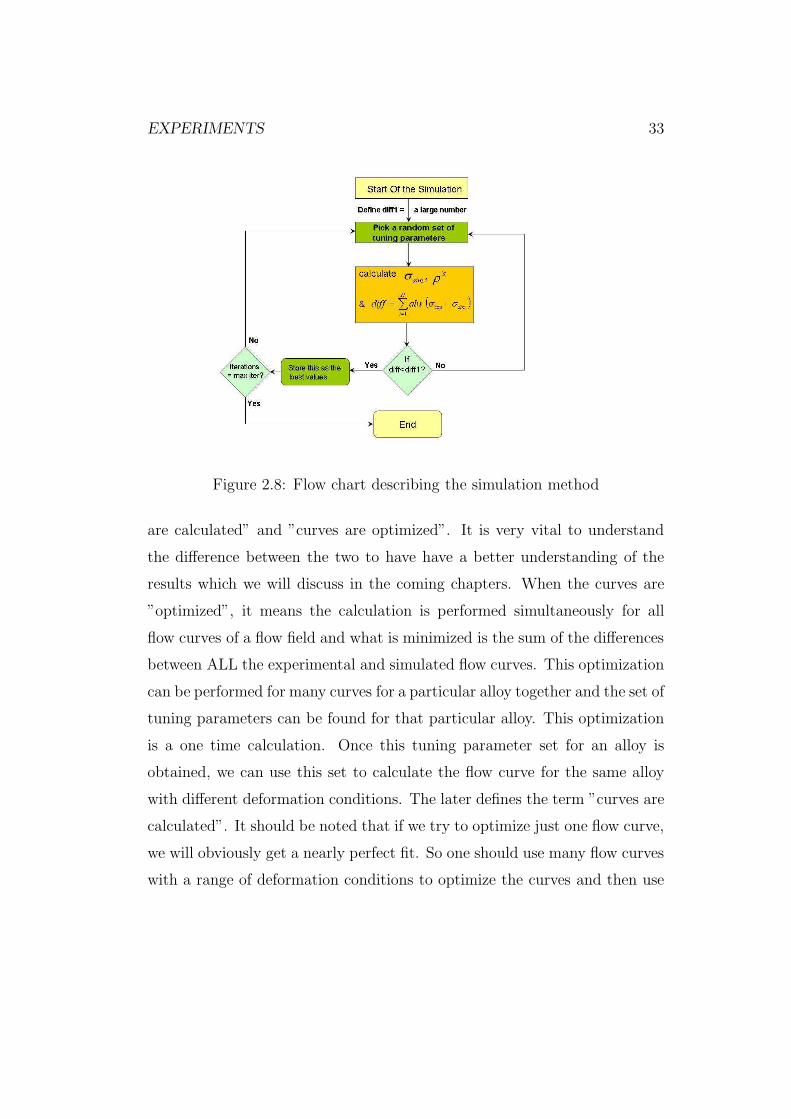
flow curves is at minimum. The flow chart describing the simulation method
is shown in figure 2.8. When we discuss the results from various models in the
following chapters, we will use two different terminologies, namely, ”curves
EXPERIMENTS 33
Figure 2.8: Flow chart describing the simulation method
are calculated” and ”curves are optimized”. It is very vital to understand
the difference between the two to have have a better understanding of the
results which we will discuss in the coming chapters. When the curves are
”optimized”, it means the calculation is performed simultaneously for all
flow curves of a flow field and what is minimized is the sum of the differences
between ALL the experimental and simulated flow curves. This optimization
can be performed for many curves for a particular alloy together and the set of
tuning parameters can be found for that particular alloy. This optimization
is a one time calculation. Once this tuning parameter set for an alloy is
obtained, we can use this set to calculate the flow curve for the same alloy
with different deformation conditions. The later defines the term ”curves are
calculated”. It should be noted that if we try to optimize just one flow curve,
we will obviously get a nearly perfect fit. So one should use many flow curves
with a range of deformation conditions to optimize the curves and then use

EXPERIMENTS 34
the determined tuning parameters to calculate the flow curve for the required
deformation conditions.
The ideal goal of the present work was to optimize a set of flow
curves for a wide range of temperatures and strain rates and then calculate
the flow curves for any deformation condition; i.e., cover the desired range
of deformation temperatures and strain rates.

Chapter 3
Three Internal Variables Model
(3IVM)
With an objective of precisely modeling the deformation processes for Alu-
minum and its alloys, this model, namely the 3IVM was initiated by Gottstein
et. al [1]. There have been numerous changes to the model since its incep-
tion. This model has been applied to predict the work hardening behavior of
alloys [49], has been coupled with texture and precipitation models [45, 46],
has been incorporated in FE codes [47] to study deformation processes like
rolling and also been applied in a through process model [51]. This model
was based on the contemporary understanding of the microstructural evolu-
tion and aims at predicting the strain hardening behavior of FCC metals and
alloys. The model makes an inherent assumption of a cellular microstructure
as is observed in most of the aluminum, copper and nickel alloys as well as
steels. During deformation, a cellular microstructure develops consisting of
cell interiors with a low dislocation density and cell walls of high dislocation
density. The mobile dislocations make their way through the crystal due
35
Three Internal Variables Model (3IVM) 36
to the applied stress to accommodate the imposed strain rate and on their
way encounter obstacles (other dislocations, solutes, precipitates etc.). The
interaction of the dislocations with each other and with obstacles is taken
into account in a statistical way to predict the strain hardening behavior.
The 3IVM, as the name suggests, makes use of 3 internal state vari-
ables namely, the mobile dislocation density (ρm), the immobile dislocation
density in the cell interiors (ρi), and the immobile dislocation density in the
cell walls (ρw). The governing equations used in the model can be divided into
2 categories; the kinetic equation of state and the structure evolution equa-
tions. The kinetic equation of state calculates the external stress required to
accommodate an imposed strain rate for a given microstructure and material
chemistry. The structure evolution equations calculate the temporal evolu-
tion of the dislocation densities. In what follows we will discuss this model
and the governing equations in more detail.
3.1 Kinetic Equation Of State
The 3IVM uses the Orowan equation (equation 4.1) as the kinetic equation
of state
γ = ǫM = ρmbv (3.1)
where, γ is the shear rate, ǫ is the strain rate, M is the average polycrystal
Taylor factor, b is the Burgers vector and v is the average velocity of the
mobile dislocations. We assume a ”jerky” motion of the dislocation, i.e., the
dislocation glides long distances before it is stopped by an obstacle. The
obstacles for moving dislocations can be other immobile dislocations also
termed forest dislocations, solutes and/or precipitates. Once a dislocation
gets stopped by an obstacle in its way, it waits in front of the obstacle until
Three Internal Variables Model (3IVM) 37
the applied stress and the thermal assistance are high enough to overcome
the obstacle. Hence the average velocity of the dislocation is expressed as
v =λ
tw + tg(3.2)
Where, λ is the average spacing of the obstacles, tw and tg are the waiting and
gliding times of the dislocation between obstacles. The waiting time of the
dislocation is much longer than the gliding time and hence tw is neglected.
The average glide velocity of the dislocation in terms of an effective stress,
τeff = τ − τ , where τ is the acting shear stress and τ is the athermal flow
stress can be approximated as
v =λ
tw= λν0exp
(−(Qglide − τeffV )
kT
)
. (3.3)
Here, ν0 is the attack frequency, Qglide is the activation energy for dislocation
glide and V is the activation volume. Substituting Equation 3.3 into Equa-
tion 4.1, Equation 4.1 can be solved for τeff . As the average forest dislocation
spacing (λi = 1/√
ρi and λw = 1/√
ρw) is different in the cell interiors and
cell walls, we obtain different values of τeff in the cell interiors (τ ieff ) and cell
walls (τweff ). These short range stresses obtained above is added to the long
range stresses (also called passing stresses) to obtain the total shear stresses
in the cell interiors and cell walls given as
τi = τ ieff + αGb
√ρi (3.4)
τw = τweff + αGb
√ρw (3.5)
The total external stress needed to accommodate a particular strain rate is
obtained by weighting the individual stresses with their respective volume
fractions as
σext = M(fiτi + fwτw) (3.6)

Three Internal Variables Model (3IVM) 38
where, fi and fw = 1 − fi are the volume fractions of the cell interiors and
cell walls respectively. Therefore, the external stress needed for any defor-
mation conditions can be calculated from the above equation. To calculate
the complete stress strain curve we need to calculate the evolution of the
dislocation densities. They are iteratively solved in tandem with the kinetic
equation of state to describe the complete strain hardening behavior.
3.2 Structure Evolution Equations
In this section we will derive an evolution law for each of the dislocation den-
sities depending on the underlying dislocation reaction/process. The general
way of representing the evolution equation is
ρx = ρ+
x − ρ−x (3.7)
where, x = m, i, w for mobile, interiors and walls, ρ+x is the rate of gain
of a particular class of dislocation density which may be a sum of one or
more terms, and ρ−x is a sum of one or more dislocation reduction or recovery
terms. In the following subsection we will consider the evolution of the mobile
dislocation density.
3.2.1 Mobile Dislocation Density
The mobile dislocations move through the crystal under an applied stress to
accommodate an imposed strain rate and on their way encounter obstacles.
A relation between an imposed strain (∆ǫ) and the mobile dislocation density
can be obtained if the Orowan equation is extended to a larger time scale. In
a time increment ∆t, a dislocation density ρ+m∆t is produced and immobilized

Three Internal Variables Model (3IVM) 39
after traveling a distance Leff , the strain associated with this is given as
ρ+
m =ǫM
b
1
Leff. (3.8)
where, Leff is the effective slip length of the dislocation which is given as
1
Leff
=1
Li
+1
Lw
+1
Lg
+1
Lp(t). (3.9)
where, Li and Lw are the average slip lengths in the cell interiors and walls
respectively and Lg is an effective grain size and Lp(t) is the mean particle
spacing at a particular instance in time t. The average slip lengths in the cell
interiors and cell walls can be expressed as Li = βi/√
ρi and Lw = βw/√
ρw
(βi and βw are constants).
The mobile dislocation density is assumed to be reduced due to 3
reactions, namely, dislocation annihilation, lock formation and dipole forma-
tion. We will derive the evolution equation for the dislocation annihilation
reaction below. The other equations can be derived analogously. It is consid-
ered that two antiparallel mobile dislocations on parallel glide planes spon-
taneously annihilate when they come closer than a critical distance, dann. In
the time dt the mobile dislocation travels a distance vdt. The probability
that this dislocation finds another mobile dislocation in the area 2dannvdt, is
given as
dp = 2dannvdtρm (3.10)
As stated above, dislocation annihilation takes place only when the two dis-
locations in consideration are on parallel glide planes and have opposite sign.
Taking this condition into consideration, the probability density in time now
becomes
p = 2dannvρm1
2n(3.11)
Three Internal Variables Model (3IVM) 40
where, n is the number of active glide systems. Using the Orowan equation,
equation 3.11 can be rewritten as
p = 2dannǫM
b
1
2n(3.12)
Taking into account that 2 mobile dislocations are lost due to an annihilation
reaction and the total density of mobile dislocations is ρm, the loss rate of
the mobile dislocation density due to annihilation can be written as
ρ−m(ann) = 2dann
ǫM
b
1
nρm (3.13)
The next reaction considered is the formation of locks (similar to Lomer
locks). Analogously the loss rate of mobile dislocations due to the formation
of locks can be derived as
ρ−m(lock) = 4dlock
ǫM
b
n − 1
nρm (3.14)
where, dlock is the critical distance for lock formation and the factor n−1
n
is used to take into consideration that for lock formation the two mobile
dislocations in consideration must be on different glide systems. The factor
4 is used in the above equation as two mobile dislocations are lost due to
a lock formation. The third process taken into account is the formation
of dipoles. It is assumed that when two mobile dislocations are not close
enough for spontaneous annihilation but are close enough to experience a
strong elastic interaction of each other, they form a dipole configuration.
The loss rate of mobile dislocations due to this reaction can be derived as
ρ−m(dipole) = 2(ddipole − dann)
ǫM
b
1
nρm (3.15)
where, ddipole is the critical distance for dipole formation. The net loss rate
of the mobile dislocations due to spontaneous annihilation, lock formation
Three Internal Variables Model (3IVM) 41
and dipole formation can be summarized as
ρ−m = ρ−
m(ann) + ρ−m(lock) + ρ−
m(dipole) (3.16)
This equation in conjunction with the production rate derived in equation 3.8
defines the net rate of change in the mobile dislocation density and is written
as
ρm = ρ+
m − ρ−m(ann) − ρ−
m(lock) − ρ−m(dipole) (3.17)
3.2.2 Immobile Dislocation Density in the cell interiors
The total rate of increase of the immobile dislocation density in the cell
interiors is equal to the rate of decrease of the mobile dislocation density due
to formation of locks.
ρ+
i (lock) = ρ−m(lock) = 4dlock
ǫM
b
n − 1
nρm (3.18)
Since the dislocation locks are sessile, the only way to decrease the immobile
dislocation density is by climb. If the velocity of climb (vclimb) is diffusion
controlled, it can be written as
vclimb =D
kTτA. (3.19)
where, D is the diffusion coefficient, τ is the total shear stress and A is the
activation area. According to [1] the activation area is considered to be
proportional to b2. The diffusion coefficient is calculated as
D = D0exp
(−Qclimb
kT
)
(3.20)
where, D0 is a constant and Qclimb is the activation energy for climb. The
rate of loss of immobile dislocations in the cell interiors can now be derived
as
ρ−i (climb) = 2dclimbvclimb
1
nρ2
i (3.21)

Three Internal Variables Model (3IVM) 42
Note that in the above equation the loss rate is quadratic in ρi. Dipoles
are not considered for the immobile dislocation density in the cell interiors
as it is assumed that all the dipoles are swept into the cell walls. The net
evolution of the dislocation density in the cell interiors can be summarized
as
ρi = ρ+
i (lock) − ρ−i (climb) (3.22)
3.2.3 Immobile Dislocation Density in the cell walls
As considered for the immobile dislocation density in the cell interiors, the
same reactions of lock formation and climb are also considered for the cell
walls and can be written as
ρ+
w(lock) = 4dlockǫM
b
n − 1
nρm (3.23)
ρ−w(climb) = 2dclimbvclimb
1
nρ2
w (3.24)
In addition to this, it is assumed that all the dipoles formed anywhere in the
crystal are all swept into the walls [52]. Hence the rate of gain of immobile
dislocations in the cell walls due to this reaction can be written as
ρ+
w(dipole) =1
fwρ−
m(dipole) (3.25)
=1
fw
2(ddipole − dann)ǫM
b
1
nρm (3.26)
Therefore the evolution of the immobile dislocation density in the cell walls
can be summarized as
ρw = ρ+
w(lock) + ρ+
w(dipole) − ρ−w(climb) (3.27)
Now that we have defined the kinetic equation of state and the structure
evolution equations, the complete stress strain curve can be calculated if the
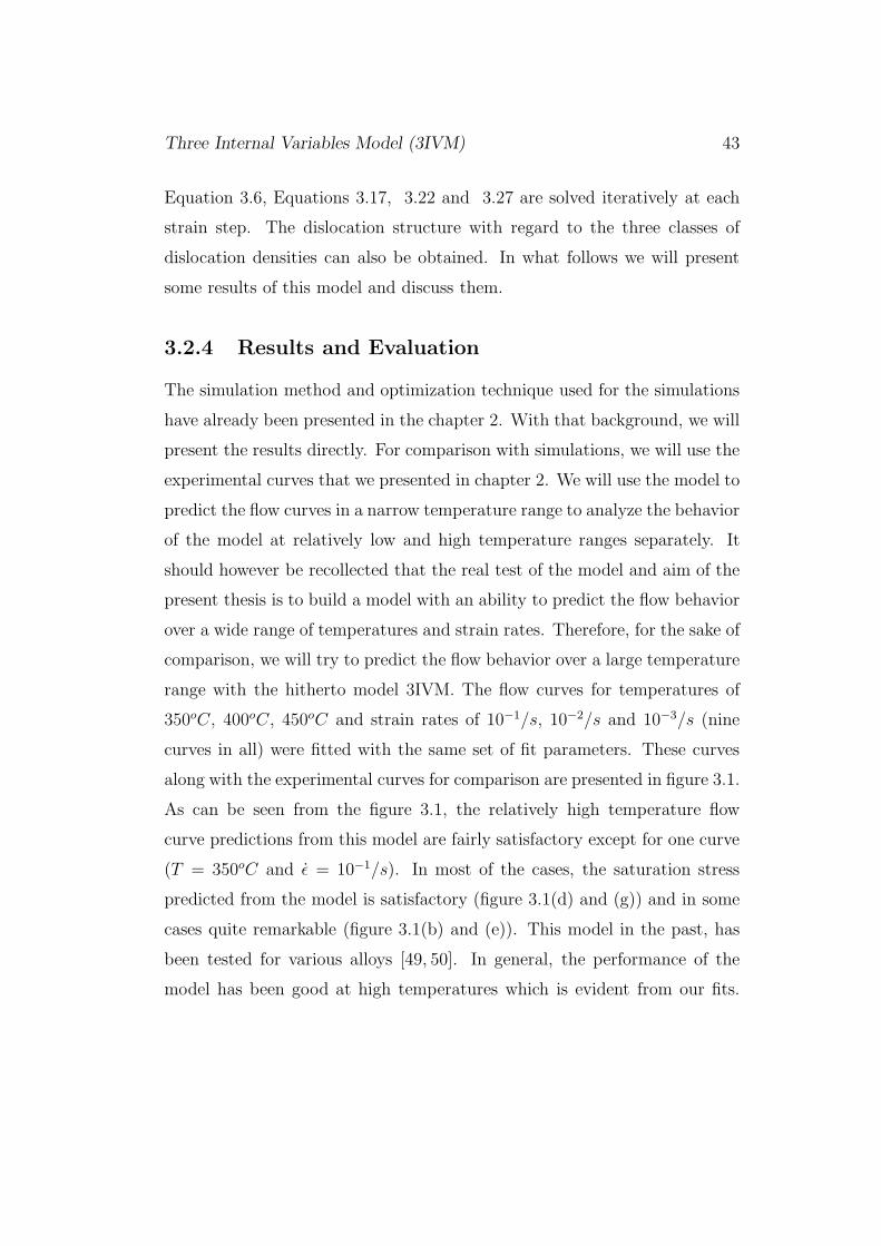
Three Internal Variables Model (3IVM) 43
Equation 3.6, Equations 3.17, 3.22 and 3.27 are solved iteratively at each
strain step. The dislocation structure with regard to the three classes of
dislocation densities can also be obtained. In what follows we will present
some results of this model and discuss them.
3.2.4 Results and Evaluation
The simulation method and optimization technique used for the simulations
have already been presented in the chapter 2. With that background, we will
present the results directly. For comparison with simulations, we will use the
experimental curves that we presented in chapter 2. We will use the model to
predict the flow curves in a narrow temperature range to analyze the behavior
of the model at relatively low and high temperature ranges separately. It
should however be recollected that the real test of the model and aim of the
present thesis is to build a model with an ability to predict the flow behavior
over a wide range of temperatures and strain rates. Therefore, for the sake of
comparison, we will try to predict the flow behavior over a large temperature
range with the hitherto model 3IVM. The flow curves for temperatures of
350oC, 400oC, 450oC and strain rates of 10−1/s, 10−2/s and 10−3/s (nine
curves in all) were fitted with the same set of fit parameters. These curves
along with the experimental curves for comparison are presented in figure 3.1.
As can be seen from the figure 3.1, the relatively high temperature flow
curve predictions from this model are fairly satisfactory except for one curve
(T = 350oC and ǫ = 10−1/s). In most of the cases, the saturation stress
predicted from the model is satisfactory (figure 3.1(d) and (g)) and in some
cases quite remarkable (figure 3.1(b) and (e)). This model in the past, has
been tested for various alloys [49, 50]. In general, the performance of the
model has been good at high temperatures which is evident from our fits.
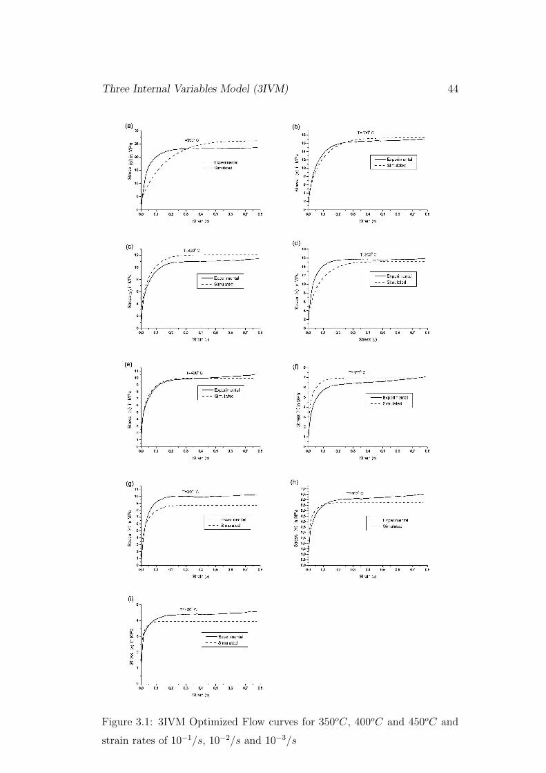
Three Internal Variables Model (3IVM) 44
Figure 3.1: 3IVM Optimized Flow curves for 350oC, 400oC and 450oC and
strain rates of 10−1/s, 10−2/s and 10−3/s

Three Internal Variables Model (3IVM) 45
Figure 3.2: Evolution of Dislocation Densities at 350oC and strain rate of
10−1/s
As a representative case for this temperature range, the temporal evolution
of the dislocation densities for a temperature of T = 350oC and a strain
rate of 10−1/s are shown in figure 3.2. Since the total dislocation density
governs the total stress needed to accommodate a particular strain rate, the
evolution of the total dislocation density ( 3.2(d)) should a follow similar
trend as the flow curves. The dislocation density reaches a saturation value
at low strains and remains almost constant similar to the stress strain curves
at high temperatures.
To analyze the predictions at low temperatures, we did a simulation
for the relatively low temperature flow curves and the optimized flow curves
Three Internal Variables Model (3IVM) 46
along with the experimental curves are shown in figure 3.3. The low tem-
perature predictions from the model are unsatisfactory. The hardening rates
are wrongly predicted for all the room temperature fits (e.g.,figure 3.3(a) (d)
and (g)). For the temperatures of 25oC and 100oC, the flow stresses are un-
der predicted at low strains and over predicted at high strains. This can be
seen from the crossing of the experimental and simulated flow curves. With
increase in temperature the quality of the fits improves (see figure 3.3(c), (f)
and (i) for 200oC). Representative for the low temperature fits, the temporal
evolution of the dislocation densities for T = 25oC and ǫ = 10−2/s are plot-
ted in figure 3.4. The trends in the stress strain curves, can be understood
from the plots of the dislocation density. The evolution of the immobile dis-
location densities at low strains is very slow leading to the under predicted
flow stress. At high strains the immobile dislocation densities evolve too fast
leading to a over predicted flow stress.
Finally we optimize both the relatively low and high temperature
ranges together. We used temperatures of 25oC, 100oC, 350oC, 400oC and
strain rates of 10−2/s and 10−3/s. These plots along with the experimental
curves are shown in figure 3.5. It can be seen from figure 3.5 (d), (g) and
(h), that the quality of the fits becomes better with increase in temperature.
Therefore, the model fits at high temperatures are satisfactory, whereas, the
model once again fails at low temperatures, especially at room temperature.
3.3 Conclusion
As we stated at the start of the chapter, we mainly aim at producing a unified
model which can describe the flow curves over a wide range of temperatures
and strain rates. The prediction of the dislocation densities in the right order

Three Internal Variables Model (3IVM) 47
Figure 3.3: 3IVM Optimized Flow curves for 25oC, 100oC and 200oC and
strain rates of 10−2/s, 10−3/s and 10−4/s
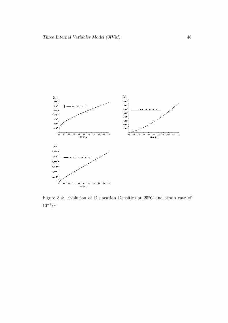
Three Internal Variables Model (3IVM) 48
Figure 3.4: Evolution of Dislocation Densities at 25oC and strain rate of
10−2/s
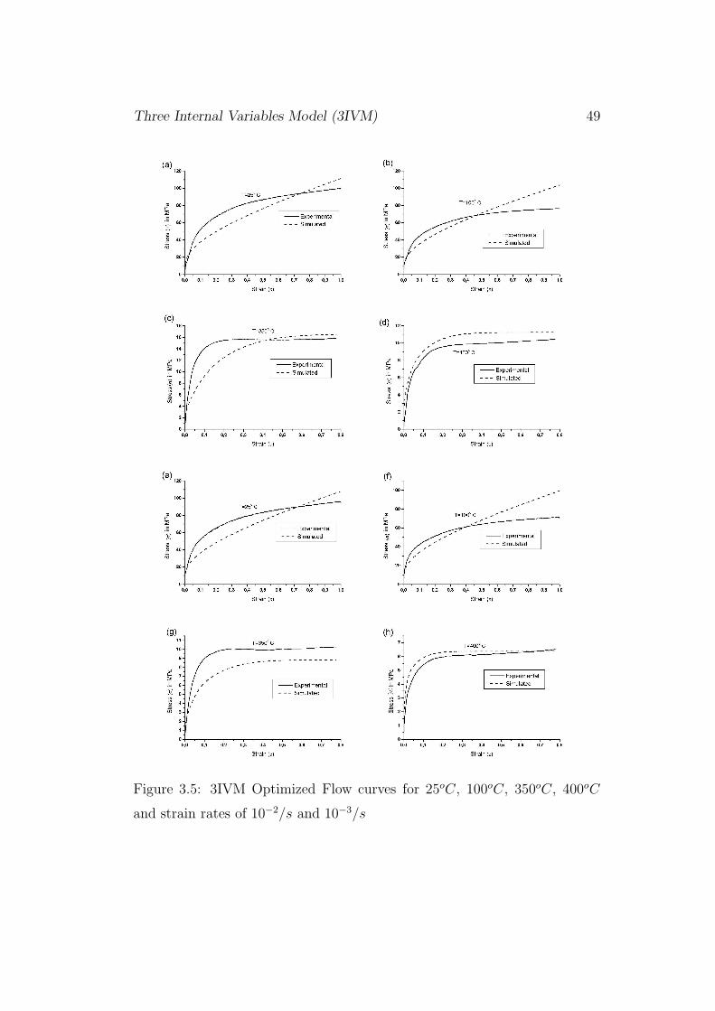
Three Internal Variables Model (3IVM) 49
Figure 3.5: 3IVM Optimized Flow curves for 25oC, 100oC, 350oC, 400oC
and strain rates of 10−2/s and 10−3/s
Three Internal Variables Model (3IVM) 50
of magnitude is also of prime importance. The 3IVM in its hitherto state
cannot fit both high and low temperature curves with the same set of fitting
parameters. As was demonstrated, the model fits at high temperatures were
very good but the model failed to make reasonable predictions at low tem-
peratures. The probable reasons for the failure of 3IVM to describe the flow
behavior over a wide range of temperatures and strain rates and the proposed
changes will be stated in the next chapter and are the main motivation to
build a novel model namely, the 3IVM+. As the name suggests it will be
an improved 3IVM. It includes some important dislocation reactions that are
missing in the 3IVM. It implements a novel kinetic equation of state to calcu-
late the stress needed to accommodate a particular strain rate. Though the
model, like the 3IVM takes into consideration 3 internal state variables, it
takes into account both dislocation climb and dislocation cross slip as possi-
ble recovery mechanisms. In addition in also considers the reactions between
mobile and immobile dislocations, which are presently missing in the 3IVM.

Chapter 4
Improved Three Internal
Variables Model (3IVM+)
The 3 internal variables model described in the previous chapter had some
shortcomings which we will discuss below and justify the modifications that
lead to a new model. This new model presented in this chapter is called
3IVM+ (with a ”plus” sign signifying an improved 3IVM). The three most
important differences in the 3IVM+ as compared to the 3IVM are,
1. The 3IVM considers only edge dislocations and hence does not include
cross slip of screw dislocations as a possible recovery mechanism. This
may not be justified especially at low temperatures where diffusion
controlled climb becomes too slow and hence dislocation cross-slip is
the ruling recovery mechanism. In contrast to the 3IVM, 3IVM+ takes
into account the effect of both dislocation climb and cross slip as the
possible recovery mechanisms.
2. The average dislocation velocity equation in the 3IVM (equation 3.3)
considers an activation energy for glide, Qglide, which is a tuning param-
51
Improved Three Internal Variables Model (3IVM+) 52
eter. Past experience with the model has shown that the flow curve
fits are very sensitive to this tuning parameter. The use of a con-
stant activation volume in the 3IVM for the thermally activated ob-
stacle overcoming process was also only an experimentation. Our new
methodology uses the analytically calculated free enthalpy for thermal
activation taking into account a variable activation volume.
3. The interaction of mobile dislocations with immobile dislocations is
completely neglected in the 3IVM. As an improvement, the present
model considers this effect and hence the missing reactions are ac-
counted for in the 3IVM+.
We en-devoured to remove the above deficiencies from the 3IVM
and formulate an improved version, the 3IVM+. In what follows we will
discuss the 3IVM+ in more detail and present some analysis with results.
It is reiterated that many concepts and the basic structure of the model is
quite similar to the 3IVM. Though the model has been thoroughly tested
only for pure aluminum (99.9% purity), it can easily be applied to alloys.
When considering modeling the flow behavior of alloys, equations related to
the effect of solutes and precipitates should be considered. These equations
will also be presented in this chapter. These equations will have an effect
only when the alloy consists of considerable solute and precipitate content.
As in the 3IVM, 3IVM+ also considers a cellular microstructural de-
scription and makes use of 3 internal state variables, namely, the three classes
of dislocation densities, the mobile dislocation density (ρm), the immobile
dislocations density in the cell interiors (ρi) and the immobile dislocation
density in the cell walls (ρw).Since no explicit distinction is made between
edge and screw dislocations, we assume that ρscrew ≈ ρedge. Similar to the

Improved Three Internal Variables Model (3IVM+) 53
3IVM, the present model makes use of the two class of equations, namely, the
kinetic equation of state and the structure evolution equations to describe
the complete flow field for the given deformation conditions and material
chemistry. However, as mentioned at the beginning of this chapter, in com-
parison to the 3IVM, we have made some major changes in the description
of the kinetic equation of state, which is discussed below.
4.1 Kinetic Equation Of State
Similar to the 3IVM, in the present model, Orowan equation is used as the
kinetic equation of state.
γ = ǫM = ρmbv (4.1)
where γ is the shear rate, b is the Burgers vector, M is the average polycrystal
Taylor factor and v is the average velocity of the mobile dislocations. To
determine the average velocity of a mobile dislocation, a jerky motion of the
dislocation is assumed. This means that the dislocation glides long distances
before it is stopped by an obstacle. The dislocation waits in front of the
obstacle until the applied stress and the thermal assistance are high enough
to overcome the obstacle. Hence, the average velocity of the dislocation is
expressed as
v =λ
tw + tg(4.2)
where, λ is the average spacing of the obstacles and tw, tg are the waiting
and gliding times of the dislocation between obstacles. Since tw >> tg,
in jerky glide condition, the average glide velocity (v) of the dislocation is
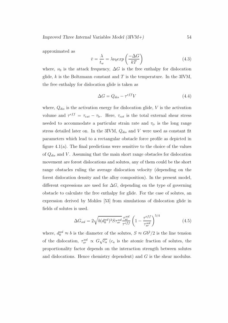
Improved Three Internal Variables Model (3IVM+) 54
approximated as
v =λ
tw= λν0exp
(−∆G
kT
)
(4.3)
where, ν0 is the attack frequency, ∆G is the free enthalpy for dislocation
glide, k is the Boltzmann constant and T is the temperature. In the 3IVM,
the free enthalpy for dislocation glide is taken as
∆G = Qdis − τ effV (4.4)
where, Qdis is the activation energy for dislocation glide, V is the activation
volume and τ eff = τext − τlr. Here, τext is the total external shear stress
needed to accommodate a particular strain rate and τlr is the long range
stress detailed later on. In the 3IVM, Qdis and V were used as constant fit
parameters which lead to a rectangular obstacle force profile as depicted in
figure 4.1(a). The final predictions were sensitive to the choice of the values
of Qdis and V . Assuming that the main short range obstacles for dislocation
movement are forest dislocations and solutes, any of them could be the short
range obstacles ruling the average dislocation velocity (depending on the
forest dislocation density and the alloy composition). In the present model,
different expressions are used for ∆G, depending on the type of governing
obstacle to calculate the free enthalpy for glide. For the case of solutes, an
expression derived by Mohles [53] from simulations of dislocation glide in
fields of solutes is used.
∆Gsol = 2√
b(dsol0 )3Sτ sol
sr
τ solsr
τ eff
(
1 − τ eff
τ solsr
)5/4
(4.5)
where, dsol0 ≈ b is the diameter of the solutes, S ≈ Gb2/2 is the line tension
of the dislocation, τ solsr ∝ G
√ca (ca is the atomic fraction of solutes, the
proportionality factor depends on the interaction strength between solutes
and dislocations. Hence chemistry dependent) and G is the shear modulus.
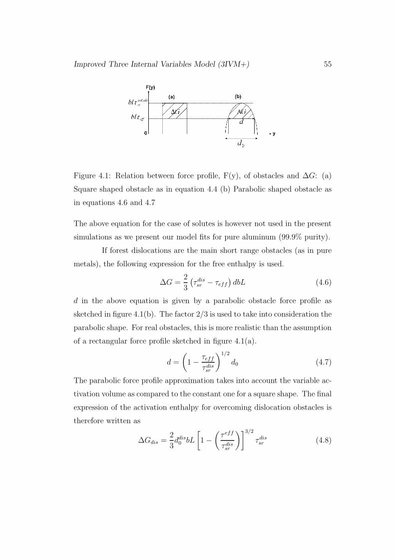
Improved Three Internal Variables Model (3IVM+) 55
Figure 4.1: Relation between force profile, F(y), of obstacles and ∆G: (a)
Square shaped obstacle as in equation 4.4 (b) Parabolic shaped obstacle as
in equations 4.6 and 4.7
The above equation for the case of solutes is however not used in the present
simulations as we present our model fits for pure aluminum (99.9% purity).
If forest dislocations are the main short range obstacles (as in pure
metals), the following expression for the free enthalpy is used.
∆G =2
3
(τdissr − τeff
)dbL (4.6)
d in the above equation is given by a parabolic obstacle force profile as
sketched in figure 4.1(b). The factor 2/3 is used to take into consideration the
parabolic shape. For real obstacles, this is more realistic than the assumption
of a rectangular force profile sketched in figure 4.1(a).
d =
(
1 − τeff
τdissr
)1/2
d0 (4.7)
The parabolic force profile approximation takes into account the variable ac-
tivation volume as compared to the constant one for a square shape. The final
expression of the activation enthalpy for overcoming dislocation obstacles is
therefore written as
∆Gdis =2
3ddis
0 bL
[
1 −(
τ eff
τdissr
)]3/2
τdissr (4.8)
Improved Three Internal Variables Model (3IVM+) 56
where, L = 1/√
ρtotal is the average dislocation spacing and τdissr = φGb
√ρtotal
(with φ being a constant fit parameter). Depending on which process governs
the overall average dislocation velocity, one of the above equations (equa-
tion 4.8 or 4.5) for ∆G can be substituted in equation 4.3 which in turn
can be substituted in the Orowan equation to calculate τ eff . Since we will
discuss simulation results for pure aluminum, we will consider the disloca-
tion cutting mechanism as the main mechanism governing the overall average
velocity of the dislocation. By the substitution operation mentioned above,
τ eff for our case is calculated as
τ eff =
(
1 −[
ln
(ǫM
ρmbν0λ
)( −3kT
2ddis0 bLτdis
sr
)]2/3)
τdissr (4.9)
As the average spacing of the dislocations (λ) is different in the cell interiors
(λi) and cell walls (λw), we obtain the effective stresses in the cell interiors
(τ effi ) and cell walls (τ eff
w ) separately. As a first trial we considered only
the effective stress in the cell interiors and neglected the effective stress in
the walls (assuming that the dislocation cutting process is important in the
cell interiors and the solute overcoming process is vital in the cell walls). It
should be stressed that during the testing of the model many variations of
the model have been considered and the present one yielded the best results.
For future improvements of the model, variations like considering a different
τdissr in the cell interiors and walls should be considered. The total resolved
shear stresses in the cell interiors (τi) and cell walls (τw) is calculated by
adding the above calculated effective stresses to the long range stresses as
τi = τ effi + αGb
√ρi + τp (4.10)
τw = τ effw + αGb
√ρw + τp (4.11)
Improved Three Internal Variables Model (3IVM+) 57
Where, α is a constant fit parameter and τp is the Orowan stress due to
the presence of particles. The total external stress is finally calculated by
weighting the total resolved shear stresses in the cell walls and cell interiors
with their respective volume fractions fw and fi = 1 − fw.
σext = M (fiτi + fwτw) (4.12)
Here, M is the average Taylor factor to take the polycrystal effect into ac-
count. For aluminum alloys with high solute content the solutes in addition
to dislocations act as obstacles for dislocation movement. In that case, the
solutes become important in determining the average velocity of the disloca-
tion. Hence, the same procedure described above is to be used to calculate
the short range stresses due to solutes using ∆Gsol from equation (4.5) in-
stead of equation (4.8).
As described in this subsection, by using the kinetic equation of state,
the total external stress needed to accommodate a particular strain rate can
be calculated for a given dislocation structure and material chemistry. To
calculate the complete stress-strain curves, in addition to the kinetic equation
of state, we need to calculate the evolution of the dislocation densities which
are described in the following section.
4.2 Structure Evolution Equations
Each of the dislocation densities considered in the model has a temporal
evolution law based on the underlying elementary dislocation processes. The
basic evolution law is of the form
ρx = ρ+
x − ρ−x
Improved Three Internal Variables Model (3IVM+) 58
where the subscript x = m, i, w indicates the identity of the dislocation as
mobile dislocation, the dislocation in the cell interiors or in the cell walls.
The gain/loss rates in the equation can be a sum of one or more gain/loss
rates. The various reactions considered in the model and their effect on the
variables are listed below.
1. Spontaneous annihilation of antiparallel dislocations on parallel glide
systems occurs; leading to a decrease in the total mobile dislocation
density: ρ−m
2. The production rate of mobile dislocations is considered by extending
the Orowan equation over a larger time scale and considering the mean
free path of the dislocations. This methodology will be described in
detail later in the chapter: ρ+m
3. Locks are formed due to the interaction of mobile dislocations on dif-
ferent glide systems; leading to a decrease in the mobile dislocation
density and an increase in the immobile dislocation density in the cell
walls and cell interiors: ρ−m, ρ+
i , ρ+w
4. When dislocations are not close enough for spontaneous annihilation
but see the elastic stresses of each other, they may form dipoles; we
assume that all the dipoles irrespective of where they are formed are
all swept into the walls by other mobile dislocations: ρ−m, ρ+
w
5. Mobile dislocations are immobilized when they interact with immobile
dislocations leading to a net decrease in the mobile dislocation den-
sity and an increase in the immobile dislocation density: ρ−m, ρ+
i , ρ+w
(Immobilization reaction)

Improved Three Internal Variables Model (3IVM+) 59
6. Interaction of mobile dislocations with immobile dislocations has a re-
covery effect. Hence leads to a decrease in the immobile dislocation
density but ρm uneffected: ρ−i , ρ−
w (clearing effect)
7. Annihilation of immobile dislocations occurs by climb leading to a de-
crease in the immobile dislocation density and hence has a recovery
effect: ρ−i , ρ−
w
8. Cross slip and subsequent spontaneous annihilation is considered as
well leading to a decrease in the immobile dislocation density, hence,
leading to recovery: ρ−i , ρ−
w
As can be readily seen from the reactions list, we make a clear distinction
between three recovery mechanisms. Though we do not distinguish between
edge and screw dislocation densities, we do consider both dislocation climb
(reaction (7)) and dislocation cross-slip (reaction (8)) as recovery mecha-
nisms. In addition to this, the motion of mobile dislocations leads to an
additional recovery mechanism (reaction (6)). We will now consider each
of the above mentioned reactions and derive the evolution law for the state
variables.
It is assumed that when 2 antiparallel dislocations on parallel glide
systems come closer than a critical distance (dann, which is a constant fit
parameter), they annihilate spontaneously (reaction (1)). The loss rate of
mobile dislocations due to the annihilation reaction is calculated similar to
the 3IVM as derived in chapter 3. Since two mobile dislocations are lost
during an annihilation reaction, the loss rate of mobile dislocations due to
spontaneous annihilation is written [1] as
ρ−m(ann) = 2pρm = 2dann
ǫM
b
1
nρm. (4.13)
Improved Three Internal Variables Model (3IVM+) 60
The temporal evolution rates for other reactions can be derived analogously
(for details see [1]). However we will list the equations for the sake of com-
pleteness. For the formation of dislocation locks (reaction (3)), a different
critical distance (dlock, which is a constant fit parameter) is used. The loss
rate of mobile dislocations due to lock formation is given as
ρ−m(lock) = 4dlock
ǫM
b
n − 1
nρm. (4.14)
When antiparallel mobile dislocations on parallel glide systems are not close
enough for spontaneous annihilation but are at a distance to mutually in-
teract they can form a dipolar configuration (reaction (4)). The loss rate of
mobile dislocations due to dipole formation is given as
ρ−m(dipole) = 2(ddipole − dann)
ǫM
b
1
nρm (4.15)
where the critical distance for dipole formation, ddipole, is stress dependent
and given as
ddipole =Gb
4πτw. (4.16)
τw is considered in the above equation as we assume that all the dipoles ir-
respective of where they are formed are all swept into the walls, where they
must be stable in order not to get annihilated immediately. The original
3IVM [1] doesn’t consider the interaction of mobile dislocations with im-
mobile dislocations. In the present model we consider this reaction. When
mobile dislocations encounter immobile dislocations on their way through
the crystal, they may get immobilized (reaction (5)). So the net effect of the
reaction is a loss of mobile dislocation density and a gain in immobile dislo-
cation density. A different critical distance, dimm (constant fit parameter), is
considered for the immobilization reaction.
ρ−m(imm) = 2dimm
ǫM
b(ρifi + ρwfw) . (4.17)

Improved Three Internal Variables Model (3IVM+) 61
It is assumed that such immobilization reactions are possible regardless of
the glide planes involved. The total loss rate of mobile dislocations can be
summarized as
ρ−m = ρ−
m(ann) + ρ−m(lock) + ρ−
m(dipole) + ρ−m(imm). (4.18)
The gain rate of mobile dislocations is calculated by extending the Orowan
equation over a larger time scale and considering that the mobile dislocation
on an average travels a mean free path (Leff ) before it is immobilized or
annihilated. In a time interval ∆t, a dislocation density ρ+m∆t is produced
and immobilized after traveling a distance Leff . This is associated with a
strain increment ∆ǫ, so
∆ǫ
∆t∼= ǫ = ρ+
mbLeff1
M. (4.19)
Hence the production rate of mobile dislocations can be written as
ρ+
m =ǫM
b
1
Leff. (4.20)
The mean free path Leff of mobile dislocations is calculated as follows
1
Leff=
1
Li+
1
Lw+
1
Lg(4.21)
where, Li = βi√ρi
and Lw = βw√ρw
are the average spacing of the dislocations in
the cell interiors and cell walls respectively and Lg is the average grain size.
βi and βw are constants which relate the spacing of the respective disloca-
tions (i,w) to the slip length, for the case that only this type of dislocation
determined the average slip length. In the 3IVM, an additional term for the
effect of precipitates was considered. On the other hand in the 3IVM+ the
Orowan stress due to precipitates will be added directly to the total exter-
nal stress calculated (when considering alloys with considerable precipitate

Improved Three Internal Variables Model (3IVM+) 62
Figure 4.2: Schematic showing the dependency of the production of mobile
dislocations on the slip length of the dislocation which in turn depends on
the cell size
Figure 4.3: The dislocation length produced during bow out is lost instanta-
neously by overcoming the particles
Improved Three Internal Variables Model (3IVM+) 63
content). The reason for the non inclusion of the precipitate effects in the
mobile dislocation density production term is as follows:
As seen in figures 4.2, the slip length of the dislocation which deter-
mines the production rate of the mobile dislocations in turn depends directly
on the cell size. As shown in figure 4.3, the presence of precipitates has neg-
ligible effect on the length of mobile dislocation produced. Therefore though
the precipitates are a hinderence to the mobile dislocations, their contribu-
tion to the production of the mobile dislocations is negligible.
The second category of dislocations considered are the immobile dis-
locations in the cell interiors (ρi). The rate of increase of the immobile
dislocation density in the cell interiors (ρ+
i ) is essentially [1] equal to the
decrease in the mobile dislocations due to lock formation and immobiliza-
tion reaction which were derived in equations (4.14) and (4.17) respectively.
Therefore the total gain rate of the immobile dislocation density in the cell
interiors is given as
ρ+
i = ρ−m(lock) + 2dimm
ǫM
bfiρi (4.22)
Similarly, the gain of immobile dislocations in the cell walls occurs due to
the formation of locks and immobilization reaction. In addition to this it is
assumed that all the dipoles are swept into the cell walls [52] irrespective of
where they are formed. Therefore the total gain rate of immobile dislocations
in the cell walls is given as
ρ+
w = ρ−m(lock) +
1
fwρ−
m(dipole) + 2dimmǫM
bρwfw (4.23)
A factor 1/fw is included for the dipole term in the above equations because
we assume that irrespective of where the dipoles are formed are all swept
into the walls. Lastly, we will consider the loss rates, ρ−i,w, of immobile
Improved Three Internal Variables Model (3IVM+) 64
dislocations in the cell interiors and cell walls, which describe the recovery
events. The first recovery reaction considered is the annihilation of immobile
dislocations by dislocation climb. The loss rate of immobile dislocations due
to this reaction is calculated as
ρ−i,w = 2vi,w
climbdann−c1
nρ2
i,w (4.24)
where, vi,wclimb is the velocity of climb of immobile dislocations. It is given as
vclimb =D
kTτi,wA. (4.25)
Here, k is the Boltzmann constant, A ≈ b2 is the activation area and D is
the temperature dependent diffusion coefficient and given as
D = D0exp(−Qclimb/kT ) (4.26)
where, D0 (fit parameter) is the diffusion constant and Qclimb is the activation
energy for climb. The second recovery event considered is the annihilation
of immobile dislocations by cross slip. To calculate the probability of cross
slip, we use the approach of Nix et. al [21]. The probability that a cross slip
event is successful may be written as
P i,wcs = exp
(
−W i,wf
kT
)
− exp
(−Wb
kT
)
(4.27)
where, Wb and W i,wf are the backward and forward activation energies re-
spectively. The backward jumps are neglected in our case and following the
approach of Bonneville and Escaig [54], the forward activation energy as a
function of stress in the cell interiors or cell walls is given as
W i,wf = Wcs
[
1 − αcsτi,w
G
]
(4.28)
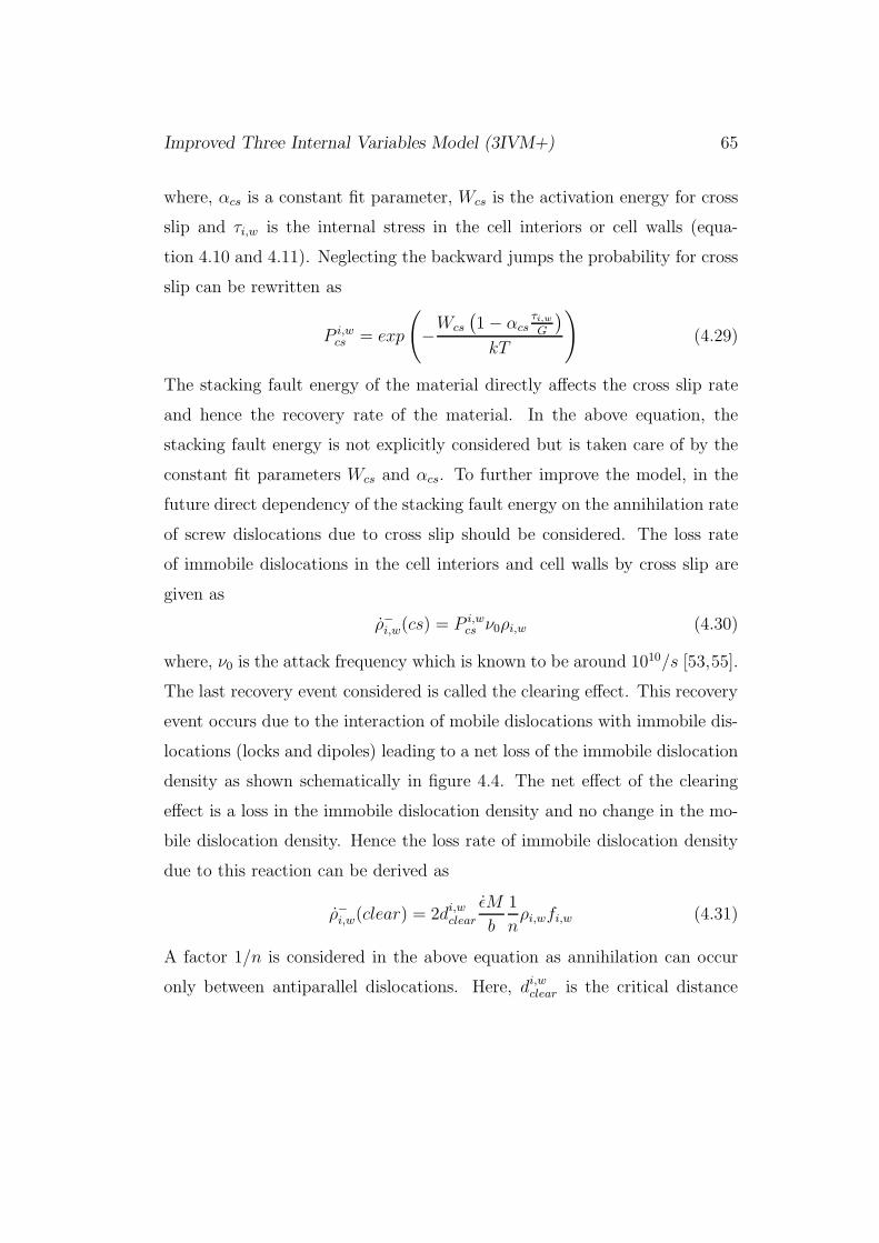
Improved Three Internal Variables Model (3IVM+) 65
where, αcs is a constant fit parameter, Wcs is the activation energy for cross
slip and τi,w is the internal stress in the cell interiors or cell walls (equa-
tion 4.10 and 4.11). Neglecting the backward jumps the probability for cross
slip can be rewritten as
P i,wcs = exp
(
−Wcs
(1 − αcs
τi,w
G
)
kT
)
(4.29)
The stacking fault energy of the material directly affects the cross slip rate
and hence the recovery rate of the material. In the above equation, the
stacking fault energy is not explicitly considered but is taken care of by the
constant fit parameters Wcs and αcs. To further improve the model, in the
future direct dependency of the stacking fault energy on the annihilation rate
of screw dislocations due to cross slip should be considered. The loss rate
of immobile dislocations in the cell interiors and cell walls by cross slip are
given as
ρ−i,w(cs) = P i,w
cs ν0ρi,w (4.30)
where, ν0 is the attack frequency which is known to be around 1010/s [53,55].
The last recovery event considered is called the clearing effect. This recovery
event occurs due to the interaction of mobile dislocations with immobile dis-
locations (locks and dipoles) leading to a net loss of the immobile dislocation
density as shown schematically in figure 4.4. The net effect of the clearing
effect is a loss in the immobile dislocation density and no change in the mo-
bile dislocation density. Hence the loss rate of immobile dislocation density
due to this reaction can be derived as
ρ−i,w(clear) = 2di,w
clear
ǫM
b
1
nρi,wfi,w (4.31)
A factor 1/n is considered in the above equation as annihilation can occur
only between antiparallel dislocations. Here, di,wclear is the critical distance

Improved Three Internal Variables Model (3IVM+) 66
Figure 4.4: Schematic showing of one possible clearing effect; dislocation (2)
and (3) are in dipole configuration. The mobile dislocation (1) can annihilate
with dislocation (2) and hence make the dislocation (3) mobile.
below which this reaction will occur and is expressed as
di,wclear = αclear
Gb
4πτi,w(4.32)
where, αclear is a constant fitting parameter. Unlike the other recovery events,
in the clearing effect, the evolution of the dislocation density is proportional
to the strain rate. Therefore we call it strain rate recovery rate and the effect
may be called strain recovery.
In this section we described the equations elucidating the evolution
of the dislocation densities. As was evident, the equations had fit parame-
ters. In the table below, we will summarize all the parameters used along
with reasonable minimum and maximum values used in the simulation and
comments.
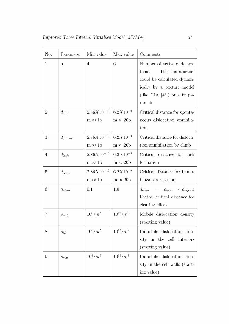
Improved Three Internal Variables Model (3IVM+) 67
No. Parameter Min value Max value Comments
1 n 4 6 Number of active glide sys-
tems. This parameters
could be calculated dynam-
ically by a texture model
(like GIA [45]) or a fit pa-
rameter
2 dann 2.86X10⁻¹⁰
m ≈ 1b
6.2X10⁻⁹
m ≈ 20b
Critical distance for sponta-
neous dislocation annihila-
tion
3 dann−c 2.86X10⁻¹⁰
m ≈ 1b
6.2X10⁻⁹
m ≈ 20b
Critical distance for disloca-
tion annihilation by climb
4 dlock 2.86X10⁻¹⁰
m ≈ 1b
6.2X10⁻⁹
m ≈ 20b
Critical distance for lock
formation
5 dimm 2.86X10⁻¹⁰
m ≈ 1b
6.2X10⁻⁹
m ≈ 20b
Critical distance for immo-
bilization reaction
6 αclear 0.1 1.0 dclear = αclear ∗ ddipole;
Factor, critical distance for
clearing effect
7 ρm,0 108/m2 1012/m2 Mobile dislocation density
(starting value)
8 ρi,0 108/m2 1012/m2 Immobile dislocation den-
sity in the cell interiors
(starting value)
9 ρw,0 108/m2 1013/m2 Immobile dislocation den-
sity in the cell walls (start-
ing value)

Improved Three Internal Variables Model (3IVM+) 68
10 α 0.5 1.0 Factor alpha used to calcu-
late the passing stress; τ =
αGb√
ρ equation 4.10
11 fw 0.01 0.4 Volume fraction of the cell
walls.
12 βi 10 300 Constant which relates the
spacing of the dislocations
in the cell interiors to the
slip length.
13 βw 10 200 Constant which relates the
spacing of the dislocations
in the cell walls to the slip
length
14 ddis0 2.0 6.0 Activation width for dislo-
cation obstacle overcoming;
This parameter is defined in
figure 4.1
15 dsol0 1.2 2.5 Activation length for solute
obstacle overcoming
16 φ 106 108 Constant used for determi-
nation of τdissr = φbG
√ρ
17 Wcs 1.1 eV 2.0 eV Activation energy for dislo-
cation cross slip
18 M 2.0 3.5 Taylor factor; If coupled
with texture model, a dy-
namic Taylor factor can be
used.
19 Qdiff 0.7 eV 1.4 eV Activation energy for bulk
diffusion
20 αch 2.0x10⁻³ 20.0x10⁻³ Constant for calculating
τ solsr = G
√caαch

Improved Three Internal Variables Model (3IVM+) 69
4.3 Results and Evaluation
To validate the model, it is tested for both relatively low (T = 25oC,
100oC, 200oC and ǫ = 10−2/s, 10−3/s, 10−4/s) and high temperature ranges
(T = 350oC, 400oC and ǫ = 10−1/s, 10−2/s, 10−3/s). The real challenge of
the model however is to make reasonable fits for a large temperature range
using the same set of optimizing parameters. The flow curves in the relatively
low temperature range, nine flow curves in all, were fitted and are shown in
figure 4.5. As shown in figure 4.5, the model fits are in excellent agreement
with the experimental flow curves for all nine deformation conditions in con-
sideration. In all cases, the hardening rates are well predicted not only at
large strains but also in the initial stages of hardening. The evolution of the
dislocation densities for T = 100oC and ǫ = 10−2 as a representative case for
the relatively low temperature range are plotted in figure 4.6. The mobile
dislocation density (figure 4.6(a)) and the immobile dislocation density in
the cell walls (figure 4.6(c)) have a large rate of increase in the initial stages
of hardening and very soon reach saturation value. On the other hand the
immobile dislocation density in the cell interiors (figure 4.6(b)) increases con-
tinously and does not reach a saturation value. This can be related to the
fact that at low temperatures the there is no steady state and the flow curves
show continuous hardening. This hardening contribution can come through
the formation of immobile dislocations. The primary contribution to the
immobile dislocation density in the cell walls are dipoles and the number of
dipoles formed decreases dramatically in the initial stages of hardening as the
stress increases (critical distance for dipole formation decreases). Therefore,
the high hardening rates at low temperatures are achieved by the constantly
increasing immobile dislocation density in the cell interiors. The absolute
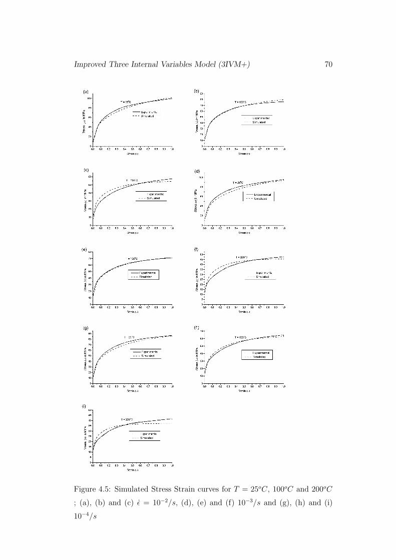
Improved Three Internal Variables Model (3IVM+) 70
Figure 4.5: Simulated Stress Strain curves for T = 25oC, 100oC and 200oC
; (a), (b) and (c) ǫ = 10−2/s, (d), (e) and (f) 10−3/s and (g), (h) and (i)
10−4/s

Improved Three Internal Variables Model (3IVM+) 71
Figure 4.6: Dislocation density evolution for T = 100oC and ǫ = 10−2/s ; (a)
Mobile dislocation density (b) Immobile dislocation density in the cell inte-
riors (c) Immobile dislocation density in the cell walls (d) Total dislocation
density.
Improved Three Internal Variables Model (3IVM+) 72
values of the dislocation densities are also within reasonable limits.
To elucidate the performance of the model at relatively high tem-
peratures, fits were performed at temperatures of T = 350oC, 400oC, 450oC
and strain rates of ǫ = 10−1/s, 10−2/s and 10−3/s. The fits are shown in
figure 4.7. The high temperature fits are good except for (T = 350oC and
ǫ = 10−1/s), where the the initial stage of deformation (upto a strain of
0.2) is wrongly predicted. In some cases (figure 4.7(b), (d) and (h)), though
the stress levels during the initial stages of deformation are over predicted
(note: a difference of 2MPa at maximum) the saturation stress is remarkably
good. The prediction of the saturation stress is especially important if the
flow curves are extrapolated beyond the experimental values as may be the
case in applying the model. The evolution of the dislocation densities for
T = 350oC and ǫ = 10−2, representative of high temperature fits are plotted
in figure 4.8. The trends of evolution of the dislocation densities don’t show
any ambiguity and are as expected. Since the flow curves at high tempera-
ture reach a steady state at low strains, the dislocation densities show similar
trends and reach a saturation value.
As was done for the 3IVM in chapter 3, the ability of the model to
fit flow curves over a wide range of temperatures is examined with 3IVM+ as
well. To check for the model fits for a large temperature range with the same
set of optimizing parameters, we choose temperatures of T = 25oC, 100oC,
350oC and 400oC and strain rates 10−2/s and 10−3/s. These flow curves are
shown in figure 4.9. As shown in the plots (comparing them with 3IVM),
the fits agree very well with experiments. Keeping in mind the fact that this
large temperature range has never been attempted or published, the fits can
be considered to be of good quality. It must be stressed that the fits are
done for the same set of optimizing parameters. For the low temperature

Improved Three Internal Variables Model (3IVM+) 73
Figure 4.7: Simulated Stress Strain curves for T = 350oC, 400oC and 450oC;
(a), (b) and (c) ǫ = 10−1/s (d), (e) and (f) 10−2/s, (g), (h) and (i) 10−3/s
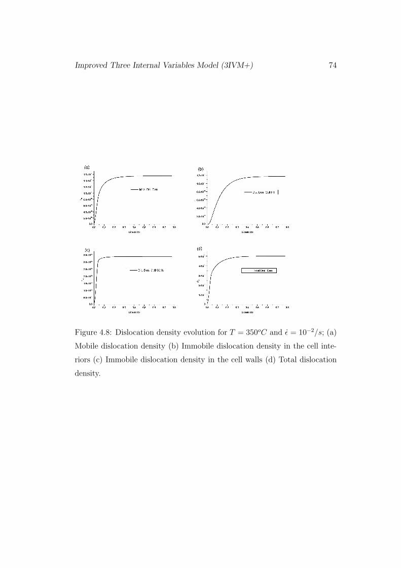
Improved Three Internal Variables Model (3IVM+) 74
Figure 4.8: Dislocation density evolution for T = 350oC and ǫ = 10−2/s; (a)
Mobile dislocation density (b) Immobile dislocation density in the cell inte-
riors (c) Immobile dislocation density in the cell walls (d) Total dislocation
density.

Improved Three Internal Variables Model (3IVM+) 75
fits (figure 4.9 (a), (b), (e) and (f)), the flow stress is under predicted. This
shortcoming could have resulted from the inherent assumption of a cellular
microstructure from the beginning of the simulation. In reality however, the
cellular microstructure develops gradually with strain. On the contrary, the
initial flow stresses are over predicted for the high temperature fits (figure 4.7
(c), (d), (g) and (h)). However the saturation stress prediction is excellent
for the whole temperature range. The evolution of dislocation densities,
for T = 100oC and ǫ = 10−2 as a representation of this large temperature
range simulation is shown in figure 4.10. Both the magnitude and trends of
evolution of the dislocation densities seem to be commensurate with the flow
curves.
4.4 Conclusion
In this chapter, an improved 3 internal variables model was presented with
the aim of describing the flow behavior of aluminum over a wide range of
deformation conditions. A cellular microstructure was assumed in the model.
Like the 3IVM, three different classes of dislocation densities, namely, mobile
dislocation density, immobile dislocation density in the cell interiors and
dislocation density in the cell walls were considered.
Unlike the 3IVM, in the present model, both dislocation climb and
cross slip were included as possible recovery mechanisms. The interaction of
mobile dislocations with immobile dislocations was also taken into account.
This interaction leads to the formulation of 2 additional reactions, namely,
the immobilization reaction and the clearing effect or strain recovery. The
model fits were presented for both relatively high and low temperature ranges
separately. The same model was used to make flow curve predictions for a

Improved Three Internal Variables Model (3IVM+) 76
Figure 4.9: Simulated Stress Strain curves for T = 25oC,100oC, 350oC,
400oC ; (a), (b), (c) and (d) ǫ = 10−2/s, (e), (f), (g) and (h) 10−3/s

Improved Three Internal Variables Model (3IVM+) 77
Figure 4.10: Dislocation Density evolution at 100oC and a strain rate of
10−2/s ; (a) Mobile dislocation density (b) Immobile dislocation density in
the cell interiors (c) Immobile dislocation density in the cell walls (d) Total
dislocation density

Improved Three Internal Variables Model (3IVM+) 78
large range of deformation conditions using the same set of fit parameters.
The ability of the present model to predict the flow behavior of pure alu-
minum in a very large range of deformation conditions was demonstrated.
To our knowledge such a large temperature range has never been tried with
any other model. The dislocation densities were predicted by the model and
are within reasonable limits. Though the model has been used for pure alu-
minum, it can also be used for complex aluminum alloys. The model has
immense scope of being coupled with texture models and recrystallization
models. The present model is very robust with respect to usage of computer
resources and hence can be used with FE codes for process simulations.
Chapter 5
Summary and Outlook
The aim of the present thesis was to develop a dislocation density based sta-
tistical work hardening model to describe the flow behaviour of FCC metals
and alloys. The various models available and their salient features had been
discussed in chapter 1. All the models discussed, had a different choice of in-
ternal variables. To our knowledge, all the work hardening models available
today restrict themselves to predicting the work hardening behaviour over a
narrow range of deformation conditions. Some of the models use a different
set of equations when dealing with high or low deformation temperatures.
On the other hand some models use the same set of equations but a different
set a fit parameters for low and high temperature ranges. A truly unified
work hardening model however must use the same set of equations and fitting
parameters for a large temperature range. This is desirable because it would
allow for more accurate and reliable predictions. In the present model we
achieved this objective of predicting the work hardening behaviour of metals
and alloys over a large range of deformation conditions.
The present model is based on the contemporary understanding of
79
Summary and Outlook 80
the microstructure and is heavily based on the 3 internal variables model
(3IVM). We make improvements to this model and hence the present model
is called the Improved 3 Internal Variables Model (3IVM+). It consists 3
internal state variables namely, the 3 categories of dislocation densities, the
mobile dislocation density (ρm), the immobile dislocation density in the cell
interiors (ρi) and the immobile dislocation density in the cell walls (ρw).
To compare the simulation results, compression experiments were
performed on pure Aluminum (99.9% purity) for a wide range of tempera-
tures and strain rates. These experimental results were discussed in chap-
ter 2. For the sake of comparison with the present model the governing equa-
tions and the results for the 3IVM were discussed in chapter 3. The 3IVM
successfully fits the flow curves at high temperatures. However, the model is
not satisfactory at low temperature range. Taking into consideration that a
wide deformation conditions range has never been considered, the fits from
3IVM+ are good in both low and high temperature ranges for the same set of
fitting parameters. The absolute values of the dislocation densities predicted
by the model are also within reasonable limits. This is especially important
for Through Process Modeling (TPM). The description of the model in detail
with the results and discussion was dealt with in chapter 4.
Though the model fits are in good agreement with experiments, there
is immense scope of improvement of the model in the future. Some of the
suggested improvements are as follows;
1. It is well known that the stacking fault energy effects the distance
between the partial dislocations and hence cross slip frequency. In our
model the dependency of the frequency of cross slip on the stacking fault
energy is not explicitly treated. This equation can be further improved
by including a direct dependency on the stacking fault energy.

Summary and Outlook 81
2. Though the equations for the effect of solutes and precipitates are in-
cluded in the model code, the model has not been tested for alloys.
3. The Taylor factor (used in equation 4.1) is currently being used in
the model as a constant fit parameter. However, the texture of the
material and hence the Taylor factor could change considerably during
deformation. The use of a dynamic Taylor factor can be done by a
coupling of the deformation model with a texture model like GIA (grain
interaction model).
4. The volume fraction of the cell walls (used in equation 4.12) is treated
as a constant fit parameter. During deformation the cell wall thickness
and hence the volume fraction of the cell walls could change consider-
ably. This effect can be taken into account by defining a law on the
change of the volume fraction of the cell walls (as done in [17]).
To conclude, the present model is robust in fitting the hardening behaviour
of metals over a wide range of deformation conditions and has immense scope
to be used in conjunction with other models.
Bibliography
[1] F. Roters, D. Raabe and G. Gottstein, Acta mater., 2000, 48, 4181
[2] H. Mughrabi, F. Ackermann and K. Herz,in Fatigue Mechanisms, 1979,
ASTM STP 675, J.T. Fong ed., ASTM, Philadelphia, PA, 69
[3] U.F. Kocks, J. Eng. Mater. Technolo., 1976, 98, 72
[4] E. Nes, Prog. Materials Sci., 1998, 41, 129
[5] U.F. Kocks and H. Mecking, Prog. In Mater. Sci., 2003,
[6] J. Gil Sevillano, Mat. Sci. and Tech. A comprehensive treatment, 1993,
[7] M. Zehetbauer and V. Seumer, Acta Metall. Mater., 1993, 41, 577
[8] G. Schoeck and A. Seeger, Report of the Bristol conference on Defects
in Crystalline Solids, Physical society London 1955, 440
[9] A. Seeger, R. Berner and H. Wolf, Z. Physic., 1959, 155, 247
[10] H. Wolf, Z. Naturf. (A), 1960, 15, 180
[11] J. Friedel, Dislocations and Mechanical Properties of Crystals, Wiley,
New York, 1957
82

Summary and Outlook 83
[12] D. Kuhlmann-Wilsdorf, Met. Trans., 1970, 1, 3173
[13] D. Kuhlmann-Wilsdorf, in Work Hardening in Tension and Fatigue
(edited by A.W. Thompson), The Metallurgical Society of AIME, New
York, 1977
[14] U.F. Kocks and H. Mecking, in strength of metals and alloys i (edited
by P. Haasen et al.,1979, Vol I, 345
[15] H. Mecking and U.F. Kocks, Acta met., 1981, 29, 1865
[16] H. Mecking, B. Nicklas, N. Zarubova and U.F. Kocks, Acta met., 1986,
34, 527 48, 171
[17] Y. Estrin and H. Mecking, Acta met., 1984, 32, 57
[18] P.S. Follansbee and U.F. Kocks, Acta metall., 1988, 36, 81
[19] S.R. Chen, M.G. Stout, U.F.Kocks, S.R. MacEwen and A.J. Beaudoin,
in Hot Deformation of Aluminum Alloys II (ed. by T.R. Bieler et al.),
The MInerals, Metals and Materials Society, Rosemont, Illinois, 1998
[20] H. Mughrabi, Acta metall., 1983, 31, 1367
[21] W.D. Nix, J.C. Gibeling and K.P. Fuchs, in Mechanical Testing for
Deformation Model Development, 1982, ASTM, STP 765, R.W. Rhode
and J.C. Swearengen eds., ASTM, 301
[22] F.B. Prinz and A.S. Argon, Acta metall., 1984, 32, 1021
[23] A.S. Argon and P. Haasen, Acta metall., 1993, 41, 3289
[24] U.F. Kocks, Phil. Mag., 1966, 13, 541

Summary and Outlook 84
[25] D.J. Llyod, B.D. McLaughlan and H. Sang, Scripta Metall, 1977, 11,
297
[26] Y. Estrin, L.S. Toth, A. Molinari and Y. Brechet, Acta mater., 1998,
46, 5509
[27] M. Muller, M. Zehetbauer A. Borbely and T. Ungar, Z. Metallk., 1995,
86, 827
[28] M. Muller, M. Zehetbauer A. Borbely and T. Ungar, Scripta metall.
mater., 1996, 35, 1461
[29] T. Ungar, L.S. Toth,J. Illy nad I. Kovacs, Acta metall., 1986, 34, 1257
[30] E. Nes, T. Pettersen and K. Marthinsen, Scripta mater., 2000, 43, 55
[31] E. Nes and K. Marthinsen, Mater. Sci. Eng., 2002, A322, 176
[32] K. Marthinsen and E. Nes, Materials Sci. Forum, 2000, 331, 1231
[33] E. Nes, K. Marthinsen and Y. Brechet, Scripta mater., 2002, 47, 607
[34] E. Nes, K. Marthinsen and B. Holmedal, Mater. Sci. Tech., 2004, 20,
1377
[35] K.F. Karhausen and F. Roters, J. of Mat. Proc. Tech., 2002, 123, 155
[36] G.V.S.S. Prasad, M. Goerdeler and G. Gottstein, Mater. Sci. and Engg.
A, 2005, 400-401, 231
[37] G. Gottstein and A.S. Argon, in Creep and Fracture of Engineering
Materials and Structures, 1984, Vol 1,.ed. B. Wilshire and D. R. G.
Owen. Pineridge Press, Swansea. UK, 1984, 15

Summary and Outlook 85
[38] G. Masing, Wiss Verff. Siemens-Konzern 3, 231 (1923)
[39] H. Mughrabi, in Strength of Metals and Alloys(edited by P. Haasen, V.
Gerold and G. Kostorz), Vol 3, p. 1615. Pergamon Press, Oxford (1980)
[40] E. Voce, J. Of Inst. of Met., 1948, 74, 537
[41] J.L. Chaboche, J. App. Mech., 1993, 60, 813
[42] F. Roters, D. Raabe and G. Gottstein, Comp. Mat. Sci., 1996, 7, 56
[43] D. raabe, F. Roters and G. Gottstein, Comp. Mat. Sci., 1996, 5, 203
[44] F. Roters, Phy. stat. sol. B, 2003, 240, 68
[45] M. Crumbach, M. Goerdeler, G. Gottstein, L. Neumann, H. Aretz and
R. Kopp, Modelling Simul. Mater. Sci. Eng, 2004, 12, s1-s18
[46] M. Goerdeler, M. Crumbach, P.. Mukhopadhyay, G. Gottstein, L. Neu-
mann and R. Kopp, Aluminium, 2004, 80, 666
[47] L. Neumann, H. Aretz, R. Kopp, M. Goerdeler, M. Crumbach and G.
Gottstein, Z. Metallk., 2003, 94, 593
[48] H. Aretz, R. Luce, M. Wolske, R. Kopp, M. Goerdeler, G. Pomana and
G. Gottstein,J. Phys. IV France, 2001, 11, 115
[49] M. Goerdeler and G. Gottstein,Mat. Sci. Eng. A, 2001, A309-310, 377
[50] G. Gottstein, M. Goerdeler, F. Roters,Light Metals 2000 Metaux Legers,
[51] M. Crumbach, M. Goerdeler, G. Gottstein, L. Neumann, H. Aretz, R.
Kopp,Modeling Simul. mater. sci., 12, S1-S18

Summary and Outlook 86
[52] J. Kratochvil and S. Libovicky,Scripta metall., 1986, 20, 1625
[53] V. Mohles, Thermisch Aktivierte Versetzungsbewegung in Kristallen auf
der Grundlage von Simulationsrechnungen, Ph. D. thesis, 1997, Shaker
Verlag Aachen, ISBN 3-8265-2365-2
[54] J. Bonneville and B. Escaig, Acta. Metall., 1979, 27, 1477
[55] A.V. Granato, K. Lucke, J. Schlipf and L.J Teutonico, J. of appl. phy.,
1964, 35, 2732

Curriculum Vitae
Personal Details:
Prasad Gurla
email: [email protected]
Education:
1995 - 1999 B.E. In Metallurgical Engineering,
N.I.T Nagpur, India.
1999 - 2002 M.Sc (engg) in Metallurgy,
IISc Bangalore, India.
2002 - 2006 Ph.D in Engineering,
IMM, RWTH Aachen Univerty.
Current Position:
2006 - present Research Engineer,
Arcelor Mittal Research Industry,
Gent, Belgium.
Skills, Interests and Achievements:
• Strong Desire to excel in the field of Material Science.
• Profound knowledge in the field of Physical and Mechanical metallurgy.
• More than 3 years experience in teaching at the University.
• Guided students for the completion of their Masters thesis.
• Excellent programming skills in C, C#, .NET (winforms), asp.net,
html, Flash AS and php.