Asymmetric motion profile planning for nanopositioning and ... · „Dieser Beitrag ist mit...

„Im Rahmen der hochschulweiten Open-Access-Strategie für die Zweitveröffentlichung identifiziert durch die Universitätsbibliothek Ilmenau.“

“Within the academic Open Access Strategy identified for deposition by Ilmenau University Library.”

„Dieser Beitrag ist mit Zustimmung des Rechteinhabers aufgrund einer (DFG-geförderten) Allianz- bzw. Nationallizenz frei zugänglich.“

„This publication is with permission of the rights owner freely accessible due to an Alliance licence and a national licence (funded by the DFG, German Research Foundation) respectively.”

Amthor, Arvid; Werner, J.; Lorenz, Andreas; Zschaeck, Stephan; Ament, Christoph:

Asymmetric motion profile planning for nanopositioning and nanomeasuring machines

URN: urn:nbn:de:gbv:ilm1-2014210268

Published OpenAccess: October 2014

Original published in: Proceedings of the Institution of Mechanical Engineers / I. - London : Sage Publ (ISSN 2041-3041). - 224 (2010) 1, S. 79-92. DOI: 10.1243/09596518JSCE826 URL: http://dx.doi.org/10.1243/09596518JSCE826 [Visited: 2014-10-14]

http://pii.sagepub.com/Control Engineering

Engineers, Part I: Journal of Systems and Proceedings of the Institution of Mechanical

http://pii.sagepub.com/content/224/1/79The online version of this article can be found at:

DOI: 10.1243/09596518JSCE826

2010 224: 79Proceedings of the Institution of Mechanical Engineers, Part I: Journal of Systems and Control EngineeringA Amthor, J Werner, A Lorenz, S Zschaeck and C Ament

Asymmetric motion profile planning for nanopositioning and nanomeasuring machines

Published by:

http://www.sagepublications.com

On behalf of:

Institution of Mechanical Engineers

can be found at:EngineeringProceedings of the Institution of Mechanical Engineers, Part I: Journal of Systems and ControlAdditional services and information for

http://pii.sagepub.com/cgi/alertsEmail Alerts:

http://pii.sagepub.com/subscriptionsSubscriptions:

http://www.sagepub.com/journalsReprints.navReprints:

http://www.sagepub.com/journalsPermissions.navPermissions:

http://pii.sagepub.com/content/224/1/79.refs.htmlCitations:

What is This?

- Feb 1, 2010Version of Record >>

at Technische Universität Ilmenau on October 14, 2014pii.sagepub.comDownloaded from at Technische Universität Ilmenau on October 14, 2014pii.sagepub.comDownloaded from

http://pii.sagepub.com/

http://pii.sagepub.com/content/224/1/79

http://www.sagepublications.com

http://www.imeche.org/home

http://pii.sagepub.com/cgi/alerts

http://pii.sagepub.com/subscriptions

http://www.sagepub.com/journalsReprints.nav

http://www.sagepub.com/journalsPermissions.nav

http://pii.sagepub.com/content/224/1/79.refs.html

http://pii.sagepub.com/content/224/1/79.full.pdf

http://online.sagepub.com/site/sphelp/vorhelp.xhtml



Asymmetric motion profile planning fornanopositioning and nanomeasuring machinesA Amthor*, J Werner, A Lorenz, S Zschaeck, and C Ament

System Analysis Group, Ilmenau University of Technolog, Ilmenau, Germany

The manuscript was received on 10 June 2009 and was accepted after revision for publication on 9 September 2009.

DOI: 10.1243/09596518JSCE826

Abstract: This work presents an analytic fourth-order trajectory planning algorithm, which isable to plan asymmetric motions with arbitrary initial and final velocities. Furthermore, theproposed algorithm is based on a set of quadratic derivates of jerk (djerk) functions andgenerates continuously differentiable trajectories in jerk, acceleration, velocity, and positionunder consideration of kinematic constraints in all these kinematical values. The trajectoriesplanned by the algorithm also have time-optimal characteristics, and a synchronizationbetween the three motion axes of the Cartesian coordinate system is ensured by the proposedmethod. These characteristics make it ideally suited for use as a trajectory planning algorithmin high-precision applications such as nanopositioning and nanomeasuring machines.

Keywords: analytic fourth-order trajectory generation, asymmetric motion planning, highprecision motion control

1 INTRODUCTION

High-performance motion control is widely needed

in modern nanopositioning. To measure and manip-

ulate structures on the nanometre scale, high-

resolution positioning stages are used. These stages

are able to position a pattern in all three dimensions

with an accuracy of less then one nanometre with

operational ranges up to several hundred milli-

metres. The work presented here is motivated by a

2006200mm2 fine positioning stage, which was

developed within the Collaborative Research Centre

622 ‘Nanopositioning and Nanomeasuring Ma-

chines’ at the Ilmenau University of Technology

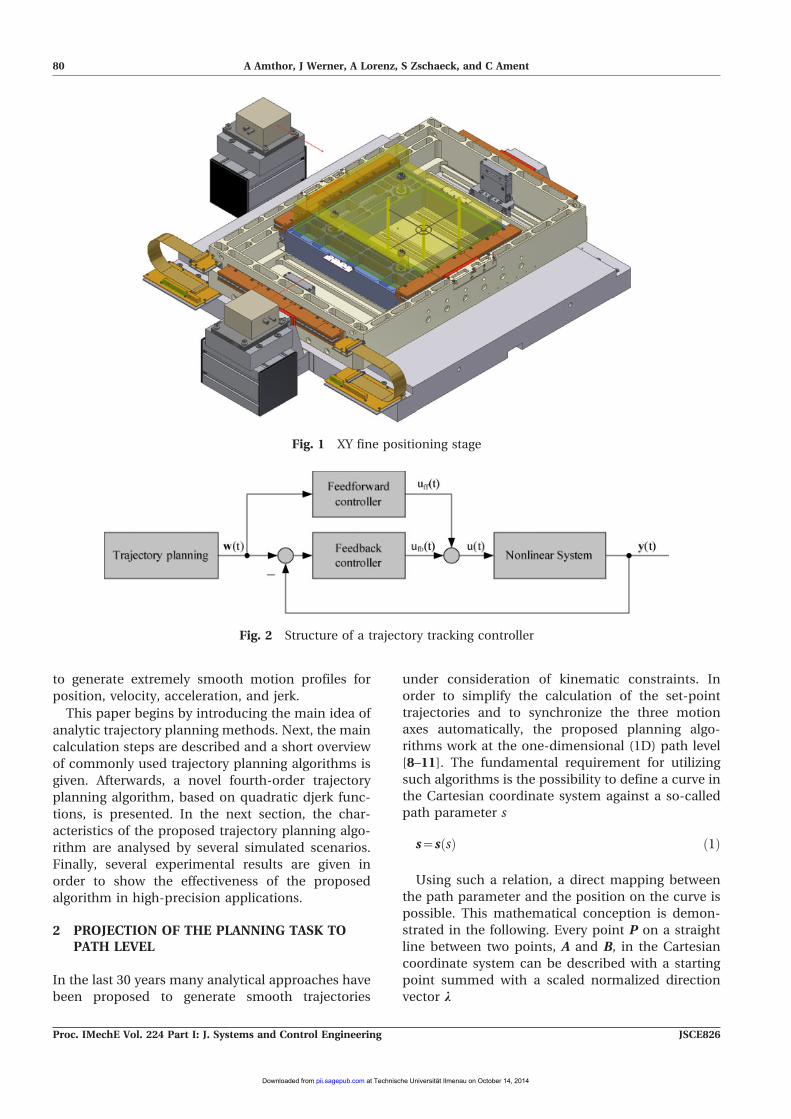
[1, 2]. As can be seen in Fig. 1, each axis is driven by

two linear voice coil actuators. The actuators are

powered by proprietary analogue amplifiers, which

provide the necessary current with the required

precision. Each axis is supported by two linear V-

grooved guideways. The position is measured by

stabilized HeNe laser interferometers with a resolu-

tion of less than 0.1 nm [3]. For data acquisition and

control, a modular dSpaceH real-time system in

combination with MATLAB/SimulinkH is utilized [4].

The control algorithm works with a sample rate of

10 kHz and operates on the amplifiers with a 16-bit

resolution.

Due to the increasing operating ranges of such

stages, positioning speed must also be scaled up. In

recent years, trajectory tracking controllers are

seeing increased usage in order to realize the

requirements of a fast and simultaneously accurate

motion over a wide spectrum of velocities [1, 5–7].

As shown in Fig. 2, a trajectory tracking controller is

typically composed of the following components, a

trajectory planning algorithm, a feedforward con-

troller, and a feedback controller. The task of the

feedforward controller is to calculate the force which

is needed to accelerate a single mass according to

the desired position trajectory. To avoid a violation

of the mechanical and electrical limitations of the

system, the trajectory planning algorithm explicitly

considers these limitations.

An important issue, especially in nanopositioning,

is the stimulation of the eigenfrequencies of the

mechanical components caused by abrupt changes

in acceleration and jerk. These vibrations have to be

minimized during motion because they decrease the

accuracy and increase the settling time of the

positioning stage. One way to solve this problem is

*Corresponding author: System Analysis Group, Ilmenau Uni-

versity of Technology, Gustav-Kirchhoff Strabe 1, Ilmenau,

Germany.

email: [email protected]

79

JSCE826 Proc. IMechE Vol. 224 Part I: J. Systems and Control Engineering

at Technische Universität Ilmenau on October 14, 2014pii.sagepub.comDownloaded from


to generate extremely smooth motion profiles for

position, velocity, acceleration, and jerk.

This paper begins by introducing the main idea of

analytic trajectory planning methods. Next, the main

calculation steps are described and a short overview

of commonly used trajectory planning algorithms is

given. Afterwards, a novel fourth-order trajectory

planning algorithm, based on quadratic djerk func-

tions, is presented. In the next section, the char-

acteristics of the proposed trajectory planning algo-

rithm are analysed by several simulated scenarios.

Finally, several experimental results are given in

order to show the effectiveness of the proposed

algorithm in high-precision applications.

2 PROJECTION OF THE PLANNING TASK TOPATH LEVEL

In the last 30 years many analytical approaches have

been proposed to generate smooth trajectories

under consideration of kinematic constraints. In

order to simplify the calculation of the set-point

trajectories and to synchronize the three motion

axes automatically, the proposed planning algo-

rithms work at the one-dimensional (1D) path level

[8–11]. The fundamental requirement for utilizing

such algorithms is the possibility to define a curve in

the Cartesian coordinate system against a so-called

path parameter s

s~s sð Þ ð1Þ

Using such a relation, a direct mapping between

the path parameter and the position on the curve is

possible. This mathematical conception is demon-

strated in the following. Every point P on a straight

line between two points, A and B, in the Cartesian

coordinate system can be described with a starting

point summed with a scaled normalized direction

vector l

Fig. 1 XY fine positioning stage

Fig. 2 Structure of a trajectory tracking controller

80 A Amthor, J Werner, A Lorenz, S Zschaeck, and C Ament

Proc. IMechE Vol. 224 Part I: J. Systems and Control Engineering JSCE826



P~AztB{Að ÞB{Að Þk k~Azkpathl ð2Þ

Thus, the scaling parameter kpath is zero at the

starting point and reflects the distance between the

considered points at the endpoint. This mathema-

tical relation is the basis for the complete trajectory

planning concept because at the path level it is

sufficient to only consider one dimension kpath.

Thus, the starting point can be described with

kpath5 0 and the endpoint with kpath~ B{Að Þ=B{Að Þk k. Hence, equation (2) defines the consid-

ered section against the path parameter kpath. Using

this mathematical connection a direct mapping

between path level and the Cartesian coordinate

system is possible.

3 PRINCIPLES OF ANALYTICAL TRAJECTORYGENERATION ALGORITHMS

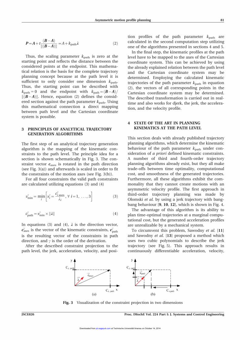
The first step of an analytical trajectory generation

algorithm is the mapping of the kinematic con-

straints to the path level. The principle idea for a

section is shown schematically in Fig. 3. The con-

straint vector caxes is rotated in the path direction

(see Fig. 3(a)) and afterwards is scaled in order to fit

the constraints of the motion axes (see Fig. 3(b)).

For all four constraints the valid path constraints

are calculated utilizing equations (3) and (4)

acmin~mini

aci~cci axesli

, V i~1, . . . , 3

� �ð3Þ

ccpath~acmin| lk k ð4Þ

In equations (3) and (4), l is the direction vector,

ccaxes is the vector of the kinematic constraints, ccpathis the resulting vector of the constraints in path

direction, and c is the order of the derivation.

After the described constraint projection to the

path level, the jerk, acceleration, velocity, and posi-

tion profiles of the path parameter kpath are

calculated in the second computation step utilizing

one of the algorithms presented in sections 4 and 5.

In the final step, the kinematic profiles at the path

level have to be mapped to the axes of the Cartesian

coordinate system. This can be achieved by using

the already explained relation between the path level

and the Cartesian coordinate system may be

determined. Employing the calculated kinematic

trajectories of the path parameter kpath in equation

(2), the vectors of all corresponding points in the

Cartesian coordinate system may be determined.

The described transformation is carried out in real-

time and also works for djerk, the jerk, the accelera-

tion, and the velocity profile.

4 STATE OF THE ART IN PLANNINGKINEMATICS AT THE PATH LEVEL

This section deals with already published trajectory

planning algorithms, which determine the kinematic

behaviour of the path parameter kpath under con-

sideration of a priori defined kinematic constraints.

A number of third and fourth-order trajectory

planning algorithms already exist, but they all make

trade-offs between time optimality, computational

cost, and smoothness of the generated trajectories.

Furthermore, all these algorithms exhibit the com-

monality that they cannot create motions with an

asymmetric velocity profile. The first approach in

third-order trajectory planning was made by

Olomski et al. by using a jerk trajectory with bang-

bang behaviour [9, 10, 12], which is shown in Fig. 4.

The advantage of this algorithm is its ability to

plan time-optimal trajectories at a marginal compu-

tational cost, but the generated acceleration profiles

are unrealizable by a mechanical system.

To circumvent this problem, Sawodny et al. [11]

and Sawodny et al. [13] proposed a method which

uses two cubic polynomials to describe the jerk

trajectory (see Fig. 5). This approach results in

continuously differentiable acceleration, velocity,

Fig. 3 Visualization of the constraint projection in two dimensions

Asymmetric motion profile planning 81




and position profiles, which can be realized by a

mechanical system.

A comparison between Fig. 4 and Fig. 5 highlights

the negative characteristic of the cubic jerk algo-

rithm. The calculated trajectories are not time-

optimal compared to the constant jerk algorithm

especially in the case of badly conditioned kinematic

constraints. Li et al. [14] presented a related

approach using a piecewise defined sine function

as the jerk profile. A deeper analysis of the algorithm

has not been performed because the characteristics

of the method of Li et al. [14] appear to be those of a

cubic jerk algorithm. A natural extension of the

described third-order trajectory planning algorithms

was proposed by Lambrechts et al. [8, 15]. They were

the first to present a fourth-order motion planning

algorithm, utilizing the idea of Olomski to determine

all kinematic profiles. The generated trajectories for

acceleration, velocity, and position are based on the

profile of the djerk, and are continuously differenti-

able. Also, time-optimal trajectory planning is

possible using this approach. Thus, Lambrechts et

al. [8, 15] merge the advantages of the constant jerk

and cubic jerk methods.

5 ASYMMETRIC FOURTH-ORDER TRAJECTORYPLANNING AT THE PATH LEVEL

Due to the extraordinary requirements of nanoposi-

tioning systems the approach of Lambrechts et al. [8,

15] is extended once again and a novel trajectory

planning algorithm is presented. The main feature of

the proposed algorithm is the ability to plan motions

with random initial and final velocities. This pro-

vides the ability to realize continuous trajectory

planning over an arbitrary number of connected

path segments. The proposed algorithm is based on

the construction of the djerk profile. This djerk

trajectory is composed of piecewise defined quad-

ratic functions as defined in equation (5). The

trajectory can be analytically integrated several

times to obtain a continuously differentiable jerk

trajectory, acceleration trajectory, velocity trajectory,

and position trajectory. For example, all profiles are

shown in Fig. 6. Assuming a starting time of zero, the

djerk trajectory can be described with seven time

intervals as depicted in Fig. 6. As can be seen in

equation (5), these seven time intervals define the

shape of the djerk trajectory and thus all other

Fig. 4 Third-order trajectory generation using constant jerk functions

Fig. 5 Third-order trajectory generation using cubic jerk functions





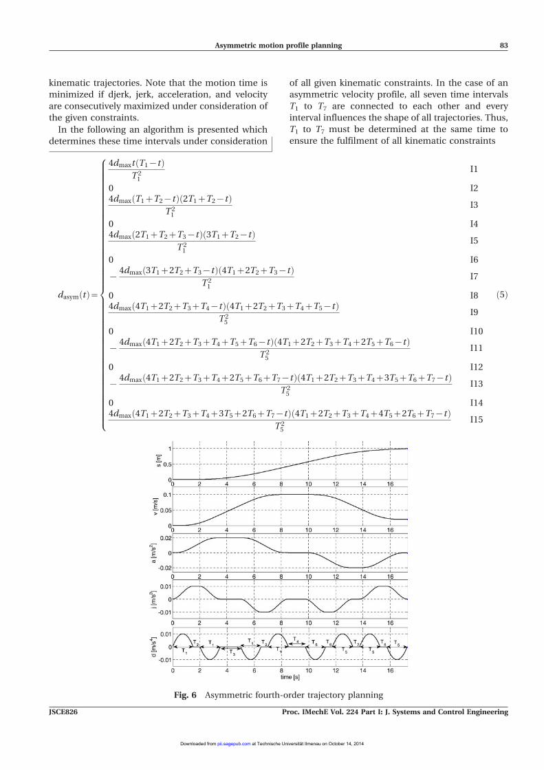
kinematic trajectories. Note that the motion time is

minimized if djerk, jerk, acceleration, and velocity

are consecutively maximized under consideration of

the given constraints.

In the following an algorithm is presented which

determines these time intervals under consideration

of all given kinematic constraints. In the case of an

asymmetric velocity profile, all seven time intervals

T1 to T7 are connected to each other and every

interval influences the shape of all trajectories. Thus,

T1 to T7 must be determined at the same time to

ensure the fulfilment of all kinematic constraints

Fig. 6 Asymmetric fourth-order trajectory planning

dasym tð Þ~

4dmaxt T1{tð ÞT 21

I1

0 I24dmax T1zT2{tð Þ 2T1zT2{tð Þ

T 21

I3

0 I44dmax 2T1zT2zT3{tð Þ 3T1zT2{tð Þ

T 21

I5

0 I6

{4dmax 3T1z2T2zT3{tð Þ 4T1z2T2zT3{tð Þ

T 21

I7

0 I84dmax 4T1z2T2zT3zT4{tð Þ 4T1z2T2zT3zT4zT5{tð Þ

T 25

I9

0 I10

{4dmax 4T1z2T2zT3zT4zT5zT6{tð Þ 4T1z2T2zT3zT4z2T5zT6{tð Þ

T 25

I11

0 I12

{4dmax 4T1z2T2zT3zT4z2T5zT6zT7{tð Þ 4T1z2T2zT3zT4z3T5zT6zT7{tð Þ

T 25

I13

0 I144dmax 4T1z2T2zT3zT4z3T5z2T6zT7{tð Þ 4T1z2T2zT3zT4z4T5z2T6zT7{tð Þ

T 25

I15

8>>>>>>>>>>>>>>>>>>>>>>>>>>>>>>>>>>>>>>>>>>>>><>>>>>>>>>>>>>>>>>>>>>>>>>>>>>>>>>>>>>>>>>>>>>:

ð5Þ





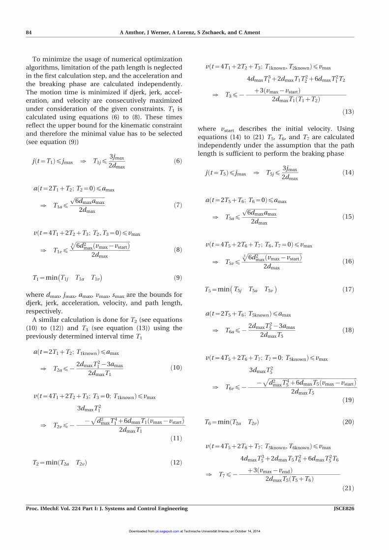
To minimize the usage of numerical optimization

algorithms, limitation of the path length is neglected

in the first calculation step, and the acceleration and

the breaking phase are calculated independently.

The motion time is minimized if djerk, jerk, accel-

eration, and velocity are consecutively maximized

under consideration of the given constraints. T1 is

calculated using equations (6) to (8). These times

reflect the upper bound for the kinematic constraint

and therefore the minimal value has to be selected

(see equation (9))

j t~T1ð Þ¡jmax [ T1j¡3jmax

2dmaxð6Þ

a t~2T1zT2; T2~0ð Þ¡amax

[ T1a¡ffiffiffiffiffiffiffiffiffiffiffiffiffiffiffiffiffiffiffiffiffiffi6dmaxamax

p2dmax

ð7Þ

v t~4T1z2T2zT3; T2,T3~0ð Þ¡vmax

[ T1v¡ffiffiffiffiffiffiffiffiffiffiffiffiffiffiffiffiffiffiffiffiffiffiffiffiffiffiffiffiffiffiffiffiffiffiffiffiffiffiffiffi6d2

max vmax{vstartð Þ3p

2dmax

ð8Þ

T1~min T1j T1a T1v

� � ð9Þ

where dmax, jmax, amax, vmax, smax are the bounds for

djerk, jerk, acceleration, velocity, and path length,

respectively.

A similar calculation is done for T2 (see equations

(10) to (12)) and T3 (see equation (13)) using the

previously determined interval time T1

a t~2T1zT2; T1knownð Þ¡amax

[ T2a¡{2dmaxT

21{3amax

2dmaxT1

ð10Þ

v t~4T1z2T2zT3; T3~0; T1knownð Þ¡vmax

[ T2v¡{

3dmaxT21

{ffiffiffiffiffiffiffiffiffiffiffiffiffiffiffiffiffiffiffiffiffiffiffiffiffiffiffiffiffiffiffiffiffiffiffiffiffiffiffiffiffiffiffiffiffiffiffiffiffiffiffiffiffiffiffiffiffiffiffiffiffiffiffiffiffid2maxT

41z6dmaxT1 vmax{vstartð Þp2dmaxT1

ð11Þ

T2~min T2a T2vð Þ ð12Þ

v t~4T1z2T2zT3; T1known,T2knownð Þ¡vmax

[ T3¡{

4dmaxT31z2dmaxT1T

22z6dmaxT

21T2

z3 vmax{vstartð Þ2dmaxT1 T1zT2ð Þ

ð13Þ

where vstart describes the initial velocity. Using

equations (14) to (21) T5, T6, and T7 are calculated

independently under the assumption that the path

length is sufficient to perform the braking phase

j t~T5ð Þ¡jmax [ T5j¡3jmax

2dmaxð14Þ

a t~2T5zT6; T6~0ð Þ¡amax

[ T5a¡ffiffiffiffiffiffiffiffiffiffiffiffiffiffiffiffiffiffiffiffiffiffi6dmaxamax

p2dmax

ð15Þ


[ T5v¡ffiffiffiffiffiffiffiffiffiffiffiffiffiffiffiffiffiffiffiffiffiffiffiffiffiffiffiffiffiffiffiffiffiffiffiffiffiffiffiffi6d2

max vmax{vstartð Þ3p

2dmax

ð16Þ

T5~min T5j T5a T5v

� � ð17Þ

a t~2T5zT6; T5knownð Þ¡amax

[ T6a¡{2dmaxT

25{3amax

2dmaxT5

ð18Þ


[ T6v¡{

3dmaxT25

{ffiffiffiffiffiffiffiffiffiffiffiffiffiffiffiffiffiffiffiffiffiffiffiffiffiffiffiffiffiffiffiffiffiffiffiffiffiffiffiffiffiffiffiffiffiffiffiffiffiffiffiffiffiffiffiffiffiffiffiffiffiffiffiffiffid2maxT

45z6dmaxT5 vmax{vstartð Þ

p2dmaxT5

ð19Þ

T6~min T2a T2vð Þ ð20Þ

v t~4T5z2T6zT7; T5known,T6knownð Þ¡vmax

[ T7¡{

4dmaxT35z2dmaxT5T

26z6dmaxT

25T6

z3 vmax{vendð Þ2dmaxT5 T5zT6ð Þ

ð21Þ





where vend is the final velocity at the end of the path.

The last calculation step is the determination of the

constant velocity phase according to equation (22)

If T4. 0, the path length is long enough and the

analytical determined switching times are valid. For

the case where T4 has a negative value, the path

length is the limiting condition. Thus, all calculated

time intervals are not valid and T1 to T7 are directly

connected to each other. Under the assumption that

T1 and T5 are limited by the path length the

equations (23) and (24) have to be fulfilled

s t~4T1z2T2zT3zT4z4T5z2T6ðzT7; T2,T3,T4,T6,T7~0Þ~send

[ 8dmaxT41z16dmaxT

31T5z12vstartT1

z12vstartT5{8dmaxT45{3send~0 ð23Þ

v t~4T1z2T2zT3zT4z4T5z2T6ðzT7; T2,T3,T4,T6,T7~0Þ~vend

[ 4dmaxT31{4dmaxT

35z3 vstart{vendð Þ~0

ð24Þ

Using these equations, T1new and T5new can be

analytically determined. If both times are smaller

than the previously calculated times T1old and T5old,

the assumption that T1 and T5 are limited by the

path length is correct. In the case of a larger T1new

and T5new, T2 and T6 are possibly limited by the path

length and equations (23) and (24) are utilized in a

modified form (all times apart from T2 and T6 are

now zero) in order to check this premise. In the case

that only one of the times T1new and T5new is limited

by the path length, this time is kept and the other

(not limited) time is replaced in equations (23) and

(24). This procedure is continued until interval times

in the acceleration and deceleration phase are

found, which are limited by the path length (namely

both times are smaller than the previously analyti-

cally calculated interval times). For clarification,

Fig. 7 shows the algorithm which determines all

interval times if T4, 0.

With the determination of T1 to T7, all parameters

of the djerk trajectory are available and thus all other

kinematic trajectories of the path parameter kpath are

defined.

In the last step of the planning algorithm, the

kinematic profiles at the path level must be mapped

to the motion axes using the already explained

relation between the path level and the Cartesian

coordinate system (see equation (2)).

The main advantage of this approach is the

avoidance of an explicit synchronization between

the motion axes, because of the geometric correla-

tion between the path level and the Cartesian

coordinate system.

It should be mentioned, that in the case of

vstart5 vend, a completely analytical determination

of the interval times T1 to T7 is possible, because the

motion has a symmetric character. Hence, the whole

profile is determined by four time intervals: the

constant djerk interval, the constant jerk interval, the

constant acceleration interval, and the constant

velocity interval. Using this relation all set-point

trajectories are symmetrical and T15T5, T25T6 as

well as T35T7. Now the planning algorithm has to

determine only four time intervals (T1 to T4) instead

of seven.

v t~4T1z2T2zT3zT4z4T5z2T6zT7; T1known,T2known,T3known,T5known,T6known,T7knownð Þ¡smax

[ T4¡{1

6dmaxT21T2z2dmaxT1T2T3z4dmaxT

31z2dmaxT1T

22z2dmaxT

21T3

| 3dmaxT3T 1T22{dmaxT5T6T

27z2dmaxT1T2T3T7z4dmaxT1T6T

22z24dmaxT

21T2T5

�{dmaxT

21T

33{3dmaxT5T

26T7z10dmaxT

21T

22z12dmaxT

21T2T6z9dmaxT

21T2T3

{9dmaxT25T6T7z2dmaxT1T

22T7{dmaxT

25T

27z16dmaxT

31T2z8dmaxT

21T3T5

z4dmaxT31T7z8dmaxT1T

22T5z6dmaxT

21T2T7z6T2vstartz3T3vstart6T6vstart

z3T7vstartz12T1vstartz6dmaxT31T3z2dmaxT1T

32z4dmaxT

21T3T6z12T5vstart

z2dmaxT21T3{8dmaxT

45{10dmaxT

25T

36z8dmaxT1T2T3T5z8dmaxT

31T6{2dmaxT5T

36

z4dmaxT1T2T3T6{6dmaxT35T7{2smaxz8dmaxT

41zdmaxT1T2T

23{16dmaxT

35T6

z16dmaxT31T5

� ð22Þ





In the symmetrical case, T1 is calculated as already

described (see equations (6) and (7)) but now the

limitation of the position can be included in the

calculation because the acceleration and the braking

phase have the same shape. Thus, the calculation is

extended to include equations (25) to (27)


[ T1v¡ffiffiffiffiffiffiffiffiffiffiffiffiffiffiffiffiffiffiffiffiffiffi6d2

maxvmax3p

2dmax

ð25Þ

s t~8T1z4T2z2T3zT4; T2,T3,T4~0ð Þ¡smax

[ T1s¡ffiffiffiffiffiffiffiffiffiffiffiffiffiffiffiffiffiffiffiffiffi3d3

maxsmax4p

2dmax

ð26Þ

T1~min T1j T1a T1v T1s

� � ð27Þ

A similar calculation is done for T2 (see equations

(10) and (28) to (30)) and T3 (see equations (31) to

(33)) using the previously determined interval times


[ T2v¡{3dmaxT

21{

ffiffiffiffiffiffiffiffiffiffiffiffiffiffiffiffiffiffiffiffiffiffiffiffiffiffiffiffiffiffiffiffiffiffiffiffiffiffiffiffiffiffiffiffiffiffiffid2maxT

41z6d2

maxT1vmax

p2dmaxT1

ð28Þ

Fig. 7 Visualization of the algorithm for determination of the time intervals T1 to T7 if T4, 0

s t~8T1z4T2z2T3zT4; T3,T4~0; T1knownð Þ¡smax

[ T2s¡

ffiffiffiffiffiffiffiffiffiffiffiffiffiffiffiffiffiffiffiffiffiffiffiffiffiffiffiffiffiffiffiffiffiffiffiffiffiffiffiffiffiffiffiffiffiffiffiffiffiffiffiffiffiffiffiffiffiffiffiffiffiffiffiffiffiffiffiffiffiffiffiffiffiffiffiffiffiffiffiffiffiffiffiffiffiffiffiffiffiffiffiffiffiffiffiffiffiffiffiffiffiffiffiffiffiffiffiffiffiffiffiffiffiffiffiffiffiffiffiffiffid2maxT

41 8dmaxT

41z81smaxz9

ffiffiffiffiffiffiffiffiffiffiffiffiffiffiffiffiffiffiffiffiffiffiffiffiffiffiffiffiffiffiffiffiffiffiffiffiffiffiffiffiffiffiffiffiffiffiffiffiffiffiffiffismax 16dmaxT

41z81smax

� �q� �3

r6dmaxT1

z2dmaxT

31

3

ffiffiffiffiffiffiffiffiffiffiffiffiffiffiffiffiffiffiffiffiffiffiffiffiffiffiffiffiffiffiffiffiffiffiffiffiffiffiffiffiffiffiffiffiffiffiffiffiffiffiffiffiffiffiffiffiffiffiffiffiffiffiffiffiffiffiffiffiffiffiffiffiffiffiffiffiffiffiffiffiffiffiffiffiffiffiffiffiffiffiffiffiffiffiffiffiffiffiffiffiffiffiffiffiffiffiffiffiffiffiffiffiffiffiffiffiffiffiffiffiffid2maxT

41 8dmaxT

41z81smaxz9

ffiffiffiffiffiffiffiffiffiffiffiffiffiffiffiffiffiffiffiffiffiffiffiffiffiffiffiffiffiffiffiffiffiffiffiffiffiffiffiffiffiffiffiffiffiffiffiffiffiffiffiffismax 16dmaxT

41z81smax

� �q� �3

r {5

3T1 ð29Þ





T2~min T2a T2v T2sð Þ ð30Þ

T3~min T3v, T3sð Þ ð33Þ

The determination of T1, T2, and T3 is followed by

the calculation of T4. This interval is only bounded

by the maximum path length and so T4 is calculated

by

The shown analytical determination of all interval

times speeds up the calculation time significantly

and therefore the implementation of the proposed

algorithm uses an analytical method of calculation

as often as possible.

6 IMPLEMENTATION ASPECTS ANDPERFORMANCE ANALYSIS

The trajectory generation algorithm is implemented

in MATLAB/Simulink and consists of two modules.

The determination of the valid constraints (see

equations (3) and (4)) at the path level (see section

3), and the calculation of the interval times T1 to T7

(see section 5) are implemented in MATLAB m-code.

The generation of the trajectories in djerk, jerk,

acceleration, velocity, and position for the path

parameter kpath and the subsequent coordinate

transformation in the Cartesian coordinate system

are done using a Simulink C-code-s-function. The

reason for using C-code-s-functions is that this part

of the trajectory planning algorithm has to be carried

out on a real-time system. Most of these systems

were programmed in C and therefore a hand-tuned

implementation will achieve the best performance.

Furthermore, C-code-s-functions allow the possibi-

lity to recycle the programmed algorithms.

In the following several examples for symmetric

and asymmetric trajectories are provided and it will

be shown that the proposed algorithm is able to

reproduce the time optimality of the constant jerk

method as well as the continuously differentiable

jerk trajectories of the algorithm proposed by Sawodny

et al. [11, 13]. In Fig. 8, the maximum djerk is quite

high in comparison to the constraints of the residual

kinematic values and thus the behaviour of the

constant jerk method can be imitated by the proposed

algorithm. As can be seen, the planned trajectory at the

path level is time-optimal; however, the calculated jerk

trajectory is continuously differentiable and thus

jumps in jerk can be avoided. Also, an emulation of

the cubic jerkmethod is possible if themaximumdjerk

is in the same range in comparison to the other

kinematic constraints (see Fig. 9). This analysis shows

that the maximum djerk is a powerful tuning para-

meter, enabling the possibility to regulate the time

optimality of the planned trajectory. Figure 10 shows a

comparison between the cubic jerk method and the

proposed algorithm to clarify the capability to generate

time-optimal and extremely smooth trajectories. It can

be easily seen that the algorithm is able to plan a

continuously differentiable jerk trajectory in connec-

tion with constant jerk intervals. This leads to a

reduction of the moving time by about 25 per cent

compared to the cubic jerk method. All the presented

examples show clearly that the proposed algorithm

s t~8T1z4T2z2T3zT4; T4~0; T1known,T2knownð Þ¡smax

[ T3s¡{

6dmaxT31z3dmaxT1T

22z9dmaxT

21T2

�

{

ffiffiffiffiffiffiffiffiffiffiffiffiffiffiffiffiffiffiffiffiffiffiffiffiffiffiffiffiffiffiffiffiffiffiffiffiffiffiffiffiffiffiffiffiffiffiffiffiffiffiffiffiffiffiffiffiffiffiffiffiffiffiffiffiffiffiffiffiffiffiffiffiffiffiffiffiffiffiffiffiffiffiffiffiffiffiffiffiffiffiffiffiffiffiffiffiffiffiffiffiffiffiffiffiffi4d2

maxT61z13d2

maxT41T

22z12d2

maxT51T2zd2

maxT21T

42

z6d2maxT

31T

32z6dmaxT1T2smaxz6dmaxT

21 smax

vuut1A

,2dmaxT1 T1zT2ð Þ ð32Þ

v t~4T1z2T2zT3; T1known; T2knownð Þ¡vmax [ T3v¡{4dmaxT

31z6dmaxT

21T2z2dmaxT1T

22z3vmax

2dmaxT1 T1zT2ð Þ ð31Þ

s t~8T1z4T2z2T3zT4; T1known,T2known,T3knownð Þ¡smax

[ T4¡{1

2dmaxT1 T 22zT1T3zT2T3z2T 2

1z3T1T2

� �| 16dmaxT41z2dmaxT

21T

23z18dmaxT

21T2T3

�z32dmaxT

31T2z4dmaxT1T

32z12dmaxT

31T3z2dmaxT1T2T

23z6dmaxT1T

22T3z20dmaxT

21T

22{3smaxÞ

ð34Þ





Fig. 8 Constant jerk method reproduced by the proposed algorithm

Fig. 9 Cubic jerk method reproduced by the proposed algorithm

Fig. 10 Dynamical performance of the proposed algorithm compared with the cubic jerkmethod





unifies the advantages of the constant jerk and the

cubic jerk methods.

In Fig. 11, an asymmetric motion is shown. The

motion starts with an initial velocity and in the

following 2 s the system is accelerated to the

maximum allowed velocity. After 3 s the system

begins to decelerate in order to reach the defined

final velocity at the defined position.

Using the proposed approach, it is possible to plan

a continuous motion along a complex trajectory in

three dimensions, which is composed of several

linear segments.

7 EXPERIMENTAL RESULTS

In order to verify the practical use of the proposed

trajectory generation method, the algorithm was

carried out on the modular dSpace real-time system

described in section 1. As already mentioned the

trajectory generation works with a sampling rate of

10 kHz and requires 5 ms for computation (using a

3GHz AMD Opteron). Figure 12 shows a typical

linear motion of the y-axis over a distance of 30mm.

As can easily be seen, the kinematic characteristic

constraints of nanopositioning machines (NPMs)

Fig. 11 Example for a movement with arbitrary initial and final velocity

Fig. 12 Linear motion of the y-axis with an asymmetric velocity profile





were kept and all generated motion profiles up to

jerk level are continuously differentiable.

Furthermore, it has to be mentioned, that in

conventional applications the interval time T1 only

lasts for a small number of sample periods and this

leads to significant discretization errors in the djerk

profile. When considering high-precision applica-

tions such as NPM systems, however, this diagnosis

is not correct because the sample rate is quite high

compared to classical applications in robotics. To

support this conclusion Fig. 13 shows the generated

djerk profile from the experiment presented in

Fig. 12. It can be seen, that T1 last for nearly 45ms,

corresponding to approximately 450 sample periods.

Thus, the discretization error of the djerk profile is

insignificant if the sample rate is high enough. In

addition to the already described experiment, an-

other test was carried out to demonstrate the ability

of the proposed algorithm to enhance the dynamic

performance of the controlling system. Figures 14

and 15 show two runs of a linear motion of the y-axis

over a distance of 30mm, each with a different

planning algorithm.

In both runs the position was controlled by a well-

tuned classical proportional–integral–derivative con-

troller in combination with a trajectory planning

Fig. 13 Discretization of the profile at the djerk level

Fig. 14 Tracking error using the constant jerk method for trajectory generation





algorithm. In Fig. 14 the constant jerk method was

utilized (see section 4). It can be seen that especially

at the starting point the tracking error is quite high at

almost 1000nm. In Fig. 15 the proposed fourth-

order trajectory planning algorithm is used.

The tracking error in the acceleration phase is

reduced by about 25 per cent to approximately

750 nm; this clearly shows the effectiveness of the

proposed algorithm in high-precision applications

such as nanopositioning.

8 CONCLUSIONS AND FUTURE WORK

In this contribution, a novel trajectory planning

algorithm is shown. The basis of the proposed

method is the transformation of a linear segment

in the three-dimensional (3D) Cartesian coordinate

system to the so-called 1D path level. This is

achieved by using the scaling vector of the segments’

vector notation as the path parameter. In the first

calculation step the kinematic constraints in djerk,

jerk, acceleration, and velocity for every axis of the

Cartesian coordinate system are mapped to the path

level. This is followed by the second step; determi-

nation of the kinematic behaviour of the path

parameter. All kinematic trajectories are based on

the djerk profile, which is composed of piecewise-

defined quadratic functions. This trajectory is analy-

tically integrated several times to obtain the trajec-

tories for jerk, acceleration, velocity, and posi-

tion. The last step of the proposed method is the

projection of the planned 1D trajectories to the 3D

Cartesian coordinate system. It was shown by

simulation and experiment, that by using this

method it is possible to create continuously differ-

entiable set-point trajectories up to the jerk level.

Furthermore, the fourth-order approach offers the

ability to plan motions with arbitrary initial and final

velocities; this new functionality will be the basis for

future work.

The next milestone will be the assembly of an

arbitrary set of motion segments, which can be

passed through without stopping. In order to realize

this objective, the segments have to be connected

with special transition curves such as clothoid or

Bloss curves, because a system following the curve at

constant speed will have a constant rate of angular

acceleration (clothoid and Bloss curve) and a

constant rate of angular jerk (Bloss curve), respec-

tively. Furthermore, these curves cannot be analyti-

cally integrated and so a numeric integration

method has to be found, which enables the

possibility to integrate the transition curves in real-

time with accuracy beyond a picometre. Another

problem that arises is the determination of the

transition velocities between the motion segments in

order to give the system enough space for braking,

especially if the last segment is very short compared

to the segments before. Finally, all mentioned future

work has to be experimentally tested with the fine

positioning stage described in section 1.

ACKNOWLEDGEMENTS

The work was done within the framework of theCollaborative Research Centre ‘Nanopositioning andNanomeasuring Machines’ at Ilmenau University ofTechnology, which is supported by the GermanResearch Foundation (DFG) and the ThuringianMinistry of Science. The authors would also like tothank all colleagues who offered help with the workpresented.

Fig. 15 Tracking error using the proposed method for trajectory generation





F Authors 2010

REFERENCES

1 Amthor, A., Zschaeck, S., and Ament, C. Positioncontrol on nanometer scale based on an adaptivefriction compensation scheme. In Proceedings ofThe 34th Annual Conference of the IEEE IndustrialElectronics Society, Orlando, 10–13 November2008, pp. 2568–2573 (IEEE Xplore).

2 Muller, M., Amthor, A., Fengler, W., and Ament,C. Model-driven development and multi-processorimplementation of a dynamic control algorithm fornanopositioning and nanomeasuring machines. J.Syst. Control Engng, 2009, 223(1), 417–429.

3 SIOS Meßtechnik GmbH. 29 October 2009, Avail-able at http://www.SIOS.de.

4 Workbench for the Nano World (customer applica-tion) dSPACE GmbH. March 2009, Available fromhttp://www.dspace.de.

5 Amthor, A., Hausotte, T., Ament, C., Li, P., andJager, G. Friction identification and compensationon nanometerscale. In Proceedings of the IFACWorld Congress 2008, Seoul, Korea, 6–11 July 2008,pp. 2014–2019 (Elsevier).

6 Amthor, A., Hausotte, T., Li, P., and Jager, G.Friction modelling on nanometerscale and experi-mental verification. In Proceedings of the Inter-nationales wissenschaftliches kolloquium, volume1, Ilmenau, Germany, 10–13 September 2007, pp.495–501 (The Rector of Ilmenau TU).

7 Amthor, A., Zschaeck, S., and Ament, C. Adaptivereibkraftkompensation zur modellbasierten posi-tionsregelung von nanopositionier- und nanomes-smaschinen. at-Automatisierungstechnik, 2009,59(2), 51–59 (in German).

8 Lambrechts, P., Boerlage, M., and Steinbuch, M.Trajectory planning and feedforward design forelectromechanical motion systems. Control EngngPract., 2004, 13(3), 145–157.

9 Olomski, J., Rathjen, O., and Leonhard, W.Continuous path generation of reference trajec-tories with limited jerk and nonlinear feedforward-feedback control of industrial robots. In Proceed-ings of the International Workshop on Robotics,Madrid, Spain, 1987, pp. 63–70.

10 Olomski, J. Trajectory planning, optimization andcontrol for industrial robots. In Proceedings of theInternational Conference on Control and applica-tions, Jerusalem, Israel, 3–6 April 1989 (IEEEXplore).

11 Sawodny, O., Aschemann, H., Lahres, S., andHofer, E. P. A low cost material handling andlogistic system for shop floor manufacturing usingan automated bridge crane. In Proceedings of the14th IFAC world congress, Beijing, People’s Repub-lic of China, 5–9 July 1999, pp. 517–522 (Perga-mon).

12 Leonhard, W. Trajectory control of a multi-axesrobot with electrical servo drives. IEE Control Sys.Mag., 1990, 10(6), 3–9.

13 Sawodny, O., Aschemann, H., and Lahres, S. Anautomated gantry crane as a large workspace robot.Control Engng Pract., 2002, 10(12), 1323–1338.

14 Li, H. Z., Gong, Z. M., Lin, W., and Lippa, T.Motion profile planning for reduced jerk andvibration residuals. SIMTech Tech. Rep., 2007,8(1), 32–37.

15 Lambrechts, P., Boerlage, M., and Steinbuch, M.Trajectory planning and feedforward design forhigh performance motion systems. In Proceedingsof the American control conference, Boston, MA, 30June–2 July 2004, pp. 4637–4642 (American Auto-matic Control Council).

APPENDIX

Notation

a acceleration on path level

amax maximum acceleration on path level

A start point in Cartesian coordinates

B end point in Cartesian coordinates

caxes constraint vector in Cartesian

coordinates

cpath constraint vector on path level

d derivative of jerk on path level

dmax maximum derivative of jerk on path

level

j jerk on path level

jmax maximum jerk on path level

k scaling parameter

P arbitrary point in Cartesian

coordinates

s path length or path parameter

smax maximum path length

t time

Tx length of the time intervals

v velocity on path level

vmax maximum velocity on path level

vstart initial velocity at the beginning of the

movement

vend final velocity at the end of the

movement

acmin scaling parameter of the constraintvector at the path level

c order of the deviation

l normalized direction vector in

Cartesian coordinates





Asymmetric motion profile planning for nanopositioning and ... · „Dieser Beitrag ist mit...

Documents

Transcript of Asymmetric motion profile planning for nanopositioning and ... · „Dieser Beitrag ist mit...