aus dem Fachbereich Geowissenschaftender Universität Bremen

No. 172

BIeil, U., A. AHn, T. Bickert, W. Böke, M. Breitzke, S. Drachenberg, E. Eades,T. Frederichs, M. Frenz, V. Heuer, C. Hilgellfeldt, V. Hopfauf, A. de Leon,

H. von Lom-Keil, K. Michels, K. Pfeifer, U. Rosiak, C. Rühlemallll, M. Segl,v: Spieß, R. Violallte, S. Watallabe, T. Westerhold, N. Zatloucal

REPORT AND PRELIMINARY RESULTS OFMETOR CRUISE M 46/3

MONTEVIDEO - MAR DEL PLATA, 04.01 - 07.02.2000

Berichte, Fachbereich Geowissenschaften, Universität Bremen, No. 172,161 pages, Bremen 2001

ISSN 0931-0800

The "Berichte aus dem Fachbereich Geowissenschaften" are produced at inegular intervals by the Department

of Geosciences, Bremen University.

They serve for the publication of experimental works, Ph.D.-theses and scientific contributions made by

members ofthe department.

RepOlis can be ordered from:

Gisela Boelen

Sonderforschungsbereich 261

Universität Bremen

Postfach 330 440

D 28334 BREMEN

Phone: (49) 421 218-4124

Fax: (49) 421218-3116

e-mail: boelen@uni-bremen.de

Citation:

Bleil, U. and cruise participants

Report and preliminary results ofMeteor Cruise M 46/3, Montevideo (Uruguay) - Mar deI Plata

(Argentine), January 4 - February 7,2000.

Berichte, Fachbereich Geowissenschaften, Universität Bremen, No. 172, 161 pages, Bremen, 2001.

ISSN 0931-0800

Content Page

1 Participants 3

2 Research Program 4

3 NalTative ofthe Cruise 6

4 Prelüninary Results 10

4.1

4.1.1

4.1.2

4.1.3

4.1.4

4.1.5

4.1.5.1

4.1.5.2

4.1.5.3

4.2

4.2.1

4.2.2

4.2.3

4.2.4

4.2.5

4.3

4.3.1

4.3.2

4.3.3

4.3.4

4.3.5

4.3.6

4.3.7

4.3.8

Underway Geophysics 10

Parasound 10

Hydrosweep 12

Navigation 12

High-Resolution Multichannel Reflection Seismies 12

Shipboard Results 22

Argentine Continental Margin (Northem Area) 26

Mud Waves in the Central Argentine Basin 26

Argentine Continental Margin (Southem Area) .41

Sedünentology 50

Sediment Sampling 50

Lithologie Core Summary 54

Physical Properties Studies 122

Geochelnistry 128

Foraminiferal Studies 134

Water and Plankton Studies 135

CTD-Profiling 135

Water Sampling 138

Nutrient Profiles 139

Chlorophyll Arlalyses 140

Plankton Sampling 142

Water Samples for Alkenone Arlalysis " 143

Dinoflagellates 145

Coccolithophorides 148

5 Ship' s Meteorological Station 151

6 Acknow1edgements and Concluding Remarks 151

7 References 152

8 Station List 154

2

1

Name

Participallts

Discipline Institution

Bleil, Ulrich, Prof. Dr., Chief ScientistAlin, Alexander, StudentBassek, Dieter, TechnicianBickert, Thorsten, Dr.Böke, Wolfgang, Dipl.-Ing.Brauner, Ralf, Dipl.-Met.Breitzke, Monika, Dr.Drachenberg, Sebastian, StudentEades, Emma, M.Sc.Frederichs, Thomas, Dr.Frenz, Michael, Dip.-Geol.Heuer, Verena, Dipl.-Geoökol.Hilgenfeldt, Christian, Dipl.-Ing.Hopfauf, Vladimir, Dr.de Leon, Alejandro, Technicianvon Lom-Keil, Hanno, Dipl.-Geophys.Michels, Klaus, Dr.Pfeifer, Kerstin, Dipl.-GeoLRosiak, Uwe, TechnicianRühlemann, Carsten, Dr.Segl, Monika, Dr.Spieß, Volkhard, Prof. Dr.Violante, Roberto, Dr.Watanabe, Silvia, Prof.Westerhold, Thomas, StudentZatloucal, Nicole, Technician

GeophysicsGeophysicsMeteorologyMarine GeologyGeophysicsMeteorologyGeophysicsMarine GeologyPaleontologyGeophysicsSedimentologyGeochemistryGeophysicsGeophysicsGeologyGeophysicsGeologyGeochemistryMarine GeologyMarine GeologyMarine GeologyGeophysicsGeology/ObserverPaleontologyMarine GeologyPaleontology

GeoBGeoBDWDGeoBGeoBDWDGeoBGeoBGeoBGeoBGeoBGeoBGeoBGeoBSHNOGeoBAWIGeoBGeoBGeoBGeoBGeoBSHNOMACNGeoBGeoB

AWI

DWD

GeoB

MACN

SHNO

Alfred Wegener Institut für Polar- und MeeresforschungColumbus Straße, 27568 Bremerhaven, Germany

Deutscher Wetterdienst - Seewetteramt ­Bernhard-Nocht-Straße 76, 20359 Hamburg, Germany

Fachbereich Geowissenschaften, Universität BremenKlagenfurter Straße, 28359 Bremen, Germany

Museo Argentino de Ciencias Naturales 'Bemardino Rivadavia'Av. Angel Gallardo 470, 1405 Buenos Aires, Argentina

Servicio de Hidrografia Naval, Departamento OceanografiaAv. Montes de Oca 2124, 1271 Buenos Aires, Argentina

3

2

Summary

Research Program

With four legs, the 'Geo Bremen South Atlantic 199912000' expedition continues a long-temlinvestigation aimed at reconstructing the mass budget and CUlTent systems of the South Atlanticduring the late Quatemary. This program began with Cruise M6/6 in 1988 and was formallyestablished as a Special Research Project (SFB 261) in July 1989 at the University of Bremen.Cruise M46 is the final SFB 261 sea operation and primarily intended to fill remaining gaps ofthe sampie and data collection in several strategie areas at the mid-Atlantic Ridge, the continentalmargin off southem Brazil, Uruguay, and Argentina as weH as in the deep Argentine Basin.

One of the two principal target regions of the third leg is the Argentine continental marginbetween the la Plata river mouth and about 46 oS aloeale of critical importance for the recon­struction of the southem Malvinas CUlTent during late Quatemary. Together with the history ofthe northem Brazil CUlTent and the frontal system between these two surface water masses, itsstudy should provide basic insight to quantify the influence of the Pacific Ocean on Atlanticpaleoclimate evolution. Far this purpose a large number of sediment cores were to be recoveredon the continental slope off Argentina from water depths between around 500 and 4000 m. Inaddition, a detailed sampling of the water column was plmmed in this working area. Shipboardactivities also inc1uded preliminary analyses of the care and sampie materials using a variety ofgeologie, geochemieal, geophysical and paleontological methods.

Prime objective of the research program planned in the deep Argentine Basin is a study of thetemporal variability of routes and intensities of Antarctic Bottom Water (AABW) CUlTents. Attheir outer fringes, where the sediment load deposits, huge drift bodies developed with extendedfields of mud waves on the flanks. Three areas around 43°40' S 148°30' W, 45°45' S 1 49 °Wand 44 oS 150 °W have been selected for dense echographie and seismic profiling nets to surveymorphology and internal structures of these spectacular sedimentary formations. The recovery ofsedimentary sequences at several locations using gravity corer and multicorer devices mainlyintends to provide an age and physical property framework for a quantitative interpretation of thedigital echosounder recordings. Sampling of the water column is to determine the actual hydro­graphie conditions.

Geophysics

Geophysical activities comprise seismic and echographie surveys as weIl as physical propertyanalyses on sediment cores. The Bremen high-resolution multichannel seismic equipment aHowsto depict small scale sedimentary structures and c10sely spaced layers which cannot be resolvedwith conventional seismic systems. Altemately using a relatively large chamber GI airgun (100 ­500 Hz) and a small volume watergun (200 1600 Hz) yields two simultaneous data sets, one ofdeep penetration contributing extended insight into the temporal and structural context of nearsurface depositional processes, and a second revealing the details of the upper, about 200 m, ofthe sediment cover. With three detailed surveys in the western Argentine Basin the seismic workmainly focuses on widespread fields of mud waves reaching wavelengths of 3 to 7 km andheights from 25 to 50 m. The deeper penetrating lower frequency seismic data are particularlyused to unravel the initial formation ofthe waves. They will be complemented by high frequencydigital recordings of the shipboard Parasound sediment echosounder and the Hydrosweep swath

4

sonar system. The broad frequency spectrum of seismoacoustic data sets acquired guarantees anoptimum morphologieal and structural resolution at all depth levels. A long seismic profile fromthe mud wave fields to the continental margin will complete the seismic work. It crosses themain AABW flow path which is characterized by intensive wim10wing and erosion. Both ship­board echographie systems are pern1anently operated during the cruise for the best possibleselection and positioning of sediment sampling locations.

Detailed core log of compressional wave velocity, magnetic susceptibility and, as a measureof density and porosity, of electrical conductivity are determined far all sediment series recov­ered. These measurements of basic physical properties are performed on board to retain the insitu conditions in optimum approximation. They are primarily intended to establish chro­nostratigraphie frameworks and also provide the necessary parameters for a quantitative inter­pretation ofthe digital Parasound records applying synthetic seismogram techniques.

Marine Geology

Prime geologie objectives of the cruise are the analysis and reconstruetion of major water masseireulation systems and sedimentm-y milieus in the western South Atlantie. For this purposewater and net sampies will be collected and sediment surface layers retrieved using multicorerand boxcorer gears as weIl as a dredge. Deeper strata are recovered with a gravity corer. Aseriesof stations is planned along several transects from the shelf into the deep Argentine Basin imme­diately south of the Rio de la Plata estuary and between 44 and 47 oS. Additional coring stationsin the mud wave areas of the abyssal Argentine Basin aim at providing the basic data for an ade­quate interpretation ofthe seismoaeoustic surveys.

The investigations pursue regional western South Atlantic studies ofthe University ofBremenSFB 261 initiated with R1V METEOR Cruises M29/l and M29/2 in 1994. The new sediment sam­pIes shall help to fill eritical gaps in information about glaciallinterglaeial fluetuations of hydro­graphie conditions. Probing of the water column with a rosette water collector and a multinetcomplement the geologie sampling program. Referenee data from recently deposited surfacesediments and the actual constitution of the water column - especially in the Malvinas Conflu­ence - are fundamental to an understanding and correct interpretation of the deeper sedimentlayers.

Sedimentology

The focus of sedimentological research interests is on sampling surfaee and late Quaternarydeposits in the different working areas of Cruise M46/3. Analyses of their grain size spectra pro­vide important information for the reconstruction of Antarctic Bottom Water and North AtlanticDeep Water (NADW) distribution in spaee and time. By correlating grain size data of surfaeesediments to the present current systems' extent and velocities the recent hydrography of theocean ean be characterized providing elues to decipher past sediment aceumulation patterns interms of transport meehanisms.

Geochemistry

Geoehemieal work on sedimentary deposits from the eontinental margin off Argentina and thedeep Argentine Basin concentrate on the reeonstruction of c1imatically controlled processes,espeeially on diagenetic variations related to paleoproduetivity. The primary prerequisite for a

5

successful study are the recovery ofreasonably undisturbed sediment sequences for which unam­biguous dating schemes can be established. High-resolution pore water analyses and samplingfor shore based solid phase investigations on gravity cores are plarmed at 2 to 3 stations. Thefonnation of specific element enrichments at glacial/interglacial transitions will be of particularinterest.

Paleobiology

To improve quality and quantity of infom1ation gathered on dinoflagellates during previousR/V METEOR cruises, the regional distribution of cysts and test fonning calcareous species willbe analyzed in surface waters and sediments during M46/3. Based on the assumption that theiroccurrence in sediments corresponds to that in surface waters and the latter is dependent on thetype of water mass and environment, dinoflagellates can be used to differentiate between majorecosystems and as a disceming tool in reconstructing past oceanic current systems. The mainaim, therefore, is to obtain a good coverage of dinoflagellates distributions in surface waters andsediments in all working areas of the cruise to detennine their major ecological, oceanographicand geological control factors, e.g., water temperature and salinity, irradiance, nutrient supply,hydrodynamic variations, transport, preservation and reworking. These data will be used as mod­els for paleoecological interpretations of the late Quatemary sediment series recovered.

3 Narrative of the Cruise

R/V METEOR sailed as scheduled in the moming of January 4, 2000 from Montevideo/ Uruguayto its first research expedition of the new millennium, Leg 3 of Cruise M46. Most of the scien­tific crew members had safely arrived from Gennany the day before, without any of the compli­cations anticipated for this date. Our scientific guests for this cruise, Mrs. Prof. Silvia Watanabefrom the Museo Argentino de Ciencias Naturales 'Bemardino Rivadavia' in Buenos Aires andDr. Roberto Violante and Alejandro de Leon from the Departarnento Oceanografia of the Servi­cio de Hidrografia Naval in Buenos Aires, also boarded in time. Dr. Violante was appointed theofficial Argentine Observer for Cruise M46/3.

Initial station work started only 10 hours after leaving port on the shallow shelf « 50 m waterdepth) with sediment coring that had marginal success. In contrast, no problems at all wereencountered during the following water sampling. At five stations over the continental slopesouth of the la Plata river mouth, the rosette water sampier was operated and divers net castshave been achieved in water depths ranging from around 500 to 4000 m. At the same time thistransect offered the opportunity to define suitable locations for a subsequently planned sedimentcoring with the multicorer and gravity corer. This was found a rather difficult task, becausenumerous complex canyons systems and abundant major slides characterize the continental mar­gin in this region. Previous R/V METEOR Cruises M29/1 and 29/2 to the same area in 1994 expe­rienced similar situations as also the foregoing Leg M46/2 further north off southem Brazil andUruguay. Nevertheless, after 7 days at sea a total of 14 geologic stations had been completed on2 transects. Gravity core lengths ofmore than 10 m were obtained in water depths below 3000 m.Towards the upper slope and shelf region, where sand-rich deposits predominate, the recoverydec1ined to less than 5 m. There, on 3 occasions curved core tubes came back on deck. The

6

45° S -+----1----'-;"-

60 0 W 55°W 50 0 W

45°W

45°W

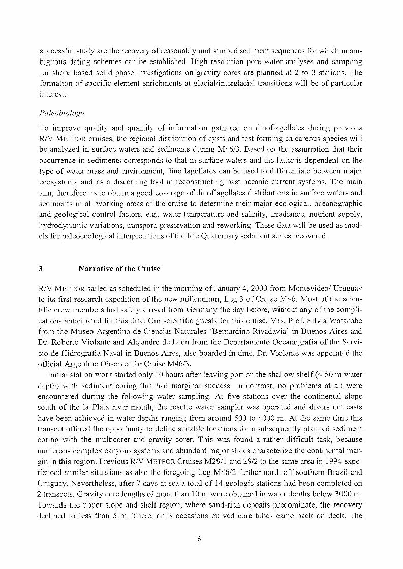
Figure 1 R/V METEOR Cruise M46/3 track and station chart. Thick !ines denote seismic pro­files. Bathymetry from Gebco Digital Atlas.

multicorer generally produced good to perfect results. Minor problems again arose from sand­rich layers.

The scientific activities of the second week concentrated on seismic surveys in the centralArgentine Basin. After several hours of testing the complete instrumentation, the streamer andair- and waterguns were deployed in the early moming of January 11 for a first, about 100 nmlong, profile from the abyssal plain to the Zapiola Drift region. Along a net of another 8 lines and

7

250 nm, morphology and internal strueture of this huge sediment body were explored around43°30' S/48°30' W to understand the temporal evolution of its emplacement. These measure­ments have been the first enduranee test of the new transpOliable compressor system on R/VMETEOR. While it was a full success from the seience point of view, certain technical aspectsand specifically the noise level on deek will need fmiher scrutiny. During the seismic campaignall other laboratories were busy with geologie, geochemical and paleontologieal analyses, geo­physical measurements and archiving of the sampIe collection from the northern Argentine eon­tinental mm"gin. Most all these procedures follow Ocean Drilling Project (ODP) standards.

On January 14 and 15, the seismic program was interrupted for station work in the 'summit'region of the Zapiola Drift. Core lengths > 12 and > 14 m indicate that at the border of thenorthward directed Antarctic bottom water masses very fine grained sediments aecumulate, pre­sumably at relatively high rates. Thereafter, the seismic team resumed their program on southerncourses until January 18, prospecting along some 320 nm of profiles the southwestern flanks ofthe Zapiola Drift around 45°45' S/49 °W, an area with impressive mud wave fields, and reachingat 46°43,3 'S the southernmost position of the cruise. We were thus cruising right in the 'roaringfOliies', frequently cited in the weather forecasts of these days. Even now during the southernsummer period they repeatedly produced typical features that make up their reputation, winds of8 occasionally 10 Bft and seas of several meters height. Neither station nor profiling work had tobe totally stopped at any time. Although the seismic gear suffered various demolitions and high­resolution seismic operations clearly reached their limits in every respect. For the people onboard, the ship temporarily became a rather unpleasant platform, particularly during night hours.

Sediment sampling at 2 stations in the southern and 3 stations in the western Zapiola Driftmud wave fields was suecessfully completed on January 19 and 20. The latter locations wereselected based on a grid of Parasound profiles recorded during R/V METEOR Cruise M29/1 in1994 and strategically positioned to collect materials from contrasting depositional regimes ondifferent wave forms and opposite flanks of one wave. Moreover, the 1994 survey allowed for anideal orientation of the new seismic lines aiming at a most complete and detailed delineation ofthe sediment wave fields. These impressive formations document paths and velocities of Antarc­tie Bottom Water flow on its northern routes and apparently need velY speeific conditions fortheir initial formation as well as their consecutive long-term existence. Both seem to be quiteperfectly met in the western realms of the Zapiola Drift around 44°S/50 °W. To study not onlythe recent developments, but also the geological past, different seismoacoustic systems wereemployed. The ship's own Parasound echosounder depicts the sediment structures down to 60 ­80 m sub-bottom depth, while the multifrequency and multichannel seismic equipment pene­trates up to 300 m sub-bottom depth with a small chamber watergun source and reaches thebasaltic oeeanic ernst at more than 2 km sub-bottom depth with a larger volume GI gun.

The seismic survey in western Zapiola Drift comprised a total of 18 lines over a distanee ofsome 460 nm. Due to very favorable, almost tropieal weather conditions, an exeellent set of dataeould be registered. On January 24, these measurement have been interrupted for the final twogeologie stations in the deep Argentine Basin. They were plaeed in a zone that Parasound reeordshad previously identified as an erosional environment. In fact, the upper layers of the cores con­tained a 2 em diameter manganese nodule and an about 6x6x3 em manganese ernst, respectively,implying a quite densely eovered field. A 270 nm long profile from the western mud wave areato the Argentine continental margin at 45 oS, that links the different sedimentation regimes and

8

crosses the main AABW pathway in the western South Atlantic, completed the seismic work onJanuary 28. The fmiher processing and interpretation of some 400 GigaByte of data collectedfrom over 170'000 shots along more than 1400 mn during a 17 days program will substantiallycontribute to a better understanding of the mud waves' pysical and geological setting and theirimplications for paleocurrent reconstructions.

After January 28, the activities concentrated on a geological and water sampling programacross the Argentine continental margin on two transects at around 45 and 46 oS. As expected

from the disappointing experiences of R/V METEOR Cruise M29/1 in 1994, we encountered aquite complex terrain. An appropriate positioning of coring sites was puzzling, despite theexcellent new bathymetry available from the Gebco Digital Atlas. The continental slope is cut byl1Umerous branched canyon systems and the Parasound records showed abundant slumps of anydimensions. Accordingly, the gravity corer recovered quite diverse, occasionally totally unex­pected sediment series.

On the southern (46 OS) profile, a total of 7 stations were occupied. The deposits above about2500 m water depth turned out to be absolutely impermeable and resistant against all attempts touse conventional devices for sampling. They caused a fourth bent core tube (the last of thiscruise) and after running a short 3 m gravity core twice in vain, the only remaining chance was toemploy a dredge. From about 1300 m water depth it recovered several cold water corals and avariety of exotic epibenthos that could not be further classified as we had no particular specialistson board. At greater water depth down to about 3500 m, the care length successively increased tomare than 10m and the multicorer generally came back on deck with weIl filled tubes. However,the sediments retrieved were mostly not the continuous late Quaternary sequences we have beenhoping for. Frequent intervals of interlayered off white, extremely stiff nannofossil oozes shouldbe (considerably?) older and indicate a complicated depositional environment with repeatedreworking and mass wasting.

The situation on the northern (45 OS) transect was altogether very similar. At the first station

there, extensive sampling of the water column down to 3000 m has been performed with severalcasts of the rosette water sampIer, the multinet and handnet. It constitutes the southeastern cornerof a 5 stations profile up to the inner shelf aiming at a detailed documentation of the actualhydrography of the Malvinas Conf1uence that was completed on February 5. While on the upperslope a dredge haul in around 1400 m water depth appeared the only practicable operation, thegravity carer (core lengths > 10 m) and the multicorer were reasonably successful beneath 2500m water depth. The last large geologic station of this cruise was finished during the evening ofFebruary 4. Befare, an extensive 30 hour Parasound and Hydrosweep survey has been accom­plished over an unusual, more than 600 m deep incision into the lower continental margin ori­

ented about perpendicular to the slope. The area around this exceptional structure ('AlmiranteBrown Transverse Canyon') should be of specific interest to a planned Ocean Drilling Projectcampaign in the western South Atlantic.

On the final transit to port, aseries of dredge hauls near the shelf edge was the last scientificactivity of the cruise. R/V METEOR safely arrived in Mar deI Plata/Argentina in the moming ofFebruary 7, 2000 ending Leg 3 of Cruise M46. Despite some adverse weather conditions andrather complicated geological settings to overcome at the Argentine continental margin, the over­all summary is absolutely positive.

9

4 Preliminary Results

4.1 Underway Geophysics

(W. Böke, M. Breitzke, V. Hopfauf, H. von Lom-Keil, V. Spieß)

Geophysical profiling activities during R/V METEOR Cruise M46/3 included continuous opera­tion of the Parasound sediment echosounder and the Hydrosweep swath sounder to detelmine thesea floor morphology, to characterize and analyze sediment deposition processes and sedimentstructures on the shelf, at the continental margin and in the deep basins and to provide infonna­tion for site selection of coring and surface sampling. Both data sets were acquired digitally.

Multichannel seismic surveys were canied out exclusively in the deep Argentine Basin, wherethe flow of the Antarctic Bottom Water (AABW) creates a unique morphology including largesediment drifts (e.g. Zapiola Drift) and giant mud waves (FLOOD & SHOR, 1988). As part of theSFB 261 research program seismoacoustic profiling studies in different parts ofthe South Atlan­tic were dedicated to the understanding of the interaction of bottom water flow and sedimen­tation and the reconstruction of paleocurrent properties in space and time. Based on the resultsofProject MUDWAVES (FLOOD et al., 1993), the first interdisciplinary research project to studymud waves in the Argentine Basin, and data from R/V METEOR Cruise M29/l (SEGL et al. ,1994) and R/V POLARSTERN Cruise ANTX/5, we have selected three survey areas, where digitalseismic and acoustic data were acquired with swath sounder, sediment echosounder and amultifrequency multichannel seismic system to image the internal structure of sediment wavesdown to several hundred meters sub-bottom depth and to investigate their relationship to pre­existing topography of sediments and basement.

With the GeoB high-resolution multichamlel seismic equipment, small scale sedimentarystructures and closely spaced layers can be imaged on a meter to sub-meter scale which can usu­ally not be resolved with conventional seismic systems. The alternating operation of a smallchamber watergun (0.16 1, 200 - 1600 Hz) and a larger chamber GI airgun (0.4 1, 100 - 500 Hz)yields simultaneously two seismic data sets, one of greater penetration into the sea floor, reveal­ing the larger scale structural framework down to oceanic basement, and one revealing finerdetails of the upper 200 - 300 m of the sediment cover beyond the Parasound penetration of 50 ­80 m. For testing purposes also another GI airgun with a larger volume (1.7 1) was used to sup­plement the data with a third seismic signal to even higher penetrations due to lower nominalfrequencies « 200 Hz) and higher signal energy.

4.1.1 Parasound

The Parasound system works both as a low-frequency sediment echosounder and as high-fi:e­quency narrow beam sounder to detennine the water depth. It makes use of the parametric effectwhich produces additional frequencies tlu'ough nonlinear acoustic interaction of finite amplitudewaves. If two sound waves of similar frequencies (here, 18 kHz and, e.g., 22 kHz) are emittedsimultaneously, a signal of the difference frequency (e.g., 4 kHz) is generated for sufficientlyhigh primary amplitudes. The new component is travelling within the emission cone of the origi­nal high frequency waves which are limited to an angle of only 4° for the equipment used. There­fore, the footprint size of 7 % of the water depth is much smaller than for conventional systemsand both vertical and lateral resolution are significantly improved.

10

The Parasound system is penllanently installed on the ship. The hull-mounted transducer

array has 128 elements on an area of about 1 m2. It requires up to 70 kW of electric power due to

the low degree of efficiency of the parametric effect. In 2 electronic cabinets, beam forming, sig­

nal generation and the separation of primary (18, 22 kHz) and secondary frequencies (4 kHz) is

accomplished. With the third electronic cabinet in the echosounder control 1'Oom the system is

operated on a 24 hour watch schedule.

Since the two-way travel time in the deep sea is long compared to the length of the reception

window of up to 266 ms, the Parasound system sends out a burst of pulses at 400 ms intervals

until the first echo retUl11s. The coverage of this discontinuous mode depends on the water depth

and produces non-equidistant shot intervals between bursts. On average, one seismogram is

recorded about every second providing a spatial resolution on the order of a few meters on seis­

mic profiles at 4.9 knots.

The main tasks of the operators are system and quality control and positioning of the recep­

tion window. Because of the limited penetration of the echosounder signal into the sediment,

only a short window c10se to the sea floor is recorded.

In addition to an analog recording with the b/w DESO 25 device, the Parasound system is

equipped with the digital data acquisition system ParaDigMA which was developed at the Uni­

versity of Bremen (SPIEß, 1993). The data are stored on two exchangeable disc drives of 4 Giga­

Byte capacity, allowing continuous recording between 5 and 10 days depending on water depth

and shot rate. The Pentium-processor based pe allows the buffering, transfer and storage of the

digital seismograms at very high repetition rates. From the emitted series of pulses usually every

second pulse is digitized and stored, resulting in recording intervals of 800 ms within a pulse

sequence. The seismograms were sampled at a frequency of 40 kHz with a typical registration

length of 266 ms for a depth window of about 200 m. The SOUlTe signal was a band limited, 2 ­

6 kHz sinusoidal wavelet of 4 kHz dominant frequency with about 500 J.ls totallength.

Already during the acquisition of the data an online processing was carried out. For all pro­

files Parasound sections were plotted with a veliical scale of several hundred meters. Most of the

changes in window depth could thereby be eliminated. From these plots a first impression of

variations in sea floor morphology, sediment coverage and sedimentation patterns along the ships

track could be obtained. To improve the signal-to-noise ratio, the echogram sections were filtered

with a wide band filter. The data were nonnalized to much less than the average maximum

amplitude to amplify in pariicular deeper and weaker reflections.

To study the influence of frequency and length of the source signal on the reflection pattern,

these parameters were systematically varied at sites, where gravity cores were recovered ('source

signal test') and the local topography was smooth enough to allow precise seismogram compari­

sons over a time period of 45 mümtes and ship's offsets on the order of some hundred meters.

The frequency of the source signal was changed in 0.5 kHz steps over the available frequency

range from 2.5 to 5.5 leHz, while the pulse length was set to 1, 2, and 4 sinus periods, respec­

tively. Each setting was leept for a time span of 2 minutes to enable later signal stacking and

evaluation of the seismogram variability together with physical property logs of the sediment

cores in detailed shore based analyses specifically aiming at quantifying interference phenomena.

During the entire cruise the combined Parasound / ParaDigMA system was operated without

significant problems. The new storage procedure with exchangeable hard discs worked success­

fully and avoided previous frequent aleli situations due to elTors of magnetic tape recording. The

11

software was adjusted to changes in ANP serial data with navigation infOlmation and updated forY2K and improved readability of the online plots.

4.1.2 Hydrosweep

The multibeam echosounder Hydrosweep on R/V METEOR was routinely used during the cruiseand serviced by the system operator and the electronics engineers. Before a software bugfix inthe ANP navigation systems, the Hydrosweep systems received erroneous navigation stringscontaining the year 100 instead of 00 which resulted in date and time errors to be corrected later.

Technical problems particularly affected the portside central 16 beams which produced erro­neous depths during extended periods of the cruise. The intem1ittently occurring problem wasdifficult to track, but seems to be temperature dependent. Extensive tests did not give any evi­dence for specific failure of analog boards or software. Another problem with the roll compensa­tion caused substantial data gaps during the mud wave surveys in the central Argentine Basin.Moreover, the weather conditions with wave heights up to 4 meters were responsible fordegraded data quality on many profiles depending on the ship's course.

Towards the end of the cruise a detailed two-day Hydrosweep and Parasound survey at thefoot ofthe South American continentalmargin provided adequate data quality.

4.1.3 Navigation

Although differential GPS navigation was available during the entire cruise, the situation wasunsatisfactory with respect to the frequent system failures due to problems with the satellitecommunication system, e.g., during radio traffic for fax, email and telephone. As the differentialGPS corrections are transmitted through the satellite carrier signal, they should not be affected byradio traffic. The problems during the cruise are therefore attributed to a technical deficiency inthe receiver components. The lack of redundancy for this precise navigation reduced data qualitynotab1y of small scale high resolution seismic surveys.

Another problem was caused by the failure of the ANP ship's navigation system to providefiltered coordinates in case of DGPS signal loss. Instead of a smooth transition to conventionalGPS positions, the ANP currently only supplies zero values for coordinates and speed affectingthe accuracy of the ship's navigation procedure to maintain constant velocity and minimize offtrack errors. Also, processing of navigation data is less precise and filtered positions can only bedeterrnine after the cruise, when the complete DVS data set becomes available.

4.1.4 High-Resolution Multichannel Reflection Seismies

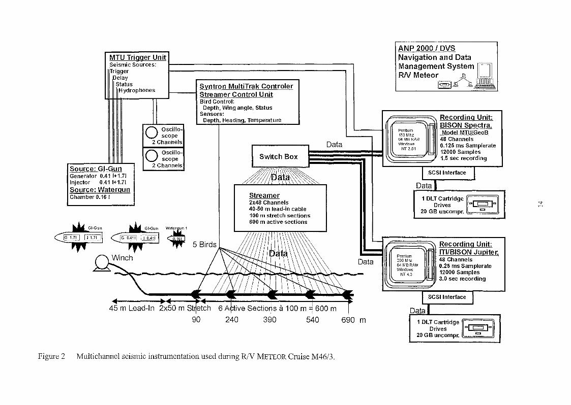
The Bremen multichannel seismic system is specifically designed to acquire high-resolutionseismic data tlu'ough optimized system components and procedural parameters. Figure 1 gives anoutline ofthe system setup as used during R/V METEOR Cruise M46/3.

Seismic Sources and Compressor

During seismic surveying, three different seismic sourees, two GI guns and one watergun, weretriggered in an altemating or quasi-simultaneous mode at time intervals between 10 and 13 S.

12

Owing to an average ship speed of 4.9 1m, a shot distance of approximately 25 to 28 m wasobtained for the aJternating mode operation (10 or 11 s), con'esponding to 50 and 56 m between

the same source. For the quasi-simultaneous mode (12 and 13 s), shot distances were 30 to 33 mfor both sources.

With the new LMF compressor available, two maximum air pressure levels of 138 and

207 bar could be used. Since all source types, the pulse station and pressure lines were capable of

handling the high pressure, an operating pressure between 180 to 190 bar was chosen to increaseseismic energy and frequency.

Each source type was shot more than 80'000 times. Due to rough weather reaching waveheights of 4 meters and wind strength of 10 Bft, the systems were operating under heavy condi­

tions and both pressure lines and electric cables were broken several times. Complete data gaps

could be mostly avoided, however, since only one of the sources had to be turned off at the same

time. While during the first survey both GI guns were deployed, we later changed to a single GI

gun to reduce the risk of firing into air. For the last three days, one GI gun could not be used due

to a broken shuttle and apparent internal defects.

The geometry of source and receiver systems during the measurements is shown in Figure 3.Ship velocity during deployment and retrieval was between 2.5 and 3.5 1m, respectively,depending on weather conditions and surface currents.

The volume of the standard GI gun (Sodera) was reduced to 2 x 0.41 1. It was towed at thestarboard side by a wire through the A-Frame, about 15 m behind the ship's stern with a lateral

offset of around 3 m. The towing wire was connected to a bow with the GI gun hanging on two

chains 40 cm beneath (Fig. 4). During deployment of the larger volume GI gun, the chain lengthwas increased to 1 meter. An elongated buoy, which stabilized the gun in a horizontal position at

a water depth of approximately 1.4 m, was connected to the bow by two rope loops. The injectorwas triggered with a delay of 30 ms with respect to the generator signal which essentially elimi­nated a bubble signal.

The second source type was a S15 watergun (Sodera) with a volume ofO.161. It was towed bya wire, which was separate from the Meteor rope holding the umbilical of the watergun, about

15 m behind the ship's stern and 5 - 7 m portside ofthe streamer. A steel frame held the water­

gun in a tight position parallel to the elongated buoy in a depth of approximate1y 0.5 m (Fig. 4).

During operations the near field source signature of the guns was checked on a digital scope inthe seismic lab.

High pressure air for gun operation was provided by the new LMF compressor. It was set up

in an oversized container on the working deck and maintained by the ship's engineers. Only

minor technical problems occulTed during this first use of the system, providing continuous sup­ply of up to 190 bar pressured air. However, für high resolution seismics with relatively small

sources, 90 % of the air production (28 m3 per minute) had to be b10wn into the atmosphere,

causing a very noisy environment adding to the high noise level of the diesel aggregate. The airconsumption ofthe sources used sums up to:

• watergun + GI gun 2 x 0.411 in alternating mode at 10 s: 0.56 m3/min,

• watergun + GI gun 2 x 0.41 1in quasi-continuous mode at 12 s: 0.93 m3/min,

• watergun + GI gun 2 x 1.71 in quasi-continuous mode at 12 s: 3.38 m3/min.During a test profile variable air pressures were employed for a detailed analysis of the signal

characteristics that will be evaluated onshore.

13

"'1".-<

Recording Unit:BISON Spectra,Model MTUlGeoB

48 Channels0.125 ms Samplerate12000 Sampies1.5 sec recording

Recording Unit:ITI/BISON Jupiter,48 Channels0.25 ms Samplerate12000 Sampies3.0 sec recording

.SCSllnterface

1 DLT Cartridge [ 1 I 11Drives "'I I I I'"

20 GB uncompr. <=I

Pentium133 Mhz64 MB RAMWindows

NT3.51

1 DLT Cartridge 1I1 I 11Drives "'I I I le20 GB uncompr. <=I

ANP 2000 I DVSNavigation and DataManagement SystemRN Meteor ~

Il§§:JjJf ~

Pentium200 Mhz64 MBRAMWindows

NT 4.0

Data

690 m

Data

Switch Box

Streamer2x48 Channels40-50 m lead-in cable100 m stretch sections600 m active sections

4AJ'

O Oscillo­scope

2 Channels

O Oscillo­scope

2 Channels

MTU Trigger UnitSeismic Sourees: 1 I

TriggerelayStatusHydrophones

45 m Lead-In 2x50 m Stqetch

90

Syntron MultiTrak Controler1111111 1----11 Streamer Control Unitl.II-IHIlI I I Bird Contro!;

Depth, Wing angle, StatusSensors:Depth, Heading, Temperature

Source: GI-GunGenerator 0.41 1+1.71Injector 0.41 1+1.71

Source: WatergunChamber 0.16 I

Figure 2 Multichannel seismic instrumentation used during RJV METEOR Cruise M46/3.

Chamber Volume :

Watergun: 0,16 I

GI-Gun 1: 2xO,41 IGI-Gun 2: 2x1.71Gun Pressure: 180-190 bar

PulserStation

NOTTO SCALE

2m

(')o:3sr_.:3(1).,

(')(')0o 3:3"'0sr.,-·CD:3 tJ)(1) tJ)., 0.,

Seismic Winch

15 m15 m

845 m

DISTANCES:

Watergun - Stern:

GI-Gun - Stern:

Blubb - Stern:

(Streamer)

Figure 3 Working deck setting during RJV METEOR Cruise M46/3.

15

15 m

2 x 0.41 I

~I (A)

Hy rophone

NOT TO SCALE

15 m

15 m

Umbilical

EüoLO

~I

~I

Umbilical

(8)

(e)

Figure 4 Towing gear and anangement for GI gun 0.41 1 (A), double GI gun 0.4 + 1.7 1 (B)and watergun (e).

16

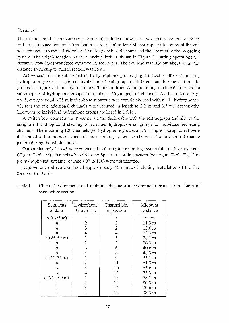
Streamer

The multichannel seismic streamer (Syntron) includes a tow lead, two stretch sections of 50 mand six active sections of 100 m length each. A 100 m long Meteor rope with a buoy at the endwas connected to the tail swivel. A 30 m long deck cable cOlmected the streamer to the recordingsystem. The winch location on the working deck is shown in Figure 3. During operations thestreamer (tow lead) was fixed with two Meteor ropes. The tow lead was laid out about 45 m, thedistance from ship to stretch section was 35 m.

Active sections are subdivided in 16 hydrophone groups (Fig. 5). Each of the 6.25 m longhydrophone groups is again subdivided into 5 subgroups of different length. One of the sub­groups is a high-resolution hydrophone with preamplifier. A programming module distributes thesubgroups of 4 hydrophone groups, i.e. a total of 20 groups, to 5 channels. As illustrated in Fig­ure 5, every second 6.25 m hydrophone subgroup was completely used with all 13 hydrophones,whereas the two additional channels were reduced in length to 2.2 m and 3.3 m, respectively.Locations ofindividual hydrophone groups are listed in Table 1.

A switch box connects the streamer via the deck cable with the seismograph and allows theassignment and optional stacking of streamer hydrophone subgroups to individual recordingchannels. The incoming 120 channe1s (96 hydrophone groups and 24 single hydrophones) weredistributed to the output channels of the recording systems as shown in Table 2 with the samepattern during the who1e cruise.

Output chmme1s 1 to 48 were connected to the Jupiter recording system (altemating mode andGI gun, Table 2a), channels 49 to 96 to the Spectra recording system (watergun, Table 2b). Sin­gle hydrophones (streamer channels 97 to 120) were not recorded.

Deployment and retrieval lasted approximately 45 minutes including installation of the fiveRemote Bird Units.

Table 1 Charmel assigmllents and midpoint distances of hydrophone groups from begin ofeach active section.

Segments Hydrophone Channel No. Midpointof25 m Group No. in Section Distance

a (0-25 m) 1 1 3.1 ma 2 3 11.3 ma 3 2 15.6 ma 4 4 23.3 m

b (25-50 m) 1 5 28.1mb 2 7 36.3 mb 3 6 40.6 mb 4 8 48.3 m

c (50-75 m) 1 9 53.1mc 2 11 61.3 mc 3 10 65.6 mc 4 12 73.3 m

d (75-100 m) 1 13 78.1 md 2 15 86.3 md 3 14 90.6 md 4 16 98.3 m

17

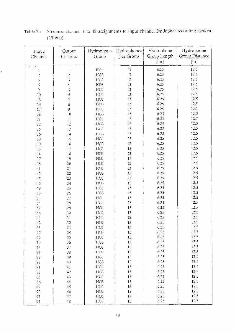
Table 2a Streamer channe1 1 to 48 assignments to input charmel for Jupiter recording system

(GI gun).

Input Output Hydrophone Hydrophones Hydrophone Hydrophone

Channel Channel Group per Group Group Length Group Distance[m] [m]

1 1 HGI 13 6.25 12.5

2 2 HG3 13 6.25 12.5

5 3 HGI 13 6.25 12.5

6 4 HG3 13 6.25 12.5

9 5 HGI 13 6.25 12.5

10 6 HG3 13 6.25 12.5

13 7 HGI 13 6.25 12.5

14 8 HG3 13 6.25 12.5

17 9 HGI 13 6.25 12.5

18 10 HG3 13 6.25 12.5

21 11 HGI 13 6.25 12.5

22 12 HG3 13 6.25 12.5

25 13 HGI 13 6.25 12.5

26 14 HG3 13 6.25 12.5

29 15 HGI 13 6.25 12.5

30 16 HG3 13 6.25 12.5

33 17 HG! 13 6.25 12.5

34 18 HG3 13 6.25 12.5

37 19 HG! 13 6.25 12.5

38 20 HG3 13 6.25 12.5

41 21 HG 1 13 6.25 12.5

42 22 HG3 13 6.25 12.5

45 23 HGI 13 6.25 12.5

46 24 HG3 13 6.25 12.5

49 25 HGI 13 6.25 12.5

50 26 HG3 13 6.25 12.5

53 27 HGI 13 6.25 12.5

54 28 HG3 13 6.25 12.5

57 29 HGI 13 6.25 12.5

58 30 HG3 13 6.25 12.5

61 31 HGI 13 6.25 12.5

62 32 HG3 13 6.25 12.5

65 33 HGI 13 6.25 12.5

66 34 HG3 13 6.25 12.5

69 35 HGI 13 6.25 12.5

70 36 HG3 13 6.25 12.5

73 37 HG1 13 6.25 12.5

74 38 HG3 13 6.25 12.5

77 39 HGI 13 6.25 12.5

78 40 HG3 13 6.25 12.5

81 41 HGI 13 6.25 12.5

82 42 HG3 13 6.25 12.5

85 43 HGI 13 6.25 12.5

86 44 HG3 13 6.25 12.5

89 45 HGI 13 6.25 12.5

90 46 HG3 13 6.25 12.5

93 47 HGI 13 6.25 12.5

94 48 HG3 13 6.25 12.5

18

Table 2b Streall1er channel 49 to 96 assignments to input channel for Spectra recording system

(watergun).

Input Output Hydrophone Hydrophones Hydrophone HydrophoneChannel Channel Group per Group Group Length Group Distance

[m] [m]

3 49 HG2 6 2.2 134 50 HG4 9 3.3 127 51 HG2 6 2.2 13

8 52 HG4 9 3.3 1211 53 HG2 6 2.2 13

12 54 HG4 9 3.3 1215 55 HG2 6 2.2 1316 56 HG4 9 3.3 1219 57 HG2 6 2.2 13

20 58 HG4 9 3.3 1223 59 HG2 6 2.2 13

24 60 HG4 9 3.3 1227 61 HG2 6 2.2 1328 62 HG4 9 3.3 1231 63 HG2 6 2.2 13

32 64 HG4 9 3.3 1235 65 HG2 6 2.2 13

36 66 HG4 9 3.3 1239 67 HG2 6 2.2 1340 68 HG4 9 3.3 1243 69 HG2 6 2.2 13

44 70 HG4 9 3.3 1247 71 HG2 6 2.2 13

48 72 HG4 9 3.3 1251 73 HG2 6 2.2 13

52 74 HG4 9 3.3 1255 75 HG2 6 2.2 13

56 76 HG4 9 3.3 1259 77 HG2 6 2.2 13

60 78 HG4 9 3.3 1263 79 HG2 6 2.2 13

64 80 HG4 9 3.3 1267 81 HG2 6 2.2 1368 82 HG4 9 3.3 1271 83 HG2 6 2.2 13

72 84 HG4 9 3.3 1275 85 HG2 6 2.2 13

76 86 HG4 9 3.3 1279 87 HG2 6 2.2 13

80 88 HG4 9 3.3 1283 89 HG2 6 2.2 13

84 90 HG4 9 3.3 1287 91 HG2 6 2.2 13

88 92 HG4 9 3.3 1291 93 HG2 6 2.2 13

92 94 HG4 9 3.3 1295 95 HG2 6 2.2 13

96 96 HG4 9 3.3 12

19

Channel 1: HG1 (HSG A/B/C/E)Channel2: HG3 (HSG A/B/C/E)Channel 3: HG2 (HSG C/E)Channel 4: HG4 (HSG B/C/E)Auxiliary : HG1 (HSG D = High-Res.)

6.25 m length6.25 m length2.2 m length3.3 m length0.25 m length

I 4 hydrophone groups ~!b~(3:25 m length each and 25 m rot;: length I.;.... ....,

,

oN

nne14chalel3 charmel1

1\~~~ 1stacking moduleI~ for channels 1-4

I I

I HG1 1HG2 I HG3 I HG4 I-

Auxiliarv A

,

~~ ,

~

~ ,to stacking ~

,~

,~

~ , ,module ~

~,

~

~, ,

~

~

I,

~,

~ - ,~

~

I, ,

~

~

~ ,

f HSGA I HSGB H~GII HSGE II 29m I 09m I03ml, 19m II

hydrophone group with 5 hydrophon subgroups A-E ßnd 6,25 m totallengthI

High-Res.Hydrophon(HSG D)

Figure 5 Multichannel streamer design used during R1V METEOR Cruise M46/3. The hydrophone group combination repeats every 5 channels.

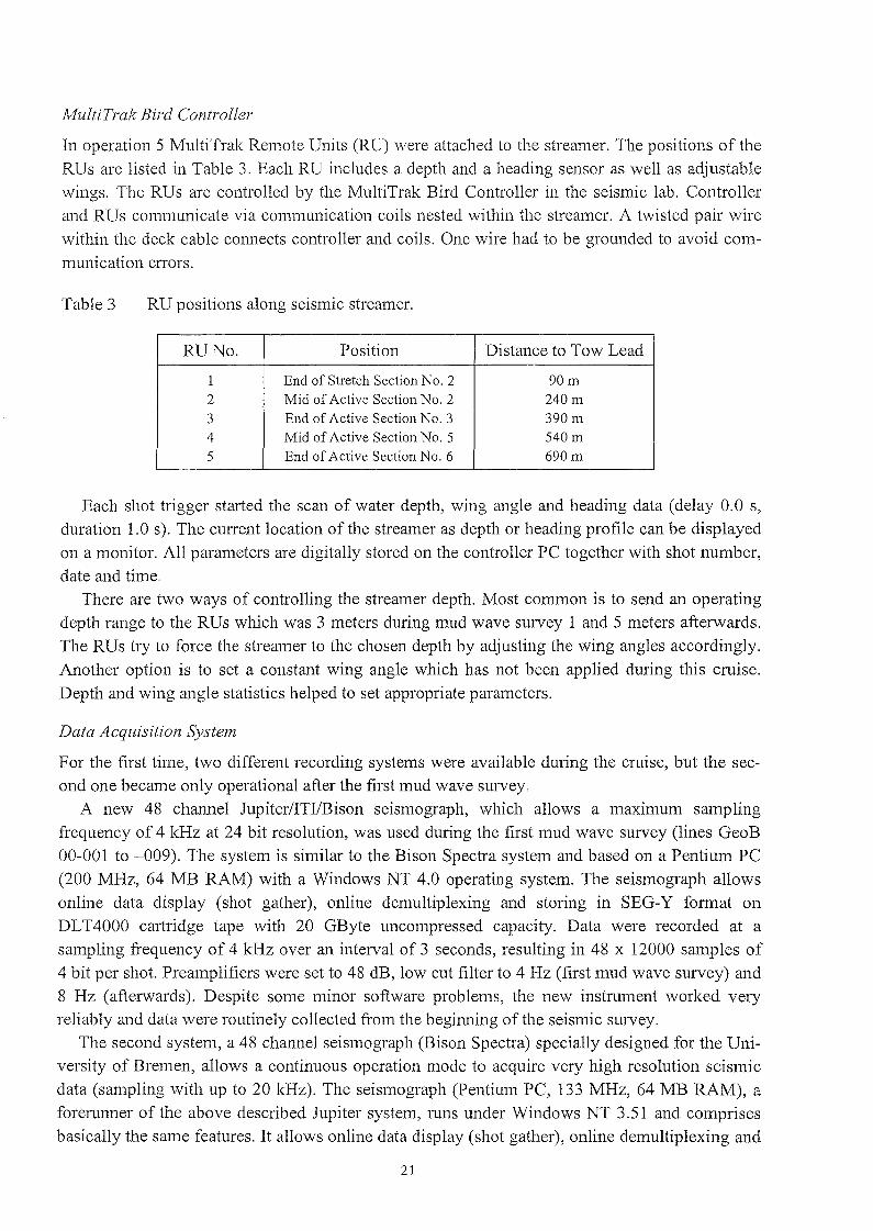
MultiTrak Bird Controller

In operation 5 MultiTrak Remote Units (RU) were attached to the streamer. The positions of theRUs are listed in Table 3. Each RU includes a depth and a heading sensor as weIl as adjustablewings. The RUs are controlled by the MultiTrak Bird Controller in the seismic lab. Controllerand RUs communicate via communication coils nested within the streamer. A twisted pair wirewithin the deck cable COlmects controller and coils. One wire had to be grounded to avoid com­munication eITors.

Table 3 RU positions along seismic streamer.

RU No. Position Distance to Tow Lead

1 End of Stretch Section No. 2 90m2 Mid of Active Section No. 2 240m3 End of Active Section No. 3 390m4 Mid of Active Section No. 5 540m5 End of Active Seetion No. 6 690m

Each shot trigger started the scan of water depth, wing angle and heading data (delay 0.0 s,duration 1.0 s). The current location of the streamer as depth 01' heading profile can be displayedon a monitor. All parameters are digitally stored on the controller PC tagether with shot number,date and time.

There are two ways of controlling the streamer depth. Most common is to send an operatingdepth range to the RUs which was 3 meters during mud wave survey 1 and 5 meters afterwards.The RUs try to force the streamer to the chosen depth by adjusting the wing angles accordingly.Another option is to set a constant wing angle which has not been applied during this cruise.Depth and wing angle statistics helped to set appropriate parameters.

Data Acquisition System

For the first time, two different recording systems were available during the cruise, but the sec­ond one became only operational after the first mud wave survey.

A new 48 channel Jupiter/ITI/Bison seismograph, which allows a maximum samplingfrequency of 4 kHz at 24 bit resolution, was used during the first mud wave survey (lines GeoB00-001 to -009). The system is similar to the Bison Spectra system and based on a Pentium PC(200 MHz, 64 MB RAM) with a Windows NT 4.0 operating system. The seismograph allowsonline data display (shot gather), online demultiplexing and storing in SEG-Y fOlmat onDLT4000 cartridge tape with 20 GByte uncompressed capacity. Data were recorded at asampling frequency of 4 kHz over an interval of 3 seconds, resulting in 48 x 12000 sampIes of4 bit per shot. Preamplifiers were set to 48 dB, low cut filter to 4 Hz (first mud wave survey) and8 Hz (afterwards). Despite same minor software problems, the new instrument worked veryreliably and data were routinely collected from the beginning of the seismic survey.

The second system, a 48 channel seismograph (Bison Spectra) specially designed for the Uni­versity of Bremen, allows a continuous operation mode to acquire very high resolution seismicdata (sampling with up to 20 kHz). The seismograph (Pentium PC, 133 MHz, 64 MB RAM), aforerunner of the above described Jupiter system, runs under Windows NT 3.51 and comprisesbasically the same features. It allows online data display (shot gather), online demultiplexing and

21

storing in SEG-Y fonnat. PreampIifiers were set to 60 dB, analog filters to 16 Hz (low cut) and2000 Hz (high cut). The sampling frequency was 8 kHz for watergun recording over a length of1500 ms. All channels were preampIified by a factor of 1000 (60 dB) to keep the incoming signalwithin the optimum voltage range for digitizing. The data were stored on a DLT4000 cartridgetape. The recording delay had to be adjusted according to the CUlTent water depth and was con­trolled t1u'ough the trigger unit. OnIine (single channel) output was not available on this cruise.

Trigger Unit

The trigger unit controls seismic sources, seismographs, bird controller, onIine plotter and digitalscope (near-field hydrophones). The unit is set up on an IBM compatible PC with a Windows NT4.0 operating system and inc1udes a real-time controller interface card (Sorcus) with 16 1/0

chaI1l1els synclu'onized by an internal c1ock. The unit is connected to an amplifiel' unit and a gunampIifier unit. The PC software allows to define arbitrary combinations of trigger signals used tooptimize the available recording time for two 01' three seismic sources and to minimize the shotdistance.

Trigger settings can be changed at any time during the survey. The recording delay can thusbe adjusted to water depth without interruption of data acquisition. The amplifiel' unit convertsthe controller output to positive 01' negative TTL levels. The gun ampIifier unit, which generatesa 60 V I 8 Amp. trigger level, controls the magnetic valves of the individual seismic sources. Itwas placed in the pulse station c10se to the gun pressure controls for an eventual immediate shut­down of gun operations.

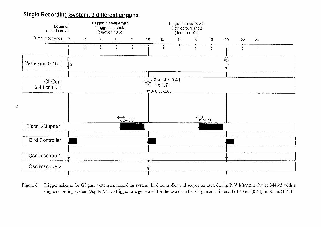
Figure 6 shows the trigger scheme used during the first mud wave survey with a singlerecording system and three different sources. Sources were shot in an alternating mode andrecorded on the same tape. In this mode an additional processing step of splitting records fromdifferent sources is required prior to standard seismic data processing. The watergun was firedevery 20 seconds, one of the GI guns also every 20 seconds. For every third or fifth GI gun shotthe trigger was switched from the small chamber (0.4 1) to the large chamber gun (1.71).

With the use of two different seismic recording systems on the second and third mud wavesurvey, the trigger rate could be further modified. Watergun and GI gun were fired in the sametrigger interval within 2 seconds and recording and data storage perfonned in parallel on bothsystems (Fig. 7). The total length of the trigger intervals had to be increased by only 2 seconds,but the lateral resolution could be improved almost a factor of 2 with a shot rate of 12 secondsfor each source along most of the profiles.

As a consequence of the parallel recording, acquisition parameters could be adjusted on eachsystem to the properties of the source with respect to signal penetration and frequency content.Watergun recording was reduced to 1.5 seconds at a sampling frequency of 8 kHz and GI gundata were recorded for 3 seconds at 4 kHz. Accordingly, all records contain 12'000 samples.

4.1.5 Shipboard Results

The hull-mounted Parasound sediment echosounder and Hydrosweep swath sounder systemswere continuously operated during a 24 hour watch schedule on the entire cruise. A track chart(Fig. 8) shows the locations of Parasound profiles and of the long multichannel seismic lineGeoB 00-036. Hydrosweep data quality was inadequate during the deep basin survey.

22

Single Recording System, 3 different airguns

Begin ofmain interval

Time in seconds 0

Trigger interval A with4 triggers, 1 shots

(duration 10 s)

246 8 10

Trigger interval B with5 triggers, 1 shots

(duration 10 s)

12 14 16 18 20 22 24

~; ; ; ; i ; : ; : i : :'-w-a-te-r-g-u-n-0-16 I 10 10 I

I • •

NW

GI-Gun0.4 I or 1.7 I

Bison-2/Jupiter

Bird Controller •

Oscilloscope 1 ~

Oscilloscope 2

cfb 2 or 4 x 0.4 I(f? 1x1.71","0+0.03/0.05

~

~+3.0

•~

Figure 6 Trigger scheme for GI gun, watergun, recording system, bird controller and scopes as used during RJV METEOR Cruise M46/3 with a

single recording system (Jupiter). Two triggers are generated for the two chamber GI gun at an interval of30 ms (0.41) or 50 ms (1.71).

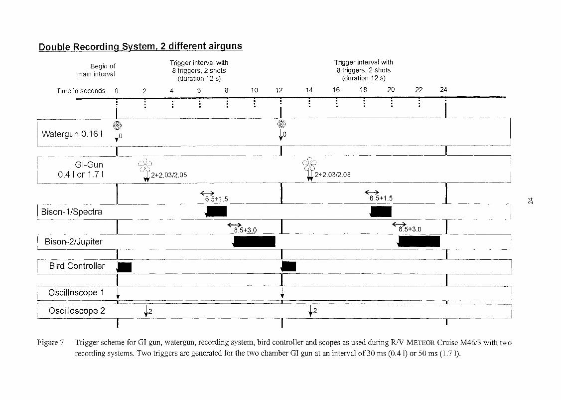
Double Recording System, 2 different airguns

Begin ofmain interval

Time in seconds 0 2

Trigger interval with8 triggers, 2 shots

(duration 12 s)

4 6 8 10 12 14

Trigger interval with8 triggers, 2 shots

(duration 12 s)

16 18 20 22 24· .. ..».» .----- ---...----.-- ---- -· . . . . . . . . . . . .· . . . . . . . . . . .l .... . . . . L' . . . .

Iwa~~rgU~6~t~ t ~C-------10 0GI Gun r<w, r\"::J

0.4 I or-1.7 I (j~-2+2.03/2.05 f 2+2.03/2_05

'i"l"'l-

<E--?6.5+1.5

<E--?6.5+1.5-

Bison-2/Jupiter

CBird Controller •] [Oscilloscope 1 ~ ~

I I

Oscilloscope 2 ~2 t2

Bison-1/Spectra

Figure 7 Trigger scheme for GI gun, watergun, recording system, bird controller and scopes as used during RJV METEOR Cruise M46/3 with tworecording systems. Two triggers are generated for the two chamber GI gun at an interval of 30 ms (004 1) or 50 ms (1.7 1).

Ol

~0101

~

01o~

l'01

~

423

443

NlJl

----+--1403

CS[f "I!

(J,§. I j443 I I - (!

I --~-4~~~~ti~~~t+-t--t--;t--t--.::r~tf-:j7~~'tiic~~t~n 463463,11--+-1-1-

) /1\\ I '\ \1-- I 1-~11 '7 I I \ \ i.) \\i'i1\\

Olo~

0101

~

01o~

l'01

~

Figure 8 Cruise M46/3 gravity coring sites (black dots), digital Parasound profiles (thin lines) and multichannel profie GeoB 00-036 (thick line).

Tracks are annotated with date, ticks set every 4 hours. Bathymetry from Gebco Digital Atlas.

In the following chapters preliminary results are discussed from the northem coring area at theArgentine continental maI"gin, the mud wave region in the deep Argentine Basin, where alsomultichannel seismic surveys were canied out during a two weeks operation, and margin sedi­

mentation in the southem coring area.

4.1.5.1 Argentine Continental Margin (Northern Area)

A five days coring operation at the begimüng of the cmise concentrated on the northem part ofthe Argentine continental margin (Fig. 9). Parasound and Hydrosweep data were particularly

helpful to identify coring sites and to characterize the depositional environment.

From the previous SFB 261 cmises to the Argentine Basin the margin was known to be a dif­ficult region to recover sediment sequences which have continuously recorded paleoenviron­

mental. This proved also to be tme for the northem downslope coring transects perforrned duringthis cmise.

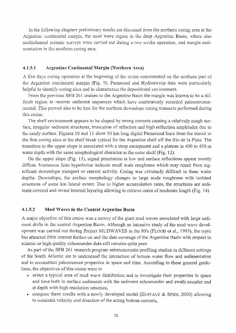
The shelf environment appears to be shaped by strang currents causing a relatively rough sur­face, irregular sediment structures, tmncation of reflectors and high reflection amplitudes due to

the sandy surface. Figures 10 and 11 show 50 km long digital Parasound lines from the transit to

the first coring sites at the shelf break typical for the Argentine shelf off the Rio de la Plata. The

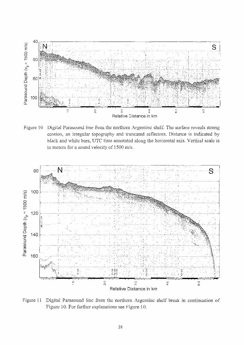
transition to the upper slope is associated with a steep escarpment and a plateau in 400 to 450 mwater depth with the same morphological character as the outer shelf (Fig. 12).

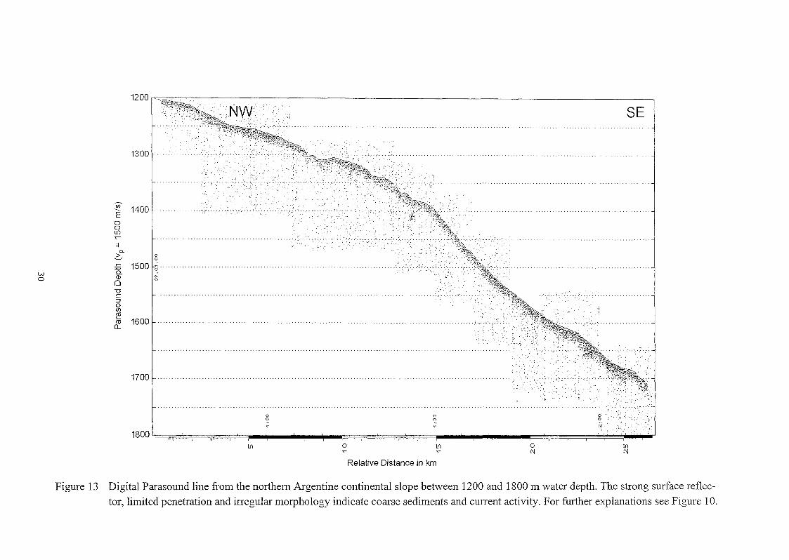
On the upper slope (Fig. 13), signal penetration is low and surface reflections appeal' mostlydiffuse. Numerous faint hyperbolae indicate small scale roughness which may resuIt from sig­

nificant downslope transport 01' cunent activity. Coring was extremely difficult in these waterdepths. Downslope, the surface morphology changes to large scale roughness with isolated

structures of some km lateral extent. Due to higher accumulation rates, the structures are sedi­

ment covered and reveal intemallayering allowing to retrieve cores ofmoderate length (Fig. 14).

4.1.5.2 Mud Waves in the Central Argentine Basin

A major objective of this cmise was a survey of the giant mud waves associated with large sedi­

ment drifts in the central Argentine Basin. AIthough an intensive study of the mud wave devel­opment was canied out during Project MUDWAVES in the 80's (FLOOD et al., 1993), the topic

has attracted littIe interest fmiher on and the data coverage ofthe Argentine Basin with respect toseismic 01' high quality echosounder data still remains quite pOOl'.

As part of the SFB 261 research program seismoacoustic profiling studies in different settings

of the South Atlantic are to understand the interaction of bottom water flow and sedimentation

and to reconstmct paleocunent properties in space and time. According to these general guide­lines, the objectives ofthis cmise were to

• select a typical area of mud wave distribution and to investigate their properties in space

and time both in surface sediments with the sediment echosounder and swath sounder andat depth with high resolution seismics,

• compare these results with a newly developed model (HOPFAUF & SPIEß, 2000) allowingto constrain velocity and direction ofthe acting bottom cunents,

26

418

398

388

408

0'1--"

~

0'1 0'10l N

~ ~

0'1./>.

~

0'10'1

~

0'1(j)

~

0'1-..J

~

20

• --,,:!1 : / ", ." em i!.' ", ,~c ," ,"",' IV

, ,<' '. 'i (I ;_/ : J :, ' 1 "I ~., ,,', " ,." ' I \\ ' : / :: " ~ , 'I; J ' ", ,""- ,

3981 ' ,! I' i .' '! I " /1: " ; :.............' " " ,'I',1/ / ) : 1 : :....... . " ! . . / ,. . .T...........+ ..:::;.~ J i <!' ';?z. ;IJ!! / : ,// i :

: : J .( : " ' / : I: :, ' .....,............ d ~'}jA.. I 'I ' /'i : I< !.> °o~:,,"I''if'-F'!''/'''': I i / / ;, ' ' ! ~, ,/ ~) ci I 0/ ......~,....4... ' / ', ' ' \ ,. F" 0; LI ~ I" , 1 '1 1)' 0':> 7pure 14// I fr ,:>°7 ,':> /" 1 ·T·..···....···J...··..·..····.. ~• • ( /' ' / /1

0, co 'O~' . I ........:

: : 1 /:) (, ~ ,. ;.> I~ ,/ : : /--' :

! ~ / / 1> / ~ (x,,:><r--- ('// l ii0 . J! L ~: : I ( 51' r_'?:!"" " 1// ' " ' .A ': V/I 00 'U: ) r / 1 ) " " i ... , '; I F'''/ / q',,/ I' I V / 1 \ ~ ~

405' ,....' A 'yU~13~ J!//) I! ' /' '....T --/ft :~:l~~:d/,/I/ j ,,0 ~~/! !, /--' V ! V·!' ~>"'\-:-',...,.hi............. ;c/i ' ': ,r I: / 'I /! 6'1", ·r····..··.., ' '; // I , ,; / ( f -' ;gg'71' / , L.. ;~ /"(/: r' I: (/' ( 'fö'lS (" " ,..................... '

1 ~!"jI ~ J .J';";j/ j / ,: /' i i ......,, ,! ," /" 1'/' j "I ' ': / / ~ : \-J "\ "j'f/I /: I : :V-: /;/ :1\ ) ! / 'r'/ /' /' : :%~ ,." I! ( ; i' , ; , ..

4181 ~ (j ~ --V . /// ,/1. _/ ! /1 ! !<' '''-...,/~j...!"......... : )'J ~:!J' ~ ,/ " ' ,,]'" -' /' ,'../ '/ ' '~r1~ \" .. '-r-..,)..;r~-...c:.: .. ' "-- "y , ,J, (

J I U

J' ( ) (' , , "; !' " ' j' r, / ,! IV ,..............' ' "I"t-, ~ • ?, IV»)iL/ '\;'-v/ V. .' ,/, i' "' '"'\I r e:v I! / I -' f····..····_·····_·..····.. , ,/ /' \ '/ .

, ~ <'l. 1 I i C . ........ ." C·c~ v;/ . . ,_ I ' ' ,~ ' ., I .,', ! J / t1 / i : h·--..--r···-- .. ~·j

N---J

0'1 0'1 0'10'10'1 0'1-..J (j) 0'1 ./>. 0l N

Figure 9 Ship's track ofRIV METEOR Cruise M46/3 at the northem Argentine continental margin. Black dots indicate gravity coring sites. Track

lines are aIlllotated every 4 hours with ticks every hour. Bathymetry from Gebco Digital Atlas with isobaths every 500 m.

40,---------------------------------------,

6011

0..>'-"

.r:.....g- 80o-0C:Jo(J)

~ 100cu0..

o~

o"I

o 0(') ::t

Relative Distance in km

olil

o'{)

Figure 10 Digital Parasound line from the northem Argentine shelf. The surface reveals strongerosion, an ilTegular topography and truncated reflectors. Distance is indicated byblack and white bars, UTC time annotated along the horizontal axis. Vertical scale isin meters for asound velocity of 1500 m/s.

olf)

... .'.~ .. , , . : .. , , .. '." " ..

···················8··

................,.';

o:t

••• " •• ; .•• , ',' 11 •• '. ';.: : • :- ;'~'. ,

. !.

: ..'..:. ':'. . ;".,; ,. ,: .. , , . ; , , ',' ~ " ".- .. " .I," •

....-.:;:.:., ,'.,'- '.:, , ;" , , " , .

oCl

:.' ':.'.:.,.'; .,'

• I , .~ • , • ;', , ,,.. • • ., • • • ,'.

,,-,> ,

;,"".

o<'l

..... , ., ... ,,'-.... ~. ,.... . ,: .~".

6.6·~~:??:.

" q--~~.

o

.... ',"-..

··N··

12000

0

"'0

140

160

110..

>'-"

80

.r:.....0...<J.)

o""0C:::lo(J)

cu......cu0..

U> 100--EooL{)......

Relative Distance in km

Figure 11 Digital Parasound line from the northem Argentine shelf break in continuation ofFigure 10. For further explanations see Figure 10.

28

U)

EooL{)

1I"-

2:-

300 I ~. I. I

:S 400 ..'".;,',.... , ;":"Q..Q)

o"0C::JotfJ(\JL.(\J

0..

N\0

500 I, .. ':,'0- , ....... ,...0.;,;",/';'. :·.,oe .:>,(.;.... .,', :;''''''''.;'<".'''.....:.'''.:,;:.... '<.. .. ','., ":<>c",'-:" '.';-' "~'·"\:'",,'i;";<'''.:,:.q

: : : : .~

o" Relative Distance in km

o(\j

Figure 12 Digital Parasound line from the upper slope ofthe northem Argentine continental margin featuring a plateau in 400 to 450 m waterdepth with similar surface characteristics as the outer shelf. For further explanations see Figure 10.

SE

lI'l(\j

o(\j

lI'l'<""

oCl

o

oo

lI'l

'"o

1800 ,-,="====~===i=====i=====i=;~"'IIIIIIIII''''-''''''-~===i=~i====i=!==P=~IIIIIIIII'''''~~-'''''~~~==i====i~~~''':~: " " [ 1I ; : , j '/ !

1700

1600

1300

1400

oo

1500 ~i·

12001'~

(j)--E00lf)......

11Q.

G..c

w ä..0 Q)

0-0C::l0(f)

C\J<-.C\J

CL

Relative Distance in km

Figure 13 Digital Parasound 1ine from the northem Argentine continental slope between 1200 and 1800 m water depth. The strang surface reflec­tor, limited penetration and irregular morphology indicate coarse sediments and current activity. For further explanations see Figure 10.

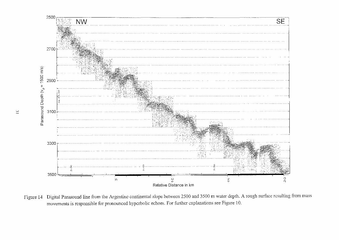
3500 !, ' " , ':'r'l:

3300 .

'<)

o

o0<

SE

li'l

"

n

o"Relative Distance in km

...: , .,.. ::,...... - .

li'l

NW............

000•••••• ('j •••.•.•.••••.•. - •. , .••• - .•• - ••••• - •••••.••••..•••.•• ··0············································ ..... ,1;"']

~ n

oo

"b" .

110-

G..cQ(j)

o"DC~ 3100 ~..UlC\l'-C\l0..

VlEooLO 2900 ~.........

w>-'

Figure 14 Digital Parasound line from the Argentine continental slope between 2500 and 3500 m water depth. A rough surface resulting from mass

movements is responsible for pronounced hyperbolic echoes. For further explanations see Figure 10.

• detel111ine lateral ehanges in mud wave distribution and shape whieh in tUl11 shall be usedto reeonstruet Quatel11ary bottom eunent aetivity as a eontribution to the sparse knowledgeof past deep water eireulation,

• eolleet multiehannel seismie data to suppOli the planning of an ODP drilling operation inthe mud wave area whieh, among others, eould provide so far not existing stratigraphieinfonnation.

The areas seleeted for the survey were chosen closer to the eontinental margin than all ProjeetMUDWAVES sites partly for logistic reasons, but also to be nearer to the main pathway for Ant­arctic Bottom Water (AABW), loeal variations in topography, whieh may influence mud wavegeneration, and to the region of postulated change in bottom water flow direction (FLOOD et al.,1993) which should also have an impact on mud wave development and shape.

Aecording to the few digital Parasound lines available frOln the previous R/V METEOR M29/1and R/V POLARSTERN ANTX/5 cruises, two survey areas were placed to northeast and southeastof the 1994 survey area along the 5500 m isobath which appeared to be a major boundary in seafloor and mud wave morphology (Fig. 8). The third area was directly on the erest of the ZapiolaDrift, where large and regular mud waves had been observed in 1994. Table 4 summarizes themultichannel seismic data acquired between January 11 and 28 mostly with two or three seismicsources fired quasi-simultaneously or in an altemating mode.

Mud Wave Survey 1: North ofthe Zapiola Drift Crest

Figure 15 shows the cruise track on the nOlihem flank of the Zapiola Drift with a total of 9 seis­mie lines. The long seismie lines GeoB 00-001 and -002 at the begüming of the first mud wavesurvey were to study the transitions from erosion in the center of the AABW flow towards themud wave fields, additionallines ananged to determine strike directions of faulting and sedimentdefonnation as well as relative accumulation rate changes in the area.

GI gun profile GeoB 00-002 (Fig. 16) shows a flat surface and a subdued morphology eom­pared to buried structures up to the crest of the Zapiola Drift indieating a stronger bottom eunentactivity in reeent times than during most earlier periods independent ofwater depth.

The digital Parasound reeord (Fig. 17) reveals in greater details the eauses of the diffuse seis­mie surfaee echoes. The surface sediments have been affected by conspicuous tectonic processesover a lateral extent of several hundred kilometers. Small vertieal faults with offsets of a fewmeters disrupt all, mostly eurved reflectors up to the sea floor, but immediate surface expressionsare missing. This may be attributed to strong bottom cunents leveling the small horst and grabentopography. In plaees an erosive charaeter beeomes evident, yet in general the surfaee is moretypical for strong winnowing and surface transport. The buried sediment appears to originatefrom an older mud wave field. An altemative explanation for the upward bending would be lat­eral eompression within the surface sediment paekage.

The small scale variability is barely resolved in the seismic data without further processing,but the Parasound data immediately provide important information to umavel ongoing processes.It may be speeulated that large seale destabilization oecurs due to sediment removal on northel11Zapiola Drift slope. Profile GeoB 00-002 was shot in a mixed mode with 2 - 4 shots of the 0.4 IGI gun followed by a single shot with 1.7 I volume chamber. Deeper structures could adequatelybe observed with the higher energy, lower frequency souree signal. Oceanie basement is tenta­tively identified at around 7.7 s TWT.

32

Table 4 R1V METEOR Cruise M46/3 summary of seismic surveys including profile number,

date and time of start and end, profile length in km and approximate number of shots

for all seismic sourees.

Mud Wave Survey I

Profile Start End Length Shots

Date Time Lat [0 f S] Lon [0 f W] Date Time Lat [0 f S] Lon [0 f W] [km]

GeoBOO-OOl 1/11/00 08:20 42 32.1 50 51.5 1/12/00 03:29 43 04.2 48 45.9 181 11490

GeoBOO-002 1/12/00 03:52 43 05.8 48 44.3 1/12/00 18:36 44 13.6 48 11.0 133 8840

GeoBOO-003 1/12/00 18:59 44 14.7 48 12.5 1/13/00 00:04 44 01.8 48 43.5 48 3050

GeoBOO-004 1/13/00 00:23 44 00.2 48 44.8 1/13/00 07:33 43 24.1 48 44.7 67 4300

GeoBOO-005 1/13/00 08:25 43 23.2 48 38.6 1/13/00 12:02 43 23.3 48 14.0 33 2170

GeoBOO-006 1/13/00 12:24 43 29.5 48 12.0 1/13/00 18:25 43 48.6 47 46.5 49 3610

GeoBOO-007 1/13/00 18:51 43 49.9 47 48.4 1/14/00 04:04 43 50.0 48 52.2 85 5530

GeoBOO-008 1/14/00 04:27 43 48.7 48 54.0 1/14/00 05:53 43 41.3 48 54.0 14 860

GeoBOO-009 1/14/00 06:24 43 40.1 48 50.9 1/14/00 11:21 43 40.0 48 16.8 46 2970

Mud Wave Survey II

GeoBOO-010 1/15/00 10:37 44 10.5 48 15.7 1/16/00 05:20 45 45.0 48 15.6 175 11230

GeoBOO-Oll 1/16/00 05:34 45 45.8 48 16.5 1/16/00 21:25 46 43.1 49 39.6 150 9510

GeoBOO-012 1/16/00 21:57 46 42.4 49 42.3 1/17/00 09:14 45 45.3 49 42.3 106 6770

GeoBOO-013 1/17/00 09:21 45 44.7 49 41.7 1/17/00 18:59 45 10.3 48 52.5 90 5780

GeoBOO-014 1/17/00 19: 19 45 08.9 48 53.0 1/17/00 20:12 45 06.8 48 58.3 8 530

GeoBOO-015 1/17/00 20:36 45 07.4 49 00.6 1/18/00 02:08 45 33.4 49 14.1 51 3320

GeoBOO-016 1/18/00 02:29 45 35.1 49 12.9 1/18/00 03:11 45 35.1 49 07.6 7 420

Mud Wave Survey III

GeoBOO-017 1/21/00 03:25 43 11.4 50 10.4 1/21/00 20:56 44 39.1 50 10.5 162 10510

GeoBOO-018 1/21/00 21:25 44 39.7 50 12.8 1/22/00 00:30 44 29.1 50 28.9 29 1850

GeoBOO-019 1/22/00 01:02 44 26.6 50 28.3 1/22/00 12:32 43 43.2 49 39.4 103 6900

GeoBOO-020 Profile omitted due to maintenance works

GeoBOO-021 1/22/00 14: 14 43 39.0 49 46.0 1/22/00 23:08 44 13.2 50 25.7 83 5340

GeoBOO-022 1/22/00 23:31 44 13.5 50 28.1 1/23/00 00:25 44 10.2 50 32.3 8 540

GeoBOO-023 1/23/00 00:48 44 08.5 50 31.8 1/23/00 09:57 43 32.9 49 51.2 85 5490

GeoBOO-024 1/23/00 12:31 43 31.3 49 53.0 1/23/00 15:29 43 31.1 50 14.1 28 1780

GeoBOO-025 1/23/00 15:59 43 31.8 50 16.3 1/23/00 22:22 43 57.6 50 44.5 61 3830

GeoBOO-026 1/23/00 22:39 43 59.1 50 44.5 1/23/00 23:42 44 02.8 50 39.1 10 630

GeoBOO-027 1/24/00 00:01 44 03.0 50 37.2 1/24/00 08:22 43 30.1 50 00.3 78 5010

GeoBOO-028 1/24/00 08:41 43 30.1 49 58.2 1/24/00 12:38 43 42.3 49 37.8 35 2370

GeoBOO-029 1/24/00 13:34 43 42.0 49 38.3 1/24/00 14: 18 43 45.1 49 41.5 7 440

GeoBOO-030 1/24/00 14:35 43 45.0 49 43.5 1/24/00 15:23 43 40.7 49 47.8 10 480

GeoBOO-031 1/24/00 15:45 43 40.6 49 47.7 1/24/00 16:48 43 36.4 49 43.1 10 630

GeoBOO-032 1/25/00 10:13 43 48.4 50 42.7 1/25/00 20:09 43 47.5 49 33.3 93 5960

GeoBOO-033 1/25/00 20:30 43 48.7 49 32.0 1/26/00 03:57 44 27.2 49 51.7 76 4470

GeoBOO-034 1/26/00 04:51 44 31.4 49 52.0 1/26/00 07:42 44 37.7 49 31.1 30 1710

GeoBOO-035 1/26/00 07:57 44 37.3 49 29.3 1/26/00 18:02 43 49.0 48 50.9 103 6050

GeoBOO-036 1/26/00 18:56 43 50.1 48 51.7 1/28/00 18:00 45 00.0 55 00.0 504 28240

Total: 2759 km, 172'610 shots

33

51W 50W 49W 48W

w.j:>.

I/

·-·_·-·-f····-·--·-··!··_·-·-·_·:t~-··-····-·r··--···---·")"-·······-ll..············ r ··-···-···· r -···: ~ . !VJ16/3 : : / : : :

43s~-J----J-------o-l--~;~~:~~;f; ~~~~-~:J-J-I-143S~ /..-"- )., 550ri-n i./ l s." i Mud Wave l: .....--- /' :...... ~J..!...! : -_/ : \,)-': : :

/,( -- j ---------~-----------k..-- ; <S 1 Survey Area I j

--/ I I I I I %I I ;8 ~ ~ ~ i Figure ~15~ ~ i

\~ ~ ~ j i i ';j" GaoS 00-005 i

_~~ __\__ __ __+_____... i_._+_______+_1 ~.o ~J-------+\ ~ !VJe~$ ~ ! ~ g ~O ~, ~ . Or 111') ..OJ (;) ce:

'''<';; ! tV'<9/1 1 l g i" °0 l\'b: ;:6 ~ i5' :

l't~ I '!i ig I~ -', ~ 1'\ '" j Figure 16 j

44s:·-·--·-r·-tiiet~~lAt~-- ·-·r·-~-·----·t"--: <?·····t;;-i·~"1~----+-~44s",: .. , . . o/arste : ~: 5000m',_ ~o polrrstern ANT'Jf!~... I rn A"4T XiS 8C~

: ~ ....: i ofZaL. :: :',: : PJei.I:!.-D---: :', 1 j Cf:, rift

: :

51W 50W 49W 48W

Figure 15 Ship's track ofRJV METEOR Cruise M46/3 in the Mud Wave Survey I area, central Argentine Basin. Thick lines indicate seismic pro­

files GeoB 00-001 to -009. Also shown are tracks ofRJV METEOR Cruise M29/1 and RJV POLARSTERN Cruise ANTX/5. Track lines

are annotated every 4 hours with ticks every hour. Bathymetry from Gebco Digital Atlas.

wU1

(/)E'--'

~

Figure 16 Multichannel seismic line GeoB 00-002 on the northern flank ofthe Zapiola Drift shot with a GI gun (see Fig. 15 for location). Unlike

south of the Zapiola Drift crest, mud waves are absent and morphology is controlled by faulting and internal deformation of the sedi­ments. Scattering surface at around 7.7 s TWT is tentatively identified as top ofthe oceanic basement.

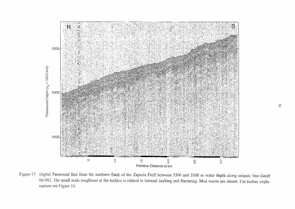
5300

---.(f)

E00lf).,-

11Q.

2:-J::Ö.(j)

0uC::J I I I.D0 '"(f)

ro'-ro0..

tri o 1ft 0" N

Relative Distance in km

1ftN

o(')

Figure 17 Digital Parasound line from the northern flank of the Zapiola Drift between 5300 and 5500 m water depth a10ng seismic line GeoB

00-002. The small scale roughness at the surface is related to internal fauHing and fracturing. Mud waves are absent. For further expla­nations see Figure 10.

Towards the crest of the drift, reflection amplitudes decrease and often a wedge shape ofintemal reflections is found. As was confirmed by coring, these sediments are very fine-grainedwith a high water content and elevated concentrations of organic components. Evidence bothfrom coring and echosounder data hence indicates drift deposits accumulating at very high rates.It was surprising to encounter areas of winnowing/erosion in immediate vicinity to fields of highaccumulation. The crest of the Zapiola Drift appears to be a major boundary for sediment depo­sition, most likely due to changes in bottom water flow pattem. We expect that a spatial analysisof the collected data will allow a detailed reconstruction of depositional regimes in this region.

Mud Wave Survey 11: South ofthe Zapiola Drift Crest

A completely different setting was found on the southem slopes of the Zapiola Drift. Fromaround 5000 m at the crest, a large area of giant mud waves extends to at least 6000 m waterdepth, the southernmost point of our survey. Weather conditions became very rough during this2.5 days survey and single charmel displays of seismic data are not available due to the highnoise level which can only be reduced by a thorough seismic processing.

The survey lines (Fig. 18) cover an area, where changes in mud wave geometry and size arelargely depth dependent. While in the R/V Meteor Cruise M29/1 survey area mud waves weredecreasing in size to greater water depth, we observed an increase which at some locations wasassociated with wave 'interference' producing steep flanks ofup to 100 meters height. A prelimi­nary interpretation of these pronounced differences would generally follow the flow pattemreconstmction of FLOOD & SHOR (1988), who predicted an E-W directed current north of thecrest which is supposed to turn into a W-E flow south of the crest sharing the southern deepwater pathway with the AABW.

The digital Parasound records shown in Figures 19 and 20 illustrate a strong migration of thewaves, their large average height and regions of 'interference' (nodal zones). The slope angle isabout constant over significant depth intervals which is different from the northem side, butsimilaI' to regional characteristics of the Mud Wave Survey ur area (see below). Figure 20 alsoreveals two changes in depositional style, where former waves with a strong migration trendlonger build up. They were first covered by a sediment package of nearly uniform thickness andthen buried so that a new geometry seems to be evolving. With the deeper penetration of theseismic data we hope to be able to determine the relative timing of such events in various parts ofthe study area, where the changes appeal' to be different. This information is certainly most criti­cal for the development of a consistent regional model of current flow pattem from the mudwave distinctive attributes.

Mud Wave Survey 111: Western End ofthe Zapiola Drift Crest

The third mud wave survey was centered around the working area ofR/V METEOR Cruise M29/1(Fig. 21), where very regular wave shapes, gradual changes in wave amplitude with water depthand 'nodal zones', which reveal characteristics of interference patterns, have been observed. Weextended this survey to greater water depth across and to the sides of the westem continuation ofthe drift crest. The same drastic change from a mud wave field in the south to an erosional settingon the northem side was encountered as during Mud Wave Survey 1. Seismic lines GeoB 00-017to -035 (Fig. 21) were positioned to allow a detailed correlation between seismic and Parasoundprofiles which in turn could be used to document the strike direction and its spatial variability.

37

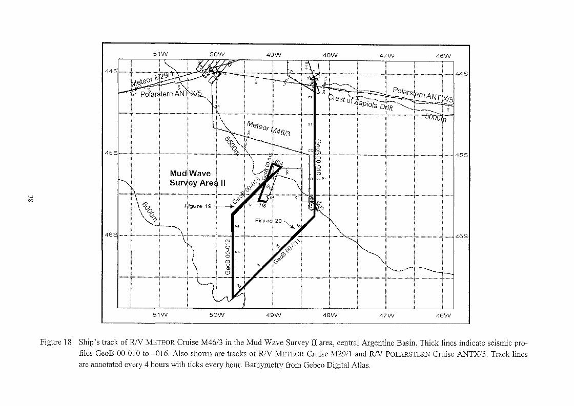
46W47W48W49W50W51W

44sl ~I··················.ji>I>~i.. TI'----"" 'v ~:k~e\eo"( \"! ';:J \ \ ~ : \ 25 ~ ~_,__... ~~\j\ ,.,: '? ',i ;! 0: ... ',-i j po/ars: !i,;' P01ar~tern AN1-xJ..5_.... ~: 0 ~rest \rf-...-.-- ~-; -....-...... tern ANT05; ~ i '\~! i 0 iap/o/a D:'- - ...

···r··T······

j j Mud1Wave 1 1 ~ I I I i-...,! ! SUrV:ey Area 11 ~ ! ! ~ !

'< : : : .:, : : :

~ \ ! i i 0 0

1 \ 6Q; Fjigure 19 -+----+1 \~j 1 1~ ',-'/~ ~ ~

w00

04

51W 50W 49W 48W 47W 46W

Figure 18 Ship's track ofR/V METEOR Cruise M46/3 in the Mud Wave Survey II area, central Argentine Basin. Thick lines indicate seismic pro­

files GeoB 00-010 to -016. Also shown are tracks ofR/V METEOR Cruise M29/1 and R/V POLARSTERN Cruise ANTX/5. Track linesare annotated every 4 hours with ticks every hour. Bathymetry from Gebco Digital Atlas.

0 0 0 0 0 0 0 0(0 0 (0 0 (0 0 (0 0

:; .,. .,.~ ~ ~ '" "-

I:).' 'i ) [' .'; 11I \ ': " \ "'i'! ,'i/ i

r

/ i':: \ "!!I!

: : : : i , I

U. 0 lI'J 0 lI'J 0 lI'J 0 lI'J'0 [l.,. [l.,. 0) 0) (}. a, 0 0

oo(0

o(0

N

ooN

lI'J 0 lI'J 0::t lI'J lI'J '0

Relative Distance in km

o(0

o::t

lI'Jr1

o(')

lI'JN

oN

lI'J

'"olI'J

sw

5700 r" ){:':iX;:',~';;i; 'i';':i;,;X',,"\:('LV

';;, .

oo

5500

~oo~···················· .

5800

(j)

E00L().,.--

11"-

G.cä..Q)

0""0C:::J0

W (f)\D m

l-

m0...

Figure 19 Digital Parasound line from the southem flank of the Zapio1a Drift between 5500 and 5800 m water depth a10ng seismic lines GeoB

00-012 and 00-013. Remarkable variations ofthe mud wave geometry and several 'nodal' zones are observed. Maximum wave height is

up to 100 m. For further explanations see Figure 10.

o(\J

o lfl

" Relative Distance in km "

lfl

5600 2'. ~/,;,<,:.,,';>, ,.: ", ,';":»" "Y:;:'-"":'>"'" "'/: "i,': '", "X :,.,:,', ;,'.'{';;;',';: (;,:':;j' ;i/"<',::,>:', ':i ," ,\:,'"

,.". !":"':(";'::':':(';'::" X;:; P/.,C>:,!':\' ;:C::;:;,::: 'i,,, ":':!':-:::~':.6::;j;: ,L;::, ;t:,: :'/';/U'?'ijL <t." ':Ci"'..;,; :";')':-;

,;":,'", ",: ;', :'i'::,:' "~i' : ":,""";;' ;i :'i:/ :\ .0:,,,,

UJ----E001.0.,-

11Q,

2:-

0

.c 5700

I 7

Q.Q)

0-0C:l

I0VlCU"-CU

CL

Figure 20 Digital Parasound line from the southern flank of the Zapiola Drift in about 5650 m water depth along seismic line GeoB 00-011. Forseveral intervals the mud waves reveal an irregular internal structure, extreme wave migration and pronounced changes in depositionalstyle indicated by sharp unconformities. For further explanations see Figure 10.

Numerous crossings of the same wave provided reliable statistical estimates of its shape

parameters. A slump surface on the northern side exposed layers, which could be traced in Para­sound and watergun data to significantly greater sub-bottom depth, offered the perfect opportu­

nity to sampIe older material and to detennine accumulation rates on longer time scales than usu­

ally possible with surface gravity cores.The watergun profile GeoB 00-033 (Fig. 22) most clearly illustrates that mud waves were

generated over significant time periods. Presumably, the accumulation the sediment drift, which

makes up about half of the sediment column in the vicinity of the survey area, was at all times

associated with the development ofmud waves on its flanks.The Parasound profile from the nOlihern side (Fig. 23), recorded along seismic line GeoB

00-028 documents strong erosion and slumping, slump SCallJS and exposed reflectors which aredeeply buried up slope. On seismic line GeoB 00-021 (Fig. 24), directed perpendicular to this

Parasound profile, exposed reflectors can be traced to depths >300 ms TWT. They were sampledat two coring sites hoping to obtain useful age inforn1ation from shore based studies for much ofthe sediment column comprised in the Parasound and watergun data, provided the respective

recoveries of several meters each have penetrated sufficiently deep through a potential surfacelayer of reworked deposits.

As shown in Figure 25, regular mud waves are dominating the surface in the center of the

study area bordered by a flat region of relatively high accumulation towards shallower water and

'nodal zones' in water depths of around 5500 m. Seismic data reveal that these 'nodal zones'

remain stationary over long time spans suggesting a direct relation to the general circulation and

deposition patterns. Also, 'nodal zones' seem to follow isobaths, but this observation awaits fur­

ther proof by shore based analyses of the completly processed data sets.

A 500 km long seismic line, GeoB 00-036 (Fig. 26), COlmects the areas ofMud Wave SurveyIII and I and extends from the crest of the Zapiola Drift through the erosional core zone in about

6000 m water depth to the foot of the Argentine continentalmargin at 5600 m water depth. Dif­

ferent seismic facies can be distinguished. In the eastern part, the Zapiola Drift, series of mud

waves in the upper sediment column is underlain by a zone of low reflectivity at greater depth.

The accumulation rates are typically high. To the west, a much more diffuse reflection pattern is

observed indicating bottom current activity and deposition of coarser material. The sea floor

topography is asymmetrical with respect to slope angles which mayaIso be attributed to ero­sional effects of the strong westem boundary contour current.

4.1.5.3 Argentine Continental Margin (Southern Area)

A 7 days coring and survey operation was perfonned towards the end of the cruise on the south­

ern Argentine continental margin (Fig. 27). Again, Parasound and Hydrosweep data were par­

ticularly helpful to identify coring sites and to characterize the depositional environment. The

margin is characterized by steep slopes and canyons senring as sediment transport pathways. In

general, the depositional setting is quite similar to the northem Argentine continental margin.Figure 28 shows the Parasound line across the Almirante Brown Transverse Canyon which is

about 600 m wide at this transect. Both levee-type sediment accumulation and erosional trunca­tion is observed on the flanks ofthe canyon.

41

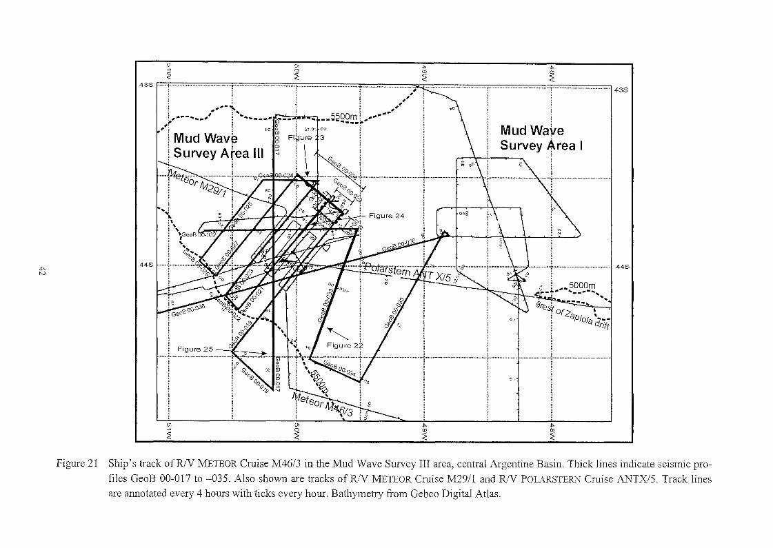
443

~

~

sc

~

ID

~

(J1~

~

(J1

:2

443

(J1 ~ ~o ID ro:2 :2 :2

433 I··· ·..···..··· · ···· ········.. ·· ···· ····· · ····t·· ···..···..··· ·~··········· ··r····.. ·······..·..·..·········· r · ···· ········..·· 143s

~ ~

i Mud Wa~eI Survey ~rea I

" . "1--

.j;..N

Figure 21 Ship's track ofR/V METEOR Cmise M46/3 in the Mud Wave Survey 111 area, central Argentine Basin. Thick lines indicate seismic pro­

files GeoB 00-017 to -035. Also shown are tracks of R/V METEOR Cmise M2911 and R/V POLARSTERN Cmise ANTX/5. Track lines

are annotated every 4 hours with ticks every hour. Bathymetry from Gebco Digital Atlas.

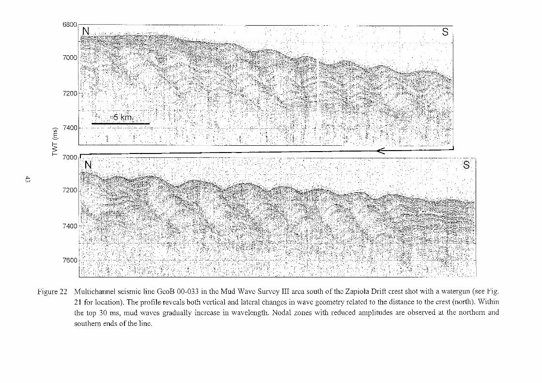
.j::>.W

Ul-S

~f-

Figure 22 Multichannel seismic line GeoB 00-033 in the Mud Wave Survey III area south ofthe Zapiola Drift crest shot with a watergun (see Fig.21 for location). The profile reveals both vertical and lateral changes in wave geometry related to the distance to the crest (north). Within

the top 30 ms, mud waves gradually increase in wavelength. Nodal zones with reduced amplitudes are observed at the northem and

southem ends of the line.

NW SE

5200

Ul--E00LO

'"""11

0..

2.-.c0..<lJ0"0c

5300.j:>. :J.j:>. 0

<IlC\lCüCl

,;, •. /( .'n'" '·,C·i

..' .\;'i;,'C' .,,"")> ;··:..H<,.·,:·:· '.: ':e: .;J:'::"~:!r'{};'3,;".. 'i '.:. ,'o',.:,:."; ,".'/' <'.' ,C.· <.,:'.;';':, .. '> :">j:j,:~"':}./r'" .<:,''-:,

."., ,.,.,.:;:":,,,,:<,,,, ;';c. hC<.'.;" ;::,",';;j,'''' :,.. :\.\:'. 'ce "','i:/ ; ..>,:

t );.. ;c< '.;- ;: ,,;.:'. '.':','. 0

;','i,,r;,:.., ...../:.} ';:..... ",:e: T' .. , ;;,i ~::;.> ;;.;,"; ••... ",.,. :':-.!,:.> .; ..' :..•' :'':·C,::.. :""','{ :,., '"

5400 ---r I r-- I I i i" --- -'-r=, I - i·~_·7r- .---' I .. ...,- T " I I I ,_...........----. _,m=j"'_ .-~Li) o Li)

"oN

Li)N

o(')

Li)(')

o=+-

Relative Distance in km

Figure 23 Digital Parasound line from the northwestem flank of the Zapiola Drift between 5200 and 5400 m water depth along seismic line GeoB

00-028. Intense erosion and truncation of reflectors is observed that was found at several hundred meters sub-bottom depth south of thedrift crest. For further explanations see Figure 10.

6800 "I:-,-,.~~~~-:-:C-~~~---::-~~~~-----C~~~~~---:Z~~~ ---'------C ~T"'--- C:=:---=---,----

(j)E

-----~

7200

I-

.p.VI

7400

7600' .' I

Figure 24 Multichannel seismic line GeoB 00-021 over the Zapiola Drift crest shot with a watergun (see Fig. 21 for location). The profile shows

the transition from erosion in the northeast to the onset ofthe mud wave field in the southwest. Buried structures reveal this change more

clearly. A sequence ofwaves in 250 ms TWT sub-bottom depth at the SW end ofthe line outcrops near its NE start (14:40).

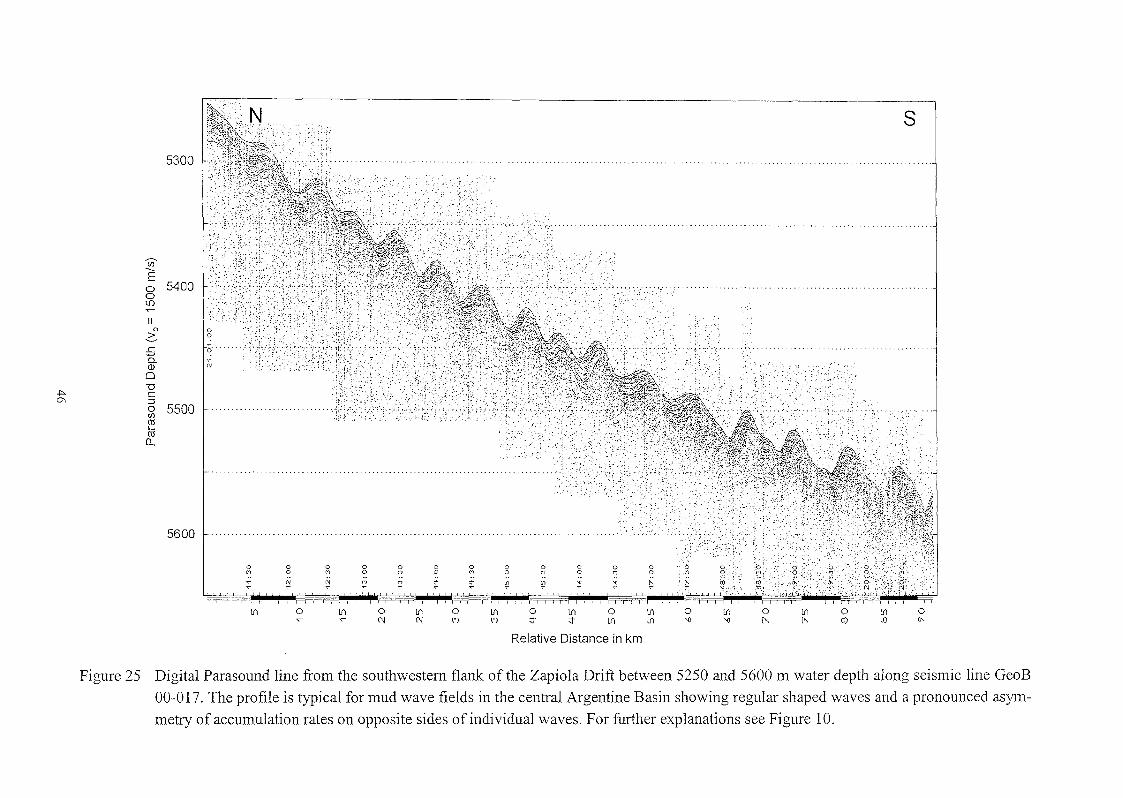
.j:>.0\

5300

r;;-Eo 5400oLO.,--

11CL

~ rb"li .;.Q) '"o"DC::JSl 5500ro'-ro

Cl.

5600

s

0 0 0 0 0 0 0 0 0 0 0 0M 0 M 0 M 0 M 0 M 0 M 0

~ ';! '" ';' ';' ;t: ".~ ~ ~ ~ ", ,

: \',' i ' , [ !!, 1-;;.'']' i :'i'i:'/"'I:">/ '(,' ';'['" \:!';,·r[~"y,·t (.

I I i i i j I I ! , i i, i : ) I I I

lf) 0 lf) 0 lf) 0 lf) 0 lf) 0 lf) 0 lf) 0 ll) 0 lf) 0

"'" 0l 0l (") (") j- j- lf) lf) '0 '0 !'- [;" 0) 0) (}.

Relative Distance in km

Figure 25 Digital Parasound line from the southwestem flank ofthe Zapiola Drift between 5250 and 5600 m water depth along seismic line GeoB

00-017. The profile is typical for mud wave fields in the central Argentine Basin showing regular shaped waves and a pronounced asym­

metry of accumulation rates on opposite sides ofindividual waves. For further explanations see Figure 10.

.j:>.--.J

7000

7500

(j)

-S 8000

~I-

8500

9000 I:';" ' , ',r i ,', ::,',' +';,i';', :::J: '0::"," ',: /':Y"'~".,:'·: ..' ,', '-.' ;je' '::'",;':,,'}:::j: ,:::;:,',,:T'i:'::i'!:'

Figure 26 Multichannel seismic line GeoB 00-036 from the Zapiola Drift across the erosional zone towards the Argentine continental margin shotwith a GI gun (see Fig. 8 for location). A gradual transition is observed from regularly shaped mud waves in the east to intensive erosion

in the center of the basin and terrigenous sedimentation at the margin.

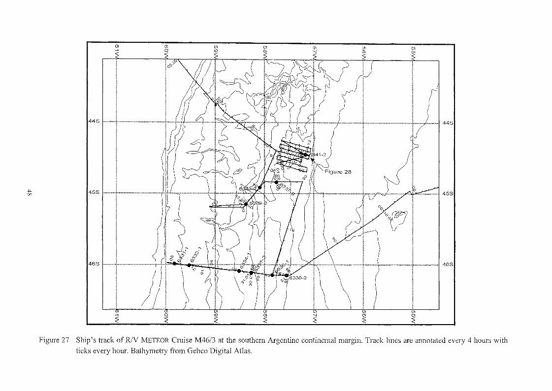
.j::.00

443

453

463

Ol~

~

~

Olo

o~

01{Jl

{Jl{Jl

~

443

453

463

Figure 27 Ship's track ofR/V METEOR Cmise M46/3 at the southem Argentine continental margin. Track lines are annotated every 4 hours withticks every hour. Bathymetry from Gebco Digital Atlas.

..,.'0

4000 I SE

4200(j)

----E00LO

'"11

0.

2-..c 4400+JQ.Q)

0-a

l8c::J0 ......U)

cuCi; I- ••••••••••••••••.

0..

4600

4800

1J'l

GeoB6341-1

o"'

g~

l{J

"'o('j

Almiral1te .Brown....

TransverseCanyon

lf1('j

o(')

g

'"

,

lf1(')

.,

Relative Distance in km

Figure 28 Digital Parasound line across the more than 600 m deep Almirante Brown Transverse Canyon. At the canyon flanks both levee-type

sedimentation and erosional truncation is observed. For further explanations see Figure 10.

4.2 Sedimentology

4.2.1 Sediment Sampling

(T. Bickeli, S. Drachenberg, E. Eades, M. Frenz, K. Michels, U. Rosiak,C. Rühlemanl1, M. Segl, T. Westerhold, N. Zatloukal)

A multicorer and a gravity carer were used to recover surface and late Quatemary sediments at

30 stations on the Argentine continental slope and in the mud wave fields ofthe Argentine Basin.In addition, a boxcorer and a dredge were employed at 3 and 8 stations, respectively, to recover

the coarse-grained sediments along the Argentine shelf edge and especially to retrieve theepibenthos adherent to gravels and rocks. Detailed infonnation on locations, deployed devices

and recovery is summarized in the station list (Chapter 8).

Multicorer

The multicorer is designed to recover undisturbed surface sediment sections together with theoverlying bottom water. The device used during Cruise M46/3 was equipped with 8 large and 4

small (10 and 6 cm inner diameter, respectively) 60 cm long plastic tubes. Usually, 10 to 12

tubes were filled with more than 20 cm of sediment and even in the coarse-grained sediments at

the upper Argentine continental slope more than 10 cm long sections were recovered. Only at

two stations (GeoB 6318-1, 6335-1) extremely hard sediments prohibited a regular recovery (see

station list, Chapter 8).

Sampling ofthe multicorer followed the standard sampling scheme:

2 large tubes were cut into 1 cm slices and stained with bengal rose to study foraminiferal

assemblages,

1 large tube was cut into 1 cm slices for dinoflagellate analysis,

1 large tube was cut into 1 cm slices and frozen for organic carbon geochemistry,

1 large tube was cut into 1 cm slices and frozen for sedimentological investigations andorganic matter microscopy,

pore waters of 1 large and 1 small tube were analyzed geochemically,

1 smal1 tube was cut into 1 cm slices for rock magnetic analyses,

1 small tube was preserved for sediment geophysical investigations,

1 large and 1 small tube were frozen as archive cores,

50 ml ofbottom water were sampled for carbon and oxygen isotope analysis.

Gravity Corer

In order to obtain long sediment cores a gravity corer with a pipe of 3, 6, 12, 15 or 18 m

length and a weight of 1.5 tons on top was used. Some 300 m of sediments were recovered with

the gravity Garer during Cruise M46/3. Individual care lengths varied between 100 and 1466 cm.Before use al1 core liners have been marked with a straight line to retain a common azimuthai

orientation of the care segments for paleomagnetic purposes. After recovery, the core liners werecut into 1 m long segments, sealed with caps at both ends and inscribed (Fig. 29).

Following the shipboard whole-core geophysicalmeasurements (Chapter 4.2.3), the segments

were cut along-core into a work and an archive half. Immediately after core opening, digital color

50

\J)~

Tab1e 5 Multicorer sampling (L = 1arge tube of 10 cm diameter, S = small tube of 6 cm diameter).

GeoB Archive Foraminifers Dinoflagellates Sedimento1ogy Nannoplankton Organic Geophysics Geochemistry OrganicStation Geochemistry Microscopy

6301-1 1 L, 1 S lL lL lL 1/2 S lL 1 S - 1/2 S6307-1 1 L, 1 S lL 1 S lL 1/2 S 1 L 1 S - 1/2 S6308-1 1 L, 1 S 2L 1 L lL lL 1 L 1 S 1 L,2 S -

6309-2 2L, 2 S 2L 1 L lL lL lL 1 S - 1 S6310-1 1 L, 1 S 1 L, 2 S lL lL 1/2 L 1 L 1 S - 1/2 L6311-2 2 L, 3 S 2L lL lL 1/2 L 1/2 L 1 S - 1/2 L6312-2 2 L, 3 S 2L lL 1/2 L 1/2 L 1 L 1 S - 1 L6313-2 1 L, 2 S 2L lL 1/2 L 1/2 L lL 1 S - 1 S6314-1 lL - - lL 1/2 L 1 L 1 S - 1/2 L6314-2 1 S 1 L lL - - - 1 S - -

6317-2 1 L, 2 S 2L lL 1/2 L 1/2 L lL 1 S 1 L 1 S6322-1 2S - - lL - 1 S 1 S - -

6330-1 1 L, 1 S 2L lL 1/2 L 1/2 L lL 1 S 1 L, 2 S 1 L6334-2 1 L, 3 S 2L lL lL 1/2 L lL 1 S - 1/2 L6336-2 1 L, 3 S 2L lL 1/2 L 1/2 L lL 1 S - 1 L6337-8 2L,3 S 2L lL 1/2 L 1/2 L 1 L 1 S - 1 L6339-1 2 L, 3 S 2L lL 1/2 L 1/2 L 1 L 1 S - 1 L6340-1 lL 1 L, 1 S 1 L 1/2 L 1/2 L 1 S 4 L, 1 S - 1 S6341-1 1 L, 3 S 2L lL 1/2 L 1/2 L lL 1 S - lL

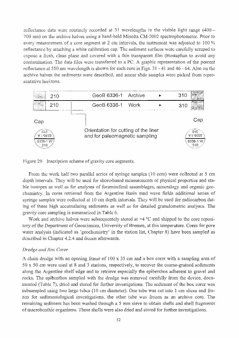
reflectance data were routinely recorded at 31 wavelengths in the visible light range (400­700 nm) on the archive halves using a hand-held Minolta CM-2002 spectrophotometer. Prior toevery measurement of a core segment at 2 cm intervals, the instrument was adjusted to 100 %

reflectance by attaching a white calibration cap. The sediment surfaces were carefully scraped toexpose a fresh, clean plane and covered with a thin transparent film (Hostaphan to avoid anycontamination. The data files were transferred to a Pe. A graphic representation of the percentreflectance at 550 nm wavelength is shown for each core in Figs. 31 - 41 and 46 - 64. Also on thearchive halves the sediments were described, and smear slide sampies were picked from repre­sentative horizons.

Cap

210

210

8eoB 6336-1 Archive

8eoB 6336-1 Work

310

310

Cap

Orientation for cutting of the linerand for paleomagnetic sampling

Figure 29 Inscription scheme of gravity core segments.

From the work half two parallel series of syringe sampies (l0 ccm) were collected at 5 cmdepth intervals. They will be used for shore-based measurements of physical properties and sta­ble isotopes as weIl as for analyses of foraminiferal assemblages, mineralogy and organic geo­chemistry. In cores retrieved from the Argentine Basin mud wave fields additional series ofsyringe sampies were collected at 10 cm depth intervals. They will be used for radiocarbon dat­ing of these high accumulating sediments as weIl as for detailed granulometric analyses. Thegravity core sampling is summarized in Table 6.

Work and archive halves were subsequentely stored at +4 °C and shipped to the core reposi­tory of the Department of Geosciences, University of Bremen, at this temperature. Cores for porewater analysis (indicated as 'geochemistry' in the station list, Chapter 8) have been sampled asdescribed in Chapter 4.2.4 and frozen afterwards.

Dredge and Box Corer

A chain dredge with an opening frame of 100 x 35 cm and a box corer with a sampling area of50 x 50 cm were used at 8 and 3 stations, respectively, to recover the coarse-grained sedimentsalong the Argentine shelf edge and to retrieve especially the epibenthos adherent to gravel androcks. The epibenthos sampled with the dredge was removed carefully from the device, docu­mented (Table 7), dried and stored for further investigations. The sediment of the box corer wassubsampled using two large tubes (l0 cm diameter). One tube was cut into 1 cm slices and fro­zen for sedimentological investigations, the other tube was frozen as an archive core. Theremaining sediment has been washed through a 5 mm sieve to obtain shells and shell fragmentsofmacrobenthic organisms. These shells were also dried and stored for further investigations.

52

Table 6 Gravity eore sampling.

V1W

Station Water Core length Organie Geoehemistry Foraminifers Paleomagneties 7 Grain-size C-14 SmearGeoB depth [m] [ern] 10 ml every 5 em 10 ml every 5 em ml every 5 em 10 ml every10 em 10 ml every 10 em shdes

6307-3 4010 1095 x x x - - x6308-3 3620 793 x x x - - x6309-1 2867 862 x x x - - x6311-1 996 466 x x x - - x6312-2 436 349 x x x - - x6313-1 481 732 x x x - - x6317-3 3112 909 x x x - - x6318-1 4176 581 x x x - - x6319-1 4185 386 x - x x x x6319-2 4097 352 x - x x x x6321-2 5098 1230 x - x x x x6322-2 5064 1416 x - x x x x6323-2 5480 1145 x - x x x x6324-1 5510 453 x - x x x x6324-2 5490 1092 x - x x x x6325-1 5353 441 x - x x x x6326-1 5300 1065 x - x x x x6327-1 5275 954 x - x x x x6328-1 5255 566 x - x x x x6329-1 5230 470 x - x x x x6330-2 3875 875 x x x - - x6334-1 2598 80 x x x - - x6335-2 2797 351 x x x - - x6336-1 3417 1015 x x x - - x6337-9 3546 1014 x x x - - x6339-2 2492 746 x x x - - x6340-2 2794 1148 x x x - - x6341-2 4180 1133 x x x - - x

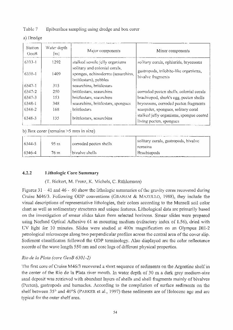
Table 7

a) Dredge

Epibenthos sampling using dredge and box corer

Station Water depthMajor components Minor components

GeoB [m]

6333-1 1292 stalked sessile jelly organisms solitat)' corals, ophiurids, bryozoanssolitary and colonial corals,

gastropods, trilobite-like organisms,6338-1 1409 sponges, echinoderms (seaurchins,

bivalve fragmentsbrittlestars), pebbles

6347-1 315 seaurchins, brittlestars

6347-2 250 brittlestars, seaurchins corroded pecten shells, colonial corals

6347-3 153 brittlestars, seaurchins brachiopod, shark's egg, pecten shells

6348-1 348 seaurchins, brittlestars, spongues bl)'ozoans, corroded pecten fragments

6348-2 168 brittlestars seaspider, spongues, solitary coral

6348-3 135 brittlestars, seaurchinsstalked jelly organisms, spongue coated

living pecten, spongues

b) Box corer (remains >5 mm in size)

6344-5 95 m cOIToded pecten shellssolitary corals, gastropods, bivalve

remaIns

6346-4 76m bivalve shells Brachiopods

4.2.2 Lithologie Core Summary

(T. Bickert, M. Frenz, K. Michels, C. Rühlemann)

Figures 31 - 41 and 46 - 60 show the lithologie summaries of the gravity cores recovered duringCmise M46/3. Following ODP conventions (GRAHAM & MAZULLO, 1988), they inc1ude thevisual descriptions of representative lithologies, their colors according to the Munsell soil colorchart as well as sedimentary stmctures and unique features. Lithological data are primarily basedon the investigation of smear slides taken from selected horizons. Smear slides were preparedusing Nm'land Optical Adhesive 61 as mounting medium (refractory index of 1.56), dried withUV light for 10 minutes. Slides were studied at 400x magnification on an Olympus BH-2petrological microscope along two perpendicular profiles across the central area ofthe cover slip.Sediment c1assificaton followed the ODP terminology. Also displayed are the color reflectancerecords ofthe wave length 550 nm and core logs of different physical properties.

Rio de la Plata (eore GeoB 6301-2)

The first core of Cruise M46/3 recovered a short sequence of sediments on the Argentine shelf inthe center of the Rio de la Plata river mouth. In water depth of 30 m a dark grey medium-sizesand deposit was retrieved with abundant layers of shells and shell fragments mainly of bivalves(Pecten), gastropods and bamac1es. According to the compilation of surface sediments on theshelf between 35° and 400 S (PARKER et al., 1997) these sediments are of Holocene age and aretypical for the outer shelf area.

54

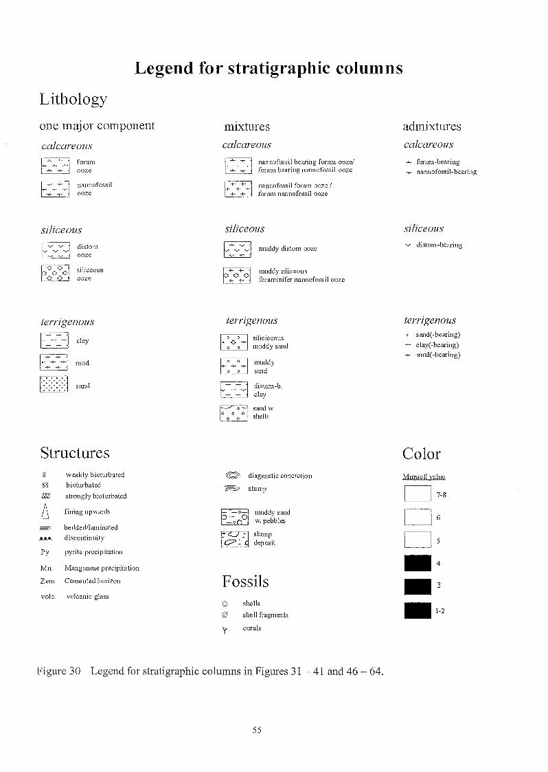
Legend for stratigraphie eolumns

Lithology

one major component

calcareous

mixturescalcareous

admixturescalcareous

foramooze

nannofossilooze EZj+

+ ++ +

nannofossil bearing foram oozelforam bearing IHUlnofossil ooze

nannofossil formll ooze Iforam nmlnofossil ooze

foram-bearing

nannofossil- bearing

siliceous siliceous siliceous

diatomooze

siliceousooze

muddy diatom ooze

nlUddy siliceousforaminifer nannofoss il ooze

...,. diatom-bearing

terrigenous terrigenous terrigenous

~ siliciceous0 smld(-bearing)

elay E23- - <>~

o 0 muddy sand clay(-bearing)

EZ3mud( -bem'ing)

~ ~ mud~

muddy~ ~

~ ~

o 0 sand

EJ sand E:3 diatom-b.-0 •• <>. - v-

elay

~sand w.

o 0 shells

Structures Colors weakly bioturbated r@; diagenetic concretion Munsell valueSS bioturbated

~ slump DSSS strongly bioturbated 7-8

jj fining upwards

~muddy smld D 6

-0 w. pebbles- bedded/laminated

~slump D-------

discontinuity0: deposit 5

Py pytite precipitation •Mn Manganese precipitation4

Zem Cemented horizon Fossils • 3volc. volcanic glass

0 shells •0 shell fragments 1-2

'r corals

Figure 30 Legend für stratigraphie eü1umns in Figures 31 - 41 and 46 - 64.

55

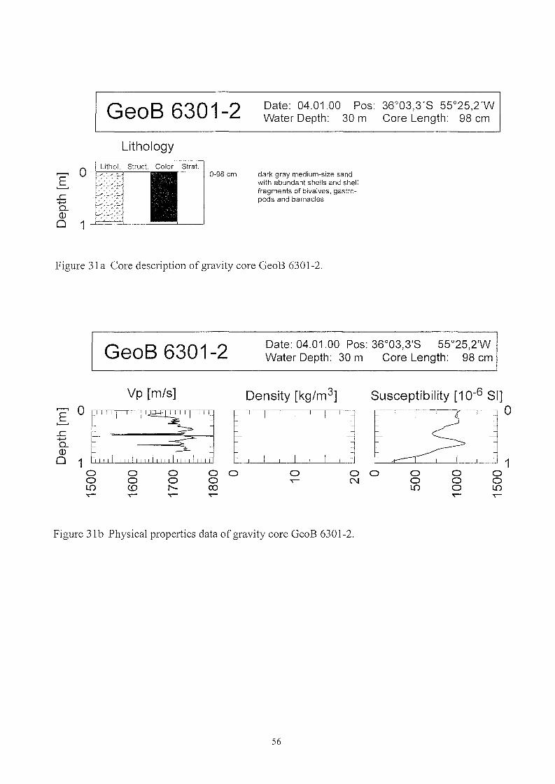
GeoB 6301-2

Lithology

Date: 04.01.00 Pos: 36°03,3'S 55°25,2'WWater Depth: 30 m Core Length: 98 cm

0-98 cm dark gray medium-size sandwith abundant shells and shellfragments of bivalves, gastro­pods and barnacles

Figure 31 a Core description of gravity core GeoB 6301-2.

GeoB 6301-2 Date: 04.01.00 Pos: 36°03,3'S 55°25,2'WWater Depth: 30 m Core Length: 98 cm

Vp [m/s] Density [kg/m 3] Susceptibility [10-6 SI],........., 0

J:E ['1""1'58 [' I

:

I

:'] [~

I

...c.......0- L(J) _"I""I"'~=0 1 I

0 0 0 0 0 0 0 0 0 0 00 0 0 0 ~ N 0 0 0L() <D I"- co L() 0 L()~ ~ ~ ~ ~ ~

Figure 31 b Physical properties data of gravity core GeoB 6301-2.

56

Table 8 Sediment constituents according to smear slide investigations.

Abiogenic components Biogenie components Grain size

(/)

(/) <l) C;; x...... (/) ...... '- (/) .~c (/) '0 <l) <l)

(/) ~ (/) (/)

S ro .S '- c<l) C;; "3 ~ 'V; '1:'- S bll(/) ro S

Station ..::, N ro ro u S "Cl <l) '2(/) S '1: .D

t 0.. Oll » u 0 .~ <8 <l) "Cl ...... »(/) u ro .~ 0 ro "Cl <l) C ro SedimentGeoB ...c: ro "Cl ro

~ Ü '2 C c '- 'S 0 ...... (3 ...... ro 0...... ;:j tt:: c 0 » ('Ij ...... ('Ij if)0.. 0' a:; ro ('Ij 0 '- 0-< ('Ij c

i5 ~ § c if)<l) J:.r... ..::.:: u Oll (/) u '- C 0

Cl u (3 '- (/)

~0 ('Ij ('Ij p:; .D

0 0 <l) J:.r... Z ~ '-~ > E u ('Ij

u u<r:

6301-2 50 15 1 34 5 - 1 25 2 - - 1 5 - - 1 10 85 10 5 sand

90 20 3 35 3 - - 30 1 - - 1 2 - - - 5 10 45 45 sand

Argentine Continental Slope at 39 to 40 oS (core transects GeoB 6307-3 through 6319-2)

Along two transects at 39 and 40 oS several cores were taken at the Argentine continental slopeto retrieve continuous late Pleistocene sediment sequences. The transects were directed slope­normal in water depth between 400 and 4000 m. However, between 1000 and 2800 m waterdepth the steep morphology prohibited any recovery. The sediment sequences were subdivided inthose of the upper slope and those of the lower slope enviromnent.

Upper slope sediments (GeoB 6311-1, 6312-2, 6313-1) from water depths between 436 and996 m consist of unconsolidated olive gray to gray muddy sands with varying amounts of bio­genic siliceous components, i.e., diatoms, radiolarians, silicoflagellates and sponge spicules. Thesediments are relatively unifonn from top to the bottom, intclTUpted only by several few cm thicklayers 01' lenses of fine sand, which indicate turbidite deposits. Core 6312-2 contains severallay­ers of dendritic coral fragments.

At the lower Argentine continental slope, in water depth between 2867 and 4010 m, longersequences of sediments were recovered which consisted mainly of dark grey to olive grey diatommud 01' muddy siliceous oozes, moderately bioturbated and mostly unconsolidated. Only in onecore (GeoB 6317-3) several semi-consolidated layers occurred in the deeper part of the core atabout 6 m which indicate an early diagenetic cementation of the fine-grained sediments. Also inthe deeper parts of the core, pyrite precipitations were COlnmon in the form of black pyritizedburrows 01' as black horizons. At the top of these pyrite containing sequences, H2S smell indi­cates the ongoing sulfate reduction in these sediments. Planktic foraminifers occur only in theuppennost part of the sediments, mostly in the upper few decimeters. Only very few specimensof benthic foraminifers could be found in the cores. This pattem might reflect the increased car­bonate dissolution during pre-Holocene times which prevented foraminifer preservation in sedi­ments ofthe late Pleistocene. Nevertheless, the smear slide study revealed mostly well preserveddiatoms assemblages worth studying with respect to the opal productivity in the frontal zone ofthe Malvinas Confluence.

Cores GeoB 6318-1, 6319-1 and 6319-2 were recovered in a special locality selected from aseismic line (BGR 98-28). At the slopes of a deep canyon the chance has been taken to retrieveolder sediments and therefore to date deep reflectors of the seismic section. However, due to thesteepness of the slopes, none of the cores were able to penetrate the envisioned sections. Thesediments recovered consisted mainly of young sediments of diatom mud with variously thicklayers of consolidated mud pebbles or of slump deposits.

57

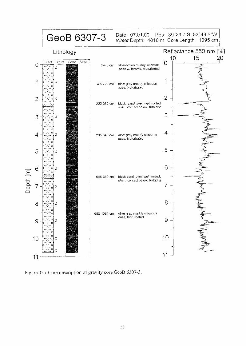
GeoB 6307-3 Date: 07.01.00 Pos: 39°23,1'8 53°49,6'WWater Depth: 4010 m Core Length: 1095 cm

4,5-222 cm olive-gray muddy siliceousooze, bioturbated

8

6

7

9

5

4

3

2

1

o

Reflectance 550 nm [0,/0]10 15 20

11

10

black sand layer, weil sorted,sharp contact below, turbidite

0-4.5 cm olive-brown muddy siliceousooze w. forams, bioturbated

222-235 cm black sand layer, weil sorted,sharp contact below, turbidite

235-645 cm olive-gray muddy siliceousooze, bioturbated

645-650 cm

650-1081 cm olive-gray muddy siliceousooze, bioturbated

Lithology

'"'- <) ::)

:) t') 0

~'.. ,---. .-".

~- -:-0

'." ...~. '-J

') ::) ~:)

-:- ..:0-1 -<, ':;, ,;:; S

3 _. :'.,.0...':; S,.r ....'- -OJ-

o Lithol. Struct Color Stra!.

:;,'~,:,"''Y S

9 if~-""'.~V S...- ~.." -...[

4 :"'..,_(;.,.Ö S...- ~_.. -....-

....... .r... _~..

8 :;."'-(,-'-<, S

10

..c+-"0..(1)

o

Figure 32a Core description of gravity core GeoB 6307-3.

58

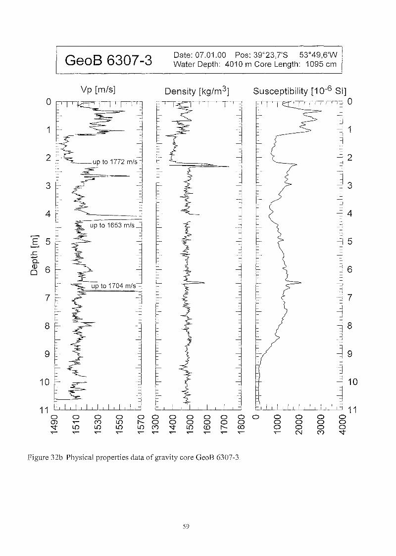
GeoB 6307-3 Date: 07.01.00 Pos: 39°23,7'8 53°49,6'WWater Depth: 4010 m Care Length: 1095 cm

2

9

-- 1

Susceptibility [10-6 SI]..---,-.,---.-.-c~-.-----r-.-r-,-,--,--" 0

Density [kg/m 3]Vp [m/s]

2

9

10

Lf10

11 110 0 0 0 0 0 0 0 0 0 0 0 0 0 0 0m ~ ('t') LO I"- 0 0 0 0 0 0 0 0 0 0~ LO LO LO LO ('t') ~ LO <.0 I"- co 0 0 0 0~ ~ ~ ~ ~ ~ ~ ~ ~ ~ ~ ~ N ('f) ~

3 3--

4 4up to 1653 m/s_

,........,E 5 5..c........0-<l)

6 60

up to 1704 m/s

7 - 7--

8 8

Figure 32b Physical properties data of gravity core GeoB 6307-3.

59

GeoB 6308-3 Date: 07.01.00 Pos: 39°18,1'8 53°57,9'WWater Depth: 3620 m Care Length: 793 cm

Lithology

1

Reflectance 550 nm [%]10 15 20

o--+-----'--~=---'---------'

6

7

4

3

8

200-450 cm dark gray muddy diatom ooze 2with mm-sized burrows,H2S-smell

450-460 cm diagenetic concretion, very hard

460-783 cm dark gray diatom mud w. blackmm-sized burrows, pyritizedH2S-smell 5

- -:- ............ -:-

O- v.Li~ol~ . Struct. Color st;l0-200 cm gray muddy diatom ooze,

uppermost part with forams

...... -:..

2, v v

S- -.- v- v ~

~ -:- S-:- V

3 s~ -:=-

.,.. v S

-:- ~ S4 - v ~

~ -:-

-.... v

'\.Q~rS....---,

E "8-y'."'-''--'

..c 5",__ " ..0' v

S- .,.. -....+-'

f -....Vp-y0..Q)

0~~~

~ S..:..'v'

6-.... .~ S-,~ v ~

"'''',.J>y,.

S,-t:'y-....v.- ....~ -'0"

7 SV'.,.."-1;Y'

S)~Ty;".v.

8 ~---

Figure 33a Core description of gravity core GeoB 6308-3.

60

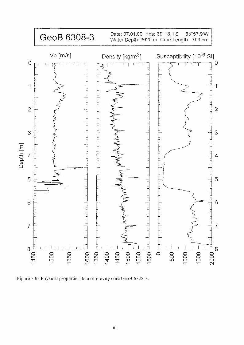
GeoB 6308-3 Date: 07.01.00 Pos: 39°18,1'8 53°57,9'WWater Depth: 3620 m Care Length: 793 cm

2

1

6

Susceptibility [10-6 SI],--,-.-;cr----,--,----,--,------,---,O

Density [kg/m 3]Vp [m/s]

4:7

80 0 0 0 0 0 0 0 0 0 0 0 0 00 L{) 0 L{) 0 L{) 0 L{) 0 0 0 0 0L{) L{) <.D ('"f) "'" "'" L{) L{) <.D L{) 0 L{) 0~ ~ ~ ~ ~ ~ ~ ~ ~ ~ ~ N

2

7

6

3 3

,..-,

E..c 4 4......Q..(1)

0

55---

Figure 33b Physical properties data of gravity core GeoB 6308-3.

61

8eoB 6309-1 Date: 07.01.00 Pos: 39°10,0'8 54°08,TWWater Depth: 2867 m Care Length: 862 cm

7

8

5

6

4

3

2

Reflectance 550 nm [%]10 15 20

O---+---'--_L..-~--olive gray siliceous muddysand with forams, bioturbated

H2S-smell

755-847 cm olive gray siliceous mudw. black mm-sized burrows

490-495 cm sandy layer, distal turbidite?

105.690 cm olive gray sliciceous mud,bioturbated

0·60 cm

60-75 cm sandy layer, turbidite?

85-105 cm sandy layer, fining upwards 1

Lithology

Lithol. Struct. Color Strat.

,'- S.- --. -'."

,r -', ..... S,-,-

.- V --/

-". (:: .....r __ S

'-' v

,r (;: -,-,-

,r "-'. --/ S'. ..... .".'-'. ,r" ,"".

,,' -,-,' ::> Sv .....

'. ,". --'~ S...... "-'........," ....' '-~

S'" ' ...." v

'. .". --'~

-.... ,'-', .-".S

,." ...... v

,- ...... -'."

.' -.- --, S(. 0::>

.- ...,- v S'. .", .....

-:-

::. 0 ()S6 :;0 v -~---- -;-

v' ......,. v

:> --- v

S,-- .,-o.. --,0_ -~- :~:

~ -~-

7 -- v S~ -~

,r .,... ......

~ v v

-", ..... ;:) S::fSf:>-~0

8 - v v S-.... -;-

:>~('J:;f

" v v S

2

3

4

o

..c.......Q.(])

o

Figure 34a Core description of gravity core GeoB 6309-1.

62

GeoB 6309-1 Date: 07.01.00 Pos: 39°10,0'8 54°08,TWWater Depth: 2867 m Core Length: 862 cm

2

3

6

Susceptibility [10-6 SI],--,-,-,---"c-r---,----,,,---r-,----,--,O11 I 11 I 1 I~

Density [kg/m3]Vp [m/s]

2

3

7 7

~- C

8 8

0 0 0 0 0 0 0 0 0 0 0 0 0 0 0 0 0 0L.{) 0 L.{) 0 L.{) 0 L.{) 0 L.{) 0 L.{) 0 0 0 0 0 0

""'"L.{) L.{) CD CD ~

""'"L.{) L.{) CD CD L.{) 0 L.{) 0 L.{) 0

..,- ..,- ..,- ~ ~ ~ ..,- ..,- ..,- ~ ~ ..,- ..,- N N (")

6

.........

..s4 4

..c......Q.(1)

0

5 - 5

Figure 34b Physica1 properties data of gravity core GeoB 6309-1.

63

GeoB 6311-1 Date: 08.01.00 Pos: 38°48,9'8 54°37,6'WWater Depth: 996 m Core Length: 466 cm

Lithology

1 -;,.::c= sI*- ~- -

s,.......,E 2 s

L.-.I

..c-I-' ., .)

0- SQ) Co ,)

0 Co 0.- -::- -......

3···· .::. ':. S

-I*- ~- ~ S,. '::'

,. '"r.- "'0 ->S4 -,-

,. "-,- -<-~ ,.

olive gray siliceous muddysand, bioturbated

15-180 cm olive gray muddy sand,bioturbated

180-190 cm sandy layer

190-453 cm olive gray muddy sand,bioturbated

Reflectance 550 nm [%>]10 15 20

O-+----'--::,---L-----'------'

1

2

3

4

5

Figure 35a Core description of gravity core GeoB 6311-1.

64

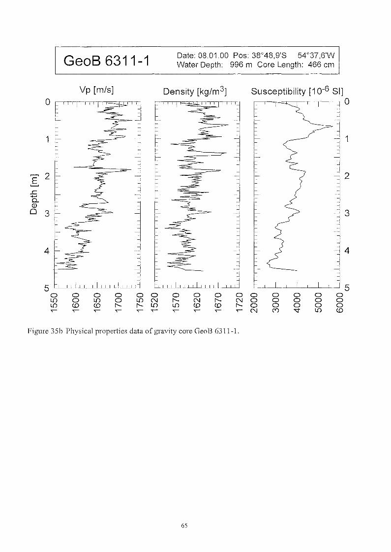
GeoB 6311-1 Date: 08.01.00 Pos: 38°48,9'8 54°37,6'WWater Depth: 996 m Care Length: 466 cm

,-,2E

..c+-'0...Q)

o 3

4

Vp [m/s] Density [kg/m3] Susceptibility [10-6 SI],-,.......--~:-r--,-------,---.,--,---,O

1

2

3

4

5 50 0 0 0 0 0 0 0 0 0 0 0 0 0 0L.O 0 L.O 0 L.O N I'-- N I'-- N 0 0 0 0 0L.O <.0 <.0 I'-- I'-- L.O L.O <.0 <.0 I'-- 0 0 0 0 0~ ~ ~ ~ ~ ~ ~ ~ ~ ~ N (Y)

"""L.O <.0

Figure 35b Physical properties data of gravity core GeoB 6311-1.

6S

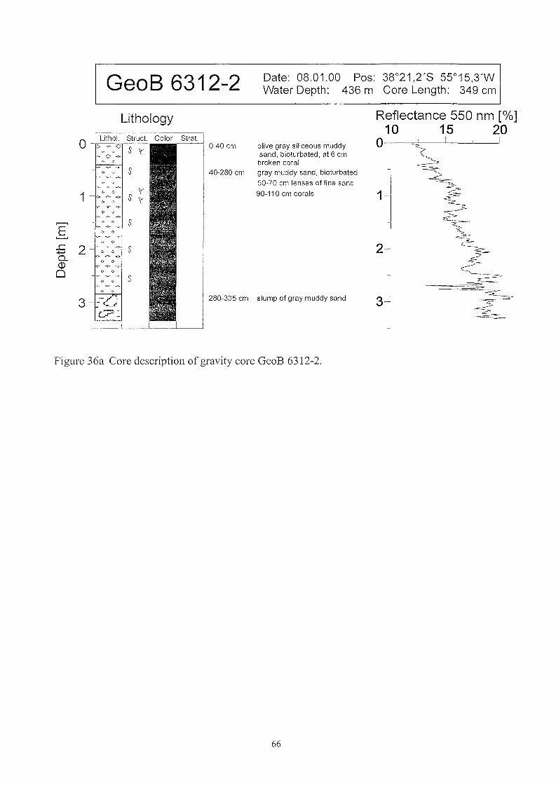
8eoB 6312-2 Date: 08.01.00 Pos: 38°21,2'S 55°15,3'WWater Depth: 436 m Care Length: 349 cm

s

2 .- ,- ,. -~- .:. -~ S:....=- ..:-

2

1

Reflectance 550 nm [%]10 15 20

O-+-~==--'-----'----'

;~~:fi:=~~~

~~~-

3

olive gray siliceous mUddysand, bioturbated, at 6 cmbroken coralgray muddy sand, bioturbated

50-70 cm lenses offine sand

90-110 cm corals

40-280 cm

0-40 cm

280-335 cm slump of gray muddy sand

'(s '(

s

s

Lithology

.;. ,;.

,~. ':'1 -- '..,. -,.(. (I

3 .:-~J

C?"--_I__--'--_-'-_--"-_----"

..c.......0...(J)

o

Figure 36a Core description of gravity core GeoB 6312-2.

66

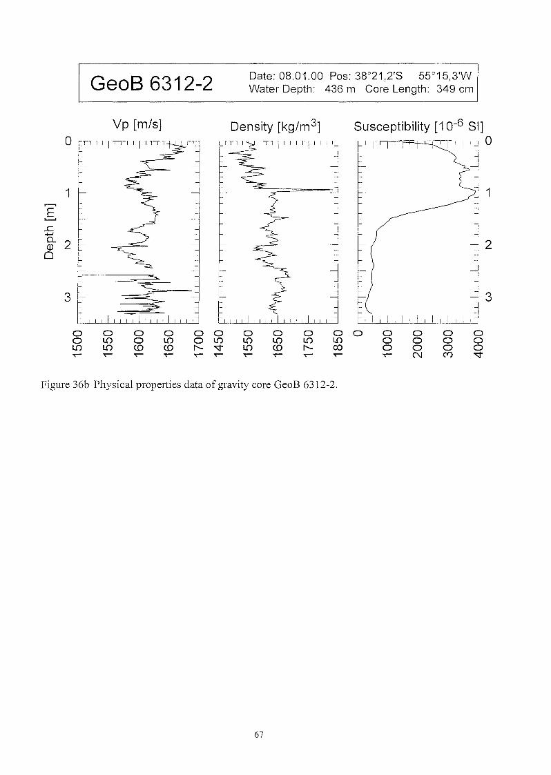
GeoB 6312-2 Date: 08.01.00 Pas: 38°21,2'8 55°15,3'WWater Depth: 436 m Care Length: 349 cm

Vp [m/s]

1

3

2

ooo-.:::t

ooo("t')

oooN

Susceptibility [10-6 SI]o

o 0 0L[) 0co 0...- ---

oL[)<0

---

Density [kg/m3]

o 0 0o L[) L[)I'- -.:::t L[)

--- --- ---

o 0o L[)<0 <0

--- ---

oL[)L[)

---

ooL[)

---

o

1

3

...c.......g- 2o

Figure 36b Physica1 propeliies data of gravity core GeoB 6312-2.

67

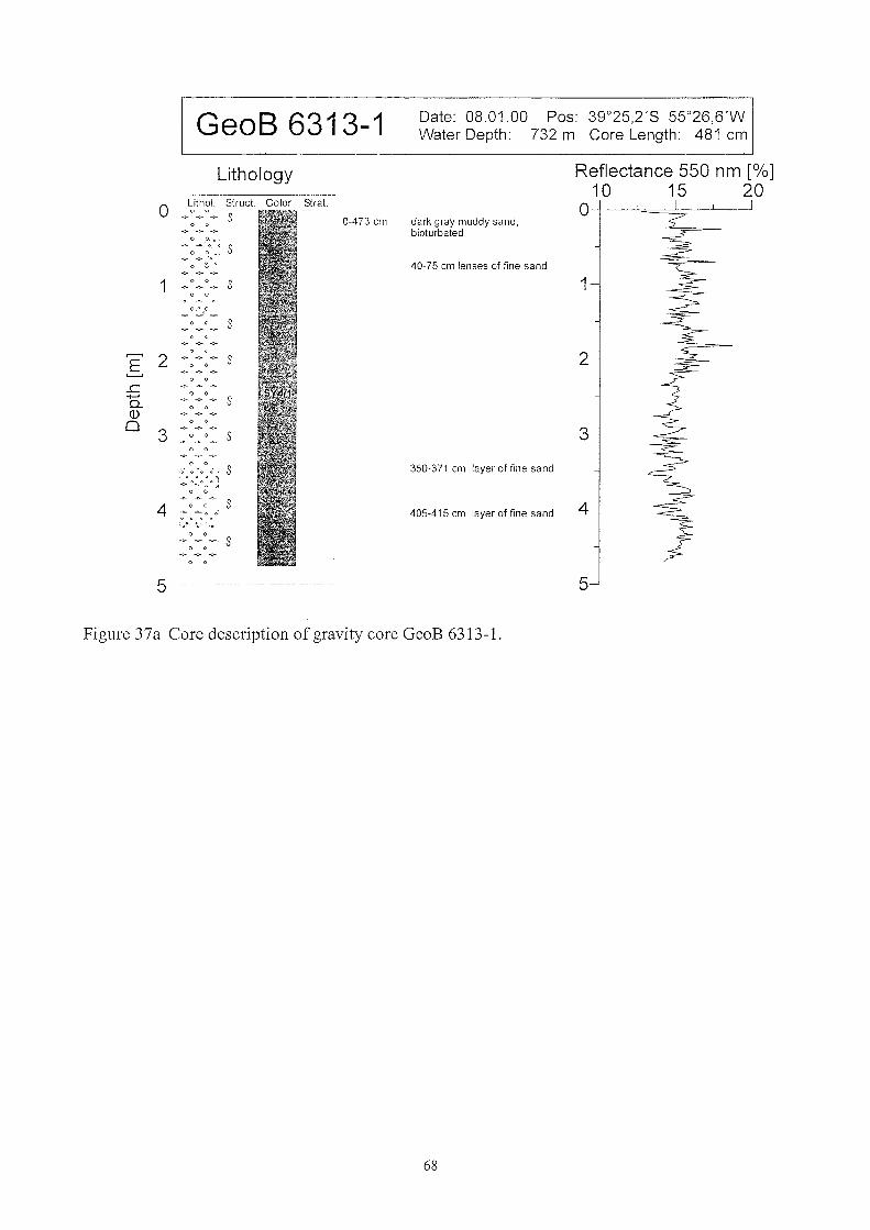
40-75 cm lenses of fine sand

4

Date: 08.01.00 Pos: 39°25,2'8 55°26,6'WWater Depth: 732 m Core Length: 481 cm

2

1

3

Reflectance 550 nm [%]10 15 20

O---t---,==,L--L.---Jdark gray muddy sand,bioturbated

350-371 cm layer of fine sand

405-415 cm layer of fine sand

s

Q Q Q 0,

-::- "~. <> " <> 0:Q "

GeoB 6313-1

Lithology--------------~-----

0Lithol. Strucl. Color Stral.

y y

S~ ~-.....0-473 cm

" "" .C>·o

->o-==-oC>~~ S_;_ ....-...·0

Q ~ 0

1 sQ" .,

-:.- -'" ->

S

,.......,2 sE

'--'

.r:...... S0...Q)

03 s

5 --------- ------------.------- 5

Figure 37a Core description ofgravity core GeoB 6313-1.

68

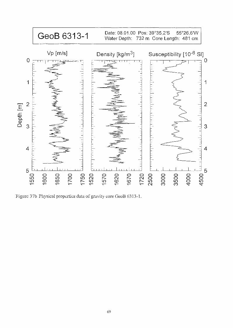
GeoB 6313-1 Date: 08.01.00 Pos: 39°35,2'8 55°26,6'WWater Depth: 732 m Core Length: 481 cm

2

4

3

Susceptibility [10-6 SI]

I 'lO1

Density [kg/m3]Vp [m/s]

4

o

1

..c+-'0...Q)

o 3

5 50 0 0 0 0 0 0 0 0 0 0 0 0 0 0L[) 0 L[) 0 L[) N l"- N l"- N 0 0 0 0 0L[) <0 <0 I"- I"- L[) L[) <0 <0 I"- L[) 0 L[) 0 L[)~ ~ ~ ~ ~ ~ ~ ~ ~ ~ N C'0 C'0

""'" ""'"Figure 37b Physical properties data of gravity core GeoB 6313-1.

69

GeoB 6317-3 Date: 09.01.00 Pos: 40°04,8'8 54°35,TWWater Depth: 3112 m Care Length: 909 cm

Lithology Reflectance 550 nm [%]10 15 20

0Lilhol. Slrucl. Color Slrat. 0-+- + S 0-17 cm olive-gray muddy siliceous-+- +- foram nannofossil ooze

biolurbaledS

17-865 cm dark gray dia10m mud, bio-lurbaled

1 S 1

s

2 s 2

s

3 -~ -:-- S 3

s

4- ...... ,-," ...... s 4-;- -:-',,'" -'0'

,", " 423-427 cm sandy layer

S 439-449 cm sandy layer..........E

'--'

.c',r ,,,.- -..... s 5....... 5-

0..(J)

0 s

6 s 6

614-689 cm 7 gray consolidaledmud horizons

76 716-741 cm 4 dark gray sand/\ layers

- ....- .........../ S

...,.. ...... "V-

B8- -e- -:-

gray muddy siliceous foram+ + 865-875 cm

nannofossil ooze, biolurbaled

9 9

Figure 38a Core description of gravity core GeoB 6317-3.

70

GeoB 6317-3 Date: 09.01.00 Pos: 40°04,8'8 54°35,TWWater Depth: 3112 m Care Length: 909 cm

1

3

4

2

7

5

6

8

Susceptibility [10-6 SI]r-r-,--,,-,--,-,-,-,--,,----r---,--,O

L..-L--L-L-L-L-.L.-JL..-L-..L-L--'--.L~9000000000LO 0000000<.0 LOOLOOLOOLO~ ~~NN(,,)(")

Density [kg/m 3]Vp [m/s]

8

~9

0 0 0 0 0 0 0 0LO LO LO LO LO LO LO LO

""'"LO <.0 I"- co (")

""'"LO

~ ~ ~ ~ ~ ~ ~ ~

3

6

7

...--.4E

.r=.+-'Q..Q)

o 5

Figure 38b Physical properties data of gravity core GeoB 6317-3.

71

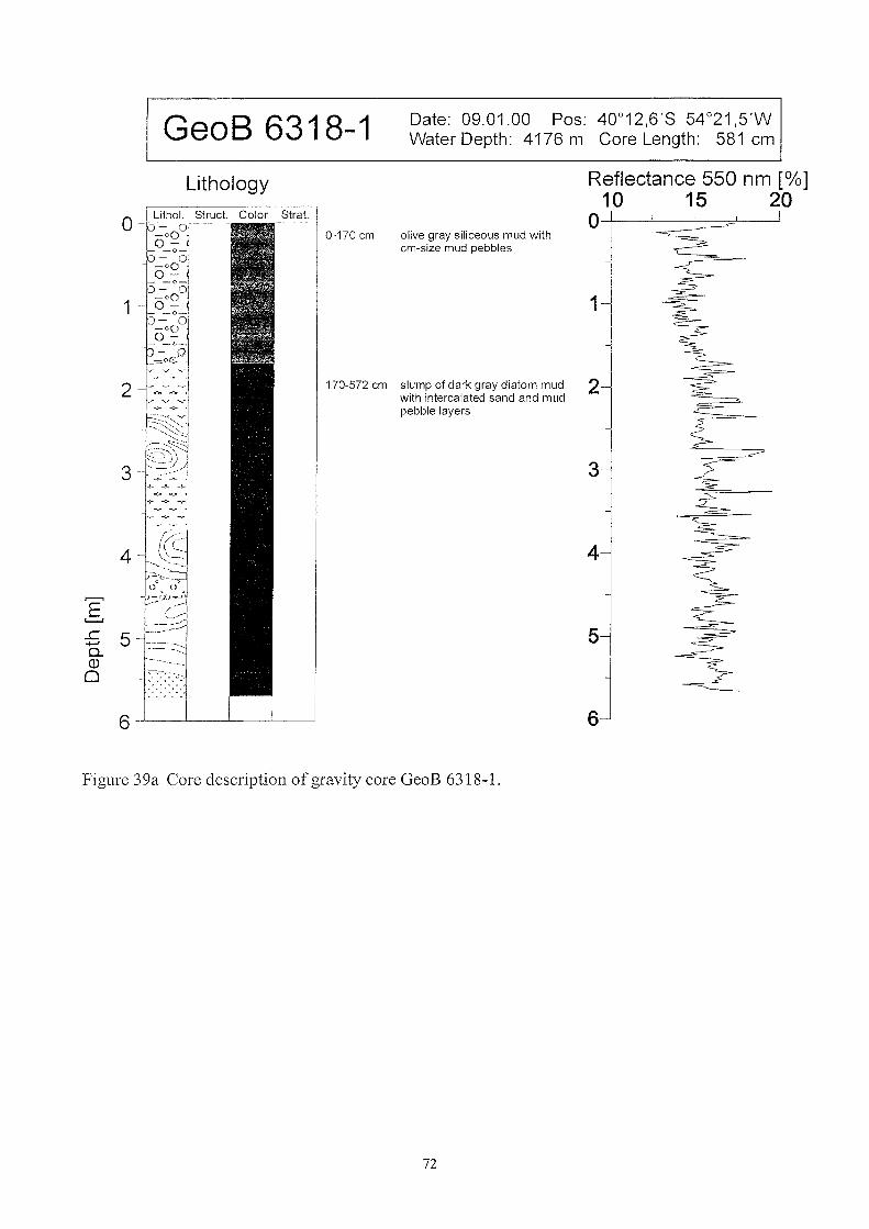
GeoB 6318-1 Date: 09.01.00 Pos: 40°12,6'8 54°21,5'WWater Depth: 4176 m Care Length: 581 cm

..c+-'0..Q)

o

Lithology

2 --l~"-"""'~'~"..'- ".'" -../

f~~~:l.-",:c:..

3~C::~~?~j1-.- -:- .

-!- -~ -~-

-.:- -:- .y ..... -,..

l·,· ~ ~.

Reflectance 550 nm [0/0]10 15 20

O-+---'---..L..---='-----iolive gray siliceous mud withcm-size mud pebbles

1

170-572 cm slump af dark gray diatam mud 2with intercalated sand and mudpebble layers

3

4

5

6

Figure 39a Core description of gravity core GeoB 6318-1.

72

GeoB 6318-1 Date: 09.01.00 Pos: 40°12,6'8 54°21,5'WWater Depth: 4179 m Core Length: 581 cm

Density [kg/m 3]

5

4

2

3

1

Susceptibility [10-6 SI]r-==c-o-~-r----.-"'-----'-.----r-, 0

'------'---'--'----"--'----'--L--L--'-_'---'-~ 6o 0 0 0 0o 0 0 0 0o 0 0 0 0N~ N (\') ""'"

ooco~

oo<.0~

o 0o 0

co ""'"~ ~

Vp [m/s]

oo<.0~

o

1

4

2

6ool{)~

,.......,E

:5 30­<Do

Figure 39b Physical properties data of gravity core GeoB 6318-1.

73

GeoB 6319-1 Date: 10.01.00 Pos: 40°12,4'8 54°21,6'WWater Depth: 4185 m Care Length: 386 cm

3

2

3

1

Reflectance 550 nm [%]10 15 20

O-+---L--'---:=-'-----'

4

olive brown diatom mud,bioturbated

220-245 cm sand layers,irregular formed

olive gray diatom mud,bioturbated

0-10 cm

10-280 cm

280-374 cm dark gray diatom mud withcm-size mud pebbles

s

Lithology

o IL~h~i.- St~uct. Color Strat.

S

S

..c+-'Q.(J)

o

Figure 40a Core description of gravity core GeoB 6319-1.

GeoB 6319-2 Date: 10.01.00 Pos: 40°12,4'8 54°21,TWWater Depth: 4097 m Care Length: 352 cm

Lithology

2

1

3

Reflectance 550 nm [0.10]10 15 20

o--j---'----'--:::::::=:==-----'

olive gray diatom mud,bioturbated, with severalslumping structures orirregular formed sandlayers

olive brown diatom mud,bioturbated

0-5 cm

5-295 cm

295-340 cm dark gray silciceous muddysand with mud pebbles

ss

Lithol. Struct. Color Strat.o

2

t.;::..:::"\/Of-: <

11-~~~ ~

~- -:-.. ..~ ......-;- -;-

--~--"'-"---......,,,, ... "-.--_.:1"__ <-

~ ~

..c+-'Q.(J)

o

E..........

Figure 41 a Core description of gravity core GeoB 6319-2.

74

GeoB 6319-1 Date: 10.01.00 Pos: 40°12,4'8 54°21,6'WWater Depth: 4185 m Core Length: 386 cm

E 20­a>o

3

Vp [m/s] Density [kg/m3] Susceptibility [10-6 SI]~~,---,--;"'''''''--,--,-,--,O

1

2

3

4 40 0 0 0 0 0 0 0 0 0 0 0 0 0t- t- t- t- 0 0 0 0 0 0 0 0 0 0...q- L{) <.0 t- ...q- L{) <.0 t- 0::> L{) L{) L{) L{) L{)"t"""" "t"""" "t"""" "t"""" "t"""" "t"""" "t"""" "t"""" "t"""" "t"""" N C'? ...q-

Figure 4Gb Physical propeliies data of gravity core GeoB 6319-1.

GeoB 6319-2 Date: 10.01.00 Pos: 40°12,4'8 54°21,TWWater Depth: 4097 m Core Length: 352 cm

3

Susceptibility [10-6 SI]r-=r---,-,--,---,--,----,--.----.-,---.,----, 0

Density [kg/m3]Vp [m/s]o

3

1 - - 1.........E'--'

J:::+-J0- 2 2a>0

oL{)L{)"t""""

oL{)<.0"t""""

o 0L{) 0t- ...q-"t"""" "t""""

ooL{)"t""""

oo<.0"t""""

o 0o 0t- 0"t"""" "t""""

oooN

oooC'?

ooo...q-

Figure 41 b Physical properties data of gravity core GeoB 6319-2.

75

Table 9 Sediment constituents according to smear slide investigation.

Abiogenic components Biogenie components Grain size

V1

V1 B "@ xC

V1 l-< V1 'CV1 'ü <l) <l) V1 ~ V1 V1

~B <l) o:J C ;:; l-< •Ci) C 'Cl-<E Oll c;:; 's ~ V1 o:J E

Station ~N o:J

o:J 0 "CI Cl) '2 V1 E 'C .D"CIt 0.. oll >... 0 ,~ c8 <l) .....,

~V1 0 o:J 0 0 0 ~ "CI<l) c Sediment...c: o:J o:J

~'2 C c l-< 's .....,

GeoB ....., ~ "CI t!:: U '2 0 >... 0 ~ 0 ....., o:J o:J Cf) U0.. 0' v o:J o:J 0 l-< 0.- o:J ci5 :.a Cl c Cf)

<l) >.L. ..><: 0 oll V1 0 l-< C o:J 0Cl 0 "0 l-< V1

~0 o:J o:J 0: .D

0 0 <l) >.L. Z p::; l-<p::; > E

() o:J0 U-<

6307-3 1 15 1 5 1 20 2 1 5 1 35 6 8 10 60 30muddy siliceous ooze- - - -

with forams

3 15 5 1 23 2 1 3 1 35 6 8 1 35 60 5muddy siliceous ooze

- - -with forams

50 11 5 2 2 25 3 3 3 35 5 5 1 30 65 5siliceous mud with

- - - -forams

150 15 1 5 1 20 1 1 1 - - - 43 2 10 - 20 50 30 muddy diatom ooze228 10 15 37 17 - 3 15 3 - - - - - - - - 100 - - sand260 10 5 5 3 20 - 2 - - - - - 45 3 10 - 15 55 30 muddy siliceous ooze

350 15 5 6 5 17 - 3 2 - - - - 35 1 10 1 15 50 30 siliceous mud430 15 5 10 5 15 - - - - - - - 30 20 - 15 45 40 siliceous mud

458 10 3 5 5 15 1 3 - - - - - 30 3 25 - 10 40 50 muddy siliceous ooze

550 15 5 10 - 25 5 1 - - - - - 30 3 6 - 5 60 35 siliceous mud

630 10 5 10 4 25 5 3 - - - - - 25 3 10 - 5 65 30 siliceous mud

648 6 6 60 5 5 15 3 - - - - - - - - 100 sand

713 10 2 5 1 30 1 1 - - - - - 40 3 7 - 10 40 50 siliceous mud

850 10 3 7 1 33 2 1 - - - - 35 5 3 - 5 45 50 siliceous mud950 15 1 5 2 30 1 3 - - - - - 37 1 5 - 10 45 45 diatom mud

1050 12 1 5 1 30 1 1 - - - - - 40 5 4 - 10 45 45 diatom mud

6308-3 1 5 3 5 2 30 3 2 5 5 25 3 10 2 5 60 35muddy diatom ooze- - -

with forams

45 10 2 3 1 20 1 10 10 30 5 5 3 5 65 30muddy diatom ooze- - - -

with forams

120 15 3 10 2 25 2 - - - - - - 40 5 5 3 15 55 30 muddy diatom ooze

170 15 2 10 2 20 1 2 - - - - 35 5 8 2 10 60 30 muddy diatom ooze270 10 3 35 - - - - - - - 40 1 10 5 50 45 muddy diatom ooze

370 10 2 3 1 30 - - 1 - - - - 40 5 7 1 10 50 40 muddy diatom ooze

470 15 2 3 2 30 1 1 5 25 5 10 1 15 50 35diatom mud with

- - - -pyrite

570 10 1 3 1 40 1 1 3 30 10 5 50 45Diatom mud with

- - - - - -pyrite

660 10 3 5 3 35 1 3 28 3 8 1 10 50 40Diatom mud with- - - - -

pyrite

760 15 3 8 2 30 1 1 1 30 10 10 55 35Diatom mud with

- - - - - -pyrite

6309-1 1 10 5 25 5 15 2 5 - - - 8 7 8 5 5 2 50 35 15siliceous muddysand with forams

72 12 12 20 12 10 5 12 5 - - 2 2 3 3 1 1 70 20 10siliceous muddysand with forams

140 10 5 10 5 20 5 5 3 - - - - 17 8 12 - 40 35 25 siliceous mud210 10 10 25 10 10 5 5 5 - - - - 10 5 5 - 70 20 10 siliceous mud255 17 8 20 5 15 5 5 - - - - - 15 5 5 - 50 30 20 siliceous mud310 20 5 18 5 16 5 5 1 - - - - 15 5 5 - 40 40 20 siliceous mud410 15 5 10 2 25 2 1 - - - - 20 5 10 - 30 40 30 siliceous mud

76

Table 9 continued

Abiogenic components Biogenie components Grain size

Vl

lfJ <l.l Cd X+-' lfJ +-' .... lfJ °CC Vl 'ü <l.l <l.l Vl ."2 lfJ lfJ "'iij6 e<J .... C<l.l Cd C ;; <2 0u) °C....Ei bll °8

lfJ e<J 6Station 2- N e<J

e<J U "Cl .~ '2 lfJ 6 °C .Dt 0< öll >. u 0 oS e<J <l.l <l.l

"Cl .=:: ~e<J lfJ e<J U e<J °2u

C .... '8 0 "Cl +-' c SedimentGeoB ..c "Cl~ 0 '2 c 0 +-' "0 e<J i:/3 0;:l J:: >. e<J ...., e<JQ.. CI Q) e<J e<J 0 0 0... e<J C

i5 ;a c c (/)

~.... cCl) {.I.; ~ öll Vl U .... e<J 0

Ci u .... Vl

~0 e<J e<J 0:: .D

00

0 <l.l {.I.; Z ~ ....~ > E u e<J

U ()-<6309-1 501 16 5 30 5 16 2 2 4 - - 1 .. 10 3 6 - 20 60 20 siliceous mud

520 10 3 25 3 17 1 1 .. - - - .. 15 5 20 .. 25 55 20 si1iceous mud610 15 5 30 5 20 .. 2 .. - - - - 15 3 5 .. 15 60 25 siliceous mud710 10 5 30 5 20 1 1 - - - .. - 15 3 10 - 10 65 25 siliceous mud810 15 5 30 5 18 2 1 - - - '. - 12 3 10 .. 5 70 25 siliceous mud

6311-1 1 5 10 31 10 10 3 10 5 1 1 7 1 5 1 60 30 10siliceous muddy

- -sand

63 15 10 35 10 10 3 15 - - - - .. 1 .. 1 - 65 20 15 muddy sand150 15 10 35 10 10 5 10 5 .. .. - - - .. 1 - 65 20 15 muddy sand202 20 10 30 10 15 3 8 4 - - - - .. .. 1 - 60 20 20 muddy sand310 22 10 35 10 15 3 .. 5 - - - .. 1 - 1 .. 60 20 20 muddy sand410 25 7 35 10 15 3 - 5 .. .. .. - - - 1 .. 60 20 20 muddy sand

6312-2 1 5 3 40 5 15 5 - 5 - - - - 10 1 10 1 30 55 15 siliceous muddysand

40 10 5 SO 10 10 10 .. 1 - - - - - - 4 - 60 30 10 muddy sand73 15 10 50 5 5 10 - 3 - - - - 1 - 2 - 60 30 10 muddy sand130 16 10 50 5 5 10 - 3 - - - - - - 1 - 60 30 10 muddy sand

190 15 5 40 10 5 10 - 5 - 10 - - - - - - 60 30 10 muddy sand withpyrite

230 25 5 35 10 5 15 - 5 - .. .. - .. - - - 60 30 10 muddy sand270 20 5 40 10 10 10 - 5 - - - - .. - - .. 60 30 10 muddy sand310 25 5 10 10 10 35 - 5 - - - - - - - .. 60 30 10 muddy sand

6313-1 1 15 1 45 30 3 2 - 1 - - - - 1 - 1 1 70 25 5 muddy sand20 20 2 50 20 5 2 - 1 - - - .. - - - - 70 25 5 muddy sand50 20 5 50 20 3 1 - - - 1 - - - - - - 70 25 5 muddy sand140 20 5 50 20 3 1 - 1 - - - - - - - - 70 25 5 muddy sand240 10 5 50 10 3 17 - 5 - - - - - - .. - 70 25 5 muddy sand320 15 7 50 10 5 8 - 5 - - - - .. - - - 70 25 5 muddy sand410 15 5 50 10 5 7 - 8 - - - - - .. - - 70 25 5 muddy sand420 10 3 55 15 5 5 - 7 - - - - - - - - 75 20 5 muddy sand

6317-3 1 15 1 1 1 10 1 - - - - 15 20 25 5 5 1 15 45 40 muddy siliceousforam nanno ooze

40 15 1 30 2 20 1 - - - - - - 15 2 10 - 45 25 30 siliceous mud160 20 3 20 5 20 3 - 1 - - - - 20 2 5 1 30 40 30 diatom mud

260 27 3 15 3 15 2 2 10 15 3 5 20 60 20 diatom mud with- - - - - Mn nodules

336 25 3 30 15 10 2 - 5 3 - - - 5 - 3 - 65 25 10 siliceous mud470 20 1 30 5 15 5 - 1 - - .. - 15 3 5 - 30 50 20 diatom mud570 25 3 25 5 10 2 - 5 - - - - 15 3 7 - 30 50 20 diatom mud640 25 5 20 3 10 2 .. 1 2 - - - 20 2 10 - 30 55 15 diatom mud645 35 3 35 2 10 2 - 3 - - - - 5 - 5 - 10 80 10 siliceous mud733 15 10 40 25 5 - 5 - - - - - - - - 100 - - sand790 15 3 20 3 15 1 .. - - - - 20 3 20 .. 15 65 20 siliceous mud832 15 2 15 2 10 2 - 1 - - - - 35 8 10 .. 20 60 20 diatom mud847 20 5 40 15 5 5 - 1 - - - - 3 3 3 - 80 15 5 muddy sand

870 10 2 5 5 3 2 - 2 - - 25 35 5 2 3 1 25 35 40 muddy siliceousforam nanno ooze

77

Table 9 continued

Abiogenic components Biogenie components Grain size

VJ

VJ .~ Ci3 x..... VJ '- VJ VJ 'C~ I:: VJ u <l) <l) ~

VJ VJ -;;;<l) (Ij I:: '- I:: 'cE '- öD Ci3 ;:; <B VJ VJN (Ij E 's VJ E

(Ij..D E

Station ~ (Ij u "d <l) '8 'Ct 0- bI) ~..... <8 <l) "d

~VJ ,S: ,S: u 0 'C 0 (Ij "d <l) I:: ~ Sediment(Ij (Ij C I:: 's -;;;GeoB ..c: ;:l "d cl:: ~ 0 I:: '8 >-. 0 -;;; "0 ..... (Ij fJ) 0l5.. v (Ij 0 0 I:: I:: I:: fJ)0' ..::: (Ij '- 0... (Ij

8 i5 ~<l) C"-< ~ bI) VJ U '- (Ij 0Cl u 0 '- VJ

~0 (Ij ö: ..D

0 0 <l) C"-< Z ~ '-~ > E u (Ij

u U<

6318-1 1 15 1 10 2 20 2 2 1 25 10 10 2 30 40 30 siliceous mud with- - - - forams

14 10 3 30 10 10 2 - 5 - - - - 15 3 10 2 60 30 10 siliceous muddysand

25 15 1 10 5 20 1 - - - - - - 30 8 10 - 20 50 30 diatommud175 10 1 10 3 25 1 - - - - - - 35 5 10 - 20 50 30 diatommud

6319-1 1 25 1 5 3 20 1 - - - - - - 30 3 10 - 35 40 25 diatom mud20 8 2 5 3 15 2 - 2 - - - - 40 3 20 - 15 60 25 muddy diatom ooze

202 25 1 5 5 20 1 - - - - - - 30 3 10 - 10 60 30 diatommud297 20 1 20 10 10 1 - 1 - - 1 - 25 2 10 - 40 40 20 diatommud

6319-2 1 15 1 5 3 30 1 - 1 - - - - 30 2 10 1 20 45 35 diatom mud20 15 1 7 3 25 1 - - - - - - 35 3 10 - 20 50 30 diatom mud

88 15 1 40 10 10 2 - - - - - - 10 2 10 - 60 30 10siliceous muddy

sand105 15 1 10 5 20 1 - - 5 - - - 30 3 10 - 10 65 25 diatom mud300 15 1 10 5 20 1 - - - - - - 35 3 10 - 10 65 25 diatom mud

305 15 1 35 15 10 2 - - - - - - 10 2 10 - 60 25 15siliceous muddy

sand

Argentine Basin Sediment Waves (core transect GeoB 6321-1 through 6329-1)

Large areas around the Zapiola Drift in the deep Argentine Basin are characterized by strongbottom CUlTents and active sediment transport. The erosiona1 and depositional processes of theseCUlTents have shaped the sediment surface and created CUlTent controlled deposits. The mostapparent features are mud waves with 3 to 7 km wave length and up to 70 m high.

Three different areas on the western Zapiola Drift were investigated by seismic surveys(Fig. 8). Significant features in each of these areas were samp1ed using gravity cores. Altogether10 gravity cores were retrieved ranging ftom 4.41 to 14.16 m in 1ength. At four sites two coreswere taken in different settings of the same feature to cover sediments of different age and/or ofdifferent sedimentation rate (according to the Parasound record).

The first of these four pairs (GeoB 6321-2 and GeoB 6322-2) sampIes a wedge-shaped sedi­ment unit near the crest ofthe Zapio1a Drift in 5050 m water depth. No mud waves are present atthis site. Towards the NNW the sediment surface is characterized by erosion. As revealed by thereflectors in the Parasound record (Fig. 42), sedimentation rates rapidly increase within about6 km toward the crest area ofthe Zapio1a Drift. Core GeoB 6321-2 was taken in a 10w sedimen­tation rate setting, whereas GeoB 6322-2 represents high sedimentation rate deposits.

Fmiher south, on the southern flank of the Zapiola Drift in 5500 m water depth a mud wavewas samp1ed by GeoB 6323-2 and GeoB 6224-2 (Fig. 43). The setting consists of several mudwaves that accumulate on their steeper northern flank, whereas the southern side is characterizedby non-deposition. This causes a northward migration of the waves, ovelTiding the deepest part

78

Table 10 Sediment constituents according to smear slide investigation.

Abiogenic components Biogenie components Grain size

t/l

t/l i!.l (;j :x:+-' t/l +-' .... t/l 'CC t/l 'ü i!.l i!.l t/l ~ t/l t/l t;j8' ro .... ci!.l (;j ,8 ;:; ~ 'U; 'C....6 ön t/l ro S

Station ~N ro ro ü S '"0 i!.l 'a t/l S 'C ..Ci

'"0t 0. bn >. ü ,'.::: ..s i!.l .=: ~t/l Ü ro ü 0 0 ~ '"0 i!.l C SedimentGeoB ..s:::: ro '"0 ro

~ 0 'a 'a c c .... 'S 0 t;j t;j ro ;;:; 0P.. ;:lQ) <t:: ro 0 >. c 0 +-' c VJ0' ü ro 0 .... 0- ro c a ;.a §i!.l ~ .oe: bn t/l ü .... 0

Ci ü '0 .... t/l

~0 ro ro ö::: ..Ci

0 0 i!.l~ Z ty; ....

ty; > c ü ro.- ü U<

6321-2 3 15 - - 1 75 - - - - - - - 5 1 2 1 2 15 83 c1ay50 10 - - - 73 - - 1 - - - - 10 3 3 - 2 18 80 diatom bearing c1ay114 10 - - - 62 - - 1 - - - - 20 3 3 - 2 30 68 diatom bearing c1ay210 7 - - - 80 - - - 1 - - - 10 1 1 - 2 18 80 diatom-bearing c1ay273 10 - - - 47 - - - 1 - - - 30 2 10 - 3 37 60 diatom mud290 2 - - - 66 - - - - - - - 25 2 5 - 2 28 70 diatom c1ay380 10 - - - 67 - - - - - - - 15 3 5 - 2 28 70 diatom-bearing c1ay490 10 - - - 67 - - - - - - - 15 3 5 - 2 28 70 diatom-bearing c1ay585 15 - - 1 57 - - 1 - - - - 20 3 3 - 5 30 65 diatom-bearing c1ay730 10 - - - 69 - - - - - - - 15 2 3 1 2 28 70 diatom-bearing c1ay770 10 - - - 67 - - - - - - - 15 3 5 - 2 28 70 diatom-bearing c1ay

880 10 - - - 38 - - - - - - 30 15 1 5 1 4 28 68 diatom bearingnannfossilmud

985 12 - - - 60 1 - - - - - 5 15 2 4 1 4 26 70 diatom-bearing c1ay

6322-2 1 20 - - - 45 - - - - - - - 30 1 2 2 2 23 75 diatom c1ay20 22 - - - 45 1 - 1 - - - - 25 3 2 1 2 25 73 diatom c1ay187 15 - - - 55 1 - 1 1 - - - 20 1 5 1 2 18 80 diatom c1ay239 20 - - - 54 1 - - 1 - - - 20 1 2 1 2 20 78 diatom c1ay360 20 - - - 53 1 - - 1 - - - 20 2 3 - 2 20 78 diatom c1ay460 20 - - - 47 1 - - 1 - - - 25 1 5 - 2 28 70 diatom c1ay472 20 - - - 43 1 - - 1 - - - 25 1 8 1 2 28 70 diatom c1ay560 15 - 1 - 42 1 - - - - - - 30 5 5 1 3 30 67 diatom c1ay763 20 - - 1 54 - - - 1 - - - 20 1 2 1 2 28 70 diatom c1ay969 20 - - - 53 2 - - 1 - - - 20 2 1 1 2 28 70 diatom c1ay1150 15 - - - 48 1 - - 1 - - - 30 1 3 1 1 29 70 diatom c1ay1190 15 - - - 47 1 - - 1 - - .. 30 2 2 2 1 29 70 diatom c1ay1330 15 - - - 50 - - - - - - - 30 1 3 1 2 28 70 diatom c1ay

6323-2 270 20 - - - 46 - - 1 - - - - 30 1 1 1 3 27 70 diatom mud282 15 - - - 49 - - - 1 - - - 30 1 3 1 2 28 70 diatom mud309 15 - - - 55 - - - 1 - - - 25 1 2 1 2 28 70 diatom mud340 15 - - - 70 - - 1 - - - - 10 1 2 1 3 22 75 diatom mud510 15 - - - 70 - - 1 - - - - 10 1 2 1 3 22 75 diatommud610 15 - - - 61 3 - - - - - - 15 2 3 1 2 28 70 diatom mud716 15 - - - 61 3 - - 2 - - - 15 2 3 1 2 28 70 diatom mud812 15 - - - 58 1 - 1 - - - - 20 1 3 1 2 28 70 diatom mud910 20 - - - 36 1 - 1 - - - - 35 1 5 1 3 47 50 diatom mud1010 15 - - - 53 1 - - 10 - - - 15 1 5 - 3 37 60 diatom mud1102 5 - - - 15 65 - 1 - - - - 10 1 3 - 30 50 20 sandy silt Cash 1ayer)1104 3 - - - - 94 - 1 - - - - 1 - 1 - 70 25 5 si1ty sand Cash 1ayer)

6324-1 5 20 - - - 36 5 - 1 - - - - 30 3 5 - 10 45 45 diatom mud29 10 - - - 75 1 - 1 - - - - 10 1 2 - 2 18 80 diatom c1ay30 10 - - - 75 1 - 1 - - - - 10 1 2 - 2 18 80 diatom c1ay100 25 - - - 50 4 - 1 1 - - - 15 1 3 - 15 30 55 diatom mud138 10 - - - 89 1 - - - - - - - - - - 10 90 si1ty c1ay180 10 - - - 68 1 - 1 - - - - 8 29 10 1 1 29 70 si1iceous mud230 15 - - - 60 1 - 1 1 - - - 10 2 10 - 3 32 65 diatommud320 15 - - - 42 - - 1 1 - - - 25 1 15 - 3 37 60 diatommud

79

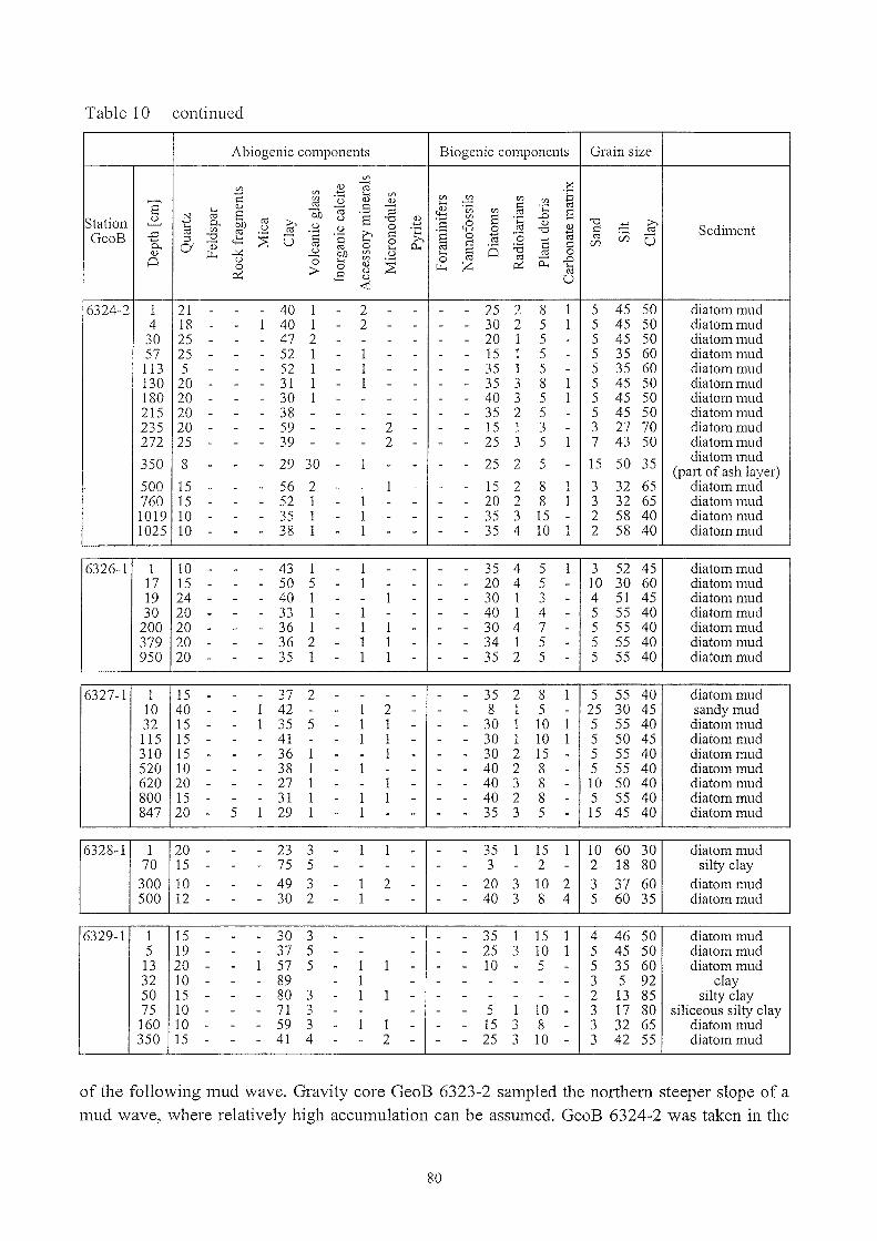
Table 10 continued

Abiogenic components Biogenie components Grain size

V>

V> 2:l (;j ~+-' V> l-< V> 'Cc V> 'ü <I) <I) V> ::2 V>

,~ tjE <I) ro (;j .5 "5l-<

'Ci) Cl-<

Ei b1J ~ V> ro l-< EiStation ~

N ro ro <.) Ei "0 2 'SV> Ei 'C .D

'"Cl1::: Cl.. cf) >. <.) 0 <8 <I)<I) .:::: i2V> ,~ ro ,~ 'C 0 ro '"Cl c Sediment

GeoB ..c: ro '"Cl ro0 'S C c '8 0 +-' '0 +-' ro V3 0P. ::l <t: ~ c 0 >. ro C

roCI 1) ro ro 0 l-< 0-< ro c

6 :.a c [/)<I) lJ:-. ..::.:: ~ cf) V> <.) l-< C 53 00 <.) 0 l-< V>

~0 CI:l ro .D

0 0 <I) lJ:-. Z P::: 0-< l-<

P::: > ,5<.) ro<.) u«

6324-2 1 21 - - - 40 1 - 2 - - - - 25 2 8 1 5 45 50 diatom mud4 18 - - 1 40 1 - 2 - - - - 30 2 5 1 5 45 50 diatommud30 25 - - - 47 2 - - - - - - 20 1 5 - 5 45 50 diatommud57 25 - - - 52 1 - 1 - - - - 15 1 5 - 5 35 60 diatommud113 5 - - - 52 1 - 1 - - - - 35 1 5 - 5 35 60 diatom mud130 20 - - - 31 1 - 1 - - - - 35 3 8 1 5 45 50 diatommud180 20 - - - 30 1 - - - - - - 40 3 5 1 5 45 50 diatommud215 20 - - - 38 - - - - - - - 35 2 5 - 5 45 50 diatommud235 20 - - - 59 - - - 2 - - - 15 1 3 - 3 27 70 diatom mud272 25 - - - 39 - - - 2 - - - 25 3 5 1 7 43 50 diatommud

350 8 29 30 1 25 2 5 15 50 35 diatommud- - - - - - - - - (pari of ash layer)500 15 - - - 56 2 - - 1 - - - 15 2 8 1 3 32 65 diatommud760 15 - - - 52 1 - 1 - - - - 20 2 8 1 3 32 65 diatommud1019 10 - - - 35 1 - 1 - - - - 35 3 15 - 2 58 40 diatom mud1025 10 - - - 38 1 - 1 - - - - 35 4 10 1 2 58 40 diatom mud

6326-1 1 10 - - - 43 1 - 1 - - - - 35 4 5 1 3 52 45 diatom mud17 15 - - - 50 5 - 1 - - - - 20 4 5 - 10 30 60 diatom mud19 24 - - - 40 1 - - 1 - - - 30 1 3 - 4 51 45 diatom mud30 20 - - - 33 1 - 1 - - - - 40 1 4 - 5 55 40 diatom mud200 20 - - - 36 1 - 1 1 - - - 30 4 7 - 5 55 40 diatom mud379 20 - - - 36 2 - 1 1 - - - 34 1 5 - 5 55 40 diatom mud950 20 - - - 35 1 - 1 1 - - - 35 2 5 - 5 55 40 diatommud

6327-1 1 15 - - - 37 2 - - - - - - 35 2 8 1 5 55 40 diatommud10 40 - - 1 42 - - 1 2 - - - 8 1 5 - 25 30 45 sandy mud32 15 - - 1 35 5 - 1 1 - - - 30 1 10 1 5 55 40 diatom mud115 15 - - - 41 - - 1 1 - - - 30 1 10 1 5 50 45 diatommud310 15 - - - 36 1 - - 1 - - - 30 2 15 - 5 55 40 diatommud520 10 - - - 38 1 - 1 - - - - 40 2 8 - 5 55 40 diatom mud620 20 - - - 27 1 - - 1 - - - 40 3 8 - 10 50 40 diatommud800 15 - - - 31 1 - 1 1 - - - 40 2 8 - 5 55 40 diatommud847 20 - 5 1 29 1 - 1 - - - - 35 3 5 - 15 45 40 diatom mud

6328-1 1 20 - - - 23 3 - 1 1 - - - 35 1 15 1 10 60 30 diatommud70 15 - - - 75 5 - - - - - - 3 - 2 - 2 18 80 silty clay

300 10 - - - 49 3 - 1 2 - - - 20 3 10 2 3 37 60 diatom mud500 12 - - - 30 2 - 1 - - - - 40 3 8 4 5 60 35 diatom mud

6329-1 1 15 - - - 30 3 - - - - - 35 1 15 1 4 46 50 diatommud5 19 - - - 37 5 - - - - - 25 3 10 1 5 45 50 diatom mud13 20 - - 1 57 5 - 1 1 - - - 10 - 5 - 5 35 60 diatom mud32 10 - - - 89 - 1 - - - - - - - 3 5 92 clay50 15 - - - 80 3 - 1 1 - - - - - - - 2 13 85 silty clay75 10 - - - 71 3 - - - - - 5 1 10 - 3 17 80 siliceous silty clay160 10 - - - 59 3 - 1 1 - - - 15 3 8 - 3 32 65 diatommud350 15 - - - 41 4 - - 2 - - - 25 3 10 - 3 42 55 diatom mud

of the following mud wave. Gravity core GeoB 6323-2 sampled the northem steeper slope of amud wave, where relatively high accumulation can be assumed. GeoB 6324-2 was taken in the

80

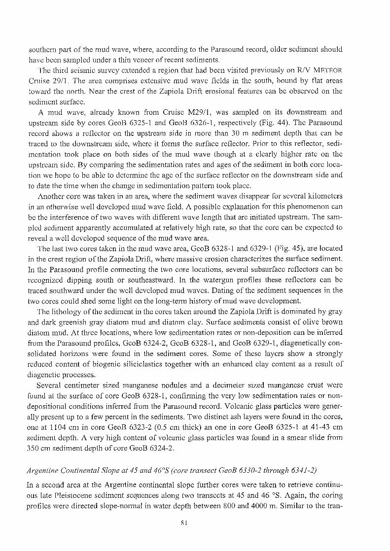
southem part of the mud wave, where, according to the Parasound record, older sediment shouldhave been sampled under a thin veneer of recent sediments.

The third seismic survey extended a region that had been visited previously on RJV METEOR

Cmise 29/1. The area comprises extensive mud wave fields in the south, bound by flat areastoward the north. Near the crest of the Zapiola Drift erosional features can be observed on thesediment surface.

A mud wave, already known from Cmise M29/1, was sampled on its downstream andupstream side by cores GeoB 6325-1 and GeoB 6326-1, respectively (Fig. 44). The Parasoundrecord shows a reflector on the upstream side in more than 30 m sediment depth that can betraced to the downstream side, where it forms the surface reflector. Prior to this reflector, sedi­mentation took place on both sides of the mud wave though at a clearly higher rate on theupstream side. By comparing the sedimentation rates and ages of the sediment in both core loca­tion we hope to be able to determine the age of the surface reflector on the downstream side andto date the time when the change in sedimentation pattem took place.

Another core was taken in an area, where the sediment waves disappeal' for several kilometersin an otherwise well developed mud wave field. A possible explanation for this phenomenon canbe the interference of two waves with different wave length that are initiated upstream. The sam­pled sediment apparently accumulated at relatively high rate, so that the core can be expected toreveal a well developed sequence ofthe mud wave area.

The last two cores taken in the mud wave area, GeoB 6328-1 and 6329-1 (Fig. 45), are locatedin the crest region of the Zapiola Drift, where massive erosion characterizes the surface sediment.In the Parasound profile connecting the two core locations, several subsurface reflectors can berecognized dipping south or southeastward. In the watergun profiles these reflectors can betraced southward under the weIl developed mud waves. Dating of the sediment sequences in thetwo cores could shed some light on the long-term history ofmud wave development.

The lithology ofthe sediment in the cores taken around the Zapiola Drift is dominated by grayand dark greenish gray diatom mud and diatom clay. Surface sediments consist of olive browndiatom mud. At three locations, where low sedimentation rates or non-deposition can be inferredfrom the Parasound profiles, GeoB 6324-2, GeoB 6328-1, and GeoB 6329-1, diagenetically con­solidated horizons were found in the sediment cores. Some of these layers show a stronglyreduced content of biogenie siliciclastics together with an enhanced clay content as a result ofdiagenetic processes.

Several centimetel' sized manganese nodules and a decimeter sized manganese crust werefound at the surface of core GeoB 6328-1, confinning the very low sedimentation rates or non­depositional conditions inferred from the Parasound record. Volcanic glass partic1es were gener­ally present up to a few percent in the sediments. Two distinct ash layers were found in the cores,one at 1104 cm in core GeoB 6323-2 (0.5 cm thick) an one in core GeoB 6325-1 at 41-43 cmsediment depth. A very high content of volcanic glass partic1es was found in a smear slide from350 cm sediment depth of core GeoB 6324-2.

Argentine Continental 8lope at 45 and 46°8 (core transect GeoB 6330-2 through 6341-2)

In a second area at the Argentine continental slope further cores were taken to retrieve continu­ous late Pleistocene sediment sequences along two transects at 45 and 46 oS. Again, the coringprofiles were directed slope-normal in water depth between 800 and 4000 m. Similar to the tran-

81

NNWI " " " " " " " " " " " " " " " " " " " " " " • " " " " " " " • " ~ " " " .. " " " ... " " " " " " " " " "

SSE5000

5050

~r+('D""""l

0('D

"'0r+:::Y

....--..-:3

'---'"

5100

.~ ","'~.". ,,"'.

. ~-

\-.2·Km:;.

"" ,; ..

...... . .. ; ,",

" "" "

.-,

" " ),

" ,," ~.

"",

" ..'"

.' :

."." ....

...... -

" ~A

,"'-"

""'<:'.. : ,"

·Ge0B 632,1·-2·

" " " " " " " " " " " " " " " " " " " " " .. " " " " " "

...... " ..

oo

·:G~p8 6322-2·..... ""

o·..'

1~~

00N

'() ... '('1

, ," -.;-

'''6~ '"

,,''. ~".

.-.;-

'~O'

':::t. ",,, .,,; ...

::"6'" ."UI' .

-". - .V)•...• '.

-"7

'" ....

.... ""

5150

Figure 42 Parasound profile recorded between 43°58.9'8/ 48°18.4'W and 44°07.1'8/ 48°14.3'W along seismic line GeoB 00-002 crossing

locations ofcores GeoB 6321-2 and 6322-2.

"

.. ,",. ,,'

• t .. " I

, .

~ I.' '.:. ~",

','

"

"

."

..~.

ooL()L()

.,~ ,

Water Depth (m)

83

oL()L()L()

.,..

..

• I ~. I; ,

~ ",

"

~~,..... ~ v! '.

oo(()L()

bl)~.-(/)(/)

0HÜ

0.-<0

I00

0:10(l)

0(l)

~.-.-<

Ü.-S(/).-(l)(/)

bl)~0

.-<('j

f$t--I.r).-<000"'1"-.....(/J

0000('f')0I.r)

"'1"'0§f$\0I.r).-<000"'1"-.....(/J

I.r)('-l

~ I

('f') "'1"0 ('-lI.r) ('f')

"'1" \0~ '0(l) §(l)

~ ('-lI(l) ('f')

,.0 ('-l'0 ('f')(l) \0'0

0:1H0 0Ü (l)(l) 0H(l) (/)

.-< (l)t;:::l H0 0H Üp.. 'H

'0 0~ (/)

;::i ~0 0(/) .-('j ....

('j

~ ü

P-. 0.-<

('f')

"'1"(l)H;::ibl).-[.I.,

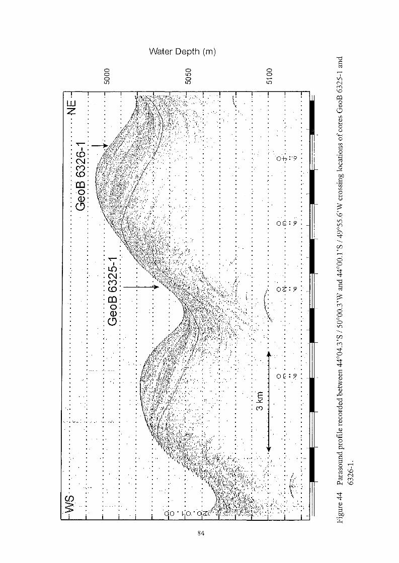
wZ

~

I

<.0NM<.0

··cn0:Q)'(9'

"

'. '. '1I':i.,,,

,.

oooLf)

"

:,,',

.'

Water Depth (m)

oLf)

oLf)

I·

.'

.'

.\'.

84

.. ,

, ,

"

. '"

(\

, .!

O~

Ok

, ,

/',:t(,. \. , .

\

' ... ' .

"

'"d§

,.......I

tr)

N('<")

\0

o:l0Q)

CjVJQ)l-<0()

4-<0VJI=:0...........ro()

..sbJ)I=:.....VJVJ0l-<()

l5:\0tr)tr)00\'<T---..ifJ.,.......

ci00'<T'<T'"d§

l5:<")

0000tr)

---..ifJ.('<")

-.f00'<T'<TI=:Q)Q)

~Q)

,..0

'"dQ)

'"dl-<0()Q)l-<Q)

..-<

t.+::0l-<P-.

'"d§ ,.......0 1VJ \0ro~

N('<")

A-i \0

'<T'<T

Q)

~bJ).....

f.I.<

5300

~.......CD•

52500CD

-0.......:::J

,........3---

'.-" : - ;." .

. ... ' :': . . . "... .: . . ... . . ....,,: ~ . . . ' .. ' ,. ' .. ' . . ....

. " ~ ~... -; "." ..., .. '.- ., ..

. ," : ..

- ~ .. ',- ....•.• ", '." ': .:. •..:.; '" •....• -. - •. ", '; .•• :'~.:: ._.~; -.:: : : >.- •.•.. "":' .'~';' .., .

: ,·".",.-..;,;'i;.~.i······.······ ··,···,··.. ···,······ .

. "; . . -".' . / . ~'. . . . .':. ~." . . . . . . .- , .'; "", . . ~....... -' ~ ," ' .. ' -. . .." ; . ", . . :..:: '.

, .~:. i:".' ~ ; ' .. ' . .: ~ . . . ;'. '. .:.:. . . .. ~ ", .'; .

: ~.'" ,' : • "~' • .;. l -. '. ; • • ", • :' " .. ' ....:. • ". • • ", ," :,,- ",

... , : :.. :?·.~ITl- .. .'" ., -!-.. ,.-. ~:J~;-~ ;. :C': : .J., .. ; ....•.. '" ..

...

I i ' ••••• .' •••••••• NW...' t) Cl

~ •••..•...•••• & ...••••••.•.••~ ••••••••••••••. 8. I.·· •••••••••. !.·.·.· .. ·.·.· ~ ~ i •••• ·•• ·••.•.• i 5200

SE •.•• 8e086329-1·· § ..•••.••••.•.• ~ .•••••.•.•••.....•.~... . ~ GeOEl6328~l' .- .

CXJVl

Figure 45 Parasound profile recorded between 43°37.1'S / 49°46.3'W and 43°42.3'S / 49°37.9'W along seismic line GeoB 00-028 crossing

locations of cores GeoB 6328-1 and 6329-1.

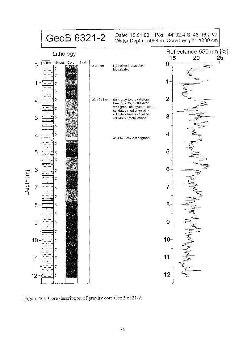
GeoB 6321-2 Date: 15.01.00 Pos: 44°02,4'8 48°16,TWWater Depth: 5098 m Core Length: 1230 cm

5

4

2

3

Reflectance 550 nm [%]15 20 25

O--+---'---L----::O-,-----'light olive brown ciay,bioturbated

410-429 cm lost segment

23-1214 cm dark gray to gray diatom­bearing ciay, bioturbated,with greenish layers of con­solidated mud alternatingwith dark layers of pyrite(or Mn?) precipitations

0-23 cmStrat.

Lithology

4 '----~ S

_0"_- _.~. S

2 ~_-_-~- S

5

o- Lithol. Struct. Color

_v_- S.....- - "..,'-v-- s

1-'- --. S

,........, 6 6E

'---'

...c-+-J

0.. 7- V" _ • ....,..

S 7<J)

0~ - ·v S

8 8- - S

~ - ~ S

9 •..r _ •..,.. S 9

S

10- .~_-_~ S 1-~---~ S

11 - ~_- _~ S 11_.~_-_~ S

12 _-_~ S 12

Figure 46a Core description of gravity care GeoB 6321-2.

86

GeoB 6321-2 Date: 15.01.00 Pos: 44°02,4'8 48°16,TWWater Depth: 5098 m Care Length: 1230 cm

2

1

3

Susceptibility [10-6 SI],---,--..-,---,--,-----,-----,,---,---,-..---r-. 0

Density [kg/m 3]Vp [m/s]

11

12

10

ooCD

oo-.;:t

ooN

o 0LOLO~

o 0 0 0 0(J) 0 ~ NLO-.;:t LO LO LO N~ ~ ~ ~ ~

10

11

12

4 4sediment lost sediment lost sediment lost

-

5- 5

.--.E

..c 6 6......0-(J)

0 7 7

8 ~ 8------~--

~9 _ 9

Figure 46b Physical properties data of gravity core GeoB 6321-2.

87

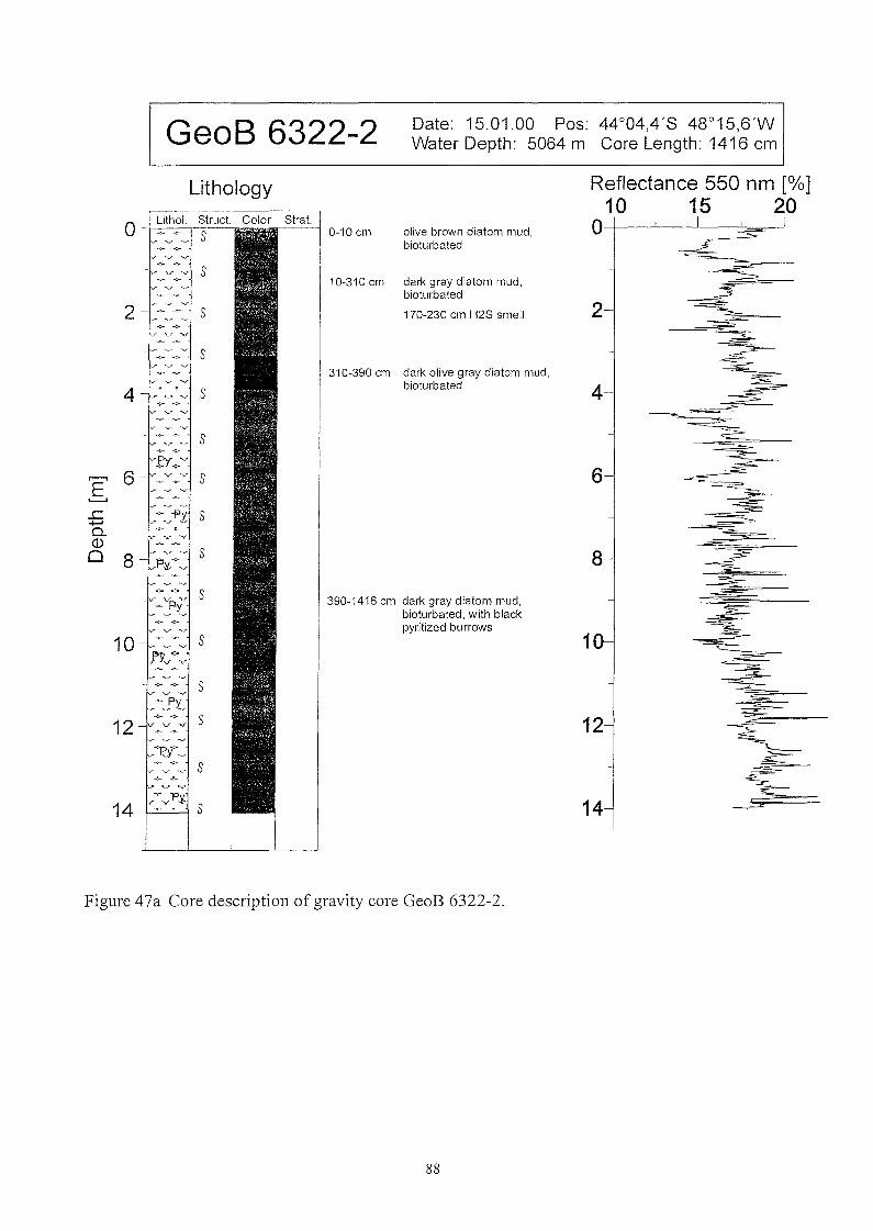
GeoB 6322-2 Date: 15.01.00 Pos: 44°04,4'S 48°15,6'WWater Depth: 5064 m Care Length: 1416 cm

Lithology

390-1416 cm dark gray diatom mud,bioturbated, with blackpyritized burrows

2

4

6

8

Reflectance 550 nm [%]10 15 20

O-+--..L..-----'--=~--'

12

14

1

dark gray diatom mud,bioturbated

170-230 cm H2S smell

olive brown diatom mud,bioturbated

dark olive gray diatom mud,bioturbated

0--10 cm

310-390 cm

I110-310 cm

s

2 - =.~=.,.= s

s

4 - -<-- -:- S'.' ."-". v." -;-

s"'fY~-'''''

,......., 6 --".'" v --.~ sE

'---'

.c -~.,--~-Pt S+-'Q.Q)

S0 8 fly~'v

-:~3{s

10 - ~ -- s.' ~ vf"Y'v

.>",.r

S~~Yx,

-<-- .>. S12 _er v v--~ .~

~...T_.S

14.-<-.•)"~

s-". ~ ~

Figure 47a Core description of gravity care GeoB 6322-2.

88

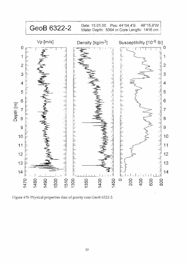
Date: 15.01.00 Pos: 44°04,4'8 48°15,6'WWater Depth: 5064 m Care Length: 1416 cm

000000L() 0 0 0 0..q- N..q- CD co""

7

8

9

10

11

12

13

14

- 2

3

4

5

6

Susceptibility [10-6 SI]I 1 I I I I I 1-=1 0

~~ 1

Density [kg/m 3]

GeoB 6322-2

Vp [m/s]

~r2l3

4

5 -

.--. 6E..c 7.......0..Q) 8 -0

9

10

11

12

13

14

0 0 0 0 0 0I'- co 0> 0 "" 0..q- ..q- ..q- L() L() C'0"" "" "" "" "" ""

Figure 47b Physical properties data of gravity core GeoB 6322-2.

89

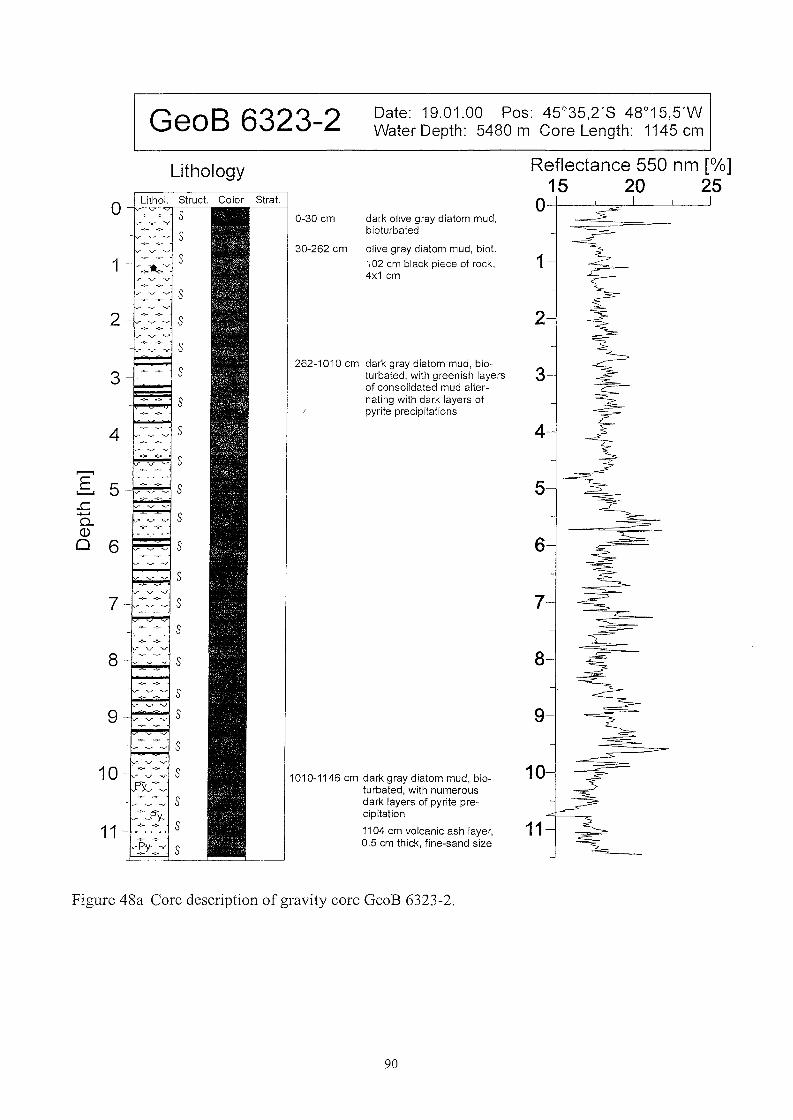
GeoB 6323-2 Date: 19.01.00 Pos: 45°35,2'8 48°15,5'WWater Depth: 5480 m Care Length: 1145 cm

1

2

Reflectance 550 nm [0/0]15 20 25

O--+---'---===-L--------L----'

9

10

11

dark olive gray diatom mud,bioturbated

olive gray diatom mud, bio!.102 cm black piece of rock,4x1 cm

8

30-262 cm

7

6

4

5

0-30 cm

262-1010 cm dark gray diatom mud, bio-turbated. with greenish layers 3of consolidated mud alter-nating with dark layers ofpyrite precipitations

1010-1146 cm dark gray diatom mud, bio­turbated, with numerousdark layers of pyrite pre­cipitation

1104 cm volcanic ash layer,0.5 cm thick, fine-sand size

Lithology

Lithol. Struc!. Color Stra!.

S

S

S

o

1

s2 ~- ~

S.-~ -/

~ -!:!-

S

S

S

S

S..........E

'---'

.c+-' S0...(])

0 6 s

sss

8 - -- S- ~. ~ ~

s9 -- -- S- ," ...,. ..".

~ .~

s10 - 00- _:..

SV" v -..r

,.py''--vS

~~J'1y~

s11~ -~-. .. ....

v'fY':..". S

Figure 48a Core description of gravity core GeoB 6323-2.

90

GeoB 6323-2 Date: 19.01.00 Pos: 45°35,2'8 48°15,5'WWater Depth: 5480 m Care Length: 1145 cm

11

9

4

1

10

2

8

- 3

ooL!)

'""

ooo'""

ooL!)

Susceptibility [10-6 SI],,-,-,--r=---.-r-,-,-..,-,----,--,--,-,O

o 0L!)L!)

'""

o 0L!) 0-.;;t L!)

'"" '""

o 0L!) 0C'0 -.;;t

'"" '""

Density [kg/m 3]

o 0I'- 0L!) C'0

'"" '""

Vp [m/s]o

1

2

3

4

9

8 -

10

11

...--. 5 5E

...c.......0- 6 - 6(J)

0

7 _ 7

Figure 48b Physical properties data of gravity core GeoB 6323-2.

91

8eoB 6324-1 Date: 19.01.00 Pos: 45°38,9'8 48°14,1 'WWater Depth: 5510 m Care Length: 453 cm

1

2

3

4

5

Reflectance 550 nm [0/0]5 10 15 20 25

O-t--...L.--l--::::::!===~'-L----'olive brown diatom mud,bioturbated

0-6 cm

6-132 cm light olive brown diatom mud,bioturbated

13-60 cm several yellowishlayer of diatom clay

132-160 cm grayish green consolidatedsilty ciay

160-200 cm greenish gray diatom mud,bioturbated

200-452 cm dark greenish gray diatommud, bioturbated

Lithology

s

,-------_._._---------,Lithol. Struct. Color Strat.o

s

1ss

s........, 2 -~ v v

E ~ -- S........... ~ v v

...c....... SD..m0 3

.~ v v- ~ -~ S~ v v

s

4 --~ ~- S

v ~

<- <-,r V V

S

5 _.-

Figure 49a Core description of gravity core GeoB 6324-1.

92

GeoB 6324-1 Date: 19.01.00 Pos: 45°38,9'S 48°14,1'WWater Depth: 5510 m Core Length: 453 cm

4

Susceptibility [10-6 SI],,-,,-,-,----,-,----,-,----,-,----,-,----,--,--,0

L-.L-L....l.-L--'--'--'--'--'--'--'--'--'--'------L-J 50000000o 0 0 0 0 0co 0 ~ N C'0 -.;;t~ N

Density [kg/m 3]Vp [m/s]

4

5'--'--'--'--'---'----L-L---l-L--'--l-L-L...l..-J

o 0 0 0000L.() 0 L.() 0000-.;;t L.() L.() <.D N -.;;t <.D~ ~ ~ ~~ ~ ~

1~

1- ~~==--

E 2 r 2

..c+-'0-(1)

0 3 3

Figure 49b Physica1 propeliies data of gravity core GeoB 6324-1.

93

GeoB 6324-2 Date: 19.01.00 Pos: 45°37,1'8 48°15,3'WWater Depth: 5490 m Core Length: 1092 cm

245-1078 cm dark greenish gray diatom mud,bioturbated

6

4

5

3

2

1

Reflectance 550 nm [%]15 20 25

o--r-=::!==:::::::======:---

9

11

10

868 cm concretion

890-1078 cm H2S smell

8

350 cm vulcanic ash layer

7

olive brown diatom mud

dark greenish gray diatom mud,bioturbated, with brown layers

greenish gray semi-consolidateddiatom mud, at top and bottomconcretionsdark greenish gray diatom mud,bioturbated

greenish-gray semi-consolidateddiatom mud w. concretions

55-98 cm

strat.I~ 0-55 cm

Lithology

1 .- SZem. 98-148 cm

S

S148-225 cm

2Zem. 225-245 cm

S

3 s~ -~

...................

S

o- _Li~.~o~~ _~yuc;t:.-'-,..,"'.", S

, ••.•.• "Y S-:- -=.-

4 s~ ..... ,..,

...--. -<- -;- sE'--'

5 -~ -- S..c ./ ..... ........... -~ ....

Q. ~....,. ...,

(])->- .,. S

06 s

-;- --0. S

7 s-~-

.,..

s

8 -~ ~ S- ..... -~

... ....,.'.~

-;- .,.S- V 'V

9 ss

...'" ............10 - s

. v ,~

->- .,. s

11

Figure 50a Core description of gravity core GeoB 6324-2.

94

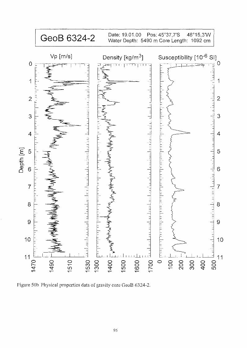
GeoB 6324-2 Date: 19.01.00 Pos: 45°37,7'8 48°15,3'WWater Depth: 5490 m Care Length: 1092 cm

2

3

1

Susceptibility [10-6 SI]r=r-~=+==I=F~-T10I I I I I I I

Density [kg/m3]Vp [m/s]

1~-

2

3

4 4--

,.........,5E 5.........

-..c -.......0-Q) 6

- 60

7 7

9

8

10

11ooL{)

000000o 0 0 0 0I"'- ~ N (V) ~~

ooCD~

ooL{)~

o 0(V) 0L{) (V)~ ~

8 -

9 -

10

~11

0 0 0l"'- m ~

~ ~ L{)~ ~ ~

Figure 50b Physieal properties data of gravity eore GeoB 6324-2.

95

GeoB 6325-1 Date: 20.01.00 Pos: 44°01,9'S 49°57,TWWater Depth: 5353 m Care Length: 441 cm

2

1

Reflectance 550 nm [%]5 10 15 20 25

O-r--'----'-:<::':::=====~--'olive brown diatom mud, soft

olive diatam mud, bioturbated

42 cm vulcanic ash, fine sand

3

4

0-5 cm

5-35 cm

35-436 cm greenish gray diatom mud,bioturbated, with several darklayers of pyrite precipitation

s

s

Lithology

Lithol. Struct. Color Strat.o

s

........, sE........

..c S......0-II0 s

3 ~f'~-~v

S

.' ~~~l.'~ S

4 s-- v ',~

.".-=-y"'P......

S

Figure 51 a Core description of gravity core GeoB 6325-1.

96

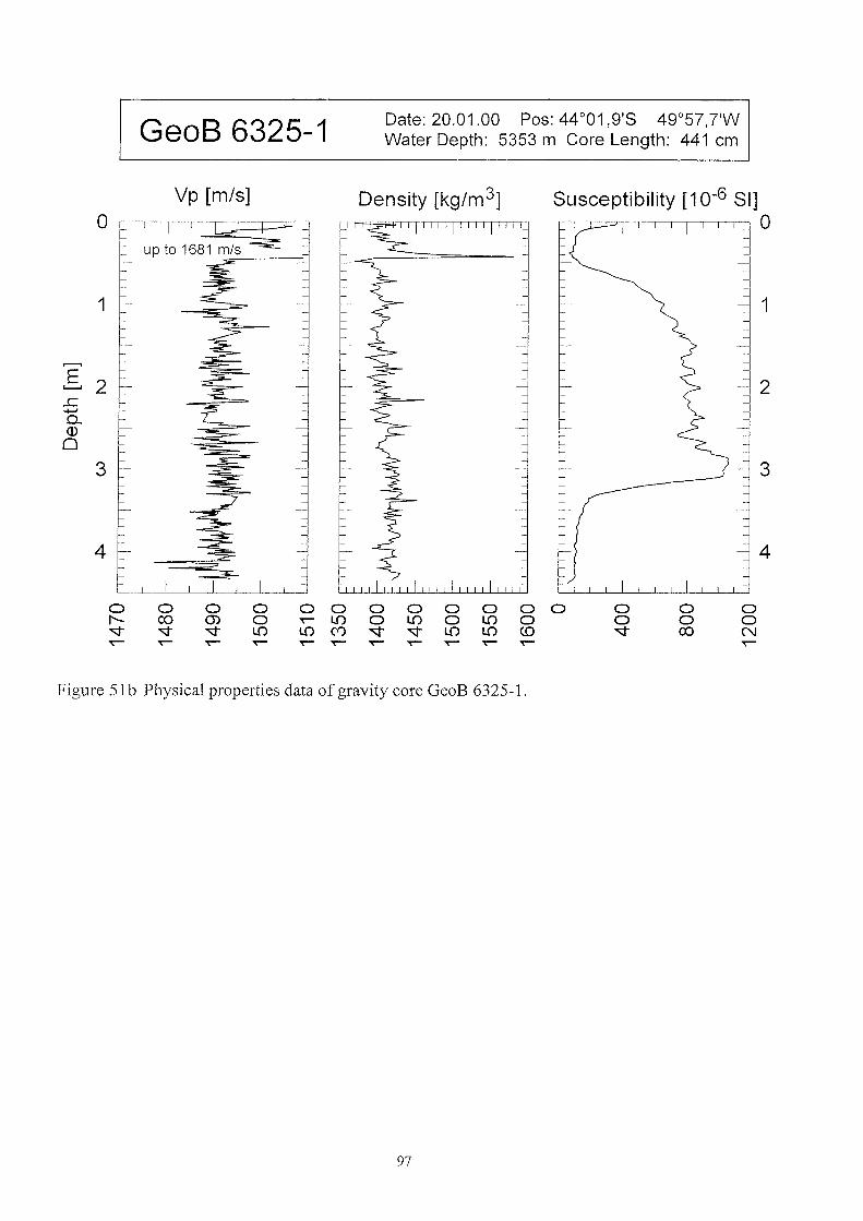
GeoB 6325-1 Date: 20.01.00 Pos: 44°01 ,9'S 49°57,TWWater Depth: 5353 m Care Length: 441 cm

1

4

ooN~

ooco

oo-.;;t

Susceptibility [10-6 SI],..---,,--=.--,-,-----,-,-,-----,-,-,0

000000o L[) 0 L[) 0-.;;t -.;;t L[) L[) <D~ ~ ~ ~ ~

Density [kg/m 3]

ooL[)~

Vp [m/s]o

1

4

...........E 2 2.......... -

..c+J

0..Q)

0

3 3

Figure 51 b Physical properties data of gravity core GeoB 6325-1.

97

GeoB 6326-1 Date: 20.01.00 Pos: 44°QO,6'S 49°56,2'WWater Depth: 5300 m Core Length: 1065 cm

Lithology

37-1047 cm greenish gray diatom mud,bioturbated, with several darklayers of pyrite precipitation

4

1

2

3

6

Reflectance 550 nm [%]10 15 20°l-..L.-~~~

5

7

9

8

11

1

olive brown diatom mud, soft

greenish gray diatom mud,bioturbated

274-325 cm abundant pyritizedburrows

774-805 abundant pyritizedburrows

0-5 cm5-37 cm

Color Strat.o.. ~~~~~~S

S

1 .. s

s

2 ~ ~ s-" v v

". .,.

S~y'~.

v

3 .. s~v-Pv

'". V V s

4 s

s

5~. ~ S... . v v~ ~

v v SV' v ','

....--. 6 ... sE

'---'

.s=. S

....... er V -••r

Q. 7 ~ .~

SQ) -~ V --/

0~ .~

s

8-ry'.,:--'

SV'~v~~'

s

9 er V -••r S

S

10 -- '-' ,~ S.,.. .,.s

11 ..

Figure 52a Core description of gravity core GeoB 6326-1.

98

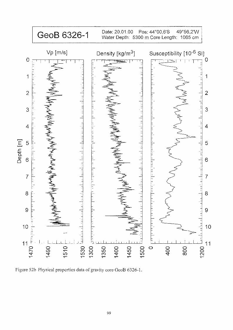
GeoB 6326-1 Date: 20.01.00 Pos: 44°00,6'S 49°56,2'WWater Depth: 5300 m Care Length: 1065 cm

2

1

10

9

11ooN...-

oo00

oo.q-

Susceptibility [10-6 SI],-,----,-,..,.,~,-----,----,---,-----,----,--, 0

o 0oLn

---

Density [kg/m 3]

o 0 0 0 0Cf) 0 Ln 0 LnLn Cf) Cf) .q- .q-...-...- ...- ...- ...-

Vp [m/s]

2

o ~'T'

1 ~

9

10

11o!'­.q-...-

3- 3-

-

4-

4---

..........E 5 5

..c+J

0..(1) 6 60

--

7 7

---

8 - 8

Figure 52b Physical properties data of gravity core GeoB 6326-1.

99

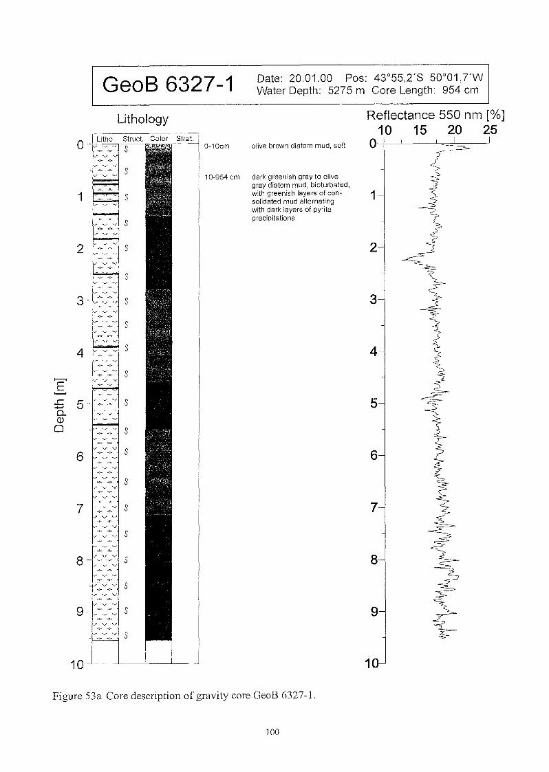
Date: 20.01.00 Pos: 43°55,2'8 50 0 01,TWWater Depth: 5275 m Care Length: 954 cm

olive brown dia10m mud, soft

dark greenish gray 10 olivegray dia10m mud, biolurbaled,wilh greenish layers of con­solidaled mud allernalingwilh dark layers of pyrileprecipilalions

Reflectance 550 nm [%l]10 15 20 25

o-l-------.L----l.--.l--=,L-------l.------l

1

2

3

4

5

6

7

8

9

1

Figure 53a Core description of gravity core GeoB 6327-1.

100

GeoS 6327-1 Date: 20.01.00 Pos: 43°55,2'8 50001,TWWater Depth: 5275 m Core Length: 954 cm

2

3

1

Susceptibility [10-6 SI]r-rT...-r-~-.--r-..-.-r,-,--.-r-T---.--ro 0

Density [kg/m 3]Vp [m/s]

2

3

1

4 - 4

,........,E..c 5 5.......Q.(])

0

6 6

7

8

9

10ooo"t""""

ooco

oo(0

oo~

o 0 0N 0L() N"t""""

7

8

9

10 L--.-L-J--L--'---"---,------'-------'-------'-------J

0000000I'- co m 0 "t"""" NN~ ~ ~ L() L() L() C'0"t"""" "t"""" "t"""" "t"""" "t"""" "t"""" "t""""

Figure 53b Physical propeliies data of gravity core GeoB 6327-1.

101

GeoB 6328-1 Date: 24.01.00 Pos: 43°38,3'8 49°44,2'WWater Depth: 5255 m Gore Length: 566 cm

128-555 cm dark greenish gray diatom mud, 3bioturbated

4

2

1

5

6

Reflectance 550 nm [o,la]5 10 15 20 25

o-t--'--'--==!=;-----J---l.----L--L--lolive brown diatom mud, soft,with cm-sized Mn noduleslight olive brown silty clay,semi-consolidatedlight yellowish brown silty c1ay

light olive brown silty clay,semi-consolidatedlight yellowish brown diatom mud

0-21 cm

21-36 cm

96-128 cm

36-75 cm

75-96 cm

Lithology

Struct. Color Strat.l---;-;-..,.----~

6 --'__-L-_--l--_-"------l

1s

s

2 -- ~- -~

v ~

S0<- .:;.

...--.E s'--'

..c 3 -- '.' v v-l-'0..

~- ~

Q) S

0

s4

- v ~

-- ~ --v ~ S

s5 -

~ -~

.~ v ~

-'- -~- S

Figure 54a Core description of gravity core GeoB 6328-1.

102

GeoB 6328-1 Date: 24.01.00 Pos: 43°38,3'8 49°44,2'WWater Depth: 5255 m Core Length: 566 cm

5

1

Susceptibility [10-6 SI]~I'''F'F~==FI=+=:!:::-J 0

L-L-'-L-.L-'-L-.L-'-L-.L--'---J 6o 0 0 0 0o 0 0 0(V) N ""t CDN

o 0o 0(j) ~

~ N

Density [kg/m 3]Vp [m/s]

1 --

o

5

6 '--'--'--'---'--'---'-'--'--'--'---'--'---'-L-J

o 0 0 0000L{) 0 L{) 0000""t L{) L{) CD (V) L{) I'-..~ ~ ~ ~~ ~ ~

2 2

..........E'--'

..r:: 3 3+-'0..Q)

~0 -4 4

Figure 54b Physical properties data of gravity core GeoB 6328-1.

103

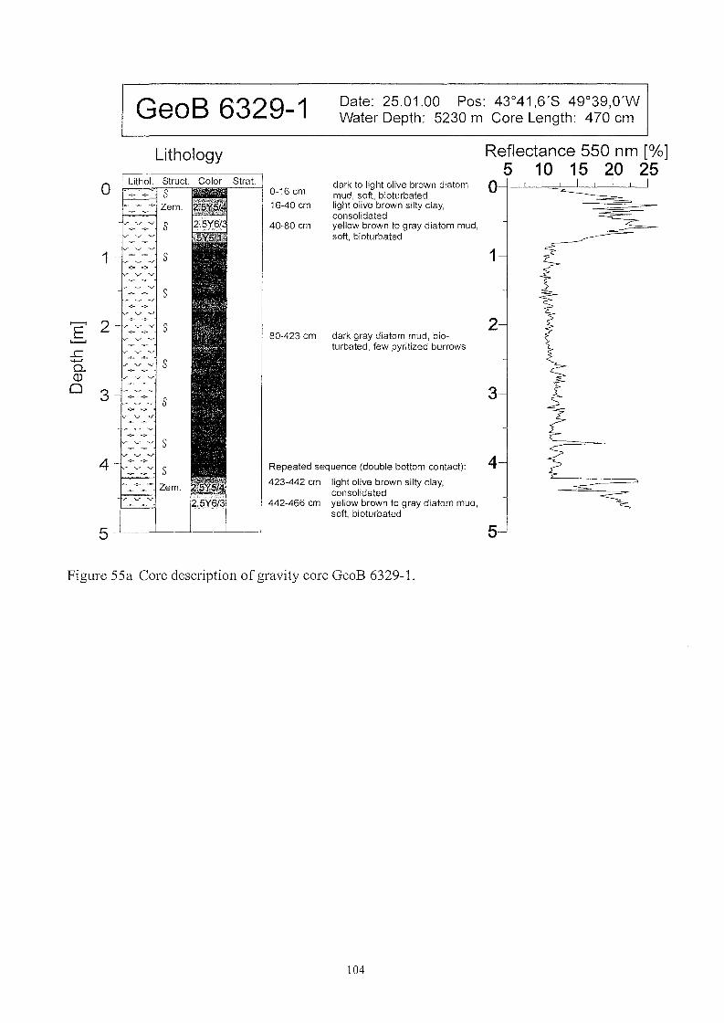
GeoB 6329-1 Date: 25.01.00 Pos: 43°41,6'8 49°39,0'WWater Depth: 5230 m Care Length: 470 cm

2

4

3

1

Reflectance 550 nm [%]5 10 15 20 25

o ~dark to light olive brown diatommud, soft, bioturbatedlight olive brown silty c1ay,consolidatedyellow brown to gray diatom mud,soft, bioturbated

0-16 cm

16-40 cm

40-80 cm

80-423 cm dark gray diatom mud, bio­turbated, few pyritized burrows

Repeated sequence (double bollom contact):

423-442 cm light olive brown silty clay,consolidated

442-466 cm yellow brown to gray diatom mud,soft, bioturbated

2.5Y6/3

s

s

Lithology

v v ·v S

v v v S

s

~~_~~ Zem.

<f ....,. --."

o .~~h~~ ~truc~ Color Stra!.

-~~-_~~ Zem.

1

E 2 -r:~._'=v S'---'

..c........0..(1)

o

5 5

Figure 55a Core description of gravity care GeoB 6329-1.

104

GeoB 6329-1 Date: 25.01.00 Pos: 43°41.6'8 49°39,O'WWater Depth: 5230 m Care Length: 470 cm

2

3

1

Susceptibility [10-6 SI]o

Density [kg/m 3]Vp [m/s]

4

A'''''d "q",""

4

repealed sequence(double bollom conlacl) (double bollom conlacl)

5 50 0 0 0 0 0 0 0 0 0 0 0 0L.[) 0 L.[) 0 0 0 0 0 0 0 0 0

"'" L.[) L.[) CO N "'" CO CO 0 N "'" CO

--- --- ~ ~ ~ ~ ~ ~ N

o

1

""""'2E..c.......Cl.(1)

o 3

Figure 55b Physica1 properties data of gravity core GeoB 6329-1.

105

GeoB 6330-2 Date: 29.01.00 Pos: 46°08,1'8 5r33,4'WWater Depth: 3875 m Care Length: 875 cm

~ ..............

s

2

1

4

3

6

5

7

Reflectance 550 nm [0/0]5 10 15 20 25 30 35o-+--.L-L-'--,!~.L.-L-'--.L-L--'---'

9

8

olive muddy diatom ooze,2 fining upward sequences,turbidites

light olive brown diatom mudw. forams, bioturbated

olive diatom mud, bioturbated

light gray to light olive graydiatom foram nannofossil ooze,bioturbated

0-30 cm

30-80 cm

80-140 cm

140-215 cm

457-860 cm dark greenish gray diatommud, bioturbated

215-425 cm olive gray diatom mud,bioturbated

425-457 cm greenish gray diatomforam nannofossil ooze,bioturbated

s

s

s

s

s

s

s

-,:- .....

s

Lithology

-v· ~;;-

s

(:: ++- +­

-+- :::.-=+- +-

(:: -+-+- +- S

-+- ::;.

o +-+- +

+ ".;

o.- Lithol. Struct. Color Str~c' ..... v S

1

2

3 s

7

6 " v'" S

9 ---'----'----'----'

8-::::: s

E:; 4......0..(1)

o

Figure 56a Core description of gravity core GeoB 6330-2.

106

GeoB 6330-2 Date: 29.01.00 Pos: 46°08,7'8 5r33,4'WWater Depth: 3875 m Core Length: 875 cm

3

2

1

7

8

Susceptibility [10-6 SI],-,--.---=-r--.--,--,.--,--.-,--,--,O

Density [kg/m 3]Vp [m/s]

7

8

...--.4 4E

..c+-'0-(1)

0 5 5os:::-;?-

6 6

9 90 0 0 0 0 0 0 0 0 0 0 0 0 0 0L{) I'- (J) ~ C'0 L{) 0 0 0 0 0 0 0 0..q- ..q- ..q- L{) L{) L{) C'0 ..q- L{) <0 I'- ..q- 00 N~ '"" '"" '"" '"" ~ '\"""" ~ ~ ~ ~ ~

Figure 56b Physical properties data of gravity core GeoB 6330-2.

107

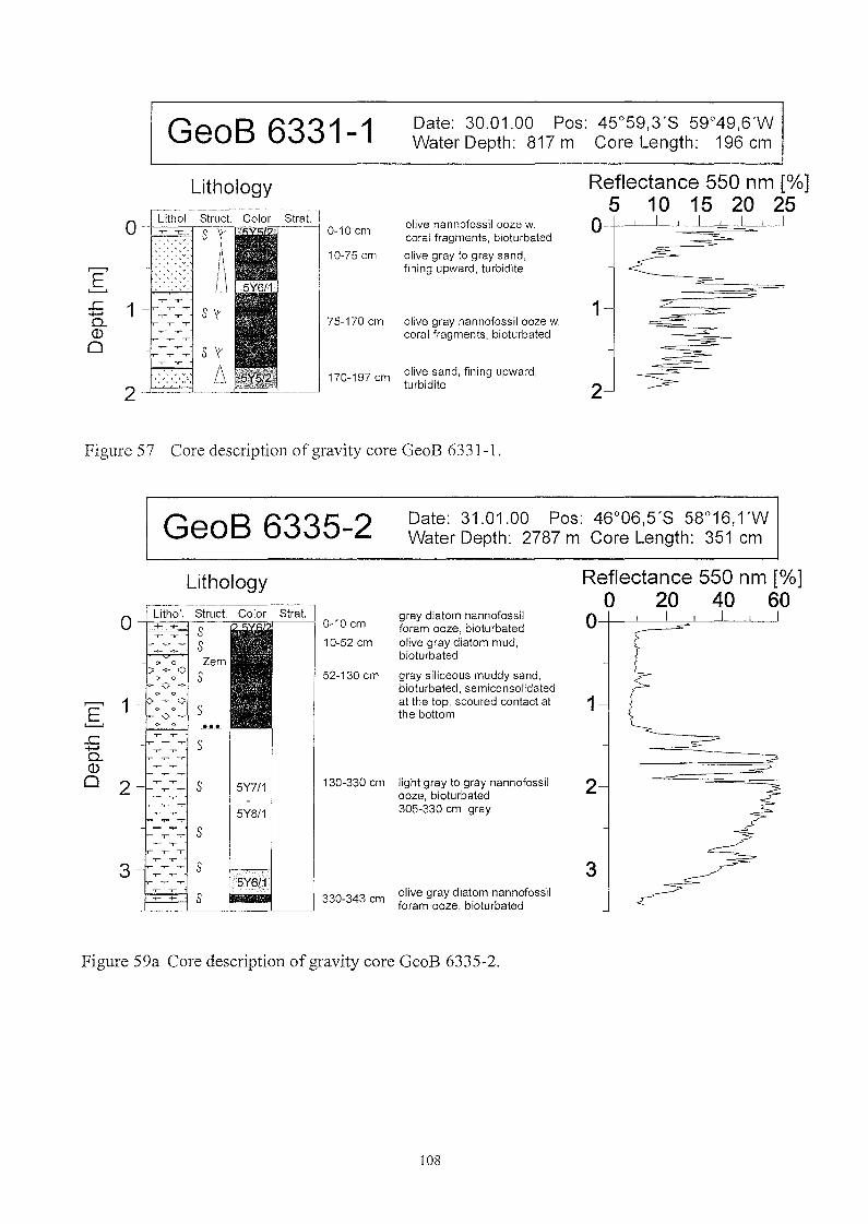
GeoB 6331-1 Date: 30.01.00 Pos: 45°59,3'8 59°49,6'WWater Depth: 817 m Core Length: 196 cm

Lithology Reflectance 550 nm [%]5 10 15 20 25

0Lithol. Struc!. Color Stra!. olive nannofossil ooze w. 0'T~'f 0-10 cm

coral fragments, bioturbated

/i 10-75cm olive gray to gray sand,r---l 1\ fining upward, turbiditeE 1\.......... LJ

..c 1 ..... sv 1~

0- 75-170cm olive gray nannofossil ooze w.Q) coral fragments, bioturbated0 S V

, , ... Y' IJ, 170-197cm olive sand, fining upward,. , "", turbidite2 2

Figure 57 Core description ofgravity core GeoB 6331-1.

GeoB 6335-2 Date: 31.01.00 Pos: 46°06,5'8 58°16,1 'WWater Depth: 2787 m Core Length: 351 cm

3

2

1

Reflectance 550 nm [%]o 20 40 60

O-+----'-----'.---=L.-.-L--.l--.Jgray diatom nannofossilforam ooze, bioturbatedolive gray diatom mud,bioturbated

gray siliceous muddy sand,bioturbated, semiconsolidatedat the top, scoured contact atthe bottom

olive gray diatom nannofossilforam ooze, bioturbated

52-130 cm

330-343 cm

130-330 cm light gray to gray nannofossilooze, bioturbated305-330 cm gray5YS/1

5Y7/1

s

o ~ S

s.,.. ...

.,...,.. -r S

.,.. ,...,.. -r

.,- ,..

"~ -~- Q

Lithology------------,

Lithol. Struc!. Stra!.o +::;::+-:+:;:-J--'","=~-------I 0-10 cmSS 10-52 cm

1--"""-0""1 Zem:): ... -;- Q;;J s-- G -;--

1

2-

..c~

0­Q)

o

Figure 59a Core description of gravity core GeoB 6335-2.

108

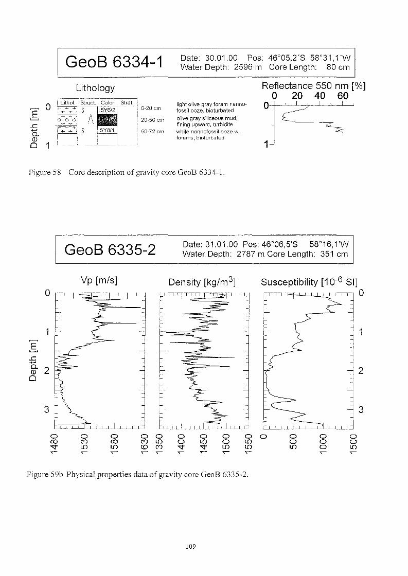
GeoB 6334-1 Date: 30.01.00 Pos: 46°05,2'8 58°31,1 'WWater Depth: 2596 m Core Length: 80 cm

Lithology

EL--l

..c+-'0..Q)

o 1

.--~ -----------,Strat.

,.,.----:;=-=.--:;c--~_:c=:::_r. 0-20 cm

20-50 cm

50-72 cm

light olive gray foram nanno­fossil ooze, bioturbated

olive gray siliceous mud,fining upward, turbiditewhite nannofossil ooze w.forams, bioturbated

Reflectance 550 nm [%]o 20 40 60

O-+--L--L---!---L---L---'----'

1

Figure 58 Core description of gravity core GeoB 6334-1.

GeoB 6335-2 Date: 31.01.00 Pos: 46°06,5'8 58°16,1'WWater Depth: 2787 m Core Length: 351 cm

Vp [m/s]

3

2

1

ooL()~

ooo~

ooL()

Susceptibility [10-6 SI]o

o 0L()L()~

ooL()~

Density [kg/m3]

o 0('f) L()CD ('f)~ ~

o00L()~

o('f)L()~

1

o

3

...---.EL--l

..c+-'

ß- 2o

Figure 59b Physical properties data of gravity core GeoB 6335-2.

109

GeoB 6336-1 Date: 31.01.00 Pos: 46°08,5'8 5r50,TWWater Depth: 3402 m Care Length: 1015 cm

30-1001 cm dark greenish gray diatom mud,bioturbated, partly mottled withpyritized burrows

Lithology

0-30 cm light brownish gray to darkgreenish gray diatom foramnannofossil ooze, bioturbated

Reflectance 550 nm [0!cJ]5 10 15 20 25

O-t-.L-L-'-----'---:::;~~

1

2

3

4

5

6

7

8

9

1

Figure 60a Core description of gravity core GeoB 6336-1.

110

GeoB 6336-1 Date: 31.01.00 Pos: 46°08,S'3 SJOSO,TWWater Depth: 3402 m Core Length: 101S cm

5

1

2

4

3

6

8

- 9

. 7

10o 0o 0<.0 m

Susceptibility [10-6 SI],.-,--,--,-----,------,---,-------,-,----, 0

Density [kg/m 3]Vp [m/s]

9

)10

0 0 0 0 0 0 0 0 0 0 0L{) 0 L{) 0 0 L{) 0 L{) 0 0-:::t L{) L{) <.0 C"? C"? -:::t -:::t L{) C"?~ ~ ~ ~ ~ ~ ~ ~ ~

4

7 -

8

6

,.......,E

:5 5Cl.(l)

o

Figure 6Gb Physical properties data of gravity core GeoB 6336-1.

111

GeoB 6337-9 Date: 01.02.00 Pos: 44°50,6'S 5r45,TWWater Depth: 3546 m Core Length: 1014 cm

:S 5 - ,:.~v s0..(1)

o s

9

7

8

6

5

4

3

2

1

Reflectance 550 nm [0/0)5 10 15 20 25

O-l-----L---'--....l---"---L.-~o!==-

1

635-639 cm layer of pyriteprecipitation

light olive brown to greenishgray diatom nannofossil foramooze, bioturbated

360-505 cm pyritized burrows

35-1000 cm dark greenish gray diatom mud,bioturbated

0-35 cm

s

s

s

s

s

s

,,0",_,"1='.1/-~P.y.->~ S

Lithology

Lithol.

S

1 s

S

J" '-' ."-;- -:-

2- ........R ....... S-;:- -~

3

4

8

Figure 61a Core description of gravity core GeoB 6337-9.

112

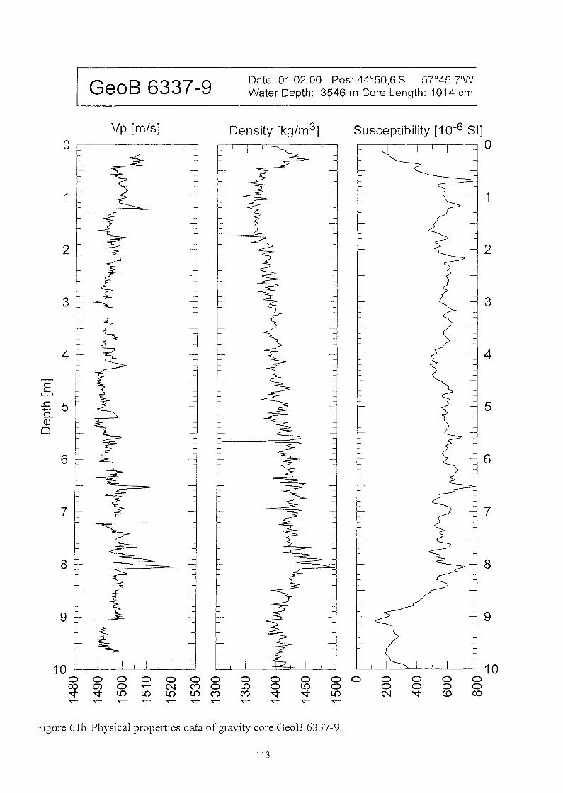
GeoB 6337-9 Date: 01.02.00 Pos: 44°50,6'8 5r45,TWWater Depth: 3546 m Care Length: 1014 cm

2

3

4

1

5

7

9

6

8

10o 0 0o 0 0""'" CD 0:::>

Susceptibility [10-6 SI],---,---,---,--,---,--,--,-----, 0

Density [kg/m 3]Vp [m/s]

3 -

2

1 -

4

7

6

8

9

Z10

0 0 0 0 0 0 0 0 0 0 0 0 00:::> (j) 0 '"" N (V) 0 L() 0 L() 0 0

""'" ""'"L() L() L() L() (V) (V)

""'" ""'"L() N

'"" '"" '"" '"" '"" '"" '"" '"" 't""'"" '"" '""

........E

:S 50..Q)

o

Figure 6Ib Physical properties data of gravity core GeoB 6337-9.

113

GeoB 6339-2 Date: 01.02.00 Pos: 45°09,3'8 5s022,S'WWater Depth: 2493 m Care Length: 746 cm

2

1

3

4

7

5

Reflectance 550 nm [%]o 20 40 60

O---+---L---I~~----l----L---llight olive gray nannofossilforam ooze, bioturbated

gray muddy siliceous foramnannofossil ooze, bioturbated

dark gray muddy sand,turbiditeolive gray diatom mud,bioturbatedolive gray radiolarian muddy 6sand, turbiditedark gray diatom mud,bioturbated

24-215 cm olive gray diatom mud,bioturbated

317 cm volcanic ash layer

215-507 cm white nannofossil ooze w.forams, bioturbated

507-542 cm

542-558 cm

558-590 cm

590-626 cm

626-648 cm

648-683 cm gray muddy sand, turbidite

683-746 cm dark olive gray diatom mudbioturbated720-728 cm turbidite

5Y8/1

s

s

s

s

s

s

Lithology

s

+- +-

.,.. .,......... ..,..,.. .,...,.. ..,.. S

Sr:=+c:::+::) S

O-' Lithoi. Struct. Color Strat. i

+- + S 0-24 cm+- +-

5-

3

7

:E.. 4(])

o

Figure 62a Core description of gravity core GeoB 6339-2.

114

GeoB 6339-2 Date: 01.02.00 Pos: 45°09,3'8 58°22,8'WWater Depth: 2493 m Care Length: 746 cm

2

1

5

7

6

ooL.()-r-

ooo-r-

ooL.()

4

~=========--l 3

Susceptibility [10-6 SI]r-r-.-.-,--,---,--,..,.--,~-.,--,-,---, 0

o 0oI'--r-

oo<0-r-

ooL()-r-

Density [kg/m 3]

o 0 0 0o L.() 00<0 <0 I'- ('f)-r- -r- -r- -r-

000L.() 0 L.().q- L.() L.()-r- -r- -r-

2

o

1

Vp [m/s]

3

5

7

6

E..c......g- 4o

Figure 62b Physical properties data of gravity core GeoB 6339-2.

115

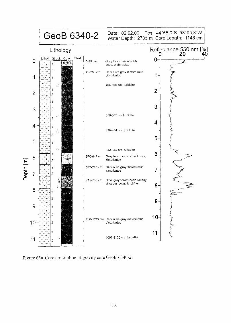
GeoB 6340-2 Date: 02.02.00 Pos: 44°55,0'8 58°05,8'WWater Depth: 2785 m Core Length: 1148 cm

..;.. -:-

...........' ".J......... -;-

9

8

7

6

5

4

3

2

1

1

11

Reflectance 550 nm [0/01o 20 40o-+-_.L------l~---L.--..!

Gray foram nannofossilooze, bioturbated

158-165 cm turbidite

436-444 cm turbidite

1097-1100 cm turbidite

552-562 cm turbidite

350-355 cm turbidite

570-642 cm Gray foram nannofossil ooze,bioturbated

29-568 cm Dark olive gray diatom mud,bioturbated

715-780 cm Olive gray foram-bear. Muddysiliceous ooze, turbidite

780-1133 cm Dark olive gray diatom mud,bioturbated

0-29 cm

642-715 cm Dark olive gray diatom mud,bioturbated

.6.

Lithology

Lithol. Struct. Strat.

++++ S

3 ~ ~ s--".'" "'- "-.,;

.:;.....:..

.~~v.~·~ s1 ...~' ......"" ..., s

-;- -;-

..-- -...... '.~

o

',.~v.~-.- s5 ~.~~~-.- S

~ -:-

~v~'••/ S2 - ~_..--v S

-."- -~.........- ......• •~v"'-.- S

...~v~-/ S

4 ~~~..-~-.- s-:- -:-

:::: s6- +-;-

+++-+- S+- ...

<> c:): -=- :~

" 0- (:: -;-

<> "8 -";"-:::.:-,> ,., ....., S

~~=:-~~: s7-~=v:~ s

.......,E............c+-"Cl.Q)

o

Figure 63a Core description of gravity core GeoB 6340-2.

116

GeoB 6340-2 Date: 02.02.00 Pos: 44°55,0'8 58°05,8'WWater Depth: 2785 m Core Length: 1148 cm

9

10

11

1

8

2

4

ooL()--

-- 3

ooo--

ooL()

Susceptibility [10-6 SI]r-r--.-...-r..-r-.---r,--,--,----,---,,---,--,O

o 0o<D--

ooL()--

Density [kg/m 3]

o 0-- 0<D ("I)-- --

o<DL()--

Vp [m/s]

4

o

8

9

10 -

11

...--. 5 5E...........c......0.. 6 - 6Q)

0

7 7

Figure 63b Physical properties data of gravity core GeoB 6340-2.

117

Date: 03.02.00 Pos: 44°27.2'S Sr10.2'WWater Depth: 4180 m Core Length: 1133 cm

283 cm: sponge

Reflectance 550 nm [%4 6 8 101214

dark greenish gray diatom nan­nofossil ooze with irregularlyspaced and sized black spots(pyrite)

oxydized layer

32 cm: sponge

GeoB 6341-2

Lithology

0Lithol. Struct. Color Strat.

0-1 cm~ ~ 5v·....·

\'"1,-)'r 1-376 cm

1

5

2~p~~ 5

\J3-

~"R ~ 5

4 376-444 cm dark greenish gray nannofossil/diatom- 4-8y-

bearing c1ay5

444-651 cm dark greenish gray diatom nannofossil

5- ooze 5~ ~

"J- ....,..

~-i?Y~ S 444-544 cm: slight H2S smell

~ ~

6- ~ ~ 6.....-.E ~ ~ 629 cm: volcanic grass bearing

'---' nf.ooze

..c+-' 651-662 cm c1ay pebbles0- 7- 7(1)

~ ~ S5 662-670 cm slumps of gray muddy sand

0.,.. .,.. 670-1131 cm dark greenish gray diatom

S nannofossil ooze with irregu-larly sized and spaced dark

8 -- ~ ~ (pyrite) spots 8.....- .......~ ~

S 790 cm: greenish burrows.....p..y~

9-~ ~

9~ ~ 890 cm: encrusted burrow ?(2 cm length)

S

10-~fVy~

10~ ~ S 1085 cm: encrusted burrow ?....- .......

(0,5cm)

11 - 1109 cm: encrusted burrow ? 11(2 cm)

J_ 1120-1133 cm: greenish burrows

Figure 64a Core description of gravity core GeoB 6341-2.

118

GeoB 6341-2 Date: 03.02.00 Pos: 44 D 27,2'S sr10,2'WWater Depth: 4170 m Core Length: 1133 cm

1

3

2

4

5

7

6

11

9

8

10

o 0 0 0o 0 0 0-.:::t <D co 0

~

Susceptibility [10-6 SI],--,---".-".-"--~,,--,,.-,,------,O

o 0o 0L() N~

Density [kg/m 3]Vp [m/s]

4

7

3

2

1 _

9

8

10

11

..c-+-'Q.. 6 ­(l)

o

,......,5E

Figure 64b Physical properties data of gravity core GeoB 6341-2.

119

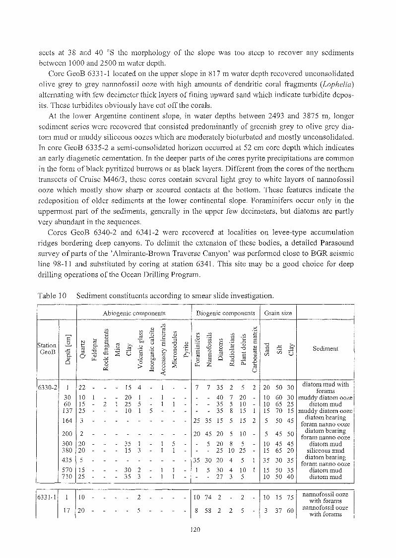
sects at 38 and 40 oS the morphology of the slope was too steep to recover any sediments

between 1000 and 2500 m water depth.Core GeoB 6331-1 located on the upper slope in 817 m water depth recovered unconsolidated

olive grey to grey nar1110fossil ooze with high amounts of dendritic coral fragments (Lophelia)

aIternating with few decimeter thick layers of fining upward sand which indicate turbidite depos­

its. These turbidites obviously have cut offthe corals.

At the lower Argentine continent slope, in water depths between 2493 and 3875 m, longer

sediment series were recovered that consisted predominantly of greenish grey to olive grey dia­tom mud or muddy siliceous oozes which are moderately bioturbated and mostly unconsolidated.

In core GeoB 6335-2 a semi-consolidated horizon occuned at 52 cm core depth which indicatesan early diagenetic cementation. In the deeper parts of the cores pyrite precipitations are COlllmon

in the fOlm ofblack pyritized bunows or as black layers. Different from the cores ofthe northern

transects of Cruise M46/3, these cores contain several light grey to white layers of nannofossilooze which mostly show sharp 01' scoured contacts at the bottom. These features indicate the

redeposition of older sediments at the lower continental slope. Foraminifers occur only in the

uppelmost part of the sediments, generally in the upper few decimeters, but diatoms are partly

very abundant in the sequences.Cores GeoB 6340-2 and 6341-2 were recovered at localities on levee-type accumulation

ridges bordering deep canyons. To delimit the extension of these bodies, a detailed Parasoundsurvey ofparis ofthe 'Almirante-Brown Traverse Canyon' was performed c10se to BGR seismicline 98-11 and substituted by coring at station 6341. This site may be a good choice for deep

drilling operations ofthe Ocean Drilling Program.

Table 10 Sediment constituents according to smear slide investigation.

Abiogenic components Biogenie components Grain size

(/)

(/) (l) (;j .~....... (/) .'!::: ..... (/)(/) .....

~(/) u (l) (l) ~ (/) (/) 1\jS (l) o;l ~ ""5

....."üJ ~ 'C.....

6 ÖD(;j ·s tB (/) o;l 6

Station ~N o;l

o;l u "0 E :§(/) 6 'e ..0

t 0- 1:>D ~ U 0 <8 o;l(l)

(l)"0 .:::: »

(/) u u 'C 0 "0 ~ o;l SedimentGeoB ..c o;l"0 o;l

~ Ü '2 "2 C ~ 6 0 "(;j ö 1\j o;l Vi Ü;:l tl:: » .......P.. CI V o;l o;l 0 0 0... o;l ~

6 :.ci ~ ~ Vi.....(l) r..r... ~ u 1:>1) (/) U ..... ~ o;l 0Ci u Ö ..... (/)

~0 o;l o;l ö::: ..0

0 0 (l) r..r... Z 0::: .....0::: > E

u o;lu U-<

6330-2 1 22 15 4 1 7 7 35 2 5 2 20 50 30 diatom mud with- - - - - - forams30 10 1 - - 20 1 - 1 - - - - 40 7 20 - 10 60 30 muddy diatom ooze60 15 - 2 1 25 5 - 1 1 - - - 35 5 10 - 10 65 25 diatommud137 25 - - - 10 1 5 - - - - - 35 8 15 1 15 70 15 muddy diatom ooze

164 3 - - - - - - - - - 25 35 15 5 15 2 5 50 45 diatom bearingforam nanno ooze

200 2 - - - - - - - - - 20 45 20 5 10 - 5 45 50 diatom bearingforam nanno ooze

300 20 - - - 35 1 - 1 5 - - 5 20 8 5 - 10 45 45 diatommud380 20 - - - 15 3 - 1 1 - - - 25 10 25 - 15 65 20 si1iceous mud

435 5 - - - - - - - - - 35 30 20 4 5 1 35 30 35 diatom bearingforam nanno ooze

570 15 - - - 30 2 - 1 1 - 1 5 30 4 10 1 15 50 35 diatom mud710 25 - - - 35 3 - 1 1 - - - 27 3 5 10 50 40 diatommud

6331-1 10 2 10 74 2 2 10 15 75 nannofossi1 ooze- with forams

17 20 5 8 58 2 2 5 3 37 60 nannofossi1 ooze-with forams

120

Table 10 continued

Abiogenic components Biogenie components Grain size

C/l

C/lC/l .8 '"@ .:5

C l-< C/l l-<C/l ·ü ()) ()) C/l~

C/l C/l 'iijE ()) c<J'"@ .5 ;:; l-< C ·Cl-<

E bJl <2 C/l C/l c<J EStation ~

N c<Je<:j u E "0 ()) ·2 C/l E ·C .D

t 0.. bJl ~..... t8 ()) "0 3C/l u u u 0 ·C 0 c<J "0 ()) J:::: ~ Sediment..c c<J c<J ·2 C c ·s 'iijGeoB ..... ;:l "0 <t:: ~ Ü ·2 0 >-, 0

.~ '0 ..... c<J ifJ Us:::::>.. CI V c<J c<J 0 l-< 0. c<J J:::: :a J:::: J:::: ifJQ) c.r... ~ u bJl C/l u l-< J:::: Q c<J 0Q u '0 l-< C/l

~0 c<J c<J 0:: .D

0 > 0 ()) c.r... Z ~ l-<

~ C u c<J>-< U U-<

6331-1 77 3 5 90 1 1 5 5 90nannofossi1 ooze- - - - - - - - - - -

with forams

87 5 2 5 86 1 1 5 5 90nannofossi1 ooze

- - - - - - - - - -with forams

140 30 - - - 30 5 - 1 3 - 3 20 3 1 4 5 35 60 nannofossi1 mud

6334-1 1 5 40 53 1 1 20 20 60Foraminifera1- - - - - - - - - - -

nannofossi1 ooze34 20 - 8 2 20 4 5 1 - - 2 10 13 10 5 - 25 40 35 si1iceous mud

60 2 5 93 2 3 95nannofossi1 ooze- - - - - - - - - - - - -

with forams

6335-2 1 3 1 36 40 15 1 3 1 30 30 40diatom nanno foram- - - - - - - -

ooze15 25 - 15 2 22 2 1 1 - - 2 3 20 3 3 1 30 40 30 diatom mud

100 20 - 15 3 15 1 - 1 - 5 15 15 10 - 55 25 20siliceous muddy- -

sand200 - - - - 1 - - - - 3 91 2 1 1 1 2 3 95 nannofossi1 ooze

336 20 15 3 10 5 1 1 3 20 15 5 2 30 35 35diatom nannofossi1

mud

6336-1 3 10 3 1 20 39 20 2 3 2 20 35 45diatom foram nanno

- - - - - - -ooze

11 15 5 20 45 10 1 3 1 25 25 50diatom foram nanno

- - - - - - - -ooze

27 25 - 10 - 20 3 - 1 - - 2 2 29 2 5 1 20 50 30 diatom mud

30 10 1 1 20 53 10 1 3 1 5 40 55diatom foram nanno- - - - - - -

ooze100 15 - 8 - 35 - - - - - - - 25 1 15 1 5 55 40 diatom mud

6337-9 1 10 5 3 8 12 42 12 1 5 2 10 40 50diatom foram nanno- - - - - -

ooze

16 10 5 2 3 1 10 50 15 1 2 1 10 30 60diatom foram nanno- - - - -

ooze60 20 - 20 - 25 2 - 1 - - 2 - 20 2 10 - 10 60 30 diatom mud100 20 - - - 40 5 - 1 1 - - - 10 3 20 - 15 35 50 diatom mud200 20 - 3 - 47 2 - 1 3 - - - 10 3 10 1 10 40 50 diatommud350 20 - - - 35 1 - 1 5 - - - 25 2 10 1 10 50 40 diatom mud425 20 - 3 - 35 1 - - 3 - - - 25 2 10 1 10 50 40 diatommud770 20 - 5 - 35 5 - 1 1 - - - 15 3 15 - 10 50 40 diatommud

6339-2 5 2 50 36 3 2 50 10 40nannofossi1

foraminifera1ooze70 20 15 3 25 3 3 2 2 18 2 7 15 55 30 diatom mud170 20 5 2 25 2 2 - 25 8 10 - 20 50 30 diatommud

241 3 97 3 97 nannofossi1 oozewith forams

121

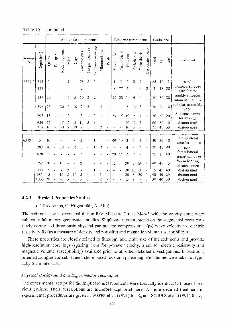
Table 10 continued

Abiogenic components Biogenie components Grain size

VJ

VJ n.l (;j X..... VJ o~ '- VJ .~~ I':: VJ

Ü n.l V VJ~

VJ VJn.l ro I':: '"3

'- I':: °CE '- 6 bD (;j '6 ~ VJ VJ ro ...a 6~

N ro ro ü '"0 E :5VJ 6 'CStation t 0. bll i? ü 0 eS n.l n.l

'"0 ..... i?ro VJ ro ü '2 üC °C 0 ro '"0 ..... I':: SedimentGeoB ...c: ;:l '"0 cI:1 ~ U °2 I':: >. § 0

.~ ö ..... ro ro CF) U..... Q) ro 0 I':: CF)0. CI ro 0 '- 0.. :..a I':: I'::v r-r... ~ ~ bll VJ ü '- I':: Cl ro 0

Cl ü 0 '- VJ

~0 ro ro 0: ...a

0 > 0 n.l r-r... Z ~ '-~ I':: ü ro

ü U>-< -<6339-2 317 5 - - 1 - 78 2 1 - - 1 5 2 2 2 1 85 10 5 sand

477 3 2 8 77 5 3 2 2 18 80nannofossil ooze

- - - - - - - - -with forams

536 20 - 2 5 10 2 2 - - 10 20 20 4 4 I 10 60 30muddy siliceous-

foram nanno ooze

596 25 30 3 10 2 5 - 1 5 15 3 - 70 20 10 radiolarian muddy- - - -sand

607 15 2 3 1 35 15 10 15 4 30 50 20Siliceous nanno- - - - - - ..

foram ooze656 25 - 15 2 5 10 2 I - - - - 20 15 5 - 60 30 10 diatommud715 10 - 30 2 30 2 1 2 2 - - - 10 3 7 1 25 40 35 diatom mud

6340-1 5 10 3 1 40 40 3 1 I 1 40 20 40foraminiferal- - - - - - -

nannofossil ooze203 20 - 30 - 35 5 - 1 2 - - - 4 - 3 - 20 40 40 mud

620 5 3 1 28 55 3 2 2 1 25 15 60foraminiferal- - - - - - -

nannofossil ooze

767 20 10 2 2 1 - 15 5 20 5 20 40 45 15foram bearing- - - - -siliceous ooze

900 15 - - 2 30 - 1 I 1 - - - 30 10 10 - 15 45 40 diatom mud985 15 - 10 5 10 5 4 I 1 - - - 20 8 20 1 40 40 20 diatommud1000 20 - 20 3 25 5 1 I 2 - - - 15 2 5 I 30 40 30 diatom mud

4.2.3 Physical Properties Studies

(T. Frederichs, C. Hilgenfeldt, A. Alin)

The sediment series recovered during RJV METEOR Cruise M46/3 with the gravity corer weresubject to laboratory geophysical studies. Shipboard measurements on the segmented cores rou­tinely comprised three basic physical parameters: compressional (p-) wave velocity vp, electricresistivity Rs (as a measure of density and porosity) and magnetic volume susceptibility K.

These properties are c10sely related to lithology and grain size of the sediments and providehigh-resolution core logs (spacing 1 cm for p-wave velocity, 2 cm for electric resistivity and

magnetic volume susceptibility) available prior to all other detailed investigations. In addition,oriented sampies for subsequent share based rock and paleomagnetic studies were taken at typi­cally 5 cm intervals.

Physical Background and Experimental Techniques

The experimental setups for the shipboard measurements were basically identical to those of pre­vious cruises. Their descriptions are therefore kept brief here. A more detailed treatment ofexperimental procedures are given in WEFER et al. (1991) for Rs and SCHULZ et al. (1991) for vp .

122

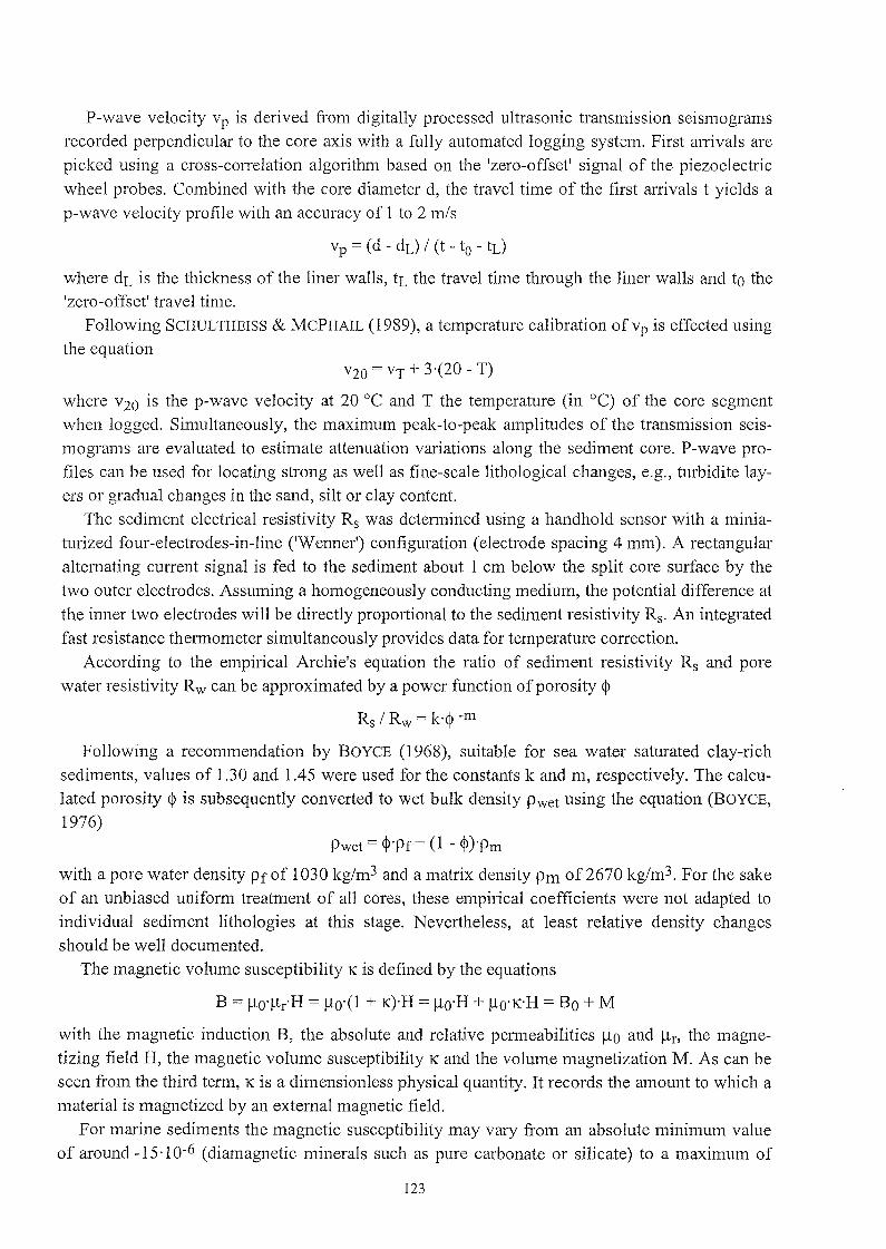
P-wave velocity vp is derived from digitally processed ultrasonic transmission seismogramsrecorded perpendicular to the core axis with a fully automated logging system. First alTivals arepicked using a cross-conelation algorithm based on the 'zero-offset' signal of the piezoelectricwheel probes. Combined with the core diameter d, the travel time of the first anivals t yields ap-wave velocity profile with an accuracy of 1 to 2 m/s

vp = (d - dL) / (t - to - tL)

where dL is the thickness of the liner walls, tL the travel time through the liner walls and to the'zero-offset' travel time.

Following SCHULTHEISS & MCPHAIL (1989), a temperature calibration ofvp is effected usingthe equation

v20 = vT + 3'(20 - T)

where v20 is the p-wave velocity at 20°C and T the temperature (in °C) of the core segmentwhen logged. Simultaneously, the maximum peak-to-peak amplitudes of the transmission seis­mograms are evaluated to estimate attenuation variations along the sediment core. P-wave pro­files can be used far locating strong as well as fine-scale lithological changes, e.g., turbidite lay­ers or gradual changes in the sand, silt or clay content.

The sediment electrical resistivity Rs was detennined using a handhold sensor with a minia­turized four-electrodes-in-line ('Wenner') configuration (electrode spacing 4 mm). A rectangularaltemating cunent signal is fed to the sediment about 1 cm below the split core surface by thetwo outer electrodes. Assuming a homogeneously conducting medium, the potential difference atthe inner two electrodes will be direct1y proportional to the sediment resistivity Rs. An integratedfast resistance thennometer simultaneously provides data for temperature conection.

According to the empirical Archie's equation the ratio of sediment resistivity Rs and porewater resistivity Rw can be approximated by apower function of parosity <p

Rs / Rw = k.<p -m

Following a recommendation by BOYCE (1968), suitable far sea water saturated clay-richsediments, values of 1.30 and 1.45 were used for the constants k and m, respectively. The ca1cu­lated porosity <p is subsequently converted to wet bulk density Pwet using the equation (BOYCE,1976)

Pwet = <p'Pf + (1 - <p)'Pm

with a pore water density Pf of 1030 kg/m3 and a matrix density Pm of 2670 kg/m3. For the sakeof an unbiased unifonn treatment of all cores, these empirical coefficients were not adapted toindividual sediment lithologies at this stage. Nevertheless, at least relative density changesshould be weIl documented.

The magnetic volume susceptibility Kis defined by the equations

B = flo'flr'H = flo'(1 + K)'H = flo·H + flo'K'H = Bo + M

with the magnetic induction B, the absolute and relative penneabilities flo and flr, the magne­tizing field H, the magnetic volume susceptibility K and the volume magnetization M. As can beseen from the third tenn, Kis a dimensionless physica1 quantity. It records the amount to which amaterial is magnetized by an extemal magnetic field.

For marine sediments the magnetic susceptibility may ValY from an absolute minimum valueof around -15'10-6 (diamagnetic minerals such as pure carbonate or silicate) to a maximum of

123

some 10.000.10-6 for basaltic debris rich in (titano-) magnetite. In most cases K is primarilydetennined by the concentration of ferrimagnetic minerals, while paramagnetic matrix compo­nents such as clays are of minor importance. High magnetic susceptibilities indicate high con­centrations of lithogenic compounds 1high iron (bio-)mineralization or low carbonate 1opal pro­ductivity and vice versa. This relation may serve for the mutual correlation of sedimentarysequences which were deposited under similar global or regional conditions.

The measuring equipment consists of a commercial Bartington M.S.2 susceptibility meterwith a 125 mm loop sensor and a non-magnetic core conveyor system. Due to the sensor's size,its sensitivity extents over a core interval of about 8 cm. Consequently, sharp susceptibilitychanges in the sediment column will appeal' smoothed in the K core log and, e.g., thin layers suchas ashes cannot appropriately be resolved by whole core susceptibility measurement.

Shipboard Results

The gravity coring program of Cruise M46/3 comprises two southeast trending transects from theArgentinean continental shelf into the Argentine Basin. One stretches between 38°21'S 155°l5'W and 39°24'S 153°50'W with water depths from 436 to 4010 m (cores GeoB 6307-3,6308-3, 6309-1, 6311-1, 6312-1). The second is located some 100 km to the southwest andcovers water depths from 732 to 4185 m between 39°25'S 155°27'W and 400 12'S 154°22'W(cares GeoB 6313-1,6317-1,6318-1,6319-1,6319-2). Fmiher sediment sequences (cores GeoB6337-9, 6339-2,6340-2) were recovered on a third transect at about 45°S between 58°23'W and57°46'W from water depths between 2493 and 3546 m. From the fourth transect at about 46°Sbetween 58°l6'W and 57°33'W (water depths 2787 to 3875 m) cores GeoB 6330-2, 6335-2 and6336-1 were subject to the measurements of physical properties. Sediments from the deeperArgentine Basin were recovered from the Zapiola Drift in water depths of 5098 and 5064 m(GeoB 6321-2 and 6322-2). The seismic and echographie acoustic mud wave surveys were sup­plemented by gravity coring water depths between 5288 and 5490 m (GeoB 6323-2, 6324-1,6324-2,6325-1,6326-1,6327-1,6328-1,6329-1).

The recovery varied between 100 (care GeoB 6301-2) and 1416 cm (core GeoB 6322-2). Atotal of 27 sediment cores with a cumulative length of 203 m was investigated (see upper part ofFigure 65). Additionally, the physical propeliies of cores GeoB 6233-2 and 6234-2 from CruiseM46/2 were measured. The results are presented in the cruise report ofM4612.

The general characteristics of the physical properties are compiled in the lower part of Fig­ure 65. Dots mark the mean values of compressional wave velocity, density and magnetic sus­ceptibility for the individual cores, vertical bars denote their standard deviations. Each diagram isdivided into five sections according to the five working areas, separating data sets from theregion off the Rio de la Plata (RP), the Argentine continental slope (ACS, transects at 39/40 oSand 45/46 OS) and the Argentine Basin with the Zapiola Drift (AB - ZD) and the mud wave area(AB - MW).

The average p-wave velocities range from 1489 to 1708 m/s. The most distinct variations withhighest standard deviations were found for the 39/40 oS transect on the Argentine continentalslope. Higher velocities in shallow water indicate coarser sediments as one would expect withdecreasing distance to the coast. This holds also for core GeoB 6301-2 (29 m water depth) withthe highest mean compressional wave velocity of all cores. Cores [rom the transects at 45/46 oSshow intennediate mean p-wave velocities between those from the 39°/40oS transect and the

124

Argentine Basin. The lowest mean compressional wave velocities were found for sediments fromthe Argentine Basin, in the mud wave area as weIl as on the Zapiola Drift. Velocities are nearlyidentical for all those eores and show only small standard deviations. In partieular, sedimentsfrom the Zapiola Drift show very few variations in their p-wave veloeities.

Overall, average densities (1367 to 1615 kg/m3) parallel the results ofp-wave velocity meas­urements, but the lithological variability of the eores from the Argentine Basin is more pro­nouneed in their densities than in their eompressional wave velocities. The higher standarddeviations of density are similar to those for the sediments from the Argentine eontinental slope.Density data far core GeoB 6301-2 are not available.

Mean magnetie susceptibilities vary from 116 to 3745.10-6 SI. Far sediments from the Argen­tine continental slope (transect 39/40 OS) high average suseeptibilities (908 to 3745.10-6 SI) eor­relate with high p-wave velocities and densities, indieating that coarser sediment components aremainly of terrigenous origin. Susceptibility inereases with deereasing water depth in these sedi­ments except for eore GeoB 6312-2 reeovered from 436 m water depth with a mean suseepti­bility (1644,10-6 SI) similar to that of sediments from deeper sites of the transect. Distinetlylower mean magnetic susceptibilities (358 and 525.10-6 SI) were found on the Argentine conti­nental slope at about 45°/46°S whieh are in the range of susceptibilities (116 to 579.10-6 SI) forsediments in the Argentine Basin from water depth ofmore than 5000 m.Physical property logs far the individual cores are shown in Figures 31 41 and 46 - 64 togetherwith the visual eore descriptions.

Rio de la Plata (core GeoB 6301 -2)

This core shows the highest p-wave velocities (mean 1708 m/s) of the entire care colleetionreflecting a very specific depositional environment with sediments of medium-size sand bearingabundant shells and shell fragments. Magnetic susceptibility (mean 816.10-6 SI) is distineHylower than for sediments from the upper continental slope (transect 39/40 OS).

Argentine Continental Slope - Transect 39/40 oS (cores GeoB 6307-3, 6308-3, 6309-1, 63Jl-1,6312-1,6313-1,6317-1,6318-1,6319-1,6319-2)

Mean values for susceptibilities range from 908 to 3745.10-6 SI, for densities from 1452 to1615 kg/m3 and for p-wave velocities from 1511 to 1647 m/s. The suseeptibility logs ofthe coresshow no obvious uniform pattern. Single seetions of several cores display similarities as, forexample, the upper 450 and 500 em ofeores GeoB 6313-1 and 6317-3. This implies eomparablesedimentation rates for both eores despite their provenanee from different water depths of 732and 3112 m, respectively.

A 100 to 150 em long seetion of notably low suseeptibilities with lower boundaries at 220,550 and 650 em in cares GeoB 6307-3, 6308-3 and 6309-1, respeetively, indieates inereasingsedimentation rates from deeper (4010 m) to shallower (2867 m) water depth. Two layers (225and 650 em) ofhigh p-wave velocities in eore GeoB 6307-3 are eaused by turbidites. A third oneat 420 em has no equivalent in the visual eore deseription. Beside these features eompressionalwave velocities as weIl as densities show only few variations. High p-wave veloeities at 450 emdepth in eare GeoB 6308-3 are eorrelated to a diagenetie eoneretion. Below 500 em eore depthvp eould not be determined due to rising H2S eontents. Densities of eore GeoB 6308-3 inereasewith a eonspieuous linear trend from top to bottom.

125

• I II I I- -

- f.-

- '-

- f-

fi 11 ' i; in f i :11

-"

\; i f-

r ;1,

-ill

r-

-

'1

f-

- -, ,- :,' f.-

0E 300~.c...... 600Olc(j)

900-l(j)c...

120000

1500

0

I 1000.c 2000......Q..(j) 30000c...

4000(j)......

~ 5000

6000

'iJ~

o(Y)«)

RP

C"1C'0r-"'--N" (i)"...-(\JI I I I I 1 I t I II'-(x)Ol~N(y)I'--(x)OlOl000"...- ...-,\,\"(Y)(Y)(Y)(Y)(Y)(Y)(Y)(Y)(Y)(Y)«)«) «)«)«)«)«) «)«)«)

AC5 39/40°5 AC545/46°5

NN N...-N..-"'-'\~~I I I I I I I I 1 I~N (Y)'<t'<tL[)«)1'--(x)0lNN NNNNNNNN(Y)(Y) (Y)(Y)(Y)(Y)(Y)(Y)(Y)(Y)«)«) «)«)«)«)«)«)«)«)

AB ·ZD AB ·MW

1770

~ 1670 - !I!t I!I.s

Q..

> 1570 -

.!••I~f-

!~! ! •• .~......1470

1700,......,

dI !IIC0

E 1600 - -

---0)~~

1500

!Idh>.

- I!! ! f-

:!:::

~HIlCf)c 1400 - I! -Q)

0 -

1300~

(f) 4000 ! ~CD

6:=. 3000

I!! I!!!!,q2000

..Cl+=lQ.. 1000 :lQ)

II~I~~()Cf)

0::J(f)

Figure 65 Mean compressional wave velocities, densities and magnetic susceptibilities of coresGeoB 6301-2 through 6340-2 as compared to variations in water depth at thesampling sites and core recovery. The veliical bars denote standard deviations. Datasets are classified according to five working areas, off the Rio de la Plata (RP), twotransects at 39°/40oS and 45°/46°S on the Argentine continental slope (ACS), theZapiola Drift (AB - ZD) and the mud wave area (AB - MW) in the Argentine Basin.

126

The p-wave velocity log of core GeoB 6317-3 resembles the density data. Highest values of

1759 m/s are attributed to four layers of dark gray sand at about 720 cm core depth which are

also correlated to increased susceptibilities.

Argentine Basin - Zapiola Drift (cores GeoB 6321-1, 6322-2)

Susceptibility pattem of the sediments from the Zapiola Drift (mean values 121 and 363.10-6 SI)differ completely from each other. The log of core GeoB 6321-2 shows slight variations around

100.10-6 SI with various horizons of increased K which are not correlated, however, to the dark

layers ofpyrite (or Mn?) precipitations in the diatom-bearing clays. In contrast, the magnetic sus­ceptibility of core GeoB 6322-2 displays more or less (pseudo-) cyc1ic changes which are also

not significantly correlated to the corels lithology. On the other hand, p-wave velocities (mean

values 1492 and 1489 rn/s) and densities (mean values 1376 and 1390 kg/m3) are very similar for

both cores.

Argentine Basin - Sediment Wave Fields (cores GeoB 6323-2, 6324-1, 6324-2, 6325-1, 6326-1,6327-1, 6328-1, 6329-1)

Cores from the sediment wave surveys yield p-wave velocities of 1450 to 1671 m/s, densities of1311 to 2297 kg/m3 and magnetic susceptibilities of 17 to 2478.10-6 SI. As a first attempt, they

may be c1assified according to their susceptibility signal into three groups.The first group consists of cores GeoB 6323-2 (mean 493.10-6 SI), 6326-1 (mean 579.10-6 SI)

and 6327-1 (mean 489.10-6 SI) and shows (pseudo-) cyc1ic patterns allowing a mutual first order

correlation. Densities (GeoB 6323-2: mean 1401 kg/m3, 6326-1: 1405 kg/m3, 6327-1: 1407

kg/m3) and p-wave velocities (GeoB 6323-2: mean 1489 m/s, 6326-1: 1494 m/s, 6327-1: 1494

m/s) are very similar in all cares. While compressional wave velocities vary around their respec­tive means, densities increase to depth. A volcanic ash layer in care GeoB 6323-2 at 1104 cm

care depth is characterized by markedly increased p-wave velocity and density, but decreasedsusceptibility.

Cores GeoB 6324-1 (mean 127.10-6 SI), 6324-2 (116.10-6 SI) and 6329-1 (123.10-6 SI) form

the second group. Its characteristic are more or less constant susceptibilities of around 100.10-6

SI with some thin layers of increased K similar to the susceptibility signals of sediments from the

Zapiola Drift. Densities (GeoB 6324-1: mean 1367 kg/m3, 6324-2: 1388 kg/m3, 6327-1: 1415kg/m3) and compressional wave velocities (GeoB 6324-1: mean 1490 m/s, 6324-2: 1492 m/s,

6329-1: 1496 m/s) showalmost no variation and only increase in a few layers of(semi-) consoli­

dated silty c1ay or diatom mud. A volcanic ash layer in core GeoB 6324-2 at 350 cm core depthyields a significantly rising p-wave velocity and slightly higher density, but no peculiarity in sus­ceptibility.

The third group comprising cares GeoB 6325-1 (mean 521.10-6 SI) and 6328-1 (163.10-6 SI)

mainly consists of diatom mud with no uniform susceptibility signal similar to the sediments

from the Argentine continental slope. Compressional wave velocities (GeoB 6325-1: mean 1493

m/s, 6328-1: 1497 m/s) and densities (GeoB 6325-1: mean 1411 kg/m3, 6328-1: 1404 kg/m3)

show very limited variations and only increase in (semi-) consolidated silty c1ay layers of core

GeoB 6328-1. A volcanic ash layer at 42 cm depth in core GeoB 6325-1 causes higher vp anddensity, but again does not affect susceptibility.

127

Argentine Continental Slope - Transect 45/46 oS (cores GeoB 6330-2, 6335-2, 6336-1, 6337-9,

6339-2, 6340-2)

Sediments from the transect across Argentine continental margin at about 45 and 46°S exhibitmagnetic susceptibilities of 5 to 1466.10-6 SI, p-wave velocities from 1451 to 1673 mls and den­

sities between 1308 and 1662 kglm3. Layers of very low susceptibility - the lowest of the entirecore collection - in cores GeoB 6330-2 (mean 418.10-6 SI), 6335-2 (471.10-6 Sr) and 6339-2

(441.10-6 sr) and prevailing low p-wave velocities are mostly related to nannofossil oozes. There

is no overall susceptibility pattern allowing an obvious correlation between the cares. A

remarkably high susceptibility peak (and also increased vp and density) in core GeoB 6339-2

within the sequence of namlOfossil oozes at about 317 cm core depth is attributed to a volcanic

ash harizon which differs from those in cores GeoB 6323-2 and 6324-2, where ashes did notaffect magnetic susceptibility. The ashes should therefore originate from different types of vol­

camsm.

4.2.4 Geochemistry

(V. Heuer, K. Pfeifer)

The continuation of geochemical investigations on sediments from the southern continental mar­gin off Argentina and in the Argentine Basin focuses on the reconstruction of climatically con­

trolled sedimentation processes with respect to diagenetic overprint. On the Cruises M29/l-2 ithad not been possible to obtain undisturbed sediment cores that would allow an unambiguousdating of the sedimentary record. Thus, the main prerequisite for a success of the present pro­

gram was to obtain reasonably undisturbed and datable cores. High resolution pore water analy­

sis and solid phase sampling of gravity cares was carried out at three suitable stations. The for­

mation of element enrichments at glacial/interglacial transitions will be of particular interest for

further investigations of these cores in Bremen.

Experimental Methods

After retrieval all cores were immediate1y stored and processed in a laboratory that was cooled to4 °C in order to prevent warming ofthe sediments.

Multicorer sampIes were processed within three hours after recovery. After sampling somesupernatant bottom water, the pore water was extracted from the sediment in the oxygen free

atmosphere of an argon filled glove-box. Before the sediment was cut into 0.5 to 5 cm slices for

pressure filtration, the pR value and the redox potential Eh were measured far each slice. Pres­

sure filtration was carried out with Teflon- and PE-squeezers and 0.2 Ilm acetate membrane fil­ters at apressure of 3 to 4 bar. The solid phase of the multicorer sediment was sampled with a

depth resolution of 1 cm in a parallel core. Electric conductivity was measured in a third parallel

core for the determination ofthe sediment's density and porosity.Gravity cores were sampled for methane and sulfide analysis within three hours after recov­

ery. To allow a quick sampling procedure, small openings of about 4 x 4 cm were cut into the

PVC liner every 25 cm. For methane analysis 2 replicates were taken. Each time 5 ml of sedi­ment were acquired by a syringe and injected into 50 ml septum vials containing 20 ml of sea­

water poisoned by RgC12. After closing the vials the mixture was homogenized and frozen. The

128

methane captured in the headspace of the vials will be analyzed at Bremen University. The repli­cate will be used for isotope analysis. The sulfide content of the sediment was measured in situ(within the core) with Ag/AgS needle electrodes. In addition, 2.5 ml of sediment were injectedinto scintillation bottles containing 5 ml of SAOB buffer which prevents degassing of H2S, pre­cipitation of metal sulfides and oxidation of S2- ions in solution. Subsequently, the sulfide con­tent of the solution was measured potentiometrically with an Ag/AgS electrode.

Within two days after recovery the 1 m segments of the gravity core have been cut lengthwiseand opened in the oxygen free atmosphere of an argon filled glove-box, where pH and Eh weremeasured every 25 cm and sediment samples were taken from the working halves for pore wateranalysis. Pressure filtration was can-ied out with Teflon- and PE-squeezers and 0.2 Ilm acetatemembrane filters at apressure of 5 to 6 bar. Depending on porosity and compressibility of thesediments, up to 20 ml ofpore water were received from each sample. Every 10 cm the sedimentwas sampled by syringes for sequential extractions ofthe solid phase. These solid phase sampleswere stored in gas-tight bottles under anoxie atmosphere at -20°C. Electric conductivity wasmeasured on the archive halves of the gravity cores to detelmine the sediment's density andporosity. After processing the gravity cores were stored at -10°C to avoid dissimilatory oxida­tion. On board RlV METEOR the pore water samples were analyzed for Fe2+, N03-, NH4+'P043-, alkalinity, and F- immediately after pressure filtration.

Nitrate and phosphate were measured photometrically using standard methods. Ammoniumwas analyzed by means of a conductivity meter. Alkalinity was calculated from a volumetrieanalysis by titration of 1-1.5 ml of sample with 0.01-0.1 molar HCl. For the photometrie analysisof iron concentrations subsamples of 1 ml were taken within the glove-box and immediatelycomplexed with 20 III ofFen-ozin. Fluoride was determined by an ion sensitive electrode. At lowconcentration levels, H2S was determined potentiometrically within the sediment core by meansof an Ag/AgS needle electrode and a reference electrode. This method is suitable for determiningH2S concentrations below IOOllmol/l. In cases where the SAOB method was used, the sediment­SAOB mixture was diluted with 5ml of purified water and the H2S concentration was deter­mined potentiometrically by an Ag/AgS electrode. Additionally, 1 ml of the pore water samplewas added to a ZnAc solution in order to fix all sulfide present as ZnS for later analysis. Whenusing the SAOB method the measured sulfide concentrations have to be related to the sediment'sporosity. The remaining pore water samples were acidified with HN03- (suprapure) to a pHvalue of 1 and stored at 4 °C for later analysis of cations by ICP-AES and AAS at Bremen Uni­versity.

Shipboard Results

Geochemical analyses were can-ied out at two stations at the continental slope off Argentina andat one deep-sea sampling site in the Argentine Basin. The gravity cores were sampled at 25 cmintervals for pore water extraction and at 10 cm intervals for solid phase specimens. The multi­corer cores were cut into 0.5 to 5 cm slices with decreasing resolution to depth. On board analy­sis ofthe pore water included pH, Eh, H2S, Fe2+, N03-, NH4+, P043-, alkalinity and F-.

At station GeoB 6308, which is located on the continental slope at a water depth of 3623 m,we found the following biogeochemical zonation: the upper 2 cm of the sediment contain oxygenas can be concluded from the presence of nitrate and a pH minimum at 2 cm below surface that iscaused by the release of protons (H'") during oxidation of organic matter. In the absence of oxy-

129

gen nitrate is used as the terminal electron acceptor for respiration. At station GeoB 6308 denitri­fication is completed at 4 cm below the sediment/water interface and accompanied by a steepdecrease of the redox potential from 400 to 200 mV. In the zone from 4 to 20 cm depth, whichwas investigated in the multicorer sediment (Fig. 66a), up to 10 ~mol/l dissolved Fe(H) indicatesthat Fe(HI) of the solid phase is consumed as an electron acceptor. UnfOliunately, sulfate andmethane could not be measured on board during Cruise M46/3.

However, potentiometrie measurements of hydrogensulfide in the gravity core GeoB 6308-4indicate that sulfate reduction takes place 4 to 6 meters below surface. Again, this conclusion issuppOlied by respective changes of the redox potential. The Eh value continuously decreasesdowncore to a minimum of-200 mV at 4 m sediment depth, remains more or less constant downto 6.5 m and is more scattered in greater depth. Since degassing could be observed in some lowerpalis of the sediment column, we assume that the sulfate reduction is followed by methano­genesis. We expect detectable amounts of methane in the samples that were taken from the 6 to11.5 m depth interval and conserved for further analysis at Bremen University.

With respect to products of organic matter degradation we found the following zonation: oncenitrate is used up far denitrification at 4 cm below the sediment/water interface, the ammoniumconcentration increases linearly with depth to 4.2 mmol/l at 11.55 m below surface. Phosphateshows a constantly increasing concentration down to a depth of 6 m, i.e. the lower end of thesulfate reduction zone, where it reaches its maximum of 195 ~mol/l. Between 6 and 8 m depthphosphate concentration decreases linearly until it exhibits rather constant though scattered val­ues below 8 meters. Alkalinity increases linearly with depth, but shows a distinct decrease in itsconcentration gradient at 4 m below surface, i.e. at the upper end ofthe sulfate reduction zone.

On the whole, the biogeochemical zonation at site GeoB 6308 meets very weIl the conceptualmodel for the organic matter respiration in marine sediments aecording to FROEHLICH et al.(1979). The nitrate penetration depth as weIl as the phosphate and ammonium contents are com­parable to data at stations GeoB 2704 and 2707 located off the Rio de la Plata in similar waterdepth that were investigated during RlV METEOR Cruise M29/l. Compared to stations GeoB6219 and 6229 which we sampled during the preceding RlV METEOR Cruise M46/2 north ofGeoB 6308 in about the same water depth, GeoB 6308 shows slightly more intense subsurfacemineralization processes, while there are less nutrients in greater sediment depth.

Station GeoB 6323 represents a deep-sea sampling site in the Argentine Basin at a water depthof 5480 m. Since no multicorer sampies were available at this site, subsurface processes cannotbe deseribed in an adequate depth resolution. The nitrate penetration depth is between 10 and35 cm below surface. Between 0.35 and 2.6 m we found up to 6 ~mol/l dissolved Fe. Unfortu­nately, sulfate could not be measured on board. Hydrogensulfide was not detectable and wecould not observe any degassing that would hint at methanogenesis. While ammonium andalkalinity inerease about constantly to depth and reach maximal values of 0.97 mmol/l and 23mmol(eq)/l, respectively, the phosphate profile indicates further interaetions with the solid phasebelow 8 m sediment depth. Both the redox potential and pH do not show distinct gradients withinthe investigated sediment depth. In total the geochemistry of the pore water at station GeoB 6323is comparable to the oligotrophie stations GeoB 6202-6 and 6206-2 from the northernmost tran­sect ofthe foregoing R/V METEOR Cruise M46/2.

130

GeoB 6308-1

Eh [mV] ph p04 [fJmol/l] NH4 [fJmol/l]

100 300 500 7.5 7.6 7.7 7.8 7.9 0 4 8 12 16 0 20 40 60

0.00 ...........L.......J....... I , "( 0.00 I.~__ :_. ___ .L_J____L __L._L-----.l.-.' 000 ---l ,. I , I 0.00 ~,•• \ ••. , .'0.04 •• 0.04 • 0.04 0.04 •• • • •• • • •

0.08 • 0.08 • 0.08 • 0.08 •E0.12 • 0.12 • 0.12 • 0.12 •0.16 0.16 0.16 0.16

• • • •0.20 0.20 0.20 0.20

S04 [mmol/I] CH4 [fJmol/l] Alkalinity [meq/I] DIC [mmol/I]

0 5 10 15 20 25 0 2 3 4 2.5 3.0 3.5 4.0 4.5 0 5 10 15 20 25

0.00, I , I , I , I 0.00 0.00

, I I , I 0.00, •,0.04 0.04 0.04 • 0.04•

•0.08

no data0.08

no data0.08 • 0.08

no dataEavailable available available

0.12 0.12 0.12 • 0.12

0.16 0.16 0.16 0.16

•0.20 0.20 0.20 0.20

H2S [fJmol/l] Fe [fJmol/l] F [mmol/I] DOC [fJmol/l]

0 5 10 15 20 25 0 4 8 12 0.0 0.5 1.0

0.00 0.00 0.00 0.00

0.04 0.04 • 0.04 0.04

•0.08

no data0.08 • 0.08 0.08

E no dataavailable available0.12 0.12 • 0.12 0.12

0.16 0.16 0.16 0.16

•0.20 0.20 0.20 0.20

N0 3 [fJmol/l] CI [mmol/l] Porosity [%]

0 20 40 60 400 450 500 550 600 50 60 70 80 90 100

0.00 --'--It'.- !

0.00 0.00

• • •0.04 •• 0.04 0.04•

•0.08 • 0.08 0.08

E no dataavailable

0.12 • 0.12 0.12

0.16 0.16 0.16

0.20 J 0.20 0.20

Fig.66a Multicorer GeoB 6308-1 pore water concentration profiles.

131

GeoB 6308-4

Eh [mV] ph P04 [lJmol/l] NH4 [lJmolll]

-300-200-100 0 100 200 7.4 7.6 7.8 8.0 0 40 80 120 160 200 0 2000 4000

o -- • ••J 0 1'······- !" .._..L _.L....._.J ..____ . .J 0 0 ~' I

~. ., ,• • \,2 • • 2 •• 2 2... •• •• • •... ' . >,•• .,4 < 4 • • 4 4

t. ,. •••.~ '\E 6 •• 6 ,I- 6 .. . 6

• • ....-,••8 • 8 •• 8 •• I "• •

~•• .:10 • • 10 10 10• • ••• • • :' ·1•• • •12 12 12 12

S04 [mmol/l] CH4 [lJmol/l] Alkalinity [meq/l] DIC [mmol/I]

0 5 10 15 20 25 0 2 3 4 0 20 40 60 0 5 10 15 20 25

0 I I I ! ! ! I I I 0 0 0

2 2 2 ,. 2

••4 4 4 •• 4

E no data6

no data6

..\.6

no data6

available available {. available

8 8 8

\8

10 10 10 10

12 12 12 12

H2S [lJmol/l] Fe [lJmol/l] F [mmol/l] DOC [lJmol/l]

0 5 10 15 20 25 0.0 0.5 1.0 1.5 2.0 2.5 0 20 40 60

0 o 1: I 0 0• , ..2 2 • 2

(~2• •

4 4 • 4 4f •

E 6 no data 6 • 6 6 no dataavailable , . •• available

8 8 •• 8.' • ..\• •10 10 • • 10 10••• • • •12 12 12 12

N0 3 [lJmol/l] CI [mmol/I] Porosity [%]

0.0 0.5 1.0 1.5 2.0 2.5 400 450 500 550 600 50 60 70 80 90 100

0

. I ·0 0

2 2 2••, .4 •• 4 4• •

t• • no dataE 6 • • • 6 6.1 available

8 .: 8 8

10

J" 10 10,., ..12 12 12

Fig.66b Gravity corer GeoB 6308-4 pore water concentration profiles.

132

GeoB 6323-3

Eh [mV] ph P04 (~mol/l] NH4 (~mol/l]

-200 0 200 7.0 7.2 7.4 7.6 7.8 0 40 80 120 0 200 400 600 8001000

0 I , I ! ! , I .1 o -'--e··'-·", __.L__-'-----.l...._L. .J 0 I! I I ! I I ! I I I 0fI!'

~"'•• 2 ...2 ... 2 2,. '.••4 ,. 4 4 '. 4

E..'

~. l.6 6

)6 6

•• '01••8 ., 8 8 8

• •• ~••10 ,$ 10 10 •• 10

• • ••12 12 12 12

S04 [mmol/l] CH4 [~mol/l] Alkalinity (meq/l] DIC (mmol/l]

0 5 10 15 20 25 0 2 3 4 0 5 10 15 20 25 0 5 10 15 20 25

0, I , \ I ( I I I 0 0 0 ! J I I ! ! I I

\2 - 2 2 2

4 - 4 4 4

E 6no data

6no data

6 \. 6 -no data

available available available8 8 8 8

10 10 10 .\ 10

•12 12 12 12

H2S (~mol/l] Fe (~mol/l] F [mmol/I] DOC (IJmol/l]

0 5 10 15 20 25 0 2 4 6 8 0 20 40 60

0 I , , I ! J 0 0 -'----..J 0• ..'... •2 2 ( .. 2 ," "

2

4 4 4 4

E no data •• no data6

available6 6 ~, 6

available8 8 8 ,I 8

10 10 10 10

• • •12 12 12 12

N0 3 (IJmol/l] CI (mmol/I] Porosity (%]

0 2 4 6 8 10 400 450 500 550 600 50 60 70 80 90 100

0

f~----'-.L.L.J 0 0

2 2 2

4 4 4

E 6 6 no data6

available8 • 8 8

10 10 10

•12 - 12 12

Fig.66c Gravity corer GeoB 6323-3 pore water concentration profiles.

133

4.2.5 Foraminiferal Studies

(S. Watanabe)

The distribution of foraminifers in the Southwest Atlantic, which was investigated in the pastfrom both surface plankton and short cores (BOLTOVSKOY, 1973), is subject of great interestsince it is an area of convergence of waters from different origins (subtropical - subantarcticconvergence zone) with seasonal displacements and probably major changes in the past.Although a lot of work has already been done, an integrated cOlTelation with other methods, suchas isotopic studies, is stilliacking. During R/V METEOR Cruise M46/3 several cores were takenand will be completely studied with that aim. A few of them have been studied on board in orderto get a preliminary account of the foraminiferal fauna.

Material and Methods

On board, the foraminiferal fauna was investigated in four cores: GeoB 6307-1, 6308-3, 6309-1and 6311-1. 2 ml samples taken at distinct intervals were washed using a 63 /lm sieve, dried andpicked. All specimens were studied, except in case of velY abundant material (both in volumeand variety of species), when up to a maximum of five extraction trays have been obtained.

Fauna description

In core GeoB 6307-1 the following levels were studied: 23, 80, 340, 450, 560, 600, 680, 800,900 and 920 cm sediment depth. The uppermost and 10welIDost samples eontained very scarceplanktic fauna of subantarctic waters. Level 80 em was abundant in various species of bothplanktic and benthie fauna, yet only one species of subtropical waters was present, Globo­quadrina dutertrei. Levels 340 to 900 cm don't have foraminifers, but radiolarians. The speciesobserved in this eore are Neogloboquadrina pachyderma, f. typica and f. superficiaria(BOLTOVSKOY, 1971), Globigerina bulloides, G. quinqueloba, Globorotalia truncatulinoides,

G. injlata, G. scitula, from cold waters and Globigerinita clarkei. Most of the N pachydermahave sinistral coiling indieating a cold water origin. The benthie fauna is charaeterized by Pleu­rostomella, Nonionella, Eponides, Cassidulina, Oridorsalis, Eggerella, Angulogerina, Bolivina,Uvigerina, Melonis, Pullenia, Globulina, Fissurina.

The following levels were studied in core GeoB 6308-3: 100, 140,200, 220, 240, 320, 340,360,500, 520, 580,600,620, 640, 700, 720 and 760 cm sediment depth. This core shows a moreregular presence of foraminifers than core 6307-1, although the three deepest samples have velYscarce and small species (or they are completely absent), but do contain radiolarians. The fol­lowing species were found: Neogloboquadrina pachyderma (f. typica and f. superficiaria), themajority with sinistral coiling, Globorotalia inflata, G. truncatulinoides truncatulinoides andG. truncatulinoides malvinensis (this subspecies has been identified in high latitudes ofthe SouthAtlantic Ocean and in antaretic and subantaretic waters, both in plankton assemblages and Qua­temary sediments (BOLTOVSKOY & WATANABE, 1980), Globigerina bulloides, G. quinqueloba,Globigerinita uvula and G. glutinata. The benthic fauna is eharacterized by Globulina, Melonis,Pleurostomella, Cassidulina, Pullenia and fragments of agglutinated tests. Level 100 has about280 specimens, the rest only between 1 and 20, or even nothing. All levels contain radiolarians.

In core GeoB 6309-1 the following levels were studied: 3,20,40,60, 100, 120, 140, 160, 180,200, 300, 400 cm sediment depth. Compared with the preeedent cores, the uppermost four sam-

134

pIes have a qualitatively and quantitatively very abundant fauna, including subtropical species.354 specimens have been found at level 3, 365 at level 20, 322 at level 40 and 350 at level 60. Atlower levels the numbers vary between 3 and 20 and at levels 180, 300 and 400 benthic fora­minifera are rare and planktonic absent. Radiolarians are observed in almost all sampies. Coldwater species are characterized by N. pachyderma (f. typica and f. superficiaria), Globigerina

bulloides, G. quinqueloba, Globorotalia inflata, G. truncatulinoides, G. truncatulinoides mal­vinensis, G. scitula and Globigerinita uvula. The species of subtropical waters are Globigeri­

noides trilobus, G. rubel' (f. alba and f. rosea), G. conglobatus, Globoquadrina dutertrei, Orbu­

lina universa, Globorotalia anfi'acta and the cosmopolitan species are Globigerinita glitinataand G. clarkei. Among the benthic species are Uvigerina peregrina abundant, Cassidulina,

Angulogerina, Bulimina, Cibicides, Quinqueloculina, Pyrgo, Nonionella, Epistomonella, Ori­

dOl'salis, Gyroidina, Pleurostomella, Fissurina.The following levels were studied in core GeoB 6311-1: 1, 20, 40, 60, 80, 100, 10, 140, 160,

180,200,220,240,280,300,320, 340, 360, 380,400,420,440 cm sediment depth. The upper­most level reveals a large cold water faunal assemblage (with more than 120 specimens) and fewsubtropical water planktic species. The sequence between 20 to 440 cm contained 5 to 30 speci­mens. Cold water species are the same as in the preceding cores. Representative for subtropicalwaters are Globigerinoides rubel' in the upper level and Globigerina cf. G. rubescens at 60 cm.Benthic species are also the same as before.

Synthesis

The studied cores suggest that influence of subtropieal waters from the Brazil Current in theinvestigated area is rather low. The presence of fauna representing warm waters concentrates inyoung sediments ofthe uppermost levels and is otherwise minimum whieh eorrelates to the over­all rapid diminishing of foraminifers with depth. Undoubtedly, the deepest core (GeoB 6307-1)reveals dissolution of foraminifers as radiolarians are present. Dissolution processes were alsomentioned by J. Harloff (in SEGL et al., 1994) in the same area. However, the still incompletestudy of cores from RJV METEOR Cruise M46/3 at present prevents eonclusive evidence.

4.3 Water and Plankton Studies

4.3.1 CTD-Profiling

(T. Bickert, K. Michels)

To get up-to-date information about the hydrographie conditions in the Malvinas Conflueneearea, a Seabird SBE-19 CTD profiler was used at 22 stations during Cruise M46/3. Since the unitis able to store the data, the profiler can be deployed together with any other device. Usually, itwas attaehed to the wire 1°m above the rosette or 50 m above the multieorer. The SBE-19 pro­filer is equipped with sensors for conduetivity, temperature, pressure and oxygen and has anadditional SeaTech light beam transmissiometer with 25 cm side view. The light beam attenua­tion eoeffieient indieates the plankton eoncentration (LBA of°= clear water, LBA of 1 = 100 %attenuation). The raw data of eaeh downcast were transferred to a Pe.

Figure 67 gives an example for a typical profile of the Malvinas Confluenee area from siteGeoB 6308-2. Five different water masses eould be defined in the western South Atlantie. In the

135

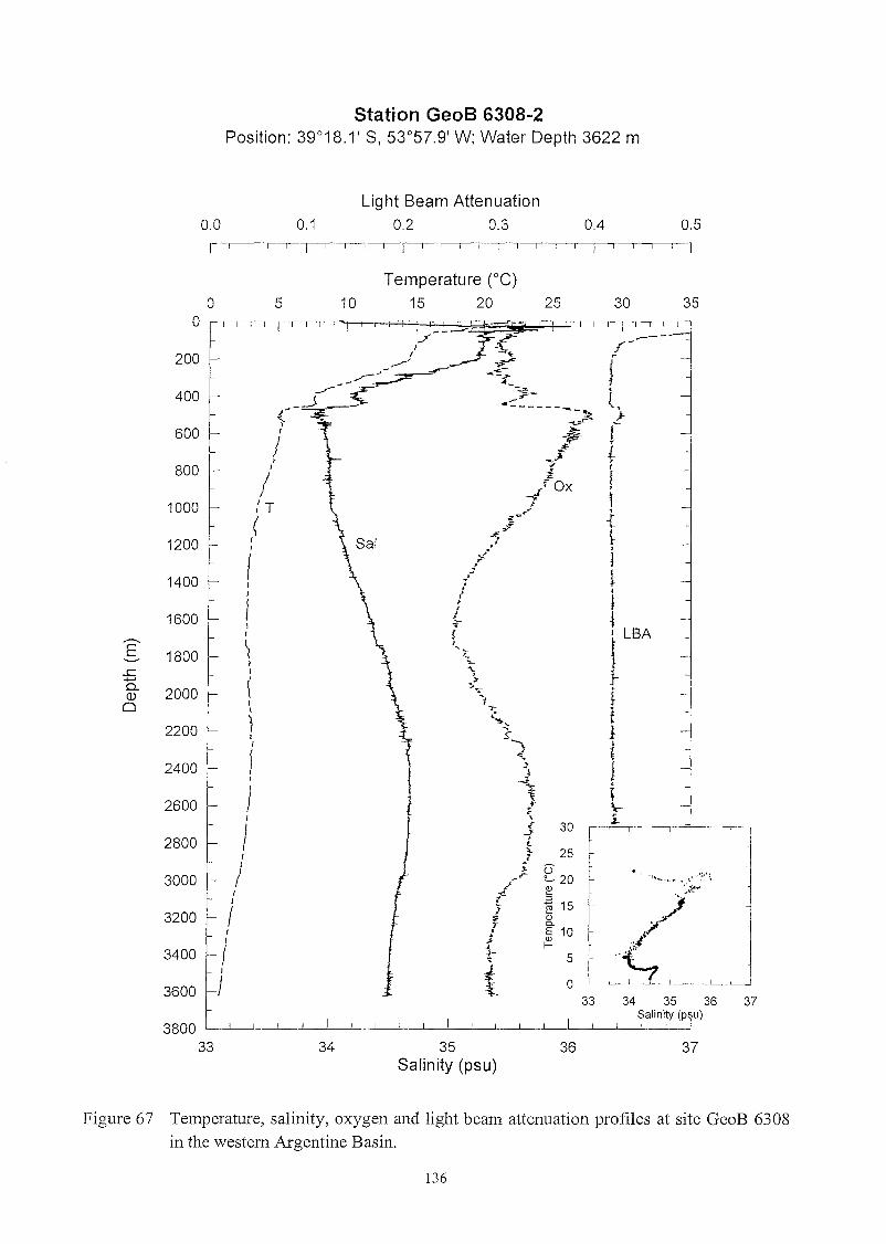
Station GeoB 6308-2Position: 39°18.1' S, 53°57.9' W; Water Depth 3622 m

Light Beam Attenuation0.0 0.1 0.2 0.3 0.4 0.5

I I I I I I I I I I I I I I I I I I I I I I I I

Temperature (OC)

0 5 10 15 20 25 30 350

<-- .----~

./-200 '" ~-r }-<~:;.

.....-400 ---- ~- t.--> ........

1.'- --------~

J-~., ~ r600 , ;"...

J ~ .,.~ t->

800 I -f,

I fOX f1000 ,'T -t t

" 1

(.;r~ {

s; ,..F

~1200 I ,I

.!',

I f1400 ~J 1I

,J

~I II

1600 L lI ..J T I LBA..........~

,tE 1800

,~

,~.......... I ~-

..c I '-; }-...... { "Cl.. ">2000 -.- tQ) '10 I

\ '"l; f~ """-,

2200 I l-.. 1I ,

fc~'" {

2400 ") !, -...J 1 t

2600 / t \--I \ i-I E 30

I .J ~~--.---,-,--

2800 t~ 25 L.

I } l/ ~ ü.... , .;1...... " ... i ~l ":--"t3000 " ~ 20

"t-l,

~ L ) ..~"JI :::l

3200 I 'j '§ 15,; <ll

1 Cl. ../I E 10I J <ll ..rI .I I- "<r3400 -r 5 -

~

I iI -t 0 I , !-....L..-......

360033 34 35 36 37

Salinity (psu)

380033 34 35 36 37

Salinity (psu)

Figure 67 Temperature, salinity, oxygen and light beam attenuation profiles at site GeoB 6308in the western Argentine Basin.

136

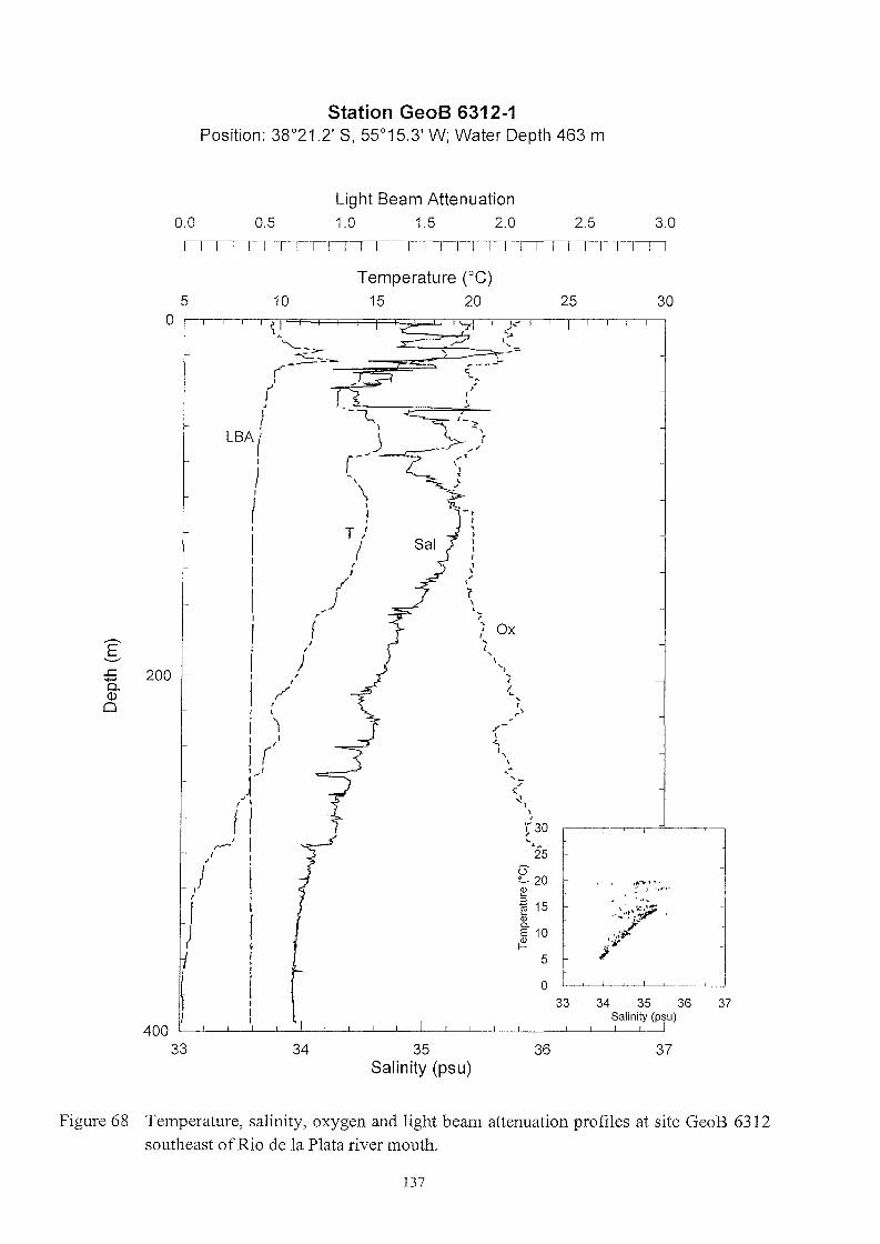
Station GeoB 6312-1Position: 38°21.2' S, 55°15.3' W; Water Depth 463 m

0.0 0.5

Light Beam Attenuation1.0 1.5 2.0 2.5 3.0

I I I I I I I I I I I I I I I I I I I I I I I I I I I I I

37

30

37

,~..~ 1 ....:' .' 'd"~

34 35 36Salinity (psu)I !---.::.J

25

33

36

5 -

o

13e...... 20~

~ 15Gi0-E 10~

".~25

po

-,I,,I\II

\,­,'r\,

?

/ Ox"{,

\

"",<.,

{, \r

;r\J,,\

\

35Salinity (psu)

Temperature (Oe)15 20

r-~

\1

T /

!,}

/)

r

34

f,

)r

/

("

(',

ILBA(

I

II,

I

II

III

II

II

!I

I ')I I

Ir'j~1

()I I

rv--' I

,/ Ir I

) III

I,-------,-----,--------l.-L

200

40033

Figure 68 Temperature, salinity, oxygen and light beam attenuation profiles at site GeoB 6312southeast ofRio de la Plata river mouth.

137

uppelIDost 470 m is the Wal111 (up to 22°C) and saline (up to 35.5 psu), but low oxygenatedSouth Atlantic Central Water (SACW). Strong gradients in temperature, salinity and oxygenmark the bottom of the SACW. Between 470 and 1100 m a salinity minimum (33.9 psu) andoxygen maximum indicate the characteristics of the Antarctic Intermediate Water (AAIW).Below, the nOlihward flowing, low oxygenated Circumpolar Deep Water (CDW) is subdividedby the thick layer of NOlih Atlantic Deep Water (NADW) into an upper and lower branch.UCDW and LCDW cores are each indicated by the oxygen minima at 1600 and 3500 m waterdepth, respectively. The NADW between 2000 and 3100 m exhibits only half of the thicknesslmown from WOCE seetions in the eastem Atlantie at about the same latitude (SIEDLER et al.,1996). This is due to the strong influenee of Antaretie Bottom Water in the deep ArgentineBasin.

From the distinetly varying parameters in the upper 200 m at site GeoB 6308 it is evident thatthis surface layer is multiple struetured due to a steplike admixture of freshwater delivered by theRio de la Plata. A detailed view on this eomplex pattem is presented by the nearby profile of theshallow water station GeoB 6312 whieh is located SE of the Rio de la Plata river mouth. Startingfrom relatively low salinities at the sea surface, repeated minima in salinity, whieh coincide withlevels of deereasing temperature, show several pulses of fresh water input down to a water depthof 25 m. Some of these layers are assoeiated with maxima in the light beam attenuation due tohigher plankton eoneentrations aceumulating on pyenoelines. The long-tenn thennocline oeeursin 150 m water depth at GeoB 6312 and in 200 m water depth at GeoB 6308. It is not clear yet,whether the relatively cold and less saline layer between 25 and 50 m belong to water of theMalvinas Confluence, which was located further south during the period of the Cruise M46/3.However, the CTD profiles give an impression, how eomplicated the hydrographie dynamies arein the upper water eolumn, especially in this area close to the Rio de la Plata estuary.

4.3.2 Water Sampling

(M. Segl)

At 12 stations a rosette with 18 water sampIers (eaeh 10 liters volume) was used to obtain watersampIes from different water depths for the analysis of stable earbon and oxygen isotopes, nutri­ents, dinoflagellates, eoeeolithophorides and, at one station, nannoplankton.

For carbon isotopes, 2 x 50 ml ofwater from each sampIer were filled into a glass bottle, eare­fully avoiding air bubbles in the filling tube and in the bottle to minimize the exchange of C02between water and air. The stable isotope sampIe was always taken immediately after the sam­pIer was opened to avoid degassing of C02 from the water. The sampIes were poisoned with0.5 ml of saturated HgCh solution. After the poisoning all sampIes were sealed airtight withmelted paraffin. The sampIes for oxygen isotope analysis were treated similarly, but were notpoisoned. The sampIes for nutrient measurements were filled into 10 ml PE bottles. The nutrientswere measured within two hours after sampling (see Chapter 4.3.3).

For coccolithophorides investigations, 2 liters ofwater were filled into a PE bottle and filtered(see Chapter 4.3.8.). Extra rosette profiles were run for particulate organic matter analyses (seeChapter 4.3.6) and dinoflagellates studies (see Chapter 4.3.7).

138

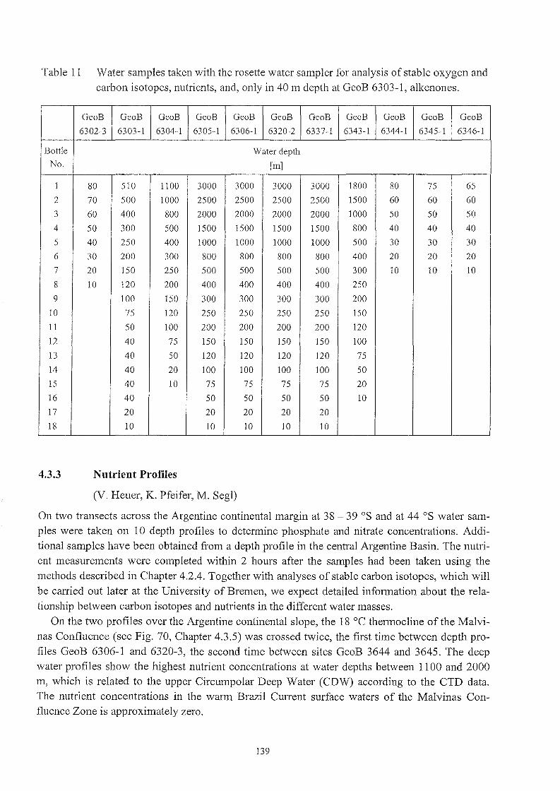
Table 11 Water sampIes taken with the rosette water sampIer for analysis of stable oxygen andcarbon isotopes, nutrients, and, only in 40 m depth at GeoB 6303-1, alkenones.

GeoB GeoB GeoB GeoB GeoB GeoB GeoB GeoB GeoB GeoB GeoB

6302-3 6303-1 6304-1 6305-1 6306-1 6320-2 6337-1 6343-1 6344-1 6345-1 6346-1

Bott1e Water depthNo. [m]

1 80 510 1100 3000 3000 3000 3000 1800 80 75 65

2 70 500 1000 2500 2500 2500 2500 1500 60 60 60

3 60 400 800 2000 2000 2000 2000 1000 50 50 50

4 50 300 500 1500 1500 1500 1500 800 40 40 40

5 40 250 400 1000 1000 1000 1000 500 30 30 30

6 30 200 300 800 800 800 800 400 20 20 20

7 20 150 250 500 500 500 500 300 10 10 10

8 10 120 200 400 400 400 400 250

9 100 150 300 300 300 300 200

10 75 120 250 250 250 250 150

11 50 100 200 200 200 200 120

12 40 75 150 150 150 150 100

13 40 50 120 120 120 120 75

14 40 20 100 100 100 100 5015 40 10 75 75 75 75 2016 40 50 50 50 50 1017 20 20 20 20 2018 10 10 10 10 10

4.3.3 Nutrient Profiles

(V. Heuer, K. Pfeifer, M. Segl)

On two transects aeross the Argentine eontinental margin at 38 - 39 oS and at 44 oS water sam­pIes were taken on 10 depth profiles to determine phosphate and nitrate eoneentrations. Addi­tional sampIes have been obtained from a depth profile in the central Argentine Basin. The nutri­ent measurements were completed within 2 hours after the sampIes had been taken using themethods deseribed in Chapter 4.2.4. Together with analyses of stable earbon isotopes, whieh willbe earried out later at the University of Bremen, we expeet detailed information about the rela­tionship between earbon isotopes and nutrients in the different water masses.

On the two profiles over the Argentine eontinental slope, the 18°C thermocline of the Malvi­nas Confluenee (see Fig. 70, Chapter 4.3.5) was crossed twiee, the first time between depth pro­files GeoB 6306-1 and 6320-3, the seeond time between sites GeoB 3644 and 3645. The deepwater profiles show the highest nutrient eoneentrations at water depths between 1100 and 2000ffi, whieh is related to the upper Cireumpolar Deep Water (CDW) aeeording to the CTD data.The nutrient eoneentrations in the warm Brazil Current surfaee waters of the Malvinas Con­fluenee Zone is approximately zero.

139

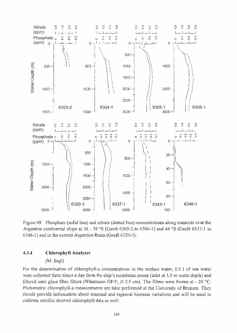
~ N '"o ci ei 0I I I I I I I

000 0ci ......: N cr1

o

2000

1000

o 0 0 0ci ~ N c0

500

o

1500 -

1000

2500

2000

I ,,,,

I I I I I I I

o 0 0 0o ......: N c0

~ N '"o 0 cl 0

o I I I I I I I

500

1000

I { I I I I !

o 0 0 0cl ,.; N M

1000

500

Nitrate(ppm)

Phosphate 0 ;; 6 6(ppm) 0 I I I I I I I

.c.....0­(1)

o

6303-21500

6304-11500 3000

6305-13000

6306-1

,,,,,

6346-1

o 0 0 0o ......: N M

..- N (") "'to ci ci 0 0I I I ! I t I I I

20

40

60

I\\IIIIIIII 80

I 6343-1100

o 0 0 0ci ......: N (V)

o

500

1000

1500

--,-<\

,,,,,,:I,,,,,,,,

I,,,,,,,,,,,,,,,,:,i 6337-1: 2000

o 0 0 0ci ......: N M

-r- N ("') '<;j"

o ci ci 0 ciI I I I I I I I I

500

1000

1500

2000

.........1

,,,,,\,,,,,

I,I,,,,,,,,,,,,,,,,,,,,

: 2500

\ 6320-3\ 3000

o 000o ~ N er?

1000

2000

3000

Nitrate(ppm)

~ N '"Phosphate 0 6 6 6

(ppm) 0 I,_~ I I I I I 0

.c.....0­(1)

o

Figure 69 Phosphate (solid line) and nitrate (dotted line) concentrations along transeets over theArgentine eontinental slope at 38 - 39 oS (GeoB 6303-2 to 6306-1) and 44 oS (GeoB 6337-1 to6346-1) and in the eentral Argentine Basin (GeoB 6320-3).

4.3.4 Chlorophyll Analyses

(M. Segl)

For the detennination of ehlorophyll-a eoneentrations in the surface water, 0.5 I of sea waterwere eolleeted three times a day from the ship's membrane pump (inlet at 3.5 m water depth) andfiltered onto glass fibre filters (Whatmann GF/F, 0 2.5 cm). The filters were frozen at - 20 oe.Photometrie chlorophyll-a measurements are later perfonned at the University of Bremen. Theyshould provide infonnation about seasonal and regional biomass variations and will be used tocalibrate satellite derived chlorophyll data as weIl.

140

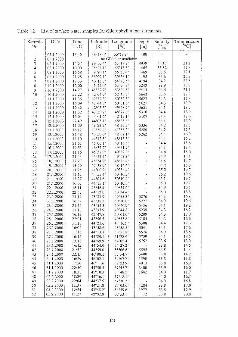
Table 12 List of surface water sampies far chlorophyll-a measurements.

Sampie Date Time Latitude Longitude Depth Salinity TemperatureNo. [UTC] [S] [W] [m] [%0] [0C]

1 05.1.2000 13:40 38°18.0' 55°19.3' 400 - -2 05.1.2000 110 GPS data available3 06.1.2000 14:57 39°50.4' 53°13.8' 4938 35.17 21.24 08.1.2000 10:00 38°21.1' 55°15.3 ' 465 33.82 19.85 08.1.2000 16:58 39°20.1 ' 55°33.4' 469 33.6 19.16 08.1.2000 21:28 55°09.1' 39°38.1 ' 1195 33.6 20.97 09.1.2000 17:33 40°13.8' 54°20.5' 4194 34.2 22.88 10.1.2000 12:00 41°22.0' 53°50.9' 5243 33.9 15.89 10.1.2000 14:27 41°37.7' 53°30.5' 5414 34.6 21.110 10.1.2000 22:22 42°04.0' 52°43.9' 5642 33.5 17.911 11.1.2000 11:35 42°37.3' 50°30.8' 5623 34.3 17.812 11.1.2000 16:09 42°44.5' 50°01.6' 5627 34.3 18.013 11.1.2000 19:42 42°05.5' 49°38.7' 5631 34.1 18.514 12.1.2000 11 :32 43°39.7' 48°27.6' 5310 34.4 16.915 12.1.2000 16:04 44°01.6' 48°17.1 ' 5107 34.4 17.016 12.1.2000 22:49 44°05.1' 48°35.6' .. 34.4 16.017 13.1.2000 11:09 43°23.2' 48°20.2' 5336 34.2 17.318 13.1.2000 16: 12 43°39.7' 47°55.9' 5280 34.2 17.519 13.1.2000 21:48 43°50.0' 48°09.1' 5262 34.4 16.920 15.1.2000 11:10 44°12.8' 48°15.5' .. 34.4 16.221 15.1.2000 21:51 45°06.1 ' 48°15.5' .. 34.4 15.822 16.1.2000 19:53 46°37.7' 49°31.7' .. 34.1 13.423 17.1.2000 11: 16 45°37.9' 49°32.3 ' .. 34.4 15.024 17.1.2000 21 :43 45°12.4' 49°03.3' .. 34.4 15.125 18.1.2000 12:27 45°34.9' 48°28.4' .. 34.4 14.726 19.1.2000 13:50 45°38.9' 48°14.4' .. 34.4 15.827 20.1.2000 11 :25 44°00.9' 49°56.4' 35.2 19.728 21.1.2000 12:12 43°55.4' 50°10.3' .. 35.2 19.629 21.1.2000 13:27 44°01.6' 50°10.4' .. 35.1 19.530 21.1.2000 16:07 44°15.1 ' 50°10.5' .. 35.0 19.731 22.1.2000 16: 11 43°46.4' 49°54.6' .. 34.9 19.532 22.1.2000 22:50 44°12.0' 50°24.4' .. 35.0 18.833 23.1.2000 11: 12 43°31.9' 49°55.3 ' 5276 34.3 16.834 31.1.2000 16:57 43°35.3 ' 50°20.0' 5277 34.9 19.635 23.1.2000 21:42 43°54.3 ' 50°40.9' 5436 35.1 19.236 24.1.2000 11: 16 43°37.9' 49°44.8' 5239 34.3 16.237 25.1.2000 16:13 43°47.8' 50°01.0' 5209 34.3 17.038 25.1.2000 22:01 43°56.5 ' 49°35.8' 5184 34.3 16.639 26.1.2000 11: 15 44°21.6' 49°16.9' 5308 34.4 17.337 26.1.2000 16:04 43°58.6' 48°58.5' 5041 34.1 17.638 27.1.2000 11: 15 44°13.1 ' 50°51.8' 5576 34.9 18.539 27.1.2000 16: 15 44°20.1' 51 °28.6' 5759 34.1 18.540 28.1.2000 13:18 44°49.9' 54°05.4' 5757 33.6 13.941 28.1.2000 16:15 44°54.0' 54°27.3' .. 33.8 14.542 28.1.2000 21:52 44°59.0' 55°06.6' 5595 33.8 14.443 29.1.2000 22:15 46°08.1 ' 57°54.7' 3400 33.8 14.244 30.1.2000 16:29 46°02.1 ' 59°07.7' 1590 33.8 11.845 31.1.2000 17:50 46°11.6' 57°23.9' 4013 33.8 16.946 31.1.2000 22:50 44°50.5' 57°45.7' 3400 33.9 16.047 01.2.2000 18:31 45°10.3' 58°48.5' 1642 34.0 11.748 02.2.2000 18:39 44°36.1' 57°18.1 ' .. 34.0 16.749 02.2.2000 22:04 44°37.5' 57°30.3 ' .. 34.0 16.850 03.2.2000 11:37 44°21.8 ' 57°03.6' 4284 33.8 17.051 04.2.2000 12:54 43°48.2' 58°59.6' 1977 33.8 12.952 05.2.2000 11 :27 42°02.8' 60°53.1' 72 33.8 20.0

141

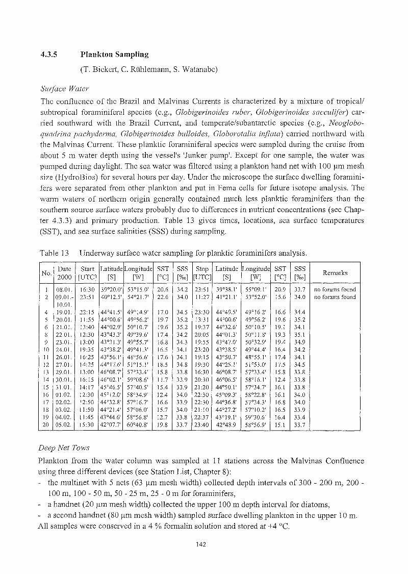
4.3.5 Plankton Sampling

(T. Bickeli, C. RühlemaIID, S. Watanabe)

SUlface Water

The confluence of the Brazil and Malvinas Currents is characterized by a mixture of tropical/

subtropical foraminiferal species (e.g., Globigerinoides ruber, Globigerinoides sacculifer) car­ried southward with the Brazil Current, and temperate/subantarctic species (e.g., Neoglobo­quadrina pachyderma, Globigerinoides bulloides, Globorotalia inflata) carried nOlihward withthe Malvinas Current. These planktic foraminiferal species were sampled during the cruise fromabout 5 m water depth using the vessel's 'Junker pump'. Except for one sampIe, the water was

pumped during daylight. The sea water was filtered using a plankton hand net with 100 11m mesh

size (HydroBios) for several hours per day. Under the microscope the surface dwelling foramini­

fers were separated from other plankton and put in Fema cells for future isotope analysis. The

wann waters of northem origin generally contained much less planktic foraminifers than thesouthem source surface waters probably due to differences innutrient concentrations (see Chap­ter 4.3.3) and primary production. Table 13 gives times, locations, sea surface temperatures

(SST), and sea surface salinities (SSS) during sampling.

Table 13 Underway surface water sampling for planktic foraminifers analysis.

No.Date Start Latitude Longitude SST SSS Stop Latitude Longitude SST SSS

Remarks2000 [UTC] [S] [W] [0C] [%0] [UTC] [S] [W] [0C] [%0]

1 08.01. 16:30 39°20.0' 53°15.0' 20.6 34.2 23:51 39°38.1' 55°09.1 ' 20.9 33.7 no forams found2 09.01.- 23:51 40°12.5' 54°21.7' 22.6 34.0 11:27 4 1°21.1' 53°52.0' 15.6 34.0 no forams found

10.01.4 19.01. 22:15 44°41.5' 49°14.9' 17.0 34.5 23:30 44°49.5' 49°16.2' 16.6 34.45 20.01. 11:55 44°00.6' 49°56.2' 19.7 35.2 13:31 44°00.6' 49°56.2' 19.6 35.26 21.01. 13:40 44°02.9' 50°10.7' 19.6 35.2 19:37 44°32.6' 50°10.5' 19.1 34.18 22.01. 12:30 43°43.3' 49°39.6' 17.4 34.2 20:05 44°01.3' 50°11.8' 19.3 35.19 23.0 I. 13:00 43°31.3' 49°55.7' 16.8 34.3 19:55 43°47.0' 50°32.9' 19.4 34.910 24.0 I. 19:35 43°38.2' 49°41.3' 16.5 34.1 23:20 43°38.5' 49°44.4' 16.4 34.2II 26.01. 16:25 43°56.1' 48°56.6' 17.6 34.1 19:15 43°50.7' 48°55.1' 17.4 34.112 27.0 I. 14:25 44°17.6' 51°15.1 ' 18.5 34.8 19:30 44°25.1 ' 51 °53.0' 17.5 34.513 29.0 I. 13:00 46°08.7' 57°33.4' 15.8 33.8 16:30 46°08.7' 57°33.4' 15.8 33.814 30.0 I. 16:15 46°02.1 ' 59°08.6' 11.7 33.9 20:30 46°06.5' 58°16.1 ' 12.4 33.815 31.01. 14:17 45°46.5' 57°40.5' 15.4 33.9 21:20 44°50.1' 57°34.7' 16.1 33.816 01.02. 12:30 45°12.0' 58°34.9' 12.4 34.0 22:30 45°09.3' 58°22.8' 16.1 34.017 02.02. 12:50 44°32.8' 57°16.7' 16.6 33.9 22:30 44°36.8' 57°34.3' 16.8 34.018 03.02. 11:50 44°21.4' 57°06.0' 15.7 34.0 21:10 44°27.2' 57°10.2' 16.5 33.919 04.02. I 1:45 43°44.6' 58°56.8' 12.7 33.8 22:37 43°19.1' 59°30.6' 16.4 33.420 05.02. 15:30 42°07.7' 60°40.8' 19.8 33.7 23:40 42°48.9 58°56.9' 15.1 33.7

Deep Net Tows

Plankton from the water column was sampled at 11 stations across the Malvinas Confluenceusing three different devices (see Station List, Chapter 8):

- the multinet with 5 nets (63 11m mesh width) collected depth intervals of 300 - 200 m, 200 -100 m, 100 - 50 m, 50 - 25 m, 25 - 0 m for foraminifers,

- a handnet (20 /lm mesh width) collected the upper 100 m depth interval for diatoms,

- a second handnet (80 11m mesh width) sampled surface dwelling plankton in the upper 10m.All sampIes were conserved in a 4 % fonnalin solution and stored at +4 oe.

142

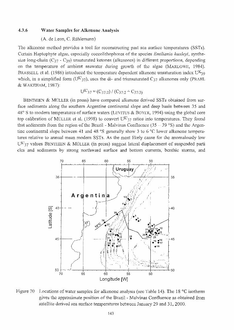
4.3.6 Water SampIes for Alkenone Analysis

(A. de Leon, C. Rühlemmm)

The alkenone method provides a tool for reconstructing past sea surface temperatures (SSTs).Certain Haptophyte algae, especially coccolithophores of the species Emiliania huxleyi, synthe­size long-chain (C37 - C39) unsaturated ketones (alkenones) in different proportions, dependingon the temperature of ambient seawater during growth of the algae (MARLOWE, 1984).BRASSELL et al. (1986) introduced the temperature dependent alkenone unsaturation index UK39which, in a simplified fonn (UK'37), uses the di- and triunsaturated C37 alkenones only (PRAHL& WAKEHAM, 1987):

UK'37 = (C37:2) / (C37:2 + C37:3)

BENTHIEN & MÜLLER (in press) have compared alkenone derived SSTs obtained from sur­face sediments along the southem Argentine continental slope and deep basin between 35 and48° S to modem temperatures of surface waters (LEVITUS & BOYER, 1994) using the global coretop calibration of MÜLLER et al. (1998) to convert UK'37 ratios into temperatures. They foundthat sediments from the region of the Brazil - Malvinas Confluence (35 - 39 OS) and the Argen­tine continental slope between 41 and 48 oS generally show 3 to 6 °C lower alkenone tempera­tures relative to annual mean modem SSTs. As the most likely cause for the anomalously lowUK'37 values BENTHIEN & MÜLLER (in press) suggest lateral displaeement of suspended partieIes and sediments by strong northward surfaee and bottom eurrents, benthic stonns, and

70 65 60 55 50

35

45

50

---~ 40

)'

Ii

I

'o"'~J

60 55

Longitude [W]65

Ar entina

35 ---- _..---

.,50 +-~+-~r--!~~--,-~-f-...::r-~-,-l-~+' ~~~~+--r--~,-4. 50

70

~ 40 -

(J)"'0:::J......:pcu-'

45

Figure 70 Locations ofwater sampies far alkenone analysis (see Table 14). The 18°C isothenngives the approximate position of the Brazil - Malvinas Confluenee as obtained fromsatellite derived sea surfaee temperatures between January 29 and 31, 2000.

143

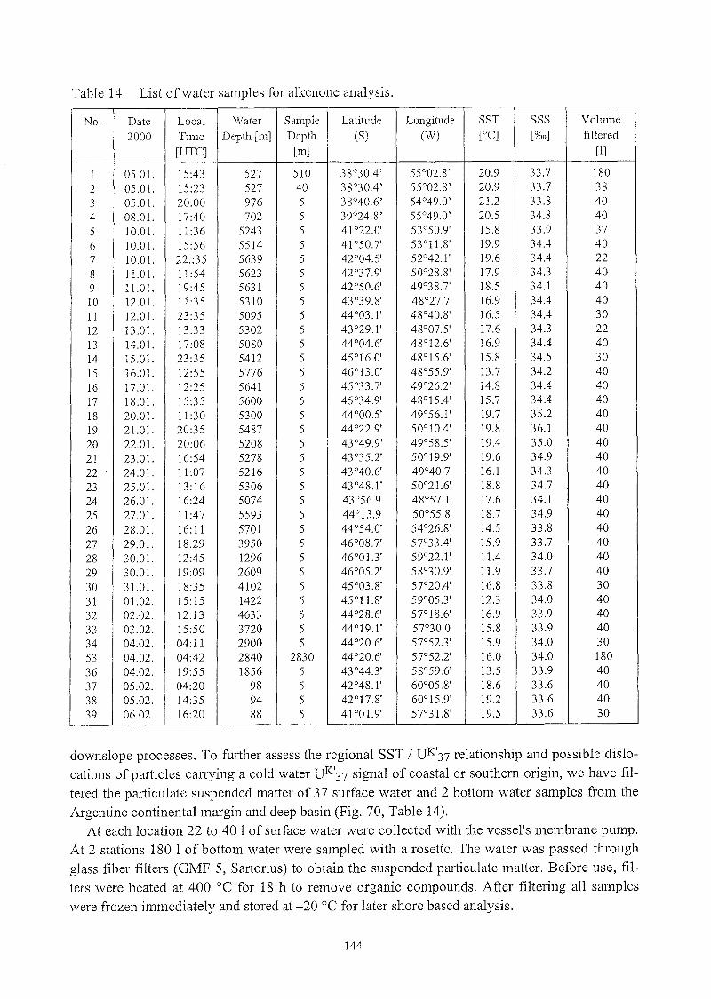
Table 14 List ofwater sampies for alkenone analysis.

No. Date Loca1 Water Samp1e Latitude Longitude SST SSS Vo1ume

2000 Time Depth [m] Depth (S) (W) [0C] [%0] filtered

[UTC] [m] [1]

1 05.01. 15:43 527 510 38°30.4' 55°02.8' 20.9 33.7 180

2 05.01. 15:23 527 40 38°30.4' 55°02.8' 20.9 33.7 38

3 05.01. 20:00 976 5 38°40.6' 54°49.0' 21.2 33.8 40

4 08.01. 17:40 702 5 39°24.8' 55°49.0' 20.5 34.8 40

5 10.01. 11:36 5243 5 41 °22.0' 53°50.9' 15.8 33.9 37

6 10.01. 15:56 5514 5 41 °50.7' 53°11.8' 19.9 34.4 40

7 10.01. 22.:35 5639 5 42°04.5' 52°42.1' 19.6 34.4 22

8 11.01. 11:54 5623 5 42°37.9' 50°28.8' 17.9 34.3 40

9 11.01. 19:45 5631 5 42°50.6' 49°38.7' 18.5 34.1 40

10 12.01. 11 :35 5310 5 43°39.8' 48°27.7 16.9 34.4 40

11 12.01. 23:35 5095 5 44°03.1' 48°40.8' 16.5 34.4 30

12 13.01. 13:33 5302 5 43°29.1' 48°07.5' 17.6 34.3 22

13 14.01. 17:08 5080 5 44°04.6' 48°12.6' 16.9 34.4 40

14 15.01. 23:35 5412 5 45°16.0' 48°15.6' 15.8 34.5 30

15 16.01. 12:55 5776 5 46°13.0' 48°55.9' 13.7 34.2 40

16 17.01. 12:25 5641 5 45°33.7' 49°26.2' 14.8 34.4 40

17 18.01. 15:35 5600 5 45°34.9' 48° 15.4' 15.7 34.4 40

18 20.01. 11 :30 5300 5 44°00.5' 49°56.1' 19.7 35.2 40

19 21.01. 20:35 5487 5 44°22.9' 50°10.4' 19.8 36.1 40

20 22.01. 20:06 5208 5 43°49.9' 49°58.5' 19.4 35.0 40

21 23.01. 16:54 5278 5 43°35.2' 50°19.9' 19.6 34.9 40

22 24.01. 11 :07 5216 5 43°40.6' 49°40.7 16.1 34.3 40

23 25.01. 13:16 5306 5 43°48.1' 50°21.6' 18.8 34.7 40

24 26.01. 16:24 5074 5 43°56.9 48°57.1 17.6 34.1 40

25 27.01. 11 :47 5593 5 44°13.9 50°55.8 18.7 34.9 40

26 28.01. 16: 11 5701 5 44°54.0' 54°26.8' 14.5 33.8 40

27 29.01. 18:29 3950 5 46°08.7' 57°33.4' 15.9 33.7 40

28 30.01. 12:45 1296 5 46°01.3' 59°22.1' 11.4 34.0 40

29 30.01. 19:09 2609 5 46°05.2' 58°30.9' 11.9 33.7 40

30 31.01. 18:35 4102 5 45°03.8' 57°20.4' 16.8 33.8 30

31 01.02. 15: 15 1422 5 45°11.8' 59°05.3' 12.3 34.0 40

32 02.02. 12: 13 4633 5 44°28.6' 57°18.6' 16.9 33.9 40

33 03.02. 15:50 3720 5 44°19.1 ' 57°30.0 15.8 33.9 40

34 04.02. 04: 11 2900 5 44°20.6' 57°52.3' 15.9 34.0 30

53 04.02. 04:42 2840 2830 44°20.6' 57°52.2' 16.0 34.0 180

36 04.02. 19:55 1856 5 43°44.3' 58°59.6' 13.5 33.9 40

37 05.02. 04:20 98 5 42°48.1' 60°05.8' 18.6 33.6 40

38 05.02. 14:35 94 5 42°17.8' 60°15.9' 19.2 33.6 40

39 06.02. 16:20 88 5 41 °01.9' 57°31.8' 19.5 33.6 30

downslope processes. To further assess the regional SST I UK'37 relationship and possible dislo­

cations of particles carrying a cold water UK'37 signal of coastal or southem origin, we have fil­

tered the particulate suspended matter of 37 surface water and 2 bottom water sampies from the

Argentine continental margin and deep basin (Fig. 70, Table 14).At each location 22 to 40 1of surface water were collected with the vessel's membrane pump.

At 2 stations 180 1 of bottom water were sampled with a rosette. The water was passed throughglass fiber filters (GMF 5, Sartorius) to obtain the suspended particulate matter. Before use, fil­

ters were heated at 400 oe for 18 h to remove organic compounds. After filtering all sampies

were frozen immediately and stored at -20 oe for later shore based analysis.

144

4.3.7 Dinoflagellates

(E. Eades, N. Zatloukal)

One of the major groups in the marine phytoplankton is represented by dinoflagellates. These

unicellular, biflagellate organisms undergo two different stages during their life cycle: a vegeta­

tive-thecate stage and a resting cyst stage which can either be calcareous or organic. Dinoflagel­lates in the motile vegetative thecate stage usually consist of cellulose, the only exception being

the calcareous walled vegetative coccoid Thoracosphaera heimii. During the cruise phytoplank­ton samples were collected from the top of the water column, ranging from the surface to 150 m

depth. They were analysed on the content of living dinoflagellates, especially calcareous resting

cysts. The main interest lies in their lateral and vertical distribution and the interaction of thespecies association and the related environmental parameters, such as temperature, salinity and

light. This may lead to a better paleoceanographic interpretation of the fossil assemblages of

dinoflagellates. For this reason also sediment samples were taken from the multicorer.

Membrane Pump

Surface water was sampled with the ship's membrane pump on transit between stations threetimes per day for about 3 hours (Table 15; a - moming, b - midday, c - aftemoon). The water was

continuously passed through a 100 flm gauze to remove larger plankton. It was then filtered

through 10 flm gauze and collected in all vessel. The water capacity which ran through the fil­

ters was measured with a water volume counter. The liter of seawater was filtered down with the

vacuum pump system, through a 5 flm polycarbonate filter to 100 ml, then stored together with

the filter in black 250 ml Nalgene polycarbonate flasks. Samples were examined for their cal­

careous dinoflagellate content. Unicellular cultures were established in polyterene Cell Wells

with different culture media (f/2 35%0, K 35%0, filtered seawater and mixtures of culture mediaand seawater). Individual specimens were then selected, placed in the cultures, and stored using

the day/night cycle and temperatures around 20°C. After isolation of living forms, the samples

were fixed with 5.5 ml formaldehyde (37 %) and stored in the dark at 4°C. These cultures will

form the basic for growth experiments which will be carried out under controlled 1aboratory con­

ditions in order to obtain insight in process influencing the cyst formation.

Rosette and CTD

At 6 stations water samples were collected with a Rosette (HydroBios No. 436918A; 18 10 1Nis­kin bottles from 7 standard water depths (150, 120, 100, 75, 50, 20, 10 m; Table 16). 54 liters

were taken from every depth. The obtained seawater was passed through a 100 flm sieve andthen filtered with 5 flm polycarbonate filters using the vacuum pump system. The samples were

fmiher treated as those taken from the membrane pump. For the determination of chlorophyll-a

concentration 4 liters of water from each depth were filtered through special glass microfibre,

folded tagether, patiially dried then wrapped in aluminium foil. They were stored at -20°C.

ChlorophYll-a measurements will be carried out later at the University ofBremen.

At all rosette stations, a Seacat SBE 19 CTD profiler with a supplementary dissolved oxygen

sensor and a light beam transmissiometer was used. Variations in association composition of

dinoflagellates will be correlated to the CTD data to gain insight in environmental factors influ­encing their distribution in the water column.

145

Multicorer

At 17 stations sampIes were taken from one large tube (10 cm diameter) of the multicarer. It was

cut into sections of 1 cm and stored at 4°C. The distribution patterns of dinoflagellate cysts in

the sediment in relation to environmental characteristics are of interest for further investigations.

The sampIes will be examined at the University ofBremen.

Results

Calcareous dinoflagellates were observed in most water sampIes throughout the cruise, although

in extremely 10w numbers. In general sampIes from the membrane pump contained the greatest

abundance, however calcareous dinoflagellates were not present in the initial sampIes, probably

due to freshwater discharge from the Rio de la Plata. They first appeared at around 38°21' S /

55°15' W. No calcareous dinoflagellates were seen in the first rosette, but they were present at all

other stations. Organic dinoflagellates were observed in many of the sampIes taken with both the

membrane pump and the rosette, often in very high numbers. It was noticed that, although there

was several species, one species largely dominated.

Table 15 Surface water sampling (membrane pump) far dinoflagellate analysis.

SampleStart I End Start I End Start and End

Temperature SalinityVolume

of Filtration of Filtration of Filh'ation filteredNo.

[UTC] Latitude [S] Longitude [W][CO] [%0]

[1]

1/5/a 12:20 115:01 38°07.04' 138°28.05' 55°34.05' I 55°06.07' 20.1 33.7 1911/6/a 10:20 I 13:40 39°28.92' I 39°48.96' 53°43.27' I 53°15.92' 21.1 33.9 2691/61b 19:02 I 22:24 39°49.50' 139°25.82' 53°15.09' I 53°46.81' 21.6 35.4 275

1/7/81b 17:12/09:44 39° 16.44' I 38°22.02' 53°60.00' 155°14.09' 22.6 34.3 5641/8/a 11:12/14:06 38°20.96' I 38°52.19' 55°15.29' I 55°28.19' 20.7 33.8 3881/81b 14:20 I 17:50 38°54.94' 139°25.02' 55°29.02' I 55°26.06' 19.3 33.8 1461/8/e 19:30 I 21:50 39°26.02' 139°38.22' 55°28.04' I 55°09.24' 20.9 33.8 3581/91b 15:59 117:05 40°07.21' 140°12.60' 54°31.35' I 54°21.52' 22.8 34.3 1811/10/a 10:04 I 13:34 41°09.40' 141°35.93' 54°01.81' I 53°32.38' 17.3 33.8 3891/101b 14:51 118:01 41°40.45' 141°54.45' 53°26.55' I 53°07.41' 21.4 34.9 2631/10/e 18:21 122:13 41°55.60' 142°03.66' 53°05.92' 152°45.29' 17.5 33.9 3621/111b 16:04 116:24 42°44.47' 142°45.03' 50°02.24' I 50°00.04' 18.1 34.3 501/11/e 19:34 I 19:49 42°50.30' 142°50.70' 49°39.50' 149°37.90' 18.4 34.2 501/12/a 12:20 I 14:55 43°43.95' 143°56.21' 48°25.59' 148°19.87' 17.1 34.4 1251/121b 17:13/19:51 44°07.05' 144°12.52' 48°14.35' I 48°17.63' 17.0 34.3 971/12/e 20:20 I 22:22 44°11.24' 144°06.28' 48°20.56' 148°32.89' 16.1 34.4 351/13/a 09:43 I 12:55 43°23.22' 143°26.52' 48°30.21' 148°10.30' 17.6 34.1 2201/131b 13:13 116:31 43°27.80' 143°41.09' 48°08.93' I 47°54.73' 17.5 34.2 3401/13/e 16:53 119:50 43°42.45' 143°50.00' 47°53.13' 147°55.14' 17.6 34.1 3491/14/a 10:34 114:02 43°39.99' 144°00.07' 48°22.19' 148°11.03' 16.6 34.4 4451/15/a 11:43 114:49 44°15.67' 144°31.20' 48°15.63' 148°15.58' 16.3 34.4 1911/151b 15:11 I 17:29 44°33.00' 144°44.68' 48°15.64' 148°15.61' 16.2 34.3 2591/15/e 17:47 I 21:16 44°46.24' 145°03.10' 48°15.56' 148°15.66' 15.7 34.4 1191/16/a 10:30 115:00 46°06.03' 146°20.33' 48°45.80' 149°06.40' 13.6 34.2 3641/161b 15:13 118:31 46°21.05' 146°32.79' 49°07.45' 149°24.58' 13.7 34.3 4601/16/e 18:35/21:36 46°33.03' 146°43.61' 49°24.95' 149°40.65' 13.9 34.2 4321/17/a 10:48 113:57 45°39.71' 145°28.11' 49°34.63' 149°17.94' 15.1 34.4 2631/17/b 14:15/17:55 45°26.97' 145°13.96' 49°16.32' I 48°57.95' 14.4 34.3 3371/17/e 18:15/21:17 45°13.09' 145°10.25' 48°56.41' 149°02.19' 15.2 34.4 2581/18/a 10:44 I 13 :44 45°20.32' I 45°34.00' 48°29.26' 148°15.06' 14.8 34.4 1971/19/a 16:18 118:39 45°32.51' 145°07.52' 48°21.68' I 48°21.57' 15.8 34.4 136

146

Table 15 continued

SampieStart I End Start I End Start and End

Temperature SalinityVolume

of Filtration of Filtration of Filtration filteredNo.

[UTC] Latitude eS] Longitude [W][CO] [%0]

[1]

l/19/b 18:49 I 22: 10 45°05.74' 144°52.42' 48°21.63' 149°00.49' 16.0 34.4 131l/20/e 19:22 I 22:15 43°53.69' 143°30.00' 49°59.96' 149°50.03' 19.9 35.3 156l/2l/a 11 :03 I 14:05 43°49.86' 144°04.93' 50°10.40' I 50°10.42' 19.5 35.2 1721/21/b 14:21 I 17:48 44°06.36' /44°23.59' 50°10.38' I 50°10.50' 19.7 35.1 1401/2l/e 18:23 121:20 44°26.41' /44°39.90' 50°10.37' I 50°12.29' 19.8 34.8 222l/22/a 10:38 114:55 43°50.53' 145°41.77' 49°47.75' 149°49.12' 19.5 34.9 171l/22/b 15:11 I 18:16 43°42.79' 143°54.38' 49°50.29' I 50°03.78' 19.1 34.5 300l/22/e 18:32 I 21:40 43°55.47' 144°07.62' 50°05.04' I 50°19.21' 19.4 35.2 172l/23/a 10:24 I 13 :39 43°31.34' 143°31.22' 49°31.97' 150°01.20' 16.5 34.4 244l/23/b 14:12/17:22 43°31.11' 143°37.10' 50°05.06' I 50°22.00' 18.4 34.4 208l/23/e 17:39/20:18 43°38.19' 143°48.76' 50°23.34' 150°34.84' 19.4 34.9 145l/24/a 10:37 114:00 43°35.94' 149°40.32' 49°38.49' 149°40.32' 16.2 34.2 94l/25/a 10:50 114:16 43°38.37' 143°48.06' 50°38.62' I 50°14.59' 18.8 34.9 2991/26/a 10:37 113:37 44°24.58' 144°10.39' 49°19.25' 149°07.96' 17.9 34.4 3441/26/b 14:27 116:22 44°06.54' 143°57.18' 49°04.85' 148°57.31' 17.3 34.3 196l/26/e 18:29 I 22:16 43°48.67' 143°54.78' 48°48.67' 149°16.34' 17.0 43.1 218l/27/a 09:49 I 13:06 44°11.09' 144°15.80' 50°41.34' I 51 °05.36' 18.8 35.0 304l/27/b 13:20 116:14 44°16.10' 144°20.17' 51°07.06' 151 °28.64' 19.1 34.9 314l/27/e 16:30 I 19:34 44°20.54' 144°24.98' 51°30.56' 151°53.56' 18.4 34.2 349l/28/a 10:17 113:21 44°45.66' 144°50.03' 53°42.68' 154°05.71' 14.5 33.8 361l/28/b 13:41 I 17:34 44°50.56' 144°56.00' 54°08.26' 154°37.16' 14.0 33.7 632l/28/e 17:45 120:59 44°56.28' 144°59.94' 54°38.54' 155°02.30' 14.4 33.7 4722/l/a 13:10 114:58 45°11.98' 145°11.73' 58°45.89' 159°05.00' 11.8 34.0 2102/l/b 17:20 I 20:20 45°11.22' 145°09.45' 59°04.86' I 58°23.51' 12.4 34.0 2452/2/a 13:14 116:46 44°32.92' 144°32.18' 57°16.05' 157°38.77' 16.5 33.9 3942/3/a 12:23 115:15 44°20.45' 144°16.16' 57°11.24' I 57°37.13' 15.6 33.9 3632/5/b 15:12 118:16 42°21.11' 142°36.19' 60°08.07' I 59°30.58' 19.0 33.6 2432/5/e 19:01 122:08 42°39.87' 142°49.62' 59°21.45' I 58°47.72' 17.7 33.7 2762/6/a 10:29 113:17 41 °36.53' 141 °34.50' 57°26.76' I 57°35.90' 15.0 33.7 2472/6/b 13:40 115:45 41°33.37' 141 °09.12' 57°35.87' I 57°32.30' 16.1 33.7 160

Table 16 Water sampies for dinoflagellate analyses (rosette casts).

GeoB Date Time Latitude Longitude Depth Temperature Sa1inity Volume filteredStation 2000 [UTC] eS] [W] [m] [0C] [%0] [1]

6302-1 05.01. 09:38-09:49 38°03.87' 55°38.72' 85 8.2 - 4875 8.1 - 4850 8.5 35.2 50.3

6302-2 10:20-10:26 20 16.0 34.85 4510 17.3 33.6 50

6306-2 06.01. 16:46-16:58 39°50.51 ' 53°13.80' 150 15.8 35.6 50100 16.4 35.6 50

6306-3 17:15-17:23 75 17.5 35.5 49

6306-4 17:41-17:49 50 18.4 36.1 5020 21.0 35.2 48.510 21.2 35.1 50

6320-2 14.01. 16:24-16:37 44°04.54' 48°12.57' 150 9.0 34.2 50120 8.8 34.3 50100 9.0 34.2 50

6320-4 19:35-19:45 75 10.6 34.2 4950 13.1 34.1 48.5

147

Table 16 continued

GeoB Date Time Latitude Longitude Depth Temperature Salinity Volume filteredStation 2000 [UTC] eS] [W] [m] [0C] [%0] [1]

6320-5 20:01-20:07 20 16.3 34.5 5010 16.9 34.1 50

6337-2 01.02. 01:07-0 1:18 44°50.61 ' 57°45.73' 150 5.1 33.9 50120 5.7 33.7 50100 6.5 33.6 50

6337-3 01:35-01:42 75 6.3 33.4 4750 7.6 33.9 50

6337-4 01:56-02:05 20 15.8 33.9 5010 16.0 34.0 50

6343-2 04.02. 14:26-14:41 43°45.95' 59°0.45' 150 5.4 33.8 50120 5.6 34.0 50100 5.7 34.1 50

6343-3 14:57-15:06 75 6.8 33.9 5050 10.0 34.1 50

6343-4 15:25-15:31 20 13.2 34.1 5010 13.3 34.0 43.2

6346-2 05.02. 10:05-10:13 41°59.97' 61°0.02' 50 11.2 33.4 5020 18.7 33.9 5010 19.6 33.9 50

4.3.8 Coccolithophorides

(M. Frenz)

Coccolithophores, autotrophie marine algae (Prymnesiophyceae), fonn a major component oftheoceanic microplankton and are one ofthe main open ocean primary producers. Their cell surfacesare covered by minute extel11al calcite scales with a complex omamentation. Coccolithophoresconstitute the single most important biogenic component of deep-sea sediments and provide flo­ral and biomarker signals documenting global change in the geological record. They are exten­sively used, therefore, in paleoecologic and paleoceanographic studies (e.g., McINTYRE & BE;WINTER & SIESSER, 1994).

Knowledge of living occurrences as well as distribution in surface sediments is aprerequisitefor paleoecologic and paleoceanographic investigations using coccoliths as proxies in Quatel11arysediments. The environmental parameters controlling these pattel11s are still poorly understoodand there have been only few studies that provided information on the distribution and occur­rence of coccolithophores in surface waters ofthe South Atlantic (MCINTYRE & BE, 1967; BAU­MANN et al., 1999).

During Cruise M46/3 an investigation of the living coccolithophore communities was carriedout in the uppermost water column. At 10 stations water sampies were taken with Niskin bottlesof the rosette generally from 6 water depths between 10 and 200 m (Table 17). In addition, sur­face water samples were obtained by the vessel's membrane pump system from about 3.5 mwater depth along the cruise track and near the water sample stations (Table 18). Mostly thesesampies were taken twice a day, in the mOl11ing and late evening.

Up to 2 1of water were immediately filtered through cellulose nitrate filters (25 mm diameter,0.45 ~m pore size) by means of a vacuum pump. Without washing, rinsing or chemical conser-

148

vation the filters were dried at 40 oe for at least 24 hand then kept pennanently dry with silicagel in transparent film to protect them from humidity. The filtered material will be used forstudies of the distribution and cOlnposition of the coccolithophores assemblages using scanningelectron microscopy (SEM). Species composition and abundance will be detennined by identifi­cation and counting on measured filter transects.

Table 17 Surface water sampling for coccolithophore analysis (rosette casts).

GeoB SampIe Latitude Longitude Water Sampling Temperature Salinity VolumeDepth Depth filtered Remarks

Station No. [S] [W] [m] [m][0C] [%0] [1]

Argentine continental slope between 38and 400 S

6302-3 I-I 38°03.81 ' 55°38.68' 96.2 10 18.65 33.61 2.0 5 mMP11-2 20 15.46 33.80 2.01-3 50 7.23 34.45 2.01-4 80 2.0 CTD 63 m

6303-2 lI-I 38°30.48' 55°2.85' 525.9 10 20.59 33.82 2.0 5mMP2II-2 20 17.26 33.98 2.0II-3 50 9.86 34.09 2.0II-4 100 8.91 34.41 2.0II-5 150 10.26 34.82 2.0II-6 200 8.45 34.62 2.0

6304-1 III-1 38°56.07' 54°27.66' 1121.3 10 22.29 34.38 2.0 5mMP4III-2 20 20.04 35.09 2.0III-3 50 19.64 36.32 2.0III-4 100 16.22 35.77 2.0III-5 150 14.60 35.60 2.0III-6 200 13.50 35.42 2.0

6305-1 IV-1 39°22.78' 53°51.50' 3997 10 19.13 34.03 2.0 5mMP5IV-2 20 16.47 34.05 2.0IV-3 50 10.09 33.95 2.0IV-4 100 14.93 35.60 2.0IV-5 150 14.66 35.62 2.0IV-6 200 13.16 35.27 2.0

6306-1 V-I 39°50.47' 53°13.81 ' 4930 10 21.16 35.10 2.0 5mMP6V-2 20 21.00 35.18 2.0V-3 50 19.01 36.04 2.0V-4 100 15.91 35.71 2.0V-5 150 15.06 35.71 2.0V-6 200 14.66 35.54 2.0

Argentme Basm

6320-1 VI-1 44°04.58' 48°12.60 5084 10 16.43 34.23 0.85 5 mMP16VI-2 20 15.25 34.18 1.2VI-3 50 10.14 34.26 2.0VI-4 100 8.07 34.19 2.0VI-5 150 7.51 34.20 2.0VI-6 200 6.05 34.14 2.0

6337-1 VII-1 44°50.59' 57°45.72' 3546 10 15.64 33.85 1.2 5 mMP 33VII-2 20 14.13 33.90 1.4VII-3 50 6.72 33.94 2.0VII-4 100 4.67 33.84 2.0VII-5 150 4.22 33.87 2.0VII-6 200 4.02 33.91 2.0

6343-1 VIII-1 43°45.36' 58°59.78' 1959 10 10.58 34.24 2.0 5 mMP 36VIII-2 20 10.23 33.91 2.0VIII-3 50 7.26 33.91 2.0VIII-4 150 4.10 33.86 2.0VIII-5 200 3.88 33.98 2.0

6344-1 IX-1 42°53.01 ' 59°59.72' 91.5 10 18.40 33.48 2.0 5 mMP 37IX-2 20 18.11 33.46 1.8

149

Table 17 cüntinued

GeoB SampIe Latitude Longitude Water Sampling Temperature Salinity Volume

Station No. [S] [W] Depth Depth [0C] [%0] filtered Remarks[m] [m] [1]

6344-1 IX-3 50 6.48 33.68 2.0IX-4 80 n.d. n.d. 2.0

6345-2 X-I 42°26.60' 60°29.90' 92.0 10 18.75 33.44 2.0 5 mMP 38X-2 20 18.74 33.43 2.0X-3 50 7.96 33.53 2.0X-4 75 n.d. n.d. 2.0

6346-1 XI-1 41°60.00' 61°00.04' 76.0 10 19.65 33.63 2.0 5 mMP 39XI-2 20 19.13 33.58 2.0XI-3 50 n.d. n.d. 2.0XI-4 65 n.d. n.d. 2.0

Table 18 Surface water sampling (membrane pump) für cüccülihüphüre analysis.

SampIe Date Time Latitude LongitudeWater Sampling

Temperature SalinityVolume

GeoB Station /Depth Depth filtered

No. 2000 (UTC) [S] [W][m] [m]

[0C] [%0][1]

Remarks

GeoB 6302/1 05.01. 12:03 38°04.68' 55°37.33' 96.7 3.5 20.0 2.0 no salinity

data2 05.01. 15:20 38°30.12' 55°03.19' 517.7 3.5 20.8 33.7 2.0 GeoB 63033 05.01. 19:02 38°37.15' 54°53.63' 829.3 3.5 21.4 33.8 1.54 05.01. 21:45 38°56.05' 54°27.64' 1119 3.5 23.0 34.2 1.8 GeoB 63045 06.01. 09:40 39°23.53' 53°49.71 ' 4013 3.5 21.5 34.0 2.0 GeoB 63056 06.01. 16:56 39°45.31 ' 53°20.79' 5159 3.5 21.8 35.4 2.0 GeoB 63067 08.01. 17:01 39°21.15' 55°31.82' 512 3.5 19.8 33.7 1.08 09.01. 23:03 40°12.77' 54°21.44' 4186 3.5 22.7 34.0 1.8 GeoB 63189 10.01. 13:00 41°22.00' 53°50.90' 5242 3.5 15.8 33.9 0.6410 10.01. 22:31 42°02.48' 52°42.09' 5639 3.5 19.7 34.3 1.311 11.01. 11 :40 42°37.35' 50°30.81 ' 5626 3.5 17.8 34.3 1.512 11.01. 19:45 42°50.60' 49°38.30' 5623 3.5 18.5 34.1 1.013 12.01. 11:40 43°40.60' 48°27.20' 5312 3.5 16.9 34.4 1.014 12.01. 21:38 44°8.10' 48°28.40' n.d. 3.5 16.3 34.4 1.015 13.01. 11: 11 44°23.20' 48°20.00' 5337 3.5 17.3 34.2 1.216 14.01. 13:50 43°57.80' 48°11.00' 5124 3.5 16.7 34.4 1.0 GeoB 632017 15.01. 22:45 45°10.70' 48°15.60' n.d. 3.5 15.9 34.4 0.818 16.01. 11:05 46°06.06' 48.46.00' 5693 3.5 13.9 34.3 1.419 16.01. 22:00 46°42.48' 49°42.38' 5923 3.5 14.0 34.3 2.020 17.01. 11 :20 45°37.75' 49°32.02' 5650 3.5 15.0 34.4 1.1521 18.01. 11: 19 45°26.40' 48°29.32' 5517 3.5 15.4 34.4 1.822 20.01. 11:25 44°00.92' 49°56.44' 5300 3.5 19.7 35.2 2.023 21.01. 11: 10 45°50.35' 50°10.42' 5265 3.5 19.5 35.2 2.024 21.01. 21 :21 44°39.90' 50°12.42' 5590 3.5 18.0 34.1 1.525 22.01. 13:05 43°40.79' 49°40.12' 5215 3.5 17.4 34.2 2.026 26.01. 19:01 43°50.22' 48°52.39' 5137 3.5 17.0 34.1 1.827 27.01. 12:33 44°14.99' 51°01.36' 5635 3.5 18.8 35.0 2.028 27.01. 23:05 44°29.89' 52°19.44' 5938 3.5 18.0 34.5 1.329 28.01. 09:27 44°44.49' 53°36.38' 5776 3.5 14.7 33.8 1.730 28.01. 21:42 44°57.86' 55°04.25' 5599 3.5 14.5 33.8 1.531 29.01. 21:05 46°08.78' 57°41.83' 3811 3.5 15.0 33.9 1.232 30.01. 10:35 46°0.24' 59°37.77' 949.2 3.5 12.2 34.0 2.033 31.01. 08:00 44°50.59' 57°45.72' 3546 3.5 15.9 34.0 1.2 GeoB 633734 01.02. 17:00 45°11.25 ' 59°05.27' 1462 3.5 12.4 34.0 1.6 GeoB 633835 03.02. 11 :40 44°21.77' 5]003.85' 4080 3.5 17.0 33.9 1.1

150

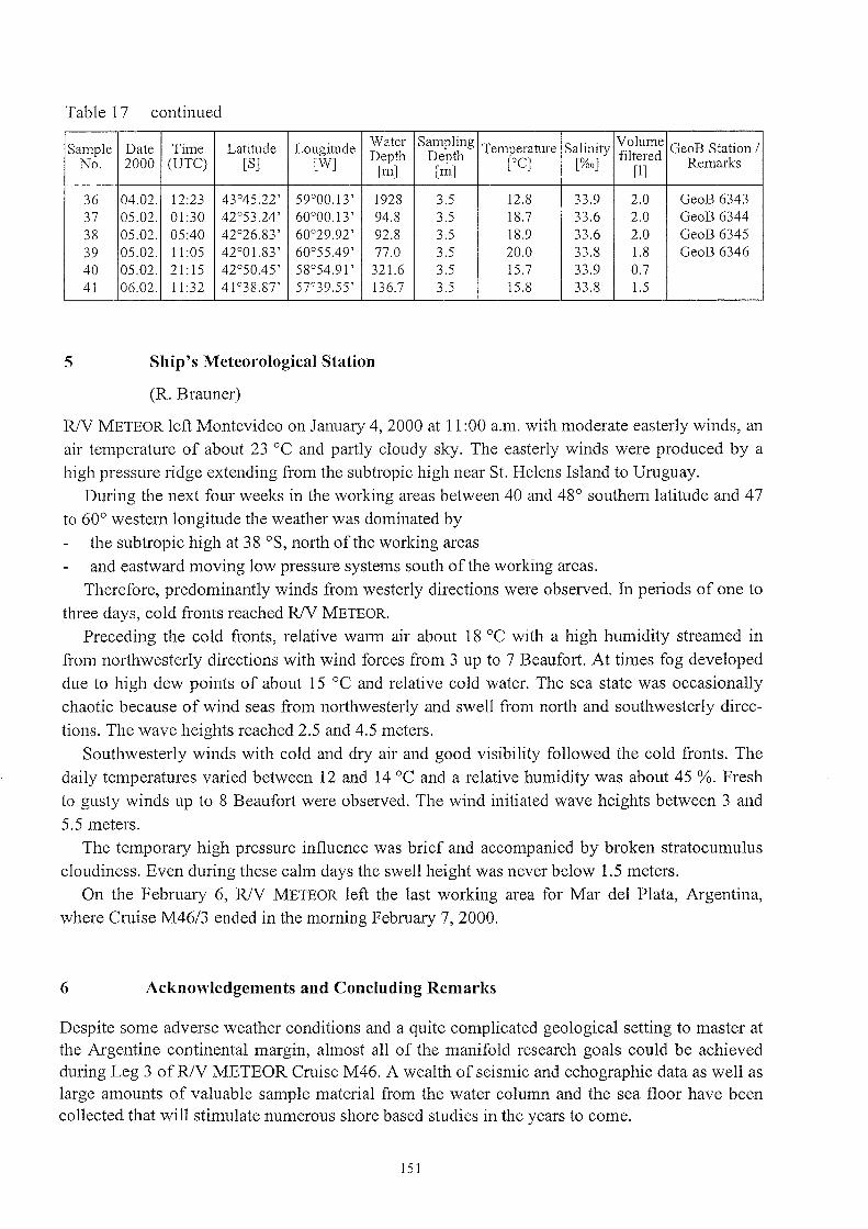
Table 17 continued

Sampie Date Time Latitude Longitude Water Sampling Temperature Salinity Volume GeoB Station /No. 2000 (UTC) eS] [W] Depth Depth [0C] [%0] filtered Remm'ks

[m] [m] [1]

36 04.02. 12:23 43°45.22' 59°00.13 ' 1928 3.5 12.8 33.9 2.0 GeoB 634337 05.02. 01:30 42°53.24' 60°00.13' 94.8 3.5 18.7 33.6 2.0 GeoB 634438 05.02. 05:40 42°26.83' 60°29.92' 92.8 3.5 18.9 33.6 2.0 GeoB 634539 05.02. 11:05 42°01.83' 60°55.49' 77.0 3.5 20.0 33.8 1.8 GeoB 634640 05.02. 21: 15 42°50.45' 58°54.91 ' 321.6 3.5 15.7 33.9 0.741 06.02. 11:32 41°38.87' 57°39.55' 136.7 3.5 15.8 33.8 1.5

5 Ship's Meteorological Station

(R. Brauner)

R/V METEOR left Montevideo on January 4,2000 at 11 :00 a.m. with moderate easterly winds, anair temperature of about 23°C and partly cloudy sky. The easterly winds were produced by ahigh pressure ridge extending from the subtropic high near St. Helens Is1and to Uruguay.

During the next four weeks in the working areas between 40 and 48° southern 1atitude and 47to 60° western longitude the weather was dominated by

the subtropic high at 38 oS, north ofthe working areasand eastward moving low pressure systems south of the working areas.

Therefore, predominantly winds from westerly directions were observed. In periods of one tothree days, cold fronts reached R/V METEOR.

Preceding the cold fronts, relative warm air about 18°C with a high humidity streamed infrom nOlihwesterly directions with wind forces from 3 up to 7 Beaufort. At times fog developeddue to high dew points of about 15°C and relative cold water. The sea state was occasionallychaotic because of wind seas from northwesterly and swell from north and southwesterly direc­

tions. The wave heights reached 2.5 and 4.5 meters.Southwesterly winds with cold and dry air and good visibility followed the cold fronts. The

daily temperatures varied between 12 and 14°C and a relative humidity was about 45 %. Freshto gusty winds up to 8 Beaufort were observed. The wind initiated wave heights between 3 and5.5 meters.

The temporary high pressure influence was brief and accompanied by broken stratocumuluscloudiness. Even during these calm days the swell height was never below 1.5 meters.

On the February 6, R/V METEOR left the last working area for Mar deI Plata, Argentina,where Cruise M46/3 ended in the moming February 7, 2000.

6 Acknowledgemellts and COllcludillg Remarks

Despite some adverse weather conditions and a quite complicated geological setting to master atthe Argentine continental margin, almost all of the manifold research goals could be achievedduring Leg 3 of R/V METEOR Cruise M46. A wealth of seismic and echographie data as weIl aslarge amounts of valuable sampIe material from the water column and the sea floor have beencollected that will stimulate numerous shore based studies in the years to come.

151

The scientific party aboard gratefully acknowledges the friendly cooperation with CaptainStefan Bülow, his officers and crew. Their perfect technical assistance substantially contributedto make this cmise a notable scientific success. We also appreciate the most valuab1e suppOli bythe Leitstelle METEOR at the University of Hamburg.

The work was funded by the Deutsche Forschungsgemeinschaft within the scope of the Son­derforschungsbereich 261 at the University ofBremen.

7 References

BAUMANN, K..-H., M. CEPEK & H. KlNKEL, 1999. Cocco1ithophores as indicators of ocean watermasses, surface water temperatures, and pa1eoproductivity - examp1es from the South Atlan­tic. In: G. Fischer & G. Wefer (eds.), Use ofproxies in pa1eoceanography: examp1es from theSouth At1antic, Springer-Verlag, Berlin, Heide1berg, 117-144.

BENTHIEN, A. & P.l MÜLLER, in press. Anoma10usly 10w alkenone temperatures caused bylateral partic1e and sediment transport in the Ma1vinas Current region, western ArgentineBasin. Deep Sea Res., 47, 2369-2393.

BOLTOVSKOY, E., 1970. Masas de agua (caracteristicas, distribucion, movimientos) en 1a super­ficie de1m Atlantico Sudoeste segun indicadores biologicos-foraminiferos. Servo Hidrogr.Naval, Argentina, Publ. H. 643, 1-99.

BOLTOVSKOY, E., 1971. Eco10gy ofthe p1anktonic foraminifera 1iving in the surface 1ayer oftheDrake Passage. Micropa1eontology, 17, 53-68.

BOLTOVSKOY, E. & S. WATANABE, 1980. Museo Argentino de Ciencias Naturales, Rev. Geol.,8,1-112.

BOYCE, R.E., 1968. Electrica1 resistivity of modem marine sediments from the Bering Sea. J.Geophys. Res., 73, 4759-4766.

BOYCE, R.E., 1976. Sound velocity - density parameters of sediment and rock from DSDP DrillSites 315 - 318 on the Line Is1ands Chain, Manihiki Plateau, and Tuamotu Ridge in thePacific Ocean. In: Schlanger, S.O., E.D. Jackson et al. (eds.), Init. Repts. DSDP, 33, 695-728.

BRASSELL, S.c., G. EGLINTON, I.T. MARLOWE, U. PFLAUMANN & M. SARNTHEIN, 1986.Mo1ecu1ar stratigraphy: a new too1 for c1imatic assessment. Nature, 320, 129-133.

FLOOD, R.D. & A.N. SHOR, 1988. Mudwaves in the Argentine Basin and their relationship to theregional bottom circu1ation patterns. Deep Sea Res., 35, 943-971.

FLOOD, R.D., A.N. SHOR & P.L. MANLEY, 1993. Morphology of abyssal mudwaves at Project'MUDWAVES' sites in the Argentine Basin. Deep Sea Res., 40, 859-888.

FROEHLICH, P.N., G.P. KLINKHAMMER, M.L. BENDER, N.A. LUEDTKE, G.R. HEATH, D.CULLEN, P. DAUPHIN, D. HAMMOND, B. HARTMAN & V. MAYNARD, 1979. Early oxidationof organic matter in pe1agic sediments of the eastern equatorial Atlantic: suboxic diagenisis.Geochim. Cosmochim. Acta, 43,1075-1090.

GRAHAM, G. & H. MAZZULLO, 1988. Handbook for shipboard sedimentologists. ODP TechnicalNote No. 8, 67p.

HOPFAUF, V. & V. SPIEß, in press. A three dimensional theory for the development and migra­tion of deep sea sedimentary waves. Deep Sea Res.

LEVITUS, S. & T. BOYER, 1994. World Ocean Atlas. 4: Temperatures, NOAA Atlas NESDIS 4.U.S. Government Printing Office.

152

MARLOWE, 1.T., 1984. Lipids as pa1eoclimatic indicators. Ph.D. Thesis, University of Bristo1,

273 p.MCINTYRE, A. & A.W.H. BE, 1967. Modern coccolithophoreae ofthe At1antic Ocean - 1. P1aco­

liths and Cyrtoliths. Deep-Sea Res., 14,561-597.MÜLLER, P.J., G. KIRST, G. RUHLAND, 1. VON STORCH & A. ROSELL-MELE, 1998. Calibration

of the alkenone paleotemperature index UK'37 based on core-tops from the eastern SouthAtlantic and the global ocean (60 0 N - 600 S). Geochim. Cosmochim. Acta, 62, 1757-1772.

PARKER, G., M.C. PATERLINI, & R.A. VIOLANTE, 1997. EI fondo marino. EI Mal' Argentino y

sus recursos pesqueros, 1, 65-87.PRAHL, F.G. & S.G. Wakeharn, 1987. Calibration of unsaturation patterns in long-chain ketone

compositions for paleotemperature assessment. Nature, 330, 367-396.SCHULTHHEISS, P.l. & S.D. MCPHAIL, 1989. An automated p-wave logger for recording fine­

scale compressional wave velocity structures in sediments. In: W. Ruddiman, M. Samthein et

al. (eds.), Proc. ODP Sei. Results, 108,407-413.SCHULZ, H.D. et al., 1991. Bericht und erste Ergebnisse der METEOR-Fahrt M16/2. Berichte,

Fachbereich Geowissenschaften, Universität Bremen, 19, 149 p.SEGL, M. et al. , 1994. Report and preliminary results of METEOR Cruise M29/1. Berichte,

Fachbereich Geowissenschaften, Universität Bremen, 58, 94 p.

SIEDLER, G., TJ. MÜLLER, R. ONKEN, M. ARHAN, H. MERCIER, RA. KING & P.M.SAUNDERS, 1996. The zonal WOCE sections in the South Atlantic. In: Wefer, G., W.H.

Berger, G. Siedler & D. Webb (eds.), The South Atlantic: Present and Past Circulation.

Springer-Verlag, Berlin, 83-104.SPIEß, V., 1993. Digitale Sedimentechographie - Neue Wege zu einer hochauflösenden Akusto­

stratigraphie. Berichte, Fachbereich Geowissenschaften, Universität Bremen, 35, 199 p.

WEFER, G. et al., 1991. Bericht und erste Ergebnisse über die METEOR-Fahrt M16/1. Berichte,

Fachbereich Geowissenschaften, Universität Bremen, 18, 120 p.WINTER, A. & W.G. SIESSER (eds.), 1994. Coccolithophores. Cambridge University Press, New

York, 242 p.

153

8 Station List M46/3

......Vl.j:o.

Station StationDate

Time [UTC]Latitude Longitude Water Depth

Sampies IGeoB Ship

2000Device seafloor Imaximum

[S] [W] [m]Core Remarks

No. No. wire length recovery

Rio de la Plata

6301-1 001 04.01. MUC 22:36 36°03,34' 55°25,21 ' 30 15 cm 5 large, 3 small tubes filled6301-2 04.01. SL6 23:05 36°03,32' 55°25,20' 30 100 cm core tube bent, geology and geophysics

Malvinas Confluence 38 - 40 oS

6302-1 002 05.01. ROS 09:41 38°03,83' 55°38,69' 96 18 sampies 6x85 m, 6x75 m, 6x50 m, dinoflagellates6302-2 05.01. ROS 10:09 38°03,81 ' 55°38,70' 97 12 sampies 6x20 m, 6x10m, dinoflagellates6302-3 05.01. ROS+CTD 10:38 38°03,82' 55°38,72' 97 8 sampies 80, 70, 60, 50, 40, 30, 20, 10 m, C13, 018,

nutrients, nannoplankton6302-4 05.01. MN 11:06 38°03,79' 55°38,61 ' 97 3 sampies 85-50, 50-25, 25-0 m, plankton >63 flm6302-5 05.01. RN 11:32 38°03,78' 55°38,49' 97 1 sampie 85-0 m, plankton >20 flm6302-6 05.01. RN 11:42 38°03,81 ' 55°38,69' 96 1 sampie 10-0 m, plankton >80 flm

6303-1 003 05.01. ROS+CTD 15:43 38°30,40' 55°02,70' 525 18 sampies 18x510 m, particulate organic matter6303-2 05.01. ROS 16:23 38°30,47' 55°02,82' 526 17samples 510,500,400,300,250,200,150,120,100,

75,50, 4x40, 20, 10 m, C13, 018, nutrients,nannoplankton

6303-3 05.01. MN 17:08 38°30,45' 55°02,83' 520 5 sampies 300-200,200-100, 100-50,50-25,25-0 m,plankton >63 flm

6303-4 05.01. RN 17:42 38°30,47' 55°02,84' 526 1 sampie 100-0 m, plankton >20 flm6303-5 05.01. RN 17:56 38°30,47' 55°02,87' 526 1 sampie 10-0 m, plankton >80 flm

6304-1 I 004 I 05.01. I ROS+CTD I 21:48 I 38°56,26' I 54°27,81' I 1109 I 15 sampies I 1100,1000,800,500,400,300,250,200,150,120, 100,75,50,20, 10 m, C13, 018,nutrients, nannoplankton

6304-2 I I 05.01. I MN I 23:25 I 38°56,25' I 54°27,87' I 1105 I 5 sampies I 300-200,200-100, 100-50,50-25,25-0 m,plankton >63 flm

6304-3 I I05.01.1 RNI

23:54 138056,50' 1 54°28,30' I 1110

I1 sampie

I100-0 m, plankton >20 flm

6304-4 05.01. RN 00:06 38°56,55' 54°28,40' 1110 1 sampie 10-0 m, plankton >80 flm

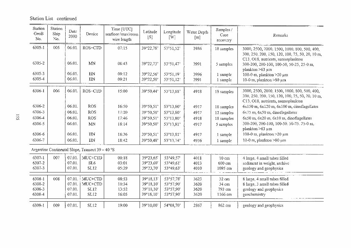
......VlVl

Station List continuedI , i i

Station StationDate

Time [UTC]Latitude Longitude Sampies /

GeoB Ship Device seafloor /maximum Water DepthCore Remarks2000 [S] [W] [m]No. No. wire length recovery

6305-1 005 06.0l. ROS+CTD 07:15 39°22,78' 53°51,52' 3986 18 sampies 3000,2500,2000,1500,1000,800,500,400,300,250,200, 150, 120, 100, 75, 50, 20, 10 m,C13, 018, nutrients, nannoplankton

6305-2 06.0l. MN 08:43 39°22,73 ' 53°51,47' 3991 5 sampies 300-200,200-100, 100-50,50-25,25-0 m,plankton >63 11m

6305-3 06.0l. RN 09:12 39°22,56' 53°51,19' 3996 1 sampie 100-0 m, plankton >20 11m6305-4 06.0l. RN 09:21 39°22,50' 53°51,12' 3991 1 sampie 10-0 m, plankton >80 11m

6306-1 006 06.01. ROS+CTD 15:00 39°50,44' 53°13,88' 4918 18 sampies 3000,2500,2000,1500,1000,800,500,400,300,250,200, 15~ 12~ 100,75,50,2~10m,C13, 018, nutrients, nannoplankton

6306-2 06.01. ROS 16:50 39°50,51 ' 53°13,80' 4917 18 sampies 6x150 m, 6x120 m, 6x100 m, dinoflagellates6306-3 06.01. ROS 17:20 39°50,50' 53°13,80' 4917 12 sampies 6x75 m, 6x50 m, dinoflagellates6306-4 06.01. ROS 17:46 39°50,51 ' 53°13,80' 4918 18 sampies 6x50 m, 6x20 m, 6x10 m, dinoflagellates

6306-5 06.01. MN 18:14 39°50,50' 53°13,81 ' 4917 5 sampies 300-200,200-100, 100-50,50-25,25-0 m,plankton >63 11m

6306-6 06.01. RN 18:36 39°50,51 ' 53°13,81 ' 4917 1 sampie 100-0 m, plankton >20 11m

6306-7 06.01. RN 18:42 39°50,48' 53°13,74' 4936 1 sampie 10-0 m, plankton >80 11m

Argentine Continental Slope, Transect 39 - 40 oS

6307-1 007 07.01. MUC+CTD 00:18 39°23,65' 53°49,57' 4011 10 cm 4 large, 4 small tubes filled6307-2 07.01. SL6 03:01 39°23,69' 53°49,61' 4013 600 cm sediment in weight, archive6307-3 07.01. SL12 05:39 39°23,70' 53°49,63' 4010 1095 cm geology and geophysics

6308-1 008 07.01. MUC+CTD 08:53 39°18,13' 53°57,78' 3623 32 cm 8 large, 4 small tubes filled6308-2 07.01. MUC+CTD 11:34 39°18,10' 53°57,90' 3620 34 cm 8 1arge, 3 small tubes filled6308-3 07.01. SL12 13:52 39°18,10' 53°57,90' 3620 793 cm geo1ogy and geophysics6308-4 07.01. SL12 16:05 39°18,10' 53°57,90' 3620 1166 cm geochemistry

6309-1 I 009 I07.01. I SL12 I 19:00 139°10,00' I 54°08,70' I 2867 I 862 cm I geology and geophysics

Station List continued

Station StationTime [UTC]

Sampies /GeoB Ship

DateDevice

seafloor / Latitude Longitude Water DepthCore Remarks

No. No.2000 maximum wire [S] [W] [m]

lengthrecovery

6309-2 07.01. MUC+CTD 20:38 39°10,00' 54°08,70' 2869 24cm 8 large, 4 smaII tubes filled

6310-1 010 07.01. MUC+CTD 23:55 39°02,67' 54°19,37' 1455 20cm 7 large, 4 smaII tubes filled6310-2 08.0I. SLI2 01:09 39°02,57' 54°19,41 ' 1456 - no recovery, core tube bent6310-3 08.01. SL6 02:21 39°02,59' 54°19,32' 1456 - no recovery

6311-16311-2

011 08.01. SL608.01. MUC+CTD

05:1105:54

38°48,89'38°48,89'

54°37,60'54°37,59'

996996

466cm25 cm

geology and geophysics8 large, 4 small tubes filled

......Vl0\

6312-1 012 08.01. MUC+CTD 10:10 38°21,20' 55°15,36' 435 26cm 8 large, 4 small tubes filled6312-2 08.01. SL6 10:52 38°21,21 ' 55°15,33' 436 349 cm geology and geophysics

6313-1 013 08.01. SL6 18:05 39°25,18' 55°26,57' 732 481 cm geology and geophysics6313-2 08.01. MUC+CTD 18:45 39°25,19' 55°26,57' 733 16 cm 6 large, 4 small tubes filled

6314-1 014 08.01. MUC+CTD 21:54 39°38,26' 55°09,27' 1187 20cm 4 large, 2 small tubes filled6314-2 08.01. MUC 22:59 39°38,22' 55°09,22' 1187 20cm 2 large, 2 small tubes filled6314-3 08.01. SL6 23:59 39°38,19' 55°09,16' 1194 no recovery

6315-1

6316-1

SL6

SL6

03:48

06:55

54°56,72'

54°49,08'

1646

2059

no recovery

no recovery

6317-1 017 09.01. SL6 10:44 40°04,83' 54°35,71 ' 3115 589 cm sediment in weight, archive

6317-2 09.01. MUC+CTD 11:36 40°04,85' 54°35,70' 3115 20 cm 7 large, 4 small tubes filled

6317-3 09.0I. SL12 14:37 40°04,83' 54°35,73' 3112 909 cm geology and geophysics

6318-1 018 09.01. SL6 18:54 40°12,60' 54°21,50' 4176 581 cm geology and geophysics

6318-2 09.01. MUC+CTD 21:10 40°12,60' 54°21,50' 4179 max. 8 cm stiff sediment stored in bags

......Vl-...J

Station List continuedI I I ,

Station StationDate

Time [UTC]Latitude Longitude Water Depth

Sampies IGeoB Ship

2000Device seafloor Imaximum

[S] [W] [m]Core Remarks

No. No. wire length recovery

6319-1 019 10.01. SL6 00:52 40°12,42' 54°21,64' 4185 386 cm geo1ogy and geophysics6319-2 10.01. SL6 04:08 40°12,38' 54°21,66' 4097 352 cm geology and geophysics

Argentine Basin - Zapio1a Drift

6320-1 020 14.01. ROS 16:01 44°04,57' 48°12,59' 5059 - not released6320-2 14.01. ROS 16:30 44°04,58' 48°12,59' 5059 18 sampies 6x150 m, 6x120 m, 6x100 m, dinoflagellates6320-3 14.01. ROS+CTD 17:51 44°04,60' 48°12,60' 5059 18 sampies 3000,2500,2000,1500,1000,800,500,400,

300,250,200, 150, 120, 100,75,50,20, 10 m,C13, 018, nutrients, nannop1ankton

6320-4 14.01. ROS 19:38 44°04,60' 48°12,56' 5058 18 sampies 6x75 m, 6x50 m, 6x20 m, dinoflagellates6320-5 14.01. ROS 20:02 44°04,61 ' 48°12,57' 5058 6 sampies 6x1°m, dinoflagellates6320-6 14.01. MN 20:23 44°04,65' 48°12,53' 5058 5 samp1es 300-200,200-100, 100-50,50-25,25-0 m,

plankton >63 ).lm6320-7 14.01. RN 20:51 44°04,67' 48°12,37' 5058 1 samp1e 100-0 m, plankton >20 ).lm6320-8 14.01. RN 21:00 44°04,67' 48°12,30' 5057 1 samp1e 10-0 m, plankton >80 ).lm

6321-1 021 14.01. SL6 22:38 44°02,40' 48°16,70' 5086 591 cm sediment in weight, archive6321-2 15.01. SLl2 01:16 44°02,39' 48°16,69' 5098 1230 cm upper 70 cm of sediment in weight,

geo1ogy and geophysics

6322-1 022 15.01. MUC 04:40 44°04,41 ' 48°15,61 ' 5061 21 cm 1 1arge, 4 small tubes fil1ed6322-2 15.01. SLl8 07:55 44°04,42' 48°15,58' 5064 1416 cm geo1ogy and geophysics

Argentine Basin - Sediment Wave Fields

6323-1 023 18.01. SL6 15:09 45°34,86' 48°15,46' 5490 586 cm sediment in weight, archive6323-2 19.01. SLl2 00:03 45°35,21 ' 48°15,51' 5480 1145 cm geo1ogy and geophysics6323-3 19.01. SLl2 04:16 45°35,25' 48°15,53' 5480 1138 cm geochemistry

6324-1 I 024 119.01. I SLl2 I 08:46 145°38,89' I 48°14,06' I 5510 I 453 cm I core tube bent, geo1ogy and geophyslCS

6324-2 SL12 12:58 48°15,32' 5490 1092 cm geo1ogy and geophysics

Station List continued

Station StationDate

Time [UTC]Latitude Longitude Water Depth

Sampies IGeoB Ship

2000Device seafloor Imaximum

[S] [W] [m]Core Remarks

No. No. wire length recovery

6325-1 025 20.01. SL6 09:25 44°01,89' 49°57,69' 5353 441 cm geology and geophysics

.....U100

6326-1 I 026 I20.01. 1 SL121

12:55 144°00,55' 1 49°56,19' I 5300 I 1065 cm I geology and geophysics

6327-1 SL12 17:18 50°01,72' 5275 954 cm geology and geophysics

6328-1 SL6 21:32 49°44,15' 5255 566cm geology and geophysics

6329-1 SL6 01:53 49°38,97' 5230 470cm geo1ogy and geophysics

Argentine Continental Slope, Transect 45 - 46 oS

6330-1 030 29.01. MUC+CTD 10:32 46°08,70' 57°33,40' 3874 30cm 8 large, 4 small tubes filled6330-2 29.01. SL12 13:14 46°08,70' 57°33,00 3875 875 cm geology and geophysics6330-3 29.01. SLl2 16:04 46°08,69' 57°33,47 3877 532 cm geochemistry

6331-1 I 031 I 30.01. I SL6 I 09:21 I 45°59,28' I 59°49,58' 1 817 I 196 cm I core tube bent, geology and geophysics

6332-1 I 032 I 30.01. I SL3 I 11 :30 I 46°00,59' I 59°31,87' I 1118 I - I no recovery

6333-1 I 033 I 30.01. I Dredge 14:09 59°22,69' 1292 1 haul epibenthos (solitary cora1s)

6334-1 I 0341

30.0

1.1SL6 19:51 58°31,11 ' 2596 80 cm geology and geophysics

6334-2 30.0l. MUC 21:38 58°31,09' 2597 11 cm 7 1arge, 4 small tubes filled

6335-1 035 31.01. MUC 00:36 46°06,51 ' 58°16,10' 2788 - 2 cm in one small tube (in bag)

6335-2 31.01. SL3 02:21 46°06,50' 58°16,09' 2787 351 cm sediment in weight, recovered,geology and geophysics

....­V1'-0

6336-1 036 31.01. SL12 06:01 46°08,50' 57°50,69' 3402 1015 cm geology and geophysics6336-2 31.01. MUC 08:10 46°08,50' 57°50,70' 3398 12 cm 7 large, 4 small tubes filled

Station List continuedi , ,

Station StationDate

Time [UTC]Latitude Longitude Water Depth

Sampies (GeoB Ship

2000Device seafloor (maximum

ES] [W] [m]Core Remarks

No. No. wire 1ength recovery

6337-1 037 31.01. ROS+CTD 23:28 44°50,62' 57°45,65' 3545 18 sampies 3000,2500,2000,1500,1000,800,500,400,300,250,20~150, 12~ 100,75,5~20, 10m,C13, 018, nutrients, nannoplankton

6337-2 01.02. ROS 01:12 44°50,57' 57°45,67' 3548 18 sampies 6x150 m, 6x120 m, 6xlOO m, dinoflagellates6337-3 01.02. ROS 01:37 44°50,59' 57°45,70' 3547 12 samples 6x75 m, 6x50 m, dinoflagellates6337-4 01.02. ROS 01:57 44°50,60' 57°45,70' 3547 12 sampies 6x20 m, 6x10m, dinoflagellates6337-5 01.02. MN 02:26 44°50,56' 57°45,71 ' 3546 5 sampies 300-200,200-100, 100-50,50-25,25-0 m,

plankton >6311m6337-6 01.02. RN 02:57 44°50,57' 57°45,71 ' 3546 1 sampie 100-0 m, plankton >20 11m6337-7 01.02. RN 03:11 44°50,60' 57°45,71' 3546 1 sampie 10-0 m, plankton >80 11m6337-8 01.02. MUC 04:18 44°50,60' 5]045,72' 3546 27cm 8 large, 4 small tubes filied6337-9 01.02. SL12 06:39 44°50,58' 57°45,72' 3546 1014 cm geology and geophysics

6338-1 038 01.02. Dredge 15:49 45°11,81' 59°05,94' 1409 1 haul gravel, epibenthos (diverse corals, sponges)

6339-1 039 01.02. MUC 21:13 45°09,28' 58°22,76' 2492 20cm 8 large, 4 small tubes filled6339-2 01.02. SL12 22:57 45°09,28' 58°22,77' 2493 746 cm geology and geophysics

6340-1 040 02.02. MUC 03:09 44°54,95' 58°05,78' 2785 30 cm 8 large, 4 small tubes filled6340-2 02.02. SL12 05:12 44°54,95' 58°05,78' 2785 1148 cm geology and geophysics

6341-16341-2

041 03.02.03.02.

MUCSL15

19:2022:05

44°27,07'44°27,19'

57°10,15'57°10,18'

41714170

31 cm1133 cm

7 large, 4 small tubes filledgeology and geophysics

6342-1 ROS+CTD 04:41 57°52,24' 2841 18 sampies 18x2830 ill, particulate organic matter

Malvinas Confluence 42 - 44 oS

6343-1 I 043 I04.02. IROS+CTD 1 13:09 143°45,00' I 58°59,40' I 1858 I 18 sampies I 3000,2500,2000, 1500, 1000,800,500,400,

300,250,200, 150, 120, 100,75,50,20, 10m,C13, 018, nutrients, nannoplankton

......0\o

Station List continued.

Station StationDate Time [UTC]

Latitude Longitude Water DepthSampies I

GeoB Ship2000

Device seafloor ImaximumeS] [W] [m]

Core RemarksNo. No. wire length recovery

6343-2 04.02. ROS 14:32 43°45,86' 59°00,37' 1790 18 sampies 6x150 m, 6x120 m, 6x100 m, dinoflagellates6343-3 04.02. ROS 15:01 43°45,54' 59°00,08' 1778 12 sampIes 6x75 m, 6x50 m, dinoflagellates6343-4 04.02. ROS 15:26 43°45,55' 59°00,15' 1777 12 sampies 6x20 m, 6xl0 m, dinoflagellates6343-5 04.02. MN 15:27 43°45,42' 59°00,00' 1778 5 sampies 300-200,200-100, 100-50,50-25,25-0 m,

plankton6343-6 04.02. RN 16:24 43°45,08' 59°00,00' 1805 1 sampie 100-0 m, plankton >20 flm6343-7 04.02. RN 16:35 43°45,00' 59°00,00' 1828 1 sampIe 10-0 m, plankton >80 flm6343-8 04.02. GKG 17:41 43°44,57' 59°00,06' 1778 - no recovery

6344-1 044 05.02. ROS+CTD 01:30 42°53,10' 59°59,90' 95 7 sampies 80,60,50,40,30,20, 10 m, C13, 018,nutrients, nannoplankton

6344-2 05.02. MN 01:48 42°53,08' 59°59,86' 95 3 sampies 75-50, 50-25, 25-0 m, plankton >63 flm6344-3 05.02. RN 02:05 42°53,06' 59°59,76' 95 1 sampIe 80-0 m, plankton >20 flm6344-4 05.02. RN 02:13 42°53,01 ' 59°59,74' 95 1 sampIe 10-0 m, plankton >80 flm6344-5 05.02. GKG 02:28 42°53,00' 59°59,74' 95 24cm sedimentology

6345-1 045 05.02. MN 05:53 42°26,58' 60°29,96' 93 3 sampIes 75-50, 50-25, 25-0 m, plankton >63 flm6345-2 05.02. ROS+CTD 06:09 42°26,61 ' 60°29,97' 93 7 sampIes 75,60,50,40,30,20, 10 m, C13, 018,

nutrients, nannoplankton

6346-1 046 05.02. ROS+CTD 09:31 42°00,00' 61°00,04'W 76 7 sampIes 80,60,50,40,30,20, 10 m, C13, 018,nutrients, nannoplankton

6346-2 05.02. ROS 10:07 41°59,98' 61°00,02'W 76 18 sampies 6x50 m, 6x20 m, 6xlO m, dinoflagellates6346-3 05.02. MN 10:21 41 °59,98' 61°00,02'W 76 3 sampies 75-50, 50-25,25-0 m, plankton >63 flm.6346-4 05.02. GKG 10:39 41 °59,99' 61°00,02'W 76 24cm sedimentology

Argentine Continental Shelf Edge

6347-1' 047 105.02.1 Dredge I 21:35 142°49,71' I 58°54,58' I 315 I 1 haul I epibenthos (echinoderrns)

6347-2 05.02. Dredge 22:37 42°49,33' 58°55,56' 250 1 hau1 epibenthos (echinoderms, ophiurids)

6347-3 05.02. Dredge 23:57 42°48,87' 58°56,94' 153 1 hau1 epibenthos (ophiurids, biva1ves)

Station List continued

Station StationDate

Time [UTC]Latitude Longitude Water Depth

Samp1es IGeoB Ship

2000Device seafloor Imaximum

[S] [W] [m]Core Remarks

No. No. wire 1ength recovery

6348-1 048 06.02. Dredge 10:42 41°36,46' 57°29,48' 348 1 hau1 epibenthos (echinoderms, bryozoans)

6348-2 06.02. Dredge 12:04 41°35,13' 57°34,12' 168 1 hau1 epibenthos (ophiurids, sponges)

6348-3 06.02. Dredge 13:04 41 °34,44' 57°35,84' 135 1 hau1 epibenthos (echinoderms, ophiurids, biva1ves)

0\.....

Equipment CTD

GKG

RN

MN

MUC

ROS

SL3

SL6

SLl2

SLl5

SLl8

CTD Profiler

Box Corer (Großkastengreifer)

Handnet

Multinet

Mu1ticorer

Rosette Multiple Water Samp1er (Kranzwasserschöpfer)

Gravity Corer (Schwerelot), 3 m

Gravity Corer (Schwerelot), 6 m

Gravity Corer (Schwerelot), 12 m

Gravity Corer (Schwerelot), 15 m

Gravity Corer (Schwerelot), 18 m

Publications of this series:

NO.1

No.2

No.3

No.4

No.5

No.6

No.7

No.8

No.9

No. 10

No. 11

No. 12

No. 13

No. 14

No.15

No. 16

No. 17

No. 18

No. 19

Wefer, G., E. Suess and cruise participantsBericht über die POLARSTERN-Fahrt ANT IV/2, Rio de Janeiro - Punta Arenas, 6.11. - 1.12.1985.60 pages, Bremen, 1986.Hoffmann, G.Holozänstratigraphie und Küstenlinienverlagelllng an der andalusischen Mittelmeerküste.173 pages, Bremen, 1988. (out of print)Wefer, G. and cruise participantsBericht über die METEOR-Fahrt M 6/6, Libreville - Las Palmas, 18.2. - 23.3.1988.97 pages, Bremen, 1988.Wefer, G., G.F. Lutze, T.J. Müller, O. Pfannkuche, W. Schenke, G. Siedler, W. ZenkKurzbericht über die METEOR-Expedition No. 6, I-Iamburg - Hamburg, 28.10.1987 - 19.5.1988.29 pages, Bremen, 1988. (out of print)Fischer, G.Stabile Kohlenstoff-Isotope in partikulärer organischer Substanz aus dem Südpolarmeer(Atlantischer Sektor). 161 pages, Bremen, 1989.Berger, W.H. and G. WeferPartikelfluß und Kohlenstoffkreislauf im Ozean.Bericht und Kurzfassungen über den Workshop vom 3.-4. Juli 1989 in Bremen.57 pages, Bremen, 1989.Wefer, G. and cruise participantsBericht über die METEOR - Fahrt M 9/4, Dakar - Santa ClllZ, 19.2. - 16.3.1989.103 pages, Bremen, 1989.Kölling, M.Modellielllng geochemischer Prozesse im Sickerwasser und Glllndwasser.135 pages, Bremen, 1990.Heinze, P.-M.Das Auftriebsgeschehen vor Peru im Spätquartär. 204 pages, Bremen, 1990. (out ofprint)Willems, H., G. Wefer, M. Rinski, B. Donner, H.-J. Bellmann, L. Eißmann, A. Müller,B.W. Flemming, H.-C. Höfle, J. Merkt, H. Streif, G. Hertweck, H. Kuntze, J. Schwaar,W. Schäfer, M.-G. Schulz, F. Grube, B. MenkeBeiträge zur Geologie und Paläontologie Norddeutschlands: Exkursionsführer.202 pages, Bremen, 1990.Wefer, G. and cruise participantsBericht über die METEOR-Fahrt M 12/1, Kapstadt - Funchal, 13.3.1990 - 14.4.1990.66 pages, Bremen, 1990.Dahmke, A., H.D. Schulz, A. Kölling, F. Kracht, A. LückeSchwelmetallspuren und geochemische Gleichgewichte zwischen Porenlösung und Sedimentim Wesermündungsgebiet. BMFT-Projekt MFU 0562, Abschlußbericht. 121 pages, Bremen, 1991.Rostek, F.Physikalische Strukturen von Tiefseesedimenten des Südatlantiks und ihre Erfassung inEcholotregistrielllngen. 209 pages, Bremen, 1991.Baumann,M.Die Ablagelllng von Tschemobyl-Radiocäsium in der Norwegischen See und in der Nordsee.133 pages, Bremen, 1991. (out ofprint)Kölling, A.Flühdiagenetische Prozesse und Stoff-Flüsse in marinen und ästuarinen Sedimenten.140 pages, Bremen, 1991.SFB 261 (ed.)1. Kolloquium des Sonderforschungsbereichs 261 der Universität Bremen (l4.Juni 1991):Der Südatlantik im Spätquartär: Rekonstruktion von Stoffhaushalt und Stromsystemen.Kurzfassungen der VOliräge und Poster. 66 pages, Bremen, 1991.Pätzold, J. and cruise participantsBericht und erste Ergebnisse über die METEOR-Farni M 15/2, Rio de Janeiro - Vitoria,18.1. - 7.2.1991. 46 pages, Bremen, 1993.Wefer, G. and cruise participantsBericht und erste Ergebnisse über die METEOR-Farn·t M 16/1, Pointe Noire - Recife,27.3. - 25.4.1991. 120 pages, Bremen, 1991.Schulz, H.D. and cruise participantsBericht und erste Ergebnisse über die METEOR-Farn-t M 16/2, Recife - Belem, 28.4. - 20.5.1991.149 pages, Bremen, 1991.