
Construction and Commissioning of a Collinear Laser ...
123
Diss. 2010 - 14 Oktober Construction and Commissioning of a Collinear Laser Spectroscopy Setup at TRIGA Mainz and Laser Spectroscopy of Magnesium Isotopes at ISOLDE (CERN) Jörg Krämer (Dissertation der Johannes Gutenberg-Universität in Mainz) GSI Helmholtzzentrum für Schwerionenforschung GmbH Planckstraße 1 · D-64291 Darmstadt · Germany Postfach 11 05 52 · D-64220 Darmstadt · Germany
Transcript of Construction and Commissioning of a Collinear Laser ...

Diss. 2010 - 14Oktober
Construction and Commissioning of aCollinear Laser Spectroscopy Setupat TRIGA MainzandLaser Spectroscopy of Magnesium Isotopesat ISOLDE (CERN)
Jörg Krämer
(Dissertation der Johannes Gutenberg-Universität in Mainz)
GSI Helmholtzzentrum für Schwerionenforschung GmbHPlanckstraße 1 · D-64291 Darmstadt · GermanyPostfach 11 05 52 · D-64220 Darmstadt · Germany


Construction and Commissioning of a
Collinear Laser Spectroscopy Setup
at TRIGA Mainz
and
Laser Spectroscopy of Magnesium Isotopes
at ISOLDE (CERN)
Dissertation
zur Erlangung des Grades
”Doktor der Naturwissenschaften”
im Promotionsfach Chemie
am Fachbereich Chemie, Pharmazie und Geowissenschaften
der Johannes Gutenberg-Universitat
in Mainz
Jorg Kramer
geb. in Alzey
Mainz, den 22. Juli 2010

i
Dekan: Prof. Dr. Wolfgang Hofmeister
Erster Berichterstatter: Prof. Dr. Wilfried NortershauserZweiter Berichterstatter: Prof. Dr. Klaus Blaum
Tag der mundlichen Prufung: 07. Oktober 2010
ii
Abstract
Collinear laser spectroscopy has been used as a tool for nuclear physics for more than 30 years.The model-independent extraction of nuclear ground-state properties from optical spectra de-livers important physics results to test the predictive power of nuclear models. A study of theisotope shift allows the extraction of the change in the mean square nuclear charge radius asa measure for nuclear size. Odd-proton or odd-neutron number isotopes have a non-vanishingtotal nuclear angular momentum (spin) and therefore exhibit a hyperfine structure in the elec-tronic transition. The detailed analysis of this property yields the nuclear spin I, the nucleardipole moment µ, and in special cases also the electric quadrupole moment Q. Collinear laserspectroscopy combines this experimental method with the spectroscopy on fast ion or atombeams, which is ideally suited for the study of short-lived isotopes and can be readily adaptedto specific experimental needs.
In this work the construction and the commissioning of a new collinear laser spectroscopysetup at the TRIGA research reactor at the University of Mainz is presented together with theexperimental investigation of magnesium isotopes with this experimental method at the COL-LAPS beamline at ISOLDE (CERN). In the neutron-rich regime of the magnesium isotopes thelimits of the so-called ”island of inversion” are situated, which marks a region with a significantamount of intruder configurations mixing to the nuclear ground states and leading to unexpectedspins and moments on which the charge radii should shed more light on.
TRIGA-LASER is one of two main branches of the TRIGA-SPEC experiment. The goal ofthe laser branch is to study the evolution of the nuclear shape around N ≈ 60 for elements withZ > 42. The neutron-rich isotopes will be produced by neutron-induced fission near the reactorcore and transported to an ion source by a gas-jet system. The collinear laser spectroscopybeamline will be presented in detail and specified by extensive test measurements. A detectionefficiency of 1 photon / 356 atoms is reached and the hyperfine structure and the isotope shiftof the two stable rubidium isotopes could be determined with an uncertainty of 7 MHz and arein excellent agreement with literature values.
Besides the nuclear physics investigations the TRIGA-LASER setup serves as a developmentplatform for the future LASPEC experiment at the FAIR facility and for other experiments, e.g.COLLAPS at ISOLDE (CERN) or BECOLA at NSCL (MSU).
The versatility of the collinear laser spectroscopy technique is exploited in the second partof this thesis to gain information on the ground-state properties of Mg isotopes. The nuclearspin and the magnetic moment of the neutron-deficient isotope 21Mg were measured applyingoptical pumping and β-NMR. The results are in good agreement with shell-model calculations.In the region of the neutron-rich isotopes the isotope shifts of the isotopes 24−32Mg were deter-mined. Therefore, several different detection methods had to be combined. Besides the classicalfluorescence spectroscopy the photon-ion coincidence technique was applied. Furthermore, theβ-asymmetry detection was for the first time used for the measurement of the isotope shift atlow production rates. This requires a good understanding of the observed line profiles for the βdetection to extract the centers of gravity of the hyperfine structures correctly. This allowed forthe measurement of the isotope shift of 31Mg with sufficient precision, which has a productionrate of only 1.5×10⁵ s−1. The radii give an insight in the evolution of nuclear deformation at thetransition to the ”island of inversion” and will be discussed with respect to nuclear deformationand to nuclear model predictions.

iii
Zusammenfassung
Die kollineare Laserspektroskopie ist seit uber 30 Jahren ein wichtiges Instrument fur die Unter-suchung der Grundzustandseigenschaften kurzlebiger Atomkerne. Die Extraktion dieser Eigen-schaften aus optischen Spektren ist kernmodellunabhangig und die so gewonnenen Daten be-sitzen ein besonders großes Gewicht beim Test der Vorhersagekraft von Kernmodellen. DieMessung der Isotopieverschiebung erlaubt es, die Anderung des mittleren quadratischen Kern-ladungsradius als Maß fur die Kerngroße zu extrahieren. Die Analyse der Hyperfeinstrukturvon Atomen ermoglicht die Bestimmung des Kernspins sowie des magnetischen Dipolmomentsund des elektrischen Quadrupolmoments. Die kollineare Laserspektroskopie kombiniert dieseUntersuchungsmethoden mit der fur kurzlebige Isotope sehr gunstigen und vielfaltig variier-baren Technik der Spektroskopie am schnellen Ionen- bzw. Atomstrahl.
In dieser Arbeit werden der Aufbau und erste Testmessungen einer neuen Apparatur fur diekollineare Laserspektroskopie am TRIGA Forschungsreaktor der Universitat Mainz vorgestelltund experimentelle Untersuchungen an Magnesiumisotopen mit dieser Methode an der Strahl-strecke COLLAPS an ISOLDE (CERN) prasentiert. Im neutronenreichen Bereich der Magne-siumisotope liegen die Grenzen der ”Island of Inversion”, welche durch das Vorhandensein vonsogenannten ”intruder”-Zustanden im Grundzustand der zughorigen Isotope ausgezeichnet ist.Diese Grundzustande fuhren zu unerwarteten Spins und Momenten, uber die die Ladungsradienweiter Aufschluss geben sollen.
TRIGA-LASER ist einer von zwei Zweigen des TRIGA-SPEC Experiments. Ein Ziel desLaserzweigs ist die Untersuchung der Kerndeformation bei N ≈ 60 fur Elemente mit Z > 42. Dieneutronenreichen Isotope sollen dabei durch neutroneninduzierte Spaltung nahe am Reaktorkernproduziert und durch ein Gas-Jet Transportsystem zu einer Ionenquelle transportiert werden.Der Aufbau der kollinearen Strahlstrecke wird hier im Detail vorgestellt und durch ausfuhrlicheTestmessungen mit stabilen Rubidiumisotopen spezifiziert. Dabei wird eine Nachweiseffizienzder Fluoreszenzphotonen von 1 Photon/356 Atome erreicht. Die Hyperfeinstruktur und dieIsotopieverschiebung der beiden stabilen Rubidiumisotope konnte mit einer Genauigkeit von7 MHz bestimmt werden und ist in ausgezeichneter Ubereinstimmung mit Literaturdaten.
Neben den kernphysikalischen Untersuchungen bei neutronenreichen Kernen, stellt TRIGA-LASER auch eine Entwicklungsplattform fur das zukunftige LASPEC Experiment bei FAIR undandere Experimente, z.B. COLLAPS bei ISOLDE (CERN) oder BECOLA am NSCL (MSU)dar.
Die ausgesprochene Vielseitigkeit der kollinearen Laserspektroskopie wird im zweiten Teildieser Arbeit ausgenutzt, um Informationen uber die Grundzustandseigenschaften von Mg Iso-topen zu erhalten. Einerseits wurde der Kernspin und das magnetische Moment des neutronen-armen Isotops 21Mg nach optischem Pumpen mittels β-NMR bestimmt. Die Ergebnisse sindin guter Ubereinstimmung mit Schalenmodellrechnungen. Im Bereich der neutronenreichen Iso-tope wurden die Isotopieverschiebungen der Isotope 24−32Mg bestimmt. Dabei mussten mehrereNachweismethoden eingesetzt werden: Neben der klassischen Fluoreszenzspektroskopie kam diePhoton-Ion Koinzidenz-Methode zum Einsatz. Daruber hinaus wurde erstmals der Nachweisder β-Asymmetrie nach optischem Pumpen fur die Messung von Isotopieverschiebungen einge-setzt. Dies setzt ein gutes Verstandnis der beobachteten Linienprofile beim Asymmetrienachweisvoraus, um die Schwerpunkte der Hyperfeinstruktur korrekt zu extrahieren. Damit konnte dieIsotopieverschiebung noch fur das Isotop 31Mg mit einer Produktionsrate von 1.5× 10⁵ s−1 aus-reichend genau bestimmt werden. Die gewonnenen Kernladungsradien geben Einblick in dieEntwicklung der Kerndeformation beim Ubergang in die ”Island of Inversion” und werden imHinblick auf die Vorhersagen bestehender Kernmodelle diskutiert.

Contents
1. Introduction 1
2. Theory 3
2.1. Atomic Physics and Laser Spectroscopy . . . . . . . . . . . . . . . . . . . . . . . 3
2.1.1. Hyperfine Structure . . . . . . . . . . . . . . . . . . . . . . . . . . . . . . 3
2.1.2. Isotope Shift . . . . . . . . . . . . . . . . . . . . . . . . . . . . . . . . . . 4
2.1.3. Atoms in External Magnetic Fields . . . . . . . . . . . . . . . . . . . . . . 6
2.1.4. Rate Equations and the Interaction of Atoms with Laser Light . . . . . . 8
2.1.5. Optical Pumping with Lasers and Atomic Polarization . . . . . . . . . . . 10
2.2. Nuclear Physics - Nuclear Ground State Properties . . . . . . . . . . . . . . . . . 11
2.2.1. The Nuclear Shell Model . . . . . . . . . . . . . . . . . . . . . . . . . . . 11
2.2.2. The Nuclear Charge Radius . . . . . . . . . . . . . . . . . . . . . . . . . . 12
2.2.3. Nuclear Moments . . . . . . . . . . . . . . . . . . . . . . . . . . . . . . . . 14
3. Experimental Techniques 17
3.1. Production of Radioactive Isotopes . . . . . . . . . . . . . . . . . . . . . . . . . . 17
3.1.1. Ion Beam Production at ISOLDE . . . . . . . . . . . . . . . . . . . . . . . 17
3.1.2. Ion Beam Production for the TRIGA-SPEC Experiment . . . . . . . . . . 19
3.2. Collinear Laser Spectroscopy with Fast Beams . . . . . . . . . . . . . . . . . . . 20
3.2.1. Specialized Applications . . . . . . . . . . . . . . . . . . . . . . . . . . . . 22
I. Commissioning of the Collinear Laser Spectroscopy Setup TRIGA-LASER at
the TRIGA Research Reactor Mainz 25
4. Layout of the TRIGA-SPEC experiment 27
5. The Collinear Laser Spectroscopy Branch TRIGA-LASER 31
5.1. The Vacuum System . . . . . . . . . . . . . . . . . . . . . . . . . . . . . . . . . . 31
5.2. The 45 Electrostatic Switchyard . . . . . . . . . . . . . . . . . . . . . . . . . . . 33
5.3. The Offline Ion Source . . . . . . . . . . . . . . . . . . . . . . . . . . . . . . . . . 34
5.4. Design of the 10 Deflection Chamber . . . . . . . . . . . . . . . . . . . . . . . . 35
5.5. The Charge-Exchange Cell . . . . . . . . . . . . . . . . . . . . . . . . . . . . . . . 36
5.6. The Optical Detection Unit . . . . . . . . . . . . . . . . . . . . . . . . . . . . . . 38
5.7. Beam Diagnostic Devices . . . . . . . . . . . . . . . . . . . . . . . . . . . . . . . 38
5.8. Overall beam transport properties . . . . . . . . . . . . . . . . . . . . . . . . . . 39
5.9. The Laser System for the First Test on Rb Atoms . . . . . . . . . . . . . . . . . 42
5.10. Data Acquisition and Experiment Control . . . . . . . . . . . . . . . . . . . . . . 42
v

vi Contents
6. Off-line Commissioning of TRIGA-LASER 45
6.1. Beam Transport and Charge Exchange . . . . . . . . . . . . . . . . . . . . . . . . 45
6.1.1. Transport Efficiency and Ion Beam Profiles . . . . . . . . . . . . . . . . . 45
6.1.2. Charge Exchange of Rubidium Ions with Potassium . . . . . . . . . . . . 46
6.2. Collinear Laser Spectroscopy with Stable Rubidium Atoms . . . . . . . . . . . . 49
6.2.1. Saturation Power and Signal-to-Noise Ratio . . . . . . . . . . . . . . . . . 50
6.2.2. Performance of the Fluorescence Detection System . . . . . . . . . . . . . 51
6.2.3. Resolution and Accuracy of the Collinear Setup . . . . . . . . . . . . . . . 53
6.2.4. The Charge Exchange Process and its Impact on the Line Shape . . . . . 56
6.2.5. Long-Term Stability of the Collinear Setup . . . . . . . . . . . . . . . . . 58
6.3. Summary and Outlook . . . . . . . . . . . . . . . . . . . . . . . . . . . . . . . . . 61
II. Moments and Radii of Exotic Magnesium Isotopes studied with Collinear
Laser Spectroscopy at ISOLDE 63
7. Collinear Laser Spectroscopy of Mg Isotopes at ISOLDE 65
7.1. Isotope Production . . . . . . . . . . . . . . . . . . . . . . . . . . . . . . . . . . . 65
7.2. The COLLAPS Setup . . . . . . . . . . . . . . . . . . . . . . . . . . . . . . . . . 65
7.2.1. Laser System and Doppler Tuning . . . . . . . . . . . . . . . . . . . . . . 68
7.2.2. Setup for β-NMR of 21Mg . . . . . . . . . . . . . . . . . . . . . . . . . . . 68
7.2.3. Setups for Isotope Shift Measurements . . . . . . . . . . . . . . . . . . . . 68
8. Magnetic Moment of the Neutron-Deficient Isotope 21Mg Determined with β-NMR 71
8.1. Experimental Results . . . . . . . . . . . . . . . . . . . . . . . . . . . . . . . . . . 71
8.2. Discussion . . . . . . . . . . . . . . . . . . . . . . . . . . . . . . . . . . . . . . . . 75
9. Charge Radii of 24−32Mg from Combined Optical and β-Asymmetry Detection 79
9.1. Optical measurements . . . . . . . . . . . . . . . . . . . . . . . . . . . . . . . . . 79
9.2. Optical Pumping and Asymmetry Detection . . . . . . . . . . . . . . . . . . . . . 80
9.3. Extraction of the Nuclear Charge Radii . . . . . . . . . . . . . . . . . . . . . . . 84
9.3.1. King Plot and Mass Shift Constants . . . . . . . . . . . . . . . . . . . . . 84
9.3.2. Mean Square Nuclear Charge Radii . . . . . . . . . . . . . . . . . . . . . . 84
9.4. Discussion . . . . . . . . . . . . . . . . . . . . . . . . . . . . . . . . . . . . . . . . 87
9.4.1. The Nuclear Charge Radius in the Droplet Model . . . . . . . . . . . . . 87
9.4.2. Comparison to Other Isotope Chains at the Island of Inversion . . . . . . 90
9.5. Summary and Outlook . . . . . . . . . . . . . . . . . . . . . . . . . . . . . . . . . 90
A. Basic Formulas for Collinear Laser Spectroscopy 93
A.1. Relativistic Doppler Formula . . . . . . . . . . . . . . . . . . . . . . . . . . . . . 93
A.2. Relativistic Isotope Shift Formula . . . . . . . . . . . . . . . . . . . . . . . . . . . 93
A.3. Differential Doppler Formula - Doppler Factor . . . . . . . . . . . . . . . . . . . . 94
A.4. Systematic Uncertainty of the Voltage Determination in the Isotope Shift . . . . 94
B. Instruction for the import of 3D models from Solid Edge to SIMION 8.0 95
B.1. Selection of individual components belonging to one electrode . . . . . . . . . . . 95
B.2. Insertion into a new part and saving to .stl . . . . . . . . . . . . . . . . . . . . . 95
B.3. Conversion to the .pa♯ format of SIMION 8.0 . . . . . . . . . . . . . . . . . . . . 95

Contents vii
C. FEM Structural Analysis for the Design of the Vacuum Chambers 97
Bibliography 99

List of Figures
1.1. The ”Island of Inversion”. . . . . . . . . . . . . . . . . . . . . . . . . . . . . . . . 2
2.1. Energy level diagram of a Na atom with nuclear spin I = 3/2. . . . . . . . . . . . 52.2. Energy level diagram of the Na D lines in a weak magnetic field to the left.
Transition from the weak to strong fields to the right. . . . . . . . . . . . . . . . 72.3. Interaction of a two-level system with a laser. . . . . . . . . . . . . . . . . . . . . 82.4. Optical pumping with σ+ light. . . . . . . . . . . . . . . . . . . . . . . . . . . . . 112.5. Single-particle levels in the Nilsson model. . . . . . . . . . . . . . . . . . . . . . . 132.6. Fermi distribution of the nuclear charge. . . . . . . . . . . . . . . . . . . . . . . . 142.7. Oblate and prolate deformation of a nucleus. . . . . . . . . . . . . . . . . . . . . 16
3.1. Different reactions induced by high-energy proton bombardment. . . . . . . . . . 183.2. Schematic view of the ISOLDE laser ion source. . . . . . . . . . . . . . . . . . . . 183.3. Yield distribution for induced fission of a 249Cf target with thermal neutrons. . . 193.4. Basic principle of the gas-jet transport and ionization system. . . . . . . . . . . . 203.5. Principle of collinear laser spectroscopy and the different possible extensions. . . 24
4.1. Layout of the TRIGA-SPEC experiment. . . . . . . . . . . . . . . . . . . . . . . 284.2. Photography of the TRIGA-SPEC experimental setup. . . . . . . . . . . . . . . . 294.3. Technical drawing of the COLETTE RFQ. . . . . . . . . . . . . . . . . . . . . . 30
5.1. 3D drawing of the TRIGA-LASER setup . . . . . . . . . . . . . . . . . . . . . . . 325.2. CAD model of the electrostatic switchyard . . . . . . . . . . . . . . . . . . . . . . 335.3. Schematic view of the offline ion source . . . . . . . . . . . . . . . . . . . . . . . 345.4. CAD model of the 10 degree deflector . . . . . . . . . . . . . . . . . . . . . . . . 355.5. 3D model of the charge-exchange cell . . . . . . . . . . . . . . . . . . . . . . . . . 375.6. Schematic view of the CEC post-acceleration supplies . . . . . . . . . . . . . . . 385.7. CAD model of the light collection unit . . . . . . . . . . . . . . . . . . . . . . . . 395.8. Simulated transmitted beam envelope for the offline source. . . . . . . . . . . . . 405.9. Beam envelope for the online beam. . . . . . . . . . . . . . . . . . . . . . . . . . 415.10. The laser system used for the tests. . . . . . . . . . . . . . . . . . . . . . . . . . . 425.11. Schematic of the data acquisition and the experiment control. . . . . . . . . . . . 43
6.1. Schematic view of the Faraday cup. . . . . . . . . . . . . . . . . . . . . . . . . . . 456.2. Ion beam profile recorded with the vane probe. . . . . . . . . . . . . . . . . . . . 476.3. Charge exchange efficiencies for different ion energies. . . . . . . . . . . . . . . . 476.4. Charge-exchange cross sections for the non-resonant charge transfer between Rb+
and K. . . . . . . . . . . . . . . . . . . . . . . . . . . . . . . . . . . . . . . . . . . 486.5. Full hyperfine spectra for the stable Rb isotopes recorded in one measurement. . 496.6. Saturation curve with observed linewidth and signal-to-noise ratio. . . . . . . . . 506.7. Resonance scan used to extract the best value of the efficiency. . . . . . . . . . . 526.8. Comparison of different optical detection systems. . . . . . . . . . . . . . . . . . 52
ix

x List of Figures
6.9. Hyperfine multiplets with transition assignment. . . . . . . . . . . . . . . . . . . 546.10. Comparison between a single Voigt fit and multiple Voigt profiles used to fit the
data. . . . . . . . . . . . . . . . . . . . . . . . . . . . . . . . . . . . . . . . . . . . 576.11. Relative intensity of the satellite peak depending on the vapor pressure in the
charge-exchange cell. . . . . . . . . . . . . . . . . . . . . . . . . . . . . . . . . . . 576.12. Settling curves of the Heinzinger PNChp10000 output voltage after big voltage
jumps. . . . . . . . . . . . . . . . . . . . . . . . . . . . . . . . . . . . . . . . . . . 586.13. Long-term voltage stability of the Heinzinger PNChp60000 high voltage supply. . 596.14. Evolution of the peak positions and the source voltage with time. . . . . . . . . . 60
7.1. The ISOLDE experimental hall. . . . . . . . . . . . . . . . . . . . . . . . . . . . . 667.2. Experimental setup for optical pumping and β NMR. . . . . . . . . . . . . . . . 677.3. Time-of-flight spectrum of 32Mg triggered on the fluorescence signal from the
photomultiplier. . . . . . . . . . . . . . . . . . . . . . . . . . . . . . . . . . . . . . 69
8.1. Hyperfine structure of 21Mg for both circular polarizations. . . . . . . . . . . . . 728.2. Nuclear magnetic resonances of 21Mg and 31Mg. . . . . . . . . . . . . . . . . . . 738.3. Comparison of the fitting result obtained with spin I = 5/2 and I = 3/2. . . . . . 748.4. Different configurations that compose the ground state of 21Mg calculated with
ANTOINE. . . . . . . . . . . . . . . . . . . . . . . . . . . . . . . . . . . . . . . . 758.5. Spin expectation values for the known T = 3/2 mirror pairs shown together with
the single particle limits. . . . . . . . . . . . . . . . . . . . . . . . . . . . . . . . . 76
9.1. Fluorescence signal of 24Mg and 26Mg. . . . . . . . . . . . . . . . . . . . . . . . . 799.2. Photon-ion coincidence signal. . . . . . . . . . . . . . . . . . . . . . . . . . . . . . 809.3. Hyperfine spectra of the odd magnesium isotopes 25,27,29Mg. . . . . . . . . . . . . 819.4. Zeeman effect and the shift of the resonance frequency in 26Mg. . . . . . . . . . . 829.5. β-asymmetry signals for the radioactive isotopes 29Mg and 31Mg. . . . . . . . . . 829.6. Distribution of all individual isotope shifts between 24Mg and 26Mg used for the
analysis. . . . . . . . . . . . . . . . . . . . . . . . . . . . . . . . . . . . . . . . . . 839.7. King plot created from the experimental isotope shifts between 24,25,26Mg and
radii from muonic data. . . . . . . . . . . . . . . . . . . . . . . . . . . . . . . . . 859.8. Changes in the mean square nuclear charge radii of the neutron-rich Mg isotopes. 869.9. Comparison of our experimental data to model predictions and theoretical calcu-
lations. . . . . . . . . . . . . . . . . . . . . . . . . . . . . . . . . . . . . . . . . . . 889.10. Charge radii of magnesium isotopes together with the results for sodium and neon. 91
C.1. FEM calculation of the mechanical deflection of the switchyard cover. . . . . . . 97

List of Tables
5.1. Ion optics voltages from SIMION simulations. . . . . . . . . . . . . . . . . . . . . 41
6.1. Experimental ion-optics voltages for best transmission. . . . . . . . . . . . . . . . 466.2. Detector efficiencies and normalized efficiencies with the values used for the cal-
culation. . . . . . . . . . . . . . . . . . . . . . . . . . . . . . . . . . . . . . . . . . 536.3. Comparison of the measured hyperfine splittings and the isotope shift with liter-
ature values. . . . . . . . . . . . . . . . . . . . . . . . . . . . . . . . . . . . . . . 55
7.1. Average production yield of radioactive magnesium isotopes at ISOLDE. . . . . . 66
8.1. Experimental spin expectation values 〈σ〉 together with theoretical predictions. . 77
9.1. Isotope shifts of the neutron-rich magnesium isotopes until 32Mg. . . . . . . . . . 819.2. Mean square nuclear charge radii and absolute radii. . . . . . . . . . . . . . . . . 85
xi

1. Introduction
The nuclear shell model has proven to be well suited for the description of nuclear propertieswith excellent predictive power for stable nuclear systems. The predictions of the magic num-bers, marking shell closures, are experimentally confirmed in many cases. The experimentaltwo-neutron separation energy for example can be used to study the energy level structure andit usually shows a significant drop when a magic neutron number is crossed, corresponding to alarger shell gap at the transition from one shell to the next. The total angular momentum of theunpaired nucleon for the even-odd case or the coupled momentum of the two unpaired nucleonsin the case of odd-odd nuclei, referred to as the nuclear spin, can be probed experimentally andin the most cases agrees with the shell-model predictions.
However, in the case of the N = 20 magic number, irregularities have been found in dif-ferent experiments, suggesting that for the elements from Z = 10 − 13 the shell gap betweenthe lower sd- and the pf -shell is reduced, masking the expected shell closure and giving riseto unexpected spectroscopic data and nuclear properties. First hints came from a mass mea-surement on neutron-rich sodium isotopes carried out in 1975 by Thibault et al. [Thi75] wherethe extracted two-neutron separation energy did not indicate a shell closure at the N = 20magic neutron number. In this so-called ”Island of Inversion” [War90] the neutrons start to fillthe pf -shell before the sd shell is closed, these configurations are often referred to as intruderconfigurations. In the case of the magnesium isotopes only these intruder configurations canexplain the anomalous spin and magnetic moment of 31Mg and 33Mg determined recently atISOLDE (CERN) with the collinear laser spectroscopy setup COLLAPS [Ney05, Yor07a]. Theisotopes that exhibit intruder configurations in the ground state are marked in the section ofthe nuclear chart presented in Fig. 1.1
There are two main mechanisms used to explain the lowering of the ν f7/2 orbit with respect tothe ν d3/2 orbit. At first, the spin-isospin interaction between protons and neutrons [Ots01] leadsto a lowering of the ν d3/2 orbit for the heavier elements because of the attractive interactionwith the partially filled π d5/2 orbit, increasing the shell gap to the ν f7/2 orbit. For the lighterelements in the island of inversion this interaction is much weaker because less protons are inthe π d5/2 orbit, lifting the ν d3/2 towards the ν f7/2 orbit. A second interaction between protonsand neutrons is the tensor force due to a meson exchange [Ots05]. This repulsive interactionbetween the π d5/2 orbit and the ν f7/2 is weak for the constituents of the island of inversionand thus allows the ν f7/2 orbit to come lower compared to the heavier isotones which makesparticle-hole excitations and mixed ground-state configurations more probable.
Proton-neutron interactions and the strongly-mixed ground-state configurations are also sup-posed to have an impact on nuclear deformation [Fed79] as a bulk property of the nucleus and arean example for how the shell model can empirically be related to geometrical nuclear properties.The mean squared nuclear charge radius
⟨r2⟩
is sensitive to static deformations and because ofthe nuclear-model independent connection to the optical isotope shift in atomic transitions it canbe probed by laser spectroscopy with high sensitivity. Laser spectroscopic isotope shift studiesin the region of Ne and Na isotopes have been performed earlier at CERN [Gei02, Hub78]. Themeasurement of the changes in the mean square nuclear charge radii of the magnesium isotopes
1

2 1. Introduction
2
8
20
28
50
22
88
2020
2828
5050
Figure 1.1.: The ”Island of Inversion”. Isotopes marked with a black triangle in the top rightcorner show pure intruder ground-state configuration. Mixed configurations are in-dicated by the black bar. Isotopes outside the region or without conclusive evidenceare without mark. The level structure for neutrons up to N = 50 is shown to theright. Taken from [Yor07b].
from 24Mg to 32Mg will shed more light on the onset of deformation and the relation of thisdeformation to their known intruder configurations.
In the region of the medium-heavy elements starting from molybdenum, the N = 60 sub-shellgap has been found to be less clear cut than it is for the lighter isotopes. This has recently beenshown in a measurement of the charge radii of neutron-rich molybdenum isotopes [Cha09] thatshow no sudden shape transition from a spherical to a deformed shape and a significantly higherincrease in radius when N = 60 is approached, but a very gradual change over a broader rangefrom N = 50 − 60. This disappearance of a shell gap has also been confirmed for the heavierelements Tc, Ru, Rh, and Pd by the two-neutron separation energy [Aud03].
However, measurements of observables directly related to the nuclear shape have not beenperformed for these elements, which will become accessible by the induced-fission productionscheme at the TRIGA reactor Mainz presented in this thesis. The study of the charge radiiand, where existing, the magnetic moments and the spins, will give an insight in the degree ofdeformation and in how far the shell structure is related to these shape changes by the degreeof configuration mixing of the ground state.
This work will give a short introduction to the TRIGA-SPEC experiment currently being setup at the TRIGA research reactor at Mainz and will present in detail the laser spectroscopicbranch TRIGA-LASER, for which the experimental ion and atom beam setup was designedand built during this PhD work. The results of laser spectroscopic test measurements for thecommissioning of the setup will conclude this part.
The second part of this thesis is devoted to nuclear structure studies of magnesium isotopescarried out at ISOLDE (CERN) with the existing collinear laser spectroscopy setup. The spinand the magnetic moment determination of the neutron-deficient 21Mg is presented and dis-cussed. Furthermore, charge radii along the isotope chain 24−32Mg are evaluated from isotope-shift measurements and the results will be discussed and compared to theory in terms of theliquid droplet model.

2. Theory
This section will give the main theoretical background and the basis for the experimental partof this thesis and the discussion of the results.
2.1. Atomic Physics and Laser Spectroscopy
The experimental method described in this thesis shows in an impressive way the link betweenatomic and nuclear physics. At first glance, laser spectroscopy is a probe for the atomic structureand therefore restricted to the extraction of observables referring to the electronic states of theatom. However, electron-nucleus interactions, beyond the point-nucleus Coulomb potential,modify the atomic properties in a subtle way. Laser spectroscopy is sensitive to these changesand allows to extract nuclear structure information.
2.1.1. Hyperfine Structure
The main contribution to the hyperfine structure is a splitting and an energy shift of the electronlevels because of the interaction of the electrons with the nuclear-spin induced magnetic dipolemoment of the nucleus which is defined as
µI = gIµNI/~ , (2.1)
with the nuclear total angular momentum I and the nuclear magneton µN = e~/2mp, wheremp denotes the proton mass. The nuclear g factor relates the experimental magnetic momentto the expected magnetic moment of a structureless point particle with spin I. Together withthe electron total angular momentum J (spin+orbit) a new coupled angular momentum
~F = ~I + ~J (2.2)
can be defined [Her08]. Let the states |ImI〉 and |JmJ〉 be the eigenstates of the operators I2
and J2 and of the z components Iz and Jz fulfilling the eigenvalue relations
I2 |ImI〉 = ~2I (I + 1) |ImI〉 (2.3)
andIz |ImI〉 = ~mI |ImI〉 (2.4)
and the same with J instead of I for the electron shell eigenstates. According to the theoryfor the coupling of angular momenta the coupled eigenstates can be derived from the individualstates by the Clebsch-Gordan expansion [Sch00]
|I, J, FmF 〉 =∑
mImJ
(ImI , JmJ |FmF ) |ImI〉 |JmJ〉 , (2.5)
with the Clebsch-Gordan (CG) coefficients
CIJFmImJmF
= (ImI , JmJ |FmF ) . (2.6)
3

4 2. Theory
From the general rules for the CG coefficients follows
F = |J − I| , |J − I| + 1, · · ·J + I , (2.7)
which can be easily interpreted as vector addition of the two angular momenta. The Hamil-ton operator describing the atomic system can now be written as the sum of the undisturbedHamiltonian plus the contribution from the magnetic dipole interaction
H = H0 + HmHFS . (2.8)
Where the index mHFS denotes ”magnetic hyperfine structure” and emphasizes that only themagnetic contribution is taken into account. The orbital motion and the intrinsic spins of theelectrons produce a mean magnetic field at the location of the nucleus B = −βJ J/~ and thusthe interaction energy with the nuclear magnetic moment becomes
HmHFS = −µI · BJ = gIµNβJI · J~2
. (2.9)
Since the coupled states |I, J, FmF 〉 are neither eigenstates of the I nor of J but of I2 and J2
one can use the definition
F 2 =(
I + J)2
= I2 + J2 + 2I · J (2.10)
to replace the operator product I · J and to obtain the final result for the hyperfine Hamiltonian
HmHFS = gIµNβJF 2 − I2 − J2
2~2. (2.11)
Letting this Hamiltonian act on the |FmF 〉 eigenstates yields the eigenvalues of each of theoperators
HmHFS |FmF 〉 = ∆E |FmF 〉 =A
2(F (F + 1) − I (I + 1) − J (J + 1)) |FmF 〉 , (2.12)
with the hyperfine A factor
A =gIµNB
J~ . (2.13)
The result is an energy shift ∆E to the total energy of the electron depending on the quantumnumbers F ,I and J . An example for an energy level diagram showing how the degeneracy ofthe states with different angular momenta is lifted because of the spin-orbit interaction (finestructure) and the interaction with the nuclear magnetic moment (hyperfine structure) is shownin Fig. 2.1 for a sodium atom.
Nuclei with angular momenta I ≥ 1 can exhibit a spectroscopic quadrupole moment Qs
which leads for electronic states with J ≥ 1 to an electric hyperfine interaction. However, forthe experiments discussed in this thesis it is not of relevance.
2.1.2. Isotope Shift
The isotope shift was discovered experimentally in 1932 [Ure32] as a shift in the line positionsof characteristic spectral lines between two isotopes of a specific element defined as δνA,A′
=νA′ − νA. This effect can be explained if the approximation of an infinitely heavy and point-likenucleus is abandoned. Two contributions add to the total isotope shift: The mass shift and thefield shift.

2.1. Atomic Physics and Laser Spectroscopy 5
fine structure
hyperfinestructure
Figure 2.1.: Energy level diagram of the lowest lying electronic states of a Na atom with nuclearspin I = 3/2 [Her08]. The numbers for the splittings are given in MHz. The diagramis not to scale. The hyperfine splitting is scaled up.
Mass Shift
The effect of the reduced mass of the electron-nucleus system on the solutions of the Schrodingerequation leading to a center-of-mass motion is referred to as the ”normal mass shift” (NMS).The reduced mass enters the Hamilton operator linearly and thus leads to a linear shift in theenergy level or the transition frequency ν. The relative shift between the isotopes with massnumbers A and A′ is
δν
ν∝ µ′ − µ
µ′= 1 − µ
µ′, (2.14)
with the reduced mass µ = me
1+ meM
, where me is the electron mass and M the mass of the nucleus.
Eq. 2.14 can be modified toδν
ν=
me
M − me
M ′
1 + me
M
≈ meM ′ −M
M ′M, (2.15)
with the approximation that me/M ≪ 1 and thus negligible in the denominator. Therefore thenormal-mass shift contribution is
δνNMS = kNMSM ′ −M
MM ′, (2.16)
with the normal mass shift constant kNMS = −νme.The calculation of the specific mass shift is not straightforward, it originates in many-electron
systems from the fact that one center-of-mass motion solely gives an incomplete description ofthe whole system. The Hamilton operator needs to be adapted and additional mass polarizationterms of the form
Hmp =1
M
∑
j<k
pj · pk (2.17)
have to be added [Dra06], where pj is the momentum of the j th electron. This is quite obviousin the case of a two-electron system, where the kinetic energy is proportional to (p1 + p2)
2 =

6 2. Theory
p12 + p2
2 + 2p1 · p2. The first two terms are responsible for the normal mass shift while thelast term is the mass-polarization term giving rise to the so-called specific mass shift (SMS). Anaccurate calculation of this contribution is very complicated also for atoms with a single valenceelectron as it is the case in our experimental work. The mass dependence of the specific massshift is the same as for the NMS:
δνSMS = kSMSM ′ −M
MM ′. (2.18)
Field Shift
Due to the finite size of the nucleus the electrostatic potential felt by the electrons which have ahigh probability density at the nucleus, particularly the s electrons, is no longer strictly ∝ 1/r.This field shift is to first order expressed by
δνFS = F × δ⟨r2⟩A,A′
(2.19)
and is proportional to the change in the mean-square nuclear charge radius from one isotope tothe other and to the electronic factor F , which describes the change in the electron density atthe nucleus ∆ |ψ (0)|2 between the initial state and the final state of an atomic transition. Fromperturbation theory follows
F = −Ze2
6ǫ0∆ |ψ (0)|2 , (2.20)
which is an excellent approximation for light and medium-heavy atoms. The measurement ofthe isotope shift therefore provides a unique tool to extract information on the nuclear size in anuclear model-independent way.
However, care has to be taken how the electronic factor F and the specific mass shift constantkSMS are derived. Purely theoretical calculations are often not sufficiently accurate even forsimple atomic systems and therefore one has to rely on the combination of different experimentalapproaches and a special combined analysis, for example the King plot with radii from muonicatom experiments [Fri92]. Moreover, for heavy nuclei the electron density cannot be assumedconstant across the whole nucleus and, thus, higher-order radial moments are not negligible anymore.
2.1.3. Atoms in External Magnetic Fields
Closely related to the hyperfine structure, the magnetic interaction between the nucleus andthe electron shell, is the interaction with external magnetic fields. The energy correction to thehyperfine energy due to a weak magnetic field will be derived in analogy to the description ofthe hyperfine structure itself. The evolution of the atomic levels in strong magnetic field will bediscussed with the Breit-Rabi formula for arbitrary field strengths.
Weak Magnetic Fields - Zeeman Effect
With a weak external field, the hyperfine structure Hamiltonian from Eq. 2.11 is disturbed by
Hmag = gJµBJz
~B. (2.21)
The matrix element for first order perturbation theory is then defined as
gJµB 〈Fm′
F |Jz
~|FmF 〉B , (2.22)

2.1. Atomic Physics and Laser Spectroscopy 7
Figure 2.2.: Energy level diagram of the Na D lines in a weak magnetic field to the left. Transitionfrom the weak to strong fields to the right with an energy scale in units of thehyperfine A factor [Her08].
with the eigenstates of the hyperfine operator from Eq. 2.5. Using the projection theorem basedon the Wigner-Eckart theorem one can write [Her08]
gJ 〈Fm′
F |Jz
~|FmF 〉 =
〈FmF | J · F |FmF 〉F (F + 1) ~2
〈Fm′
F | Fz |FmF 〉 = gFmF . (2.23)
Here the binomial relation
J · F =F 2 + J2 − I2
2(2.24)
and the known eigenvalues from Sec. 2.1.1 were used. The gF factor is defined as
gF = gJF (F + 1) + J (J + 1) − I (I + 1)
2F (F + 1). (2.25)
The Zeeman shift in a weak external magnetic field becomes now
∆EZee = gFµBBmF . (2.26)
The effect of the Zeeman splitting on a typical atomic level scheme is shown in Fig. 2.2In the strong field limit (Paschen-Back regime) the coupling between I and J breaks down
because the interaction energy with the external field exceeds the hyperfine coupling energy.Now the energy splitting is dominated by the interaction of the electron magnetic momentgJµBBmJ on which the small correction caused by the nuclear magnetic moment gIµNBmI issuperposed.
Arbitrary Field Strength - Breit-Rabi Formula
The level shift in an arbitrarily strong external magnetic field can be derived with a similarapproach but one has also to take the interaction of the nuclear spin I with the external fieldinto account. In the case of J = 1/2 this can be solved analytically and the result is theBreit-Rabi formula
W± =A
4± A
2
√
1 +8mF
2I + 1µB
B
A+
(
2µBB
A
)2
, (2.27)

8 2. Theory
E2
E1(a) (b) (c)
hν=E2-E
1
Figure 2.3.: Interaction of a two-level system with a laser. The processes are: (a) inducedabsorption, (b) induced (or stimulated) emission, (c) spontaneous emission of aphoton.
which combines the cases for the weak and the strong field and is also exact in the intermediateregion. The positive sign has to be used for the mJ = 1/2 case and the negative sign appliesfor the mJ = −1/2 case. The evolution of the mF levels as a function of the magnetic field isshown in Fig. 2.2.
2.1.4. Rate Equations and the Interaction of Atoms with Laser Light
If we consider a simple two-level electronic system, which is a valid first-order approximationfor many transitions, the interaction with the radiation field from a laser can be described by arate model. The processes that occur are shown schematically in Fig. 2.3. The probability forthe absorption of a photon per time unit is proportional to the spectral energy density ρ (ν) ofthe radiation field, i.e., the number of photons with the energy hν = E2 −E1 at the atomic site:
p12 = B12ρ (ν) , (2.28)
with the Einstein A coefficient B12 of the induced absorption. The spectral energy density ρ (ν)is given by Planck’s radiation law [Dem93].
ρ (ν) =8πν2
c3hν
ehν/kT − 1. (2.29)
An excited atom can be stimulated by an already existing photon to emit another photon whichincreases the number of photons in the relevant mode by one. In analogy to the absorption andwith the Einstein coefficient of the induced emission, the probability is
p21 = B21ρ (ν) . (2.30)
The third process does not require an interaction with the field and is explained in terms ofQED by interactions with a vacuum field that lead to a decay of the excited state [Her08]. Theprobability for this spontaneous emission is given by the Einstein coefficient
psp21 = A21 . (2.31)
In the steady state of a closed two-level scheme the absorption rate must be equal to the totalemission rate giving the rate equation
A21N2 +B21ρ (ν)N2 = B12N1ρ (ν) (2.32)

2.1. Atomic Physics and Laser Spectroscopy 9
where Ni is the number of atoms in the state Ei. The population numbers Ni follow theBoltzmann distribution for thermal equilibrium
Ni ∝ gie−Ei/kT , (2.33)
with the statistical weight gi of the state Ei being a measure for the degeneracy of the state withrespect to other quantum numbers, like angular momenta, for example. Using this distributionin the rate equation allows to extract important relations for the Einstein coefficients:
B12 =g2g1B21 (2.34)
and
A21 =8πhν3
c3B21 . (2.35)
The number of atoms in the state i decaying to the ground state k per time interval dt in theabsence of a light field is given by
dNi = −AikNidt . (2.36)
The solution for this differential equation is an exponential decay
Ni = Ni0e−t/τ (2.37)
with the life timeτi = 1/Aik . (2.38)
The natural linewidth of this fluorescence process, which can be deduced by treating the atomin a classical oscillator model, is a Lorentz profile
IL (ω) = I0δνn/π
2
4 (ν − ν0)2 + (δνn)2
(2.39)
with a linewidth (FWHM=full width half maximum)
δνn =1
2πτi. (2.40)
Doppler Broadening
The observed resonance lines in laser spectroscopy are usually subject to various broadeningmechanisms with the Doppler broadening, due to the thermal energy distribution in the atomicensemble, often as the dominant case. While the natural linewidth of an allowed dipole tran-sitions from the ground state is typically of the order of a few ten MHz, laser spectroscopy onatomic gases at room temperature can result in observed resonances with a width of a few GHz.The laser frequency νL to excite a single atom in a gas with the velocity ~v with |~v| ≪ c isDoppler shifted against ν0, the resonance frequency at rest, according to
νL = ν0 + ~k · ~v/2π , (2.41)
where ~k with∣∣∣~k∣∣∣ = 2π/λ is the wave vector of the laser light. Let the wave vector be oriented
along the z axis. The velocity distribution of a thermal gas in one dimension is then given by aBoltzmann distribution
n (vz) dz ∝ e−(vz/vw)2dvz , (2.42)
10 2. Theory
with the most probable velocity vw = (2kT/m)1/2. vz can now be expressed by the velocityin Eq. 2.41 and the result is the number of atoms that absorb light in the frequency interval[ν, ν + dν], which is proportional to the emitted light intensity
IG (ν) = I0 (ν0) e−
(
cν−ν0
ν0vw
)2
. (2.43)
This is a Gaussian profile with a Doppler width, the FWHM of the Gauss profile, given by
δνD =2πν
c
√
8kT ln 2/m . (2.44)
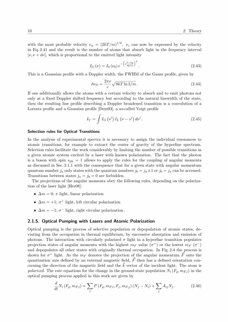
If one additionally allows the atoms with a certain velocity to absorb and to emit photons notonly at a fixed Doppler shifted frequency but according to the natural linewidth of the state,then the resulting line profile describing a Doppler broadened transition is a convolution of aLorentz profile and a Gaussian profile [Dem93], a so-called Voigt profile
IV =
∫
IG(ν ′)IL(ν − ν ′
)dν ′ . (2.45)
Selection rules for Optical Transitions
In the analysis of experimental spectra it is necessary to assign the individual resonances toatomic transitions, for example to extract the center of gravity of the hyperfine spectrum.Selection rules facilitate the work considerably by limiting the number of possible transitions ina given atomic system excited by a laser with known polarization. The fact that the photonis a boson with spin sph = 1 allows to apply the rules for the coupling of angular momentaas discussed in Sec. 2.1.1 with the consequence that for a given state with angular momentumquantum number ja only states with the quantum numbers jb = ja±1 or jb = ja can be accessed.Transitions between states ja = jb = 0 are forbidden.
The projections of the angular momenta obey the following rules, depending on the polariza-tion of the laser light [Her08]:
• ∆m = 0; π light, linear polarization
• ∆m = +1; σ+ light, left circular polarization
• ∆m = −1; σ− light, right circular polarization .
2.1.5. Optical Pumping with Lasers and Atomic Polarization
Optical pumping is the process of selective population or depopulation of atomic states, de-viating from the occupation in thermal equilibrium, by successive absorption and emission ofphotons. The interaction with circularly polarized σ light in a hyperfine transition populatesprojection states of angular momenta with the highest mF value (σ+) or the lowest mF (σ−)and depopulates all other states with originally thermal occupation. In Fig. 2.4 the process isshown for σ+ light. As the mF denotes the projection of the angular momentum ~F onto thequantization axis defined by an external magnetic field, ~F then has a defined orientation con-cerning the direction of the magnetic field and the ~k vector of the incident light. The atom ispolarized. The rate equations for the change in the ground-state population Ni (Fg,mF,i) in theoptical pumping process applied in this work are given by
d
dtNi (Fg,mF,i) =
∑
i
P (Fg,mF,i, Fj ,mF,j) (Nj −Ni) +∑
j
AijNj . (2.46)

2.2. Nuclear Physics - Nuclear Ground State Properties 11
P3/2 , F=2
S1/2 , F=1 -2 -1 0 1 2 mF
σ+
Figure 2.4.: Optical pumping with σ+ light. The excitation follows the selection rule ∆mF = +1,while the states can decay to substates with ∆mF = ±1 or 0.
Here P (Fg,mF,i, Fj ,mF,j) is the probability for induced absorption or emission and Aij is thespontaneous decay probability of the excited state j with population Nj . The polarization of the
coupled angular momentum ~F leads inherently to a nuclear polarization which can be decoupledfrom the atomic shell by switching on a strong external magnetic field (Paschen-Back effect).The effect of this nuclear polarization on the β decay will be discussed in the next section.
2.2. Nuclear Physics - Nuclear Ground State Properties
Laser spectroscopic studies on exotic isotopes reveal important information on nuclear groundstate properties like spins, nuclear magnetic moments and electric quadrupole moments. Thedefinitions and the basic models describing these physical quantities will be summarized in thissection.
2.2.1. The Nuclear Shell Model
Experimental hints like the discrete energy of γ rays emitted from excited nuclei and the existenceof ”magic numbers”, i.e. neutron or proton numbers at which the separation energy or theexcitation energy for a nucleon is large compared to neighboring nuclei, suggest a shell structureof the nucleus in analogy to the atomic structure. However, the nucleons do not move in acentral Coulomb potential but in an effective mean field produced by the nucleons. One possiblepotential to describe the mean interaction between the nucleons in a spherical nucleus is theWoods-Saxon potential [Pov06]
Vcentr (r) =−V0
1 + e(r−c)/a, (2.47)
deduced from the two-parameter Fermi distribution for the nuclear matter. The parameters cand a describe the size and the skin thickness of the nucleus as it will be discussed in Ch. 2.2.2.The solution of the Schrodinger equation for this potential leads to discrete energy levels de-scribed by the set of quantum numbers nlj . As nucleons have an intrinsic spin of 1/2 anadditional spin-orbit interaction term has to be added to the potential. While the spin-orbitterm in atomic physics causes only small corrections to the energy given by the main quantumnumber N , the l · s term in nuclear physics leads to correction of the same order of magnitude asthe main quantum number. This results in new shell closures that very successfully describe theobserved magic numbers. The properties of the nucleus can now be explained by the propertiesof individual nucleons outside closed shells. The nuclear spin of odd-A nuclei for example isgiven by the total angular momentum of the unpaired nucleon. For odd-odd nuclei the angular

12 2. Theory
momenta of the unpaired proton and the unpaired neutron can couple to a total spin I whichis resricted by
|Ip − In| ≤ I ≤ Ip + In , (2.48)
according to the coupling rules for angular momenta.For the description of deformed nuclei the Nilsson model [Nil55] has proven to be a very
good model to study the evolution of single-particle orbitals with increasing deformation. Ananisotropic harmonic oscillator potential is used to describe the mean field with deformation
VN =m
2
(ω2(x2 + y2
)+ ω2
zz2)
+ C(
ls)
+Dl2 , (2.49)
with the modified frequency
ω2z = ω2
0
(
1 − 4
3ǫ2
)
. (2.50)
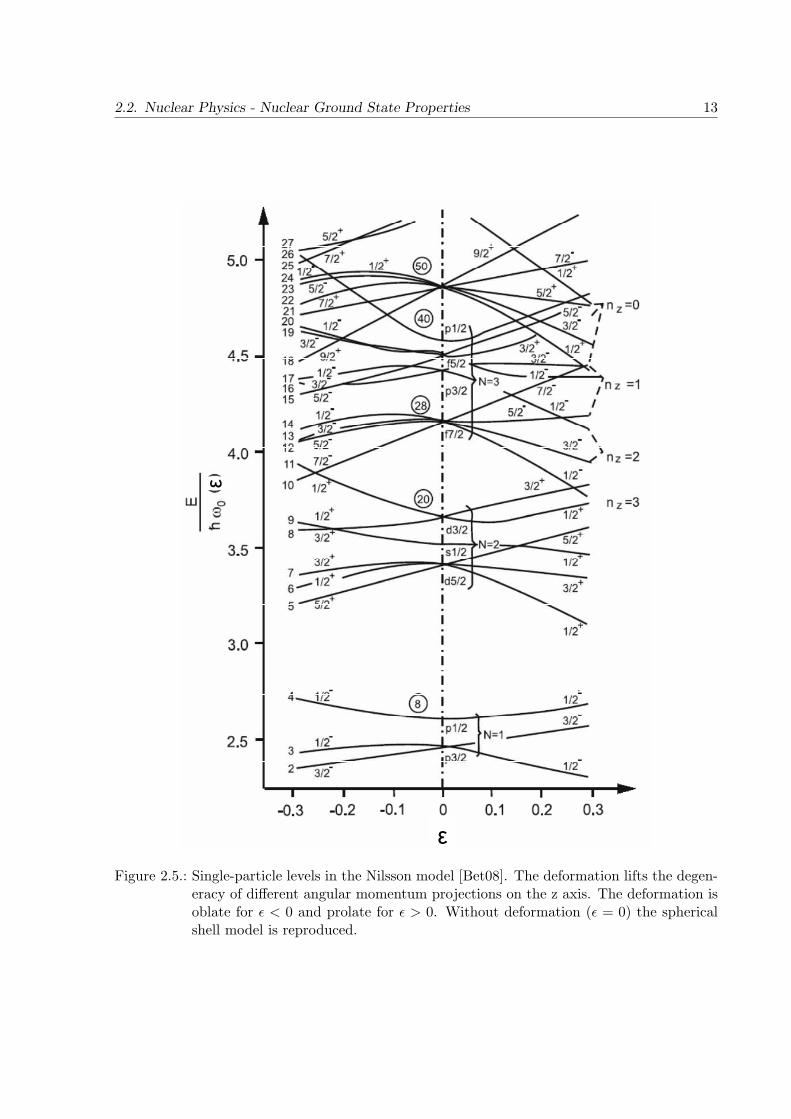
The parameter ǫ2 describes the nuclear deformation and can be transformed into the commonlyused β parameter. The single-particle states as a function of the deformation are shown inFig. 2.5. Negative deformation parameters refer to an oblate deformation while positive de-formation parameters denote prolately deformed nuclei. For vanishing deformation, the levelstructure from the spherical shell model is reproduced. The individual levels are assigned bytheir projection of the single-particle angular momentum Ωπ with parity π, the principal quan-tum number of the major shell N , and the number of nodes of the z-axis wavefunction nz.
2.2.2. The Nuclear Charge Radius
The nuclear charge radius was already mentioned in Ch. 2.1.2 in the field-shift contribution ofthe isotope shift. Formally, the mean square nuclear charge radius is defined as [Pov06]
⟨r2⟩
= 4π
∞∫
0
r2ρ (r) r2dr , (2.51)
with the radial charge distribution of the protons ρ (r). For the description of medium-heavynuclei the two parameter Fermi distribution
ρ (r) =ρ (0)
1 + e(r−c)/a(2.52)
gives good agreement with experimental radii. At the radius r = c the charge density reacheshalf of the total value. An empirical value for a spherical nucleus with mass A is
c = 1.12 fmA1/3 . (2.53)
For deformed nuclei with quadrupole deformation parameter β the half-density radius can beparametrized as
c = R0 (1 + βY20 (Θ,Φ)) , (2.54)
with the monopole radius R0 and the spherical harmonic Y20 (Θ,Φ). The parameter a is con-nected to a skin thickness t, which is the distance on which the charge density varies from 90%to 10% of the maximum value via
a =t
2 ln 9. (2.55)
Fig. 2.6 shows the two parameter Fermi distribution for a medium-heavy nucleus.
2.2. Nuclear Physics - Nuclear Ground State Properties 13
ε
ε
Figure 2.5.: Single-particle levels in the Nilsson model [Bet08]. The deformation lifts the degen-eracy of different angular momentum projections on the z axis. The deformation isoblate for ǫ < 0 and prolate for ǫ > 0. Without deformation (ǫ = 0) the sphericalshell model is reproduced.

14 2. Theory
0 2 4 6 80,0
0,2
0,4
0,6
0,8
1,0
ρ(r)
/ ρ
(0)
r / fm
c
Figure 2.6.: Fermi distribution of the nuclear charge for A = 40 and a skin thickness of t =2.37 fm.
2.2.3. Nuclear Moments
The magnetic dipole moment µ and the electric quadrupole moment Q of the nucleus are im-portant observable quantities accessible with different experimental techniques and predicted bynuclear models.
Magnetic Dipole Moment
In the classical picture the motion of a charged particle causes a magnetic field with a vectorpotential [Bet08]
~A (~r) =µ0
4π
∫ ~j (~r′)
|~r − ~r′|d3r′ , (2.56)
with the current density ~j (~r) of the charged particle motion. The potential can be rewrittenwith the multipole expansion
1
|~r − ~r′| =1
r
∞∑
l=0
(r′
r
)l
Pl (cosα) , (2.57)
where the Pl denote the Legendre polynomials. The first non-vanishing term of this expansionis the dipole term (l = 1), which can be expressed as
~A (~r) =µ0
4π
~µ× ~r
r3. (2.58)
~µ is the magnetic dipole moment defined as
~µ =1
2
∫ (
~r ×~j (~r))
d3r . (2.59)
For the motion of charged particles with the mass m the current density can be expressed bythe charge density ρ (~r) and the linear momentum ~p (~r) by
~j (~r) =ρ (~r) ~p (~r)
m. (2.60)

2.2. Nuclear Physics - Nuclear Ground State Properties 15
Inserting this in Eq. 2.59 the magnetic moment gets connected to the angular momentum ~L (~r) =~r × ~p (~r):
~µ =1
2
∫
ρ(
~r′) ~L (~r′)
md3r′ . (2.61)
The quantum mechanical analogon, the magnetic dipole operator µ, is defined as
µ =e
2m
∫
ψ∗ (r) Lψ (r) d3r . (2.62)
In the case of the nucleus, µ is composed of a contribution from the orbital angular momentum~l and the nucleonic spin ~s. In the single-particle model (Schmidt model) only the quantumnumbers of the unpaired nucleon determine the magnetic moment and a gs factor needs to bedefined to connect the intrinsic spins of the nucleons to a classical angular momentum and,hence, to their magnetic moments. The gl factor is only introduced to distinguish betweenprotons and neutrons. The magnetic moment is now given as
µ = µN
(
gl l + gss)
, (2.63)
with the g factors in units of the nuclear magneton µN = e~
2mp[Pov06]:
• gl (p) = 1 gs (p) = 5.58522
• gl (n) = 0 gs (n) = −3.8256 .
For a nucleus with the coupled angular momentum I = L + S and the eigenstates |ImI〉 theexpectation value is
µnucl =µN
~〈ψnucl| gl l + gss |ψnucl〉 (2.64)
which can be rewritten with the Wigner Eckart theorem [Pov06] to
µnucl =µN
~2gnucl
⟨
I⟩
, (2.65)
with the nuclear g factor gnucl. The magnetic moment as an observable is the value obtainedfor the maximum projection of the nuclear spin with MI = I. In the single-particle model themagnetic moment then reduces to
µnucl = µN
(
gl ±gs − gl
2l + 1
)
I, I = l ± 1/2 . (2.66)
The values obtained by this model can be regarded as boundaries for the observed experimentalvalues. In most nuclei the ground state is not defined by only one configuration, correlationsand mixing between different configurations have to be taken into account and also contributeto the magnetic moment.
Electric Quadrupole Moment
In analogy to the treatment of the current density of the moving charges in the nucleus toderive the magnetic moment, the multipole expansion of the scalar potential Φ (~r) with thecharge density ρ (~r) is used to get an expression for the electric quadrupole moment. The scalarpotential produced by the static charge density of the nucleus is given by
Φ (~r) =1
4πǫ0
∫ρ (~r′)
|~r − ~r′|d3r′ (2.67)

16 2. Theory
z z(a) (b)
Figure 2.7.: Oblate and prolate deformation of a nucleus. The oblate deformation results ina negative quadrupole moment (a). Prolately deformed nuclei have a positivequadrupole moment (b).
and the first three orders of the expansion [Bet08] are the monopole term
Φ0 (r) =Q
r, (2.68)
with the total charge Q, the dipole term, which in the nucleus vanishes due to symmetry reasonsand the quadrupole term
Φ2 (r) =Q0
2r3, (2.69)
with the electric quadrupole moment
Q0 =
∫
ρ(~r′) (
3z′2 − r′2)d3r′ . (2.70)
The quadrupole moment is connected to nuclear deformation. A negative Q refers to oblatelydeformed nuclei (Fig. 2.7 (a)) while prolate deformation causes a positive Q as depicted inFig. 2.7 (b).

3. Experimental Techniques
In this chapter the basic experimental techniques applied during this PhD work will be presentedand discussed, starting from different approaches for the production of exotic nuclei and reachingout to the principle of collinear laser spectroscopy and the different detection methods.
3.1. Production of Radioactive Isotopes
Radioactive nuclei can be produced mainly in three different ways: by charged-particle inducedfragmentation, spallation or fission in accelerator facilities, by neutron-induced fission in a nu-clear research reactor, or by spontaneous fission. The first method has been employed to studymagnesium isotopes in the framework of this thesis and the second one will be the technique usedin near future at the TRIGA reactor for which a laser spectroscopy experiment was designedand installed during this work.
3.1.1. Ion Beam Production at ISOLDE
The ISOL technique (Isotope Separator On Line) [Rav79] has been exploited for many years toproduce intense beams of radioactive ions. A solid target made of e.g. uranium carbide (UC2)or silicon carbide (SiC) is exposed to the high energy proton beam from an accelerator. Theenergy of a proton or another light ion hitting a target nucleus is distributed over all nucleons andthus produces a highly-excited nucleus. De-excitation happens by the emission of single protonsor neutrons (spallation) or by induced fission of the target nucleus. As a third alternativeproduction channel light nuclei from the mother nucleus are separated by fragmentation. Thedifferent reactions are shown in Fig. 3.1. Because of the combination of these processes theproton bombardment allows to produce a large variety of isotopes of different elements, whichcan be modified by the choice of the target material and the energy of the incident beam.
Several types of ion sources can now be coupled to the target container to allow the reactionproducts to be ionized. Some elemental selectivity can be obtained by choosing an appropriateway of ionization. The alkali elements and other metals for example can be ionized in a surfaceion source, while noble gases require a plasma ion source due to their high ionization potential.A major improvement in element selectivity and thus in the reduction of isobaric background,which cannot be separated by magnetic dipole separators, was obtained by the application ofelement selective resonant laser ionization in a hot cavity ion source [Mis93]. The unique atomicstructure of an element is used as a fingerprint and resonant excitation with lasers in two or threesteps with a final ionization step is used to ionize only the element of interest. Contaminationfrom other ionization processes can be suppressed by e.g. the choice of the transfer tube materialor by choosing a more elaborate source design, for example the laser ion source trap LIST [Sch08].The schematic of the laser ion source used at ISOLDE (CERN) is shown in Fig. 3.2 [Iso10]. Thereaction products effuse out of the hot target in a heated transfer line and arrive in the ionizertube, where the interaction with the laser and the ionization takes place. The target and thetransfer line temperature are important parameters for proper performance of the source withrespect to stable ion output and moderate isobaric contaminations. However, the fact that the
17

18 3. Experimental Techniques
incident proton
neutronproton
highly excited nucleus
evaporation
evaporation
fission
evaporation of nucleonsfrom the fission products
Figure 3.1.: Different reactions induced by high-energy proton bombardment [Bet08]. The frag-mentation process is similar to the fission process but with large mass asymmetryand therefore not shown separately.
proton beamtarget (e.g. UC2)
transfer lineeffusion
ionizationhigh voltage
ground potentialextraction
Laser for resonant ionization
Figure 3.2.: Schematic view of the ISOLDE laser ion source, according to [Iso10].
3.1. Production of Radioactive Isotopes 19
production rates / s-1
N
Z50
50 82
stable> 106
105 – 106
103 – 105
101 – 103
10-1 – 101
10-3 – 10-1
< 10-3Cu
As
Rb
Tc
Sn
Xe
Pr
Gd
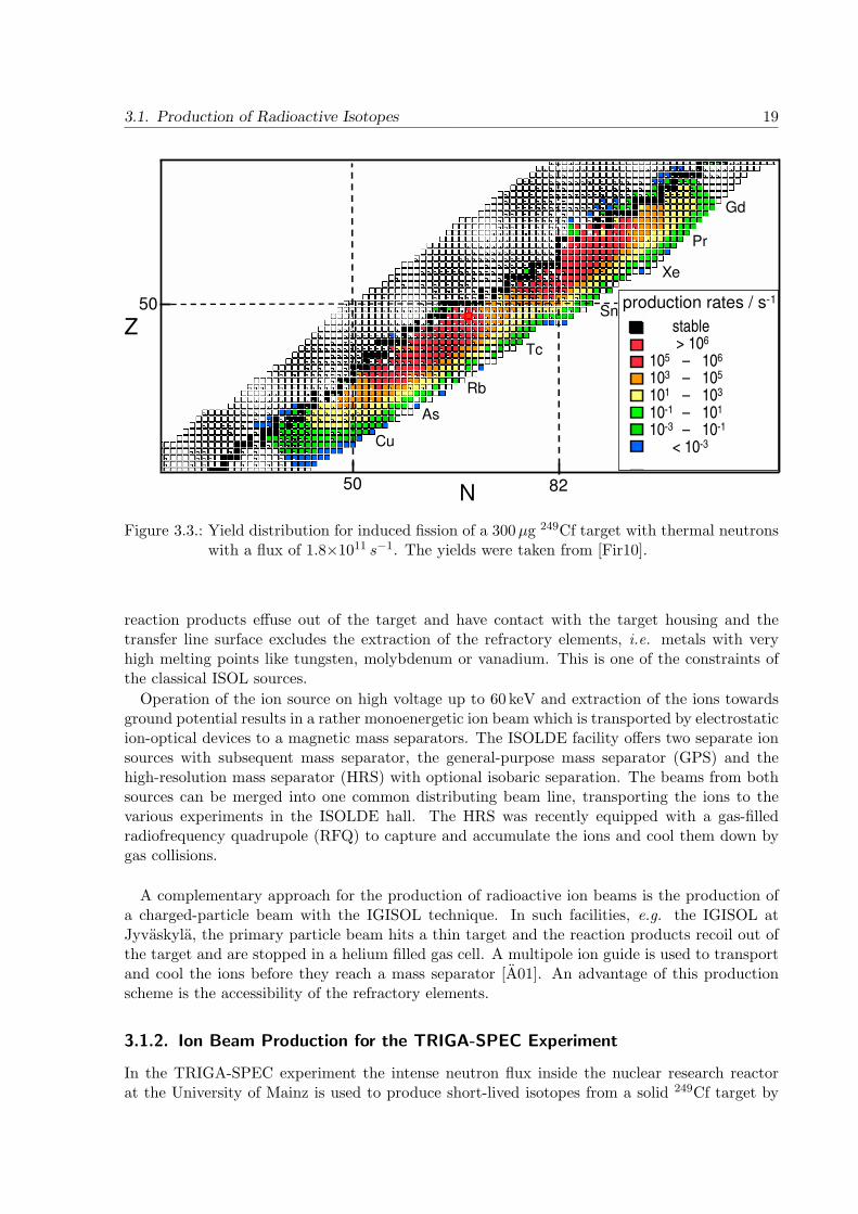
Figure 3.3.: Yield distribution for induced fission of a 300µg 249Cf target with thermal neutronswith a flux of 1.8×10¹¹ s−1. The yields were taken from [Fir10].
reaction products effuse out of the target and have contact with the target housing and thetransfer line surface excludes the extraction of the refractory elements, i.e. metals with veryhigh melting points like tungsten, molybdenum or vanadium. This is one of the constraints ofthe classical ISOL sources.
Operation of the ion source on high voltage up to 60 keV and extraction of the ions towardsground potential results in a rather monoenergetic ion beam which is transported by electrostaticion-optical devices to a magnetic mass separators. The ISOLDE facility offers two separate ionsources with subsequent mass separator, the general-purpose mass separator (GPS) and thehigh-resolution mass separator (HRS) with optional isobaric separation. The beams from bothsources can be merged into one common distributing beam line, transporting the ions to thevarious experiments in the ISOLDE hall. The HRS was recently equipped with a gas-filledradiofrequency quadrupole (RFQ) to capture and accumulate the ions and cool them down bygas collisions.
A complementary approach for the production of radioactive ion beams is the production ofa charged-particle beam with the IGISOL technique. In such facilities, e.g. the IGISOL atJyvaskyla, the primary particle beam hits a thin target and the reaction products recoil out ofthe target and are stopped in a helium filled gas cell. A multipole ion guide is used to transportand cool the ions before they reach a mass separator [A01]. An advantage of this productionscheme is the accessibility of the refractory elements.
3.1.2. Ion Beam Production for the TRIGA-SPEC Experiment
In the TRIGA-SPEC experiment the intense neutron flux inside the nuclear research reactorat the University of Mainz is used to produce short-lived isotopes from a solid 249Cf target by

20 3. Experimental Techniques
to Roots pump
ion source
skimmer extraction electrode
+ ++
carrier gas
aerosols +fission products
capillary
to Roots pump
ion source
skimmer extraction electrode
+ ++
carrier gas
aerosols +fission products
capillary
Figure 3.4.: Basic principle of the gas-jet transport and ionization system. The fission productsare stopped in the target chamber shown on the left and guided by the gas jet tothe ion source setup shown on the right.
neutron-induced fission. The fission fragments show an asymmetric distribution with a lightermass and a heavier mass branch both situated on the neutron-rich side of the nuclear chart.The yield distribution in the nuclear chart is shown in Fig. 3.3. A target chamber is placed nearthe reactor core in one of the beam ports and exposed to the flux of the thermal neutrons of1.8 × 1011 cm−2s−1. The fission products are transported from the chamber to an ion sourceby an aerosol-interspersed He gas jet [Ste80]. This method has already been applied earlier foran online mass separator for γ-ray studies of radioactive alkaline earth and lanthanide isotopes[Bru85]. The recoil nuclei leaving the target material are thermalized inside the target chamberin the helium transport gas at a pressure of typically 2 to 5 bar and attach to aerosol clustersof e.g. KCl or carbon. A laminar flow through a polyethylene capillary with ≈ 1 mm innerdiameter allows several meters of transport length with low losses. In Fig. 3.4 the basic principleof the production and transport method is shown schematically. Before the reaction productsenter the ion source, the essential part of the carrier gas is separated by the expansion in apressure gradient created by a strong Roots pump and a skimmer in front of the ion source’sentrance aperture. In earlier experiments the stable operation of surface and plasma ion sourcescoupled to a gas jet has been demonstrated [Bru85, Maz76].
3.2. Collinear Laser Spectroscopy with Fast Beams
In the classical approach of collinear laser spectroscopy a laser beam is superimposed with anion or atom beam with an energy of several keV to several ten keV. The particles are excitedin flight and the resulting fluorescence light can be detected with a photomultiplier tube. Onebig advantage compared to the spectroscopy in a gas cell is the compression of the longitudinalvelocity component because of the acceleration of the thermally distributed ion ensemble inthe external electric field between the ion source and the extraction optics. This effect can beunderstood if we consider two ions of the ensemble to be accelerated. Let the first ion’s velocity

3.2. Collinear Laser Spectroscopy with Fast Beams 21
component in the direction of extraction (z direction) be zero. The second ion should havethe full thermal velocity vz =
√
2kT/m. Both particles undergo acceleration a in the potentialdifference U between two electrodes with the spacing d. The final velocity of the first ion isaccording to basic kinematics
v′1 = at1 =√
2da =√
2eU/m , (3.1)
where the expression d = 12at
21 was used to eliminate the time t1. The second particle’s velocity
is given byv′2 = vz + at2 (3.2)
and the time can be eliminated by the expression
d =1
2at22 + vzt2 , (3.3)
giving t = −vz/a+√
v2z/a
2 + 2d/a. Inserting this in 3.2 gives the velocity of the ion with initialcomponent vz
v′2 =√
2eU/m
√
1 +v2z
2eU/m≈√
2eU/m+v2z
2√
2eU/m, (3.4)
which can now be compared to the velocity of the first ion. While the initial velocity differencewas the thermal velocity vtherm =
√
2kT/m, the difference after acceleration becomes
δvz =√
2kT/m× 1/2
√
kT
eU(3.5)
and is hence reduced by a factor proportional to√
1/U which is referred to as a velocity bunchingeffect. The line width of an optical transition probed by a laser in the z direction is thereforereduced by the same factor since the residual Doppler width is proportional to the velocitydistribution (see Ch. 2.1.4). For a typical case with a surface ion source as used in our testexperiment with a temperature of 1500 K and an acceleration voltage of 10 keV the compressionfactor for the line width becomes ≈280. This means that the linewidth obtained by spectroscopyin a gas of typically several GHz reduces to several tens of MHz which is of the order of thenatural linewidth of the allowed optical dipole transitions and therefore allows to perform high-resolution measurements giving access to hyperfine structures even of excited atomic levels.
The Doppler shift on the laser frequency in the rest frame of the moving particles allows toperform Doppler tuning : The ion velocity is changed by applying an additional voltage gradientbefore the optical detection setup, changing the frequency in the rest frame of the atom. Thelaser frequency can be kept fixed, allowing even the use of fixed-frequency lasers in special cases.Generally, it is much easier to stabilize a laser to a fixed, well-known frequency than to tune itwith high reproducibility of every frequency along the scan range. The Doppler-shifted frequencyν ′ for an ion with charge e and rest mass m accelerated with the total voltage difference U isgiven by (see App. A)
ν ′ = νlaser
(eU +mc2
)
mc2
1 ±
√
1 −(
mc2
eU +mc2
)2
(3.6)
where the − has to be used for collinear and the + has to be used for anti-collinear laser-ion geometry. The high accuracy of the laser spectroscopic technique requires a relativistic
22 3. Experimental Techniques
calculation even at these relatively low energies. With the commonly used high-voltage amplifiersto apply the tuning voltage, a typical maximum scanning range of 1000 V can be obtained, whichin the case of magnesium at νlaser = 280 nm for example, with total voltages of 50 keV and a massof 30 u corresponds to a frequency range of 20 GHz. This is sufficient to scan hyperfine structuresalso with greater interval factors. For isotope shift measurements, however, an additional staticoffset voltage is commonly used to jump from one isotope to the other.
3.2.1. Specialized Applications
The optical detection of the fluorescence photons with a scanning voltage applied to the opticaldetection setup can be considered as the classical approach of collinear laser spectroscopy. How-ever, restrictions concerning the sensitivity of the detection setup, limiting the lowest-possibleparticle yield of the species of interest or limited access with commercially available laser sys-tems have led to the development of specialized techniques to enhance the capabilities of theexperimental method.
Charge Exchange and Spectroscopy with Fast Atoms
The field of usage of collinear laser spectroscopy can be expanded to neutral atoms if the secondacceleration or deceleration stage in the setup is equipped with a charge exchange cell (CEC).Further details about the principle of the CEC and the neutralization will be given in Ch.5.5and Ch. 6.1.2.
Photon-Ion Coincidence Detection
Laser straylight produces a considerable amount of background on the photomultiplier in theclassical optical detection scheme, limiting the sensitivity at very low yields of radioactive iso-topes. This background can be reduced if the photomultiplier is gated to the signal of a de-structive particle detector at the end of the beamline. The idea is that only photon events arecounted that produce a particle signal after the time of flight to the detector [Eas86]. In order totrigger the gate on the particle signal, an appropriate way to delay the photon signal has to bechosen to avoid dead-time losses. The width of the gate has to be chosen according to the lengthof the optical setup. An increase in signal to noise of a factor of 1600 has been demonstrated inpast experiments [Eas86]. At TRIGA-LASER a particle detector for the coincidence techniquewas recently built and tested during a diploma thesis [Sie10].
An alternative to the destructive detection of single ions or atoms is to gate on the releasepulse of the ion bunch from an RFQ cooler and buncher. In this special case all fluorescenceevents occur during a short period corresponding to the length of the ion bunch.
β-Asymmetry Detection by Optical Pumping and β-NMR
The sensitivity of the standard optical fluorescence detection even with the coincidence techniqueis limited by the laser-induced background to about 104 ions s−1 to obtain a reasonable signal-to-noise ratio within a short time. For more exotic short-lived isotopes with lower yields, a differentmethod can be applied. Circularly polarized σ laser light is used to polarize the ions by opticalpumping (see Ch. 2.1.5). The nuclear polarization achieved by optical pumping and decouplingof the nuclear and the atomic spin in a strong magnetic field leads to a spatial anisotropy in theemission of the positrons/electrons from the β decay. This anisotropy can therefore be detectedand used as a probe for the resonant pumping process. The intensity of emitted electrons or

3.2. Collinear Laser Spectroscopy with Fast Beams 23
positrons is given by the projection of the β particle velocity ~v on the spin ~I of the polarizednuclei [Kon59]
I (ΘeI) = 1 +A~I
|~I|· ~v/c = 1 +Av/c cos ΘeI , (3.7)
with a parameter A = a×PI that can directly be linked to the degree of nuclear polarization PI
and an angle dependence. In the implanted crystal the polarization decays with time due to theinteraction with the host medium (spin-lattice relaxation). The easiest way to experimentallydetect such an asymmetry is a setup with two opposing particle detectors, e.g. scintillators,arranged in two planes perpendicular to the nuclear spin direction. The difference of the countrates of both detectors yields the asymmetry.
Instead of just detecting the asymmetry as a function of the applied Doppler tuning voltage, aresonant destruction of the polarization and hence, the asymmetry, can be achieved by applyinga radio-frequency field to the nuclei implanted in the crystal. In the process of this nuclearmagnetic resonance (NMR) the polarization is reduced resonantly by induced transitions betweenindividual magnetic substates mI . The energy shift of a level with the quantum number mI ina strong magnetic field is given by
∆E (mI) = −mIgIµNB = −mI~ωL (3.8)
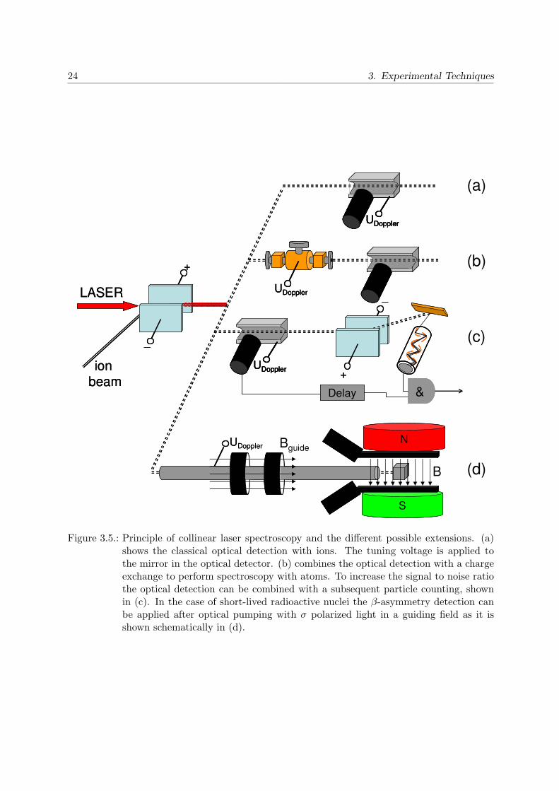
(see Eq.2.27 in the strong field approximation), with the Larmor frequency ωL = gIµNB/~. Adisturbing oscillating magnetic field, tuned to the Larmor frequency and applied perpendicularlyto the strong magnetic field axis, mixes the substates by transitions with the selection rule∆mI = ±1 and leads to an equally distributed population of the states and a destruction of theβ-decay asymmetry. From the Larmor frequency the nuclear gI factor can be deduced if themagnetic field B is known accurately or is eliminated from Eq. 3.8 with a reference measurement.A schematic view of a collinear laser spectroscopy setup summarizing the different possibledetection methods is shown in Fig. 3.5.
24 3. Experimental Techniques
UDoppler
_
+
UDoppler
UDoppler
+
_
Delay &
LASER
ionbeam
UDopplerN
S
UDopplerUDopplerUDoppler
_
+
UDopplerUDopplerUDoppler
UDopplerUDoppler
+
_
Delay &
LASER
ionbeam
UDopplerN
S
(a)
(b)
(c)
(d)
Bguide
B
Figure 3.5.: Principle of collinear laser spectroscopy and the different possible extensions. (a)shows the classical optical detection with ions. The tuning voltage is applied tothe mirror in the optical detector. (b) combines the optical detection with a chargeexchange to perform spectroscopy with atoms. To increase the signal to noise ratiothe optical detection can be combined with a subsequent particle counting, shownin (c). In the case of short-lived radioactive nuclei the β-asymmetry detection canbe applied after optical pumping with σ polarized light in a guiding field as it isshown schematically in (d).
Part I.
Commissioning of the Collinear Laser
Spectroscopy Setup TRIGA-LASER at
the TRIGA Research Reactor Mainz
25


4. Layout of the TRIGA-SPEC experiment
In the TRIGA-SPEC experiment exotic nuclei produced by neutron-induced fission near the coreof the TRIGA research reactor at the Institute of Nuclear Chemistry Mainz will be studied bycollinear laser spectroscopy or Penning trap mass spectrometry [Ket08]. A schematic overviewof the whole setup is given in Fig. 4.1 showing the different stages from production of the short-lived isotopes, ion beam formation and preparation up to the final experiments. Fig. 4.2 showsa photography of the whole experimental setup still in the construction phase.
The reaction products from the target (see Ch. 3.1.2) are transported on aerosols in a gas jetinto an electron cyclotron resonance (ECR) ion source. The ECR is equipped with permanentmagnets to create the magnetic field for the confinement of the electrons in the plasma. Theelectron motion is driven by a 2.54 GHz microwave field coupled into the plasma chamber ofthe source from above by hollow conductors and an antenna. This allows to inject the aerosolsand the fission products from the back side of the source. The whole source is operated at upto 30 keV high voltage and the ions are accelerated towards an extraction electrode at groundpotential.
A 90 magnetic dipole sector magnet is used to mass separate the ions of interest for theparticular experiment from the large variety of ion species that are produced in the ECR source.The magnet from the Chinese company Lanzhou Lanke Complete Set of Machinery has a 0.5mbending radius, a pole gap of 50 mm, and produces a maximum field of 1.2T. The maximumcurrent rating is 250 A. The iron yokes at the entrance and the exit of the magnet are designedaccording to a Rogowski profile to exhibit double-focussing properties. This means that a parallelbeam that enters the magnet is focussed in both planes with the same focal length. To supplythe current for the magnet, a high-power current source System 8500 MPS853 from Danfysik isused.
Due to the relatively low yields of the fission process with 107 particles s−1 at maximumbefore ionization, a normal continuous beam operation of the experiment would result in verylong integration time needed to see a signal. For the laser experiment, this might not be possibleat all, even if care is taken in reducing the background. In the case of the Penning trap theproblem is the ion-beam energy of several keV required for an efficient mass separation in thedipole magnet, because the Penning trap can only accept and trap ions with energies of a fewhundred eV. A pulsed drift tube is therefore needed to slow down the ions by switched electricfields, which only works efficiently with a pulsed beam. Otherwise, only a small fraction of thecontinuous beam would be cut and decelerated, resulting in a particle rate of less than one ionper second. Therefore, a radio frequency quadrupole (RFQ) cooler and buncher will be installedright after the separation magnet. This will allow timing the pulsed drift tube with the ionbunch in the case of TRIGA-TRAP and gating the photomultiplier on the bunch, reducing thelaser induced background by a large amount. The COLETTE RFQ [Lun09] formerly used atISOLDE in the MISTRAL experiment has been allocated for this purpose. It is a linear Paultrap filled with a buffer gas and operated at high voltage, in which the ions are trapped bystatic and radio frequency electric fields and cooled by collisions with the buffer gas atoms. Thetechnical design of the cooler is shown in Fig. 4.3. The release of the cooled ions results in abunched beam with significantly lower transverse phase space volume and narrow longitudinal
27
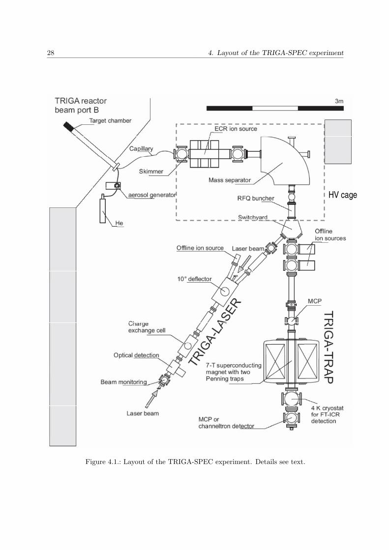
28 4. Layout of the TRIGA-SPEC experiment
HV cage
Figure 4.1.: Layout of the TRIGA-SPEC experiment. Details see text.

29
(a)
(c)(b)
Figure 4.2.: Photography of the TRIGA-SPEC experimental setup (May 2009). (a) is the highvoltage cage for the ion source. (b) is the collinear laser spectroscopy setup and (c)is the Penning trap setup with the superconducting magnet.

30 4. Layout of the TRIGA-SPEC experiment
Figure 4.3.: Technical drawing of the COLETTE RFQ [Lun09]. The ion beam is injected fromthe left. The central part includes the gas-filled radiofrequency quadrupole (RFQ)that can be floated to the potential of the ion source to stop the ions inside the gascell. After accumulation and cooling the ions are ejected on the right.
energy spread. The drift tube for the Penning trap experiment as well as the optical detectorin the laser spectroscopy setup can then be triggered on the ejection pulse of the RFQ.
The Penning trap setup TRIGA-TRAP is a two-stage Penning trap which is mounted in a7 T superconducting magnet. The first trap is a cylindrical purification trap to remove isobariccontamination and to cool the ions in a He buffer gas. The second trap is a hyperbolic Penningtrap for the mass measurements by ion-cyclotron resonance either by recording the time of flightfrom the trap to a particle detector as a function of the excitation frequency (TOF-ICR) or byperforming a Fourier transformation of the induced ion mirror current in the trap electrodes(FT-ICR). Both methods use the resonant excitation of the ion cyclotron motion in the trapat the cyclotron frequency ωC = eB/m. If the magnetic field B is known accurately or canbe eliminated by a reference measurement, the mass m can be calculated from the frequencyωC (see [Ket08] for further information). The application of carbon clusters as the aerosol usedfor the gas-jet transport offers a unique possibility to calibrate the mass measurement to thestandard mass, defined by the isotope 12C. The ion source is expected to produce a mass comb ofcarbon clusters with a wide variety of masses, allowing to find a suitable reference mass n×12 u,with integer n, for every isotope mass studied at a time. For off-line measurements a carboncluster source operated with a pulsed frequency-doubled Nd:YAG laser is included that allowsfor cluster generation using laser ablation.

5. The Collinear Laser Spectroscopy Branch
TRIGA-LASER
A high spectral resolution and a good transport and detection efficiency are the main designconsiderations for a collinear laser experiment. The ions or atoms of interest usually have lowproduction rates and additional losses during the transport have to be avoided. In addition, thespectral line position needs to be extracted with high precision. Careful simulation of the beamsteering and focussing elements before the charge exchange cell (CEC) ensure a configurationwith low losses and an approximately spherical beam profile. Field gradient studies on theapertures of the detection chamber and CEC respectively, allow a design of the drift sectionsto minimize field penetration and hence, a blow-up of the longitudinal velocity spread of theion beam after post acceleration or deceleration. For the simulation the SIMION code [Dah90]was used, which uses a Runge-Kutta algorithm to numerically solve the equation of motion ofa single particle in a given field geometry defined by the solution of the Laplace equation. Thegeometries for the simulations can be imported from a 3D CAD program, in which the wholebeam line with all components have been designed. An instruction for this import procedurecan be found in App. B.
The complete TRIGA-LASER setup including the beam transport part after the separatormagnet is shown in Fig. 5.1. All parts except the quadrupoles and the charge-exchange cell,which were already existing, are custom designs that have been developed and built during thisPhD work.
5.1. The Vacuum System
The choice of a vacuum standard is an essential part of the design of a vacuum beamline.The final pressure, maximum bakeout temperatures, and maintenance time are differing a lotcomparing copper sealed conflat flanges with ordinary rubber sealed flanges. For its relativelylow cost, the sufficiently low minimum pressure of 1×10⁻⁷ mbar and the very short time to openand close the system as all flanges are fixed with clamps only, the ISO-K standard with vitonseals was chosen for our setup. The vacuum pressure is maintained by 3 EBARA ET-300WSturbo pumps with purely magnetic bearings in the main sections and Edwards XDS10 scrollpumps for the pre-vacuum side. Since the ion-beam switchyard and the beamline connectingit with the 10 deflector is not installed yet, there are three sections separated by air-actuatedvacuum valves. The valves can be controlled manually or by pre set switching pressures of thevacuum gauges in order to avoid accidental ventilation of the whole setup in case of a leak. Thefirst section is containing the off-line ion source used for the commissioning of the setup. Thesmall ISO-K100 vacuum cross is pumped by a Pfeiffer TPU170 and an Edwards rotating vanepump. In the second section beam shaping and steering takes place in order to prepare the ionbeam to enter the small apertures of the charge-exchange cell and the fluorescence detector inthe third vacuum section and match the particle beam to the transversal laser beam profile.
31
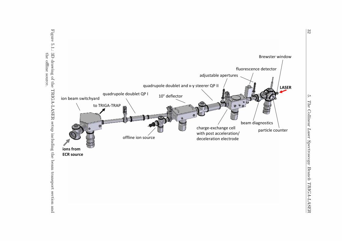
325.
The
Collin
ear
Laser
Spectro
scopy
Bra
nch
TR
IGA
-LA
SE
R
ion beam switchyardquadrupole doublet QP I
10° deflector
quadrupole doublet and x-y steerer QP II
charge-exchange cell
with post acceleration/
deceleration electrode
fluorescence detector
adjustable apertures
beam diagnostics
particle counter
offline ion source
Brewster window
ions from
ECR source
LASER
to TRIGA-TRAP
Figu
re5.1.:
3Ddraw
ing
ofth
eT
RIG
A-L
ASE
Rsetu
pin
cludin
gth
ebeam
transp
ortsection
and
the
offlin
esou
rce.
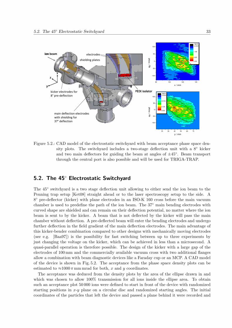
5.2. The 45 Electrostatic Switchyard 33
kicker electrodes for
8° pre-deflection
main deflection electrodes
with shielding for
37° deflection
electrodes
shielding plates
PEEK isolator
ion beam
z
y
x
kicker electrodes for
8° pre-deflection
main deflection electrodes
with shielding for
37° deflection
electrodes
shielding plates
PEEK isolator
ion beam
z
y
x
z
y
x
80 100 120 140
-100
-50
0
50
100
x / mm
φ X / m
rad
-0.5000
1.188
2.875
4.000
20 30 40 50 60 70
-100
-50
0
50
100
y / mm
φ Y /
mra
d
-0.5000
0.8125
2.125
3.000
ion #
ion #
Figure 5.2.: CAD model of the electrostatic switchyard with beam acceptance phase space den-sity plots. The switchyard includes a two-stage deflection unit with a 8 kickerand two main deflectors for guiding the beam at angles of ±45. Beam transportthrough the central port is also possible and will be used for TRIGA-TRAP.
5.2. The 45 Electrostatic Switchyard
The 45 switchyard is a two stage deflection unit allowing to either send the ion beam to thePenning trap setup [Ket08] straight ahead or to the laser spectroscopy setup to the side. A8 pre-deflector (kicker) with plane electrodes in an ISO-K 160 cross before the main vacuumchamber is used to predefine the path of the ion beam. The 37 main bending electrodes withcurved shape are shielded and can remain on their deflection potential, no matter where the ionbeam is sent to by the kicker. A beam that is not deflected by the kicker will pass the mainchamber without deflection. A pre-deflected beam will enter the bending electrodes and undergofurther deflection in the field gradient of the main deflection electrodes. The main advantage ofthis kicker-bender combination compared to other designs with mechanically moving electrodes(see e.g. [Baa97]) is the possibility for fast switching between up to three experiments byjust changing the voltage on the kicker, which can be achieved in less than a microsecond. Aquasi-parallel operation is therefore possible. The design of the kicker with a large gap of theelectrodes of 100 mm and the commercially available vacuum cross with two additional flangesallow a combination with beam diagnostic devices like a Faraday cup or an MCP. A CAD modelof the device is shown in Fig. 5.2. The acceptance from the phase space density plots can beestimated to ≈1000πmm mrad for both, x and y coordinates.
The acceptance was deduced from the density plots by the area of the ellipse drawn in andwhich was chosen to allow 100% transmission for all ions inside the ellipse area. To obtainsuch an acceptance plot 50 000 ions were defined to start in front of the device with randomizedstarting positions in x-y plane on a circular disc and randomized starting angles. The initialcoordinates of the particles that left the device and passed a plane behind it were recorded and

34 5. The Collinear Laser Spectroscopy Branch TRIGA-LASER
graphite oven
with W inlay (on HV)
HV isolator
turbo pump
acceleration gap
beam shaping
Einzel lens
grounded
electrodes
z
y
x
graphite oven
with W inlay (on HV)
HV isolator
turbo pump
acceleration gap
beam shaping
Einzel lens
grounded
electrodes
z
y
x
z
y
x
55 60 65 70-10
-5
0
5
x / mm
φ X /
mm
-2.000
5.500
13.00
20.50
28.00
ion #
Figure 5.3.: Schematic view of the offline ion source and density plots of the phase space of theemitted ions. The offline ions from the oven on high voltage are accelerated by thefirst extraction electrode. A subsequent Einzel lens is used to form an ion beamwith small divergence angle. The emittance extracted from the phase space plots isestimated to be ≈10πmm mrad at 10 keV.
evaluated. The deflection voltages extracted from the simulation are ±93.3V per keV ion energyfor the kicker and the main electrodes, giving ±2800 V for a 30 keV ion beam.
5.3. The Offline Ion Source
For first test experiments and commissioning of the ion optical devices, a simple ion sourcewas constructed which is based on a resistively heated graphite oven [Gep00]. This oven wasoriginally designed to produce an atomic beam, but for alkali and earth-alkali elements surfaceionization [Dre68] allows the production of ion beams which can be extracted with an appropriateelectrode geometry. The usage of a tungsten inlay facilitates the ionization and increases theion yield. Fig. 5.3 shows the schematic drawing of the ion source and the extraction optics. Theoven itself is put on a high potential, defining the ion energy after extraction and accelerationby the first electrode after the oven. The second electrode is again put on high voltage to forman Einzel lens together with the extraction electrode and the following electrode. The fourthelectrode at the end exit flange is grounded and has no effect in this configuration. With thisarrangement a nearly collimated beam with an emittance of ≈10πmm mrad at 10 keV can beformed, which is extracted from the phase space plots from Fig. 5.3 and is indicated by theellipse. For the simulation a randomly distributed ensemble of ions with the thermal kineticenergy of ≈0.2 eV and randomly distributed emission angles was starting inside the model ofthe graphite tube being on a constant potential. Only the ions that effused out of the tube wereaccelerated. The voltage gradient existing on the real source due to the heating voltage appliedon the tube was neglected.
In order to apply the acceleration voltage for the source, a compact high voltage cage wasconstructed which allows to put the whole source and the current supply for the oven on upto 10 kV. A Tauscher HTT-25F isolation transformer is used to float the ground potential ofthe 100 A supply. The water cooling tubes for the oven are wound at a length of 10 m insidethe cage before being connected to the cooling water supply in order to restrict the current
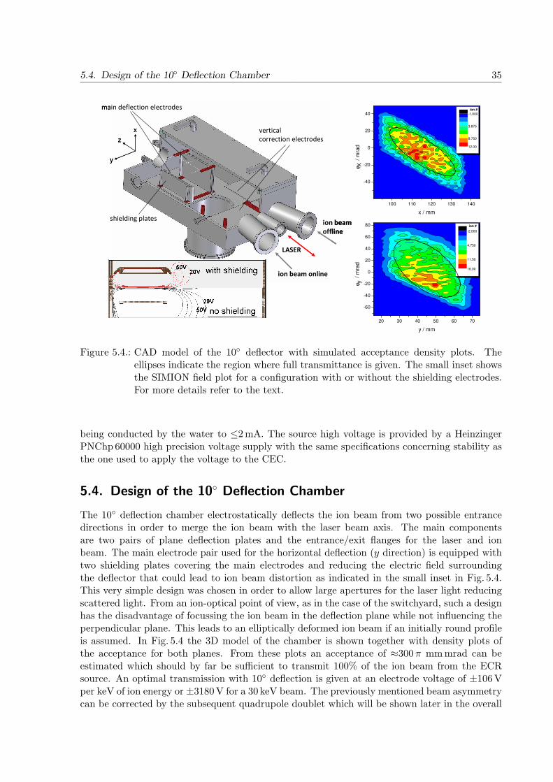
5.4. Design of the 10 Deflection Chamber 35
100 110 120 130 140
-40
-20
0
20
40
φX /
mra
d
x / mm
-1.000
3.875
8.750
12.00
20 30 40 50 60 70
-60
-40
-20
0
20
40
60
80
y / mm
φy /
mra
d
-2.000
4.750
11.50
16.00
ion #
ion #
main deflection electrodes
shielding plates
vertical
correction electrodes
LASER
ion beam online
z
y
x
ion beam
offline
main deflection electrodes
shielding plates
vertical
correction electrodes
LASER
ion beam online
z
y
x
z
y
x
ion beam
offline
Figure 5.4.: CAD model of the 10 deflector with simulated acceptance density plots. Theellipses indicate the region where full transmittance is given. The small inset showsthe SIMION field plot for a configuration with or without the shielding electrodes.For more details refer to the text.
being conducted by the water to ≤2 mA. The source high voltage is provided by a HeinzingerPNChp 60000 high precision voltage supply with the same specifications concerning stability asthe one used to apply the voltage to the CEC.
5.4. Design of the 10 Deflection Chamber
The 10 deflection chamber electrostatically deflects the ion beam from two possible entrancedirections in order to merge the ion beam with the laser beam axis. The main componentsare two pairs of plane deflection plates and the entrance/exit flanges for the laser and ionbeam. The main electrode pair used for the horizontal deflection (y direction) is equipped withtwo shielding plates covering the main electrodes and reducing the electric field surroundingthe deflector that could lead to ion beam distortion as indicated in the small inset in Fig. 5.4.This very simple design was chosen in order to allow large apertures for the laser light reducingscattered light. From an ion-optical point of view, as in the case of the switchyard, such a designhas the disadvantage of focussing the ion beam in the deflection plane while not influencing theperpendicular plane. This leads to an elliptically deformed ion beam if an initially round profileis assumed. In Fig. 5.4 the 3D model of the chamber is shown together with density plots ofthe acceptance for both planes. From these plots an acceptance of ≈300π mm mrad can beestimated which should by far be sufficient to transmit 100% of the ion beam from the ECRsource. An optimal transmission with 10 deflection is given at an electrode voltage of ±106 Vper keV of ion energy or ±3180 V for a 30 keV beam. The previously mentioned beam asymmetrycan be corrected by the subsequent quadrupole doublet which will be shown later in the overall

36 5. The Collinear Laser Spectroscopy Branch TRIGA-LASER
transmission simulations (see Section 5.8).
For beam monitoring purposes a Faraday cup is installed inside the vacuum chamber next tothe exit flange on the source axis. With the deflection voltage turned off, the primary ion beamcurrent can be measured.
5.5. The Charge-Exchange Cell
The charge-exchange cell (CEC) was adopted from an earlier experiment [Bac74, Ant78] andonly the surrounding chamber and the high-voltage platform were constructed in this PhDwork. The cell consists of a tubular housing with beam entrance and exit apertures containingthe neutralizing agent (e.g. metallic Na, K, Cs, Rb) in a small reservoir. The center of the cellis electrically heated to melt and evaporate the metal. Both ends of the cell are cooled withcopper blocks that are chilled by circulating synthetic low conductance thermalizing liquid byan external chiller. A stainless steel wire wick ensures the distribution of the liquid metal andthe reflow to the reservoir. The whole cell is mounted on an isolated platform and can be put ona well defined potential up to ±10 kV to post-accelerate or -decelerate the ion beam for Dopplertuning. An electrode in front of the cell defines the acceleration gap together with the wall ofthe vacuum chamber and minimizes the field gradient close to the aperture of the cell. Afterneutralization the atoms keep the energy defined by the CEC potential. Residual ions can bedeflected and separated from the atom beam with a small kicker configuration right after thecell. Fig. 5.5 shows the 3D CAD model of the CEC and the vacuum chamber. The acceptancefrom the simulation is estimated to be ≈20πmm mrad. This is much smaller than the valuesfor the other devices and is caused by the small entrance and exit apertures of the CEC of7 mm together with the 200 mm length. Consequently, the subsequent optical detection regionwith slightly larger apertures does only have a minor effect on the limiting phase space of thetransmitted beam after passing the CEC. As will be shown later in Section 5.3 the offline ionsource produces an ion beam with an emittance small enough to be transmitted through theCEC and the optical detection setup with low losses, provided, careful beam shaping is donebeforehand.
The voltages to perform the Doppler tuning are supplied by a Kepco BOP500 voltage amplifierwith an amplification factor of fKepco ≈ 50 fed by the output of a bipolar 16 Bit DAC allowingvoltages from -500 V to +500 V and a high precision high voltage supply Heinzinger PNChp10000with a maximum voltage of 10 kV with selectable polarity and a precision of 1 × 10⁻⁵ in 8 hoperation time. At a later stage of the experiment the 10 kV supply will be used to make voltagejumps to go from one isotope to another for isotope shift measurements. The Kepco amplifierwill be used for fast scanning of the voltage around the value given by the Heinzinger supply.Hence, the amplifier voltage is added to the main acceleration/deceleration voltage by floatingthe high voltage supply. A schematic view of this setup can be seen in Fig. 5.6. A Julie ResearchLabs high voltage divider KV-10R with an accuracy of 10−4 and an Agilent 34401A precisionmultimeter are used to measure the applied voltage. The total acceleration voltage for theDoppler shift in this experiment is therefore
Utotal = Usource −(
UHeinzinger + fKepco × UDAC
)
. (5.1)
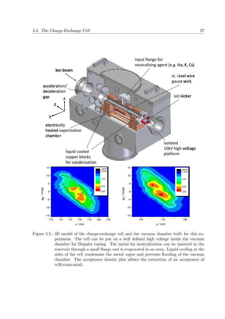
5.5. The Charge-Exchange Cell 37
ion beam
acceleration/
deceleration
gap ion kicker
liquid cooled
copper blocks
for condensation
electrically
heated vaporization
chamber
input flange for
neutralizing agent (e.g. Na, K, Cs)
st. steel wire
gauze wick
isolated
10kV high voltage
platform
z
y
x
ion beam
acceleration/
deceleration
gap ion kicker
liquid cooled
copper blocks
for condensation
electrically
heated vaporization
chamber
input flange for
neutralizing agent (e.g. Na, K, Cs)
st. steel wire
gauze wick
isolated
10kV high voltage
platform
z
y
x
z
y
x
110 112 114 116 118 120 122
-15
-10
-5
0
5
10
15
x / mm
φ X /
mra
d
-0.5000
1.750
4.000
5.500
170 175 180
-15
-10
-5
0
5
10
15
y / mm
φ Y /
mra
d
-0.5000
1.563
3.625
5.000
ion # ion #
Figure 5.5.: 3D model of the charge-exchange cell and the vacuum chamber built for this ex-periment. The cell can be put on a well defined high voltage inside the vacuumchamber for Doppler tuning. The metal for neutralization can be inserted in thereservoir through a small flange and is evaporated in an oven. Liquid cooling at thesides of the cell condensate the metal vapor and prevents flooding of the vacuumchamber. The acceptance density plot allows the extraction of an acceptance of≈20πmm mrad.
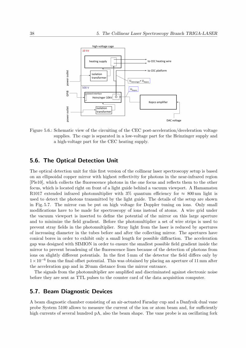
38 5. The Collinear Laser Spectroscopy Branch TRIGA-LASER
to CEC platform
to CEC heating wire
isolation
transformer
isolation
transformer
heating supply
Heinzinger 10kV
Kepco amplifier
500 V
10 kV
po
we
ro
utl
et
DAC voltage
high-voltage cage
po
we
ro
utl
et
GP
IB
isolated interface
UKepco
UHeinzinger+ UKepco
Figure 5.6.: Schematic view of the circuiting of the CEC post-acceleration/deceleration voltagesupplies. The cage is separated in a low-voltage part for the Heinzinger supply anda high-voltage part for the CEC heating supply.
5.6. The Optical Detection Unit
The optical detection unit for this first version of the collinear laser spectroscopy setup is basedon an ellipsoidal copper mirror with highest reflectivity for photons in the near-infrared region[Ple10], which collects the fluorescence photons in the one focus and reflects them to the otherfocus, which is located right on front of a light guide behind a vacuum viewport. A HamamatsuR1017 extended infrared photomultiplier with 3% quantum efficiency for ≈ 800 nm light isused to detect the photons transmitted by the light guide. The details of the setup are shownin Fig. 5.7. The mirror can be put on high voltage for Doppler tuning on ions. Only smallmodifications have to be made for spectroscopy of ions instead of atoms. A wire grid underthe vacuum viewport is inserted to define the potential of the mirror on this large apertureand to minimize the field gradient. Before the photomultiplier a set of wire strips is used toprevent stray fields in the photomultiplier. Stray light from the laser is reduced by aperturesof increasing diameter in the tubes before and after the collecting mirror. The apertures haveconical bores in order to exhibit only a small length for possible diffraction. The accelerationgap was designed with SIMION in order to ensure the smallest possible field gradient inside themirror to prevent broadening of the fluorescence lines because of the detection of photons fromions on slightly different potentials. In the first 5 mm of the detector the field differs only by1×10−6 from the final offset potential. This was obtained by placing an aperture of 11 mm afterthe acceleration gap and in 20 mm distance from the mirror entrance.
The signals from the photomultiplier are amplified and discriminated against electronic noisebefore they are sent as TTL pulses to the counter card of the data acquisition computer.
5.7. Beam Diagnostic Devices
A beam diagnostic chamber consisting of an air-actuated Faraday cup and a Danfysik dual vaneprobe System 5100 allows to measure the current of the ion or atom beam and, for sufficientlyhigh currents of several hundred pA, also the beam shape. The vane probe is an oscillating fork

5.8. Overall beam transport properties 39
drift tube
with apertures
(grounded part)
ellipsoidal Cu mirror
light guide
photomultiplier
tube (PMT)
PEEK isolator
and acceleration gap
vacuum viewport
ion beam
cooled PMT
housing
z
y
xdrift tube
with apertures
(HV part)
52
36,4
F1
F2
Figure 5.7.: CAD model of the light collection unit. The ellipsoidal collecting mirror can be puton a high voltage in order to perform Doppler tuning on ion beams. The apertureswith increasing diameter towards the optical detection unit reduce the stray-lightbackground from the laser beam.
mounted at an angle of 45 which passes the ion beam and detects the current as a function ofthe oscillation angle. The beam profiles for both beam components can be monitored with anoscilloscope.
The successful improvement of the sensitivity of our spectroscopy setup has recently beendemonstrated with the photon-ion coincidence technique [Eas86] with calcium ions, which ispart of a diploma thesis [Sie10]. The detector designed for this purpose uses a commercialDeTech 470 secondary electron multiplier (channeltron) to detect the secondary electrons fromthe impact of the ions or atoms on a copper conversion dynode. For the detection of ions thebeam can be deflected on to the dynode by a pair of electrodes. For the detection of atomsa conversion electrode that is also used to reflect the laser beam out of the beam line can bemoved into the beam axis with an air-actuated linear feedthrough. The detector unit is housedin a standard Iso-K160 cross and therefore very compact.
A detection efficiency of ≈ 60% has been demonstrated and it was possible to clearly identify aresonance from 104 ions/s after about 20 min with the coincidence unit, while the purely opticaldetection did not even show an indication for a resonance after the same time.
5.8. Overall beam transport properties
After simulating and designing the individual parts of the setup, the transmission through thecomplete TRIGA-LASER beamline was studied and optimized. This was done for the beamfrom the offline source and for ”online” beams, starting in front of the switchyard. The re-sults give an idea for the voltages needed for first experimental tests and first estimates of thetransport efficiency. For the offline beam transmission the beam extracted as described in Sec-

40 5. The Collinear Laser Spectroscopy Branch TRIGA-LASER
0.0
0.5
1.0
1.5
2.0
2.5
3.0
3.5
4.0
0 500 1000 1500 20004.0
3.5
3.0
2.5
2.0
1.5
1.0
0.5
0.0
particle detection
optical detection
CE
C
QP
2
QP
1
source optics
10° defl.
r X /
mm
rY /
mm
z / mm
Figure 5.8.: Simulated beam envelope for both transversal beam components (x/y) for the offlinebeam with ǫ=10πmm mrad at 10 keV energy. The boxes representing the individualdevices are scaled to represent the respective free aperture. The total ion transmis-sion was simulated to be 97%.
tion 5.3 was guided through the line and the voltages were manually tuned to reach a maximumtransmission of 97%. The simulated beam envelope for the transmission through the wholeexperimental setup for both transversal beam components is shown in Fig. 5.8. The voltages forthe electrostatic elements are given in Tab. 5.1. The main losses occur in the charge-exchangecell and on the apertures of the optical detection unit.
For the online case three different beam initial conditions were studied. At first, the trans-port of cooled ions with 30 keV kinetic energy, extracted from the cooler with an emittance of≈8πmm mrad [Lun09] and ions coming directly from the magnet separator with an emittanceof ≈20πmm mrad and ≈30πmm mrad which are typical values for the ISOLDE ion source andwere adopted for this study. The initial beam diameter was fixed to 7 mm and only the diver-gence angle was changed to fulfill the different phase-space conditions. The efficiency for thetransmission of the cooled beam was optimized to 98% with voltages for the ion-optical elementsgiven in Tab. 5.1. The uncooled beams are transported with significantly lower efficiencies be-cause of losses mainly in the CEC. From the 20πmm mrad 76% of the ions reach the detectionplane at the end of the beamline. The 30πmm mrad beam is transported with 50% efficiency.The beam envelope as a function of the beam z-coordinate for the cooled low-emittance beamis shown in Fig. 5.9. It is clearly visible that the switchyard causes a beam distortion, focussingthe beam only in the plane where the deflection takes place, but the two quadrupole doublets(QPI and QPII), one behind the switchyard and one following the 10 deflector allow to form abeam in the CEC and the light detection unit with only a small elliptical deformation. This issufficient for a good spatial overlap of laser and ion beam for collinear laser spectroscopy and themoderate divergence of the beam after the light collector still allows an efficient ion counting,since the conversion dynode of the particle counter can accept beam diameters of up to 20 mm.
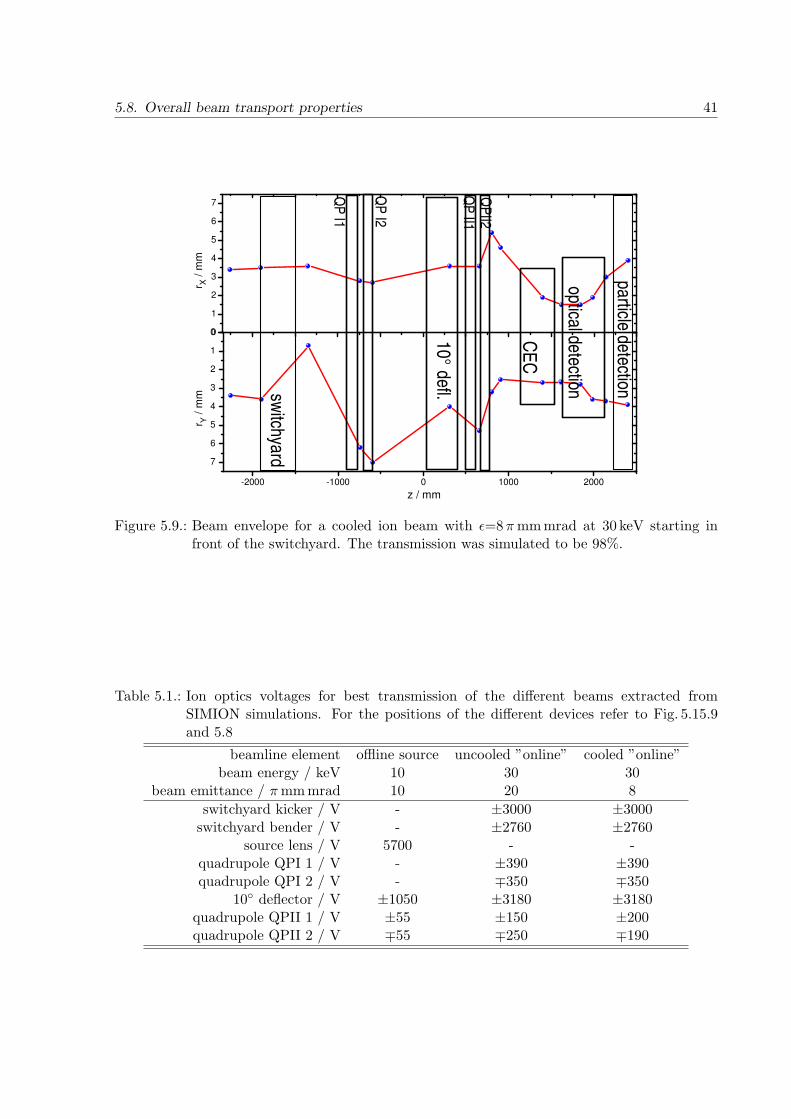
5.8. Overall beam transport properties 41
0
1
2
3
4
5
6
7
-2000 -1000 0 1000 2000
7
6
5
4
3
2
1
0
particle detection
optical detection
CE
C
QP
II2Q
P II1
switchyard
10° defl.
r X /
mm
QP
I1
QP
I2
rY /
mm
z / mm
Figure 5.9.: Beam envelope for a cooled ion beam with ǫ=8πmm mrad at 30 keV starting infront of the switchyard. The transmission was simulated to be 98%.
Table 5.1.: Ion optics voltages for best transmission of the different beams extracted fromSIMION simulations. For the positions of the different devices refer to Fig. 5.15.9and 5.8
beamline element offline source uncooled ”online” cooled ”online”beam energy / keV 10 30 30
beam emittance / πmm mrad 10 20 8
switchyard kicker / V - ±3000 ±3000switchyard bender / V - ±2760 ±2760
source lens / V 5700 - -quadrupole QPI 1 / V - ±390 ±390quadrupole QPI 2 / V - ∓350 ∓350
10 deflector / V ±1050 ±3180 ±3180quadrupole QPII 1 / V ±55 ±150 ±200quadrupole QPII 2 / V ∓55 ∓250 ∓190

42 5. The Collinear Laser Spectroscopy Branch TRIGA-LASER
PID
diode laserpiezo
wave meter
beam
splitter
He-Ne laser
fiber
to beamline
feedback loop
Figure 5.10.: The laser system used for the first tests with stable rubidium atoms. The laser wasfrequency-stabilized with a wavemeter and the light was guided to the experimentwith a fiber.
5.9. The Laser System for the First Test on Rb Atoms
For the first laser spectroscopy tests with rubidium atoms a diode laser setup was used to producethe 780 nm probe laser light. A schematic view of the laser system is shown in Fig. 5.10. TheToptica DL100 laser was frequency stabilized by a HighFinesse WS7 wavelength meter whichwas calibrated prior to each measurement with a two-mode stabilized helium-neon laser. Inthe wavemeter control program the set wavelength is compared to the actual value to producean error signal. After processing with a digital PID regulator, this feedback signal is sent tothe piezo actuator of the diode-laser grating for wavelength tuning. Under stable conditionsconcerning ambient temperature and air pressure, a frequency error of only 6 MHz in 8 h wasobserved. However, it should be noted that this measurement was done in the laser laboratoryand not in the reactor experimental hall.
The stabilized output of the laser was transported to the entrance window of the apparatuswith a fiber, where the coupling to the beamline was accomplished by a set of mirrors andiris apertures. To ensure high transmission of the linearly polarized laser and a low level ofscattering light the entrance and exit quartz windows were installed at the Brewster angle of57.2. Together with a careful adjustment of the laser beam through the beamline with thehelp of the adjustable apertures in front and behind the CEC, a transmission of 96% could bereached. The diameter of the well collimated laser inside the light collection unit was adjustedto be ≈4 mm offering enough distance from the edges of the small apertures of the CEC to keepscattered light in the detector on a reasonable level and ensure a reasonable overlap with theion beam according to Fig. 5.9 and Fig. 5.8. The details of the laser background and its impacton the overall performance of the fluorescence detection will be discussed in the Ch. 6.2.2
5.10. Data Acquisition and Experiment Control
The primary task of the experiment control is to acquire the counts from the photomultiplieras a function of the voltage applied to the charge-exchange cell or the optical detection unit,and to measure this voltage with high precision. The implementation of all static voltages forthe ion-optical devices in a common control system is planned for the future and has recently

5.10. Data Acquisition and Experiment Control 43
PC
Trigger
16 Bit DAC32 Bit Counter
GPIB
KEPCO x50high voltage amplifier
CEC PMT
Heinzinger10high voltage supply
HV divider
Agilentmultimeter
SOURCE
Heinzinger 60high voltage supply
voltages
GPIB
signal
&
Gate generator
Figure 5.11.: Schematic of the data acquisition and the experiment control. The shown configu-ration is used for scanning the voltage either with the Kepco amplifier or with theHeinzinger 10 kV supply. For further details refer to the text.
started as a diploma thesis [Ham10].The data acquisition program was created in LabView and allows communicating with the
Heinzinger high-voltage supply and the Agilent precision multimeter via GPIB. The Kepco am-plifier is controlled by the DAC of a multi I/O card also providing four 32 Bit counter channelsused for the pre-processed TTL-pulses from the photomultiplier counting electronics. The pro-gram records the number of counts for each measurement step of typically 20 ms (dwell time)as a function of the DAC voltage for the Kepco amplifier or the Heinzinger supply which areramped during one scan. A pre-defined number of total scans allows integrating individual scansdirectly. Because of timing problems with the PC-based LabView and other background pro-cesses which affected the dwell time during the first tests, the measurement gate was createdexternally by a NIM digital gate generator and a coincidence unit. Fig. 5.11 shows the schematicof the experiment control.


6. Off-line Commissioning of TRIGA-LASER
For a first performance test of the experimental setup the search for an easy solution concerningion production and required laser system, but still with the ability to also test the charge-exchange cell, led to rubidium as an ideal test candidate. The infrared wavelength of the5 2S1/2 → 5 2P3/2 D2 transition of 780 nm in the atom is easily supplied by a low-priced laserdiode in a relatively simple external cavity setup and the ions can easily be produced by surfaceionization in a hot cavity.
6.1. Beam Transport and Charge Exchange
The results presented in this section are mainly based on beam intensity measurements withFaraday cups. In some cases the adjustable apertures were used as charge collectors to extractthe ratio of ions passing the charge-exchange cell. The current was measured with a Keithley6485 picoamperemeter.
For the intensity measurement of the atom beam the
ion / atom beam collector
suppressor
signalsuppressor
voltage
Figure 6.1.: Schematic view of theFaraday cup.
cylindrical suppressor electrode in the Faraday cup (seeFig. 6.1) was put on positive potential (≈30 V) to extractsecondary electrons emitted from the impinging atoms.This electron current was then measured. A calibrationmeasurement with ions showed that with this particulargeometry on average three electrons were released per in-cident particle.
6.1.1. Transport Efficiency and Ion Beam Profiles
The ion beam transport efficiency through the complete setup can only be roughly estimated asit is impossible to measure the ion current in every position of the beamline. Eventual losses inthe extraction optics of the ion source for example, cannot be quantified. For a 6 keV rubidiumion beam the efficiency was determined by measuring the current on two identical Faraday cups,one inside the 10 deflection chamber and the other one behind the optical detection unit. Afterfine adjustments to the ion-optical elements a transmission efficiency of 70% was obtained. Thevoltage settings for this case are given in Tab. 6.1.
After the installation of two identical adjustable apertures in front of the charge-exchangecell and behind the optical detection system, another transmission test was done by measuringthe current on the closed apertures, which is an aluminum plate with a number of aperturesof different diameter. The result was a transmission of 71% in agreement with the previousresult, showing that losses between the 10 deflection chamber and the CEC are negligible. Thevoltages applied to the electrodes are also listed in Tab. 6.1. The need for a correction voltage inthe 10 deflection chamber shows that the offline source housing and its connection to the setupare not exactly straight and cause the ion beam to enter at a small angle in the vertical plane.The agreement with the simulations that predicted a transmission of 97% (see Chapter 5.8) is
45
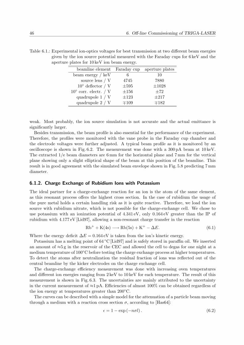
46 6. Off-line Commissioning of TRIGA-LASER
Table 6.1.: Experimental ion-optics voltages for best transmission at two different beam energiesgiven by the ion source potential measured with the Faraday cups for 6 keV and theaperture plates for 10 keV ion beam energy.
beamline element Faraday cup aperture plates
beam energy / keV 6 10source lens / V 4745 7880
10 deflector / V ±595 ±102810 corr. electr. / V ±156 ±72
quadrupole 1 / V ±123 ±217quadrupole 2 / V ∓109 ∓182
weak. Most probably, the ion source simulation is not accurate and the actual emittance issignificantly larger.
Besides transmission, the beam profile is also essential for the performance of the experiment.Therefore, the profiles were monitored with the vane probe in the Faraday cup chamber andthe electrode voltages were further adjusted. A typical beam profile as it is monitored by anoscilloscope is shown in Fig. 6.2. The measurement was done with a 300 pA beam at 10 keV.The extracted 1/e beam diameters are 6 mm for the horizontal plane and 7 mm for the verticalplane showing only a slight elliptical shape of the beam at this position of the beamline. Thisresult is in good agreement with the simulated beam envelope shown in Fig. 5.8 predicting 7 mmdiameter.
6.1.2. Charge Exchange of Rubidium Ions with Potassium
The ideal partner for a charge-exchange reaction for an ion is the atom of the same element,as this resonant process offers the highest cross section. In the case of rubidium the usage ofthe pure metal holds a certain handling risk as it is quite reactive. Therefore, we load the ionsource with rubidium nitrate, which is not possible for the charge-exchange cell. We chose touse potassium with an ionization potential of 4.341 eV, only 0.164 eV greater than the IP ofrubidium with 4.177 eV [Lid97], allowing a non-resonant charge transfer in the reaction
Rb+ + K(4s) −→ Rb(5s) + K+ − ∆E. (6.1)
Where the energy deficit ∆E = 0.164 eV is taken from the ion’s kinetic energy.Potassium has a melting point of 64 C [Lid97] and is safely stored in paraffin oil. We inserted
an amount of ≈5 g in the reservoir of the CEC and allowed the cell to degas for one night at amedium temperature of 100C before testing the charge exchange process at higher temperatures.To detect the atoms after neutralization the residual fraction of ions was reflected out of thecentral beamline by the kicker electrodes on the charge exchange cell.
The charge-exchange efficiency measurement was done with increasing oven temperaturesand different ion energies ranging from 2 keV to 10 keV for each temperature. The result of thismeasurement is shown in Fig. 6.3. The uncertainties are mainly attributed to the uncertaintyin the current measurement of ≈1 pA. Efficiencies of almost 100% can be obtained regardless ofthe ion energy at temperatures greater than 200C.
The curves can be described with a simple model for the attenuation of a particle beam movingthrough a medium with a reaction cross section σ, according to [Has64]:
ǫ = 1 − exp (−nσl) . (6.2)

6.1. Beam Transport and Charge Exchange 47
-10 -5 0 5 10 15
0
50
100
150
200
250
sig
nal /
a.u
.
scanner position / mm
horizontal plane vertical plane
Figure 6.2.: Ion beam profile recorded with the vane probe for a beam current of 300 pA. The1/e2 beam diameters for the slightly elliptically deformed beam are 6 mm for thehorizontal plane and 7 mm for the vertical plane.
80 100 120 140 160 180 200
0
20
40
60
80
100- 10 keV
- 8 keV
- 6 keV
- 4 keV
- 2 keV
eff
icie
ncy /
%
cell temperature / °C
Figure 6.3.: Charge exchange efficiencies for different ion energies as a function of the cell tem-perature. The curves show fits with the model described in the text, allowing toextract the charge-exchange cross sections.

48 6. Off-line Commissioning of TRIGA-LASER
2 4 6 8 10
6
8
10
12
14
16
18
20
22
24
26
28
30
32
2 4 6 8 10
tota
l cro
ss s
ectio
n / 1
0-1
6 c
m2
ion energy / keV
Figure 6.4.: Charge-exchange cross sections for the non-resonant charge transfer between Rb+
and K. The error bars refer to the statistical error from the fit to the efficiencydata shown in Fig. 6.3. The two outer curves represent the confidence band dueto the systematic uncertainty caused by the unknown interaction length in thecharge-exchange cell. There is a significant increase in the cross section with alocal maximum, which is typical for this type of reaction [Per65]. A fit to the dataaccording to Eq. 6.4up to an energy of 8 keV is indicated by the solid red line.
Where l is the length of the interaction region and n is the atom density of the medium.Replacing n with a parametrization of the vapor pressure of liquid potassium as a function ofthe temperature [Alc84], one obtains
ǫ = 1 − exp
(
−10−4453 K
T+4.402NAσl
Vmol p0
)
, (6.3)
with the constants NA the Avogadro number, Vmol the standard volume per mol and p0 thestandard pressure. The vapor pressure in the active region of the CEC deduced from theparametrization for 200C is Pvap = 10−4453 K/473 K+4.402 = 1 × 10⁻² mbar while the ambientpressure in the vacuum chamber remains unchanged at 1 × 10⁻⁶ mbar. This shows that thecondensation and reflow of the potassium at the outer cooling blocks, which were kept at tem-peratures of 45C, works nicely1.
A fit to the data with the cross section as a free parameter results in the values for σ shown inFig. 6.4. An interaction length of 7±2 cm was assumed, as the precise extension of the K vaporcloud inside the CEC is unknown and can only be estimated. Therefore the large systematicuncertainties on the cross sections marked by the two limiting curves. It was shown for othercombinations of alkali ions and vapor [Per65], that the non-resonant cross sections are of theorder of 10−15 − 10−16 cm2 and that the global trend of the cross section follows the relation
1The CEC is now operational for more than one year without refill.

6.2. Collinear Laser Spectroscopy with Stable Rubidium Atoms 49
-500 -400 -300 -200 -100 0 100 200 300 400 500
36000
39000
42000
45000
48000
87Rb
85Rb
cou
nts
scan voltage / V
Figure 6.5.: Full hyperfine spectra for the stable Rb isotopes recorded in one measurement. Thespectra are the sum of 10 individual scans taken with 1 V steps and a dwell time of20 ms. The laser power was 1 mW and the atom intensity was 1.2×10⁸ atoms/s.
[Per65]
σ ∝ exp
(
−a∆Eh√
2Ekin/m
)
, (6.4)
with the element specific constant a, the energy deficit ∆E, the ion mass m and Planck’sconstant h. This relation is valid until a maximum is reached for a certain energy depending on∆E. Above this value the cross section decreases monotonically with increasing particle energyas in the case of the resonant charge exchange. Our results are in good agreement with this,reproducing the correct order of magnitude and showing a maximum at 8 keV. A fit to the dataexcluding the cross section for 10 keV, which is already decreasing, is shown by the solid redline. Unfortunately, the behavior for higher energies cannot be studied so far, because of thelimited high-voltage specifications of the offline-source cage.
For further laser spectroscopy tests, a cell temperature of 140C was chosen in most cases inorder to increase the lifetime of the CEC and the potassium filling and for convenient heatingand cooling times. This offers a charge-exchange efficiency of ≈ 10%. It will be shown later,that besides the charge exchange reaction further collisions may occur at higher cell pressures,which change the kinetic energy of some atoms, leading to a visible effect in the lineshape of thelaser spectroscopic resonances (see Ch. 6.2.4).
6.2. Collinear Laser Spectroscopy with Stable Rubidium Atoms
The ion beam transport tests and the commissioning of the charge-exchange cell were onlypreparatory work for the main task of the setup: collinear laser spectroscopy on a fast atomicbeam. A full hyperfine spectrum for both naturally abundant isotopes 85Rb and 87Rb recorded
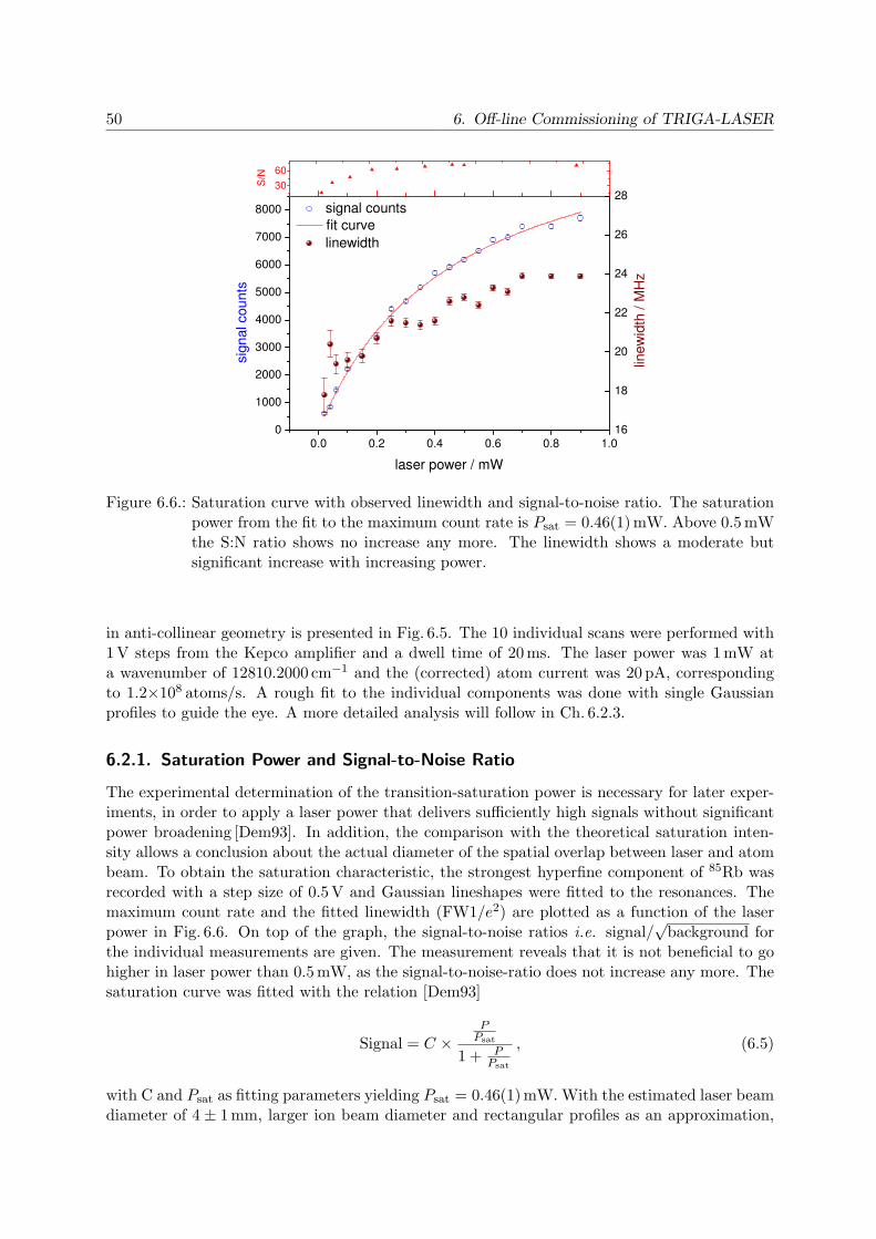
50 6. Off-line Commissioning of TRIGA-LASER
0.0 0.2 0.4 0.6 0.8 1.00
1000
2000
3000
4000
5000
6000
7000
8000
16
18
20
22
24
26
2830
60
signal counts
fit curve
sig
na
l cou
nts
laser power / mW
linewidth
lin
ew
idth
/ M
Hz
S/N
Figure 6.6.: Saturation curve with observed linewidth and signal-to-noise ratio. The saturationpower from the fit to the maximum count rate is Psat = 0.46(1)mW. Above 0.5 mWthe S:N ratio shows no increase any more. The linewidth shows a moderate butsignificant increase with increasing power.
in anti-collinear geometry is presented in Fig. 6.5. The 10 individual scans were performed with1 V steps from the Kepco amplifier and a dwell time of 20 ms. The laser power was 1 mW ata wavenumber of 12810.2000 cm−1 and the (corrected) atom current was 20 pA, correspondingto 1.2×10⁸ atoms/s. A rough fit to the individual components was done with single Gaussianprofiles to guide the eye. A more detailed analysis will follow in Ch. 6.2.3.
6.2.1. Saturation Power and Signal-to-Noise Ratio
The experimental determination of the transition-saturation power is necessary for later exper-iments, in order to apply a laser power that delivers sufficiently high signals without significantpower broadening [Dem93]. In addition, the comparison with the theoretical saturation inten-sity allows a conclusion about the actual diameter of the spatial overlap between laser and atombeam. To obtain the saturation characteristic, the strongest hyperfine component of 85Rb wasrecorded with a step size of 0.5 V and Gaussian lineshapes were fitted to the resonances. Themaximum count rate and the fitted linewidth (FW1/e2) are plotted as a function of the laserpower in Fig. 6.6. On top of the graph, the signal-to-noise ratios i.e. signal/
√background for
the individual measurements are given. The measurement reveals that it is not beneficial to gohigher in laser power than 0.5 mW, as the signal-to-noise-ratio does not increase any more. Thesaturation curve was fitted with the relation [Dem93]
Signal = C ×P
Psat
1 + PPsat
, (6.5)
with C and Psat as fitting parameters yielding Psat = 0.46(1) mW. With the estimated laser beamdiameter of 4 ± 1 mm, larger ion beam diameter and rectangular profiles as an approximation,

6.2. Collinear Laser Spectroscopy with Stable Rubidium Atoms 51
one obtains for the saturation intensity of the D2 transition Isat = 3.7(9) mW/cm2, which is ingood agreement with the theoretical value of Itheo
sat = 3.05 mW/cm2 [Ste01a].
6.2.2. Performance of the Fluorescence Detection System
The overall efficiency of the optical detector is composed of the geometric efficiency of thecollecting ellipsoidal mirror ǫgeo, the transmission of the inverted viewport and the light guideǫtrans, and the quantum efficiency of the photomultiplier QE according to
ǫtotal = ǫgeo × ǫtrans ×QE. (6.6)
The experimental observable is the number of real fluorescence counting events on top of thebackground at resonance per time unit, divided by the number of atoms that passed the detectorin the same time interval. For our test experiment with naturally abundant 85Rb (72%) and thecalibration of the Faraday cup as described in section 6.1.2, this leads to the expression
ǫtotal =signal
jatoms × 0.72 ×Nscans × tdwell, (6.7)
with an atom flux of jatoms = Icupatoms × 1/3. Nscans is the number of accumulated scans and tdwell
is the measurement time per channel. In Fig. 6.7 the resonance which was used to extract thebest value of ǫtotal = 1 photon/356 atoms for the total efficiency is shown.
Because of the lack of mass separation in the beam, any contamination of the ion beam wouldlead to underestimated values for the measured efficiency and the real efficiency will scale linearlywith the fraction of impurities. In order to further increase the number of detected photons peratom the reflectivity of the mirror could be optimized, which so far only has a copper surfacepolished by hand.
In order to get an idea about the performance of the detector in comparison with similardevices, our results were compared to the existing fluorescence detection setup used at ISOLDEin the COLLAPS experiment[Neu81]. The setup there consists of a 20 cm long mirror and in thecase of Mg and Be ions (UV) two lens stages and two photomultipliers. For infrared wavelengthsas in the case of Ba a light guide was used to collect the light from the chamber. For a realcomparability of the efficiencies of the different detectors ǫtotal was normalized by the quantumefficiency to account for the different photomultipliers used, the different transition strengths bythe Einstein B coefficient [Dem93], and the different numbers of excitation cycles per meter inthe detector volume by the atom/ion velocity v multiplied by the excited-state life time τ . Thenormalized efficiency can be expressed as
ǫnormgeo =
ǫtotalQE ×B × v × τ
. (6.8)
In this way of comparing the individual detectors the present setup shows an excellent perfor-mance with 14 times higher efficiency compared to the present COLLAPS detector (see Ta-ble 6.2). Results of detector simulations with the optical ray tracing software FRED [Eng10]are shown as bar chart in Fig. 6.8. The calculated efficiencies were normalized to the measuredefficiency at TRIGA-LASER. The ray-tracing simulations [Ham10] show excellent agreementwith the measured results. Only the performance of the Ba detection setup was predicted to bebetter, which may be caused by transmission losses in the light guide that are not included inthe simulation.
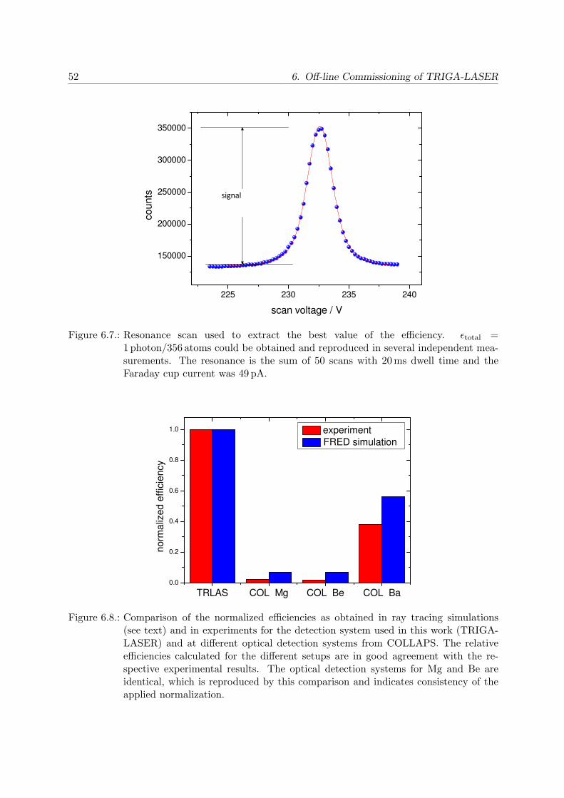
52 6. Off-line Commissioning of TRIGA-LASER
225 230 235 240
150000
200000
250000
300000
350000
counts
scan voltage / V
signal
Figure 6.7.: Resonance scan used to extract the best value of the efficiency. ǫtotal =1 photon/356 atoms could be obtained and reproduced in several independent mea-surements. The resonance is the sum of 50 scans with 20 ms dwell time and theFaraday cup current was 49 pA.
TRLAS COL Mg COL Be COL Ba0.0
0.2
0.4
0.6
0.8
1.0
norm
aliz
ed e
ffic
iency
experiment
FRED simulation
Figure 6.8.: Comparison of the normalized efficiencies as obtained in ray tracing simulations(see text) and in experiments for the detection system used in this work (TRIGA-LASER) and at different optical detection systems from COLLAPS. The relativeefficiencies calculated for the different setups are in good agreement with the re-spective experimental results. The optical detection systems for Mg and Be areidentical, which is reproduced by this comparison and indicates consistency of theapplied normalization.

6.2. Collinear Laser Spectroscopy with Stable Rubidium Atoms 53
Table 6.2.: Detector efficiencies, normalized efficiency ǫnormgeo and noise-normalized efficiency ǫnoise
as defined in the text. All values required for the calculation according to Eq. 6.8and Eq. 6.9 are included for the four detector setups.
Experiment TRIGA-LASER COLLAPS Ba COLLAPS Mg COLLAPS Be
Reference This work [Neu81] This work [Gep10]ǫtotal 2.9 × 10⁻³ 1.0 × 10⁻² 5 × 10⁻⁴ 8.3 × 10⁻⁵
QE / % 5 20 25 20τ / ns 26.3 8.4 3.9 8,7Background / 1/s 200 000 15 000 15 000 15 000B / 1020 m/kg 10.8 12.1 3.4 2.1v / 105 m/s 1.51 2.06 6.34 10.8ǫnormgeo /10−26 a.u. 20.5 7.15 1.44 1.74
ǫnoise / 10−29 a.u. 10.5 26.1 5.87 6.72
ǫnormgeo,relǫnormgeo,relǫnormgeo,rel 1 0.34 0.069 0.088
ǫnoise,relǫnoise,relǫnoise,rel 1 2.49 0.56 0.64
Besides efficiency, the background level in the detection section is defining the overall per-formance of an optical detector and therefore needs to be taken into account. Here the maincontribution to the noise is treated as statistical fluctuations of the stray light caused by thelaser. In this case ǫnorm
geo is modified by the noise, i.e. the square root of the background countrate per mW of incident laser power. Again, to correct for the influence of the photomultiplier’squantum efficiency on the background rate, the result is multiplied by the square root of thequantum efficiency according to
ǫnoise = ǫnormgeo ×
√
QE
background(6.9)
and is called noise-normalized efficiency. From this point of view the TRIGA-LASER opticaldetection unit is performing similar well as the existing systems at ISOLDE because its perfor-mance measure is slightly reduced by the high background level. In Table 6.2 the results aresummarized.
A more practical figure for the efficiency of an optical detector is the minimal particle beamintensity needed to get a visible signal in a reasonable time. Currently, with the TRIGA-LASERsetup developed in this work a signal-to-noise ratio of 2 in a resonance scan of 20 points can bereached for rubidium in a 6 h integration time with a beam intensity of only 1× 10⁴ particles/s,assuming stable voltages and a laser that is stable in intensity and frequency (see Ch. 6.2.5).
At the present status our detector is competitive, although we suffer from the rather highbackground level. Further optimization of the apertures in the beamline, especially right afterthe Brewster windows, may reduce the background and, hence, the noise. This will be subjectto further studies together with a completely new design of the light collector [Ham10] using acombined approach of imaging and non-imaging optics.
6.2.3. Resolution and Accuracy of the Collinear Setup
The high-voltage divider used to measure the voltages applied to the charge-exchange cell wascalibrated with the Heinzinger PNChp10000 high voltage supply, which is specified to be accurate

54 6. Off-line Commissioning of TRIGA-LASER
280 290 300 310 320 330 340
30000
35000
40000
45000
50000
55000
counts
scan voltage / V
-30 -20 -10 0 10 20 30 40 50 60
30000
35000
counts
scan voltage / V
180 190 200 210 220 230 240 250
30000
35000
40000
co
unts
scan voltage / V
-500 -490 -480 -470 -460 -450 -440
29500
30000
30500
31000
counts
scan voltage / V
85Rb 85Rb
87Rb87Rb
F=3 → F=2 →
F=2 → F=1→
4
32
3
2
1
3
21
2
1
0
S1/2
P3/2
F=2
F=3
F=1
F=2F=3
F=4
S1/2
P3/2
F=2
F=3
F=1
F=2F=3
F=4
S1/2
P3/2
F=2
F=3
F=1
F=2F=3
F=4
I=5/2
S1/2
P3/2
F=1
F=2
F=0
F=1
F=2
F=3
S1/2
P3/2
F=1
F=2
F=0
F=1
F=2
F=3
I=3/2
Figure 6.9.: Hyperfine multiplets of the two stable rubidium isotopes. The assignment of thetransitions was done according to the selection rules for dipole transitions. Theresonances were fitted with Gaussian profiles of one common FWHM. The centerpositions, the intensities, the baseline and the linewidth (FWHM) were free fittingparameters. In Tab. 6.3 the results of the extracted level spacings are shown incomparison to literature values.
in voltage to 2×10⁻⁴. This yielded a divider ratio of D = 1001.212(5). With this voltage dividerthe Kepco high voltage amplifier could be calibrated and an amplification factor of fKepco = 50.09was extracted.
The experimentally well known hyperfine structure and the isotope shift of 85Rb to 87Rb[Ste01a] were studied in detail to investigate the resolution and the accuracy of our experiment.The measurement was performed with the Kepco amplifier and a source voltage of 9976 Vmeasured with the voltage divider. The laser was stabilized to 12810.1633 cm−1 throughoutthe measurement. The individual peaks of the hyperfine multiplets were fitted with Gaussianprofiles for the extraction of the hyperfine structure parameters. A more detailed discussionabout the line shape will follow later. In Fig. 6.9 the multiplets are shown together with theassignment of the individual transitions. All peaks from allowed transitions are visible and eventhe closely neighboring peaks in the F = 2 multiplet of 85Rb can be separated. Also transitionswhich are subject to hyperfine pumping (in the 85Rb F = 2 and the 87Rb F = 1 case) arevisible, showing the advantage of a short distance between the charge-exchange cell and thedetector. Tab. 6.3 compares the extracted hyperfine splittings with the literature values takenfrom [Ste01a]. The frequencies were calculated from the voltage differences in non-relativistic
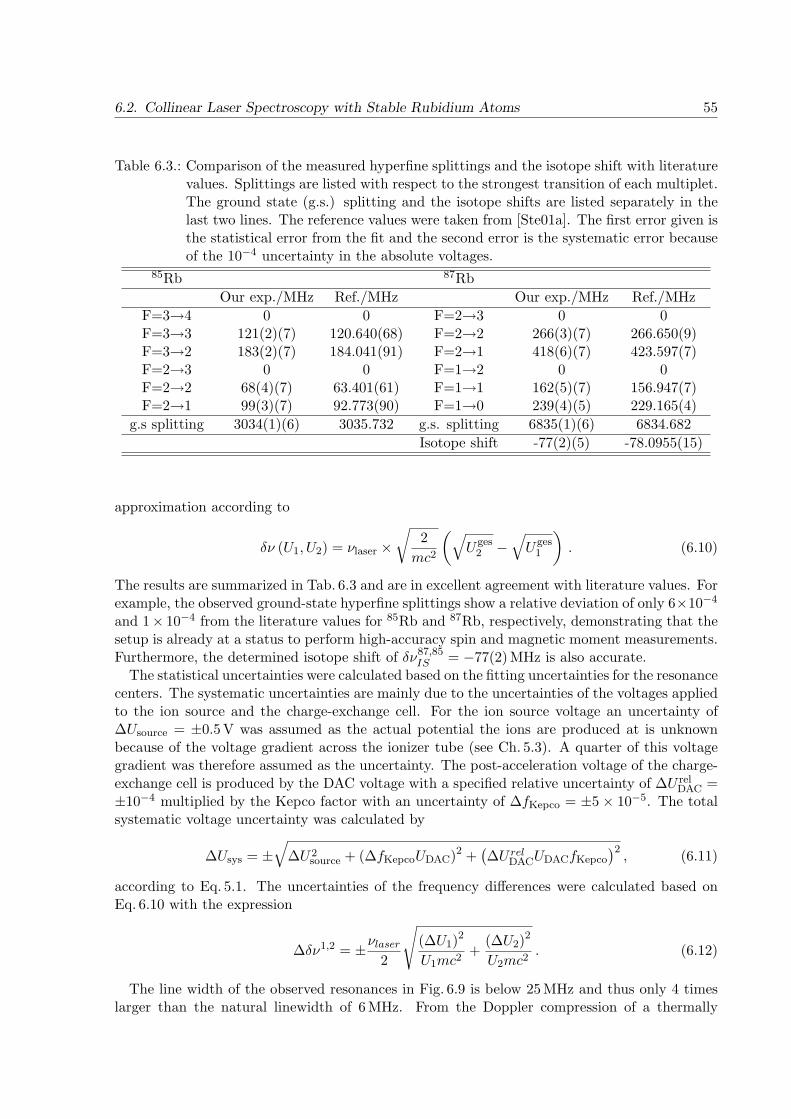
6.2. Collinear Laser Spectroscopy with Stable Rubidium Atoms 55
Table 6.3.: Comparison of the measured hyperfine splittings and the isotope shift with literaturevalues. Splittings are listed with respect to the strongest transition of each multiplet.The ground state (g.s.) splitting and the isotope shifts are listed separately in thelast two lines. The reference values were taken from [Ste01a]. The first error given isthe statistical error from the fit and the second error is the systematic error becauseof the 10−4 uncertainty in the absolute voltages.
85Rb 87Rb
Our exp./MHz Ref./MHz Our exp./MHz Ref./MHz
F=3→4 0 0 F=2→3 0 0F=3→3 121(2)(7) 120.640(68) F=2→2 266(3)(7) 266.650(9)F=3→2 183(2)(7) 184.041(91) F=2→1 418(6)(7) 423.597(7)F=2→3 0 0 F=1→2 0 0F=2→2 68(4)(7) 63.401(61) F=1→1 162(5)(7) 156.947(7)F=2→1 99(3)(7) 92.773(90) F=1→0 239(4)(5) 229.165(4)
g.s splitting 3034(1)(6) 3035.732 g.s. splitting 6835(1)(6) 6834.682
Isotope shift -77(2)(5) -78.0955(15)
approximation according to
δν (U1, U2) = νlaser ×√
2
mc2
(√
Uges2 −
√
Uges1
)
. (6.10)
The results are summarized in Tab. 6.3 and are in excellent agreement with literature values. Forexample, the observed ground-state hyperfine splittings show a relative deviation of only 6×10⁻⁴
and 1× 10⁻⁴ from the literature values for 85Rb and 87Rb, respectively, demonstrating that thesetup is already at a status to perform high-accuracy spin and magnetic moment measurements.Furthermore, the determined isotope shift of δν87,85
IS = −77(2)MHz is also accurate.The statistical uncertainties were calculated based on the fitting uncertainties for the resonance
centers. The systematic uncertainties are mainly due to the uncertainties of the voltages appliedto the ion source and the charge-exchange cell. For the ion source voltage an uncertainty of∆Usource = ±0.5V was assumed as the actual potential the ions are produced at is unknownbecause of the voltage gradient across the ionizer tube (see Ch. 5.3). A quarter of this voltagegradient was therefore assumed as the uncertainty. The post-acceleration voltage of the charge-exchange cell is produced by the DAC voltage with a specified relative uncertainty of ∆U rel
DAC =±10−4 multiplied by the Kepco factor with an uncertainty of ∆fKepco = ±5 × 10⁻⁵. The totalsystematic voltage uncertainty was calculated by
∆Usys = ±√
∆U2source + (∆fKepcoUDAC)2 +
(∆U rel
DACUDACfKepco
)2, (6.11)
according to Eq. 5.1. The uncertainties of the frequency differences were calculated based onEq. 6.10 with the expression
∆δν1,2 = ±νlaser
2
√
(∆U1)2
U1mc2+
(∆U2)2
U2mc2. (6.12)
The line width of the observed resonances in Fig. 6.9 is below 25 MHz and thus only 4 timeslarger than the natural linewidth of 6 MHz. From the Doppler compression of a thermally

56 6. Off-line Commissioning of TRIGA-LASER
distributed ensemble (refer to Ch. 3.2) one would expect a residual line width matching thenatural line width. The observed broadening cannot be attributed to a divergence in the beamwhich is limited to about 3 mrad in our setup for good transmission, but to the voltage gradientin the ion source. Depending on the origin of ionization, the ion’s initial potential varies alongthe ionizer tube leading to an increase of the actual velocity spread and to additional Dopplerbroadening. The 10 kV total acceleration voltage results in a differential Doppler shift of ≈10 MHz/V. The observed width therefore corresponds to only 2V variation of the potential theion is produced at, which can be expected with our source configuration. With a different typeof surface ion source with indirect heating (e.g. electron impact heating), the resonances shouldbecome significantly narrower.
6.2.4. The Charge Exchange Process and its Impact on the Line Shape
In Ch. 6.1.2 it was already discussed that the charge exchange reaction leads to a small energyloss of all particles of the order of 0.1 V due to the energy gap in the ionization potentials betweenK and Rb. This energy deficit however, does not change the line profile. To fully understand theobserved line shape, which to the first order can be described by a Voigt profile [Dem93], otherreactions besides the charge exchange to the ground state of Rb have to be taken into account.There are several possible inelastic reactions contributing to the additional energy loss of someof the particles passing the charge-exchange cell [Ben86]:
Rb+ + K (4s) → Rb+ + K (4p) − ∆E → Rb+ + K (4s) − ∆E + hν , (6.13)
if the collision occurs prior to the neutralization, or for inelastic collisions after the chargeexchange reaction, e.g.
Rb (5s) + K (4s) → Rb (5s) + K (4p) − ∆E → Rb (5s) + K (4s) − ∆E + hν , (6.14)
where the potassium gets excited and
Rb (5s) + K (4s) → Rb (5p) + K (4s) − ∆E → Rb (5s) + K (4s) − ∆E + hν , (6.15)
for an excitation of the rubidium atom. A third type of reaction is the charge exchange into thefirst excited state of rubidium:
Rb+ + K (4s) → Rb (5p) + K+ − ∆E → Rb (5s) + K+ − ∆E + hν . (6.16)
The energy deficit ∆E corresponds to the energy gap of ≈ 1.6 eV between the ns ground stateand the np first excited state of the potassium or the rubidium atom, respectively and results ina shift in the resonance position. The analysis of the observed spectra shows that one reactionof this type is not sufficient to fit the data satisfactorily. Depending on the cell temperature asignificant amount of particles have suffered from two inelastic collisions. Fig. 6.10 shows thecomparison between a regular single Voigt fit and a fit with three equally spaced Voigt profilesof common width with a distance of 1.6V for a CEC temperature of 180C. For clarity theresiduals are also plotted. The difference in the peak position estimated by a single Voigt fit tothe fit with three profiles is 0.1 V, which corresponds to ≈1 MHz in frequency.
If the assumptions made above are correct, then the relative peak height of the satellite peaksshould depend on the vapor pressure in the cell, being a measure for the collision probability.The peak intensity ratios between the main peak and the leftmost peak were studied at differentcell temperatures and the parametrization from Eq. 6.3 was used to estimate the vapor pres-sures. From Fig. 6.11 we can conclude that there is indeed an increase in the intensity of thesatellite peak with increasing potassium vapor pressure in the charge-exchange cell supportingthe assumption of collisional excitation.
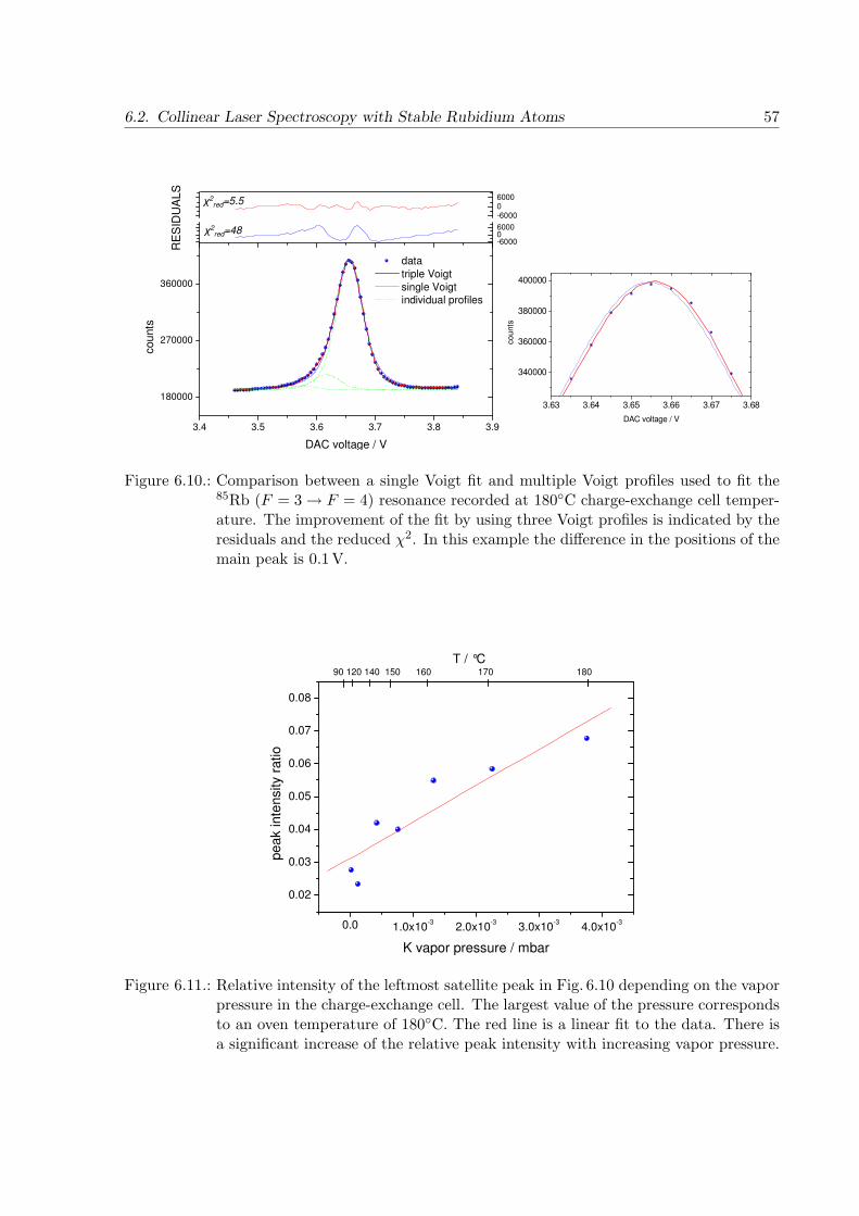
6.2. Collinear Laser Spectroscopy with Stable Rubidium Atoms 57
3.63 3.64 3.65 3.66 3.67 3.68
340000
360000
380000
400000
co
unts
DAC voltage / V3.4 3.5 3.6 3.7 3.8 3.9
180000
270000
360000
-600006000
-600006000
data
triple Voigt
single Voigt
individual profiles
cou
nts
DAC voltage / V
RE
SID
UA
LS
χ2red=5.5
χ2red=48
Figure 6.10.: Comparison between a single Voigt fit and multiple Voigt profiles used to fit the85Rb (F = 3 → F = 4) resonance recorded at 180C charge-exchange cell temper-ature. The improvement of the fit by using three Voigt profiles is indicated by theresiduals and the reduced χ2. In this example the difference in the positions of themain peak is 0.1 V.
0.0 1.0x10⁻³
2.0x10⁻³
3.0x10⁻³
4.0x10⁻³
0.02
0.03
0.04
0.05
0.06
0.07
0.08
pea
k inte
nsity r
atio
K vapor pressure / mbar
90 120 140 150 160 170 180
T / °C90 120 140 150 160 170 180
Figure 6.11.: Relative intensity of the leftmost satellite peak in Fig. 6.10 depending on the vaporpressure in the charge-exchange cell. The largest value of the pressure correspondsto an oven temperature of 180C. The red line is a linear fit to the data. There isa significant increase of the relative peak intensity with increasing vapor pressure.
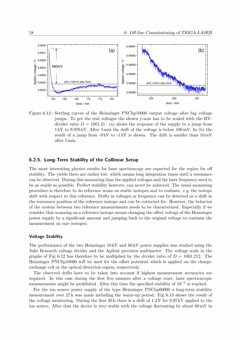
58 6. Off-line Commissioning of TRIGA-LASER
155 160 165 170 175 180
9.9632
9.9633
9.9634
9.9635
9.9636
9.9637
9.9638
Agile
nt
voltage /
V
time / min
drift <100mV after 5min
225 228 231
-0.99886
-0.99885
-0.99884
-0.99883
-0.99882
-0.99881
Agile
nt
voltage / V
time / min
drift <10mV after 5min
(a) (b)
480mV
Figure 6.12.: Settling curves of the Heinzinger PNChp10000 output voltage after big voltagejumps. To get the real voltages the shown y-axis has to be scaled with the HV-divider ratio D = 1001.21. (a) shows the response of the supply to a jump from1 kV to 9.976 kV. After 5 min the drift of the voltage is below 100 mV. In (b) theresult of a jump from -9 kV to -1 kV is shown. The drift is smaller than 10 mVafter 5 min.
6.2.5. Long-Term Stability of the Collinear Setup
The most interesting physics results for laser spectroscopy are expected for the region far offstability. The yields there are rather low, which means long integration times until a resonancecan be observed. During this measuring time the applied voltages and the laser frequency need tobe as stable as possible. Perfect stability however, can never be achieved. The usual measuringprocedure is therefore to do reference scans on stable isotopes and to evaluate, e.g, the isotopeshift with respect to this reference. Drifts in voltages or frequency can be detected as a shift inthe resonance position of the reference isotope and can be corrected for. However, the behaviorof the system between two reference measurements needs to be characterized. Especially if weconsider that scanning on a reference isotope means changing the offset voltage of the Heinzingerpower supply by a significant amount and jumping back to the original voltage to continue themeasurement on rare isotopes.
Voltage Stability
The performance of the two Heinzinger 10 kV and 60 kV power supplies was studied using theJulie Research voltage divider and the Agilent precision multimeter. The voltage scale in thegraphs of Fig. 6.12 has therefore to be multiplied by the divider ratio of D = 1001.212. TheHeinzinger PNChp10000 will be used for the offset potential which is applied on the charge-exchange cell or the optical detection region, respectively.
The observed drifts have to be taken into account if highest measurement accuracies arerequired. In this case during the first five minutes after a voltage reset, laser spectroscopicmeasurements might be prohibited. After this time the specified stability of 10−5 is reached.
For the ion source power supply of the type Heinzinger PNChp60000 a long-term stabilitymeasurement over 27 h was made including the warm-up period. Fig. 6.13 shows the result ofthe voltage monitoring. During the first 20 h there is a drift of 1.2 V for 9.97 kV applied to theion source. After that the device is very stable with the voltage fluctuating by about 80 mV in
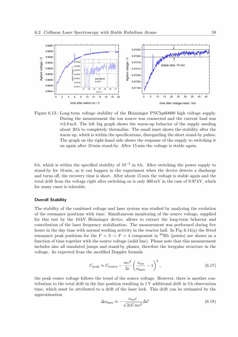
6.2. Collinear Laser Spectroscopy with Stable Rubidium Atoms 59
0 2 4 6 8 10 12 14 16 18 20
9.9644
9.9646
9.9648
9.9650
9.9652
9.9654
9.9656
9.9658
9.9660
A
gile
nt voltage /
V
time / h
21 22 23 24 25 26 27
9.97215
9.97218
9.97221
9.97224
9.97227
9.97230
9.97233
Agile
nt voltage /
V
time / h
drift 80mV
in 6 h!
0 5 10 15 20 25 30 35 40 45
9.97194
9.97200
9.97206
9.97212
9.97218
9.97224
9.97230
Agile
nt voltage /
V
time / min
stable after 15 min
time after switch-on / h time after voltage reset / min
Figure 6.13.: Long-term voltage stability of the Heinzinger PNChp60000 high voltage supply.During the measurement the ion source was connected and the current load was≈2.8 mA. The left big graph shows the warm-up behavior of the supply needingabout 20 h to completely thermalize. The small inset shows the stability after thewarm up, which is within the specifications, disregarding the short stand-by pulses.The graph on the right-hand side shows the response of the supply to switching iton again after 10 min stand-by. After 15 min the voltage is stable again.
6 h, which is within the specified stability of 10−5 in 8 h. After switching the power supply tostand-by for 10 min, as it can happen in the experiment when the device detects a dischargeand turns off, the recovery time is short. After about 15 min the voltage is stable again and thetotal drift from the voltage right after switching on is only 300 mV in the case of 9.97 kV, whichfor many cases is tolerable.
Overall Stability
The stability of the combined voltage and laser system was studied by analyzing the evolutionof the resonance positions with time. Simultaneous monitoring of the source voltage, suppliedfor this test by the 10 kV Heinzinger device, allows to extract the long-term behavior andcontribution of the laser frequency stabilization. The measurement was performed during fivehours in the day time with normal working activity in the reactor hall. In Fig. 6.14(a) the fittedresonance peak positions for the F = 3 → F = 4 component in 85Rb (points) are shown as afunction of time together with the source voltage (solid line). Please note that this measurementincludes also all simulated jumps and stand-by phases, therefore the irregular structure in thevoltage. As expected from the modified Doppler formula
Upeak ≈ Usource −mc2
2e
(νres
νlaser− 1
)2
, (6.17)
the peak center voltage follows the trend of the source voltage. However, there is another con-tribution to the total drift in the line position resulting in 1 V additional drift in 5 h observationtime, which must be attributed to a drift of the laser lock. This drift can be estimated by theapproximation
∆νlaser ≈ − νrese√2eUmc2
∆U (6.18)
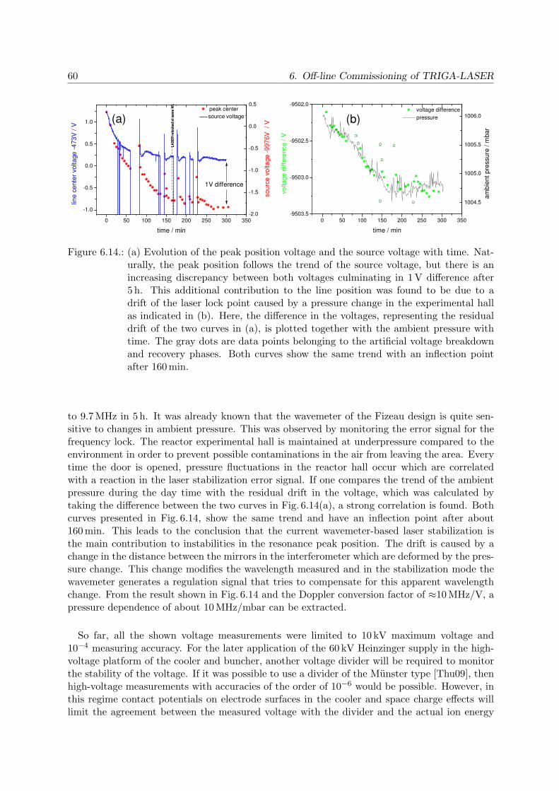
60 6. Off-line Commissioning of TRIGA-LASER
0 50 100 150 200 250 300 350
-1.0
-0.5
0.0
0.5
1.0
-2.0
-1.5
-1.0
-0.5
0.0
0.5peak center
line
cen
ter
vo
lta
ge
-4
73
V /
V
time / min
sou
rce
vo
lta
ge
-9
97
6V
/
V
source voltage
LA
SE
R r
elo
cke
d a
t sa
me W
L
1V difference
0 50 100 150 200 250 300 350-9503.5
-9503.0
-9502.5
-9502.0
1004.5
1005.0
1005.5
1006.0 voltage difference
volta
ge
diffe
rence /
V
time / min
pressure
am
bie
nt
pre
ssure
/ m
ba
r
(a) (b)
Figure 6.14.: (a) Evolution of the peak position voltage and the source voltage with time. Nat-urally, the peak position follows the trend of the source voltage, but there is anincreasing discrepancy between both voltages culminating in 1 V difference after5 h. This additional contribution to the line position was found to be due to adrift of the laser lock point caused by a pressure change in the experimental hallas indicated in (b). Here, the difference in the voltages, representing the residualdrift of the two curves in (a), is plotted together with the ambient pressure withtime. The gray dots are data points belonging to the artificial voltage breakdownand recovery phases. Both curves show the same trend with an inflection pointafter 160 min.
to 9.7 MHz in 5 h. It was already known that the wavemeter of the Fizeau design is quite sen-sitive to changes in ambient pressure. This was observed by monitoring the error signal for thefrequency lock. The reactor experimental hall is maintained at underpressure compared to theenvironment in order to prevent possible contaminations in the air from leaving the area. Everytime the door is opened, pressure fluctuations in the reactor hall occur which are correlatedwith a reaction in the laser stabilization error signal. If one compares the trend of the ambientpressure during the day time with the residual drift in the voltage, which was calculated bytaking the difference between the two curves in Fig. 6.14(a), a strong correlation is found. Bothcurves presented in Fig. 6.14, show the same trend and have an inflection point after about160 min. This leads to the conclusion that the current wavemeter-based laser stabilization isthe main contribution to instabilities in the resonance peak position. The drift is caused by achange in the distance between the mirrors in the interferometer which are deformed by the pres-sure change. This change modifies the wavelength measured and in the stabilization mode thewavemeter generates a regulation signal that tries to compensate for this apparent wavelengthchange. From the result shown in Fig. 6.14 and the Doppler conversion factor of ≈10 MHz/V, apressure dependence of about 10 MHz/mbar can be extracted.
So far, all the shown voltage measurements were limited to 10 kV maximum voltage and10−4 measuring accuracy. For the later application of the 60 kV Heinzinger supply in the high-voltage platform of the cooler and buncher, another voltage divider will be required to monitorthe stability of the voltage. If it was possible to use a divider of the Munster type [Thu09], thenhigh-voltage measurements with accuracies of the order of 10−6 would be possible. However, inthis regime contact potentials on electrode surfaces in the cooler and space charge effects willlimit the agreement between the measured voltage with the divider and the actual ion energy

6.3. Summary and Outlook 61
after extraction. A 10−5 measurement would therefore be sufficient for the purpose of mostexperiments at TRIGA-LASER which might be obtained using a 60 kV Julie Research dividerwith an additional temperature stabilization.
With regard to the laser stabilization, there would be the possibility to install the frequency ref-erence, like a wavemeter, an FPI, or even the frequency comb in the temperature- and pressure-stabilized laser laboratory of the institute and to couple the laser light through a fiber reachingfrom the laser laboratory to the experiment in the reactor hall. A short-term solution whichcould improve the wavelength stability is a hermetically sealed housing for the wavemeter keptat constant pressure and temperature.
6.3. Summary and Outlook
The current TRIGA-LASER setup is already at a stage to allow the measurement of nuclearspins and moments of radioactive isotopes by studying the hyperfine structure. It was shown inthe commissioning measurements that high-resolution scans of atomic hyperfine structures arepossible and that the results agree with literature values. The voltages applied are satisfactorilystable with the power supplies working according to their specifications.
The upgrade of the post-acceleration/-deceleration voltage devices, which includes a high-voltage cage to float the offset voltage supply and the charge-exchange cell voltage supply onthe scanning voltage, will be the next step towards the full functionality of the setup, involvingalso isotope-shift measurements with the jump-scan method.
After successful tests of the ion source, the mass separator, and the RFQ cooler and buncher,measurements of charge radii of the neutron-rich isotopes of elements starting from molybdenumand above will be performed to study the shape change at N=60 with a prolate deformation,which is supposed to vanish for nuclei above Mo [Cha09].
Besides the potential to perform laser spectroscopy on unknown ground, the TRIGA-LASERexperiment gives a unique opportunity to perform important development work towards highersensitivity of detectors [Ham10] or higher accuracy of the voltage measurement for the existingCOLLAPS experiment at ISOLDE (CERN), but especially it serves as the prototype of theLASPEC beamline for laser spectroscopy on atomic beams at the future facility FAIR at GSI[Rod10].


Part II.
Moments and Radii of Exotic
Magnesium Isotopes studied with
Collinear Laser Spectroscopy at
ISOLDE
63

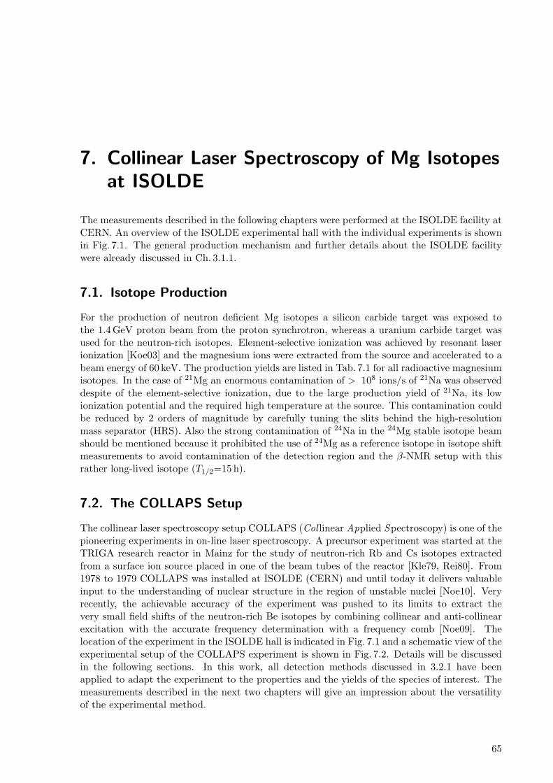
7. Collinear Laser Spectroscopy of Mg Isotopes
at ISOLDE
The measurements described in the following chapters were performed at the ISOLDE facility atCERN. An overview of the ISOLDE experimental hall with the individual experiments is shownin Fig. 7.1. The general production mechanism and further details about the ISOLDE facilitywere already discussed in Ch. 3.1.1.
7.1. Isotope Production
For the production of neutron deficient Mg isotopes a silicon carbide target was exposed tothe 1.4 GeV proton beam from the proton synchrotron, whereas a uranium carbide target wasused for the neutron-rich isotopes. Element-selective ionization was achieved by resonant laserionization [Koe03] and the magnesium ions were extracted from the source and accelerated to abeam energy of 60 keV. The production yields are listed in Tab. 7.1 for all radioactive magnesiumisotopes. In the case of 21Mg an enormous contamination of > 108 ions/s of 21Na was observeddespite of the element-selective ionization, due to the large production yield of 21Na, its lowionization potential and the required high temperature at the source. This contamination couldbe reduced by 2 orders of magnitude by carefully tuning the slits behind the high-resolutionmass separator (HRS). Also the strong contamination of 24Na in the 24Mg stable isotope beamshould be mentioned because it prohibited the use of 24Mg as a reference isotope in isotope shiftmeasurements to avoid contamination of the detection region and the β-NMR setup with thisrather long-lived isotope (T1/2=15 h).
7.2. The COLLAPS Setup
The collinear laser spectroscopy setup COLLAPS (Col linear Applied Spectroscopy) is one of thepioneering experiments in on-line laser spectroscopy. A precursor experiment was started at theTRIGA research reactor in Mainz for the study of neutron-rich Rb and Cs isotopes extractedfrom a surface ion source placed in one of the beam tubes of the reactor [Kle79, Rei80]. From1978 to 1979 COLLAPS was installed at ISOLDE (CERN) and until today it delivers valuableinput to the understanding of nuclear structure in the region of unstable nuclei [Noe10]. Veryrecently, the achievable accuracy of the experiment was pushed to its limits to extract thevery small field shifts of the neutron-rich Be isotopes by combining collinear and anti-collinearexcitation with the accurate frequency determination with a frequency comb [Noe09]. Thelocation of the experiment in the ISOLDE hall is indicated in Fig. 7.1 and a schematic view of theexperimental setup of the COLLAPS experiment is shown in Fig. 7.2. Details will be discussedin the following sections. In this work, all detection methods discussed in 3.2.1 have beenapplied to adapt the experiment to the properties and the yields of the species of interest. Themeasurements described in the next two chapters will give an impression about the versatilityof the experimental method.
65

66 7. Collinear Laser Spectroscopy of Mg Isotopes at ISOLDE
CRIS
Figure 7.1.: The ISOLDE experimental hall with the transport beamline and the individualexperiments.
Table 7.1.: Average production yield of radioactive magnesium isotopes at ISOLDE. The yieldsfor the neutron-deficient isotopes 21−23Mg are obtained with a silicon carbide (SiC)target and the neutron-rich isotopes are produced with a uranium carbide target.Laser resonance ionization was used to ionize the species. 1 ion/µC correspondsto approximately 1 ion/s, depending on the current and the pulse structure of theprotons.
Isotope yield / ions/µC Isotope yield / ions/µC
21Mg < 1 × 10⁴ 28Mg 3.6×10⁷
22Mg 9×10⁵ 29Mg 1.2×10⁶
23Mg 1.4×10⁷ 30Mg 4.6×10⁵
24Mg stable 31Mg 1.5×10⁵
25Mg ” 32Mg 4.2×10⁴
26Mg ” 33Mg 5.3×10³
27Mg 1.4×10⁶

7.2. The COLLAPS Setup 67
LASER
+
++ + + + + + + +
BII
B
T
tuning voltage
weak guiding field
strong field
scintillator and PMT
MgO crystal
optical pumping β-asymmetrydetection
Doppler tuningdeflection
_
+
acceleration
+
optical detection
Mg+ from
ISOLDE
PMT
LASER
+
++ + + + + + + +
BIIBII
B
T
B
T
tuning voltage
weak guiding field
strong field
scintillator and PMT
MgO crystal
optical pumping β-asymmetrydetection
Doppler tuningdeflection
_
+
acceleration
+
optical detection
Mg+ from
ISOLDE
PMT
β-NMR
Figure 7.2.: Top view of the experimental setup used for optical pumping followed by β-NMR.The ions from ISOLDE are exposed to circularly polarized laser light in a weakmagnetic guiding field. The resulting atomic polarization is adiabatically rotatedin the transition region between the weak longitudinal guiding field and the strongperpendicular NMR field. In the strong field the nuclear moment is decoupled fromthe electron shell before the ion is implanted into a MgO crystal. Two opposingpairs of scintillators (left and right) are used to detect the asymmetry of the βdecay. A radio frequency signal can be applied to a coil around the crystal (notshown in this figure) to resonantly destroy the nuclear polarization and thus the βasymmetry.
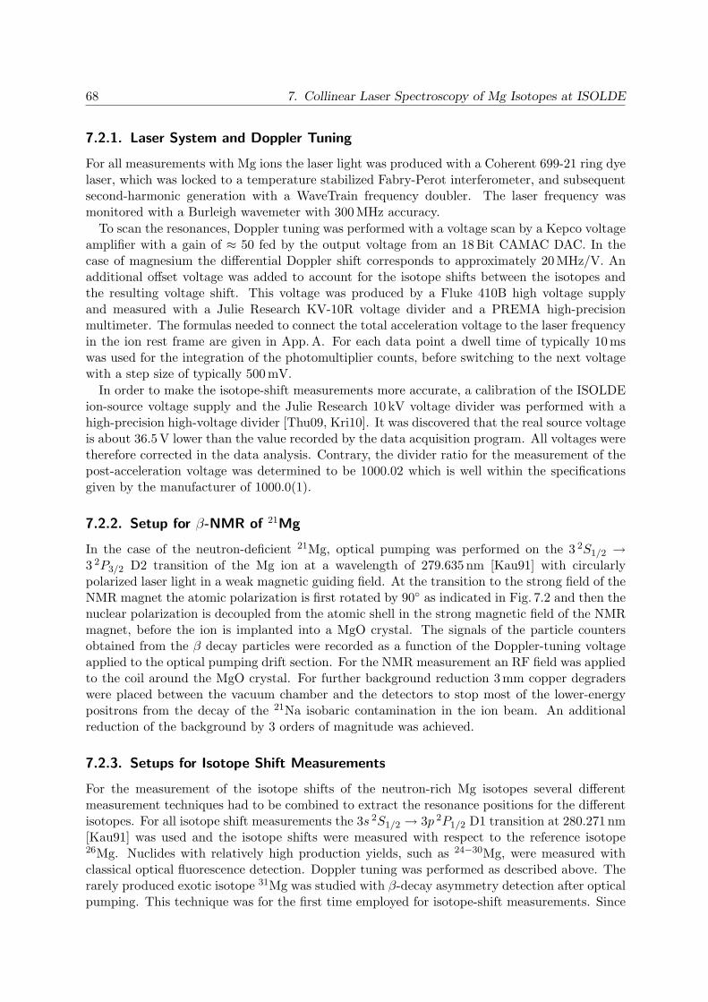
68 7. Collinear Laser Spectroscopy of Mg Isotopes at ISOLDE
7.2.1. Laser System and Doppler Tuning
For all measurements with Mg ions the laser light was produced with a Coherent 699-21 ring dyelaser, which was locked to a temperature stabilized Fabry-Perot interferometer, and subsequentsecond-harmonic generation with a WaveTrain frequency doubler. The laser frequency wasmonitored with a Burleigh wavemeter with 300 MHz accuracy.
To scan the resonances, Doppler tuning was performed with a voltage scan by a Kepco voltageamplifier with a gain of ≈ 50 fed by the output voltage from an 18 Bit CAMAC DAC. In thecase of magnesium the differential Doppler shift corresponds to approximately 20 MHz/V. Anadditional offset voltage was added to account for the isotope shifts between the isotopes andthe resulting voltage shift. This voltage was produced by a Fluke 410B high voltage supplyand measured with a Julie Research KV-10R voltage divider and a PREMA high-precisionmultimeter. The formulas needed to connect the total acceleration voltage to the laser frequencyin the ion rest frame are given in App. A. For each data point a dwell time of typically 10 mswas used for the integration of the photomultiplier counts, before switching to the next voltagewith a step size of typically 500 mV.
In order to make the isotope-shift measurements more accurate, a calibration of the ISOLDEion-source voltage supply and the Julie Research 10 kV voltage divider was performed with ahigh-precision high-voltage divider [Thu09, Kri10]. It was discovered that the real source voltageis about 36.5 V lower than the value recorded by the data acquisition program. All voltages weretherefore corrected in the data analysis. Contrary, the divider ratio for the measurement of thepost-acceleration voltage was determined to be 1000.02 which is well within the specificationsgiven by the manufacturer of 1000.0(1).
7.2.2. Setup for β-NMR of 21Mg
In the case of the neutron-deficient 21Mg, optical pumping was performed on the 3 2S1/2 →3 2P3/2 D2 transition of the Mg ion at a wavelength of 279.635 nm [Kau91] with circularlypolarized laser light in a weak magnetic guiding field. At the transition to the strong field of theNMR magnet the atomic polarization is first rotated by 90 as indicated in Fig. 7.2 and then thenuclear polarization is decoupled from the atomic shell in the strong magnetic field of the NMRmagnet, before the ion is implanted into a MgO crystal. The signals of the particle countersobtained from the β decay particles were recorded as a function of the Doppler-tuning voltageapplied to the optical pumping drift section. For the NMR measurement an RF field was appliedto the coil around the MgO crystal. For further background reduction 3 mm copper degraderswere placed between the vacuum chamber and the detectors to stop most of the lower-energypositrons from the decay of the 21Na isobaric contamination in the ion beam. An additionalreduction of the background by 3 orders of magnitude was achieved.
7.2.3. Setups for Isotope Shift Measurements
For the measurement of the isotope shifts of the neutron-rich Mg isotopes several differentmeasurement techniques had to be combined to extract the resonance positions for the differentisotopes. For all isotope shift measurements the 3s 2S1/2 → 3p 2P1/2 D1 transition at 280.271 nm[Kau91] was used and the isotope shifts were measured with respect to the reference isotope26Mg. Nuclides with relatively high production yields, such as 24−30Mg, were measured withclassical optical fluorescence detection. Doppler tuning was performed as described above. Therarely produced exotic isotope 31Mg was studied with β-decay asymmetry detection after opticalpumping. This technique was for the first time employed for isotope-shift measurements. Since

7.2. The COLLAPS Setup 69
6.00 6.25 6.50 6.75 7.00 7.25
450
500
550
600
650
700
even
ts
time of flight / µs
CENTER: 6.48 µs
Figure 7.3.: Time-of-flight spectrum of 32Mg triggered on the fluorescence signal from the pho-tomultiplier. The center position is 6.48µs and the full width a the base is 170 ns.
it relies on the understanding and modeling of the line profile in β-asymmetry detection toextract the resonance positions it was crucial to have a candidate where both techniques can beapplied and compared. Therefore, 29Mg was remeasured with β detection. Additionally, photon-ion coincidence detection (see Ch. 3.2.1) was used to increase the signal-to-noise ratio for themeasurement on 32Mg. The coincidence measurement on 32Mg required the determination ofthe correct delay and further electronics to make the photomultiplier signals coincident withthe particle counter signals. In Fig. 7.3 the time-of-flight spectrum of 32Mg is shown which wasused to set the correct time delay produced by a DGG222 delay generator and the gate widthfor the photon signals, set by a CAEN N93B dual timer, to coincide with the events from theparticle counter. The center position of the coincidence peak is 6.48µs. The width at the baseis about 170 ns. A conservative time gate of 400 ns was chosen to be sure not to miss any realcoincidence events.


8. Magnetic Moment of the Neutron-Deficient
Isotope 21Mg Determined with β-NMR
Nuclei far from β-stability can be used as a benchmark for the nuclear shell model which is welladapted to predict the observables of nuclei in the valley of stability. The validity in the exoticregion needs to be further investigated. 21Mg is one of the few accessible Tz = 3/2 cases in thesd shell [Fir04]. The fact that the magnetic moment of the mirror nucleus 21F is also knownallows to study the mirror symmetry in the sd shell.
8.1. Experimental Results
To detect the spatial asymmetry in the emission of the β-decay positrons (see Ch. 3.2.1) thesignals of the scintillators (left and right) were recorded. The asymmetry can be quantified as
a =Nleft −Nright
Nleft +Nright, (8.1)
with the count rates N of the photomultipliers attached to the scintillators. The hyperfinestructure in the optical transition was obtained by recording the asymmetry a as a function of theDoppler-tuning voltage applied to the optical pumping line. The result for both σ polarizationsis shown in Fig. 8.1 together with the atomic level scheme. The fit to the data was performedby numerically solving the rate equations of the optical pumping process and calculating theresulting asymmetry from the assumed hyperfine structure pattern [Kei00]. Free parameters werethe asymmetry offset and a slope of the baseline and the hyperfine structure parameters A for theground-state and the excited-state splitting. The spin was originally fixed to I = 5/2 accordingto the shell model predictions. Not taken into account was a possible elliptical polarization ofthe laser light affecting the polarization, which might be the reason for the small deviationsbetween the experimental resonances and the fitted profiles.
At first, the extracted resonance positions were only used to find the optimal position for theβ-NMR measurement. Staying on a constant voltage at the position of the strongest peak, i.e.the first peak of the right hyperfine multiplet for σ− light, the rf signal was applied, leading to aresonant destruction of the asymmetry and hence, to a smaller asymmetry signal. The resultingresonance after a total integration time of 12 h is shown in Fig. 8.2 (a). The data is the sum oftwo individual measurements. The fitted function is not a Lorentzian because this would only beobserved for a monochromatic radio-frequency excitation. Here, however, a sinusoidal frequencymodulation of 5 kHz amplitude was applied to artificially broaden the profile. Hence, a largerstep size could be used when tuning the rf frequency to allow for shorter measurement times.Substituting the sinusoidal frequency modulation ν (t) = ν + M sin (ωt) into the Lorentzianprofile and integrating over a modulation period modifies the profile to [Yor07b]
f (ν, ν0,Γ,M) ∝∫ 1
−1
1 +
[2 (Mτ + ν − ν0)
Γ
]2−1
dτ√1 − τ2
, (8.2)
71
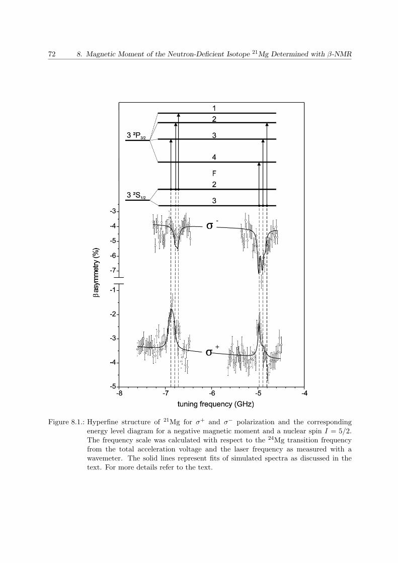
72 8. Magnetic Moment of the Neutron-Deficient Isotope 21Mg Determined with β-NMR
Figure 8.1.: Hyperfine structure of 21Mg for σ+ and σ− polarization and the correspondingenergy level diagram for a negative magnetic moment and a nuclear spin I = 5/2.The frequency scale was calculated with respect to the 24Mg transition frequencyfrom the total acceleration voltage and the laser frequency as measured with awavemeter. The solid lines represent fits of simulated spectra as discussed in thetext. For more details refer to the text.
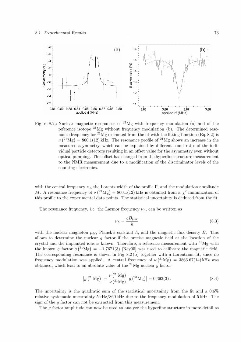
8.1. Experimental Results 73
3,85 3,86 3,87 3,88
0,10
0,11
0,12
0,13
0,14
0,15
16
β asym
me
try (
%)
applied rf (MHz)
16
15
14
13
12
11
(a) (b)
Figure 8.2.: Nuclear magnetic resonances of 21Mg with frequency modulation (a) and of thereference isotope 31Mg without frequency modulation (b). The determined reso-nance frequency for 21Mg extracted from the fit with the fitting function (Eq. 8.2) isν(21Mg
)= 860.1(12) kHz. The resonance profile of 21Mg shows an increase in the
measured asymmetry, which can be explained by different count rates of the indi-vidual particle detectors resulting in an offset value for the asymmetry even withoutoptical pumping. This offset has changed from the hyperfine structure measurementto the NMR measurement due to a modification of the discriminator levels of thecounting electronics.
with the central frequency ν0, the Lorentz width of the profile Γ, and the modulation amplitudeM . A resonance frequency of ν
(21Mg
)= 860.1(12) kHz is obtained from a χ2 minimization of
this profile to the experimental data points. The statistical uncertainty is deduced from the fit.
The resonance frequency, i.e. the Larmor frequency νL, can be written as
νL =gBµN
h(8.3)
with the nuclear magneton µN , Planck’s constant h, and the magnetic flux density B. Thisallows to determine the nuclear g factor if the precise magnetic field at the location of thecrystal and the implanted ions is known. Therefore, a reference measurement with 31Mg withthe known g factor g
(31Mg
)= −1.7671(3) [Ney05] was used to calibrate the magnetic field.
The corresponding resonance is shown in Fig. 8.2 (b) together with a Lorentzian fit, since nofrequency modulation was applied. A central frequency of ν
(31Mg
)= 3866.67(14) kHz was
obtained, which lead to an absolute value of the 21Mg nuclear g factor
∣∣g(21Mg
)∣∣ =
ν(21Mg
)
ν (31Mg)
∣∣g(31Mg
)∣∣ = 0.393(3) . (8.4)
The uncertainty is the quadratic sum of the statistical uncertainty from the fit and a 0.6%relative systematic uncertainty 5 kHz/860 kHz due to the frequency modulation of 5 kHz. Thesign of the g factor can not be extracted from this measurement.
The g factor amplitude can now be used to analyze the hyperfine structure in more detail as

74 8. Magnetic Moment of the Neutron-Deficient Isotope 21Mg Determined with β-NMR
-3,5 -3,0 -2,5 -2,0 -1,5 -1,0 -0,5
-0,055
-0,050
-0,045
-0,040
-0,035
-0,030
-0,025
-0,020
-0,015
-0,010
β asym
metr
y (
%)
scan voltage / V
σ+
tuning frequency (GHz)-7 -6 -5
-1
-2
-3
-4
-5
Figure 8.3.: Comparison of the fitting result obtained with spin I = 5/2 shown as a solid redcurve and a simulation for spin I = 3/2, shown as the blue dashed line, with the Afactor fixed to the value deduced from the g factor as described in the text.
it is now possible to calculate the hyperfine A factor
A =gIµNB
J(8.5)
and to use it as a fixed parameter in the fitting procedure. As the total separation of theindividual multiplets is determined by the A factor (see Ch. 2.1.1) and the nuclear spin I ac-cording to Eq. 2.12, the spin I can be extracted in this way. Therefore, another Mg referenceisotope has to be used to eliminate the unknown magnetic field of the moving electrons at thenuclear site. Using the stable reference isotope 25Mg with spin I = 5/2, a magnetic moment ofµ(25Mg
)= −0.85545(8)µN [Rag89], and A
(25Mg
)= 596.254376(54) MHz [Ita81] the A factor
is∣∣A(21Mg
)∣∣ =
∣∣(g(21Mg
)A(25Mg
)5/2)/µ(25Mg
)∣∣ = 684(4)MHz . (8.6)
A reasonable fit to the data shown in Fig. 8.3 with this A factor as a fixed parameter is onlypossible with spin I = 5/2. Other values result in either a too large hyperfine splitting or thesplitting is too small and the peak positions predicted by the fitting function do not match thereal positions at all, as it is demonstrated for I = 3/2 as an example in Fig. 8.3.
The sign of the g factor can now be fixed by studying its impact on the hyperfine structurecenter of gravity. For this, the isotope shift between 21Mg and 24Mg is estimated based on themass shift constant KMS = −954(12) GHz u obtained from theoretical calculations [Ber03] toδν21,24 = KMS× mAmA′
mA−mA′
= 5.65(7)GHz, neglecting the small field-shift contribution. Assuming
a positive g factor the experimental isotope shift calculated from the center of gravity of 21Mgand the resonance position of 24Mg is 5.95 GHz whereas it is 5.63 GHz for the negative sign. Itcan therefore be concluded that the sign of the g factor and, hence, the magnetic moment, isnegative. Finally, the nuclear magnetic moment can be calculated from the g factor and thenuclear spin I to
µ(21Mg
)= g
(21Mg
)× I × µN = −0.983(7)µN . (8.7)
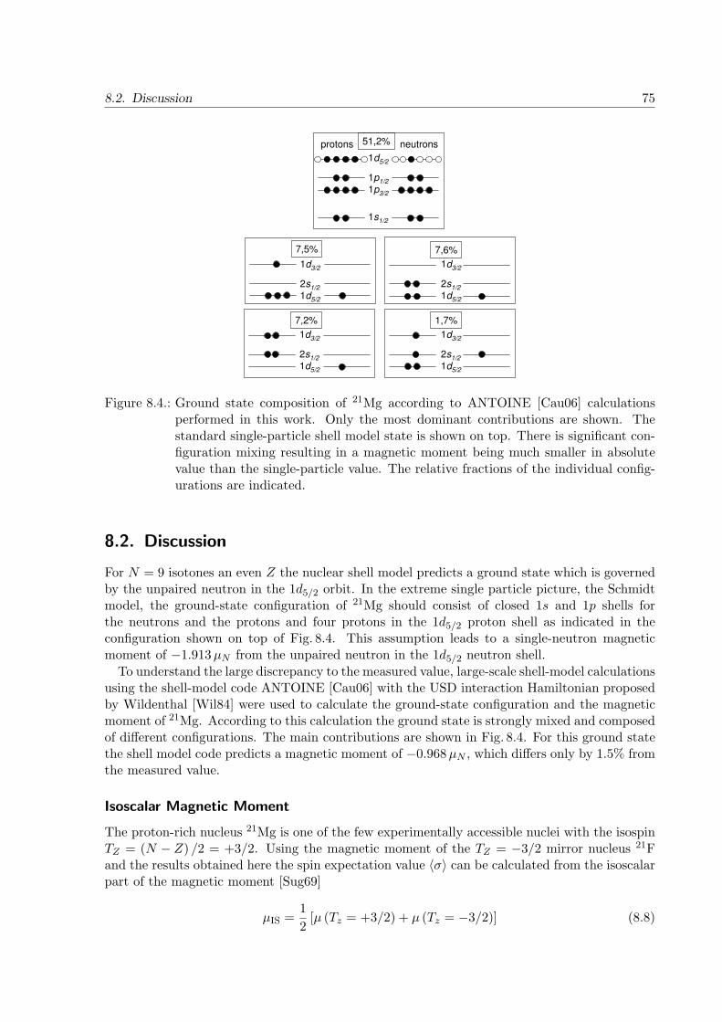
8.2. Discussion 75
1d3/2
2s1/2
1d5/2
7,6%
1d3/2
2s1/2
1d5/2
7,5%
1d3/2
2s1/2
1d5/2
7,2%
1d3/2
2s1/2
1d5/2
1,7%
protons neutrons
1d5/2
1p1/2
1p3/2
1s1/2
51,2%
Figure 8.4.: Ground state composition of 21Mg according to ANTOINE [Cau06] calculationsperformed in this work. Only the most dominant contributions are shown. Thestandard single-particle shell model state is shown on top. There is significant con-figuration mixing resulting in a magnetic moment being much smaller in absolutevalue than the single-particle value. The relative fractions of the individual config-urations are indicated.
8.2. Discussion
For N = 9 isotones an even Z the nuclear shell model predicts a ground state which is governedby the unpaired neutron in the 1d5/2 orbit. In the extreme single particle picture, the Schmidtmodel, the ground-state configuration of 21Mg should consist of closed 1s and 1p shells forthe neutrons and the protons and four protons in the 1d5/2 proton shell as indicated in theconfiguration shown on top of Fig. 8.4. This assumption leads to a single-neutron magneticmoment of −1.913µN from the unpaired neutron in the 1d5/2 neutron shell.
To understand the large discrepancy to the measured value, large-scale shell-model calculationsusing the shell-model code ANTOINE [Cau06] with the USD interaction Hamiltonian proposedby Wildenthal [Wil84] were used to calculate the ground-state configuration and the magneticmoment of 21Mg. According to this calculation the ground state is strongly mixed and composedof different configurations. The main contributions are shown in Fig. 8.4. For this ground statethe shell model code predicts a magnetic moment of −0.968µN , which differs only by 1.5% fromthe measured value.
Isoscalar Magnetic Moment
The proton-rich nucleus 21Mg is one of the few experimentally accessible nuclei with the isospinTZ = (N − Z) /2 = +3/2. Using the magnetic moment of the TZ = −3/2 mirror nucleus 21Fand the results obtained here the spin expectation value 〈σ〉 can be calculated from the isoscalarpart of the magnetic moment [Sug69]
µIS =1
2[µ (Tz = +3/2) + µ (Tz = −3/2)] (8.8)

76 8. Magnetic Moment of the Neutron-Deficient Isotope 21Mg Determined with β-NMR
0 5 10 15 20 25 30 35 40
-0,5
0,0
0,5
1,0
1,5
35K -
35S
17N -
17Ne
j'=l'-1/2
23Ne -
23Al
21F -
21Mg
13B -
13O
< σ
>
A
j=l+1/2
9Li -
9C
T=3/2
Figure 8.5.: Spin expectation values for the known T = 3/2 mirror pairs shown together withthe single-particle limits indicated as solid red lines for the j = l+ 1/2 cases and asdashed blue lines for the j′ = l′−1/2 cases. The values were taken from this work andfrom [Mat99, Mat95, Gei05, Wil71, Bur54, Cor83, Uen96, Mer06, Oza06, Mat96].
using the relation [Sug73]
〈σ〉 =2µIS/µN − I
(µp + µn) /µN − 1/2. (8.9)
I is the total angular momentum (spin) of the nucleus, µp = 2.793µN and µn = −1.913µN arethe free-nucleon magnetic moments for the proton and the neutron, respectively. For the mirrorpair
(21F, 21Mg
)we obtain the value 〈σ〉 = 1.15.
The extreme single-particle model predicts a value of 〈σ〉 = 1 for a nucleon in the single particlestate j = l+1/2. Empirical values for T = 1/2 are consistently smaller than one. In the T = 3/2case only three mirror pairs with a j = l+1/2 ground state have been investigated experimentally,so far. In the
(13B, 13O
)case the spin expectation value is 0.758(2) [Huh98] which agrees well
with the known empirical systematics from T = 1/2 nuclei. The(9Li, 9C
)system exhibits a large
value of 〈σ〉 = 1.441(2) [Mat95, Huh98]. For the third pair(23Ne ,23 Al
), the spin expectation
value is 0.82(58) [Gei05, Oza06] but the uncertainty on the magnetic moment of 23Al is too largeto judge whether 〈σ〉 is larger or smaller than one. The results for all known T = 3/2 mirrorpairs are summarized in Fig. 8.5. All experimental results for the four T = 3/2,j = l + 1/2mirror pairs together with the predictions from the extreme single-particle model and the shellmodel are summarized in Tab. 8.1.
It was tried to reproduce the occurrence of spin expectation values greater than unity byincluding isospin non-conserving effects (INC) [Orm89] in the shell-model calculations [Man98],but the resulting 〈σ〉 value for
(9Li, 9C
)was still 18% smaller than the experimental value.
Finally, it was shown that intruder configurations are the key to reproducing the large value

8.2. Discussion 77
Table 8.1.: Experimental spin expectation values 〈σ〉 for the four T = 3/2, j = l + 1/2 mirrorpairs and theoretical predictions from the single-particle (s.p.) model, the shell modelwith isospin non-conserving interactions (INC), with the universal sd (USD) interac-tion [Wil84] for the sd-shell or with the p shell two-body matrix element (PTBME)interaction [Jul92] for the p-shell and with the Warburton Brown p shell (WBP)interaction for the p-sd shell [War92].
Mirror pair Exp. s.p. INC USD/PTBME WBP(21F, 21Mg
)1.15(2)a 1.00 1.15b 1.11a -
(9Li, 9C
)1.44(2)b 1.00 1.18b 1.09b 1,47c
(23Ne, 23Al
)0.82(58)d 1.00 - 0.82a -
(13B, 13O
)0.758(2)e 1.00 - - -
athis workbvalues taken from [Man98, Huh98]cvalues taken from [Uts05]dvalues taken from [Gei05, Oza06]evalues taken from [Mat96, Wil71]
[Uts05], meaning that the model space used for the shell-model calculations had to be extendedto the sd shell [War92].
In the case of the A=21 mirror pair, already the isospin-symmetric shell model reproduces theexperimental magnetic moments rather well with −0.968µN for 21Mg and +3.888µN for 21F.This results in 〈σ〉 = 1.11. The value changes slightly to 1.15, in excellent agreement with theexperimental value, if the Coulomb interaction for the protons and asymmetric nucleon-nucleoninteractions are taken into account [Man98].


9. Charge Radii of 24−32Mg from Combined
Optical and β-Asymmetry Detection
In the measurements described in this chapter the classical optical detection was combinedfor the first time with the detection of the β asymmetry to determine isotope shifts for theextraction of nuclear radii. This was only possible by carefully studying and simulating thespectra observed in the β detection [Kei00] and taking systematic line shifts due to the appliedmagnetic guiding field into account. To check for the consistency of this method the isotope shiftbetween 26Mg and 29Mg was measured with combined fluorescence and asymmetry detectionand with fluorescence detection only.
9.1. Optical measurements
Typical spectra of 24Mg and 26Mg as examples for the even-even isotopes are shown in Fig. 9.1.The single resonances of these isotopes were fitted with Voigt profiles with the Lorentz widthfixed to the natural linewidth of 41.4 MHz and the Doppler width as a free parameter that wastypically 24 MHz. A small satellite peak on the left side caused by ions that have undergonea collisional excitation with the residual gas and were therefore slower by ≈ 4.5 eV was alsoincluded in the fitting routine by a second Voigt profile. This energy loss corresponds to theenergy gap of the 3 2S → 3 2P transition. Such side peaks are also visible in the odd-isotopecases with hyperfine structure and are accounted for by the fitting routine. Together with theresonance center voltage, the total acceleration voltage was calculated from the source voltageand the detection region offset voltage:
Utotal = Usource −(
Uoffset + fKepco × UDAC
)
. (9.1)
0.7 0.8 0.9 1.0 1.1 1.2 1.3
0
50000
100000
150000
200000
250000
300000
350000
cou
nts
DAC voltage / V
0.4 0.5 0.6 0.7 0.8 0.9 1.0 1.10
10000
20000
30000
40000
50000
60000
co
unts
DAC voltage / V
Figure 9.1.: Fluorescence signal of 24Mg (left) and 26Mg (right). The resonances are the sumof 20 individual scans. The side peak from collisional excitation is well pronouncedand included in the fitting routine (see text).
79
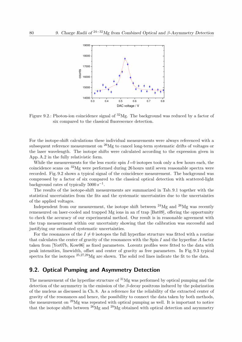
80 9. Charge Radii of 24−32Mg from Combined Optical and β-Asymmetry Detection
0.3 0.4 0.5 0.6 0.7 0.814000
15000
16000
17000
18000
19000
coun
ts
DAC voltage / V
Figure 9.2.: Photon-ion coincidence signal of 32Mg. The background was reduced by a factor ofsix compared to the classical fluorescence detection.
For the isotope-shift calculations these individual measurements were always referenced with asubsequent reference measurement on 26Mg to cancel long-term systematic drifts of voltages orthe laser wavelength. The isotope shifts were calculated according to the expression given inApp. A.2 in the fully relativistic form.
While the measurements for the less exotic spin I=0 isotopes took only a few hours each, thecoincidence scans on 32Mg were performed during 26 hours until seven reasonable spectra wererecorded. Fig. 9.2 shows a typical signal of the coincidence measurement. The background wascompressed by a factor of six compared to the classical optical detection with scattered-lightbackground rates of typically 5000 s−1.
The results of the isotope-shift measurements are summarized in Tab. 9.1 together with thestatistical uncertainties from the fits and the systematic uncertainties due to the uncertaintiesof the applied voltages.
Independent from our measurement, the isotope shift between 24Mg and 26Mg was recentlyremeasured on laser-cooled and trapped Mg ions in an rf trap [Bat09], offering the opportunityto check the accuracy of our experimental method. Our result is in reasonable agreement withthe trap measurement within our uncertainty showing that the calibration was successful andjustifying our estimated systematic uncertainties.
For the resonances of the I 6= 0 isotopes the full hyperfine structure was fitted with a routinethat calculates the center of gravity of the resonances with the Spin I and the hyperfine A factortaken from [Yor07b, Kow06] as fixed parameters. Lorentz profiles were fitted to the data withpeak intensities, linewidth, offset and center of gravity as free parameters. In Fig. 9.3 typicalspectra for the isotopes 25,27,29Mg are shown. The solid red lines indicate the fit to the data.
9.2. Optical Pumping and Asymmetry Detection
The measurement of the hyperfine structure of 31Mg was performed by optical pumping and thedetection of the asymmetry in the emission of the β-decay positrons induced by the polarizationof the nucleus as discussed in Ch. 8. As a reference for the reliability of the extracted center ofgravity of the resonances and hence, the possibility to connect the data taken by both methods,the measurement on 29Mg was repeated with optical pumping as well. It is important to noticethat the isotope shifts between 26Mg and 29Mg obtained with optical detection and asymmetry
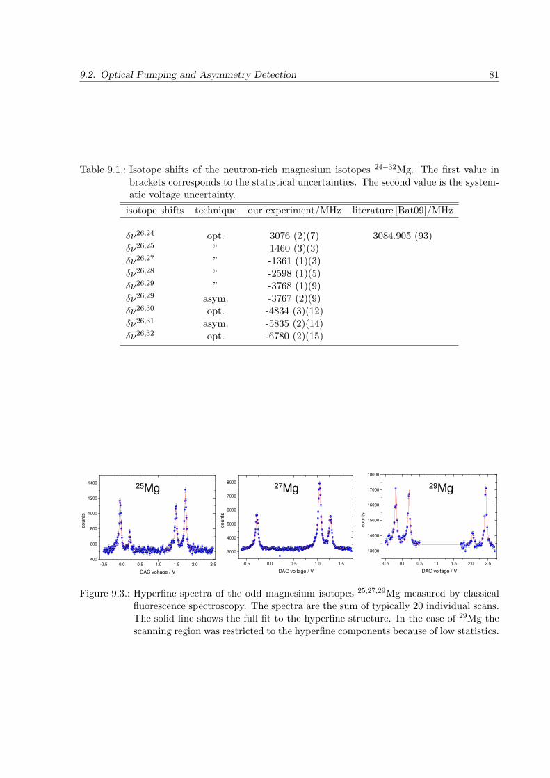
9.2. Optical Pumping and Asymmetry Detection 81
Table 9.1.: Isotope shifts of the neutron-rich magnesium isotopes 24−32Mg. The first value inbrackets corresponds to the statistical uncertainties. The second value is the system-atic voltage uncertainty.
isotope shifts technique our experiment/MHz literature [Bat09]/MHz
δν26,24 opt. 3076 (2)(7) 3084.905 (93)δν26,25 ” 1460 (3)(3)δν26,27 ” -1361 (1)(3)δν26,28 ” -2598 (1)(5)δν26,29 ” -3768 (1)(9)δν26,29 asym. -3767 (2)(9)δν26,30 opt. -4834 (3)(12)δν26,31 asym. -5835 (2)(14)δν26,32 opt. -6780 (2)(15)
-0.5 0.0 0.5 1.0 1.5
3000
4000
5000
6000
7000
8000
co
un
ts
DAC voltage / V
-0.5 0.0 0.5 1.0 1.5 2.0 2.5400
600
800
1000
1200
1400
co
un
ts
DAC voltage / V
-0.5 0.0 0.5 1.0 1.5 2.0 2.5
13000
14000
15000
16000
17000
18000
co
un
ts
DAC voltage / V
25Mg 27Mg 29Mg
Figure 9.3.: Hyperfine spectra of the odd magnesium isotopes 25,27,29Mg measured by classicalfluorescence spectroscopy. The spectra are the sum of typically 20 individual scans.The solid line shows the full fit to the hyperfine structure. In the case of 29Mg thescanning region was restricted to the hyperfine components because of low statistics.

82 9. Charge Radii of 24−32Mg from Combined Optical and β-Asymmetry Detection
3 2S1/2
3 2P1/2
mJ=1/2
mJ=-1/2
mJ=-1/2
mJ=1/2
no field weak magnetic field
σ+ σ-
1.05 MHz/G
0.58 MHz/G
Figure 9.4.: Zeeman effect and the shift of the resonance frequency in 26Mg for excitation withσ-polarized light.
-1.0 -0.5 0.0 0.5 1.0 1.5 2.0 2.5 3.0-0.025
-0.020
-0.015
-0.010
-0.005
0.000
0.005
asym
metr
y
DAC voltage / V
-2 -1 0 1 2 3
-0.06
-0.04
-0.02
0.00
0.02
0.04
asym
metr
y
DAC voltage / V
Figure 9.5.: β-asymmetry signals for the radioactive isotopes 29Mg (a) and 31Mg (b) for σ−
polarization together with the results from the fits with the calculated asymmetryfrom optical pumping.
detection, given in Tab. 9.1 are in excellent agreement within the uncertainties justifying ourapproach to connect both methods.
As the asymmetry measurements as well as the reference scans on 26Mg all took place withthe weak axial magnetic guiding field of ≈5 G turned on, the Zeeman effect has to be takeninto account in the determination of the isotope shift. The asymmetry fitting routine alreadyincludes this effect for the calculation of the center of gravity, but the resonance positions ofthe reference isotope 26Mg have to be corrected. Depending on the laser polarization and theselection rules for optical transitions in Zeeman substates, the real resonance position is shiftedby δν = ±1/2
(gJ
(S1/2
)+ gJ
(P1/2
))µBB as it is indicated in Fig. 9.4. For the 5 G magnetic
field and with the gJ factors gJ
(S1/2
)= 1.5 and gJ
(P1/2
)= 0.83 this results in a shift of
±8.2(8)MHz. This shift was considered before calculating the individual isotope shifts. Thetreatment of the asymmetry spectra and how the fitting function is composed was alreadydescribed in Ch. 8.1. The spectra for both isotopes and for σ− polarizations are presented inFig. 9.5 together with the results of the least-squares fit.
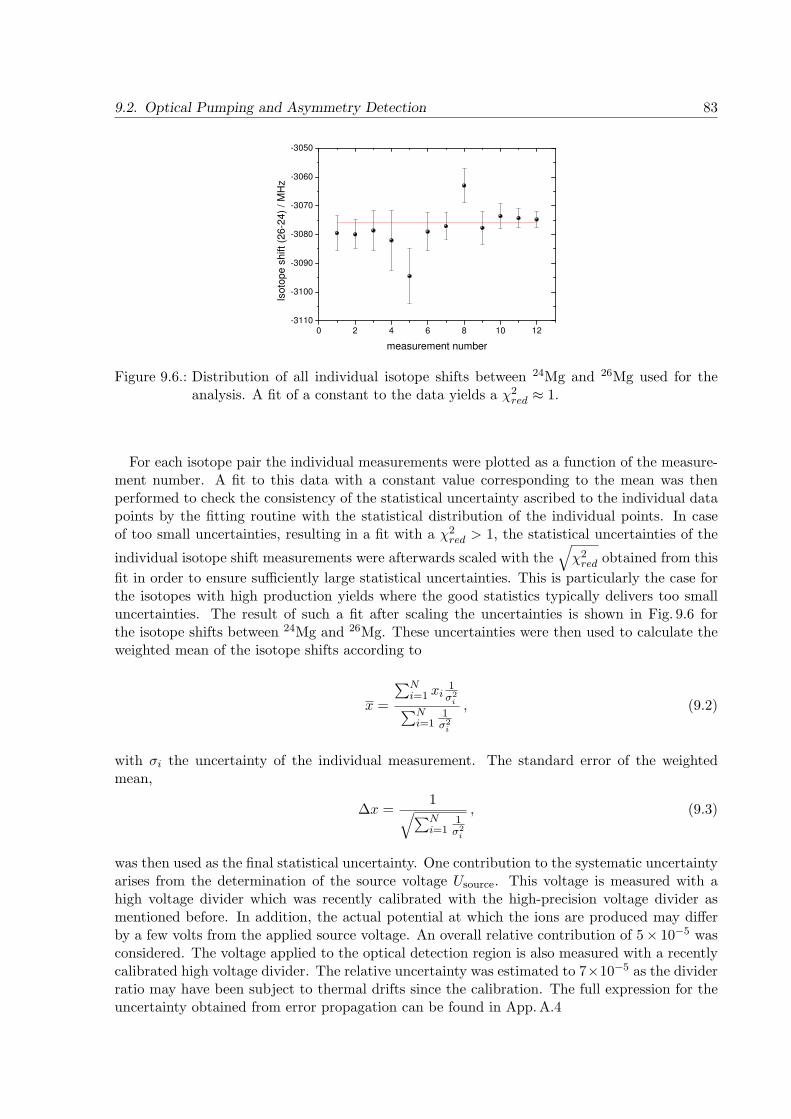
9.2. Optical Pumping and Asymmetry Detection 83
0 2 4 6 8 10 12-3110
-3100
-3090
-3080
-3070
-3060
-3050
Isoto
pe s
hift
(26-2
4)
/ M
Hz
measurement number
Figure 9.6.: Distribution of all individual isotope shifts between 24Mg and 26Mg used for theanalysis. A fit of a constant to the data yields a χ2
red ≈ 1.
For each isotope pair the individual measurements were plotted as a function of the measure-ment number. A fit to this data with a constant value corresponding to the mean was thenperformed to check the consistency of the statistical uncertainty ascribed to the individual datapoints by the fitting routine with the statistical distribution of the individual points. In caseof too small uncertainties, resulting in a fit with a χ2
red > 1, the statistical uncertainties of the
individual isotope shift measurements were afterwards scaled with the√
χ2red obtained from this
fit in order to ensure sufficiently large statistical uncertainties. This is particularly the case forthe isotopes with high production yields where the good statistics typically delivers too smalluncertainties. The result of such a fit after scaling the uncertainties is shown in Fig. 9.6 forthe isotope shifts between 24Mg and 26Mg. These uncertainties were then used to calculate theweighted mean of the isotope shifts according to
x =
∑Ni=1 xi
1σ2
i∑N
i=11σ2
i
, (9.2)
with σi the uncertainty of the individual measurement. The standard error of the weightedmean,
∆x =1
√∑Ni=1
1σ2
i
, (9.3)
was then used as the final statistical uncertainty. One contribution to the systematic uncertaintyarises from the determination of the source voltage Usource. This voltage is measured with ahigh voltage divider which was recently calibrated with the high-precision voltage divider asmentioned before. In addition, the actual potential at which the ions are produced may differby a few volts from the applied source voltage. An overall relative contribution of 5× 10⁻⁵ wasconsidered. The voltage applied to the optical detection region is also measured with a recentlycalibrated high voltage divider. The relative uncertainty was estimated to 7×10⁻⁵ as the dividerratio may have been subject to thermal drifts since the calibration. The full expression for theuncertainty obtained from error propagation can be found in App. A.4

84 9. Charge Radii of 24−32Mg from Combined Optical and β-Asymmetry Detection
9.3. Extraction of the Nuclear Charge Radii
In order to extract the changes in the mean-square nuclear charge radii, data from radii de-termined with studies of muonic magnesium atoms need to be combined with theoretical cal-culations of the field shift constant. A King plot then yields the specific mass shift constant.Absolute radii can afterwards be calculated with a reference charge radius for one isotope.
9.3.1. King Plot and Mass Shift Constants
The isotope shift can be expressed by the mass-shift and the field-shift contribution accordingto (see Ch. 2.1.2):
δνA,A′
= (kNMS + kSMS)︸ ︷︷ ︸
KMS
×mA′ −mA
mA′mA+ F × δ
⟨r2⟩A,A′
. (9.4)
For the field shift factor F = −127(6) MHz/fm2 we use ab initio calculations from Berengutet al. [Ber03] which for other alkali and alkali-earth metals have proven to be consistent withexperimental values to better than 5%.
The normal-mass-shift constant can easily be calculated using the transition frequency ν0
[Kau91] bykNMS = −ν0 ×me = −586.618 GHz u (9.5)
with the electron mass me in atomic mass units. To determine the mass-shift factor a King plotwith the the known δ
⟨r2⟩
from 24Mg to 25Mg and 26Mg from muonic data [Fri92] based on themodified isotope shifts
δνA,A′
ourwork ×mAmA′
mA′ −mA︸ ︷︷ ︸
y
= KMS + F × δ⟨r2⟩A,A′
muon
mAmA′
mA′ −mA︸ ︷︷ ︸
x
(9.6)
was evaluated. Plotting the y values as a function of the x values as indicated by the bracesshould result in a linear function and a linear fit with the field-shift constant as a fixed parameterallows to extract the mass-shift constant. Fig. 9.7 shows the resulting King plot. The solid redline is the result of the linear fit with the slope fixed to the theoretical value for F . The dashedlines are fits with the slope fixed to F ± ∆F . The total mass shift constant KMS, i.e. theaxis intercept extracted from the fit is KMS = −954(1) GHz u with the uncertainty composedof the statistical uncertainty from the fit and the systematic uncertainty of the field shift andits impact on the axis intercept. The specific mass shift constant can now be calculated to (seeCh. 2.1.2)
kSMS = KMS − kNMS = −367(1)GHz u , (9.7)
with the transition frequency ν and the electron mass me This value is in agreement with thetheoretical value ktheo
SMS = −373(12) GHz u derived in [Ber03] which has a too large uncertaintyto use it for the evaluation of the radii directly.
9.3.2. Mean Square Nuclear Charge Radii
The δ⟨r2⟩A,A′
can now be calculated for the isotope pairs from 24Mg to 32Mg. The resultsare summarized in Tab. 9.2 together with the absolute value for the radii which were calculatedaccording to
⟨r2A⟩1/2
=(⟨r226⟩
+ δ⟨r2⟩26,A
)1/2, (9.8)

9.3. Extraction of the Nuclear Charge Radii 85
0 20 40 60 80 100
-965
-960
-955
24-25
24-26δν
AA
'/(A
-A') / G
Hz u
δ < r2> AA'/(A-A') / fm2 u
Figure 9.7.: King plot created from the experimental isotope shifts between 24,25,26Mg ob-tained in this work and radii from muonic data. The solid red line indicatesthe least squares linear fit with the slope fixed to the theoretical electronic fac-tor F = −127(6) MHz/fm2 [Ber03]. The dashed lines are fits with the slope fixed toF + ∆F and F − ∆F , marking the boundaries for the slope of the line.
Table 9.2.: Mean square nuclear charge radii and absolute radii for 26Mg up to 32Mg. The firstuncertainty given in brackets denotes the statistical uncertainties and the secondnumber is the uncertainty in the determination of the mass shift constant. Thisuncertainty is changing the slope of the charge radius as a function of the atomicmass number as it is acting on all radii equally.
(26, A′) δ⟨r2⟩26,A′
/ fm2 absolute radius r / fm
24 0.15 (2)(1) 3.060 (6)(70)25 -0.02 (3)(1) 3.03 (1)(4)26 - 3.035 (4)27 0.01 (1)(1) 3.037 (3)(3)28 0.21 (1)(2) 3.070 (3)(7)29 optical 0.31 (1)(3) 3.084 (2)(10)29 asym. 0.31 (2)(3) 3.085 (6)(10)30 0.56 (2)(4) 3.125 (6)(15)31 0.80 (2)(5) 3.163 (4)(20)32 0.96 (2)(6) 3.190 (7)(20)
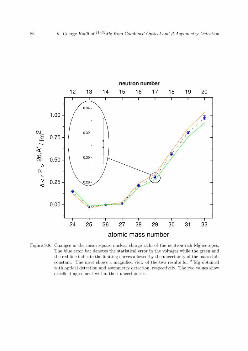
86 9. Charge Radii of 24−32Mg from Combined Optical and β-Asymmetry Detection
24 25 26 27 28 29 30 31 32
0.00
0.25
0.50
0.75
1.00
12 13 14 15 16 17 18 19 20
δ <
r 2
> 2
6,A
' / fm
2
atomic mass number
0.28
0.30
0.32
0.34
neutron number
Figure 9.8.: Changes in the mean square nuclear charge radii of the neutron-rich Mg isotopes.The blue error bar denotes the statistical error in the voltages while the green andthe red line indicate the limiting curves allowed by the uncertainty of the mass shiftconstant. The inset shows a magnified view of the two results for 29Mg obtainedwith optical detection and asymmetry detection, respectively. The two values showexcellent agreement within their uncertainties.

9.4. Discussion 87
assuming a reference radius for 26Mg of r26=3.035(4) fm [Fri92]. The total statistical uncertain-ties have been calculated from the statistical uncertainties of the isotope shifts using Gaussianerror propagation. The systematic uncertainty of the voltage determination is included in themass-shift constant obtained from the King plot. This uncertainty approximately has the samemass dependence
mA−mA′
mAmA′
as the mass shift. The field shift is therefore independent from this
contribution. For more details refer to App. A.4. The remaining systematic uncertainty origi-nates only from the uncertainty of the mass-shift constant determined from the King plot. Allchanges in radii were calculated based on the same mass-shift constant and therefore also thesame uncertainty acts on the radii. The uncertainty therefore systematically changes all δ
⟨r2⟩.
Two borders for the trend of the radii are defined by the uncertainty of the mass-shift con-stant. Fig. 9.8 shows the data presented in Tab. 9.2. The contribution of the mass shift constantuncertainty is indicated by the red and the green border curves.
9.4. Discussion
Many theoretical studies of nuclei near the N = 20 shell closure exist but the charge radiusis addressed in only a few of them, whereas the deformation parameter β2, describing thequadrupole deformation of the nucleus, is more often evaluated. To compare the experimentalresults obtained here to different nuclear models and calculations, the nuclear charge radius mustthus be linked to the commonly used deformation parameter β2. The droplet model is thereforeused to calculate the changes in the mean-square charge radii as a function of theoreticallyderived deformations.
9.4.1. The Nuclear Charge Radius in the Droplet Model
The droplet model is a more refined substitute for the liquid-drop model with the main differencebeing the individual distributions of the neutrons and the protons. Therefore, the model can, forexample, account for the development of neutron skins for neutron-rich nuclei. All coefficientswere deduced from fitting to experimental data, as it was also done in the liquid-drop model.The nuclear charge radius is given by the expression [Mye83]
⟨r2⟩
=⟨r2⟩
u+⟨r2⟩
r+⟨r2⟩
d, (9.9)
with the size and shape contribution
⟨r2⟩
u=
3
5R2
(
1 + α22 +
10
21α3
2 −27
35α4
2
)
. (9.10)
The second term is a redistribution effect because of the Coulomb repulsion slightly increasingthe proton density on the surface of the nucleus and is given by
⟨r2⟩
r=
12
175C ′R2
(
1 +14
5α2
2 +28
15α3
2 −29
5α4
2
)
. (9.11)
The parameter C ′ in Eq. 9.11 can be approximated to C ′ ≈ 0.0156 × ZA−1/3. The last term inEq. 9.9
⟨r2⟩
d= 3b2 , (9.12)
with b = 0.99 fm, adds a constant contribution because of the diffuseness of the nucleus. Theparameter α2 can be expressed by the commonly used deformation parameter according to
α2 =
√
5
4πβ2 . (9.13)

88 9. Charge Radii of 24−32Mg from Combined Optical and β-Asymmetry Detection
24 26 28 30 32 34
-0.4
-0.2
0.0
0.2
0.4
0.6
0.8
1.0
1.2 experiment
spherical droplet model
droplet model with b2 from exp.
droplet model with b2 from MM model
droplet model with b2 from RMF calc.
droplet model with b2 from SMO calc.
droplet model with b2 from SM, no intruder conf.
droplet model with b2 from SM, with intruder conf.
δ<r 2
>26,
A' /
fm
2
mass number A
Figure 9.9.: Comparison of the experimental data to model predictions and theoretical calcula-tions with reference to 26Mg. The orange triangles are obtained from the dropletmodel with experimental deformation parameters from [Ram01]. The blue dotsare results from the droplet model using the macroscopic-microscopic model (MM)according to [Zhi06]. The red stars are predictions from the relativistic mean-field calculations (RMF) with effective nucleon-nucleon interactions [Mit02] and theviolet hexagons refer to mean-field calculations with density-dependent separablemonopole nucleon-nucleon interaction (SMO) [Ste02]. The results from shell modelcalculations with and without intruder configurations in the ground state [Cau01]are shown by the half-filled green rhombs.

9.4. Discussion 89
R is a measure for the size of the nucleus, including protons and neutrons, and is a modifiedliquid drop radius
R = r0A1/3 (1 + ǫ) , (9.14)
with r0 = 1.18 fm and ǫ defined according to [Mye83]. ǫ depends on empirical parameters de-scribing e.g. the ratio of the surface area of a deformed nucleus to the area of a sphere withthe same volume or variations of the Coulomb potential for the transition from spherical todeformed nuclei.
Now we can calculate the changes in the mean square radii using deformation parametersfrom theory or other experiments and compare them with our results. A prediction for purelyspherical configurations can be achieved by fixing β to zero for all isotopes. The trend of thecharge radii for this simplified model can be seen in Fig. 9.9 indicated by the blue triangles. Goodagreement is observed for radii radii from 25Mg up to 27Mg. For the nucleus 24Mg with wellknown deformation there is a big discrepancy, and also the isotopes 29−32Mg deviate considerablyfrom the predictions of the spherical droplet model, which may be a hint for the onset of intruderconfigurations in the ground states of these isotopes. The calculation of the charge radii withdeformation parameters from experimental B (E2) values deduced from electron scattering andCoulomb excitation measurements for even-even nuclei [Ram01] shown as orange triangles inFig. 9.9 is in good agreement from 24Mg up to 28Mg. For the more exotic isotopes however, ourmeasurement exhibits a slightly steeper slope for the radii changes.
The use of the β2 predictions from the macroscopic-microscopic (MM) model [Zhi06] in ourdroplet radii calculation shows the best agreement with the present data set. Only the δ
⟨r2⟩
for 25Mg deviates by more than five times the error bars from the experimental result. Thistheoretical description combines a macroscopic model for the nucleus, in this case the liquid-drop model, with a microscopic model accounting for shell effects by spin-orbit interactions andpairing effects [Nil69]. The sum of the total energy derived by both models is then minimizedto determine the ground-state configuration. Zhi and Ren [Zhi06] refined the microscopic modelby employing isospin-dependent spin-orbit interaction parameters, κ and µ, which describe theeffects of the proton-neutron interactions in light exotic nuclei. This may be the foundation ofthe good agreement with the experimental data, as the reordering and lowering of single-particleorbits, being an attribute of the island of inversion, can be linked to nucleon-nucleon interactions[Uts99]. One should note that the ǫ2 parameter used in [Zhi06] refers to a different nuclear shapeparameterization [Mol95]. But ǫ2 can be transformed into the commonly used β2. Therefore, agraph is plotted in [Nil69] showing the relation between the parameters that was used here for agraphical conversion from ǫ2 into β2, which were then used to calculate the changes in the radii.
The relativistic mean field approach (RMF) [Mit02] is a fully relativistic quantum field theorywhich treats the nucleons as Dirac spinors interacting with each other by meson exchange [Rin96].The mean-field approximation is used to reduce the number of allowed meson interactions basedon symmetry considerations. The nucleonic quantum numbers, the coupling constants, and thenucleon mass, i.e. the parameters of the Lagrange density used to calculate the total energy ofthe system, are adjusted in order to give the best agreement to known experimental data. Thereare a number of standard parameter sets often used in the calculations. The pairing effect onthe total energy is included in the theory by the BCS formalism [Moe92]. The agreement of thecharge radii derived from this theory with our results and with all other predictions shown inFig. 9.9 is poor. The progress of the radii does not even show the correct trend and predicts aspherical nucleus for 32Mg.
Qualitatively good agreement with the experimental results is observed for the many-bodyperturbative mean-field approach with density-dependent separable monopole nucleon-nucleon

90 9. Charge Radii of 24−32Mg from Combined Optical and β-Asymmetry Detection
interactions (SMO) [Ste01b]. In this theory the wave function for the ground state of thenucleus is described by a Slater determinant of the single-particle states [Vau72]. A Hartree-Fock approximation for the nucleon-nucleon interaction is used in which the individual nucleonis described as a particle interacting with a mean field produced by the other nucleons. For thismean field Stevenson et al. use the SMO interaction [Ste01a]. The trend of the δ
⟨r2⟩
is wellreproduced and also the decrease in the radii for nuclei with A > 32 predicted by the MM modelis well pronounced.
In contrast to the Hartree-Fock method the shell model calculations involve nuclear wavefunctions as linear combinations of Slater determinants. In Fig. 9.9 the predictions from thismodel are shown as half-filled green rhombs. The Hamiltonian consists of kinetic energy op-erators for the nucleons and two-body interactions between protons and neutrons. A specialdiagonalization scheme is used to calculate the coefficients of the wave functions [Cau99]. Fromthe shell model point of view, the large deformations of the magnesium isotopes for A > 30 areaccompanied by the lowering of the pf orbits and intruder configurations mixing to the groundstates in addition to the normal sd configurations [Cau01]. The significance of these particlehole-excitations to the pf shell in the explanation of the experimental deformation properties of32Mg is very well illustrated in the comparison of the shell-model predictions for the normal andthe intruder configuration. The δ
⟨r2⟩
deduced from the simulation with normal configuration istoo small, predicting a smaller radius than for 30Mg, while the simulation involving the intruderstates gives reasonable agreement with our data. For 34Mg the normal configuration withoutparticle-hole excitations gives better agreement with the macroscopic-microscopic model. Inthe case of 30Mg our result lies between the predicted radii from the shell model for normal orintruder configuration.
In summary, the experimental charge radii show a clear deviation from the predictions ofthe spherical shell model. Only models that account for nuclear deformations can describethe changes in the mean square nuclear charge radii qualitatively correct. However, the bestagreement is achieved by the macroscopic-microscopic model that reproduces the experimentalradii rather well.
9.4.2. Comparison to Other Isotope Chains at the Island of Inversion
Magnesium is not the only element which exhibits intruder configurations and large deforma-tions in the ground states when neutron-rich isotopes are considered. Similar experimentalobservations have been made with sodium [Thi75, Wil80] and neon [Pri99] for which isotopeshift measurements are also available [Hub78, Gei02]. For comparison, the result for the chargeradii for the three elements are plotted together as a function of the neutron number in Fig. 9.10.All three chains show similar behavior with a minimum for the radius around N = 14 and in-creasing radii to both sides. Na and Mg show the same increase in the slope from N = 17to N = 18. While this trend in the case of Na is caused by the onset of intruder configura-tions [Wil80], the normal ground state configuration of 30Mg can already explain the significantincrease in deformation that is observed.
9.5. Summary and Outlook
In this thesis the preceding work on the nuclear structure of magnesium isotopes studied withcollinear laser spectroscopy [Yor07b, Kow06] was continued. The spin and the magnetic momentof the neutron-deficient isotope 21Mg were measured for the first time, which allowed to study theproperties of mirror nuclei in one of the few accessible cases for Tz = −3/2. An anomaly in the

9.5. Summary and Outlook 91
12 14 16 18 203.00
3.05
3.10
3.15
3.20
2.9
3.0
3.1
3.2
3.3
2.91
2.94
2.97
3.00
3.03
A=26
rms r
ad
ius
/ fm
neutron number N
Mg
Na
Ne
A=26
Figure 9.10.: Charge radii of magnesium isotopes together with the results for sodium and neonas a function of the neutron number. The red dots show the results of our work.The blue dots refer to the sodium data [Hub78] and the green dots are the radiiof the neon isotopes [Gei02]. The systematic uncertainties due to the uncertaintyin the mass shift constant were omitted as they would not change the qualitativetrend in the radii, but only the slopes. The line crossing the three plots connectsthe A = 26 isobars of the three elements.

92 9. Charge Radii of 24−32Mg from Combined Optical and β-Asymmetry Detection
isoscalar magnetic moment was revealed, which can be reproduced by shell model calculationsby taking isospin non-conserving effects into account.
Furthermore, the measurement of the isotope shift of the 24−32Mg isotope chain with combinedoptical spectroscopy and β-asymmetry detection induced by optical pumping allowed to studythe structural changes at the transition to the island of inversion, where intruder states contributesignificantly to the ground-state configuration. Our measurement has shown that the changefrom the normal configuration for 30Mg to the intruder configuration for 31Mg is visible only ina small kink in the changes in charge radii as there is already a significant deformation in theground state for 30Mg. Our measurements are in good agreement with predictions of deformationparameters from the macroscopic-microscopic model [Zhi06].
To complete the work on the magnesium isotopes the radii for the neutron-deficient 21−24Mgwill be measured in 2010, again combining β detection with classical optical detection. Theseresults together with the results presented in this thesis will give an insight to the evolution ofnuclear shape throughout the whole sd shell.

A. Basic Formulas for Collinear Laser
Spectroscopy
A.1. Relativistic Doppler Formula
The Doppler shifted frequency that a particle with rest mass m moving with the velocity v = βcexperiences from a laser superimposed in parallel or anti-parallel direction is given by
ν ′ = νlaser ×1 ± β√
1 − β2, (A.1)
where the - applies for collinear geometry and the + for anti-collinear laser-particle geometry.The β can be calculated from the energy conservation for a particle being accelerated by thepotential difference U in a homogeneous electric field according to
eU = mc2
(
1√
1 − β2− 1
)
. (A.2)
This can be solved for β:
β =
√
1 −(
mc2
eU +mc2
)2
. (A.3)
The result can be inserted in Eq.A.1 and the Doppler shifted frequency as a function of theacceleration voltage is
ν ′ = νlaser
(eU +mc2
)
mc2
1 ±
√
1 −(
mc2
eU +mc2
)2
. (A.4)
A.2. Relativistic Isotope Shift Formula
The isotope shift between two isotopes of mass m1 and m2 with the resonance positions givenby the total acceleration voltages U1 and U2 can be calculated by
∆νIS = νlaser ×
(eU1 +m1c
2)
m1c2
1 ±
√
1 −(
m1c2
eU1 +m1c2
)2
(A.5)
−(eU2 +m2c
2)
m2c2
1 ±
√
1 −(
m2c2
eU2 +m2c2
)2
(A.6)
with the negative sign for collinear and the positive sign for anti-collinear geometry.
93
94 A. Basic Formulas for Collinear Laser Spectroscopy
A.3. Differential Doppler Formula - Doppler Factor
Starting from the classical approximation of the Doppler shift
ν ′ ≈ νlaser ×(
1 ±√
2eU
mc2
)
, (A.7)
the Doppler factor is the differential change ∂ν ′ in the frequency for a voltage change ∂U :
∂ν ′ =νlasere√2eUmc2
∂U (A.8)
A.4. Systematic Uncertainty of the Voltage Determination in the
Isotope Shift
In the non-relativistic treatment of the Doppler effect the isotope shift is given by
∆ν = ν0
(√
2eU1
m1c2−√
2eU2
m2c2
)
. (A.9)
With the substitutions U1 = Usource +U(1)offset and U2 = Usource +U
(2)offset, where U
(i)offset denotes the
offset voltage applied to the optical detection setup, and m2 = m1 + ∆m ≡ m + ∆m this canbe modified to
∆ν = ν0
√
2eUsource
mc2
√
U(1)offset
Usource−
√
U(2)offset/Usource
∆m/m
. (A.10)
A Taylor expansion of the square root and the approximation 1 + ∆m/(2m) ≈ 1 gives the finalresult for an approximated isotope shift:
∆ν ≈ ν0
√
2eUsource
2mc2
(∆m
m− ∆U
Usource
)
, (A.11)
with ∆U = U(2)offset − U
(1)offset. Based on Eq. A.11 the error propagation for the systematic voltage
uncertainty can be calculated. The result for the relative uncertainty of Uoffset σ (∆U)rel is
σ (∆ν)offset = ν0
√
eUsource
2mc2∆U
Usourceσ (∆U)rel . (A.12)
With the approximation that the isotope shift is mainly given by the mass shift, the expressioncan be modified to
σ (∆ν)offset ≈ CmA −mA′
mAmA′
(A.13)
and thus shows the same mass dependence as the mass shift. This allows to omit this uncertaintyin the change of the nuclear charge radii, if the mass shift constant is determined with a Kingplot. The voltage uncertainty is then implicitly included.
The uncertainty of the source voltage determination can be modified in a similar way and isgiven by
σ (∆ν)source = ν0/2
√
eUsource
2mc2
(∆U
Usource+
∆m
m
)
σ (Usource)rel . (A.14)

B. Instruction for the import of 3D models
from Solid Edge to SIMION 8.0
We start with an assembled body (.asm) consisting of several parts (.par). SIMION is capableof importing 3D CAD files in .stl format. The construction file of the assembly needs to beconverted stepwise to individual .stl files for each electrode. Isolators have to be omitted.
B.1. Selection of individual components belonging to one electrode
All parts not belonging to the electrode we want to export can simply be deleted. Please notethat the file must not be saved! (A backup copy is recommended!) If some of the componentsare part of sub assemblies, then these sub assemblies have to be opened and the parts have tobe deleted there (do not save!). In no case use the function ”Bearbeiten” or ”Modify” as everychange will be saved immediately and the original file will be lost.
B.2. Insertion into a new part and saving to .stl
When only the parts of the single electrode are left, choose ”Neues Teil erstellen” or ”create newpart”. Now click the function ”Einfugen–Kopie eines Teils” or ’Insert–part copy” and choosethe main assembly you have worked on. You will see the one single electrode appear. Now youcan save this part as e.g. ”part-1.stl”. Now all open files can be closed and you can proceed withthe second electrode. By doing so in the same way you can be sure that all electrodes have theirpre-defined positions, as they are all positioned with respect to the same coordinate system.
B.3. Conversion to the .pa♯ format of SIMION 8.0
For the conversion the SIMION add-on ”SL-Tools” is used, which is included in SIMION 8.0.You choose the function ”STL→PA” and the file to convert. To include several electrodes in one.pa♯, you simply replace the electrode number with ”%” and SIMION will automatically look forall files belonging to this geometry. Using the function ”scale” you can influence the resolutionof your conversion. After refining and creation of the .pa0 file, the scale can be adjusted tomatch the real dimensions of your geometry.
95

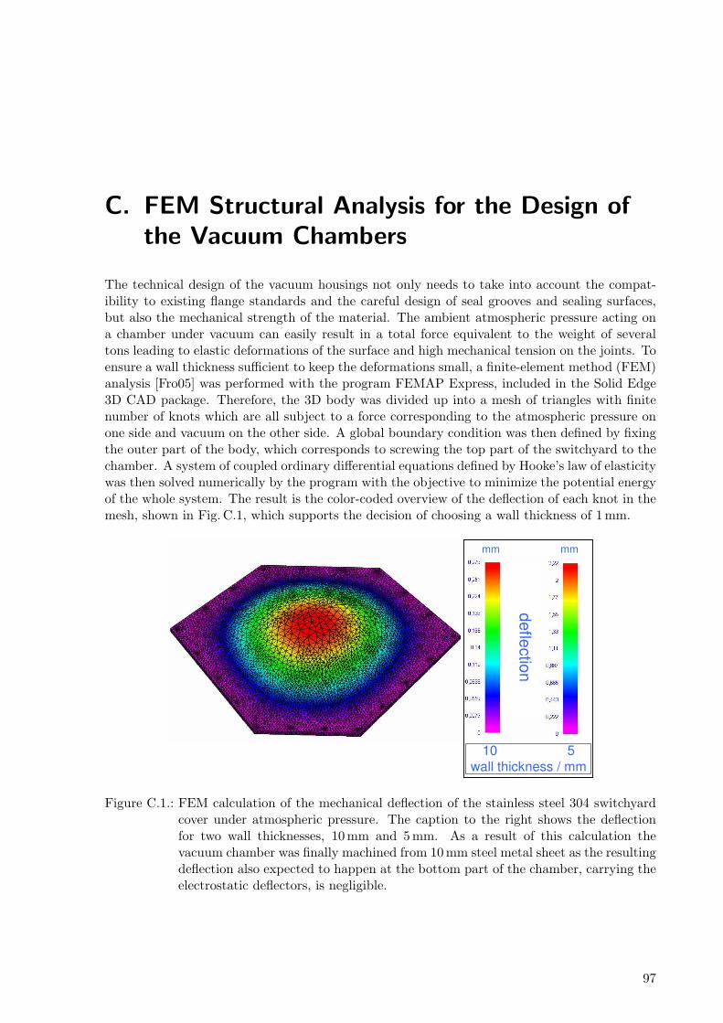
C. FEM Structural Analysis for the Design of
the Vacuum Chambers
The technical design of the vacuum housings not only needs to take into account the compat-ibility to existing flange standards and the careful design of seal grooves and sealing surfaces,but also the mechanical strength of the material. The ambient atmospheric pressure acting ona chamber under vacuum can easily result in a total force equivalent to the weight of severaltons leading to elastic deformations of the surface and high mechanical tension on the joints. Toensure a wall thickness sufficient to keep the deformations small, a finite-element method (FEM)analysis [Fro05] was performed with the program FEMAP Express, included in the Solid Edge3D CAD package. Therefore, the 3D body was divided up into a mesh of triangles with finitenumber of knots which are all subject to a force corresponding to the atmospheric pressure onone side and vacuum on the other side. A global boundary condition was then defined by fixingthe outer part of the body, which corresponds to screwing the top part of the switchyard to thechamber. A system of coupled ordinary differential equations defined by Hooke’s law of elasticitywas then solved numerically by the program with the objective to minimize the potential energyof the whole system. The result is the color-coded overview of the deflection of each knot in themesh, shown in Fig. C.1, which supports the decision of choosing a wall thickness of 1 mm.
mm mm
10 5
wall thickness / mm
defle
ctio
n
Figure C.1.: FEM calculation of the mechanical deflection of the stainless steel 304 switchyardcover under atmospheric pressure. The caption to the right shows the deflectionfor two wall thicknesses, 10 mm and 5 mm. As a result of this calculation thevacuum chamber was finally machined from 10 mm steel metal sheet as the resultingdeflection also expected to happen at the bottom part of the chamber, carrying theelectrostatic deflectors, is negligible.
97


Bibliography
[A01] J. Aysto. Development and applications of the IGISOL technique. Nuclear Physics A,693:477–494, 2001.
[Alc84] C. B. Alcock, V. P. Itkin, and M. K. Horrigan. Vapor pressure of the metallic elements.Can. Metall. Q., 23:309–313, 1984.
[Ant78] K. R. Anton, S. L. Kaufman, W. Klempt, R. Neugart, E. W. Otten, and B. Schin-zler. Narrowed optical lines observed in laser method for use with accelerated beams.Hyperfine Interactions, 4(1):87–90, 1978.
[Aud03] G. Audi, A. H. Wapstra, and C. Thibault. The 2003 atomic mass evaluation: (II).tables, graphs and references. Nuclear Physics A, 729(1):337–676, 2003.
[Baa97] R. Baartman. 60 keV beam transport line and switchyard for ISAC. American PhysicalSociety, Particle Acceleration Meeting, page 2778, 1997.
[Bac74] M. Bacal and W. Reichelt. Metal vapor confinement in vacuum. Rev. Sci. Instrum.,45(6):769–772, 1974.
[Bat09] V. Batteiger, S. Knuenz, M. Herrmann, G. Saathoff, H. A. Schuessler, B. Bernhardt,T. Wilken, R. Holzwarth, T. W. Haensch, and Th. Udem. Precision spectroscopy ofthe 3s − 3p fine-structure doublet in Mg+. Phys. Rev. A, 80(2):022503, Aug 2009.doi:10.1103/PhysRevA.80.022503.
[Ben86] N. Bendali, H.T. Duong, P. Juncar, J.M. Saint Jalm, and J.L. Vialle. Na+ -Na chargeexchange processes studied by collinear laser spectroscopy. Journal of Physics B: Atomicand Molecular Physics, 19(2):233, 1986.
[Ber03] J. C. Berengut, V. A. Dzuba, and V. V. Flambaum. Isotope-shift calculations foratoms with one valence electron. Phys. Rev. A, 68(2):022502, Aug 2003. doi:10.1103/PhysRevA.68.022502.
[Bet08] K. Bethge, G. Walter, and B. Wiedemann. Kernphysik. Springer, Berlin, 2008.
[Bru85] M. Bruegger, N. Hildebrand, T. Karlewski, N. Trautmann, A.K. Mazumdar, andG. Herrmann. Operation of a high temperature ion source at the helium-jet on-lineisotope separator facility HELIOS. Nuclear Instruments and Methods in Physics Re-search Section A: Accelerators, Spectrometers, Detectors and Associated Equipment,234(2):218 – 223, 1985. ISSN 0168-9002. doi:DOI: 10.1016/0168-9002(85)90908-8.
[Bur54] B. F. Burke, M. W. P. Strandberg, V. W. Cohen, and W. S. Koski. The nuclearmagnetic moment of S-35 by microwave spectroscopy. Physical Review, 93(1):193–194,1954.
[Cau99] E. Caurier and F. Nowacki. Present status of shell-model techniques. Acta PhysicaPolonica B, 30:705, 1999.
99

100 Bibliography
[Cau01] E. Caurier, F. Nowacki, and A. Poves. Shell model studies of neutron-rich nuclei.Nuclear Physics A, 693(1-2):374 – 382, 2001. ISSN 0375-9474. doi:DOI: 10.1016/S0375-9474(00)00579-0.
[Cau06] E. Caurier. Shell-model code ANTOINE. http://sbgat194.in2p3.fr/theory/antoine,1989-2006.
[Cha09] F.C. Charlwood, K. Baczynska, J. Billowes, P. Campbell, B. Cheal, T. Eronen, D.H.Forest, A. Jokinen, T. Kessler, I.D. Moore, H. Penttilae, R. Powis, M. Rueffer, A. Saas-tamoinen, G. Tungate, and J. Aeystoe. Nuclear charge radii of molybdenum fissionfragments. Physics Letters B, 674(1):23 – 27, 2009. ISSN 0370-2693. doi:DOI:10.1016/j.physletb.2009.02.050.
[Cor83] F. D. Correll, L. Madansky, R. A. Hardekopf, and J. W. Sunier. Nuclear moments of9Li. Physical Review C, 28:862–874, 1983.
[Dah90] D. A. Dahl, J. E. Delmore, and A. D. Appelhans. SIMION PC/PS2 electrostatic lensdesign program. volume 61, pages 607–609. AIP, 1990. doi:10.1063/1.1141932.
[Dem93] W. Demtroeder. Laserspektroskopie. Springer Verlag, Berlin, 1993.
[Dra06] G.W.F. Drake. Handbook of Atomic, Molecular and Optical Physics. Springer, NewYork, 2006.
[Dre68] M. J. Dresser. The saha-langmuir equation and its application. Journal of AppliedPhysics, 39(1):338–339, 1968. doi:10.1063/1.1655755.
[Eas86] D. A. Eastham, P. M. Walker, J. R. H. Smith, J. A. R. Griffith, D. E. Evans, S. A. Wells,M. J. Fawcett, and I. S. Grant. Coincidence laser spectroscopy - a new ultrasensitivetechnique for fast ionic or atomic-beams. Optics Communications, 60(5):293–295, 1986.
[Eng10] Photon Engineering. FRED. http://www.photonengr.com/index.html, 2010.
[Fed79] P. Federman and S. Pittel. Unified shell-model description of nuclear deformation.Phys. Rev. C, 20(2):820–829, Aug 1979. doi:10.1103/PhysRevC.20.820.
[Fir04] R.B. Firestone. Nuclear data sheets for A = 21. Nuclear Data Sheets, 103(2):269 –324, 2004. ISSN 0090-3752. doi:DOI: 10.1016/j.nds.2004.11.003.
[Fir10] LBL fission homepage. http://ie.lbl.gov/fission/249cft.txt, 2010.
[Fri92] G. Fricke, J. Herberz, Th. Hennemann, G. Mallot, L. A. Schaller, L. Schellenberg,C. Piller, and R. Jacot-Guillarmod. Behavior of the nuclear charge radii systematicsin the s-d shell from muonic atom measurements. Phys. Rev. C, 45(1):80–89, Jan 1992.doi:10.1103/PhysRevC.45.80.
[Fro05] P. Froehlich. FEM Anwendungspraxis, Einstieg in die Finite Elemente Analyse.Vieweg, Wiesbaden, 2005.
[Gei02] R. W. Geithner. Nuclear Moments and Differences in Mean Square Charge Radii ofShort-Lived Neon Isotopes by Collinear Laser Spectroscopy. Dissertation, JohannesGutenberg-Universitaet, 2002.

Bibliography 101
[Gei05] W. Geithner, B. A. Brown, K. M. Hilligsoe, S. Kappertz, M. Keim, G. Kotrotsios,P. Lievens, K. Marinova, R. Neugart, H. Simon, and S. Wilbert. Nuclear momentsof neon isotopes in the range from 17Ne at the proton drip line to neutron-rich 25Ne.Phys. Rev. C, 71(064319), 2005.
[Gep00] Ch. Geppert. Optimierung der Atomstrahlquelle und der Laser-Ionisationsregionfuer die resonante Laserionisations-Massenspektrometrie. Diplomarbeit, JohannesGutenberg-Universitaet Mainz, 2000.
[Gep10] Ch. Geppert. Private communication, 2010.
[Ham10] M. Hammen. Konstruktion, Aufbau und Test eines effizienten Fluoreszenznachweisesfuer die kollineare Laserspektroskopie am TRIGA Mainz. Diplomarbeit, JohannesGutenberg-Universitaet Mainz, 2010.
[Has64] J. B. Hasted. Physics of Atomic Collisions. Butterworths, London, UK, 1964.
[Her08] I.V. Hertel and C.P. Schulz. Atome, Molekuele und optische Physik. Springer, Berlin,2008.
[Hub78] G. Huber, F. Touchard, S. Buettgenbach, C. Thibault, R. Klapisch, H. T. Duong,S. Liberman, J. Pinard, J. L. Vialle, P. Juncar, and P. Jacquinot. Spins, magnetic mo-ments, and isotope shifts of 21−31Na by high resolution laser spectroscopy of the atomicD1 line. Phys. Rev. C, 18(5):2342–2354, Nov 1978. doi:10.1103/PhysRevC.18.2342.
[Huh98] M. Huhta, P. F. Mantica, D. W. Anthony, B. A. Brown, B. S. Davids, R. W. Ibbotson,D. J. Morrissey, C. F. Powell, and M. Steiner. Anomalous p-shell isoscalar magneticmoments: Remeasurement of 9C and the influence of isospin nonconservation. Phys.Rev. C, 57:R2790, 1998.
[Iso10] ISOLDE homepage. http://isolde.web.cern.ch/ISOLDE/, 2010.
[Ita81] W. M. Itano and D. J. Wineland. Precision measurement of the ground-statehyperfine constant of 25Mg+. Phys. Rev. A, 24(3):1364–1373, Sep 1981. doi:10.1103/PhysRevA.24.1364.
[Jul92] R. E. Julies, W. A. Richter, and B. A. Brown. The 0p shell revisited. S. Afr. J. Phys.,15:35, 1992.
[Kau91] V. Kaufman and W. C. Martin. Wavelengths and energy level classifications of mag-nesium spectra for all stages of ionization (Mg I through Mg XII). Journal of Physicaland Chemical Reference Data, 20(1):83–152, 1991. doi:10.1063/1.555879.
[Kei00] M. Keim, U. Georg, A. Klein, R. Neugart, M. Neuroth, S. Wilbert, P. Lievens, L. Ver-meeren, B. Brown, and Isolde Collaboration. Measurement of the electric quadrupolemoments of 2629Na. The European Physical Journal A - Hadrons and Nuclei, 8(1):31–40, 2000. 10.1007/s100500070117.
[Ket08] J. Ketelaer, J. Kraemer, D. Beck, K. Blaum, M. Block, K. Eberhardt, G. Eitel, R. Fer-rer, C. Geppert, S. George, F. Herfurth, J. Ketter, Sz. Nagy, D. Neidherr, R. Neugart,W. Noertershaeuser, J. Repp, C. Smorra, N. Trautmann, and C. Weber. TRIGA-SPEC: A setup for mass spectrometry and laser spectroscopy at the research reactorTRIGA mainz. Nuclear Instruments and Methods in Physics Research Section A:

102 Bibliography
Accelerators, Spectrometers, Detectors and Associated Equipment, 594(2):162 – 177,2008. ISSN 0168-9002. doi:DOI: 10.1016/j.nima.2008.06.023.
[Kle79] W. Klempt, J. Bonn, and R. Neugart. Nuclear moments and charge radii of neutron-rich Rb isotopes by fast-beam laser spectroscopy. Physics Letters B, 82(1):47 – 50, 1979.ISSN 0370-2693. doi:DOI: 10.1016/0370-2693(79)90422-2.
[Koe03] U. Koester, V. N. Fedoseyev, A. N. Andreyev, U. C. Bergmann, R. Catherall, andJ. Cederkaell et al. On-line yields obtained with the ISOLDE RILIS. Nuclear In-struments and Methods in Physics Research Section B: Beam Interactions with Ma-terials and Atoms, 204:347 – 352, 2003. ISSN 0168-583X. doi:DOI: 10.1016/S0168-583X(02)01956-0. 14th International Conference on Electromagnetic Isotope Separa-tors and Techniques Related to their Applications.
[Kon59] E J Konopinski. The experimental clarification of the laws of beta-radioactivity. Annual Review of Nuclear Science, 9(1):99–158, 1959. doi:10.1146/annurev.ns.09.120159.000531.
[Kow06] M. Kowalska. Ground state properties of neutron-rich Mg isotopes the ”island of inver-sion” studied with laser and β-NMR spectroscopy. Dissertation, Johannes Gutenberg-Universitaet Mainz, 2006.
[Kri10] A. Krieger. Voltage calibration of the ISOLDE high voltage platforms using a highprecision voltage divider and applying collinear fast beam spectroscopy. submitted toNucl. Instrum. Methods Phys. Res., Sect. B, (-):–, 2010.
[Lid97] D.R. Lide. Handbook of Chemistry and Physics. CRC Press, Boca Raton, Florida,1997.
[Lun09] D. Lunney, C. Bachelet, C. Gunaut, S. Henry, and M. Sewtz. COLETTE: A linearPaul-trap beam cooler for the on-line mass spectrometer MISTRAL. Nuclear Instru-ments and Methods in Physics Research Section A: Accelerators, Spectrometers, De-tectors and Associated Equipment, 598(2):379 – 387, 2009. ISSN 0168-9002. doi:DOI:10.1016/j.nima.2008.09.050.
[Man98] P. F. Mantica, D. W. Anthony, B. A. Brown, B. Davids, G. Georgiev, M. Huhta, R. W.Ibbotson, P. A. Lofy, J. I. Prisciandro, and M. Steiner. Isospin nonconserving effectsin light, Tz = −3/2 nuclei. AIP Conf. Proc., 455:66–71, 1998.
[Mat95] K. Matsuta, M. Fukuda, Tanigaki M., M. T. Minamisono, Y. Nojiri, M. Mihara,T. Onishi, T. Yamaguchi, A. Harada, M. Sasaki, T. Miyake, S. Fukuda, K. Yoshida,A. Ozawa, T. Kobayashi, I. Tanihata, J. R. Alonso, G. F. Krebs, and T. J. M. Symons.Magnetic moment of proton drip-line nucleus 9c. Nucl. Phys. A, 588:153, 1995.
[Mat96] K. Matsuta, T. Minamisono, M. Tanigaki, M. Fukuda, Y. Nojiri, M. Mihara, T. On-ishi, T. Yamaguchi, A. Harada, M. Sasaki, T. Miyake, K. Minamisono, T. Fukao,K. Sato, Y. Matsumoto, T. Ohtsubo, S. Fukuda, S. Momota, K. Yoshida, A. Ozawa,T. Kobayashi, I. Tanihata, J. R. Alonso, G. F. Krebs, and T. J. M. Symons. Magneticmoments of proton drip-line nuclei O-13 and C-9. Hyperfine Interactions, 97-8(1-4):519–526, 1996.

Bibliography 103
[Mat99] K. Matsuta, T. Onishi, M. Fukuda, T. Minamisono, H. Akai, M. Sasaki, T. Ya-maguchi, T. Miyake, K. Sato, K. Minamisono, F. Ohsumi, Y. Muramoto, S. Oui,C. Ha, K. Tanaka, K. Kidera, A. Morishita, A. Kitagawa, M. Torikoshi, M. Kanazawa,T. Nishio, S. Koda, T. Ohtsubo, S. Fukuda, Y. Nojiri, S. Momota, A. Ozawa,K. Yoshida, T. Suzuki, T. Kobayashi, I. Tanihata, S. S. Hanna, J. R. Alonso, G. F.Krebs, and T. J. M. Symons. Electromagnetic moments of short lived beta emittersF-21, Mg-23, Si-27 and Ca-39. Hyperfine Interactions, 121(1-8):673–677, 1999.
[Maz76] A.K. Mazumdar, H. Wagner, W. Walcher, and T. Lund. Connection experiments witha hollow cathode ion source and a helium gas jet system for on-line isotope separation.Nuclear Instruments and Methods, 139:319 – 323, 1976. ISSN 0029-554X. doi:DOI:10.1016/0029-554X(76)90692-3.
[Mer06] T. J. Mertzimekis, P. F. Mantica, A. D. Davies, S. N. Liddick, and B. E. Tomlin.Ground state magnetic dipole moment of K-35. Physical Review C, 73(2):024318,2006.
[Mis93] V.I. Mishin, V.N. Fedoseyev, H.-J. Kluge, V.S. Letokhov, H.L. Ravn, F. Scheerer,Y. Shirakabe, S. Sundell, and O. Tengblad. Chemically selective laser ion-source forthe CERN-ISOLDE on-line mass separator facility. Nuclear Instruments and Methodsin Physics Research Section B: Beam Interactions with Materials and Atoms, 73(4):550– 560, 1993. ISSN 0168-583X. doi:DOI: 10.1016/0168-583X(93)95839-W.
[Mit02] P. Mitra, G. Gangopadhyay, and B. Malakar. Deformation constrained calculationfor light nuclei in generalized hybrid derivative coupling model. Physical Review C,65(3):034329, 2002.
[Moe92] P. Moeller and J. R. Nix. Nuclear pairing models. Nuclear Physics A, 536(1):20 – 60,1992. ISSN 0375-9474. doi:DOI: 10.1016/0375-9474(92)90244-E.
[Mol95] P. Moller, J. R. Nix, W. D. Myers, and W. J. Swiatecki. Nuclear ground-state massesand deformations. Atomic Data and Nuclear Data Tables, 59(2):185–381, 1995.
[Mye83] W.D. Myers and K.H. Schmidt. An update on droplet-model charge distributions.Nuclear Physics A, 410(1):61 – 73, 1983. ISSN 0375-9474. doi:DOI: 10.1016/0375-9474(83)90401-3.
[Neu81] R. Neugart. Laser spectroscopy on mass-separated radioactive beams. Nuclear Instru-ments and Methods in Physics Research, 186(1-2):165 – 175, 1981. ISSN 0167-5087.doi:DOI: 10.1016/0029-554X(81)90902-2.
[Ney05] G. Neyens, M. Kowalska, D. Yordanov, K. Blaum, P. Himpe, P. Lievens, S. Mallion,R. Neugart, N. Vermeulen, Y. Utsuno, and T. Otsuka. Measurement of the spin andmagnetic moment of 31Mg: Evidence for a strongly deformed intruder ground state.Physical Review Letters, 94(2):022501, 2005.
[Nil55] S. G. Nilsson. Binding states of individual nucleons in strongly deformed nuclei. Dan.Mat. Fys. Medd., 29(16), 1955.
[Nil69] S.G. Nilsson, C.F. Tsang, A. Sobiczewski, Z. Szymanski, S. Wycech, C. Gustafson,I.L Lamm, P. Moeller, and B. Nilsson. On the nuclear structure and stability of heavyand superheavy elements. Nuclear Physics A, 131(1):1 – 66, 1969. ISSN 0375-9474.doi:DOI: 10.1016/0375-9474(69)90809-4.

104 Bibliography
[Noe09] W. Noertershaeuser, D. Tiedemann, M. Zakova, Z. Andjelkovic, K. Blaum, M. L. Bis-sell, R. Cazan, G. W. F. Drake, Ch. Geppert, M. Kowalska, J. Kraemer, A. Krieger,R. Neugart, R. Sanchez, F. Schmidt-Kaler, Z.-C. Yan, D. T. Yordanov, and C. Zim-mermann. Nuclear charge radii of 7,9,10Be and the one-neutron halo nucleus 11Be.Phys. Rev. Lett., 102(6):062503, Feb 2009. doi:10.1103/PhysRevLett.102.062503.
[Noe10] Laser spectroscopy of radioactive isotopes. http://www.gsi.de/forschung/ap/projects/laser/survey.html, 2010.
[Orm89] W. E. Ormand and B. A. Brown. Empirical isospin non-conserving hamiltonians forshell-model calculations. Nucl. Phys. A, 491:1, 1989.
[Ots01] T. Otsuka, R. Fujimoto, Y. Utsuno, B. A. Brown, M. Honma, and T. Mizusaki. Magicnumbers in exotic nuclei and spin-isospin properties of the NN interaction. PhysicalReview Letters, 87:082502, 2001.
[Ots05] T. Otsuka, T. Suzuki, R. Fujimoto, H. Grawe, and Y. Akaishi. Evolution of nuclearshells due to the tensor force. Physical Review Letters, 95(23):232502, 2005.
[Oza06] A. Ozawa, K. Matsuta, T. Nagatomo, M. Mihara, K. Yamada, T. Yamaguchi, T. Oht-subo, S. Momota, T. Izumikawa, T. Sumikama, Y. Nakashima, H. Fujiwara, S. Ku-mashiro, R. Matsumiya, M. Ota, D. Shinojima, and H. Tanaka. Measurement of thespin and the magnetic moment of 23Al. Phys. Rev. C, 74:021301R, 2006.
[Per65] Julius Perel, Richard H. Vernon, and Howard L. Daley. Measurement of cesium andrubidium charge-transfer cross sections. Phys. Rev., 138(4A):A937–A945, May 1965.doi:10.1103/PhysRev.138.A937.
[Ple10] Datenblatt Beschichtungen. http://www.pleiger-laseroptik.de/pdf-Dateien/Datenblaetter202006.pdf, 2010.
[Pov06] B. Povh, K. Rith, C. Scholz, and F. Zetsche. Teilchen und Kerne. Springer, Berlin,2006.
[Pri99] B. V. Pritychenko, T. Glasmacher, P. D. Cottle, M. Fauerbach, R. W. Ibbotson, K. W.Kemper, V. Maddalena, A. Navin, R. Ronningen, A. Sakharuk, H. Scheit, and V. G.Zelevinsky. Role of intruder configurations in 26,28Ne and 30,32Mg. Physics Letters B,461(4):322 – 328, 1999. ISSN 0370-2693. doi:DOI: 10.1016/S0370-2693(99)00850-3.
[Rag89] P. Raghavan. Table of nuclear moments. Atomic Data and Nuclear Data Tables,42(2):189–292, 1989.
[Ram01] S. Raman, C.W. Nestor Jr., and P. Tikkanen. Transition probability from the groundto the first-excited 2+ state of even-even nuclides. Atomic Data and Nuclear DataTables, 78(1):1 – 128, 2001. ISSN 0092-640X. doi:DOI: 10.1006/adnd.2001.0858.
[Rav79] H. L. Ravn. Experiments with intense secondary beams of radioactive ions. PhysicsReports, 54(3):201–259, 1979.
[Rei80] L. Von Reisky, J. Bonn, S.L. Kaufman, L. Kugler, E.-W. Otten, J.-M. Rodriguez-Giles,K.P.C. Spath, and D. Weskott. An on-line mass separator for fission-produced alkaliisotopes. Nuclear Instruments and Methods, 172(3):423 – 430, 1980. ISSN 0029-554X.doi:DOI: 10.1016/0029-554X(80)90329-8.

Bibliography 105
[Rin96] P. Ring. Relativistic mean field theory in finite nuclei. Progress in Particle and NuclearPhysics, 37:193 – 263, 1996. ISSN 0146-6410. doi:DOI: 10.1016/0146-6410(96)00054-3.
[Rod10] D. Rodriguez, K. Blaum, W. Noertershaeuser, M. Ahammed, A. Algora, and G. Audiet al. MATS and LASPEC: High-precision experiments using ion traps and lasers atFAIR. Eur. Phys. J. Special Topics, 183:1, 2010.
[Sch00] F. Scheck. Theoretische Physik 2. Springer, Berlin, 2000.
[Sch08] F. Schwellnus, K. Blaum, C. Geppert, T. Gottwald, H. J. Kluge, C. Mattolat,W. Nortershauser, K. Wies, and K. Wendt. The laser ion source and trap (LIST)- a highly selective ion source. Nuclear Instruments and Methods in Physics ResearchSection B-Beam Interactions with Materials and Atoms, 266(19-20):4383–4386, 2008.
[Sie10] B. Sieber. Aufbau und Test eines Detektorsystems zum Koinzidennachweis von Ionenund Photonen fuer die kollineare Laserspektroskopie am TRIGA-Forschungsreaktor.Diplomarbeit, Johannes Gutenberg-Universitaet Mainz, 2010.
[Ste80] E. Stender, N. Trautmann, and G. Herrman. Use of alkali halide clusters in a gas-jetrecoil-transport system. Radiochemical and Radioanalytical Letters, 42:291, 1980.
[Ste01a] D. A. Steck. Rubidium 87 D line data. http://steck.us/alkalidata/, 2001.
[Ste01b] P. Stevenson, M. R. Strayer, and J. Rikovska Stone. Many-body perturbation calculationof spherical nuclei with a separable monopole interaction. Phys. Rev. C, 63(5):054309,Apr 2001. doi:10.1103/PhysRevC.63.054309.
[Ste02] P. D. Stevenson, J. R. Stone, and M. R. Strayer. Mean field calculation of Ne, Mgand Si nuclei at N=20 with the separable monopole interaction. Physics Letters B,545(3-4):291–297, 2002.
[Sug69] K. Sugimoto. Magnetic moments and β-decay ft values of mirror nuclei. Phys. Rev.,182:1051, 1969.
[Sug73] K. Sugimoto. Proceedings of the international conference on nuclear moments andnuclear structure. J. Phys. Soc. Jpn., 34, Supplement:197, 1973.
[Thi75] C. Thibault, R. Klapisch, C. Rigaud, A. M. Poskanzer, R. Prieels, L. Lessard,and W. Reisdorf. Direct measurement of the masses of 11Li and 26−32Na withan on-line mass spectrometer. Phys. Rev. C, 12(2):644–657, Aug 1975. doi:10.1103/PhysRevC.12.644.
[Thu09] Th. Thuemmler, R. Marx, and Ch. Weinheimer. Precision high voltage divider for theKATRIN experiment. New. J. Phys., 11(103007), 2009.
[Uen96] H. Ueno, K. Asahi, H. Izumi, K. Nagata, H. Ogawa, A. Yoshimi, H. Sato, M. Adachi,Y. Hori, K. Mochinaga, H. Okuno, N. Aoi, M. Ishihara, A. Yoshida, G. Liu, T. Kubo,N. Fukunishi, T. Shimoda, H. Miyatake, M. Sasaki, T. Shirakura, N. Takahashi, S. Mit-suoka, and W.D. SchmidtOtt. Magnetic moments of 17N and 17B. Physical ReviewC, 53:21422151, 1996.
[Ure32] Harold C. Urey, F. G. Brickwedde, and G. M. Murphy. A hydrogen isotope of mass 2and its concentration. Phys. Rev., 40(1):1–15, Apr 1932. doi:10.1103/PhysRev.40.1.
106 Bibliography
[Uts99] Yutaka Utsuno, Takaharu Otsuka, Takahiro Mizusaki, and Michio Honma. Varyingshell gap and deformation in N ∼ 20 unstable nuclei studied by the monte carlo shellmodel. Phys. Rev. C, 60(5):054315, Oct 1999. doi:10.1103/PhysRevC.60.054315.
[Uts05] Y. Utsuno. Anomalous magnetic moment of 9C and shell quenching in exotic nuclei.Eur. Phys. J. A, 25:209, 2005.
[Vau72] D. Vautherin and D. M. Brink. Hartree-fock calculations with skyrme’s interaction. I.spherical nuclei. Phys. Rev. C, 5(3):626–647, Mar 1972. doi:10.1103/PhysRevC.5.626.
[War90] E. K. Warburton, J. A. Becker, and B. A. Brown. Mass systematics for A = 29-44nuclei - the deformed A≈32 region. Physical Review C, 41(3):1147–1166, 1990.
[War92] E. K. Warburton and B. A. Brown. Effective interactions for the 0p1s 0d nuclearshell-model space. Phys. Rev. C, 46:923, 1992.
[Wil71] R. L. Williams and L. Madansky. B-13 nuclear magnetic dipole moment. PhysicalReview C, 3(6):2149–2150, 1971.
[Wil80] B. H. Wildenthal and W. Chung. Collapse of the conventional shell-model orderingin the very-neutron-rich isotopes of Na and Mg. Phys. Rev. C, 22(5):2260–2262, Nov1980. doi:10.1103/PhysRevC.22.2260.
[Wil84] B. H. Wildenthal. Empirical strengths of spin operators in nuclei. Progress in Par-ticle and Nuclear Physics, 11:5 – 51, 1984. ISSN 0146-6410. doi:DOI: 10.1016/0146-6410(84)90011-5.
[Yor07a] D. T. Yordanov, M. Kowalska, K. Blaum, M. De Rydt, K. T. Flanagan, P. Lievens,R. Neugart, G. Neyens, and H. H. Stroke. Spin and magnetic moment of 33Mg:Evidence for a negative-parity intruder ground state. Physical Review Letters,99(21):212501, 2007.
[Yor07b] D.T. Yordanov. From 27Mg to 33Mg: Transition to the Island of Inversion. Disserta-tion, Katolieke Universiteit Leuven, 2007.
[Zhi06] Q. J. Zhi and Z. Z. Ren. Systematic calculations on the ground state properties of Mgisotopes by the macroscopic-microscopic model. Physics Letters B, 638(2-3):166–170,2006.

.

Publications
1. D. Rodriguez, K. Blaum, W. Nortershauser, M. Ahammed, A. Algora, G. Audi, J. Aysto,D. Beck, M. Bender, J. Billowes, M. Block, C. Bohm, G. Bollen, M. Brodeur, T. Brunner,B.A. Bushaw, R.B. Cakirli, P. Campbell, D. Cano-Ott, G. Cortes, J.R. Crespo Lopez-Urrutia, P. Das, A. Dax, A. De, P. Delheij, T. Dickel, J. Dilling, K. Eberhardt, S. Eliseev,S. Tenauer, K.T. Flanagan, R. Ferrer, J.-E. Garca-Ramos, E. Gartzke, H. Geissel, S.George, C. Geppert, M.B. Gomez-Hornillos, Y. Gusev, D. Habs, P.-H. Heenen, S. Heinz,F. Herfurth, A. Herlert, M. Hobein, G. Huber, M. Huyse, C. Jesch, A. Jokinen, O. Kester,J. Ketelaer, V. Kolhinen, I. Koudriavtsev, M. Kowalska, J. Kramer, S. Kreim, A. Krieger,T. Kuhl, A.M. Lallena, A. Lapierre, F. Le Blanc, Y.A. Litvinov, D. Lunney, T. Martinez,G. Marx, M. Matos, E. Minaya-Ramirez, I. Moore, S. Nagy, S. Naimi, D. Neidherr, D.Nesterenko, G. Neyens, Y.N. Novikov, M. Petrick, W.R. Pla, A. Popov, W. Quint, A. Ray,P.-G. Reinhard, J. Repp, C. Roux, B. Rubio, R. Sanchez, B. Schabinger, C. Scheidenberger,D. Schneider, R. Schuch, S. Schwarz, L. Schweikhard, M. Seliverstov, A. Solders, M.Suhonen, J. Szerypo, J.L. Tain, P.G. Thirolf, J. Ullrich, P. Van Duppen, A. Vasiliev, G.Vorobjev, C. Weber, K. Wendt, M. Winkler, D. Yordanov and F. Ziegler MATS andLaSpec: High-precision experiments using ion traps and lasers at FAIR European PhysicalJournal, Special Topics 183, 1-123 (2010)
2. B. Cheal, E. Mane, J. Billowes, M. L. Bissell, K. Blaum, B. A. Brown, F. C. Charlwood,K. T. Flanagan, D. H. Forest, C. Geppert, M. Honma, A. Jokinen, M. Kowalska, A.Krieger, J. Kramer, I. D. Moore, R. Neugart, G. Neyens, W. Nortershauser, M. Schug, H.H. Stroke, P. Vingerhoets, D. T. Yordanov, and M. Zakova Nuclear Spins and Momentsof Ga Isotopes Reveal Sudden Structural Changes between N =40 and N =50 PhysicalReview Letters, 104, 252502 (2010)
3. M. Zakova, Z. Andjelkovic, M. L. Bissell, K. Blaum, G. W. F. Drake, C. Geppert,M. Kowalska, J. Kramer, A. Krieger, T. Neff, R. Neugart, M. Lochmann, R. Sanchez,F. Schmidt-Kaler, D. Tiedemann, Z.-C. Yan, D. T. Yordanov, C. Zimmermann, andW. Nortershauser. Isotope shift measurements in the 2s1/2 to 2p3/2 transition of Be+and extraction of the nuclear charge radii for 7,10,11Be. Journal of Physics G-Nuclearand Particle Physics, 37:055107, 2010.
4. M. Eibach, T. Beyer, K. Blaum, M. Block, K. Eberhardt, F. Herfurth, C. Geppert,J. Ketelaer, J. Ketter, J. Kramer, A. Krieger, K. Knuth, S. Nagy, W. Nortershauser, andC. Smorra. Transport of fission products with a helium gas-jet at Triga-Spec. NuclearInstruments and Methods in Physics Research A, 613:226–231, 2010.
5. K. T. Flanagan, P. Vingerhoets, M. Avgoulea, J. Billowes, M. L. Bissell, K. Blaum,B. Cheal, M. De Rydt, V. N. Fedosseev, D. H. Forest, C. Geppert, U. Koster, M. Kowal-ska, J. Kramer, K. L. Kratz, A. Krieger, E. Mane, B. A. Marsh, T. Materna, L. Mathieu,P. L. Molkanov, R. Neugart, G. Neyens, W. Nortershauser, M. D. Seliverstov, O. Serot,M. Schug, M. A. Sjoedin, J. R. Stone, N. J. Stone, H. H. Stroke, G. Tungate, D. T. Yor-danov, and Y. M. Volkov. Nuclear spins and magnetic moments of Cu-71,Cu-73,Cu-75: In-version of π 2p(3/2) and π 1f(5/2) levels in Cu-75. Physical Review Letters, 103(14):142501,2009.
6. J. Kramer, K. Blaum, M. De Rydt, K.T. Flanagan, C. Geppert, M. Kowalska, P. Lievens,R. Neugart, G. Neyens, W. Nortershauser, H.H. Stroke, P. Vingerhoets, and D.T. Yor-

danov. Nuclear ground-state spin and magnetic moment of 21Mg. Physics Letters B,678:465–469, 2009.
7. W. Nortershauser, D. Tiedemann, M. Zakova, Z. Andjelkovic, K. Blaum, M. L. Bissell,R. Cazan, G. W. F. Drake, C. Geppert, M. Kowalska, J. Kramer, A. Krieger, R. Neugart,R. Sanchez, F. Schmidt-Kaler, Z. C. Yan, D. T. Yordanov, and C. Zimmermann. Nuclearcharge radii of Be-7,Be-9,Be-10 and the one-neutron halo nucleus Be-11. Physical ReviewLetters, 102(6):062503, 2009.
8. R. Sanchez, M. Zakova, C. Geppert, J. Kramer, A. Krieger, D. Tiedemann, and W. Nor-tershauser. Frequency-comb-based measurements of lithium and beryllium isotopes fornuclear structure studies. Canadian Journal of Physics, 87:825–834, 2009.
9. R. Sanchez, M. Zakova, Z. Andjelkovic, B. Bushaw, K. Dasgupta, G. Ewald, C. Geppert,H.-J. Kluge, J. Kramer, M. Nothhelfer, D. Tiedemann, D. Winters, and W. Nortershauser.Absolute frequency measurements on the 2s→3s transition of lithium-6,7. New Journalof Physics, 11:073016, 2009.
10. J. Ketelaer, J. Kramer, D. Beck, K. Blaum, M. Block, K. Eberhardt, G. Eitel, R. Fer-rer, C. Geppert, S. George, F. Herfurth, J. Ketter, Sz. Nagy, D. Neidherr, R. Neugart,W. Nortershauser, J. Repp, C. Smorra, N. Trautmann, and C. Weber. Triga-spec: Asetup for mass spectrometry and laser spectroscopy at the research reactor Triga mainz.Nuclear Instruments and Methods in Physics Research A, 594:162–177, 2008.