First-Principles Study of Non-Collinear Magnetism and Spin ...
189
First-Principles Study of Non-Collinear Magnetism and Spin-Orbit Driven Physics in Nanostructures at Surfaces Dissertation zur Erlangung des Doktorgrades der Mathematisch-Naturwissenschaftlichen Fakult¨ at der Christian-Albrechts-Universit¨ at zu Kiel vorgelegt von SilkeSchr¨oder aus Hamburg Kiel 2013
Transcript of First-Principles Study of Non-Collinear Magnetism and Spin ...
First-Principles Study of
Non-Collinear Magnetism and
Spin-Orbit Driven Physics in
Nanostructures at Surfaces
Dissertation
zur Erlangung des Doktorgrades
der Mathematisch-Naturwissenschaftlichen Fakultat
der Christian-Albrechts-Universitat zu Kiel
vorgelegt von
Silke Schroder
aus Hamburg
Kiel
2013
Erster Gutachter: Prof. Dr. Stefan HeinzeZweiter Gutachter: Prof. Dr. Eckhard Pehlke
Tag der mundlichen Prufung: 28.06.2013Zum Druck genehmigt: 21.10.2013
gez. Prof. Dr. Wolfgang J. Duschl, Dekan
Inhaltsangabe
In dieser Arbeit werden die strukturellen, elektronischen und magnetischen Eigen-schaften von Nanostrukturen an Oberflachen, insbesondere fur ultradunne Filmeund einzelne Adatome, untersucht. Hierzu wird die Dichtefunktionaltheorie mittelsder implementierten ’Full-Potential Linearized Augmented Plane Wave’ (FLAPW)Methode verwendet. Im Schwerpunkt dieser Arbeit liegen komplexe nichtkollineareSpinstrukturen, die aufgrund von konkurrierenden Wechselwirkungen und dem Ef-fekt der Spin-Bahn-Kopplung auftreten konnen.
Zunachst wird die Herkunft von solchen Strukturen untersucht. Innichtkollinearen magnetischen Ordnungen sind die Spins benachbarter Atome wederparallel noch antiparallel zueinander ausgerichtet, sondern konnen jeden beliebi-gen Winkel einschließen. Solch eine Spinkonfiguration findet sich z. B. in einerMonolage von Cr auf Pd(111). Diese weist einen Neel-Zustand auf, welcher sichdurch einen Winkel von 120 zwischen den magnetischen Momenten benachbarterAtome auszeichnet. Es wird gezeigt, dass dieser magnetische Grundzustand durchdie topologische Frustration der antiferromagnetischen Austauschkopplung zwischennachsten Nachbarn hervorgerufen wird. Die Simulation von Bildern der spinpolar-isierten Rastertunnelmikroskopie (RTM) erlaubt den direkten Vergleich mit demExperiment und ermoglicht so die erste Beobachtung eines theoretisch vorherge-sagten sowie experimentell nachgewiesenen Neel-Zustandes. Ein noch interessan-terer nichtkollinearer Grundzustand tritt in der Doppellage Mn auf W(110) auf.Hier sind die magnetischen Momente einer antiparallelen Spinanordnung senkrechtzur Oberflache verkippt und rotieren auf einem Kegel mit einem Offnungswinkelvon 30. Es wird demonstriert, dass dieser transversale konische Spinspiralenzus-tand von Spinwechselwirkungen hoherer Ordnung verursacht wird. Der erste Fundeiner solchen komplexen magnetischen Struktur an einer Oberflache verdeutlichtdie Relevanz der Spinwechselwirkungen uber den paarweisen Heisenberg-Austauschhinaus.
Weiterhin enthalt diese Arbeit eine Studie des Tunnel-Anisotropie-Magnetowi-derstandes (TAMR) von einzelnen Atomen, die auf magnetischen dunnen Filmenauf W(110) adsorbiert sind. Aufgrund der Austauschwechselwirkung zwischen demmagnetischen Moment des Adatoms und der darunter befindlichen Spinstruktur derProbe, ist es moglich, den Spin zu rotieren ohne ein externes Magnetfeld anzule-gen. Somit kann ein direkter Vergleich zwischen dem berechneten TAMR und denRTM Experimenten stattfinden. Es wird gezeigt, dass der TAMR vom Mischenvon d-Zustanden mit unterschiedlicher Orbitalsymmetrie aufgrund der Spin-Bahn-
Kopplung herruhrt. Dieses Mischen verursacht magnetisierungsrichtungsabhangi-ge Anderungen in der Vakuumzustandsdichte, die fur ein einzelnes Co-Adatom aufeiner Doppellage Fe auf W(110) in etwa 20% betragen. Tauscht man dieses Co-Atomdurch ein Ir-Atom mit starkerer Spin-Bahn-Kopplung aus, so kann der TAMR umeinen Faktor von bis zu vier erhoht werden. Fur Co-Atome, die auf einem Filmadsorbieren, welcher wie die Mn-Monolage auf W(110) einen Spinspiralenzustandauf atomarer Skala besitzt, rangiert der TAMR im Bereich von −25% bis +25%.
Abstract
In this thesis, the structural, electronic, and magnetic properties of nanostructures atsurfaces, such as ultra-thin films and single adatoms, are explored based on densityfunctional theory as implemented within the full-potential linearized plane wave(FLAPW) method. The focus of this work are complex non-collinear spin structuresdue to competing magnetic interactions and the effect of spin-orbit coupling.
First, the origin of non-collinear magnetic structures is examined, i.e., structuresin which the spins of neighboring atoms are aligned neither parallel nor antiparallelto each other but can take arbitrary angles. Such a non-collinear spin texture isfound in a monolayer of Cr on Pd(111), which exhibits a Neel state with angles of120 between adjacent magnetic moments. It is demonstrated that this magneticground state arises due to topological frustration of the antiferromagnetic nearest-neighbor exchange coupling. Spin-polarized scanning tunneling microscopy (STM)images are simulated and allow for a direct comparison with experimental resultsleading to the first theoretically predicted and experimentally confirmed observationof a Neel state. An even more intriguing non-collinear magnetic state occurs in thedouble layer of Mn on W(110), where the magnetic moments of an antiparallelspin arrangement are canted with respect to the surface plane and rotate on acone with an opening angle of about 30. It is shown that this transverse conicalspin-spiral state is induced by higher-order spin interactions. The first finding ofsuch a complex magnetic structure at a surface demonstrates the relevance of spininteractions beyond pair-wise Heisenberg exchange.
Furthermore, this thesis contains a study of the tunneling anisotropic magnetore-sistance (TAMR) of single atoms adsorbed on magnetic thin films on W(110). Dueto the exchange coupling of the magnetic moment of the adatom to the underly-ing sample’s spin structure, it is feasible to rotate the spin without an externalmagnetic field and allow a direct comparison of the calculated TAMR with STMexperiments. It is demonstrated that the TAMR stems from the mixing of d stateswith different orbital symmetry due to the spin-orbit interaction. This mixing in-duces magnetization-direction dependent changes in the vacuum density of statesthat are on the order of 20% for a single Co adatom on the double layer Fe onW(110). By replacing the Co atom with an Ir atom, which exhibits a strongerspin-orbit coupling, the TAMR can be enhanced by a factor of up to four. For Coadatoms adsorbed on the Mn monolayer on W(110), which shows an atomic-scalespin spiral state, the TAMR is found to be in the range of −25% to +25%.

Contents
1 Introduction 1
2 Density functional theory 92.1 The Hohenberg-Kohn theorem . . . . . . . . . . . . . . . . . . . . . . 92.2 The Kohn-Sham equations . . . . . . . . . . . . . . . . . . . . . . . . 122.3 Exchange-correlation potentials . . . . . . . . . . . . . . . . . . . . . 142.4 The self-consistency cycle . . . . . . . . . . . . . . . . . . . . . . . . 15
3 Solving the Kohn-Sham equations with FLAPW 173.1 APW method . . . . . . . . . . . . . . . . . . . . . . . . . . . . . . . 173.2 LAPW method . . . . . . . . . . . . . . . . . . . . . . . . . . . . . . 193.3 The FLAPW method . . . . . . . . . . . . . . . . . . . . . . . . . . . 20
3.3.1 Film Calculations With FLAPW . . . . . . . . . . . . . . . . 213.3.2 The Representation of the Density and the Potential . . . . . 233.3.3 The Generalized Eigenvalue Problem . . . . . . . . . . . . . . 243.3.4 Brillouin Zone Integration within FLAPW . . . . . . . . . . . 253.3.5 Determination of the Total Energy . . . . . . . . . . . . . . . 26
4 Modeling Magnetic Systems 294.1 Stoner Model . . . . . . . . . . . . . . . . . . . . . . . . . . . . . . . 294.2 Heisenberg Model . . . . . . . . . . . . . . . . . . . . . . . . . . . . . 34
4.2.1 The classical Heisenberg model on a Bravais lattice . . . . . . 364.3 Simulation of Spin-Polarized Scanning Tunneling Microscopy Images . 38
4.3.1 The Tersoff-Hamann Approximation . . . . . . . . . . . . . . 404.3.2 The Spin-Polarized Tersoff Hamann Theory . . . . . . . . . . 424.3.3 Independent-Orbital Approximation . . . . . . . . . . . . . . . 45
5 Non-collinear Magnetism within DFT 475.1 Constrained Magnetic Moments . . . . . . . . . . . . . . . . . . . . . 485.2 Spin Spirals . . . . . . . . . . . . . . . . . . . . . . . . . . . . . . . . 495.3 The Generalized Bloch Theorem . . . . . . . . . . . . . . . . . . . . . 505.4 Non-collinear magnetism in FLAPW . . . . . . . . . . . . . . . . . . 52
6 Spin-Orbit Coupling 556.1 The Relativistic Density Functional Theory . . . . . . . . . . . . . . 56
v
Contents
6.2 Spin-Orbit Coupling . . . . . . . . . . . . . . . . . . . . . . . . . . . 576.3 The Magnetocrystalline Anisotropy and the Orbital Moment . . . . . 596.4 Perturbation Theory . . . . . . . . . . . . . . . . . . . . . . . . . . . 606.5 Spin-Orbit Coupling in FLAPW . . . . . . . . . . . . . . . . . . . . . 62
6.5.1 Local Force Theorem . . . . . . . . . . . . . . . . . . . . . . . 626.5.2 Variational Methods . . . . . . . . . . . . . . . . . . . . . . . 63
6.6 The Dzyaloshinskii-Moriya Interaction . . . . . . . . . . . . . . . . . 65
7 Spin Frustration on a Triangular Lattice: Cr/Pd(111) 717.1 Computational Details . . . . . . . . . . . . . . . . . . . . . . . . . . 727.2 Structural Properties of Cr/Pd(111) . . . . . . . . . . . . . . . . . . . 737.3 The Neel state of Cr/Pd(111) . . . . . . . . . . . . . . . . . . . . . . 747.4 Experimental Verification of the Neel State . . . . . . . . . . . . . . . 78
7.4.1 Experimental Details . . . . . . . . . . . . . . . . . . . . . . . 787.4.2 Spin-Polarized STM Images: Theory vs. Experiment . . . . . 797.4.3 Tip Magnetization Switching Events . . . . . . . . . . . . . . 81
7.5 Conclusions . . . . . . . . . . . . . . . . . . . . . . . . . . . . . . . . 83
8 Conical Spin-spiral State Driven by Higher-Order Spin Interactions 858.1 Experimental Observations . . . . . . . . . . . . . . . . . . . . . . . . 868.2 Explaining the STM images . . . . . . . . . . . . . . . . . . . . . . . 888.3 Computational Details . . . . . . . . . . . . . . . . . . . . . . . . . . 908.4 Magnetic Properties of the Mn Double Layer on W(110) . . . . . . . 918.5 Conical Spin Spirals Induced by Spin-Orbit Coupling . . . . . . . . . 958.6 Conical Spin Spirals Induced by Higher-Order Spin Interactions . . . 988.7 Simulation of spin-polarized STM images . . . . . . . . . . . . . . . . 1028.8 Corrugation Amplitudes . . . . . . . . . . . . . . . . . . . . . . . . . 1058.9 The Tunneling Anisotropic Magnetoresistance Effect in a Conical
Spin-Spiral State . . . . . . . . . . . . . . . . . . . . . . . . . . . . . 1088.10 Conclusions . . . . . . . . . . . . . . . . . . . . . . . . . . . . . . . . 110
9 Tunneling Anisotropic Magnetoresistance at the Single Atom Limit 1139.1 TAMR of the Fe Double-Layer on W(100) . . . . . . . . . . . . . . . 115
9.1.1 Calculation of the TAMR of the Double Layer Fe on W(110) . 1179.2 Co Adatom on Fe/W(110) . . . . . . . . . . . . . . . . . . . . . . . . 119
9.2.1 TAMR of the Co Adatom on the Double Layer Fe on W(110) 1229.2.2 Model of the TAMR . . . . . . . . . . . . . . . . . . . . . . . 126
9.3 Non-magnetic Single Iridium Adatom on the Double Layer Fe onW(110) . . . . . . . . . . . . . . . . . . . . . . . . . . . . . . . . . . 1299.3.1 Spin-Polarization of the Ir Adatom on the Double Layer Fe
on W(110) . . . . . . . . . . . . . . . . . . . . . . . . . . . . . 130
vi
Contents
9.3.2 The TAMR Effect of the Ir Adatom on the Double Layer Feon W(110) . . . . . . . . . . . . . . . . . . . . . . . . . . . . . 132
9.4 Co Adatom on the Mn monolayer on W(110) . . . . . . . . . . . . . . 1439.4.1 Spin Analysis of the Co Adatom on the Single Layer Mn on
W(110) . . . . . . . . . . . . . . . . . . . . . . . . . . . . . . 1449.4.2 The TAMR of the Co Adatom on the Single Layer Mn on
W(110) . . . . . . . . . . . . . . . . . . . . . . . . . . . . . . 146
10 Summary 151
11 Bibliography 157
List of Abbreviations 171
vii

Contents
viii
1 Introduction
Nowadays, the fast processing and storage of huge amounts of data play a key rolein information technology. In today’s hard-disk drives the information is stored interms of magnetic bits or domains, i.e., small patches exhibiting a certain magneticpolarization that can be read as a logical ’1’ or ’0’. A quantity that presents thebenchmark for technology achievements in this area is the so-called areal density,i.e., the number of bits that can be stored per surface area. For instance, in state-of-the-art laptop type products released by Hitachi GST an areal density of about375 Gbits/in2 is achieved [1]. In comparison to the first commercial hard-disk drivethat has been produced by IBM in 1956 this number has been improved of about200,000,000 times. A major breakthrough in this field has been the discovery of theGiant Magnetoresistance (GMR) in 1988 by P. Grunberg and A. Fert [2, 3], whowere honored by the 2007 Nobel Prize in Physics. It triggered the development ofa new research field - Spin(elec)tronics. In 1997, only 10 years after the discoveryof the GMR, the magnetoresistive read heads based on the GMR hit the market asfirst generation spintronic devices and accelerated the technology improvement withannual growth rates of up to 100% for the areal density [4].
Spintronics aims at exploiting the electronic spin degree of freedom by eitheradding it to conventional charge based electronic devices or by using it alone. Con-cerning the performance of non-volatile spintronic devices in comparison to conven-tional semiconductor devices, one expects an increased data processing speed andincreased integration densities while the power consumption decreases [5]. However,on the path towards quantum information processing there are several topics to bedealt with such as the microscopic mechanisms of spin transport and coherence aswell as the understanding of the magneto-and spindynamics concerning magneticswitching processes. Furthermore, the reduced dimensions of the magnetic elementsrequire the investigation of magnetism on the nanoscale, which is in the focus of thisthesis.
The spin is a fundamental property of the electron, such as its mass and charge.It can lead to the formation of a magnetic moment in a solid, and the exchangecoupling can give rise to magnetic ordering, such as ferro- or antiferromagnetism.Furthermore, the spin and the crystal lattice can couple due to the relativistic effectof spin-orbit coupling (SOC). It is a well-known fact that this leads to a preferredmagnetization direction within the lattice denoted as magnetocrystalline anisotropy.Due to the inversion asymmetry at surfaces and interfaces spin-orbit coupling canalso give rise to a coupling of spins known as Dzyaloshinskii-Moriya interaction
1
1 Introduction
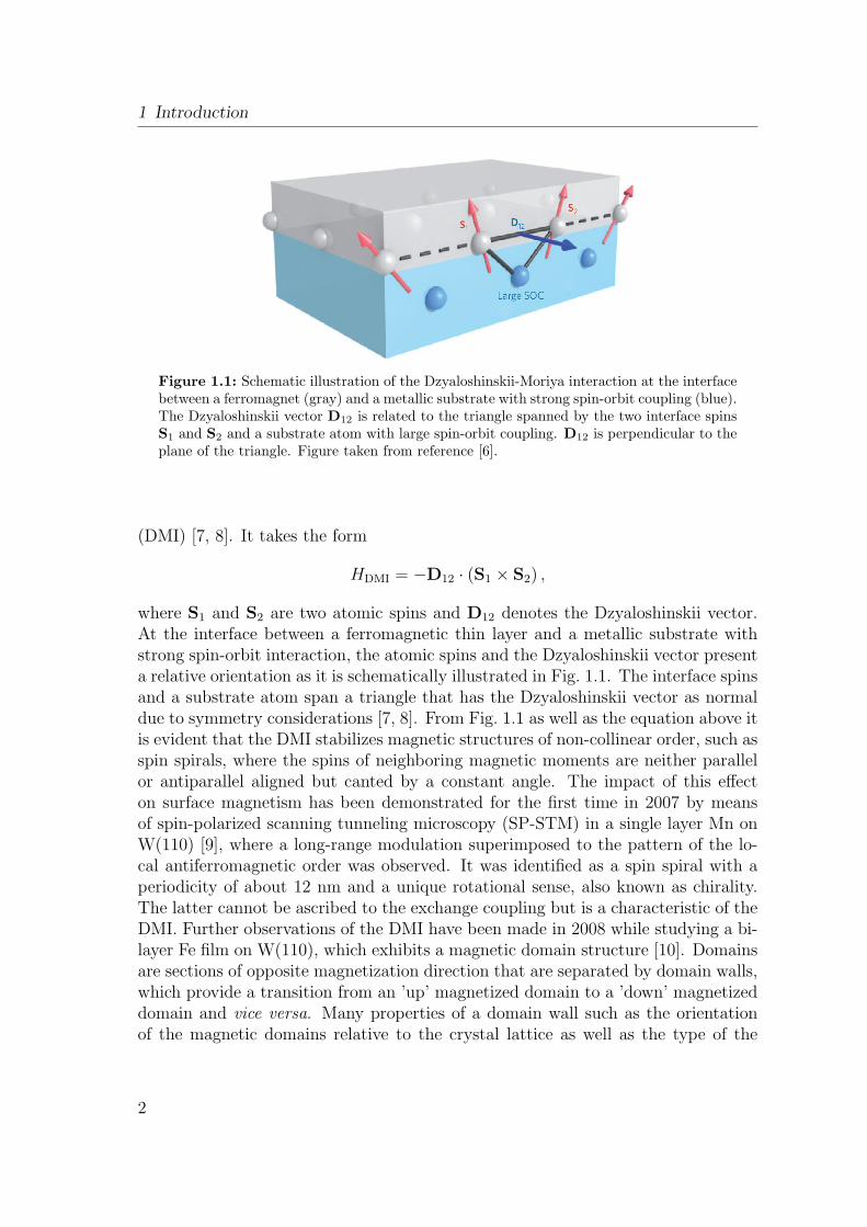
Figure 1.1: Schematic illustration of the Dzyaloshinskii-Moriya interaction at the interfacebetween a ferromagnet (gray) and a metallic substrate with strong spin-orbit coupling (blue).The Dzyaloshinskii vector D12 is related to the triangle spanned by the two interface spinsS1 and S2 and a substrate atom with large spin-orbit coupling. D12 is perpendicular to theplane of the triangle. Figure taken from reference [6].
(DMI) [7, 8]. It takes the form
HDMI = −D12 · (S1 × S2) ,
where S1 and S2 are two atomic spins and D12 denotes the Dzyaloshinskii vector.At the interface between a ferromagnetic thin layer and a metallic substrate withstrong spin-orbit interaction, the atomic spins and the Dzyaloshinskii vector presenta relative orientation as it is schematically illustrated in Fig. 1.1. The interface spinsand a substrate atom span a triangle that has the Dzyaloshinskii vector as normaldue to symmetry considerations [7, 8]. From Fig. 1.1 as well as the equation above itis evident that the DMI stabilizes magnetic structures of non-collinear order, such asspin spirals, where the spins of neighboring magnetic moments are neither parallelor antiparallel aligned but canted by a constant angle. The impact of this effecton surface magnetism has been demonstrated for the first time in 2007 by meansof spin-polarized scanning tunneling microscopy (SP-STM) in a single layer Mn onW(110) [9], where a long-range modulation superimposed to the pattern of the lo-cal antiferromagnetic order was observed. It was identified as a spin spiral with aperiodicity of about 12 nm and a unique rotational sense, also known as chirality.The latter cannot be ascribed to the exchange coupling but is a characteristic of theDMI. Further observations of the DMI have been made in 2008 while studying a bi-layer Fe film on W(110), which exhibits a magnetic domain structure [10]. Domainsare sections of opposite magnetization direction that are separated by domain walls,which provide a transition from an ’up’ magnetized domain to a ’down’ magnetizeddomain and vice versa. Many properties of a domain wall such as the orientationof the magnetic domains relative to the crystal lattice as well as the type of the
2
domain wall and its chirality can be governed by the DMI. Thus, this effect needsto be taken into consideration for the development of novel spintronic devices. Forinstance, in Pt/CoFe/MgO and Ta/CoFe/MgO it was observed that the domainwalls are driven into opposite directions by applying a current. This behavior hasbeen explained based on the left-handed chirality induced by the DMI [11]. Hence,it can be suggested that current-controlled spintronic devices could be tailored byselecting the materials adjacent to the ferromagnet.
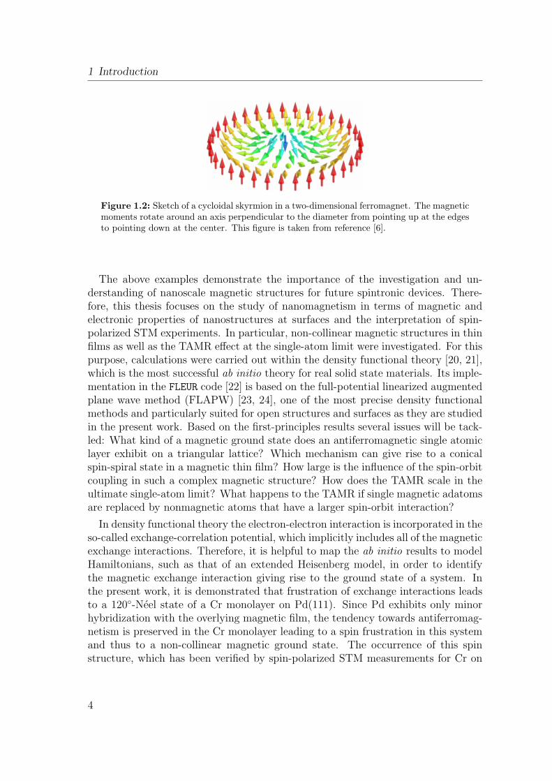
A very promising nanoscale magnetic structure that is driven likewise by theDMI and could be used as an information carrier in ultra-dense memory and logicdevices is the skyrmion – a chiral spin structure with a whirling configuration that istopologically protected and exhibits particle-like properties (cf. Fig. 1.2 (a)) [6, 12].It has been first observed in 2009 in bulk magnets such as MnSi [13, 14, 15]. Recently,the occurrence of a skyrmion lattice in a magnetic thin film has been reported fora monolayer of Fe on the (111) surface of Ir [16]. It was shown that the two-dimensional square lattice of skyrmions is enforced by the four-spin interaction, i.e.,a spin interaction beyond the pair-wise Heisenberg exchange. Later in this thesis,a second example will be presented where it is demonstrated that the higher-orderterms are crucial for the magnetic ground state.
In contrast to the situation in the bulk systems, the skyrmion phase in the Femonolayer does not need a magnetic field in order to be stabilized, since it presentsthe magnetic ground state of the system. Skyrmions can be moved with electricalcurrents of very small density (≈ 106 Am−2) [17, 18] in comparison to currentdensities of approximately 1011 to 1012 Am−2 [6] needed for the motion of domainwalls. Besides the current-induced motion of the skyrmions their small size of only afew nanometers (or atoms) allows for a significant reduction of the spacing betweenbits with respect to that of domains. While the domain wall width can be as smallas a few nanometers, too, the size of a domain has a lower limit of 30 to 40 nm,which can hardly be reduced. However, up to now the formation of skyrmions hasbeen exclusively studied at temperatures below room temperature, although fromthe theoretical point-of-view it is expected that skyrmions are also stable at roomtemperature [6, 16].
Finally, another route towards novel spintronic devices is given by the tunnelinganisotropic magnetoresistance (TAMR). This effect occurs if two metallic electrodesare separated by an insulating barrier such as a vacuum layer. The resistance de-pends on the magnetization directions of one of those electrodes with respect to thecurrent flow. For instance, in a double layer Fe film [19] it has been demonstratedthat the domain walls can be detected using a nonmagnetic STM tip since the lo-cal density of states of the sample depends on the magnetization direction. Thisresult was explained by means of ab initio calculations and could be ascribed to thehybridization of states with different orbital character. It leads to a differential con-ductivity that depends on the magnetization direction and allows for the resolutionof magnetic structures at the nanometer scale.
3
1 Introduction
Figure 1.2: Sketch of a cycloidal skyrmion in a two-dimensional ferromagnet. The magneticmoments rotate around an axis perpendicular to the diameter from pointing up at the edgesto pointing down at the center. This figure is taken from reference [6].
The above examples demonstrate the importance of the investigation and un-derstanding of nanoscale magnetic structures for future spintronic devices. There-fore, this thesis focuses on the study of nanomagnetism in terms of magnetic andelectronic properties of nanostructures at surfaces and the interpretation of spin-polarized STM experiments. In particular, non-collinear magnetic structures in thinfilms as well as the TAMR effect at the single-atom limit were investigated. For thispurpose, calculations were carried out within the density functional theory [20, 21],which is the most successful ab initio theory for real solid state materials. Its imple-mentation in the FLEUR code [22] is based on the full-potential linearized augmentedplane wave method (FLAPW) [23, 24], one of the most precise density functionalmethods and particularly suited for open structures and surfaces as they are studiedin the present work. Based on the first-principles results several issues will be tack-led: What kind of a magnetic ground state does an antiferromagnetic single atomiclayer exhibit on a triangular lattice? Which mechanism can give rise to a conicalspin-spiral state in a magnetic thin film? How large is the influence of the spin-orbitcoupling in such a complex magnetic structure? How does the TAMR scale in theultimate single-atom limit? What happens to the TAMR if single magnetic adatomsare replaced by nonmagnetic atoms that have a larger spin-orbit interaction?
In density functional theory the electron-electron interaction is incorporated in theso-called exchange-correlation potential, which implicitly includes all of the magneticexchange interactions. Therefore, it is helpful to map the ab initio results to modelHamiltonians, such as that of an extended Heisenberg model, in order to identifythe magnetic exchange interaction giving rise to the ground state of a system. Inthe present work, it is demonstrated that frustration of exchange interactions leadsto a 120-Neel state of a Cr monolayer on Pd(111). Since Pd exhibits only minorhybridization with the overlying magnetic film, the tendency towards antiferromag-netism is preserved in the Cr monolayer leading to a spin frustration in this systemand thus to a non-collinear magnetic ground state. The occurrence of this spinstructure, which has been verified by spin-polarized STM measurements for Cr on
4
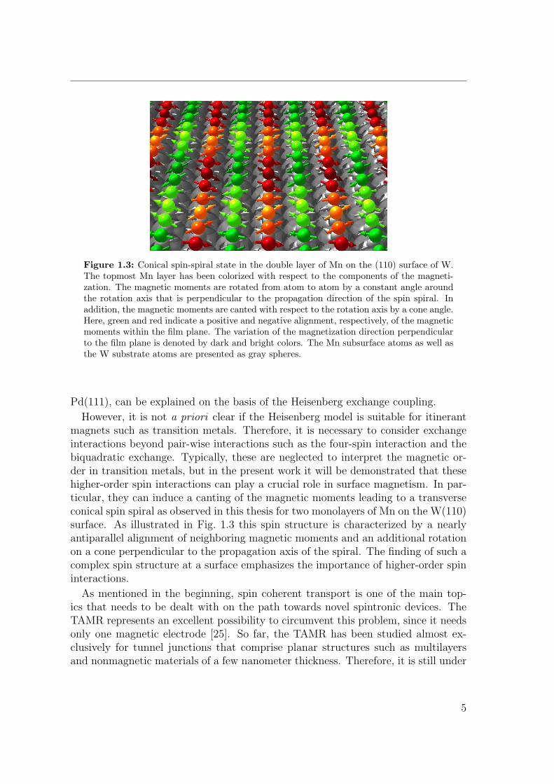
Figure 1.3: Conical spin-spiral state in the double layer of Mn on the (110) surface of W.The topmost Mn layer has been colorized with respect to the components of the magneti-zation. The magnetic moments are rotated from atom to atom by a constant angle aroundthe rotation axis that is perpendicular to the propagation direction of the spin spiral. Inaddition, the magnetic moments are canted with respect to the rotation axis by a cone angle.Here, green and red indicate a positive and negative alignment, respectively, of the magneticmoments within the film plane. The variation of the magnetization direction perpendicularto the film plane is denoted by dark and bright colors. The Mn subsurface atoms as well asthe W substrate atoms are presented as gray spheres.
Pd(111), can be explained on the basis of the Heisenberg exchange coupling.
However, it is not a priori clear if the Heisenberg model is suitable for itinerantmagnets such as transition metals. Therefore, it is necessary to consider exchangeinteractions beyond pair-wise interactions such as the four-spin interaction and thebiquadratic exchange. Typically, these are neglected to interpret the magnetic or-der in transition metals, but in the present work it will be demonstrated that thesehigher-order spin interactions can play a crucial role in surface magnetism. In par-ticular, they can induce a canting of the magnetic moments leading to a transverseconical spin spiral as observed in this thesis for two monolayers of Mn on the W(110)surface. As illustrated in Fig. 1.3 this spin structure is characterized by a nearlyantiparallel alignment of neighboring magnetic moments and an additional rotationon a cone perpendicular to the propagation axis of the spiral. The finding of such acomplex spin structure at a surface emphasizes the importance of higher-order spininteractions.
As mentioned in the beginning, spin coherent transport is one of the main top-ics that needs to be dealt with on the path towards novel spintronic devices. TheTAMR represents an excellent possibility to circumvent this problem, since it needsonly one magnetic electrode [25]. So far, the TAMR has been studied almost ex-clusively for tunnel junctions that comprise planar structures such as multilayersand nonmagnetic materials of a few nanometer thickness. Therefore, it is still under
5
1 Introduction
debate how the TAMR scales down in the single-atom limit. This thesis addressesthe smallest nanostructure that could be used as a potential spintronic device – thesingle atom on a magnetic surface. However, the direct comparison of theoreticaland experimental results is a major issue in the investigation of the TAMR in singleatoms, since the techniques used so far for the fabrication of nanoscale contacts didnot allow for a well-defined microscopic structure of the contacts. Here, a systemwill be introduced for the first time that is suited for a direct comparison of theoryand experiment. It comprises a single atom, such as a Co or an Ir atom, that isadsorbed on a magnetic surface. The magnetization direction of the adatom alignsto that of the nearest magnetic atoms of the film below due to the strong exchangecoupling. This allows for an adjustment of the spin direction without the use of anexternal magnetic field. Here, different magnetic templates are chosen such as thedomain wall structure in a double layer of Fe on W(110) [19, 26, 27] or the atomicscale spin-spiral state of a monolayer of Mn on W(110) [9]. In a nanoscale domainstructure the magnetic moment of the adatom can be aligned perpendicular or par-allel to the film plane depending on its position on the domain or the domain wall.In an atomic-scale spin-spiral state, on the other hand, it can take every angle thatis provided by the magnetic moments of the underlying film. Then, the TAMR canbe studied by comparing the local vacuum density of states above the adatom fordifferent magnetization directions. Since the spin-orbit coupling is imprinted ontothe electronic structure via the magnetization direction dependent hybridization ofdifferent d orbitals in the adatom, the density of states becomes anisotropic andinduces the TAMR. This allows for the use of nonmagnetic STM tips and a directcomparison of theoretical and experimental results. Furthermore, the basic prin-ciple of the TAMR, namely the magnetization dependent hybridization of d stateswith different orbital character, can be explained based on a simple model that isintroduced in this work.
This thesis is structured into two parts:In chapters 2 to 6 the methods and underlying theory of the electronic structurecalculations are introduced. The idea and concept of the density functional theoryto solve the quantum mechanical many-particle problem are presented in chapter2. The Full Potential Linearized Augmented Plane Wave (FLAPW) method, whichranks amongst the most accurate implementations of the density functional theory,is described in chapter 3. In the present thesis the program code FLEUR [22] hasbeen used, which is based on the FLAPW method. It is particularly suited to treatsystems with complex magnetic structure. Chapter 4 deals with elementary modelsof magnetism that provide a basis for the understanding of the ab initio results. TheStoner model describes the occurrence of ferromagnetism and antiferromagnetismin terms of the nonmagnetic density of states. The Heisenberg model offers a simpledescription of the magnetic interactions in terms of the exchange parameters andthus discusses the tendency of a system towards non-collinear magnetism. For adirect comparison of the ab initio calculations and the spin-polarized STM results,
6
the spin-polarized Tersoff-Hamann model is introduced that provides a formulationof the spin-polarized tunneling current. The implementation of non-collinear mag-netism in the FLAPW method is presented in chapter 5. Finally, in chapter 6 therelativistic effect of spin-orbit coupling is presented as well as its implementation inthe FLEUR code.
The results of this thesis are organized in chapters 7 to 9. As a first example ofa non-collinear magnetic structure the 120 Neel state is discussed in chapter 7. Ithas been observed in a monolayer of Cr on the (111) surface of Pd and is driven bythe topological spin frustration. A much more complex magnetic structure, namelya three-dimensional conical spin-spiral state, is presented in chapter 8. It has beendiscovered in a double layer of Mn on the (110) surface of W, and it is demonstratedhere that it can be ascribed to the higher-order spin interactions. Furthermore, theinfluence of spin-orbit coupling effects onto a non-collinear magnetic structure interms of the Dzyaloshinskii-Moriya interaction (DMI) and the tunneling anisotropicmagnetoresistance (TAMR) has been studied in this system. In chapter 9 the TAMRis studied systematically for different Cr and Ir ad-atoms on ultrathin films on the(110) surface of W. It is explained on the basis of a simple model that describes themixing of surface states with different orbital character.
7

1 Introduction
8
2 Density functional theory
The quantum mechanical treatment of a solid constitutes a complex many-particleproblem. In order to calculate the total energy and the ground state properties ofsuch a system the non-relativistic Schrodinger equation
H|Ψ(r1, r2, ..., rN)⟩ = E|Ψ(r1, r2, ..., rN)⟩ (2.1)
needs to be solved for a multi-dimensional N -particle wave function Ψ. Since this isa nontrivial task, approaches like the Born-Oppenheimer approximation have beenmade to simplify the problem. The Born-Oppenheimer approximation is based uponthe fact that due to the large difference in mass, the electrons move much faster thanthe nuclei and therefore considers the latter ones as point charges at fixed positions.In this way, the total system can be reduced to a many-electron system in an externalpotential vext generated by the atomic nuclei.
Due to the antisymmetry and the multi-dimensionality of the N -electron wavefunction Ψ(r1, r2, ..., rN), the remaining many-electron problem is still very com-plex and computationally demanding. Typical approaches to solve the resultingSchrodinger equation, such as the full diagonalization, lead to an exponential in-crease in the computational effort with the number of electrons. In order to treatthis problem in an efficient way, the density functional theory (DFT) chooses theelectron density n(r) as the basic quantity. This theory has been established byHohenberg and Kohn [20] as well as Kohn and Sham [21] and will be explained inmore detail in this chapter.
2.1 The Hohenberg-Kohn theorem
The basic idea of the DFT is to describe the ground state energy of a many-electronsystem and its properties by the electron density solely without the loss of infor-mation. Inspired by the Thomas-Fermi model [28, 29], P. Hohenberg and W. Kohnstated that in the case of a system with a nondegenerate ground-state
• the total energy is a unique functional of the ground-state electron density n(r),
and
• the exact ground-state density minimizes the energy functional E [n(r)].
9
2 Density functional theory
In order to prove the first theorem, an electronic system is considered that is influ-enced by an external potential vext(r) and the Coulomb repulsion. In this case, theHamiltonian has the form
H = T + U + V (2.2)
where T is the operator of the kinetic energy of the system, U is the operator of theelectron-electron interaction energy, and V is the operator of the interaction withan external potential. The electron density of the ground-state Ψ is denoted as
n(r) = ⟨Ψ|N∑i=1
δ (r− ri) |Ψ⟩. (2.3)
In the following, it is demonstrated that different external potentials vext(r) andv′ext(r) with vext(r) = v′ext(r) + const must generate different ground state densitiesn(r) and n′(r). The ground-state energies are given as
E0 = ⟨Ψ|H|Ψ⟩ (2.4)
andE ′
0 = ⟨Ψ′|H′|Ψ′⟩ (2.5)
with H = T + U + V and H′ = T + U + V ′, respectively. Due to the Ritz variationalprinciple it applies that
E0 = ⟨Ψ|H′|Ψ⟩ − ⟨Ψ|V ′ − V |Ψ⟩ > ⟨Ψ′|H′|Ψ′⟩ − ⟨Ψ|V ′ − V |Ψ⟩ (2.6)
leading to
E0 > E ′0 −
∫(v′ext(r) − vext(r))n(r)d3r. (2.7)
Interchanging the primed and unprimed quantities and assuming n′(r) = n(r), it isobtained analogously that
E ′0 > E0 −
∫(vext(r) − v′ext(r))n(r)d3r. (2.8)
Adding Eq. (2.7) and (2.8) results in
E0 > E ′0 −
∫(v′ext(r) − vext(r))n(r)d3r (2.9)
> E0 −∫
(vext(r) − v′ext(r))n(r)d3r −∫
(v′ext(r) − vext(r))n(r)d3r
> E0 (2.10)
10
2.1 The Hohenberg-Kohn theorem
which is wrong. Thus, it can be concluded that vext(r) is a unique functional ofn(r). Moreover, the full ground-state energy is a unique functional of n(r), sincethe kinetic energy T and the electron-electron interactions U are known. Onlythe external potential vext(r) defines the Hamiltonian H. Therefore, the energy isrewritten as a functional of the electron density n(r):
E[n(r)] = T [n(r)] + U [n(r)] +
∫vext(r)n(r)d3r (2.11)
= FHK [n(r)] +
∫vext(r)n(r)d3r
In order to prove the second theorem, it is assumed that for a given externalpotential vext(r) the ground-state density is n0(r) and the ground state wave functionis Ψ0. In this case, the expression in Eq. (2.11) is written as
Evext [n] = FHK +
∫vext(r)n(r)d3r (2.12)
= ⟨Ψ0|T + U + V0|Ψ0⟩
where n(r) denotes an arbitrary density. By applying the variational principle itfollows that
Evext [n] ≥ ⟨Ψ0|T + U + V0|Ψ0⟩ (2.13)
= FHK [n0] +
∫vext(r)n0(r)d
3r
= Evext [n0] = E0[n0].
This means that the correct ground-state density indeed minimizes the energy func-tional. In this way, the determination of the electronic ground state for a givenexternal potential vext has been reduced to the minimization of the energy func-tional Evext [n].
Furthermore, the Hohenberg-Kohn theorem can be extended in order to describedegenerate [30] and spin-polarized systems [31, 32]. The extension to spin-polarizedDFT is carried out by including an external magnetic field B(r) in the Hamiltonoperator, and introducing spin-dependent electron densities n↑(r) and n↓(r) as wellas a magnetization density m(r) = n↑(r)−n↓(r). Then, the energy functional reads
E[n(r),m(r)] ≥ E[n0(r),m0(r)]. (2.14)
The proof for the spin-polarized case is similar to the one performed in the nonmag-netic case. Hence, the Hohenberg-Kohn theorem also applies for magnetic systems.
In order to make use of this simplification, a reasonable representation of theenergy functional is necessary, which will be introduced in the next section.
11
2 Density functional theory
2.2 The Kohn-Sham equations
A promising representation of the energy functional E[n(r)] is ascribed to W. Kohnand L. J. Sham [21]. They decided to map the many-electron problem onto a systemof non-interacting particles in an effective potential veff. Then, the many-electrondensity can be written in terms of single-particle wave functions:
n(r) = 2
N/2∑i=1
|ψi(r)|2, (2.15)
with the factor ’2’ originating from the spin degeneracy. In order to describe it ascorrectly as possible, the energy functional is split into several contributions:
E[n] =
∫vextn(r)d3r +
1
2
∫ ∫n(r)n(r′)
|r− r′|d3rd3r′ +G[n] (2.16)
= Eext[n] + EH [n] +G[n].
The first term, Eext[n], includes the potential energy caused by the atomic nuclei.The second term EH [n] arises from the Coulomb interaction of the electrons withinthe approximation of Hartree. The universal functional G[n] itself splits into twofurther contributions:
G[n] = TS[n] + Exc[n] (2.17)
where TS[n] is the kinetic energy of a system of non-interacting electrons:
TS[n] = −2N∑i=1
∫ψ∗i (r)
~2m
∇2ψi(r)d3r, (2.18)
and the functional Exc[n] contains all the exchange and correlation effects. Theaccurate description of the kinetic energy is a benefit of this formalism as TS[n]contributes significantly to the total energy. Since there is no exact expression ofExc[n], approximations need to be made. Some of them will be introduced in section2.3.
From section 2.1 it can be concluded that the energy functional is not only mini-mized by the ground state electron density n(r), but also with respect to the groundstate wave function ψi. Due to the conservation of the number of particles, the wavefunctions need to be normalized in this case:∫
|ψi(r)|2d3r = 1 −→N∑i=1
∫|ψi(r)|2d3r = N. (2.19)
12
2.2 The Kohn-Sham equations
This condition is taken into account by introducing Lagrange multipliers ϵi. Afterapplying the variational principle to Eq. (2.16), the Kohn-Sham equations result in(
− ~2
2m∇2 + veff(r)
)ψi(r) = ϵiψi(r) (2.20)
resembling the single-particle Schrodinger equation with the eigenfunctions ψi. Be-sides the external potential vext, the Hartree potential
vH =
∫n(r′)
|r− r′|, (2.21)
and the exchange correlation potential
vxc =δExc[n]
δn(r)(2.22)
contribute to the effective potential veff
veff(r) = vext(r) + vH(r) + vxc(r). (2.23)
Since vH and vxc depend on the electronic density and, at the same time, are requiredto solve the Kohn-Sham equations, this problem needs to be tackled by means of aself-consistency method.
The generalization of the Kohn-Sham equations with respect to spin-polarizedsystems is carried out by replacing the spin-dependent electron densities, n↑(r) andn↓(r), as well as the magnetization density m(r) with the density matrix ραβ(r). Inorder to obtain the generalized Kohn-Sham equations, the electronic and magneti-zation densities need to be reproduced by Pauli spinors:
ψi(r) =
(ψ↑i (r)
ψ↓i (r)
). (2.24)
Then, the electronic and the magnetization densities can be written as
n(r) =N∑i=1
|ψi(r)|2, (2.25)
and
m(r) =N∑i=1
ψ∗i (r)σψi(r), (2.26)
respectively. The components of σ are the Pauli-spin matrices. The Application ofthe variational principle yields the generalized Kohn-Sham equations exhibiting the
13
2 Density functional theory
form of the Schrodinger-Pauli equation:(− ~2
2m∇2 + veff + σ ·Beff
)ψi = ϵiψi(r). (2.27)
There are two terms contributing to the additional effective magnetic field Beff inEq. (2.27). The first one is originating from the variation of the exchange-correlationenergy with respect to the magnetization density m. The other one is due to anexternal magnetic field Bext:
Beff(r) = Bxc(r) + Bext(r) (2.28)
with
Bxc(r) =δExc[n(r),m(r)]
δm(r). (2.29)
Further simplifications of Eq. (2.27) can be made regarding the spin direction. In acollinear magnetic ordering, as in the ferromagnetic or the antiferromagnetic case,the parallel or antiparallel magnetic moments may coincide with a certain axis, suchas the z-axis, without loss of generality. Thus, the Hamilton operator becomes diag-onal in both spin components of the spinor, which can be decoupled and the problembecomes independently solvable for the spin-up and the spin-down component. Fur-thermore, the total energy and other ground state properties of the system remainfunctionals of the spin-up and the spin-down density n↑(r) and n↓(r). These areexpressed in terms of spin-dependent single-particle wave functions:
nσ=↑,↓(r) =N∑i=1
|ψσi (r)|2. (2.30)
2.3 Exchange-correlation potentials
In principle, the DFT enables the exact determination of a solid’s ground state prop-erties except for the exchange-correlation effects contained in the energy functionalExc[n]. There is no accurate representation of this functional, and therefore, it needsto be approximated. The simplest approach is to assume the exchange-correlationenergy to be locally represented by a uniform electron gas of the same electronicand magnetic density. In this case the exchange-correlation energy has the followingform:
Exc[n(r), |m(r)|] =
∫n(r)ϵxc(n(r), |m(r)|)d3r. (2.31)
Here, ϵxc is not a functional but a function of the electron density n(r) and theabsolute value of the magnetization density |m(r)|, which is due to the parallelalignment of the exchange-correlation field Bxc and the magnetization density m(r).
14
2.4 The self-consistency cycle
This approach is called the local density approximation (LDA) [31] or local spin-density approximation (LSDA) if the spin-polarization is considered as in the presentwork. The exchange-correlation potential, on the other hand, is written as
vxc(r) = ϵxc(n(r), |m(r)|) + n(r)∂ϵxc(n(r), |m(r)|)
∂n(r), (2.32)
and the magnetic field results as below
Bxc(r) = n(r)∂ϵxc(n(r), |m(r)|)
∂|m(r)|m(r). (2.33)
The validity of the LSDA is assumed only in the case of a slowly varying density,which is rare for atomic systems. Nevertheless, the LSDA yields extremely goodresults even in the case of inhomogeneous systems. Further optimization can beachieved by considering spatially varying electronic densities and introducing localgradients of the electron and magnetization density. This method is known as the’Generalized Gradient Approximation’ (GGA) [33]. The LDA and GGA are themost common approximations for the exchange-correlation potential.
2.4 The self-consistency cycle
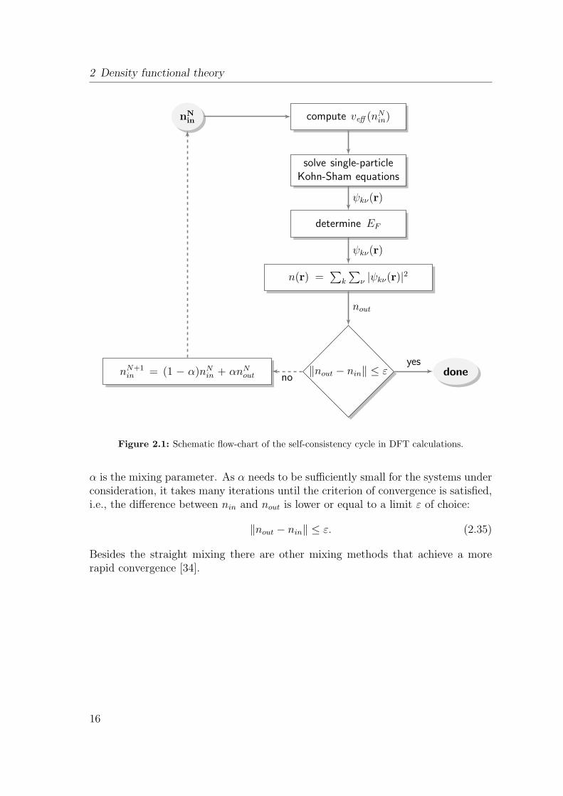
As outlined above, solving the Kohn-Sham equations is performed within a self-consistency method. At first, a starting electronic density nin is constructed. Then,the self-consistency cycle is run through iteratively (see Fig. 2.1):
Based on the density nNin(r), the Hartree and the exchange-correlation potential,
vH(nin) and vxc(nin), are computed, and the effective potential veff(nin) is calculated.The latter one is inserted into the Kohn-Sham equations, which can be solved bymeans of exploiting the periodicity of a crystal via the Bloch’s theorem. The Hamil-ton matrix is set up and diagonalized for every single Bloch vector k that covers theBrillouin zone. In the next step, the eigenvalues and -states of the Hamilton matrixare used to determine the Fermi energy employing the occupation of bands assignedto the energy Eν . It starts at the lowest energy and continues until the sum of theweights w(k, Eν(k∥) − EF ) = w(k∥)(e
Eν(k∥)−EF )/kBT + 1)−1 equals the total numberN of electrons per unit cell. The resulting condition fixes the Fermi energy. Thecalculation of the electronic density nN
out is carried out by a sum over all occupiedstates:
n(r) =∑k
∑ν
|ψkν(r)|2. (2.34)
In the last step, a new starting density nN+1in results from mixing the densities nN
in
and nNout. It is done in order to improve the numerical stability of the calculation.
The simplest mixing method is the straight mixing nN+1in = (1−α)nN
in+αnNout, where
15
2 Density functional theory
..compute veff (nNin).nN
in.
solve single-particleKohn-Sham equations
.
determine EF
.
n(r) =∑
k
∑ν |ψkν(r)|2
.
∥nout − nin∥ ≤ ε
.
done
.
nN+1in = (1 − α)nN
in + αnNout
.
ψkν(r)
.
ψkν(r)
.
nout
.
yes
.
no
Figure 2.1: Schematic flow-chart of the self-consistency cycle in DFT calculations.
α is the mixing parameter. As α needs to be sufficiently small for the systems underconsideration, it takes many iterations until the criterion of convergence is satisfied,i.e., the difference between nin and nout is lower or equal to a limit ε of choice:
∥nout − nin∥ ≤ ε. (2.35)
Besides the straight mixing there are other mixing methods that achieve a morerapid convergence [34].
16
3 Solving the Kohn-Sham equations with FLAPW
In the previous chapter, the complex many-particle problem has been transferredinto a single-particle problem by means of the DFT. In the following, several basissets are discussed that allow for the solution of the Kohn-Sham equations. Therefore,a method will be introduced that provides the proper basis set as well as a gooddescription of the potential. This method is called the ’full-potential linearizedaugmented plane wave’ method (FLAPW) [35].
The easy implementation of plane waves qualifies them as a clearly promisingbasis set, since they are orthogonal and at the same time diagonal in the momentum,i.e., they are eigenfunctions of the kinetic energy operator. Their major drawbackis the description of the electrons’ wave functions near the atomic nuclei. Here,the latter ones are heavily oscillating due to the 1/r dependency of the Coulombpotential. Hence, large wave vectors are needed to reproduce the total wave functioncorrectly. A common approach to avoid the oscillations, is the application of so-called pseudopotentials [36], where the core states are projected out of the Hamiltonoperator leading to weaker binding potentials. Therefore, they are describing thestructure of the valence electrons only. Furthermore, the pseudo-wave functions maybe represented using fewer Fourier components than the all-electron wave functionsat the same time. But the construction of pseudopotentials is often very complicated,therefore, an alternative way of representing the oscillations near the nuclei is chosenhere, which is the application of radial wave functions. This procedure has beensuggested by J. C. Slater [37] and is called the ’augmented plane wave’ method(APW).
3.1 APW method
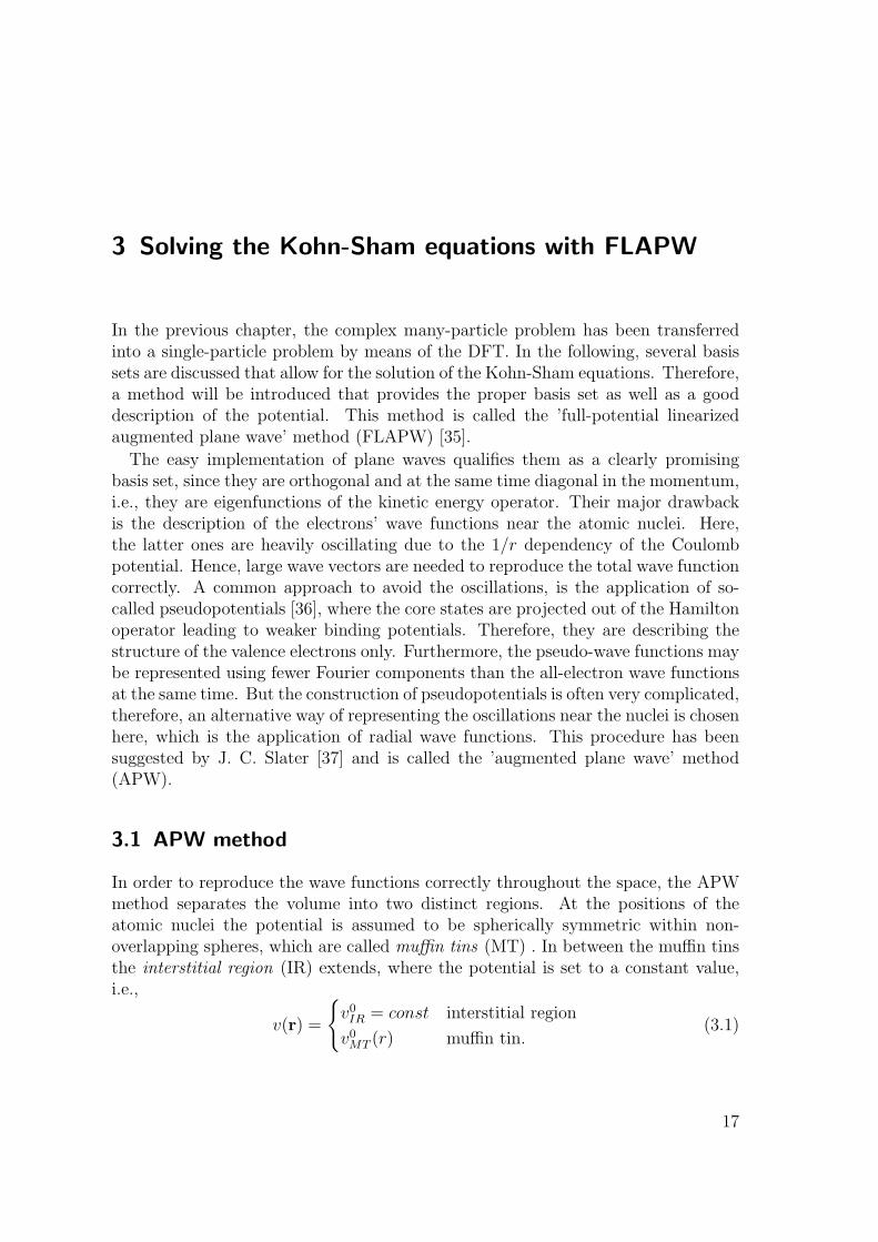
In order to reproduce the wave functions correctly throughout the space, the APWmethod separates the volume into two distinct regions. At the positions of theatomic nuclei the potential is assumed to be spherically symmetric within non-overlapping spheres, which are called muffin tins (MT) . In between the muffin tinsthe interstitial region (IR) extends, where the potential is set to a constant value,i.e.,
v(r) =
v0IR = const interstitial region
v0MT (r) muffin tin.(3.1)
17
3 Solving the Kohn-Sham equations with FLAPW
MT
IR
Figure 3.1: The division of the space in the APW method. Spheres represent the muffintins centered at the position of the atomic nuclei. The dark region denotes the interstitialregion in between the muffin tins.
It is known that for a constant potential the fundamental solutions of theSchrodinger equation are plane waves, whereas the radial Schrodinger equation in aspherical potential is solved by radial functions times spherical harmonics. There-fore, the present approximation of the potential allows for the expansion of thesingle-particle wave functions as below:
φG(k, r) =
ei(G+k)r interstitial region∑L
AµGL (k)ul(r)YL(r) muffin tin µ, (3.2)
where k denotes the Bloch vector and G the reciprocal lattice vector. L abbreviatesthe quantum numbers l and m, and r specifies the location inside the muffin tin µwith respect to its center. The functions ul are solutions of the radial Schrodingerequation, including the energy parameter El and the spherical component of thepotential v(r): (
− ~2
2m
∂2
∂r2+
~2
2m
l(l + 1)
r2+ v(r)
)rul(r) = Elrul(r). (3.3)
The condition of continuous wave functions at the transition from the muffin tinspheres to the interstitial region determines the coefficients AG
µL(k). Thus, the APWform a set of continuous basis functions covering all space. Nevertheless, this choiceof a basis set has several disadvantages:
• The APW offer only little variational freedom, since the energy parameters El
and the quantum numbers l, m need to be kept fixed. Furthermore, a correctdescription of the system is obtained solely, if El equals the band energies.At the same time the ul’s depend on the band energies and thus a simplediagonalization of the Hamilton matrix is impossible and leads to a nonlinear
18
3.2 LAPW method
problem.
• For infinitesimal ul at the boundary of the muffin tin spheres the matchingcondition is not satisfied anymore, and as a result, the plane waves and radialfunctions decouple. This is called the asymptotic problem.
3.2 LAPW method
In order to eliminate the problems listed in the section above, O. Krogh Andersen[38] as well as D. D. Koelling and G. O. Arbman [39] linearized the APW basis by
adding the energy derivative ul(r) = ∂ul(E,r)∂E
to the radial solution ul(E, r) of theSchrodinger equation. Therefore, ul is expanded into a Taylor-series around El
ul(E, r) = ul(El, r) + ul(El, r)(E − El) + O[(E − El)2]. (3.4)
Here, O[(E −El)2] is due to the fact that the linearized APW (LAPW) basis func-
tions are constructed from linear combinations of ul and ul to obtain an energyindependent basis. The errors introduced in the wave functions are of the order of(E − El)
2. After the application of the variational principle the errors in the com-puted band energies result in the order of (E−El)
4. For this reason, the linearizationworks well for a wide energy range.
In comparison to the APW method the extra coefficients BµGL (k) are added to
the LAPW basis guaranteeing that the basis functions inside the muffin tin spheresmatch continuously and differentially onto the plane waves in the interstitial region:
φG(k, r) =
ei(G+k)r interstitial region∑L
(AµG
L (k)ul(r) +BµGL (k)ul(r)
)YL(r) muffin tin µ.
(3.5)
The ul are obtained by taking the energy derivative of Eq. (3.3) resulting in(− ~2
2m
∂2
∂r2+
~2
2m
l(l + 1)
r2+ v(r) − El
)rul(r) = rul(r). (3.6)
Furthermore, they have to meet the normalization requirement∫ RMT
0
u2l (r)r2dr = 1. (3.7)
By differentiating Eq. (3.7) with respect to the energy, it is shown that the ul andul need to fulfill the requirement of orthogonalization at the same time∫ RMT
0
ul(r)ul(r)r2dr = 0, (3.8)
19

3 Solving the Kohn-Sham equations with FLAPW
since every linear combination of ul and ul solves Eq. (3.6). Thus, they form acomplete and orthogonal basis set inside the muffin tin spheres as the sphericalharmonics Ylm are orthogonal by definition. Unfortunately, the core states still needa separate treatment considering that the plane waves are nonorthogonal to them.This causes a problem for so-called semi-core states, i.e., energetically high statesof the electrons close to the nuclei. Due to their strong delocalization they do notreside completely within the muffin tin spheres. As a result, the energy parameterEl, which is originally assigned to those states, is used for the description of thehigher valence electrons. This is for instance the case for the p-states of the earlytransition metals. In order to avoid this problem local orbitals can be introduced[40].
The introduction of the LAPW basis fixes the main issues of the APW method:
• Since El no longer equals the band energies, the Hamilton matrix is energyindependent, and the energies can be determined within a single diagonaliza-tion.
• The extension of the muffin-tin potentials to non-spherical potentials is eas-ily performed, since the LAPW basis set offers a large variational freedom.This results in the full-potential linearized augmented plane wave method(FLAPW).
• If the ul vanish at the muffin-tin boundaries, their radial derivatives and the ulare generally nonzero. Therefore, the continuity condition at the boundariesis always satisfied and there is no asymptote problem.
Since both, the APW and the LAPW method, have the representation of the basisas plane waves in common, the nonlinearity of the APW basis can only be avoidedby a large eigenvalue problem. The basis functions inside the muffin-tin spheres arecoupled to the plane waves in the interstitial region via the matching condition atthe boundary. Thus, they can only be varied indirectly by manipulating the planewave coefficients. The variation becomes independent with a finite number of planewaves and at maximum the same number of functions in the muffin tin spheres. Inorder to exploit the larger variational freedom of the LAPW method compared withthe APW method, the number of plane waves needs to be increased.
3.3 The FLAPW method
In the case of close packed metallic systems the LAPW method provides a gooddescription. However, for open structures, i.e., structures of reduced symmetrylike semiconductors, surfaces and interfaces, the shape-approximations applied tothe potential become difficult to justify. The FLAPW method [23] considers the
20

3.3 The FLAPW method
inclusion of a warped potential in the interstitial region and non-spherical terms inthe muffin tin rather than approximating the potential:
v(r) =
∑G
vGI eiGr interstitial region,∑
L
vGMT (r)YL(r) muffin tin spheres.(3.9)
The charge density may be phrased analogously:
v(r) =
∑G
ρGI eiGr interstitial region,∑
L
ρGMT (r)YL(r) muffin tin spheres.(3.10)
3.3.1 Film Calculations With FLAPW
Since there is great interest in studying phenomena at surfaces and thin films, theexact computation of those systems has become more and more important nowa-days. Unfortunately, they exhibit a lack of the translational symmetry, and sinceonly Bloch vectors k∥ parallel to the surface are used, the description of these sys-tems is numerically very demanding. An attempt to tackle this problem has beenprovided by reintroducing the periodicity perpendicular to the surface by means ofa periodically repeating film in the direction of the symmetry break. This thin-slabapproximation only yields reasonable results if the vacuum layer is chosen suffi-ciently large. Otherwise, the interaction between the films becomes too strong andthe system loses its features of the semi-infinite crystal.
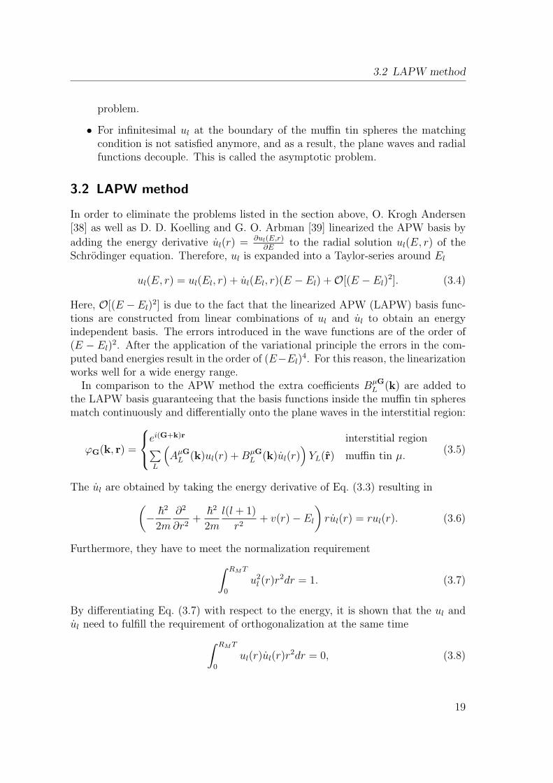
Another approach is to divide the space into three distinct regions, which is madeuse of by the FLAPW method for thin films. In addition to the muffin tin spheresand interstitial region already known from the FLAPW method, a vacuum region isintroduced (cf. Fig. 3.2). As a result, the interstitial region spreads from −D
2to +D
2
along the z-direction, which is defined to be perpendicular to the film surface. Dueto the lack of periodicity along the z-axis, the computed unit cell stretches from −∞to +∞. In consequence of this partitioning, the wave functions in the interstitialregion may be kept the same as in the FLAPW method for bulk systems. Theycan still be expanded in terms of plane waves, but instead of D the parameter Dis used to define wave vectors perpendicular to the film. Here, D needs to satisfythe condition D < D in order to gain a larger variational freedom. In this way, theplane waves are written as
φG∥G⊥(k, r) = ei(G∥+k∥)r∥eiG⊥z with G⊥ =2πn
D. (3.11)
k∥ and G∥ represent the two-dimensional Bloch and wave vectors, respectively. r∥ isthe component of r that is aligned parallel to the film, whereas G⊥ is the wave vector
21
3 Solving the Kohn-Sham equations with FLAPW
D
2
D
2-
D
2-~
D
2
~
Figure 3.2: The unit cell in a film calculation with FLAPW
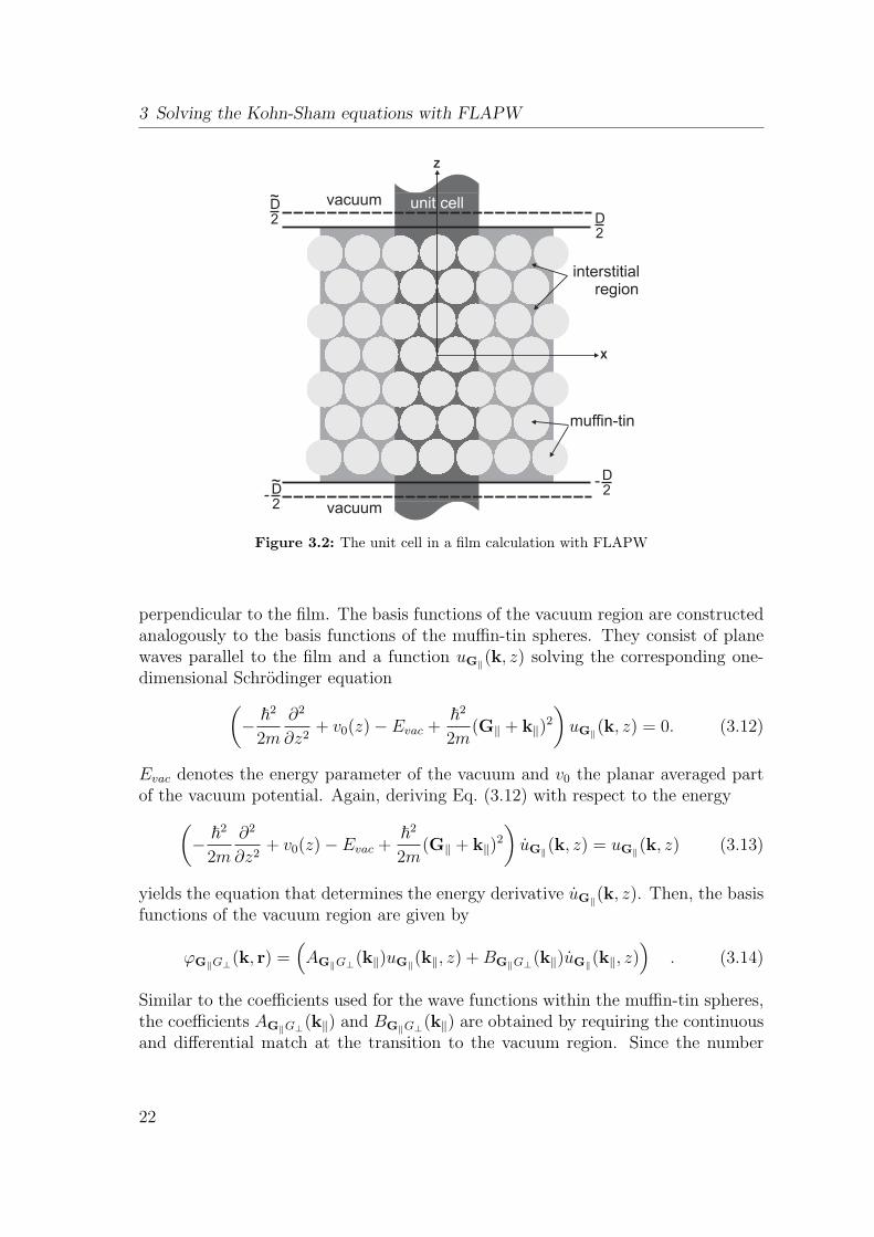
perpendicular to the film. The basis functions of the vacuum region are constructedanalogously to the basis functions of the muffin-tin spheres. They consist of planewaves parallel to the film and a function uG∥(k, z) solving the corresponding one-dimensional Schrodinger equation(
− ~2
2m
∂2
∂z2+ v0(z) − Evac +
~2
2m(G∥ + k∥)
2
)uG∥(k, z) = 0. (3.12)
Evac denotes the energy parameter of the vacuum and v0 the planar averaged partof the vacuum potential. Again, deriving Eq. (3.12) with respect to the energy(
− ~2
2m
∂2
∂z2+ v0(z) − Evac +
~2
2m(G∥ + k∥)
2
)uG∥(k, z) = uG∥(k, z) (3.13)
yields the equation that determines the energy derivative uG∥(k, z). Then, the basisfunctions of the vacuum region are given by
φG∥G⊥(k, r) =(AG∥G⊥(k∥)uG∥(k∥, z) +BG∥G⊥(k∥)uG∥(k∥, z)
). (3.14)
Similar to the coefficients used for the wave functions within the muffin-tin spheres,the coefficients AG∥G⊥(k∥) and BG∥G⊥(k∥) are obtained by requiring the continuousand differential match at the transition to the vacuum region. Since the number
22
3.3 The FLAPW method
of basis functions is significantly lower in the vacuum, its basis provides a smallervariational freedom compared to the basis of the interstitial region. Due to the workfunction, the energy spectrum of electrons is smaller in the vacuum and therefore,it is convenient to use a whole series of energy parameters instead of the energyparameter Evac
EG⊥vac = Evac −
~2
2mG2
⊥ (3.15)
to increase the variational freedom. This allows for basis functions uG∥(k, z), whichare depending on G⊥.
For thin films the FLAPW basis set takes the form
φG∥G⊥(k∥, r) =
ei(G∥+k∥)r∥ e
iG⊥zinterstitial region(
AG∥G⊥(k∥)uG∥(k∥, z)
+BG∥G⊥(k∥)uG∥(k∥, z))ei(G∥+k∥)r∥
vacuum
∑L
(AµG
L (k)ul(r) +BµGL (k)ul(r)
)Yl,m(r) muffin-tin µ.
(3.16)It traces back to H. Krakauer, M. Posternak and A. J. Freeman [24].
3.3.2 The Representation of the Density and the Potential
The charge density ρ and the potential v resemble the wave functions in the FLAPWmethod. In the interstitial region they consist of three-dimensional plane waves, inthe muffin tin they are represented by spherical harmonics and radial functions. Inthe vacuum region two-dimensional plane waves in combination with z-dependentfunctions describe the density and the potential, respectively. In general, the chargedensity is given by
ρ = eN∑i
|ψi(r)|2 (3.17)
with the sum over all occupied states. Since the expansion of the wave functions isrestricted by a wave vector cut-off kmax >
∣∣k∥ + G∣∣ that is included quadratically in
the charge density, it is necessary to consider a cut off Gmax = 2kmax for the densityand the potential. According to this, many coefficients need to be computed andstored. In order to minimize the computational effort, the symmetry of the systemhas to be exploited due to the fact that the potential and the density possess thesymmetry of the lattice. For this reason, the plane waves may be substituted bysymmetrized plane waves, which are called star functions. In the interstitial region
23
3 Solving the Kohn-Sham equations with FLAPW
the star functions have the form
Φ3Ds (r) =
1
Nop
∑op
eiRG(r−τ ). (3.18)
R|τ denotes a symmetry operation of the three-dimensional space group. Nop
is assigned to the number of performable symmetry operations. By means of thisrepresentation, plane waves that are equivalent in symmetry can be combined to aso-called star. Analogously, the two-dimensional plane waves in the vacuum regionare merged in two-dimensional star functions Φ2D
s (r) with regard to the symmetryoperations of the two-dimensional space group. In a similar way, the expansion ofthe charge density and the potential in the muffin tin is performed by benefittingfrom the point symmetry of the atoms. In this case the symmetrized wave functionsare called lattice harmonics instead of star functions. They result from the linearcombinations of the spherical harmonics
Kν (r) =∑m
cαν,mYL (r) . (3.19)
The lattice harmonics are real, orthonormal and invariant concerning symmetryoperations of the point group.
In summary, the expansion of the charge density in all of the three distinct regionsis specified as follows
ρ (r) =
∑s
ρsΦ3Ds (r) interstitial region,∑
s
ρs (z) Φ2Ds (r) vacuum region,∑
ν
ρµν (r)Kν(r) muffin tin sphere µ.
(3.20)
The potential is expanded in the same way.
3.3.3 The Generalized Eigenvalue Problem
Despite the fact that plane waves form an orthogonal basis set, the FLAPW func-tions behave different due to the spatial division into specific regions. The muffintins are cut out from the unit cell in which the orthogonality is defined. Therefore,the basis functions of different regions are able to overlap, but at the same time theyare non-orthogonal. The degree of non-orthogonality is given by the overlap matrixS, and in the FLAPW basis it results in the overlap matrix S not being diagonal,but Hermitian:
SGG′=
∫φ∗G′(r)φG(r)d3r. (3.21)
24
3.3 The FLAPW method
Here, and in the rest of this section, the index k for the Bloch vector is dropped forreasons of simplicity even though setting up the basis set as well as the Hamiltonianmatrix is done for every Bloch vector independently. However, inserting the non-orthogonal basis set |ϕi⟩ =
∑GciG|φG⟩ in the secular equation (2.20) yields
(H− ϵiS) ci = 0, (3.22)
where ci denotes the coefficient vector corresponding to the ith eigenvalue. Equation(3.22) is called a generalized eigenvalue problem. It can be reduced to a standardeigenvalue problem by applying the Cholesky decomposition. In order to achievethis, the overlap matrix is split into a matrix product of a lower triangular matrix Lwith only positive diagonal elements and its Hermitian conjugate L†. This procedureis correct as it applies for every Hermitian and positive definite matrix [41]:
S = LL†. (3.23)
After the insertion of Eq. (3.23) in Eq. (3.22) and multiplying with L−1 from theleft, the eigenvalue problem gains the following simple form
L−1H(L−1)†L†ci = ϵiL†ci (3.24)
⇔ Pxi = ϵixi.
The eigenvectors ci can be obtained by back-transforming the xi
ci = (L†)−1xi. (3.25)
3.3.4 Brillouin Zone Integration within FLAPW
The computation of certain quantities such as the electronic density in an infiniteperiodic solid happens in terms of the integration of periodic functions over theBrillouin zone described by the Bloch vector k and the band energy ν. Theseintegrations are carried out over those parts of the Brillouin zone, where the bandenergy ϵν(k) is lower than the Fermi energy, i.e., the states need to be occupied.Then, the integrals have this form
1
VBZ
∫BZ
∑ν,ϵν(k)<EF
fν(k)d3k. (3.26)
Here, VBZ denotes the volume of the Brillouin zone and f is the function to beintegrated. The computational effort caused by the Brillouin zone integration isdecreased by the exploitation of the point symmetry, which restricts the integrationto the irreducible part of the Brillouin zone only. There are several methods toperform the integration like the tetrahedron method [42] or the special point methods
25
3 Solving the Kohn-Sham equations with FLAPW
of Chadi and Cohen [43] as well as Monkhorst and Pack [44]. The latter are methodsin order to integrate slowly varying periodic functions of k. Then, the function needsto be calculated on a discrete mesh of k points, each one of them featuring a specificweight. In this way, the integration is transformed into a sum of a set of k points.In order to permit only those states, which are located below the Fermi energy, anenergy cut off parameter is assigned to every k point. Due to the discretization inmomentum space the charge density undergoes sudden changes, which might preventa convergence. Therefore, the chosen step function is replaced by the Fermi function
f (ϵν) =1
(e(ϵν(k)−EF )/kBT + 1)(3.27)
introducing a temperature broadening. Choosing the appropriate temperature Taccelerates the convergence.
3.3.5 Determination of the Total Energy
An important ground-state property of a solid state system is the total energy. Itdepends on many parameters such as the structure of the lattice, the lattice constant,the magnetic order, and the orientation of the magnetization in space if spin-orbitcoupling (SOC) is taken into account. The minimum energy determines the groundstate and, consequently, the other properties of the system. Therefore, it is ofimportance to compute this quantity as exact as possible. The total energy consistsof the term describing the energy of the electrons, Eq. (2.16), and an additionalterm Eii as a result of the Coulomb interaction of the atomic nuclei:
E[n] = TS[n] + Eext[n] + EH [n] + Exc + Eii. (3.28)
Eii is given as
Eii = e2M∑
µ,µ′=1µ=µ′
ZµZµ′
∥Rµ −Rµ′∥. (3.29)
µ denotes the atoms of the crystal at the position Rµ. The Nabla operator ∇2
included in the kinetic energy TS should not be applied explicitly due to numericalreasons. Therefore, TS is rewritten in terms of single-particle eigenvalues ϵi
TS[n] =N∑i=1
ϵi −∫n(r)veff(r)d3r −
∫m(r) ·Beff(r)d3r. (3.30)
This representation is obtained from the Kohn-Sham equations (2.20). Anotherproblem are the Coulomb singularities originating from the atomic nuclei. As M.Weinert, E. Wimmer and A. J. Freeman showed [35], the occurrence of the singu-
26
3.3 The FLAPW method
larities is avoided by combining the contributions of the kinetic and the potentialenergy. Assuming that the external potential arises from the atomic nuclei solelyand excluding the existence of an external magnetic field, i.e.,
vext(r) = −M∑µ=1
Zµ
r−Rµ, Bext = 0, (3.31)
the total energy may be obtained via Eq. (3.28). During the iterative procedureEq. (3.28) depicts only an approximation. The ground state energy E0[n0] is ob-tained after achieving the self-consistency.
27

3 Solving the Kohn-Sham equations with FLAPW
28
4 Modeling Magnetic Systems
In order to provide a framework to interpret the results obtained from ab initiocalculations, it is convenient to develop model concepts based on relatively simpleassumptions. Since the present thesis deals with magnetic systems, this chapterfocuses on the Stoner model, the Heisenberg model as well as the spin-polarizedTersoff-Hamann model.
4.1 Stoner Model
The Stoner model [45, 46, 47, 48] expresses the competition between the exchangeinteraction in terms of the exchange integral I and the kinetic energy in terms of thedensity of states (DOS) n(EF ) at the Fermi energy EF . It is based upon the fact thatwithin the spin density functional theory the magnetization density m(r) = |m(r)|of a solid is usually much smaller than the electronic density n(r). Thus, performinga Taylor expansion of the exchange-correlation energy ϵxc(n(r),m(r)) with ζ = m
n
results in:
ϵ(n, ζ) = ϵ(n, 0) +1
2ϵ′′xc(n, 0)ζ2 + ... . (4.1)
The magnetic field Bxc (cf. Eq. (2.29)) is written as follows
Bxc =1
n2ϵ′′xc(n, 0)m. (4.2)
Bxc acts as an additional spin-dependent contribution vxc to the nonmagneticexchange-correlation potential v0xc. This extra term has the same absolute valuein both spin channels. It is attractive for the majority spin (+) and repulsive forthe minority spin (−):
v±xc = v0xc ∓ vxc(r)m(r). (4.3)
The Stoner model neglects the spatial variation and uses the approximation
v±xc = v0xc ∓1
2IM. (4.4)
Here, the magnetic moment per atom is given as the integral of the magnetizationdensity over the muffin tin,
∫MT
m(r)d3r. vxc is replaced by the exchange integralI which is also called Stoner parameter. Due to the constant shift of ∓1
2IM the
potential has the same spatial shape as in the non-magnetic case. Therefore, the
29
4 Modeling Magnetic Systems
wave functions ψ±i (r) remain unchanged while the eigenvalues ϵ±i are rigidly shifted
by ∓12IM as well:
ψ±i (r) = ψ0(r) and ϵ±i = ϵ0i ∓
1
2IM. (4.5)
The subscript i is the abbreviation of kν, namely the wave vectors k and the bandindices ν. The constant shift in the energy eigenvalues gives rise to a spin split in thebandstructure, whereas the shape of the bands remains unaltered. As a consequence,the local spin densities of states keep the shape of the non-magnetic DOS with asimultaneous shift of ±1
2IM :
n±(E) =∑ν
∫BZ
δ(E − ϵ±i )d3k = n0(E ± 1
2IM), (4.6)
where the integrated volume is the Brillouin zone (BZ). The criterion for the exis-tence of ferromagnetism can be derived from Eq. (4.6). The number N of electronsper atom and the magnetic moment M of the unit cell are yielded by integratingthe DOS over all occupied states up to the Fermi energy EF :
N =
∫E<EF
[n0
(E +
1
2IM
)+ n0
(E − 1
2IM
)]dE, (4.7)
and
M =
∫E<EF
[n0
(E +
1
2IM
)− n0
(E − 1
2IM
)]dE. (4.8)
Assuming charge neutrality, Eq. (4.7) can be applied to determine the Fermi energyEF = EF (M) given that n0(E) andN are known. In that case, the magnetic momentM is obtained by substituting EF with EF (M) leading to a nonlinear equation:
M = F (M) (4.9)
=
∫E<EF (M)
[n0
(E +
1
2IM
)− n0
(E − 1
2IM
)]dE.
From Eq. (4.9) it can be deduced that the function F (M) satisfies the followingconditions:
• F (0) = 0,
• F (M) = −F (−M),
• F (±∞) = ±M∞,
• F ′(M) > 0.
30
4.1 Stoner Model
F(M)
MS
-MS
M 8
(B)(A)
M
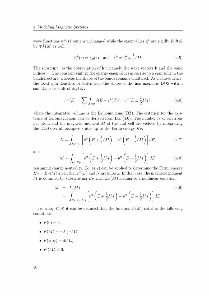
Figure 4.1: Graphical solution of Eq. (4.9).
The last condition is owing to the fact that n0(E) > 0. Here, M∞ is the satura-tion magnetization for full spin-polarization according to Hund’s rule, i.e., all themajority spin states are occupied and the minority states are empty.
Equation (4.9) can be solved graphically as it is shown in Fig. 4.1. There are twokinds of functions F (M) satisfying the conditions above. In the first case (A) thetrivial paramagnetic solution F (M) = M = 0 is considered. The function denotedwith (B) has three solutions of which only the nontrivial ones for M = ±MS havea finite spontaneous magnetization. The nonmagnetic solution M = 0 is unstable.Fig. 4.1 shows that there always exists a solution with finite magnetization if theslope of F (M) at M = 0 is larger than one. Therefore, the necessary and at thesame time sufficient condition for the existence of a ferromagnetic solution is
F ′(0) > 1. (4.10)
The derivation of Eq. (4.9) with respect to M reads
F ′(M) =I
2
[n0
(EF +
1
2IM
)+ n0
(EF − 1
2IM
)](4.11)
+
[n0
(EF +
1
2IM
)− n0
(EF − 1
2IM
)]dEF
dM,
and setting M = 0 in Eq. (4.11) results in the Stoner criterion of ferromagnetism:
F ′(0) = In0(EF ) > 1. (4.12)
This criterion represents an instability condition. It states that for a large exchangeintegral I and a large nonmagnetic DOS n0(EF ) at the Fermi energy the ferromag-
31
4 Modeling Magnetic Systems
netic phase is more stable than the paramagnetic one.
In a simple approximation the DOS is proportional to the inverse of the band-width. This is the case for the d-bands in transition metals. Therefore, the prob-ability of exhibiting a magnetic ground state increases for a small bandwidth. Inthe limiting case of single atoms the smallest bandwidth, i.e., zero bandwidth isachieved. Hence, atoms do always satisfy the Stoner criterion. The more commonelements that fulfill the Stoner criterion also in bulk are Fe, Co and Ni, which arethe typical bulk ferromagnets. Another example are surface systems, where due tothe reduction of the coordination the bandwidth becomes smaller and thus elementsthat are non-magnetic in bulk might become magnetic at the surface.
The extension to the Stoner model for antiferromagnetism is performed by includ-ing the influences of an external magnetic field H = (0, 0, H) [49, 50]. From firstorder perturbation theory it follows that the relation between the external magneticfield and the induced magnetism is given by the susceptibility χAF :
M = χAFH. (4.13)
Since antiferromagnetism features alternating magnetic moments M and −M ,the magnetic field and the magnetic moments generate the following exchange-correlation potentials:
v±xc,1 = v0xc ± ∆v±xc,1 = v0xc ±(
1
2IM + µBH
)v±xc,2 = v0xc ± ∆v±xc,2 = v0xc ∓
(1
2IM + µBH
)(4.14)
grouping the atoms into two sublattices 1 and 2. Similar to Eq. (4.9) the presentproblem has to be solved self-consistently. Unfortunately, the paramagnetic densitiesn± cannot be obtained by a simple shift of ±1
2IM anymore. Using the basic features
of the Green’s functions the magnetic moment is calculated as below
M =
∫ EF (M) [n+0 (E) − n−
0 (E)]dE (4.15)
= − 1
πIm
(∫ EF (M) [G+
00(E) −G−00(E)
]dE
)
= − 1
π
∑i
Im
(∫ EF (M)
G00i(E)
[∆v+i − ∆v−i
]G0
i0(E)dE + O(∆v3i )dE
).
32
4.1 Stoner Model
Written in terms that are linear in ∆v±xc the moment M is given as follows
M = χ0AF
(IM
2µB
+H
). (4.16)
The spin susceptibility χ0AF is defined as
χ0AF =
2µB
πIm
∫ EF (M)[∑even i
G00i(E)G0
i0(E) −∑odd i
G00i(E)G0
i0(E)
]
=2µB
πIm
∫ EF (M)[∑
all i
G00i(E)G0
i0(E) − 2∑odd i
G00i(E)G0
i0(E)
]= 2µB [−n0(EF ) + a(EF )]
= 2µB [a(EF ) − n0(EF )] . (4.17)
Solving Eq. (4.16) with respect to M yields
M = χAFH =
(1 − Iχ0
AF
2µB
)−1
χ0AFH = SAFχ
0AFH, (4.18)
where the spin susceptibility χAF is enhanced by a factor SAF . The Stoner criterionof antiferromagnetism results from Eq. (4.18)
Iχ0AF
2µB
> 1, (4.19)
which can be rewritten as
I[a(EF ) − n0(EF )
]> 1 (4.20)
by using the expression in Eq. (4.17). In conclusion, it can be stated that a smallnon-magnetic DOS n0(EF ) at the Fermi energy favors antiferromagnetism even ifthe coefficient a(EF ) is unknown.
In order to illustrate the Stoner criterion, it is useful to consider a simple DOSexhibiting for example a rectangular form:
n0(EF ) =
W−1 −W
2< E < W
2
0 |E| > W2,
(4.21)
where the bandwidth is given by the parameter W . In this case, a(EF ) may be eval-uated approximately from the Green function G0(E). The main contribution arises
33
4 Modeling Magnetic Systems
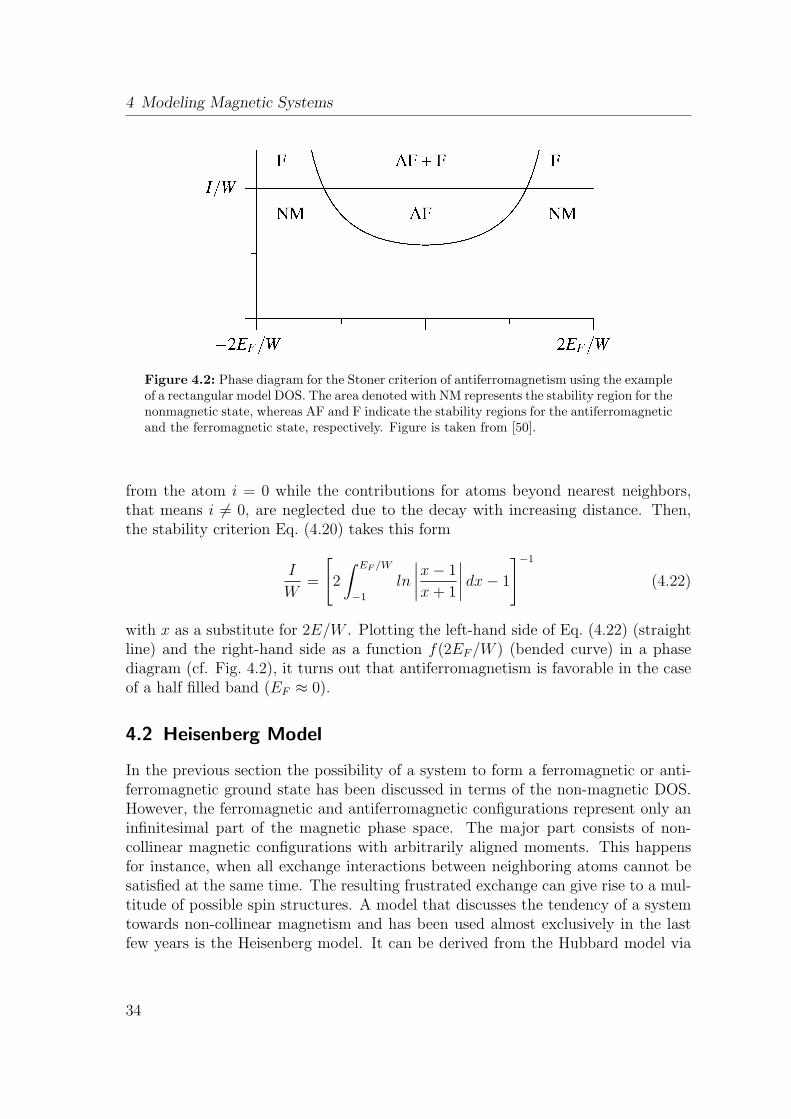
Figure 4.2: Phase diagram for the Stoner criterion of antiferromagnetism using the exampleof a rectangular model DOS. The area denoted with NM represents the stability region for thenonmagnetic state, whereas AF and F indicate the stability regions for the antiferromagneticand the ferromagnetic state, respectively. Figure is taken from [50].
from the atom i = 0 while the contributions for atoms beyond nearest neighbors,that means i = 0, are neglected due to the decay with increasing distance. Then,the stability criterion Eq. (4.20) takes this form
I
W=
[2
∫ EF /W
−1
ln
∣∣∣∣x− 1
x+ 1
∣∣∣∣ dx− 1
]−1
(4.22)
with x as a substitute for 2E/W . Plotting the left-hand side of Eq. (4.22) (straightline) and the right-hand side as a function f(2EF/W ) (bended curve) in a phasediagram (cf. Fig. 4.2), it turns out that antiferromagnetism is favorable in the caseof a half filled band (EF ≈ 0).
4.2 Heisenberg Model
In the previous section the possibility of a system to form a ferromagnetic or anti-ferromagnetic ground state has been discussed in terms of the non-magnetic DOS.However, the ferromagnetic and antiferromagnetic configurations represent only aninfinitesimal part of the magnetic phase space. The major part consists of non-collinear magnetic configurations with arbitrarily aligned moments. This happensfor instance, when all exchange interactions between neighboring atoms cannot besatisfied at the same time. The resulting frustrated exchange can give rise to a mul-titude of possible spin structures. A model that discusses the tendency of a systemtowards non-collinear magnetism and has been used almost exclusively in the lastfew years is the Heisenberg model. It can be derived from the Hubbard model via
34
4.2 Heisenberg Model
perturbation theory by expanding it into a spin model and replacing the spin op-erators by classical spin vectors [51]. The Hubbard model is the simplest model todescribe the short-range repulsive interactions between fermions in a lattice. Thereare two contributions to the Hamilton operator H = T + U : the kinetic energy Tof electrons hopping between atoms of adjacent lattice sites, and the Coulomb en-ergy U arising from the on-site repulsion of the charges on the electrons. In secondorder the perturbative treatment results in the Hamilton operator of the classicalHeisenberg model:
H = −∑i,j
JijSi · Sj (4.23)
where the sum is over all magnetic atoms of the system. The Jij represent theHeisenberg exchange parameters of the magnetic moments (referred to as spins) Si
and Sj that are located at the lattices sites i and j. In general the Si and Sj areoperators, which are usually treated as classical vectors assuming that
S2i = S2, for all i. (4.24)
That means all the spins have the same magnitude S. The Heisenberg model isespecially suitable for the description of the isotropic exchange interaction betweenhighly localized spins that are typically found in systems such as metal oxides. Inthese systems Jij can be restricted to the ferromagnetic (J1 > 0) and the antiferro-magnetic (J1 < 0) nearest-neighbor interaction, since the pair interaction betweennearest neighbors dominates over the rest of the farther distant pairs. For itiner-ant systems the exchange constants Jij follow the characteristic oscillatory decayingasymptotic behavior of the Ruderman-Kittel-Kasuya-Yoshida (RKKY) interaction[52], which describes the coupling of localized magnetic moments by means of theindirect exchange via the conducting electrons. However, in itinerant magnets itis not always the case that the Heisenberg model reproduces the correct magneticground state due to its restriction as a localized model. Therefore, it is necessary toconsider the terms of higher order resulting from the perturbation of the Hubbardmodel. While the second order perturbation treatment reproduces the Heisenbergmodel, the next nonzero term, which is of fourth order, yields to two additionalterms: the biquadratic interaction
Hbiq = −∑ij
Bij (Si · Sj)2 (4.25)
35
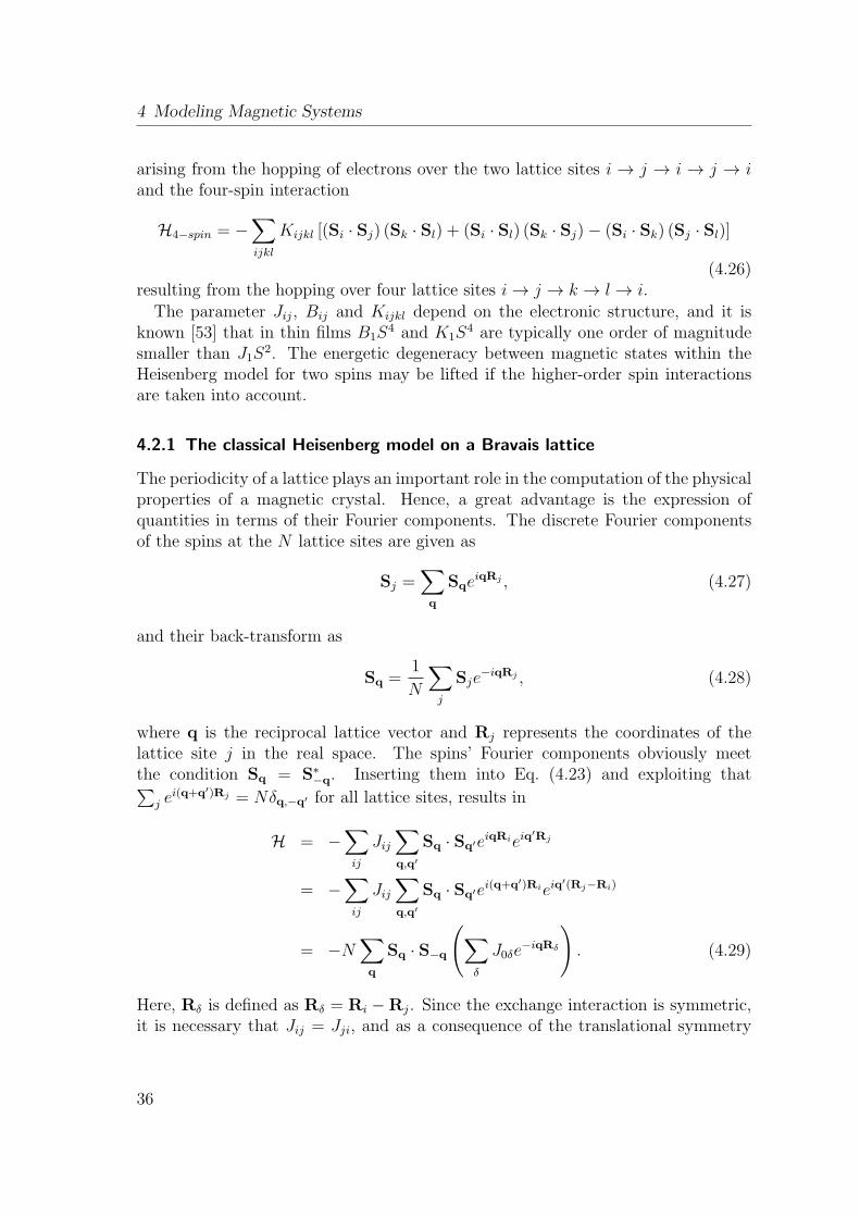
4 Modeling Magnetic Systems
arising from the hopping of electrons over the two lattice sites i → j → i → j → iand the four-spin interaction
H4−spin = −∑ijkl
Kijkl [(Si · Sj) (Sk · Sl) + (Si · Sl) (Sk · Sj) − (Si · Sk) (Sj · Sl)]
(4.26)resulting from the hopping over four lattice sites i→ j → k → l → i.
The parameter Jij, Bij and Kijkl depend on the electronic structure, and it isknown [53] that in thin films B1S
4 and K1S4 are typically one order of magnitude
smaller than J1S2. The energetic degeneracy between magnetic states within the
Heisenberg model for two spins may be lifted if the higher-order spin interactionsare taken into account.
4.2.1 The classical Heisenberg model on a Bravais lattice
The periodicity of a lattice plays an important role in the computation of the physicalproperties of a magnetic crystal. Hence, a great advantage is the expression ofquantities in terms of their Fourier components. The discrete Fourier componentsof the spins at the N lattice sites are given as
Sj =∑q
SqeiqRj , (4.27)
and their back-transform as
Sq =1
N
∑j
Sje−iqRj , (4.28)
where q is the reciprocal lattice vector and Rj represents the coordinates of thelattice site j in the real space. The spins’ Fourier components obviously meetthe condition Sq = S∗
−q. Inserting them into Eq. (4.23) and exploiting that∑j e
i(q+q′)Rj = Nδq,−q′ for all lattice sites, results in
H = −∑ij
Jij∑q,q′
Sq · Sq′eiqRieiq′Rj
= −∑ij
Jij∑q,q′
Sq · Sq′ei(q+q′)Rieiq′(Rj−Ri)
= −N∑q
Sq · S−q
(∑δ
J0δe−iqRδ
). (4.29)
Here, Rδ is defined as Rδ = Ri −Rj. Since the exchange interaction is symmetric,it is necessary that Jij = Jji, and as a consequence of the translational symmetry
36
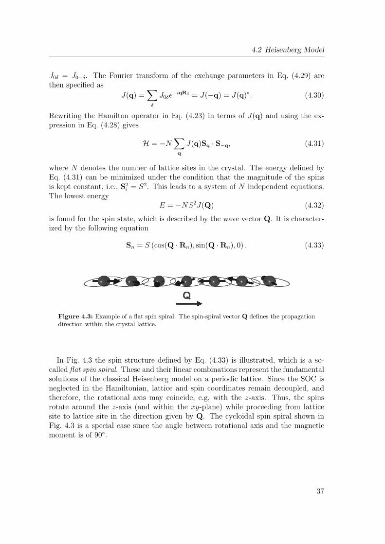
4.2 Heisenberg Model
J0δ = J0−δ. The Fourier transform of the exchange parameters in Eq. (4.29) arethen specified as
J(q) =∑δ
J0δe−iqRδ = J(−q) = J(q)∗. (4.30)
Rewriting the Hamilton operator in Eq. (4.23) in terms of J(q) and using the ex-pression in Eq. (4.28) gives
H = −N∑q
J(q)Sq · S−q, (4.31)
where N denotes the number of lattice sites in the crystal. The energy defined byEq. (4.31) can be minimized under the condition that the magnitude of the spinsis kept constant, i.e., S2
i = S2. This leads to a system of N independent equations.The lowest energy
E = −NS2J(Q) (4.32)
is found for the spin state, which is described by the wave vector Q. It is character-ized by the following equation
Sn = S (cos(Q ·Rn), sin(Q ·Rn), 0) . (4.33)
Figure 4.3: Example of a flat spin spiral. The spin-spiral vector Q defines the propagationdirection within the crystal lattice.
In Fig. 4.3 the spin structure defined by Eq. (4.33) is illustrated, which is a so-called flat spin spiral. These and their linear combinations represent the fundamentalsolutions of the classical Heisenberg model on a periodic lattice. Since the SOC isneglected in the Hamiltonian, lattice and spin coordinates remain decoupled, andtherefore, the rotational axis may coincide, e.g, with the z-axis. Thus, the spinsrotate around the z-axis (and within the xy-plane) while proceeding from latticesite to lattice site in the direction given by Q. The cycloidal spin spiral shown inFig. 4.3 is a special case since the angle between rotational axis and the magneticmoment is of 90.
37
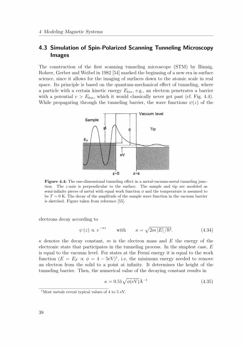
4 Modeling Magnetic Systems
4.3 Simulation of Spin-Polarized Scanning Tunneling MicroscopyImages
The construction of the first scanning tunneling microscope (STM) by Binnig,Rohrer, Gerber and Weibel in 1982 [54] marked the beginning of a new era in surfacescience, since it allows for the imaging of surfaces down to the atomic scale in realspace. Its principle is based on the quantum-mechanical effect of tunneling, wherea particle with a certain kinetic energy Ekin, e.g., an electron penetrates a barrierwith a potential v > Ekin, which it would classically never get past (cf. Fig. 4.4).While propagating through the tunneling barrier, the wave functions ψ(z) of the
Figure 4.4: The one-dimensional tunneling effect in a metal-vacuum-metal tunneling junc-tion. The z-axis is perpendicular to the surface. The sample and tip are modeled assemi-infinite pieces of metal with equal work function ϕ and the temperature is assumed tobe T = 0 K. The decay of the amplitude of the sample wave function in the vacuum barrieris sketched. Figure taken from reference [55].
electrons decay according to
ψ (z) ∝ e−κz
with κ =√
2m |E| /~2. (4.34)
κ denotes the decay constant, m is the electron mass and E the energy of theelectronic state that participates in the tunneling process. In the simplest case, Eis equal to the vacuum level. For states at the Fermi energy it is equal to the workfunction (E = EF ∝ ϕ = 4 − 5eV)1, i.e, the minimum energy needed to removean electron from the solid to a point at infinity. It determines the height of thetunneling barrier. Then, the numerical value of the decaying constant results in
κ = 0.51√ϕ(eV)A−1 (4.35)
1Most metals reveal typical values of 4 to 5 eV.
38
4.3 Simulation of Spin-Polarized Scanning Tunneling Microscopy Images
with eV being the unit of the wave function and A−1 being the unit of the decayconstant.
The knowledge of the wave function allows for the calculation of the probabilityto find an electron of the sample at the location of the tip (z = s):
w = |ψ(s)|2 = |ψ(0)|2 e−2κs. (4.36)
By decreasing the distance between tip and sample to the order of a few A, thewave functions overlap and electrons can tunnel from the sample to the tip and viceversa. The average net tunneling current is zero. Therefore, a small bias voltagecan be applied that raises the Fermi niveau of the sample with respect to that of thetip. In the case of a positive bias the electrons can tunnel through the vacuum fromthe tip to the sample. A negative bias voltage leads to the reversal of the tunnelingdirection. Thus, one can conclude that only those electronic states contribute to thetunneling current that are available within a small energy range close to the Fermilevel. By summing over all electronic states µ of the sample this assumption leadsto
I (s, V ) ∝ e−2κs
EF∑Eµ=EF−eV
|ψ(0)|2 . (4.37)
Equation (4.37) reveals the origin of the high resolution in STM experiments: ifone sets the work function in Eq. (4.35) to ϕ = 4 eV, the decay constant is about
κ ≈ 1 A−1
and the current in Eq. (4.37) decays with e2 ≈ 7.4 per A, so that evena small change in height causes an increase in the tunneling current of almost oneorder of magnitude. This sensitivity allows for a vertical resolution of the order of0.01 A and can be exploited in the constant-current mode, i.e., while the tunnelingcurrent is kept constant by adjusting the vertical position of the STM tip, the lateral(r∥) scan of the tip over the sample surface generates a topographic STM image.
Typically, the STM probe tip is fabricated from metal wires such as W, Pt-Ir alloysor Au. By coating such non-magnetic STM tips with a magnetic material, e.g., Fe,Gd or Cr [27, 56, 57, 58], or producing them from magnetic bulk material [59], anadditional contribution to the tunneling current can be measured that originatesfrom the imbalance of majority and minority electrons close to the Fermi level. Itdepends on the angle between the local magnetization direction of the sample andthe tip, also known as TMR effect [60]. The spin-dependent tunneling allows forthe investigation of magnetic structures down to the atomic scale. Since the presentthesis focuses on nanoscale magnetic order, an expression for the spin-dependenttunneling current will be derived based on the spin-polarized Tersoff-Hamann model[61] and the independent orbital approximation [55, 62].
39
4 Modeling Magnetic Systems
4.3.1 The Tersoff-Hamann Approximation
In order to describe the tunneling current, several theoretical models have beendeveloped – most of them follow the tunneling-Hamiltonian formalism that hasbeen established by J. Bardeen [63]. Within this approach, which is derived via thetime-dependent perturbation theory, the tunneling current I is given to first order.It is obtained from the eigenstates of the unperturbed subsystems, i.e., the sample(S) and the STM tip (T). In the non-spin-polarized case it is defined as
I (V,RT ) =2πe
~∑µν
[f(ES
µ − ESF
)− f
(ET
ν − ETF
)]|Mµν |2 δ
(ET
µ − ESν − eV
),
(4.38)where I is a function of the sample bias voltage V and the position of the tip RT .The occupation is included by means of the Fermi-Dirac function f (E − EF ) =
1 + e(E−EF )/kBT −1. E
(T/S)F is the Fermi energy of the tip/sample and Mµν is the
tunneling matrix element between the states ΨSµ of the sample and ΨT
ν of the tip.Note that Ψµ and Ψν are nonorthogonal eigenstates of different Hamiltonians. Fi-
nally, E(S/T )µ/ν represents the energy of state Ψ
(S/T )µ/ν in the absence of tunneling. The
conservation of energy during the tunneling process, i.e., elastic tunneling is guar-anteed by the δ function. The major issue in handling Eq. (4.38) is the evaluationof the matrix elements
Mµν (RT ) = ⟨ΨTν |UT |ΨS
µ⟩ =
∫VT
dVΨTν UTΨS
µ (4.39)
for the potential UT of the tip. According to Bardeen’s theory [63] the matrixelements can be transformed into a surface integral over any surface lying entirelywithin the vacuum barrier by means of the Green’s theorem:
Mµν = − ~2
2m
∫dS (Ψ∗
ν∇Ψµ − Ψµ∇Ψ∗ν) . (4.40)
The expression in parentheses in Eq. (4.40) is also known as the current operator jµν .The calculation of the matrix elements Mµν in (4.40) requires explicit expressionsfor the wave functions Ψµ and Ψν of the sample and the tip. Since the atomicstructure of the tip is generally unknown, Tersoff and Hamann [64, 65] made severalassumptions in order to simplify the modeling of the tip: According to Eq. (4.37) thetunneling current decays exponentially with the tip-sample distance s. Therefore, itcan be assumed that only the outermost tip apex atom contributes significantly tothe tunneling current and the matrix elements can be calculated by approximating
40
4.3 Simulation of Spin-Polarized Scanning Tunneling Microscopy Images
the wave function of the tip as s wave, i.e.,
ΨTν = C
e−κρ
κρ, (4.41)
where the normalization coefficient C fits the wave functions in the vacuum contin-uously to those in the tip potential. ρ = |r−RT | is the radial distance from thecenter RT of the tip apex atom. Then, the matrix elements result in
Mνµ (RT ) = −2πC~2
κmΨS
µ (RT ) . (4.42)
Hence, the approximation of the tip in the vacuum as s wave leads to a directproportionality of the matrix elements to the value of the sample wave functionsat the position of the tip, RT . Inserting the matrix elements into Eq. (4.38) andconsidering the limit kBT → 0 the tunneling current is given as
I (RT , V ) =16π3C2~3eκ2m2
V nT
∫ E+EF
E
dϵ nS (RT , ϵ) . (4.43)
Here, the DOS of the tip has been assumed to be constant, since it is basicallydestructured with respect to that of the sample. In the limit of small bias voltagesthe current reduces further to
I (RT , V ) =16π3C2~3eκ2m2
V nTnS (RT , EF + eV ) . (4.44)
Deriving Eq. (4.44) with respect to the bias voltage V defines the differential con-ductivity
dI
dV=
16π3C2~3e2
κ2m2nTnS (RT , EF + eV ) . (4.45)
It is directly proportional to the local DOS of the sample nS (RT , EF + eV ) at theposition of the tip RT at the energy EF + eV . It is measured in the spectroscopymode of the STM. By varying the bias voltage eV the local DOS of the samplecan be investigated. This approximation has been likewise successfully applied tosemiconductor [66] and transition-metal surfaces [67, 68].
As mentioned above, STM tips are usually fabricated from W or Pt-Ir alloys.These elements belong to the class of transition metals that exhibit some d-likestates close to the Fermi level. Therefore, it is convenient to consider tip stateswith l = 0 as proposed by Chen [55, 69, 70]. He established the derivative rulethat relates the matrix element to the orbital character of the tip wave function.For instance, if the tip wave function is approximated by a pz orbital, the resulting
41

4 Modeling Magnetic Systems
matrix element is given as
Mµ,pz (RT ) = −2πCpz~2
κm
∂
∂zΨS
µ (RT ) , (4.46)
where Cpz is the normalization constant2. The matrix element reveals a proportion-ality to the spatial derivative of the tip wave function at the position RT . In general,it can be derived by rewriting the angular dependence of the tip wave function interms of x, y, z and replace them by the derivative, i.e.,
x→ ∂
∂x, y → ∂
∂y, z → ∂
∂z. (4.47)
By means of the matrix elements obtained for (m = 0) orbitals Chen demonstratedfor close packed metal surfaces [71] that instead of following the contour of the localDOS at the Fermi level, the tip rather traces the contour of a fictitious surfacethat is determined by the derivatives of the sample surface wave functions. Thisbehavior results in a stronger atomic corrugation than that of the charge density.Orbitals with m = 0 such as px or py, on the other hand, exhibit a particular chargedistribution with a node at the center of the tip. While scanning a surface thatshows maxima in the local DOS above the atomic positions the overlap of the tipand the sample wave functions is minimized on top of a surface atom and maximizedabove a hollow site. Thus, the topographic STM image shows anti-corrugation, i.e.,atoms are detected as depressions and hollow sites as protrusions.
4.3.2 The Spin-Polarized Tersoff Hamann Theory
The extension to the spin-polarized case [61] is carried out by replacing the wavefunction ΨT
µ of the tip by two component spinors with respect to the magnetizationaxis eTM of the tip:
ΨTν =
(ψTν↑0
)or ΨT
ν =
(0ψTν↓
), (4.48)
where ↑ (↓) denotes the electrons of majority (minority) spin. Since the tip is as-sumed to reveal collinear magnetism, i.e., ferromagnetic or antiferromagnetic order,it is possible to express the tip states in terms of pure spin up and pure spin downstates. The magnetic structure in the sample, on the other, hand may exhibit avariety of different possible spin arrangements, such as non-collinear magnetic orderor spin-density waves, leading to a mixing of the spin up and spin down states. Fur-thermore, a coupling of both spin components can be expected even for a collinearmagnetic sample if the quantization axes of the tip and the sample are not parallel
2The expression in Eq. (4.46) is derived analogously to the Tersoff Hamann model. For detailsrefer to references [55, 69, 70].
42
4.3 Simulation of Spin-Polarized Scanning Tunneling Microscopy Images
aligned. Thus, the spinor of the electronic states of the sample reads
ΨSµ =
(ψSµ↑
ψSµ↓
). (4.49)
Analogously to the non-spin-polarized case, where scattering processes are neglected,i.e., elastic single-particle tunneling, the extension to the spin-polarized current as-sumes a spin conservation during the tunneling process. Thus, the matrix elementscan be expressed as
Mσνµ (RT ) = ⟨ΨT
ν |UT |ΨSµ⟩ = ⟨ψT
νσ |UTσσ|ψSµσ⟩, (4.50)
where the matrix of the tip potential UT is diagonal in spin space. σ =↑, ↓ denotesthe spin index of the tip state that is involved in the tunneling. Thus, tip wavefunctions with higher quantum numbers, l = 0, have been neglected. For both,the spin-up and spin-down s states, the decay constant κ is assumed to be thesame. Also the same normalization coefficient will be applied. Assuming that thespin-up, n↑
T , and the spin-down, n↓T DOS of the tip are constant in energy, they
have to be different in size in order to account for the magnetization of the tip,
mT =(n↑T − n↓
T
)eTM . Insertion of Mσ
νµ in Eq. (4.38) leads to
I (RT , V, θ) =8π3C2~3eκ2m2
∫dϵgV (ϵ)
∑µ
δ (Eµ − ϵ)
×[n↑T
∣∣ψSµ↑ (RT )
∣∣2 + n↓T
∣∣ψSµ↓ (RT )
∣∣2] (4.51)
with gV (ϵ) = f(ϵ−EF )− f(ϵ+ eV −EF ). The angle enclosed by the magnetizationdirection of the tip and the sample at the position RT is denoted as θ(RT , V ).The expression in (4.51) is maximal for a parallel and minimal for an antiparallelalignment of the tip and the sample magnetization (θ = 0 and θ = 180).
For general magnetic structures the spin-polarized tunneling current I can bedecomposed into a nonmagnetic and a magnetic part:
I (RT , V, θ) = I0 (RT , V ) + IP (RT , V, θ)
=4π3C2~3eκ2m2
[nT nS (RT , V ) + mTmS (RT , V )] . (4.52)
Here, nS (RT , V ) = n↑S (RT , V ) + n↓
S (RT , V ) represents the energy-integrated lo-cal DOS of the sample and mS (RT , V ) is the corresponding vector of the energy-integrated local magnetization DOS nS (RT , V ) = n↑
S (RT , V ) + n↓S (RT , V ) of the
43
4 Modeling Magnetic Systems
sample3. It is given as
mS (RT , ϵ) =∑µ
δ(ϵµ − ϵ)ΨS†µ (RT )σΨS
µ(RT ) (4.53)
mS (RT , V ) =
∫(f(ϵ− ϵF ) − f(ϵ+ eV − ϵF ))mS (RT , ϵ) dϵ. (4.54)
Here, σ is the known Pauli’s spin matrix. nS (RT , V ) and nS (RT , V ) are definedanalogously by replacing σ by the unity matrix. Apparently, the spin-polarizedcontribution of the tunneling current (second term in Eq. (4.52)) depends on theprojection of mS onto the tip magnetization mT and thus scales with the cosineof the angle between the magnetization directions of the tip and the sample. Inthe case of a nonmagnetic sample or an non-spin-polarized tip, the second term inEq. (4.52) vanishes and the model resembles the original Tersoff-Hamann model.
Based on the results derived above the differential conductivity that is measuredin the spectroscopy mode of a spin-polarized STM (SP-STM) is obtained as
dI
dV(RT , V ) ∝ nTnS (RT , EF + eV ) + mTmS (RT , EF + eV ) . (4.55)
In contrast to the spin-polarized tunneling current in Eq. (4.52) it is directly pro-portional to the local DOS, nS, and the magnetization DOS, mS, of the sample atthe energy EF + eV .
It is possible to decouple the spin-polarized and the non-spin-polarized tunnelingcurrent via the constant current image mode of the spin-polarized STM [61]. Theconstant current image results from the vertical adjustment ∆z
(r∥, V, θ
)of the tip
in order to keep the tunneling current constant. For a sample surface with two-dimensional translational symmetry the change in both, the non-spin-polarized andthe spin-polarized part of the current I, can be written in terms of a two-dimensionalFourier expansion with respect to the reciprocal surface lattice vectors Gn
∥ :
∆I(r∥, z, V, θ
)=∑n =0
∆IGn∥
(z, V, θ) eiGn
∥ r∥ . (4.56)
Here, the ∆IGn∥
(r∥, z, V, θ
)are the tip-sample distance (z) dependent expansion
coefficients. They decay exponentially with increasing length of the reciprocal latticevectors Gn
∥ [67]. Therefore, the STM image is primarily dominated by the smallest
nonvanishing reciprocal lattice vector G1∥:
∆I(r∥, z, V, θ
)∝ e
−2z
√2m/~2|EF+eV |+
(G1
∥/2)2
. (4.57)
3nT as well as mT refer to the densities of states of the tip.
44
4.3 Simulation of Spin-Polarized Scanning Tunneling Microscopy Images
In comparison to a nonmagnetic state any magnetic superstructure lowers the trans-lational symmetry and leads to a larger periodicity in the real space. Accordingly,the corresponding reciprocal lattice vector becomes smaller with respect to thatof the chemical unit cell. Due to the filtering effect of the vacuum, waves with thesmallest lattice vector Gn
∥ extend furthest into the vacuum and thus contribute mostto the STM image. Therefore, a topographic spin-polarized STM image obtainedin the constant-current mode reflects rather the magnetic superstructure than theatomic structure. This has been first demonstrated for the two-dimensional antifer-romagnetism at surfaces [72].
4.3.3 Independent-Orbital Approximation
The expression for the spin-polarized tunneling current in Eq. (4.52) is derived forgeneral magnetic structures. However, since it requires the exact information aboutthe electronic structure of the sample in the vacuum, the simulation of complexmagnetic structures is difficult within the spin-polarized Tersoff-Hamann model. Inthe following, a simple method will be introduced that allows for the calculationof spin-polarized STM images of an arbitrary complex magnetic structure withoutthe accurate knowledge of the electronic structure [62]. It is based on the atomicsuperposition as presented in [55, 64, 65, 73].
In the limit of low bias voltage the integrated local DOS of the sample can bereplaced by the local DOS at the Fermi energy resulting in
ns (RT , EF ) =∑α
(n↑α + n↓
α
)exp (−2κ |RT −Rα|) , (4.58)
where the atomic superposition is expressed as the sum over all surface atoms α atthe position Rα. It is assumed that the local DOS from each surface atom contributesto the tunneling current of the STM tip at the position RT with an exponential decay.κ denotes the decay constant as given in Eq. (4.34) with κ =
√2mϕ/~2 using the
work function ϕ. n↑α and n↓
α represent the DOS of the surface atom α at the Fermilevel in the majority and minority spin channel, respectively.
The local magnetization DOS is given as
eTm (RT , EF ) =∑α
(n↑α − n↓
α
)cos θαexp (−2κ |RT −Rα|) , (4.59)
where the angle θα specifies the rotation of the local magnetization axis at the atomα with respect to the tip magnetization direction eT .
Under the assumption that the electronic structure of all surface atoms α is the
45
4 Modeling Magnetic Systems
same, the spin-polarized tunneling current in the simple model can be expressed as
I (RT ) ∝∑α
[1 + PTPS cos θα] exp (−2κ |RT −Rα|) . (4.60)
Here, the spin-polarization of the tip and the sample is given by
PT =n↑T − n↓
T
n↑T + n↓
T
and PS =n↑S − n↓
S
n↑S + n↓
S
, respectively. (4.61)
The product of the spin-polarization of the tip and the sample, Peff = PTPS, isthe effective spin-polarization of the system, which remains as the only unknownparameter in the approach presented above.
Finally, the simple model of the spin-polarized tunneling current allows for a directcomparison of constant-current and constant-height images as well as quantitativevalues of the corrugation amplitude. The corrugation amplitude, i.e., the difference∆z in the tip height as a function of the lateral tip position r∥ is given as
∆z(r∥)
= −∆I(r∥, z0
)dI0/dz(z0)
=∆I(r∥, z0
)2κI0(z0)
. (4.62)
Here, z0 denotes an average tip-sample distance, where the tunneling current canbe split into a lateral constant part I0(z0) and a small variation ∆I
(r∥, z0
)leading
to the expression above.
46
5 Non-collinear Magnetism within DFT
Collinear magnetic configurations, i.e. , the parallel and antiparallel alignment ofneighboring magnetic moments, represent only a small number of possible magneticarrangements. The major part of spin structures reveals an arbitrary alignment ofneighboring magnetic moments, i.e., non-collinear magnetism. Within the DFT itis possible to go beyond collinear magnetism by adjusting the representation of thedensity in order to describe non-collinear magnetic orders. Therefore, the electronand magnetization densities n and m are replaced by the Hermitian 2 × 2 densitymatrix ρ. Both concepts are completely equivalent.
The density matrix is defined as
ρ =1
2n · I2 + σ ·m =
1
2
(n+mz mx − imy
mx + imy n−mz
), (5.1)
where I2 is the unity matrix and σ is the vector of the Pauli spin matrices. Similarly,the Hermitian 2 × 2 potential matrix is defined as
v = v · I2 + µBσ ·B =
(v + µBBz µB(Bx − iBy)
µB(Bx + iBy) v − µBBz
). (5.2)
The components of the density matrix are given in terms of the solutions of theKohn-Sham equation:
ραβ =N∑ν=1
ψ∗ναψνβ. (5.3)
Including the potential matrix (Eq. (5.2)) the Kohn-Sham equations (Eq. (2.20))take the following form: (
− ~2
2m∇2I2 + v
)ψν = ϵνψν . (5.4)
The kinetic energy part of the Hamiltonian is diagonal in both spin directions.However, the off-diagonal part of the potential matrix, i.e., v12 = µB(Bx − iBy)and v21 = µB(Bx + iBy), couples the two components ψν of the Pauli spinor. Inthe collinear case this behavior is unproblematic, since the quantization axis ofthe spin can be chosen parallel to the z-axis without loss of generality. Thus, Bx
and By become zero and the off-diagonal elements v12 and v21 vanish. Both spin
47
5 Non-collinear Magnetism within DFT
directions decouple and Eq. (5.4) can be solved for every direction separately, i.e,treating v↑ = µB(Bx + iBy) and v↓ = µB(Bx − iBy) like the nonmagnetic problem.In a non-collinear magnetic calculation the computational effort to diagonalize theHamilton matrix increases with the third power of the number of basis functions incomparison with a collinear calculation. Another drawback is the reduction of thesymmetry of the system due to the non-collinearity, resulting in an increase of theirreducible wedge of the Brillouin zone and, in addition, a larger number of Blochvectors k. Since the computational effort increases linearly with the number of Blochvectors, too, the calculation of non-collinear systems is highly time-consuming. It isrecommended to start the studies with the collinear calculations and use them as astarting point for the non-collinear ones afterwards.
5.1 Constrained Magnetic Moments
Non-collinear magnetic configurations do not necessarily represent extrema of theenergy functional E[n(r),m(r)]. Therefore, Dederichs et al. [74] extended the DFTto systems that tend to exhibit arbitrary constraints. This is done by introducingboundary conditions to keep the local magnetic moments of the atoms fixed ina specific direction. Hence, Lagrange multipliers are needed to pin the magneticmoment of the atom in the direction eα within the muffin tin sphere α. They havethe form of local magnetic fields. The energy functional reads then
Econstr [n(r),m(r), eα] = E[n(r),m(r)]
+ µB
∑α
Bαc
(∫MTα
m(r)d3r − eα
(eα ·
∫MTα
m(r)d3r
))= E[n(r),m(r)] + µB
∑α
Bαc ·(Mα −Mα
∥)
= E[n(r),m(r)] + µB
∑α
Bαc ·Mα
⊥. (5.5)
The minimum of the energy functional provides the state of lowest energy meetingsimultaneously the condition of constrained magnetic moments. The minimizationof Eq. (5.5) with respect to the wave functions yields the Kohn-Sham equationswithin the muffin-tin sphere α plus an additional term:
ϵiψi(r) =
− ~2
2m∇2 + veff (r) + µB
[σ ·Beff (r) + σ ·
(Bα
c − eα (eα ·Bαc ))]
ψi(r).
(5.6)
48
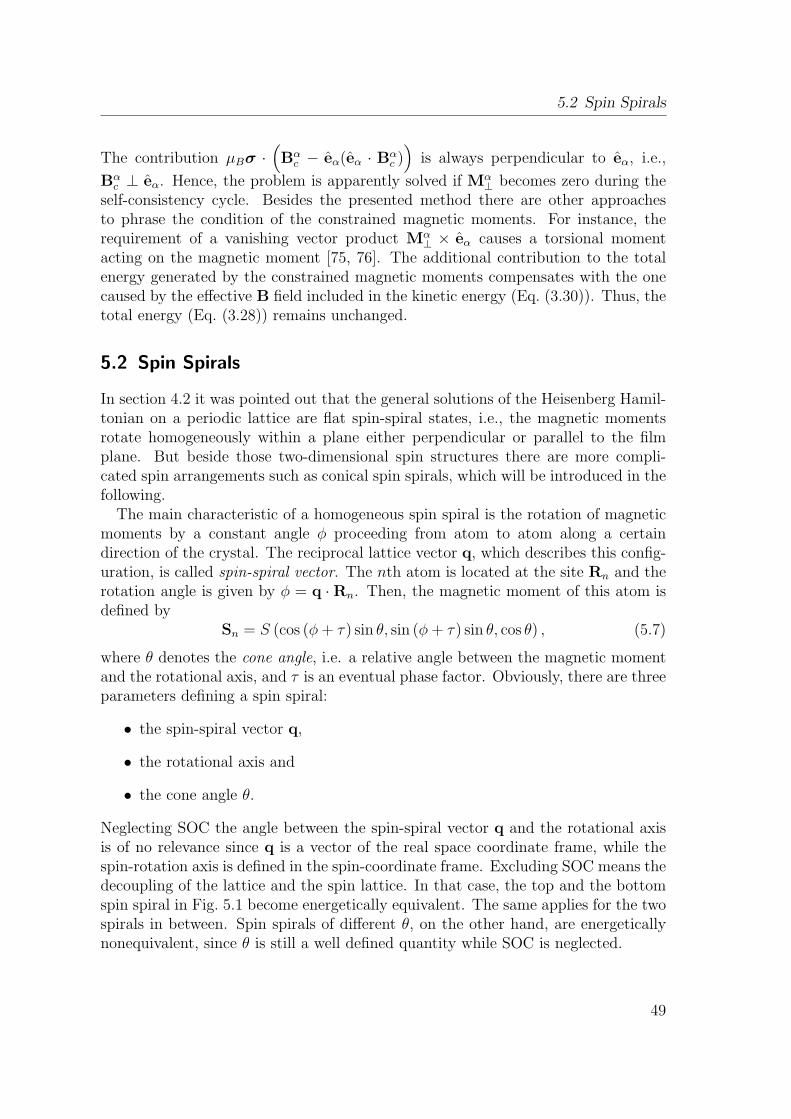
5.2 Spin Spirals
The contribution µBσ ·(Bα
c − eα(eα · Bαc ))
is always perpendicular to eα, i.e.,
Bαc ⊥ eα. Hence, the problem is apparently solved if Mα
⊥ becomes zero during theself-consistency cycle. Besides the presented method there are other approachesto phrase the condition of the constrained magnetic moments. For instance, therequirement of a vanishing vector product Mα
⊥ × eα causes a torsional momentacting on the magnetic moment [75, 76]. The additional contribution to the totalenergy generated by the constrained magnetic moments compensates with the onecaused by the effective B field included in the kinetic energy (Eq. (3.30)). Thus, thetotal energy (Eq. (3.28)) remains unchanged.
5.2 Spin Spirals
In section 4.2 it was pointed out that the general solutions of the Heisenberg Hamil-tonian on a periodic lattice are flat spin-spiral states, i.e., the magnetic momentsrotate homogeneously within a plane either perpendicular or parallel to the filmplane. But beside those two-dimensional spin structures there are more compli-cated spin arrangements such as conical spin spirals, which will be introduced in thefollowing.
The main characteristic of a homogeneous spin spiral is the rotation of magneticmoments by a constant angle ϕ proceeding from atom to atom along a certaindirection of the crystal. The reciprocal lattice vector q, which describes this config-uration, is called spin-spiral vector. The nth atom is located at the site Rn and therotation angle is given by ϕ = q ·Rn. Then, the magnetic moment of this atom isdefined by
Sn = S (cos (ϕ+ τ) sin θ, sin (ϕ+ τ) sin θ, cos θ) , (5.7)
where θ denotes the cone angle, i.e. a relative angle between the magnetic momentand the rotational axis, and τ is an eventual phase factor. Obviously, there are threeparameters defining a spin spiral:
• the spin-spiral vector q,
• the rotational axis and
• the cone angle θ.
Neglecting SOC the angle between the spin-spiral vector q and the rotational axisis of no relevance since q is a vector of the real space coordinate frame, while thespin-rotation axis is defined in the spin-coordinate frame. Excluding SOC means thedecoupling of the lattice and the spin lattice. In that case, the top and the bottomspin spiral in Fig. 5.1 become energetically equivalent. The same applies for the twospirals in between. Spin spirals of different θ, on the other hand, are energeticallynonequivalent, since θ is still a well defined quantity while SOC is neglected.
49
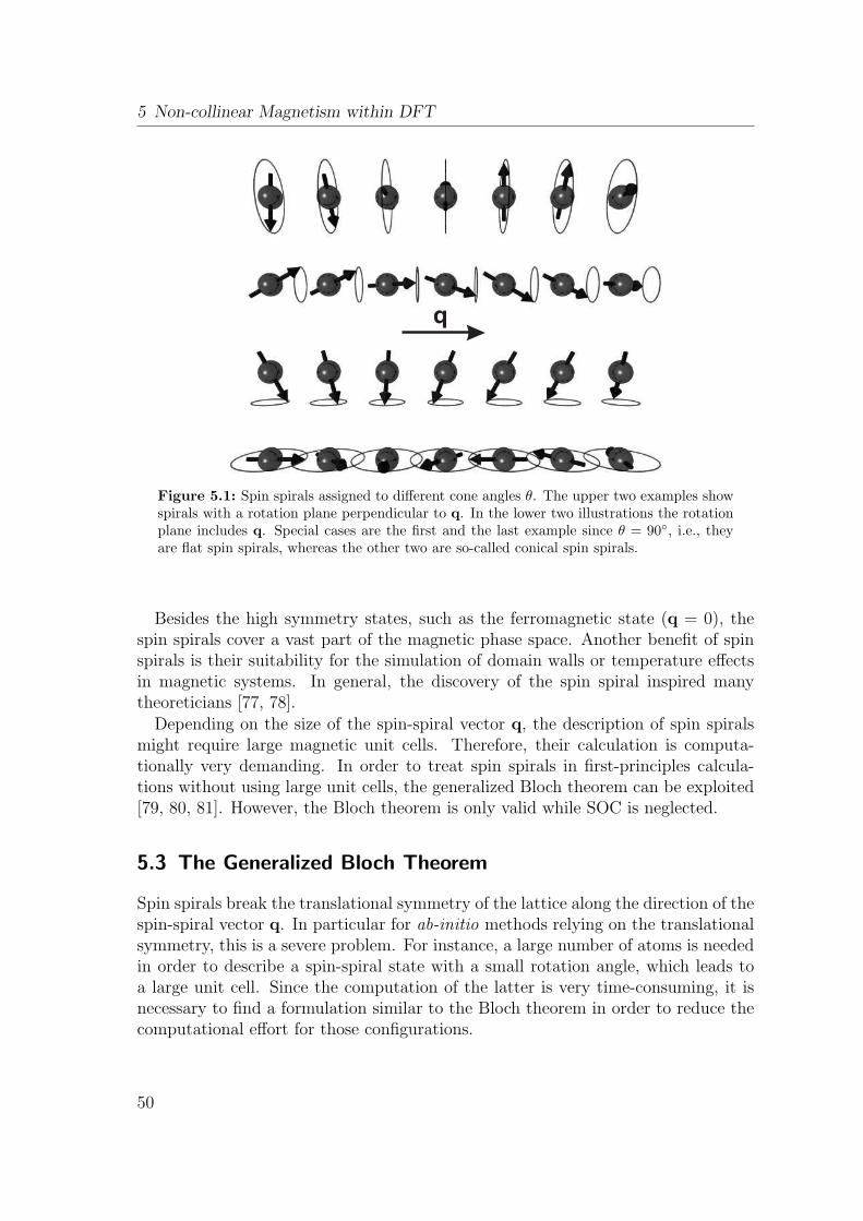
5 Non-collinear Magnetism within DFT
q
Figure 5.1: Spin spirals assigned to different cone angles θ. The upper two examples showspirals with a rotation plane perpendicular to q. In the lower two illustrations the rotationplane includes q. Special cases are the first and the last example since θ = 90, i.e., theyare flat spin spirals, whereas the other two are so-called conical spin spirals.
Besides the high symmetry states, such as the ferromagnetic state (q = 0), thespin spirals cover a vast part of the magnetic phase space. Another benefit of spinspirals is their suitability for the simulation of domain walls or temperature effectsin magnetic systems. In general, the discovery of the spin spiral inspired manytheoreticians [77, 78].
Depending on the size of the spin-spiral vector q, the description of spin spiralsmight require large magnetic unit cells. Therefore, their calculation is computa-tionally very demanding. In order to treat spin spirals in first-principles calcula-tions without using large unit cells, the generalized Bloch theorem can be exploited[79, 80, 81]. However, the Bloch theorem is only valid while SOC is neglected.
5.3 The Generalized Bloch Theorem
Spin spirals break the translational symmetry of the lattice along the direction of thespin-spiral vector q. In particular for ab-initio methods relying on the translationalsymmetry, this is a severe problem. For instance, a large number of atoms is neededin order to describe a spin-spiral state with a small rotation angle, which leads toa large unit cell. Since the computation of the latter is very time-consuming, it isnecessary to find a formulation similar to the Bloch theorem in order to reduce thecomputational effort for those configurations.
50
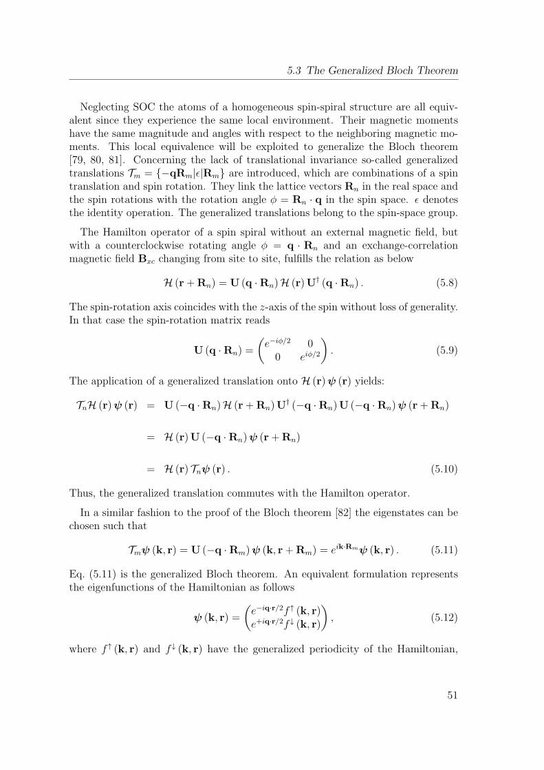
5.3 The Generalized Bloch Theorem
Neglecting SOC the atoms of a homogeneous spin-spiral structure are all equiv-alent since they experience the same local environment. Their magnetic momentshave the same magnitude and angles with respect to the neighboring magnetic mo-ments. This local equivalence will be exploited to generalize the Bloch theorem[79, 80, 81]. Concerning the lack of translational invariance so-called generalizedtranslations Tm = −qRm|ϵ|Rm are introduced, which are combinations of a spintranslation and spin rotation. They link the lattice vectors Rn in the real space andthe spin rotations with the rotation angle ϕ = Rn · q in the spin space. ϵ denotesthe identity operation. The generalized translations belong to the spin-space group.
The Hamilton operator of a spin spiral without an external magnetic field, butwith a counterclockwise rotating angle ϕ = q · Rn and an exchange-correlationmagnetic field Bxc changing from site to site, fulfills the relation as below
H (r + Rn) = U (q ·Rn)H (r)U† (q ·Rn) . (5.8)
The spin-rotation axis coincides with the z-axis of the spin without loss of generality.In that case the spin-rotation matrix reads
U (q ·Rn) =
(e−iϕ/2 0
0 eiϕ/2
). (5.9)
The application of a generalized translation onto H (r)ψ (r) yields:
TnH (r)ψ (r) = U (−q ·Rn)H (r + Rn)U† (−q ·Rn)U (−q ·Rn)ψ (r + Rn)
= H (r)U (−q ·Rn)ψ (r + Rn)
= H (r) Tnψ (r) . (5.10)
Thus, the generalized translation commutes with the Hamilton operator.
In a similar fashion to the proof of the Bloch theorem [82] the eigenstates can bechosen such that
Tmψ (k, r) = U (−q ·Rm)ψ (k, r + Rm) = eik·Rmψ (k, r) . (5.11)
Eq. (5.11) is the generalized Bloch theorem. An equivalent formulation representsthe eigenfunctions of the Hamiltonian as follows
ψ (k, r) =
(e−iq·r/2f ↑ (k, r)e+iq·r/2f ↓ (k, r)
), (5.12)
where f ↑ (k, r) and f ↓ (k, r) have the generalized periodicity of the Hamiltonian,
51
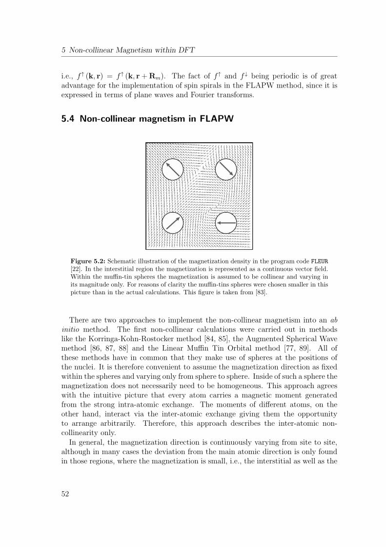
5 Non-collinear Magnetism within DFT
i.e., f ↑ (k, r) = f ↑ (k, r + Rm). The fact of f ↑ and f ↓ being periodic is of greatadvantage for the implementation of spin spirals in the FLAPW method, since it isexpressed in terms of plane waves and Fourier transforms.
5.4 Non-collinear magnetism in FLAPW
Figure 5.2: Schematic illustration of the magnetization density in the program code FLEUR[22]. In the interstitial region the magnetization is represented as a continuous vector field.Within the muffin-tin spheres the magnetization is assumed to be collinear and varying inits magnitude only. For reasons of clarity the muffin-tins spheres were chosen smaller in thispicture than in the actual calculations. This figure is taken from [83].
There are two approaches to implement the non-collinear magnetism into an abinitio method. The first non-collinear calculations were carried out in methodslike the Korringa-Kohn-Rostocker method [84, 85], the Augmented Spherical Wavemethod [86, 87, 88] and the Linear Muffin Tin Orbital method [77, 89]. All ofthese methods have in common that they make use of spheres at the positions ofthe nuclei. It is therefore convenient to assume the magnetization direction as fixedwithin the spheres and varying only from sphere to sphere. Inside of such a sphere themagnetization does not necessarily need to be homogeneous. This approach agreeswith the intuitive picture that every atom carries a magnetic moment generatedfrom the strong intra-atomic exchange. The moments of different atoms, on theother hand, interact via the inter-atomic exchange giving them the opportunityto arrange arbitrarily. Therefore, this approach describes the inter-atomic non-collinearity only.
In general, the magnetization direction is continuously varying from site to site,although in many cases the deviation from the main atomic direction is only foundin those regions, where the magnetization is small, i.e., the interstitial as well as the
52
5.4 Non-collinear magnetism in FLAPW
vacuum region. Therefore, the magnetization density m has the form of a continu-ous vector field. This approach has been applied by Nordstrom and Singh [90], whopublished the first calculation investigating the intra-atomic non-collinearity. How-ever, the intra-atomic exchange is not of interest for the study of the surfaces andinterfaces of the 3d transition metals, since the non-collinearity in the intra-atomicexchange is expected to be rather small in those systems.
The concept used for the implementation in the FLEUR program code [22] is a”hybrid” approach, which handles the magnetization direction in the interstitialand the vacuum region continuously, whereas the magnetization direction is keptfixed within the muffin-tin spheres (cf. Fig. 5.2) [83, 91]. As mentioned above,the FLAPW method makes use of the augmented plane waves as basis functions.In order to extend this method onto spin dependent collinear systems, the spinorsχgσ=↑,↓ are introduced analogously to the Pauli spinors in Eq. (2.24):
χg↑ =
(10
)χg↓ =
(01
), (5.13)
where the index g refers to the fact that the χgσ are defined relatively to the global
quantizations axis (for example the z-axis). Hence, the basis functions in the inter-stitial region are written as
φG(k, r) = ei(k+G)·rχgσ. (5.14)
Generalizing this expression for the case of non-collinear magnetism means that thepotential matrix v is not a diagonal matrix anymore. Thus, the Hamilton operatorin Eq. (5.4) needs to be fully diagonalized.
Since the local spin coordinate frame is used solely in the muffin-tin spheres, thebasis set does not need to be changed in the interstitial and the vacuum region, wherethe basis functions are represented by the global spin frame. A transformation ofthe spinors χg
σ into the local coordinate frame of the χlσ is performed by means of a
unitary transformation Ugl:
χlσ = Uglχg
σ =
(eiα2 cos
(β2
)e−iα
2 sin(β2
)− e
iα2 sin
(β2
)e−iα
2 cos(β2
) )χgσ. (5.15)
Considering the local and the global quantization axis the basis set now takes the
53
5 Non-collinear Magnetism within DFT
following form:
φG,σ(k, r) =
ei(G+k)r
χgσ interstitial region
AG∥G⊥σ (k∥)u
G∥σ (k∥, z)
+BG∥G⊥σ (k∥)u
G∥σ (k∥, z)
ei(G∥+k∥)r∥ χg
σ
vacuum region
∑σα
∑L
(AµG
Lσσα(k)ul(r) + BµGLσσα(k)ul(r)
)YL(r)χσα muffin tin α
(5.16)Again, L abbreviates lm and the sum in the muffin tins considers the local spindirections. The AµG
L and BµGL have to meet the following boundary condition
ei(k+G)rχσ =∑σα
∑L
(AµG
Lσσα(k)uαlσα(r) +BµGLσσα(k)uαlσα(r)
)YL(r)χαg
σα . (5.17)
Thus, the global spin-coordinate frame can be transformed into the local frame by arotation given via the Euler angles α and β. In the present case, the Euler angles areequivalent to the polar angles of the local quantization axis in the global coordinateframe, namely α = ϕ and β = θ.
As a result of the matching condition at the boundary of the interstitial regionand the muffin-tins, the spin up and spin down basis functions couple. Nevertheless,a non-collinear calculation can be transferred into a collinear one by transformingthe non-collinear coefficients A and B as below
AnocoL,G,↑(k) = χT
↑gUglχ↑gAL,G,↑(k) (5.18)
BnocoL,G,↑(k) = χT
↑gUglχ↑gBL,G,↑(k) (5.19)
AnocoL,G,↓(k) = χT
↓gUglχ↓gAL,G,↓(k) (5.20)
BnocoL,G,↓(k) = χT
↓gUglχ↓gBL,G,↓(k). (5.21)
In this way, the calculation can be performed as in the collinear case, which is muchsimpler to solve.
54
6 Spin-Orbit Coupling
Relativistic effects play a more important role at surfaces and in ultra-thin films thanin bulk systems. Neel explained this behavior with the reduced number of neighborsat the surface giving rise to the so-called magnetocrystalline surface anisotropy [92].It describes the difference in the magnetic energy found for different magnetizationdirections, and leads to the distinction between an easy magnetization axis (minimalenergy) and a hard magnetization axis (maximal energy). The magnetic anisotropyis caused by the spin-orbit coupling (SOC) and the magnetic dipolar interaction.The latter senses the outer boundaries of the sample and gives rise to the shapeanisotropy, while the SOC couples the spin and the lattice, which leads to themagnetocrystalline anisotropy. In small magnetic systems, such as the magneticmono- or double layers studied in the present work, the contribution of the magneticdipole-dipole energy to the magnetic anisotropy is of the order of ∼ 0.1 meV, which issmall compared to the contribution of the magnetocrystalline anisotropy (∼ 1 meV).Therefore, the dipole-dipole interaction is neglected in the following.
Further consequences of the SOC are the Rashba effect [93, 94], which will notbe discussed in this thesis, and the Dzyaloshinskii-Moriya interaction (DMI) [7, 8],which are both effects of a lack of inversion symmetry in the considered system. Thelatter favors non-collinear magnetic structures with a unique rotational sense. Thus,left and right rotating spin structures that are degenerate within the Heisenbergmodel exhibit a difference in energy in the presence of the Dzyaloshinskii-Moriyainteraction. This has been demonstrated in crystals, i.e., bulk systems, withoutinversion symmetry (cf. [95]). However, since surfaces always lack inversion symme-try, the Dzyaloshinskii-Moriya interaction needs to be considered in such systems.Recently, it has been shown that the DMI plays a crucial role in surface magnetism[9]. Furthermore, the strength of the SOC and thus the strength of the DMI de-pends on the atomic number, i.e., it has to be considered in systems comprisingheavy elements, such as W or Ir.
In this chapter, the SOC and its effects are presented. The relativistic descriptionof many-electron systems is introduced as well as the treatment of the SOC in thedensity functional theory and its implementation in the FLAPW method. Finally,the Dzyaloshinskii-Moriya interaction will be explained in more detail.
55
6 Spin-Orbit Coupling
6.1 The Relativistic Density Functional Theory
The Kohn-Sham equation reads as a single-particle Dirac equation if the relativisticeffects are taken into account:(
cα · p + (β − 1)mc2 + Veff (r))Ψi = ϵiΨi, (6.1)
where α and β are the Dirac matrices,
α =
(0 σσ 0
)and β =
(I2 00 −I2
). (6.2)
Here, σ is the vector of the Pauli matrices σx, σy and σz, and p denotes the momen-tum operator. I2 is the (2×2) identity matrix and Ψi identifies the four-componentDirac spinor represented by large and small components φi(r) and χi(r), respectively.The index i abbreviates the Bloch vector k, the band index i and the spin-quantumnumber σ. Written in terms of the Dirac spinors, the charge and magnetizationdensity of the ground state have the following form
n(r) =N∑i
(φ†i (r)φi(r) + χ†
i (r)χi(r))
(6.3)
and
m(r) =N∑i
(φ†i (r)σφi(r) + χ†
i (r)σχi(r)). (6.4)
A straight and, at the same time, accurate procedure to solve Eq. (6.1) is theextension of the FLAPW basis set to all four components. The basis would thencontain four times as many functions as the non-relativistic and nonmagnetic basisset. In that case the computational time needed for the diagonalization of theHamilton matrix would increase by a factor of 43 = 64. But as long as no SOCeffects are treated, it is sufficient to include only those correction terms into thenon-relativistic calculation that contribute to the diagonal elements of the Hamiltonmatrix. This method is called the scalar-relativistic calculation, and it has beensuggested by D. Koelling and B. Harmon [96]. In this approach only the electronswithin the muffin tin spheres are treated relativistically, since the kinetic energy ofthe electrons is large near the nuclei and the relativistic effects become stronger. Inthe vacuum and the interstitial region the basis functions remain non-relativistic.
56
6.2 Spin-Orbit Coupling
6.2 Spin-Orbit Coupling
In the limiting case of small velocities v2/c2 ≪ 1 of the valence electrons, Eq. (6.1)can be reduced to a Pauli equation. To achieve this, the Dirac operator is expandedin v2/c2 and transformed afterwards (cf. e.g. [97]). The resulting equation is aSchrodinger-like equation including the first relativistic corrections of the order ofO(1/c2). The corresponding Hamilton operator is called Pauli operator and takesthe form
HPauli =p2
2m− e · v − p4
8m3c2+
e~2
8m2c2∇ · E +
e~4m2c2
σ · (E× p) . (6.5)
The first and the second contribution represent the non-relativistic kinetic energyand the electrostatic potential energy, respectively. They form the non-relativisticHamilton operator. The third and the fourth term do not depend on the spin S =σ/2 and, in addition to the first two contributions, result in the scalar-relativisticHamilton operator. The third term in Eq. (6.5) is a correction term due to thekinematical mass enhancement. Here, the fourth summand can be interpreted asa smearing out of the electrostatic interaction between the electron and the nucleidue to rapid quantum oscillations. That means that the expectation value of r doesnot possess sharp eigenfunctions because of the zitterbewegung that the electronperforms, which is of the order of the Compton wave length λC = ~/mc. As a resultthe electron responds sensitively to the electric field E. The very last contribution inEq. (6.5) is finally the spin-orbit interaction HSOC . It originates from the couplingof the electronic spin with the magnetic field that the electron experiences whileit moves in the vicinity of the nuclei. This orbital movement is coupled directlywith the crystal lattice via the electric potential of the ions. It contributes to themagnetocrystalline anisotropy .
As mentioned above, the SOC effect occurs mainly close to the nuclei, since thekinetic energy of the electron and thus the gradient of the potential is largest in thisregion. The potential may be spherically approximated in the vicinity of the nuclei:v(r) ≃ v(r). According to J. C. Maxwell the electric field reads then as follows(cf. e.g. [98]):
E = −∇v(r) = −r
r
dv
dr, (6.6)
and gives the SOC Hamiltonian the following form
HSOC = − e~4m2c2r
dv
drσ · (r× p)
=−e~2
2m2c2r
dv
dr︸ ︷︷ ︸L · S
= ξ(r)L · S. (6.7)
57
6 Spin-Orbit Coupling
L represents the operator of the angular momentum and ξ(r) is the SOC constantas a function of the radial distance r from the position of the nuclei. Since the mag-netism in the 3d transition metals is originating from the d-electrons, it is reasonableto average the SOC constant over the d-orbitals in order to reduce ξ to a simpleconstant.
Regarding the representation of the basis functions in Eq. (5.16), the expectationvalue of the SOC operator HSOC may be separated into a matrix element of theposition space and the spin space, respectively. In position space the matrix ele-ment ξL,σ,σ
′
k,ν,ν′ = ⟨ν, L, σ|ξ(r)|ν ′, L, σ′⟩ provides the strength of the SOC. The radial
part ξL,σ,σ′
k,ν,ν′ can be evaluated directly from the scalar-relativistic approximation. Anestimation of the coupling strength is obtained by assuming the Coulomb potentialto be v(r) = −Z · e/r and using the non-relativistic radial functions Rnl(r) ∝ rl.This results in
ξnl ∝⟨nl|1
r
Z
r2|nl⟩Z4
a3B
1
n3l2. (6.8)
The proportional relation (6.8) shows that ξnl increases with the fourth order of theatomic number, Z4. In the case of the 3d transition metals ξnl is of the order ofabout 50 meV [99].
In spin space the matrix element L · S describes the angular dependency of theSOC, which is the main contribution to the anisotropy.The matrix element de-pends on the spin-quantization axis Ω, which has been aligned parallel1 to themagnetization direction ΩM of the effective magnetic field Beff . The angular de-pendence of L · S in the 2 × 2 spin space obtained for an arbitrary spin orien-tation Ω = (sinϕ sin θ, cosϕ sin θ, cos θ) is yielded after the computation of theΩz = (0, 0, 1) direction and a subsequent unitary transformation U (cf. Eq. (5.15)):
⟨lmlσ|L · S|lm′lσ
′⟩(0, 0) −→ ⟨lmlσ|U†(ϑ, φ) (L · S)U(ϑ, φ)|lm′lσ
′⟩(ϑ, φ) (6.9)
=⇒(
⟨↑ |L · S| ↑⟩ ⟨↑ |L · S| ↓⟩⟨↓ |L · S| ↑⟩ ⟨↓ |L · S| ↓⟩
)(ϑ, φ) = (6.10)
=
(cosϑ − sinϑ− sinϑ − cosϑ
)Lz
+
(12
sinϑ(eiφL+ + e−iφL−) cos2 (ϑ2)eiφL− − sin2 (ϑ
2)e−iφL+
cos2 (ϑ2)e−iφL+ − sin2 (ϑ
2)eiφL− −1
2sinϑ(eiφL+ + e−iφL−)
),
where the operators L± ≡ Lx ± iLy are applied onto the YL.
1Technically, the spin and its magnetic moment are aligned antiparallel. However, for reasons ofsimplification both are assumed parallel and µB is set to a negative value.
58
6.3 The Magnetocrystalline Anisotropy and the Orbital Moment
6.3 The Magnetocrystalline Anisotropy and the Orbital Moment
In order to estimate the magnitude of the SOC effect on the basis of density func-tional theory, it is useful to consider a quantity that is directly related to this effect.The magnetocrystalline anisotropy is such a quantity, since it introduces a preferredmagnetization direction within the crystal and breaks the rotational invariance ofthe Hamilton operator with respect to the spin quantization axis. Rotating the en-ergy from a direction of low energy (easy axis) towards a direction of high energy(hard axis) is typically of the order 10−6 to 10−3 eV/atom and represents a verysmall correction to the total magnetic energy [100].
Bruno suggested a simple physical model that relates the orbital moment ml =µBL to the magnetocrystalline anisotropy K [100, 101]. The spin splitting ϵ±i ≈ IMof the bands is assumed to be much larger than the bandwidth W due to exchange.The off-diagonal elements of the spin-orbit interaction matrix HSOC , which mix bothspin channels, may then be neglected. This results in the resemblance of the SOCto an effective magnetic field Horb acting merely onto the orbital moment ml:
HSOC = −ml ·Horb with Horb =±ξ2µB
ΩM . (6.11)
Here, the sign ± represents the d band filling with more or less than five electronsand ΩM is the magnetization direction.
The effect of this field is described by a second degree tensor of the orbital sus-ceptibility χ
(2)orb. The expectation value of the orbital moment ⟨ml⟩ and the SOC
energy ESOC are then given in the lowest order of Horb as follows
⟨ml⟩ = χ(2)orb ·Horb
=±ξ2µB
χ(2)orb ·ΩM (6.12)
and
ESOC = −1
2Horb · χ(2)
orb ·Horb
= −1
2
ξ2
4µ2B
ΩM · χ(2)orb ·ΩM . (6.13)
In crystals, which feature uniaxial magnetic anisotropy, the symmetry axis may bealigned to the z axis without loss of generality. This applies for instance in ultrathin
59
6 Spin-Orbit Coupling
films and at surfaces2. Hence, the susceptibility has the form of a diagonal matrix:
χ(2)orb =
χ(2)11orb 0 0
0 χ(2)22orb 0
0 0 χ(2)33orb
. (6.14)
The orbital moment and the SOC energy result in
ml,z = ± ξ
2µB
[χ(2)33orb +
(χ(2)11orb − χ
(2)33orb
)sin2 θ
](6.15)
(6.16)
and
ESOC = −1
2
ξ2
4µ2B
[χ(2)33orb +
(χ(2)11orb − χ
(2)33orb
)sin2 θ
], (6.17)
respectively, where θ is the angle between the normal of the plane and the mag-netization. According to this model the magnetic anisotropy energy K is directlyproportional to the anisotropy of the orbital moments ∆m = ml (ΩM2) −ml (ΩM1)for two different magnetizations ΩM2 and ΩM1 :
K =ξ
4µB
∆ml. (6.18)
Equation (6.18) expresses that the anisotropy of the magnetic moment is of about0.1 µB/atom if an anisotropy energy of 1 meV/atom and a spin-orbit couplingconstant of ξ = 50 meV is considered, which is a typical value in ultrathin films.
6.4 Perturbation Theory
Since the SOC effect is rather small in 3d transition metals compared to the band-width or the exchange splitting, it is convenient to treat it within the framework ofperturbation theory.
The energy difference due to SOC results from the second order perturbationtheory:
∆ESOC =∑
Ψ1 =Ψ0
|⟨Ψ1|HSOC |Ψ0⟩|2
E0 − E1. (6.19)
2An extension to cubic systems is possible without further ado, but since they are isotropic in
this order of Horb, i.e., χ(2)11orb = χ
(2)22orb = χ
(2)33orb , the non-linear orbital susceptibility needs
to be considered, which is given by a fourth degree tensor χ(4)orb. For further details refer to
[100, 102, 103].
60
6.4 Perturbation Theory
Ψ0 and Ψ1 denote the unperturbed ground state and the excited state, respectively.The corrections to the wave functions are given by the first order perturbationtheory:
δ|Ψ0⟩ =∑
Ψ1 =Ψ0
⟨Ψ1|HSOC |Ψ0⟩|Ψ1⟩E0 − E1
. (6.20)
The considered excited states are located above the Fermi energy, and may bepopulated by electrons characterized by a certain momentum k from an occupiedstate via an excitation with or without a spin flip. In particular, the denominatorof Eq. (6.19) shows that states close in energy give large contributions. At the sametime it has to be kept in mind that∣∣E0 − E1
∣∣≫ ∣∣⟨Ψ1 |HSOC |Ψ0⟩∣∣2 . (6.21)
This condition is not fulfilled by pairs of states, whose energy difference is in therange of ξ. In that case the perturbation theory of quasi degenerate states needs tobe applied.
The anisotropy K1 of uniaxial systems may be estimated roughly from the band-width W of the d electrons via second order perturbation theory:
K1 ∼ξ2
W. (6.22)
The anisotropy constants of nth order are characterized by the proportionality of thedirection dependency of the energy with respect to the nth power of the directionalcosines. This leads to the linking between the anisotropy constants and the matrixelement (L · S)n resulting from the nth order perturbation theory. In the case ofuniaxial systems, which are discussed in this thesis, the first non vanishing termsoccur in second order, whereas for cubic systems the fourth order perturbationtheory needs to be considered [100, 102, 103]. In general, the anisotropy constantsof nth order are proportional to W ·
(ξW
)nleading to a rapid convergence of the
anisotropy energy as a function of the order n.
After the expansion of the eigenstates via the exploitation of the symmetry of thematrix elements L · S, the energy difference due to SOC reads
∆ESOC = −ξ2∑
m1,m2,m3,m4
⟨↑ |⟨m1|L·S|m2⟩| ↑⟩⟨↑ |⟨m3|L·S|m4⟩| ↑⟩G (m1,m2,m3,m4) .
(6.23)Here, G (m1,m2,m3,m4) depends on the unperturbed band structure only and thematrix elements L · S are functions of the magnetization direction ΩM . The evalu-ation of the matrix elements yields
∆ESOC = K0 +K1 sin θ2, (6.24)
61
6 Spin-Orbit Coupling
where K1 is the so-called magnetocrystalline anisotropy. The great advantage of theperturbation theory is that the anisotropy constants can be calculated without eval-uating the total energy of the system explicitly in dependence of the magnetizationdirection. On the other hand, it fails in treating degenerate states properly.
6.5 Spin-Orbit Coupling in FLAPW
As mentioned at the beginning of this chapter the diagonalization of the full rela-tivistic Hamilton matrix is numerically very challenging and therefore the methodsintroduced so far require huge computational effort in order to solve the Kohn-Sham-Dirac equation (6.1). Hence, the scalar-relativistic approximation is considered firstand the SOC is included in an additional step. Bearing in mind that it is only asmall quantity, the Brillouin zone integration requires a dense mesh of Bloch vectorsk. This results in another increase in computing time. A further drawback occursif SOC and spin spiral calculations are combined. The generalized Bloch theoremonly holds in the absence of SOC. Due to the coupling of the spin and the lattice,the translational symmetry is broken leading to necessarily large magnetic unit cells.Thus, it is preferable to minimize this effort via one of the following methods.
In the present thesis the SOC has been taken into account in two different ways.Since it is a small effect, it can be treated as a perturbation based on the localforce theorem as a first approximation (cf. reference [104]). This method providesgood results for magnetic configurations in many cases. However, for non-collinearmagnetic systems no conclusion can be drawn due to the small number of publishedresults so far. Alternatively, the SOC may be computed self-consistently, for whichthere are two different implementations available: collinear configurations are calcu-lated self-consistently in second variation [105]. Non-collinear states are investigatedin first order pertubation theory.
6.5.1 Local Force Theorem
A. R. Mackintosh and O. K. Andersen established the basic principle of this theorem[106]. The extension to magnetic systems was carried out by A. Oswald et al. [107]and further generalized by A. I. Liechtenstein et al. [108]. It is based on the ideathat in a linear approximation the total energies show only little difference beforeand after the application of small perturbations to a system. In the case of SOC,the unperturbed (H0) and the perturbed Hamiltonian (H1 = H0 + HSOC) have tobe considered. Regarding Eqs. (3.28) to (3.30) the total energies of the states canbe split into two contributions:
E0 =N∑i
ϵi,0 + Erest,0 and E1 =N∑i
ϵi,1 + Erest,1, respectively. (6.25)
62
6.5 Spin-Orbit Coupling in FLAPW
The first term is formed by the sum of the single-particle energies ϵi, and the secondone, Erest, contains the remaining energy contributions. It can be demonstratedthat in first order perturbation the second terms cancel each other and leave thesingle-particle energies solely (for further details refer to [104]). That means thatthe interaction ’drops’ out of the total energy difference. Obviously, it is sufficientto compare the sum over the single-particle eigenvalues of both systems in orderto observe a change in total energy if the perturbation is small enough. In thecase of spin-orbit interaction the single-particle energies of different magnetizationdirections are compared in order to estimate the magnetic anisotropy energy:
∆ESOC =N∑i
ϵi,1 (ΩM2) −N∑i
ϵi,1 (ΩM1) . (6.26)
Thus, the change in the total energies of the initial and the perturbed state can besubstituted with the difference of the sums of the single-particle eigenvalues of thetwo states.
6.5.2 Variational Methods
The second variational treatment of the spin-orbit interaction [105] is based on theidea that the eigenfunctions of the scalar-relativistic Hamilton operator represent amore efficient basis set for the diagonalization of the relativistic Hamilton operatorthan the original LAPW basis. Therefore, fewer basis functions can be used withoutintroducing a large error. After having determined the scalar-relativistic eigenvectorsφkν′σ′ =
∑n c
nkν′σ′ϕn
kσ′ the wave functions Ψkν(r) are expanded as follows
Ψkν(r) =
2NS∑ν′σ′
Cνkν′σ′φkν′σ′(r). (6.27)
NS represents the number of basis functions per spin. The expansion coefficientsCν
kν′σ′ have been multiplied with the Pauli spinor related to σ′. They are given viathe following eigenvalue problem:
2NS∑ν′′,σ′′
⟨kν ′σ′ |H|kν ′′σ′′⟩Cνkν′′σ′′ = ϵkνC
νkν′σ′ . (6.28)
Since the spin-orbit contribution is negligible, the overlap matrix remains diagonal.The Hamilton matrix, on the other hand, consists of the scalar-relativistic eigenval-
63
6 Spin-Orbit Coupling
ues ϵ0kνσ as diagonal elements and matrix elements resulting from the SOC:
⟨kνσ |H|kν ′σ′⟩ = ϵ0kνσδν,ν′δσ,σ′ + ⟨lmlσ|L · S|lm′lσ
′⟩ × (6.29)
× cn∗
kνσ(A∗αlσ A
αlσ′ξαlσσ′ + A∗α
lσ Bαlσ′ ξαlσσ′ +B∗α
lσ Aαlσ′ ξαlσσ′ +B∗α
lσ Bαlσ′ ξαlσσ′)cn
′
kν′σ′ .
Aα and Bα still represent the coefficients of the LAPW basis in the muffin tin α.The ξαlσσ′ , ξαlσσ′ and ξαlσσ′ denote the radial spin-orbit interaction coefficients of theatom type α belonging to the fundamental unit cell. They are given by the radialscalar-relativistic wave functions u and their derivatives with respect to the energy,u. The spin-quantization axis Ω is chosen parallel to the effective magnetic fieldBeff (cf. Eq. (6.29)). Equation (6.10) is then diagonalized in the 2 × 2 spin spaceand the resulting eigenfunctions are projected onto APW’s:
Ψkν(r) =N∑i
2NS∑ν′σ′
Cνkν′σ′cnkν′σ′ϕn
kσ′(r)
=2∑σ′
N∑i
ckνσ′ϕnkσ′(r). (6.30)
Afterwards, the new charge and magnetization densities are calculated fromEqs. (6.3) and (6.4).
The advantage of the second variational method is the decrease of the sizeof the Hamilton matrix compared with the one of the LAPW basis withoutcausing a large error. This is due to the employment of the scalar-relativistic wavefunctions. It needs to be kept in mind that this method does not represent a pertur-bative treatment of the SOC but a self-consistent consideration of relativistic effects.
In contrast to the second variation that first considers the scalar-relativistic Hamil-ton matrix in order to treat the SOC with its solutions afterwards, the first varia-tion starts with the solution of the complete Hamiltonian. The use of the scalar-relativistic basis set in the case of non-collinear calculations would be inconvenient,since the non-collinearity already leads to a coupling of minority and majority spin.Thus, the full Hamilton matrix needs to be diagonalized, and cannot be split intotwo separate calculations for spin up and spin down (cf. Eq. (5.4)). The reductionof the computational effort may be accomplished by the calculation of the matrixelements of the SOC operator via simplified analytic formulae developed by S. J.Youn et al. [109]. In the following, the Bloch vector k and the reciprocal latticevector G are abbreviated as kn = k + G. Based on the spin-orbit Hamiltonian(Eq. (6.7)) and the FLAPW basis set (Eq. (3.16)) the matrix elements of the SOC
64
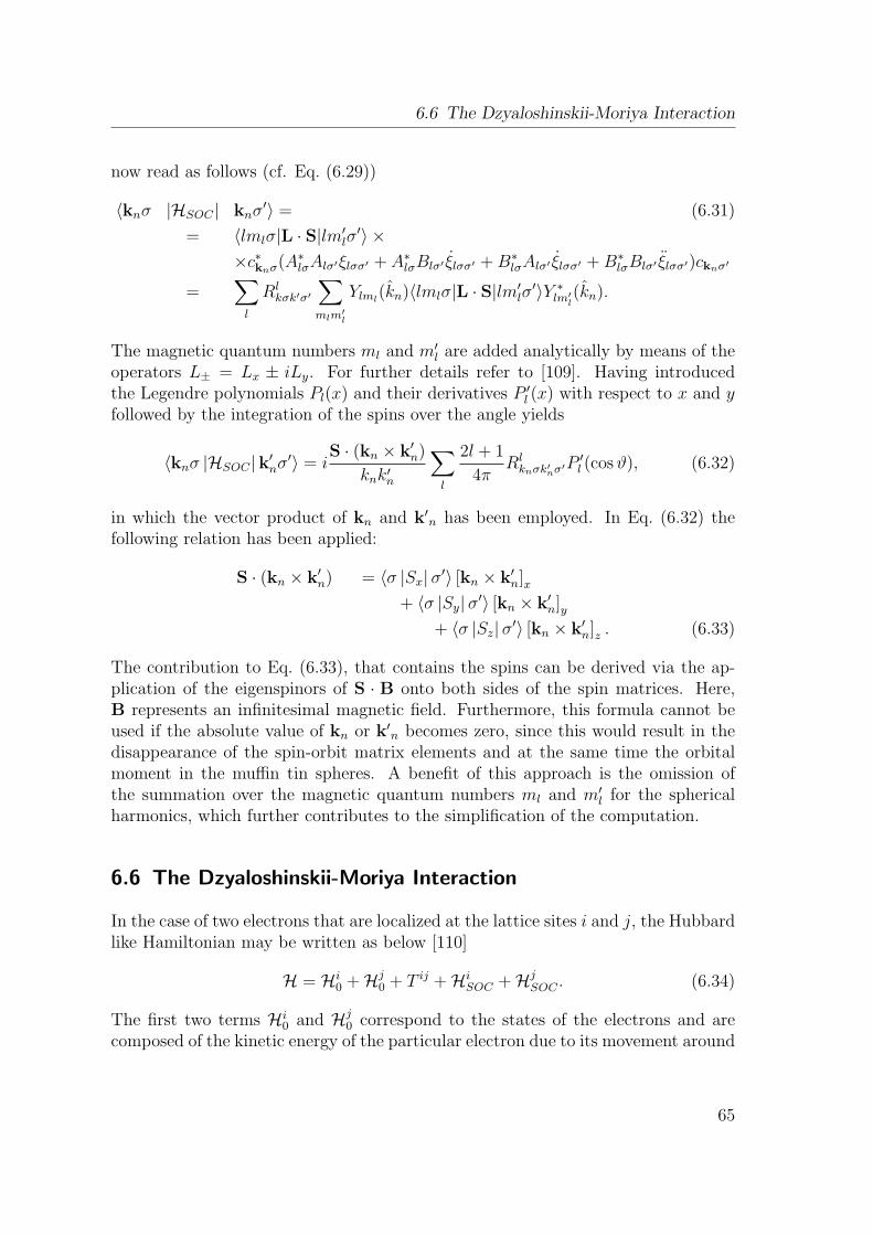
6.6 The Dzyaloshinskii-Moriya Interaction
now read as follows (cf. Eq. (6.29))
⟨knσ |HSOC | knσ′⟩ = (6.31)
= ⟨lmlσ|L · S|lm′lσ
′⟩ ××c∗knσ(A∗
lσAlσ′ξlσσ′ + A∗lσBlσ′ ξlσσ′ +B∗
lσAlσ′ ξlσσ′ +B∗lσBlσ′ ξlσσ′)cknσ′
=∑l
Rlkσk′σ′
∑mlm
′l
Ylml(kn)⟨lmlσ|L · S|lm′
lσ′⟩Y ∗
lm′l(kn).
The magnetic quantum numbers ml and m′l are added analytically by means of the
operators L± = Lx ± iLy. For further details refer to [109]. Having introducedthe Legendre polynomials Pl(x) and their derivatives P ′
l (x) with respect to x and yfollowed by the integration of the spins over the angle yields
⟨knσ |HSOC |k′nσ
′⟩ = iS · (kn × k′
n)
knk′n
∑l
2l + 1
4πRl
knσk′nσ′P ′
l (cosϑ), (6.32)
in which the vector product of kn and k′n has been employed. In Eq. (6.32) the
following relation has been applied:
S · (kn × k′n) = ⟨σ |Sx|σ′⟩ [kn × k′
n]x+ ⟨σ |Sy| σ′⟩ [kn × k′
n]y+ ⟨σ |Sz|σ′⟩ [kn × k′
n]z . (6.33)
The contribution to Eq. (6.33), that contains the spins can be derived via the ap-plication of the eigenspinors of S · B onto both sides of the spin matrices. Here,B represents an infinitesimal magnetic field. Furthermore, this formula cannot beused if the absolute value of kn or k′
n becomes zero, since this would result in thedisappearance of the spin-orbit matrix elements and at the same time the orbitalmoment in the muffin tin spheres. A benefit of this approach is the omission ofthe summation over the magnetic quantum numbers ml and m′
l for the sphericalharmonics, which further contributes to the simplification of the computation.
6.6 The Dzyaloshinskii-Moriya Interaction
In the case of two electrons that are localized at the lattice sites i and j, the Hubbardlike Hamiltonian may be written as below [110]
H = Hi0 + Hj
0 + T ij + HiSOC + Hj
SOC . (6.34)
The first two terms Hi0 and Hj
0 correspond to the states of the electrons and arecomposed of the kinetic energy of the particular electron due to its movement around
65
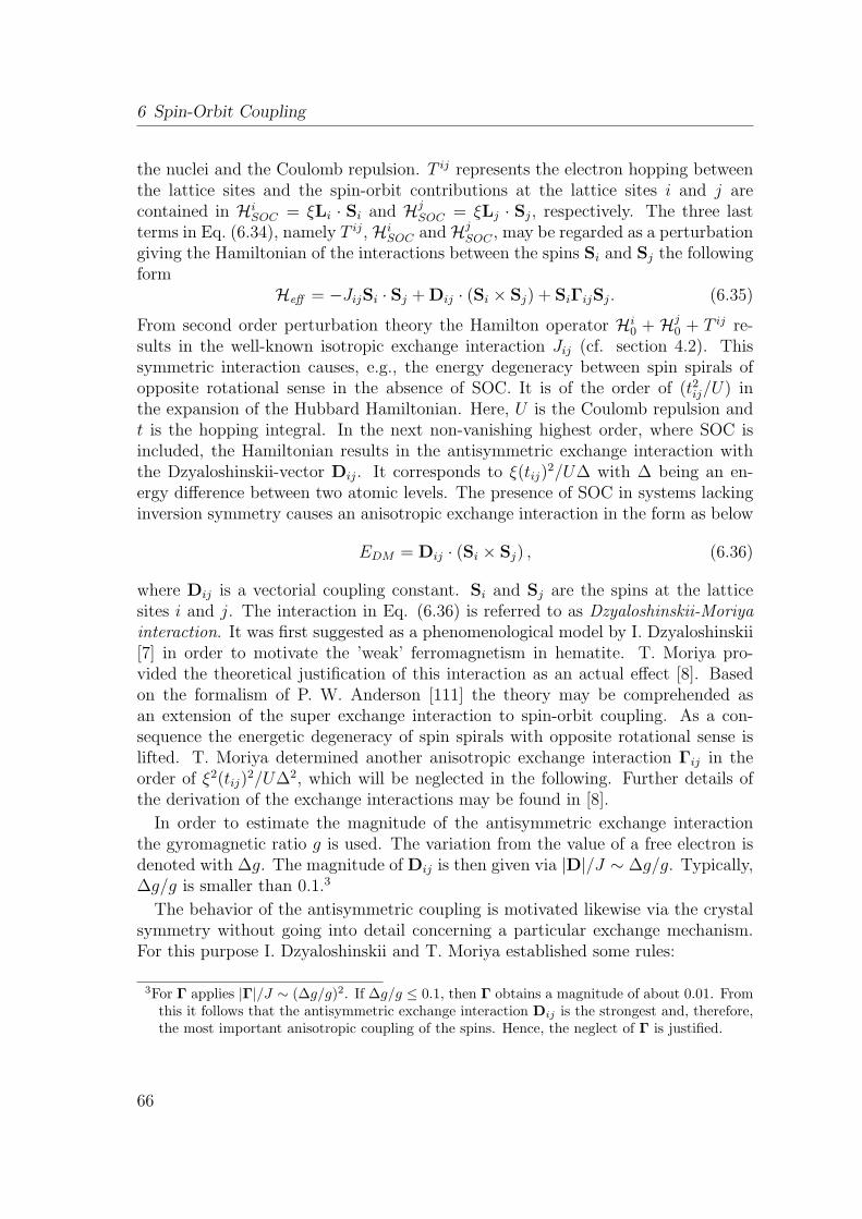
6 Spin-Orbit Coupling
the nuclei and the Coulomb repulsion. T ij represents the electron hopping betweenthe lattice sites and the spin-orbit contributions at the lattice sites i and j arecontained in Hi
SOC = ξLi · Si and HjSOC = ξLj · Sj, respectively. The three last
terms in Eq. (6.34), namely T ij, HiSOC and Hj
SOC , may be regarded as a perturbationgiving the Hamiltonian of the interactions between the spins Si and Sj the followingform
Heff = −JijSi · Sj + Dij · (Si × Sj) + SiΓijSj. (6.35)
From second order perturbation theory the Hamilton operator Hi0 + Hj
0 + T ij re-sults in the well-known isotropic exchange interaction Jij (cf. section 4.2). Thissymmetric interaction causes, e.g., the energy degeneracy between spin spirals ofopposite rotational sense in the absence of SOC. It is of the order of (t2ij/U) inthe expansion of the Hubbard Hamiltonian. Here, U is the Coulomb repulsion andt is the hopping integral. In the next non-vanishing highest order, where SOC isincluded, the Hamiltonian results in the antisymmetric exchange interaction withthe Dzyaloshinskii-vector Dij. It corresponds to ξ(tij)
2/U∆ with ∆ being an en-ergy difference between two atomic levels. The presence of SOC in systems lackinginversion symmetry causes an anisotropic exchange interaction in the form as below
EDM = Dij · (Si × Sj) , (6.36)
where Dij is a vectorial coupling constant. Si and Sj are the spins at the latticesites i and j. The interaction in Eq. (6.36) is referred to as Dzyaloshinskii-Moriyainteraction. It was first suggested as a phenomenological model by I. Dzyaloshinskii[7] in order to motivate the ’weak’ ferromagnetism in hematite. T. Moriya pro-vided the theoretical justification of this interaction as an actual effect [8]. Basedon the formalism of P. W. Anderson [111] the theory may be comprehended asan extension of the super exchange interaction to spin-orbit coupling. As a con-sequence the energetic degeneracy of spin spirals with opposite rotational sense islifted. T. Moriya determined another anisotropic exchange interaction Γij in theorder of ξ2(tij)
2/U∆2, which will be neglected in the following. Further details ofthe derivation of the exchange interactions may be found in [8].
In order to estimate the magnitude of the antisymmetric exchange interactionthe gyromagnetic ratio g is used. The variation from the value of a free electron isdenoted with ∆g. The magnitude of Dij is then given via |D|/J ∼ ∆g/g. Typically,∆g/g is smaller than 0.1.3
The behavior of the antisymmetric coupling is motivated likewise via the crystalsymmetry without going into detail concerning a particular exchange mechanism.For this purpose I. Dzyaloshinskii and T. Moriya established some rules:
3For Γ applies |Γ|/J ∼ (∆g/g)2. If ∆g/g ≤ 0.1, then Γ obtains a magnitude of about 0.01. Fromthis it follows that the antisymmetric exchange interaction Dij is the strongest and, therefore,the most important anisotropic coupling of the spins. Hence, the neglect of Γ is justified.
66
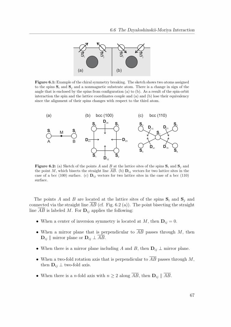
6.6 The Dzyaloshinskii-Moriya Interaction
(a) (b)
Si SjSi Sj
Figure 6.1: Example of the chiral symmetry breaking. The sketch shows two atoms assignedto the spins Si and Sj and a nonmagnetic substrate atom. There is a change in sign of theangle that is enclosed by the spins from configuration (a) to (b). As a result of the spin-orbitinteraction the spin and the lattice coordinates couple and (a) and (b) lose their equivalencysince the alignment of their spins changes with respect to the third atom.
(a)
A B
MSi Sj
S5
S1
S2
S4
S3D13
D41D15
D21
(c) bcc (110)(b) bcc (100)
S1 S2
S4 S3
D12
D41
D34
D23
Figure 6.2: (a) Sketch of the points A and B at the lattice sites of the spins Si and Sj andthe point M , which bisects the straight line AB. (b) Dij vectors for two lattice sites in thecase of a bcc (100) surface. (c) Dij vectors for two lattice sites in the case of a bcc (110)surface.
The points A and B are located at the lattice sites of the spins Si and Sj andconnected via the straight line AB (cf. Fig. 6.2 (a)). The point bisecting the straightline AB is labeled M . For Dij applies the following:
• When a center of inversion symmetry is located at M , then Dij = 0.
• When a mirror plane that is perpendicular to AB passes through M , thenDij ∥ mirror plane or Dij ⊥ AB.
• When there is a mirror plane including A and B, then Dij ⊥ mirror plane.
• When a two-fold rotation axis that is perpendicular to AB passes through M ,then Dij ⊥ two-fold axis.
• When there is a n-fold axis with n ≥ 2 along AB, then Dij ∥ AB.
67
6 Spin-Orbit Coupling
The first rule reveals that a lack of inversion symmetry is in general a basic conditionfor the existence of the antisymmetric exchange interaction in a crystal lattice. Thisplays an important role in particular for surfaces of magnetic materials as they arestudied within this thesis, which always lack inversion symmetry. This has beenrecently demonstrated in experiment and theory for a monolayer of Mn on W(110)[9]. From the above symmetry considerations the direction of the Dzyaloshinskiivector Dij between two lattice sites can be derived for any crystal symmetry suchas in the case of the bcc (110) and (110) surfaces in Fig. 6.2 (b) and (c).
The methods to include SOC in the FLAPW method (cf. section 6.5) cannotbe applied directly to spin spirals. The generalized Bloch theorem (Eq. (5.11))does not hold in the presence of SOC, since the atoms with different magnetizationdirection are not equivalent anymore, and the translational symmetry is broken.Alternatively, the first variational method is employable in order to calculate thespin structure via the super cell approach. However, the unit cell corresponding toa small spin-spiral vector q can become very large and, therefore, those calculationsmay become unfeasible even for today’s supercomputers. Therefore, the calculationof the Dzyaloshinskii-Moriya interaction is treated via first order perturbation theoryin the FLEUR code [112], since it is linear in the SOC constant ξ. That means thecorrections to the band energies are approximately given by the expectation values
⟨ψk′,ν′|HSOC |ψk,ν⟩ =(⟨ψ↑
k′,ν′|⟨ψ↓k′,ν′|
)(H↑↑SOC H↑↓
SOC
H↓↑SOC H↓↓
SOC
)(|ψ↑
k,ν⟩|ψ↓
k,ν⟩
)(6.37)
of the SOC operator HSOC and the eigenstates Ψk,ν to the unperturbed Hamiltonian.This approach only allows for the computation of the antisymmetric exchange asthe expectation values vanish for collinear magnetic states. The components of theSOC Hamilton matrix possess the periodicity of the lattice. Therefore, it appliesthat
Hσσ′
SOC
(e∓iq·r/2fσ′
(k, r))
= e∓iq·r/2fσ′
SOC (k, r)
Hσσ′
SOCψσ′
ν (k, r) = e∓iq·r/2fσ′
SOC (k, r) , (6.38)
where the fσ′(k, r) and fσ′
SOC (k, r) represent any lattice periodic functions. σ de-notes the spin alignment ↑ and ↓, respectively. Then, the matrix elements of HSOC
can be expressed as follows
⟨ψ↑k′,ν′ |H
↑↑SOC |ψ
↑k,ν⟩ =
∫d3ei(k−k′)·rf ↑↑(r),
⟨ψ↓k′,ν′ |H
↓↓SOC |ψ
↓k,ν⟩ =
∫d3ei(k−k′)·rf ↓↓(r),
(6.39)
68
6.6 The Dzyaloshinskii-Moriya Interaction
⟨ψ↓k′,ν′|H
↓↑SOC |ψ
↑k,ν⟩ =
∫d3ei(k−k′−q)·rf ↓↑(r),
⟨ψ↑k′,ν′|H
↑↓SOC |ψ
↓k,ν⟩ =
∫d3ei(k−k′+q)·rf ↑↓(r). (6.40)
They are only nonzero if the exponents become zero. Thus, it is sufficient to consideronly the diagonal elements, and the Hamilton matrix takes the following form:
⟨ψk′,ν′|HSOC |ψk,ν⟩ = N(⟨f ↑|f ↑⟩ + ⟨f ↓|f ↓⟩
), (6.41)
where N specifies the number of chemical unit cells. The Bloch factors cancel eachother and as a result the correction to the band energies holds for all atoms.
Then the HSOC matrix elements for spin-spiral states are expressed explicitly interms of the LAPW basis. Since the spin-orbit contribution is rather small in theinterstitial region, the calculation of the HSOC matrix elements is performed withinthe muffin tins, where the basis functions are given in Eq. (3.5) and (3.16):
φσG(k, r) =
∑L
(AµGσ
L (k)uσl (r) +BµGσL (k)uσl (r)
)YL(r). (6.42)
Here, L abbreviates the quantum numbers l and m. In order to distinguish thespin indices of the local (muffin tin dependent) spin coordinate frame from the onesdefined in the global coordinate frame, the first are marked with tildes (˜). Then,the expansion of the wave functions ψk,ν reads:
ψk,ν =∑G
C ↑G,k,νφ
↑G
C ↓G,k,νφ
↓G
=∑L
YL(ϑ, φ)
a↑k,ν,Lu↑l (r) + b↑k,ν,Lu↑l (r)
a↓k,ν,Lu↓l (r) + b↓k,ν,Lu
↓l (r)
(6.43)
where the coefficients AµGσL (k) and BµGσ
L (k) are introduced via
aσk,ν,L =∑G
cσk,ν,GAµGσL (k) and bσk,ν,L =
∑G
cσk,ν,GBµGσL (k). (6.44)
Then, the wave functions are rotated from the local to the global coordinate frame.The A and B coefficients of the muffin tin in the global frame read
aσ′σ
k,ν,L = Uσ′σMT
∑G
aσk,ν,L and bσ′σ
k,ν,L = Uσ′σMT
∑G
bσk,ν,L. (6.45)
The wave functions are further rotated until their coordinate frame corresponds to
69
6 Spin-Orbit Coupling
the real-space coordinate frame denoted with the index rs:
⟨ψk′,ν′|U†rsHSOCUrs|ψk,ν⟩ =
∫MT
ψ†k′,ν′(r)U
†rsHSOCUrsψk,ν(r)d3r. (6.46)
Since the angular momentum operator L commutes with the spherically symmetricfunctions, the real-space integration of the matrix elements is split into an angularand a radial part. Employing Eq. (6.9) gives the following expression of the angularintegrals
Aσ′σl,m′,m =
∫ π
0
dϑ
∫ 2π
0
dφ(− sinϑ)Yl,m(ϑ, φ)∗Lσ′σYl,m(ϑ, φ). (6.47)
The radial integrals are given as
Rσ′σl,u,u =
∫ RMT
0
drr2ξuσ′
l (r)uσl (r) , Rσ′σl,u,u =
∫ RMT
0
drr2ξuσ′
l (r)uσl
Rσ′σl,u,u =
∫ RMT
0
drr2ξuσ′
l (r)uσl (r) , Rσ′σl,u,u =
∫ RMT
0
drr2ξuσ′
l (r)uσl (r) (6.48)
Introducing
T σ′,σ =∑l,m′,m
∑σ′σ
Aσ′σl,m′,m
(aσ
′σ′∗k′,ν′,l,m′aσσk,ν,l,mRσ′σ
l,u,u + aσ′σ′∗
k′,ν′,l,m′bσσk,ν,l,mRσ′σl,u,u
+bσ′σ′∗
k′,ν′,l,m′aσσk,ν,l,mRσ′σl,u,u + bσ
′σ′∗k′,ν′,l,m′bσσk,ν,l,mRσ′σ
l,u,u
)(6.49)
the expectation value results in
∆E = ⟨ψk′,ν′ |U†rsHSOCUrs|ψk,ν⟩ =
T ↑↑ + T ↓↓ k′ = k,
T ↑↓ k′ = k + q,
T ↓↑ k′ = k− q,
0 else.
(6.50)
70
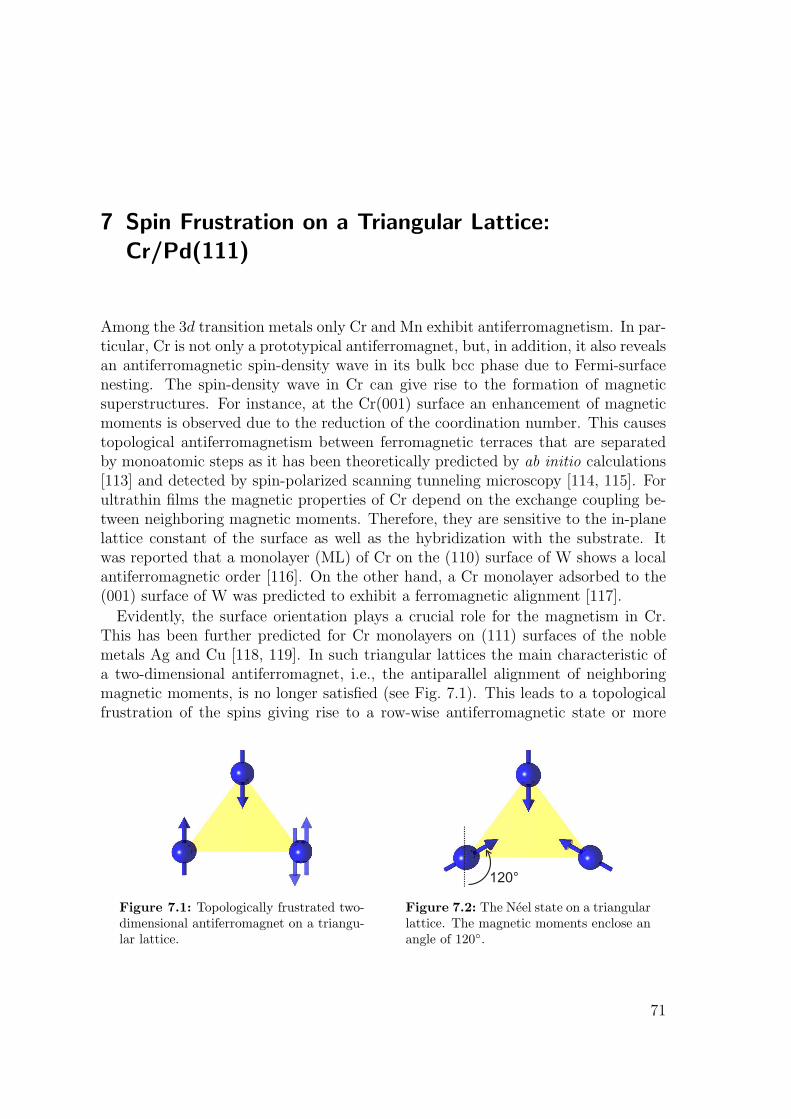
7 Spin Frustration on a Triangular Lattice:Cr/Pd(111)
Among the 3d transition metals only Cr and Mn exhibit antiferromagnetism. In par-ticular, Cr is not only a prototypical antiferromagnet, but, in addition, it also revealsan antiferromagnetic spin-density wave in its bulk bcc phase due to Fermi-surfacenesting. The spin-density wave in Cr can give rise to the formation of magneticsuperstructures. For instance, at the Cr(001) surface an enhancement of magneticmoments is observed due to the reduction of the coordination number. This causestopological antiferromagnetism between ferromagnetic terraces that are separatedby monoatomic steps as it has been theoretically predicted by ab initio calculations[113] and detected by spin-polarized scanning tunneling microscopy [114, 115]. Forultrathin films the magnetic properties of Cr depend on the exchange coupling be-tween neighboring magnetic moments. Therefore, they are sensitive to the in-planelattice constant of the surface as well as the hybridization with the substrate. Itwas reported that a monolayer (ML) of Cr on the (110) surface of W shows a localantiferromagnetic order [116]. On the other hand, a Cr monolayer adsorbed to the(001) surface of W was predicted to exhibit a ferromagnetic alignment [117].
Evidently, the surface orientation plays a crucial role for the magnetism in Cr.This has been further predicted for Cr monolayers on (111) surfaces of the noblemetals Ag and Cu [118, 119]. In such triangular lattices the main characteristic ofa two-dimensional antiferromagnet, i.e., the antiparallel alignment of neighboringmagnetic moments, is no longer satisfied (see Fig. 7.1). This leads to a topologicalfrustration of the spins giving rise to a row-wise antiferromagnetic state or more
Figure 7.1: Topologically frustrated two-dimensional antiferromagnet on a triangu-lar lattice.
120°
Figure 7.2: The Neel state on a triangularlattice. The magnetic moments enclose anangle of 120.
71
7 Spin Frustration on a Triangular Lattice: Cr/Pd(111)
complex magnetic structures, such as spin spirals or the Neel state – a configurationthat is characterized by magnetic moments enclosing an angle of 120 as illustratedin Fig. 7.2. The Neel state has first been observed experimentally only in a Mnmonolayer on the (111) surface of Ag [120]. However, this discovery conflicts withtheoretical calculations performed within the DFT, which predict a row-wise anti-ferromagnetic state [118].
In systems such as the monolayers of Mn or Cr on Ag(111) the formation ofalloys due to intermixing is problematic. This difficulty can be avoided by choosingsubstrates such as Pd(111), where the surface energy and thus the hybridization ofthe magnetic thin film with the substrate is different. The difference in hybridizationand the in-plane lattice constant leads to a change in the exchange coupling of thesystem, which can induce non-collinear magnetic order such as the Neel state.
In order to shed light onto this issue, in this chapter the magnetism of a singlemonolayer of Cr on Pd(111) is investigated. This happens by means of DFT calcu-lations that are compared to experimental results obtained by spin-polarized STM. First, the stacking of the film as well as the collinear magnetic ordering, i.e., fer-romagnetic or antiferromagnetic, is examined. By studying the energy dispersion ofspin-spiral structures on a freestanding monolayer of Cr(111) and Cr deposited onPd(111) the influence of the substrate onto the magnetic exchange interactions willbe analyzed that results in a non-collinear magnetic ground state. The comparisonof simulated spin-polarized STM images of the spin-spiral state with the experimen-tal data allows for the identification of the
(√3 ×
√3)
superstructure as Neel state.Moreover, the direct comparison of the simulated spin-polarized STM images withthe experimental results allows for the estimation of the magnetization direction ofthe tip with respect to the magnetization direction of the sample.
Parts of this chapter have been published in Physical Review B [58].
7.1 Computational Details
The ab initio calculations have been carried out within the GGA [33] if not statedotherwise. For the structural relaxation the theoretical lattice constant of Pd (aPd =3.981 A [121]) has been used. A symmetric film consisting of seven monolayersPd(111) with one monolayer Cr on each side has been applied. A mesh of 72k∥ points in the irreducible wedge of the two-dimensional Brillouin zone has beenemployed as well as about 160 basis functions per atom. To calculate the spinspirals an asymmetric film consisting of six layers of Pd(111) and one layer of Cr infcc stacking has been employed. The structural relaxations were adopted from therow-wise antiferromagnetic state and it was made use of 1024 k∥ points in the entiretwo-dimensional Brillouin zone as well as about 110 basis functions per atom.
72
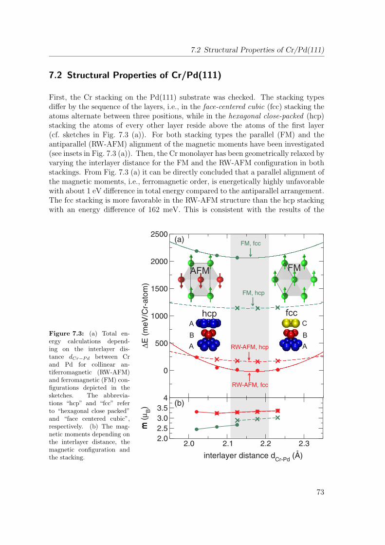
7.2 Structural Properties of Cr/Pd(111)
7.2 Structural Properties of Cr/Pd(111)
First, the Cr stacking on the Pd(111) substrate was checked. The stacking typesdiffer by the sequence of the layers, i.e., in the face-centered cubic (fcc) stacking theatoms alternate between three positions, while in the hexagonal close-packed (hcp)stacking the atoms of every other layer reside above the atoms of the first layer(cf. sketches in Fig. 7.3 (a)). For both stacking types the parallel (FM) and theantiparallel (RW-AFM) alignment of the magnetic moments have been investigated(see insets in Fig. 7.3 (a)). Then, the Cr monolayer has been geometrically relaxed byvarying the interlayer distance for the FM and the RW-AFM configuration in bothstackings. From Fig. 7.3 (a) it can be directly concluded that a parallel alignment ofthe magnetic moments, i.e., ferromagnetic order, is energetically highly unfavorablewith about 1 eV difference in total energy compared to the antiparallel arrangement.The fcc stacking is more favorable in the RW-AFM structure than the hcp stackingwith an energy difference of 162 meV. This is consistent with the results of the
Figure 7.3: (a) Total en-ergy calculations depend-ing on the interlayer dis-tance dCr−Pd between Crand Pd for collinear an-tiferromagnetic (RW-AFM)and ferromagnetic (FM) con-figurations depicted in thesketches. The abbrevia-tions “hcp” and “fcc” referto “hexagonal close packed”and “face centered cubic”,respectively. (b) The mag-netic moments depending onthe interlayer distance, themagnetic configuration andthe stacking.
AFM FM
A
B
A
A
B
C
hcp fcc
RW-
RW-
73
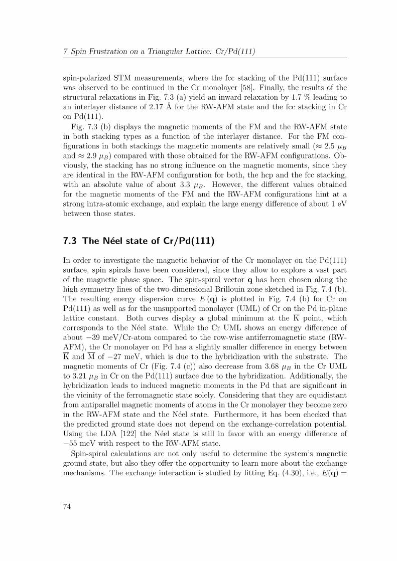
7 Spin Frustration on a Triangular Lattice: Cr/Pd(111)
spin-polarized STM measurements, where the fcc stacking of the Pd(111) surfacewas observed to be continued in the Cr monolayer [58]. Finally, the results of thestructural relaxations in Fig. 7.3 (a) yield an inward relaxation by 1.7 % leading toan interlayer distance of 2.17 A for the RW-AFM state and the fcc stacking in Cron Pd(111).
Fig. 7.3 (b) displays the magnetic moments of the FM and the RW-AFM statein both stacking types as a function of the interlayer distance. For the FM con-figurations in both stackings the magnetic moments are relatively small (≈ 2.5 µB
and ≈ 2.9 µB) compared with those obtained for the RW-AFM configurations. Ob-viously, the stacking has no strong influence on the magnetic moments, since theyare identical in the RW-AFM configuration for both, the hcp and the fcc stacking,with an absolute value of about 3.3 µB. However, the different values obtainedfor the magnetic moments of the FM and the RW-AFM configurations hint at astrong intra-atomic exchange, and explain the large energy difference of about 1 eVbetween those states.
7.3 The Neel state of Cr/Pd(111)
In order to investigate the magnetic behavior of the Cr monolayer on the Pd(111)surface, spin spirals have been considered, since they allow to explore a vast partof the magnetic phase space. The spin-spiral vector q has been chosen along thehigh symmetry lines of the two-dimensional Brillouin zone sketched in Fig. 7.4 (b).The resulting energy dispersion curve E (q) is plotted in Fig. 7.4 (b) for Cr onPd(111) as well as for the unsupported monolayer (UML) of Cr on the Pd in-planelattice constant. Both curves display a global minimum at the K point, whichcorresponds to the Neel state. While the Cr UML shows an energy difference ofabout −39 meV/Cr-atom compared to the row-wise antiferromagnetic state (RW-AFM), the Cr monolayer on Pd has a slightly smaller difference in energy betweenK and M of −27 meV, which is due to the hybridization with the substrate. Themagnetic moments of Cr (Fig. 7.4 (c)) also decrease from 3.68 µB in the Cr UMLto 3.21 µB in Cr on the Pd(111) surface due to the hybridization. Additionally, thehybridization leads to induced magnetic moments in the Pd that are significant inthe vicinity of the ferromagnetic state solely. Considering that they are equidistantfrom antiparallel magnetic moments of atoms in the Cr monolayer they become zeroin the RW-AFM state and the Neel state. Furthermore, it has been checked thatthe predicted ground state does not depend on the exchange-correlation potential.Using the LDA [122] the Neel state is still in favor with an energy difference of−55 meV with respect to the RW-AFM state.
Spin-spiral calculations are not only useful to determine the system’s magneticground state, but also they offer the opportunity to learn more about the exchangemechanisms. The exchange interaction is studied by fitting Eq. (4.30), i.e., E(q) =
74
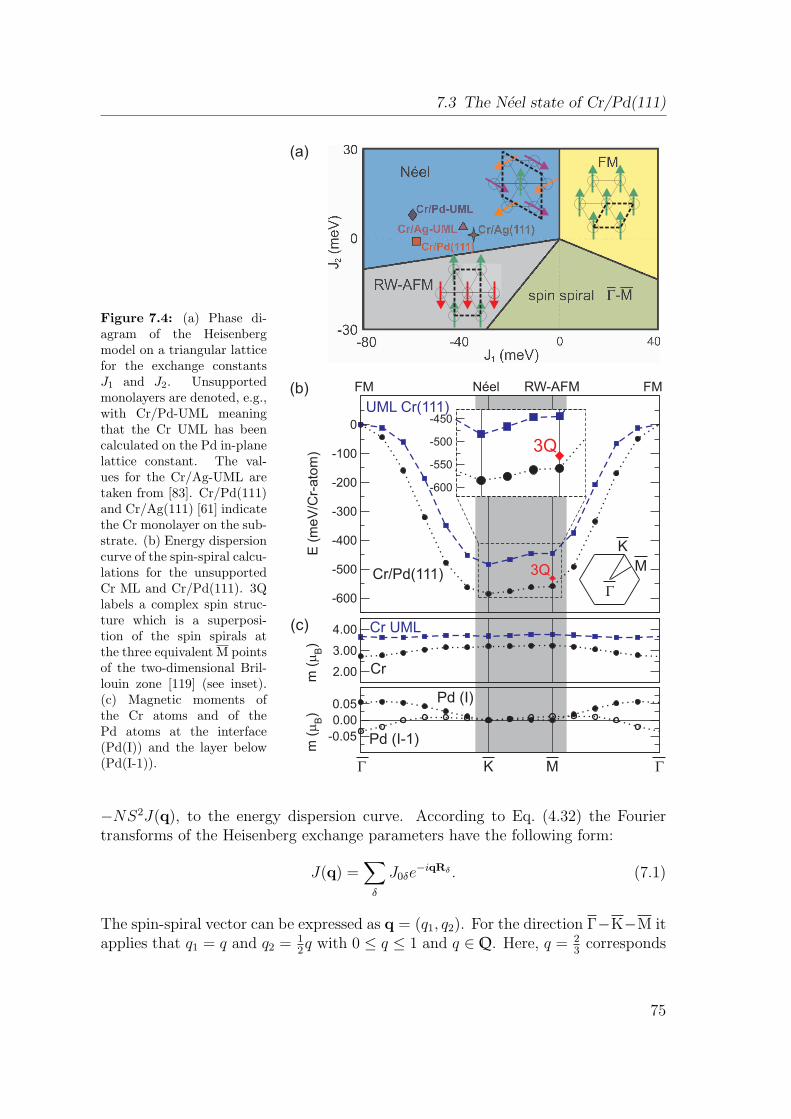
7.3 The Neel state of Cr/Pd(111)
Figure 7.4: (a) Phase di-agram of the Heisenbergmodel on a triangular latticefor the exchange constantsJ1 and J2. Unsupportedmonolayers are denoted, e.g.,with Cr/Pd-UML meaningthat the Cr UML has beencalculated on the Pd in-planelattice constant. The val-ues for the Cr/Ag-UML aretaken from [83]. Cr/Pd(111)and Cr/Ag(111) [61] indicatethe Cr monolayer on the sub-strate. (b) Energy dispersioncurve of the spin-spiral calcu-lations for the unsupportedCr ML and Cr/Pd(111). 3Qlabels a complex spin struc-ture which is a superposi-tion of the spin spirals atthe three equivalent M pointsof the two-dimensional Bril-louin zone [119] (see inset).(c) Magnetic moments ofthe Cr atoms and of thePd atoms at the interface(Pd(I)) and the layer below(Pd(I-1)).
-600
-500
-400
-300
-200
-100
0
E (
meV
/Cr-
ato
m)
2.00
3.00
4.00
m (
mB)
-0.05
0.00
0.05
m (
mB)
-600
-550
-500
-450
G K M G
Cr/Pd(111)
Cr UML
Pd (I)
Pd (I-1)
UML Cr(111)
Cr
3Q
3Q
(a)
(c)
(b) FM RW-AFMNéel FM
G
M
K
−NS2J(q), to the energy dispersion curve. According to Eq. (4.32) the Fouriertransforms of the Heisenberg exchange parameters have the following form:
J(q) =∑δ
J0δe−iqRδ . (7.1)
The spin-spiral vector can be expressed as q = (q1, q2). For the direction Γ−K−M itapplies that q1 = q and q2 = 1
2q with 0 ≤ q ≤ 1 and q ∈ Q. Here, q = 2
3corresponds
75
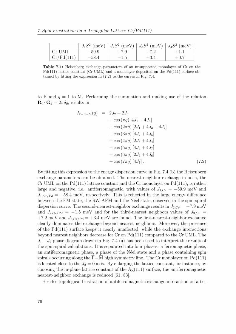
7 Spin Frustration on a Triangular Lattice: Cr/Pd(111)
J1S2 (meV) J2S
2 (meV) J3S2 (meV) J4S
2 (meV)Cr UML −59.9 +7.9 +7.2 +1.1Cr/Pd(111) −58.4 −1.5 +3.4 +0.7
Table 7.1: Heisenberg exchange parameters of an unsupported monolayer of Cr on thePd(111) lattice constant (Cr-UML) and a monolayer deposited on the Pd(111) surface ob-tained by fitting the expression in (7.2) to the curves in Fig. 7.4.
to K and q = 1 to M. Performing the summation and making use of the relationRi ·Gk = 2πδik results in
JΓ−K−M(q) = 2J2 + 2J6
+ cos (πq) [4J1 + 4J5]
+ cos (2πq) [2J1 + 4J3 + 4J7]
+ cos (3πq) [4J2 + 4J5]
+ cos (4πq) [2J3 + 4J4]
+ cos (5πq) [4J4 + 4J7]
+ cos (6πq) [2J5 + 4J6]
+ cos (7πq) [4J7] . (7.2)
By fitting this expression to the energy dispersion curve in Fig. 7.4 (b) the Heisenbergexchange parameters can be obtained. The nearest-neighbor exchange in both, theCr UML on the Pd(111) lattice constant and the Cr monolayer on Pd(111), is ratherlarge and negative, i.e., antiferromagnetic, with values of J1,Cr = −59.9 meV andJ1,Cr/Pd = −58.4 meV, respectively. This is reflected in the large energy differencebetween the FM state, the RW-AFM and the Neel state, observed in the spin-spiraldispersion curve. The second-nearest-neighbor exchange results in J2,Cr = +7.9 meVand J2,Cr/Pd = −1.5 meV and for the third-nearest neighbors values of J3,Cr =+7.2 meV and J3,Cr/Pd = +3.4 meV are found. The first-nearest-neighbor exchangeclearly dominates the exchange beyond nearest neighbors. Moreover, the presenceof the Pd(111) surface keeps it nearly unaffected, while the exchange interactionsbeyond nearest neighbors decrease for Cr on Pd(111) compared to the Cr UML. TheJ1−J2 phase diagram drawn in Fig. 7.4 (a) has been used to interpret the results ofthe spin-spiral calculations. It is separated into four phases: a ferromagnetic phase,an antiferromagnetic phase, a phase of the Neel state and a phase containing spinspirals occurring along the Γ−M high symmetry line. The Cr monolayer on Pd(111)is located close to the J2 = 0 axis. By enlarging the lattice constant, for instance, bychoosing the in-plane lattice constant of the Ag(111) surface, the antiferromagneticnearest-neighbor exchange is reduced [61, 83].
Besides topological frustration of antiferromagnetic exchange interaction on a tri-
76
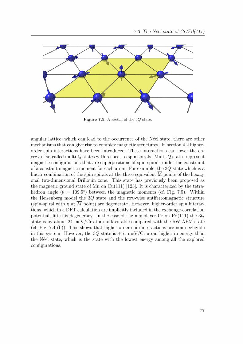
7.3 The Neel state of Cr/Pd(111)
Figure 7.5: A sketch of the 3Q state.
angular lattice, which can lead to the occurrence of the Neel state, there are othermechanisms that can give rise to complex magnetic structures. In section 4.2 higher-order spin interactions have been introduced. These interactions can lower the en-ergy of so-called multi-Q states with respect to spin spirals. Multi-Q states representmagnetic configurations that are superpositions of spin-spirals under the constraintof a constant magnetic moment for each atom. For example, the 3Q-state which is alinear combination of the spin spirals at the three equivalent M points of the hexag-onal two-dimensional Brillouin zone. This state has previously been proposed asthe magnetic ground state of Mn on Cu(111) [123]. It is characterized by the tetra-hedron angle (θ = 109.5) between the magnetic moments (cf. Fig. 7.5). Withinthe Heisenberg model the 3Q state and the row-wise antiferromagnetic structure(spin-spiral with q at M point) are degenerate. However, higher-order spin interac-tions, which in a DFT calculation are implicitly included in the exchange-correlationpotential, lift this degeneracy. In the case of the monolayer Cr on Pd(111) the 3Qstate is by about 24 meV/Cr-atom unfavorable compared with the RW-AFM state(cf. Fig. 7.4 (b)). This shows that higher-order spin interactions are non-negligiblein this system. However, the 3Q state is +51 meV/Cr-atom higher in energy thanthe Neel state, which is the state with the lowest energy among all the exploredconfigurations.
77
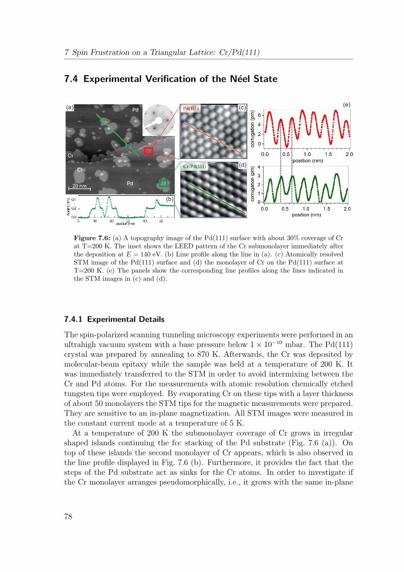
7 Spin Frustration on a Triangular Lattice: Cr/Pd(111)
7.4 Experimental Verification of the Neel State
(a)
(b)
(c)
(d)
(e)
Figure 7.6: (a) A topography image of the Pd(111) surface with about 30% coverage of Crat T=200 K. The inset shows the LEED pattern of the Cr submonolayer immediately afterthe deposition at E = 140 eV. (b) Line profile along the line in (a). (c) Atomically resolvedSTM image of the Pd(111) surface and (d) the monolayer of Cr on the Pd(111) surface atT=200 K. (e) The panels show the corresponding line profiles along the lines indicated inthe STM images in (c) and (d).
7.4.1 Experimental Details
The spin-polarized scanning tunneling microscopy experiments were performed in anultrahigh vacuum system with a base pressure below 1 × 10⁻¹⁰ mbar. The Pd(111)crystal was prepared by annealing to 870 K. Afterwards, the Cr was deposited bymolecular-beam epitaxy while the sample was held at a temperature of 200 K. Itwas immediately transferred to the STM in order to avoid intermixing between theCr and Pd atoms. For the measurements with atomic resolution chemically etchedtungsten tips were employed. By evaporating Cr on these tips with a layer thicknessof about 50 monolayers the STM tips for the magnetic measurements were prepared.They are sensitive to an in-plane magnetization. All STM images were measured inthe constant current mode at a temperature of 5 K.
At a temperature of 200 K the submonolayer coverage of Cr grows in irregularshaped islands continuing the fcc stacking of the Pd substrate (Fig. 7.6 (a)). Ontop of these islands the second monolayer of Cr appears, which is also observed inthe line profile displayed in Fig. 7.6 (b). Furthermore, it provides the fact that thesteps of the Pd substrate act as sinks for the Cr atoms. In order to investigate ifthe Cr monolayer arranges pseudomorphically, i.e., it grows with the same in-plane
78
7.4 Experimental Verification of the Neel State
lattice constant as the Pd substrate, low-energy electron-diffraction (LEED) hasbeen applied at an energy of E=140 eV. These measurements reveal that the Crlayer is free from dislocation network (compare with inset in Fig. 7.6 (a)), sincethey show a clear p(1 × 1) pattern lacking of any additional structures around thespots. The atomically resolved Pd(111) surface and an island of the submonolayerdeposition of Cr on the Pd(111) surface presented in Fig. 7.6 (c) and (d) exhibit astructure that clearly corresponds to the chemical unit cell illustrated in Fig. 7.3. Itdemonstrates the pseudomorphic growth of the Cr monolayer on top of the Pd(111)surface. This is further emphasized by the line profiles shown in Fig. 7.6 (e), wherethe maxima correspond to the atoms of Pd and Cr, respectively. The distancebetween the maxima agrees with the interatomic distance of 2.71 A between Pdatoms in the single crystal.
7.4.2 Spin-Polarized STM Images: Theory vs. Experiment
Based on the DFT results the Neel state is proposed as the magnetic ground stateof the monolayer Cr on Pd(111). In order to confirm this prediction, the imagesobtained in the spin-polarized STM experiments are compared with those computedby means of first-principles calculations (cf. Fig. 7.7). The simulated STM imageshave been calculated within the framework of the spin-polarized Tersoff-Hamannmodel [61] introduced in section 4.3.
Figure 7.7 (a) displays the STM measurement of the Cr monolayer on Pd(111)with a bare W tip, i.e., it shows the nonmagnetic chemical contrast. The comparisonwith the line profiles in Fig. 7.7 (e) as well as with the simulated STM image inFig. 7.7 (i) allows for attributing the observed protrusions to the Cr atoms. Thespin-polarized STM measurements carried out with magnetically sensitive Cr coatedW tips produce three qualitatively different contrasts (Fig. 7.7 (b)-(d)). While twoimages, Fig. 7.7 (b) and (c), show a hexagonal pattern, Fig. 7.7 (d) features athreefold symmetry. Compared to the chemical unit cell these images are rotatedby 30. From the line profiles in Fig. 7.7 (f) and (g), respectively, it follows that thedistance between protrusions is of 0.46 nm corresponding to a
√3 ×
√3 unit cell of
the Pd(111) surface.While it is known that the Cr coated W tips are sensitive to an in-plane magne-
tization [124] the actual orientation within the plane is uncertain and can changefrom one measurement to the other. On the one hand, this is an advantage in or-der to observe different spin-polarized STM contrasts of a spin structure. On theother hand, a comparison with the theoretical calculations is needed in order toidentify the real tip’s in-plane magnetization direction. This has been done for theSTM images in Fig. 7.7 (b)-(d). Depending on the magnetization direction eT ofthe tip with respect to the sample’s magnetization the spin-polarized STM imagesof the Neel structure exhibit three different spin-polarized STM contrasts [61, 118].For instance, if the tip magnetization is fully aligned to one of the Cr moments of
79
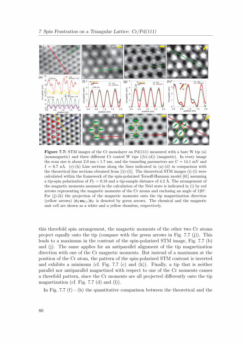
7 Spin Frustration on a Triangular Lattice: Cr/Pd(111)
0.0 0.5 1.0 1.5 2.00
3
6
9
12
co
rru
ga
tio
n(p
m)
position (nm)
0.27 nm
0.0 0.5 1.0 1.5 2.00
1
2
3
4
corr
ugation
(pm
)
position (nm)0.0 0.5 1.0 1.5 2.0
0
1
2
3
4
corr
ugation
(pm
)
position (nm)0.0 0.5 1.0 1.5 2.0
0
1
2
3
4corr
ugation
(pm
)
position (nm)
0.46 nm
(f) (g) (h)
(e)
(j)
(d)
(i) (k) (l)
(c)(b)(a) eT eT eT
eT eTeT
exp.
theoretic.
exp.
exp.exp.
exp.theoretic.
theoretic. 150
theoretic.eT
mCr
13o
eT
mCr
eT
mCr
theoretic. 150
0
3
6
9
120.46 nm
Figure 7.7: STM images of the Cr monolayer on Pd(111) measured with a bare W tip (a)(nonmagnetic) and three different Cr coated W tips ((b)-(d)) (magnetic). In every imagethe scan size is about 2.0 nm× 1.7 nm, and the tunneling parameters are U = 14.1 mV andI = 6.7 nA. (e)-(h) Line sections along the lines indicated in (a)-(d) in comparison withthe theoretical line sections obtained from [(i)-(l)]. The theoretical STM images (i)-(l) werecalculated within the framework of the spin-polarized Tersoff-Hamann model [61] assuminga tip-spin polarization of PT = 0.18 and a tip-sample distance of 4.2 A. The arrangement ofthe magnetic moments assumed in the calculation of the Neel state is indicated in (i) by redarrows representing the magnetic moments of the Cr atoms and enclosing an angle of 120.For (j)-(k) the projection of the magnetic moments onto the tip magnetization direction(yellow arrows) (eTmCr)eT is denoted by green arrows. The chemical and the magneticunit cell are shown as a white and a yellow rhombus, respectively.
this threefold spin arrangement, the magnetic moments of the other two Cr atomsproject equally onto the tip (compare with the green arrows in Fig. 7.7 (j)). Thisleads to a maximum in the contrast of the spin-polarized STM image, Fig. 7.7 (b)and (j). The same applies for an antiparallel alignment of the tip magnetizationdirection with one of the Cr magnetic moments. But instead of a maximum at theposition of the Cr atom, the pattern of the spin-polarized STM contrast is invertedand exhibits a minimum (cf. Fig. 7.7 (c) and (k)). Finally, a tip that is neitherparallel nor antiparallel magnetized with respect to one of the Cr moments causesa threefold pattern, since the Cr moments are all projected differently onto the tipmagnetization (cf. Fig. 7.7 (d) and (l)).
In Fig. 7.7 (f) - (h) the quantitative comparison between the theoretical and the
80
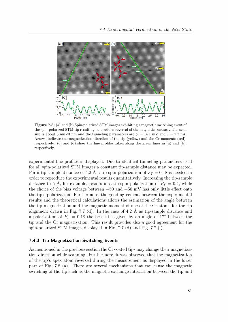
7.4 Experimental Verification of the Neel State
Figure 7.8: (a) and (b) Spin-polarized STM images exhibiting a magnetic switching event ofthe spin-polarized STM tip resulting in a sudden reversal of the magnetic contrast. The scansize is about 3 nm×3 nm and the tunneling parameters are U = 14.1 mV and I = 7.7 nA.Arrows indicate the magnetization direction of the tip (yellow) and the Cr moments (red),respectively. (c) and (d) show the line profiles taken along the green lines in (a) and (b),respectively.
experimental line profiles is displayed. Due to identical tunneling parameters usedfor all spin-polarized STM images a constant tip-sample distance may be expected.For a tip-sample distance of 4.2 A a tip-spin polarization of PT = 0.18 is needed inorder to reproduce the experimental results quantitatively. Increasing the tip-sampledistance to 5 A, for example, results in a tip-spin polarization of PT = 0.4, whilethe choice of the bias voltage between −50 and +50 mV has only little effect ontothe tip’s polarization. Furthermore, the good agreement between the experimentalresults and the theoretical calculations allows the estimation of the angle betweenthe tip magnetization and the magnetic moment of one of the Cr atoms for the tipalignment drawn in Fig. 7.7 (d). In the case of 4.2 A as tip-sample distance anda polarization of PT = 0.18 the best fit is given by an angle of 17 between thetip and the Cr magnetization. This result provides also a good agreement for thespin-polarized STM images displayed in Fig. 7.7 (d) and Fig. 7.7 (l).
7.4.3 Tip Magnetization Switching Events
As mentioned in the previous section the Cr coated tips may change their magnetiza-tion direction while scanning. Furthermore, it was observed that the magnetizationof the tip’s apex atom reversed during the measurement as displayed in the lowerpart of Fig. 7.8 (a). There are several mechanisms that can cause the magneticswitching of the tip such as the magnetic exchange interaction between the tip and
81
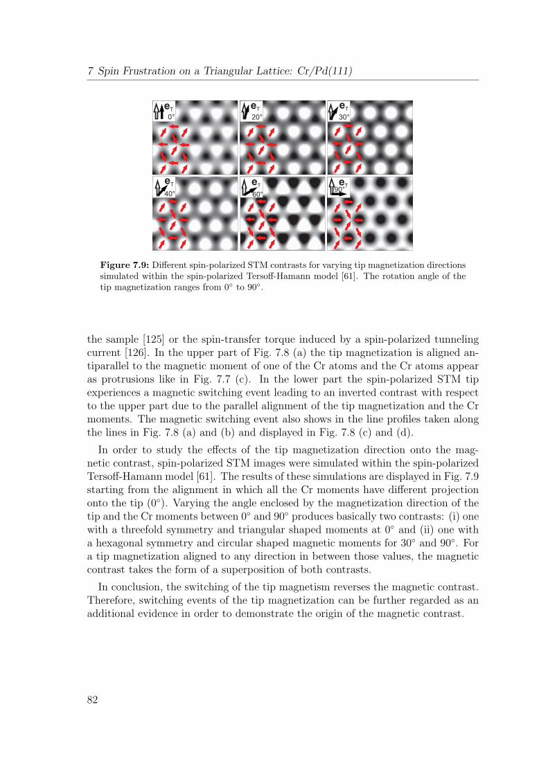
7 Spin Frustration on a Triangular Lattice: Cr/Pd(111)
eT
eT
eT
eT
eT
eT
0° 30°20°
90°60°40°
Figure 7.9: Different spin-polarized STM contrasts for varying tip magnetization directionssimulated within the spin-polarized Tersoff-Hamann model [61]. The rotation angle of thetip magnetization ranges from 0 to 90.
the sample [125] or the spin-transfer torque induced by a spin-polarized tunnelingcurrent [126]. In the upper part of Fig. 7.8 (a) the tip magnetization is aligned an-tiparallel to the magnetic moment of one of the Cr atoms and the Cr atoms appearas protrusions like in Fig. 7.7 (c). In the lower part the spin-polarized STM tipexperiences a magnetic switching event leading to an inverted contrast with respectto the upper part due to the parallel alignment of the tip magnetization and the Crmoments. The magnetic switching event also shows in the line profiles taken alongthe lines in Fig. 7.8 (a) and (b) and displayed in Fig. 7.8 (c) and (d).
In order to study the effects of the tip magnetization direction onto the mag-netic contrast, spin-polarized STM images were simulated within the spin-polarizedTersoff-Hamann model [61]. The results of these simulations are displayed in Fig. 7.9starting from the alignment in which all the Cr moments have different projectiononto the tip (0). Varying the angle enclosed by the magnetization direction of thetip and the Cr moments between 0 and 90 produces basically two contrasts: (i) onewith a threefold symmetry and triangular shaped moments at 0 and (ii) one witha hexagonal symmetry and circular shaped magnetic moments for 30 and 90. Fora tip magnetization aligned to any direction in between those values, the magneticcontrast takes the form of a superposition of both contrasts.
In conclusion, the switching of the tip magnetism reverses the magnetic contrast.Therefore, switching events of the tip magnetization can be further regarded as anadditional evidence in order to demonstrate the origin of the magnetic contrast.
82
7.5 Conclusions
7.5 Conclusions
In this chapter the magnetism of a Cr monolayer on the triangular lattice providedby pseudomorphic growth on Pd(111) has been investigated. Structural relaxationshave been taken into account for the DFT study, which reveal that the Cr monolayerprefers the fcc stacking and an antiferromagnetic exchange coupling of the magneticmoments. The tendency towards an antiparallel alignment of the neighboring mag-netic moments results in the occurrence of the 120 Neel state as found by spin-spiralcalculations along the high-symmetry lines of the two-dimensional Brillouin zone.Testing the influence of higher-order spin interactions onto the system by consider-ing the 3Q state in the calculations confirmed the Neel state as the magnetic groundstate. The good agreement between simulated spin-polarized STM images of thismagnetic structure with the experimental results allowed the proof of the Neel stateas the magnetic ground state. Further, evidence for the switching of the tip magneti-zation directions was found by a detailed analysis of the tip magnetization directionin the spin-polarized STM measurements.
83
7 Spin Frustration on a Triangular Lattice: Cr/Pd(111)
84
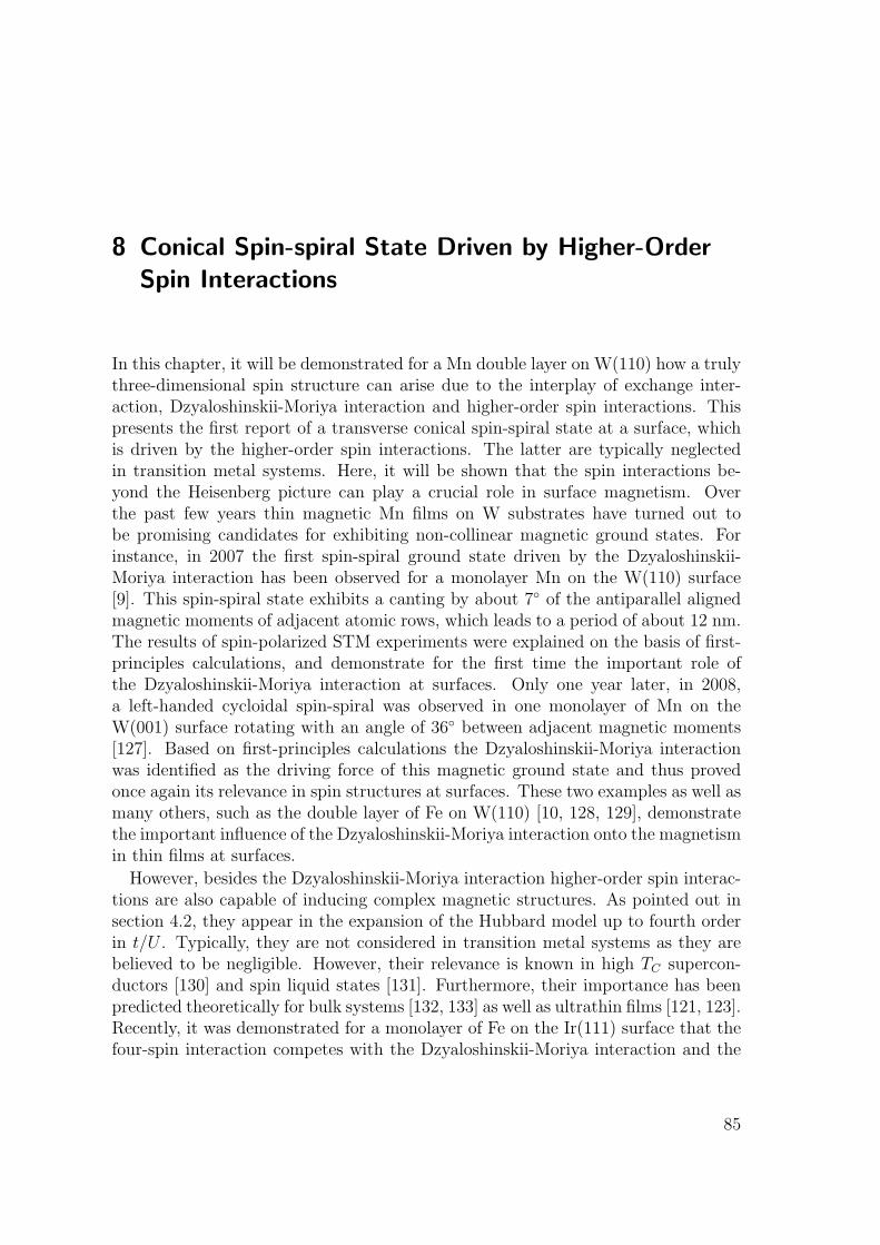
8 Conical Spin-spiral State Driven by Higher-OrderSpin Interactions
In this chapter, it will be demonstrated for a Mn double layer on W(110) how a trulythree-dimensional spin structure can arise due to the interplay of exchange inter-action, Dzyaloshinskii-Moriya interaction and higher-order spin interactions. Thispresents the first report of a transverse conical spin-spiral state at a surface, whichis driven by the higher-order spin interactions. The latter are typically neglectedin transition metal systems. Here, it will be shown that the spin interactions be-yond the Heisenberg picture can play a crucial role in surface magnetism. Overthe past few years thin magnetic Mn films on W substrates have turned out tobe promising candidates for exhibiting non-collinear magnetic ground states. Forinstance, in 2007 the first spin-spiral ground state driven by the Dzyaloshinskii-Moriya interaction has been observed for a monolayer Mn on the W(110) surface[9]. This spin-spiral state exhibits a canting by about 7 of the antiparallel alignedmagnetic moments of adjacent atomic rows, which leads to a period of about 12 nm.The results of spin-polarized STM experiments were explained on the basis of first-principles calculations, and demonstrate for the first time the important role ofthe Dzyaloshinskii-Moriya interaction at surfaces. Only one year later, in 2008,a left-handed cycloidal spin-spiral was observed in one monolayer of Mn on theW(001) surface rotating with an angle of 36 between adjacent magnetic moments[127]. Based on first-principles calculations the Dzyaloshinskii-Moriya interactionwas identified as the driving force of this magnetic ground state and thus provedonce again its relevance in spin structures at surfaces. These two examples as well asmany others, such as the double layer of Fe on W(110) [10, 128, 129], demonstratethe important influence of the Dzyaloshinskii-Moriya interaction onto the magnetismin thin films at surfaces.
However, besides the Dzyaloshinskii-Moriya interaction higher-order spin interac-tions are also capable of inducing complex magnetic structures. As pointed out insection 4.2, they appear in the expansion of the Hubbard model up to fourth orderin t/U . Typically, they are not considered in transition metal systems as they arebelieved to be negligible. However, their relevance is known in high TC supercon-ductors [130] and spin liquid states [131]. Furthermore, their importance has beenpredicted theoretically for bulk systems [132, 133] as well as ultrathin films [121, 123].Recently, it was demonstrated for a monolayer of Fe on the Ir(111) surface that thefour-spin interaction competes with the Dzyaloshinskii-Moriya interaction and the
85
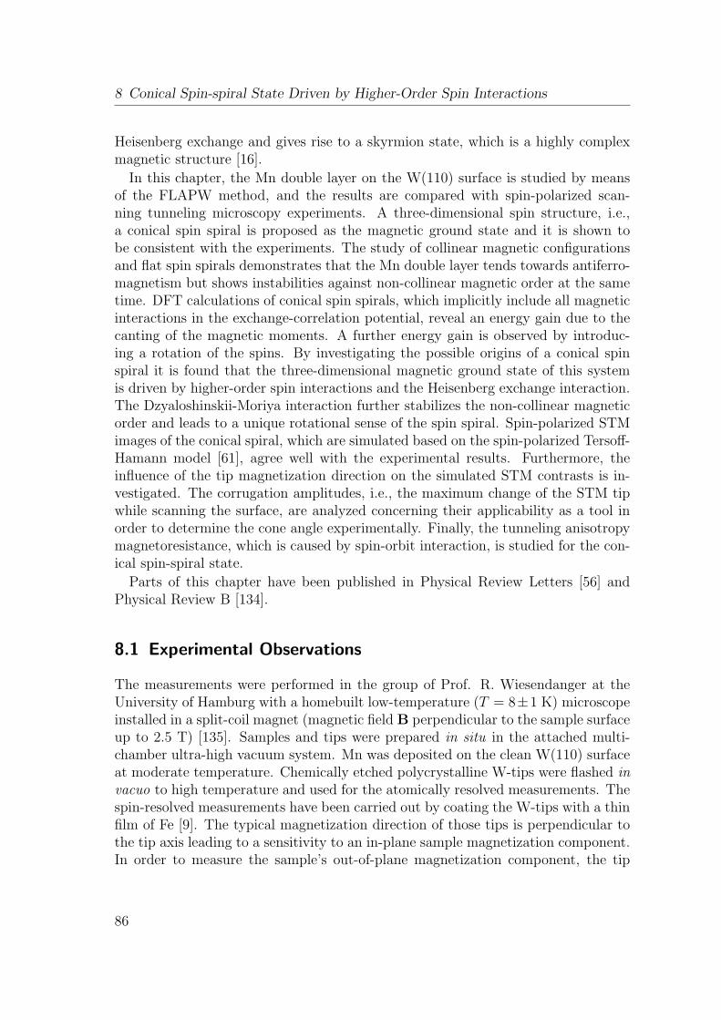
8 Conical Spin-spiral State Driven by Higher-Order Spin Interactions
Heisenberg exchange and gives rise to a skyrmion state, which is a highly complexmagnetic structure [16].
In this chapter, the Mn double layer on the W(110) surface is studied by meansof the FLAPW method, and the results are compared with spin-polarized scan-ning tunneling microscopy experiments. A three-dimensional spin structure, i.e.,a conical spin spiral is proposed as the magnetic ground state and it is shown tobe consistent with the experiments. The study of collinear magnetic configurationsand flat spin spirals demonstrates that the Mn double layer tends towards antiferro-magnetism but shows instabilities against non-collinear magnetic order at the sametime. DFT calculations of conical spin spirals, which implicitly include all magneticinteractions in the exchange-correlation potential, reveal an energy gain due to thecanting of the magnetic moments. A further energy gain is observed by introduc-ing a rotation of the spins. By investigating the possible origins of a conical spinspiral it is found that the three-dimensional magnetic ground state of this systemis driven by higher-order spin interactions and the Heisenberg exchange interaction.The Dzyaloshinskii-Moriya interaction further stabilizes the non-collinear magneticorder and leads to a unique rotational sense of the spin spiral. Spin-polarized STMimages of the conical spiral, which are simulated based on the spin-polarized Tersoff-Hamann model [61], agree well with the experimental results. Furthermore, theinfluence of the tip magnetization direction on the simulated STM contrasts is in-vestigated. The corrugation amplitudes, i.e., the maximum change of the STM tipwhile scanning the surface, are analyzed concerning their applicability as a tool inorder to determine the cone angle experimentally. Finally, the tunneling anisotropymagnetoresistance, which is caused by spin-orbit interaction, is studied for the con-ical spin-spiral state.
Parts of this chapter have been published in Physical Review Letters [56] andPhysical Review B [134].
8.1 Experimental Observations
The measurements were performed in the group of Prof. R. Wiesendanger at theUniversity of Hamburg with a homebuilt low-temperature (T = 8±1 K) microscopeinstalled in a split-coil magnet (magnetic field B perpendicular to the sample surfaceup to 2.5 T) [135]. Samples and tips were prepared in situ in the attached multi-chamber ultra-high vacuum system. Mn was deposited on the clean W(110) surfaceat moderate temperature. Chemically etched polycrystalline W-tips were flashed invacuo to high temperature and used for the atomically resolved measurements. Thespin-resolved measurements have been carried out by coating the W-tips with a thinfilm of Fe [9]. The typical magnetization direction of those tips is perpendicular tothe tip axis leading to a sensitivity to an in-plane sample magnetization component.In order to measure the sample’s out-of-plane magnetization component, the tip
86
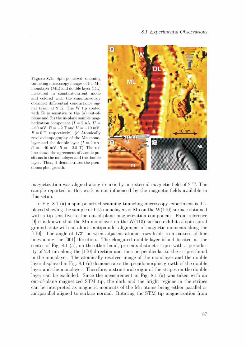
8.1 Experimental Observations
Figure 8.1: Spin-polarized scanningtunneling microscopy images of the Mnmonolayer (ML) and double layer (DL)measured in constant-current modeand colored with the simultaneouslyobtained differential conductance sig-nal taken at 9 K. The W tip coatedwith Fe is sensitive to the (a) out-of-plane and (b) the in-plane sample mag-netization component (I = 2 nA, U =+60 mV, B = +2 T and U = +10 mV,B = 0 T, respectively). (c) Atomicallyresolved topography of the Mn mono-layer and the double layer (I = 2 nA,U = −40 mV, B = −2.5 T). The redline shows the agreement of atomic po-sitions in the monolayer and the doublelayer. Thus, it demonstrates the pseu-domorphic growth.
magnetization was aligned along its axis by an external magnetic field of 2 T. Thesample reported in this work is not influenced by the magnetic fields available inthis setup.
In Fig. 8.1 (a) a spin-polarized scanning tunneling microscopy experiment is dis-played showing the sample of 1.15 monolayers of Mn on the W(110) surface obtainedwith a tip sensitive to the out-of-plane magnetization component. From reference[9] it is known that the Mn monolayer on the W(110) surface exhibits a spin-spiralground state with an almost antiparallel alignment of magnetic moments along the[110]. The angle of 173 between adjacent atomic rows leads to a pattern of finelines along the [001] direction. The elongated double-layer island located at thecenter of Fig. 8.1 (a), on the other hand, presents distinct stripes with a periodic-ity of 2.4 nm along the [110] direction and thus perpendicular to the stripes foundin the monolayer. The atomically resolved image of the monolayer and the doublelayer displayed in Fig. 8.1 (c) demonstrates the pseudomorphic growth of the doublelayer and the monolayer. Therefore, a structural origin of the stripes on the doublelayer can be excluded. Since the measurement in Fig. 8.1 (a) was taken with anout-of-plane magnetized STM tip, the dark and the bright regions in the stripescan be interpreted as magnetic moments of the Mn atoms being either parallel orantiparallel aligned to surface normal. Rotating the STM tip magnetization from
87
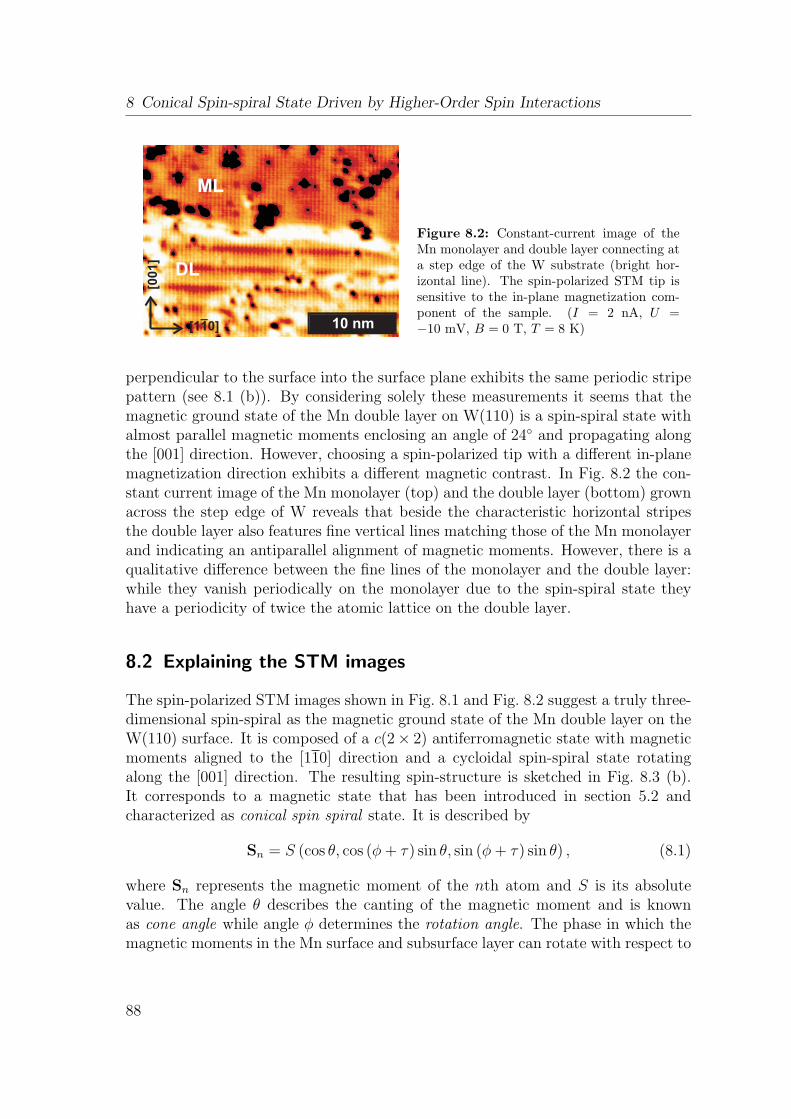
8 Conical Spin-spiral State Driven by Higher-Order Spin Interactions
Figure 8.2: Constant-current image of theMn monolayer and double layer connecting ata step edge of the W substrate (bright hor-izontal line). The spin-polarized STM tip issensitive to the in-plane magnetization com-ponent of the sample. (I = 2 nA, U =−10 mV, B = 0 T, T = 8 K)
perpendicular to the surface into the surface plane exhibits the same periodic stripepattern (see 8.1 (b)). By considering solely these measurements it seems that themagnetic ground state of the Mn double layer on W(110) is a spin-spiral state withalmost parallel magnetic moments enclosing an angle of 24 and propagating alongthe [001] direction. However, choosing a spin-polarized tip with a different in-planemagnetization direction exhibits a different magnetic contrast. In Fig. 8.2 the con-stant current image of the Mn monolayer (top) and the double layer (bottom) grownacross the step edge of W reveals that beside the characteristic horizontal stripesthe double layer also features fine vertical lines matching those of the Mn monolayerand indicating an antiparallel alignment of magnetic moments. However, there is aqualitative difference between the fine lines of the monolayer and the double layer:while they vanish periodically on the monolayer due to the spin-spiral state theyhave a periodicity of twice the atomic lattice on the double layer.
8.2 Explaining the STM images
The spin-polarized STM images shown in Fig. 8.1 and Fig. 8.2 suggest a truly three-dimensional spin-spiral as the magnetic ground state of the Mn double layer on theW(110) surface. It is composed of a c(2 × 2) antiferromagnetic state with magneticmoments aligned to the [110] direction and a cycloidal spin-spiral state rotatingalong the [001] direction. The resulting spin-structure is sketched in Fig. 8.3 (b).It corresponds to a magnetic state that has been introduced in section 5.2 andcharacterized as conical spin spiral state. It is described by
Sn = S (cos θ, cos (ϕ+ τ) sin θ, sin (ϕ+ τ) sin θ) , (8.1)
where Sn represents the magnetic moment of the nth atom and S is its absolutevalue. The angle θ describes the canting of the magnetic moment and is knownas cone angle while angle ϕ determines the rotation angle. The phase in which themagnetic moments in the Mn surface and subsurface layer can rotate with respect to
88
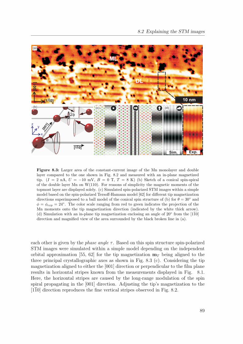
8.2 Explaining the STM images
Figure 8.3: Larger area of the constant-current image of the Mn monolayer and doublelayer compared to the one shown in Fig. 8.2 and measured with an in-plane magnetizedtip. (I = 2 nA, U = −10 mV, B = 0 T, T = 8 K) (b) Sketch of a conical spin-spiralof the double layer Mn on W(110). For reasons of simplicity the magnetic moments of thetopmost layer are displayed solely. (c) Simulated spin-polarized STM images within a simplemodel based on the spin-polarized Tersoff-Hamann model [62] for different tip magnetizationdirections superimposed to a ball model of the conical spin structure of (b) for θ = 30 andϕ = ϕexp = 24. The color scale ranging from red to green indicates the projection of theMn moments onto the tip magnetization direction (indicated by the white thick arrow).(d) Simulation with an in-plane tip magnetization enclosing an angle of 20 from the [110]direction and magnified view of the area surrounded by the black broken line in (a).
each other is given by the phase angle τ . Based on this spin structure spin-polarizedSTM images were simulated within a simple model depending on the independentorbital approximation [55, 62] for the tip magnetization mT being aligned to thethree principal crystallographic axes as shown in Fig. 8.3 (c). Considering the tipmagnetization aligned to either the [001] direction or perpendicular to the film planeresults in horizontal stripes known from the measurements displayed in Fig. 8.1.Here, the horizontal stripes are caused by the long-range modulation of the spinspiral propagating in the [001] direction. Adjusting the tip’s magnetization to the[110] direction reproduces the fine vertical stripes observed in Fig. 8.2.
89
8 Conical Spin-spiral State Driven by Higher-Order Spin Interactions
Since in a STM experiment without external magnetic field the tip magnetizationdirection cannot be assigned to coincide with one of the principal axes, further spin-polarized STM images have been simulated with a slightly canted tip as it is shownin Fig. 8.3 (d). The canting of the magnetization component of the tip leads to asuperposition of the contrasts obtained for the [110] and the [001] direction, respec-tively. Therefore, the resulting spin-polarized STM image contains the fine stripesalong [001] as well as the long-range modulation producing the (horizontal) stripesalong [110]. Such a contrast is in good agreement with the experimental observa-tions and thus the proposed conical spin-spiral state can explain the measurements.However, the question arises what is the mechanism of such an intriguing magneticstate, which has not been discovered before at a surface. In order to tackle this prob-lem, first-principles calculations of the electronic structure have been performed asdescribed in the following sections.
8.3 Computational Details
The first-principles calculations have been carried out applying the FLAPW methodand using the experimental lattice constant of W (a = 3.165 A). For the collinearcalculations an asymmetric film was considered consisting of seven layers of W andtwo layers on Mn. A wavevector cut-off of kmax = 3.6 a.u.−1 has been used for thebasis functions, and 24 k∥ points in the irreducible wedge of the two-dimensionalBrillouin zone have been employed. The structural relaxations have been performedby means of force minimization within the GGA [33]. The energetically most favor-able collinear calculation was found to be the row-wise antiferromagnetic II state (seeFig. 8.4) with an inward relaxed distance by 2.5% between the W-interface and theMn subsurface layer corresponding to an interlayer distance of dW−Mn = 2.180 A.The interlayer distance between the Mn subsurface and the Mn surface layer isdMn−Mn = 1.998 A corresponding to an inward relaxation of 10.6%. The magneticproperties as well as the spin-spiral calculations have been examined within the LDA[122].
The flat spin-spirals were calculated scalar-relativistically using the structuralrelaxations of the row-wise antiferromagnetic II state and an asymmetric film offive layers of W and two layers of Mn. In order to calculate the spin spirals self-consistently, the generalized Bloch theorem has been employed [79, 80, 81]. Calcu-lations with a film consisting of seven layers of W and two layers of Mn have beenperformed to test the influence of the slab thickness. However, the results werefound to be in good agreement with the results for the seven layer film. The 484 k∥points were distributed in the entire two-dimensional Brillouin zone of the p(1 × 1)unit cell for the full energy dispersion plotted in Fig. 8.5 (a). Spin spirals close tothe row-wise antiferromagnetic II state (see inset in Fig. 8.5(a)) have been computedusing a mesh of 961 k∥ points. For the flat spin-spirals the wave vector cut-off has
90
8.4 Magnetic Properties of the Mn Double Layer on W(110)
been kmax = 3.6 a.u.−1.
Calculations of the conical spin spirals have been carried out in the c(2 × 2) unitcell (compare with Fig. 8.4) using an asymmetric film comprising seven layers of Wwith two layers of Mn on top. 280 k∥ points have been employed and the wave-vector cut-off was kmax = 3.6 a.u.−1. Convergence tests concerning k-point densityand wave-vector cut-offs have been made for 560 k∥ points and kmax = 3.8 a.u.−1
giving the same results.
Spin-orbit coupling was taken into account in second variation [105] for collinearconfigurations in order to obtain the magneto-crystalline anisotropy energy using1260 k∥ points in the full two-dimensional Brillouin zone. The Dzyaloshinskii-Moriyainteraction has been considered by treating the SOC in first order perturbation fornon-collinear magnetic structures as introduced in section 6.6 [112]. Starting fromthe self-consistently calculated spin spirals, the Dzyaloshinskii-Moriya interactionhas been obtained by using 2025 k∥ points for flat spin spirals and 1026 k∥ pointsfor conical spin-spirals. The computation of the local density of states in the vacuumhas been accomplished making use of 280 k∥ points and kmax = 3.8 a.u.−1.
8.4 Magnetic Properties of the Mn Double Layer on W(110)
A first step towards understanding the magnetic properties of the Mn double layeron the W(110) surface is taken by studying the collinear configurations illustratedin Fig. 8.4. There are four configurations: (i) the ferromagnetic configuration (FM)with all magnetic moments aligned parallel, (ii) the layered antiferromagnetic config-uration (LAFM), where the magnetic moments within one layer align parallel whilethe layers couple antiparallel, and two row-wise antiferromagnetic structures formedby an antiferromagnetic checkerboard arrangement in each Mn layer resulting ineither (iii) a parallel (RW-AFM I) or (iv) an antiparallel alignment (RW-AFM II)of the magnetic moments along the [001] direction.
From the total energy calculations it becomes clear that the Mn double layerprefers an antiparallel alignment of the atoms since the RW-AFM II state is lowestin energy. The LAFM state (∆E = +34 meV) and the RW-AFM I state (∆E =+62 meV) are higher in energy but still energetically more favorable than the FMstate (∆E = +137 meV). This is further reflected in the exchange constants up tothe third neighbor, which were extracted from these total energy differences. Theyresult in J1 = −20.6 meV for the interlayer nearest-neighbor exchange, J2,eff =−6.9 meV for the intralayer nearest-neighbor exchange and J3 = −5.2 meV for theinterlayer next-nearest-neighbor exchange (cf. Fig 8.4). The negative values indicatea tendency towards antiferromagnetism within the Heisenberg model.
Furthermore, by including the SOC into the calculations the magneto-crystallineanisotropy of this system is obtained. It was found that for the RW-AFM II statethe preferred magnetization axis (easy axis) is the [110] direction. Aligning the
91
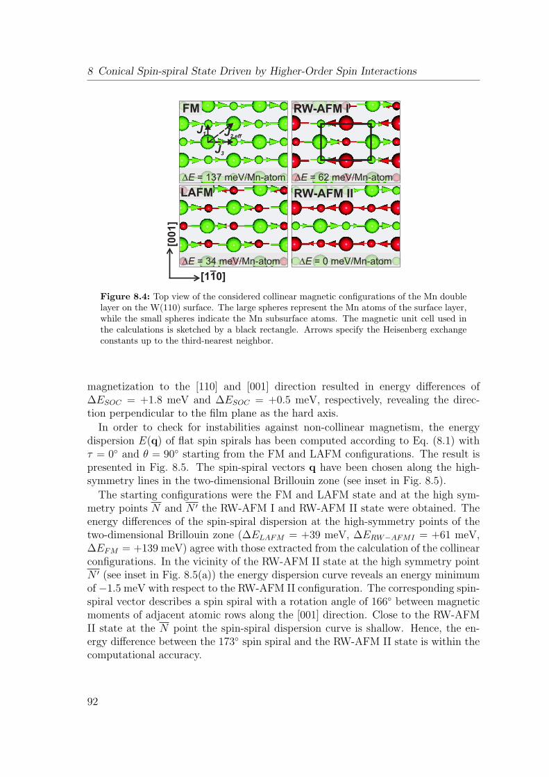
8 Conical Spin-spiral State Driven by Higher-Order Spin Interactions
J2,eff
Figure 8.4: Top view of the considered collinear magnetic configurations of the Mn doublelayer on the W(110) surface. The large spheres represent the Mn atoms of the surface layer,while the small spheres indicate the Mn subsurface atoms. The magnetic unit cell used inthe calculations is sketched by a black rectangle. Arrows specify the Heisenberg exchangeconstants up to the third-nearest neighbor.
magnetization to the [110] and [001] direction resulted in energy differences of∆ESOC = +1.8 meV and ∆ESOC = +0.5 meV, respectively, revealing the direc-tion perpendicular to the film plane as the hard axis.
In order to check for instabilities against non-collinear magnetism, the energydispersion E(q) of flat spin spirals has been computed according to Eq. (8.1) withτ = 0 and θ = 90 starting from the FM and LAFM configurations. The result ispresented in Fig. 8.5. The spin-spiral vectors q have been chosen along the high-symmetry lines in the two-dimensional Brillouin zone (see inset in Fig. 8.5).
The starting configurations were the FM and LAFM state and at the high sym-metry points N and N ′ the RW-AFM I and RW-AFM II state were obtained. Theenergy differences of the spin-spiral dispersion at the high-symmetry points of thetwo-dimensional Brillouin zone (∆ELAFM = +39 meV, ∆ERW−AFMI = +61 meV,∆EFM = +139 meV) agree with those extracted from the calculation of the collinearconfigurations. In the vicinity of the RW-AFM II state at the high symmetry pointN ′ (see inset in Fig. 8.5(a)) the energy dispersion curve reveals an energy minimumof −1.5 meV with respect to the RW-AFM II configuration. The corresponding spin-spiral vector describes a spin spiral with a rotation angle of 166 between magneticmoments of adjacent atomic rows along the [001] direction. Close to the RW-AFMII state at the N point the spin-spiral dispersion curve is shallow. Hence, the en-ergy difference between the 173 spin spiral and the RW-AFM II state is within thecomputational accuracy.
92
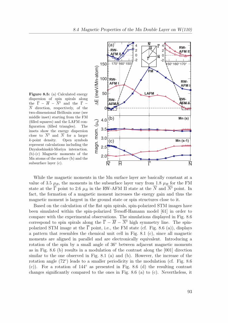
8.4 Magnetic Properties of the Mn Double Layer on W(110)
Figure 8.5: (a) Calculated energydispersion of spin spirals alongthe Γ − H − N ′ and the Γ −N direction, respectively, of thetwo-dimensional Brillouin zone (seemiddle inset) starting from the FM(filled squares) and the LAFM con-figuration (filled triangles). Theinsets show the energy dispersionclose to N ′ and N for a largerk-point density. Open symbolsrepresent calculations including theDzyaloshinskii-Moriya interaction.(b)-(c) Magnetic moments of theMn atoms of the surface (b) and thesubsurface layer (c).
DE
(m
eV
/Mn-a
tom
)
RW-AFM I
RW-AFM II
LAFM
FM
RW-AFM I
RW-AFM II
G
GN
H
NI
NI
G NH
RW-AFM II
RW-AFM II
magn. m
om
. (
)m
B
Mn (s)
Mn (s-1)(c)
(b)
(a)
While the magnetic moments in the Mn surface layer are basically constant at avalue of 3.5 µB, the moments in the subsurface layer vary from 1.8 µB for the FMstate at the Γ point to 2.6 µB in the RW-AFM II state at the N and N ′ point. Infact, the formation of a magnetic moment increases the energy gain and thus themagnetic moment is largest in the ground state or spin structures close to it.
Based on the calculation of the flat spin spirals, spin-polarized STM images havebeen simulated within the spin-polarized Tersoff-Hamann model [61] in order tocompare with the experimental observations. The simulations displayed in Fig. 8.6correspond to spin spirals along the Γ − H − N ′ high symmetry line. The spin-polarized STM image at the Γ point, i.e., the FM state (cf. Fig. 8.6 (a)), displaysa pattern that resembles the chemical unit cell in Fig. 8.1 (c), since all magneticmoments are aligned in parallel and are electronically equivalent. Introducing arotation of the spin by a small angle of 36 between adjacent magnetic momentsas in Fig. 8.6 (b) results in a modulation of the contrast along the [001] directionsimilar to the one observed in Fig. 8.1 (a) and (b). However, the increase of therotation angle (72) leads to a smaller periodicity in the modulation (cf. Fig. 8.6(c)). For a rotation of 144 as presented in Fig. 8.6 (d) the resulting contrastchanges significantly compared to the ones in Fig. 8.6 (a) to (c). Nevertheless, it
93
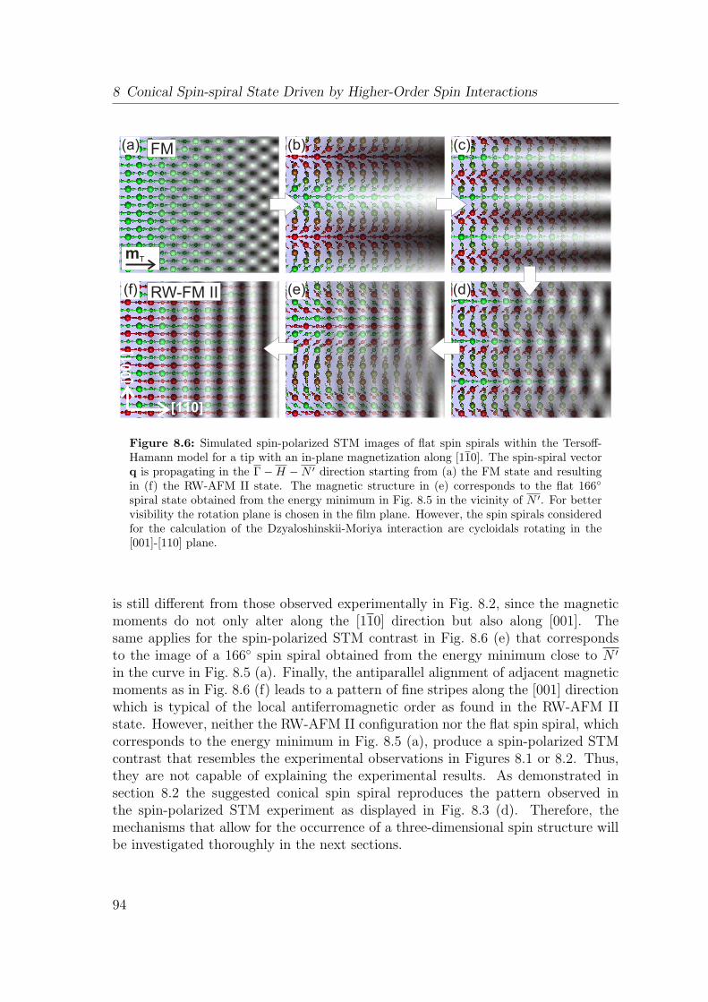
8 Conical Spin-spiral State Driven by Higher-Order Spin Interactions
(a)
(f)
(b) (c)
(e) (d)
[00
1]
[1 0]1
Figure 8.6: Simulated spin-polarized STM images of flat spin spirals within the Tersoff-Hamann model for a tip with an in-plane magnetization along [110]. The spin-spiral vectorq is propagating in the Γ−H −N ′ direction starting from (a) the FM state and resultingin (f) the RW-AFM II state. The magnetic structure in (e) corresponds to the flat 166
spiral state obtained from the energy minimum in Fig. 8.5 in the vicinity of N ′. For bettervisibility the rotation plane is chosen in the film plane. However, the spin spirals consideredfor the calculation of the Dzyaloshinskii-Moriya interaction are cycloidals rotating in the[001]-[110] plane.
is still different from those observed experimentally in Fig. 8.2, since the magneticmoments do not only alter along the [110] direction but also along [001]. Thesame applies for the spin-polarized STM contrast in Fig. 8.6 (e) that correspondsto the image of a 166 spin spiral obtained from the energy minimum close to N ′
in the curve in Fig. 8.5 (a). Finally, the antiparallel alignment of adjacent magneticmoments as in Fig. 8.6 (f) leads to a pattern of fine stripes along the [001] directionwhich is typical of the local antiferromagnetic order as found in the RW-AFM IIstate. However, neither the RW-AFM II configuration nor the flat spin spiral, whichcorresponds to the energy minimum in Fig. 8.5 (a), produce a spin-polarized STMcontrast that resembles the experimental observations in Figures 8.1 or 8.2. Thus,they are not capable of explaining the experimental results. As demonstrated insection 8.2 the suggested conical spin spiral reproduces the pattern observed inthe spin-polarized STM experiment as displayed in Fig. 8.3 (d). Therefore, themechanisms that allow for the occurrence of a three-dimensional spin structure willbe investigated thoroughly in the next sections.
94
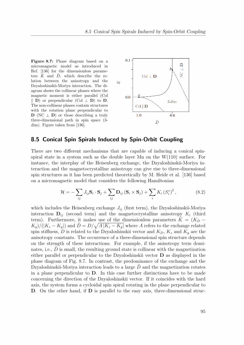
8.5 Conical Spin Spirals Induced by Spin-Orbit Coupling
Figure 8.7: Phase diagram based on amicromagnetic model as introduced inRef. [136] for the dimensionless parame-ters K and D, which describe the re-lation between the anisotropy and theDzyaloshinskii-Moriya interaction. The di-agram shows the collinear phases where themagnetic moment is either parallel (Col∥ D) or perpendicular (Col ⊥ D) to D.The non-collinear phases contain structureswith the rotation plane perpendicular toD (NC ⊥ D) or those describing a trulythree-dimensional path in spin space (3-dim). Figure taken from [136].
8.5 Conical Spin Spirals Induced by Spin-Orbit Coupling
There are two different mechanisms that are capable of inducing a conical spin-spiral state in a system such as the double layer Mn on the W(110) surface. Forinstance, the interplay of the Heisenberg exchange, the Dzyaloshinskii-Moriya in-teraction and the magnetocrystalline anisotropy can give rise to three-dimensionalspin structures as it has been predicted theoretically by M. Heide et al. [136] basedon a micromagnetic model that considers the following Hamiltonian
H = −∑ij
JijSi · Sj +∑ij
Dij (Si × Sj) +∑i
Ki (Szi )2 , (8.2)
which includes the Heisenberg exchange Jij (first term), the Dzyaloshinskii-Moriyainteraction Dij (second term) and the magnetocrystalline anisotropy Ki (thirdterm). Furthermore, it makes use of the dimensionless parameters K = (KD −Ky)/(|Kz −Ky|) and D = D/
√A |Kz −Ky| where A refers to the exchange related
spin stiffness, D is related to the Dzyaloshinskii vector and KD, Kz and Ky are theanisotropy constants. The occurrence of a three-dimensional spin structure dependson the strength of these interactions. For example, if the anisotropy term domi-nates, i.e., D is small, the resulting ground state is collinear with the magnetizationeither parallel or perpendicular to the Dzyaloshinskii vector D as displayed in thephase diagram of Fig. 8.7. In contrast, the predominance of the exchange and theDzyaloshinskii-Moriya interaction leads to a large D and the magnetization rotatesin a plane perpendicular to D. In this case further distinctions have to be madeconcerning the direction of the Dzyaloshinskii vector. If it coincides with the hardaxis, the system forms a cycloidal spin spiral rotating in the plane perpendicular toD. On the other hand, if D is parallel to the easy axis, three-dimensional struc-
95
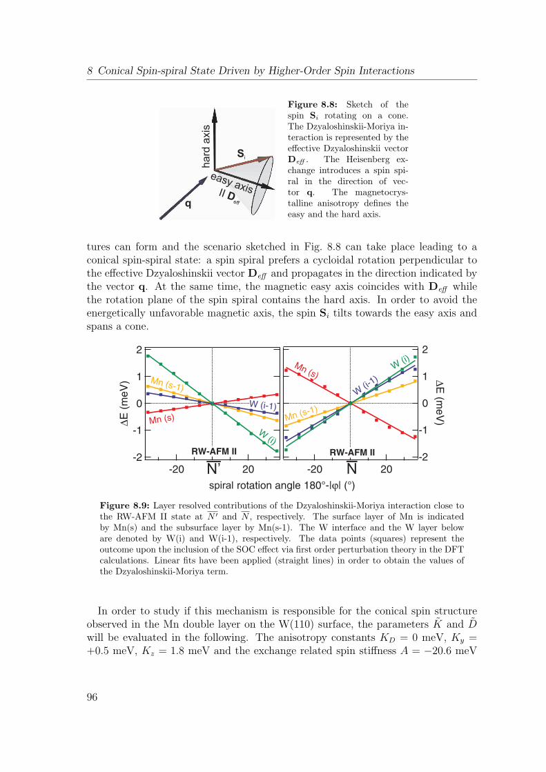
8 Conical Spin-spiral State Driven by Higher-Order Spin Interactions
ha
rd a
xis
easy axis
q
Si
II Deff
Figure 8.8: Sketch of thespin Si rotating on a cone.The Dzyaloshinskii-Moriya in-teraction is represented by theeffective Dzyaloshinskii vectorDeff . The Heisenberg ex-change introduces a spin spi-ral in the direction of vec-tor q. The magnetocrys-talline anisotropy defines theeasy and the hard axis.
tures can form and the scenario sketched in Fig. 8.8 can take place leading to aconical spin-spiral state: a spin spiral prefers a cycloidal rotation perpendicular tothe effective Dzyaloshinskii vector Deff and propagates in the direction indicated bythe vector q. At the same time, the magnetic easy axis coincides with Deff whilethe rotation plane of the spin spiral contains the hard axis. In order to avoid theenergetically unfavorable magnetic axis, the spin Si tilts towards the easy axis andspans a cone.
spiral
N’ N
Figure 8.9: Layer resolved contributions of the Dzyaloshinskii-Moriya interaction close tothe RW-AFM II state at N ′ and N , respectively. The surface layer of Mn is indicatedby Mn(s) and the subsurface layer by Mn(s-1). The W interface and the W layer beloware denoted by W(i) and W(i-1), respectively. The data points (squares) represent theoutcome upon the inclusion of the SOC effect via first order perturbation theory in the DFTcalculations. Linear fits have been applied (straight lines) in order to obtain the values ofthe Dzyaloshinskii-Moriya term.
In order to study if this mechanism is responsible for the conical spin structureobserved in the Mn double layer on the W(110) surface, the parameters K and Dwill be evaluated in the following. The anisotropy constants KD = 0 meV, Ky =+0.5 meV, Kz = 1.8 meV and the exchange related spin stiffness A = −20.6 meV
96
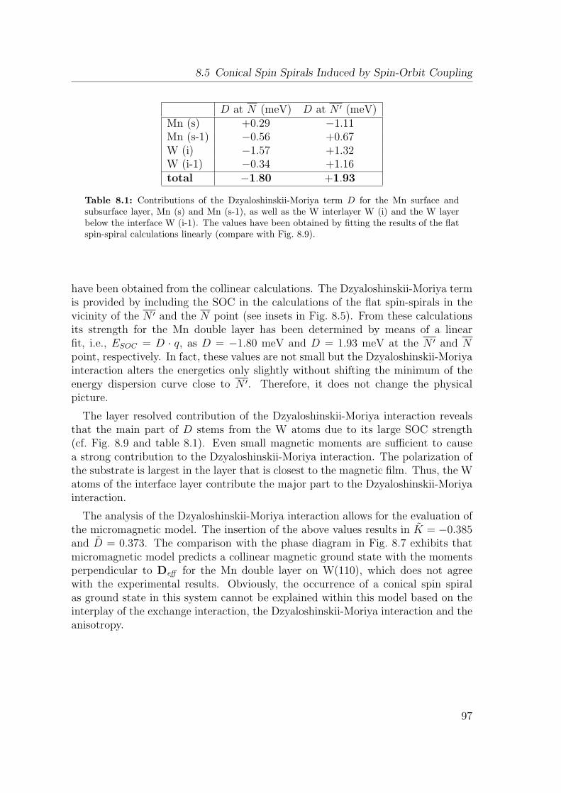
8.5 Conical Spin Spirals Induced by Spin-Orbit Coupling
D at N (meV) D at N ′ (meV)Mn (s) +0.29 −1.11Mn (s-1) −0.56 +0.67W (i) −1.57 +1.32W (i-1) −0.34 +1.16total −1.80 +1.93
Table 8.1: Contributions of the Dzyaloshinskii-Moriya term D for the Mn surface andsubsurface layer, Mn (s) and Mn (s-1), as well as the W interlayer W (i) and the W layerbelow the interface W (i-1). The values have been obtained by fitting the results of the flatspin-spiral calculations linearly (compare with Fig. 8.9).
have been obtained from the collinear calculations. The Dzyaloshinskii-Moriya termis provided by including the SOC in the calculations of the flat spin-spirals in thevicinity of the N ′ and the N point (see insets in Fig. 8.5). From these calculationsits strength for the Mn double layer has been determined by means of a linearfit, i.e., ESOC = D · q, as D = −1.80 meV and D = 1.93 meV at the N ′ and Npoint, respectively. In fact, these values are not small but the Dzyaloshinskii-Moriyainteraction alters the energetics only slightly without shifting the minimum of theenergy dispersion curve close to N ′. Therefore, it does not change the physicalpicture.
The layer resolved contribution of the Dzyaloshinskii-Moriya interaction revealsthat the main part of D stems from the W atoms due to its large SOC strength(cf. Fig. 8.9 and table 8.1). Even small magnetic moments are sufficient to causea strong contribution to the Dzyaloshinskii-Moriya interaction. The polarization ofthe substrate is largest in the layer that is closest to the magnetic film. Thus, the Watoms of the interface layer contribute the major part to the Dzyaloshinskii-Moriyainteraction.
The analysis of the Dzyaloshinskii-Moriya interaction allows for the evaluation ofthe micromagnetic model. The insertion of the above values results in K = −0.385and D = 0.373. The comparison with the phase diagram in Fig. 8.7 exhibits thatmicromagnetic model predicts a collinear magnetic ground state with the momentsperpendicular to Deff for the Mn double layer on W(110), which does not agreewith the experimental results. Obviously, the occurrence of a conical spin spiralas ground state in this system cannot be explained within this model based on theinterplay of the exchange interaction, the Dzyaloshinskii-Moriya interaction and theanisotropy.
97

8 Conical Spin-spiral State Driven by Higher-Order Spin Interactions
8.6 Conical Spin Spirals Induced by Higher-Order SpinInteractions
The conical spin spiral observed in the Mn double layer on W(110) is evidently notdue to the mechanism introduced in the previous section. However, as pointed out insections 4.2 and 7.3, spin interactions beyond the Heisenberg exchange, namely thebiquadratic and the four-spin interaction, can lift the degeneracy of spin structuresthat are energetically equivalent within the Heisenberg picture. These interactionsrepresent the second mechanism that could give rise to a conical spin-spiral groundstate. For transition metal systems it has been shown theoretically that the higher-order spin interactions are important in bulk systems [132, 133] and in ultrathinfilms [121, 123, 137]. Furthermore, the crucial role of the four-spin interaction insurface magnetism has been recently demonstrated in theory and experiment for anFe monolayer on the Ir(111) surface [16].
In order to check whether conical spin spirals can indeed be more favorable thanthe RW-AFM II state or flat spin spirals, their total energy has been directly calcu-lated using the FLAPW method. Since the spin structure suggested by the experi-ment is an antiferromagnetic configuration superimposed to a spin-spiral state, thecalculations require a c (2 × 2) unit cell as it is indicated in Fig. 8.10. In this casethe starting configuration is the RW-AFM II state. In a first step, only the cantingof the magnetic moment with respect to the surface plane will be considered. Therotation due to the spin spiral will be introduced afterwards based on the optimumcanting angle.
As a start, the magnetic moments, which are aligned along the [110] direction,are canted with respect to the film plane by the angle θ (see sketch in Fig. 8.10)while taking into account the phase angle τ (compare with Eq. (8.1)) between themoments in the surface and the subsurface layer. Assigning the value of τ to 0, 90
and 180 results in the configurations I to III sketched in the upper row of Fig. 8.10(a) to (c).
Upon canting of the magnetic moments an energy minimum is observed for con-figuration I (Fig. 8.10 (a)), i.e., τ = 0, and a cone angle of θ = 30 (see Fig. 8.11).It is by 10.0 meV/Mn-atom lower in energy than the RW-AFM II state. For con-figuration II (Fig. 8.10 (b)), i.e., τ = 90, the energy gain is 8.4 meV/Mn-atom forθ = 25.. Configuration III (Fig. 8.10 (c)), i.e., τ = 180, has the overall smallestenergy gain with 5.1 meV/Mn-atom for θ = 30..
In order to identify the interaction giving rise to the canting of the magnetic mo-ments, the total energy of the DFT calculations, in which all magnetic interactionsare implicitly included in the exchange-correlation potential, can be mapped to amodel that includes the Heisenberg exchange as well as the higher-order spin inter-actions. Since the Heisenberg exchange is constant for all pairs of parallel magneticmoments Si and Sj in the RW-AFM II state (see Fig. 8.4), the energy change for
98
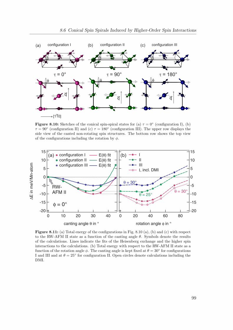
8.6 Conical Spin Spirals Induced by Higher-Order Spin Interactions
(a) (b)
[1 0]1
q
q
f
q
q
f
q
q
f
(c)
t = 0° t = 90° t = 180°
configuration I configuration II configuration III
Figure 8.10: Sketches of the conical spin-spiral states for (a) τ = 0 (configuration I), (b)τ = 90 (configuration II) and (c) τ = 180 (configuration III). The upper row displays theside view of the canted non-rotating spin structures. The bottom row shows the top viewof the configurations including the rotation by ϕ.
(a) (b)configuration I
configuration II
configuration III
I
II
III
I
Figure 8.11: (a) Total energy of the configurations in Fig. 8.10 (a), (b) and (c) with respectto the RW-AFM II state as a function of the canting angle θ. Symbols denote the resultsof the calculations. Lines indicate the fits of the Heisenberg exchange and the higher spininteractions to the calculations. (b) Total energy with respect to the RW-AFM II state as afunction of the rotation angle ϕ. The canting angle is kept fixed at θ = 30 for configurationsI and III and at θ = 25 for configuration II. Open circles denote calculations including theDMI.
99
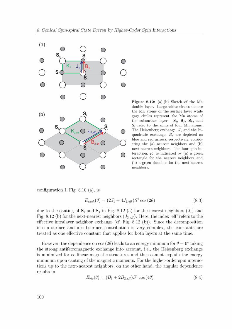
8 Conical Spin-spiral State Driven by Higher-Order Spin Interactions
Si
Sk
Sl
Sj
Si
Sk
SlSj
(a)
(b)
J1 B1K1
J2,eff
B2,eff
K2,eff
Figure 8.12: (a),(b) Sketch of the Mndouble layer. Large white circles denotethe Mn atoms of the surface layer whilegray circles represent the Mn atoms ofthe subsurface layer. Si, Sj , Sk, andSl refer to the spins of four Mn atoms.The Heisenberg exchange, J , and the bi-quadratic exchange, B, are depicted asblue and red arrows, respectively, consid-ering the (a) nearest neighbors and (b)next-nearest neighbors. The four-spin in-teraction, K, is indicated by (a) a greenrectangle for the nearest neighbors and(b) a green rhombus for the next-nearestneighbors.
configuration I, Fig. 8.10 (a), is
Eexch(θ) = (2J1 + 4J2,eff )S2 cos (2θ) (8.3)
due to the canting of Si and Sj in Fig. 8.12 (a) for the nearest neighbors (J1) andFig. 8.12 (b) for the next-nearest neighbors (J2,eff ). Here, the index ’eff’ refers to theeffective intralayer neighbor exchange (cf. Fig. 8.12 (b)). Since the decompositioninto a surface and a subsurface contribution is very complex, the constants aretreated as one effective constant that applies for both layers at the same time.
However, the dependence on cos (2θ) leads to an energy minimum for θ = 0 takingthe strong antiferromagnetic exchange into account, i.e., the Heisenberg exchangeis minimized for collinear magnetic structures and thus cannot explain the energyminimum upon canting of the magnetic moments. For the higher-order spin interac-tions up to the next-nearest neighbors, on the other hand, the angular dependenceresults in
Ebiq(θ) = (B1 + 2B2,eff )S4 cos (4θ) (8.4)
100
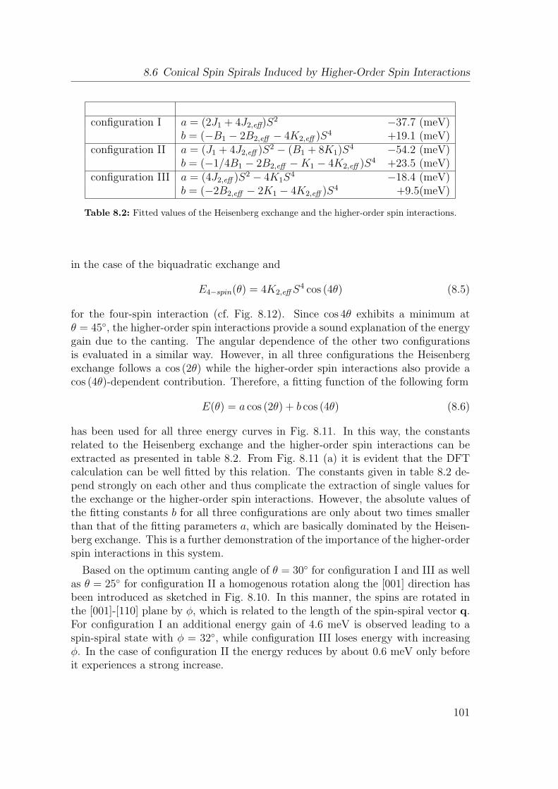
8.6 Conical Spin Spirals Induced by Higher-Order Spin Interactions
configuration I a = (2J1 + 4J2,eff)S2 −37.7 (meV)b = (−B1 − 2B2,eff − 4K2,eff )S4 +19.1 (meV)
configuration II a = (J1 + 4J2,eff )S2 − (B1 + 8K1)S4 −54.2 (meV)
b = (−1/4B1 − 2B2,eff −K1 − 4K2,eff )S4 +23.5 (meV)configuration III a = (4J2,eff )S2 − 4K1S
4 −18.4 (meV)b = (−2B2,eff − 2K1 − 4K2,eff )S4 +9.5(meV)
Table 8.2: Fitted values of the Heisenberg exchange and the higher-order spin interactions.
in the case of the biquadratic exchange and
E4−spin(θ) = 4K2,eff S4 cos (4θ) (8.5)
for the four-spin interaction (cf. Fig. 8.12). Since cos 4θ exhibits a minimum atθ = 45, the higher-order spin interactions provide a sound explanation of the energygain due to the canting. The angular dependence of the other two configurationsis evaluated in a similar way. However, in all three configurations the Heisenbergexchange follows a cos (2θ) while the higher-order spin interactions also provide acos (4θ)-dependent contribution. Therefore, a fitting function of the following form
E(θ) = a cos (2θ) + b cos (4θ) (8.6)
has been used for all three energy curves in Fig. 8.11. In this way, the constantsrelated to the Heisenberg exchange and the higher-order spin interactions can beextracted as presented in table 8.2. From Fig. 8.11 (a) it is evident that the DFTcalculation can be well fitted by this relation. The constants given in table 8.2 de-pend strongly on each other and thus complicate the extraction of single values forthe exchange or the higher-order spin interactions. However, the absolute values ofthe fitting constants b for all three configurations are only about two times smallerthan that of the fitting parameters a, which are basically dominated by the Heisen-berg exchange. This is a further demonstration of the importance of the higher-orderspin interactions in this system.
Based on the optimum canting angle of θ = 30 for configuration I and III as wellas θ = 25 for configuration II a homogenous rotation along the [001] direction hasbeen introduced as sketched in Fig. 8.10. In this manner, the spins are rotated inthe [001]-[110] plane by ϕ, which is related to the length of the spin-spiral vector q.For configuration I an additional energy gain of 4.6 meV is observed leading to aspin-spiral state with ϕ = 32, while configuration III loses energy with increasingϕ. In the case of configuration II the energy reduces by about 0.6 meV only beforeit experiences a strong increase.
101
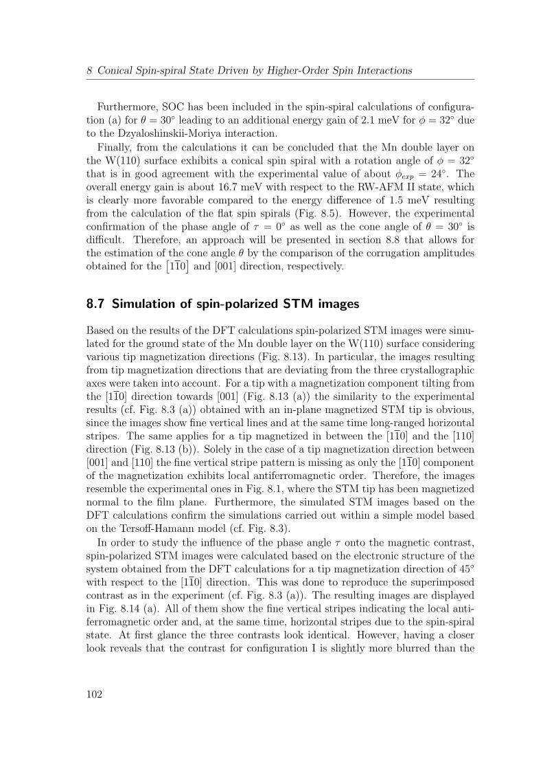
8 Conical Spin-spiral State Driven by Higher-Order Spin Interactions
Furthermore, SOC has been included in the spin-spiral calculations of configura-tion (a) for θ = 30 leading to an additional energy gain of 2.1 meV for ϕ = 32 dueto the Dzyaloshinskii-Moriya interaction.
Finally, from the calculations it can be concluded that the Mn double layer onthe W(110) surface exhibits a conical spin spiral with a rotation angle of ϕ = 32
that is in good agreement with the experimental value of about ϕexp = 24. Theoverall energy gain is about 16.7 meV with respect to the RW-AFM II state, whichis clearly more favorable compared to the energy difference of 1.5 meV resultingfrom the calculation of the flat spin spirals (Fig. 8.5). However, the experimentalconfirmation of the phase angle of τ = 0 as well as the cone angle of θ = 30 isdifficult. Therefore, an approach will be presented in section 8.8 that allows forthe estimation of the cone angle θ by the comparison of the corrugation amplitudesobtained for the
[110]
and [001] direction, respectively.
8.7 Simulation of spin-polarized STM images
Based on the results of the DFT calculations spin-polarized STM images were simu-lated for the ground state of the Mn double layer on the W(110) surface consideringvarious tip magnetization directions (Fig. 8.13). In particular, the images resultingfrom tip magnetization directions that are deviating from the three crystallographicaxes were taken into account. For a tip with a magnetization component tilting fromthe [110] direction towards [001] (Fig. 8.13 (a)) the similarity to the experimentalresults (cf. Fig. 8.3 (a)) obtained with an in-plane magnetized STM tip is obvious,since the images show fine vertical lines and at the same time long-ranged horizontalstripes. The same applies for a tip magnetized in between the [110] and the [110]direction (Fig. 8.13 (b)). Solely in the case of a tip magnetization direction between[001] and [110] the fine vertical stripe pattern is missing as only the [110] componentof the magnetization exhibits local antiferromagnetic order. Therefore, the imagesresemble the experimental ones in Fig. 8.1, where the STM tip has been magnetizednormal to the film plane. Furthermore, the simulated STM images based on theDFT calculations confirm the simulations carried out within a simple model basedon the Tersoff-Hamann model (cf. Fig. 8.3).
In order to study the influence of the phase angle τ onto the magnetic contrast,spin-polarized STM images were calculated based on the electronic structure of thesystem obtained from the DFT calculations for a tip magnetization direction of 45
with respect to the [110] direction. This was done to reproduce the superimposedcontrast as in the experiment (cf. Fig. 8.3 (a)). The resulting images are displayedin Fig. 8.14 (a). All of them show the fine vertical stripes indicating the local anti-ferromagnetic order and, at the same time, horizontal stripes due to the spin-spiralstate. At first glance the three contrasts look identical. However, having a closerlook reveals that the contrast for configuration I is slightly more blurred than the
102
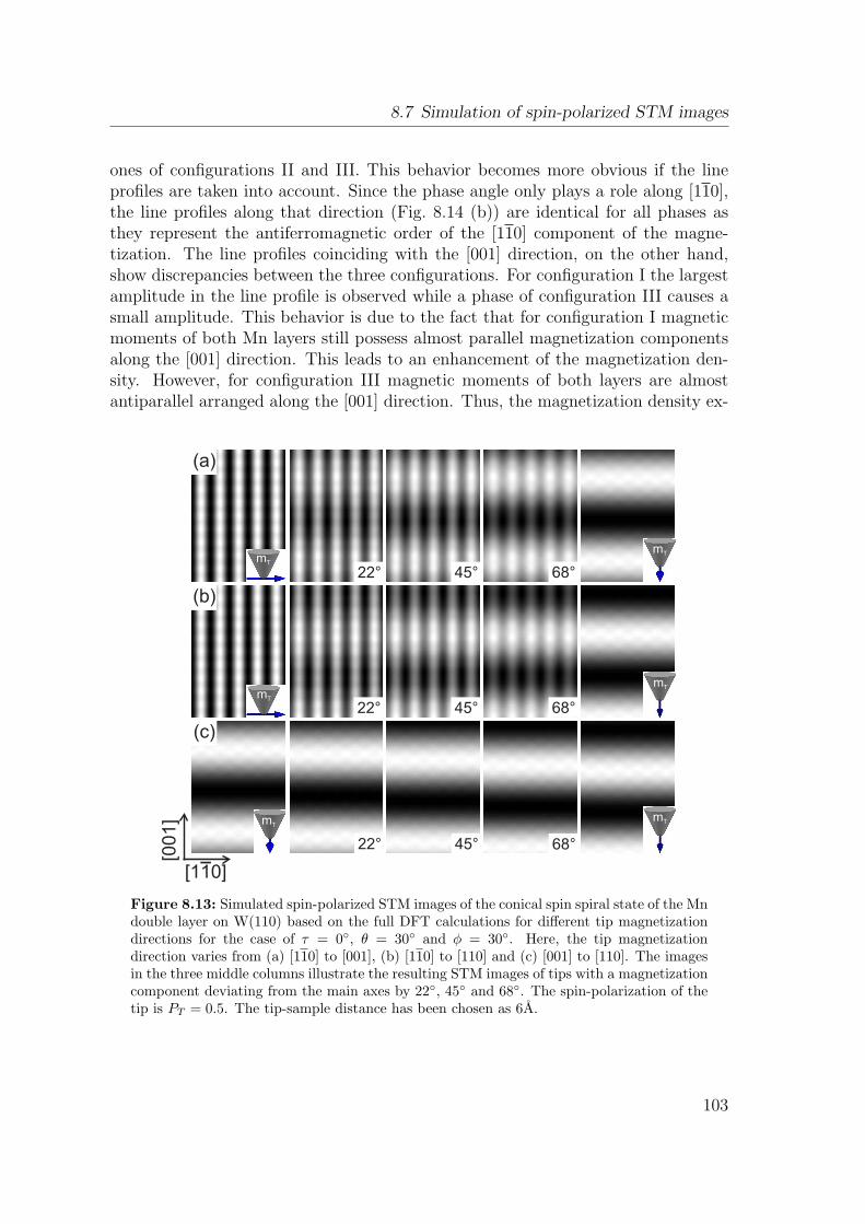
8.7 Simulation of spin-polarized STM images
ones of configurations II and III. This behavior becomes more obvious if the lineprofiles are taken into account. Since the phase angle only plays a role along [110],the line profiles along that direction (Fig. 8.14 (b)) are identical for all phases asthey represent the antiferromagnetic order of the [110] component of the magne-tization. The line profiles coinciding with the [001] direction, on the other hand,show discrepancies between the three configurations. For configuration I the largestamplitude in the line profile is observed while a phase of configuration III causes asmall amplitude. This behavior is due to the fact that for configuration I magneticmoments of both Mn layers still possess almost parallel magnetization componentsalong the [001] direction. This leads to an enhancement of the magnetization den-sity. However, for configuration III magnetic moments of both layers are almostantiparallel arranged along the [001] direction. Thus, the magnetization density ex-
22°
22°
22°
45°
45°
45° 68°
68°
68°
[1 0]1
[00
1]
mT
mT
mT
mT
mTmT
(c)
(b)
(a)
Figure 8.13: Simulated spin-polarized STM images of the conical spin spiral state of the Mndouble layer on W(110) based on the full DFT calculations for different tip magnetizationdirections for the case of τ = 0, θ = 30 and ϕ = 30. Here, the tip magnetizationdirection varies from (a) [110] to [001], (b) [110] to [110] and (c) [001] to [110]. The imagesin the three middle columns illustrate the resulting STM images of tips with a magnetizationcomponent deviating from the main axes by 22, 45 and 68. The spin-polarization of thetip is PT = 0.5. The tip-sample distance has been chosen as 6A.
103
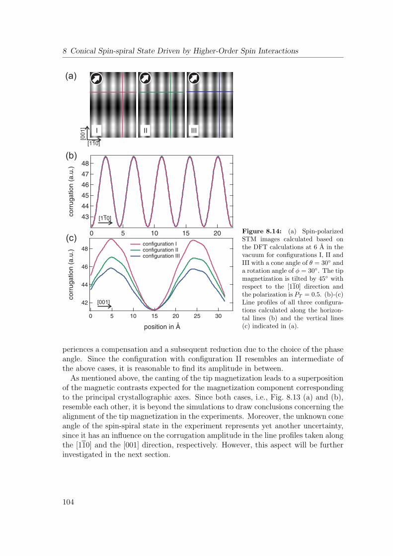
8 Conical Spin-spiral State Driven by Higher-Order Spin Interactions
(a)
(b)
I
(c)
[1 0]1
[00
1]
[1 0]1
[001]
IIIII
Figure 8.14: (a) Spin-polarizedSTM images calculated based onthe DFT calculations at 6 A in thevacuum for configurations I, II andIII with a cone angle of θ = 30 anda rotation angle of ϕ = 30. The tipmagnetization is tilted by 45 withrespect to the [110] direction andthe polarization is PT = 0.5. (b)-(c)Line profiles of all three configura-tions calculated along the horizon-tal lines (b) and the vertical lines(c) indicated in (a).
periences a compensation and a subsequent reduction due to the choice of the phaseangle. Since the configuration with configuration II resembles an intermediate ofthe above cases, it is reasonable to find its amplitude in between.
As mentioned above, the canting of the tip magnetization leads to a superpositionof the magnetic contrasts expected for the magnetization component correspondingto the principal crystallographic axes. Since both cases, i.e., Fig. 8.13 (a) and (b),resemble each other, it is beyond the simulations to draw conclusions concerning thealignment of the tip magnetization in the experiments. Moreover, the unknown coneangle of the spin-spiral state in the experiment represents yet another uncertainty,since it has an influence on the corrugation amplitude in the line profiles taken alongthe [110] and the [001] direction, respectively. However, this aspect will be furtherinvestigated in the next section.
104
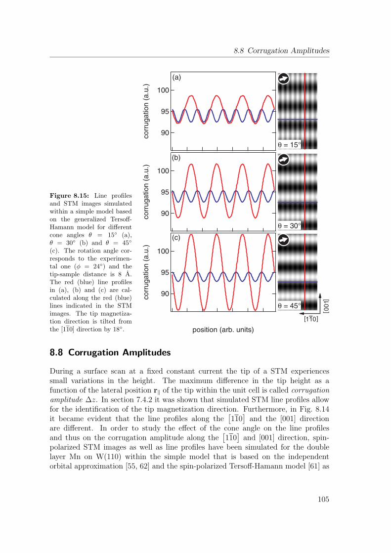
8.8 Corrugation Amplitudes
Figure 8.15: Line profilesand STM images simulatedwithin a simple model basedon the generalized Tersoff-Hamann model for differentcone angles θ = 15 (a),θ = 30 (b) and θ = 45
(c). The rotation angle cor-responds to the experimen-tal one (ϕ = 24) and thetip-sample distance is 8 A.The red (blue) line profilesin (a), (b) and (c) are cal-culated along the red (blue)lines indicated in the STMimages. The tip magnetiza-tion direction is tilted fromthe [110] direction by 18.
00
1
1 01
8.8 Corrugation Amplitudes
During a surface scan at a fixed constant current the tip of a STM experiencessmall variations in the height. The maximum difference in the tip height as afunction of the lateral position r∥ of the tip within the unit cell is called corrugationamplitude ∆z. In section 7.4.2 it was shown that simulated STM line profiles allowfor the identification of the tip magnetization direction. Furthermore, in Fig. 8.14it became evident that the line profiles along the
[110]
and the [001] directionare different. In order to study the effect of the cone angle on the line profilesand thus on the corrugation amplitude along the
[110]
and [001] direction, spin-polarized STM images as well as line profiles have been simulated for the doublelayer Mn on W(110) within the simple model that is based on the independentorbital approximation [55, 62] and the spin-polarized Tersoff-Hamann model [61] as
105
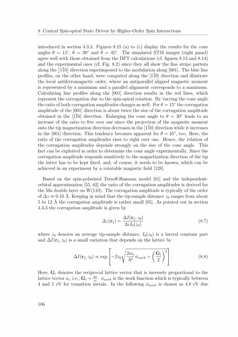
8 Conical Spin-spiral State Driven by Higher-Order Spin Interactions
introduced in section 4.3.3. Figures 8.15 (a) to (c) display the results for the coneangles θ = 15, θ = 30 and θ = 45. The simulated STM images (right panel)agree well with those obtained from the DFT calculations (cf. figures 8.13 and 8.14)and the experimental ones (cf. Fig. 8.2) since they all show the fine stripe patternalong the
[110]
direction superimposed to the modulation along [001]. The blue lineprofiles, on the other hand, were computed along the [110] direction and illustratethe local antiferromagnetic order, where an antiparallel aligned magnetic momentis represented by a minimum and a parallel alignment corresponds to a maximum.Calculating line profiles along the [001] direction results in the red lines, whichrepresent the corrugation due to the spin-spiral rotation. By varying the cone anglethe ratio of both corrugation amplitudes changes as well. For θ = 15 the corrugationamplitude of the [001] direction is about twice the size of the corrugation amplitudeobtained in the [110] direction. Enlarging the cone angle to θ = 30 leads to anincrease of the ratio to five over one since the projection of the magnetic momentonto the tip magnetization direction decreases in the [110] direction while it increasesin the [001] direction. This tendency becomes apparent for θ = 45, too. Here, theratio of the corrugation amplitudes rises to eight over one. Hence, the relation ofthe corrugation amplitudes depends strongly on the size of the cone angle. Thisfact can be exploited in order to determine the cone angle experimentally. Since thecorrugation amplitude responds sensitively to the magnetization direction of the tipthe latter has to be kept fixed, and, of course, it needs to be known, which can beachieved in an experiment by a rotatable magnetic field [128].
Based on the spin-polarized Tersoff-Hamann model [61] and the independent-orbital approximation [55, 62] the ratio of the corrugation amplitudes is derived forthe Mn double layer on W(110). The corrugation amplitude is typically of the orderof ∆z ≈ 0.10 A. Keeping in mind that the tip-sample distance z0 ranges from about5 to 12 A the corrugation amplitude is rather small [65]. As pointed out in section4.3.3 the corrugation amplitude is given by
∆z(r∥) =∆I(r∥, z0)
2κI0(z0)(8.7)
where z0 denotes an average tip-sample distance, I0(z0) is a lateral constant partand ∆I(r∥, z0) is a small variation that depends on the lattice by
∆I(r∥, z0) ∝ exp
−2z0
√2me
~2ϕwork +
(Gi
2
)2 . (8.8)
Here, Gi denotes the reciprocal lattice vector that is inversely proportional to thelattice vector ai, i.e., Gi = 2π
ai. ϕwork is the work function which is typically between
4 and 5 eV for transition metals. In the following ϕwork is chosen as 4.8 eV due
106
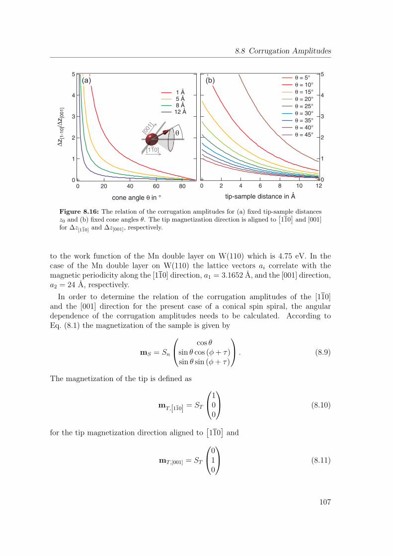
8.8 Corrugation Amplitudes
q[001
][1 0]1
(b)(a)
Figure 8.16: The relation of the corrugation amplitudes for (a) fixed tip-sample distancesz0 and (b) fixed cone angles θ. The tip magnetization direction is aligned to
[110]and [001]
for ∆z[110] and ∆z[001], respectively.
to the work function of the Mn double layer on W(110) which is 4.75 eV. In thecase of the Mn double layer on W(110) the lattice vectors ai correlate with themagnetic periodicity along the [110] direction, a1 = 3.1652 A, and the [001] direction,a2 = 24 A, respectively.
In order to determine the relation of the corrugation amplitudes of the [110]and the [001] direction for the present case of a conical spin spiral, the angulardependence of the corrugation amplitudes needs to be calculated. According toEq. (8.1) the magnetization of the sample is given by
mS = Sn
cos θsin θ cos (ϕ+ τ)sin θ sin (ϕ+ τ)
. (8.9)
The magnetization of the tip is defined as
mT,[110] = ST
100
(8.10)
for the tip magnetization direction aligned to[110]
and
mT,[001] = ST
010
(8.11)
107
8 Conical Spin-spiral State Driven by Higher-Order Spin Interactions
along [001]. Therefore, the dependence of the corrugation on the cone angle θcorresponds to
mT,[110] ·mS ∝ cos θ along[110]
and mT,[001] ·mS ∝ sin θ along [001]. (8.12)
With ∆z[110] ∝ cos θ and ∆z[001] ∝ sin θ the ratio results in
∆z[110]∆z[001]
= cot(θ) ·exp
(−2z0
√2me
~2 · ϕwork + ( πa1
)2)
exp(−2z0
√2me
~2 · ϕwork + ( πa2
)2) . (8.13)
It has been calculated for either a fixed tip-sample distance zdist (Fig. 8.16(a)) or afixed cone angle θ (Fig. 8.16(b)).
Both figures, Fig. 8.16(a) and (b), show that for large cone angles and largetip-sample distances the ratio of the corrugation amplitudes becomes nearly zero,i.e., ∆z[001] becomes very large. First of all, this is due to the fact that magneticconfigurations described by a small lattice vector ai decay faster with increasing tip-sample distance than those with a large lattice vector as it is seen from Eq. (8.8).Secondly, with increasing cone angle the projected magnetization component in the[110] direction becomes smaller. Therefore, the study of the cone angle is quitecomplex since it requires a well-known tip magnetization direction and a sufficientlysmall tip-sample distance. Up to now there is no direct experimental confirmationof the theoretical cone angle of θ = 30. However, with a ratio of about four over onefor ∆z[001] versus ∆z[110] obtained in spin-polarized STM experiments [138] the coneangle of the spin-spiral state found in a double layer Mn on W(110) can be estimatedto be between 30 and 45 if the tip-sample distance is assumed as 8 A. Therefore,an optimum cone angle of 30 as found in the DFT calculations is consistent withthe experimental data.
8.9 The Tunneling Anisotropic Magnetoresistance Effect in aConical Spin-Spiral State
The conical spin-spiral ground state of the Mn double layer on the (110) surfaceof W is well suited for the study of a transport effect due to SOC which is knownas tunneling anisotropic magnetoresistance (TAMR). In contrast to the junctionsused for the tunneling magnetoresistance effect (TMR), a magnetic tunnel junctionneeds to comprise only one magnetic electrode opposed to a nonmagnetic electrodein order to give rise to the TAMR effect. Due to changes in the electronic structurethe TAMR causes a magnetization-direction-dependent change in the tunneling re-sistance. It has first been observed in another ultra-thin film system – the doublelayer of Fe on the W(110) surface – where it has been demonstrated that the SOC
108
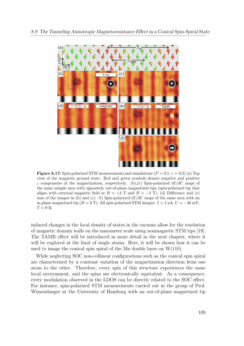
8.9 The Tunneling Anisotropic Magnetoresistance Effect in a Conical Spin-Spiral State
(c)(b) 4 nm
(a)
[001]
[10
]1
(d) = 1/2 (b - a) magnetic = 1/2 (a + b) TAMR(e)
(f)
lTAMR
lM
Figure 8.17: Spin-polarized STM measurements and simulations (P = 0.1, γ = 0.2) (a) Topview of the magnetic ground state. Red and green symbols denote negative and positivez components of the magnetization, respectively. (b),(c) Spin-polarized dI/dU maps ofthe same sample area with oppositely out-of-plane magnetized tips (spin-polarized tip thataligns with external magnetic field at B = +2 T and B = −2 T). (d) Difference and (e)sum of the images in (b) and (c). (f) Spin-polarized dI/dU maps of the same area with anin-plane magnetized tip (B = 0 T). All spin-polarized STM images: I = 1 nA, U = −40 mV,T = 9 K
induced changes in the local density of states in the vacuum allow for the resolutionof magnetic domain walls on the nanometer scale using nonmagnetic STM tips [19].The TAMR effect will be introduced in more detail in the next chapter, where itwill be explored at the limit of single atoms. Here, it will be shown how it can beused to image the conical spin spiral of the Mn double layer on W(110).
While neglecting SOC non-collinear configurations such as the conical spin spiralare characterized by a constant variation of the magnetization direction from oneatom to the other. Therefore, every spin of this structure experiences the samelocal environment, and the spins are electronically equivalent. As a consequence,every modulation observed in the LDOS can be directly related to the SOC effect.For instance, spin-polarized STM measurements carried out in the group of Prof.Wiesendanger at the University of Hamburg with an out-of-plane magnetized tip
109
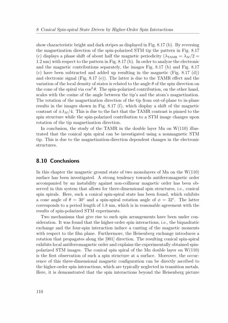
8 Conical Spin-spiral State Driven by Higher-Order Spin Interactions
show characteristic bright and dark stripes as displayed in Fig. 8.17 (b). By reversingthe magnetization direction of the spin-polarized STM tip the pattern in Fig. 8.17(c) displays a phase shift of about half the magnetic periodicity (λTAMR = λM/2 =1.2 nm) with respect to the pattern in Fig. 8.17 (b). In order to analyze the electronicand the magnetic contributions separately, the images Fig. 8.17 (b) and Fig. 8.17(c) have been subtracted and added up resulting in the magnetic (Fig. 8.17 (d))and electronic signal (Fig. 8.17 (e)). The latter is due to the TAMR effect and thevariation of the local density of states is related to the angle θ of the spin direction onthe cone of the spiral via cos2 θ. The spin-polarized contribution, on the other hand,scales with the cosine of the angle between the tip’s and the atom’s magnetization.The rotation of the magnetization direction of the tip from out-of-plane to in-planeresults in the images shown in Fig. 8.17 (f), which display a shift of the magneticcontrast of ±λM/4. This is due to the fact that the TAMR contrast is pinned to thespin structure while the spin-polarized contribution to a STM image changes uponrotation of the tip magnetization direction.
In conclusion, the study of the TAMR in the double layer Mn on W(110) illus-trated that the conical spin spiral can be investigated using a nonmagnetic STMtip. This is due to the magnetization-direction dependent changes in the electronicstructures.
8.10 Conclusions
In this chapter the magnetic ground state of two monolayers of Mn on the W(110)surface has been investigated. A strong tendency towards antiferromagnetic orderaccompanied by an instability against non-collinear magnetic order has been ob-served in this system that allows for three-dimensional spin structures, i.e., conicalspin spirals. Here, such a conical spin-spiral state has been found, which exhibitsa cone angle of θ = 30 and a spin-spiral rotation angle of ϕ = 32. The lattercorresponds to a period length of 1.8 nm, which is in reasonable agreement with theresults of spin-polarized STM experiments.
Two mechanisms that give rise to such spin arrangements have been under con-sideration. It was found that the higher-order spin interactions, i.e., the biquadraticexchange and the four-spin interaction induce a canting of the magnetic momentswith respect to the film plane. Furthermore, the Heisenberg exchange introduces arotation that propagates along the [001] direction. The resulting conical spin-spiralexhibits local antiferromagnetic order and explains the experimentally obtained spin-polarized STM images. The conical spin spiral of the Mn double layer on W(110)is the first observation of such a spin structure at a surface. Moreover, the occur-rence of this three-dimensional magnetic configuration can be directly ascribed tothe higher-order spin interactions, which are typically neglected in transition metals.Here, it is demonstrated that the spin interactions beyond the Heisenberg picture
110
8.10 Conclusions
can play an important role in such systems.The further examination of the influence of the tip magnetization direction on the
spin-polarized STM contrasts has been carried out based on simulated STM imagescalculated within the Tersoff-Hamann model. In order to allow for the identificationof the cone angle the corrugation amplitudes corresponding to the modulation alongthe
[110]
and [001] direction, respectively, as well as their ratio have been studied.Finally, the influence of the SOC on a conical spin spiral in terms of the tunnelinganisotropic magnetoresistance has been investigated.
111

8 Conical Spin-spiral State Driven by Higher-Order Spin Interactions
112
9 Tunneling Anisotropic Magnetoresistance at theSingle Atom Limit
In 1975 M. Julliere discovered the tunneling magnetoresistance (TMR) [60] – a mag-netoresistive effect that occurs due to spin-dependent tunneling in nanosize magnetictunnel junctions. As illustrated schematically in Fig. 9.1 (a) the latter consist oftwo ferromagnetic layers that are separated by a thin insulating layer through whichthe electrons can tunnel from one ferromagnetic electrode to the other. Accordingto Julliere’s model the tunneling takes place considering the following assumptions(i) the spin of the tunneling electrons is conserved and (ii) the conductance G isproportional to the product of the densities of states of the ferromagnets in theparallel (P) or antiparallel (AP) alignment, respectively. By applying an externalmagnetic field the magnetizations of the electrodes can be switched from parallel(high tunneling probability) to antiparallel (low tunneling probability). While theexperiments of M. Julliere had to be realized at very low temperatures [60] the TMReffect at room temperature was achieved in the 90s by Moodera [139] and Miyazaki[140]. This allows for the application of the TMR effect in read heads of modern harddisk drives. Furthermore, the discovery of the TMR gave rise to the developmentof the magnetoresistive random-access memory (MRAM) – a non-volatile random-access memory technology. Due to SOC the resistance can become anisotropic, i.e.,it depends on the magnetization direction of the tunnel junction with respect tothe crystallographic axes as sketched in Fig. 9.1 (b). For the observation of thiseffect the junction needs only a single magnetic electrode separated from a nonmag-netic electrode by an insulating layer. Due to magnetization-direction dependentchanges in the electronic structure the tunneling current between these electrodesexhibits differences for a film that is magnetized either out-of-plane (⊥) or in-plane(∥) [19, 25, 141, 142]. This effect has been established as tunneling anisotropic mag-netoresistance (TAMR) . The TAMR offers an alternative route towards spintronicdevices as it circumvents the restriction of coherent spin-dependent transport [25]in contrast to the TMR.
The TAMR has first been observed in STM measurements of a double-layer filmof Fe on the W(110) surface [19]. It also occurs in planar tunnel junctions thatinvolve ferromagnetic semiconductors [25]. Furthermore, the application of magnetictransition-metal electrodes allows for the operation of such nanoscale devices at roomtemperature [143, 144]. Other experiments have been conducted concerning theTAMR in metal-semiconductor Fe/GaAs/Au junctions [145] and transition-metal
113
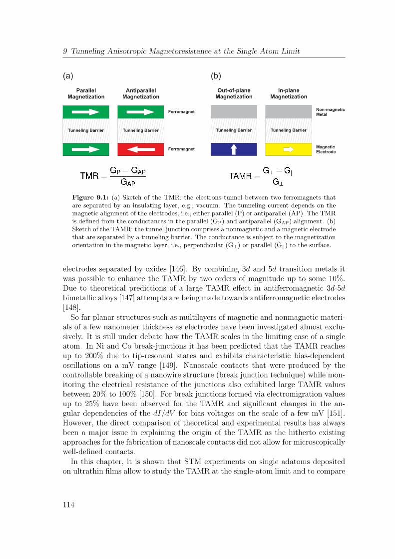
9 Tunneling Anisotropic Magnetoresistance at the Single Atom Limit
Tunneling Barrier Tunneling Barrier
Ferromagnet
Ferromagnet
ParallelMagnetization
AntiparallelMagnetization
Tunneling Barrier Tunneling Barrier
Non-magneticMetal
MagneticElectrode
Out-of-planeMagnetization
In-planeMagnetization
(a) (b)
Figure 9.1: (a) Sketch of the TMR: the electrons tunnel between two ferromagnets thatare separated by an insulating layer, e.g., vacuum. The tunneling current depends on themagnetic alignment of the electrodes, i.e., either parallel (P) or antiparallel (AP). The TMRis defined from the conductances in the parallel (GP) and antiparallel (GAP) alignment. (b)Sketch of the TAMR: the tunnel junction comprises a nonmagnetic and a magnetic electrodethat are separated by a tunneling barrier. The conductance is subject to the magnetizationorientation in the magnetic layer, i.e., perpendicular (G⊥) or parallel (G∥) to the surface.
electrodes separated by oxides [146]. By combining 3d and 5d transition metals itwas possible to enhance the TAMR by two orders of magnitude up to some 10%.Due to theoretical predictions of a large TAMR effect in antiferromagnetic 3d-5dbimetallic alloys [147] attempts are being made towards antiferromagnetic electrodes[148].
So far planar structures such as multilayers of magnetic and nonmagnetic materi-als of a few nanometer thickness as electrodes have been investigated almost exclu-sively. It is still under debate how the TAMR scales in the limiting case of a singleatom. In Ni and Co break-junctions it has been predicted that the TAMR reachesup to 200% due to tip-resonant states and exhibits characteristic bias-dependentoscillations on a mV range [149]. Nanoscale contacts that were produced by thecontrollable breaking of a nanowire structure (break junction technique) while mon-itoring the electrical resistance of the junctions also exhibited large TAMR valuesbetween 20% to 100% [150]. For break junctions formed via electromigration valuesup to 25% have been observed for the TAMR and significant changes in the an-gular dependencies of the dI/dV for bias voltages on the scale of a few mV [151].However, the direct comparison of theoretical and experimental results has alwaysbeen a major issue in explaining the origin of the TAMR as the hitherto existingapproaches for the fabrication of nanoscale contacts did not allow for microscopicallywell-defined contacts.
In this chapter, it is shown that STM experiments on single adatoms depositedon ultrathin films allow to study the TAMR at the single-atom limit and to compare
114
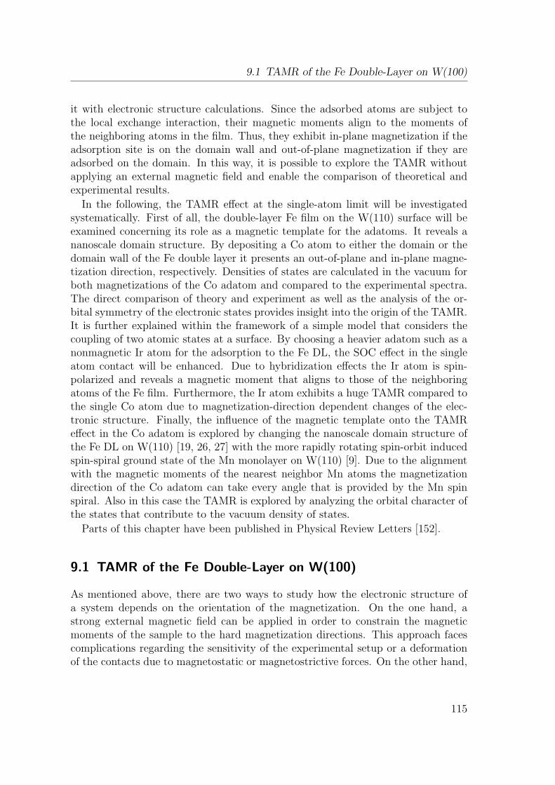
9.1 TAMR of the Fe Double-Layer on W(100)
it with electronic structure calculations. Since the adsorbed atoms are subject tothe local exchange interaction, their magnetic moments align to the moments ofthe neighboring atoms in the film. Thus, they exhibit in-plane magnetization if theadsorption site is on the domain wall and out-of-plane magnetization if they areadsorbed on the domain. In this way, it is possible to explore the TAMR withoutapplying an external magnetic field and enable the comparison of theoretical andexperimental results.
In the following, the TAMR effect at the single-atom limit will be investigatedsystematically. First of all, the double-layer Fe film on the W(110) surface will beexamined concerning its role as a magnetic template for the adatoms. It reveals ananoscale domain structure. By depositing a Co atom to either the domain or thedomain wall of the Fe double layer it presents an out-of-plane and in-plane magne-tization direction, respectively. Densities of states are calculated in the vacuum forboth magnetizations of the Co adatom and compared to the experimental spectra.The direct comparison of theory and experiment as well as the analysis of the or-bital symmetry of the electronic states provides insight into the origin of the TAMR.It is further explained within the framework of a simple model that considers thecoupling of two atomic states at a surface. By choosing a heavier adatom such as anonmagnetic Ir atom for the adsorption to the Fe DL, the SOC effect in the singleatom contact will be enhanced. Due to hybridization effects the Ir atom is spin-polarized and reveals a magnetic moment that aligns to those of the neighboringatoms of the Fe film. Furthermore, the Ir atom exhibits a huge TAMR compared tothe single Co atom due to magnetization-direction dependent changes of the elec-tronic structure. Finally, the influence of the magnetic template onto the TAMReffect in the Co adatom is explored by changing the nanoscale domain structure ofthe Fe DL on W(110) [19, 26, 27] with the more rapidly rotating spin-orbit inducedspin-spiral ground state of the Mn monolayer on W(110) [9]. Due to the alignmentwith the magnetic moments of the nearest neighbor Mn atoms the magnetizationdirection of the Co adatom can take every angle that is provided by the Mn spinspiral. Also in this case the TAMR is explored by analyzing the orbital character ofthe states that contribute to the vacuum density of states.
Parts of this chapter have been published in Physical Review Letters [152].
9.1 TAMR of the Fe Double-Layer on W(100)
As mentioned above, there are two ways to study how the electronic structure ofa system depends on the orientation of the magnetization. On the one hand, astrong external magnetic field can be applied in order to constrain the magneticmoments of the sample to the hard magnetization directions. This approach facescomplications regarding the sensitivity of the experimental setup or a deformationof the contacts due to magnetostatic or magnetostrictive forces. On the other hand,
115
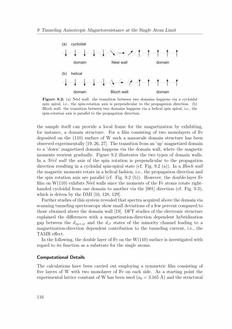
9 Tunneling Anisotropic Magnetoresistance at the Single Atom Limit
(a) cycloidal
(b) helical
Bloch wall
Néel wall
domain
domaindomain
domain
Figure 9.2: (a) Neel wall: the transition between two domains happens via a cycloidalspin spiral, i.e., the spin-rotation axis is perpendicular to the propagation direction. (b)Bloch wall: the transition between two domains happens via a helical spin spiral, i.e., thespin-rotation axis is parallel to the propagation direction.
the sample itself can provide a local frame for the magnetization by exhibiting,for instance, a domain structure. For a film consisting of two monolayers of Fedeposited on the (110) surface of W such a nanoscale domain structure has beenobserved experimentally [19, 26, 27]. The transition from an ’up’ magnetized domainto a ’down’ magnetized domain happens via the domain wall, where the magneticmoments reorient gradually. Figure 9.2 illustrates the two types of domain walls.In a Neel wall the axis of the spin rotation is perpendicular to the propagationdirection resulting in a cycloidal spin-spiral state (cf. Fig. 9.2 (a)). In a Bloch wallthe magnetic moments rotate in a helical fashion, i.e., the propagation direction andthe spin rotation axis are parallel (cf. Fig. 9.2 (b)). However, the double-layer Fefilm on W(110) exhibits Neel walls since the moments of the Fe atoms rotate right-handed cycloidal from one domain to another via the [001] direction (cf. Fig. 9.3),which is driven by the DMI [10, 128, 129].
Further studies of this system revealed that spectra acquired above the domain viascanning tunneling spectroscopy show small deviations of a few percent compared tothose obtained above the domain wall [19]. DFT studies of the electronic structureexplained the differences with a magnetization-direction dependent hybridizationgap between the dxy+zx and the dz2 states of the minority channel leading to amagnetization-direction dependent contribution to the tunneling current, i.e., theTAMR effect.
In the following, the double layer of Fe on the W(110) surface is investigated withregard to its function as a substrate for the single atoms.
Computational Details
The calculations have been carried out employing a symmetric film consisting offive layers of W with two monolayer of Fe on each side. As a starting point theexperimental lattice constant of W has been used (a0 = 3.165 A) and the structural
116
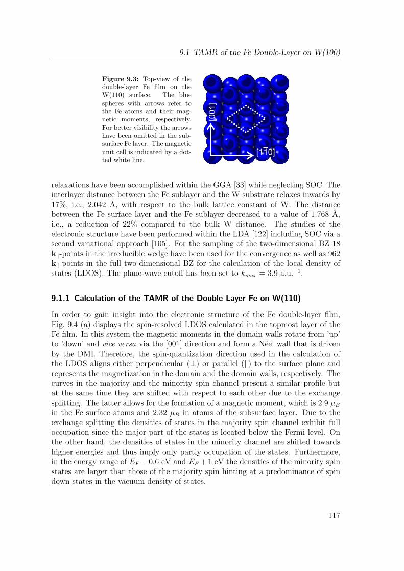
9.1 TAMR of the Fe Double-Layer on W(100)
Figure 9.3: Top-view of thedouble-layer Fe film on theW(110) surface. The bluespheres with arrows refer tothe Fe atoms and their mag-netic moments, respectively.For better visibility the arrowshave been omitted in the sub-surface Fe layer. The magneticunit cell is indicated by a dot-ted white line.
[1 0]1
[00
1]
relaxations have been accomplished within the GGA [33] while neglecting SOC. Theinterlayer distance between the Fe sublayer and the W substrate relaxes inwards by17%, i.e., 2.042 A, with respect to the bulk lattice constant of W. The distancebetween the Fe surface layer and the Fe sublayer decreased to a value of 1.768 A,i.e., a reduction of 22% compared to the bulk W distance. The studies of theelectronic structure have been performed within the LDA [122] including SOC via asecond variational approach [105]. For the sampling of the two-dimensional BZ 18k∥-points in the irreducible wedge have been used for the convergence as well as 962k∥-points in the full two-dimensional BZ for the calculation of the local density ofstates (LDOS). The plane-wave cutoff has been set to kmax = 3.9 a.u.−1.
9.1.1 Calculation of the TAMR of the Double Layer Fe on W(110)
In order to gain insight into the electronic structure of the Fe double-layer film,Fig. 9.4 (a) displays the spin-resolved LDOS calculated in the topmost layer of theFe film. In this system the magnetic moments in the domain walls rotate from ’up’to ’down’ and vice versa via the [001] direction and form a Neel wall that is drivenby the DMI. Therefore, the spin-quantization direction used in the calculation ofthe LDOS aligns either perpendicular (⊥) or parallel (∥) to the surface plane andrepresents the magnetization in the domain and the domain walls, respectively. Thecurves in the majority and the minority spin channel present a similar profile butat the same time they are shifted with respect to each other due to the exchangesplitting. The latter allows for the formation of a magnetic moment, which is 2.9 µB
in the Fe surface atoms and 2.32 µB in atoms of the subsurface layer. Due to theexchange splitting the densities of states in the majority spin channel exhibit fulloccupation since the major part of the states is located below the Fermi level. Onthe other hand, the densities of states in the minority channel are shifted towardshigher energies and thus imply only partly occupation of the states. Furthermore,in the energy range of EF − 0.6 eV and EF + 1 eV the densities of the minority spinstates are larger than those of the majority spin hinting at a predominance of spindown states in the vacuum density of states.
117
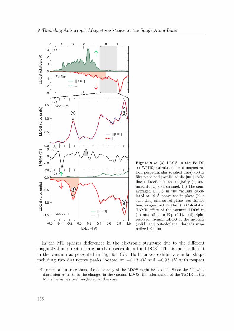
9 Tunneling Anisotropic Magnetoresistance at the Single Atom Limit
||
||
||
1
2
1 2
(a)
(b)
(c)
(d)
Fe film
Figure 9.4: (a) LDOS in the Fe DLon W(110) calculated for a magnetiza-tion perpendicular (dashed lines) to thefilm plane and parallel to the [001] (solidlines) direction in the majority (↑) andminority (↓) spin channel. (b) The spin-averaged LDOS in the vacuum calcu-lated at 10 A above the in-plane (bluesolid line) and out-of-plane (red dashedline) magnetized Fe film. (c) CalculatedTAMR effect of the vacuum LDOS in(b) according to Eq. (9.1). (d) Spin-resolved vacuum LDOS of the in-plane(solid) and out-of-plane (dashed) mag-netized Fe film.
In the MT spheres differences in the electronic structure due to the differentmagnetization directions are barely observable in the LDOS1. This is quite differentin the vacuum as presented in Fig. 9.4 (b). Both curves exhibit a similar shapeincluding two distinctive peaks located at −0.13 eV and +0.93 eV with respect
1In order to illustrate them, the anisotropy of the LDOS might be plotted. Since the followingdiscussion restricts to the changes in the vacuum LDOS, the information of the TAMR in theMT spheres has been neglected in this case.
118
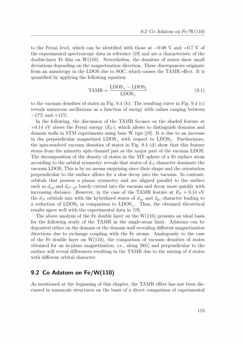
9.2 Co Adatom on Fe/W(110)
to the Fermi level, which can be identified with those at −0.08 V and +0.7 V ofthe experimental spectroscopy data in reference [19] and are a characteristic of thedouble-layer Fe film on W(110). Nevertheless, the densities of states show smalldeviations depending on the magnetization direction. These discrepancies originatefrom an anisotropy in the LDOS due to SOC, which causes the TAMR effect. It isquantified by applying the following equation
TAMR =LDOS⊥ − LDOS∥
LDOS⊥(9.1)
to the vacuum densities of states in Fig. 9.4 (b). The resulting curve in Fig. 9.4 (c)reveals numerous oscillations as a function of energy with values ranging between−17% and +11%.
In the following, the discussion of the TAMR focuses on the shaded feature at+0.14 eV above the Fermi energy (EF ), which allows to distinguish domains anddomain walls in STM experiments using bare W tips [19]. It is due to an increasein the perpendicular magnetized LDOS⊥ with respect to LDOS∥. Furthermore,the spin-resolved vacuum densities of states in Fig. 9.4 (d) show that this featurestems from the minority spin channel just as the major part of the vacuum LDOS.The decomposition of the density of states in the MT sphere of a Fe surface atomaccording to the orbital symmetry reveals that states of dz2 character dominate thevacuum LDOS. This is by no means surprising since their shape and the orientationperpendicular to the surface allows for a slow decay into the vacuum. In contrast,orbitals that possess a planar symmetry and are aligned parallel to the surfacesuch as dxy and dx2−y2 barely extend into the vacuum and decay more quickly withincreasing distance. However, in the case of the TAMR feature at EF + 0.14 eVthe dz2 orbitals mix with the hybridized states of dxy and dyz character leading toa reduction of LDOS∥ in comparison to LDOS⊥. Thus, the obtained theoreticalresults agree well with the experimental data in [19].
The above analysis of the Fe double layer on the W(110) presents an ideal basisfor the following study of the TAMR in the single-atom limit. Adatoms can bedeposited either on the domain or the domain wall revealing different magnetizationdirections due to exchange coupling with the Fe atoms. Analogously to the caseof the Fe double layer on W(110), the comparison of vacuum densities of statesobtained for an in-plane magnetization, i.e., along [001] and perpendicular to thesurface will reveal differences resulting in the TAMR due to the mixing of d stateswith different orbital character.
9.2 Co Adatom on Fe/W(110)
As mentioned at the beginning of this chapter, the TAMR effect has not been dis-cussed in nanoscale structures on the basis of a direct comparison of experimental
119
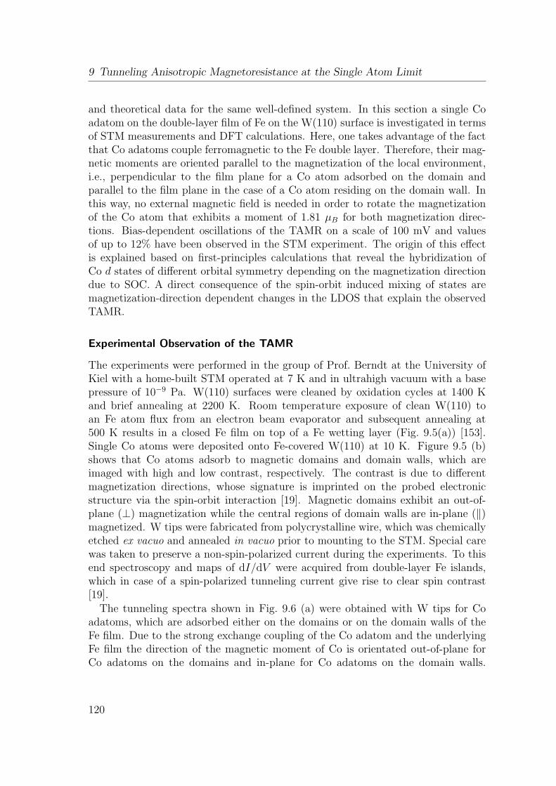
9 Tunneling Anisotropic Magnetoresistance at the Single Atom Limit
and theoretical data for the same well-defined system. In this section a single Coadatom on the double-layer film of Fe on the W(110) surface is investigated in termsof STM measurements and DFT calculations. Here, one takes advantage of the factthat Co adatoms couple ferromagnetic to the Fe double layer. Therefore, their mag-netic moments are oriented parallel to the magnetization of the local environment,i.e., perpendicular to the film plane for a Co atom adsorbed on the domain andparallel to the film plane in the case of a Co atom residing on the domain wall. Inthis way, no external magnetic field is needed in order to rotate the magnetizationof the Co atom that exhibits a moment of 1.81 µB for both magnetization direc-tions. Bias-dependent oscillations of the TAMR on a scale of 100 mV and valuesof up to 12% have been observed in the STM experiment. The origin of this effectis explained based on first-principles calculations that reveal the hybridization ofCo d states of different orbital symmetry depending on the magnetization directiondue to SOC. A direct consequence of the spin-orbit induced mixing of states aremagnetization-direction dependent changes in the LDOS that explain the observedTAMR.
Experimental Observation of the TAMR
The experiments were performed in the group of Prof. Berndt at the University ofKiel with a home-built STM operated at 7 K and in ultrahigh vacuum with a basepressure of 10−9 Pa. W(110) surfaces were cleaned by oxidation cycles at 1400 Kand brief annealing at 2200 K. Room temperature exposure of clean W(110) toan Fe atom flux from an electron beam evaporator and subsequent annealing at500 K results in a closed Fe film on top of a Fe wetting layer (Fig. 9.5(a)) [153].Single Co atoms were deposited onto Fe-covered W(110) at 10 K. Figure 9.5 (b)shows that Co atoms adsorb to magnetic domains and domain walls, which areimaged with high and low contrast, respectively. The contrast is due to differentmagnetization directions, whose signature is imprinted on the probed electronicstructure via the spin-orbit interaction [19]. Magnetic domains exhibit an out-of-plane (⊥) magnetization while the central regions of domain walls are in-plane (∥)magnetized. W tips were fabricated from polycrystalline wire, which was chemicallyetched ex vacuo and annealed in vacuo prior to mounting to the STM. Special carewas taken to preserve a non-spin-polarized current during the experiments. To thisend spectroscopy and maps of dI/dV were acquired from double-layer Fe islands,which in case of a spin-polarized tunneling current give rise to clear spin contrast[19].
The tunneling spectra shown in Fig. 9.6 (a) were obtained with W tips for Coadatoms, which are adsorbed either on the domains or on the domain walls of theFe film. Due to the strong exchange coupling of the Co adatom and the underlyingFe film the direction of the magnetic moment of Co is orientated out-of-plane forCo adatoms on the domains and in-plane for Co adatoms on the domain walls.
120
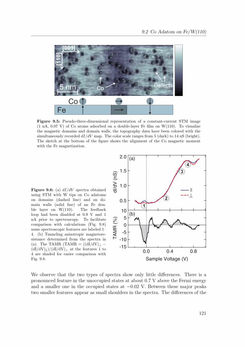
9.2 Co Adatom on Fe/W(110)
[001]
[10]
1
Figure 9.5: Pseudo-three-dimensional representation of a constant-current STM image(1 nA, 0.07 V) of Co atoms adsorbed on a double-layer Fe film on W(110). To visualizethe magnetic domains and domain walls, the topography data have been colored with thesimultaneously recorded dI/dV map. The color scale ranges from 5 (dark) to 14 nS (bright).The sketch at the bottom of the figure shows the alignment of the Co magnetic momentwith the Fe magnetization.
Figure 9.6: (a) dI/dV spectra obtainedusing STM with W tips on Co adatomson domains (dashed line) and on do-main walls (solid line) of an Fe dou-ble layer on W(110). The feedbackloop had been disabled at 0.9 V and 1nA prior to spectroscopy. To facilitatecomparison with calculations (Fig. 9.8)some spectroscopic features are labeled 1–4. (b) Tunneling anisotropic magnetore-sistance determined from the spectra in(a). The TAMR (TAMR = ((dI/dV)⊥ −(dI/dV)∥)/(dI/dV)⊥ at the features 1 to4 are shaded for easier comparison withFig. 9.8.
2
3
4
1
||
We observe that the two types of spectra show only little differences. There is apronounced feature in the unoccupied states at about 0.7 V above the Fermi energyand a smaller one in the occupied states at −0.02 V. Between these major peakstwo smaller features appear as small shoulders in the spectra. The differences of the
121
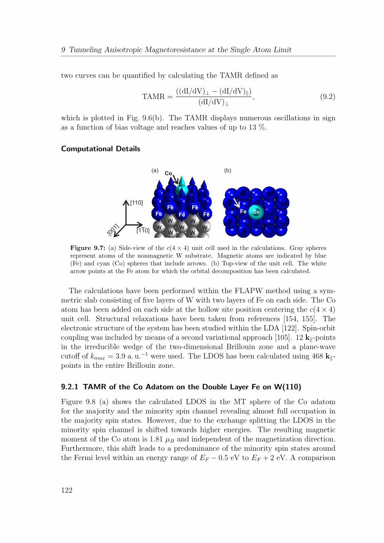
9 Tunneling Anisotropic Magnetoresistance at the Single Atom Limit
two curves can be quantified by calculating the TAMR defined as
TAMR =((dI/dV)⊥ − (dI/dV)∥)
(dI/dV)⊥, (9.2)
which is plotted in Fig. 9.6(b). The TAMR displays numerous oscillations in signas a function of bias voltage and reaches values of up to 13 %.
Computational Details
(a) (b)
Fe Fe Fe
FeFe
W
W
W
W
W W W
Co
Fe Co
[110]
[001
][1 0]1
Figure 9.7: (a) Side-view of the c(4 × 4) unit cell used in the calculations. Gray spheresrepresent atoms of the nonmagnetic W substrate. Magnetic atoms are indicated by blue(Fe) and cyan (Co) spheres that include arrows. (b) Top-view of the unit cell. The whitearrow points at the Fe atom for which the orbital decomposition has been calculated.
The calculations have been performed within the FLAPW method using a sym-metric slab consisting of five layers of W with two layers of Fe on each side. The Coatom has been added on each side at the hollow site position centering the c(4 × 4)unit cell. Structural relaxations have been taken from references [154, 155]. Theelectronic structure of the system has been studied within the LDA [122]. Spin-orbitcoupling was included by means of a second variational approach [105]. 12 k∥-pointsin the irreducible wedge of the two-dimensional Brillouin zone and a plane-wavecutoff of kmax = 3.9 a. u.−1 were used. The LDOS has been calculated using 468 k∥-points in the entire Brillouin zone.
9.2.1 TAMR of the Co Adatom on the Double Layer Fe on W(110)
Figure 9.8 (a) shows the calculated LDOS in the MT sphere of the Co adatomfor the majority and the minority spin channel revealing almost full occupation inthe majority spin states. However, due to the exchange splitting the LDOS in theminority spin channel is shifted towards higher energies. The resulting magneticmoment of the Co atom is 1.81 µB and independent of the magnetization direction.Furthermore, this shift leads to a predominance of the minority spin states aroundthe Fermi level within an energy range of EF − 0.5 eV to EF + 2 eV. A comparison
122
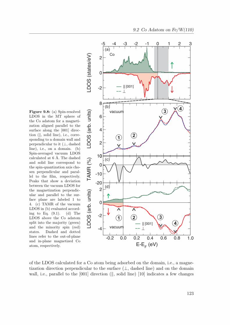
9.2 Co Adatom on Fe/W(110)
Figure 9.8: (a) Spin-resolvedLDOS in the MT sphere ofthe Co adatom for a magneti-zation aligned parallel to thesurface along the [001] direc-tion (∥, solid line), i.e., corre-sponding to a domain wall andperpendicular to it (⊥, dashedline), i.e., on a domain. (b)Spin-averaged vacuum LDOScalculated at 6 A. The dashedand solid line correspond tothe spin-quantization axis cho-sen perpendicular and paral-lel to the film, respectively.Peaks that show a deviationbetween the vacuum LDOS forthe magnetization perpendic-ular and parallel to the sur-face plane are labeled 1 to4. (c) TAMR of the vacuumLDOS in (b) evaluated accord-ing to Eq. (9.1). (d) TheLDOS above the Co adatomsplit into the majority (green)and the minority spin (red)states. Dashed and dottedlines refer to the out-of-planeand in-plane magnetized Coatom, respectively.
3
21
4
4
321
||
||
Co
(a)
(b)
(c)
(d)
of the LDOS calculated for a Co atom being adsorbed on the domain, i.e., a magne-tization direction perpendicular to the surface (⊥, dashed line) and on the domainwall, i.e., parallel to the [001] direction (∥, solid line) [10] indicates a few changes
123
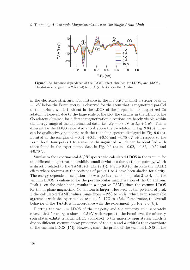
9 Tunneling Anisotropic Magnetoresistance at the Single Atom Limit
3
2
14
Figure 9.9: Distance dependence of the TAMR effect obtained for LDOS∥ and LDOS⊥.
The distance ranges from 2 A (red) to 10 A (violet) above the Co atom.
in the electronic structure. For instance in the majority channel a strong peak at−1 eV below the Fermi energy is observed for the atom that is magnetized parallelto the surface, which is absent in the LDOS of the perpendicular magnetized Coadatom. However, due to the large scale of the plot the changes in the LDOS of theCo adatom obtained for different magnetization directions are barely visible withinthe energy range of the experimental data, i.e., EF − 0.3 eV to EF + 1 eV. This isdifferent for the LDOS calculated at 6 A above the Co adatom in Fig. 9.8 (b). Theycan be qualitatively compared with the tunneling spectra displayed in Fig. 9.6 (a).Located at the energies of −0.07, +0.16, +0.56 and +0.78 eV with respect to theFermi level, four peaks 1 to 4 may be distinguished, which can be identified withthose found in the experimental data in Fig. 9.6 (a) at −0.02, +0.32, +0.52 and+0.70 V.
Similar to the experimental dI/dV spectra the calculated LDOS in the vacuum forthe different magnetizations exhibits small deviations due to the anisotropy, whichis directly related to the TAMR (cf. Eq. (9.1)). Figure 9.8 (c) displays the TAMReffect where features at the positions of peaks 1 to 4 have been shaded for clarity.The energy dependent oscillations show a positive value for peaks 2 to 4, i.e., thevacuum LDOS is enhanced for the perpendicular magnetization of the Co adatom.Peak 1, on the other hand, results in a negative TAMR since the vacuum LDOSfor the in-plane magnetized Co adatom is larger. However, at the position of peak1 the calculated TAMR values range from −19% to +9%, which is in reasonableagreement with the experimental results of −12% to +5%. Furthermore, the overallbehavior of the TAMR is in accordance with the experiment (cf. Fig. 9.6 (b)).
Plotting the vacuum LDOS of the majority and the minority spin separatelyreveals that for energies above +0.3 eV with respect to the Fermi level the minorityspin states exhibit a larger LDOS compared to the majority spin states, which isdue to different vacuum decay properties of the s, p and d orbitals that contributeto the vacuum LDOS [154]. However, since the profile of the vacuum LDOS in the
124
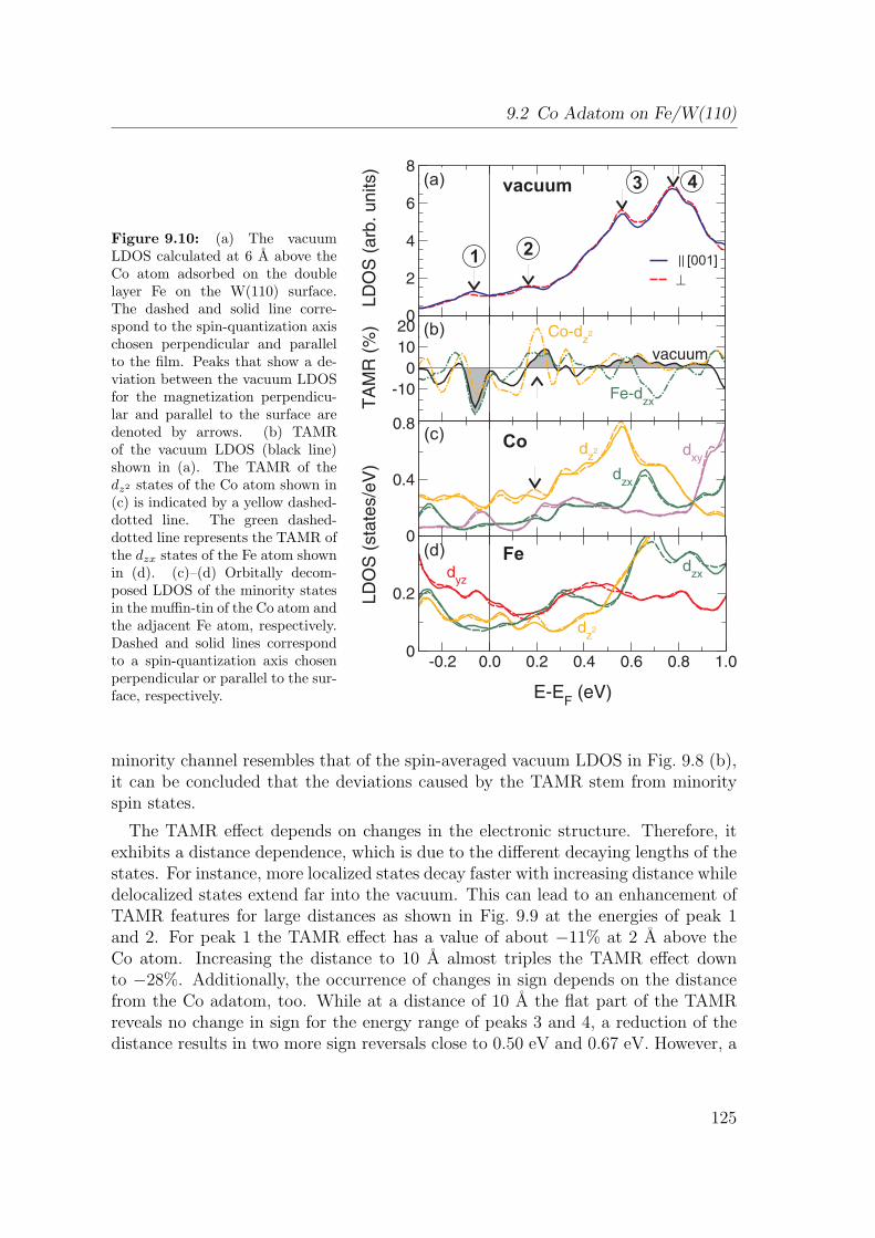
9.2 Co Adatom on Fe/W(110)
Figure 9.10: (a) The vacuumLDOS calculated at 6 A above theCo atom adsorbed on the doublelayer Fe on the W(110) surface.The dashed and solid line corre-spond to the spin-quantization axischosen perpendicular and parallelto the film. Peaks that show a de-viation between the vacuum LDOSfor the magnetization perpendicu-lar and parallel to the surface aredenoted by arrows. (b) TAMRof the vacuum LDOS (black line)shown in (a). The TAMR of thedz2 states of the Co atom shown in(c) is indicated by a yellow dashed-dotted line. The green dashed-dotted line represents the TAMR ofthe dzx states of the Fe atom shownin (d). (c)–(d) Orbitally decom-posed LDOS of the minority statesin the muffin-tin of the Co atom andthe adjacent Fe atom, respectively.Dashed and solid lines correspondto a spin-quantization axis chosenperpendicular or parallel to the sur-face, respectively.
Fe
Co
||
vacuum
21
3 4
[001]
minority channel resembles that of the spin-averaged vacuum LDOS in Fig. 9.8 (b),it can be concluded that the deviations caused by the TAMR stem from minorityspin states.
The TAMR effect depends on changes in the electronic structure. Therefore, itexhibits a distance dependence, which is due to the different decaying lengths of thestates. For instance, more localized states decay faster with increasing distance whiledelocalized states extend far into the vacuum. This can lead to an enhancement ofTAMR features for large distances as shown in Fig. 9.9 at the energies of peak 1and 2. For peak 1 the TAMR effect has a value of about −11% at 2 A above theCo atom. Increasing the distance to 10 A almost triples the TAMR effect downto −28%. Additionally, the occurrence of changes in sign depends on the distancefrom the Co adatom, too. While at a distance of 10 A the flat part of the TAMRreveals no change in sign for the energy range of peaks 3 and 4, a reduction of thedistance results in two more sign reversals close to 0.50 eV and 0.67 eV. However, a
125
9 Tunneling Anisotropic Magnetoresistance at the Single Atom Limit
tip-sample distance of 2 A does not correspond to the tunneling regime, but can beexplored experimentally in the contact regime.
The TAMR effect originates from the spin-orbit induced mixing of electronic stateswith different orbital character. Therefore, it is useful to analyze the mechanismbehind it in terms of an orbital decomposition of the density of states (cf. Fig. 9.10(c)). Given that the LDOS of the majority spin channel is low around the Fermilevel (cf. 9.8 (d)) only the d states of the minority channel are taken into account.Comparing the d-orbitals of the Co atom (Fig. 9.10 (c)) to the vacuum LDOS(Fig. 9.10 (a)) demonstrates that the electronic states that contribute to the changesat the positions of peaks 2 to 4 are mainly of dz2 character. However, peak 1 cannotbe ascribed to the dz2 states of the Co atom. Its occurrence can only be explainedby the hybridization of states of the Co atom and the adjacent Fe atom (cf. Fig. 9.7(b)). At the Co atom feature 1 is of dxy character while it is of dzx type in the Fefilm.
The small deviations due to different magnetization directions, ⊥ and ∥, are like-wise present in the orbital decomposition of the LDOS at the Co and the Fe atom.In Fig. 9.10 (b) their TAMR effects (Co: yellow line; Fe: green line) are compared tothe total TAMR effect (black line) of the vacuum LDOS. For the features at peaks2 to 4 the dz2 states of the Co atom reproduce the trend of the total TAMR in mostinstances, while the minimum at peak 1 agrees well with TAMR of the Fe-dzx states.Hence, it is necessary to consider the electronic structure of the Fe atoms as well asthe Co atom in order to understand the origin of the TAMR effect at feature 1 inthis system.
9.2.2 Model of the TAMR
The results above demonstrate that the anisotropy of the LDOS is directly relatedto changes in the electronic structure due to SOC. These changes originate from themixing of d states with different orbital character such as dz2 and the dzx states.This is easily seen for peak 2 (cf. Fig. 9.10 (a) and (c)) at the Co atom: the LDOS⊥of the dz2 states exhibits an enhancement as well as a shift towards higher energieswith respect to the dz2 states of the in-plane magnetization direction. Furthermore,a small peak occurring in the LDOS⊥ of the dzx states at the same energy hintsto a hybridization between the states with an orbital character of dz2 and dzx.Calculating the difference between the dz2 states of ⊥ and ∥ magnetization accordingto Eq. (9.1) results in a TAMR curve with similar behavior compared to the TAMRof the vacuum LDOS (cf. Fig. 9.10 (b)).
In order to capture the essence of the TAMR effect, a simple model based onthe Green’s function G(E) is introduced in the following. It describes two localizedatomic states at a surface that interact via SOC (cf. Fig. 9.11):
(E · 1 −H− Σ)G(E) = 1. (9.3)
126
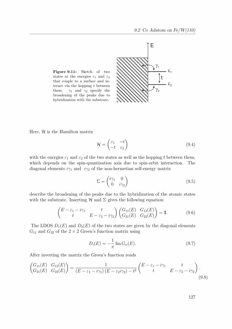
9.2 Co Adatom on Fe/W(110)
Figure 9.11: Sketch of twostates at the energies ε1 and ε2that couple to a surface and in-teract via the hopping t betweenthem. γ1 and γ2 specify thebroadening of the peaks due tohybridization with the substrate.
E
g1
g2
t
e1
e2
Here, H is the Hamilton matrix
H =
(ε1 −t−t ε2
)(9.4)
with the energies ε1 and ε2 of the two states as well as the hopping t between them,which depends on the spin-quantization axis due to spin-orbit interaction. Thediagonal elements iγ1 and iγ2 of the non-hermetian self-energy matrix
Σ =
(iγ1 00 iγ2
)(9.5)
describe the broadening of the peaks due to the hybridization of the atomic stateswith the substrate. Inserting H and Σ gives the following equation:(
E − ε1 − iγ1 tt E − ε2 − iγ2
)(G11(E) G12(E)G21(E) G22(E)
)= 1. (9.6)
The LDOS D1(E) and D2(E) of the two states are given by the diagonal elementsG11 and G22 of the 2 × 2 Green’s function matrix using
Di(E) = − 1
πImGii(E). (9.7)
After inverting the matrix the Green’s function reads(G11(E) G12(E)G21(E) G22(E)
)=
1
(E − ε1 − iγ1) (E − ε2iγ2) − t2
(E − ε1 − iγ1 t
t E − ε2 − iγ2
).
(9.8)
127
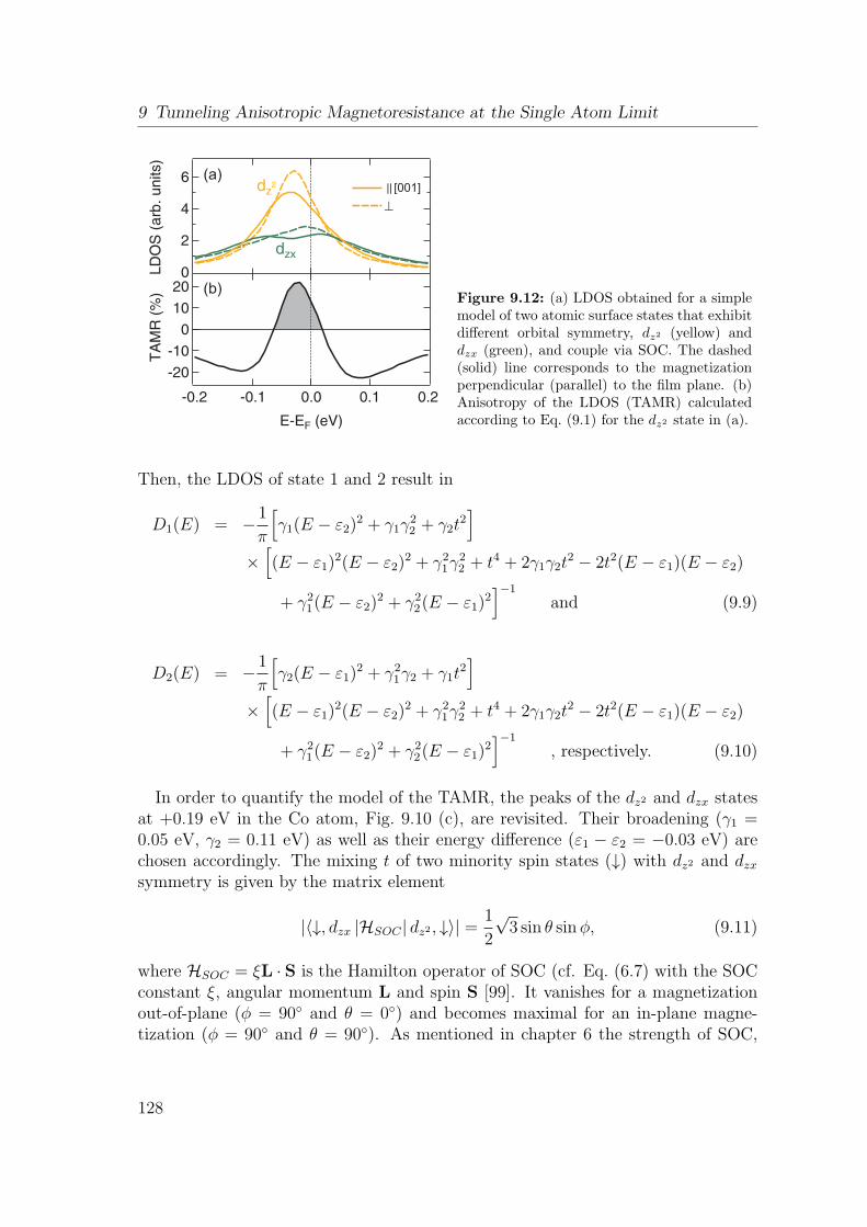
9 Tunneling Anisotropic Magnetoresistance at the Single Atom Limit
||(a)
(b)
[001]
Figure 9.12: (a) LDOS obtained for a simplemodel of two atomic surface states that exhibitdifferent orbital symmetry, dz2 (yellow) anddzx (green), and couple via SOC. The dashed(solid) line corresponds to the magnetizationperpendicular (parallel) to the film plane. (b)Anisotropy of the LDOS (TAMR) calculatedaccording to Eq. (9.1) for the dz2 state in (a).
Then, the LDOS of state 1 and 2 result in
D1(E) = − 1
π
[γ1(E − ε2)
2 + γ1γ22 + γ2t
2]
×[(E − ε1)
2(E − ε2)2 + γ21γ
22 + t4 + 2γ1γ2t
2 − 2t2(E − ε1)(E − ε2)
+ γ21(E − ε2)2 + γ22(E − ε1)
2]−1
and (9.9)
D2(E) = − 1
π
[γ2(E − ε1)
2 + γ21γ2 + γ1t2]
×[(E − ε1)
2(E − ε2)2 + γ21γ
22 + t4 + 2γ1γ2t
2 − 2t2(E − ε1)(E − ε2)
+ γ21(E − ε2)2 + γ22(E − ε1)
2]−1
, respectively. (9.10)
In order to quantify the model of the TAMR, the peaks of the dz2 and dzx statesat +0.19 eV in the Co atom, Fig. 9.10 (c), are revisited. Their broadening (γ1 =0.05 eV, γ2 = 0.11 eV) as well as their energy difference (ε1 − ε2 = −0.03 eV) arechosen accordingly. The mixing t of two minority spin states (↓) with dz2 and dzxsymmetry is given by the matrix element
|⟨↓, dzx |HSOC | dz2 , ↓⟩| =1
2
√3 sin θ sinϕ, (9.11)
where HSOC = ξL · S is the Hamilton operator of SOC (cf. Eq. (6.7) with the SOCconstant ξ, angular momentum L and spin S [99]. It vanishes for a magnetizationout-of-plane (ϕ = 90 and θ = 0) and becomes maximal for an in-plane magne-tization (ϕ = 90 and θ = 90). As mentioned in chapter 6 the strength of SOC,
128
9.3 Non-magnetic Single Iridium Adatom on the Double Layer Fe on W(110)
ξ, is on the order of about 50 meV for 3d-transition metals [99]. Thus, the mixingparameter t is chosen as 0 meV for the ⊥ magnetization direction and 40 meV forthe ∥ magnetization direction. Fig. 9.12 (a) displays the result of the model derivedabove. The LDOS of the dz2 and the dzx states are enhanced for the ⊥ magnetiza-tion and, furthermore, exhibit a small energy shift in the position of the peak withrespect to the LDOS of the in-plane magnetization. This is in agreement with theresults of the DFT calculations in Fig. 9.10 (c). The model TAMR in Fig. 9.12 isobtained by taking only the dz2 states into account. The resulting shape is similarto the one of a single dz2 peak as indicated by an arrow in Fig. 9.10 (b). It shows asign reversal at lower and higher energies. With values up to 20% the model TAMRis in good agreement with the TAMR of the Co dz2 states (22%) obtained in theelectronic structure calculations. However, the TAMR values of the vacuum LDOSare smaller due to the neglect of the s- and p states within the model.
Conclusions
In this section, the TAMR of a single Co atom adsorbed on a double layer of Feon the W(110) has been investigated. With values ranging between −19% to +9%the TAMR based on first-principles calculations compares reasonable with the ex-perimental values ranging from −12% to +5%. The origin of the TAMR has beenascribed to the mixing of 3d states with different orbital character in the Co atom.The main contribution to the vacuum LDOS originates from the dz2 states of theminority spin channel in the Co atom that mix with d resonances and thus lead toa magnetization-direction dependence of the LDOS in the vacuum. The features ofthe TAMR were captured in a model of two interacting atomic states.
9.3 Non-magnetic Single Iridium Adatom on the Double LayerFe on W(110)
So far, the focus has been on single magnetic atoms adsorbed on a magnetic thinfilm such as the Co atom in the section before. Indeed, such an atom exhibits a largemagnetic moment of up to 1.8 µB, but the SOC effect is weak in elements of the3d series. A way to increase the TAMR effect is to choose a heavier element fromthe 5d series instead of a 3d metal to be adsorbed on the Fe film. Spin-polarizationdue to the magnetic thin film allows the formation of a sufficiently large magneticmoment in the 5d adatom. In the following, it is demonstrated by the example ofan Ir adatom how this strategy heads to a giant TAMR effect on the order of up to60 %.
129
9 Tunneling Anisotropic Magnetoresistance at the Single Atom Limit
Computational Details
The ab initio calculations have been performed using a symmetric slab consisting offive layers of W with two layers of Fe on each side while employing the experimentallattice constant of W, a = 3.165 A. The Ir atom is centered within a c(4 × 4) unitcell on both sides of the slab (cf. inset in Fig. 9.13 (a)). Structural relaxationshave been carried out via force minimization for the Ir adatoms and the Fe atomsof the film within the GGA [33]. The equilibrium interlayer distance between theIr atom and the next-nearest Fe atom is reduced by 28%, i.e., 1.61 A, compared tothe W bulk. The analysis of the electronic structure has been carried out within theLDA [122] if not stated otherwise. The SOC effect has been included by applying asecond variational approach [105] using 12 k∥-points in the irreducible wedge of thetwo-dimensional Brillouin zone. A plane-wave cutoff of kmax = 3.9 a.u.−1 has beenused. The LDOS in the muffin-tin as well as in the vacuum has been computedusing 280 k∥-points in the entire Brillouin zone.
9.3.1 Spin-Polarization of the Ir Adatom on the Double Layer Fe on W(110)
As mentioned above, the hybridization between the Fe atoms of the double-layerfilm and the Ir adatom lead to a spin-polarization of the latter. This is observedby comparing the spin-resolved local densities of states in the MT spheres of theadjacent Fe atoms, Fig. 9.13 (a), to that of the Ir atom in Fig. 9.13 (b). Severalpeaks located at EF − 3.6 eV and EF − 0.75 eV in the majority channel (green) aswell as EF + 1.5 eV in the minority channel (red) occur in both the Fe atoms andthe Ir atom and hint at hybridized states. Recalling the LDOS calculated in theFe film in section 9.1.1 (cf. Fig. 9.4 (a)) shows that the exchange splitting of thespin channels changes slightly if an Ir atom is deposited onto the film. The resultingmagnetic moment of the Fe atom 4 in the inset of Fig. 9.13 (a) amounts to +2.72 µB
in the GGA [33] and +2.62 µB within the LDA [122], i.e., it is reduced with respectto the Fe moment of 2.9 µB in the surface layer of the double-layer film. However,the LDOS of the Ir atoms exhibits likewise an exchange splitting as observed inFig. 9.13 (b), which leads to magnetic moments of +0.87 µB within the GGA and+0.77 µB within the LDA. Evidently, for both exchange-correlation potentials the Iratom is significantly spin-polarized. Furthermore, it follows from Fig. 9.13 (b) thatthe minority spin states dominate at lower energies while close to the Fermi levelstates of the majority spin govern the LDOS. This tendency is further illustrated bycalculating the spin-polarization in the Ir adatom according to
PIr =(LDOS↑ − LDOS↓)
(LDOS↑ + LDOS↓). (9.12)
Fig. 9.13 (b) represents the resulting curve. It exhibits several sign reversals for thespin-polarization in the Ir atom. In the energy range of EF − 1 eV and EF + 1 eV
130

9.3 Non-magnetic Single Iridium Adatom on the Double Layer Fe on W(110)
Figure 9.13: (a) LDOS inthe MT spheres of the neigh-boring Fe atoms 3 and 4 (seeinset) in the majority andminority spin channel. (b)Spin-dependent LDOS cal-culated in the MT sphereof the Ir atom. (c) Spin-polarization of the LDOS in(b) according to Eq. (9.3.1).(c) LDOS in the vacuum cal-culated at 6 A above theIr atom. Green and redlines correspond to the ma-jority (↑) and minority (↓)spin channels. (d) Spin-polarization of the vacuumLDOS calculated in a rangeof 2 A (red line) to 10 A (vi-olet line) above the Ir atomaccording to Eq. (9.3.1).
Ir-atom
vacuum
Fe-atom
##
(a)
(b)
(c)
(d)
(e)
Ir
12
34
it is maximum at EF − 0.77 eV and a value of PIr = 0.82. The sign of the spin-polarization changes at EF + 0.35 eV leading to a minimum value of PIr = −0.69at EF + 0.85 eV. At 6 A above the Ir adatom a similar behavior is observed. Thevacuum LDOS presented in Fig. 9.13 (d) reveals a dominance of majority spinstates for energies up to EF +0.54 eV. For higher energies the LDOS in the minoritychannel increases. This is also visible in the spin-polarization in the vacuum, which
131
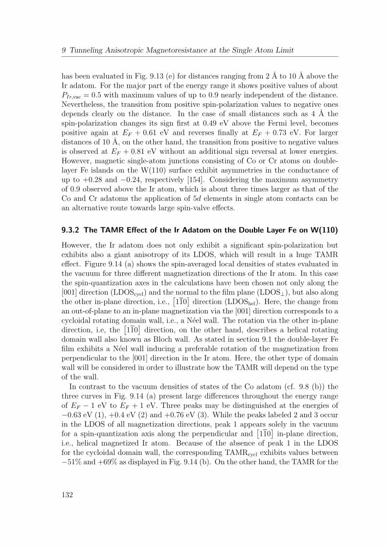
9 Tunneling Anisotropic Magnetoresistance at the Single Atom Limit
has been evaluated in Fig. 9.13 (e) for distances ranging from 2 A to 10 A above theIr adatom. For the major part of the energy range it shows positive values of aboutPIr,vac = 0.5 with maximum values of up to 0.9 nearly independent of the distance.Nevertheless, the transition from positive spin-polarization values to negative onesdepends clearly on the distance. In the case of small distances such as 4 A thespin-polarization changes its sign first at 0.49 eV above the Fermi level, becomespositive again at EF + 0.61 eV and reverses finally at EF + 0.73 eV. For largerdistances of 10 A, on the other hand, the transition from positive to negative valuesis observed at EF + 0.81 eV without an additional sign reversal at lower energies.However, magnetic single-atom junctions consisting of Co or Cr atoms on double-layer Fe islands on the W(110) surface exhibit asymmetries in the conductance ofup to +0.28 and −0.24, respectively [154]. Considering the maximum asymmetryof 0.9 observed above the Ir atom, which is about three times larger as that of theCo and Cr adatoms the application of 5d elements in single atom contacts can bean alternative route towards large spin-valve effects.
9.3.2 The TAMR Effect of the Ir Adatom on the Double Layer Fe on W(110)
However, the Ir adatom does not only exhibit a significant spin-polarization butexhibits also a giant anisotropy of its LDOS, which will result in a huge TAMReffect. Figure 9.14 (a) shows the spin-averaged local densities of states evaluated inthe vacuum for three different magnetization directions of the Ir atom. In this casethe spin-quantization axes in the calculations have been chosen not only along the[001] direction (LDOScycl) and the normal to the film plane (LDOS⊥), but also alongthe other in-plane direction, i.e.,
[110]
direction (LDOShel). Here, the change froman out-of-plane to an in-plane magnetization via the [001] direction corresponds to acycloidal rotating domain wall, i.e., a Neel wall. The rotation via the other in-planedirection, i.e, the
[110]
direction, on the other hand, describes a helical rotatingdomain wall also known as Bloch wall. As stated in section 9.1 the double-layer Fefilm exhibits a Neel wall inducing a preferable rotation of the magnetization fromperpendicular to the [001] direction in the Ir atom. Here, the other type of domainwall will be considered in order to illustrate how the TAMR will depend on the typeof the wall.
In contrast to the vacuum densities of states of the Co adatom (cf. 9.8 (b)) thethree curves in Fig. 9.14 (a) present large differences throughout the energy rangeof EF − 1 eV to EF + 1 eV. Three peaks may be distinguished at the energies of−0.63 eV (1), +0.4 eV (2) and +0.76 eV (3). While the peaks labeled 2 and 3 occurin the LDOS of all magnetization directions, peak 1 appears solely in the vacuumfor a spin-quantization axis along the perpendicular and
[110]
in-plane direction,i.e., helical magnetized Ir atom. Because of the absence of peak 1 in the LDOSfor the cycloidal domain wall, the corresponding TAMRcycl exhibits values between−51% and +69% as displayed in Fig. 9.14 (b). On the other hand, the TAMR for the
132
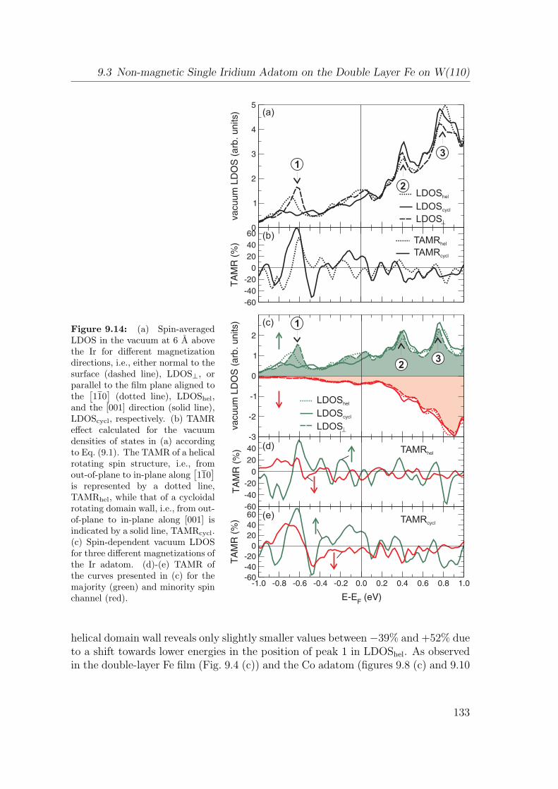
9.3 Non-magnetic Single Iridium Adatom on the Double Layer Fe on W(110)
Figure 9.14: (a) Spin-averagedLDOS in the vacuum at 6 A abovethe Ir for different magnetizationdirections, i.e., either normal to thesurface (dashed line), LDOS⊥, orparallel to the film plane aligned tothe
[110](dotted line), LDOShel,
and the [001] direction (solid line),LDOScycl, respectively. (b) TAMReffect calculated for the vacuumdensities of states in (a) accordingto Eq. (9.1). The TAMR of a helicalrotating spin structure, i.e., fromout-of-plane to in-plane along
[110]
is represented by a dotted line,TAMRhel, while that of a cycloidalrotating domain wall, i.e., from out-of-plane to in-plane along [001] isindicated by a solid line, TAMRcycl.(c) Spin-dependent vacuum LDOSfor three different magnetizations ofthe Ir adatom. (d)-(e) TAMR ofthe curves presented in (c) for themajority (green) and minority spinchannel (red).
32
1
3
2
1
(a)
(c)
(d)
(b)
(e)
TAMRhel
TAMRcycl
TAMRhel
TAMRcycl
LDOShel
LDOScycl
LDOShel
LDOScycl
LDOS
LDOS
helical domain wall reveals only slightly smaller values between −39% and +52% dueto a shift towards lower energies in the position of peak 1 in LDOShel. As observedin the double-layer Fe film (Fig. 9.4 (c)) and the Co adatom (figures 9.8 (c) and 9.10
133
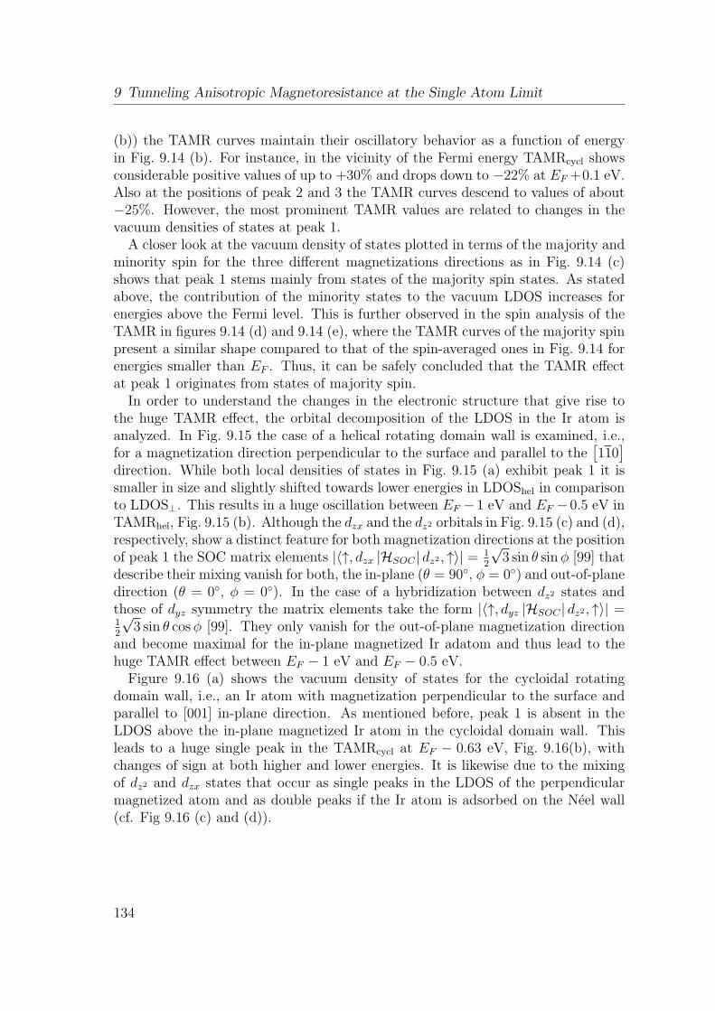
9 Tunneling Anisotropic Magnetoresistance at the Single Atom Limit
(b)) the TAMR curves maintain their oscillatory behavior as a function of energyin Fig. 9.14 (b). For instance, in the vicinity of the Fermi energy TAMRcycl showsconsiderable positive values of up to +30% and drops down to −22% at EF +0.1 eV.Also at the positions of peak 2 and 3 the TAMR curves descend to values of about−25%. However, the most prominent TAMR values are related to changes in thevacuum densities of states at peak 1.
A closer look at the vacuum density of states plotted in terms of the majority andminority spin for the three different magnetizations directions as in Fig. 9.14 (c)shows that peak 1 stems mainly from states of the majority spin states. As statedabove, the contribution of the minority states to the vacuum LDOS increases forenergies above the Fermi level. This is further observed in the spin analysis of theTAMR in figures 9.14 (d) and 9.14 (e), where the TAMR curves of the majority spinpresent a similar shape compared to that of the spin-averaged ones in Fig. 9.14 forenergies smaller than EF . Thus, it can be safely concluded that the TAMR effectat peak 1 originates from states of majority spin.
In order to understand the changes in the electronic structure that give rise tothe huge TAMR effect, the orbital decomposition of the LDOS in the Ir atom isanalyzed. In Fig. 9.15 the case of a helical rotating domain wall is examined, i.e.,for a magnetization direction perpendicular to the surface and parallel to the
[110]
direction. While both local densities of states in Fig. 9.15 (a) exhibit peak 1 it issmaller in size and slightly shifted towards lower energies in LDOShel in comparisonto LDOS⊥. This results in a huge oscillation between EF −1 eV and EF −0.5 eV inTAMRhel, Fig. 9.15 (b). Although the dzx and the dz2 orbitals in Fig. 9.15 (c) and (d),respectively, show a distinct feature for both magnetization directions at the positionof peak 1 the SOC matrix elements |⟨↑, dzx |HSOC | dz2 , ↑⟩| = 1
2
√3 sin θ sinϕ [99] that
describe their mixing vanish for both, the in-plane (θ = 90, ϕ = 0) and out-of-planedirection (θ = 0, ϕ = 0). In the case of a hybridization between dz2 states andthose of dyz symmetry the matrix elements take the form |⟨↑, dyz |HSOC | dz2 , ↑⟩| =12
√3 sin θ cosϕ [99]. They only vanish for the out-of-plane magnetization direction
and become maximal for the in-plane magnetized Ir adatom and thus lead to thehuge TAMR effect between EF − 1 eV and EF − 0.5 eV.
Figure 9.16 (a) shows the vacuum density of states for the cycloidal rotatingdomain wall, i.e., an Ir atom with magnetization perpendicular to the surface andparallel to [001] in-plane direction. As mentioned before, peak 1 is absent in theLDOS above the in-plane magnetized Ir atom in the cycloidal domain wall. Thisleads to a huge single peak in the TAMRcycl at EF − 0.63 eV, Fig. 9.16(b), withchanges of sign at both higher and lower energies. It is likewise due to the mixingof dz2 and dzx states that occur as single peaks in the LDOS of the perpendicularmagnetized atom and as double peaks if the Ir atom is adsorbed on the Neel wall(cf. Fig 9.16 (c) and (d)).
134
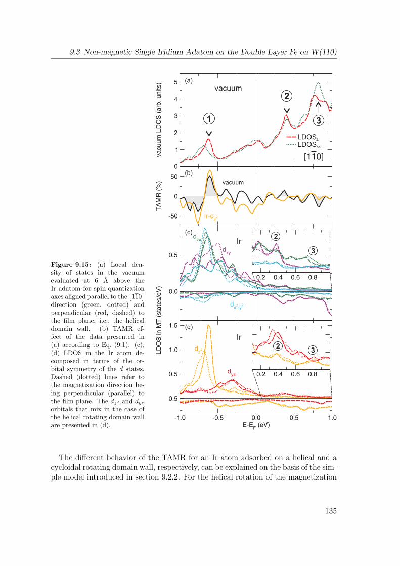
9.3 Non-magnetic Single Iridium Adatom on the Double Layer Fe on W(110)
Figure 9.15: (a) Local den-sity of states in the vacuumevaluated at 6 A above theIr adatom for spin-quantizationaxes aligned parallel to the
[110]
direction (green, dotted) andperpendicular (red, dashed) tothe film plane, i.e., the helicaldomain wall. (b) TAMR ef-fect of the data presented in(a) according to Eq. (9.1). (c),(d) LDOS in the Ir atom de-composed in terms of the or-bital symmetry of the d states.Dashed (dotted) lines refer tothe magnetization direction be-ing perpendicular (parallel) tothe film plane. The dz2 and dyzorbitals that mix in the case ofthe helical rotating domain wallare presented in (d).
1 3
2
(c)
(d)
(a)
(b)
vacuum
Ir
Ir
vacuum
3
2
32
LDOShel
LDOS
The different behavior of the TAMR for an Ir atom adsorbed on a helical and acycloidal rotating domain wall, respectively, can be explained on the basis of the sim-ple model introduced in section 9.2.2. For the helical rotation of the magnetization
135
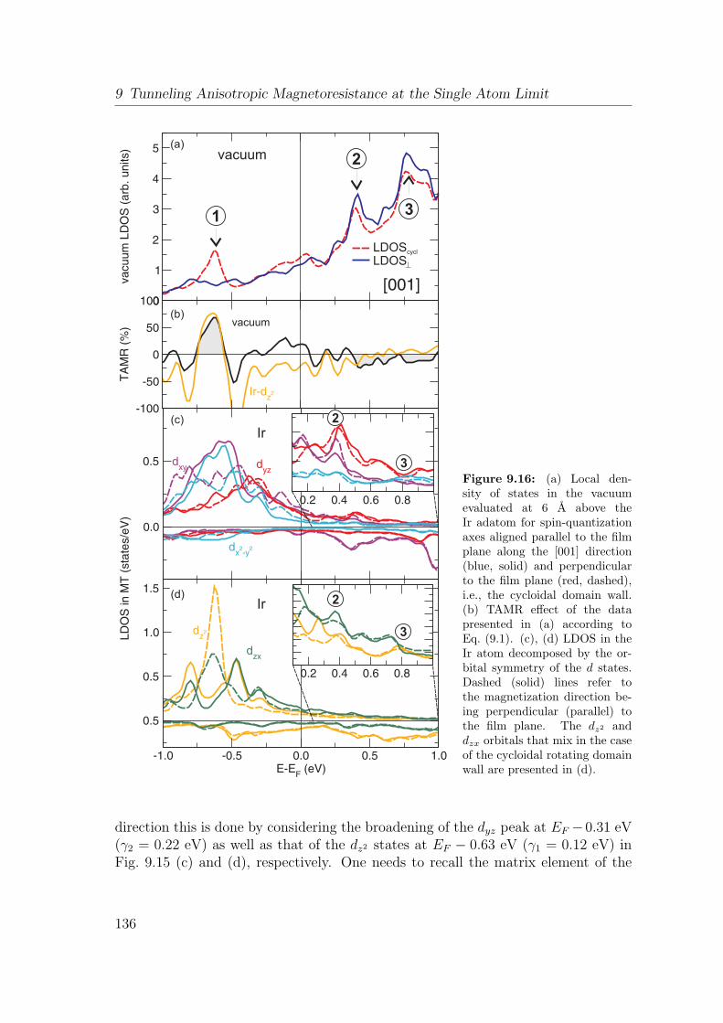
9 Tunneling Anisotropic Magnetoresistance at the Single Atom Limit
13
2
(c)
(d)
(a)
(b)
3
2
3
2
vacuum
Ir
Ir
vacuum
LDOScycl
LDOS
Figure 9.16: (a) Local den-sity of states in the vacuumevaluated at 6 A above theIr adatom for spin-quantizationaxes aligned parallel to the filmplane along the [001] direction(blue, solid) and perpendicularto the film plane (red, dashed),i.e., the cycloidal domain wall.(b) TAMR effect of the datapresented in (a) according toEq. (9.1). (c), (d) LDOS in theIr atom decomposed by the or-bital symmetry of the d states.Dashed (solid) lines refer tothe magnetization direction be-ing perpendicular (parallel) tothe film plane. The dz2 anddzx orbitals that mix in the caseof the cycloidal rotating domainwall are presented in (d).
direction this is done by considering the broadening of the dyz peak at EF −0.31 eV(γ2 = 0.22 eV) as well as that of the dz2 states at EF − 0.63 eV (γ1 = 0.12 eV) inFig. 9.15 (c) and (d), respectively. One needs to recall the matrix element of the
136
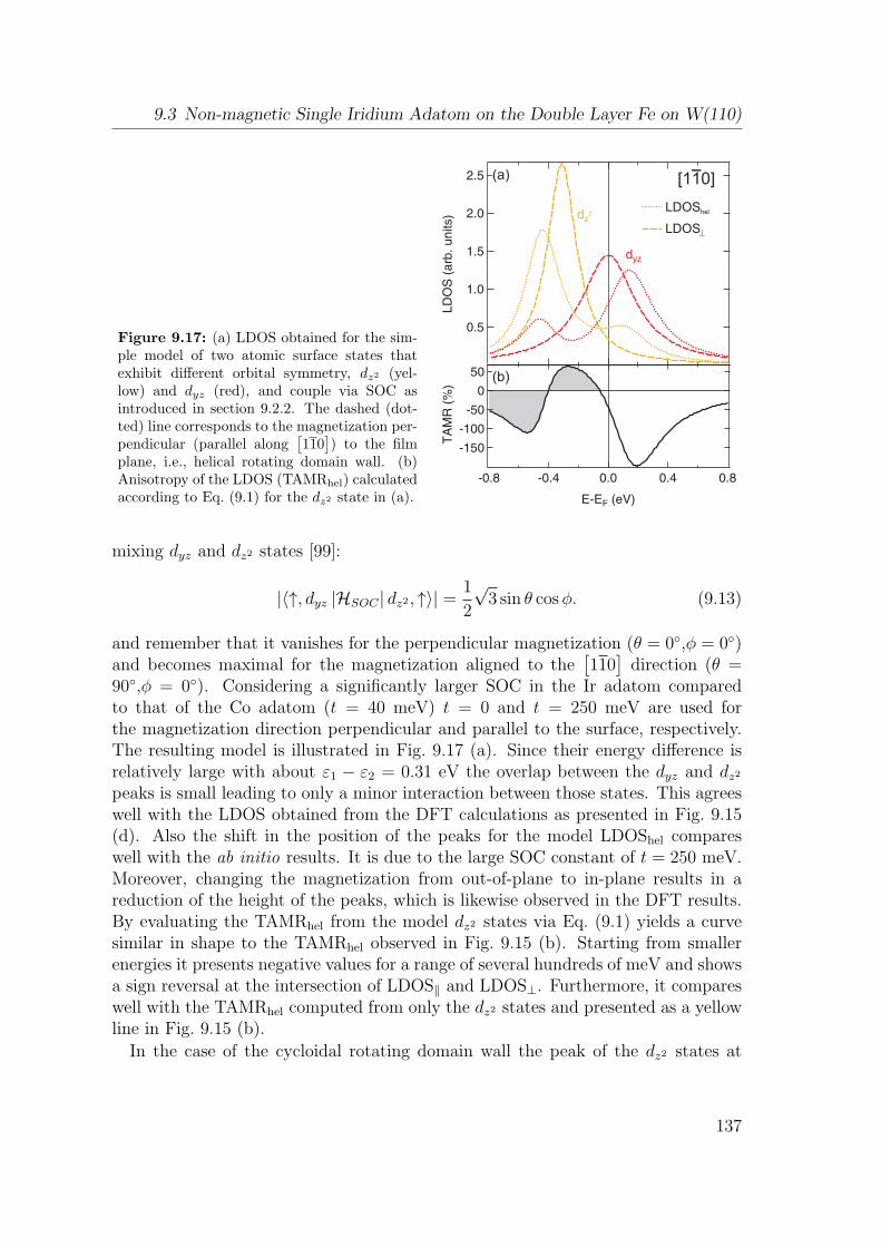
9.3 Non-magnetic Single Iridium Adatom on the Double Layer Fe on W(110)
Figure 9.17: (a) LDOS obtained for the sim-ple model of two atomic surface states thatexhibit different orbital symmetry, dz2 (yel-low) and dyz (red), and couple via SOC asintroduced in section 9.2.2. The dashed (dot-ted) line corresponds to the magnetization per-pendicular (parallel along
[110]) to the film
plane, i.e., helical rotating domain wall. (b)Anisotropy of the LDOS (TAMRhel) calculatedaccording to Eq. (9.1) for the dz2 state in (a).
LDOShel
LDOS
mixing dyz and dz2 states [99]:
|⟨↑, dyz |HSOC | dz2 , ↑⟩| =1
2
√3 sin θ cosϕ. (9.13)
and remember that it vanishes for the perpendicular magnetization (θ = 0,ϕ = 0)and becomes maximal for the magnetization aligned to the
[110]
direction (θ =90,ϕ = 0). Considering a significantly larger SOC in the Ir adatom comparedto that of the Co adatom (t = 40 meV) t = 0 and t = 250 meV are used forthe magnetization direction perpendicular and parallel to the surface, respectively.The resulting model is illustrated in Fig. 9.17 (a). Since their energy difference isrelatively large with about ε1 − ε2 = 0.31 eV the overlap between the dyz and dz2peaks is small leading to only a minor interaction between those states. This agreeswell with the LDOS obtained from the DFT calculations as presented in Fig. 9.15(d). Also the shift in the position of the peaks for the model LDOShel compareswell with the ab initio results. It is due to the large SOC constant of t = 250 meV.Moreover, changing the magnetization from out-of-plane to in-plane results in areduction of the height of the peaks, which is likewise observed in the DFT results.By evaluating the TAMRhel from the model dz2 states via Eq. (9.1) yields a curvesimilar in shape to the TAMRhel observed in Fig. 9.15 (b). Starting from smallerenergies it presents negative values for a range of several hundreds of meV and showsa sign reversal at the intersection of LDOS∥ and LDOS⊥. Furthermore, it compareswell with the TAMRhel computed from only the dz2 states and presented as a yellowline in Fig. 9.15 (b).
In the case of the cycloidal rotating domain wall the peak of the dz2 states at
137
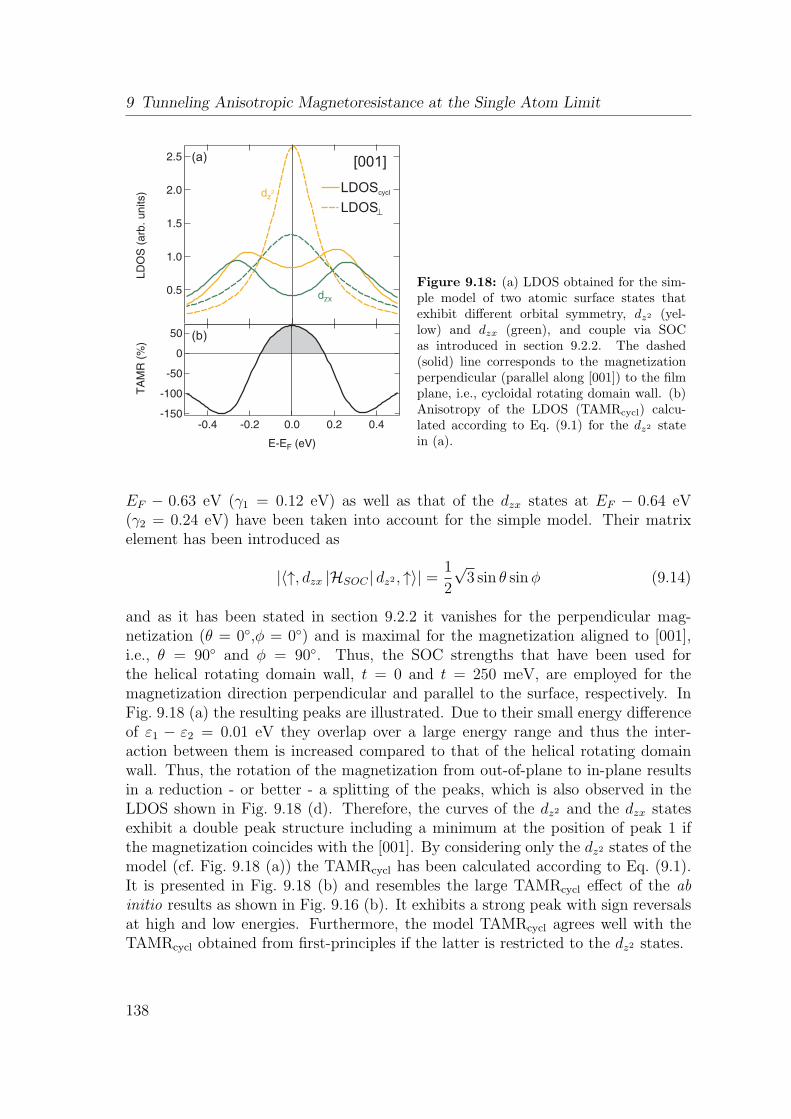
9 Tunneling Anisotropic Magnetoresistance at the Single Atom Limit
LDOScycl
LDOS
Figure 9.18: (a) LDOS obtained for the sim-ple model of two atomic surface states thatexhibit different orbital symmetry, dz2 (yel-low) and dzx (green), and couple via SOCas introduced in section 9.2.2. The dashed(solid) line corresponds to the magnetizationperpendicular (parallel along [001]) to the filmplane, i.e., cycloidal rotating domain wall. (b)Anisotropy of the LDOS (TAMRcycl) calcu-lated according to Eq. (9.1) for the dz2 statein (a).
EF − 0.63 eV (γ1 = 0.12 eV) as well as that of the dzx states at EF − 0.64 eV(γ2 = 0.24 eV) have been taken into account for the simple model. Their matrixelement has been introduced as
|⟨↑, dzx |HSOC | dz2 , ↑⟩| =1
2
√3 sin θ sinϕ (9.14)
and as it has been stated in section 9.2.2 it vanishes for the perpendicular mag-netization (θ = 0,ϕ = 0) and is maximal for the magnetization aligned to [001],i.e., θ = 90 and ϕ = 90. Thus, the SOC strengths that have been used forthe helical rotating domain wall, t = 0 and t = 250 meV, are employed for themagnetization direction perpendicular and parallel to the surface, respectively. InFig. 9.18 (a) the resulting peaks are illustrated. Due to their small energy differenceof ε1 − ε2 = 0.01 eV they overlap over a large energy range and thus the inter-action between them is increased compared to that of the helical rotating domainwall. Thus, the rotation of the magnetization from out-of-plane to in-plane resultsin a reduction - or better - a splitting of the peaks, which is also observed in theLDOS shown in Fig. 9.18 (d). Therefore, the curves of the dz2 and the dzx statesexhibit a double peak structure including a minimum at the position of peak 1 ifthe magnetization coincides with the [001]. By considering only the dz2 states of themodel (cf. Fig. 9.18 (a)) the TAMRcycl has been calculated according to Eq. (9.1).It is presented in Fig. 9.18 (b) and resembles the large TAMRcycl effect of the abinitio results as shown in Fig. 9.16 (b). It exhibits a strong peak with sign reversalsat high and low energies. Furthermore, the model TAMRcycl agrees well with theTAMRcycl obtained from first-principles if the latter is restricted to the dz2 states.
138
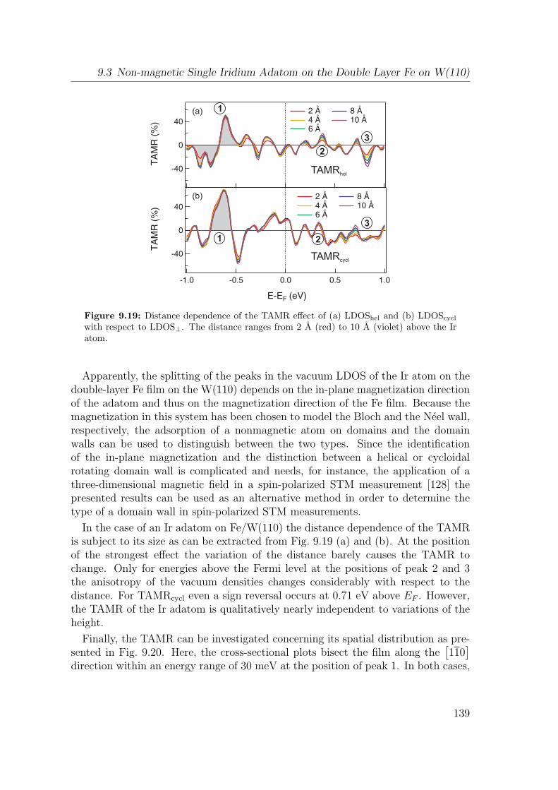
9.3 Non-magnetic Single Iridium Adatom on the Double Layer Fe on W(110)
(a)
(b)
3
21
3
2
1
TAMRhel
TAMRcycl
Figure 9.19: Distance dependence of the TAMR effect of (a) LDOShel and (b) LDOScyclwith respect to LDOS⊥. The distance ranges from 2 A (red) to 10 A (violet) above the Iratom.
Apparently, the splitting of the peaks in the vacuum LDOS of the Ir atom on thedouble-layer Fe film on the W(110) depends on the in-plane magnetization directionof the adatom and thus on the magnetization direction of the Fe film. Because themagnetization in this system has been chosen to model the Bloch and the Neel wall,respectively, the adsorption of a nonmagnetic atom on domains and the domainwalls can be used to distinguish between the two types. Since the identificationof the in-plane magnetization and the distinction between a helical or cycloidalrotating domain wall is complicated and needs, for instance, the application of athree-dimensional magnetic field in a spin-polarized STM measurement [128] thepresented results can be used as an alternative method in order to determine thetype of a domain wall in spin-polarized STM measurements.
In the case of an Ir adatom on Fe/W(110) the distance dependence of the TAMRis subject to its size as can be extracted from Fig. 9.19 (a) and (b). At the positionof the strongest effect the variation of the distance barely causes the TAMR tochange. Only for energies above the Fermi level at the positions of peak 2 and 3the anisotropy of the vacuum densities changes considerably with respect to thedistance. For TAMRcycl even a sign reversal occurs at 0.71 eV above EF . However,the TAMR of the Ir adatom is qualitatively nearly independent to variations of theheight.
Finally, the TAMR can be investigated concerning its spatial distribution as pre-sented in Fig. 9.20. Here, the cross-sectional plots bisect the film along the
[110]
direction within an energy range of 30 meV at the position of peak 1. In both cases,
139
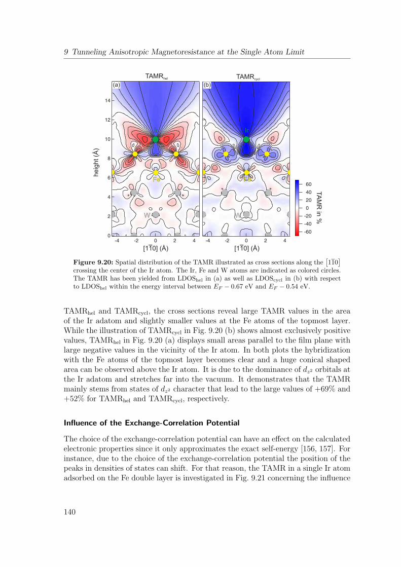
9 Tunneling Anisotropic Magnetoresistance at the Single Atom Limit
TAM
R in
%
[1 0] (Å)1[1 0] (Å)1
he
igh
t (Å
)
W
Fe
Ir
W
Fe
Ir
(a) (b)
TAMRhel TAMRcycl
Figure 9.20: Spatial distribution of the TAMR illustrated as cross sections along the[110]
crossing the center of the Ir atom. The Ir, Fe and W atoms are indicated as colored circles.The TAMR has been yielded from LDOShel in (a) as well as LDOScycl in (b) with respectto LDOShel within the energy interval between EF − 0.67 eV and EF − 0.54 eV.
TAMRhel and TAMRcycl, the cross sections reveal large TAMR values in the areaof the Ir adatom and slightly smaller values at the Fe atoms of the topmost layer.While the illustration of TAMRcycl in Fig. 9.20 (b) shows almost exclusively positivevalues, TAMRhel in Fig. 9.20 (a) displays small areas parallel to the film plane withlarge negative values in the vicinity of the Ir atom. In both plots the hybridizationwith the Fe atoms of the topmost layer becomes clear and a huge conical shapedarea can be observed above the Ir atom. It is due to the dominance of dz2 orbitals atthe Ir adatom and stretches far into the vacuum. It demonstrates that the TAMRmainly stems from states of dz2 character that lead to the large values of +69% and+52% for TAMRhel and TAMRcycl, respectively.
Influence of the Exchange-Correlation Potential
The choice of the exchange-correlation potential can have an effect on the calculatedelectronic properties since it only approximates the exact self-energy [156, 157]. Forinstance, due to the choice of the exchange-correlation potential the position of thepeaks in densities of states can shift. For that reason, the TAMR in a single Ir atomadsorbed on the Fe double layer is investigated in Fig. 9.21 concerning the influence
140
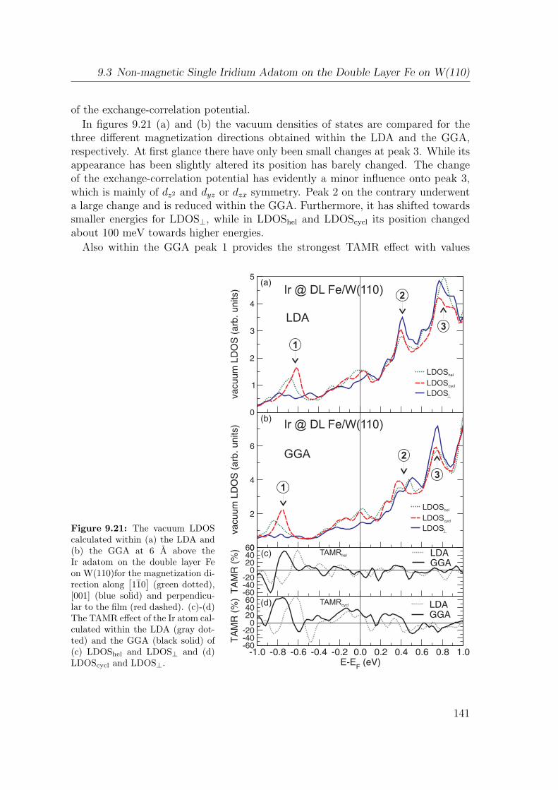
9.3 Non-magnetic Single Iridium Adatom on the Double Layer Fe on W(110)
of the exchange-correlation potential.
In figures 9.21 (a) and (b) the vacuum densities of states are compared for thethree different magnetization directions obtained within the LDA and the GGA,respectively. At first glance there have only been small changes at peak 3. While itsappearance has been slightly altered its position has barely changed. The changeof the exchange-correlation potential has evidently a minor influence onto peak 3,which is mainly of dz2 and dyz or dzx symmetry. Peak 2 on the contrary underwenta large change and is reduced within the GGA. Furthermore, it has shifted towardssmaller energies for LDOS⊥, while in LDOShel and LDOScycl its position changedabout 100 meV towards higher energies.
Also within the GGA peak 1 provides the strongest TAMR effect with values
Figure 9.21: The vacuum LDOScalculated within (a) the LDA and(b) the GGA at 6 A above theIr adatom on the double layer Feon W(110)for the magnetization di-rection along
[110](green dotted),
[001] (blue solid) and perpendicu-lar to the film (red dashed). (c)-(d)The TAMR effect of the Ir atom cal-culated within the LDA (gray dot-ted) and the GGA (black solid) of(c) LDOShel and LDOS⊥ and (d)LDOScycl and LDOS⊥.
LDA
GGA
(c)
(a)
(b)
(d)
1
3
2
1
3
2
Ir @ DL Fe/W(110)
Ir @ DL Fe/W(110)
TAMRhel
TAMRcycl
LDOShel
LDOScycl
LDOS
LDOShel
LDOScycl
LDOS
141
9 Tunneling Anisotropic Magnetoresistance at the Single Atom Limit
ranging from −61% to +52% and −23% to +66% for TAMRhel and TAMRcycl,respectively. It is basically of dz2 and dzx or dyz symmetry, i.e., the charge densitystretches perpendicular to the surface and far into the vacuum. Nevertheless, it shiftsby about 120 meV towards lower energies. As Fig. 9.20 demonstrates, the strongTAMR effect emerges from the hybridization of the Ir atom and the topmost layerof the Fe film. Therefore, the shift of peak 1 is due to a reduction of the magneticmoments of the next-nearest neighboring Fe atoms from 2.73 µB to 2.62 µB uponchanging from the GGA to the LDA.
The TAMR of the curves presented in Fig. 9.21 (a) and (b) is given in Fig. 9.21(c) and (d). Due to its nature as a result of the SOC effect it has been expected thatthe TAMR experiences at least some smaller changes. However, in the case of theIr atom the TAMR effect is qualitatively independent of the exchange-correlationpotential and so are all conclusions drawn in the previous sections.
Conclusions
In this section the TAMR was discussed for a nonmagnetic single atom from the5d series. An Ir atom resembles the Co atom chemically, but exhibits a strongerSOC at the same time. Due to hybridization with the atoms of the topmost Felayer a magnetic moment of +0.77 µB has been induced in the Ir atom leading to aspin-polarization of up to 0.9. This is about three times larger as the values of up to0.28 observed in Co adatoms on Fe double-layer island on W(110) [154]. The hugespin-polarization and the strong SOC lead to a TAMR effect that has been amplifiedby factors of three to four. It gives huge values up to 69% compared to the TAMRof maximum 19% found in the single Co atom. The origin of the huge TAMR effecthas been ascribed to the mixing of dz2 states with those of dzx symmetry and thelarge SOC constant ξ of Ir on the order of 250 meV. Finally, the influence of theexchange-correlation potential onto the TAMR effect has been analyzed.
In comparison to +19% observed in a single Co atom the TAMR effect in the Iratom experiences an amplification of a factor of 2.7 and 3.6, respectively, due to thestrong SOC effect.
142
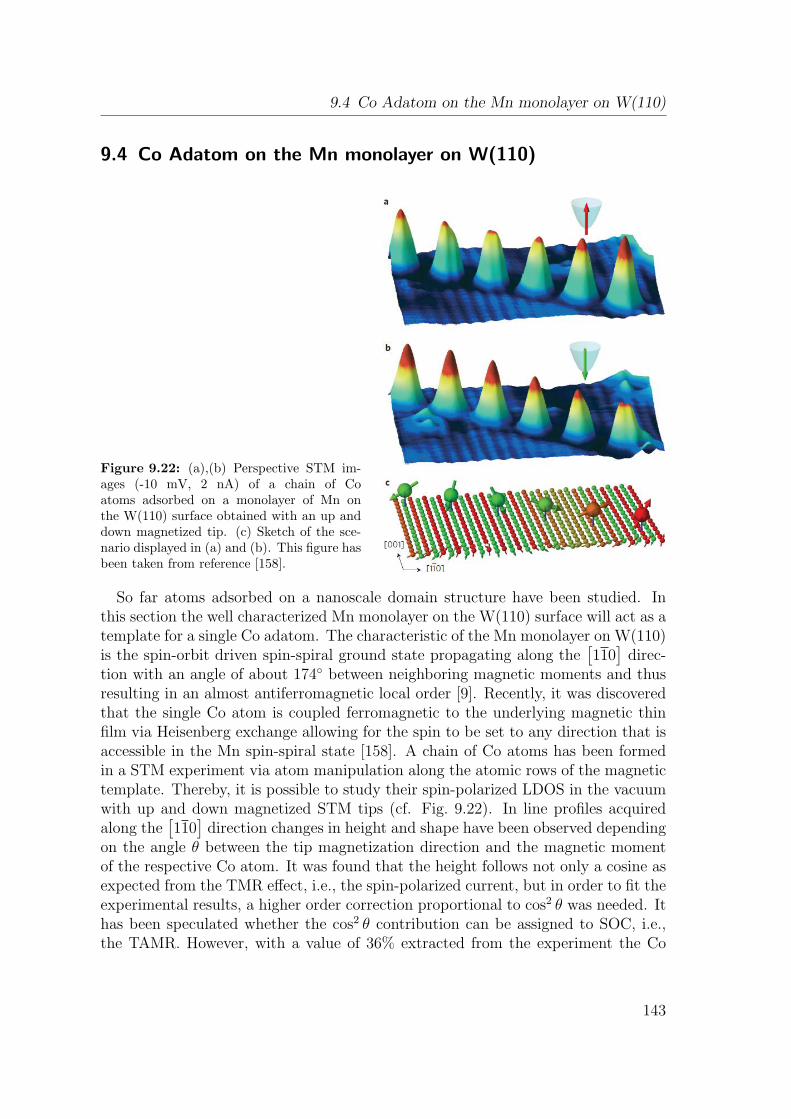
9.4 Co Adatom on the Mn monolayer on W(110)
9.4 Co Adatom on the Mn monolayer on W(110)
Figure 9.22: (a),(b) Perspective STM im-ages (-10 mV, 2 nA) of a chain of Coatoms adsorbed on a monolayer of Mn onthe W(110) surface obtained with an up anddown magnetized tip. (c) Sketch of the sce-nario displayed in (a) and (b). This figure hasbeen taken from reference [158].
So far atoms adsorbed on a nanoscale domain structure have been studied. Inthis section the well characterized Mn monolayer on the W(110) surface will act as atemplate for a single Co adatom. The characteristic of the Mn monolayer on W(110)is the spin-orbit driven spin-spiral ground state propagating along the
[110]
direc-tion with an angle of about 174 between neighboring magnetic moments and thusresulting in an almost antiferromagnetic local order [9]. Recently, it was discoveredthat the single Co atom is coupled ferromagnetic to the underlying magnetic thinfilm via Heisenberg exchange allowing for the spin to be set to any direction that isaccessible in the Mn spin-spiral state [158]. A chain of Co atoms has been formedin a STM experiment via atom manipulation along the atomic rows of the magnetictemplate. Thereby, it is possible to study their spin-polarized LDOS in the vacuumwith up and down magnetized STM tips (cf. Fig. 9.22). In line profiles acquiredalong the
[110]
direction changes in height and shape have been observed dependingon the angle θ between the tip magnetization direction and the magnetic momentof the respective Co atom. It was found that the height follows not only a cosine asexpected from the TMR effect, i.e., the spin-polarized current, but in order to fit theexperimental results, a higher order correction proportional to cos2 θ was needed. Ithas been speculated whether the cos2 θ contribution can be assigned to SOC, i.e.,the TAMR. However, with a value of 36% extracted from the experiment the Co
143
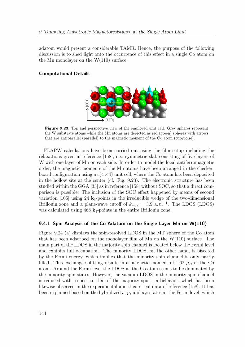
9 Tunneling Anisotropic Magnetoresistance at the Single Atom Limit
adatom would present a considerable TAMR. Hence, the purpose of the followingdiscussion is to shed light onto the occurrence of this effect in a single Co atom onthe Mn monolayer on the W(110) surface.
Computational Details
[1 0]1
[001]
Figure 9.23: Top and perspective view of the employed unit cell. Grey spheres representthe W substrate atoms while the Mn atoms are depicted as red (green) spheres with arrowsthat are antiparallel (parallel) to the magnetic moment of the Co atom (turquoise).
FLAPW calculations have been carried out using the film setup including therelaxations given in reference [158], i.e., symmetric slab consisting of five layers ofW with one layer of Mn on each side. In order to model the local antiferromagneticorder, the magnetic moments of the Mn atoms have been arranged in the checker-board configuration using a c(4×4) unit cell, where the Co atom has been depositedin the hollow site at the center (cf. Fig. 9.23). The electronic structure has beenstudied within the GGA [33] as in reference [158] without SOC, so that a direct com-parison is possible. The inclusion of the SOC effect happened by means of secondvariation [105] using 24 k∥-points in the irreducible wedge of the two-dimensionalBrillouin zone and a plane-wave cutoff of kmax = 3.9 a. u.−1. The LDOS (LDOS)was calculated using 468 k∥-points in the entire Brillouin zone.
9.4.1 Spin Analysis of the Co Adatom on the Single Layer Mn on W(110)
Figure 9.24 (a) displays the spin-resolved LDOS in the MT sphere of the Co atomthat has been adsorbed on the monolayer film of Mn on the W(110) surface. Themain part of the LDOS in the majority spin channel is located below the Fermi leveland exhibits full occupation. The minority LDOS, on the other hand, is bisectedby the Fermi energy, which implies that the minority spin channel is only partlyfilled. This exchange splitting results in a magnetic moment of 1.62 µB of the Coatom. Around the Fermi level the LDOS at the Co atom seems to be dominated bythe minority spin states. However, the vacuum LDOS in the minority spin channelis reduced with respect to that of the majority spin – a behavior, which has beenlikewise observed in the experimental and theoretical data of reference [158]. It hasbeen explained based on the hybridized s, pz and dz2 states at the Fermi level, which
144
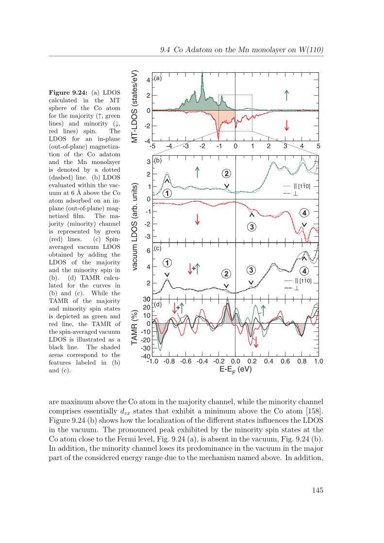
9.4 Co Adatom on the Mn monolayer on W(110)
Figure 9.24: (a) LDOScalculated in the MTsphere of the Co atomfor the majority (↑, greenlines) and minority (↓,red lines) spin. TheLDOS for an in-plane(out-of-plane) magnetiza-tion of the Co adatomand the Mn monolayeris denoted by a dotted(dashed) line. (b) LDOSevaluated within the vac-uum at 6 A above the Coatom adsorbed on an in-plane (out-of-plane) mag-netized film. The ma-jority (minority) channelis represented by green(red) lines. (c) Spin-averaged vacuum LDOSobtained by adding theLDOS of the majorityand the minority spin in(b). (d) TAMR calcu-lated for the curves in(b) and (c). While theTAMR of the majorityand minority spin statesis depicted as green andred line, the TAMR ofthe spin-averaged vacuumLDOS is illustrated as ablack line. The shadedareas correspond to thefeatures labeled in (b)and (c).
||
(a)
(d)
(b)
||
(c)
+
+
1
32 4
1
3
2
4
are maximum above the Co atom in the majority channel, while the minority channelcomprises essentially dzx states that exhibit a minimum above the Co atom [158].Figure 9.24 (b) shows how the localization of the different states influences the LDOSin the vacuum. The pronounced peak exhibited by the minority spin states at theCo atom close to the Fermi level, Fig. 9.24 (a), is absent in the vacuum, Fig. 9.24 (b).In addition, the minority channel loses its predominance in the vacuum in the majorpart of the considered energy range due to the mechanism named above. In addition,
145
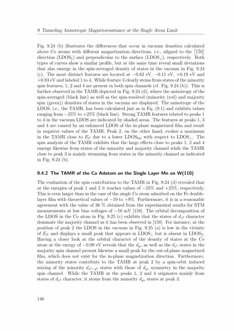
9 Tunneling Anisotropic Magnetoresistance at the Single Atom Limit
Fig. 9.24 (b) illustrates the differences that occur in vacuum densities calculatedabove Co atoms with different magnetization directions, i.e., aligned to the
[110]
direction (LDOS∥) and perpendicular to the surface (LDOS⊥), respectively. Bothtypes of curves show a similar profile, but at the same time reveal small deviationsthat also emerge in the spin-averaged density of states in the vacuum in Fig. 9.24(c). The most distinct features are located at −0.82 eV, −0.11 eV, +0.19 eV and+0.83 eV and labeled 1 to 4. While feature 3 clearly stems from states of the minorityspin features, 1, 2 and 4 are present in both spin channels (cf. Fig. 9.24 (b)). This isfurther observed in the TAMR depicted in Fig. 9.24 (d), where the anisotropy of thespin-averaged (black line) as well as the spin-resolved (minority (red) and majorityspin (green)) densities of states in the vacuum are displayed. The anisotropy of theLDOS, i.e., the TAMR, has been calculated just as in Eq. (9.1) and exhibits valuesranging from −25% to +25% (black line). Strong TAMR features related to peaks 1to 4 in the vacuum LDOS are indicated by shaded areas. The features at peaks 1, 3and 4 are caused by an enhanced LDOS of the in-plane magnetized film and resultin negative values of the TAMR. Peak 2, on the other hand, evokes a maximumin the TAMR close to EF due to a lower LDOShel with respect to LDOS⊥. Thespin analysis of the TAMR exhibits that the large effects close to peaks 1, 2 and 4emerge likewise from states of the minority and majority channel while the TAMRclose to peak 3 is mainly stemming from states in the minority channel as indicatedin Fig. 9.24 (b).
9.4.2 The TAMR of the Co Adatom on the Single Layer Mn on W(110)
The evaluation of the spin contribution to the TAMR in Fig. 9.24 (d) revealed thatat the energies of peak 1 and 2 it reaches values of −25% and +25%, respectively.This is even larger than in the case of the single Co atom adsorbed on the Fe double-layer film with theoretical values of −19 to +9%. Furthermore, it is in a reasonableagreement with the value of 36 % obtained from the experimental results for STMmeasurements at low bias voltages of −10 mV [158]. The orbital decomposition ofthe LDOS in the Co atom in Fig. 9.25 (c) exhibits that the states of dz2 characterdominate the majority channel as it has been observed in [158]. For instance, at theposition of peak 2 the LDOS in the vacuum in Fig. 9.25 (a) is low in the vicinityof EF and displays a small peak that appears in LDOS⊥ but is absent in LDOS∥.Having a closer look at the orbital character of the density of states at the Coatom at the energy of −0.09 eV reveals that the dyz as well as the dz2 states in themajority spin channel present likewise a small peak for the out-of-plane magnetizedfilm, which does not exist for the in-plane magnetization direction. Furthermore,the minority states contribute to the TAMR at peak 2 by a spin-orbit inducedmixing of the minority dx2−y2 states with those of dyz symmetry in the majorityspin channel. While the TAMR at the peaks 1, 2 and 4 originates mainly fromstates of dz2 character, it stems from the minority dyz states at peak 3.
146

9.4 Co Adatom on the Mn monolayer on W(110)
Figure 9.25: (a) The vacuum LDOS evalu-ated at 6 A above the Co atom for the in-plane (green, dotted) and out-of-plane (red,dashed) magnetized Mn film. (b) TAMR cal-culated for the curves in (a) according toEq. (9.1). Shaded areas correspond to thefeatures labeled in (a). (c) Orbital decompo-sition of the LDOS at the Co atom for thein-plane and out-of-plane spin quantization.
Co
(c)
(b)
||
(a)
vacuum
2
41
3
Figure 9.26 shows cross-sections of the majority and the minority spin of thein-plane (Fig. 9.26(a)) and out-of-plane (Fig. 9.26 (b)) magnetized film calculatedalong the yellow line in Fig. 9.23. The energy range has been chosen within 10 meVabove the Fermi energy for a better comparison with the calculations in reference[158]. According to Serrate et el. [158] the circular shape of the majority LDOSat the Co atom is because of the dz2 states that dominate the charge density closeto the Fermi energy. They are rotationally symmetric perpendicular to the surfaceand result in a maximum above the central Mn row. Further amplification is due tothe hybridization with states of s and pz symmetry. In the minority channel, on theother hand, the shape of the LDOS at the Co adatom resembles a double lobe withits node being aligned to the central Mn row due to the predominance of states with
147
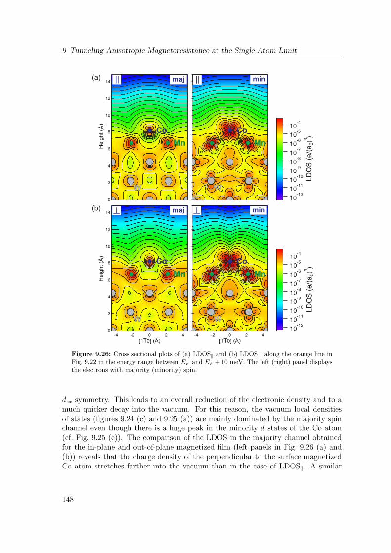
9 Tunneling Anisotropic Magnetoresistance at the Single Atom Limit
(a)
(b)
maj min
maj min
[1 0] (Å)1 [1 0] (Å)1
Heig
ht (Å
)H
eig
ht (Å
)
|| ||
Co
Mn
W
Co
Mn
W
Co
Mn
W
Co
Mn
W
Figure 9.26: Cross sectional plots of (a) LDOS∥ and (b) LDOS⊥ along the orange line inFig. 9.22 in the energy range between EF and EF +10 meV. The left (right) panel displaysthe electrons with majority (minority) spin.
dzx symmetry. This leads to an overall reduction of the electronic density and to amuch quicker decay into the vacuum. For this reason, the vacuum local densitiesof states (figures 9.24 (c) and 9.25 (a)) are mainly dominated by the majority spinchannel even though there is a huge peak in the minority d states of the Co atom(cf. Fig. 9.25 (c)). The comparison of the LDOS in the majority channel obtainedfor the in-plane and out-of-plane magnetized film (left panels in Fig. 9.26 (a) and(b)) reveals that the charge density of the perpendicular to the surface magnetizedCo atom stretches farther into the vacuum than in the case of LDOS∥. A similar
148
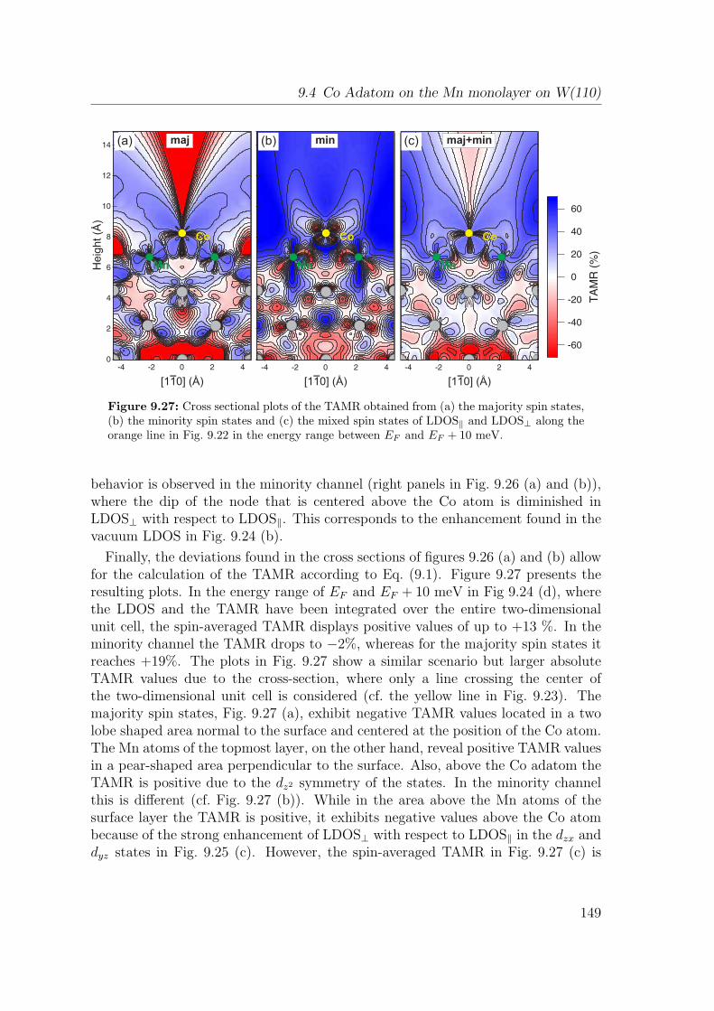
9.4 Co Adatom on the Mn monolayer on W(110)
Co
Mn
W
Co
Mn
W
Co
Mn
W
[1 0] (Å)1 [1 0] (Å)1[1 0] (Å)1
He
igh
t (Å
)
maj min maj+min(a) (b) (c)
Figure 9.27: Cross sectional plots of the TAMR obtained from (a) the majority spin states,(b) the minority spin states and (c) the mixed spin states of LDOS∥ and LDOS⊥ along theorange line in Fig. 9.22 in the energy range between EF and EF + 10 meV.
behavior is observed in the minority channel (right panels in Fig. 9.26 (a) and (b)),where the dip of the node that is centered above the Co atom is diminished inLDOS⊥ with respect to LDOS∥. This corresponds to the enhancement found in thevacuum LDOS in Fig. 9.24 (b).
Finally, the deviations found in the cross sections of figures 9.26 (a) and (b) allowfor the calculation of the TAMR according to Eq. (9.1). Figure 9.27 presents theresulting plots. In the energy range of EF and EF + 10 meV in Fig 9.24 (d), wherethe LDOS and the TAMR have been integrated over the entire two-dimensionalunit cell, the spin-averaged TAMR displays positive values of up to +13 %. In theminority channel the TAMR drops to −2%, whereas for the majority spin states itreaches +19%. The plots in Fig. 9.27 show a similar scenario but larger absoluteTAMR values due to the cross-section, where only a line crossing the center ofthe two-dimensional unit cell is considered (cf. the yellow line in Fig. 9.23). Themajority spin states, Fig. 9.27 (a), exhibit negative TAMR values located in a twolobe shaped area normal to the surface and centered at the position of the Co atom.The Mn atoms of the topmost layer, on the other hand, reveal positive TAMR valuesin a pear-shaped area perpendicular to the surface. Also, above the Co adatom theTAMR is positive due to the dz2 symmetry of the states. In the minority channelthis is different (cf. Fig. 9.27 (b)). While in the area above the Mn atoms of thesurface layer the TAMR is positive, it exhibits negative values above the Co atombecause of the strong enhancement of LDOS⊥ with respect to LDOS∥ in the dzx anddyz states in Fig. 9.25 (c). However, the spin-averaged TAMR in Fig. 9.27 (c) is
149
9 Tunneling Anisotropic Magnetoresistance at the Single Atom Limit
still negative above the Co atom. At the same time it reveals positive values withinelongated areas above the W atoms of the interface layer. They result in +13 % forthe spin-averaged TAMR due to the dominance of the majority spin states at 6 Ain the vacuum.
Conclusions
In this section the TAMR effect has been investigated for a single Co atom adsorbedon the Mn monolayer on W(110). This substrate is characterized by a spin-orbitdriven spin-spiral ground state that allows for any direction of the Co magneticmoment provided by the underlying spin-spiral due to strong local exchange cou-pling. By rotating the magnetization direction from in-plane to out-of plane in thefirst-principles calculation changes in the vacuum density of states have been ob-served that range from −25% to +25%. Hence, a single Co atom adsorbed on aMn monolayer exhibits an even larger TAMR effect than a Co atom adsorbed onthe Fe double-layer film. Furthermore, it agrees well with the experimental value of36 % evaluated from the line profiles in reference [158]. Thus, the cos2 θ variation ofheight and shape of the peaks can be ascribed to the TAMR. The changes observedin the electronic structure have been explained based on the mixing of d orbitalswith different symmetry. This leads to differences in height and shape of the partialcharge density at the Fermi energy above the Co atom. Since a distinct TAMRfeature emerges from states close to the Fermi energy, this effect is accessible evenin the limiting case of small bias voltages.
150
10 Summary
In this thesis, a density functional theory study of non-collinear magnetism andspin-orbit coupling effects on nanostructures such as ultrathin magnetic films andadatoms at surfaces has been presented. The investigation of magnetism at thenanoscale is of great importance in the field of spintronics. Non-collinear magneticstructures of the size of a few atoms or even in the single-atom limit might representthe building blocks of information carriers in future spintronic devices. Therefore,it is important to understand the mechanisms behind the formation of non-collinearspin structures and the influence of spin-orbit coupling on such nanoscale structures.The calculations were performed using one of the most accurate methods, namelythe full-potential linearized plane wave method [23, 24], that is based on densityfunctional theory [20, 21] as implemented in the FLEUR code [22]. After introducingthe theoretical concepts and the applied methods in chapters 2 to 6 three differenttopics have been addressed.
In chapter 7 a Cr monolayer on the Pd(111) surface has been investigated as aprototype system for spin frustration on a triangular lattice. Two-dimensional anti-ferromagnets such as Cr monolayers are characterized by an antiparallel alignmentof neighboring magnetic atoms due to the exchange coupling. On a triangular latticethe antiferromagnetic ordering between nearest neighbors can lead to a topologicalfrustration of the spins resulting in a non-collinear spin structure, such as the 120
Neel state. It has been predicted for Cr monolayers on the (111) surfaces of Agand Cu [118, 119] and experimentally observed in a monolayer of Mn on Ag(111)[120]. Here, the Pd(111) surface acts as a substrate for the Cr monolayer. By per-forming structural relaxations it was found that the Cr monolayer favors a row-wiseantiferromagnetic alignment by about 162 meV/Cr atom in the fcc stacking withrespect to the hcp stacking if only collinear configurations are considered. The mag-netic phase space has been scanned by means of spin-spiral calculations along thehigh-symmetry lines of the two-dimensional Brillouin zone. For an unsupported Crmonolayer on the Pd(111) lattice constant as well as the Cr monolayer on Pd(111)a global minimum was obtained at the K point, which corresponds to the 120
Neel state with an energy difference of about 39 meV/Cr atom and 27 meV/Cratom, respectively, in comparison to the row-wise antiferromagnetic alignment ofthe spins. By mapping the ab initio results onto the Heisenberg model the exchangeconstants could be extracted. Cr on Pd(111) reveals a clear dominance of the anti-ferromagnetic nearest neighbor exchange over the second and third nearest neighborexchange interaction. Also spin interactions beyond pair-wise exchange have been
151
10 Summary
taken into account by calculating a superposition state of spin spirals: the 3Q state,which has been found to be about 24 meV/Cr atom more unfavorable than the row-wise antiferromagnetic configuration. Thus, the Neel presents the magnetic groundstate of the monolayer Cr on Pd(111). In order to compare the DFT results withthe spin-polarized STM measurements images have been simulated within the spin-polarized Tersoff-Hamann model [61] for different in-plane magnetizations of the tip.Thereby, the predicted Neel state was confirmed. A quantitative comparison of sim-ulated and experimental line profiles allowed for the determination of the in-planetip magnetization direction in the spin-polarized STM experiments.
A more complex magnetic nanoscale structure has been presented in chapter 8dedicated to the double layer of Mn on W(110). Besides Cr, Mn represents the other3d transition metal for which two-dimensional antiferromagnetism is expected dueto the tendency towards antiferromagnetic exchange coupling. For example, thishas been observed for the Mn monolayer on W(110) [9], where the magnetic mo-ments of neighboring atoms are almost antiparallel aligned. The small tilting anglebetween the magnetic moments is due the Dzyaloshinskii-Moriya interaction, whichprefers a non-collinear magnetic ground state and thus induces a spin spiral. In thissystem, the importance of the Dzyaloshinskii-Moriya interaction at a surface hasbeen demonstrated for the first time. As has been shown in this thesis also the Mndouble layer prefers an antiparallel coupling of nearest neighbor magnetic momentsleading to an antiferromagnetic checkerboard spin arrangement within the layers.Additionally, the surface and subsurface layer couple antiferromagnetic resulting ina parallel alignment of the spins along the
[110]
direction and antiferromagneticorder along the [001] direction. Among the considered collinear states this configu-ration is by about 137 meV/Mn atom energetically more favorable than an entirelyferromagnetic spin arrangement. From these calculations the conclusion was drawnthat the Mn double layer on W(110) exhibits a preference of antiferromagnetism.By scanning the magnetic phase space via the calculation of flat spin-spirals alongthe high-symmetry lines of the two-dimensional Brillouin zone a tendency towardsnon-collinear magnetic order was observed for this system. However, the resultingflat spin-spiral state was only about 1.5 meV/Mn atom more favorable in energythan the preferred collinear antiferromagnetic configuration. By simulating spin-polarized STM images within a simple model based on the spin-polarized Tersoff-Hamann model [62] it was demonstrated that this spin-spiral state could not explainthe results obtained in the spin-polarized STM measurements. Furthermore, it wasshown that the experimental STM contrast could only be reproduced by a trans-verse conical spin spiral state. In this structure the antiparallel aligned magneticmoments of neighboring atoms rotate on a cone with the propagation direction ofthe spin spiral being perpendicular to the magnetization direction. By mappingthe DFT results onto an extended Heisenberg model it was demonstrated that thecanting of the magnetic moments is induced by exchange interactions beyond near-est neighbors, namely the four-spin interaction and the biquadratic exchange. The
152
rotation, on the other hand, originates from the Heisenberg exchange and is stabi-lized by the Dzyaloshinskii-Moriya interaction. The resulting spin structure is about16.7 meV/Mn atom lower in energy than the collinear antiferromagnetic state andexhibits a cone angle of θ = 30 as well a rotation angle of ϕ = 32. This find-ing presents the first observation of a conical spin-spiral state in an ultrathin filmand demonstrates the crucial role of the higher-order spin interactions in surfacemagnetism.
By means of spin-polarized STM images simulated within the spin-polarizedTersoff-Hamann model [61] the influence of the tip magnetization direction ontothe observed pattern has been studied. Thus, it was demonstrated that for complexmagnetic structures it might be preferable to vary the tip magnetization directionaccording to the three crystallographic axes in order to detect every pattern origi-nating from the magnetic structure. Furthermore, the experimental determinationof the cone angle is a non-trivial task. Therefore, the relation of the corrugation am-plitudes, i.e., the maximum difference in the tip height during an STM measurementin dependence on the cone angle has been studied in the present work utilizing thespin-polarized Tersoff-Hamann model and the independent-orbital approximation[62] in order to provide an informative basis for future spin-polarized STM mea-surements. Finally, the tunneling anisotropic magnetoresistance (TAMR) has beeninvestigated in the double layer Mn on W(110). This effect leads to magnetization-direction dependent changes in the electronic structure and can be detected by meansof spin-polarized and non-spin-polarized scanning tunneling microscopy. Since it ispinned to the electronic structure, the TAMR contrast does not vary with respect tothe rotation of the tip magnetization direction. For instance, in a non-spin-polarizedSTM measurement it provides the possibility to distinguish magnetic structures suchas domains and domain walls without the use of an external field [19].
Finally, the TAMR is investigated for single adatoms on ultrathin magnetic filmson W(110) in chapter 9. Single magnetic and nonmagnetic atoms present the small-est possible logical unit in a future spintronic device. A major issue in the studyof the TAMR is the direct comparison of theoretical and experimental results. Byconsidering single atoms adsorbed on magnetic ultrathin films with a non-collinearspin structure the direction of the adatom’s magnetic moment can be controlled viathe adsorption site and the exchange coupling with the neighboring atoms of theunderlying film. In addition, the experiments can be carried out without the useof an external magnetic field thereby circumventing problems such as a potentialdeformation of the contacts. First, the TAMR has been studied for a double layerof Fe on W(110), which presents the substrate for the single atoms. The Fe doublelayer exhibits a nanoscale domain structure on W(110) with magnetic moments thatrotate right-handed and cycloidal via the [001] direction in the Neel type domainwalls [10, 128, 129]. By rotating the spins in the Fe film from out-of-plane to in-plane along the [001] direction the local densities of states in the vacuum exhibitdeviations depending on the magnetization direction. They can be quantified via
153
10 Summary
the TAMR. It is defined as the difference between the local densities of states forthe two magnetization directions divided by the densities of states of one of theconfigurations. It reveals energy dependent oscillations in sign ranging from −17%to +11% for the Fe double layer on W(110). The TAMR feature that can be relatedto the experiments from Bode et al. [19], who found a significant deviation in thedI/dU signals measured above the domain and the domain wall at U = 0.07 V, islocated at +0.14 eV above the Fermi energy and is of the order of 11%. Upon thedecomposition of the density of states in the muffin tin spheres of the Fe atoms, theTAMR feature can be ascribed to the spin-orbit induced mixing of dz2 states withthe hybridized dxy and dyz orbitals in the minority spin channel.
In the next step, the TAMR has been studied for single Co adatoms on the Fedouble layer on W(110). Here, it presents a similar range of values between −19%and +9% which agrees with the experimental values of −12% to +5% observed inSTM measurements. The strongest TAMR feature is located at 0.07 eV below theFermi level and has a strength of −19%. It stems from the hybridization of minorityspin states in the Co atom and the Fe atoms of the underlying film and is of dxycharacter at Co and dyz in the Fe film. In order to capture the essence of the TAMR,a simple model has been introduced that describes the mixing of two atomic states ata surface by means of the Green’s functions. It illustrates the concept of spin-orbitinduced mixing of states with different orbital character and by revisiting the dz2and dzx states in the Co adatom obtained from DFT calculations the resulting modelTAMR agrees well with the TAMR of the DFT results. However, by choosing an Iradatom instead of a Co adatom the TAMR effect can be increased to values of upto 70%. Due to hybridization with the adjacent Fe atoms of the film the Ir adatomreveals an induced magnetic moment of +0.77 µB and +0.87 µB within the LDA[31] and the GGA [33], respectively. In comparison to the magnetic moment of theCo adatom, i.e., 1.81 µB obtained within the LDA [31], the magnetic moment of theIr adatom is half as large. Nevertheless, it exhibits a spin-polarization of up to 0.9,which is about three times larger than that of the Co adatom on Fe/W(110) [154].Thus, the use of 5d elements instead of those of the 3d series does not only result ina larger TAMR but might also present a new route towards larger spin-valve effects.Furthermore, the TAMR of the Ir adatom has not only been studied for the case ofa cycloidal rotating domain wall, i.e., the Neel wall, but also for a Bloch wall, whichexhibits a helical rotation from ’up’ to ’down’ via the
[110]
direction. In both cases,the TAMR exhibits large values that range from −51% to +69% and from −39% to+52% in the cycloidal and helical domain wall, respectively. At the same time theTAMR of the cycloidal domain wall can be distinguished from that of the helicaldomain wall due to the spin-orbit induced splitting of the peaks. In the case of acycloidal domain wall, the mixing of dz2 states with those of dzx symmetry leads to apronounced peak at −0.63 eV with respect to the Fermi energy for the out-of-planemagnetized adatom, which is absent in the vacuum local density of states of thein-plane magnetization direction. In the case of the helical domain wall, the mixing
154
of dz2 states with those of dyz symmetry results in peaks for both magnetizationdirections that differ slightly in height and energy position. Therefore, it may bepossible to make use of the TAMR in single atoms in order to determine the domainwall type in STM experiments.
Finally, the TAMR of a Co adatom on the monolayer Mn on W(110) has been in-vestigated. As mentioned before, the monolayer Mn on W(110) exhibits a spin-orbitdriven spin-spiral state with almost antiparallel alignment of neighboring magneticmoments propagating along the
[110]
direction [9]. Due to the ferromagnetic cou-pling of the Co adatom and the adjacent Mn atoms of the film the magnetic momentof the adatom can be set to any magnetization direction that is accessible in the spinspiral [158]. For this system, the TAMR ranges from −25% to +25% and a largefeature at 0.09 eV below the Fermi level can be ascribed to the mixing of the dz2states with dyz orbitals of both spin channels. Moreover, the TAMR value of +25%agrees well with the value of +36% extracted from spin-polarized STM experiments[158].
In conclusion, the magnetism of nanostructures at surfaces has been investigatedin this thesis. It was demonstrated that not only the frustration of Heisenberg ex-change coupling but also spin-interactions beyond pair-wise exchange, such as thefour-spin interaction and the biquadratic exchange, can induce non-collinear mag-netic structures. In particular, it has been demonstrated that the Mn double layeron W(110) exhibits a conical spin-spiral state due to higher-order spin interactions.This shows that such terms can play a crucial role for magnetic nanostructures atsurfaces. Furthermore, it was shown that the formation of such non-collinear mag-netic structures can be further stabilized by the Dzyaloshinskii-Moriya interaction.Another central topic of this thesis was the study of the TAMR on the basis of singleatoms on magnetic thin films concerning a future application in spintronic devices.It was demonstrated that the use of single atoms adsorbed on ultrathin magneticfilms allow for a direct comparison of theoretical and experimental results. TAMRvalues of up to 25% have been observed in Co adatoms. Furthermore, the use of aIr instead of a Co as adatom gives TAMR values of up to 70%. Therefore, choosinga 5d element in the tunnel junction shows promising results since both, the TAMRand the spin-valve effect can be explicitly enhanced compared to that of an adatomof the 3d series.
155

10 Summary
156
11 Bibliography
[1] Data sheet, Hitachi GST Travelstar 5K500.B.
[2] M. N. Baibich, J. M. Broto, A. Fert, F. N. Van Dau, F. Petroff,P. Etienne, G. Creuzet, A. Friederich and J. Chazelas, Giant Mag-netoresistance of (001)Fe/(001)Cr Magnetic Superlattices, Phys. Rev. Lett.61, 2472 (1988).
[3] G. Binasch, P. Grunberg, F. Saurenbach and W. Zinn, Enhanced mag-netoresistance in layered magnetic structures with antiferromagnetic interlayerexchange, Phys. Rev. B 39, 4828 (1989).
[4] A. Berger, in 40th Springschool, Spintronics – From GMR to QuantumInformation.
[5] S. A. Wolf, D. D. Awschalom, R. A. Buhrman, J. M. Daughton,S. von Molnar, M. L. Roukes, A. Y. Chtchelkanova and D. M.Treger, Spintronics: A Spin-Based Electronics Vision for the Future, Science294, 1488 (2001).
[6] A. Fert, V. Cros and J. Sampaio, Skyrmions on the track, Nature Nan-otechnology 8, 152 (2013).
[7] I. E. Dzyaloshinskii, Thermodynamic theory of weak ferromagnetism inantiferromagnetic substances, Sov. Phys. JETP 5, 1259 (1957).
[8] T. Moriya, Anisotropic Superexchange Interaction and Weak Ferromag-netism, Phys. Rev. 120, 91 (1960).
[9] M. Bode, M. Heide, K. von Bergmann, P. Ferriani, S. Heinze,G. Bihlmayer, A. Kubetzka, O. Pietzsch, S. Blugel and R. Wiesen-danger, Chiral magnetic order at surfaces driven by inversion asymmetry,Nature 447, 190 (2007).
[10] M. Heide, G. Bihlmayer and S. Blugel, Dzyaloshinskii-Moriya inter-action accounting for the orientation of magnetic domains in ultrathin films:Fe/W(110), Phys. Rev. B 78, 140403 (2008).
157
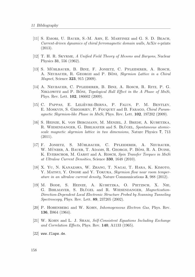
11 Bibliography
[11] S. Emori, U. Bauer, S.-M. Ahn, E. Martinez and G. S. D. Beach,Current-driven dynamics of chiral ferromagnetic domain walls, ArXiv e-prints(2013).
[12] T. H. R. Skyrme, A Unified Field Theory of Mesons and Baryons, NuclearPhysics 31, 556 (1962).
[13] S. Muhlbauer, B. Binz, F. Jonietz, C. Pfleiderer, A. Rosch,A. Neubauer, R. Georgii and P. Boni, Skyrmion Lattice in a ChiralMagnet, Science 323, 915 (2009).
[14] A. Neubauer, C. Pfleiderer, B. Binz, A. Rosch, R. Ritz, P. G.Niklowitz and P. Boni, Topological Hall Effect in the A Phase of MnSi,Phys. Rev. Lett. 102, 186602 (2009).
[15] C. Pappas, E. Lelievre-Berna, P. Falus, P. M. Bentley,E. Moskvin, S. Grigoriev, P. Fouquet and B. Farago, Chiral Param-agnetic Skyrmion-like Phase in MnSi, Phys. Rev. Lett. 102, 197202 (2009).
[16] S. Heinze, K. von Bergmann, M. Menzel, J. Brede, A. Kubetzka,R. Wiesendanger, G. Bihlmayer and S. Blugel, Spontaneous atomic-scale magnetic skyrmion lattice in two dimensions, Nature Physics 7, 713(2011).
[17] F. Jonietz, S. Muhlbauer, C. Pfleiderer, A. Neubauer,W. Munzer, A. Bauer, T. Adams, R. Georgii, P. Boni, R. A. Duine,K. Everschor, M. Garst and A. Rosch, Spin Transfer Torques in MnSiat Ultralow Current Densities, Science 330, 1648 (2010).
[18] X. Yu, N. Kanazawa, W. Zhang, T. Nagai, T. Hara, K. Kimoto,Y. Matsui, Y. Onose and Y. Tokura, Skyrmion flow near room temper-ature in an ultralow current density, Nature Communications 3, 988 (2012).
[19] M. Bode, S. Heinze, A. Kubetzka, O. Pietzsch, X. Nie,G. Bihlmayer, S. Blugel and R. Wiesendanger, Magnetization-Direction-Dependent Local Electronic Structure Probed by Scanning TunnelingSpectroscopy, Phys. Rev. Lett. 89, 237205 (2002).
[20] P. Hohenberg and W. Kohn, Inhomogeneous Electron Gas, Phys. Rev.136, B864 (1964).
[21] W. Kohn and L. J. Sham, Self-Consistent Equations Including Exchangeand Correlation Effects, Phys. Rev. 140, A1133 (1965).
[22] www.flapw.de.
158
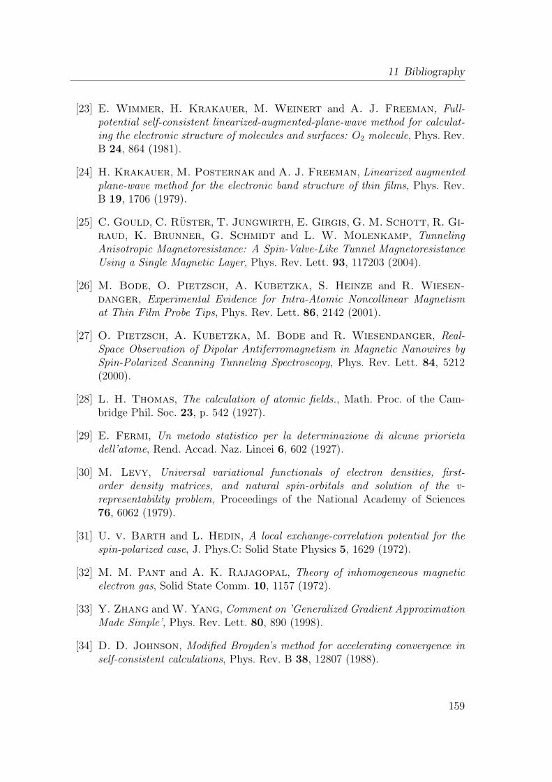
11 Bibliography
[23] E. Wimmer, H. Krakauer, M. Weinert and A. J. Freeman, Full-potential self-consistent linearized-augmented-plane-wave method for calculat-ing the electronic structure of molecules and surfaces: O2 molecule, Phys. Rev.B 24, 864 (1981).
[24] H. Krakauer, M. Posternak and A. J. Freeman, Linearized augmentedplane-wave method for the electronic band structure of thin films, Phys. Rev.B 19, 1706 (1979).
[25] C. Gould, C. Ruster, T. Jungwirth, E. Girgis, G. M. Schott, R. Gi-raud, K. Brunner, G. Schmidt and L. W. Molenkamp, TunnelingAnisotropic Magnetoresistance: A Spin-Valve-Like Tunnel MagnetoresistanceUsing a Single Magnetic Layer, Phys. Rev. Lett. 93, 117203 (2004).
[26] M. Bode, O. Pietzsch, A. Kubetzka, S. Heinze and R. Wiesen-danger, Experimental Evidence for Intra-Atomic Noncollinear Magnetismat Thin Film Probe Tips, Phys. Rev. Lett. 86, 2142 (2001).
[27] O. Pietzsch, A. Kubetzka, M. Bode and R. Wiesendanger, Real-Space Observation of Dipolar Antiferromagnetism in Magnetic Nanowires bySpin-Polarized Scanning Tunneling Spectroscopy, Phys. Rev. Lett. 84, 5212(2000).
[28] L. H. Thomas, The calculation of atomic fields., Math. Proc. of the Cam-bridge Phil. Soc. 23, p. 542 (1927).
[29] E. Fermi, Un metodo statistico per la determinazione di alcune priorietadell’atome, Rend. Accad. Naz. Lincei 6, 602 (1927).
[30] M. Levy, Universal variational functionals of electron densities, first-order density matrices, and natural spin-orbitals and solution of the v-representability problem, Proceedings of the National Academy of Sciences76, 6062 (1979).
[31] U. v. Barth and L. Hedin, A local exchange-correlation potential for thespin-polarized case, J. Phys.C: Solid State Physics 5, 1629 (1972).
[32] M. M. Pant and A. K. Rajagopal, Theory of inhomogeneous magneticelectron gas, Solid State Comm. 10, 1157 (1972).
[33] Y. Zhang and W. Yang, Comment on ’Generalized Gradient ApproximationMade Simple’, Phys. Rev. Lett. 80, 890 (1998).
[34] D. D. Johnson, Modified Broyden’s method for accelerating convergence inself-consistent calculations, Phys. Rev. B 38, 12807 (1988).
159
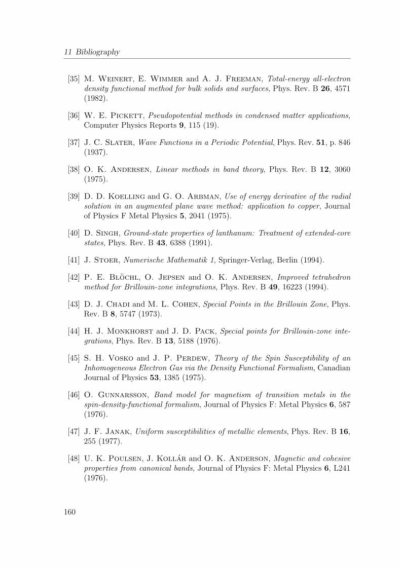
11 Bibliography
[35] M. Weinert, E. Wimmer and A. J. Freeman, Total-energy all-electrondensity functional method for bulk solids and surfaces, Phys. Rev. B 26, 4571(1982).
[36] W. E. Pickett, Pseudopotential methods in condensed matter applications,Computer Physics Reports 9, 115 (19).
[37] J. C. Slater, Wave Functions in a Periodic Potential, Phys. Rev. 51, p. 846(1937).
[38] O. K. Andersen, Linear methods in band theory, Phys. Rev. B 12, 3060(1975).
[39] D. D. Koelling and G. O. Arbman, Use of energy derivative of the radialsolution in an augmented plane wave method: application to copper, Journalof Physics F Metal Physics 5, 2041 (1975).
[40] D. Singh, Ground-state properties of lanthanum: Treatment of extended-corestates, Phys. Rev. B 43, 6388 (1991).
[41] J. Stoer, Numerische Mathematik 1, Springer-Verlag, Berlin (1994).
[42] P. E. Blochl, O. Jepsen and O. K. Andersen, Improved tetrahedronmethod for Brillouin-zone integrations, Phys. Rev. B 49, 16223 (1994).
[43] D. J. Chadi and M. L. Cohen, Special Points in the Brillouin Zone, Phys.Rev. B 8, 5747 (1973).
[44] H. J. Monkhorst and J. D. Pack, Special points for Brillouin-zone inte-grations, Phys. Rev. B 13, 5188 (1976).
[45] S. H. Vosko and J. P. Perdew, Theory of the Spin Susceptibility of anInhomogeneous Electron Gas via the Density Functional Formalism, CanadianJournal of Physics 53, 1385 (1975).
[46] O. Gunnarsson, Band model for magnetism of transition metals in thespin-density-functional formalism, Journal of Physics F: Metal Physics 6, 587(1976).
[47] J. F. Janak, Uniform susceptibilities of metallic elements, Phys. Rev. B 16,255 (1977).
[48] U. K. Poulsen, J. Kollar and O. K. Anderson, Magnetic and cohesiveproperties from canonical bands, Journal of Physics F: Metal Physics 6, L241(1976).
160
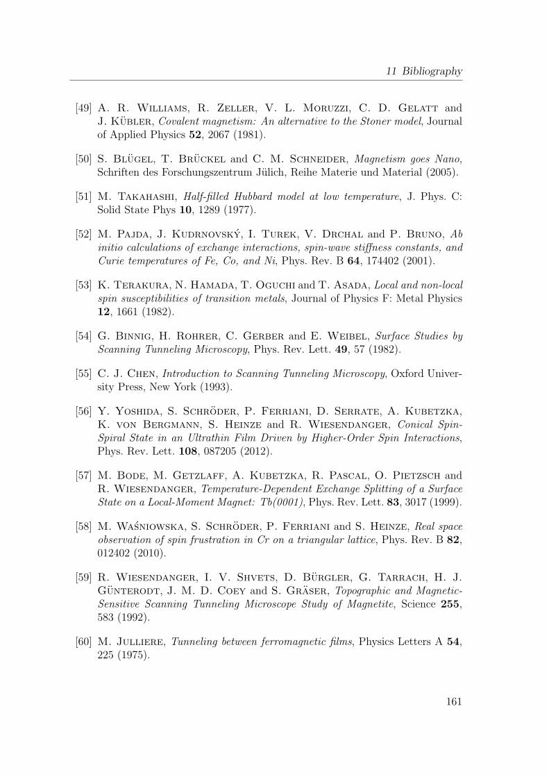
11 Bibliography
[49] A. R. Williams, R. Zeller, V. L. Moruzzi, C. D. Gelatt andJ. Kubler, Covalent magnetism: An alternative to the Stoner model, Journalof Applied Physics 52, 2067 (1981).
[50] S. Blugel, T. Bruckel and C. M. Schneider, Magnetism goes Nano,Schriften des Forschungszentrum Julich, Reihe Materie und Material (2005).
[51] M. Takahashi, Half-filled Hubbard model at low temperature, J. Phys. C:Solid State Phys 10, 1289 (1977).
[52] M. Pajda, J. Kudrnovsky, I. Turek, V. Drchal and P. Bruno, Abinitio calculations of exchange interactions, spin-wave stiffness constants, andCurie temperatures of Fe, Co, and Ni, Phys. Rev. B 64, 174402 (2001).
[53] K. Terakura, N. Hamada, T. Oguchi and T. Asada, Local and non-localspin susceptibilities of transition metals, Journal of Physics F: Metal Physics12, 1661 (1982).
[54] G. Binnig, H. Rohrer, C. Gerber and E. Weibel, Surface Studies byScanning Tunneling Microscopy, Phys. Rev. Lett. 49, 57 (1982).
[55] C. J. Chen, Introduction to Scanning Tunneling Microscopy, Oxford Univer-sity Press, New York (1993).
[56] Y. Yoshida, S. Schroder, P. Ferriani, D. Serrate, A. Kubetzka,K. von Bergmann, S. Heinze and R. Wiesendanger, Conical Spin-Spiral State in an Ultrathin Film Driven by Higher-Order Spin Interactions,Phys. Rev. Lett. 108, 087205 (2012).
[57] M. Bode, M. Getzlaff, A. Kubetzka, R. Pascal, O. Pietzsch andR. Wiesendanger, Temperature-Dependent Exchange Splitting of a SurfaceState on a Local-Moment Magnet: Tb(0001), Phys. Rev. Lett. 83, 3017 (1999).
[58] M. Wasniowska, S. Schroder, P. Ferriani and S. Heinze, Real spaceobservation of spin frustration in Cr on a triangular lattice, Phys. Rev. B 82,012402 (2010).
[59] R. Wiesendanger, I. V. Shvets, D. Burgler, G. Tarrach, H. J.Gunterodt, J. M. D. Coey and S. Graser, Topographic and Magnetic-Sensitive Scanning Tunneling Microscope Study of Magnetite, Science 255,583 (1992).
[60] M. Julliere, Tunneling between ferromagnetic films, Physics Letters A 54,225 (1975).
161
11 Bibliography
[61] D. Wortmann, S. Heinze, P. Kurz, G. Bihlmayer and S. Blugel,Resolving Complex Atomic-Scale Spin Structures by Spin-Polarized ScanningTunneling Microscopy, Phys. Rev. Lett. 86, 4132 (2001).
[62] S. Heinze, Simulation of spin-polarized scanning tunneling microscopy imagesof nanoscale non-collinear magnetic structures, Applied Physics A: MaterialsScience & Processing 85, 407 (2006).
[63] J. Bardeen, Tunnelling from a Many-Particle Point of View, Phys. Rev.Lett. 6, 57 (1961).
[64] J. Tersoff and D. R. Hamann, Theory and Application for the ScanningTunneling Microscope, Phys. Rev. Lett. 50, 1998 (1983).
[65] J. Tersoff and D. R. Hamann, Theory of the scanning tunneling micro-scope, Phys. Rev. B 31, 805 (1985).
[66] V. P. LaBella, H. Yang, D. W. Bullock, P. M. Thibado, P. Kratzerand M. Scheffler, Atomic Structure of the GaAs(001) − (2 × 4) SurfaceResolved Using Scanning Tunneling Microscopy and First-Principles Theory,Phys. Rev. Lett. 83, 2989 (1999).
[67] S. Heinze, S. Blugel, R. Pascal, M. Bode and R. Wiesendanger,Prediction of bias-voltage-dependent corrugation reversal for STM images ofbcc (110) surfaces: W(110), Ta(110), and Fe(110), Phys. Rev. B 58, 16432(1998).
[68] S. Heinze, R. Abt, S. Blugel, G. Gilarowski and H. Niehus, ScanningTunneling Microscopy Images of Transition-Metal Structures Buried BelowNoble-Metal Surfaces, Phys. Rev. Lett. 83, 4808 (1999).
[69] C. J. Chen, Theory of scanning tunneling spectroscopy, Journal of VacuumScience Technology A: Vacuum, Surfaces, and Films 6, 319 (1988).
[70] C. J. Chen, Microscopic view of scanning tunneling microscopy, Journal ofVacuum Science Technology A: Vacuum, Surfaces, and Films 9, 44 (1991).
[71] C. J. Chen, Origin of atomic resolution on metal surfaces in scanning tun-neling microscopy, Phys. Rev. Lett. 65, 448 (1990).
[72] S. Heinze, M. Bode, A. Kubetzka, O. Pietzsch, X. Nie, S. Blugeland R. Wiesendanger, Real-Space Imaging of Two-Dimensional Antiferro-magnetism on the Atomic Scale, Science 288, 1805 (2000).
162
11 Bibliography
[73] A. R. Smith, R. Yang, H. Yang, W. R. Lambrecht, A. Dick andJ. Neugebauer, Aspects of spin-polarized scanning tunneling microscopy atthe atomic scale: experiment, theory, and simulation, Surface Science 561,154 (2004).
[74] P. H. Dederichs, S. Blugel, R. Zeller and H. Akai, Ground States ofConstrained Systems: Application to Cerium Impurities, Phys. Rev. Lett. 53,2512 (1984).
[75] V. P. Antropov, M. I. Katsnelson, B. N. Harmon, M. van Schilf-gaarde and D. Kusnezov, Spin dynamics in magnets: Equation of motionand finite temperature effects, Phys. Rev. B 54, 1019 (1996).
[76] V. P. Antropov, M. I. Katsnelson, M. van Schilfgaarde and B. N.Harmon, AbInitio Spin Dynamics in Magnets, Phys. Rev. Lett. 75, 729(1995).
[77] O. N. Mryasov, A. I. Liechtenstein, L. M. Sandratskii and V. A.Gubanov, Magnetic structure of FCC iron, Journal of Physics: CondensedMatter 3, 7683 (1991).
[78] M. Uhl, L. Sandratskii and J. Kubler, Electronic and magnetic statesof γ-Fe, Journal of Magnetism and Magnetic Materials 103, 314 (1992).
[79] C. Herring, Magnetism, Academic, New York (1966).
[80] L. M. Sandratskii, Energy Band Structure Calculations for Crystals withSpiral Magnetic Structure, physica status solidi (b) 136, 167 (1986).
[81] P. Kurz, F. Forster, L. Nordstrom and S. Blugel, Ab initio treatmentof noncollinear magnets with the full-potential linearized augmented plane wavemethod, Phys. Rev. B 69, 24415 (2004).
[82] N. W. Ashcroft and N. D. Mermin, Solid State Physics, Holt, Rinehartand Wilson (1976).
[83] P. Kurz, Non-collinear Magnetism at Surfaces and in Ultrathin Films, Ph.D.thesis, RWTH Aachen (2000).
[84] L. M. Sandratskii and P. G. Guletskii, Symmetrised method for thecalculation of the band structure of noncollinear magnets, Journal of PhysicsF: Metal Physics 16, L43 (1986).
[85] L. Sandratskii and P. Guletskii, Energy band structure of BBC iron atfinite temperatures, Journal of Magnetism and Magnetic Materials 79, 306(1989).
163
11 Bibliography
[86] J. Kubler, K. H. Hock, J. Sticht and A. R. Williams, Density func-tional theory of non-collinear magnetism, Journal of Physics F: Metal Physics18, 469 (1988).
[87] J. Kubler, K.-H. Hock, J. Sticht and A. R. Williams, Local spin-density functional theory of noncollinear magnetism (invited), Journal of Ap-plied Physics 63, 3482 (1988).
[88] J. Sticht, K.-H. Hck and J. Kbler, Non-collinear itinerant magnetism:the case of Mn 3 Sn, Journal of Physics: Condensed Matter 1, 8155 (1989).
[89] O. N. Mryasov, V. A. Gubanov and A. I. Liechtenstein, Spiral-spin-density-wave states in fcc iron: Linear-muffin-tin-orbitals band-structure ap-proach, Phys. Rev. B 45, 12330 (1992).
[90] L. Nordstrom and D. J. Singh, Noncollinear Intra-atomic Magnetism,Phys. Rev. Lett. 76, 4420 (1996).
[91] P. Kurz, F. Forster, L. Nordstrom, G. Bihlmayer and S. Blugel,Ab initio treatment of noncollinear magnets with the full-potential linearizedaugmented plane wave method, Phys. Rev. B 69, 024415 (2004).
[92] L. Neel, L’approche a la saturation de la magnetostriction, J. Phys. Rad. 15,376 (1954).
[93] Y. A. Bychkov and E. I. Rashba, Oscillatory effects and the magneticsusceptibility of carriers in inversion layers, J. Phys. C: Solid State Phys. 15,6039 (1984).
[94] Y. A. Bychkov and E. I. Rashba, Properties of a 2D electron gas withlifted spectral degeneracy, Sov. Phys. JETP Lett. 39, 78 (1984).
[95] M. Uchida, Y. Onose, Y. Matsui and Y. Takura, Real-space observationof helical spin order, Science 311, 359 (2006).
[96] D. D. Koelling and B. N. Harmon, A technique for relativistic spin-polarised calculations, J. Phys. C: Solid State Physics 10, 3107 (1977).
[97] G. Baym, Lectures On Quantum Mechanics, Lecture Notes and Supplementsin Physics, Westview Press (1974).
[98] J. D. Jackson, Klassische Elektrodynamik, Gruyter, 3 ed. (2002).
[99] E. Abate and M. Asdente, Tight-Binding Calculation of 3d Bands of Fewith and without Spin-Orbit Coupling, Phys. Rev. 140, A1303 (1965).
164
11 Bibliography
[100] P. Bruno, in 24. IFF-Ferienkurs, Magnetismus von Festkorpern und Grenz-flachen, p. 24.1, Forschungszentrum Julich GmbH (1993).
[101] P. Bruno, Dipolar magnetic surface anisotropy in ferromagnetic thin filmswith interfacial roughness, Journal of applied physics 64, 3153 (1988).
[102] P. Bruno, Tight-binding approach to the orbital magnetic moment and mag-netocrystalline anisotropy of transition-metal monolayers, Phys. Rev. B 39,865 (1989).
[103] S. Blugel, Magnetische Anisotropie und Magnetostriktion,www.fz-juelich.de/iff/staff/Bluegel S/Lectures, Vorlesungsskript.
[104] M. Methfessel and J. Kubler, Bond analysis of heats of formation: appli-cation to some group VIII and IB hydrides, J. Phys. F: Met. Phys. pp. 141–161(1982).
[105] C. Li, A. J. Freeman, H. J. F. Jansen and C. L. Fu, Magneticanisotropy in low-dimensional ferromagnetic systems: Fe monolayers onAg(001), Au(001), and Pd(001) substrates, Phys. Rev. B 42, 5433 (1990).
[106] A. R. Mackintosh and O. K. Andersen, Electrons at the Fermi Surface(1980), cambridge University Press, Cambridge.
[107] A. Oswald, R. Zeller, P. J. Braspenning and P. H. Dederichs, In-teraction of magnetic impurities of Cu and Ag, J. Phys. F: Met. Phys. 15, 193(1985).
[108] A. I. Liechtenstein, M. I. Katsnelson, V. P. Antropov and V. A.Gubanov, Local spin density functional approach to the theory of exchangeinteractions in ferromagnetic metals and alloys, Journal of Magnetism andMagnetic Materials 67, 65 (1987).
[109] S. J. Youn, W. Mannstadt and A. J. Freeman, Analytic Spin-OrbitCoupling Matrix Element Formulae in FLAPW Calculations, J. Comp. Phys.172, 387 (2001).
[110] A. Crepieux and C. Lacroix, Dzyaloshinsky-Moriya interactions inducedby symmetry breaking at a surface, J. Magn. Magn. Mater. 182, 341 (1998).
[111] P. W. Anderson, New Approach to the Theory of Superexchange Interac-tions, Phys. Rev. 115, 2 (1959).
[112] M. Heide, G. Bihlmayer and S. Blugel, Describing DzyaloshinskiiMoriyaspirals from first principles, Physica B: Cond. Mat. 404, 2678 (2009).
165
11 Bibliography
[113] S. Blugel, D. Pescia and P. H. Dederichs, Ferromagnetism versus an-tiferromagnetism of the Cr(001) surface, Phys. Rev. B 39, 1392 (1989).
[114] R. Wiesendanger, H.-J. Guntherodt, G. Guntherodt, R. J. Gam-bino and R. Ruf, Observation of vacuum tunneling of spin-polarized electronswith the scanning tunneling microscope, Phys. Rev. Lett. 65, 247 (1990).
[115] M. Kleiber, M. Bode, R. Ravlic and R. Wiesendanger, Topology-Induced Spin Frustrations at the Cr(001) Surface Studied by Spin-PolarizedScanning Tunneling Spectroscopy, Phys. Rev. Lett. 85, 4606 (2000).
[116] B. Santos, J. Puerta, J. I. Cerda, R. Stumpf, K. von Bergmann,R. Wiesendanger, M. Bode, F. McCarty and F. de la Figuera,Structure and magnetism of ultra-thin chromium layers on W(110), New Jour-nal of Physics 10, 013005 (2008).
[117] P. Ferriani, S. Heinze, G. Bihlmayer and S. Blugel, Unexpected trendof magnetic order of 3d transition-metal monolayers on W(001), Phys. Rev.B 72, 024452 (2005).
[118] S. Heinze, P. Kurz, D. Wortmann, G. Bihlmayer and S. Blugel,Complex Magnetism in Ultra-Thin Films: Atomic-Scale Spin Structures andResolution by Spin-Polarized Scanning Tunneling Microscopy, Applied PhysicsA 75, 25 (2002).
[119] P. Kurz, G. Bihlmayer and S. Blugel, Noncollinear magnetism of Crand Mn monolayers on Cu(111), Journal of Applied Physics 87, 6101 (2000).
[120] C. L. Gao, W. Wulfhekel and J. Kirschner, Revealing the 120 Anti-ferromagnetic Neel Structure in Real Space: One Monolayer Mn on Ag(111),Phys. Rev. Lett. 101, 267205 (2008).
[121] B. Hardrat, A. Al-Zubi, P. Ferriani, S. Blugel, G. Bihlmayer andS. Heinze, Complex magnetism of iron monolayers on hexagonal transitionmetal surfaces from first principles, Phys. Rev. B 79, 094411 (2009).
[122] S. H. Vosko, L. Wilk and M. Nusair, Accurate spin-dependent electronliquid correlation energies for local spin density calculations: a critical analy-sis, Canadian Journal of Physics 58, 1200 (1980).
[123] P. Kurz, G. Bihlmayer, K. Hirai and S. Blugel, Three-DimensionalSpin Structure on a Two-Dimensional Lattice: Mn /Cu(111), Phys. Rev. Lett.86, 1106 (2001).
[124] M. Bode, Spin-polarized scanning tunnelling microscopy, Reports on Progressin Physics 66, 523 (2003).
166
11 Bibliography
[125] R. Schmidt, C. Lazo, H. Holscher, U. H. Pi, V. Caciuc, A. Schwarz,R. Wiesendanger and S. Heinze, Probing the Magnetic Exchange Forcesof Iron on the Atomic Scale, Nano Letters 9, 200 (2009).
[126] S. Krause, L. Berbil-Bautista, G. Herzog, M. Bode and R. Wiesen-danger, Current-Induced Magnetization Switching with a Spin-PolarizedScanning Tunneling Microscope, Science 317, 1537 (2007).
[127] P. Ferriani, K. von Bergmann, E. Y. Vedmedenko, S. Heinze,M. Bode, M. Heide, G. Bihlmayer, S. Blugel and R. Wiesendanger,Atomic-Scale Spin Spiral with a Unique Rotational Sense: Mn Monolayer onW(001), Phys. Rev. Lett. 101, 027201 (2008).
[128] S. Meckler, N. Mikuszeit, A. Preßler, E. Y. Vedmedenko, O. Piet-zsch and R. Wiesendanger, Real-Space Observation of a Right-RotatingInhomogeneous Cycloidal Spin Spiral by Spin-Polarized Scanning TunnelingMicroscopy in a Triple Axes Vector Magnet, Phys. Rev. Lett. 103, 157201(2009).
[129] S. Meckler, O. Pietzsch, N. Mikuszeit and R. Wiesendanger, Micro-magnetic description of the spin spiral in Fe double-layer stripes on W(110),Phys. Rev. B 85, 024420 (2012).
[130] R. Coldea, S. M. Hayden, G. Aeppli, T. G. Perring, C. D. Frost,T. E. Mason, S.-W. Cheong and Z. Fisk, Spin Waves and ElectronicInteractions in La2CuO4, Phys. Rev. Lett. 86, 5377 (2001).
[131] F. L. Pratt, P. J. Baker, S. J. Blundell, T. Lancaster, S. Ohira-Kawamura, C. Baines, Y. Shimizu, K. Kanoda, I. Watanabe andG. Saito, Magnetic and non-magnetic phases of a quantum spin liquid, Na-ture 471, 612 (2010).
[132] S. Lounis and P. H. Dederichs, Mapping the magnetic exchange interac-tions from first principles: Anisotropy anomaly and application to Fe, Ni, andCo, Phys. Rev. B 82, 180404 (2010).
[133] R. Singer, F. Dietermann and M. Fahnle, Spin Interactions in bcc andfcc Fe beyond the Heisenberg Model, Phys. Rev. Lett. 107, 017204 (2011).
[134] K. von Bergmann, M. Menzel, D. Serrate, Y. Yoshida,S. Schroder, P. Ferriani, A. Kubetzka, R. Wiesendanger andS. Heinze, Tunneling anisotropic magnetoresistance on the atomic scale,Phys. Rev. B 86, 134422 (2012).
167
11 Bibliography
[135] O. Pietzsch, A. Kubetzka, D. Haude, M. Bode and R. Wiesendan-ger, A low-temperature ultrahigh vacuum scanning tunneling microscope witha split-coil magnet and a rotary motion stepper motor for high spatial reso-lution studies of surface magnetism, Review of Scientific Instruments 71, 424(2000).
[136] M. Heide, G. Bihlmayer, P. Mavropoulos, A. Bringer andS. Bluegel, Spin Orbit Driven Physics at Surfaces, Ψk, Scientific Highlightof the Month (2006).
[137] P. Ferriani, I. Turek, S. Heinze, G. Bihlmayer and S. Blugel, Mag-netic Phase Control in Monolayer Films by Substrate Tuning, Phys. Rev. Lett.99 (2007).
[138] Y. Yoshida, private communication.
[139] J. S. Moodera, L. R. Kinder, T. M. Wong and R. Meservey, LargeMagnetoresistance at Room Temperature in Ferromagnetic Thin Film TunnelJunctions, Phys. Rev. Lett. 74, 3273 (1995).
[140] T. Yaoi, S. Ishio and T. Miyazaki, Dependence of magnetoresistance ontemperature and applied voltage in a 82Ni-Fe/Al-Al2O3/Co tunneling junc-tion, Journal of Magnetism and Magnetic Materials 126, 430 (1993).
[141] A. Matos-Abiague and J. Fabian, Anisotropic tunneling anisotropic mag-netoresistance and tunneling anisotropic magnetoresistance: spin-orbit coup-ling in magnetic tunnel junctions, Phys. Rev. B 79, 155303 (2009).
[142] A. Matos-Abiague, M. Gmitra and J. Fabian, Angular dependence of thetunneling anisotropic magnetoresistance in magnetic tunnel junctions, Phys.Rev. B 80, 045312 (2009).
[143] A. B. Shick, F. Maca, J. Masek and T. Jungwirth, Prospect for roomtemperature tunneling anisotropic magnetoresistance effect: Density of statesanisotropies in CoPt systems, Phys. Rev. B 73, 024418 (2006).
[144] A. N. Chantis, K. D. Belashchenko, E. Y. Tsymbal and M. vanSchilfgaarde, Tunneling Anisotropic Magnetoresistance Driven by Reso-nant Surface States: First-Principles Calculations on an Fe(001) Surface,Phys. Rev. Lett. 98, 046601 (2007).
[145] J. Moser, A. Matos-Abiague, D. Schuh, W. Wegscheider, J. Fabianand D. Weiss, Tunneling Anisotropic Magnetoresistance and Spin-Orbit Cou-pling in Fe/GaAs/Au Tunnel Junctions, Phys. Rev. Lett. 99, 056601 (2007).
168
11 Bibliography
[146] L. Gao, X. Jiang, S.-H. Yang, J. D. Burton, E. Y. Tsymbal andS. S. P. Parkin, Bias Voltage Dependence of Tunneling Anisotropic Mag-netoresistance in Magnetic Tunnel Junctions with MgO and Al2O3 TunnelBarriers, Phys. Rev. Lett. 99, 226602 (2007).
[147] A. B. Shick, S. Khmelevskyi, O. N. Mryasov, J. Wunderlich andT. Jungwirth, Spin-orbit coupling induced anisotropy effects in bimetallicantiferromagnets: A route towards antiferromagnetic spintronics, Phys. Rev.B 81, 212409 (2010).
[148] B. G. Park, J. Wunderlich, X. Marti, V. Holy, Y. Kurosaki,M. Yamada, H. Yamamoto, A. Nishide, J. Hayakawa, H. Takahashi,A. B. Shick and T. Jungwirth, A spin-valve-like magnetoresistance of anantiferromagnet-based tunnel junction, Nature Mat. 10, 347 (2011).
[149] J. D. Burton, R. F. Sabirianov, J. P. Velev, O. N. Mryasov andE. Y. Tsymbal, Effect of tip resonances on tunneling anisotropic magne-toresistance in ferromagnetic metal break-junctions: A first-principles study,Phys. Rev. B 76, 144430 (2007).
[150] M. Viret, M. Gabureac, F. Ott, C. Fermon, C. Barreteau,G. Autes and R. Guirado-Lopez, Giant anisotropic magneto-resistancein ferromagnetic atomic contacts, Eur. Phys. J. B 51, 1 (2006).
[151] K. I. Bolotin, F. Kuemmeth and D. C. Ralph, Anisotropic Magnetore-sistance and Anisotropic Tunneling Magnetoresistance due to Quantum Inter-ference in Ferromagnetic Metal Break Junctions, Phys. Rev. Lett. 97, 127202(2006).
[152] N. Neel, S. Schroder, N. Ruppelt, P. Ferriani, J. Kroger,R. Berndt and S. Heinze, Tunneling Anisotropic Magnetoresistance at theSingle-Atom Limit, Phys. Rev. Lett. 110, 037202 (2013).
[153] A. Kubetzka, M. Bode, O. Pietzsch and R. Wiesendanger, Spin-Polarized Scanning Tunneling Microscopy with Antiferromagnetic Probe Tips,Phys. Rev. Lett. 88, 057201 (2002).
[154] N. Neel, P. Ferriani, M. Ziegler, S. Heinze, J. Kroger andR. Berndt, Energy-resolved spin-polarized tunneling and exchange couplingof Co and Cr atoms on Fe islands on W(110), Phys. Rev. B 85, 155406 (2012).
[155] P. Ferriani, C. Lazo and S. Heinze, Origin of the spin polarization ofmagnetic scanning tunneling microscopy tips, Phys. Rev. B 82, 054411 (2010).
169
[156] J. P. Perdew and M. Levy, Physical Content of the Exact Kohn-ShamOrbital Energies: Band Gaps and Derivative Discontinuities, Phys. Rev. Lett.51, 1884 (1983).
[157] B. Kohler, P. Ruggerone and M. Scheffler, Ab initio study of theanomalies in the He-atom-scattering spectra of H/Mo(110) and H/W(110),Phys. Rev. B 56, 13503 (1997).
[158] D. Serrate, P. Ferriani, Y. Yoshida, S.-W. Hla, M. Menzel, K. vonBergmann, S. Heinze, A. Kubetzka and R. Wiesendanger, Imagingand manipulating the spin direction of individual atoms, Nature Nanotechno-logy 5 5, 127202 (2010).
170
List of Abbreviations
EF Fermi energyAFM antiferromagnetAPW augmented plane wave methodBZ Brillouin zoneDFT density functional theoryDMI Dzyaloshinskii-Moriya interactionDOS density of statesfcc face centered cubicFLAPW full-potential linearized augmented plane wave methodFM ferromagneticGGA generalized gradient approximationGMR giant magnetoresistancehcp hexagonal close packedIR interstitial regionLAFM layered antiferromagnetLAPW linearized augmented plane wave methodLDA local density approximationLDOS local density of statesLEED low-energy electron-diffractionLSDA local spin density approximationMAE magnetocrystalline anisotropy energyML monolayerML monolayerMRAM magnetoresistive random-access memoryMT muffin tinRKKY Ruderman-Kittel-Kasuya-Yoshida interactionRW-AFM row-wise antiferromagnetSOC spin-orbit couplingSP-STM spin-polarized scanning tunneling microscopy/scanning tunneling
microscopeTAMR tunneling anisotropic magnetoresistanceTMR tunneling magnetoresistanceUML unsupported monolayer
171

172
Veroffentlichungen und Konferenzbeitrage
Veroffentlichungen
• M. Wasniowska, S. Schroder, P. Ferriani, and S. HeinzeReal-space observation of spin frustration in Cr on a triangular latticePhysical Review B 82, 012402 (2010)
• Y. Yoshida, S. Schroder, P. Ferriani, D. Serrate, A. Kubetzka, K. vonBergmann, S. Heinze, and R. WiesendangerConical spin-spiral state in an ultra-thin film driven by higher-order spin in-teractionsPhysical Review Letters 108, 087205 (2012)
• K. von Bergmann, M. Menzel, D. Serrate, Y. Yoshida, S. Schroder, P. Ferriani,A. Kubetzka, R. Wiesendanger, and S. HeinzeTunneling anisotropic magnetoresistance on the atomic scalePhysical Review B 86, 134422 (2012)
• N. Neel, S. Schroder, N. Ruppelt, P. Ferriani, J. Kroger, R. Berndt, and S.HeinzeTunneling anisotropic magnetosresistance at the single-atom limitPhysical Review Letters 110, 037202 (2013)
Konferenzbeitrage und Poster
Vortrage
• 25.03.2010 S. Schroder, P. Ferriani, S. HeinzeNon-collinear magnetism in the double layer Mn/W(110)DPG Fruhjahrstagung der Sektion Kondensierte Materie, Regensburg,Deutschland
• 30.08.2011 S. Schroder, Y.Yoshida, P. Ferriani, D. Serrate, K. von Bergmann,A. Kubetzka, R. Wiesendanger, S. HeinzeConical spin-spiral state in the Mn double layer on W(110)European Conference on Surface Science, Wroc law, Polen
173
• 02.11.2011 S. Schroder, Y.Yoshida, P. Ferriani, D. Serrate, K. von Bergmann,A. Kubetzka, R. Wiesendanger, S. HeinzeConical spin-spiral state in an ultra-thin film driven by higher-order spin in-teractions56th Annual Conference on Magnetism and Magnetic Materials, Scottsdale,Arizona, USA
Poster
• 21.07.2009 S. Schroder, M. Wasniowska, P. Ferriani, S. HeinzeToplogical spin frustration in the Cr monolayer on Pd(111)20th International Colloquium on Magnetic Films and Surfaces, Freie Univer-sitat, Berlin, Deutschland
• 14.09.2010 S. Schroder, P. Ferriani, S. HeinzeNon-collinear magnetism in the double layer Mn/W(110)Ψk Conference 2010, Berlin, Deutschland
• 18.03.2011 S. Schroder, P. Ferriani, S. HeinzeSpin-structure of the Mn double layer on W(110)DPG Fruhjahrstagung der Sektion AMOP und der Sektion Kondensierte Ma-terie, Dresden, Deutschland
Wissenschaftliche Aktivitaten
• 09.03-20.03.2009 40th IFF SpringschoolSpintronics – From GMR to Quantum InformationForschungszentrum Julich, Deutschland
• 17.05.-28.05.2010 Spring College on NanoscienceThe Abdus Salam International Centre for Theoretical PhysicsTrieste, Italien
174
Lebenslauf
Personliche Daten
Silke Schroder
Griegstraße 3122763 Hamburg
geboren am 21.01.1983 in Hamburg
deutsch
Schulausbildung
1989-1993 Grundschule Hainholz, Elmshorn
1993-2002 Elsa-Brandstrom-Schule, Elmshorn
06/2002 Allgemeine Hochschulreife
Studium
10/2002-10/2004 Grundstudium Physik an der Universitat Hamburg
10/2004-06/2008 Hauptstudium Physik an der Universitat Hamburg
04/2007-06/2008 Diplomarbeit am Institut fur Angewandte Physik,Universitat HamburgElektronische und magnetische Effekte der Spin-Bahn-Kopplungauf nicht-kollineare magnetische Strukturen an Oberflachen
06/2008 Diplom Physik
Promotion
09/2008-06/2013 Promotion PhysikFirst-Principles Study of Non-Collinear Magnetism and Spin-Orbit Driven Physics in Nanostructures at Surfaces
09/2008-08/2009 am Institut fur Angewandte Physik, Universitat Hamburg
09/2009-06/2013 am Institut fur Theoretische Physik und Astrophysik, Christian-Albrechts Universitat zu Kiel

Danksagung
An dieser Stelle mochte ich mich bei allen bedanken, die mich in den letzten Jahrenbegleitet, gefordert, unterstutzt und somit zum Gelingen dieser Arbeit beigetragenhaben.
Mein erster Dank geht an Prof. Dr. Stefan Heinze, da er die Durchfuhrung dieserArbeit in seiner Gruppe fur mich uberhaupt erst moglich gemacht hat. Zudemverstand er es mich uber die Jahre hinweg stets zu motivieren und von Anfang anfur die Spintronik zu begeistern. Hierfur und fur die intensive Betreuung mochte ichihm herzlichst danken.
Bei Dr. Paolo Ferriani mochte ich mich fur seine Hilfe und Unterstutzung bedanken,insbesondere wenn es mit den Rechnungen nicht voranging. Daruber hinaus gilt ihmals Grundungsmitglied unserer Fahrgemeinschaft mein tiefster Dank dafur, dass eruns sein Auto zur Verfugung gestellt und es unseren Fahrkunsten anvertraut hat.Schließlich mochte ich ihm noch fur das Korrekturlesen dieser Arbeit danken.
Fur die Ubernahme des Zweitgutachtens der Dissertation mochte ich an dieser StelleProf. Dr. Eckhard Pehlke ganz herzlich danken. Prof. Dr. Wolfgang Duschl giltmein Dank fur die Ubernahme des Prufungsvorsitzes. Bei Prof. Dr. Berndt mochteich mich dafur bedanken, dass er sich als Prufer fur die Disputation zur Verfugungstellt.
Der Gruppe ’Rastersensormethoden’ von Prof. Dr. Roland Wiesendanger amInstitut fur Angewandte Physik der Universitat Hamburg danke ich fur dieerfolgreiche Zusammenarbeit und die schone Zeit in Hamburg. Besonderer Dank gilthierbei Dr. Marta Wasniowska, Dr. Yasuo Yoshida, Dr. Kirsten von Bergmann,Dr. Andre Kubetzka, Dr. David Serrate und Dr. Matthias Menzel fur vieleergiebige Diskussionen und die Durchfuhrung der Experimente.
Ebenfalls bedanken mochte ich mich bei Prof. Dr. Richard Berndt,Prof. Dr. Jorg Kroger, Dr. Nicolas Neel und Nico Ruppelt fur die schone Zusam-menarbeit und die experimentellen Ergebnisse.
Bei Prof. Dr. Stefan Blugel und Dr. Gustav Bihlmayer mochte ich mich fur vielewertvolle Tipps im Umgang mit FLEUR bedanken. Weiterhin danke ich den Mit-gliedern der Gruppe Quantum Theory of Materials des Peter Grunberg Instituts furdie Gestaltung des Rahmenprogramms bei diversen Konferenzen.
Allen ehemaligen und aktuellen Mitgliedern der Gruppe ’Theory of Spintronics’mochte ich ebenfalls danken fur die schone Zeit, die ich in dieser Gruppeverbringen durfte. Meinen Kollegen Dr. Cesar Lazo, Dr. Bjorn Hardrat,Dr. Alexander Thiess, Dr. Urs Wilke, Franziska Schubert, Gregor Michalicek undSimon Fichtner mochte ich fur die gute Buroatmosphare und viele interessanteGesprache danken. Besonderer Dank gilt Cesar und Dr. Bertrand Dupe fur dasKorrekturlesen dieser Arbeit.
Ich danke den Mitarbeitern des Instituts fur Theoretische Physik und Astrophysikan der Universitat Kiel fur die angenehme Arbeitsatmosphare.
Bodo Krause-Kyora und Dr. Simone Knief danke ich fur ihre Unterstutzung beimparallelen Rechnen auf den Linuxclustern in Hamburg beziehungsweise Kiel.
Weiterhin bedanke ich mich auch beim Norddeutschen Verbund fur Hoch- undHochstleistungsrechnen (HLRN) fur die zur Verfugung gestellte Rechenzeit.
Mein ganz besonderer Dank geht an meine Eltern, meine Familie und meine Freunde,deren Liebe und Unterstutzung ich mir immer sicher sein konnte.
Eidesstattliche Erklarung
Hiermit versichere ich an Eides statt, dass die vorliegende Dissertation – abgesehenvon der Beratung durch meinen wissenschaftlichen Lehrer und der Verwendung derangegebenen Hilfsmittel – nach Inhalt und Form meine eigene ist.
Sie hat weder ganz noch teilweise an einer Stelle im Rahmen eines Prufungsver-fahrens vorgelegen. Die hier vorgestellten Ergebnisse sind in Teilen bereits in wis-senschaftlichen Fachzeitschriften veroffentlicht worden. Eine ausfuhrliche Publika-tionsliste findet sich auf S. 173 ff.
Diese Arbeit ist unter Einhaltung der Regeln guter wissenschaftlicher Praxis derDeutschen Forschungsgemeinschaft entstanden.
Kiel, den


![[DCSB] Wolfgang Schmidle et al. (DAI) chronOntology: A time gazetteer with principles](https://static.fdokument.com/doc/165x107/58ee7bb51a28abfb1f8b46bd/dcsb-wolfgang-schmidle-et-al-dai-chronontology-a-time-gazetteer-with.jpg)