
Continuous Audio Object Recognition Diploma Thesis
75
Continuous Audio Object Recognition Diploma Thesis Florian Kraft Supervisors: Prof. Dr. Alex Waibel Prof. Dr. Kristian Kroschel Dr. Thomas Schaaf PhD. cand. Rob Malkin University of Karlsruhe (TH), Germany May 2005
Transcript of Continuous Audio Object Recognition Diploma Thesis
Continuous Audio Object Recognition
Diploma Thesis
Florian Kraft
Supervisors:
Prof. Dr. Alex Waibel
Prof. Dr. Kristian Kroschel
Dr. Thomas Schaaf
PhD. cand. Rob Malkin
University of Karlsruhe (TH), Germany
May 2005

Eidesstattliche Erklarung
Hiermit erklare ich an Eides Statt, dass ich die vorliegende Arbeit selbstandig
und ohne unerlaubte fremde Hilfe angefertigt, andere als die angegebenen Quellen
und Hilfsmittel nicht benutzt und die den benutzten Quellen wortlich oder in-
haltlich entnommenen Stellen als solche kenntlich gemacht habe.
Florian Kraft
Karlsruhe, den 31. Mai 2005

Acknowledgements
I would like to thank Prof. Alex Waibel and Prof. Kristian Kroschel for giving
me the opportunity to do research in the field of sound event recognition and for
participating in my thesis jury. I am very glad that Prof. Waibel made it possible
for me to study at the Interactive Systems Labs at Carnegie Mellon University
in Pittsburgh and that I received the financial support necessary through the
interACT scholarship. I would also like to thank my supervisors Dr. Thomas
Schaaf and Rob Malkin for their inspiring ideas and their support throughout
my studies, especially during my time at CMU. The experience, expertise and
general guidance of all supervisors contributed to the production of my thesis. I
would also like to thank Christian Fugen for his help with the Janus Decoder.
Finally, I thank my wife Michaela and my parents for supporting me throughout
the course of my studies.
i

Abstract
The detection of sound events is a key technology for a various set of audio
applications. Sounds are able to transport information through vision borders.
Therefore, a humanoid robot assigned with kitchen tasks improves its interactive
behavior with the environment a lot when using acoustics. While audio scene
analysis employs a lot of subjects, this thesis deals with the recognition of pre-
segmented as well as continuous audio objects using single channel microphone
input. Further prior knowledge on scenes with single and multiple sources was
not used. This means that recognition is performed without information on the
audio context like source positions and statistical information on typical event
sequences. The three explored feature sets consisted of MFCCs with first and
second order temporal derivatives, PCA-ICA features without using temporal
context and PCA-ICA features on several context window sizes. In a first batch
of experiments those features were evaluated for GMMs, forward and ergodic
HMMs on predefined segments for single source data, which was recorded in dif-
ferent kitchens. The results show that for single source data MFCC features
perform worse than ICA features, independent of the classifier. Further, ICA
features covering temporal context gave even better results. The comparison
of forward and ergodic models for different number of states revealed that the
kitchen task class set generally favors ergodic HMMs instead of left-right models.
Another experiment confirmed the superiority of ICA to MFCCs with respect to
the number of gaussian parameters. While the ICA features for an architecture,
which cover shared global interclass properties, appeared to be superior on single
source data, this benefit could not be shown under continuous real world cooking
conditions with background noise. Scarce class occurrences in realworld condi-
tioned data in combination with low recognition performance showed that source
separation, confidence measures and multi track hypothesis output need to be
considered in future research directions. Furthermore, the mapping of acoustic
entities to semantics during labeling and training has to be performed carefully.
ii

Zusammenfassung
Die Gerauscherkennung ist fur viele Audio-Applikationen eine Schlusseltechnolo-
gie. Gerausche konnen Informationen unabhangig von optischen Hindernissen
ubertragen. Dies macht sie auch fur die Erkennung in einem humanoiden Kuchen-
roboter interessant. Das Gebiet der Audio-Szenenanalyse umfasst Teildisziplinen
wie Gerauschlokalisation, Gerauschtrennung und Gerauschklassifikation. Auf-
grund des Umfangs dieser Themen beschaftigt sich diese Diplomarbeit mit der
Untersuchung von Erkennungstechniken fur zunachst vorgegebene Gerauschab-
schnitte. Weitere Experimente evaluieren die gleichen Techniken auf kontinuier-
lichen Aufnahmen von echten Kochszenarien. In beiden Fallen wurde ein Mikro-
fonkanal ohne Hinzunahme von sonstigem Wissen untersucht. Solches Vorwissen,
wie Kenntnisse uber Positionen der Gerauschquellen oder die Berucksichtigung
von Statistiken uber den Ablauf von Verhaltens-Sequenzen, verbessert im Allge-
meinen die Gerauscherkennung. Da die Beschaffung dieser Informationen jedoch
sehr aufwendig ist, wurden sie in dieser Arbeit nicht berucksichtigt. Diese Ar-
beit untersucht vielmehr die rein akustischen Eigenschaften von Klangen und
Gerauschen und deren Erkennung anhand von Aufnahmen in Kuchenumgebun-
gen. Zu diesem Zweck wurden drei ausgewahlte Merkmalsextraktoren in Kombi-
nation mit GMMs, links-rechts HMMs und ergodischen HMMs Erkennungstests
unterzogen. Die ersten Merkmale basierten auf MFCCs unter Berucksichtigung
von Kontext durch die Erweiterung der Merkmalsvektoren um die ersten und
zweiten zeitlichen Ableitungen der MFCCs. Weiterhin wurde die Verwendung
von PCA-ICA Merkmalen ohne und mit Kontext untersucht. Um die Indepen-
dent Components, welche als Gerausch-Subcharakteristiken interpretiert werden
konnen, gemeinsam in der Merkmals- und auch in der Zeit-Dimension zu ex-
trahieren, wurden verschieden große und zeitlich stark uberlappende Ausschnitte
von Merkmalssequenzen analysiert. Eine erste Experiment-Reihe verglich alle
Kombinationen von Merkmalsextraktoren und Klassifikatoren auf Aufnahmen
mit einer Gerauschquelle pro Aufnahmeabschnitt. Die zugrundeliegenden Auf-
iii

nahmen wurden in verschiedenen Kuchen aufgenommen. Die Ergebnisse zeigen,
dass fur Aufnahmen mit je einer Gerauschquelle die MFCC Merkmale von ICA
Merkmalen ubertroffen werden, wobei die Hinzunahme von Kontext wiederum
Verbesserung brachte. Beim Vergleich von links-rechts HMMs mit ergodischen
HMMs bei variierender Anzahl an Zustanden verbesserte sich die Erkennung wenn
alle Klassen ergodische Topolgien verwendeten mehr als entsprechende links-
rechts Topologien. Weitere Experimente bestatigten die Erkennungsunterschiede
zwischen kontextabhangiger und kontextunabhangiger ICA und MFCCs bei kon-
stanter Anzahl an Gaussverteilungsparametern. Die Merkmale der verwendeten
ICA-Architektur, welche globale Gerauschteilcharakteristiken zwischen Klassen
reprasentieren, konnten fur die wahrend des Kochens entstandenen Aufnahmen
zu keiner Verbesserung gegenuber der MFCC-Merkmalen fuhren. Das seltene
Auftreten der untersuchten Klassen in den Aufnahmen und niedrige Erkennungs-
ergebnisse sprechen dafur Quellentrennung, Konfidenzmaße und mehrspurige Hy-
pothesenausgaben in zukunftigen Untersuchungen einfließen zu lassen. Weiter-
hin sollten die Abbildungen von akustischen auf semantische Einheiten beim La-
belvorgang, im Training und wahrend der Erkennung sorgfaltig eingebaut werden,
um die Evaluationsbedingungen und die Erkennerleistung zu verbessern.

Contents
1 Introduction 1
1.1 Motivation . . . . . . . . . . . . . . . . . . . . . . . . . . . . . . . 1
1.2 Objective . . . . . . . . . . . . . . . . . . . . . . . . . . . . . . . 2
2 Related Work 4
3 Methodology & Theory 9
3.1 Pre-processing . . . . . . . . . . . . . . . . . . . . . . . . . . . . . 9
3.1.1 Baseline Feature Extraction . . . . . . . . . . . . . . . . . 9
3.1.2 Independent Component Feature Extraction . . . . . . . . 10
3.1.3 Temporal Independent Component Feature Extraction . . 15
3.2 Classifier . . . . . . . . . . . . . . . . . . . . . . . . . . . . . . . . 15
3.2.1 Gaussian mixture models . . . . . . . . . . . . . . . . . . . 18
3.2.2 Hidden markov models . . . . . . . . . . . . . . . . . . . . 19
3.3 Segmentation . . . . . . . . . . . . . . . . . . . . . . . . . . . . . 20
3.3.1 Model based Approaches . . . . . . . . . . . . . . . . . . . 21
3.3.2 Energy based Approaches . . . . . . . . . . . . . . . . . . 21
3.3.3 Metric based Approaches . . . . . . . . . . . . . . . . . . . 21
3.4 Decoding . . . . . . . . . . . . . . . . . . . . . . . . . . . . . . . . 23
4 Experiments 25
4.1 Class Selection . . . . . . . . . . . . . . . . . . . . . . . . . . . . 25
4.2 Data Collection and Labeling . . . . . . . . . . . . . . . . . . . . 25
4.3 Evaluation on Single Source Data with given Segment Borders . . 29
4.3.1 Evaluation Criterions . . . . . . . . . . . . . . . . . . . . . 29
4.3.2 Significance Test . . . . . . . . . . . . . . . . . . . . . . . 31
4.3.3 GMM Results . . . . . . . . . . . . . . . . . . . . . . . . . 32
4.3.4 HMM Results . . . . . . . . . . . . . . . . . . . . . . . . . 35
v

vi Table of Contents
4.3.5 Comparison of GMM and HMM results . . . . . . . . . . . 40
4.3.6 Fixed Gaussian Experiment . . . . . . . . . . . . . . . . . 43
4.4 Evaluation on Continuous Multiple Source Data . . . . . . . . . . 46
4.4.1 Evaluation Criteria for multi event recognition . . . . . . . 46
4.4.2 Results and Discussion for Continuous Multi Source Data . 51
5 Conclusion 54
5.1 Summary . . . . . . . . . . . . . . . . . . . . . . . . . . . . . . . 54
5.2 Future Directions . . . . . . . . . . . . . . . . . . . . . . . . . . . 56
Appendix 58
A Instructions for cooks 58
B Data storage 60
B.1 Directory Structure . . . . . . . . . . . . . . . . . . . . . . . . . . 60
B.2 Scripts . . . . . . . . . . . . . . . . . . . . . . . . . . . . . . . . . 61

List of Figures
3.1 Contextual feature stream generation for sliding context windows
covering 5 feature frames . . . . . . . . . . . . . . . . . . . . . . . 16
3.2 Nonstacked ICA-unmixing matrix . . . . . . . . . . . . . . . . . . 16
3.3 3 frames stacked ICA-unmixing matrix . . . . . . . . . . . . . . . 17
3.4 5 frames stacked ICA-unmixing matrix . . . . . . . . . . . . . . . 17
3.5 7 frames stacked ICA-unmixing matrix . . . . . . . . . . . . . . . 17
3.6 9 frames stacked ICA-unmixing matrix . . . . . . . . . . . . . . . 18
3.7 Two 3-state Hidden Markov Models, on the left an ergodic model
and on the right a forward connected model allowing state skipping 20
4.1 Illustration of recording configuration. . . . . . . . . . . . . . . . 26
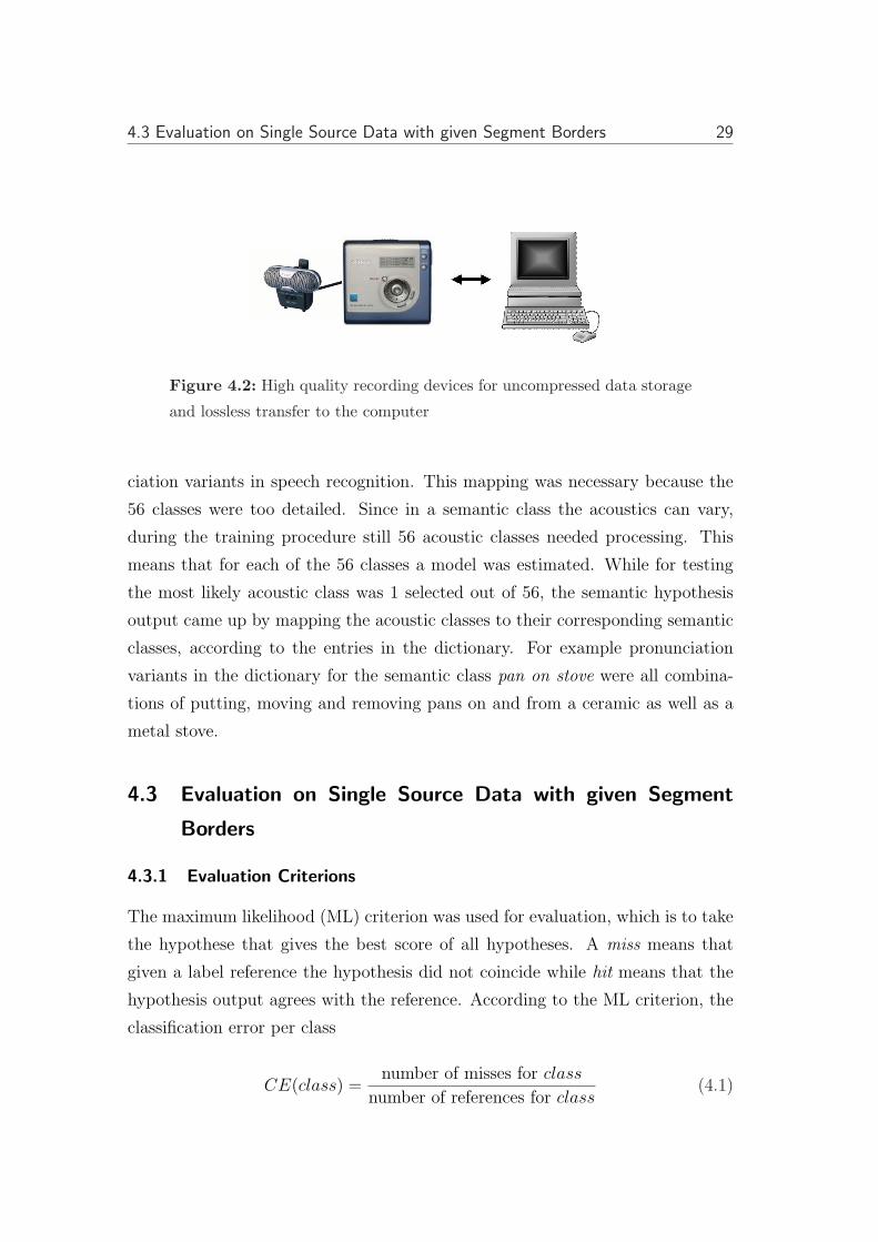
4.2 High quality recording devices for uncompressed data storage and
lossless transfer to the computer . . . . . . . . . . . . . . . . . . . 29
4.3 Confusion matrix visualization for ergodic 3 state HMMs with
ICA7 features. . . . . . . . . . . . . . . . . . . . . . . . . . . . . . 39
4.4 Recall equivalent: CAPTURE measures which part of the refer-
ences could be covered by the hypothesis. The visualization of
CAP(B) is shown. . . . . . . . . . . . . . . . . . . . . . . . . . . . 49
4.5 Precision equivalent: CA1 measures which part of the hypothesis
gave a correct assertion. . . . . . . . . . . . . . . . . . . . . . . . 50
vii

List of Tables
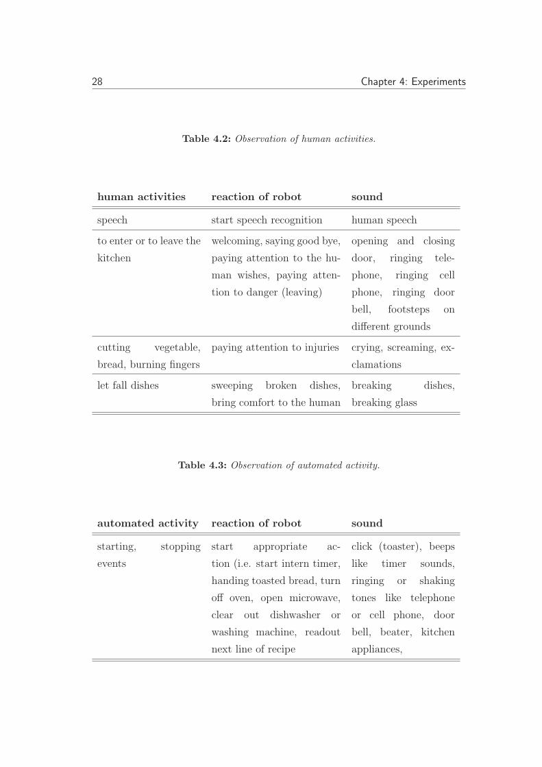
4.1 Observation of dangerous situations. . . . . . . . . . . . . . . . . 27
4.2 Observation of human activities. . . . . . . . . . . . . . . . . . . . 28
4.3 Observation of automated activity. . . . . . . . . . . . . . . . . . . 28
4.4 Collected Data. . . . . . . . . . . . . . . . . . . . . . . . . . . . . 30
4.5 Results and parameters for Gaussian mixture models. . . . . . . . 32
4.6 McNemar’s significance test for GMMs with α-fractile = 0.05. ”1”
means significant difference, ”0” means no significant difference. . 35
4.7 Error ERR for ergodic and forward HMMs. . . . . . . . . . . . . 40
4.8 Precisions PREC for ergodic and forward HMMs. . . . . . . . . . 41
4.9 Class averaged number of Gaussians per system estimated accord-
ing to BIC. . . . . . . . . . . . . . . . . . . . . . . . . . . . . . . 41
4.10 McNemar’s significance test for 2-state HMMs with α-fractile =
0.05. ”1” means significant difference, ”0” means no significant
difference. . . . . . . . . . . . . . . . . . . . . . . . . . . . . . . . 42
4.11 McNemar’s significance test for 3-state HMMs with α-fractile =
0.05. ”1” means significant difference, ”0” means no significant
difference. . . . . . . . . . . . . . . . . . . . . . . . . . . . . . . . 42
4.12 McNemar’s significance test for 4-state HMMs with α-fractile =
0.05. ”1” means significant difference, ”0” means no significant
difference. . . . . . . . . . . . . . . . . . . . . . . . . . . . . . . . 43
4.13 McNemar’s significance test for baseline features with α-fractile =
0.05. ”1” means significant difference, ”0” means no significant
difference. . . . . . . . . . . . . . . . . . . . . . . . . . . . . . . . 44
4.14 McNemar’s significance test for ICA1 features with α-fractile =
0.05. ”1” means significant difference, ”0” means no significant
difference. . . . . . . . . . . . . . . . . . . . . . . . . . . . . . . . 44
viii

ix
4.15 McNemar’s significance test for ICA7 features with α-fractile =
0.05. ”1” means significant difference, ”0” means no significant
difference. . . . . . . . . . . . . . . . . . . . . . . . . . . . . . . . 45
4.16 McNemar’s significance test for systems with fixed number of gaus-
sians and α-fractile = 0.05. ”1” means significant difference, ”0”
means no significant difference. . . . . . . . . . . . . . . . . . . . 46
4.17 Error ERR while using the same total number of Gaussians. . . . 46
4.18 Precisions PREC for stacked and unstacked GMMs and ergodic
HMMs while using 15 Gaussians at total. . . . . . . . . . . . . . . 47
4.19 CAPTURE measure for multi source data . . . . . . . . . . . . . 52
4.20 CA1 measure for multi source data. . . . . . . . . . . . . . . . . . 52
4.21 FOVERLAP measure for multi source data. . . . . . . . . . . . . 53

1 Introduction
We are continually surrounded by sound, which means our ears forward sound
to the brain uninterruptedly. The importance of the meanings sounds have for
our life leads to a continuous scanning of sound for sound properties which are
relevant for us.
Audio signals are responsable for many vital emotions in humans. Hearing speech,
music and environmental sounds triggers the creation of stories in our minds,
affects our behavior and our reactions. Our auditive sense forms a strong connec-
tion to our environment. Various digital audio applications which detect, retrieve,
store and process audio signals open fascinating possibilities.
Environmental sound detection is one of those key technologies which are im-
portant for scientific audio applications. Personal diaries make it possible to find
interesting situations in our daily lives by searching for acoustic changes. Context-
aware mobile devices can learn about their environment by acoustic cues, so that
they may adapt their behavior, for example by adjusting the ringing volume or
by individually and automatically answering calls. Content-based information
retrieval systems may enable us to ask for video genres or special movies indexed
by sound events as birdsong, gunshots or screams.
1.1 Motivation
This thesis deals with the recognition of kitchen sounds relevant for a humanoid
robot being developed as part of the [SFB588] project on humanoid robots in
particular, but the suggested approaches should be useful for related recognition
tasks and research on special noise reduction techniques, too. The aim of the
sound event recognizer proposed in this work is to build a system which will
be able to further improve the interactive behavior of the humanoid kitchen
robot which is supposed to assist mostly elderly and disabled people in kitchen

2 Chapter 1: Introduction
environments. The system should be able to recognize audible warnings, state
signals and help controlling the attention of the robot in case of danger. Such
sound events can be beeps of microwaves and ovens to let the robot know that
food can be served. The recognition of pushing down a toaster can trigger a
deadlock event detection which could prevent a fire. It can happen that one
forgets to switch off the stove because of a phone call or the door bell, a pot
might boil over or sizzling oil in a pan might catch fire. These are situations
in which the robot needs to pay attention in order to choose the right action.
The ability to recognize and thus to respond to all these audio-signals greatly
improves the environmental model of a humanoid robot, especially in situations
where there is little or no visual evidence for what is going on.
1.2 Objective
For the task of this thesis to classify environmental kitchen sounds, an example
based approach seems to be the right choice since the domain is limited to a cer-
tain number of classes. After investigating related work and setting up criteria
of class selection, a set of classes can be determined. For this setup maximal
informative features representing the characteristics of the selected sounds need
to be found. Furthermore, a combination of those features with appropriate clas-
sification stages needs to be evaluated empirically. To test if the selected features
perform well, a series of experiments have to be evaluated for given segment bor-
ders. Another experiment will reveal which kind of difficulties appear when the
proposed approach is applied to recordings of real world cooking tasks. Therefore
it will be of interest if the implicit model based segmentation works sufficiently
well. If not, a segmentation stage needs to be proposed. A further point of inter-
est is how recognition performance degrades when more than one sound is present
at a time. Depending on the degree of degradation an error analysis should make
it possible to recommend a solution.
The remainder of this thesis is organized as follows: In the next chapter I will
discuss related work. In chapter 3 the details of feature extraction and classifi-
cation stages are explained. Then, in the first part of chapter 4, I will review

1.2 Objective 3
the class selection and data collection procedure before describing the results of
my experiments. I will conclude with a summarization of the main results and a
discussion of future research directions.

2 Related Work
This chapter summarizes publications which are relevant for the recognition of
kitchen sound events. Most of these papers deal with sounds without restriction
to a specific acoustic domain, while this is the case for the sound recognition used
by a humanoid robot that works in a kitchen. This means that some authors in-
tend to distinguish between sound types for a rough categorization and others are
more interested in the audio event recognition process itself such that the acous-
tic domains seem to be selected randomly. Also note, that some authors worked
with training databases consisting of sounds collected from CDs and from the
internet, while this work is interested in real-world sound event recognition and
is therefore based on real-world recordings. Nevertheless the various feature sets
and classifiers, which are applied in the publications shown in this chapter, are
of interest for the specific task of kitchen sound event recognition. Most authors
use information theoretic approaches to improve standard preprocessed features
in combination with Gaussian Mixture Models, Hidden Markov Models or Sup-
port Vector Machines. A choice of related work is shown in the following sections.
[Lu, Zhang, Li] use Support Vector Machine (SVM) classifiers to distinguish be-
tween the 5 sound classes silence, music, background sound, pure speech, and
non-pure speech which includes speech over music and speech over noise. They
achieve up to 96% recognition accuracy using a Gaussian kernel. Classification
was performed per frame and segmentation borders were assumed where classes
changed after a smoothing technique was applied on a sliding window over three
frames. The database consisted of 4 hours recording with about 2600 audio clips
collected from TV programs, the Internet, audio and music CDs. The smoothing
process is rule based and assumes misclassification where one frame has been
classified as belonging to a different class from the surrounding ones. If three
neighboring frames were classified as part of three different classes, the middle

2.0 Objective 5
frame had to be declared as belonging to the class the same class as the first
frame. If the center frame was detected as silence the rules were not applied
since silence is much more likely to appear only with duration of one frame than
the other classes. [Lu, Zhang, Li] also compare SVM results with k-nearest neigh-
bor and GMM classifiers, where a superiority of the SVM classifier was found for
this kind of task.
[Cho, Choi, Bang] employ non-negative matrix factorization (NMF) which learns
parts-based representation in the task of sound classification. NMF based fea-
tures are compared to ICA features. 5 state HMMs were trained using stan-
dard maximum likelihood training procedure. The database consisted of TIMIT
speech data, recordings from commercial CDs and some environmental sounds
downloaded from the internet. Their NMF basis images show more local prop-
erties, while ICA basis images, on the other hand, appear to be spread more
globally. This means that each NMF basis vector showed the auditory receptive
field characteristics which activate only few selected frequencies over time, while
the activations for each ICA basis vector were spread out over a global range.
The superiority of NMF compared to ICA reported in this paper can be explained
by the database and the ICA architecture used. The database contained sounds
which had been resampled at 8kHz and the underlying ICA architecture was not
explained at all. 2 of 10 classes were speech and another 5 were music related
sounds. The 3 remaining typical environmental classes only contained less than
19% of the tested sounds. Therefore the evidence for superiority of NMF to ICA
concerning environmental sounds in general is uncertain.
A comparison of MFCCs and MPEG7 features is reported by [Xiong et al.]. For
purposes of classification HMMs are investigated using both maximum likelihood
criteria as well as entropic training as explained by [Casey01]. The paper does
not reveal which kind of MPEG7 feature branch was actually used but it seems
that the authors compared the PCA variant to MFCCs since they only mention
the optional application of ICA and do not report explicit results concerning
ICA features. Their database consisted of broadcast TV interfering background
noise. Best results were achieved using MPEG7 features in combination with

6 Chapter 2: Related Work
entropically trained HMMs. Nearly the same performance (0.13% absolute dif-
ference) was achieved by MFCCs in combination with standard maximum likeli-
hood HMMs.
In [Kwon, Lee] ICA based feature extraction for phoneme recognition is compared
to MFCCs representing state of the art speech recognition features. [Kwon, Lee]
observed that ICA features perform better than MFCCs when using a small
training database while ICA features perform poorer than MFCCs when used
on large databases. After a modification of ICA application an accuracy was
reported, which would be comparable to the result obtained when using MFCCs
on a large database. The modification in this paper is that ICA was also used to
extract independent components in the time domain. Compared to FFT this has
the advantage that ICA uses filters which have been learned from speech signals
that have non-uniform center frequencies and non-uniform filter weights. There
is the common problem of phase sensitivity when using localized basis functions.
Phase shift is not relevant in speech recognition when segments of speech signals
are kept short. This is why after estimating the ICA unmixing matrix a Hilbert
transform was used to obtain smoother estimates of the energy coefficients. Af-
terwards a second ICA stage working in the frequency domain was chained to
remove redundant time shift information.
[Hyvarinen, Hurri et al.] introduce a framework with several models of statistical
structure for coding of image sequences. Sparseness is a property that is used in
ICA. An extension of ICA to cover temporal coherence as well as energy correla-
tions is called ”spatiotemporal bubbles”. Thus a spatiotemporal basis vector can
represent a contour element moving in a specific direction. This idea of extracting
basis functions in ICA covering topographic as well as temporal continuity will
be transferred to sequences of audio features in chapter 3.1.3.
[Dufaux, Besacier et al.] automatically detect and recognize impulsive sounds
such as glass breaking, human screams, gunshots, explosions and slamming doors.
They use a median filter to normalize sequences of energy activations in 10 and
40 frequency bands. For segmentation a sequence of binary decisions was per-

2.0 Objective 7
formed on this normalized frame sequence, using an adaptive threshold. High
quality recordings taken from different sound libraries were classified on frames
of the frequency bands mentioned, using GMMs and HMMs. The authors report
recognition results of 98% at 70dB and above 80% at 0dB SNR, even under severe
Gaussian white noise degradations.
[Casey02] introduces a system for automatic classification of environmental sounds,
musical instruments, music genre and human speakers which has been incorpo-
rated into the MPEG-7 international standard for multimedia content descrip-
tion. This system can also be used for computing similarity metrics between
a target sound and other sounds in a database. [Casey02] is trying to find a
representation that offers a compromise between dimensionality reduction and
information loss. That is why the use of SVD, PCA and ICA is proposed. This
can achieve dimensionality reduction whilst retaining maximum information. Af-
ter spectrum normalization with applying the L2 norm on dB scaled frequency
bins a reduced set of basis functions received from a SVD-ICA system is stored
per class, while retaining those basis functions which code most information mea-
sured on the eigenvalues of the covariance matrix. [Casey02] suggest finding sta-
tistically independent bases per class by application of ICA on the reduced basis
vectors received by SVD. This means that ICA has to be applied on each class-
dependent matrix consisting of eigenvectors in the frequency domain rather than
their corresponding coefficients. Once the bases have been stored, acoustic input
can be classified after each normalized spectral frame has been projected against
all bases. Finally the scores of all corresponding HMMs were compared and the
class with the highest score is supposed to be present in the audio data.
[Kim, Burred et al.] compare three different MPEG-7 features with MFCC for
general sound classification, using a 7-state left-right HMM classifier. The three
branches are PCA, ICA and non-negative matrix factorization (NMF). Their
database consists of 12 classes with 60 examples in each class. 10 classes were
taken from the ”Sound Ideas” [SoundIdeas] database which is a collection of
sound effects. The remaining 2 classes were male and female speech. 3 different
feature dimensions were compared. [Kim, Burred et al.] conclude that MFCC

8 Chapter 2: Related Work
perform better than MPEG-7 features. A thourough look at the results shows
that this conclusion is only correct for the two lower dimensional features, while
ICA and PCA performed better for the highest feature dimensionality tested.
Even the middle dimensional features performed only slightly better in the case
of MFCC than the ICA features. Finally, it is not clear if this superiority really
comes from the feature extractors themselves because MPEG-7 feature extraction
is both usually and in the authors implementation performed on normalized log
scale octave bands, while MFCCs work on logarithmic melscale coefficients. On
the other hand, MPEG7 features are intercomparable while performing on the
same frequency bands. Therefore their results show a significant superiority of
ICA and PCA over the NMF features.
3 Methodology & Theory
After giving a basic explanation and interpretation of three preprocessing ap-
proaches in this chapter, a brief recall on two well known classifiers with respect
to the environmental sound domain will be given. The combination of preproces-
sors and classifiers will be evaluated in later chapters to show whether the sug-
gested methods can improve a baseline sound recognition system. Segmentation
and Decoding were explored in the last two subsections for the sake of complete-
ness and to provide an interface for future research directions, even though their
implementation was out of scope for this thesis.
3.1 Pre-processing
The following subsections give a theoretical background for one basic and two
further advanced preprocessing techniques.
3.1.1 Baseline Feature Extraction
For the baseline system a feature extraction standard was chosen which is state-
of-the-art baseline for speech recognition and which many researchers working
on sound event recognition use as well. After applying an FFT on a 16msec
hamming smoothened window of data sampled at 44.1 kHz, I filtered 20 melscale
coefficients, calculated 13 cepstral coefficients on the log melscales and filtered
context by first and second temporal derivatives, which resulted in further 26
coefficients. Both MFCCs and temporal derivatives were unified in 39 dimensional
feature frames.

10 Chapter 3: Methodology & Theory
3.1.2 Independent Component Feature Extraction
In order to achieve the goal of finding the characteristics of a sound event, it is
possible to think of a sound event as consisting of a mixture of subcharacteristic
properties. One way to find these properties is to use independent component
analysis (ICA). The following subsection provides a general understanding of
ICA and its application in the context of sound event recognition. This second
pre-processing technique is motivated by a mathematical interpretation of sub-
characteristic properties describing a sound. This technique constitutes the body
for the thesis and will be reused by the third preprocessing stage which will be
examined. Using a finite number of feature sequence frames, ICA looks for a
certain view of this data stream which is most efficient in terms of statistics.
By keeping this view estimated on training data also for recognition purposes as
well, the test data can be classified in a feature space that codes maximum infor-
mation with a minimum of coding length. To reach maximum coding efficiency
either the basis vectors of a new basis (the new view) need to be independent,
since dependency would mean redundancy or the new feature stream needs to be
expressed by a basis which makes the feature coefficients maximum independent.
The coding efficiency for the given data sequence which asks for independence in
the linear combination of a transformed feature stream with the new basis can
be kept either in the new basis, or in the transformed data. These two possibili-
ties result in two different ICA architectures, which are explained in [Bartlett98]
for the vision domain. Each architecture needs to store the counterpart to the
independent components received from the training feature sequences. Counter-
part, in this context, means that when making the coefficients of the new feature
representation stream independent, the basis has to be stored and vice versa.
By multiplying a test feature vector with the inverse of the stored matrix, the
underlying hidden sources of the mixing process are revealed.
When looking at the ICA architecture used in this thesis the interpretation of
ICA application is as follows: A single sound event can be regarded as if it was
a combination of properties. Some of these properties might be shared with
a subset of other classes. Other properties might be shared with yet another
subset of some other classes. Therefore, each class can be seen as an individual
3.1 Pre-processing 11
combination of properties which can be shared among all classes. The separation
into properties can make use of high order statistics, so ICA searches for directions
in the feature space in a way that resulting independent components (which can
be the new feature frames in this ICA architecture) show independence of a higher
order than is reachable by a covariance matrix which contains only second order
statistics.
For the application of environmental sound recognition, this entails searching for
independent components in all environmental sound classes all at once. Note
that this ICA architecture differs from the one proposed by [Casey02] since the
procedure described here looks for independence based on inter class analysis
while [Casey02] extracts intra-class independent components. Both procedures
seem to be reasonable for classifying environmental sounds while the favor for
the inter-class case in this thesis comes from the number of parameters that are
invariant to the number of classes in the recognition process. For the architecture
used by [Casey02] an unmixing matrix has to be stored per class. [Casey02]
therefore needs to project each feature frame against as many bases as classes are
present in the recognition task during classification.
Preparations
In order to make the ICA estimation more effective some preparatory steps are
useful. After subtracting the mean, the data is whitened, which means applying a
linear transformation that removes the covariances and normalizes the variances
to unit length. Removing covariances is equivalent to decorrelating the observa-
tion matrix. By whitening the data the number of free parameters of the ICA
basis matrix to be estimated is also decreased from n2 to n(n−1)/2 [Hyvarinen99]
because the transformation makes the matrix orthogonal and an orthogonal ma-
trix contains only n(n− 1)/2 degrees of freedom. The whitening transformation,
which includes the decorrelation, can always be calculated by a singular value
decomposition (SVD) of the covariance matrix. The dimensionality was reduced
to 13 while at the same time keeping at least 95% of the information according
to the measure
I(k) =
∑ki=1 D(i, i)∑nj=1 D(j, j)
(3.1)
12 Chapter 3: Methodology & Theory
where D is the diagonal matrix of sorted eigenvalues received from SVD, k is
the number of kept basis vectors and n is the original number of basis vectors.
Decorrelation is a weak kind of making the data independent which should speed
up the estimation of the independent components of higher statistical order.
ICA transformation
One mathematical key to finding the relation between coding efficiency and inde-
pendence is entropy, which is related to the coding length of a random variable.
As explained by [Hyvarinen99] a sparse distribution of a random variable has less
entropy than a Gaussian distribution of a random variable with the same mean
and covariance since the sparse one concentrates its values more on a specific
value. An example of such a sparse distribution is a spiky probability density
function (pdf) with heavy tails is the Laplace distribution
p(usuperGaussian) =1√2exp(
√2|usuperGaussian|) (3.2)
The corresponding random variable is called a super-Gaussian random vari-
able. The second possibility for a random variable to be non-Gaussian is to
be sub-Gaussian which also means that it has less entropy than a corresponding
Gaussian-distributed random variable. This typically results in a flat pdf con-
stant near zero and being very small for other values. An example for such a
sub-Gaussian distribution is the uniform distribution
p(usub−Gaussian) =
12√
3if |usub−Gaussian| ≤
√3
0 otherwise(3.3)
The Central Limit Theorem tells us that the distribution of the sum of two inde-
pendent random variables tends to get more Gaussian-distributed. The other way
round, to measure if two random variables are getting more independent, their
change of non-Gaussianity has to be observed. Non-Gaussianity can be measured
using negentropy. After calculating the mean and covariance of a random vari-
able u, the entropy of its corresponding Gaussian distribution can be obtained.
Negentropy is the entropy difference between this Gaussian distribution and u’s
real distribution. For a random variable u it is defined by
J(u) = H(uGaussian)−H(u). (3.4)

3.1 Pre-processing 13
Negentropy’s properties are always giving non-negative values, which are zero if
and only if u has a Gaussian distribution. Further negentropy is invariant for
invertible linear transformation. The calculation of negentropy is costly when
using the real distribution of a random variable, which means that the samples
itself had to contribute to the computation. In practice an approximation
J ≈ c[E{G(u)} − E{G(s)}]2 (3.5)
of negentropy is often used with c being a constant proportional factor. Here
s ∼ N(0, 1) is a zero mean unit variance Gaussian random variable, while u is
assumed to have zero mean unit variance as well. Some examples for general
purpose contrast functions G are
G1(w) = 14w4
G2(w) = 1alog(cosh(aw)) 1 ≤ a ≤ 2
G3(w) = 1bexp(−bw2/2) b ≈ 1.
(3.6)
G1 gives kurtosis which is a classical measure for non-Gaussianity. It is defined
by
kurt(u) = E{u4} − 3(E{u2})2 (3.7)
and is a normalized version of the fourth central moment of a distribution. The
disadvantage using kurtosis is that this measure is very sensitive to outliers.
[Hyvarinen99] investigated the robustness of the contrastfunctions on artificial
source signals, two of which were sub-Gaussian, and two were super-Gaussian.
The source signals were mixed using several different random matrices, whose
elements were drawn from a standardized Gaussian distribution. For test of ro-
bustness four outliers whose values were ±10 were added in random locations.
[Hyvarinen99] results show that G2’s estimates are better than the estimates by
G1 while G3 gives slightly better results than G2 since it grows more slowly and
therefore is more robust to outliers.
Now a brief look on the terminology of ICA variables is useful. The ICA tu-
torial by [Hyvarinen99] may also help to understand ICA basics. As already
mentioned, the ICA transformation essentially aims at discovering the hidden
14 Chapter 3: Methodology & Theory
information components y, which can be received by transformation and contain
the subcharacteristic properties we are looking for. The observed feature frames
can be regarded as the basis of a stochastic process. By constraining the hidden
information components y with statistical properties the transformation matrix
W can be estimated. There are two possibilities for constraining the y compo-
nents. First, the dimensionality could be reduced by constraining the number
of y components while retrieving maximum information of the observations x,
which leads to the application of PCA or factor analysis. The second possibility
is to require statistical independence of the components y, which means that no
value of one component should contain information on other components. While
factor analysis requires a Gaussian distribution of the data examined, for which
independent components can be found easily, ICA looks for the statistical in-
dependence of non-Gaussian data. Since sound events are suspected to often
have non-Gaussian distributions ICA can be applied, with expecting reasonable
transformed data. The previously mentioned transformation matrix W reveals
the hidden subcharacteristic information y = Wx by unmixing the observed
frequency frames in the sense of statistical independence. The unmixing filter
W = MB> combines the whitening matrix M and the ICA basis B into one
matrix only, which will be used to project the observed features onto the new
characteristic feature space. Often ICA is shown in the form of the mixing filter
A = M−1B to show how the observed data x = Ay is composed.
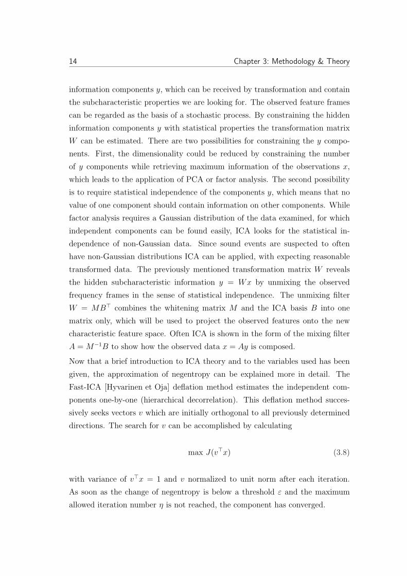
Now that a brief introduction to ICA theory and to the variables used has been
given, the approximation of negentropy can be explained more in detail. The
Fast-ICA [Hyvarinen et Oja] deflation method estimates the independent com-
ponents one-by-one (hierarchical decorrelation). This deflation method succes-
sively seeks vectors v which are initially orthogonal to all previously determined
directions. The search for v can be accomplished by calculating
max J(v>x) (3.8)
with variance of v>x = 1 and v normalized to unit norm after each iteration.
As soon as the change of negentropy is below a threshold ε and the maximum
allowed iteration number η is not reached, the component has converged.
3.2 Classifier 15
3.1.3 Temporal Independent Component Feature Extraction
The characteristics of sounds are spread out in the frequency domain as well as
in the time domain. This is why it is also important to extend the basis functions
over several frames, which restricts the independent component analysis to pick
out only those subcharacteristics which also need to be shared over a given time
window of frame length t. This can be performed by passing not only frame
by frame to the analysis stage but rather by simply stacking all frames with
dimensionality d of the time window in a new frame with dimensionality d · t.This stacking has to be done iteratively for all frames of dimensionality d with
a time window sliding frame by frame. The resulting frames of dimensionality
d · t then have to be passed to the independent component analysis. They cover
context of size t−1 and overlap widely, as shown in illustration 3.1. Figure 3.2 is
a visualization of an ICA unmixing matrix without covering context, while figures
3.3, 3.4, 3.5 and 3.6 cover context with sliding windows over 3, 5, 7 and 9 frames,
which were used as input to ICA. In these figures, the vertical axis corresponds to
basis coefficients, while within all figures showing filters for stacked feature inputs,
the horizontal axis corresponds to time. For visualization purpose a normalization
of matrix coefficients was performed such that maximal values correspond to the
color black while white represents minimal matrix coefficients, which can be also
negative. Note that in the figures showing context dependent filters some basis
vectors exhibit strong temporal patterns, and some seem to be completely static.
3.2 Classifier
After extracting relevant features for the sound domain in form of short time
snapshot sequences, their typical values per class need to be learned, including
their change over time. One way to find a mapping to classes is simply to learn the
distributions of feature coefficients belonging to one class. In this case temporal
behavior may be coded implicitly in the distributions when context is used in the
feature set. A standard approach to learn these feature coefficient distributions is
summarized in the next subsection. Another possibility is to use explicit mapping
of temporal behavior given by the feature stream, which will be explained in the

16 Chapter 3: Methodology & Theory
Figure 3.1: Contextual feature stream generation for sliding context win-
dows covering 5 feature frames
Figure 3.2: Nonstacked ICA-unmixing matrix

3.2 Classifier 17
Figure 3.3: 3 frames stacked ICA-unmixing matrix
Figure 3.4: 5 frames stacked ICA-unmixing matrix
Figure 3.5: 7 frames stacked ICA-unmixing matrix

18 Chapter 3: Methodology & Theory
Figure 3.6: 9 frames stacked ICA-unmixing matrix
second subsection.
3.2.1 Gaussian mixture models
For the classification of the three proposed features Gaussian mixture models
(GMMs) are a good choice since they cover the feature space with several different
weighted multivariate distributions. First of all the number of Gaussians per class
has to be determined. In order to do so, all pre-processed features belonging to
one class are collected. Then the Bayesian Information Criterion scores (BIC
scores) [Chen et al.] for clustering this data with k-means into 1..k clusters has
to be compared. The maximum number of clusters is k = number of frames50
, to
have at least 50 samples on average for one cluster, since a rule of thumb says
to take at leat 100 samples per free parameter and frames are half overlapping.
The highest BIC score leads to the corresponding number of Gaussians for the
Gaussian mixture parameter estimation of this class. After that all other classes
need the same processing. A Gaussian mixture model is a weighted sum of normal
distributions which can be evaluated according to
fx(x) =1
(2π)n2 |Σ| 12
exp[−1
2(x− µ)T Σ−1(x− µ)
], (3.9)
where µ is the mean vector and Σ the covariance matrix. The weights are itera-
tively estimated using the EM algorithm according to the aim of maximizing the
likelihood for the observed probability density function. The covariance matrix
was kept diagonal.

3.2 Classifier 19
3.2.2 Hidden markov models
Hidden Markov models (HMMs) [Rabiner et al.] are widely used for speech recog-
nition and are increasingly applied for the purpose of environmental sound recog-
nition as well. While GMMs, as a special case of HMMs, have to decide frame by
frame which is the most likely class, HMMs behave in a similar way, however cov-
ering temporal dynamics between frames belonging to one class. For this reason,
class decisions can be made on frame sequences rather than single frames. Since
in the HMM case characteristics can be coded along paths as they appear in the
recording, HMMs should be superior to GMMs in covering temporal aspects un-
der idealized circumstances (which means when there is an optimal topology for
each individual sound). An HMM consists of N states, a transition probability
matrix A = {aij}, a distribution of initial probabilities πi, a set of observation
densities and the output probabilities bj(x) =∑M
m=1 cjmN(x, µjm, Σjm), where
N is the normal distribution with mean µ and covariance matrix Σ weighted by
cjm. Here, parameter estimation is also done iteratively according to the EM al-
gorithm. Since an HMM topology describes possible transition paths for feature
frame sequences over time the following two subsections explain the models that
seemed relevant for recognizing environmental sounds.
Ergodic Models
An ergodic HMM has a full connected topology. Transitions from any state to
any other state, including self loops as shown on the left of figure 3.7, are allowed.
Training was initialized with one state, and the same steps were applied as if there
were Gaussian mixture models. But rather than calculating the BIC scores for
a different number of clusters, k-means has to be applied with the same number
of clusters as states will be there in the ergodic topology. Since k-means enables
us to know which frames are similar distributed and therefore should belong to
the same state, all frames for this cluster can be accumulated and the number
of Gaussians for this state can be estimated as described for the case of having
no HMM topology with the BIC approach. After this initial estimation for the
number of Gaussians per state Viterbi training was applied.
20 Chapter 3: Methodology & Theory
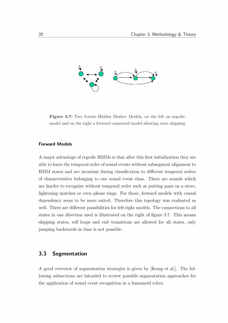
Figure 3.7: Two 3-state Hidden Markov Models, on the left an ergodic
model and on the right a forward connected model allowing state skipping
Forward Models
A major advantage of ergodic HMMs is that after this first initialization they are
able to learn the temporal order of sound events without subsegment alignment to
HMM states and are invariant during classification to different temporal orders
of characteristics belonging to one sound event class. There are sounds which
are harder to recognize without temporal order such as putting pans on a stove,
lightening matches or even phone rings. For those, forward models with causal
dependency seem to be more suited. Therefore this topology was evaluated as
well. There are different possibilities for left-right models. The connections to all
states in one direction used is illustrated on the right of figure 3.7. This means
skipping states, self loops and exit transitions are allowed for all states, only
jumping backwards in time is not possible.
3.3 Segmentation
A good overview of segmentation strategies is given by [Kemp et al.]. The fol-
lowing subsections are intended to review possible segmentation approaches for
the application of sound event recognition in a humanoid robot.

3.3 Segmentation 21
3.3.1 Model based Approaches
In model based segmentation [Bakis et al.] approaches acoustic classes have to be
defined and trained before segmentation (i.e. HMMs, GMMs). This means that
the distribution of feature vectors for each condition is modeled as a Gaussian
mixture. Each feature vector gives a likelihood of the frame for all classes. An
HMM, modeling allowed class transitions, can be used to output the most likely
path through the classes modeled by their Gaussians, when applying the Viterbi
algorithm. The borders of segments are assumed to be at time points where
Viterbi tells a change of the trace.
3.3.2 Energy based Approaches
Energy based segmentation searches for breaking intervals in an audio signal by
using thresholds. It is assumed that segment borders are in the center of these
breaking intervals.
After computing the power for a short time analysis window, a smoothing fil-
ter may be applied to remove artefacts. For smoothing Finite Impulse Response
(FIR) filters or median filters over several frames are possible. An energy thresh-
old has to be defined and the regions of the signal which have energy below the
assumed value are going to be categorized as silence. Basically, silence periods can
be detected with this segmenting approach if the energy was below the threshold
for a given time period.
3.3.3 Metric based Approaches
Metric based segmentation can be used for several kind of acoustic data which
contain speech, music and environmental sounds. Therefore, two neighbored
sliding windows of sets containing acoustic vectors with underlying Gaussian
mixture models are compared according to a suited distance measure.
For two probability density functions PA and PB, each modeling one of those
windows, a suited segmentation distance measure proposed by [Siegler, et al.] is
22 Chapter 3: Methodology & Theory
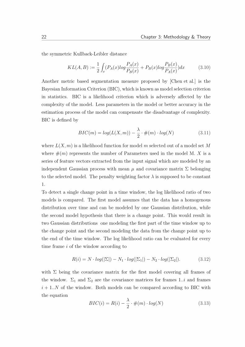
the symmetric Kullback-Leibler distance
KL(A,B) :=1
2
∫
x(PA(x)log
PA(x)
PB(x)+ PB(x)log
PB(x)
PA(x))dx (3.10)
Another metric based segmentation measure proposed by [Chen et al.] is the
Bayesian Information Criterion (BIC), which is known as model selection criterion
in statistics. BIC is a likelihood criterion which is adversely affected by the
complexity of the model. Less parameters in the model or better accuracy in the
estimation process of the model can compensate the disadvantage of complexity.
BIC is defined by
BIC(m) = log(L(X,m))− λ
2·#(m) · log(N) (3.11)
where L(X,m) is a likelihood function for model m selected out of a model set M
where #(m) represents the number of Parameters used in the model M. X is a
series of feature vectors extracted from the input signal which are modeled by an
independent Gaussian process with mean µ and covariance matrix Σ belonging
to the selected model. The penalty weighting factor λ is supposed to be constant
1.
To detect a single change point in a time window, the log likelihood ratio of two
models is compared. The first model assumes that the data has a homogenous
distribution over time and can be modeled by one Gaussian distribution, while
the second model hypothesis that there is a change point. This would result in
two Gaussian distributions one modeling the first part of the time window up to
the change point and the second modeling the data from the change point up to
the end of the time window. The log likelihood ratio can be evaluated for every
time frame i of the window according to
R(i) = N · log(|Σ|)−N1 · log(|Σ1|)−N2 · log(|Σ2|). (3.12)
with Σ being the covariance matrix for the first model covering all frames of
the window. Σ1 and Σ2 are the covariance matrices for frames 1..i and frames
i + 1..N of the window. Both models can be compared according to BIC with
the equation
BIC(i) = R(i)− λ
2·#(m) · log(N) (3.13)

3.4 Decoding 23
and #(m) again being the number of parameters in model M . A change point
will be detected at time
t = argmaxiBIC(i) (3.14)
if BIC(t) > 0 which means that the model with two Gaussian distributions is
favored according to its model complexity and accuracy. As long as both models
(one with a single Gaussian distribution and the second with two distributions)
are similar, BIC(i) will be increasing, otherwise decreasing.
Multiple change points may be detected by applying the single change point
algorithm successively until an inflection point is found and then restarting the
algorithm with an interval starting from the last detected inflection point.
3.4 Decoding
After a processing of the continuous audio input stream, the classifiers 3.2 can be
employed by a decoder. This section explains how to use a decoder with respect
to the application in a robot.
A decoder searches in a continuous audio input stream for the most likely sequence
of class name outputs. If the class models allow flexible duration alignments, as
given in the HMM case, at each time frame different hypothesis candidates can
be competing. Only those hypothesis candidates compete, which meet each other
in a lattice, depending on their duration modeling. The lattice is used to con-
struct paths, allowed by the syntax of a grammar according to the durational
constraints of the classes.
The most likely hypothesis at a time does not necessarily have to stay the winner
after future frames will have been processed. The question arises when to be sure
that the part of the hypothesis being processed so far will not change during the
future progress of decoding. For a kitchen robot this is important to know due
to providing fast and secure reactions. To answer this question it is necessary to
know when a candidate hypothesis can be declared as beaten and can be removed.
The answer can be given after considering the simpler case where two hypothesis
candidates meet in the same lattice node representing an allowed class transition
according to a not necessarily used grammar. Then their scores will be compared
and only a backpointer to the class having the better score will be stored. As

24 Chapter 3: Methodology & Theory
soon as there is a timepoint when all still active hypothesis candidates meet in
only one lattice node the corresponding best hypothesis can be output earliest
with certainty according to [Spohrer82]. This output starts from the time point
in the past when the same event happened the last time or the data input started.
Freeing memory for beaten hypothesis candidates have not beed implemented
for the decoder of the JANUS Recognition Toolkit [JRTk] and can be done as
follows. As long as the predecessor of a node belonging to a beaten candidate
has only one successor namely the one who was just beaten it can be removed
and backpointers can be cleaned up to free memory. This removal process has to
be done iteratively backwards in time for this candidate to be removed until a
node of the dying candidate has another not dying successor which corresponds
to another still competing hypothesis candidate.

4 Experiments
First this chapter describes which criteria led to a selection of classes used in
this work. Then the explanation will be given how recordings and data labeling
were performed. Further parts of this experimental section are divided in the
evaluation of recordings where only one sound source was available at a time and
a second part where overlapping sounds were present in the recordings.
4.1 Class Selection
The humanoid robot has the task to support and assist humans in the kitchen.
An initial brain storming which sounds may occur in a kitchen environment even
under extreme conditions and a selection of those which can be relevant for an
interaction between humans and robots led to the categories shown on top of
tables 4.1, 4.2 and 4.3. After the categories were determined, all relevant sound
instances which belong to each category were tried to be found.
4.2 Data Collection and Labeling
Nearly all sounds selected by the categories found in the last chapter were recorded
in 5 kitchens using the Sony stereo microphone ECM-719 and a Sony High-
Minidisc Walkman MZ-NH700 (see figure 4.2). The small portable recorder al-
lowed uncompressed PCM recordings at 44.1 kHz with 16 bit per channel on a
1 Gigabyte Disc and lossless data transfer via USB. I collected roughly 6,000
sound events and segmented them manually. The segments were divided into
70% training and 30% test data by random. There is an overlapping of kitchens
used for training and testing because not every kitchen had the same devices. In
the 5th kitchen, data was recorded for three real world cooking tasks. Volunteers
were asked to make eggs and bacon with toast, pancakes or spaghetti bolognese.

26 Chapter 4: Experiments
Figure 4.1: Illustration of recording configuration.
In 4 kitchens only one sound source per recording was tried to capture while elim-
inating other sounds like fridge noise or clock ticks. When a relevant sound was
found during the labeling process, which still had an overlapping with another
one, this segment was not used for training. It also happened quite often that a
sound produced by the recorder during data storage affected the recording. In
those cases the affected segments were left out, too, while plain versions of this
sound where also used to train the class that contains all non-relevant sounds.
This special class got the name others and covers for example fridge cracks, street
noise, birds, moving of oven sheets, opening and closing the dishwasher. Each
source was recorded multiple times from different locations to account for differ-
ent reverberation conditions as illustrated by figure 4.1. All recognition systems
performed on the first channel of the stereo microphone.
The recordings were labelled into 56 classes which were later semantically mapped
to 21 classes [table 4.4] using parallel connected HMMs as known from pronun-

4.2 Data Collection and Labeling 27
Table 4.1: Observation of dangerous situations.
activities danger sound
pan is taken off, put on or
moved on the stove, arbi-
trary cooking sounds on the
stove
forgotten to switch off
the hotplate
contact sound be-
tween hotplate and
pan
sizzling in the pan pan catches fire sizzling
boiling water in the pan no more water, water
boils over
boiling water, fizzling
to toast deadlock of the toaster
⇒ fire
click
switching on a gas stove too big blaze to light a match,
cigarette lighter,
lighter, noise of
burning gas
water leaks out (dish
washer, sink unit, washing
machine)
water damage running water, flowing
water
baking, cooking, boiling burned food, fire egg timer
28 Chapter 4: Experiments
Table 4.2: Observation of human activities.
human activities reaction of robot sound
speech start speech recognition human speech
to enter or to leave the
kitchen
welcoming, saying good bye,
paying attention to the hu-
man wishes, paying atten-
tion to danger (leaving)
opening and closing
door, ringing tele-
phone, ringing cell
phone, ringing door
bell, footsteps on
different grounds
cutting vegetable,
bread, burning fingers
paying attention to injuries crying, screaming, ex-
clamations
let fall dishes sweeping broken dishes,
bring comfort to the human
breaking dishes,
breaking glass
Table 4.3: Observation of automated activity.
automated activity reaction of robot sound
starting, stopping
events
start appropriate ac-
tion (i.e. start intern timer,
handing toasted bread, turn
off oven, open microwave,
clear out dishwasher or
washing machine, readout
next line of recipe
click (toaster), beeps
like timer sounds,
ringing or shaking
tones like telephone
or cell phone, door
bell, beater, kitchen
appliances,
4.3 Evaluation on Single Source Data with given Segment Borders 29
Figure 4.2: High quality recording devices for uncompressed data storage
and lossless transfer to the computer
ciation variants in speech recognition. This mapping was necessary because the
56 classes were too detailed. Since in a semantic class the acoustics can vary,
during the training procedure still 56 acoustic classes needed processing. This
means that for each of the 56 classes a model was estimated. While for testing
the most likely acoustic class was 1 selected out of 56, the semantic hypothesis
output came up by mapping the acoustic classes to their corresponding semantic
classes, according to the entries in the dictionary. For example pronunciation
variants in the dictionary for the semantic class pan on stove were all combina-
tions of putting, moving and removing pans on and from a ceramic as well as a
metal stove.
4.3 Evaluation on Single Source Data with given Segment
Borders
4.3.1 Evaluation Criterions
The maximum likelihood (ML) criterion was used for evaluation, which is to take
the hypothese that gives the best score of all hypotheses. A miss means that
given a label reference the hypothesis did not coincide while hit means that the
hypothesis output agrees with the reference. According to the ML criterion, the
classification error per class
CE(class) =number of misses for class
number of references for class(4.1)

30 Chapter 4: Experiments
Table 4.4: Collected Data.
class # training ex. # test ex. all ex.
(dur. in sec) (dur. in sec) (dur. in sec)
boiling 221 (662) 98 (319) 319 (981)
bread cutter 25 (40) 11 (27) 36 (67)
cutting vegetables 134 (89) 58 (41) 192 (130)
door 114 (101) 50 (44) 164 (144)
door bell 50 (110) 22 (55) 72 (164)
egg timer ring 11 (34) 6 (17) 17 (51)
footsteps 240 (140) 104 (66) 344 (206)
lighter 84 (42) 37 (20) 121 (61)
match 141 (131) 62 (59) 203 (189)
microwave beep 110 (30) 49 (17) 159 (47)
others 858 (1130) 369 (547) 1227 (1677)
oven switch 472 (133) 208 (60) 680 (194)
oven timer 12 (16) 6 (8) 18 (24)
overboiling 186 (129) 81 (70) 267 (199)
pan stove 584 (308) 256 (132) 840 (439)
pan sizzling 107 (343) 46 (146) 153 (489)
phones 134 (920) 63 (393) 197 (1313)
speech 125 (82) 55 (38) 180 (120)
stove error 18 (12) 8 (5) 26 (17)
toaster 119 (92) 53 (46) 172 (138)
water 421 (1129) 184 (464) 605 (1593)
total 4166 (5670) 1826 (2573) 5992 (8243)

4.3 Evaluation on Single Source Data with given Segment Borders 31
and the precision per class
PREC(class) =number of correct hits for class
number of hypotheses for class(4.2)
were evaluated to report an averaged classification error (ERR) and an averaged
precision value (PREC) over all classes. This makes all classes equal important,
since the number of samples differed between classes.
4.3.2 Significance Test
The experiments in this section were performed on data with given segment bor-
ders. When comparing error rates p1 and p2 of two systems for isolated sounds
of the same data set, p1 and p2 are not independent. This is because similar
algorithms may have errors in common. Therefore [Gillick89] offers a more direct
and elegant solution using the test of [McNemar47].
The test’s null hypothesis asserts that, given that only one of the two recogni-
tion systems makes an error, it is equally likely to be either one. This means
that the estimation of the conditional probability that the one recognition sys-
tem makes an error on an utterance, given that only one of the two recognizers
makes an error, should give the same estimate for the other system. The num-
ber of sound events n10, which are incorrectly classified by the first system and
correctly classified by the second system, follow a binomial distribution B(k, q)
with k = n10 + n01 being the sum of all errors made by only one system. With
q01 =Pr(System1 classifies an utterance correctly, System2 classifies the same
utterance incorrectly) and q10 vice versa, [Gillick89] defines q = q10/(q01+ q10).
For the null hypothesis q = 1/2, n10 has a B(k, 1/2) distribution. For a random
variable M drawn from B(k, 1/2), the probability
P =
2Pr(n10 ≤ M ≤ k) if n10>k/2
2Pr(0 ≤ M ≤ n10) if n10 < k/2
1.0 if n10=k/2
(4.3)
gives the ratio of occasions for which the observed difference arised by chance. If
P < α, where for example α = 0.05 is the significance level, a significant difference
is available and the null hypothesis has to be rejected. The probabilities were
32 Chapter 4: Experiments
computed by
P =
2∑k
m=n10
k
m
(12
)kif n10>k/2
2∑n10
m=0
k
m
(12
)kif n10<k/2
(4.4)
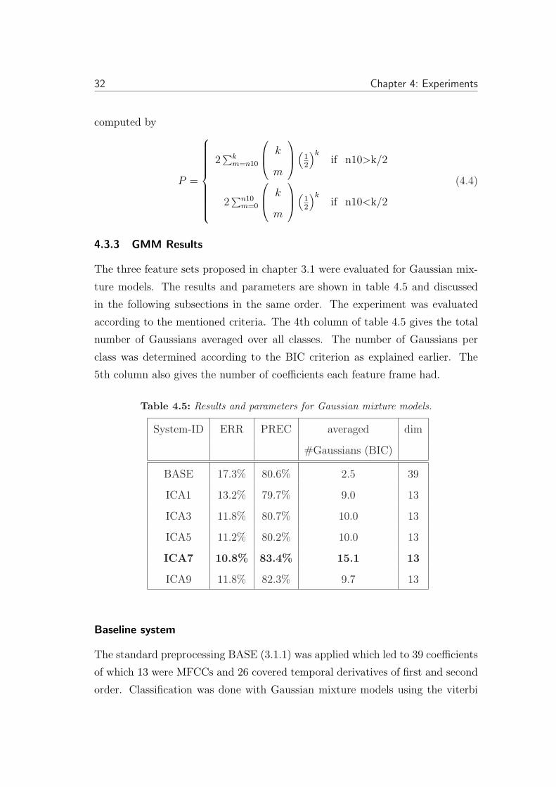
4.3.3 GMM Results
The three feature sets proposed in chapter 3.1 were evaluated for Gaussian mix-
ture models. The results and parameters are shown in table 4.5 and discussed
in the following subsections in the same order. The experiment was evaluated
according to the mentioned criteria. The 4th column of table 4.5 gives the total
number of Gaussians averaged over all classes. The number of Gaussians per
class was determined according to the BIC criterion as explained earlier. The
5th column also gives the number of coefficients each feature frame had.
Table 4.5: Results and parameters for Gaussian mixture models.
System-ID ERR PREC averaged dim
#Gaussians (BIC)
BASE 17.3% 80.6% 2.5 39
ICA1 13.2% 79.7% 9.0 13
ICA3 11.8% 80.7% 10.0 13
ICA5 11.2% 80.2% 10.0 13
ICA7 10.8% 83.4% 15.1 13
ICA9 11.8% 82.3% 9.7 13
Baseline system
The standard preprocessing BASE (3.1.1) was applied which led to 39 coefficients
of which 13 were MFCCs and 26 covered temporal derivatives of first and second
order. Classification was done with Gaussian mixture models using the viterbi

4.3 Evaluation on Single Source Data with given Segment Borders 33
algorithm. The error ERR on the test set was about 17% while the averaged
precision PREC was about 81% as shown in table 4.5.
Standard ICA features
Contextless ICA features were calculated on 20 log melscale coefficients after
centering and whitening the data. Centering, whitening and projection could
be summarized in one matrix transformation. The error ERR decreased by 4%
compared to the baseline while the precision measure PREC is about the same
as in the baseline system. Note that the ICA system only uses 13 dimensional
features instead of the baseline with 39 dimensions. This difference shows that
independent components are able to cover relevant information on environmental
sound data quite well. Nevertheless, some classes were found to have worse
results. Very silent sounds like taking a pan off the stove or silence itself were
detected seldom while many classes with pitch could be identified nearly without
error.
ICA on temporal stacked features
Before applying ICA and classifying as in the standard ICA approach additionally
temporal stacking was applied as explained in chapter 3.1.3.
As table 4.5 shows, the performance of all stacked variants was found to be
better than the baseline system and the ICA system without stacking. The
classification error ERR decreases with increasing number of stacked frames up
to a minimum at 7 frames while 9 frames has a slightly worse performance. This
general decrease obviously is due to temporal ICA’s nature to extract relevant
information from both time and frequency domain. Since keeping the number
of coefficients for the classifier constant while increasing the context size, ICA’s
performance has to decrease at some point, because with the same number of
parameters more information needs to be coded. This overdrawing might also
lead to only rarely shared basis vectors between sound classes which does not
have to be bad in view of the deconvolution of sound event characteristics, but
the effect of overfitting not necessarily neighbored subcharacteristics overweighs.
Accordingly the same happens analog to the averaged precision PREC with a

34 Chapter 4: Experiments
small drop for the ICA5 system. The trend of performing better when having
more context is due to receiving stronger characteristics when more temporal
context information is available. Further note that the additional information
that the frames are stacked according to their time order can be obtained during
dimensionality reduction. 7 neighbored frames correspond to a time window
width of 80ms since 20ms frames are half overlapping.
Discussion
The superiority of ICA compared to the baseline seems to be obvious in terms
of ERR and PREC. But when having a look on the number of Gaussian param-
eters it is observable that with increasing recognition performance the number
of Gaussians raised also. This observation holds for the improvement for contex-
tual systems, too. Therefore, another experiment needs to analyze this effect by
keeping the number of Gaussians constant. This experiment will be discussed in
section ??. McNemar’s significance test further confirms that there is a difference
between the 7 frames stacked ICA system and the baseline features as well as
between ICA7 and the unstacked ICA1 for GMM classifiers (see table 4.6). The
improvement from the baseline features to the ICA system using no context could
not be shown to be significant. While the dimension of the ICA basis was 13x13
for all ICA systems no matter if unstacked or stacked, the unmixing matrices
which contain both the whitening transformation and the ICA basis grew to the
number of coefficients each system had after stacking per frame. Stacked features
were received by sliding windows of sizes 3, 5, 7 and 9 frames. The dimensionality
after stacking of the melscale coefficients grew to 60, 100, 140 and 180. This new
dimensionality was again reduced by retaining a subset of eigenvectors, which
were given by SVD. This subset was chosen by sorting the eigenvectors according
to the size of their eigenvalues and keeping the most informative ones (at least
95% proportional information according to the measure shown in equation 3.1),
resulting in 13 dimensions for all context sizes. So, the resulting unmixing ma-
trix sizes were 13x20, 13x60, 13x100, 13x140 and 13x180 for systems with window
frame sizes 1, 3, 5, 7 and 9. The computational efficiency during evaluating SVD
on the covariance matrix increases a lot with a growing number of stacked frames
but this is an offline process only done once for all classes together. Although

4.3 Evaluation on Single Source Data with given Segment Borders 35
there are more trained parameters in the stacking systems than in a conventional
feature extraction process like the standard preprocessing, some parameters can
be economized during classifier training.
Table 4.6: McNemar’s significance test for GMMs with α-fractile = 0.05.
”1” means significant difference, ”0” means no significant difference.
GM
MIC
A1
GM
MIC
A7
GMM BASE 0 1
GMM ICA1 1
4.3.4 HMM Results
Gaussian mixture models can be regarded as a special case of HMMs, i.e. those
with only one state. By allowing to have more than one state, the temporal
distribution of different characteristics of some sound classes were expected to be
modeled more efficiently. To find out if the subcharacteristics of environmental
kitchen sounds can be modeled better with forward or ergodic connected topolo-
gies, all feature and classifier combinations with 2, 3 and 4 state HMMs were
evaluated. For both types of topologies the error ERR will be reported first,
followed by the precision measure PREC. Finally each subsection relates the re-
sults to the number of Gaussian parameters. In the following tables BASE again
represents the baseline feature set and ICAn represents the ICA systems applied
on contextual windows of size n.
Ergodic HMMs
When comparing the error ERR between the baseline and the nonstacked and
stacked ICA systems, which are shown in table 4.7, ICA systems show better
recognition results than the baseline throughout all systems regardless to the
36 Chapter 4: Experiments
number of states. For all number of ergodic HMM states used this superiority is
significant at least for the baseline features and ICA7 (see tables 4.10, 4.11 and
4.12). Now observe that with increasing number of context up to 7 frames there is
a trend to have less errors with only two exceptions being ERG ICA3 for 3 states
and ERG ICA1 for 4 states. 9 frames contextual window show less performance.
This is highly probable due to saturation of the ICA basis as already explained
for the GMM systems. When looking for the best system for a given number of
states, ERG ICA7 is the best one for ergodic models. The winning system for
this type of topology is a 3 state system of ICA features for 7 frame windows.
By the look of the precision measure PREC for ergodic HMMs shown by table 4.8,
the best systems are ICA systems with context, when comparing same number of
states according to PREC. These contextual ICA systems all had better precision
values than the baseline and ICA without context. A trend to improve precision
is observable at least up to 7 frame windows for 2 and 4 state systems. The 3
state nonstacked ICA system shows less precision performance than the baseline.
Even when looking on the PREC values for increasing context, ERG ICA3 and
ERG ICA5 have less precision than the nonstacked ERG ICA1, while the pre-
cision for ERG ICA7 jumps up and clearly outperforms the baseline. To relate
the error rates and precisions to the number of Gaussians shown in table 4.17,
first note that the baseline has three times more coefficients for feature vector
than ICA systems. The table reports averaged number of Gaussians per system
estimated by BIC. When comparing the number of Gaussians be aware that to
know the number of Gaussian parameters for the baseline you need to multiply
the values by 78 since the feature dimensionality is 39 leading to 39 means and
39 variance coefficients in the diagonal covariance matrix. For the same reason
the number of Gaussian parameters for ICA systems can be evaluated when mul-
tiplying the values by 26. To compare Gaussian parameters instead of number of
Gaussians the first column needs to be multiplied by 3. For ergodic systems the
table mainly shows that with increasing number of states the number of Gaus-
sians increases for the baseline and all ICA feature sets. When an ICA system
makes use of stacking in most cases it needs more Gaussians than the nonstacked
variants. This observation qualifies the improvement of ERR and PREC through
to increasing stacking sizes. For this reason the fixed Gaussian experiment shown

4.3 Evaluation on Single Source Data with given Segment Borders 37
in a later section needs to clarify whether this recognition trend is invariant to
the number of Gaussians. The baseline features could be compared with the
ICA7 features in the case where both system topologies have 3 ergodic connected
states. The number of Gaussians is roughly about the same with respect to the
feature dimensions. The corresponding error rates had a significant improvement
(see table 4.11) in favor of 3 state ergodic ICA7.
Forward HMMs
When relating ERR for forward connected HMMs between the baseline features
and ICA feature sets (table 4.7), ICA systems show much better error rates, as
already present for ergodic HMMs. Those improvements from baseline features
to ICA1 and ICA7 features, as well as the improvement from contextless ICA1
to ICA7 features are significant (tables 4.10, 4.11 and 4.12). When looking at
systems with same number of states, more stacking brought improvement for 2
states up to a stacking size of 5 frames, for 3 states up to 7 frames and for 4
states up to 9 frames except FWD ICA3 with 4 states. It seems that the error
ERR improves, when the context size and the number of states are increasing
simultaneously. This means, that the more overlapping each neighbored frame
pair has, the stronger the temporal and causal dependencies can be covered,
when the number of Gaussians is uncompressed over time. Up to a stacking
size of 7 frames, 3 state forward HMMs performed better than corresponding
2 and 4 state systems. The best forward system was FWD ICA7 for 3 states.
Like in ergodic systems PREC (table 4.8) shows that ICA on context windows
have best precision, when comparing systems with the same number of states.
These best context systems again were better than ICA without context. For
2, 3 and 4 states PREC decreased with increasing context. Sole exception was
outlier FWD ICA3 with 3 states, only performing slightly better than the context
successor FWD ICA5. All ICA systems with and without context had better
PREC results than the baseline. When checking the corresponding number of
Gaussians in table 4.17 again, it is observable that most stacked ICA systems
need more Gaussians according to BIC. For the baseline and all ICA features the
number of Gaussians increased with increasing number of states, while nonstacked
FWD ICA1 did not have this trend for 3 and 4 states. 3 state forward models
38 Chapter 4: Experiments
had similar number of Gaussians for different context sizes while the performance
increased with stacking measured with ERR.
Comparison of Forward and Ergodic HMM Results
As in the two sections before, the error rates ERR will be compared before re-
lating precisions between ergodic and forward topologies. Finally the parameter
differences are reviewed. In general, ergodic HMMs achieved better error rates
than forward HMMs when comparing same feature classifier combinations. The
systems for which this is not the case have underlined values. There is a maxi-
mal ERR difference of 0.7% between the two types of topologies for the systems
with underlined values. For the other systems ergodic models are performing
better. These observations show that ergodic models are a good choice for the
environmental kitchen class set. Ergodic state transitions allow different tem-
poral frame orders inbetween sounds while short time context is captured by
stacking. For example, the doorhandle in the class door should be trained and
recognized with assignment to same states by appropriate kmeans initialization.
Therefore, opening and closing a door can be handled by the same class since
the temporal order is not such important when only interested in an event door.
The same argumentation holds for detecting speech. Ergodic models performed
better for speech since the phoneme order is not relevant for detection of speech.
An ergodic model can cover arbitrary phoneme orders while a forward model can
not. However, the superiority of forward models to ergodic models could not be
shown to be significant (refer to tables 4.10, 4.11 and 4.12) for ICA1 and ICA7
systems in general when applying the same type of topology for all classes at once.
Baseline features on the other hand had significant better results for all ergodic
models when comparing to forward models. Pushing down a toaster, switching
on a lighter and ring tones were among the classes which could be modeled best
with forward models. Ergodic models performed better for the already mentioned
classes speech and doors. The class others, which is a garbage model, performed
very well for ergodic models as well. Best system in terms of ERR was ergodic
ICA7 with 3 states at 9.4% error while the corresponding forward topology led to
10.5%. Both topologies agree in terms of ERR that the baseline was beaten by
ICA systems and that stacking improves performance. Note that these results are

4.3 Evaluation on Single Source Data with given Segment Borders 39
averaged values shown a general tendency of topology favors. The best topology
should still be selected per class.
For all recognition systems confusion matrices were produced to identify which
classes where mainly confused by this example based approach. The visualization
of the confusion matrix for the best system is shown in figure 4.3 where the num-
ber of Gaussians was estimated by BIC. Most confused classes among all systems
were speech and water, and subclasses like put pan on stove and move pan on
stove, while the main activations are on the diagonal, which shows reasonable
recognition performance.
Figure 4.3: Confusion matrix visualization for ergodic 3 state HMMs with
ICA7 features.
Precision results (table 4.8) are only better for one third of forward topologies
compared to the ergodic ones, which is shown by underlined values. In contrast to
the ERR comparison both topologies have similar precision results. Nevertheless,
best precision values were given for 3 states by the ergodic HMMs when using
ICA7 features. The same results were gained by the best forward connected
system ICA7 with 2 states. The total best precision system for both topologies is
ergodic ICA9 for 4 states, which has nearly the same result as the just mentioned

40 Chapter 4: Experiments
best ERR system ergodic ICA7 with 3 HMM states. The number of Gaussians
for both topologies are about the same. In 3 of 4 cases forward models had better
ERR rates, but those needed more Gaussians. The nonstacked ICA systems with
3 states differed most, even if this difference is only 2.7 Gaussians on average.
Table 4.7: Error ERR for ergodic and forward HMMs.
System-ID 2 states 3 states 4 states
ERG BASE 20.2% 14.4% 16.1%
ERG ICA1 12.2% 11.5% 11.5%
ERG ICA3 11.9% 10.8% 11.7%
ERG ICA5 11.8% 11.5% 11.1%
ERG ICA7 10.7% 9.4% 10.5%
ERG ICA9 11.8% 10.4% 11.3%
FWD BASE 23.3% 20.6% 19.4%
FWD ICA1 13.1% 12.3% 13.9%
FWD ICA3 12.1% 11.0% 11.7%
FWD ICA5 11.1% 11.0% 12.3%
FWD ICA7 11.5% 10.5% 11.4%
FWD ICA9 11.2% 11.5% 11.1%
4.3.5 Comparison of GMM and HMM results
In terms of ERR and PREC the 2 state ergodic ICA systems without stacking
and with stacking over 7 frames (tables 4.7, 4.8) performed better than their
corresponding 1 state systems (table 4.5). These differences could not be shown
to be significant (tables 4.14 and 4.15. For all 2, 3 and 4 state ergodic systems
the GMMs were beaten in terms of PREC except for 2 state ergodic models with
baseline features. Results for ergodic 3 and 4 state topologies compared to GMMs
when using ICA1 (table 4.14) and ICA7 (table 4.15) features are significant.
Also note that the evaluation criteria are average values and different classes
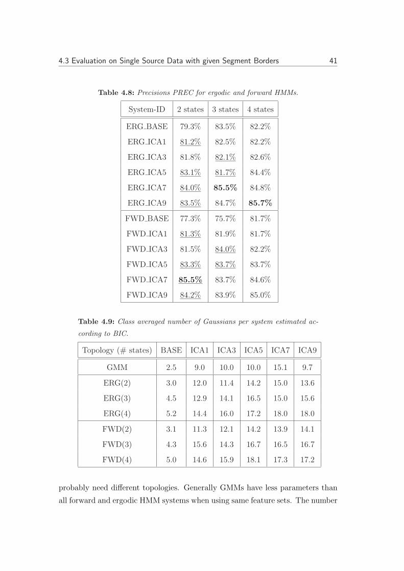
4.3 Evaluation on Single Source Data with given Segment Borders 41
Table 4.8: Precisions PREC for ergodic and forward HMMs.
System-ID 2 states 3 states 4 states
ERG BASE 79.3% 83.5% 82.2%
ERG ICA1 81.2% 82.5% 82.2%
ERG ICA3 81.8% 82.1% 82.6%
ERG ICA5 83.1% 81.7% 84.4%
ERG ICA7 84.0% 85.5% 84.8%
ERG ICA9 83.5% 84.7% 85.7%
FWD BASE 77.3% 75.7% 81.7%
FWD ICA1 81.3% 81.9% 81.7%
FWD ICA3 81.5% 84.0% 82.2%
FWD ICA5 83.3% 83.7% 83.7%
FWD ICA7 85.5% 83.7% 84.6%
FWD ICA9 84.2% 83.9% 85.0%
Table 4.9: Class averaged number of Gaussians per system estimated ac-
cording to BIC.
Topology (# states) BASE ICA1 ICA3 ICA5 ICA7 ICA9
GMM 2.5 9.0 10.0 10.0 15.1 9.7
ERG(2) 3.0 12.0 11.4 14.2 15.0 13.6
ERG(3) 4.5 12.9 14.1 16.5 15.0 15.6
ERG(4) 5.2 14.4 16.0 17.2 18.0 18.0
FWD(2) 3.1 11.3 12.1 14.2 13.9 14.1
FWD(3) 4.3 15.6 14.3 16.7 16.5 16.7
FWD(4) 5.0 14.6 15.9 18.1 17.3 17.2
probably need different topologies. Generally GMMs have less parameters than
all forward and ergodic HMM systems when using same feature sets. The number

42 Chapter 4: Experiments
Table 4.10: McNemar’s significance test for 2-state HMMs with α-fractile
= 0.05. ”1” means significant difference, ”0” means no significant differ-
ence.
ER
G2
ICA
1
ER
G2
ICA
7
FW
D2
BA
SE
FW
D2
ICA
1
FW
D2
ICA
7
ERG2 BASE 0 1 1 0 1
ERG2 ICA1 1 1 0 1
ERG2 ICA7 1 1 0
FWD2 BASE 1 1
FWD2 ICA1 1
Table 4.11: McNemar’s significance test for 3-state HMMs with α-fractile
= 0.05. ”1” means significant difference, ”0” means no significant differ-
ence.
ER
G3
ICA
1
ER
G3
ICA
7
FW
D3
BA
SE
FW
D3
ICA
1
FW
D3
ICA
7
ERG3 BASE 1 1 1 1 0
ERG3 ICA1 1 1 0 1
ERG3 ICA7 1 1 0
FWD3 BASE 1 1
FWD3 ICA1 1
of Gaussians for ICA7 features is comparable between GMMs and 3 state ergodic
HMMs. Therefore, the ergodic system is preferable since the best error rates from
both classifiers are in favor of ergodic HMMs.
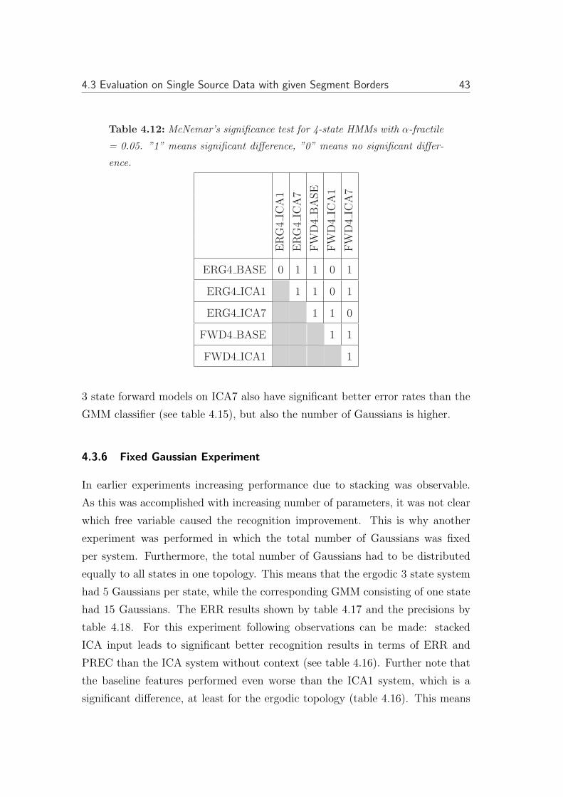
4.3 Evaluation on Single Source Data with given Segment Borders 43
Table 4.12: McNemar’s significance test for 4-state HMMs with α-fractile
= 0.05. ”1” means significant difference, ”0” means no significant differ-
ence.
ER
G4
ICA
1
ER
G4
ICA
7
FW
D4
BA
SE
FW
D4
ICA
1
FW
D4
ICA
7
ERG4 BASE 0 1 1 0 1
ERG4 ICA1 1 1 0 1
ERG4 ICA7 1 1 0
FWD4 BASE 1 1
FWD4 ICA1 1
3 state forward models on ICA7 also have significant better error rates than the
GMM classifier (see table 4.15), but also the number of Gaussians is higher.
4.3.6 Fixed Gaussian Experiment
In earlier experiments increasing performance due to stacking was observable.
As this was accomplished with increasing number of parameters, it was not clear
which free variable caused the recognition improvement. This is why another
experiment was performed in which the total number of Gaussians was fixed
per system. Furthermore, the total number of Gaussians had to be distributed
equally to all states in one topology. This means that the ergodic 3 state system
had 5 Gaussians per state, while the corresponding GMM consisting of one state
had 15 Gaussians. The ERR results shown by table 4.17 and the precisions by
table 4.18. For this experiment following observations can be made: stacked
ICA input leads to significant better recognition results in terms of ERR and
PREC than the ICA system without context (see table 4.16). Further note that
the baseline features performed even worse than the ICA1 system, which is a
significant difference, at least for the ergodic topology (table 4.16). This means

44 Chapter 4: Experiments
Table 4.13: McNemar’s significance test for baseline features with α-
fractile = 0.05. ”1” means significant difference, ”0” means no significant
difference.
ER
G2
BA
SE
ER
G3
BA
SE
ER
G4
BA
SE
FW
D2
BA
SE
FW
D3
BA
SE
FW
D4
BA
SE
GMM BASE 0 1 1 1 0 0
ERG2 BASE 1 1 1 0 0
ERG3 BASE 1 1 1 1
ERG4 BASE 1 1 1
FWD2 BASE 1 1
FWD3 BASE 0
Table 4.14: McNemar’s significance test for ICA1 features with α-fractile
= 0.05. ”1” means significant difference, ”0” means no significant differ-
ence.
ER
G2
ICA
1
ER
G3
ICA
1
ER
G4
ICA
1
FW
D2
ICA
1
FW
D3
ICA
1
FW
D4
ICA
1
GMM ICA1 0 1 1 0 1 1
ERG2 ICA1 1 1 0 1 1
ERG3 ICA1 0 1 0 0
ERG4 ICA1 1 0 0
FWD2 ICA1 0 1
FWD3 ICA1 0
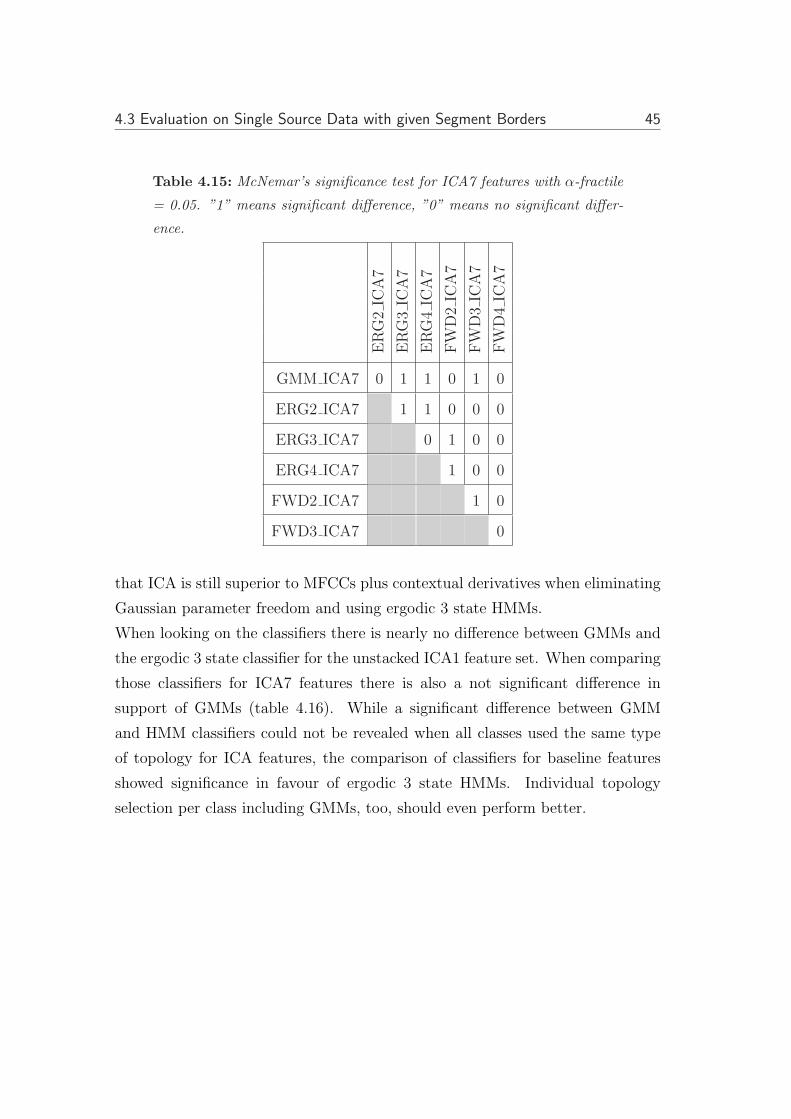
4.3 Evaluation on Single Source Data with given Segment Borders 45
Table 4.15: McNemar’s significance test for ICA7 features with α-fractile
= 0.05. ”1” means significant difference, ”0” means no significant differ-
ence.
ER
G2
ICA
7
ER
G3
ICA
7
ER
G4
ICA
7
FW
D2
ICA
7
FW
D3
ICA
7
FW
D4
ICA
7
GMM ICA7 0 1 1 0 1 0
ERG2 ICA7 1 1 0 0 0
ERG3 ICA7 0 1 0 0
ERG4 ICA7 1 0 0
FWD2 ICA7 1 0
FWD3 ICA7 0
that ICA is still superior to MFCCs plus contextual derivatives when eliminating
Gaussian parameter freedom and using ergodic 3 state HMMs.
When looking on the classifiers there is nearly no difference between GMMs and
the ergodic 3 state classifier for the unstacked ICA1 feature set. When comparing
those classifiers for ICA7 features there is also a not significant difference in
support of GMMs (table 4.16). While a significant difference between GMM
and HMM classifiers could not be revealed when all classes used the same type
of topology for ICA features, the comparison of classifiers for baseline features
showed significance in favour of ergodic 3 state HMMs. Individual topology
selection per class including GMMs, too, should even perform better.

46 Chapter 4: Experiments
Table 4.16: McNemar’s significance test for systems with fixed number
of gaussians and α-fractile = 0.05. ”1” means significant difference, ”0”
means no significant difference.
cGM
MIC
A1
cGM
MIC
A7
cER
G3
BA
SE
cER
G3
ICA
1
cER
G3
ICA
7
cGMM BASE 0 1 1 0 1
cGMM ICA1 1 1 0 1
cGMM ICA7 0 1 0
cERG3 BASE 1 0
cERG3 ICA1 1
Table 4.17: Error ERR while using the same total number of Gaussians.
System-ID GMM ERG-3
BASE 12.4% 12.2%
ICA1 10.6% 10.9%
ICA7 9.2% 10.2%
4.4 Evaluation on Continuous Multiple Source Data
4.4.1 Evaluation Criteria for multi event recognition
To compare the hypothesis output of different recognition systems and to evaluate
multiple source recordings an evaluation criterion needs to be selected. In the
single source data case precision could measure how safe an output is while the
measure recall shows which proportion of available sounds could be detected.
These two criteria should not be used for multisource data when an overlapping
of sounds is present. For the given setup the hypothesis cannot output more than
one hypothesis at a time. This is why a recall measure cannot reach 100% as soon

4.4 Evaluation on Continuous Multiple Source Data 47
Table 4.18: Precisions PREC for stacked and unstacked GMMs and er-
godic HMMs while using 15 Gaussians at total.
System-ID GMM ERG-3
BASE 80.6% 82.8%
ICA1 82.8% 82.2%
ICA7 85.0% 83.4%
as two sounds occur at the same time even if one of them was detected. Further
the recall performance would decrease the longer time parts have more than one
source. A precision measure is not defined for a single hypothesis output in
the multi reference case, since it assumes that references are mutually exclusive.
Rather a modification of both measures is necessary to account for overlapping
sounds while having one hypothesis stream at a time. An intuitive modification
of precision is to score those parts of the hypothesis as correct, if they are present
in any of the class reference tracks. This is shown by an example in figure 4.5,
where the first parts of both hypotheses A and B were declared as CORRECT,
although reference B was present during the first part of hypothesis A, too. For a
sequence of hypothesis hi and references rf (i) for the same time interval selected
by a general mapping function f(x) a classification accuracy measure
CA1 :=
∑i duration( hi | hi = rf(hi) )∑
j duration(hj)(4.5)
can be defined. This measure accounts for the reliability that a hypothesis output
agrees with a reference since all parts of the hypothesis which are not present in
the references are declared as false alarms. In an illustration of CA1 in figure 4.5
the last part of hypothesis B was declared as FALSE for this reason, even it was
not present in any reference. Note that CA1 is in the range from 0 to 1, where
1 means that all parts of the hypotheses did coincide with one of all references
for same time slots. This measure does not tell which ratio of present sounds
were detected. But this is rather important for the recognition of dangerous
situations through sound cues by a humanoid robot. The corresponding measure
for single source data is recall and measures only those hypothesis parts, for
which references are available at same time slots. For multiple source data it can

48 Chapter 4: Experiments
happen that while examining one reference class the corresponding hypothesis
was present in another reference class for the same time window. This should not
affect the evaluation of the focused reference class if the hypothesized output was
in deed available in the acoustics. This is why during evaluation the modificated
recall measure should leave these reference parts out, which have hypothesis,
coinciding with other class reference tracks. The reference parts of a selected
class, which are neither detected by the hypothesis, nor the found hypothesis is
not available in another reference track, will be scored as not detected. In the
example, shown by figure 4.4, only the part b2 of a reference class B was not
detected (FALSE classification), because for the time window b1 the hypothesis
does not agree with the reference B, to be sure, but since during b1 the hypothesis
agrees with another reference track A, it will not be taken into account for this
measure. In the example, the last part of hypothesis B was also not taken into
account because recall similar measures rather set out from the reference than
from the hypothesis. With reference sequences ri,c for the class c and a function
d giving the duration this leads to a time based capturing measure defined by
CAP (class) :=
CAPenumerator(class)CAPdenominator(class)
if CAPdenominator(class) > 0
0 otherwise(4.6)
with
CAPenumerator(class) :=∑
i
d( hi | hi = rf(hi),class ) (4.7)
and
CAPdenominator(class) :=∑
j
[ d(rj,class) − RULEOUT (j, class)] (4.8)
where
RULEOUT (j, class) := d( 4rj,class | ∀c 6= class : hf(4rj,class) 6= rf(4rj,class),c )
(4.9)
is the part of the references ruled out. 4rj,c is any possible subset of the jth
reference time slot in class c. A time based measure over all classes is
CAPTURE :=
∑#(classes)
k=1CAPenumerator(k)∑#(classes)
l=1CAPdenominator(l)
if∑#(classes)
l=1 CAPdenominator(l) > 0
0 otherwise
(4.10)
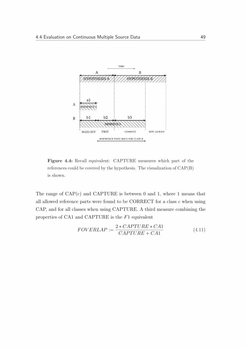
4.4 Evaluation on Continuous Multiple Source Data 49
Figure 4.4: Recall equivalent: CAPTURE measures which part of the
references could be covered by the hypothesis. The visualization of CAP(B)
is shown.
The range of CAP(c) and CAPTURE is between 0 and 1, where 1 means that
all allowed reference parts were found to be CORRECT for a class c when using
CAP, and for all classes when using CAPTURE. A third measure combining the
properties of CA1 and CAPTURE is the F1 equivalent
FOV ERLAP :=2 ∗ CAPTURE ∗ CA1
CAPTURE + CA1(4.11)

50 Chapter 4: Experiments
Figure 4.5: Precision equivalent: CA1 measures which part of the hypoth-
esis gave a correct assertion.
4.4.2 Results and Discussion for Continuous Multi Source Data
Experiments for continuous multi source data was performed on the baseline fea-
ture set and on several ICA systems using GMM and 3 state ergodic classifiers.
As result from previous experiments, fixed number of Gaussians were used due
to comparison issues. Tables 4.20 and 4.19 report the results for a multi source
adapted precision and recall measure. Values in table 4.21 account for hypothesis
output reliability as well as for the proportion of detected sounds.
The first two mentioned tables show that recognition results are much worse than
for single source data. This has several reasons. First to mention is that this eval-
uation is measured timebased, making classes more important the longer their
occurrence is. During the process of labeling it was found that relevant classes
had very sparse occurrences except the garbage class others. This explains in part
that multiple source data results are worse than single source ones in terms of the
false alarm measuring CA1 criterion. Note that in the recognition systems there
was not used any prior knowledge and no grammars which could have accounted

4.4 Evaluation on Continuous Multiple Source Data 51
for this problem. The criterion CAPTURE, which is recall similar, performs also
bad because of a far too small training data base. Especially, the class others
needs a lot more training amount and training variation as long as no confi-
dence measure is used to create multi class hypothesis output tracks. Untrained
devices, like for example a noisy exhaust duct, and background noise degraded
performance, too. The background noise also included speech of 4 speakers in a
neighbored room which was only added as reference when the acoustics surely let
identify it.
Furthermore, acoustic property labels are more desirable than semantic ones since
a semantic hypothesis statement is only useful, if all sound event classes cannot
be mixed up pairwise only due to their acoustic properties. Otherwise the rec-
ognizer might detect a part of an acoustic event which in deed can occur in time
parts of another sound and therefore the wrong semantic output is hypothesized.
Semantic labels are also problematic when not all acoustic possible instances were
trained. For instance the acoustics of footsteps in a kitchen environment highly
depends on the ground material as well as the shoe types. In the experiments all
probands had different shoes and different behaviour in moving which resulted in
recognition differences for the sound event class footsteps depending on the cook.
The next observation is that ergodic 3 state models perform slightly better than
GMMs in terms of CA1 and FOVERLAP for the baseline and stacked ICA fea-
tures. This means that at least the reliability of hypothesis outputs can be
improved by ergodic 3 state models.
The baseline features led to better results than ICA features for overlapping multi
source data. One possible reason for this is that the chosen ICA architecture prob-
ably has problems to detect a sound event when more than one is present at a
time. This sensitivity might be due to the ICA architectures property to look for
global subcharacteristics rather than local ones.
Further, it’s hard to compare the model based implicit segmentation with hand-
made labels for a one stream hypothesis output. This is because when more
than one sound is present at a time, the hypothesis can change at uncontrollable
time points between the present sound classes. This means that some segment
borders coincided with the labels, while many other segment borders appeared
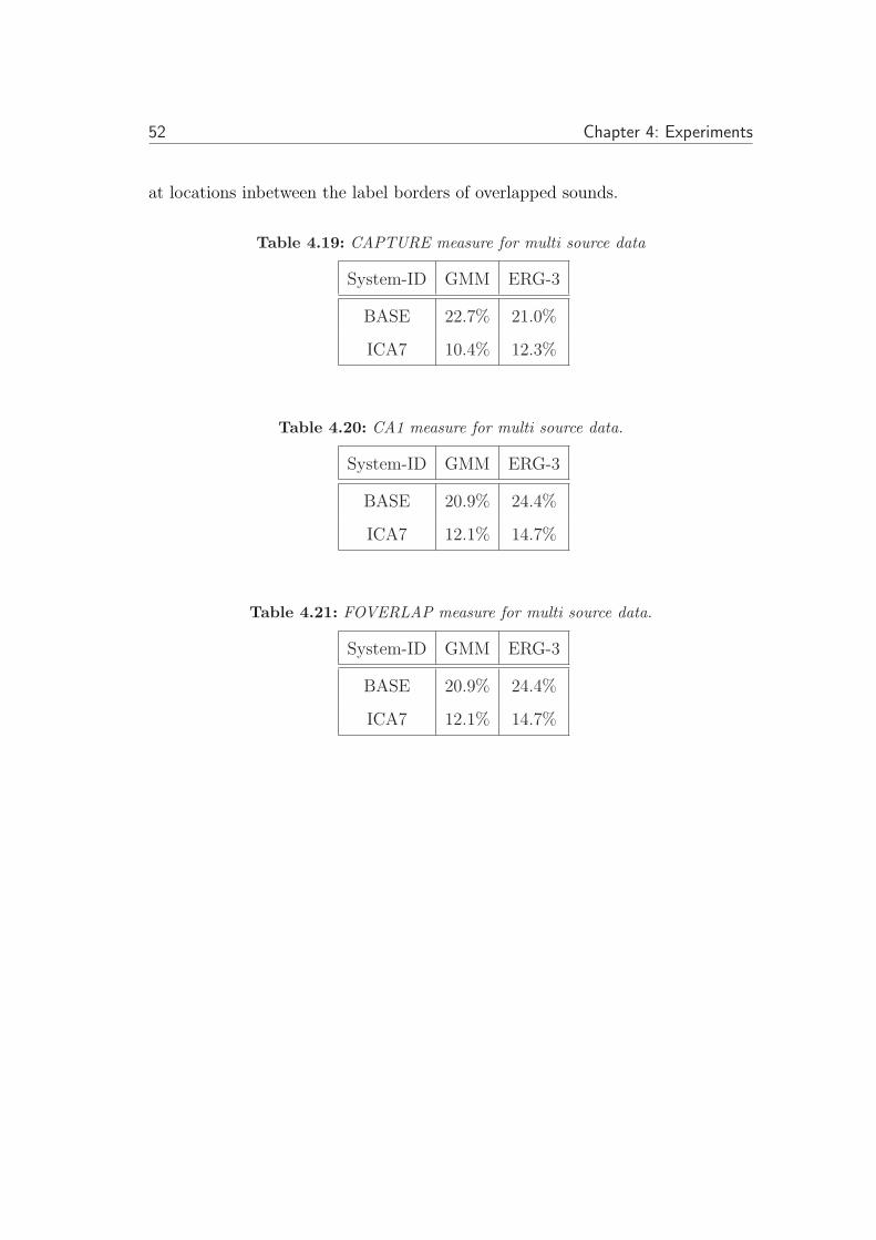
52 Chapter 4: Experiments
at locations inbetween the label borders of overlapped sounds.
Table 4.19: CAPTURE measure for multi source data
System-ID GMM ERG-3
BASE 22.7% 21.0%
ICA7 10.4% 12.3%
Table 4.20: CA1 measure for multi source data.
System-ID GMM ERG-3
BASE 20.9% 24.4%
ICA7 12.1% 14.7%
Table 4.21: FOVERLAP measure for multi source data.
System-ID GMM ERG-3
BASE 20.9% 24.4%
ICA7 12.1% 14.7%

5 Conclusion
5.1 Summary
Motivated by the ultimate goal of providing an audio sense for a humanoid robot,
which is intended to perform tasks in a kitchen environment, different sound
recognition architectures were investigated. The pre-processing, which focused
on ICA because of its ability to represent shared audio subcharacteristics, was
combined with GMMs, forward and ergodic HMM topologies of first order. The
sound event recognition systems tested used only mono microphone input and no
other prior knowledge. Initially it was explained theoretically how the decoder
of a run-on system can determine the earliest time when the system is able to
output its best hypothesis without a later change. It was found that this can be
employed by an approach that outputs parts of concurrent competing hypotheses.
In the experimental part, first several experiments were performed on real world
recordings segmented manually. Concerning the recordings which capture one
source at a time, the usage of ICA was justified for the task of identifying real
world environmental sounds. For this purpose three pre-processing main branches
were explored. The results for this kind of data with GMM / ergodic 3 state HMM
classifier were that MFCCs including temporal derivatives were outperformed by
contextless ICA features with 23.7% / 20.1% relative error reduction and when
adding context by 37.6% / 34.7% while ICA features had only one third of the
dimensionality the MFCC baseline features had.
Even with a fixed number of Gaussians, which were equally distributed over
states, this benefit was perceptible in all tested cases. The relative error reduc-
tions for GMMs / ergodic 3 state HMMs from the baseline to nonstacked ICA
was 14.5% / 10.7%. Furthermore, ICA features on widely overlapping temporal
contextual windows were found to improve accuracy compared to the baseline fea-
tures by a relatively error reduction of 11.7% and 16.4% when GMM and ergodic

54 Chapter 5: Conclusion
3 state HMMs were applied. The optimal window size for this feature dimen-
sionality was determined empirically by keeping the dimensionality constant and
increasing the window’s temporal expansion until accuracy decreased and coding
optimality was exhausted. When each class got an individual estimate for the
number of Gaussians according to the model selection criterion BIC, the three
state ergodic HMMs performed best with ICA features in a context of seven
frames. The fixed Gaussian experiment revealed that GMMs modeled stacked
ICA features slightly better than ergodic HMMs with the distribution conditions
already mentioned. This difference is not significant, while same types of topolo-
gies were applied for all classes per system. A significant improvement due to
topology selection was found for the baseline system in favour for the ergodic
models.
Then, the fixed Gaussian systems of the one source per segment experiments
were tested on continuous data with multiple overlapping sources recorded during
real world cooking tasks, again without adding background knowledge. There-
fore, timebased multi source evaluation measures were derived. The results show
that the combinations of pre-processing and classification stages, which perform
reasonable well on single source data, have heavy problems when dealing with
overlapping sounds including noise, like an exhaust duct and background speech.
Even the baseline features performed better than ICA features, which might
reveal that the search for shared global properties in all classes by ICA is not
optimal for that kind of task. Ergodic 3-state models improved recognition perfor-
mance a bit. This means that individual topology selection affects the recognition
performance.
This second batch of experiments, performed on multiple sources, further showed
that the system had to deal with many classes which were not of interest. During
the process of labeling, it was found that class segments of the real world cooking
tasks, which were relevant to the three categories used for class selection, had
few occurrences throughout the recordings as a whole. This and the observa-
tion of performance degradation from single to multi source data indicate that
the training data base is far too small. For a robust recognition of the selected
environmental kitchen sounds much more data needs to be collected. Note also
that semantic labels were used which was found to adversely affect classes with

5.2 Future Directions 55
similar acoustic parts. Furthermore, it appeared that for one track hypothesis
outputs on multi source data the comparison of model based segmentation bor-
ders and manually labelled borders is not useful, because when more than one
sound is present at a time, the hypothesis can change at uncontrollable time
points between the present sound classes.
5.2 Future Directions
First the author would like to suggest to combine the recognition system with a
discriminative approach, because many false alarms occurred in the multi source
case while the relevant classes had only few occurrences. When discriminating the
classes especially from the garbage class with approaches like LDA and SVM, the
general disadvantage of example-based systems needing huge training databases
can be alleviated. Individual and automatic class based topology selection is
of interest because experiments showed that recognition results depend on the
topology since different sounds need different temporal rhythmic alignments.
The categorization of sounds that are either unknown or have not been trained
enough makes a hierarchical clustering in combination with different feature sets
representing perceptual characteristics necessary. For loudness (depending on the
distance between microphone and source) and duration modeling fuzzy set ap-
proaches are conceivable. Providing both semantic and acoustic properties in the
labels is expensive but would not deliver outputs where for example the sound of
a bread cutting machine and an electric egg beater were mixed up. In particular
the creation of a dictionary for acoustic units, which can be mapped to seman-
tic entities as pronunciation variants in speech recognition, should be performed.
Such an acoustic dictionary with even smaller acoustic units would already affect
the training procedure, when performed on acoustic labels rather than semantic
ones. By providing an interface from such a dictionary to a database of physical
material properties for use in synthetic audio simulation, sound characteristics
could be examined. The simulation can be done by means of finite element meth-
ods where geometric shapes, materials and collision forces can be exchanged for
rigid as well as nonrigid bodies. By saving objects eigenmodes in physical sim-
ulations per shape the materials responsible for the origin of sound should be

56 Chapter 5: Conclusion
identifiable. Getting many real world recordings of dangerous situations like ex-
plosions is difficult but they can be predicted by means of simulation.
Using prior knowledge as well as source separation promise the highest increase
in recognition performance. The expenditure for getting robust n-gram priors is
high, since a lot of recordings and labeling of real world cooking tasks would be
necessary. The author suggests to define grammars by using knowledge on obvi-
ous human behavior. Combining sound localizers which indicate the distance and
direction of sources with knowledge of the position of acoustic sources would help
minimize false alarms. Further, the recognition setup should include a recognition
track for each class performing on well separated and segmented source streams.
A suggestion for source separation is to combine a multi microphone approach
with blind source separation using ISA [Casey00].
Last, but not least, the examination of ICA evaluating independent components
per class to receive more local sound properties needs to be proposed. This means
getting better intra-class properties than inter-class properties. The resulting sys-
tem could be tested using ICA itself as classifier. By formulating a confidence
measure such ICA classifiers could also output one activation stream per class as
simultaneous hypotheses.

A Instructions for cooks
Thank you for helping with our data-collection!
We plan to build a robot which is able to help in a kitchen, therefore the robot
has to learn what happens in a kitchen during cooking. We are working on the
ear of the robot so that he can hear and recognize certain sounds in a kitchen
that occur during cooking.
During this task, you are asked to cook a meal in a kitchen. Please act nat-
urally, but also cooperatively. For this reason we have some instructions for you.
You will be recorded during your task with audio and video devices.
• Act naturally as if you were in the kitchen of a friend but also cooperatively
• You have to find what you need and tidy things up
• No music or TV during cooking
Before cooking you will get an introduction into the kitchen. You will get a
cooking task with some minor instructions.

Task 1:
Cook 3-4 eggs (sunny side up or easy and over) with bacon and make toast.
• Eggs and bacon are in the fridge
• Toast is stored beside the microwave
Task 2:
Cook spaghetti with bolognese sauce
• spaghetti is in the cabinet
• ground meet is in the fridge
Task 3:
Make some pancakes
• Eggs and milk are in the fridge
• flour is available as well
HAVE FUN :)

B Data storage
All scripts, experiments and collected data including labels will be stored
on the intern network of the Interactive Systems Labs, Karlsruhe, at the
end of this diploma thesis.
B.1 Directory Structure
Directories beginning with the letter ”e” represent systems using ergodic
HMMs, while directories beginning with the letter ”l” contain systems with
forward connected HMMs. GMM systems begin with ”C”. Systems for the
fixed Gaussian experiments end with the letters ”cg”. The first numbers in
directory names for HMM systems tells the stacking size, while the second
number gives how many states were used. When baseline features were
used, the first number was replaced by a ”f”. Each recognition system
consists of the following subdirectories:
– basis stores the basis, mixing filters and unmixing filters
– db contains the training and test database description
– desc contains all description files for features, codebooks, topologies
etc.
– kmeans stores kmeans information per class as well as the ”$feature-
init-gaussians” and ”$feature-init-gaussiansPerState” files, which give
the number of Gaussians estimated by BIC
– labels stores labels produced during training
– means stores the means matrix used as preprocessing for ICA
– param stores the codebook and distribution parameters

60 Chapter B: Data storage
– results contains the hypothesis results
– samples contains accumulated samples per class and per state
B.2 Scripts
Script files which are not censored due to the JANUS license agreement are
listed.
– averageNumberGaussians.tcl extracts the number of Gaussians used
by a system
– calcSilThresh.tcl energy based silence segmenting algorithm (not used
for the experiments)
– countshortsegment.tcl outputs the number of segments in the database
which are shorter than a variable
– createMinLengthConstraintDict.tcl adds minimum length constraints
to a dictionary file
– createOthers.tcl writes a label track ”others” for time intervals not
used by any of the track per class labels
– createTopoTree.tcl creates a topology tree description file for a given
class set
– duration.tcl extracts the available recording amount per class in the
database
– eval.tcl evaluates single source recognition system outputs including
confusion matrices and class merging functionality
– evalotime.tcl evaluates multi source overlapping recognition system
outputs using the measure CAPTURE
– evalonline.tcl evaluates multi source overlapping recognition system
outputs using the measure CA1
– getMinDurationPerClass.tcl outputs the shortest segment lengths per
class

2.2 Scripts 61
– merge.tcl merges classes according to a merging lists
– runFile.tcl tests a system and outputs hypotheses from the decoder
– saveResultMergedPerSeg.tcl reads a results per segment file and writes
the corresponding results per segment file for merged classes (only used
for the significance test explicitly, because eval.tcl can merge classes
itself
– saveSilPerKitchen.tcl collects silence frames per location for threshold
estimation (not used in experiments)
– $system/correctms.tcl outputs how many milli seconds of a hypothesis
are correct for overlapping multi track labels
– $system/bicPerState.tcl outputs a bic estimate for the number of gaus-
sians per state
– $system/testConfusion.tcl outputs results per segment file, recall, pre-
cision and confusion matrix for a single source
– db/db.tcl creates dictionary by splitting training and test set randomly
– SIGTEST/sigTest.tcl compares the results per segment files for test of
significance
– SIGTEST/sigMap.tcl creates Latex source for significance tables
– SIGTEST/sigCalcP.tcl outputs the probability used in McNemar’s sig-
nificance test
Bibliography
[Hyvarinen et Oja] Hyvarinen, Oja. (1997). ”A fast fixed-point algorithm for in-
dependent component analysis”. In Neural Computation, 9(7):1483-1492,
1997.
[Kim, Burred et al.] Kim, Burred, Sikora. (2004). ”How efficient is MPEG-7 for
general sound recognition?”. AES 25th International Conference, London,
United Kingdom, 2004 June.
[Casey00] Casey, Westner. (2000). ”Separation of Mixed Audio Sources by In-
dependent Subspace Analysis”. Internation Computer Music Conference
(ICMC), August 2000.
[SoundIdeas] Sound Ideas Website, www.sound-ideas.com.
[SFB588] Website of the SFB 588 project, www.sfb588.uni-karlsruhe.de.
[Casey02] Casey. (2002). ”General Sound Classification and Similarity in MPEG-
7”. Organized Sound, vol. 6:2, 2002, MERL Cambridge Research Laboratory
[Dufaux, Besacier et al.] Dufaux, Besacier, Ansorge, Pellandini. (2000). ”Auto-
matic sound detection and recognition for noisy environment”. In Proc. of
the X European Signal Processing Conference, EUSIPCO 2000, Tampere,
Finland.
[Hyvarinen, Hurri et al.] Hyvarinen, Hurri, Vayrynen. (2003). ”Bubbles: a unify-
ing framework for low-level statistical properties of natural image sequences”.
JoSAA, vol. 20, no. 7, pp. 1237-1252, July 2003.
[Kwon, Lee] Kwon, Lee. (2004). ”Phoneme recognition using ICA-based feature
extraction and transformation”, International Conference on Spoken Lan-
guage Processing, October 2004.
[Xiong et al.] Xiong, Radhakrishnan, Divakaran, Huang. (2003). ”Comparing
MFCC and MPEG-7 Audio Features for Feature Extraaction, Maximum
Likelihood HMM and Entropic Prior HMM for Sports Audio Classification”.
IEEE International Conference on Multimedia and Expo (ICME), Vol. 3, pp.
397-400, July 2003.
[Lu, Zhang, Li] Lu, Zhang, Li. (2003). ”Content-based audio classification and
segmentation by using support vector machines”. ACM Multimedia Systems
Journal. 8 (6), pp. 482-492, March 2003.
[Cho, Choi, Bang] Cho, Choi, Bang. (2003). ”Non-negative component parts of
sound for classification”. Signal Processing and Information Technology, IS-
SPIT 2003. December 2003.
[Casey01] Casey. (2001). ”Reduced-rank spectra and entropic priors as consistent
and reliable cues for general sound recognition”. Proceeding of the Workshop
on Consistent & Reliable Acoustic Cues for Sound Analysis, 2001.
[Bartlett98] Bartlett. (1998). ”Independent component representations for face
recognition”. Proceedings of the SPIE Symposium on Electronic Imaging:
Science and Technology. Conference on Human Vision and Electronic Imag-
ing III, San Jose, California, January 1998.
[Hyvarinen99] Hyvarinen. (1999). ”Independent Component Analysis: A Tuto-
rial”. A revised version appeared in Neural Networks under the title ”Inde-
pendent Component Analysis: Algorithms and Applications”, 13(4-5):411-
430, 2000.
[Siegler, et al.] Siegler, Jain, Raj, Stern. (1997). ”Automatic segmentation, classi-
fication and clustering of broadcast news audio”. Proceedings of the DARPA
Speech Recognition workshop, The Westfileds Conference Center, Chantilly
VA, February 1997.
[Chen et al.] Chen, Gopalakrishnan. (1998). ”Speaker, environment and chan-
nel change detection and clustering via the Bayesian Information Crite-
rion”. DARPA Broadcast News Transcription and Understanding Workshop,
Landsdowne, VA, Febrauary 1998.
[Rabiner et al.] Rabiner. (1989). ”A Tutorial on Hidden Markov Models and Se-
lected Applications in Speech Recognition”. Proceedings of the IEEE, Vol.
77, No. 2, February 1989.
[Bakis et al.] Bakis, Chen, Gopalakrishnan, Gopinath, Maes, Polymenakos,
Franz. (1997). ”Transcription of broadcast news shows with the IBM large
vocabulary speech recognition system”. Proceedings of the Speech Recogni-
tion Workshop, pp 67-72, 1997.

[Kemp et al.] Kemp, Schmidt, Westphal, Waibel. (2000). ”Strategies for auto-
matic segmentation of audio data”. Proceedings of the IEEE International
Conference on Acoustics, Speech, and Signal Processing, ICASSP 2000.
[Hyvarinen99] Hyvarinen. (1999). ”Fast and Robust Fixed-Point Algorithms for
Independent Component Analysis”. IEEE Transactions on Neural Networks,
Vol. 10, No. 3, May 1999.
[Spohrer82] Brown, Spohrer, Hochschild, Baker. (1982). ”Partial traceback and
dynamic programming”. Proceedings of the IEEE International Conference
on Acoustics, Speech and Signal Processing, pages 1629-1632, 1982.
[JRTk] The Ibis-Gang. September 2002. ”JRTk and Ibis”.
http://isl.ira.uka.de/ jrtk/doc.Janus5/janus-doku/janus-doku.html
[Gillick89] Gillick, Cox. (1989). ”Some statistical issues in the comparison of
speech recognition algorithms”. Proceedings of the IEEE Conference on
Acoustics, Speech and Signal Processing, Glasgow, pp 532-535, 1989.
[McNemar47] McNemar. ”Note on the sampling error of the difference between
correlated proportions or percentages.” Psychometrika, 12:153-157, 1947.