core.ac.uk · on post-war US data we indeed find robust evidence for a ... Francesco Bianchi, Uwe...

econstor www.econstor.eu

Der Open-Access-Publikationsserver der ZBW – Leibniz-Informationszentrum WirtschaftThe Open Access Publication Server of the ZBW – Leibniz Information Centre for Economics

Standard-Nutzungsbedingungen:

Die Dokumente auf EconStor dürfen zu eigenen wissenschaftlichenZwecken und zum Privatgebrauch gespeichert und kopiert werden.

Sie dürfen die Dokumente nicht für öffentliche oder kommerzielleZwecke vervielfältigen, öffentlich ausstellen, öffentlich zugänglichmachen, vertreiben oder anderweitig nutzen.

Sofern die Verfasser die Dokumente unter Open-Content-Lizenzen(insbesondere CC-Lizenzen) zur Verfügung gestellt haben sollten,gelten abweichend von diesen Nutzungsbedingungen die in der dortgenannten Lizenz gewährten Nutzungsrechte.

Terms of use:

Documents in EconStor may be saved and copied for yourpersonal and scholarly purposes.

You are not to copy documents for public or commercialpurposes, to exhibit the documents publicly, to make thempublicly available on the internet, or to distribute or otherwiseuse the documents in public.

If the documents have been made available under an OpenContent Licence (especially Creative Commons Licences), youmay exercise further usage rights as specified in the indicatedlicence.

zbw Leibniz-Informationszentrum WirtschaftLeibniz Information Centre for Economics

Tillmann, Peter; Wolters, Maik H.

Working Paper

The changing dynamics of US inflation persistence:A quantile regression approach

Kiel Working Paper, No. 1951

Provided in Cooperation with:Kiel Institute for the World Economy (IfW)

Suggested Citation: Tillmann, Peter; Wolters, Maik H. (2014) : The changing dynamics of USinflation persistence: A quantile regression approach, Kiel Working Paper, No. 1951

This Version is available at:http://hdl.handle.net/10419/100701

0

The changing dynamics of US inflation persistence: a quantile regression approach

Peter Tillmann and Maik H. Wolters

No. 1951 | August 2014

1

Kiel Institute for the World Economy, Kiellinie 66, 24105 Kiel, Germany

Kiel Working Paper No. 1951 | August 2014

The changing dynamics of US inflation persistence: a quantile regression approach*

Peter Tillmann and Maik H. Wolters

Abstract: We examine both the degree and the structural stability of inflation persistence at different quantiles of the conditional inflation distribution. Previous research focused exclusively on persistence at the conditional mean of the inflation rate. As economic theory provides reasons for inflation persistence to differ across conditional quantiles, this is a potentially severe constraint. Conventional studies of inflation persistence cannot identify changes in persistence at selected quantiles that leave persistence at the median of the distribution unchanged. Based on post-war US data we indeed find robust evidence for a structural break in persistence at all quantiles of the inflation process in the early 1980s. While prior to the 1980s inflation was not mean reverting, quantile autoregression based unit root tests suggest that since the end of the Volcker disinflation the unit root can be rejected at every quantile of the conditional inflation distribution. Keywords: inflation persistence, quantile regressions, structural breaks, unit root test, monetary policy, Federal Reserve

JEL classification: E31, E37, E58, C22 Peter Tillmann Justus Liebig University Gießen Licher Straße 66 D-35394 Gießen, Germany [email protected] Maik H. Wolters Kiel Institute for the World Economy Kiellinie 66 24105 Kiel, Germany [email protected]

* We thank Tim Oliver Berg, Francesco Bianchi, Uwe Hassler, Mehdi Hosseinkouchack, Vivien Lewis, Barbara Meller and Johannes Stroebel as well as seminar participants at the DIW Berlin, the IWH Halle, the RWTH Aachen, the University of Osnabru¨ck, the 2012 Spring Meeting of Young Economists (Mannheim) and the 18th Conference on Computing in Economics and Finance (Prague) for very helpful discussions and comments.

___________________________________

The responsibility for the contents of the working papers rests with the author, not the Institute. Since working papers are of a preliminary nature, it may be useful to contact the author of a particular working paper about results or caveats before referring to, or quoting, a paper. Any comments on working papers should be sent directly to the author. Coverphoto: uni_com on photocase.com

mailto:[email protected]

The changing dynamics of US inflation persistence:

a quantile regression approach∗

Peter Tillmann†

Justus Liebig University Giessen, Germany

Maik H. Wolters‡

University of Kiel and Kiel Institute for the World Economy, Germany

August 11, 2014

Abstract

We examine both the degree and the structural stability of inflation persistence at

different quantiles of the conditional inflation distribution. Previous research focused

exclusively on persistence at the conditional mean of the inflation rate. As economic

theory provides reasons for inflation persistence to differ across conditional quantiles,

this is a potentially severe constraint. Conventional studies of inflation persistence cannot

identify changes in persistence at selected quantiles that leave persistence at the median

of the distribution unchanged. Based on post-war US data we indeed find robust evidence

for a structural break in persistence at all quantiles of the inflation process in the early

1980s. While prior to the 1980s inflation was not mean reverting, quantile autoregression

based unit root tests suggest that since the end of the Volcker disinflation the unit root

can be rejected at every quantile of the conditional inflation distribution.

Keywords: inflation persistence, quantile regressions, structural breaks, unit root test,

monetary policy, Federal Reserve

JEL classification: E31, E37, E58, C22

∗We thank Tim Oliver Berg, Francesco Bianchi, Uwe Hassler, Mehdi Hosseinkouchack, Vivien Lewis,Barbara Meller and Johannes Stroebel as well as seminar participants at the DIW Berlin, the IWH Halle,the RWTH Aachen, the University of Osnabruck, the 2012 Spring Meeting of Young Economists (Mannheim)and the 18th Conference on Computing in Economics and Finance (Prague) for very helpful discussions andcomments.

†Email: [email protected]‡Email: [email protected] (corresponding author)

1

1 Introduction

It is well known that the stance and the strategy of monetary policy in many advanced

economies underwent important structural changes over the past decades. Many of these

changes can be associated with specific dates in history, such as the early 1980s Volcker

disinflation in the US. Other changes are gradual and thus more difficult to identify. The

changing nature of monetary policy is likely to be reflected in the time series properties of

inflation dynamics. While shifts in the mean and the variance of inflation could be interpreted

in light of monetary policy changes, another indicator is the degree of persistence, or inertia,

in the inflation process. Persistence refers to the speed at which the inflation rate returns to

its mean following a shock. Even if the mean inflation rate falls due to the central bank’s

increased focus on price stability, fluctuations in inflation can be short-lived or long-lasting

- in part depending on the determination of monetary policy to bring inflation back on an

implicit or explicit target rate.1

Hence, the persistence properties of inflation have received considerable attention in the em-

pirical literature. In a recent survey article, Fuhrer (2011, p. 448) summarizes the abundant

literature on the nature and the sources of persistent inflation dynamics in the US. He argues

”that the contribution to inflation from its unit root component has diminished significantly

in recent decades. [...] With regard to the specific autocorrelation properties of a stationary

inflation rate, the picture is considerably murkier.”

We revisit the changing nature of inflation persistence in the US. We add to the literature on

inflation persistence in three ways. First, we use a quantile regression approach which allows

us to examine the degree of inflation persistence at different conditional quantiles of inflation.

Thus far the literature focuses on persistence evaluated at the conditional mean. This neglects

the fact that inflation following shocks drawn from the tails of the shock distribution might

exhibit a different pattern of inertia than inflation close to the mean. Second, we draw

on techniques recently developed by Oka and Qu (2011) to estimate structural changes in

regression quantiles at unknown dates to detect structural changes in persistence for different

inflation quantiles. This allows us to examine whether changes in persistence are synchronized

across inflation quantiles and whether shifts in persistence at the mean inflation rate are

informative about the entire distribution of inflation outcomes. Third, we use the quantile

autoregression unit root tests developed in Koenker and Xiao (2004) and Galvao (2009) to

test whether inflation follows a unit root process—at different quantiles and globally—in the

different regimes identified with the structural break tests.

In contrast to standard estimates of inflation persistence at the conditional mean, our em-

pirical specification allows us to estimate the degree of inflation persistence conditional on

different magnitudes and signs of shocks. Such differences in inflation persistence over the

conditional inflation distribution could be for example caused by nominal wage rigidities,

menu costs or asymmetric monetary policy. Standard estimates at the conditional mean

cannot distinguish between these important differences in the effects of shocks to inflation.

1Other factors such as a reduction in the degree of wage indexation since the early 1980s, see Hoffman,Peersman and Straub (2010), would also lead to a reduction in persistence, although a more gradual decline.

2

Quantile regressions offer a natural way to empirically assess the importance of these asym-

metries. In particular, quantile regressions allow us to analyze whether the timing and the

nature of changes of inflation persistence have been synchronous at different parts of the

conditional distribution.

Based on a battery of post-war US inflation rates at monthly and quarterly frequency, we

derive two key findings:

First, for all monthly inflation rates we provide evidence for a structural break in persistence

at all quantiles of the inflation process occurring in the early 1980s. Persistence at the

conditional mean as well as persistence at the outer quantiles is significantly lower after the

Volcker disinflation. This result is robust with respect to changes in mean inflation and the

variance of inflation. We do not find, in contrast, breaks in the persistence of quarterly

inflation series, i.e. deflator-based inflation rates.

Second, quantile autoregression based unit root tests show that since the end of the Volcker

disinflation the unit root can be rejected at every quantile, both for monthly and quarterly

rates. Prior to 1980 the unit root hypothesis could not be rejected over the whole conditional

inflation distribution. This sheds light on the recent work on the changing forecastability

of inflation. Stock and Watson (2007) model the inflation rate as an integrated moving

average process and argue that the difficulty to forecast inflation rates might stem from

changing relative roles of a permanent and a transitory component in the inflation process.

In our paper, however, we show that the empirical support for the assumption of a unit root

component in the inflation process has disappeared not only at the mean inflation rate but

at all quantiles.

The remainder of the paper is organized as follows: section 2 briefly surveys the available

empirical literature. Our empirical approach is presented in section 3. Section 4 introduces

the data set and discusses the main results. A set of robustness checks is documented in

section 5. The final section concludes.

2 A brief review of the literature on inflation persistence

In his survey on inflation persistence, Fuhrer (2011, p. 448) summarizes the empirical ev-

idence: ”All authors agree that in the US and many other developed countries inflation

exhibited considerable persistence from the 1960s to the mid-1980s. After that time, the

statistical evidence is mixed. For both the US and other countries studies fall on both sides

of the argument about the possibility of declining reduced-form persistence.”

Let us briefly survey the key contributions to the picture described by Fuhrer. In one of the

earliest studies, Taylor (2000) finds a break in US inflation persistence that coincides with

the Volcker disinflation. Cecchetti and Debelle (2006) and Levin and Piger (2006) assess

inflation persistence for major industrial economies and find that conditional on a break in

the intercept inflation is much less persistent than previously thought. Both papers stress

the need to account for shifts in mean inflation. Neglecting shifts in mean inflation could

lead to spuriously high estimates of the sum of the autoregressive coefficients in the inflation

process.

3

These contributions do not examine structural changes in inflation persistence at potentially

unknown points in time. Cogley, Primiceri and Sargent (2010) use a time-varying vector

autoregression to estimate the nonstationary trend component of inflation, which they asso-

ciate with the Fed’s inflation target. Changes in trend inflation could then lead to changes

in persistence of aggregate inflation. They are able to show a reduced persistence in the gap

between inflation and the pure random walk component of the inflation rate in the Volcker-

Greenspan era.2 Pivetta and Reis (2007), in contrast, use Bayesian methods and do not find

a change in the persistence of GDP deflator inflation in the US. According to their results

based on rolling-window and recursive samples inflation persistence is high and unchanged

over the past decades. Benati (2008) systematically evaluates the impact of regime shifts in

monetary policy on the persistence properties of inflation. His estimates of the sum of the

autoregressive coefficients in a univariate process of CPI inflation drop significantly in the

post-Volcker period. Persistence of PCE and deflator inflation, however, remains high even

after the Volcker-era.

An alternative approach to modeling nonlinearities in the persistence properties of inflation

is to specify a smooth transition autoregressive (STAR) model where a nonlinear transition

function governs the shift between different regimes. Following this line, Nobay, Paya and

Peel (2010) find US inflation to be more mean reverting the further away inflation is from

its mean. It is important to note that the STAR approach rests on the assumption of a

specific functional form of the transition function. Quantile regressions, in contrast, offer a

particularly attractive alternative as they do not require a priori assumptions.

O’Reilly and Whelan (2005) focus on the Euro area and show the difficulty to find empirical

support for a reduction in inflation persistence there. Evidence on inflation persistence at

the level of disaggregate inflation is provided by Clark (2006). His results reveal that the

aggregation process induces persistence into the aggregate inflation series despite disaggregate

inflation exhibiting little persistence.

A separate strand of the literature examines the degree of fractional integration of the inflation

process. Kumar and Okimoto (2007) find a break in the order of fractional integration of

monthly US CPI inflation in 1982. Long run persistence—or long memory—of inflation

is much lower after the Volcker disinflation period. Recently, Hassler and Meller (2011)

extend this line of research and present a test for multiple structural changes in the degree

of fractional integration applied to monthly CPI inflation in the US. Conditional on a shift

in mean inflation, which they locate in 1981, they find a break in 1973 only. At this date,

that coincides with the collapse of the Bretton Woods system and the first oil crisis, inflation

persistence significantly increases. A second break in 1980 proves to be insignificant.3

Taken together, the literature indeed supports Fuhrer’s (2011) cautious view. The present

paper revisits the changing nature of inflation persistence. A potential explanation behind

2Kang, Kim and Morley (2009) model regime shifts in persistence in an unobserved components model.They document a shift to the low-persistence regime in the early 1980s. Zhang and Clovis (2009) use formaltests for structural stability of autoregressive models to document shifts in US inflation persistence.

3Since the long memory property of inflation examined in these studies can be approximated by an au-toregressive process of very high order, a change in the degree of fractional integration can be interpreted asa shift in inflation persistence over the very long run. The approach taken in this paper, however, focuses onautoregressive processes of lower order.

4

these divergent results could be a sizable degree of heterogeneity of inflation persistence at

different conditional quantiles of inflation. If persistence differs according to the size or the

sign of the shocks driving inflation, the mean inflation rate would not be informative about the

true nature of persistence. To address this issue, we model inflation persistence at different

quantiles of the inflation process.

Our study is closely related to the recent work of Tsong and Lee (2011). These authors also

model inflation in a quantile framework but do not assess time-variation in persistence at

individual quantiles. Our key contribution is to apply recently developed tests for structural

breaks at unknown time to the question of inflation persistence. We find that the results

for a long sample as analyzed in Tsong and Lee (2011) and for subsamples before and after

important structural breaks are very different.

3 The quantile approach to inflation persistence

In this section we introduce the measurement of inflation persistence and sketch the test for

structural breaks in persistence at different quantiles and the quantile autoregression based

unit root test.

3.1 Measuring inflation persistence

Our preferred measure of persistence is the sum of the autoregressive coefficients in a uni-

variate process of inflation. By using this reduced form measure of inflation persistence we

do not take a stand on the structural sources of persistence. A change in persistence detected

by our measure is consistent with a variety of structural changes in the conduct of monetary

policy, the nature of nominal rigidities or the properties of shocks hitting the economy. Let

πt be the inflation measure, α an intercept term and εt a serially uncorrelated error term.

The AR(q) process is

πt = α+

q∑

k=1

βkπt−k + εt (1)

The sum of autoregressive coefficients is ρ =∑q

k=1 βk. According to Andrews and Chen

(1994), ρ is the preferred scalar measure of persistence in πt, since a monotonic relationship

exists between ρ and the cumulative impulse response function of πt+j to εt. We rewrite

expression (1) as

πt = α+ ρπt−1 +

q−1∑

k=1

γk∆πt−k + εt (2)

where ∆πt = πt − πt−1. If ρ = 1, the inflation process contains a unit root. If |ρ| < 1, the

process is stationary. In the empirical application below we set the lag length to q = 4 for

quarterly data and q = 12 for monthly data.

Estimates of ρ obtained from least squares estimation suffer from a bias as ρ approaches unity.

Therefore, the literature typically resorts to Hansen’s (1999) median unbiased estimator of

ρ. This estimator, however, has not yet been developed for quantile autoregressive models.

We follow Tsong and Lee (2011) and, when referring to estimates for conditional quantiles,

5

report results based on the standard quantile regression estimates by Koenker and Bassett

(1978).

3.2 Persistence at different quantiles

Quantiles are values that divide a distribution such that a given proportion of observations is

located below the quantile. The τ−th quantile is defined as the value qτ (πt|πt−1, ..., πt−q) such

that the probability that the conditional inflation rate will be less than qτ (πt|πt−1, ..., πt−q) is

τ and the probability that it will be more than qτ (πt|πt−1, ..., πt−q) is 1−τ . The AR(q) process

of inflation dynamics at quantile τ can be written as a quantile autoregression, QAR(q)

qτ (πt|πt−1, ..., πt−q) = α (τ) + ρ (τ)πt−1 +

q−1∑

k=1

γk (τ)∆πt−k. (3)

Estimating the persistence parameter at different quantiles of the distribution instead of the

mean can be done with quantile regressions as introduced by Koenker and Bassett (1978).

Following the work of Koenker and Xiao (2004, 2006), this gives us the persistence param-

eter conditional on a grid of values for τ . Quantile regressions impose no functional form

constraints on parameter values over the conditional distribution of the inflation rate.

The interpretation of the quantile regression approach to inflation persistence is straightfor-

ward: estimates of ρ(τ) reveal the extent of inflation persistence at the quantile τ conditional

on past values of inflation πt−1, ..., πt−q . Thus, shocks to the inflation process of different

size and magnitude are allowed to lead to different patterns of persistence. If inflation is for

example very high relative to recent inflation realizations this means that a large positive

shock to inflation has occurred and that inflation is located above the mean conditional on

past observations somewhere in the upper conditional quantiles. If inflation is lower than in

the previous quarters, this means that a negative shock to inflation has occurred and that

inflation conditional on past observations is located below the mean somewhere in the lower

conditional quantiles. It is important, however, not to confuse the unconditional inflation

distribution and the inflation distribution conditional on past inflation data. We cannot in-

terpret persistence at, say, the τ = 0.2 quantile as reflecting persistence at low absolute levels

of inflation. Rather, it measures persistence when inflation exhibits a large negative deviation

from its conditional mean.

3.3 Breaks in persistence at different quantiles

We test for structural breaks in inflation persistence that might show up in any part of the

conditional inflation distribution. Qu (2008) and Oka and Qu (2011) have developed tests

for structural change with unknown timing in regression quantiles. The tests are subgradient

based and have good properties in small samples.

The test is run in two stages as recommended by Qu (2008) and Oka and Qu (2011). First,

we test for structural stability across a range of quantiles using the DQ-test. This is a general

test for changes in the entire conditional distribution of inflation. Since we do not have any

prior information as to which part of the conditional inflation rate distribution is subject

6

to a break we test for a relatively large range of τ ∈ {0.20, 0.25, ..., 0.80}. An even larger

range would have the disadvantage that the power of the test decreases as opposed to the

case where prior information is used to trim the range of quantiles. In a second step we test

for structural change in prespecified quantiles using the SQτ -test. If the DQ-test rejects the

null hypothesis of no structural break, the SQτ -test can reveal structural breaks in different

parts of the conditional inflation rate distribution. In this way we can detect in which parts

of the distribution the actual change takes place and obtain a full picture about the stability

of persistence across quantiles.

The tests allow for multiple structural breaks with unknown timing. The test procedure runs

sequentially: first, for a given number of breaks, the break dates and the AR parameters are

estimated jointly by minimizing the quantile check function over all permissible break dates.

The range of permissible break dates excludes the first and the final 5% of the observations.

We repeat this procedure for one to a maximum of ten possible structural breaks. Second, we

use the DQ- and SQτ -test to test how many structural breaks have occurred in the sample.

This test proceeds stepwise and first tests the existence of one structural break against the

null hypothesis of no structural break. Let ξ(τ) = (α(τ), ρ(τ), γ1(τ), ..., γq−1(τ)) denote the

vector of parameters in equation (3) at quantile τ and suppose our inflation series contains

T observations. Then the hypotheses for the DQ-test are:

H∗0 : ξi(τ) = ξ0(τ) for all i and for all τ ∈ {0.20, 0.25, ..., 0.80}

H∗1 : ξi(τ) =

ξ1(τ) for i = 1, 2, ..., t

ξ2(τ) for i = t+ 1, ..., T.for some τ ∈ {0.20, 0.25, ..., 0.80}

The two hypotheses for the SQτ -test are given by:

H0 : ξi(τ) = ξ0(τ) for all i for a given τ ∈ {0.20, 0.25, ..., 0.80}

H1 : ξi(τ) =

ξ1(τ) for i = 1, 2, ..., t

ξ2(τ) for i = t+ 1, ..., T.for a given τ ∈ {0.20, 0.25, ..., 0.80}

First, we estimate the AR parameters at the different conditional quantiles under the null of

no structural break. Afterwards, we estimate the AR parameters at the different conditional

quantiles separately for the subsamples based on the previously estimated break dates. If a

structural break exists, the estimated parameters under the null hypothesis are not close to

the true values for at least one subset of the sample. The estimated residuals will persistently

fall below (or above) the true quantile, forcing the subgradient to take a large value.

If the null hypothesis of no structural change is rejected, we test in sequential steps the null

hypothesis of 1 break against the alternative hypothesis of 2 breaks using the DQ(l+1|l)- and

the SQτ (l+1|l)-tests. If we find evidence in favor of 2 breaks we check the null hypothesis of

2 breaks against the alternative hypothesis of 3 breaks and so on. Tables for critical values

are provided in Qu (2008).

7

3.4 Quantile autoregression-based unit root testing

Once different regimes have been identified using the structural break tests, we examine

differences in persistence in more detail. In particular we are interested in the question

whether in a specific regime the inflation process contains a unit root, i.e. shocks to inflation

have permanent effects, or whether inflation is stationary. This information is of crucial

importance for central banks to assess which actions are needed to achieve a certain inflation

target. While confidence bands are useful to check whether differences in persistence across

quantiles are statistically significant, formal tests are more reliable specifically under the null

hypothesis of a unit root.

We use the quantile autoregression-based unit root test developed in Koenker and Xiao (2004)

and Galvao (2009). With this test we can check whether inflation displays unit root behavior

within certain quantiles.4 The test is run in two stages. First we test for unit root behavior

in specific quantiles. Afterwards, we use a Kolgomorov-Smirnov (KS) type test to check

global mean reversion. Even if inflation is best described as a unit root process in a range

of quantiles, but is mean reverting in the rest of the conditional distribution this may be

sufficient to ensure global mean reversion. The test gives more detailed results than the

augmented Dickey-Fuller (ADF) test as it allows for heterogeneous effects on inflation. The

test is therefore able to show differences in persistence at different quantiles when inflation is

hit by shocks of different size and sign.

Besides allowing for asymmetric effects of shocks on inflation, an important advantage of

QAR-based unit root tests over standard unit root tests is an increase in power as shown by

Koenker and Xiao (2004). To understand this power gain a comparison with Hansen (1995)

is helpful. He shows that including more covariates can lead to substantial power gains

when compared to univariate unit root tests. Interestingly the limiting distribution of the

t-statistic of Koenker and Xiao (2004) and Galvao (2009) resemble the limiting distribution

of tests discussed in Hansen (1995). Hence QAR-based unit root tests could be seen as a tool

for systematically resorting to the framework of Hansen (1995) without including additional

covariates.

Having estimated equation (3) our interest lies in the null hypothesis H0 : ρ (τ) = 1. We can

test this at different values of τ to analyze the persistence of the inflation impact of positive

and negative shocks and shocks of different magnitude.

To test H0 : ρ (τ) = 1 we use the t-stat for ρ (τ) proposed by Koenker and Xiao (2004) which

can be written as

tn (τ) =f (F−1 (τ))√τ (1− τ)

(π′−1MZπ−1

)1/2(ρ (τ)− 1) , (4)

where f (F−1 (τ)) is a consistent estimator of f(F−1 (τ)

), with f and F representing the

probability and cumulative density functions of εt in equation (2), π−1 is the vector of lagged

inflation observations and MZ is the projection matrix onto the space orthogonal to Z =

(1,∆πt−1,∆πt−2, ...,∆πt−q+1).

4An application of the quantile autoregression-based unit root test to GDP can be found in Hosseinkouchackand Wolters (2013).

8

While the test statistic in equation (4) allows us to test the unit root hypothesis at prespecified

quantiles, we want to analyze in addition global persistence of inflation by testing jointly over

a large range of quantiles τ ∈ T , with T = {0.20, 0.25, ..., 0.80}. Koenker and Xiao (2004)

and Galvao (2009) extend the testing procedure to a KS type test, which is given by:

QKS = sup|tn(τ)|, (5)

where tn(τ) is the t-statistic in equation (4).

The limiting distribution of tn(τ) and QKS are nonstandard. As discussed by Galvao (2009),

the limiting distribution of tn(τ) can be written as

tn (τ)D→ δ

(∫ 1

0W 2

1 (r) dr

)−1/2 ∫ 1

0W 1 (r) dW1 (r) +

√1− δ2N (0, 1) ,

whereD→ signifies convergence in distribution,W1 (r) is a Brownian motion,W 1 (r) =W1 (r)−[∫ 1

0 (4− 6s)W1 (s) ds− r∫ 10 (6− 12s)W1 (s) ds

]and N (0, 1) is a standard normal random

variable independent from the first component of the limiting distribution. Let ψτ (x) =

τ − I (x < 0) and εtτ be the residuals from the regression equation (3), then the weighting

parameter, δ, is

δ =σεψ

σε√τ (1− τ)

,

where σε is the long-run variance of εt and σεψ is the long-run covariance of εt and ψτ (εtτ ).

We follow the suggestions of Koenker and Xiao (2004) and Galvao (2009) to estimate the

nuisance parameters.

The limiting distribution of QKS can be obtained by a simulation strategy as described in

Galvao (2009):

1. For each τi ∈ T compute δ(τi).

2. For each δ(τi) simulate one realization from the Dickey-Fuller and standard normal dis-

tributions independently and compute t(τi) = δ(τi)(∫ 1

0 W21

)−1/2 ∫ 10 W 1dW1+

√1− δ(τi)2

N(0, 1), and finally, take the maximum of the absolute values over τi.

3. Repeating the last step a large number of times (we run 10000 repetitions), one can

compute the critical value on the 5% level as the corresponding 0.95 quantile from the

empirical distribution of the suprema.

4 Data and results

4.1 The data set

We use measures of post-war US inflation based on three alternative price indices with two

different frequencies. The first measure is inflation expressed as the annualized quarter-on-

quarter or month-on-month percentage change of the Consumer Price Index (CPI) for all

urban consumers. The second measure is the annualized quarter-on-quarter or month-on-

month percentage change of the Personal Consumption Expenditure (PCE) chain-type price

9

index. Our third measure is the quarter-on-quarter percentage change of the GDP deflator.

All data series are taken from the FRED database at the Federal Reserve Bank of St. Louis.

All data series are seasonally adjusted.

The time series for monthly CPI starts in 1947M2 and goes through 2013M12 (796 observa-

tions). The quarterly CPI and the GDP deflator series cover 1947Q2-2013Q4 (267 observa-

tions). The monthly and quarterly PCE series start later and cover 1959M2-2013M12 (647

observations) and 1959Q2 to 2013Q4 (219 observations), respectively. We use four lags for

quarterly data and 12 lags for monthly data to compute a persistence measure that covers

one year.5

To contrast selected results with inflation dynamics in the euro area (EA), we also collect

different series for EA inflation. We use the Harmonized Index of Consumer Prices (HICP)

for the EA and the EA GDP deflator. The EA GDP deflator is available on a quarterly basis,

while we can use quarterly and monthly versions of the HICP series. For the HICP series we

use two versions. First, we use the HICP series for all 18 current member countries (HICP

EA 18). As not all countries were members of the EA over the whole sample, this means

that series includes developments outside the EA for the earlier part of the sample. Second,

we use the HICP series with a changing composition of member countries (HICP EA CC).

This series includes at each point in time the current members of the EA. Thus, this series

reflects inflation dynamics within the EA only. So, overall we have five inflation measures

for the euro area: quarterly GDP deflator inflation, quarterly and monthly HICP EA 18 and

quarterly and monthly HICP EA CC. The samples are 1996Q2-2013Q3 (70 observations)

for the GDP deflator series, 1996Q2-2013Q4 (71 observations) for the quarterly HICP EA

18 series, 1996M2-2013M12 (215 observations) for the monthly HICP EA 18 series, 1990Q2-

2013Q4 (95 observations) for the quarterly HICP EA CC series, and 1990M2-2013M12 (287

observations) for the monthly HICP EA CC series, respectively. Data sources are Eurostat

for the GDP deflator series and HICP EA 18 and the European Central Bank for the HICP

EA CC inflation series. All inflation series are seasonally adjusted.

4.2 Results

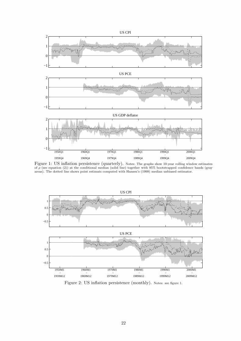
As a first step, we study the behavior of inflation persistence at the conditional median

and mean of the series. Figures (1) and (2) present rolling-window estimates of US inflation

persistence together with bootstrapped confidence bands for a 10-year window. The bootstrap

algorithm is a version of the block-bootstrap algorithm for quantile regression presented in

Fitzenberger (1997).6 The solid line shows estimates at the conditional median, while the

dotted line shows estimates at the conditional mean (without confidence band).

5These choices of the lag order are sufficient to eliminate serial correlation from the residuals. Durbin-Watson tests for the total sample and the subsamples do not indicate any serial correlation left in the estimationresiduals.

6For each bootstrap blocks of the variables are drawn randomly from the whole sample. For each of the 1000bootstraps the QAR estimates are computed to get an estimate of the distribution of ρ(τ ). Choosing a blocksize larger than one allows to capture autocorrelation. However, we found that there is no autocorrelation inthe residuals as we allow for a sufficiently high number of lags in the AR(q) process for inflation. Therefore theconfidence bands computed with a standard bootstrap (with block size equal to one) yield extremely similarconfidence bands as a block bootstrap so that we only present results for the former.

10

The results reflect the consensus view portrayed before: US inflation has become less persis-

tent since the early 1980s. This tendency is more pronounced for monthly inflation rates and,

in particular, for CPI inflation. Inflation persistence based on the GDP deflator, instead, ex-

hibits fewer signs of instability, which is consistent with Pivetta and Reis’s (2007) finding and

Benati’s (2008) result that persistence of CPI inflation has decreased, while it has remained

high for PCE and deflator inflation. Prior to the early 1980s, when the correlation between

all three measures of inflation was high, persistence behaved similarly. Since then, however,

persistence diverged across alternative series. Moreover, some confidence bands still contain

the unit root case.

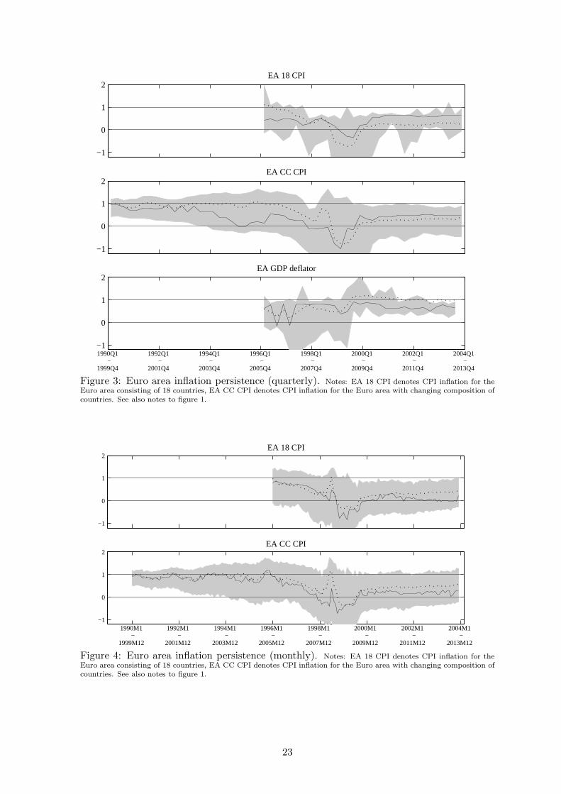
Figures (3) and (4) show the same measures of persistence for EA inflation. The crucial

question is whether the establishment of European Monetary Union (EMU) in 1999 has led

to a drop in inflation persistence. Interestingly, however, the fall in persistence observable in

the late 1990s is not statistically significant. Nevertheless, for most EA inflation rates the

case of ρ equal to unity is no longer covered by the bootstrapped confidence bands. The

creation of EMU coincides with inflation being no longer described by a unit root process.

In order to assess whether these findings are informative for the entire range of inflation

quantiles, we now turn to the results from quantile regressions.7 To test for the existence

of structural breaks in persistence at different quantiles, we report results for the DQ-test

introduced in the previous section. Table (1) shows the estimated break dates over the

conditional inflation distribution (τ ∈ {0.20, 0.25, ..., 0.80}).

Three findings stand out. First, we do not find evidence for structural breaks in quarterly US

inflation rates after the early 1950s, i.e. neither in the 1970s nor after the Volcker disinflation.8

Second, a highly significant break is found in both monthly series of US inflation which is

clearly associated with the Volker disinflation in the early 1980s. It seems that the aggregation

process that transforms monthly price level data to quarterly series is not innocuous with

respect to the time series properties of inflation. Third, for the EA there is not a single

structural break date.

Because the previous test for a joint break at all quantiles might be too restrictive, figure

(5) reports the results of the SQτ -test for breaks at specific quantiles for the US monthly

inflation series for which the DQ-test signaled a structural break.

Monthly CPI inflation exhibits breaks over the entire range of inflation quantiles. While

there is also evidence for a break in CPI inflation in the early 1950s, the breaks occurring

in the 1980s are more interesting for our purposes. The shift in monetary policy under Paul

Volcker had a profound impact on the inflation process leading to a break in persistence at

all conditional quantiles. The considerably weaker evidence for a regime shifts in inflation

dynamics for other inflation series reflects a general difficulty. Based on time series evidence

7The figures discussed before show that quantile regressions at the conditional median, i.e. least absolutedeviation estimates, are useful complements to least squares regressions even if one is only interested incharacterizing the location of the conditional distribution rather than estimates in the tails of the conditionaldistribution. The sharp deflationary spike in the US series in 2008Q4 leads to a decrease in estimated inflationpersistence at the conditional mean (Hansen’s (1999) unbiased median estimator), but not at the conditionalmedian. The latter estimate is robust against outliers.

8Note that Kim (2000), Nason (2006) and Noriega and Ramos-Francia (2009) find signs of instability ininflation persistence in 1973.

11

a structural break is often difficult to locate despite convincing narrative evidence for the

existence of a policy change. This points to the gradual effect of policy changes on observed

inflation dynamics.9

While we see evidence for structural breaks, we do not know both the size and the sign of these

shifts yet. Figures (1) and (2) showed a decrease in inflation persistence at the conditional

median and mean of the inflation distribution only. To illustrate the nature of these breaks

for the whole range of quantiles, figures (6) to (10) plot the estimated constant α(τ) and

the persistence parameter ρ(τ) together with bootstrapped 95% confidence bands at different

quantiles τ ∈ {0.20, 0.25, ..., 0.80} for different subsamples. For the quarterly US inflation

rates we show estimates before and after 1981Q3, while the subsamples for the monthly US

inflation rates are based on the break points as suggested by the DQ-test in table (1).

In all figures the level-shifts in persistence across subsamples are apparent. The level-shift

is visible even for those series for which the DQ-test does not signal structural instability.

After 1981 persistence unanimously falls. This fall is more pronounced for CPI inflation

and less clear for PCE and deflator inflation.10 Our quantile regressions reveal that the fall

in persistence is indeed a characteristic of all inflation quantiles. Not only mean inflation

became significantly less inertial, but also inflation following particularly large shocks, either

negative or positive ones.

We also find that persistence is typically not equal across the conditional quantiles. For some

cases, i.e. for quarterly CPI inflation, persistence at high quantiles significantly deviates from

persistence evaluated at the mean inflation rate. In this case large shocks to inflation generate

stronger inertia than smaller shocks. This asymmetric nature of inflation persistence across

conditional quantiles cannot be detected by conventional measures of persistence.11

Finally, we are particularly interested in the question whether inflation follows a unit root

process or is characterized as stationary. Tables (2) to (4) show point estimates at different

quantiles and results for the QAR-based unit root test and QKS-test for the whole sample

and different subsamples. The subsamples are again chosen based on the break points as

suggested by the DQ-test for monthly inflation and we split the sample again in 1981Q3 for

quarterly inflation series.

The point estimates show sizable changes in inflation persistence. For all three inflation

measures including the quarterly and the monthly series, inflation persistence is much lower

after 1981 than before. The difference is most pronounced for CPI inflation.12 Our quantile

regressions reveal that the fall in persistence is indeed a characteristic of all inflation quan-

tiles. Not only mean inflation became significantly less inertial, but also inflation following

particularly large shocks, either negative or positive ones. The QAR-based unit root tests

confirm this observation. Prior to 1981 the unit root hypothesis cannot be rejected over al-

most the whole conditional inflation distribution for all three inflation measures. After 1981,

9Wieland and Wolters (2011), for example, show that following the Volcker disinflation forecasters overes-timated inflation until the 1990s.

10This is consistent with evidence provided by Zhang and Clovis (2009).11Inflation persistence being higher following large shocks is also consistent with menu cost models as

pioneered by Ball and Mankiw (1994).12This is consistent with evidence provided by Zhang and Clovis (2009).

12

however, we can rule out a unit root in the inflation process at all conditional quantiles. Even

in the aftermath of large shocks inflation is mean reverting. Tsong and Lee (2011) also find

a unit root for inflation in the upper conditional quantiles, but mean reversion in the lower

conditional quantiles. Their finding is based on a long sample. Our results suggest that this

finding disappears once we allow for structural breaks. The mixed test results for the whole

sample shown in tables (2) to (4) disguise the subsample results according to which we can

clearly split the sample into a unit root and a mean reverting regime.

5 Robustness

In this section we evaluate the robustness of our findings with respect to two modifications of

the empirical specification: changes in the range of quantiles considered and breaks in mean

and the variance of inflation, respectively.

5.1 The role of the chosen range of quantiles

We repeat the DQ-test and the SQτ -test for a wider range of quantiles τ ∈ {0.05, 0.10, ..., 0.95}.

While this wider range covers also the more extreme tails compared to our baseline case a

disadvantage is a decrease in the power of the DQ-test. Furthermore, it might be too ambi-

tious to try to detect structural change in the 5th and 95th percentile using a relatively small

number of observations.

The test results for the DQ-test are, however, almost unchanged.13 The DQ-test finds the

same break in 1981 for monthly US CPI inflation and no break in the quarterly US inflation

series nor the EA inflation series. Regarding US monthly PCE inflation, the break in 1980M4

vanishes and instead a break in 1990M10 is found, reflecting that uncertainty regarding

structural breaks is considerably higher for US PCE than for US CPI inflation. Running the

SQτ -test yields a number of additional breaks in the extreme tails of the conditional inflation

distribution. However, as these do not translate into breaks detected by the DQ-test, these

are probably spurious and due to the relatively low number of observations in the outer

quantiles.

5.2 The role of changes in mean inflation

Neglecting a break in mean inflation could lead to spuriously high estimates of the sum of the

autoregressive coefficients. In their analysis of changes in the degree of fractional integration

of US inflation, Hassler and Meller (2011) demean the inflation rate before and after 1981

separately to control for a level shift. To corroborate the robustness of our results, we follow

Hassler and Meller (2011) and subtract the mean from the monthly US CPI inflation and

US PCE inflation series separately for each subsample as identified by the DQ-test. We then

employ again the DQ-test to detect breaks in the entire conditional distribution.

The breaks found, see table (5), include the dates found in the baseline case. Note that we

find many more break dates over the sample period. Many of them, however, will disappear

13To save space these findings are available upon request.

13

below when we also control for changes in inflation volatility. The SQτ -test, see figure (11),

shows that persistence of monthly CPI inflation still changes at all conditional quantiles. In

addition, monthly PCE inflation now also exhibits signs of changes in persistence, at least for

persistence evaluated at the mean of the distribution and some neighboring quantiles. These

findings support the notion that the baseline results are not obscured by structural breaks in

the mean inflation rate.

The estimates of the persistence parameter as a function of the quantile in the different

regimes, see figures (13) and (14), are broadly unchanged. The inflation process changed at

all conditional quantiles in 1951 and 1981. Furthermore, all other results remain valid. Taken

together, accounting for shifts in the mean inflation rate does not affect our main results.

5.3 The role of changes in mean inflation and the variance of inflation

The estimates of inflation persistence might not only by obscured by changes in the mean

of the inflation process, but also by shifting volatilities. To account for this, we not only

subtract the subsample-specific means but also normalize the series by their subsample-

specific variance. Each inflation series then has a mean of zero and a variance of one. The

results should thus be immune with respect to shifts in first and second moments. Table (6)

shows the results of the DQ-test in this case. The test detects again a break in monthly CPI

and PCE inflation in the early 1980s and in addition a break in PCE inflation in 1991 which

is, however, only significant on the 10% level. The test does not detect the additional breaks

found previously when adjusting the inflation series for changes in mean inflation, but not

the volatility of inflation. So, the large number of breaks found in section 5.2 reflect changes

in volatility of inflation. In contrast, the structural break in the early 1980s is not caused by

changes in mean inflation or the volatility in inflation, but is indicative of structural changes

in persistence.

Figure (12) shows the results from the SQτ -test and confirms that the breaks in all quantiles

of monthly CPI inflation remain unchanged once we control for variance shifts. All other

breaks detected before, also those in the 1950s, disappear. As regards monthly PCE inflation

we find that in the early 1980s only the shifts at τ = 0.50 and the lower conditional quantiles

exhibit a break.

The persistence estimates as a function of the conditional quantile, which are shown in fi-

gures (15) and (16), corroborate our baseline findings. Since the Volcker disinflation inflation

persistence is lower at each quantile and each quantile-specific persistence estimate is statis-

tically indistinguishable from persistence at τ = 0.50. Thus, we conclude that our baseline

results are robust with respect to shifts in first and second moments of inflation dynamics.

6 Concluding remarks

We draw on recently developed methods to identify structural breaks at conditional quantiles

to study the changing nature of US inflation persistence. The framework is flexible enough

to allow for asymmetries of inflation persistence across inflation quantiles - a characteristic

of the data that accords well with several theoretical foundations.

14

We find strong and robust evidence for a reduction in persistence at all conditional quantiles of

US inflation in the early 1980s. Thus, we contributed to the literature on inflation persistence

by providing a missing key element: when there are shifts in monetary policy not only

persistence at the conditional mean changes. Rather, the results support the notion that the

entire inflation process reflects shifts in monetary policy. While Benati (2008) documents

that shifts in monetary policy reduce persistence, we show that the new monetary policy

regime in the US left its footprint on the entire conditional distribution of inflation.

Our results add to our knowledge about the conduct of monetary policy. The reduction in

persistence is consistent with monetary policy successfully stabilizing inflation around the

mean. Even shocks drawn from the tails of the distribution have only a short-lived impact

on inflation as monetary policy keeps the inflation rate under control. It remains to be seen

how the recent shift towards unconventional monetary policy measures since 2008 or the

prolonged period of very low inflation rates are reflected in the conditional distribution of

inflation. We leave that issue for future research.

References

[1] Andrews, D. W. K. and H.-Y. Chen (1994): ”Approximately median-unbiased esti-

mation of autoregressive models”, Journal of Business and Economics Statistics 12,

187-204.

[2] Ball, L. and N. G. Mankiw (1994): ”Asymmetric price adjustment and economic

fluctuations”, The Economic Journal 104, 247-261.

[3] Benati, L. (2008): ”Investigating inflation persistence across monetary regimes”,

Quarterly Journal of Economics 123, 1005-1060.

[4] Cecchetti, S. G. and G. Debelle (2006): ”Has the inflation process changed?”, Eco-

nomic Policy April 2006, 311-352.

[5] Clark, T. E. (2006): ”Disaggregate evidence on the persistence of consumer price

inflation”, Journal of Applied Econometrics 21, 563-587.

[6] Cogley, T., G. Primiceri and T. J. Sargent (2010): ”Inflation-gap persistence in the

U.S.”, American Economic Journal: Macroeconomics 2, 43-69.

[7] Fitzenberger, B. (1997): ”The moving blocks bootstrap and robust inference for linear

least squares and quantile regressions”, Journal of Econometrics 82, 235-287.

[8] Fuhrer, J. C. (2011): ”Inflation persistence”, in B. Friedman and M. Woodford (eds.),

Handbook of Monetary Economics, Volume 3A, Elsevier, North-Holland.

[9] Galvao, A. F. (2009): ”Unit root quantile autoregression testing using covariates”,

Journal of Econometrics 152, 165-178.

[10] Hakkio, C. S. (2008): ”PCE and CPI inflation differentials: converting inflation fore-

casts”, Federal Reserve Bank of Kansas City Economic Review Q1, 51-68

15

[11] Hansen, B. E. (1995): ”Rethinking the univariate approach to unit root testing”,

Econometric Theory 11(5), 1148-1171.

[12] Hansen, B. E. (1999): ”The grid bootstrap and the autoregressive model”, The Review

of Economics and Statistics 81, 594-607.

[13] Hassler, U. and B. Meller (2011): ”Detecting multiple breaks in long memory: the

case of U.S. inflation”, Empirical Economics 46(2), 653-680.

[14] Hosseinkouchack, M. and M.H. Wolters (2013): ”Do large recessions reduce output

permanently?”, Economics Letters 121(3), 516-519.

[15] Holden, S. and F. Wulfsberg (2009): ”How strong is the macroeconomic case for

downward real wage rigidity?”, Journal of Monetary Economics, 56(4), 605-615.

[16] Kang, K. H., C.-J. Kim and J. Morley (2009): ”Changes in U.S. inflation persistence”,

Studies in Nonlinear Dynamics & Econometrics 13, Article 1.

[17] Kim, J.-Y. (2000): ”Detection of change in persistence of a linear time series”, Journal

of Econometrics 95, 97-116.

[18] Koenker, R. and G. W. Bassett (1978): ”Regression quantiles”, Econometrica 46,

33-50.

[19] Koenker, R. and Z. Xiao (2004): ”Unit root quantile autoregression inference”, Jour-

nal of the American Statistical Association 99, 775-787.

[20] Koenker, R. and Z. Xiao (2006): ”Quantile autoregression”, Journal of the American

Statistical Association 101, 980-1006.

[21] Kumar, M. S. and T. Okimoto (2007): ”Dynamics of persistence in international

inflation rates”, Journal of Money, Credit and Banking 39, 1457-1479.

[22] Levin, A. T. and J. M. Piger (2006): ”Is inflation persistence intrinsic in industrial

economies?”, unpublished, Board of Governors of the Federal Reserve System.

[23] Nason, J. M. (2000): ”Instability in U.S. Inflation: 1967-2005”, Economic Review,

Second Quarter 2006, Federal Reserve Bank of Atlanta.

[24] Nobay, B., I. Paya and D. A. Peel (2010): ”Inflation dynamics in the U.S.: global but

not local mean reversion”, Journal of Money, Credit and Banking 42, 135-148.

[25] Nobay, B. and D. A. Peel (2003): ”Optimal discretionary monetary policy in a model

of asymmetric central bank preferences”, The Economic Journal 113, 657-665.

[26] Noriega, A. and M. Ramos-Francia (2009): ”The dynamics of persistence in US infla-

tion”, Economics Letters 105, 168-172.

[27] Hofmann, B., G. Peersman and R. Straub (2010): ”Time variation in U.S. wage

dynamics”, unpublished, European Central Bank.

16

[28] Oka, T. and Z. Qu (2011): ”Estimating structural changes in regression quantiles”,

Journal of Econometrics 162, 248-276.

[29] O’Reilly, G. and K. Whelan (2005): ”Has euro-area inflation persistence changed over

time?”, The Review of Economics and Statistics 87, 709-720.

[30] Pivetta, F. and R. Reis (2007): ”The persistence of inflation in the United States”,

Journal of Economic Dynamics and Control 31, 1326-1358.

[31] Qu, Z. (2008): ”Testing for structural change in regression quantiles”, Journal of

Econometrics 146, 170-184.

[32] Stock, J. H. and M. W. Watson (2007): ”Why has U.S. inflation become harder to

forecast?”, Journal of Money, Credit and Banking 39, 3-32.

[33] Taylor, J. B. (2000): ”Low inflation, pass-through, and the pricing power of firms”,

European Economic Review 44, 1389-1408.

[34] Tsong, C.-C. and C.-F. Lee (2011): ”Asymmetric inflation dynamics: evidence from

quantile regression analysis”, Journal of Macroeconomics 33, 668-680.

[35] Wieland, V. and M. H. Wolters (2011): ”Forecasting and policy making”, in prepa-

ration for G. Elliott and A. Timmermann (eds.), Handbook of Economic Forecasting,

Volume 2, Elsevier.

[36] Zhang, C. and J. Clovis (2009): ”Modeling US inflation dynamics: persistence and

monetary policy regimes”, Empirical Economics 36, 455-477.

17

Table 1: Tests for structural breaks in regression quantiles (DQ-Test)

Series 1st break date 2nd break date 3rd break date 4th break date

US CPI (q) - - - -US PCE (q) - - - -US GDP defl (q) 1953Q1* - - -

US CPI (m) 1952M9*** 1981M9*** 2000M11** -US PCE (m) 1980M4*** - - -

EA 18 CPI (q) - - - -EA CC CPI (q) - - - -EA 18 GDP defl (q) - - - -

EA 18 CPI (m) - - - -EA CC CPI (m) - - - -

Notes: Results for the DQ-Test for breakpoints over the conditional inflation distribution (τ ∈ {0.20, 0.25, ...,0.80}).*, **, *** refer to the 10%, 5%, and 1% significance level. EA 18 denotes time series for the Euro area containingall 18 countries. EA CC denotes time series for the Euro area with changing country composition.

18

Table 2: Results for quantile unit root tests on quarterly US inflation rates

Series Sample τ 0.20 0.30 0.40 0.50 0.60 0.70 0.80

US CPI (q) 1947Q2-2013Q4 ρ(τ ) 0.74 0.72 0.89 0.86 0.92 0.94 0.94Unit root no no yes no yes yes yest-stat -4.29 -4.92 -2.44 -2.90 -2.15 -1.37 -0.93critical value -2.34 -2.56 -2.60 -2.67 -2.63 -2.63 -2.56

KS-test unit root: no QKS=4.92 cv=2.89

1947Q2-1981Q3 ρ(τ ) 0.77 0.87 0.95 0.96 0.95 0.92 0.93Unit root no yes yes yes yes yes yest-stat -3.20 -1.84 -0.91 -0.88 -0.99 -1.74 -1.16critical value -2.55 -2.54 -2.65 -2.61 -2.62 -2.49 -2.50


1981Q4-2013Q4 ρ(τ ) 0.43 0.43 0.43 0.42 0.46 0.52 0.56Unit root no no no no no no not-stat -3.95 -5.35 -5.60 -6.31 -5.39 -4.01 -3.27critical value -2.58 -2.55 -2.62 -2.62 -2.55 -2.39 -2.23


US PCE (q) 1959Q2-2013Q4 ρ(τ ) 0.81 0.88 0.87 0.90 0.94 0.97 0.94Unit root no no no no yes yes yest-stat -3.29 -2.64 -3.29 -2.57 -1.24 -0.56 -1.00critical value -2.38 -2.62 -2.59 -2.58 -2.55 -2.58 -2.56


1959Q2-1981Q3 ρ(τ ) 0.82 0.88 0.92 0.93 1.01 0.94 0.99Unit root no no yes yes yes yes yest-stat -2.73 -2.81 -1.64 -1.25 0.17 -0.83 -0.09critical value -2.34 -2.57 -2.48 -2.63 -2.52 -2.73 -2.74

KS-test unit root: yes QKS=2.81 cv=2.90

1981Q4-2013Q4 ρ(τ ) 0.69 0.67 0.73 0.64 0.63 0.58 0.60Unit root no no no no no no not-stat -2.59 -3.26 -3.28 -4.40 -3.90 -3.58 -2.97critical value -2.20 -2.41 -2.51 -2.36 -2.34 -2.29 -2.54


US GDP- 1947Q2-2013Q4 ρ(τ ) 0.76 0.78 0.86 0.89 0.92 0.98 1.06deflator Unit root no no no no yes yes yes

t-stat -4.94 -5.56 -4.38 -2.81 -1.99 -0.50 1.18critical value -2.60 -2.59 -2.64 -2.56 -2.61 -2.54 -2.54


1947Q2-1981Q3 ρ(τ ) 0.75 0.82 0.89 0.92 0.94 0.96 1.01Unit root yes yes yes yes yes yes yest-stat -2.33 -2.47 -1.69 -1.36 -0.92 -0.44 0.11critical value -2.73 -2.73 -2.64 -2.56 -2.43 -2.55 -2.37


1981Q4-2013Q4 ρ(τ ) 0.77 0.71 0.69 0.68 0.66 0.80 0.90Unit root no no no no no no yest-stat -4.10 -4.04 -5.32 -5.17 -4.67 -2.80 -1.02critical value -2.54 -2.56 -2.63 -2.55 -2.67 -2.61 -2.54


Notes: The table shows estimates of inflation persistence of three different quarterly US inflation series (column 1)and different subsamples (columns 2) at different quantiles (columns 4-10). Statistics reported are point estimates ofinflation persistence, ρ(τ), whether the unit root cannot be rejected (yes) or is rejected (no), the according t-statisticand corresponding critical value at the 5% significance level. The null hypothesis is rejected if the t-statistic is smallerthan the critical value. The last row for each sample shows results for the KS-test: The entry unit root shows whetherthe unit root cannot be rejected (yes) or is rejected (no) over the whole conditional inflation distribution. QKS isthe test statistic and cv indicates the critical value on the 5% significance level. The unit root hypothesis is rejectedif QKS is larger than the critical value.

19

Table 3: Results for quantile unit root tests on monthly US CPI inflation rates

Series Sample τ 0.20 0.30 0.40 0.50 0.60 0.70 0.80

US CPI (m) 1947M2-2011M8 ρ(τ ) 0.70 0.79 0.82 0.87 0.90 0.91 0.89Unit root no no no no yes yes yest-stat -5.66 -5.30 -4.94 -3.37 -2.59 -1.96 -2.03critical value -2.62 -2.62 -2.62 -2.64 -2.61 -2.53 -2.45


1947M2-1952M9 ρ(τ ) 0.03 0.42 0.40 0.56 0.60 0.43 0.52Unit root no yes yes yes yes yes not-stat -4.19 -2.34 -2.51 -1.97 -1.51 -2.41 -2.34critical value -2.31 -2.63 -2.60 -2.53 -2.67 -2.58 -2.23


1952M10-1981M9 ρ(τ ) 0.92 0.91 0.96 1.00 1.00 0.98 0.97Unit root yes yes yes yes yes yes yest-stat -1.39 -1.81 -0.96 -0.10 -0.01 -0.36 -0.50critical value -2.53 -2.55 -2.71 -2.73 -2.72 -2.60 -2.42


1981M10-2000M11 ρ(τ ) 0.29 0.36 0.58 0.56 0.57 0.56 0.46Unit root no no no no no no not-stat -5.75 -5.81 -4.30 -4.09 -4.09 -3.24 -3.05critical value -2.51 -2.57 -2.53 -2.65 -2.56 -2.52 -2.67


2000M12-2013M12 ρ(τ ) -0.31 0.03 0.08 0.33 0.43 0.34 0.28Unit root no no no no no no yest-stat -3.64 -4.11 -4.96 -3.93 -3.04 -2.98 -2.34critical value -2.58 -2.58 -2.59 -2.51 -2.31 -2.32 -2.34


Notes: The table shows estimates of inflation persistence for monthly US CPI inflation (column 1) and differentsubsamples (columns 2) at different quantiles (columns 4-10). Statistics reported are point estimates of inflationpersistence, ρ(τ), whether the unit root cannot be rejected (yes) or is rejected (no), the according t-statistic andcorresponding critical value at the 5% significance level. The null hypothesis is rejected if the t-statistic is smallerthan the critical value. The last row for each sample shows results for the KS-test: The entry unit root showswhether the unit root cannot be rejected (yes) or is rejected (no) over the whole conditional inflation distribution.QKS is the test statistic and cv indicates the critical value on the 5% significance level. The unit root hypothesis isrejected if QKS is larger than the critical value.

20

Table 4: Results for quantile unit root tests on monthly US PCE inflation rates

Series Sample τ 0.20 0.30 0.40 0.50 0.60 0.70 0.80

US PCE (m) 1959M2-2013M12 ρ(τ ) 0.81 0.85 0.89 0.94 0.94 0.95 1.01Unit root no no no yes yes yes yest-stat -4.28 -4.09 -2.89 -1.54 -1.58 -1.40 0.32critical value -2.49 -2.53 -2.56 -2.62 -2.62 -2.59 -2.56


1959M2-1980M4 ρ(τ ) 0.86 0.93 0.94 0.99 1.00 1.04 1.11Unit root no yes yes yes yes yes yest-stat -3.01 -1.55 -1.32 -0.15 -0.08 0.89 1.85critical value -2.40 -2.48 -2.60 -2.56 -2.60 -2.72 -2.59


1980M5-2013M12 ρ(τ ) 0.67 0.64 0.59 0.59 0.68 0.72 0.73Unit root no no no no no no not-stat -3.50 -4.18 -5.58 -5.69 -4.44 -3.46 -2.99critical value -2.58 -2.53 -2.53 -2.53 -2.44 -2.38 -2.43


Notes: The table shows estimates of inflation persistence for monthly US PCE inflation (column 1) and differentsubsamples (columns 2) at different quantiles (columns 4-10). Statistics reported are point estimates of inflationpersistence, ρ(τ), whether the unit root cannot be rejected (yes) or is rejected (no), the according t-statistic andcorresponding critical value at the 5% significance level. The null hypothesis is rejected if the t-statistic is smallerthan the critical value. The last row for each sample shows results for the KS-test: The entry unit root showswhether the unit root cannot be rejected (yes) or is rejected (no) over the whole conditional inflation distribution.QKS is the test statistic and cv indicates the critical value on the 5% significance level. The unit root hypothesis isrejected if QKS is larger than the critical value.

Table 5: Tests for structural breaks in regression quantiles with demeaned data (DQ-test)

Series 1st break date 2nd break date 3rd break date 4th Break date 5th break date

US CPI (m) 1952M9*** 1967M7** 1975M1** 1981M9*** 2000M11***US PCE (m) 1981M2* 1990M10** - -

Notes: The table shows results for the DQ-Test for breakpoints over the conditional inflation distribution (τ ∈{0.20, 0.25, ..., 0.80}) after controlling for a mean shift. *, **, *** refer to the 10%, 5%, and 1% significance level.

Table 6: Tests for structural breaks in regression quantiles with standardized data (DQ-test)

Series 1st break date 2nd break date 3rd break date 4th Break date 5th break date

US CPI (m) 1982M4*** - - -US PCE (m) 1981M2** 1991M1* - - -

Notes: The table shows results for the DQ-Test for breakpoints over the conditional inflation distribution (τ ∈{0.20, 0.25, ..., 0.80}) after controlling for shifts in the mean and the variance. *, **, *** refer to the 10%, 5%, and1% significance level.

21

−1

0

1

2US CPI

−1

0

1

2US PCE

−1

0

1

2US GDP deflator

1950Q1 −

1959Q4

1960Q1 −

1969Q4

1970Q1 −

1979Q4

1980Q1 −

1989Q4

1990Q1 −

1999Q4

2000Q1 −

2009Q4

Figure 1: US inflation persistence (quarterly). Notes: The graphs show 10-year rolling window estimatesof ρ (see equation (2)) at the conditional median (solid line) together with 95% bootstrapped confidence bands (grayareas). The dotted line shows point estimats computed with Hansen’s (1999) median unbiased estimator.

−0.5

0

0.5

1

US CPI

−0.5

0

0.5

1

US PCE

1950M1 −

1959M12

1960M1 −

1969M12

1970M1 −

1979M12

1980M1 −

1989M12

1990M1 −

1999M12

2000M1 −

2009M12

Figure 2: US inflation persistence (monthly). Notes: see figure 1.

22

−1

0

1

2EA 18 CPI

−1

0

1

2EA CC CPI

−1

0

1

2EA GDP deflator

1990Q1 −

1999Q4

1992Q1 −

2001Q4

1994Q1 −

2003Q4

1996Q1 −

2005Q4

1998Q1 −

2007Q4

2000Q1 −

2009Q4

2002Q1 −

2011Q4

2004Q1 −

2013Q4

Figure 3: Euro area inflation persistence (quarterly). Notes: EA 18 CPI denotes CPI inflation for theEuro area consisting of 18 countries, EA CC CPI denotes CPI inflation for the Euro area with changing composition ofcountries. See also notes to figure 1.

−1

0

1

2EA 18 CPI

−1

0

1

2EA CC CPI

1990M1 −

1999M12

1992M1 −

2001M12

1994M1 −

2003M12

1996M1 −

2005M12

1998M1 −

2007M12

2000M1 −

2009M12

2002M1 −

2011M12

2004M1 −

2013M12

Figure 4: Euro area inflation persistence (monthly). Notes: EA 18 CPI denotes CPI inflation for theEuro area consisting of 18 countries, EA CC CPI denotes CPI inflation for the Euro area with changing composition ofcountries. See also notes to figure 1.

23

0.2

0.3

0.4

0.5

0.6

0.7

0.8

1950 1960 1970 1980 1990 2000 2010

US monthly CPIUS monthly PCE

Figure 5: Estimated break points at different quantiles (monthly). Notes: The graph shows break-points estimated with the SQτ -test at all quantiles τ ∈ {0.20, 0.25, ...,0.80} (vertical axis) for monthly US CPI andPCE inflation on the 5% significance level.

24

0.20 0.40 0.60 0.80−1

0

1

2

3 1947Q2 − 1981Q3

Con

stan

t0.20 0.40 0.60 0.80

−1

0

1

2

3 1981Q4 − 2013Q4

0.20 0.40 0.60 0.800

0.5

1

Quantiles

Per

sist

ence

0.20 0.40 0.60 0.800

0.5

1

Quantiles

Figure 6: Estimated parameters at different quantiles for quarterly US CPI inflation. Notes: Thegraphs show estimates of the constant α and the persistence parameter ρ at different quantiles τ ∈ {0.20, 0.25, ...,0.80}for different subsamples. The gray areas indicate 95% bootstrapped confidence bands. The horizontal line showsHansen’s (1999) median unbiased estimator together with 95% grid-t bootstrap confidence bands.

0.20 0.40 0.60 0.80−1

0

1

2

3 1959Q1 − 1981Q3

Con

stan

t

0.20 0.40 0.60 0.80−1

0

1

2

3 1981Q4 − 2013Q4

0.20 0.40 0.60 0.800

0.5

1

Quantiles

Per

sist

ence

0.20 0.40 0.60 0.800

0.5

1

Quantiles

Figure 7: Estimated parameters at different quantiles for quarterly US PCE inflation. Notes:see figure 6.

25

0.20 0.40 0.60 0.80−1

0

1

2

3 1947Q2 − 1981Q3

Con

stan

t0.20 0.40 0.60 0.80

−1

0

1

2

3 1981Q4 − 2013Q4

0.20 0.40 0.60 0.800

0.5

1

Quantiles

Per

sist

ence

0.20 0.40 0.60 0.800

0.5

1

Quantiles

Figure 8: Estimated parameters at different quantiles for quarterly US GDP deflator inflation.Notes: see figure 6.

0.20 0.40 0.60 0.80−4

−2

0

2

4

6 1947M2 − 1952M9

Con

stan

t

0.20 0.40 0.60 0.80−4

−2

0

2

4

6 1952M10 − 1981M9

0.20 0.40 0.60 0.80−4

−2

0

2

4

6 1981M10 − 2000M11

0.20 0.40 0.60 0.80−4

−2

0

2

4

6 2000M12 − 2013M12

0.20 0.40 0.60 0.80−1

−0.5

0

0.5

1

Quantiles

Per

sist

ence

0.20 0.40 0.60 0.80−1

−0.5

0

0.5

1

Quantiles0.20 0.40 0.60 0.80

−1

−0.5

0

0.5

1

Quantiles0.20 0.40 0.60 0.80

−1

−0.5

0

0.5

1

Quantiles

Figure 9: Estimated parameters at different quantiles for monthly US CPI inflation. Notes:The subsamples are chosen based on the estimated break points of the DQ-test for monthly US CPI inflation. Forfurther notes see figure 6.

26

0.20 0.40 0.60 0.80−1

0

1

2

3 1959M2 − 1980M4

Con

stan

t0.20 0.40 0.60 0.80

−1

0

1

2

3 1981M5 − 2013M12

0.20 0.40 0.60 0.800

0.5

1

Quantiles

Per

sist

ence

0.20 0.40 0.60 0.800

0.5

1

Quantiles

Figure 10: Estimated parameters at different quantiles for monthly US PCE inflation. Notes:The subsamples are chosen based on the estimated break points of the DQ-test for monthly US PCE inflation. Forfurther notes see figure 6.

0.2

0.3

0.4

0.5

0.6

0.7

0.8

1950 1960 1970 1980 1990 2000 2010


Figure 11: Estimated break points at different quantiles (monthly, demeaned). Notes: The graphshows breakpoints estimated with the SQτ -test at all quantiles τ ∈ {0.20, 0.25, ...,0.80} (vertical axis) after controllingfor a mean shift for US CPI and PCE inflation on the 5% significance level.

0.2

0.3

0.4

0.5

0.6

0.7

0.8

1950 1960 1970 1980 1990 2000 2010


Figure 12: Estimated break points at different quantiles (monthly, standardized). Notes: Thegraph shows breakpoints estimated with the SQτ -test at all quantiles τ ∈ {0.20, 0.25, ...,0.80} (vertical axis) aftercontrolling for mean and volatility shifts for US CPI and PCE inflation on the 5% significance level.

27

0.20 0.50 0.80

−5

0

5

47M2 − 51M8

Con

stan

t

0.20 0.50 0.80

−5

0

5

51M9 − 67M7

0.20 0.50 0.80

−5

0

5

67M8 − 75M1

0.20 0.50 0.80

−5

0

5

75M2 − 82M12

0.20 0.50 0.80

−5

0

5

83M1 − 00M11

0.20 0.50 0.80

−5

0

5

00M12 − 13M12

0.20 0.50 0.80−1

−0.5

0

0.5

1

1.5

Quantiles

Per

sist

ence

0.20 0.50 0.80−1

−0.5

0

0.5

1

1.5

Quantiles0.20 0.50 0.80

−1

−0.5

0

0.5

1

1.5

Quantiles0.20 0.50 0.80

−1

−0.5

0

0.5

1

1.5

Quantiles0.20 0.50 0.80

−1

−0.5

0

0.5

1

1.5

Quantiles0.20 0.50 0.80

−1

−0.5

0

0.5

1

1.5

Quantiles

Figure 13: Inflation persistence (monthly US CPI) after controlling for a mean shift. Notes: Thegraphs show estimates of the constant α and the persistence parameter ρ at different quantiles τ ∈ {0.20, 0.25, ...,0.80}for different subsamples. The gray areas indicate 95% bootstrapped confidence bands. The subsamples are chosen basedon the estimated break points of the DQ-test for US CPI inflation. US CPI inflation has been demeaned separatelyfor the subsamples. The horizontal line shows Hansen’s (1999) median unbiased estimator together with 95% grid-tbootstrap confidence bands.

0.20 0.40 0.60 0.80

−2

0

2

1959M2 − 1981M2

Con

stan

t

0.20 0.40 0.60 0.80

−2

0

2

1981M3 − 1990M10

0.20 0.40 0.60 0.80

−2

0

2

1990M11 − 2013M12

0.20 0.40 0.60 0.80

0

0.5

1

Quantiles

Per

sist

ence

0.20 0.40 0.60 0.80

0

0.5

1

Quantiles0.20 0.40 0.60 0.80

0

0.5

1

Quantiles

Figure 14: Inflation persistence (monthly US PCE) after controlling for a mean shift. Notes: Thegraphs show estimates of the constant α and the persistence parameter ρ at different quantiles τ ∈ {0.20, 0.25, ...,0.80}for different subsamples. The gray areas indicate 95% bootstrapped confidence bands. The subsamples are chosen basedon the estimated break points of the DQ-test for US PCE inflation. US PCE inflation has been demeaned separatelyfor the subsamples. The horizontal line shows Hansen’s (1999) median unbiased estimator together with 95% grid-tbootstrap confidence bands.

28

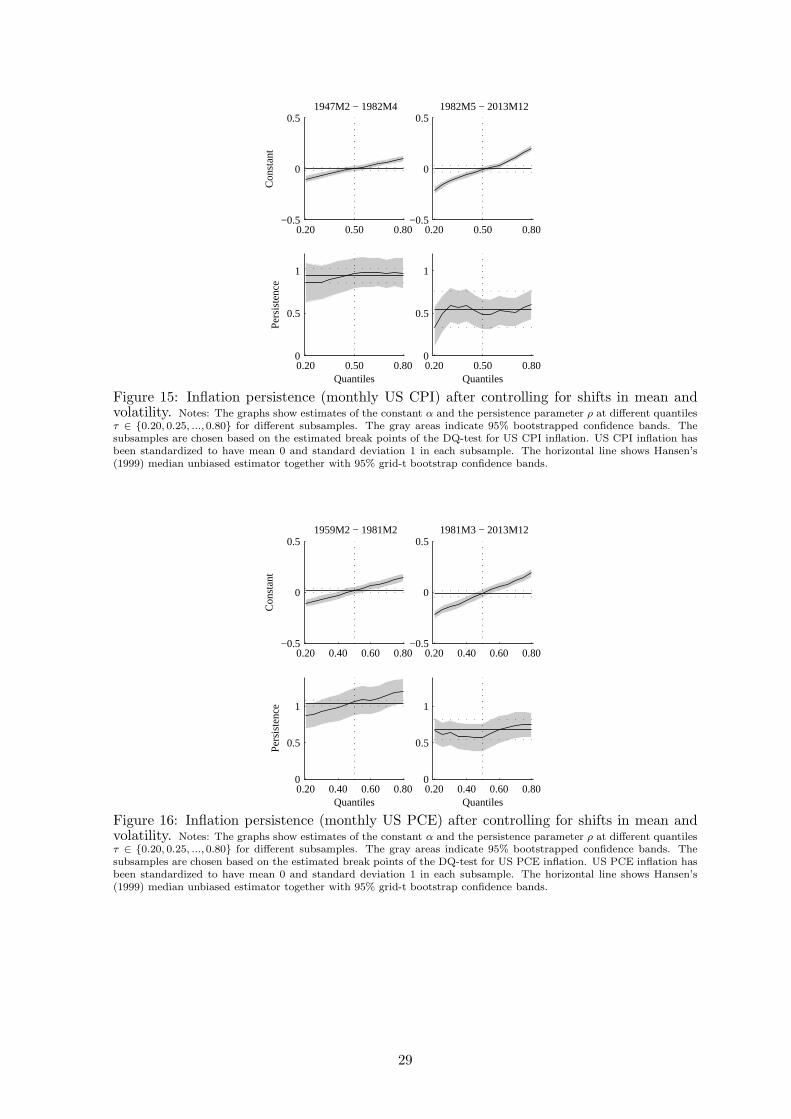
0.20 0.50 0.80−0.5

0

0.5 1947M2 − 1982M4

Con

stan

t

0.20 0.50 0.80−0.5

0

0.5 1982M5 − 2013M12

0.20 0.50 0.800

0.5

1

Quantiles

Per

sist

ence

0.20 0.50 0.800

0.5

1

Quantiles

Figure 15: Inflation persistence (monthly US CPI) after controlling for shifts in mean andvolatility. Notes: The graphs show estimates of the constant α and the persistence parameter ρ at different quantilesτ ∈ {0.20, 0.25, ...,0.80} for different subsamples. The gray areas indicate 95% bootstrapped confidence bands. Thesubsamples are chosen based on the estimated break points of the DQ-test for US CPI inflation. US CPI inflation hasbeen standardized to have mean 0 and standard deviation 1 in each subsample. The horizontal line shows Hansen’s(1999) median unbiased estimator together with 95% grid-t bootstrap confidence bands.

0.20 0.40 0.60 0.80−0.5

0

0.5 1959M2 − 1981M2

Con

stan

t

0.20 0.40 0.60 0.80−0.5

0

0.5 1981M3 − 2013M12

0.20 0.40 0.60 0.800

0.5

1

Quantiles

Per

sist

ence

0.20 0.40 0.60 0.800

0.5

1

Quantiles

Figure 16: Inflation persistence (monthly US PCE) after controlling for shifts in mean andvolatility. Notes: The graphs show estimates of the constant α and the persistence parameter ρ at different quantilesτ ∈ {0.20, 0.25, ...,0.80} for different subsamples. The gray areas indicate 95% bootstrapped confidence bands. Thesubsamples are chosen based on the estimated break points of the DQ-test for US PCE inflation. US PCE inflation hasbeen standardized to have mean 0 and standard deviation 1 in each subsample. The horizontal line shows Hansen’s(1999) median unbiased estimator together with 95% grid-t bootstrap confidence bands.

29

core.ac.uk · on post-war US data we indeed find robust evidence for a ... Francesco Bianchi, Uwe...

Documents

Transcript of core.ac.uk · on post-war US data we indeed find robust evidence for a ... Francesco Bianchi, Uwe...