core.ac.uk · student who enrolls in the third year of college without access to credit markets,...

econstor www.econstor.eu

Der Open-Access-Publikationsserver der ZBW – Leibniz-Informationszentrum WirtschaftThe Open Access Publication Server of the ZBW – Leibniz Information Centre for Economics

Standard-Nutzungsbedingungen:

Die Dokumente auf EconStor dürfen zu eigenen wissenschaftlichenZwecken und zum Privatgebrauch gespeichert und kopiert werden.

Sie dürfen die Dokumente nicht für öffentliche oder kommerzielleZwecke vervielfältigen, öffentlich ausstellen, öffentlich zugänglichmachen, vertreiben oder anderweitig nutzen.

Sofern die Verfasser die Dokumente unter Open-Content-Lizenzen(insbesondere CC-Lizenzen) zur Verfügung gestellt haben sollten,gelten abweichend von diesen Nutzungsbedingungen die in der dortgenannten Lizenz gewährten Nutzungsrechte.

Terms of use:

Documents in EconStor may be saved and copied for yourpersonal and scholarly purposes.

You are not to copy documents for public or commercialpurposes, to exhibit the documents publicly, to make thempublicly available on the internet, or to distribute or otherwiseuse the documents in public.

If the documents have been made available under an OpenContent Licence (especially Creative Commons Licences), youmay exercise further usage rights as specified in the indicatedlicence.

zbw Leibniz-Informationszentrum WirtschaftLeibniz Information Centre for Economics

Solis, Alex

Working Paper

Credit access and college enrollment

Working Paper, Department of Economics, Uppsala University, No. 2013:12

Provided in Cooperation with:Department of Economics, Uppsala University

Suggested Citation: Solis, Alex (2013) : Credit access and college enrollment, WorkingPaper, Department of Economics, Uppsala University, No. 2013:12, http://nbn-resolving.de/urn:nbn:se:uu:diva-204400

This Version is available at:http://hdl.handle.net/10419/82577

Department of EconomicsWorking Paper 2013:12


Alex Solis

Department of Economics Working paper 2013:12Uppsala University July 2013P.O. Box 513 ISSN 1653-6975 SE-751 20 UppsalaSwedenFax: +46 18 471 14 78


Alex Solis

Papers in the Working Paper Series are published on internet in PDF formats. Download from http://www.nek.uu.se or from S-WoPEC http://swopec.hhs.se/uunewp/

Credit Access and College Enrollment∗

Alex Solis†

May 30, 2012

Abstract

Does limited access to credit explain some of the gap in schooling attainment between childrenfrom richer and poorer families? I present new evidence on this important question using datafrom two loan programs for college students in Chile. Both programs offer loans to students whoscore above a threshold on the national college admission test, enabling a regression discontinuityevaluation design. I find that students who score just above the cutoff have nearly 20 percentagepoints higher enrollment in first, second and third year than students who score just below, whichrepresent relative increases of 100% , 213% and 446% respectively. More importantly, access tothe loan program effectively eliminates the family income gradient in enrollment among studentswith similar test scores.

JEL Codes: I22, I24, I28, O1Keywords: college enrollment, credit constraints, income gap, college dropout, Chile

∗I would like to thank David Card, Alain de Janvry, Frederico Finan, and Elizabeth Sadoulet for their supportand advice. Joshua Angrist, Peter Berck, Nils Gottfries, Eric Hanushek, Catie Hausman, Patrick Kline, GianmarcoLeón, Ethan Ligon, Jeremy Magruder, Edward Miguel, Emmanuel Saez, Sofia Villas-Boas, Brian Wright and seminarparticipants at the Interamerican Development Bank, LACEA 2010 Annual Meeting, MOOD workshop 2011, NEUDC2011, New Economic School, PacDev 2011, PUC Rio, Universidad Católica de Concepción, University of BarcelonaII workshop on Economics of Education, University of San Francisco, University Pompeu Fabra, Uppsala University,World Bank social mobility workshop and UC Berkeley ARE Development Workshop, Development Seminar, AREDepartment Seminar, Development Lunch, and Labor Lunch, provided useful comments. I would like to thankFrancisco Meneses, Gonzalo Sanhueza and Humberto Vergara for providing the data and for their comments. Igratefully acknowledge financial support from the Confederación Andina de Fomento CAF and from the Center forEquitable Growth at the University of California, Berkeley. A previous version of this paper circulated under the title“Credit Constraints for Higher Education.” All errors are my own.†Email: [email protected]. Department of Economics, Uppsala University P.O. Box 513 75120 Uppsala, Sweden;

Uppsala Center of Labor Studies; and Department of Economics, Universidad Católica de Concepción. .

1

mailto:[email protected]

1 Introduction

Students from richer families are more likely to attend, persist at, and graduate from college thanstudents from poor families. Whether the gap is due entirely to differences in tastes and abilities,or is partially driven by credit constraints faced by lower income families, is a matter of muchdebate. Some analysts argue that the gap is mainly a reflection of long-run differences in educationalinvestment, both at home and in schools, that affect the readiness for college (e.g., Cameron andHeckman (2001); Keane and Wolpin (2001); Carneiro and Heckman (2002); and Cameron and Taber(2004). Others have argued that liquidity constraints prevent some relatively able poor studentsfrom enrolling in college (e.g., Lang (1993); Kane (1994, 1996); Card (1999); Belley and Lochner(2007); Lochner and Monge-Naranjo (2011a); and Brown, Scholz and Seshadri (2012)).1,2

Measuring the effects of credit constraints on college enrollment is a difficult task because de-termining whether a family has access to credit is difficult or impossible. Moreover, even if accessto credit were directly observed, there are many other unobserved variables that affect college en-rollment and are likely to be correlated with access to credit, leading to biased estimates.3 Forexample, students from high income families may have better access to credit markets, but alsomay have stronger preferences for college education, better academic preparation, and superior cog-nitive and non-cognitive skills unobserved by the econometrician. On the supply side, access toloans is sometimes correlated with ability, for example, Van der Klauuw (2002) argues that col-leges’ grants are increasingly based on academic merit and are used to encourage the best admittedstudents to enroll in a given college, rather than being used to assist students from low incomefamilies. In addition, the admission process relies on unobserved and subjective measures, such asrecommendation letters, parental alumni status, etc. Recognizing the problem, tests of the creditconstraint hypothesis have relied mainly on indirect measures of credit access that lead to mixed -and sometimes inconsistent - findings.

In this paper, I exploit sharp eligibility rules of two loan programs recently introduced in Chile.These programs give access to college tuition loans for students who score above a certain thresholdon the national college admission test. Around the eligibility cutoff these programs provide tuitionloans directly, which are as good as randomly assigned (Lee (2008)) enabling a regression discon-tinuity design that addresses the problems of unobserved omitted variables and selection. Thus,these loan programs allow for a direct and unbiased estimate of the causal effect of credit access on

1See Lochner and Monge-Naranjo (2011b) for a detailed review of the literature.2A different approach if given by Attanasio and Kaufmann (2009) and Kaufmann (2010), they use differences in

the expected returns and information sets between students from high and low income families to explain the collegeenrollment differences in Mexico, concluding that the sensitivity of low income students to change in direct costssuggests the presence of credit constraints.

3This econometric problem has also been documented in the literature that estimate the price elasticity of demandfor college education (e.g. Manski and Wise (1983), McPherson and Schapiro (1991), Van der Klaauw (2002), Dynarski(2003) and Nielsen, Sorensen and Taber (2010)).

2

college enrollment and college progress.4,5

A key feature of my analysis is the availability of detailed student-level data that present sev-eral advantages over the samples used in earlier studies. First, I observe the entire population ofindividuals who participate in the national college admission process, including full informationon their enrollment (institutions, programs, preferences, etc.). Second, I observe the two variablesthat completely determine college admission: the scores on the national college admission tests6

and high school GPA, ruling out potential biases from admission processes that weight subjectivecharacteristics. Third, the two loan programs provide access to standardized loans to eligible stu-dents, offered by the government and private banks, eliminating potential endogeneity of loan offersdesigned to attract better students. The nature of the loan programs, that gives credit access asgood as randomly around the threshold, the admission system characteristics, and the availabilityof these data, allow a reliable evaluation of the causal effects of credit access on college enrollmentand college progress. To the best of my knowledge, this is the first paper that uses an exogenoussource of access to loans and the entire population of students and institutions that participate inthe college admission process.

My analysis shows that access to the loan programs increases the college enrollment probabilityby 18 percentage points - equivalent to a nearly 100% increase in the enrollment rate of the groupwith test scores just below the eligibility threshold. Students from the lowest family income quintilebenefit the most: for these students access to the loans causes a 140% increase in the probability ofenrollment (on a baseline enrollment rate of 15% for students just below the cutoff).

More importantly, access to the loan programs appears to eliminate the relatively large incomegradient in college enrollment. Among those who are barely ineligible for loans, students from therichest quintiles are twice as likely to enroll as students from the poorest quintile. On the contrary,among students who are barely eligible, the enrollment gap is statistically zero.

The literature on the importance of liquidity constraints has focused mainly on college enroll-ment, but programs that promote enrollment would not have any significant effect on educationalattainment if they attract students who are unable to graduate. For this reason, a different strandof literature examines the impact of aid on persistence, dropout and graduation rates (e.g. Dynarski(2003); DesJardins, Ahlburg and McCall (2002); Bettinger (2004); Singell (2004); and Stinebrick-ner and Stinebrickner (2008)), with a similar level of disagreement on the conclusions, than theliterature on college enrollment.7

This strand of the literature faces additional econometric problems. Enrolled students constitute4In terms of the methodology, Canton and Blom (2010) and Gurgand, Lorenceau and Melonio (2011) perform an

RDD analysis using information on Mexican and South African students.5Rau, Rojas and Urzúa (2013) analyzes enrollment, dropout rates, and earnings for one of the two loans analyzed

here, The State Guaranteed Loan program. Using a sequential schooling decision model with unobserved heterogeneity.6Language and mathematics tests are mandatory and science and history are optional (students choose at least

one of the last two).7See Chen (2008) and Hossler et al (2009) for a survey of the literature.

3

a self-selected sample of individuals, and therefore the realationship between credit constraints andpersistence and dropout rates cannot be interepreted as a causal relation. Furthermore, in mostcases, the analysis is performed using information from a single institution or restricted group ofinstitutions. That implies two more concerns. First, the analysis depends critically on the char-acteristics of the analyzed institution. Second, in many cases, transferred students are mistakenlyconsidered dropouts.

The data used in this paper allows following students up to their third year of enrollment. Usingthe same exogenous variation in access to loans, I estimate the causal effect on college progress,defined as enrollment in the second and the third year. Using the population of students thatparticipate in the admission process eliminates the selection bias in the analysis of college progress,and using all institutions eliminates the bias associated with transferred students and presentsgeneral evidence not contingent on one institution.

In this context, I estimate that for each student who enrolls in second year of college withoutaccess to credit, 3.1 enroll in the second year when access to loans is available. Moreover, for everystudent who enrolls in the third year of college without access to credit markets, 5.5 do so whenthey have access to loans.

Additionally, access to the loan programs eliminates the income gradient in second and thirdyear college enrollment. Among those barely ineligible for loans, students from the poorest incomequintile enroll at 6% and 3% in the second and third years respectively, while students from therichest quintile enroll at 20% in both years. On the contrary, among those barely eligible for loans,there is no statistical difference in the enrollment rate in the second and third year between therichest and the poorest students, both groups enroll at the rate of 20%.

To interpret these results as evidence of credit access, I estimate the effect of lower than marketinterest rates and low enforceability, a “price effect” (see Dynarski (2003); and Lochner and Monge-Naranjo (2011a)), using a second natural experiment that gives exogenous access to a scholarshipprogram that reduces tuition costs dramatically when loans are available for everybody. Studentsthat score more than the scholarship cutoff face a reduction of 90% on tuition cost while studentsthat are ineligible for the scholarship still can use the loans to finance college. I find that studentswith access to loans have the same enrollment rate as those who benefit from a reduced tuition cost,i.e. the price effect is zero.

To reinforce the idea of credit access being the most important factor driving the results onenrollment, I use survey data from a subset of students around the threshold, to analyze directlythe importance of financial problems on the enrollment decision. The rate of students respondingthat financial problems prevent them to enroll in college drops between 10 to 12 percentage pointsat the cutoff. Finally, I present a test that uses the differences in interest rates and enforceabilityof the two loans and the different predicted responses for different income quintiles to decomposethe enrollment effect into price and access effects. I find that the price effect is small and conclude

4

that the overall effect is driven by loan access.The paper is organized as follows. Section 2 describes the background and the data. Section 3

discusses the empirical strategy. Section 4 presents the empirical evidence for the effects of creditaccess on college enrollment and progress, and the enrollment gap by family income. Finally Section5 presents the decomposition of the effect into access and price effects. Section 6 concludes.

2 Background and Data

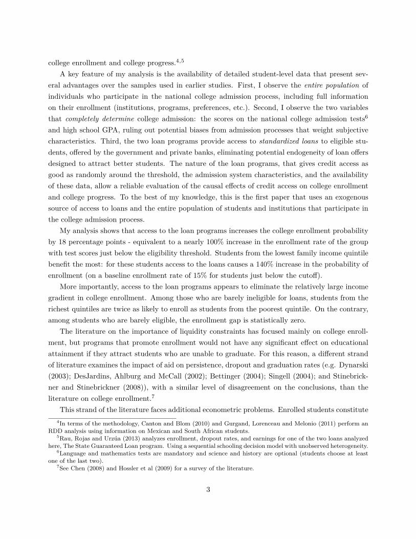
One key feature of the data is the possibility to observe every aspect of a partially centralized collegeadmission process and the entire population of students that participate in a college admissionprocess nationwide. The admission process is based on the college admission test (Prueba deSelección Universitaria, PSU Test hereafter), which is taken by 96% of all students graduatingfrom high school each year.8 Some students take it even when they do not plan to enroll in tertiaryeducation, because sometimes it is required as a high school graduation certificate. The test is takensimultaneously across the country only once a year, and can be taken as many times as wanted afterpaying a fee.9 The admission process is described in figure 1, it depicts students decisions and theinformation available for them.

Figure 1: Time-line of the college admission process

Note: Above the time-line, the decisions taken by students. Below the time-line, the timing of informationreleases.

Students need to register for the PSU test and complete a socioeconomic verification form8Source: Ministry of Education.9The fee is about $50 or CLP 25,000 (pesos of 2012) and is waived for all students graduating from public and

voucher schools who apply for a waiver.

5

(Formulario Único de Acreditación Socioeconómica, FUAS) before graduating from high school.Few days after graduation students write the PSU test and within two weeks students know whetherthey are eligible for the two loans analyzed here and for almost all scholarships available from publicfunds. Around the same days, students are informed about their scores in the PSU test.

2.1 The College Admission Test and Placement.

The PSU test consists of two mandatory tests on language and mathematics and two optional tests.The average on the mandatory tests is referred to as the PSU score, and is used for college placementand for loans and grants eligibility.10

The tests have only multiple choice questions which are answered on a special sheet that isgraded automatically by a photo optical device, and therefore, it is not subject to manipulationby students or graders. PSU scores are normalized to a distribution with mean 500 and standarddeviation of 100 to make them comparable among years. The scores range from 150 to 850 points.11

Once students know their PSU scores, they can apply to two types of universities, called “tra-ditional” and “private”. The “traditional” universities consist of 25 institutions that were foundedbefore the educational reform of 1981. Some are public and others are privately funded, but allreceive direct funding from the government (Aporte Fiscal Directo).

The 33 universities created after the reform of 1981 are called “private” universities. They donot receive direct funding from the government, and before 2006, their students were excluded fromthe credit system with public funds. Their growth has been rapid and steady, increasing enrollmentfrom a handful of students in 1991 to nearly half of the student body in 2009.

Both types of universities use the PSU test score to select students. Traditional universities usethe test as a mechanism to centrally allocate applicants. The allocation process is as follows: Afterknowing their scores, students apply to up to 8 programs, and all the students applying to anygiven program are ranked using the scores on the PSU tests (the two mandatory and one optionaltest), and high school GPA. Seats are offered to the best scoring students in each program and therest are put on a waiting list. If a student is accepted into more than one program, she is placed inher highest preference and is eliminated from all other rankings. If students do not matriculate inspecifics dates, spots become available following the ranking on the wait list.

Private universities receive applications independently, but they also select applicants consid-ering the PSU test score and high school GPA. They prefer students with higher PSU scores forfour reasons. First, it is required by law that the institutions that receive students with the State

10The optional tests are (1) History and Social Sciences and (2) Sciences, which includes modules on biology,chemistry, and physics. They are not considered for loan eligibility, but they are considered in the placement scorethat is a factor in admission to college programs.

11The PSU test is implemented by the Council of Chancellors of Chilean Universities (Consejo de Rectores de lasUniversidades Chilenas: CRUCH), which organizes the traditional universities that are as described below.

6

Guaranteed Loan program (SGL) select students based on the PSU score.12 This loan programhas become the main source of financing for these universities and explains its rapid growth since2006. Second, private universities use PSU scores to distinguish the quality of the students, it isthe best ability measure available. Third, all the universities in the country compete to get indirectgovernmental funding (Aporte Fiscal Indirecto), which is calculated based on PSU scores from thestudents enrolled in each institution every year (this funding is the second source of earnings forprivate universities). Fourth, the PSU scores of the student body are used to publicize the qualityof the programs to attract more students. Each year, before the PSU test, universities disclose thePSU score of the last student enrolled in each program (program cutoff score or puntaje de corte)to signal how much in demand they are.

After the whole enrollment process is finished, universities inform the ministry about the enroll-ment in all their programs, and the ministry assigns loans, grants and scholarships.

2.2 Financial Aid

Financial aid from the Education Ministry is assigned according to the information provided bystudents before the PSU test, in the economic status verification form (the FUAS form). Thisinformation is sent by the ministry to the Chilean tax authority (Servicio de Impuestos Internos orSII) to verify the information and classify students in income quintiles. One of the most importantcharacteristics of the Chilean college admission process is that, except for one program, all aid (loansand scholarships) managed by the State is assigned depending on PSU scores and income quintilesdetermined by the tax authority with the information from the FUAS form. Table 1 summarizesall college related financial aid given or managed by the Ministry of Education.

The only two college tuition loans given with public funds in the country are the TraditionalUniversity Loan program (Crédito Solidario, TUL hereafter) and the State Guaranteed Loan pro-gram (SGL hereafter). The same eligibility criteria are used in both programs, namely, studentsare required to be classified by the tax authority in one of the four poorest income quintiles, andscore at least 475 points in the PSU test. The only difference in terms of eligibility is that TUL isgiven to students enrolling in one of the 25 traditional universities, while the latter can be used atany of the 44 accredited universities in the country (all the traditional universities and 18 privateuniversities).

Both programs aim to cover tuition costs (only), up to the reference tuition. The referencetuition is an amount calculated by the Ministry of Education about how much a program shouldcost depending on the institution assets’ quality and the labor market perspectives after graduationof any program. On average the reference tuition is slightly less than 90% of the actual tuition cost.Any part not covered by these loans has to be covered by the student.

12Law 20,027, title III, article 7. This law created the SGL on June of 2005. All accredited universities receivestudents with SGL.

7

On average, annual college tuition is 1.8 million pesos (pesos of 2009, or 3.6 thousand U.S.dollars), while the median family income is 4.5 million in nominal terms (9 thousand dollars).13

Therefore, even after receiving one of these loans to matriculate in college, the non-covered portionof the tuition and the indirect costs may still be a financial burden for families in the bottom incomequintiles, leaving space for liquidity constraints.

13Calculated using the household survey CASEN 2009. Per capita Income (PPP) is approximately 14 thousanddollars (pesos of 2009). The difference is indication of the inequality in the income distribution.

8

Table 1: Requirement for scholarships

PANEL A: Requirements for loans and scholarships.% Recipients1 Requirements:with respect to: Income PSU Institution

Population Eligibles quintiles Cutoff type Cover(1) (2) (3) (4) (5) (6)

LoansState Guaranteed 9.46% 27.90% 1 to 4 475 Accredited+ (a)Traditional Loan 8.58% 21.92% 1 to 4 475 Traditional++ (a)Scholarships and Grants

Bicentenario 4.70% 55.14% 1 and 2 550 Traditional (a)Juan Gomez Millas 0.02% 0.87% 1 and 2 640 Accredited2 (a)PSU Score grant 0.02% 0.05% 1 to 4 - Accredited3 (b)Exellence 2.32% 4.78% 1 to 4 - Accredited2,4 (a)Teacher’s children: BHDP 1.02% 3.98% 1 to 4 500 All5,6 (c)Pedagogy: BPED 0.07% 0.74% all 600 Accredited5 (b)

PANEL B: Income quintile definitons.(∗)

Income Quintile I II III IVUpper bound Monthly family Income in CLP 178,366 306,000 469,625 777,218Upper bound Monthly family Income in USD 364 624 958 1,586

Notes:(1): Column (1) reports the ratio of recipients over students taking the test for the first time. Column (2) correspondto the ratio of recipients over those that take the PSU test for the first time, have applied to the benefit, belong toeligible quintiles and score more than the respective cutoff.(2): Only students graduating from voucher and public high schools.(3): National or regional best PSU score.(4): Only for students in the top 5% of their graduating high school.(5): Only student with high school GPA greater than 5.5 are eligible for BHDP, and only GPA greater than 6.0 forBPED. High School GPA goes from 1 to 7 points.(6): Only for children of teachers and employees from voucher of public schools.(+): “Accredited” refers to all accredited colleges (traditional and private) and accredited vocational institutions.(++): “Traditional” refers to traditional universities which are all accredited.(a): Funds up to reference cost.(b): Funds up to fixed value, about the same magnitude than reference tuition US$2,250 for univ., which correspondsto the average reference tuition, and US$1,000 for vocational programs).(c): Funds up to US$1,000 which correspond to a quarter of the university average tuition or total vocational schooltuition.(*): Source: CASEN 2009. Calculated using autonomous income per family. Household autonomous income includedsalaries, rents, subsidies from the governments, pensions, etc. for all members of the family.

2.2.1 The Traditional University Loan Program

The Traditional University Loan Program is managed by the universities, which determine theamount to lend and are in charge of the collection process.14

14It was introduced in 1981 as part of an educational reform. However the eligibility criteria used in this paper wasintroduced in 2006.

9

This loan has special conditions that make it very attractive to students. The real interestrate on this loan is about 2% per year with a maximum of 15 years of payments - after that, thedebt is written off. Repayment starts two years after the student’s graduation and the installmentscorrespond to 5% of the borrower’s income. Moreover, any portion of tuition not covered by thisloan can be covered by the State Guaranteed Loan.

Despite these special characteristics, the loan has a low repayment rate (from 52 to 60% forthe years considered). One possible reason is that the universities are in charge of collecting loanpayments in the first stage and, in a second stage, a central organization named Fondo Solidario;neither are specialists in collecting loans. In recent years, the Chilean government has made somemodifications that allow the tax authority to retain tax refunds and publicize names of defaultingstudents; this has increased the repayment rate to 80% (in some cases) of all reprogrammed loans.15

The low enforceability and the low interest rate indicate the existence of a subsidy component inthis loan scheme.

2.2.2 State Guaranteed Loan program

The State Guaranteed Loan program allows private banks to provide college tuition loans to eligiblestudents. These loans are guaranteed by the state and by higher education institutions. To beeligible, students need to fulfill the three requirements mentioned above and enroll in one of the 44accredited universities.

Out of the 58 institutions that provide college education in Chile, 77.6% participate in theprogram. Of the remainder, 19% are not accredited institutions and 3.4% have dropped out ofthe program. Some institutions ask for higher PSU scores to guarantee the loan, but 85% of allprograms require the standard 475 PSU score to be eligible.

This loan scheme is very similar to loans currently available in the conventional financial market.First, the real interest rate was about 6% per year in the years considered, which corresponds tothe government long-run interest rate,16 and is slightly higher than the mortgage rate for the sameperiod. Anecdotally, this loan and its interest rate led to massive street protests in 2011 and 2012.It was considered too expensive, because some graduates had to pay up to 17% of their income aftergraduation.

Second, private banks make the loans and are in charge of the repayment process. Privatebanks can use all available legal mechanisms to recover the debt, including release of informationto credit score institutions, asset impoundment, and judicial collection. Releasing information tocredit scores institutions is important in the labor market in Chile, because usually firms requestthat potential employees not appear as defaulters in credit score records.

15Source: Fondo Solidario de Crédito Universitario.16Source: International Comparative Higher Education and Finance Project. State University of New York at

Buffalo.

10

Third, installments do not depend on the borrower’s income. The SGL program requires studentsto start repayment 18 months after graduation in monthly installments for 20 years.

Fourth, to increase the enforceability of the debt, the loan contract has special clauses thatinvolve the tax authority and employers. Employers are mandated to deduct repayments directlyfrom payroll and to make payments directly to banks. The law also establishes penalties to employerswho do not comply with this process. Additionally, the loan contract allows the tax authority toretain tax refunds in case the former student does not pay the lending bank. This last characteristichas proven to be an efficient measure, increasing repayment for these traditional loans since 2002.

In the case of dropouts, the higher education institution guarantees the loan: 90% of the capitalplus interest for the first year, 70% for the second, and 60% for the third year onward. The stateguarantees up to 90% when the educational institution covers less than that percentage. In theevent that a student stops paying, after the bank implements all mechanisms used to collect theloans, the guarantors (the state and/or the educational institution) must pay the bank and becomeresponsible for enforcing collection from the student.

For all these reasons, I argue that this loan scheme can be used as a market benchmark.17

2.2.3 Other Loans Available

In order to have a broad picture of what type of loans students have available in the conventionalfinancial market, here I briefly describe other sources of financing. First, some colleges offer schol-arships or loans to complement the loans described above. The objective of these loans is to attractthe best students, and therefore, these scholarships and loans require much higher PSU scores than475. Hence, the presence of such loans will not confound the effects of the two loan programs thatI study.

There are two types of loans given by private banks: the Corfo loans (“crédito Corfo”),18 andprivate bank loans. To get any of these loans, students need a guarantor, who needs to certify agood credit record, be employed, have a regular income source, and have a minimum family incomeor assets to use as collateral.

Corfo loans are offered by private banks, which manage the entire process, using resourcescoming from the Corfo development office. These loans have interest rates that vary among banks,ranging from 6.8% to 8.5% (real annual), and require a minimum guarantor monthly income of CLP600,000 (USD 1,225), corresponding to a family income in the bottom part of the fourth incomequintile (see Panel B on Table 1 for the definition of the income quintiles).

Secondly, banks also offer loans with their own resources. The most relevant is the one given by17This program was designed to give a market alternative to students who did not have access to traditional loans:

students in private universities and vocational schools.18Corfo (Corporación de Fomento a la Producción) is a development office from the government.

11

BancoEstado.19 This loan is aimed at lower income families, but the two poorest income quintilesand part of the third are excluded. The minimum family monthly income required to apply for thisloan is CLP 350,000 (USD 714). The real interest rate lies between 6.6% and 6.8% annually. Allother loans from private banks have very similar requirements but ask for higher minimum familyincome, starting at CLP 600,000 (USD 1,225).

Both of these loans depend on family characteristics that exclude students from the poorestfamilies. The income requirement is the main source of exclusion, but some families are excludedwhen they do not have a stable income source or have bad credit records. This is especiallyimportant in a country with high levels of labor market informality. According to the nationalhousehold survey CASEN, in 2006, 36% of all workers are in the informal sector (self-employed orwithout a contract), and therefore students from those families were excluded from getting collegeloans in the regular market. Moreover, students need to rely on family altruism to get supportwhen asking for loans.20 In contrast, the two loan programs analyzed in this paper do not dependin family characteristics for 80% of the population (the four poorest income quintiles).

2.3 Data and Sample

This paper combines several sources of administrative data that allows to observe in detail theoutcome of the college admission process. The first data source in this paper is the registry ofstudents who enroll for the PSU test. It contains individual data on PSU scores, high school GPA,which determine placement in universities; and a rich set of socioeconomic characteristics, such asself-reported family income, parent education, school of graduation, etc. for the years 2007 to 2009.

The PSU data set also contains information on the application preferences to traditional uni-versities and the placement results from the centralized mechanism.

The second source of data used in this paper is the enrollment in higher education data set fromthe Ministry of Education. It includes the enrollment outcome of the process described above (forall programs and institutions) for the same period of time.21

The enrollment data for 2008 and 2009 also contain information about the enrollment status ofstudents enrolled initially in 2007 and 2008. I use this data to measure the effect of credit accesson college progress (enrollment in the second and third year of college) and on dropout rates.

The third source of information is the FUAS application form data set for the same years. Thekey element in this data set is the income quintile reported by the tax authority that determineseligibility for the two loan programs and for six scholarship programs. Moreover this data setcontains the assignment to benefits and take up for the traditional loan.

19A private bank with partial ownership by the government of Chile.20Brown, Scholz and Seshadri (2012) have indicated this factor as an important source of credit constraints.21All data sets were merged using the national identification number, RUN (Rol Único Nacional).

12

The last set of information used in this paper corresponds to loan take up for the State Guaran-teed Loan Program from the INGRESA commission, the organization created to manage this creditprogram in 2006.22

The data present two sources of selection that may be problematic. First, students that do notcomplete the FUAS socioeconomic form before the PSU test are not eligible, and therefore they arenot affected by the cutoff. Second, because students can take the PSU test as many times as desired,a student may try repeatedly until getting a score equal to or greater than 475, self-selecting to beeligible for loans

I address the first problem by restricting the analysis to students who comply with all therequirements to get the TUL or the SGL loan before the PSU test (preselected students, hereafter).For this sample of students, crossing the threshold implies a sharp change in access to tuition loans.To address the second problem (to eliminate the self-selection into treatment), I restrict the sampleto students that are first-time test takers. Specifically, to students that graduate from high schoolthe same year they take the PSU test.

3 Empirical Strategy

As described in the previous section, two financing programs in Chile offer college tuition loans tostudents who satisfy three conditions: first, complete the socioeconomic verification form FUASbefore taking the PSU test; second, are classified in one of the poorest four income quintiles by thetax authority; and third, score at least 475 points on the PSU test.

This last requirement enables a sharp regression discontinuity design for those students thatcomply with the first two conditions. Students receive access to loans as good as randomizedaround the cutoff (Lee, 2008) and, therefore comparing college enrollment rates for the group at orjust above the cutoff (the “treatment” group) and the group just below (the “control” group) givesthe causal effect of credit access on college enrollment.

Hahn, Todd and Van der Klaauw (2001), Van der Klaauw (2008), Lee (2008), and Lee andLemieux (2010) describe the conditions under which a RDD gives a causal estimation. The intuitionis simple. If we assume that each individual’s score (the running or assignment variable) has arandom component with a continuous density, then the probability of scoring ε above the cutoff orscoring ε below is the same (for a sufficiently small ε). Therefore, even though the score dependson the individual characteristics (selection), being eligible for treatment in this small neighborhoodof the cutoff is as good as random assignment. Thus, students barely below the cutoff can be usedas a counterfactual to students barely above the cutoff, because the only difference between these

22The assignment rule was fulfilled for all years except 2006, the first year of implementation, when the commissionmanaging the SGL program misassigned part of the loans. Therefore, I do not consider 2006 from the analysis. In allother years, the assignment rule was fulfilled perfectly.

13

two groups is that students above the cutoff receive the treatment.Ideally, we would compare the average outcome for students at a small neighborhood of the

threshold, but usually there is not enough data in this small vicinity, and thus the estimation suffersfrom small sample bias. Lee and Lemieux (2010) suggest the following equation as an equivalentspecification to estimate the RDD.

Yi = β0 + β1 · 1(Ti > τ) + f(Ti − τ) + ξi (1)

Where 1(Ti > τ) is an indicator function for whether the student i’s PSU score Ti is equal to orgreater than the eligibility threshold τ ; the term (Ti − τ) accounts for the influence of the runningvariable on Yi in a flexible nonlinear function f(·); and ξi is, a mean zero error. The parameter β0

captures the expected value of Yi for students barely below the cutoff and β1 captures the increasein the expected value of Yi for individuals ε above the cutoff.

Equation (1) allows using students who are not necessarily close to the cutoff. The advantageis the increased statistical power due to adding more data to the estimation. The disadvantage isthe bias produced by individuals who are farther from the cutoff when f is not correctly specified.Imbens and Kalyanaraman (2012) propose a method to calculate an asymptotically optimal band-width to use a local linear regression in equation (1), where they use a squared error loss functionto weigh these two biases.

The results shown in this paper are based on a local linear regression using the optimal bandwidthof Imbens and Kalyanaraman, which in this case gives a bandwidth of 44 PSU points around thecutoff (w∗ = 44). Nevertheless, the results are highly robust to different bandwidths and functionalspecifications.23

Alternatively, to use the whole population of students, the follow specification interacts thecondition of being preselected with the indicator of scoring at least the cutoff.

Yi = β0 + β1 · 1(Ti > τ) + β2 · PreSeli + β3 · 1(Ti > τ) · PreSeli + f(Ti − τ) + ξi (2)

In this case β1 is the change in the probability of enrollment in college after scoring at leastthe cutoff for those ineligible for loans (those who did not complete FUAS or were classified in therichest quintile). This parameter captures whether scoring more than the cutoff plays the role of asignal for the students. For example, scoring the cutoff or more may be interpreted by students asthey are suitable for college because the State want to finance their studies in case of being eligible.

The variable PreSeli is an indicator of being classified in one of the poorest four income quintiles23Additionally, I will use equation (1) to test if baseline characteristics are balanced around the threshold to test

the local continuity assumption implicit in RDD.

14

after filling the FUAS form. The coefficient β2 captures if there is any difference in the probabilityof enrollment between those who complete FUAS and those who don’t. Those who complete thesocioeconomic form may be more interested in the loans, either because they have higher preferencesfor college or higher preferences for the terms of the loans.

In this specification, the parameter of interest is β3 which measure the effect on college enrollmentfor those students that scoring at least the cutoff imply a change in their access to tuition loans.

3.1 Enrollment in Second and Third year

One concern from the policy maker’s perspective is that access to loans may have an effect only oninitial enrollment, but not on the graduation rate, if loans are given to students without the properpreparation for college education. Hence, it is not sufficient to observe an effect in the first yearenrollment rate to reduce the education attainment gap.

I estimate the causal effects of access to loans on enrollment in second and third year of college,using the same exogenous variation. In this case, I deal with the problem of selection into treatmentin the second or third year of college using a fuzzy RDD.

In the previous case, eligibility for loans was determined sharply by the score in one PSU attempt.For second (third) year enrollment, students have the chance to retake the PSU test once (twice)(since the test is written once a year). Students with scores lower than the cutoff may enroll incollege for the first year, expecting that they can get access to loans from the second (third) yearif they score at least 475 in a subsequent attempt, thus self-selecting into treatment. For this case,eligibility is not fully determined by the score of the first attempt (the probability of being eligiblefor loans for second and third year enrollment is not zero for the control group). Nevertheless, theprobability of being eligible still jumps discontinuously at the threshold, because not all studentswho scored below 475 in their first attempt retake the test, and only a portion of those succeedin scoring 475 or more in subsequent attempts. This allows a fuzzy RDD, where eligibility in thesecond and third year is instrumented by being eligible in the first, i.e. a dummy for scoring greaterthan or equal to 475 in the first year.

Specifically, I perform a two stage least square regression as follows:

Eligi = γ0 + γ1 · 1(Ti > τ) + f(Ti − τ) + ηi (3)

Yi = β0 + β1 · Eligi + f(Ti − τ) + νi (4)

The term 1(Ti > τ), the indicator function for scoring greater than or equal to the cutoff in thefirst attempt, is used as instrument for being eligible for loans. Eligi takes on the value 1 if studenti is eligible for college loans in the year of analysis, and zero otherwise. The dependent variable Yi

corresponds to the outcome of interest: enrollment in the second year, or enrollment in the third

15

year (or dropout status for the analysis in the appendix). All the other variables are defined as inequation (1).

Now, the parameter β1 measures the effect of having access to college loans on enrollment inthe second and third year for those for whom the treatment status does not change in the followingyears, after taking the PSU test for the first time.

4 Results

This section presents the empirical evidence organized as follows. Section 4.1 tests the conditionsfor a valid RDD: random loan assignment, absence of manipulation of PSU scores, and balance onbaseline characteristics between the eligible and non-eligible students around the cutoff. Section 4.2shows results for the estimation of the causal effect of loan access on college enrollment. Section 4.3presents results by income groups and revisits the college enrollment gap. Section 4.4 presents theeffects on college progress, and the family income gap on progress. Section 5 decomposes the priceand the access effect.

All the following RD results are restricted to the group who took the PSU test for the firsttime (see section 2.3 for details), and scored 44 PSU points around the loan program cutoff whichcorrespond to the I&K optimal bandwidth that allows to control linearly for the running variable(see section 3).

4.1 Conditions for a valid RD design

4.1.1 Loan Eligibility

Figure 2 shows that the probability of completing the FUAS socio economic form and being classifiedinto the four poorest income quintiles (being pre-selected for loans) do not change at the cutoff (forall students and for students by year of PSU process). Each dot in every figure represents the averagerate of pre-selection for students in bins of 2 PSU points, and the dashed lines correspond to fittedvalues from a regression that control for the PSU score using fourth order splines at each side of thethreshold and 95% confidence intervals. For pre-selected students, loan eligibility changed sharplyfrom 0 to 1 at 475, and forms the basis for the RD evaluation design.

16

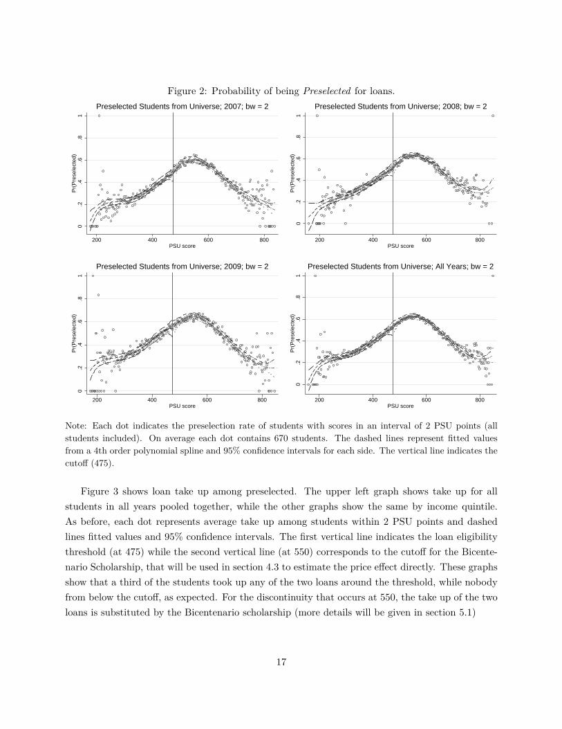
Figure 2: Probability of being Preselected for loans.0

.2.4

.6.8

1P

r(P

rese

lect

ed)

200 400 600 800PSU score

Preselected Students from Universe; 2007; bw = 2

0.2

.4.6

.81

Pr(

Pre

sele

cted

)

200 400 600 800PSU score


0.2

.4.6

.81

Pr(

Pre

sele

cted

)

200 400 600 800PSU score


0.2

.4.6

.81

Pr(

Pre

sele

cted

)

200 400 600 800PSU score

Preselected Students from Universe; All Years; bw = 2

Note: Each dot indicates the preselection rate of students with scores in an interval of 2 PSU points (allstudents included). On average each dot contains 670 students. The dashed lines represent fitted valuesfrom a 4th order polynomial spline and 95% confidence intervals for each side. The vertical line indicates thecutoff (475).

Figure 3 shows loan take up among preselected. The upper left graph shows take up for allstudents in all years pooled together, while the other graphs show the same by income quintile.As before, each dot represents average take up among students within 2 PSU points and dashedlines fitted values and 95% confidence intervals. The first vertical line indicates the loan eligibilitythreshold (at 475) while the second vertical line (at 550) corresponds to the cutoff for the Bicente-nario Scholarship, that will be used in section 4.3 to estimate the price effect directly. These graphsshow that a third of the students took up any of the two loans around the threshold, while nobodyfrom below the cutoff, as expected. For the discontinuity that occurs at 550, the take up of the twoloans is substituted by the Bicentenario scholarship (more details will be given in section 5.1)

17

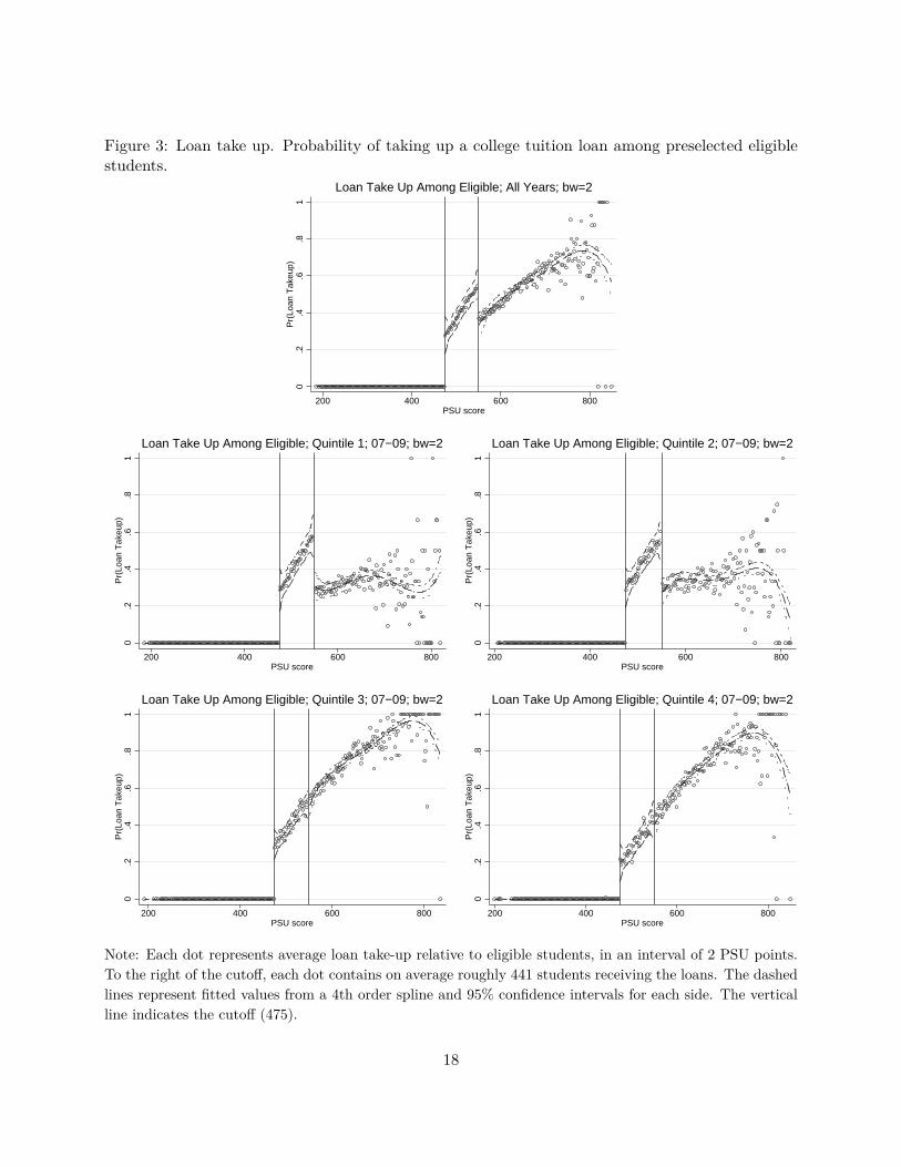
Figure 3: Loan take up. Probability of taking up a college tuition loan among preselected eligiblestudents.

0.2

.4.6

.81

Pr(

Loan

Tak

eup)

200 400 600 800PSU score

Loan Take Up Among Eligible; All Years; bw=2

0.2

.4.6

.81

Pr(

Loan

Tak

eup)

200 400 600 800PSU score

Loan Take Up Among Eligible; Quintile 1; 07−09; bw=2

0.2

.4.6

.81

Pr(

Loan

Tak

eup)

200 400 600 800PSU score


0.2

.4.6

.81

Pr(

Loan

Tak

eup)

200 400 600 800PSU score


0.2

.4.6

.81

Pr(

Loan

Tak

eup)

200 400 600 800PSU score


Note: Each dot represents average loan take-up relative to eligible students, in an interval of 2 PSU points.To the right of the cutoff, each dot contains on average roughly 441 students receiving the loans. The dashedlines represent fitted values from a 4th order spline and 95% confidence intervals for each side. The verticalline indicates the cutoff (475).

18

4.1.2 Local Continuity Assumption: Manipulation of the Assignment variable.

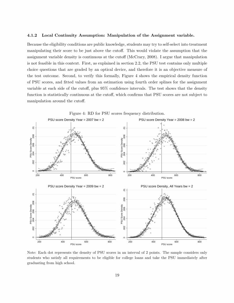
Because the eligibility conditions are public knowledge, students may try to self-select into treatmentmanipulating their score to be just above the cutoff. This would violate the assumption that theassignment variable density is continuous at the cutoff (McCrary, 2008). I argue that manipulationis not feasible in this context. First, as explained in section 2.2, the PSU test contains only multiplechoice questions that are graded by an optical device, and therefore it is an objective measure ofthe test outcome. Second, to verify this formally, Figure 4 shows the empirical density functionof PSU scores, and fitted values from an estimation using fourth order splines for the assignmentvariable at each side of the cutoff, plus 95% confidence intervals. The test shows that the densityfunction is statistically continuous at the cutoff, which confirms that PSU scores are not subject tomanipulation around the cutoff.

Figure 4: RD for PSU scores frequency distribution.

0.0

02.0

04.0

06.0

08.0

1P

SU

Sco

re D

ensi

ty

200 400 600 800PSU score

PSU score Density Year = 2007 bw = 20

.002

.004

.006

.008

.01

PS

U S

core

Den

sity

200 400 600 800PSU score


0.0

02.0

04.0

06.0

08.0

1P

SU

Sco

re D

ensi

ty

200 400 600 800PSU score


0.0

02.0

04.0

06.0

08.0

1P

SU

Sco

re D

ensi

ty

200 400 600 800PSU score

PSU score Density, All Years bw = 2

Note: Each dot represents the density of PSU scores in an interval of 2 points. The sample considers onlystudents who satisfy all requirements to be eligible for college loans and take the PSU immediately aftergraduating from high school.

19

4.1.3 Local Continuity Assumption: Balance of Covariates.

As a second test for the validity of the regression discontinuity design, I show that baseline charac-teristics are balanced at the cutoff.

First, as mentioned in section 2, no other aid or loan program influences the financial conditionsfor students in the vicinity of 475 (see Table 1). Secondly, I use equation (1) to show the balanceon covariates at the discontinuity, where Yi is now a covariate.

Table 2 and 3 shows the balance of covariates (for a linear f using the optimal bandwidth ofw∗ = 44 PSU points) for the population of students, for the group that is preselected for loans, andfor preselected students by income quintile. The first column in each category shows the level of thecovariate at the cutoff (the parameter β0 in equation 1), the second column shows the change onthe covariate for students barely above the threshold (β1) and the third column the t-value of thedifference. In Table 2 the population, the preselected sample and the first two income quintiles, andin table 3 the last three income quintiles. Table 2 shows that all covariates are balanced with fewexceptions. The population is not balanced at the 10% level of significance in number of femalesand high school GPA. Above the threshold there is approximately 1% more females students, andsurprisingly students have a 0.3% lower GPA. For the second poorest income quintile, number offemales and the indicator whether the student work previous the PSU test are not balanced at the5% of significance. Table 3 reports similar conclusions, students above the cutoff are very similarto those barely below the cutoff, except for two or three characteristics in each quintile.24 Thisevidence shows that the differences that appear in the data are in line with error of type I, i.e. fromthe 170 t-tests reported in these tables, 13, 6 and 0 reject the null at the significance levels of 10%,5% and 1% respectively, below the hypothetical levels of 17, 8.5 and 1.7.

Figure 5 shows the balance on 11 of these baseline characteristics presented in Table 2 for thepreselected group. All variables appear perfectly balanced at the cutoff.

All the conditions for a valid RDD are satisfied. Therefore, the comparison between studentsbarely eligible and barely ineligible will give the causal effects of access to loans on enrollment andprogress.

24The unbalance on type of high school is considered as only one characteristics since voucher, public and privateschools are perfectly collinear.

20

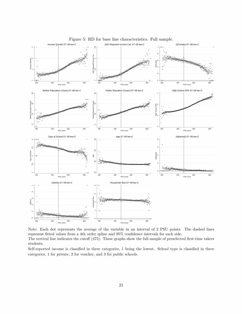
Figure 5: RD for base line characteristics. Full sample.

12

34

Inco

me

Qui

ntile

200 400 600 800PSU score

Income Quintile 07−09 bw=2

11.

52

2.5

Sel

f−R

epor

ted

Inco

me

Cat

.

200 400 600 800PSU score

Self−Reported Income Cat. 07−09 bw=2

0.2

.4.6

.81

1(F

emal

e)

200 400 600 800PSU score

1(Female) 07−09 bw=2

510

1520

Mot

her

Edu

catio

n (Y

ears

)

200 400 600 800PSU score

Mother Education (Years) 07−09 bw=2

510

1520

Fat

her

Edu

catio

n (Y

ears

)

200 400 600 800PSU score

Father Education (Years) 07−09 bw=2

45

67

Hig

h S

choo

l GP

A

200 400 600 800PSU score

High School GPA 07−09 bw=2

11.

52

2.5

3T

ype

of S

choo

l

200 400 600 800PSU score

Type of School 07−09 bw=2

1520

2530

Age

200 400 600 800PSU score

Age 07−09 bw=2

0.1

.2.3

.41(

Mar

ried)

200 400 600 800PSU score

1(Married) 07−09 bw=2

0.2

.4.6

.81

1(W

ork)

200 400 600 800PSU score

1(Work) 07−09 bw=2

02

46

8H

ouse

hold

Siz

e

200 400 600 800PSU score

Household Size 07−09 bw=2

Note: Each dot represents the average of the variable in an interval of 2 PSU points. The dashed linesrepresent fitted values from a 4th order spline and 95% confidence intervals for each side.The vertical line indicates the cutoff (475). These graphs show the full sample of preselected first-time takersstudents.Self-reported income is classified in three categories, 1 being the lowest. School type is classified in threecategories, 1 for private, 2 for voucher, and 3 for public schools.

21

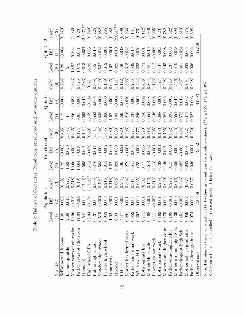
Table2:

Balan

ceof

Covariates.

Popu

latio

n,preselectedan

dby

incomequ

intiles

Popu

latio

nPr

eselected

Quintile

1Quintile

2Le

vel

Dif

abs(t)

Level

Dif

abs(t)

Level

Dif

abs(t)

Level

Dif

abs(t)

Varia

ble:

(1)

(2)

(3)

(4)

(5)

(6)

(7)

(8)

(9)

(10)

(11)

(12)

Self-repo

rted

Income

1.38

0.00

3(0.58)

1.28

-0.003

(0.405

)1.12

-0.005

(0.764

)1.28

-0.004

(0.279

)Incomequ

intile

2.09

0.01

4(0.777

)1.83

0.02

0(1.334

)1

2Mothe

ryearsof

educ

ation

10.96

-0.019

(0.518

)10

.66

-0.002

(0.035

)9.86

-0.093

(1.343

)10

.92

0.10

4(1.039

)Fa

ther

yearsof

educ

ation

11.03

-0.008

(0.19)

10.64

-0.010

(0.174

)9.81

-0.068

(0.875

)10

.79

0.03

1(0.28)

1(female)

0.54

10.00

9(1.729

)*0.59

30.00

1(0.191

)0.59

30.01

5(1.583

)0.61

3-0.037

(2.467

)**

Highscho

olGPA

53.94

-0.175

(1.751

)*55

.13

-0.070

(0.59)

55.59

-0.114

(0.7)

54.92

0.06

3(0.249

)Pu

blic

high

scho

ol0.43

70.00

5(0.938

)0.47

60.01

1(1.501

)0.55

30.00

3(0.308

)0.45

0.01

9(1.225

)Vo

uche

rhigh

scho

ol0.51

5-0.004

(0.701

)0.50

8-0.009

(1.204

)0.43

8-0.003

(0.299

)0.53

2-0.013

(0.882

)Pr

ivatehigh

scho

ol0.04

30.00

0(0.216

)0.01

3-0.002

(1.585

)0.00

60.00

0(0.149

)0.01

2-0.004

(1.265

)1(marrie

d)1.02

-0.001

(0.718

)1.02

0.00

0(0.089

)1.02

-0.002

(0.625

)1.02

-0.001

(0.282

)1(work)

0.03

0.00

1(0.628

)0.02

80.00

0(0.033

)0.03

-0.004

(1.151

)0.02

20.01

0(2.061

)**

HH

size

4.47

-0.005

(0.241

)4.49

-0.021

(0.829

)4.59

0.00

6(0.172

)4.46

-0.048

(0.899

)Mothe

rha

sform

alwork

0.29

10.00

1(0.304

)0.27

9-0.001

(0.206

)0.21

6-0.010

(1.306

)0.31

5-0.013

(0.936

)Fa

ther

hasform

alwork

0.55

20.00

4(0.811

)0.51

50.00

5(0.771

)0.43

7-0.003

(0.265

)0.54

90.01

8(1.181

)W

illleaveHH

0.20

20.00

0(0.035

)0.23

-0.003

(0.577

)0.24

6-0.004

(0.424

)0.22

3-0.010

(0.76)

Bothpa

rentsliv

e0.77

10.00

1(0.34)

0.77

0.00

6(0.979

)0.75

60.00

4(0.438

)0.77

30.00

1(0.112

)Mothe

rHou

sewife

0.49

8-0.001

(0.156

)0.51

40.00

2(0.318

)0.55

10.00

8(0.864

)0.48

10.01

6(1.046

)Pa

rentsdo

notwork

0.11

-0.002

(0.516

)0.11

8-0.001

(0.305

)0.13

60.00

8(1.126

)0.11

2-0.009

(0.995

)Bothpa

rentswork

0.16

20.00

1(0.298

)0.13

8-0.001

(0.153

)0.08

8-0.007

(1.377

)0.14

7-0.003

(0.23)

Mothe

rsomehigh

ered

uc.

0.17

50.00

0(0.029

)0.14

60.00

1(0.195

)0.08

10.00

2(0.298

)0.14

50.00

8(0.782

)Fa

ther

somehigh

ered

uc.

0.18

9-0.001

(0.274

)0.15

0.00

0(0.052

)0.09

5-0.005

(0.845

)0.13

70.00

3(0.322

)Mothe

rdrop

outhigh

Sch.

0.43

90.00

0(0.076

)0.45

9-0.002

(0.245

)0.55

10.01

5(1.566

)0.41

9-0.013

(0.894

)Fa

ther

drop

outhigh

Sch.

0.45

1-0.002

(0.346

)0.48

2-0.003

(0.424

)0.57

20.01

4(1.467

)0.46

1-0.024

(1.613

)Mothe

rcolle

gegrad

uate

0.05

90.00

2(0.87)

0.04

20.00

1(0.22)

0.01

70.00

2(0.701

)0.03

30.00

5(0.875

)Fa

ther

colle

gegrad

uate

0.07

40.00

0(0.057

)0.04

6-0.001

(0.259

)0.02

20.00

3(0.968

)0.03

60.00

2(0.308

)Observatio

ns15

0356

7935

241

303

1724

9

Note:

Difrefers

totheβ

1of

equa

tion(1).

t-values

inpa

renthe

sis(in

absolute

values).

(**):p6

5%,(*):p6

10%

Self-repo

rted

incomeis

classifi

edin

threecategorie

s,1be

ingthelowest.

22

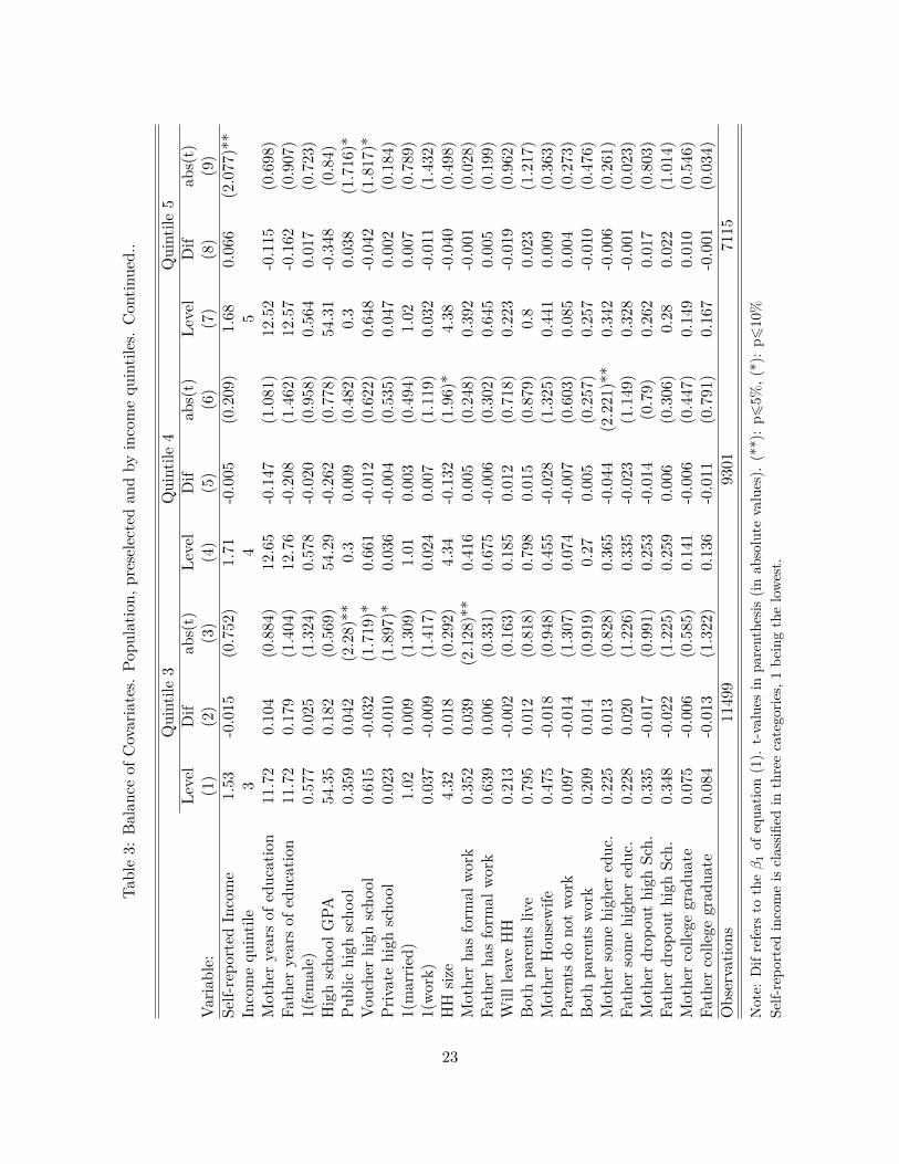
Table3:

Balan

ceof

Covariates.

Popu

latio

n,preselectedan

dby

incomequ

intiles.Con

tinue

d..

Quintile

3Quintile

4Quintile

5Le

vel

Dif

abs(t)

Level

Dif

abs(t)

Level

Dif

abs(t)

Varia

ble:

(1)

(2)

(3)

(4)

(5)

(6)

(7)

(8)

(9)

Self-repo

rted

Income

1.53

-0.015

(0.752

)1.71

-0.005

(0.209

)1.68

0.06

6(2.077

)**

Incomequ

intile

34

5Mothe

ryearsof

educ

ation

11.72

0.10

4(0.884

)12

.65

-0.147

(1.081

)12

.52

-0.115

(0.698

)Fa

ther

yearsof

educ

ation

11.72

0.17

9(1.404

)12

.76

-0.208

(1.462

)12

.57

-0.162

(0.907

)1(female)

0.57

70.02

5(1.324

)0.57

8-0.020

(0.958

)0.56

40.01

7(0.723

)Highscho

olGPA

54.35

0.18

2(0.569

)54

.29

-0.262

(0.778

)54

.31

-0.348

(0.84)

Public

high

scho

ol0.35

90.04

2(2.28)**

0.3

0.00

9(0.482

)0.3

0.03

8(1.716

)*Vo

uche

rhigh

scho

ol0.61

5-0.032

(1.719

)*0.66

1-0.012

(0.622

)0.64

8-0.042

(1.817

)*Pr

ivatehigh

scho

ol0.02

3-0.010

(1.897

)*0.03

6-0.004

(0.535

)0.04

70.00

2(0.184

)1(marrie

d)1.02

0.00

9(1.309

)1.01

0.00

3(0.494

)1.02

0.00

7(0.789

)1(work)

0.03

7-0.009

(1.417

)0.02

40.00

7(1.119

)0.03

2-0.011

(1.432

)HH

size

4.32

0.01

8(0.292

)4.34

-0.132

(1.96)*

4.38

-0.040

(0.498

)Mothe

rha

sform

alwork

0.35

20.03

9(2.128

)**

0.41

60.00

5(0.248

)0.39

2-0.001

(0.028

)Fa

ther

hasform

alwork

0.63

90.00

6(0.331

)0.67

5-0.006

(0.302

)0.64

50.00

5(0.199

)W

illleaveHH

0.21

3-0.002

(0.163

)0.18

50.01

2(0.718

)0.22

3-0.019

(0.962

)Bothpa

rentsliv

e0.79

50.01

2(0.818

)0.79

80.01

5(0.879

)0.8

0.02

3(1.217

)Mothe

rHou

sewife

0.47

5-0.018

(0.948

)0.45

5-0.028

(1.325

)0.44

10.00

9(0.363

)Pa

rentsdo

notwork

0.09

7-0.014

(1.307

)0.07

4-0.007

(0.603

)0.08

50.00

4(0.273

)Bothpa

rentswork

0.20

90.01

4(0.919

)0.27

0.00

5(0.257

)0.25

7-0.010

(0.476

)Mothe

rsomehigh

ered

uc.

0.22

50.01

3(0.828

)0.36

5-0.044

(2.221

)**

0.34

2-0.006

(0.261

)Fa

ther

somehigh

ered

uc.

0.22

80.02

0(1.226

)0.33

5-0.023

(1.149

)0.32

8-0.001

(0.023

)Mothe

rdrop

outhigh

Sch.

0.33

5-0.017

(0.991

)0.25

3-0.014

(0.79)

0.26

20.01

7(0.803

)Fa

ther

drop

outhigh

Sch.

0.34

8-0.022

(1.225

)0.25

90.00

6(0.306

)0.28

0.02

2(1.014

)Mothe

rcolle

gegrad

uate

0.07

5-0.006

(0.585

)0.14

1-0.006

(0.447

)0.14

90.01

0(0.546

)Fa

ther

colle

gegrad

uate

0.08

4-0.013

(1.322

)0.13

6-0.011

(0.791

)0.16

7-0.001

(0.034

)Observatio

ns11

499

9301

7115

Note:

Difrefers

totheβ

1of

equa

tion(1).

t-values

inpa

renthe

sis(in

absolute

values).

(**):p6

5%,(*):p6

10%

Self-repo

rted

incomeis

classifi

edin

threecategorie

s,1be

ingthelowest.

23

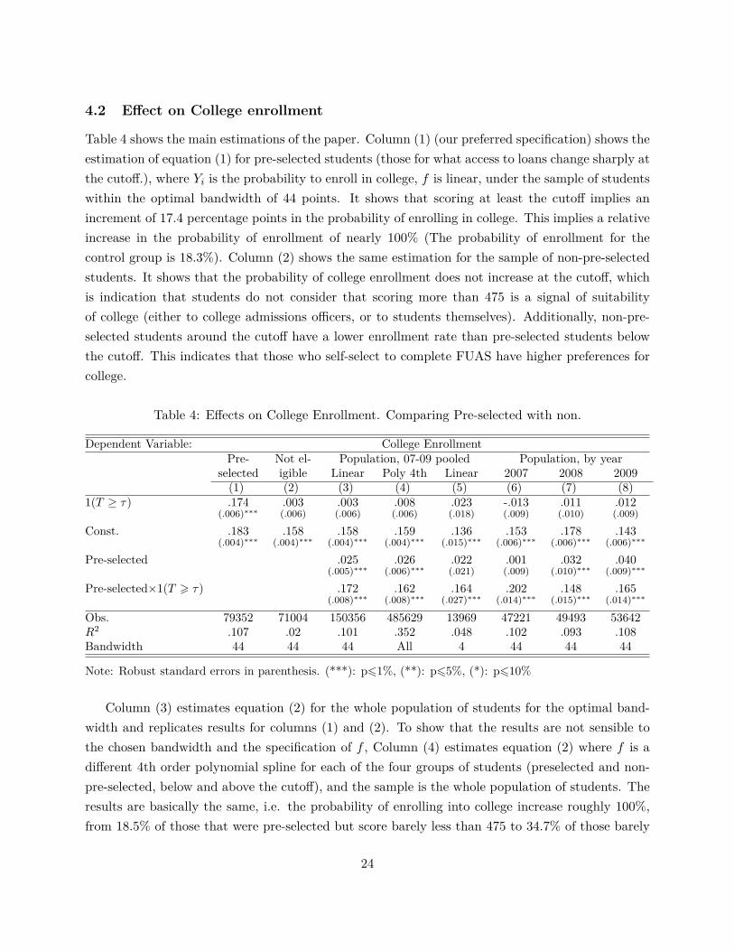
4.2 Effect on College enrollment

Table 4 shows the main estimations of the paper. Column (1) (our preferred specification) shows theestimation of equation (1) for pre-selected students (those for what access to loans change sharply atthe cutoff.), where Yi is the probability to enroll in college, f is linear, under the sample of studentswithin the optimal bandwidth of 44 points. It shows that scoring at least the cutoff implies anincrement of 17.4 percentage points in the probability of enrolling in college. This implies a relativeincrease in the probability of enrollment of nearly 100% (The probability of enrollment for thecontrol group is 18.3%). Column (2) shows the same estimation for the sample of non-pre-selectedstudents. It shows that the probability of college enrollment does not increase at the cutoff, whichis indication that students do not consider that scoring more than 475 is a signal of suitabilityof college (either to college admissions officers, or to students themselves). Additionally, non-pre-selected students around the cutoff have a lower enrollment rate than pre-selected students belowthe cutoff. This indicates that those who self-select to complete FUAS have higher preferences forcollege.

Table 4: Effects on College Enrollment. Comparing Pre-selected with non.

Dependent Variable: College EnrollmentPre- Not el- Population, 07-09 pooled Population, by year

selected igible Linear Poly 4th Linear 2007 2008 2009(1) (2) (3) (4) (5) (6) (7) (8)

1(T ≥ τ) .174 .003 .003 .008 .023 -.013 .011 .012(.006)∗∗∗ (.006) (.006) (.006) (.018) (.009) (.010) (.009)

Const. .183 .158 .158 .159 .136 .153 .178 .143(.004)∗∗∗ (.004)∗∗∗ (.004)∗∗∗ (.004)∗∗∗ (.015)∗∗∗ (.006)∗∗∗ (.006)∗∗∗ (.006)∗∗∗

Pre-selected .025 .026 .022 .001 .032 .040(.005)∗∗∗ (.006)∗∗∗ (.021) (.009) (.010)∗∗∗ (.009)∗∗∗

Pre-selected×1(T > τ) .172 .162 .164 .202 .148 .165(.008)∗∗∗ (.008)∗∗∗ (.027)∗∗∗ (.014)∗∗∗ (.015)∗∗∗ (.014)∗∗∗

Obs. 79352 71004 150356 485629 13969 47221 49493 53642R2 .107 .02 .101 .352 .048 .102 .093 .108Bandwidth 44 44 44 All 4 44 44 44

Note: Robust standard errors in parenthesis. (***): p61%, (**): p65%, (*): p610%

Column (3) estimates equation (2) for the whole population of students for the optimal band-width and replicates results for columns (1) and (2). To show that the results are not sensible tothe chosen bandwidth and the specification of f , Column (4) estimates equation (2) where f is adifferent 4th order polynomial spline for each of the four groups of students (preselected and non-pre-selected, below and above the cutoff), and the sample is the whole population of students. Theresults are basically the same, i.e. the probability of enrolling into college increase roughly 100%,from 18.5% of those that were pre-selected but score barely less than 475 to 34.7% of those barely

24

above the threshold. Column (5), shows a third specification, f is linear again, but the bandwidthis 4 PSU points.25 The results are even stronger: scoring equal to or greater than 475 implies anincrease of 16.2 percentage points in the probability of enrolling, but this time the control groupenrolls at a 13.6%, and therefore the relative increase is 120%. Moreover the pre-selected groupis now not statistically different than the group that did not complete FUAS. Nevertheless theseresults may be affected for small sample bias, despite the fact that the sample is quite large (roughly14,000 students).

Finally columns (6) to (8) show regressions for the preferred specification (equation (2) with alinear f , within a bandwidth of 44 points) for each year separately. As a sign of robustness, thesecolumns show that the same conclusions can be inferred every single year, considering that eachyear is an independent the natural experiment.

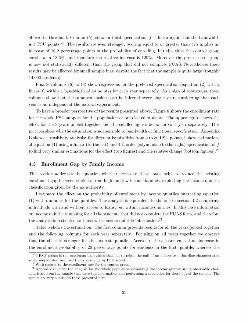
To have a broader perspective of the results presented above, Figure 6 shows the enrollment ratefor the whole PSU support for the population of preselected students. The upper figure shows theeffect for the 3 years pooled together and the smaller figures below for each year separately. Thispictures show why the estimation is not sensible to bandwidth or functional specification. AppendixB shows a sensitivity analysis: for different bandwidths from 2 to 80 PSU points, I show estimationsof equation (1) using a linear (to the left) and 4th order polynomial (to the right) specification of fto find very similar estimations for the effect (top figures) and the relative change (bottom figures).26

4.3 Enrollment Gap by Family Income

This section addresses the question whether access to these loans helps to reduce the existingenrollment gap between students from high and low income families, exploiting the income quintileclassification given by the ax authority.

I estimate the effect on the probability of enrollment by income quintiles interacting equation(1) with dummies for the quintiles. The analysis is equivalent to the one in section 4.2 comparingindividuals with and without access to loans, but within income quintiles. In this case informationon income quintile is missing for all the students that did not complete the FUAS form, and thereforethe analysis is restricted to those with income quintile information.27

Table 5 shows the estimation. The first column presents results for all the years pooled togetherand the following columns for each year separately. Focusing on all years together we observethat the effect is stronger for the poorest quintile. Access to these loans caused an increase inthe enrollment probability of 20 percentage points for students in the first quintile, whereas the

254 PSU points is the maximum bandwidth that fail to reject the null of no difference in baseline characteristicswhen simple t-test are used (not controlling by PSU score)

26With respect to the enrollment rate for the control group.27Appendix C shows the analysis for the whole population estimating the income quintile using observable char-

acteristics from the sample that have this information and performing a prediction for those out of the sample. Theresults are very similar to those presented here.

25

enrollment rate for barely ineligible students is 13.3 percent in this quintile. This implies thathaving access to tuition loans led to a 151% increase in the enrollment rate.

Figure 6: RD for College enrollment. Full sample.

0.2

.4.6

.81

Pr

(Col

lege

Enr

ollm

ent)

200 400 600 800PSU score

College Enrollment; All Years; bw=2

0.2

.4.6

.81

Pr

(Col

lege

Enr

ollm

ent)

200 400 600 800PSU score

College Enrollment Year=2007 bw=2

0.2

.4.6

.81

Pr

(Col

lege

Enr

ollm

ent)

200 400 600 800PSU score


0.2

.4.6

.81

Pr

(Col

lege

Enr

ollm

ent)

200 400 600 800PSU score


Note: Each dot represents average college enrollment within bins of 2 PSU points (bw=2).The dashed lines represent fitted values from a 4th order spline and 95% confidence intervals for each side.The vertical line indicates the cutoff (475).These graphs show the full sample of students fulfilling all requirements to be eligible for college loans andtaking the PSU immediately after graduating from high school.

26

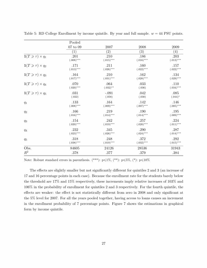
Table 5: RD College Enrollment by income quintile. By year and full sample. w = 44 PSU points.

Pooled07 to 09 2007 2008 2009(1) (2) (3) (4)

1(T > τ) × q1 .201 .210 .186 .203(.008)∗∗∗ (.015)∗∗∗ (.016)∗∗∗ (.013)∗∗∗

1(T > τ) × q2 .171 .211 .160 .157(.013)∗∗∗ (.026)∗∗∗ (.022)∗∗∗ (.022)∗∗∗

1(T > τ) × q3 .164 .210 .162 .134(.017)∗∗∗ (.031)∗∗∗ (.028)∗∗∗ (.029)∗∗∗

1(T > τ) × q4 .070 .064 .033 .110(.020)∗∗∗ (.032)∗∗ (.036) (.034)∗∗∗

1(T > τ) × q5 .031 -.091 .042 .085(.022) (.058) (.030) (.044)∗

q1 .133 .164 .142 .146(.008)∗∗∗ (.009)∗∗∗ (.007)∗∗∗ (.005)∗∗∗

q2 .166 .219 .190 .195(.016)∗∗∗ (.014)∗∗∗ (.014)∗∗∗ (.009)∗∗∗

q3 .154 .242 .257 .224(.020)∗∗∗ (.019)∗∗∗ (.020)∗∗∗ (.011)∗∗∗

q4 .232 .345 .290 .287(.023)∗∗∗ (.026)∗∗∗ (.024)∗∗∗ (.014)∗∗∗

q5 .318 .248 .372 .292(.038)∗∗∗ (.019)∗∗∗ (.032)∗∗∗ (.015)∗∗∗

Obs. 84605 24126 28536 31943R2 .378 .377 .379 .384


The effects are slightly smaller but not significantly different for quintiles 2 and 3 (an increase of17 and 16 percentage points in each case). Because the enrollment rate for the students barely belowthe threshold are 17% and 15% respectively, these increments imply relative increases of 103% and106% in the probability of enrollment for quintiles 2 and 3 respectively. For the fourth quintile, theeffects are weaker: the effect is not statistically different from zero in 2008 and only significant atthe 5% level for 2007. For all the years pooled together, having access to loans causes an incrementin the enrollment probability of 7 percentage points. Figure 7 shows the estimations in graphicalform by income quintile.

27

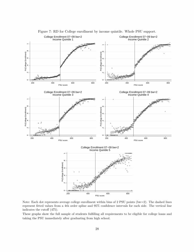
Figure 7: RD for College enrollment by income quintile. Whole PSU support.0

.2.4

.6.8

1P

r(C

olle

ge E

nrol

lmen

t)

200 400 600 800PSU score

College Enrollment 07−09 bw=2Income Quintile 1

0.2

.4.6

.81

Pr(

Col

lege

Enr

ollm

ent)

200 400 600 800PSU score


0.2

.4.6

.81

Pr(

Col

lege

Enr

ollm

ent)

200 400 600 800PSU score


0.2

.4.6

.81

Pr(

Col

lege

Enr

ollm

ent)

200 400 600 800PSU score


0.2

.4.6

.81

Pr(

Col

lege

Enr

ollm

ent)

200 400 600 800PSU score


Note: Each dot represents average college enrollment within bins of 2 PSU points (bw=2). The dashed linesrepresent fitted values from a 4th order spline and 95% confidence intervals for each side. The vertical lineindicates the cutoff (475).These graphs show the full sample of students fulfilling all requirements to be eligible for college loans andtaking the PSU immediately after graduating from high school.

28

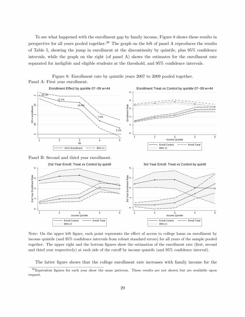
To see what happened with the enrollment gap by family income, Figure 8 shows these results inperspective for all years pooled together.28 The graph on the left of panel A reproduces the resultsof Table 5, showing the jump in enrollment at the discontinuity by quintile, plus 95% confidenceintervals, while the graph on the right (of panel A) shows the estimates for the enrollment rateseparated for ineligible and eligible students at the threshold, and 95% confidence intervals.

Figure 8: Enrollment rate by quintile years 2007 to 2009 pooled together.Panel A: First year enrollment.

20.1%

17.1%

16.4%

7.0%

3.1%

0.0

5.1

.15

.2D

if in

enr

ollm

ent

1 2 3 4 5qq

Dif in Enrollment 95% CI

Enrollment Effect by quintile 07−09 w=44

0.1

.2.3

.4.5

Enr

ollm

ent R

ate

1 2 3 4 5Income Quintile

Enroll Control Enroll Treat95% CI

Enrollment Treat vs Control by quintile 07−09 w=44

Panel B: Second and third year enrollment.

0.1

.2.3

.42n

d Y

ear

Enr

ollm

ent R

ate



2nd Year Enroll: Treat vs Control by quintil

0.1

.2.3

.43r

d Y

ear

Enr

ollm

ent R

ate



3rd Year Enroll: Treat vs Control by quintil

Note: On the upper left figure, each point represents the effect of access to college loans on enrollment byincome quintile (and 95% confidence intervals from robust standard errors) for all years of the sample pooledtogether. The upper right and the bottom figures show the estimation of the enrollment rate (first, secondand third year respectively) at each side of the cutoff by income quintile (and 95% confidence interval).

The latter figure shows that the college enrollment rate increases with family income for the28Equivalent figures for each year show the same patterns. These results are not shown but are available upon

request.

29

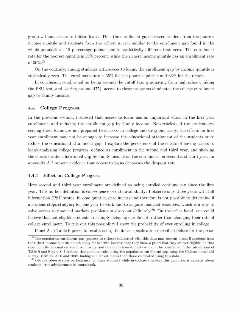
group without access to tuition loans. Thus the enrollment gap between student from the poorestincome quintile and students from the richest is very similar to the enrollment gap found in thewhole population - 15 percentage points, and is statistically different than zero. The enrollmentrate for the poorest quintile is 15% percent, while the richest income quintile has an enrollment rateof 30%.29

On the contrary, among students with access to loans, the enrollment gap by income quintile isstatistically zero. The enrollment rate is 35% for the poorest quintile and 33% for the richest.

In conclusion, conditional on being around the cutoff (i.e. graduating from high school, takingthe PSU test, and scoring around 475), access to these programs eliminates the college enrollmentgap by family income.

4.4 College Progress.

In the previous section, I showed that access to loans has an important effect in the first yearenrollment, and reducing the enrollment gap by family income. Nevertheless, if the students re-ceiving these loans are not prepared to succeed in college and drop out easily, the effects on firstyear enrollment may not be enough to increase the educational attainment of the students or toreduce the educational attainment gap. I explore the persistence of the effects of having access toloans analyzing college progress, defined as enrollment in the second and third year, and showingthe effects on the educational gap by family income on the enrollment on second and third year. Inappendix A I present evidence that access to loans decreases the dropout rate.

4.4.1 Effect on College Progress

Here second and third year enrollment are defined as being enrolled continuously since the firstyear. This ad hoc definition is consequence of data availability: I observe only three years with fullinformation (PSU scores, income quintile, enrollment) and therefore is not possible to determine ifa student stops studying for one year to work and to acquire financial resources, which is a way tosolve access to financial markets problems or drop out definitely.30 On the other hand, one couldbelieve that not eligible students are simply delaying enrollment, rather than changing their rate ofcollege enrollment. To rule out this possibility I show the probability of ever enrolling in college.

Panel A in Table 6 presents results using the linear specification described before for the prese-29The population enrollment gap (poorest to richest) calculated with this data may present biases if students from

the richest income quintile do not apply for benefits, because may they know a priori that they are not eligible. In thatcase, quintile information would be missing, and therefore those students wouldn’t be considered in the calculations ofTable 5 and Figure 8. I address that problem calculating the population enrollment gap using the Chilean householdsurvey: CASEN 2006 and 2009, finding similar estimates than those calculated using this data.

30I do not observe class performance for these students while in college, therefore this definition is agnostic aboutstudents’ true advancement in coursework.

30

lected sample in the first three columns and for the whole population in the last three.31,32

Table 6: Enrollment in Second and third years of college for all students around the cutoff in 2007and 2008. w = 44

PANEL A: 2SLS IV RegressionPre-selected Population

Dependent Var.: Enrollment Enrollment Ever Enrollment Enrollment Ever2nd year 3rd year Enrolled 2nd year 3rd year Enrolled

(1) (2) (3) (4) (5) (6)Eligible .197 .190 .154 .199 .201 .146

(.010)∗∗∗ (.012)∗∗∗ (.008)∗∗∗ (.013)∗∗∗ (.016)∗∗∗ (.011)∗∗∗

Const. .099 .048 .316 .090 .052 .287(.006)∗∗∗ (.007)∗∗∗ (.005)∗∗∗ (.004)∗∗∗ (.004)∗∗∗ (.004)∗∗∗

1(T > τ) -.001 -.009 .007(.006) (.008) (.007)

Pre-selected .008 -.007 .031(.007) (.008) (.007)∗∗∗

Obs. 48044 22819 78072 94234 46153 147638R2 .074 .086 .119 .052 .064 .113PANEL B: First StageInstrumented: Ever been Eligible for loans

Intrument—> 1(T > τ) Pre-selected×1(T > τ)Intrument .782 .790 .867 .768 .773 .858

(.005)∗∗∗ (.008)∗∗∗ (.003)∗∗∗ (.008)∗∗∗ (.012)∗∗∗ (.005)∗∗∗

Note: Robust standard errors in parenthesis. (***): p61%.

Column (1) shows the enrollment probability in the second year: having access to college tuitionloans increases the probability of reaching the second year of college by 20 percentage points. Inrelation to the enrollment rate for the control group (10 percent), the effect at the discontinuity isequivalent to a 200%. Column (2) shows that third year enrollment,33 increases by 19 percentagepoints for those barely eligible for loans. Relatively to the enrollment rate for the control group (4.8percent), the effect is equivalent to a 400% increase in the probability of reaching up to third year inconsecutive years. Column (3) shows that just having access to the loans increases the probabilityof ever being enrolled in college in 15 percentage points which, relatively to those just ineligible,correspond to an increase of 50%.

31The results are highly robust to different functional specifications and different bandwidths. These results are notshown but are available upon request.

32Panel B in Table 6 shows the first stages of the different definitions of eligibility used in the 2SLS setting forenrollment in second and third year, i.e. the portion of compliers.

33Here, we only observe the behavior of the cohort that took the PSU for the first time in 2007. They are the onlyones that can be track up to the third year in the data.

31

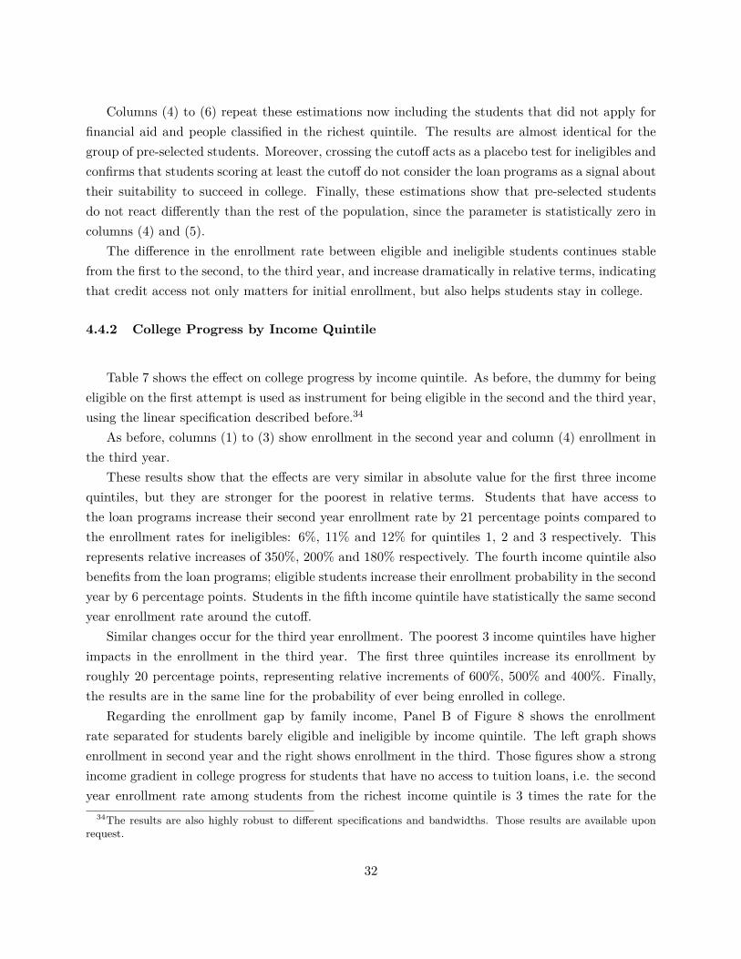
Columns (4) to (6) repeat these estimations now including the students that did not apply forfinancial aid and people classified in the richest quintile. The results are almost identical for thegroup of pre-selected students. Moreover, crossing the cutoff acts as a placebo test for ineligibles andconfirms that students scoring at least the cutoff do not consider the loan programs as a signal abouttheir suitability to succeed in college. Finally, these estimations show that pre-selected studentsdo not react differently than the rest of the population, since the parameter is statistically zero incolumns (4) and (5).

The difference in the enrollment rate between eligible and ineligible students continues stablefrom the first to the second, to the third year, and increase dramatically in relative terms, indicatingthat credit access not only matters for initial enrollment, but also helps students stay in college.

4.4.2 College Progress by Income Quintile

Table 7 shows the effect on college progress by income quintile. As before, the dummy for beingeligible on the first attempt is used as instrument for being eligible in the second and the third year,using the linear specification described before.34

As before, columns (1) to (3) show enrollment in the second year and column (4) enrollment inthe third year.

These results show that the effects are very similar in absolute value for the first three incomequintiles, but they are stronger for the poorest in relative terms. Students that have access tothe loan programs increase their second year enrollment rate by 21 percentage points compared tothe enrollment rates for ineligibles: 6%, 11% and 12% for quintiles 1, 2 and 3 respectively. Thisrepresents relative increases of 350%, 200% and 180% respectively. The fourth income quintile alsobenefits from the loan programs; eligible students increase their enrollment probability in the secondyear by 6 percentage points. Students in the fifth income quintile have statistically the same secondyear enrollment rate around the cutoff.

Similar changes occur for the third year enrollment. The poorest 3 income quintiles have higherimpacts in the enrollment in the third year. The first three quintiles increase its enrollment byroughly 20 percentage points, representing relative increments of 600%, 500% and 400%. Finally,the results are in the same line for the probability of ever being enrolled in college.

Regarding the enrollment gap by family income, Panel B of Figure 8 shows the enrollmentrate separated for students barely eligible and ineligible by income quintile. The left graph showsenrollment in second year and the right shows enrollment in the third. Those figures show a strongincome gradient in college progress for students that have no access to tuition loans, i.e. the secondyear enrollment rate among students from the richest income quintile is 3 times the rate for the

34The results are also highly robust to different specifications and bandwidths. Those results are available uponrequest.

32

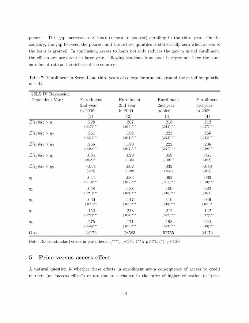
poorest. This gap increases to 8 times (richest to poorest) enrolling in the third year. On thecontrary, the gap between the poorest and the richest quintiles is statistically zero when access tothe loans is granted. In conclusion, access to loans not only reduces the gap in initial enrollment,the effects are persistent in later years, allowing students from poor backgrounds have the sameenrollment rate as the richest of the country.

Table 7: Enrollment in Second and third years of college for students around the cutoff by quintile.w = 44

2SLS IV RegressionDependent Var.: Enrollment Enrollment Enrollment Enrollment

2nd year 2nd year 2nd year 3rd yearin 2008 in 2009 pooled in 2009

(1) (2) (3) (4)Eligible× q1 .228 .207 .218 .212

(.017)∗∗∗ (.019)∗∗∗ (.013)∗∗∗ (.017)∗∗∗

Eligible× q2 .261 .198 .223 .256(.033)∗∗∗ (.031)∗∗∗ (.023)∗∗∗ (.033)∗∗∗

Eligible× q3 .266 .189 .222 .236(.038)∗∗∗ (.037)∗∗∗ (.027)∗∗∗ (.039)∗∗∗

Eligible× q4 .084 .029 .059 .061(.038)∗∗ (.045) (.030)∗∗ (.038)

Eligible× q5 -.054 .062 .032 -.048(.062) (.039) (.033) (.062)

q1 .044 .083 .063 .030(.010)∗∗∗ (.012)∗∗∗ (.007)∗∗∗ (.010)∗∗∗

q2 .058 .128 .100 .028(.021)∗∗∗ (.021)∗∗∗ (.016)∗∗∗ (.021)

q3 .060 .147 .110 .049(.026)∗∗ (.026)∗∗∗ (.019)∗∗∗ (.026)∗

q4 .152 .278 .212 .142(.027)∗∗∗ (.034)∗∗∗ (.022)∗∗∗ (.027)∗∗∗

q5 .275 .171 .198 .244(.049)∗∗∗ (.026)∗∗∗ (.023)∗∗∗ (.049)∗∗∗

Obs. 24172 28583 52755 24172


5 Price versus access effect

A natural question is whether these effects in enrollment are a consequence of access to creditmarkets (an “access effect”) or are due to a change in the price of higher education (a “price

33

effect”), a consequence of implicit subsidy components, such as lower than the market interest ratesor low repayment enforceability, that are present in these tuition loans.35

To decompose the total effect into price and access effects, I present the following three tests.

5.1 Estimating the price effect directly

The first test estimates the price effect directly, specifically it compares the enrollment rate ofstudents who must finance the full tuition cost to those who receive a scholarship that covers italmost in full, in a context where access to credit is available for everybody (no access effect). Asusual, students who receive scholarships are different from those who do not. To address theseendogeneity problems, I use another natural experiment of the same type as exogenous variation inaccess to scholarships.

Table 1 presented the requirements to qualify for scholarships delivered by the Ministry ofEducation. Most of them depend on PSU score cutoffs, enabling the use of a regression discontinuitydesign. In particular, the Bicentenario scholarship is available to students who comply with thefollowing requirements. First, complete the FUAS socioeconomic form and are classified on thetwo poorest income quintiles. Second, enroll in traditional universities, and third, score above 550points in the PSU test.36 This scholarship program is the third in importance in the country, it isgiven to 4.7% of the universe of students and 55% of eligible students. Moreover, it covers in fullthe reference tuition37 (on average 90% of the total tuition cost), hence constitutes a significantdrop in the cost of university education.

Because all students scoring 475 PSU points or higher have access to college credit markets(secured by the existence of the two loan programs discussed above), there is no access effectaround the Bicentenario grant cutoff. Therefore, the comparison between the college enrollmentrates of those who score barely above the grant cutoff of 550 PSU points, with those slightly belowgives the causal effect of the reduction in tuition cost on the enrollment rate, the price effect.

The upper graph in Figure 9 shows the rate of students receiving the Bicentenario grant amongstudents who meet all requirements around the grant cutoff point (as before the sample is restrictedto preselected students that take the PSU for the first time to avoid selection). By definition,nobody below the threshold received the benefit, while 38% of students barely above the thresholdreceived the grant, and therefore their tuition was reduced by approximately 90%.

35Dynarski (2003) called these effects the liquidity and subsidy effects respectively.36The same tests are made to check the validity of RDD: Balance on observed characteristics, bunching at the cutoff,

and a discontinuous number of recipients around the cutoff. Those tests are not presented here but are available uponrequest.

37Reference tuition is a value determined by the Ministry of Education. It calculates what the tuition at a givenuniversity should be based on its characteristics (quality of education, demand for programs, prestige, etc.). Onaverage, reference tuition corresponds to 90% of effective tuition fixed by universities.

34

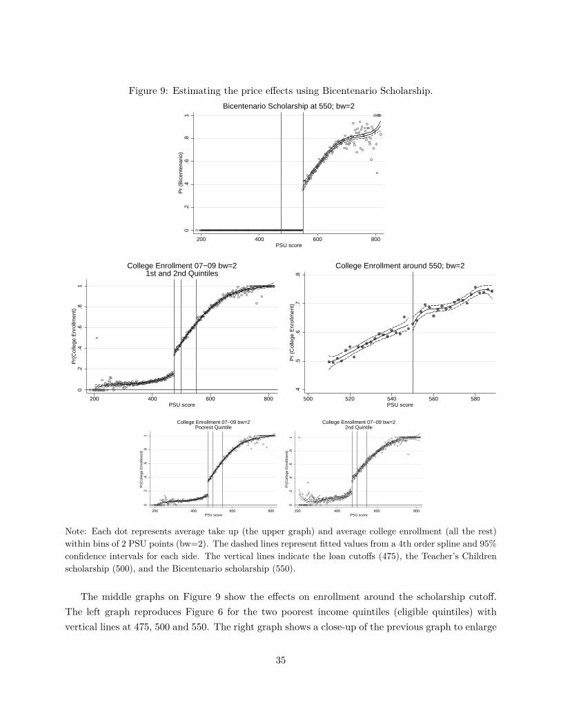
Figure 9: Estimating the price effects using Bicentenario Scholarship.

0.2

.4.6

.81

Pr

(Bic

ente

nario

)

200 400 600 800PSU score

Bicentenario Scholarship at 550; bw=2

0.2

.4.6

.81

Pr(

Col

lege

Enr

ollm

ent)

200 400 600 800PSU score

College Enrollment 07−09 bw=21st and 2nd Quintiles

.4.5

.6.7

.8P

r (C

olle

ge E

nrol

lmen

t)

500 520 540 560 580PSU score

College Enrollment around 550; bw=2

0.2

.4.6

.81

Pr(

Col

lege

Enr

ollm

ent)

200 400 600 800PSU score

College Enrollment 07−09 bw=2Poorest Quintile

0.2

.4.6

.81

Pr(

Col

lege

Enr

ollm

ent)

200 400 600 800PSU score

College Enrollment 07−09 bw=22nd Quintile

Note: Each dot represents average take up (the upper graph) and average college enrollment (all the rest)within bins of 2 PSU points (bw=2). The dashed lines represent fitted values from a 4th order spline and 95%confidence intervals for each side. The vertical lines indicate the loan cutoffs (475), the Teacher’s Childrenscholarship (500), and the Bicentenario scholarship (550).

The middle graphs on Figure 9 show the effects on enrollment around the scholarship cutoff.The left graph reproduces Figure 6 for the two poorest income quintiles (eligible quintiles) withvertical lines at 475, 500 and 550. The right graph shows a close-up of the previous graph to enlarge

35

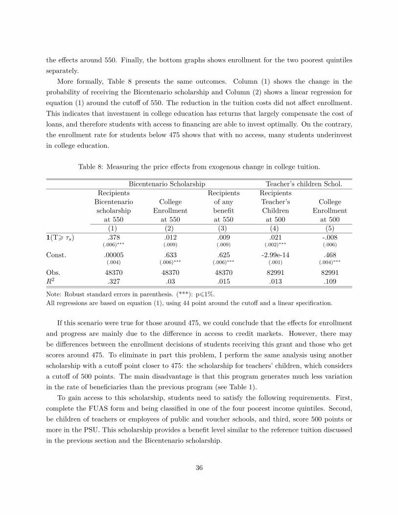
the effects around 550. Finally, the bottom graphs shows enrollment for the two poorest quintilesseparately.

More formally, Table 8 presents the same outcomes. Column (1) shows the change in theprobability of receiving the Bicentenario scholarship and Column (2) shows a linear regression forequation (1) around the cutoff of 550. The reduction in the tuition costs did not affect enrollment.This indicates that investment in college education has returns that largely compensate the cost ofloans, and therefore students with access to financing are able to invest optimally. On the contrary,the enrollment rate for students below 475 shows that with no access, many students underinvestin college education.

Table 8: Measuring the price effects from exogenous change in college tuition.

Bicentenario Scholarship Teacher’s children Schol.Recipients Recipients RecipientsBicentenario College of any Teacher’s Collegescholarship Enrollment benefit Children Enrollment

at 550 at 550 at 550 at 500 at 500(1) (2) (3) (4) (5)

1(T> τs) .378 .012 .009 .021 -.008(.006)∗∗∗ (.009) (.009) (.002)∗∗∗ (.006)

Const. .00005 .633 .625 -2.99e-14 .468(.004) (.006)∗∗∗ (.006)∗∗∗ (.001) (.004)∗∗∗

Obs. 48370 48370 48370 82991 82991R2 .327 .03 .015 .013 .109

Note: Robust standard errors in parenthesis. (***): p61%.All regressions are based on equation (1), using 44 point around the cutoff and a linear specification.

If this scenario were true for those around 475, we could conclude that the effects for enrollmentand progress are mainly due to the difference in access to credit markets. However, there maybe differences between the enrollment decisions of students receiving this grant and those who getscores around 475. To eliminate in part this problem, I perform the same analysis using anotherscholarship with a cutoff point closer to 475: the scholarship for teachers’ children, which considersa cutoff of 500 points. The main disadvantage is that this program generates much less variationin the rate of beneficiaries than the previous program (see Table 1).

To gain access to this scholarship, students need to satisfy the following requirements. First,complete the FUAS form and being classified in one of the four poorest income quintiles. Second,be children of teachers or employees of public and voucher schools, and third, score 500 points ormore in the PSU. This scholarship provides a benefit level similar to the reference tuition discussedin the previous section and the Bicentenario scholarship.

36

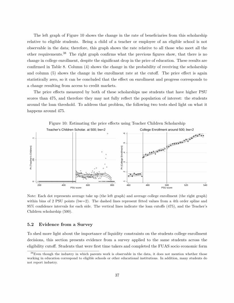
The left graph of Figure 10 shows the change in the rate of beneficiaries from this scholarshiprelative to eligible students. Being a child of a teacher or employee of an eligible school is notobservable in the data; therefore, this graph shows the rate relative to all those who meet all theother requirements.38 The right graph confirms what the previous figures show, that there is nochange in college enrollment, despite the significant drop in the price of education. These results areconfirmed in Table 8. Column (4) shows the change in the probability of receiving the scholarshipand column (5) shows the change in the enrollment rate at the cutoff. The price effect is againstatistically zero, so it can be concluded that the effect on enrollment and progress corresponds toa change resulting from access to credit markets.

The price effects measured by both of these scholarships use students that have higher PSUscores than 475, and therefore they may not fully reflect the population of interest: the studentsaround the loan threshold. To address that problem, the following two tests shed light on what ithappens around 475.

Figure 10: Estimating the price effects using Teacher Children Scholarship

0.0

5.1

Pr

(Tea

cher

’s C

hild

ren)

200 400 600 800PSU score

Teacher’s Children Scholar. at 500; bw=2

.1.2

.3.4

.5.6

Pr

(Col

lege

Enr

ollm

ent)

460 480 500 520 540PSU score

College Enrollment around 500; bw=2

Note: Each dot represents average take up (the left graph) and average college enrollment (the right graph)within bins of 2 PSU points (bw=2). The dashed lines represent fitted values from a 4th order spline and95% confidence intervals for each side. The vertical lines indicate the loan cutoffs (475), and the Teacher’sChildren scholarship (500).

5.2 Evidence from a Survey

To shed more light about the importance of liquidity constraints on the students college enrollmentdecisions, this section presents evidence from a survey applied to the same students across theeligibility cutoff. Students that were first time takers and completed the FUAS socio economic form

38Even though the industry in which parents work is observable in the data, it does not mention whether thoseworking in education correspond to eligible schools or other educational institutions. In addition, many students donot report industry.

37

between 2007 and 2009 were invited by email to answer a web survey performed in October of 2012.The survey was designed for a broader study on the relationship of education on different outcomes(see Solis, 2013). The survey was administered by the Universidad Católica de Concepción, atraditional university that is part of CRUCH, which sent the emails and merged the responses toadministrative data from the PSU process, to enrollment on higher education, etc.

The first concern it is how representative of the population it is the survey sample. Over the200 thousand emails that were sent, roughly 25 thousand were opened (12.5%), and 10 thousandresponded (5%), and thus, the rate of response among those who viewed the invitation was 40%.

There is many reasons that potentially can explain this rate of response. First, these emailsaddresses were self-reported by students between 2007 and 2009, and they may have not beenkept by the students after they entered to study or work. Second, it may be that the invitationemail went directly to spam folders, mainly because the invitation was sent through an emailaddress not previously known by the students, and contained words such as “invitation”, “survey”,“questionnaire”, “raffle”, “Ipad”, and “tablet”, all of which are considered to raise red flags fromemail servers. Third, students may follow common recommendation from IT technicians that suggestnot opening emails from unknown senders.39

To show whether there is selection among the survey respondents, I use equation (1) to comparebaseline characteristics between survey respondents and the population across the cutoff and resultsare reported on Table 9.40 For each base line characteristic, Column (1) indicates the populationlevel for students at the cutoff (ε below the cutoff), Column (2) indicates the jump on the valueof that characteristics for students that are (barely) above the cutoff, Column (4) shows the levelfor survey respondents (below the cutoff), Column (5) shows the difference in levels for surveyrespondents above the cutoff, and finally Column (7) compares the levels between the populationand the survey.

This table shows, first, that surveyed students above and below the threshold are comparablein observables, suggesting that both groups can be considered as a good counterfactual. Second,that around the threshold, survey respondents are almost identical to the population, except for2 characteristics that are significantly different at the 10% level: Sex and type of high school.Moreover, Panel A in Table 10 shows that students that answer the survey show the same increasesin college enrollment relative to the population previously presented (this table shows a linearspecification with the optimal bandwidth w

∗ = 44, a fourth order polynomial using the wholesample and by income quintile. Together, this evidence suggests that the surveyed sample is arepresentative sample of the population of interest.

39To increase the response rate the survey offered a raffle of 3 tablets and 5 gift cards ($20 each).40Each element of equation (1) is interacted with an indicator for survey respondents

38

Table 9: Survey Balance of Covariates

Population Survey DifferenceLevel Jump Sd Level Jump Sd Level Sd(1) (2) (3) (4) (5) (6) (7) (8)

Income quintile 1.82 0.01 (0.02) 1.87 -0.03 (0.09) 0.04 (0.07)Self-reported income 1.28 -0.01 (0.01) 1.32 -0.05 (0.04) 0.04 (0.03)Mother years of Ed. 10.61 0.01 (0.05) 10.76 -0.03 (0.3) 0.15 (0.24)Father years of Ed. 10.60 -0.02 (0.06) 10.66 0.17 (0.35) 0.06 (0.28)1(Female) 0.59 0.01 (0.01) 0.64 -0.04 (0.04) 0.06 (0.03)*High School GPA 55.94 0.05 (0.06) 56.06 0.16 (0.36) 0.12 (0.28)Public School 0.48 0.01 (0.01) 0.54 -0.05 (0.04) 0.06 (0.03)*Voucher School 0.51 -0.01 (0.01) 0.44 0.06 (0.04) -0.07 (0.04)*Private School 0.01 0.00 (0.002) 0.02 -0.01 (0.01) 0.00 (0.01)Who Finance Studies 1.90 0.01 (0.02) 1.76 0.13 (0.13) -0.14 (0.1)1(Married) 0.01 0.00 (0.002) 0.00 0.02 (0.01)** -0.01 (0.01)1(Work) 0.08 0.00 (0.004) 0.07 0.01 (0.02) -0.01 (0.02)HH size 4.49 -0.02 (0.03) 4.68 0.03 (0.15) 0.19 (0.12)Mother in formal work 0.27 0.00 (0.01) 0.32 -0.02 (0.04) 0.04 (0.03)Father in formal work 0.51 0.01 (0.01) 0.55 -0.06 (0.04) 0.04 (0.03)Live with parents 1.72 0.00 (0.02) 1.66 0.00 (0.12) -0.06 (0.09)Will live out HH 0.23 0.00 (0.01) 0.19 0.02 (0.03) -0.04 (0.03)Expect aid to study 0.37 0.00 (0.003) 0.36 0.00 (0.04) 0.00 (0.03)Both parent live 0.77 0.01 (0.01) 0.77 0.01 (0.03) 0.00 (0.03)

Note: Robust standard errors in parenthesis. (**): p65%, (*): p610%

Figure 13 shows the questionnaire structure and Panel B of Table 10 shows the results for themain questions. The first 4 columns in Panel B of Table 10 show the RD regressions where thedependent variable is an indicator whether a student reported not having enrolled because financialproblems (specifically the indicator takes the value of 1 if a student marked options “I could notafford it” or “I had to work to get income”, in question Q2b of figure 13). Columns (1) and (2)consider the whole sample of surveyed students across the threshold (for a linear and a 4th orderpolynomial specification of the control function f in equation (1)). These columns indicate that30% of all students below the eligibility cutoff report that financial problems prevent them to enrollin college. Whereas becoming eligible for loans reduce that figure in 10 to 12 percentage points.Columns (3) and (4) show the same regressions but conditional to the sample of students that neverenrolled in college. Among them, 56% report that they never enrolled in college because financialproblems while the answer rate get reduced in 12 to 14 percentage point for those students thatbecome eligible.

39

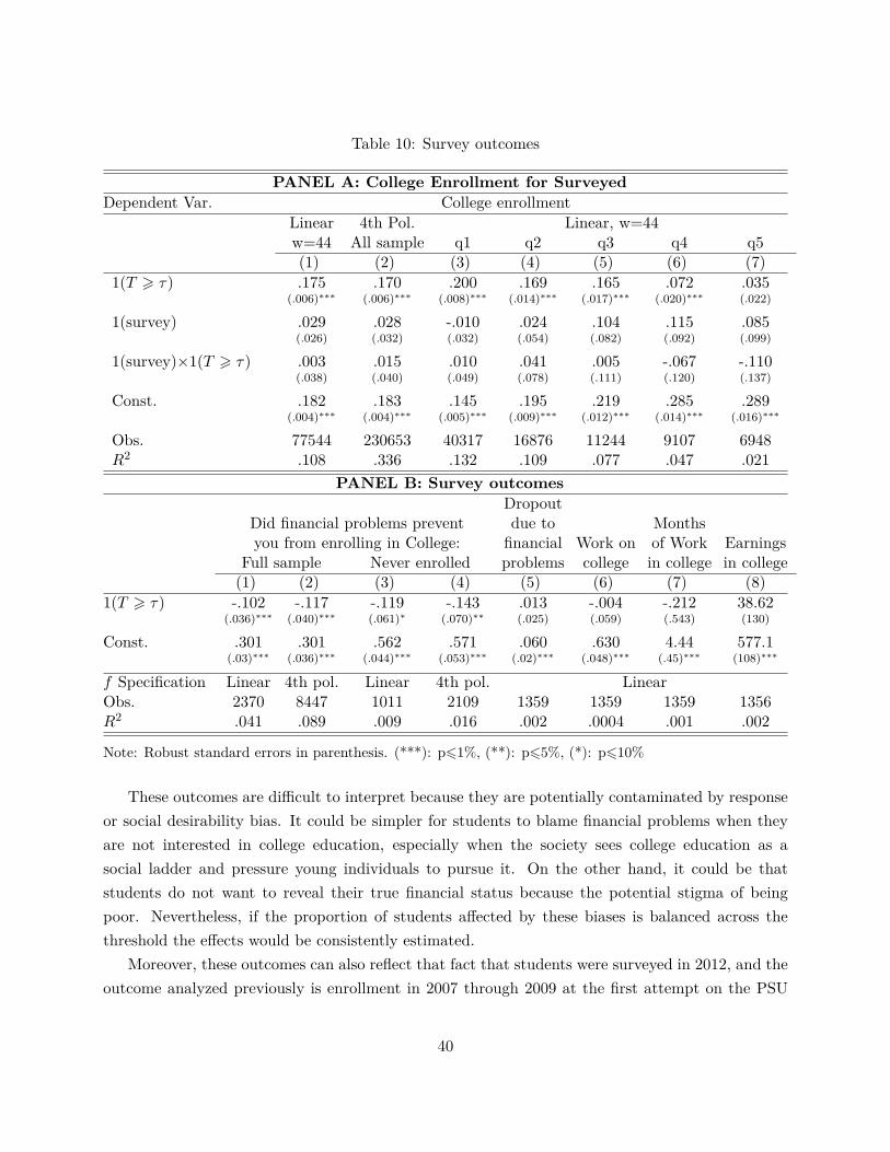
Table 10: Survey outcomes

PANEL A: College Enrollment for SurveyedDependent Var. College enrollment

Linear 4th Pol. Linear, w=44w=44 All sample q1 q2 q3 q4 q5(1) (2) (3) (4) (5) (6) (7)

1(T > τ) .175 .170 .200 .169 .165 .072 .035(.006)∗∗∗ (.006)∗∗∗ (.008)∗∗∗ (.014)∗∗∗ (.017)∗∗∗ (.020)∗∗∗ (.022)

1(survey) .029 .028 -.010 .024 .104 .115 .085(.026) (.032) (.032) (.054) (.082) (.092) (.099)

1(survey)×1(T > τ) .003 .015 .010 .041 .005 -.067 -.110(.038) (.040) (.049) (.078) (.111) (.120) (.137)

Const. .182 .183 .145 .195 .219 .285 .289(.004)∗∗∗ (.004)∗∗∗ (.005)∗∗∗ (.009)∗∗∗ (.012)∗∗∗ (.014)∗∗∗ (.016)∗∗∗

Obs. 77544 230653 40317 16876 11244 9107 6948R2 .108 .336 .132 .109 .077 .047 .021

PANEL B: Survey outcomesDropout

Did financial problems prevent due to Monthsyou from enrolling in College: financial Work on of Work Earnings

Full sample Never enrolled problems college in college in college(1) (2) (3) (4) (5) (6) (7) (8)

1(T > τ) -.102 -.117 -.119 -.143 .013 -.004 -.212 38.62(.036)∗∗∗ (.040)∗∗∗ (.061)∗ (.070)∗∗ (.025) (.059) (.543) (130)

Const. .301 .301 .562 .571 .060 .630 4.44 577.1(.03)∗∗∗ (.036)∗∗∗ (.044)∗∗∗ (.053)∗∗∗ (.02)∗∗∗ (.048)∗∗∗ (.45)∗∗∗ (108)∗∗∗

f Specification Linear 4th pol. Linear 4th pol. LinearObs. 2370 8447 1011 2109 1359 1359 1359 1356R2 .041 .089 .009 .016 .002 .0004 .001 .002


These outcomes are difficult to interpret because they are potentially contaminated by responseor social desirability bias. It could be simpler for students to blame financial problems when theyare not interested in college education, especially when the society sees college education as asocial ladder and pressure young individuals to pursue it. On the other hand, it could be thatstudents do not want to reveal their true financial status because the potential stigma of beingpoor. Nevertheless, if the proportion of students affected by these biases is balanced across thethreshold the effects would be consistently estimated.

Moreover, these outcomes can also reflect that fact that students were surveyed in 2012, and theoutcome analyzed previously is enrollment in 2007 through 2009 at the first attempt on the PSU

40

test. Many students who did not enroll in the first attempt enrolled in subsequent years, sometimesafter they score at least the cutoff in the following attempts on the PSU test. Therefore, studentsthat enrolled, but not in their first attempt are not asked why they did not in the first attempt.

With these problems in mind it is interesting to see that the magnitude of the effects across thethreshold is not statistically different than the increment in college enrollment presented previously,and this evidence goes in line with the idea that liquidity constraints are the most important causeof the difference in college enrollment across the cutoff.

Column (5) on Table 10, shows if the dropout decision is affected by access to the loan programs(question Q7 in the survey presented in figure 13). The reported results are conditional on havingenrolled in college once and therefore it suffers for at least two types of biases: small sample biasand selection bias. The former because only 13% of respondents have enrolled and dropout, andthe latter because those who enroll in college from below the cutoff are from families with higherincome and more educated backgrounds, which should bias the effects negatively. Contrary to theliquidity constraint hypothesis, the estimated effect is positive, but not significantly different thatzero. These results are consistent with those on Stinebrickner and Stinebrickner (2008) for the U.S.who find that credit constraints are not an important factor to determine dropout decisions.

Finally to investigate why students with access to the two loan program dropout less, and enrollin second and third year with higher probability than their counterfactual below the cutoff (seesection 4.4 below) I analyze answers to questions about work during college. Column (6) showsthat the probability of working during college, column (7) and (8) show the intensity of the workduring college, measured as the number of months during the year worked, and total earnings. Theliquidity constraint hypothesis predicts that access to loans would allow students to avoid workingin the intensive and extensive margins: Students that do not have access to loans (below the cutoff)would need to find a job and work more hours to fund their investments in college. Again theanalysis presented in this table, is conditional on having enrolled in college and therefore cannot beinterpreted as causal. The first two measures of work are consistent with the liquidity constrainthypotheses, and the third is not, although neither is significantly different than zero.

41

Table 11: RD Private College Enrollment by income quintile. By year and full sample. w = 44PSU points.

PANEL A: Regression by quintileDependent Var.: College Enrollment in year

Pooled07 to 09 2007 2008 2009(1) (2) (3) (4)

1(PSU>τ) x q1 .105 .107 .073 .125(.007)∗∗∗ (.011)∗∗∗ (.013)∗∗∗ (.011)∗∗∗

1(PSU>τ) x q2 .086 .097 .059 .112(.011)∗∗∗ (.020)∗∗∗ (.019)∗∗∗ (.020)∗∗∗

1(PSU>τ) x q3 .071 .085 .076 .060(.015)∗∗∗ (.025)∗∗∗ (.025)∗∗∗ (.027)∗∗

1(PSU>τ) x q4 .020 -.012 .019 .053(.018) (.026) (.032) (.032)∗

1(PSU>τ) x q5 .018 -.056 .048 .019(.020) (.040) (.028)∗ (.042)

q1 .100 .074 .120 .106(.004)∗∗∗ (.007)∗∗∗ (.008)∗∗∗ (.007)∗∗∗

q2 .140 .092 .159 .152(.008)∗∗∗ (.013)∗∗∗ (.013)∗∗∗ (.012)∗∗∗

q3 .173 .109 .175 .219(.010)∗∗∗ (.017)∗∗∗ (.018)∗∗∗ (.018)∗∗∗

q4 .219 .158 .242 .260(.013)∗∗∗ (.020)∗∗∗ (.024)∗∗∗ (.023)∗∗∗

q5 .231 .189 .209 .316(.014)∗∗∗ (.032)∗∗∗ (.018)∗∗∗ (.031)∗∗∗

Obs. 86463 24889 29404 32170R2 .206 .167 .204 .243Quintile PANEL B: Relative increaseq1 105% 145% 61% 118%q2 61% 105% 37% 74%q3 41% 78% 43% 27%q4 9% -8% 8% 20%q5 8% -30% 23% 6%


5.3 Responses for Differentiated Access to Credit Markets

The third test analyzes the different response of groups with differentiated access to credit markets.The price and the access effects can be decomposed by observing the different aggregate behaviorof these groups. The price effect can be obtained decomposed from the access effect by observing

42

the behavior of students from families that traditionally have had access to loans in the Chileanfinancial market.

As discussed in section 2, the fourth and fifth quintiles have access to private loans with interestrates similar to the SGL. The fourth quintile is also eligible for SGL and TUL, so the total effectfor that group is composed only of the price effect. Under the hypothesis that the price effect iszero, the inclusion of the SGL should not produce any change in the enrollment rate for the fourthquintile.

This hypothesis is tested using the enrollment rate in private universities where SGL is the onlyprogram available. Table 11 shows that there is no change in enrollment for the fourth quintile inprivate universities in 2007, 2009 and for all the sample pooled together and in 2008 the effects ismarginally significant. This confirms that SGL is equivalent to the loans in the conventional creditmarket (without price effect). Additionally, the larger response for the first two quintiles, which donot have access to other loans in the formal market, indicates that these effects are driven by theaccessibility of loans rather than a change in the price of education.41

Having access to the SGL implies a 105% increase in the probability of enrollment for the firstquintile, while the increment is 61% and 44% for quintiles two and three respectively, indicatingthat those with less financial opportunities are the ones driven the effects.

None of the three tests presented here are a perfect measure of how important the access effect is,but taken together they are evidence indicating that the results shown in the previous sections aremainly driven by the partial elimination of credit access restrictions for the lowest income quintiles.

6 Conclusions

In this paper, I exploit the sharp eligibility rules of two programs in Chile that give access totuition loans to students who score above a given threshold on the national college admission test.This enables a regression discontinuity design which, combined with full information on students’enrollment and financial aid benefits, and an admission system that weights only two observedvariables, allow the unbiased estimation of the causal effect of credit access on college enrollmentand progress.

The results around the cutoff show that, for every student who enrolls in college with no accessto loans, 2 students enroll when these loans are available. This change in enrollment is mainlydriven by students from families of the poorest three income quintiles. This enrollment effect isenhanced over time in the second and third years of college. For each student without access tothese loans who persists in the second and in third years, 3.1 and 5.5 students enroll in the secondand third year respectively when they do have access to these financial programs.

41Panel B of Table 11 gives the relative importance of these effects, the change in enrollment relative to the rate ofthose barely ineligible.

43

The results above are interpreted as the effects of access to credit markets on college enrollmentand college progress, because three different tests that decompose the total effect into price andaccess effects indicate that price component is very small to non-significantly different than zero.

Most strikingly, this paper shows that access to the loan programs appears to eliminate therelatively large income gradient in college enrollment and progress. Among students who are barelyineligible for loans, those coming from the richest quintile are twice as likely to enroll as studentsfrom the poorest income quintile, an enrollment gap very similar to the whole population. Incontrast, among students who are barely eligible, the gap is zero.

The same is true for enrollment in the second and third year. Students from the richest incomequintile are 3 and 8 times more likely to enroll compared to students from the poorest incomequintile in second and third year respectively when these loan programs are barely not available.On the contrary, among students that are barely eligible, there is no statistical difference betweenthe enrollment rates of the richest and the poorest students.

Around the threshold all baseline characteristics are balanced, including ability and family in-come, therefore, I conclude that access to financing explains almost entirely the enrollment and theeducational attainment gap between students with different family income (conditional on partici-pating in the admissions process and being at the cutoff).

The evidence shows that incomplete credit markets prevent students from low income familiesfrom investing in human capital. Credit access therefore has implications for the inter-generationaldistribution of education and income.

7 References

1. Attanasio, O. and K. M. Kaufmann, “Educational Choices, Subjective Expectations, andCredit Constraints,” NBER Working Papers #15087, 2009.

2. Becker, Gary S., “Human Capital and the Personal Distribution of Income”. (W. S. WoytinskiLecture) Ann Arbor Michigan: University of Michigan Press, 1967.

3. Belley, Philippe, and Lance Lochner, “The Changing Role of Family Income and Ability inDetermining Educational Achievement,” Journal of Human Capital, 1 (2007), 37–89.

4. Bettinger, Eric, “How Financial Aid Affects Persistence,” NBER Working Paper No. w10242,(2004).

5. Brown, Meta, John K. Scholz and Ananth Seshadri, “A New Test of Borrowing Constraintsfor Education,” Review of Economic Studies, 79 (2012), 511–538.

6. Canton, Erik, and Andreas Blom, “Student support and academic performance: Experiencesat private universities in Mexico” Education Economics, 18 (2010), 49–65.

44

7. Card, David, “The Causal Effect of Education on Earnings,” In O. Ashenfelter, and D. Card,eds., Handbook of Labor Economics, Vol. 3A (Amsterdam: Elsevier Science, North-Holland,1999), 1801–63.

8. ———, “Estimating the Return to Schooling: Progress on Some Persistent Econometric Prob-lems,” Econometrica, 69(2001), 1127–60.

9. Carneiro, Pedro, and James J. Heckman, “The Evidence on Credit Constraints in Post-secondary Schooling,” Economic Journal, 112 (2002), 705-34.

10. Cameron, Stephen, and James J. Heckman, “The Dynamics of Educational Attainment forBlack, Hispanic, and White Males,” Journal of Political Economy, 109 (2001), 455–99.

11. Cameron, Stephen, and Christopher Taber, “Estimation of Educational Borrowing ConstraintsUsing Returns to Schooling,” Journal of Political Economy, 112 (2004), 132-182.

12. Chen, Rong, “Financial Aid and Student Dropout in Higher Education: A HeterogeneousResearch Approach” in J. C. Smart, ed., Higher Education: Handbook of Theory and Research,Vol. 23 (Amsterdam: Elsevier Science, North-Holland, 2008), 209-239.

13. DesJardins, Stephen L., Dennis A. Ahlburg, and Brain P. McCall, “Simulating the Longitu-dinal Effects of Changes in Financial Aid on Student Departure from College,” The Journalof Human Resources. 37 (2002), 653-679.

14. Dinkelman, Taryn & Claudia. A. Martínez, “Investing in Schooling in Chile: The Role of In-formation about Financial Aid for Higher Education,” The Review of Economics and Statistics(forthcoming)

15. Dynarski, Susan M., “Does Aid Matter? Measuring the Effect of Student Aid on CollegeAttendance and Completion,” American Economic Review, 93 (2003), 279-288.

16. Gurgand, Marc, Adrien Lorenceau, and Thomas Melonio, “Student Loans: Liquidity Con-straint and Higher Education in South Africa,” Paris School of Economics working paper No.2011-20, 2011.

17. Hahn, Jinyong, Petra E. Todd, and Wilbert Van der Klaauw, “Identification and Estimation ofTreatment Effects with a Regression-Discontinuity Design,” Econometrica, 69 (2001), 201-209.

18. Heckman, James J., Thomas M. Lyons, and Petra. E. Todd, “Understanding Black-WhiteWage Differentials, 1960-1990,” The American Economic Review, 90 (2000), 344-349.

45

19. Hossler, Don, Mary Ziskin, Jacob P.K. Gross, Sooyeon Kim, and Osman. Cekic (2009) “Stu-dent Aid and Its Role in Encouraging Persistence” in J. Smart, ed., Higher Education: Hand-book of Theory and Research, Vol. 24, (Amsterdam: Elsevier Science, North-Holland, 2000),389-425.

20. Imbens, Guido W., and Karthik Kalyanaraman, “Optimal Bandwidth Choice for the Regres-sion Discontinuity Estimator,” The Review of Economic Studies, 79 (2012), 933–959.

21. Imbens, Guido W., and Thomas Lemieux, “Regression Discontinuity Designs: A Guide toPractice,” Journal of Econometrics, 142 (2008), 615–635.

22. Kane, Thomas J., “College Entry by Blacks since 1970: The Role of College Costs, FamilyBackground, and the Returns to Education,” Journal of Political Economy, 105 (1994), 878-911.

23. ———, “College Costs, Borrowing Constraints and the Timing of College Entry,” EasternEconomic Journal, 22 (1996), 181–94.

24. Keane, Michael P., and Kenneth I. Wolpin, “The Effect of Parental Transfers and BorrowingConstraints on Educational Attainment,” International Economic Review, 42 (2001), 1051-1103.

25. Lang, Kevin, “Ability Bias, Discount Rate Bias, and the Return to Education,” Manuscript.Department of Economics, Boston University, 1993.

26. Lee, David. S., “Randomized Experiments from Non-random Selection in U.S. House Elec-tions,” Journal of Econometrics, 142 (2008), 675–97.

27. Lee, David S., and Thomas Lemieux, “Regression Discontinuity Designs in Economics,” Jour-nal of Economic Literature, 48 (2010), 281–355.

28. Lochner, Lance J., and Alexander Monge-Naranjo, “The nature of credit constraints andhuman capital”, American Economic Review 101 (2011), 2487–2529.

29. ———, “Credit Constraints In Education” NBER Working Paper No. w17435, 2011.

30. Manski, Charles F., and David A. Wise, College Choice in America, Cambridge, MA. HarvardUniversity Press, 1983.

31. McCrary, Justin, “Manipulation of the Running Variable in the Regression DiscontinuityDesign: A Density Test” Journal of Econometrics, 142 (2008), 698–714.

46

32. McPherson, Michael S., and Morton O. Schapiro, “Does Student Aid Affect College Enroll-ment? New Evidence on a Persistent Controversy,” American Economic Review, 81 (1991),309-18.

33. Nielsen, Helena S., Torben Sørensen, and Christopher R. Taber, “Estimating the Effect ofStudent Aid on College Enrollment: Evidence from a Government Grant Policy Reform,”American Economic Journal: Economic Policy, 2 (2010), 185–215.

34. Rau, Tomás, Eugenio Rojas, and Sergio Urzúa. “Loans for Higher Education: Does the DreamCome True?”, NBER working paper no 19138 (2013)

35. Singell, Larry D., “Come and Stay a While: Does Financial Aid Effect Retention Conditionedon Enrollment at a Large Public University?,” Economics of Education Review, 23 (2004),459–71.

36. Solis, Alex. “Does Higher Education Cause Political Participation?: Evidence From a Regres-sion Discontinuity Design”. Mimeo (2013) (available athttp://alexsolis.webs.com/EducationonpoliticalparticipationNew.pdf)

37. Stinebrickner Ralph, and Todd Stinebrickner, “The Effect of Credit Constraints on the CollegeDrop-Out Decision: A Direct Approach Using a New Panel Study,” The American EconomicReview, 98 (2008), 2163-2184.

38. Van Der Klaauw, Wilbert, “Estimating the Effect of Financial Aid Offers on College enroll-ment: A Regression–Discontinuity Approach,” International Economic Review, 43 (2002),1249–1287.

39. Van Der Klaauw, Wilbert, “Regression–Discontinuity Analysis: A Survey of Recent Develop-ments in Economics,” Labour, 22 (2008), 219–245.

47

http://alexsolis.webs.com/EducationonpoliticalparticipationNew.pdf

A Appendix: Dropout Rates

Few papers try to document the causal effects of financial aid on retention conditional on enroll-ment and dropout rates. Exceptions are Dynarski (2003), Bettinger (2004), Singell (2004) andStinebrickner and Stinebrickner (2008), with mixed conclusions.

In this section, I study the effects of college loans on the dropout status of the students in thisquasi experiment. The main difference between these results and those in the previous section isthat here the sample is restricted to students who enrolled in college when they first took the PSUtest, while in the previous analysis the comparison was made with respect to all students aroundthe cutoff. This analysis shed light on the potential problems faced by the literature.

Because this section compares only students who self-selected into college around the cutoff,the estimates are no longer causal effects, but rather are correlations that can be illustrative incomparison to the previous results. First I check what types of biases are underlying the correlationsby comparing observable characteristics. Table 12 shows the estimation of equation (1) for the samegroup of covariates for students around the cutoff, with each column corresponding to those whoenrolled in 2007 through 2009. As expected, students without access to loans who enroll in collegeare different from those eligible for loans: they come from higher income families (indicated bythe income quintile and the self-reported income), suggesting that these students relied on familyresources to enroll; they have better educated parents and come from higher quality schools (morestudents from public schools above the cutoff, and more students from voucher schools below),which may indicate a higher preference for college education.

The available data does not provide a definitive measure of dropout status for the students.Some students may not enroll in one year but go back to finish their programs after some timeout. I will therefore use different definitions of dropout. The first definition, named “dropout after1 year” is an indicator function that takes the value 1 if a student enrolls after taking the PSUtest for the first time, but is not enrolled the year immediately after. Similarly, “dropout after 2years” takes the value of 1 if somebody enrolled in 2007, but was not enrolled in 2009. Becausethese definitions do not capture the possibility of coming back after some years of absence, I definea third measure of attrition. The variable “dropout in 2009” is an indicator variable that takes thevalue of 1 for any student who enrolled in 2007 or 2008 but was not enrolled in 2009, the last yearI observe the enrolling behavior of these students. This measure allow those who enroll in 2007to miss 2008 but come back in 2009, but do not capture those who may come back in later years.Finally, to distinguish between the first two definitions, I define a variable named “dropout in 2ndyear” to equal 1 if a student enrolled the first 2 years but did not show up in the third.

Table 13 reports the estimate of the same linear specification in a 2 stage least square settingto control for self-selection on the eligibility condition, adding as covariates all the observable char-acteristics to control for any selection on observables. Column (1) shows the dropout rate after the

48

first year of college. Students barely eligible for loans drop out 6 percentage points less frequentlythan ineligibles. The dropout rate for students without access to these loans is 19%; this impliesthat the probability of dropping out after the first year of college experiences a 31% decrease.

Column (2) shows the estimates for the definition “dropout in 2009” indicating that eligiblestudents drop out 5 percentage points less than constrained ones. Column (3) shows dropout ratesover a longer span of time: “dropout after 2 years of college.” Eligible students dropped out lessfrequently, by 11 percentage points. In relative terms, this effect implies a 38% decrease in thisdropout rate. Column (4) shows that the dropout rate does not fall significantly for the studentsenrolled in a second year, but the relative magnitudes confirm the previous result: there is a 26%reduction in the dropout probability.

These correlations help explain the long run enrollment results previously reported but theyalso help to reconcile results from the literature. One important issue is the selection process thatis evident here. Students who enroll in college are different than the underlying population, andtherefore the effects estimated from the sample conditional on enrollment present a bias towardszero. In this case, the dropout results are much smaller than the results from enrollment andprogress which are due to family income compensating for access to loans. Nevertheless, they arerelatively large and highly significant.

49

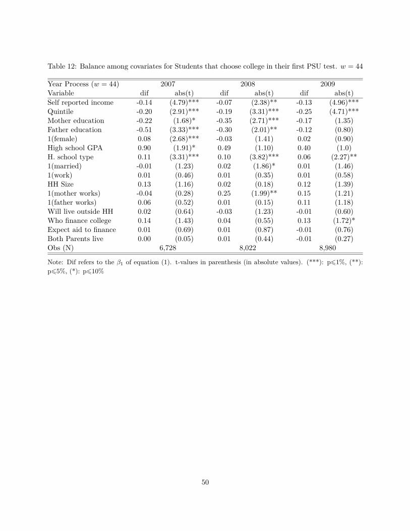
Table 12: Balance among covariates for Students that choose college in their first PSU test. w = 44

Year Process (w = 44) 2007 2008 2009Variable dif abs(t) dif abs(t) dif abs(t)Self reported income -0.14 (4.79)*** -0.07 (2.38)** -0.13 (4.96)***Quintile -0.20 (2.91)*** -0.19 (3.31)*** -0.25 (4.71)***Mother education -0.22 (1.68)* -0.35 (2.71)*** -0.17 (1.35)Father education -0.51 (3.33)*** -0.30 (2.01)** -0.12 (0.80)1(female) 0.08 (2.68)*** -0.03 (1.41) 0.02 (0.90)High school GPA 0.90 (1.91)* 0.49 (1.10) 0.40 (1.0)H. school type 0.11 (3.31)*** 0.10 (3.82)*** 0.06 (2.27)**1(married) -0.01 (1.23) 0.02 (1.86)* 0.01 (1.46)1(work) 0.01 (0.46) 0.01 (0.35) 0.01 (0.58)HH Size 0.13 (1.16) 0.02 (0.18) 0.12 (1.39)1(mother works) -0.04 (0.28) 0.25 (1.99)** 0.15 (1.21)1(father works) 0.06 (0.52) 0.01 (0.15) 0.11 (1.18)Will live outside HH 0.02 (0.64) -0.03 (1.23) -0.01 (0.60)Who finance college 0.14 (1.43) 0.04 (0.55) 0.13 (1.72)*Expect aid to finance 0.01 (0.69) 0.01 (0.87) -0.01 (0.76)Both Parents live 0.00 (0.05) 0.01 (0.44) -0.01 (0.27)Obs (N) 6,728 8,022 8,980

Note: Dif refers to the β1 of equation (1). t-values in parenthesis (in absolute values). (***): p61%, (**):p65%, (*): p610%

50

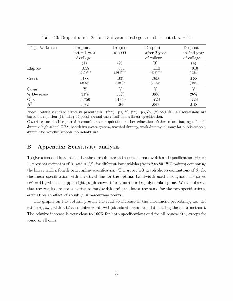
Table 13: Dropout rate in 2nd and 3rd years of college around the cutoff. w = 44

Dep. Variable : Dropout Dropout Dropout Dropoutafter 1 year in 2009 after 2 year in 2nd yearof college of college of college

(1) (2) (3) (4)Eligible -.058 -.051 -.110 -.010

(.017)∗∗∗ (.018)∗∗∗ (.033)∗∗∗ (.024)

Const. .188 .201 .293 .038(.099)∗ (.105)∗ (.155)∗ (.124)

Covar Y Y Y Y% Decrease 31% 25% 38% 26%Obs. 14750 14750 6728 6728R2 .032 .04 .067 .018

Note: Robust standard errors in parenthesis. (***): p61%, (**): p65%, (*):p610%. All regressions arebased on equation (1), using 44 point around the cutoff and a linear specification.Covariates are “self reported income”, income quintile, mother education, father education, age, femaledummy, high school GPA, health insurance system, married dummy, work dummy, dummy for public schools,dummy for voucher schools, household size.

B Appendix: Sensitivity analysis

To give a sense of how insensitive these results are to the chosen bandwidth and specification, Figure11 presents estimates of β1 and β1/β0 for different bandwidths (from 2 to 80 PSU points) comparingthe linear with a fourth order spline specification. The upper left graph shows estimations of β1 forthe linear specification with a vertical line for the optimal bandwidth used throughout the paper(w∗ = 44), while the upper right graph shows it for a fourth order polynomial spline. We can observethat the results are not sensitive to bandwidth and are almost the same for the two specifications,estimating an effect of roughly 18 percentage points.

The graphs on the bottom present the relative increase in the enrollment probability, i.e. theratio (β1/β0), with a 95% confidence interval (standard errors calculated using the delta method).The relative increase is very close to 100% for both specifications and for all bandwidth, except forsome small ones.

51

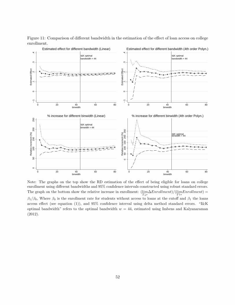
Figure 11: Comparison of different bandwidth in the estimation of the effect of loan access on collegeenrollment.

I&K optimalbandwidth = 44

−.1

0.1

.2.3

.4E

stim

ated

Effe

ct

0 20 40 60 80binwidth

Estimated effect for different bandwidth (Linear)

I&K optimalbandwidth = 44

−.1

0.1

.2.3

.4E

stim

ated

Effe

ct

0 20 40 60 80binwidth

Estimated effect for different bandwidth (4th order Polyn.)

I&K optimalbinwidth = 44

050

100

150

200

250

Rel

ativ

e in

crem

ent (

%)

0 20 40 60 80binwidth

% increase for different binwidth (Linear)

I&K optimalbinwidth = 44

050

100

150

200

250

Rel

ativ

e in

crem

ent (

%)

0 20 40 60 80binwidth

% increase for different binwidth (4th order Polyn.)

Note: The graphs on the top show the RD estimation of the effect of being eligible for loans on collegeenrollment using different bandwidths and 95% confidence intervals constructed using robust standard errors.The graph on the bottom show the relative increase in enrollment: (lim

T↓τ∆Enrollment)/(lim

T↑τEnrollment) =

β1/β0, Where β0 is the enrollment rate for students without access to loans at the cutoff and β1 the loansaccess effect (see equation (1)), and 95% confidence interval using delta method standard errors. “I&Koptimal bandwidth” refers to the optimal bandwidth w = 44, estimated using Imbens and Kalyanaraman(2012).

52

C Appendix: Analysis by quintile for the whole population

To determine how important access to tuition loans is explaining the college enrollment gap byfamily income is necessary to estimate enrollment by income quintile. Unfortunately in the dataused in this paper the income quintile information is only available for those students that completedthe FUAS form. Hence the analysis in section 4.3 uses the sub-sample of individuals that competedthat socioeconomic form. In this appendix I estimate the income quintile for the whole populationusing all characteristics available for the students. I performed an estimation of the income quintileusing the sample with the information and performed an out of sample prediction for those with noinformation.

The effects of enrollment by income quintile calculated in this way are almost identical thanthose reported in section 4.3.

Figure 12: Effects on College Enrollment. By income quintiles (predicted using self reported incomecategory)

All q1 q2 q3 q4 q5(1) (2) (3) (4) (5) (6)

1(T > τ) .003 -.003 .002 .002 .020 .010(.006) (.006) (.015) (.019) (.021) (.017)

Const. .158 .088 .125 .192 .228 .327(.004)∗∗∗ (.004)∗∗∗ (.010)∗∗∗ (.013)∗∗∗ (.015)∗∗∗ (.012)∗∗∗

Pre-selected .025 .058 .071 .032 .059(.005)∗∗∗ (.006)∗∗∗ (.013)∗∗∗ (.017)∗ (.020)∗∗∗

Pre-selected×1(T> τ) .172 .202 .168 .162 .051(.008)∗∗∗ (.010)∗∗∗ (.020)∗∗∗ (.025)∗∗∗ (.029)∗

Obs. 150356 74412 24701 18534 15838 12163R2 .101 .151 .129 .083 .045 .018

Note: Robust standard errors in parenthesis. (***): p61%, (**): p65%, and (*): p610%.

53

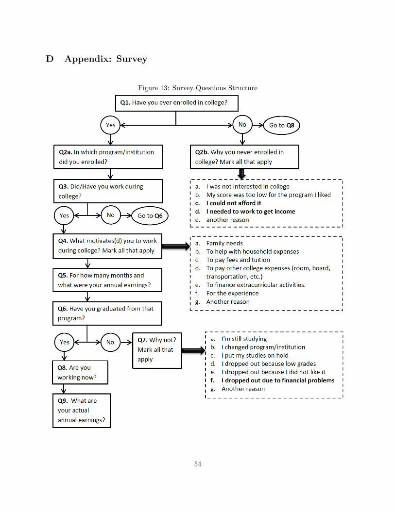
D Appendix: Survey

Figure 13: Survey Questions Structure

54

WORKING PAPERS*

Editor: Nils Gottfries

2012:5 Pedro Carneiro and Rita Ginja, Long Term Impacts of Compensatory

Preschool on Health and Behavior: Evidence from Head Start. 82 pp.

2012:6 Magnus Carlsson and Stefan Eriksson, Do Reported Attitudes towards

Immigrants Predict Ethnic Discrimination? 23 pp.

2012:7 Mikael Bask and Christian R. Proaño, Optimal Monetary Policy under

Learning in a New Keynesian Model with Cost Channel and Inflation Inertia.

25 pp.

2012:8 Mikael Elinder and Oscar Erixson, Every man for himself. Gender, Norms

and Survival in Maritime Disasters. 78 pp.

2012:9 Bertil Holmlund, Wage and Employment Determination in Volatile Times:

Sweden 1913–1939. 43 pp.

2012:10 Indraneel Chakraborty, Hans A. Holter and Serhiy Stepanchuk, Marriage

Stability, Taxation and Aggregate Labor Supply in the U.S. vs. Europe. 63

pp.

2012:11 Niklas Bengtsson, Bertil Holmlund and Daniel Waldeström, Lifetime versus

Annual Tax Progressivity: Sweden, 1968–2009. 56 pp.

2012:12 Martin Jacob and Jan Södersten, Mitigating shareholder taxation in small

open economies? 16 pp.

2012:13 John P. Conley, Ali Sina Önder and Benno Torgler, Are all High-Skilled

Cohorts Created Equal? Unemployment, Gender, and Research Productivity.

19 pp.

2012:14 Che-yan Liang and Mattias Nordin, The Internet, News Consumption, and

Political Attitudes. 29 pp.

2012:15 Krzysztof Karbownik and Michal Myck, For some mothers more than others:

how children matter for labour market outcomes when both fertility and

female employment are low. 28 pp.

2012:16 Karolina Stadin, Vacancy Matching and Labor Market Conditions. 51 pp.

2012:17 Anne Boschini, Jan Pettersson, Jesper Roine, The Resource Curse and its

Potential Reversal. 46 pp.

2012:18 Gunnar Du Rietz, Magnus Henrekson and Daniel Waldenström, The Swedish

Inheritance and Gift Taxation, 1885–2004. 47pp.

* A list of papers in this series from earlier years will be sent on request by the department.

2012:19 Helge Bennmarker, Erik Grönqvist and Björn Öckert, Effects of contracting

out employment services: Evidence from a randomized experiment. 55 pp.

2012:20 Pedro Carneiro and Rita Ginja, Partial Insurance and Investments in

Children. 32pp.

2013:1 Jan Pettersson and Johan Wikström, Peeing out of poverty? Human fertilizer

and the productivity of farming households. 43 pp.

2013:2 Olof Åslund and Mattias Engdahl, The value of earning for learning:

Performance bonuses in immigrant language training. 52 pp.

2013:3 Michihito Ando, Estimating the effects of nuclear power facilities on local

income levels: A quasi-experimental approach. 44 pp.

2013:4 Matz Dahlberg, Karin Edmak and Heléne Lundqvist, Ethnic Diversity and

Preferences for Redistribution: Reply. 23 pp.

2013:5 Ali Sina Önder and Marko Terviö, Is Economics a House Divided? Analysis

of Citation Networks. 20 pp.

2013:6 Per Engström and Eskil Forsell, Demand effects of consumers' stated and

revealed preferences. 27 pp.

2013:7 Che-Yuan Liang, Optimal Inequality behind the Veil of Ignorance. 26 pp.

2013:8 Pia Fromlet, Monetary Policy Under Discretion Or Commitment? -An

Empirical Study. 57 pp.

2013:9 Olof Åslund and Mattias Engdahl, Open borders, transport links and local

labor markets. 41 pp.

2013:10 Mohammad Sepahvand, Roujman Shahbazian and Ranjula Bali Swain, Time

Investment by Parents in Cognitive and Non-cognitive Childcare Activities.

31 pp.

2013:11 Miia Bask and Mikael Bask, Social Influence and the Matthew Mechanism:

The Case of an Artificial Cultural Market. 13 pp

2013:12 Alex Solis, Credit access and college enrollment. 54 pp

See also working papers published by the Office of Labour Market Policy Evaluation

http://www.ifau.se/ ISSN 1653-6975

http://www.ifau.se/

core.ac.uk · student who enrolls in the third year of college without access to credit markets,...

Documents

Transcript of core.ac.uk · student who enrolls in the third year of college without access to credit markets,...