econstor www.econstor.eu

Der Open-Access-Publikationsserver der ZBW – Leibniz-Informationszentrum WirtschaftThe Open Access Publication Server of the ZBW – Leibniz Information Centre for Economics

Standard-Nutzungsbedingungen:

Die Dokumente auf EconStor dürfen zu eigenen wissenschaftlichenZwecken und zum Privatgebrauch gespeichert und kopiert werden.

Sie dürfen die Dokumente nicht für öffentliche oder kommerzielleZwecke vervielfältigen, öffentlich ausstellen, öffentlich zugänglichmachen, vertreiben oder anderweitig nutzen.

Sofern die Verfasser die Dokumente unter Open-Content-Lizenzen(insbesondere CC-Lizenzen) zur Verfügung gestellt haben sollten,gelten abweichend von diesen Nutzungsbedingungen die in der dortgenannten Lizenz gewährten Nutzungsrechte.

Terms of use:

Documents in EconStor may be saved and copied for yourpersonal and scholarly purposes.

You are not to copy documents for public or commercialpurposes, to exhibit the documents publicly, to make thempublicly available on the internet, or to distribute or otherwiseuse the documents in public.

If the documents have been made available under an OpenContent Licence (especially Creative Commons Licences), youmay exercise further usage rights as specified in the indicatedlicence.

zbw Leibniz-Informationszentrum WirtschaftLeibniz Information Centre for Economics

Autor, David; Dorn, David; Hanson, Gordon H.; Song, Jae

Working Paper

Trade Adjustment: Worker Level Evidence

IZA Discussion Papers, No. 8514

Provided in Cooperation with:Institute for the Study of Labor (IZA)

Suggested Citation: Autor, David; Dorn, David; Hanson, Gordon H.; Song, Jae (2014) : TradeAdjustment: Worker Level Evidence, IZA Discussion Papers, No. 8514

This Version is available at:http://hdl.handle.net/10419/103478

DI

SC

US

SI

ON

P

AP

ER

S

ER

IE

S

Forschungsinstitut zur Zukunft der ArbeitInstitute for the Study of Labor

Trade Adjustment: Worker Level Evidence

IZA DP No. 8514

September 2014

David H. AutorDavid DornGordon H. HansonJae Song

Trade Adjustment: Worker Level Evidence

David H. Autor MIT, NBER and IZA

David Dorn

University of Zurich and IZA

Gordon H. Hanson UCSD, NBER and IZA

Jae Song

U.S. Social Security Administration

Discussion Paper No. 8514 September 2014

IZA

P.O. Box 7240 53072 Bonn

Germany

Phone: +49-228-3894-0 Fax: +49-228-3894-180

E-mail: iza@iza.org

Any opinions expressed here are those of the author(s) and not those of IZA. Research published in this series may include views on policy, but the institute itself takes no institutional policy positions. The IZA research network is committed to the IZA Guiding Principles of Research Integrity. The Institute for the Study of Labor (IZA) in Bonn is a local and virtual international research center and a place of communication between science, politics and business. IZA is an independent nonprofit organization supported by Deutsche Post Foundation. The center is associated with the University of Bonn and offers a stimulating research environment through its international network, workshops and conferences, data service, project support, research visits and doctoral program. IZA engages in (i) original and internationally competitive research in all fields of labor economics, (ii) development of policy concepts, and (iii) dissemination of research results and concepts to the interested public. IZA Discussion Papers often represent preliminary work and are circulated to encourage discussion. Citation of such a paper should account for its provisional character. A revised version may be available directly from the author.

IZA Discussion Paper No. 8514 September 2014

ABSTRACT

Trade Adjustment: Worker Level Evidence* We analyze the effect of exposure to international trade on earnings and employment of U.S. workers from 1992 through 2007 by exploiting industry shocks to import competition stemming from China’s spectacular rise as a manufacturing exporter paired with longitudinal data on individual earnings by employer spanning close to two decades. Individuals who in 1991 worked in manufacturing industries that experienced high subsequent import growth garner lower cumulative earnings, face elevated risk of obtaining public disability benefits, and spend less time working for their initial employers, less time in their initial two-digit manufacturing industries, and more time working elsewhere in manufacturing and outside of manufacturing. Earnings losses are larger for individuals with low initial wages, low initial tenure, and low attachment to the labor force. Low-wage workers churn primarily among manufacturing sectors, where they are repeatedly exposed to subsequent trade shocks. High-wage workers are better able to move across employers with minimal earnings losses, and are more likely to move out of manufacturing conditional on separation. These findings reveal that import shocks impose substantial labor adjustment costs that are highly unevenly distributed across workers according to their skill levels and conditions of employment in the pre-shock period. JEL Classification: F16, H55, J23, J31, J63 Keywords: trade flows, labor demand, earnings, job mobility, social security programs Corresponding author: David Autor Department of Economics MIT 40 Ames Street, E17-216 Cambridge, MA 02142 USA E-mail: dautor@mit.edu

* Forthcoming in Quarterly Journal of Economics. We thank Stéphane Bonhomme, David Card, Pinelopi Goldberg, Lawrence Katz, Patrick Kline, Brian Kovak and numerous seminar and conference participants for valuable comments, and Gerald Ray and David Foster of the U.S. Social Security Administration for facilitating data access and staff research time for this project. Jan Bietenbeck provided valuable research assistance. Dorn acknowledges funding from the Spanish Ministry of Science and Innovation (ECO2010-16726 and JCI2011-09709). Autor and Hanson acknowledge funding from the National Science Foundation (grant SES-1227334). The findings and conclusions expressed herein are those of the authors and do not represent the views of the Social Security Administration.

Introduction

Among the most significant recent changes in the global economy is the rapid emergence of China

from a technologically backward and largely closed economy to the world’s third largest manu-

facturing producer in the space of just two decades. Between 1990 and 2000, the share of world

manufacturing exports originating in China increased from 2% to 5%, and then accelerated to 12%

in 2007 and to 16% in 2011 (Figure I). For U.S. manufacturing, China’s expanding role in global

trade represents a substantial competitive shock. Not only is China’s export growth concentrated

in manufacturing—the sector that still accounts for the majority of U.S. trade—but its growth in

imports, in particular from the United States and other high income countries, has been sluggish,

thus leading to large trade imbalances. During the last decade, China’s average current account

surplus was 5% of GDP, the mirror image of the U.S. current account deficit over the period. As

Chinese imports to the United States surged, U.S. manufacturing employment underwent a historic

contraction. Although the level of employment in U.S. manufacturing had been declining modestly

since the start of the 1980s, this trend gained pace in the mid-1990s and accelerated sharply in the

2000s: the number of workers employed in U.S. manufacturing fell by 9.7 percentage points between

1991 and 2001 and by an additional 16.1 percentage points between 2001 and 2007.1

In this paper, we examine how exposure to rising competition from China affects the employment

and earnings trajectories of U.S. workers over the medium to long run. We define trade exposure

as the growth in U.S. imports from China over 1991 to 2007 that occurred in a worker’s initial

industry of affiliation. By categorizing workers according to their sector of employment at the time

the shock commences, we isolate the extended consequences of exposure to import competition and

avoid selection problems arising from the post-shock re-sorting of workers across industries.2 The

choice of the outcome period is dictated on the front end by the availability of bilateral trade data

that can be matched to U.S. manufacturing industries and on the back end by the onset of the

Great Recession, which severely battered U.S. manufacturing. These years span much of China’s

export boom, as the 1990s and especially the early 2000s—following China’s entry into the WTO

in 2001—were the years when the country’s export growth accelerated.

Using individual-level, longitudinal data from the U.S. Social Security Administration, we esti-

mate the impact of exposure to Chinese import competition on cumulative earnings, employment,

movement across sectors, movement across regions, and receipt of Social Security benefits over the1Using County Business Patterns data, we calculate that U.S. manufacturing employment was 18.3 million in 1991,

16.6 million in 2001, 13.9 million in 2007, and 11.4 million in 2011.2Our approach using longitudinal data is comparable to Walker (2012) and Hummels, Jorgensen, Munch, and

Xiang (2013), and is also related to Menezes-Filho and Muendler (2011).

1

period 1992 to 2007. The data permit us to decompose worker employment spells by firm, industry,

and place of residence, and to examine variation in trade impacts according to worker and firm

characteristics.3 To account for possible correlation between industry imports and industry domes-

tic demand or productivity shocks, we instrument for the change in U.S. imports from China using

import growth in other high income countries within 397 harmonized manufacturing industries.4

Key to our identification strategy is that China’s growth over the period appears to be driven

by rapid improvements in industrial production resulting from rising TFP, capital accumulation,

migration to urban areas, and enhancements in infrastructure, each of which was a consequence

of its transition to a more market-oriented economy (Naughton [2007]; Hsieh and Klenow [2009];

Hsieh and Ossa [2011]).5 Brandt, van Biesebroeck and Zhang (2012) estimate that over the period

1998 to 2007, China had average annual TFP growth in manufacturing of 8.0%. In the same time

frame, China accounted for an astonishing three quarters of worldwide growth in manufacturing

value added that occurred in low and middle-income nations (Hanson [2012]).

Our work contributes to the rapidly developing literature on the labor market consequences of

globalization, much of which focuses on the consequences of international competition for wages

and employment at the firm, industry, or region level.6 Concerning China’s impact on U.S. labor

markets, recent findings imply that greater import exposure results in higher rates of plant exit and

more rapid declines in plant employment (Bernard, Jensen, and Schott [2006]), larger decreases in

manufacturing employment and increases in unemployment and labor force non-participation rates

in regions that specialize in industries in which China’s presence is strong (Autor, Dorn, and Hanson

[2013a]), and larger employment declines in industries in which the threat of reversion to high import

barriers was erased by China’s joining the WTO (Pierce and Schott [2013]).

The current paper extends the literature on labor market impacts of trade by shifting the focus

from aggregate market level reactions to adjustments at the worker level. By estimating the difference

in outcomes among workers who ex ante are observationally similar except for their industry of

employment, our analysis captures variation in the incidence of trade-induced disruptions to earnings

and employment caused by proximity to the shock.7 Implicitly, this variation in incidence arises3Limitations of the SSA data include not recording hours worked, within-year spells of unemployment, or receipt

of government benefits other than through Social Security.4Our identification strategy follows Autor, Dorn, and Hanson (2013a) and Bloom, Draca, and Van Reenen (2011).5China’s export growth is the culmination of a sequence of reforms that began in the 1980s. Naughton (1996)

marks 1984 as the year that China’s tilt toward exports initiated. In 1992, China launched a further wave of reformsthat welcomed foreign direct investment and promoted Special Economic Zones. China’s 2001 WTO entry solidifiedits most-favored-nation status in the United States, though it had enjoyed de facto MFN status since 1980.

6See Amiti and Davis (2012) and Hummels, Jorgensen, Munch, and Xiang (2013) on trade and firms; Artuc,Chaudhuri, and McLaren (2010) and Ebenstein, Harrison, McMillan, and Phillips (2011) on trade and industries; andChiquiar (2008), Topalova (2010), and Kovak (2013) on trade and regions.

7For structural analyses of trade shocks and labor market dynamics in the presence of search frictions and entry

2

from frictions to moving workers between jobs, since, absent such frictions, wages would equalize for

similar workers at all moments of time and we would detect no earnings differences across workers

either in the short or long run. Though our approach prevents us from estimating the impact of trade

on equilibrium employment or wages for entire skill groups, it allows us to quantify the distribution

of incidence among workers along four margins of worker adjustment: the change in earnings at

the initial employer (intensive margin), the change in earnings associated with job loss (extensive

margin), the change in earnings associated with uptake of government benefits (transfer margin),

and the change in earnings associated with moving between employers, industries, and/or regions

(reallocation margin). Decomposing changes in earnings across these margins reveals where in the

adjustment process frictions arise and which types of workers face larger adjustment burdens.

The research we present also relates to an influential literature on the long run consequences of

job loss. In pioneering work, Jacobsen, LaLonde, and Sullivan (1993) draw on administrative data

to identify episodes in which plants engage in mass layoffs, meaning that they dismiss a substantial

fraction of their employees within a short time span.8 While we follow this literature in using

administrative data to examine the long-run effects of shocks on worker outcomes, we break from

it by focusing on the specific shock of China’s export growth. It is by identifying the source of the

shock that we see worker adjustment along intensive, extensive, transfer and reallocation margins.

To preview the results, we find that workers more exposed to trade with China exhibit lower cu-

mulative earnings and employment and higher receipt of Social Security Disability Insurance (SSDI)

over the sample window of 1992 through 2007. The difference between a manufacturing worker at

the 75th percentile of industry trade exposure and one at the 25th percentile of exposure amounts

to cumulative earnings reductions of 46% of initial yearly income and to one-half of an additional

month where payments from SSDI are the main source of income. Trade exposure increases job

churning across firms, industries, and sectors. More exposed workers spend less time working for

their initial employer, less time working in their initial two-digit manufacturing industry, and more

time working elsewhere in manufacturing and outside manufacturing altogether.

The magnitudes of job churn and adjustment in earnings and employment differ substantially

across demographic groups. Workers with lower labor force attachment, shorter tenure, and lower

earnings incur larger losses in subsequent earnings and employment, while losses for workers with

and exit costs, see Helpman, Itskhoki, and Redding (2010), Helpman, Itskhoki, Muendler, and Redding (2012), Coşar(2011), Dix-Carneiro (2014), and Coşar, Guner and Tybout (2011).

8See also Sullivan and von Wachter (2009), von Wachter, Song, and Manchester (2009), and Couch and Placzek(2010) for recent work that uses administrative data, and see Neal (1995), Parent (2000), and Chan and Stevens(2001) for representative work on job loss using survey data. An alternative approach to study job loss uses the CPSDisplaced Workers Survey (DWS) (e.g., Addison, Fox, and Ruhm [1995]; Kletzer [2000]; Farber [2005]).

3

high initial earnings are modest.9 Distinct from their high-wage counterparts, low-wage workers

churn primarily among manufacturing industries, where they remain exposed to trade shocks.

Import competition is but one of the forces impinging on U.S. manufacturing. Technological

progress has been rapid in computer and skill intensive sectors (Doms, Dunne, and Troske [1997];

Autor, Katz, and Krueger [1998]), and to the degree this is correlated with industry trade exposure,

it poses a potential confound for our identification strategy.10 To capture industry exposure to

technical change, we control for capital and technology intensity, as well as industry pre-trends in

employment and wages. We further perform falsification tests to verify that future increases in

trade exposure do not predict past changes in worker outcomes. These robustness tests support the

interpretation that our identification strategy isolates industry level shocks caused by rising import

competition rather than other temporal confounds. Our results are also robust to a broad set of

alternative measures of trade exposure to China.

Our analysis complements Autor, Dorn, and Hanson (2013a), who estimate changes in employ-

ment and average earnings across U.S. local labor markets resulting from regional exposure to import

competition from China. Because that work uses repeated cross sections on geographic localities, it

cannot address how individuals adjust to trade shocks. We are able to measure worker-level con-

sequences by focusing on the substantial differences in trade exposure that derive from the initial

industry of employment. In alternative specifications, we also control for trade exposure operating

through workers’ regions of residence, although variation in geographic exposure to trade is less well

measured in our data. Consistent with Autor, Dorn, and Hanson (2013a), we find little evidence

that geographic mobility is an important mechanism through which trade adjustment operates.

We begin by documenting our approach to estimating the effects of exposure to trade shocks

and describing the data. Section 2 provides estimates of the impact of trade shocks on cumulative

earnings, employment, and benefit receipts for high-attachment workers. Section 3 examines het-

erogeneity in the consequences of trade shocks by individual characteristics and conditions of initial

employment. Section 4 explores alternative measures of trade exposure, and section 5 concludes.

1 Motivation, Identification and Data

We examine changes in outcomes for workers over the 1992 to 2007 period that are associated

with exposure to growing imports from China. The context for our analysis is one in which China9These results contrast with earlier literature, which finds that earnings losses for affected workers are relatively

uniform across worker type (e.g., Jacobson, LaLonde and Sullivan [1993]; von Wachter, Manchester and Song [2009]).10Reassuringly, Autor, Dorn and Hanson (2013b,c) find that across U.S. local labor markets, exposure to import

competition and exposure to computerization are essentially uncorrelated.

4

experiences productivity growth, factor accumulation, and reductions in trade costs, which lead its

exports to expand. Trade theory predicts how such shocks affect wages in China, the United States,

and the rest of the world (e.g., Hsieh and Ossa [2011]; di Giovanni, Levchenko, and Zhang [2011]).

Our interest here is reduced form and relatively narrow in focus: we seek to capture the changes in

earnings and employment that workers in exposed industries encounter when adjusting to the shock.

1.1 Industry Trade Shocks

As theoretical motivation, consider an economy with two sectors, one that is directly exposed to

trade shocks in the rest of the world and one that is not.11 In the long run, but not necessarily the

short run, labor is mobile between sectors, equalizing wages for similarly skilled workers. Implicitly,

non-labor factors are immobile across sectors, as in the specific factors model (Feenstra [2004]).

Suppose that productivity growth abroad causes product demand to fall for the economy’s trade

exposed industry. The immediate impact is to reduce the industry’s demand for labor, causing its

nominal wages to fall and inducing some of its workers to relocate to the unexposed sector. If there

are frictions in moving labor between industries, adjustment will be slow, forcing nominal wages in

the exposed industry to remain below those in the non-exposed industry during the transition. Over

time, labor will continue to exit the exposed sector until inter-industry wages are again equilibrated.

Summing worker earnings over the pre-shock, shock, and post-shock periods, nominal and real

cumulative incomes for workers initially employed in the exposed sector will be less than for workers

initially employed in the unexposed sector. The resulting earnings differences, attributable entirely

to the transitional phase, are increasing in the extent of labor immobility across sectors in both the

short and medium run. This effect on cumulative earnings, and the associated churning in workers

across employers, industries and possibly regions, are the focus of our empirical analysis.

Empirically, we capture shocks to foreign export supply using changes in China’s presence in the

U.S. market. Our baseline measure of trade exposure is the change in the import penetration ratio

for a U.S. industry over the period 1991 to 2007, defined as

�IP j,⌧ =�MUC

j,⌧

Yj,91 +Mj,91 � Ej,91, (1)

where for U.S. industry j, �MUCj⌧ is the change in imports from China over the period 1991 to

2007 and Yj0 +Mj0 �Ej0 is initial absorption (measured as industry shipments, Yj0, plus industry

imports, Mj0, minus industry exports, Ej0). We choose 1991 as the initial year as it is the earliest11An online theoretical appendix provides the formal analysis underlying this discussion.

5

period for which we have disaggregated bilateral trade data for a large number of country pairs that

we can match to U.S. manufacturing industries.

A natural concern with equation (1) as a measure of trade exposure is that observed changes

in the import penetration ratio may in part reflect domestic shocks to U.S. industries. Even if

the factors driving China’s export growth are internal supply shocks, U.S. industry import demand

shocks may still contaminate observed bilateral trade flows. To capture the China supply-driven

component in U.S. imports from China, we instrument for trade exposure in (1) with the variable

�IPOj⌧ =�MOC

j,⌧

Yj,88 +Mj,88 �Xj,88, (2)

where �MOCj,⌧ is the change in imports from China from 1991 to 2007 in non-U.S. high income

countries, based on the industry in which the worker was employed in 1988, three years prior to the

base year.12 We use industry of employment in 1988, rather than 1991, to account for worker sorting

across industries in anticipation of future trade with China. The motivation for the instrument in

(2) is that high income economies are similarly exposed to growth in Chinese imports that is driven

by supply shocks originating in China.13 Thus, the identifying assumption is that industry import

demand shocks are weakly correlated across high-income economies. In an online appendix, we

regress the value in (1) on the value in (2), which is equivalent to the first-stage regression in the

estimation without controls. The coefficient is 0.855 and the t-statistic and R-squared are 9.20 and

0.34, indicating the strong predictive power of import growth in other high income countries for U.S.

import growth from China.

A potential threat to our identification strategy is that product demand shocks are correlated

across high-income countries, implying that our IV estimates may be contaminated by correlation

between import growth and unobserved components of product demand. This would tend to bias a

negative impact of trade exposure on earnings and employment toward zero. To help address this

concern, we alternatively measure the change in trade exposure using a gravity-based strategy, which

captures changes in China’s industry productivity relative to changes in U.S. industry productivity,

akin to the change in China-U.S. comparative advantage. The gravity approach neutralizes demand

conditions in importing countries by using the change in China’s exports relative to U.S. exports

within destination markets, helping isolate supply and trade-cost-driven changes in China’s export12These countries are Australia, Denmark, Finland, Germany, Japan, New Zealand, Spain, and Switzerland, which

are the high income countries for which we can obtain disaggregated bilateral HS trade data back to 1991.13An alternative identification strategy would be to consider specific policy shocks that may have contributed to

China’s export growth, as in Bloom, Draca and Van Reenen (2011), who exploit the end of the Multifibre Arrangement(MFA), or Pierce and Schott (2012), who exploit China’s accession to the WTO.

6

performance. Our gravity and IV estimates end up being very similar, suggesting that correlated

import demand shocks across countries are not driving our results.

An additional threat to identification is that growth in imports from China may be due to tech-

nology shocks affecting all high-income countries that have shifted employment away from apparel,

footwear, furniture, and other labor-intensive industries. We address this issue in the estimation by

employing an extensive set of initial-year industry controls that potentially account for confounding

technology shocks. We discuss additional robustness tests in the sections that follow.14

1.2 Measuring Trade Exposure

There is immense variation in import growth across industries. We use data on trade flows from UN

Comtrade, concorded from HS product codes to 397 four-digit SIC manufacturing industries (see

the Data Appendix). A combination of these data with information on shipments by U.S. four-digit

industry from the NBER Productivity Database (Bartelsman, Becker, and Gray [2000]) yields the

industry-level trade exposure measure of equation (1). Figure II plots on the horizontal axis the

change in industry import penetration from China from 1991 to 2007 and on the vertical axis the

share of production workers in industry employment in 1991—meant to capture industry dependence

on less-skilled labor. Each four-digit industry is a point on the graph. We use common symbols for

industries that fall within each of ten broad sectors, where each sector consists of industries that

have relatively similar production-worker employment shares.

Focusing first on changes in import penetration at the sector level, which are reported in the

legend to Figure II, the sectors with the largest increase in exposure from 1991 to 2007—whose

component industries include points located on the far right of the figure—tend to be those intensive

in the use of production workers. These highly trade exposed sectors include toys, sports equipment,

and other products (whose industries appear as squares), with a 32.6 percentage point increase in

import penetration; apparel, leather (footwear), and textiles (shown as hollow diamonds), with a

16.7 percentage point increase; and furniture and wood products (shown as triangles), with a 15.2

percentage point increase. The four digit industries within each of these broad sectors are located

relatively far up the vertical axis, indicating a high level of production worker intensity. Also

exposed to trade is machinery, electrical machinery, and electronics where import penetration grew

by 15.2 percentage points. In the United States, this sector contains both more-skill and less-skill

intensive industries (e.g., semiconductors in the former and computer peripherals in the latter group),14Recent evidence (e.g., Bloom, Draca, and Van Reenen [2011]; Autor, Dorn, and Hanson [2013c]) suggests that

automation and related changes in technology are not what is behind rising import penetration from China.

7

evident in the wide vertical range of the plus plotting symbols in Figure II. In China, the dominant

industries within this sector include finished computers and telecommunications equipment (e.g.,

cell phone handsets), within which the country specializes in the processing of components and final

assembly. The least exposed sectors in Figure II—food products, beverages, and tobacco; chemical

and petroleum products; and transportation equipment—each have changes in import penetration of

less than two percentage points and thus their industries are clustered vertically close to the y-axis.

These sectors have in common intensive use of natural resources or physical capital. Overall, the

broad patterns of sectoral import growth are consistent with China’s strong comparative advantage

in labor-intensive activities (Amiti and Freund [2010]; Huang, Ju, and Yue [2011]).

Notwithstanding the differences in trade exposure by broad sector, factor intensity is not the

whole story behind China’s export growth. Visible in Figure II is variation in the change in industry

import penetration within broad sectors. The location of the hollow diamonds high on the vertical

axis confirms the apparel and textile industries’ dependence on production workers. Yet, within the

sector, the most exposed industries see changes in import penetration of over 90 percentage points,

whereas the least exposed see changes of less than 10 percentage points. Within sector variation

in trade exposure is consistent with the idiosyncratic nature of comparative advantage (Schott

[2004]). Factor intensity determines high level patterns of specialization (Romalis [2004]), with other

factors shaping which goods countries produce. In China’s case, the factors affecting within broad

sector export performance include the ease of offshoring (Feenstra and Hanson [2005]), proximity to

suppliers or buyers (Koopman, Wang, and Wei [2012]), and the phase-out of rules favoring state-

owned firms in exporting (Khandelwal, Schott, and Wei [2013]). In the empirical analysis, we include

controls for the ten broad sectors indicated in Figure II, meaning that our identification strategy

exploits variation in import growth among industries with similar skill intensities.

It is worthy of note that China’s export production also relies heavily on imported inputs. During

the sample period, approximately half of China’s manufacturing exports were produced by export

processing plants, which import parts from abroad and assemble these inputs into final export goods

(Feenstra and Hanson [2005]). The importance of processing plants in China’s exports suggests that

the gross value of its exports overstates actual value added in the country. Recent evidence suggests,

however, that the domestic content of China’s exports is substantial and rising. Koopman, Wang,

and Wei (2012) find that the share of domestic value added in China’s total exports rose from 50%

in 1997 to over 60% in 2007. Even within the highly specialized export processing sector, domestic

value added rose from 32% of gross exports in 2000 to 46% in 2006 (Kee and Tang [2012]). Our

instrumental variable strategy does not require that China is the sole producer of the goods it ships

8

abroad but rather that the growth of its manufacturing exports is driven largely by factors internal

to China. To account for how input trade may affect the transmission of trade shocks in China

to U.S. industries, we use six alternative measures of changes in import competition, alongside our

principal measure in equation (1), discussed in section 4.

1.3 Worker Level Data

We draw on the Annual Employee-Employer File (EE) extract from the Master Earnings File (MEF)

of the U.S. Social Security Administration to study longitudinal earnings histories for a randomly

selected one percent of workers in the United States. Most of our analysis explores the impact

of import competition on workers’ career outcomes during the years 1992 and 2007, while using

data since 1972 as control variables and for robustness checks. For each worker and year, we

observe total annual earnings, and an employer identification number (EIN) and detailed industry

code (SIC) for the worker’s main employer.15 We augment the EE data using additional Social

Security Administration data files that provide basic demographic characteristics of workers, their

income obtained from Social Security benefits and from self-employment, and information on total

employment and payroll for each firm represented in the data.16 The data lamentably do not contain

information on hours worked or on spells of unemployment less than one calendar year in duration.

From 1993 forward, we also observe an individual’s county of residence and can therefore match

the worker to the commuting zone in which he resides.17 Measuring trade exposure in the local labor

market is complicated by a lack of geographic information for earlier years and for workers without

employment in a given year; further, the one percent extract of the SSA data provides an imprecise

measurement of local industry composition.18 In light of these limitations, we examine the regional

dimension of worker exposure to trade shocks in extensions to the main results but not in the baseline

specification. Since the correlation between industry-level and region-level trade exposure is small

in the data (correlation coefficient of 0.12), the main results for worker adjustment to industry-level

trade shocks are not sensitive to controlling for variation in geographic trade exposure.

We focus on workers who were born between 1943 and 1970 and study their outcomes over the

period 1992 to 2007, during which these individuals were between 22 and 64 years old. We use

two samples in the estimation. Our primary sample of 508,129 workers consists of workers with15For workers who have multiple jobs in a given year, we aggregate earnings across all jobs and retain the EIN and

SIC of the employer that accounted for the largest share of the worker’s earnings.16We lack information on receipt of other forms of government benefits.17The 722 commuting zones, which cover the entire U.S. mainland, are clusters of counties that share strong

within-cluster and weak between-cluster commuting ties in the 1990 Census.18In order to mitigate these problems, we impute a worker’s 1991 residential location (see Data Appendix) and

incorporate tabulations of industry employment by county from the 1990 County Business Patterns.

9

high labor force attachment in each year from 1988 to 1991 (i.e., prior to the outcome period),

with earnings that equal or exceed the equivalent of 1,600 annual hours of work at the real 1989

Federal minimum wage. The full sample, containing 880,465 workers, adds workers with low labor

force attachment and comprises all working-age individuals who had positive earnings (and a valid

industry code) for at least one year each during 1987 through 1989 and 1990 through 1992.19

2 Impacts of Trade Exposure on Earnings and Employment

We begin by examining the impact of trade exposure on total earnings and employment, and next

consider worker adjustment to trade shocks through transitions between jobs, regions, and receipt

of benefits. We study five main worker outcomes over the sample period: total labor earnings, the

number of years with positive labor earnings, earnings per year for years with non-zero earnings, total

self-employment income, and total Social Security Disability Insurance (SSDI) benefits received.20

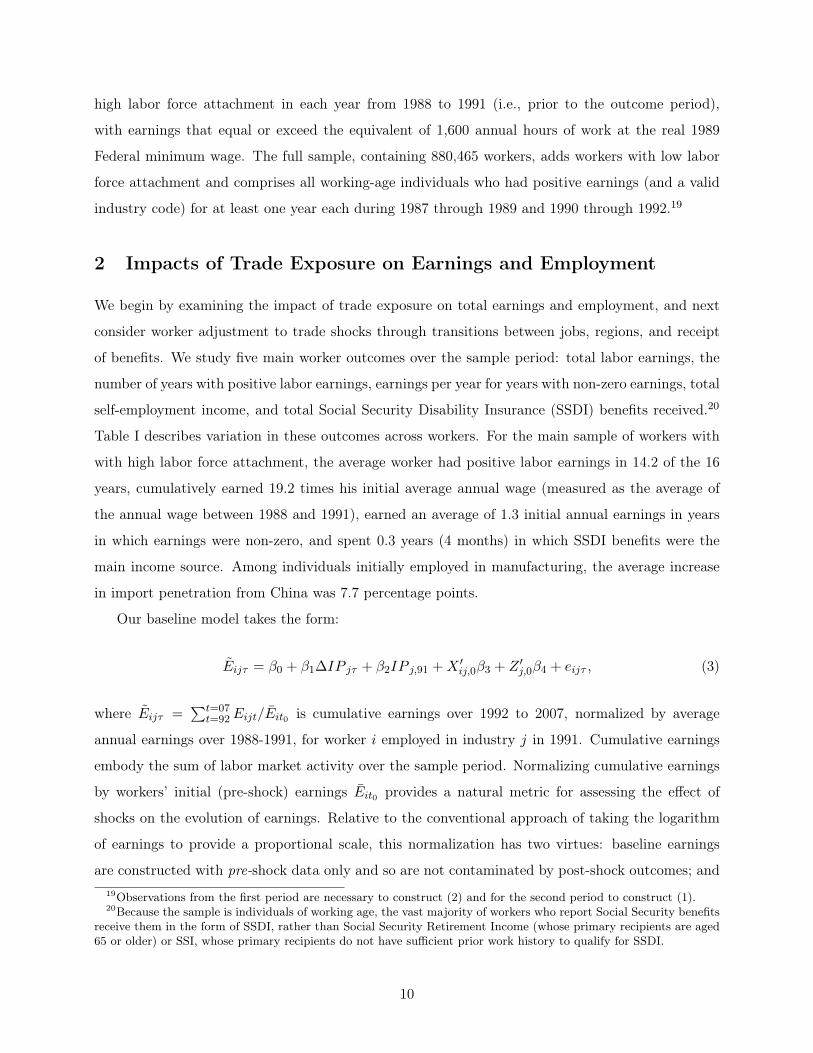
Table I describes variation in these outcomes across workers. For the main sample of workers with

with high labor force attachment, the average worker had positive labor earnings in 14.2 of the 16

years, cumulatively earned 19.2 times his initial average annual wage (measured as the average of

the annual wage between 1988 and 1991), earned an average of 1.3 initial annual earnings in years

in which earnings were non-zero, and spent 0.3 years (4 months) in which SSDI benefits were the

main income source. Among individuals initially employed in manufacturing, the average increase

in import penetration from China was 7.7 percentage points.

Our baseline model takes the form:

Eij⌧ = �0 + �1�IP j⌧ + �2IP j,91 +X 0ij,0�3 + Z 0

j,0�4 + eij⌧ , (3)

where Eij⌧ =Pt=07

t=92Eijt/Eit0 is cumulative earnings over 1992 to 2007, normalized by average

annual earnings over 1988-1991, for worker i employed in industry j in 1991. Cumulative earnings

embody the sum of labor market activity over the sample period. Normalizing cumulative earnings

by workers’ initial (pre-shock) earnings Eit0 provides a natural metric for assessing the effect of

shocks on the evolution of earnings. Relative to the conventional approach of taking the logarithm

of earnings to provide a proportional scale, this normalization has two virtues: baseline earnings

are constructed with pre-shock data only and so are not contaminated by post-shock outcomes; and19Observations from the first period are necessary to construct (2) and for the second period to construct (1).20Because the sample is individuals of working age, the vast majority of workers who report Social Security benefits

receive them in the form of SSDI, rather than Social Security Retirement Income (whose primary recipients are aged65 or older) or SSI, whose primary recipients do not have sufficient prior work history to qualify for SSDI.

10

scaling post-shock earnings by the pre-shock baseline circumvents the problem that log earnings are

undefined when income from some period or source is zero.

We model the cumulative shock due to trade exposure in equation (3) as a function of import

penetration in 1991 (IP j,91) plus the growth in import penetration from 1991 to 2007, which is

equivalent to the initial condition plus the average annual change (�IP j⌧ , as defined in equation

(1)). The vector Xij0 contains controls for the worker’s gender, birth year, race, and foreign-born

status, average log annual earnings over 1988 to 1991 and its interaction with worker age, lagged

earnings growth from 1988 to 1991, indicators for labor market experience and for tenure as of

1991 in the worker’s primary firm, the level and growth of the primary firm’s average wage between

1988 and 1991, and indicators for the size of the primary firm.The vector Zj,0 controls for economic

conditions in industry j in 1991, discussed in more detail below. While trade exposure and industry

characteristics vary at the level of workers’ 4-digit industries in 1991, standard errors are clustered

at the level of 3-digit industries, thus allowing for correlation in error terms among workers who are

initially employed in the same or in closely related industries.

Implicitly, our analysis compares workers with similar demographic characteristics, employment

histories, and average firm and industry characteristics, some of whom work in industries subject to

import competition from China and some of whom do not. If labor markets are frictionless, such

that workers can costlessly change industries and obtain identical compensation in alternative lines

of work, we will see no earnings or employment impacts from exposure to China trade—though we

should still be able to detect inter-firm and inter-industry mobility induced by trade exposure. If

growing imports from China cause wages to change for entire groups of similarly skilled workers, our

approach would also fail to identify such adjustments in earnings or employment, since in this case

the wage effects would not be firm or industry-specific. Conversely, we will find that trade impacts

worker outcomes if trade shocks induce exposed firms to cut wages and employment, and either

firm or industry-specific human capital make it costly for workers to change employers or industries

(Neal [1995]), or search and matching frictions reduce the gains from changing jobs in the event of

separation (Helpman, Itskhoki, and Redding [2010]; Rogerson and Shimer [2011]).

A further consideration is that individuals will be exposed to trade not just through their initial

industry of employment but also through their region of residence. Regions more vulnerable to im-

port competition from China—by virtue of being specialized in sectors in which China has a strong

comparative advantage—have undergone larger reductions in overall employment and earnings (Au-

tor, Dorn, and Hanson [2013a]). We also address how workers are affected by an import shock to

the industries of other workers in their local labor market, in addition to the own-industry trade

11

shock. The local labor market trade exposure for worker i is measured by averaging the value of (1)

across all other workers in the same initial commuting zone of residence, while the instrument for

local labor market import exposure is the corresponding average of other workers’ values of (2).

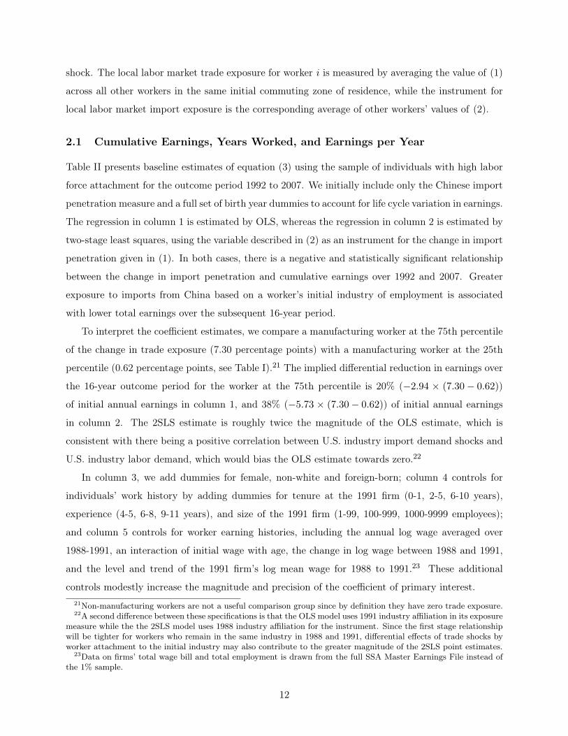
2.1 Cumulative Earnings, Years Worked, and Earnings per Year

Table II presents baseline estimates of equation (3) using the sample of individuals with high labor

force attachment for the outcome period 1992 to 2007. We initially include only the Chinese import

penetration measure and a full set of birth year dummies to account for life cycle variation in earnings.

The regression in column 1 is estimated by OLS, whereas the regression in column 2 is estimated by

two-stage least squares, using the variable described in (2) as an instrument for the change in import

penetration given in (1). In both cases, there is a negative and statistically significant relationship

between the change in import penetration and cumulative earnings over 1992 and 2007. Greater

exposure to imports from China based on a worker’s initial industry of employment is associated

with lower total earnings over the subsequent 16-year period.

To interpret the coefficient estimates, we compare a manufacturing worker at the 75th percentile

of the change in trade exposure (7.30 percentage points) with a manufacturing worker at the 25th

percentile (0.62 percentage points, see Table I).21 The implied differential reduction in earnings over

the 16-year outcome period for the worker at the 75th percentile is 20% (�2.94 ⇥ (7.30� 0.62))

of initial annual earnings in column 1, and 38% (�5.73 ⇥ (7.30� 0.62)) of initial annual earnings

in column 2. The 2SLS estimate is roughly twice the magnitude of the OLS estimate, which is

consistent with there being a positive correlation between U.S. industry import demand shocks and

U.S. industry labor demand, which would bias the OLS estimate towards zero.22

In column 3, we add dummies for female, non-white and foreign-born; column 4 controls for

individuals’ work history by adding dummies for tenure at the 1991 firm (0-1, 2-5, 6-10 years),

experience (4-5, 6-8, 9-11 years), and size of the 1991 firm (1-99, 100-999, 1000-9999 employees);

and column 5 controls for worker earning histories, including the annual log wage averaged over

1988-1991, an interaction of initial wage with age, the change in log wage between 1988 and 1991,

and the level and trend of the 1991 firm’s log mean wage for 1988 to 1991.23 These additional

controls modestly increase the magnitude and precision of the coefficient of primary interest.21Non-manufacturing workers are not a useful comparison group since by definition they have zero trade exposure.22A second difference between these specifications is that the OLS model uses 1991 industry affiliation in its exposure

measure while the the 2SLS model uses 1988 industry affiliation for the instrument. Since the first stage relationshipwill be tighter for workers who remain in the same industry in 1988 and 1991, differential effects of trade shocks byworker attachment to the initial industry may also contribute to the greater magnitude of the 2SLS point estimates.

23Data on firms’ total wage bill and total employment is drawn from the full SSA Master Earnings File instead ofthe 1% sample.

12

Industries that are subject to greater import competition may also be exposed to other economic

shocks that are confounded with China trade. To capture overall industry exposure to trade, col-

umn 6 includes controls for initial trade penetration by Chinese and non-Chinese imports in the

worker’s industry. Column 7 adds dummies for 10 manufacturing sectors, meaning that the regres-

sion models compare outcomes for manufacturing workers who are initially employed in different

sub-industries of the same sector. To address differential rates of technological progress across man-

ufacturing industries, in column 8 we include controls for the 1990 level of computer investment, the

share of investment allocated to high-tech equipment, the capital/value added ratio, and the 1991

employment share and log average hourly wage of production workers. This column further includes

the share of imported intermediate inputs in material purchases (from Feenstra and Hanson [1999])

to capture overall industry exposure to offshoring. To account for pre-existing trends in industry

growth, column 9 adds measures of changes in industry employment shares and log average wage

levels during the preceding 16 years, 1976 to 1991.

The additional controls in columns 6 through 9 have little substantive impact on the estimated

impact of import penetration. The coefficient of -6.86 on the import penetration in the final column

is about 20 percent larger than in the initial 2SLS specification (column 2). This suggests that

conditional on demographic measures, workers with somewhat higher potential earnings are initially

employed in industries that subsequently experience sharper rises in trade exposure. Accounting

for these sources of heterogeneity thus leads to a slightly larger estimate of the earnings losses that

workers experience due to trade exposure. To gauge the economic magnitude of this point estimate,

we again compare the implied impact on earnings of a manufacturing worker at the 75th versus 25th

percentile of the change in trade exposure. Multiplying by the point estimate in column (9), we find

a reduction of cumulative earnings by approximately one half of an initial annual wage for the more

exposed worker (�6.86⇥ (7.30� 0.62) = 45.8).

The upper panel of Table III considers two additional labor market outcomes. Column 2 esti-

mates the impact of trade exposure on the number of years between 1992 and 2007 in which the

worker has non-zero labor earnings. This measure of the extensive margin of employment is coarse:

an individual who works a single day in a year will have non-zero earnings, so even prolonged periods

of non-employment will go undetected unless they span a full calendar year. The point estimate of

-0.53 in column (2) is negative, suggesting that increases in industry trade exposure reduce subse-

quent years of employment. But this coefficient is not statistically significant and it implies only a

modest effect of trade exposure on years with positive earnings.24 The third column of Table III24The drop in employment years for a manufacturing worker at the 75th percentile of exposure relative to a worker

13

considers the impact of trade exposure on earnings per year of employment (in multiples of the initial

annual wage) for years in which labor earnings are non-zero. The point estimate of -0.39 (t = 2.8)

suggests that trade exposure depresses future earnings: specifically, earnings are differentially re-

duced by 2.6% per year (�0.39 ⇥ 6.7) for a worker initially employed in an industry at the 75th

percentile of exposure relative to a worker at the 25th percentile of exposure. In combination, the

estimates in columns 2 and 3 reveal that the net reductions in cumulative earnings seen in column

9 of Table II (and replicated in Table III column 1) stem primarily from reductions in within-year

earnings rather than from additional years with zero earnings. These within-year earnings declines

are, in turn, a combination of reduced earnings per hour and reduced hours worked, the relative

contributions of which we cannot disentangle with our data.

Could these results merely reflect the secular decline of labor-intensive U.S. manufacturing em-

ployment rather than the period-specific effects of exposure to China trade? We explore this concern

in panel B of Table III by testing whether the growth in import competition from China in the 1990s

and 2000s “predicts” earnings and employment outcomes for an earlier cohort of workers that was

not directly exposed to Chinese competition.25 This falsification test provides scant evidence of the

hypothesized confound. Column 1B estimates a negative relationship between cumulative earnings

and future industry level China trade exposure occurring during the 1990s and 2000s, but the point

estimate is insignificant and less than one-tenth the magnitude of the analogous contemporaneous

estimate in panel A. Column 2B finds a weakly positive relationship between years of non-zero labor

income and subsequent industry trade exposure, opposite to panel A. Finally, column 3B finds a

small, negative and insignificant relationship between annual wages in years with non-zero earnings

and subsequent trade exposure. In net, future trade exposure is a poor predictor for past earn-

ings and employment outcomes for workers, suggesting that our main findings are not plausibly

attributable to industry-specific trends that predate the rise of import competition from China.

Figure III provides a dynamic view of these findings by plotting the estimated effect of import

exposure on worker cumulative outcomes calculated on a rolling annual basis for each year from

1991 to 2007. The estimating equations underlying the top panel of the figure are identical to those

in our baseline regression (Table III, column 9) except that in place of workers’ cumulative earnings

over the entire period 1992 through 2007, we use cumulative earnings up through the year indicated

at the 25th percentile is 3.6% of a year (�0.54⇥ 6.7), or about two weeks, during the 16-year outcome period.25We draw on an extended version of the Social Security data to construct cumulative earnings from 1976 to

1991 for workers who were between 22 and 64 years of age during this earlier period, and use these data to examinewhether their employment outcomes during 1976 through 1991 are correlated with later, post-1991 changes in Chineseimport penetration that subsequently occurred in their initial industries. The sample for the analysis of the 1976-1991period uses the same sampling criteria as our main sample, and hence comprises the workers who earned at least theequivalent of $8,193 at 2007 values in each of the four years preceding the outcome period.

14

on the horizontal axis. Trade exposure remains the total change over the 1991 to 2007 period, such

that the figure depicts how the impact of trade exposure amasses over time. The figure reveals a

significant adverse effect of trade exposure on cumulative earnings in every year between 1992 and

2007. The impact coefficients become progressively more negative over the 1990s and then grow

even more rapidly after 2001; the 2001-2007 total decrease is nearly twice that for 1992-2001.

The path of earnings evident in the upper panel of Figure III encompasses multiple possible

channels of adjustment. If workers’ initial sectoral affiliations are relatively durable, the monotonic

decrease in earnings may be a consequence of extended exposure to the rise in import competition.

Alternatively, trade shocks may increase churning across jobs, impairing workers’ ability to find

secure positions or to obtain equivalently high quality matches with new employers, as would be

consistent with labor market scarring effects. We present initial evidence of the connection between

import competition and job churn in the bottom panel of Figure III, which follows the structure of

the top panel but replaces the dependent variable with workers’ cumulative number of changes in

employers and employment to non-employment transitions as of a given year. From 1992 forward,

the coefficients are uniformly positive and are significantly so for all years after 1997. More trade

exposed workers have a larger number of job changes, where the sum of these changes steadily grows

as the trade shock becomes fully expressed. We subsequently explore whether these more frequent

job changes also entail greater mobility across sectors or regions.

The time pattern in the top panel of Figure III highlights an important nuance in interpreting

our impact estimates: the rise in China trade exposure is an ongoing process that builds momentum

in the early 1990s as China embraces export-led development, and then accelerates after 2001 as

the country further opens its markets. Thus, the time pattern of coefficients in Figure III does not

constitute an “event study” as in traditional mass-layoff analyses—that is, a discrete shock followed

by a time path of adjustments—but rather depicts the interaction between two economic forces,

rising import penetration and ongoing worker adaptation. We similarly find that at the industry-

level, increases in trade exposure exhibit strong serial correlation: no sizable industry experiences

a large increase in trade competition in the 2000s that did not also experience one in the 1990s, or

vice versa. Industries that are in the top tercile of trade exposure in one decade but the bottom

tercile in the other account for just 1% of all manufacturing workers in our sample. These attributes

of the data motivate our parameterization of the rise in China’s import penetration in equation (3)

as a single long change over the period 1991 through 2007.

15

2.2 Worker Mobility across Firms, Industries and Sectors

A strength of the SSA longitudinal data is that they permit us to observe the earnings, employment,

and job reallocation margins by which workers and, indirectly, their employers, adjust to changes

in import penetration. We analyze this reallocation process by decomposing the total worker-

level effect of trade exposure seen in Table III into a set of additive, mutually exclusive channels

that include: employment observed at the worker’s initial employer; employment at other firms

within the worker’s initial two-digit industry; employment at firms within manufacturing but outside

the worker’s initial industry; employment outside of manufacturing entirely; and employment at

new firms whose industry is unrecorded in the data. This analysis encompasses the direct impact

of rising import competition on workers’ tenure and earnings at their initial employers as well

as any subsequent, potentially offsetting effects of moves across employers, across sub-sectors of

manufacturing, and between the manufacturing and non-manufacturing sectors.26

Table IV presents the results, beginning in panel A with cumulative earnings. The first column

(1A) replicates our main estimate for the impact of trade exposure on cumulative earnings among

high attachment workers, while columns 2 through 6 decompose this net earnings effect into its

constituent additive parts: initial firm; new firm in same industry and sector; new industry in

same sector; new sector; and sector missing.27 The negative and significant coefficients in columns

2A and 3A reveal that workers initially employed in industries that undergo substantial increases

in trade exposure experience both sharply reduced earnings at their initial employers and lower

subsequent income from other firms in the same two-digit industry. Do these reductions stem from

changes at the extensive margin (reduced years of work), the intensive margin (reduced earnings

per year), or both? The estimates in columns 2B and 3B, which consider employment rather than

earnings, indicate that the answer is some of both. Comparing across panels, cumulative earnings

fall by about 50% more than cumulative employment at both the initial employer and in the initial

industry. Columns 2C and 3C confirm this implication: trade exposure significantly reduces earnings

per year of employment at the initial firm and at subsequent firms in the same industry.

These impacts at the initial firm and industry may of course be offset by gains in other sectors.

Indeed, we know from the small and insignificantly negative net estimate of trade exposure on26Prior to the year 2000, industry information is available for 96-97% of all workers is a given year. However,

industry codes are missing for most firms that were incorporated in or after the year 2000. The Social Security datavery rarely record changes in firms’ industry affiliation, and worker outcomes at the initial firm (column 2 of TableIV) thus correspond to outcomes in the initial industry.

27In panels A and B (cumulative earnings and cumulative years of employment), summing the coefficients in columns2 through 6 produces the value in column 1. This adding-up property does not apply to panel C because the outcomevariable, earnings per year employed, is a conditional value.

16

years of employment (column 1B) that employment losses are almost entirely offset: trade-impacted

workers make back their employment losses in the initial firm and industry through employment

outside of the original two-digit industry. Column 4B indicates that trade-exposed workers spend

more years employed at firms that belong to a different two-digit industry within their initial sector

of employment. But these offsetting employment gains from reallocation to other two-digit industries

within manufacturing are only just over half as large as the losses incurred with the original employer

and two-digit industry (4.65/(6.20 + 2.04) = 0.56), indicating that trade exposure in a worker’s

initial firm reduces the worker’s total manufacturing employment net of mobility within the sector.28

Columns 5B and 6B complete the employment picture by considering employment outside of the

worker’s initial sector and at firms whose industry could not be identified. Workers who are initially

employed in trade-exposed industries experience offsetting employment gains in both categories,

though results for employment outside of manufacturing are imprecisely estimated.

While trade-exposed workers appear to offset most of their employment losses in the initial firm

and two digit industry through employment further afield, they do not fully offset lost earnings in

subsequent employment. In particular, panel A demonstrates that earnings gains in other man-

ufacturing industries are only half as large as the losses incurred with the original employer and

industry (5.91/(9.11+ 3.00) = 0.49), while earnings gains outside of manufacturing are on net close

to zero. Thus, to the degree that trade-impacted manufacturing workers succeed in offsetting initial

earnings losses, this primarily occurs through subsequent earnings gains with other manufacturing

firms outside of the immediate two-digit industry. This result is surprising since U.S. manufacturing

is a comparatively small and rapidly contracting sector throughout the time period of our study

(see footnote 1). Panel C finally demonstrates that the discrepancy between the large trade-induced

reduction in cumulative earnings and the insignificant trade-induced reduction in employment years

is explained by lower earnings per year of employment both at the initial firm and at subsequent

employers within and outside of manufacturing.29

Why don’t employment transitions allow initially trade exposed workers to fully recoup declines

in earnings with the initial employer? The literature on job loss provides one potential answer (e.g.,

Neal [1995]): displacement destroys industry specific human capital, leaving affected workers in

positions for which they are poorly suited relative to non-displaced workers. A parallel explanation28Column 6B shows moderate employment gains at firms with a missing industry code, a large majority of which

were incorporated in the years 2000 to 2007, when a new data collection process no longer recorded informationon industry. Even if one assumes that the new firms that employ former manufacturing employees all operate inthe manufacturing sector, there is still a sizable negative effect of trade exposure on manufacturing employment orearnings, which may be seen by summing the coefficients across columns 2, 3, 4 and 6 of Panel A or B.

29The results in panel C must be interpreted with care, however, since the earnings-per-year effects combine variationstemming from changes in weeks worked, hours worked per week, and earnings per hour of work.

17

is that workers’ specific skills cause them to seek out positions in which they remain exposed to

import competition, notwithstanding the predilection of trade impacted workers to exit their original

two digit sector. Figure IV provides insight into this latter mechanism by depicting the correlation

between workers’ trade exposure at their initial employers and at their current employers for each

year between 1991 and 2007.30 In the years immediately following 1991, few workers have yet

separated from their original firms, and hence the correlation remains close to one. Over time,

the correlation between initial and current firm trade exposure falls, as job transitions proceed

apace, but remains strongly positive, leveling off at 0.43 in the final year (2007). As a benchmark

against which to evaluate the persistence of trade exposure, Figure IV also plots counterfactual

correlations in which trade exposure at any new employer is set to zero, such that the reported series

summarizes the cumulative likelihood of having left the initial firm as of a given year. Logically this

counterfactual correlation also declines over time, reflecting the rising likelihood of having departed

from the original place of work. But the counterfactual decline is far more rapid than the actual series

and ends up at the much lower level of 0.17 in 2007. By implication, were trade-exposed workers to

exit manufacturing immediately after the first job separation, their net subsequent exposure would

be 60% lower than in the actual data. Thus, even after changing employers, initially trade-exposed

workers appear likely to remain in high exposure industries which are subject to further trade shocks.

2.3 Do Workers Adjust to Trade Exposure through Geographic Mobility?

Transitions across employers and industries are one mechanism by which workers adapt to the con-

sequences of import competition. Moving between geographic locations is another. The literature

provides mixed evidence on mobility responses to labor market shocks. The flow of labor across U.S.

cities and states following changes in regional labor demand appears to be sluggish and incomplete

(Topel [1986]; Blanchard and Katz [1992]; Glaeser and Gyourko [2005]). This sluggishness is most

pronounced among less educated workers, who make up a disproportionate share of manufacturing

employment (Bound and Holzer [2000]; Notowidigdo [2013]). Consistent with limited mobility re-

sponses, Autor, Dorn, and Hanson (2013a) find little impact of regional trade exposure on changes

in regional population. We revisit the issue of geographic relocation by extending our analysis to

consider whether workers initially employed in more trade exposed industries are more likely to

change their place of residence during the sample period.

The SSA data provides a county code for the residence address associated with each individual30The correlations compare the 1991-2007 growth of import penetration between the industry that employed a

worker in 1991 and the industry that employed a worker in the subsequent year indicated on the y-axis. Thiscorrelation is 1.0 by construction in 1991.

18

record in a given year. Since individuals may reside in one location and work in another, residence

may be a noisy indicator of the employment location. However, because we designate geographic

units to be commuting zones—which are defined precisely to be the regions within which individuals

usually both live and work—there is a built in buffer against such noise. Other limitations of

individual addresses are that they do not appear in the data until 1993, are not available for all

workers, and are never observed for individuals who are not employed in a given year.31

We match a worker’s county of residence in 1993 to the corresponding commuting zone and

define a worker to have changed locations if the commuting zone of residence subsequently changes.

Despite its limitations, the SSA data appear to accord well with other sources in capturing the

frequency of location changes. Molloy, Smith and Wozniak (2011) use the Census to calculate that

12.9% of workers changed their commuting zone between 1995 and 2000; in our SSA sample over the

same time frame, the mobility rate is 14.4%. Because geographic information is not available until

1993, when analyzing regional mobility we define the outcome period to be 1994 to 2007 instead of

1992 to 2007. As above, we define the change in import penetration using (1) and continue to use

the instrument defined in (2).

Table V presents results on the regional dimension of adjustment to trade shocks. Column

1 repeats the baseline specifications for the shorter outcome period 1994 to 2007, which causes

estimates to differ slightly (but not qualitatively) from those in panel A of Table III. We examine the

consequences of trade exposure on geographic mobility in columns 2A through 4A by decomposing

the earnings that a worker accumulated from 1994 to 2007 according to whether the earnings were

accrued in the initial commuting zone, in a different commuting zone, or, in 6% of cases, in locations

that are missing a commuting zone identifier.

If workers respond to trade shocks by moving between regions, import exposure will have a

negative effect on total earnings in the initial commuting zone in which a worker resides—shown in

column 2—which would indicate reduced labor supply in the location where a worker is employed

when trade exposure starts to rise. But there would be a positive effect on total earnings in future

commuting zones of residence—shown in columns 3 and 4—indicating a shift in labor supply across

regions in response to the shock. This pattern is nowhere present in the data. In panel A, the impact

of trade exposure on cumulative earnings as a share of initial period earnings is negative not just for

workers’ initial commuting zones (column 2A) but also for cumulative earnings in other commuting

zones (column 3A), and for cumulative earnings in commuting zones that we cannot classify because

information on a worker’s initial or subsequent location is missing (column 4A). More trade exposed31We are able to determine the 1993 county code of residence for 94% of workers in our main sample.

19

workers thus receive less in total earnings in all local labor markets in which they reside, suggesting

that geographic mobility is not a primary mechanism for adjusting to trade shocks.

Results for cumulative years of non-zero earnings in panel B also fail to indicate that trade

exposure causes geographic mobility to increase. Workers initially employed in industries subject

to greater import competition have lower cumulative years with non-zero earnings not just in their

initial commuting zone (column 2B) but also in other (column 3B) and in unidentified commuting

zones (column 4B), though none of these effects is significant. The decline in cumulative earnings

by location in panel A is instead driven largely by reduced earnings per year of employment in all

commuting zones in which a worker resides (columns 2C-4C). In sum, the results of Table V give

further indication that regional mobility is of limited import as a mechanism through which workers

adjust to changes in trade exposure.

2.4 Social Security Benefits as a Channel of Adjustment

Alongside changes in employment and earnings, a complementary channel by which workers may

adjust to employment shocks is through job search, retraining and transfer programs, such as the

federal Trade Adjustment Assistance (TAA) program, state unemployment insurance programs, and

numerous need-based transfer programs. One such adjustment program that is observable in our

data is the federal Social Security Disability Insurance (SSDI), which provides income transfers and

Medicare coverage to workers who have developed a physical or mental disability that prevents

them from being gainfully employed.32 Since workers cannot obtain SSDI if they are employed, it

is plausible that the trade-induced declines in employment and earnings seen in Table III may have

a counterpart in increased SSDI participation. We explore this possibility in Table VI by analyzing

the impact of trade exposure on SSDI enrollment along four margins: the number of years receiving

SSDI as a primary income source, cumulative income from SSDI, the probability of receiving SSDI

at any point, and the number of years with positive SSDI income for those who receive any benefits.

The first panel of Table VI shows the effect of trade exposure on the primary source of income

during each year that is observed in our data: labor income (column 1); self-employment income

(column 2); SSDI income (column 3); and no recorded income (column 4). Echoing the results in

Table III, column 2A shows a negative but insignificant relationship between trade exposure and

years with labor earnings as the main source of income: among the workers in our main sample32To become insured by the SSDI program, an individual must have worked in at least five of the ten most recent

years in covered employment. Prior literature has established that enrollment in the SSDI program is generallycountercyclical, and that local economic shocks can induce sharp rises in SSDI applications and subsequent awards(Black, Daniel and Sanders [2002]; Autor and Duggan [2003]; Autor, Dorn and Hanson [2013a]).

20

(with strong initial labor force attachment), spending a full calendar year out of work is uncommon.

In column 2A of Table VI, trade exposure is also negatively but not significantly correlated with

total years in which self-employment is the primary income source, indicating that transitions into

self-employment are not an important mechanism for worker adjustment to trade shocks. However,

column 3A finds that trade exposure predicts a significant increase in years receiving SSDI as the

primary income source. Applying our 75th and 25th percentile comparison among manufacturing

workers, the more trade-exposed worker spends an additional half month receiving SSDI benefits as

the primary income source during the 16 year outcome window. This is a modest effect. By way of

context, the average manufacturing worker spends approximately five months (0.43 years) over the

sample period with SSDI benefits as his or her main income source.33

In untabulated results, we repeat the analysis above while replacing receipt of SSDI with receipt

of any type of Social Security benefit, which includes SSDI, Social Security Retirement Income, and

Supplemental Security Income. The results are nearly identical to those Table VI, consistent with

our main sample containing working-age individuals with high-attachment to the labor force who

are unlikely to qualify for other types of Social Security payments.

Panel B of Table VI studies more closely the impact of trade exposure on income (rather than

employment) by considering self-employment and SSDI income alongside wage income. Column 2B

finds a negligible impact of trade exposure on self-employment income. Commensurate with the

increased duration of SSDI benefit receipts documented in column 3A, column 3B shows a positive

and statistically significant effect of trade exposure on receipt of SSDI income (measured in percent-

age points of the initial average wage). The point estimate of 0.35 implies that a manufacturing

worker at the third quartile of exposure receives an additional 2.3% of initial annual earnings in SSDI

benefits relative to a manufacturing worker at the first quartile of exposure. Thus, SSDI benefits

only replace a small fraction—about 5 percent—of the income lost to trade exposure.34

Panel C decomposes the increased duration of SSDI benefit receipts into intensive and extensive

margins. While trade exposure significantly increases the likelihood that a worker receives SSDI at

some point in the next 16 years, the impact is modest. Comparing the 75th and 25th percentile

manufacturing worker, the increment to the probability of any SSDI receipt over 16 years is only 0.6

percentage points, with no significant effect on years of receipt conditional on receiving SSDI. This

pattern is also evident in the bottom panel of Online Appendix Figure A.2, which shows that the33Workers may exit the labor force and obtain SSDI in the same calendar year without having both sources of

income concurrently. In addition, SSDI recipients are permitted to work up to a Substantial Gainful Activity threshold(currently $1,010 per month for non-blind adults) without jeopardizing their SSDI benefits.

34Our data indicate that SSDI payments average 47 percent of initial average labor earnings for years in whichworkers in our sample receive SSDI.

21

effect of trade exposure on the incidence of SSDI receipt cumulates slowly over the 16 year outcome

window. Thus, disability plays an important role on the extreme extensive margin—among workers

who exit the labor force altogether—but the majority of trade-exposed workers with an initial

strong labor force attachment remain attached to the labor market, albeit at reduced earnings. As

subsequent analysis shows, SSDI is a more important adjustment margin for less attached workers.

3 Heterogeneity in Worker Adjustment to Trade Exposure

We have so far followed the literature on mass layoffs by limiting our sample to workers with high

labor force attachment. This exclusive focus on high-attachment workers may miss an important

dimension of heterogeneity in adjustment to adverse shocks. If workers with weaker attachment

are at greater risk of job displacement or face fewer outside employment options, they may be

differentially harmed by adverse trade shocks. Alternatively, if these workers are particularly likely

to exit the labor market regardless of circumstance, adverse trade shocks may not alter their career

trajectories. We assess these differences by comparing results from Table VI to estimates for the

full sample that includes workers with low labor force attachment. We then extend the analysis to

explore heterogeneity in adjustment according to workers’ firm tenure, age, and earnings levels.

3.1 High versus Low Labor Force Attachment Workers

Table VII expands our sample to include workers who had any labor income in at least one year

during 1987-1989 and one year during 1990-1992, which brings our sample size from 508,129 to

880,465. The additional workers of the extended sample either had zero earnings, or earned less

than the salary of a full-time minimum wage job in at least one of the years 1988 to 1991. While our

data do not contain information on hours worked, it is likely that the expanded sample contains many

more part-time and intermittent workers.35 For consistency with the broadened sample definition,

trade exposure is now measured as the average exposure of the industries that employed a worker

during the years 1990 to 1992 while the instrument is based on industry affiliation in 1987 to 1989. All

firm- and industry-specific control variables are also averaged over 1990 through 1992, and outcomes

are measured over the subsequent period of 1993 to 2007.

We begin in panel A of Table VII by replicating the main specification of Table VI for the original

high labor force attachment sample, using suitably modified variable definitions. These changes in35The minimal pre-period earnings of workers in the extended sample are likely a poor proxy of their earnings

potential, and they complicate an analysis of future earnings that are expressed in multiples of initial earnings as inTable II. We therefore focus on employment outcomes, as in Table 5.

22

variable definitions have no substantive effect on the main estimates. Combining high and low labor

force attachment workers in panel B magnifies trade’s negative impact on years worked and positive

impact on SSDI reliance. In column 1B of Table VII, the negative coefficient on total years with

main income from labor earnings is sixty percent larger in absolute value than the high attachment

coefficient in panel A (and is now marginally statistically significant), implying that among low

attachment workers, adjustment at the (extreme) extensive margin of full-year non-employment is

comparatively common. In column 2, the reduction in years with main income from self-employment

is larger in absolute value terms in the full sample than in the high attachment sample.

Columns 3 and 5 capture the differential responsiveness of SSDI take-up in the two samples.

Extending the sample to include low attachment workers increases the coefficient on cumulative

years with SSDI as the main income source by 160% (column 3) and the coefficient on ever receiving

SSDI income by 120% (column 5). Because low attachment workers are more likely to exit the labor

force after a trade shock, as seen in column 1, they are also more likely to take up SSDI, which is

unavailable while workers are gainfully employed. Thus, greater usage of SSDI benefits and larger

extensive margin employment adjustments go hand-in-hand.

3.2 High versus Low Tenure Workers, Younger versus Older Workers

Low tenure workers comprise a second segment of the labor market omitted by mass layoff studies.

Seniority-based employment rules may insulate older workers from external shocks while exposing

younger workers to greater risk of career disruption (Oreopoulos, von Wachter and Heisz [2012]).

Alternatively, workers with higher tenure may suffer greater losses from trade exposure since their

ability to adapt to new employers may be limited (Jacobsen, LaLonde, and Sullivan [1993]).

In the first two panels of Table VIII, we compare the impact of trade exposure on employment

and earnings for workers with low job tenure at their initial firms (defined as less than five years as

of 1991) to those with high initial tenure (five-plus years in 1991).36 Condensing the specification

in Table IV, we disaggregate worker outcomes according to three mutually exclusive employment

venues: the initial employer (column 2), subsequent employers in manufacturing (column 3), and

employers outside manufacturing or with a missing industry code (column 4).37 For reference, the

online appendix displays the average trade exposure of manufacturing workers in both high and

low tenure subsamples, as well as the exposure for other subsamples that we explore subsequently.36The low and high-tenure groups are drawn from our primary sample with high-attachment workers, and the 5-year

tenure cutoff splits this sample roughly in half.37For workers initially employed in manufacturing, ‘same sector’ and ‘other sector’ denote manufacturing and non-

manufacturing, respectively.

23

While average trade exposure for low-tenure workers is about one-fourth larger than for high-tenure

workers, there is little difference in the timing of exposure within the 1991 to 2007 period. In each

subsample that we consider, about one quarter of the increase in trade competition occurs 1991 to

1999, and three quarters in 1999 to 2007, when import growth from China accelerates strongly. The

different coefficient estimates for trade impacts on earnings and employment across subsamples of

workers cannot therefore be explained by a differential timing of import shocks.

Akin to the Table VII estimates for low-attachment workers, panels A1 and A2 of Table VIII

reveal that the negative impacts of trade exposure on cumulative earnings and on earnings per year

worked are substantially larger for the low tenure group. In panel A1, the effect of trade exposure

on cumulative earnings for low-tenure workers is 8.7 times as large as the estimated effect for high-

tenure workers (panel A2). The difference between low and high tenure workers begins at the initial

employer. Low-tenure workers experience more than twice the reduction in employment years as

high-tenure workers, and more than three times the loss in earnings at the initial firm (panels A1

and A2, column 2). Low tenure workers make up little of this loss through earnings from other

employers (panel A1, columns 3 and 4). The comparatively modest but still negative and significant

cumulative earnings losses for high tenure workers at the initial firm are offset—by a factor of nearly

two-thirds—through gains at employers outside the initial sector (panel A2, column 4). Earnings

losses for low-tenure workers are not explained by lost years of employment; in fact, the estimated

cumulative employment effect is weakly positive. It appears instead that their annual earnings in

subsequent employment lies substantially below their earnings in the original firm.

One reason low tenure workers may be more affected by trade is simply that they are young,

with employers preferring to sever ties first with those having less labor-market experience. Panels

B1 and B2 of Table VIII separate workers by age, with the younger cohort being 22 to 35 years old

in 1992 and the older cohort being 36 to 49 years old in that year. Coefficient estimates are modestly

larger for the younger workers, but the difference between the two groups is slight and statistically

insignificant. Thus, the larger impacts of trade on low tenure workers in panels A1 and A2 appear

to be driven more by their brief attachment to their initial employer than by their youth.

3.3 Differences in Adjustment by Earnings Capacity

The clear pattern emerging from Tables VII and VIII is that workers who have a weaker foothold in

the labor market suffer the largest proportionate earnings losses from trade shocks. This suggests

more broadly that the adverse effects of trade shocks may be greatest for workers with low earnings

capacity, a possibility that we explore in Table IX by separately estimating the impact of trade

24

on workers subdivided into terciles of average annual pre-exposure earnings (1988 through 1991)

relative to others in their age cohort. By making within-cohort comparisons, this sample split

captures differences in earnings capacity that are likely to stem from factors such as education and

ability—not directly observable in our data—rather than experience and seniority.

Table IX confirms that the adverse impacts of trade exposure on worker outcomes are inversely

monotone in initial earnings. Column 1 of the top panel finds a large and highly significant negative

estimate of the impact of trade exposure on cumulative earnings of bottom-tercile workers. Scaling

by the 75/25 metric, the point estimate implies that a low-wage worker in manufacturing at the

75th percentile of exposure loses 1.2 (�18.3 ⇥ 6.7) additional years of initial annual earnings over

the subsequent sixteen years relative to a worker at the 25th percentile of exposure. This effect is

nearly three times as large as the impact for the full sample (Table II, column 9). In comparison, the

estimated impact for middle-tercile workers (panel B) is only half as large as the impact for bottom

tercile workers, while the estimated impact for top-tercile workers (panel C) is essentially zero.

Why are the adverse impacts larger for low-wage than for high-wage workers? One possibility

is that import competition differentially reduces firms’ demand for lower skill workers while leaving

high-wage workers relatively unscathed. The subsequent rows of Table IX do not support this con-

jecture. High, middle and low-wage workers experience similarly large declines in earnings obtained

from the initial employer (column 2). What differs between these groups is their subsequent labor

market adjustment. High-wage workers recover from initial shocks by moving out of the impacted

sector. Middle and low-wage workers are less able to offset those losses through sectoral mobility.

High-wage workers on average make up one-fourth of their loss with the initial employer through

additional earnings from other firms in the same sector (column 3), and they recoup most of the

remaining three-fourths at employers outside of manufacturing (column 4). Middle-wage workers, by

contrast, replace around one-third of earnings lost with the initial employer through earnings else-

where in manufacturing, and they suffer further losses outside of the original sector. At the other

extreme, low-wage workers experience no offsetting increase in earnings within the same sector, and

they accrue even larger earnings declines outside of the original sector.

The second rows of each panel in Table IX offer further insight into the adjustment process by

focusing on years of employment rather than cumulative earnings. Workers at all wage levels experi-

ence substantial reductions in years of employment at the initial employer. However, the magnitude

of this reduction is nearly twice as great for high-wage relative to middle or low-wage workers. While

all three groups appear to largely offset lost earnings years (though not lost earnings) at the ini-

tial firm through additional employment, their subsequent employment venues differ substantially.

25

Low-wage workers primarily offset lost employment at the initial firm with employment elsewhere

in the manufacturing sector; middle-wage workers offset losses with extra employment both inside

and outside manufacturing; and high-wage workers appear primarily to obtain new employment

outside manufacturing—highlighting that these workers are particularly mobile across industries.

Thus, while workers at all earnings levels exhibit heightened job churning as a consequence of trade

shocks, workers at different earnings levels differ substantially in how they adjust to these shocks.

The third rows of each panel in Table IX reveal an additional contrast among earnings groups: low

and middle-wage workers experience substantial declines in earnings per year both at the initial firm

and at subsequent employers. High-wage workers, by contrast, exhibit no adverse earnings effects,

even as they move across firms and sectors.38 What explains the contrast in earnings consequences

among skill groups? One proximate explanation focuses on the differences in their sectoral mobility

identified in the second row of Table IX. High-wage workers primarily offset losses at their initial

firm by moving out of manufacturing. Low-wage workers, however, disproportionately remain in

manufacturing, where their subsequent earnings are subject to rapidly accelerating trade pressure

throughout the 1990s and 2000s. A potential cause of this low rate of inter-sectoral mobility is that

low-wage workers may be earning rents in manufacturing—that is, wages or net surplus that exceed

their alternatives opportunities outside of manufacturing (Katz and Summers, 1989; Gittleman and

Pierce, 2011). As trade pressure erodes these rents, workers may therefore choose to accept lower

pay in manufacturing rather than seek employment outside of it.

An online appendix investigates whether these differences in reallocation of workers across firms

and sectors also operate through differential geographic mobility. Import exposure does indeed shift

the employment of high-wage workers from the initial commuting zone toward other regions, while

the opposite pattern is observed for workers with middle or low wages. The greater geographic

mobility response of high-wage workers is consistent with previous research on U.S. domestic migra-38Among low-wage workers, the implied 75/25 differential loss in earnings per year amounts to 7.8% (�1.2 ⇥ 6.7)

annually, while for middle-wage workers, the in-year earnings losses are only approximately half as large. This resultappears to stand in contrast with the local labor market evidence from Autor, Dorn and Hanson (2013a), who findthat CZ-level trade exposure reduces the log weekly earnings of currently employed college and non-college workersby similar (modest) amounts. Why do the earnings effects of trade exposure measured at the worker level differsubstantially by skill group while those measured at the CZ level do not? Noting that our SSA annual earnings dataindicate that only a small percentage of primary sample workers has zero earnings over the course of a full-year, wehypothesize that the fall in within-year earnings detected in the SSA data (Table IX) is reflected primarily in a rise inthe odds of non-participation during the survey reference week in the Census and American Community Survey dataused in the Autor, Dorn and Hanson (2013a) analysis. Consistent with this supposition, Autor, Dorn and Hanson(2013a, Table 5) find that trade shocks induce a much sharper fall in the probability of labor force participationduring the survey reference week among non-college than non-college workers: -0.83 versus -0.30 percentage pointsper thousand dollars of CZ exposure. The small drop in weekly earnings of low-education workers detected by Autor,Dorn and Hanson (2013a), combined with a large increase in their non-participation, is potentially consistent withthe significant decline in the cumulative annual earnings of low-wage workers detected above.

26

tion (Wozniak [2010]; Notowidigdo [2013]), but the increase in employment years outside the initial

commuting zone is not significant either for high-wage workers, or for any of the previously studied

tenure and age subsamples. Across all groups of workers, trade exposure induces considerably more

mobility across firms and sectors than across space.

In the SSA data, workers with low earnings are differentially impacted by trade shocks. No

distinctions between low and high-wage workers appear in the literature on mass layoffs, however,

where low and high-skill workers fare equally poorly subsequent to large contractions in their initial

firms. In an online appendix, we examine when and how workers separate from their initial employer

in response to changes in trade exposure. Not surprisingly, more trade exposed workers are more

likely to separate from their initial place of work, with the impact of trade exposure on separation

being larger for low-wage workers than for high-wage workers. When we categorize job exits by their

proximity to a mass layoff at the initial firm, we find that the contribution of mass-layoff separations

to total separations is highest among low-wage and lowest among high-wage workers. Separations

from the initial employer immediately before a mass layoff have the opposite pattern, being relatively

high among high-wage workers. While trade exposure significantly increases the likelihood that a

low-wage worker leaves the initial firm during a mass layoff, the only significant effect among high-

wage workers is for separations before mass layoffs. This difference in pre-mass layoff separations

between low and high-wage workers is, naturally, absent in the mass-layoff literature since that work

focuses exclusively on workers who have separated during a mass layoff (e.g., Jacobson, LaLonde

and Sullivan [1993]; von Wachter, Manchester and Song [2009]). In contrast to existing literature

that concludes that mass layoffs have equally scarring effects for workers of all skill levels, our results

suggest instead that high-wage workers are less exposed to mass layoffs and are more likely to leave

their initial firm in a pre-layoff period when presumably a larger fraction of separations is voluntary.

4 Alternative Measures of Trade Exposure

In this section, we consider alternative measures of workers’ exposure to trade with China. We first

explore specifications that measure exposure not only to trade competition in the worker’s industry,

but also in the worker’s local labor market of residence. We then re-estimate the regressions for

cumulative earnings, cumulative employment years, and earnings per year of employment from

panel A of Table III for six alternative measures of industry-level trade shocks.

27

4.1 Industry-Level and Region-Level Trade Exposure

Our main analysis finds that workers who were employed in subsequently import-exposed industries

accumulate substantially lower earnings over their careers than comparable workers in industries

with little trade competition, a result consistent with labor market frictions preventing workers

from smoothly adjusting to trade shocks. If trade-exposed industries were highly segregated across

local labor markets, these results could be consistent with moving frictions inhibiting flows across

local labor markets, even while reallocation within these markets is frictionless. This would imply

that workers in trade-exposed industries would obtain lower earnings than those in a low-exposure

industries primarily because they are located in differentially trade-exposed regions. We explore

this hypothesis by testing how our main results are affected by controlling for import exposure in

a worker’s initial commuting zone of residence, where a CZ’s industry exposure is defined as the

average growth of Chinese import penetration in the industries of all other workers who reside in

the individual’s initial commuting zone.39

Table X follows Table V by analyzing the impact of trade competition on earnings, employment,

and geographic mobility during the shortened outcome period of 1994 to 2007. Column 1 shows the

impact of industry-level trade exposure on earnings and employment (replicating column 1 of Table

V), column 2 regresses the same outcomes on commuting zone-level trade exposure and a set of

indicator variables for the nine Census divisions that absorb regional trends, and column 3 combines

the two exposure measures.40 Columns 2 and 3 of panel A show that workers initially residing in

CZs with larger increases in trade exposure had significantly lower cumulative earnings over the

1994 to 2007 period. Results for CZ trade exposure are similar either with (column 2A) or without

(column 3A) initial own industry trade exposure in the regression; in parallel fashion, results for own

industry trade exposure change only modestly when CZ trade exposure is added (columns 1A and

3A). The regions of residence of workers in trade-exposed industries are sufficiently dispersed across

space that the correlation coefficient between industry-level and CZ-level trade exposure is only 0.12.

The industry-level effects reported earlier are hence not primarily capturing geographic variation in

worker’s trade exposure. The negative earnings effect of a trade-exposed industry, conditional on39To obtain the employment weights of all industries in a commuting zone, we draw on the 1990 County Business

Patterns, as in Autor, Dorn, and Hanson (2013a). The CBP provides more precise measures of industry employmentstructure at the county level than our main data, a one percent random sample of Social Security Administrationdata. The SSA data provide workers’ county of residence as of 1993. We impute 1991 location, taking advantage ofthe fact that most workers did not change employers, and presumably did not change region, between 1991 and 1993.The Data Appendix provides a detailed description of the imputation procedure.

40In combining both industry and regional exposure to trade, our approach complements McLaren and Hakobyan(2010). Though our use of panel data contrasts with their use of Census data on repeated cross-sections of individuals,our results that industry exposure is more consequential than regional exposure are qualitatively similar to theirs.

28

trade exposure of the local labor market, is consistent with the presence of labor market frictions

that prevent a smooth relocation of workers across industries within local labor markets.

To interpret the magnitude of the impacts of trade exposure, we use the estimates of column

3A to compare manufacturing workers who are at the 75th versus 25th percentiles of industry trade

exposure, or at the 75th versus 25th percentile of regional trade exposure. Over the period 1994 to

2007, the worker in the more exposed industry received 40.5% lower cumulative earnings valued in

terms of initial average annual earnings, while the worker in the more exposed local labor market

earned 19.7% less than a peer in a less-exposed location.41 The results on local labor market exposure

accord with Autor, Dorn, and Hanson (2013a), who find that commuting zones more exposed to

China trade had lower growth in household wage income. To compare with their estimates, we

calculate the decline in annual wage income per worker between the start and end of our sample

for CZs at the 75th versus 25th percentiles of trade exposure, and use a corresponding calculation

based on findings from Autor, Dorn, and Hanson (2013a). From Table X, we estimate that the

annual earnings in the more exposed CZs decline by 2.5% of workers’ initial annual earnings during

the sample period, while we estimate a reduction of average household income per adult of -2.4%

between 1990 and 2007 using estimates from Autor, Dorn, and Hanson (2013a).42

Panels B and C show the impact of greater regional trade exposure on cumulative years with

positive earnings (columns 2B and 3B) and average earnings per year employed (columns 2C and 3C).

While earnings per year fall with greater local trade exposure (columns 1A and 1B), the impact on

years worked is, surprisingly, positive. Given the large, negative effect of trade exposure on earnings,

the slight corresponding increase in total years of employment may be an income effect. It also bears

note that these estimates use our main sample of workers with high labor force attachment. While

Table VII indicates that industry-level trade shocks particularly reduce employment of less-attached

workers, we are unable to include the low-attachment subsample in the Table X analysis since we

cannot measure workers’ residential locations when they are not employed.

The final three columns of Table X disaggregate the earnings and employment outcomes in col-41These results reflect the fact that trade exposure of manufacturing workers varies much more at the industry level

(P75-P25 differential of 6.68) than at the CZ level (P75-P75 differential of 0.83).42We multiply the P75-P25 differential of CZ exposure across all workers with the coefficient in column 2A of

Table X to obtain a cumulative earnings loss of 0.86 ⇥ (�20.30) = �17.50. Assuming that the annual earnings lossincreases linearly over time (as roughly suggested by Figure III), we calculate that the final year 2007 contributes2/14 to the total earnings loss over the 14-year outcome period, corresponding to a decline of annual income by2/1⇥4(�17.50) = �2.50 percentage points of an initial annual income between start and end of the sample period. InAutor, Dorn and Hanson (2013a), the difference between the import exposure of a CZ at the 75th and 25th percentileis 1.11 (with import exposure measured in $1,000 of imports per worker, and averaged over the periods 1990-2000and 2000-2007), and multiplication with the estimated effect of import exposure on average household wage incomeper adult yields a differential earnings decline of 1.11⇥ (�2.14) = �2.36 percent of base-year earnings.

29

umn 3 according to the CZ of residence in which workers accumulated their earnings and employment.

Almost all earnings losses due to local labor market exposure occur in the initial, trade-exposed CZ,

while losses due to industry exposure are more dispersed across locations (columns 4A to 6A). Work-

ers who are initially located in a trade-exposed region do not appear to spend significantly more

employment years in other local labor markets (column 5B).

In summary, the low correlation between industry and local labor market trade exposure allows

us to focus on the former shock, which is better observed in our data and contributes more to the

variation in career outcomes across manufacturing workers, without confounding it with the latter

dimension of exposure that was the focus of Autor, Dorn and Hanson (2013a).

4.2 Alternative Measures of Industry-Level Trade Exposure

In this section, we use alternative measures of industry exposure to import competition to re-estimate

regressions from panel A of Table II. Table XI contains the results, with baseline estimates from

Table III shown in panel A. The alternative measures of trade exposure are as follows:

(i) Gravity-based measure of trade exposure. Our primary strategy for identifying the impact

of trade exposure as measured in equation (1) is based on the assumption that growth in imports

from China in high income countries is due to supply shocks in China, or global changes in trade

policy toward China, rather than import demand shocks in these economies. As an alternative to

instrumenting for observed U.S. imports from China with other wealthy countries’ imports from

China, we determine the supply shock component of import growth from China using the gravity

model of trade. With data on bilateral imports by high income countries at the industry level over

1991 to 2007, we estimate a gravity model in which the dependent variable is log industry imports

from China minus log industry imports from the United States and the regressors are dummy

variables for the importing country, dummy variables for the industry, and standard gravity model

controls for trade costs. Taking the China-U.S. difference in log imports removes import demand

shocks in the destination market that are common across sources of supply. Changes over time in the

residuals from this regression represent the change in China’s comparative advantage in an industry

relative to the United States. Following the procedure described in the appendix to Autor, Dorn,

and Hanson (2013a), we use these residuals to construct an alternative measure of import growth.

The gravity-based approach, shown in panel B of Table XI, allows us to estimate the impacts

of trade exposure on cumulative earnings under different identifying assumptions. Since we have

neutralized market-level import demand via the gravity estimation, the new identifying assumption

is that changes in China-U.S. comparative advantage are uncorrelated with U.S. product demand

30

shocks. Because the gravity-based measure captures the change in China-U.S. competitiveness

across high income markets, it subsumes supply shocks in both countries. Hence, we now allow

changes in productivity in either nation to affect cumulative earnings for U.S. workers and no longer

assume that U.S. and China supply shocks are uncorrelated. While the gravity-based measure

broadens the impact coefficient to reflect China-U.S. relative export growth, the much more rapid

pace of productivity growth in China over the sample period suggests that advances in the country’s

industrial capabilities are likely to be what drives changes in China-U.S. comparative advantage.

(ii) Other low-income countries. Changes in import penetration from China may overstate the

change in trade exposure for U.S. workers if China competes with other low-wage countries in the

U.S. market. One worry is that imports from China simply displace other countries’ exports to the

United States. To address this concern, we add to imports from China imports from all other low-

income countries. Given that China accounts for over 90 percent of recent growth in U.S. imports

from low-wage economies, this modification is unlikely to materially affect the trade penetration

measure. Results using this measure of trade exposure are shown in panel C of Table XI.

To provide further comparisons with alternative low-wage-country sources of U.S. imports, we

replace import penetration from China with import penetration from Mexico and Central America.

Results for this outcome are in Panel D of Table XI. Over the sample period, Mexico had minimal

industrial productivity growth (Hanson [2011]), making U.S. demand shocks a relatively important

driver for growth in U.S. imports from Mexico, especially when compared to China. We would

therefore expect our instrumentation strategy to perform poorly for Mexico, as absent strong export

supply shocks its shipments to high income countries would be particularly subject to idiosyncratic

demand shocks in these markets. Below, we confirm that growth in import penetration from Mexico

and Central America has effects that are economically small and statistically insignificant.

(iii) Other destination markets. Growth in China’s exports affects U.S. industry output not just

through intensifying competition in the U.S. consumer market but also in foreign markets in which

U.S. firms compete with China. Following this logic, we expand the definition of import penetration

in equation (1) to include all destination markets to which U.S. industries export goods. Results

using this measure of trade exposure are shown in panel E of Table XI.

(iv) Net imports. China’s growth causes an increased supply of goods to the U.S. market but

may also increase demand for U.S. exports. To account for U.S. exports to China, we also measure

trade exposure using net imports rather than gross imports, which allows U.S. exports to China to

offset some of the loss in production from greater import penetration. Because U.S. manufacturing

imports from China are six times larger than U.S. manufacturing exports to China, this change

31

has a relatively modest effect on the trade exposure measure. Yet, this approach does add the

challenge of instrumenting for U.S. net imports from China, requiring that we find an exogenous

source of variation in U.S. exports to the country. We use two instruments for U.S. net imports from

China. One, given by equation (2), is other high income country imports from China, as in our core

specification; the second is the analogous expression to (2) for other high income country exports to

China. This instrumentation strategy assumes that growth in high income country exports to China

is driven by shocks to China’s economy and that high income country exports respond similarly to

these shocks. The latter condition may hold imperfectly if high income countries vary widely in

their export strengths, an issue of possible concern for the United States given its unusually broad

resource base. Results using this measure of trade penetration are shown in panel F of Table XI.

(v) Factor content of trade. If the labor content of production varies across China’s exports,

measuring trade in dollar terms may not accurately capture the impact of import growth on U.S.

workers (Borjas, Freeman, and Katz [1997]; Burstein and Vogel [2011]). To account for sectoral

differences in labor intensity, we measure net imports in worker equivalent units, using direct and

indirect labor usage in the production of industry outputs, based on the 1992 U.S. input-output

table. Our measure calculates industry exposure to trade by imputing labor services embodied in

net imports using net imports times employment per dollar of gross shipments in U.S. industries

(Ej0/Yj0), where Ej0 is based on the direct plus indirect employment of labor used to manufacture

goods in an industry. Results using this exposure measure are shown in panel G of Table XI.

(vi) Intermediate inputs. Growth in exports by China represents not just greater competition for

U.S. producers but also greater supply of inputs that U.S. industries require, which may positively

affect U.S. productivity (Goldberg, Khandelwal, Pavcnik, and Topalova [2010]). To account for

input supply effects, we adjust total industry imports for imports of intermediate inputs by netting

out the latter, which we estimate based on the 1992 U.S. input-output table. Results using this

measure of trade exposure are in panel H of Table XI.

Table XI documents that each of these alternative measures of trade exposure has a negative

impact on cumulative earnings of workers over the 16-year sample period, consistent with the main

results in Table III. The estimated effects are statistically significant in all specifications except panel

D, where import penetration is measured for Mexico and Central America and not for China. Impact

coefficients for net imports in panel F are around one third smaller than for the baseline specification

in panel A, possibly reflecting difficulties in using other high income countries to instrument for U.S.

exports to China or positive effects of growth in U.S. exports to China on worker adjustment to

changes in trade exposure. Results for cumulative years with positive earnings and for cumulative

32

earnings per year worked also reflect the pattern of our main specification in Table III, which

documented strong negative effects of exposure to Chinese imports on earnings per year, and more

modest effects on employment years. The estimates in Table XI underscore the robustness of our

results to alternative specifications of rising import competition from China.

5 Conclusion

China’s spectacular export growth in recent decades provides a rare opportunity to examine how

workers adjust to trade shocks. Changes in trade flows typically have myriad causes and are jointly

determined with other outcomes of interest. In the case of China, its economically rudimentary state

at the time the country began to open to foreign trade and investment meant that its subsequent

export growth would be driven by the convergence of its economy toward the global technology

frontier rather than by idiosyncratic shocks in its trading partners. We exploit this feature of recent

Chinese history to examine how U.S. workers adjust to a surge in imports in their initial industries of

employment. Data from the Social Security Administration give us a unique longitudinal perspective

over an extended period of time to observe how workers respond to greater import competition.

Workers who in 1991—prior to China’s rapid growth—were employed in industries that were

subsequently exposed to greater import competition from China experienced lower cumulative earn-

ings, weakly lower cumulative employment, lower earnings per year worked, and greater reliance

on Social Security Disability Insurance over the 1992 to 2007 period. Exposure to trade induces

workers to move between employers and industries but generates little spatial mobility. Workers

initially employed in industries with larger increases in import competition were more likely to leave

their initial employer, their initial two-digit industry, and manufacturing overall.

There is considerable heterogeneity across workers in adjustment to import competition, which

distinguishes our work from previous analyses that examine the labor market consequences of mass

layoffs or intensifying import competition. Reductions in cumulative earnings are concentrated

among workers with low initial wages, workers with low tenure at their initial firm, and workers

with weak attachment to the labor force. Trade competition also affects the careers of high-wage

workers, who rapidly separate from their initial employers and move to other firms, often outside

manufacturing. Our results are robust to including a large set of worker, firm and industry controls,

to using alternative measures of trade exposure, and to falsification tests which verify that future

increases in trade exposure do not predict past changes in worker outcomes by industry.

We focus on import growth from China while recognizing that China actively participates in

33

global production networks. Goods exported by China use inputs produced in other developing

economies and in high-income countries. Still, China’s enormous size and its rapid rate of technol-

ogy convergence means that its own growth has been a major impulse for the expansion of global

production networks in recent decades. Our findings do not preclude a role for other countries in

the recent growth in U.S. imports of labor-intensive manufactures.

Data appendix

Social Security Data

Our main source of data is the Annual Employee-Employer File (EE), an extract from the Master

Earnings File (MEF) of the U.S. Social Security Administration that provides longitudinal earnings

histories for a randomly selected one percent of workers in the United States. These data provide

annual earnings, an employer identification number (EIN), and a Standard Industrial Classification

(SIC) code for each job that a worker held. Our analysis draws on information covering the years 1972

through 2007. For workers who have multiple jobs in a given year, we aggregate earnings across all

jobs and retain the EIN of the employer that accounted for the largest share of the worker’s earnings.

Earnings data are inflated to 2007 using the Personal Consumption Expenditure Index, and annual

uncapped earnings are Winsorized at the 99th percentile of each year’s wage distribution in order to

mitigate the impact of outliers on the empirical analysis. We augment the EE data with individual-

level information on birth year, sex, race and immigrant status (U.S. or foreign born) from the SSA’s

NUMIDENT file, which records information from Social Security card application forms. We code

race as non-white if the race indicator is missing in the data, which is the case for about 3.5% of

all observations. We also add information on annual uncapped self-employment earnings from the

MEF (available since 1992), and on Social Security benefit entitlement and benefit amounts from

the Master Beneficiary Record (MBR). The Social Security program that is most relevant for our

study of working-age individuals is Disability Insurance.

For about 97% of all employees in 1991, we are able to match the EIN of the employer to

firm data that provides information on industry and firm size, measured by total employment and

payroll in the complete MEF data. The industry classification is based on firms’ registration with the

Internal Revenue Service (IRS). Coders at the Social Security Administration transform the write-in

information from the IRS form to a four-digit SIC code, or to a three-digit or two-digit SIC code

if the description of firm activity is not sufficiently detailed to permit a more precise classification.

The IRS switched from a paper-based application for obtaining an EIN to an online application

34

procedure in the year 2000 and the Standard Industrial Classification was replaced by the North

American Industry Classification System (NAICS) starting in 1997. For a large portion of new firms

that have been incorporated as of these years, we are no longer able to observe industry codes, and

the fraction of workers with missing industry information thus grows from 3-4% throughout the

1990s to 20% by 2007.

We are able to observe the county of residence for at least 95% of all employees in each year

between 1993 and 2007. Information on residential location is however unavailable prior to 1993,

and is never observed when an individual is not employed in a given calendar year. The data also

contain county codes for firms, but these correspond to the location where a firm is registered, and

not necessarily to an employee’s place of work. Since our analysis measures trade exposure in 1991,

we impute a worker’s residential location in 1991 for the subsection of the analysis that compares

the impacts of trade exposure at the industry and local labor market levels. Most workers in our

sample did not change employers between 1991 and 1993, and we thus largely rely on the first

observed location in 1993 as a proxy for location in 1991.43 Following Dorn (2009) and Autor and

Dorn (2013), we aggregate geographic information to the level of 722 commuting zones that cover

the entire mainland of the United States. Commuting zones are clusters of countries that are linked

by strong within-cluster commuting ties, and they approximate the concept of local labor markets.

Since our one percent sample of Social Security data is too small to provide precise measurement

of detailed industry composition at the commuting zone level, we instead draw on tabulations of

employment by industry by county from the 1990 County Business Pattern to compute local industry

structure.

Our main sample comprises workers who were born between 1943 and 1970. We use this sample

to study outcomes during the period 1992 to 2007 when these workers were between 22 and 64 years

old. The sample is restricted to workers who were earning at least $8,193 per year in each of the four

years 1988 to 1991, prior to the outcome period. The value of $8,193 (in 2007 dollars) corresponds

to the earnings of a worker who was employed during 1,600 annual hours at the Federal minimum

wage of 1989. The sample size of this main sample is 508,129. We also show additional results for

an extended sample that includes workers with a weaker labor force attachment. This alternative43More specifically, the imputation uses the following sequential procedure: (1) use the worker’s first observed

residential location (usually in 1993) as a proxy for 1991 location if (a) the worker continues to be employed at the1991 firm, or else if (b) the worker’s 1991 firm employs other individuals in the worker’s first observed location duringany of the years 1993-1997, or else if (c) the worker’s 1991 firm is registered in the location where the worker’s firstresidence is observed; (2) otherwise assume that the worker’s 1991 location was: (a) the location where, during theyears 1993 to 1997, we observe most worker-years for other employees of the worker’s 1991 firm, or else (b) the locationwhere the 1991 firm was registered, or else (c) the location where we observe most worker-years for the worker’s initialindustry during 1993 to 1997. Step (1a) of the imputation assigns a 1991 residential location to 68% of workers inour main sample, with steps (1b)-(1c) and (2a)-(2c) contributing another 18% and 14%, respectively.

35

sample comprises the 880,465 workers who had positive earnings (and a valid industry code) during

at least one year in each of the three-year periods 1987 to 1989 and 1990 to 1992.

Matching trade data to industries

Data on international trade for 1991 to 2007 are from the UN Comrade Database (http:// com-

trade.un.org/db/default.aspx ), which gives bilateral imports for six-digit HS products. To concord

these data to four-digit SIC industries, we proceed as follows. First, we take the crosswalk in Pierce

and Schott (2009), which assigns 10-digit HS products to four-digit SIC industries (at which level

each HS product maps into a single SIC industry) and aggregate up to the level of six-digit HS

products and four-digit SIC industries (at which level some HS products map into multiple SIC

industries). To perform the aggregation, we use data on US import values at the 10-digit HS level,

averaged over 1995 to 2005. The crosswalk assigns HS codes to all but a small number of SIC

industries. We slightly aggregate the four-digit SIC industries so that each of the resulting 397 man-

ufacturing industries matches to at least one trade code, and none is immune to trade competition

by construction. We also aggregate the trade data to three-digit and two-digit SIC industries in

order to construct measures of import exposure for firms whose industry is not identified at the

four-digit level in the Social Security Administration data. Details on our industry classification are

available on request. Second, we combine the HS-SIC crosswalk with six-digit HS Comrade data

on imports for the United States (for which Comrade has six-digit HS trade data from 1991 to

2007) and for all other high-income countries that have data covering the sample period (Australia,

Denmark, Finland, Germany, Japan, New Zealand, Spain, and Switzerland) and then aggregate up

to SIC industries. All import amounts are inflated to 2007 USD using the Personal Consumption

Expenditure deflator.

References

Addison, John T., Douglas A. Fox, and Christopher J. Ruhm, “Trade and Displacement in Manu-facturing,” Monthly Labor Review, 118 (1995), 58-67.

Amiti, Mary, and Donald Davis, “Trade, Firms, and Wages: Theory and Evidence,” Review ofEconomic Studies, forthcoming, 2012.

Amiti, Mary, and Caroline Freund, “An Anatomy of China’s Export Growth,” in China’s GrowingRole in World Trade, Robert Feenstra and Shang-Jin Wei, eds. (Chicago: National Bureau ofEconomic Research, 2010).

Artuc, Erhan, Shubham Chaudhuri, and John McLaren, “Trade Shocks and Labor Adjustment:A Structural Empirical Approach,” American Economic Review, 100 (2010), 1008-1045.

36

Autor, David H. and David Dorn, “The Growth of Low Skill Service Jobs and the Polarizationof the U.S. Labor Market,” American Economic Review, 103 (2013), 1593-1597.

Autor, David H., David Dorn, and Gordon H. Hanson, “The China Syndrome: Local Labor Mar-ket Effects of Import Competition in the United States,” American Economic Review, 103 (2013a),2121-2168.

____, “The Geography of Trade and Technology Shocks in the United States,” AmericanEconomic Review Papers and Proceedings, 103 (2013b), 220-225.

____, “Untangling Trade and Technology: Evidence from Local Labor Markets,” NBER Work-ing Paper No. 18938, 2013c.

Autor, David H., and Mark Duggan, “The Rise in the Disability Rolls and the Decline in Unem-ployment,” Quarterly Journal of Economics, 118 (2003), 157-206.

____, “The Growth in the Social Security Disability Rolls: A Fiscal Crisis Unfolding,” Journalof Economic Perspectives, 20 (2006), 71-96.

Autor, David H., Lawrence F. Katz, and Alan B. Krueger, “Computing Inequality: Have Com-puters Changed the Labor Market?,” Quarterly Journal of Economics, 113 (1998), 1169-1213.

Bartelsman, Eric J., Randy A. Becker, and Wayne B. Gray, “The NBER Manufacturing IndustryDatabase,” mimeo, National Bureau of Economic Research, 2000.

Bernard, Andrew B., J. Bradford Jensen, and Peter K. Schott, “Survival of the Best Fit: Expo-sure to Low-Wage Countries and the (Uneven) Growth of U.S. Manufacturing Plants,” Journal ofInternational Economics, 68 (2006), 219-237.

Biscourp, Pierre, and Francis Kramarz, “Employment, Skill Structure and International Trade:Firm-level Evidence for France,” Journal of International Economics, 72 (2007), 22-51.

Black, Dan, Kermit Daniel, and Seth Sanders, “The Impact of Economic Conditions on Par-ticipation in Disability Programs: Evidence from the Coal Boom and Bust,” American EconomicReview, 92 (2002), 27-50.

Blanchard, Olivier Jean, and Lawrence F. Katz, “Regional Evolutions,” Brookings Papers onEconomic Activity, 1 (1992), 1-75.

Bloom, Nicholas, Mirko Draca, and John Van Reenen, “Trade Induced Technical Change? TheImpact of Chinese Imports on Diffusion, Innovation, and Productivity,” mimeo, Stanford University,2011.

Borjas, George J., Richard B. Freeman, and Lawrence F. Katz, “How Much Do Immigration andTrade Affect Labor Market Outcomes?,” Brookings Papers on Economic Activity, 1 (1997), 1-90.

Bound, John, and Harry J. Holzer, “Demand Shifts, Population Adjustments, and Labor MarketOutcomes during the 1980s,” Journal of Labor Economics, 18 (2000), 20-54.

Brandt, Loren, Johannes Van Biesebroeck, and Yifan Zhang, “Creative Accounting or CreativeDestruction? Firm-Level Productivity Growth in Chinese Manufacturing,” Journal of DevelopmentEconomics, 97 (2012), 339-351.

Chan, Sewin, and Ann Huff Stevens, “Job Loss and Employment Patterns of Older Workers,”Journal of Labor Economics, 19 (2001), 484-521.

Chiquiar, Daniel, “Globalization, Regional Wage Differentials, and the Stolper-Samuelson Theo-rem: Evidence from Mexico,” Journal of International Economics, 74 (2008), 70-93.

Cosar, A. Kerem, “Adjusting to Trade Liberalization: Reallocation and Labor Market Policies,”mimeo, University of Chicago, 2011.

Cosar, A. Kerem, Nezih Guner and James Tybout, “Firm Dynamics, Job Turnover, and WageDistributions in an Open Economy,” mimeo, University of Chicago, 2011.

Couch, Kenneth A, and Dana W Placzek, “Earnings Losses of Displaced Workers Revisited,”American Economic Review, 100 (2010), 572–589.

37

di Giovanni, Julian, Andrei Levchenko, and Jing Zhang, “The Global Welfare Impact of China:Trade Integration and Technological Change,” mimeo, University of Michigan, 2011.

Dix-Carneiro, Rafael, “Trade Liberalization and Labor Market Dynamics,” Econometrica, 82(2014), 825-885.

Doms, Mark, Timothy Dunne, and Kenneth R. Troske, “Workers, Wages, and Technology,”Quarterly Journal of Economics, 112 (1997), 253-290.

Ebenstein, Avraham, Ann Harrison, Margaret McMillan, and Shannon Phillips, “Estimatingthe Impact of Trade and Offshoring on American Workers Using the Current Population Surveys,”mimeo, UC Berkeley, 2011.

Farber, Henry S., “What Do We Know about Job Loss in the United States? Evidence from theDisplaced Workers Survey, 1981-2004,” Economic Perspectives, 2nd Quarter (2005), 13-28.

Feenstra, Robert C., Advanced International Trade (Princeton, NJ: Princeton University Press,2004).

Feenstra, Robert C., and Gordon H. Hanson, “Ownership and Control in Outsourcing to China:Estimating the Property-Rights Theory of the Firm,” Quarterly Journal of Economics, 120 (2005),729-761.

Gittleman, Maury, and Brooks Pierce, “Inter-Industry Wage Differentials, Job Content and Un-observed Ability.” Industrial and Labor Relations Review, 64 (2011), 356-374.

Glaeser, Edward L., and Joseph Gyourko, “Urban Decline and Durable Housing,” Journal ofPolitical Economy, 113 (2005), 345-375.

Hanson, Gordon, “The Rise of Middle Kingdoms: Emerging Economies in Global Trade,” Journalof Economic Perspectives, 26 (2012), 41-64.

Helpman, Elhanan, Oleg Itskhoki, and Stephen Redding, “Inequality and Unemployment in aGlobal Economy,” Econometrica, 78 (2010), 1239-1283.

Helpman, Elhanan, Oleg Itskhoki, Marc-Andreas Muendler, and Stephen Redding, “Trade andInequality: From Theory to Estimation,” NBER Working Paper No. 17991, 2012.

Holmes, Thomas J., and John J. Stevens, “An Alternative Theory of the Plant Size Distributionwith an Application to Trade,” mimeo, University of Minnesota, 2010.

Hsieh, Chang-Tai, and Peter J. Klenow, “Misallocation and Manufacturing TFP in China andIndia,” Quarterly Journal of Economics, 124 (2009), 1403-1448.

Hsieh, Chang-Tai, and Ralph Ossa, “A Global View of Productivity Growth in China,” NBERWorking Paper No. 16778, 2011.

Huang, Hanwei, Jiandong Ju, and Vivian Yue, “Structural Adjustments in Production and In-ternational Trade: Theory and Evidence from China,” mimeo, Tsinghua University, 2011.

Hummels, David, Rasmus Jorgensen, Jakob Munch, and Chong Xiang, “The Wage and Em-ployment Effects of Outsourcing: Evidence from Danish Matched Worker-Firm Data,” AmericanEconomic Review, forthcoming, 2013.

Jacobson, Louis S., Robert LaLonde, and Daniel G. Sullivan, “Earnings Losses of DisplacedWorkers,” American Economic Review, 83 (1993), 685-709.

Katz, Lawrence F., and Lawrence H. Summers, “Industry Rents: Evidence and Implications.”Brookings Papers on Economic Activity: Microeconomics, (1989): 209-290.

Khandelwal, Amit, Peter Schott, and Shang-Jin Wei, “Trade Liberalization and Embedded In-stitutional Reform: Evidence from Chinese Exporters,” American Economic Review, forthcoming,2013

Kletzer, Lori G, ”Trade and Job Loss in US. Manufacturing, 1979-1994,” in The Impact ofInternational Trade on Wages, Robert Feenstra, ed. (Cambridge, MA: National Bureau of EconomicResearch, 2000).

38

Koopman, Robert, Zhi Wang, and Shang-Jin Wei, “Estimating Domestic Content in Exportswhen Processing Trade is Pervasive,” Journal of Development Economics, 99 (2012), 178-189.

Kovak, Brian, “Regional Effects of Trade Reform: What is the Correct Measure of Liberaliza-tion?,” American Economic Review, 103 (2013), 1960-1976.

McLaren, John, and Shushanik Hakobyan, “Looking for Local Labor Market Effects of NAFTA,”NBER Working Paper No. 16535, 2010.

Menezes-Filho, Naercio A., and Marc-Andreas Muendler, “Labor Reallocation in Response toTrade Reform,” mimeo, UC San Diego, 2011.

Molloy, Raven, Christopher L. Smith, and Abigail Wozniak, “Internal Migration in the UnitedStates,” Journal of Economic Perspectives, 25 (2011), 173-96.

Naughton, Barry, “China’s Emergence and Prospects as a Trading Nation,” Brookings Papers onEconomic Activity, 2 (1996), 273-344.

____, The Chinese Economy: Transitions and Growth (Cambridge, MA: MIT Press, 20070.Neal, Derek, “Industry-Specific Human Capital: Evidence from Displaced Workers,” Journal of

Labor Economics, 13 (1995), 653-677.Notowidigdo, Matthew J., “The Incidence of Local Labor Demand Shocks,” mimeo, University

of Chicago, 2013.Oreopoulos, Philip, Till von Wachter, and Andrew Heisz, “The Short- and Long-Term Career

Effects of Graduating in a Recession,” American Economic Journal: Applied Economics, 4 (2012),1-29.

Parent, Daniel, “Industry-Specific Capital and the Wage Profile: Evidence from the NationalLongitudinal Survey of Youth and the Panel Study of Income Dynamics,” Journal of Labor Eco-nomics, 18 (2000), 306-323.

Pierce, Justin R., and Peter Schott, “A Concordance between Ten Digit Harmonized SystemCodes and SIC/NAICS Product Classes and Industries,” NBER Working Paper No. 15548, 2009.

Pierce, Justin R., and Peter Schott, “The Surprisingly Swift Decline of U.S. ManufacturingEmployment,” NBER Working Paper No. 18655, 2012.

Rogerson, William, and Robert Shimer, “Search in Macroeconomic Models of the Labor Market,”in Handbook of Labor Economics, Vol 4A, Orley Ashenfelter and David Card, eds., (Amsterdam:Elsevier, 2011).

Romalis, John, “Factor Proportions and the Structure of Commodity Trade,” American EconomicReview, 94 (2004), 67-97.

Schott, Peter, “Across-Product versus within-Product Specialization in International Trade,”Quarterly Journal of Economics, 119 (2004), 647-678.

Sullivan, Daniel, and Till von Wachter, “Job Displacement and Mortality: An Analysis UsingAdministrative Data,” Quarterly Journal of Economics, 124 (2009), 1265-1306.

Topalova, Petia, “Factor Immobility and Regional Impacts of Trade Liberalization: Evidence onPoverty from India,” American Economic Journal: Applied Economics, 2 (2010), 1-41.

Topel, Robert H., “Local Labor Markets,” Journal of Political Economy, 94 (1986), 111-143.Topel, Robert H., “Specific Capital and Unemployment: Measuring the Costs and Consequences

of Job Loss,” Carnegie-Rochester Conference Series on Public Policy, 33 (1990), 181-214.von Wachter, Till, and Stefan Bender, “In the Right Place at the Wrong Time: The Role of

Firms and Luck in Young Workers’ Careers,” American Economic Review, 96 (2006), 1679-1705.von Wachter, Till, Jae Song, and Joyce Manchester, “Long-Term Earnings Losses due to Mass

Layoffs During the 1982 Recession: An Analysis Using U.S. Administrative Data from 1974 to 2004,”mimeo, Columbia University, 2009.

Walker, W. Reed, “The Transitional Costs of Sectoral Reallocation: Evidence From the CleanAir Act and the Workforce,” Quarterly Journal of Economics, 128 (2012), 1787-1835.

39

Wozniak, Abigail K., “Are College Graduates More Responsive to Distant Labor Market Oppor-tunities?,” Journal of Human Resources, 45 (2010), 944-970.

40

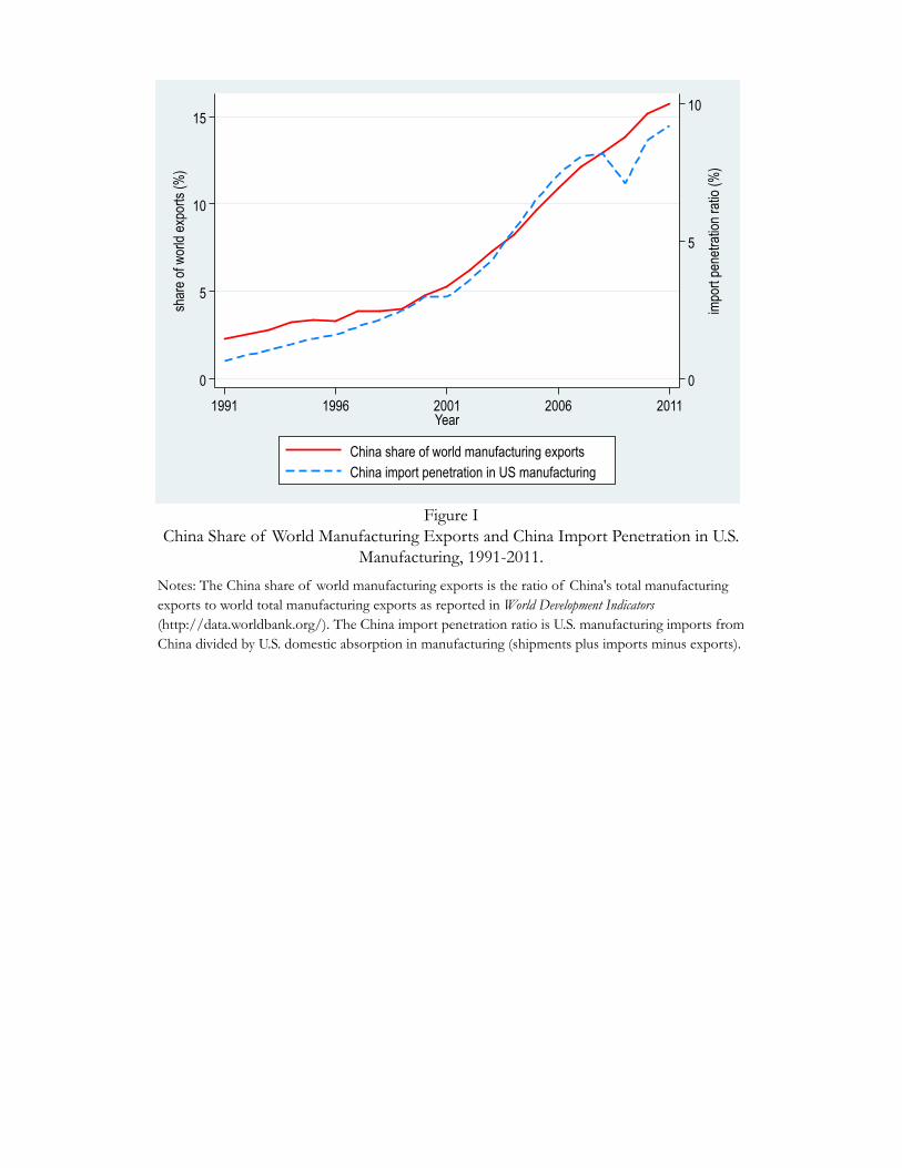
Figure IChina Share of World Manufacturing Exports and China Import Penetration in U.S.

Manufacturing, 1991-2011.

Notes: The China share of world manufacturing exports is the ratio of China's total manufacturing exports to world total manufacturing exports as reported in World Development Indicators (http://data.worldbank.org/). The China import penetration ratio is U.S. manufacturing imports from China divided by U.S. domestic absorption in manufacturing (shipments plus imports minus exports).

0

5

10

impo

rt pe

netra

tion

ratio

(%)

0

5

10

15

shar

e of

wor

ld e

xpor

ts (%

)

1991 1996 2001 2006 2011Year

China share of world manufacturing exportsChina import penetration in US manufacturing

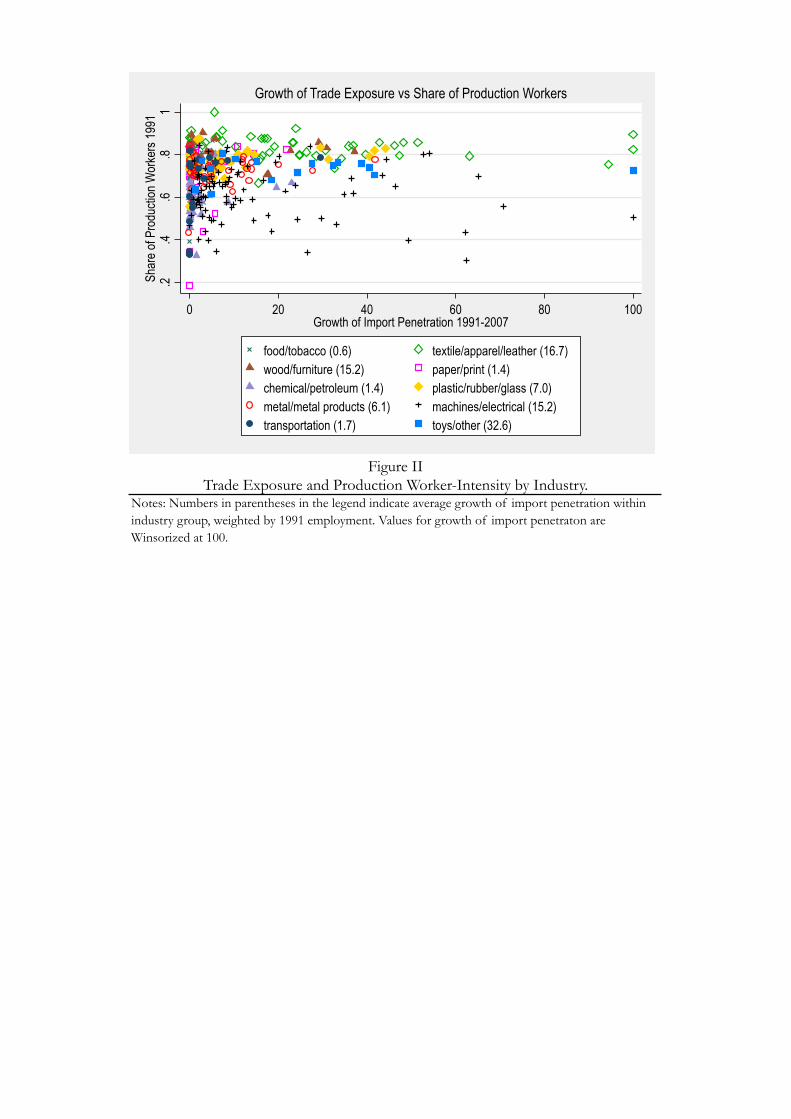
Notes: Numbers in parentheses in the legend indicate average growth of import penetration within industry group, weighted by 1991 employment. Values for growth of import penetraton are Winsorized at 100.

Figure IITrade Exposure and Production Worker-Intensity by Industry.

.2.4

.6.8

1Sh

are

of P

rodu

ctio

n W

orke

rs 1

991

0 20 40 60 80 100Growth of Import Penetration 1991-2007

food/tobacco (0.6) textile/apparel/leather (16.7) wood/furniture (15.2) paper/print (1.4) chemical/petroleum (1.4) plastic/rubber/glass (7.0) metal/metal products (6.1) machines/electrical (15.2) transportation (1.7) toys/other (32.6)

Growth of Trade Exposure vs Share of Production Workers

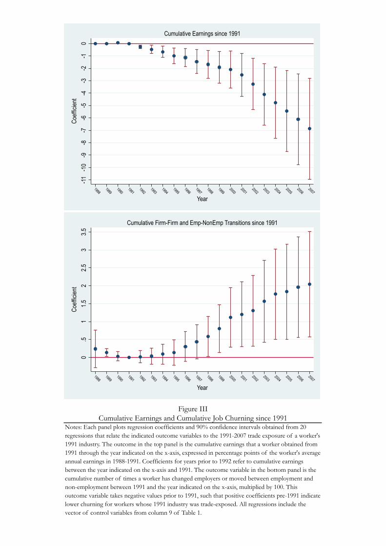
Figure IIICumulative Earnings and Cumulative Job Churning since 1991

Notes: Each panel plots regression coefficients and 90% confidence intervals obtained from 20 regressions that relate the indicated outcome variables to the 1991-2007 trade exposure of a worker's 1991 industry. The outcome in the top panel is the cumulative earnings that a worker obtained from 1991 through the year indicated on the x-axis, expressed in percentage points of the worker's average annual earnings in 1988-1991. Coefficients for years prior to 1992 refer to cumulative earnings between the year indicated on the x-axis and 1991. The outcome variable in the bottom panel is the cumulative number of times a worker has changed employers or moved between employment and non-employment between 1991 and the year indicated on the x-axis, multiplied by 100. This outcome variable takes negative values prior to 1991, such that positive coefficients pre-1991 indicate lower churning for workers whose 1991 industry was trade-exposed. All regressions include the vector of control variables from column 9 of Table 1.

-11

-10

-9-8

-7-6

-5-4

-3-2

-10

19881989

19901991

19921993

19941995

19961997

19981999

20002001

20022003

20042005

20062007

Year

Coef

ficie

nt

Cumulative Earnings since 1991

0.5

11.

52

2.5

33.

5

19881989

19901991

19921993

19941995

19961997

19981999

20002001

20022003

20042005

20062007

Year

Coef

ficie

nt

Cumulative Firm-Firm and Emp-NonEmp Transitions since 1991

Figure IVPersistence of Trade Exposure since 1991

Notes: The graph plots regression coefficients and 90% confidence intervals obtained from 2x16 regressions that relate the 1991-2007 trade exposure of a worker's industry in the year indicated on the x-axis to the 1991-2007 trade exposure of the worker's intial 1991 industry. The counterfactual data series sets trade exposure to zero for all firms except the worker's initial employer. It refers to a hypothetical scenario in which no worker joins a trade-exposed firm after separating from their initial firm, and so all persistence in trade exposure is due to workers who have not separated from their initial firm.

0.2

.4.6

.81

1.2

19911992

19931994

19951996

19971998

19992000

20012002

20032004

20052006

2007

Year

Conditional correlation in trade exposure between 1991 firm and firm in indicated yearCounterfactual with zero trade exposure in all firms except 1991 firm

Coef

ficie

nt

Firm mobility and trade exposure

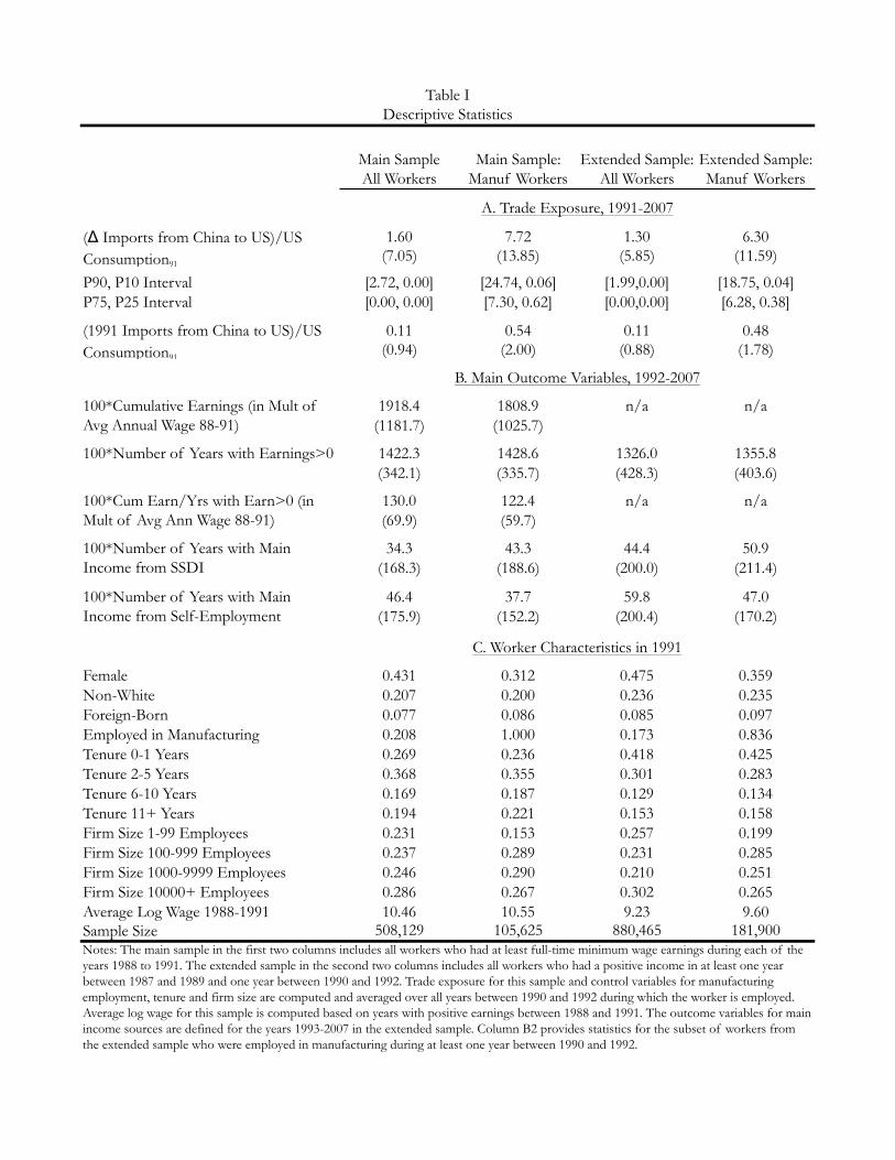
1.60 7.72 1.30 6.30(7.05) (13.85) (5.85) (11.59)

P90, P10 Interval [2.72, 0.00] [24.74, 0.06] [1.99,0.00] [18.75, 0.04]P75, P25 Interval [0.00, 0.00] [7.30, 0.62] [0.00,0.00] [6.28, 0.38]

0.11 0.54 0.11 0.48(0.94) (2.00) (0.88) (1.78)

1918.4 1808.9 n/a n/a(1181.7) (1025.7)

1422.3 1428.6 1326.0 1355.8(342.1) (335.7) (428.3) (403.6)

130.0 122.4 n/a n/a(69.9) (59.7)

34.3 43.3 44.4 50.9(168.3) (188.6) (200.0) (211.4)

46.4 37.7 59.8 47.0(175.9) (152.2) (200.4) (170.2)

Female 0.431 0.312 0.475 0.359Non-White 0.207 0.200 0.236 0.235Foreign-Born 0.077 0.086 0.085 0.097Employed in Manufacturing 0.208 1.000 0.173 0.836Tenure 0-1 Years 0.269 0.236 0.418 0.425Tenure 2-5 Years 0.368 0.355 0.301 0.283Tenure 6-10 Years 0.169 0.187 0.129 0.134Tenure 11+ Years 0.194 0.221 0.153 0.158Firm Size 1-99 Employees 0.231 0.153 0.257 0.199Firm Size 100-999 Employees 0.237 0.289 0.231 0.285Firm Size 1000-9999 Employees 0.246 0.290 0.210 0.251Firm Size 10000+ Employees 0.286 0.267 0.302 0.265Average Log Wage 1988-1991 10.46 10.55 9.23 9.60Sample Size 508,129 105,625 880,465 181,900Notes: The main sample in the first two columns includes all workers who had at least full-time minimum wage earnings during each of the years 1988 to 1991. The extended sample in the second two columns includes all workers who had a positive income in at least one year between 1987 and 1989 and one year between 1990 and 1992. Trade exposure for this sample and control variables for manufacturing employment, tenure and firm size are computed and averaged over all years between 1990 and 1992 during which the worker is employed. Average log wage for this sample is computed based on years with positive earnings between 1988 and 1991. The outcome variables for main income sources are defined for the years 1993-2007 in the extended sample. Column B2 provides statistics for the subset of workers from the extended sample who were employed in manufacturing during at least one year between 1990 and 1992.

C. Worker Characteristics in 1991

100*Cumulative Earnings (in Mult of Avg Annual Wage 88-91)

100*Number of Years with Earnings>0

100*Cum Earn/Yrs with Earn>0 (in Mult of Avg Ann Wage 88-91)

100*Number of Years with Main Income from SSDI

100*Number of Years with Main Income from Self-Employment

(1991 Imports from China to US)/US Consumption91

B. Main Outcome Variables, 1992-2007

Table IDescriptive Statistics

A. Trade Exposure, 1991-2007

(Δ Imports from China to US)/US Consumption91

Main SampleAll Workers

Main Sample: Manuf Workers

Extended Sample: All Workers

Extended Sample: Manuf Workers

OLS(1) (2) (3) (4) (5) (6) (7) (8) (9)

-2.939 * -5.726 ** -6.017 ** -6.099 ** -6.883 ** -6.436 ** -5.695 * -6.728 ** -6.864 **(1.150) (1.425) (1.475) (1.395) (1.351) (2.450) (2.326) (2.392) (2.477)

Birth year dummies yes yes yes yes yes yes yes yes yes

Demographic controls yes yes yes yes yes yes yes

Employment history yes yes yes yes yes yes

Earnings history yes yes yes yes yes

Initial import levels yes yes yes yes

10 mfg industry dummies yes yes yes

Industry characteristics yes yes

Pretrends ind emp and wage yes

Table IIImports from China and Cumulative Earnings, 1992-2007: OLS and 2SLS Estimates

Dependent Var: 100 x Earnings 1992-2007 (in Multiples of Initial Annual Wage)

2SLS

(Δ China Imports)/ US Consumption91

Notes: N=508,129. All regressions include a constant and a full set of birth year dummies. Demographic controls in column 3 include dummies for female, non-white and foreign-born. Employment history controls in column 4 include dummies for tenure at 1991 firm (0-1, 2-5, 6-10 years), experience (4-5, 6-8, 9-11 years), and size of 1991 firm (1-99, 100-999, 1000-9999 employees). Earnings history controls in column 5 include the worker's annual log wage averaged over 1988-1991, an interaction of intial wage with age, and the change in log wage between 1988 and 1991, as well as the level and trend of the 1991 firm's log mean wage for the period 1988-1991. Columns 6-9 add controls for a worker's 1991 manufacturing industry, starting with initial trade penetration by Chinese and non-Chinese imports in column 6 (coefficients indicated in the table). Column 7 adds dummies for 10 manufacturing sub-industries, column 8 adds 1991 levels for employment share of production workers, log average wage, capital/value added, and 1990 levels for computer investment, share of investment allocated to high-tech equipment, and fraction of intermediate goods among imports in 1990, and column 9 additionally controls for changes in industry employment share and log average wage level during the preceding 16 years (1976-1991). Robust standard errors in parentheses are clustered on start-of-period 3-digit industry. ~ p ≤ 0.10, * p ≤ 0.05, ** p ≤ 0.01.

Cumulative Years w/ Earnings/Earnings Earnings>0 Year

(1) (2) (3)

-6.864 ** -0.535 -0.393 **(2.477) (0.505) (0.140)

-0.432 0.695 -0.064(1.996) (0.856) (0.112)

Table III Imports from China 1992-2007 and Cumulative Earnings, Years with Earnings, and

Earnings per Year 1992-2007 and 1976-1991: 2SLS EstimatesDep Vars: 100 x Cumulative Earnings; 100 x Years with Earnings; 100 x Earnings per

Year of Employment (in Multiples of Initial Annual Wage)

A. Treatment Period 1992-2007

Notes: N=508,792 in Panel I and N=301,490 in Panel II, except N=506,339 and N=300,239 in column 3 where the dependent variable is not defined for individuals who are never employed during the entire outcome period. Regressions in Panel I include the full control vector from column 9 of Table 2. Regressions in Panel II include the same controls except tenure, experience and firm size; and industry-level controls are measured either for 1975 or for 1972 (intermediate imports, computer investment and high tech equipment). Robust standard errors in parentheses are clustered on start-of-period 3-digit industry. ~ p ≤ 0.10, * p ≤ 0.05, ** p ≤ 0.01.

(Δ China Imports)/ US Consumption91

B. Pre-Period 1976-1991

(Δ China Imports)/ US Consumption91

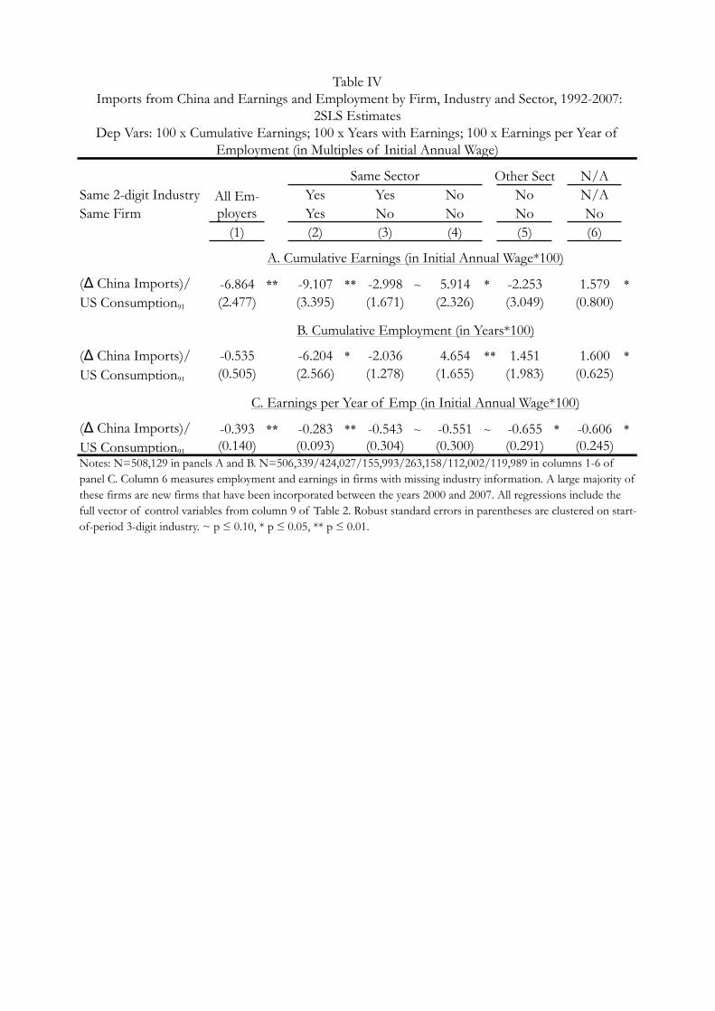
Other Sect N/ASame 2-digit Industry Yes Yes No No N/ASame Firm Yes No No No No

(1) (2) (3) (4) (5) (6)

-6.864 ** -9.107 ** -2.998 ~ 5.914 * -2.253 1.579 *(2.477) (3.395) (1.671) (2.326) (3.049) (0.800)

-0.535 -6.204 * -2.036 4.654 ** 1.451 1.600 *(0.505) (2.566) (1.278) (1.655) (1.983) (0.625)

-0.393 ** -0.283 ** -0.543 ~ -0.551 ~ -0.655 * -0.606 *(0.140) (0.093) (0.304) (0.300) (0.291) (0.245)

Table IV Imports from China and Earnings and Employment by Firm, Industry and Sector, 1992-2007:

2SLS EstimatesDep Vars: 100 x Cumulative Earnings; 100 x Years with Earnings; 100 x Earnings per Year of

Employment (in Multiples of Initial Annual Wage)

Same Sector

A. Cumulative Earnings (in Initial Annual Wage*100)

(Δ China Imports)/ US Consumption91

(Δ China Imports)/ US Consumption91

Notes: N=508,129 in panels A and B. N=506,339/424,027/155,993/263,158/112,002/119,989 in columns 1-6 of panel C. Column 6 measures employment and earnings in firms with missing industry information. A large majority of these firms are new firms that have been incorporated between the years 2000 and 2007. All regressions include the full vector of control variables from column 9 of Table 2. Robust standard errors in parentheses are clustered on start-of-period 3-digit industry. ~ p ≤ 0.10, * p ≤ 0.05, ** p ≤ 0.01.

B. Cumulative Employment (in Years*100)

(Δ China Imports)/ US Consumption91

C. Earnings per Year of Emp (in Initial Annual Wage*100)

All Em-ployers

Initial Other N/ACZ CZ CZ

(1) (2) (3) (4)

-6.649 ** -3.558 * -2.307 ~ -0.785(2.417) (1.396) (1.281) (0.542)

-0.653 -0.008 -0.491 -0.154(0.513) (0.599) (0.539) (0.253)

-0.418 ** -0.344 ** -0.741 * -1.010 *(0.152) (0.124) (0.369) (0.398)

C. Earnings/Year (in Initial Annual Wage*100)

(Δ China Imports)/ US Consumption91

Notes: N=508,129, except smaller samples in panel C. Column 1 shows aggregate results for earnings and employment. Columns 2-4 subdivide results into employment and earnings obtained while residing in the 1993 Commuting Zone of residence (column 2), in all CZs other than the 1993 CZ of residence (column 3), and in CZs than cannot be classified because either the 1993 location or subsequent location of the worker is unknown (column 4). All regressions include the full control vector from column 9 of Table 2, and a dummy for the 6% of workers whose 1993 CZ is unknown. Robust standard errors in parentheses are clustered on start-of-period 3-digit industry. ~ p ≤ 0.10, * p ≤ 0.05, ** p ≤ 0.01.

Table VImports from China and Earnings and Employment by Geographic Location, 1994-

2007: 2SLS EstimatesDep Vars: 100 x Cumulative Earnings; 100 x Years with Earnings; 100 x Earnings

per Year of Employment (in Multiples of Initial Annual Wage)

All CZ

A. Cum. Earnings (in Initial Annual Wage*100)

(Δ China Imports)/ US Consumption91

B. Cumulative Employment (in Years*100)

(Δ China Imports)/ US Consumption91

*

** *

*

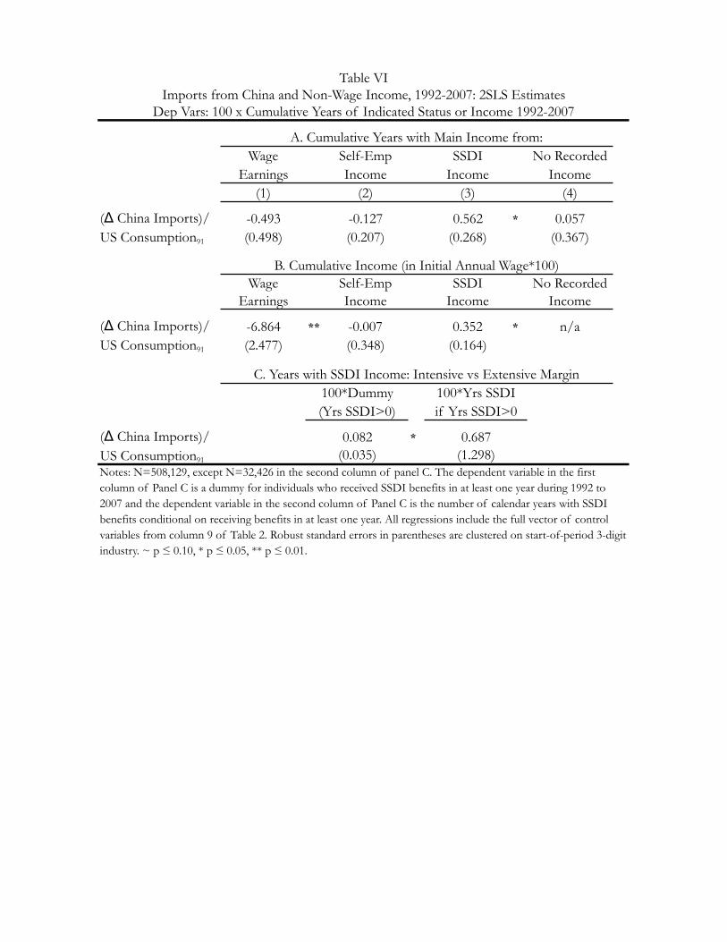
100*Dummy

0.082

(Yrs SSDI>0) if Yrs SSDI>0100*Yrs SSDI

Notes: N=508,129, except N=32,426 in the second column of panel C. The dependent variable in the first column of Panel C is a dummy for individuals who received SSDI benefits in at least one year during 1992 to 2007 and the dependent variable in the second column of Panel C is the number of calendar years with SSDI benefits conditional on receiving benefits in at least one year. All regressions include the full vector of control variables from column 9 of Table 2. Robust standard errors in parentheses are clustered on start-of-period 3-digit industry. ~ p ≤ 0.10, * p ≤ 0.05, ** p ≤ 0.01.

(0.035)0.687

Income(4)

SSDI

(Δ China Imports)/ US Consumption91

No Recorded

Income

(1.298)

0.562

Table VIImports from China and Non-Wage Income, 1992-2007: 2SLS Estimates

Dep Vars: 100 x Cumulative Years of Indicated Status or Income 1992-2007

WageEarnings

(2)

A. Cumulative Years with Main Income from:

IncomeSelf-Emp

(3)(1)

No Recorded

Income

(0.164)0.352

C. Years with SSDI Income: Intensive vs Extensive Margin

-0.007(0.348)

-6.864 n/a

(Δ China Imports)/ US Consumption91

-0.493(0.498)

-0.127

B. Cumulative Income (in Initial Annual Wage*100)

0.057(0.367)(0.207)

Income

(Δ China Imports)/ US Consumption91

(0.268)

SSDIEarnings Income

Self-Emp

(2.477)

Wage

(1) (2) (3) (4)

-0.613 -0.152 0.438 * 0.327 0.056 *

(0.415) (0.157) (0.202) (0.330) (0.026)

-0.991 ~ -0.694 * 1.137 ** 0.548 0.125 **(0.569) (0.301) (0.431) (0.426) (0.043)

Table VIIImports from China and Cum. Years of Emp and SSDI Receipt by Worker Sample: 2SLS Estimates. Dep Vars: 100 x Cumulative Years with Income from Indicated Sources and 100 x Dummy for SSDI

Income, 1993-2007

Cumulative Years with Main Income from:

A. Main Sample: High LF Attachment

(Δ China Imports)/ US Consumption91

Wage Earnings

100*Dummy (Yrs SSDI>0)

(5)

Self- Employmt

SSDI Benefits No Income

Notes: Panel A includes workers who earned at least the equivalent of a full-time minimum wage job in each of the four years 1988 to 1991. Panel B adds workers with low annual incomes or interrupted careers who were employed at least in one year during 1987-1989, and one year during 1990-1992. All regressions include the full vector of control variables from colum 9 of Table 2, except that all industry- and firm-related variables are averaged over those years in which a worker was employed during 1990 to 1992. Robust standard errors in parentheses are clustered on start-of-period 3-digit industry. ~ p ≤ 0.10, * p ≤ 0.05, ** p ≤ 0.01.

N=880,465

N=508,129

B. Extended Sample: High and Low LF Attachment

(Δ China Imports)/ US Consumption91

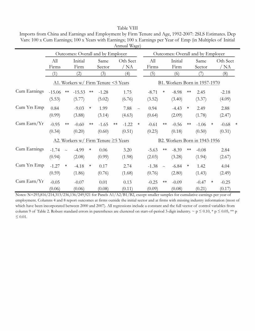
(1) (2) (3) (4) (5) (6) (7) (8)

Cum Earnings -15.06 ** -15.53 ** -1.28 1.75 -8.71 * -8.98 ** 2.45 -2.18(5.53) (5.77) (5.02) (6.76) (3.52) (3.40) (3.37) (4.09)

Cum Yrs Emp 0.84 -9.03 * 1.99 7.88 ~ 0.94 -4.43 * 2.49 2.88(0.99) (3.88) (3.14) (4.63) (0.64) (2.09) (1.78) (2.47)

Cum Earn/Yr -0.95 ** -0.60 ** -1.65 ** -1.22 * -0.61 ** -0.56 ** -1.06 * -0.68 *(0.34) (0.20) (0.60) (0.51) (0.23) (0.18) (0.50) (0.31)

Cum Earnings -1.74 ~ -4.99 * 0.06 3.20 -5.63 ** -8.39 ** -0.08 2.84(0.94) (2.08) (0.99) (1.98) (2.03) (3.28) (1.94) (2.67)

Cum Yrs Emp -1.27 * -4.18 * 0.17 2.74 -1.38 ~ -6.84 * 1.42 4.04(0.59) (1.86) (0.76) (1.68) (0.76) (2.80) (1.43) (2.49)

Cum Earn/Yr -0.05 -0.07 0.01 0.13 -0.25 ** -0.09 -0.47 * -0.25(0.06) (0.06) (0.08) (0.11) (0.09) (0.08) (0.21) (0.17)

Notes: N=293,816/214,313/236,136/249,921 for Panels A1/A2/B1/B2, except smaller samples for cumulative earnings per year of employment. Columns 4 and 8 report outcomes at firms outside the initial sector and at firms with missing industry information (most of which have been incorporated between 2000 and 2007). All regressions include a constant and the full vector of control variables from column 9 of Table 2. Robust standard errors in parentheses are clustered on start-of-period 3-digit industry. ~ p ≤ 0.10, * p ≤ 0.05, ** p ≤ 0.01.

A1. Workers w/ Firm Tenure <5 Years

A2. Workers w/ Firm Tenure ≥5 Years

Table VIIIImports from China and Earnings and Employment by Firm Tenure and Age, 1992-2007: 2SLS Estimates. Dep Vars: 100 x Cum Earnings; 100 x Years with Earnings; 100 x Earnings per Year of Emp (in Multiples of Initial

Annual Wage)

Outcomes: Overall and by EmployerAll

FirmsInitial Firm

Same Sector

Oth Sect / NA

B2. Workers Born in 1943-1956

Outcomes: Overall and by EmployerAll

FirmsInitial Firm

Same Sector

Oth Sect / NA

B1. Workers Born in 1957-1970

(1) (2) (3) (4)

-18.27 ** -8.78 * 0.85 -10.34 *(5.76) (3.84) (5.21) (4.52)

-0.20 -4.10 ~ 4.50 ~ -0.60(1.30) (2.23) (2.73) (2.68)

-1.16 ** -0.44 ~ -2.71 ** -1.34 **(0.34) (0.24) (0.85) (0.45)

-9.93 ** -8.50 ** 2.73 -4.16(3.65) (3.27) (2.38) (3.17)

-0.37 -4.43 * 2.84 ~ 1.22(0.65) (2.03) (1.65) (1.88)

-0.61 ** -0.51 ** -0.67 ~ -0.67 *(0.22) (0.17) (0.35) (0.31)

-0.22 -9.15 ~ 2.24 6.69(2.07) (4.69) (2.36) (5.38)

-0.41 -7.79 ~ 1.10 6.28(0.55) (4.29) (1.59) (4.29)

0.03 -0.04 0.07 0.03(0.14) (0.12) (0.29) (0.22)

Notes: N=169,386/169,357/169,386 for panels A/B/C, except smaller samples for cumulative earnings per year. Earnings and employment outcomes are reported cumulatively over all firms that employ a worker during the outcome period (columns 1), and separately for the initial firm (column 2), other firms of the same sector (column 3), and firms that are either outside the initial sector or have missing industry information (column 4). All regressions include a constant and the full vector of control variables from column 9 of Table 2. Robust standard errors in parentheses are clustered on start-of-period 3-digit industry. ~ p ≤ 0.10, * p ≤ 0.05, ** p ≤ 0.01.

Cum Earnings

Cum Yrs Emp

Cum Earn/Yr

Cum Earnings

Cum Yrs Emp

Cum Earn/Yr

A. Initial Wage in Bottom Tercile of Cohort

B. Initial Wage in Middle Tercile of Cohort

C. Initial Wage in Top Tercile of Cohort

Cum Earnings

Cum Yrs Emp

Cum Earn/Yr

Table IXImports from China and Earnings and Employment by Subgroup of

Workers: 2SLS EstimatesDep Vars: 100 x Cum Earnings; 100 x Years with Earnings; 100 x Earnings

per Year of Emp (in Multiples of Initial Annual Wage)

Worker Outcomes -- Overall and by Employer

All FirmsInitial Firm

Oth Firm, Same Sector

Other Sector/

NA

II. Initial

III. Other

IV. N/A

(1) (2) (3) (4) (5) (6)

-6.65 ** -6.07 ** -3.31 ** -2.09 ~ -0.66(2.42) (2.16) (1.24) (1.25) (0.59)

-20.30 ** -19.68 ** -16.88 ** -0.56 -2.24(6.72) (6.79) (4.59) (4.88) (1.38)

-0.65 -0.65 -0.14 -0.38 -0.14(0.51) (0.50) (0.65) (0.58) (0.31)

2.26 ~ 2.33 ~ 0.42 1.15 0.76(1.23) (1.22) (3.13) (2.74) (0.71)

-0.42 ** -0.37 ** -0.30 ** -0.71 * -0.97 **(0.15) (0.14) (0.12) (0.36) (0.36)

-1.66 ** -1.62 ** -1.59 ** -1.02 ~ -1.33 ~(0.58) (0.59) (0.52) (0.58) (0.81)

Table XEffect of Exposure to Chinese Imports at the Industry and Commuting Zone Level on Earnings and

Employment: 2SLS EstimatesDep Var: 100 x Cumulative Earnings, Years of Employment, or Earnings/Year, 1994-2007

Outcomes Measured at

I. All CZ

A. Outcome: Cumulative Earnings

(Δ Imports from China to US)/ US Consumption91

CZ Avg of [Δ Imports from China to US)/ US Consumption91]

B. Outcome: Cumulative Years of Employment

(Δ Imports from China to US)/ US Consumption91

CZ Avg of [Δ Imports from China to US)/ US Consumption91]

C. Outcome: Earnings per Year of Employment

(Δ Imports from China to US)/ US Consumption91

CZ Avg of [Δ Imports from China to US)/ US Consumption91]Notes: N=508,129, except smaller samples in Panel C. The commuting zone (CZ) average of import exposure for worker i in CZ j is defined as the average trade exposure of all other workers -i located in CZ j, according to the industry employment structure obtained from the 1990 County Business Patterns. Workers' 1991 CZ of residence is not observed in the data and thus imputed based on available location and employment information. For most workers, it corresponds to the observed 1993 CZ of residence. All regressions include the full control vector from column 9 of Table 2 and regressions in columns 2-6 include a dummy for observations with missing 1993 CZ and dummies for 1991 Census divisions. Robust standard errors in parentheses are two-way clustered on start-of-period 3-digit industry and on imputed 1991 CZ of residence. ~ p ≤ 0.10, * p ≤ 0.05, ** p ≤ 0.01.

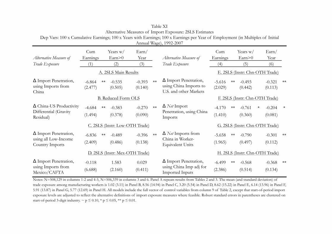
Cum Years w/ Earn/ Cum Years w/ Earn/Alternative Measure of Earnings Earn>0 Year Alternative Measure of Earnings Earn>0 YearTrade Exposure (1) (2) (3) Trade Exposure (4) (5) (6)

-6.864 ** -0.535 -0.393 ** -5.616 ** -0.493 -0.321 **(2.477) (0.505) (0.140) (2.029) (0.442) (0.113)

-4.684 ** -0.383 -0.270 ** -4.170 ** -0.761 * -0.204 *

(1.494) (0.378) (0.090) (1.410) (0.360) (0.081)

-6.836 ** -0.489 -0.396 ** -5.658 ** -0.790 -0.301 **

(2.409) (0.486) (0.138) (1.965) (0.497) (0.112)

-0.118 1.583 0.029 -6.499 ** -0.568 -0.368 **

(6.688) (2.160) (0.411) (2.386) (0.514) (0.134)

Table XIAlternative Measures of Import Exposure: 2SLS Estimates

Dep Vars: 100 x Cumulative Earnings; 100 x Years with Earnings; 100 x Earnings per Year of Employment (in Multiples of Initial Annual Wage), 1992-2007

E. 2SLS (Instr: Chn-OTH Trade)

F. 2SLS (Instr: Chn-OTH Trade)

Δ Net Import Penetration, using China Imports

Δ Import Penetration, using Imports from China

Δ China-US Productivity Differential (Gravity Residual)

Δ Import Penetration, using China Imports to U.S. and other Markets

A. 2SLS Main Results

Notes: N=508,129 in columns 1-2 and 4-5, N=506,339 in columns 3 and 6. Panel A repeats results from Tables 2 and 3. The mean (and standard deviation) of trade exposure among manufacturing workers is 1.02 (3.11) in Panel B, 8.56 (14.94) in Panel C, 3.20 (5.54) in Panel D, 8.62 (15.22) in Panel E, 6.14 (13.96) in Panel F, 5.91 (13.87) in Panel G, 5.77 (12.69) in Panel H. All models include the full vector of control variables from column 9 of Table 2, except that start-of-period import exposure levels are adjusted to reflect the alternative definitions of import exposure measures where feasible. Robust standard errors in parentheses are clustered on start-of-period 3-digit industry. ~ p ≤ 0.10, * p ≤ 0.05, ** p ≤ 0.01.

B. Reduced Form OLS

D. 2SLS (Instr: Mex-OTH Trade)

Δ Import Penetration, using Imports from Mexico/CAFTA

H. 2SLS (Instr: Chn-OTH Trade)

Δ Import Penetration, using China Imp adj for Imported Inputs

C. 2SLS (Instr: Low-OTH Trade) G. 2SLS (Instr: Chn-OTH Trade)

Δ Import Penetration, using all Low-Income Country Imports

Δ Net Imports from China in Worker-Equivalent Units