
Defaultable term structure models: macroeconomic impact ...
331
TECHNISCHE UNIVERSIT ¨ AT M ¨ UNCHEN Lehrstuhl f¨ ur Finanzmathematik Defaultable term structure models: macroeconomic impact and valuation of complex credit- and inflation-linked derivatives Melanie Ilg Vollst¨andiger Abdruckder von der Fakult¨at f¨ ur Mathematik der Technischen Universit¨atM¨ unchen zur Erlangung des akademischen Grades eines Doktors der Naturwissenschaften (Dr. rer. nat.) genehmigten Dissertation. Vorsitzender: Univ.-Prof. Dr. Claudia Czado Pr¨ ufer der Dissertation: 1. Univ.-Prof. Dr. Rudi Zagst 2. Univ.-Prof. Dr. R¨ udiger Kiesel (Universit¨atDuisburg-Essen) 3. Univ.-Prof. Dr. Ralf Werner (Universit¨atAugsburg) Die Dissertation wurde am 24.01.2013 bei der Technischen Universit¨at M¨ unchen eingereicht und durch die Fakult¨at f¨ ur Mathematik am 14.05.2013 angenommen.
Transcript of Defaultable term structure models: macroeconomic impact ...
TECHNISCHE UNIVERSITAT MUNCHENLehrstuhl fur Finanzmathematik
Defaultable term structure models:macroeconomic impact and valuationof complex credit- and inflation-linked
derivatives
Melanie Ilg
Vollstandiger Abdruck der von der Fakultat fur Mathematik der TechnischenUniversitat Munchen zur Erlangung des akademischen Grades eines
Doktors der Naturwissenschaften (Dr. rer. nat.)
genehmigten Dissertation.
Vorsitzender: Univ.-Prof. Dr. Claudia Czado
Prufer der Dissertation: 1. Univ.-Prof. Dr. Rudi Zagst
2. Univ.-Prof. Dr. Rudiger Kiesel(Universitat Duisburg-Essen)
3. Univ.-Prof. Dr. Ralf Werner(Universitat Augsburg)
Die Dissertation wurde am 24.01.2013 bei der Technischen UniversitatMunchen eingereicht und durch die Fakultat fur Mathematik am 14.05.2013angenommen.

ii

Abstract
This thesis is concerned with the pricing of credit- and inflation-linked prod-ucts within a defaultable term structure framework that incorporates macroe-conomic and firm-specific factors. In particular, we introduce a general pric-ing framework from which several models are derived differing in the assump-tions regarding the number of economic factors, observability and correlationof these factors. For this family of models, we study the determinants of non-defaultable and defaultable bond prices by directly including observable aswell as unobservable macroeconomic factors into the different set-ups.Based on the general version of the defaultable term structure model, wedetermine prices for credit default swaps in closed form and further deduceexact dynamics of credit default swap spreads. Approximating these ex-act dynamics enables us to present closed-form solutions for complex creditderivatives like credit default swaptions and constant maturity credit defaultswaps. We use a full simulation approach to test the pricing formulas forthese credit derivatives and to compare our results to literature.Further, we apply a variant of our general term structure framework to thepricing of inflation-linked assets. We use a framework that decomposes theshort rate into a real short rate and an inflation short rate. Starting withstandard inflation-linked derivatives like zero-coupon inflation-linked swapsand year-on-year inflation-linked swaps, we extend our framework to the pric-ing of complex hybrid inflation-linked derivatives incorporating interest rate,equity or credit components. We derive closed-form solutions for inflation-linked equity options and credit default swaps. Also, we present a feasibleapproximation for pricing hybrid inflation-linked derivatives in closed formenabling a fast and accurate pricing for such complex derivatives.
iii

iv

Zusammenfassung
Diese Dissertation befasst sich mit der Bewertung von kreditrisikobehaftetenund inflationsindexierten Produkten innerhalb eines ausfallbehafteten Zins-strukturmodells, das sowohl makrookonomische als auch firmenspezifischeFaktoren integriert. Ausgehend von einem allgemeinen Bewertungsansatzwerden mehrere Modelle abgeleitet, welche sich in den Annahmen bezuglichder Anzahl okonomischer Faktoren und deren Beobachtbarkeit und Kor-relation unterscheiden. Fur diese verschiedenen Ansatze werden anhand derIntegration von beobachtbaren und unbeobachtbaren makrookonomischenFaktoren potentielle Treiber risikoloser und ausfallbehafteter Bondpreise ana-lysiert.Basierend auf der allgemeinen Version des ausfallbehafteten Zinsstruktur-modells werden Preise fur Credit Default Swaps in geschlossener Form be-stimmt und des Weiteren exakte Dynamiken der Credit Default Swap Spreadsabgeleitet. Das Approximieren dieser exakten Dynamiken erlaubt nun dieBewertung von komplexen Kreditderivaten wie Credit Default Swaptionsund Constant Maturity Credit Default Swaps in geschlossener Form. Ab-schließend werden diese Ergebnisse gegen eine simulationsbasierte Bewertunggetestet und mit der bestehenden Literatur verglichen.Eine Variante des allgemeinen Bewertungsmodells wird zudem verwendet,um inflationsindexierte Produkte zu bewerten. Dieser Ansatz zerlegt dieShortrate in eine reale Shortrate und eine Inflations-Shortrate. Ausgehendvon Standard-Inflationsderivaten wie Zero-Coupon- und Year-on-Year Infla-tion-Linked Swaps wird die Bewertung auf komplexe, hybride, inflationsin-dexierte Derivate ausgeweitet. Diese hybriden Derivate beinhalten zusatzlicheZins-, Equity- und Kreditkomponenten. Es werden geschlossene Bewertungs-formeln fur inflationsindexierte Equity Optionen und Credit Default Swapshergeleitet. Des Weiteren wird eine Approximation fur die Bewertung vonhybriden, inflationsindexierten Derivaten in geschlossener Form vorgestellt,welche eine schnelle und akkurate Bewertung fur komplexe Derivate erlaubt.
v

vi

Acknowledgements
First of all, I would like to thank my supervisor Prof. Dr. Rudi Zagst whooffered me the possibility to do a dissertation at the Institute for Mathemati-cal Finance at the TU Munchen. He contributed substantially to this thesisby initiating the topic and through his ideas, feedback and support. Duringmy stay at the institute, he provided the academic working environment andmaintained it afterwards with his ongoing interest and advice.Furthermore, I would like to thank Prof. Dr. Rudiger Kiesel and Prof. Dr.Ralf Werner for serving as reverees for this thesis and to Prof. Dr. ClaudiaCzado for chairing the examination board.Finally, I would like to express my gratitude to my former colleagues at theInstitute for Mathematical Finance for their encouragement and for numer-ous helpful discussions throughout the years.
vii

viii

Contents
1 Introduction 11.1 Motivation . . . . . . . . . . . . . . . . . . . . . . . . . . . . . 11.2 Objectives and Structure . . . . . . . . . . . . . . . . . . . . . 2
2 Mathematical Fundamentals 52.1 Point Processes and Intensities . . . . . . . . . . . . . . . . . . 52.2 Ito Processes and Stochastic Differential Equations . . . . . . 72.3 Financial Markets . . . . . . . . . . . . . . . . . . . . . . . . . 132.4 Kalman Filter . . . . . . . . . . . . . . . . . . . . . . . . . . . 21
3 Pricing Credit Risk 253.1 Structural Models . . . . . . . . . . . . . . . . . . . . . . . . . 253.2 Reduced-Form Models . . . . . . . . . . . . . . . . . . . . . . 273.3 Hybrid Models . . . . . . . . . . . . . . . . . . . . . . . . . . 28
4 A Generalized Five Factor Model 294.1 The Set-Up . . . . . . . . . . . . . . . . . . . . . . . . . . . . 304.2 The Extended Schmid-Zagst Model . . . . . . . . . . . . . . . 424.3 A Further Enhancement of the Schmid-Zagst Model - The Five
Factor Approach . . . . . . . . . . . . . . . . . . . . . . . . . 444.4 The Real and Inflation Short-Rate Model . . . . . . . . . . . . 474.5 A Simplified Version of the General Set-Up - The Correlated
Five Factor Approach . . . . . . . . . . . . . . . . . . . . . . . 504.6 Summary of Models . . . . . . . . . . . . . . . . . . . . . . . . 524.7 Calibrating the Models to Market Data . . . . . . . . . . . . . 564.8 Comparing the Models . . . . . . . . . . . . . . . . . . . . . . 77
5 Pricing Credit Derivatives 895.1 Survival Probability . . . . . . . . . . . . . . . . . . . . . . . . 925.2 Default Digital Put Option . . . . . . . . . . . . . . . . . . . . 935.3 Default Put Option . . . . . . . . . . . . . . . . . . . . . . . . 96
ix

x CONTENTS
5.4 Forward Credit Default Swap . . . . . . . . . . . . . . . . . . 995.4.1 The Dynamics of the Forward Credit Default Swap
Spread . . . . . . . . . . . . . . . . . . . . . . . . . . . 1065.4.2 Exact versus Approximated Dynamics of the Forward
Credit Default Swap Spread . . . . . . . . . . . . . . . 1245.4.3 Introducing Counterparty Risk . . . . . . . . . . . . . 150
5.5 Credit Default Swaption . . . . . . . . . . . . . . . . . . . . . 1575.5.1 Big Bang/Small Bang . . . . . . . . . . . . . . . . . . 170
5.6 Constant Maturity Credit Default Swap . . . . . . . . . . . . 175
6 Pricing Inflation-Indexed Derivatives 1876.1 Inflation-Indexed Swaps . . . . . . . . . . . . . . . . . . . . . 1896.2 Inflation-Indexed Options . . . . . . . . . . . . . . . . . . . . 1956.3 Inflation Hybrids . . . . . . . . . . . . . . . . . . . . . . . . . 197
6.3.1 Inflation-Linked Equity Options . . . . . . . . . . . . . 2106.3.2 Inflation-Indexed Credit Default Swap . . . . . . . . . 212
7 Summary and Conclusion 223
A Determination of θr 227
B Results of the Calibration 231
C Credit Derivatives 261
D FCDS Counterparty Risk 269
E Inflation-Indexed Derivatives 285

Chapter 1
Introduction
1.1 Motivation
The recent financial crisis turned the spotlight to credit risk pricing. Thedeterioration in prices and ratings of complex credit derivatives left the com-munity wondering if the models in use are capable of pricing highly structuredproducts, and whether default and its determinants are captured correctly.The majority of losses and provisions which occured during the crisis werenot due to actual losses caused by default but corrections of prices with re-spect to counterparty risk. So far, the assumptions for pricing derivativeshave been that there is no counterparty risk inherent especially for interbanktransactions resulting in risk-free values. But since the bail-out of AIG oneof the biggest player in so-called credit default swaps, which are a type of in-surance against the default of a certain reference asset, the focus of traders,financial engineers and regulators lies in adjusting derivatives’ prices withrespect to counterparty risk (CVA).There are two main approaches to credit risk pricing, structural and reduced-form models. While the former tries to model default directly by assuming itsoccurrence when the firm’s value crosses a certain threshold (i.e. outstand-ing debt), the latter focuses on modelling the default probability instead.Although the rational behind structural models is easy to understand, theyfail in exactly specifying default. Contrarily, reduced-form models assumethe default event of being exogenously given. For these models default is notexplainable by any observable data and comes totally unexpected. In order toovercome the shortcomings of both approaches, a third class of models havearosen. Hybrid models combine characteristics of both approaches thereforelinking default probabilities to macroeconomic or microeconomic data.The literature on determinants of sovereign und bond spreads is extensive.
1

2 CHAPTER 1. INTRODUCTION
Yet, the discussion is still going on about which economic factors are drivingthe spreads, how spreads and determinants are related and how to uncoverthe relationships respectively find the determinants. A popular approachfor specifying determinants is to use regression analysis for spreads and aset of candidate determinants. However, the results of these studies do notlink the economic risk dynamics to asset prices. The true relationship of thespread and its driving factors remains unexplained. Therefore, more recentapproaches use economic risk factors in no-arbitrage term structure mod-els directly linking the determinants to prices and emphasizing the growinginterest in hybrid credit models. All approaches have in common that al-though the choice of factors to be included in the test varied substantially,only a portion of credit spread changes could be explained. The majority ofvariation, however, appeared to be driven by a common factor that is stillunexplained.
1.2 Objectives and Structure
The main objective of this thesis is to study hybrid credit risk models withrespect to their ability in explaining credit spreads and their usage for pric-ing complex derivatives. It is our aim to further develop and promote hy-brid credit risk models because of their linkage to economic factors, whichwe believe crucial for pricing and forecasting credit risk especially for riskmanagement purposes like stress testing, future exposure and counterpartyrisk. Concerning the pricing of derivatives we want to improve the usageof our proposed defaultable term structure model by proposing closed-formsolutions that could help to reduce the computational burden of risk man-agement applications.The remainder of this thesis is organized as follows: In Chapter 2 we intro-duce and familiarize the reader with the basic concepts in (financial) mathe-matics that are used throughout this thesis. Chapter 3 outlines the originsand building blocks of the main credit risk pricing models and embeds ourdefaultable term structure framework into these approaches.In Section 4.1 of Chapter 4 we introduce the general version of our defaultableterm structure model and derive pricing formulas for non-defaultable zero-coupon bonds in Theorem 4.2 as well as for defaultable zero-coupon bondsin Theorem 4.3. From this general set-up we deduce several models differingin the assumptions regarding the number of economic factors, observabilityand correlation. For example, the extended Schmid-Zagst model of Section4.2 was first introduced by Antes, Ilg, Schmid & Zagst (2008) and incorp-

CHAPTER 1. INTRODUCTION 3
orates an observable macroeconomic factor in its term structure, whereasthe real and inflation short-rate model of Section 4.4, for which a variant ofit was first published by Hagedorn, Meyer & Zagst (2007), makes use of asecond unobservable macroeconomic factor. Based on these models we testin Sections 4.7 and 4.8 a set of macroeconomic factors with respect to theirimpact on sovereign and bond spreads. We use factors that either representa single driving factor or are a composition of several factors representingthe current or future state of the economy. Our choice of factors is based ontheir recurrent appearance in literature. Among our set of factors are widelyaccepted factors like the gross domestic product, that was used in severalstudies by e.g. Bonfim (2009), Glen (2005), Hilscher & Nosbusch (2010)and Rowland (2005), the consumer price index, that was used by Ang &Piazzesi (2003) and Cantor & Packer (1996) in addition to some of the previ-ously mentioned studies, and the industrial production, that was analyzed byFiglewski, Frydman & Liang (2012), Krishnan, Ritchken & Thomson (2005)and Krishnan, Ritchken & Thomson (2010). In addition to those well-knownmacroeconomic factors, we study the composite indices of leading and coin-cident indicators which are an aggregate of macroeconomic factors and giveindications concerning the state of the economy. These indices are publishedby The Conference Board (see TCB (2001)) and appeared e.g. in the workof Huang & Kong (2003). In Sections 4.7 and 4.8 we describe in detail thecalibration as well as the analysis of the obtained results.Based on the defaultable term structure model of Chapter 4, we determine inChapter 5 prices for credit default swaps in closed form also after controllingfor counterparty risk. The results for credit default swaps of Theorems 5.13,5.15 and 5.18 extend the work of Schmid (2002) and Antes, El Moufatich,Schmid & Zagst (2009) to our general framework introduced in Section 4.1of Chapter 4 with respect to different assumptions concerning the recoverypayments. Then, in Section 5.4.3 we further extend these results by incorp-orating counterparty risk based on the work of Jarrow & Yu (2001) who usedso-called primary and secondary firms in order to model default dependen-cies. In Section 5.4.1 we deduce from the closed-form solutions of Theorems5.13, 5.15 and 5.18 dynamics of credit default swap spreads in a consistentway while keeping the link to economic factors. After approximating the ex-act dynamics in Section 5.4.2 by lognormal and shifted-lognormal dynamics,we present closed-form solutions based on these approximations for credit de-fault swaptions in Theorems 5.33 and 5.34, and for constant maturity creditdefault swaps in Theorems 5.38, 5.39 and 5.40. In addition, we show in Sec-tion 5.5.1 how to incorporate the new quoting mechanism for credit defaultswaps, i.e. a constant cds spread (cf. Markit (2009a) and Markit (2009b)),into the pricing of credit default swaptions and we outline in Theorem 5.35
4 CHAPTER 1. INTRODUCTION
how to price a credit default swaption if the option maturity does not coincidewith the start of the credit default swap. We use a full simulation approachto test the pricing formulas for those credit derivatives and to compare ourresults to literature, e.g. Krekel & Wenzel (2006) and Brigo & Mercurio(2006).In Chapter 6 we outline the pricing of inflation-linked derivatives within ourterm structure model. This chapter extends the work of Hagedorn et al.(2007) to pricing hybrid inflation-linked derivatives. Starting with standardderivatives like zero-coupon inflation swaps we extend our pricing frameworkto hybrid products combining inflation with interest rates in Theorem 6.6according to the work of Dodgson & Kainth (2006). We test the approx-imated semi-analytical solution of Theorem 6.6 against the pricing by meansof simulation. Further, we introduce in Theorem 6.7 derivatives combiningthe characteristics of inflation and equity analogously to Hammarlid (2010),and in Theorem 6.9 we extend our inflation set-up to credit derivatives andmake use of results obtained in Chapter 5 in order to price an inflation-indexed credit default swap introduced by Avogaro (2006). Finally, Chapter7 concludes.

Chapter 2
Mathematical Fundamentals
This chapter is meant to introduce and familiarize the reader with the mathe-matical fundamentals and notations which will be used in this thesis. Thefirst section deals with point processes and intensities while the next sectionoutlines the basics of stochastic differential equations. Section 2.3 introducesthe concepts of financial markets and Section 2.4 presents the Kalman fil-tering technique which we will use later on as suggested in Schmid (2002).Mainly this chapter is based on Zagst (2002) but the usage of other sourceswill be explicitly stated at the appropriate places.
2.1 Point Processes and Intensities
The concept of point processes is an important source for credit risk mod-elling. Therefore, we start with these processes and further introduce inten-sities of point processes. A main class of credit risk models, the so-calledreduced-form models (cf. Chapter 3), make use of intensities.
In the following we assume a filtered probability space (Ω,F , Q, F), i.e. asigma-algebra F on the non-empty sample space Ω which is further equippedwith a probability measure Q and a filtration F = (Ft)t≥0.
Definition 2.1 (Point Processes)Let (Tn)n∈N be a monotonously increasing series of random variables withvalues in [0,∞] and T (0) = 0. If it holds for Tn < ∞: Tn(ω) < Tn+1(ω),∀ω ∈ Ω, then N(t) defined as
N(t) :=∑
n≥1
1t≥Tn
5

6 CHAPTER 2. MATHEMATICAL FUNDAMENTALS
is called the (Tn)n∈N0-associated point process.Further, N(t) is non-explosive if it holds supn∈N
Tn = ∞, Q − a.s..
Definition 2.2 (Stopping Time)Let τ be a random variable in R
+ ∪ ∞ with τ ≤ t ∈ Ft for any t ≥ 0,then τ is a stopping time with respect to the filtration F.
Lemma 2.3A point process N is adapted if and only if the associated series (Tn)n∈N is aseries of stopping times.
Proof:see Protter (1990), Theorem I.22.
Definition 2.4 (Intensity)Let N be a non-explosive, adapted point process and c a non-negative, pro-gressively measurable process, such that it holds for all t ≥ 0
∫ t
0
c(s)ds < ∞Q − a.s. .
If it further holds for all non-negative, predictable processes C
EQ
[∫ ∞
0
C(s)dN(s)
]= EQ
[∫ ∞
0
C(s) · c(s)ds
],
then N is said to admit the intensity c.
Theorem 2.5 (Martingale Characterization of Intensity)
(i) Assume N(t) admits the intensity c, M is given as M(t) := N(t) −∫ t
0c(s)ds, and C is a predictable process with
EQ
[∫ t
0|C(s)|c(s)ds
]< ∞, t ≥ 0, then
∫ t
0C(s)dM(s) is a martingale.
(ii) If it additionally holds EQ
[∫ t
0c(s)ds
]< ∞, t ≥ 0, then M is a mar-
tingale.
(iii) Let N(t) be a non-explosive, adapted, (Tn)n∈N0 associated point process
and let N(t∧ Tn)−∫ t∧Tn
0c(s)ds be a martingale ∀n ∈ N0. Then c(t) is
the intensity of N(t).

CHAPTER 2. MATHEMATICAL FUNDAMENTALS 7
Proof:see Bremaud (1981), pages 27-28.
If we now assume the point process N(t) to be represented by the indicatorfunction 1t≥τ for a stopping time τ and that N admits a right-continuousintensity c with EQ
[sup0≤s≤t c(s)
]< ∞, ∀t ≥ 0. Then according to Theorem
2.5 (ii) M(t) is a martingale and it holds for ε > 0:
Q (t < τ ≤ t + ε| Ft) = EQ
[1t<τ≤t+ε
∣∣Ft
]
= EQ [N(t + ε) − N(t)| Ft]
= EQ [M(t + ε) − M(t)| Ft] + EQ
[∫ t+ε
t
c(s)ds
∣∣∣∣Ft
]
= EQ
[∫ t+ε
t
c(s)ds
∣∣∣∣Ft
].
Additionally, it holds (see e.g. Schmid (2002))
c(t) = limε→0
Q (t < τ ≤ t + ε| Ft)
ε.
In credit risk models the stopping time τ is defined as the time of default of areference entity, e.g. the time when a company is unable to meet its financialobligations. With this in mind, the intensity c, which is often also referredto as hazard rate, can be interpreted as the arrival rate of default within thenext infinitesimal time period [t, t+ ε] given all available information at timet.
2.2 Ito Processes and Stochastic Differential
Equations
An important tool in financial mathematics are Ito processes for describingthe performance of prices. In this section we introduce those processes andfurther important applications of stochastic analysis. If not stated otherwisewe consult Zagst (2002). For further reading we also recommend Øksendal(1998) and Karatzas & Shreve (1991).

8 CHAPTER 2. MATHEMATICAL FUNDAMENTALS
Definition 2.6 (Ito Process)Let W be an m-dimensional Brownian motion. A stochastic process is calledan Ito process if for all t ≥ 0
Xt = X0 +
∫ t
0
µ(s)ds +
∫ t
0
σ(s)dW (s),
with X0 being F0-measurable and µ and σ = (σ1, ..., σm) (m-dimensional)progressively measurable stochastic processes with
∫ t
0
|µ(s)|ds < ∞
and ∫ t
0
σ2j (s)ds < ∞
Q-a.s. ∀ t ≥ 0, j = 1, . . . ,m.An n-dimensional Ito process is given by an n-dimensional vectorX = (X1, . . . , Xn)′, n ∈ N, whose elements are an Ito process.
The Ito process is often denoted in another way via a so-called stochasticdifferential equation (SDE):
dX(t) = µ(t)dt + σ(t)dW (t)
= µ(t)dt +m∑
j=1
σj(t)dWj(t).
Since financial derivatives are often constructed as a function of an Ito pro-cess it is helpful to know how this new process looks like and under whichconditions it will be an Ito process again. The following lemma states thenecessary conditions for a one-dimensional Ito process but can be extendedfor higher dimension (see e.g. Zagst (2002), page 29).
Theorem 2.7 (Ito’s Lemma)Let X = (X(t))t≥0 be an Ito process with
dX(t) = µ(t)dt +m∑
j=1
σj(t)dWj(t)
and G : R × [0,∞) → R be twice continuously differentiable in the firstvariable and once continuously differentiable in the second. Then it holds forall t ∈ [0,∞)
dG(X(t), t) = [Gt(X(t), t) + Gx(X(t), t)µ(t) +Gxx(X(t), t)
2||σ(t)||2]dt
+Gx(X(t), t)σ(t)dW (t).

CHAPTER 2. MATHEMATICAL FUNDAMENTALS 9
Proof:See Korn & Korn (1999), page 48-50.
Now, we define a strong solution of a given SDE and give conditions forthe existence and uniqueness of such a strong solution.
Definition 2.8 (Strong Solution)Let µ : R
n × [0,∞) → Rn and σ : R
n × [0,∞) → Rn×m, n,m ∈ N, be
measurable with respect to the corresponding Borel σ-algebras. If there existsan n-dimensional Ito-process X on the filtered probability space (Ω,F , Q, F)such that
X(t) = x +
∫ t
0
µ(X(s), s)ds +
∫ t
0
σ(X(s), s)dW (s) Q-a.s., X(0) = x,
with x ∈ Rn, then X is called a strong solution of the SDE
dX(t) = µ(X(t), t)dt + σ(X(t), t)dW (t), ∀ t ≥ 0, X(0) = x .
Theorem 2.9 (Existence and Uniqueness)Let the functions µ and σ of the previously stated SDE be continuous suchthat for all t > 0, x, y ∈ R
n and a constant K > 0 the following conditionshold I:
1. ||µ(x, t)−µ(y, t)||+||σ(x, t)−σ(y, t)|| ≤ K ·||x−y|| (Lipschitz condition)
2. ||µ(x, t)||2 + ||σ(x, t)||2 ≤ K2(1 + ||x||2) (growth condition).
Then there exists a unique, continuous strong solution X of the SDE and aconstant C which depends only on K and T > 0 such that it holds:
EQ[||X(t)||2] ≤ C(1 + ||x||2)eC·t ∀t ∈ [0, T ].
Furthermore it holds that
EQ[ sup0≤t≤T
||X(t)||2] < ∞.
Proof:See Korn & Korn (1999), page 127-133.
In this thesis, we will work with linear stochastic differential equations thatare defined in the following. Further, we present the unique strong solutionof this special class of SDEs.
I||x||, x ∈ Rn×m, denotes the Euclidean norm with ||x|| :=
√∑ni=1
∑mj=1 x2
ij .
10 CHAPTER 2. MATHEMATICAL FUNDAMENTALS
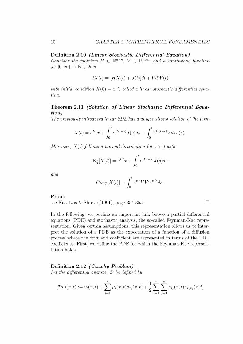
Definition 2.10 (Linear Stochastic Differential Equation)Consider the matrices H ∈ R
n×n, V ∈ Rn×m and a continuous function
J : [0,∞) → Rn, then
dX(t) = [HX(t) + J(t)]dt + V dW (t)
with initial condition X(0) = x is called a linear stochastic differential equa-tion.
Theorem 2.11 (Solution of Linear Stochastic Differential Equa-tion)The previously introduced linear SDE has a unique strong solution of the form
X(t) = eHtx +
∫ t
0
eH(t−s)J(s)ds +
∫ t
0
eH(t−s)V dW (s).
Moreover, X(t) follows a normal distribution for t > 0 with
EQ[X(t)] = eHtx +
∫ t
0
eH(t−s)J(s)ds
and
CovQ[X(t)] =
∫ t
0
eHsV V ′eH′sds.
Proof:see Karatzas & Shreve (1991), page 354-355.
In the following, we outline an important link between partial differentialequations (PDE) and stochastic analysis, the so-called Feynman-Kac repre-sentation. Given certain assumptions, this representation allows us to inter-pret the solution of a PDE as the expectation of a function of a diffusionprocess where the drift and coefficient are represented in terms of the PDEcoefficients. First, we define the PDE for which the Feynman-Kac represen-tation holds.
Definition 2.12 (Cauchy Problem)Let the differential operator D be defined by
(Dv)(x, t) := vt(x, t) +n∑
i=1
µi(x, t)vxi(x, t) +
1
2
n∑
i=1
n∑
j=1
aij(x, t)vxixj(x, t)
CHAPTER 2. MATHEMATICAL FUNDAMENTALS 11
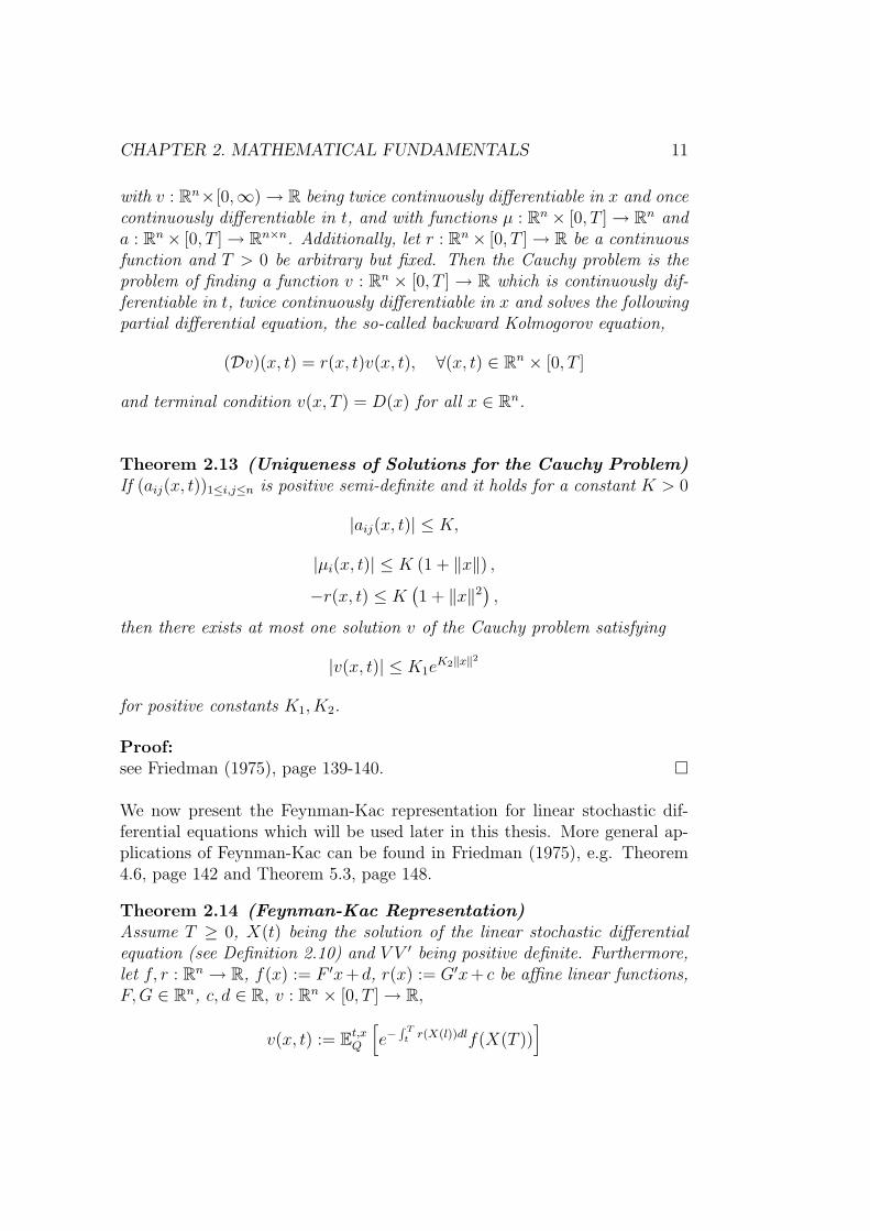
with v : Rn×[0,∞) → R being twice continuously differentiable in x and once
continuously differentiable in t, and with functions µ : Rn × [0, T ] → R
n anda : R
n × [0, T ] → Rn×n. Additionally, let r : R
n × [0, T ] → R be a continuousfunction and T > 0 be arbitrary but fixed. Then the Cauchy problem is theproblem of finding a function v : R
n × [0, T ] → R which is continuously dif-ferentiable in t, twice continuously differentiable in x and solves the followingpartial differential equation, the so-called backward Kolmogorov equation,
(Dv)(x, t) = r(x, t)v(x, t), ∀(x, t) ∈ Rn × [0, T ]
and terminal condition v(x, T ) = D(x) for all x ∈ Rn.
Theorem 2.13 (Uniqueness of Solutions for the Cauchy Problem)If (aij(x, t))1≤i,j≤n is positive semi-definite and it holds for a constant K > 0
|aij(x, t)| ≤ K,
|µi(x, t)| ≤ K (1 + ‖x‖) ,
−r(x, t) ≤ K(1 + ‖x‖2
),
then there exists at most one solution v of the Cauchy problem satisfying
|v(x, t)| ≤ K1eK2‖x‖2
for positive constants K1, K2.
Proof:see Friedman (1975), page 139-140.
We now present the Feynman-Kac representation for linear stochastic dif-ferential equations which will be used later in this thesis. More general ap-plications of Feynman-Kac can be found in Friedman (1975), e.g. Theorem4.6, page 142 and Theorem 5.3, page 148.
Theorem 2.14 (Feynman-Kac Representation)Assume T ≥ 0, X(t) being the solution of the linear stochastic differentialequation (see Definition 2.10) and V V ′ being positive definite. Furthermore,let f, r : R
n → R, f(x) := F ′x+ d, r(x) := G′x+ c be affine linear functions,F,G ∈ R
n, c, d ∈ R, v : Rn × [0, T ] → R,
v(x, t) := Et,xQ
[e−
∫ Tt
r(X(l))dlf(X(T ))]

12 CHAPTER 2. MATHEMATICAL FUNDAMENTALS
and II the differential operator D be defined as in Definition 2.12 withµ(x, t) := Hx + J(t), aij(x, t) :=
∑mk=1 VikVjk = (V V ′)ij. Then it holds that
v(X0,x(t), t) = E0,xQ
[e−
∫ Tt
r(X(l))dlf(X(T ))|Ft
]
and v(x, t) is the unique solution of the Cauchy problem and fulfills the growthcondition
|v(x, t)| ≤ K1eK2‖x‖2
for positive constants K1, K2.
Proof:see Antes (2004), page 36-37.
Hence, the unique solution of the Cauchy problem is given by this expectedvalue as a function depending on the initial parameters (x, t) of the SDE. Ingeneral, the reverse is not true. But if it is possible to determine the expectedvalue and to show that this expected value solves the Cauchy problem thenit is the unique solution.In order to solve the PDE that it is obtained by means of the Feynman-Kacrepresentation, the next theorem will be used within this thesis.
Theorem 2.15 (Linear Differential Equation)Consider the inhomogeneous linear differential equation
y′(x) = a(x)y(x) + b(x)
with continuous functions a and b, b 6= 0. Then, the solution of this differ-ential equation is
y(x) = eA(x)
(∫ x
x0
b(t)e−A(t)dt + C
),
with C ∈ R and A′ = a.
Proof:see Walter (1986), §2.
IIThe superscript in Et,xQ indicates that X(t) = x.
CHAPTER 2. MATHEMATICAL FUNDAMENTALS 13
2.3 Financial Markets
In order to get a consistent framework we present below the most impor-tant building blocks for financial markets. We start with introducing a gen-eral model for financial markets. Throughout this section we consult Zagst(2002). Other textbooks regarding introductions of financial markets areBrigo & Mercurio (2006) with an emphasis on interest-rate markets, Musiela& Rutkowski (1997) and Bingham & Kiesel (2004).
Definition 2.16 (Financial Market)The primary financial market M(Q) on the filtered probability space(Ω,F, Q, F) with the filtration F(W ), F = FT (W ), consists of n + 1 primarytraded assets whose prices are non-negative Ito processes on [0, T ]:
dPi(t) = µi(t)dt +m∑
j=1
σij(t)dWj(t) , i = 0, . . . , n ,
with an m-dimensional Brownian motion W and progressively measurablestochastic processes µi and σij. Furthermore, these processes satisfy the con-ditions ∫ T
0
|µi(s)|ds < ∞ Q − a.s.
and
EQ
[∫ T
0
σ2ij(s)ds
]< ∞ ∀ j = 1, . . . ,m .
For pricing purposes we want to rewrite the primary traded assets with re-spect to another unit price (numeraire).
Definition 2.17 (Numeraire)A price process (X(t))t∈[0,T ] that satisfies
X(t) > 0 ∀ t ∈ [0, T ]
is a numeraire in the financial market M(Q).
In the following, we want to use P0 as numeraire and hence define it asthe riskless cash account by taking a stochastic process r which satisfies theabove condition such that
dP0(t) = r(t) · P0(t)dt , P0(0) = 1.
14 CHAPTER 2. MATHEMATICAL FUNDAMENTALS
Hence, the discounted prices of the primary traded assets are
Pi(t) := P−10 (t) · Pi(t), t ∈ [0, T ], i = 0, . . . , n ,
with
P0(t) = 1 ,
dPi(t) = µi(t)dt +m∑
j=1
σij(t)dWj(t) ,
µi(t) = (µi(t) − r(t) · Pi(t)) · P−10 (t) ,
and
σij(t) = σij(t) · P−10 (t)
for all i = 1, . . . , n, j = 1, . . . ,m, t ∈ [0, T ].
In order to simplify the calculation of prices, respectively expected values,we need to find a measure under which the discounted price processes aremartingales.
Definition 2.18 (Equivalent Martingale Measure)
A probability measure Q on the measure space (Ω,F) is called an equivalentmartingale measure to Q if:
(i) Q is equivalent to Q, i.e. Q and Q have the same null sets.
(ii) The discounted price process P = (P1(t), . . . , Pn(t))t∈[0,T ] is an n-dimen-
sional Q-martingale, i.e.
P (t) = EQ
[P (s)
∣∣∣Ft
], s > t
and
EQ
[∫ T
0
||σP (s)||2ds
∣∣∣∣Ft
]< ∞.
The set of equivalent martingale measures to Q is denoted by M(Q).
The next theorem describes how such an equivalent martingale measure Qcan be constructed. As a result we get an arbitrage-free financial market.

CHAPTER 2. MATHEMATICAL FUNDAMENTALS 15
Theorem 2.19 (Discounted Market Characterization)Suppose there exists an m-dimensional progressively measurable stochasticprocess γ such that the no-arbitrage condition
µi(t) − σi(t) · γ(t) = r(t) · Pi(t) λ ⊗ Q − a.s. on [0, T ], i = 1, . . . , n ,
with σi := (σi1, . . . , σim), and the Novikov condition
EQ
[e
12
∫ T0 ||γ(s)||2ds
]< ∞
are fulfilled.Furthermore, let the probability measure Q on (Ω,F) be defined as
Q(A) = QL(γ,T )(A) = EQ [1A · L(γ, T )] ∀A ∈ F
withL(γ, T ) := e−
∫ T0 γ(s)′dW (s)− 1
2
∫ T0 ||γ(s)||2ds.
Then the stochastic process W =(W (t)
)t∈[0,T ]
defined by
dW (t) := γ(t)dt + dW (t) on [0, T ]
is a Q-Brownian motion and the price processes have the following represen-tation in terms of W :
dP0(t) = 0,
dPi(t) = σi(t)dW (t), σi := (σi1, . . . , σim) , i = 1, . . . , n ,
dPi(t) = r(t) · Pi(t)dt + σi(t)dW (t), i = 1, . . . , n.
If additionally the martingale condition
EQ
[∫ T
0
σ2ij(t)dt
]< ∞ ∀ i = 1, . . . , n , j = 1, . . . ,m ,
holds, then Q is an equivalent martingale measure with L being the Radon-Nikodym derivative of Q with respect to Q.
Proof:See Zagst (2002), pages 59f.
Having found an equivalent martingale measure Q we wonder about theprices of financial products like e.g. derivatives with primary traded assetsas underlyings.

16 CHAPTER 2. MATHEMATICAL FUNDAMENTALS
Definition 2.20 (Contingent Claim)A random variable D(T ) on (Ω,F) whose discounted value up to time t
P0(t) · D(T ) is lower bounded for all t ∈ [0, T ], is named a European contin-gent claim with maturity T .
Definition 2.21 (Contingent Claim Prices)
Under Q ∈ M(Q) the expected-value process of a European contingent claimD is given by
V QD (t) := P0(t) · EQ
[D(T )|Ft
], t ∈ [0, T ].
If this process V QD (t) is unique in M(Q), it is called the price of the contingent
claim D, VD(t).
If our financial market M(Q) is complete, the prices of European contin-gent claims are unique. We call a financial market complete if all contingentclaims D(T ) can be replicated by an admissible trading strategy III.
A powerful tool for pricing financial derivatives is the change of numerairewhere the martingale property of the newly discounted price process is pre-served under the changed probability measure.
Theorem 2.22 (Change of Numeraire)Let X = (X(t))t∈[0,T ] be a non-dividend-paying numeraire in M(Q) and
Q ∈ M(Q). If the discounted numeraire process X = (X(t))t∈[0,T ] with
X(t) := P−10 (t) · X(t), t ∈ [0, T ], is a Q-martingale, then there exists a
probability measure QX on (Ω,F), defined by its Radon-Nikodym derivative
L(T ) with respect to Q,
L(t) =dQX
dQ
∣∣∣∣Ft
=X(t)
X(0) · P0(t), t ∈ [0, T ],
anddL(t) = −L(t)γ(t)dW (t),
such that the discounted primary traded asset prices PXi , i = 1, . . . , n, are
QX-martingales. Furthermore, the expected-value process of a contingent
IIIAn admissible trading strategy is a self-financing trading strategy with (discounted)price processes which are λ ⊗ Q-a.s. bounded below.

CHAPTER 2. MATHEMATICAL FUNDAMENTALS 17
claim D = D(T ) with maturity T under Q and numeraire P0 coincides withthe expected-value process of D under QX and numeraire X, i.e.
P0(t) · EQ
[D(T )
∣∣∣Ft
]= X(t) · EQX
[DX(T )
∣∣∣Ft
]
for all t ∈ [0, T ].
Proof:See Zagst (2002), pages 87f.
A popular application of the above financial market is the famous Black-Scholes Model (see Black & Scholes (1973)) of which we present a generalizedversion (see e.g. Zagst (2002)). Within the terms of this model the financialmarket is free of arbitrage as well as complete, i.e. the price process of aEuropean contingent claim is unique.
Theorem 2.23 (Generalized Black-Scholes)Suppose that m = n = 1 and that the primary traded assets with prices P0
and P1 are given by
dP0(t) = r(t) · P0(t)dt , P0(0) = 1 ,
dP1(t) = µ(t) · P1(t)dt + σ(t) · P1(t)dW (t) , P1(0) > 0 ,
with σ > 0 such that the no-arbitrage, the Novikov and the martingale con-ditions of Theorem 2.19 are satisfied. Then this financial market is free ofarbitrage, and the price process of any European contingent claim D=D(T)with maturity T is given by
VD(t) = P0(t) · EQ
[D(T )|Ft
]= EQ
[e−
∫ Tt
r(s)ds · D(T )|Ft
]
for t ∈ [0, T ], Q ∈ M(Q).
Proof:See Zagst (2002), pages 77-78.
An important and well known result of this theorem are the formulas forEuropean options. Here we present the call option price within the general-ized Black-Scholes framework.
Theorem 2.24 (Generalized Black-Scholes Call Option Price)Let the assumptions of Theorem 2.23 be satisfied and let r and σ be deter-ministic. Then the price at time t ∈ [0, T ] of a European call option withstrike X and terminal payoff D(T ) = max P1(T ) − X, 0 is given by
CallBS(t, T,X) = P1(t) · N (d1) − e−∫ T
tr(s)ds · X · N (d2)

18 CHAPTER 2. MATHEMATICAL FUNDAMENTALS
with
d1 :=ln(
P1(t)X
)+∫ T
tr(s)ds + 1
2σ2
Y
σY
, d2 := d1 − σY ,
and
σY = σY (t, T ) :=
√∫ T
t
σ2(s)ds .
N denotes the standard normal cumulative distribution function.
Proof:See Zagst (2002), pages 79-80.
An extension of the Black-Scholes formula is the so-called Black formula(see Black (1976)) for futures prices. Since we make use of Black’s formulain the following chapters we present it here too.Let F (t, T ) be defined as
F (t, T ) := e∫ T
tr(s)ds · P1(t) t ∈ [0, T ].
Theorem 2.25 (Generalized Black Price)Let the assumptions of Theorem 2.23 be satisfied and let r and σ be determin-istic. Then the price at time t ∈ [0, T ] of a European call option written ona financial instrument with price process (F (t, T ))t∈[0,T ] and terminal payoffD(T ) = max F (T, T ) − X, 0 is given by
CallBlack(t, T,X) = e−∫ T
tr(s)ds · (F (t, T ) · N (d1) − X · N (d2))
with
d1 :=ln(
F (t,T )X
)+ 1
2σ2
Y
σY
, d2 := d1 − σY ,
and
σY = σY (t, T ) :=
√∫ T
t
σ2(s)ds .
N denotes the standard normal cumulative distribution function.
Proof:See Zagst (2002), pages 81-87.
CHAPTER 2. MATHEMATICAL FUNDAMENTALS 19
Interest-Rate Markets
Interest-rate markets are a special case of the introduced financial marketswhere in general the set of primary traded assets consists of zero-couponbonds with different maturities. A zero-coupon bond is a financial contractwhich pays its holder a nominal N (:=1) at the end of the maturity T . Itsprice at time t is given by
P (t, T ) = Ne−R(t,T )·(T−t)
where R(t, T ) denotes the continuous zero or spot rate, i.e. the interest ratewhich is guaranteed for the time period [t, T ].Describing an interest market completely is a challenge since there are in-finitely many zero-coupon bonds with different maturities on the market.Therefore an approach is to concentrate on a single interest rate instead oftrying to model all possible rates R(t, T ) and to describe the whole termstructure T → R(t, T ) by means of this special rate. There are two rateswhich are commonly used, namely the short rate and the forward short rate.
Definition 2.26 (Short Rate and Forward Short Rate)The short rate r(t) at time t is the interest rate for an infinitesimal timeperiod. It is defined as
r(t) := R(t, t) := − lim∆t→0
ln P (t, t + ∆t)
∆t= − ∂
∂Tln P (t, T )|T=t.
The forward short rate f(t, T ) at time t is the interest rate for an infinitesimaltime period at time T but derived at time t. It is defined as
f(t, T ) := R(t, T, T ) := − lim∆t→0
ln P (t, T + ∆t) − ln P (t, T )
∆t
= − ∂
∂Tln P (t, T ),
where R(t, T1, T2) denotes the forward zero rate given by
R(t, T1, T2) := − ln P (t, T2) − ln P (t, T1)
T2 − T1
,
i.e. the interest rate for the time period [T1, T2] derived at time t.
We now define our primary interest-rate market MIRM(Q) on the completeprobability space (Ω,F, Q) with filtration F(W ). The market is supposed to

20 CHAPTER 2. MATHEMATICAL FUNDAMENTALS
be frictionless and trading is allowed continuously up to a fixed time T ∗. Thenumeraire of our interest-rate market is the so-called cash account P0 with
P0(t) = e∫ t
t0r(s)ds
, t0 ≤ t ≤ T ≤ T ∗ .
The SDE of the cash account is
dP0(t) = r(t)P0(t)dt
with P0(0) = 1 and r being a progressively measurable process with
∫ T ∗
t0
|r(s)|ds < ∞ Q-a.s. .
The primary traded assets, which are driven by an m-dimensional Brownianmotion W = (W1(t), . . . ,Wm(t))t∈[t0,T ∗] with t0 ∈ [0, T ∗], consist of zero-coupon bonds with prices P (t, T ), t ≤ T . Those prices are described bynon-negative Ito processes as in Definition 2.16 with
dP (t, T ) = µP (t, T )dt +m∑
j=1
σPj(t, T )dWj(t),
where µP and σPj, j = 1, . . . ,m are progressively measurable stochasticprocesses such that it holds for all T ∈ [t0, T
∗]:
∫ T
t0
|µP (s, T )|ds < ∞ Q-a.s.
and
EQ
[∫ T
t0
σ2Pj(s, T )ds
]< ∞, ∀j = 1, . . . ,m.
So far, the only differences between the general financial market M(Q) andthe interest-rate market MIRM(Q) are the number of primary assets, whichis not limited anymore to n, and the time horizon which was changed to[t0, T
∗] instead of [0,T].MIRM(Q) is defined to be arbitrage-free if any finite interest-rate marketMIRM(Q, Tn), which is based on a finite number of zero-coupon bonds withmaturities T ∈ Tn := T1, . . . , Tn ⊂ [t0, T
∗], is free of arbitrage.The definition of an equivalent martingale measure has to be slightly ex-tended compared to Definition 2.18 in order to fit into the new framework.
Definition 2.27 (Equivalent Martingale Measure in MIRM(Q))A probability measure Q on (Ω,F) is called an equivalent martingale measurewith respect to Q if
CHAPTER 2. MATHEMATICAL FUNDAMENTALS 21
1. Q is equivalent to Q,
2. The discounted price process (P (t, T ))t∈[t0,T ] is a Q-martingale for allT ∈ [t0, T
∗].
The conditions under which the existence of an equivalent martingale mea-sure is guaranteed are similar to Theorem 2.19. We just have to make surethat the time horizon is changed to [t0, T
∗], especially for the integrals in theNovikov and martingale conditions. Additionally, the martingale conditionand the no-arbitrage condition have to be fulfilled for all t0 ≤ t ≤ T ≤ T ∗
(see Zagst (2002), page 103ff). The completeness of our primary interest-rate market is linked to the completeness of a finite interest rate market sinceMIRM(Q) is said to be complete if any contingent claim D(TD), TD ∈ [t0, T
∗],is attainable in a finite interest-rate market MIRM(Q, Tn). Thus, if there ex-ists an equivalent martingale measure for MIRM(Q) and if this interest-ratemarket is complete then the expected-value process of the contingent claimD is unique. For more general conditions about pricing contingent claims seeZagst (2002), page 107f.
2.4 Kalman Filter
In this section we present the Kalman filter which will be used later on forcalibration purposes. The main application of the Kalman filter technique,which was introduced by Kalman (1960), is the modelling and estimationof unobservable processes. Furthermore, if there are any parameters withinthe set-up of the model which are to be estimated, this can also be done bymeans of the Kalman filter and a maximum likelihood estimation. In thissection we refer to Harvey (1989). Other textbooks covering this topic aree.g. Øksendal (1998) who devotes a chapter for the linear filtering problem,especially the Kalman-Bucy filter. He also cites references for non-linearcases. Greg Welch and Gary Bishop of the University of North Carolinaprovide on their webpageIV an extensive overview of books, articles, tutorialsand research related to the Kalman filter.
State Space ModelThe state space model describes the development of the unobservable pro-cess and its linkage to given data. The dynamics of the process, i.e. itsevolution from one point in time to another, are given by the transitionequation whereas the measurement equation determines the relation of this
IVhttp://www.cs.unc.edu/∼welch/kalman/

22 CHAPTER 2. MATHEMATICAL FUNDAMENTALS
process to measurable information. We consider a linear state space modelfor t = 1, . . . , T
Yt = Ztαt + dt + εt (measurement equation),αt = Ttαt−1 + ct + ηt (transition equation),
with
Yt N × 1 vector with observable information at time t,αt m × 1 state vector at time t,ct ∈ R
m constant term of transition equation at time t,dt ∈ R
N constant term of measurement equation at time t,Zt ∈ R
N×m coefficient matrix of state vector for measurement equation,Tt ∈ R
m×m coefficient matrix of state vector for transition equation,εt ∼ NN(0, Ht) disturbance term of measurement equation,ηt ∼ Nm(0, Qt) disturbance term of transition equation.
Furthermore, it must hold that εt and ηt are sequences of independent randomvectors with E(εtη
′s) = 0 for all s, t = 1, . . . , T . Additionally, the initial state
α0 has to be independent of εt and ηt with α0 being normally distributed,i.e. α0 ∼ Nm(a0, P0) for a0 ∈ R
m and P0 ∈ Rm×m.
Based on this state space model, we now present the Kalman filter algo-rithm which will be used in order to get an estimate of αt with respect to allavailable information up to time t.
Algorithm
• Initialize a0 and P0.
• For t = 1, . . . , T evaluate
– the prediction equation
at|t−1 = Ttat−1 + ct
Pt|t−1 = TtPt−1T′t + Qt,
– and the update equation
at = at|t−1 + Pt|t−1Z′tF
−1t (yt − Ztat|t−1 − dt)
Pt = Pt|t−1 − Pt|t−1Z′tF
−1t ZtPt|t−1
with Ft = ZtPt|t−1Z′t + Ht.

CHAPTER 2. MATHEMATICAL FUNDAMENTALS 23
In order to check if the model is well-specified Harvey (1989), e.g. page 256,suggests to test the standardized innovations
νt :=yt − Ztat|t−1 − dt√
ft
with ft being the corresponding element on the diagonal of Ft since theseresiduals should be independent and standard normally distributed. He pro-poses testing e.g. for serial correlation, for heteroscedasticity and for nor-mality.
Theorem 2.28 (Properties of the Kalman Filter)It holds that (
αt
Yt
)|Yt−1 = yt−1, . . . , Y1 = y1
∼ Nm+N
((at|t−1
Ztat|t−1 + dt
),
(Pt|t−1 Pt|t−1Z
′t
ZtPt|t−1 ZtPt|t−1Z′t + Ht
))
andαt|Yt = yt, . . . , Y1 = y1 ∼ Nm(at, Pt)
for t = 1, . . . , T .Moreover, the minimum mean square estimate of αt for available data y1, . . . , yt
is given by at.
Proof:see Harvey (1989), page 109-110.
With the help of this theorem we are now able to estimate any unknownparameters of the state space model. If the disturbance terms and the ini-tial state α0 are normally distributed, then by Theorem 2.28 it follows thatE[αt|yt−1, . . . , y1] = at|t−1 and Cov[αt|yt−1, . . . , y1] = Pt|t−1. Hence, if we con-dition the measurement equation with respect to t − 1 we obtain a normaldistribution with
Et−1[yt] = yt|t−1 = Ztat|t−1 + dt
and covariance matrix Ft. Since we are dealing with a normal distribution,the log-likelihood sums up to
log(L(y1, . . . , yT , Θ)) = −NT
2log(2π) − 1
2
T∑
t=1
log |Ft| −1
2
T∑
t=1
vTt F−1
t vt,

24 CHAPTER 2. MATHEMATICAL FUNDAMENTALS
with L denoting the likelihood function, Θ the vector of unknown parameters,N the length of Yt and vt := yt − yt|t−1 for t = 1, . . . , T . This is also calledprediction error decomposition as vt can be seen as a prediction error. Forfurther information about maximum likelihood estimation and the predictionerror decomposition refer to Harvey (1989), Chapter 3.4, page 125-147.
Within this thesis we use the software package S-PLUS finmetrics for anycomputations regarding the Kalman filter.

Chapter 3
Pricing Credit Risk
This chapter outlines the main approaches of credit risk modelling: struc-tural models and reduced-form models. The former approach tries to modeldefault by directly using the assets of the firm, whereas the latter approachdoes not concentrate on modelling the firm’s asset process. Here, the defaultevent is typically given exogenously and default happens completely unex-pected.Also, there exists a third approach where so-called hybrid models use charac-teristics of both the structural and the reduced-form models. These modelsassume a linkage between the hazard rate of default and the value of thefirm’s assets. The models presented in this thesis belong to this class ofcredit risk models since they do not try to specify exactly the firm’s assetsbut incorporate market data as well as firm-specific information.
3.1 Structural Models
Characteristic of this approach is the attempt to model the evolution ofthe firm’s assets in order to deduce the value of corporate debt and to pricecredit risk. The most utilized credit event is the firm’s default. Therefore, theattention is directed to a lower barrier which represents the default threshold.If the firm’s assets reach this boundary for the first time, the default will betriggered and the firm will go bankrupt. This mechanism can be seen as asavety covenant whose goal is to protect bondholders against stockholders.Structural models have their intellectual roots in the work of Merton (1974).His approach to corporate debt assumes a constant rate of interest r andseveral standard conditions like e.g. unrestricted borrowing and lending, notaxes and transaction costs, and continuously trading in time. The firm is
25
26 CHAPTER 3. PRICING CREDIT RISK
assumed to have one liability with a terminal payoff L and default may onlyhappen at the debt’s maturity T . The firm’s value process is modelled as ageometric Brownian motion
dV (t) = V (t) · ((r − k)dt + σdW (t))
with constants σ and k where the latter represents the payout ratio in case itis positive otherwise the capital inflow. The price process X of the defaultableclaim is given at time T as:
X = L · 1V (T )≥L + V (T ) · 1V (T )<L = L − max (L − V (T ), 0).
Hence, the payoff of a defaultable zero-coupon bond can be interpreted asthe payoff of a default-free zero-coupon bond with face value L less the payoffof a European put option which is written on the assets V of the firm withstrike price L and exercise date T . Therefore, the value of the firm’s debtat time t is the difference of a zero-coupon bond with face value L and theprice of a European put option at t. The value of this European put optioncan be written in closed form with the help of the Black-Scholes formula (seeTheorem 2.24). And since the assets of the firm are the sum of the firm’sdebt and equity, we get the value of the equity as the price of a Europeancall option also written on the firm’s assets by means of the put-call parityfor European options.
First-passage-time models are an extension to the Merton model allowingdefault to happen before and at the debt’s maturity. The time of defaultis specified as the first-passage time of the firm’s assets relative to a bar-rier, which can be random and either exogenously or endogenously given.Black & Cox (1976) extend Merton’s framework by letting default happen ifthe firm’s assets are below some triggering level at maturity or if they crossa time-dependent level before maturity. Kim, Ramaswamy & Sundaresan(1993) and Longstaff & Schwartz (1995) incorporate stochastic interest ratesinto the model by assuming either a Cox-Ingersoll-Ross process or a Vasicekprocess.An advantage of structural models is that default is modelled endogenouslyby means of the firm’s assets and therefore allows for the usage of market in-formation. But a major drawback of the above introduced structural modelsis the fact that short-term credit spreads are close to zero due to the assetvalue being modelled as a continuous process. In order to circumvent thisshortcoming, Zhou (2001) adds a jump process to the dynamics of the assets.

CHAPTER 3. PRICING CREDIT RISK 27
3.2 Reduced-Form Models
The reduced-form approach is motivated by the difficulty of exactly speci-fying default, i.e. it is often impossible to find variables such as the firm’sassets on whose particular constellation default depends with certainity. De-fault often happens without meeting all the defined requirements or it fails tohappen although all requirements are met. Therefore, the idea is not to focuson the exact definition of the default event and the modelling of the firm’svalue, but to work with the evolution of the probability of default at anypoint in time instead. In order to model the default event as a total surprise,the default time (τ) is set as a non-predictable stopping time (see Section2.1). Then, default is described as the first jump of a special point process(see also Section 2.1), i.e. a Poisson process (see e.g Brigo & Mercurio (2006),Appendix C). The Poisson process can have either constant, deterministic orstochastic (Cox process) intensities. For example, if we assume the inten-sity c to be a positive, stochastic, adapted and right-continuous process withΛ(T ) :=
∫ T
0c(s)ds being strictly increasing and denoting its cumulated in-
tensity or hazard function. Then, for Poisson processes the jump time τ canbe transformed according to its cumulated intensity Λ:
Λ(τ) =: ζ ⇒ τ = Λ−1(ζ)
with ζ being a standard exponential random variable (see McNeil, Frey &Embrechts (2005), Lemma 9.13). Therefore, using the cumulated distributionof an exponential random variable, we can determine the probability of thejump being after time t, also called the survival probability up to time t:
Q(τ > t) = Q(Λ(τ) > Λ(t)) = Q(ζ > Λ(t)) = EQ
[e−
∫ t0 c(s)ds
].
The variable ζ is independent of all other variables, hence being an externalsource of randomness. With these assumptions, monitoring basic market ob-servables gives not a complete information with respect to default since theexogenous component is independent of the default-free market data.Jarrow & Turnbull (1992) introduce the reduced-form approach by assuminga constant intensity and a pre-defined payoff at default. The work of Lando(Lando (1994), Lando (1997), and Lando (1998)) extends this framework us-ing stochastic intensities (Cox processes).Advantages of reduced-form models are their positive credit spreads even forshort maturities as opposed to structural models and the fact that they arecompletely data-driven, i.e. their parameters can be fitted easily to marketdata. However, a shortcoming of this type of models is the fact that the

28 CHAPTER 3. PRICING CREDIT RISK
intensity process is specified exogenously. Hence, there exists no linkage be-tween default and any drivers of default, therefore making default completelyunexpected.
3.3 Hybrid Models
Hybrid models try to circumvent the drawbacks of structural and reduced-form models (i.e. short-term credit spreads of zero, intensities that arespecified completely exogenously) and therefore combine characteristics ofstructural and reduced-form models. By doing this, they provide a linkagebetween the likelihood of default and data that is supposed to drive or indi-cate default.Starting with a structural framework, Duffie & Lando (2001) assume thatthe bondholders only receive incomplete information about the firm’s value.They show that this set-up is consistent with a reduced-form approach sinceit admits an intensity and short-term credit spreads greater than zero.Another way to build hybrid models is to start with reduced-form modelsand relate the probability of default to observable or unobservable factors.Cathcart & El-Jahel (1998) assume default to be driven by a signaling pro-cess, whereas Bakshi, Madan & Zhang (2006) incorporate an unobservablemacroeconomic factor as well as an observable firm-specific factor for whichthey use e.g. stock prices.The models presented in this thesis are also hybrid models and are based onthe work of Schmid & Zagst (2000). Schmid & Zagst (2000) assume creditspreads to be driven by an unobservable uncertainty index that aggregates allavailable information concerning the quality of a firm. This model is furtherextended with an additional observable macroeconomic factor influencinginterest rates as well as credit spreads by Antes et al. (2008).

Chapter 4
A Generalized Five FactorModel
Within this chapter we present a hybrid model which links macroeconomicand firm-specific information to the performance of interest rates and creditspreads. Our framework is mainly based on the work of Schmid & Zagst(2000) who introduced a defaultable term structure model which is drivenby an additional factor comprising an aggregation of market and/or firm-specific data. This model is built by three factors, namley the short rate r,the so-called uncertainty index u and the short-rate spread s. The short rater was first modelled as a mean-reverting Hull-White or square-root process,both with a time-dependent mean-reversion level. The short-rate spread swhich is meant to be the difference between the spreads of defaultable andnon-defaultable bonds for an infinitesimal maturity follows a square-root pro-cess and is influenced by the uncertainty index u. This uncertainty index isto be understood as an aggregation of all available information regarding thecreditworthiness of the firm and/or relevant macroeconomic data. Highervalues of this index u indicate a deterioration in the obligor’s state and leadto increasing credit spreads. As before, this index is also described by asquare-root process. Cathcart & El-Jahel (1998) were the first to introducea process similar to the uncertainty index u. The so-called signaling pro-cess explicitely drives the default in their framework. Kalemanova & Schmid(2002) tested the three factor model of Schmid and Zagst on German andItalian government bonds and obtained good approximations of the giventerm structures. The choice of square-root processes prevents the short rateand the short-rate spread to take on negative values which is a desirablecharacteristic of this framework since e.g. credit spreads should be thoughtof as a compensation for bearing credit risk and thus should be non-negative.Unfortunately, these square-root processes complicate the estimation proced-
29

30 CHAPTER 4. A GENERALIZED FIVE FACTOR MODEL
ure considerably. Therefore Roth & Zagst (2004) simplified the three factorSchmid-Zagst model by replacing the square-root processes by Vasicek pro-cesses. Although this change leads to possible negative values for the shortrate and the short-rate spread, the authors showed that neglecting the posi-tivity constraint does not influence the pricing quality compared to the pre-ceding model.There are many articles in literature which analyze the impact of macroe-conomic factors on interest rates as well as credit spreads. Additionally,the dependence of credit spreads on factors stemming from firm-specific in-formation is examined. E.g. Ang & Piazzesi (2003) analyzed the effect ofmacro variables on non-defaultable bond prices and on the dynamics of theyield curve using inflation and economic growth factors. They found that theforecasting performance is improved by incorporating macroeconomic factorswhich are also found to be able to explain a great portion of the variationin bond yields. Krishnan et al. (2005) showed that firm-specific and mar-ket variables are important in explaining credit spread levels and changesfor banking and non-banking firms. A similar study was done by Avramov,Jostova & Philipov (2007) who found that more than 50 % of the variationof credit spread changes can be explained by a combination of common andfirm-specific fundamentals.Hence, a further enhancement of the Schmid-Zagst model was developed byAntes et al. (2008) who incorporated an additional macroeconomic factor inboth the short rate and the short-rate spread. Since literature indicates thatthere is more than just one explanatory macroeconomic variable we devotethis chapter to work out a framework which incorporates two factors repre-senting economic data in the short rate as well as the short-rate spread.
This chapter is organized as follows. In Section 4.1 we set up our generalframework which is used to derive the various types of models which will bepresented in the following five sections. Section 4.7 is devoted to the dataand the estimation procedure. Afterwards, a comparison of the calibrationresults is presented in Section 4.8.
4.1 The Set-Up
We assume a frictionless market where trading takes place continuously andwhere investors act as price takers. Additionally there are no transactioncosts, no taxes and no informational asymmetries. All random variables andstochastic processes will be defined on a probability space (Ω,G, Q) whichdescribes the uncertainty in the financial market. Furthermore, we assume

CHAPTER 4. A GENERALIZED FIVE FACTOR MODEL 31
this probability space to be equipped with three filtrations H, F, and G whichfulfill the assumptions of completeness and right-continuity. H = (Ht)0≤t≤T ∗
is the filtration generated by the process H with H(t) = 1T d≤t for a de-fault time T d and a fixed terminal time horizon T ∗. This default time is anon-negative random variable on the probability space with Q
(T d = 0
)= 0
and Q(T d > t
)> 0 for every t ∈ (0, T ∗] . F = (Ft)0≤t≤T ∗ is supposed to be
the filtration which is generated by the multi-dimensional Brownian motionW (t) with F0 being trivial , whereas G = (Gt)0≤t≤T ∗ is to be the enlargedfiltration G = H ∨ F, namely Gt = Ht∨Ft for every t. Additionally, thereexist on the probability space two F-adapted processes, the short rate processr(t) and the short spread process s(t).
In the following we will assume that under the martingale measure Q F
has the martingale invariance property with respect to G, meaning anyF−martingale follows also a G−martingale (see Bielecki & Rutkowski (2004),page 167). This assumption is equivalent to the fact that for any t ∈ (0, T ∗]
and any Q−integrable FT ∗−measurable random variable X with Q being amartingale measure it holds that EQ [X| Gt] = EQ [X| Ft] (see Bielecki &Rutkowski (2004), page 242).
The introduced interest-rate market contains four different types of tradedassets. As numeraire serves the non-defaultable cash account
P0(t) = e∫ t0 r(l)dl,
which is an investment of value one for an infinitesimal short maturity withsuccessive reinvestment up to time t.Furthermore, we can invest into non-defaultable zero-coupon bonds and de-faultable zero-coupon bonds with maturities T ∈ [0, T ∗].
Definition 4.1 (Defaultable Zero-Coupon Bond)A zero-coupon bond with face value 1 and maturity T which pays 1 at matur-ity, if there has been no default before time T , and the recovery rate z
(T d)
at default T d, if T d ≤ T , is called a defaultable zero-coupon bond with priceP d(t, T ).
The recovery rate is to be understood as a fraction of the market value ofthe bond just before the default P d
−(T d, T ). Additionally it is assumed thatz (t) is a Ft-adapted, continuous process with z (t) ∈ [0, 1) for all t.The fourth traded asset is the defaultable money-market account defined by
P d0 (t) =
(1 +
∫ t
0
(z(l) − 1)dH(l)
)e∫ t0 r(l)+s(l)L(l)dl,
32 CHAPTER 4. A GENERALIZED FIVE FACTOR MODEL
with L(t) = 1T d>t being the survival indicator. This defaultable accountis defined analogously to the non-defaultable case, i.e. it is an investment ofvalue one in a defaultable zero-coupon bond of infinitesimal short maturitywith subsequent reinvestment in case of no default.The prices of the financial instruments can be determined under the martin-gale measure Q as the conditional present value of all future payoffs. Hence,the price of the non-defaultable zero-coupon bond is given by
P (t, T ) = EQ
[e−
∫ Tt
r(l)dl∣∣∣Ft
].
The price of a defaultable zero-coupon bond is determined for t < min(T d, T )by the expected value of the recovery payment in case of a default between[t, T ] and the payment at the maturity T if there is no default:
1T d>t·P d(t, T ) = EQ
[∫ T
t
e−∫ u
tr(l)dlz(u)P d
−(u, T )dH(u) + e−∫ T
tr(l)dlL(T )
∣∣∣∣Gt
].
Analogously to e.g. Schmid (2004) and Antes (2004) it can be shown thatby means of some technical conditions with respect to r and s the price of adefaultable zero-coupon bond is determined by
P d(t, T ) = EQ
[e−
∫ Tt
(r(l)+s(l))dl∣∣∣Ft
]
for t < min(T d, T ).
Having generally introduced our financial market, we now present in de-tail the processes which are crucial for our five factor framework.For a fixed terminal time horizon T ∗, let the following stochastic differentialequations be satisfied for 0 ≤ t ≤ T ∗:The short rate r which is driven by two macroeconomic factors (w1 and w2)is described by a three-factor Hull-White process.
dr(t) = (θr(t) + brw1w1(t) + brw2w2(t) − arr(t)) dt
+ σr
√1 − ρ2
rw1− ρ2
rw2dWr(t) + σrρrw1dWw1(t) + σrρrw2dWw2(t).
The macroeconomic factors w1 and w2 are given by correlated Vasicek pro-cesses and can be chosen to be observable or unobservable.
dw1(t) = (θw1 − aw1w1(t)) dt + σw1dWw1(t),
dw2(t) = (θw2 − aw2w2(t)) dt + σw2ρw1w2dWw1(t) + σw2
√1 − ρ2
w1w2dWw2(t).

CHAPTER 4. A GENERALIZED FIVE FACTOR MODEL 33
The uncertainty index u summarizes all available information concerning thecreditworthiness of a company. This index is assumed to be unobservableand is described by a Vasicek process.
du(t) = (θu − auu(t)) dt + σudWu(t).
The short-rate spread s represents the difference between the spreads of de-faultable and non-defaultable bonds and is also given by a Vasicek process.This process is affected by the firm-specific uncertainty index u as well asthe macroeconomic factors w1 and w2.
ds(t) = (θs + bsuu(t) − bsw1w1(t) − bsw2w2(t) − ass(t)) dt
+ σs
√1 − ρ2
su − ρ2sw1
− ρ2sw2
dWs(t) + σsρsudWu(t)
+ σsρsw1dWw1(t) + σsρsw2dWw2(t),
For the constants it holds
ar, aw1 , aw2 , au, as > 0 ,
σr, σw1 , σw2 , σu, σs > 0 ,
θw1 , θw2 , θu, θs ≥ 0 ,
brw1 , brw2 , bsu, bsw1 , bsw2 ∈ R ,
ρw1w2 , ρrw1 , ρrw2 , ρsu, ρsw1 , ρsw2 ∈ [−1, 1] ,
and θr is a continuous deterministic function.Furthermore, W := (Wr,Ww1 ,Ww2 ,Wu,Ws)
′ is a five-dimensional Brownianmotion on the filtered probability space (Ω,G, Q, G).Then, the above system of five stochastic differential equations has a uniquesolution for any given vector of initial values (r(0), w1(0), w2(0), u(0), s(0))’∈ R
5 (see Theorem 2.11).Suppose there exists a progressively measurable processγ(t) = (γr(t), γw1(t), γw2(t), γu(t), γs(t))
′ with
dQt
dQt
= e−∫ t0 γ(l)dW (l)− 1
2
∫ t0 ‖γ(l)‖2dl,
where Qt and Qt are the restrictions of Q and Q on Gt.Additionally, let γ satisfy the Novikov condition
EQ
[e
12
∫ T∗
0 ‖γ(l)‖2dl]
< ∞
34 CHAPTER 4. A GENERALIZED FIVE FACTOR MODEL
and let the following equations be true for real constants λr, λw1 , λw2 , λu,λs:
I
γr(t) = λrσrr(t) − δλrσrw2(t)
+1√
1 − ρ2rw1
− ρ2rw2
(ρrw2
ρw1w2√1 − ρ2
w1w2
− ρrw1)γw1(t)
− (1 − δ)ρrw2√
1 − ρ2rw1
− ρ2rw2
λw2σw2w2(t) with δ ∈ 0, 1,
γw1(t) = λw1σw1w1(t),
γw2(t) = λw2σw2w2(t) −ρw1w2√
1 − ρ2w1w2
γw1(t),
γu(t) = λuσuu(t),
γs(t) = λsσss(t) −ρsuγu(t) + ρsw1γw1(t) + ρsw2γw2(t)√
1 − ρ2su − ρ2
sw1− ρ2
sw2
.
According to Theorem 2.19, the process
W (t) := W (t) +
∫ t
0
γ(l)dl
is now a Q-Brownian motion. Therefore, under the measure Q the stochasticdifferential equations can be written as:
dr(t) =(θr(t) + brw1w1(t) + brw2w2(t) − arr(t)
)dt
+ σr
√1 − ρ2
rw1− ρ2
rw2dWr(t) + σrρrw1dWw1(t) + σrρrw2dWw2(t),
dw1(t) = (θw1 − aw1w1(t)) dt + σw1dWw1(t),
dw2(t) = (θw2 − aw2w2(t)) dt + σw2ρw1w2dWw1(t) + σw2
√1 − ρ2
w1w2dWw2(t),
du(t) = (θu − auu(t)) dt + σudWu(t),
ds(t) = (θs + bsuu(t) − bsw1w1(t) − bsw2w2(t) − ass(t)) dt
+ σs
√1 − ρ2
su − ρ2sw1
− ρ2sw2
dWs(t) + σsρsudWu(t)
+ σsρsw1dWw1(t) + σsρsw2dWw2(t),
with II ar = ar + λrσ2r
√1 − ρ2
rw1− ρ2
rw2, aw2 = aw2 + λw2σ
2w2
√1 − ρ2
w1w2,
as = as + λsσ2s
√1 − ρ2
su − ρ2sw1
− ρ2sw2
, ai = ai + λiσ2i , i = w1, u, and
IThis approach is adapted to Schmid (2002), page 54.IIThroughout this work we assume ar, aw1
, aw2, au, as to be positive in order to preserve
the mean-reverting quality of the processes under the measure Q.
CHAPTER 4. A GENERALIZED FIVE FACTOR MODEL 35
brw2 = brw2 + δσr(λrσr
√1 − ρ2
rw1− ρ2
rw2− λw2σw2ρrw2), δ ∈ 0, 1.
Within this framework the price of a non-defaultable zero-coupon bond hasan affine term structure given in the next theorem.
Theorem 4.2 (Price of a Non-Defaultable Zero-Coupon Bond)The price of a non-defaultable zero-coupon bond is given by
P (t, T ) = EQ
[e−
∫ Tt
r(l)dl|Ft
]= P (t, T, r(t), w1(t), w2(t)),
with
P (t, T, r, w1, w2) = eA(t,T )−B(t,T )r−E1(t,T )w1−E2(t,T )w2
and
B(t, T ) =1
ar
(1 − e−ar(T−t)
),
E1(t, T ) = brw1
1
ar
(1 − e−aw1 (T−t)
aw1
+e−aw1 (T−t) − e−ar(T−t)
aw1 − ar
),
E2(t, T ) = brw2
1
ar
(1 − e−aw2 (T−t)
aw2
+e−aw2 (T−t) − e−ar(T−t)
aw2 − ar
),
A(t, T ) =
∫ T
t
1
2σ2
r(B(l, T ))2 +1
2σ2
w1(E1(l, T ))2 +
1
2σ2
w2(E2(l, T ))2
+ σw1σw2ρw1w2E1(l, T )E2(l, T ) + σrσw1ρrw1B(l, T )E1(l, T )
+ σrσw2
(ρrw1ρw1w2 + ρrw2
√1 − ρ2
w1w2
)B(l, T )E2(l, T )
− θr(l)B(l, T ) − θw1E1(l, T ) − θw2E2(l, T )dl.
Proof:According to Feynman-Kac (see Theorem 2.14) the following differentialequation must hold:
rP = Pt
+(θr(t) + brw1w1 + brw2w2 − arr
)Pr
+ (θw1 − aw1w1) Pw1
+ (θw2 − aw2w2) Pw2
+1
2
(σ2
rPrr + σ2w1
Pw1w1 + σ2w2
Pw2w2 + 2σw1σw2ρw1w2Pw1w2
+ 2σrσw1ρrw1Prw1 + 2σrσw2
(ρrw1ρw1w2 + ρrw2
√1 − ρ2
w1w2
)Prw2
).

36 CHAPTER 4. A GENERALIZED FIVE FACTOR MODEL
Using the affine term structure, we derive the partial derivatives of P :III
Pt = (At − Btr − (E1)tw1 − (E2)tw2) · P ,Pr = −B · P , Prr = B2 · P ,Pw1 = −E1 · P , Pw1w1 = (E1)
2 · P ,Pw2 = −E2 · P , Pw2w2 = (E2)
2 · P ,Prw1 = BE1 · P , Pw1w2 = E1E2 · P ,Prw2 = BE2 · P .
Substituting these terms and dividing by P > 0, we arrive at:
r = At − Btr − (E1)tw1 − (E2)tw2
+(θr(t) + brw1w1 + brw2w2 − arr
)(−B)
+ (θw1 − aw1w1) (−E1)
+ (θw2 − aw2w2) (−E2)
+1
2
(σ2
rB2 + σ2
w1(E1)
2 + σ2w2
(E2)2 + 2σw1σw2ρw1w2E1E2
+ 2σrσw1ρrw1BE1 + 2σrσw2
(ρrw1ρw1w2 + ρrw2
√1 − ρ2
w1w2
)BE2
).
Regrouping the terms, the equation takes on the form:
0 = r (arB − 1 − Bt)
+ w1 (aw1E1 − brw1B − (E1)t)
+ w2
(aw2E2 − brw2B − (E2)t
)
+ At − θr(t)B − θw1E1 − θw2E2
+1
2
(σ2
rB2 + σ2
w1(E1)
2 + σ2w2
(E2)2 + 2σw1σw2ρw1w2E1E2
+ 2σrσw1ρrw1BE1 + 2σrσw2
(ρrw1ρw1w2 + ρrw2
√1 − ρ2
w1w2
)BE2
).
IIIThroughout this thesis, we denote with Px, x ∈ t, r, w1, w2, s, u the partial derivativeof the function P with respect to x. The same logic holds for functions like A(t, T ) andB(t, T ).

CHAPTER 4. A GENERALIZED FIVE FACTOR MODEL 37
We obtain a system of linear differential equations for A,B,E1, and E2 bycomparing the coefficients:
Bt = arB − 1
(E1)t = aw1E1 − brw1B
(E2)t = aw2E2 − brw2B
−At =1
2
(σ2
rB2 + σ2
w1(E1)
2 + σ2w2
(E2)2 + 2σw1σw2ρw1w2E1E2
+ 2σrσw1ρrw1BE1 + 2σrσw2
(ρrw1ρw1w2 + ρrw2
√1 − ρ2
w1w2
)BE2
)
− θr(t)B − θw1E1 − θw2E2.
Since the condition P (T, T ) = 1 must be fulfilled for all r, w1, w2 ∈ R itholds A(T, T ) = B(T, T ) = E1(T, T ) = E2(T, T ) = 0. By means of thetransformation τ = T − t and the given terminal conditions, the differentialequations result in (cf. Theorem 2.15):
B(t, T ) = e−ar(T−t)
∫ T−t
0
earldl = e−ar(T−t) 1
ar
(ear(T−t) − 1
)
=1
ar
(1 − e−ar(T−t)
),
E1(t, T ) = e−aw1 (T−t)
∫ T−t
0
eaw1 lbrw1B(0, l)dl
= brw1
1
ar
(1 − e−aw1 (T−t)
aw1
+e−aw1 (T−t) − e−ar(T−t)
aw1 − ar
),
E2(t, T ) = e−aw2 (T−t)
∫ T−t
0
eaw2 lbrw2B(0, l)dl
= brw2
1
ar
(1 − e−aw2 (T−t)
aw2
+e−aw2 (T−t) − e−ar(T−t)
aw2 − ar
),
A(t, T ) =
∫ T
t
1
2σ2
r(B(l, T ))2 +1
2σ2
w1(E1(l, T ))2 +
1
2σ2
w2(E2(l, T ))2
+ σw1σw2ρw1w2E1(l, T )E2(l, T ) + σrσw1ρrw1B(l, T )E1(l, T )
+ σrσw2
(ρrw1ρw1w2 + ρrw2
√1 − ρ2
w1w2
)B(l, T )E2(l, T )
− θr(l)B(l, T ) − θw1E1(l, T ) − θw2E2(l, T )dl.
In Appendix A we show how the deterministic function θr can be derived.

38 CHAPTER 4. A GENERALIZED FIVE FACTOR MODEL
Analogously to the non-defaultable case, the price of a defaultable zero-coupon bond also exhibits an affine term structure.
Theorem 4.3 (Price of a Defaultable Zero-Coupon Bond)For t <min(T d, T ) the price of a defaultable zero-coupon bond is given by
P d(t, T ) = EQ
[e−
∫ Tt
(r(l)+s(l))dl|Ft
]= P d(t, T, r(t), w1(t), w2(t), s(t), u(t)),
with
P d(t, T, r, w1, w2, s, u) = eAd(t,T )−Bd(t,T )r−Cd(t,T )s−Dd(t,T )u−Ed1 (t,T )w1−Ed
2 (t,T )w2
and
Bd(t, T ) = B(t, T ) =1
ar
(1 − e−ar(T−t)
),
Cd(t, T ) =1
as
(1 − e−as(T−t)
),
Dd(t, T ) = bsu1
as
(1 − e−au(T−t)
au
+e−au(T−t) − e−as(T−t)
au − as
),
Ed1(t, T ) = − bsw1
1
as
(1 − e−aw1 (T−t)
aw1
+e−aw1 (T−t) − e−as(T−t)
aw1 − as
)
+ brw1
1
ar
(1 − e−aw1 (T−t)
aw1
+e−aw1 (T−t) − e−ar(T−t)
aw1 − ar
),
Ed2(t, T ) = − bsw2
1
as
(1 − e−aw2 (T−t)
aw2
+e−aw2 (T−t) − e−as(T−t)
aw2 − as
)
+ brw2
1
ar
(1 − e−aw2 (T−t)
aw2
+e−aw2 (T−t) − e−ar(T−t)
aw2 − ar
),
Ad(t, T ) =
∫ T
t
1
2σ2
r(Bd(l, T ))2 +
1
2σ2
s(Cd(l, T ))2 +
1
2σ2
u(Dd(l, T ))2
+1
2σ2
w1(Ed
1(l, T ))2 +1
2σ2
w2(Ed
2(l, T ))2
+ σw1σw2ρw1w2Ed1(l, T )Ed
2(l, T ) + σrσw1ρrw1Bd(l, T )Ed
1(l, T )
+ σsσuρsuCd(l, T )Dd(l, T ) + σsσw1ρsw1C
d(l, T )Ed1(l, T )
+ σrσw2
(ρrw1ρw1w2 + ρrw2
√1 − ρ2
w1w2
)Bd(l, T )Ed
2(l, T )
+ σsσw2
(ρsw1ρw1w2 + ρsw2
√1 − ρ2
w1w2
)Cd(l, T )Ed
2(l, T )
+ σrσs(ρrw1ρsw1 + ρrw2ρsw2)Bd(l, T )Cd(l, T ) − θr(l)B
d(l, T )
− θsCd(l, T ) − θuD
d(l, T ) − θw1Ed1(l, T ) − θw2E
d2(l, T )dl.

CHAPTER 4. A GENERALIZED FIVE FACTOR MODEL 39
Proof:According to Feynman-Kac (see Theorem 2.14) the following differentialequation must hold:
(r + s)P d = P dt
+(θr(t) + brw1w1 + brw2w2 − arr
)P d
r
+ (θw1 − aw1w1) P dw1
+ (θw2 − aw2w2) P dw2
+ (θu − auu) P du
+ (θs + bsuu − bsw1w1 − bsw2w2 − ass) P ds
+1
2
(σ2
rPdrr + σ2
sPdss + σ2
uPduu + σ2
w1P d
w1w1+ σ2
w2P d
w2w2
+ 2σw1σw2ρw1w2Pdw1w2
+ 2σrσw1ρrw1Pdrw1
+ 2σrσw2
(ρrw1ρw1w2 + ρrw2
√1 − ρ2
w1w2
)P d
rw2+ 2σsσuρsuP
dsu
+ 2σrσs(ρrw1ρsw1 + ρrw2ρsw2)Pdsr + 2σsσw1ρsw1P
dsw1
+ 2σsσw2
(ρsw1ρw1w2 + ρsw2
√1 − ρ2
w1w2
)P d
sw2
).
Using the affine term structure, we get the following partial derivatives:
P dt = (Ad
t − Bdt r − (Ed
1)tw1 − (Ed2)tw2 − Cd
t s − Ddt u) · P d ,
P dr = −Bd · P d , P d
w1w1= (Ed
1)2 · P d , P d
w1w2= Ed
1Ed2 · P d ,
P dw1
= −Ed1 · P d , P d
w2w2= (Ed
2)2 · P d , P d
sr = BdCd · P d ,P d
w2= −Ed
2 · P d , P dss = (Cd)2 · P d , P d
sw1= CdEd
1 · P d ,P d
s = −Cd · P d , P duu = (Dd)2 · P d , P d
sw2= CdEd
2 · P d ,P d
u = −Dd · P d , P drw1
= BdEd1 · P d , P d
su = CdDd · P d ,P d
rr = (Bd)2 · P d , P drw2
= BdEd2 · P d.
Substituting these terms and dividing by P d > 0, we arrive at:
r + s = Adt − Bd
t r − (Ed1)tw1 − (Ed
2)tw2 − Cdt s − Dd
t u
+(θr(t) + brw1w1 + brw2w2 − arr
)(−Bd)
+ (θw1 − aw1w1) (−Ed1)
+ (θw2 − aw2w2) (−Ed2)
+ (θu − auu) (−Dd)

40 CHAPTER 4. A GENERALIZED FIVE FACTOR MODEL
+ (θs + bsuu − bsw1w1 − bsw2w2 − ass) (−Cd)
+1
2
(σ2
r(Bd)2 + σ2
s(Cd)2 + σ2
u(Dd)2 + σ2
w1(Ed
1)2 + σ2
w2(Ed
2)2
+ 2σw1σw2ρw1w2Ed1E
d2 + 2σrσw1ρrw1B
dEd1
+ 2σrσw2
(ρrw1ρw1w2 + ρrw2
√1 − ρ2
w1w2
)BdEd
2 + 2σsσuρsuCdDd
+ 2σrσs(ρrw1ρsw1 + ρrw2ρsw2)BdCd + 2σsσw1ρsw1C
dEd1
+ 2σsσw2
(ρsw1ρw1w2 + ρsw2
√1 − ρ2
w1w2
)CdEd
2
).
Regrouping the terms, the equation takes on the form:
0 = r(arB
d − 1 − Bdt
)
+ w1
(aw1E
d1 − brw1B
d + bsw1Cd − (Ed
1)t
)
+ w2
(aw2E
d2 − brw2B
d + bsw2Cd − (Ed
2)t
)
+ u(auD
d − bsuCd − Dd
t
)
+ s(asC
d − 1 − Cdt
)
+ Adt − θr(t)B
d − θsCd − θuD
d − θw1Ed1 − θw2E
d2
+1
2
(σ2
r(Bd)2 + σ2
s(Cd)2 + σ2
u(Dd)2 + σ2
w1(Ed
1)2 + σ2
w2(Ed
2)2
+ 2σw1σw2ρw1w2Ed1E
d2 + 2σrσw1ρrw1B
dEd1
+ 2σrσw2
(ρrw1ρw1w2 + ρrw2
√1 − ρ2
w1w2
)BdEd
2 + 2σsσuρsuCdDd
+ 2σrσs(ρrw1ρsw1 + ρrw2ρsw2)BdCd + 2σsσw1ρsw1C
dEd1
+ 2σsσw2
(ρsw1ρw1w2 + ρsw2
√1 − ρ2
w1w2
)CdEd
2
).
We obtain a system of linear differential equations for Ad, Bd, Cd, Dd, Ed1 , and
Ed2 by comparing the coefficients:
Bdt = arB
d − 1
Cdt = asC
d − 1
Ddt = auD
d − bsuCd
(Ed1)t = aw1E
d1 − brw1B
d + bsw1Cd
(Ed2)t = aw2E
d2 − brw2B
d + bsw2Cd

CHAPTER 4. A GENERALIZED FIVE FACTOR MODEL 41
−Adt =
1
2
(σ2
r(Bd)2 + σ2
s(Cd)2 + σ2
u(Dd)2 + σ2
w1(Ed
1)2 + σ2
w2(Ed
2)2
+ 2σw1σw2ρw1w2Ed1E
d2 + 2σrσw1ρrw1B
dEd1
+ 2σrσw2
(ρrw1ρw1w2 + ρrw2
√1 − ρ2
w1w2
)BdEd
2 + 2σsσuρsuCdDd
+ 2σrσs(ρrw1ρsw1 + ρrw2ρsw2)BdCd + 2σsσw1ρsw1C
dEd1
+ 2σsσw2
(ρsw1ρw1w2 + ρsw2
√1 − ρ2
w1w2
)CdEd
2
)
− θr(t)Bd − θsC
d − θuDd − θw1E
d1 − θw2E
d2 .
Since the condition P d(T, T ) = 1 must be fulfilled for all r, w1, w2, s, u ∈ R
it holds that Ad(T, T ) = Bd(T, T ) = Cd(T, T ) = Dd(T, T ) = Ed1(T, T ) =
Ed2(T, T ) = 0. By means of the transformation τ = T − t and the given
terminal conditions, the differential equations result in (cf. Theorem 2.15):
Bd(t, T ) = B(t, T ) =1
ar
(1 − e−ar(T−t)
),
Cd(t, T ) =1
as
(1 − e−as(T−t)
),
Dd(t, T ) = e−au(T−t)
∫ T−t
0
eaulbsuCd(0, l)dl
= bsu1
as
(1 − e−au(T−t)
au
+e−au(T−t) − e−as(T−t)
au − as
),
Ed1(t, T ) = e−aw1 (T−t)
∫ T−t
0
eaw1 l(brw1B
d(0, l) − bsw1Cd(0, l)
)dl
= − bsw1
1
as
(1 − e−aw1 (T−t)
aw1
+e−aw1 (T−t) − e−as(T−t)
aw1 − as
)
+ brw1
1
ar
(1 − e−aw1 (T−t)
aw1
+e−aw1 (T−t) − e−ar(T−t)
aw1 − ar
),
Ed2(t, T ) = e−aw2 (T−t)
∫ T−t
0
eaw2 l(brw2B
d(0, l) − bsw2Cd(0, l)
)dl
= − bsw2
1
as
(1 − e−aw2 (T−t)
aw2
+e−aw2 (T−t) − e−as(T−t)
aw2 − as
)
+ brw2
1
ar
(1 − e−aw2 (T−t)
aw2
+e−aw2 (T−t) − e−ar(T−t)
aw2 − ar
),
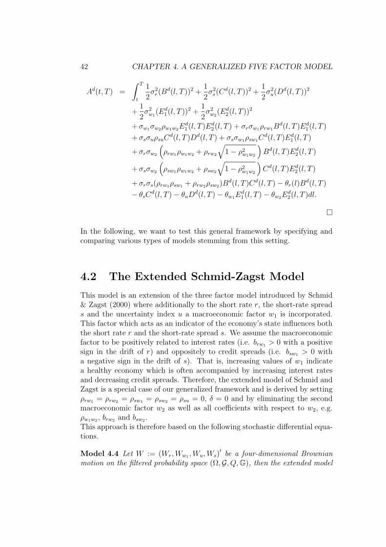
42 CHAPTER 4. A GENERALIZED FIVE FACTOR MODEL
Ad(t, T ) =
∫ T
t
1
2σ2
r(Bd(l, T ))2 +
1
2σ2
s(Cd(l, T ))2 +
1
2σ2
u(Dd(l, T ))2
+1
2σ2
w1(Ed
1(l, T ))2 +1
2σ2
w2(Ed
2(l, T ))2
+ σw1σw2ρw1w2Ed1(l, T )Ed
2(l, T ) + σrσw1ρrw1Bd(l, T )Ed
1(l, T )
+ σsσuρsuCd(l, T )Dd(l, T ) + σsσw1ρsw1C
d(l, T )Ed1(l, T )
+ σrσw2
(ρrw1ρw1w2 + ρrw2
√1 − ρ2
w1w2
)Bd(l, T )Ed
2(l, T )
+ σsσw2
(ρsw1ρw1w2 + ρsw2
√1 − ρ2
w1w2
)Cd(l, T )Ed
2(l, T )
+ σrσs(ρrw1ρsw1 + ρrw2ρsw2)Bd(l, T )Cd(l, T ) − θr(l)B
d(l, T )
− θsCd(l, T ) − θuD
d(l, T ) − θw1Ed1(l, T ) − θw2E
d2(l, T )dl.
In the following, we want to test this general framework by specifying andcomparing various types of models stemming from this setting.
4.2 The Extended Schmid-Zagst Model
This model is an extension of the three factor model introduced by Schmid& Zagst (2000) where additionally to the short rate r, the short-rate spreads and the uncertainty index u a macroeconomic factor w1 is incorporated.This factor which acts as an indicator of the economy’s state influences boththe short rate r and the short-rate spread s. We assume the macroeconomicfactor to be positively related to interest rates (i.e. brw1 > 0 with a positivesign in the drift of r) and oppositely to credit spreads (i.e. bsw1 > 0 witha negative sign in the drift of s). That is, increasing values of w1 indicatea healthy economy which is often accompanied by increasing interest ratesand decreasing credit spreads. Therefore, the extended model of Schmid andZagst is a special case of our generalized framework and is derived by settingρrw1 = ρrw2 = ρsw1 = ρsw2 = ρsu = 0, δ = 0 and by eliminating the secondmacroeconomic factor w2 as well as all coefficients with respect to w2, e.g.ρw1w2 , brw2 and bsw2 .This approach is therefore based on the following stochastic differential equa-tions.
Model 4.4 Let W := (Wr,Ww1 ,Wu,Ws)′ be a four-dimensional Brownian
motion on the filtered probability space (Ω,G, Q, G), then the extended model
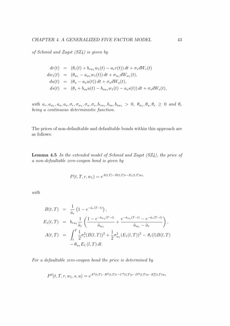
CHAPTER 4. A GENERALIZED FIVE FACTOR MODEL 43
of Schmid and Zagst (SZ4) is given by
dr(t) = (θr(t) + brw1w1(t) − arr(t)) dt + σrdWr(t)
dw1(t) = (θw1 − aw1w1(t)) dt + σw1dWw1(t),
du(t) = (θu − auu(t)) dt + σudWu(t),
ds(t) = (θs + bsuu(t) − bsw1w1(t) − ass(t)) dt + σsdWs(t),
with ar, aw1 , au, as, σr, σw1 , σu, σs, brw1 , bsu, bsw1 > 0, θw1 , θu, θs ≥ 0 and θr
being a continuous deterministic function.
The prices of non-defaultable and defaultable bonds within this approach areas follows:
Lemma 4.5 In the extended model of Schmid and Zagst (SZ4), the price ofa non-defaultable zero-coupon bond is given by
P (t, T, r, w1) = eA(t,T )−B(t,T )r−E1(t,T )w1
with
B(t, T ) =1
ar
(1 − e−ar(T−t)
),
E1(t, T ) = brw1
1
ar
(1 − e−aw1 (T−t)
aw1
+e−aw1 (T−t) − e−ar(T−t)
aw1 − ar
),
A(t, T ) =
∫ T
t
1
2σ2
r(B(l, T ))2 +1
2σ2
w1(E1(l, T ))2 − θr(l)B(l, T )
− θw1E1 (l, T ) dl.
For a defaultable zero-coupon bond the price is determined by
P d(t, T, r, w1, s, u) = eAd(t,T )−Bd(t,T )r−Cd(t,T )s−Dd(t,T )u−Ed1 (t,T )w1

44 CHAPTER 4. A GENERALIZED FIVE FACTOR MODEL
with
Bd(t, T ) = B(t, T ) =1
ar
(1 − e−ar(T−t)
),
Cd(t, T ) =1
as
(1 − e−as(T−t)
),
Dd(t, T ) = bsu1
as
(1 − e−au(T−t)
au
+e−au(T−t) − e−as(T−t)
au − as
),
Ed1(t, T ) = − bsw1
1
as
(1 − e−aw1 (T−t)
aw1
+e−aw1 (T−t) − e−as(T−t)
aw1 − as
)
+ brw1
1
ar
(1 − e−aw1 (T−t)
aw1
+e−aw1 (T−t) − e−ar(T−t)
aw1 − ar
),
Ad(t, T ) =
∫ T
t
1
2σ2
r(Bd(l, T ))2 +
1
2σ2
s(Cd(l, T ))2 +
1
2σ2
u(Dd(l, T ))2
+1
2σ2
w1(Ed
1(l, T ))2 − θr(l)Bd(l, T ) − θsC
d(l, T ) − θuDd(l, T )
− θw1Ed1(l, T )dl.
Schmid et al. (see Antes et al. (2008)) showed that the introduction of amacroeconomic factor improves the power of the Schmid and Zagst frame-work by comparing the extended version with its preceding three factor ver-sion. They obtained as a result that both the levels and the changes of creditspreads could be explained better by this additional factor.Following the work of Schmid et al. we test five factor models against theextended model of Schmid and Zagst. Furthermore, since Schmid et al. usedthe growth rate of the nominal GDP as representative of w1, we want to ana-lyze the impact of other macroeconomic indicators, which are supposed to begood proxies of the economy, on the performance of the extended framework.
4.3 A Further Enhancement of the Schmid-
Zagst Model - The Five Factor Approach
Since the introduction of a macroeconomic factor yields promising resultsin explaining credit spreads and pricing defaultable bonds (see Antes et al.(2008)), the performance could be further improved by a second macroe-conomic factor. There can be found various articles in the literatur whichanalyze the impact of macroeconomic factors on credit spreads and whichfound that there is more than just one explanatory variable. E.g. Amatoa

CHAPTER 4. A GENERALIZED FIVE FACTOR MODEL 45
& Luisi (2006) analyzed the impact of aggregate risk factors on corporatespreads. These risk factors comprised of macroeconomic data like consumerprice index, industrial production and unemployment rates. The authorsfound several factors which exhibit strong effects on corporate spreads. Wu& Zhang (2008) used a dynamic factor model in order to identify three fun-damental risk dimensions namely inflation, real output growth, and financialmarket volatility. For each risk dimension they summarized several timeseries and extracted a common factor capturing the systematic dynamics.Then, they linked the fundamental risk dimensions to US Treasury yieldsand corporate bond spreads.
The model is reached by enhancing the extended four factor model withan additional macroeconomic factor w2 and by allowing this factor to be cor-related with w1. As before, we set ρrw1 = ρrw2 = ρsw1 = ρsw2 = ρsu = 0 andδ = 0, i.e. brw2 = brw2 .
Model 4.6 Let W := (Wr,Ww1 ,Ww2 ,Wu,Ws)′ be a five-dimensional Brown-
ian motion on the filtered probability space (Ω,G, Q, G), then the five factorversion of the model of Schmid and Zagst (SZ5) is given by
dr(t) = (θr(t) + brw1w1(t) + brw2w2(t) − arr(t)) dt + σrdWr(t)
dw1(t) = (θw1 − aw1w1(t)) dt + σw1dWw1(t),
dw2(t) = (θw2 − aw2w2(t)) dt + σw2ρw1w2dWw1(t) + σw2
√1 − ρ2
w1w2dWw2(t),
du(t) = (θu − auu(t)) dt + σudWu(t),
ds(t) = (θs + bsuu(t) − bsw1w1(t) − bsw2w2(t) − ass(t)) dt + σsdWs(t),
with ar, aw1 , aw2 , au, as, σr, σw1 , σw2 , σu, σs, brw1 , bsu, bsw1 > 0, brw2 , bsw2 ∈ R,θw1 , θw2 , θu, θs ≥ 0, ρw1w2 ∈ [−1, 1] and θr being a continuous deterministicfunction.
Here, we skip the restrictions regarding the influence of w2 on the short rateand the short-rate spread, i.e. brw2 , bsw2 ∈ R, since there are macroeconomicfactors, e.g. inflation, whose impact is not known for sure.Prices for zero-coupon bonds also exist within this framework and can bederived from the general case, see Theorem 4.2 and Theorem 4.3.
Lemma 4.7 In the five factor version of the Schmid-Zagst model (SZ5), theprice of a non-defaultable zero-coupon bond is given by
P (t, T, r, w1, w2) = eA(t,T )−B(t,T )r−E1(t,T )w1−E2(t,T )w2

46 CHAPTER 4. A GENERALIZED FIVE FACTOR MODEL
with
B(t, T ) =1
ar
(1 − e−ar(T−t)
),
E1(t, T ) = brw1
1
ar
(1 − e−aw1 (T−t)
aw1
+e−aw1 (T−t) − e−ar(T−t)
aw1 − ar
),
E2(t, T ) = brw2
1
ar
(1 − e−aw2 (T−t)
aw2
+e−aw2 (T−t) − e−ar(T−t)
aw2 − ar
),
A(t, T ) =
∫ T
t
1
2σ2
r(B(l, T ))2 +1
2σ2
w1(E1(l, T ))2 +
1
2σ2
w2(E2(l, T ))2
+ σw1σw2ρw1w2E1(l, T )E2(l, T ) − θr(l)B(l, T )
− θw1E1 (l, T ) − θw2E2 (l, T ) dl.
For a defaultable zero-coupon bond the price is determined by
P d(t, T, r, w1, w2, s, u) = eAd(t,T )−Bd(t,T )r−Cd(t,T )s−Dd(t,T )u−Ed1 (t,T )w1−Ed
2 (t,T )w2
with
Bd(t, T ) = B(t, T ) =1
ar
(1 − e−ar(T−t)
),
Cd(t, T ) =1
as
(1 − e−as(T−t)
),
Dd(t, T ) = bsu1
as
(1 − e−au(T−t)
au
+e−au(T−t) − e−as(T−t)
au − as
),
Ed1(t, T ) = − bsw1
1
as
(1 − e−aw1 (T−t)
aw1
+e−aw1 (T−t) − e−as(T−t)
aw1 − as
)
+ brw1
1
ar
(1 − e−aw1 (T−t)
aw1
+e−aw1 (T−t) − e−ar(T−t)
aw1 − ar
),
Ed2(t, T ) = − bsw2
1
as
(1 − e−aw2 (T−t)
aw2
+e−aw2 (T−t) − e−as(T−t)
aw2 − as
)
+ brw2
1
ar
(1 − e−aw2 (T−t)
aw2
+e−aw2 (T−t) − e−ar(T−t)
aw2 − ar
),
Ad(t, T ) =
∫ T
t
1
2σ2
r(Bd(l, T ))2 +
1
2σ2
s(Cd(l, T ))2 +
1
2σ2
u(Dd(l, T ))2
+1
2σ2
w1(Ed
1(l, T ))2 +1
2σ2
w2(Ed
2(l, T ))2
+ σw1σw2ρw1w2Ed1(l, T )Ed
2(l, T ) − θr(l)Bd(l, T )
− θsCd(l, T ) − θuD
d(l, T ) − θw1Ed1(l, T ) − θw2E
d2(l, T )dl.

CHAPTER 4. A GENERALIZED FIVE FACTOR MODEL 47
As a special case of this approach, we follow the work of Merz (2007) wherew2 is supposed to be an unobservable factor. Therefore, w2 takes on therole as an unobservable macroeconomic index which is orthogonal to w1 andwhich could be seen as an aggregation of influences on the economy. Thismeans that in Model 4.6 ρw1w2 is set to zero as well as bsw2 . The last conditionis necessary since otherwise there would be two unobservable terms in thedrift of the short-rate spread which could be hard to discriminate. Hence,for this special case, the pricing formula of a defaultable zero-coupon bondP d(t, T ) simplifies to the one given in Lemma 4.5.
4.4 The Real and Inflation Short-Rate Model
The real and inflation short-rate model was first introduced by Hagedornet al. (2007)(see also Hagedorn (2005) and Meyer (2005)). It decomposes theshort rate r into the real short rate rR and the inflation short rate rI :
r(t) = rR(t) + rI(t)
where the real short rate evolves according to the SDE
drR(t) = (θR(t) + bRw1w1(t) − aRrR(t)) dt + σRdWR(t),
with positive constants bRw1 , aR, σR and a continuous, deterministic functionθR(t). Furthermore, the inflation short rate follows the SDE
drI(t) = (θI − aIrI(t)) dt + σIρw1IdWw1(t) + σI
√1 − ρ2
w1IdWI(t),
with positive constants aI , σI , a non-negative constant θI and independentBrownian motions WR, WI and Ww1 . In contrast to Hagedorn et al. (2007),where the constant ρw1I was set to zero, we allow ρw1I to be within [−1, 1].As in the models before, w1 is a macroeconomic factor represented here bythe growth rate of the real GDP and satisfies the SDE
dw1(t) = (θw1 − aw1w1(t)) dt + σw1dWw1(t),
with positive constants aw1 , σw1 and a non-negative constant θw1 .This approach also fits in our general framework of a five factor model. If welet the inflation short rate rI be represented by the second macroeconomicfactor w2, and if we take the process r as the sum of real short rate rR andinflation short rate rI , respectively w2, with
θr(t) := θR(t) + θI , ar := aR , brw1 := bRw1 ,Wr := WR ,

48 CHAPTER 4. A GENERALIZED FIVE FACTOR MODEL
brw2 := aR − aI (brw2 := aR − aI with δ = 1),
σr := σR where σR equals the term σr
√1 − ρ2
rw1− ρ2
rw2of Section 4.1,
ρrw1 =σw2
σr
ρw1w2 , ρrw2 =σw2
σr
√1 − ρ2
w1w2, ρsw1 = ρsw2 = ρsu = 0 ,
and λr := λr√1−ρ2
rw1−ρ2
rw2
, we end up with the following model. IV Model 4.8
extends the non-defaultable set-up of Hagedorn et al. (2007) by introducinga firm-specific uncertainty index u and the short-rate spread s.
Model 4.8 Let W := (Wr,Ww1 ,Ww2 ,Wu,Ws)′ be a five-dimensional Brown-
ian motion on the filtered probability space (Ω,G, Q, G), then the real andinflation short-rate model (INF) is given by
dr(t) = (θr(t) + brw1w1(t) + brw2w2(t) − arr(t)) dt + σrdWr(t)
+ σw2ρw1w2dWw1(t) + σw2
√1 − ρ2
w1w2dWw2(t)
dw1(t) = (θw1 − aw1w1(t)) dt + σw1dWw1(t),
dw2(t) = (θw2 − aw2w2(t)) dt + σw2ρw1w2dWw1(t) + σw2
√1 − ρ2
w1w2dWw2(t),
du(t) = (θu − auu(t)) dt + σudWu(t),
ds(t) = (θs + bsuu(t) − bsw1w1(t) − bsw2w2(t) − ass(t)) dt + σsdWs(t),
with ar, aw1 , aw2 , au, as, σr, σw1 , σw2 , σu, σs, brw1 , bsu, bsw1 > 0, brw2 , bsw2 ∈ R,θw1 , θw2 , θu, θs ≥ 0, ρw1w2 ∈ [−1, 1] and θr being a continuous deterministicfunction.
The pricing formulas of zero-coupon bonds for this set-up are a special caseof Theorem 4.2 and Theorem 4.3.
Lemma 4.9 In the real and inflation short-rate model (INF) the price of anon-defaultable zero-coupon bond is given by
P (t, T, r, w1, w2) = eA(t,T )−B(t,T )r−E1(t,T )w1−E2(t,T )w2
= eA(t,T )−B(t,T )rR−E1(t,T )w1−(E2(t,T )+B(t,T ))w2
= P (t, T, rR, w1, w2)
with
B(t, T ) =1
ar
(1 − e−ar(T−t)
),
IVWe use here the notation r in order to indicate the theoretical framework of Section4.1.

CHAPTER 4. A GENERALIZED FIVE FACTOR MODEL 49
E1(t, T ) = brw1
1
ar
(1 − e−aw1 (T−t)
aw1
+e−aw1 (T−t) − e−ar(T−t)
aw1 − ar
),
E2(t, T ) = brw2
1
ar
(1 − e−aw2 (T−t)
aw2
+e−aw2 (T−t) − e−ar(T−t)
aw2 − ar
),
A(t, T ) =
∫ T
t
1
2
(σ2
r + σ2w2
)(B(l, T ))2 +
1
2σ2
w1(E1(l, T ))2 +
1
2σ2
w2(E2(l, T ))2
+ σw1σw2ρw1w2E1(l, T ) (B(l, T ) + E2(l, T )) + σ2w2
B(l, T )E2(l, T )
− θr(l)B(l, T ) − θw1E1 (l, T ) − θw2E2 (l, T ) dl.
For a defaultable zero-coupon bond the price is determined by
P d(t, T, r, w1, w2, s, u) = eAd(t,T )−Bd(t,T )r−Cd(t,T )s−Dd(t,T )u−Ed1 (t,T )w1−Ed
2 (t,T )w2
= eAd(t,T )−Bd(t,T )rR−Cd(t,T )s−Dd(t,T )u−Ed1 (t,T )w1
· e−(Ed2 (t,T )+Bd(t,T ))w2
= P d(t, T, rR, w1, w2, s, u)
with
Bd(t, T ) = B(t, T ) =1
ar
(1 − e−ar(T−t)
),
Cd(t, T ) =1
as
(1 − e−as(T−t)
),
Dd(t, T ) = bsu1
as
(1 − e−au(T−t)
au
+e−au(T−t) − e−as(T−t)
au − as
),
Ed1(t, T ) = − bsw1
1
as
(1 − e−aw1 (T−t)
aw1
+e−aw1 (T−t) − e−as(T−t)
aw1 − as
)
+ brw1
1
ar
(1 − e−aw1 (T−t)
aw1
+e−aw1 (T−t) − e−ar(T−t)
aw1 − ar
),
Ed2(t, T ) = − bsw2
1
as
(1 − e−aw2 (T−t)
aw2
+e−aw2 (T−t) − e−as(T−t)
aw2 − as
)
+ brw2
1
ar
(1 − e−aw2 (T−t)
aw2
+e−aw2 (T−t) − e−ar(T−t)
aw2 − ar
),
Ad(t, T ) =
∫ T
t
1
2
(σ2
r + σ2w2
)(Bd(l, T ))2 +
1
2σ2
s(Cd(l, T ))2 +
1
2σ2
u(Dd(l, T ))2
+1
2σ2
w1(Ed
1(l, T ))2 +1
2σ2
w2(Ed
2(l, T ))2 + σ2w2
Bd(l, T )Ed2(l, T )
+ σw1σw2ρw1w2Ed1(l, T )
(Bd(l, T ) + Ed
2(l, T ))− θr(l)B
d(l, T )
− θsCd(l, T ) − θuD
d(l, T ) − θw1Ed1(l, T ) − θw2E
d2(l, T )dl.
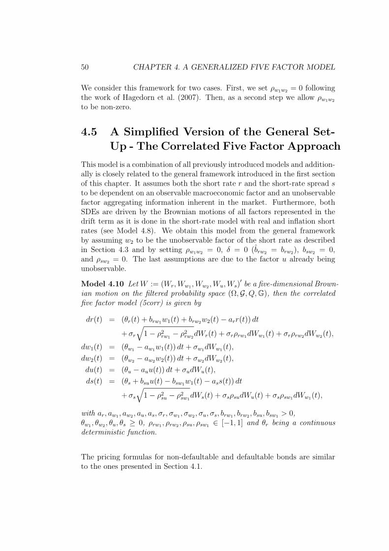
50 CHAPTER 4. A GENERALIZED FIVE FACTOR MODEL
We consider this framework for two cases. First, we set ρw1w2 = 0 followingthe work of Hagedorn et al. (2007). Then, as a second step we allow ρw1w2
to be non-zero.
4.5 A Simplified Version of the General Set-
Up - The Correlated Five Factor Approach
This model is a combination of all previously introduced models and addition-ally is closely related to the general framework introduced in the first sectionof this chapter. It assumes both the short rate r and the short-rate spread sto be dependent on an observable macroeconomic factor and an unobservablefactor aggregating information inherent in the market. Furthermore, bothSDEs are driven by the Brownian motions of all factors represented in thedrift term as it is done in the short-rate model with real and inflation shortrates (see Model 4.8). We obtain this model from the general frameworkby assuming w2 to be the unobservable factor of the short rate as describedin Section 4.3 and by setting ρw1w2 = 0, δ = 0 (brw2 = brw2), bsw2 = 0,and ρsw2 = 0. The last assumptions are due to the factor u already beingunobservable.
Model 4.10 Let W := (Wr,Ww1 ,Ww2 ,Wu,Ws)′ be a five-dimensional Brown-
ian motion on the filtered probability space (Ω,G, Q, G), then the correlatedfive factor model (5corr) is given by
dr(t) = (θr(t) + brw1w1(t) + brw2w2(t) − arr(t)) dt
+ σr
√1 − ρ2
rw1− ρ2
rw2dWr(t) + σrρrw1dWw1(t) + σrρrw2dWw2(t),
dw1(t) = (θw1 − aw1w1(t)) dt + σw1dWw1(t),
dw2(t) = (θw2 − aw2w2(t)) dt + σw2dWw2(t),
du(t) = (θu − auu(t)) dt + σudWu(t),
ds(t) = (θs + bsuu(t) − bsw1w1(t) − ass(t)) dt
+ σs
√1 − ρ2
su − ρ2sw1
dWs(t) + σsρsudWu(t) + σsρsw1dWw1(t),
with ar, aw1 , aw2 , au, as, σr, σw1 , σw2 , σu, σs, brw1 , brw2 , bsu, bsw1 > 0,θw1 , θw2 , θu, θs ≥ 0, ρrw1 , ρrw2 , ρsu, ρsw1 ∈ [−1, 1] and θr being a continuousdeterministic function.
The pricing formulas for non-defaultable and defaultable bonds are similarto the ones presented in Section 4.1.

CHAPTER 4. A GENERALIZED FIVE FACTOR MODEL 51
Lemma 4.11 In the correlated five factor model (5corr) the price of a non-defaultable zero-coupon bond is given by
P (t, T, r, w1, w2) = eA(t,T )−B(t,T )r−E1(t,T )w1−E2(t,T )w2
with
B(t, T ) =1
ar
(1 − e−ar(T−t)
),
E1(t, T ) = brw1
1
ar
(1 − e−aw1 (T−t)
aw1
+e−aw1 (T−t) − e−ar(T−t)
aw1 − ar
),
E2(t, T ) = brw2
1
ar
(1 − e−aw2 (T−t)
aw2
+e−aw2 (T−t) − e−ar(T−t)
aw2 − ar
),
A(t, T ) =
∫ T
t
1
2σ2
r(B(l, T ))2 +1
2σ2
w1(E1(l, T ))2 +
1
2σ2
w2(E2(l, T ))2
+ σrσw1ρrw1B(l, T )E1(l, T )
+ σrσw2ρrw2B(l, T )E2(l, T )
− θr(l)B(l, T ) − θw1E1(l, T ) − θw2E2(l, T )dl.
For a defaultable zero-coupon bond the price is determined by
P d(t, T, r, w1, w2, s, u) = eAd(t,T )−Bd(t,T )r−Cd(t,T )s−Dd(t,T )u−Ed1 (t,T )w1−Ed
2 (t,T )w2
with
Bd(t, T ) = B(t, T ) =1
ar
(1 − e−ar(T−t)
),
Cd(t, T ) =1
as
(1 − e−as(T−t)
),
Dd(t, T ) = bsu1
as
(1 − e−au(T−t)
au
+e−au(T−t) − e−as(T−t)
au − as
),
Ed1(t, T ) = − bsw1
1
as
(1 − e−aw1 (T−t)
aw1
+e−aw1 (T−t) − e−as(T−t)
aw1 − as
)
+ brw1
1
ar
(1 − e−aw1 (T−t)
aw1
+e−aw1 (T−t) − e−ar(T−t)
aw1 − ar
),

52 CHAPTER 4. A GENERALIZED FIVE FACTOR MODEL
Ed2(t, T ) = E2(t, T ) = brw2
1
ar
(1 − e−aw2 (T−t)
aw2
+e−aw2 (T−t) − e−ar(T−t)
aw2 − ar
),
Ad(t, T ) =
∫ T
t
1
2σ2
r(Bd(l, T ))2 +
1
2σ2
s(Cd(l, T ))2 +
1
2σ2
u(Dd(l, T ))2
+1
2σ2
w1(Ed
1(l, T ))2 +1
2σ2
w2(Ed
2(l, T ))2
+ σrσw1ρrw1Bd(l, T )Ed
1(l, T ) + σrσw2ρrw2Bd(l, T )Ed
2(l, T )
+ σsσuρsuCd(l, T )Dd(l, T ) + σsσw1ρsw1C
d(l, T )Ed1(l, T )
+ σrσsρrw1ρsw1Bd(l, T )Cd(l, T ) − θr(l)B
d(l, T )
− θsCd(l, T ) − θuD
d(l, T ) − θw1Ed1(l, T ) − θw2E
d2(l, T )dl.
4.6 Summary of Models
Table 4.1 and Table 4.2 outline all used models and parameter settings withinthis thesis. In the following, the extended model of Schmid and Zagst willbe abbreviated by SZ4, the enhancement of this model by SZ5. Both frame-works will be further differentiated by the used macroeconomic factors, e.g.gross domestic product (GDP) or inflation (CPI), or by the unobservabilityof the newly introduced factor, i.e. SZ5 versus SZ5u. Also within the realand inflation model there will be two settings, namely one assuming uncorre-lated macroeconomic factors (INF) and another abandoning this assumption(INFcorr). Furthermore, the correlated five factor model, which is a simpli-fied version of the general set-up, will also be presented within these tablesby the label 5corr.
Altogether, the newly introduced models can be summarized as follows:The correlated five factor model (5corr, see Model 4.10, page 50) is the mostgeneral set-up because it assumes two macroeconomic factors (w1 observable,w2 non-observable) driving the short rate r. For the short-rate spread s itallows one observable macroeconomic factor (w1) and one unobservable firm-specific factor (u). Additionally, the dynamics of the short rate r and theshort-rate spread s make use of the Brownian shocks of the macroeconomicand firm-specific factors.Omitting the Brownian shocks of the macroeconomic and firm-specific fac-tors in the dynamics of the short rate r and the short-rate spread s leads us tothe five factor approach of the Schmid-Zagst framework (see Model 4.6, page45). Again, we incorporate two macroeconomic factors (w1 and w2). In thesetting of SZ5 we assume both macroeconomic factors to be observable andboth entering the drift of the short rate r and the short-rate spread s. The

CHAPTER 4. A GENERALIZED FIVE FACTOR MODEL 53
setting SZ5u works with an observable (w1) and an unobservable macroeco-nomic factor (w2) in the short rate r and an observable macroeconomic (w1)and an unobservable firm-specific factor (u) in the short-rate spread s.Further, relaxing the assumption of a second macroeconomic factor driv-ing the short rate r leads us to the four factor version of the Schmid-Zagstframework (SZ4, see Model 4.4, page 42). Here, only one observable macroe-conomic factor (w1) enters the short rate r and the short-rate spread s.Finally, the real and inflation short-rate model with its two settings (INFand INFcorr, see Model 4.8, page 48) also assumes two macroeconomic fac-tors (w1 and rI), where the second is thought to be unobservable and stemsfrom an additional set of market data (inflation linked bonds) on which themodel is calibrated. INFcorr assumes the second macroeconomic factor, theso-called inflation short rate rI , to be also driven from the Brownian shocksof the observable macroeconomic factor (w1). The variant called INF doesnot incorporate these shocks. Like 5corr, the real and inflation short-ratemodel makes use of several Brownian shocks driving the short rate r. Butunlike 5corr, it does not incorporate any additional Brownian shocks in theshort-rate spread s. Therefore, INF and INFcorr are similar to the SZ5 set-up.
The next sections are dedicated to the calibration and the comparison ofthe above introduced models. First, we want to analyze which observablemacroeconomic factor is the best input. For this purpose, we use the mostsimple of the above models namely the extended model of Schmid and Zagst(SZ4) which contains only one observable macroeconomic factor (w1). Sec-ondly, we further analyze if the introduction of a second macroeconomicfactor improves the pricing ability of the models. Especially, we study if theobservability of the second macroeconomic factor and correlated Brownianshocks have an impact on the pricing.

54C
HA
PT
ER
4.A
GE
NE
RA
LIZ
ED
FIV
EFA
CT
OR
MO
DE
L
dr(t) = (θr(t) + brw1w1(t) + brw2w2(t) − arr(t)) dt + σr
√1 − ρ2
rw1− ρ2
rw2dWr(t) + σrρrw1dWw1(t) + σrρrw2dWw2(t)
θr(t) brw1 brw2 ar σr ρrw1 ρrw2
SZ4 ∈ R > 0 := 0 > 0 > 0 := 0 := 0 one m.f.(∈ R)
SZ5 ∈ R > 0 ∈ R > 0 > 0 := 0 := 0 two m.f.sSZ5u ∈ R > 0 := 1 > 0 > 0 := 0 := 0 2nd m.f.
unobs.
INF :=θR(t)+ θI := bRw1 := aR − aI := aR := σR√1−ρ2
rw1−ρ2
rw2
:=σw2
σrρw1w2 :=
σw2
σr
√1− ρ2
w1w22nd m.f.
∈ R > 0 ∈ R > 0 > 0 = 0 > 0 unobs.
INFcorr :=θR(t)+ θI := bRw1 := aR − aI := aR := σR√1−ρ2
rw1−ρ2
rw2
:=σw2
σrρw1w2 :=
σw2
σr
√1− ρ2
w1w22nd m.f.
∈ R > 0 ∈ R > 0 > 0 ∈ [−1, 1] > 0 unobs.5corr ∈ R > 0 := 1 > 0 > 0 ∈ [−1, 1] ∈ [−1, 1] 2nd m.f.
unobs.
dw1(t) = (θw1 − aw1w1(t)) dt + σw1dWw1(t)
θw1 aw1 σw1
SZ4 ≥ 0 > 0 > 0 m.f. given by GDPn, GDPr, CPI, IP, Prod, CILI, CICISZ5 ≥ 0 > 0 > 0 m.f. given by GDPrSZ5u ≥ 0 > 0 > 0 m.f. given by GDPrINF ≥ 0 > 0 > 0 m.f. given by GDPr
INFcorr ≥ 0 > 0 > 0 m.f. given by GDPr5corr ≥ 0 > 0 > 0 m.f. given by GDPr
Table 4.1: Assumptions regarding the parameters for the different models which are derived from the generalframework in Section 4.1. Macroeconomic factor is abbreviated by m.f. and unobservable by unobs.

CH
AP
TE
R4.A
GE
NE
RA
LIZ
ED
FIV
EFA
CT
OR
MO
DE
L55
dw2(t) = (θw2 − aw2w2(t)) dt + σw2ρw1w2dWw1(t) + σw2
√1 − ρ2
w1w2dWw2(t)
θw2 aw2 σw2 ρw1w2
SZ4 := 0 := 0 := 0 := 0 no 2nd m.f.SZ5 ≥ 0 > 0 > 0 ∈ [−1, 1] m.f. given by CPISZ5u ≥ 0 > 0 > 0 := 0 m.f. unobs.INF := θI ≥ 0 := aI > 0 := σI > 0 := 0 m.f. unobs.
INFcorr := θI ≥ 0 := aI > 0 := σI > 0 ∈ [−1, 1] m.f. unobs.5corr ≥ 0 > 0 > 0 := 0 m.f. unobs.
du(t) = (θu − auu(t)) dt + σudWu(t)
θu au σu
≥ 0 > 0 > 0 unobs. in all models
ds(t) = (θs + bsuu(t) − bsw1w1(t) − bsw2w2(t) − ass(t)) dt + σsρsudWu(t)+ σs
√1 − ρ2
su − ρ2sw1
− ρ2sw2
dWs(t) + σsρsw1dWw1(t) + σsρsw2dWw2(t)
θs bsu bsw1 bsw2 as σs ρsu ρsw1 ρsw2
SZ4 ≥ 0 := 1 > 0 (∈ R) := 0 > 0 > 0 := 0 := 0 := 0 one m.f.SZ5 ≥ 0 := 1 > 0 ∈ R > 0 > 0 := 0 := 0 := 0 two m.f.sSZ5u ≥ 0 := 1 > 0 := 0 > 0 > 0 := 0 := 0 := 0 w/o 2nd m.f.INF ≥ 0 := 1 > 0 ∈ R > 0 > 0 := 0 := 0 := 0 two m.f.s
INFcorr ≥ 0 := 1 > 0 ∈ R > 0 > 0 := 0 := 0 := 0 two m.f.s5corr ≥ 0 := 1 > 0 := 0 > 0 > 0 ∈ [−1, 1] ∈ [−1, 1] := 0 w/o 2nd m.f.
Table 4.2: Assumptions regarding the parameters for the different models which are derived from the generalframework in Section 4.1. Macroeconomic factor is abbreviated by m.f. and unobservable by unobs.
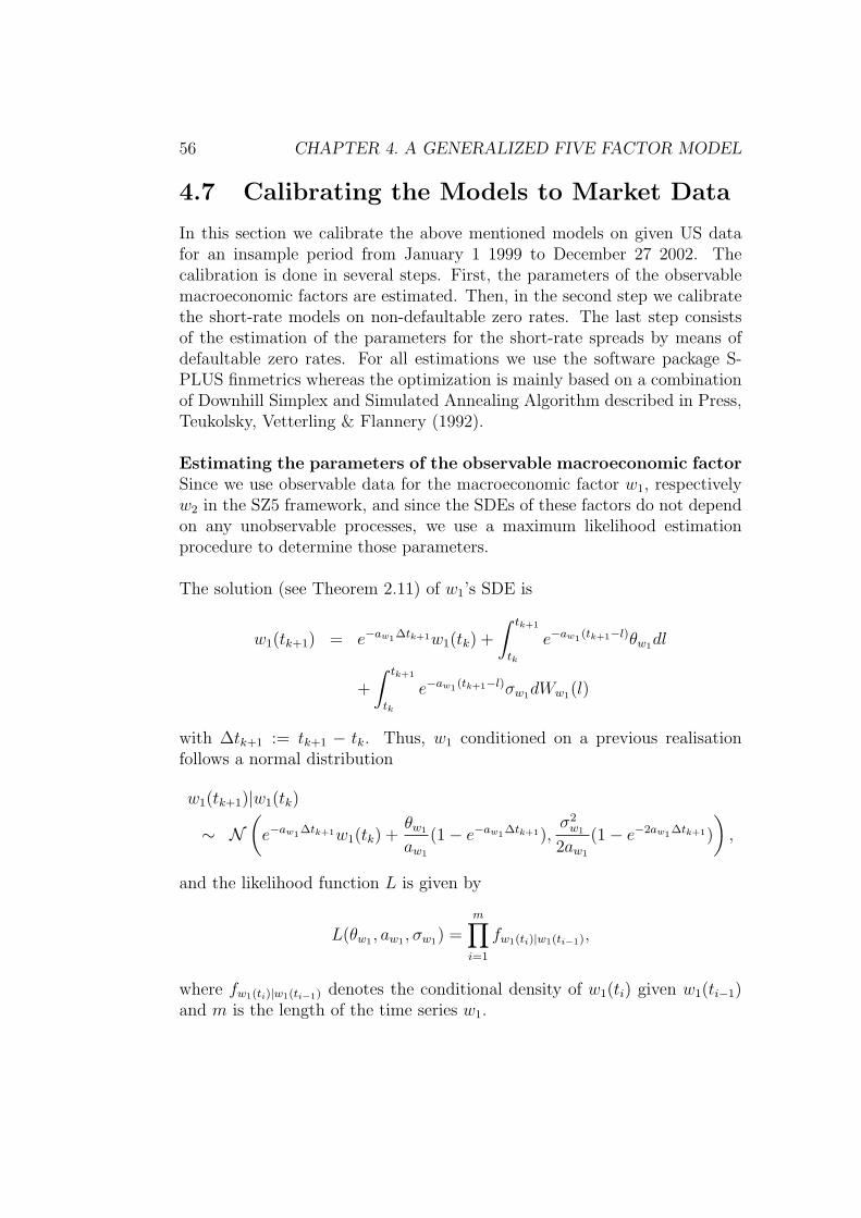
56 CHAPTER 4. A GENERALIZED FIVE FACTOR MODEL
4.7 Calibrating the Models to Market Data
In this section we calibrate the above mentioned models on given US datafor an insample period from January 1 1999 to December 27 2002. Thecalibration is done in several steps. First, the parameters of the observablemacroeconomic factors are estimated. Then, in the second step we calibratethe short-rate models on non-defaultable zero rates. The last step consistsof the estimation of the parameters for the short-rate spreads by means ofdefaultable zero rates. For all estimations we use the software package S-PLUS finmetrics whereas the optimization is mainly based on a combinationof Downhill Simplex and Simulated Annealing Algorithm described in Press,Teukolsky, Vetterling & Flannery (1992).
Estimating the parameters of the observable macroeconomic factorSince we use observable data for the macroeconomic factor w1, respectivelyw2 in the SZ5 framework, and since the SDEs of these factors do not dependon any unobservable processes, we use a maximum likelihood estimationprocedure to determine those parameters.
The solution (see Theorem 2.11) of w1’s SDE is
w1(tk+1) = e−aw1∆tk+1w1(tk) +
∫ tk+1
tk
e−aw1 (tk+1−l)θw1dl
+
∫ tk+1
tk
e−aw1 (tk+1−l)σw1dWw1(l)
with ∆tk+1 := tk+1 − tk. Thus, w1 conditioned on a previous realisationfollows a normal distribution
w1(tk+1)|w1(tk)
∼ N(
e−aw1∆tk+1w1(tk) +θw1
aw1
(1 − e−aw1∆tk+1),σ2
w1
2aw1
(1 − e−2aw1∆tk+1)
),
and the likelihood function L is given by
L(θw1 , aw1 , σw1) =m∏
i=1
fw1(ti)|w1(ti−1),
where fw1(ti)|w1(ti−1) denotes the conditional density of w1(ti) given w1(ti−1)and m is the length of the time series w1.
CHAPTER 4. A GENERALIZED FIVE FACTOR MODEL 57
Within the SZ4 framework (see Model 4.4) we test seven different macroe-conomic factors as representatives for w1. All of those factors are commonlysupposed to have good predicting power with respect to the state of theeconomy.
(i) Nominal Gross Domestic Product (GDPn)The gross domestic product is a measure of total production and totalconsumption of goods and services within the United States. Hence, itgives the most comprehensive picture of the power of the U.S. economy.Its value is published quarterly with a delay of one quarter, i.e. it isfinally known at the end of the following quarter. Therefore we takeinto account a lag of 6 month in our calibration procedure.The growth rate of GDP is used e.g. by Bonfim (2009) who analyzesempirically the determinants of corporate credit default taking intoaccount firm-specific and macroeconomic information. The obtainedresults suggest that the GDP growth rate belongs to the most impor-tant ones within the group of all considered variables.Furthermore, the growth rate of GDP is incorporated in several studiesanalyzing the impact of macroeconomic variables on credit risk andsovereign ratings: Glen (2005) finds with the help of GDP growthrates a strong link between macroeconomic conditions and the abil-ity to service debt. Hilscher & Nosbusch (2010) investigate the impactof macroeconomic fundamentals on sovereign credit spreads with theGDP being the main input in form of its growth, its volatility andseveral ratios, e.g. debt/GDP.
(ii) Real Gross Domestic Product (GDPr)The real gross domestic product is adjusted for price changes in orderto measure the GDP, respectively the production within the UnitedStates, regardless of changes in the purchasing power. The publicationfollows the same schedule as for the nominal GDP. Thus, we also con-sider a time lag of 2 quarters. Both the nominal and the real GDP arepublished by the U.S. Department of Commerce: Bureau of EconomicAnalysisV.As mentioned above, the growth rate of GDP is often used in empiri-cal studies regarding credit risk and ratings. Some explicitly state thereal GDP as input variable. E.g. Rowland (2005) incorporates the realGDP growth rate in his study of determinants of ratings, creditwor-thiness and spreads for emerging market sovereign debt. One of his
Vhttp://www.bea.gov

58 CHAPTER 4. A GENERALIZED FIVE FACTOR MODEL
findings is that the real GDP growth rate seems to have a significantimpact on spreads.
(iii) Consumer Price Index (CPI)The consumer price index measures the development of the averageprice of goods and services consumed by households. Thus, its per-centage change indicates inflation. Since around 80 % of the U.S.population lives in urban areas, the CPI-U is the most popular rep-resentative of the CPI. A further differentiation within the CPI is itsvalue apart from prices of energy and food. Since those products leadto a high volatility within the CPI time series and often overlap long-term trends, we use the index called: ”Consumer Price Index for AllUrban Consumers: All Items Less Food & Energy” which is publishedby the U.S. Department of Labor: Bureau of Labor StatisticsVI. TheCPI is published on a monthly basis with a delay of two and a halfmonths. Therefore, we incorporate the CPI with a lag of three monthsin our calibration.Some of the above works also make use of the CPI next to the GDP,e.g. Glen (2005) and Rowland (2005). Additionally, Ang & Piazzesi(2003) incorporate the CPI in their analysis of macro variables andtheir effect on bond prices and on the dynamics of the yield curve.Cantor & Packer (1996) study determinants of sovereign ratings andfind that inflation belongs to the group of factors which seem to playan important role.
(iv) Industrial Production (IP)This production index measures real output. Since the majority of vari-ation in the national output of the U.S. is due to the industry sector,this index indicates structural developments in the U.S. economy. It isreleased by the Board of Governors of the Federal Reserve SystemVII
with a monthly frequency and a time delay of 1 and a half monthsincluding revisions for the previous 3 months. Hence, we allow for atime lag of 3 months which is in line with the above indices whose finalpublications are also preceded by preliminary reports.The growth rate in industrial production is used by Figlewski et al.(2012) who analyze reduced-form models by allowing the hazard rateto depend on firm-specific factors and macroeconomic conditions. Theyinclude the industrial production as a factor that indicates the directionwhere the economy is moving to. They also claim that the growth rate
VIhttp://www.bls.govVIIhttp://www.federalreserve.gov

CHAPTER 4. A GENERALIZED FIVE FACTOR MODEL 59
in industrial production might be a better measure than the growthrate in real GDP since the latter covers all economic activity includingsectors which may be unrelated to corporate credit conditions.Also, Ang & Piazzesi (2003) include the growth rate of industrial pro-duction in their study of a term structure model with inflation andeconomic growth factors. Here, IP is assumed to capture real activity.Furthermore, Krishnan et al. (2005) and Krishnan et al. (2010) usethe growth rate in industrial production for their analysis of changesin credit spreads and their study in predicting future firm-level creditspreads.
(v) Productivity (Prod)The most often used measure of productivity within the United Statesis the so-called labor productivity which determines the output perhour of all persons. Its importance stems from the fact that labor costsare easily identified and account for the majority of the output’s value.The most comprehensive measure of productivity is that of the businesssector whose output covers about 80 % of the GDP. Hence, its growthis strongly correlated with the growth of the GDP. The publicationof the labor productivity is every quarter by the U.S. Department ofLabor: Bureau of Labor Statistics. Like the GDP this index is releasedat the end of the following quarter which leads to a lag of 6 months inour analysis.
(vi) Composite Index Of Leading Indicators (CILI)The composite index of leading indicators (CILI) is an aggregate of teneconomic releases which all show patterns that are related to the busi-ness cycle, e.g average weekly hours worked in the manufacturing indus-tries as a predictor for changes in unemployment, manufacturer’s neworders for consumer goods/materials indicating future revenues, S&P500 and interest rate spread reflecting investors’ expectations about theeconomy and changes in the yield curve (see TCB (2001)). This indexof leading indicators tries to cover the overall state of the macroeco-nomy and to reveal common turning point patterns within the seriesof indicators in order to judge the future state of the economy, i.e. thenext six to nine months. By aggregating several economic indicators itgives a summary of the economy and additionally decreases the impactof volatility given by a single indicator. The composite index of leadingindicators is published by The Conference Board VIII IX at the end of
VIIIhttp://www.conference-board.org and http://tcb-indicators.orgIXWe got the time series from Reuters using its RIC aUSCLEAD/A.
60 CHAPTER 4. A GENERALIZED FIVE FACTOR MODEL
every month with a lag of one month. Since several indicators withinthe composite index are also published with a timing lag and are hencerepresented by projected data, the composite index allows for revisionsof the most recent months. Consistent to the above data, we use athree month publication lag.Huang & Kong (2003) examine determinants of corporate bond creditspreads by using explanatory variables which capture different aspectsof credit risk, e.g. default rates, interest rates, equity market factorsand macroeconomic indicators. Their main findings are that also vari-ables like the Conference Board’s composite indices of indicators, whichhave not been used before in the literature, have significant explainingpower for credit spread changes.
(vii) Composite Index Of Coincident Indicators (CICI)The composite index of coincident indicators (CICI) is also publishedby The Conference BoardX. The main purpose of this index is to de-scribe the current state of the economy. It is composed by four individ-ual indicators which are said to be in-step with the current economiccycle. These indicators are employees on non-agricultural payrolls re-flecting actual changes in hiring and firing, personal income less trans-fer payments measuring the general health of the economy, index ofindustrial production which historically captured most of movementsin total industrial output, and manufacturing and trade sales measur-ing real total spending. Like CILI, the composite index of coincidentindicators is published on a monthly basis including available data aswell as estimates. Hence, this index will also be revised in the followingmonths when the actual data of the underlying indicators are finallypublished. In order to justify the publishing delay of almost 2 monthsand the revisions we allow for a lag of 3 months.
The model is calibrated on weekly data, therefore we need to break downthe given macroeconomic data with a frequency of 1 respectively 3 monthsto a weekly time series. This is done by means of the interpolation used forinflation-linked bondsXI:
ω(tm) := ωm−3 +tm − 1
d(m)(ωm−2 − ωm−3) ,
where d(m) indicates the number of days in the corresponding month m, re-spectiveley quarter, tm the actual date where we want to get a value of ω with
XWe got the time series from Reuters using its RIC aUSCOINDIF/A.XIFor further information refer to e.g. Agence France Tresor (http://www.aft.gouv.fr/)
CHAPTER 4. A GENERALIZED FIVE FACTOR MODEL 61
0 ≤ tm ≤ d(m) and ωm the published index value for the month (quarter) m.The lag of one month (quarter) inherent in the above interpolation is due tothe fact that the index value ωm for the month (quarter) m will be valid forthe whole month (quarter), i.e. starting from the first day and lasting untilthe last day of the month (quarter), but will be available at the earliest onsome day in the following month (quarter) m + 1. Since it is unlikely thatthe publishment is on the very first day of the following month (quarter)and therefore, it cannot be assumed that the index value ωm of the month(quarter) before is already known on all days of the next month (quarter)m + 1. If the lag between the end of the respective month (quarter) and thepublishment of its index value is even longer, the interpolated index value isobtained by
ω(tm) := ωm−d−2 +tm − 1
d(m)(ωm−d−1 − ωm−d−2) ,
with d denoting the lag between the end of the period for which the indexvalue is valid and its publishment.Afterwards, we need to calculate growth rates for the respective macroeco-nomic data. As the original GDP time series is released quarterly we calculateevery week the growth rate with respect to 3 months. For the CPI we deter-mine annual growth rates because the index is published with an accuracy ofjust one decimal place and we observed that the values of the index do notchange for several months. In order to prevent low growth rates and a fluctu-ation around zero we again use annual growth rates for industrial productionand the composite indices since changes for months as well as quarters arenegligible. For the growth rate in productivity we proceed as with the GDPand determine growth rates with respect to a quarter.Although the whole model is calibrated on weekly data, we only use monthly
data for calibrating the macroeconomic factors. This is done in order to avoida possibly high autocorrelation within the interpolated data set. The resultsof the maximum likelihood estimation for the macroeconomic factors aregiven in Table 4.3. In all cases, the given data seem to fit into our modelassumption since the mean reversion levels which are determined by
θw1
aw1are
near the corresponding empirical means.
Estimating the parameters of the short rate rIn order to get the parameters of the short rate (ar, br, σr, ρrw1 , ρrw2 , λr, λw1 , λw2)we use the Kalman filtering method (see Section 2.4) which requires a statespace form consisting of a measurement equation and a transition equation.The measurement equation is derived from the affine relationship between
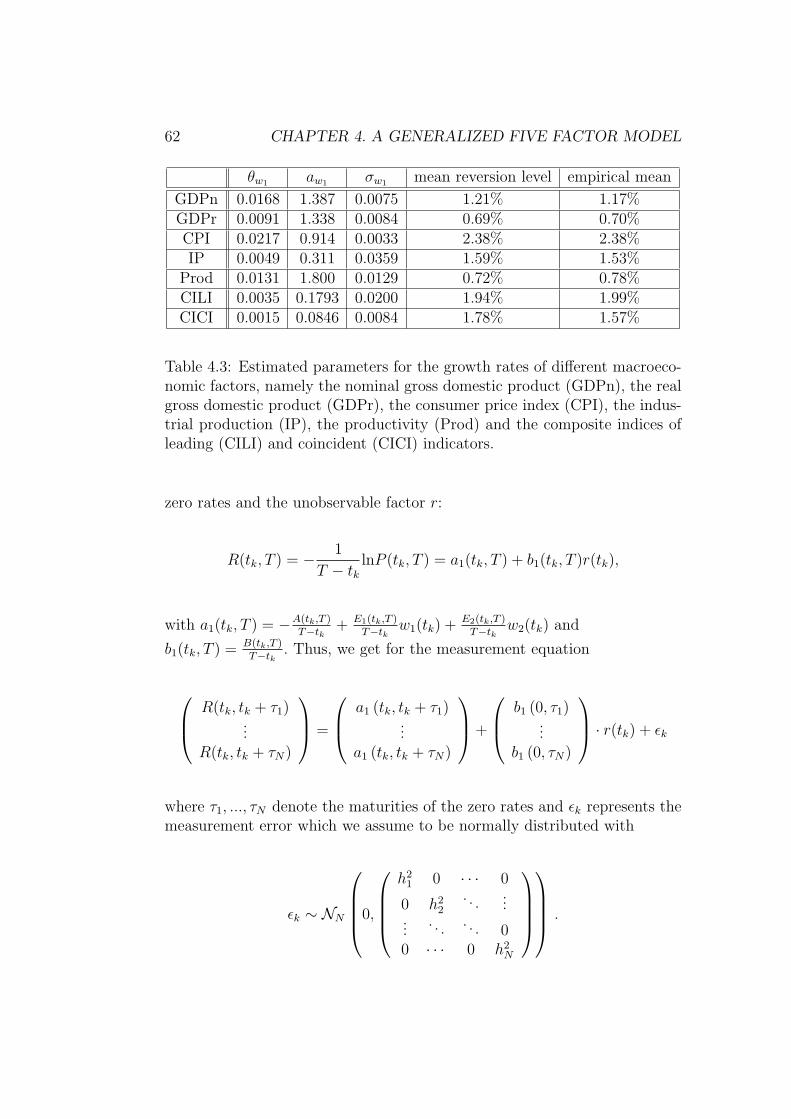
62 CHAPTER 4. A GENERALIZED FIVE FACTOR MODEL
θw1 aw1 σw1 mean reversion level empirical mean
GDPn 0.0168 1.387 0.0075 1.21% 1.17%GDPr 0.0091 1.338 0.0084 0.69% 0.70%CPI 0.0217 0.914 0.0033 2.38% 2.38%IP 0.0049 0.311 0.0359 1.59% 1.53%
Prod 0.0131 1.800 0.0129 0.72% 0.78%CILI 0.0035 0.1793 0.0200 1.94% 1.99%CICI 0.0015 0.0846 0.0084 1.78% 1.57%
Table 4.3: Estimated parameters for the growth rates of different macroeco-nomic factors, namely the nominal gross domestic product (GDPn), the realgross domestic product (GDPr), the consumer price index (CPI), the indus-trial production (IP), the productivity (Prod) and the composite indices ofleading (CILI) and coincident (CICI) indicators.
zero rates and the unobservable factor r:
R(tk, T ) = − 1
T − tklnP (tk, T ) = a1(tk, T ) + b1(tk, T )r(tk),
with a1(tk, T ) = −A(tk,T )T−tk
+ E1(tk,T )T−tk
w1(tk) + E2(tk,T )T−tk
w2(tk) and
b1(tk, T ) = B(tk,T )T−tk
. Thus, we get for the measurement equation
R(tk, tk + τ1)...
R(tk, tk + τN)
=
a1 (tk, tk + τ1)...
a1 (tk, tk + τN)
+
b1 (0, τ1)...
b1 (0, τN)
· r(tk) + εk
where τ1, ..., τN denote the maturities of the zero rates and εk represents themeasurement error which we assume to be normally distributed with
εk ∼ NN
0,
h21 0 · · · 0
0 h22
. . ....
.... . . . . . 0
0 · · · 0 h2N
.

CHAPTER 4. A GENERALIZED FIVE FACTOR MODEL 63
The transition equation is derived from the solution of the SDE (see Theorem2.11) of the short rate r which yields
r(tk+1) = e−ar∆tk+1r(tk) +
∫ tk+1
tk
e−ar(tk+1−l)(θr(l) + brw1w1(l) + brw2w2(l))dl
+
∫ tk+1
tk
e−ar(tk+1−l)σr
√1 − ρ2
rw1− ρ2
rw2dWr(l)
+
∫ tk+1
tk
e−ar(tk+1−l)σrρrw1dWw1(l) +
∫ tk+1
tk
e−ar(tk+1−l)σrρrw2dWw2(l),
Approximating θr(l), w1(l) and w2(l) by θr(tk), w1(tk), w2(tk), we obtain thetransition equation
r(tk+1) = e−ar∆tk+1r(tk) +
∫ ∆tk+1
0
e−arl(θr(tk) + brw1w1(tk) + brw2w2(tk))dl
+
∫ tk+1
tk
e−ar(tk+1−l)σrρrw1dWw1(l) +
∫ tk+1
tk
e−ar(tk+1−l)σrρrw2dWw2(l)
+ ηk+1 ,
where ηk+1 is defined as∫ tk+1
tke−ar(tk+1−l)σrdWr(l) with
ηk+1 ∼ N1
(0,
∫ ∆tk+1
0
e−2arlσ2rdl
)= N1
(0,
σ2r
2ar
(1 − e−2ar∆tk+1
)).
The two stochastic integrals in the above equation are approximated with∫ tk+1
tke−ar(tk+1−l)σrρrwi
dWwi(l) ≈ e−ar(∆tk+1)σrρrwi
∆Wwi(tk+1), i = 1, 2, where
∆Wwi(tk+1) := Wwi
(tk+1) − Wwi(tk) is obtained by inserting the time series
of wi, i = 1, 2, into the solution of its SDE (see page 56).This procedure is used if we have observable time series for w1 and w2. If oneof these processes is unobservable the above equations have to be rewritten.We do not perform this in detail but refer to the next passage where weexplain the procedure for two unobservable processes, namely s and u.The vector of parameters for the short rates of the models SZ4, SZ5, SZ5uand 5corr, which only differ by the number of macroeconomic factors, by theircorrelation and by their observability, are determined by the same procedure.The data is given by weekly par yields of US Treasury Strips of maturities(τ) 3 months, 6 months, 1 year, 2, 3, 4, 5, 7, 10, 20 and 25 years which arecollected from BloombergXII. We transform these par yields in continuous
XIIThe Bloomberg tickers for the US Treasury Strips are: C0793M, C0796M, C0791Y,C0792Y, C0793Y, C0794Y, C0795Y, C0797Y, C07910Y, C07920Y, C07925Y.

64 CHAPTER 4. A GENERALIZED FIVE FACTOR MODEL
GDPn GDPr CPI IP Prod CILI CICI
ar 0.6042 0.5922 0.3144 0.6188 0.4707 0.3258 0.3290brw1 0.0355 0.0532 0.0416 0.0263 0.0971 0.0527 0.0042σr 0.0095 0.0092 0.0101 0.0117 0.0124 0.0099 0.0113λr -2204.3 -1344.0 -1082.6 -1559.1 -471.0 -575.5 -561.4λw1 -13605.2 -3475.3 -4023.9 -66.4 -538.3 -54.3 -359.6h1 0.0103 0.0137 0.0130 0.0075 0.0122 0.0101 0.0106h2 0.0124 0.0094 0.0106 0.0105 0.0097 0.0119 0.0118h3 0.0089 0.0063 0.0094 0.0035 0.0068 0.0066 0.0080h4 0.0048 0.0021 0.0027 0.0019 0.0024 0.0026 0.0027h5 0.0021 0.0023 0.0017 0.0053 0.0007 0.0006 0.0003h6 0.0019 0.0047 0.0008 0.0048 0.0011 0.0019 0.0019h7 0.0025 0.0054 0.0023 0.0044 0.0035 0.0028 0.0028h8 0.0049 0.0058 0.0046 0.0062 0.0063 0.0045 0.0040h9 0.0063 0.0092 0.0050 0.0091 0.0062 0.0064 0.0050h10 0.0032 0.0028 0.0029 0.0071 0.0054 0.0037 0.0039h11 0.0133 0.0113 0.0127 0.0090 0.0110 0.0098 0.0111ar 0.4070 0.4775 0.2030 0.4066 0.3980 0.2698 0.2570aw1 0.6195 1.0810 0.8710 0.2254 1.7100 0.1577 0.0593
meanreversion 3.18% 3.84% 3.24% 3.07% 4.08% 4.07% 3.84%
Table 4.4: Estimated parameters for the short rate r within the SZ4 frame-work for different macroeconomic factors w1. The mean reversion of r, whichis given in the last row, compares to an empirical mean of 3.91% of the zerorates with a maturity of 3 months.
zero rates and use them as input for R(tk, tk + τ) of the measurement equa-tion.As previously mentioned, it is not always clear in which way interest rates areinfluenced by macroeconomic factors. Therefore, we relax the restrictions ofnon-negativity regarding brw1 for the factor CPI in the SZ4 model (see Model4.4). The results of the estimation (see Table 4.4) propose that all factors’influence is in the same direction. Table 4.4 shows the estimated parametersof the SZ4 framework for different representatives of the factor w1. Based onthese estimates we can calculate the mean reversion of the short rate r bymedian(θr)+brw1
θw1aw1
arand compare it with the empirical mean of 3.91% of the ob-
served 3-months zero rates. The fit of the different four factor models (SZ4)

CHAPTER 4. A GENERALIZED FIVE FACTOR MODEL 65
is promising since the calculated mean reversion levels are near the empiricalmean especially for GDPr, Prod, CILI, and CICI. In addition, the scales ofthe estimated volatilities of the measurement errors h1, . . . , h11 indicate thatall seven versions of the SZ4 framework have a similar ability of explainingnon-defaultable zero rates.For the five factor versions of the SZ and the correlated framework (i.e. SZ5,SZ5u, 5corr) we use the real gross domestic product (GDPr) as representativeof w1. The second factor is represented by the consumer price index (CPI)in the case of SZ5 (see Model 4.6) and it is chosen to be unobservable inthe case of SZ5u (see Model 4.6) and 5corr (see Model 4.10). We assume forthe estimation of the parameters of SZ5 that brw2 ∈ R since the interactionbetween the two given factors is not known for sure. Within the frameworkof SZ5u and 5corr we define brw2 to be 1 and ρw1w2 to be 0 in order to pre-vent problems of identification. Table 4.5 presents the estimated parameters.We do not give the parameters of w1 and of w2 if they are assumed to beobservable, since we already estimated these parameters in the first step (seeTable 4.3). Compared to the results of the four factor model (SZ4) e.g. withinput GDPr or the composite indices (see Table 4.4) we can conclude thatthe five factor versions (SZ5, SZ5u, 5corr) yield promising results especiallyif we look at the volatilities of the measurement errors h1, . . . , h11 which areon average smaller than the ones of the SZ4 frameworks with the exceptionof the long-term maturities, i.e. h10 and h11. This indicates that the addi-tional factor is able to explain an extra portion of the variation. The secondmacroeconomic factor (w2) also changes the influence of the GDPr. If weincorporate the CPI as an additional factor, the value of brw1 increases in-dicating a bigger impact of the GDPr. But since the CPI affects the shortrate in the opposite direction (brw2 < 0) the increase in brw1 is mostly dueto the interaction between GDPr and CPI. In the case of an unobservablefactor w2, where we assume the same direction of influence as for the GDPr,the impact of the GDPr decreases in the case of the SZ5u framework as brw1
is smaller than in the SZ4 framework. Here, the unobservable factor seemsto be able to better explain the variation and therefore reduces the influenceof the GDPr. In the case of the 5corr framework, where it is assumed thatthe short rate is correlated with both the macroeconomic factor and the un-observable factor, brw1 increases compared to the SZ4 framework in responseto the newly incorporated shocks of the factors w1 and w2. If we calculate
the mean reversion level of the short rate r bymedian(θr)+brw1
θw1aw1
+brw2
θw2aw2
arand
compare it to the mean of the given 3-months zero rates we see that all threemodels obtain a good fit. Especially the models with an additional unob-servable factor approach easily the empirical mean.
66 CHAPTER 4. A GENERALIZED FIVE FACTOR MODEL
The parameters of the short rate within the real and inflation short-rateframework (INF and INFcorr, see Model 4.8) are estimated in a different waythan the parameters of the other models. Since it is assumed that the shortrate r is the sum of the real short rate rR and the inflation short rate rI theparameters of these processes are estimated independently but both with thehelp of a Kalman filter and a state space model similar to the above men-tioned. We use the same data as Hagedorn et al. (2007) who first introducedthis interest rate model based on real and inflation short rates. The real zerorates are generated with the help of inflation-linked bonds XIII. In the U.S.these bonds come in the most common structure of capital-indexed bondslike in Sweden, the United Kingdom, France and Canada. Capital-indexedbonds pay a real coupon as the nominal of these bonds is indexed by a capitalmultiplier which is given as the ratio of an inflation-indexed process at time tand at a certain reference day tbase. Furthermore, a deflation floor is built inwhich prevents the capital multiplier of being smaller than 1. The indexingis based on the CPI-U with the linear interpolation technique introduced inthe previous passage. The real rates are determined by assuming a Nelson-Siegel structure and by approximating at weekly measurement points themarket prices of US Treasury Inflation Protection Securities (TIPS). Theinput data for estimating the parameters of the inflation short rate is de-termined by substracting the real rates from the nominal rates which wederived from US Treasury Strips. As the real rates are calculated by as-suming the Nelson-Siegel framework, the nominal rates are also smoothedby Nelson-Siegel curves in order to avoid any systematic errors. For furtherinformation about the derivation of the real rates see Hagedorn et al. (2007).Table 4.6 gives the estimated parameters of the real short rate rR and theinflation short rate rI which is assumed to be uncorrelated with w1 (GDPr)in the framework INF (ρw1w2 := 0) and correlated with w1 in the frameworkINFcorr (ρw1w2 ∈ R). We can observe that the influence of the real grossdomestic product (measured by brw1) is bigger for the real rates than thenominal ones (see Table 4.4). Both versions of the inflation short rate rI dohave a good fit since the volatilities of the measurement errors h1, . . . , h11
are of similar scale. As in the case of the five factor model of Schmid-Zagst,SZ5 (see Model 4.6), the correlation between the factors w1 and w2 takes ona negative value. The additional impact of the inflation rate for the nomi-nal short rate is given by the parameter brw2 which is determined under thereal-world measure by aR −aw2 and results in -0.1753 (INF), i.e. an oppositeimpact of w1 and w2, respectively 0.3111 (INFcorr), also indicating together
XIIIFor further information about inflation-linked bonds see Deacon, Derry & Mirfend-ereski (2004).
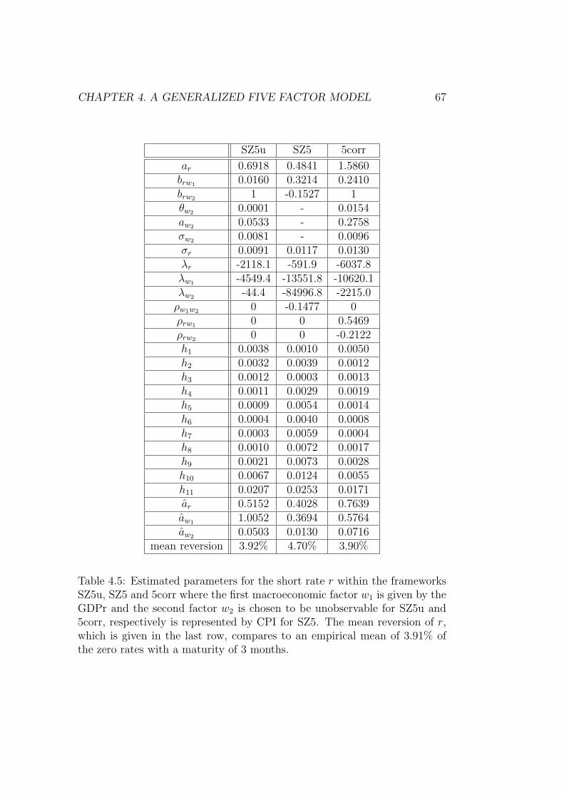
CHAPTER 4. A GENERALIZED FIVE FACTOR MODEL 67
SZ5u SZ5 5corr
ar 0.6918 0.4841 1.5860brw1 0.0160 0.3214 0.2410brw2 1 -0.1527 1θw2 0.0001 - 0.0154aw2 0.0533 - 0.2758σw2 0.0081 - 0.0096σr 0.0091 0.0117 0.0130λr -2118.1 -591.9 -6037.8λw1 -4549.4 -13551.8 -10620.1λw2 -44.4 -84996.8 -2215.0
ρw1w2 0 -0.1477 0ρrw1 0 0 0.5469ρrw2 0 0 -0.2122h1 0.0038 0.0010 0.0050h2 0.0032 0.0039 0.0012h3 0.0012 0.0003 0.0013h4 0.0011 0.0029 0.0019h5 0.0009 0.0054 0.0014h6 0.0004 0.0040 0.0008h7 0.0003 0.0059 0.0004h8 0.0010 0.0072 0.0017h9 0.0021 0.0073 0.0028h10 0.0067 0.0124 0.0055h11 0.0207 0.0253 0.0171ar 0.5152 0.4028 0.7639aw1 1.0052 0.3694 0.5764aw2 0.0503 0.0130 0.0716
mean reversion 3.92% 4.70% 3.90%
Table 4.5: Estimated parameters for the short rate r within the frameworksSZ5u, SZ5 and 5corr where the first macroeconomic factor w1 is given by theGDPr and the second factor w2 is chosen to be unobservable for SZ5u and5corr, respectively is represented by CPI for SZ5. The mean reversion of r,which is given in the last row, compares to an empirical mean of 3.91% ofthe zero rates with a maturity of 3 months.
68 CHAPTER 4. A GENERALIZED FIVE FACTOR MODEL
with the negative correlation a tendency of opposite impact . Hence, if weallow for correlated factors w1 and w2 the sign of the correlation is the sameas in the framework SZ5, but the direction of the impact of the factor w2
changes since the sign of brw2 is the same as for brw1 as opposed to brw1 > 0and brw2 < 0 for SZ5. But otherwise, if ρw1w2 is to be 0, brw2 takes on thesame sign as in the case of SZ5 namely opposite to the impact of the GDPr,though ρw1w2 < 0 in SZ5 . This result - in addition with the results for SZ5- emphasizes the previously stated fact that the influence of certain factorson the short rate respectively interest rates is an open question. The meanreversion level of the short rate in the real and inflation short-rate model
is determined bymedian(θR)+θw2+bRw1
θw1aw1
+(aR−aw2 )θw2aw2
aRresulting in 3.30% (INF)
and 3.32% (INFcorr). Compared to the empirical mean of the 3-months zerorates (3.91%), the real and inflation short-rate framework (INF and INFcorr)fits the data as good as the other discussed frameworks.
Estimating the parameters of the short-rate spread s and the un-certainty index uThe parameters (as, σs, λs, θs, bsu, bsw1 , bsw2 , au, σu, λu, θu, ρsu, ρsw1 , ρsw2) of
the processes s and u are also estimated by means of the Kalman filter.Here, we obtain the measurement equation by substracting non-defaultablezero rates R(tk, T ) = − 1
T−tklnP (tk, T ) from defaultable zero rates
Rd(tk, T ) = − 1T−tk
lnP d(tk, T ) in order to obtain the spread S(tk, T ):
S(tk, T ) = Rd(tk, T ) − R(tk, T )
=Cd(tk, T )
T − tks(tk) +
Dd(tk, T )
T − tku(tk) −
Ad(tk, T ) − A(tk, T )
T − tk
+Ed
1(tk, T ) − E1(tk, T )
T − tkw1(tk) +
Ed2(tk, T ) − E2(tk, T )
T − tkw2(tk).
If we define cd(tk, T ) = Cd(tk,T )T−tk
, dd(tk, T ) = Dd(tk,T )T−tk
, ad(tk, T ) as the sum ofall terms independent of s and u, and
X(tk) :=
(s(tk)u(tk)
),
the measurement equation yields
S(tk, tk + τ1)...
S(tk, tk + τN)
=
ad (tk, tk + τ1)...
ad (tk, tk + τN)
+
cd (0, τ1) dd (0, τ1)...
...cd (0, τN) dd (0, τN)
·X(tk)+εk
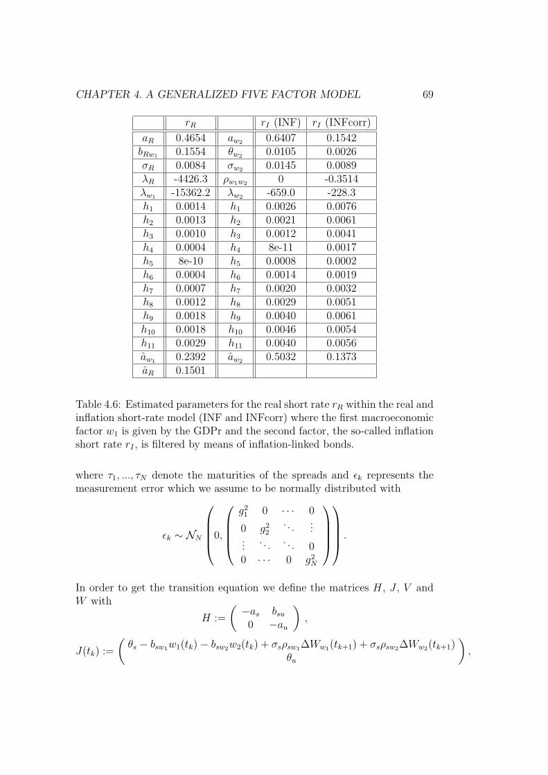
CHAPTER 4. A GENERALIZED FIVE FACTOR MODEL 69
rR rI (INF) rI (INFcorr)
aR 0.4654 aw2 0.6407 0.1542bRw1 0.1554 θw2 0.0105 0.0026σR 0.0084 σw2 0.0145 0.0089λR -4426.3 ρw1w2 0 -0.3514λw1 -15362.2 λw2 -659.0 -228.3h1 0.0014 h1 0.0026 0.0076h2 0.0013 h2 0.0021 0.0061h3 0.0010 h3 0.0012 0.0041h4 0.0004 h4 8e-11 0.0017h5 8e-10 h5 0.0008 0.0002h6 0.0004 h6 0.0014 0.0019h7 0.0007 h7 0.0020 0.0032h8 0.0012 h8 0.0029 0.0051h9 0.0018 h9 0.0040 0.0061h10 0.0018 h10 0.0046 0.0054h11 0.0029 h11 0.0040 0.0056aw1 0.2392 aw2 0.5032 0.1373aR 0.1501
Table 4.6: Estimated parameters for the real short rate rR within the real andinflation short-rate model (INF and INFcorr) where the first macroeconomicfactor w1 is given by the GDPr and the second factor, the so-called inflationshort rate rI , is filtered by means of inflation-linked bonds.
where τ1, ..., τN denote the maturities of the spreads and εk represents themeasurement error which we assume to be normally distributed with
εk ∼ NN
0,
g21 0 · · · 0
0 g22
. . ....
.... . . . . . 0
0 · · · 0 g2N
.
In order to get the transition equation we define the matrices H, J , V andW with
H :=
(−as bsu
0 −au
),
J(tk) :=
(θs − bsw1w1(tk) − bsw2w2(tk) + σsρsw1∆Ww1(tk+1) + σsρsw2∆Ww2(tk+1)
θu
),

70 CHAPTER 4. A GENERALIZED FIVE FACTOR MODEL
V :=
(σs
√1 − ρ2
su + ρ2sw1
+ ρ2sw2
σsρsu
0 σu
),W := (Ws,Wu)
′ ,
where dWw1 , respectively dWw2 , is approximated by ∆Ww1(tk+1) := Ww1(tk+1)−Ww1(tk). Thus, the SDEs of s and u can be written as
dX(tk) = HX(tk) + J(tk)dt + V dW (tk).
Using Theorem 2.11 the solution of dX is
Xk+1 = eH∆tk+1Xk +
∫ tk+1
tk
eH(tk+1−l)J(l)dl +
∫ tk+1
tk
eH(tk+1−l)V dW (l).
If we approximate J(l) by J(tk) the transition equation can be written as
X(tk+1) = eH∆tk+1X(tk) +
∫ ∆tk+1
0
eHlJ(tk)dl + ηk+1,
with ηk+1 :=∫ tk+1
tkeH(tk+1−l)V dW (l) following a normal distribution
ηk+1 ∼ N2
(0,
∫ ∆tk+1
0
eHlV V ′eH′ldl
).
The procedure to determine the parameters for the processes s and u is thesame throughout all discussed models since the only differences are the useof a second factor w2 and the correlated shocks in the SDE of the short-rate spread. The data is given by weekly par yields of US Industrials ratedBBB1 and A2 whose maturities are 3 months, 6 months, 1 year, 2, 3, 4,5, 7, 10, 20 and 25 years. As before this data stems from BloombergXIV.Again, we transform these par yields in continuous zero rates, substract thenon-defaultable zero rates in order to derive the credit spreads and smooththe resulting rates by means of Nelson-Siegel curves. We use these creditspreads as input for S(tk, tk + τ) of the measurement equation.Throughout all models we assume bsu to be 1 as the process u is already un-observable. In the case of the five factor models with an unobservable secondmacroeconomic factor w2, SZ5u (see Model 4.6) and 5corr (see Model 4.10),we additionally assume bsw2 = 0 since there is already an unobservable factoru in the short-rate spread. Including a second unobservable factor wouldhave led to problems regarding the differentiation of the two unobservablefactors. This assumption gives the short-rate spread of the SZ5u framework
XIVThe Bloomberg tickers are for the rating A2: C0063M, C0066M, C0061Y,... andC0083M, C0086M, C0081Y,... for the rating BBB1.

CHAPTER 4. A GENERALIZED FIVE FACTOR MODEL 71
the same form as the short-rate spreads within the four factor framework(SZ4, see Model 4.4) and a similar appearance to the SZ4 framework in caseof the 5corr framework. Hence, we expect similar results for SZ5u, 5corr andSZ4 frameworks with respect to the short-rate spread s.Figlewski et al. (2012) indicate in their study of corporate defaults that in-flation is understood to be an important macroeconomic factor but its effectis unclear, since, unlike the common perception, high inflation could also de-crease default risk by reducing the value of required debt service payments.Hence, as in the case of the short rate r we do not restrict the parameter bsw1
in the case of the SZ4 model with CPI to non-negative values, but as beforethe results indicate that the impact of the CPI is of the same direction as forthe other macroeconomic factors. Table 4.7 and Table 4.8 give the results ofthe four factor models (SZ4) where we can observe that the models exhibita similar fitting ability with respect to the mean reversion levels. The mean
reversion levels are determined withθs−bsw1
θw1aw1
+bsuθuau
asand are close to the
empirical means of the given 3-months credit spreads, which yield 0.83% forthe rating A2 and 1.08% for the rating BBB1. Additionally, the volatilitiesof the measurement errors g1, . . . , g11 are of the same scale indicating thatall macroeconomic factors have a similar ability to explain the variation.Table 4.9 and Table 4.10 present the estimated parameters for the five factormodels (SZ5, SZ5u, 5corr, INF, INFcorr). Like before, we do not restrictthe parameter bsw2 and find that in case of the SZ5 framework where thefactor w2 is given by the CPI, its impact is opposite to the impact of thefirst factor w1 (GDPr). Whereas for the two versions of the real and infla-tion short-rate framework (INF, INFcorr) the impact of the inflation shortrate is of the same direction as for the GDPr regardless if we account forcorrelation between w1 and w2. The only difference seems to be the fact thatthere is a shift in the impact of the two factors meaning that bsw1 decreasesand bsw2 increases if we allow ρw1w2 to be non-zero. The different impact ofinflation is in line with the findings of Figlewski et al. (2012) who show thatincorporating several macroeconomic factors can lead to unexpected resultsin explaining credit risk. Although the 5corr model is a five factor frame-work, its short-rate spread is built similarly to the factor s of the four factorversions (SZ4) since it makes no use of the factor w2. Therefore, we expectthe parameters of the 5corr model for credit spreads to behave similarly tothe parameters of the four factor version (SZ4) with GDPr input. Especially,since the only difference of these two versions are the correlated shocks in theSDE of the short-rate spread s (cf. Model 4.4 vs. Model 4.10). As expected,the impact of the macroeconomic factor w1 measured by the parameter bsw1
is of the same scale for both models and rating classes. Furthermore, the

72 CHAPTER 4. A GENERALIZED FIVE FACTOR MODEL
volatilities of the measurement errors g1, . . . , g11 also behave like the ones ofthe other four factor models (SZ4), i.e. there seem to be difficulties for veryshort and long maturities. But the incorporation of correlated shocks leadsto smaller volatilities for mid-term maturities than it is the case for the SZ4framework. As expected above, the SZ5u framework also exhibits the samebehaviour with respect to parameters and volatilities of measurement errorsas the models of the SZ4 framework. Compared with the four factor versionsof SZ4 (see Table 4.7 and Table 4.8) the five factor models’ mean reversion
levelsθs−bsw1
θw1aw1
−bsw2
θw2aw2
+bsuθuau
ascome as close to the empirical means and the
volatilities of the measurement errors (especially for SZ5, INF and INFcorr)are on average smaller as the ones for the four factor model. Thus, the in-corporation of a fifth factor does also improve the fitting ability for creditspreads given this factor appears both in the short rate r and the short-ratespread s. Whereas the usage of correlated shocks within the credit spreadframework does not seem to improve the fitting ability as opposed to an ad-ditional factor.

CH
AP
TE
R4.A
GE
NE
RA
LIZ
ED
FIV
EFA
CT
OR
MO
DE
L73
GDPn GDPr CPI IPA2 BBB1 A2 BBB1 A2 BBB1 A2 BBB1
as 1.2514 0.5835 1.7272 0.7287 1.1386 0.6143 0.7883 0.3368bsw1 0.0694 0.0976 0.0549 0.1266 0.0650 0.1608 0.0285 0.0093σs 0.0012 0.0025 0.0092 0.0055 0.0044 0.0051 0.0042 0.0043θs 0.0006 0.0004 0.0116 0.0075 0.0050 0.0039 0.0042 0.0029λs -37608.5 -7492.3 -13296.3 -11908.4 -7793.7 -5079.6 -1121.3 -8268.9θu 0.0059 0.0016 0.0004 0.0005 0.0006 0.0013 0.0028 0.0005au 0.5514 0.2287 0.1160 0.4612 0.0970 0.1953 1.0004 0.5993σu 0.0044 0.0056 0.0038 0.0066 0.0031 0.0060 0.0096 0.0074λu -11538.0 -4550.6 -5251.9 -8501.3 -7001.3 -3477.9 -8200.1 -2834.4g1 0.0056 0.0009 0.0004 0.0007 0.0063 0.0013 0.0014 0.0007g2 0.0076 0.0023 0.0006 0.0004 0.0005 0.0002 0.0002 0.0003g3 0.0006 0.0007 0.0001 0.0001 0.0008 0.0003 0.0005 0.0004g4 0.0004 0.0005 0.0002 0.0003 0.0006 0.0011 0.0002 0.0004g5 0.0005 0.0006 0.0002 0.0002 0.0003 0.0049 7e-5 0.0038g6 0.0019 0.0002 0.0002 5e-5 0.0026 0.0095 0.0011 0.0003g7 0.0030 8e-5 0.0008 0.0003 0.0011 0.0007 0.0064 0.0001g8 0.0014 0.0006 0.0011 0.0009 0.0030 0.0004 0.0099 0.0029g9 0.0015 0.0070 0.0036 0.0131 0.0086 0.0005 0.0021 0.0014g10 0.0031 0.0067 0.0032 0.0058 0.0057 0.0030 0.0048 0.0085g11 0.0093 0.0098 0.0096 0.0046 0.0121 0.0130 0.0065 0.0113as 1.2012 0.5380 0.5914 0.3711 0.9852 0.4844 0.7689 0.1810au 0.3327 0.0846 0.0414 0.0946 0.0299 0.0708 0.2495 0.4459
meanreversion 0.83% 1.08% 0.83% 1.05% 0.82% 1.06% 0.83% 1.07%
Table 4.7: Estimated parameters for the short-rate spread s and the uncertainty index u within the SZ4 frameworkfor different macroeconomic factors w1. The mean reversion of s, which is given in the last row, compares to anempirical mean of 0.83% (A2) and 1.08% (BBB1) of the credit spreads with a maturity of 3 months.

74 CHAPTER 4. A GENERALIZED FIVE FACTOR MODEL
Prod CILI CICIA2 BBB1 A2 BBB1 A2 BBB1
as 1.9363 1.2145 0.6851 0.6544 0.5167 0.3484bsw1 0.1541 0.1327 0.0168 0.0142 0.2534 0.0684σs 0.0056 0.0063 0.0074 0.0061 0.0039 0.0047θs 0.0163 0.0129 0.0017 0.0019 0.0003 0.0004λs -6142.2 -2961.2 -8776.9 -8554.3 -13735.9 -1907.7θu 0.0023 0.0009 0.0003 0.0003 0.0007 0.0004au 1.9219 0.7769 0.0639 0.0499 0.0839 0.0954σu 0.0125 0.0070 0.0019 0.0018 0.0021 0.0027λu -11620.9 -15598.6 -5026.1 -5687.4 -11403.2 -9697.5g1 0.0008 0.0011 0.0028 0.0019 0.0015 0.0016g2 0.0005 0.0010 0.0014 0.0019 0.0028 0.0021g3 0.0007 0.0002 0.0013 0.0008 0.0017 0.0014g4 0.0005 0.0011 0.0005 0.0007 0.0005 0.0005g5 0.0005 0.0005 0.0001 3e-5 0.0004 0.0002g6 0.0001 0.0002 2e-5 0.0001 0.0005 0.0001g7 0.0002 8e-5 0.0002 4e-5 0.0001 2e-5g8 0.0011 0.0004 0.0006 0.0006 0.0004 0.0013g9 0.0056 0.0019 0.0008 0.0010 0.0004 0.0012g10 0.0041 0.0027 0.0021 0.0054 0.0014 0.0016g11 0.0079 0.0031 0.0028 0.0050 0.0019 0.0047as 1.7451 1.0955 0.2053 0.3331 0.3050 0.3055au 0.0933 0.0120 0.0459 0.0323 0.0327 0.0226
meanreversion 0.85% 1.08% 0.80% 1.09% 0.78% 1.09%
Table 4.8: Estimated parameters for the short-rate spread s and the uncer-tainty index u within the SZ4 framework for different macroeconomic factorsw1. The mean reversion of s, which is given in the last row, compares to anempirical mean of 0.83% (A2) and 1.08% (BBB1) of the credit spreads witha maturity of 3 months.

CH
AP
TE
R4.A
GE
NE
RA
LIZ
ED
FIV
EFA
CT
OR
MO
DE
L75
SZ5u SZ5 5corr INF INFcorrA2 BBB1 A2 BBB1 A2 BBB1 A2 BBB1 A2 BBB1
as 0.6774 0.5963 1.7385 1.3715 0.3742 0.3430 1.2941 1.2482 1.1084 0.9528bsw1 0.0524 0.0114 0.0131 0.0473 0.0882 0.1343 0.1295 0.0483 0.0157 0.0340bsw2 0 0 -0.0028 -0.0052 0 0 0.0729 0.0611 0.2205 0.1801σs 0.0086 0.0102 0.0097 0.0083 0.0094 0.0099 0.0077 0.0056 0.0073 0.0067θs 0.0030 0.0011 0.0113 0.0123 0.0029 0.0039 0.0035 0.0035 0.0015 0.0010λs -2575.5 -1910.9 -13131.8 -12954.9 -3151.3 -3353.6 -18367.2 -29956.5 -11967.6 -13148.1θu 0.0006 0.0005 0.0003 0.0002 7e-5 0.0001 0.0010 0.0005 0.0005 0.0006au 0.1969 0.0872 0.0971 0.0802 0.0958 0.1619 0.1124 0.0449 0.0446 0.0502σu 0.0042 0.0028 0.0038 0.0037 0.0033 0.0028 0.0043 0.0037 0.0035 0.0035λu -5206.4 -5124.7 -4721.4 -4821.1 -4756.5 -3991.4 -3003.0 -1751.1 -2366.2 -1521.7ρsu 0 0 0 0 0.1401 0.1737 0 0 0 0ρsw1 0 0 0 0 -0.0591 -0.0842 0 0 0 0
Table 4.9: Estimated parameters for the short-rate spread s and the uncertainty index u within the five factorframeworks SZ5u, SZ5, 5corr, INF and INFcorr.
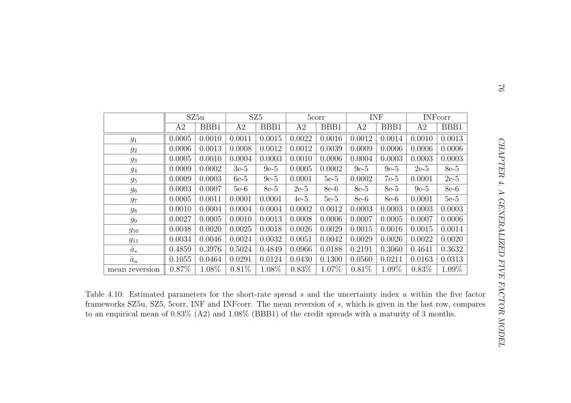
76C
HA
PT
ER
4.A
GE
NE
RA
LIZ
ED
FIV
EFA
CT
OR
MO
DE
L
SZ5u SZ5 5corr INF INFcorrA2 BBB1 A2 BBB1 A2 BBB1 A2 BBB1 A2 BBB1
g1 0.0005 0.0010 0.0011 0.0015 0.0022 0.0016 0.0012 0.0014 0.0010 0.0013g2 0.0006 0.0013 0.0008 0.0012 0.0012 0.0039 0.0009 0.0006 0.0006 0.0006g3 0.0005 0.0010 0.0004 0.0003 0.0010 0.0006 0.0004 0.0003 0.0003 0.0003g4 0.0009 0.0002 3e-5 9e-5 0.0005 0.0002 9e-5 9e-5 2e-5 8e-5g5 0.0009 0.0003 6e-5 9e-5 0.0001 5e-5 0.0002 7e-5 0.0001 2e-5g6 0.0003 0.0007 5e-6 8e-5 2e-5 8e-6 8e-5 8e-5 9e-5 8e-6g7 0.0005 0.0011 0.0001 0.0001 4e-5 5e-5 8e-6 8e-6 0.0001 5e-5g8 0.0010 0.0004 0.0004 0.0004 0.0002 0.0012 0.0003 0.0003 0.0003 0.0003g9 0.0027 0.0005 0.0010 0.0013 0.0008 0.0006 0.0007 0.0005 0.0007 0.0006g10 0.0048 0.0020 0.0025 0.0018 0.0026 0.0029 0.0015 0.0016 0.0015 0.0014g11 0.0034 0.0046 0.0024 0.0032 0.0051 0.0042 0.0029 0.0026 0.0022 0.0020as 0.4859 0.3976 0.5024 0.4849 0.0966 0.0188 0.2191 0.3060 0.4641 0.3632au 0.1055 0.0464 0.0291 0.0124 0.0430 0.1300 0.0560 0.0211 0.0163 0.0313
mean reversion 0.87% 1.08% 0.81% 1.08% 0.83% 1.07% 0.81% 1.09% 0.83% 1.09%
Table 4.10: Estimated parameters for the short-rate spread s and the uncertainty index u within the five factorframeworks SZ5u, SZ5, 5corr, INF and INFcorr. The mean reversion of s, which is given in the last row, comparesto an empirical mean of 0.83% (A2) and 1.08% (BBB1) of the credit spreads with a maturity of 3 months.

CHAPTER 4. A GENERALIZED FIVE FACTOR MODEL 77
4.8 Comparing the Models
Having calibrated the different models with the help of market data, we nowwant to find out which model yields the best results in explaining the data.First of all, we compare the average pricing errors of the different frameworksby calculating the absolute deviations for the insample period from January1 1999 to December 27 2002 and for the out-of-sample period from January3 2003 to December 31 2004XV. In order to identify any structural differ-ences we do this for every single maturity as well as for the average over allmaturities. Then, we will apply a linear regression to the market prices fordetermining whether they are explained well by model prices. Afterwards,we analyze by means of the Akaike Information Criterion if the fitting abil-ity is just due to an increase of factors. Finally, we conclude by testing thestandardized innovations with respect to the requirements of the state spacemodel.
Absolute Deviations: Pricing errors between US Treasury Stripsand non-defaultable model pricesTable B.2 in the Appendix illustrates the pricing errors between the zerorates of US Treasury Strips and the ones determined by the various models.The introduction of a second macroeconomic factor w2 improves the pricingpower as long as this second factor is chosen to be unobservable as in theSZ5u and the 5corr frameworks. This is in line with Antes et al. (2008)who found that the short-rate model of Bakshi et al. (2006) outperforms theextended Schmid-Zagst model (SZ4) since Bakshi et al. (2006) assume theirmacroeconomic factor to be unobservable. Due to the fact that all short-ratemodels within this thesis incorporate at least one observable macroeconomicfactor into the short-rate, we omit a comparison with the model of Bakshiand concentrate instead on models that are based on macroeconomic input.For most of the maturities between 3 months and 10 years the SZ5u or the5corr version are the best models with respect to pricing error, often far bet-ter than the others. Only for long-term maturities, i.e. 20 and 25 years, thesemodels exhibit the same problems as can be observed for the majority of themodels. The SZ5 framework which consists of two observable processes w1
and w2 driven by the real gross domestic product and the consumer priceindex yields promising results for short-term maturities which are addition-ally to the maturities at the long end often problematic to fit. The pricing ofSZ5 shows like the ones of SZ5u and 5corr better results for short maturities
XVWe use this time period in order to match the calibration period and results of Hage-dorn et al. (2007).
78 CHAPTER 4. A GENERALIZED FIVE FACTOR MODEL
indicating that a second factor - even if it is observable - helps to explainthe market data. But for mid-term and long-term maturities this effect fadesand the SZ5 framework tends to reach worse results than the rest. The twoversions of the five factor model built on a real and an inflation short-rate(INF and INFcorr), where the second factor w2, the so-called inflation shortrate, is also unobservable and filtered with the help of inflation-linked bonds,take on positions between the other five factor models. They do not reachthe low pricing errors as SZ5u and 5corr do, but most of the time they rangeamong the best models. Astonishingly, these two models yield the lowestpricing error for the maturity of 25 years. Within the extended model ofSchmid and Zagst (SZ4) we tested seven different economic factors GDPn,GDPr, CPI, IP, Prod, CILI and CICI. By means of the absolute deviationsthere is no factor which can be singled out as the best one. The pricing errorsare in the same range for all seven economic factors. For short-term matur-ities there are the industrial production (IP) and the real gross domesticproduct (GDPr) followed by the composite indices of leading (CILI) and co-incident indicators (CICI) which perform best. But it changes for mid-termand long-term maturities where the consumer price index (CPI), the nominalgross domestic product (GDPn) and the composite index of leading indic-ators (CILI) take over the leading position among the four factor models.For the out-of-sample period we get a similar picture as the SZ5u as well asthe 5corr framework yield good results for short-term and mid-term matur-ities. But for longer maturities both versions are outperformed by almostall other models. The same holds for the other five factor models even foralmost all maturities. This is in line with the common expectation that theout-of-sample performance gets worse if additional factors are incorporated,especially if they are observable. Within the four factor models (SZ4) it isagain difficult to determine the best macroeconomic factor since the rankingwithin the seven factors changes often. But next to the industrial production(IP) for short maturities, the productivity (Prod) for mid-range maturities,and the gross domestic product (GDP) for long maturities, it is the com-posite index of leading indicators (CILI) that obtains one of the best resultsacross all maturities.With the help of Table B.1 showing the absolute deviations averaged over allmaturities and over the maturities between one and ten years, we can con-clude that the incorporation of an additional factor w2 can help to improvethe pricing power for non-defaultable bonds if this factor is chosen to be un-observable as in the frameworks SZ5u and 5corr, or if this factor is filteredwith the help of inflation-linked bond data. Choosing w2 to be observablelike it is done in SZ5 does not have any additional impact as it can be seenin Table B.2 where its absolute deviations are one of the worst. The ranking

CHAPTER 4. A GENERALIZED FIVE FACTOR MODEL 79
of the four factor models indicates CILI to be the best for the insample andout-of-sample.
Absolute Deviations: Pricing errors between US corporate creditspreads and defaultable model pricesTables B.3 and B.4 in the Appendix contain the average pricing errors forthe credit spreads rated A2 and BBB1. Here, we emphasize that the model5corr is actually a five factor model but as in the case of SZ5u the short-ratespread is not influenced by the fifth factor. The only difference to the modelsof SZ4 are the correlated diffusion terms which appear in the SDE of theshort-rate spread s. The diffusion term of the first macroeconomic factorlinks the short-rate spread of 5corr to the short-rate spreads of the other fivefactor models since the values of ∆Ww1 are exogenously given by the data offactor w1 and the previously estimated parameters of its SDE (see Section4.7). Therefore, we expect 5corr to behave similarly to both the four factorand the five factor models regarding the pricing of defaultable bonds. Theinsample pricing errors of the rating A2 (see Table B.3) indicate that the fivefactor models perform best as opposed to the four factor versions with 5corrmarking the transition between both frameworks: For short-term maturities(3M, 6M, 1Y) almost all four factor versions (SZ4) yield better results thanthe five factor models with 5corr even being the worst of all. For the matur-ities from 2 years to 25 years the five factor models including 5corr take onthe leading position. Only for long-term maturities (20Y, 25Y) 5corr gets inline with the four factor models at the end of the ranking. Except for shortmaturities the composite indices (CILI, CICI) tend to be the best four factorversions. As predicted, the performance of SZ5u is similar to the four factorversion with GDPr since both are based on the same macroeconomic factorand the same set-up for the short-rate spread s. If we take a look at theaverages over all maturities for rating A2 in Table B.1, we see the dominat-ing role of the five factor frameworks over the four factor ones whose bestinsample representatives seems to be the composite indices CILI and CICI.Within the five factor framework the models which are based on the infla-tion short rate tend to be the best. For the credit spreads rated BBB1 (seeTable B.4) we get a similar picture since the five factor versions are amongthe best ones for the maturities from 2 years to 25 years with 5corr beingthe exception as before for long-term maturities. Especially the model basedon the incorporation of an inflation short rate takes on the majority of thetop positions. As in the case of the A2 rated credit spreads, almost all fourfactor versions outperform the models with an additional factor for short-term maturities. The means over all maturities, respectively the ones from1 to 10 years, also indicate the dominance of the five factor frameworks and

80 CHAPTER 4. A GENERALIZED FIVE FACTOR MODEL
the composite indices being the best four factor ones (see Table B.1). Theout-of-sample pricing errors for credit spreads rated A2 and BBB1 show thaton average the totality of the five factor versions performs better than thefour factor ones but there are exceptions like CPI, CICI and CILI for ratingA2 and Prod, CICI and CILI for rating BBB1 (see Table B.1). Consideringthe absolute deviations for every single maturity shows that the five factormodels are always under the best models for maturities longer than one year.But as before there are four factor versions like CILI, CICI, Prod, CPI andGDPr as well as the special five factor cases 5corr and SZ5u, whose creditspread set-up is similar - respectively equal - to the four factor case, whichalso yield top positions for several maturities (see Tables B.3 and B.4).Altogether, the results for credit spreads confirm that the introduction ofan additional factor improves the pricing power of our framework. An al-ternative to an additional factor in the short-rate spread s seems to be theincorporation of the diffusion terms of all factors influencing the short-ratespread, as it is done in 5corr. But since the differences in the pricing errorsare small, it is difficult to determine the best model within the generalizedframework as well as within the SZ4 framework.
Absolute Deviations: SummaryTaking also into account the results for non-defaultable interest rates, we canconclude that incorporating an additional factor yields promising results. Butsince it is difficult to choose the best macroeconomic factor we propose touse one observable macroeconomic factor w1 which would probably be rep-resented best by the real gross domestic product (GDPr) or the compositeindex of leading indicators (CILI). Our choice is based on the promising re-sults obtained by all models that are based on the former factor (SZ4 withGDPr, 5corr, SZ5u, INF, INFcorr) and the fact that the four factor version(SZ4) using the composite index always yielded good results as opposed tothe other tested macroeconomic factors. For the second macroeconomic fac-tor w2 we suggest to use an unobservable macroeconomic index which onlydrives the short rate r, or to filter the inflation short rate which is supposedto influence the short rate r as well as the short-rate spread s from additionaldata provided by inflation-linked bonds.Comparing the pricing errors for the three tested categories (US TreasuryStrips, US Industrials rated A2 and BBB1) we can conclude that the riskierthe category, the closer are the results of the different models (see Table B.1):For credit spreads rated BBB1 the average pricing errors are the smallest ofthe three categories and do not differ much between the models. But theaverage pricing errors become already bigger for credit spreads rated A2 in-dicating that there are influences which cannot be captured by one or two

CHAPTER 4. A GENERALIZED FIVE FACTOR MODEL 81
macroeconomic factors. The pricing errors of the interest rates finally displaythe importance of the right choice for the macroeconomic factor as well asthe model set-up since there are big differences between the insample andout-of-sample performances of the different factors.
Linear Regression: Market price versus model implied priceAs a further quantitative measure we apply the linear regression model
PMarket(t, T ) = β0 + β1PModel(t, T ) + ε, ε ∼ N(0, σ2
ε ) i.i.d
where PMarket denotes the market price and PModel the corresponding modelprice of non-defaultable zero rates respectively defaultable credit spreads.For good working models we expect the regression parameters β0 and β1 tobe near 0 and 1 and the confidence intervals to be more dense. Tables B.5to B.16 contain the values of R2 and the 95%-confidence intervals of the dif-ferent models for all given maturities.
Linear Regression: Non-defaultable bond pricesFor non-defaultable zero rates we observe the same ranking and findingswithin the five factor frameworks as before. The SZ5u and the 5corr modelsyield the best R2 values among the five factor models but have some prob-lems for the two longest maturities (20Y, 25Y) where the R2 decreases and β0
as well as β1 take on values significantly different from 0 and 1, respectively.The SZ5 model with two observable macroeconomic processes reaches highR2 and dense intervals for short-term maturities 3M, 6M and 1Y. But re-sults for the following maturities reflect the problems of this model since thevalues of R2 are decreasing and the confidence intervals widen considerablyand depart of the expected values, especially for the longer maturities. Thetwo versions of the real and inflation short-rate model (INF, INFcorr), whichonly differ by the assumptions about ρw1w2 , can be grouped in between theother five factor models regarding their results for non-defaultable zero rates.For the majority of the maturities they yield better results than SZ5 but per-form worse than SZ5u and 5corr. As observed for the other models, R2 andespecially the confidence intervals for longer maturities worsen. Within thefour factor models the results do not differ very much. These models exhibitthe same problems as the five factor models for longer maturities, namelylower R2, wider confidence intervals and βi, i = 0, 1, which back away fromtheir expected values. In comparison to the five factor models we see thatall four factor models are outperformed by SZ5u and 5corr but obtain bet-ter results than SZ5 apart from the short-term maturities. A differentiation

82 CHAPTER 4. A GENERALIZED FIVE FACTOR MODEL
between the four factor models and the real and inflation short-rate models(INF, INFcorr) is not possible because the results do not favour any versions.
Linear Regression: Defaultable bond pricesThe regressions for credit spreads yield results which are very similar acrossall models. Here, we omit the model SZ5u since its short-rate spread is mod-elled according to the short-rate spread in the SZ4 framework. The fifthfactor within SZ5u only appears in the short rate r leaving the short-ratespread as in SZ4. The real and inflation short-rate models (INF, INFcorr)obtain better results than the SZ5 framework for longer maturities. Simi-lar to the non-defaultable case the confidence intervals widen for short-termand long-term maturities but in contrast to the non-defaultable results theconfidence intervals stay close around the expected values of 0 and 1. How-ever, this does not hold for the 5corr model where the confidence intervals ofβ1 for long-term maturities are far away from 1 although they yield bettervalues of R2 as e.g. SZ5 and the four factor models. Additionally, the R2 of5corr for short-term maturities are the worst across all models emphasizingthe above mentioned problems. As before, the results within the four factormodels do not differ very much. There are maturities or even rating classesfor which one four factor model outperforms the others but it is impossibleto single out one model as the best. Compared to the five factor models weconclude that for mid-term maturities there is almost no difference. The fourfactor models yield slightly better results for short-term maturities but areoutperformed by the five factor models except 5corr for long-term maturities.Here, the R2 are lower and the confidence intervals are considerably widerthan those of the five factor models. Especially the confidence intervals forβ1 are often placed far away from 1, e.g. for the four factor versions withGDPn, Prod and IP. The only exceptions at the long end are the compositeindices CILI and CICI whose confidence intervalls and R2 differ distinctivelyfrom the other four factor versions and perform similar or even better, e.g.CICI, than several five factor models.
Linear Regression: SummarySummarizing these results we conclude that the incorporation of an addi-tional factor does improve the short rate r if this factor is unobservable. Incase of the short-rate spread s the results are too close across all presentedmodels to give a distinct answer. It seems that a second observable factor asin SZ5 and additionally included diffusion terms as in 5corr do not improvethe performance and do not solve the problems arising for short and longmaturities; on the contrary, they tend to further intensify those effects (e.g.5corr).

CHAPTER 4. A GENERALIZED FIVE FACTOR MODEL 83
Akaike Information Criterion: Best fit versus minimum numberof parametersA model’s ability to fit the data is generally increased by including an addi-tional factor. In order to justify the additional factors we compare by meansof the Akaike Information Criterion (AIC, see Akaike (1974)) the five factormodels with the four factor models which are considered as a reduced formof the previous mentioned ones. The AIC which is defined as
AIC = 2k − 2 ln L
with k being the number of parameters and L the likelihood function, linksthe number of parameters with the fitting ability of a given model. Hence, itsaim is to find a model which explains best the data using a minimum numberof parameters at the same time. By applying the AIC we want to verify thatthe improvement of the model’s performance does not only depend on theincrease of factors.Table 4.11 shows the loglikelihoods for the different models. The loglikeli-hoods of the five factor models exceed the loglikelihoods of all four factormodels even after controlling for the additional factors. There is just one ex-ception for the non-defaultable case, namely the model of Schmid and Zagst(SZ5) where two given macroeconomic factors are incorporated. It yields aloglikelihood which has the same order of magnitude as the loglikelihoods ofthe four factor models. Even the loglikelihoods for credit spreads (A2, BBB1)suggest that 5corr takes on a position between the four and five factor mod-els. Although its short-rate spread s involves as many factors as the modelsof the SZ4 framework, its loglikelihood yields higher values which, however,do not reach the level of the other five factor models. The loglikelihoods ofthe other special case SZ5u illustrate the fact that its credit spreads havethe same set-up as the SZ4 framework, i.e. for rating A2 and BBB1 SZ5uranks between the four factor versions with input Prod and GDPr, althoughits loglikelihood for the non-defaultable case is the best of all models. Thefitting ability of the composite indices of several macroeconomic factors, CILIand CICI, tend to be better than the ability of one single factor and comeextremely close to the results of 5corr.Summarizing the outcome of the Akaike Information Criterion we infer thatthe five factor models can be considered better models than the four factorversions, although a second observable macroeconomic factor as in SZ5 con-tinues to be questionable.
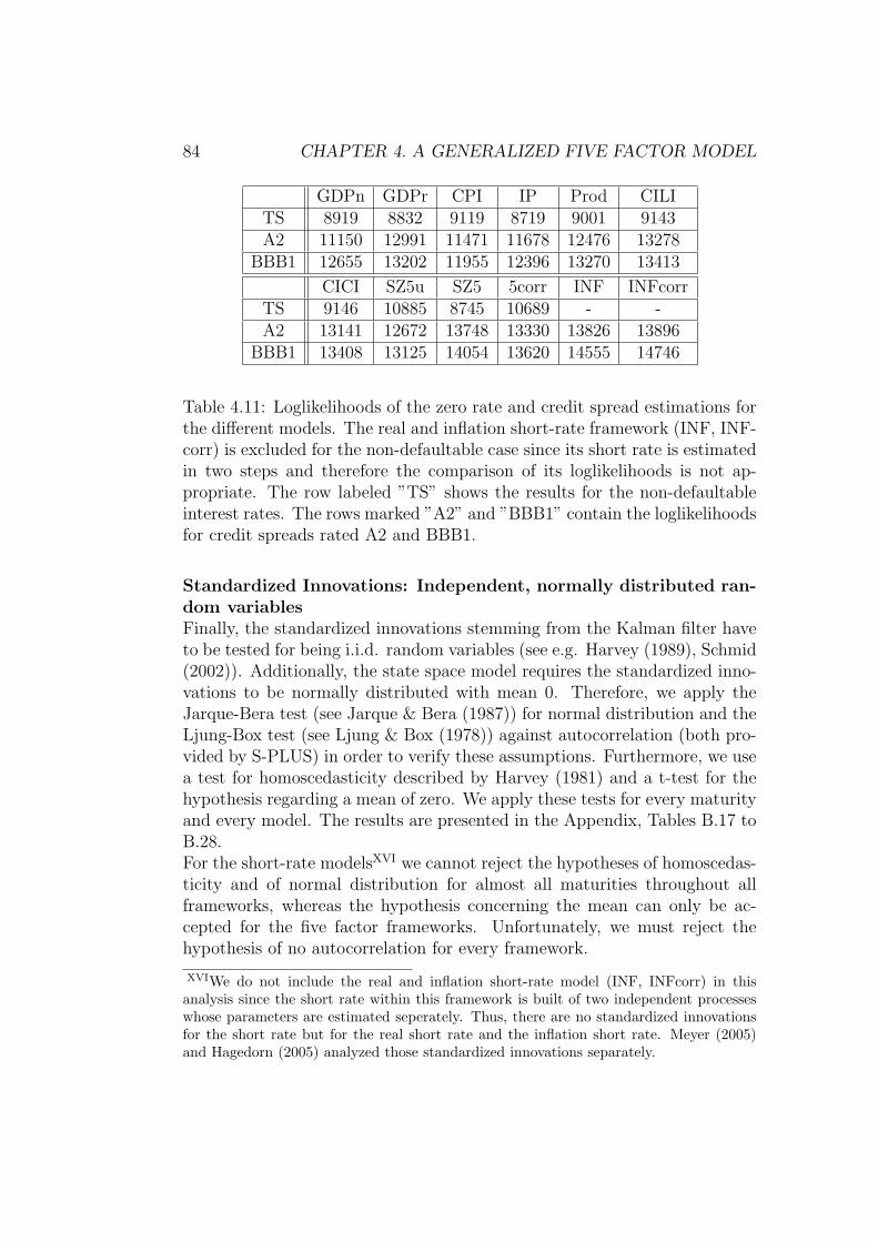
84 CHAPTER 4. A GENERALIZED FIVE FACTOR MODEL
GDPn GDPr CPI IP Prod CILITS 8919 8832 9119 8719 9001 9143A2 11150 12991 11471 11678 12476 13278
BBB1 12655 13202 11955 12396 13270 13413
CICI SZ5u SZ5 5corr INF INFcorrTS 9146 10885 8745 10689 - -A2 13141 12672 13748 13330 13826 13896
BBB1 13408 13125 14054 13620 14555 14746
Table 4.11: Loglikelihoods of the zero rate and credit spread estimations forthe different models. The real and inflation short-rate framework (INF, INF-corr) is excluded for the non-defaultable case since its short rate is estimatedin two steps and therefore the comparison of its loglikelihoods is not ap-propriate. The row labeled ”TS” shows the results for the non-defaultableinterest rates. The rows marked ”A2” and ”BBB1” contain the loglikelihoodsfor credit spreads rated A2 and BBB1.
Standardized Innovations: Independent, normally distributed ran-dom variablesFinally, the standardized innovations stemming from the Kalman filter haveto be tested for being i.i.d. random variables (see e.g. Harvey (1989), Schmid(2002)). Additionally, the state space model requires the standardized inno-vations to be normally distributed with mean 0. Therefore, we apply theJarque-Bera test (see Jarque & Bera (1987)) for normal distribution and theLjung-Box test (see Ljung & Box (1978)) against autocorrelation (both pro-vided by S-PLUS) in order to verify these assumptions. Furthermore, we usea test for homoscedasticity described by Harvey (1981) and a t-test for thehypothesis regarding a mean of zero. We apply these tests for every maturityand every model. The results are presented in the Appendix, Tables B.17 toB.28.For the short-rate modelsXVI we cannot reject the hypotheses of homoscedas-ticity and of normal distribution for almost all maturities throughout allframeworks, whereas the hypothesis concerning the mean can only be ac-cepted for the five factor frameworks. Unfortunately, we must reject thehypothesis of no autocorrelation for every framework.
XVIWe do not include the real and inflation short-rate model (INF, INFcorr) in thisanalysis since the short rate within this framework is built of two independent processeswhose parameters are estimated seperately. Thus, there are no standardized innovationsfor the short rate but for the real short rate and the inflation short rate. Meyer (2005)and Hagedorn (2005) analyzed those standardized innovations separately.

CHAPTER 4. A GENERALIZED FIVE FACTOR MODEL 85
The tests of the standardized innovations received from credit spreads favourthe real and inflation short-rate framework (INF, INFcorr) over SZ5 and 5corrsince the hypotheses of homoscedasticity, of normal distribution and of a zeromean cannot be rejected for the majority of maturities. However, within theSZ5 and 5corr models we must often reject the hypotheses of no autocor-relation, of homoscedasticity and of zero mean. In contrast to the short-rate models, the hypothesis of no autocorrelation cannot always be rejectedthroughout all frameworks. Analogous to previous findings, the results of the5corr model resemble those of the four factor models, e.g. CILI, CICI, GDPr,GDPn and CPI, as well as the results of the five factor models, e.g. SZ5. De-pending on the macroeconomic factor, the four factor models yield differentresults. The performance of the composite indices CILI and CICI are similarto the performances of five factor models like INF and INFcorr. The TablesB.22 and B.23 in the Appendix display more entries, especially for the cat-egories normal distribution (ND), homoscedasticity (HS) and mean of zero(M0), than the tables of other SZ4 versions indicating that these hypothesescannot be rejected for more maturities. The hypotheses of no autocorrelationand of a mean of zero must still be rejected for many SZ4 cases but thereare exceptions, e.g. the models based on the gross domestic product (GDPn,GDPr) and the composite indices (CILI, CICI). For the frameworks depend-ing on the productivity (Prod) and the industrial production (IP) even thehypotheses of homoscedasticity and of normal distribution must be rejectedfor many maturities.Altogether, we can conclude that the assumptions regarding the standardizedinnovations are fulfilled sufficiently throughout all models whereas the fivefactor frameworks tend to yield more stable results with respect to the short-rate models. If we additionally consider the tests based on credit spreads,the real and inflation short-rate models (INF, INFcorr) seem to reach themost satisfactory results within the five factor models. Within the four fac-tor frameworks the composite indices CILI and CICI tend to work best.
ConclusionThe pricing errors as well as the various tests lead us to the conclusion thatthe incorporation of an additional factor does indeed improve the perfor-mance of our framework. We showed that the better ability to fit marketprices is not only due to the increased number of parameters. Furthermore,an additional factor seems to stabilize the estimation procedure as suggestedby the results of the tests of the standardized innovations.
86 CHAPTER 4. A GENERALIZED FIVE FACTOR MODEL
Within our different five factor frameworks the models with a macroeconomicfactor which is not observable (SZu, 5corr, INF, INFcorr) yield the mostpromising results. Especially the performance of the short rate r improvesby this additional factor (see SZ5u and 5corr). However, the results for theshort-rate spread s do not clearly favour five factor models over four factorones, but they do suggest that introducing a second observable macroeco-nomic factor (SZ5) and correlated diffusion terms (5corr) do not improve themodels’ overall performance.We tested several macroeconomic fundamentals in order to get a properchoice for the economic factor. The results indicate that all tested vari-ables do a good job in explaining non-defaultable and defaultable zero ratesbut altogether the composite indices of leading (CILI) and coincident indic-ators (CICI) as well as the gross domestic product (GDPn, GDPr) seem tobe plausible representatives for the state of an economy.Dependent on the purpose, we recommend the usage of the SZ5u or 5corrframeworks if the main intension lies on the pricing of non-defaultable anddefaultable interest-rate products. However, if the focus is mainly on thepricing of defaultable assets, the choice of the four factor framework SZ4would reduce the complexity of the calculations and would still yield satis-fying results when using one of the composite indices (CILI, CICI) or thedomestic product (GDPn, GDPr). For pricing inflation-linked products, wesuggest the usage of the real and inflation short-rate model (INF, INFcorr).Since the results of INF and INFcorr only differ slightly, we favour the set-upINF because of its reduced number of parameters and therefore its reducedcomplexity. Although, we found the real and inflation short-rate model tobe one of the best, we do not recommend it for pricing purposes in generalsince the availability of inflation-linked bonds for the calibration procedureis limited. Due to these findings, we continue in the next chapter to developthe pricing formulas for our general set-up of Section 4.1 such that the resultswill hold for all models discussed in this chapter. In order to get a betterinsight into the proposed dynamics of Section 5.4.2 and pricing formulas ofSections 5.5 and 5.6, we will use the four factor model SZ4 because of its re-duced complexity and its good performance. But all results obtained for theSZ4 framework can be derived analogously for all other frameworks withinthis thesis.
Our findings are in line with the literature. First, the fact that the perfectmacroeconomic factor is not easy to get is indicated by Figlewski et al. (2012)who try to find ”stylized facts” about the importance of specific macro-factorsand their impact on credit risk. Though there is an increase in explanatorypower by adding macroeconomic factors, it is difficult to single out factors

CHAPTER 4. A GENERALIZED FIVE FACTOR MODEL 87
which dominate alternative ones. Furthermore, their work shows that theestimated relationships are not stable over time and that the coefficientsand the signs of the macroeconomic factors vary widely depending on theadditionally included factors. This suggests that there is a considerable cor-relation among the factors and that their inherent information about creditrisk overlap. Second, the closeness of the four and five factor models in pric-ing credit spreads can be explained by the work of Collin-Dufresne, Goldstein& Martin (2001). Using a regression analysis they conclude that only onequarter of the variation in credit spreads can be explained by economic fac-tors as e.g. the return on S&P and the change in its implied volatility (VIX),whereas the remaining residuals are highly cross-correlated and are mostlydriven by a common factor. Hence, they suggest that this common factoris unlikely a firm-specific but a systematic one. Therefore, they redo the re-gression by incorporating several proxies for this macro factor and find thatthis only adds limited extra explanatory power. They conclude that there isan aggregate factor which is common to all corporate bonds and which seemsto be more important in explaining credit spread changes than firm-specificfactors. So, our incorporation of one macroeconomic factor like GDP or es-pecially one of the composite indices in addition to an unobservable factoras an aggregation of firm-specific and/or systematic information, is justifiedby their findings. Furthermore, the disappointing results of the SZ5 model,which uses two observable factors, and the promising results obtained bythe INF and INFcorr frameworks, which are based on a second unobservablefactor entering the short-rate spread, are along the line with the study ofCollin-Dufresne et al. (2001).
However, two developments which took place in the markets during the firstdecade of the new millennium are strongly related to the topic of determi-nants of credit spread and need to be stressed: the recent financial crisis andthe growing importance of credit default swaps (CDS). While the majorityof studies about determinants of credit spreads rely on bond data beforethe crisis, newer studies are based on spreads of credit default swaps alsoincorporating post-crisis data sets. This leaves us wondering whether thepreviously found determinants still influence credit spreads and whether theresults obtained for bond spreads are still valid for CDS spreads.Apart from the fact that CDS spreads already come as a spread and do notneed the specification of a benchmark risk-free curve as it is required forextracting the credit spread out of bond data, CDS spreads also appear toreflect changes in credit risk more efficiently (cf. studies analyzing the re-lationship between CDS spreads and rating changes, e.g. Hull, Predescu &White (2004), Di Cesare (2005)). Blanco, Brennan & Marsh (2005) claim
88 CHAPTER 4. A GENERALIZED FIVE FACTOR MODEL
that CDS spreads reflect more quickly changes in the underlying’s risk thanbond spreads do. Further, Blanco et al. (2005) provide evidence that CDSas well as bond markets work quite well in the long run, but in the short runCDS spreads react more timely. They also study the determinants of changesin credit spreads and CDS spreads and conclude that analogous to the studyof Collin-Dufresne et al. (2001) a large part of the variation of both spreadscannot be explained and furthermore, that the ”first principal componentexplains a large and essentially identical proportion of the variation of theresiduals”.Ericsson, Jacobs & Oviedo (2009) analyze by means of a linear regressionapproach the dependence of CDS premia and variables suggested by eco-nomic theory for the period of 1999 until 2002. Their findings are that theestimated coefficients are consistent with theory and the explanatory poweris higher than in existing works on corporate bond spreads, also emphasizedby a limited evidence for a residual common factor. This indicates that thevariables suggested by economic theory are important for describing the pric-ing of such instruments. Further, they argue by the similarity of bond andCDS cashflows that occur until (bond coupons vs. CDS spreads) - respec-tively at (loss in bond vs. replacement of loss for CDS buyer) - default thatthe implied relationship between theoretical factors and spreads still hold.Di Cesare & Guazzarotti (2010) study the effects of the financial crisis ondeterminants of CDS spread changes for the period from January 2002 untilMarch 2009. They confirm that the factors identified by the literature havemaintained their importance by showing that the models explain the changesalmost the same way before and during the crisis. Further, they claim thatthe CDS spreads were moving increasingly together during the crisis, indi-cating the existence of a common factor that still remains unexplained.Taking this altogether, we are confident that our findings will also hold forthe recent time period and for CDS spreads, respectively credit derivativesbased on CDS in general. Therefore, we will develop in the next chaptera consistent pricing framework for derivatives written on CDS by derivingdynamics of the CDS spread that reflect the dependence on firm-specific andmacroeconomic risk factors.
Chapter 5
Pricing Credit Derivatives
So far, the bond market was assumed to be the best place to monitor thecreditworthiness of a borrower. But in the last decade, the market for creditderivatives has grown substantially. Credit derivatives allow investors to buyor sell easily the credit risk of a certain reference entity without being ex-posed to its default risk, e.g. not owning the defaultable bond of a companyon which the derivative is written. Therefore, credit derivatives are used forhedging against credit risk of a certain reference entity as well as for purespeculation, e.g. short-selling credit risk. The most popular credit derivativeis the Credit Default Swap (CDS) which works like an insurance. The buyerof a CDS (the protection buyer) makes regular premium payments to theprotection seller in order to be compensated if a certain credit event (de-fault) occurs. Usually, credit events that trigger such protection paymentsare bankruptcy, failure to pay or restructuring.Antes et al. (2009) determine closed-form solutions for credit default optionsand credit default swaps for the extended Schmid-Zagst model which westudy in Chapter 4 (see Model 4.4). In their work, the four factors of theSZ4 model are calibrated to historical data of the period 2002-2008 and fittedto market prices of credit default swaps. Antes et al. (2009) show that themodel performs well even during the crisis of 2007/2008 and is capable ofdisplaying the latest market signals, e.g. an increase of credit risk.In this chapter we will build on the work of Antes et al. (2009) and rewrite thepricing of credit default options and swaps for our general five factor frame-work that was introduced in Section 4.1 of Chapter 4 and from which allpreviously discussed models were derived (cf. Sections 4.2 - 4.5). Therefore,if not stated otherwise all results refer to the pricing framework of Section4.1. Further, we extend it to more complex derivatives like Credit DefaultSwaptions (see Section 5.5) and Constant Maturity Credit Default Swaps(see Section 5.6) which both rely on the future spread of a CDS. Therefore,
89
90 CHAPTER 5. PRICING CREDIT DERIVATIVES
we introduce in Section 5.4 so-called Forward Credit Default Swaps for dif-ferent assumptions concerning the proctection payments. Further, we derivethe dynamics of the FCDS spread by means of its closed-form solution whilekeeping the link to macroeconomic and firm-specific factors. Our procedureensures that we are consistent with our defaultable term structure modelof Chapter 4 in addition to being able to price analytically complex creditderivatives.During the credit crisis, investors began to worry about the creditworthinessof their counterparties as well as the missing standardization of credit deriva-tives, making it impossible to compare contracts. Especially for CDS, thetailor-made contracts lead to spreads that are not comparable. Therefore,a new quoting mechanism was introduced in 2009 (see e.g. Markit (2009a))which proposes to only use a constant set of spreads for pricing CDS andexchanging an upfront payment instead. We outline in Section 5.5.1 how thepricing of a Credit Default Swaption could be amended in order to accountfor this standardization. In addition, we show how to include the creditwor-thiness of the derivative’s counterparty in the derivation of a CDS spread(see Subsection 5.4.3).In the following three sections, we introduce the necessary building terms forvaluing CDS. The definitions, theorems and propositions of these subsectionsare cited or inspired by the work of Schmid (2002) and Antes et al. (2009).
In the previous chapter the short-rate spread s was used to price default-able zero-coupon bonds. In this chapter, we want to price derivatives whoseunderlying is such a defaultable zero-coupon bond or is related to one. But,since the recovery rate of such a derivative deviates from the recovery rate ofthe underlying, we need a short-rate spread szero which is of the same qualityas the short-rate spread s but with a recovery of zero.
Definition 5.1The zero-recovery short-rate spread szero is implicitely given by
(1 − z(t)) · szero(t) = s(t) , 0 ≤ t ≤ T ∗ ,
where s(t) is the short-rate spread process and z(t) is the recovery-rate processwith 0 ≤ z(t) < 1.
By introducing the zero-recovery short-rate spread, we are now able to priceunder a zero-recovery assumption. As opposed to reduced-form frameworkswe do not rely on a non-negative intensity for pricing defaultable contingentclaims. Instead our model as well as the models in e.g. Antes et al. (2009)

CHAPTER 5. PRICING CREDIT DERIVATIVES 91
and Schmid (2004) are based on a defaultable money-market account, i.e.
P d0 (t) =
(1 +
∫ t
0
(z(l) − 1)dH(l)
)e∫ t0 r(l)+s(l)L(l)dl,
where the short-rate spread s is not necessarily non-negative.
Proposition 5.2Let Y be a FT−measurable random variable with EQ [|Y |q] < ∞ for someq > 1. Under the zero-recovery assumption, i.e. under the assumption thatthe contingent claim is knocked out at default of the reference credit asset,and with the stochastic processes specified for r, w1, w2, s, u, and szero, theprice process, VL,T :
VL,T (t) = EQ
[e−
∫ Tt
r(l)dl Y · L (T )∣∣∣ Gt
], 0 ≤ t < T d,
is given byVL,T (t) = L (t) · VT (t) ,
with L(t) = 1T d>t. The adapted continuous process VT is defined by
VT (t) = EQ
[e−
∫ Tt
(r(l)+szero(l))dlY | Ft
], 0 ≤ t < T,
and VT (t) = 0 for t ≥ T. This equation has a unique solution in the spaceconsisting of every semimartingale, J, such that EQ [supt |Jt|q] < ∞ for someq > 1.
Proof:See Proposition 6.4.1 in Schmid (2004), page 230, where Ft needs to be re-placed by Gt in order to get the result under the enlarged filtration G. Usingthe martingale invariance property (see page 31 in Chapter 4) yields thestated result.
Remark:The above Proposition holds for our general framework of Section 4.1 as wellas for all models derived from it (cf. Sections 4.2 - 4.5), since in all set-upsthe processes r and s are solutions of linear stochastic differential equationsor are an affine linear function of such solutions (cf. the short-rate r in Sec-tion 4.4 where the short rate is the sum of the inflation short rate and thereal short rate). Therefore, r and s fulfill the technical requirements neededfor Proposition 5.2.

92 CHAPTER 5. PRICING CREDIT DERIVATIVES
In the following, we assume the recovery rate z to be a known constant.With this assumption, we are able to state the dynamics for szero as well asthe price of a defaultable zero-recovery zero-coupon bond.
Proposition 5.3Let z(t) = z be a constant for all 0 ≤ t ≤ T ∗, then the SDE for the zero-
recovery short-rate spread under the equivalent martingale measure Q is givenby
dszero(t) = [θszero + bszerouu(t) − bszerow1w1(t) − bszerow2w2(t) − asszero(t)]dt
+ σszero
√1 − ρ2
su − ρ2sw1
− ρ2sw2
dWs(t) + σszeroρsudWu(t)
+ σszeroρsw1dWw1(t) + σszeroρsw2dWw2(t) ,
with θszero = θs
1−z, bszerou = bsu
1−z, bszerow1 =
bsw1
1−z, bszerow2 =
bsw2
1−z, σszero = σs
1−z.
Furthermore, the price of a zero-recovery zero-coupon bond is given by
P d,zero(t, T ) = eAd,zero(t,T )−Bd,zero(t,T )r−Cd,zero(t,T )szero−Dd,zero(t,T )u
·e−Ed,zero1 (t,T )w1−Ed,zero
2 (t,T )w2
where the functions Ad,zero(t, T ), Bd,zero(t, T ), Cd,zero(t, T ), Dd,zero(t, T ),Ed,zero
1 (t, T ) and Ed,zero2 (t, T ) have the same structure as in Theorem 4.3 with
θs, bsu, bsw1, bsw2 and σs substituted by θszero, bszerou, bszerow1, bszerow2 andσszero.
Proof:Analogously to the proof of Theorem 4.3.
5.1 Survival Probability
With szero being an approximation of the intensity, it holds
Q(T d > t|Ft) = EQ [L(t)|Ft]
= e−
t∫0
szero(l)dl.
Hence the survival probability within our general framework is as follows.

CHAPTER 5. PRICING CREDIT DERIVATIVES 93
Theorem 5.4 (Survival Probability)For 0 ≤ t ≤ T the survival probability up to time T conditioned on theinformation of time t is:
L(t) · P S(t, T ) : = EQ [L(T )|Gt]
= L(t) · EQ
[e−
T∫t
szero(l)dl|Ft
]
= L(t) · eAS(t,T )−CS(t,T )szero−DS(t,T )u−ES1 (t,T )w1−ES
2 (t,T )w2
= L(t) · P S(t, T, szero, u, w1, w2)
with
CS(t, T ) =1
as
(1 − e−as(T−t)
),
DS(t, T ) =bszerou
as
(1 − e−au(T−t)
au
+e−au(T−t) − e−as(T−t)
au − as
),
ES1 (t, T ) = −bszerow1
as
(1 − e−aw1 (T−t)
aw1
+e−aw1 (T−t) − e−as(T−t)
aw1 − as
),
ES2 (t, T ) = −bszerow2
as
(1 − e−aw2 (T−t)
aw2
+e−aw2 (T−t) − e−as(T−t)
aw2 − as
),
and
AS(t, T ) =
∫ T
t
[12σ2
szero(CS(l, T ))2 +1
2σ2
u(DS(l, T ))2 +
1
2σ2
w1(ES
1 (l, T ))2
+1
2σ2
w2(ES
2 (l, T ))2 + σw1σw2ρw1w2ES1 (l, T )ES
2 (l, T )
+ σuσszeroρsuCS(l, T )DS(l, T ) + σw1σszeroρsw1C
S(l, T )ES1 (l, T )
+ σw2σszero
(ρsw1ρw1w2 + ρsw2
√1 − ρ2
w1w2
)CS(l, T )ES
2 (l, T )
− θszeroCS(l, T ) − θuDS(l, T ) − θw1E
S1 (l, T ) − θw2E
S2 (l, T )
]dl.
The proof of this Theorem follows directly from Theorem 4.3 by setting allterms related to r equal to zero and replacing all terms indexed by s withequivalent terms indexed by szero.
5.2 Default Digital Put Option
Credit derivatives are mainly dependent on the time of default (T d) andpayments that are triggered by the default event. A simple credit derivative

94 CHAPTER 5. PRICING CREDIT DERIVATIVES
pays a fixed payoff that is due on the default of a reference entity.
Definition 5.5A default digital put option pays a fixed payoff p at the time of default (T d)of a reference credit asset.
Theorem 5.6The time t price of the default digital put option is given by
EQ
[∫ T
t
p · e−∫ u
tr(l)dldH (u)
∣∣∣∣Gt
]= L (t) · p · V ddp
T d (t, T )
with
V ddpT d (t, T ) = EQ
[∫ T
t
e−∫ u
t(r(l)+szero(l))dlszero (u) du
∣∣∣∣Ft
]
=
∫ T
t
EQ
[e−
∫ ut
(r(l)+szero(l))dlszero (u)∣∣∣Ft
]du.
Proof:See page 243 in Schmid (2004) where Ft needs to be replaced by Gt in orderto get the result under the enlarged filtration G. The stated result followsfrom using the martingale invariance property (see page 31 in Chapter 4).
Remark:Analogously to Proposition 5.2, the above result also holds for our generalframework of Section 4.1 because of r and szero being solutions of linearstochastic differential equations. Therefore, the necessary technical condi-tions hold for applying Corollary 6.2.1 in Schmid (2004) and for interchang-ing expectation and integration.
In order to calculate the expected value we need the following theorem.
Theorem 5.7
v(r, szero, u, w1, w2, t, T ) := EQ
[e−
∫ Tt
(r(l)+szero(l))dlszero (T )∣∣∣Ft
]
= P d,zero(t, T )
·(F (t, T ) + H(t, T )szero(t) + I(t, T )u(t)
+ J1(t, T )w1(t) + J2(t, T )w2(t))

CHAPTER 5. PRICING CREDIT DERIVATIVES 95
with
H(t, T ) = e−as(T−t),
J1(t, T ) = bszerow1 ·e−as(T−t) − e−aw1 (T−t)
as − aw1
,
J2(t, T ) = bszerow2 ·e−as(T−t) − e−aw2 (T−t)
as − aw2
,
I(t, T ) = −bszerou ·e−as(T−t) − e−au(T−t)
as − au
,
F (t, T ) = −1
2
((σszeroCd,zero(t, T )
)2+(σuD
d,zero(t, T ))2)
+θw1 · (Ed,zero1 (t, T ) − E1(t, T )) + θw2 · (Ed,zero
2 (t, T ) − E2(t, T ))
+θuDd,zero(t, T ) + θszeroCd,zero(t, T )
−∫ T
t
σ2w1
Ed,zero1 (l, T )J1(l, T ) + σ2
w2Ed,zero
2 (l, T )J2(l, T )dl
−∫ T
t
σw1σw2ρw1w2(Ed,zero1 (l, T )J2(l, T ) + Ed,zero
2 (l, T )J1(l, T ))dl
−∫ T
t
σw1σrρrw1Bd,zero(l, T )J1(l, T )dl
−∫ T
t
σw2σr(ρrw1ρw1w2 + ρrw2
√1 − ρ2
w1w2)Bd,zero(l, T )J2(l, T )dl
−∫ T
t
σszeroσuρsu(Cd,zero(l, T )I(l, T ) + Dd,zero(l, T )H(l, T ))dl
−∫ T
t
σszeroσw1ρsw1(Ed,zero1 (l, T )H(l, T ) + Cd,zero(l, T )J1(l, T ))dl
−∫ T
t
σszeroσr(ρrw1ρsw1 + ρrw2ρsw2)Bd,zero(l, T )H(l, T )dl
−∫ T
t
σw2σszero(ρsw1ρw1w2 + ρsw2
√1 − ρ2
w1w2)(Cd,zero(l, T )J2(l, T )
+Ed,zero2 (l, T )H(l, T ))dl.
The proof of this Theorem can be found in Appendix C on page 261.

96 CHAPTER 5. PRICING CREDIT DERIVATIVES
5.3 Default Put Option
Instead of just paying a fixed amount at default, a Default Put Option makesa payment at the time of default (T d) that is linked to the value of thereference asset at T d.
Definition 5.8A default put on a zero-coupon bond pays at the time of default (T d) of thebond a payoff which depends on the underlying’s value at default.
Theorem 5.9For t ≤ T ≤ T ∗ the price of a default put with maturity T whose underlyingreference asset is a zero-coupon bond maturing at T ∗ is given by
EQ
[∫ T
t
e−∫ l
tr(x)dx(1 − Z(l))dH(l)
∣∣∣∣ Gt
]
= L(t) · V dpT d (t, T, T ∗)
= L(t) · (V ddpT d (t, T ) − P d(t, T ∗) + P d,∗(t, T, T ∗))
where the payoff takes place at default (T d) by replacement to the differenceof par, i.e. the difference between the face value and the market value Z atdefault. P d,∗(t, T, T ∗) is derived in Proposition 5.10.
Proof:The proof is given by Antes et al. (2009). For a better understanding, wewill state the proof as well.Let Z be the value of the zero-coupon bond upon default, then we obtain
EQ
[∫ T
t
e−∫ l
tr(x)dx(1 − Z(l))dH(l)
∣∣∣∣ Gt
]
= L(t)V ddpT d (t, T ) − EQ
[∫ T ∗
t
e−∫ l
tr(x)dxZ(l)dH(l)
∣∣∣∣ Gt
]
+ EQ
[e−
∫ Tt
r(x)dxL(T )
∫ T ∗
T
e−∫ l
Tr(x)dxZ(l)dH(l)
∣∣∣∣ Gt
]

CHAPTER 5. PRICING CREDIT DERIVATIVES 97
= L(t) · (V ddpT d (t, T ) − P d(t, T ∗) + P d,zero(t, T ∗))
+ EQ
[e−
∫ Tt
r(x)dxL(T )EQ
[∫ T ∗
T
e−∫ l
Tr(x)dxZ(l)dH(l)
∣∣∣∣ GT
] ∣∣∣∣ Gt
]
+ EQ
[e−
∫ Tt
r(x)dxL(T )EQ
[e−
∫ T∗
Tr(x)dxL(T ∗)
∣∣∣ GT
] ∣∣∣ Gt
]
−EQ
[e−
∫ Tt
r(x)dxL(T )EQ
[e−
∫ T∗
Tr(x)dxL(T ∗)
∣∣∣ GT
] ∣∣∣ Gt
]
= L(t) · (V ddpT d (t, T ) − P d(t, T ∗) + P d,zero(t, T ∗))
+ EQ
[e−
∫ Tt
r(x)dxL(T )P d(T, T ∗)∣∣∣ Gt
]
−EQ
[e−
∫ Tt
r(x)dxL(T )P d,zero(T, T ∗)∣∣∣ Gt
]
Prop.5.2= L(t) · (V ddp
T d (t, T ) − P d(t, T ∗) + P d,zero(t, T ∗))
+ L(t)EQ
[e−
∫ Tt
(r(x)+szero(x))dxP d(T, T ∗)∣∣∣ Ft
]
−L(t)EQ
[e−
∫ Tt
(r(x)+szero(x))dxP d,zero(T, T ∗)∣∣∣ Ft
]
= L(t) · (V ddpT d (t, T ) − P d(t, T ∗))
+ L(t)EQ
[e−
∫ Tt
(r(x)+szero(x))dxP d(T, T ∗)∣∣∣ Ft
]
= L(t) · (V ddpT d (t, T ) − P d(t, T ∗) + P d,∗(t, T, T ∗))
=: L(t) · V dpT d (t, T, T ∗),
with P d,∗(t, T, T ∗) := EQ
[e−
∫ Tt
r(x)+szero(x)dxP d(T, T ∗)∣∣∣ Ft
]which is given in
the following proposition.
Proposition 5.10For t < T d
P d,∗(t, T, T ∗) := EQ
[e−
∫ Tt
r(x)+szero(x)dxP d(T, T ∗)∣∣∣ Ft
]
= P d,∗(t, T, T ∗, r(t), s(t), u(t), w1(t), w2(t))
is given by
P d,∗(t, T, T ∗) = eAd,∗(t,T,T ∗)−Bd,∗(t,T,T ∗)r−Cd,∗(t,T,T ∗)s−Dd,∗(t,T,T ∗)u
· e−Ed,∗1 (t,T,T ∗)w1−Ed,∗
2 (t,T,T ∗)w2
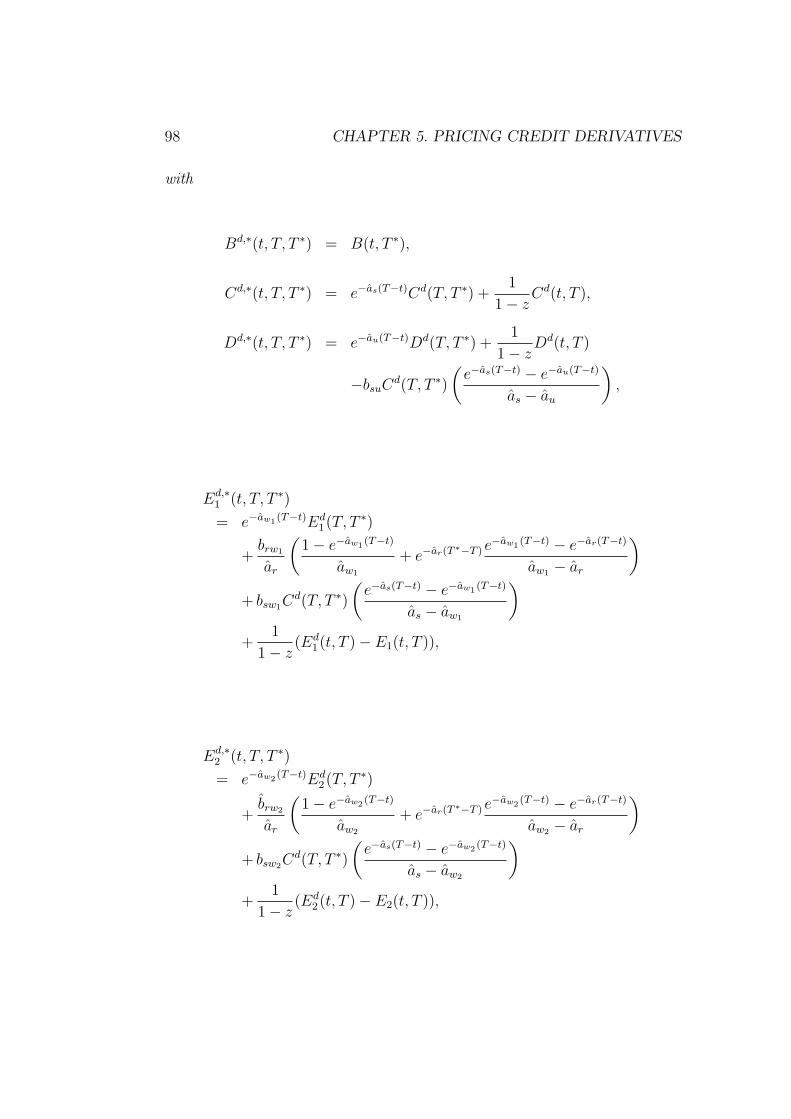
98 CHAPTER 5. PRICING CREDIT DERIVATIVES
with
Bd,∗(t, T, T ∗) = B(t, T ∗),
Cd,∗(t, T, T ∗) = e−as(T−t)Cd(T, T ∗) +1
1 − zCd(t, T ),
Dd,∗(t, T, T ∗) = e−au(T−t)Dd(T, T ∗) +1
1 − zDd(t, T )
−bsuCd(T, T ∗)
(e−as(T−t) − e−au(T−t)
as − au
),
Ed,∗1 (t, T, T ∗)
= e−aw1 (T−t)Ed1(T, T ∗)
+brw1
ar
(1 − e−aw1 (T−t)
aw1
+ e−ar(T ∗−T ) e−aw1 (T−t) − e−ar(T−t)
aw1 − ar
)
+ bsw1Cd(T, T ∗)
(e−as(T−t) − e−aw1 (T−t)
as − aw1
)
+1
1 − z(Ed
1(t, T ) − E1(t, T )),
Ed,∗2 (t, T, T ∗)
= e−aw2 (T−t)Ed2(T, T ∗)
+brw2
ar
(1 − e−aw2 (T−t)
aw2
+ e−ar(T ∗−T ) e−aw2 (T−t) − e−ar(T−t)
aw2 − ar
)
+ bsw2Cd(T, T ∗)
(e−as(T−t) − e−aw2 (T−t)
as − aw2
)
+1
1 − z(Ed
2(t, T ) − E2(t, T )),

CHAPTER 5. PRICING CREDIT DERIVATIVES 99
and
Ad,∗(t, T, T ∗)
= Ad(T, T ∗) +
∫ T
t
1
2
(σ2
r(Bd,∗(l, T, T ∗))2 + σ2
s(Cd,∗(l, T, T ∗))2
+ σ2u(D
d,∗(l, T, T ∗))2 + σ2w1
(Ed,∗1 (l, T, T ∗))2 + σ2
w2(Ed,∗
2 (l, T, T ∗))2
+ σw1σw2ρw1w2Ed,∗1 (l, T, T ∗)Ed,∗
2 (l, T, T ∗)
+ σrσw1ρrw1Bd,∗(l, T, T ∗)Ed,∗
1 (l, T, T ∗)
+ σsσuρsuCd,∗(l, T, T ∗)Dd,∗(l, T, T ∗)
+ σsσw1ρsw1Cd,∗(l, T, T ∗)Ed,∗
1 (l, T, T ∗)
+ σrσw2
(ρrw1ρw1w2 + ρrw2
√1 − ρ2
w1w2
)Bd,∗(l, T, T ∗)Ed,∗
2 (l, T, T ∗)
+ σsσw2
(ρsw1ρw1w2 + ρsw2
√1 − ρ2
w1w2
)Cd,∗(l, T, T ∗)Ed,∗
2 (l, T, T ∗)
+ σrσs(ρrw1ρsw1 + ρrw2ρsw2)Bd,∗(l, T, T ∗)Cd,∗(l, T, T ∗)
− θr(l)Bd,∗(l, T, T ∗) − θsC
d,∗(l, T, T ∗) − θuDd,∗(l, T, T ∗)
− θw1Ed,∗1 (l, T, T ∗) − θw2E
d,∗2 (l, T, T ∗)dl.
The proof of this proposition is given in Appendix C on page 263.
5.4 Forward Credit Default Swap
Credit Default Swaps (CDS) are recently the most popular credit derivatives.The CDS market has grown fastly during the last years due to the character-istics of these derivatives. Although a CDS is a form of insurance, it is notdependent on the real exposure of the underlying asset. Hence, Credit De-fault Swaps allow to buy and sell protection without the need of holding therespective underlying asset. Therefore, CDS are not only used for hedgingpurposes but also for taking speculative positions.
Definition 5.11 (Credit Default Swap)A Credit Default Swap (CDS) is a contract where the protection buyer paysa regular spread s(T0, T0, Tm) at times Ti, i = 1 . . . m to the protection selleras long as the reference entity has not defaulted. At default (T d < Tm) ofthe reference asset, the protection seller makes a replacement payment to theprotection buyer.

100 CHAPTER 5. PRICING CREDIT DERIVATIVES
Definition 5.12 (Forward Credit Default Swap)A Forward Credit Default Swap (FCDS) is a contract which is entered attime t < T0 and which consists of a CDS starting in T0 with payments ofs(t, T0, Tm) at times Ti, i = 1 . . . m. The contract expires without any pay-ments if there is a default before T0.
The value of a Credit Default Swap is mainly determined by the sort of pay-ments that are made at the time of default T d. Assuming that the protectionpayment is linked to the value of the reference entity by replacing its differ-ence to par at default, the price of the CDS can be derived by means of theDefault Put Option of Theorem 5.9.
Theorem 5.13If the underlying reference asset is a zero-coupon bond with maturity T ∗, thenfor t < T0 < Tm ≤ T ∗ the spread s(t, T0, Tm) of the FCDS is
s(t, T0, Tm) =V dp
T d (t, T0, Tm, T ∗)∑mi=1 P d,zero(t, Ti)
with V dpT d (t, T0, Tm, T ∗) = V ddp
T d (t, Tm)−V ddpT d (t, T0)+P d,∗(t, Tm, T ∗)−P d,∗(t, T0, T
∗).
Proof:The value of the premium leg of a swap starting at T0 and ending at Tm isgiven by the discounted sum of swap spread payments:
EQ
[s
m∑
i=1
e−∫ Ti
t r(l)dlL(Ti)
∣∣∣∣∣ Gt
]
= sm∑
i=1
EQ
[e−
∫ Tit r(l)dlL(Ti)
∣∣∣ Gt
]
Prop.5.2= s
m∑
i=1
L(t) · EQ
[e−
∫ Tit r(l)+szero(l)dl
∣∣∣ Ft
]
= s · L(t)m∑
i=1
P d,zero(t, Ti)
The value of the protection leg at time t equals the value of a default put(c.f. Theorem 5.9) starting at T0 and maturing at Tm:I
IFor Fubini’s Theorem see Duffie (1996), page 282.

CHAPTER 5. PRICING CREDIT DERIVATIVES 101
EQ
[e−
∫ T0t r(l)dlL(T0)
∫ Tm
T0
e−∫ l
T0r(x)dx
(1 − Z(l))dH(l)
∣∣∣∣ Gt
]
= EQ
e−∫ T0
t r(l)dlL(T0) EQ
[∫ Tm
T0
e−∫ l
T0r(x)dx
(1 − Z(l))dH(l)
∣∣∣∣ GT0
]
︸ ︷︷ ︸Th.5.9
= L(T0)·V dp
Td(T0,Tm,T ∗) with V dp
Td(T0,·,·) FT0
−measurable
∣∣∣∣∣∣∣∣∣∣∣
Gt
Prop.5.2= L(t)EQ
[e−
∫ T0t r(l)+szero(l)dlV dp
T d (T0, Tm, T ∗)∣∣∣ Ft
]
Th.5.9= L(t)
(EQ
[e−
∫ T0t r(l)+szero(l)dl(V ddp
T d (T0, Tm) − P d(T0, T∗))∣∣∣ Ft
]
+EQ
[e−
∫ T0t r(l)+szero(l)dlP d,∗(T0, Tm, T ∗))
∣∣∣ Ft
] )
= L(t)(EQ
[e−
∫ T0t r(l)+szero(l)dlV ddp
T d (T0, Tm)∣∣∣ Ft
]− P d,∗(t, T0, T
∗)
+ EQ
[e−
∫ T0t r(l)+szero(l)dl
EQ
[e−∫ Tm
T0r(l)+szero(l)dl
P d(Tm, T ∗)∣∣∣ FT0
] ∣∣∣ Ft
] )
= L(t)(EQ
[e−
∫ T0t r(l)+szero(l)dlV ddp
T d (T0, Tm)∣∣∣ Ft
]− P d,∗(t, T0, T
∗)
+ EQ
[e−
∫ Tmt
r(l)+szero(l)dlP d(Tm, T ∗)∣∣∣ Ft
]
︸ ︷︷ ︸=P d,∗(t,Tm,T ∗)
)
= L(t)(EQ
[e−
∫ T0t r(l)+szero(l)dl
∫ Tm
T0
EQ
[e−∫ l
T0r(x)+szero(x)dx
szero(l)∣∣∣ FT0
]dl
∣∣∣∣ Ft
]
−P d,∗(t, T0, T∗) + P d,∗(t, Tm, T ∗)
)
= L(t)(EQ
[∫ Tm
T0
e−∫ l
tr(x)+szero(x)dxszero(l)dl
∣∣∣∣ Ft
]
−P d,∗(t, T0, T∗) + P d,∗(t, Tm, T ∗)
)
Fubini= L(t)
(∫ Tm
T0
EQ
[e−
∫ lt
r(x)+szero(x)dxszero(l)∣∣∣ Ft
]dl
−P d,∗(t, T0, T∗) + P d,∗(t, Tm, T ∗)
)

102 CHAPTER 5. PRICING CREDIT DERIVATIVES
= L(t)(∫ Tm
t
EQ
[e−
∫ lt
r(x)+szero(x)dxszero(l)∣∣∣ Ft
]dl
−∫ T0
t
EQ
[e−
∫ lt
r(x)+szero(x)dxszero(l)∣∣∣ Ft
]dl
−P d,∗(t, T0, T∗) + P d,∗(t, Tm, T ∗)
)
= L(t)(V ddpT d (t, Tm) − V ddp
T d (t, T0) − P d,∗(t, T0, T∗) + P d,∗(t, Tm, T ∗))
⇒ The swap spread of a Forward Credit Default Swap is determined byequating the premium leg and the protection leg:
s(t, T0, Tm) =V ddp
T d (t, Tm) − V ddpT d (t, T0) + P d,∗(t, Tm, T ∗) − P d,∗(t, T0, T
∗)∑mi=1 P d,zero(t, Ti)
=:V dp
T d (t, T0, Tm, T ∗)∑mi=1 P d,zero(t, Ti)
Proposition 5.14The spread s(T0, T0, Tm) at T0 of a CDS contract starting in T0 with the samecharacteristics as in Definition 5.12 is given by
s(T0, T0, Tm) =V ddp
T d (T0, Tm) + P d,∗(T0, Tm, T ∗) − P d(T0, T∗)∑m
i=1 P d,zero(T0, Ti).
Proof:For t := T0 the spread s(t, T0, Tm) of Theorem 5.13 simplifies to the statedresult with V ddp
T d (T0, T0) = 0 and P d,∗(T0, T0, T∗) = P d(T0, T
∗).
Alternatively, the protection payment of a Credit Default Swap can be fixedin advance similar to a Default Digital Put Option of Theorem 5.6. For ex-ample, it is common to assume for quoting purposes a recovery rate Z of40% in the CDS market.

CHAPTER 5. PRICING CREDIT DERIVATIVES 103
Theorem 5.15If the CDS pays at default a fraction of the face value, the swap spread of aForward Credit Default Swap simplifies to
s(t, T0, Tm) =V dp
ZT d(t, T0, Tm)∑mi=1 P d,zero(t, Ti)
with V dpZT d(t, T0, Tm) = (1−Z)(V ddp
T d (t, Tm)−V ddpT d (t, T0)) and recovery rate Z.
Proof:The premium leg is the same as in Theorem 5.13. The protection leg iscalculated analogously to Theorem 5.13:
EQ
[e−
∫ T0t r(l)dlL(T0)
∫ Tm
T0
e−∫ l
T0r(x)dx
(1 − Z)dH(l)
∣∣∣∣ Gt
]
= (1 − Z)EQ
e−∫ T0
t r(l)dlL(T0) EQ
[∫ Tm
T0
e−∫ l
T0r(x)dx
dH(l)
∣∣∣∣ GT0
]
︸ ︷︷ ︸Th.5.6
= L(T0)·Vddp
Td(T0,Tm) with V ddp
Td(T0,·) FT0
−meas.
∣∣∣∣∣∣∣∣∣∣∣
Gt
Prop.5.2= L(t) · (1 − Z)EQ
[e−
∫ T0t r(l)+szero(l)dlV ddp
T d (T0, Tm)∣∣∣ Ft
]
= . . . (see Theorem 5.13)
= L(t) · (1 − Z)(V ddpT d (t, Tm) − V ddp
T d (t, T0))
=: L(t) · V dpZT d(t, T0, Tm) .
By equating the two legs and solving for s(t, T0, Tm) we obtain the statedresult.
Proposition 5.16The spread s(T0, T0, Tm) at T0 of a CDS contract starting in T0 with the samecharacteristics as in Theorem 5.15 is given by
s(T0, T0, Tm) =(1 − Z)V ddp
T d (T0, Tm)∑mi=1 P d,zero(T0, Ti)
.

104 CHAPTER 5. PRICING CREDIT DERIVATIVES
Proof:For t := T0 the spread s(t, T0, Tm) of Theorem 5.15 simplifies to the statedresult with V ddp
T d (T0, T0) = 0.
In order to calculate the protection leg of the above CDS, a numerical in-tegration has to be performed since the function V ddp
T d cannot be calculatedanalytically. For an approximation, we use the so-called default bucketing(see Brigo & Chourdakis (2009)) where we divide the period [T0, Tm] in in-
tervals [Tj−1, Tj], j = 1 . . . n, T0 = T0 < T1 < · · · < Tn = Tm and delay thedefault payment until the end of the corresponding interval. If the length ofsuch an interval is chosen adequately, the time gap between the times whenthe payment should be due (T d) and when it is assumed to be made (Tj) isalmost neglectable.For the approximated CDS rate, we need the following proposition:
Proposition 5.17For t < T d
P ∗(t, Tj−1, Tj) := EQ
[e−
∫ Tj−1t r(x)+szero(x)dxP (Tj−1, Tj)
∣∣∣∣ Ft
]
= P ∗(t, Tj−1, Tj, r(t), szero(t), u(t), w1(t), w2(t))
is given by
P ∗(t, Tj−1, Tj) = eA∗(t,Tj−1,Tj)−B∗(t,Tj−1,Tj)r−C∗(t,Tj−1,Tj)szero−D∗(t,Tj−1,Tj)u
· e−E∗1 (t,Tj−1,Tj)w1−E∗
2 (t,Tj−1,Tj)w2
with A∗, B∗, C∗, D∗, E∗1 , and E∗
2 given in the proof in Appendix C.
The proof of the proposition is given in Appendix C on page 266.
The next theorem illustrates how the default bucketing leads to a simpli-fied calculation of the FCDS spread since the terms of the Default DigitalPut Option (V ddp
T d ) vanish.
Theorem 5.18If the protection is paid as a fraction of the face value as in Theorem 5.15and the protection payments are only made at certain dates Tj, j = 1 . . . n,

CHAPTER 5. PRICING CREDIT DERIVATIVES 105
the swap spread of a Forward Credit Default Swap simplifies to
s(t, T0, Tm) =(1 − Z)
∑nj=1
(P ∗(t, Tj−1, Tj) − P d,zero(t, Tj)
)∑m
i=1 P d,zero(t, Ti)
=V dp
ZT(t, T0, Tm)
∑mi=1 P d,zero(t, Ti)
with recovery rate Z.
Proof:The premium leg is the same as in Theorem 5.13. The protection leg is givenby:
EQ
[e−
∫ T0t r(l)dlL(T0)
n∑
j=1
e−∫ Tj
T0r(x)dx(1 − Z)1Tj−1<T d<Tj
∣∣∣∣∣ Gt
]
= (1 − Z)n∑
j=1
EQ
[e−
∫ Tjt r(x)dxL(Tj−1)(1 − L(Tj))
∣∣∣∣ Gt
]
= (1 − Z)n∑
j=1
(EQ
[e−
∫ Tjt r(x)dxL(Tj−1)
∣∣∣∣ Gt
]
−EQ
[e−
∫ Tjt r(x)dxL(Tj)
∣∣∣∣ Gt
])
Prop.5.2= L(t)(1 − Z)
n∑
j=1
(EQ
[e−
∫ Tj−1t r(x)+szero(x)dxe
−∫ Tj
Tj−1r(x)dx
∣∣∣∣∣ Ft
]
−EQ
[e−
∫ Tjt r(x)+szero(x)dx
∣∣∣∣ Ft
])
= L(t)(1 − Z)n∑
j=1
(EQ
[e−
∫ Tj−1t r(x)+szero(x)dxP (Tj−1, Tj)
∣∣∣∣ Ft
]
−P d,zero(t, Tj))
= L(t)(1 − Z)n∑
j=1
(P ∗(t, Tj−1, Tj) − P d,zero(t, Tj)
)
=: L(t)V dp
ZT(t, T0, Tm) .
By equating the two legs and solving for s(t, T0, Tm) we obtain the statedresult.

106 CHAPTER 5. PRICING CREDIT DERIVATIVES
5.4.1 The Dynamics of the Forward Credit Default
Swap Spread
So far, we derived semi-analytical solutions for credit derivatives within ourproposed framework incorporating macroeconomic and firm-specific factors.However, there exist credit derivatives that rely on the evolution of a CDSspread over time or its value for a certain future time. Determining such a fu-ture CDS spread can be time consuming as well as CPU consuming if factorshave to be simulated and numerical integrals have to be calculated for eachscenario. A popular way to overcome this is to just assume dynamics for theCDS spread that can be easily handled, e.g. lead to closed-form solutions forcertain derivatives, or to use models that work well for interest rate deriva-tives and adapt it to a credit risk framework (see e.g. Schoenbucher (2000)for a LIBOR market model inspired adaption). The purpose of this sectionis to derive FCDS spread dynamcis that are consistent with our frameworkand that keep the link to macroeconomic and firm-specific factors.Since all formulas are based on the generalized five factor framework of Chap-ter 4 we introduce for the sake of convenience the following notation
dx(t) = µx(t)dt + (~σx)′dW (t)
with x ∈ r, u, w1, w2, s, szero based on the SDE of pages 34 and 92, and
dW (t) := (dWr(t), dWw1(t), dWw2(t), dWu(t), dWs(t))′.
First, we derive the dynamcis for a FCDS that assumes a replacement tothe difference of par for the protection payment.
Theorem 5.19Under the equivalent martingale measure Q the dynamics of a Forward CreditDefault Swap spread determined by Theorem 5.13 evolve according to thefollowing stochastic differential equation:
ds(t, T0, Tm)
= µfcds(t, T0, Tm, T ∗)dt + σrfcds(t, T0, Tm, T ∗)dWr(t)
+ σsfcds(t, T0, Tm, T ∗)dWs(t) + σu
fcds(t, T0, Tm, T ∗)dWu(t)
+ σw1fcds(t, T0, Tm, T ∗)dWw1(t) + σw2
fcds(t, T0, Tm, T ∗)dWw2(t) .

CHAPTER 5. PRICING CREDIT DERIVATIVES 107
The functions µfcds(t, T0, Tm, T ∗), σrfcds(t, T0, Tm, T ∗), σs
fcds(t, T0, Tm, T ∗),σu
fcds(t, T0, Tm, T ∗), σw1fcds(t, T0, Tm, T ∗) and σw2
fcds(t, T0, Tm, T ∗) are defined inthe proof.
Proof:According to Theorem 5.13 the dynamcis of the Forward Credit Default Swapspread are determined by II
ds(t, T0, Tm)
=
(m∑
i=1
P d,zero(t, Ti)
)−1
· d(V dp
T d (t, T0, Tm, T ∗))
+ V dpT d (t, T0, Tm, T ∗) · d
(m∑
i=1
P d,zero(t, Ti)
)−1
+ d
⟨V dp
T d (t, T0, Tm, T ∗),
(m∑
i=1
P d,zero(t, Ti)
)−1⟩.
We obtain the following results by splitting this formula in several buildingblocks.
(i)
d
(m∑
i=1
P d,zero(t, Ti)
)
=m∑
i=1
d(P d,zero(t, Ti))
=m∑
i=1
P d,zerot (t, Ti)dt + P d,zero(t, Ti)
[− Bd,zero(t, Ti)dr(t)
−Cd,zero(t, Ti)dszero(t) − Dd,zero(t, Ti)du(t) − Ed,zero1 (t, Ti)dw1(t)
−Ed,zero2 (t, Ti)dw2(t)
]+[
II〈X1,X2〉 :=∑m
j=1
∫ t
0σ1j(s)·σ2j(s)ds denotes the quadratic covariance of the processes
X1 and X2 with dXi(t) = µi(t)dt +∑m
j=1 σij(t)dWj(t), i = 1, 2.

108 CHAPTER 5. PRICING CREDIT DERIVATIVES
12P d,zero(t, Ti)
[σ2
r(Bd,zero(t, Ti))
2
+ σ2szero(Cd,zero(t, Ti))
2 + σ2u(D
d,zero(t, Ti))2
+ σ2w1
(Ed,zero1 (t, Ti))
2 + σ2w2
(Ed,zero2 (t, Ti))
2
+ 2σw1σw2ρw1w2Ed,zero1 (t, Ti)E
d,zero2 (t, Ti)
+ 2σrσw1ρrw1Bd,zero(t, Ti)E
d,zero1 (t, Ti)
+ 2σrσw2
(ρrw1ρw1w2 + ρrw2
√1 − ρ2
w1w2
)
·Bd,zero(t, Ti)Ed,zero2 (t, Ti)
+ 2σszeroσuρsuCd,zero(t, Ti)D
d,zero(t, Ti)+ 2σrσszero(ρrw1ρsw1 + ρrw2ρsw2)·Bd,zero(t, Ti)C
d,zero(t, Ti)
+ 2σszeroσw1ρsw1Cd,zero(t, Ti)E
d,zero1 (t, Ti)
+ 2σszeroσw2
(ρsw1ρw1w2 + ρsw2
√1 − ρ2
w1w2
)
·Cd,zero(t, Ti)Ed,zero2 (t, Ti)
]
=: P d,zeroxx (t, Ti)
]dt
=[ m∑
i=1
(P d,zero
t (t, Ti) + P d,zero(t, Ti)[− Bd,zero(t, Ti)µr(t)
−Cd,zero(t, Ti)µszero(t) − Dd,zero(t, Ti)µu(t) − Ed,zero1 (t, Ti)µw1(t)
−Ed,zero2 (t, Ti)µw2(t)
]+ P d,zero
xx (t, Ti))]
dt
−[ m∑
i=1
P d,zero(t, Ti)Bd,zero(t, Ti)
](~σr)
′dW (t)
−[ m∑
i=1
P d,zero(t, Ti)Cd,zero(t, Ti)
](~σszero)′dW (t)
−[ m∑
i=1
P d,zero(t, Ti)Dd,zero(t, Ti)
](~σu)
′dW (t)
−[ m∑
i=1
P d,zero(t, Ti)Ed,zero1 (t, Ti)
](~σw1)
′dW (t)
−[ m∑
i=1
P d,zero(t, Ti)Ed,zero2 (t, Ti)
](~σw2)
′dW (t)
=: µ∑i P d,z(t)dt + σr∑
i P d,z(t)dWr(t) + σs∑i P d,z(t)dWs(t)
+ σu∑i P d,z(t)dWu(t) + σw1∑
i P d,z(t)dWw1(t) + σw2∑i P d,z(t)dWw2(t)
=: µ∑i P d,z(t)dt + (~σ∑
i P d,z(t))′dW (t)

CHAPTER 5. PRICING CREDIT DERIVATIVES 109
with
µ∑i P d,z(t) = (r(t) + szero(t))
m∑
i=1
P d,zero(t, Ti)
according to the differential equations which hold for the functionsAd,zero, Bd,zero, Cd,zero, Dd,zero, Ed,zero
1 and Ed,zero2 .
Using Ito (see Theorem 2.7) with
g(x, t) =1
x⇒ gt(x, t) = 0 , gx(x, t) = − 1
x2, gxx(x, t) =
2
x3,
we determine the first building block:
d
(m∑
i=1
P d,zero(t, Ti)
)−1
= − 1
[∑m
i=1 P d,zero(t, Ti)]2 · d
(m∑
i=1
P d,zero(t, Ti)
)
+1
2· 2
[∑m
i=1 P d,zero(t, Ti)]3
(~σ∑
i P d,z(t))′
~σ∑i P d,z(t)dt
=
(− 1
[∑m
i=1 P d,zero(t, Ti)]2 · µ∑
i P d,z(t)
+1
[∑m
i=1 P d,zero(t, Ti)]3 ·(~σ∑
i P d,z(t))′
~σ∑i P d,z(t)
)dt
− 1
[∑m
i=1 P d,zero(t, Ti)]2 ·(~σ∑
i P d,z(t))′
dW (t)
=: µ(∑
i P d,z)−1(t)dt − 1
[∑m
i=1 P d,zero(t, Ti)]2 ·(~σ∑
i P d,z(t))′
dW (t)
(ii)
d(P d,∗(t, T, T ∗)
)
= P d,∗t (t, T, T ∗)dt + P d,∗(t, T, T ∗)
[−Bd,∗(t, T, T ∗)dr(t)
−Cd,∗(t, T, T ∗)ds(t) − Dd,∗(t, T, T ∗)du(t) − Ed,∗1 (t, T, T ∗)dw1(t)
−Ed,∗2 (t, T, T ∗)dw2(t)
]+[

110 CHAPTER 5. PRICING CREDIT DERIVATIVES
12P d,∗(t, T, T ∗)
[σ2
r(Bd,∗(t, T, T ∗))2
+ σ2s(C
d,∗(t, T, T ∗))2 + σ2u(D
d,∗(t, T, T ∗))2
+ σ2w1
(Ed,∗1 (t, T, T ∗))2 + σ2
w2(Ed,∗
2 (t, T, T ∗))2
+2σw1σw2ρw1w2Ed,∗1 (t, T, T ∗)Ed,∗
2 (t, T, T ∗)
+ 2σrσw1ρrw1Bd,∗(t, T, T ∗)Ed,∗
1 (t, T, T ∗)+ 2σrσw2
(ρrw1ρw1w2 + ρrw2
√1 − ρ2
w1w2
)
·Bd,∗(t, T, T ∗)Ed,∗2 (t, T, T ∗)
+ 2σsσuρsuCd,∗(t, T, T ∗)Dd,∗(t, T, T ∗)
+ 2σrσs(ρrw1ρsw1 + ρrw2ρsw2)·Bd,∗(t, T, T ∗)Cd,∗(t, T, T ∗)
+ 2σsσw1ρsw1Cd,∗(t, T, T ∗)Ed,∗
1 (t, T, T ∗)+ 2σsσw2
(ρsw1ρw1w2 + ρsw2
√1 − ρ2
w1w2
)
·Cd,∗(t, T, T ∗)Ed,∗2 (t, T, T ∗)
]
=: P d,∗xx (t, T, T ∗)
]dt
=[P d,∗
t (t, T, T ∗) + P d,∗(t, T, T ∗)[− Bd,∗(t, T, T ∗)µr(t)
−Cd,∗(t, T, T ∗)µs(t) − Dd,∗(t, T, T ∗)µu(t) − Ed,∗1 (t, T, T ∗)µw1(t)
−Ed,∗2 (t, T, T ∗)µw2(t)
]+ P d,∗
xx (t, T, T ∗)]dt
−P d,∗(t, T, T ∗)[Bd,∗(t, T, T ∗) (~σr)
′ + Cd,∗(t, T, T ∗) (~σs)′
+ Dd,∗(t, T, T ∗) (~σu)′ + Ed,∗
1 (t, T, T ∗) (~σw1)′
+ Ed,∗2 (t, T, T ∗) (~σw2)
′]dW (t)
=: µP d∗(t, T, T ∗)dt + σrP d∗(t, T, T ∗)dWr(t)
+ σsP d∗(t, T, T ∗)dWs(t) + σu
P d∗(t, T, T ∗)dWu(t)
+ σw1
P d∗(t, T, T ∗)dWw1(t) + σw2
P d∗(t, T, T ∗)dWw2(t)
=: µP d∗(t, T, T ∗)dt + (~σP d∗(t, T, T ∗))′ dW (t)
with
µP d∗(t, T, T ∗) = (r(t) + szero(t))P d,∗(t, T, T ∗)
according to the differential equations which hold for the functions Ad,∗,Bd,∗, Cd,∗, Dd,∗, Ed,∗
1 and Ed,∗2 (see the proof of Proposition 5.10).

CHAPTER 5. PRICING CREDIT DERIVATIVES 111
(iii)
d(V ddp
T d (t, T ))
= d(∫ T
t
(P d,zero(t, x)(F (t, x) + H(t, x)szero(t) + I(t, x)u(t)
+ J1(t, x)w1(t) + J2(t, x)w2(t)))dx)
= d(∫ T
t
P d,zero(t, x)F (t, x)dx)
+ d(szero(t)
∫ T
t
P d,zero(t, x)H(t, x)dx)
+ d(u(t)
∫ T
t
P d,zero(t, x)I(t, x)dx)
+ d(w1(t)
∫ T
t
P d,zero(t, x)J1(t, x)dx)
+ d(w2(t)
∫ T
t
P d,zero(t, x)J2(t, x)dx)
We show the calculation only for the second term since the other termswill be done analogously. First, we consider the parametric integral
H(t, r, szero, u, w1, w2) :=
∫ T
t
h(t, x, r, szero, u, w1, w2)dx
:=
∫ T
t
P d,zero(t, x)H(t, x)dx
with the function h being continuous on[0, T ∗] × [t, T ] × Ir × Is × Iu × Iw1 × Iw2 for intervals Iy,y = r, szero, u, w1, w2 since P d,zero(t, x) and H(t, x) are continuous on
this domain. Therefore H(t, r, szero, u, w1, w2) is continuous on[0, T ∗] × Ir × Is × Iu × Iw1 × Iw2 (see e.g. Walter (1990), page 241).Furthermore, h is continuously partially differentiable with respect tot, r, szero, u, w1, and w2, hence H(t, r, szero, u, w1, w2) is continuouslydifferentiable with respect to either t, r, szero, u, w1, or w2 (see Walter(1990)):
δH
δy(t, r, szero, u, w1, w2) =
∫ T
t
δh
δy(t, x, r, szero, u, w1, w2)dx
y = t, r, szero, u, w1, w2. By means of the same arguments we can show
that δHδy
(t, r, szero, u, w1, w2) is also differentiable with respect to z,
z = t, r, szero, u, w1, w2 (also see Walter (1990), page 242). Applying
Ito to the parametric integral H(t, r, szero, u, w1, w2) we obtain the dy-

112 CHAPTER 5. PRICING CREDIT DERIVATIVES
namics of∫ T
tP d,zero(t, x)H(t, x)dx:
d(∫ T
t
P d,zero(t, x)H(t, x)dx)
= dH =δH
δtdt +
∑
i
δH
δyi
dyi +1
2
∑
i,j
δ2H
δyiδyj
d < yi, yj >
with
δH
δt=
∫ T
t
δh
δt(t, x, r, szero, u, w1, w2)dx − h(t, t, r, szero, u, w1, w2)
δH
δy=
∫ T
t
δh
δy(t, x, r, szero, u, w1, w2)dx, y = r, szero, u, w1, w2
δ2H
δyiδyj
=
∫ T
t
δ2h
δyiδyj
(t, x, r, szero, u, w1, w2)dx, yi, yj = r, szero, u, w1, w2.
Therefore we obtain
d(∫ T
t
P d,zero(t, x)H(t, x)dx)
=(∫ T
t
P d,zero(t, x)Ht(t, x) + H(t, x)P d,zerot (t, x)dx
− P d,zero(t, t)H(t, t)︸ ︷︷ ︸=1
)dt
−(∫ T
t
H(t, x)P d,zero(t, x)Bd,zero(t, x)dx)dr(t)
−(∫ T
t
H(t, x)P d,zero(t, x)Cd,zero(t, x)dx)dszero(t)
−(∫ T
t
H(t, x)P d,zero(t, x)Dd,zero(t, x)dx)du(t)
−(∫ T
t
H(t, x)P d,zero(t, x)Ed,zero1 (t, x)dx
)dw1(t)
−(∫ T
t
H(t, x)P d,zero(t, x)Ed,zero2 (t, x)dx
)dw2(t)
+(∫ T
t
H(t, x)P d,zeroxx (t, x)dx
)dt

CHAPTER 5. PRICING CREDIT DERIVATIVES 113
=: µ∫PH(t, T )dt + σr∫PH(t, T )dWr(t) + σszero∫
PH (t, T )dWs(t)
+ σu∫PH(t, T )dWu(t) + σw1∫
PH(t, T )dWw1(t) + σw2∫
PH(t, T )dWw2(t)
=: µ∫PH(t, T )dt + (~σ∫PH(t, T ))′dW (t)
Finally, using Ito we get as a result for the second term:
d(szero(t)
∫ T
t
P d,zero(t, x)H(t, x)dx)
=
∫ T
t
P d,zero(t, x)H(t, x)dx · d(szero(t)
)
+szero(t) · d(∫ T
t
P d,zero(t, x)H(t, x)dx)
+d
⟨szero(t),
∫ T
t
P d,zero(t, x)H(t, x)dx
⟩
=
∫ T
t
P d,zero(t, x)H(t, x)dx ·(µszero(t)dt + (~σszero)′dW (t)
)
+ szero(t) ·(µ∫PH(t, T )dt + (~σ∫PH(t, T ))′dW (t)
)
+((~σszero)′(~σ∫PH(t, T ))
)dt.
Therefore by doing the analogous calculations for the other terms andsumming up the resulting terms with respect to dt and dW , we get thefollowing result:
d(V ddp
T d (t, T ))
=: µV ddp(t, T )dt + σrV ddp(t, T )dWr(t) + σszero
V ddp (t, T )dWs(t)
+ σuV ddp(t, T )dWu(t) + σw1
V ddp(t, T )dWw1(t) + σw2
V ddp(t, T )dWw2(t)
=: µV ddp(t, T )dt + (~σV ddp(t, T ))′dW (t).
114 CHAPTER 5. PRICING CREDIT DERIVATIVES
(iv)
d
⟨V dp
T d (t, T0, Tm, T ∗),
(m∑
i=1
P d,zero(t, Ti)
)−1⟩
Th.5.13= d
⟨V ddp
T d (t, Tm) − V ddpT d (t, T0) + P d,∗(t, Tm, T ∗) − P d,∗(t, T0, T
∗),(
m∑
i=1
P d,zero(t, Ti)
)−1⟩
(i)−(iii)=
[(~σV ddp(t, Tm) − ~σV ddp(t, T0) + ~σP d∗(t, Tm, T ∗) − ~σP d∗(t, T0, T
∗)
)′
· −1
[∑m
i=1 P d,zero(t, Ti)]2
(~σ∑
i P d,z(t)
)]dt
=: µ〈 〉(t, T0, Tm, T ∗)dt
By combining (i)-(iv) we get the dynamics of s(t, T0, Tm):
ds(t, T0, Tm)
=
(m∑
i=1
P d,zero(t, Ti)
)−1
· d(V dp
T d (t, T0, Tm, T ∗))
+ V dpT d (t, T0, Tm, T ∗) · d
(m∑
i=1
P d,zero(t, Ti)
)−1
+ d
⟨V dp
T d (t, T0, Tm, T ∗),
(m∑
i=1
P d,zero(t, Ti)
)−1⟩
=1∑m
i=1 P d,zero(t, Ti)
((µV ddp(t, Tm) − µV ddp(t, T0) + µP d∗(t, Tm, T ∗)
−µP d∗(t, T0, T∗))dt
+(~σV ddp(t, Tm) − ~σV ddp(t, T0) + ~σP d∗(t, Tm, T ∗) − ~σP d∗(t, T0, T
∗))′
dW (t))
+ V dpT d (t, T0, Tm, T ∗)
(µ(∑
i P d,z)−1(t)dt −(~σ∑
i P d,z(t))′
[∑m
i=1 P d,zero(t, Ti)]2dW (t)
)
+ µ〈 〉(t, T0, Tm, T ∗)dt

CHAPTER 5. PRICING CREDIT DERIVATIVES 115
=: µfcds(t, T0, Tm, T ∗)dt + σrfcds(t, T0, Tm, T ∗)dWr(t)
+ σsfcds(t, T0, Tm, T ∗)dWs(t) + σu
fcds(t, T0, Tm, T ∗)dWu(t)
+ σw1fcds(t, T0, Tm, T ∗)dWw1(t) + σw2
fcds(t, T0, Tm, T ∗)dWw2(t)
=: µfcds(t, T0, Tm, T ∗)dt + (~σfcds(t, T0, Tm, T ∗))′ dW (t).
The determination of the FCDS dynamics in case of protection paymentsby replacement to par and its results enable us to also give the dynamics ofForward Credit Default Swaps that pay a fraction of the face value in caseof default.
Theorem 5.20If the recovery of the reference asset is paid as a fraction of the face value(see Theorem 5.15), the dynamics of a Forward Credit Default Swap spread
under the equivalent martingale measure Q evolve according to the followingstochastic differential equation:
ds(t, T0, Tm)
= µZfcds(t, T0, Tm)dt + σrZ
fcds(t, T0, Tm)dWr(t) + σsZfcds(t, T0, Tm)dWs(t)
+ σuZfcds(t, T0, Tm)dWu(t) + σw1Z
fcds(t, T0, Tm)dWw1(t)
+ σw2Zfcds(t, T0, Tm)dWw2(t) .
The functions µZfcds(t, T0, Tm), σrZ
fcds(t, T0, Tm), σsZfcds(t, T0, Tm), σuZ
fcds(t, T0, Tm),
σw1Zfcds(t, T0, Tm), and σw2Z
fcds(t, T0, Tm) are defined in the proof.
Proof:Since the value of the protection leg simplifies to (1 − Z)(V ddp
T d (t, Tm) −V ddp
T d (t, T0)), the building block (ii) in the proof of Theorem 5.19 is not neededanymore and the building block (iv) is reduced by the parts of P d,∗ and mul-

116 CHAPTER 5. PRICING CREDIT DERIVATIVES
tiplied by (1 − Z). Therefore we get for the dynamics
ds(t, T0, Tm)
=
(m∑
i=1
P d,zero(t, Ti)
)−1
· d(V dp
ZT d(t, T0, Tm))
+ V dpZT d(t, T0, Tm) · d
(m∑
i=1
P d,zero(t, Ti)
)−1
+ d
⟨V dp
ZT d(t, T0, Tm),
(m∑
i=1
P d,zero(t, Ti)
)−1⟩
=(1 − Z)∑m
i=1 P d,zero(t, Ti)
((µV ddp(t, Tm) − µV ddp(t, T0)
)dt
+(~σV ddp(t, Tm) − ~σV ddp(t, T0)
)′dW (t)
)
+ V dpZT d(t, T0, Tm)
(µ(∑
i P d,z)−1(t)dt −(~σ∑
i P d,z(t))′
[∑m
i=1 P d,zero(t, Ti)]2dW (t)
)
+ µZ〈 〉(t, T0, Tm)dt
=: µZfcds(t, T0, Tm)dt + σrZ
fcds(t, T0, Tm)dWr(t) + σsZfcds(t, T0, Tm)dWs(t)
+ σuZfcds(t, T0, Tm)dWu(t) + σw1Z
fcds(t, T0, Tm)dWw1(t)
+ σw2Zfcds(t, T0, Tm)dWw2(t)
=: µZfcds(t, T0, Tm)dt +
(~σZ
fcds(t, T0, Tm))′
dW (t).
For the FCDS spread where we use the so-called default bucketing in orderto approximate the protection leg, the dynamcis further simplify as opposedto the above cases.
Theorem 5.21If the recovery of the reference entity is paid as a fraction of the face value andthe protection leg is approximated according to Theorem 5.18, the dynamicsof a Forward Credit Default Swap spread under the equivalent martingale
CHAPTER 5. PRICING CREDIT DERIVATIVES 117
measure Q evolve according to the following stochastic differential equation:
ds(t, T0, Tm)
= µZTfcds(t, T0, Tm)dt + σrZT
fcds(t, T0, Tm)dWr(t) + σsZTfcds(t, T0, Tm)dWs(t)
+ σuZTfcds(t, T0, Tm)dWu(t) + σw1ZT
fcds (t, T0, Tm)dWw1(t)
+ σw2ZTfcds (t, T0, Tm)dWw2(t) .
The functions µZTfcds(t, T0, Tm), σrZT
fcds(t, T0, Tm), σsZTfcds(t, T0, Tm), σuZT
fcds(t, T0, Tm),
σw1ZTfcds (t, T0, Tm), and σw2ZT
fcds (t, T0, Tm) are defined in the proof.
Proof:The protection leg of the previous theorem is further simplified by the as-sumptions of the protection payments. Therefore, the dynamics result in:
ds(t, T0, Tm)
=
(m∑
i=1
P d,zero(t, Ti)
)−1
· d(
(1 − Z)n∑
j=1
(P ∗(t, Tj−1, Tj) − P d,zero(t, Tj))
)
+ (1 − Z)n∑
j=1
(P ∗(t, Tj−1, Tj) − P d,zero(t, Tj)) · d
(m∑
i=1
P d,zero(t, Ti)
)−1
+ d
⟨(1 − Z)
n∑
j=1
(P ∗(t, Tj−1, Tj) − P d,zero(t, Tj)),
(m∑
i=1
P d,zero(t, Ti)
)−1⟩
=(1 − Z)∑m
i=1 P d,zero(t, Ti)
( n∑
j=1
(µP ∗(t, Tj−1, Tj) − µP d,z(t, Tj)
)dt
+n∑
j=1
(~σP ∗(t, Tj−1, Tj) − ~σP d,z(t, Tj)
)′dW (t)
)
+ (1 − Z)n∑
j=1
(P ∗(t, Tj−1, Tj) − P d,zero(t, Tj))(µ(∑
i P d,z)−1(t)dt

118 CHAPTER 5. PRICING CREDIT DERIVATIVES
− 1
[∑m
i=1 P d,zero(t, Ti)]2 ·(~σ∑
i P d,z(t))′
dW (t))
+
((1 − Z)
n∑
j=1
(~σP ∗(t, Tj−1, Tj) − ~σP d,z(t, Tj)
))′
· −1
[∑m
i=1 P d,zero(t, Ti)]2
(~σ∑
i P d,z(t)
)dt
=: µZTfcds(t, T0, Tm)dt + σrZT
fcds(t, T0, Tm)dWr(t) + σsZTfcds(t, T0, Tm)dWs(t)
+ σuZTfcds(t, T0, Tm)dWu(t) + σw1ZT
fcds (t, T0, Tm)dWw1(t)
+ σw2ZTfcds (t, T0, Tm)dWw2(t)
=: µZTfcds(t, T0, Tm)dt +
(~σZT
fcds(t, T0, Tm))′
dW (t) .
The dynamics of P ∗(t, Tj−1, Tj) are calculated similar to the dynamics ofP d,zero (see pages 107ff, (i) with m = 1 such that µP d,z(t) = µ∑
i P d,z(t) and
~σP d,z(t) = ~σ∑i P d,z(t)) and P d,∗ (see pages 109ff, (ii)) and evolve according
to:
dP ∗(t, Tj−1, Tj)
=[P ∗
t (t, Tj−1, Tj) + P ∗(t, Tj−1, Tj)[− B∗(t, Tj−1, Tj)µr(t)
−C∗(t, Tj−1, Tj)µszero(t) − D∗(t, Tj−1, Tj)µu(t) − E∗1(t, Tj−1, Tj)µw1(t)
−E∗2(t, Tj−1, Tj)µw2(t)
]+ P ∗
xx(t, Tj−1, Tj)]dt
−P ∗(t, Tj−1, Tj)[B∗(t, Tj−1, Tj) (~σr)
′ + C∗(t, Tj−1, Tj) (~σszero)′
+ D∗(t, Tj−1, Tj) (~σu)′ + E∗
1(t, Tj−1, Tj) (~σw1)′
+ E∗2(t, Tj−1, Tj) (~σw2)
′]dW (t)
=: µP ∗(t, Tj−1, Tj)dt + σrP ∗(t, Tj−1, Tj)dWr(t) + σw1
P ∗(t, Tj−1, Tj)dWw1(t)
+ σw2P ∗(t, Tj−1, Tj)dWw2(t) + σu
P ∗(t, Tj−1, Tj)dWu(t)
+ σsP ∗(t, Tj−1, Tj)dWs(t)
=: µP ∗(t, Tj−1, Tj)dt +(~σP ∗(t, Tj−1, Tj)
)′dW (t)
where µP ∗(t, Tj−1, Tj) equals (r(t) + szero(t))P ∗(t, Tj−1, Tj) according to thedifferential equations in the proof of Proposition 5.17.
The following lemma is an important input to further simplify the FCDSspread dynamics.

CHAPTER 5. PRICING CREDIT DERIVATIVES 119
Lemma 5.22In the dynamcis of V ddp
T d (cf. (iii) in the proof of Theorem 5.19) the drift is
µV ddp(t, T ) = (r(t) + szero(t))V ddpT d (t, T ) − szero(t) .
Proof:This follows directly from Corollary 6.2.1 in Schmid (2004), page 193, with(cf. Theorem 5.6)
L (t) V ddpT d (t, T ) = EQ
[∫ T
t
e−∫ u
tr(l)dldH (u)
∣∣∣∣Gt
].
Analogously to pages 242 - 243 in Schmid (2004), we obtain
d(L(t)V ddp
T d (t))
= −dH(t) + r(t)L(t)V ddpT d (t)dt + dm(t)
= −szero(t)dt + (r(t) + szero(t))L(t)V ddpT d (t)dt + dm(t) ,
for some martingales m and m and t ≤ T .
With these results the dynamics of the Forward Credit Default Swap spreadcan be simplified for the three cases introduced above: namely a CDS wherethe default payment takes place at default by replacement to the differenceto par (see Theorem 5.13 and Theorem 5.19), a CDS where the default pay-ment is assumed to be a fraction of the face value (see Theorem 5.15 andTheorem 5.20), and a CDS which also pays a fraction of the face value incase of default but where the payment is assumed to take place at certaindates (see Theorem 5.18 and Theorem 5.21).
Proposition 5.23In the case of Theorem 5.19 the dynamics can be written as
ds(t, T0, Tm)
=
((~σ∑
i P d,z(t))′
~σ∑i P d,z(t)
[∑m
i=1 P d,zero(t, Ti)]2 s(t, T0, Tm) + µ〈 〉(t, T0, Tm, T ∗)
)dt
+
((~σV ddp(t, Tm) − ~σV ddp(t, T0) + ~σP d∗(t, Tm, T ∗) − ~σP d∗(t, T0, T
∗))′
−s(t, T0, Tm)(~σ∑
i P d,z(t))′)
1∑mi=1 P d,zero(t, Ti)
dW (t) ,
with µ〈 〉(t, T0, Tm, T ∗) given in the proof of Theorem 5.19, (iv).

120 CHAPTER 5. PRICING CREDIT DERIVATIVES
Proof:With the help of Theorem 5.13, of Lemma 5.22 and of the relationsµP d∗(t, T, T ∗) = (r(t) + szero(t))P d,∗(t, T, T ∗) andµ∑
i P d,z(t) = (r(t) + szero(t))∑m
i=1 P d,zero(t, Ti) (see (i) and (ii) in the proofof Theorem 5.19) , the dynamics of the Forward Credit Default Swap derivedin Theorem 5.19 simplify to
ds(t, T0, Tm)
=µV ddp(t, Tm) − µV ddp(t, T0) + µP d∗(t, Tm, T ∗) − µP d∗(t, T0, T
∗)∑mi=1 P d,zero(t, Ti)
dt
+ V dpT d (t, T0, Tm)µ(
∑i P d,z)−1(t)dt
+ µ〈 〉(t, T0, Tm, T ∗)dt
+
(~σV ddp(t, Tm) − ~σV ddp(t, T0) + ~σP d∗(t, Tm, T ∗) − ~σP d∗(t, T0, T
∗))′
∑mi=1 P d,zero(t, Ti)
dW (t)
−V dpT d (t, T0, Tm)
1
[∑m
i=1 P d,zero(t, Ti)]2 ·(~σ∑
i P d,z(t))′
dW (t)
= (r(t) + szero(t))s(t, T0, Tm)dt − (r(t) + szero(t))s(t, T0, Tm)dt
+
(~σ∑
i P d,z(t))′
~σ∑i P d,z(t)
[∑m
i=1 P d,zero(t, Ti)]2 s(t, T0, Tm)dt + µ〈 〉(t, T0, Tm, T ∗)dt
+
(~σV ddp(t, Tm) − ~σV ddp(t, T0) + ~σP d∗(t, Tm, T ∗) − ~σP d∗(t, T0, T
∗))′
∑mi=1 P d,zero(t, Ti)
dW (t)
−s(t, T0, Tm)
(~σ∑
i P d,z(t))′
∑mi=1 P d,zero(t, Ti)
dW (t)
=
((~σ∑
i P d,z(t))′
~σ∑i P d,z(t)
[∑m
i=1 P d,zero(t, Ti)]2 s(t, T0, Tm) + µ〈 〉(t, T0, Tm, T ∗)
)dt
+
((~σV ddp(t, Tm) − ~σV ddp(t, T0) + ~σP d∗(t, Tm, T ∗) − ~σP d∗(t, T0, T
∗))′
−s(t, T0, Tm)(~σ∑
i P d,z(t))′)
1∑mi=1 P d,zero(t, Ti)
dW (t) .
Proposition 5.24If the recovery of the reference entity is paid as a fraction of the face value,the dynamics of Theorem 5.20 simplify to

CHAPTER 5. PRICING CREDIT DERIVATIVES 121
ds(t, T0, Tm)
=
((~σ∑
i P d,z(t))′
~σ∑i P d,z(t)
[∑m
i=1 P d,zero(t, Ti)]2 s(t, T0, Tm) + µZ
〈 〉(t, T0, Tm)
)dt
+1∑m
i=1 P d,zero(t, Ti)
((1 − Z)
(~σV ddp(t, Tm) − ~σV ddp(t, T0)
)′
−s(t, T0, Tm) ·(~σ∑
i P d,z(t))′)
dW (t)
with
µZ〈 〉(t, T0, Tm)
= (1 − Z)
(~σV ddp(t, Tm) − ~σV ddp(t, T0)
)′
· −1
[∑m
i=1 P d,zero(t, Ti)]2
(~σ∑
i P d,z(t)
).
Proof:By means of Theorem 5.15, of Lemma 5.22 and the relation which holds forµ∑
i P d,z (cf. (i) in the proof of Theorem 5.19), the dynamics can be writtenas follows:
ds(t, T0, Tm)
=(1 − Z)
(µV ddp(t, Tm) − µV ddp(t, T0)
)
∑mi=1 P d,zero(t, Ti)
dt
+ V dpZT d(t, T0, Tm)µ(
∑i P d,z)−1(t)dt + µZ
〈 〉(t, T0, Tm)dt
+(1 − Z)∑m
i=1 P d,zero(t, Ti)
(~σV ddp(t, Tm) − ~σV ddp(t, T0)
)′dW (t)
−V dpZT d(t, T0, Tm)
1
[∑m
i=1 P d,zero(t, Ti)]2 ·(~σ∑
i P d,z(t))′
dW (t)

122 CHAPTER 5. PRICING CREDIT DERIVATIVES
= (r(t) + szero(t))s(t, T0, Tm)dt − (r(t) + szero(t))s(t, T0, Tm)dt
+
(~σ∑
i P d,z(t))′
~σ∑i P d,z(t)
[∑m
i=1 P d,zero(t, Ti)]2 s(t, T0, Tm)dt + µZ
〈 〉(t, T0, Tm)dt
+(1 − Z)∑m
i=1 P d,zero(t, Ti)
(~σV ddp(t, Tm) − ~σV ddp(t, T0)
)′dW (t)
−s(t, T0, Tm)
(~σ∑
i P d,z(t))′
∑mi=1 P d,zero(t, Ti)
dW (t)
=
((~σ∑
i P d,z(t))′
~σ∑i P d,z(t)
[∑m
i=1 P d,zero(t, Ti)]2 s(t, T0, Tm) + µZ
〈 〉(t, T0, Tm)
)dt
+1∑m
i=1 P d,zero(t, Ti)
((1 − Z)
(~σV ddp(t, Tm) − ~σV ddp(t, T0)
)′
−s(t, T0, Tm) ·(~σ∑
i P d,z(t))′)
dW (t) .
µZ〈 〉(t, T0, Tm) is calculated according to (iv) in the proof of Theorem 5.19
with V dpT d (t, T0, Tm, T ∗) being replaced by V dp
ZT d(t, T0, Tm) of Theorem 5.15:
µZ〈 〉(t, T0, Tm)
= (1 − Z)
(~σV ddp(t, Tm) − ~σV ddp(t, T0)
)′
· −1
[∑m
i=1 P d,zero(t, Ti)]2
(~σ∑
i P d,z(t)
).
Proposition 5.25If the recovery of the reference entity is paid as a fraction of the face valueand the protection leg is approximated by a sum, the dynamics of Theorem5.21 can also be written as
ds(t, T0, Tm)
=
((~σ∑
i P d,z(t))′
~σ∑i P d,z(t)
[∑m
i=1 P d,zero(t, Ti)]2 s(t, T0, Tm)

CHAPTER 5. PRICING CREDIT DERIVATIVES 123
+
((1 − Z)
n∑
j=1
(~σP ∗(t, Tj−1, Tj) − ~σP d,z(t, Tj)
))′
· −1
[∑m
i=1 P d,zero(t, Ti)]2
(~σ∑
i P d,z(t)
))dt
+
((1 − Z)∑m
i=1 P d,zero(t, Ti)
n∑
j=1
(~σP ∗(t, Tj−1, Tj) − ~σP d,z(t, Tj)
)′
− s(t, T0, Tm)
(~σ∑
i P d,z(t))′
∑mi=1 P d,zero(t, Ti)
)dW (t) .
Proof:Using Theorem 5.18, Theorem 5.21 and the relation for µP d,z as in the proofsbefore, the FCDS dynamics reduce to
ds(t, T0, Tm)
=(1 − Z)∑m
i=1 P d,zero(t, Ti)
n∑
j=1
(µP ∗(t, Tj−1, Tj) − µP d,z(t, Tj)
)dt
+ (1 − Z)n∑
j=1
(P ∗(t, Tj−1Tj) − P d,zero(t, Tj))µ(∑
i P d,z)−1(t)dt
+
((1 − Z)
n∑
j=1
(~σP ∗(t, Tj−1, Tj) − ~σP d,z(t, Tj)
))′
· −1
[∑m
i=1 P d,zero(t, Ti)]2
(~σ∑
i P d,z(t)
)dt
+(1 − Z)∑m
i=1 P d,zero(t, Ti)
n∑
j=1
(~σP ∗(t, Tj−1, Tj) − ~σP d,z(t, Tj)
)′dW (t)
−(1 − Z)
∑nj=1(P
∗(t, Tj−1Tj) − P d,zero(t, Tj))
[∑m
i=1 P d,zero(t, Ti)]2 ·
(~σ∑
i P d,z(t))′
dW (t)
= (r(t) + szero(t))s(t, T0, Tm)dt − (r(t) + szero(t))s(t, T0, Tm)dt
+
(~σ∑
i P d,z(t))′
~σ∑i P d,z(t)
[∑m
i=1 P d,zero(t, Ti)]2 s(t, T0, Tm)dt
124 CHAPTER 5. PRICING CREDIT DERIVATIVES
+
((1 − Z)
n∑
j=1
(~σP ∗(t, Tj−1, Tj) − ~σP d,z(t, Tj)
))′
· −1
[∑m
i=1 P d,zero(t, Ti)]2
(~σ∑
i P d,z(t)
)dt
+(1 − Z)∑m
i=1 P d,zero(t, Ti)
n∑
j=1
(~σP ∗(t, Tj−1, Tj) − ~σP d,z(t, Tj)
)′dW (t)
− s(t, T0, Tm)
(~σ∑
i P d,z(t))′
∑mi=1 P d,zero(t, Ti)
dW (t)
5.4.2 Exact versus Approximated Dynamics of the For-ward Credit Default Swap Spread
In order to get a better insight into the proposed dynamcis, we now leavethe general framework of Section 4.1 that was used so far and take one of itsspecial cases, the four factor framework of Schmid and Zagst (SZ4, cf. Model4.4), for an example and present its dynamics of a Forward Credit DefaultSwap in a more detailed way. The proposed dynamics can then be used e.g.for pricing derivatives written on a CDS.If we want to work with these dynamics we can choose between the followingalternatives:
1. We can simulate the exact dynamics. Hence we need for every timestep the values of the factors r(t), s(t), u(t) and w1(t). Also we have tointegrate numerically several intergrals. Therefore, it would be easierto just simulate the factors over time and calculate the CDS spreads(t, T0, Tm) at the specific point in time we need.
2. We approximate the exact dynamcis in order to get dynamics thatcan be handled much easier (e.g. for simulation) and can be furtherprocessed, i.e. yielding closed-form solutions for certain derivatives.
Assumption 5.26In the SZ4 framework the exact dynamics of the FCDS spread presented inProposition 5.23, Proposition 5.24, and Proposition 5.25 can be approximated

CHAPTER 5. PRICING CREDIT DERIVATIVES 125
by lognormal dynamcis
ds(t, T0, Tm)
=
((~σ∑
i P d,z(t))′
~σ∑i P d,z(t)
[∑m
i=1 P d,zero(t, Ti)]2
+
(σrB
d,zero(t, y), σszeroCd,zero(t, y), σuDd,zero(t, y), σw1E
d,zero1 (t, y)
)
· 1
[∑m
i=1 P d,zero(t, Ti)]
(~σ∑
i P d,z(t)
))s(t, T0, Tm)dt
−((
σrBd,zero(t, y), σszeroCd,zero(t, y), σuD
d,zero(t, y), σw1Ed,zero1 (t, y)
)
+
(~σ∑
i P d,z(t))′
∑mi=1 P d,zero(t, Ti)
)s(t, T0, Tm)dW (t)
with y ∈ [T0, Tm] and frozen factors of r, szero, u, w1 in ~σ∑i P d,z and P d,zero at
time t.
Approximation for Proposition 5.23: Within the SZ4 framework theterms ~σP d∗ = (σr
P d∗ , σsP d∗ , σ
uP d∗ , σ
w1
P d∗)′ and ~σV ddp = (σr
V ddp , σsV ddp , σ
uV ddp , σ
w1
V ddp)′
of the above dynamics are as follows. The vector ~σP d∗(t, Tm, T ∗)−~σP d∗(t, T0, T∗)
consists of
σrP d∗(t, Tm, T ∗) − σr
P d∗(t, T0, T∗)
= −σrPd∗(t, Tm, T ∗)Bd∗(t, Tm, T ∗) + σrP
d∗(t, T0, T∗)Bd∗(t, T0, T
∗)
= −σrBd,zero(t, T ∗)(P d∗(t, Tm, T ∗) − P d∗(t, T0, T
∗)) ,
σsP d∗(t, Tm, T ∗) − σs
P d∗(t, T0, T∗)
= −σsPd∗(t, Tm, T ∗)Cd∗(t, Tm, T ∗) + σsP
d∗(t, T0, T∗)Cd∗(t, T0, T
∗) ,
σuP d∗(t, Tm, T ∗) − σu
P d∗(t, T0, T∗)
= −σuPd∗(t, Tm, T ∗)Dd∗(t, Tm, T ∗) + σuP
d∗(t, T0, T∗)Dd∗(t, T0, T
∗) ,
and
σw1
P d∗(t, Tm, T ∗) − σw1
P d∗(t, T0, T∗)
= −σw1Pd∗(t, Tm, T ∗)Ed∗
1 (t, Tm, T ∗) + σw1Pd∗(t, T0, T
∗)Ed∗1 (t, T0, T
∗) .

126 CHAPTER 5. PRICING CREDIT DERIVATIVES
For the vector ~σV ddp(t, Tm) − ~σV ddp(t, T0) it holds that
σrV ddp(t, Tm) − σr
V ddp(t, T0)
= −σr
∫ Tm
T0
Bd,zero(t, y)P d,zero(t, y)(F (t, y) + szero(t)H(t, y) + u(t)I(t, y)
+ w1(t)J1(t, y))dy ,
σsV ddp(t, Tm) − σs
V ddp(t, T0)
= −σszero
∫ Tm
T0
Cd,zero(t, y)P d,zero(t, y)(F (t, y) + szero(t)H(t, y) + u(t)I(t, y)
+ w1(t)J1(t, y))dy + σszero
∫ Tm
T0
P d,zero(t, y)H(t, y)dy ,
σuV ddp(t, Tm) − σu
V ddp(t, T0)
= −σu
∫ Tm
T0
Dd,zero(t, y)P d,zero(t, y)(F (t, y) + szero(t)H(t, y) + u(t)I(t, y)
+ w1(t)J1(t, y))dy + σu
∫ Tm
T0
P d,zero(t, y)I(t, y)dy ,
and
σw1
V ddp(t, Tm) − σw1
V ddp(t, T0)
= −σw1
∫ Tm
T0
Ed,zero1 (t, y)P d,zero(t, y)
(F (t, y) + szero(t)H(t, y) + u(t)I(t, y)
+ w1(t)J1(t, y))dy + σw1
∫ Tm
T0
P d,zero(t, y)J1(t, y)dy .
Therefore, the components of the vector ~σP d∗(t, Tm, T ∗) − ~σP d∗(t, T0, T∗) are
approximated as follows with y ∈ [T0, Tm].
σsP d∗(t, Tm, T ∗) − σs
P d∗(t, T0, T∗)
≈ −σszeroCd,zero(t, y)(P d∗(t, Tm, T ∗) − P d∗(t, T0, T
∗)) ,
since it holds (see Proposition 5.10 on page 97)
Cd,∗(t, T, T ∗) =1
1 − zCd(t, T ) + e−as(T−t)Cd(T, T ∗)
and we assume it to be approximately
σsCd,∗(t, T, T ∗) ≈ σs
1 − zCd(t, T ) = σszeroCd,zero(t, T ) ,

CHAPTER 5. PRICING CREDIT DERIVATIVES 127
0 0.25 0.5 0.75 1 1.25 1.50%
0.01%
0.025%factor r, maturity 1Y
time (in years)
0 0.25 0.5 0.75 1 1.25 1.5−0.005%
0%
0.005%factor w, maturity 1Y
time (in years)
0 0.25 0.5 0.75 1 1.25 1.5
−0.1%0%
0.1%
factor szero, maturity 1Y
time (in years)
0 0.25 0.5 0.75 1 1.25 1.5−0.2%
0%
0.2%factor u, maturity 1Y
time (in years)
0 0.25 0.5 0.75 1 1.25 1.50%
0.01%
0.025%factor r, maturity 3Y
time (in years)
0 0.25 0.5 0.75 1 1.25 1.5−0.005%
0%
0.005%factor w, maturity 3Y
time (in years)
0 0.25 0.5 0.75 1 1.25 1.5
−0.1%0%
0.1%
factor szero, maturity 3Y
time (in years)
0 0.25 0.5 0.75 1 1.25 1.5−0.2%
0%
0.2%factor u, maturity 3Y
time (in years)
0 0.25 0.5 0.75 1 1.25 1.50%
0.01%
0.025%factor r, maturity 10Y
time (in years)
0 0.25 0.5 0.75 1 1.25 1.5−0.005%
0%
0.005%factor w, maturity 10Y
time (in years)
0 0.25 0.5 0.75 1 1.25 1.5
−0.1%0%
0.1%
factor szero, maturity 10Y
time (in years)
0 0.25 0.5 0.75 1 1.25 1.5−0.2%
0%
0.2%factor u, maturity 10Y
time (in years)
Figure 5.1: Each subplot of this figure gives the exact result (representedby squares) as well as the approximation (represented by diamonds) of~σP d∗(t, Tm, T ∗) − ~σP d∗(t, T0, T
∗) (see page 126) for the factors r, w, szero
and u in the SZ4 framework for different maturities (1Y, 3Y, 10Y), i.e.Tm − T0 ∈ 1, 3, 10. The results are based on the parameters of GDPrfor rating A2 (cf. Tables 4.4 and 4.7), Tm = T0, y = T0 and z = 0.1. Thex-axis represents the forward starting time, i.e. T0 − t.
especially for close T and T ∗. Analogously, we assume
σuP d∗(t, Tm, T ∗) − σu
P d∗(t, T0, T∗)
≈ −σuDd,zero(t, y)(P d∗(t, Tm, T ∗) − P d∗(t, T0, T
∗)) ,
with (cf. Proposition 5.10)
Dd,∗(t, T, T ∗) ≈ 1
1 − zDd(t, T ) = Dd,zero(t, T )
since bsu
1−z= bszerou, and
σw1
P d∗(t, Tm, T ∗) − σw1
P d∗(t, T0, T∗)
≈ −σw1Ed,zero1 (t, y)(P d∗(t, Tm, T ∗) − P d∗(t, T0, T
∗)) ,
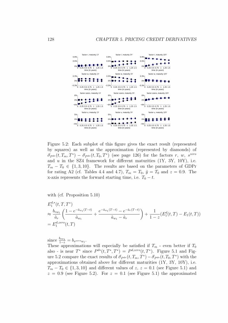
128 CHAPTER 5. PRICING CREDIT DERIVATIVES
0 0.25 0.5 0.75 1 1.25 1.50%
0.5%
0.9%factor r, maturity 1Y
time (in years)
0 0.25 0.5 0.75 1 1.25 1.5−0.3%
0%
0.3%factor w, maturity 1Y
time (in years)
0 0.25 0.5 0.75 1 1.25 1.5−6%
0%
6%factor szero, maturity 1Y
time (in years)
0 0.25 0.5 0.75 1 1.25 1.5−5%
0%
5%factor u, maturity 1Y
time (in years)
0 0.25 0.5 0.75 1 1.25 1.50%
0.5%
0.9%factor r, maturity 3Y
time (in years)
0 0.25 0.5 0.75 1 1.25 1.5−0.3%
0%
0.3%factor w, maturity 3Y
time (in years)
0 0.25 0.5 0.75 1 1.25 1.5−6%
0%
6%factor szero, maturity 3Y
time (in years)
0 0.25 0.5 0.75 1 1.25 1.5−5%
0%
5%factor u, maturity 3Y
time (in years)
0 0.25 0.5 0.75 1 1.25 1.50%
0.5%
0.9%factor r, maturity 10Y
time (in years)
0 0.25 0.5 0.75 1 1.25 1.5−0.3%
0%
0.3%factor w, maturity 10Y
time (in years)
0 0.25 0.5 0.75 1 1.25 1.5−6%
0%
6%factor szero, maturity 10Y
time (in years)
0 0.25 0.5 0.75 1 1.25 1.5−5%
0%
5%factor u, maturity 10Y
time (in years)
Figure 5.2: Each subplot of this figure gives the exact result (representedby squares) as well as the approximation (represented by diamonds) of~σP d∗(t, Tm, T ∗) − ~σP d∗(t, T0, T
∗) (see page 126) for the factors r, w, szero
and u in the SZ4 framework for different maturities (1Y, 3Y, 10Y), i.e.Tm − T0 ∈ 1, 3, 10. The results are based on the parameters of GDPrfor rating A2 (cf. Tables 4.4 and 4.7), Tm = T0, y = T0 and z = 0.9. Thex-axis represents the forward starting time, i.e. T0 − t.
with (cf. Proposition 5.10)
Ed,∗1 (t, T, T ∗)
≈ brw1
ar
(1 − e−aw1 (T−t)
aw1
+e−aw1 (T−t) − e−ar(T−t)
aw1 − ar
)+
1
1 − z(Ed
1(t, T ) − E1(t, T ))
= Ed,zero1 (t, T )
sincebsw1
1−z= bszerow1 .
These approximations will especially be satisfied if Tm - even better if T0
also - is near T ∗ since P d∗(t, T ∗, T ∗) = P d,zero(t, T ∗). Figure 5.1 and Fig-ure 5.2 compare the exact results of ~σP d∗(t, Tm, T ∗)−~σP d∗(t, T0, T
∗) with theapproximations obtained above for different maturities (1Y, 3Y, 10Y), i.e.Tm − T0 ∈ 1, 3, 10 and different values of z, z = 0.1 (see Figure 5.1) andz = 0.9 (see Figure 5.2). For z = 0.1 (see Figure 5.1) the approximated

CHAPTER 5. PRICING CREDIT DERIVATIVES 129
values are close to the exact results of ~σP d∗(t, Tm, T ∗) − ~σP d∗(t, T0, T∗) for
all factors and maturities, especially for short maturities, i.e. Tm − T0 = 1.However, for z = 0.9 (see Figure 5.2) the differences between the exact andapproximated values increase especially for the factors szero and u. Here,the approximation seems to work better for longer maturities (10Y) for thefactors w, u and szero indicating interdependencies between maturity and z.
Further, we approximate ~σV ddp(t, Tm) − ~σV ddp(t, T0) as follows where we as-sume certain integrals to be neglectable.
0 0.25 0.5 0.75 1 1.25 1.50%
4%
8%
12%factor szero, maturity 3Y
time (in years)0 0.25 0.5 0.75 1 1.25 1.5
0%
4%
8%
12%factor u, maturity 3Y
time (in years)0 0.25 0.5 0.75 1 1.25 1.5
−0.5%
−0.25%
0%factor w, maturity 3Y
time (in years)
Figure 5.3: This figure contains the integrals (see page 129)
σszero
∫ Tm
T0P d,zero(t, y)H(t, y)dy, σu
∫ Tm
T0P d,zero(t, y)I(t, y)dy and
σw1
∫ Tm
T0P d,zero(t, y)J1(t, y)dy for z = 0.1 (represented by squares) and
z = 0.9 (represented by diamonds). The values are based on the parametersof GDPr for rating A2 (cf. Tables 4.4 and 4.7) and the maturity 3Y, i.e.Tm − T0 = 3.
σrV ddp(t, Tm) − σr
V ddp(t, T0)
≈ −σrBd,zero(t, y)
∫ Tm
T0
P d,zero(t, y)(F (t, y) + szero(t)H(t, y)
+ u(t)I(t, y) + w1(t)J1(t, y))dy
= −σrBd,zero(t, y)(V ddp
T d (t, Tm) − V ddpT d (t, T0)) ,
σsV ddp(t, Tm) − σs
V ddp(t, T0)
≈ −σszeroCd,zero(t, y)(V ddpT d (t, Tm) − V ddp
T d (t, T0))
+σszero
∫ Tm
T0
P d,zero(t, y)H(t, y)dy
≈ −σszeroCd,zero(t, y)(V ddpT d (t, Tm) − V ddp
T d (t, T0)) ,

130 CHAPTER 5. PRICING CREDIT DERIVATIVES
σuV ddp(t, Tm) − σu
V ddp(t, T0)
≈ −σuDd,zero(t, y)(V ddp
T d (t, Tm) − V ddpT d (t, T0))
+σu
∫ Tm
T0
P d,zero(t, y)I(t, y)dy
≈ −σuDd,zero(t, y)(V ddp
T d (t, Tm) − V ddpT d (t, T0)) ,
and
σw1
V ddp(t, Tm) − σw1
V ddp(t, T0)
≈ −σw1Ed,zero1 (t, y)(V ddp
T d (t, Tm) − V ddpT d (t, T0))
+σw1
∫ Tm
T0
P d,zero(t, y)J1(t, y)dy
≈ −σw1Ed,zero1 (t, y)(V ddp
T d (t, Tm) − V ddpT d (t, T0)) ,
with y ∈ [T0, Tm].Figure 5.3 shows the values of the three integrals which we assume to beneglectable for a maturity of three years and different values of z, z = 0.1and z = 0.9. As before, the approximation works well for z = 0.1 sincethe values of the integrals for all factors are close to zero. For z = 0.9 thevalues deviate from zero especially for the factors u and szero. Figure 5.4and Figure 5.5 compare the exact results of ~σV ddp(t, Tm) − ~σV ddp(t, T0) withthe approximations obtained above for different maturities (1Y, 3Y, 10Y),i.e. Tm − T0 ∈ 1, 3, 10 and different values of z, z = 0.1 (see Figure 5.4)and z = 0.9 (see Figure 5.5). Similar to the results of the approximationfor ~σP d∗(t, Tm, T ∗)−~σP d∗(t, T0, T
∗), the approximations are close to the exactresults for z = 0.1 and the differences increase for z = 0.9, mainly for thefactors u and szero.Hence, by means of incorporating these approximations (see also page 114for µ〈 〉) and by neglecting certain terms we obtain for the dynamics of theFCDS spread as given in Proposition 5.23
ds(t, T0, Tm)
=
((~σ∑
i P d,z(t))′
~σ∑i P d,z(t)
[∑m
i=1 P d,zero(t, Ti)]2 s(t, T0, Tm) + µ〈 〉(t, T0, Tm, T ∗)
)dt

CHAPTER 5. PRICING CREDIT DERIVATIVES 131
+
((~σV ddp(t, Tm) − ~σV ddp(t, T0) + ~σP d∗(t, Tm, T ∗) − ~σP d∗(t, T0, T
∗))′
−s(t, T0, Tm)(~σ∑
i P d,z(t))′)
1∑mi=1 P d,zero(t, Ti)
dW (t)
Th.5.13≈((
~σ∑i P d,z(t)
)′~σ∑
i P d,z(t)
[∑m
i=1 P d,zero(t, Ti)]2
+
(σrB
d,zero(t, y), σszeroCd,zero(t, y), σuDd,zero(t, y), σw1E
d,zero1 (t, y)
)
· 1
[∑m
i=1 P d,zero(t, Ti)]
(~σ∑
i P d,z(t)
))s(t, T0, Tm)dt
+
(−(σrB
d,zero(t, y), σszeroCd,zero(t, y), σuDd,zero(t, y), σw1E
d,zero1 (t, y)
)
−(~σ∑
i P d,z(t))′
∑mi=1 P d,zero(t, Ti)
)s(t, T0, Tm)dW (t)
Approximation for Proposition 5.24: Also, in case of SZ4 it holds that
µZ〈 〉(t, T0, Tm)
= (1 − Z)
(σr
V ddp(t, Tm) − σrV ddp(t, T0)
)σr
∑mi=1 P d,zero(t, Ti)B
d,zero(t, Ti)
[∑m
i=1 P d,zero(t, Ti)]2
+(1 − Z)
(σs
V ddp(t, Tm) − σsV ddp(t, T0)
)σszero
∑mi=1 P d,zero(t, Ti)C
d,zero(t, Ti)
[∑m
i=1 P d,zero(t, Ti)]2
+(1 − Z)
(σu
V ddp(t, Tm) − σuV ddp(t, T0)
)σu
∑mi=1 P d,zero(t, Ti)D
d,zero(t, Ti)
[∑m
i=1 P d,zero(t, Ti)]2
+(1 − Z)
(σw1
V ddp(t, Tm) − σw1
V ddp(t, T0)
)σw1
∑mi=1 P d,zero(t, Ti)E
d,zero1 (t, Ti)
[∑m
i=1 P d,zero(t, Ti)]2
with the vector ~σV ddp as before (see page 124ff).Then, similar to the case discussed before (see also Proposition 5.24 for µZ
〈 〉
and Figures 5.3 -5.5 for the approximations of ~σV ddp(t, Tm)−~σV ddp(t, T0)), the

132 CHAPTER 5. PRICING CREDIT DERIVATIVES
0 0.25 0.5 0.75 1 1.25 1.5−0.05%
−0.025%
0%factor r, maturity 1Y
time (in years)
0 0.25 0.5 0.75 1 1.25 1.5−0.05%
0%
0.05%factor w, maturity 1Y
time (in years)
0 0.25 0.5 0.75 1 1.25 1.5−1%
0%
1%factor szero, maturity 1Y
time (in years)
0 0.25 0.5 0.75 1 1.25 1.5−0.5%
0%
0.5%factor u, maturity 1Y
time (in years)
0 0.25 0.5 0.75 1 1.25 1.5−0.1%
−0.05%
0%factor r, maturity 3Y
time (in years)
0 0.25 0.5 0.75 1 1.25 1.5−0.1%
0%
0.1%factor w, maturity 3Y
time (in years)
0 0.25 0.5 0.75 1 1.25 1.5−2%
0%
2%factor szero, maturity 3Y
time (in years)
0 0.25 0.5 0.75 1 1.25 1.5−2%
0%
2%factor u, maturity 3Y
time (in years)
0 0.25 0.5 0.75 1 1.25 1.5−0.4%
−0.2%
0%factor r, maturity 10Y
time (in years)
0 0.25 0.5 0.75 1 1.25 1.5−0.1%
0%
0.1%factor w, maturity 10Y
time (in years)
0 0.25 0.5 0.75 1 1.25 1.5−2%
0%
2%factor szero, maturity 10Y
time (in years)
0 0.25 0.5 0.75 1 1.25 1.5−5%
0%
5%factor u, maturity 10Y
time (in years)
Figure 5.4: Each subplot of this figure gives the exact result (representedby squares) as well as the approximation (represented by diamonds) of~σV ddp(t, Tm) − ~σV ddp(t, T0) (see page 129) for the factors r, w, szero and uin the SZ4 framework for different maturities (1Y, 3Y, 10Y), i.e. Tm − T0 ∈1, 3, 10. The results are based on the parameters of GDPr for rating A2(cf. Tables 4.4 and 4.7), y = T0 and z = 0.1. The x-axis represents theforward starting time, i.e. T0 − t.
approximated dynamics for Proposition 5.24 are
ds(t, T0, Tm)
=
((~σ∑
i P d,z(t))′
~σ∑i P d,z(t)
[∑m
i=1 P d,zero(t, Ti)]2 s(t, T0, Tm) + µZ
〈 〉(t, T0, Tm)
)dt
+1∑m
i=1 P d,zero(t, Ti)
((1 − Z)
(~σV ddp(t, Tm) − ~σV ddp(t, T0)
)′
−s(t, T0, Tm) ·(~σ∑
i P d,z(t))′)
dW (t)
Th.5.15≈((
~σ∑i P d,z(t)
)′~σ∑
i P d,z(t)
[∑m
i=1 P d,zero(t, Ti)]2
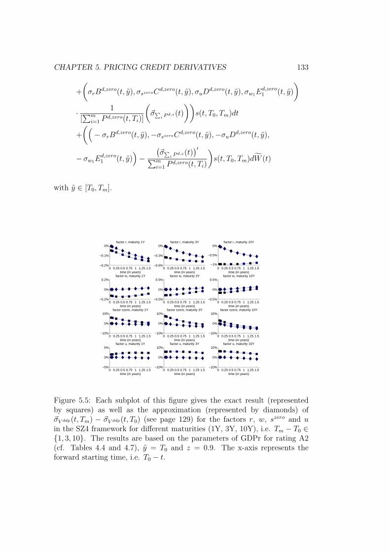
CHAPTER 5. PRICING CREDIT DERIVATIVES 133
+
(σrB
d,zero(t, y), σszeroCd,zero(t, y), σuDd,zero(t, y), σw1E
d,zero1 (t, y)
)
· 1
[∑m
i=1 P d,zero(t, Ti)]
(~σ∑
i P d,z(t)
))s(t, T0, Tm)dt
+
((− σrB
d,zero(t, y),−σszeroCd,zero(t, y),−σuDd,zero(t, y),
−σw1Ed,zero1 (t, y)
)−
(~σ∑
i P d,z(t))′
∑mi=1 P d,zero(t, Ti)
)s(t, T0, Tm)dW (t)
with y ∈ [T0, Tm].
0 0.25 0.5 0.75 1 1.25 1.5−0.2%
−0.1%
0%factor r, maturity 1Y
time (in years)
0 0.25 0.5 0.75 1 1.25 1.5−0.2%
0%
0.2%factor w, maturity 1Y
time (in years)
0 0.25 0.5 0.75 1 1.25 1.5−10%
0%
10%factor szero, maturity 1Y
time (in years)
0 0.25 0.5 0.75 1 1.25 1.5−5%
0%
5%factor u, maturity 1Y
time (in years)
0 0.25 0.5 0.75 1 1.25 1.5−0.6%
−0.3%
0%factor r, maturity 3Y
time (in years)
0 0.25 0.5 0.75 1 1.25 1.5−0.5%
0%
0.5%factor w, maturity 3Y
time (in years)
0 0.25 0.5 0.75 1 1.25 1.5−10%
0%
10%factor szero, maturity 3Y
time (in years)
0 0.25 0.5 0.75 1 1.25 1.5−10%
0%
10%factor u, maturity 3Y
time (in years)
0 0.25 0.5 0.75 1 1.25 1.5−1%
−0.5%
0%factor r, maturity 10Y
time (in years)
0 0.25 0.5 0.75 1 1.25 1.5−0.5%
0%
0.5%factor w, maturity 10Y
time (in years)
0 0.25 0.5 0.75 1 1.25 1.5−10%
0%
10%factor szero, maturity 10Y
time (in years)
0 0.25 0.5 0.75 1 1.25 1.5−10%
0%
10%factor u, maturity 10Y
time (in years)
Figure 5.5: Each subplot of this figure gives the exact result (representedby squares) as well as the approximation (represented by diamonds) of~σV ddp(t, Tm) − ~σV ddp(t, T0) (see page 129) for the factors r, w, szero and uin the SZ4 framework for different maturities (1Y, 3Y, 10Y), i.e. Tm − T0 ∈1, 3, 10. The results are based on the parameters of GDPr for rating A2(cf. Tables 4.4 and 4.7), y = T0 and z = 0.9. The x-axis represents theforward starting time, i.e. T0 − t.

134 CHAPTER 5. PRICING CREDIT DERIVATIVES
Approximation for Proposition 5.25: Finally, for the third case we need
the vector(~σP ∗(t, Tj−1, Tj) − ~σP d,z(t, Tj)
)which consists of
σrP ∗(t, Tj−1, Tj) − σr
P d,z(t, Tj)
= −σr(B∗(t, Tj−1, Tj)P
∗(t, Tj−1, Tj) − Bd,zero(t, Tj)Pd,zero(t, Tj))
= −σrBd,zero(t, Tj)(P
∗(t, Tj−1, Tj) − P d,zero(t, Tj)) ,
σsP ∗(t, Tj−1, Tj) − σs
P d,z(t, Tj)
= −σszero(C∗(t, Tj−1, Tj)P∗(t, Tj−1, Tj) − Cd,zero(t, Tj)P
d,zero(t, Tj))
= −σszero(Cd,zero(t, Tj−1)P∗(t, Tj−1, Tj) − Cd,zero(t, Tj)P
d,zero(t, Tj)) ,
σuP ∗(t, Tj−1, Tj) − σu
P d,z(t, Tj)
= −σu(D∗(t, Tj−1, Tj)P
∗(t, Tj−1, Tj) − Dd,zero(t, Tj)Pd,zero(t, Tj))
= −σu(Dd,zero(t, Tj−1)P
∗(t, Tj−1, Tj) − Dd,zero(t, Tj)Pd,zero(t, Tj)) ,
and
σw1P ∗(t, Tj−1, Tj) − σw1
P d,z(t, Tj)
= −σw1(E∗1(t, Tj−1, Tj)P
∗(t, Tj−1, Tj) − Ed,zero1 (t, Tj)P
d,zero(t, Tj)) .
The components of the vector(~σP ∗(t, Tj−1, Tj)−~σP d,z(t, Tj)
)can be approx-
imated by assuming Tj−1 ≈ Tj with
σsP ∗(t, Tj−1, Tj) − σs
P d,z(t, Tj)
≈ −σszeroCd,zero(t, Tj)(P∗(t, Tj−1, Tj) − P d,zero(t, Tj)) ,
σuP ∗(t, Tj−1, Tj) − σu
P d,z(t, Tj)
≈ −σuDd,zero(t, Tj)(P
∗(t, Tj−1, Tj) − P d,zero(t, Tj)) ,
and
σw1P ∗(t, Tj−1, Tj) − σw1
P d,z(t, Tj)
≈ −σw1Ed,zero1 (t, Tj)(P
∗(t, Tj−1, Tj) − P d,zero(t, Tj)).
where we use (see also page 268 for E∗1(t, Tj−1, Tj))
E∗1(t, Tj−1, Tj) = E1(t, Tj) + (Ed,zero
1 (t, Tj−1) − E1(t, Tj−1))
≈ Ed,zero1 (t, Tj)
CHAPTER 5. PRICING CREDIT DERIVATIVES 135
for Tj−1 ≈ Tj.The dynamics of the FCDS according to Proposition 5.25 can now be writtenas
ds(t, T0, Tm)
≈((
~σ∑i P d,z(t)
)′~σ∑
i P d,z(t)
[∑m
i=1 P d,zero(t, Ti)]2 s(t, T0, Tm)
+(1 − Z)
∑nj=1
(P ∗(t, Tj−1, Tj) − P d,zero(t, Tj)
)
[∑m
i=1 P d,zero(t, Ti)]2
(~σ∑
i P d,z(t)
)′
·(σrB
d,zero(t, y), σszeroCd,zero(t, y), σuDd,zero(t, y), σw1E
d,zero1 (t, y)
)′)dt
+
(−
(1 − Z)∑n
j=1
(P ∗(t, Tj−1, Tj) − P d,zero(t, Tj)
)
∑mi=1 P d,zero(t, Ti)
·(σrB
d,zero(t, y), σszeroCd,zero(t, y), σuDd,zero(t, y), σw1E
d,zero1 (t, y)
)
− s(t, T0, Tm)
(~σ∑
i P d,z(t))′
∑mi=1 P d,zero(t, Ti)
)dW (t)
Th.5.18= s(t, T0, Tm)
((~σ∑
i P d,z(t))′
~σ∑i P d,z(t)
[∑m
i=1 P d,zero(t, Ti)]2 +
(~σ∑
i P d,z(t))′
∑mi=1 P d,zero(t, Ti)
·(σrB
d,zero(t, y), σszeroCd,zero(t, y), σuDd,zero(t, y), σw1E
d,zero1 (t, y)
)′)dt
−((
σrBd,zero(t, y), σszeroCd,zero(t, y), σuD
d,zero(t, y), σw1Ed,zero1 (t, y)
)
+
(~σ∑
i P d,z(t))′
∑mi=1 P d,zero(t, Ti)
)s(t, T0, Tm)dW (t) ,
with y ∈ [T0, Tm].
Note that we can end up with the same lognormal dynamics no matterwhich recovery assumptions for the reference entity we make. Also, usingthe default bucketing approach in order to circumvent certain integrals hasno advantages so far, since the critical terms vanish during the above ap-proximations. But, assuming a fine grid for the default bucketing results inanother version of lognormal dynamics as shown in the next Corollary.

136 CHAPTER 5. PRICING CREDIT DERIVATIVES
Corollary 5.27For fine time steps Tj − Tj−1 in Proposition 5.25, the dynamics reduce to
ds(t, T0, Tm)
= s(t, T0, Tm)
((~σ∑
i P d,z(t))′
~σ∑i P d,z(t)
[∑m
i=1 P d,zero(t, Ti)]2 dt −
(~σ∑
i P d,z(t))′
∑mi=1 P d,zero(t, Ti)
dW (t)
).
Proof:Assuming the time steps Tj − Tj−1 in the numerator of Proposition 5.25 to
be very fine, we get P ∗(t, Tj−1, Tj) ≈ P ∗(t, Tj, Tj) = P d,zero(t, Tj). With ananalogous approximation as above, we obtain the dynamics.
There exists another useful approximation of the dynamics in Proposition5.24, the so-called shifted-lognormal distribution (see Brigo & Mercurio (2006),page 454ff). It assumes the FCDS spread to be the sum of a lognormallydistributed X(t) and a real constant γ, i.e.
s(t, T0, Tm) = X(t) + γ.
Assumption 5.28In the SZ4 framework the exact dynamics of the FCDS spread presented inProposition 5.24 can be approximated by shifted-lognormal dynamcis
ds(t, T0, Tm)
=
(~σ∑
i P d,z(t))′
~σ∑i P d,z(t)
[∑m
i=1 P d,zero(t, Ti)]2
(s(t, T0, Tm) − (1 − Z)∆TiK
)dt
−(~σ∑
i P d,z(t))′
∑mi=1 P d,zero(t, Ti)
(s(t, T0, Tm) − (1 − Z)∆TiK
)dW (t)
with equidistant ∆Ti := Ti − Ti−1 i = 1 . . . m, frozen factors r, szero, u, w1 in~σ∑
i P d,z and P d,zero at time t, and a constant K.
Approximation for Proposition 5.24: Within the SZ4 framework weassume the following approximations to hold by fixing y ∈ [T0, Tm] and byassuming as before certain integrals to be neglectable (see also Figure 5.3 for

CHAPTER 5. PRICING CREDIT DERIVATIVES 137
an analysis of these integrals).
σrV ddp(t, Tm) − σr
V ddp(t, T0)
≈ −σr
m∑
i=1
P d,zero(t, Ti)Bd,zero(t, Ti)
(F (t, Ti) + szero(t)H(t, Ti)
+ u(t)I(t, Ti) + w1(t)J1(t, Ti))(Ti − Ti−1)
=(F (t, y) + szero(t)H(t, y) + u(t)I(t, y) + w1(t)J1(t, y)
)∆Tiσ
r∑i P d,z(t)
σsV ddp(t, Tm) − σs
V ddp(t, T0)
≈(F (t, y) + szero(t)H(t, y) + u(t)I(t, y) + w1(t)J1(t, y)
)∆Tiσ
s∑i P d,z(t)
+ σszero
∫ Tm
T0
P d,zero(t, y)H(t, y)dy
≈(F (t, y) + szero(t)H(t, y) + u(t)I(t, y) + w1(t)J1(t, y)
)∆Tiσ
s∑i P d,z(t)
σuV ddp(t, Tm) − σu
V ddp(t, T0)
≈(F (t, y) + szero(t)H(t, y) + u(t)I(t, y) + w1(t)J1(t, y)
)∆Tiσ
u∑i P d,z(t)
+ σu
∫ Tm
T0
P d,zero(t, y)I(t, y)dy
≈(F (t, y) + szero(t)H(t, y) + u(t)I(t, y) + w1(t)J1(t, y)
)∆Tiσ
u∑i P d,z(t)
σw1
V ddp(t, Tm) − σw1
V ddp(t, T0)
≈(F (t, y) + szero(t)H(t, y) + u(t)I(t, y) + w1(t)J1(t, y)
)∆Tiσ
w1∑i P d,z(t)
+ σw1
∫ Tm
T0
P d,zero(t, y)J1(t, y)dy
≈(F (t, y) + szero(t)H(t, y) + u(t)I(t, y) + w1(t)J1(t, y)
)∆Tiσ
w1∑i P d,z(t)
with y ∈ [T0, Tm] and ∆Ti := Ti − Ti−1 equidistant for i = 1 . . . m.Figure 5.6 and Figure 5.7 compare the exact results of ~σV ddp(t, Tm)−~σV ddp(t, T0)with the approximations obtained above for different maturities (1Y, 3Y,10Y), i.e. Tm − T0 ∈ 1, 3, 10 and different values of z, z = 0.1 (see Figure5.6) and z = 0.9 (see Figure 5.7). We obtain results that are very similarto the previous approximation for ~σV ddp(t, Tm) − ~σV ddp(t, T0) (see page 129).
138 CHAPTER 5. PRICING CREDIT DERIVATIVES
Analogously to Figures 5.4 and 5.5, the approximations work well for all fac-tors r, w, u, szero and z = 0.1, also for the factors r and w if z = 0.9. Butthe differences in the results increase for z = 0.9, especially for u and szero.
Hence, we obtain for the dynamics with a fixed y ∈ [T0, Tm] (see also Propo-sition 5.24 for µZ
〈 〉)
ds(t, T0, Tm)
=
((~σ∑
i P d,z(t))′
~σ∑i P d,z(t)
[∑m
i=1 P d,zero(t, Ti)]2 s(t, T0, Tm) + µZ
〈 〉(t, T0, Tm)
)dt
+1∑m
i=1 P d,zero(t, Ti)
((1 − Z)
(~σV ddp(t, Tm) − ~σV ddp(t, T0)
)′
−s(t, T0, Tm) ·(~σ∑
i P d,z(t))′)
dW (t)
≈((
~σ∑i P d,z(t)
)′~σ∑
i P d,z(t)
[∑m
i=1 P d,zero(t, Ti)]2 s(t, T0, Tm)
+(1 − Z)(F (t, y) + szero(t)H(t, y) + u(t)I(t, y) + w1(t)J1(t, y)
)∆Ti
·(
σr∑i P d,z(t), σ
s∑i P d,z(t), σ
u∑i P d,z(t), σ
w1∑i P d,z(t)
)
· −1
[∑m
i=1 P d,zero(t, Ti)]2
(~σ∑
i P d,z(t)
))dt
+
((F (t, y) + szero(t)H(t, y) + u(t)I(t, y) + w1(t)J1(t, y)
)
· (1 − Z)∆Ti
(σr∑
i P d,z(t), σs∑
i P d,z(t), σu∑
i P d,z(t), σw1∑
i P d,z(t)
)
− s(t, T0, Tm) ·(~σ∑
i P d,z(t))′)
1∑mi=1 P d,zero(t, Ti)
dW (t)
≈((
~σ∑i P d,z(t)
)′~σ∑
i P d,z(t)
[∑m
i=1 P d,zero(t, Ti)]2 s(t, T0, Tm)
−(1 − Z)∆TiK ·(~σ∑
i P d,z(t))′(~σ∑i P d,z(t))
[∑m
i=1 P d,zero(t, Ti)]2
)dt
+((1 − Z)∆TiK
(~σ∑
i P d,z(t))′ − s(t, T0, Tm) ·
(~σ∑
i P d,z(t))′
)∑mi=1 P d,zero(t, Ti)
dW (t)
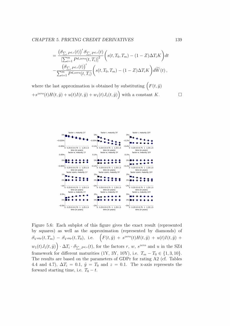
CHAPTER 5. PRICING CREDIT DERIVATIVES 139
=
(~σ∑
i P d,z(t))′
~σ∑i P d,z(t)
[∑m
i=1 P d,zero(t, Ti)]2
(s(t, T0, Tm) − (1 − Z)∆TiK
)dt
−(~σ∑
i P d,z(t))′
∑mi=1 P d,zero(t, Ti)
(s(t, T0, Tm) − (1 − Z)∆TiK
)dW (t) ,
where the last approximation is obtained by substituting(F (t, y)
+szero(t)H(t, y) + u(t)I(t, y) + w1(t)J1(t, y))
with a constant K.
0 0.25 0.5 0.75 1 1.25 1.5−0.05%
−0.025%
0%factor r, maturity 1Y
time (in years)
0 0.25 0.5 0.75 1 1.25 1.5−0.05%
0%
0.05%factor w, maturity 1Y
time (in years)
0 0.25 0.5 0.75 1 1.25 1.5−1%
0%
1%factor szero, maturity 1Y
time (in years)
0 0.25 0.5 0.75 1 1.25 1.5−0.5%
0%
0.5%factor u, maturity 1Y
time (in years)
0 0.25 0.5 0.75 1 1.25 1.5−0.1%
−0.05%
0%factor r, maturity 3Y
time (in years)
0 0.25 0.5 0.75 1 1.25 1.5−0.1%
0%
0.1%factor w, maturity 3Y
time (in years)
0 0.25 0.5 0.75 1 1.25 1.5−2%
0%
2%factor szero, maturity 3Y
time (in years)
0 0.25 0.5 0.75 1 1.25 1.5−2%
0%
2%factor u, maturity 3Y
time (in years)
0 0.25 0.5 0.75 1 1.25 1.5−0.4%
−0.2%
0%factor r, maturity 10Y
time (in years)
0 0.25 0.5 0.75 1 1.25 1.5−0.1%
0%
0.1%factor w, maturity 10Y
time (in years)
0 0.25 0.5 0.75 1 1.25 1.5−2%
0%
2%factor szero, maturity 10Y
time (in years)
0 0.25 0.5 0.75 1 1.25 1.5−5%
0%
5%factor u, maturity 10Y
time (in years)
Figure 5.6: Each subplot of this figure gives the exact result (representedby squares) as well as the approximation (represented by diamonds) of
~σV ddp(t, Tm) − ~σV ddp(t, T0), i.e.(F (t, y) + szero(t)H(t, y) + u(t)I(t, y) +
w1(t)J1(t, y))· ∆Ti · ~σ∑
i P d,z(t), for the factors r, w, szero and u in the SZ4
framework for different maturities (1Y, 3Y, 10Y), i.e. Tm − T0 ∈ 1, 3, 10.The results are based on the parameters of GDPr for rating A2 (cf. Tables4.4 and 4.7), ∆Ti = 0.1, y = T0 and z = 0.1. The x-axis represents theforward starting time, i.e. T0 − t.

140 CHAPTER 5. PRICING CREDIT DERIVATIVES
0 0.25 0.5 0.75 1 1.25 1.5−0.2%
−0.1%
0%factor r, maturity 1Y
time (in years)
0 0.25 0.5 0.75 1 1.25 1.5−0.2%
0%
0.2%factor w, maturity 1Y
time (in years)
0 0.25 0.5 0.75 1 1.25 1.5−10%
0%
10%factor szero, maturity 1Y
time (in years)
0 0.25 0.5 0.75 1 1.25 1.5−5%
0%
5%factor u, maturity 1Y
time (in years)
0 0.25 0.5 0.75 1 1.25 1.5−0.6%
−0.3%
0%factor r, maturity 3Y
time (in years)
0 0.25 0.5 0.75 1 1.25 1.5−0.5%
0%
0.5%factor w, maturity 3Y
time (in years)
0 0.25 0.5 0.75 1 1.25 1.5−10%
0%
10%factor szero, maturity 3Y
time (in years)
0 0.25 0.5 0.75 1 1.25 1.5−10%
0%
10%factor u, maturity 3Y
time (in years)
0 0.25 0.5 0.75 1 1.25 1.5−1%
−0.5%
0%factor r, maturity 10Y
time (in years)
0 0.25 0.5 0.75 1 1.25 1.5−0.5%
0%
0.5%factor w, maturity 10Y
time (in years)
0 0.25 0.5 0.75 1 1.25 1.5−10%
0%
10%factor szero, maturity 10Y
time (in years)
0 0.25 0.5 0.75 1 1.25 1.5−10%
0%
10%factor u, maturity 10Y
time (in years)
Figure 5.7: Each subplot of this figure gives the exact result (representedby squares) as well as the approximation (represented by diamonds) of
~σV ddp(t, Tm) − ~σV ddp(t, T0), i.e.(F (t, y) + szero(t)H(t, y) + u(t)I(t, y) +
w1(t)J1(t, y))· ∆Ti · ~σ∑
i P d,z(t), for the factors r, w, szero and u in the SZ4
framework for different maturities (1Y, 3Y, 10Y), i.e. Tm − T0 ∈ 1, 3, 10.The results are based on the parameters of GDPr for rating A2 (cf. Tables4.4 and 4.7), ∆Ti = 0.1, y = T0 and z = 0.9. The x-axis represents theforward starting time, i.e. T0 − t.
In order to obtain the constant K we match moments as it is proposed by e.g.Brigo & Masetti (2006), page 15. Also, we follow the approach heavily usedfor LIBOR models (see e.g Mercurio & Morini (2007)) where freezing certainfactors at time t0 has shown to have no major impact on the dynamics. Wework with the frozen dynamics of r, w1, s and u. Therefore, the functions~σ∑
i P d,z(x), P d,zero(x, T ) and µZ〈 〉(x, T0, Tm) are now deterministic. Assum-
ing the existence of the following expected values, we equate the dynamicsof Proposition 5.24 with the dynamics of the above approximation: III

CHAPTER 5. PRICING CREDIT DERIVATIVES 141
EQ[s(t, T0, Tm)∣∣Ft]
≈ s(t, T0, Tm)
(1 +
∫ t
t
(~σ∑
i P d,z(x))′
~σ∑i P d,z(x)
[∑m
i=1 P d,zero(x, Ti)]2 dx
)
︸ ︷︷ ︸(∗)
+
∫ t
t
µZ〈 〉(x, T0, Tm)dx
!= EQ[sapprox(t, T0, Tm)
∣∣Ft]
= (1 − Z)∆TiK
+
(s(t, T0, Tm) − (1 − Z)∆TiK
)e
∫ tt
(~σ∑
i Pd,z (x)
)′~σ∑
i Pd,z (x)
[∑m
i=1Pd,zero(x,Ti)]
2 dx
Using the approximation ex = 1 + x for (*), it holds
s(t, T0, Tm)e
∫ tt
(~σ∑
i Pd,z (x)
)′~σ∑
i Pd,z (x)
[∑mi=1
Pd,zero(x,Ti)]2 dx
+
∫ t
t
µZ〈 〉(x, T0, Tm)dx
!= (1 − Z)∆TiK
+
(s(t, T0, Tm) − (1 − Z)∆TiK
)e
∫ tt
(~σ∑
i Pd,z (x)
) ′~σ∑
i Pd,z (x)
[∑mi=1
Pd,zero(x,Ti)]2 dx
.
Therefore, the constant K is calculated as
K =
∫ t
tµZ〈 〉(x, T0, Tm)dx
(1 − Z)∆Ti
1 − e
∫ tt
(~σ∑
i Pd,z (x)
)′~σ∑
i Pd,z (x)
[∑m
i=1Pd,zero(x,Ti)]
2 dx
.
IIIFor the shifted-lognormal dynamics dX(t) = α(t)(X(t)− γ)dt + β(t)(X(t)− γ)dW (t)with a real constant γ, and deterministic functions α(t) and β(t), it holds
X(T ) = γ + (X(t) − γ)e∫
T
tα(x)dx− 1
2
∫T
tβ2(x)dx+
∫T
tβ(x)dW (x)
(see e.g. Brigo & Mercurio (2006), page 454).

142 CHAPTER 5. PRICING CREDIT DERIVATIVES
In the following we analyze how well the approximated dynamics work as op-posed to the FCDS spread we would get by simulating the factors r, s, u, w1
and using the formulas for the FCDS spread given in Section 5.4. The analy-sis is based on the set of parameters called GDPr of Chapter 4 for the ratingclass A2. We want to emphasize that this analysis is of theoretical nature andtherefore assume the parameters as appropriate although they are obtainedby means of defaultable bonds. However, parameters that are calibratedon defaultable bonds are not always suitable for pricing credit derivatives.The quoting mechanism and especially the assumptions concerning recoveryrates differ within the markets. Hence, it would be appropriate to calibrateon quoted CDS spreads with the help of the closed-form solution of Section5.4.The following figures outline the evolution of Forward Credit Default Swapsfor different maturities (3Y, 5Y, 7Y, 10Y) of the CDS and for different for-ward starting times (0.25Y, 0.5Y, 0.75Y, 1Y, 1.5Y). We use 20,000 scenariosand set z to 0.9 in line with the results of Antes et al. (2009) (see Defini-tion 5.1). In Figure 5.8 the FCDS spreads assuming a protection paymentof replacement to par are determined by simulating the factors r, s, u, w1
until end of the forward starting time and then using the formula of The-orem 5.13. In addition to that, the approximated lognormal dynamics ofAssumption 5.26 are used with y = T0. For forward starting times underone year, the differences between the FCDS spreads are less than 5bp. Forforward starting times over a year, the differences increase up to 10bp for amaturity of ten years. Furthermore, the differences seem to be dependent onthe maturity of the underlying CDS. The longer the maturity of the CDS,the more the FCDS spreads deviate - especially for longer forward startingtimes. Analogously, Figure 5.9 shows the FCDS spreads assuming recovery asa fraction of face value and protection payments at certain dates. The resultsare obtained by means of Theorem 5.18 and by means of the approximatedlognormal dynamics under the recovery assumption Z = 0.75. This value ischosen arbitrarily in order to get results of the same dimension as in Figure5.8. Here, the differences between the FCDS spreads are smaller for shorterforward starting times as in the aforementioned case. But unlike before, thedifferences (especially for longer forward starting times) become smaller forincreasing maturities of the underlying CDS. Figure 5.10 until Figure 5.13outline the results for the FCDS spreads asuming recovery as a fraction offace value with Z = 0.75. Each figure represents the results for a givenCDS maturity (3Y, 5Y, 7Y, 10Y) in order to account for the second approx-imation (shifted-lognormal) of the FCDS spread dynamics (see Assumption5.28). The differences between the FCDS spread determined by means ofTheorem 5.15 and by means of lognormal dynamics behave as in the case

CHAPTER 5. PRICING CREDIT DERIVATIVES 143
of Figure 5.9. But the FCDS spreads determined with the shifted-lognormalassumptions match extremely well the results obtained via simulating thefactors and using Theorem 5.15.Summarizing the above results, we can claim the approximated dynamics towork well up to a forward starting time of one year no matter which recoveryassumptions hold. Further, in case of recovery as a fraction of face valuethe approximation using shifted-lognormal dynamics even yields promisingresults for longer forward starting times.

144C
HA
PT
ER
5.P
RIC
ING
CR
ED
ITD
ER
IVA
TIV
ES
0 0.25 0.5 0.75 1 1.25 1.50.7%
0.8%
0.9%
1.0%
1.1%
1.2%CDS maturity 3Y
time (in years)
FC
DS
spr
ead
0 0.25 0.5 0.75 1 1.25 1.51.1%
1.2%
1.3%
1.4%
1.5%
1.6%
1.7%CDS maturity 5Y
time (in years)
FC
DS
spr
ead
0 0.25 0.5 0.75 1 1.25 1.51.5%
1.6%
1.7%
1.8%
1.9%
2.0%
2.1%CDS maturity 7Y
time (in years)
FC
DS
spr
ead
0 0.25 0.5 0.75 1 1.25 1.52.1%
2.2%
2.3%
2.4%
2.5%
2.6%
2.7%
2.8%CDS maturity 10Y
time (in years)
FC
DS
spr
ead
Figure 5.8: Each subplot of this figure shows FCDS spreads for different forward starting times (0.25Y, 0.5Y, 0.75Y,1Y, 1.5Y) and for a given maturity of the corresponding CDS (3Y, 5Y, 7Y, 10Y). The broken line represents theresults obtained by the approximated lognormal dynamics, whereas the diamonds give the solutions of Theorem5.13. The plot is based on 20,000 scenarios and z = 0.9.

CH
AP
TE
R5.P
RIC
ING
CR
ED
ITD
ER
IVA
TIV
ES
145
0 0.25 0.5 0.75 1 1.25 1.51.0%
1.1%
1.2%
1.3%
1.4%
CDS maturity 3Y
time (in years)
FC
DS
spr
ead
0 0.25 0.5 0.75 1 1.25 1.51.0%
1.1%
1.2%
1.3%
1.4%
CDS maturity 5Y
time (in years)
FC
DS
spr
ead
0 0.25 0.5 0.75 1 1.25 1.51.0%
1.1%
1.2%
1.3%
1.4%
CDS maturity 7Y
time (in years)
FC
DS
spr
ead
0 0.25 0.5 0.75 1 1.25 1.51.0%
1.1%
1.2%
1.3%
1.4%
CDS maturity 10Y
time (in years)
FC
DS
spr
ead
Figure 5.9: Each subplot of this figure shows FCDS spreads for different forward starting times (0.25Y, 0.5Y, 0.75Y,1Y, 1.5Y) and for a given maturity of the corresponding CDS (3Y, 5Y, 7Y, 10Y). The broken line represents theresults obtained by the approximated lognormal dynamics, whereas the diamonds give the solutions of Theorem5.18. The plot is based on 20,000 scenarios, Z = 0.75 and z = 0.9.

146C
HA
PT
ER
5.P
RIC
ING
CR
ED
ITD
ER
IVA
TIV
ES
0 0.251.07%
1.08%
time (in years)
FC
DS
spr
ead
0 0.25 0.51.14%
1.15%
1.16%
1.17%
1.18%
time (in years)
FC
DS
spr
ead
0 0.25 0.5 0.751.2%
1.21%
1.22%
1.23%
1.24%
time (in years)
FC
DS
spr
ead
0 0.25 0.5 0.75 11.25%
1.26%
1.27%
1.28%
1.29%
1.30%
time (in years)
FC
DS
spr
ead
0 0.25 0.5 0.75 1 1.25 1.51.32%
1.34%
1.36%
1.38%
1.40%
time (in years)
FC
DS
spr
ead
Figure 5.10: Each subplot of this figures shows FCDS spreads for a given forward starting time (0.25Y, 0.5Y, 0.75Y,1Y, 1.5Y) in case of a CDS with maturity of 3 years. The broken line represents the results obtained by theapproximated lognormal dynamics, the solid line shows the results of the shifted-lognormal dynamics, whereas thediamonds give the solutions of Theorem 5.15. The plot is based on 20,000 scenarios, Z = 0.75 and z = 0.9.

CH
AP
TE
R5.P
RIC
ING
CR
ED
ITD
ER
IVA
TIV
ES
147
0 0.251.16%
1.17%
1.18%
time (in years)F
CD
S s
prea
d0 0.25 0.5
1.22%
1.23%
1.24%
1.25%
1.26%
time (in years)
FC
DS
spr
ead
0 0.25 0.5 0.751.26%
1.27%
1.28%
1.29%
1.30%
time (in years)
FC
DS
spr
ead
0 0.25 0.5 0.75 11.30%
1.32%
1.34%
1.36%
1.38%
1.40%
time (in years)
FC
DS
spr
ead
0 0.25 0.5 0.75 1 1.25 1.51.35%
1.37%
1.39%
1.41%
1.43%
1.45%
time (in years)
FC
DS
spr
ead
Figure 5.11: Each subplot of this figures shows FCDS spreads for a given forward starting time (0.25Y, 0.5Y, 0.75Y,1Y, 1.5Y) in case of a CDS with maturity of 5 years. The broken line represents the results obtained by theapproximated lognormal dynamics, the solid line shows the results of the shifted-lognormal dynamics, whereas thediamonds give the solutions of Theorem 5.15. The plot is based on 20,000 scenarios, Z = 0.75 and z = 0.9.
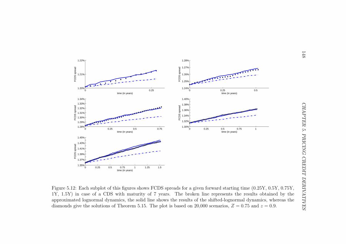
148C
HA
PT
ER
5.P
RIC
ING
CR
ED
ITD
ER
IVA
TIV
ES
0 0.251.20%
1.21%
1.22%
time (in years)
FC
DS
spr
ead
0 0.25 0.51.24%
1.25%
1.26%
1.27%
1.28%
time (in years)
FC
DS
spr
ead
0 0.25 0.5 0.751.28%
1.29%
1.30%
1.31%
1.32%
1.33%
1.34%
time (in years)
FC
DS
spr
ead
0 0.25 0.5 0.75 11.30%
1.32%
1.34%
1.36%
1.38%
1.40%
time (in years)
FC
DS
spr
ead
0 0.25 0.5 0.75 1 1.25 1.51.35%
1.37%
1.39%
1.41%
1.43%
1.45%
time (in years)
FC
DS
spr
ead
Figure 5.12: Each subplot of this figures shows FCDS spreads for a given forward starting time (0.25Y, 0.5Y, 0.75Y,1Y, 1.5Y) in case of a CDS with maturity of 7 years. The broken line represents the results obtained by theapproximated lognormal dynamics, the solid line shows the results of the shifted-lognormal dynamics, whereas thediamonds give the solutions of Theorem 5.15. The plot is based on 20,000 scenarios, Z = 0.75 and z = 0.9.

CH
AP
TE
R5.P
RIC
ING
CR
ED
ITD
ER
IVA
TIV
ES
149
0 0.251.20%
1.21%
1.22%
1.23%
time (in years)F
CD
S s
prea
d0 0.25 0.5
1.24%
1.25%
1.26%
1.27%
1.28%
time (in years)
FC
DS
spr
ead
0 0.25 0.5 0.751.26%
1.27%
1.28%
1.29%
1.30%
1.31%
1.32%
time (in years)
FC
DS
spr
ead
0 0.25 0.5 0.75 11.28%
1.30%
1.32%
1.34%
1.36%
1.38%
time (in years)
FC
DS
spr
ead
0 0.25 0.5 0.75 1 1.25 1.51.32%
1.34%
1.36%
1.38%
1.40%
1.42%
1.44%
time (in years)
FC
DS
spr
ead
Figure 5.13: Each subplot of this figures shows FCDS spreads for a given forward starting time (0.25Y, 0.5Y, 0.75Y,1Y, 1.5Y) in case of a CDS with maturity of 10 years. The broken line represents the results obtained by theapproximated lognormal dynamics, the solid line shows the results of the shifted-lognormal dynamics, whereas thediamonds give the solutions of Theorem 5.15. The plot is based on 20,000 scenarios, Z = 0.75 and z = 0.9.

150 CHAPTER 5. PRICING CREDIT DERIVATIVES
5.4.3 Introducing Counterparty Risk
All previously calculated credit default swaps share the assumption that nei-ther the protection payer nor the protection seller will experience any de-faults. Hence, these events are not priced into the credit default swap. Butsince the collaps of Lehman Brothers in 2008 and the problems of AIG, one ofthe biggest players in the CDS market, counterparties of OTC transactionsare not considered undefaultable anymore.Schmid (2002) suggested an approach how to price defaultable interest-rateswaps for a predecessor of our framework. In this section we introduce a firststep towards pricing counterparty risk inherent in credit default swaps. Weadopt the view of the protection buyer who considers her counterparty riskyas opposed to herself. But the following calculations can be generalized inorder to incorporate both counterparties as risky ones.In the literature there are several approaches for calculating counterparty riskadjustments (CVA) for credit default swaps. The structural default modelis used by e.g. Liang, Zhou, Zhou & Ma (2011) who model the correla-tion of the counterparty and the reference entity by two correlated geometricBrownian motions assuming a constant interest rate. Lipton & Sepp (2009)propose a multi-dimensional jump-diffusion process that drives the joint dy-namics of asset values. Intensity contagion models where default intensitiesof the surviving firm are dependent on the default of the counterparty areused by e.g. Jarrow & Yu (2001), Leung & Kwok (2005) and Bao, Chen &Li (2012). Brigo & Chourdakis (2009) determine unilateral CVA for CDSassuming the intensities to be CIR processes and using a Gaussian copulafor the dependence structure. Brigo & Capponi (2010) generalize the workof Brigo & Chourdakis (2009) in order to calculate bilateral CVA. Bielecki,Crepey, Jeanblanc & Zargari (2012) introduce a Markovian copula set-upin order to model the joint default between counterparty and the referenceentity.We follow the approach of Jarrow & Yu (2001) who use so-called primaryand secondary firms in order to model default dependencies, but we do notrestrict ourselves to constant interest rates or intensities as it is partiallydone in the above mentioned approaches. The default intensity of the pri-mary firm is assumed to only depend on the filtration F which is generatedby the state variables, whereas the default intensity of the secondary firmis dependent on the filtration F as well as the status of the primary firm.In our case, the protection seller is categorized as a secondary firm and thereference asset of the CDS is assumed to be a primary firm. We extend ournotation as follows: The superscript cp indicates that the variable belongsto the counterparty and the superscript ref refers to variables belonging to
CHAPTER 5. PRICING CREDIT DERIVATIVES 151
the reference asset. Further, the enlarged filtration Gcp,ref = F∨H
cp∨Href
is given as Gcp,reft = Ft∨Hcp
t ∨Hreft for every t, whereas Gcp
t is built byGcp
t = FT ∗∨Hcpt ∨Href
T ∗ for every t ∈ [0, T ∗], with Gcp0 = FT ∗∨Href
T ∗ for t = 0.Hence, the default intensity of the reference asset is adapted to the filtrationF = (Ft)0≤t≤T ∗ and the default intensity of the protection seller is adapted to
the filtration Gcp =
(Gcp
t
)0≤t≤T ∗
. In this context the default intensity of the
reference asset szero,ref takes on the form as in Proposition 5.3 and the defaultintensity of the protection seller is given by szero,cp(t) = szero,cp(t)+c1T d,ref≤t
with szero,cp as in Proposition 5.3 and c a constant.Again, we pose ourselves into our general framework introduced in Chapter4. Therefore, the results obtained in this section can be used for all mod-els derived from the general framework. Further, we take on the view ofthe protection buyer who assumes herself to be free of default risk and thecounterparty to be defaultable with a recovery rate of zero. The referenceasset of the CDS is deemed to be a primary firm in a sense that its defaultintensity is not dependent on the defaults of the protection buyer and seller.However, we assume that the default of the reference asset increases the de-fault intensity of the protection seller, i.e. the protection seller is a secondaryfirm. This assumption is not unrealistic if we assume the protection sellerto be e.g. a big player on the CDS market where contracts on that specificreference asset are traded on a large scale. Hence, a default of the referenceasset would lead to protection payments to be made by the protection selleron every sold CDS written on that reference asset.First, we give the spread of a FCDS according to the assumptions of The-orem 5.18. In the following, we assume the recovery of the counterparty tobe zero. Though, this assumption can be easily changed.
Proposition 5.29 (cf. Theorem 5.18)If the recovery of the reference asset is paid at certain dates and as a fractionof the face value, the swap spread of a Forward Credit Default Swap whichincorporates counterparty risk is
scp(t, T0, Tm)
=(1 − Z)
∑nj=1
(e−c(Tj−Tj−1) ·
(P d,z,cp,ref (t, Tj−1, Tj) − P d,z,cp,ref (t, Tj)
) )∑m
i=1 P d,zero(t, Ti),
where we assume the recovery of the counterparty to be zero. The functionsP d,z,cp,ref (t, Tj) and P d,z,cp,ref (t, Tj−1, Tj) are given in Appendix D, LemmaD.1 and Lemma D.2.
Proof:Since we assume the protection buyer to be safe, the payment leg is calculated
152 CHAPTER 5. PRICING CREDIT DERIVATIVES
as before (see Theorem 5.13). However, the protection leg is now given by
EQ
[e−
∫ T0t r(l)dlLref (T0)
n∑
j=1
e−∫ Tj
T0r(x)dx(1 − Z)1Tj−1<T d,ref≤Tj
Lcp(Tj)
∣∣∣∣∣ Gcp,reft
]
= (1 − Z)n∑
j=1
(EQ
[e−
∫ Tjt r(x)dxLref (Tj−1)L
cp(Tj)
∣∣∣∣ Gcp,reft
]
−EQ
[e−
∫ Tjt r(x)dxLref (Tj)L
cp(Tj)
∣∣∣∣ Gcp,reft
]),
with
EQ
[e−
∫ Tjt r(x)dxLref (Tj)L
cp(Tj)
∣∣∣∣ Gcp,reft
]
= EQ
[EQ
[e−
∫ Tjt r(x)dxLref (Tj)L
cp(Tj)
∣∣∣∣ Gcpt
] ∣∣∣∣ Gcp,reft
]
= EQ
[e−
∫ Tjt r(x)dxLref (Tj)EQ
[Lcp(Tj)
∣∣∣ Gcpt
] ∣∣∣∣ Gcp,reft
]
= EQ
[e−
∫ Tjt r(x)dxLref (Tj)e
−∫ Tj
t szero,cp(x)dx
∣∣∣∣ Gcp,reft
]
= EQ
[e−
∫ Tjt r(x)dxLref (Tj)e
−∫ Tj
t szero,cp(x)+c1Td,ref≤x
dx
∣∣∣∣ Gcp,reft
]
= EQ
[e−
∫ Tjt r(x)+szero,cp(x)dxLref (Tj)e
−c(Tj−T d,ref )(1−Lref (Tj))
∣∣∣∣ Gcp,reft
]
= EQ
[e−
∫ Tjt r(x)+szero,cp(x)dxLref (Tj)
∣∣∣∣ Gcp,reft
]
Prop.5.2= Lref (t) · EQ
[e−
∫ Tjt r(x)+szero,cp(x)+szero,ref (x)dx
∣∣∣∣ Ft
]
= Lref (t) · P d,z,cp,ref (t, Tj)
and
EQ
[e−
∫ Tjt r(x)dxLref (Tj−1)L
cp(Tj)
∣∣∣∣ Gcp,reft
]
= EQ
[EQ
[e−
∫ Tjt r(x)dxLref (Tj−1)L
cp(Tj)
∣∣∣∣ Gcpt
] ∣∣∣∣ Gcp,reft
]
= EQ
[e−
∫ Tjt r(x)+szero,cp(x)dxLref (Tj−1)e
−c(Tj−T d,ref )(1−Lref (Tj))
∣∣∣∣ Gcp,reft
]

CHAPTER 5. PRICING CREDIT DERIVATIVES 153
= EQ
[e−
∫ Tjt r(x)+szero,cp(x)dxLref (Tj)
∣∣∣∣ Gcp,reft
]
+ EQ
[e−
∫ Tjt r(x)+szero,cp(x)dx1Tj−1<T d,ref≤Tj
e−c(Tj−T d,ref )
∣∣∣∣ Gcp,reft
]
≈ EQ
[e−
∫ Tjt r(x)+szero,cp(x)dxLref (Tj)
∣∣∣∣ Gcp,reft
]
+ EQ
[e−
∫ Tjt r(x)+szero,cp(x)dx(Lref (Tj−1) − Lref (Tj))e
−c(Tj−Tj−1)
∣∣∣∣ Gcp,reft
]
Prop.5.2= Lref (t) · (1 − e−c(Tj−Tj−1)) · P d,z,cp,ref (t, Tj)
+ Lref (t) · e−c(Tj−Tj−1) · EQ
[e−
∫ Tjt r(x)+szero,cp(x)dxe−
∫ Tj−1t szero,ref (x)dx
∣∣∣∣ Ft
]
= Lref (t) · (1 − e−c(Tj−Tj−1)) · P d,z,cp,ref (t, Tj)
+ Lref (t) · e−c(Tj−Tj−1) · P d,z,cp,ref (t, Tj−1, Tj) ,
with P d,z,cp,ref (t, Tj) and P d,z,cp,ref (t, Tj−1, Tj) of Appendix D.
If we give up the approximation of the protection leg of Theorem 5.18 butkeep all assumptions regarding the recovery rates, we arrive at the frameworkof Theorem 5.15.
Proposition 5.30 (cf. Theorem 5.15)If the recovery of the reference asset is paid at default and as a fractionof the face value, the swap spread of a Forward Credit Default Swap whichincorporates counterparty risk is
scp(t, T0, Tm)
=(1 − Z)
∑nj=1
(V cp,ref (t, Tm) − V cp,ref (t, T0)
)∑m
i=1 P d,zero(t, Ti),
where we assume the recovery of the counterparty to be zero. The functionV cp,ref is given in Appendix D, Lemma D.3.
Proof:Again, we assume the protection buyer to be safe. Hence the payment leglooks like before (see Proposition 5.29).The protection leg is calculated as
(1 − Z)EQ
[e−
∫ T0t r(l)dlLref (T0)
∫ Tm
T0
e−∫ l
T0r(x)dx
Lcp(l)dHref (l)
∣∣∣∣ Gcp,reft
]
154 CHAPTER 5. PRICING CREDIT DERIVATIVES
with IV
EQ
[e−
∫ T0t r(l)dlLref (T0)
∫ Tm
T0
e−∫ l
T0r(x)dx
Lcp(l)dHref (l)
∣∣∣∣ Gcp,reft
]
= EQ
[Lref (T0)EQ
[∫ Tm
T0
e−∫ l
tr(x)dxLcp(l)dHref (l)
∣∣∣∣ Gcpt
] ∣∣∣∣ Gcp,reft
]
= EQ
[Lref (T0)
∫ Tm
T0
e−∫ l
tr(x)dx
EQ
[Lcp(l) | Gcp
t
]dHref (l)
∣∣∣∣ Gcp,reft
]
= EQ
[Lref (T0)
∫ Tm
T0
e−∫ l
tr(x)dxe−
∫ lt
szero,cp(x)dxdHref (l)
∣∣∣∣ Gcp,reft
]
= EQ
[Lref (T0)
∫ Tm
T0
e−∫ l
tr(x)+szero,cp(x)+c1
Td,ref≤xdx
dHref (l)
∣∣∣∣ Gcp,reft
]
= EQ
[Lref (T0)
∫ Tm
T0
e−∫ l
tr(x)+szero,cp(x)dx+c max (0,l−T d,ref )dHref (l)
∣∣∣∣ Gcp,reft
]
= EQ
[Lref (T0)
∫ Tm
T0
e−∫ l
tr(x)+szero,cp(x)dx+0 dHref (l)
∣∣∣∣ Gcp,reft
]
Lemma D.3= EQ
[e−
∫ T0t r(x)+szero,cp(x)dxLref (T0)V
cp,ref (T0, Tm)∣∣∣ Gcp,ref
t
]
Prop. 5.2= Lref (t) · EQ
[e−
∫ T0t r(x)+szero,cp(x)+szero,ref (x)dxV cp,ref (T0, Tm)
∣∣∣ Ft
]
= Lref (t) · EQ
[∫ Tm
T0
e−∫ l
tr(x)+szero,cp(x)+szero,ref (x)dxszero,ref (l)dl
∣∣∣∣ Ft
]
Fubini= Lref (t) ·
∫ Tm
T0
EQ
[e−
∫ lt
r(x)+szero,cp(x)+szero,ref (x)dxszero,ref (l)∣∣∣ Ft
]dl
= Lref (t) ·∫ Tm
t
EQ
[e−
∫ lt
r(x)+szero,cp(x)+szero,ref (x)dxszero,ref (l)∣∣∣ Ft
]dl
−Lref (t) ·∫ T0
t
EQ
[e−
∫ lt
r(x)+szero,cp(x)+szero,ref (x)dxszero,ref (l)∣∣∣ Ft
]dl
Lemma D.3= Lref (t) · (V cp,ref (t, Tm) − V cp,ref (t, T0))
Finally, if we remove the assumption regarding the recovery of face valueof the reference asset (cf. Theorem 5.13), we arrive at the following proposi-tion.
IVFor Fubini’s Theorem see Duffie (1996), page 282.

CHAPTER 5. PRICING CREDIT DERIVATIVES 155
Proposition 5.31 (cf. Theorem 5.13)The swap spread of a Forward Credit Default Swap according to Theorem5.13 which incorporates counterparty risk is
scp(t, T0, Tm)
=V cp,ref (t, Tm) − V cp,ref (t, T0) + P ∗,cp,ref (t, Tm, T ∗) − P ∗,cp,ref (t, T0, T
∗)∑mi=1 P d,zero(t, Ti)
,
where we assume the recovery of the counterparty to be zero. The functionsV cp,ref and P ∗,cp,ref are given in Appendix D, Lemma D.3 and D.4.
Proof:The payment leg is the same as in Proposition 5.30 above, and the protectionleg is calculated as
EQ
[e−
∫ T0t r(l)dlLref (T0)
∫ Tm
T0
e−∫ l
T0r(x)dx
Lcp(l)(1 − Zref (l))dHref (l)
∣∣∣∣ Gcp,reft
]
= EQ
[e−
∫ T0t r(l)dlLref (T0)
∫ Tm
T0
e−∫ l
T0r(x)dx
Lcp(l)dHref (l)
∣∣∣∣ Gcp,reft
]
−EQ
[e−
∫ T0t r(l)dlLref (T0)
∫ Tm
T0
e−∫ l
T0r(x)dx
Lcp(l)Zref (l)dHref (l)
∣∣∣∣ Gcp,reft
]
Prop 5.30= Lref (t) · (V cp,ref (t, Tm) − V cp,ref (t, T0))
−EQ
[Lref (T0)
∫ Tm
T0
e−∫ l
tr(x)dx
EQ
[Lcp(l)| Gcp
t
]Zref (l)dHref (l)
∣∣∣∣ Gcp,reft
]
= Lref (t) · (V cp,ref (t, Tm) − V cp,ref (t, T0))
−EQ
[Lref (T0)
∫ Tm
T0
e−∫ l
tr(x)dxe−
∫ lt
szero,cp(x)dxZref (l)dHref (l)
∣∣∣∣ Gcp,reft
]
= Lref (t) · (V cp,ref (t, Tm) − V cp,ref (t, T0))
−EQ
[Lref (T0)
∫ Tm
T0
e−∫ l
tr(x)+szero,cp(x)+c1
Td,ref≤xdx
Zref (l)dHref (l)
∣∣∣∣ Gcp,reft
]
= Lref (t) · (V cp,ref (t, Tm) − V cp,ref (t, T0))
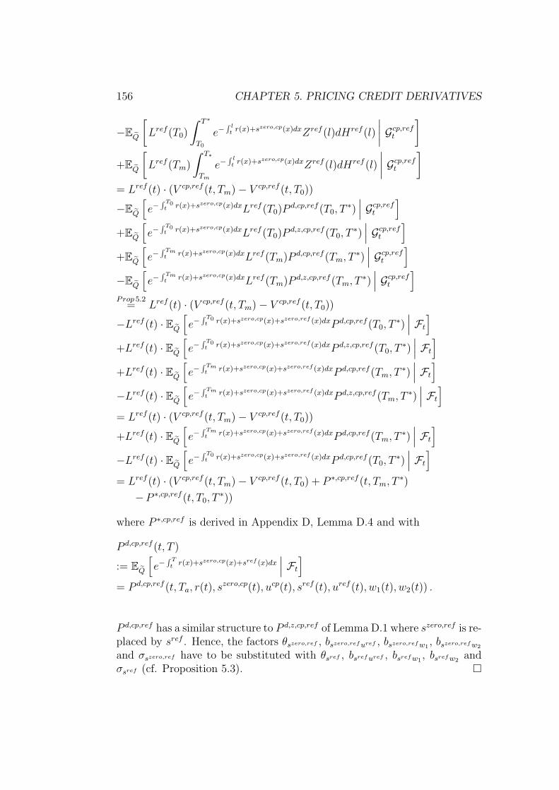
156 CHAPTER 5. PRICING CREDIT DERIVATIVES
−EQ
[Lref (T0)
∫ T ∗
T0
e−∫ l
tr(x)+szero,cp(x)dxZref (l)dHref (l)
∣∣∣∣ Gcp,reft
]
+EQ
[Lref (Tm)
∫ T∗
Tm
e−∫ l
tr(x)+szero,cp(x)dxZref (l)dHref (l)
∣∣∣∣ Gcp,reft
]
= Lref (t) · (V cp,ref (t, Tm) − V cp,ref (t, T0))
−EQ
[e−
∫ T0t r(x)+szero,cp(x)dxLref (T0)P
d,cp,ref (T0, T∗)∣∣∣ Gcp,ref
t
]
+EQ
[e−
∫ T0t r(x)+szero,cp(x)dxLref (T0)P
d,z,cp,ref (T0, T∗)∣∣∣ Gcp,ref
t
]
+EQ
[e−
∫ Tmt
r(x)+szero,cp(x)dxLref (Tm)P d,cp,ref (Tm, T ∗)∣∣∣ Gcp,ref
t
]
−EQ
[e−
∫ Tmt
r(x)+szero,cp(x)dxLref (Tm)P d,z,cp,ref (Tm, T ∗)∣∣∣ Gcp,ref
t
]
Prop 5.2= Lref (t) · (V cp,ref (t, Tm) − V cp,ref (t, T0))
−Lref (t) · EQ
[e−
∫ T0t r(x)+szero,cp(x)+szero,ref (x)dxP d,cp,ref (T0, T
∗)∣∣∣ Ft
]
+Lref (t) · EQ
[e−
∫ T0t r(x)+szero,cp(x)+szero,ref (x)dxP d,z,cp,ref (T0, T
∗)∣∣∣ Ft
]
+Lref (t) · EQ
[e−
∫ Tmt
r(x)+szero,cp(x)+szero,ref (x)dxP d,cp,ref (Tm, T ∗)∣∣∣ Ft
]
−Lref (t) · EQ
[e−
∫ Tmt
r(x)+szero,cp(x)+szero,ref (x)dxP d,z,cp,ref (Tm, T ∗)∣∣∣ Ft
]
= Lref (t) · (V cp,ref (t, Tm) − V cp,ref (t, T0))
+Lref (t) · EQ
[e−
∫ Tmt
r(x)+szero,cp(x)+szero,ref (x)dxP d,cp,ref (Tm, T ∗)∣∣∣ Ft
]
−Lref (t) · EQ
[e−
∫ T0t r(x)+szero,cp(x)+szero,ref (x)dxP d,cp,ref (T0, T
∗)∣∣∣ Ft
]
= Lref (t) · (V cp,ref (t, Tm) − V cp,ref (t, T0) + P ∗,cp,ref (t, Tm, T ∗)
−P ∗,cp,ref (t, T0, T∗))
where P ∗,cp,ref is derived in Appendix D, Lemma D.4 and with
P d,cp,ref (t, T )
:= EQ
[e−
∫ Tt
r(x)+szero,cp(x)+sref (x)dx∣∣∣ Ft
]
= P d,cp,ref (t, Ta, r(t), szero,cp(t), ucp(t), sref (t), uref (t), w1(t), w2(t)) .
P d,cp,ref has a similar structure to P d,z,cp,ref of Lemma D.1 where szero,ref is re-placed by sref . Hence, the factors θszero,ref , bszero,ref uref , bszero,ref w1
, bszero,ref w2
and σszero,ref have to be substituted with θsref , bsref uref , bsref w1, bsref w2
andσsref (cf. Proposition 5.3).

CHAPTER 5. PRICING CREDIT DERIVATIVES 157
It is remarkable that by incorporating unilateral counterparty risk, we main-tain the closed form of the FCDS spread formulas.In a second step, this approach can be further extended in order to accountalso for the risk of default for the third party involved in a FCDS contract.
5.5 Credit Default Swaption
In this section we aim to price the optionality to enter into a CDS (calledCredit Default Swaption or CDS Option) by means of an analytical formulawhile staying within our framework.Alfonsi & Brigo (2005) also introduce an analytical formula for CDS optionsbut under a CIR intensity framework with a deterministic short rate. In thissimplified framework, they can use a variant of Jamshidian’s decomposition(cf. Jamshidian (1989)) in order to obtain the result. Additionally, theymention but do not further present a possible way to price a CDS optionwhen the short rate also follows a CIR process. According to them, thiscould be done by mapping the two-dimensional CIR process ”in an analo-gous tractable two-dimensional Gaussian dynamics that preserves as muchas possible of the original CIR structure”. This, however, again underlinesthe beauty of our Gaussian framework: the analytical tractability. Brigo& El-Bachir (2010) propose an extension of the work of Alfonsi & Brigo(2005) by using a shifted square-root jump-diffusion model which yields asemi-analytical formula.Schoenbucher (2000) introduces a credit risk model based on the LIBORmarket model using processes for the effective default-free forward rates andeffective forward credit spreads. Within this framework an approximate so-lution for CDS options exists. By changing to a swap-based market model,he shows that an exact formula for CDS options exists. More details to themethods used in this article can be found in Schoenbucher (2003).In their paper, Krekel & Wenzel (2006) implement Schoenbucher’s originalmodel for pricing Credit Default Swaptions and Constant Maturity CreditDefault Swaps (see also next section) with Monte Carlo simulation. In ad-dition, they use closed-form solutions derived by Schoenbucher (2003) andBrigo (2005) as control variates in order to increase accuracy. Furthermore,they present a new closed-form solution for CDS options allowing for timevarying volatilities and decorrelated discrete default intensities.

158 CHAPTER 5. PRICING CREDIT DERIVATIVES
Definition 5.32 Credit Default SwaptionA (payer) Credit Default Swaption (CDS Option) gives its holder the right to
enter a CDS at time T0 with swap rate S. In exchange for premiums paid atT1, . . . , Tm or until default, this CDS makes a protection payment if defaultoccurs in [T0, Tm].
The value of a European style CDS Option, where the option expires at Tand the swap starts at T0, is given by:
EQ
[e−
∫ Tt
r(l)dlL(T )EQ
[L(T0)
(∫ Tm
T0
e−∫ u
T0r(l)dl
(1 − Z(u))dH(u)
−Sm∑
i=1
e−∫ Ti
T0r(l)dlL(Ti)
)+∣∣∣∣∣GT
]∣∣∣∣∣Gt
]
= EQ
[e−
∫ Tt
r(l)dlL(T )EQ
[L(T0)
(s(T0, T0, Tm)
m∑
i=1
e−∫ Ti
T0r(l)dlL(Ti)
−S
m∑
i=1
e−∫ Ti
T0r(l)dlL(Ti)
)+∣∣∣∣∣GT
]∣∣∣∣∣Gt
]
= EQ
e−∫ T
tr(l)dlL(T0)
(s(T0, T0, Tm) − S
)+m∑
i=1
e−∫ Ti
T0r(l)dlL(Ti)
︸ ︷︷ ︸E
Q
[∑m
i=1 e−∫ TiT0
r(l)dlL(Ti)
∣∣∣∣∣GT0
]
∣∣∣∣∣∣∣∣∣∣∣∣∣∣
Gt
= EQ
[e−
∫ Tt
r(l)dlL(T0)(s(T0, T0, Tm) − S
)+m∑
i=1
P d,zero(T0, Ti)
∣∣∣∣∣Gt
]
Prop.5.2= L(t)· EQ
[e−
∫ Tt
r(l)dl−∫ T0
t szero(l)dl(s(T0, T0, Tm) − S
)+m∑
i=1
P d,zero(T0, Ti)
∣∣∣∣∣Ft
]
= L(t) · V cdso(t, T, T0, Tm) .
If the option maturity coincides with the beginning of the swap (i.e. T = T0),the value of a European style CDS Option simplifies to
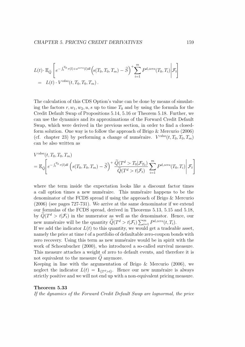
CHAPTER 5. PRICING CREDIT DERIVATIVES 159
L(t)· EQ
[e−
∫ T0t r(l)+szero(l)dl
(s(T0, T0, Tm) − S
)+m∑
i=1
P d,zero(T0, Ti)
∣∣∣∣∣Ft
]
= L(t) · V cdso(t, T0, T0, Tm) .
The calculation of this CDS Option’s value can be done by means of simulat-ing the factors r, w1, w2, u, s up to time T0 and by using the formula for theCredit Default Swap of Propositions 5.14, 5.16 or Theorem 5.18. Further, wecan use the dynamics and its approximations of the Forward Credit DefaultSwap, which were derived in the previous section, in order to find a closed-form solution. One way is to follow the approach of Brigo & Mercurio (2006)(cf. chapter 23) by performing a change of numeraire. V cdso(t, T0, T0, Tm)can be also written as
V cdso(t, T0, T0, Tm)
= EQ
[e−
∫ T0t r(l)dl
(s(T0, T0, Tm) − S
)+ Q(T d > T0|FT0)
Q(T d > t|Ft)
m∑
i=1
P d,zero(T0, Ti)
∣∣∣∣∣Ft
]
where the term inside the expectation looks like a discount factor timesa call option times a new numeraire. This numeraire happens to be thedenominator of the FCDS spread if using the approach of Brigo & Mercurio(2006) (see pages 727-731). We arrive at the same denominator if we extendour formulas of the FCDS spread, derived in Theorems 5.13, 5.15 and 5.18,by Q(T d > t|Ft) in the numerator as well as the denominator. Hence, our
new numeraire will be the quantity Q(T d > t|Ft)∑m
i=1 P d,zero(t, Ti).If we add the indicator L(t) to this quantity, we would get a tradeable asset,namely the price at time t of a portfolio of defaultable zero-coupon bonds withzero recovery. Using this term as new numeraire would be in spirit with thework of Schoenbucher (2000), who introduced a so-called survival measure.This measure attaches a weight of zero to default events, and therefore it isnot equivalent to the measure Q anymore.Keeping in line with the argumentation of Brigo & Mercurio (2006), weneglect the indicator L(t) = 1T d>t. Hence our new numeraire is alwaysstrictly positive and we will not end up with a non-equivalent pricing measure.
Theorem 5.33If the dynamics of the Forward Credit Default Swap are lognormal, the price

160 CHAPTER 5. PRICING CREDIT DERIVATIVES
at time t of a Credit Default Swaption is given by the formula
L(t) ·m∑
i=1
P d,zero(t, Ti)(s(t, T0, Tm) · N (d1) − S · N (d2)) ,
with
d1 :=ln(
s(t,T0,Tm)
S
)+ 1
2σ2
Y
σY
, d2 := d1 − σY ,
and
σY = σY (t, T0) :=
√∫ T0
t
σ2(s)ds .
N denotes the standard normal cumulative distribution function.
Proof:The price of a CDS Option where the swap starts at the maturity of theoption is L(t) · V cdso(t, T0, T0, Tm) with
V cdso(t, T0, T0, Tm)
= EQ
[e−
∫ T0t r(l)dl
(s(T0, T0, Tm) − S
)+ Q(T d > T0|FT0)
Q(T d > t|Ft)
m∑
i=1
P d,zero(T0, Ti)
∣∣∣∣∣Ft
].
The Radon-Nikodym derivative (cf. Theorem 2.19 and Theorem 2.22) defin-
ing the new measure Q0,m is given by
dQ0,m
dQ
∣∣∣∣∣Ft
=Q(T d > t|Ft)
∑mi=1 P d,zero(t, Ti) · P0(t0)
Q(T d > t0|Ft0)∑m
i=1 P d,zero(t0, Ti) · P0(t)t0 < t < Ti ∀i,
with P0 being the non-defaultable cash account (see Chapter 4). The numer-ator of the FCDS spread s(t, T0, Tm) is the value of the protection leg. Thisvalue can be seen as the price of a CDS where the premium is paid upfront.Therefore, we can interpret the FCDS spread as a ratio between a tradeableasset and our numeraire. Further, the FCDS spread is a martingale underthis numeraire’s measure.The change of numeraire yields
V cdso(t, T0, T0, Tm)
=m∑
i=1
P d,zero(t, Ti)EQ0,m
[(s(T0, T0, Tm) − S
)+∣∣∣∣Ft
]

CHAPTER 5. PRICING CREDIT DERIVATIVES 161
Since we assume the FCDS spread to be lognormal under Q with σ(t) beingprogessively measurable and satisfying the Novikov condition (cf. Theorem2.19), the FCDS spread follows a driftless geometric Brownian motion under
the new measure Q0,m (ds(t, T0, Tm) = s(t, T0, Tm)σ(t)dW ). Hence, we getby means of a variant of Black’s formula (cf. Theorem 2.25) the price of aCDS Option at time t
L(t) · V cdso(t, T0, T0, Tm)
= L(t) ·m∑
i=1
P d,zero(t, Ti)(s(t, T0, Tm) · N (d1) − S · N (d2)) ,
with
d1 :=ln(
s(t,T0,Tm)
S
)+ 1
2σ2
Y
σY
, d2 := d1 − σY ,
and
σY = σY (t, T0) :=
√∫ T0
t
σ2(s)ds .
N denotes the standard normal cumulative distribution function.
Theorem 5.34The price of a Payer Credit Default Swaption in the SZ4 framework (cf.Model 4.4) at time t is approximately given by Theorem 5.33
(a) with s(t, T0, Tm) determined by Theorem 5.13, Theorem 5.15 or The-orem 5.18 and
σY (t, T0) =(∫ T0
t
(σrB
d,zero(x, y) +σr∑
i P d,z(x)∑m
i=1 P d,zero(x, Ti)
)2
+
(σszeroCd,zero(x, y) +
σszero∑i P d,z(x)
∑mi=1 P d,zero(x, Ti)
)2
+
(σuD
d,zero(x, y) +σu∑
i P d,z(x)∑m
i=1 P d,zero(x, Ti)
)2
+
(σw1E
d,zero1 (x, y) +
σw1∑i P d,z(x)
∑mi=1 P d,zero(x, Ti)
)2
dx
) 12

162 CHAPTER 5. PRICING CREDIT DERIVATIVES
where y ∈ [T0, Tm], if the dynamics of the FCDS evolve according to thelognormal approximations of Assumption 5.26. The factors r, szero, u, w1,which are input for σY (t, T0), are frozen at time t.
(b) where in the Theorem’s formula s(t, T0, Tm) is replaced bys(t, T0, Tm)−(1−Z)∆TiK, derived according to Theorem 5.15. Further,
the strike S is substituted by S − (1 − Z)∆TiK and σY is given by
σY (t, T0) =
(∫ T0
t
(~σ∑
i P d,z(x))′ (
~σ∑i P d,z(x)
)
(∑m
i=1 P d,zero(x, Ti))2 dx
) 12
,
if the dynamics of the FCDS evolve according to the shifted-lognormalapproximation of Assumption 5.28. The factors r, szero, u, w1, whichare input for σY (t, T0), are frozen at time t.
Proof:
(a) We show the application of Theorem 5.33 in case of Theorem 5.13and the lognormal approximation of the FCDS spread’s dynamics ofAssumption 5.26. The theorem is analogously applied in case of theFCDS spread being derived by Theorem 5.15 or Theorem 5.18.As mentioned in the proof of Theorem 5.33, we regard the FCDS spreadas a martingale under the measure Q0,m. Hence, the lognormal dynam-
ics under the measure Q are transformed by the change of numeraireto the driftless dynamics
ds(t, T0, Tm) =
−((
σrBd,zero(t, y), σszeroCd,zero(t, y), σuD
d,zero(t, y), σw1Ed,zero1 (t, y)
)
+
(~σ∑
i P d,z(t))′
∑mi=1 P d,zero(t, Ti)
)s(t, T0, Tm)dW (t) ,
with y ∈ [T0, Tm].
In the SZ4 framework W (t) is a four-dimensional vector consisting of
(Wr(t), Ww1(t), Wu(t), Ws(t))′. We simplify the above dynamics by re-
placing the four-dimensional W (t) with a one-dimensional one, W∗(t),such that we preserve the variance of the process:
ds(t, T0, Tm) = σ∗(t)s(t, T0, Tm)dW∗(t) ,

CHAPTER 5. PRICING CREDIT DERIVATIVES 163
where
σ∗(t) =((
σrBd,zero(t, y) +
σr∑i P d,z(t)∑m
i=1 P d,zero(t, Ti)
)2
+
(σszeroCd,zero(t, y) +
σszero∑i P d,z(t)∑m
i=1 P d,zero(t, Ti)
)2
+
(σuD
d,zero(t, y) +σu∑
i P d,z(t)∑mi=1 P d,zero(t, Ti)
)2
+
(σw1E
d,zero1 (t, y) +
σw1∑i P d,z(t)∑m
i=1 P d,zero(t, Ti)
)2) 12
.
Freezing the factors r, szero, u, w1 at time t and inserting the above intothe formula of Theorem 5.33 will yield the stated result.
(b) If the FCDS spread dynamics evolve according to the shifted-lognormalapproximation of the pages 137ff, we end up again with driftless dy-namics after changing the numeraire. Under the new measure Q0,m thespread’s dynamics are
ds(t, T0, Tm) = −(~σ∑
i P d,z(t))′
∑mi=1 P d,zero(t, Ti)
(s(t, T0, Tm)−(1−Z)∆TiK
)dW (t) ,
with K being a constant and ∆Ti being the equidistant interval be-tween spread payments.As done above, we freeze the factors r, szero, u, w1 at time t and re-place the four-dimensional vector W (t) with the one-dimensional W∗(t).Hence, the dynamics are
ds(t, T0, Tm) =√√√√(~σ∑
i P d,z(t))′ (
~σ∑i P d,z(t)
)
(∑m
i=1 P d,zero(t, Ti))2
(s(t, T0, Tm) − (1 − Z)∆TiK
)dW∗(t) .
The spread s(t, T0, Tm) can also be written as
s(t, T0, Tm) = X(t) + (1 − Z)∆TiK
with
dX(t) =
√√√√(~σ∑
i P d,z(t))′ (
~σ∑i P d,z(t)
)
(∑m
i=1 P d,zero(t, Ti))2 X(t)dW∗(t) .

164 CHAPTER 5. PRICING CREDIT DERIVATIVES
Therefore, the price of the Credit Default Swaption equalsL(t) · V cdso(t, T0, T0, Tm) with
V cdso(t, T0, T0, Tm)
=m∑
i=1
P d,zero(t, Ti)EQ0,m
[(s(T0, T0, Tm) − S
)+∣∣∣∣Ft
]
=m∑
i=1
P d,zero(t, Ti)EQ0,m
[(X(T0) − (S − (1 − Z)∆TiK)
)+∣∣∣∣Ft
].
Applying Theorem 5.33 for the process X(t) and the strike
S − (1 − Z)∆TiK, we obtain the pricing formula.
As before, we want to analyze how well the proposed approximated dynam-ics of the FCDS spread work as opposed to the full simulation of the factorsr, s, u, w1. The study is based again on the parameters called GDPr for therating class A2 of Chapter 4 with z = 0.9 and Z = 0.75. Since the approx-imated lognormal dynamics yield equal results in Section 5.4 no matter whichrecovery assumptions are made, we restrict ourselves to the dynamics withrecovery of face value of Proposition 5.24 and Assumption 5.26 in order tocompare it with the shifted-lognormal dynamics of Assumption 5.28 and theresults obtained via simulation of all factors based on 20,000 scenarios.Table 5.1 outlines the present value of a CDS Option with strike 0.7%, ex-piring in 1 year and written on a CDS running for 5 more years if the valuesfor σszero differ. For small and moderate values of σszero the formula basedon the lognormal dynamics of Theorem 5.34 (a) yields similar results as theformula based on the shifted-lognormal dynamics of Theorem 5.34 (b) sincethe difference to the simulation results are for both approaches within a fewbasis points. But for increasing values of σszero the differences between thelognormal based formula and the simulation (column 5) grow substantially,whereas the differences of the formula assuming shifted-lognormal dynamicsto the simulation (columns 6) also increase but much slower. Therefore, forsmall values of σszero we can recommend the usage of both pricing formulas ofCDS Options and for increasing values of σszero the formula based on shifted-lognormal dynamics still yields promising results. But for higher values ofσszero we advise the usage of a full simulation.

CHAPTER 5. PRICING CREDIT DERIVATIVES 165
Table 5.2 contains the present value of a CDS Option for different strikesand different expiries (0.25, 0.75 and 1 year). The underlying CDS of theoption is again supposed to run for five years. As in the analysis of the FCDSspreads of Section 5.4, the results based on the shifted-lognormal dynamicsare not dependent on the forward starting time of the credit default swaprespectively option expiry. However, the difference of the results of Theorem5.34 (a) to the simulation get bigger for longer option expiries especially ifthe strike is chosen such that the option is on the border of being out ofthe money. Again, we can conclude that both approximations work well foroptions that are in the money. For options not deep in the money and witha longer time period until expiry, we again prefer the usage of the formulabased on the shifted-lognormal dynamics.
σszero Formula (a) Formula (b) Simulation Difference (a) Difference (b)
0.01 6.26% 6.26% 6.23% -0.03% -0.03%0.05 6.15% 6.15% 6.17% 0.02% 0.02%0.09 5.90% 5.91% 5.94% 0.03% 0.02%0.13 5.50% 5.54% 5.56% 0.06% 0.02%0.15 5.24% 5.31% 5.37% 0.13% 0.06%0.17 4.93% 5.06% 5.16% 0.23% 0.10%0.19 4.57% 4.79% 4.89% 0.33% 0.10%0.20 4.37% 4.65% 4.79% 0.42% 0.14%0.30 1.81% 3.30% 3.59% 1.77% 0.28%0.40 0.06% 2.13% 2.44% 2.38% 0.31%
Table 5.1: Present values of CDS Options for different values of σszero (column1), expiring in 1 year and written on a CDS running for 5 years. The pricesare calculated by formula of Theorem 5.34 (a) (column 2) and (b) (column 3)and via simulation of factors r, s, u, w1 (column 4) assuming a strike of 0.7%.Column 5 and 6 contain the differences of the results obtained by formula(column 2 and 3) to the simulation results (column 4).

166 CHAPTER 5. PRICING CREDIT DERIVATIVES
Strike Formula (a) Formula (b) Simulation Difference (a) Difference (b)
Expiry 0.25Y0.1% 12.45% 12.45% 12.45% 0.00% 0.00%0.3% 10.12% 10.12% 10.13% -0.01% -0.01%0.5% 7.79% 7.79% 7.81% -0.02% -0.02%0.7% 5.46% 5.46% 5.50% -0.03% -0.03%0.9% 3.13% 3.16% 3.21% -0.08% -0.06%1.1% 0.86% 1.18% 1.27% -0.41% -0.09%1.3% 0.01% 0.21% 0.25% -0.24% -0.04%1.5% 0.00% 0.02% 0.02% -0.02% 0.00%1.7% 0.00% 0.00% 0.00% 0.00% 0.00%
Expiry 0.75Y0.1% 12.07% 12.07% 12.05% 0.02% 0.02%0.3% 10.00% 10.00% 9.99% 0.01% 0.01%0.5% 7.93% 7.93% 7.94% 0.00% 0.00%0.7% 5.87% 5.87% 5.90% -0.03% -0.03%0.9% 3.80% 3.87% 3.94% -0.14% -0.07%1.1% 1.77% 2.14% 2.24% -0.47% -0.10%1.3% 0.36% 0.94% 1.01% -0.65% -0.07%1.5% 0.02% 0.33% 0.34% -0.32% -0.02%1.7% 0.00% 0.09% 0.08% -0.08% 0.01%
Expiry 1.00Y0.1% 11.71% 11.71% 11.67% 0.04% 0.04%0.3% 9.77% 9.77% 9.74% 0.03% 0.03%0.5% 7.83% 7.83% 7.81% 0.02% 0.02%0.7% 5.88% 5.89% 5.90% -0.02% -0.01%0.9% 3.94% 4.02% 4.09% -0.15% -0.06%1.1% 2.03% 2.39% 2.49% -0.46% -0.10%1.3% 0.58% 1.21% 1.29% -0.71% -0.08%1.5% 0.07% 0.51% 0.54% -0.47% -0.02%1.7% 0.00% 0.19% 0.18% -0.17% 0.01%
Table 5.2: Present values of CDS Options for different strikes (column 1),expiring in 0.25, 0.75 and 1 year and written on a CDS running for 5 years.The prices are calculated by formula of Theorem 5.34 (a) (column 2) and(b) (column 3) and via simulation of factors r, s, u, w1 (column 4). Column5 and 6 contain the differences of the results obtained by formula (column 2and 3) to the simulation results (column 4).

CHAPTER 5. PRICING CREDIT DERIVATIVES 167
If the CDS Option expires before the swap starts, i.e. T < T0, we getan additional term in the expected value, namely
V cdso(t, T, T0, Tm) =
EQ
[e−
∫ T0t r(l)+szero(l)dle+
∫ T0T
r(l)dl(s(T0, T0, Tm) − S
)+m∑
i=1
P d,zero(T0, Ti)
∣∣∣∣∣Ft
].
Theorem 5.35The price of a Payer Credit Default Swaption, where the option’s expiry doesnot coincide with the start of the swap, is given by
L(t) · V cdso(t, T, T0, Tm) =
L(t) ·m∑
i=1
P d,zero(t, Ti)
·(
Y s0 N
ln(
Y s(t)
Y S(t)
)+ µY s(t, T0) − µY S(t, T0) + 1
2σ2
+(T0)√
σ2+(T0)
−Y S0 N
ln(
Y s(t)
Y S(t)
)+ µY s(t, T0) − µY S(t, T0) − 1
2σ2
+(T0)√
σ2+(T0)
)
in the SZ4 framework (cf. Model 4.4), where the terms in the above for-mula are defined in the proof. N denotes the standard normal cumulativedistribution function.
Proof:By the change of numeraire we obtain for the price of a Credit DefaultSwaption
L(t) · V cdso(t, T, T0, Tm) =
L(t) ·m∑
i=1
P d,zero(t, Ti)EQ0,m
[e+
∫ T0T
r(l)dl(s(T0, T0, Tm) − S
)+∣∣∣∣Ft
].
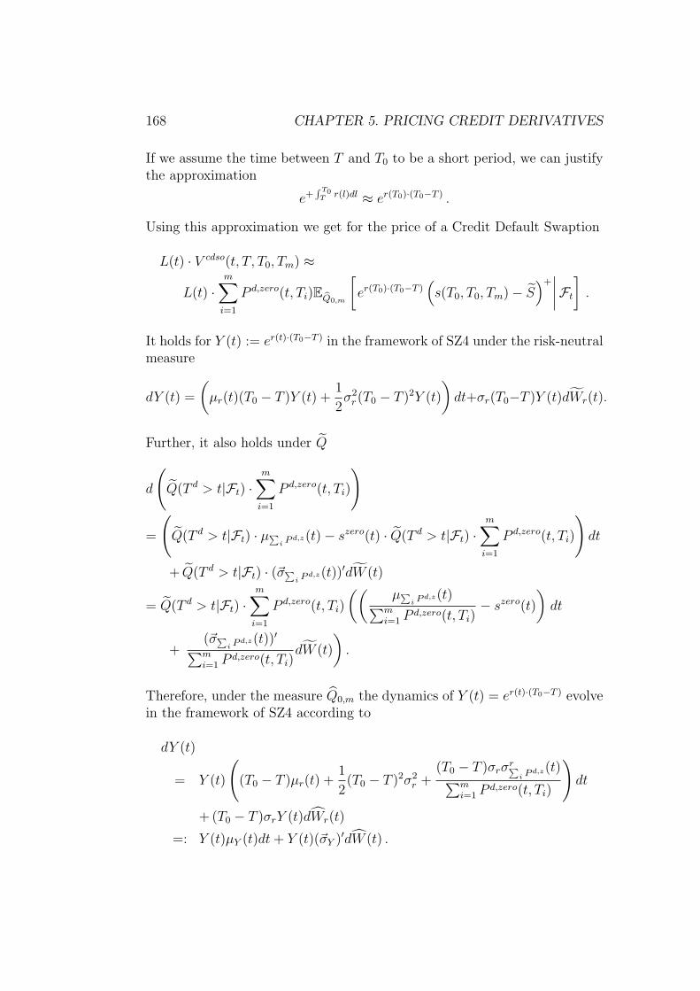
168 CHAPTER 5. PRICING CREDIT DERIVATIVES
If we assume the time between T and T0 to be a short period, we can justifythe approximation
e+∫ T0
Tr(l)dl ≈ er(T0)·(T0−T ) .
Using this approximation we get for the price of a Credit Default Swaption
L(t) · V cdso(t, T, T0, Tm) ≈
L(t) ·m∑
i=1
P d,zero(t, Ti)EQ0,m
[er(T0)·(T0−T )
(s(T0, T0, Tm) − S
)+∣∣∣∣Ft
].
It holds for Y (t) := er(t)·(T0−T ) in the framework of SZ4 under the risk-neutralmeasure
dY (t) =
(µr(t)(T0 − T )Y (t) +
1
2σ2
r(T0 − T )2Y (t)
)dt+σr(T0−T )Y (t)dWr(t).
Further, it also holds under Q
d
(Q(T d > t|Ft) ·
m∑
i=1
P d,zero(t, Ti)
)
=
(Q(T d > t|Ft) · µ∑
i P d,z(t) − szero(t) · Q(T d > t|Ft) ·m∑
i=1
P d,zero(t, Ti)
)dt
+ Q(T d > t|Ft) · (~σ∑i P d,z(t))′dW (t)
= Q(T d > t|Ft) ·m∑
i=1
P d,zero(t, Ti)
((µ∑
i P d,z(t)∑mi=1 P d,zero(t, Ti)
− szero(t)
)dt
+(~σ∑
i P d,z(t))′∑mi=1 P d,zero(t, Ti)
dW (t)
).
Therefore, under the measure Q0,m the dynamics of Y (t) = er(t)·(T0−T ) evolvein the framework of SZ4 according to
dY (t)
= Y (t)
((T0 − T )µr(t) +
1
2(T0 − T )2σ2
r +(T0 − T )σrσ
r∑i P d,z(t)∑m
i=1 P d,zero(t, Ti)
)dt
+ (T0 − T )σrY (t)dWr(t)
=: Y (t)µY (t)dt + Y (t)(~σY )′dW (t) .

CHAPTER 5. PRICING CREDIT DERIVATIVES 169
Combining the process Y (t) with s(t, T0, Tm) and S yields two new processes
Y s(t) and Y S(t) with the following dynamics under the measure Q0,m
dY S(t) = d(Y (t) · S)
= SdY (t)
dY s(t) = d(Y (t) · s(t, T0, Tm))
= s(t, T0, Tm)dY (t) + Y (t)ds(t, T0, Tm) + d 〈Y (t), s(t, T0, Tm)〉=
(µY (t)dt + ( ~σY )′dW (t)
)s(t, T0, Tm)Y (t)
−((
σrBd,zero(t, y), σszeroCd,zero(t, y), σuD
d,zero(t, y), σw1Ed,zero1 (t, y)
)
+
(~σ∑
i P d,z(t))′
∑mi=1 P d,zero(t, Ti)
)s(t, T0, Tm)Y (t)dW (t)
− (T0 − T )σr
(σr∑
i P d,z(t)∑mi=1 P d,zero(t, Ti)
+ σrBd,zero(t, y)
)s(t, T0, Tm)Y (t)dt
=: s(t, T0, Tm)Y (t)µY s(t)dt + s(t, T0, Tm)Y (t)(~σY s(t))′dW (t)
= Y s(t)(µY s(t)dt + (~σY s(t))′dW (t)
)
where s(t, T0, Tm) is a driftless lognormal process (cf. proof (a) of Theorem5.34) and y ∈ [T0, Tm].If we freeze all stochastic terms of r, szero, u, w1 at time t - as we have alreadydone before for the spread s(t, T0, Tm) - in order to obtain a deterministic
drift, both processes, Y S(t) and Y s(t), are geometric Brownian motions withdeterministic drift and volatility.We are left to solve
EQ0,m
[(Y s(T0) − Y S(T0)
)+∣∣∣∣Ft
],
which looks like some sort of exchange option, for which e.g. Margrabe (1978)and Fischer (1978) proposed closed-form solutions. A more general proof canbe found in Li (2008) (see e.g. Proposition 1 on page 6) which we make use of.
Again, we replace the four-dimensional process dW (t) with a one-dimensional,such that
dY S(t) = SY (t)(µY (t)dt + (T0 − T )σrdW 1∗ (t))
= Y S(t)(µY (t)dt + (T0 − T )σrdW 1∗ (t))
dY s(t) = s(t, T0, Tm)Y (t)(µY s(t)dt +√
(~σY s(t))′~σY s(t)dW 2∗ (t))
= Y s(t)(µY s(t)dt +√
(~σY s(t))′~σY s(t)dW 2∗ (t))

170 CHAPTER 5. PRICING CREDIT DERIVATIVES
Further, we assume ρ to be the correlation between Y s and Y S. With
Y s0 := EQ0,m
[Y s(T0)| Ft] = Y s(t)e∫ T0
t µY s (x)dx ,
Y S0 := EQ0,m
[Y S(T0)
∣∣∣Ft
]= Y S(t)e
∫ T0t µY (x)dx ,
µY s(t, T0) :=
∫ T0
t
µY s(x)dx ,
µY S(t, T0) :=
∫ T0
t
µY (x)dx ,
σ2Y s(t, T0) :=
∫ T0
t
(~σY s(x))′~σY s(x)dx ,
σ2
Y S(t, T0) := (σr(T0 − T ))2(T0 − t) ,
σ2+(T0) := σ2
Y s(t, T0) + σ2
Y S(t, T0) + 2ρ
√σ2
Y s(t, T0)√
σ2
Y S(t, T0)
we obtain
EQ0,m
[(Y s(T0) − Y S(T0)
)+∣∣∣∣Ft
]
= Y s0 N
ln(
Y s(t)
Y S(t)
)+ µY s(t, T0) − µ
Y S(t, T0) + 12σ2
+(T0)√
σ2+(T0)
−Y S0 N
ln(
Y s(t)
Y S(t)
)+ µY s(t, T0) − µY S(t, T0) − 1
2σ2
+(T0)√
σ2+(T0)
5.5.1 Big Bang/Small Bang
In 2009 new standards for CDS were introduced. The so-called CDS BigBang (see Markit (2009a)) proposes global changes in CDS contracts as wellas quoting changes for single name CDS in the North American market. Sim-ilarly, the CDS Small Bang (see Markit (2009b)) extends the CDS Big Bangto European corporate and sovereign CDS markets. In addition to that,Markit (2009c) provides forthcoming standards for corporate and sovereignCDS markets in Australia, New Zealand, Japan and for Emerging Markets.Those standards are in favour of an upfront payment instead of quoting the

CHAPTER 5. PRICING CREDIT DERIVATIVES 171
spread which makes the CDS zero at initiation (par spread). The spreadpayments are fixed at a certain level which is e.g. 100 or 500 basis points perannum for North America, and 25, 100, 500 or 1000 basis points for Europe(plus some additional spreads at 300 and 750 bp).Reasons for the convention changes are that the market seeks for a stand-ardization in CDS contracts which would lead to a simplified processing oftrades and to a netting of offsetting CDS positions. Since investors prefer asmall upfront payment and wish to recoupon their existing trades by usingthe fixed coupons, several coupon options are permitted (cf. the Europeancase of 25, 100, 500 and 1000 bp). But in order to standardize the contractsthe number of possible coupons is limited.
Therefore, under the newly introduced CDS standards, the payoff of a CDSOption depends on the dynamics of the upfront payment. I.e. it holds for aEuropean option where the option’s maturity coincides with the start of theCDS
EQ
[e−
∫ T0t r(l)dlL(T0)
(∫ Tm
T0
e−∫ u
T0r(l)dl
(1 − Z(u))dH(u)
−Puf − S
m∑
i=1
e−∫ Ti
T0r(l)dlL(Ti)
)+∣∣∣∣∣Gt
]
= EQ
[e−
∫ T0t r(l)dlL(T0)
(Puf (T0, T0, Tm) + S
m∑
i=1
e−∫ Ti
T0r(l)dl
−Puf − Sm∑
i=1
e−∫ Ti
T0r(l)dlL(Ti)
)+∣∣∣∣∣Gt
]
= EQ
[e−
∫ T0t r(l)dlL(T0)
(Puf (T0, T0, Tm) − Puf
)+∣∣∣∣Gt
]
Prop.5.2= L(t)EQ
[e−
∫ T0t r(l)+szero(l)dl
(Puf (T0, T0, Tm) − Puf
)+∣∣∣∣Ft
]
= L(t) · V ufcdso(t, T0, T0, Tm) .
with Puf being the fixed contractual upfront payment due at T0 andPuf (t, T0, Tm) denoting the upfront payment at time t of a CDS starting atT0 with the same spread and payment days of the contract.The value of the upfront payment at time t is the difference between the

172 CHAPTER 5. PRICING CREDIT DERIVATIVES
protection leg and the payment leg (cf. definition of FCDS in Section 5.4):
Puf (t, T0, Tm)
= EQ
[e−
∫ T0t r(l)dlL(T0)
∫ Tm
T0
e−∫ l
T0r(x)dx
(1 − Z(l))dH(l)
∣∣∣∣ Gt
]
−EQ
[S
m∑
i=1
e−∫ Ti
t r(l)dlL(Ti)
∣∣∣∣∣ Gt
]
= L(t) ·(
V dpT d (t, T0, Tm, T ∗) − S
m∑
i=1
P d,zero(t, Ti)
).
For L(t) = 1 we obtain the dynamics of the upfront payment
dPuf (t, T0, Tm)
= d(V dp
T d (t, T0, Tm, T ∗))− d
(S
m∑
i=1
P d,zero(t, Ti)
)
= (r(t) + szero(t)) · Puf (t, T0, Tm)dt
+ (~σV ddp(t, Tm) − ~σV ddp(t, T0) + ~σP d∗(t, Tm, T ∗) − ~σP d∗(t, T0, T∗)
− S · ~σ∑i P d,z(t))′dW (t)
with results of the proof of Theorem 5.19 (i)-(iii).If we pose ourselves in the framework of SZ4 (cf. Model 4.4) and followthe approximations of the pages 126ff we obtain lognormal dynamics for theupfront payment Puf (t, T0, Tm), i.e. we assume for the components of thevector ~σP d∗(t, Tm, T ∗) − ~σP d∗(t, T0, T
∗)
σuP d∗(t, Tm, T ∗) − σu
P d∗(t, T0, T∗)
≈ −σuDd,zero(t, y)(P d∗(t, Tm, T ∗) − P d∗(t, T0, T
∗)) ,
(r,s and w1 analogously) and for components of the vector ~σV ddp(t, Tm) −~σV ddp(t, T0)
σuV ddp(t, Tm) − σu
V ddp(t, T0)
≈ −σuDd,zero(t, y)(V ddp
T d (t, Tm) − V ddpT d (t, T0)) ,

CHAPTER 5. PRICING CREDIT DERIVATIVES 173
(s,u and w1 analogously). Hence, we get with
~σV ddp(t, Tm) − ~σV ddp(t, T0) + ~σP d∗(t, Tm, T ∗) − ~σP d∗(t, T0, T∗)
≈ −(σrB
d,zero(t, y), σszeroCd,zero(t, y), σuDd,zero(t, y), σw1E
d,zero1 (t, y)
)
· (V ddpT d (t, Tm) − V ddp
T d (t, T0) + P d∗(t, Tm, T ∗) − P d∗(t, T0, T∗))︸ ︷︷ ︸
V dp
Td(t,T0,Tm,T ∗)
dPuf (t, T0, Tm)
≈ (r(t) + szero(t)) · Puf (t, T0, Tm)dt
+
(−(σrB
d,zero(t, y), σszeroCd,zero(t, y), σuDd,zero(t, y), σw1E
d,zero1 (t, y)
)′
·V dpT d (t, T0, Tm, T ∗) − S · ~σ∑
i P d,z(t)
)′
dW (t)
= (r(t) + szero(t)) · Puf (t, T0, Tm)dt
+
(−(σrB
d,zero(t, y), σszeroCd,zero(t, y), σuDd,zero(t, y), σw1E
d,zero1 (t, y)
)′
·V dpT d (t, T0, Tm, T ∗) − S ·
(−(σr
m∑
i=1
P d,zero(t, Ti)Bd,zero(t, Ti),
σszero
m∑
i=1
P d,zero(t, Ti)Cd,zero(t, Ti), σu
m∑
i=1
P d,zero(t, Ti)Dd,zero(t, Ti),
σw1
m∑
i=1
P d,zero(t, Ti)Ed,zero1 (t, Ti)
)′))′
dW (t)
≈ (r(t) + szero(t)) · Puf (t, T0, Tm)dt
+
(−(σrB
d,zero(t, y), σszeroCd,zero(t, y), σuDd,zero(t, y), σw1E
d,zero1 (t, y)
)
·(
V dpT d (t, T0, Tm, T ∗) − S
m∑
i=1
P d,zero(t, Ti)
))dW (t)
= Puf (t, T0, Tm) ·(
(r(t) + szero(t)) dt −(σrB
d,zero(t, y), σszeroCd,zero(t, y), σuDd,zero(t, y), σw1E
d,zero1 (t, y)
)dW (t)
)
=: Puf (t, T0, Tm) · (µuf (t)dt + (~σuf (t))′dW (t))

174 CHAPTER 5. PRICING CREDIT DERIVATIVES
with y ∈ [T0, Tm]. Since r and szero are Gaussian, Puf (t, T0, Tm) followslognormal dynamics.By means of the above assumptions, the price of a CDS Option is given inclosed form.
Proposition 5.36In the SZ4 framework (cf. Model 4.4) the price at time t of a CDS option is
V ufcdso(t, T0, T0, Tm)
= Puf (t, T0, Tm) · N (d1) − Puf · e−µ∫ r+s(t,T0)+ 12σ2∫
r+s(t,T0) · N (d2)
with
d1 :=ln(
Puf (t,T0,Tm)
Puf
)+ µ∫ r+s(t, T0) − 1
2σ2∫
r+s(t, T0) + 1
2σ2
+(T0)√
σ2+(T0)
,
d2 = d1 −√
σ2+(T0) .
µ∫ r+s(t, T0), σ2+(T0) and σ2∫
r+s(t, T0) are defined in the proof below. N (·)
denotes the standard normal cumulative distribution function.
Proof:If Puf (t, T0, Tm) evolves according to lognormal dynamics we obtain for theprice of a CDS option
V ufcdso(t, T0, T0, Tm)
= EQ
[e−
∫ T0t r(l)+szero(l)dl
(Puf (T0, T0, Tm) − Puf
)+∣∣∣∣Ft
]
= EQ
[(Y (T0) − Y (T0)
)+∣∣∣∣Ft
]
with
Y (t) := e−∫ t
tr(l)+szero(l)dl · Puf (t, T0, Tm)
Y (t) := e−∫ t
tr(l)+szero(l)dl · Puf .
Both Y (t) and Y (t) follow lognormal dynamics because Puf (t, T0, Tm) is log-normal (see comment before this Proposition) and
∫ t
t
r(l) + szero(l)dl
∣∣∣∣Ft
∼ N (µ∫ r+s(t, t), σ2∫
r+s(t, t))
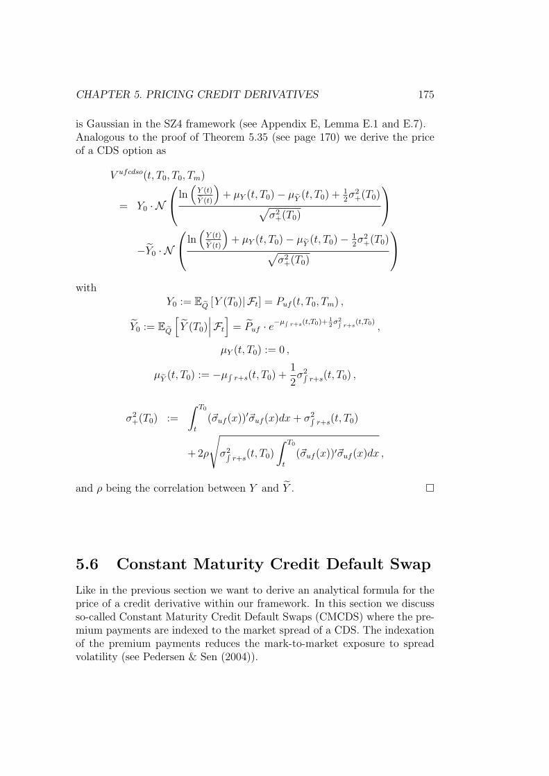
CHAPTER 5. PRICING CREDIT DERIVATIVES 175
is Gaussian in the SZ4 framework (see Appendix E, Lemma E.1 and E.7).Analogous to the proof of Theorem 5.35 (see page 170) we derive the priceof a CDS option as
V ufcdso(t, T0, T0, Tm)
= Y0 · N
ln(
Y (t)
Y (t)
)+ µY (t, T0) − µY (t, T0) + 1
2σ2
+(T0)√
σ2+(T0)
−Y0 · N
ln(
Y (t)
Y (t)
)+ µY (t, T0) − µY (t, T0) − 1
2σ2
+(T0)√
σ2+(T0)
withY0 := EQ [Y (T0)| Ft] = Puf (t, T0, Tm) ,
Y0 := EQ
[Y (T0)
∣∣∣Ft
]= Puf · e−µ∫ r+s(t,T0)+ 1
2σ2∫
r+s(t,T0)
,
µY (t, T0) := 0 ,
µY (t, T0) := −µ∫ r+s(t, T0) +1
2σ2∫
r+s(t, T0) ,
σ2+(T0) :=
∫ T0
t
(~σuf (x))′~σuf (x)dx + σ2∫r+s(t, T0)
+ 2ρ
√
σ2∫r+s
(t, T0)
∫ T0
t
(~σuf (x))′~σuf (x)dx ,
and ρ being the correlation between Y and Y .
5.6 Constant Maturity Credit Default Swap
Like in the previous section we want to derive an analytical formula for theprice of a credit derivative within our framework. In this section we discussso-called Constant Maturity Credit Default Swaps (CMCDS) where the pre-mium payments are indexed to the market spread of a CDS. The indexationof the premium payments reduces the mark-to-market exposure to spreadvolatility (see Pedersen & Sen (2004)).

176 CHAPTER 5. PRICING CREDIT DERIVATIVES
Pedersen & Sen (2004) present a closed-form expression for valuing CMCDSby assuming an affine model for the hazard rate. At the reset days, theyjust write the floating premium payments as functions of the hazard rate.By using Taylor’s approximation and the risky discount factors, they obtainan approximated closed-form solution. Analogous to the default-free case(cf. LIBOR market model, e.g. Zagst (2002) Chapter 4.7), Brigo (2005)postulates a market model of one- and two-period CDS forward rates andtheir joint dynamics under a single pricing measure for CMCDS. Further,he presents an approximated valuation formula for CMCDS which only de-pends on the one-period rates, their volatilities and their correlations. Krekel& Wenzel (2006) who analyze the pricing of credit derivatives within the LI-BOR market model with default risk, also derive a closed-form solution forCMCDS. This formula is similar to Brigo’s but relaxes the assumption ofconstant and homogeneous volatilities for the default intensities. They alsocompare the results of valuing a CMCDS by means of a Monte Carlo simu-lation as opposed to the closed-form formula of Brigo (2005). They find thatthe formula is sufficiently accurate but the formula’s results deviate heavilyfrom the output of the Monte Carlo simulation for higher volatilities andlonger constant maturity periods.
Definition 5.37 Constant Maturity Credit Default SwapA Constant Maturity Credit Default Swap (CMCDS) is a contract which pro-tects for the time [T0, Tm] against default of a reference credit. As for normalCDS the protection consists of a payment if default occurs in [T0, Tm]. Thepremium payments are due on Ti, i = 1, . . . ,m, T0 < Ti ≤ Tm except thatthere has been a default of the reference credit since the last payment day.The premium payment at time Ti is a CDS rate s(Ti−1, Ti−1, Ti−1+c) whichis settled at Ti−1 for a swap starting at this settlement day and maturing inTi−1+c, c > 0.
The protection leg of a CMCDS is the same as for an ordinary CDS (cf.Section 5.4)
EQ
[e−
∫ T0t r(l)dlL(T0)
∫ Tm
T0
e−∫ u
T0r(l)dl
(1 − Z(u))dH(u)
∣∣∣∣Gt
]
CHAPTER 5. PRICING CREDIT DERIVATIVES 177
The premium leg of a CMCDS is built as follows
EQ
[e−
∫ T0t r(l)dlL(T0)
m∑
i=1
e−∫ Ti
T0r(l)dlL(Ti)s(Ti−1, Ti−1, Ti−1+c)
∣∣∣∣∣Gt
]
=m∑
i=1
EQ
[e−
∫ Tit r(l)dlL(Ti)s(Ti−1, Ti−1, Ti−1+c)
∣∣∣Gt
]
= L(t)m∑
i=1
EQ
[e−
∫ Tit r(l)+szero(l)dls(Ti−1, Ti−1, Ti−1+c)
∣∣∣Ft
]
= L(t)m∑
i=1
EQ
[e−
∫ Ti−1t r(l)dls(Ti−1, Ti−1, Ti−1+c)
Q(T d > Ti−1|FTi−1)
Q(T d > t|Ft)
·P d,zero(Ti−1, Ti)
∣∣∣∣Ft
]
= L(t)m∑
i=1
P d,zero(t, Ti)EQi−1,i[s(Ti−1, Ti−1, Ti−1+c)| Ft]
where the last equality is derived by a change of numeraire.The Radon-Nikodym derivative (cf. Theorem 2.19 and Theorem 2.22) defin-
ing the new measure Qi−1,i is given by
Li−1,i(t) =dQi−1,i
dQ
∣∣∣∣∣Ft
=Q(T d > t|Ft) · P d,zero(t, Ti) · P0(t0)
Q(T d > t0|Ft0) · P d,zero(t0, Ti) · P0(t)t0 < t < Ti ∀i,
with P0 being the non-defaultable cash account (see Chapter 4).Further it holds
dLi−1,i(t)
=P0(t0)
Q(T d > t0|Ft0) · P d,zero(t0, Ti)
(d
(1
P0(t)
)· Q(T d > t|Ft) · P d,zero(t, Ti)
+1
P0(t)· d(Q(T d > t|Ft) · P d,zero(t, Ti)
))
178 CHAPTER 5. PRICING CREDIT DERIVATIVES
=P0(t0)
Q(T d > t0|Ft0) · P d,zero(t0, Ti)
(d
(1
P0(t)
)· Q(T d > t|Ft) · P d,zero(t, Ti)
+1
P0(t)
(P d,zero(t, Ti) · dQ(T d > t|Ft) + Q(T d > t|Ft) · dP d,zero(t, Ti)
))
page 107ff= Li−1,i(t)
(−r(t)dt − szero(t)dt + (r(t) + szero(t))dt +
~σP d,z(t, Ti)′
P d,zero(t, Ti)dW (t)
)
= Li−1,i(t) ·~σP d,z(t, Ti)
′
P d,zero(t, Ti)dW (t)
= −Li−1,i(t) · γ(t)dW (t)
with γ(t) := − ~σPd,z (t,Ti)
′
P d,zero(t,Ti).
If we assume - as previously done - lognormal dynamics, we are now ableto compute the premium leg of a CMCDS.
Theorem 5.38If the dynamics of the Forward Credit Default Swap are lognormal under Qthe value of the premium leg of a CMCDS at time t is given as
L(t)m∑
i=1
P d,zero(t, Ti)EQi−1,i[s(Ti−1, Ti−1, Ti−1+c)| Ft]
= L(t)m∑
i=1
P d,zero(t, Ti) · s(t, Ti−1, Ti−1+c) · e∫ Ti−1
t µs(x,Ti−1,Ti−1+c)dx
with µs defined in the proof.
Proof:If it holds for the spread of a FCDS under Q
ds(t, Ta, Tb) = s(t, Ta, Tb) ·(µs(t, Ta, Tb)dt + ~σs(t, Ta, Tb)
′dW (t))
,
its dynamics under the new numeraire Q(T d > t|Ft) · P d,zero(t, Ti) are (cf.dLi−1,i)
ds(t, Ta, Tb) = s(t, Ta, Tb) ·((
µs(t, Ta, Tb) + ~σs(t, Ta, Tb)′ ~σP d,z(t, Ti)
P d,zero(t, Ti)
)dt
+~σs(t, Ta, Tb)′dW (t)
)
=: s(t, Ta, Tb) ·(µs(t, Ta, Tb)dt + ~σs(t, Ta, Tb)
′dW (t))
.

CHAPTER 5. PRICING CREDIT DERIVATIVES 179
Hence, the expectation under the measure Qi−1,i
EQi−1,i[s(Ti−1, Ti−1, Ti−1+c)| Ft]
can be calculated as
EQi−1,i[s(Ti−1, Ti−1, Ti−1+c)| Ft]
≈ s(t, Ti−1, Ti−1+c) · e∫ Ti−1
t µs(x,Ti−1,Ti−1+c)dx
where we freeze the factors r, szero, u, w1, w2 in µs at time t.
The exponential term of the above approximation can be considered as aconvexity adjustment compensating the fact that the FCDS spreads(Ti−1, Ti−1, Ti−1+c) is not a martingale under the applied forward measure.In the SZ4 framework with its lognormal approximations (see Assumption5.26) this adjustment is calculated as in the next theorem.
Theorem 5.39The premium leg of a Constant Maturity Credit Default Swap in the SZ4framework (cf. Model 4.4) is
L(t)m∑
i=1
P d,zero(t, Ti)EQi−1,i[s(Ti−1, Ti−1, Ti−1+c)| Ft]
= L(t)m∑
i=1
P d,zero(t, Ti) · s(t, Ti−1, Ti−1+c) · e∫ Ti−1
t µs(x,Ti−1,Ti−1+c)dx
with
µs(x, Ti−1, Ti−1+c)
=
(~σ∑
j P d,z(x))′
~σ∑j P d,z(x)
[∑i−1+cj=i P d,zero(x, Tj)
]2 +
(~σ∑
j P d,z(x))′
∑i−1+cj=i P d,zero(x, Tj)
·((
σrBd,zero(x, y), σszeroCd,zero(x, y), σuD
d,zero(x, y), σw1Ed,zero1 (x, y)
)′
+
(σrB
d,zero(x, Ti), σszeroCd,zero(x, Ti), σuDd,zero(x, Ti), σw1E
d,zero1 (x, Ti)
)′)
+σ2rB
d,zero(x, y)Bd,zero(x, Ti) + σ2szeroCd,zero(x, y)Cd,zero(x, Ti)
+σ2uD
d,zero(x, y)Dd,zero(x, Ti) + σ2w1
Ed,zero1 (x, y)Ed,zero
1 (x, Ti)
180 CHAPTER 5. PRICING CREDIT DERIVATIVES
where y ∈ [Ti−1, Ti−1+c] and the factors r, szero, u and w1 in P d,zero and in~σ∑
j P d,z are frozen at time t.
Proof:Using Assumption 5.26, the approximated lognormal dynamics of the FCDSspread are under Q given by
ds(t, Ti−1, Ti−1+c)
=
((~σ∑j P d,z(t)
)′~σ∑
j P d,z(t)[∑i−1+c
j=i P d,zero(t, Tj)]2
+
(σrB
d,zero(t, y), σszeroCd,zero(t, y), σuDd,zero(t, y), σw1E
d,zero1 (t, y)
)
· 1[∑i−1+cj=i P d,zero(t, Tj)
](
~σ∑j P d,z(t)
))s(t, Ti−1, Ti−1+c)dt
+
(−(σrB
d,zero(t, y), σszeroCd,zero(t, y), σuDd,zero(t, y), σw1E
d,zero1 (t, y)
)
−
(~σ∑
j P d,z(t))′
∑i−1+cj=i P d,zero(t, Tj)
)s(t, Ti−1, Ti−1+c)dW (t)
with y ∈ [Ti−1, Ti−1+c],
and the dynamics of the new numeraire Q(T d > t|Ft) · P d,zero(t, Ti) are
dQ(T d > t|Ft) · P d,zero(t, Ti)
= Q(T d > t|Ft)dP d,zero(t, Ti) − szero(t)Q(T d > t|Ft)Pd,zero(t, Ti)dt
page 107ff= Q(T d > t|Ft)P
d,zero(t, Ti)
(r(t)dt +
~σP d,z(t, Ti)′
P d,zero(t, Ti)dW (t)
)
= Q(T d > t|Ft)Pd,zero(t, Ti)
(r(t)dt
−(
σrBd,zero(t, Ti), σszeroCd,zero(t, Ti), σuD
d,zero(t, Ti), σw1Ed,zero1 (t, Ti)
)dW (t)
).

CHAPTER 5. PRICING CREDIT DERIVATIVES 181
Hence, we obtain for
µs(t, Ti−1, Ti−1+c)
=
(~σ∑
j P d,z(t))′
~σ∑j P d,z(t)
[∑i−1+cj=i P d,zero(t, Tj)
]2
+
(σrB
d,zero(t, y), σszeroCd,zero(t, y), σuDd,zero(t, y), σw1E
d,zero1 (t, y)
)
·
(~σ∑
j P d,z(t)
)
[∑i−1+cj=i P d,zero(t, Tj)
]
+
((σrB
d,zero(t, y), σszeroCd,zero(t, y), σuDd,zero(t, y), σw1E
d,zero1 (t, y)
)
+
(~σ∑
j P d,z(t))′
∑i−1+cj=i P d,zero(t, Tj)
)
·(
σrBd,zero(t, Ti), σszeroCd,zero(t, Ti), σuD
d,zero(t, Ti), σw1Ed,zero1 (t, Ti)
)′
.
In order to calculate the integral of µs the factors r, szero, u, w1 need to befrozen at time t.
Due to the promising results obtained in Section 5.4.2 for the shifted dy-namics we also present a closed-form solution based on that assumption.
Theorem 5.40Assuming the FCDS spread evolves according to the shifted dynamics (see As-sumption 5.28), the present value of the premium leg of a Constant MaturityCredit Default Swap in the SZ4 framework (cf. Model 4.4) is
L(t)m∑
i=1
P d,zero(t, Ti)EQi−1,i[s(Ti−1, Ti−1, Ti−1+c)| Ft]
= L(t)m∑
i=1
P d,zero(t, Ti) ·(
(1 − Z) · ∆T · K
+(s(t, Ti−1, Ti−1+c) − (1 − Z) · ∆T · K) · e∫ Ti−1
t µsK(x,Ti−1,Ti−1+c)dx
)

182 CHAPTER 5. PRICING CREDIT DERIVATIVES
with ∆T being the period length of the CDS represented by s(t, Ti−1, Ti−1+c)and
µsK(t, Ti−1, Ti−1+c)
=
(~σ∑
j P d,z(t))′
~σ∑j P d,z(t)
[∑i−1+cj=i P d,zero(t, Tj)
]2 +
(~σ∑
j P d,z(t))′
∑i−1+cj=i P d,zero(t, Tj)
·(
σrBd,zero(t, Ti), σszeroCd,zero(t, Ti), σuD
d,zero(t, Ti), σw1Ed,zero1 (t, Ti)
)′
.
where the factors r, szero, u, w1 are frozen at time t.
Proof:Assuming the dynamics of the FCDS spread under Q to be
ds(t, Ti−1, Ti−1+c)
=
(~σ∑
j P d,z(t))′
~σ∑j P d,z(t)
[∑i−1+cj=i P d,zero(t, Tj)
]2(
s(t, Ti−1, Ti−1+c) − (1 − Z)∆TjK
)dt
−
(~σ∑
j P d,z(t))′
∑i−1+cj=i P d,zero(t, Tj)
(s(t, Ti−1, Ti−1+c) − (1 − Z)∆TjK
)dW (t)
with K determined as described on page 140, the change of numeraire resultsin the following dynamics for s under Qi−1,i
ds(t, Ti−1, Ti−1+c)
=
(~σ∑
j P d,z(t))′
~σ∑j P d,z(t)
[∑i−1+cj=i P d,zero(t, Tj)
]2(
s(t, Ti−1, Ti−1+c) − (1 − Z)∆TjK
)dt.
+
( (~σ∑
j P d,z(t))′
∑i−1+cj=i P d,zero(t, Tj)
(s(t, Ti−1, Ti−1+c) − (1 − Z)∆TjK
))
·(
σrBd,zero(t, Ti), σszeroCd,zero(t, Ti), σuD
d,zero(t, Ti), σw1Ed,zero1 (t, Ti)
)′
dt
−
(~σ∑
j P d,z(t))′
∑i−1+cj=i P d,zero(t, Tj)
(s(t, Ti−1, Ti−1+c) − (1 − Z)∆TjK
)dW (t).
CHAPTER 5. PRICING CREDIT DERIVATIVES 183
Hence, the expected value of s(Ti−1, Ti−1, Ti−1+c) under Qi−1,i is (see footnoteon page 140)
EQi−1,i[s(Ti−1, Ti−1, Ti−1+c)| Ft]
= (1 − Z) · ∆Tj · K+(s(t, Ti−1, Ti−1+c) − (1 − Z) · ∆Tj · K) · e
∫ Ti−1t µsK(x,Ti−1,Ti−1+c)dx
with
µsK(t, Ti−1, Ti−1+c)
=
(~σ∑
j P d,z(t))′
~σ∑j P d,z(t)
[∑i−1+cj=i P d,zero(t, Tj)
]2 +
(~σ∑
j P d,z(t))′
∑i−1+cj=i P d,zero(t, Tj)
·(
σrBd,zero(t, Ti), σszeroCd,zero(t, Ti), σuD
d,zero(t, Ti), σw1Ed,zero1 (t, Ti)
)′
.
In order to calculate the integral of µsK the factors r, s, u, w1 need to befrozen at time t. Further, in order to account for the change of numerairethe factor K needs to be recalculated under the measure Qi−1,i according topage 140.
In the following we study the behaviour of the CMCDS pricing formulasas opposed to the simulation of the factors r, s, u, w1. Again we pose our-selves in the framework of SZ4 with the parameters called GDPr for therating class A2 derived in Chapter 4 with z = 0.9 and Z = 0.75. We omitthe pricing of the protection legs since they are determined the same way forall alternatives. Hence, we compare the present values of the premium legsof a CMCDS with quarterly premium payments determined by the formulasof Theorem 5.39 and Theorem 5.40 assuming a recovery as a fraction of facevalue with the results of a simulation based on 20,000 scenarios.Table 5.3 shows the results for CMCDS premium legs where the CMCDStenor coincides with the swap maturity. As indicated by the results for theFCDS spreads (cf. page 165), the differences of the formulas as opposedto the simulation results increase for longer tenors respectively maturitiesbecause longer forward starting periods are needed if the CMCDS maturitylengthens. This effect can be especially seen for the lognormal approximation

184 CHAPTER 5. PRICING CREDIT DERIVATIVES
(column 5). Our finding is in line with the results of Krekel & Wenzel (2006)who recommend to price by means of simulation for maturities longer than 5years. In the case of the formula based on the shifted-lognormal dynamics wewould also recommend a simulation for tenors longer than 5 years. However,when assuming lognormal dynamics for FCDS spreads we advise to use theCMCDS formula only for short maturites up to 3 years.In Table 5.4 the results for a CMCDS premium leg with a constant tenor anda swap maturity of 1 year are shown for different values of σszero . Analogouslyto the results of the CDS option (see Table 5.1) the differences between theclosed-form and the simulation-based solutions grow for increasing values ofσszero . The results obtained by the formula assuming lognormal dynamicsalready deviate severely for moderate values of σszero whereas the closed-form solution based on shifted-lognormal dynamics start to depart heavilyfor higher values of σszero . Corresponding to the results of Krekel & Wenzel(2006), we recommend to use the formulas up to moderate values of σszero
and a full simulation for CMCDS pricing for high values.
Tenor Formula Formula shift Simulation Difference Difference shift
1Y 3.37% 3.39% 3.44% 0.07% 0.05%2Y 7.59% 7.68% 7.92% 0.33% 0.24%3Y 11.23% 11.42% 11.53% 0.30% 0.11%4Y 14.01% 14.33% 14.73% 0.72% 0.40%5Y 16.03% 16.48% 16.90% 0.87% 0.43%6Y 17.44% 18.00% 18.90% 1.46% 0.90%7Y 18.39% 19.06% 20.06% 1.67% 1.00%
Table 5.3: Present values of the premium leg of a CMCDS for differentCMCDS tenors (column 1), starting in 0.25 years and running for the sameamount of years as the CMCDS tenor with quarterly premium payments. Theprices are calculated by formula of Theorem 5.39 (column 2) and Theorem5.40 (column 3) and via simulation of factors r, s, u, w1 (column 4). Column5 and 6 contain the differences of the results obtained by formula (column 2and 3) to the simulation (column 4).
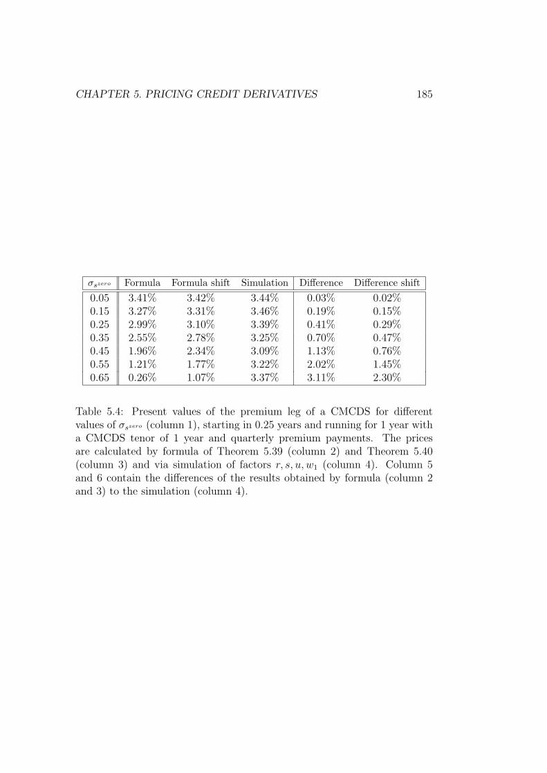
CHAPTER 5. PRICING CREDIT DERIVATIVES 185
σszero Formula Formula shift Simulation Difference Difference shift
0.05 3.41% 3.42% 3.44% 0.03% 0.02%0.15 3.27% 3.31% 3.46% 0.19% 0.15%0.25 2.99% 3.10% 3.39% 0.41% 0.29%0.35 2.55% 2.78% 3.25% 0.70% 0.47%0.45 1.96% 2.34% 3.09% 1.13% 0.76%0.55 1.21% 1.77% 3.22% 2.02% 1.45%0.65 0.26% 1.07% 3.37% 3.11% 2.30%
Table 5.4: Present values of the premium leg of a CMCDS for differentvalues of σszero (column 1), starting in 0.25 years and running for 1 year witha CMCDS tenor of 1 year and quarterly premium payments. The pricesare calculated by formula of Theorem 5.39 (column 2) and Theorem 5.40(column 3) and via simulation of factors r, s, u, w1 (column 4). Column 5and 6 contain the differences of the results obtained by formula (column 2and 3) to the simulation (column 4).

186 CHAPTER 5. PRICING CREDIT DERIVATIVES

Chapter 6
Pricing Inflation-IndexedDerivatives
In the 1980’s governments started to issue inflation-linked bonds, e.g. UKGILTS, US TIPS and French OATis. Reasons for those issuances could be(see Dodgson & Kainth (2006)) the wish to better match the liabilities to thefuture income which tends to rise with inflation, the hope for a cheaper bor-rowing due to an ”inflation-risk premium”, or the wish to strengthen ”thecredibility of economic policy regarding inflation”. For investors like pen-sion funds and insurance companies those bonds are attractive since theyhelp to protect their future exposure, e.g. pensions tend to increase withinflation. Since the range of inflation-linked bonds is limited, a market forinflation-indexed derivatives developed in order to fulfill the requirementsof the clients. By means of tailor-made inflation derivatives the clients’ fu-ture liabilities could now be matched more closely. The more complex thesederivatives become the more grows the need for pricing models. A popularapproach is based on a foreign-currency analogy where the valuation of aninflation derivative becomes equivalent to the pricing of cross-currency inter-est rate derivatives. In this approach the inflation index acts as an exchangerate between the nominal and the real economy. Articles introducing sucha framework are those of Hughston (1998), and Jarrow & Yildirim (2003).For example, Jarrow & Yildirim (2003) model the instantaneous nominaland real forward rates in a Heath-Jarrow-Morton framework as correlatedone factor processes and the inflation rate as a lognormal exchange rate.The equivalent formulation of that framework in terms of short rates canbe found in Mercurio (2005). An important advantage of that approach isthe analytical tractability due to the normal respectively lognormal distribu-tions. However, drawbacks are the possibility of negative rates, and the factthat the real interest rates are unobservable, therefore making it difficult to
187
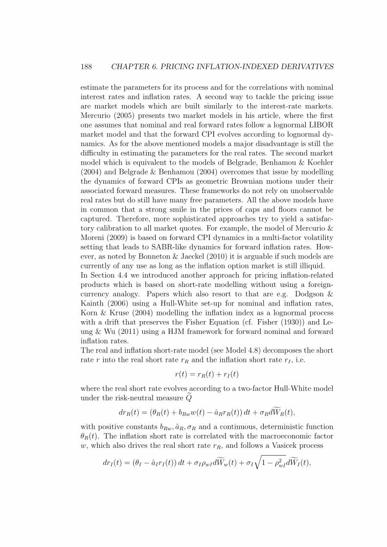
188 CHAPTER 6. PRICING INFLATION-INDEXED DERIVATIVES
estimate the parameters for its process and for the correlations with nominalinterest rates and inflation rates. A second way to tackle the pricing issueare market models which are built similarly to the interest-rate markets.Mercurio (2005) presents two market models in his article, where the firstone assumes that nominal and real forward rates follow a lognormal LIBORmarket model and that the forward CPI evolves according to lognormal dy-namics. As for the above mentioned models a major disadvantage is still thedifficulty in estimating the parameters for the real rates. The second marketmodel which is equivalent to the models of Belgrade, Benhamou & Koehler(2004) and Belgrade & Benhamou (2004) overcomes that issue by modellingthe dynamics of forward CPIs as geometric Brownian motions under theirassociated forward measures. These frameworks do not rely on unobservablereal rates but do still have many free parameters. All the above models havein common that a strong smile in the prices of caps and floors cannot becaptured. Therefore, more sophisticated approaches try to yield a satisfac-tory calibration to all market quotes. For example, the model of Mercurio &Moreni (2009) is based on forward CPI dynamics in a multi-factor volatilitysetting that leads to SABR-like dynamics for forward inflation rates. How-ever, as noted by Bonneton & Jaeckel (2010) it is arguable if such models arecurrently of any use as long as the inflation option market is still illiquid.In Section 4.4 we introduced another approach for pricing inflation-relatedproducts which is based on short-rate modelling without using a foreign-currency analogy. Papers which also resort to that are e.g. Dodgson &Kainth (2006) using a Hull-White set-up for nominal and inflation rates,Korn & Kruse (2004) modelling the inflation index as a lognormal processwith a drift that preserves the Fisher Equation (cf. Fisher (1930)) and Le-ung & Wu (2011) using a HJM framework for forward nominal and forwardinflation rates.The real and inflation short-rate model (see Model 4.8) decomposes the shortrate r into the real short rate rR and the inflation short rate rI , i.e.
r(t) = rR(t) + rI(t)
where the real short rate evolves according to a two-factor Hull-White modelunder the risk-neutral measure Q
drR(t) = (θR(t) + bRww(t) − aRrR(t)) dt + σRdWR(t),
with positive constants bRw, aR, σR and a continuous, deterministic functionθR(t). The inflation short rate is correlated with the macroeconomic factorw, which also drives the real short rate rR, and follows a Vasicek process
drI(t) = (θI − aIrI(t)) dt + σIρwIdWw(t) + σI
√1 − ρ2
wIdWI(t),

CHAPTER 6. PRICING INFLATION-INDEXED DERIVATIVES 189
with positive constants aI , σI , a non-negative constant θI and independentBrownian motions WR, WI and Ww.Our set-up is inspired by the so-called Fisher Equation (cf. Fisher (1930))which states that today’s nominal interest rate for the period up to time Tis the sum of the real interest rate for that period and the expected inflationup to time T . The true inflation for that period as well as the true realrate will be only known after the end of that period. Furthermore, realinterest rates are not directly observable in the market. Therefore, we donot explicitly model the real economy as it is done in Hughston (1998) andJarrow & Yildirim (2003). Instead, we assume that the nominal short rateis driven by two unobservable processes capturing the market’s expectationsfor the real interest rate and the inflation rate. This framework is similarto that of Dodgson & Kainth (2006) who ”ignore the existence of a ”real”economy” by only modelling the inflation rate and the nominal short rate ascorrelated Hull-White processes. The advantage of our set-up and the one ofDodgson & Kainth (2006) is the analytical tractability due to the Gaussianprocesses. But shortcomings are that smiles of market prices as a function ofstrikes and products depending on the correlation of different forward ratescannot be captured very well.For notational convenience we omit the subscript for the macroeconomicfactor w and refer to the inflation short rate as rI instead of w2 (cf. Model4.8). Further, the risk-free bond of Lemma 4.9 simplifies to
P (t, T, r, w, rI) = eA(t,T )−BR(t,T )rR−E1(t,T )w−BI(t,T )rI
since it holds brw2 := aR−aI and E1(t, T )+BR(t, T ) = BI(t, T ). Additionally,within this chapter we use the notation
BX+/−Y (t, T ) :=1
aX + / − aY
(1 − e−(ax+/−aY )(T−t)
).
6.1 Inflation-Indexed Swaps
Definition 6.1An Inflation-Indexed Swap consists of two legs where one is paying a fixedrate and the other is paying the inflation rate calculated over a predefinedperiod. The inflation rate is determined as the percentage return of the CPIindex over the respective time interval.

190 CHAPTER 6. PRICING INFLATION-INDEXED DERIVATIVES
In a zero-coupon swap, the inflation-indexed leg pays at maturity Tm theinflation rate of the time interval [T0, Tm] times the nominal value N
N ·(
CPI(Tm)
CPI(T0)− 1
),
whereas the other leg pays the percentage return of the fixed rate c
N ·((1 + c)(Tm−T0) − 1
).
For a Year-On-Year (YOY) Swap, the fixed leg pays the amount
N · c · ∆i , ∆i := Ti − Ti−1 , i = 1 . . . m
at the set of dates T1, . . . , Tm. The amount payable at times T1, . . . , Tm ofthe inflation-indexed leg is derived as
N · ∆i ·(
CPI(Ti)
CPI(Ti−1)− 1
).
The inflation-indexed derivatives market is dominated by zero-coupon inflation-indexed swaps which are used as hedges for inflation bond exposures (seeBonneton & Jaeckel (2010)).
Theorem 6.2 (Zero-Coupon Inflation-Indexed Swap)In the real and inflation short-rate model, the price at time t of a zero-couponinflation-indexed swap is given by
V zciis(t, T0, Tm) = N ·(
CPI(t)
CPI(T0)PR(t, Tm) − P (t, Tm) · (1 + c)(Tm−T0)
).
PR denotes the price of a real zero-coupon bond which is calculated similarlyto the risk-free bond in the four factor framework of Schmid and Zagst (cf.Theorem 4.5).

CHAPTER 6. PRICING INFLATION-INDEXED DERIVATIVES 191
Proof:At time t > T0, the value of the zero-coupon inflation-indexed swap is
V zciis(t, T0, Tm)
= EQ
[N · e−
∫ Tmt
r(x)dx ·((
CPI(Tm)
CPI(T0)− 1
)−((1 + c)(Tm−T0) − 1
))∣∣∣∣Ft
]
= N · EQ
[e−
∫ Tmt
r(x)dx · CPI(Tm)
CPI(T0)
∣∣∣∣Ft
]− N · P (t, Tm) · (1 + c)(Tm−T0)
= N ·(
EQ
[e−
∫ Tmt
r(x)dx · CPI(t)
CPI(T0)· e∫ Tm
trI(x)dx
∣∣∣∣Ft
]− P (t, Tm) · (1 + c)(Tm−T0)
)
= N ·(
CPI(t)
CPI(T0)· EQ
[e−
∫ Tmt
rR(x)dx∣∣∣Ft
]− P (t, Tm) · (1 + c)(Tm−T0)
)
= N ·(
CPI(t)
CPI(T0)PR(t, Tm) − P (t, Tm) · (1 + c)(Tm−T0)
)
The term EQ
[CPI(Tm) · e−
∫ Tmt
r(x)dx∣∣∣Ft
]= CPI(t) · PR(t, Tm) denotes a
zero-coupon inflation bond which ”is generally not available directly buta useful theoretical tool” (see Dodgson & Kainth (2006)). With the helpof Theorem 6.2, real discount factors PR respectively zero-coupon inflationbonds can be stripped from quotes of zero-coupon inflation-indexed swapswhich are given in terms of the fixed rate c for maturities Tm: For example,at t = T0 it holds PR(T0, Tm) = P (T0, Tm) · (1 + c)(Tm−T0) .However, the inflation market is still not liquid as Dodgson & Kainth (2006)note in their paper. Extracting prices of zero-coupon inflation bonds frominflation-linked swaps and bonds show discrepancies, especially for the USmarket.
Year-on-year (YoY) inflation swaps are traded at much lower volumes thanzero-coupon inflation swaps, but are important for building more exotic prod-ucts. Since the inflation payments do not reference the inflation index fromthe start date (T0) to the coupon date but have different accrual periods, thevaluation of the YoY inflation swap is model-dependent.
Theorem 6.3 (Year-on-Year Inflation-Indexed Swap)In the real and inflation short-rate model, the price at time t of a year-on-yearinflation-indexed swap is

192 CHAPTER 6. PRICING INFLATION-INDEXED DERIVATIVES
V yoyiis(t, Tm) = N ·m∑
i=1
∆i ·PR(t, Ti) · P (t, Ti−1)
PR(t, Ti−1)· eCyoy(t,Ti−1,Ti)
−N · (1 + c) ·m∑
i=1
∆i · P (t, Ti) .
The correlation adjustment factor Cyoy is defined as
Cyoy(t, Ti−1, Ti) =bRwσwσIρwI
(aR − aw)aI
·(Bw(Ti−1, Ti) · (Bw(t, Ti−1) − BI+w(t, Ti−1))
−BR(Ti−1, Ti) · (BR(t, Ti−1) − BI+R(t, Ti−1)))
.
Proof:At time t, the value of the year-on-year inflation-indexed swap can be writtenas
V yoyiis(t, Tm)
= EQ
[N ·
m∑
i=1
e−∫ Ti
t r(x)dx · ∆i ·(
CPI(Ti)
CPI(Ti−1)− 1
)∣∣∣∣∣Ft
]
−EQ
[N · c ·
m∑
i=1
e−∫ Ti
t r(x)dx · ∆i
∣∣∣∣∣Ft
]
= N ·m∑
i=1
∆i ·(
EQ
[e−
∫ Tit r(x)dx · e
∫ TiTi−1
rI(x)dx
∣∣∣∣Ft
]− P (t, Ti)
)
−N · c ·m∑
i=1
∆i · P (t, Ti) .
Since the integrals over the short rate r and the inflation short rate rI are
normal, the expectation EQ
[e−
∫ Tit r(x)dxe
∫ TiTi−1
rI(x)dx
∣∣∣∣Ft
]can be also written
as
EQ
[e−
∫ Ti−1t r(x)dxe
−∫ Ti
Ti−1rR(x)dx
∣∣∣∣Ft
]
I= EQ
[e−
∫ Ti−1t r(x)dx
∣∣∣Ft
]· EQ
[e−∫ Ti
Ti−1rR(x)dx
∣∣∣∣Ft
]
· eCovarQ
[ ∫ Ti−1t rI(x)+rR(x)dx ,
∫ TiTi−1
rR(x)dx∣∣∣Ft
]

CHAPTER 6. PRICING INFLATION-INDEXED DERIVATIVES 193
= P (t, Ti−1) · EQ
[e−∫ Ti
Ti−1rR(x)dx
∣∣∣∣Ft
]· eCovar
Q
[ ∫ Ti−1t rI(x)dx ,
∫ TiTi−1
rR(x)dx∣∣∣Ft
]
· eCovarQ
[ ∫ Ti−1t rR(x)dx ,
∫ TiTi−1
rR(x)dx∣∣∣Ft
]
= P (t, Ti−1) · eCyoy(t,Ti−1,Ti) · EQ
[e−
∫ Tit rR(x)dx+
∫ Ti−1t rR(x)dx
∣∣∣Ft
]
· eCovarQ
[ ∫ Ti−1t rR(x)dx ,
∫ Tit rR(x)dx−
∫ Ti−1t rR(x)dx
∣∣∣Ft
]
= P (t, Ti−1) · eCyoy(t,Ti−1,Ti) · EQ
[e−
∫ Tit rR(x)dx
∣∣∣Ft
]· EQ
[e∫ Ti−1
t rR(x)dx∣∣∣Ft
]
· eCovarQ
[ ∫ Ti−1t rR(x)dx ,
∫ Tit rR(x)dx
∣∣∣Ft
]
· eCovarQ
[ ∫ Ti−1t rR(x)dx ,−
∫ Ti−1t rR(x)dx
∣∣∣Ft
]
· eCovarQ
[−∫ Ti
t rR(x)dx ,∫ Ti−1
t rR(x)dx∣∣∣Ft
]
= P (t, Ti−1) · eCyoy(t,Ti−1,Ti)· PR(t, Ti) · EQ
[e∫ Ti−1
t rR(x)dx∣∣∣Ft
]· e−V ar
Q
[ ∫ Ti−1t rR(x)dx
∣∣∣Ft
]
II=
PR(t, Ti) · P (t, Ti−1)
EQ
[e−
∫ Ti−1t rR(x)dx
∣∣∣Ft
] · eCyoy(t,Ti−1,Ti)
=PR(t, Ti) · P (t, Ti−1)
PR(t, Ti−1)· eCyoy(t,Ti−1,Ti) ,
with the rules for expectations of normal random variablesI II and
Cyoy(t, Ti−1, Ti) := CovarQ
[∫ Ti−1
t
rI(x)dx ,
∫ Ti
Ti−1
rR(x)dx
∣∣∣∣Ft
].
The calculation of the covariance is straightforward (see Lemma E.1 of Ap-pendix E).
In general, there is a lag between the date for the index and the paymentday. This lag could be a few days, a few weeks or even longer. Therefore,another correlation adjustment is needed to correct this discrepancy. Forexample, if the inflation-indexed payments of a year-on-year swap are dueafter the inflation index is fixed, i.e. Tipay > Ti, a second adjustment factoris introduced.
IIt holds for Xi ∼ N (µXi, σ2
Xi) i = 1, 2: E
[eXi
]= eµXi
+σ2Xi
2 i = 1, 2 and
E[eX1+X2
]= eµX1
+µX2+
V ar[X1+X2]2 = E
[eX1]· E[eX2]· eCovar[X1,X2] since
V ar[X1 + X2] = σ2X1
+ σ2X2
+ 2 · Covar[X1,X2] (see e.g. Mueller (1991), page 552).
IIIt holds for X ∼ N (µX , σ2X): E
[eX]
= eµX+σ2X
2 and E[e−X
]= e−µX+
σ2X
2 . Hence, it
also holds 1E[e−X ]
= eµX−σ2X
2 = E[eX]· e−σ2
X .

194 CHAPTER 6. PRICING INFLATION-INDEXED DERIVATIVES
Proposition 6.4 (Delayed Payment)The inflation-indexed leg of a year-on-year swap with delayed payments attime Tipay > Ti, ∀ i is valued according to
EQ
[e−
∫ Tipay
t r(x)dx · CPI(Ti)
CPI(Ti−1)
∣∣∣∣Ft
]
=PR(t, Ti) · P (t, Ti−1) · P (t, Tipay)
PR(t, Ti−1) · P (t, Ti)· eCyoy(t,Ti−1,Ti) · eCdel(t,Ti−1,Ti,Tipay ) .
The correlation adjustment factor Cdel(t, Ti−1, Ti, Tipay) is defined at the endof the proof.
Proof:The payment of the ith period of the inflation-indexed leg is based on
EQ
[e−
∫ Tipay
t r(x)dx · CPI(Ti)
CPI(Ti−1)
∣∣∣∣Ft
]
= EQ
[e−
∫ Tipay
Tir(x)dx · e−
∫ Tit r(x)dx · e
∫ TiTi−1
rI(x)dx
∣∣∣∣Ft
]
footn. I= EQ
[e−
∫ Tit r(x)dx · e
∫ TiTi−1
rI(x)dx
∣∣∣∣Ft
]· EQ
[e−
∫ Tipay
Tir(x)dx
∣∣∣∣Ft
]
· eCovarQ
[−∫ Ti
t r(x)dx+∫ Ti
Ti−1rI(x)dx ,−
∫ Tipay
Tir(x)dx
∣∣∣Ft
]
Th.6.3=
PR(t, Ti) · P (t, Ti−1)
PR(t, Ti−1)· eCyoy(t,Ti−1,Ti) · EQ
[e−
∫ Tipay
t r(x)dx+∫ Ti
t r(x)dx∣∣∣Ft
]
· eCovarQ
[−∫ Ti
t r(x)dx ,−∫ Tipay
Tir(x)dx
∣∣∣Ft
]
· eCovar
Q
[ ∫ TiTi−1
rI(x)dx ,−∫ Tipay
Tir(x)dx
∣∣∣Ft
]
=PR(t, Ti) · P (t, Ti−1)
PR(t, Ti−1)· eCyoy(t,Ti−1,Ti) · EQ
[e−
∫ Tipay
t r(x)dx∣∣∣Ft
]
·EQ
[e∫ Ti
t r(x)dx∣∣∣Ft
]· eCovar
Q
[−∫ Tipay
t r(x)dx ,∫ Ti
t r(x)dx∣∣∣Ft
]
· eCovarQ
[ ∫ Tit r(x)dx ,
∫ Tipay
Tir(x)dx
∣∣∣Ft
]
· eCovarQ
[ ∫ TiTi−1
rI(x)dx ,−∫ Tipay
Tir(x)dx
∣∣∣Ft
]
=PR(t, Ti) · P (t, Ti−1) · P (t, Tipay)
PR(t, Ti−1)· eCyoy(t,Ti−1,Ti) · eCdel(t,Ti−1,Ti,Tipay )
·EQ
[e∫ Ti
t r(x)dx∣∣∣Ft
]· eCovar
Q
[−∫ Ti
t r(x)dx ,∫ Ti
t r(x)dx∣∣∣Ft
]
footn. II=
PR(t, Ti) · P (t, Ti−1) · P (t, Tipay)
PR(t, Ti−1) · EQ
[e−
∫ Tit r(x)dx
∣∣∣Ft
] · eCyoy(t,Ti−1,Ti)· eCdel(t,Ti−1,Ti,Tipay )

CHAPTER 6. PRICING INFLATION-INDEXED DERIVATIVES 195
with
Cdel(t, Ti−1, Ti, Tipay) := CovarQ
[∫ Ti
Ti−1
rI(x)dx ,−∫ Tipay
Ti
r(x)dx
∣∣∣∣Ft
]
= −CovarQ
[∫ Ti
Ti−1
rI(x)dx ,
∫ Tipay
Ti
rI(x)dx
∣∣∣∣Ft
]
−CovarQ
[∫ Ti
Ti−1
rI(x)dx ,
∫ Tipay
Ti
rR(x)dx
∣∣∣∣Ft
].
The covariance terms are determined in Lemma E.3.
CovarQ
[∫ Ti
Ti−1
rI(x)dx ,
∫ Tipay
Ti
rI(x)dx
∣∣∣∣Ft
]
=σ2
I
a2I
·(a2
I · e−aI(Ti−Ti−1) · BI+I(t, Ti−1) · BI(Ti−1, Ti) · BI(Ti, Tipay)
+ aI · BI(Ti, Tipay) · (BI(Ti−1, Ti) − BI+I(Ti−1, Ti)))
CovarQ
[∫ Ti
Ti−1
rI(x)dx ,
∫ Tipay
Ti
rR(x)dx
∣∣∣∣Ft
]
=bRwσwσIρwI
(aR − aw)aI
·(Bw(Ti, Tipay) · (Bw(Ti−1, Ti) − BI+w(Ti−1, Ti)
+ aI · e−aw(Ti−Ti−1) · BI(Ti−1, Ti) · BI+w(t, Ti−1))
−BR(Ti, Tipay) · (BR(Ti−1, Ti) − BI+R(Ti−1, Ti)
+ aI · e−aR(Ti−Ti−1) · BI(Ti−1, Ti) · BI+R(t, Ti−1)))
For convexity adjustments due to delayed payments see also the article ofBrody, Crosby & Li (2008). They determined those adjustments for zero-coupon inflation swaps and YoY inflation swaps in a multi-factor version ofthe Hughston (1998) model and the Jarrow & Yildirim (2003) model.
6.2 Inflation-Indexed Options
In this section we present how inflation-indexed options are valued. Exem-plary, we will show the pricing of an inflation-indexed caplet which is a calloption on the CPI-implied inflation rate.
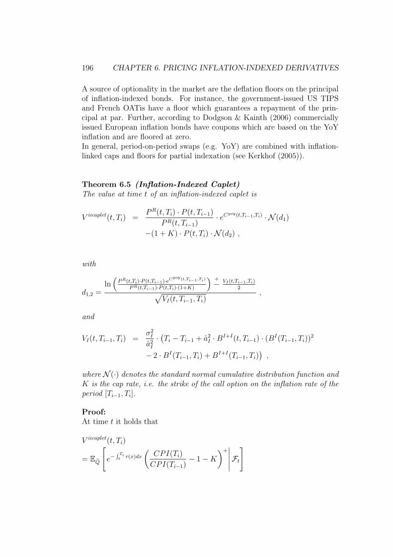
196 CHAPTER 6. PRICING INFLATION-INDEXED DERIVATIVES
A source of optionality in the market are the deflation floors on the principalof inflation-indexed bonds. For instance, the government-issued US TIPSand French OATis have a floor which guarantees a repayment of the prin-cipal at par. Further, according to Dodgson & Kainth (2006) commerciallyissued European inflation bonds have coupons which are based on the YoYinflation and are floored at zero.In general, period-on-period swaps (e.g. YoY) are combined with inflation-linked caps and floors for partial indexation (see Kerkhof (2005)).
Theorem 6.5 (Inflation-Indexed Caplet)The value at time t of an inflation-indexed caplet is
V iicaplet(t, Ti) =PR(t, Ti) · P (t, Ti−1)
PR(t, Ti−1)· eCyoy(t,Ti−1,Ti) · N (d1)
−(1 + K) · P (t, Ti) · N (d2) ,
with
d1,2 =ln(
P R(t,Ti)·P (t,Ti−1)·eCyoy(t,Ti−1,Ti)
P R(t,Ti−1)·P (t,Ti)·(1+K)
) +− VI(t,Ti−1,Ti)
2√VI(t, Ti−1, Ti)
,
and
VI(t, Ti−1, Ti) =σ2
I
a2I
·(Ti − Ti−1 + a2
I · BI+I(t, Ti−1) · (BI(Ti−1, Ti))2
− 2 · BI(Ti−1, Ti) + BI+I(Ti−1, Ti))
,
where N (·) denotes the standard normal cumulative distribution function andK is the cap rate, i.e. the strike of the call option on the inflation rate of theperiod [Ti−1, Ti].
Proof:At time t it holds that
V iicaplet(t, Ti)
= EQ
[e−
∫ Tit r(x)dx
(CPI(Ti)
CPI(Ti−1)− 1 − K
)+∣∣∣∣∣Ft
]

CHAPTER 6. PRICING INFLATION-INDEXED DERIVATIVES 197
= EQ
[e−
∫ Tit r(x)dx
(e∫ Ti
Ti−1rI(x)dx − (1 + K)
)+∣∣∣∣∣Ft
]
= EQ
[(e−
∫ Tit r(x)dxe
∫ TiTi−1
rI(x)dx − (1 + K) · e−∫ Ti
t r(x)dx
)+∣∣∣∣∣Ft
]
Th. 6.3=
PR(t, Ti) · P (t, Ti−1)
PR(t, Ti−1)· eCyoy(t,Ti−1,Ti) · N (d1) − (1 + K) · P (t, Ti) · N (d2) ,
with
d1,2 =ln(
P R(t,Ti)·P (t,Ti−1)·eCyoy(t,Ti−1,Ti)
P R(t,Ti−1)·P (t,Ti)·(1+K)
) +− VI(t,Ti−1,Ti)
2√VI(t, Ti−1, Ti)
,
and
VI(t, Ti−1, Ti) = V arQ
[∫ Ti
Ti−1
rI(x)dx
∣∣∣∣Ft
]
Lemma E.1= σ2
I ·(∫ Ti−1
t
(BI(y, Ti) − BI(y, Ti−1)
)2dy +
∫ Ti
Ti−1
(BI(y, Ti))2dy
)
=σ2
I
a2I
·(Ti − Ti−1 + a2
I · BI+I(t, Ti−1) · (BI(Ti−1, Ti))2 − 2 · BI(Ti−1, Ti)
+ BI+I(Ti−1, Ti))
.
The derivation of the Margrabe-like formula is done analogously to page170 based on two lognormal distributions. For a detailed derivation ofCyoy(t, Ti−1, Ti) please refer to Lemma E.1.
The prices of inflation-indexed caps and floors can now be obtained easilysince these derivatives are sums of caplets respectively floorlets. Inflation-indexed floorlets are put options on the inflation rate and are, therefore,priced analogously to inflation-indexed caplets.
6.3 Inflation Hybrids
The pricing of inflation hybrids is straightforward if the asset can be decom-posed into interest-related and inflation-related terms which are then priced

198 CHAPTER 6. PRICING INFLATION-INDEXED DERIVATIVES
independently. But if we consider more exotic and complex products, thevaluation can become quite difficult. As in Dodgson & Kainth (2006) wehave a closer look on an interest-rate caplet which is linked to the inflationrate. The payoff of this product is
max
(∆i ·
(L(Ti−1, Ti) + K1 − K2 ·
(CPI(Ti)
CPI(Ti−1)− 1
)), 0
)
with ∆i := Ti − Ti−1, the LIBOR rate L and constants K1, K2. This hybridcaplet pays the difference - if positive - between the LIBOR rate L for lendingat time Ti−1 for the period [Ti−1, Ti] added to a constant K1 and K2-timesthe inflation rate for the same period. In that sense, it is a bet on the realinterest rate leveraged by the factors K1 and K2.The value of this caplet at time t is just the discounted expectation of theabove payoff
V iihybrid(t, Ti−1, Ti)
= EQ
[e−
∫ Tit r(x)dx · ∆i ·
(L(Ti−1, Ti) + K1 − K2 ·
(CPI(Ti)
CPI(Ti−1)− 1
))+∣∣∣∣∣Ft
]
= P (t, Ti)
·EP (·,Ti)
[(1
P (Ti−1, Ti)− 1 + ∆i ·
(K1 + K2 ·
(1 − e
∫ TiTi−1
rI(x)dx
)))+∣∣∣∣∣Ft
],
where the last row is derived by changing the measure to the Ti-forwardmeasure.One way to determine the value of that hybrid asset is by simulating the pathsfor the real short rate, the macroeconomic factor and the inflation short rate.A faster way is to approximate the sum of the two lognormals with a nor-mal distribution and matching mean and variance. According to Dodgson &Kainth (2006) this method is supposed to work quite well for small variances.
Theorem 6.6 (Inflation-Linked Hybrid Caplet)At time t the value of the above described hybrid caplet can be approximatedby
V iihybrid(t, Ti−1, Ti)
= P (t, Ti) ·(σhybridfN (X) +
(µhybrid − 1 + ∆i · (K1 + K2)
)· N (−X)
)
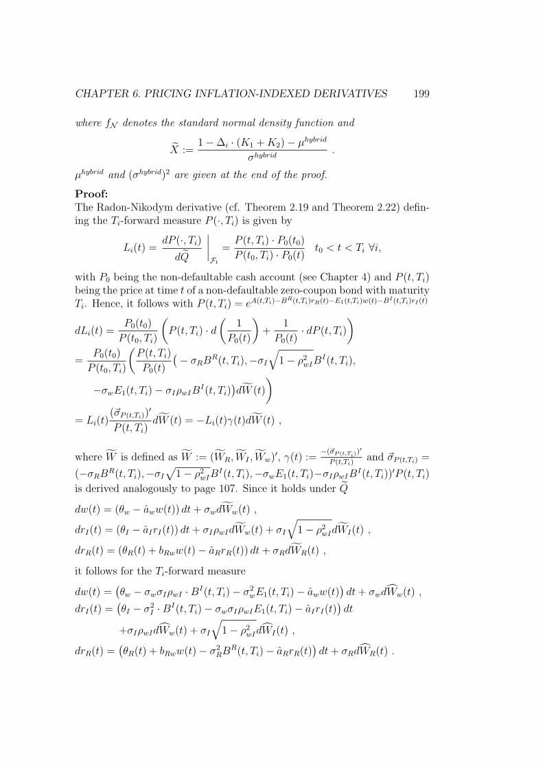
CHAPTER 6. PRICING INFLATION-INDEXED DERIVATIVES 199
where fN denotes the standard normal density function and
X :=1 − ∆i · (K1 + K2) − µhybrid
σhybrid.
µhybrid and (σhybrid)2 are given at the end of the proof.
Proof:The Radon-Nikodym derivative (cf. Theorem 2.19 and Theorem 2.22) defin-ing the Ti-forward measure P (·, Ti) is given by
Li(t) =dP (·, Ti)
dQ
∣∣∣∣Ft
=P (t, Ti) · P0(t0)
P (t0, Ti) · P0(t)t0 < t < Ti ∀i,
with P0 being the non-defaultable cash account (see Chapter 4) and P (t, Ti)being the price at time t of a non-defaultable zero-coupon bond with maturityTi. Hence, it follows with P (t, Ti) = eA(t,Ti)−BR(t,Ti)rR(t)−E1(t,Ti)w(t)−BI(t,Ti)rI(t)
dLi(t) =P0(t0)
P (t0, Ti)
(P (t, Ti) · d
(1
P0(t)
)+
1
P0(t)· dP (t, Ti)
)
=P0(t0)
P (t0, Ti)
(P (t, Ti)
P0(t)
(− σRBR(t, Ti),−σI
√1 − ρ2
wIBI(t, Ti),
−σwE1(t, Ti) − σIρwIBI(t, Ti)
)dW (t)
)
= Li(t)(~σP (t,Ti))
′
P (t, Ti)dW (t) = −Li(t)γ(t)dW (t) ,
where W is defined as W := (WR, WI , Ww)′, γ(t) :=−(~σP (t,Ti)
)′
P (t,Ti)and ~σP (t,Ti) =
(−σRBR(t, Ti),−σI
√1 − ρ2
wIBI(t, Ti),−σwE1(t, Ti)−σIρwIB
I(t, Ti))′P (t, Ti)
is derived analogously to page 107. Since it holds under Q
dw(t) = (θw − aww(t)) dt + σwdWw(t) ,
drI(t) = (θI − aIrI(t)) dt + σIρwIdWw(t) + σI
√1 − ρ2
wIdWI(t) ,
drR(t) = (θR(t) + bRww(t) − aRrR(t)) dt + σRdWR(t) ,
it follows for the Ti-forward measure
dw(t) =(θw − σwσIρwI · BI(t, Ti) − σ2
wE1(t, Ti) − aww(t))dt + σwdWw(t) ,
drI(t) =(θI − σ2
I · BI(t, Ti) − σwσIρwIE1(t, Ti) − aIrI(t))dt
+σIρwIdWw(t) + σI
√1 − ρ2
wIdWI(t) ,
drR(t) =(θR(t) + bRww(t) − σ2
RBR(t, Ti) − aRrR(t))dt + σRdWR(t) .

200 CHAPTER 6. PRICING INFLATION-INDEXED DERIVATIVES
In order to approximate the lognormals 1P (Ti−1,Ti)
and e∫ Ti
Ti−1rI(x)dx
, we need
to determine their means and variances.Since it holds for X ∼ N (µX , σ2
X) E[ 1eX ] = 1
E[eX ]· eσ2
X (cf. footnotes on page
193), the mean of the lognormal 1P (Ti−1,Ti)
can be obtained by
EP (·,Ti)
[1
P (Ti−1, Ti)
∣∣∣∣Ft
]=
1
EP (·,Ti) [P (Ti−1, Ti)| Ft]
·eV arP (·,Ti)[A(Ti−1,Ti)−BR(Ti−1,Ti)rR(Ti−1)−E1(Ti−1,Ti)w(Ti−1)−BI(Ti−1,Ti)rI(Ti−1)|Ft] .
Further, we can determine the expected value ofP (Ti−1, Ti) = eA(Ti−1,Ti)−BR(Ti−1,Ti)rR(Ti−1)−E1(Ti−1,Ti)w(Ti−1)−BI(Ti−1,Ti)rI(Ti−1) un-der the Ti-forward measure, by first calculating the expected value under themeasure Q and then adjusting the expectation by the terms which enteredthe drift of dw(t), drI(t) and drR(t) due to the change of measure. Ana-logously as in the proof of Lemma E.1, it now holds under the Ti-forwardmeasure for rI
rI(x)∣∣Ft
= rI(t) · e−aI(x−t) + θI · BI(t, x)
− σ2I
∫ x
t
e−aI(x−y)BI(y, Ti)dy − σwσIρwI
∫ x
t
e−aI(x−y)E1(y, Ti)dy
+ σI · ρwI
∫ x
t
e−aI(x−y)dWw(y) + σI
√1 − ρ2
wI
∫ x
t
e−aI(x−y)dWI(y) ,
and for w
w(x)∣∣Ft
= w(t) · e−aw(x−t) + θI · Bw(t, x)
− σwσIρwI
∫ x
t
e−aw(x−y)BI(y, Ti)dy − σ2w
∫ x
t
e−aw(x−y)E1(y, Ti)dy
+ σw
∫ x
t
e−aw(x−y)dWw(y) ,
and for rR
rR(x)∣∣Ft
= rR(t) · e−aR(x−t) +
∫ x
t
θR(y)e−aR(x−y)dy
CHAPTER 6. PRICING INFLATION-INDEXED DERIVATIVES 201
+bRw
aR − aw
(w(t) − θw
aw
)·(e−aw(x−t) − e−aR(x−t)
)+
bRw · θw
aw
BR(t, x)
+ bRw
∫ x
t
e−aR(x−y)
(−σwσIρwI
∫ y
t
e−aw(y−z)BI(z, Ti)dz
− σ2w
∫ y
t
e−aw(y−z)E1(z, Ti)dz
)dy − σ2
R
∫ x
t
e−aR(x−y)BR(y, Ti)dy
+bRw · σw
aR − aw
∫ x
t
(e−aw(x−y) − e−aR(x−y))dWw(y)
+ σR
∫ x
t
e−aR(x−y)dWR(y) ,
Hence, the expectation under Q needs to be adjusted as follows
EP (·,Ti) [P (Ti−1, Ti)| Ft]
= EP (·,Ti)
[eA(Ti−1,Ti)−BR(Ti−1,Ti)rR(Ti−1)−E1(Ti−1,Ti)w(Ti−1)−BI(Ti−1,Ti)rI(Ti−1)
∣∣∣Ft
]
= EQ
[eA(Ti−1,Ti)−BR(Ti−1,Ti)rR(Ti−1)−E1(Ti−1,Ti)w(Ti−1)−BI(Ti−1,Ti)rI(Ti−1)
∣∣∣Ft
]
·eE1(Ti−1,Ti)·(W1(Ti−1)+W2(Ti−1)) · eBI(Ti−1,Ti)·(I1(Ti−1)+I2(Ti−1,I))
·eBR(Ti−1,Ti)·(R1(Ti−1)+R2(Ti−1)+R3(Ti−1)) ,
with
E1(Ti−1, Ti) · (W1(Ti−1) + W2(Ti−1))
:= E1(Ti−1, Ti)
(σ2
w
∫ Ti−1
t
e−aw(Ti−1−y)E1(y, Ti)dy
+ σwσIρwI
∫ Ti−1
t
e−aw(Ti−1−y)BI(y, Ti)dy
)
being the adjustment for the term −E1(Ti−1, Ti)w(Ti−1), and
BI(Ti−1, Ti) · (I1(Ti−1) + I2(Ti−1, I))
:= BI(Ti−1, Ti)
(σwσIρwI
∫ Ti−1
t
e−aI(Ti−1−y)E1(y, Ti)dy
+ σ2I
∫ Ti−1
t
e−aI(Ti−1−y)BI(y, Ti)dy
)
the adjustment for the term −BI(Ti−1, Ti)rI(Ti−1), and with

202 CHAPTER 6. PRICING INFLATION-INDEXED DERIVATIVES
BR(Ti−1, Ti) · (R1(Ti−1) + R2(Ti−1) + R3(Ti−1))
:= BR(Ti−1, Ti)
(σ2
R
∫ Ti−1
t
e−aR(Ti−1−y)BR(y, Ti)dy
+ brw
∫ Ti−1
t
e−aR(Ti−1−y)W1(y)dy + brw
∫ Ti−1
t
e−aR(Ti−1−y)W2(y)dy
)
being the adjustment for the term −BR(Ti−1, Ti)rR(Ti−1), where the last twoterms (R1 and R2) are due to the fact that the factor w also enters the driftof rR.Closed-form solutions for these adjustment terms are given in Lemma E.5 inthe Appendix.Further, the mean of P (Ti−1, Ti) under Q can be decomposed into
EQ [P (Ti−1, Ti)| Ft]
= EQ
[EQ
[e−∫ Ti
Ti−1r(x)dx
∣∣∣∣FTi−1
]∣∣∣∣Ft
]
= EQ
[e−∫ Ti
Ti−1r(x)dx
∣∣∣∣Ft
]
= EQ
[e−
∫ Tit r(x)dxe+
∫ Ti−1t r(x)dx
∣∣∣Ft
]
footn. I= EQ
[e−
∫ Tit r(x)dx
∣∣∣Ft
]· EQ
[e∫ Ti−1
t r(x)dx∣∣∣Ft
]· eCovar
Q
[−∫ Ti
t r(x)dx ,∫ Ti−1
t r(x)dx∣∣∣Ft
]
= P (t, Ti) · EQ
[e∫ Ti−1
t r(x)dx∣∣∣Ft
]· eCovar
Q
[−∫ Ti−1
t r(x)dx ,∫ Ti−1
t r(x)dx∣∣∣Ft
]
·eCovarQ
[−∫ Ti
Ti−1r(x)dx ,
∫ Ti−1t r(x)dx
∣∣∣Ft
]
footn. II=
P (t, Ti)
EQ
[e−
∫ Ti−1t r(x)dx
∣∣∣Ft
] · e−CovarQ
[ ∫ TiTi−1
r(x)dx ,∫ Ti−1
t r(x)dx∣∣∣Ft
]
=P (t, Ti)
P (t, Ti−1)· e−Covar
Q
[ ∫ TiTi−1
r(x)dx ,∫ Ti−1
t r(x)dx∣∣∣Ft
]
,
with the help of the footnotes of page 193. The mean of e∫ Ti
Ti−1rI(x)dx
can bedetermined analogously by adjusting the expectation under the measure Q
EP (·,Ti)
[e∫ Ti
Ti−1rI(x)dx
∣∣∣∣Ft
]= EQ
[e∫ Ti
Ti−1rI(x)dx
∣∣∣∣Ft
]· e−I3(Ti−1,Ti)−I4(Ti−1,Ti,I)
with
I3(Ti−1, Ti) :=
∫ Ti
Ti−1
σwσIρwI
∫ x
t
e−aI(x−y)E1(y, Ti)dydx

CHAPTER 6. PRICING INFLATION-INDEXED DERIVATIVES 203
and
I4(Ti−1, Ti, I) :=
∫ Ti
Ti−1
σ2I
∫ x
t
e−aI(x−y)BI(y, Ti)dydx
being the adjustments term for rI due to the change of measure (cf. abovedynamics for rI under the Ti-forward measure).
Under Q it holds
EQ
[e∫ Ti
Ti−1rI(x)dx
∣∣∣∣Ft
]
= EQ
[e−
∫ Tit r(x)dxe
∫ TiTi−1
rI(x)dxe∫ Ti
t r(x)dx
∣∣∣∣Ft
]
footn. I= EQ
[e−
∫ Tit r(x)dxe
∫ TiTi−1
rI(x)dx
∣∣∣∣Ft
]· EQ
[e∫ Ti
t r(x)dx∣∣∣Ft
]
·eCovarQ
[−∫ Ti
t r(x)dx+∫ Ti
Ti−1rI(x)dx ,
∫ Tit r(x)dx
∣∣∣Ft
]
Th. 6.3=
P (t, Ti−1) · PR(t, Ti)
PR(t, Ti−1)· eCyoy(t,Ti−1,Ti) · EQ
[e∫ Ti
t r(x)dx∣∣∣Ft
]
·eCovarQ
[−∫ Ti
t r(x)dx+∫ Ti
Ti−1rI(x)dx ,
∫ Tit r(x)dx
∣∣∣Ft
]
=P (t, Ti−1) · PR(t, Ti)
PR(t, Ti−1)· eCyoy(t,Ti−1,Ti) · EQ
[e∫ Ti
t r(x)dx∣∣∣Ft
]
·eCovarQ
[−∫ Ti
t r(x)dx ,∫ Ti
t r(x)dx∣∣∣Ft
]
· eCovarQ
[ ∫ TiTi−1
rI(x)dx ,∫ Ti
t r(x)dx∣∣∣Ft
]
footn. II=
P (t, Ti−1) · PR(t, Ti) · eCyoy(t,Ti−1,Ti)
PR(t, Ti−1) · EQ
[e−
∫ Tit r(x)dx
∣∣∣Ft
] · eCovarQ
[ ∫ TiTi−1
rI(x)dx ,∫ Ti
t r(x)dx∣∣∣Ft
]
=P (t, Ti−1) · PR(t, Ti)
PR(t, Ti−1) · P (t, Ti)· eCyoy(t,Ti−1,Ti) · eCovar
Q
[ ∫ TiTi−1
rI(x)dx ,∫ Ti
t r(x)dx∣∣∣Ft
]
=P (t, Ti−1) · PR(t, Ti)
PR(t, Ti−1) · P (t, Ti)· eCyoy(t,Ti−1,Ti) · eCovar
Q
[ ∫ TiTi−1
rI(x)dx ,∫ Ti
t rI(x)dx∣∣∣Ft
]
·eCovarQ
[ ∫ TiTi−1
rI(x)dx ,∫ Ti
t rR(x)dx∣∣∣Ft
]
=P (t, Ti−1) · PR(t, Ti)
PR(t, Ti−1) · P (t, Ti)· eCyoy(t,Ti−1,Ti) · eCovar
Q
[ ∫ TiTi−1
rI(x)dx ,∫ Ti
t rI(x)dx∣∣∣Ft
]
·eCovarQ
[ ∫ TiTi−1
rI(x)dx ,∫ Ti−1
t rR(x)dx∣∣∣Ft
]
· eCovarQ
[ ∫ TiTi−1
rI(x)dx ,∫ Ti
Ti−1rR(x)dx
∣∣∣Ft
]
=P (t, Ti−1) · PR(t, Ti)
PR(t, Ti−1) · P (t, Ti)· eCovar
Q
[ ∫ TiTi−1
rI(x)dx ,∫ Ti
t rI(x)dx∣∣∣Ft
]
·eCovarQ
[ ∫ TiTi−1
rI(x)dx ,∫ Ti−1
t rR(x)dx∣∣∣Ft
]
· eCovarQ
[ ∫ Tit rI(x)dx ,
∫ TiTi−1
rR(x)dx∣∣∣Ft
]
204 CHAPTER 6. PRICING INFLATION-INDEXED DERIVATIVES
with
Cyoy(t, Ti−1, Ti) = CovarQ
[∫ Ti−1
t
rI(x)dx ,
∫ Ti
Ti−1
rR(x)dx
∣∣∣∣Ft
].
The covariances and the additional terms needed for adjusting the expectedvalue under the risk-neutral measure in order to determine it under the Ti-forward measure are given in Lemma E.5 in the Appendix.
Now, we can approximate the discounted payoff by
V iihybrid(t, Ti−1, Ti) = P (t, Ti) · EP (·,Ti)
[(Xhybrid − 1 + ∆i · (K1 + K2)
)+∣∣∣Ft
],
where Xhybrid is normal with the same mean and variance as1
P (Ti−1,Ti)− K2 · ∆i · e
∫ TiTi−1
rI(x)dx.
The variance for the lognormal 1P (Ti−1,Ti)
is given by III
V arP (·,Ti)
[1
P (Ti−1, Ti)
∣∣∣∣Ft
]
= V arP (·,Ti)
[e−A(Ti−1,Ti)+BR(Ti−1,Ti)rR(Ti−1)+E1(Ti−1,Ti)w(Ti−1)+BI(Ti−1,Ti)rI(Ti−1)
∣∣∣Ft
]
footn. III=
(EP (·,Ti)
[1
P (Ti−1, Ti)
∣∣∣∣Ft
])2
·(eV arP (·,Ti)[BR(Ti−1,Ti)rR(Ti−1)+E1(Ti−1,Ti)w(Ti−1)+BI(Ti−1,Ti)rI(Ti−1)|Ft] − 1
)
where the variance is obtained with the help of the equations for rR(x)∣∣Ft
,
rI(x)∣∣Ft
and w(x)∣∣Ft
(cf. pages 200ff)
V arP (·,Ti)
[−A(Ti−1, Ti) + BR(Ti−1, Ti) · rR(Ti−1) + E1(Ti−1, Ti) · w(Ti−1)
+ BI(Ti−1, Ti) · rI(Ti−1)∣∣Ft
]
= (BR(Ti−1, Ti))2 · V arQ
[σR
∫ Ti−1
t
e−aR(Ti−1−l)dWR(l)
∣∣∣∣Ft
]
+ (BI(Ti−1, Ti))2 · V arQ
[σI
√1 − ρ2
wI
∫ Ti−1
t
e−aI(Ti−1−l)dWI(l)
∣∣∣∣Ft
]
IIIIt holds for Xi ∼ N (µXi, σ2
Xi), i = 1, 2: V ar[eXi ] = (E[eXi ])2 · (eσ2
Xi − 1) and
V ar[eX1+X2 ] = E[eX1 ] · E[eX2 ] · (eCovar[X1+X2] − 1) (see e.g. Mueller (1991), page 552).

CHAPTER 6. PRICING INFLATION-INDEXED DERIVATIVES 205
+ V arQ
[∫ Ti−1
t
(BR(Ti−1, Ti) ·
σwbRw
aR − aw
·(e−aw(Ti−1−l) − e−aR(Ti−1−l)
)
+ E1(Ti−1, Ti) · σw · e−aw(Ti−1−l)+ BI(Ti−1, Ti) · σIρwI · e−aI(Ti−1−l))dWw(l)
∣∣∣Ft
]
= (BR(Ti−1, Ti) · σR)2BR+R(t, Ti−1) + (BI(Ti−1, Ti) · σI)2(1 − ρ2
wI)BI+I(t, Ti−1)
+
∫ Ti−1
t
(BR(Ti−1, Ti) ·
σwbRw
aR − aw
·(e−aw(Ti−1−l) − e−aR(Ti−1−l)
))2
dl
+
∫ Ti−1
t
(E1(Ti−1, Ti) · σw · e−aw(Ti−1−l)
)2dl
+
∫ Ti−1
t
(BI(Ti−1, Ti) · σIρwI · e−aI(Ti−1−l)
)2dl
+2
∫ Ti−1
t
(E1(Ti−1, Ti) · σw · e−aw(Ti−1−l))(BI(Ti−1, Ti) · σIρwI · e−aI(Ti−1−l))dl
+2
∫ Ti−1
t
BR(Ti−1, Ti) ·σwbRw
aR − aw
e−aw(Ti−1−l)(E1(Ti−1, Ti) · σw · e−aw(Ti−1−l))dl
−2
∫ Ti−1
t
BR(Ti−1, Ti) ·σwbRw
aR − aw
e−aR(Ti−1−l)(E1(Ti−1, Ti) · σw · e−aw(Ti−1−l))dl
+2
∫ Ti−1
t
BR(Ti−1, Ti) ·σwbRw
aR − aw
e−aw(Ti−1−l)(BI(Ti−1, Ti) · σIρwI · e−aI(Ti−1−l))dl
−2
∫ Ti−1
t
BR(Ti−1, Ti) ·σwbRw
aR − aw
e−aR(Ti−1−l)(BI(Ti−1, Ti) · σIρwI · e−aI(Ti−1−l))dl
= (BR(Ti−1, Ti) · σR)2 · BR+R(t, Ti−1) + (BI(Ti−1, Ti) · σI)2 · BI+I(t, Ti−1)
+
(BR(Ti−1, Ti) · σwbRw
aR − aw
)2
·(Bw+w(t, Ti−1) − 2 · Bw+R(t, Ti−1) + BR+R(t, Ti−1)
)
+ (E1(Ti−1, Ti) · σw)2 · Bw+w(t, Ti−1)
+ 2 · E1(Ti−1, Ti) · σw · BI(Ti−1, Ti) · σIρwI · BI+w(t, Ti−1)
+ 2 · BR(Ti−1, Ti)σwbRw
aR − aw
·(E1(Ti−1, Ti) · σw ·
(Bw+w(t, Ti−1) − Bw+R(t, Ti−1)
)
+ BI(Ti−1, Ti) · σIρwI ·(BI+w(t, Ti−1) − BI+R(t, Ti−1)
) ).
The variance is the same under both measures since the drift only is affectedby the change of measure.
Analogously, the variance of the lognormal e∫ Ti
Ti−1rI(x)dx
is

206 CHAPTER 6. PRICING INFLATION-INDEXED DERIVATIVES
V arP (·,Ti)
[e∫ Ti
Ti−1rI(x)dx
∣∣∣∣Ft
]
footn. III=
(EP (·,Ti)
[e∫ Ti
Ti−1rI(x)dx
∣∣∣∣Ft
])2
·(
eV arP (·,Ti)
[ ∫ TiTi−1
rI(x)dx∣∣∣Ft
]
− 1
)
where it holds (cf. Theorem 6.5)
V arP (·,Ti)
[∫ Ti
Ti−1
rI(x)dx
∣∣∣∣Ft
]= V arQ
[∫ Ti
Ti−1
rI(x)dx
∣∣∣∣Ft
]= VI(t, Ti−1, Ti)
For the variance of the sum of these lognormals, we also need to know thecovariance. We obtain this covariance with the help of the equations for
rR(x)∣∣Ft
, rI(x)∣∣Ft
and w(x)∣∣Ft
(cf. pages 200ff) and∫ Ti
Ti−1rI(x)dx
∣∣∣∣Ft
(cf.
Lemma E.1 in the Appendix).
CP,∫
rI
= CovarP (·,Ti)
[BR(Ti−1, Ti) · rR(Ti−1) + E1(Ti−1, Ti) · w(Ti−1)
+ BI(Ti−1, Ti) · rI(Ti−1) ,
∫ Ti
Ti−1
rI(x)dx
∣∣∣∣Ft
]
= CovarQ
[BR(Ti−1, Ti) · rR(Ti−1) + E1(Ti−1, Ti) · w(Ti−1)
+ BI(Ti−1, Ti) · rI(Ti−1) ,
∫ Ti
Ti−1
rI(x)dx
∣∣∣∣Ft
]
= CovarQ
[BR(Ti−1, Ti)
bRwσw
aR − aw
∫ Ti−1
t
(e−aw(Ti−1−y) − e−aR(Ti−1−y))dWw(y)
+ E1(Ti−1, Ti)σw
∫ Ti−1
t
e−aw(Ti−1−y)dWw(y)
+ BI(Ti−1, Ti)σIρwI
∫ Ti−1
t
e−aI(Ti−1−y)dWw(y) ,
σIρwI
(∫ Ti−1
t
(BI(y, Ti) − BI(y, Ti−1))dWw(y) +
∫ Ti
Ti−1
BI(y, Ti)dWw(y)
)∣∣∣∣Ft
]
+ CovarQ
[BI(Ti−1, Ti)σI
√1 − ρ2
wI
∫ Ti−1
t
e−aI(Ti−1−y)dWI(y) ,
σI
√1 − ρ2
wI
(∫ Ti−1
t
(BI(y, Ti) − BI(y, Ti−1))dWI(y) +
∫ Ti
Ti−1
BI(y, Ti)dWI(y)
)∣∣∣∣Ft
]
CHAPTER 6. PRICING INFLATION-INDEXED DERIVATIVES 207
= CovarQ
[BR(Ti−1, Ti)
bRwσw
aR − aw
∫ Ti−1
t
(e−aw(Ti−1−y) − e−aR(Ti−1−y))dWw(y)
+ E1(Ti−1, Ti)σw
∫ Ti−1
t
e−aw(Ti−1−y)dWw(y)
+ BI(Ti−1, Ti)σIρwI
∫ Ti−1
t
e−aI(Ti−1−y)dWw(y) ,
σIρwI
∫ Ti−1
t
(BI(y, Ti) − BI(y, Ti−1))dWw(y)
∣∣∣∣Ft
]
+ CovarQ
[BI(Ti−1, Ti)σI
√1 − ρ2
wI
∫ Ti−1
t
e−aI(Ti−1−y)dWI(y) ,
σI
√1 − ρ2
wI
∫ Ti−1
t
(BI(y, Ti) − BI(y, Ti−1))dWI(y)
∣∣∣∣Ft
]
= BR(Ti−1, Ti)bRwσwσIρwI
aR − aw
∫ Ti−1
t
BI(Ti−1, Ti)e−aI(Ti−1−y)(e−aw(Ti−1−y)
− e−aR(Ti−1−y))dy + E1(Ti−1, Ti)σwσIρwI
∫ Ti−1
t
e−aw(Ti−1−y)BI(Ti−1, Ti)e−aI(Ti−1−y)dy
+ BI(Ti−1, Ti)σ2Iρ
2wI
∫ Ti−1
t
e−aI(Ti−1−y)BI(Ti−1, Ti)e−aI(Ti−1−y)dy
+ BI(Ti−1, Ti)σ2I (1 − ρ2
wI)
∫ Ti−1
t
e−aI(Ti−1−y)BI(Ti−1, Ti)e−aI(Ti−1−y)dy
= BI(Ti−1, Ti) ·[σwbRwσIρwI
aR − aw
· BR(Ti−1, Ti) · (BI+w(t, Ti−1) − BI+R(t, Ti−1))
+ E1(Ti−1, Ti) · σwσIρwI · BI+w(t, Ti−1) + BI(Ti−1, Ti) · σ2I · BI+I(t, Ti−1)
],
such that
CovarP (·,Ti)
[1
P (Ti−1, Ti), e∫ Ti
Ti−1rI(x)dx
∣∣∣∣Ft
]
footn. III= EP (·,Ti)
[1
P (Ti−1, Ti)
∣∣∣∣Ft
]· EP (·,Ti)
[e∫ Ti
Ti−1rI(x)dx
∣∣∣∣Ft
]·(eCP,
∫rI − 1
)
Finally, we obtain the hybrid payoff by normal approximation
V iihybrid(t, Ti−1, Ti)
= P (t, Ti) · EP (·,Ti)
[(Xhybrid − 1 + ∆i · (K1 + K2)
)+∣∣∣Ft
],

208 CHAPTER 6. PRICING INFLATION-INDEXED DERIVATIVES
= P (t, Ti)
∫
y≥X
(σhybrid · y + µhybrid − 1 + ∆i · (K1 + K2)
)· fN (y)dy
= P (t, Ti) ·(σhybridfN (X) +
(µhybrid − 1 + ∆i · (K1 + K2)
)· N (−X)
)
where fN denotes the standard normal density function and
X := 1−∆i·(K1+K2)−µhybrid
σhybrid . Further, µhybrid and (σhybrid)2 denote the meanand variance of
1P (Ti−1,Ti)
− K2 · ∆i · e∫ Ti
Ti−1rI(x)dx
under the P (·, Ti)-forward measure:
µhybrid
= EP (·,Ti)
[1
P (Ti−1, Ti)− K2 · ∆i · e
∫ TiTi−1
rI(x)dx
∣∣∣∣Ft
]
= EP (·,Ti)
[1
P (Ti−1, Ti)
∣∣∣∣Ft
]− K2 · ∆i · EP (·,Ti)
[e∫ Ti
Ti−1rI(x)dx
∣∣∣∣Ft
]
and
(σhybrid)2
= V arP (·,Ti)
[1
P (Ti−1, Ti)− K2 · ∆i · e
∫ TiTi−1
rI(x)dx
∣∣∣∣Ft
]
= V arP (·,Ti)
[1
P (Ti−1, Ti)
∣∣∣∣Ft
]+ (K2 · ∆i)
2 · V arP (·,Ti)
[e∫ Ti
Ti−1rI(x)dx
∣∣∣∣Ft
]
− 2 · K2 · ∆i · CovarP (·,Ti)
[1
P (Ti−1, Ti), e∫ Ti
Ti−1rI(x)dx
∣∣∣∣Ft
]
Figure 6.1 compares the dependence on σI for the normal approximation ofTheorem 6.6 with the results obtained via simulation with 10,000 scenarios.We used the parameters of the INFcorr framework given in Chapter 4 (seeSection 4.7 with Tables 4.3 and 4.6) with K1 = 0.005 and K2 ∈ 0.5, 1.0, 1.5.The first row of Figure 6.1 contains the results for K2 = 0.5, the second rowfor K2 = 1.0 and the third for K2 = 1.5. Further, the left-hand side ofthe figure shows the result for σR = 0.005 whereas the right-hand side forσR = 0.1. The results in Figure 6.1 indicate that the normal approximationoverestimates the true value. Especially for increasing σI and decreasing K2,the approximation deviates from the simulated results. However, the approx-imated values approach the results obtained by simulation for growing K2

CHAPTER 6. PRICING INFLATION-INDEXED DERIVATIVES 209
0% 5% 10% 15%0%
10%20%30%40%50%60%
sigmaI
PV
0% 5% 10% 15%0%
10%
20%
30%
40%
sigmaI
PV
0% 5% 10% 15%0%
5%
10%
15%
20%sigmaR=0.005
sigmaI
PV
0% 5% 10% 15%0%
10%20%30%40%50%60%
sigmaI
PV
0% 5% 10% 15%0%
10%
20%
30%
40%
sigmaIP
V
0% 5% 10% 15%0%
5%
10%
15%
20%sigmaR=0.1
sigmaI
PV
Figure 6.1: The present value of a hybrid inflation caplet (cf. Theorem6.6) with a tenor of 1 year and maturity in 10 years for varying values ofσI . The results are obtained via normal approximation (given by diamonds)and via simulation for 10,000 paths (given by squares). The parameters aretaken from the model INFcorr of Section 4.7 with K1 = 0.005 and K2 ∈0.5, 1.0, 1.5 where the rows of the figure represent K2 in increasing order,i.e. the first row contains K2 = 0.5. The left part of the figure is obtainedby setting σR = 0.005, the right part by σR = 0.1.
even for higher values of σI . The reason for this is that for small values of K2
the inflation as well as the interest rate impact the value of the hybrid caplet.For growing values of K2, the caplet is mainly driven by the inflation andits volatility. We can confirm - as noted by Dodgson & Kainth (2006) - thatthe normal approximation yields extremely accurate results for small valuesof σI and σR. Dependent on the factors K1 and K2, the approximation evenholds for higher volatilities. Realistic parameters in a Hull-White inflationset-up are according to Dodgson & Kainth (2006) σI , σR ≤ 0.02. Hence, wecan conclude that the normal approximation is a fast way to approximatehybrid payoffs for realistic parameters within our framework.

210 CHAPTER 6. PRICING INFLATION-INDEXED DERIVATIVES
6.3.1 Inflation-Linked Equity Options
Investors who want the real value of their equity portfolio to remain at leastequal to its original value, can use inflation-linked equity options to do so(see Kerkhof (2005)). For example, buying the stock and a spread optionwhich pays the difference (if positive) between the inflation and the stockreturn, guarantees the real value of the equity. Furthermore, according toDodgson & Kainth (2006) bonds paying the maximum of an equity indexand a price index are ”an increasingly popular retail product”. Based onthat observation Hammarlid (2010) introduces a European call option withan inflation-linked strike and prices this product under certain assumptions,namely a log-normal distribution of the ratio of the stock return and theinflation-linked bond price. Both papers refer to a payoff of the form
max
(CPI(T )
CPI(T0)− S(T )
S(T0), 0
)
with S being an equity index. While Dodgson & Kainth (2006) do not pro-vide a pricing for such payoffs, Hammarlid (2010) rewrites the payoff suchthat the non-traded inflation index is substituted by a zero-coupon inflation-linked bond. Hence, this payoff can be regarded as an exchange option andcan be priced by means of a change of numeraire (cf. Margrabe (1978)).Following the approach of Hammarlid (2010) we introduce an additionalprocess describing continuous stock returns into our set-up. This processwas previously introduced in Meyer (2005) and Hagedorn et al. (2007) whoanalyzed interest rate models and equtiy models which incorporate macroe-conomic information. We assume that under the risk-neutral measure Qthe process of the continuous stock return evolves according to the followingequation
dRE(t) = (αE + bER rR(t) − bEI rI(t) + bEw w(t)) dt + σEdWE(t) ,
with an uncorrelated Brownian motion WE, αE ∈ R and positive constantsbER, bEI , bEw, σE. Further, the equity index S(T ) as well as the inflation
index CPI(T ) are lognormal with S(T ) = S(0)e∫ T0 RE(x)dx and
CPI(T ) = CPI(0)e∫ T0 rI(x)dx. Hence, we pose ourselves in a similar set-up
as in Hammarlid (2010), but start with modelling different processes, e.g.inflation short rate vs. proportional change of index.
Theorem 6.7 (Inflation-Linked Equity Option)The value at time t (t ≤ T0 ≤ Ti) of a European option referring to an equityindex and having an inflation-linked strike with payoff
max
(CPI(T )
CPI(T0)− S(T )
S(T0), 0
)
CHAPTER 6. PRICING INFLATION-INDEXED DERIVATIVES 211
is
V iieopt(t, T0, Ti) = P (t, Ti) ·(
EP (·,Ti)
[e∫ Ti
T0rI(x)dx
∣∣∣Ft
]· N (d1)
−EP (·,Ti)
[e∫ Ti
T0RE(x)dx
∣∣∣Ft
]· N (d2)
)
with
d1 =1√
VEI(t, T0, Ti)·
ln
EP (·,Ti)
[e∫ Ti
T0rI(x)dx
∣∣∣Ft
]
EP (·,Ti)
[e∫ Ti
T0RE(x)dx
∣∣∣Ft
]
+
1
2VEI(t, T0, Ti)
,
d2 = d1 −√
VEI(t, T0, Ti) ,
and
VEI(t, T0, Ti) = V arP (·,Ti)
[∫ Ti
T0
rI(x)dx
∣∣∣∣Ft
]+ V arP (·,Ti)
[∫ Ti
T0
RE(x)dx
∣∣∣∣Ft
]
+2 CovarP (·,Ti)
[∫ Ti
T0
rI(x)dx ,
∫ Ti
T0
RE(x)dx
∣∣∣∣Ft
].
Proof:By a change of measure the value of the European option at time t,(t ≤ T0 ≤ Ti), is
V iieopt(t, T0, Ti)
= EQ
[e−
∫ Tit r(x)dx
(e∫ Ti
T0rI(x)dx − e
∫ TiT0
RE(x)dx)+∣∣∣∣Ft
]
= P (t, Ti) · EP (·,Ti)
[(e∫ Ti
T0rI(x)dx − e
∫ TiT0
RE(x)dx)+∣∣∣∣Ft
]
= P (t, Ti) ·(
EP (·,Ti)
[e∫ Ti
T0rI(x)dx
∣∣∣Ft
]· N (d1)
−EP (·,Ti)
[e∫ Ti
T0RE(x)dx
∣∣∣Ft
]· N (d2)
)
with
d1 =1√
VEI(t, T0, Ti)·
ln
EP (·,Ti)
[e∫ Ti
T0rI(x)dx
∣∣∣Ft
]
EP (·,Ti)
[e∫ Ti
T0RE(x)dx
∣∣∣Ft
]
+
1
2VEI(t, T0, Ti)
,
d2 = d1 −√
VEI(t, T0, Ti) ,

212 CHAPTER 6. PRICING INFLATION-INDEXED DERIVATIVES
and
VEI(t, T0, Ti) = V arP (·,Ti)
[∫ Ti
T0
rI(x)dx
∣∣∣∣Ft
]+ V arP (·,Ti)
[∫ Ti
T0
RE(x)dx
∣∣∣∣Ft
]
+2 CovarP (·,Ti)
[∫ Ti
T0
rI(x)dx ,
∫ Ti
T0
RE(x)dx
∣∣∣∣Ft
].
The formula is based as before on two lognormal distributions. The term
VI(t, T0, Ti) = V arP (·,Ti)
[∫ Ti
T0rI(x)dx
∣∣∣Ft
]= V arQ
[∫ Ti
T0rI(x)dx
∣∣∣Ft
]is given
in Theorem 6.5. Also, a detailed derivation of the above terms can be foundin the Appendix (Lemma E.6).
The most challenging part in pricing such products will be the choice ofparameters - especially for correlation - as long as there is no liquid market.We somehow circumvent this problematic part by letting WE be indepen-dent of the Brownian motions of the other processes. However, if we omitthis assumption such hybrid products like this are needed to calibrate theadditional correlation parameters.
6.3.2 Inflation-Indexed Credit Default Swap
In addition to the above mentioned hybrid products there exist approacheslinking not only inflation and interest rates, but inflation and credit. Kerkhof(2005) mentions in his survey of inflation derivatives inflation-linked CDOand CDS. By means of an inflation-linked CDS an investor can trade on hisview on inflation and credit correlation. Avogaro (2006) introduces a CDSwhose premium payments are based on the inflation rate. We will adopt thepayoffs of that approach but will model the underlying factors according toour set-up.
Definition 6.8An Inflation-Indexed Credit Default Swap is a CDS where the premium pay-ments are a combination of the CDS spread and the inflation rate representedby the ratio of the CPI at the beginning and the end of each payment period.
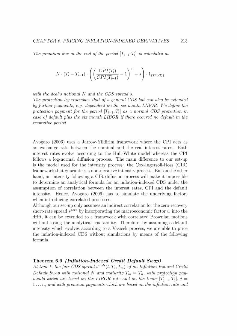
CHAPTER 6. PRICING INFLATION-INDEXED DERIVATIVES 213
The premium due at the end of the period [Ti−1, Ti] is calculated as
N · (Ti − Ti−1) ·((
CPI(Ti)
CPI(Ti−1)− 1
)+
+ s
)· 1T d>Ti
with the deal’s notional N and the CDS spread s.The protection leg resembles that of a general CDS but can also be extendedby further payments, e.g. dependent on the six month LIBOR. We define theprotection payment for the period [Ti−1, Ti] as a normal CDS protection incase of default plus the six month LIBOR if there occured no default in therespective period.
Avogaro (2006) uses a Jarrow-Yildirim framework where the CPI acts asan exchange rate between the nominal and the real interest rates. Bothinterest rates evolve according to the Hull-White model whereas the CPIfollows a log-normal diffusion process. The main difference to our set-upis the model used for the intensity process: the Cox-Ingersoll-Ross (CIR)framework that guarantees a non-negative intensity process. But on the otherhand, an intensity following a CIR diffusion process will make it impossibleto determine an analytical formula for an inflation-indexed CDS under theassumption of correlation between the interest rates, CPI and the defaultintensity. Hence, Avogaro (2006) has to simulate the underlying factorswhen introducing correlated processes.Although our set-up only assumes an indirect correlation for the zero-recoveryshort-rate spread szero by incorporating the macroeconomic factor w into thedrift, it can be extended to a framework with correlated Brownian motionswithout losing the analytical tractability. Therefore, by assuming a defaultintensity which evolves according to a Vasicek process, we are able to pricethe inflation-indexed CDS without simulations by means of the followingformula.
Theorem 6.9 (Inflation-Indexed Credit Default Swap)At time t, the fair CDS spread siicds(t, T0, Tm) of an Inflation-Indexed Credit
Default Swap with notional N and maturity Tm = Tn, with protection pay-ments which are based on the LIBOR rate and on the tenor [Tj−1, Tj], j =1 . . . n, and with premium payments which are based on the inflation rate and

214 CHAPTER 6. PRICING INFLATION-INDEXED DERIVATIVES
on the tenor [Ti−1, Ti], i = 1 . . . m, is
siicds(t, T0, Tm)
=1∑m
i=1(Ti − Ti−1)P d,zero(t, Ti)·[
n∑
j=1
(P (t, Tj−1) · P S(t, Tj) · e
CovarQ
[ ∫ Tj−1t rR(x)dx ,
∫ Tjt szero(x)dx
∣∣∣∣Ft
]
· eCovarQ
[ ∫ Tj−1t rI(x)dx ,
∫ Tjt szero(x)dx
∣∣∣∣Ft
]
− P d,zero(t, Tj)
)
+ V ddpT d (t, Tm) − V ddp
T d (t, T0) − P d,∗(t, T0, T∗) + P d,∗(t, Tm, T ∗)
−m∑
i=1
(Ti − Ti−1) ·(Ecds
Q(t, Ti−1, Ti) · N (d1) − P d,zero(t, Ti) · N (d2)
)]
with
d1,2 =
ln
(Ecds
Q(t,Ti−1,Ti)
P d,zero(t,Ti)
)+− VI(t,Ti−1,Ti)
2
√VI(t, Ti−1, Ti)
.
The other terms in the above formula are given in the proof.
Proof:The value at time t of the premium leg
EQ
[N ·
m∑
i=1
(Ti − Ti−1) · e−∫ Ti
t r(x)dx
((CPI(Ti)
CPI(Ti−1)− 1
)+
+ siicds
)· 1T d>Ti
∣∣∣∣∣Gt
]
= L(t) · N ·m∑
i=1
(Ti − Ti−1) · EQ
[e−
∫ Tit r(x)+szero(x)dx ·
(e∫ Ti
Ti−1rI(x)dx − 1
)+∣∣∣∣∣Ft
]
+ L(t) · N ·m∑
i=1
(Ti − Ti−1) · siicds · P d,zero(t, Ti)
depends on the term
EQ
[(e−∫ Ti
t r(x)+szero(x)dx+∫ Ti
Ti−1rI(x)dx − e−
∫ Tit r(x)+szero(x)dx
)+∣∣∣∣∣Ft
]
for whose derivation we need the following components. The variance
VI(t, Ti−1, Ti) := V arQ
[∫ Ti
Ti−1rI(x)dx
∣∣∣Ft
]which is already given in Theorem

CHAPTER 6. PRICING INFLATION-INDEXED DERIVATIVES 215
6.5. The expected value
EcdsQ
(t, Ti−1, Ti) := EQ
[e−∫ Ti
t r(x)+szero(x)dx+∫ Ti
Ti−1rI(x)dx
∣∣∣∣Ft
]
footn. I= EQ
[e−
∫ Tit r(x)+szero(x)dx
∣∣∣Ft
]· EQ
[e∫ Ti
Ti−1rI(x)dx
∣∣∣∣Ft
]
· eCovarQ
[−∫ Ti
t rR(x)+rI(x)+szero(x)dx ,∫ Ti
Ti−1rI(x)dx
∣∣∣Ft
]
= EQ
[e−
∫ Tit r(x)+szero(x)dx
∣∣∣Ft
]· EQ
[e∫ Ti
Ti−1rI(x)dx
∣∣∣∣Ft
]
· eCovarQ
[−∫ Ti
t rR(x)dx ,∫ Ti
Ti−1rI(x)dx
∣∣∣Ft
]
· eCovarQ
[−∫ Ti
t rI(x)dx ,∫ Ti
Ti−1rI(x)dx
∣∣∣Ft
]
· eCovarQ
[−∫ Ti
t szero(x)dx ,∫ Ti
Ti−1rI(x)dx
∣∣∣Ft
]
can be decomposed into P d,zero(t, Ti) and into the expected value of e∫ Ti
Ti−1rI(x)dx
and related covariance terms.The expected value under the measure Q is already determined in Section6.3 (cf. proof of Theorem 6.6):
EQ
[e∫ Ti
Ti−1rI(x)dx
∣∣∣∣Ft
]
=P (t, Ti−1) · PR(t, Ti)
P (t, Ti) · PR(t, Ti−1)· eCovar
Q
[ ∫ TiTi−1
rI(x)dx ,∫ Ti−1
t rR(x)dx∣∣∣Ft
]
· eCovarQ
[ ∫ TiTi−1
rI(x)dx ,∫ Ti
t rI(x)dx∣∣∣Ft
]
· eCovarQ
[ ∫ TiTi−1
rR(x)dx ,∫ Ti
t rI(x)dx∣∣∣Ft
]
where the covariance terms under the measure Q are equivalent to thosegiven in the proof of Theorem 6.6.The first component of
CovarQ
[∫ Ti
t
rI(x)dx ,
∫ Ti
Ti−1
rI(x)dx
∣∣∣∣Ft
]
= CovarQ
[∫ Ti−1
t
rI(x)dx ,
∫ Ti
Ti−1
rI(x)dx
∣∣∣∣Ft
]+ VI(t, Ti−1, Ti)
is given in Proposition 6.4, and the remaining covariance terms in LemmaE.7.Hence, it holds (cf. Theorem 6.5)
EQ
[(e−∫ Ti
t r(x)+szero(x)dx+∫ Ti
Ti−1rI(x)dx − e−
∫ Tit r(x)+szero(x)dx
)+∣∣∣∣∣Ft
]
= EcdsQ
(t, Ti−1, Ti) · N (d1) − P d,zero(t, Ti) · N (d2)

216 CHAPTER 6. PRICING INFLATION-INDEXED DERIVATIVES
with
d1,2 =
ln
(Ecds
Q(t,Ti−1,Ti)
P d,zero(t,Ti)
)+− VI(t,Ti−1,Ti)
2
√VI(t, Ti−1, Ti)
.
The value of the protection leg at time t is
EQ
[N ·
n∑
j=1
(Tj − Tj−1) · e−∫ Tj
t r(x)dx · L(Tj−1, Tj) · 1T d>Tj
∣∣∣∣∣Gt
]
+ EQ
[N ·
∫ Tn
T0
e−∫ l
tr(x)dx(1 − Z(l))dH(l)
∣∣∣∣∣Gt
]
= L(t) · N ·n∑
j=1
EQ
[e−
∫ Tjt r(x)+szero(x)dx ·
(e
∫ Tj
Tj−1r(x)dx − 1
)∣∣∣∣∣Ft
]
+ L(t) · N · (V ddpT d (t, Tm) − V ddp
T d (t, T0) − P d,∗(t, T0, T∗) + P d,∗(t, Tm, T ∗))
= L(t) · N ·n∑
j=1
(EQ
[e−
∫ Tj−1t r(x)dx · e−
∫ Tjt szero(x)dx
∣∣∣∣Ft
]− P d,zero(t, Tj)
)
+ L(t) · N · (V ddpT d (t, Tm) − V ddp
T d (t, T0) − P d,∗(t, T0, T∗) + P d,∗(t, Tm, T ∗))
footn. I= L(t) · N ·
n∑
j=1
(EQ
[e−
∫ Tj−1t r(x)dx
∣∣∣∣Ft
]· EQ
[e−
∫ Tjt szero(x)dx
∣∣∣∣Ft
]
· eCovarQ
[ ∫ Tj−1t rR(x)+rI(x)dx ,
∫ Tjt szero(x)dx
∣∣∣∣Ft
]
− P d,zero(t, Tj)
)
+ L(t) · N · (V ddpT d (t, Tm) − V ddp
T d (t, T0) − P d,∗(t, T0, T∗) + P d,∗(t, Tm, T ∗))
= L(t) · N ·n∑
j=1
(P (t, Tj−1) · P S(t, Tj) · e
CovarQ
[ ∫ Tj−1t rR(x)dx ,
∫ Tjt szero(x)dx
∣∣∣∣Ft
]
· eCovarQ
[ ∫ Tj−1t rI(x)dx ,
∫ Tjt szero(x)dx
∣∣∣∣Ft
]
− P d,zero(t, Tj)
)
+ L(t) · N · (V ddpT d (t, Tm) − V ddp
T d (t, T0) − P d,∗(t, T0, T∗) + P d,∗(t, Tm, T ∗))
with Tn = Tm and T0 = T0. The covariance terms are given in Lemma E.7in the Appendix. The first equivalence is due to Theorem 5.13 assuming azero-coupon bond with maturity T ∗ as underlying reference asset. The thirdequivalence follows from the footnote introduced in the proof of Theorem 6.3.The last equivalence is based on a decomposition of the covariance terms and

CHAPTER 6. PRICING INFLATION-INDEXED DERIVATIVES 217
on the survival probability of Theorem 5.4.
In the following, we compare CDS spreads obtained by the above formulawith plain vanilla CDS spreads of Theorem 5.13 for a forward starting CDSthat matures in five years. We use the parameters of the uncorrelated infla-tion short-rate framework of Chapter 4 (see model INF with data set BBB1in Table 4.3, Table 4.6, Table 4.9 and Table 4.10). Further, we assume thepremium payments to be quarterly and the tenor of the LIBOR-based pro-tection payments to be six months. We analyze the impact of higher levels ofthe inflation short rate rI and the short-rate spread s, i.e. θs and θI , as wellas the dependence of the spreads on σI . Figure 6.2 presents in the upper rowthe spreads of a plain vanilla CDS, whereas the lower row gives the spreads ofa structured CDS as given in Theorem 6.9. The plots in the first column areobtained with θs = 0.001 and the ones in the second column with θs = 0.005.In each subplot, diamonds refer to results based on θI = 0.01 and squaresrefer to results based on θI = 0.005.As expected, all spreads increase for higher values of θs indicating an in-
creased risk of default. The spreads of the structured CDS (given in thesecond row) are on a high level for small values of σI and drop for increasingσI . As opposed to the spreads of the structured CDS, the plain vanilla CDSspreads start at a lower level and increase slightly for greater values of σI .In order to compare these results, it must be noted that the premium pay-ments of the structured CDS consists of two parts: the CDS spread siicds
given in Figure 6.2 and the inflation rate - if positive - for the respectiveperiod which has to be paid on top of the CDS spread. Further, the protec-tion payments of the structured CDS differ from the plain vanilla CDS sincea second term based on the LIBOR rate is included. In Tables 6.1 -6.4 wecompare the performance of the CDS spreads by introducing two simplifiedversions of the structured CDS. First, we eliminate the LIBOR-based pro-tection payments such that the protection leg is equal to the plain vanillacase but keep the premium payments linked to the inflation rate. This struc-tured CDS is labelled CPI in the Tables 6.1 - 6.4. Second, we reverse thesechanges by keeping the LIBOR-based protection payments but eliminate thepremium payments based on CPI. This structured CDS is labelled LIBORin the Tables 6.1 - 6.4. The plain vanilla CDS is denoted by PLAIN and theset-up of Theorem 6.9 is called CPI&LIBOR.Comparing Tables 6.1 - 6.4, we see at first glance that the structures PLAINand CPI with equivalent protection legs but differing premium legs obtainsimilar results throughout all combinations of θs, θI and σI . The CDS spreadsof the structures PLAIN and CPI increase for greater values of σI . Ana-

218 CHAPTER 6. PRICING INFLATION-INDEXED DERIVATIVES
0% 1% 2% 3%0%
2%
4%
6%
8%
sigmaI
CD
S s
prea
d
0% 1% 2% 3%1.5%
2.0%
2.5%
3.0%
3.5%
thetaS=0.001
sigmaI
CD
S s
prea
d
0% 1% 2% 3%0%
2%
4%
6%
8%
sigmaI
CD
S s
prea
d
0% 1% 2% 3%1.5%
2.0%
2.5%
3.0%
3.5%
thetaS=0.005
sigmaI
CD
S s
prea
d
Figure 6.2: CDS spreads calculated within the inflation short-rate framework(ρwI = 0, cf. model INF in Chapter 4) by means of the formulas given inTheorem 5.13 and Theorem 6.9 for a CDS starting in 1 year and maturingin 5 years. The first row gives the results of Theorem 5.13 and the secondrow the spreads obtained by Theorem 6.9. The results in the left column arebased on θs = 0.001, the results in the right column on θs = 0.005. In eachsubplot, diamonds refer to results based on θI = 0.01 and squares refer toresults based on θI = 0.005. Premium payments are quarterly, whereas thetenor of the LIBOR-based protection payment of the CDS given in Theorem6.9 is 6 months.
logously, the performances of the structures LIBOR and CPI&LIBOR, whichalso share the same protection leg but differ in the set-up of the premiumlegs, show similarities. Both structures have CDS spreads that start on ahigh level but decrease for greater values of σI .Table 6.1 and Table 6.2 contain CDS spreads that are determined for θs =0.001, whereas the Tables 6.3 and 6.4 are based on a higher mean reversionlevel (θs = 0.005). As expected, we see that all spreads given in Table 6.3and Table 6.4 are higher than the spreads of the first two tables, accounting

CHAPTER 6. PRICING INFLATION-INDEXED DERIVATIVES 219
for the increased default probabilities.If we look in detail at the structures PLAIN and CPI, we can conclude thatboth structures yield higher CDS spreads for increasing σI and lower CDSspreads for greater values of θI . An increase in the volatility of the inflationshort rate rI impacts directly the default probabilities as well as the prices ofriskless bonds, since rI enters the SDEs of the short rate r and the short-ratespread s. Therefore increasing values of σI imply a higher risk of default andhigher prices of riskless bonds. The influence of θI is opposite to σI , since thespreads decline for higher values of θI . This is mainly due to the fact that theinflation short-rate rI reduces the drift of the short-rate spread s (bsI > 0)resulting in lower probabilities of default. For the given set of parameters,the same relationship holds for the short rate r since the parameter brI isnegative resulting in lower interest rates for higher values of rI .However, there are differences in the behaviour of the structures PLAIN andCPI. For small values of σI the spreads of the structure CPI are lower thanthe ones of the plain vanilla CDS (PLAIN). For increasing values of σI thestructure CPI yields higher spreads than the plain vanilla case. Since thepremium payments of the structure CPI consists of the spread siicds and anadditional inflation premium, the expected value of this second term influ-ences the spread. The additional inflation premium is only due if the inflationrate of the respective period is positive, hence the additional term is an op-tionality on the inflation rate and is therefore driven by the volatility of theinflation short rate rI . For small values of σI , the expectation about thefuture inflation rate is that it is mainly increasing. Hence, it is expectedthat the additional inflation premium has to be paid for the majority of theperiods. This expectation reduces the CDS spread of the structure CPI asopposed to the structure PLAIN because the protection payments are as-sumed to be equal. For higher values of σI , the probability of the additionalinflation premium not being paid increases. Therefore, the CDS spreads ofthe structure CPI approach and even exceed the results of the plain vanillaCDS due to the costs of the optionality.The structures LIBOR and CPI&LIBOR differ from the previously discussedstructures by the set-up of the protection leg. Here, the proctection leg hasan additional term that is based on the LIBOR rate for a specified tenor.The impact of this additional term can be observed by the higher level ofthe CDS spreads of the structures LIBOR and CPI&LIBOR throughout allcombinations of θI , θs and σI . The influence of θI on the CDS spreads ofthe structures LIBOR and CPI&LIBOR is similar to the structures PLAINand CPI: A higher mean reversion level of the inflation short rate implieslower probabilities of default and therefore lower CDS spreads that have tobe paid. The influence of σI on the CDS spreads of the structures LIBOR

220 CHAPTER 6. PRICING INFLATION-INDEXED DERIVATIVES
and CPI&LIBOR is opposite to the structures PLAIN and CPI: The CDSspreads decline for increasing values of σI . As noted above, the inflationshort rate rI influences also the riskless interest rates. Therefore, a highervolatility in the interest rates increases the probability of the additional pro-tection payments becoming smaller. The behaviour of the CDS spreads ofthe structure CPI&LIBOR is analogous to the structure CPI with respectto σI . The premium payments of the structure CPI&LIBOR contain an ad-ditional inflation premium as opposed to the premium leg of the structureLIBOR. For small values of σI , the expected value of this inflation premiumreduces the value of the constant CDS spread siicds to be paid in the structureCPI&LIBOR. However, for increasing values of σI , the probability of the in-flation premium being positive decreases. Therefore the CDS spreads of thestructure CPI&LIBOR approach the ones of the structure LIBOR. Finally,for all four structures it can be observed that for increased mean reversionlevel and volatility of the inflation short rate, i.e. θI = 0.01 and σI = 0.03,the CDS spreads become closer.Summarizing the above analysis, we can conclude that including an addi-tional protection payment can increase the CDS spreads substantially asopposed to the plain vanilla case. In addition, the introduction of an op-tional premium payment can decrease the CDS spread but not in all cases.The value of such a structured CDS stronlgy depends on the correlation ofthe driving factors for the default probability and for the additional premiumand protection cash flows.
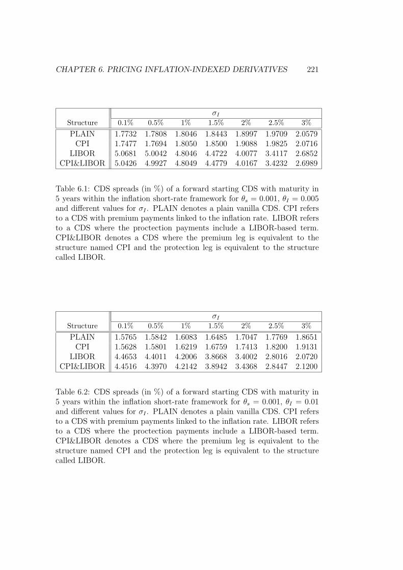
CHAPTER 6. PRICING INFLATION-INDEXED DERIVATIVES 221
σI
Structure 0.1% 0.5% 1% 1.5% 2% 2.5% 3%
PLAIN 1.7732 1.7808 1.8046 1.8443 1.8997 1.9709 2.0579CPI 1.7477 1.7694 1.8050 1.8500 1.9088 1.9825 2.0716
LIBOR 5.0681 5.0042 4.8046 4.4722 4.0077 3.4117 2.6852CPI&LIBOR 5.0426 4.9927 4.8049 4.4779 4.0167 3.4232 2.6989
Table 6.1: CDS spreads (in %) of a forward starting CDS with maturity in5 years within the inflation short-rate framework for θs = 0.001, θI = 0.005and different values for σI . PLAIN denotes a plain vanilla CDS. CPI refersto a CDS with premium payments linked to the inflation rate. LIBOR refersto a CDS where the proctection payments include a LIBOR-based term.CPI&LIBOR denotes a CDS where the premium leg is equivalent to thestructure named CPI and the protection leg is equivalent to the structurecalled LIBOR.
σI
Structure 0.1% 0.5% 1% 1.5% 2% 2.5% 3%
PLAIN 1.5765 1.5842 1.6083 1.6485 1.7047 1.7769 1.8651CPI 1.5628 1.5801 1.6219 1.6759 1.7413 1.8200 1.9131
LIBOR 4.4653 4.4011 4.2006 3.8668 3.4002 2.8016 2.0720CPI&LIBOR 4.4516 4.3970 4.2142 3.8942 3.4368 2.8447 2.1200
Table 6.2: CDS spreads (in %) of a forward starting CDS with maturity in5 years within the inflation short-rate framework for θs = 0.001, θI = 0.01and different values for σI . PLAIN denotes a plain vanilla CDS. CPI refersto a CDS with premium payments linked to the inflation rate. LIBOR refersto a CDS where the proctection payments include a LIBOR-based term.CPI&LIBOR denotes a CDS where the premium leg is equivalent to thestructure named CPI and the protection leg is equivalent to the structurecalled LIBOR.

222 CHAPTER 6. PRICING INFLATION-INDEXED DERIVATIVES
σI
Structure 0.1% 0.5% 1% 1.5% 2% 2.5% 3%
PLAIN 3.3125 3.3201 3.3440 3.3838 3.4395 3.5111 3.5984CPI 3.2844 3.3059 3.3411 3.3861 3.4450 3.5189 3.6084
LIBOR 6.5684 6.5081 6.3198 6.0064 5.5682 5.0059 4.3204CPI&LIBOR 6.5403 6.4939 6.3170 6.0086 5.5736 5.0138 4.3304
Table 6.3: CDS spreads (in %) of a forward starting CDS with maturity in5 years within the inflation short-rate framework for θs = 0.005, θI = 0.005and different values for σI . PLAIN denotes a plain vanilla CDS. CPI refersto a CDS with premium payments linked to the inflation rate. LIBOR refersto a CDS where the proctection payments include a LIBOR-based term.CPI&LIBOR denotes a CDS where the premium leg is equivalent to thestructure named CPI and the protection leg is equivalent to the structurecalled LIBOR.
σI
Structure 0.1% 0.5% 1% 1.5% 2% 2.5% 3%
PLAIN 3.0315 3.0393 3.0635 3.1039 3.1605 3.2331 3.3218CPI 3.0163 3.0340 3.0753 3.1284 3.1934 3.2720 3.3654
LIBOR 5.9051 5.8445 5.6554 5.3406 4.9006 4.3359 3.6475CPI&LIBOR 5.8898 5.8393 5.6672 5.3651 4.9335 4.3749 3.6911
Table 6.4: CDS spreads (in %) of a forward starting CDS with maturity in5 years within the inflation short-rate framework for θs = 0.005, θI = 0.01and different values for σI . PLAIN denotes a plain vanilla CDS. CPI refersto a CDS with premium payments linked to the inflation rate. LIBOR refersto a CDS where the proctection payments include a LIBOR-based term.CPI&LIBOR denotes a CDS where the premium leg is equivalent to thestructure named CPI and the protection leg is equivalent to the structurecalled LIBOR.

Chapter 7
Summary and Conclusion
In this thesis we studied the determinants of non-defaultable and defaultablebond prices within a defaultable term structure model by directly includingthe chosen factors into the pricing framework. We tested the inclusion ofobservable as well as unobservable macroeconomic factors into the pricingframework and found that observable macroeconomic factors are capable ofimproving the pricing. But the impact of observable macroeconomic fac-tors is limited, since there is still a large portion of systematic behaviourthat cannot be explained. In line with these findings, we also analyzed thecombined incorporation of observable and unobservable macroeconomic fac-tors and obtaind promising results. Further, we used this defaultable termstructure model for pricing credit as well as inflation-linked derivatives. Wederived and analyzed closed-form solutions for a range of complex deriva-tives like credit default swaptions, constant maturity credit default swapsand hybrid inflation-linked derivatives, enabling its usage in valuation andrisk management.In Chapter 4 we introduced a family of models based on a defaultable termstructure model that incorporates macroeconomic and firm-specific factors.This approach is influenced by the literature of determinants of sovereign andbond prices which indicates that both prices are driven by common factorsand that defaultable bond prices can be also explained by firm-specific fac-tors. Since the availability of firm-specific data is sparse, its disclosure oftencomes with a delay of up to one year (annual reports) and its content is addi-tionally disturbed by regulatory requirements, we assumed the firm-specificdata entering our model to be unobservable. However, there is a wide rangeof macroeconomic factors published on a regular basis that are supposed todrive sovereign as well as defaultable bonds. We tested a collection of ob-servable factors for its ability to explain bond prices, including well-knownfactors as well as factors that, so far, have not been widely used in literature.
223

224 CHAPTER 7. SUMMARY AND CONCLUSION
Also, we analyzed whether there is an additional impact by including severalobservable as well as unobservable macroeconomic factors. We led the readerin detail through the modelling, the selection of macroeconomic factors, thecalibration process and the analysis of the results. We found that the grossdomestic product as well as the composite indices of leading and coincidentindicators performed best with respect to pricing errors and fitting abilities.Further, we concluded that the usage of more than one macroeconomic factorin both the non-defaultable and the defaultable pricing framework increasedthe pricing ability and stabilized the estimation procedure. Especially, if wefollowed the findings in the literature and combined an observable and anunobservable macroeconomic factor we obtained good fitting abilities. Sofar, research indicates that bond prices are explained by macroeconomic fac-tors like gross domestic product (GDP), but also that the major part in thevariance in bond prices can be explained by a common factor which is stillunknown. Our set-up is therefore in line with current research and is flexibleenough to react on future developments by additionally including more fac-tors or changing the factors from being unobservable to observable or viceversa.In Chapter 5 we used the defaultable term structure model for pricing inclosed form complex credit derivatives as credit default swaps, credit defaultswaptions and constant maturity credit default swaps while still keeping thelink to macroeconomic and firm-specific factors. This approach allowed usto use the pricing framework for bonds of Chapter 4 and extend it to creditderivatives. Research indicates that the determinants of bond prices arestill valid for credit derivatives. Therefore, we started with the defaultableterm structure framework and derived in a consistent way the dynamics ofthe credit default swap spread. An approximated version of these dynamicsallowed us to price credit default swaptions and constant maturity credit de-fault swaps in closed form without having to use time-consuming simulationsof risk factors. We studied the results of these semi-analytical solutions incomparison to a full simulation approach of all factors defined in the termstructure model. The semi-analytical formulas yielded promising results upto mid-term maturities and moderate volatilities of credit spreads. Thesefindings are in line with research (see e.g. Krekel & Wenzel (2006)) thattested other approaches for pricing such derivatives and obtained similar re-sults. Further, we extended the pricing of credit default swaptions to thecase where the credit default swap spread is fixed in advance instead of be-ing determined at par. This new requirement of setting up credit defaultswaps is proposed by the market in order to increase the standardizationof these over-the-counter (OTC) contracts. Due to recent developments, wealso outlined how the pricing of credit default swaps changed if additionally

CHAPTER 7. SUMMARY AND CONCLUSION 225
the credit risk of the counterparty had to be included. Given certain assump-tions, we showed that the pricing was still possible in closed form.In Chapter 6 we applied a variant of our term structure framework to thepricing of inflation-linked assets. We used a framework that decomposes theshort rate into a real short rate and an inflation short rate. Starting withstandard inflation-linked derivatives like zero-coupon inflation-linked swapsand year-on-year inflation-linked swaps, we further extended our frameworkto the pricing of inflation-indexed caplets. Since inflation-linked assets helpto protect future exposures and lock in real values their popularity as well asthe market for tailor-made solutions grows rapidly. Therefore, we outlinedthe pricing of complex hybrid inflation-linked derivatives incorporating inter-est rate, equity or credit components. We derived closed-form solutions forinflation-linked equity options and credit default swaps. Also, we presented afeasible approximation for pricing hybrid inflation-linked derivatives in closedform enabling a fast and accurate pricing for such complex derivatives givenmoderate market conditions.
Altogether, the contribution of this thesis to academic literature and practiceis twofold: We help to expand the analysis of determinants of bond pricesto the field of term structure models respectively hybrid models by general-izing the work of Antes et al. (2008) and by testing several macroeconomicfactors as well as composite indices for their ability to explain sovereign andbond spreads. The majority of studies concerning the topic of credit spreaddeterminants is based on a structural framework although structural mod-els display severe shortcomings in pricing credit risk. Therefore, this thesispromotes the usage and further development of hybrid models because ofits explicit linkage to macroeconomic factors. Further, our analysis is car-ried out by incorporating the candidate factors into the pricing model andnot by simply regressing the credit spread data against macroeconomic andfirm-specific data. Also, by generalizing the work of Antes et al. (2008) andby extending the works of Antes et al. (2009) and Hagedorn et al. (2007) topricing complex credit derivatives respectively hybrid inflation-linked deriva-tives, we provide a framework that is capable of pricing bonds as well ascomplex derivatives in closed form, therefore enabling its usage especially inrisk management with its challenges in determining potential future expo-sure and counterparty value adjustments on a single asset basis as well ason portfolio or netting-set level. These challenges ask for pricing frameworksthat are capable of pricing a wide range of assets while covering the driv-ing factors of the state of economy. Additionally, our framework is able tospeed up the computation of such risk management figures. By means of its(approximated) closed-form solutions for a variety of complex derivatives our

226 CHAPTER 7. SUMMARY AND CONCLUSION
framework reduces the need to simulate all factors until the final time horizonand/or helps to improve accuracy of simulation-based pricing by serving ascontrol variates.

Appendix A
Determination of θr
We follow the proposal of Hull & White (1990) and determine the determin-istic function θr by adjusting it to the term structure at time t = 0. This isdone by means of the forward short rate (see Definition 2.26). With the helpof the Leibniz integral rule I we get for the forward short rate
−f(t, T ) =∂
∂Tln P (t, T )
=∂
∂T(A(t, T ) − B(t, T )r(t) − E1(t, T )w1(t) − E2(t, T )w2(t))
=1
2σ2
rB(T, T )2 +1
2σ2
w1E1(T, T )2 +
1
2σ2
w2E2(T, T )2
+ σw1σw2ρw1w2E1(T, T )E2(T, T ) + σrσw1ρrw1B(T, T )E1(T, T )
+ σrσw2
(ρrw1ρw1w2 + ρrw2
√1 − ρ2
w1w2
)B(T, T )E2(T, T )
− θr(T )B(T, T ) − θw1E1 (T, T ) − θw2E2 (T, T )
+
∫ T
t
(σ2
rB(l, T )(B(l, T ))T + σ2w1
E1(l, T )(E1(l, T ))T
+ σ2w2
E2(l, T )(E2(l, T ))T
+ σw1σw2ρw1w2((E1(l, T ))T E2(l, T ) + E1(l, T )(E2(l, T ))T )
+ σrσw1ρrw1((B(l, T ))T E1(l, T ) + B(l, T )(E1(l, T ))T )
ILeibniz Integral Rule:
∂
∂z
∫ b(z)
a(z)
f(x, z)dx =
∫ b(z)
a(z)
∂f
∂zdx + f(b(z), z)
∂b
∂z− f(a(z), z)
∂a
∂z
227

228 CHAPTER A. DETERMINATION OF θr
+ σrσw2
(ρrw1ρw1w2 + ρrw2
√1 − ρ2
w1w2
)((B(l, T ))T E2(l, T )
+ B(l, T )(E2(l, T ))T )
− θr(l)(B(l, T ))T − θw1(E1(l, T ))T − θw2(E2(l, T ))T
)dl
−(B(t, T ))T r(t) − (E1(t, T ))T w1(t) − (E2(t, T ))T w2(t) ,
where the first four rows of the last equality vanish sinceB(T, T ) = E1(T, T ) = E2(T, T ) = 0. Furthermore, using again the Leibnizintegral rule we obtain
−fT (t, T ) := − ∂
∂Tf(t, T )
= σ2rB(T, T )(B(T, T ))T + σ2
w1E1(T, T )(E1(T, T ))T
+ σ2w2
E2(T, T )(E2(T, T ))T
+ σw1σw2ρw1w2((E1(T, T ))T E2(T, T ) + E1(T, T )(E2(T, T ))T )
+ σrσw1ρrw1((B(T, T ))T E1(T, T ) + B(T, T )(E1(T, T ))T )
+ σrσw2
(ρrw1ρw1w2 + ρrw2
√1 − ρ2
w1w2
)((B(T, T ))T E2(T, T )
+ B(T, T )(E2(T, T ))T )
− θr(T )(B(T, T ))T − θw1(E1(T, T ))T − θw2(E2(T, T ))T
+
∫ T
t
(σ2
r((B(l, T ))2T + B(l, T )(B(l, T ))TT )
+ σ2w1
((E1(l, T ))2T + E1(l, T )(E1(l, T ))TT )
+ σ2w2
((E2(l, T ))2T + E2(l, T )(E2(l, T ))TT )
+ σw1σw2ρw1w2((E1(l, T ))TT E2(l, T ) + 2(E1(l, T ))T (E2(l, T ))T
+ E1(l, T )(E2(l, T ))TT )
+ σrσw1ρrw1((B(l, T ))TT E1(l, T ) + 2(B(l, T ))T (E1(l, T ))T
+ B(l, T )(E1(l, T ))TT )
+ σrσw2
(ρrw1ρw1w2 + ρrw2
√1 − ρ2
w1w2
)((B(l, T ))TT E2(l, T )
+ 2(B(l, T ))T (E2(l, T ))T + B(l, T )(E2(l, T ))TT )
− θr(l)(B(l, T ))TT − θw1(E1(l, T ))TT − θw2(E2(l, T ))TT
)dl
−(B(t, T ))TT r(t) − (E1(t, T ))TT w1(t) − (E2(t, T ))TT w2(t) ,
where terms in the first seven rows can be cancelled usingB(T, T ) = E1(T, T ) = E2(T, T ) = (E1(T, T ))T = (E2(T, T ))T = 0.We can rearrange this equation with the help of (B(T, T ))T = 1,
(B(t, T ))TT = −ar(B(t, T ))T ,
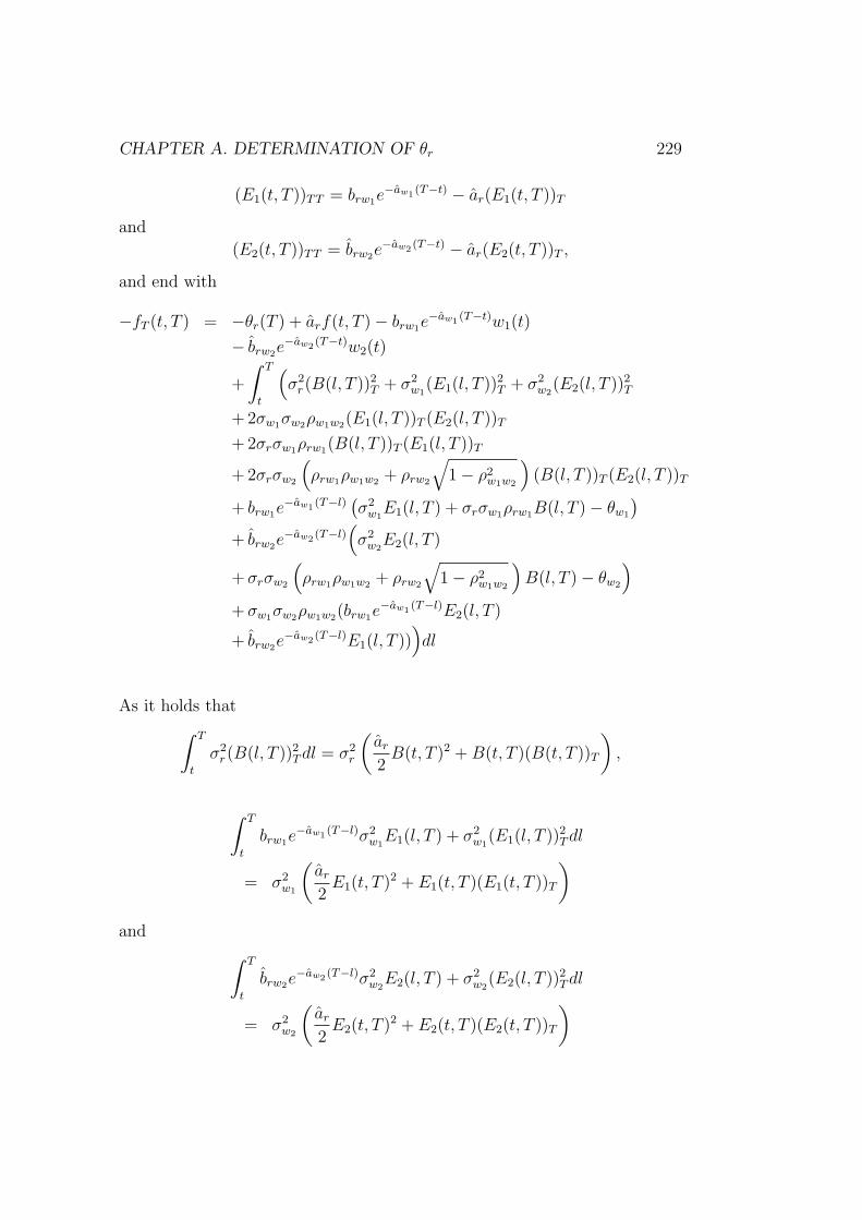
CHAPTER A. DETERMINATION OF θr 229
(E1(t, T ))TT = brw1e−aw1 (T−t) − ar(E1(t, T ))T
and
(E2(t, T ))TT = brw2e−aw2 (T−t) − ar(E2(t, T ))T ,
and end with
−fT (t, T ) = −θr(T ) + arf(t, T ) − brw1e−aw1 (T−t)w1(t)
− brw2e−aw2 (T−t)w2(t)
+
∫ T
t
(σ2
r(B(l, T ))2T + σ2
w1(E1(l, T ))2
T + σ2w2
(E2(l, T ))2T
+ 2σw1σw2ρw1w2(E1(l, T ))T (E2(l, T ))T
+ 2σrσw1ρrw1(B(l, T ))T (E1(l, T ))T
+ 2σrσw2
(ρrw1ρw1w2 + ρrw2
√1 − ρ2
w1w2
)(B(l, T ))T (E2(l, T ))T
+ brw1e−aw1 (T−l)
(σ2
w1E1(l, T ) + σrσw1ρrw1B(l, T ) − θw1
)
+ brw2e−aw2 (T−l)
(σ2
w2E2(l, T )
+ σrσw2
(ρrw1ρw1w2 + ρrw2
√1 − ρ2
w1w2
)B(l, T ) − θw2
)
+ σw1σw2ρw1w2(brw1e−aw1 (T−l)E2(l, T )
+ brw2e−aw2 (T−l)E1(l, T ))
)dl
As it holds that
∫ T
t
σ2r(B(l, T ))2
T dl = σ2r
(ar
2B(t, T )2 + B(t, T )(B(t, T ))T
),
∫ T
t
brw1e−aw1 (T−l)σ2
w1E1(l, T ) + σ2
w1(E1(l, T ))2
T dl
= σ2w1
(ar
2E1(t, T )2 + E1(t, T )(E1(t, T ))T
)
and
∫ T
t
brw2e−aw2 (T−l)σ2
w2E2(l, T ) + σ2
w2(E2(l, T ))2
T dl
= σ2w2
(ar
2E2(t, T )2 + E2(t, T )(E2(t, T ))T
)

230 CHAPTER A. DETERMINATION OF θr
we obtain for θr
θr(T )
= fT (t, T ) + arf(t, T ) + ΦT (t, T ) + arΦ(t, T )
− brw1e−aw1 (T−t)w1(t) − brw2e
−aw2 (T−t)w2(t)
− brw1
θw1
aw1
(1 − e−aw1 (T−t)) − brw2
θw2
aw2
(1 − e−aw2 (T−t))
+brw1σrσw1ρrw1
araw1(aw1 − ar)
((aw1 − ar)(1 − e−aw1 (T−t)) + aw1(e
−(ar+aw1 )(T−t)
− e−2ar(T−t)))
+brw2σrσw2
(ρrw1ρw1w2 + ρrw2
√1 − ρ2
w1w2
)
araw2(aw2 − ar)
((aw2 − ar)(1 − e−aw2 (T−t))
+ aw2(e−(ar+aw2 )(T−t) − e−2ar(T−t))
)
+brw1 brw2σw1σw2ρw1w2
(aw1 − ar)(aw2 − ar)araw1 aw2
(aw1 aw2(−e−2ar(T−t) + e−(ar+aw1 )(T−t)
+ e−(ar+aw2 )(T−t)) − ar(aw1 + aw2 − ar)e−(aw1+aw2 )(T−t)
+ (aw1 − ar)(aw2 − ar)(1 − e−aw1 (T−t) − e−aw2 (T−t)))
with Φ(t, T ) := 12σ2
rB(t, T )2 + 12σ2
w1E1(t, T )2 + 1
2σ2
w2E2(t, T )2.
By setting t := 0, T := t we get θr(t). In order to determine f(0, t) andfT (0, t) for every t we need to know the term structure at time 0. We derivethe term structure with the help of non-defaultable bonds which we only havefor certain maturities. Therefore we fit the data on a Nelson-Siegel curve (seeNelson & Siegel (1987)) by non-linear regression. Thus, we assume the zerorates to follow
R(0, t) = β0 + (β1 + β2)1 − e
− tβ3
tβ3
− β2e− t
β3 .
Then, within the Nelson-Siegel framework it holds for the instantaneous for-ward rate
f(0, t) = β0 + β1e− t
β3 + β2t
β3
e− t
β3
and for its derivative
fT (0, t) = −β1
β3
e− t
β3 + β2(1
β3
− t
(β3)2)e
− tβ3 .

Appendix B
Results of the Calibration
This chapter contains the result of the models analyzed in Chapter 4, Sec-tion 4.8. The analysis is based on an insample period from January 1 1999to December 27 2002 and an out-of-sample period from January 3 2003 toDecember 31 2004.Tables B.1 to B.4 contain the pricing errors between market and model im-plied prices for the different four and five factor models.Tables B.5 to B.16 show the resulting confidence intervalls as well as theconstants of the linear regression.Tables B.17 to B.28 outline the tests of the standardized innovations withrespect to the requirements of the state space model.
231
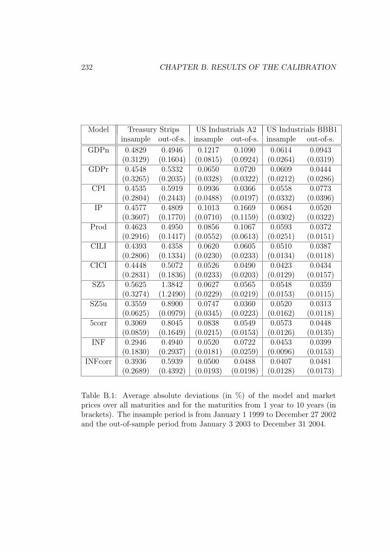
232 CHAPTER B. RESULTS OF THE CALIBRATION
Model Treasury Strips US Industrials A2 US Industrials BBB1insample out-of-s. insample out-of-s. insample out-of-s.
GDPn 0.4829 0.4946 0.1217 0.1090 0.0614 0.0943(0.3129) (0.1604) (0.0815) (0.0924) (0.0264) (0.0319)
GDPr 0.4548 0.5332 0.0650 0.0720 0.0609 0.0444(0.3265) (0.2035) (0.0328) (0.0322) (0.0212) (0.0286)
CPI 0.4535 0.5919 0.0936 0.0366 0.0558 0.0773(0.2804) (0.2443) (0.0488) (0.0197) (0.0332) (0.0396)
IP 0.4577 0.4809 0.1013 0.1669 0.0684 0.0520(0.3607) (0.1770) (0.0710) (0.1159) (0.0302) (0.0322)
Prod 0.4623 0.4950 0.0856 0.1067 0.0593 0.0372(0.2916) (0.1417) (0.0552) (0.0613) (0.0251) (0.0151)
CILI 0.4393 0.4358 0.0620 0.0605 0.0510 0.0387(0.2806) (0.1334) (0.0230) (0.0233) (0.0134) (0.0118)
CICI 0.4448 0.5072 0.0526 0.0490 0.0423 0.0434(0.2831) (0.1836) (0.0233) (0.0203) (0.0129) (0.0157)
SZ5 0.5625 1.3842 0.0627 0.0565 0.0548 0.0359(0.3274) (1.2490) (0.0229) (0.0219) (0.0153) (0.0115)
SZ5u 0.3559 0.8900 0.0747 0.0360 0.0520 0.0313(0.0625) (0.0979) (0.0345) (0.0223) (0.0162) (0.0118)
5corr 0.3069 0.8045 0.0838 0.0549 0.0573 0.0448(0.0859) (0.1649) (0.0215) (0.0153) (0.0126) (0.0135)
INF 0.2946 0.4940 0.0520 0.0722 0.0453 0.0399(0.1830) (0.2937) (0.0181) (0.0259) (0.0096) (0.0153)
INFcorr 0.3936 0.5939 0.0500 0.0488 0.0407 0.0481(0.2689) (0.4392) (0.0193) (0.0198) (0.0128) (0.0173)
Table B.1: Average absolute deviations (in %) of the model and marketprices over all maturities and for the maturities from 1 year to 10 years (inbrackets). The insample period is from January 1 1999 to December 27 2002and the out-of-sample period from January 3 2003 to December 31 2004.
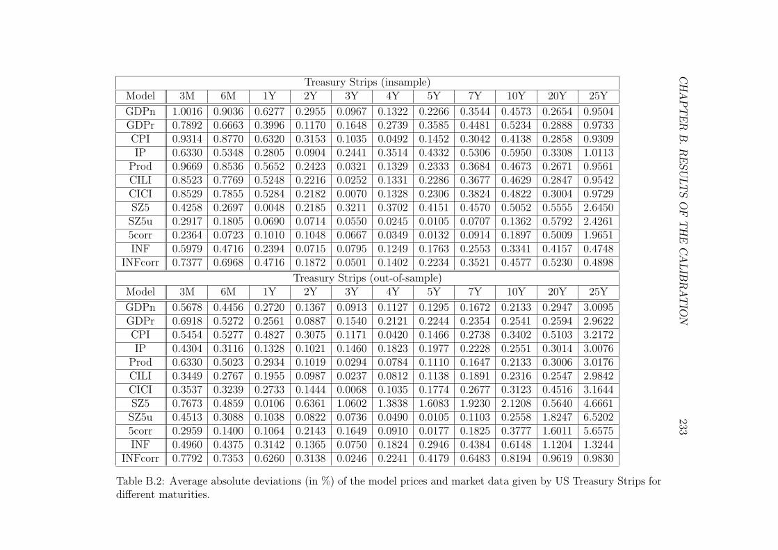
CH
AP
TE
RB
.R
ESU
LT
SO
FT
HE
CA
LIB
RA
TIO
N233
Treasury Strips (insample)Model 3M 6M 1Y 2Y 3Y 4Y 5Y 7Y 10Y 20Y 25Y
GDPn 1.0016 0.9036 0.6277 0.2955 0.0967 0.1322 0.2266 0.3544 0.4573 0.2654 0.9504GDPr 0.7892 0.6663 0.3996 0.1170 0.1648 0.2739 0.3585 0.4481 0.5234 0.2888 0.9733CPI 0.9314 0.8770 0.6320 0.3153 0.1035 0.0492 0.1452 0.3042 0.4138 0.2858 0.9309IP 0.6330 0.5348 0.2805 0.0904 0.2441 0.3514 0.4332 0.5306 0.5950 0.3308 1.0113
Prod 0.9669 0.8536 0.5652 0.2423 0.0321 0.1329 0.2333 0.3684 0.4673 0.2671 0.9561CILI 0.8523 0.7769 0.5248 0.2216 0.0252 0.1331 0.2286 0.3677 0.4629 0.2847 0.9542CICI 0.8529 0.7855 0.5284 0.2182 0.0070 0.1328 0.2306 0.3824 0.4822 0.3004 0.9729SZ5 0.4258 0.2697 0.0048 0.2185 0.3211 0.3702 0.4151 0.4570 0.5052 0.5555 2.6450SZ5u 0.2917 0.1805 0.0690 0.0714 0.0550 0.0245 0.0105 0.0707 0.1362 0.5792 2.42615corr 0.2364 0.0723 0.1010 0.1048 0.0667 0.0349 0.0132 0.0914 0.1897 0.5009 1.9651INF 0.5979 0.4716 0.2394 0.0715 0.0795 0.1249 0.1763 0.2553 0.3341 0.4157 0.4748
INFcorr 0.7377 0.6968 0.4716 0.1872 0.0501 0.1402 0.2234 0.3521 0.4577 0.5230 0.4898
Treasury Strips (out-of-sample)Model 3M 6M 1Y 2Y 3Y 4Y 5Y 7Y 10Y 20Y 25Y
GDPn 0.5678 0.4456 0.2720 0.1367 0.0913 0.1127 0.1295 0.1672 0.2133 0.2947 3.0095GDPr 0.6918 0.5272 0.2561 0.0887 0.1540 0.2121 0.2244 0.2354 0.2541 0.2594 2.9622CPI 0.5454 0.5277 0.4827 0.3075 0.1171 0.0420 0.1466 0.2738 0.3402 0.5103 3.2172IP 0.4304 0.3116 0.1328 0.1021 0.1460 0.1823 0.1977 0.2228 0.2551 0.3014 3.0076
Prod 0.6330 0.5023 0.2934 0.1019 0.0294 0.0784 0.1110 0.1647 0.2133 0.3006 3.0176CILI 0.3449 0.2767 0.1955 0.0987 0.0237 0.0812 0.1138 0.1891 0.2316 0.2547 2.9842CICI 0.3537 0.3239 0.2733 0.1444 0.0068 0.1035 0.1774 0.2677 0.3123 0.4516 3.1644SZ5 0.7673 0.4859 0.0106 0.6361 1.0602 1.3838 1.6083 1.9230 2.1208 0.5640 4.6661SZ5u 0.4513 0.3088 0.1038 0.0822 0.0736 0.0490 0.0105 0.1103 0.2558 1.8247 6.52025corr 0.2959 0.1400 0.1064 0.2143 0.1649 0.0910 0.0177 0.1825 0.3777 1.6011 5.6575INF 0.4960 0.4375 0.3142 0.1365 0.0750 0.1824 0.2946 0.4384 0.6148 1.1204 1.3244
INFcorr 0.7792 0.7353 0.6260 0.3138 0.0246 0.2241 0.4179 0.6483 0.8194 0.9619 0.9830
Table B.2: Average absolute deviations (in %) of the model prices and market data given by US Treasury Strips fordifferent maturities.

234C
HA
PT
ER
B.R
ESU
LT
SO
FT
HE
CA
LIB
RA
TIO
N
US Industrials A2 (insample)Model 3M 6M 1Y 2Y 3Y 4Y 5Y 7Y 10Y 20Y 25Y
GDPn 0.0990 0.0751 0.0521 0.0283 0.0230 0.0499 0.0816 0.1383 0.1971 0.2658 0.3285GDPr 0.0394 0.0199 0.0029 0.0113 0.0057 0.0113 0.0277 0.0621 0.1086 0.1916 0.2349CPI 0.0489 0.0286 0.0211 0.0194 0.0127 0.0238 0.0434 0.0841 0.1370 0.2690 0.3411IP 0.0391 0.0148 0.0210 0.0219 0.0020 0.0350 0.0707 0.1366 0.2099 0.2849 0.2786
Prod 0.0504 0.0197 0.0450 0.0537 0.0319 0.0041 0.0264 0.0810 0.1443 0.2346 0.2513CILI 0.0965 0.0782 0.0507 0.0201 0.0066 0.0002 0.0060 0.0234 0.0540 0.1410 0.2051CICI 0.1127 0.0908 0.0590 0.0246 0.0127 0.0099 0.0071 0.0115 0.0381 0.0877 0.1243SZ5 0.0730 0.0541 0.0260 0.0004 0.0050 2e-5 0.0105 0.0380 0.0800 0.1712 0.23155corr 0.1095 0.0906 0.0584 0.0231 0.0061 0.0006 0.0010 0.0126 0.0483 0.2277 0.3433SZ5u 0.0281 0.0140 0.0191 0.0276 0.0213 0.0095 0.0136 0.0498 0.1009 0.2273 0.3102INF 0.0867 0.0639 0.0327 0.0028 0.0081 0.0067 5e-5 0.0208 0.0554 0.1250 0.1696
INFcorr 0.0801 0.0588 0.0288 0.0003 0.0076 0.0050 0.0049 0.0275 0.0611 0.1132 0.1627
US Industrials A2 (out-of-sample)Model 3M 6M 1Y 2Y 3Y 4Y 5Y 7Y 10Y 20Y 25Y
GDPn 0.0754 0.0612 0.0472 0.0300 0.0212 0.0622 0.1011 0.1639 0.2215 0.2244 0.1907GDPr 0.0291 0.0118 0.0034 0.0098 0.0059 0.0080 0.0238 0.0605 0.1139 0.2428 0.2830CPI 0.0322 0.0183 0.0180 0.0102 0.0088 0.0121 0.0175 0.0283 0.0430 0.0958 0.1183IP 0.0503 0.0149 0.0263 0.0334 0.0026 0.0576 0.1175 0.2273 0.3466 0.4798 0.4798
Prod 0.0514 0.0165 0.0448 0.0525 0.0343 0.0046 0.0284 0.0922 0.1722 0.3219 0.3550CILI 0.0728 0.0763 0.0581 0.0224 0.0056 0.0002 0.0035 0.0184 0.0550 0.1626 0.1907CICI 0.0819 0.0844 0.0642 0.0256 0.0080 0.0066 0.0071 0.0058 0.0249 0.0999 0.1303SZ5 0.0368 0.0360 0.0226 0.0004 0.0048 1e-5 0.0099 0.0364 0.0791 0.1831 0.2121SZ5u 0.0159 0.0122 0.0135 0.0167 0.0148 0.0070 0.0082 0.0323 0.0639 0.1029 0.10905corr 0.0556 0.0610 0.0465 0.0170 0.0039 0.0005 0.0007 0.0080 0.0306 0.1539 0.2262INF 0.0554 0.0548 0.0372 0.0042 0.0087 0.0084 3e-5 0.0307 0.0919 0.2431 0.2592
INFcorr 0.0440 0.0419 0.0267 0.0002 0.0080 0.0055 0.0032 0.0273 0.0677 0.1502 0.1623
Table B.3: Average absolute deviations (in %) of the model prices and market data given by US Industrials A2 fordifferent maturities.

CH
AP
TE
RB
.R
ESU
LT
SO
FT
HE
CA
LIB
RA
TIO
N235
US Industrials BBB1 (insample)Model 3M 6M 1Y 2Y 3Y 4Y 5Y 7Y 10Y 20Y 25Y
GDPn 0.0548 0.0377 0.0241 0.0207 0.0179 0.0101 0.0019 0.0316 0.0784 0.1841 0.2136GDPr 0.0364 0.0190 0.0021 0.0117 0.0087 0.0005 0.0123 0.0382 0.0751 0.1943 0.2720CPI 0.0341 0.0127 0.0167 0.0415 0.0478 0.0435 0.0333 0.0069 0.0427 0.1497 0.1851IP 0.0283 0.0111 0.0153 0.0274 0.0239 0.0125 0.0034 0.0386 0.0899 0.2203 0.2819
Prod 0.0631 0.0335 0.0068 0.0269 0.0253 0.0143 0.0009 0.0307 0.0711 0.1668 0.2133CILI 0.0715 0.0530 0.0300 0.0086 0.0007 0.0021 0.0009 0.0124 0.0390 0.1445 0.1986CICI 0.0651 0.0483 0.0276 0.0106 0.0054 0.0033 0.0001 0.0108 0.0323 0.1068 0.1555SZ5 0.0645 0.0447 0.0208 0.0018 0.0044 0.0026 0.0037 0.0214 0.0527 0.1622 0.2244SZ5u 0.0690 0.0494 0.0238 0.0047 0.0133 0.0167 0.0157 0.0102 0.0292 0.1405 0.19935corr 0.0699 0.0508 0.0281 0.0083 0.0018 0.0001 0.0023 0.0115 0.0359 0.1696 0.2516INF 0.0570 0.0391 0.0182 0.0021 0.0040 0.0033 5e-5 0.0101 0.0294 0.1283 0.2066
INFcorr 0.0613 0.0436 0.0225 0.0048 0.0007 0.0001 0.0039 0.0173 0.0403 0.1054 0.1483
US Industrials BBB1 (out-of-sample)Model 3M 6M 1Y 2Y 3Y 4Y 5Y 7Y 10Y 20Y 25Y
GDPn 0.0627 0.0476 0.0273 0.0156 0.0170 0.0112 0.0017 0.0403 0.1102 0.3131 0.3905GDPr 0.0387 0.0211 0.0018 0.0160 0.0127 0.0006 0.0180 0.0547 0.0965 0.1177 0.1109CPI 0.0287 0.0118 0.0132 0.0429 0.0552 0.0545 0.0448 0.0104 0.0559 0.2353 0.2979IP 0.0293 0.0110 0.0155 0.0327 0.0289 0.0148 0.0038 0.0421 0.0878 0.1467 0.1594
Prod 0.0362 0.0185 0.0064 0.0147 0.0139 0.0080 0.0007 0.0176 0.0440 0.1115 0.1374CILI 0.0606 0.0480 0.0292 0.0082 0.0007 0.0019 0.0008 0.0105 0.0314 0.0983 0.1362CICI 0.0714 0.0574 0.0367 0.0129 0.0048 0.0033 9e-5 0.0130 0.0391 0.1057 0.1333SZ5 0.0466 0.0345 0.0174 0.0012 0.0037 0.0018 0.0032 0.0160 0.0370 0.1017 0.1313SZ5u 0.0490 0.0368 0.0188 0.0037 0.0097 0.0114 0.0100 0.0073 0.0214 0.0740 0.10245corr 0.0746 0.0587 0.0354 0.0103 0.0015 0.0001 0.0029 0.0131 0.0313 0.1108 0.1540INF 0.0631 0.0484 0.0266 0.0030 0.0056 0.0053 6e-5 0.0180 0.0485 0.0982 0.1222
INFcorr 0.0595 0.0466 0.0276 0.0067 0.0008 0.0002 0.0051 0.0234 0.0574 0.1394 0.1622
Table B.4: Average absolute deviations (in %) of the model prices and market data given by US Industrials BBB1for different maturities.
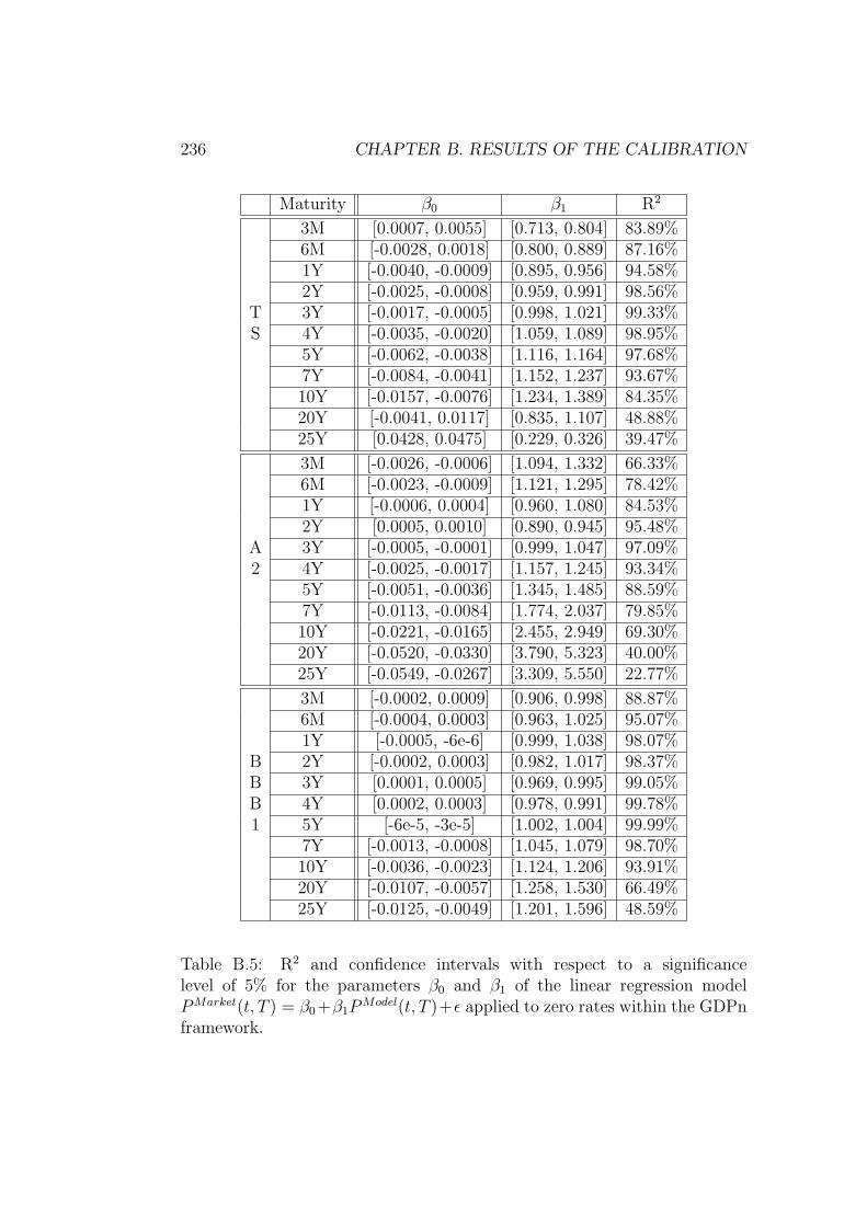
236 CHAPTER B. RESULTS OF THE CALIBRATION
Maturity β0 β1 R2
3M [0.0007, 0.0055] [0.713, 0.804] 83.89%6M [-0.0028, 0.0018] [0.800, 0.889] 87.16%1Y [-0.0040, -0.0009] [0.895, 0.956] 94.58%2Y [-0.0025, -0.0008] [0.959, 0.991] 98.56%
T 3Y [-0.0017, -0.0005] [0.998, 1.021] 99.33%S 4Y [-0.0035, -0.0020] [1.059, 1.089] 98.95%
5Y [-0.0062, -0.0038] [1.116, 1.164] 97.68%7Y [-0.0084, -0.0041] [1.152, 1.237] 93.67%10Y [-0.0157, -0.0076] [1.234, 1.389] 84.35%20Y [-0.0041, 0.0117] [0.835, 1.107] 48.88%25Y [0.0428, 0.0475] [0.229, 0.326] 39.47%
3M [-0.0026, -0.0006] [1.094, 1.332] 66.33%6M [-0.0023, -0.0009] [1.121, 1.295] 78.42%1Y [-0.0006, 0.0004] [0.960, 1.080] 84.53%2Y [0.0005, 0.0010] [0.890, 0.945] 95.48%
A 3Y [-0.0005, -0.0001] [0.999, 1.047] 97.09%2 4Y [-0.0025, -0.0017] [1.157, 1.245] 93.34%
5Y [-0.0051, -0.0036] [1.345, 1.485] 88.59%7Y [-0.0113, -0.0084] [1.774, 2.037] 79.85%10Y [-0.0221, -0.0165] [2.455, 2.949] 69.30%20Y [-0.0520, -0.0330] [3.790, 5.323] 40.00%25Y [-0.0549, -0.0267] [3.309, 5.550] 22.77%
3M [-0.0002, 0.0009] [0.906, 0.998] 88.87%6M [-0.0004, 0.0003] [0.963, 1.025] 95.07%1Y [-0.0005, -6e-6] [0.999, 1.038] 98.07%
B 2Y [-0.0002, 0.0003] [0.982, 1.017] 98.37%B 3Y [0.0001, 0.0005] [0.969, 0.995] 99.05%B 4Y [0.0002, 0.0003] [0.978, 0.991] 99.78%1 5Y [-6e-5, -3e-5] [1.002, 1.004] 99.99%
7Y [-0.0013, -0.0008] [1.045, 1.079] 98.70%10Y [-0.0036, -0.0023] [1.124, 1.206] 93.91%20Y [-0.0107, -0.0057] [1.258, 1.530] 66.49%25Y [-0.0125, -0.0049] [1.201, 1.596] 48.59%
Table B.5: R2 and confidence intervals with respect to a significancelevel of 5% for the parameters β0 and β1 of the linear regression modelPMarket(t, T ) = β0+β1P
Model(t, T )+ε applied to zero rates within the GDPnframework.

CHAPTER B. RESULTS OF THE CALIBRATION 237
Maturity β0 β1 R2
3M [0.0029, 0.0066] [0.732, 0.806] 89.04%6M [-0.0007, 0.0027] [0.826, 0.896] 91.90%1Y [-0.0024, -0.0004] [0.928, 0.969] 97.55%2Y [-0.0024, -0.0014] [1.009, 1.030] 99.49%
T 3Y [-0.0035, -0.0017] [1.055, 1.093] 98.37%S 4Y [-0.0070, -0.0043] [1.136, 1.191] 97.10%
5Y [-0.0111, -0.0072] [1.211, 1.292] 94.78%7Y [-0.0156, -0.0093] [1.277, 1.405] 89.30%10Y [-0.0261, -0.0147] [1.387, 1.608] 77.55%20Y [-0.0110, 0.0087] [0.891, 1.234] 42.12%25Y [0.0426, 0.0475] [0.230, 0.330] 37.19%
3M [-0.0007, 2e-5] [1.012, 1.097] 92.03%6M [-0.0005, -0.0001] [1.014, 1.057] 97.86%1Y [-3e-5, 6e-5] [0.992, 1.002] 99.86%2Y [0.0001, 0.0004] [0.960, 0.984] 99.18%
A 3Y [8e-6, 0.0001] [0.988, 0.9998] 99.81%2 4Y [-0.0004, -0.0002] [1.018, 1.038] 99.49%
5Y [-0.0009, -0.0004] [1.040, 1.085] 97.71%7Y [-0.0019, -0.0009] [1.078, 1.171] 91.67%10Y [-0.0033, -0.0014] [1.110, 1.267] 81.21%20Y [-0.0049, -0.0002] [0.994, 1.319] 48.82%25Y [-0.0033, 0.0031] [0.787, 1.207] 29.80%
3M [-0.0003, 0.0006] [0.925, 1.002] 92.34%6M [-0.0002, 0.0002] [0.973, 1.010] 98.18%1Y [-5e-5, -7e-6] [1.001, 1.005] 99.98%2Y [9e-6, 0.0002] [0.987, 1.005] 99.55%
B 3Y [6e-5, 0.0002] [0.987, 0.999] 99.81%B 4Y [-1e-5, 1e-6] [0.9996, 1.0004] 100%B 5Y [-0.0004, -0.0002] [1.007, 1.022] 99.72%1 7Y [-0.0013, -0.0007] [1.037, 1.081] 97.74%
10Y [-0.0029, -0.0016] [1.093, 1.183] 92.42%20Y [-0.0063, -0.0018] [1.188, 1.460] 64.09%25Y [-0.0062, 0.0001] [1.124, 1.517] 46.06%
Table B.6: R2 and confidence intervals with respect to a significancelevel of 5% for the parameters β0 and β1 of the linear regression modelPMarket(t, T ) = β0 +β1P
Model(t, T )+ε applied to zero rates within the GDPrframework.
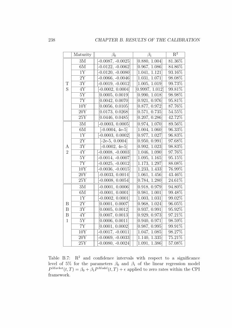
238 CHAPTER B. RESULTS OF THE CALIBRATION
Maturity β0 β1 R2
3M [-0.0087, -0.0025] [0.880, 1.004] 81.36%6M [-0.0122, -0.0062] [0.967, 1.086] 84.86%1Y [-0.0120, -0.0080] [1.041, 1.121] 93.16%2Y [-0.0066, -0.0046] [1.031, 1.071] 98.08%
T 3Y [-0.0019, -0.0012] [1.005, 1.019] 99.73%S 4Y [-0.0002, 0.0004] [0.9997, 1.012] 99.81%
5Y [0.0005, 0.0019] [0.990, 1.018] 98.98%7Y [0.0042, 0.0070] [0.921, 0.976] 95.81%10Y [0.0056, 0.0105] [0.877, 0.972] 87.76%20Y [0.0173, 0.0268] [0.571, 0.735] 54.55%25Y [0.0446, 0.0485] [0.207, 0.286] 42.72%
3M [-0.0003, 0.0005] [0.974, 1.070] 89.56%6M [-0.0004, 4e-5] [1.004, 1.060] 96.33%1Y [-0.0003, 0.0002] [0.977, 1.027] 96.83%2Y [-2e-5, 0.0004] [0.950, 0.991] 97.68%
A 3Y [-0.0002, 4e-5] [0.992, 1.023] 98.83%2 4Y [-0.0008, -0.0003] [1.046, 1.090] 97.76%
5Y [-0.0014, -0.0007] [1.095, 1.165] 95.15%7Y [-0.0025, -0.0012] [1.173, 1.297] 88.08%10Y [-0.0036, -0.0015] [1.233, 1.433] 76.99%20Y [-0.0033, 0.0014] [1.061, 1.456] 43.46%25Y [-0.0008, 0.0054] [0.784, 1.280] 24.61%
3M [-0.0001, 0.0006] [0.918, 0.979] 94.80%6M [-0.0001, 0.0001] [0.981, 1.001] 99.48%1Y [-0.0002, 0.0001] [1.003, 1.031] 99.02%
B 2Y [0.0001, 0.0007] [0.968, 1.024] 96.05%B 3Y [0.0005, 0.0012] [0.937, 0.991] 95.92%B 4Y [0.0007, 0.0013] [0.929, 0.973] 97.21%1 5Y [0.0006, 0.0011] [0.940, 0.971] 98.59%
7Y [0.0001, 0.0002] [0.987, 0.995] 99.91%10Y [-0.0017, -0.0011] [1.047, 1.085] 98.27%20Y [-0.0069, -0.0033] [1.140, 1.335] 75.21%25Y [-0.0080, -0.0024] [1.091, 1.386] 57.08%
Table B.7: R2 and confidence intervals with respect to a significancelevel of 5% for the parameters β0 and β1 of the linear regression modelPMarket(t, T ) = β0 + β1P
Model(t, T ) + ε applied to zero rates within the CPIframework.
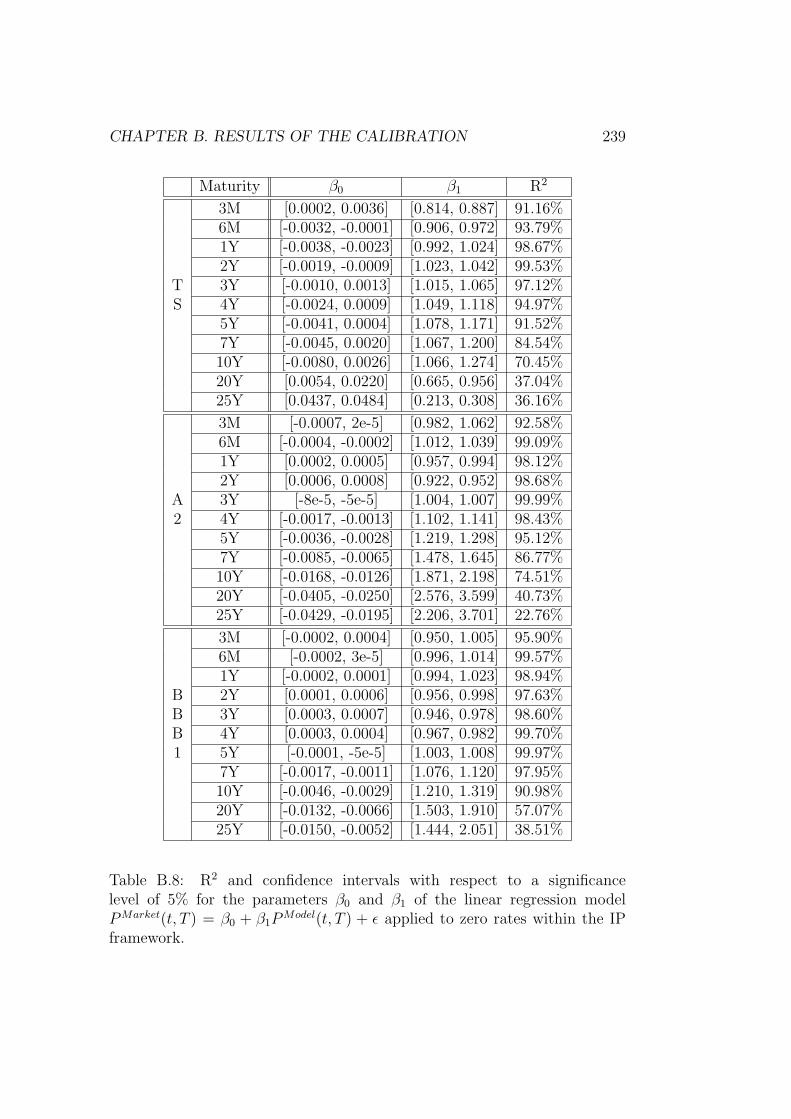
CHAPTER B. RESULTS OF THE CALIBRATION 239
Maturity β0 β1 R2
3M [0.0002, 0.0036] [0.814, 0.887] 91.16%6M [-0.0032, -0.0001] [0.906, 0.972] 93.79%1Y [-0.0038, -0.0023] [0.992, 1.024] 98.67%2Y [-0.0019, -0.0009] [1.023, 1.042] 99.53%
T 3Y [-0.0010, 0.0013] [1.015, 1.065] 97.12%S 4Y [-0.0024, 0.0009] [1.049, 1.118] 94.97%
5Y [-0.0041, 0.0004] [1.078, 1.171] 91.52%7Y [-0.0045, 0.0020] [1.067, 1.200] 84.54%10Y [-0.0080, 0.0026] [1.066, 1.274] 70.45%20Y [0.0054, 0.0220] [0.665, 0.956] 37.04%25Y [0.0437, 0.0484] [0.213, 0.308] 36.16%
3M [-0.0007, 2e-5] [0.982, 1.062] 92.58%6M [-0.0004, -0.0002] [1.012, 1.039] 99.09%1Y [0.0002, 0.0005] [0.957, 0.994] 98.12%2Y [0.0006, 0.0008] [0.922, 0.952] 98.68%
A 3Y [-8e-5, -5e-5] [1.004, 1.007] 99.99%2 4Y [-0.0017, -0.0013] [1.102, 1.141] 98.43%
5Y [-0.0036, -0.0028] [1.219, 1.298] 95.12%7Y [-0.0085, -0.0065] [1.478, 1.645] 86.77%10Y [-0.0168, -0.0126] [1.871, 2.198] 74.51%20Y [-0.0405, -0.0250] [2.576, 3.599] 40.73%25Y [-0.0429, -0.0195] [2.206, 3.701] 22.76%
3M [-0.0002, 0.0004] [0.950, 1.005] 95.90%6M [-0.0002, 3e-5] [0.996, 1.014] 99.57%1Y [-0.0002, 0.0001] [0.994, 1.023] 98.94%
B 2Y [0.0001, 0.0006] [0.956, 0.998] 97.63%B 3Y [0.0003, 0.0007] [0.946, 0.978] 98.60%B 4Y [0.0003, 0.0004] [0.967, 0.982] 99.70%1 5Y [-0.0001, -5e-5] [1.003, 1.008] 99.97%
7Y [-0.0017, -0.0011] [1.076, 1.120] 97.95%10Y [-0.0046, -0.0029] [1.210, 1.319] 90.98%20Y [-0.0132, -0.0066] [1.503, 1.910] 57.07%25Y [-0.0150, -0.0052] [1.444, 2.051] 38.51%
Table B.8: R2 and confidence intervals with respect to a significancelevel of 5% for the parameters β0 and β1 of the linear regression modelPMarket(t, T ) = β0 + β1P
Model(t, T ) + ε applied to zero rates within the IPframework.

240 CHAPTER B. RESULTS OF THE CALIBRATION
Maturity β0 β1 R2
3M [0.0021, 0.0068] [0.702, 0.793] 83.47%6M [-0.0014, 0.0031] [0.788, 0.877] 86.85%1Y [-0.0027, 0.0003] [0.884, 0.944] 94.56%2Y [-0.0013, 0.0002] [0.949, 0.978] 98.81%
T 3Y [-0.0003, 7e-5] [0.995, 1.004] 99.91%S 4Y [-0.0023, -0.0013] [1.052, 1.072] 99.50%
5Y [-0.0050, -0.0030] [1.106, 1.147] 98.31%7Y [-0.0072, -0.0034] [1.141, 1.219] 94.63%10Y [-0.0144, -0.0069] [1.224, 1.369] 85.83%20Y [-0.0038, 0.0114] [0.841, 1.104] 50.88%25Y [0.0429, 0.0475] [0.228, 0.322] 39.50%
3M [-0.0001, 0.0006] [0.914, 0.992] 91.95%6M [-0.0004, -0.0001] [1.005, 1.047] 97.85%1Y [0.0003, 0.0009] [0.905, 0.986] 91.03%2Y [0.0015, 0.0021] [0.779, 0.849] 90.94%
A 3Y [0.0010, 0.0014] [0.861, 0.897] 97.82%2 4Y [8e-5, 0.0001] [0.987, 0.993] 99.95%
5Y [-0.0013, -0.0010] [1.094, 1.122] 99.17%7Y [-0.0044, -0.0034] [1.288, 1.378] 94.29%10Y [-0.0090, -0.0067] [1.527, 1.713] 85.05%20Y [-0.0196, -0.0118] [1.788, 2.327] 52.37%25Y [-0.0200, -0.0082] [1.528, 2.305] 31.47%
3M [0.0014, 0.0022] [0.793, 0.873] 89.21%6M [0.0006, 0.0011] [0.902, 0.948] 96.90%1Y [-0.0002, -2e-5] [1.002, 1.013] 99.83%
B 2Y [-0.0003, 0.0002] [0.980, 1.022] 97.79%B 3Y [-2e-5, 0.0004] [0.963, 0.999] 98.24%B 4Y [0.0001, 0.0003] [0.976, 0.995] 99.50%1 5Y [-3e-5, -1e-5] [1.001, 1.002] 100%
7Y [-0.0008, -0.0003] [1.020, 1.058] 98.26%10Y [-0.0018, -0.0004] [1.031, 1.119] 91.89%20Y [-0.0017, 0.0021] [0.883, 1.100] 61.16%25Y [0.0001, 0.0050] [0.736, 1.012] 43.17%
Table B.9: R2 and confidence intervals with respect to a significancelevel of 5% for the parameters β0 and β1 of the linear regression modelPMarket(t, T ) = β0 + β1P
Model(t, T ) + ε applied to zero rates within the Prodframework.
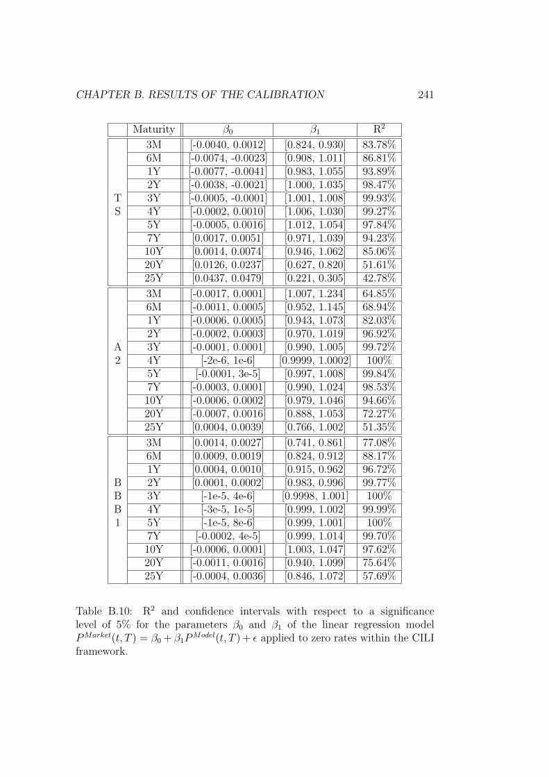
CHAPTER B. RESULTS OF THE CALIBRATION 241
Maturity β0 β1 R2
3M [-0.0040, 0.0012] [0.824, 0.930] 83.78%6M [-0.0074, -0.0023] [0.908, 1.011] 86.81%1Y [-0.0077, -0.0041] [0.983, 1.055] 93.89%2Y [-0.0038, -0.0021] [1.000, 1.035] 98.47%
T 3Y [-0.0005, -0.0001] [1.001, 1.008] 99.93%S 4Y [-0.0002, 0.0010] [1.006, 1.030] 99.27%
5Y [-0.0005, 0.0016] [1.012, 1.054] 97.84%7Y [0.0017, 0.0051] [0.971, 1.039] 94.23%10Y [0.0014, 0.0074] [0.946, 1.062] 85.06%20Y [0.0126, 0.0237] [0.627, 0.820] 51.61%25Y [0.0437, 0.0479] [0.221, 0.305] 42.78%
3M [-0.0017, 0.0001] [1.007, 1.234] 64.85%6M [-0.0011, 0.0005] [0.952, 1.145] 68.94%1Y [-0.0006, 0.0005] [0.943, 1.073] 82.03%2Y [-0.0002, 0.0003] [0.970, 1.019] 96.92%
A 3Y [-0.0001, 0.0001] [0.990, 1.005] 99.72%2 4Y [-2e-6, 1e-6] [0.9999, 1.0002] 100%
5Y [-0.0001, 3e-5] [0.997, 1.008] 99.84%7Y [-0.0003, 0.0001] [0.990, 1.024] 98.53%10Y [-0.0006, 0.0002] [0.979, 1.046] 94.66%20Y [-0.0007, 0.0016] [0.888, 1.053] 72.27%25Y [0.0004, 0.0039] [0.766, 1.002] 51.35%
3M [0.0014, 0.0027] [0.741, 0.861] 77.08%6M [0.0009, 0.0019] [0.824, 0.912] 88.17%1Y [0.0004, 0.0010] [0.915, 0.962] 96.72%
B 2Y [0.0001, 0.0002] [0.983, 0.996] 99.77%B 3Y [-1e-5, 4e-6] [0.9998, 1.001] 100%B 4Y [-3e-5, 1e-5] [0.999, 1.002] 99.99%1 5Y [-1e-5, 8e-6] [0.999, 1.001] 100%
7Y [-0.0002, 4e-5] [0.999, 1.014] 99.70%10Y [-0.0006, 0.0001] [1.003, 1.047] 97.62%20Y [-0.0011, 0.0016] [0.940, 1.099] 75.64%25Y [-0.0004, 0.0036] [0.846, 1.072] 57.69%
Table B.10: R2 and confidence intervals with respect to a significancelevel of 5% for the parameters β0 and β1 of the linear regression modelPMarket(t, T ) = β0 + β1P
Model(t, T ) + ε applied to zero rates within the CILIframework.

242 CHAPTER B. RESULTS OF THE CALIBRATION
Maturity β0 β1 R2
3M [-0.0045, 0.0010] [0.827, 0.939] 82.53%6M [-0.0079, -0.0026] [0.914, 1.021] 86.06%1Y [-0.0082, -0.0046] [0.993, 1.064] 94.05%2Y [-0.0039, -0.0022] [1.003, 1.037] 98.62%
T 3Y [-0.0001, -4e-5] [1.000, 1.002] 100%S 4Y [0.0003, 0.0012] [1.002, 1.021] 99.53%
5Y [0.0001, 0.0019] [1.007, 1.044] 98.36%7Y [0.0024, 0.0057] [0.963, 1.028] 94.63%10Y [0.0019, 0.0077] [0.945, 1.057] 85.72%20Y [0.0133, 0.0243] [0.620, 0.811] 51.54%25Y [0.0444, 0.0485] [0.209, 0.292] 40.51%
3M [-0.0027, -0.0005] [1.059, 1.321] 60.88%6M [-0.0022, -0.0003] [1.031, 1.254] 66.58%1Y [-0.0017, -0.0004] [1.037, 1.186] 80.77%2Y [-0.0007, -0.0002] [1.017, 1.076] 95.93%
A 3Y [-0.0002, 0.0001] [0.989, 1.018] 98.87%2 4Y [2e-5, 0.0002] [0.980, 0.999] 99.54%
5Y [0.0001, 0.0002] [0.985, 0.995] 99.84%7Y [-0.0002, 1e-5] [0.998, 1.015] 99.60%10Y [-0.0008, -0.0002] [1.012, 1.055] 97.67%20Y [-0.0012, 0.0002] [0.972, 1.073] 88.60%25Y [-0.0007, 0.0014] [0.913, 1.052] 79.15%
3M [0.0003, 0.0017] [0.814, 0.932] 80.42%6M [3e-5, 0.0010] [0.885, 0.969] 90.36%1Y [-0.0001, 0.0004] [0.954, 0.997] 97.47%
B 2Y [-0.0001, 0.0001] [0.992, 1.008] 99.66%B 3Y [-0.0001, 3e-5] [0.998, 1.008] 99.88%B 4Y [-4e-5, 3e-5] [0.999, 1.004] 99.96%1 5Y [-1e-6, 7e-7] [0.9999, 1.0001] 100%
7Y [-0.0002, 2e-5] [0.994, 1.007] 99.76%10Y [-0.0005, 1e-5] [0.986, 1.022] 98.34%20Y [-0.0007, 0.0014] [0.913, 1.031] 83.60%25Y [0.0001, 0.0031] [0.842, 1.008] 70.00%
Table B.11: R2 and confidence intervals with respect to a significancelevel of 5% for the parameters β0 and β1 of the linear regression modelPMarket(t, T ) = β0 + β1P
Model(t, T ) + ε applied to zero rates within the CICIframework.

CHAPTER B. RESULTS OF THE CALIBRATION 243
Maturity β0 β1 R2
3M [0.0054, 0.0076] [0.807, 0.857] 95.43%6M [0.0017, 0.0036] [0.902, 0.944] 97.33%1Y [-0.0001, -1e-6] [0.9996, 1.0007] 100%2Y [-0.0032, -0.001] [1.038, 1.085] 97.50%
T 3Y [-0.0070, -0.0026] [1.076, 1.168] 91.87%S 4Y [-0.0142, -0.0077] [1.174, 1.307] 86.82%
5Y [-0.0223, -0.0124] [1.257, 1.453] 78.34%7Y [-0.0279, -0.0089] [1.174, 1.532] 51.88%10Y [0.0193, 0.0494] [0.122, 0.660] 3.84%20Y [0.0613, 0.0831] [-0.422, -0.025] 2.34%25Y [0.0485, 0.0517] [0.220, 0.317] 36.82%
3M [-0.0007, 0.0006] [0.949, 1.101] 77.56%6M [-0.0006, 0.0004] [0.955, 1.074] 84.51%1Y [-0.0004, 0.0001] [0.986, 1.050] 95.10%2Y [-9e-6, -5e-7] [0.99999, 1.001] 100%
A 3Y [4e-5, 0.0001] [0.985, 0.996] 99.85%2 4Y [-1e-7, 2e-7] [0.99998, 1.000] 100%
5Y [-0.0003, -0.0001] [1.010, 1.027] 99.63%7Y [-0.0009, -0.0004] [1.030, 1.084] 96.64%10Y [-0.0019, -0.0007] [1.045, 1.151] 89.06%20Y [-0.0022, 0.0013] [0.899, 1.143] 56.96%25Y [-0.0003, 0.0046] [0.702, 1.023] 35.29%
3M [0.0012, 0.0023] [0.788, 0.892] 83.05%6M [0.0008, 0.0016] [0.867, 0.938] 92.55%1Y [0.0003, 0.0007] [0.949, 0.979] 98.70%
B 2Y [-6e-6, 2e-5] [0.998, 1.001] 99.99%B 3Y [-0.0001, 9e-7] [0.999, 1.005] 99.94%B 4Y [-4e-5, 5e-6] [0.999, 1.002] 99.99%1 5Y [-0.0001, 2e-5] [0.999, 1.005] 99.96%
7Y [-0.0003, 0.0001] [0.999, 1.025] 99.14%10Y [-0.0007, 0.0003] [0.995, 1.054] 95.77%20Y [0.0002, 0.0030] [0.866, 1.032] 71.24%25Y [0.0019, 0.0057] [0.743, 0.962] 53.36%
Table B.12: R2 and confidence intervals with respect to a significancelevel of 5% for the parameters β0 and β1 of the linear regression modelPMarket(t, T ) = β0 + β1P
Model(t, T ) + ε applied to zero rates within the SZ5framework.

244 CHAPTER B. RESULTS OF THE CALIBRATION
Maturity β0 β1 R2
3M [0.0043, 0.0060] [0.861, 0.901] 97.38%6M [0.0006, 0.0020] [0.950, 0.983] 98.49%1Y [-0.0011, -0.0005] [1.009, 1.022] 99.77%2Y [-0.0011, -0.0004] [1.010, 1.025] 99.70%
T 3Y [-0.0004, 0.0004] [0.994, 1.010] 99.66%S 4Y [-0.0005, -0.0002] [1.004, 1.011] 99.93%
5Y [-0.0003, -0.0002] [1.002, 1.005] 99.99%7Y [0.0043, 0.0053] [0.905, 0.925] 99.36%10Y [0.0101, 0.0119] [0.801, 0.833] 98.03%20Y [0.0353, 0.0387] [0.390, 0.452] 77.79%25Y [ 0.0523, 0.0538] [0.145, 0.187] 54.00%
3M [-0.0007, -0.0002] [1.043, 1.095] 96.98%6M [-0.0003, 0.0001] [0.993, 1.031] 98.24%1Y [0.0003, 0.0006] [0.918, 0.960] 97.36%2Y [0.0006, 0.0010] [0.871, 0.920] 96.13%
A 3Y [0.0004, 0.0007] [0.911, 0.946] 98.17%2 4Y [0.0001, 0.0002] [0.973, 0.990] 99.61%
5Y [-0.0005, -0.0002] [1.027, 1.049] 99.43%7Y [-0.0017, -0.0010] [1.117, 1.183] 95.80%10Y [-0.0036, -0.0021] [1.237, 1.374] 87.40%20Y [-0.0079, -0.0032] [1.401, 1.787] 56.26%25Y [-0.0076, -0.0005] [1.241, 1.802] 35.72%
3M [0.0011, 0.0023] [0.788, 0.894] 82.76%6M [0.0007, 0.0015] [0.868, 0.941] 92.21%1Y [0.0002, 0.0006] [0.953, 0.986] 98.51%
B 2Y [-0.0001, -7e-6] [1.002, 1.012] 99.87%B 3Y [-0.0002, 0.0001] [0.992, 1.012] 99.48%B 4Y [-0.0001, 0.0002] [0.981, 1.003] 99.36%1 5Y [-4e-5, 0.0002] [0.979, 0.998] 99.52%
7Y [-0.0001, 4e-5] [0.994, 1.007] 99.77%10Y [-0.0008, -0.0002] [1.020, 1.054] 98.62%20Y [-0.0023, 0.0003] [1.030, 1.183] 79.78%25Y [-0.0021, 0.0018] [0.967, 1.196] 62.80%
Table B.13: R2 and confidence intervals with respect to a significancelevel of 5% for the parameters β0 and β1 of the linear regression modelPMarket(t, T ) = β0 +β1P
Model(t, T ) + ε applied to zero rates within the SZ5uframework.

CHAPTER B. RESULTS OF THE CALIBRATION 245
Maturity β0 β1 R2
3M [0.0047, 0.0057] [0.884, 0.908] 99.03%6M [0.0005, 0.0011] [0.982, 0.995] 99.77%1Y [-0.0023, -0.0015] [1.034, 1.051] 99.64%2Y [-0.0030, -0.0020] [1.039, 1.059] 99.50%
T 3Y [-0.0018, -0.0010] [1.016, 1.034] 99.61%S 4Y [-0.0013, -0.0008] [1.013, 1.022] 99.89%
5Y [-0.0002, -2e-5] [1.000, 1.004] 99.97%7Y [0.0054, 0.0065] [0.890, 0.910] 99.35%10Y [0.0115, 0.0134] [0.783, 0.818] 97.49%20Y [0.0340, 0.0380] [0.395, 0.467] 73.25%25Y [0.0509, 0.0528] [0.154, 0.200] 52.20%
3M [-0.0015, 0.0008] [0.942, 1.233] 51.36%6M [-0.0007, 0.0013] [0.872, 1.118] 55.15%1Y [-0.0003, 0.0011] [0.888, 1.049] 73.22%2Y [4e-5, 0.0005] [0.947, 1.003] 95.78%
A 3Y [5e-5, 0.0002] [0.985, 0.997] 99.8%2 4Y [-1e-5, -6e-7] [1.000, 1.001] 100%
5Y [-2e-5, -8e-6] [1.000, 1.002] 100%7Y [0.0001, 0.0003] [0.973, 0.991] 99.58%10Y [0.0008, 0.0013] [0.907, 0.953] 96.97%20Y [0.0045, 0.0059] [0.670, 0.784] 75.42%25Y [0.0068, 0.0088] [0.535, 0.691] 53.82%
3M [-0.0001, 0.0014] [0.831, 0.966] 77.00%6M [-0.0003, 0.0008] [0.898, 0.995] 87.89%1Y [-0.0003, 0.0004] [0.955, 1.007] 96.50%
B 2Y [-5e-5, 0.0001] [0.986, 1.001] 99.69%B 3Y [5e-6, 4e-5] [0.997, 1.000] 99.99%B 4Y [-3e-6, -9e-7] [1.0001, 1.0003] 100%1 5Y [5e-6, 5e-5] [0.995, 0.998] 99.98%
7Y [0.0002, 0.0005] [0.965, 0.981] 99.64%10Y [0.0010, 0.0016] [0.897, 0.934] 97.87%20Y [0.0047, 0.0063] [0.673, 0.769] 80.79%25Y [0.0066, 0.0088] [0.573, 0.699] 65.52%
Table B.14: R2 and confidence intervals with respect to a significancelevel of 5% for the parameters β0 and β1 of the linear regression modelPMarket(t, T ) = β0 +β1P
Model(t, T ) + ε applied to zero rates within the 5corrframework.

246 CHAPTER B. RESULTS OF THE CALIBRATION
Maturity β0 β1 R2
3M [0.0027, 0.0068] [0.821, 0.915] 86.34%6M [-0.0010, 0.0029] [0.913, 1.002] 89.78%1Y [-0.0026, -0.0002] [0.996, 1.049] 96.63%2Y [-0.0009, -0.0001] [1.007, 1.024] 99.61%
T 3Y [0.0006, 0.0018] [0.969, 0.993] 99.25%S 4Y [0.0007, 0.0027] [0.947, 0.985] 97.95%
5Y [0.0011, 0.0041] [0.913, 0.970] 95.37%7Y [0.0066, 0.0111] [0.783, 0.864] 88.69%10Y [0.0145, 0.0206] [0.626, 0.733] 75.36%20Y [0.0350, 0.0417] [0.316, 0.431] 44.26%25Y [0.0379, 0.0441] [0.269, 0.381] 38.69%
3M [-0.0018, -0.0003] [1.078, 1.272] 73.51%6M [-0.0015, -0.0003] [1.060, 1.209] 81.29%1Y [-0.0010, -0.0003] [1.044, 1.123] 93.46%2Y [-0.0001, -4e-5] [1.004, 1.010] 99.95%
A 3Y [4e-5, 0.0002] [0.977, 0.994] 99.61%2 4Y [3e-5, 0.0002] [0.9837, 0.996] 99.80%
5Y [-7e-7, 2e-7] [1.0000, 1.0001] 100%7Y [-0.0004, -0.0001] [1.003, 1.032] 98.98%10Y [-0.0009, -0.0001] [0.999, 1.063] 95.15%20Y [-0.0017, 0.0004] [0.956, 1.100] 79.28%25Y [-0.0012, 0.0019] [0.891, 1.097] 63.61%
3M [-0.0002, 0.0011] [0.889, 1.004] 83.60%6M [-0.0004, 0.0005] [0.950, 1.026] 92.76%1Y [-0.0003, 0.0001] [0.995, 1.027] 98.70%
B 2Y [-0.0001, -2e-5] [1.002, 1.005] 99.99%B 3Y [8e-6, 0.0001] [0.993, 1.000] 99.95%B 4Y [2e-5, 0.0001] [0.994, 0.999] 99.97%1 5Y [-1e-6, -3e-7] [1.00001, 1.0001] 100%
7Y [-0.0003, -4e-5] [1.003, 1.017] 99.75%10Y [-0.0006, 3e-5] [0.999, 1.036] 98.25%20Y [0.0002, 0.0023] [0.912, 1.034] 82.67%25Y [0.0017, 0.0046] [0.829, 1.002] 67.90%
Table B.15: R2 and confidence intervals with respect to a significancelevel of 5% for the parameters β0 and β1 of the linear regression modelPMarket(t, T ) = β0 + β1P
Model(t, T ) + ε applied to zero rates within the INFframework.
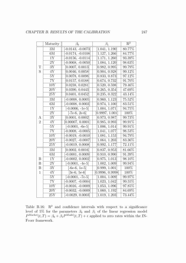
CHAPTER B. RESULTS OF THE CALIBRATION 247
Maturity β0 β1 R2
3M [-0.0143, -0.0073] [1.041, 1.190] 80.77%6M [-0.0174, -0.0108] [1.127, 1.266] 84.77%1Y [-0.0156, -0.0114] [1.171, 1.260] 93.39%2Y [-0.0068, -0.0050] [1.084, 1.120] 98.63%
T 3Y [0.0007, 0.0013] [0.982, 0.995] 99.79%S 4Y [0.0046, 0.0058] [0.904, 0.928] 99.12%
5Y [0.0078, 0.0098] [0.833, 0.873] 97.12%7Y [0.0157, 0.0188] [0.674, 0.732] 91.70%10Y [0.0238, 0.0281] [0.520, 0.598] 79.46%20Y [0.0390, 0.0443] [0.265, 0.354] 47.69%25Y [0.0401, 0.0452] [0.235, 0.322] 43.14%
3M [-0.0008, 0.0005] [0.960, 1.123] 75.52%6M [-0.0008, 0.0003] [0.974, 1.100] 83.51%1Y [-0.0006, -1e-5] [1.004, 1.071] 94.75%2Y [-7e-6, 2e-6] [0.9997, 1.001] 100%
A 3Y [0.0001, 0.0002] [0.973, 0.987] 99.73%2 4Y [0.00007, 0.0001] [0.985, 0.993] 99.91%
5Y [-0.0001, -6e-5] [1.006, 1.014] 99.91%7Y [-0.0008, -0.0005] [1.041, 1.077] 98.53%10Y [-0.0019, -0.0010] [1.081, 1.153] 94.79%20Y [-0.0027, -0.0007] [1.064, 1.203] 83.36%25Y [-0.0019, 0.0008] [0.992, 1.177] 72.11%
3M [0.0002, 0.0016] [0.837, 0.953] 81.66%6M [-0.0001, 0.0009] [0.910, 0.990] 91.39%
B 1Y [-0.0002, 0.0002] [0.975, 1.013] 98.10%B 2Y [-0.0001, -4e-5] [1.002, 1.009] 99.94%B 3Y [-6e-6, 1e-5] [0.999, 1.001] 100%1 4Y [3e-6, 5e-6] [0.9996, 0.9998] 100%
5Y [-0.0001, -7e-5] [1.004, 1.009] 99.97%7Y [-0.0007, -0.0004] [1.023, 1.042] 99.55%10Y [-0.0016, -0.0009] [1.053, 1.096] 97.85%20Y [-0.0032, -0.0009] [1.060, 1.192] 84.69%25Y [-0.0029, 0.0003] [1.019, 1.203] 73.44%
Table B.16: R2 and confidence intervals with respect to a significancelevel of 5% for the parameters β0 and β1 of the linear regression modelPMarket(t, T ) = β0 + β1P
Model(t, T ) + ε applied to zero rates within the IN-Fcorr framework.

248C
HA
PT
ER
B.R
ESU
LT
SO
FT
HE
CA
LIB
RA
TIO
N
Treasury Strips US Industrials A2 US Industrials BBB1Maturity NAC HS ND M0 NAC HS ND M0 NAC HS ND M0
3M - x - - - x∗∗∗ x∗ x x∗+ x∗∗ x∗∗ x∗
6M - x x+ - - x∗∗∗ x∗ x x∗∗∗ x∗∗ x x1Y - x∗ x - - x x∗
+ x x∗∗ x∗∗ x∗ x2Y - - x - - x x∗ x - x∗∗∗
+ x∗ x∗
3Y - x∗∗∗+ x∗ x - x∗∗ x∗ - x∗∗ x∗∗
+ x∗ x+
4Y - x x - - x - - - x∗ x∗ x5Y - x x - - x - - - x∗∗
+ x -7Y - x x - - x - x - x∗∗
+ x+ -10Y - x x - - x - x - - - -20Y - x x - - x+ - - - - x∗
+ -25Y - - - - - x x∗∗
+ - - - x∗∗∗ -
Table B.17: Test of the standardized innovations within the GDPn framework. The residuals of a given maturity aretested for the hypotheses of no autocorrelation (NAC), of homoscedasticity (HS), if they are drawn from a normaldistribution (ND) and if they have a mean of 0 (M0). x indicates that the hypothesis cannot be rejected at a 5%level. The superscript * signifies that 2.5% of the biggest outliers are removed from the data set. ** stands for aremoval of 5% of the outliers and *** for 10%. The subscript + indicates that we use 1% as the level of significance.

CH
AP
TE
RB
.R
ESU
LT
SO
FT
HE
CA
LIB
RA
TIO
N249
Treasury Strips US Industrials A2 US Industrials BBB1Maturity NAC HS ND M0 NAC HS ND M0 NAC HS ND M0
3M - x x+ - x x∗∗∗+ x∗ - x∗ x∗∗∗ x∗∗ x∗
6M - x x+ - - - x∗∗∗+ x x∗ x∗∗ x∗ x
1Y - x∗∗ x - - - x∗∗∗ x∗ - - - -2Y - - x∗ - x∗ x∗∗ x∗∗∗ x x x∗ x∗∗ x3Y - x x - - - x∗∗ x x∗∗ x∗∗∗ x∗∗ -4Y - x x+ - - x∗∗∗ x∗ x - x∗∗ x∗∗∗
+ -5Y - x x - - x x∗ x - x∗∗ x∗ -7Y - x x - - x x∗ x - x∗∗ x -10Y - x x - - x x∗
+ x - - x x∗
20Y - x x - - - x x - x x+ -25Y - - x∗∗∗
+ - - - x x - x x+ -
Table B.18: Test of the standardized innovations within the GDPr framework. The residuals of a given maturity aretested for the hypotheses of no autocorrelation (NAC), of homoscedasticity (HS), if they are drawn from a normaldistribution (ND) and if they have a mean of 0 (M0). x indicates that the hypothesis cannot be rejected at a 5%level. The superscript * signifies that 2.5% of the biggest outliers are removed from the data set. ** stands for aremoval of 5% of the outliers and *** for 10%. The subscript + indicates that we use 1% as the level of significance.

250C
HA
PT
ER
B.R
ESU
LT
SO
FT
HE
CA
LIB
RA
TIO
N
Treasury Strips US Industrials A2 US Industrials BBB1Maturity NAC HS ND M0 NAC HS ND M0 NAC HS ND M0
3M - x∗∗ x - x x∗∗∗+ x∗∗ x∗
+ x x∗∗+ x∗∗ x∗∗∗
6M - x∗∗∗ x - x x∗∗∗ x∗ x x∗ x∗∗∗ x x1Y - - x∗∗∗ - - x∗∗∗ x∗ x∗∗
+ - - - -2Y - - x - x+ x∗∗
+ x∗ - - - x -3Y x∗∗∗
+ x∗∗∗+ x∗ x+ x x∗∗ x∗∗ x - x∗∗∗
+ x∗ -4Y - x x - - x∗∗
+ x - x x+ x∗ -5Y - x x - - - x - x∗∗∗ x∗
+ x∗ x7Y - x∗ x+ - - - x∗∗ - - - x∗ -10Y - x x+ - - x∗∗∗ x∗
+ - - - x+ -20Y - x∗∗∗ - - - x x - - - x∗∗∗ -25Y - - - - - x x - - - x∗∗∗ x∗∗∗
Table B.19: Test of the standardized innovations within the CPI framework. The residuals of a given maturity aretested for the hypotheses of no autocorrelation (NAC), of homoscedasticity (HS), if they are drawn from a normaldistribution (ND) and if they have a mean of 0 (M0). x indicates that the hypothesis cannot be rejected at a 5%level. The superscript * signifies that 2.5% of the biggest outliers are removed from the data set. ** stands for aremoval of 5% of the outliers and *** for 10%. The subscript + indicates that we use 1% as the level of significance.
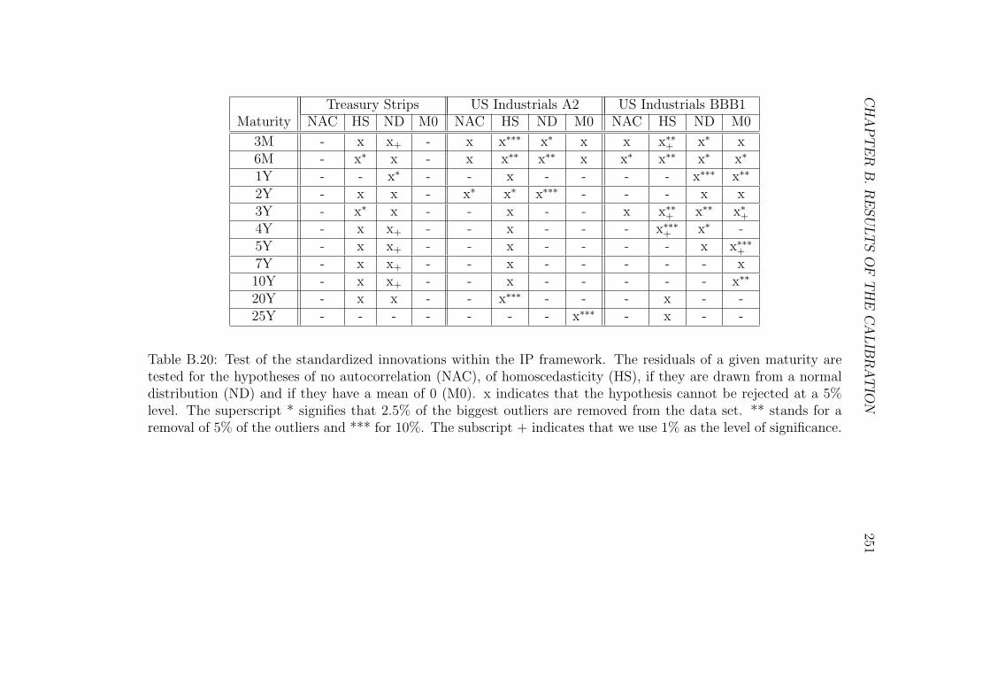
CH
AP
TE
RB
.R
ESU
LT
SO
FT
HE
CA
LIB
RA
TIO
N251
Treasury Strips US Industrials A2 US Industrials BBB1Maturity NAC HS ND M0 NAC HS ND M0 NAC HS ND M0
3M - x x+ - x x∗∗∗ x∗ x x x∗∗+ x∗ x
6M - x∗ x - x x∗∗ x∗∗ x x∗ x∗∗ x∗ x∗
1Y - - x∗ - - x - - - - x∗∗∗ x∗∗
2Y - x x - x∗ x∗ x∗∗∗ - - - x x3Y - x∗ x - - x - - x x∗∗
+ x∗∗ x∗+
4Y - x x+ - - x - - - x∗∗∗+ x∗ -
5Y - x x+ - - x - - - - x x∗∗∗+
7Y - x x+ - - x - - - - - x10Y - x x+ - - x - - - - - x∗∗
20Y - x x - - x∗∗∗ - - - x - -25Y - - - - - - - x∗∗∗ - x - -
Table B.20: Test of the standardized innovations within the IP framework. The residuals of a given maturity aretested for the hypotheses of no autocorrelation (NAC), of homoscedasticity (HS), if they are drawn from a normaldistribution (ND) and if they have a mean of 0 (M0). x indicates that the hypothesis cannot be rejected at a 5%level. The superscript * signifies that 2.5% of the biggest outliers are removed from the data set. ** stands for aremoval of 5% of the outliers and *** for 10%. The subscript + indicates that we use 1% as the level of significance.
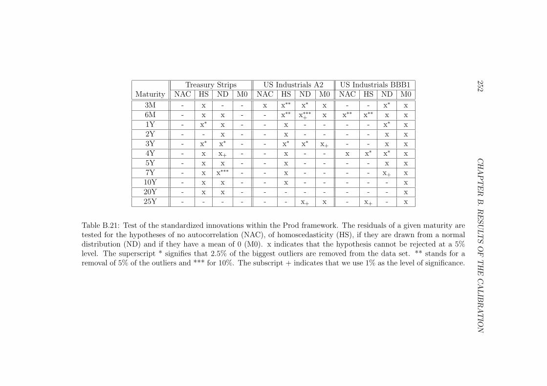
252C
HA
PT
ER
B.R
ESU
LT
SO
FT
HE
CA
LIB
RA
TIO
N
Treasury Strips US Industrials A2 US Industrials BBB1Maturity NAC HS ND M0 NAC HS ND M0 NAC HS ND M0
3M - x - - x x∗∗ x∗ x - - x∗ x6M - x x - - x∗∗ x∗∗∗
+ x x∗∗ x∗∗ x x1Y - x∗ x - - x - - - - x∗ x2Y - - x - - x - - - - x x3Y - x∗ x∗ - - x∗ x∗ x+ - - x x4Y - x x+ - - x - - x x∗ x∗ x5Y - x x - - x - - - - x x7Y - x x∗∗∗ - - x - - - - x+ x10Y - x x - - x - - - - - x20Y - x x - - - - - - - - x25Y - - - - - - x+ x - x+ - x
Table B.21: Test of the standardized innovations within the Prod framework. The residuals of a given maturity aretested for the hypotheses of no autocorrelation (NAC), of homoscedasticity (HS), if they are drawn from a normaldistribution (ND) and if they have a mean of 0 (M0). x indicates that the hypothesis cannot be rejected at a 5%level. The superscript * signifies that 2.5% of the biggest outliers are removed from the data set. ** stands for aremoval of 5% of the outliers and *** for 10%. The subscript + indicates that we use 1% as the level of significance.
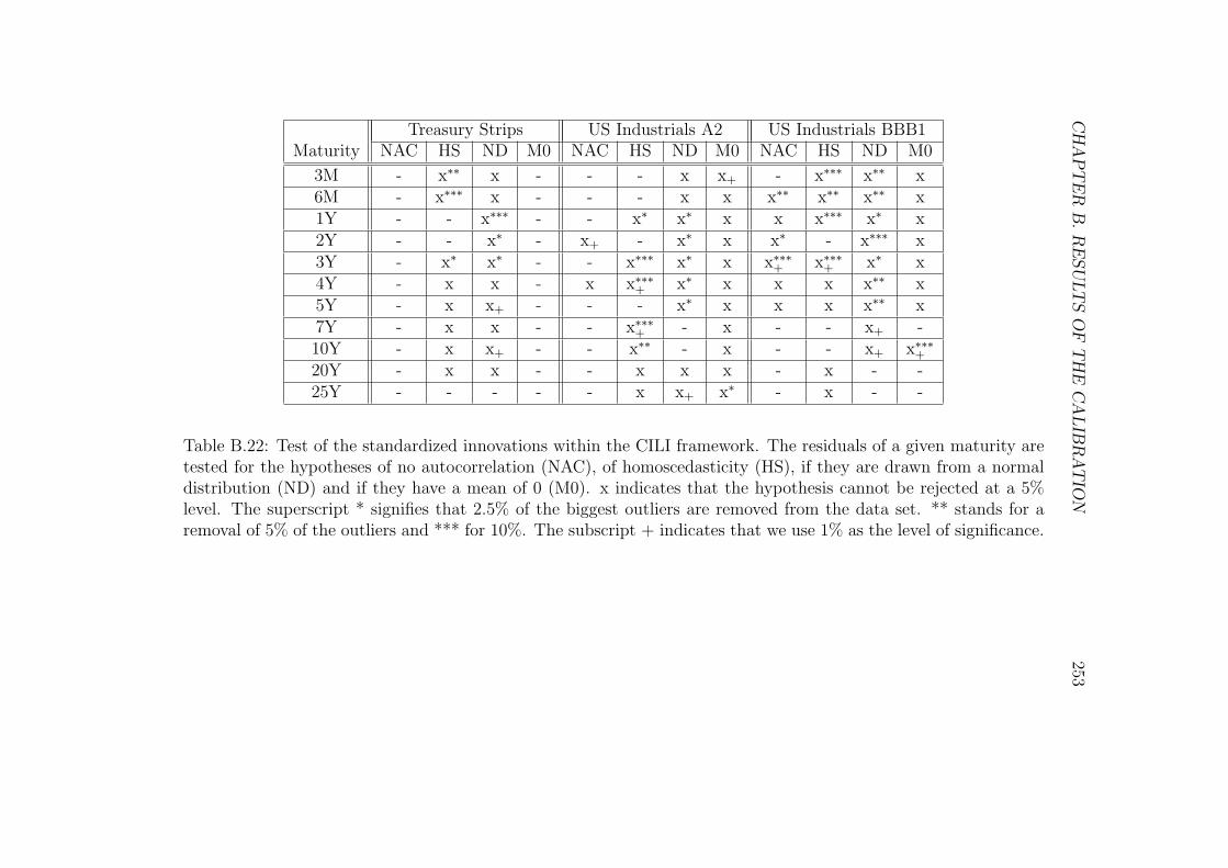
CH
AP
TE
RB
.R
ESU
LT
SO
FT
HE
CA
LIB
RA
TIO
N253
Treasury Strips US Industrials A2 US Industrials BBB1Maturity NAC HS ND M0 NAC HS ND M0 NAC HS ND M0
3M - x∗∗ x - - - x x+ - x∗∗∗ x∗∗ x6M - x∗∗∗ x - - - x x x∗∗ x∗∗ x∗∗ x1Y - - x∗∗∗ - - x∗ x∗ x x x∗∗∗ x∗ x2Y - - x∗ - x+ - x∗ x x∗ - x∗∗∗ x3Y - x∗ x∗ - - x∗∗∗ x∗ x x∗∗∗
+ x∗∗∗+ x∗ x
4Y - x x - x x∗∗∗+ x∗ x x x x∗∗ x
5Y - x x+ - - - x∗ x x x x∗∗ x7Y - x x - - x∗∗∗
+ - x - - x+ -10Y - x x+ - - x∗∗ - x - - x+ x∗∗∗
+
20Y - x x - - x x x - x - -25Y - - - - - x x+ x∗ - x - -
Table B.22: Test of the standardized innovations within the CILI framework. The residuals of a given maturity aretested for the hypotheses of no autocorrelation (NAC), of homoscedasticity (HS), if they are drawn from a normaldistribution (ND) and if they have a mean of 0 (M0). x indicates that the hypothesis cannot be rejected at a 5%level. The superscript * signifies that 2.5% of the biggest outliers are removed from the data set. ** stands for aremoval of 5% of the outliers and *** for 10%. The subscript + indicates that we use 1% as the level of significance.

254C
HA
PT
ER
B.R
ESU
LT
SO
FT
HE
CA
LIB
RA
TIO
N
Treasury Strips US Industrials A2 US Industrials BBB1Maturity NAC HS ND M0 NAC HS ND M0 NAC HS ND M0
3M - x∗ x - - - x x x∗∗+ x∗∗
+ x∗∗∗ -6M - x∗∗∗ x - - x∗ x x x∗ x∗∗ x∗∗ x∗∗∗
+
1Y - - x∗∗∗ - - x x∗ x x x∗∗∗ x∗ x∗∗∗
2Y - - x∗ - x x x∗ x x x∗∗∗+ x∗∗ x
3Y - x∗ x∗ - - x x∗ x x x∗∗∗ x∗ x∗∗+
4Y - x - - - x x∗ x x x x∗ x5Y - x - - x x x∗ x x∗ x∗∗ x∗∗ -7Y - x x+ - - x x x∗∗ - x∗∗∗
+ x∗∗ -10Y - x x+ - - x x x∗
+ - - x∗ -20Y - x - - - x x∗ x∗ - x x x25Y - - - - - x x∗ x - x x x∗∗∗
Table B.23: Test of the standardized innovations within the CICI framework. The residuals of a given maturity aretested for the hypotheses of no autocorrelation (NAC), of homoscedasticity (HS), if they are drawn from a normaldistribution (ND) and if they have a mean of 0 (M0). x indicates that the hypothesis cannot be rejected at a 5%level. The superscript * signifies that 2.5% of the biggest outliers are removed from the data set. ** stands for aremoval of 5% of the outliers and *** for 10%. The subscript + indicates that we use 1% as the level of significance.

CH
AP
TE
RB
.R
ESU
LT
SO
FT
HE
CA
LIB
RA
TIO
N255
Treasury Strips US Industrials A2 US Industrials BBB1Maturity NAC HS ND M0 NAC HS ND M0 NAC HS ND M0
3M - x x x - - x∗∗∗ - - x∗∗ x∗∗+ x+
6M - x x∗ - x x∗∗∗ x∗∗∗ x x∗+ x∗∗ x∗∗ -
1Y - x∗∗∗ x∗ x - - x∗∗∗ x x x∗∗∗ x∗∗ -2Y - x∗ - - - - x∗ x - - x∗∗∗ x+
3Y - x∗∗ - - x - x∗ x x x∗ x∗∗ -4Y - x∗ - x+ - - x∗ x - - x∗∗∗ x5Y - x∗ x∗∗∗ x - x∗∗∗ x∗∗ x - - x∗∗ -7Y - x x∗∗∗ x - x∗∗∗ x∗∗∗ x - - x+ -10Y - x x∗∗ x - x∗∗∗
+ x∗∗∗ x+ - - x+ -20Y - x x - - - x x - x - -25Y - - - - - x x∗∗∗ x - x - -
Table B.24: Test of the standardized innovations within the SZ5 framework. The residuals of a given maturity aretested for the hypotheses of no autocorrelation (NAC), of homoscedasticity (HS), if they are drawn from a normaldistribution (ND) and if they have a mean of 0 (M0). x indicates that the hypothesis cannot be rejected at a 5%level. The superscript * signifies that 2.5% of the biggest outliers are removed from the data set. ** stands for aremoval of 5% of the outliers and *** for 10%. The subscript + indicates that we use 1% as the level of significance.

256C
HA
PT
ER
B.R
ESU
LT
SO
FT
HE
CA
LIB
RA
TIO
N
Treasury Strips US Industrials A2 US Industrials BBB1Maturity NAC HS ND M0 NAC HS ND M0 NAC HS ND M0
3M - - x x x x∗∗∗ x∗∗ x+ - x∗∗ x∗∗ x6M - - x∗ x∗∗ - - x∗∗∗ x∗∗∗ x∗ x∗∗
+ x∗ x∗+
1Y - x∗∗∗ x∗ x∗∗∗ - - x∗∗∗ - x∗∗ - x∗∗∗ x∗
2Y - - x x - x∗∗∗+ x∗ x∗∗∗
+ - - x∗∗∗+ x
3Y - - x∗ x x∗ x∗ x∗ x - x∗∗∗ x x∗∗∗+
4Y - x∗∗ x∗ x x∗ x∗ x∗∗ x x+ x∗ x∗ -5Y - x∗∗∗
+ x x - x∗+ x∗ x∗∗∗ - x∗ x∗ x∗∗
+
7Y - x∗∗∗ x∗∗∗ x∗∗∗ - x∗∗ x∗+ x∗∗∗ - - x∗∗ x
10Y - x∗∗∗ x∗∗∗ - - x x∗∗∗+ - - - x∗
+ -20Y - - x∗∗ - - x x∗∗∗ - - x x+ -25Y - - - - - x x - - x x+ -
Table B.25: Test of the standardized innovations within the SZ5u. The residuals of a given maturity are tested forthe hypotheses of no autocorrelation (NAC), of homoscedasticity (HS), if they are drawn from a normal distribution(ND) and if they have a mean of 0 (M0). x indicates that the hypothesis cannot be rejected at a 5% level. Thesuperscript * signifies that 2.5% of the biggest outliers are removed from the data set. ** stands for a removal of5% of the outliers and *** for 10%. The subscript + indicates that we use 1% as the level of significance.

CH
AP
TE
RB
.R
ESU
LT
SO
FT
HE
CA
LIB
RA
TIO
N257
Treasury Strips US Industrials A2 US Industrials BBB1Maturity NAC HS ND M0 NAC HS ND M0 NAC HS ND M0
3M - - x∗∗∗ - - - x - x∗∗∗+ - x∗∗∗ -
6M - - x∗∗ - - - x x x∗ - x∗ -1Y - x∗∗ x∗ x∗ x∗ x∗∗∗ x∗∗ x x x∗∗
+ x∗∗ x2Y - - x x∗∗ - - x∗ x+ - x∗∗∗ - -3Y - - x∗ x - - x∗ x+ - x∗ x∗∗ x∗∗∗
+
4Y x∗∗∗ x∗ x∗ x x∗ x∗∗∗ x∗∗ x x∗ x∗∗ x∗∗∗ -5Y - x∗∗∗
+ x∗ x∗∗∗+ - x∗∗∗
+ x∗∗ x∗∗ - - - -7Y - x∗∗∗
+ x∗∗∗ - - x+ x - - - - x∗∗
10Y - - x∗∗∗ - - x x - - x∗ - x20Y - - x∗ - - x x - - x - -25Y - - - - - x x+ - - x - -
Table B.26: Test of the standardized innovations within the 5corr framework. The residuals of a given maturity aretested for the hypotheses of no autocorrelation (NAC), of homoscedasticity (HS), if they are drawn from a normaldistribution (ND) and if they have a mean of 0 (M0). x indicates that the hypothesis cannot be rejected at a 5%level. The superscript * signifies that 2.5% of the biggest outliers are removed from the data set. ** stands for aremoval of 5% of the outliers and *** for 10%. The subscript + indicates that we use 1% as the level of significance.

258C
HA
PT
ER
B.R
ESU
LT
SO
FT
HE
CA
LIB
RA
TIO
N
US Industrials A2 US Industrials BBB1Maturity NAC HS ND M0 NAC HS ND M0
3M - - x∗ x∗+ x∗ x∗∗∗ x∗∗ x∗
6M x x∗∗∗ x∗∗∗ x x x∗∗ x∗ x1Y - x∗∗∗ x∗∗ x x - x∗∗∗ x∗∗∗
2Y - x∗∗∗ x∗ x - x∗∗∗+ x∗∗ x∗∗
3Y x - x∗∗ x x x∗ x∗∗ x4Y - x∗∗∗ x∗ x - x∗∗ x∗∗ x∗∗∗
+
5Y - x x∗ x - x x -7Y - x x+ x - x x -10Y - x x+ x - x - -20Y - x x x - x x∗∗ x25Y - x x - - x x -
Table B.27: Test of the standardized innovations within the INFcorr framework for defaultable bonds. The residualsof a given maturity are tested for the hypotheses of no autocorrelation (NAC), of homoscedasticity (HS), if they aredrawn from a normal distribution (ND) and if they have a mean of 0 (M0). x indicates that the hypothesis cannotbe rejected at a 5% level. The superscript * signifies that 2.5% of the biggest outliers are removed from the dataset. ** stands for a removal of 5% of the outliers and *** for 10%. The subscript + indicates that we use 1% as thelevel of significance.

CH
AP
TE
RB
.R
ESU
LT
SO
FT
HE
CA
LIB
RA
TIO
N259
US Industrials A2 US Industrials BBB1Maturity NAC HS ND M0 NAC HS ND M0
3M - - x∗ - x∗ x∗∗ x∗∗∗ x6M - - x∗ - x∗ x∗∗∗ x∗∗ x+
1Y - - x∗∗ x∗ x x∗∗∗+ x∗∗∗ -
2Y - - x - - - x∗∗ x3Y x∗ x∗∗∗
+ x∗∗ x x x∗ x∗∗∗ x∗+
4Y - - x∗ x∗ - x∗∗∗ x∗∗∗ x5Y - x∗∗∗ x∗∗∗ x∗ - x∗∗∗ x∗ x7Y - x - x∗ - x+ x∗ x10Y - x - - - x+ x x20Y - x x x - x x -25Y - x x x∗ - x x -
Table B.28: Test of the standardized innovations within the INF framework for defaultable bonds. The residuals ofa given maturity are tested for the hypotheses of no autocorrelation (NAC), of homoscedasticity (HS), if they aredrawn from a normal distribution (ND) and if they have a mean of 0 (M0). x indicates that the hypothesis cannotbe rejected at a 5% level. The superscript * signifies that 2.5% of the biggest outliers are removed from the dataset. ** stands for a removal of 5% of the outliers and *** for 10%. The subscript + indicates that we use 1% as thelevel of significance.

260 CHAPTER B. RESULTS OF THE CALIBRATION

Appendix C
Credit Derivatives
In order to improve the readability of Chapter 5 certain proofs are given inthis chapter.
Proof of Theorem 5.7:
According to Feynman-Kac (see Theorem 2.14) v(r, szero, u, w1, w2, t, T ) solvesthe following equation:
(r + szero)v = vt + [θr(t) + brw1w1 + brw2w2 − arr]vr
+ [θszero + bszerouu − bszerow1w1 − bszerow2w2 − asszero]vszero
+ [θu − auu]vu + [θw1 − aw1w1]vw1 + [θw2 − aw2w2]vw2
+1
2
(σ2
rvrr + σ2szerovszeroszero + σ2
uvuu + σ2w1
vw1w1 + σ2w2
vw2w2
+ 2σw1σw2ρw1w2vw1w2 + 2σrσw1ρrw1vrw1
+ 2σrσszero(ρrw1ρsw1 + ρrw2ρsw2)vrszero
+ 2σrσw2
(ρrw1ρw1w2 + ρrw2
√1 − ρ2
w1w2
)vrw2
+ 2σszeroσuρsuvszerou + 2σszeroσw1ρsw1vszerow1
+ 2σszeroσw2
(ρsw1ρw1w2 + ρsw2
√1 − ρ2
w1w2
)vszerow2
)
with terminal condition v(r, szero, u, w1, w2, T, T ) = szero(T ).Also, it is assumed that v takes on the formv(t, T ) = P d,zero(t, T ) · (F (t, T )+G(t, T )r(t)+H(t, T )szero(t)+ I(t, T )u(t)+J1(t, T )w1(t) + J2(t, T )w2(t)).
261

262 CHAPTER C. CREDIT DERIVATIVES
Inserting the partial derivatives
vt = (Ad,zerot − Bd,zero
t r − Cd,zerot szero − Dd,zero
t u − (Ed,zero1 )tw1 − (Ed,zero
2 )tw2) · v+ (Ft + Gtr + Hts
zero + Itu + (J1)tw1 + (J2)tw2) · P d,zero ,vrr = (Bd,zero)2 · v − 2GBd,zero · P d,zero , vr = −Bd,zero · v + G · P d,zero ,vszeroszero = (Cd,zero)2 · v − 2HCd,zero · P d,zero , vszero = −Cd,zero · v + H · P d,zero ,vuu = (Dd,zero)2 · v − 2IDd,zero · P d,zero , vu = −Dd,zero · v + I · P d,zero ,
vw1w1 = (Ed,zero1 )2 · v − 2J1E
d,zero1 · P d,zero , vw1 = −Ed,zero
1 · v + J1 · P d,zero ,
vw2w2 = (Ed,zero2 )2 · v − 2J2E
d,zero2 · P d,zero , vw2 = −Ed,zero
2 · v + J2 · P d,zero ,
vw1w2 = Ed,zero1 Ed,zero
2 · v − (Ed,zero2 J1 + Ed,zero
1 J2) · P d,zero ,
vrw1 = Bd,zeroEd,zero1 · v − (Bd,zeroJ1 + Ed,zero
1 G) · P d,zero ,
vrw2 = Bd,zeroEd,zero2 · v − (Bd,zeroJ2 + Ed,zero
2 G) · P d,zero ,vrszero = Bd,zeroCd,zero · v − (Bd,zeroH + Cd,zeroG) · P d,zero ,
vszerow1 = Cd,zeroEd,zero1 · v − (Cd,zeroJ1 + Ed,zero
1 H) · P d,zero ,
vszerow2 = Cd,zeroEd,zero2 · v − (Cd,zeroJ2 + Ed,zero
2 H) · P d,zero ,vszerou = Cd,zeroDd,zero · v − (Dd,zeroH + Cd,zeroI) · P d,zero ,
dividing by P d,zero > 0 and canceling terms with the help of the PDEs forAd,zero
t , Bd,zerot , Cd,zero
t , Dd,zerot , (Ed,zero
1 )t and (Ed,zero2 )t (see Proposition 5.3
and Theorem 4.3), we end up with
Ft + θr(t)G + θw1J1 + θw2J2 + θuI + θszeroH − σ2szeroCd,zeroH − σ2
rBd,zeroG
−σ2w1
Ed,zero1 J1 − σ2
w2Ed,zero
2 J2 − σ2uD
d,zeroI
−σw1σw2ρw1w2(Ed,zero1 J2 + Ed,zero
2 J1) − σrσw1ρrw1(Bd,zeroJ1 + Ed,zero
1 G)
−σrσw2
(ρrw1ρw1w2 + ρrw2
√1 − ρ2
w1w2
)(Bd,zeroJ2 + Ed,zero
2 G)
−σrσszero(ρrw1ρsw1 + ρrw2ρsw2)(Bd,zeroH + Cd,zeroG)
−σszeroσw1ρsw1(Ed,zero1 H + Cd,zeroJ1) − σszeroσuρsu(C
d,zeroI + Dd,zeroH)
−σszeroσw2
(ρsw1ρw1w2 + ρsw2
√1 − ρ2
w1w2
)(Ed,zero
2 H + Cd,zeroJ2)
+ r(Gt − arG)
+ szero(Ht − asH)
+ u(It − auI + bszerouH)
+ w1((J1)t + brw1G − aw1J1 − bszerow1H)
+ w2((J2)t + brw2G − aw2J2 − bszerow2H)
= 0.

CHAPTER C. CREDIT DERIVATIVES 263
This equation results in the following PDEs
Gt = arG,
Ht = asH,
It = auI − bszerouH,
(J1)t = aw1J1 + bszerow1H − brw1G,
(J2)t = aw2J2 + bszerow2H − brw2G,
Ft = −θr(t)G − θw1J1 − θw2J2 − θuI − θszeroH + σ2szeroCd,zeroH
+ σ2rB
d,zeroG + σ2w1
Ed,zero1 J1 + σ2
w2Ed,zero
2 J2 + σ2uD
d,zeroI
+ σw1σw2ρw1w2(Ed,zero1 J2 + Ed,zero
2 J1)
+ σrσw1ρrw1(Bd,zeroJ1 + Ed,zero
1 G)
+ σrσw2
(ρrw1ρw1w2 + ρrw2
√1 − ρ2
w1w2
)(Bd,zeroJ2 + Ed,zero
2 G)
+ σrσszero(ρrw1ρsw1 + ρrw2ρsw2)(Bd,zeroH + Cd,zeroG)
+ σszeroσw1ρsw1(Ed,zero1 H + Cd,zeroJ1) + σszeroσuρsu(C
d,zeroI + Dd,zeroH)
+ σszeroσw2
(ρsw1ρw1w2 + ρsw2
√1 − ρ2
w1w2
)(Ed,zero
2 H + Cd,zeroJ2) .
By means of the terminal condition (G(T, T ) = 0, F (T, T ) = 0, H(T, T ) = 1,I(T, T ) = 0, J1(T, T ) = 0, J2(T, T ) = 0) and since it holds that
−Ct = H,
−Dt = I,
−(Ed,zero1 − E1)t = J1,
−(Ed,zero2 − E2)t = J2,
we obtain the stated solutions with G(t, T ) = 0 and Theorem 2.15.
Proof of Proposition 5.10:
Applying Feynman-Kac (see Theorem 2.14) we get the following equation:
(r + szero)P d,∗
= P d,∗t
+(θr(t) + brw1w1 + brw2w2 − arr
)P d,∗
r
+ (θw1 − aw1w1) P d,∗w1
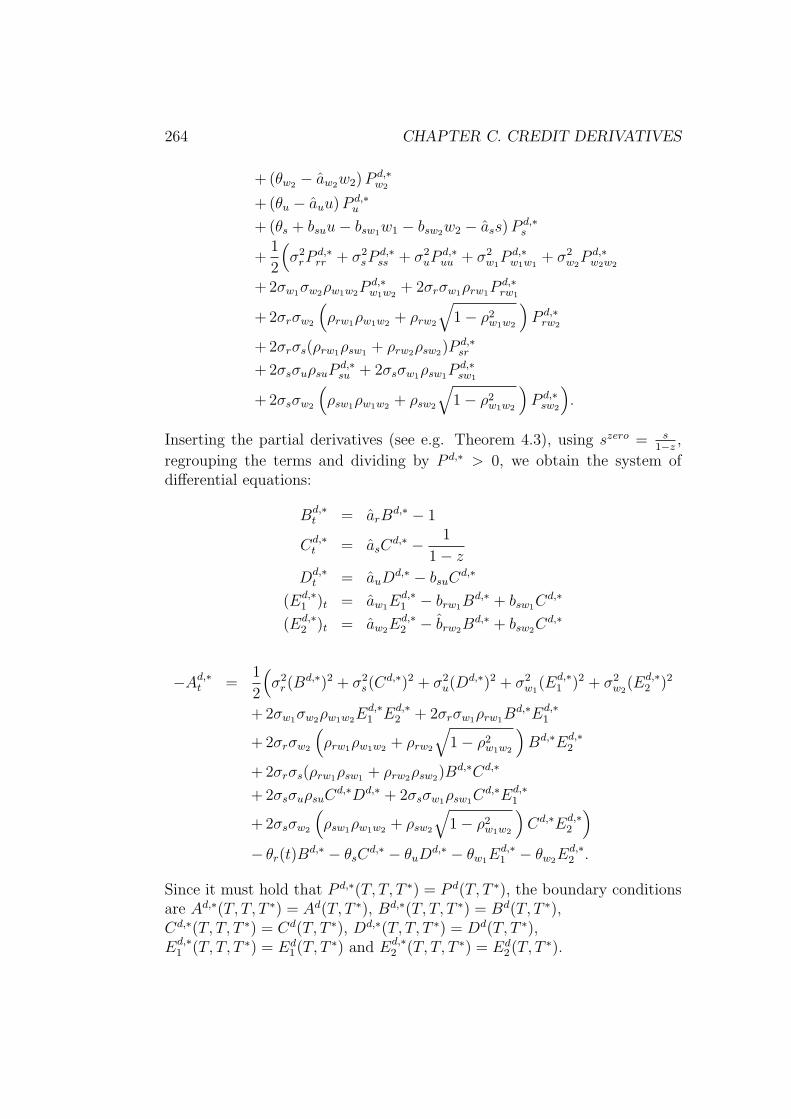
264 CHAPTER C. CREDIT DERIVATIVES
+ (θw2 − aw2w2) P d,∗w2
+ (θu − auu) P d,∗u
+ (θs + bsuu − bsw1w1 − bsw2w2 − ass) P d,∗s
+1
2
(σ2
rPd,∗rr + σ2
sPd,∗ss + σ2
uPd,∗uu + σ2
w1P d,∗
w1w1+ σ2
w2P d,∗
w2w2
+ 2σw1σw2ρw1w2Pd,∗w1w2
+ 2σrσw1ρrw1Pd,∗rw1
+ 2σrσw2
(ρrw1ρw1w2 + ρrw2
√1 − ρ2
w1w2
)P d,∗
rw2
+ 2σrσs(ρrw1ρsw1 + ρrw2ρsw2)Pd,∗sr
+ 2σsσuρsuPd,∗su + 2σsσw1ρsw1P
d,∗sw1
+ 2σsσw2
(ρsw1ρw1w2 + ρsw2
√1 − ρ2
w1w2
)P d,∗
sw2
).
Inserting the partial derivatives (see e.g. Theorem 4.3), using szero = s1−z
,
regrouping the terms and dividing by P d,∗ > 0, we obtain the system ofdifferential equations:
Bd,∗t = arB
d,∗ − 1
Cd,∗t = asC
d,∗ − 1
1 − z
Dd,∗t = auD
d,∗ − bsuCd,∗
(Ed,∗1 )t = aw1E
d,∗1 − brw1B
d,∗ + bsw1Cd,∗
(Ed,∗2 )t = aw2E
d,∗2 − brw2B
d,∗ + bsw2Cd,∗
−Ad,∗t =
1
2
(σ2
r(Bd,∗)2 + σ2
s(Cd,∗)2 + σ2
u(Dd,∗)2 + σ2
w1(Ed,∗
1 )2 + σ2w2
(Ed,∗2 )2
+ 2σw1σw2ρw1w2Ed,∗1 Ed,∗
2 + 2σrσw1ρrw1Bd,∗Ed,∗
1
+ 2σrσw2
(ρrw1ρw1w2 + ρrw2
√1 − ρ2
w1w2
)Bd,∗Ed,∗
2
+ 2σrσs(ρrw1ρsw1 + ρrw2ρsw2)Bd,∗Cd,∗
+ 2σsσuρsuCd,∗Dd,∗ + 2σsσw1ρsw1C
d,∗Ed,∗1
+ 2σsσw2
(ρsw1ρw1w2 + ρsw2
√1 − ρ2
w1w2
)Cd,∗Ed,∗
2
)
− θr(t)Bd,∗ − θsC
d,∗ − θuDd,∗ − θw1E
d,∗1 − θw2E
d,∗2 .
Since it must hold that P d,∗(T, T, T ∗) = P d(T, T ∗), the boundary conditionsare Ad,∗(T, T, T ∗) = Ad(T, T ∗), Bd,∗(T, T, T ∗) = Bd(T, T ∗),Cd,∗(T, T, T ∗) = Cd(T, T ∗), Dd,∗(T, T, T ∗) = Dd(T, T ∗),Ed,∗
1 (T, T, T ∗) = Ed1(T, T ∗) and Ed,∗
2 (T, T, T ∗) = Ed2(T, T ∗).

CHAPTER C. CREDIT DERIVATIVES 265
Hence the differential equations result in (cf. Theorem 2.15 and Theorem4.3)
Ad,∗(t, T, T ∗) = Ad,∗(T, T, T ∗) −∫ T
t
Ad,∗t (l, T, T ∗)dl,
Bd,∗(t, T, T ∗) = e−ar(T−t)(Bd,∗(T, T, T ∗) +
∫ T−t
0
earldl)
=1
ar
(1 − e−ar(T ∗−t)
)= Bd(t, T ∗) = B(t, T ∗),
Cd,∗(t, T, T ∗) = e−as(T−t)(Cd,∗(T, T, T ∗) +
1
1 − z
∫ T−t
0
easldl)
= e−as(T−t)Cd(T, T ∗) +1
1 − zCd(t, T ),
Dd,∗(t, T, T ∗)
= e−au(T−t)(Dd,∗(T, T, T ∗) +
∫ T−t
0
eaulbsuCd,∗(0, l, l + T ∗ − T )dl
)
= e−au(T−t)Dd(T, T ∗) − bsuCd(T, T ∗)
(e−as(T−t) − e−au(T−t)
as − au
)
+1
1 − zDd(t, T ),
Ed,∗1 (t, T, T ∗)
= e−aw1 (T−t)(Ed,∗
1 (T, T, T ∗) +
∫ T−t
0
eaw1 l(brw1Bd,∗(0, l, l + T ∗ − T )
− bsw1Cd,∗(0, l, l + T ∗ − T ))dl
)
= e−aw1 (T−t)Ed1(T, T ∗)
+brw1
ar
(1 − e−aw1 (T−t)
aw1
+ e−ar(T ∗−T ) e−aw1 (T−t) − e−ar(T−t)
aw1 − ar
)
+ bsw1Cd(T, T ∗)
(e−as(T−t) − e−aw1 (T−t)
as − aw1
)
+1
1 − z(Ed
1(t, T ) − E1(t, T )),
Ed,∗2 (t, T, T ∗) is determined analogously.

266 CHAPTER C. CREDIT DERIVATIVES
Proof of Proposition 5.17:
According to Feynman-Kac (see Theorem 2.14) the following differentialequation must hold:
(r + szero)P ∗
= P ∗t
+(θr(t) + brw1w1 + brw2w2 − arr
)P ∗
r
+ (θw1 − aw1w1) P ∗w1
+ (θw2 − aw2w2) P ∗w2
+ (θu − auu) P ∗u
+ (θszero + bszerouu − bszerow1w1 − bszerow2w2 − asszero) P ∗
szero
+1
2
(σ2
rP∗rr + σ2
szeroP ∗szeroszero + σ2
uP∗uu + σ2
w1P ∗
w1w1+ σ2
w2P ∗
w2w2
+ 2σw1σw2ρw1w2P∗w1w2
+ 2σrσw1ρrw1P∗rw1
+ 2σrσw2
(ρrw1ρw1w2 + ρrw2
√1 − ρ2
w1w2
)P ∗
rw2
+ 2σrσszero(ρrw1ρsw1 + ρrw2ρsw2)P∗szeror
+ 2σszeroσuρsuP∗szerou + 2σszeroσw1ρsw1P
∗szerow1
+ 2σszeroσw2
(ρsw1ρw1w2 + ρsw2
√1 − ρ2
w1w2
)P ∗
szerow2
).
Inserting the partial derivatives (see e.g. Theorem 4.3), regrouping the termsand dividing by P ∗ > 0, we obtain the solution analogously to Theorem 4.3:
B∗t = arB
∗ − 1
C∗t = asC
∗ − 1
D∗t = auD
∗ − bszerouC∗
(E∗1)t = aw1E
∗1 − brw1B
∗ + bszerow1C∗
(E∗2)t = aw2E
∗2 − brw2B
∗ + bszerow2C∗
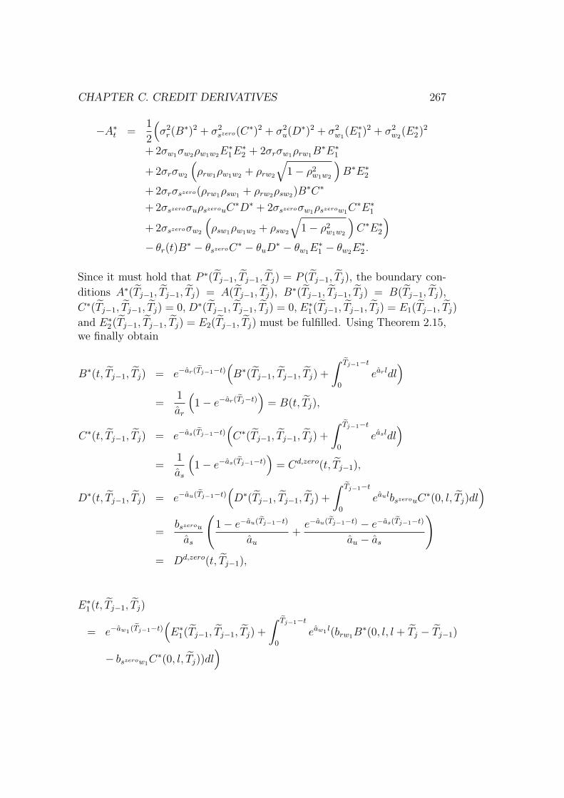
CHAPTER C. CREDIT DERIVATIVES 267
−A∗t =
1
2
(σ2
r(B∗)2 + σ2
szero(C∗)2 + σ2u(D
∗)2 + σ2w1
(E∗1)
2 + σ2w2
(E∗2)
2
+ 2σw1σw2ρw1w2E∗1E
∗2 + 2σrσw1ρrw1B
∗E∗1
+ 2σrσw2
(ρrw1ρw1w2 + ρrw2
√1 − ρ2
w1w2
)B∗E∗
2
+ 2σrσszero(ρrw1ρsw1 + ρrw2ρsw2)B∗C∗
+ 2σszeroσuρszerouC∗D∗ + 2σszeroσw1ρszerow1C
∗E∗1
+ 2σszeroσw2
(ρsw1ρw1w2 + ρsw2
√1 − ρ2
w1w2
)C∗E∗
2
)
− θr(t)B∗ − θszeroC∗ − θuD
∗ − θw1E∗1 − θw2E
∗2 .
Since it must hold that P ∗(Tj−1, Tj−1, Tj) = P (Tj−1, Tj), the boundary con-
ditions A∗(Tj−1, Tj−1, Tj) = A(Tj−1, Tj), B∗(Tj−1, Tj−1, Tj) = B(Tj−1, Tj),
C∗(Tj−1, Tj−1, Tj) = 0, D∗(Tj−1, Tj−1, Tj) = 0, E∗1(Tj−1, Tj−1, Tj) = E1(Tj−1, Tj)
and E∗2(Tj−1, Tj−1, Tj) = E2(Tj−1, Tj) must be fulfilled. Using Theorem 2.15,
we finally obtain
B∗(t, Tj−1, Tj) = e−ar(Tj−1−t)(B∗(Tj−1, Tj−1, Tj) +
∫ Tj−1−t
0
earldl)
=1
ar
(1 − e−ar(Tj−t)
)= B(t, Tj),
C∗(t, Tj−1, Tj) = e−as(Tj−1−t)(C∗(Tj−1, Tj−1, Tj) +
∫ Tj−1−t
0
easldl)
=1
as
(1 − e−as(Tj−1−t)
)= Cd,zero(t, Tj−1),
D∗(t, Tj−1, Tj) = e−au(Tj−1−t)(D∗(Tj−1, Tj−1, Tj) +
∫ Tj−1−t
0
eaulbszerouC∗(0, l, Tj)dl
)
=bszerou
as
(1 − e−au(Tj−1−t)
au
+e−au(Tj−1−t) − e−as(Tj−1−t)
au − as
)
= Dd,zero(t, Tj−1),
E∗1(t, Tj−1, Tj)
= e−aw1 (Tj−1−t)(E∗
1(Tj−1, Tj−1, Tj) +
∫ Tj−1−t
0
eaw1 l(brw1B∗(0, l, l + Tj − Tj−1)
− bszerow1C∗(0, l, Tj))dl
)

268 CHAPTER C. CREDIT DERIVATIVES
=brw1
ar
(1 − e−aw1 (Tj−t)
aw1
+e−aw1 (Tj−t) − e−ar(Tj−t)
aw1 − ar
)
− bszerow1
as
(1 − e−aw1 (Tj−1−t)
aw1
+e−aw1 (Tj−1−t) − e−as(Tj−1−t)
aw1 − as
),
E∗2(t, Tj−1, Tj)
= e−aw2 (Tj−1−t)(E∗
2(Tj−1, Tj−1, Tj) +
∫ Tj−1−t
0
eaw2 l(brw2B∗(0, l, l + Tj − Tj−1)
− bszerow2C∗(0, l, Tj))dl
)
=brw2
ar
(1 − e−aw2 (Tj−t)
aw2
+e−aw2 (Tj−t) − e−ar(Tj−t)
aw2 − ar
)
− bszerow2
as
(1 − e−aw2 (Tj−1−t)
aw2
+e−aw2 (Tj−1−t) − e−as(Tj−1−t)
aw2 − as
),
A∗(t, Tj−1, Tj)
= A∗(Tj−1, Tj−1, Tj) −∫ Tj−1
t
A∗t (l, Tj−1, Tj)dl
= A(Tj−1, Tj) +
∫ Tj−1
t
1
2
(σ2
r(B∗(l, Tj−1, Tj))
2 + σ2szero(C∗(l, Tj−1, Tj))
2
+ σ2u(D
∗(l, Tj−1, Tj))2 + σ2
w1(E∗
1(l, Tj−1, Tj))2 + σ2
w2(E∗
2(l, Tj−1, Tj))2
+ σw1σw2ρw1w2E∗1(l, Tj−1, Tj)E
∗2(l, Tj−1, Tj)
+ σrσw1ρrw1B∗(l, Tj−1, Tj)E
∗1(l, Tj−1, Tj)
+ σszeroσuρsuC∗(l, Tj−1, Tj)D
∗(l, Tj−1, Tj)
+ σszeroσw1ρsw1C∗(l, Tj−1, Tj)E
∗1(l, Tj−1, Tj)
+ σrσw2
(ρrw1ρw1w2 + ρrw2
√1 − ρ2
w1w2
)B∗(l, Tj−1, Tj)E
∗2(l, Tj−1, Tj)
+ σszeroσw2
(ρsw1ρw1w2 + ρsw2
√1 − ρ2
w1w2
)C∗(l, Tj−1, Tj)E
∗2(l, Tj−1, Tj)
+ σrσszero(ρrw1ρsw1 + ρrw2ρsw2)B∗(l, Tj−1, Tj)C
∗(l, Tj−1, Tj)
− θr(l)B∗(l, Tj−1, Tj) − θszeroC∗(l, Tj−1, Tj) − θuD
∗(l, Tj−1, Tj)
− θw1E∗1(l, Tj−1, Tj) − θw2E
∗2(l, Tj−1, Tj)dl.
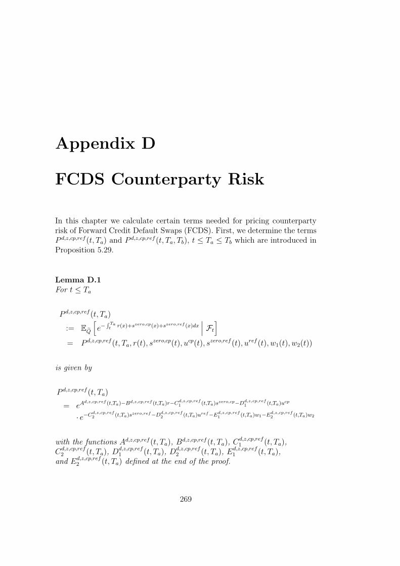
Appendix D
FCDS Counterparty Risk
In this chapter we calculate certain terms needed for pricing counterpartyrisk of Forward Credit Default Swaps (FCDS). First, we determine the termsP d,z,cp,ref (t, Ta) and P d,z,cp,ref (t, Ta, Tb), t ≤ Ta ≤ Tb which are introduced inProposition 5.29.
Lemma D.1For t ≤ Ta
P d,z,cp,ref (t, Ta)
:= EQ
[e−
∫ Tat
r(x)+szero,cp(x)+szero,ref (x)dx∣∣∣ Ft
]
= P d,z,cp,ref (t, Ta, r(t), szero,cp(t), ucp(t), szero,ref (t), uref (t), w1(t), w2(t))
is given by
P d,z,cp,ref (t, Ta)
= eAd,z,cp,ref (t,Ta)−Bd,z,cp,ref (t,Ta)r−Cd,z,cp,ref1 (t,Ta)szero,cp−Dd,z,cp,ref
1 (t,Ta)ucp
· e−Cd,z,cp,ref2 (t,Ta)szero,ref−Dd,z,cp,ref
2 (t,Ta)uref−Ed,z,cp,ref1 (t,Ta)w1−Ed,z,cp,ref
2 (t,Ta)w2
with the functions Ad,z,cp,ref (t, Ta), Bd,z,cp,ref (t, Ta), Cd,z,cp,ref1 (t, Ta),
Cd,z,cp,ref2 (t, Ta), Dd,z,cp,ref
1 (t, Ta), Dd,z,cp,ref2 (t, Ta), Ed,z,cp,ref
1 (t, Ta),and Ed,z,cp,ref
2 (t, Ta) defined at the end of the proof.
269

270 CHAPTER D. FCDS COUNTERPARTY RISK
Proof:In the following, we assume all Brownian motions to be uncorrelated.With Feynman-Kac (see Theorem 2.14) we obtain
(r + szero,cp + szero,ref )P d,z,cp,ref
= P d,z,cp,reft
+(θr(t) + brw1 · w1 + brw2 · w2 − ar · r
)· P d,z,cp,ref
r
+ (θw1 − aw1 · w1) · P d,z,cp,refw1
+ (θw2 − aw2 · w2) · P d,z,cp,refw2
+(θszero,cp + bszero,cpucp · ucp − bszero,cpw1 · w1 − bszero,cpw2 · w2
− ascp · szero,cp)· P d,z,cp,ref
szero,cp + (θucp − aucp · ucp) · P d,z,cp,refucp
+(θszero,ref + bszero,ref uref · uref − bszero,ref w1
· w1 − bszero,ref w2· w2
− asref · szero,ref)· P d,z,cp,ref
szero,ref +(θuref − auref · uref
)· P d,z,cp,ref
uref
+1
2·(σ2
r · P d,z,cp,refrr + σ2
szero,cp · P d,z,cp,refszero,cpszero,cp + σ2
szero,ref · P d,z,cp,refszero,ref szero,ref
+ σ2ucp · P d,z,cp,ref
ucpucp + σ2uref · P d,z,cp,ref
uref uref + σ2w1
· P d,z,cp,refw1w1
+ σ2w2
· P d,z,cp,refw2w2
+ 2 · σw1 · σw2 · ρw1w2 · P d,z,cp,refw1w2
+ 2 · σr · σw1 · ρrw1 · P d,z,cp,refrw1
+ 2 · σr · σw2 ·(ρrw1 · ρw1w2 + ρrw2 ·
√1 − ρ2
w1w2
)· P d,z,cp,ref
rw2
+ 2 · σr · σszero,cp · (ρrw1 · ρscpw1 + ρrw2 · ρscpw2) · P d,z,cp,refszero,cpr
+ 2 · σr · σszero,ref · (ρrw1 · ρsref w1+ ρrw2 · ρsref w2
) · P d,z,cp,refszero,ref r
+ 2 · σszero,cp · σucp · ρscpucp · P d,z,cp,refszero,cpucp
+ 2 · σszero,cp · σw1 · ρscpw1 · P d,z,cp,refszero,cpw1
+ 2 · σszero,ref · σuref · ρsref uref · P d,z,cp,refszero,ref uref
+ 2 · σszero,ref · σw1 · ρsref w1· P d,z,cp,ref
sref w1
+ 2 · σszero,cp · σw2 ·(ρscpw1 · ρw1w2 + ρscpw2 ·
√1 − ρ2
w1w2
)· P d,z,cp,ref
szero,cpw2
+ 2 · σszero,ref · σw2 ·(ρsref w1
· ρw1w2 + ρsref w2·√
1 − ρ2w1w2
)· P d,z,cp,ref
szero,ref w2
+ 2 · σszero,cp · σszero,ref · (ρscpw1 · ρsref w1+ ρscpw2 · ρsref w2
)),
with boundary condition P d,z,cp,ref (Ta, Ta) = 1, i.e.Ad,z,cp,ref (Ta, Ta) = Bd,z,cp,ref (Ta, Ta) = Cd,z,cp,ref
1 (Ta, Ta) = · · · = 0 .Inserting the partial derivatives (see e.g. Theorem 4.3), regrouping the termsand dividing by P d,z,cp,ref > 0, we arrive at the below system of differential

CHAPTER D. FCDS COUNTERPARTY RISK 271
equations.
(Bd,z,cp,ref )t = ar · Bd,z,cp,ref − 1
(Cd,z,cp,ref1 )t = ascp · Cd,z,cp,ref
1 − 1
(Cd,z,cp,ref2 )t = asref · Cd,z,cp,ref
2 − 1
(Dd,z,cp,ref1 )t = aucp · Dd,z,cp,ref
1 − bszero,cpucp · Cd,z,cp,ref1
(Dd,z,cp,ref2 )t = auref · Dd,z,cp,ref
2 − bszero,ref uref · Cd,z,cp,ref2
(Ed,z,cp,ref1 )t
= aw1 · Ed,z,cp,ref1 − brw1 · Bd,z,cp,ref + bszero,cpw1 · Cd,z,cp,ref
1
+ bszero,ref w1· Cd,z,cp,ref
2
(Ed,z,cp,ref2 )t
= aw2 · Ed,z,cp,ref2 − brw2 · Bd,z,cp,ref + bszero,cpw2 · Cd,z,cp,ref
1
+ bszero,ref w2· Cd,z,cp,ref
2
and
−(Ad,z,cp,ref )t =1
2·(σ2
r · (Bd,z,cp,ref )2 + σ2szero,cp · (Cd,z,cp,ref
1 )2 + σ2szero,ref · (Cd,z,cp,ref
2 )2
+σ2ucp · (Dd,z,cp,ref
1 )2 + σ2uref · (Dd,z,cp,ref
2 )2 + σ2w1
· (Ed,z,cp,ref1 )2
+σ2w2
· (Ed,z,cp,ref2 )2 + 2 · σw1 · σw2 · ρw1w2 · Ed,z,cp,ref
1 · Ed,z,cp,ref2
+2 · σr · σw1 · ρrw1 · Bd,z,cp,ref · Ed,z,cp,ref1
+2 · σr · σw2 ·(ρrw1 · ρw1w2 + ρrw2 ·
√1 − ρ2
w1w2
)· Bd,z,cp,ref · Ed,z,cp,ref
2
+2 · σr · σszero,cp · (ρrw1 · ρscpw1 + ρrw2 · ρscpw2) · Bd,z,cp,ref · Cd,z,cp,ref1
+2 · σr · σszero,ref · (ρrw1 · ρsref w1+ ρrw2 · ρsref w2
) · Bd,z,cp,ref · Cd,z,cp,ref2
+2 · σszero,cp · σucp · ρscpucp · Cd,z,cp,ref1 · Dd,z,cp,ref
1
+2 · σszero,cp · σw1 · ρscpw1 · Cd,z,cp,ref1 · Ed,z,cp,ref
1
+2 · σszero,ref · σuref · ρsref uref · Cd,z,cp,ref2 · Dd,z,cp,ref
2
+2 · σszero,ref · σw1 · ρsref w1· Cd,z,cp,ref
2 · Ed,z,cp,ref1
+2 · σszero,cp · σw2
(ρscpw1 · ρw1w2 + ρscpw2 ·
√1 − ρ2
w1w2
)· Cd,z,cp,ref
1 · Ed,z,cp,ref2
+2 · σszero,ref · σw2 ·(ρsref w1
· ρw1w2 + ρsref w2·√
1 − ρ2w1w2
)·Cd,z,cp,ref
2 · Ed,z,cp,ref2
+2 · σszero,cp · σszero,ref · (ρscpw1 · ρsref w1+ ρscpw2 · ρsref w2
) · Cd,z,cp,ref1 · Cd,z,cp,ref
2
)
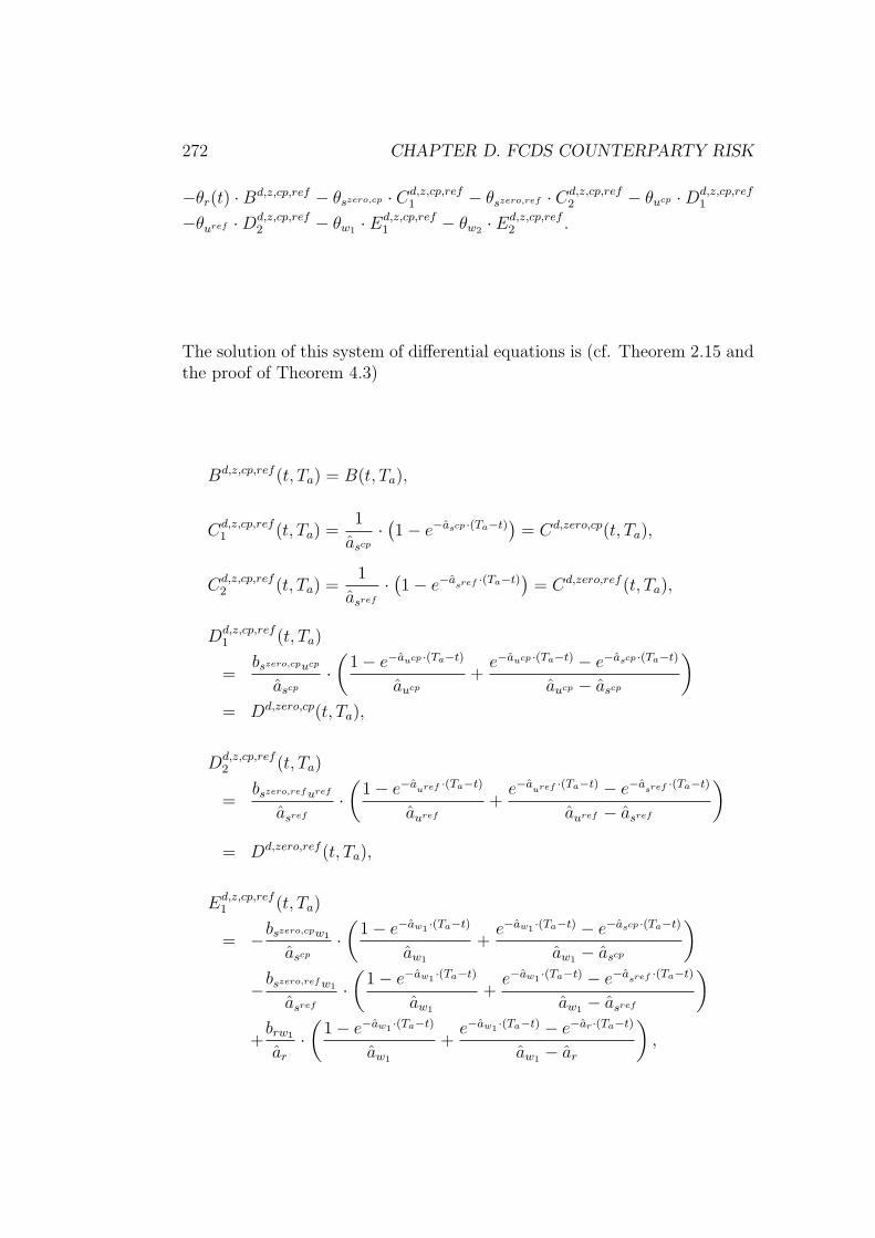
272 CHAPTER D. FCDS COUNTERPARTY RISK
−θr(t) · Bd,z,cp,ref − θszero,cp · Cd,z,cp,ref1 − θszero,ref · Cd,z,cp,ref
2 − θucp · Dd,z,cp,ref1
−θuref · Dd,z,cp,ref2 − θw1 · Ed,z,cp,ref
1 − θw2 · Ed,z,cp,ref2 .
The solution of this system of differential equations is (cf. Theorem 2.15 andthe proof of Theorem 4.3)
Bd,z,cp,ref (t, Ta) = B(t, Ta),
Cd,z,cp,ref1 (t, Ta) =
1
ascp
·(1 − e−ascp ·(Ta−t)
)= Cd,zero,cp(t, Ta),
Cd,z,cp,ref2 (t, Ta) =
1
asref
·(1 − e−a
sref ·(Ta−t))
= Cd,zero,ref (t, Ta),
Dd,z,cp,ref1 (t, Ta)
=bszero,cpucp
ascp
·(
1 − e−aucp ·(Ta−t)
aucp
+e−aucp ·(Ta−t) − e−ascp ·(Ta−t)
aucp − ascp
)
= Dd,zero,cp(t, Ta),
Dd,z,cp,ref2 (t, Ta)
=bszero,ref uref
asref
·(
1 − e−auref ·(Ta−t)
auref
+e−a
uref ·(Ta−t) − e−asref ·(Ta−t)
auref − asref
)
= Dd,zero,ref (t, Ta),
Ed,z,cp,ref1 (t, Ta)
= −bszero,cpw1
ascp
·(
1 − e−aw1 ·(Ta−t)
aw1
+e−aw1 ·(Ta−t) − e−ascp ·(Ta−t)
aw1 − ascp
)
−bszero,ref w1
asref
·(
1 − e−aw1 ·(Ta−t)
aw1
+e−aw1 ·(Ta−t) − e−a
sref ·(Ta−t)
aw1 − asref
)
+brw1
ar
·(
1 − e−aw1 ·(Ta−t)
aw1
+e−aw1 ·(Ta−t) − e−ar·(Ta−t)
aw1 − ar
),
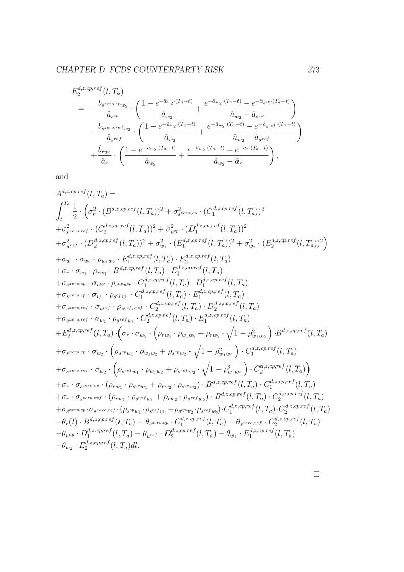
CHAPTER D. FCDS COUNTERPARTY RISK 273
Ed,z,cp,ref2 (t, Ta)
= −bszero,cpw2
ascp
·(
1 − e−aw2 ·(Ta−t)
aw2
+e−aw2 ·(Ta−t) − e−ascp ·(Ta−t)
aw2 − ascp
)
−bszero,ref w2
asref
·(
1 − e−aw2 ·(Ta−t)
aw2
+e−aw2 ·(Ta−t) − e−a
sref ·(Ta−t)
aw2 − asref
)
+brw2
ar
·(
1 − e−aw2 ·(Ta−t)
aw2
+e−aw2 ·(Ta−t) − e−ar·(Ta−t)
aw2 − ar
),
and
Ad,z,cp,ref (t, Ta) =∫ Ta
t
1
2·(σ2
r · (Bd,z,cp,ref (l, Ta))2 + σ2
szero,cp · (Cd,z,cp,ref1 (l, Ta))
2
+σ2szero,ref · (Cd,z,cp,ref
2 (l, Ta))2 + σ2
ucp · (Dd,z,cp,ref1 (l, Ta))
2
+σ2uref · (Dd,z,cp,ref
2 (l, Ta))2 + σ2
w1· (Ed,z,cp,ref
1 (l, Ta))2 + σ2
w2· (Ed,z,cp,ref
2 (l, Ta))2)
+σw1 · σw2 · ρw1w2 · Ed,z,cp,ref1 (l, Ta) · Ed,z,cp,ref
2 (l, Ta)
+σr · σw1 · ρrw1 · Bd,z,cp,ref (l, Ta) · Ed,z,cp,ref1 (l, Ta)
+σszero,cp · σucp · ρscpucp · Cd,z,cp,ref1 (l, Ta) · Dd,z,cp,ref
1 (l, Ta)
+σszero,cp · σw1 · ρscpw1 · Cd,z,cp,ref1 (l, Ta) · Ed,z,cp,ref
1 (l, Ta)
+σszero,ref · σuref · ρsref uref · Cd,z,cp,ref2 (l, Ta) · Dd,z,cp,ref
2 (l, Ta)
+σszero,ref · σw1 · ρsref w1· Cd,z,cp,ref
2 (l, Ta) · Ed,z,cp,ref1 (l, Ta)
+Ed,z,cp,ref2 (l, Ta) ·
(σr · σw2 ·
(ρrw1 · ρw1w2 + ρrw2 ·
√1 − ρ2
w1w2
)·Bd,z,cp,ref (l, Ta)
+σszero,cp · σw2 ·(ρscpw1 · ρw1w2 + ρscpw2 ·
√1 − ρ2
w1w2
)· Cd,z,cp,ref
1 (l, Ta)
+σszero,ref · σw2 ·(ρsref w1
· ρw1w2 + ρsref w2·√
1 − ρ2w1w2
)· Cd,z,cp,ref
2 (l, Ta))
+σr · σszero,cp · (ρrw1 · ρscpw1 + ρrw2 · ρscpw2) · Bd,z,cp,ref (l, Ta) · Cd,z,cp,ref1 (l, Ta)
+σr · σszero,ref · (ρrw1 · ρsref w1+ ρrw2 · ρsref w2
) · Bd,z,cp,ref (l, Ta) · Cd,z,cp,ref2 (l, Ta)
+σszero,cp ·σszero,ref ·(ρscpw1 ·ρsref w1+ρscpw2 ·ρsref w2
)·Cd,z,cp,ref1 (l, Ta)·Cd,z,cp,ref
2 (l, Ta)
−θr(l) · Bd,z,cp,ref (l, Ta) − θszero,cp · Cd,z,cp,ref1 (l, Ta) − θszero,ref · Cd,z,cp,ref
2 (l, Ta)
−θucp · Dd,z,cp,ref1 (l, Ta) − θuref · Dd,z,cp,ref
2 (l, Ta) − θw1 · Ed,z,cp,ref1 (l, Ta)
−θw2 · Ed,z,cp,ref2 (l, Ta)dl.

274 CHAPTER D. FCDS COUNTERPARTY RISK
Lemma D.2For t ≤ Ta ≤ Tb
P d,z,cp,ref (t, Ta, Tb)
:= EQ
[e−
∫ Tbt r(x)+szero,cp(x)dxe−
∫ Tat
szero,ref (x)dx∣∣∣ Ft
]
= P d,z,cp,ref (t, Ta, Tb, r(t), szero,cp(t), ucp(t), szero,ref (t), uref (t), w1(t), w2(t))
is given by
P d,z,cp,ref (t, Ta, Tb)
= eAd,z,cp,ref (t,Ta,Tb)−Bd,z,cp,ref (t,Ta,Tb)r−Cd,z,cp,ref1 (t,Ta,Tb)s
zero,cp−Dd,z,cp,ref1 (t,Ta,Tb)u
cp
·e−Cd,z,cp,ref2 (t,Ta,Tb)s
zero,ref−Dd,z,cp,ref2 (t,Ta,Tb)u
ref−Ed,z,cp,ref1 (t,Ta,Tb)w1
·e−Ed,z,cp,ref2 (t,Ta,Tb)w2
with the functions Ad,z,cp,ref (t, Ta, Tb), Bd,z,cp,ref (t, Ta, Tb), Cd,z,cp,ref1 (t, Ta, Tb),
Cd,z,cp,ref2 (t, Ta, Tb), Dd,z,cp,ref
1 (t, Ta, Tb), Dd,z,cp,ref2 (t, Ta, Tb), Ed,z,cp,ref
1 (t, Ta, Tb),and Ed,z,cp,ref
2 (t, Ta, Tb) defined at the end of the proof.
Proof:With Feynman-Kac (see Theorem 2.14) we arrive for t ≤ Ta at the samesystem of differential equations as in the proof of Lemma D.1. Since it holdsfor P d,z,cp,ref (t, Ta, Tb) that
P d,z,cp,ref (t, Ta, Tb)
= EQ
[e−
∫ Tat
r(x)+szero,cp(x)+szero,ref (x)dxEQ
[e−
∫ TbTa
r(x)+szero,cp(x)dx∣∣∣ FTa
] ∣∣∣ Ft
]
= EQ
[e−
∫ Tat
r(x)+szero,cp(x)+szero,ref (x)dxP d,zero,cp(Ta, Tb)∣∣∣ Ft
],
the boundary condition is P d,z,cp,ref (Ta, Ta, Tb) = P d,zero,cp(Ta, Tb). Thisboundary condition translates into the following equationsAd,z,cp,ref (Ta, Ta, Tb) = Ad,zero,cp(Ta, Tb), Bd,z,cp,ref (Ta, Ta, Tb) = Bd,zero,cp(Ta, Tb),Cd,z,cp,ref
1 (Ta, Ta, Tb) = Cd,zero,cp(Ta, Tb), Cd,z,cp,ref2 (Ta, Ta, Tb) = 0,
Dd,z,cp,ref1 (Ta, Ta, Tb) = Dd,zero,cp(Ta, Tb), Dd,z,cp,ref
2 (Ta, Ta, Tb) = 0,Ed,z,cp,ref
1 (Ta, Ta, Tb) = Ed,zero,cp1 (Ta, Tb),
and Ed,z,cp,ref2 (Ta, Ta, Tb) = Ed,zero,cp
2 (Ta, Tb). With these conditions, we fi-

CHAPTER D. FCDS COUNTERPARTY RISK 275
nally obtain with Theorem 2.15
Bd,z,cp,ref (t, Ta, Tb) = e−ar·(Ta−t) ·(Bd,z,cp,ref (Ta, Ta, Tb) +
∫ Ta−t
0
ear·ldl)
=1
ar
·(1 − e−ar·(Tb−t)
)= B(t, Tb),
Cd,z,cp,ref1 (t, Ta, Tb) = e−ascp ·(Ta−t) ·
(Cd,z,cp,ref
1 (Ta, Ta, Tb) +
∫ Ta−t
0
eascp ·ldl)
=1
ascp
·(1 − e−ascp ·(Tb−t)
)= Cd,zero,cp(t, Tb),
Cd,z,cp,ref2 (t, Ta, Tb) = e−a
sref ·(Ta−t) ·(Cd,z,cp,ref
2 (Ta, Ta, Tb) +
∫ Ta−t
0
easref ·ldl
)
=1
asref
·(1 − e−a
sref ·(Ta−t))
= Cd,zero,ref (t, Ta),
Dd,z,cp,ref1 (t, Ta, Tb)
= e−aucp (Ta−t) ·(Dd,z,cp,ref
1 (Ta, Ta, Tb)
+
∫ Ta−t
0
eaucp ·l · bszero,cpucp · Cd,z,cp,ref1 (0, l, Tb − Ta + l)dl
)
=bszero,cpucp
ascp
·(
1 − e−aucp ·(Tb−t)
aucp
+e−aucp ·(Tb−t) − e−ascp ·(Tb−t)
aucp − ascp
)
= Dd,zero,cp(t, Tb),
Dd,z,cp,ref2 (t, Ta, Tb)
= e−auref (Ta−t) ·
(Dd,z,cp,ref
2 (Ta, Ta, Tb)
+
∫ Ta−t
0
eauref ·l · bszero,ref uref · Cd,z,cp,ref
2 (0, l, Tb − Ta + l)dl)
=bszero,ref uref
asref
·(
1 − e−auref ·(Ta−t)
auref
+e−a
uref ·(Ta−t) − e−asref ·(Ta−t)
auref − asref
)
= Dd,zero,ref (t, Ta),

276 CHAPTER D. FCDS COUNTERPARTY RISK
Ed,z,cp,ref1 (t, Ta, Tb)
= e−aw1 ·(Ta−t) ·(Ed,z,cp,ref
1 (Ta, Ta, Tb)
+
∫ Ta−t
0
eaw1 ·l · (brw1 · Bd,z,cp,ref (0, l, l + Tb − Ta)
− bszero,cpw1 · Cd,z,cp,ref1 (0, l, l + Tb − Ta)
− bszero,ref w1· Cd,z,cp,ref
2 (0, l, l + Tb − Ta))dl)
= −bszero,cpw1
ascp
·(
1 − e−aw1 ·(Tb−t)
aw1
+e−aw1 ·(Tb−t) − e−ascp ·(Tb−t)
aw1 − ascp
)
−bszero,ref w1
asref
·(
1 − e−aw1 ·(Ta−t)
aw1
+e−aw1 ·(Ta−t) − e−a
sref ·(Ta−t)
aw1 − asref
)
+brw1
ar
·(
1 − e−aw1 ·(Tb−t)
aw1
+e−aw1 ·(Tb−t) − e−ar·(Tb−t)
aw1 − ar
),
Ed,z,cp,ref2 (t, Ta, Tb)
= e−aw2 ·(Ta−t) ·(Ed,z,cp,ref
2 (Ta, Ta, Tb)
+
∫ Ta−t
0
eaw2 ·l · (brw2 · Bd,z,cp,ref (0, l, l + Tb − Ta)
− bszero,cpw2 · Cd,z,cp,ref1 (0, l, l + Tb − Ta)
− bszero,ref w2· Cd,z,cp,ref
2 (0, l, l + Tb − Ta))dl)
= −bszero,cpw2
ascp
·(
1 − e−aw2 ·(Tb−t)
aw2
+e−aw2 ·(Tb−t) − e−ascp ·(Tb−t)
aw2 − ascp
)
−bszero,ref w2
asref
·(
1 − e−aw2 ·(Ta−t)
aw2
+e−aw2 ·(Ta−t) − e−a
sref ·(Ta−t)
aw2 − asref
)
+brw2
ar
·(
1 − e−aw2 ·(Tb−t)
aw2
+e−aw2 ·(Tb−t) − e−ar·(Tb−t)
aw2 − ar
),
and
Ad,z,cp,ref (t, Ta, Tb) = Ad,z,cp,ref (Ta, Ta, Tb) −∫ Ta
t
Ad,z,cp,reft (l, Ta, Tb)dl
= Ad,zero,cp(Ta, Tb) +
∫ Ta
t
1
2·(σ2
r · (Bd,z,cp,ref (l, Ta, Tb))2
+σ2szero,cp · (Cd,z,cp,ref
1 (l, Ta, Tb))2 + σ2
szero,ref · (Cd,z,cp,ref2 (l, Ta, Tb))
2
+σ2ucp · (Dd,z,cp,ref
1 (l, Ta, Tb))2 + σ2
uref · (Dd,z,cp,ref2 (l, Ta, Tb))
2
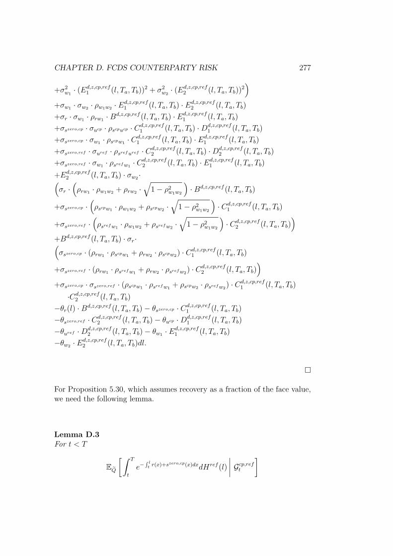
CHAPTER D. FCDS COUNTERPARTY RISK 277
+σ2w1
· (Ed,z,cp,ref1 (l, Ta, Tb))
2 + σ2w2
· (Ed,z,cp,ref2 (l, Ta, Tb))
2)
+σw1 · σw2 · ρw1w2 · Ed,z,cp,ref1 (l, Ta, Tb) · Ed,z,cp,ref
2 (l, Ta, Tb)
+σr · σw1 · ρrw1 · Bd,z,cp,ref (l, Ta, Tb) · Ed,z,cp,ref1 (l, Ta, Tb)
+σszero,cp · σucp · ρscpucp · Cd,z,cp,ref1 (l, Ta, Tb) · Dd,z,cp,ref
1 (l, Ta, Tb)
+σszero,cp · σw1 · ρscpw1 · Cd,z,cp,ref1 (l, Ta, Tb) · Ed,z,cp,ref
1 (l, Ta, Tb)
+σszero,ref · σuref · ρsref uref · Cd,z,cp,ref2 (l, Ta, Tb) · Dd,z,cp,ref
2 (l, Ta, Tb)
+σszero,ref · σw1 · ρsref w1· Cd,z,cp,ref
2 (l, Ta, Tb) · Ed,z,cp,ref1 (l, Ta, Tb)
+Ed,z,cp,ref2 (l, Ta, Tb) · σw2 ·(
σr ·(ρrw1 · ρw1w2 + ρrw2 ·
√1 − ρ2
w1w2
)· Bd,z,cp,ref (l, Ta, Tb)
+σszero,cp ·(ρscpw1 · ρw1w2 + ρscpw2 ·
√1 − ρ2
w1w2
)· Cd,z,cp,ref
1 (l, Ta, Tb)
+σszero,ref ·(ρsref w1
· ρw1w2 + ρsref w2·√
1 − ρ2w1w2
)· Cd,z,cp,ref
2 (l, Ta, Tb))
+Bd,z,cp,ref (l, Ta, Tb) · σr·(σszero,cp · (ρrw1 · ρscpw1 + ρrw2 · ρscpw2) · Cd,z,cp,ref
1 (l, Ta, Tb)
+σszero,ref · (ρrw1 · ρsref w1+ ρrw2 · ρsref w2
) · Cd,z,cp,ref2 (l, Ta, Tb)
)
+σszero,cp · σszero,ref · (ρscpw1 · ρsref w1+ ρscpw2 · ρsref w2
) · Cd,z,cp,ref1 (l, Ta, Tb)
·Cd,z,cp,ref2 (l, Ta, Tb)
−θr(l) · Bd,z,cp,ref (l, Ta, Tb) − θszero,cp · Cd,z,cp,ref1 (l, Ta, Tb)
−θszero,ref · Cd,z,cp,ref2 (l, Ta, Tb) − θucp · Dd,z,cp,ref
1 (l, Ta, Tb)
−θuref · Dd,z,cp,ref2 (l, Ta, Tb) − θw1 · Ed,z,cp,ref
1 (l, Ta, Tb)
−θw2 · Ed,z,cp,ref2 (l, Ta, Tb)dl.
For Proposition 5.30, which assumes recovery as a fraction of the face value,we need the following lemma.
Lemma D.3For t < T
EQ
[∫ T
t
e−∫ l
tr(x)+szero,cp(x)dxdHref (l)
∣∣∣∣ Gcp,reft
]

278 CHAPTER D. FCDS COUNTERPARTY RISK
is determined by
Lref (t) ·∫ T
t
(P d,z,cp,ref (t, l) · (K(t, l) + M ref (t, l) · szero,ref (t)
+ N ref (t, l) · uref (t) + O1(t, l) · w1(t) + O2(t, l) · w2(t)))dl
with the functions K(t, T ), M ref (t, T ), N ref (t, T ), O1(t, T ) and O2(t, T ) asgiven in the proof.
Proof:It holds (c.f. Theorem 5.6)
EQ
[∫ T
t
e−∫ l
tr(x)+szero,cp(x)dxdHref (l)
∣∣∣∣ Gcp,reft
]= Lref (t) · V cp,ref (t, T )
with
V cp,ref (t, T ) = EQ
[∫ T
t
e−∫ l
tr(x)+szero,cp(x)+szero,ref (x)dxszero,ref (l)dl
∣∣∣∣ Ft
]
=
∫ T
t
EQ
[e−
∫ lt
r(x)+szero,cp(x)+szero,ref (x)dxszero,ref (l)∣∣∣ Ft
]dl.
Further, using Feynman-Kac (see Theorem 2.14) for
vcp,ref (t, T, r, szero,cp, uzero,cp, szero,ref , uzero,ref , w1, w2)
:= EQ
[e−
∫ Tt
r(x)+szero,cp(x)+szero,ref (x)dxszero,ref (T )∣∣∣ Ft
]
= P d,z,cp,ref (t, T ) · (K(t, T ) + L(t, T ) · r(t) + M cp(t, T ) · szero,cp(t)
+ M ref (t, T ) · szero,ref (t) + N cp(t, T ) · ucp(t) + N ref (t, T ) · uref (t)
+ O1(t, T ) · w1(t) + O2(t, T ) · w2(t))
we obtain the same equation as in Lemma D.1 with P d,z,cp,ref replaced byvcp,ref . Since it must hold vcp,ref (T, T ) = szero,ref (T ), the boundary condi-tions are M ref (T, T ) = 1 and K(T, T ) = L(T, T ) = · · · = 0. Now, we usethe same procedure as it is done in Theorem 5.7. We insert the respectivederivatives of vcp,ref which all contain P d,z,cp,ref , we divide the whole equationby P d,z,cp,ref > 0 and cancel terms with the help of the PDEs for Ad,z,cp,ref ,Bd,z,cp,ref , Cd,z,cp,ref
1 , Cd,z,cp,ref2 , Dd,z,cp,ref
1 , Dd,z,cp,ref2 , Ed,z,cp,ref
1 , and Ed,z,cp,ref2
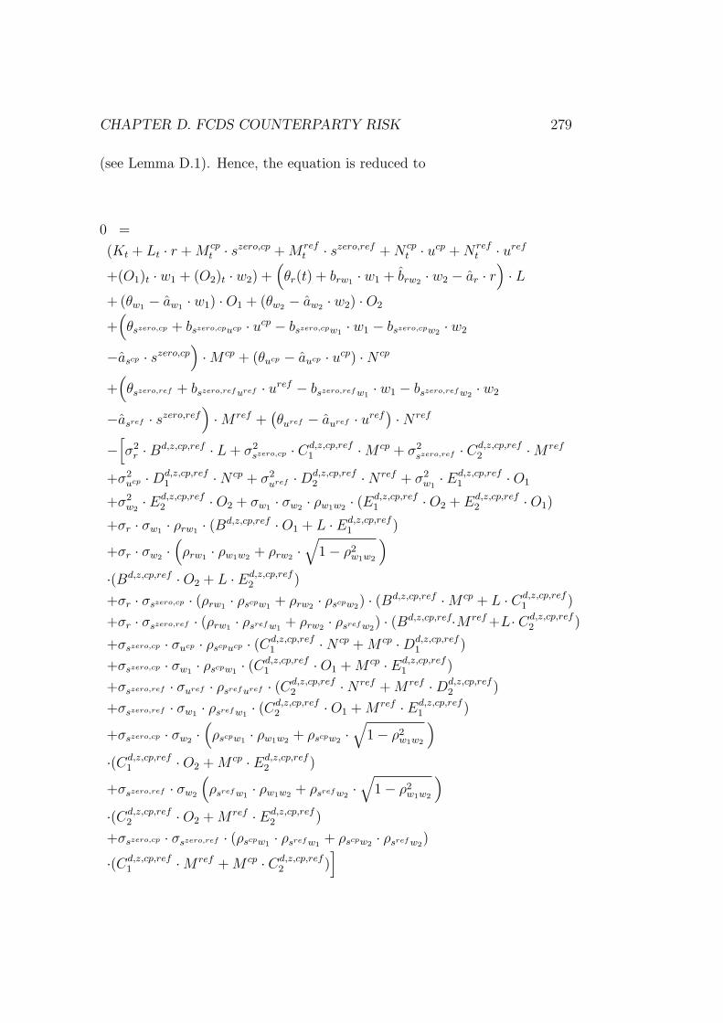
CHAPTER D. FCDS COUNTERPARTY RISK 279
(see Lemma D.1). Hence, the equation is reduced to
0 =
(Kt + Lt · r + M cpt · szero,cp + M ref
t · szero,ref + N cpt · ucp + N ref
t · uref
+(O1)t · w1 + (O2)t · w2) +(θr(t) + brw1 · w1 + brw2 · w2 − ar · r
)· L
+ (θw1 − aw1 · w1) · O1 + (θw2 − aw2 · w2) · O2
+(θszero,cp + bszero,cpucp · ucp − bszero,cpw1 · w1 − bszero,cpw2 · w2
−ascp · szero,cp)· M cp + (θucp − aucp · ucp) · N cp
+(θszero,ref + bszero,ref uref · uref − bszero,ref w1
· w1 − bszero,ref w2· w2
−asref · szero,ref)· M ref +
(θuref − auref · uref
)· N ref
−[σ2
r · Bd,z,cp,ref · L + σ2szero,cp · Cd,z,cp,ref
1 · M cp + σ2szero,ref · Cd,z,cp,ref
2 · M ref
+σ2ucp · Dd,z,cp,ref
1 · N cp + σ2uref · Dd,z,cp,ref
2 · N ref + σ2w1
· Ed,z,cp,ref1 · O1
+σ2w2
· Ed,z,cp,ref2 · O2 + σw1 · σw2 · ρw1w2 · (Ed,z,cp,ref
1 · O2 + Ed,z,cp,ref2 · O1)
+σr · σw1 · ρrw1 · (Bd,z,cp,ref · O1 + L · Ed,z,cp,ref1 )
+σr · σw2 ·(ρrw1 · ρw1w2 + ρrw2 ·
√1 − ρ2
w1w2
)
·(Bd,z,cp,ref · O2 + L · Ed,z,cp,ref2 )
+σr · σszero,cp · (ρrw1 · ρscpw1 + ρrw2 · ρscpw2) · (Bd,z,cp,ref · M cp + L · Cd,z,cp,ref1 )
+σr · σszero,ref · (ρrw1 · ρsref w1+ ρrw2 · ρsref w2
) · (Bd,z,cp,ref·M ref +L· Cd,z,cp,ref2 )
+σszero,cp · σucp · ρscpucp · (Cd,z,cp,ref1 · N cp + M cp · Dd,z,cp,ref
1 )
+σszero,cp · σw1 · ρscpw1 · (Cd,z,cp,ref1 · O1 + M cp · Ed,z,cp,ref
1 )
+σszero,ref · σuref · ρsref uref · (Cd,z,cp,ref2 · N ref + M ref · Dd,z,cp,ref
2 )
+σszero,ref · σw1 · ρsref w1· (Cd,z,cp,ref
2 · O1 + M ref · Ed,z,cp,ref1 )
+σszero,cp · σw2 ·(ρscpw1 · ρw1w2 + ρscpw2 ·
√1 − ρ2
w1w2
)
·(Cd,z,cp,ref1 · O2 + M cp · Ed,z,cp,ref
2 )
+σszero,ref · σw2
(ρsref w1
· ρw1w2 + ρsref w2·√
1 − ρ2w1w2
)
·(Cd,z,cp,ref2 · O2 + M ref · Ed,z,cp,ref
2 )
+σszero,cp · σszero,ref · (ρscpw1 · ρsref w1+ ρscpw2 · ρsref w2
)
·(Cd,z,cp,ref1 · M ref + M cp · Cd,z,cp,ref
2 )]

280 CHAPTER D. FCDS COUNTERPARTY RISK
After rearranging the terms, we arrive at the following differential equations
Lt − ar · L = 0 ,
M cpt − ascp · M cp = 0 ,
M reft − asref · M ref = 0 ,
N cpt + bszero,cpucp · M cp − aucp · N cp = 0 ,
N reft + bszero,ref uref · M ref − auref · N ref = 0 ,
(O1)t + brw1 · L − bszero,cpw1 · M cp − bszero,ref w1· M ref − aw1 · O1 = 0 ,
(O2)t + brw2 · L − bszero,cpw2 · M cp − bszero,ref w2· M ref − aw2 · O2 = 0 ,
Kt + θr(t) · L + θw1 · O1 + θw2 · O2 + θucp · N cp + θuref · N ref
+θszero,cp · M cp + θszero,ref · M ref − [. . . ] = 0 .
Considering the boundary conditions, the solutions of these differential equa-tions are (cf. Theorem 2.15)
L(t, T ) = 0 ,
M cp(t, T ) = 0 ,
M ref (t, T ) = e−asref ·(T−t) ,
N cp(t, T ) = 0 ,
N ref (t, T ) = −bszero,ref uref · e−asref ·(T−t) − e−a
uref ·(T−t)
asref − auref
,
O1(t, T ) = bszero,ref w1· e−a
sref ·(T−t) − e−aw1 ·(T−t)
asref − aw1
,
O2(t, T ) = bszero,ref w2· e−a
sref ·(T−t) − e−aw2 ·(T−t)
asref − aw2
,
K(t, T ) = −∫ T
t
Kt(l, T )dl .
The lemma below is needed for Proposition 5.31.
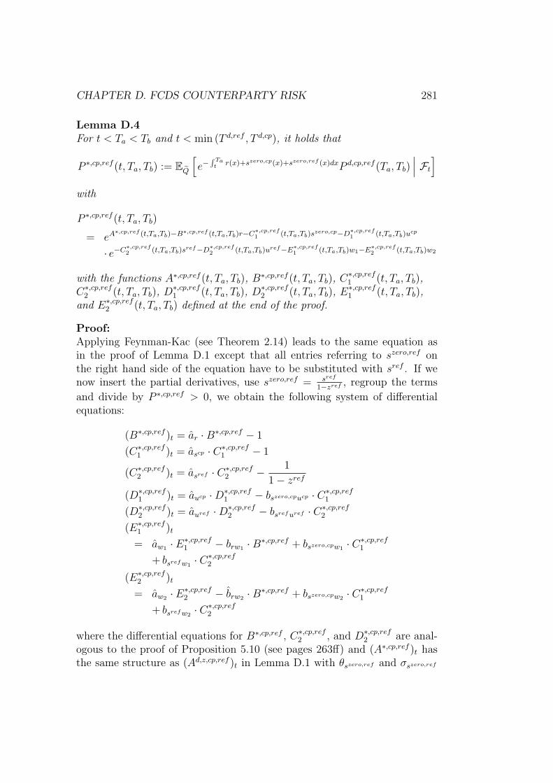
CHAPTER D. FCDS COUNTERPARTY RISK 281
Lemma D.4For t < Ta < Tb and t < min (T d,ref , T d,cp), it holds that
P ∗,cp,ref (t, Ta, Tb) := EQ
[e−
∫ Tat
r(x)+szero,cp(x)+szero,ref (x)dxP d,cp,ref (Ta, Tb)∣∣∣ Ft
]
with
P ∗,cp,ref (t, Ta, Tb)
= eA∗,cp,ref (t,Ta,Tb)−B∗,cp,ref (t,Ta,Tb)r−C∗,cp,ref1 (t,Ta,Tb)s
zero,cp−D∗,cp,ref1 (t,Ta,Tb)u
cp
· e−C∗,cp,ref2 (t,Ta,Tb)s
ref−D∗,cp,ref2 (t,Ta,Tb)u
ref−E∗,cp,ref1 (t,Ta,Tb)w1−E∗,cp,ref
2 (t,Ta,Tb)w2
with the functions A∗,cp,ref (t, Ta, Tb), B∗,cp,ref (t, Ta, Tb), C∗,cp,ref1 (t, Ta, Tb),
C∗,cp,ref2 (t, Ta, Tb), D∗,cp,ref
1 (t, Ta, Tb), D∗,cp,ref2 (t, Ta, Tb), E∗,cp,ref
1 (t, Ta, Tb),and E∗,cp,ref
2 (t, Ta, Tb) defined at the end of the proof.
Proof:Applying Feynman-Kac (see Theorem 2.14) leads to the same equation asin the proof of Lemma D.1 except that all entries referring to szero,ref onthe right hand side of the equation have to be substituted with sref . If wenow insert the partial derivatives, use szero,ref = sref
1−zref , regroup the terms
and divide by P ∗,cp,ref > 0, we obtain the following system of differentialequations:
(B∗,cp,ref )t = ar · B∗,cp,ref − 1
(C∗,cp,ref1 )t = ascp · C∗,cp,ref
1 − 1
(C∗,cp,ref2 )t = asref · C∗,cp,ref
2 − 1
1 − zref
(D∗,cp,ref1 )t = aucp · D∗,cp,ref
1 − bszero,cpucp · C∗,cp,ref1
(D∗,cp,ref2 )t = auref · D∗,cp,ref
2 − bsref uref · C∗,cp,ref2
(E∗,cp,ref1 )t
= aw1 · E∗,cp,ref1 − brw1 · B∗,cp,ref + bszero,cpw1 · C∗,cp,ref
1
+ bsref w1· C∗,cp,ref
2
(E∗,cp,ref2 )t
= aw2 · E∗,cp,ref2 − brw2 · B∗,cp,ref + bszero,cpw2 · C∗,cp,ref
1
+ bsref w2· C∗,cp,ref
2
where the differential equations for B∗,cp,ref , C∗,cp,ref2 , and D∗,cp,ref
2 are anal-ogous to the proof of Proposition 5.10 (see pages 263ff) and (A∗,cp,ref )t hasthe same structure as (Ad,z,cp,ref )t in Lemma D.1 with θszero,ref and σszero,ref

282 CHAPTER D. FCDS COUNTERPARTY RISK
replaced by θsref and σsref . Since it must hold that P ∗,cp,ref (Ta, Ta, Tb) =P d,cp,ref (Ta, Tb), the boundary conditions areA∗,cp,ref (Ta, Ta, Tb) = Ad,cp,ref (Ta, Tb), B∗,cp,ref (Ta, Ta, Tb) = Bd,cp,ref (Ta, Tb),C∗,cp,ref
1 (Ta, Ta, Tb) = Cd,cp,ref1 (Ta, Tb), C∗,cp,ref
2 (Ta, Ta, Tb) = Cd,cp,ref2 (Ta, Tb),
D∗,cp,ref1 (Ta, Ta, Tb) = Dd,cp,ref
1 (Ta, Tb), D∗,cp,ref2 (Ta, Ta, Tb) = Dd,cp,ref
2 (Ta, Tb),E∗,cp,ref
1 (Ta, Ta, Tb) = Ed,cp,ref1 (Ta, Tb) and E∗,cp,ref
2 (Ta, Ta, Tb) = Ed,cp,ref2 (Ta, Tb).
Hence, the differential equations result in (c.f. Theorem 2.15 and Proposition5.10)
B∗,cp,ref (t, Ta, Tb) = e−ar·(Ta−t) ·(B∗,cp,ref (Ta, Ta, Tb) +
∫ Ta−t
0
ear·ldl)
=1
ar
·(1 − e−ar·(Tb−t)
)= B(t, Tb),
C∗,cp,ref1 (t, Ta, Tb) = e−ascp ·(Ta−t) ·
(C∗,cp,ref
1 (Ta, Ta, Tb) +
∫ Ta−t
0
eascp ·ldl)
=1
ascp
·(1 − e−ascp ·(Tb−t)
)= Cd,cp(t, Tb),
C∗,cp,ref2 (t, Ta, Tb)
= e−asref ·(Ta−t) ·
(C∗,cp,ref
2 (Ta, Ta, Tb) +1
1 − zref·∫ Ta−t
0
easref ·ldl
)
= e−asref ·(Ta−t) · Cd,ref (Ta, Tb) +
1
1 − zref· Cd,ref (t, Ta),
D∗,cp,ref1 (t, Ta, Tb)
= e−aucp (Ta−t) ·(D∗,cp,ref
1 (Ta, Ta, Tb)
+
∫ Ta−t
0
eaucp ·l · bszero,cpucp · C∗,cp,ref1 (0, l, Tb − Ta + l)dl
)
=bszero,cpucp
ascp
·(
1 − e−aucp ·(Tb−t)
aucp
+e−aucp ·(Tb−t) − e−ascp ·(Tb−t)
aucp − ascp
)
= Dd,zero,cp(t, Tb),

CHAPTER D. FCDS COUNTERPARTY RISK 283
D∗,cp,ref2 (t, Ta, Tb)
= e−auref (Ta−t) ·
(D∗,cp,ref
2 (Ta, Ta, Tb)
+
∫ Ta−t
0
eauref ·l · bsref uref · C∗,cp,ref
2 (0, l, Tb − Ta + l)dl)
= e−auref ·(Ta−t) · Dd,ref (Ta, Tb)
− bsref uref · Cd,ref (Ta, Tb) ·(
e−asref ·(Ta−t) − e−a
uref ·(Ta−t)
asref − auref
)
+1
1 − zref· Dd,ref (t, Ta),
E∗,cp,ref1 (t, Ta, Tb)
= e−aw1 ·(Ta−t)(E∗,cp,ref
1 (Ta, Ta, Tb)
+
∫ Ta−t
0
eaw1 ·l(brw1 · B∗,cp,ref (0, l, l + Tb − Ta)
− bszero,cpw1 · C∗,cp,ref1 (0, l, l + Tb − Ta)
− bsref w1· C∗,cp,ref
2 (0, l, l + Tb − Ta))dl)
= e−aw1 ·(Ta−t) · Ed,cp,ref1 (Ta, Tb)
+brw1
ar
·(
1 − e−aw1 ·(Ta−t)
aw1
+ e−ar·(Tb−Ta) e−aw1 ·(Ta−t) − e−ar·(Ta−t)
aw1 − ar
)
− bszero,cpw1
ascp
·(
1 − e−aw1 ·(Ta−t)
aw1
+ e−ascp ·(Tb−Ta) e−aw1 ·(Ta−t) − e−ascp ·(Ta−t)
aw1 − ascp
)
+ bsref w1Cd,ref (Ta, Tb)
(e−a
sref (Ta−t) − e−aw1 (Ta−t)
asref − aw1
)
+1
1 − zref(Ed,ref
1 (t, Ta) − Eref1 (t, Ta)),
E∗,cp,ref2 (t, Ta, Tb) is determined analogously.
A∗,cp,ref (t, Ta, Tb) = A∗,cp,ref (Ta, Ta, Tb) −∫ Ta
t
A∗,cp,reft (l, Ta, Tb)dl .

284 CHAPTER D. FCDS COUNTERPARTY RISK
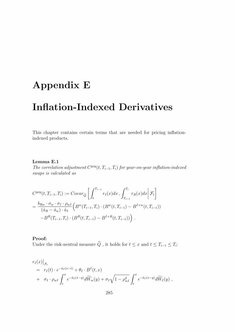
Appendix E
Inflation-Indexed Derivatives
This chapter contains certain terms that are needed for pricing inflation-indexed products.
Lemma E.1The correlation adjustment Cyoy(t, Ti−1, Ti) for year-on-year inflation-indexedswaps is calculated as
Cyoy(t, Ti−1, Ti) := CovarQ
[∫ Ti−1
t
rI(x)dx ,
∫ Ti
Ti−1
rR(x)dx
∣∣∣∣Ft
]
=bRw · σw · σI · ρwI
(aR − aw) · aI
(Bw(Ti−1, Ti) · (Bw(t, Ti−1) − BI+w(t, Ti−1))
−BR(Ti−1, Ti) · (BR(t, Ti−1) − BI+R(t, Ti−1)))
.
Proof:Under the risk-neutral measure Q , it holds for t ≤ x and t ≤ Ti−1 ≤ Ti:
rI(x)∣∣Ft
= rI(t) · e−aI(x−t) + θI · BI(t, x)
+ σI · ρwI
∫ x
t
e−aI(x−y)dWw(y) + σI
√1 − ρ2
wI
∫ x
t
e−aI(x−y)dWI(y) ,
285

286 CHAPTER E. INFLATION-INDEXED DERIVATIVES
∫ Ti
Ti−1
rI(x)dx
∣∣∣∣Ft
= rI(t)
∫ Ti
Ti−1
e−aI(x−t)dx + θI
∫ Ti
Ti−1
BI(t, x)dx
+ σI · ρwI
∫ Ti
Ti−1
∫ x
t
e−aI(x−y)dWw(y)dx
+ σI
√1 − ρ2
wI
∫ Ti
Ti−1
∫ x
t
e−aI(x−y)dWI(y)dx
= rI(t) · e−aI(Ti−1−t) · BI(Ti−1, Ti)
+θI
aI
(Ti − Ti−1 − e−aI(Ti−1−t) · BI(Ti−1, Ti)
)
+ σI · ρwI
(∫ Ti−1
t
(BI(y, Ti) − BI(y, Ti−1))dWw(y) +
∫ Ti
Ti−1
BI(y, Ti)dWw(y)
)
+ σI
√1 − ρ2
wI
(∫ Ti−1
t
(BI(y, Ti) − BI(y, Ti−1))dWI(y) +
∫ Ti
Ti−1
BI(y, Ti)dWI(y)
),
and
rR(x)∣∣Ft
= rR(t) · e−aR(x−t) +
∫ x
t
θR(y)e−aR(x−y)dy
+ bRw
∫ x
t
w(y)e−aR(x−y)dy + σR
∫ x
t
e−aR(x−y)dWR(y)
= rR(t) · e−aR(x−t) +
∫ x
t
θR(y)e−aR(x−y)dy
+bRw
aR − aw
(w(t) − θw
aw
)·(e−aw(x−t) − e−aR(x−t)
)+
bRw · θw
aw
BR(t, x)
+bRw · σw
aR − aw
∫ x
t
(e−aw(x−y) − e−aR(x−y))dWw(y)
+ σR
∫ x
t
e−aR(x−y)dWR(y) ,
∫ Ti
Ti−1
rR(x)dx
∣∣∣∣Ft
= rR(t)
∫ Ti
Ti−1
e−aR(x−t)dx +
∫ Ti
Ti−1
∫ x
t
θR(y)e−aR(x−y)dydx

CHAPTER E. INFLATION-INDEXED DERIVATIVES 287
+bRw
aR − aw
(w(t) − θw
aw
)∫ Ti
Ti−1
(e−aw(x−t) − e−aR(x−t)
)dx
+bRw · θw
aw
∫ Ti
Ti−1
BR(t, x)dx
+bRw · σw
aR − aw
∫ Ti
Ti−1
∫ x
t
(e−aw(x−y) − e−aR(x−y))dWw(y)dx
+σR
∫ Ti
Ti−1
∫ x
t
e−aR(x−y)dWR(y)dx
= rR(t) · e−aR(Ti−1−t) · BR(Ti−1, Ti)
+
∫ Ti−1
t
θR(y)e−aR(Ti−1−y)BR(Ti−1, Ti)dy +
∫ Ti
Ti−1
θR(y)BR(y, Ti)dy
+bRw
aR − aw
(w(t) − θw
aw
)·(e−aw(Ti−1−t)Bw(Ti−1, Ti) − e−aR(Ti−1−t)BR(Ti−1, Ti)
)
+bRw · θw
aw · aR
(Ti − Ti−1 − e−aR(Ti−1−t)BR(Ti−1, Ti)
)
+bRw · σw
aR − aw
(∫ Ti−1
t
(e−aw(Ti−1−y)Bw(Ti−1, Ti) − e−aR(Ti−1−y)BR(Ti−1, Ti))dWw(y))
+bRw · σw
aR − aw
(∫ Ti
Ti−1
(Bw(y, Ti) − BR(y, Ti))dWw(y))
+σR
(∫ Ti−1
t
e−aR(Ti−1−y)BR(Ti−1, Ti)dWR(y) +
∫ Ti
Ti−1
BR(y, Ti)dWR(y))
.
Hence, the covariance CovarQ
[∫ Ti−1
trI(x)dx ,
∫ Ti
Ti−1rR(x)dx
∣∣∣Ft
]is calculated
as follows:
Cyoy(t, Ti−1, Ti)
= CovarQ
[σI · ρwI
∫ Ti−1
t
BI(y, Ti−1)dWw(y) ,
bRw · σw
aR − aw
∫ Ti−1
t
(e−aw(Ti−1−y)Bw(Ti−1, Ti) − e−aR(Ti−1−y)BR(Ti−1, Ti))dWw(y)
∣∣∣∣Ft
]
=bRw · σw · σI · ρwI
aR − aw
∫ Ti−1
t
BI(y, Ti−1) · (e−aw(Ti−1−y)Bw(Ti−1, Ti)
− e−aR(Ti−1−y)BR(Ti−1, Ti))dy
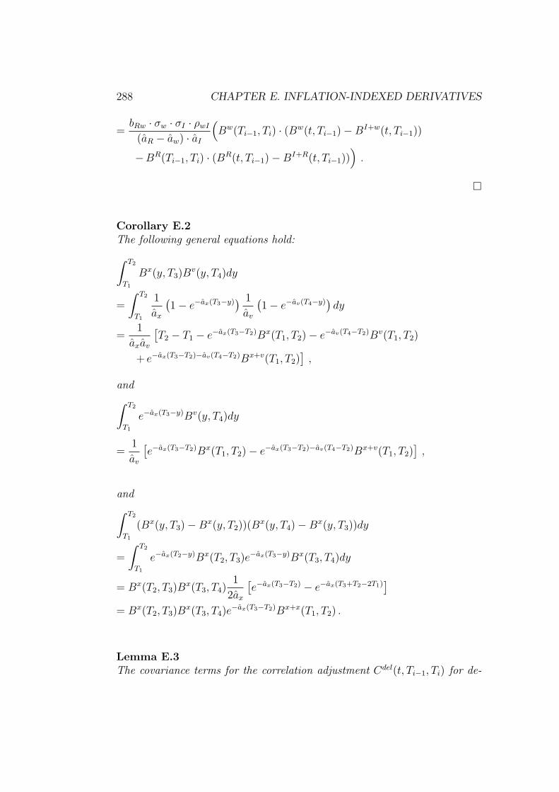
288 CHAPTER E. INFLATION-INDEXED DERIVATIVES
=bRw · σw · σI · ρwI
(aR − aw) · aI
(Bw(Ti−1, Ti) · (Bw(t, Ti−1) − BI+w(t, Ti−1))
−BR(Ti−1, Ti) · (BR(t, Ti−1) − BI+R(t, Ti−1)))
.
Corollary E.2The following general equations hold:
∫ T2
T1
Bx(y, T3)Bv(y, T4)dy
=
∫ T2
T1
1
ax
(1 − e−ax(T3−y)
) 1
av
(1 − e−av(T4−y)
)dy
=1
axav
[T2 − T1 − e−ax(T3−T2)Bx(T1, T2) − e−av(T4−T2)Bv(T1, T2)
+ e−ax(T3−T2)−av(T4−T2)Bx+v(T1, T2)]
,
and
∫ T2
T1
e−ax(T3−y)Bv(y, T4)dy
=1
av
[e−ax(T3−T2)Bx(T1, T2) − e−ax(T3−T2)−av(T4−T2)Bx+v(T1, T2)
],
and
∫ T2
T1
(Bx(y, T3) − Bx(y, T2))(Bx(y, T4) − Bx(y, T3))dy
=
∫ T2
T1
e−ax(T2−y)Bx(T2, T3)e−ax(T3−y)Bx(T3, T4)dy
= Bx(T2, T3)Bx(T3, T4)
1
2ax
[e−ax(T3−T2) − e−ax(T3+T2−2T1)
]
= Bx(T2, T3)Bx(T3, T4)e
−ax(T3−T2)Bx+x(T1, T2) .
Lemma E.3The covariance terms for the correlation adjustment Cdel(t, Ti−1, Ti) for de-
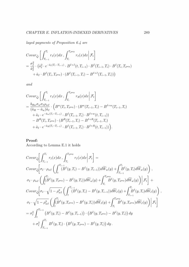
CHAPTER E. INFLATION-INDEXED DERIVATIVES 289
layed payments of Proposition 6.4 are
CovarQ
[∫ Ti
Ti−1
rI(x)dx ,
∫ Tipay
Ti
rI(x)dx
∣∣∣∣Ft
]
=σ2
I
a2I
·(a2
I · e−aI(Ti−Ti−1) · BI+I(t, Ti−1) · BI(Ti−1, Ti) · BI(Ti, Tipay)
+ aI · BI(Ti, Tipay) · (BI(Ti−1, Ti) − BI+I(Ti−1, Ti)))
and
CovarQ
[∫ Ti
Ti−1
rI(x)dx ,
∫ Tipay
Ti
rR(x)dx
∣∣∣∣Ft
]
=bRwσwσIρwI
(aR − aw)aI
·(Bw(Ti, Tipay) · (Bw(Ti−1, Ti) − BI+w(Ti−1, Ti)
+ aI · e−aw(Ti−Ti−1) · BI(Ti−1, Ti) · BI+w(t, Ti−1))
−BR(Ti, Tipay) · (BR(Ti−1, Ti) − BI+R(Ti−1, Ti)
+ aI · e−aR(Ti−Ti−1) · BI(Ti−1, Ti) · BI+R(t, Ti−1))).
Proof:According to Lemma E.1 it holds
CovarQ
[∫ Ti
Ti−1
rI(x)dx ,
∫ Tipay
Ti
rI(x)dx
∣∣∣∣Ft
]=
CovarQ
[σI · ρwI
(∫ Ti−1
t
(BI(y, Ti) − BI(y, Ti−1))dWw(y) +
∫ Ti
Ti−1
BI(y, Ti)dWw(y)
),
σI · ρwI
(∫ Ti
t
(BI(y, Tipay) − BI(y, Ti))dWw(y) +
∫ Tipay
Ti
BI(y, Tipay)dWw(y)
)∣∣∣∣Ft
]+
CovarQ
[σI ·
√1 − ρ2
wI
(∫ Ti−1
t
(BI(y, Ti) − BI(y, Ti−1))dWI(y) +
∫ Ti
Ti−1
BI(y, Ti)dWI(y)
),
σI ·√
1 − ρ2wI
(∫ Ti
t
(BI(y, Tipay) − BI(y, Ti))dWI(y) +
∫ Tipay
Ti
BI(y, Tipay)dWI(y)
)∣∣∣∣Ft
]
= σ2I
∫ Ti−1
t
(BI(y, Ti) − BI(y, Ti−1)
)·(BI(y, Tipay) − BI(y, Ti)
)dy
+ σ2I
∫ Ti
Ti−1
BI(y, Ti) ·(BI(y, Tipay) − BI(y, Ti)
)dy .

290 CHAPTER E. INFLATION-INDEXED DERIVATIVES
The integrals within the above covariance can be calculated with the help ofthe equations of Corollary E.2. Hence, it holds for
CovarQ
[∫ Ti
Ti−1
rI(x)dx ,
∫ Tipay
Ti
rI(x)dx
∣∣∣∣Ft
]
=σ2
I
a2I
[a2
Ie−aI(Ti−Ti−1)BI(Ti, Tipay)BI(Ti−1, Ti)B
I+I(t, Ti−1)
+(1 − e−aI(Tipay−Ti))BI(Ti−1, Ti) + (e−aI(Tipay−Ti) − 1)BI+I(Ti−1, Ti)
]
=σ2
I
a2I
[a2
Ie−aI(Ti−Ti−1)BI(Ti, Tipay)BI(Ti−1, Ti)B
I+I(t, Ti−1)
+aIBI(Ti, Tipay)(BI(Ti−1, Ti) − BI+I(Ti−1, Ti))
].
With the help of Lemma E.1 and Corollary E.2 it also holds
CovarQ
[∫ Ti
Ti−1
rI(x)dx ,
∫ Tipay
Ti
rR(x)dx
∣∣∣∣Ft
]=
CovarQ
[σI · ρwI
(∫ Ti−1
t
(BI(y, Ti) − BI(y, Ti−1))dWw(y) +
∫ Ti
Ti−1
BI(y, Ti)dWw(y)
),
bRw · σw
aR − aw
(∫ Ti
t
(e−aw(Ti−y)Bw(Ti, Tipay) − e−aR(Ti−y)BR(Ti, Tipay))dWw(y)
+
∫ Tipay
Ti
(Bw(y, Tipay) − BR(y, Tipay))dWw(y)
)∣∣∣∣Ft
]
=σI · ρwI · bRw · σw
aR − aw
∫ Ti−1
t
(BI(y, Ti) − BI(y, Ti−1))(e−aw(Ti−y)Bw(Ti, Tipay)
−e−aR(Ti−y)BR(Ti, Tipay))dy
+
∫ Ti
Ti−1
BI(y, Ti)(e−aw(Ti−y)Bw(Ti, Tipay) − e−aR(Ti−y)BR(Ti, Tipay))dy
=σI · ρwI · bRw · σw
aI · (aR − aw)
[Bw(Ti, Tipay)(e−aw(Ti−Ti−1)(1 − e−aI(Ti−Ti−1))Bw+I(t, Ti−1)
+Bw(Ti−1, Ti) − Bw+I(Ti−1, Ti)) − BR(Ti, Tipay)(BR(Ti−1, Ti) − BR+I(Ti−1, Ti)
+e−aR(Ti−Ti−1)(1 − e−aI(Ti−Ti−1))BR+I(t, Ti−1))
]

CHAPTER E. INFLATION-INDEXED DERIVATIVES 291
=σI · ρwI · bRw · σw
aI · (aR − aw)
[Bw(Ti, Tipay)(aIe
−aw(Ti−Ti−1)BI(Ti−1, Ti)Bw+I(t, Ti−1)
+Bw(Ti−1, Ti) − Bw+I(Ti−1, Ti)) − BR(Ti, Tipay)(
aIe−aR(Ti−Ti−1)BI(Ti−1, Ti)B
R+I(t, Ti−1) + BR(Ti−1, Ti) − BR+I(Ti−1, Ti))
]
Corollary E.4The following general equations hold:
(a)
∫ x
t
e−a1(x−l)e−a2(Ti−l)dl = e−a2(Ti−x)B1+2(t, x)
(b)
∫ x
t
e−a1(x−l)B2(l, Ti)dl =1
a2
[B1(t, x) − e−a2(Ti−x)B1+2(t, x)]
(c)
∫ x
t
e−a1(x−l)
∫ l
t
e−a2(l−y)dydl
=
∫ x
t
e−a1(x−l)B2(t, l)dl =1
a2
[B1(t, x) − e−a2(x−t)B1−2(t, x)]
(d)
∫ x
t
e−a1(x−l)
∫ l
t
e−a2(l−y)e−a3(Ti−y)dydl
=
∫ x
t
e−a1(x−l) 1
a2 + a3
(e−a3(Ti−l) − e−a2(l−t)−a3(Ti−t))dl
=1
a2 + a3
[e−a3(Ti−x)B1+3(t, x) − e−a3(Ti−t)−a2(x−t)B1−2(t, x)]
=1
a2 + a3
[e−a3(Ti−x)B1+3(t, x) − e−a3(Ti−t)−a1(x−t)B2−1(t, x)]

292 CHAPTER E. INFLATION-INDEXED DERIVATIVES
(e)
∫ Ti
Ti−1
∫ x
t
e−a1(x−l)e−a2(Ti−l)dldx
(a)=
∫ Ti
Ti−1
e−a2(Ti−x)B1+2(t, x)dx
=
∫ Ti
Ti−1
1
a1 + a2
(e−a2(Ti−x) − e−a2(Ti−t)e−a1(x−t))dx
=1
a1 + a2
(B2(Ti−1, Ti) − e−a1(Ti−1−t)−a2(Ti−t)B1(Ti−1, Ti))
(f)
∫ Ti
Ti−1
∫ x
t
e−a1(x−l)B2(l, Ti)dldx
(b)=
∫ Ti
Ti−1
1
a2
[B1(t, x) − e−a2(Ti−x)B1+2(t, x)]dx
(e)=
1
a2
[1
a1
(Ti − Ti−1 − e−a1(Ti−1−t)B1(Ti−1, Ti)) −1
a1 + a2
(B2(Ti−1, Ti)
−e−a1(Ti−1−t)−a2(Ti−t)B1(Ti−1, Ti))]
(g)
∫ Ti
Ti−1
∫ x
t
e−a1(Ti−l)dldx
=
∫ Ti
Ti−1
1
a1
(e−a1(Ti−x) − e−a1(Ti−t))dx
=1
a1
[B1(Ti−1, Ti) − e−a1(Ti−t)(Ti − Ti−1)]
Lemma E.5The terms needed for the approximation of an inflation hybrid’s price inTheorem 6.6 are given in this lemma’s proof.
Proof:In order to determine the expected value of 1
P (Ti−1,Ti)under the Ti-forward
measure we need to adjust the risk-neutral value by the following terms

CHAPTER E. INFLATION-INDEXED DERIVATIVES 293
resulting from the change of measure.
I1(x) := σwσIρwI
∫ x
t
e−aI(x−l)E1(l, Ti)dl
Cor.E.4(a)(b)=
σwσIρwIbRw
aR
( 1
aw
(BI(t, x) − e−aw(Ti−x)BI+w(t, x)
)
+1
aw − aR
(e−aw(Ti−x)BI+w(t, x) − e−aR(Ti−x)BI+R(t, x)
) )
I2(x, I) := σ2I
∫ x
t
e−aI(x−l)BI(l, Ti)dl
Cor.E.4(b)=
σ2I
aI
(BI(t, x) − e−aI(Ti−x)BI+I(t, x)
)
W1(x) := σ2w
∫ x
t
e−aw(x−l)E1(l, Ti)dl
Cor.E.4(a)(b)=
σ2wbRw
aR
( 1
aw
(Bw(t, x) − e−aw(Ti−x)Bw+w(t, x)
)
+1
aw − aR
(e−aw(Ti−x)Bw+w(t, x) − e−aR(Ti−x)Bw+R(t, x)
) )
W2(x) := σwσIρwI
∫ x
t
e−aw(x−l)BI(l, Ti)dl
Cor.E.4(b)=
σwσIρwI
aI
(Bw(t, x) − e−aI(Ti−x)BI+w(t, x)
)
R1(x) := σ2R
∫ x
t
e−aR(x−l)BR(l, Ti)dl
Cor.E.4(b)=
σ2R
aR
(BR(t, x) − e−aR(Ti−x)BR+R(t, x)
)
R2(x) := bRw
∫ x
t
e−aR(x−l)W1(l)dl
= σ2wbRw
∫ x
t
e−aR(x−l)
∫ l
t
e−aw(l−y)E1(y, Ti)dydl
Cor.E.4(c)(d)=
σ2wb2
Rw
aR
[ 1
a2w
(BR(t, x) − e−aw(x−t)BR−w(t, x)
)
294 CHAPTER E. INFLATION-INDEXED DERIVATIVES
− 1
2a2w
(e−aw(Ti−x)BR+w(t, x) − e−aw(Ti+x−2t)BR−w(t, x)
)
+1
aw − aR
( 1
2aw
(e−aw(Ti−x)BR+w(t, x) − e−aw(Ti+x−2t)BR−w(t, x)
)
− 1
aw + aR
(e−aR(Ti−x)BR+R(t, x) − e−aR(Ti+x−2t)Bw−R(t, x)
))]
R3(x) := bRw
∫ x
t
e−aR(x−l)W2(l)dl
= σwσIρwIbRw
∫ x
t
e−aR(x−l)
∫ l
t
e−aw(l−y)BI(y, Ti)dydl
Cor.E.4(c)(d)=
σwσIρwIbRw
aI
(1
aw
(BR(t, x) − e−aw(x−t)BR−w(t, x)
)
− 1
aw + aI
(e−aI(Ti−x)BR+I(t, x) − e−aI(Ti−t)−aw(x−t)BR−w(t, x)
))
The terms needed for the expected value of e∫ Ti
Ti−1rI(x)dx
under the Ti-forwardmeasure are determined analogously.
I3(Ti−1, Ti) :=
∫ Ti
Ti−1
I1(x)dx
= σwσIρwI
∫ Ti
Ti−1
∫ x
t
e−aI(x−l)E1(l, Ti)dldx
Cor.E.4(e)(f)=
σwσIρwIbRw
aR
[ 1
aw
[ 1
aI
(Ti − Ti−1 − e−aI(Ti−1−t)BI(Ti−1, Ti)
)
− 1
aw + aI
(Bw(Ti−1, Ti) − e−aw(Ti−t)−aI(Ti−1−t)BI(Ti−1, Ti)
) ]
+1
aw − aR
[ 1
aI + aw
(Bw(Ti−1, Ti) − e−aw(Ti−t)−aI(Ti−1−t)BI(Ti−1, Ti)
)
− 1
aR + aI
(BR(Ti−1, Ti) − e−aR(Ti−t)−aI(Ti−1−t)BI(Ti−1, Ti)
) ]]
I4(Ti−1, Ti, I) :=
∫ Ti
Ti−1
I2(x, I)dx
= σ2I
∫ Ti
Ti−1
∫ x
t
e−aI(x−l)BI(l, Ti)dldx
Cor.E.4(f)=
σ2I
a2I
(Ti − Ti−1 − BI(Ti−1, Ti)(e
−aI(Ti−1−t) +1
2(1 − e−aI(Ti+Ti−1−2t)))
)

CHAPTER E. INFLATION-INDEXED DERIVATIVES 295
The covariance in the expected value of 1P (Ti−1,Ti)
can be decomposed into
CovarP (·,Ti)
[∫ Ti
Ti−1
r(x)dx ,
∫ Ti−1
t
r(x)dx
∣∣∣∣Ft
]
= CovarQ
[∫ Ti
Ti−1
r(x)dx ,
∫ Ti−1
t
r(x)dx
∣∣∣∣Ft
]
= CovarQ
[∫ Ti
Ti−1
rR(x)dx ,
∫ Ti−1
t
rR(x)dx
∣∣∣∣Ft
]
+CovarQ
[∫ Ti
Ti−1
rR(x)dx ,
∫ Ti−1
t
rI(x)dx
∣∣∣∣Ft
]
+CovarQ
[∫ Ti
Ti−1
rI(x)dx ,
∫ Ti−1
t
rR(x)dx
∣∣∣∣Ft
]
+CovarQ
[∫ Ti
Ti−1
rI(x)dx ,
∫ Ti−1
t
rI(x)dx
∣∣∣∣Ft
]
where the second term is already given in Lemma E.1 and the last term inLemma E.3. The remaining terms are obtained by combining the terms withWi, i = w or i = R, of the integrals
∫rR(x)dx and
∫rI(x)dx of Lemma E.1.
CovarQ
[∫ Ti−1
t
rR(x)dx ,
∫ Ti
Ti−1
rR(x)dx
∣∣∣∣Ft
]
= CovarQ
[bRw · σw
aR − aw
(∫ Ti−1
t
(Bw(y, Ti−1) − BR(y, Ti−1))dWw(y)
+σR
∫ Ti−1
t
BR(y, Ti−1)dWR(y))
,bRw · σw
aR − aw
(∫ Ti
Ti−1
(Bw(y, Ti) − BR(y, Ti))dWw(y)
+
∫ Ti−1
t
(e−aw(Ti−1−y)Bw(Ti−1, Ti) − e−aR(Ti−1−y)BR(Ti−1, Ti))dWw(y))
+σR
(∫ Ti−1
t
e−aR(Ti−1−y)BR(Ti−1, Ti)dWR(y) +
∫ Ti
Ti−1
BR(y, Ti)dWR(y))∣∣∣∣Ft
]
=
∫ Ti−1
t
σ2RBR(y, Ti−1)e
−aR(Ti−1−y)BR(Ti−1, Ti)dy
+
∫ Ti−1
t
(bRwσw
aR − aw
)2 (Bw(y, Ti−1) − BR(y, Ti−1)
)
·(e−aw(Ti−1−y)Bw(Ti−1, Ti) − e−aR(Ti−1−y)BR(Ti−1, Ti)
)dy

296 CHAPTER E. INFLATION-INDEXED DERIVATIVES
Cor.E.2= BR(Ti−1, Ti)
((BR(t, Ti−1) − BR+R(t, Ti−1)
) 1
aR
(σ2
R +
(bRwσw
aR − aw
)2)
−(BR(t, Ti−1) − BR+w(t, Ti−1)
) 1
aw
(bRwσw
aR − aw
)2)
+ Bw(Ti−1, Ti)
((Bw(t, Ti−1) − Bw+w(t, Ti−1)
) 1
aw
(bRwσw
aR − aw
)2
−(Bw(t, Ti−1) − BR+w(t, Ti−1)
) 1
aR
(bRwσw
aR − aw
)2)
and
CovarQ
[∫ Ti−1
t
rR(x)dx ,
∫ Ti
Ti−1
rI(x)dx
∣∣∣∣Ft
]
= CovarQ
[bRw · σw
aR − aw
∫ Ti−1
t
(Bw(y, Ti−1) − BR(y, Ti−1))dWw(y) ,
σI · ρwI
(∫ Ti−1
t
(BI(y, Ti) − BI(y, Ti−1))dWw(y) +
∫ Ti
Ti−1
BI(y, Ti)dWw(y)
)∣∣∣∣Ft
]
=
∫ Ti−1
t
σIρwI
(BI(y, Ti) − BI(y, Ti−1)
)· bRwσw
aR − aw
·(Bw(y, Ti−1) − BR(y, Ti−1)
)dy
Cor.E.2=
bRwσwσIρwI
aR − aw
BI(Ti−1, Ti)( 1
aw
(BI(t, Ti−1) − BI+w(t, Ti−1))
− 1
aR
(BI(t, Ti−1) − BI+R(t, Ti−1)))
.
Furthermore, it holds
CovarQ
[∫ Ti
t
rI(x)dx ,
∫ Ti
Ti−1
rR(x)dx
∣∣∣∣Ft
]
= CovarQ
[∫ Ti−1
t
rI(x)dx ,
∫ Ti
Ti−1
rR(x)dx
∣∣∣∣Ft
]
+ CovarQ
[∫ Ti
Ti−1
rI(x)dx ,
∫ Ti
Ti−1
rR(x)dx
∣∣∣∣Ft
]
where the first covariance is given in Lemma E.1 and the second covarianceis obtained with the help of the previously calculated covariance and Lemma

CHAPTER E. INFLATION-INDEXED DERIVATIVES 297
E.7, i.e.
CovarQ
[∫ Ti
Ti−1
rI(x)dx ,
∫ Ti
Ti−1
rR(x)dx
∣∣∣∣Ft
]
= CovarQ
[∫ Ti
Ti−1
rI(x)dx ,
∫ Ti
t
rR(x)dx
∣∣∣∣Ft
]
−CovarQ
[∫ Ti
Ti−1
rI(x)dx ,
∫ Ti−1
t
rR(x)dx
∣∣∣∣Ft
].
Lemma E.6The terms needed for the European option with an inflation-linked strike ofTheorem 6.7 are given in this lemma’s proof.
Proof:It holds under the risk-neutral measure Q that
RE(x)∣∣Ft
= RE(t) + αE(x − t) + bER
∫ x
t
rR(y)dy
−bEI
∫ x
t
rI(y)dy + bEw
∫ x
t
w(y)dy +
∫ x
t
σEdWE(y)
= RE(t) + αE(x − t) + bER
(rR(t)BR(t, x) +
∫ x
t
θR(y)BR(y, x)dy
+bRw
aR − aw
(w(t) − θw
aw
)(Bw(t, x) − BR(t, x)
)
+bRwθw
aRaw
(x − t − BR(t, x)
)
+bRwσw
aR − aw
(∫ x
t
Bw(y, x) − BR(y, x)dWw(y)
)
+σR
∫ x
t
BR(y, x)dWR(y)
)
−bEI
(rI(t)B
I(t, x) +θI
aI
(x − t − BI(t, x)
)
+σIρwI
∫ x
t
BI(y, x)dWw(y) + σI
√1 − ρ2
wI
∫ x
t
BI(y, x)dWI(y)
)

298 CHAPTER E. INFLATION-INDEXED DERIVATIVES
+bEw
(w(t)Bw(t, x) +
θw
aw
(x − t − Bw(t, x))
+σw
∫ x
t
Bw(y, x)dWw(y)
)+
∫ x
t
σEdWE(y)
and
∫ Ti
Ti−1
RE(x)dx
∣∣∣∣Ft
= RE(t)(Ti − Ti−1) + αE(1
2T 2
i − 1
2T 2
i−1 − t(Ti − Ti−1))
+bERrR(t)1
aR
(Ti − Ti−1 − e−aR(Ti−1−t)BR(Ti−1, Ti)
)
+bERbRw
aR − aw
(w(t) − θw
aw
)(1
aw
(Ti − Ti−1 − e−aw(Ti−1−t)Bw(Ti−1, Ti)
)
− 1
aR
(Ti − Ti−1 − e−aR(Ti−1−t)BR(Ti−1, Ti)
))
+bERbRwθw
aRaw
(1
2T 2
i − 1
2T 2
i−1 − t(Ti − Ti−1)
− 1
aR
(Ti − Ti−1 − e−aR(Ti−1−t)BR(Ti−1, Ti)
))
−bEIrI(t)1
aI
(Ti − Ti−1 − e−aI(Ti−1−t)BI(Ti−1, Ti)
)
−bEIθI
aI
(1
2T 2
i − 1
2T 2
i−1 − t(Ti − Ti−1)
− 1
aI
(Ti − Ti−1 − e−aI(Ti−1−t)BI(Ti−1, Ti)
))
+bEww(t)1
aw
(Ti − Ti−1 − e−aw(Ti−1−t)Bw(Ti−1, Ti)
)
+bEwθw
aw
(1
2T 2
i − 1
2T 2
i−1 − t(Ti − Ti−1)
− 1
aw
(Ti − Ti−1 − e−aw(Ti−1−t)Bw(Ti−1, Ti)
))
+bER
(∫ Ti
t
θR(y)1
aR
(Ti − y − BR(y, Ti))dy
−∫ Ti−1
t
θR(y)1
aR
(Ti−1 − y − BR(y, Ti−1))dy
)

CHAPTER E. INFLATION-INDEXED DERIVATIVES 299
+
∫ Ti
Ti−1
(bERbRwσw
aR − aw
(1
aw
(Ti − y − Bw(y, Ti)) −1
aR
(Ti − y − BR(y, Ti))
)
−bEIσIρwI1
aI
(Ti − y − BI(y, Ti)) + bEwσw1
aw
(Ti − y − Bw(y, Ti)))dWw(y)
+
∫ Ti−1
t
(bERbRwσw
aR − aw
(1
aw
(Ti − Ti−1 − e−aw(Ti−1−y)Bw(Ti−1, Ti))
− 1
aR
(Ti − Ti−1 − e−aR(Ti−1−y)BR(Ti−1, Ti))
)
−bEIσIρwI1
aI
(Ti − Ti−1 − e−aI(Ti−1−y)BI(Ti−1, Ti))
+bEwσw1
aw
(Ti − Ti−1 − e−aw(Ti−1−y)Bw(Ti−1, Ti)))dWw(y)
+
∫ Ti
Ti−1
bERσR1
aR
(Ti − y − BR(y, Ti))dWR(y)
+
∫ Ti−1
t
bERσR1
aR
(Ti − Ti−1 − e−aR(Ti−1−y)BR(Ti−1, Ti))dWR(y)
−∫ Ti
Ti−1
bEIσI
√1 − ρ2
wI
1
aI
(Ti − y − BI(y, Ti))dWI(y)
−∫ Ti−1
t
bEIσI
√1 − ρ2
wI
1
aI
(Ti − Ti−1 − e−aI(Ti−1−y)BI(Ti−1, Ti))dWI(y)
+
∫ Ti
Ti−1
σE(Ti − y)dWE(y) +
∫ Ti−1
t
σE(Ti − Ti−1)dWE(y)
The variance of∫ Ti
Ti−1RE(x)dx is determined as follows:
V arP (·,Ti)
[∫ Ti
Ti−1
RE(x)dx
∣∣∣∣Ft
]
= V arQ
[∫ Ti
Ti−1
RE(x)dx
∣∣∣∣Ft
]
=
∫ Ti
Ti−1
(bERbRwσw
aR − aw
(1
aw
(Ti − y − Bw(y, Ti)) −1
aR
(Ti − y − BR(y, Ti))
)
−bEIσIρwI1
aI
(Ti − y − BI(y, Ti)) + bEwσw1
aw
(Ti − y − Bw(y, Ti)))2
dy
+
∫ Ti−1
t
(bERbRwσw
aR − aw
(1
aw
(Ti − Ti−1 − e−aw(Ti−1−y)Bw(Ti−1, Ti))
300 CHAPTER E. INFLATION-INDEXED DERIVATIVES
− 1
aR
(Ti − Ti−1 − e−aR(Ti−1−y)BR(Ti−1, Ti))
)
−bEIσIρwI1
aI
(Ti − Ti−1 − e−aI(Ti−1−y)BI(Ti−1, Ti))
+bEwσw1
aw
(Ti − Ti−1 − e−aw(Ti−1−y)Bw(Ti−1, Ti)))2
dy
+
∫ Ti
Ti−1
(bERσR
1
aR
(Ti − y − BR(y, Ti))
)2
dy
+
∫ Ti−1
t
(bERσR
1
aR
(Ti − Ti−1 − e−aR(Ti−1−y)BR(Ti−1, Ti))
)2
dy
+
∫ Ti
Ti−1
(bEIσI
√1 − ρ2
wI
1
aI
(Ti − y − BI(y, Ti))
)2
dy
+
∫ Ti−1
t
(bEIσI
√1 − ρ2
wI
1
aI
(Ti − Ti−1 − e−aI(Ti−1−y)BI(Ti−1, Ti))
)2
dy
+
∫ Ti
Ti−1
(σE(Ti − y))2 dy +
∫ Ti−1
t
(σE(Ti − Ti−1))2 dy
The first equivalence is due to the fact that the change of measure only affectsthe drift terms. Therefore, the variances and covariances are the same forthe risk-neutral measure Q and the Ti-forward measure.Analogously, the covariance between
∫ Ti
Ti−1rI(x)dx and
∫ Ti
Ti−1RE(x)dx can be
obtained by means of the following integrals:
CovarP (·,Ti)
[∫ Ti
Ti−1
rI(x)dx ,
∫ Ti
Ti−1
RE(x)dx
∣∣∣∣Ft
]
= CovarQ
[σI · ρwI
(∫ Ti−1
t
(BI(y, Ti) − BI(y, Ti−1))dWw(y) +
∫ Ti
Ti−1
BI(y, Ti)dWw(y)
)
+σI
√1 − ρ2
wI
(∫ Ti−1
t
(BI(y, Ti) − BI(y, Ti−1))dWI(y) +
∫ Ti
Ti−1
BI(y, Ti)dWI(y)
),
+
∫ Ti
Ti−1
(bERbRwσw
aR − aw
(1
aw
(Ti − y − Bw(y, Ti)) −1
aR
(Ti − y − BR(y, Ti))
)
−bEIσIρwI1
aI
(Ti − y − BI(y, Ti)) + bEwσw1
aw
(Ti − y − Bw(y, Ti)))dWw(y)
+
∫ Ti−1
t
(bERbRwσw
aR − aw
(1
aw
(Ti − Ti−1 − e−aw(Ti−1−y)Bw(Ti−1, Ti))

CHAPTER E. INFLATION-INDEXED DERIVATIVES 301
− 1
aR
(Ti − Ti−1 − e−aR(Ti−1−y)BR(Ti−1, Ti))
)
−bEIσIρwI1
aI
(Ti − Ti−1 − e−aI(Ti−1−y)BI(Ti−1, Ti))
+bEwσw1
aw
(Ti − Ti−1 − e−aw(Ti−1−y)Bw(Ti−1, Ti)))dWw(y)
−∫ Ti
Ti−1
bEIσI
√1 − ρ2
wI
1
aI
(Ti − y − BI(y, Ti))dWI(y)
−∫ Ti−1
t
bEIσI
√1 − ρ2
wI
1
aI
(Ti − Ti−1 − e−aI(Ti−1−y)BI(Ti−1, Ti))dWI(y)
∣∣∣∣Ft
]
= −bEIσ2I (1 − ρ2
wI)1
aI
(∫ Ti−1
t
(Ti − Ti−1 − e−aI(Ti−1−y)BI(Ti−1, Ti))
·(BI(y, Ti) − BI(y, Ti−1))dy +
∫ Ti
Ti−1
(Ti − y − BI(y, Ti))BI(y, Ti)dy
)
+σIρwI
(∫ Ti
Ti−1
BI(y, Ti)
(bERbRwσw
aR − aw
(1
aw
(Ti − y − Bw(y, Ti))
− 1
aR
(Ti − y − BR(y, Ti))
)− bEIσIρwI
1
aI
(Ti − y − BI(y, Ti))
+bEwσw1
aw
(Ti − y − Bw(y, Ti))
)dy
+
∫ Ti−1
t
(BI(y, Ti) − BI(y, Ti−1))
(bERbRwσw
aR − aw
(1
aw
(Ti − Ti−1
−e−aw(Ti−1−y)Bw(Ti−1, Ti)) −1
aR
(Ti − Ti−1 − e−aR(Ti−1−y)BR(Ti−1, Ti))
)
−bEIσIρwI1
aI
(Ti − Ti−1 − e−aI(Ti−1−y)BI(Ti−1, Ti))
+bEwσw1
aw
(Ti − Ti−1 − e−aw(Ti−1−y)Bw(Ti−1, Ti))
)dy
)
In order to calculate all these integrals we need in addition to the previouslyintroduce building blocks of Corollary E.2, the following ones:
∫ T2
T1
yBx(y, T3)dy
=1
ax
[1
2(T 2
2 − T 21 ) − 1
ax
(T2e−ax(T3−T2) − T1e
−ax(T3−T1)) + e−ax(T3−T2)Bx(T1, T2)] ,

302 CHAPTER E. INFLATION-INDEXED DERIVATIVES
and
∫ T2
T1
Bx(y, T3)dy
=1
ax
[T2 − T1 − e−ax(T3−T2)Bx(T1, T2)] .
Analogously to the proof of Theorem 6.6 we need to adjust the drift ofdRE(t) when changing the measure from Q to the Ti-forward measure. Since
dP (·, Ti) is driven by dWi, i = w,R, I and it holds for RE under Q
RE(x)∣∣Ft
= RE(t) + αE(x − t) + bER
∫ x
t
rR(y)dy
−bEI
∫ x
t
rI(y)dy + bEw
∫ x
t
w(y)dy +
∫ x
t
σEdWE(y)
we need to adjust the integrals +bER
∫ x
trR(y)dy, −bEI
∫ x
trI(y)dy and
+bEw
∫ x
tw(y)dy when changing to the Ti-forward measure. Hence, for the
expectation EP (·,Ti)
[∫ Ti
T0RE(x)dx
∣∣∣Ft
]we need to adjust the expected value
under the risk-neutral measure EQ
[∫ Ti
T0RE(x)dx
∣∣∣Ft
]with three additional
terms.Since under the Ti-forward measure the drift of the inflation short rate rI
is extended by −σ2I · BI(t, Ti) − σwσIρwIE1(t, Ti), the expectation under the
risk-neutral measure needs to be adjusted by the following term (see alsopage 200):
bEI
∫ Ti
Ti−1
∫ x
t
∫ y
t
e−aI(y−l)(σ2
IBI(l, Ti) + σwσIρwIE1(l, Ti)
)dldydx
= bEI
∫ Ti
Ti−1
∫ x
t
∫ x
l
e−aI(y−l)(σ2
IBI(l, Ti) + σwσIρwIE1(l, Ti)
)dydldx
= bEI
∫ Ti
Ti−1
∫ x
t
BI(l, x)(σ2
IBI(l, Ti) + σwσIρwIE1(l, Ti)
)dldx
Lemma E.5= − bEI
aI
(I3(Ti−1, Ti) + I4(Ti−1, Ti, I)−σwσIρwII5(Ti−1, Ti)−σ2
II6(Ti−1, Ti, I))

CHAPTER E. INFLATION-INDEXED DERIVATIVES 303
with
I5(Ti−1, Ti) :=
∫ Ti
Ti−1
∫ x
t
E1(l, Ti)dldx
Cor.E.4(g)=
bRw
aR
(1
aw
(1
2(T 2
i − T 2i−1) − t(Ti − Ti−1) −
1
aw
(Bw(Ti−1, Ti)
−e−aw(Ti−t)(Ti − Ti−1))) +1
aw − aR
(1
aw
(Bw(Ti−1, Ti)
−e−aw(Ti−t)(Ti − Ti−1)) −1
aR
(BR(Ti−1, Ti) − e−aR(Ti−t)(Ti − Ti−1)))
),
and
I6(Ti−1, Ti, I) :=
∫ Ti
Ti−1
∫ x
t
BI(l, Ti)dldx
Cor.E.4(g)=
1
aI
(1
2(T 2
i − T 2i−1) −
1
aI
(BI(Ti−1, Ti) + (aIt − e−aI(Ti−t))(Ti − Ti−1))
),
Under the Ti-forward measure the drift for the macroeconomic factor w showsadditional terms as opposed to the risk-neutral measure, i.e. −σwσIρwI ·BI(t, Ti) − σ2
wE1(t, Ti). Therefore the adjustment for the expectation of∫ Ti
T0RE(x)dx with respect to the macroeconomic factor w (see also page 200)
is determined by
−bEw
∫ Ti
Ti−1
∫ x
t
∫ y
t
e−aw(y−l)(σ2
wE1(l, Ti) + σwσIρwIBI(l, Ti)
)dldydx
= −bEw
∫ Ti
Ti−1
∫ x
t
∫ x
l
e−aw(y−l)(σ2
wE1(l, Ti) + σwσIρwIBI(l, Ti)
)dydldx
= −bEw
∫ Ti
Ti−1
∫ x
t
Bw(l, x)(σ2
wE1(l, Ti) + σwσIρwIBI(l, Ti)
)dldx
=bEw
aw
(σIσwρwII7(Ti−1, Ti) + σ2
wI8(Ti−1, Ti)
−σIσwρwII6(Ti−1, Ti, I) − σ2wI5(Ti−1, Ti)
)

304 CHAPTER E. INFLATION-INDEXED DERIVATIVES
with
I7(Ti−1, Ti) :=
∫ Ti
Ti−1
∫ x
t
e−aw(x−l)BI(l, Ti)dldx
Cor.E.4(f)=
1
aI
(1
aw
(Ti − Ti−1 − e−aw(Ti−1−t)Bw(Ti−1, Ti))
− 1
aw + aI
(BI(Ti−1, Ti) − e−aw(Ti−1−t)−aI(Ti−t)Bw(Ti−1, Ti))
),
and
I8(Ti−1, Ti) :=
∫ Ti
Ti−1
∫ x
t
e−aw(x−l)E1(l, Ti)dldx
Cor.E.4(e)(f)=
bRw
aR
(1
aw
(1
aw
(Ti − Ti−1 − e−aw(Ti−1−t)Bw(Ti−1, Ti))
− 1
2aw
Bw(Ti−1, Ti)(1 − e−aw(Ti+Ti−1−2t)))
+1
aw − aR
(1
2aw
Bw(Ti−1, Ti)(1 − e−aw(Ti+Ti−1−2t))
− 1
aw + aR
(BR(Ti−1, Ti) − e−aR(Ti−t)−aw(Ti−1−t)Bw(Ti−1, Ti)))
),
For the real short rate rR we need to consider the new term in the driftunder the Ti-forward measure, i.e. −σ2
RBR(t, Ti), as well as the influence ofw(t) on the drift of rR (i.e. brww(t)) which adds an additional term to theadjustment:
−bER
∫ Ti
Ti−1
∫ x
t
∫ y
t
e−aR(y−l)
(σ2
RBR(l, Ti)
+bRw
∫ l
t
e−aw(l−s)(σ2
wE1(s, Ti) + σwσIρwIBI(s, Ti)
)ds
)dldydx
= −bER
∫ Ti
Ti−1
∫ x
t
∫ x
l
e−aR(y−l)σ2RBR(l, Ti)dydldx
−bER
∫ Ti
Ti−1
∫ x
t
∫ y
t
e−aR(y−l)
(
+bRw
∫ l
t
e−aw(l−s)(σ2
wE1(s, Ti) + σwσIρwIBI(s, Ti)
)ds
)dldydx
CHAPTER E. INFLATION-INDEXED DERIVATIVES 305
= −bER
∫ Ti
Ti−1
∫ x
t
BR(l, x)σ2RBR(l, Ti)dldx
−bER
∫ Ti
Ti−1
∫ x
t
∫ y
t
e−aR(y−l)
(
+bRw
∫ l
t
e−aw(l−s)(σ2
wE1(s, Ti) + σwσIρwIBI(s, Ti)
)ds
)dldydx
Lemma E.5= bER
(1
aR
(I4(Ti−1, Ti, R)−σ2
RI6(Ti−1, Ti, R))−bRwσwσIρwII9(Ti−1, Ti, I)
−b2Rwσ2
w
aR
(I9(Ti−1, Ti, w) +1
aw − aR
(I10(Ti−1, Ti, w) − I10(Ti−1, Ti, R)))
),
with
I9(Ti−1, Ti, I) :=
∫ Ti
Ti−1
∫ x
t
∫ y
t
∫ l
t
e−aR(y−l)e−aw(l−s)BI(s, Ti)dsdldydx
=1
aI
(∫ Ti
Ti−1
∫ x
t
∫ y
t
∫ l
t
e−aR(y−l)e−aw(l−s)dsdldydx − I10(Ti−1, Ti, I)
)
=1
aI
(∫ Ti
Ti−1
∫ x
t
∫ y
t
e−aR(y−l)Bw(t, l)dldydx − I10(Ti−1, Ti, I)
)
=1
aI
(∫ Ti
Ti−1
∫ x
t
1
aw
(BR(t, y) − 1
aR − aw
(e−aw(y−t) − e−aR(y−t))
)dydx
−I10(Ti−1, Ti, I)
)
=1
aI
(∫ Ti
Ti−1
1
aw
(1
aR
(x − t − BR(t, x)) − 1
aR − aw
(Bw(t, x) − BR(t, x))
)dx
−I10(Ti−1, Ti, I)
)
=1
aI
(1
aw
(1
aR
(1
2(T 2
i − T 2i−1) − t(Ti − Ti−1)
+1
aR
(e−aR(Ti−1−t)BR(Ti−1, Ti) − (Ti − Ti−1)
))
− 1
aR − aw
(1
aR
(e−aR(Ti−1−t)BR(Ti−1, Ti) − (Ti − Ti−1)
)
− 1
aw
(e−aw(Ti−1−t)Bw(Ti−1, Ti) − (Ti − Ti−1)
)))− I10(Ti−1, Ti, I)
)
306 CHAPTER E. INFLATION-INDEXED DERIVATIVES
and
I10(Ti−1, Ti, x) :=
∫ Ti
Ti−1
∫ x
t
∫ y
t
∫ l
t
e−aR(y−l)e−aw(l−s)e−ax(Ti−s)dsdldydx
=
∫ Ti
Ti−1
∫ x
t
∫ y
t
e−aR(y−l)e−ax(Ti−l)Bw+x(t, l)dldydx
=
∫ Ti
Ti−1
∫ x
t
1
aw + ax
(e−ax(Ti−y)BR+x(t, y) − e−ax(Ti−t)
aR − aw
(e−aw(y−t) − e−aR(y−t))
)dydx
=
∫ Ti
Ti−1
1
aw + ax
(1
aR + ax
(1
ax
(e−ax(Ti−x) − e−ax(Ti−t)) − e−ax(Ti−t)BR(t, x))
− 1
aR − aw
(e−ax(Ti−t)Bw(t, x) − e−ax(Ti−t)BR(t, x))
)dx
=1
aw + ax
(1
aR + ax
(1
ax
(Bx(Ti−1, Ti) − e−ax(Ti−t)(Ti − Ti−1)
)
+1
aR
(e−ax(Ti−t)−aR(Ti−1−t)BR(Ti−1, Ti) − e−ax(Ti−t)(Ti − Ti−1)
))
− 1
aR − aw
(− 1
aw
(e−ax(Ti−t)−aw(Ti−1−t)Bw(Ti−1, Ti) − e−ax(Ti−t)(Ti − Ti−1)
)
+1
aR
(e−ax(Ti−t)−aR(Ti−1−t)BR(Ti−1, Ti) − e−ax(Ti−t)(Ti − Ti−1)
))).
Lemma E.7The covariance terms needed for the inflation-indexed CDS of Theorem 6.9are given in this lemma’s proof.
Proof:
CovarQ
[∫ Ti
t
rR(x)dx ,
∫ Ti
Ti−1
rI(x)dx
∣∣∣∣Ft
]
page 286= CovarQ
[bRw · σw
aR − aw
∫ Ti
t
(Bw(y, Ti) − BR(y, Ti))dWw(y) ,
σI · ρwI
(∫ Ti−1
t
(BI(y, Ti) − BI(y, Ti−1))dWw(y) +
∫ Ti
Ti−1
BI(y, Ti)dWw(y)
)∣∣∣∣Ft
]

CHAPTER E. INFLATION-INDEXED DERIVATIVES 307
=bRwσwσIρwI
aR − aw
∫ Ti−1
t
(BI(y, Ti) − BI(y, Ti−1)
)·(Bw(y, Ti) − BR(y, Ti)
)dy
+bRwσwσIρwI
aR − aw
∫ Ti
Ti−1
BI(y, Ti) ·(Bw(y, Ti) − BR(y, Ti)
)dy
Cor.E.2=
bRwσwσIρwI
aR − aw
( 1
awaI
(Ti − Ti−1 − Bw(t, Ti) − BI(t, Ti) + BI+w(t, Ti)
+BI(t, Ti−1) + e−aw(Ti−Ti−1)(Bw(t, Ti−1) − BI+w(t, Ti−1)
))
− 1
aRaI
(Ti − Ti−1 − BR(t, Ti) − BI(t, Ti) + BI+R(t, Ti)
+BI(t, Ti−1) + e−aR(Ti−Ti−1)(BR(t, Ti−1) − BI+R(t, Ti−1)
))).
This follows from using Bx(t, Ti) = Bx(Ti−1, Ti)+e−ax(Ti−Ti−1)Bx(t, Ti−1) andwith:
∫ Ti−1
t
(Bx(y, Ti) − Bx(y, Ti−1)) Bz(y, Ti))dy
=
∫ Ti−1
t
e−ax(Ti−1−y)Bx(Ti−1, Ti)Bz(y, Ti))dy
=1
az
Bx(Ti−1, Ti)[Bx(t, Ti−1) − e−az(Ti−Ti−1)Bx+z(t, Ti−1)
]
=1
azax
(1 − e−ax(Ti−Ti−1))[Bx(t, Ti−1) − e−az(Ti−Ti−1)Bx+z(t, Ti−1)
]
=1
azax
[Bx(t, Ti−1) − (Bx(t, Ti) − Bx(Ti−1, Ti)) − e−az(Ti−Ti−1)Bx+z(t, Ti−1)
+ (Bx+z(t, Ti) − Bx+z(Ti−1, Ti))].
Under the risk-neutral measure Q , it holds for t ≤ x and t ≤ Ti−1 ≤ Ti:
szero(x)∣∣Ft
= szero(t) · e−as(x−t) +
∫ x
t
θszeroe−as(x−y)dy
− bszerow
∫ x
t
w(y)e−as(x−y)dy − bszeroI
∫ x
t
rI(y)e−as(x−y)dy
+ bszerou
∫ x
t
u(y)e−as(x−y)dy + σszero
∫ x
t
e−as(x−y)dWs(y)
308 CHAPTER E. INFLATION-INDEXED DERIVATIVES
= szero(t) · e−as(x−t) + θszeroBs(t, x)
− bszerow
as − aw
(w(t) − θw
aw
)(e−aw(x−t) − e−as(x−t)
)− bszerow · θw
aw
Bs(t, x)
− bszeroI
as − aI
(rI(t) −
θI
aI
)(e−aI(x−t) − e−as(x−t)
)− bszeroI · θI
aI
Bs(t, x)
+bszerou
as − au
(u(t) − θu
au
)(e−au(x−t) − e−as(x−t)
)+
bszerou · θu
au
Bs(t, x)
+ σszero
∫ x
t
e−as(x−y)dWs(y)
+bszerou · σu
as − au
∫ x
t
(e−au(x−y) − e−as(x−y))dWu(y)
− bszerow · σw
as − aw
∫ x
t
(e−aw(x−y) − e−as(x−y))dWw(y)
− bszeroI · σIρwI
as − aI
∫ x
t
(e−aI(x−y) − e−as(x−y))dWw(y)
− bszeroI · σI
√1 − ρ2
wI
as − aI
∫ x
t
(e−aI(x−y) − e−as(x−y))dWI(y)
and
∫ Ti
t
szero(x)dx
∣∣∣∣Ft
= szero(t) · Bs(t, Ti) +θszero
as
(Ti − t − Bs(t, Ti))
− bszerow
as − aw
(w(t) − θw
aw
)(Bw(t, Ti) − Bs(t, Ti)
)
− bszeroI
as − aI
(rI(t) −
θI
aI
)(BI(t, Ti) − Bs(t, Ti)
)
+bszerou
as − au
(u(t) − θu
au
)(Bu(t, Ti) − Bs(t, Ti)
)
+(Ti − t − Bs(t, Ti)
)·(
bszerouθu
asau
− bszerowθw
asaw
− bszeroIθI
asaI
)
+ σszero
∫ Ti
t
Bs(y, Ti)dWs(y)
CHAPTER E. INFLATION-INDEXED DERIVATIVES 309
+bszerou · σu
as − au
∫ Ti
t
Bu(y, Ti) − Bs(y, Ti)dWu(y)
− bszerow · σw
as − aw
∫ Ti
t
Bw(y, Ti) − Bs(y, Ti)dWw(y)
− bszeroI · σIρwI
as − aI
∫ Ti
t
BI(y, Ti) − Bs(y, Ti)dWw(y)
− bszeroI · σI
√1 − ρ2
wI
as − aI
∫ Ti
t
BI(y, Ti) − Bs(y, Ti)dWI(y) .
Hence, the covariance CovarQ
[∫ Ti
tszero(x)dx,
∫ Ti
Ti−1rI(x)dx
∣∣∣Ft
]is calculated
analogously to the last determined covariance
CovarQ
[∫ Ti
trR(x)dx,
∫ Ti
Ti−1rI(x)dx
∣∣∣Ft
]with the help of Corollary E.2 and
the comments on page 307:
CovarQ
[∫ Ti
t
szero(x)dx ,
∫ Ti
Ti−1
rI(x)dx
∣∣∣∣Ft
]
page 286= CovarQ
[−bszerow · σw
as − aw
∫ Ti
t
Bw(y, Ti) − Bs(y, Ti)dWw(y)
− bszeroI · σIρwI
as − aI
∫ Ti
t
BI(y, Ti) − Bs(y, Ti)dWw(y)
− bszeroI · σI
√1 − ρ2
wI
as − aI
∫ Ti
t
BI(y, Ti) − Bs(y, Ti)dWI(y) ,
+ σI
√1 − ρ2
wI
(∫ Ti−1
t
(BI(y, Ti) − BI(y, Ti−1))dWI(y) +
∫ Ti
Ti−1
BI(y, Ti)dWI(y)
)
+ σI · ρwI
(∫ Ti−1
t
(BI(y, Ti) − BI(y, Ti−1))dWw(y) +
∫ Ti
Ti−1
BI(y, Ti)dWw(y)
)∣∣∣∣Ft
]
= −bszeroI · σ2I
as − aI
(∫ Ti−1
t
(BI(y, Ti) − Bs(y, Ti)
)·(BI(y, Ti) − BI(y, Ti−1)
)dy
+
∫ Ti
Ti−1
(BI(y, Ti) − Bs(y, Ti)
)· BI(y, Ti)dy
)
− bszerow · σw · σI · ρwI
as − aw
(∫ Ti
Ti−1
(Bw(y, Ti) − Bs(y, Ti)
)· BI(y, Ti)dy
+
∫ Ti−1
t
(Bw(y, Ti) − Bs(y, Ti)
)·(BI(y, Ti) − BI(y, Ti−1)
)dy)

310 CHAPTER E. INFLATION-INDEXED DERIVATIVES
Cor.E.2= − bszerowσwσIρwI
as − aw
( 1
awaI
(Ti − Ti−1 − Bw(t, Ti) − BI(t, Ti) + BI+w(t, Ti)
+ BI(t, Ti−1) + e−aw(Ti−Ti−1)(Bw(t, Ti−1) − BI+w(t, Ti−1)
))
− 1
asaI
(Ti − Ti−1 − Bs(t, Ti) − BI(t, Ti) + BI+s(t, Ti)
+ BI(t, Ti−1) + e−as(Ti−Ti−1)(Bs(t, Ti−1) − BI+s(t, Ti−1)
)))
− bszeroIσ2I
as − aI
( 1
(aI)2
(Ti − Ti−1 − 2BI(t, Ti) + BI+I(t, Ti)
+ BI(t, Ti−1) + e−aI(Ti−Ti−1)(BI(t, Ti−1) − BI+I(t, Ti−1)
))
− 1
asaI
(Ti − Ti−1 − Bs(t, Ti) − BI(t, Ti) + BI+s(t, Ti)
+ BI(t, Ti−1) + e−as(Ti−Ti−1)(Bs(t, Ti−1) − BI+s(t, Ti−1)
)))
Furthermore, the following covariance terms can also be calculated by meansof Corollary E.2:
CovarQ
[∫ Ti
t
szero(x)dx ,
∫ Ti−1
t
rI(x)dx
∣∣∣∣Ft
]
page 286= CovarQ
[−bszerow · σw
as − aw
∫ Ti
t
Bw(y, Ti) − Bs(y, Ti)dWw(y)
− bszeroI · σIρwI
as − aI
∫ Ti
t
BI(y, Ti) − Bs(y, Ti)dWw(y)
− bszeroI · σI
√1 − ρ2
wI
as − aI
∫ Ti
t
BI(y, Ti) − Bs(y, Ti)dWI(y) ,
σI ·ρwI
(∫ Ti−1
t
BI(y, Ti−1)dWw(y)
)+σI
√1 − ρ2
wI
(∫ Ti−1
t
BI(y, Ti−1)dWI(y)
)∣∣∣∣Ft
]
= −bszeroI · σ2I
as − aI
(∫ Ti−1
t
(BI(y, Ti) − Bs(y, Ti)
)· BI(y, Ti−1)dy
)
− bszerow · σw · σI · ρwI
as − aw
(∫ Ti−1
t
(Bw(y, Ti) − Bs(y, Ti)
)· BI(y, Ti−1)dy
)
Cor.E.2= −bszeroIσ
2I
as − aI
( 1
(aI)2
(Ti−1 − t − BI(t, Ti−1)
+ e−aI(Ti−Ti−1)(BI+I(t, Ti−1) − BI(t, Ti−1)
))

CHAPTER E. INFLATION-INDEXED DERIVATIVES 311
− 1
asaI
(Ti−1 − t − BI(t, Ti−1) + e−as(Ti−Ti−1)
(BI+s(t, Ti−1) − Bs(t, Ti−1)
)))
− bszerowσwσIρwI
as − aw
( 1
awaI
(Ti−1 − t − BI(t, Ti−1)
+ e−aw(Ti−Ti−1)(BI+w(t, Ti−1) − Bw(t, Ti−1)
))
− 1
asaI
(Ti−1 − t − BI(t, Ti−1) + e−as(Ti−Ti−1)
(BI+s(t, Ti−1) − Bs(t, Ti−1)
)))
and
CovarQ
[∫ Ti
t
szero(x)dx ,
∫ Ti−1
t
rR(x)dx
∣∣∣∣Ft
]
page 286= CovarQ
[−bszerow · σw
as − aw
∫ Ti
t
Bw(y, Ti) − Bs(y, Ti)dWw(y)
− bszeroI · σIρwI
as − aI
∫ Ti
t
BI(y, Ti) − Bs(y, Ti)dWw(y) ,
bRw · σw
aR − aw
(∫ Ti−1
t
(Bw(y, Ti−1) − BR(y, Ti−1))dWw(y))|Ft
]
= −bRw · σw
aR − aw
·(
bszeroI · σI · ρwI
as − aI
(∫ Ti−1
t
(Bw(y, Ti−1) − BR(y, Ti−1)
)·(BI(y, Ti) − Bs(y, Ti)
)dy)
+bszerow · σw
as − aw
(∫ Ti−1
t
(Bw(y, Ti−1) − BR(y, Ti−1)
)·(Bw(y, Ti) − Bs(y, Ti)
)dy))
Cor.E.2= − bszerow · bRw · σ2
w
(as − aw)(aR − aw)
( 1
(aw)2
(Ti−1 − t − Bw(t, Ti−1)
+e−aw(Ti−Ti−1)(Bw+w(t, Ti−1) − Bw(t, Ti−1)
))
− 1
awas
(Ti−1 − t − Bw(t, Ti−1) + e−as(Ti−Ti−1)
(Bw+s(t, Ti−1) − Bs(t, Ti−1)
))
− 1
awaR
(Ti−1 − t − BR(t, Ti−1) + e−aw(Ti−Ti−1)
(Bw+R(t, Ti−1) − Bw(t, Ti−1)
))
+1
asaR
(Ti−1 − t − BR(t, Ti−1) + e−as(Ti−Ti−1)
(Bs+R(t, Ti−1) − Bs(t, Ti−1)
)))

312 CHAPTER E. INFLATION-INDEXED DERIVATIVES
−bszeroI · bRw · σw · σI · ρwI
(aR − aw)(as − aI)
( 1
awaI
(Ti−1 − t − Bw(t, Ti−1)
+e−aI(Ti−Ti−1)(Bw+I(t, Ti−1) − BI(t, Ti−1)
))
− 1
awas
(Ti−1 − t − Bw(t, Ti−1) + e−as(Ti−Ti−1)
(Bw+s(t, Ti−1) − Bs(t, Ti−1)
))
− 1
aI aR
(Ti−1 − t − BR(t, Ti−1) + e−aI(Ti−Ti−1)
(BI+R(t, Ti−1) − BI(t, Ti−1)
))
+1
asaR
(Ti−1 − t − BR(t, Ti−1) + e−as(Ti−Ti−1)
(Bs+R(t, Ti−1) − Bs(t, Ti−1)
)))

Bibliography
Akaike, H. (1974). A new look at the statistical model identification, IEEETransactions on Automatic Control 19(6): 716–723.
Alfonsi, A. & Brigo, D. (2005). Credit default swaps calibration and op-tion pricing with the SSRD stochastic intensity and interest-rate model,Finance and Stochastics 9(1): 29–42.
Amatoa, J. & Luisi, M. (2006). Macro factors in the term structure of creditspreads, Bank for International Settlement Working Paper Series, No.203 .
Ang, A. & Piazzesi, M. (2003). A no-arbitrage vector autoregression of termstructure dynamics with macroeconomic and latent variables, Journalof Monetary Economics 50: 745–787.
Antes, S. (2004). Empirische Validierung von hybriden defaultable BondModellen, Diplomarbeit, Technische Universitat Munchen.
Antes, S., El Moufatich, F., Schmid, B. & Zagst, R. (2009). Modeling andpricing of credit derivatives using macroeconomic information, Journalof Financial Transformation 26: 60–68.
Antes, S., Ilg, M., Schmid, B. & Zagst, R. (2008). Empirical evaluation of hy-brid defaultable bond pricing models, Journal of Applied MathematicalFinance 15(3): 219–249.
Avogaro, M. (2006). Inflation-Indexed Credit Default Swaps, Master Thesis,Bocconi University.
Avramov, D., Jostova, G. & Philipov, A. (2007). Understanding changes incorporate credit spreads, Financial Analysts Journal 63(2): 90–105.
Bakshi, G., Madan, D. & Zhang, F. (2006). Investigating the role of system-atic and firm-specific factors in default risk: Lessons from empiricallyevaluating credit risk, Journal of Business 79: 1955–1987.
313

314 BIBLIOGRAPHY
Bao, Q., Chen, S. & Li, S. (2012). Unilateral CVA for CDS in a contagionmodel with stochastic pre-intensity and interest, Economic Modelling29(2): 471–477.
Belgrade, N. & Benhamou, E. (2004). Reconciling year on year and zerocoupon inflation swap: A market model approach, Working Paper .
Belgrade, N., Benhamou, E. & Koehler, E. (2004). A market model forinflation, Working Paper .
Bielecki, T. R., Crepey, S., Jeanblanc, M. & Zargari, B. (2012). Valuationand hedging of CDS counterparty exposure in a Markov copula model,International Journal of Theoretical and Applied Finance 15(1): 1–39.
Bielecki, T. R. & Rutkowski, M. (2004). Credit Risk: Modeling, Valuationand Hedging, Springer.
Bingham, N. H. & Kiesel, R. (2004). Risk Neutral Valuation - Pricing andHedging of Financial Derivatives, Springer.
Black, F. (1976). The pricing of commodity contracts, Journal of FinancialEconomics 3(1-2): 167–179.
Black, F. & Cox, J. (1976). Valuing corporate securities: Some effect of bondindenture provisions, The Journal of Finance 31(2): 351–367.
Black, F. & Scholes, M. (1973). The pricing of options and corporate liabil-ities, Journal of Political Economy 81: 637–654.
Blanco, R., Brennan, S. & Marsh, I. (2005). An empirical analysis of thedynamic relationship between investment-grade bonds and credit defaultswaps, Journal of Finance 60(5): 2255–2281.
Bonfim, D. (2009). Credit risk drivers: Evaluating the contribution of firmlevel information and of macroeconomic dynamics, Journal of Banking& Finance 33(2): 281–299.
Bonneton, J. & Jaeckel, P. (2010). Inflation derivatives, Encyclopedia ofQuantitative Finance, R. Cont (Ed), John Wiley & Sons .
Bremaud, P. (1981). Point Processes and Queues, Springer Verlag, NewYork.
Brigo, D. (2005). Constant maturity default swap pricing with market model,Working Paper, Short version in Risk Magazine 2006 .

BIBLIOGRAPHY 315
Brigo, D. & Capponi, A. (2010). Bilateral counterparty risk with applicationto CDSs, Risk Magazine, pp. 85–90.
Brigo, D. & Chourdakis, K. (2009). Counterparty risk for credit defaultswaps: Impact of spread volatility and default correlation, InternationalJournal of Theoretical and Applied Finance 12(7): 1007–1026.
Brigo, D. & El-Bachir, N. (2010). An exact formula for default swaptions’pricing in the SSRJD stochastic intensity model, Mathematical Finance20(3): 365–382.
Brigo, D. & Masetti, M. (2006). Risk neutral pricing of counterparty risk,Counterparty Credit Risk Modeling: Risk Management, Pricing andRegulation, M. Pykhtin (Ed), Risk Books, London, pp. 285–336.
Brigo, D. & Mercurio, F. (2006). Interest Rate Models - Theory and Practice,Second Edition, Springer.
Brody, D., Crosby, J. & Li, H. (2008). Convexity adjustments in inflation-linked derivatives, Risk Magazine, pp. 124–129.
Cantor, R. & Packer, F. (1996). Determinants and impact of sovereign creditratings, Federal Reserve Bank of New York Economic Policy Review2(2): 37–54.
Cathcart, L. & El-Jahel, L. (1998). Valuation of defaultable bonds, TheJournal of Fixed Income 8(1): 65–78.
Collin-Dufresne, P., Goldstein, R. S. & Martin, J. S. (2001). The determi-nants of credit spread changes, The Journal of Finance 55(6): 2177–2207.
Deacon, M., Derry, A. & Mirfendereski, D. (2004). Inflation-Indexed Securi-ties: Bonds, Swaps and Other Derivatives, Second Edition, Wiley.
Di Cesare, A. (2005). Do market-based indicators anticipate rating agencies?Evidence for international banks, Economic Notes 35(1): 121–150.
Di Cesare, A. & Guazzarotti, G. (2010). An analysis of the determinantsof credit default swap spread changes before and during the subprimefinancial turmoil, Bank of Italy Research Paper Series - Termi di Dis-cussione, No. 749 .
Dodgson, M. & Kainth, D. (2006). Inflation-linked derivatives, Royal Bankof Scotland, Risk Training Course .
316 BIBLIOGRAPHY
Duffie, D. (1996). Dynamic Asset Pricing Theory, Princeton UniversityPress.
Duffie, D. & Lando, D. (2001). Term structures of credit spreads with in-complete accounting information, Econometrica 69(3): 633–664.
Ericsson, J., Jacobs, K. & Oviedo, R. (2009). The determinants of creditdefault swap premia, Journal of Financial and Quantitative Analysis44(1): 109–132.
Figlewski, S., Frydman, H. & Liang, W. (2012). Modeling the effect ofmacroeconomic factors on corporate default and credit rating transi-tions, International Review of Economics & Finance 21(1): 87–105.
Fischer, S. (1978). Call option pricing when the exercise price is uncertain,and the valuation of index bonds, The Journal of Finance 33(1): 169–176.
Fisher, I. (1930). The Theory of Interest, MacMillan Press Ltd.
Friedman, A. (1975). Stochastic Differential Equations and Applications,Volume 1, Academic Press.
Glen, J. (2005). Debt and firm vulnerability, Corporate Restructuring:Lessons from experience, M. Pomerleano and W. Shaw (Eds), TheWorld Bank, pp. 237–260.
Hagedorn, H. (2005). Inflation-Linked Bonds, Diplomarbeit, Technische Uni-versitat Munchen.
Hagedorn, H., Meyer, T. & Zagst, R. (2007). Integrated modelling of stockand bond markets, International Journal of Finance 19(1): 4252–4277.
Hammarlid, O. (2010). European call option with inflation-linked strike,Research Report 2010:2, Stockholm University .
Harvey, A. C. (1981). The Econometric Analysis of Time Series, Philip AllanPublisher Limited.
Harvey, A. C. (1989). Forecasting, Structural Time Series Models and theKalman Filter, Cambridge University Press.
Hilscher, J. & Nosbusch, Y. (2010). Determinants of sovereign risk: Macroe-conomic fundamentals and the pricing of sovereign debt, Review of Fi-nance 14(2): 235–262.

BIBLIOGRAPHY 317
Huang, J. & Kong, W. (2003). Explaining credit spread changes: Some newevidence from option-adjusted spreads of bond indexes, Stern School ofBusiness Working Paper, No. FIN-03-013 .
Hughston, L. (1998). Inflation derivatives, Merrill Lynch and King’s CollegeReport (with added note 2004) .
Hull, J., Predescu, M. & White, A. (2004). The relationship between creditdefault swap spreads, bond yields, and credit rating announcements,Journal of Banking & Finance 28(11): 2789–2811.
Hull, J. & White, A. (1990). Pricing interest-rate-derivative securities, TheReview of Financial Studies 3(4): 573–592.
Jamshidian, F. (1989). An exact bond option formula, The Journal of Fi-nance 44(1): 205–209.
Jarque, C. M. & Bera, A. K. (1987). A test for normality of observations andregression residuals, International Statistical Review 55(5): 163–172.
Jarrow, R. & Turnbull, S. (1992). Credit risk: Drawing the analogy, RiskMagazine 5(9): 63–70.
Jarrow, R. & Yildirim, Y. (2003). Pricing treasury inflation protected secu-rities and related derivatives using an HJM model, Journal of Financialand Quantitative Analysis 38(2): 337–358.
Jarrow, R. & Yu, F. (2001). Counterparty risk and the pricing of defaultablesecurities, The Journal of Finance 56(5): 1765–1799.
Kalemanova, A. & Schmid, B. (2002). Credit spreads between german anditalian medium term zero coupon bonds - empirical assessment of athree-factor defaultable term structure model, Research in InternationalBusiness and Finance 16: 497–533.
Kalman, R. (1960). A new approach to linear filtering and prediction prob-lems, Transaction of the ASME - Journal of Basic Engineering 82: 35–45.
Karatzas, I. & Shreve, S. E. (1991). Brownian Motion and Stochastic Calcu-lus, Second Edition, Springer.
Kerkhof, J. (2005). Inflation derivatives explained - markets, products, andpricing, Lehman Brothers .

318 BIBLIOGRAPHY
Kim, I. J., Ramaswamy, K. & Sundaresan, S. (1993). Does default risk incoupons affect the valuation of corporate bonds? A contingent claimsmodel, Financial Management 22(3): 117–131.
Korn, R. & Korn, E. (1999). Optionsbewertung und Portfolio-Optimierung,Vieweg.
Korn, R. & Kruse, S. (2004). A simple model to value inflation-linked finan-cial products, Blaetter der DGVFM 16(3): 351–367.
Krekel, M. & Wenzel, J. (2006). A unified approach to credit default swap-tion and constant maturity credit default swap valuation, Berichte desFrauenhofer ITWM, No. 96 .
Krishnan, C. N. V., Ritchken, P. H. & Thomson, J. B. (2005). Monitoring andcontrolling bank risk: Does risky debt help?, The Journal of Finance60(1): 343–378.
Krishnan, C. N. V., Ritchken, P. H. & Thomson, J. B. (2010). Predictingcredit spreads, Journal of Financial Intermediation 19(4): 529–563.
Lando, D. (1994). Three esssays on contingent claims pricing, Phd Thesis,Cornell University .
Lando, D. (1997). Modelling bonds and derivatives with default risk, Mathe-matics of Derivative Securities, M. Dempster and S. Pliska (Eds), Cam-bridge University Press, pp. 369–393.
Lando, D. (1998). On Cox processes and credit risky securities, Review ofDerivatives Research 2(2-3): 99–120.
Leung, K. & Wu, L. (2011). Inflation derivatives: From market model modelto foreign currency analogy, submitted for publication .
Leung, S. Y. & Kwok, Y. K. (2005). Credit default swap valuation withcounterparty risk, The Kyoto Economic Review 74(1): 25–45.
Li, M. (2008). The impact of return nonnormality on exchange options,Journal of Futures Markets 28(9): 845–870.
Liang, J., Zhou, P., Zhou, Y. & Ma, J. (2011). Valuation of credit de-fault swap with counterparty default risk by structural model, AppliedMathematics 2: 106–117.

BIBLIOGRAPHY 319
Lipton, A. & Sepp, A. (2009). Credit value adjustment for credit defaultswaps via the structural default model, The Journal of Credit Risk5(2): 127–150.
Ljung, G. & Box, G. (1978). On a measure of lack of fit in time series models,Biometrika 65(2): 297–303.
Longstaff, F. & Schwartz, E. (1995). A simple approach to valuing risky fixedand floating rate debt, The Journal of Finance 50(3): 789–819.
Margrabe, W. (1978). The value of an option to exchange one asset foranother, The Journal of Finance 33(1): 177–186.
Markit (2009a). The CDS big bang: Understanding the changes to the globalCDS contract and north american conventions.
Markit (2009b). The CDS small bang: Understanding the global contractand european convention changes.
Markit (2009c). Forthcoming CDS convention changes.
McNeil, A. J., Frey, R. & Embrechts, P. (2005). Quantitative Risk Manage-ment: Concepts, Techniques and Tools, Princeton University Press.
Mercurio, F. (2005). Pricing inflation-indexed derivatives, Quantitative Fi-nance 5(2): 289–302.
Mercurio, F. & Moreni, N. (2009). A multi-factor SABR model for forward in-flation rates, Bloomberg Portfolio Research, No. 2009-08-FRONTIERS.
Mercurio, F. & Morini, M. (2007). No-arbitrage dynamics for a tractableSABR term structure LIBOR model, Bloomberg Portfolio Research, No.2010-03-FRONTIERS .
Merton, R. (1974). On the pricing of corporate debt: The risk structure ofinterest rates, The Journal of Finance 29(2): 449–470.
Merz, C. (2007). Empirical Analysis of Credit Default Swaps, Diplomarbeit,Universitat Ulm.
Meyer, T. (2005). Integrierte Modellierung von Zins- und Aktienmarkten,Diplomarbeit, Technische Universitat Munchen.
Mueller, P. H. (1991). Wahrscheinlichkeitsrechnung und MathematischeStatistik, Akademischer Verlag, Berlin.

320 BIBLIOGRAPHY
Musiela, M. & Rutkowski, M. (1997). Martingale Methods in Financial Mod-elling, Springer.
Nelson, C. & Siegel, A. (1987). Parsimonious modelling of yield curves, TheJournal of Business 60(4): 473–489.
Øksendal, B. (1998). Stochastic Differential Equations, Springer.
Pedersen, C. & Sen, S. (2004). Valuation of constant maturity default swaps,Lehman Brothers: Quantitative Credit Research Quarterly .
Press, W. H., Teukolsky, S. A., Vetterling, W. T. & Flannery, B. (1992).Numerical Recipes in C - The Art of Scientific Computing, CambridgeUniversity Press.
Protter, P. (1990). Stochastic Integration and Differential Equations,Springer Verlag, Berlin.
Roth, J. & Zagst, R. (2004). Three-factor defaultable term structure models,International Journal of Pure and Applied Mathematics 2004(2): 249–285.
Rowland, P. (2005). Determinants of spread, credit ratings and creditwor-thiness for emerging market sovereign debt: A follow-up study usingpooled data analysis, Banco de la Republica, Working Paper .
Schmid, B. (2002). Pricing Credit Linked Financial Instruments: Theoryand Empirical Evidence, Springer.
Schmid, B. (2004). Credit Risk Pricing Models - Theory and Practice,Springer.
Schmid, B. & Zagst, R. (2000). A three-factor defaultable term structuremodel, The Journal of Fixed Income 10(2): 63–79.
Schoenbucher, P. J. (2000). A LIBOR market model with default risk, Work-ing Paper .
Schoenbucher, P. J. (2003). A note on survival measures and the pricingof options on credit default swaps, National Center of Competence inResearch Financial Valuation and Risk Management, Working PaperSeries, No. 111 .
TCB (2001). Business Cycle Indicators Handbook, The Conference Board,New York.

BIBLIOGRAPHY 321
Walter, W. (1986). Gewohnliche Differentialgleichungen, Springer.
Walter, W. (1990). Analysis 2, Springer.
Wu, L. & Zhang, F. X. (2008). A no-arbitrage analysis of macroeconomicdeterminants of the credit spread term structure, Management Science54(6): 1160–1175.
Zagst, R. (2002). Interest Rate Management, Springer.
Zhou, C. (2001). The term structure of credit spreads with jump risk, Journalof Banking & Finance 25(11): 2015–2040.