From Circuit Theory to System Theory. Lotfi Zadeh, 1954: System Theory Fuzzy Set Theorie.
Density functional theory on a lattice
Zur Erlangung des akademischen Grades einesDoktors der Naturwissenschaften
der Mathematisch-Naturwissenschaftlichen Fakultätder Universität Augsburg
vorgelegteDissertation
vonStefan Schenk
Augsburg, Mai 2009
Erstgutachter: Priv.-Doz. Dr. P. SchwabZweitgutachter: Prof. Dr. G.-L. Ingold
Tag der mündlichen Prüfung: 16. Juli 2009
Contents
1 Introduction 5
2 Spinless Fermions 9
2.1 Model . . . . . . . . . . . . . . . . . . . . . . . . . . . . . . . . . . . . . . 9
2.2 Ferromagnetic, antiferromagnetic and gapless phase . . . . . . . . . . . . . 11
3 Static density functional theory 15
3.1 Density functional theory by Legendre transformation . . . . . . . . . . . 15
3.2 Approximations . . . . . . . . . . . . . . . . . . . . . . . . . . . . . . . . . 17
3.2.1 Local density approximation . . . . . . . . . . . . . . . . . . . . . . 17
3.2.2 Gradient approximations . . . . . . . . . . . . . . . . . . . . . . . . 19
3.2.3 Exact-exchange method . . . . . . . . . . . . . . . . . . . . . . . . 19
3.3 Practical applications . . . . . . . . . . . . . . . . . . . . . . . . . . . . . . 21
3.3.1 Charge gap in the spinless fermion model . . . . . . . . . . . . . . 22
3.3.2 Stability of the homogeneous system . . . . . . . . . . . . . . . . . 24
3.3.3 Static susceptibility . . . . . . . . . . . . . . . . . . . . . . . . . . 27
3.3.4 Scattering from a single impurity . . . . . . . . . . . . . . . . . . . 29
4 Time-dependent density functional theory 37
4.1 Time-dependent density functional theory by Legendre transformation . . 37
4.1.1 The Keldysh time-evolution . . . . . . . . . . . . . . . . . . . . . . 37
4.1.2 Action functional . . . . . . . . . . . . . . . . . . . . . . . . . . . . 39
4.1.3 Gauge invariance . . . . . . . . . . . . . . . . . . . . . . . . . . . . 40
4.1.4 Dynamical susceptibility and causality . . . . . . . . . . . . . . . . 41
4.2 Approximations . . . . . . . . . . . . . . . . . . . . . . . . . . . . . . . . . 43
4.3 Dynamic Susceptibility . . . . . . . . . . . . . . . . . . . . . . . . . . . . . 44
5 Transport through a quantum dot 49
5.1 Model . . . . . . . . . . . . . . . . . . . . . . . . . . . . . . . . . . . . . . 49
5.2 Effective potentials from exact diagonalization . . . . . . . . . . . . . . . . 51
5.3 Linear conductance . . . . . . . . . . . . . . . . . . . . . . . . . . . . . . . 54
5.4 Results . . . . . . . . . . . . . . . . . . . . . . . . . . . . . . . . . . . . . . 57
5.4.1 General features . . . . . . . . . . . . . . . . . . . . . . . . . . . . 57
5.4.2 Local density approximation . . . . . . . . . . . . . . . . . . . . . . 58
5.4.3 Exact exchange approximation . . . . . . . . . . . . . . . . . . . . 61
5.4.4 Exchange-correlation potentials from exact diagonalization . . . . . 62
3
Contents
6 Resumé 65
A Some details of the spinless fermion model 69
A.1 Jordan-Wigner-Transformation . . . . . . . . . . . . . . . . . . . . . . . . 69A.2 Bethe ansatz for spinless fermions . . . . . . . . . . . . . . . . . . . . . . . 69
B Hohenberg-Kohn theorem 73
C Legendre transformations within DFT 75
C.1 Definition . . . . . . . . . . . . . . . . . . . . . . . . . . . . . . . . . . . . 75C.2 Existence within the DFT context . . . . . . . . . . . . . . . . . . . . . . 75C.3 V-representability . . . . . . . . . . . . . . . . . . . . . . . . . . . . . . . . 76
D Properties of the dynamical susceptibility 77
E Transparent boundaries 79
F Potentials from exact diagonalizations for bulk systems 81
F.1 Applicability of the exact diagonalization procedure to bulk systems . . . 81F.2 Constructing nonlocal potentials from the exact susceptibility . . . . . . . 85
4
1 Introduction
Density functional theory (DFT) was formulated more than 40 years ago by Pierre Hohen-berg, Walter Kohn and Lu Jeu Sham [1, 2]. Since then it has been continuously developedand extended and is now one of the most commonly used tools for the study of electronicstructure in condensed matter physics and quantum chemistry. Its basic idea is to ex-press the ground state energy in terms of the particle density and thereby providing amapping between an interacting many-body system and a noninteracting single-particleHamiltonian. Already in the first years DFT has been used not only for calculationsof electron densities but also of spin densities [2, 3]. Other important extensions arethe inclusion of vector potentials [3, 4, 5, 6] and time-dependent potentials [7, 8, 9, 10].The former allows for calculations with magnetic fields and expresses the ground stateenergy as a functional of the density and the current-density, while the latter leads totime-dependent densities. Both extensions are needed for a fully gauge invariant formu-lation of density functional theory. Furthermore – while the static formulation allowsonly for ground state properties, e. g. the ground state energy – time-dependent densityfunctional theory (TDDFT) gives also access to excitation energies via the singularitiesof the linear response function [11].
Contrary to these successes, one crucial ingredient for practical applications of densityfunctional theory, the so-called exchange-correlation energy, is not known exactly. Oftenthe interaction is split into two parts, the Hartree energy, which is easy to incorporateinto the formalism, and the exchange-correlation energy. Unfortunately the constructionof the theory makes approximations for this latter part quite intransparent. Identifying awell defined (explicit) expansion parameter, e. g. the interaction strength, and expandingup to a certain order in this parameter, is not that straightforward and obvious for DFT.Although known in principle for quite a long time [12, 13] this method has not beenapplied to DFT until the 90-ties [14, 15]. Especially the first order expansion in theinteraction – the so-called exact-exchange method (EXX) – has received much attentionsince then and seems to give better results than older approximations [16], like the localdensity approximation (LDA) [1, 2] or the generalized gradient approximation (GGA)[17]. These are not derived from perturbation theory in the interaction strength but areconstructed around the (nearly) homogeneous system, such that the homogeneous systemis exact. In this case the exchange-correlation energy can be determined for example fromMonte-Carlo simulations of the homogeneous system. Slow variations of the density canbe taken into account by the use of density gradients. Although these approximationsmay be fully replaced by the exact-exchange method and higher order expansions at somepoint in the future, they are still heavily used, since the latter significantly increase thecomputational complexity.
Despite these problems with the exchange-correlation energy, density functional the-
5
Chapter 1. Introduction
ory became an important tool for the theoretical investigation of materials. On the otherhand practical applications of DFT have further deficiencies even beyond the approxima-tions for the exchange-correlation energy. For example, the Fermi surface and excitationenergies are often extracted from the Kohn-Sham levels of static DFT – although it isnot guaranteed that these quantities coincide with the real Fermi surface and excitationsof the interacting system [18, 19]. In principle the band gap can be obtained from sucha calculation [20], but it is often underestimated within the local density approximation.It was found that the discontinuities of the exact exchange-correlation potential, almostalways not captured within LDA, contribute significantly to the gap [21, 22].
Do discrepancies between theory and experiment arise from insufficient exchange-correlation potentials or from the misusage of density functional theory? It is a promisingapproach to investigate such problems by means of simple lattice models [23, 24]. DFTresults for one-dimensional lattices have been compared to exact diagonalizations of nottoo small systems [25, 26], quantum Monte Carlo simulations [27] and results from den-sity matrix renormalization group (DMRG) calculations [28]. On the other hand onehas to be careful when concluding from the quality of, for example, the local densityapproximation in one dimension to its performance in higher dimensions. The differenceis that in the former case there is no Fermi surface but only two distinct Fermi points.Thus the description as a Fermi liquid is no longer valid and has to be replaced by thenotion of a Luttinger liquid [29, 30, 31].
In this work we will study one-dimensional systems. Our main motivation for usingsuch a model is the wealth of known properties to compare with. In addition, since a fewyears much work has been done to realize such systems in the laboratory. For example,nowadays it is possible to use single-wall carbon nanotubes [32, 33], ultra-cold atomicgases in optical lattices [34, 35, 36] or the edge states of a fractional quantum Hall fluid[37] to investigate a Luttinger liquid experimentally. These carbon nanotubes or other(almost) one-dimensional systems, like for example Indium phosphide nanowires, havesome interesting applications as functional electronic devices on a molecular scale [38, 39].Another approach uses organic molecules for building such a device [40]. In the experi-mental setup this organic molecule is usually contacted by two gold electrodes and thecurrent voltage characteristics are measured [41, 42, 43, 44]. There are two distinct waysof modeling such systems theoretically: On one hand one can use simple phenomenolog-ical models [45], where additional effects, like e. g. driving with a laser field [46, 47] orsome disorder [48], are comparably easy to incorporate. On the other hand one may usea realistic model of the experimental setup to calculate the transport properties [49, 50].However, early experimental results and density functional calculations for such systemsdiffered by several orders of magnitude. There has been much work done to understandand overcome the problems on the theoretical [51, 52, 53, 54] and the experimental side[55], and nowadays the difference is often less than an order of magnitude [55].
Despite these successes there are still open questions left. For example, there are stilla few cases where density functional theory and experiment disagree. More importantfrom a conceptual point of view is the question whether the use of exchange-correlationpotentials which are calculated from equilibrium quantities is justified for such a non-equilibrium situation. Even in the linear response regime the behavior of DFT is not fully
6
understood. For example, it was found by comparing a DFT calculation on the basis ofthe exact exchange-correlation potential with results from DMRG [56] that it often issufficient to use a naive approach for calculating the linear conductance, which neglectsthe so-called exchange-correlation kernel. Furthermore, as the previously mentioned(almost) one-dimensional systems are nowadays of great interest, it is necessary for thediscussion of the results from density functional theory to understand the peculiaritiesof the approximations within this context.
In this thesis we investigate the successes and failures of the local density approxima-tion and the exact-exchange approximation by comparison with exact results for trans-port properties, like the transmission through an impurity or the conductance througha small interacting system. In a further step we develop a scheme for calculating theexchange-correlation potential from exact diagonalizations of small systems, a procedurewhich is also feasible for strong interactions. In order to do so we use a one-dimensionalmodel of spinless fermions with nearest-neighbor interaction. For this model the Betheansatz [57] is an efficient tool for determining the ground state energy or the Drudeweight of the homogeneous system, thus providing the ingredients for the local densityapproximation. At half filling even some analytical results for the infinitely long systemare known from bosonization [58]. Small systems – up to about 25 lattice sites – can beexactly diagonalized without any problem, and for larger systems one can also use thedensity matrix renormalization group formalism [59, 60] to obtain accurate results.
This work is organized as follows: In the next chapter we introduce the model ofspinless fermions and we also recapitulate some known results. In the third chapterwe introduce the static (current-) density functional theory. Usually this is done byproving the Hohenberg-Kohn theorem and then by a variation procedure to find theKohn-Sham Hamiltonian. However we use an alternative approach which uses Legendretransformations to establish a mapping between the many-body and the single-particleHamiltonian [61]. The advantage of this formulation is that it is easily extendable toother systems, like systems with a finite current or a time-dependent potential [62]. Afterintroducing DFT and some of its approximations we reexamine some of the results bySchönhammer and Gunnarson [22, 23, 24] and add our own observations. The fourthchapter introduces the time-dependent DFT. To identify the successes and limits of thelocal density approximation we focus here on the dynamical susceptibility. In the fifthchapter we use a one-dimensional system consisting of noninteracting leads and a smallinteracting region to analyze DFT. We are especially interested in the results for thelinear conductance through the interacting region. After showing the poor performanceof LDA for this problem we use an exact diagonalization procedure to obtain improvedexchange-correlation potentials, leading to a conductance which is close to the exactone. Finally in the last chapter we summarize our findings and propose some ideas forcontinuing these investigations.
7

Chapter 1. Introduction
8
2 Spinless Fermions
2.1 Model
We consider a tight-binding model of spinless fermions with nearest-neighbor interactionand periodic boundary conditions. In this work we restrict ourselves to one-dimensionalmodels. For formal aspects such as the Hamiltonian or the formulation of (current-)density functional theory this is just for the sake of simplicity of notation. On the otherhand we know numerous properties of this one-dimensional model, which we can use forthe local density approximation or for comparison with results from density functionaltheory. The Hamiltonian can be written as
H = T + V +∑
l
vlnl (2.1)
where
T = −t∑
l
(
eiφl c+l cl+1 + e−iφl c+l+1cl
)
(2.2)
is the kinetic energy (~ = 1) and
V = V∑
l
(
nl −1
2
)(
nl+1 −1
2
)
. (2.3)
is the interaction. The local on-site potential is denoted by vl and φl is a local phase whichcan be associated with a magnetic field. The hat denotes operator-valued quantities. c+l isa creation operator and cl annihilates a particle at site l and nl = c+l cl is the occupationnumber operator. The system size is denoted by L and N stands for the number ofparticles on the lattice. The lattice constant is equal to one.
One immediately sees that
nl =∂H
∂vl. (2.4)
Analogous we find the current operator
l =∂H
∂φl, (2.5)
where
l = −it(
eiφl c+l cl+1 − e−iφl c+l+1cl
)
(2.6)
9
Chapter 2. Spinless Fermions
is the local current between sites l and l + 1. An important relation that connects thedensities and currents is the continuity equation. It can be found easily in the Heisenbergpicture as
d
dtnl = i [H, nl] = − (l − l−1) . (2.7)
This implies that, for time-independent systems, the current is constant throughout thewhole ring. The currents 〈l〉 and densities 〈nl〉 are observables and thus invariant undergauge transformations, which are described by the unitary operator
U = exp
{
i∑
l
χlnl
}
. (2.8)
The Hamiltonian then transforms as
H −→ UHU+ −
∑
l
χlnl, (2.9)
thereby implying the relations for the local phases and potentials:
φl → φl + χl − χl+1
vl → vl − χl.(2.10)
Invariants are thenel = φl − (vl+1 − vl), (2.11)
corresponding to the electric field in electrodynamics, and the total phase
Φ =∑
l
φl, (2.12)
corresponding to the magnetic flux. Note that for a system of charged particles on a ringin a perpendicular magnetic field, Φ equals 2π times the magnetic flux in units of theflux quantum [63]. So for our system the local phase can be almost gauged away withonly a remaining phase Φ =
∑
l φl modulo 2π at the boundary.The solution of the homogeneous system (vl = 0) has been found by C. N. Yang and
C. P. Yang using the Bethe ansatz technique [57, 64, 65]. In this series of papers theyconsider the Heisenberg XXZ model
HXXZ = −J
∑
l
(
σ(l)x σ(l+1)
x + σ(l)y σ(l+1)
y + ∆ σ(l)z σ(l+1)
z
)
. (2.13)
which is equivalent to our model of spinless fermions with J = t2 and ∆ = −V
2t . Therelation between these two models can be seen by means of the Jordan-Wigner trans-formation [66]. Some of the details are shown in Appendix A.1. In a later chapter weemploy the solution of the homogeneous system to obtain the exchange-correlation ener-gies and potentials within the local density approximation. A short introduction to theBethe ansatz is presented in Appendix A.2.
10
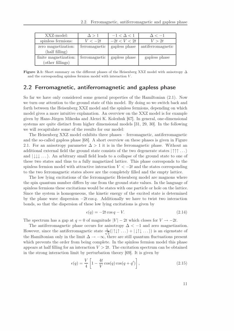
2.2. Ferromagnetic, antiferromagnetic and gapless phase
XXZ-model: ∆ > 1 −1 < ∆ < 1 ∆ < −1
spinless fermions: V < −2t −2t < V < 2t V > 2t
zero magnetization: ferromagnetic gapless phase antiferromagnetic(half filling)
finite magnetization: ferromagnetic gapless phase gapless phase(other fillings)
Figure 2.1: Short summary on the different phases of the Heisenberg XXZ model with anisotropy ∆and the corresponding spinless fermion model with interaction V .
2.2 Ferromagnetic, antiferromagnetic and gapless phase
So far we have only considered some general properties of the Hamiltonian (2.1). Nowwe turn our attention to the ground state of this model. By doing so we switch back andforth between the Heisenberg XXZ model and the spinless fermions, depending on whichmodel gives a more intuitive explanation. An overview on the XXZ model is for examplegiven by Hans-Jürgen Mikeska and Alexei K. Kolezhuk [67]. In general, one-dimensionalsystems are quite distinct from higher dimensional models [31, 29, 30]. In the followingwe will recapitulate some of the results for our model:
The Heisenberg XXZ model exhibits three phases – ferromagnetic, antiferromagneticand the so-called gapless phase [68]. A short overview on these phases is given in Figure2.1. For an anisotropy parameter ∆ > 1 it is in the ferromagnetic phase. Without anadditional external field the ground state consists of the two degenerate states |↑↑↑ . . . 〉and | ↓↓↓ . . . 〉. An arbitrary small field leads to a collapse of the ground state to one ofthese two states and thus to a fully magnetized lattice. This phase corresponds to thespinless fermion model with attractive interaction V < −2t and the states correspondingto the two ferromagnetic states above are the completely filled and the empty lattice.
The low lying excitations of the ferromagnetic Heisenberg model are magnons wherethe spin quantum number differs by one from the ground state values. In the language ofspinless fermions these excitations would be states with one particle or hole on the lattice.Since the system is homogeneous, the kinetic energy of the excited state is determinedby the plane wave dispersion −2t cos q. Additionally we have to twist two interactionbonds, so that the dispersion of these low lying excitations is given by
ǫ(q) = −2t cos q − V. (2.14)
The spectrum has a gap at q = 0 of magnitude |V | − 2t which closes for V → −2t.The antiferromagnetic phase occurs for anisotropy ∆ < −1 and zero magnetization.
However, since the antiferromagnetic state 1√2(| ↑↓↑ . . . 〉 + | ↓↑↓ . . . 〉) is an eigenstate of
the Hamiltonian only in the limit ∆ → −∞, there are still quantum fluctuations presentwhich prevents the order from being complete. In the spinless fermion model this phaseappears at half filling for an interaction V > 2t. The excitation spectrum can be obtainedin the strong interaction limit by perturbation theory [69]. It is given by
ǫ(q) =V
4
[
1 −4t
Vcos(q) cos(q + q′)
]
, (2.15)
11
Chapter 2. Spinless Fermions
01
2π π
3
2π 2π
q
0
1
2
3
4
5
ω
0.02
0.05
0.1
0.2
0.5
1
2
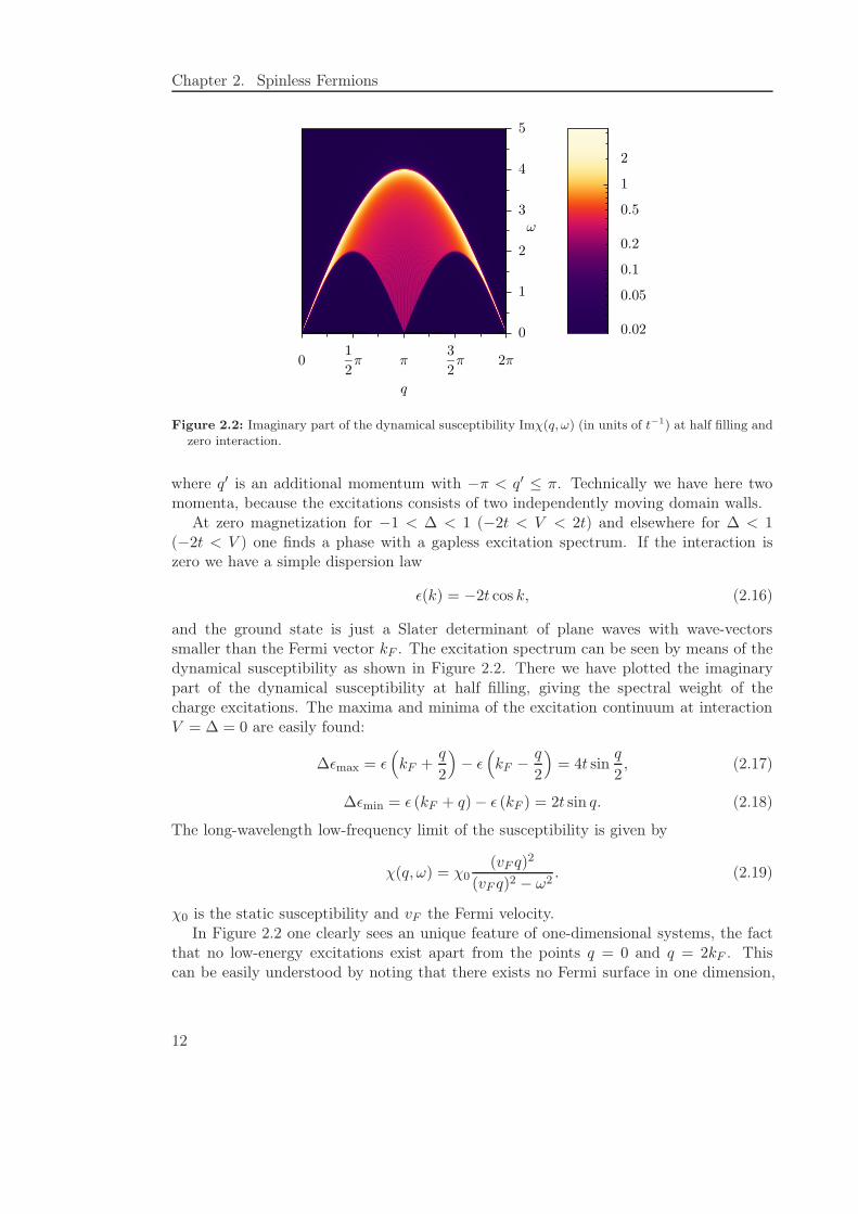
Figure 2.2: Imaginary part of the dynamical susceptibility Imχ(q, ω) (in units of t−1) at half filling andzero interaction.
where q′ is an additional momentum with −π < q′ ≤ π. Technically we have here twomomenta, because the excitations consists of two independently moving domain walls.
At zero magnetization for −1 < ∆ < 1 (−2t < V < 2t) and elsewhere for ∆ < 1(−2t < V ) one finds a phase with a gapless excitation spectrum. If the interaction iszero we have a simple dispersion law
ǫ(k) = −2t cos k, (2.16)
and the ground state is just a Slater determinant of plane waves with wave-vectorssmaller than the Fermi vector kF . The excitation spectrum can be seen by means of thedynamical susceptibility as shown in Figure 2.2. There we have plotted the imaginarypart of the dynamical susceptibility at half filling, giving the spectral weight of thecharge excitations. The maxima and minima of the excitation continuum at interactionV = ∆ = 0 are easily found:
∆ǫmax = ǫ(
kF +q
2
)
− ǫ(
kF −q
2
)
= 4t sinq
2, (2.17)
∆ǫmin = ǫ (kF + q) − ǫ (kF ) = 2t sin q. (2.18)
The long-wavelength low-frequency limit of the susceptibility is given by
χ(q, ω) = χ0(vF q)
2
(vF q)2 − ω2. (2.19)
χ0 is the static susceptibility and vF the Fermi velocity.In Figure 2.2 one clearly sees an unique feature of one-dimensional systems, the fact
that no low-energy excitations exist apart from the points q = 0 and q = 2kF . Thiscan be easily understood by noting that there exists no Fermi surface in one dimension,
12
2.2. Ferromagnetic, antiferromagnetic and gapless phase
just two distinct points. The reduced phase space of the low lying excitations leads to abreakdown of the Fermi liquid theory for the interacting system and to a new concept,the so-called Luttinger liquid [58, 30]. One finds that the excitation spectrum from thesusceptibility is qualitatively the same as in Figure 2.2. Yet there are differences, forexample the Fermi velocity in (2.19) is renormalized with the interaction [70],
v =πt sin(2η)
π − 2η, (2.20)
where η is a parametrization of the interaction and is defined by
V = −2t cos(2η). (2.21)
The static susceptibility is also renormalized:
χ0 =π − 2η
2πη sin(2η). (2.22)
The other relevant low energy limit is q → 2kF . In this case the susceptibility shows apower law divergence, given by [71]
χ(q, ω) ∼1
[ω2 − v2(q − 2kF )2]1−1
2Θ
, (2.23)
where Θ parametrizes the interaction according to 2Θ = 1 − 2π arcsin ∆.
13

Chapter 2. Spinless Fermions
14
3 Static density functional theory
In this chapter we examine density functional theory for static potentials and phases.Its basic idea is to express the ground state energy of an interacting many-body systemas a functional of the densities. The existence of such a functional is provided by theHohenberg-Kohn theorem [1], which we present in Appendix B. In a next step one usesthe constrained search method [72, 73, 61] and a variational principle [2] to determinea single-particle Hamiltonian, the so-called Kohn-Sham Hamiltonian, whose eigenstatesallow the calculation of the true ground state energy and density of the interactingHamiltonian. An introduction to density functional theory can be found for examplein [74, 75, 76]. However we take another point of view and present density functionaltheory in the context of Legendre transformations [62], which lies also at the heart ofthe constrained search method [61]. Besides a clear and insightful formulation of DFT,the approach using the Legendre transformation also gives a clear and precise way forextending density functional theory to more complex problems like the inclusion of vector-potentials, finite temperatures or systems, which are out of equilibrium. However, withinthis chapter we confine ourselves to models with static potentials vl and vector-potentials,which only enter via the phases φl in the hopping term. After the formulation of densityfunctional theory in the next section we introduce some approximations for an essentialingredient, the so-called exchange-correlation potential. Amongst them are the localdensity approximation and the exact-exchange method. Finally, in the last part of thischapter we investigate the quality of the approximations. The discussion on the localdensity approximation is also presented in [77].
3.1 Density functional theory by Legendre transformation
The principal idea behind current density functional theory is to establish a mappingbetween an interacting many-particle system H with local potentials vl and phases φl anda single-particle system Hs with effective potentials vs
l and phases φsl . These Hamiltonian
can be written as
H = −t∑
l
(
eiφl c+l cl+1 + e−iφl c+l+1cl
)
+ V∑
l
nlnl+1 +∑
l
vlnl (3.1)
and
Hs = −t
∑
l
(
eiφsl c+l cl+1 + e−iφs
l c+l+1cl
)
+∑
l
vsl nl . (3.2)
The ground state energy of the Hamiltonian (3.1), E = 〈H〉, is then a function of the po-tentials {vl} and the phases {φl}. Their conjugated variables, the densities and currents
15
Chapter 3. Static density functional theory
can then be found as
nl = 〈nl〉 =∂E
∂vl, jl = 〈l〉 =
∂E
∂φl. (3.3)
Now we introduce the Legendre transform F of the ground state energy which transformsfrom the potentials and phases to the new variables {nl} and {jl} according to the relation
F [n, j] = E −∑
l
vlnl −∑
l
φljl. (3.4)
Here n and j is a shorthand notation for the sets {nl} and {jl}. The local potentials andphases can be recovered by
vl = −∂F
∂nl, φl = −
∂F
∂jl. (3.5)
In order to establish the mapping between the interacting and the single-particlesystem, the ground state energy of the latter is transformed analogously,
F s[ns, js] = Es −∑
l
vsl n
sl −
∑
l
φsl j
sl . (3.6)
Considering the single-particle system at the same densities as the interacting system,ns
l = nl and jsl = jl, rewriting F as F s + (F − F s) and using the back-transformation(3.5) gives a relation between the single-particle and many-body potentials,
vsl = vl +
∂EHXC
∂nl, φs
l = φl +∂EHXC
∂jl. (3.7)
Here we have defined the Hartree-Exchange-Correlation energy as EHXC ≡ F −F s. Thedifference
vsl − vl =
∂EHXC
∂nl= vHXC
l (3.8)
is then the so-called Hartree-exchange-correlation potential. In the traditional formu-lation of DFT the mapping between the interacting and the single-particle system isprovided by the Hohenberg-Kohn theorem and the so-called v-representability of theinteracting density. In our context these theorems ensure the existence of the Legen-dre transformation and the back-transformation. The Hohenberg-Kohn theorem can befound in Appendix B and the relation between these theorems and Legendre transformsis discussed in more detail in Appendix C.
The ground state energy of the interacting system can be found by the reversedtransformation, F → E, which can be expressed in terms of single-particle quantities as
E = F +∑
l
vlnl +∑
l
φljl
= F s + (F − F s) +∑
l
[vsl + (vl − vs
l )]nl +∑
l
[φsl + (φl − φs
l )]jl
= Es +EHXC +∑
l
(vl − vsl )nl +
∑
l
(φl − φsl )jl.
(3.9)
16
3.2. Approximations
Es can be evaluated as the sum over the N lowest eigenvalues of the single-particlesystem
Es =
N∑
j=1
ǫj . (3.10)
Clearly, the ground state energy is not only the sum of eigenvalues of the noninteractingHamiltonian, but one also has to take the correction EHXC −
∑
l vHXCl nl into account.
As we will see later these corrections are quite important and should not be neglected.Introducing explicitly the Hartree contribution, EH, through
EHXC = EH + EXC (3.11)
with EH = V∑
l nlnl+1, we arrive at the standard relation
vsl = vl + vH
l + vXCl . (3.12)
The Hartree potential is apparently vHl = V (nl−1 + nl+1) and the exchange-correlation
potential is given by
vXCl =
∂EXC
∂nl. (3.13)
In addition we get for the single-particle phases
φsl = φl + φXC
l , φXCl =
∂EXC
∂jl(3.14)
since the Hartree energy depends on the densities only. Please note that the single-particle potentials and phases depend, by construction, on the densities and the currents.Therefore the auxiliary system has to be determined self-consistently with respect to thedensities and currents. The exchange correlation energy can be formally written as
EXC = 〈0| T + V |0〉 − 〈0s| Ts |0s〉 − EH +
∑
l
φXCl jl , (3.15)
where |0〉 and |0s〉 are the ground state wave functions of the interacting and the single-particle system, respectively. Up to now we have been avoiding the problem of determin-ing the exchange-correlation energy explicitly. Since this is a hard problem we have tomake some approximations. Some of the possible approximations are presented in thenext sections.
3.2 Approximations
3.2.1 Local density approximation
A simple approximation for the exchange-correlation energy is the so-called local densityapproximation (LDA). There the exchange-correlation energy is written as
EXC[n, j] =∑
l
ǫXC(nl, jl). (3.16)
17
Chapter 3. Static density functional theory
Thus the exchange-correlation potentials and phases
vXCl =
∂EXC
∂nl=∂ǫXC
∂nland ΦXC
l =∂EXC
∂jl=∂ǫXC
∂jl. (3.17)
are functions of the local density and current-density only. This local energy ǫXC can bedetermined from the exact exchange-correlation energy of the static homogeneous systemfor given density n and current j,
ǫXC =EXC
L, (3.18)
where EXC is calculated from the exact ground state energy according to equation (3.15).For the three-dimensional electron gas this energy is usually obtained by analytical cal-culations for certain limiting cases and quantum monte carlo simulations followed by ainterpolation procedure [78, 79]. For our system of spinless fermions this can efficiently bedone with the Bethe ansatz [57], hence we call the exact ground state energy EBA(n, j).A detailed presentation of the Bethe ansatz is shown in the Appendix A.2. Admittedlythe Bethe ansatz solution is found as a function of n and φ. Thus the phase variable hasto be eliminated from this expression in favor of the current, using the relation
j =1
L
∂EBA(n, φ)
∂φ(3.19)
for the homogeneous system. The second term in (3.15), which we denote E0(φ), is givenby the single-particle result (−π/L < φ < π/L)
E0(φ) = E0 · cosφ , E0 ≃ −2t
πL sin(πn), (3.20)
where the latter relation holds for large L. Since φ ∼ 1/L, we may expand for small φ;in particular, the Drude weights, DBA and D0, are defined according to the followingrelations (φ→ 0):
EBA(φ) − EBA(0) = DBALφ2 (3.21)
E0(φ) − E0(0) = D0Lφ2 (3.22)
Note that DBA and D0 are functions of the density, and DBA depends on the interactionV . For example, D0 = (t/π) sin(nπ) = vF /2π, where vF is the bare Fermi velocity, andDBA = πt sinµ/[4µ(π − µ)] for half filling (n = 1/2), where V (in the range −2t . . . 2t)is related to µ by V = −2t cosµ [80].
Combining the above relations, we obtain
ǫXC(n, j) =1
L
(EBA(n, 0) − E0(n, 0)
)− V n2 +
1
2λXCj2, (3.23)
where
λXC(n) =1
2
(1
D0(n)−
1
DBA(n)
)
. (3.24)
18
3.2. Approximations
−2
−1
0
1
2
vX
C(j
=0)/t
0 0.2 0.4 0.6 0.8 1
n
V = 1.0 t
V = 1.5 t
V = 2.0 t
V = 3.0 t
V = 4.0 t
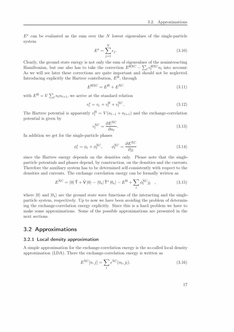
Figure 3.1: Exchange-correlation potential as function of the density at j = 0 for various interactions.Potentials with V > 2 have a jump at n = 0.5.
Note that λXC(n) ≤ 0 since DBA(n) ≤ D0(n). The resulting approximation may becalled current-LDA (C-LDA) and is obviously exact if the system is homogeneous. Theexchange-correlation potential for current j equal to zero and the second-order contribu-tion λXC are depicted in Figures 3.1 and 3.2, respectively. The validity of the approxi-mation for other than the homogeneous system will be examined later.
3.2.2 Gradient approximations
In contrast to e. g. the Hartree-Fock approximation, density functional theory withinthe local density approximation is a local theory. This has the advantage that thecomputational costs are significantly lower in DFT+LDA. A way to improve LDA isto take not only the local densities but also its gradients into account
EXC[n] =∑
l
ǫXC(nl,∇nl). (3.25)
This definition leads to the so-called generalized gradient approximation (GGA). A shortoverview on GGA and earlier gradient approximations can be found for example in [74]and a variety of different functionals in use are shown in [75]. The construction of amodern GGA, based on a number of exact conditions, can be found in [81]. However,within this work we will not investigate the gradient approximations, so we do not gointo more detail.
3.2.3 Exact-exchange method
Another way of approximating the exchange-correlation energy is the exact-exchangemethod (EXX) which is exact up to first order in the interaction [14, 82]. It showssome similarities with the Hartree-Fock approximation, but retains some of the com-putational simplicity of the density functional formalism, which is especially relevant
19
Chapter 3. Static density functional theory
−2
−1
0
1
2
λxc/2t
0 0.2 0.4 0.6 0.8 1
n
V = 1.0 t
V = 1.5 t
V = 2.0 t
V = 3.0 t
V = 4.0 t
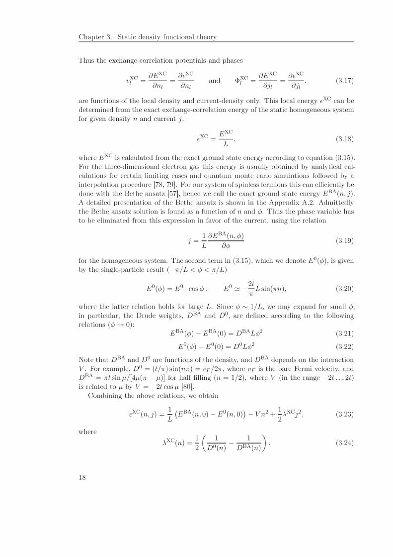
Figure 3.2: Second order correction to the exchange-correlation potential for currents j 6= 0 as a functionof the density.
for systems with long-range interaction. For our one-dimensional artificial system withnearest-neighbor interaction Hartree-Fock calculations are faster since it only modifiesthe secondary diagonals of the Hamiltonian while the exact-exchange method needs acomplicated calculation scheme, as we will see in the following.
In principle the exact-exchange approximation, also known as the optimized effectivepotential approach [12, 13, 15], even allows higher order approximations. Basically thisscheme expands the ground state energy in orders of the interaction just as in usualperturbation theory. The first order contributions are the Hartree and the exchangeenergy,
EHXC[n] ≈ EH[n] + EX[n], (3.26)
where EH[n] = V∑
l nlnl+1. The exchange energy is given by
EX = −V∑
l
[occ.∑
j
ϕ∗j [n](l)ϕj [n](l + 1)
] [occ.∑
k
ϕ∗k[n](l + 1)ϕk[n](l)
]
, (3.27)
where the sums over j and k go over the occupied states ϕ of the single-particle Hamilto-nian, i. e. the lowest N eigenstates. The main difference to the usual perturbation theoryis that the orbitals ϕj [n] depend on the densities and are eigenstates of the Kohn-ShamHamiltonian but not of an arbitrary single-particle Hamiltonian, as the Hartree-Fockorbitals would be. The corresponding potential is then obtained by taking the derivative
vxl =
∂EX
∂nl=∑
l′,l′′
occ.∑
i
∂EX
∂ϕi(l′′)
∂ϕi(l′′)
∂vl′
∂vl′
∂nl+
∂EX
∂ϕ∗i (l
′′)
∂ϕ∗i (l
′′)
∂vl′
∂vl′
∂nl. (3.28)
The indices l′ and l′′ go over the lattice (1 . . . L) while the sum over i again goes over theoccupied states. The first term of both summands on the right hand side is simple to
20
3.3. Practical applications
determine from (3.27) and we have for example:
∂EX
∂ϕi(l′′)= −V
occ.∑
j
(ϕ∗
j (l′′)ϕj (l
′′ + 1)ϕ∗i (l
′′ + 1) + ϕ∗i (l
′′ − 1)ϕ∗j (l
′′)ϕj (l′′ − 1)
). (3.29)
The second terms in (3.28) can be found by first order perturbation theory. Considerthe Hamiltonian Hs which corresponds to the eigenstates ϕj and perturb it with a smallpotential term δvl′ nl′ . Then the derivative is
∂ϕi(l′′)
∂vl′= lim
δvl′→0
ϕvl′+δvl′
i (l′′) − ϕvl′
i (l′′)
δvl′=∑
k 6=i
ϕk(l′′)ϕ∗
k(l′)ϕi(l′)
ǫi − ǫk. (3.30)
The ǫν are the eigenenergies of the single-particle Hamiltonian. The sum over k includesall eigenstates of the Hamiltonian except the i-th. Finally, the last expression of (3.28)is the inverse of the susceptibility and can be derived by applying (3.30) to the relationnl =
∑occ.j ϕ∗
j (l)ϕj (l):
χll′ =∂nl
∂vl′=
occ.∑
i
∑
j 6=i
ϕ∗i (l)ϕj(l)ϕ
∗j (l
′)ϕi(l′)
ǫi − ǫj+ c.c. (3.31)
Combining the results and inserting into (3.28) one gets an expression for the exchangepotential
vxl = −2V
∑
l′,l′′
occ.∑
i,j
∑
k 6=i
{ϕ∗
j (l′′)ϕj (l
′′ + 1)ϕ∗i (l
′′ + 1)ϕk(l′′)ϕ∗k(l
′)ϕi(l′)
ǫi − ǫk+ c.c.
}
χ−1ll′ .
(3.32)Note that the susceptibility χ has an eigenvalue which is zero. This eigenvalue corre-sponds to a homogeneous change of the density and thus is not particle number conserv-ing. So we have to exclude it before inverting χ.
The calculation of this exchange-potential is already numerically expensive. So, al-though possible, the inclusion of higher order terms is not feasible. However, the correla-tion energy can be approximated analogous to the local density approximation (3.16),
EHXC[n] = EH[n] + EX[n] +∑
l
ǫC(nl), (3.33)
where ǫC can be determined from the exact solution of the homogeneous system. In thefollowing we denote the resulting approximation by EXX+LDA.
3.3 Practical applications
We have seen that density functional theory provides a way of mapping many-body prop-erties onto a single-particle problem. Unfortunately therefore one has to make two sac-rifices. First, one cannot extract every many-particle quantity from a density functional
21
Chapter 3. Static density functional theory
calculation. For example the excitation energies or the density of states are conceptsthat lie outside the static formalism. The second sacrifice is the approximation of theexchange-correlation potential. So there are certainly limitations to density functionaltheory and it is the aim of this section to investigate them. A thorough review of thequality of the local density approximation when applied to realistic materials can befound for example in [83].
3.3.1 Charge gap in the spinless fermion model
An important quantity to distinguish metals from insulators and to characterize the in-sulator is the band gap (see for example [84]). It is common knowledge in the DFTcommunity that usually the local density approximation underestimates the band gapwhile the Hartree-Fock theory would overestimate it. So sometimes a material is found tobe a metal in density functional calculations while experiments show it to be a semicon-ductor or insulator. The band gap problem has been studied intensively in the literature,in particular it has been pointed out that a discontinuity in the exchange-correlationpotential is crucial [19, 21, 85]. Lattice models are quite useful for the understandingof such problems [22, 23, 24]. We now repeat some of the work done for our model ofspinless fermions. The charge gap can be defined as the difference
∆ = µN+1 − µN , (3.34)
where µN is the chemical potential of a N -particle system and, according to [20], canbe calculated as µN = EN − EN−1. The Kohn-Sham gap is defined as the difference ofthe lowest unoccupied (molecular) orbital (LUMO) and the highest occupied (molecular)orbital (HOMO),
∆KS = ǫN+1 − ǫN . (3.35)
If the exchange-correlation energy has no discontinuities as a function of the particlenumber [21], the two quantities are identical in the thermodynamic limit. Please notethat we need to solve three self-consistent calculations for particle numbers N − 1, Nand N + 1 to obtain ∆, while ∆KS only uses results from a N -particle calculation.
For the investigation of the charge gap we first look at the homogeneous system. Therea gap opens for strong interactions V > 2t. In this case the local density approximationgives the correct ground state energies EN . Thus the gap ∆ obtained from the homoge-neous system is obviously exact. On the other hand, since the system is homogeneous, theHartree potential and the exchange-correlation potential also have to be homogeneous.Therefore the potentials contribute only by a global energy shift. The eigenstates of thisHamiltonian are then just plain waves with a cosine dispersion and no gap at all. Sowe see that in this case the Kohn-Sham gap ∆KS is always zero for arbitrary interactionstrength, whereas ∆ 6= 0 for V > 2t. We can now conclude that the exchange-correlationpotential is discontinuous, as seen also in Figure 3.1. So in this case the band gap iscompletely due to the discontinuity of the exchange-correlation potential.
Next we investigate the gap in a weakly interacting system, i. e. within the gaplessphase with |V | < 2. There we open a gap by inserting the potential vl = u cos 2kF l,
22
3.3. Practical applications
4
5
6
7
∆G
ap/t
0 0.5 1 1.5 2
V/t
exact: ∆
exact: ∆KS
LDA: ∆
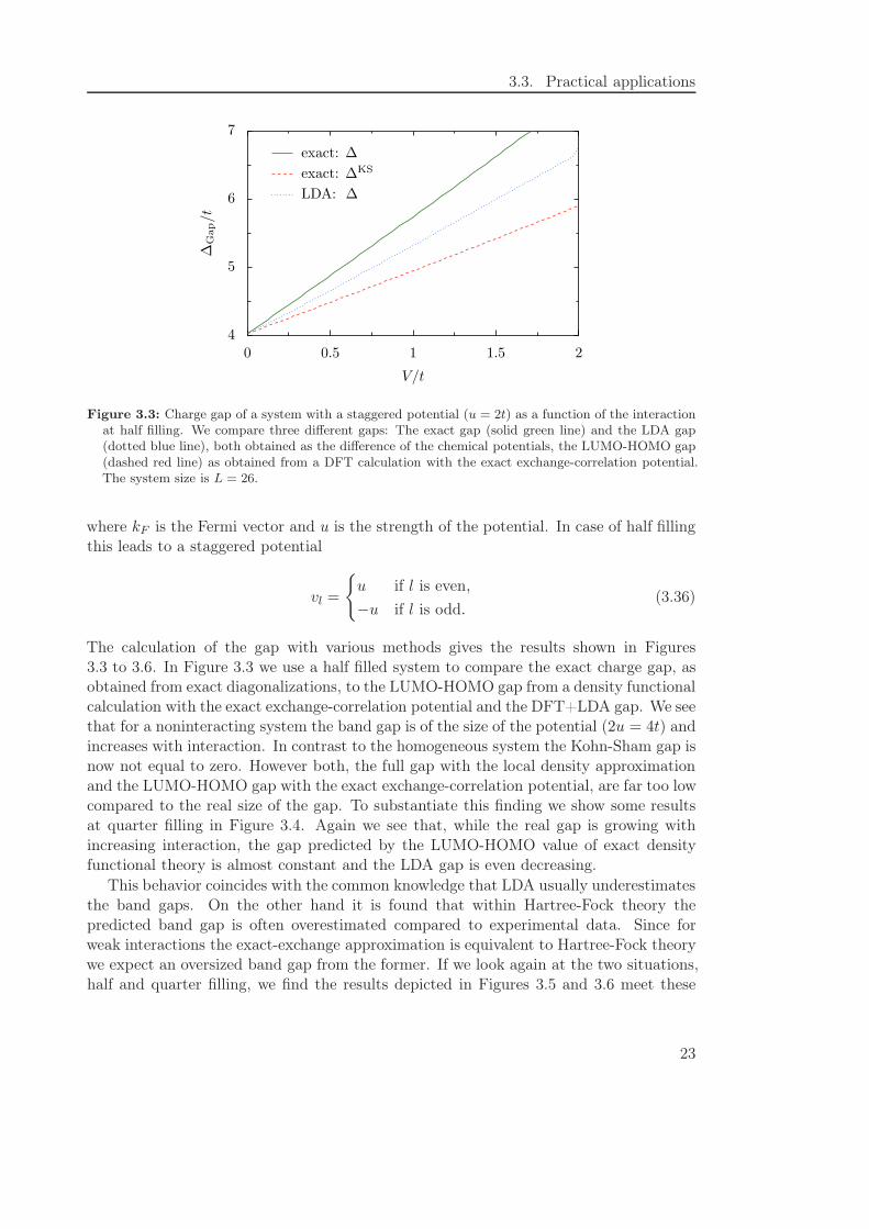
Figure 3.3: Charge gap of a system with a staggered potential (u = 2t) as a function of the interactionat half filling. We compare three different gaps: The exact gap (solid green line) and the LDA gap(dotted blue line), both obtained as the difference of the chemical potentials, the LUMO-HOMO gap(dashed red line) as obtained from a DFT calculation with the exact exchange-correlation potential.The system size is L = 26.
where kF is the Fermi vector and u is the strength of the potential. In case of half fillingthis leads to a staggered potential
vl =
{
u if l is even,
−u if l is odd.(3.36)
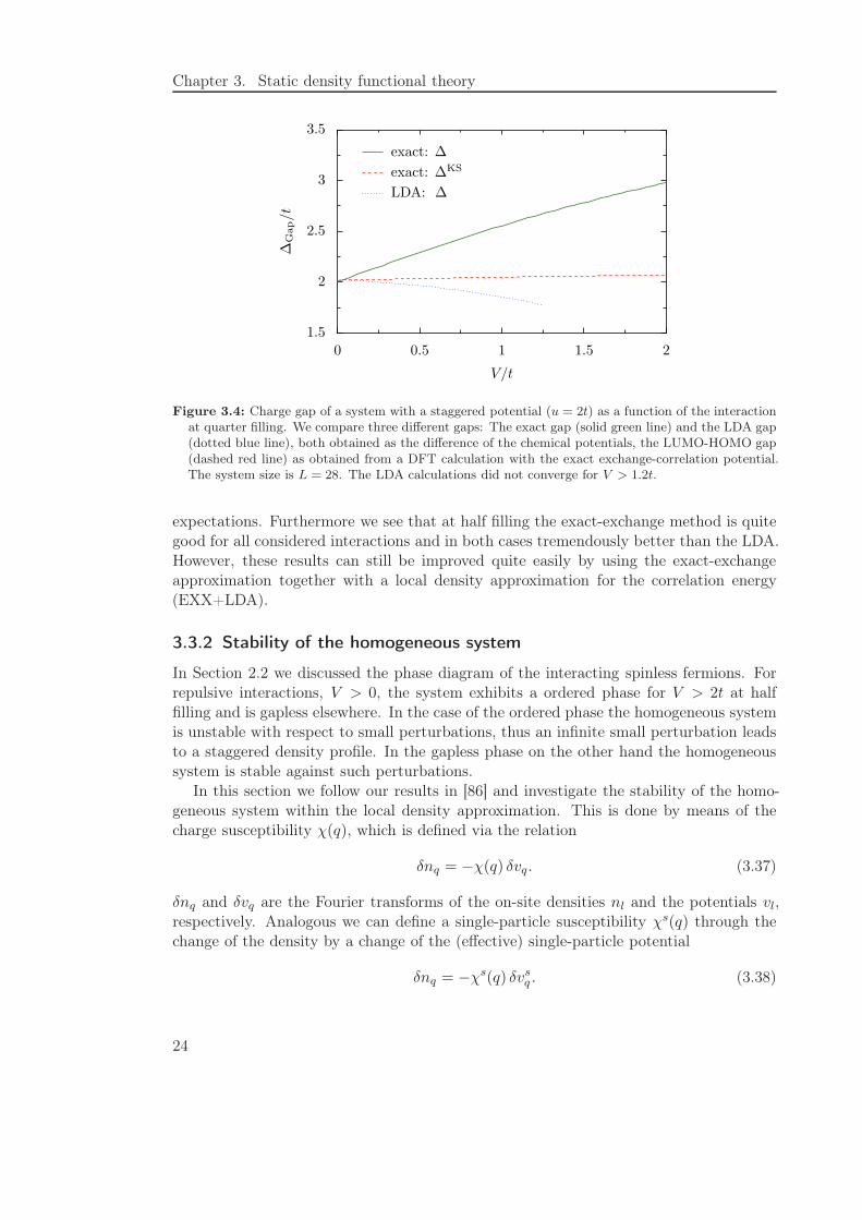
The calculation of the gap with various methods gives the results shown in Figures3.3 to 3.6. In Figure 3.3 we use a half filled system to compare the exact charge gap, asobtained from exact diagonalizations, to the LUMO-HOMO gap from a density functionalcalculation with the exact exchange-correlation potential and the DFT+LDA gap. We seethat for a noninteracting system the band gap is of the size of the potential (2u = 4t) andincreases with interaction. In contrast to the homogeneous system the Kohn-Sham gap isnow not equal to zero. However both, the full gap with the local density approximationand the LUMO-HOMO gap with the exact exchange-correlation potential, are far too lowcompared to the real size of the gap. To substantiate this finding we show some resultsat quarter filling in Figure 3.4. Again we see that, while the real gap is growing withincreasing interaction, the gap predicted by the LUMO-HOMO value of exact densityfunctional theory is almost constant and the LDA gap is even decreasing.
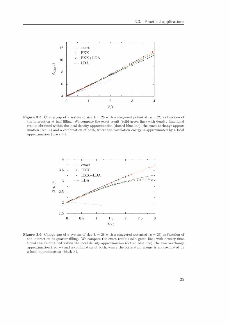
This behavior coincides with the common knowledge that LDA usually underestimatesthe band gaps. On the other hand it is found that within Hartree-Fock theory thepredicted band gap is often overestimated compared to experimental data. Since forweak interactions the exact-exchange approximation is equivalent to Hartree-Fock theorywe expect an oversized band gap from the former. If we look again at the two situations,half and quarter filling, we find the results depicted in Figures 3.5 and 3.6 meet these
23
Chapter 3. Static density functional theory
1.5
2
2.5
3
3.5
∆G
ap/t
0 0.5 1 1.5 2
V/t
exact: ∆
exact: ∆KS
LDA: ∆
Figure 3.4: Charge gap of a system with a staggered potential (u = 2t) as a function of the interactionat quarter filling. We compare three different gaps: The exact gap (solid green line) and the LDA gap(dotted blue line), both obtained as the difference of the chemical potentials, the LUMO-HOMO gap(dashed red line) as obtained from a DFT calculation with the exact exchange-correlation potential.The system size is L = 28. The LDA calculations did not converge for V > 1.2t.
expectations. Furthermore we see that at half filling the exact-exchange method is quitegood for all considered interactions and in both cases tremendously better than the LDA.However, these results can still be improved quite easily by using the exact-exchangeapproximation together with a local density approximation for the correlation energy(EXX+LDA).
3.3.2 Stability of the homogeneous system
In Section 2.2 we discussed the phase diagram of the interacting spinless fermions. Forrepulsive interactions, V > 0, the system exhibits a ordered phase for V > 2t at halffilling and is gapless elsewhere. In the case of the ordered phase the homogeneous systemis unstable with respect to small perturbations, thus an infinite small perturbation leadsto a staggered density profile. In the gapless phase on the other hand the homogeneoussystem is stable against such perturbations.
In this section we follow our results in [86] and investigate the stability of the homo-geneous system within the local density approximation. This is done by means of thecharge susceptibility χ(q), which is defined via the relation
δnq = −χ(q) δvq. (3.37)
δnq and δvq are the Fourier transforms of the on-site densities nl and the potentials vl,respectively. Analogous we can define a single-particle susceptibility χs(q) through thechange of the density by a change of the (effective) single-particle potential
δnq = −χs(q) δvsq . (3.38)
24
3.3. Practical applications
4
6
8
10
12
∆G
ap/t
0 1 2 3 4
V/t
exact
EXX
EXX+LDA
LDA
Figure 3.5: Charge gap of a system of size L = 26 with a staggered potential (u = 2t) as function ofthe interaction at half filling. We compare the exact result (solid green line) with density functionalresults obtained within the local density approximation (dotted blue line), the exact-exchange approx-imation (red +) and a combination of both, where the correlation energy is approximated by a localapproximation (black ×).
1.5
2
2.5
3
3.5
4
∆G
ap/t
0 0.5 1 1.5 2 2.5 3
V/t
exact
EXX
EXX+LDA
LDA
Figure 3.6: Charge gap of a system of size L = 28 with a staggered potential (u = 2t) as function ofthe interaction at quarter filling. We compare the exact result (solid green line) with density func-tional results obtained within the local density approximation (dotted blue line), the exact-exchangeapproximation (red +) and a combination of both, where the correlation energy is approximated bya local approximation (black ×).
25
Chapter 3. Static density functional theory
Using equation (3.12), δvHq /δnq′ = δqq′ δv
Hq /δnq and the analogous result for δvXC
q /δnq′
we rewrite δvsq as
δvsq = δvq + δvH
q + δvXCq = δvq +
(
δvHq
δnq+δvXC
q
δnq
)
δnq. (3.39)
Inserting (3.37) into this expression and equating (3.37) and (3.38) gives then a relationbetween χ(q) and χs(q),
χ(q) = χs(q){1 +
[2V cos(q) + fXC(q)
]χ(q)
}(3.40)
or
χ(q) =χs(q)
1 + [2V cos(q) + fXC(q)]χs(q). (3.41)
Here, 2V cos(q) is the Hartree term from (3.39) and fXC is the derivative of the exchange-correlation potential with respect to the density. In the thermodynamic limit (L → ∞)the susceptibility of the auxiliary system is given by
χs(q) =1
4πt sin(q/2)ln
∣∣∣∣
sin(q/2) + sin kF
sin(q/2) − sin kF
∣∣∣∣
(3.42)
with the Fermi wave vector kF . Equation (3.41) is exact if one knows the exact expressionof the exchange-correlation kernel fXC(q). In case of the local density approximation thiskernel is independent of q and only depends on the filling.
The stability boundary of the homogeneous system is determined by the conditionthat the static susceptibility becomes infinite and changes sign, i. e. if
1
χs(q)+ V (q) + fXC(q) = 0. (3.43)
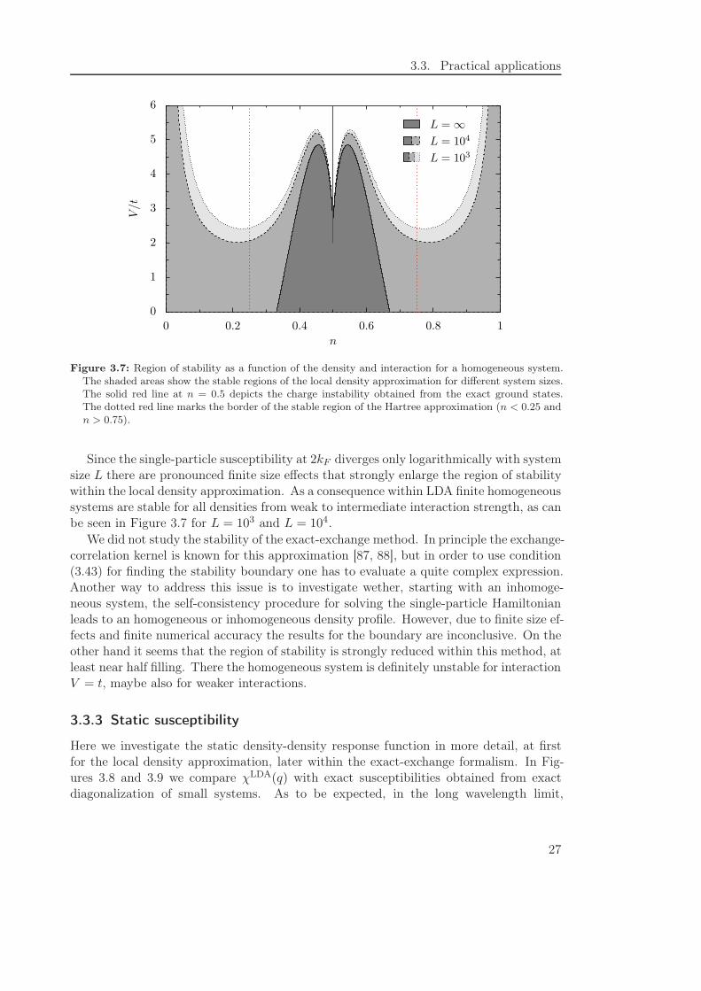
Due to the logarithmic divergence of χs(q) for q → 2kF this is equivalent to the conditionthat V (q) + fXC(q) changes sign. Figure 3.7 shows the region of stability for the localdensity approximation in the n-V -plane for the infinite system and for finite systems oflength L = 103 and L = 104, respectively. If we investigate the weak interacting case inmore detail we find
fXCLDA =
∂2
∂n2
(ǫBA − ǫH
)= −V (2kF ) + O(V 2), (3.44)
which cancels the V (q)-part of the denominator for q → 2kF . So in first order in theinteraction we cannot draw a conclusion about the stability of the homogeneous system.Numerically one finds that the second order correction of fXC
LDA changes sign at nc ≈ 0.331,thus limiting the range of stability to nc < N < 1−nc at weak coupling. In contrast, theHartree approximation is stable only for V (2kF ) > 0, i. e. below quarter and above threequarter filling, while the exact ground state is unstable only at half filling for interactionsV > 2t.
26
3.3. Practical applications
0
1
2
3
4
5
6
V/t
0 0.2 0.4 0.6 0.8 1
n
L = ∞
L = 104
L = 103
Figure 3.7: Region of stability as a function of the density and interaction for a homogeneous system.The shaded areas show the stable regions of the local density approximation for different system sizes.The solid red line at n = 0.5 depicts the charge instability obtained from the exact ground states.The dotted red line marks the border of the stable region of the Hartree approximation (n < 0.25 andn > 0.75).
Since the single-particle susceptibility at 2kF diverges only logarithmically with systemsize L there are pronounced finite size effects that strongly enlarge the region of stabilitywithin the local density approximation. As a consequence within LDA finite homogeneoussystems are stable for all densities from weak to intermediate interaction strength, as canbe seen in Figure 3.7 for L = 103 and L = 104.
We did not study the stability of the exact-exchange method. In principle the exchange-correlation kernel is known for this approximation [87, 88], but in order to use condition(3.43) for finding the stability boundary one has to evaluate a quite complex expression.Another way to address this issue is to investigate wether, starting with an inhomoge-neous system, the self-consistency procedure for solving the single-particle Hamiltonianleads to an homogeneous or inhomogeneous density profile. However, due to finite size ef-fects and finite numerical accuracy the results for the boundary are inconclusive. On theother hand it seems that the region of stability is strongly reduced within this method, atleast near half filling. There the homogeneous system is definitely unstable for interactionV = t, maybe also for weaker interactions.
3.3.3 Static susceptibility
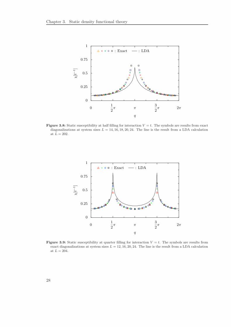
Here we investigate the static density-density response function in more detail, at firstfor the local density approximation, later within the exact-exchange formalism. In Fig-ures 3.8 and 3.9 we compare χLDA(q) with exact susceptibilities obtained from exactdiagonalization of small systems. As to be expected, in the long wavelength limit,
27
Chapter 3. Static density functional theory
0
0.25
0.5
0.75
1
χ[t−
1]
01
2π π
3
2π 2π
q
: Exact : LDA
Figure 3.8: Static susceptibility at half filling for interaction V = t. The symbols are results from exactdiagonalizations at system sizes L = 14, 16, 18, 20, 24. The line is the result from a LDA calculationat L = 202.
0
0.25
0.5
0.75
1
χ[t−
1]
01
2π π
3
2π 2π
q
: Exact : LDA
Figure 3.9: Static susceptibility at quarter filling for interaction V = t. The symbols are results fromexact diagonalizations at system sizes L = 12, 16, 20, 24. The line is the result from a LDA calculationat L = 204.
28
3.3. Practical applications
q → 0, perfect agreement is found. Technically, there is a cancellation between thesusceptibility 1/χs(0) = 2πt sin kF and the second derivative of the Hartree energyǫH = −(2t/π) sin kF + V n2 with respect to n = kF/π. Therefore
χLDA(q → 0) =
(∂2ǫBA
∂n2
)−1
=1
L
∂N
∂µ(3.45)
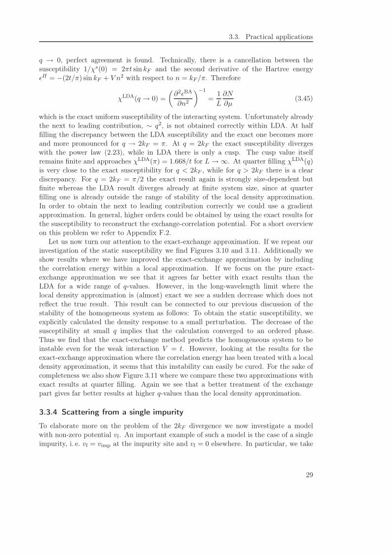
which is the exact uniform susceptibility of the interacting system. Unfortunately alreadythe next to leading contribution, ∼ q2, is not obtained correctly within LDA. At halffilling the discrepancy between the LDA susceptibility and the exact one becomes moreand more pronounced for q → 2kF = π. At q = 2kF the exact susceptibility divergeswith the power law (2.23), while in LDA there is only a cusp. The cusp value itselfremains finite and approaches χLDA(π) = 1.668/t for L→ ∞. At quarter filling χLDA(q)is very close to the exact susceptibility for q < 2kF , while for q > 2kF there is a cleardiscrepancy. For q = 2kF = π/2 the exact result again is strongly size-dependent butfinite whereas the LDA result diverges already at finite system size, since at quarterfilling one is already outside the range of stability of the local density approximation.In order to obtain the next to leading contribution correctly we could use a gradientapproximation. In general, higher orders could be obtained by using the exact results forthe susceptibility to reconstruct the exchange-correlation potential. For a short overviewon this problem we refer to Appendix F.2.
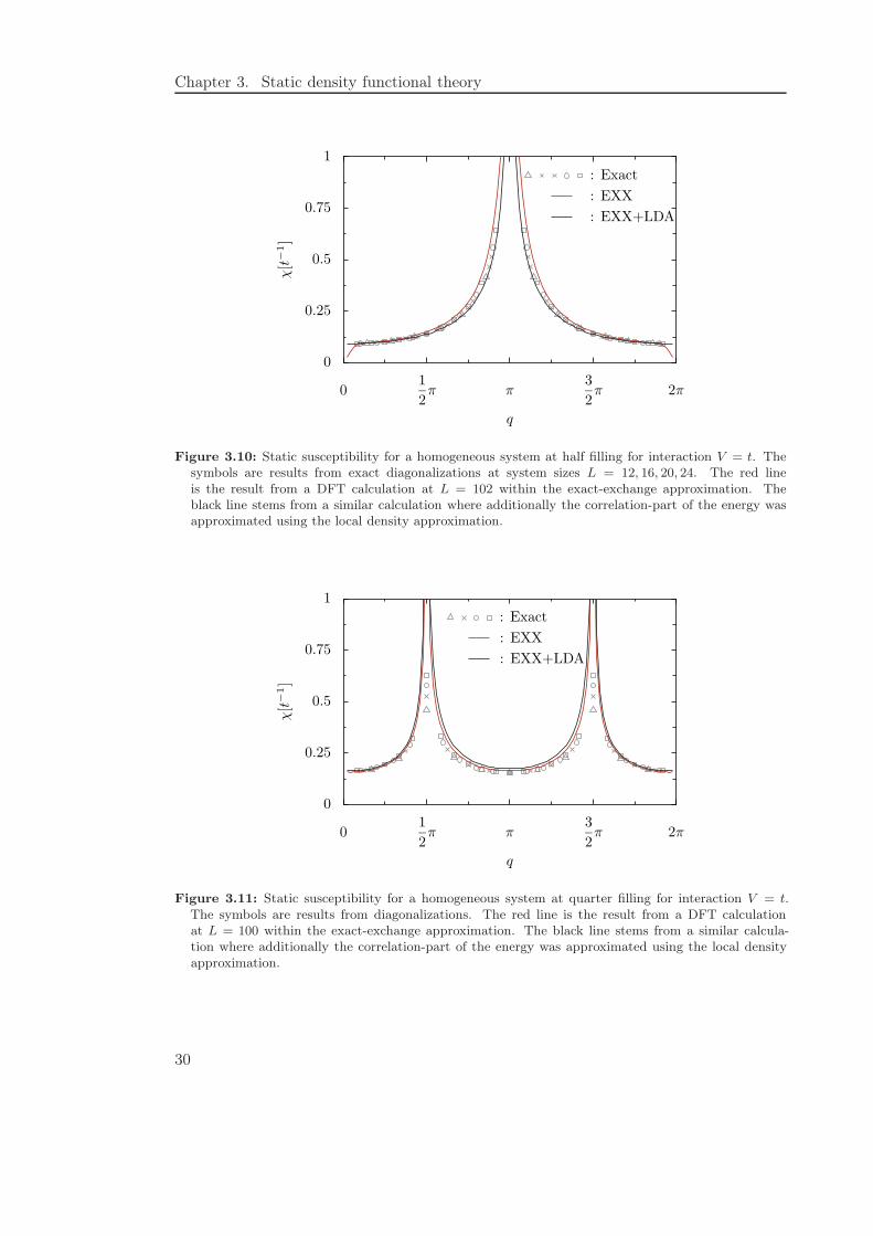
Let us now turn our attention to the exact-exchange approximation. If we repeat ourinvestigation of the static susceptibility we find Figures 3.10 and 3.11. Additionally weshow results where we have improved the exact-exchange approximation by includingthe correlation energy within a local approximation. If we focus on the pure exact-exchange approximation we see that it agrees far better with exact results than theLDA for a wide range of q-values. However, in the long-wavelength limit where thelocal density approximation is (almost) exact we see a sudden decrease which does notreflect the true result. This result can be connected to our previous discussion of thestability of the homogeneous system as follows: To obtain the static susceptibility, weexplicitly calculated the density response to a small perturbation. The decrease of thesusceptibility at small q implies that the calculation converged to an ordered phase.Thus we find that the exact-exchange method predicts the homogeneous system to beinstable even for the weak interaction V = t. However, looking at the results for theexact-exchange approximation where the correlation energy has been treated with a localdensity approximation, it seems that this instability can easily be cured. For the sake ofcompleteness we also show Figure 3.11 where we compare these two approximations withexact results at quarter filling. Again we see that a better treatment of the exchangepart gives far better results at higher q-values than the local density approximation.
3.3.4 Scattering from a single impurity
To elaborate more on the problem of the 2kF divergence we now investigate a modelwith non-zero potential vl. An important example of such a model is the case of a singleimpurity, i. e. vl = vimp at the impurity site and vl = 0 elsewhere. In particular, we take
29
Chapter 3. Static density functional theory
: EXX
: EXX+LDA
0
0.25
0.5
0.75
1
χ[t−
1]
01
2π π
3
2π 2π
q
: Exact
Figure 3.10: Static susceptibility for a homogeneous system at half filling for interaction V = t. Thesymbols are results from exact diagonalizations at system sizes L = 12, 16, 20, 24. The red lineis the result from a DFT calculation at L = 102 within the exact-exchange approximation. Theblack line stems from a similar calculation where additionally the correlation-part of the energy wasapproximated using the local density approximation.
: EXX
: EXX+LDA
0
0.25
0.5
0.75
1
χ[t−
1]
01
2π π
3
2π 2π
q
: Exact
Figure 3.11: Static susceptibility for a homogeneous system at quarter filling for interaction V = t.The symbols are results from diagonalizations. The red line is the result from a DFT calculationat L = 100 within the exact-exchange approximation. The black line stems from a similar calcula-tion where additionally the correlation-part of the energy was approximated using the local densityapproximation.
30
3.3. Practical applications
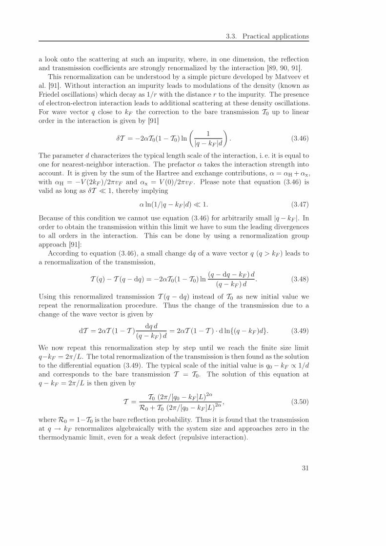
a look onto the scattering at such an impurity, where, in one dimension, the reflectionand transmission coefficients are strongly renormalized by the interaction [89, 90, 91].
This renormalization can be understood by a simple picture developed by Matveev etal. [91]. Without interaction an impurity leads to modulations of the density (known asFriedel oscillations) which decay as 1/r with the distance r to the impurity. The presenceof electron-electron interaction leads to additional scattering at these density oscillations.For wave vector q close to kF the correction to the bare transmission T0 up to linearorder in the interaction is given by [91]
δT = −2αT0(1 − T0) ln
(1
|q − kF |d
)
. (3.46)
The parameter d characterizes the typical length scale of the interaction, i. e. it is equal toone for nearest-neighbor interaction. The prefactor α takes the interaction strength intoaccount. It is given by the sum of the Hartree and exchange contributions, α = αH +αx,with αH = −V (2kF )/2πvF and αx = V (0)/2πvF . Please note that equation (3.46) isvalid as long as δT ≪ 1, thereby implying
α ln(1/|q − kF |d) ≪ 1. (3.47)
Because of this condition we cannot use equation (3.46) for arbitrarily small |q− kF |. Inorder to obtain the transmission within this limit we have to sum the leading divergencesto all orders in the interaction. This can be done by using a renormalization groupapproach [91]:
According to equation (3.46), a small change dq of a wave vector q (q > kF ) leads toa renormalization of the transmission,
T (q) − T (q − dq) = −2αT0(1 − T0) ln(q − dq − kF ) d
(q − kF ) d. (3.48)
Using this renormalized transmission T (q − dq) instead of T0 as new initial value werepeat the renormalization procedure. Thus the change of the transmission due to achange of the wave vector is given by
dT = 2αT (1 − T )dq d
(q − kF ) d= 2αT (1 − T ) · d ln{(q − kF )d}. (3.49)
We now repeat this renormalization step by step until we reach the finite size limitq−kF = 2π/L. The total renormalization of the transmission is then found as the solutionto the differential equation (3.49). The typical scale of the initial value is q0 − kF ∝ 1/dand corresponds to the bare transmission T = T0. The solution of this equation atq − kF = 2π/L is then given by
T =T0 (2π/[q0 − kF ]L)2α
R0 + T0 (2π/[q0 − kF ]L)2α , (3.50)
where R0 = 1−T0 is the bare reflection probability. Thus it is found that the transmissionat q → kF renormalizes algebraically with the system size and approaches zero in thethermodynamic limit, even for a weak defect (repulsive interaction).
31
Chapter 3. Static density functional theory
0
0.1
0.2
0.3
Dru
de
Wei
ghtD/t
−2 −1 0 1 2
Interaction V/t
L = 62 L = 102 L = 202
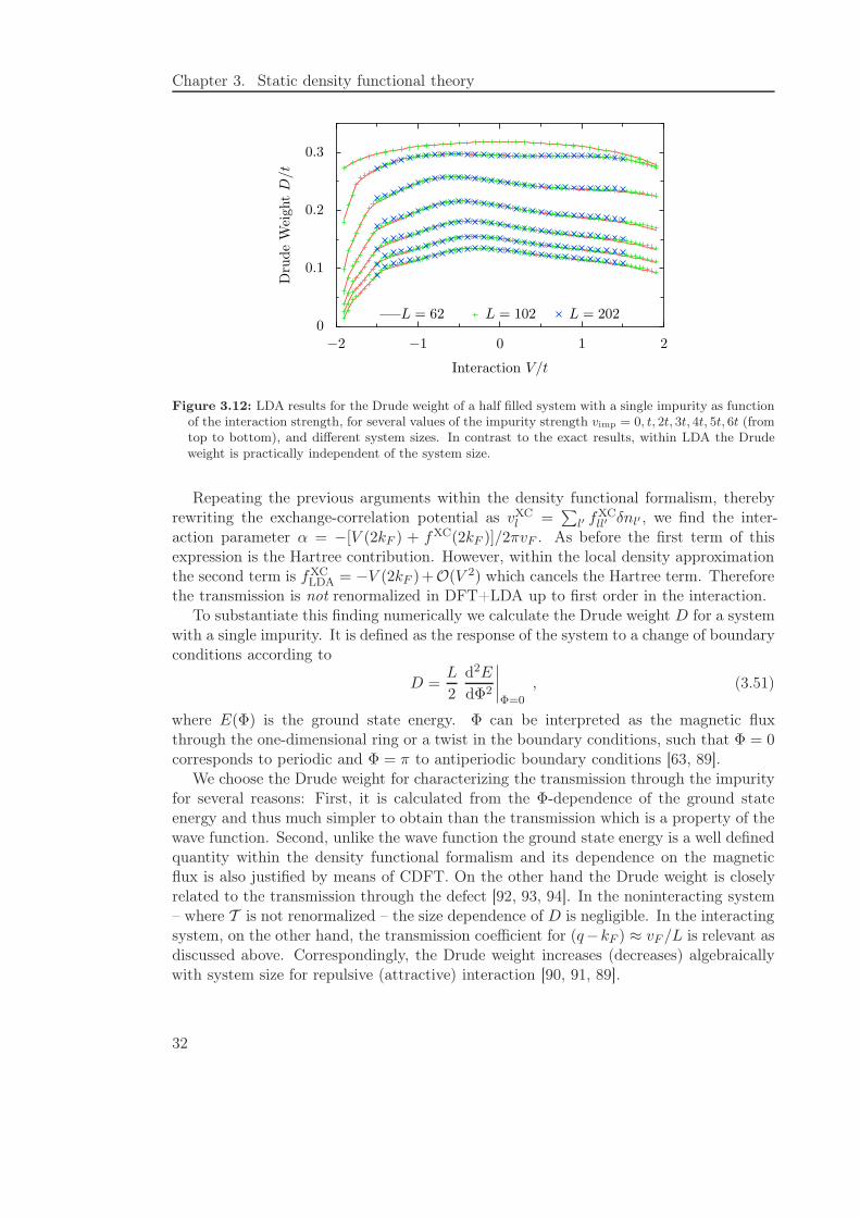
Figure 3.12: LDA results for the Drude weight of a half filled system with a single impurity as functionof the interaction strength, for several values of the impurity strength vimp = 0, t, 2t, 3t, 4t, 5t, 6t (fromtop to bottom), and different system sizes. In contrast to the exact results, within LDA the Drudeweight is practically independent of the system size.
Repeating the previous arguments within the density functional formalism, therebyrewriting the exchange-correlation potential as vXC
l =∑
l′ fXCll′ δnl′ , we find the inter-
action parameter α = −[V (2kF ) + fXC(2kF )]/2πvF . As before the first term of thisexpression is the Hartree contribution. However, within the local density approximationthe second term is fXC
LDA = −V (2kF )+O(V 2) which cancels the Hartree term. Thereforethe transmission is not renormalized in DFT+LDA up to first order in the interaction.
To substantiate this finding numerically we calculate the Drude weight D for a systemwith a single impurity. It is defined as the response of the system to a change of boundaryconditions according to
D =L
2
d2E
dΦ2
∣∣∣∣Φ=0
, (3.51)
where E(Φ) is the ground state energy. Φ can be interpreted as the magnetic fluxthrough the one-dimensional ring or a twist in the boundary conditions, such that Φ = 0corresponds to periodic and Φ = π to antiperiodic boundary conditions [63, 89].
We choose the Drude weight for characterizing the transmission through the impurityfor several reasons: First, it is calculated from the Φ-dependence of the ground stateenergy and thus much simpler to obtain than the transmission which is a property of thewave function. Second, unlike the wave function the ground state energy is a well definedquantity within the density functional formalism and its dependence on the magneticflux is also justified by means of CDFT. On the other hand the Drude weight is closelyrelated to the transmission through the defect [92, 93, 94]. In the noninteracting system– where T is not renormalized – the size dependence of D is negligible. In the interactingsystem, on the other hand, the transmission coefficient for (q−kF ) ≈ vF /L is relevant asdiscussed above. Correspondingly, the Drude weight increases (decreases) algebraicallywith system size for repulsive (attractive) interaction [90, 91, 89].
32
3.3. Practical applications
0
0.1
0.2
0.3
Dru
de
Wei
ghtD/t
−1.5 −1 −0.5 0 0.5 1 1.5
Interaction V/t
L = 14
L = 30
L = 62
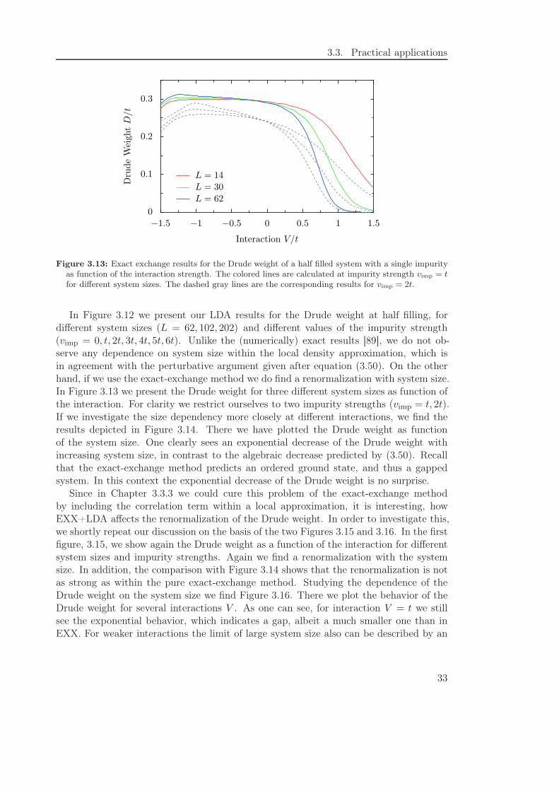
Figure 3.13: Exact exchange results for the Drude weight of a half filled system with a single impurityas function of the interaction strength. The colored lines are calculated at impurity strength vimp = tfor different system sizes. The dashed gray lines are the corresponding results for vimp = 2t.
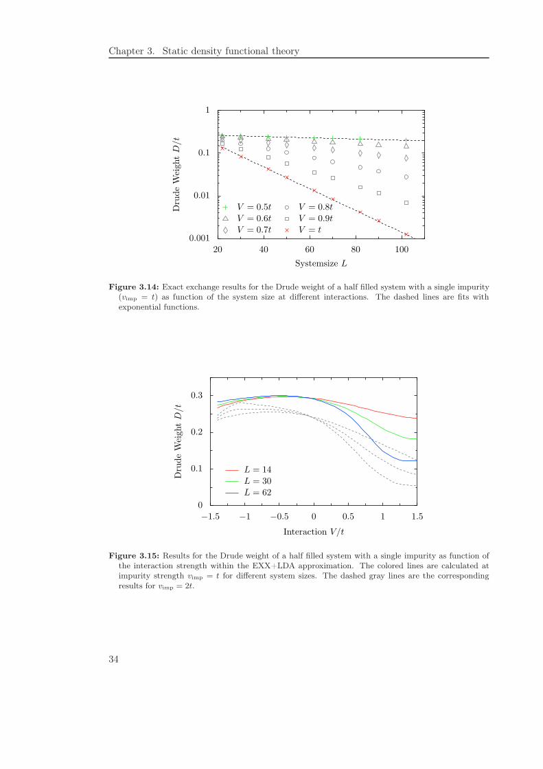
In Figure 3.12 we present our LDA results for the Drude weight at half filling, fordifferent system sizes (L = 62, 102, 202) and different values of the impurity strength(vimp = 0, t, 2t, 3t, 4t, 5t, 6t). Unlike the (numerically) exact results [89], we do not ob-serve any dependence on system size within the local density approximation, which isin agreement with the perturbative argument given after equation (3.50). On the otherhand, if we use the exact-exchange method we do find a renormalization with system size.In Figure 3.13 we present the Drude weight for three different system sizes as function ofthe interaction. For clarity we restrict ourselves to two impurity strengths (vimp = t, 2t).If we investigate the size dependency more closely at different interactions, we find theresults depicted in Figure 3.14. There we have plotted the Drude weight as functionof the system size. One clearly sees an exponential decrease of the Drude weight withincreasing system size, in contrast to the algebraic decrease predicted by (3.50). Recallthat the exact-exchange method predicts an ordered ground state, and thus a gappedsystem. In this context the exponential decrease of the Drude weight is no surprise.
Since in Chapter 3.3.3 we could cure this problem of the exact-exchange methodby including the correlation term within a local approximation, it is interesting, howEXX+LDA affects the renormalization of the Drude weight. In order to investigate this,we shortly repeat our discussion on the basis of the two Figures 3.15 and 3.16. In the firstfigure, 3.15, we show again the Drude weight as a function of the interaction for differentsystem sizes and impurity strengths. Again we find a renormalization with the systemsize. In addition, the comparison with Figure 3.14 shows that the renormalization is notas strong as within the pure exact-exchange method. Studying the dependence of theDrude weight on the system size we find Figure 3.16. There we plot the behavior of theDrude weight for several interactions V . As one can see, for interaction V = t we stillsee the exponential behavior, which indicates a gap, albeit a much smaller one than inEXX. For weaker interactions the limit of large system size also can be described by an
33
Chapter 3. Static density functional theory
0.001
0.01
0.1
1
Dru
de
Wei
ghtD/t
20 40 60 80 100
Systemsize L
V = 0.5t
V = 0.6t
V = 0.7t
V = 0.8t
V = 0.9t
V = t
Figure 3.14: Exact exchange results for the Drude weight of a half filled system with a single impurity(vimp = t) as function of the system size at different interactions. The dashed lines are fits withexponential functions.
0
0.1
0.2
0.3
Dru
de
Wei
ghtD/t
−1.5 −1 −0.5 0 0.5 1 1.5
Interaction V/t
L = 14
L = 30
L = 62
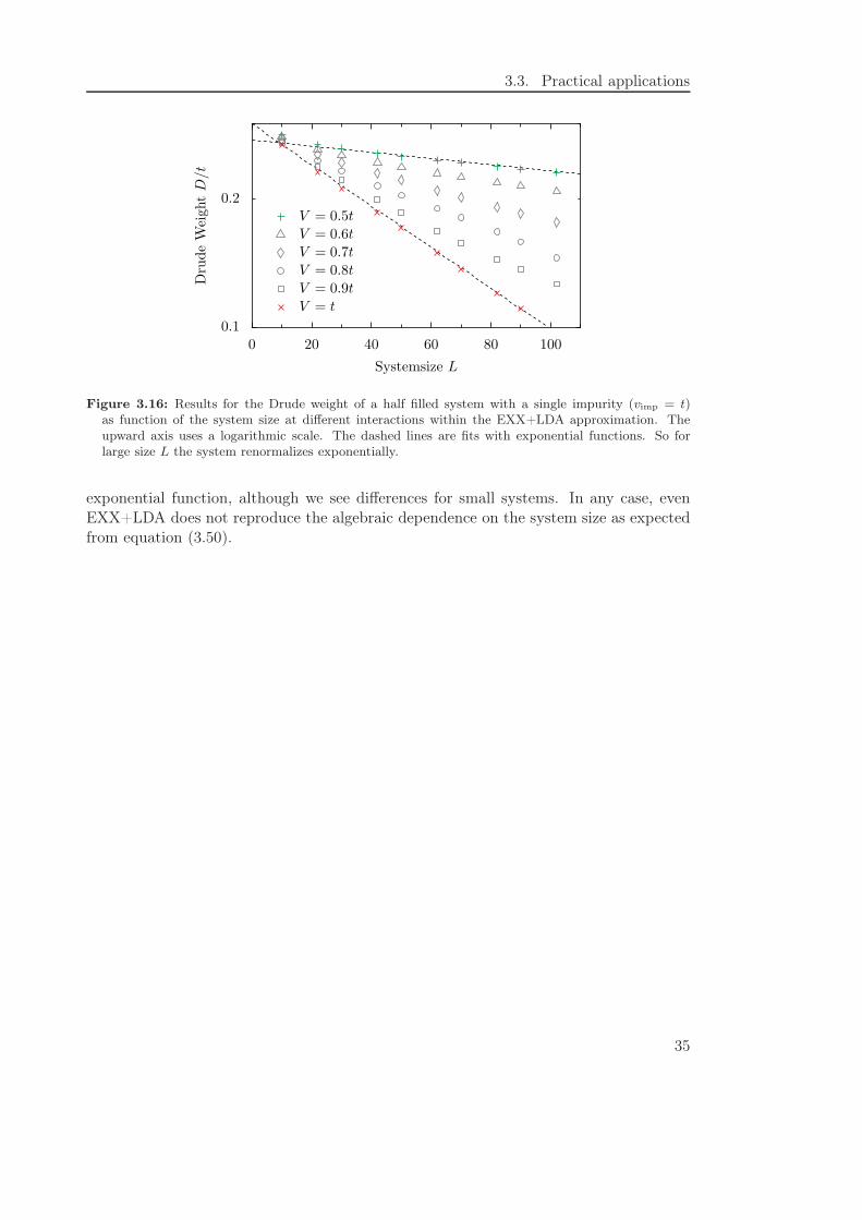
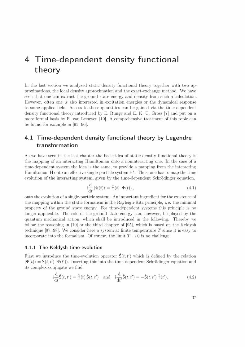
Figure 3.15: Results for the Drude weight of a half filled system with a single impurity as function ofthe interaction strength within the EXX+LDA approximation. The colored lines are calculated atimpurity strength vimp = t for different system sizes. The dashed gray lines are the correspondingresults for vimp = 2t.
34
3.3. Practical applications
0.1
0.2D
rude
Wei
ghtD/t
0 20 40 60 80 100
Systemsize L
V = 0.5t
V = 0.6t
V = 0.7t
V = 0.8t
V = 0.9t
V = t
Figure 3.16: Results for the Drude weight of a half filled system with a single impurity (vimp = t)as function of the system size at different interactions within the EXX+LDA approximation. Theupward axis uses a logarithmic scale. The dashed lines are fits with exponential functions. So forlarge size L the system renormalizes exponentially.
exponential function, although we see differences for small systems. In any case, evenEXX+LDA does not reproduce the algebraic dependence on the system size as expectedfrom equation (3.50).
35

Chapter 3. Static density functional theory
36
4 Time-dependent density functional
theory
In the last section we analyzed static density functional theory together with two ap-proximations, the local density approximation and the exact-exchange method. We haveseen that one can extract the ground state energy and density from such a calculation.However, often one is also interested in excitation energies or the dynamical responseto some applied field. Access to these quantities can be gained via the time-dependentdensity functional theory introduced by E. Runge and E. K. U. Gross [7] and put on amore formal basis by R. van Leeuwen [10]. A comprehensive treatment of this topic canbe found for example in [95, 96].
4.1 Time-dependent density functional theory by Legendre
transformation
As we have seen in the last chapter the basic idea of static density functional theory isthe mapping of an interacting Hamiltonian onto a noninteracting one. In the case of atime-dependent system the idea is the same, to provide a mapping from the interactingHamiltonian H onto an effective single-particle system Hs. Thus, one has to map the timeevolution of the interacting system, given by the time-dependent Schrödinger equation,
id
dt|Ψ(t)〉 = H(t) |Ψ(t)〉 , (4.1)
onto the evolution of a single-particle system. An important ingredient for the existence ofthe mapping within the static formalism is the Rayleigh-Ritz principle, i. e. the minimalproperty of the ground state energy. For time-dependent systems this principle is nolonger applicable. The role of the ground state energy can, however, be played by thequantum mechanical action, which shall be introduced in the following. Thereby wefollow the reasoning in [10] or the third chapter of [95], which is based on the Keldyshtechnique [97, 98]. We consider here a system at finite temperature T since it is easy toincorporate into the formalism. Of course, the limit T → 0 is no challenge.
4.1.1 The Keldysh time-evolution
First we introduce the time-evolution operator S(t, t′) which is defined by the relation|Ψ(t)〉 = S(t, t′) |Ψ(t′)〉. Inserting this into the time-dependent Schrödinger equation andits complex conjugate we find
id
dtS(t, t′) = H(t) S(t, t′) and i
d
dt′S(t, t′) = −S(t, t′) H(t′). (4.2)
37
Chapter 4. Time-dependent density functional theory
t
−iβ
0−
t−
t+
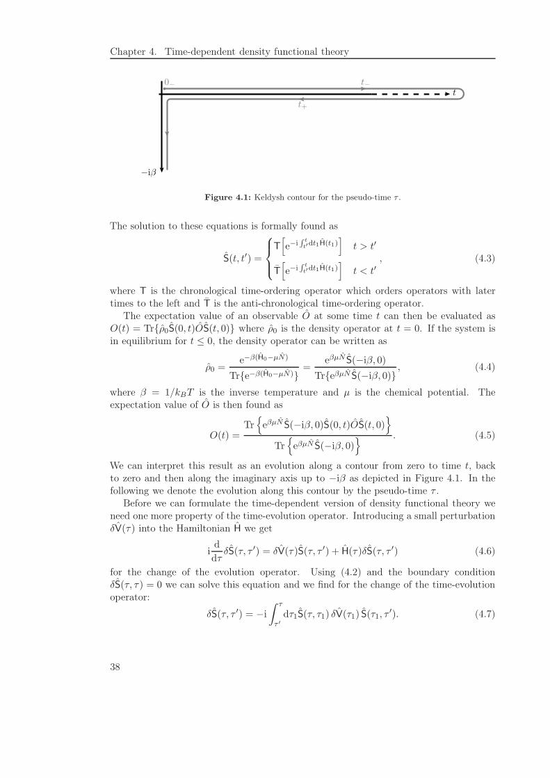
Figure 4.1: Keldysh contour for the pseudo-time τ .
The solution to these equations is formally found as
S(t, t′) =
T
[
e−iR t
t′dt1H(t1)
]
t > t′
T
[
e−iR t
t′dt1H(t1)
]
t < t′, (4.3)
where T is the chronological time-ordering operator which orders operators with latertimes to the left and T is the anti-chronological time-ordering operator.
The expectation value of an observable O at some time t can then be evaluated asO(t) = Tr{ρ0S(0, t)OS(t, 0)} where ρ0 is the density operator at t = 0. If the system isin equilibrium for t ≤ 0, the density operator can be written as
ρ0 =e−β(H0−µN)
Tr{e−β(H0−µN)}=
eβµN S(−iβ, 0)
Tr{eβµN S(−iβ, 0)}, (4.4)
where β = 1/kBT is the inverse temperature and µ is the chemical potential. Theexpectation value of O is then found as
O(t) =Tr{
eβµN S(−iβ, 0)S(0, t)OS(t, 0)}
Tr{
eβµN S(−iβ, 0)} . (4.5)
We can interpret this result as an evolution along a contour from zero to time t, backto zero and then along the imaginary axis up to −iβ as depicted in Figure 4.1. In thefollowing we denote the evolution along this contour by the pseudo-time τ .
Before we can formulate the time-dependent version of density functional theory weneed one more property of the time-evolution operator. Introducing a small perturbationδV(τ) into the Hamiltonian H we get
id
dτδS(τ, τ ′) = δV(τ)S(τ, τ ′) + H(τ)δS(τ, τ ′) (4.6)
for the change of the evolution operator. Using (4.2) and the boundary conditionδS(τ, τ) = 0 we can solve this equation and we find for the change of the time-evolutionoperator:
δS(τ, τ ′) = −i
∫ τ
τ ′
dτ1S(τ, τ1) δV(τ1) S(τ1, τ′). (4.7)
38
4.1. Time-dependent density functional theory by Legendre transformation
4.1.2 Action functional
The role of the ground state energy in static density functional theory is now played bythe functional
A[v, φ] = i ln Tr{
eβµNS(−iβ; 0−)
}
. (4.8)
Please note that v and φ are contour variables, i. e. they may take different values onthe forward and the backward branch, and S is the time-evolution operator along thecontour in Figure 4.1. Physical potentials can be recovered by requiring v(t+) = v(t−)after the calculation, where t+ and t− indicate equal times on the backward and forwardcontour, respectively. Since we want to use a Legendre transformation to transform fromthe potentials to their conjugate variables, the densities, and thus obtaining the effectivesingle-particle potential we need to check that for A equations analogous to (3.3) hold.By using (4.7) we find for a variation in the potential
δA
δvl(τ)=
Tr{
eβµN S(−iβ, 0)S(0, τ)nlS(τ, 0−)}
Tr{
eβµN S(−iβ, 0−)} = nl(τ). (4.9)
Similarly we find for a variation in the phase
δA
δφl(τ)= jl(τ). (4.10)
In the next step we perform the Legendre transformation from the potentials and phasesto the densities and currents,
A[n, j] = A[v, φ] −
∫
Cdτ∑
l
nl(τ)vl(τ) −
∫
Cdτ∑
l
jl(τ)Φl(τ). (4.11)
The subscript C implies integration over the whole contour. As usual one recovers thelocal potentials and phases by
δA
δnl(τ)= −vl(τ) and
δA
δjl(τ)= −φl(τ). (4.12)
If we follow the same procedure for a noninteracting system Hs, i. e. by defining atime-evolution operator Ss(t, t′) and then introducing the functional As similar to (4.8),we can again perform a Legendre transformation from the single-particle potentials andphases to their conjugate variables
As[n, j] = As[vs, φs] −
∫
Cdτ∑
l
nl(τ)vsl (τ) −
∫
Cdτ∑
l
jl(τ)φsl (τ). (4.13)
Since we want our auxiliary system Hs to yield the same densities and currents as theinteracting system H we relate A and As through the identity
A[n, j] = As[n, j] + (A[n, j] −As[n, j]) = As[n, j] +AHXC[n, j]. (4.14)
39
Chapter 4. Time-dependent density functional theory
The last equality is simply the definition of the Hartree-exchange-correlation functionalAHXC[n, j]. Using (4.12) we find the following rule for determining the effective single-particle quantities,
vl(τ) = vsl (τ) − vHXC
l (τ),
φl(τ) = φsl (τ) − φXC
l (τ),(4.15)
where the Hartree-exchange-correlation potential vHXCl (τ) is defined as
vHXCl (τ) =
δAHXC
δnl(τ). (4.16)
Since the Hartree term does not depend on the currents, we find
φXCl (τ) =
δAXC
δjl(τ), (4.17)
which also depends on all densities and currents. Please remember that all these quan-tities depend on the contour-time variable τ instead of the physical time t. Thus thevariation of the potentials (phases) in positive t-direction is independent of the variationin negative t-direction. Physical potentials can be recovered by requiring physical den-sities, i. e. they are the same on the forward and the backward branch of the contour.Then we have
vHXCl (t) =
δAHXC
δnl(τ)
∣∣∣∣n=nl(t),j=jl(t)
and φXCl (t) =
δAHXC
δjl(τ)
∣∣∣∣n=nl(t),j=jl(t)
. (4.18)
4.1.3 Gauge invariance
An important point we have neglected up to now is the gauge invariance of our system.The influence of gauge invariance on density functional theory is twofold: On one handit is desirable that not only the interacting system but also the single-particle system isgauge-invariant. On the other hand the gauge invariance affects the Legendre transform,because the transform (4.11) is no longer unique. So the question arises, if this non-uniqueness affects physical quantities.
We begin by shortly repeating how a gauge transformation (2.8) affects the potentialsand phases:
φ′l = φl + χl − χl+1
v′l = vl − χl(4.19)
Thus, if we variate the generating functional A in the direction of these gauge transfor-mations, we get
δA = A[v′, φ′] − A[v, φ] = −
∫
Cdτ∑
l
[χl(τ)nl(τ) + (χl+1(τ) − χl(τ)) jl(τ)] . (4.20)
40
4.1. Time-dependent density functional theory by Legendre transformation
Partial integration of the first term and resummation of the second term leads to
δA = −
∫
Cdτ∑
l
χl(τ) [nl(τ) + jl(τ) − jl−1(τ)] . (4.21)
Since A is gauge invariant, it follows that δA = 0 for all χl(τ), thereby implying thecontinuity equation (2.7). Thus our question from above has to be answered with: yes,the gauge invariance does affect physical quantities, but in a completely desirable way,since it enforces the continuity equation.
Of course, the gauge transformation is recovered by the back-transformation fromthe densities to the potentials, A[n, j] → A[v, φ]. In this case one can exploit thatthe Legendre transform uses an extremal condition (cf. Appendix C) and calculate theextremum under the constraint that the continuity equation is fulfilled,
A[v, φ] = extn,j
{
A[n, j] −
∫
Cdτ∑
l
χl(τ) [nl(τ) + jl(τ) − jl−1(τ)]
}
. (4.22)
Here the χl(τ) are the Lagrange parameters. Invoking, as before, a partial integration ofthe first term and a resummation of the second, the extremum is now given by
δA
δnl(τ)+ χl(τ) = −vl(τ) (4.23)
andδA
δjl(τ)+ χl+1(τ) − χl(τ) = −φl(τ). (4.24)
Comparing this expressions with (4.12) we find the original gauge transformation (4.19).
4.1.4 Dynamical susceptibility and causality
After this introduction of time-dependent density functional theory we now turn our at-tention to an important quantity which is accessible within this framework, the dynamicalsusceptibility. For example, the explicit evaluation on the contour of the density-densityresponse function gives
χnn(l, τ, l′, τ ′) = −δnl(τ)
δvl′(τ ′)= i⟨TC [∆nl(τ)∆nl′(τ
′)]⟩. (4.25)
Here ∆nl(τ) is a density fluctuation operator ∆nl(τ) = nl(τ)−〈nl(τ)〉 in the Heisenbergpicture. Switching back to physical potentials, where δv(t) = δv(t+) = δv(t−), we find
δnl(t) = −
∫
dt′∑
l′
[
χ(l, τ, l′, τ ′)∣∣τ=t,τ ′=t′
−
− χ(l, τ, l′, τ ′)∣∣τ=t,τ ′=t′+
]
δvl′(t′), (4.26)
where the change of sign in the second term comes from the integration on the backwardsbranch of the contour. Inserting (4.25) gives
δnl(t) = −
∫
dt′∑
l′
χRnn(l, t, l′, t′) δvl′(t
′), (4.27)
41
Chapter 4. Time-dependent density functional theory
with the definition χRnn(l, t, l′, t′) = iΘ(t − t′) 〈[nl(t), nl′(t
′)]〉 for the retarded density-density correlation function. The step function Θ originates from the cancellation ofterms for t′ > t.
If we repeat the whole argument for the single-particle functional As we find accord-ingly the single-particle susceptibility χs
nn. Since the solution of our single-particle systemprovides us with χs
nn and we are interested in the response χnn of the interacting system,we need a relation between the two. This can be found by noticing that the Legendretransformation provides also a relation between A[n, j] and the susceptibility,
[χnn(l, τ, l′, τ ′)
]−1=
δ2A
δnl(τ) δnl′(τ ′). (4.28)
Then, using this relation together with (4.14) we find
[χnn]−1 = [χsnn]−1 + fHXC
nn , (4.29)
where we defined the so-called Hartree-exchange-correlation kernel as
fHXCnn (l, τ, l′, τ ′) =
δvHXCl (τ)
δnl′(τ ′). (4.30)
Please note that it is defined as functional derivative on the contour. Applying thesame procedure as for the susceptibilities when going back from the pseudo-times on theKeldysh contour to physical times gives a retarded Hartree-exchange-correlation kernel,which therefore introduces a source of memory into the calculation. This causality cru-cially depends on the fact that the variations of the potential along the forward and thebackward part of the contour are independent. If we would use physical potentials in thedefinition of the susceptibility, for example,
δ2A
δvl(t) δvl′(t′)=
δnl(t)
δvl′(t′)= −χnn(l, t, l′, t′), (4.31)
the left-hand side would be symmetric under exchange of (l, t) and (l′, t′). Thus theresponse function χ would not be zero for t′ > t, i. e. not causal [99, 100, 96].
In the preceding discussion we used χnn to illustrate the principle of the Keldyshformalism, but similarly we may consider the density-current- or the current-currentcorrelation functions (χnj , χjn and χjj). Hence we will use a matrix notation to denotethe susceptibility in the following,
χ =
(
χRnn χR
nj
χRjn χR
jj
)
. (4.32)
Accordingly the Hartree-exchange-correlation kernel has a similar structure,
fHXC =
(
fHXCnn,R fHXC
nj,R
fHXCjn,R fHXC
jj,R
)
, (4.33)
42
4.2. Approximations
where the elements fHXCµν,R are the retarded versions of
fHXCµν (l, τ, l′, τ ′) =
δ2AHXC
δµl(τ) δνl′(τ ′). (4.34)
Thus (4.29) can be written in the form
[χ]−1 = [χs]−1 + fHXC or χ =[1 + χsfHXC
]−1χs. (4.35)
The components of the matrix (4.32) are related via the continuity equation or gaugetransformations. A short summary of these relations and a few symmetries can be foundin Appendix D.
4.2 Approximations
Clearly, similar to the static formalism, we have avoided the problem of solving the time-dependent many-body Schrödinger equation by putting all interaction effects into theHartree-exchange-correlation potential. However, since we do not know this quantity,we have to use some approximations. As already discussed in Chapter 3, we separatethe Hartree potential from the exchange-correlation potential. Since in the Hartree po-tential the interaction is instantaneous there is no further complication within the time-dependent formalism. So we have vHXC = vH + vXC and the kernel of the susceptibilitybecomes fHXC = fH + fXC. Therefore the susceptibility (4.35) reduces to the standardRPA expression if fXC = 0. Note that fH only has an nn-entry, in Fourier representationgiven by V (q) = 2V cos q. However, as we saw in Section 4.1.4, the exchange-correlationpotential does in principle have a memory, i. e. it depends on all previous densities. Thesimplest approximation is then to assume that the system evolves adiabatically, whichmeans that it is completely determined by the densities (and currents) at the consid-ered time. In this case we can just reuse the exchange-correlation potentials and phasescalculated from the static exchange-correlation energy (3.23).
It does, however, make an essential difference if we consider charge densities only ortogether with the current-densities. In the first case this assumption, together with thelocal density approximation, gives the so-called adiabatic LDA, also known as ALDA,while we denote the second case with C-ALDA where the C stands for the current. Themain difference between these two is that the ALDA is a truly local approximation bothin space and in time while the inclusion of currents takes some nonlocal effects, again bothin space and in time, into account [9]. The reason for this is simply particle conservationas can be seen from the continuity equation for our one-dimensional lattice model,
− ω n(q, ω) + 2 sinq
2j(q, ω) = 0 (4.36)
or in real spacenl(t) = jl−1(t) − jl(t). (4.37)
A more thorough investigation of nonlocal exchange-correlation potentials, that can beconstructed with help of currents, can be found in [9, 101] and the resulting functional has
43
Chapter 4. Time-dependent density functional theory
been tested for example by P. L. de Boeij [102]. The adiabatic LDA has been comparedwith exact results in [103, 104]. For the calculation of the exchange-correlation kernelwithin the exact-exchange approximation we refer to [87, 88]. It has already been appliedin [105, 106, 107, 108].
4.3 Dynamic Susceptibility
Now we investigate the dynamical susceptibility within C-ALDA in more detail. Inparticular, we consider a homogeneous system with total flux Φ → 0. In this limit, thecurrent also vanishes, j → 0. In this case we find that the off-diagonal elements of theHartree-exchange-correlation kernel (4.33), fHXC
jn and fHXCnj , both vanish, because the
expansion of the ground state energy with respect to the current has no first order term.Thus fHXC contains only the two terms fHXC
nn and fHXCjj , and the χnn-element of (4.35)
is given by
χnn(q, ω) = χsnn(q, ω) − χs
nn(q, ω)fHXCnn χnn(q, ω) − χs
nj(q, ω)fHXCjj χjn(q, ω). (4.38)
Employing particle conservation (D.5) we rewrite the density-current correlators in termsof the density-density response. Solving then for χnn we get
χnn(q, ω) =χs
nn(q, ω)
1 + χsnn(q, ω)
[
fHXCnn + ω2
4 sin2(q/2)fHXC
jj
] , (4.39)
where fHXCnn and fHXC
jj are, due to the local adiabatic approximation, independent of q
and ω. If fHXCjj = 0 we recover the approximation known as ALDA.
In order to discuss this result in more detail, recall that in the long-wavelength low-frequency limit the density response of the single-particle system is given by
χsnn(q, ω) ≃ χs
stat(qvF )2
(qvF )2 − (ω + i0)2, (4.40)
where vF is the Fermi-velocity and the static susceptibility is given by χsstat = 1/πvF .
Considering the limit ω = 0, q → 0, and noting that
fXCnn =
1
L
(∂2EBA
∂n2−∂2E0
∂n2− 2LV
)
(4.41)
it is straightforward to verify that the density response of the interacting system is
χstat =
(1
L
∂2EBA
∂n2
)−1
. (4.42)
On the other hand, taking q → 0 first, we find
χjj(q = 0, ω → 0) = −2DBA, (4.43)
44
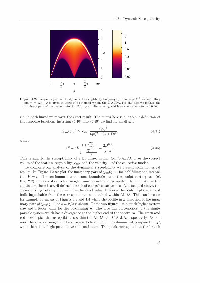
4.3. Dynamic Susceptibility
01
2π π
3
2π 2π
q
0
1
2
3
4
5
ω
0.02
0.05
0.1
0.2
0.5
1
2
Figure 4.2: Imaginary part of the dynamical susceptibility Imχnn(q, ω) in units of t−1 for half fillingand V = 1.0t. ω is given in units of t obtained within the C-ALDA. For the plot we replace theimaginary part of the denominator in (D.3) by a finite value, η, which we choose here to be 0.005t.
i. e. in both limits we recover the exact result. The minus here is due to our definition ofthe response function. Inserting (4.40) into (4.39) we find for small q, ω
χnn(q, ω) ≃ χstat(qv)2
(qv)2 − (ω + i0)2, (4.44)
where
v2 = v2F
1 + fHXCnn
πvF
1 −fHXC
jj vF
π
=2DBA
χstat. (4.45)
This is exactly the susceptibility of a Luttinger liquid. So, C-ALDA gives the correctvalues of the static susceptibility χstat and the velocity v of the collective modes.
To complete our analysis of the dynamical susceptibility we present some numericalresults. In Figure 4.2 we plot the imaginary part of χnn(q, ω) for half filling and interac-tion V = t. The continuum has the same boundaries as in the noninteracting case (cf.Fig. 2.2), but now its spectral weight vanishes in the long-wavelength limit. Above thecontinuum there is a well-defined branch of collective excitations. As discussed above, thecorresponding velocity for q → 0 has the exact value. However the contour plot is almostindistinguishable from the corresponding one obtained within ALDA. This can be seenfor example by means of Figures 4.3 and 4.4 where the profile in ω-direction of the imag-inary part of χnn(q, ω) at q = π/2 is shown. These two figures use a much higher systemsize and a lower value for the broadening η. The blue line corresponds to the single-particle system which has a divergence at the higher end of the spectrum. The green andred lines depict the susceptibilities within the ALDA and C-ALDA, respectively. As onesees, the spectral weight of the quasi-particle continuum is diminished compared to χs,while there is a single peak above the continuum. This peak corresponds to the branch
45
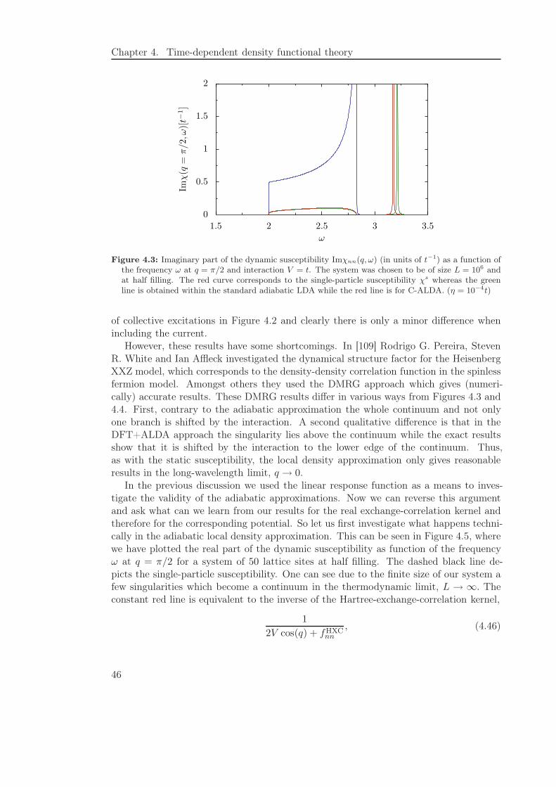
Chapter 4. Time-dependent density functional theory
0
0.5
1
1.5
2
Imχ(q
=π/2,ω
)[t−
1]
1.5 2 2.5 3 3.5
ω
Figure 4.3: Imaginary part of the dynamic susceptibility Imχnn(q, ω) (in units of t−1) as a function ofthe frequency ω at q = π/2 and interaction V = t. The system was chosen to be of size L = 106 andat half filling. The red curve corresponds to the single-particle susceptibility χs whereas the greenline is obtained within the standard adiabatic LDA while the red line is for C-ALDA. (η = 10−4t)
of collective excitations in Figure 4.2 and clearly there is only a minor difference whenincluding the current.
However, these results have some shortcomings. In [109] Rodrigo G. Pereira, StevenR. White and Ian Affleck investigated the dynamical structure factor for the HeisenbergXXZ model, which corresponds to the density-density correlation function in the spinlessfermion model. Amongst others they used the DMRG approach which gives (numeri-cally) accurate results. These DMRG results differ in various ways from Figures 4.3 and4.4. First, contrary to the adiabatic approximation the whole continuum and not onlyone branch is shifted by the interaction. A second qualitative difference is that in theDFT+ALDA approach the singularity lies above the continuum while the exact resultsshow that it is shifted by the interaction to the lower edge of the continuum. Thus,as with the static susceptibility, the local density approximation only gives reasonableresults in the long-wavelength limit, q → 0.
In the previous discussion we used the linear response function as a means to inves-tigate the validity of the adiabatic approximations. Now we can reverse this argumentand ask what can we learn from our results for the real exchange-correlation kernel andtherefore for the corresponding potential. So let us first investigate what happens techni-cally in the adiabatic local density approximation. This can be seen in Figure 4.5, wherewe have plotted the real part of the dynamic susceptibility as function of the frequencyω at q = π/2 for a system of 50 lattice sites at half filling. The dashed black line de-picts the single-particle susceptibility. One can see due to the finite size of our system afew singularities which become a continuum in the thermodynamic limit, L → ∞. Theconstant red line is equivalent to the inverse of the Hartree-exchange-correlation kernel,
1
2V cos(q) + fHXCnn
, (4.46)
46
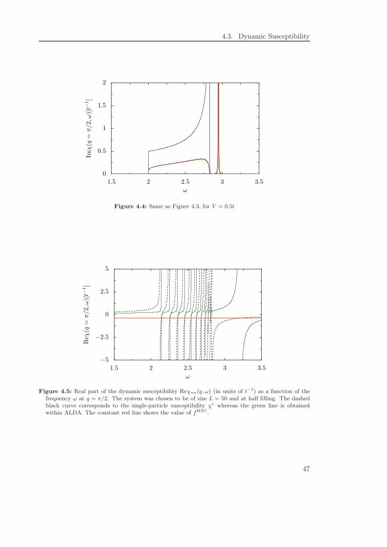
4.3. Dynamic Susceptibility
0
0.5
1
1.5
2Imχ(q
=π/2,ω)[t−
1]
1.5 2 2.5 3 3.5
ω
Figure 4.4: Same as Figure 4.3, for V = 0.5t
−5
−2.5
0
2.5
5
Reχ
(q=π/2,ω)[t−
1]
1.5 2 2.5 3 3.5
ω
Figure 4.5: Real part of the dynamic susceptibility Reχnn(q, ω) (in units of t−1) as a function of thefrequency ω at q = π/2. The system was chosen to be of size L = 50 and at half filling. The dashedblack curve corresponds to the single-particle susceptibility χs whereas the green line is obtainedwithin ALDA. The constant red line shows the value of fHXC.
47
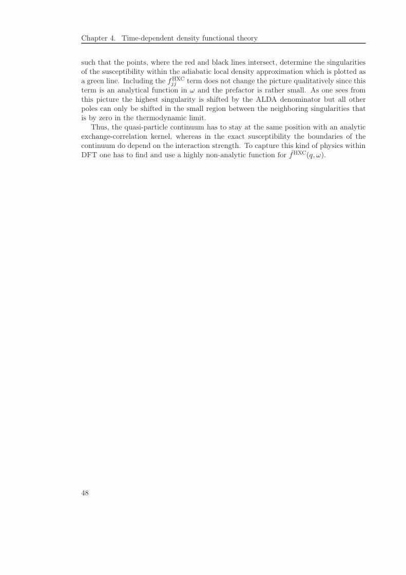
Chapter 4. Time-dependent density functional theory
such that the points, where the red and black lines intersect, determine the singularitiesof the susceptibility within the adiabatic local density approximation which is plotted asa green line. Including the fHXC
jj term does not change the picture qualitatively since thisterm is an analytical function in ω and the prefactor is rather small. As one sees fromthis picture the highest singularity is shifted by the ALDA denominator but all otherpoles can only be shifted in the small region between the neighboring singularities thatis by zero in the thermodynamic limit.
Thus, the quasi-particle continuum has to stay at the same position with an analyticexchange-correlation kernel, whereas in the exact susceptibility the boundaries of thecontinuum do depend on the interaction strength. To capture this kind of physics withinDFT one has to find and use a highly non-analytic function for fHXC(q, ω).
48
5 Transport through a quantum dot
As already said before, DFT is an important tool for determining the electronic structureof materials. In recent years the application of density functional theory to the electronictransport through interfaces between two materials or through nanocontacts between twoleads became more and more important. In the following we concentrate on the latter.As an application they can be used for electronics of molecular size while from a theo-retical point of view they consist of open systems out of equilibrium. Both features, theopen system and the non-equilibrium are very difficult to treat theoretically. In order toinvestigate the quality of density functional theory when applied to such a problem, oneneeds to decide whether discrepancies to the experiment or other theoretical approachesarise because of an insufficient modeling of said features or because of the underlyingapproximation for the exchange-correlation potential. In the following we focus on thelatter question and study the conductance through a quantum dot by means of the linearconductance which only depends on equilibrium quantities. Moreover we employ a modelwhich has already been investigated using the density-matrix renormalization group ap-proach (DMRG). Thus we are able to assess the quality of different approximations evenfor strong interactions.
5.1 Model
In this chapter we modify our model of spinless fermions. We follow [56], where theauthors used DMRG to calculate the exact conductance of a quantum dot attached toleads. Figure 5.1 is a schematic picture of this model. The Hamiltonian can be writtenas
H = HC + HL + HR + HC↔L + HC↔R (5.1)
where HC is the Hamiltonian for the central system. HL and HR stand for the left andright lead, respectively, while HC↔L and HC↔R are the couplings between the leads andthe system. The central system HC consists of ten real-space sites. The first two sitesare noninteracting, whereas the next five sites, the (quantum) dot, are interacting andcan also be tuned by a gate voltage vgate. The last three sites are again noninteracting.Therefore the corresponding Hamiltonian can be written as
HC = −9∑
l=1
tl,l+1
(c+l cl+1 + c+l+1cl
)+ V
6∑
l=3
(
nl −1
2
)(
nl+1 −1
2
)
+7∑
l=3
vgate nl. (5.2)
49
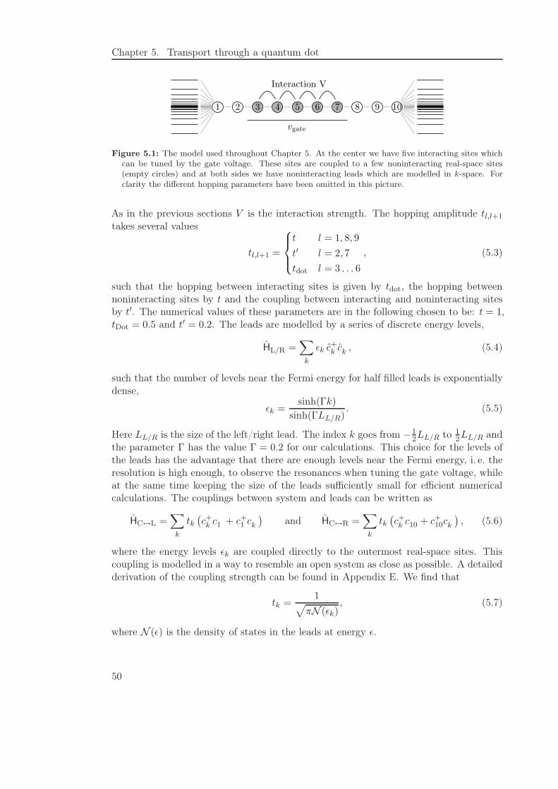
Chapter 5. Transport through a quantum dot
1 2 3 4 5 6 7 8 9 10
vgate
Interaction V
Figure 5.1: The model used throughout Chapter 5. At the center we have five interacting sites whichcan be tuned by the gate voltage. These sites are coupled to a few noninteracting real-space sites(empty circles) and at both sides we have noninteracting leads which are modelled in k-space. Forclarity the different hopping parameters have been omitted in this picture.
As in the previous sections V is the interaction strength. The hopping amplitude tl,l+1
takes several values
tl,l+1 =
t l = 1, 8, 9
t′ l = 2, 7
tdot l = 3 . . . 6
, (5.3)
such that the hopping between interacting sites is given by tdot, the hopping betweennoninteracting sites by t and the coupling between interacting and noninteracting sitesby t′. The numerical values of these parameters are in the following chosen to be: t = 1,tDot = 0.5 and t′ = 0.2. The leads are modelled by a series of discrete energy levels,
HL/R =∑
k
ǫk c+k ck , (5.4)
such that the number of levels near the Fermi energy for half filled leads is exponentiallydense,
ǫk =sinh(Γk)
sinh(ΓLL/R). (5.5)
Here LL/R is the size of the left/right lead. The index k goes from −12LL/R to 1
2LL/R andthe parameter Γ has the value Γ = 0.2 for our calculations. This choice for the levels ofthe leads has the advantage that there are enough levels near the Fermi energy, i. e. theresolution is high enough, to observe the resonances when tuning the gate voltage, whileat the same time keeping the size of the leads sufficiently small for efficient numericalcalculations. The couplings between system and leads can be written as
HC↔L =∑
k
tk(c+k c1 + c+1 ck
)and HC↔R =
∑
k
tk(c+k c10 + c+10ck
), (5.6)
where the energy levels ǫk are coupled directly to the outermost real-space sites. Thiscoupling is modelled in a way to resemble an open system as close as possible. A detailedderivation of the coupling strength can be found in Appendix E. We find that
tk =1
√
πN (ǫk), (5.7)
where N (ǫ) is the density of states in the leads at energy ǫ.
50
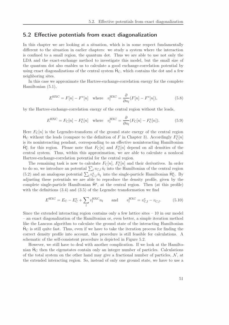
5.2. Effective potentials from exact diagonalization
5.2 Effective potentials from exact diagonalization
In this chapter we are looking at a situation, which is in some respect fundamentallydifferent to the situation in earlier chapters: we study a system where the interactionis confined to a small region, the quantum dot. Thus we are able to use not only theLDA and the exact-exchange method to investigate this model, but the small size ofthe quantum dot also enables us to calculate a good exchange-correlation potential byusing exact diagonalizations of the central system HC, which contains the dot and a fewneighboring sites.
In this case we approximate the Hartree-exchange-correlation energy for the completeHamiltonian (5.1),
EHXC = F [n] − F s[n] where vHXCl =
∂
∂nl(F [n] − F s[n]), (5.8)
by the Hartree-exchange-correlation energy of the central region without the leads,
EHXC = FC[n] − F sC[n] where vHXC
l =∂
∂nl(FC[n] − F s
C[n]). (5.9)
Here FC[n] is the Legendre-transform of the ground state energy of the central regionHC without the leads (compare to the definition of F in Chapter 3). Accordingly F s
C[n]is its noninteracting pendant, corresponding to an effective noninteracting HamiltonianHs
C for this region. Please note that FC[n] and F sC[n] depend on all densities of the
central system. Thus, within this approximation, we are able to calculate a nonlocalHartree-exchange-correlation potential for the central region.
The remaining task is now to calculate FC[n], F sC[n] and their derivatives. In order
to do so, we introduce an potential∑
l vC,l nl into the Hamiltonian of the central region
(5.2) and an analogous potential∑
l vsC,l nl into the single-particle Hamiltonian Hs
C. Byadjusting these potentials we are able to reproduce the density profile, given by thecomplete single-particle Hamiltonian Hs, at the central region. Then (at this profile)with the definitions (3.4) and (3.5) of the Legendre transformation we find
EHXC = EC − EsC +
∑
l
vHXCl nl and vHXC
l = vsC,l − vC,l. (5.10)
Since the extended interacting region contains only a few lattice sites – 10 in our model– an exact diagonalization of the Hamiltonian or, even better, a simple iteration methodlike the Lanczos algorithm to calculate the ground state of the interacting HamiltonianHC is still quite fast. Thus, even if we have to take the iteration process for finding thecorrect density profile into account, this procedure is still feasible for calculations. Aschematic of the self-consistent procedure is depicted in Figure 5.2.
However, we still have to deal with another complication. If we look at the Hamilto-nian HC then the eigenstates contain only an integer number of particles. Calculationsof the total system on the other hand may give a fractional number of particles, N , atthe extended interacting region. So, instead of only one ground state, we have to use a
51
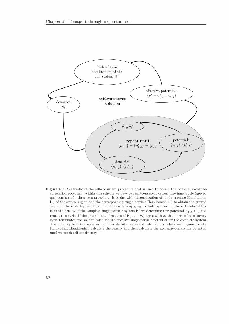
Chapter 5. Transport through a quantum dot
Kohn-Sham
hamiltonian of the
full system Hs
densities
{nl}
effective potentials
{vsl = vs
C,l − vC,l}self-consistent
solution
repeat until
{nC,l} = {nsC,l} = {nl }
HC, HsC
densities
{nC,l}, {nsC,l}
potentials
{vC,l}, {vsC,l}
Figure 5.2: Schematic of the self-consistent procedure that is used to obtain the nonlocal exchange-correlation potential. Within this scheme we have two self-consistent cycles. The inner cycle (greyedout) consists of a three-step procedure. It begins with diagonalization of the interacting HamiltonianHC of the central region and the corresponding single-particle Hamiltonian H
sC to obtain the ground
state. In the next step we determine the densities nsC,l, nC,l of both systems. If these densities differ
from the density of the complete single-particle system Hs we determine new potentials vs
C,l, vC,l and
repeat this cycle. If the ground state densities of HC and HsC agree with nl the inner self-consistency
cycle terminates and we can calculate the effective single-particle potential for the complete system.The outer cycle is the same as for other density functional calculations, where we diagonalize theKohn-Sham Hamiltonian, calculate the density and then calculate the exchange-correlation potentialuntil we reach self-consistency.
52
5.2. Effective potentials from exact diagonalization
superposition of states with different particle numbers. The most simple superpositionis described by the density operator
ρ = α |N, 0〉 〈N, 0| + (1 − α) |N + 1, 0〉 〈N + 1, 0| , (5.11)
where |N, 0〉 denotes the N -particle ground state. N lies between the integer numbersN and N + 1 and α = N + 1 −N is chosen, such that Tr{ρN} = N . We can motivatethis ansatz by considering the density operator for the grand canonical ensemble
ρ =1
Ze−β(HC−µN). (5.12)
The partition function is defined as Z = Tr{e−β(HC−µN)}, β is the inverse temperature,µ the chemical potential and N the particle number operator of the system. The zerotemperature limit β → ∞ gives a projector to a single state ρ = |N, 0〉 〈N, 0| and thenumber of particles as a function of the chemical potential is a step-function. If we chooseµ = EN+1 − EN , where EN is the energy of the N -particle ground state, the system isexactly in between the N - and the N + 1-particle ground state,
ρ =1
2(|N, 0〉 〈N, 0| + |N + 1, 0〉 〈N + 1, 0|) . (5.13)
Any slight deviation of this value gives again a pure state with an integer number ofparticles. However if we use an arbitrary small but finite temperature the steps betweenthe particle numbers are broadened and we can adjust µ to give any fractional particlenumber. In this case the dominant part of the density operator reads:
ρ =1
Z
[
|N, 0〉 〈N, 0| e−β(EN−µN) + |N + 1, 0〉 〈N + 1, 0| e−β(EN+1−µ(N+1))]
. (5.14)
One then finds the relation
µ = EN+1 − EN +1
βln
(1
α− 1
)
. (5.15)
between µ and α. Considering only discrete systems (and neglecting degeneracies) wecan always choose the temperature small enough so that only the two states |N, 0〉 and|N + 1, 0〉 contribute significantly. This was also found in [110] for the ground stateenergy of a system with fractional particle number. In the following we abbreviate thisapproximation with ED (exact diagonalization). In Figure 5.3 we show an example forthe Hartree-exchange-correlation potential at the central region obtained with DFT+EDcompared to the potential from the exact-exchange method.
The exact diagonalization procedure, as discussed in this section, is by constructionnot applicable to long chains of interacting fermions. However, one may ask, if we cangeneralize this procedure to such systems. A straightforward generalization is to look atsite l and calculate the exchange-correlation energy for this site from exact diagonaliza-tion of this site together with its neighbors. By studying the static susceptibility withthis generalization we find two inherent artifacts that render this method useless. Thecorresponding discussion can be found in Appendix F.1.
53
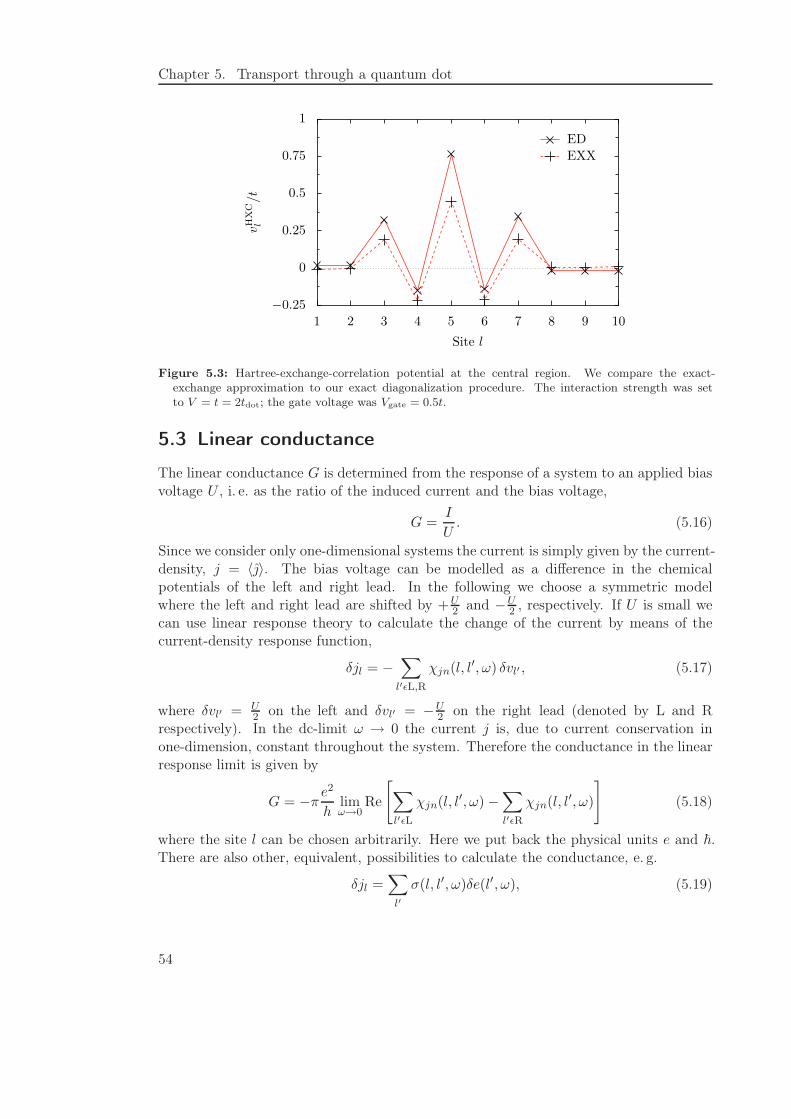
Chapter 5. Transport through a quantum dot
−0.25
0
0.25
0.5
0.75
1
vH
XC
l/t
1 2 3 4 5 6 7 8 9 10
Site l
ED
EXX
Figure 5.3: Hartree-exchange-correlation potential at the central region. We compare the exact-exchange approximation to our exact diagonalization procedure. The interaction strength was setto V = t = 2tdot; the gate voltage was Vgate = 0.5t.
5.3 Linear conductance
The linear conductance G is determined from the response of a system to an applied biasvoltage U , i. e. as the ratio of the induced current and the bias voltage,
G =I
U. (5.16)
Since we consider only one-dimensional systems the current is simply given by the current-density, j = 〈〉. The bias voltage can be modelled as a difference in the chemicalpotentials of the left and right lead. In the following we choose a symmetric modelwhere the left and right lead are shifted by +U
2 and −U2 , respectively. If U is small we
can use linear response theory to calculate the change of the current by means of thecurrent-density response function,
δjl = −∑
l′ǫL,R
χjn(l, l′, ω) δvl′ , (5.17)
where δvl′ = U2 on the left and δvl′ = −U
2 on the right lead (denoted by L and Rrespectively). In the dc-limit ω → 0 the current j is, due to current conservation inone-dimension, constant throughout the system. Therefore the conductance in the linearresponse limit is given by
G = −πe2
hlimω→0
Re
[∑
l′ǫL
χjn(l, l′, ω) −∑
l′ǫR
χjn(l, l′, ω)
]
(5.18)
where the site l can be chosen arbitrarily. Here we put back the physical units e and ~.There are also other, equivalent, possibilities to calculate the conductance, e. g.
δjl =∑
l′
σ(l, l′, ω)δe(l′, ω), (5.19)
54
5.3. Linear conductance
where e(l, ω) = iωφl − vl+1 + vl corresponds to the electric field and σ is the nonlocalconductivity. In a gauge where the electric field is put into the local phase one finds
G = πe2
hlimω→0
Re1
iω(χjj(l, lL↔C , ω) + χjj(l, lC↔R, ω)) . (5.20)
Here the indices lL↔C and lC↔R denote the sites of the system coupled to the left andright lead, respectively. All other elements of the sums vanish because of the constantpotential. Using a static gauge transformation we can shift these two indices to anyposition on the central region. For practical application of equation (5.20) it is favorableto evaluate the current-current correlation function not at the bonds to the leads but atthe first bonds within the central region (l1→2 and l9→10 with the notation of fig. 5.1).The reason simply is that in the former case we have to evaluate the current from everyenergy level of the leads to the central region while the latter only needs the currentbetween two sites. Since the exact result does not depend on l one may also choose l asl1↔2 and as l9↔10 and again average over this two values, so that the conductance of thesingle-particle system becomes
Gs = πe2
hlimω→0
Re1
2iω
∑
k,p
|〈k| l1↔2+ l9↔10
|p〉|2 (fk − fp)
ω + ǫp − ǫk + iη
= πe2
hlimω→0
−η
2ω
∑
k,p
|〈k| l1↔2+ l9↔10
|p〉|2 (fk − fp)
(ω + ǫp − ǫk)2 + η2
= πe2
hη∑
k,p
|〈k| l1↔2+ l9↔10
|p〉|2 (fk − fp)
[(ǫp − ǫk)2 + η2]2(ǫk − ǫp).
(5.21)
Since we are dealing with a finite system the parameter η is kept bigger than zero.This leads to a broadening of the energy levels and to an additional source/drain in thecontinuity equation for the leads,
∂tnl + ηnl + jl − jl−1 = 0. (5.22)
η must be chosen large enough, so that enough particles are created/annihilated in theleads to sustain the current through the system. On the other hand if it is too large,too much details of the conductance are smeared out. A sensible choice for our systemis found to be η = 0.4 · 10−4. Due to the relations between the current-current, current-density and density-density correlator one can also use χnn to calculate the conductance.Beginning with (5.18) and using the continuity equation (5.22), one finds
Gs =πe2η
2h
∑
k,p
∣∣∣〈k| NL + NR |p〉
∣∣∣
2(fk − fp)
(ǫp − ǫk)2 + η2(ǫk − ǫp). (5.23)
Here NL and NR are the occupation number operator for the left and the right lead,respectively. Using the same argument as before we symmetrized the expression withrespect to exchanging L↔ R.
55
Chapter 5. Transport through a quantum dot
As already stated during the discussion of the susceptibilities in Chapters 3 and 4the susceptibility of the interacting system is given by the single-particle susceptibilitymodified by a denominator similar to the random-phase approximation (RPA). Thereforewe also have to modify the conductance. If we use, for example, the density-densitycorrelator to calculate the conductance (5.23),
G = πe2
2hlimω→0
Re∑
l,l′ǫL,R
(iω + η)χnn(l, l′, ω) = πe2η
2hRe
∑
l,l′ǫL,R
χnn(l, l′, 0), (5.24)
with L and R denoting the left and the right lead, the correction to the single-particlesusceptibility is given by the matrix equation
χnn =[1 − χs
nnfHXCnn
]−1χs
nn. (5.25)
The elements of the matrix χnn are given by [χnn]ll′ = χnn(l, l′, 0). We will see soon thatthe Hartree-exchange-correlation kernel fHXC
nn is irrelevant for the model and approxima-tions of the present study. Nevertheless we complete here the general discussion. Weanalyze equation (5.25) under the assumption that fHXC
nn can be truncated in real spacefor positions that are far from the interacting region. Clearly this assumption holds forthe ALDA, where fHXC
nn is confined to the interacting region. In this case it is given by
[fHXCnn ]ll′ =
fXCALDA(nl) if l = l′and l, l′ interacting
V if l = l′ + 1, l′ − 1 and l, l′ interacting
0 otherwise
, (5.26)
where l and l′ are interacting sites. Please remember that fXCLDA(nl) = ∂vXC(nl)/∂nl.
V is the interaction strength and the elements on the secondary diagonal are derivedfrom the Hartree potentials. Since we need only the double sum of the susceptibilities(5.24) and fHXC
nn is confined to the interacting region, we do not have to solve the matrixequation (5.25) but the simpler equations
∑
i,j ǫ L,R
[χnn]ij =∑
i,j ǫ L,R
[χsnn]ij +
∑
l,m ǫ C
(∑
i ǫ L,R
[χsnn]il
)
[fHXCnn ]lm
(∑
j ǫ L,R
[χnn]mj
)
(5.27)
and
∑
j ǫ L,R
[χnn]lj =∑
j ǫ L,R
[χsnn]lj +
∑
l′,m ǫ C
[χsnn]ll′ [f
HXCnn ]l′m
(∑
j ǫ L,R
[χnn]mj
)
. (5.28)
Here C denotes the sites of the central region. The second equation is needed to calculatethe last term of the first equation. Therefore the index l only denotes sites of theinteracting system and the second equation can be solved self-consistently. Thus in amore compact syntax the conductance can be written as
G = Gs +πe2η
2hRe{χs fHXC
nn χ}
χ = χs + χsred f
HXCnn χ,
(5.29)
56
5.4. Results
with the vectors χ =∑
jǫL,R[χnn]lj and χs =∑
jǫL,R[χsnn]lj . χ
sred is a ‘reduced’ suscepti-
bility of the single-particle system, which only takes into account changes of the densityin the interacting system due to variations of the potential at the interacting system.The solution of this reduced form of the matrix equation does in our case (ALDA for fiveinteracting sites) only need the inversion of a 5 × 5-matrix instead of a L× L-matrix asin (5.25) and is thus numerically quite efficient.
As already stated before the exchange-correlation kernel is irrelevant for the calcula-tion of the linear conductance within our model. Rewriting equation 5.19 as
δjl =∑
l′
σs(l, l′)[δe(l′) + δeHXC(l′)
], (5.30)
where σs is the single-particle conductivity and δeHXC = −vHXCl+1 +vHXC
l , we can rephrase
the above statement as: The internal field δeHXC does not contribute to the conductivity.This can be easily seen in one dimension: Particle conservation implies the current isconstant throughout the system, i. e. σs does not depent on the position l. Additionallywe have the symmetry σs(l, l′) = σs(l′, l), thus it also does not depend on l′. Then thecurrent through our dot becomes
δj = σs∑
l′
[δe(l′) + δeHXC(l′)
]. (5.31)
Inserting the explicit expression for the internal field we see that most terms of the sumcancel and only the two Hartree-exchange-correlation potentials at the interfaces to theleads contribute. If they are small, as to be expected for our system where the interactionis confined to a small region, we may neglect them and find that σs = σ.
5.4 Results
Calculating the conductance for our model system with various approximations for differ-ent interaction strengths gives a number of interesting results. With figures 5.4 to 5.11 weshow a representative overview of these results. In the previous section we have alreadyargued that the Hartree-exchange-correlation kernel is negligible. In fact, within thelocal density approximation the contribution of this kernel is zero, because the exchange-correlation potential is confined to the interacting region. Thus we use G = Gs in thefollowing discussion.
5.4.1 General features
The first figure, 5.4, shows the conductance as function of the gate voltage for the non-interacting system (grey line) and for a relatively weak interaction, V = 0.5t = tdot (redline). The results in this graph were obtained with LDA. The first, trivial, observationsare that there are five resonances and the conductance at each of the resonances is equalto one. The number of the resonances is just the number of energy levels of our dot andoccur whenever, by tuning vgate, one of the levels is at the Fermi energy. The height of
57
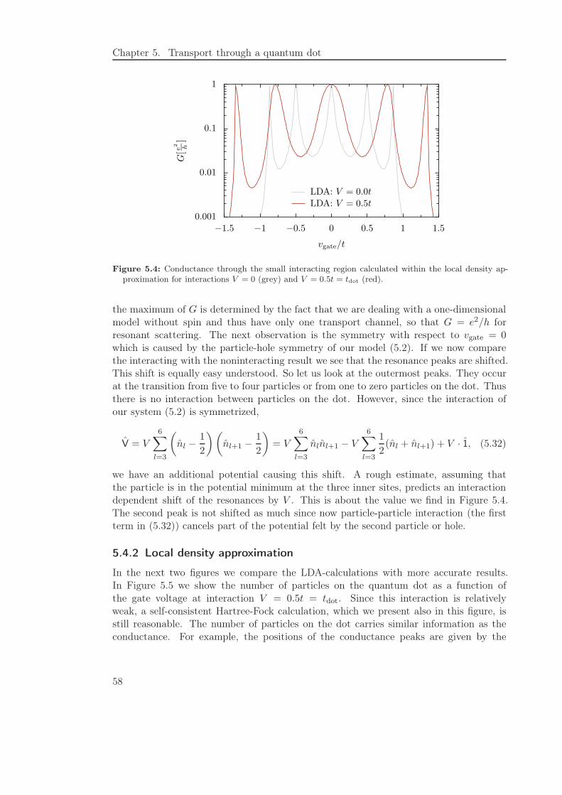
Chapter 5. Transport through a quantum dot
0.001
0.01
0.1
1
G[e
2 h]
−1.5 −1 −0.5 0 0.5 1 1.5
vgate/t
LDA: V = 0.0t
LDA: V = 0.5t
Figure 5.4: Conductance through the small interacting region calculated within the local density ap-proximation for interactions V = 0 (grey) and V = 0.5t = tdot (red).
the maximum of G is determined by the fact that we are dealing with a one-dimensionalmodel without spin and thus have only one transport channel, so that G = e2/h forresonant scattering. The next observation is the symmetry with respect to vgate = 0which is caused by the particle-hole symmetry of our model (5.2). If we now comparethe interacting with the noninteracting result we see that the resonance peaks are shifted.This shift is equally easy understood. So let us look at the outermost peaks. They occurat the transition from five to four particles or from one to zero particles on the dot. Thusthere is no interaction between particles on the dot. However, since the interaction ofour system (5.2) is symmetrized,
V = V
6∑
l=3
(
nl −1
2
)(
nl+1 −1
2
)
= V
6∑
l=3
nlnl+1 − V
6∑
l=3
1
2(nl + nl+1) + V · 1, (5.32)
we have an additional potential causing this shift. A rough estimate, assuming thatthe particle is in the potential minimum at the three inner sites, predicts an interactiondependent shift of the resonances by V . This is about the value we find in Figure 5.4.The second peak is not shifted as much since now particle-particle interaction (the firstterm in (5.32)) cancels part of the potential felt by the second particle or hole.
5.4.2 Local density approximation
In the next two figures we compare the LDA-calculations with more accurate results.In Figure 5.5 we show the number of particles on the quantum dot as a function ofthe gate voltage at interaction V = 0.5t = tdot. Since this interaction is relativelyweak, a self-consistent Hartree-Fock calculation, which we present also in this figure, isstill reasonable. The number of particles on the dot carries similar information as theconductance. For example, the positions of the conductance peaks are given by the
58
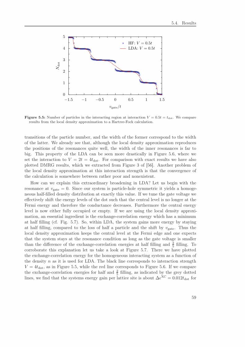
5.4. Results
0
1
2
3
4
5
Ndot
−1.5 −1 −0.5 0 0.5 1 1.5
vgate/t
HF: V = 0.5t
LDA: V = 0.5t
Figure 5.5: Number of particles in the interacting region at interaction V = 0.5t = tdot. We compareresults from the local density approximation to a Hartree-Fock calculation.
transitions of the particle number, and the width of the former correspond to the widthof the latter. We already see that, although the local density approximation reproducesthe positions of the resonances quite well, the width of the inner resonances is far tobig. This property of the LDA can be seen more drastically in Figure 5.6, where weset the interaction to V = 2t = 4tdot. For comparison with exact results we have alsoplotted DMRG results, which we extracted from Figure 3 of [56]. Another problem ofthe local density approximation at this interaction strength is that the convergence ofthe calculation is somewhere between rather poor and nonexistent.
How can we explain this extraordinary broadening in LDA? Let us begin with theresonance at vgate = 0. Since our system is particle-hole symmetric it yields a homoge-neous half-filled density distribution at exactly this value. If we tune the gate voltage weeffectively shift the energy levels of the dot such that the central level is no longer at theFermi energy and therefore the conductance decreases. Furthermore the central energylevel is now either fully occupied or empty. If we are using the local density approxi-mation, an essential ingredient is the exchange-correlation energy which has a minimumat half filling (cf. Fig. 5.7). So, within LDA, the system gains more energy by stayingat half filling, compared to the loss of half a particle and the shift by vgate. Thus thelocal density approximation keeps the central level at the Fermi edge and one expectsthat the system stays at the resonance condition as long as the gate voltage is smallerthan the difference of the exchange-correlation energies at half filling and 2
5 filling. Tocorroborate this explanation let us take a look at Figure 5.7. There we have plottedthe exchange-correlation energy for the homogeneous interacting system as a function ofthe density n as it is used for LDA. The black line corresponds to interaction strengthV = 4tdot, as in Figure 5.5, while the red line corresponds to Figure 5.6. If we comparethe exchange-correlation energies for half and 2
5 filling, as indicated by the grey dottedlines, we find that the systems energy gain per lattice site is about ∆ǫXC = 0.012tdot for
59
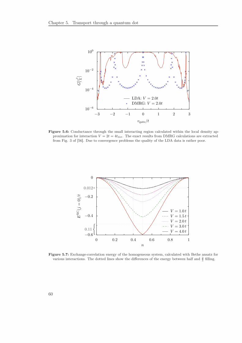
Chapter 5. Transport through a quantum dot
10−6
10−4
10−2
100
G[e
2 h]
−3 −2 −1 0 1 2 3
vgate/t
LDA: V = 2.0t
DMRG: V = 2.0t
Figure 5.6: Conductance through the small interacting region calculated within the local density ap-proximation for interaction V = 2t = 4tdot. The exact results from DMRG calculations are extractedfrom Fig. 3 of [56]. Due to convergence problems the quality of the LDA data is rather poor.
−0.6
−0.4
−0.2
0
EX
C(j
=0)/t
0 0.2 0.4 0.6 0.8 1
n
{
{
0.11
0.012
V = 1.0 t
V = 1.5 t
V = 2.0 t
V = 3.0 t
V = 4.0 t
Figure 5.7: Exchange-correlation energy of the homogeneous system, calculated with Bethe ansatz forvarious interactions. The dotted lines show the differences of the energy between half and 2
5filling.
60
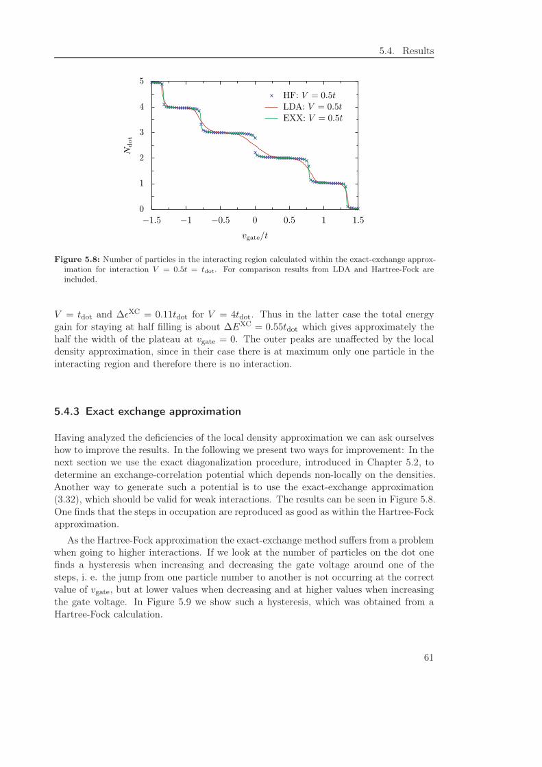
5.4. Results
0
1
2
3
4
5
Ndot
−1.5 −1 −0.5 0 0.5 1 1.5
vgate/t
HF: V = 0.5t
LDA: V = 0.5t
EXX: V = 0.5t
Figure 5.8: Number of particles in the interacting region calculated within the exact-exchange approx-imation for interaction V = 0.5t = tdot. For comparison results from LDA and Hartree-Fock areincluded.
V = tdot and ∆ǫXC = 0.11tdot for V = 4tdot. Thus in the latter case the total energygain for staying at half filling is about ∆EXC = 0.55tdot which gives approximately thehalf the width of the plateau at vgate = 0. The outer peaks are unaffected by the localdensity approximation, since in their case there is at maximum only one particle in theinteracting region and therefore there is no interaction.
5.4.3 Exact exchange approximation
Having analyzed the deficiencies of the local density approximation we can ask ourselveshow to improve the results. In the following we present two ways for improvement: In thenext section we use the exact diagonalization procedure, introduced in Chapter 5.2, todetermine an exchange-correlation potential which depends non-locally on the densities.Another way to generate such a potential is to use the exact-exchange approximation(3.32), which should be valid for weak interactions. The results can be seen in Figure 5.8.One finds that the steps in occupation are reproduced as good as within the Hartree-Fockapproximation.
As the Hartree-Fock approximation the exact-exchange method suffers from a problemwhen going to higher interactions. If we look at the number of particles on the dot onefinds a hysteresis when increasing and decreasing the gate voltage around one of thesteps, i. e. the jump from one particle number to another is not occurring at the correctvalue of vgate, but at lower values when decreasing and at higher values when increasingthe gate voltage. In Figure 5.9 we show such a hysteresis, which was obtained from aHartree-Fock calculation.
61
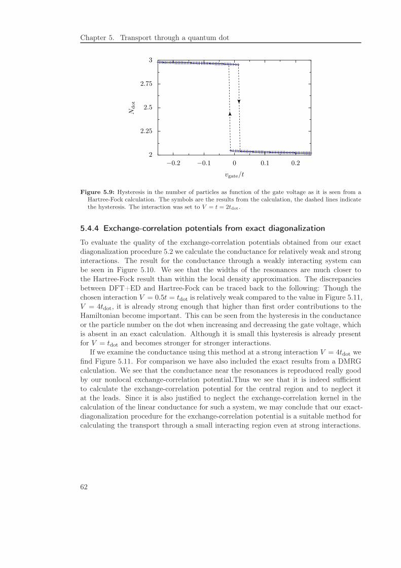
Chapter 5. Transport through a quantum dot
2
2.25
2.5
2.75
3
Ndot
−0.2 −0.1 0 0.1 0.2
vgate/t
Figure 5.9: Hysteresis in the number of particles as function of the gate voltage as it is seen from aHartree-Fock calculation. The symbols are the results from the calculation, the dashed lines indicatethe hysteresis. The interaction was set to V = t = 2tdot.
5.4.4 Exchange-correlation potentials from exact diagonalization
To evaluate the quality of the exchange-correlation potentials obtained from our exactdiagonalization procedure 5.2 we calculate the conductance for relatively weak and stronginteractions. The result for the conductance through a weakly interacting system canbe seen in Figure 5.10. We see that the widths of the resonances are much closer tothe Hartree-Fock result than within the local density approximation. The discrepanciesbetween DFT+ED and Hartree-Fock can be traced back to the following: Though thechosen interaction V = 0.5t = tdot is relatively weak compared to the value in Figure 5.11,V = 4tdot, it is already strong enough that higher than first order contributions to theHamiltonian become important. This can be seen from the hysteresis in the conductanceor the particle number on the dot when increasing and decreasing the gate voltage, whichis absent in an exact calculation. Although it is small this hysteresis is already presentfor V = tdot and becomes stronger for stronger interactions.
If we examine the conductance using this method at a strong interaction V = 4tdot wefind Figure 5.11. For comparison we have also included the exact results from a DMRGcalculation. We see that the conductance near the resonances is reproduced really goodby our nonlocal exchange-correlation potential.Thus we see that it is indeed sufficientto calculate the exchange-correlation potential for the central region and to neglect itat the leads. Since it is also justified to neglect the exchange-correlation kernel in thecalculation of the linear conductance for such a system, we may conclude that our exact-diagonalization procedure for the exchange-correlation potential is a suitable method forcalculating the transport through a small interacting region even at strong interactions.
62
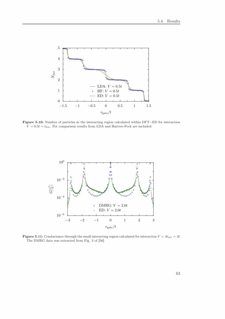
5.4. Results
0
1
2
3
4
5
Ndot
−1.5 −1 −0.5 0 0.5 1 1.5
vgate/t
LDA: V = 0.5t
HF: V = 0.5t
ED: V = 0.5t
Figure 5.10: Number of particles in the interacting region calculated within DFT+ED for interactionV = 0.5t = tdot. For comparison results from LDA and Hartree-Fock are included.
10−6
10−4
10−2
100
G[e
2 h]
−3 −2 −1 0 1 2 3
vgate/t
DMRG: V = 2.0t
ED: V = 2.0t
Figure 5.11: Conductance through the small interacting region calculated for interaction V = 4tdot = 2t.The DMRG data was extracted from Fig. 3 of [56].
63

Chapter 5. Transport through a quantum dot
64
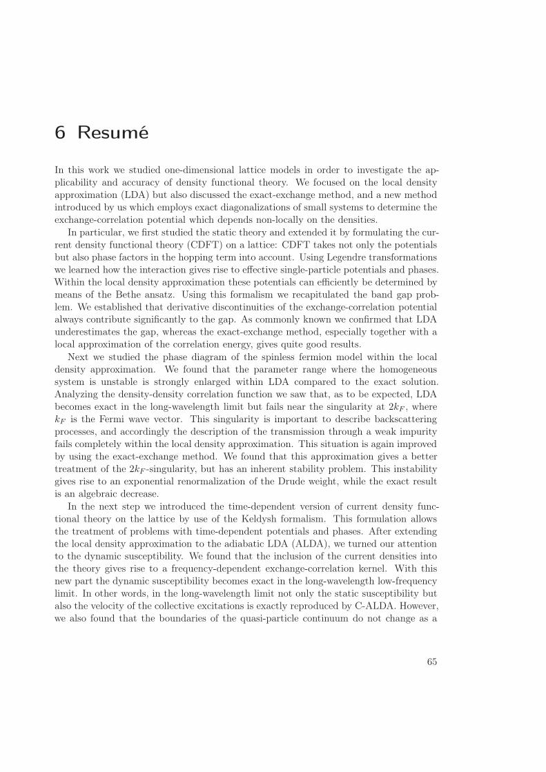
6 Resumé
In this work we studied one-dimensional lattice models in order to investigate the ap-plicability and accuracy of density functional theory. We focused on the local densityapproximation (LDA) but also discussed the exact-exchange method, and a new methodintroduced by us which employs exact diagonalizations of small systems to determine theexchange-correlation potential which depends non-locally on the densities.
In particular, we first studied the static theory and extended it by formulating the cur-rent density functional theory (CDFT) on a lattice: CDFT takes not only the potentialsbut also phase factors in the hopping term into account. Using Legendre transformationswe learned how the interaction gives rise to effective single-particle potentials and phases.Within the local density approximation these potentials can efficiently be determined bymeans of the Bethe ansatz. Using this formalism we recapitulated the band gap prob-lem. We established that derivative discontinuities of the exchange-correlation potentialalways contribute significantly to the gap. As commonly known we confirmed that LDAunderestimates the gap, whereas the exact-exchange method, especially together with alocal approximation of the correlation energy, gives quite good results.
Next we studied the phase diagram of the spinless fermion model within the localdensity approximation. We found that the parameter range where the homogeneoussystem is unstable is strongly enlarged within LDA compared to the exact solution.Analyzing the density-density correlation function we saw that, as to be expected, LDAbecomes exact in the long-wavelength limit but fails near the singularity at 2kF , wherekF is the Fermi wave vector. This singularity is important to describe backscatteringprocesses, and accordingly the description of the transmission through a weak impurityfails completely within the local density approximation. This situation is again improvedby using the exact-exchange method. We found that this approximation gives a bettertreatment of the 2kF -singularity, but has an inherent stability problem. This instabilitygives rise to an exponential renormalization of the Drude weight, while the exact resultis an algebraic decrease.
In the next step we introduced the time-dependent version of current density func-tional theory on the lattice by use of the Keldysh formalism. This formulation allowsthe treatment of problems with time-dependent potentials and phases. After extendingthe local density approximation to the adiabatic LDA (ALDA), we turned our attentionto the dynamic susceptibility. We found that the inclusion of the current densities intothe theory gives rise to a frequency-dependent exchange-correlation kernel. With thisnew part the dynamic susceptibility becomes exact in the long-wavelength low-frequencylimit. In other words, in the long-wavelength limit not only the static susceptibility butalso the velocity of the collective excitations is exactly reproduced by C-ALDA. However,we also found that the boundaries of the quasi-particle continuum do not change as a
65
Chapter 6. Resumé
function of the interaction strength, which does not reflect the true situation.In the fifth chapter we studied a model consisting of a small interacting region coupled
to two leads and calculated the linear conductance through this ‘quantum dot’. To assessthe quality of the results obtained from density functional theory, we checked themagainst results calculated within the Hartree-Fock approximation and with the densitymatrix renormalization group algorithm. We realized that even for weak interactionsthe local density approximation dramatically overestimates the width of the resonancepeaks. For stronger interactions this leads to a conductance which is several orders ofmagnitude higher than the true result. The reason for this problem is that the LDAnot only favors a homogeneous density profile, but also keeps the quantum dot near halffilling. We also found that the exact-exchange approximation gives reasonable results forweak interactions. Another interesting property of this model is that we do not have totake the exchange-correlation kernel into account for the calculation of the conductance,i. e. the internal field due to the interaction can be neglected. This can be done wheneverthe system has only one transport channel and the Hartree-exchange-correlation potentialis negligible at the contacts to the leads.
Since the local density approximation gave poor results, we looked for a way to deter-mine improved exchange-correlation potentials, depending not only on the local densitybut on all densities of the central region. This can be done by using exact diagonaliza-tions of the central region for the interacting and the single-particle case evaluated at thesame densities as the full system. We found that such an exchange-correlation potentialimproves the conductance dramatically.
Naturally we were not able to answer all open questions, so this work can be extendedin several ways: For example, up to now we have considered only systems with onetransport channel. One could simply add another channel by including the spin of aparticle, which would lead to the Hubbard model. In this case we could still use theBethe ansatz to determine the exchange-correlation potential within the local densityapproximation [111]. If we calculate the conductance through a small interacting regionwithin this model we will probably encounter situations where the exchange-correlationkernel cannot be neglected.
The exchange-correlation kernel was discussed in this work only within the adiabaticLDA and the C-ALDA. So in order to generalize the calculation of the conductanceto systems with a larger number of channels, where the local density approximationprobably still fails, we need for example to evaluate this kernel within the exact-exchangeapproximation. In this case we could investigate the influence of the exchange-correlationkernel on the conductance. We would also be able to answer the question whether theexact-exchange approximation improves the results for dynamical susceptibility.
So far we have considered only the linear conductance through a quantum dot. A nextstep would be to go beyond this linear regime and calculate the full I-V -characteristics.This is nowadays often done using the so-called ‘non-equilibrium Green’s functions’ to-gether with the Landauer-Büttiker formalism [49, 50]. However, this approach has twoproblems: First, it uses the eigenfunctions of the Kohn-Sham Hamiltonian to calculate theGreen’s functions, which is not justified within density functional theory. A second diffi-culty is that the transport through an interacting region is in principle a non-equilibrium
66
situation. Thus also a non-equilibrium exchange-correlation potential is required. Incontrast, recent calculations of the I-V -characteristics use equilibrium potentials only.Therefore it would be most interesting to see how the exchange-correlation potential fora non-equilibrium situation could be determined and how it affects the results.
67

Chapter 6. Resumé
68
A Some details of the spinless fermion
model
A.1 Jordan-Wigner-Transformation
The Jordan-Wigner transformation [66] is a way to transform a Heisenberg XXZ model
− J∑
l
(
σ(l)x σ(l+1)
x + σ(l)y σ(l+1)
y + ∆ σ(l)z σ(l+1)
z
)
(A.1)
into a model of spinless fermions with nearest-neighbor interaction. The relation betweenthe spin- and particle-operators are
σ(l)z = 2nl − 1
σ(l)− = exp
{
−iπ
l−1∑
i=1
nl
}
cl(A.2)
where σ(l)− = 1
2(σ(l)x − iσ
(l)y ). Using this the Heisenberg model can be written as
− 2J︸︷︷︸
t
∑
l
(c+l cl+1 + c+l+1cl
)−4J∆︸ ︷︷ ︸
V
∑
l
(
nl −1
2
)(
nl+1 −1
2
)
, (A.3)
where N is the particle number and L is the lattice size. So we have J = t2 and ∆ = −V
2twhere t and V are our usual spinless fermion parameters.
A.2 Bethe ansatz for spinless fermions
A useful and quite general tool for solving one-dimensional systems is the ansatz intro-duced by Bethe [112]. Some models that have been solved with this ‘Bethe ansatz’ are forexample the one-dimensional Bose gas [113, 114], the Heisenberg XXZ magnet [57, 64, 65],the Heisenberg XYZ chain [115] and the Hubbard model [111]. A comprehensive work onthis subject and related problems is the book by Korepin, Bogoliubov and Izergin [70].
Since we are basically working with a Heisenberg XXZ model we follow closely Yangand Yang [57] and only translate it into the spinless fermion language. Consider thehomogeneous spinless fermion model with nearest-neighbor interaction
H = −t∑
l
(c+l cl+1 + c+l+1cl
)+ V
∑
l
nlnl+1. (A.4)
69
Appendix A. Some details of the spinless fermion model
We are looking for the ground state solution |Ψ〉 of this Hamiltonian,
H |Ψ〉 = E |Ψ〉 , (A.5)
where |Ψ〉 can be written as
|Ψ〉 =∑
x1,...xN
ψ(x1 . . . xN ) c+x1c+x2
. . . c+xN|0〉 . (A.6)
Here |0〉 is the vacuum state and x1, . . . xN are the positions of the N particles. Now lookonto an ordered sector of the configuration space with x1 < x2 < . . . < xN . Consider aconfiguration 〈config| with N particles at positions x1, . . . xN where no pair of particlesis located at neighboring sites. Then applying 〈config| from the left to (A.5) gives
− tN∑
j=1
ψ(. . . xj − 1 . . .) + ψ(. . . xj + 1 . . .) = Eψ(x1 . . . xN ). (A.7)
If two particles are neighboring, xm+1 = xm + 1, we get the equation
− t∑
j 6=mj 6=m+1
[ψ(. . . xj − 1 . . .) + ψ(. . . xj + 1 . . .)] +
− t [ψ(. . . xm − 1, xm + 1 . . .) + ψ(. . . xm, xm + 2 . . .)]
= (E − V )ψ(x1 . . . xN ).
(A.8)
Now we make a plane-wave ansatz for the wave-function:
ψ(x1 . . . xN ) =∑
Perm.
APerm. exp
i
N∑
j=1
pPerm(j)xj
. (A.9)
The sum goes over all possible permutations of the momenta {pi}i=1...N . APerm. is aprefactor that depends on the permutation. Inserting this ansatz into (A.7) we get arelation for the energy as in the noninteracting case,
E = −2tN∑
j=1
cos pj. (A.10)
Using this together with (A.8) we obtain
AP
AQ= −
t+ t ei(p+q) + V eip
t+ t ei(p+q) + V eiq(A.11)
for the ratio of two amplitudes AP and AQ, where AP belongs to a permutation . . . p, q, . . .and AQ to the same permutation where only p and q are switched. This equation canalso be expressed as
AP = −e−iΘAQ, (A.12)
70
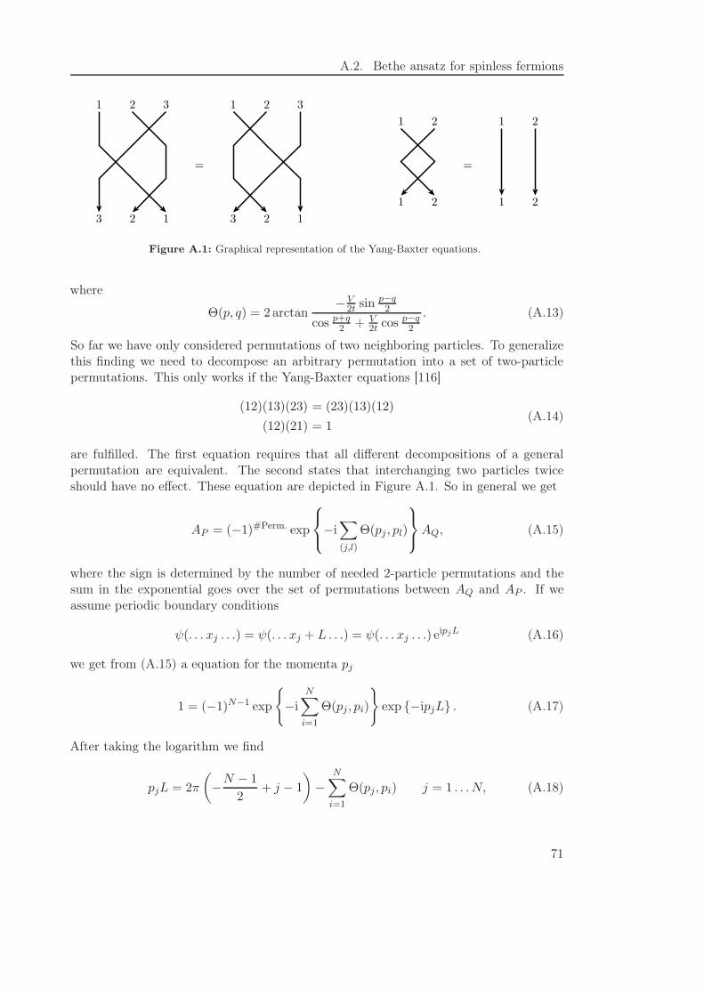
A.2. Bethe ansatz for spinless fermions
1 2 3
3 2 1
=
1 2 3
3 2 1
1 2
1 2
=
1 2
1 2
Figure A.1: Graphical representation of the Yang-Baxter equations.
where
Θ(p, q) = 2 arctan−V
2t sin p−q2
cos p+q2 + V
2t cos p−q2
. (A.13)
So far we have only considered permutations of two neighboring particles. To generalizethis finding we need to decompose an arbitrary permutation into a set of two-particlepermutations. This only works if the Yang-Baxter equations [116]
(12)(13)(23) = (23)(13)(12)
(12)(21) = 1(A.14)
are fulfilled. The first equation requires that all different decompositions of a generalpermutation are equivalent. The second states that interchanging two particles twiceshould have no effect. These equation are depicted in Figure A.1. So in general we get
AP = (−1)#Perm. exp
−i∑
(j,l)
Θ(pj , pl)
AQ, (A.15)
where the sign is determined by the number of needed 2-particle permutations and thesum in the exponential goes over the set of permutations between AQ and AP . If weassume periodic boundary conditions
ψ(. . . xj . . .) = ψ(. . . xj + L . . .) = ψ(. . . xj . . .) eipjL (A.16)
we get from (A.15) a equation for the momenta pj
1 = (−1)N−1 exp
{
−iN∑
i=1
Θ(pj, pi)
}
exp {−ipjL} . (A.17)
After taking the logarithm we find
pjL = 2π
(
−N − 1
2+ j − 1
)
−N∑
i=1
Θ(pj, pi) j = 1 . . . N, (A.18)
71
Appendix A. Some details of the spinless fermion model
where the first term is found by taking the logarithm of the factor (−1)N = eiπN+2πj. Thevalues of j are chosen such that the solution of this equation gives the ground state. Sincethe function Θ depends on the momenta this equation has to be solved self-consistently.The ground state energy of the system can then be calculated from (A.10).
If we are investigating a system with a magnetic flux through the one-dimensionalring, this flux leads to an additional phase at the boundary. It is therefore easy toincorporate into the formalism just by introducing an additional phase factor eiΦ intoequation (A.16). This leads to an additional term, Φ, which has to be added to the righthand side of equation (A.18).
72
B Hohenberg-Kohn theorem
The Hohenberg-Kohn theorem marks the birth of density functional theory [1] by statingthat the ground state energy of an interacting many-body system is a unique functionalof the density. If such a system is described by the Hamiltonian
H = T + V +
∫
drv(r)n(r), (B.1)
where T and V describe the kinetic and interaction energy and v(r) is the potential, thetheorem reads [1]:
The potential v(r) is (up to a trivial additive constant) a unique functional of thedensity n(r) = 〈n(r)〉.
It is elegantly proofed for nondegenerate ground states by reductio ad absurdum:
Assume that two potentials v(r), v′(r), which differ by more than a constant, leadto the same density n(r). Then the corresponding ground states Ψ and Ψ′ are aredifferent, because they are the eigenstates of the different Hamiltonian H and H ′.Since the ground state minimizes the eigenenergy, we find
E′ =⟨Ψ′∣∣H ′ ∣∣Ψ′⟩ < 〈Ψ|H ′ |Ψ〉 = 〈Ψ|H |Ψ〉 +
∫
dr [v′(r) − v(r)]n(r). (B.2)
Thus we get
E′ < E +
∫
dr [v′(r) − v(r)]n(r), (B.3)
and similarly by exchanging primed and unprimed variables
E < E′ +
∫
dr [v(r) − v′(r)]n(r). (B.4)
Addition of these two expression leads to
E + E′ < E′ + E, (B.5)
which contradicts itself.
So we can conclude that a potential v(r) is uniquely determined by the density n(r).Furthermore, since the potential determines the Hamiltonian the density also determinesthe ground state energy, i. e. it is a unique functional of the density, E = E[n]. Ifthe ground state is degenerate, the above reasoning would lead to E + E′ ≤ E′ + E,which is no contradiction. In this case or, for example, in spin-density functional theory
73
Appendix B. Hohenberg-Kohn theorem
the uniqueness is no longer guaranteed. A discussion of this problem can be found forexample in [117, 118, 119].
74
C Legendre transformations within DFT
C.1 Definition
The Legendre transform g(p) of a function f(x) can be defined as [120]
g(p) = maxx
{px− f(x)} . (C.1)
Clearly, a necessary condition for the maximum of this expression is given by
∂
∂x(px− f(x))
!= 0, (C.2)
from where the usual expression for p,
p =∂f(x)
∂x, (C.3)
follows. However, this condition alone is not sufficient, furthermore we need the convexityof f(x) to ensure the existence of the maximum.
C.2 Existence within the DFT context
Within the context of static density functional theory, the existence of the Legendretransform of the ground state energy can be proved by a variant of the Hohenberg-Kohntheorem [1]. In order to do so we rewrite (C.1) as
F [n] = maxv
{
E[v] −∑
l
vlnl
}
, (C.4)
where E[v] is the ground state energy as a functional of the potential v = vl and thedensities nl = ∂E/∂vl. Please note that we changed the sign (−f → E), so that E[v] mustbe concave for the Legendre transform to exist. Concavity is ensured by the condition
(1 − λ)E[v] + λE[u] < E[(1 − λ)v + λu] (C.5)
with two different potentials v and u for all parameters λ between 0 and 1. Rewritingthe energies as expectation values this condition becomes
(1 − λ) 〈Ψv|Hv |Ψv〉 + λ 〈Ψu|Hu |Ψu〉 < 〈Ψλ|Hλ |Ψλ〉 , (C.6)
where the Hv and Hu are the Hamiltonian corresponding to the potentials v and u. Ψv
and Ψu are the respective eigenstates. The Hamiltonian Hλ belongs to the potential
75
Appendix C. Legendre transformations within DFT
(1 − λ)v + λu with the eigenstate Ψλ. Rewriting the right hand side in terms of theHamiltonian Hv and Hu one finds that the functional E[v] is convex if
(1 − λ) 〈Ψv|Hv |Ψv〉 + λ 〈Ψu|Hu |Ψu〉 < (1 − λ) 〈Ψλ|Hv |Ψλ〉 + λ 〈Ψλ|Hu |Ψλ〉 . (C.7)
On the other hand, assuming nondegenerate ground states, we have 〈Ψv|Hv |Ψv〉 <〈Ψλ|Hv |Ψλ〉 and 〈Ψu|Hu |Ψu〉 < 〈Ψλ|Hu |Ψλ〉. Therefore this condition is fulfilled andthus the Legendre transform exists. A similar proof can be found for example in [76].
C.3 V-representability
Given a potential v that leads to a density n, the Hohenberg-Kohn theorem provides thatthis potential can be uniquely determined by the density. It does not, however, providethe existence of such a potential, i. e. given a certain density it is possible that thereexists no potential that leads to this density. The question of v-representability of staticsystems has been studied for example in [72, 61, 121]. In the noninteracting spinlessfermion model a not v-representable density is for example given by
nl =
{
0 if l even
1 if l odd. (C.8)
If for a given density a potential exists the corresponding density is v-representable. Thequestion of v-representability is important for practical applications of DFT since oneuses a mapping between the interacting many-particle system and a noninteracting one[2], which should yield the same density as the interacting one. Thus if the interactingdensity is not v-representable in the noninteracting system density functional theorycannot be applied.
Within the formulation by means of Legendre transformations the problem of v-representability transforms to the questions, whether the functional F s[ns] (cf. Eq. (3.6))exists at the density of the many-body system, ns = n, or in other words, whether theback-transformation F s[n] → Es[vs] exists.
76
D Properties of the dynamical
susceptibility
The density and current density response functions obey Onsager’s relations:
χnn(l, l′, ω; {φl}) = χnn(l′, l, ω; {−φl})
χnj(l, l′, ω; {φl}) = −χjn(l′, l, ω; {−φl})
χjj(l, l′, ω; {φl}) = χjj(l
′, l, ω; {−φl})
(D.1)
The minus sign in the second relation reflects that the current is odd under time reversal.Considering a homogeneous situation we obtain
χnn(q, ω;φ) = χnn(−q, ω;−φ)
χnj(q, ω;φ) = −χjn(−q, ω;−φ)
χjj(q, ω;φ) = χjj(−q, ω;−φ)
(D.2)
where q is the wave vector. For the single-particle system the explicit results are asfollows:
χsµν(q, ω;φ) = −
1
L
∑
k
nk − nk+q
ω + ǫk − ǫk+q + i0κµν (D.3)
where κnn = 1, κnj = κjn = vk+q/2, and κjj = v2k+q/2. In addition, ǫk = −2t cos(k + φ)
is the free-particle dispersion, vk = ∂ǫk/∂k the corresponding velocity, and nk denotesthe Fermi function. We note also that
χnj(q, ω;φ) = χjn(q, ω;φ) (D.4)
due to parity symmetry. Particle conservation implies
ω χnn = 2 sinq
2χnj
ω2 χnn =[
2 sinq
2
]2χjj
(D.5)
where we suppressed the argument (q, ω;φ) for simplicity. These relations allow writingthe density and current response in gauge-invariant form, for example
δn(q, ω) =χnn(q, ω)
2i sin q2
e(q, ω) (D.6)
where e(q, ω) = −iω φ(q, ω) − 2i sin q2 v(q, ω). Equivalently
δj(q, ω) =χjj(q, ω)
iωe(q, ω) (D.7)
such that ω δn(q, ω) = 2 sin q2 δj(q, ω).
77
Appendix D. Properties of the dynamical susceptibility
78
E Transparent boundaries
To calculate transport through a finite system it would be optimal if one could modelan open system in such a way that the boundaries are transparent, i. e. that there is nobackscattering. In general, this is difficult to achieve. However, if we require only that aparticle at the Fermi energy is not backscattered and use an small imaginary potentialat the leads, thereby implying a finite lifetime of a particle, we can model our systemaccordingly.
Consider the Hamiltonian of a lead attached to some reals space sites,
H = −t∑
l
(c+l cl+1 + c+l+1cl
)−∑
k
tk(c+0 ck + c+k c0
)+∑
k
ǫkc+k ck . (E.1)
The first term describes the hopping on the real space sites, whereas the last term repre-sents the lead. The second terms gives the coupling between the two. In the followingwe determine the coupling strength tk to suit our needs. Without backscattering theeigenfunction can be written in the form
|Ψq〉 =∑
l
e−iql |l〉 +∑
k
Ak |k〉 , (E.2)
where |l〉 = c+l |0〉 and |k〉 = c+k |0〉 with the vacuum state |0〉. Now applying the Hamil-tonian onto this state we find
H |Ψq〉 =
(
−te−iq −∑
k
tkAk
)
|l = 1〉−2t cos q∑
l=2,...
e−iql |l〉+∑
k
(ǫkAk − tk) |k〉 , (E.3)
so that |Ψq〉 is an eigenstate if the two conditions
−te−iq −∑
k tkAk!= −2t cos q
ǫkAk − tk!= −2t cos q
(E.4)
are fulfilled. If we take the Fermi vector at half filling, q = π2 , the right hand side becomes
zero. Now solving the second equation for Ak and inserting it into the first we get
i −∑
k
t2kǫk
= i −
∫
dǫN (ǫ)t2kǫ
!= 0. (E.5)
Here N (ǫ) is the density of states at the leads. This condition is fulfilled if
N (ǫ)t2kǫ
!= iδ(ǫ). (E.6)
79
Appendix E. Transparent boundaries
This equation can be solved if the energy has a small imaginary part which can be set tozero at the end of the calculation. We then see that
tk =1
√
πN (ǫk). (E.7)
80
F Potentials from exact diagonalizations
for bulk systems
F.1 Applicability of the exact diagonalization procedure to
bulk systems
The main question of this section is, how to generalize the exact diagonalization procedurefrom Chapter 5.2 to find nonlocal exchange-correlation potentials in bulk systems wherethe interaction is not confined to a small region. It can be accomplished by using theapproximation
EHXC[n] =∑
l
EEDl (nl−m, . . . , nl+m)
M, (F.1)
where M = 2m+ 1 is the size of the subsystems to be diagonalized exactly. EEDl is the
difference of the ground state energies of the interacting and the noninteracting subsys-tem evaluated at the densities nl−m, . . . , nl+m, similar to (5.9). The Hartree-exchange-correlation potential is then found to be
vHXCl =
l+m∑
i=l−m
∂
∂nl
EEDi (ni−m, . . . , ni+m)
M. (F.2)
The most important technical difference to the application of this method to the systemwith the small interacting region is that now we have to sweep through the completesystem and diagonalize a subsystem for every lattice site. Disregarding the limits ofnumerics, it is obvious that if the size of the subsystem reaches the size of the total system,M → L, this method becomes exact. However due to numerical limits we have to usesmall sizes for the subsystem, M = 3, . . . 9. To assess the quality of this approximationwe return to our prominent test case of Chapter 3, the static susceptibility, which canbe calculated from the density profile of a homogeneous system with a weak impurity atone site. The results for various values of M are shown in Figure F.1. For comparison wealso included the results obtained by exact diagonalizations of small systems and resultsfrom LDA.
Although this method becomes exact for M = L, this approximation is far worse thanthe local density approximation, for several reasons: The most striking problem is thatthe static susceptibility in the long-wavelength limit q → 0 reaches not the correct valuebut the value of the noninteracting system, 1
vF π . One also observes that the susceptibilityoscillates as a function of q which is also an artifact of the approximation. A morethorough investigation shows that the intersections of the susceptibility with the exact
81
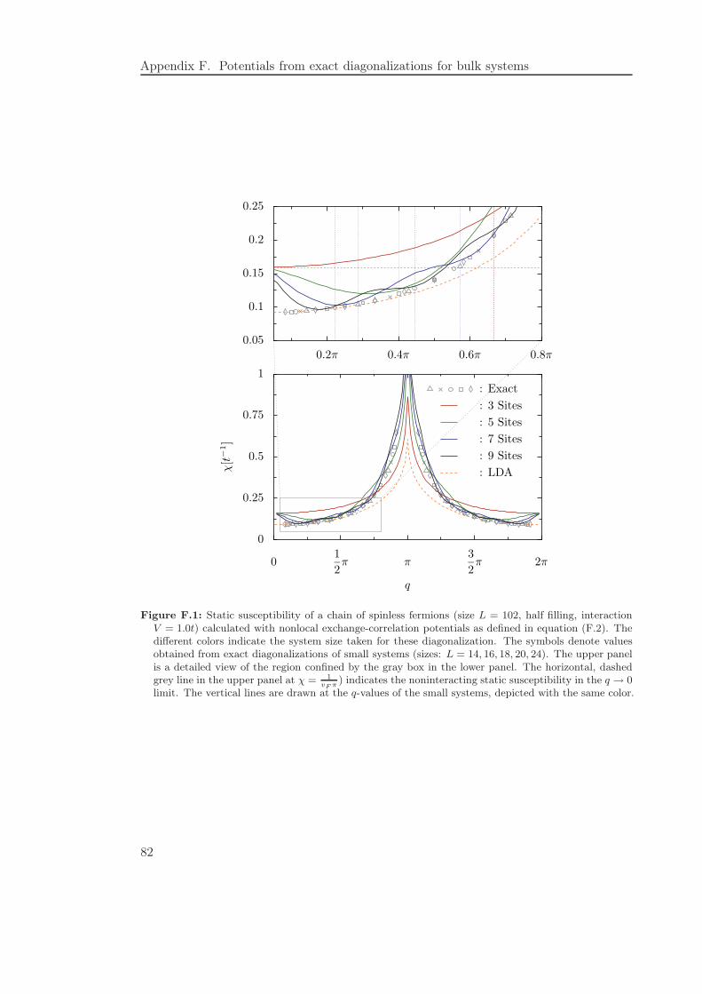
Appendix F. Potentials from exact diagonalizations for bulk systems
: 3 Sites
: 5 Sites
: 7 Sites
: 9 Sites
: LDA
0
0.25
0.5
0.75
1
χ[t−
1]
01
2π π
3
2π 2π
q
: Exact
0.05
0.1
0.15
0.2
0.25
0.2π 0.4π 0.6π 0.8π
Figure F.1: Static susceptibility of a chain of spinless fermions (size L = 102, half filling, interactionV = 1.0t) calculated with nonlocal exchange-correlation potentials as defined in equation (F.2). Thedifferent colors indicate the system size taken for these diagonalization. The symbols denote valuesobtained from exact diagonalizations of small systems (sizes: L = 14, 16, 18, 20, 24). The upper panelis a detailed view of the region confined by the gray box in the lower panel. The horizontal, dashedgrey line in the upper panel at χ = 1
vF π) indicates the noninteracting static susceptibility in the q → 0
limit. The vertical lines are drawn at the q-values of the small systems, depicted with the same color.
82
F.1. Applicability of the exact diagonalization procedure to bulk systems
values are given by the q-values that exist in the subsystems, qS = 2πM j where 1 . . .M − 1,
with the exception of qS = 0.
These peculiarities can be understood as follows: We begin by considering variationsof the Hartree-exchange-correlation potential,
δvHXCl =
1
M
l+m∑
x=l−m
[δvsl (x) − δvl(x)] . (F.3)
The parameter x can be understood as the position of the center of a subsystem andthus specifies the subsystem where the potential is taken from. Thus we also have tosum over all subsystems that contain the site l and therefore contribute to the potential.Since we discuss the susceptibility of the homogeneous system in q-space, we need theFourier transform of δvHXC, which is given by
δvHXCq =
1
M
L∑
l=1
e−iqll+m∑
x=l−m
[δvsl (x) − δvl(x)] . (F.4)
The potentials vsl and vl, determined from a subsystem centered at x depends only on
the densities at x−m, . . . x+m. Therefore this expression can be expanded as
δvHXCq =
1
M
L∑
l=1
e−iqll+m∑
x=l−m
x+m∑
y=x−m
[δvs
l (x)
δny−δvl(x)
δny
]
δny. (F.5)
Using the definition of the susceptibility we can replace the two fractions by the inverseof the corresponding susceptibility of the subsystem,
δvHXCq =
1
M
L∑
l=1
e−iqll+m∑
x=l−m
l+m∑
y=l−m
{
[χsS(y − l)]−1 − [χS(y − l)]−1
}
δny. (F.6)
Here we have used the homogeneity of the system twice. First, it is necessary for writingthe susceptibility as a function of the difference y−l, and second, it enables us to eliminatethe index x specifying the subsystem. In particular we choose the subsystem specifiedby x = l. Carrying out the sum over x gives just a factor M and using the substitutionsy → y − l and l → l + y we find
δvHXCq =
m∑
y=−m
{
[χsS(y)]
−1 − [χS(y)]−1} L+y∑
l=1+y
e−iq(l−y)δnl
=
m∑
y=−m
eiqy{
[χsS(y)]−1 − [χS(y)]
−1} L∑
l=1
e−iqlδnl
=m∑
y=−m
eiqy{
[χsS(y)]−1 − [χS(y)]
−1}
δnq.
(F.7)
83
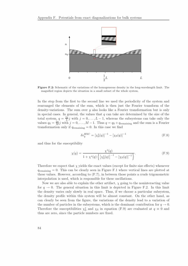
Appendix F. Potentials from exact diagonalizations for bulk systems
01
2L L
n
n0δn
δn δn
Figure F.2: Schematic of the variations of the homogeneous density in the long-wavelength limit. Themagnified region depicts the situation in a small subset of the whole system.
In the step from the first to the second line we used the periodicity of the system andrearranged the elements of the sum, which is then just the Fourier transform of thedensity-variations. The sum over y also looks like a Fourier transformation but is onlyin special cases. In general, the values that q can take are determined by the size of thetotal system, q = 2π
L j with j = 0, . . . , L − 1, whereas the subsystems can take only thevalues qS = 2π
M j with j = 0, . . . ,M − 1. Thus q = qS + qremaining and the sum is a Fouriertransformation only if qremaining = 0. In this case we find
δvHXCq = [χs
S(q)]−1 − [χS(q)]
−1 (F.8)
and thus for the susceptibility
χ(q) =χs(q)
1 + χs(q){[χs
S(q)]−1
− [χS(q)]−1} . (F.9)
Therefore we expect that χ yields the exact values (except for finite size effects) wheneverqremaining = 0. This can be clearly seen in Figure F.1 where vertical lines are plotted atthese values. However, according to (F.7), in between those points a crude trigonometricinterpolation is used, which is responsible for these oscillations.
Now we are also able to explain the other artifact, χ going to the noninteracting valuefor q → 0. The general situation in this limit is depicted in Figure F.2. In this limitthe density varies only slowly in real space. Thus, if we choose a particular subsystem,the density profile within this system will be almost constant. On the other hand, ascan clearly be seen from the figure, the variations of the density lead to a variation ofthe number of particles in the subsystems, which is the dominant contribution for q → 0.Therefore the susceptibilities χs
S and χS in equation (F.9) are evaluated at q ≡ 0 andthus are zero, since the particle numbers are fixed.
84
F.2. Constructing nonlocal potentials from the exact susceptibility
F.2 Constructing nonlocal potentials from the exact
susceptibility
We have seen that the local density approximation performs poorly when calculating thesusceptibility. Now we can ask ourselves, if we can use the exact results of the densityresponse function for small systems to obtain a better exchange-correlation functional.Of course, one may use the exact-exchange approximation, but this method has twoproblems: First, the inherent instability of the homogeneous system and second, thecomputational complexity scales very poorly with system size compared to the LDA. Itis indeed possible to construct an approximation based on the susceptibility; in fact thelimit q → 0 of such a construction has been used to construct a gradient approximation[74].
We start with the local density approximation for the exchange-correlation energy,
EXCLDA[n] =
∑
l
ǫXCLDA(nl) → vXC
l =∂ǫXC
LDA
∂n
∣∣∣∣n=nl
. (F.10)
Since this approximation is exact in the homogeneous case we construct our approxima-tion around the LDA. Unlike the various flavors of the gradient approximation we do notuse the local densities and their gradients but pairs of densities,
EXC[n] =∑
l
ǫXC1 (nl) +
1
2
∑
l,l′
ǫXC2 (nl, nl′ ; l − l′). (F.11)
The exchange-correlation potential is then
vXCl =
∂ǫXC1 (nl)
∂nl+∑
l′
∂ǫXC2 (nl, nl′ ; l − l′)
∂nl. (F.12)
Here we have assumed that ǫXC2 is symmetric under the exchange of l and l′. Earlier we
stated that we construct the nonlocal potential around the local density approximation.Hence we choose ǫXC
1 = ǫXCLDA. Since the LDA is exact for the homogeneous system we
have to construct ǫXC2 such that it is zero if nl and nl′ are equal to the density of the
homogeneous system n = NL . The most simple expression satisfying this condition is
ǫXC2 (nl, nl′ ; l − l′) = fXC
2 (n, l − l′) · (nl − n)(nl′ − n), (F.13)
where the quantity fXC2 depends only on the average density (or the particle number) and
the distance l− l′. As the name suggests this quantity is part of the exchange-correlationkernel of the susceptibility as can be seen in the usual way of writing the variations ofthe effective single-particle potential in q-space as
δvsq = δvq + δvH
q + δvLDAq + δvLR
q . (F.14)
vLRq is the Fourier transform of the second term in (F.12) and fXC
2 (n, q) =∂vLR
q
∂nq. The
acronym LR stands for linear response, which is used to determine fXC2 as we will see.
85
Appendix F. Potentials from exact diagonalizations for bulk systems
The susceptibility can then be written as
χ(q) =χs(q)
1 + χs(q)[2V cos q + fXC
LDA + fXC2 (q)
] . (F.15)
If we have an approximation for χ(q), we can calculate the prefactor of our nonlocalpotential
fXC2 (q) = [χ(q)]−1 − [χs(q)]−1 − 2V cos q − fXC
LDA, (F.16)
or in real space
fXC2 (n, l − l′) =
1
L
∑
q
eiq(l−l′)fXC2 (n, q). (F.17)
Using the homogeneous system as input, this exchange-correlation potential should befairly good even for inhomogeneous systems, as long as the inhomogeneities are withinthe linear response regime of the homogeneous system.
The connection of this approximation to the gradient expansions can be seen on thebasis of equation (F.11), where the second term can be written as
EXC2 [n] =
1
2
∑
l,l′
fXC2 (l − l′) · (nl − n)(nl′ − n) =
1
2L
∑
q 6=0
fXC2 (q) · n−qnq. (F.18)
The last equality can be found by inserting the Fourier representation of fXC2 and the
densities. Thereby the q = 0 term of nl and n cancel each other. Please also note thatfXC2 (q) goes to zero for q → 0 since this limit is already described by the local density
approximation. Using the symmetry fXC2 (q) = fXC
2 (−q) we see that the lowest orderexpansion of fXC
2 (q) in powers of q is proportional to q2. On the other hand if we usethe lowest order gradient expansion (see for example [74]) we have
EXC2 [n] = −
1
2
∑
l
B · (∇nl)2 = −
1
2L
∑
q
q2B · n−qnq, (F.19)
where again we inserted the Fourier representation for the densities. Thus we see that thegradient expansion is given by the lowest order term of our nonlocal exchange-correlationpotential. On the other hand it is clear that we need an infinite sum of higher order termsto reproduce the singularity at q = 2kF .
86
Bibliography
[1] P. Hohenberg, W. Kohn, Inhomogeneous Electron Gas, Phys. Rev. 136, B864(1964).
[2] W. Kohn, L. J. Sham, Self-Consistent Equations Including Exchange and Correla-tion Effects, Phys. Rev. 140, A1133 (1965).
[3] A. K. Rajagopal, J. Callaway, Inhomogeneous Electron Gas, Phys. Rev. B 7, 1912(1973).
[4] G. Vignale, M. Rasolt, Density-Functional Theory in Strong Magnetic Fields, Phys.Rev. Lett. 59, 2360 (1987).
[5] G. Vignale, M. Rasolt, Current- and spin-density-functional theory for inhomoge-neous electronic systems in strongg magnetic fields, Phys. Rev. B 37, 10685 (1988).
[6] G. Diener, Current-density-functional theory for a non-relativistic electron gas ina strong magnetic field, J. Phys.: Condens. Matter 3, 9417 (1991).
[7] E. Runge, E. K. U. Gross, Density-Functional Theory for Time-Dependent Systems,Phys. Rev. Lett. 52, 997 (1984).
[8] E. K. U. Gross, W. Kohn, Local Density-Functional Theory of Frequency-DependentLinear Response, Phys. Rev. Lett. 55, 2850 (1985).
[9] G. Vignale, W. Kohn, Current-Dependent Exchange-Correlation Potential for Dy-namical Linear Response Theory, Phys. Rev. Lett. 77, 2037 (1996).
[10] R. van Leeuwen, Causality and Symmetry in Time-Dependent Density-FunctionalTheory, Phys. Rev. Lett. 80, 1280 (1998).
[11] M. Petersilka, U. J. Gossman, E. K. U. Gross, Excitation Energies from Time-Dependent Density-Functional Theory, Phys. Rev. Lett. 76, 1212 (1996).
[12] R. T. Sharp, G. K. Horton, A Variational Approach to the Unipotential Many-Electron Problem, Phys. Rev. 90, 317 (1953).
[13] J. D. Talman, W. F. Shadwick, Optimized effective atomic central potential, Phys.Rev. A 14, 36 (1976).
[14] A. Görling, M. Levy, Exact Kohn-Sham scheme based on perturbation theory, Phys.Rev. A 50, 196 (1994).
87
Bibliography
[15] T. Grabo, E. K. U. Gross, Density-functional theory using an optimized exchange-correlation potential, Chem. Phys. Lett. 240, 141 (1995).
[16] M. Städele, M. Moukara, J. A. Majewski, P. Vogl, A. Görling, Exact exchangeKohn-Sham formalism applied to semiconductors, Phys. Rev. B 59, 10031 (1999).
[17] D. C. Langreth, J. P. Perdew, Theory of nonuniform electronic systems. I. Analysisof the gradient approximation and a generalization that works, Phys. Rev. B 21,5469 (1980).
[18] K. Schönhammer, O. Gunnarson, Difference between the quasiparticle and the Kohn-Sham-Fermi surface, Phys. Rev. B 37, 3128 (1988).
[19] L. J. Sham, M. Schlüter, Density Functional Theory of the Energy Gap, Phys. Rev.Lett. 51, 1888 (1983).
[20] J. F. Janak, Proof that ∂E/∂ni = ǫi in density-functional theory, Phys. Rev. B 18,7165 (1978).
[21] J. P. Perdew, M. Levy, Physical Content of the Exact Kohn-Sham Orbital Energies:Band Gaps and Derivative Discontinuities, Phys. Rev. Lett. 51, 1884 (1983).
[22] O. Gunnarson, K. Schönhammer, Density-Functional Treatment of an Exactly Solv-able Semiconductor Model, Phys. Rev. Lett. 56, 1968 (1986).
[23] K. Schönhammer, O. Gunnarson, Discontinuity of the exchange-correlation poten-tial in density functional theory, J. Phys. C: Solid State Phys. 20, 3675 (1987).
[24] K. Schönhammer, O. Gunnarson, R. M. Noack, Density-funcitonal theory on alattice: Comparison with exact numerical results for a model with strongly correlatedelectrons, Phys. Rev. B 52, 2504 (1995).
[25] N. A. Lima, M. F. Silva, L. N. Oliveira, K. Capelle, Density Functionals Not Basedon the Electron Gas: Local-Density Approximation for a Luttinger Liquid, Phys.Rev. Lett. 90, 146402 (2003).
[26] C. Verdozzi, Time-Dependent Density-Functional Theory and Strongly CorrelatedSystems: Insight from Numerical Studies, Phys. Rev. Lett. 101, 166401 (2008).
[27] G. Xianlong, M. Polini, M. P. Tosi, J. Vivaldo L. Campo, K. Capelle, M. Rigol,Bethe ansatz density-functional theory of ultracold repulsive fermions in one-dimensional optical lattices, Phys. Rev. B 73, 165120 (2006).
[28] G. Xianlong, M. Rizzi, M. Polini, R. Fazio, M. P. Tosi, J. V. L. Campo, K. Capelle,Luther-Emery Phase and Atomic-Density Waves in a Trapped Fermion Gas, Phys.Rev. Lett. 98, 030404 (2007).
[29] J. Sólyom, The Fermi gas model of one-dimensional conductors, Adv. Phys. 28,201 (1979).
88
Bibliography
[30] H. J. Schulz, Fermi liquids and non-Fermi liquids, in Proceedings of Les HouchesSummer School LXI, edited by E. Akkermans, G. Montambaux, J. Pichard and J.Zinn-Justin (Elsevier, Amsterdam, 1995), p. 533.
[31] J. Voit, One-dimensional Fermi liquids, Rep. Prog. Phys. 58, 977 (1995).
[32] S. J. Tans, M. H. Devoret, H. Dai, A. Thess, R. E. Smalley, L. J. Geerligs, C. Dekker,Individual single-wall carbon nanotubes as quantum wires, Nature 386, 474 (1997).
[33] M. Bockrath, D. H. Cobden, J. Lu, A. G. Rinzler, R. E. Smalley, L. Balents, P. L.McEuen, Luttinger-liquid behaviour in carbon nanotubes, Nature 397, 598 (1999).
[34] H. Moritz, T. Stöferle, K. Günter, M. Köhl, T. Esslinger, Confinement InducedMolecules in a 1D Fermi Gas, Phys. Rev. Lett. 94, 210401 (2005).
[35] I. Bloch, J. Dalibard, W. Zwerger, Many-body physics with ultracold gases, Rev.Mod. Phys. 80, 885 (2008).
[36] S. Giorgini, L. P. Pitaevskii, S. Stringari, Theory of ultracold atomic Fermi gases,Rev. Mod. Phys. 80, 1215 (2008).
[37] A. M. Chang, Chiral Luttinger liquids at the fractional quantum Hall edge, Rev.Mod. Phys. 75, 1449 (2003).
[38] X. Duan, Y. Huang, Y. Cui, J. Wang, C. M. Lieber, Indium phosphide nanowiresas building blocks for nanoscale electronic and optoelectronic devices, Nature 409,66 (2001).
[39] S. J. Tans, A. R. M. Verschueren, C. Dekker, Room-temperature transistor basedon a single carbon nanotube, Nature 393, 49 (1998).
[40] A. Aviram, M. A. Ratner, Molecular Rectifiers, Chem. Phys. Lett. 29, 277 (1974).
[41] M. A. Reed, C. Zhou, C. J. Muller, T. P. Burgin, J. M. Tour, Conductance of aMolecular Junction, Science 278, 252 (1997).
[42] C. Kergueris, J.-P. Bourgoin, S. Palacin, D. Esteve, C. Urbina, M. Magoga,C. Joachim, Electron transport through a metal-molecule-metal junction, Phys. Rev.B 59, 12505 (1999).
[43] X. D. Cui, A. Primak, X. Zarate, J. Tomfohr, O. F. Sankey, A. L. Moore, T. A.Moore, D. Gust, G. Harris, S. M. Lindsay, Reproducible Measurement of Single-Molecule Conductivity, Science 294, 571 (2001).
[44] J. Reichert, R. Ochs, D. Beckmann, H. B. Weber, M. Mayor, H. v. Löhneysen,Driving Current through Single Organic Molecules, Phys. Rev. Lett. 88, 176804(2002).
[45] A. Nitzan, Electron transmission through molecules and molecular interfaces, Annu.Rev. Phys. Chem. 52, 681 (2001).
89
Bibliography
[46] S. Kohler, J. Lehman, P. Hänggi, Driven quantum transport on the nanoscale, Phys.Rep. 406, 379 (2005).
[47] F. J. Kaiser, P. Hänggi, S. Kohler, Coulomb repulsion effects in driven electrontransport, Eur. Phys. J. B 54, 201 (2006).
[48] F. J. Kaiser, P. Hänggi, S. Kohler, Molecular electronics in junctions with energydisorder, New J. Phys. 10, 065013 (2008).
[49] S. Kurth, G. Stefanucci, C.-O. Almbladh, A. Rubio, E. K. U. Gross, Time-dependent quantum transport: A practical scheme using density functional theory,Phys. Rev. B 72, 035308 (2005).
[50] A. Arnold, F. Weigend, F. Evers, Quantum chemistry calculations for molecules cou-pled to reservoirs: Formalism, implementation, and application to benzenedithiol,J. Chem. Phys. 126, 174101 (2007).
[51] F. Evers, F. Weigend, M. Koentopp, Conductance of molecular wires and transportcalculations based on density-functional theory, Phys. Rev. B 69, 235411 (2004).
[52] C. Toher, A. Filippetti, S. Sanvito, K. Burke, Self-Interaction Errors in Density-Functional Calculations of Electronic Transport, Phys. Rev. Lett. 95, 146402(2005).
[53] M. Koentopp, K. Burke, F. Evers, Zero-bias molecular electronics: Exchange-correlation corrections to Landauer’s formula, Phys. Rev. B 73, 121403 (2006).
[54] S.-H. Ke, H. U. Baranger, W. Yang, Role of the exchange-correlation potential inab initio electron transport calculations, J. Chem. Phys. 126, 201102 (2007).
[55] S. M. Lindsay, M. A. Ratner, Molecular Transport Junctions: Clearing Mists, Adv.Mater. 19, 23 (2007).
[56] P. Schmitteckert, F. Evers, Exact ground state density functional theory for im-purity models coupled to external reservoirs and transport calculations, Phys. Rev.Lett. 100, 086401 (2008).
[57] C. N. Yang, C. P. Yang, One-Dimensional Chain of Anisotropic Spin-Spin Inter-actions. I. Proof of Bethe’s Hypothesis for Ground State in a Finite System, Phys.Rev. 150, 321 (1966).
[58] F. D. M. Haldane, ‘Luttinger liquid theory’ of one-dimensional quantum fluids: I.Properties of the Luttinger model and their extension to the general 1D interactingspinless Fermi gas, J. Phys. C: Solid State Phys. 14, 2585 (1981).
[59] S. R. White, Density Matrix Formulation for Quantum Renormalization Groups,Phys. Rev. Lett. 69, 2863 (1992).
90
Bibliography
[60] S. R. White, Density-matrix agorithms for quantum renormalization groups, Phys.Rev. B 48, 10345 (1993).
[61] E. H. Lieb, Density Functionals for Coulomb Systems, Int. J. Quant. Chem. 24,243 (1983).
[62] R. Fukuda, T. Kotani, Y. Suzuki, S. Yokojima, Density Functional Theory throughLegendre Transformation, Prog. Theo. Phys. 92, 833 (1994).
[63] U. Eckern, P. Schwab, Normal persistent currents, Adv. Phys. 44, 387 (1995).
[64] C. N. Yang, C. P. Yang, One-Dimensional Chain of Anisotropic Spin-Spin Inter-actions. II. Properties of the Ground-State Energy Per Lattice Site for an InfiniteSystem, Phys. Rev. 150, 327 (1966).
[65] C. N. Yang, C. P. Yang, One-Dimensional Chain of Anisotropic Spin-Spin Interac-tions. III. Applications, Phys. Rev. 151, 258 (1966).
[66] P. Jordan, E. Wigner, Über das Paulische Äquivalenzverbot, Z. Phys. 47, 631 (1928).
[67] H.-J. Mikeska, A. K. Kolezhuk, One-Dimensional Magnetism, Lect. Notes Phys.645, 1 (2004).
[68] F. D. M. Haldane, General Relation of Correlation Exponents and Spectral Prop-erties of One-Dimensional Fermi-Systems: Application to the Anisotropic S = 1
2Heisenberg Chain, Phys. Rev. Lett. 45, 1358 (1980).
[69] N. Ishimura, H. Shiba, Dynamical Correlation Functions of One-DimensionalAnisotropic Heisenberg Model with Spin 1/2, Phys. Rev. 136, B864 (1964).
[70] V. E. Korepin, N. M. Bogoliubov, A. G. Izergin, Quantum Inverse ScatteringMethod and Correlation Functions (Cambridge University Press, 1993).
[71] A. Luther, I. Peschel, Calculation of critical exponents in two dimensions fromquantum field theory in one dimension, Phys. Rev. B 12, 3908 (1975).
[72] M. Levy, Universal variational functional of electron densities, first-order densitymatrices, and natural spin-orbitals and solution of the v-representability problem,Proc. Nat. Acad. Sci. USA 76, 6062 (1979).
[73] M. Levy, Electron densities in search of Hamiltonians, Phys. Rev. A 26, 1200(1982).
[74] G. F. Giuliani, G. Vignale, Quantum Theory of the Electron Liquid, chapter 7,327–404 (Cambridge University Press, 2005).
[75] J. Kohanoff, N. I. Gidopoulos, Density Functional Theory: Basics, New Trends andApplications, volume 2, chapter 26, 532–568 (John Wiley & Sons, Ltd, Chichester,2003).
91
Bibliography
[76] H. Eschrig, The Fundamentals of Density Functional Theory (B. G. Teubner Ver-lagsgesellschaft Leipzig, 1996).
[77] M. Dzierzawa, U. Eckern, S. Schenk, P. Schwab, Current density functional theoryfor one-dimensional fermions, in Proceedings of Coherence and Correlations inNanostructures, Ustron, Polen, Phys. Status Solidi B 246, 941 (2009).
[78] J. P. Perdew, A. Zunger, Self-interaction correction to density funcitonal approxi-mations for many-electron systems, Phys. Rev. B 23, 5048 (1981).
[79] D. Ceperley, Ground state of the fermion one-component plasma: A Monte Carlostudy in two and three dimensions, Phys. Rev. B 18, 3126 (1978).
[80] B. Sutherland, B. S. Shastry, Adiabatic Transport Properties of an Exactly SolubleOne-Dimensional Quantum Many-Body Problem, Phys. Rev. Lett. 65, 1833 (1990).
[81] J. P. Perdew, K. Burke, M. Ernzerhof, Generalized Gradient Approximation MadeSimple, Phys. Rev. Lett. 77, 3865 (1996).
[82] A. Görling, Orbital- and state-dependent functionals in density-functional theory,J. Chem. Phys. 123, 062203 (2005).
[83] R. O. Jones, O. Gunnarson, The density functional formalism, its application andprospects, Rev. Mod. Phys. 61, 689 (1989).
[84] N. W. Ashcroft, N. D. Mermin, Solid State Physics (Thomson Learning, 1976).
[85] D. W. Hess, J. W. Serene, Quasiparticle band structure and density-functional the-ory: Single-particle excitations and band gaps in lattice models, Int. J. Quant. Chem.69, 265 (1998).
[86] S. Schenk, M. Dzierzawa, P. Schwab, U. Eckern, Successes and failures of BetheAnsatz Density Functional Theory, Phys. Rev. B 78, 165102 (2008).
[87] A. Görling, Exact Exchange Kernel for Time-Dependent Density-Functional The-ory, Int. J. Quant. Chem. 69, 265 (1998).
[88] A. Görling, Exact exchange-correlation kernel for dynamic response properties andexcitation energies in density-functional theory, Phys. Rev. A 57, 3433 (1998).
[89] P. Schmitteckert, T. Schulze, C. Schuster, P. Schwab, U. Eckern, Anderson Local-ization versus Delocalization of Interacting Fermions in One Dimension, Phys. Rev.Lett. 80, 560 (1998).
[90] C. L. Kane, M. P. A. Fisher, Transport in a One-Channel Luttinger Liquid, Phys.Rev. Lett. 68, 1220 (1992).
[91] K. A. Matveev, D. Yue, L. I. Glazman, Tunneling in One-Dimensional Non-Luttinger Electron Liquid, Phys. Rev. Lett. 71, 3351 (1993).
92
Bibliography
[92] W. Kohn, Theory of the Insulating State, Phys. Rev. 133, A171 (1964).
[93] B. S. Shastry, B. Sutherland, Twisted Boundary Conditions and Effective Mass inHeisenberg-Ising and Hubbard Rings, Phys. Rev. Lett. 65, 243 (1990).
[94] R. A. Molina, P. Schmitteckert, D. Weinmann, R. A. Jalabert, G.-L. Ingold, J.-L. Pichard, Residual conductance of correlated one-dimensional nanosystems: Anumerical approach, Eur. Phys. J. B 39, 107 (2004).
[95] M. A. L. Marques, C. A. Ullrich, F. Nogueira, A. Rubio, K. Burke, E. K. U. Gross,editors, Time-Dependent Density Functional Theory, Lecture Notes in Physics, vol-ume 706 (Springer, Berlin Heidelberg, 2006).
[96] R. van Leeuwen, Key Concepts in Time-Dependent Density-Functional Theory, Int.J. Mod. Phys. B 15, 1969 (2001).
[97] L. V. Keldysh, Diagram Technique for nonequilibrium processes, Sov. Phys. JETP20, 1018 (1965).
[98] J. Rammer, H. Smith, Quantum field-theoretical methods in transport theory ofmetals, Rev. Mod. Phys. 58, 323 (1986).
[99] E. K. U. Gross, C. A. Ullrich, U. J. Gossman, Density Functional Theory, NATOASI Series, volume B337 (Plenum Press, New York, 1995).
[100] E. K. U. Gross, J. F. Dobson, M. Petersilka, Density Functional Theory (Springer,1996).
[101] G. Vignale, C. A. Ullrich, S. Conti, Time-Dependent Density Functional TheoryBeyond the Adiabatic Local Density Approximation, Phys. Rev. Lett. 79, 4878(1997).
[102] P. L. de Boeji, F. Kootstra, J. A. Berger, R. van Leeuwen, J. G. Snijders, Currentdensity functional theory for optical spectra: A polarization functional, J. Chem.Phys. 115, 1995 (2001).
[103] M. Petersilka, E. K. U. Gross, Excitation energies from Time-Dependent DensityFunctional Theory Using Exact and Approximate Potentials, Int. J. Quant. Chem.80, 534 (2000).
[104] F. Aryasetiawan, O. Gunnarson, A. Rubio, Excitation energies from time-dependentdensity-functional formalism for small systems, Europhys. Lett. 57, 683 (2002).
[105] M. Hellgren, U. von Barth, Linear density response function within the time-dependent exact-exchange approximation, Phys. Rev. B 78, 115107 (2000).
[106] H. O. Wijewardane, C. A. Ullrich, Real-Time Electron Dynamics with Exact-Exchange Time-Dependent Density-Functional Theory, Phys. Rev. Lett. 100,056404 (2008).
93
Bibliography
[107] Y. Shigeta, K. Hirao, S. Hirata, Exact-exchange time-dependent density-functionaltheory with the frequency-dependent kernel, Phys. Rev. A 73, 010502 (2006).
[108] Y.-H. Kim, A. Görling, Excitonic Optical Spectrum of Semiconductors Obtained byTime-Dependent Density-Functional Theory with the Exact-Exchange Kernel, Phys.Rev. Lett. 89, 096402 (2002).
[109] R. G. Pereira, S. R. White, I. Affleck, Exact Edge Singularities and DynamicalCorrelations in Spin-1/2 Chains, Phys. Rev. Lett. 100, 027206 (2008).
[110] J. P. Perdew, R. G. Parr, M. Levy, J. Jose L. Balduz, Density-Functional Theoryfor Fractional Particle Number: Derivative Discontinuities of the Energy, Phys.Rev. Lett. 49, 1691 (1982).
[111] E. H. Lieb, F. Y. Wu, Absence of Mott Transition in an Exact Solution of the Short-Range, One-Band Model in One Dimension, Phys. Rev. Lett. 68, 1445 (1968).
[112] H. Bethe, Zur Theorie der Metalle. I. Eigenwerte und Eigenfunktionen der linearenAtomkette, J. Phys.: Condens. Matter 3, 9417 (1931).
[113] E. H. Lieb, W. Liniger, Exact Analysis of an Interacting Bose Gas. I. The GeneralSolution and the Ground State, Phys. Rev. 130, 1605 (1963).
[114] E. H. Lieb, Exact Analysis of an Interacting Bose Gas. II. The Excitation Spectrum,Phys. Rev. 130, 1616 (1963).
[115] R. J. Baxter, One-Dimensional Anisotropic Heisenberg Chain, Phys. Rev. Lett. 26,834 (1971).
[116] C. N. Yang, S-Matrix for the One-Dimensional N -Body Problem with Repulsive orAttractive δ-Functions Interaction, Phys. Rev. 168, 1920 (1968).
[117] K. Capelle, G. Vignale, Nonuniqueness of the Potentials of Spin-Density-FunctionalTheory, Phys. Rev. Lett. 86, 5546 (2001).
[118] C. A. Ullrich, Nonuniqueness in spin-density-functional theory on lattices, Phys.Rev. B 72, 073102 (2005).
[119] K. Capelle, C. A. Ullrich, G. Vignale, Degenerate ground states and nonuniquepotentials: Breakdown and restoration of density functionals, Phys. Rev. A 76,012508 (2007).
[120] R. T. Rockafellar, Convex Analysis (Princeton University Press, 1970).
[121] W. Kohn, v-Representability and Density Functional Theory, Phys. Rev. Lett. 51,1596 (1983).
94
Acknowledgements
At this point I would like to thank all the people that contributed in one way or anotherto this thesis.
Especially, I would like to thank Prof. Dr. Ulrich Eckern for giving me the opportunity tojoin his group and work on such a interesting field as the foundations of density functionaltheory.
A great many thanks go to Priv.-Doz. Dr. Peter Schwab for supervising this thesis. Hisadvice and the many discussions have been very helpful for my understanding of physicsin general and the intricacies of density functional theory in particular.
I would also like to thank Prof. Dr. Gert-Ludwig Ingold for acting as second referee ofthis thesis.
I am also obliged to Dr. Michael Dzierzawa for sharing his deep knowledge of numericsand for double-checking some of my numerical results.
My special thanks go to Franz Kaiser for many stimulating discussions about physicsand the rest of life.
Many thanks to Dr. Cosima Schuster for her insight into the DFT calculations for realworld materials.
I would also like thank Ralf Utermann for keeping the compute cluster in good shape.
Finally, I would like to thank the members of both groups, Theoretische Physik I andTheoretische Physik II, for a most pleasant atmosphere.
95

96
Curriculum vitae
Name: Stefan Schenk
Geburtsdatum: 21.09.1979
Geburtsort: Starnberg
Ausbildung:
Seit 2006: Wissenschaftlicher Mitarbeiter bei Prof. Dr. U. Eckern amLehrstuhl für Theoretische Physik II, Universität Augsburg
2000-2006: Studium der Physik an der Universität Augsburg,Abschluss als Diplom-Physiker
1999-2000: Zivildienst
1990-1999: Besuch des Gymnasiums Donauwörth,Abschluss mit Abitur
97