Design and analysis of a lightweight parallel adaptive ...DESIGN AND ANALYSIS OF A LIGHTWEIGHT...

Thomas Dickopf, Dorian Krause, Rolf Krause and Mark Potse

Design and analysis of a lightweightparallel adaptive scheme for the

solution of the monodomain equation

ICS Preprint No. 2013-07

8 March 2013

Via Giuseppe Buffi 13 CH-6904 Lugano phone: +41 58 666 4690 fax: +41 58 666 4536

http://ics.unisi.ch

DESIGN AND ANALYSIS OF A LIGHTWEIGHT PARALLEL

ADAPTIVE SCHEME FOR THE SOLUTION OF THE

MONODOMAIN EQUATION

THOMAS DICKOPF†∗, DORIAN KRAUSE† , ROLF KRAUSE† , AND MARK POTSE†‡

Abstract. Numerical simulation of the non-linear reaction-diffusion equations in computationalelectrocardiology requires locally high spatial resolution to capture the multiscale effects related to theelectrical activation of the heart accurately, namely the strongly varying action potential. Here, wepropose a novel lightweight adaptive algorithm which aims at combining the plainness of structuredmeshes with the resolving capabilities of unstructered adaptive meshes. Our “patch-wise adaptive”approach is based on locally structured mesh hierarchies which are glued along their interfaces bya non-conforming mortar element discretization. To further increase the overall efficiency, we keepthe spatial meshes constant over suitable time windows in which error indicators are accumulated.This approach facilitates strongly varying mesh sizes in neighboring patches as well as in consecutivetime steps. For the transfer of the dynamic variables between different spatial approximation spaceswe compare the L2-projection and a local approximation. Finally, since an implicit-explicit timediscretization is employed for stability reasons, we derive a spatial preconditioner which is tailoredto the special structure of the patch-wise adaptive meshes.

We analyze the (parallel) performance and scalability of the resulting method by several realisticexamples from computational electrocardiology of different sizes. Additionally, we compare ourmethod to a standard adaptive refinement strategy using unstructured meshes. As it turns out, ournovel adaptive scheme provides a very good balance between reduction in degrees of freedom andoverall (parallel) efficiency.

Key words. Adaptivity, Electrophysiology, Mortar finite elements

AMS subject classifications. 35K57, 65N30, 65Y05

1. Introduction. In recent years the mathematical modeling and numericalsimulation of the electrophysiology of the heart has been an active field of multi-disciplinary research. New possibilities have been opened up for the in-silico study ofthe electrical processes underlying the mechanical contraction of the heart as well asthe study of disease-related disorders in the electrical activation sequence [31].

The electrical activation of the heart can be modeled by non-linear reaction-diffusion equations, in particular, by the bidomain and monodomain equation. Sincethe action potential features high temporal and spatial gradients, full heart simulationson uniform meshes require between O(106) and O(108) degrees of freedom and O(104)time steps. At the same time, since the action potential exhibits wave-like behavior,spatial adaptivity is a promising approach for reducing the computational demandsof electrophysiological simulations. Yet, the design of efficient adaptive methods forthis problem class is a challenging task and still an open issue in many regards.

The main contribution of this article is the presentation and analysis of a noveladaptive scheme for time-dependent non-linear reaction-diffusion equations. The pre-sented method was designed to exhibit a low memory footprint, to be well suited forcontemporary central processing units and to be relatively simple to implement andparallelize. To this end we use non-conforming locally structured adaptive meshesand matrix-free block preconditioning. The use of a non-conforming discretization iscentral as it gives flexibility in the choice of the local mesh widths.

Focusing on the monodomain cardiac reaction-diffusion equation, this work con-tributes to the ongoing exploration of the design space for adaptive methods which

∗Lehrstuhl fur Angewandte Mathematik, Heinrich-Heine-Universitat, Dusseldorf, Germany†Institute of Computational Science, Universita della Svizzera italiana, Lugano, Switzerland‡Cardiovascular Research Institute, Maastricht University, Maastricht, The Netherlands

1

2 DICKOPF, KRAUSE, KRAUSE, POTSE

is particularly large and complicated when the architecture of contemporary paral-lel computers is taken into account. Our numerical tests show that the presentedtechniques achieve the design goals specified above. The patch-wise adaptivity ap-proach turns out to be a reasonable compromise between ease of implementation andreduction of numbers of degrees of freedom.

Outline. In the remainder of Section 1 related work is reviewed. In Section 2 weintroduce the problem setting and discuss an implicit-explicit temporal discretizationof the monodomain equation. In Section 3 we present our novel adaptive algorithmand its implementation. Section 4 is devoted to numerical studies, the results of whichare discussed in Section 5.

Related work. Most adaptive schemes in the literature can be classified as ei-ther unstructured adaptive mesh refinement (UAMR) or structured adaptive mesh

refinement (SAMR) algorithms. UAMR methods are popular in the finite elementcommunity and usually characterized by the use of multilevel finite element spacesconstructed on locally refined conforming meshes [23]. Conforming UAMR methodsusually require complicated mesh management code and tend to exhibit only low sus-tained performance and scalability on contemporary architectures. More recently, dis-continuous Galerkin discretizations on conforming and in particular non-conformingmeshes have been studied [20].

In contrast, SAMR methods mostly use non-conforming locally structured meshesorganized either in a tree structure or as a collection of nested, overlapping patches(block-structured SAMR methods) [5, 17, 36]. These methods are often employed withfinite difference or finite volume discretizations. In the context of finite element dis-cretizations one often uses algebraic constraints to cope with hanging nodes. Similarto closures used in conforming UAMR, one enforces 2:1 or 4:1 coarse-to-fine ratios,adding additional complexity. SAMR algorithms have been shown to perform well oncontemporary architectures and to be weakly scalable [37, 40]. Burstedde et al. [11]discuss the extension of tree-based SAMR to forests of octrees.

The approach presented in this article uses a conforming unstructured coarse do-main tessellation similar to Burstedde et al. [11] but instead of local octrees we employlocal structured tensor meshes. One could view this as the block-structured equiv-alent of the forest-of-octrees approach, except that we do not allow local refinementwithin elements of the coarse tessellation. This restriction serves the simplicity ofthe approach which is a major goal of this work. Another difference is the use of anon-conforming discretization instead of an algebraic treatment of hanging nodes.

In this work we employ a mortar element discretization [7] which is known topermit stable numerical solution of elliptic problems in the presence of large jumpsin mesh widths across subdomain interfaces. The mortar element method has beenused before for the adaptive discretization of static elliptic problems, e.g., by Bernadiand Maday [6]. In contrast to this work, we use locally structured conforming mesheswith weak constraints only on interfaces between elements of the coarse tessellation.Hoppe et al. [21] present an adaptive method using UAMR together with a mortardiscretization.

Adaptive mesh refinement techniques in cardiac simulation have been covered bya large number of publications. Deuflhard et al. [14, 16, 38] study multilevel adaptivefinite elements for the solution of the monodomain and bidomain reaction-diffusionequations. Bendahmane et al. [4] study a wavelet-based multiresolution algorithmincluding local time stepping for the bidomain equation. Whiteley [39] describes atwo-level adaptive method. Spatial refinement is controlled by the gradient of the ex-tra cellular potential or the transmembrane voltage. The high coarse-to-fine ratio is

AN ADAPTIVE SCHEME FOR THE MONODOMAIN EQUATION 3

handled by imposing interpolated coarse values as Dirichlet boundary condition to thefine mesh. Cherry et al. [12, 13] apply standard AMR techniques [5] for the solutionof the monodomain equation. Belhamadia [3] describes the use of anisotropic meshadaptation for the bidomain equation. Lines et al. [24] combine multilevel finite ele-ments with wave-front tracking to solve the bidomain equation on a two-dimensionaladaptive mesh. In the SAMR algorithm presented by Tragenstein et al. [35] weakconstraints are enforced at the interface between coarse and fine meshes during thediffusion step. A second-order operator splitting method is combined with local timestepping for the integration of the gating and state variables of the Ruo-Ludy I model.Ying [44, 45] describes an AMR algorithm on general body-fitted hexahedral finiteelements. In this work the same second-order splitting is used as in Tragenstein etal. [35] but with local time stepping for the diffusion term. The interpolated valuesfrom coarser meshes serve as boundary conditions for finer levels. Pennacchio [27, 28]analyzes the mortar element method for the computation of extra-celullar potentialson statically refined non-conforming meshes.

We draw further comparisons between our new approach and the related work inthe discussion of the numerical results in Section 5.

2. Problem. In this section we introduce the monodomain equation and discussthe temporal discretization by a semi-implicit Euler method.

2.1. The monodomain equation. The focus of this article is the numericalsolution of the monodomain equation which describes the evolution of the trans-membrane voltage u(x, t) and the S state variables s(x, t) (which are cellular gatingvariables or ionic concentrations) by a non-linear coupled parabolic equation:

Cm∂u

∂t=

1

χ∇ · (G∇u)− Iion(u, s)− Is in Ω × (0, T ) ,

ds

dt= Z(u, s) in Ω × (0, T ) ,

G∇u = 0 on ∂Ω × (0, T ) ,

(2.1)

with initial conditions at time t = 0. Here, Ω ⊂ R3, T > 0, Cm = 1µF/cm2,

χ = 103 cm−1 is the membrane surface-to-volume ratio, Iion denotes the non-linearionic current and Is = Is(x, t) is an externally applied stimulus current. The tuple(S, s,Z, Iion) is referred to as the membrane model.

In this study we consider the relatively simple yet physiologically realistic mem-brane model described by Bernus et al. [9]. This model features five gating variablesand no variable ionic concentrations.

2.2. Implicit-explicit Euler integration. We consider the discretization ofthe monodomain equation using a finite element approximation space Y ⊂ L2(Ω)with π = πα. The construction of appropriate ansatz and test spaces will bediscussed in Section 3.2. For the sake of clarity of presentation, we consider a singleapproximation space here. In the adaptive scheme presented in Section 3, the spaceY is fixed only over a time interval (t1, t2) ⊂ (0, T ), a so-called time window. Thefinal solution at time t2, transferred to the new approximation space as discussed inSection 3.3, then serves as initial condition on the next interval (t2, t3).


The weak formulation of Equation (2.1) for test functions v ∈ Y is given by

Cm

(

∂u

∂t, v

)

L2(Ω)

= −1

χ(G∇u,∇v)L2(Ω) − (Iion(u, s) + Is, v)L2(Ω) ,

(

ds

dt, v

)

L2(Ω)

= (Z(u, s), v)L2(Ω) .

(2.2)

Note that we use a globally non-conforming but locally conforming space Y such thatEquation (2.2) is well defined.

Due to the strongly non-linear terms Iion, Z and because of the potentially largenumber of state variables, explicit or implicit-explicit (IMEX) time discretizations forEquation (2.2) are usually preferred over fully implicit discretizations. In this studywe use a first-order splitting between the parabolic equation and the ODEs. For theparabolic equation we use an IMEX Euler method, treating the stiff diffusion currentimplicitly and the non-linear ionic current explicitly. For the gating variables we useRush-Larsen integration [33]. Even though the employed time discretization is onlyconditionally stable, previous work with a finite difference code [22] showed that it isstable for reasonable time step sizes even for very high resolution heart models.

In order to be able to apply Rush-Larsen integration we need to decouple theODE terms in Equation (2.2). We do so by approximating

(Zj(u, s), v)L2(Ω) ≈ (IYZj(u, s), v)L2(Ω) , j = 1, . . . , S , (2.3)

and then lump the mass matrices on the left and right-hand side of the secondequation in (2.2), such that the masses cancel out. The operator IY is definedas follows. For a map g ∈ C0(R × RS), and two finite element functions u =∑

α uαπα ∈ Y, s =∑

α sαπα ∈ YS we have g(u, s) ∈ L2(Ω). Then we defineIYg(u, s) =

∑

α g(uα, sα)πα ∈ Y. Note that (IYg(u, s)) (x) is the nodal interpola-tion of IYg (u(x), s(x)) if π is a nodal basis.

We moreover approximate

(Iion(u, s), v)L2(Ω) ≈ (IYIion(u, s), v)L2(Ω) (2.4)

to reduce the cost involved in the evaluation of this term. Since Iion(

u(

x, t), s(x, t))

is a strongly non-linear function of x and expensive to evaluate, quadrature is ofhigh cost. Using the approximation (2.4) we can compute the contribution of theionic current to the parabolic equation by evaluating Iion at the mesh nodes andmultiplying by a mass matrix. A similar approximation was used by Colli Franzoneand Pavarino [15].

For a time step size τ > 0, the IMEX Euler step from time t = i · τ to time t+ τrequires the solution of a linear system of equations. Denoting by

(

ui, si)

the trans-membrane voltage and state variables at time t, we obtain the new transmembranevoltage at time t+ τ by solving

a(ui+1, v) = f i(v) for all v ∈ Y , (2.5)

with

a(u, v) = Cm(u, v)L2(Ω) +τ

χ(G∇u,∇v)L2(Ω) ,

f i(v) =(

Cmui, v

)

L2(Ω)− τ

(

IYIion(ui, si) + Is, v

)

L2(Ω).

(2.6)


As stated above, we approximate the coupled system of ordinary differential equationsgoverning the dynamics of s by a lumped version where the masses cancel out. Hence,all the equations decouple and we are left with solving dimY individual ordinarydifferential equations

dsαdt

= IYZ(

uiα, sα)

in (t, t+ τ) (2.7)

with initial conditions siα. Rush-Larsen integration exploits the special form of Z tosolve (2.7) exactly on the interval (t, t+ τ); see [33].

3. Methods. In Algorithm 1 we present a schematic of the time integrationscheme used in this work.

We employ a time window based dynamic adaptation procedure [10, 34]. Insteadof constructing new spatial approximation spaces in each time step we fix the ap-proximation space over one so-called lap, which consists of several time steps. Theadaptation of the approximation is then based on accumulated error indicators. Theintegration over a lap is repeated multiple times to find an optimal approximationspace that captures the solution behavior.

The advantage of this approach is that the overhead of the adaptive strategy(construction of a new approximation space and transfer of dynamic variables be-tween spaces) is reduced. On the downside, however, this scheme typically leads toapproximation spaces with higher dimensions.

Algorithm 1 Time integration algorithm (schematic)

tcur ← 0Y← coarse approximations spacewhile tcur < T do

Construct a smaller approximation space Y′ by coarsening5: Transfer dynamic variables u, s to Y′ (See Section 3.3) and update Y← Y′

Save all dynamic variablesfor j = 1 to nrep + 1 do

Clear all error indicator values.for i = 1 to lap do

10: Evaluate right-hand side f (Equation (2.6))Integrate state variables sSolve for transmembrane voltage u (see Section 3.4)Accumulate error indicators (see Section 3.5)

end for

15: if j < nrep + 1 then

Construct a larger approximation space Y′ by refinement (see Section 3.6)break if Y′ equals Y or if the estimated error is small enoughRestore the saved variables u, s and transfer them to Y′. Update Y← Y′

end if

20: end for

tcur ← tcur + lap · τend while

3.1. The geometric setup. In classical h-adaptive unstructured (multilevel)finite element methods, the approximation space is usually chosen as piecewise poly-nomials on a conforming mesh. Adaptation of the approximation space is achieved


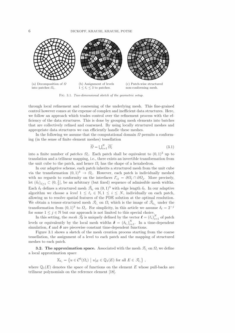
(a) Decomposition of Ωinto patches Ωi.

3321223 1 2 2 3 2

132133331

33

3212233

23

1321

323 3

1 2 3113121332

11231

2323

23

2222

2 211122

2133333

322

3 1 3 332

3222

3 3 31 2 22

31

3

1 131

31

13

1232

31 2

2 22

23

11

(b) Assignment of levels1 ≤ ℓi ≤ 3 to patches.

(c) Patch-wise structurednon-conforming mesh.

Fig. 3.1. Two-dimensional sketch of the geometric setup.

through local refinement and coarsening of the underlying mesh. This fine-grainedcontrol however comes at the expense of complex and inefficient data structures. Here,we follow an approach which trades control over the refinement process with the ef-ficiency of the data structures. This is done by grouping mesh elements into batchesthat are collectively refined and coarsened. By using locally structured meshes andappropriate data structures we can efficiently handle these meshes.

In the following we assume that the computational domain Ω permits a conform-ing (in the sense of finite element meshes) tessellation

Ω =⋃N

i=1Ωi (3.1)

into a finite number of patches Ωi. Each patch shall be equivalent to (0, 1)3 up totranslation and a trilinear mapping, i.e., there exists an invertible transformation fromthe unit cube to the patch, and hence Ωi has the shape of a hexahedron.

In our adaptive scheme, each patch inherits a structured mesh from the unit cubevia the transformation (0, 1)3 → Ωi. However, each patch is individually meshedwith no regards to conformity on the interfaces Γij = ∂Ωi ∩ ∂Ωj . More precisely,let (δℓ)ℓ≥1 ⊂ (0, 12 ], be an arbitrary (but fixed) sequence of admissible mesh widths.

Each δℓ defines a structured mesh Tδℓ on (0, 1)3 with edge length δℓ. In our adaptivealgorithm we choose a level 1 ≤ ℓi ∈ N, 1 ≤ i ≤ N , individually on each patch,allowing us to resolve spatial features of the PDE solution at the optimal resolution.We obtain a tensor-structured mesh Tℓi on Ωi which is the image of Tδℓi

under the

transformation from (0, 1)3 to Ωi. For simplicity, in this article we assume δℓ = 2−j

for some 1 ≤ j ∈ N but our approach is not limited to this special choice.In this setting, the mesh Tℓ is uniquely defined by the vector ℓ = (ℓi)

Ni=1 of patch

levels or equivalently by the local mesh widths δ = (δℓi)Ni=1. In a time-dependent

simulation, ℓ and δ are piecewise constant time-dependent functions.Figure 3.1 shows a sketch of the mesh creation process starting from the coarse

tessellation, the assignment of a level to each patch and the mapping of structuredmeshes to each patch.

3.2. The approximation space. Associated with the mesh Tℓi on Ωi we definea local approximation space

Xℓi =

u ∈ C0(Ωi)∣

∣ u|E ∈ Q1(E) for all E ∈ Tℓi

,

where Q1(E) denotes the space of functions on the element E whose pull-backs aretrilinear polynomials on the reference element [18].


It is well known that the product space Xℓ =∏N

i=1 Xℓi is not well suited for thediscretization of (2.5) since it provides no control over the jump of functions on aninterface Γij and hence one cannot bound the consistency error in terms of the meshsize [43]. The mortar finite element method [7] fixes this by forcing the jump ofthe solution on the skeleton to be zero in a weak sense. This is accomplished eitherby incorporating the condition into the space (in which case ansatz and test spaceare subspaces of Xℓ) or by introducing Lagrange multiplier, hence, replacing problem(2.5) by a saddle point problem. Here, we follow the first approach, though we will notassemble operator represenations on the constrained subspace but implement them ina matrix-free fashion using the space Xℓ.

In the following we briefly review the key aspects of the mortar element methodas we employ it. For more information we refer to Bernardi, Maday and Rapetti [8].

3.2.1. Mortar constraints. Let S =⋃N

i,j=1 Γij denote the skeleton of codi-mension one. On the interface Γij , two potentially different hypersurface meshes areinduced by the adjacent patches. For each Γij = Γji we designate one side as mortar

(or master) side whereas the other side is termed non-mortar (or slave). This choiceinduces a decomposition

S =⋃M

m=1 γm

of the skeleton into the mortars (and similarly into non-mortars).

To define a suitable subspace Yℓ ⊂ Xℓ, we choose a discrete Lagrange multiplier

space Mγm⊂ L2(γm) for each mortar γm. The choice of Mγm

is discussed below. Wecall a function u ∈ Xℓ admissible if

∫

γm

(ui|γm− uj |γm

)µ dS(x) = 0 for all µ ∈Mγmand m = 1, . . . ,M . (3.2)

For the discretization of (2.5) we use the following constrained space (space of admis-sible functions) as ansatz and test space:

Yℓ = u ∈ Xℓ | Equation (3.2) holds for u .

For our choice of Mγmwe have Yℓ ⊂ C

0(Ω) only in case of ℓi = ℓj for all i, j.

In our method, the mortar side is always associated with the finer mesh, i.e.,γm = Γij if δℓi < δℓj . If δℓi = δℓj we make an arbitrary (but fixed) choice.

The following sets of mesh nodes are used in subsequent sections. Note thatthroughout the paper we use small greek letters for mesh nodes and use a dot toidentify nodes on non-mortar sides.

Nℓi = Mesh nodes of Tℓi ,

N

ℓi = Interior mesh nodes of Tℓi ,

Nγm,i = Mesh nodes on interface γm induced by the mortar side ,

Nγm,j = Mesh nodes on interface γm induced by the non-mortar side ,

N

γm,j =

α ∈ Nγm,j

∣

∣ α ∈ γm \ ∂γm

,

N∂

γm,j = Nγm,j \N

γm,j .

By θ = (θα)α∈⋃

Ni=1

Nℓiwe denote the nodal basis of Xℓ.


3.2.2. Dual Lagrange multipliers. We use dual Lagrange multipliers [42, 43]to span the multiplier space Mγm

. Dual Lagrange multipliers have the advantage thatthe resulting nodal basis functions of Yℓ have local support (or, equivalently, that themortar projection matrix is sparse). For a fixed interface γm = Γij we define

Mγm= span

ψα

α∈N

γm,j

,

i.e., we associate one basis function with each mesh node located in the interiorof the non-mortar side. As we retain the degrees of freedom associated with meshnodes on the wire basket

⋃Mm=1 ∂γm, the space Mγm

has the correct dimension. Tocompensate for the fact that no multipliers are associated with the nodes on ∂γm,we need to modify the basis functions in boundary elements in order to preserve theapproximation properties of the multiplier space.

Dual multipliers are characterized by the biorthogonality condition∫

γm

ψαθβ dS(x) = δαβ

∫

γm

θβ dS(x) for α, β ∈ N

γm,j . (3.3)

Biorthogonality does not hold for β ∈ ∂γm.Since γm is the image of (0, 1)2 under a bilinear mapping (up to translation) and

since the surface mesh induced by Tℓj is a structured mesh, we can define the basisfunctions in terms of one-dimensional dual multiplier functions [43]. We account forthe non-constant area element of the potentially curved surface γm by rescaling thefunctions appropriately by the inverse area element [19].

3.2.3. Mortar projection. Let us briefly discuss the algebraic representationof the constraints (3.2). For a mortar γm = Γij we can write the values of u ∈ Xℓ onthe mortar side as u|γm

=∑

α umα θα. Similar, on the non-mortar side, we can write

u|γm=

∑

α unmα θα. Inserting µ = ψβ in Equation (3.2) we obtain

0 =

∫

γm

(

∑

α unmα θα −

∑

α umα θα

)

ψβ dS(x)

= unmβ

∫

γm

θβ dS(x) +

∫

γm

(

∑

α∈N ∂γm,j

unmα θα −∑

α umα θα

)

ψβ dS(x) .

We introduce the matrices D, M, C with

Dαβ = δαβ

∫

γm

θβ dS(x) , Mαε =

∫

γm

ψαθε dS(x) , Cαν = −

∫

γm

ψαθν dS(x) ,

for α, β ∈ N γm,j , ε ∈ Nγm,i and ν ∈ N ∂

γm,j . The mortar projection is represented by

P = D−1[

M C]

. Introducing uS = (unmα )α∈N

γm,jand uM =

[

(umε )ε∈Nγm,i

(unmν )ν∈N ∂γm,j

]

, we

can rewrite Equation (3.2) as uS = PuM. Note that D is a diagonal matrix.

3.2.4. A basis of Yℓ. We obtain a basis of the constrained space Yℓ by elim-inating the basis functions associated with nodes in the interior of the non-mortarside of each interface. More precisely, we categorize all mesh nodes as follows: Theinner nodes are mesh nodes located in the interior of a patch Ωi. Master nodes aremesh nodes located on a mortar or at the boundary of a non-mortar (i.e., on the

wire basket). The remaining slave nodes are precisely mesh nodes in⋃M

m=1 N γm,j .

Starting from the nodal basis θ we construct a new basis π of Yℓ ⊂ Xℓ as follows:


• Basis functions associated with inner nodes are not modified, i.e., πα = θαfor α ∈ N

ℓi.

• Basis functions associated with slave nodes are dropped. The number of slavenodes is exactly the codimension of Yℓ ⊂ Xℓ.

• Basis functions associated with master nodes are modified in the followingway: If α ∈ Nγm,i and α ∈ N ∂

γm,j for a mortar γm = Γij , we define

πα = θα +∑

β∈N

γm,jMβαD

−1

ββθβ ,

πα = θα +∑

β∈N

γm,jCβαD

−1

ββθβ .

Since D is diagonal, πα and πα have local support.In shorthand notation we can write π = QTθ with

QT =

[

1 0 0

0 1 PT

]

.

Here, we ordered the degrees of freedom in Xℓ and Yℓ so that inner nodes come first,then master nodes, and finally all slave nodes. For more details we refer to Maday etal. [25] and Bernardi et al. [8].

Because the basis functions in π are linear combinations of basis functions of Xℓ,we can easily express the stiffness matrix on Yℓ in terms of the block-diagonal stiffnessmatrix on Xℓ. A short calculation reveals that

AYℓ = QTAXℓQ (3.4)

which we use to implement the sparse matrix-vector multiplication byAYℓ in a matrix-free fashion. In fact, only AXℓ is assembled in parallel on all patches.

3.3. Transfer operator. The transfer of dynamic variables (transmembranevoltage and state variables) between two approximation spaces Yℓ(t) and Yℓ(t′) at twodifferent times t and t′ is needed in Algorithm 1 to obtain a representation of thediscrete solution in a new tailored approximation space.

The choice of mortar and non-mortar sides of an interface Γij = Γji depends onthe level and hence differs for Yℓ(t) and Yℓ(t′). Consequently, even though the meshesTℓi(t) and Tℓi(t′) are nested for every patch Ωi (with either one being the finer or thecoarser) there is no simple relationship (in the sense of an interpolation operator oralike) between the basis functions π and π′. In particular, patch-wise local transferdefines a mapping Xℓ(t) → Xℓ(t′) that usually does not map Yℓ(t) into Yℓ(t′).

In the context of a finite element discretization, the transfer via an L2-projectionis a natural choice. However, since the L2-projection is a non-local operator, itsevaluation requires the solution of a linear system for (1+S) right-hand sides (one foreach dynamic variable). For this reason we consider a second local transfer operator.

3.3.1. L2-transfer. We realize the transfer between the approximation spacesYℓ(t) and Yℓ(t′) by means of an L2-orthogonal projection, ignoring the embedding intothe product spaces for the time being. Hence Π : Yℓ(t) → Yℓ(t′) is characterized by

(Πu, v)L2(Ω) = (u, v)L2(Ω) for all v ∈ Yℓ(t′) .

In contrast to a patch-wise local transfer operator, the L2-projection Π is a globaloperator, the evaluation of which requires the solution of a linear system (unlessYℓ(t) ⊂ Yℓ(t′)). Precisely, with respect to the bases π and π′, Π is represented by

Π = T−11 T2 . (3.5)


Here, T1 is the standard mass matrix on the space Yℓ(t′), i.e., the matrix representa-tion of the L2-scalar product with respect to basis π′ and

(T2)αβ =

∫

Ω

π′απβ dx .

Using the definition of π and π′ in terms of the standard nodal basis functions, we canimplement multiplication by T1 and T2 via multiplication of block matrices, cf. (3.4).

We use a (preconditioned) conjugate gradient method for solving T1 (Πz) = T2z.The size of this linear system depends on the number of dynamic variables (e.g., thenumber of gating variables and ionic concentrations in the chosen membrane model)and hence the solution can be expensive.

3.3.2. Local transfer. To reduce the cost of the transfer operator, we considerthe following alternative operator

Π = QT(∏N

i=1 Ti3

)

Q , QT =

[

1 0 0

0 1 0

]

.

Here, Ti3 denotes a local interpolation or projection operator Xℓi(t) → Xℓi(t′). The

matrix QT maps Xℓ(t′) to Yℓ(t′) by simply omitting slave values. We note that Π is alocal operator similar to the interpolation and projection operators used in unstruc-tured adaptive finite element methods.

3.4. Linear solver and preconditioning. In this study we use a precondi-tioned conjugate gradient solver in the constrained space Yℓ to solve the linear systemsarising in the IMEX Euler time discretization (Equation (2.5)) and the application ofthe L2-transfer Π (Equation (3.5)).

For conforming discretizations, block Jacobi ILU preconditioners have proven tobe efficient and exhibit good strong scalability in the number of subdomains, cf. [22].This motivates the use of the same preconditioning strategies for the adaptive method.However, a block decomposition of the stiffness matrix on the product space Xℓ isinsufficient as we have verified experimentally. Hence, we need to use a block decom-position of the basis π of Yℓ. Here, again, explicit assembly of the local blocks ofAYℓ is to be avoided as they feature a relatively high bandwidth in rows correspond-ing to master nodes and are cumbersome to handle efficiently with commonly usedsparse matrix formats. Therefore, we prefer to refrain from constructing a local ILUdecomposition.

In the present study we apply a fixed number of steps of a CG solver to the localsystem AYℓ

i z = r starting from a zero initial guess. Our experiments have shownthat a very small number of iterations (e.g., four) is optimal in terms of the time tosolution for this preconditioner.

The sparse matrix-vector multiplication is implemented as follows. Considering

the patch Ωi, 1 ≤ i ≤ N , let us write u =[

uI uM]T

, i.e., we order the degrees offreedom such that interior nodes come first. Then we can write the square subblockof AYℓ corresponding to the degrees of freedom in Ωi as

AYℓ

i =

[

1 0 0 0

0 1 CTD−1 CTM−1

] [

AXℓ

i 0

0 AXℓ

op,SS

]

1 0

0 1

0 D−1C

0 D−1M

, (3.6)


where AXℓ

i itself is a 3 × 3 block matrix according to a decomposition of nodes into

interior, master and slave nodes. By AXℓ

op,SS we denote the slave-slave matrix entrieson the non-mortar side opposite to the mortar face. Comparing (3.6) and (3.4) wefind that applying AYℓ

i requires one additional sparse matrix-vector multiplication onthe mortar side of patch faces.

3.5. Error indication and estimation. In this study, we use the residualerror estimator introduced by Wohlmuth [41] to estimate the spatial (energy) errorfor the elliptic problem (2.5). This error estimator is tailored for mortar elementdiscretizations. Our implementation omits the higher-order volume term and usesmidpoint quadrature (instead of high-order or exact quadrature) to reduce the cost ofevaluating the error indicators. By ηΣi we denote the indicator for the acummulatederror on patch Ωi over one complete lap, i.e.,

(

ηΣi)2

=∑

E∈Tℓi

∑lapj=1 η

2E(tcur + j · τ) .

3.6. Marking strategy. The choice of the level vector ℓ is based on the ac-cumulated indicators ηΣi . In this work we only consider marking strategies as usedin multilevel finite element methods, in particular a maximum-based strategy whichmarks patches for refinement (ℓi → ℓi + 1) or coarsening (ℓi → ℓi − 1) based on theratio ηΣi /maxj η

Σj :

ℓi ←

ℓi + 1 if ηΣi ≥ b(

maxj ηΣj

)

ℓi − 1 if ηΣi ≤ a(

maxj ηΣj

)

ℓi else

for some chosen values 0 ≤ a < b ≤ 1. Hence, the patch level ℓi changes by at mostone level in each mesh adaptation step. An average-based strategy is applicable aswell but was found to be less efficient in early tests.

We use a weighted estimated error [23] for comparison against a given tolerance:

(

∑

i

(

ηΣi)2)1/2

atol + rtol · ‖uℓ‖L2(Ω)

≤ tol . (3.7)

A mesh is accepted (i.e., no further passes are performed) if either a) Equation (3.7)is fulfilled, b) no elements are marked for refinement or c) the maximal number ofrepetitions is reached in Algorithm 1. Note that it might not be possible to satisfyEquation (3.7), e.g., due to a bound on the level ℓi ≤ ℓmax.

3.7. Measuring depolarization times. The depolarization time is an impor-tant observable in electrophysiological simulation. Usually it is defined as

tdepol(x) = min time t | si(x, t) ≥ q ,

for a given (membrane model-dependent) index 1 ≤ i ≤ S and threshold q. For theBernus membrane model we use i = 1 (the m gate) and q = 0.98.

In practice, tdepol is measured at mesh nodes and interpolated between them.Since tdepol is not time-dependent, however, it is not possible to treat the depolar-ization time like other dynamic variables in a monodomain simulation. In particular,the approximation space Yℓ(t) is not well suited to approximate tdepol since Yℓ(t) willhave (by design) low approximation quality far away from the depolarization front.


Here, we propose to use a second approximation space for the depolarization front.Since tdepol is an observable, we are flexible in the choice of the space. In this study,we use a product space

Xdepol = X(ℓdepol,ℓdepol,...,ℓdepol)

with a fixed level 1 ≤ ℓdepol on all patches. The level ℓdepol is chosen a priori.In many cases, it is sufficient to capture tdepol on a coarser mesh than required

for the computation of u and s. However, even for moderate ℓdepol, the memoryrequired for storing tdepol can be a significant portion of the total memory usage,defying the purpose of an adaptive approach. Fortunately it is not necessary to holdall components of tdepol in memory at all times since cells depolarize only once duringthe depolarization phase. The array storing tdepol

∣

∣

Ωican be allocated on demand when

the first mesh node in the patch Ωi depolarizes and is removed from main memory(and written to disk) when all nodes in Ωi are depolarized. In this way, memoryhas to be committed only for relatively few patches. The reduction of the memoryusage achieved by this implementation is directly proportional to the reduction in thenumber of degrees of freedom due to the adaptive strategy.

3.8. Implementation aspects. By design, the data structures required for theimplementation of Algorithm 1 are straightforward extensions of data structures usedin standard conforming (structured) finite element codes. In the implementationused in this study we maintain an array of pointers (with fixed length N) pointing toinstances of a structure storing

• the coefficients of the dynamic variables u, s with respect to the productspace nodal basis;

• local product space mass and stiffness matrices;• projection matrices D, C and M for each of the six faces; as well as• auxiliary (temporary) variables.

For mass and stiffness matrices we only need to store coefficients due to the structurednature of the local meshes. Multiplication is implemented as a stencil operation.

For fine level patches containing on the order of 323 elements, this data structurenaturally leads to “blocked” traversal of the degrees of freedom. In particular, theworking set of the local block preconditioner discussed in Section 3.4 potentially fitsinto the level-three (or even level-two) cache of contemporary central processing units.

Only a minimal amount of metadata must be maintained. Each patch stores, foreach of its neighbors, the index of the patch on the other side of the face, the level ofthis patch and the choice of the master/slave side.

3.9. Parallelization. Our adaptive scheme permits parallelization using tech-niques well known in the finite element community. The presented parallelizationscheme is optimized for moderately large systems (up to several hundreds of process-ing elements) but not for massively parallel processing, cf. Section 4.3.

For the parallelization of the method we use a non-overlapping decomposition ofthe coarse tessellation. Hence, each patch Ωi is assigned to one processing element.The patch data structure discussed above can be reused without much modification.Only the metadata must be extended to store the owner processing element (identifiedby its rank) and the local index of neighboring patches.

An effective load balancing scheme must take into acount weights (wi)Ni=1 ∈ RN

that are assigned to each patch to account for the differences in computational in-tensity. A natural choice for these weights is the number of elements δ−3

ℓi. In our


implementation we augment this estimate for the load per patch by measured timingsto improve the load estimation. In this study we use a Knapsack solver [32] to com-pute a well balanced partition of the coarse tesselation. This load balancing algorithmtakes into account the weights but not the topology of the tesselation.

Point-to-point communication is required for the repartitioning of the mesh, i.e.,to exchange patch data when patches migrate, and in the implementation of the mor-

tar operations, i.e., for the application of the operators Q and QT used for mappingbetween constrained and product space.

In our implementation we exchange one message per patch per face. Messages canbe distinguished by using the local patch index and face number as message tag. Bystoring the projection matrices D, C and M for the same mortar on both processingelements we can tune the implementation to only communicate slave values (of whichthere are fewer on the interface) and hence reduce the communication volume.

4. Results. The following tests have been performed on the Cray XE6 “MonteRosa” at the Swiss National Supercomputing Center, featuring dual-socket nodes withAMD Interlagos CPUs, 32 GiB main memory per node and a Gemini interconnect.To avoid a negative impact of the shared floating point units in the Bulldozer mi-croarchitecture, in all experiments we placed only one process per Bulldozer module.

Our codes are written in Fortran 90 and compiled with the PGI 12.5-0 compiler.

4.1. Small-scale problem. In this section, we analyze the performance of thepresented adaptive scheme for a model problem as used by Colli Franzone et al. [14].We considered the domain Ω = (0, 1)2 × (0, 1

16 ) (in units of centimeters) and fibersoriented in the xy plane with an angle of 45 with respect to the axes, i.e.,

al = [2−1/2, 2−1/2, 0]T at = [0, 0, 1]T an = [2−1/2,−2−1/2, 0]T

and

G = 2 · al ⊗ al + 0.25562 · (at ⊗ at + an ⊗ an) mS/cm .

We applied a stimulation current of Is = 250µA/cm2 for 14ms in ( 38 ,

58 )

2×(0, 116 ) ⊂ Ω.

The coarse tessellation consisted of 16×16×1 hexahedra (N = 162). We set ℓmax = 3

and chose (δℓ)3ℓ=1 so that level one corresponded to 43 elements/patch, level two to 83

elements/patch and level three to 163 elements/patch. The mesh width on the finestlevel corresponded to a 256×256×16 structured mesh on Ω. We used a time step sizeτ = 0.025ms, lap = 20 and an absolute tolerance of 10−8 for the linear solver. Themesh adaptation was driven by the marking strategy described in Section 3.6 withparameters a = 0.2, b = 0.5, atol = 10−3, rtol = 1 and tol = 10−2. We compared ouradaptive solution method to a structured grid solution method on a 256 × 256 × 16finite element mesh using a Block Jacobi ILU method with 16 subdomains.

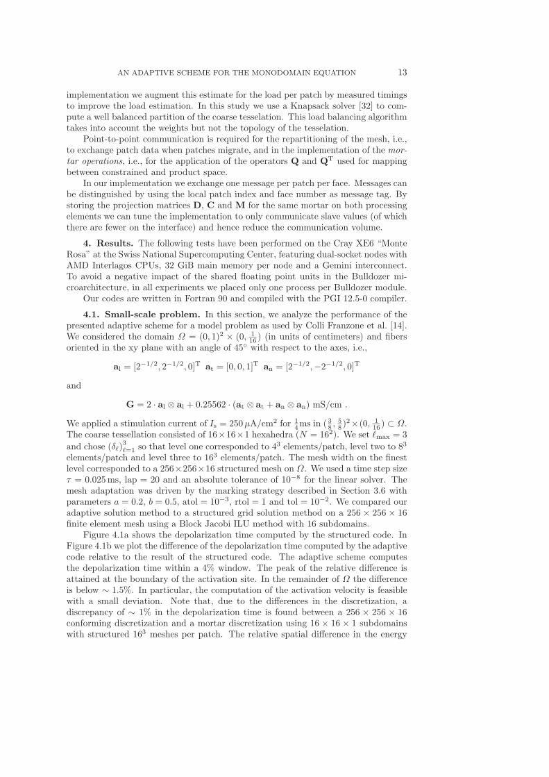
Figure 4.1a shows the depolarization time computed by the structured code. InFigure 4.1b we plot the difference of the depolarization time computed by the adaptivecode relative to the result of the structured code. The adaptive scheme computesthe depolarization time within a 4% window. The peak of the relative difference isattained at the boundary of the activation site. In the remainder of Ω the differenceis below ∼ 1.5%. In particular, the computation of the activation velocity is feasiblewith a small deviation. Note that, due to the differences in the discretization, adiscrepancy of ∼ 1% in the depolarization time is found between a 256 × 256 × 16conforming discretization and a mortar discretization using 16 × 16 × 1 subdomainswith structured 163 meshes per patch. The relative spatial difference in the energy


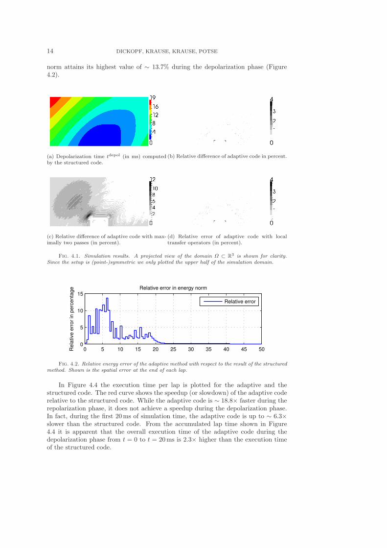
norm attains its highest value of ∼ 13.7% during the depolarization phase (Figure4.2).

(a) Depolarization time tdepol (in ms) computedby the structured code.

(b) Relative difference of adaptive code in percent.

(c) Relative difference of adaptive code with max-imally two passes (in percent).

(d) Relative error of adaptive code with localtransfer operators (in percent).

Fig. 4.1. Simulation results. A projected view of the domain Ω ⊂ R3 is shown for clarity.Since the setup is (point-)symmetric we only plotted the upper half of the simulation domain.

0 5 10 15 20 25 30 35 40 45 500

5

10

15Relative error in energy norm

Rela

tive e

rror

in p

erc

enta

ge

Relative error

Fig. 4.2. Relative energy error of the adaptive method with respect to the result of the structuredmethod. Shown is the spatial error at the end of each lap.

In Figure 4.4 the execution time per lap is plotted for the adaptive and thestructured code. The red curve shows the speedup (or slowdown) of the adaptive coderelative to the structured code. While the adaptive code is ∼ 18.8× faster during therepolarization phase, it does not achieve a speedup during the depolarization phase.In fact, during the first 20ms of simulation time, the adaptive code is up to ∼ 6.3×slower than the structured code. From the accumulated lap time shown in Figure4.4 it is apparent that the overall execution time of the adaptive code during thedepolarization phase from t = 0 to t = 20ms is 2.3× higher than the execution timeof the structured code.


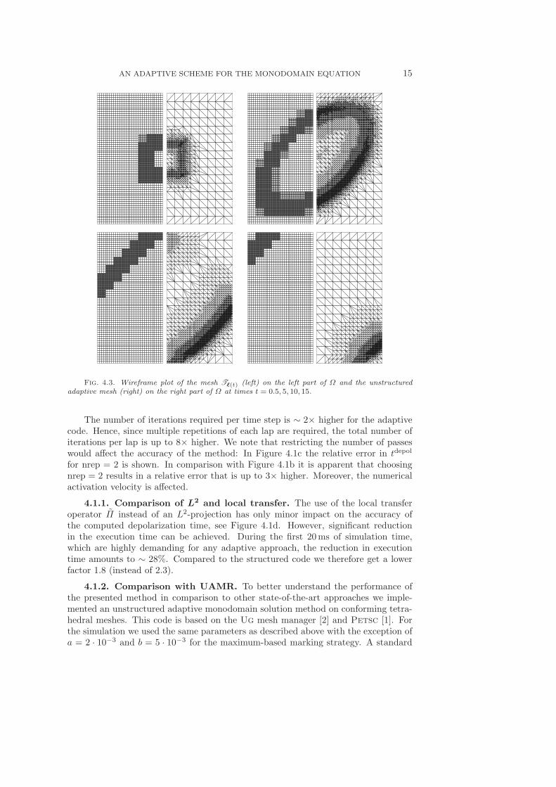
Fig. 4.3. Wireframe plot of the mesh Tℓ(t) (left) on the left part of Ω and the unstructuredadaptive mesh (right) on the right part of Ω at times t = 0.5, 5, 10, 15.

The number of iterations required per time step is ∼ 2× higher for the adaptivecode. Hence, since multiple repetitions of each lap are required, the total number ofiterations per lap is up to 8× higher. We note that restricting the number of passeswould affect the accuracy of the method: In Figure 4.1c the relative error in tdepol

for nrep = 2 is shown. In comparison with Figure 4.1b it is apparent that choosingnrep = 2 results in a relative error that is up to 3× higher. Moreover, the numericalactivation velocity is affected.

4.1.1. Comparison of L2 and local transfer. The use of the local transferoperator Π instead of an L2-projection has only minor impact on the accuracy ofthe computed depolarization time, see Figure 4.1d. However, significant reductionin the execution time can be achieved. During the first 20ms of simulation time,which are highly demanding for any adaptive approach, the reduction in executiontime amounts to ∼ 28%. Compared to the structured code we therefore get a lowerfactor 1.8 (instead of 2.3).

4.1.2. Comparison with UAMR. To better understand the performance ofthe presented method in comparison to other state-of-the-art approaches we imple-mented an unstructured adaptive monodomain solution method on conforming tetra-hedral meshes. This code is based on the Ug mesh manager [2] and Petsc [1]. Forthe simulation we used the same parameters as described above with the exception ofa = 2 · 10−3 and b = 5 · 10−3 for the maximum-based marking strategy. A standard


0 5 10 15 20 25 30 35 40 45 500

500

1000

1500Lap time

Tota

l tim

e for

lap [s]

0 5 10 15 20 25 30 35 40 45 50

10−1

100

101

102

Simulation time [ms]

Speedup o

f adaptive c

ode

Structured

Adaptive

Speedup

0 5 10 15 20 25 30 35 40 45 500

2000

4000

6000

8000


Accum

ula

ted lap tim

e [s]

0 5 10 15 20 25 30 35 40 45 500.1

0.3

1.0

3.2

10.0Accumulated lap time

Speedup o

f adaptive c

ode

Fig. 4.4. Measured execution times. The upper graph shows the walltime for the execution of alap of 20 time steps. Note that in the adaptive code each lap is repeated up to four times (cf. Figure4.5). The lower plot shows the accumulated execution time. The point (20ms, 0.44) is highlighted.

residual based error estimator for the Poisson equation was used. The initial mesh wasobtained from a 16×16×1 element structured mesh by subdividing each hexahedroninto six tetraheda. The maximal number of refinements was set to four.

Figure 4.3 shows wireframe plots of the meshes constructed by the non-conformingmethod and by the UAMR code at different stages of the simulation. The UAMRalgorithm captures the anistropy of the solution better but it also requires refinementin a broader area around the depolarization front due to closures. During the simu-lation time t = 5ms to t = 15ms the non-conforming meshes consist of up to 3.38×more mesh nodes. At the same time, the weighted estimated error measured by thenon-conforming code is 2.4× lower than the estimated error measured by the UAMRalgorithm. Note, though, that the residual error estimators used in both algorithmsfeature different efficiency indices. The UAMR algorithm requires on average 3.9×more passes over a lap. Even though we use an ILU preconditioner in our UAMRmethod (instead of a block version as in the non-conforming adaptive method), we seean increase to up to 16 iterations per time step (compared to 15 for the non-conformingcode), most likely due to the worsening quality of the finite element mesh.

Since our UAMR implementation is not as well optimized as the non-conformingadaptive code we refrain from reporting execution times for this example.

4.2. Large-scale problem. In this section we analyze the performance of theproposed adaptive method on a realistic large-scale problem. We considered the modelof a left ventricle, cropped at base and apex, as presented in Colli Franzone andPavarino [15] with the same fiber orientations. The conductivity values were chosenas in Section 4.1; the geometry of [15] was scaled by 1.4 to match it to previouslyapplied models, cf. [30]. We applied a stimulation current of Is = 250µA/cm2 for 1msin the image of (0.95, 1)× (0.125, 0.175)× (0.125, 0.175) under the parametrization of


0 5 10 15 20 25 30 35 40 45 500

400

800

1200

Number of linear solver iterations


Num

ber

of itera

tions for

lap

0 5 10 15 20 25 30 35 40 45 501

2

5

10

Incre

ase in n

um

ber

of itera

tions

Structured

Adaptive

Relative

0 5 10 15 20 25 30 35 40 45 500

1

2

3

4

5Number of passes


Num

ber

of passes

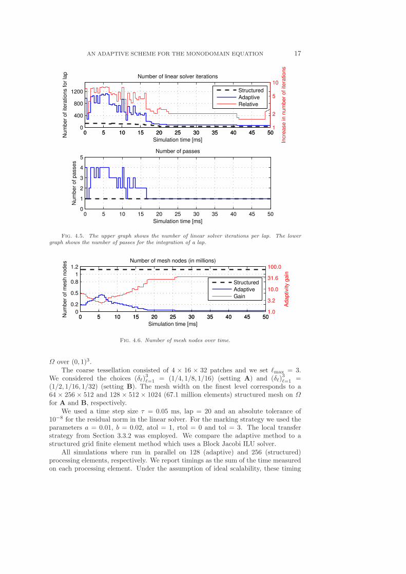
Fig. 4.5. The upper graph shows the number of linear solver iterations per lap. The lowergraph shows the number of passes for the integration of a lap.

0 5 10 15 20 25 30 35 40 45 500

0.2

0.5

0.8

1

1.2Number of mesh nodes (in millions)


Num

ber

of m

esh n

odes

0 5 10 15 20 25 30 35 40 45 501.0

3.2

10.0

31.6

100.0

Adaptivity g

ain

Structured

Adaptive

Gain

Fig. 4.6. Number of mesh nodes over time.

Ω over (0, 1)3.The coarse tessellation consisted of 4 × 16 × 32 patches and we set ℓmax = 3.

We considered the choices (δℓ)3ℓ=1 = (1/4, 1/8, 1/16) (setting A) and (δℓ)

3ℓ=1 =

(1/2, 1/16, 1/32) (setting B). The mesh width on the finest level corresponds to a64 × 256 × 512 and 128 × 512 × 1024 (67.1 million elements) structured mesh on Ωfor A and B, respectively.

We used a time step size τ = 0.05 ms, lap = 20 and an absolute tolerance of10−8 for the residual norm in the linear solver. For the marking strategy we used theparameters a = 0.01, b = 0.02, atol = 1, rtol = 0 and tol = 3. The local transferstrategy from Section 3.3.2 was employed. We compare the adaptive method to astructured grid finite element method which uses a Block Jacobi ILU solver.

All simulations where run in parallel on 128 (adaptive) and 256 (structured)processing elements, respectively. We report timings as the sum of the time measuredon each processing element. Under the assumption of ideal scalability, these timing


0 50 100 150 200 250 3000

2000

4000

6000Lap time

Tota

l tim

e for

lap [s]

0 50 100 150 200 250 30010

−1

100

101

102


Speedup o

f adaptive c

ode

Structured

Adaptive

Speedup

0 50 100 150 200 250 3000

2

4

6x 10

4 Lap time

Tota

l tim

e for

lap [s]

0 50 100 150 200 250 30010

−1

100

101

102

Simulation time [ms] Speedup o

f adaptive c

ode

Fig. 4.7. Execution time of the adaptive code in comparison to a structured code for A (upperplot) and B (lower plot).

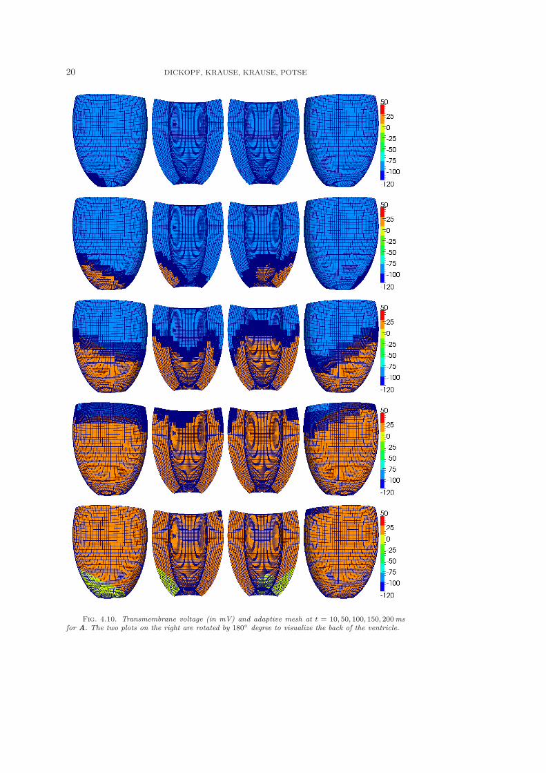
results correspond to the serial execution time. The computed transmembrane voltageuℓ and the adapted meshes at different steps are shown in Figure 4.10.

The measured execution times (Figure 4.7) show a similar picture as we obtainedfor the small-scale problem, i.e., while the adaptive procedure achieves significantspeedup during the repolarization phase, this does not hold for the depolarizationphase. During the first ∼ 150ms of simulation time, each lap is on average integratedthree times, with some laps requiring four or five passes. At its minimum, the reduc-tion in number of mesh nodes is found to be 4.4 and 5.2 for A and B, respectively.

As in Section 4.1, the number of linear solver iterations per time step is ∼ 2×higher for A than for the structured code. For B, however, the number of solveriterations is very high. In fact, for some time steps the linear solver did not reach thedesired tolerance within 100 iterations (the maximal number specified).

Finally, for setting A, in Figure 4.9 we analyze the distribution of the executiontime over the individual components of the algorithm. For times t = 50, t = 100and t = 150ms, the majority of the execution time is spent in the linear solver.Evaluation of Iion, integration of the state variables and the error estimation takeonly a small percentage of the computation time. On the other hand, collectiveand point-to-point communication account for a large part of the execution time, inparticular at t = 10ms and t = 200ms. The communication time itself is dominatedby the time spent in collective communication (in particular, MPI_Allreduce calls inthe linear solver).

4.3. Parallel scalability. In this section we analyze the strong scalability ofour implementation. The considered benchmark solves the monodomain equation onΩ = (0, 1)2 × (0, 14 ) (in units of centimeters). We used the same fibre orientationsas Pavarino and Scacchi [26] with the same conductivity tensor as in Section 4.1. Astimulation current of strength Is = 250µA/cm2 was applied for 1ms in (0, 18 )

3 ⊂ Ω.The coarse tessellation was a structured 16× 16× 4 mesh on Ω. We set ℓmax = 3


0 50 100 150 200 250 3000

500

1000

1500

2000Number of linear solver iterations


Num

ber

of itera

tions for

lap

0 50 100 150 200 250 3001

2

5

10

Incre

ase in n

um

ber

of itera

tions

Structured

Adaptive

Relative

0 50 100 150 200 250 3000

2000

4000

6000Number of linear solver iterations


Num

ber

of itera

tions for

lap

0 50 100 150 200 250 30010

0

101

102

Incre

ase in n

um

ber

of itera

tions

Structured

Adaptive

Relative

Fig. 4.8. Number of linear solver iterations for A (upper plot) and B (lower plot).

10 50 100 150 2000

25

50

75

100Distribution of lap execution time


Perc

enta

ge o

f to

tal tim

e

Communication

Error estimator

CG solver (excl.)

Preconditioner

Mortar subroutines

Membrane model

Fig. 4.9. Distribution of the execution time at five different time slots (chosen as in Figure4.10) for A. The time measurements are taken from the last pass over the lap.

and chose (δℓ)3ℓ=1 = (1/2, 1/8, 1/32). We used a time step size τ = 0.05 ms, lap = 10

and repeated each lap up to nine times (nrep = 9). The mesh adaptation was drivenby a maximum-based marking strategy (see Section 3.6) with a = 0.01 and b = 0.1.

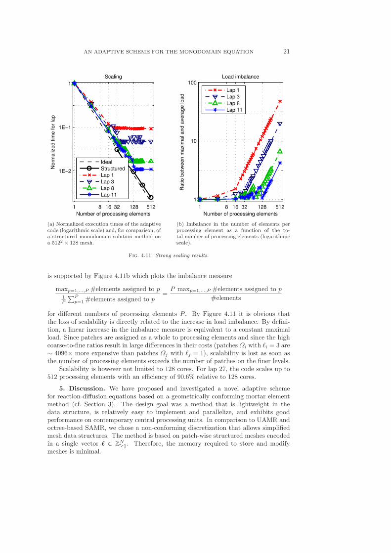
In Figure 4.11a we plot the normalized execution times of the adaptive code fordifferent laps. For comparison, the scaling of a monodomain solver on a structured5122 × 128 mesh is shown (this solution method uses a block Jacobi ILU from thePetsc [1] package). The scaling of the adaptive code is good up to a certain number ofprocessing elements (which depends on the lap) where execution time stagnates whenadding additional processing elements. The fact that the execution time stays constantand does not increase thereafter indicates that the loss of scalability is associated witha poor load balance rather than, e.g., communication inefficiencies. This hypothesis


Fig. 4.10. Transmembrane voltage (in mV) and adaptive mesh at t = 10, 50, 100, 150, 200msfor A. The two plots on the right are rotated by 180 degree to visualize the back of the ventricle.


1 8 16 32 128 512

1E−2

1E−1

1

Scaling

Number of processing elements

Norm

aliz

ed tim

e for

lap

Ideal

Structured

Lap 1

Lap 3

Lap 8

Lap 11

(a) Normalized execution times of the adaptivecode (logarithmic scale) and, for comparison, ofa structured monodomain solution method ona 5122 × 128 mesh.

1 8 16 32 128 512

1

10

100Load imbalance

Number of processing elements

Ratio b

etw

een m

axim

al and a

vera

ge load

Lap 1

Lap 3

Lap 8

Lap 11

(b) Imbalance in the number of elements perprocessing element as a function of the to-tal number of processing elements (logarithmicscale).

Fig. 4.11. Strong scaling results.

is supported by Figure 4.11b which plots the imbalance measure

maxp=1,...,P #elements assigned to p1P

∑Pp=1 #elements assigned to p

=P maxp=1,...,P #elements assigned to p

#elements

for different numbers of processing elements P . By Figure 4.11 it is obvious thatthe loss of scalability is directly related to the increase in load imbalance. By defini-tion, a linear increase in the imbalance measure is equivalent to a constant maximalload. Since patches are assigned as a whole to processing elements and since the highcoarse-to-fine ratios result in large differences in their costs (patches Ωi with ℓi = 3 are∼ 4096× more expensive than patches Ωj with ℓj = 1), scalability is lost as soon asthe number of processing elements exceeds the number of patches on the finer levels.

Scalability is however not limited to 128 cores. For lap 27, the code scales up to512 processing elements with an efficiency of 90.6% relative to 128 cores.

5. Discussion. We have proposed and investigated a novel adaptive schemefor reaction-diffusion equations based on a geometrically conforming mortar elementmethod (cf. Section 3). The design goal was a method that is lightweight in thedata structure, is relatively easy to implement and parallelize, and exhibits goodperformance on contemporary central processing units. In comparison to UAMR andoctree-based SAMR, we chose a non-conforming discretization that allows simplifiedmesh data structures. The method is based on patch-wise structured meshes encodedin a single vector ℓ ∈ ZN

≥1. Therefore, the memory required to store and modifymeshes is minimal.


When assembled as a sparse matrix, the stiffness matrix on the mortar-constrainedspace has a relatively high bandwidth at master nodes on interfaces where patches withfine and coarse local meshes intersect. Storing this matrix in standard formats (e.g.,CRS or CCS), though possible, does not allow for full exploitation of the structureof Tℓ. For this reason we implemented matrix-vector multiplications in a matrix-freesetup using stencil type operations. Motivated by the success of Block Jacobi ILUpreconditioning reported in previous work [22], we have chosen a Block Jacobi methodfor the adaptive scheme as well. By using a local CG solver for the preconditioner weremain in a matrix-free setup and obtain a very memory-efficient method.

For the small-scale problem and problem A in Section 4.2, our method requiresapproximately twice as many iterations as an ILU or Block Jacobi ILU preconditioneron a conforming structured mesh. In Figures 4.5 and 4.8 the total number of iterations(taking into account multiple repetitions) are shown. The results for settingB indicatethat the iteration numbers are influenced by the coarse-to-fine ratio. However, itis well known that also for conforming discretizations and, e.g., multigrid solvers,spatial adaptivity can have a negative impact on the solver efficiency. In fact, theILU-preconditioned CG used in the UAMR algorithm required more iterations thanthe linear solver in the non-conforming algorithm, as reported in Section 4.1.

To reduce the overhead due to adaptivity, we have applied two optimization tech-niques in this study. First, we used a low-order quadrature to approximate the residualerror estimator (Section 3.5). The error in the estimated error due to this modifica-tion is within a few percent. Moreover, we have introduced a local transfer operator(Section 4.1.1) which can be used as a drop-in replacement for the L2-transfer.

The proposed parallelization scheme has been shown to be effective up to severalhundreds of cores (Section 4.3). When the number of patches on the finer mesh lev-els is too low compared to the number of processing elements, maintaining the loadbalance may become difficult. As one expects in an adaptive scheme with varyingnumber of degrees of freedom, parallel efficiency varies over the course of a simu-lation. A hybrid MPI+threads implementation (e.g., using OpenMP for loop-levelparallelism) might be used to improve the scaling at larger core counts.

The design of adaptive numerical algorithms necessitates a trade-off between com-putational efficiency and the “optimality” of the constructed approximation spaces.The presented method represents an edge case in this spectrum of adaptive methods,as it vigorously favors efficiency of the datastructures over a reduction in the degreesof freedom. This choice has two important consequences that can be observed in ourexperiments. On the one hand, we measure a relatively low reduction in the degreesof freedom compared to other UAMR and SAMR methods. Considering a two-levelmethod with coarse-to-fine ratio r, a back-of-the-envelope calculation shows that r3

is an upper bound for the reduction in the degrees of freedom achieved if the depolar-ization front is an axis-aligned hyperplane and the coarse tesselation is a (sufficientlyfine) structured mesh. For setting A in Section 4.2 this means that the adaptivitygain is bounded by 43 = 64. For a more complicated shape of the depolarization front,the gain by adaptivity will be smaller. This is in fact what we observe. For A, thereduction in the number of mesh nodes is only about 4.4× at its minimum. On theother hand, the number of repetitions required to find a tailored mesh (given a desirederror tolerance and a bound on the maximal level) is low compared to, e.g., an UAMRalgorithm (cf. Section 4.1.2). In all our experiments, our marking strategy terminatedwithin 3 – 5 passes over a time window. Since the mesh Tℓ is encoded by the vector


ℓ it is possible to adapt the mesh to the solution disregarding the refinement history.This could be used to develop more effective problem-tailored marking strategies thatwould further speed up the adaptive method.

In the presented numerical experiments we have compared our adaptive methodto a state-of-the-art structured solver for the monodomain equation. The observed netslowdown of the adaptive code relative to a structured code that we measure in Section4.2, is explained by the combination of a comparably low reduction in the degrees offreedom, the higher solver cost (2×), the need to repeat laps multiple times, additionaloverhead (data transfer, matrix reassembly, error estimation) and differences in theparallel scalability. An improved preconditioner and marking strategy might helpto narrow or close this gap. Let us point out that all comparisons have been madebetween the adaptive strategy and a structured uniform monodomain code, whichtypically outperform unstructured uniform monodomain codes that are most relevantfor practical applications.

As is the case for any adaptive method, in order to deal with complex geome-tries, a suitable coarse tesselation has to be constructed. For complicated geometriesas obtained from medical imaging, the construction of a suitable coarse tesselationas used in Section 3.1 might be difficult. Another aspect is that many models forheart tissue feature jumps in the coefficients and use different membrane models indifferent regions. Also these heterogeneities have to be to be taken into account whenconstructing the coarse tesselation.

Among the related work listed in Section 1, only Deuflhard et al. [14, 16, 38] andYing and Hendriquez [45] considered (semi-)implicit time discretization for three-dimensional problems. Weiser et al. [38] reported that for a fibrillation study theemployed adaptive scheme does not provide a reduction in the compute time despitea remarkable reduction of degrees of freedom by a factor of 150.

Ying and Hendriquez [45] reported a 17× speedup for a simulation of a dog heartventricle. They used a second-order CBDF scheme for the Luo-Rudy I membranemodel and a geometric multigrid solver for the diffusion. Local time stepping wasused for computing the transmembrane voltage on spatially nested meshes. In ourstudy, we have chosen a first-order time integration scheme that is currently mostpopular in computational electrocardiology [22, 29]. For comparison, our structuredcode requires about 3.6µs per time step per degree of freedom on a 2.1GHz AMDInterlagos CPU. Based on the parameters given by Ying and Hendriquez [45] theiruniform grid solution method requires about 50µs per time step per degree of freedomon a 3.6GHz Intel Xeon. Moreover, we only consider spatial adaptivity to allow foran unbiased assessment of the efficiency of the non-conforming adaptive scheme.

In contrast to Ying and Hendriquez [45] we used timings per time step/lap toassess the performance of the proposed method. In general, we do not consider end-to-end computing time a good measure for the efficiency of an adaptive scheme since asufficiently long repolarization phase can mask potential inefficiencies of the adaptivescheme during the (more interesting) depolarization phase.

Note that none of these studies have addressed the issue of computing depolar-ization times on the adaptive meshes (Section 3.7) or parallelization (Section 3.9).

Acknowledgments. This work was supported by a grant from the Swiss Na-tional Supercomputing Centre (CSCS) under project ID 397 and by the project “AHigh Performance Approach to Cardiac Resynchronization Therapy” within the con-text of the “Initiativa Ticino in Rete” and the “Swiss High Performance and Produc-


tivity Computing” (HP2C) initiative. M.P. was financially supported by a grant fromthe Fondazione Cardiocentro Ticino.

REFERENCES

[1] S. Balay, J. Brown, K. Buschelman, W. D. Gropp, D. Kaushik, M. G. Knep-

ley, L. Curfman McInnes, B. F. Smith, and H. Zhang, PETSc web page, 2011.http://www.mcs.anl.gov/petsc.

[2] P. Bastian, K. Birken, K. Johannsen, S. Lang, N. Neuss, H. Rentz-Reichert, and

C. Wieners, UG - A Flexible Software Toolbox for Solving Partial Differential Equations,Comput. Vis. Sci., 1 (1997), pp. 27–40.

[3] Y. Belhamadia, A time-dependent adaptive remeshing for electrical waves of the heart, IEEETrans. Biomed. Eng., 55 (2008), pp. 443–452.

[4] M. Bendahmane, R. Burger, and R. Ruiz-Baier, A multiresolution space-time adaptivescheme for the bidomain model in electrocardiology, Numer. Meth. Part. D. E., 26 (2010),pp. 1377–1404.

[5] M. J. Berger and P. Colella, Local adaptive mesh refinement for shock hydrodynamics, J.Comput. Phys., 82 (1989), pp. 64–84.

[6] C. Bernardi and Y. Maday, Mesh adaptivity in finite elements using the mortar method,

Revue Europeenne des Elements, 9 (2000), pp. 451–465.[7] C. Bernardi, Y. Maday, and A. T. Patera, A new nonconforming approach to domain

decomposition: The mortar element method, in Nonlinear Partial Differential Equationsand Their Applications, H. Brezis and J. L. Lions, eds., 299, Pitman Res. Notes Math.Ser., 1994, pp. 13–51.

[8] C. Bernardi, Y. Maday, and F. Rapetti, Basics and some applications of the mortar elementmethod, GAMM-Mitt. 28, 2 (2005), pp. 97–123.

[9] O. Bernus, R. Wilders, C. W. Zemlin, H. Verschelde, and A. V. Panfilov, A compu-tationally efficient electrophysiological model of human ventricular cells, Am. J. Physiol.Heart Circ. Physiol., 282 (2002), pp. H2296–H2308.

[10] C. Burstedde, O. Ghattas, G. Stadler, T. Tu, and L. C. Wilcox, Towards adaptive meshPDE simulations on petascale computers, in TeraGrid 2008, 2008.

[11] C. Burstedde, L. C. Wilcox, and O. Ghattas, p4est: Scalable algorithms for parallel adap-tive mesh refinement on forests of octrees, SIAM J. Sci. Comput., 33 (2011), pp. 1103–1133.

[12] E. M. Cherry, H. S. Greenside, and C. S. Henriquez, A space-time adaptive method forsimulating complex cardiac dynamics, Phys. Rev. Lett., 84 (2000), pp. 1343–1346.

[13] , Efficient simulation of three-dimensional anisotropic cardiac tissue using an adaptivemesh refinement method, Chaos, 13 (2003), pp. 853–865.

[14] P. Colli Franzone, P. Deuflhard, B. Erdmann, J. Lang, and L. F. Pavarino, Adaptivityin space and time for reaction-diffusion systems in electrocardiology, SIAM J. Sci. Comput.,28 (2006), pp. 942–962.

[15] P. Colli Franzone and L. F. Pavarino, A parallel solver for reaction-diffusion systems incomputational electrocardiology, Math. Model Meth. App. Sci., 14 (2004), pp. 883–911.

[16] P. Deuflhard, B. Erdmann, R. Roitzsch, and G. T. Lines, Adaptive finite element simu-lation of ventricular fibrillation dynamics, Comput. Vis. Sci., 12 (2009), pp. 201–205.

[17] L. F. Diachin, R. Hornung, P. Plassmann, and A. Wissink, Parallel adaptive mesh refine-ment, in Parallel Processing for Scientific Computing, M. A. Heroux, P. Raghavan, andH. D. Simon, eds., Society for Industrial and Applied Mathematics, 2006.

[18] A. Ern and J.-L. Guermond, Theory and Practice of Finite Elements, Springer, 2004.[19] B. Flemisch and B. Wohlmuth, Stable Lagrange multipliers for quadrilateral meshes of curved

interfaces in 3d, Comput. Meth. Appl. Mech. Eng., 196 (2007), pp. 1589–1602.[20] G. Gassner, F. Lorcher, and C.-D. Munz, A discontinuous galerkin scheme based on a

space-time expansion II. viscous flow equations in multi dimensions, J. Sci. Comput., 34(2008), pp. 260–286.

[21] R. Hoppe, Y. Iliash, Y. Kuznetsov, Y. Vassilevski, and B. Wohlmuth, Analysis andparallel implementation of adaptive mortar finite element methods, East–West J. Numer.Math., 6 (1998), pp. 223–248.

[22] D. Krause, M. Potse, T. Dickopf, R. Krause, A. Auricchio, and F. Prinzen, Hybridparallelization of a large-scale heart model, in Facing the Multicore - Challenge II, R. Keller,D. Kramer, and J.-P. Weiss, eds., vol. 7174 of Lecture Notes in Computer Science, Springer,2012, pp. 120–132.

[23] J. Lang, Adaptive Multilevel Solution of Nonlinear Parabolic PDE Systems: Theory, Al-


gorithm, and Applications, Lecture Notes in Computational Science and Engineering,Springer, 2000.

[24] G. T. Lines, P. Grottum, and A. Tveito, Modeling the electrical activity of the heart:A bidomain model of the ventricles embedded in a torso, Comput. Vis. Sci., 5 (2003),pp. 195–213.

[25] Y. Maday, C. Mavriplis, and A. T. Patera, Nonconforming mortar element methods - Ap-plication to spectral discretizations, in Domain Decomposition Methods, 1989, pp. 392–418.

[26] L. F. Pavarino and S. Scacchi, Multilevel additive schwarz preconditioners for the bidomainreaction-diffusion system, SIAM J. Sci. Comput., 31 (2008), pp. 420–443.

[27] M. Pennacchio, A non-conforming domain decomposition method for the cardiac potentialproblem, in Comput. Cardiol., 2001, pp. 537–540.

[28] , The mortar finite element method for the cardiac “bidomain” model of extracellularpotential, J. Sci. Comp., 20 (2004), pp. 191–210.

[29] G. Plank, R. A. Burton, P. Hales, M. Bishop, T. Mansoori, M. O. Bernabeu, A. Garny,

A. J. Prassl, C. Bollensdorff, F. Mason, F. Mahmood, B. Rodriguez, V. Grau, J. E.

Schneider, D. Gavaghan, and P. Kohl, Generation of histo-anatomically representativemodels of the individual heart: tools and application, Philos. Transact. A Math. Phys. Eng.Sci., 367 (2009), pp. 2257–2292.

[30] M. Potse, B. Dube, J. Richer, A. Vinet, and R. M. Gulrajani, A comparison of mono-domain and bidomain reaction-diffusion models for action potential propagation in thehuman heart, IEEE Trans. Biomed. Eng., 53 (2006), pp. 2425–2435.

[31] M. Potse, D. Krause, L. Bacharova, R. Krause, F. W. Prinzen, and A. Auricchio,Similarities and differences between electrocardiogram signs of left bundle-branch blockand left-ventricular uncoupling, Europace, 14 (2012), pp. v33–v39.

[32] C. A. Rendleman, V. E. Beckner, M. Lijewski, W. Crutchfield, and J. B. Bell, Par-allelization of structured, hierarchical adaptive mesh refinement algorithms, Comput. Vis.Sci., 3 (2000), pp. 147–157.

[33] S. Rush and H. Larsen, A practical algorithm for solving dynamic membrane equations, IEEETrans. Biomed. Eng., 25 (1978), pp. 389 –392.

[34] S. Sun and M. F. Wheeler, Mesh adaptation strategies for discontinuous galerkin methodsapplied to reactive transport problems, in Proceedings of the 2004 International Conferenceon Computing, Communication and Control Technologies, H.-W. Chu, M. Savoie, andB. Sanchez, eds., vol. 1, 2004, pp. 223–228.

[35] J. A. Trangenstein and C. Kim, Operator splitting and adaptive mesh refinement for theLuo-Rudy I model, J. Comput. Phys., 196 (2004), pp. 645–679.

[36] T. Tu, D. R. O’Hallaron, and O. Ghattas, Scalable parallel octree meshing for terascaleapplications, in Proceedings of the 2005 ACM/IEEE conference on Supercomputing, SC’05, Washington, DC, USA, 2005, IEEE Computer Society.

[37] B. Van Straalen, P. Colella, D. T. Graves, and N. Keen, Petascale block-structuredAMR applications without distributed meta-data, in Proceedings of the 17th InternationalEuro-Par Conference 2011, 2011. to appear.

[38] M. Weiser, B. Erdmann, and P. Deuflhard, On efficiency and accuracy in cardioelectricsimulation, in Progress in Industrial Mathematics at ECMI 2008, H.-G. Bock, F. Hoog,A. Friedman, et al., eds., vol. 15 of Mathematics in Industry, Springer Berlin Heidelberg,2010, pp. 371–376.

[39] J. P. Whiteley, Physiology driven adaptivity for the numerical solution of the bidomain equa-tions, Ann. Biomed. Eng., 35 (2007), pp. 1510–1520.

[40] A. M. Wissink, R. D. Hornung, S. R. Kohn, S. S. Smith, and N. Elliott, Large scaleparallel structured AMR calculations using the SAMRAI framework, in Proceedings of the2001 ACM/IEEE conference on Supercomputing, 2001, pp. 6–6.

[41] B. Wohlmuth, A residual based estimator for mortar finite element discretizations, Numer.Math., 84 (1999), pp. 143–171.

[42] , A mortar finite element method using dual spaces for the Lagrange multiplier, SIAMJ. Numer. Anal., 38 (2000), pp. 989–1012.

[43] , Discretization Techniques and Iterative Solvers Based on Domain Decomposition,vol. 17, Springer, 2001.

[44] W. Ying, A multilevel adaptive approach for computational cardiology, PhD thesis, Duke Uni-versity, 2005.

[45] W. Ying and C. S. Henriquez, Adaptive mesh refinement for modeling cardiac electricaldynamics, Chaos, (2011). submitted.

Design and analysis of a lightweight parallel adaptive ...DESIGN AND ANALYSIS OF A LIGHTWEIGHT...

Documents

Transcript of Design and analysis of a lightweight parallel adaptive ...DESIGN AND ANALYSIS OF A LIGHTWEIGHT...