Gliederung

1. Populäre Einführung I: Astrometrie2. Populäre Einführung II: Hipparcos und Gaia3. Wissenschaft aus Hipparcos-Daten I 4. Wissenschaft aus Hipparcos-Daten II5. Hipparcos: Technik und Mission6. Astrometrische Grundlagen 7. Hipparcos Datenreduktion Hauptinstrument8. Hipparcos Datenreduktion Tycho9. Gaia: Technik und Mission10. Gaia Global Iterative Solution11. Wissenschaft aus Gaia-Daten12. Sternklassifikation mit Gaia13. SIM und andere Missionen

Sternklassifikation mit Gaia

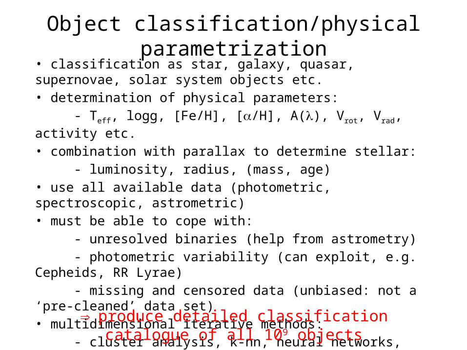
Object classification/physical parametrization

• classification as star, galaxy, quasar, supernovae, solar system objects etc.• determination of physical parameters:

- Teff, logg, [Fe/H], [/H], A(), Vrot, Vrad, activity etc.

• combination with parallax to determine stellar:

- luminosity, radius, (mass, age)• use all available data (photometric, spectroscopic, astrometric)• must be able to cope with:

- unresolved binaries (help from astrometry)

- photometric variability (can exploit, e.g. Cepheids, RR Lyrae)

- missing and censored data (unbiased: not a ‘pre-cleaned’ data set)• multidimensional iterative methods:

- cluster analysis, k-nn, neural networks, interpolation methods• required for astrometric reduction (identification of quasars, variables etc.)• maybe discovery of new types of objects produce detailed classification catalogue of all 109 objects

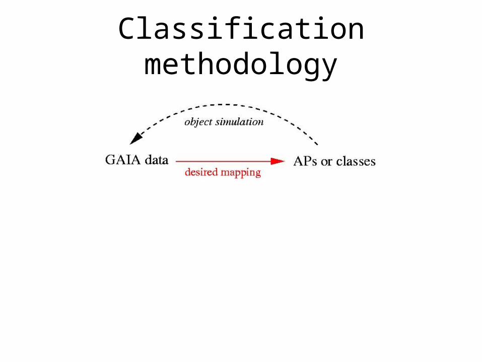
Classification methodology

Minimum Distance Methods (MDM)

astrophysical parameter(s)

d1,d2 data

D distance to a template

Neural Networks

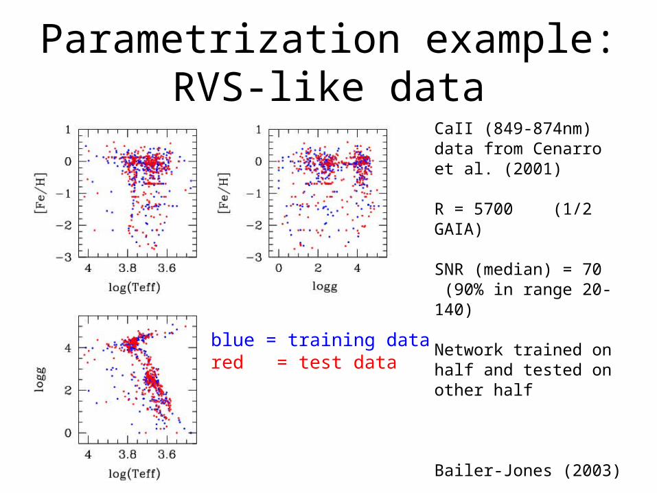
Parametrization example: RVS-like data

blue = training datared = test data

CaII (849-874nm) data from Cenarro et al. (2001)

R = 5700 (1/2 GAIA)

SNR (median) = 70 (90% in range 20-140)

Network trained on half and tested on other half

Bailer-Jones (2003)

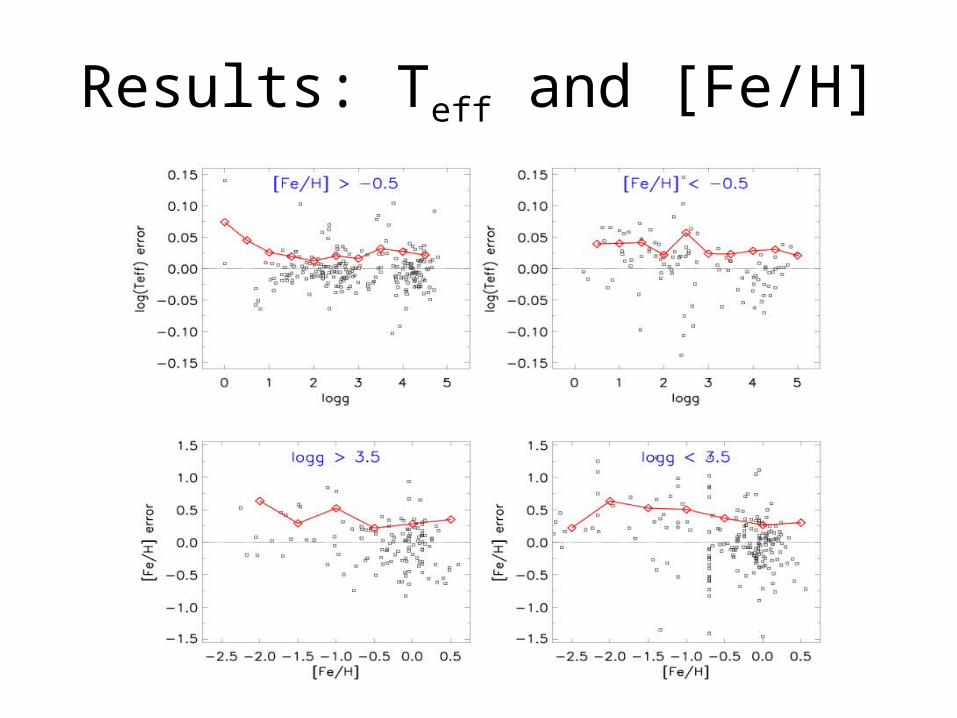
Results: Teff and [Fe/H]

Classification issues

• different data sensitivities to APs (Teff strong; [Fe/H] weak)

• wide range of object types– inhomogeneous stellar models– hierarchical classifier

• binary stars (raises dimensionality)• stellar variability• degeneracy• inhomogeneous data• calibration• etc.

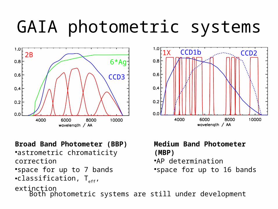
GAIA photometric systems

Broad Band Photometer (BBP)●astrometric chromaticity correction●space for up to 7 bands●classification, T

eff, extinction

Medium Band Photometer (MBP)●AP determination●space for up to 16 bands

6*Ag

CCD3

2B 1X CCD1b CCD2

Both photometric systems are still under development

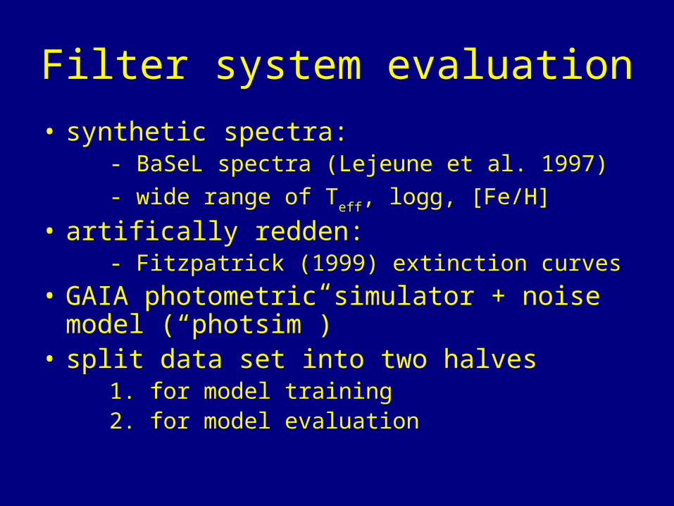
Filter system evaluation

• synthetic spectra: - BaSeL spectra (Lejeune et al. 1997)

- wide range of Teff

, logg, [Fe/H]

• artifically redden: - Fitzpatrick (1999) extinction curves

• GAIA photometric simulator + noise model (“photsim”)

• split data set into two halves 1. for model training 2. for model evaluation

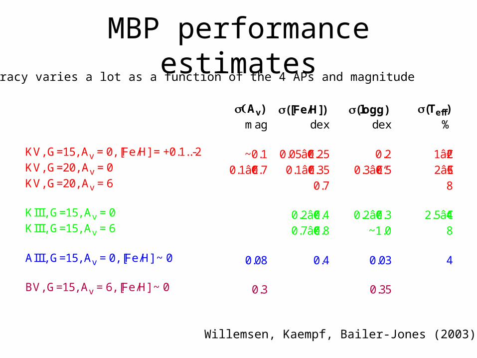
MBP performance estimates

mag dex dex %

~0.1 0.05‒0.25 0.20.1‒0.35

0.7 8

~1.0 8

0.08 0.4 0.03 4

0.3 0.35

Av) ([Fe/H]) (logg) (Teff)

KV, G=15, Av = 0, [Fe/H] = +0.1..-2 1–2KV, G=20, Av = 0 0.1‒0.7 0.3–0.5 2–5KV, G=20, Av = 6

KIII, G=15, Av = 0 0.2–0.4 0.2–0.3 2.5–4KIII, G=15, Av = 6 0.7–0.8

AIII, G=15, Av = 0, [Fe/H] ~ 0

BV, G=15, Av = 6, [Fe/H] ~ 0

Accuracy varies a lot as a function of the 4 APs and magnitude

Willemsen, Kaempf, Bailer-Jones (2003)

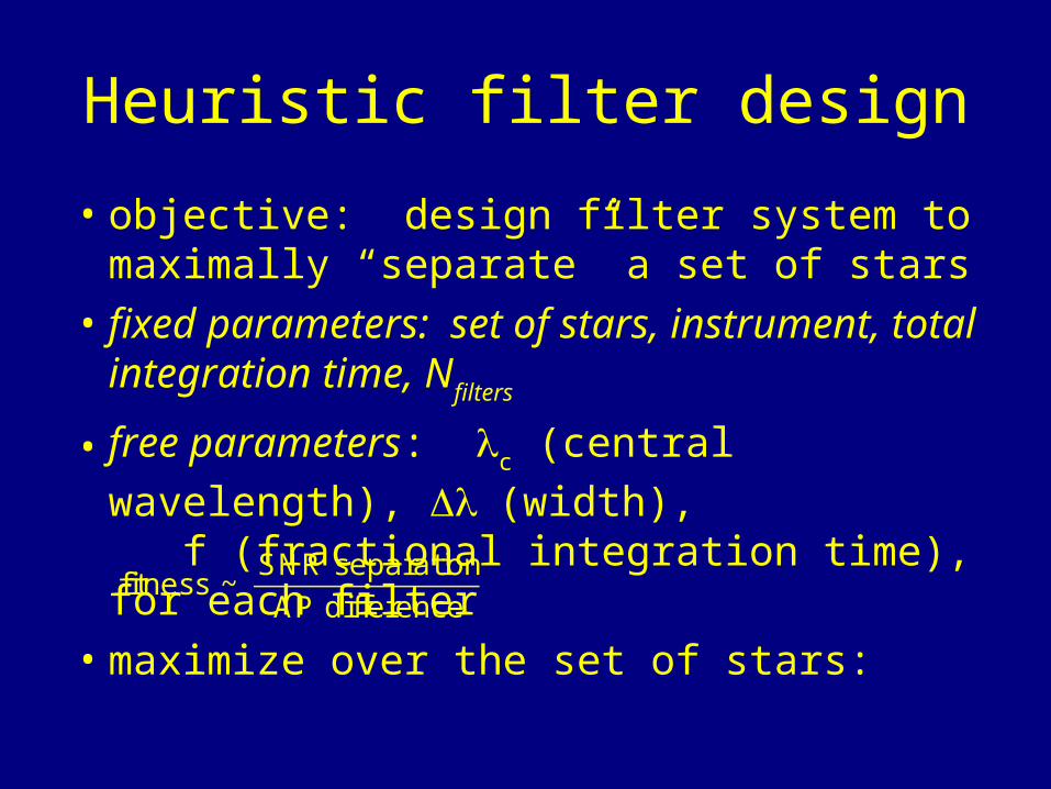
Heuristic filter design

• objective: design filter system to maximally “separate” a set of stars

• fixed parameters: set of stars, instrument, total integration time, N

filters

• free parameters: c (central wavelength),

(width), f (fractional integration time), for each filter

• maximize over the set of stars:

fitness ~SNR separation

AP difference

Evolutionary algorithm

initialise population

simulate counts (and errors) from each star in each filter system

calculate fitness ofeach filter system

select fitter filter systems(probability a fitness)

mutate filter systemparameters

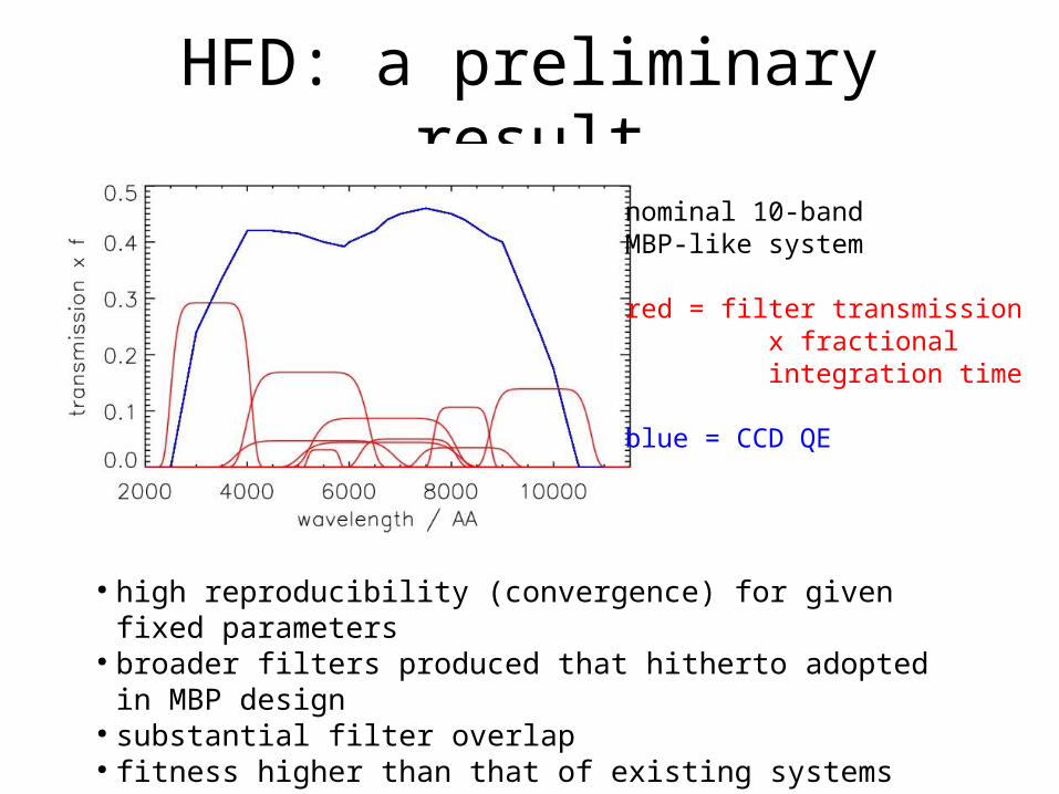
HFD: a preliminary result

nominal 10-band MBP-like system

red = filter transmission x fractional integration time

blue = CCD QE

● high reproducibility (convergence) for given fixed parameters● broader filters produced that hitherto adopted in MBP design● substantial filter overlap● fitness higher than that of existing systems (e.g. 1X)