DIPLOMARBEIT

Titel der Diplomarbeit

„Laser Beam Engineering for Material Processing“

Verfasser

Dipl. Ing. (FH) Christian Haselberger

angestrebter akademischer Grad

Magister der Naturwissenschaften (Mag. rer. nat.)

Wien, 2009

Studienkennzahl lt. Studienblatt: A 419

Studienrichtung lt. Studienblatt: Chemie

Betreuerin / Betreuer: Univ.-Prof. Dipl.-Ing. Dr. Wolfgang Kautek

brought to you by COREView metadata, citation and similar papers at core.ac.uk

provided by OTHES

1

Contents

Contents 1

Abstract 3

Kurzfassung 3

1 Introduction 5

2 Theoretical Background 7

2.1 The Basics 7

2.2 Pulse Generation 9

2.2.1 Principle 9

2.2.2 Ti:Sapphire Oscillator 11

2.2.3 Prism Compression 11

2.2.4 Pockels Cell 12

2.3 Pulse Characterization 12

2.3.1 Energy and Power 13

2.3.2 Intensity Autocorrelation 14

2.3.3 Frequency-Resolved Optical Gating (FROG) 16

2.3.4 Beam Diameter Determination – Moving Edge 18

2.4 Pulse Modification 19

2.4.1 Pulse Shaper 19

2.5 Inverse Pulsed Laser Deposition (IPLD) 22

3 Experimental 23

3.1 Laser Setup 23

3.2 Ablation Experiments 27

4 Results and Discussion 29

4.1 Pulse Characterization 29

4.2 Microscope Objective Characterization 31

4.2.1 Beam Diameter – “Moving Edge” Method 31

4.2.2 Determination of the Group Velocity Dispersion 33

4.3 Pulse Shaper 33

4.4 Thin Film Ablation Experiments 43

5 Conclusion and Outlook 47

6 Appendix 49

Bibliography 51

Curriculum Vitae 59

2

3

Abstract

A main focus of this diploma work was the characterization of femtosecond laser

pulses. A LabVIEW program for autocorrelation measurements was adapted to deliver

results at an interval of up to 2 Hz and a FROG (frequency-resolved optical gating)

device was developed to characterize the phase of laser pulses. Ablation experiments

were carried out to determine the dependence of the fs-laser ablation threshold on the

thickness of thin diamond like films. These experiments served as preparation for the

setup, adjustment, and calibration of a pulse shaper in a new configuration with a high-

power femtosecond oscillator.

Kurzfassung

Ein wichtiger Bestandteil dieser Diplomarbeit war die Charakterisierung von Femto-

sekunden-Laserpulsen. Dazu wurde das bestehende LabVIEW Programm für die

Autokorrelationsmessungen adaptiert und ermöglicht nun Messungen mit einer

Geschwindigkeit von bis zu 2 Hz. Ebenfalls wurde ein FROG (frequency-resolved

optical gating) aufgebaut, womit auch die Phasenanteile der Femtosekunden-

Laserpulse gemessen werden können. Mittels Ablationsexperimenten wurde die

Abhängigkeit der Ablationsschwelle von der Filmdicke von diamantähnlichen Kohlen-

stoffschichten ermittelt. Zur erweiterten Durchführung von Ablationsexperimenten

wurden der Aufbau, die Justage und die Kalibrierung eines Pulsformers in Kopplung

eines leistungsstarken Femtosekundenoszillators realisiert.

4

5

1 Introduction

Lasers (light amplification by stimulated emission of radiation) and their technology

are known since 50 years [1]. There are many different fields of application like cutting,

welding, and labelling in industrial material processing and in diagnostics and surgery

in medical science. Lasers normally are known from television or laser shows because

of their strong and impressive colour. Of course the colours are impressive as it can be

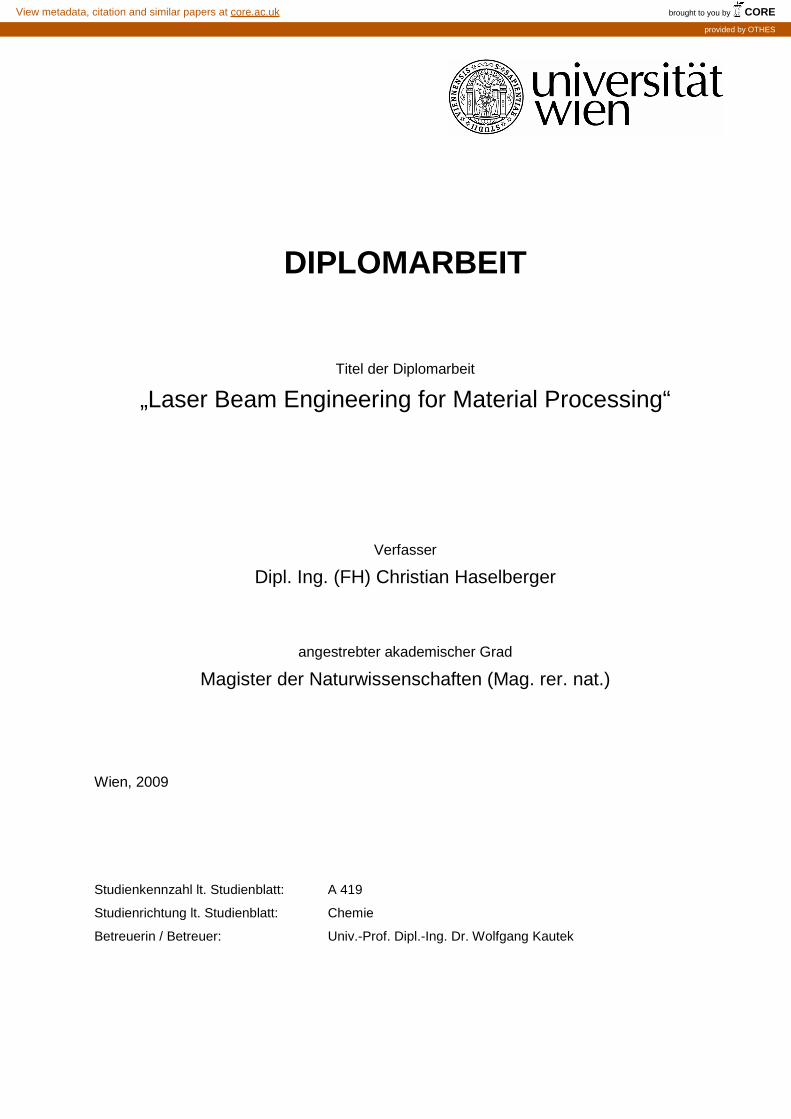
seen inside the laser oscillator used in our lab (see Figure 1) but this is only a side effect.

There is much attention on pulsed lasers with pulse lengths in the femtosecond and

recently in the attosecond regime. Thermal diffusion control in femtosecond laser

processing of solids is restricted to nanoscale dimensions, which has been one of the

reasons of the breakthrough of this category of lasers in materials machining [2]. That

means that femtosecond excitation provides the promising perspective that laser

radiation interaction with the evolving plasma is minimized and that heat affected

zones are reduced into the nanoscale range in contrast to pico- and nanosecond laser

processing. Near-infrared ultrashort laser pulses down to durations of 5 fs yielded

unexpected machining qualities characterised by high precision and deterministic

features [3].

Figure 1: Impressive green scattered light inside the sub-60-fs high-power 11 MHz laser system

with fs-power-oscillator technology used in our lab

A laser-technological objective was also the adaptive laser beam engineering for

material processing. This new technological approach explores the excitation of optical

phonons in order to reduce processing energy thresholds. Theory suggests a resonant

6

coherent enhancement of the phonon modes excited by femtosecond laser pulses in

dielectric media which and can be measured with a transient transmission setup [4].

There is experimental work proving this for LiTaO3 [5]. Coherent phonons have been

shown to exist in technologically relevant materials like α-quartz [6]. This opens the

potential for nanostructuring of optical materials by adaptive irradiation systems on

the basis of a novel industrial-suited 60 fs-laser oscillator technology integrated with a

pulse shaper allowing temporal design of 60 fs laser pulses. The temporal pulse shaping

generated by phase modulation will be followed by adaptive, feedback-controlled

material processing. Thus, a cost-efficient nanostructuring technology of photonic

materials comes within sight.

In the following work a pulsed Ti:sapphire laser with a pulse length of 60 fs was used in

combinations with an intensity autocorrelator, a FROG, a pulse shaper and a

microscope to carry out fs-laser ablation of thin diamond like carbon films. Therefore

chapter 2 will give an overview of the theoretical background of all methods and devices

used during the work. In chapter 3 the whole setup including the measurement devices

will be introduced and chapter 4 contains results and discussion. The conclusion and

outlook will be in chapter 5. In the appendix the LabVIEW program written for

acquiring the autocorrelation trace will be described.

7

2 Theoretical Background

This chapter describes the background of all used experimental techniques. It is

described how laser pulses are generated and how their spectral and temporal

properties can be influenced and measured.

2.1 The Basics

What is an ultrashort laser pulse? There is a simple answer: it is a very short burst of

electro-magnetic energy. Mathematically the pulse electric field E(x,y,z,t) is described

by the product of a sine wave and a pulse-envelope function. The electric field is

dependent on space and time. For simplicity some assumptions are made. The vector

character of the pulse electric field is ignored because the field is treated as linearly

polarized. Although we are mainly interested in the temporal features of the pulse and

therefore ignore the spatial part of the field. The resulting time-dependent electric field

E(t) can be written as [7]

( ) ..)(

2

1)( )(0 ccetItE tti +⋅= −φω

(1)

Where ω0 is the carrier angular frequency and I(t) and φ(t) are the time-dependent

intensity and phase of the pulse. The term c.c. means complex conjugate and is

required to get a real pulse field. For simpler mathematics the complex-conjugate term

is ignored which is commonly called the “analytic signal” approximation and this yields

a complex electric pulse field which is used for further mathematical descriptions:

)()()( tietItE φ−⋅= (2)

The carrier wave tie 0ω is removed because it cannot be measured reliably and makes

mathematics easier too. As the complex-conjugate term is removed the real part is

taken twice. The yielded equation can be solved for the intensity which can be

measured for example by the intensity autocorrelation described in chapter 2.3.2

2

)()( tEtI = (3)

The phase can be measured by FROG described in chapter 2.3.3

))(Re(

))(Im(arctan)(

tE

tEt −=φ (4)

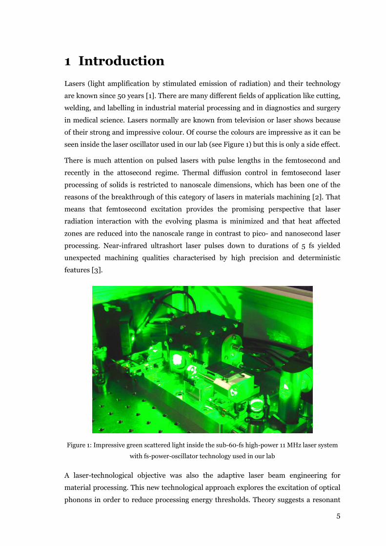
A sample pulse is shown in Figure 2 where the different meanings of the electro-

magnetic field, the amplitude of field, and the intensity are shown. An important

8

property of the pulse is the pulse length which is normally defined as the full width at

half maximum (FWHM).

-20 -10 0 10 20

-1,0

-0,8

-0,6

-0,4

-0,2

0,0

0,2

0,4

0,6

0,8

1,0in

ten

sity

/ a

.u.

time / fs

intensity

amplitude

electric fieldFWHM

Figure 2: A Gaussian laser pulse showing the amplitude and the electric field and the

corresponding intensity

The pulse electric field can also be described in the frequency domain. The Fourier

transform of the time domain field yields the frequency domain field

∫∞

∞−

−= dtetEE tiωω )()(~

(5)

and in terms of intensity S(ω) and phase ϕ(ω)

)()()(

~ ωϕωω ieSE −⋅= (6)

S(ω) is the frequency spectrum which will be measured with a spectrometer and the

spectral phase can be retrieved from the FROG trace. The inverse Fourier transform of

the frequency domain yields the time domain electric field

∫∞

∞−= ω

πω detEtE ti)(

~2

1)( (7)

In the laboratory the time dependent intensity is the most interesting part but as there

is a relation to the frequency domain this is being checked too. A deviation in spectral

phase changes the pulse shape in time domain.

9

The time and frequency dependent phases can be written as a Taylor series expansion

...2

)( 22

10 +++=φφφφ t

tt (8)

...2

)()()( 2

20

100 +−

+−+=ϕωωϕωωϕωϕ (9)

The first order term tφ1 corresponds to a shift in time and describes the time delay of

the pulse relative to the pulse without delay. The greater this term is the later or earlier

the pulse arrives. The second order term is called linear chirp and describes the linear

dependence of the velocity vs. frequency of light. One example of linear dispersion is

glass where red light travels faster than blue light. For optical elements the group delay

dispersion is introduced which describes the different velocities of light in medium

dependent on the frequency. For an optical element this describes the broadening of a

laser pulse while passing it.

A further definition is the time-bandwidth product ν∆∆t which gives a correlation

between pulse length and spectral width. Consequently a large spectral width yields a

short pulse duration. It can be shown that for any spectrum the shortest pulse in time

always occurs for a constant spectral phase ϕ(ω). These pulses are called Fourier

limited pulses.

2.2 Pulse Generation

So far a mathematical description of the laser pulses was made. The generation of them

with physical components will be described next.

2.2.1 Principle

The laser which generates the optical pulses usually consists of an optical resonator

(Figure 3) build by two mirrors and a gain medium. The very beginning of the light is

spontaneous emission (fluorescence) of the gain medium. This light can travel between

the two mirrors and is amplified through the gain medium (a laser crystal) each round

trip due to stimulated emission. This process is described in more details in [8, 9].

Without a gain medium the circulating light would become weaker in each resonator

round trip because of the losses of the optical components, e.g. mirrors have a

reflection less than 100%. The gain medium has to amplify the light more than the

losses weaken it to get an overall amplification. Therefore it needs an external energy

supply to get “pumped”, e.g. in form of a pump light or an electric current. At the

output coupler mirror a fraction of the light circulating in the resonator is transmitted

resulting in the laser beam useable for the experiments. The output laser light can be

10

continuous or pulsed depending on the resonator design and the gain medium. For

continuous operation only a single resonator mode (=a wave with only one fixed

frequency) can oscillate. For mode-locked lasers, the bandwidth (=width of the

frequency spectrum) can be very large, which means multiple modes oscillate in the

resonator and result under some circumstances in laser pulses [10].

gain loss

Lcavity length

high reflector output coupler

Figure 3: A laser resonator and its components

A single mode is a single wave and has to fulfil the self-consistency condition which

means it has to reproduce its exact transverse amplitude profile (without any rescaling)

only after a full resonator round trip. The phase must also be reproduced after one

round trip and so has to be an integer multiple of 2π. The phase condition limits the

resonator modes to certain optical frequencies [10]. When superposing these modes

with a fixed phase pulses are obtained which is called “mode locking”. There are two

methods namely active mode locking (needs an additional electronic circuit) which is

usually limited to picosecond pulses and passive mode locking which allows much

shorter pulses, e.g. femtosecond pulses [11].

νR

τP

T =1/vR R

I(t)

tφ(t)

I( )ω

ϕ ω( )

t

ω

ω

envelope

Figure 4: A pulse train (left) and the frequency spectrum (right) of a mode locked laser

Mode locking produces a pulse train with constant temporal distances in the time

domain where the distance depends on the round-trip time TR of a pulse inside the

11

laser cavity (see Figure 4). In the frequency domain a frequency comb with constant

spacing which equals the repetition rate νR is observed. If the resolution of the

spectrometer is not high enough the envelope of the frequency comb will be measured.

The round-trip time and the repetition rate are indirect proportional and depend on the

length of the laser resonator. The longer the resonator the lower is the repetition rate.

The pulse length τP and the spectral width ∆νP are inversely proportional [11]. The

shortest pulses (Fourier limited) can be obtained with a flat phase in time and

frequency domain as shown in Figure 4. Depending on the gain medium laser light

(continuous wave or pulsed) at different centre wavelengths and energies can be

produced. One example for the gain medium is the Ti:sapphire crystal.

2.2.2 Ti:Sapphire Oscillator

The titanium sapphire crystal (Al2O3 crystal doped with titanium ions) is most widely

used for solid state lasers. It can operate over a wide wavelength range 660-1180nm

[12]. Commercially available Ti:sapphire lasers are typically pumped with a frequency

doubled Nd:YAG or Nd:YO4 laser at 532 nm. Pulse lengths less than 5 fs have already

been generated using Ti:sapphire. One oscillation of the electric field, which lasts 2.7 fs

at 800 nm for Ti:sapphire, is the theoretical limit for the pulse length [13].

It is a goal to maximize the energy of a single pulse but because of the short duration

the peak intensity is very high which leads to a physical boundary of the crystal. One

solution is the elongation of the resonator length because the pulse energy is directly

proportional to the laser cavity length [14]. A second possibility is to positively or

negatively disperse (=stretch) the pulse to get smaller peak intensities inside the

resonator. But then the pulses have to be compressed outside the resonator to get short

pulses again [15]. A possible oscillator setup is shown in Figure 18 in the experimental

section.

2.2.3 Prism Compression

There are different approaches to compensate the positive dispersion of optical pulses.

One is the use of diffraction gratings to generate negative dispersion, but this

introduces relatively large losses and is not easy to adjust to zero dispersion [16].

Another approach is the use of prism pairs which provide low loss and they are easy to

adjust from negative to positive dispersion values [17]. The principle arrangement is

shown in Figure 5 consisting of four identical prisms. The p-polarized beam enters at

the Brewster’s angle at each surface for minimum reflection losses. In this configura-

tion negative dispersion can be obtained because different wavelength components will

travel on slightly different optical paths, e.g. the phase delay for the blue component is

12

larger than that for the red component. The negative dispersion obtained from this

effect is proportional to the prism separation d. But there is also positive dispersion

resulting from propagation in the prism which can be easily adjusted by changing how

much of the prism II is inserted into the optical path [11]. An arrangement with a

negative introduced dispersion with only two prisms can be obtained by placing a

mirror at the symmetry plane of the four prism arrangement marked in Figure 5.

Consequently the incident and return beam are collinear and in opposite directions.

Beam separation can be achieved by an offset of the return beam in a different height.

symmetryplane

I

II III

IV

d

Figure 5: A four-prism compressor introducing negative dispersion

2.2.4 Pockels Cell

The oscillator of a pulsed laser system generates a train of pulses with a constant

repetition rate, i.e. the time between two consecutive pulses is constant depending on

the length of the resonator. For various reasons it is often necessary to pick certain

pulses from such a train, transmit them, and block all others. This can be realized by a

pulse picker, which consists of two crossed polarizers and a Pockels cell in between

[10]. In this configuration no light can pass. But applying a certain high voltage (=half-

wave voltage [10]) to the Pockels cell, it acts like a λ/2-plate and turns the plane of

polarization of the incident light 90° and allows the light to pass through the arrange-

ment. Continuous modulation of the high voltage allows the reduction of the repetition

rate as well as the transmission of a single pulse.

2.3 Pulse Characterization

On the previous pages the generation and manipulation of laser pulses and pulse train

was described. But before such pulses are used for experiments, it is necessary to

characterize these pulses properly to provide information about the experimental

conditions.

13

Optical pulses can be characterized with many different parameters:

o temporal and spectral intensity

o temporal and spectral phase

o temporal pulse duration

o pulse energy

o peak power

o repetition rate

o beam shape and diameter

There are methods of complete pulse characterization [18] to receive the electric field

dependent on time, and the intensity and phase of the spectrum of ultrashort laser

pulses. The two most widely used techniques are FROG (frequency-resolved optical

gating) [7] which will be described in chapter 2.3.3 and SPIDER (spectral inter-

ferometry for direct electric-field reconstruction) [19]. Both measure the time- and

frequency-dependent intensity and phase of a laser pulse indirectly because up to now

there is no electronic device which is fast enough to measure these properties directly.

2.3.1 Energy and Power

Measurement of the energy of a laser pulse is usually done using a pyroelectric device.

The increase of the temperature due the energy of the laser pulse gives a proportional

electrical response. According to the thermal load the material needs time to return to

the original value before a new measurement can be started. This fact limits the

maximum measurable repetition rate.

Figure 6: Typical electrical response of a pyroelectric detector [9]

14

The electrical response of pyroelectric devices is constant over a wide wavelength range

and therefore can be used for many different wavelengths without recalibration. In

Figure 6 there is a typical response versus time of such a detector where the peak value

of the signal is proportional to the pulse energy [9].

For high repetition rates the measurement of the average power is the only way to get

the pulse energy. Therefore the knowledge of the repetition rate is required to calculate

the energy from the power. The use of a thermoelectric photodetector with a long

thermal time constant leads us to an equilibrium temperature depending on the

average power. Dividing the average power by the repetition rate yields the pulse

energy.

2.3.2 Intensity Autocorrelation

The characterization of the temporal profile of the laser pulse is the basis of any laser

optimization. Generally a short event is measured with an even shorter event. But on

the femtosecond time scale this is hardly possible and there is no electric device to

measure the pulse directly. So an approach is introduced to measure the pulse by itself.

This technique is called autocorrelation [7].

The intensity autocorrelation (in this work also referred to as autocorrelation), A(2)(τ),

is one possible implementation of this technique and yields the temporal intensity vs.

time of a laser pulse. The setup is shown in Figure 7. The pulse to be analyzed is split

into two where one is variably delayed with respect to the other. Both parts are then

focused, spatially overlapping, onto a nonlinear optical medium, such as a second-

harmonic-generation (SHG) crystal. There is also a collinear setup which can be found

in [9].

beamsplitter

variable

delay τ

E(t- )τ

E(t)

SHGcrystal

detector(photodiode)

aperture

pulse to be measured

E (t, )sig τ

Figure 7: Setup for an intensity autocorrelator using second-harmonic generation

15

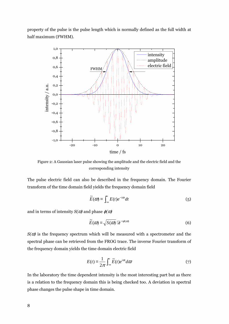
The crystal produces light with double frequency (half wavelength) of the incident light,

e.g. 400 nm in the case of a 800 nm Ti:sapphire laser which has an electric field

proportional to the two input pulses [7]

)()(),( ττ −∝ tEtEtE SHG

sig (10)

and same for the intensity

)()(),( ττ −∝ tItItI SHGsig (11)

Because the detectors are too slow to resolve ),( τtI SHGsig the integral over time will be

measured

∫∞

∞−−= dttItIA )()()()2( ττ (12)

The intensity A(2)(τ) depends on the delay τ and there will not be an intensity if the

delay is too large and the pulses are not overlapping any more. The intensity is

recorded with a detector (commonly a photodiode) and the FWHM (full width at half

maximum) of the autocorrelation can be obtained. To get the FWHM of the laser pulse

a factor has to be considered which depends on the pulse shape.

0

1

-200 200

Gauss

sech2

fast rising

fast falling

inte

nsi

ty /

a.u

.

time / fs

0

1

-200 200

inte

nsi

ty /

a.u

.

time / fs

0

1

-200 200

Gauss

sech2

fast rising

fast falling

inte

nsi

ty /

a.u

.

time / fs

0

1

-200 200

inte

nsi

ty /

a.u

.

time / fs

pulse shape autocorrelation

Figure 8: Different pulse shapes (left) and their corresponding autocorrelation trace (right)

(modified [14])

In the top row of Figure 8 a Gaussian and a sech2 pulse with 100 fs is shown and the

corresponding autocorrelation. As shown the autocorrelation function for the Gaussian

16

pulse is broader than for the sech2 pulse. So the knowledge of the pulse shape is

essential for correct determination of the pulse length. If the pulse shape is Gaussian

then the FWHM of the autocorrelation has to be divided by a factor of 1.414, for a sech2

pulse the factor is 1.543 to obtain the FWHM of the laser pulse. Asymmetric and

complex pulse shapes cannot be measured since their shape gets lost (see bottom row

in Figure 8). The autocorrelation always yields a symmetric trace.

The advantage of intensity autocorrelation is its easy implementation but if the exact

pulse shape is not know it is not possible to determine the exact pulse length. Further-

more information about the phase in frequency and time domain cannot be obtained.

Therefore additional techniques have been developed, for example the spectral phase

interferometry for direct electric field reconstruction (SPIDER) [19] and the frequency-

resolved optical gating (FROG). Both can determine the complete electrical field of

ultrashort laser pulses. In this work the FROG technique was used and therefore will be

described next.

2.3.3 Frequency-Resolved Optical Gating (FROG)

The principle setup for this technique is the same as for the intensity autocorrelation

except the photodetector is exchanged with a spectrometer used for detection (see

Figure 9). At each time delay a spectrum is recorded instead of an intensity signal. This

means that the FROG trace is in the frequency-time-domain and therefore includes

time and frequency information [7].

spectrometer

beamsplitter

variable

delay τ

E(t- )τ

E(t)

SHGcrystal aperture

pulse to be measured

E (t, )sig τ

Figure 9: Setup for a FROG using second-harmonic generation

17

The amplitude and phase of the incident laser field E(t) are then retrieved from the

FROG trace by using an iterative algorithm which is usually convergent in realistic

cases. In an SHG FROG the spectrometer detects the intensity:

2

)()(),( dtetEtEI tiSHGFROG

ωττω −∞

∞−⋅−= ∫ (13)

The FROG measures the complete intensity and phase dependent on time and

frequency with two exceptions. It cannot measure the absolute phase ϕ0 and the pulse

arrival time which corresponds to ϕ1. There are also different variations of the FROG

geometries for example the PG FROG (polarization-gate) and the THG FROG (third

harmonic generation). The main advantage of the SHG FROG is its sensitivity. It

involves only a second order nonlinearity which yields stronger signals than the third

order effects.

wavelength / nm900800700

inte

nsi

ty /

a.u

.

1

0,75

0,5

0,25

0

ph

ase

/ rad

3,2e-1

2,8e-1

2,4e-1

2,0e-1

1,6e-1

1,2e-1

8,0e-2

4,0e-2

-6,9e-18

a) b)

c) d)

time / fs

wa

vel

en

gth

/ n

m

time / fs

wa

vel

en

gth

/ n

m

Figure 10: a) FROG trace of an ideal 60 fs pulse, b) retrieved trace, c) retrieved temporal pulse,

d) and retrieved spectrum

In Figure 10 a FROG trace (a) of an ideal 60 fs Gaussian pulse is shown. After the

iterative algorithm was applied an electric field (c) and frequency spectrum (d) were

retrieved which results in a retrieved FROG trace shown in (b). As the pulse is ideal the

phases should be flat. But it can be seen, that in time domain the phase is in the order

of 10-5 radians and therefore practically zero. In frequency domain the phase is linear

and therefore only corresponds to a time shift of the laser pulse and does not affect the

pulse itself.

18

2.3.4 Beam Diameter Determination – Moving Edge

The fluence of the laser beam is a very important property. It is the energy per area and

therefore the radius of the laser beam has to be determined. Laser beams can have

different spatial beam profiles, e.g. the Ti:sapphire laser has a Gaussian beam profile.

For determination one can use the “moving edge” method [3]. Figure 11 shows the

scheme of the setup. The razor blade is scanned through the focus area and the

transmitted energy for each position is recorded with a detector.

detector(photodiode)

microscopeobjective or

focusing lens

razor blade

translationx-direction

laser beam

Figure 11: Scheme of the "moving edge" determining the beam radius

As the beam profile is Gaussian in x- and y-direction the fluence distribution F(x, y) can

be described as

( )22

20

2

0),(yx

weFyxF+⋅−

⋅= (14)

where F0 is the maximum fluence and w0 is the beam radius. By definition the fluence

F(x,y) has decreased to F0/e2 at the radius w0. Calculating the transmitted energy ET

depending on the position of the razor blade yields [3]

∫∞

⋅−

⋅⋅⋅==l

w

x

T dxewFlxE

2

0

2

00 2)(

π (15)

y

x

razo

r b

lad

e

translationx-direction

Figure 12: Perspective of the photodiode for the "moving edge" measurement

19

With this equation the numerical data can be fitted and the beam radius can be

obtained.

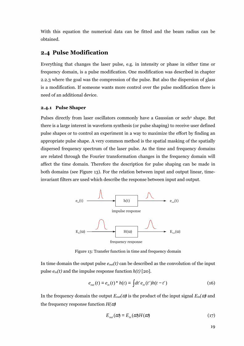
2.4 Pulse Modification

Everything that changes the laser pulse, e.g. in intensity or phase in either time or

frequency domain, is a pulse modification. One modification was described in chapter

2.2.3 where the goal was the compression of the pulse. But also the dispersion of glass

is a modification. If someone wants more control over the pulse modification there is

need of an additional device.

2.4.1 Pulse Shaper

Pulses directly from laser oscillators commonly have a Gaussian or sech2 shape. But

there is a large interest in waveform synthesis (or pulse shaping) to receive user defined

pulse shapes or to control an experiment in a way to maximize the effort by finding an

appropriate pulse shape. A very common method is the spatial masking of the spatially

dispersed frequency spectrum of the laser pulse. As the time and frequency domains

are related through the Fourier transformation changes in the frequency domain will

affect the time domain. Therefore the description for pulse shaping can be made in

both domains (see Figure 13). For the relation between input and output linear, time-

invariant filters are used which describe the response between input and output.

h(t)e (t)in e (t)out

impulse response

H( )ωE ( )in ω E ( )out ω

frequency response

Figure 13: Transfer function in time and frequency domain

In time domain the output pulse eout(t) can be described as the convolution of the input

pulse ein(t) and the impulse response function h(t) [20].

∫ −=∗= )'()'(')()()( tthtedtthtete ininout (16)

In the frequency domain the output Eout(ω) is the product of the input signal Ein(ω) and

the frequency response function H(ω)

)()()( ωωω HEE inout = (17)

20

The relation between H(ω) and h(t) can be described by the Fourier transformation

∫−= tiethdtH ωω )()( (18)

and

∫= tieHdth ωωωπ

)(2

1)( (19)

Equation (18) is used to get the frequency response function for a desired time re-

sponse. The control of the frequency domain of ultrashort pulses is much easier than

the control of the time domain which is in the femtosecond regime. The principle setup

of this pulse shaping technique is shown in Figure 14. It consists of a pair of gratings

and lenses, and a pulse shaping mask. Without the mask the setup is known as “zero

dispersion compressor” which means the input laser pulse will remain unchanged when

passing the setup. The frequency components of the incident laser pulse will be

angularly dispersed by the first grating and then focused by the first lens with the focal

length f to the back focal plane which is the Fourier plane. At this plane the frequency

components are spatially separated. The first lens performs the Fourier transformation

of the angular dispersion from the grating to the spatial separation. The separated

frequency components can be changed by an amplitude and/or a phase mask. After the

manipulation the components are again recombined through the second lens and

grating to a single beam. A shaped output pulse depending on the mask is received.

mask(e.g. programmable)

grating 1 grating 2

f f f f

Fourier plane

lens 1 lens 2

Figure 14: Setup scheme of a pulse shaper

The mask can be build up through fixed masks or programmable masks like the LC-

SLMs (liquid crystal spatial light modulator). Using fixed masks provides excellent

21

pulse shaping quality but it is not easy to provide continuous phase variations whereas

binary phases work well. With a LC-SLM the continuous change of the phase and/or

amplitude for each separate pixel is possible at the same time. It is also possible to

change the mask and therefore the output pulse shape within 100 ms and less.

In principle the pulse shaper can be operated in two modes namely with and without

feedback from the experiment. Without the feedback (Figure 15a) the knowledge of the

input pulse as well as the output pulse has to be available. Therefore the mask can be

calculated and applied to the display. This open loop configuration needs a good

calibration of the LC-SLM to provide exact translation of the theoretically calculated

mask to the physical device.

The programmable LC display offers the possibility of a feedback controlled system

(Figure 15b) which is also called adaptive pulse shaping. The computer starts the

experiment with a random mask and updates it according to the algorithm and the

current state of the experiment. With this strategy the mask is optimized until the

experiment is in the desired state. It is possible to remove a chirp of the input pulse [21]

as well as the control of chemical reactions [22]. The only requirement for the closed

loop control is a measurable optimization parameter which is directly fed to the

computer. In adaptive pulse shaping the knowledge of the input pulse as well as the

output pulse is not necessary. There is also no need to calibrate the SLM like in open

loop control. The only requirement is the specification of the experimental outcome to

be optimized and the algorithm for optimizing.

FemtosecondOscillator

PulseShaper

Experiment &Diagnostics

Computer Controlbased on Pulse Shaper,Calibration, and Userspecified Pulse Shape

FemtosecondOscillator

PulseShaper

Experiment &Diagnostics

Computer ControlledLearning Algorithm

based on User specifiedExperimental Objective

a)

b)

Figure 15: Experiment setup with a pulse shaper a) without and b) with feedback control

22

As it is possible to generate complicate pulses there is need of good characterization

measurement techniques. The intensity autocorrelation is useless as it cannot recover

the pulse shape appropriately. Therefore FROG is a method which is good known and

can recover intensity and phase vs. time.

2.5 Inverse Pulsed Laser Deposition (IPLD)

In the experiments described later thin films were processed. Therefore the production

method will be shortly described in the following section.

Pulsed laser deposition is a well known method for growing thin films [23]. Several

geometries were proposed to get even more homogeneous films. One arrangement is

the inverse pulsed laser deposition [24, 25] which is shown in Figure 16. The whole

arrangement is inside a vacuum chamber for evacuation and then pure gas e.g. argon or

nitrogen is introduced. If there is no inert gas the plasma will react with the oxygen in

air.

rotating target (C)

plume laser beam(KrF, 248 nm, 20 ns)

substrate (Si)

substrate holder

Figure 16: IPLD geometry for growing thin films

The high power pulsed laser beam is focused onto the target of the desired composition.

The target material is vaporized and ejected in form of a plume. The backward motion

of the plasma particles is used for growing the thin film. In the original PLD

configuration the substrate is above the plume and faces it [23]. As the substrate is

static this results in a decreasing film thickness on the substrate with increasing

distance from the ablated laser spot. In comparison to the PLD configuration improved

surface quality and higher deposition rates in the high-pressure domain are reported

[25].

23

3 Experimental

3.1 Laser Setup

The general setup is shown in Figure 17 as a flow chart with black boxes for the

different functionalities for an easy description of the “light flow”.

FemtosecondOscillator

Modify Intensity andRepetition Rate

PulseCompression

Microscope

Autocorrelation

FROG

Pulse Shaper

A B

C

D

Figure 17: General setup scheme (light flow) used for the experiments

The laser pulses were generated with a Ti:sapphire oscillator (Scientific XXL

Femtosource from Femtolasers) which have a pulse length of 60 fs at FWHM (in fact at

point C after the compression), a repetition rate of 11 MHz, a centre wavelength of

800 nm and a average power of about 2.3 W. This results in high pulse energies

(>200 nJ directly after the oscillator) which can only be reached due to positive chirped

pulse generation used inside the oscillator (pulse length of a few ps). The optical path of

the laser beam inside the oscillator is shown in Figure 18. The pump source for the

Ti:sapphire crystal is a diode pumped frequency doubled Nd:YVO4 continuous wave

laser (Coherent Verdi V18) with a centre wavelength of 532 nm and a maximum power

of 18 W. In the experiments the Ti:sapphire crystal is only pumped with a power of

13.5 W. The short cavity arm is terminated with a SBR (saturable Bragg reflector) for

mode locking. The long cavity arm is extended with a Harriot cell [26] to get high

energy pulses. The laser pulses are reflected eight times on each of the two mirrors of

the Harriot cell which results in an optical path of several meters. After the output

coupler, which terminates the long cavity arm, the spot size is enlarged using a 1:2

telescope consisting of two lenses. The average output power of the oscillator is in the

range of 2.3 W which is measured with a powermeter (Spectra-Physics model 407A) at

point A marked in Figure 17. At the same point the frequency spectrum is checked

24

continuously during the experiments with a spectrometer (Ocean Optics USB4000)

because a deviation in the spectrum leads to different pulse lengths.

pump laser532 nmTi:sapphire

crystal

Harriot cell

output coupler

SBR

Figure 18: Setup of a Ti:sapphire high power fs-laser

The pulses intensity and repetition rate can be modified in the second part. For

changing the light intensity a λ/2-plate, which changes the plane of polarization, in

combination with a polarizer is used. The repetition rate can be changed from 5 Hz to 5

kHz with a Pockels cell and two crossed polarizers. In the third part the positively

chirped pulses from the oscillator were compressed with a prism compressor using a

two prism arrangement. Care must be taken not to clip a part of the dispersed beam

which results in a clipped frequency spectrum. The spectrum has to be checked at point

C marked in Figure 17 and has to be the same as at point A. After the prism

compression (point C) the laser pulse has the desired properties, e.g. energy, pulse

length and repetition rate. Because of the light absorption of the Pockels cell and the

prism compression the pulse energy has a maximum value of 150 nJ at point C. These

pulses can directly go to point D where the laser pulses can be characterized with the

autocorrelation or the FROG or the pulses can be used for the experiments under the

microscope. But it is also possible to go from C to D through the pulse shaper to modify

the pulses shape and characterize these pulses and carry out experiments. The different

optical light paths can be set by a flip mirrors.

The autocorrelator and the FROG use the same physical setup. The principle method is

based on the second harmonic generation using a BBO crystal (β-barium borate) using

a non-collinear setup. For the autocorrelation the intensity is detected with a

photodiode detector and for the FROG the photodiode is exchanged with a

spectrometer (Ocean Optics USB4000) capturing the spectrum of the frequency

25

doubled signal. The necessary time delay is produced by a computer controlled

translation stage (PI M405.DG Precision Translation Stage). The program used for

measuring the autocorrelation is written in LabVIEW (Version 8.5) which allows a full

automatic continuous acquisition of the laser pulse width. One autocorrelation diagram

can be measured within half a second. As described in chapter 2.3.2 the pulse shape has

to be known to calculate the pulse length from the autocorrelation length. The

LabVIEW program uses a factor of 1.41, e.g. a Gaussian pulse shape is taken, to convert

the autocorrelation length. The pulse length is the FWHM. During the experiments the

pulse length is checked continuously to guarantee constant experimental conditions.

For complete determination of the intensity and phase of the pulses FROG is used. The

current version of the LabVIEW program captures a defined number of spectra at

different time delays, extracts the data around the second harmonic frequency and

stores the data in a file. This file can be read with the Femtosoft FROG3 software [27]

to retrieve intensity and phase of the laser pulse. As the data measurement and

retrieval process are two different programs, the acquisition is not continuously and

also lasts much longer then the autocorrelation acquisition.

Microscope

The moving edge and ablation experiments were made using a microscope. With the

used microscope Axio Imager.M1 from Zeiss it is possible to couple the laser beam

through the objective and focus the laser beam onto the sample. As the laser pulses go

through glass in the objectives the pulses will be linearly dispersed. Therefore chirped

mirrors, which are designed to compensate the dispersions of the used Zeiss objectives,

are settled into the beam. Additional care has been taken by measuring the pulse

energy because not all energy at the input of the microscope is measured after the

objective. A factor has been calculated to get the energy of the pulses directly at the

experiments depending on the input energy.

Moving Edge

The razor blade is mounted on an object holder and moved with the microscope

translation stage. For measuring the transmitted light a photodiode connected to the

oscilloscope is used. The focus is set to the sharp edge of the razor blade. As the laser

spot is very small and therefore the fluence is very high the laser power has to be

reduced to avoid destruction of the razor blade. Then the razor blade is scanned

stepwise through the focus and the voltage corresponding to the transmitted light is

recorded.

26

Laser / System

Pump Source

FEMTOSOURCE scientific XL (Ti:Sapphire)

COHERENT Verdi V18 532 nm 18 W

Nominal Pulse Length: 60 fs (after compression)

Centre Wavelength: 800 nm

Repetition Rate: 11 MHz

Average Output Power @ 11 MHz: 2.3 W

Pulse Energy: >200 nJ

Pockels Cell

Head / Crystal

Control Unit

Timing Unit

Pockels Cell Driver (high voltage

generation)

Bergmann ds11b/KD*P

Femtolasers Frequency Power Control

(Model: FPC Type: XL)

Bergmann Bme-PTO2

Bergmann PCD3i

Powermeter OPHIR NOVA DISPLAY + PD10-PJ-SH-V2

Powermeter Spectra-Physics model 407A

Microscope

Digital Camera

Objectives

ZEISS Axio Imager.M1

AxioCam MRc5

Axio Vision Rel. 4.7 (Software)

Zeiss EC „Plan-Neofluar“ 10x0,3 M27

Zeiss EC „Plan-Neofluar“ 20x0,5 M27

Zeiss EC „Plan-Neofluar“ 40x0,75 M27

Zeiss LD EC „Plan-Neofluar“ 63x0,75 Korr M27

Zeiss LD EC „Epiplan-Neofluar“ 100x0,75 DIC M27

Oscilloscope LeCroy WaveRunner 64Xi 600 MHz 10 GS/s

Pulse Shaper

LCM

Setup like used at the University of Kassel

CRI SPATIAL LIGHT MODULATOR SLM-640-P

controlled via LabVIEW

Data Acquisition Board NI USB-6221

Micrometer Stages

Controller

PI M-405.DG Precision Translation Stage

PI C-848.43 Digital DC-Servo-Motor Controller

Spectrometers

Software

Ocean Optics USB4000-UV-VIS

Ocean Optics USB4000-VIS-NIR

Ocean Optics SpectraSuite + OmniDriverSPAM

2008.05.29

Atomic Force Microscope (AFM) NT-MDT NTEGTA Aura

100x100 µm Scanner

LabVIEW Version 8.5

Frog Retrieval Software Femtosoft Technologies FROG 3.2.2

Table 1: Equipment and software used for experiments

27

Pockels Cell

The physical setup of the used Pockels cell consists of four different parts. The main

part is the head with the crystal KD*P (potassium dideuterium phosphate) utilizing the

Pockels effect [10]. The second part is the high voltage unit (Bergman BCD3i) which

drives the crystal. A voltage of about 7 kV is necessary to turn the plane of light 90°. It

is a challenging task for the electronic part to apply this voltage within a few

nanoseconds. Care has to be taken if very sensitive measurements are made in the

surroundings because the electromagnetic field of the high voltage unit of the Pockels

cell induces current in other electronic circuits and wires which results in systematic

faults. The control unit (Femtolasers Frequency Power Control, Model: FPC, Type: XL)

is used for setting the number of transmitted pulses and the repetition rate. The timing

unit (Bergmann Bme-PTO2) uses the information of the control unit and generates the

switching functions for the high voltage unit. To synchronize the timing unit to the

pulse train the latter is measured with a photodiode at point A marked in Figure 17. The

timing unit generates two signals which control the high voltage unit and therefore

switch on and off the high voltage.

3.2 Ablation Experiments

IPLD – Inverse Pulsed Laser Deposition

This method was used to create thin diamond-like carbon (DLC) films used for the

ablation experiments. The preparation technique employed here results in tetrahedral

amorphous carbon (ta-C) with sp3 contents as high as ~80% [28]. Therefore the

deposition chamber was first evacuated to a base pressure of 1.5–2.10-4 Pa by a turbo

molecular pump, and then the pressure was increased to 5 Pa by introducing high-

purity (99.999%) argon gas using a flow configuration. The graphite target, rotating at

10 rpm, was ablated at 10 Hz repetition rate by KrF laser pulses (248 nm, 20 ns) of

7 J/cm2 fluence. The beam was focused by a 35 cm focal length UV grade fused silica

lens onto an approximately 1 mm2 area of the target surface at 45 degree angle of

incidence. Observations described in [29] made it possible to characterize the lateral

thickness distribution by means of measuring the changes in the film thickness along

the two axes of the laser spot. In each experiment, films were collected on two, 8-mm

wide polished silicon stripes, fixed right above the rotating target, at room temperature.

The thickness distribution of the carbon layer was measured using profilometry and is

shown in Figure 19. The production and characterization of the used films was done by

the Department of Optics and Quantum Electronics at the University of Szeged.

28

Experiments

The ablation experiments were carried out under the microscope with the 63x Zeiss

Neofluar objective with NA=0.75. Different combinations of pulse energies and

numbers were used to create irradiated zones. The irradiated areas were inspected in

situ in reflection mode and afterwards by a atomic force microscope (NTEGRA AURA)

in contact mode.

0 10 20 30 40 50

0

50

100

150

200

250

300

350

thickness = 318.4e-0.07392*position

thic

kn

ess

/ n

m

position / mm

measured data

exponential fit

Figure 19: Thickness profile of the thin film used for the ablation experiments

29

4 Results and Discussion

4.1 Pulse Characterization

Every day the output power and the pulse length are checked several times because the

long time stability is affected by the high energy regime mode. In Figure 21 a sample

autocorrelation of the optimized system without the pulse shaper is shown. The

measured data are fitted with a Gaussian shape and then the pulse length is

determined. At low intensities the measured data deviate from the ideal Gauss shape

depending on the degree of optimization of the laser. Therefore in the online

measurement system (see appendix) two data fits are made. The first uses the whole

dataset to fit a Gaussian shape into the pulse and the second fit only uses the intensities

of the measured data points which are above 40 percent of the peak intensity (this

value can easily be changed). For a well adjusted system this two fits are equal.

To get a well adjusted system the oscillator has to be optimized first. It is the goal to run

the system always in the same state and therefore get the same properties of the laser

pulses. There are three properties/parameters to check at the output of the oscillator.

The first is the average output power of the oscillator which should be in the range of

2.3 W for this particular device. The second parameter is the frequency spectrum which

is compared with a reference spectrum which was saved when the oscillator was

optimized. A typical frequency spectrum generated from the oscillator is shown in

Figure 20. Finally the spatial shape of the laser pulse is checked because it is possible to

get a spatial shape deviating from a Gaussian. There are two main parameters to

optimize the oscillator namely the stability range which changes the length of the short

cavity arm and the second is the input coupling of the pump laser.

At the output of the oscillator the laser pulses are dispersed and the prism compression

has to be adjusted to get short pulses after the compression. Therefore the position of

the second prism is changed as described in the theoretical part to introduce more or

less negative dispersion. For the pulse length measurement the autocorrelation is used

for daily use but also FROG traces were taken to check the phases. The following figures

show the typical output of the laser oscillator characterized by the spectrometer (Figure

20), the autocorrelation (Figure 21), and the FROG (Figure 22). The pulse duration

measured with the autocorrelation was 58 fs.

30

780 790 800 810 820

0,0

0,2

0,4

0,6

0,8

1,0

inte

nsi

ty /

a.u

.

wavelength / nm

Figure 20: Spectrum of a 58 fs laser pulse of the FEMTOSOURCE scientific XL oscillator

-400 -200 0 200 400

0,0

0,2

0,4

0,6

0,8

1,0

inte

nsi

ty /

a.u

.

delay / fs

Figure 21: Intensity autocorrelation of a 58 fs laser pulse of the FEMTOSOURCE scientific XL

oscillator

The pulse duration was compared with the FROG result which yielded a pulse length of

59 fs. In addition the FROG trace shows the temporal and spectral phase and it can be

seen that it is not flat and therefore the pulses are not Fourier-limited. Looking at the

scale of the phases one may assumes a large phase. But the effective phase is about 1.5

radians (~0.5π) because the shown phase only affects the pulse if the intensity is not

31

zero. The retrieved frequency spectrum is slightly different from the one in Figure 20.

The reason may be the calibration of the spectrometer necessary for the recalculation of

the original spectrum from the second harmonic spectrum.

a) b)

time / fs time / fs

wa

ve

len

gth

/ n

m

wa

ve

len

gth

/ n

m

time / fs6004002000-200-400-600

inte

nsi

ty /

a.u

.

1

0,75

0,5

0,25

0

ph

ase

/ rad

2,2e+1

2,0e+1

1,8e+1

1,6e+1

1,4e+1

1,2e+1

1,0e+1

8,0e+0

6,0e+0

4,0e+0

2,0e+0

0,0e+0

wavelength / nm1.000950900850800750700650600

inte

nsi

ty /

a.u

.

1

0,75

0,5

0,25

0

ph

ase

/ rad

5,0e+0

4,0e+0

3,0e+0

2,0e+0

1,0e+0

0,0e+0

c) d)

Figure 22: FROG analyses of the fs-laser pulse a) measured and b) retrieved trace c) retrieved

electric field and d) retrieved frequency domain

4.2 Microscope Objective Characterization

4.2.1 Beam Diameter – “Moving Edge” Method

This method is used to determine the laser beam radius at the focus of the microscope

objectives. With the knowledge of the radius and the pulse energy the fluence can be

calculated which is the crucial parameter for material ablation treated in the

experiments.

The measured data were fitted with Origin 8.0. The program does not support user

defined fitting functions with an integral as described in equation (15) which was

retrieved in the theoretical section. Thus the integral has to be solved to get a fitting

function usable in Origin. First the boundaries of the integral need to be changed

because all experiments start with zero light intensity moving to maximum intensity

and therefore the transmitted light has to be integrated from -∞ to the actual position l

32

∫∞−

⋅−

⋅⋅⋅==l

w

x

T dxewFlxE

2

0

2

00 2)(

π (20)

Integrating this equation yields

0for

244

214

)(

0

0

200

200

0

200

>

⋅⋅⋅⋅++⋅⋅=

+

⋅+⋅⋅⋅=

w

w

xerfwFCwF

Cw

xerfwFxET

ππ

π

(21)

For the final fitting function the first two constant parts of equation (21) are replaced by

y0 and an offset variable x0 in x-direction is introduced to allow a shift of the data in x-

direction.

−⋅⋅⋅⋅+=0

02000 2

4 w

xxerfwFyy

π (22)

It can be seen that the measured data fit very well to the Gaussian shape (Figure 23).

0 2 4 6 8 10

0

200

400

600

800

1000

1200

1400

inte

nsi

ty /

a.u

.

x / µm

measured data for 10x objective

fit

Figure 23: Dataset and fit for the laser beam radius of the 10x objective

The results for all objectives are shown in Table 1. It can be seen that the higher the

numerical aperture of the objective the smaller is the beam radius in the focus which

corresponds to the resolution of the objective. Objectives with the same numerical

aperture show nearly the same beam radius.

33

Objective Numerical aperture NA Beam radius w0 / µm

10x 0.3 3.4

20x 0.5 1.8

40x 0.75 1.1

63x 0.75 1.2

100x 0.75 1.0

Table 2: Beam radius at the focus of different objectives measured with the moving edge method

4.2.2 Determination of the Group Velocity Dispersion

The objectives introduce dispersions because of the lenses inside which results in a

broadening of the laser pulses. To compensate the dispersions chirped mirrors are

used. The measurement of the autocorrelation of the laser pulses passing the chirped

mirrors and the objective showed that the dispersion can be compensated and therefore

the pulse length of the input and output pulse is the same.

4.3 Pulse Shaper

Substantial attention and time was spent for the assembling and characterization of the

femtosecond pulse shaper. The setup of the pulse shaper relies on the construction

plans of Jens Köhler (University of Kassel). It is designed for fs-lasers with a centre

wavelength of 800 nm, a maximum spectral width of 90 nm (base width and not

FWHM), and a maximum beam diameter of 5 mm. The LC-SLM is a 640 pixel phase

only modulator.

In Figure 24, the top view of the pulse shaper with its main components, which are

listed in Table 3, is depicted. The height of the input and output beam is about 9.5

inches and is changed to the nominal height of 2 inches of the laser beam in our setup

due to periscopes which are not shown.

Optical path

The optical path (Figure 24) runs along the components 1 to 11. The plane of the light

between the parts 4 to 8 is parallel to the ground plate to provide a normal incidence to

the SLM (part 6). The length of the optical path between the gratings 3 and 9 should be

four times the focal length of the cylindrical mirrors 2 and 10. At the centre, the SLM

introduces phase shifts in the spatially dispersed frequency space (= Fourier plane).

34

L6 L1 R1 R6

L3R3

L2 R2

L5 R5L7

L4

R7

R4

FE

3

5

4 8

7

9

1

2

11

10

6

Figure 24: Top view of the pulse shaper

35

Parts

Part No. Description

1 + 11 Periscopes to change beam height from 2 to 9.5 inches

2 + 10 Mirrors for input and output coupling

3 + 9 Gratings, Wasatch Photonics, Dickson 1840 lpmm Volume Phase Holographic

(VPH) Transmission Grating for 800 nm

4 + 8 Cylindrical mirrors, f = 220 mm, BK7, silver coated, size 80x20 mm

5 + 7 Plane mirrors, BK7, silver coated, size 110x20x20 mm

6 Liquid Crystal Spatial Light Modulator LC-SLM CRi SLM-640-P

Table 3: Optical parts of the pulse shaper

A precise alignment of the pulse shaper is necessary in order not to introduce

dispersions. It is the goal that a defined input pulse should not change its properties by

passing the pulse shaper setup. There is a summary of the alignment steps done for the

pulse shaper. A complete technical documentation with the drawings of all parts and

more detailed adjustment documentation is available [30].

Alignment Steps

There are different apertures with different heights and aperture sizes and there are

some further utilities for the correct alignment of the laser beam in the pulse shaper.

They are listed in Table 4. All optical components can be easily removed to align the

laser beam along the apertures and then added precisely again.

Part No. Description

1 124.0 mm HeNe-aperture

2 132.5 mm reticule for the left side

3 132.5 mm reticule for the right side

4 Screen for the Fourier plane

5 139.3 mm fs-laser-aperture

6 Optical mount simulator

7 Iris apertures

8 Variable height apertures

Table 4: List of apertures and utilities for laser beam alignment

o First of all the convolution mirrors have to be aligned. The beam reflected from

the left cylindrical mirror is reflected orthogonally from the left convolution

mirror and further reflected orthogonally from the right convolution mirror to

the right cylindrical mirror. The plane of the beam between these parts has to be

in parallel to the ground plate. Therefore a HeNe-laser beam is adjusted to go

36

through 124.0 mm HeNe-apertures from L1 to L2 to L3. The left convolution

mirror is added and has to be aligned in a way that the reflected beam passes

the apertures at positions FE and R4. The right convolution mirror is added too

and aligned in a way that the reflected beam passes the apertures at the

positions R2 and R1.

o The second part is the horizontal, vertical, and rotational adjustment of the

cylindrical mirrors. Therefore a HeNe-laser beam is adjusted with 124.0 mm

HeNe-apertures along the positions R1 to R2 to R3. The beam is reflected from

the right to the left convolution mirror and then to the cylindrical mirror. The

cylindrical mirror has to be aligned in a way that the beam is self-reflected. The

rotation of the left cylindrical mirror has to be aligned in a way that the profile

of the reflected divergent beam is horizontally.

o Next the vertical adjustment of the reflected beam of the cylindrical mirror will

be done. The 132.5 mm left reticule is added at position L5. The vertical

alignment of the left cylindrical mirror has to be changed until the reflected

beam hits the centre of the reticule.

o Then a mirror is set into the left grating mount. The mount has to be adjusted in

a way that the beam is self-reflected for the horizontal position and then

vertically aligned to be parallel to the ground plate. The reflected beam is fixed

with two iris apertures.

o The distance between the Fourier plane and the cylindrical mirrors should be

one focal length. Hence two parallel beams are coupled into the setup in reverse

direction using the installed iris apertures in the last step. The parallel beams

hit the left cylindrical mirror and then are focused. The intersection point of the

beams equals the focal point of the cylindrical mirror and so the position of the

mirror is changed with the micrometer screw until the intersection point meets

the Fourier plane (using the screen for the Fourier plane)

o As the position of the left cylindrical mirror has changed the vertical adjustment

has to be repeated like 3 steps ago.

o The last five steps have to be done with all positions mirrored for the right

cylindrical mirror.

o The parts setup until now should not change the beam profile. For this check

the HeNe beam (with a good spatial beam profile) is coupled into the setup with

the iris apertures installed before. The beam is reflected from the mirror in the

grating mount, the cylindrical mirror, the convolution mirror and same at the

mirrored side. The beams profile should be the same like without the setup at a

37

comparable distance. Otherwise the positions and the rotations of the

cylindrical mirrors can be changed slightly.

o Next the tilt angle of the gratings is aligned. Thus the laser beam is aligned

along the positions R1, R2, and R3. The tilt angle of the mount of the left grating

is aligned in a way that the beam is self-reflected. Same adjustment can be done

for the mirrored side.

o At this point the first time the fs-laser beam is used. It is aligned with the

139.3 mm apertures along the points L1 to L2 to L3. The former installed mirror

is exchanged with the grating now. The optical mount of the left grating is

exchanged with the optical mount simulator so that the gratings vertical axis is

vertical orthogonal to the ground plate. The angle of the grating is

approximately aligned 45° to the incident laser beam. The rotation of the

grating is aligned in a way that the first order diffraction is horizontally, which

can be checked in some distance. The plane of the first order diffraction and the

input beam should be in a plane parallel to the optical table.

o Then the diffraction efficiency of the grating is maximized. It is easier to use an

800 nm non-mode-locked laser beam. The angle of the grating has to be

changed until the power of the first order diffraction has its maximum. Then the

optical mount simulator can be exchanged with the optical mount again.

o The last two steps have to be done for the right grating in the same manner.

o The principle geometrical alignment is ready and the input and output coupling

has to be done.

o Therefore an 800 nm laser beam is aligned with the 124.0 mm HeNe-apertures

along the positions R1, R2, and R3. The position of the laser beam is fixed with

iris apertures between the left grating and the convolution mirror and behind

the left grating (the first order diffraction). The mirror left to the left grating is

installed in a way that the beam is parallel to the ground plane and in the

direction of the input periscope as shown in Figure 24. At the positions L7 and

L6 the beam is fixed with variable height apertures.

o The fs-laser beam can be coupled into the pulse shaper like in the final state as

shown in Figure 24. The output laser beam is also fixed with two iris apertures

like on the left side and the mirror for the output coupling can be installed.

o To check the correct height of the beam in the Fourier plane the screen for this

purpose is settled into the pulse shaper at position FE. The tilt angle of the

38

grating and the cylindrical mirror has to be changed in opposite direction to

keep the plane of the spread spectrum parallel to the ground plane.

o The spatial chirp can be checked when the laser beam is watched in some

distance and the spread beam is partially blocked in the Fourier plane. If there

is a spatial chirp it can be removed by rotating or changing the angle of the right

grating.

o There should not be a temporal chirp too. It is necessary that the pulse shaper is

an exact 4f-setup. To check the temporal chirp the autocorrelation is one

possibility but as it is not a complete characterization another method has to be

used, e.g. FROG. To remove a possible chirp the positions of the cylindrical

mirrors and the right grating can be changed slightly. The input pulse should be

reconstructed without any change at the output when there is no light

modulator in the Fourier plane – also called zero-dispersion compressor.

o The LC-SLM can be added to the setup and aligned to be in the centre. The

introduced dispersion can be compensated through the change of the position

of the cylindrical mirrors

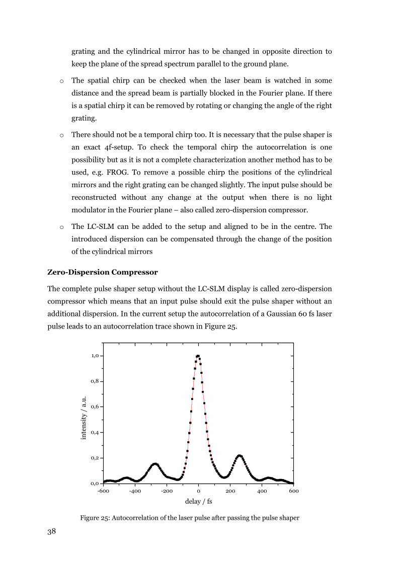
Zero-Dispersion Compressor

The complete pulse shaper setup without the LC-SLM display is called zero-dispersion

compressor which means that an input pulse should exit the pulse shaper without an

additional dispersion. In the current setup the autocorrelation of a Gaussian 60 fs laser

pulse leads to an autocorrelation trace shown in Figure 25.

-600 -400 -200 0 200 400 600

0,0

0,2

0,4

0,6

0,8

1,0

inte

nsi

ty /

a.u

.

delay / fs

Figure 25: Autocorrelation of the laser pulse after passing the pulse shaper

39

It can be seen that the Gaussian pulse shape cannot be reconstructed. Up to now it is

not clear if there is a misalignment or if one of the optical parts introduces changes in

the phase or amplitude. Every change of the alignment of the gratings or mirrors led to

a worse autocorrelation than the showed one. In principle such wings are due to third

order dispersions which can only be introduced by the gratings in our setup. Many

different settings were tried but none led to a perfect alignment. It should be noticed

that the centre peak has a FWHM only a few fs greater than the input pulse and

therefore the pulse shaper seems to be well aligned.

Absorption Losses

Next the losses inside the pulse shaper were checked. The developer of the pulse shaper

specifies in his documentation that losses between input and output are less than 50 %

but the measured loss is about 54 %. Table 5 shows the power measured at different

positions in the pulse shaper and the relative losses for the components were

calculated. It can be seen that the gratings have a loss greater than 20 % which is much

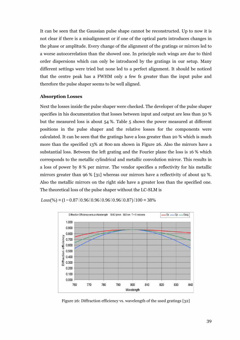
more than the specified 13% at 800 nm shown in Figure 26. Also the mirrors have a

substantial loss. Between the left grating and the Fourier plane the loss is 16 % which

corresponds to the metallic cylindrical and metallic convolution mirror. This results in

a loss of power by 8 % per mirror. The vendor specifies a reflectivity for his metallic

mirrors greater than 96 % [31] whereas our mirrors have a reflectivity of about 92 %.

Also the metallic mirrors on the right side have a greater loss than the specified one.

The theoretical loss of the pulse shaper without the LC-SLM is

%38100)87.096.096.096.096.087.01((%) =⋅⋅⋅⋅⋅⋅−=Loss

Figure 26: Diffraction efficiency vs. wavelength of the used gratings [32]

40

Position Power / mW Power / % Loss / %

input 1.2 100

after first (left) grating 0.95 79.2 20.8

at Fourier plane 0.8 66.7 15.8

after right cylinder mirror 0.69 57.5 13.8

output / after the second grating 0.55 45.8 20.3

Table 5: Transmitted power and losses of the mirrors and gratings

SLM Calibration

To drive the pulse shaper without a feedback loop it is necessary to characterize the

properties of the LC-SLM. First the relation between applied voltage and the

introduced phase and second the relation between the pixels and the effected

wavelength has to be calibrated. With these two informations the laser pulse can be

changed with the pulse shaper in a defined way.

Phase vs. Voltage Calibration

The used LC-SLM is a phase-only modulator. To calibrate the phase vs. voltage the LC-

SLM is used outside the pulse shaper. The plane of polarization of the input light has to

be 45° to the standard used horizontal polarization. This means that there is light

polarized along the horizontal and the vertical axis and therefore parallel to the

extraordinary and the ordinary axis of the liquid crystals. Applying voltage to the liquid

crystals results in a change of the refraction index along the extraordinary axis and

therefore a phase shift between the horizontally and vertically polarized light. If the

phase shift between the two parts equals π the plane of polarization will be turned 90°.

If there is a polarizer behind the LC-SLM aligned parallel to the incident light the setup

works like an amplitude modulator where the transmitted light intensity depends on

the applied voltage. In Figure 27 the dependence of the transmitted light intensity vs.

applied voltage is shown. The maximum intensities are measured when the phase shift

between ordinary and extraordinary beam is a multiple of 2π and the minimum

intensities at odd multiples of π. As the refraction index is wavelength dependent a

continuous monochromatic wave laser has to be used which a very small frequency

spectrum has compared to a pulsed laser. If a HeNe is used there is a calibration curve

to convert the data to the desired wavelength (in this case 800 nm). For the

measurement data shown in Figure 27 the Ti:sapphire laser was used in continuous

wave mode.

41

The transmission T dependent on the introduced phase φ between ordinary and

extraordinary beam can be described as [33]

( ))cos(12

1

2cos2 φφ +⋅=

=T (23)

where the phase can be rewritten as

( )12arccos2 −+= Tkπφ (24)

The term 2πk is necessary because it is not possible to calculate a phase greater than π

with the arccos-function but the real phase shift is greater. The display manufacturer

states that at maximum voltage the introduced phase is less than π [33] and therefore

the minimum at a voltage of 1700 counts equals a phase shift of π. So the complete

dependence of the introduced phase vs. applied voltage can be calculated (see Figure

28).

0 500 1000 1500 2000 2500 3000 3500 4000

0,0

0,1

0,2

0,3

0,4

0,5

0,6

0,7

0,8

0,9

1,0

tra

nsm

issi

on

/ a

.u.

voltage / a.u.

Figure 27: Transmitted light of the LC-SLM vs. applied voltage

Wavelength vs. Pixel Calibration

This calibration is necessary to know which wavelength is affected when a defined

voltage / phase is applied to a pixel. To do this the LC-SLM is settled into the complete

aligned pulse shaper and the Ti:sapphire laser is used in pulsed mode. If the LC-SLM

had the ability for amplitude modulation all pixel would be set to zero transmission and

one pixel to full transmission. Then the spectrum of the transmitted light is measured

and the wavelength with peak intensity corresponds to the pixel which is set to full

42

transmission. But the used LC-SLM is a phase-only modulator and so the same

approach as above is used. The plane of polarization is turned to 45° and a polarizer is

set behind the pulse shaper which yields an amplitude modulation. So one pixel after

the other is set to full transmission at one time and the peak of the transmitted

spectrum is recorded. The results are shown in Figure 29. Because the used fs-laser

beam does not show a spectral width of about 90 nm the data are fitted and

extrapolated.

0 500 1000 1500 2000 2500 3000 3500 4000

0

1

2

3

4

5

π

π

π

π

ph

ase

/ r

ad

voltage / a.u.

π

Figure 28: Introduced phase vs. voltage calibration

With this calibration data the pulse shape of the laser pulses can be changed in a

defined way. But as the main setup has some unknown dispersions until now it was not

spent much time on creating phase masks. In Figure 30 the autocorrelation of a double

pulse shaped with the pulse shaper is shown. The shown shape at time delay zero is

only due to the convolution of the autocorrelation. Only the outer two pulses exist. For

generation of the double pulses it is necessary to set the pixels alternately to phase zero

and phase π. If two or more consecutive pixels are set to zero phase and the same

number of pixels to phase π the time delay between the double pulses is decreased

which can be seen in Figure 30. Practically the sharp jumps between the pixels cannot

be set due to the design of the liquid crystals and therefore the desired pattern will be

smoothed. The effect is seen in the figure as the replicas of the centre pulse have a

slightly different shape.

Similar to these experiments different sets of phases can be applied in order to control

experiments by temporally shaped pulses.

43

0 100 200 300 400 500 600

740

760

780

800

820

840

860

wa

ve

len

gth

/ n

m

pixel number

fit measured linear

Figure 29: Wavelength vs. pixel number calibration

-3000 -2000 -1000 0 1000 2000 3000

0,0

0,2

0,4

0,6

0,8

1,0 10 pixels grouped

inte

nsi

ty /

a.u

.

delay / fs

-3000 -2000 -1000 0 1000 2000 3000

0,0

0,2

0,4

0,6

0,8

1,0

5 pixels grouped

inte

nsi

ty /

a.u

.

Figure 30: Autocorrelation trace of a double pulse shaped with the pulse shaper

4.4 Thin Film Ablation Experiments

It has been shown that the ablation threshold fluence Fth of thin thermally conducting

films on thermally poor conducting substrates is lowered for nanosecond laser pulses

when the film thickness d becomes less than the heat diffusion length Lth.

0 10 20 30 40 50

0

ph

ase

pixel number

π

0 10 20 30 40 50

0

ph

ase

pixel number

π

44

The heat diffusion length is defined by [34]

τDLth 2= (25)

where D is the thermal diffusivity and τ the pulse length. Due to the short pulse length

of 60 fs, the longer electron-phonon relaxation time τe-p has to be considered and the

pulse length τ should be replaced by τe-p [2, 3] in the formula above. τe-p for ta-C, in

contrast to metals like gold [35] (τe-p ~710-830 fs [36]) , is comparatively low, i.e.

~220 fs [37].

In the following experiments DLC films were investigated using different pulse energies

and numbers. Figure 31 shows typical cross sections of the ablated and modified

surface recorded with the atomic force microscope. At high energies/fluences and a

high number of pulses deep ablation craters are observed (a) whereas at single shot

experiments and low fluences only a modification of the surface results (d). To yield the

threshold fluences Fth the focal beam radius is determined with the D2 vs. lnE method

[3]

( )thth

EEwE

EwD lnln2ln2 2

020

2 −== (26)

where D2 is the squared diameter of the crater, w0 the beam radius, E the pulse energy,

and Eth the threshold pulse energy. With the knowledge of the focal beam diameter the

dependence of the squared crater diameter according to the logarithmic fluence can be

shown (Figure 32) and the threshold fluence Fth calculated.

-250

-200

-150

-100

-50

0

50

100

d)c)b)

ab

lati

on

dep

th /

nm

0.79 Jcm-2

@ 2000#

0.46 Jcm-2

@ 10#

0.68 Jcm-2

@ 1#

0.46 Jcm-2

@ 1#

a)

5 µm

Figure 31: AFM topographies show typical ablated and modified surfaces

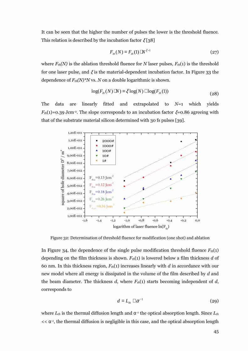
45

It can be seen that the higher the number of pulses the lower is the threshold fluence.

This relation is described by the incubation factor ξ [38]

1)1()( −⋅= ξNFNF thth (27)

where Fth(N) is the ablation threshold fluence for N laser pulses, Fth(1) is the threshold

for one laser pulse, and ξ is the material-dependent incubation factor. In Figure 33 the

dependence of Fth(N)*N vs. N on a double logarithmic is shown.

))1(log()log())(log( thth FNNNF +=⋅ ξ

(28)

The data are linearly fitted and extrapolated to N=1 which yields

Fth(1)=0.39 Jcm-2. The slope corresponds to an incubation factor ξ=0.86 agreeing with

that of the substrate material silicon determined with 30 fs pulses [39].

-1,6 -1,4 -1,2 -1,0 -0,8 -0,6 -0,4 -0,2 0,0

1,00E-012

2,00E-012

3,00E-012

4,00E-012

5,00E-012

6,00E-012

7,00E-012

8,00E-012

9,00E-012

1,00E-011

1,10E-011

1,20E-011

2000#

1000#

100#

10#

1#

squ

are

of

ho

le d

iam

ete

r D

2 /

m2

logarithm of laser fluence ln(Fth

)

Fth,a=0.13 Jcm

-2

Fth,a=0.12 Jcm

-2

Fth,a=0.18 Jcm

-2

Fth,a=0.26 Jcm

-2

Fth,m

=0.16 Jcm-2

Figure 32: Determination of threshold fluence for modification (one shot) and ablation

In Figure 34, the dependence of the single pulse modification threshold fluence Fth(1)

depending on the film thickness is shown. Fth(1) is lowered below a film thickness d of

60 nm. In this thickness region, Fth(1) increases linearly with d in accordance with our

new model where all energy is dissipated in the volume of the film described by d and

the beam diameter. The thickness d, where Fth(1) starts becoming independent of d,

corresponds to

1−+= αthLd (29)

where Lth is the thermal diffusion length and α-1 the optical absorption length. Since Lth

<< α-1, the thermal diffusion is negligible in this case, and the optical absorption length

46

α-1 controls the energy density. This contrasts to gold films, where the electronic

diffusivity is mainly determining the ablation threshold, since the electron-phonon

coupling is much weaker in gold and α-1 = 12 nm [35].

1 10 100 1000

0,1

1

10

100

1000

acc

um

ula

ted

flu

ence

Fth

(N)*

N /

Jcm

-2

number of pulses N

Figure 33: Incubation factor for silicon ablation equals ξ=0.86

0 50 100 150 200 250 300 350

0,00

0,05

0,10

0,15

0,20

0,25

0,30

0,35

0,40

mo

dif

ica

tio

n t

hre

sho

ld f

lue

nce

Fth

/ J

cm-2

film thickness / nm

Figure 34: Single pulse modification thresholds depending on film thickness

These results show that the modification thresholds determined for bulk materials

cannot be compared to thin film modification thresholds. Various surface effects have

to be considered in order to predict modification fluences.

47

5 Conclusion and Outlook

It has been shown that the current laser setup is a very flexible and powerful tool to

carry out many kinds of experiments. Especially the usage of the pulse shaper leads to

promising results. Up to now only fixed masks were applied to the LC-SLM resulting in

static laser pulse shapes. Because the input pulse and the LC-SLM have to be

characterized well the experimental effort is quite high. Using a static approach it can

be very exhausting to gain an optimal output pulse shape for a defined task. As the LC-

SLM is controlled by the computer it is possible to drive the pulse shaper setup in a

feedback controlled loop. Therefore a feedback parameter from the experiment has to

be fed to the computer which adaptively optimizes the applied mask to optimize the

experiment. Currently the pulse shaper is tested with the feedback control loop to

minimize the pulse length by maximizing the SHG signal. Comparing the LC-SLM

display in use to former SLM types (128 pixels) the higher number of pixels (640

pixels) enables us to gain better temporal resolution. Furthermore, the electronics for

LC displays is getting faster and therefore allows multiple changes of the phase mask

per second.

Single shot experiments reveal a modification of thin DLC films with volume increase

followed by the ablation of the completely converted low density phase in analogy to

the ablation of carbohydrate polymers. This demonstrates that multi-fs-pulse processes

are concerned with highly incubated carbonaceous materials. The modification

threshold of nanoscale DLC films with single pulse treatments, is lowered below a film

thickness of 60 nm. Due to strong electron-phonon coupling the optical absorption

length controls the behaviour of the modification threshold in contrast to gold films,

where the electronic diffusivity is mainly determining the modification threshold, since

the electron-phonon coupling is much weaker. These results demonstrate that dynamic

properties of nanoscale materials can be directly investigated by fs-laser modification

evaluations.

48

49

6 Appendix

The program for acquiring the autocorrelation trace is written in LabVIEW. The front

panel is shown in Figure 35. At the top right the frequency spectrum is shown as it is

very important for optimizing the laser pulses. A previously stored “good working”

frequency spectrum can be loaded to compare it with the actual one. If the actual one is

too different from the stored one the laser pulses will not be appropriate.

At the bottom left the control panel can be found where the approximate number of

acquisition data and the acquisition frequency can be set. Further the position of the

stage, where the two split pulses overlap perfectly, can be set as well as the size of the

delay scan window. Care has to be taken because it is not possible to set maximum

acquisition frequency at maximum data points and maximum scan area. The position

of maximum intensity only needs to be set roughly. There is a button on the right side

called “Auto x-Offset” for the fine adjustment to set the autocorrelation peak to the

centre of the scan area. At zero intensity the measured voltage of the photodiode is not

zero but it can be set to zero in the program with the button “Auto y-Offset”.

After starting the data acquisition the autocorrelation data are displayed at the bottom

right. Next to this window some values are shown which correspond to the measured

pulse length. The peak FWHM corresponds to the fitted Gaussian shape which analyses

only the intensities greater than 40 % of the maximum intensity. If there are side wings

they will not affect this value. As the real pulse length is a factor 1.41 shorter than the

FWHM of the autocorrelation trace, the value will be displayed in “peak pulse length”.

Underneath these two values there are the corresponding values but including the

whole intensity dataset. For a good laser pulse setting the values of the peak and the

whole dataset should be the same which reveals no side wings. The delay between the

overlapping pulses is generated by the movement of a translational stage which is

shown in the window on the top right.

It is possible to store a single autocorrelation trace and its corresponding frequency

spectrum to a data file by marking the check box “Single Shot & Save” for later use.

50

Figure 35: Front panel of the program measuring the autocorrelation

51

Bibliography

[1] T. H. Maiman, Stimulated Optical Radiation in Ruby, Nature 1960, 187, 493.

[2] J. Krüger, W. Kautek, The femtosecond pulse laser: a new tool for micromachining, Laser Physics 1999,

9, 30.

[3] J. Krüger, W. Kautek, Ultrashort pulse laser interaction with dielectrics and polymers, Polymers and

Light 2004, 168, 247.

[4] Y. X. Yan, E. B. Gamble, K. A. Nelson, Impulsive Stimulated Scattering - General Importance in

Femtosecond Laser-Pulse Interactions with Matter, and Spectroscopic Applications, Journal of Chemical

Physics 1985, 83, 5391.

[5] L. Dhar, J. A. Rogers, K. A. Nelson, Time-Resolved Vibrational Spectroscopy in the Impulsive

Limit, Chemical Reviews 1994, 94, 157.

[6] A. Rundquist, J. Broman, D. Underwood, D. Blank, Polarization-dependent detection of impulsive

stimulated Raman scattering in alpha-quartz, Journal of Modern Optics 2005, 52, 2501.

[7] R. Trebino, Frequency-resolved optical gating: the measurement of ultrashort laser pulses, Kluwer

Academic Publishers, 2000.

[8] D. Meschede, Optik, Licht und Laser, 2nd ed., Teubner Verlag, 2005.

[9] C. Rullière, Femtosecond laser pulses : principles and experiments, 2nd ed., Springer, 2005.

[10] P. Rüdiger, Encyclopedia of Laser Physics and Technology, http://www.rp-

photonics.com/encyclopedia.html last accessed 26.4.2009

[11] U. Keller, Recent developments in compact ultrafast lasers, Nature 2003, 424, 831.

[12] W. T. Silfvast, Laser fundamentals, 2nd ed., Cambridge University Press, 2004.

[13] F. Krausz, T. Metzger, J. Rauschenberger, A. Apolonski, K. Schmid, A. Baltuska,

Ultrakurze Laserpulse: Erzeugung und Anwendung, Laser Technik Journal 2005, 2, 27.

[14] G. Steinmeyer, Wie misst man kurze Laserpulse? Welche Verfahren gibt es?, Laser Technik Journal

2005, 2, 34.

[15] S. Naumov, A. Fernandez, R. Graf, P. Dombi, F. Krausz, A. Apolonski, Approaching the

microjoule frontier with femtosecond laser oscillators, New Journal of Physics 2005, 7.

[16] E. B. Treacy, Optical Pulse Compression with Diffraction Gratings, Ieee Journal of Quantum

Electronics 1969, Qe 5, 454.

[17] R. L. Fork, O. E. Martinez, J. P. Gordon, Negative Dispersion Using Pairs of Prisms, Optics

Letters 1984, 9, 150.

[18] I. A. Walmsley, V. Wong, Characterization of the electric field of ultrashort optical pulses, Journal of

the Optical Society of America B-Optical Physics 1996, 13, 2453.

[19] C. Iaconis, I. A. Walmsley, Spectral phase interferometry for direct electric-field reconstruction of

ultrashort optical pulses, Optics Letters 1998, 23, 792.

[20] A. M. Weiner, Femtosecond pulse shaping using spatial light modulators, Review of Scientific

Instruments 2000, 71, 1929.

52

[21] D. Yelin, D. Meshulach, Y. Silberberg, Adaptive femtosecond pulse compression, Optics Letters

1997, 22, 1793.

[22] A. Assion, T. Baumert, M. Bergt, T. Brixner, B. Kiefer, V. Seyfried, M. Strehle, G. Gerber,

Control of chemical reactions by feedback-optimized phase-shaped femtosecond laser pulses, Science 1998,

282, 919.

[23] P. R. Willmott, J. R. Huber, Pulsed laser vaporization and deposition, Reviews of Modern Physics

2000, 72, 315.

[24] L. Egerhazi, Z. Geretovszky, T. Szorenyi, Thickness distribution of carbon nitride films grown by

inverse-pulsed laser deposition, Applied Surface Science 2005, 247, 182.

[25] L. Egerhazi, Z. Geretovszky, T. Szorenyi, Inverse pulsed laser deposition, Applied Physics a-

Materials Science & Processing 2008, 93, 789.

[26] A. Sennaroglu, J. G. Fujimoto, Design criteria for Herriott-type multi-pass cavities for ultrashort pulse

lasers, Optics Express 2003, 11, 1106.

[27] Femtosoft Technologies, Frog 3.2.2, http://www.femtosoft.biz/demo.shtml last accessed

26.4.2009

[28] J. Robertson, Diamond-like amorphous carbon, Materials Science & Engineering R-Reports 2002, 37,

129.

[29] Z. Geretovszky, T. Szorenyi, Compositional and thickness distribution of carbon nitride films grown

by PLD in the target plane, Thin Solid Films 2004, 453-54, 172.

[30] J. Köhler, Kompakter, flexibler und hochauflösender 2x640 Pixel-Pulsformer für

Femtosekunden-Laserpulse; Technische Dokumentation, 2003.

[31] TOPAG, Laser Optik Katalog, http://www.topag.de/komponenten/optik.html last accessed

25. 4. 2009

[32] Wasatch Photonics, Efficiency of Transmission Gratings,

http://www.wasatchphotonics.com/gratingspecs/Dickson1840lpmmVolumePhaseHologr

aphicTransmissionGratingfor800nm.htm last accessed 25. 4. 2009

[33] CRI, Spatial Light Modulator Systems User Manual, 1.3 ed., Cambridge Research &

Instrumentation, Inc., 2004.

[34] E. Matthias, J. Siegel, S. Petzoldt, M. Reichling, H. Skurk, O. Kading, E. Neske, In-Situ

Investigation of Laser-Ablation of Thin-Films, Thin Solid Films 1995, 254, 139.

[35] J. Krüger, D. Dufft, R. Koter, A. Hertwig, Femtosecond laser-induced damage of gold films, Applied

Surface Science 2007, 253, 7815.

[36] R. H. M. Groeneveld, R. Sprik, A. Lagendijk, Femtosecond Spectroscopy of Electron-Electron and

Electron-Phonon Energy Relaxation in Ag and An, Physical Review B 1995, 51, 11433.

[37] E. Carpene, E. Mancini, C. Dallera, D. Schwen, C. Ronning, S. De Silvestri, Ultrafast carrier

dynamics in tetrahedral amorphous carbon: carrier trapping versus electron-hole recombination, New

Journal of Physics 2007, 9.

53

[38] Y. Jee, M. F. Becker, R. M. Walser, Laser-Induced Damage on Single-Crystal Metal-Surfaces,

Journal of the Optical Society of America B-Optical Physics 1988, 5, 648.

[39] J. Bonse, S. Baudach, J. Kruger, W. Kautek, M. Lenzner, Femtosecond laser ablation of silicon-

modification thresholds and morphology, Applied Physics a-Materials Science & Processing 2002, 74, 19.

54

Abbreviations

AFM atomic force microscope

BBO β-barium borate

cw-laser continuous wave laser

DLC diamond-like carbon

FROG frequency-resolved optical gating

fs femtosecond = 10-15 seconds

FWHM full width at half maximum

HeNe-laser helium neon laser

IPLD inverse-pulsed laser deposition

KD*P potassium dideuterium phosphate

KrF-laser krypton fluoride laser

LC SLM liquid crystal spatial light modulator

NA numerical aperture

Nd:YAG neodymium doped yttrium aluminium granet

Nd:YVO4 neodymium doped yttrium vanadate

nm nanometer = 10-9 meter

PLD pulsed laser deposition

ps picosecond = 10-12 seconds

sech2 squared hyperbolic secant function

SHG second harmonic generation

SLM spatial light modulator

SPIDER spectral interferometry for direct electric-field reconstruction

UV ultra violet

55

List of Figures

Figure 1: Impressive green scattered light inside the sub-60-fs high-power 11 MHz laser

system with fs-power-oscillator technology used in our lab 5

Figure 2: A Gaussian laser pulse showing the amplitude and the electric field and the

corresponding intensity 8

Figure 3: A laser resonator and its components 10

Figure 4: A pulse train and the frequency spectrum of a mode locked laser 10

Figure 5: A four-prism compressor introducing negative dispersion 12

Figure 6: Typical electrical response of a pyroelectric detector 13

Figure 7: Setup for an intensity autocorrelator using second-harmonic generation 14

Figure 8: Different pulse shapes and their corresponding autocorrelation trace 15

Figure 9: Setup for a FROG using second-harmonic generation 16

Figure 10: a) FROG trace of an ideal 60 fs pulse, b) retrieved trace, c) retrieved

temporal pulse, d) and retrieved spectrum 17

Figure 11: Scheme of the "moving edge" determining the beam radius 18

Figure 12: Perspective of the photodiode for the "moving edge" measurement 18

Figure 13: Transfer function in time and frequency domain 19

Figure 14: Setup scheme of a pulse shaper 20

Figure 15: Experiment setup with a pulse shaper a) without and b) with feedback

control 21

Figure 16: IPLD geometry for growing thin films 22

Figure 17: General setup scheme (light flow) used for the experiments 23

Figure 18: Setup of a Ti:sapphire high power fs-laser 24

Figure 19: Thickness profile of the thin film used for the ablation experiments 28

Figure 20: Spectrum of a 58 fs laser pulse of the oscillator 30

Figure 21: Intensity autocorrelation of a 58 fs laser pulse of the oscillator 30

Figure 22: FROG analyses of the fs-laser pulse a) measured and b) retrieved trace c)

retrieved electric field and d) retrieved frequency domain 31

Figure 23: Dataset and fit for the laser beam radius of the 10x objective 32

Figure 24: Top view of the pulse shaper 34

Figure 25: Autocorrelation of the laser pulse after passing the pulse shaper 38

Figure 26: Diffraction efficiency vs. wavelength of the used gratings 39

Figure 27: Transmitted light of the LC-SLM vs. applied voltage 41

Figure 28: Introduced phase vs. voltage calibration 42

Figure 29: Wavelength vs. pixel number calibration 43

Figure 30: Autocorrelation trace of a double pulse shaped with the pulse shaper 43

56

Figure 31: AFM topographies show typical ablated and modified surfaces 44

Figure 32: Determination of threshold fluence for modification and ablation 45

Figure 33: Incubation factor for silicon ablation equals ξ=0.86 46

Figure 34: Single pulse modification thresholds depending on film thickness 46

Figure 35: Front panel of the program measuring the autocorrelation 50

List of Tables

Table 1: Equipment and software used for experiments 26

Table 2: Beam radius at the focus of different objectives measured with moving edge 33

Table 3: Optical parts of the pulse shaper 35

Table 4: List of apertures and utilities for laser beam alignment 35

Table 5: Transmitted power and losses of the mirrors and gratings 40

57

Abstract

A main focus of this diploma work was the characterization of femtosecond laser

pulses. A LabVIEW program for autocorrelation measurements was adapted to deliver

results at an interval of up to 2 Hz and a FROG (frequency-resolved optical gating)

device was developed to characterize the phase of laser pulses. Ablation experiments

were carried out to determine the dependence of the fs-laser ablation threshold on the

thickness of thin diamond like films. These experiments served as preparation for the

setup, adjustment, and calibration of a pulse shaper in a new configuration with a high-

power femtosecond oscillator.

Kurzfassung

Ein wichtiger Bestandteil dieser Diplomarbeit war die Charakterisierung von Femto-

sekunden-Laserpulsen. Dazu wurde das bestehende LabVIEW Programm für die

Autokorrelationsmessungen adaptiert und ermöglicht nun Messungen mit einer

Geschwindigkeit von bis zu 2 Hz. Ebenfalls wurde ein FROG (frequency-resolved

optical gating) aufgebaut, womit auch die Phasenanteile der Femtosekunden-

Laserpulse gemessen werden können. Mittels Ablationsexperimenten wurde die

Abhängigkeit der Ablationsschwelle von der Filmdicke von diamantähnlichen Kohlen-

stoffschichten ermittelt. Zur erweiterten Durchführung von Ablationsexperimenten

wurden der Aufbau, die Justage und die Kalibrierung eines Pulsformers in Kopplung

eines leistungsstarken Femtosekundenoszillators realisiert.

58

59

Curriculum Vitae

Personal Details

Name Christian Haselberger

Date of Birth 18. März 1982

Nationality Austria

Education

2004 - 2009 University of Vienna

Study Program Chemistry

Diploma Theses “Laser Beam Engineering for

Material Processing”

2002 - 2005 University of Applied Sciences Technikum Wien

Study Program Electronics

Diploma Theses “ Prototyp für Blob-basiertes

Tracking mehrerer Personen in Videodaten“

1996 - 2001 HTL for Electronics / Automation

Karlstein / Thaya

1992 - 1996 Secondary Modern School

Waldhausen / Strudengau

1988 - 1992 Elementary School

Dorfstetten