
Diplomarbeit Entwicklung eines kompakten Sende ...
124
Transcript of Diplomarbeit Entwicklung eines kompakten Sende ...
Institute of High Frequency TechnologyProf. Dr.-Ing. Dirk Heberling
Master Thesis
Development of an algorithm for
the obtention of the SAR image
from Near-Field recorded data in a
Mobile RCS Handheld
Iban Ibañez Domenech
Matr.-Nr. 340327
6. June 2014
Supervised by:
Prof. Dr.-Ing. Dirk Heberling
Dipl.-Ing. Thomas Dallman

II

I hereby declare that I have created this work completely on my own and used no othersources or tools except for the ocial attendance by the Institute of High FrequencyTechnology than the ones listed, and that i have marked any citations accordingly.
Also i give permission to the RWTH Aachen University to view, store, print, repro-duce, and distribute this work as a whole or in part.Aachen, 6. June 2014
(Iban Ibañez Domenech)

IV

V
Assignment of Tasks
Bildgebende Radarverfahren können dazu eingesetzt werden, um beliebige Objekteso abzubilden, wie diese in entsprechenden Frequenzbereichen von Radarsystemenwahrgenommen werden. Um solche Radarziele möglichst exibel vermessen und vi-sualisieren zu können soll am Institut für Hochfrequenztechnik ein Handheld zur-mobilen Radarbildgebung aufgebaut werden. Dazu werden Bildgebungsalgorithmenbenötigt, welche für den Einsatz auf einem Handgerät geeignet sind. Anforderungenan diese sind unter anderem Robustheit gegenüber Mess- und Positionierungsfehlernund geringer Rechenaufwand. Ziel dieser Arbeit ist daher die Auswahl, die Imple-mentierung und der Vergleich vorhandener Algorithmen zur Radarbildgebung unterbesonderer Berücksichtigung der genannten Anforderungen.

VI

VII
Summary
Development of an algorithm for the obtention of the SARimage from Near-Field recorded data in a Mobile RCSHandheld
In this thesis two dimensional radar imaging solutions are investigated, implementedand analysed in order to be used in a Mobile RCS Handheld which requires somespecic constraints which must be overcome. One algorithm in the frequency domaincalled Fast Cyclical Convolution (FCC) and two more alternatives in the time do-main called Back-Projection (BP) and Fat Factorized Back-Projection (FFBP) arepresented. Since the existence of phase errors must be taken into account the scope ofthis thesis was expanded to the investigation, implementation and analysis of anothertype of algorithm which are called autofocusing algorithms. Several possible vari-ants are introduced and an appropiate algorithm was selected and analysed. Duringthe simulations both types of algorithms were also combined in order to study theircompatibility. The results show satisfactory and promising performance for severalscenarios studied.

VIII

IX
Contents
1. Introduction 11.1. Project Overview . . . . . . . . . . . . . . . . . . . . . . . . . . . . . . 11.2. Algorithm Constraints . . . . . . . . . . . . . . . . . . . . . . . . . . . 3
2. Radar fundamentals 52.1. Radar equation . . . . . . . . . . . . . . . . . . . . . . . . . . . . . . . 5
2.1.1. Bistatic case . . . . . . . . . . . . . . . . . . . . . . . . . . . . . 62.1.2. Monostatic case . . . . . . . . . . . . . . . . . . . . . . . . . . . 6
2.2. Radar Cross Section (RCS) . . . . . . . . . . . . . . . . . . . . . . . . 62.3. Radar Waveforms . . . . . . . . . . . . . . . . . . . . . . . . . . . . . . 9
2.3.1. Continous Wave (CW) . . . . . . . . . . . . . . . . . . . . . . . 92.3.2. Frequency modulated continous wave (FMCW) . . . . . . . . . 92.3.3. Stepped Frequency Continous Wave (SFCW) . . . . . . . . . . . 102.3.4. Chirp pulse or Linear Frequency Modulated (LFM) . . . . . . . 10
3. SAR fundamentals 133.1. SAR geometry and modes . . . . . . . . . . . . . . . . . . . . . . . . . 143.2. Basic SAR Imaging Algorithm . . . . . . . . . . . . . . . . . . . . . . . 15
3.2.1. Polar Reformatting . . . . . . . . . . . . . . . . . . . . . . . . . 183.2.2. Point Spread Function . . . . . . . . . . . . . . . . . . . . . . . 19
3.3. Improvements to the image quality . . . . . . . . . . . . . . . . . . . . 213.3.1. Zero padding . . . . . . . . . . . . . . . . . . . . . . . . . . . . 213.3.2. Windowing . . . . . . . . . . . . . . . . . . . . . . . . . . . . . 22
4. Errors producing image defocus 234.1. Error sources . . . . . . . . . . . . . . . . . . . . . . . . . . . . . . . . 234.2. Error modelation . . . . . . . . . . . . . . . . . . . . . . . . . . . . . . 24
5. Suitable imaging algorithms 275.1. Frequency Domain . . . . . . . . . . . . . . . . . . . . . . . . . . . . . 28
5.1.1. Fast Cyclical Convolution . . . . . . . . . . . . . . . . . . . . . 285.2. Time Domain . . . . . . . . . . . . . . . . . . . . . . . . . . . . . . . . 32
5.2.1. Back Projection . . . . . . . . . . . . . . . . . . . . . . . . . . . 325.2.2. Fast Factorized Back-Projection . . . . . . . . . . . . . . . . . . 36
6. Autofocusing Algorithms 436.1. Why should it be applied? . . . . . . . . . . . . . . . . . . . . . . . . . 43

X Contents
6.2. Types of algorithms . . . . . . . . . . . . . . . . . . . . . . . . . . . . . 436.2.1. Model-based algorithms . . . . . . . . . . . . . . . . . . . . . . 456.2.2. Estimation-based algorithms . . . . . . . . . . . . . . . . . . . . 46
6.3. Phase gradient Autofocus (PGA) . . . . . . . . . . . . . . . . . . . . . 486.3.1. Constraints . . . . . . . . . . . . . . . . . . . . . . . . . . . . . 486.3.2. Fundamentals . . . . . . . . . . . . . . . . . . . . . . . . . . . . 49
6.4. Pre-processing autofocus with coordinate descent optimization . . . . . 556.4.1. Constraints . . . . . . . . . . . . . . . . . . . . . . . . . . . . . 556.4.2. Fundamentals . . . . . . . . . . . . . . . . . . . . . . . . . . . . 55
7. Implementation and Simulations 617.1. Simulations of Imaging Algorithms . . . . . . . . . . . . . . . . . . . . 61
7.1.1. System and target conguration . . . . . . . . . . . . . . . . . . 627.1.2. Metrics of image quality . . . . . . . . . . . . . . . . . . . . . . 627.1.3. Fast Cyclical Convolution (FCC) algorithm simulations . . . . . 667.1.4. Back-Projection (BP) algorithm simulations . . . . . . . . . . . 677.1.5. BP vs FCC simulations . . . . . . . . . . . . . . . . . . . . . . . 757.1.6. FFBP vs BP simulations . . . . . . . . . . . . . . . . . . . . . . 78
7.2. Simulations of Autofocusing Algorithms . . . . . . . . . . . . . . . . . 827.2.1. System and target conguration . . . . . . . . . . . . . . . . . . 827.2.2. Focusing metrics . . . . . . . . . . . . . . . . . . . . . . . . . . 837.2.3. Phase error eects in SAR image . . . . . . . . . . . . . . . . . 847.2.4. Pre-processing Autofocusing simulations and results . . . . . . . 87
8. Conclusions and Future work 1018.1. Conclusions . . . . . . . . . . . . . . . . . . . . . . . . . . . . . . . . . 1018.2. Future work suggestions . . . . . . . . . . . . . . . . . . . . . . . . . . 103
Appendices 105
A. Generation of the scattered near-eld in MATLAB 107
List of Figures 109
Bibliography 111

1
1. Introduction
1.1. Project Overview
In the context of a university research project of the Institute of High Frequency Tech-nology (IHF) at the RWTH Aachen University a mobile RCS Handheld is currentlyunder development which should generate a two-dimensional radar image of arbitraryobjects (see Fig. 1.1). Therefore a wave transmitted by a Vector Network Analizer(VNA) and reected by a target is measured. Based on this data the radar imageis built through an imaging algorithm. Moreover for the correct composition of allcaptured data, the respective positions of the handheld in relation to the object mustbe known in real time with high enough accuracy. In this work the analysis of dierentradar imaging algorithms is performed for this purpose and the most suitable solutionwill be proposed.
The imaging solution shall suit some constraints which are explained in the next sectionin detail. The main constraint is that the portable handheld is supposed to makemeasurements in the near-eld region and therefore far-eld approximations cannot bedone. Also other constraints which the algorithm has to face are presented in this work.This led to the study of several techniques which can overcome this electromagneticeld condition. The imaging algorithms studied have been divided into two mainblocks: Two solutions which are working in the time-domain and one solution whichis working in the frequency domain. For all techniques the study was performed boththeorically and by simulations in order to give an idea which algorithms can be usedin the mobile RCS Handheld ensuring a great capability in terms of image quality andcomputational costs together with other characteristics.
Moreover the position estimation of the mobile handheld used for the raw scattereddata processing is not ideal and many errors with dierent nature may be introduced.Hence the scope of this project has been extended and another block of algorithmshas been analysed. These algorithms are called Autofocusing algorithms and will beexplained in detail throughout this thesis.
The structure of this thesis is organized as following: In chapter 1.2 a detailed ex-planation of the initial constraints for the algorithms is presented. In chapter 2 thefundamentals of radar are introduced. In chapter 3 the fundamentals of SAR imag-ing are presented in order to give an idea on what the dierent imaging algorithmsare based on. In chapter 4 a study of the sources which can produce errors duringthe collection of the data is shown. Also the models of dierent possible errors areintroduced. In chapter 5 the theory of each of the analysed imaging algorithms in

2 1. Introduction
RCS Imaging Handheld
Micro-
computer
Vector Network Analyzer
Antenna 1 Antenna 2
RCS Image
Acceleration
Sensor
GPS
Module
GPS
Antenna
Sensor Data Radar Data
Radar Imaging
Algorithm
Position
Estimation
Algorithm
Figure 1.1.: Project overview
this thesis is explained into detail. In chapter 6 several autofocusing techniques arebriey introduced and the theory of two estimation-based solutions are presented, oneon a post-processing basis and another one on a pre-processing basis. In chapter 7the simulation results for both imaging and autofocusing algorithms are shown anddiscussed. Finally in chapter 8 a brief summary of the work is presented and someinteresting and meaningful conclusions are extracted. Also suggestions for future workare depicted.

1.2. Algorithm Constraints 3
1.2. Algorithm Constraints
The algorithm used in the micro-computer of the Mobile RCS Handheld responsiblefor processing the scattered radar data must fulll several constraints to obtain theRCS image of a target. These are listed below:
1. Near-Field assumption: The Mobile RCS Handheld is a device developedfor the analysis of targets located in the Near-Field region. Therefore, in orderbe capable to obtain the most accurate possible target images, the algorithmto develop must consider the fact that the scattered eld data recorded in thisregion may dier from the collected in the Far-Field. The basic radar imagingalgorithms introduced many years ago were developed to work only in the Far-Field region, and thus, these are not suitable for its project purposes.
2. Robustness:
The nature of targets under analysis can introduce a lower SNR to the image.The targets size, its shape or the materials they are made of inuence highlythis result
The geometry of the radar system that is, how the radar is moved duringthe measurements varies the way the data is collected.
Position errors due to propagation eects, target motion, radar position esti-mation or other error sources causing a degradation in the result. For thisreason the algorithm used in the mobile device shall be able rstly to sup-port a wide range of imagery, system's geometry and targets nature, andsecondly to compensate a wide range of errors that may occur during theradar measurements.
3. Resolution and Detection As well as for any radar imaging application, theresolution level achieved by the algorithm plays a crucial role in the ability toobtain a proper image of the target with all details of its shape. In the casethe resolution is not high enough, many ambiguities between dierent points onthe target can introduce diculties to understand the object's shape properly.Therefore the success of any algorithm for this purpose must be quantied bythis concept.
4. Computational time The collection of the radar data and its processing bythe micro-computer should be performed in real-time. Hence, a highly time-consuming algorithm is not acceptable for this project. For the calculation ofcomputational complexity the asymtotic notation or also called big O notationhas been used, giving an idea of the magnitude order of operations needed foreach algorithm, independent on the kind of operation performed.
The goal of this thesis to propose the most suitable algorithms taking into account allthese demanding constraints.

4
5
2. Radar fundamentals
Since the main goal of this thesis is to analyse the dierent suitable algorithms for SARimaging in a Mobile RCS Handheld, several basic principles about imaging techniquesrequire to be introduced.Radar (acronym for RAdio Detection And Ranging) is a system that uses the charac-teristics of the reected electromagnetic eld to detect and locate objects by obtainingits range. Some characteristics of this system give an exceptional performace againstmany situations, such as weather conditions. Moreover its resolution is independentfrom distance. Therefore it can be used in many applications such as navigation,weather sensing, objects imaging and on many platforms such as aircraft, terrestrialplatforms and satellites.
2.1. Radar equation
A radar sends directional pulses of electromagnetic energy and detects the presence,position and motion of an object by analyzing the round-trip time elapsed until aportion of the energy reected from the object back to the radar receiver is captured.The radar's antenna captures the portion of this reected signal which travels in thedirection the receiver is located. This data is analysed and processed to performimaging afterwards.The radar range equation describes the ratio between the transmitted and receivedpower. It is important to distinguish between two kinds of geometric congurations,the bistatic case, explained in section 2.1.1, and the monostatic case in section 2.1.2.For the former, the radar transmitter and receiver are located in dierent points, asshown in Fig. 2.1a. For the latter, both antennas have the same location, as presentedin Fig. 2.1b. The parameters Wi represent power density per unit of area. Thecorresponding absolute power value is obtained by multiplying the power density pereective area as following:
Pi = Aeff ·Wi (2.1)

6 2. Radar fundamentals
2.1.1. Bistatic case
For the bistatic conguration, the captured and radiated power ratio has the followingexpression:
PcapPrad
=GTx ·GRx · λ2 · σ(4π)3 · (R1R2)2 (2.2)
where system losses are ignored. Both GTx and GRx represent the transmitter antennaand receiver antenna gains, respectively. λ is the wavelength value at an specicfrequency. σ represents the RCS value for an specic point of view. Finally R1 andR2 are the values of the distances from the transmitter antenna and from the receiverantenna to the target, respectively. A graphic example of this conguration is shownin Fig. 2.1a.
2.1.2. Monostatic case
For the monostatic conguration the power ratio has a similar expression:
PcapPrad
=GTx ·GRx · λ2 · σ
(4π)3 · (R)4 (2.3)
where R = R1 = R2 compared to (2.2). The variables have been already introducedin the bistatic case. the graphic example of this conguration can be found in Fig.2.1b.The monostatic case is the conguration considered in this project. The radar signalis both transmitted and received through the same antenna.
2.2. Radar Cross Section (RCS)
Scattering is known as the physical radar phenomenon occurring when an electro-magnetic (EM) wave hits an uniform or non-uniform object. The wave direction isdeviated in several directions depending on the shape of the object [1]. The directionof the Radar signals reected depends on both the wavelength of the EM wave andthe shape of the objects, also called scatterers. Let call s the size of the scatterer. Ifλ << s optical mechanisms like specular reections are produced. For λ ≈ s resonantexcitation of the scatterer is present, also called Mie region. When λ >> s a dipolemoment is induced within the scatterer, phenomenon also called Rayleigh scattering[1].Moreover, scattering classication can also be performed not only according to the sizeof the object, but also to its geometrical primitives, such as planar surfaces, curvedsurfaces, corners and edges. A more detailed explanation about this classication isdepicted in [1].RCS measures the ratio of the electromagnetic power density intercepted and scatteredby a specic object or scatterer for a particular direction and at a specic frequency

2.2. Radar Cross Section (RCS) 7
radar Tx
Transmited wave
radar Rx
Collected scattered wave
σ
Prad
W1 PsPcapR1
R2
· Omnidirectional Tx and RxW2
(a) Bistatic conguration
radar Tx/Rx
Transmited wave
Collected scattered wave
σ
Prad
W1
Ps
R
· Omnidirectional Tx and Rx
R
Pcap
W2
(b) Monostatic conguration
Figure 2.1.: Bistatic and Monostatic congurations
and polarization [1]. Therefore the reectivity characteristics of an object can be stud-ied with this value and thus, how detectable it is. These results are mainly used toget a deeper understanding of the scattering behaviour of objects.In order to express the RCS mathematically, RCS (σ) can be also dened as "theequivalent area intercepting the amount of power that, when scattered isotropically,produces at the radar receiver a power density W s that is equal to the density scat-tered by the actual object" [2]. The unit of RCS is square-meters (m2).Expressing W i as the power density of an incident plane wave from the radar Tx, thepower Pr reected by this object can be expressed, if the RCS area (σ) of the objectis known, like following:
Pr = σ ·W i (2.4)
where σ is the RCS of the object.The power Pr specied in (2.4) is ideally reradiated isotropically and therefore thepower density W s collected at the receiver will be:
W s =Pr
4πR2= σ · W
i
4πR2(2.5)
From (2.5) the denition of the RCS can be obtained the RCS ideal expression withthe far eld assumtion:
8 2. Radar fundamentals
σ = limx→∞
4πR2 · Ws
W i(2.6)
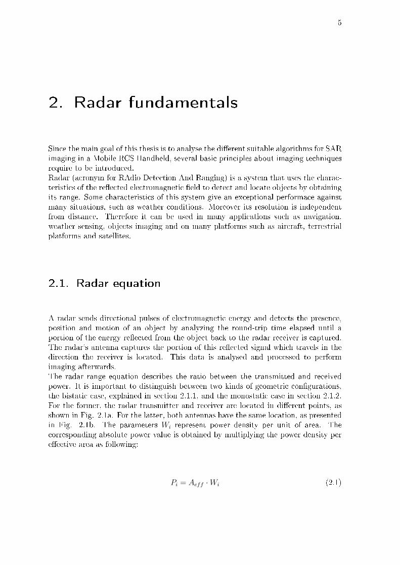
As it is shown in Fig. 2.2, the energy is scattered in all directions but obviously onlythe portion in the direction of the radar receiver is used in the RCS denition.It is also important to mention how the polarization of the wave gets aected duringthe whole proces.Firstly, the transmitted wave will be arbitrarily polarized but mostly vertically (V) orhorizontally (H). Then, when the wave impacts with the scatterer, the portion whichis reected back to the radar will contain components in both possible polarisations,always depending on the RCS properties of the target. That means that in the re-ceived data not only information from the initial polarization will be present, but alsocross-polarisation terms will appear.From the raw backscattered data of an object in a wide range of frequency and aspectangles, the application of suitable algorithms considering the corresponding eld regionand geometry characteristics can generate an image of the target, that is, how this ob-ject looks and where its stronger scatterer regions are located [1].
radarR
Collected scattered energy
Figure 2.2.: Scattered energy in all directions

2.3. Radar Waveforms 9
2.3. Radar Waveforms
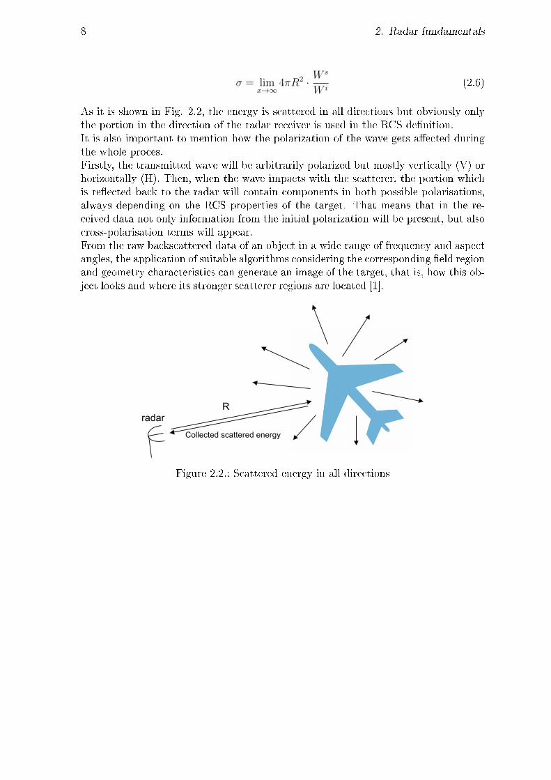
Several waveforms can be used for the formation of the radar signal and every kind ofsignal may be used for specic Radar applications. In the following, some examplesare presented. Following denitions are necessary:
Maximum detectable range (Rmax) Means the maximum distance in which the ob-ject can be located in order to detect it properly and avoid ambiguity betweenpulses. This concept only makes sense for waveforms in which there is an incre-ment of frequency in some cycles or pulses. The period of these cycles or pulseswill determine this maximum range Rmax.
Range resolution (∆r) Means the minimum distance between two close scattererswhich the radar system is able to distinguish. This concept makes sense only inthe case the wavefront is not continuous.
2.3.1. Continous Wave (CW)
The basic wavefront which can be used is the Continous Wave (CW), consisting ofa simple sinusoidal tone as shown in Fig. 2.4a. The tone received in the radar willideally be the same with a dierent frequency, due to Doppler eect, and thereforethe relative velocity of a moving object can be estimated. However, the range of thetarget cannot be determined in this case [3].
2.3.2. Frequency modulated continous wave (FMCW)
A Frequency Modulated Continous Wave (FMCW) can solve this problem by modu-lating the frequency of the signal by increasing the frequency progressively in time upto a specic threshold where the modulation cycle restarts, as shown in Fig. 2.4b.With this method the frequency dierence between transmitted and received signalwill determine the time delay between them. However it is important to emphasizethat in order to avoid range unambiguity the round-trip time to the target must besmaller than the modulation time of one cycle T , and thus the maximum detectablerange is:
Rmax = cT
2(2.7)
For targets at a long range the cycle duration T becomes impractically long [3].Since the frequency in this wavefront is increased progressively and continuously, andnot by a pulse per pulse basis, no closed expression is obtained for the range resolu-tion.

10 2. Radar fundamentals
2.3.3. Stepped Frequency Continous Wave (SFCW)
Another wavefront is the Stepped Frequency Continous Wave (SFCW), which works insimilar way as the FMCW explained before but in this case the frequency is modulatedstep-wise in a discrete way [4][1]. The N subwave frequencies are fn = fo+(n+1) ·∆fwhere T is the time between subwaves, as seen in Fig. 2.4c. With this approach, agreat characteristic is provided: The phase of the scattered eld is proportional to therange as following:
Es[f ] = A · e−j2k·Ro (2.8)
Hence it is obvious that the range Ro can be extracted by an inverse fourier transfor-mation and the range prole of the target is obtained with this method, as explainedwith more detail in the following section 3.2.For this wavefront, the maximum range detectable is inversely proportional to thefrequency step ∆f = B
Nas given by
Rmax =N · c2B
(2.9)
and the resolution is inversely proportional to the total frequency bandwidth B usedto modulate the signal, as following:
∆r =c
2B(2.10)
2.3.4. Chirp pulse or Linear Frequency Modulated (LFM)
Finally, a pulse waveform can be used, and specially the chirp pulse, also called LFMpulse. Although it has the same time duration as other conventional pulses such asrectangular pulse, its frequency range is much wider [5]. In Fig. 2.4d its appearancein time domain can be seen, where τ is the duration of the chirp pulse and TPR thetime elapsed from on pulse to another, also shown graphically in Fig. 2.3. The radarworking with these pulse waveforms is also known as pulsed radar.In this case the maximum detectable range is:
Rmax = cTPR
2(2.11)
and the range resolution is proportional to its pulse duration:
∆r = cτ
2(2.12)
Due to the characteristics of this waveform , it is the most common method used inradar applications [1].
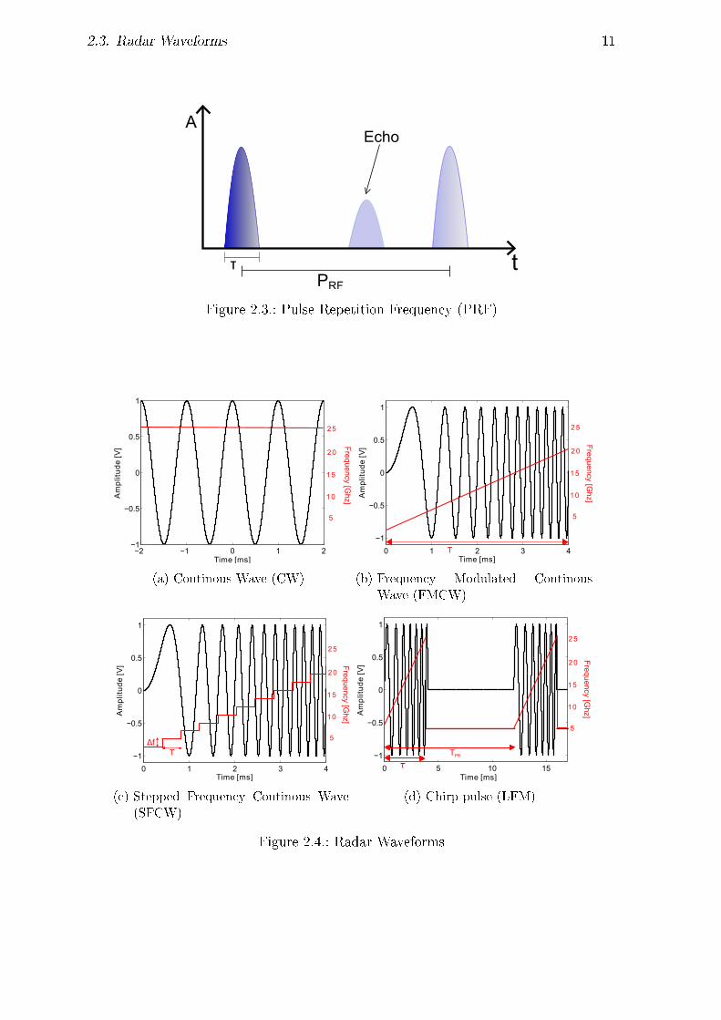
2.3. Radar Waveforms 11
PRFt
A
τ
Echo
Figure 2.3.: Pulse Repetition Frequency (PRF)
−2 −1 0 1 2−1
−0.5
0
0.5
1
Time [ms]
Am
plit
ud
e[V
]
5
1 0
1 5
2 0
2 5
Frequ
ency [Ghz]
(a) Continous Wave (CW)
0 1 2 3 4
−1
−0.5
0
0.5
1
Time [ms]
Am
plit
ud
e[V
]
5
1 0
1 5
2 0
2 5
Frequ
ency [Ghz]
(b) Frequency Modulated Continous
Wave (FMCW)
0 1 2 3 4
−1
−0.5
0
0.5
1
Time [ms]
Amplitude[V]
ΔfT
5
10
15
20
25
(c) Stepped Frequency Continous Wave
(SFCW)
0 5 10 15
−1
−0.5
0
0.5
1
Am
plit
ud
e[V
]
TPR
5
1 0
1 5
2 0
2 5
Frequency [G
hz]
(d) Chirp pulse (LFM)
Figure 2.4.: Radar Waveforms

12
13
3. SAR fundamentals
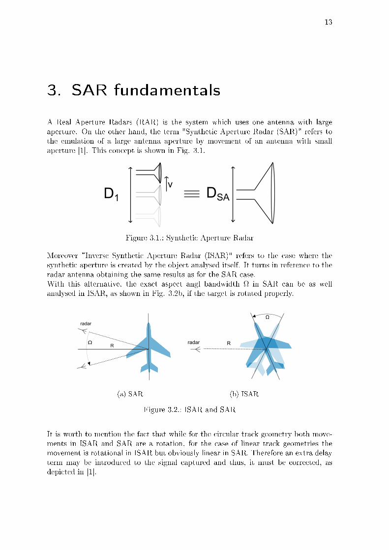
A Real Aperture Radars (RAR) is the system which uses one antenna with largeaperture. On the other hand, the term "Synthetic Aperture Radar (SAR)" refers tothe emulation of a large antenna aperture by movement of an antenna with smallaperture [1]. This concept is shown in Fig. 3.1.
D1 DSAv
Figure 3.1.: Synthetic Aperture Radar
Moreover "Inverse Synthetic Aperture Radar (ISAR)" refers to the case where thesynthetic aperture is created by the object analysed itself. It turns in reference to theradar antenna obtaining the same results as for the SAR case.With this alternative, the exact aspect angl bandwidth Ω in SAR can be as wellanalysed in ISAR, as shown in Fig. 3.2b, if the target is rotated properly.
R
radar
Ω
(a) SAR
Rradar
Ω
(b) ISAR
Figure 3.2.: ISAR and SAR
It is worth to mention the fact that while for the circular track geometry both move-ments in ISAR and SAR are a rotation, for the case of linear track geometries themovement is rotational in ISAR but obviously linear in SAR. Therefore an extra delayterm may be introduced to the signal captured and thus, it must be corrected, asdepicted in [1].

14 3. SAR fundamentals
3.1. SAR geometry and modes
For the case of a linear track 2D geometry, there are two dierent available modesfor SAR, according to the scanning methods. Stripmap mode is performed whenthe radar collects the scattered signals xing the pointing direction of the antenna inreference to the trackpath, as it can be seen in Fig. 3.3b. Spotlight mode is the casein which the pointing direction is xed in reference to the target analysed, as shownin Fig. 3.3a.However, for the circular track or other exotic track geometries case, obviouslyonly Spotlight mode makes sense, with the geometry shown in Fig. 3.3c and Fig.3.3d, respectively.
(a) Spotlight mode for linear tracks (b) Stripmap mode
(c) Spotlight mode for circu-
lar tracks
(d) Spotlight mode for exotic geome-
tries
Figure 3.3.: ISAR and SAR modes for many 2D track geometries
For this project, all geometries have been considered and used for the simulations,but only the spotlight mode has been analysed in detail because of our purpose. TheMobile RCS Handheld works by analysing an object from many dierent angularpositions which directly implies this SAR mode.
3.2. Basic SAR Imaging Algorithm 15
3.2. Basic SAR Imaging Algorithm
For ISAR imaging and generally for all radar imaging applications, the main tool withwhich the scattered eld data Es(f, θ) is processed in order to get an image of thetarget is the Fast Fourier Transformation (FFT).That is due to the fact that in the mathematical characteristics of the scattered radarcollected data, the distance information is located in the phase. Considering a monos-tatic case and a distance R from the radar to the target, the mathematical expressionof the scattered wave can be approximated as following:
Es(f) ∼= A · e−j2( 2πfc
)R (3.1)
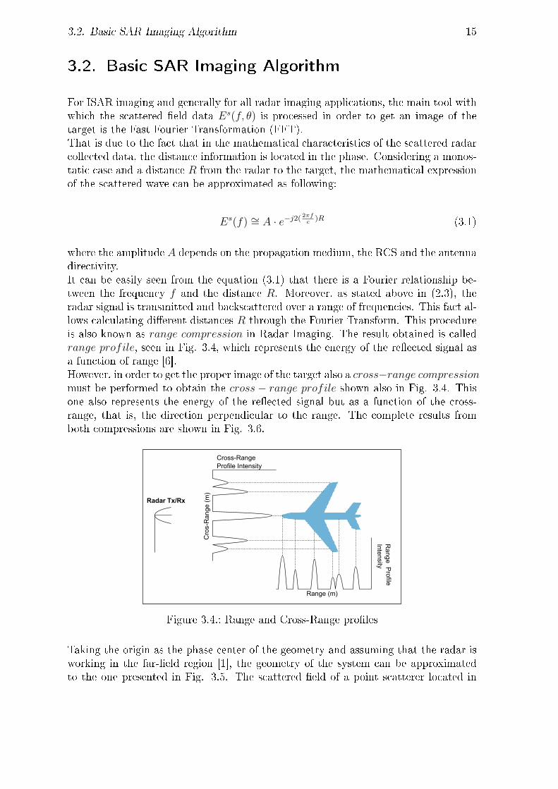
where the amplitude A depends on the propagation medium, the RCS and the antennadirectivity.It can be easily seen from the equation (3.1) that there is a Fourier relationship be-tween the frequency f and the distance R. Moreover, as stated above in (2.3), theradar signal is transmitted and backscattered over a range of frequencies. This fact al-lows calculating dierent distances R through the Fourier Transform. This procedureis also known as range compression in Radar Imaging. The result obtained is calledrange profile, seen in Fig. 3.4, which represents the energy of the reected signal asa function of range [6].However, in order to get the proper image of the target also a cross−range compressionmust be performed to obtain the cross− range profile shown also in Fig. 3.4. Thisone also represents the energy of the reected signal but as a function of the cross-range, that is, the direction perpendicular to the range. The complete results fromboth compressions are shown in Fig. 3.6.
Range (m)
Cro
s-R
ange
(m
)
Cross-Range Profile Intensity
Range P
rofileIntensity
Radar Tx/Rx
Figure 3.4.: Range and Cross-Range proles
Taking the origin as the phase center of the geometry and assuming that the radar isworking in the far-eld region [1], the geometry of the system can be approximatedto the one presented in Fig. 3.5. The scattered eld of a point scatterer located in

16 3. SAR fundamentals
(xo, yo) can thus be approximated to:
Es(k, θ) ∼= Ao · e−j2~k ~ro (3.2)
where Ao is the scattered eld amplitude, ~k the vector wave number and ~ro the vectordening the location of the scatterer in P (xo, yo).
The argument in the phase term of (3.2) can be developed as:
~k · ~ro = k · (x · cos θ + y · sin θ) · (x · xo + y · yo)= k cos θ · xo + k sin θ · yo= kx · xo + ky · yo
(3.3)
Rewriting now equation (3.2), the scattered eld is expressed like:
Es(k, θ) ∼= Ao · e−j2k cos θ·xo · e−j2k sin θ·yo (3.4)
Assuming also that the scattered data has been collected for a small frequency band-width, the wave number can be approximated to be constant [1]:
k ∼= kc = 2πfc/c (3.5)
And in a similar manner, for a small angular bandwidth, the following aproximationcan be applied:
cos θ ∼= 1
sin θ ∼= θ(3.6)
The equation (3.4) can be rewritten now once again:
Es(k, θ) ∼= Ao · e−j2kc·xo · e−j2kcθ·yo
= Ao · e−j2π( 2fc
)·xo · e−j2π( kcθπ
)·yo(3.7)
P(xo,yo)
ro
y
x
radar
k·ro
θ
k
Figure 3.5.: Geometry for monostatic SAR imaging within Far-Field region
3.2. Basic SAR Imaging Algorithm 17
Reached this point, it can be noticed that the application of an FFT in both fre-quency and aspect angle allows the obtention of xo from the former and of yo from thelatter.
F−12 Es(k, θ) = Ao · F−1
1 e−j2π( 2fc
)·xo · F−11 e−j2π( kcθ
π)·yo
= Ao ·[∫ ∞−∞
1
πe−j2π( k
π)·xo · ej2π( k
π)·xdk
]·[∫ ∞−∞
π
kce−j2πθ·yo · ej2πθ·ydθ
]= A′0 · δ(x− xo, y − yo)= ISAR(x, y)
(3.8)
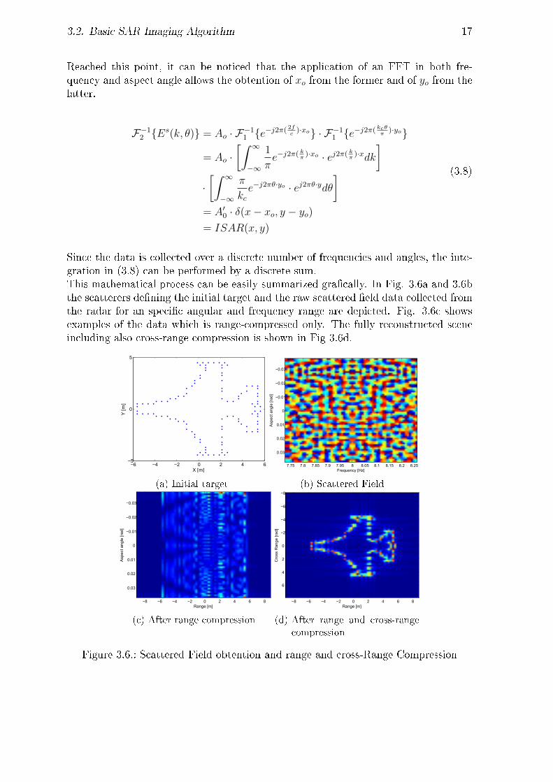
Since the data is collected over a discrete number of frequencies and angles, the inte-gration in (3.8) can be performed by a discrete sum.This mathematical process can be easily summarized gracally. In Fig. 3.6a and 3.6bthe scatterers dening the initial target and the raw scattered eld data collected fromthe radar for an specic angular and frequency range are depicted. Fig. 3.6c showsexamples of the data which is range-compressed only. The fully reconstructed sceneincluding also cross-range compression is shown in Fig 3.6d.
−6 −4 −2 0 2 4 6−5
0
5
X [m]
Y [
m]
(a) Initial target
Frequency [Hz]
Asp
ect a
ngle
[rad
]
7.75 7.8 7.85 7.9 7.95 8 8.05 8.1 8.15 8.2 8.25
−0.03
−0.02
−0.01
0
0.01
0.02
0.03
(b) Scattered Field
Range [m]
Asp
ect a
ngle
[rad
]
−8 −6 −4 −2 0 2 4 6 8
−0.03
−0.02
−0.01
0
0.01
0.02
0.03
(c) After range compression
Range [m]
Cro
ss R
ange
[rad
]
−8 −6 −4 −2 0 2 4 6 8
−8
−6
−4
−2
0
2
4
6
(d) After range and cross-range
compression
Figure 3.6.: Scattered Field obtention and range and cross-Range Compression

18 3. SAR fundamentals
3.2.1. Polar Reformatting
All the steps explained above are valid if both the frequency and angular bandwidthare relatively small. Usually less than one tenth of the center frequency for the formerand around 5o for the latter are considered to be small enough [1]. Only in this casethe approximations in (3.5) and (3.6) are valid.However, if this is not the case, the direct computation of the two dimensional FFTwill lead to extremely blurred images. Therefore another step will have to be includedin order to avoid such an eect in the image.By having a look at the far-eld equation of the scattered data without the approxi-mations in (3.4), it is clear that there is a Fourier relationship between k cos θ and xand between k sin θ and y.
Es(k, θ) ∼= Ao · e−j2k cos θ·xo · e−j2k sin θ·yo
= Ao · e−j2kx·xo · e−j2ky ·yo(3.9)
where kx = k cos θ and ky = k sin θ.Hence the computation of the FFT can only be applied if the scattered data is trans-formed from the polar coordinates (k, θ) to a uniform grid on kx−ky plane, also knownas k − space [1]. This process is shown in Fig. 3.7, where the green points representthe reformatted coordinates.This transformation of the data, also called polar reformatting, can be done throughan interpolation. This step will introduce a small unavoidable error, which is in anycase uncomparable to the error obtained without applying the polar reformatting.Important to mention is that with some kind of interpolations such as four-nearestneighbor approximation, this error can be highly minimized [1].
140 150 160 170 180 190 200 210 220 230−50
−40
−30
−20
−10
0
10
20
30
40
50
kx
ky
Figure 3.7.: Polar Reformatting
3.2. Basic SAR Imaging Algorithm 19
3.2.2. Point Spread Function
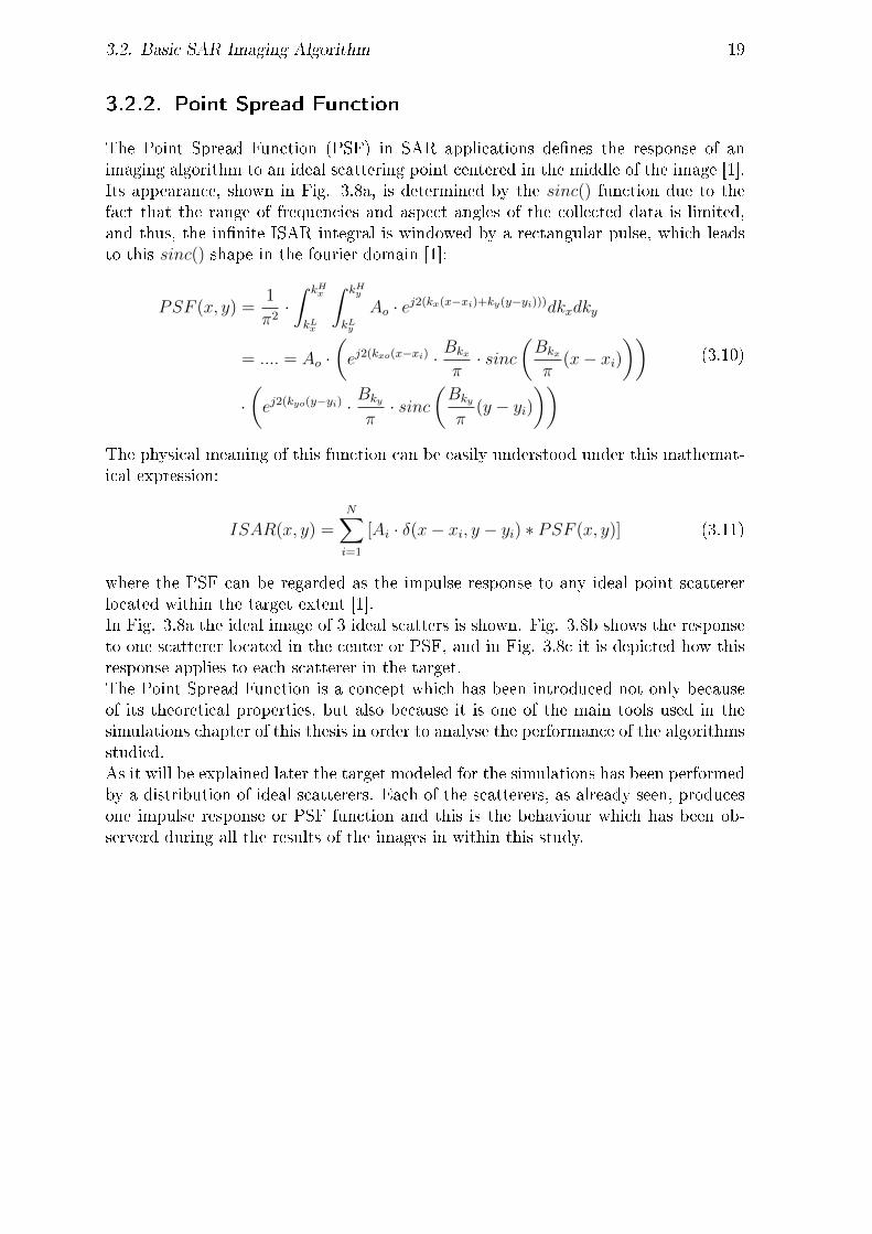
The Point Spread Function (PSF) in SAR applications denes the response of animaging algorithm to an ideal scattering point centered in the middle of the image [1].Its appearance, shown in Fig. 3.8a, is determined by the sinc() function due to thefact that the range of frequencies and aspect angles of the collected data is limited,and thus, the innite ISAR integral is windowed by a rectangular pulse, which leadsto this sinc() shape in the fourier domain [1]:
PSF (x, y) =1
π2·∫ kHx
kLx
∫ kHy
kLy
Ao · ej2(kx(x−xi)+ky(y−yi)))dkxdky
= .... = Ao ·(ej2(kxo(x−xi) · Bkx
π· sinc
(Bkx
π(x− xi)
))·(ej2(kyo(y−yi) ·
Bky
π· sinc
(Bky
π(y − yi)
)) (3.10)
The physical meaning of this function can be easily understood under this mathemat-ical expression:
ISAR(x, y) =N∑i=1
[Ai · δ(x− xi, y − yi) ∗ PSF (x, y)] (3.11)
where the PSF can be regarded as the impulse response to any ideal point scattererlocated within the target extent [1].In Fig. 3.8a the ideal image of 3 ideal scatters is shown. Fig. 3.8b shows the responseto one scatterer located in the center or PSF, and in Fig. 3.8c it is depicted how thisresponse applies to each scatterer in the target.The Point Spread Function is a concept which has been introduced not only becauseof its theoretical properties, but also because it is one of the main tools used in thesimulations chapter of this thesis in order to analyse the performance of the algorithmsstudied.As it will be explained later the target modeled for the simulations has been performedby a distribution of ideal scatterers. Each of the scatterers, as already seen, producesone impulse response or PSF function and this is the behaviour which has been ob-serverd during all the results of the images in within this study.

20 3. SAR fundamentals
−5
0
5
−5
0
50
1
2
3
4
5
X [m]Y [m]
Am
plit
ud
e
(a) Ideal scatterers
−5
0
5
−5
0
5
0
0.2
0.4
0.6
0.8
1
X [m]Y [m]
Res
po
nse
(b) Point spread Function
−5
0
5
−5
0
5
1
2
3
4
Range [m]Cross − range [m]
ISA
R
(c) ISAR image
Figure 3.8.: PSF physical meaning

3.3. Improvements to the image quality 21
3.3. Improvements to the image quality
Considering the way the radar signal is processed in any kind of imaging solution ingeneral, there are some design parameters or operations which can be applied to thedata before and during the processing of almost any algorithm in order to improveits ISAR image quality. As it was shown in section 3.2, the concept of Fast FourierTransformation (FFT) plays a crucial role in the development of any imaging algo-rithm. Therefore operations such as zero padding and windowing to the data previousto the application of the FFT can improve considerably the result obtained after thisone. In following sections a brief explanation of these techniques is explained and af-terwards the improvement simulation results of the integration of these methods withthe imaging algorithms is presented in section 7.
3.3.1. Zero padding
Zero padding is one of the methods that can be used to improve the quality of anISAR image. It is based on the fact that the concatenation of samples with value zeroin one signal domain produces an interpolation on the other domain. An example ofthis concept is shown with the rectangular pulse rect(f/T ) in the frequency domainand its IFFT, T · sinc(tT ), to make it easier to understand how this technique works.In Fig. 3.9a the sampled sinc() function obtained has only one sample dierent thanzero but if a zero padding with factor 3 is applied, that is, adding nulled samples up tohaving 3 times the number of samples of the original sampled pulse, it can be observedhow the discretized signal in this case is interpolated with a factor 3, obtaining adiscrete signal much closer to the corresponding continous signal.
T
1/T t(s)f(Hz)
IFFT
(a) Without zero padding3T
1/(3T) t(s)f(Hz)
IFFT
(b) Zero padding (factor 3)
Figure 3.9.: Zero padding eect
22 3. SAR fundamentals
By using this technique in the context of this thesis, it is important to mention thatan underlying assumption is made. For the scattered eld data Es(f, θ) the zero-padding is applied usually in the frequency domain. That means that it is assumedthat the values of the scattered eld for this other frequency values are 0 and there-fore the extra information which would be provided by this data is not taken intoaccount.
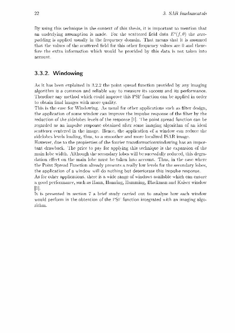
3.3.2. Windowing
As it has been explained in 3.2.2 the point spread function provided by any imagingalgorithm is a common and reliable way to measure its success and its performance.Therefore any method which could improve this PSF function can be applied in orderto obtain nal images with more quality.This is the case for Windowing. As usual for other applications such as lter design,the application of some window can improve the impulse response of the lter by thereduction of the sidelobes levels of the response [1]. The point spread function can beregarded as an impulse response obtained after some imaging algorithm of an idealscatterer centered in the image. Hence, the application of a window can reduce thesidelobes levels leading, thus, to a smoother and more localized ISAR image.However, due to the propierties of the fourier transformationwindowing has an impor-tant drawback. The price to pay for applying this technique is the expansion of themain lobe width. Although the secondary lobes will be sucessfully reduced, this degra-dation eect on the main lobe must be taken into account. Thus, in the case wherethe Point Spread Function already presents a really low levels for the secondary lobes,the application of a window will do nothing but deteriorate this impulse response.As for other applications, there is a wide range of windows available which can ensurea good performance, such as Hann, Hanning, Hamming, Blackman and Kaiser window[1].It is presented in section 7 a brief study carried out to analyse how each windowwould perform in the obtention of the PSF function integrated with an imaging algo-rithm.

23
4. Errors producing image defocus
In real measurements with a Mobile RCS Handheld, some sources can produce phaseerrors to the scattered data captured and therefore errors in the calculation of therange distances from the radar device to the scatterers under analysis. This eectleads to a defocus eect degrading the nal image obtained [7].In section 4.1 the main sources of phase errors that may be introduced during the col-lection of the data is presented. In section 4.2 is the modeling of the errors consideredin this thesis explained.
4.1. Error sources
All sorts of errors might be caused basically from three main sources which are depictedin Table 4.1.
Radar position estimation errorIMU and GPS accuracy errors
Own object motionTransactional motionRotational motion
Scene related errorsMultiple reectionsClutter
Table 4.1.: Main phase error sources
For the rst group, it is obvious that the estimation of the position of the Mobile RCSHandheld will have some accuracy limitations and therefore some error is introducedin the calculation of the range distance to the target.Secondly, if the object is not static during the measurements it will obviously introducea defocus in the SAR image. The object movement has been divided into two basiccomponents, transactional and rotational.Finally, another phenomenons like multiple reections and clutter can cause delayerrors or the appearence of virtual scatterers.

24 4. Errors producing image defocus
4.2. Error modelation
Considering the scattered near-eld captured in ideal conditions as
Es(f, θ) =
∫ ∞0
∫ 2π
0
ψ(ρ, φ)exp−j
2πλ
2d
2dρdρdφ (4.1)
a phase error cause an error function φe(θ). This function has a spatial dependencyand therefore has dierent values for each step in the along-track direction. In otherwords, this function has dierent values in the range [0, 2π] for each pulse transmited.If the track geometry is circular, this function depends on the azimuth of the along-track. This error function degrades the data as depicted in (4.2).
Es(f, θ) = Es(f, θ) · ejφe(θ) (4.2)
For this reason, since the error is introduced in phase of the scattered eld, if only aconventional imaging algorithm is applied to this data, a defocused ISAR image willbe obtained, due to the wrong calculations of the range distances d = d+ ε.This phenomenon is shown in Fig. 4.1 where it can be seen how the error is introducedin the calculation of the range distance to the target locations.
x
y
Target
π
-π
d=d+ε˜d
ϕe
Figure 4.1.: Phase error eect during data collection
Since the sort of errors produced in the real world is too complex to reach a commonfunction to express all possibilities, a representative range of error functions possibleto be present during radar measurements have been studied and analysed. These arelinear or rst polynomial order, second order polynomial, high order polynomial andrandom gaussian error functions. The models are shown in Fig. 4.2.Depending on their nature and magnitude, the eects to the image quality producedby these phase errors are dierent.Table 4.2 shows the theorical eects produced on the SAR image for each kind oferror [7]. These eects are corroborated by the corresponding simulations in chapter7.

4.2. Error modelation 25
0 50 100 150 200 250 3000
π/2
π
2π/2
2π
Phase e
rror
(rad)
Azimuth position (Pulse)
(a) First order polynomial func-
tion
0 50 100 150 200 250 3000
π/2
π
2π/2
2π
Phase e
rror
(rad)
Azimuth position (Pulse)
(b) Second order polynomial
function
0 50 100 150 200 250 3000
π/2
π
2π/2
2π
Phase e
rror
(rad)
Azimuth position (Pulse)
(c) High order polynomial func-
tion
0 50 100 150 200 250 3000
π/2
π
2π/2
2π
Phase e
rror
(rad)
Azimuth position (Pulse)
(d) Random function
Figure 4.2.: Representative error modelation
Phase Error Type Along-track phase variation Image Eect
Low-frequency
polynomial order 1 Geometric displacementpolynomial order 2 Image defocus, less resolutionpolynomial higher order Distorted mainlobeRandom gaussian noise Loss of contrast, SNR degraded
Table 4.2.: Theoretical defocus eect of the errors modeled
Later in section 6 some techniques to compensate them are explained in detail. More-over in chapter 7 several simulations have been performed to show some examplesof how these errors degrade the nal SAR image, and how this degradation is xedthrough an autofocusing algorithm.

26

27
5. Suitable imaging algorithms
As it has been explained in section 3.2, the algorithm used in the portable device mustsuit a basic condition: The ability to work in the Near-Field range.Ignoring the directivity of antennas and considering a monostatic geometry where bothradar transmitter and receiver are located in the Mobile RCS Handheld, the expressionof the electromagnetic eld in this region looks like:
Es =
∫ ∞0
∫ 2π
0
ψ(ρ, φ)e−j
2πλ
2d
2dρdρdφ (5.1)
where ψ(ρ, φ) denes the reectivity function of the scatterers contained in the targetand ρ and φ the polar coordinates dening its positions. d represents the distancebetween radar antenna and any point in the target. As it can be observed in (5.1), theapproximations for far-eld region for the distance calculation from the radar Tx/Rxto the scatterers are obviously no longer available [8]. In the near eld region theexpression for the distance must be calculated exactly like:
d =√R2 + ρ2 − 2Rρ cos (φ− θ) (5.2)
Therefore some of the possibilities facing this problem have been analysed deeply in thisthesis in both frequency and time domain and are listed below:
Fast Cyclical Convolution Also called Focusing Operator algorithm, which restoreschanges in the amplitude and phase of the near-eld wave on its way betweenthe radar antenna and the target, as explained with more detail in section 5.1.1
Back-Projection Also called Tomographic Back-Projection, which performs only therange-compression through an IFFT computation for each angular step and back-projects the data [8], as explained in section 5.2.1.
Fast Factorized Back-Projection Is an improvement of the classic Back-Projectionalgorithm which consists on previously factorising the raw scattered data andback-projecting it independently for each region of the target [9]. A detailedexplanation of this method is presented in section 5.2.2.
Although all algorithms studied work under dierent theorical considerations andpoints of view, the main principle explained in section 3.2 is common for all solu-tions and all them are based on its key operation, the FFT.

28 5. Suitable imaging algorithms
5.1. Frequency Domain
In this section, the algorithms used have the common characteristic that both arange and azimuth compression is applied through fast fourier transformations, asit has been seen for the basic SAR imaging algorithm already explained in section3.2.
5.1.1. Fast Cyclical Convolution
The obtention of an unblurred image for near-eld SAR imaging can be obtained, asstated in [10], through a focusing operator applied to every given frequency and an-gular sample, restoring the changes in the amplitude and phase of the near-eld waveon its way between the radar antenna and the target.This process corresponds to the following mathematical expression:∫ ∞
0
∫ 2π
0
Es(f, θ) · ξ(f, θ, ρ, φ) dfdθ (5.3)
where the focusing operator is expressed as:
ξ(f, θ, ρ, φ) = ej2πλ
2d · d2 (5.4)
and d has been calculated exactly, as stated in (5.2).Substituting this operator in (5.3) it is obtained:∫ ∞
0
∫ 2π
0
Es(f, θ) · ej2πλ
2d · d2dfdθ (5.5)
which looks like the two dimensional inverse Fourier Transformation used in the basicISAR algorithm valid for far-eld, explained in section 3.2.The main dierence in comparison to the basic approach is the way this transformationis performed. On the one hand, since the focusing operator depends actually onthe dierence φ − θ and the scattered eld depends only on the aspect angle θ, theintegration in θ domain can be regarded as a circular convolution along this angle [10].Moreover, it is known that a convolution can be computed with a product in fourierdomain. On the other hand the integration in frequency is simply computed in thediscrete domain with the sum of the dierent frequency samples of the scattered eldpreviosuly recorded [10]:
ψ(ρ, φ) =
∫ ∞0
∫ 2π
0
Es(f, θ) · ξ(f, ρ, φ− θ)dfdθ
=
∫ ∞0
Es(f, θ) ∗ ξ(f, ρ, φ)df
ψ(ρ, φ) =∑f
Es(f, θ) ∗ ξ(f, ρ, φ)
=∑f
IFFTφ[FFTφ[Es(f, θ)] · FFTφ[ξ(f, ρ, φ)]]
(5.6)

5.1. Frequency Domain 29
The SAR image obtained is in this case is in polar coordinates, and thus a polar tocartesian interpolation must be computed afterwards.
ISAR(ρ, φ)interpolation−−−−−−−→ ISAR(x, y) (5.7)
This step will obviously introduce a small error in the image, depending on the reso-lution used.
Angular sampling rate
For this algorithm a limitation in the angular sampling shall be considered beforeperforming the cyclical convolution stated in (5.6). Otherwise, aliasing eects in ournal image will be present and additional undesired virtual objects will be introduced[11]. As explained in (5.2) the angular dependence is present in the distance calculatedfor the near-eld case. Thus, the calculation of the maximum of the rst derivate ofthe distance d(ρ, φ), depicted in (5.2), with regard to φ, is performed. With thisexpression the maximum variation of the scattered eld in the angular direction canbe calculated:
∂d(ρ, φ)
∂φ|max =
Rρ sinφ√R2 + ρ2 − 2Rρ cosφ
|max =Rρ√R2 + ρ2
(5.8)
Thus, the maximum change on the phase information of the focusing operator is:
∆θ|max =2fmaxRρi,max
c√R2 + ρ2
i,max
(5.9)
where fmax is the highest frequency used to store the scattered eld and ρimax themaximum distance imaged to the center of the target, because the largest oscillationsin the scattered eld will be produced by the most distant scatterer to the targetcenter. Finally, the angular sampling rate applied to the scattered eld Es in (5.3)must necessarily fulll [11]:
∆φ <c√R2 + ρ2
i,max
4fmaxRρi,max(5.10)
Hence, the focusing operator previously calculated will be sampled with this rate.Also a resampling of the scattered eld with the same rate will be needed through aninterpolation in angular direction [11] in order to carry out the convolution operationbetween scattered eld Es and focusing operator ξ.Due to the fact that the scattered eld is obtained along a concrete angular rangesometimes smaller than the whole angle rate [0, 2π], it is important to mention that azero padding to the scattered eld will be applied to cover all the angular samples inthe range [0, 2π] in order to make possible its convolution in fourier domain with thefocusing operator in (5.6).

30 5. Suitable imaging algorithms
Computational Cost
The focusing operator ξ(f, ρ, φ) is constant for a given system. Hence, taking advan-tatge of this characteristic, its FFT can be previously stored to reduce signically thecomputation time [11].The theorical computational complexity of this method O(NρNfNφlog2Nφ) dependson the sampling rate of both polar radius ρ and angle φ coordinates, and frequencysampling rate [11]. For this theorical cost calculation, the FFT applied to the scatteredeld has been neglected [12].

5.1. Frequency Domain 31
Es(f,θ) ξ(f,ρ,φ)
FFTφ FFTφ
IFFTφ
Σf
CartesianInterpolation
ISAR(ρ,φ)
ISAR(x,y)
AngularResampling
Figure 5.1.: Fast Cyclical Convolution Algorithm

32 5. Suitable imaging algorithms
5.2. Time Domain
All the algorithms used in this section have the same basic characteristic in common.The scattered eld data obtained for a range of frequencies and aspect angles is range-compressed through a FFT in range dimension, in the same way explained in theprevious section 5.1. However, for the cross-range dimension there is no compressionthrough an inverse fourier transformation. The data is, thus, computed in a pulse-per-pulse basis, without applying an IFFT in the azimuth direction.The main algorithm based on it is the so-called Back-Projection (BP) or Tomo-graphic Reconstruction, based on the Circular Radon Transform [13][14] to obtaincross-sectional scans of an object. Due to its pulse per pulse processing method thisalgorithm can suit near-eld region radar data.Nowadays it is still the base of other algorithms used for this purpose, with dierentimprovements such as Fast Factorized Back-Projection (FFBP) explained in section5.2.2 in order to reduce its high computational cost for big images. A more detailedexplanation of BP and its improved version (FFBP) is presented in sections 5.2.1 and5.2.2.
5.2.1. Back Projection
The Back-Projection or also known as Tomographic Reconstruction is a techniqueused for many years in many applications such as medicine, non-destructive testing/e-valuation, astronomy, and of course radar imaging to look inside objects and analyzeinternal structures [15]. However, the problem in general is that the whole data pro-cessing can be computationally very intensive.As mentioned before, the use of the Radon Transform is the main idea of this method.Working in the near-eld region, the scattered eld data depending on frequency andaspect angle has the expression presented before in 5.1:
Es =
∫ ∞0
∫ 2π
0
ψ(ρ, φ)exp−j
2πλ
2d
2dρ dρdφ (5.11)
By selecting a specic aspect angle θm and applying the inverse FFT only in thefrequency dimension, the range prole qθm(r) of the target can be obtained from thisspecic angle as follows [8]:
qθm(r) = IFFTEsθm(k) =
∫ ∞−∞
∫ ∞−∞
1
R2m
ψ(x, y)δ(Rm − r)dxdy (5.12)
where Rm represents a matrix variable containing for the m-th pulse the distancesfrom the radar to all (x, y) pixels of the image. Equation (5.12) is the description ofthe circular Radon Transform of the target's reectivity function, suitable in near-eldregion. Looking at the equation with more detail its physical meaning can be deduced:The received signal under a spherical omnidirectionnal wavefront radiation is the sum
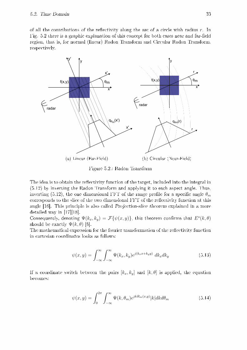
5.2. Time Domain 33
of all the contributions of the reectivity along the arc of a circle with radius r. InFig. 5.2 there is a graphic explanation of this concept for both cases near and far-eldregion, that is, for normal (linear) Radon Transform and Circular Radon Transform,respectively.
y
x
x'
y'
f(x,y) θm
x'
qθm(x')
radar
(a) Linear (Far-Field)
y
x
r
f(x,y) θm
r
radar
qθm(r)
(b) Circular (Near-Field)
Figure 5.2.: Radon Transform
The idea is to obtain the reectivity function of the target, included into the integral in(5.12) by inverting the Radon Transform and applying it to each aspect angle. Thus,inverting (5.12), the one dimensional FFT of the range prole for a specic angle θmcorresponds to the slice of the two dimensional FFT of the reectivity function at thisangle [16]. This principle is also called Projection-slice theorem explained in a moredetailed way in [17][18].Consequently, denoting Ψ(kx, ky) = Fψ(x, y), this theorem conrms that Es(k, θ)should be exactly Ψ(k, θ) [8].The mathematical expression for the fourier transformation of the reectivity functionin cartesian coordinates looks as follows:
ψ(x, y) =
∫ ∞−∞
∫ ∞−∞
Ψ(kx, ky)ej(kxx+kyy) dkxdky (5.13)
If a coordinate switch between the pairs [kx, ky] and [k, θ] is applied, the equationbecomes:
ψ(x, y) =
∫ 2π
0
∫ ∞−∞
Ψ(k, θm)ejkRm(x,y)|k|dkdθm (5.14)

34 5. Suitable imaging algorithms
where θm is a concrete azimuth aspect angle and Rm(x, y) the distance from the radarantenna to each pixel in (x, y) coordiantes of the image at this angle θm.Applying now the already explained Projection-slice theorem to equation (5.14), thereectivity function can be expressed as follows [8]:
ψ(x, y) =
∫ 2π
0
[∫ ∞−∞
Es(k, θm)ejkRm(x,y)|k| dk]dθm (5.15)
By applying a lter to the scattered eld data H(k) = |k|, the function of the lteredeld can be expressed like Qθm(k) = Es
θm(k) · |k|, and, thus, the equation (5.15) can
be rewritted like:
ψ(x, y) =
∫ 2π
0
[∫ ∞−∞
Qθm(k) · ejkRm(x,y)dk
]dθm (5.16)
And nally it can be noticed that the bracketed part of the equation is nothing but theFFT of the function qθm(r) evaluated in all pixels of the image with distance Rm(x, y)to the radar antenna. Hence, the last equation obtained for the reectivity functionwhich is the SAR image of the target analysed under a wide range of azimuth aspectangles becomes [8]:
ψ(x, y) =
∫ 2π
0
qθm(Rm(x, y))dθm (5.17)
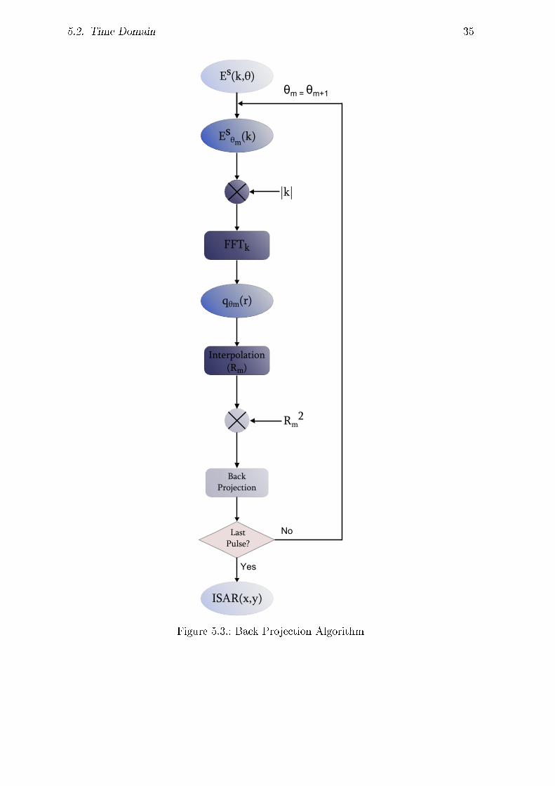
This is the nal result of a back-projection process, where a sum of all ltered rangeproles qθm(Rm(x, y)) interpolated for all pixels (x, y) with distance Rm(x, y) and fromeach azimuth angle step θm, is applied. In Fig. 5.3 a detailed graphic explanation ofthe whole algorithm is shown.
Computational Cost
The implementation of this algorithm has a theorical computational cost ofO(NxNyNθ),where Nx and Ny are the number of pixels of the nal image in x and y direction,respectively, and Nθ the number of azimuth angle steps [8]. In this calculation, theFFT operations to obtain the range proles as well as the interpolation process forRm(x, y) distances have been neglected.
5.2. Time Domain 35
Esθm(k)
FFTk
BackProjection
ISAR(x,y)
Es(k,θ)
|k|
qθm(r)
Interpolation(Rm)
Rm2
LastPulse?
Yes
No
θm = θm+1
Figure 5.3.: Back Projection Algorithm
36 5. Suitable imaging algorithms
5.2.2. Fast Factorized Back-Projection
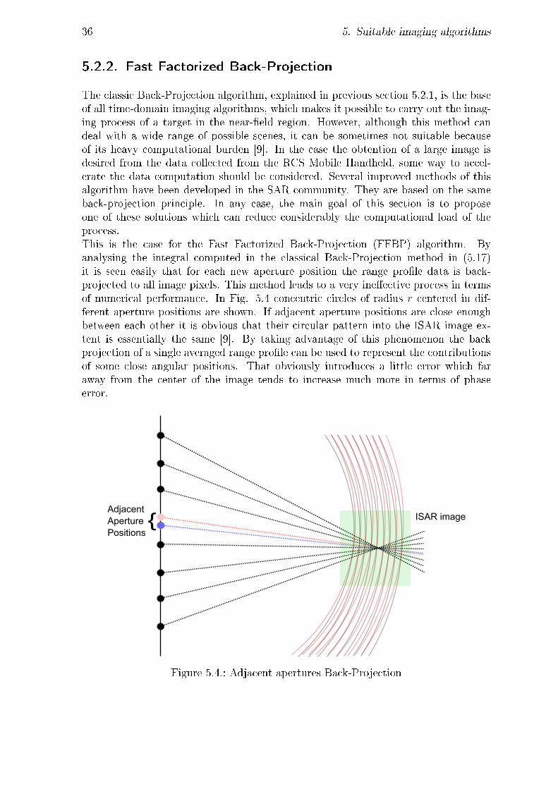
The classic Back-Projection algorithm, explained in previous section 5.2.1, is the baseof all time-domain imaging algorithms, which makes it possible to carry out the imag-ing process of a target in the near-eld region. However, although this method candeal with a wide range of possible scenes, it can be sometimes not suitable becauseof its heavy computational burden [9]. In the case the obtention of a large image isdesired from the data collected from the RCS Mobile Handheld, some way to accel-erate the data computation should be considered. Several improved methods of thisalgorithm have been developed in the SAR community. They are based on the sameback-projection principle. In any case, the main goal of this section is to proposeone of these solutions which can reduce considerably the computational load of theprocess.This is the case for the Fast Factorized Back-Projection (FFBP) algorithm. Byanalysing the integral computed in the classical Back-Projection method in (5.17)it is seen easily that for each new aperture position the range prole data is back-projected to all image pixels. This method leads to a very ineective process in termsof numerical performance. In Fig. 5.4 concentric circles of radius r centered in dif-ferent aperture positions are shown. If adjacent aperture positions are close enoughbetween each other it is obvious that their circular pattern into the ISAR image ex-tent is essentially the same [9]. By taking advantage of this phenomenon the backprojection of a single averaged range prole can be used to represent the contributionsof some close angular positions. That obviously introduces a little error which faraway from the center of the image tends to increase much more in terms of phaseerror.
ISAR imageAdjacentAperturePositions
Figure 5.4.: Adjacent apertures Back-Projection

5.2. Time Domain 37
It is important to emphasize that this assumption can be only made under the basiccondition that the sampling rate of the aperture track is high enough. In order notto back-project all the data to the nal image, a factorisation of the data will haveto be carried out in several stages, previous to the nal back-projection step, whichwill be performed only once after the data is factorised. It has been observed thatthe exact way in which the data will be divided and the level of factorisation, that is,the number of stages or iterations, will depend on the geometry of the scenario andcan be customized. The general approach to describe the method on which all thefactorisation variations are based is explained below.
Factorisation
The scattered eld data is factorised in a recursive way into sub-data sets correspond-ing to sub-images of the whole image. In other words, only the range prole samplesqθm(r) needed for the pixels of a sub-image are selected, discarding the rest for theformation of this sub-image [19] as it is shown in Fig. 5.5 for the rst stage. Thisstep is performed for all subimages in one factorisation step, and the whole process isrepeated in the next iteration with new sub-sub-images.
stage 1 stage 2 stage 3
q(r,θq)
qmn(r,θq)
Figure 5.5.: Range factorisation
where q(s)(r, θq) contains all the samples of the factorised range prole from the aspectangle θq in the stage s. q(s)
mn(r, θq) represents the part of the samples needed to formthe subimage mn.The factorisation design depends on many parameters, such as the factorisation factorQ which indicates in how many parts the new sub-image is divided in each direction,and S which determines the number of stages or iterations performed.Moreover, the factorisation can also be done only in one direction instead of in bothdirectios (x, y), as explained in [20], or even be performed by blocks of the track usingonly some specic track samples for dierent sub-images as explained in [9].However, in this section a basic factorisation with a factor Q = 2 in both directions(x, y) is described in order to make the comprehension of the main principle easier.The obtention of this sub-range in the actual stage is done by suming the contributionsof sub-ranges from the previous stage that correspond to the subimage mn. Moreover,a little delay ∆rpq,mn is applied in order to compensate the little range dierences

38 5. Suitable imaging algorithms
due to the new aspect angles positions, as shown in Fig. 5.6. The result of that arethe selected samples needed from the whole range function for new decimated tracklocations yp.
subimage mn
rθq,mn
yp
yq
Δrpq,mn
Figure 5.6.: Focusing delay
Thus its mathematical expression is:
q(s)mn(r, θq) =
(q+1)Q−1∑p=qQ
q(s−1)m′n′ (r −∆rpq,mn, θp) · ejkc∆rpq,mn (5.18)
where∆rpq,mn = (yp − yq) sin θqmn (5.19)
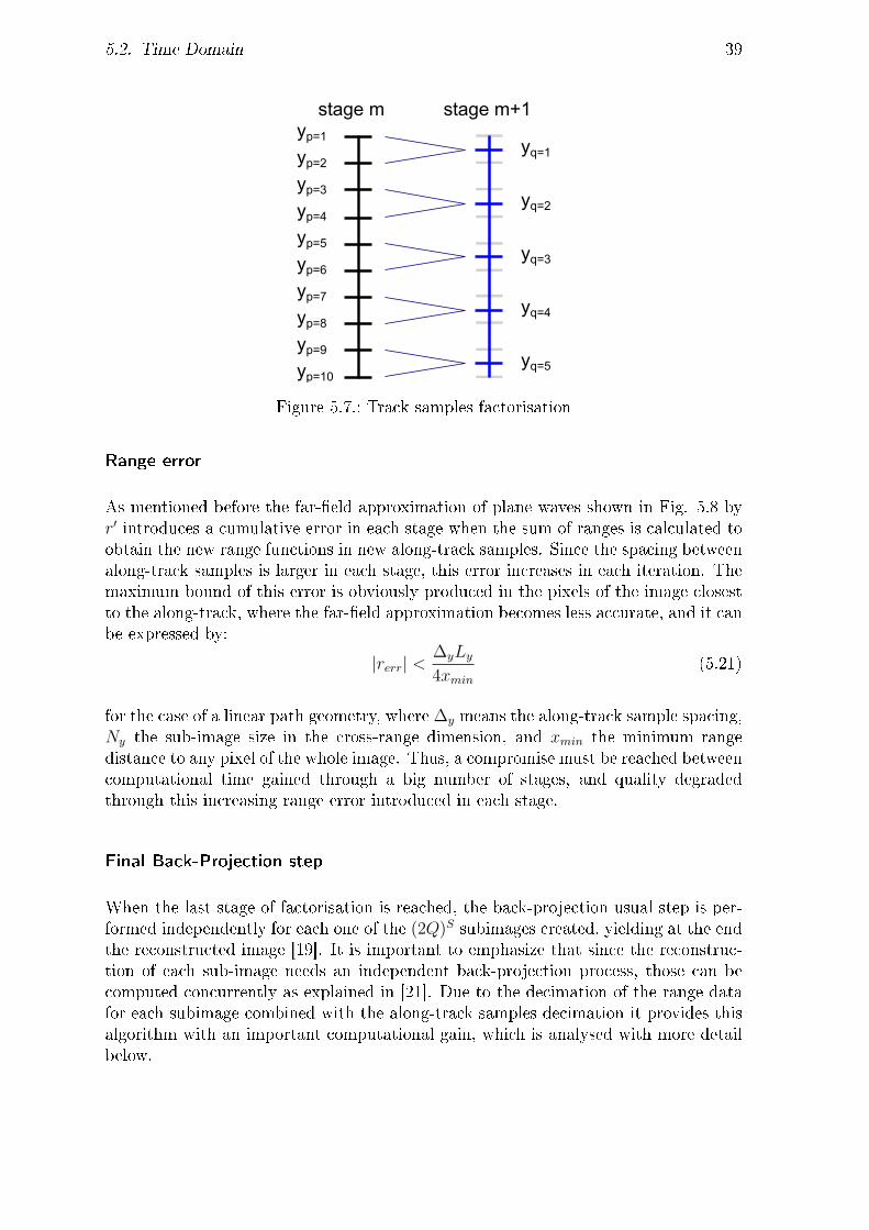
is the delay applied to focus the data to the center of the specic subimage mn.The new decimated track locations yq are calculated with the decimation shown inFig. 5.7. In this case, the decimation factor is also Q = 2 for the along-tracksampling, and the new decimated track samples can be expressed as in equation(5.20).
yq =1
Q
(q+1)Q−1∑p=qQ
yp (5.20)
However, a far-eld approximation is made in the calculation of this focusing delay, andthus, a little range-error will be introduced. Moreover, since the along track samplingin each stage is becoming lower, the error will become larger in each stage. Thereforea compromise between number of stages used during the factorisation and the rangeerror level introduced must be reached. A more detailed analysis of the possible levelsof this error given below.
5.2. Time Domain 39
stage m stage m+1yp=1
yp=2
yp=3
yp=4
yp=5
yp=6
yp=7
yp=8
yp=9
yp=10
yq=1
yq=2
yq=3
yq=4
yq=5
Figure 5.7.: Track samples factorisation
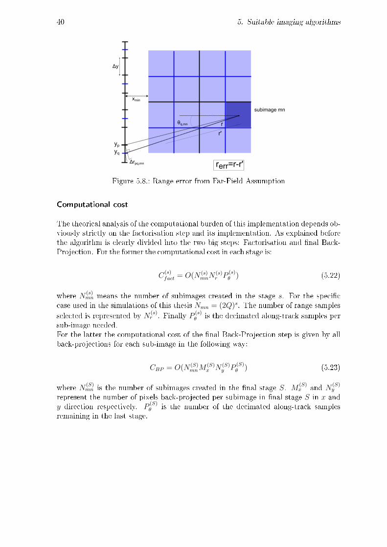
Range error
As mentioned before the far-eld approximation of plane waves shown in Fig. 5.8 byr′ introduces a cumulative error in each stage when the sum of ranges is calculated toobtain the new range functions in new along-track samples. Since the spacing betweenalong-track samples is larger in each stage, this error increases in each iteration. Themaximum bound of this error is obviously produced in the pixels of the image closestto the along-track, where the far-eld approximation becomes less accurate, and it canbe expressed by:
|rerr| <∆yLy4xmin
(5.21)
for the case of a linear path geometry, where ∆y means the along-track sample spacing,Ny the sub-image size in the cross-range dimension, and xmin the minimum rangedistance to any pixel of the whole image. Thus, a compromise must be reached betweencomputational time gained through a big number of stages, and quality degradedthrough this increasing range error introduced in each stage.
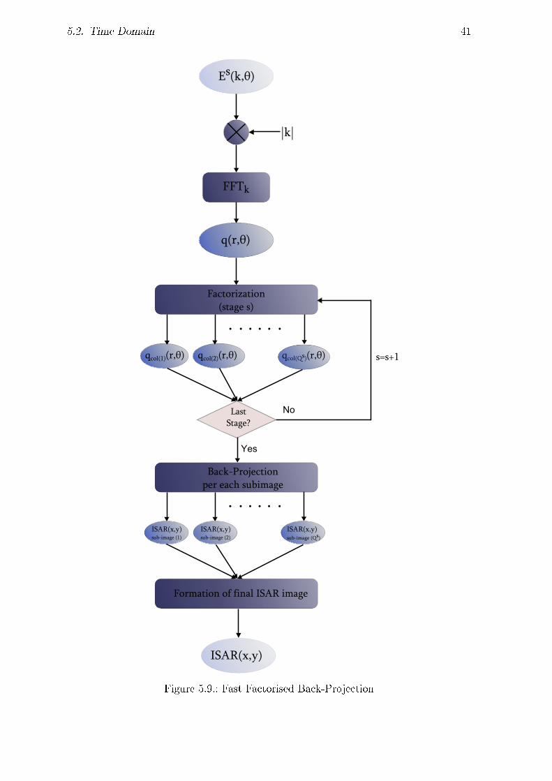
Final Back-Projection step
When the last stage of factorisation is reached, the back-projection usual step is per-formed independently for each one of the (2Q)S subimages created, yielding at the endthe reconstructed image [19]. It is important to emphasize that since the reconstruc-tion of each sub-image needs an independent back-projection process, those can becomputed concurrently as explained in [21]. Due to the decimation of the range datafor each subimage combined with the along-track samples decimation it provides thisalgorithm with an important computational gain, which is analysed with more detailbelow.
40 5. Suitable imaging algorithms
subimage mn
rθq,mn
xmin
yp
yq
Δy
Δrpq,mn rerr=r-r'
r'
Figure 5.8.: Range error from Far-Field Assumption
Computational cost
The theorical analysis of the computational burden of this implementation depends ob-viously strictly on the factorisation step and its implementation. As explained beforethe algorithm is clearly divided into the two big steps: Factorisation and nal Back-Projection. For the former the computational cost in each stage is:
C(s)fact = O(N (s)
mnN(s)r P
(s)θ ) (5.22)
where N (s)mn means the number of subimages created in the stage s. For the specic
case used in the simulations of this thesis Nmn = (2Q)s. The number of range samplesselected is represented by N (s)
r . Finally P (s)θ is the decimated along-track samples per
sub-image needed.For the latter the computational cost of the nal Back-Projection step is given by allback-projections for each sub-image in the following way:
CBP = O(N (S)mnM
(S)x N (S)
y P(S)θ ) (5.23)
where N (S)mn is the number of subimages created in the nal stage S. M (S)
x and N (S)y
represent the number of pixels back-projected per subimage in nal stage S in x andy direction respectively. P
(S)θ is the number of the decimated along-track samples
remaining in the last stage.
5.2. Time Domain 41
FFTk
ISARhxfyu
Eshkfθu
|k|
qhrfθu
Factorizationhstage?su
qcolh1uhrfθu qcolhQsuhrfθu?
LastStage?
Yes
No
s=sm1
Back2Projectionper?each?subimage
ISARhxfyusub2image?h1u
Formation?of?final?ISAR?image
qcolh2uhrfθu
ISARhxfyusub2image?h2u
ISARhxfyusub2image?hQsu
Figure 5.9.: Fast Factorised Back-Projection

42

43
6. Autofocusing Algorithms
6.1. Why should it be applied?
The resolution achieved in SAR imagery depends strictly on the imaging algorithmapplied to obtain the nal image from the scattered data. In order to obtain high-resolution images it is crucial to apply the correct matching azimuth lter, which canbe always calculated theorically and will work perfectly in ideal conditions [1].However, even in our case of real near-eld radar measurements, several factors ex-plained in section 4 such as the inertial measurement unit accuracy limitations or somepropagation eects will introduce phase perturbations in the calculation of the rangedistances to the scatterers [22]. For this reason the need of a solution to compensatethis possible eect have lead during this project to the analysis of an autofocus algo-rithm which is suitable for this project case and which can be sucessfully integratedwith the imaging algorithm presented in chapter 5.Thus several possibilities and its suitability for this project have been deeply studied.A detailed explanation of all the autofocusing techniques studied is presented below insection 6.2, and specially the Phase Gradient Autofocus (PGA) and a pre-processingautofocus technique through a coordinate descent estimation are presented in sections6.3 and 6.4, respectively.
6.2. Types of algorithms
All the sort of possibilities for the autofocusing algorithms can be classied in dierentways:
• The moment in which it is applied:
1. Pre-processing of the raw scattered data
2. Post-Processing of the SAR image
• The mathematical approach used:
1. Model-based
2. Estimation-based

44 6. Autofocusing Algorithms
For the rst classication the autofocusing algorithm can be performed either as apost-processing technique after obtaining the degraded SAR image with phase errorsas shown in the scheme in Fig. 6.1a or applied previously to the degraded row databefore imaging. For the latter case the normal procedure can be performed afterwardsas seen in the scheme of Fig. 6.1b.
Es(k,θ)
Es(k,θ)
ImagingeAlgorithm
AUTOFOCUS
ε(θ)
~
ISAR(x,y)~
ISAR(x,y)focused
Post-processing
Final Image focusing
(a) Pre-Processing
Es(k,θ)
Es(k,θ)
ImagingeAlgorithm
AUTOFOCUS
ε(θ)
~
ISAR(x,y)focused
Pre-processing
Row data compensation
Es(k,θ)fixed
(b) Post-Processing
Figure 6.1.: Autofocus block performance
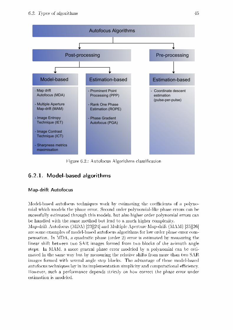
For the rst type of post-processing autofocus algorithms a wide range of possibilitieshas been researched during this project to study its suitability for the Mobile RCSHandheld. On the other hand all autofocusing techniques can be divided generallyinto 2 main blocks: Model-based, also called parametric algorithms and estimation-based, also called non-parametric algorithms. In Fig. 6.2 the classication of allthe possibilities studied and taken into account for this project is shown. A detailedexplanation of all alternatives in each block is presented in the following sections 6.2.1,6.2.2, 6.3 and 6.4.
6.2. Types of algorithms 45
AutofocusCAlgorithms
Post-processing Pre-processing
Model-based Estimation-based Estimation-based
-CMapCdriftCCAutofocusC(MDA)
-CMultipleCApertureCCCMap-driftC(MAM)
-CImageCEntropyCCTechniqueC(IET)
-CImageCContrastCCCTechniqueC(ICT)
-CSharpnessCmetricsCCCmaximisation
-CProminentCPointCCProcessingC(PPP)
-CRankCOneCPhaseCCCEstimationC(ROPE)
-CPhaseCGradientCCAutofocusC(PGA)
-CCCoordinateCdescentCCCestimationCCCC(pulse-per-pulse)
Figure 6.2.: Autofocus Algorithms classication
6.2.1. Model-based algorithms
Map-drift Autofocus
Model-based autofocus techniques work by estimating the coecients of a polyno-mial which models the phase error. Second order polynomial-like phase errors can besucessfully estimated through this models, but also higher order polynomial errors canbe handled with the same method but lead to a much higher complexity.Map-drift Autofocus (MDA) [23][24] and Multiple Aperture Map-drift (MAM) [25][26]are some examples of model-based autofocus algorithms for low order phase error com-pensation. In MDA, a quadratic phase (order 2) error is estimated by measuring thelinear shift between two SAR images formed from two blocks of the azimuth anglesteps. In MAM, a more general phase error modeled by a polynomial can be esti-mated in the same way but by measuring the relative shifts from more than two SARimages formed with several angle step blocks. The advantage of these model-basedautofocus techniques lay in its implementation simplicity and computational eciency.However, such a performance depends strictly on how correct the phase error underestimation is modeled.
46 6. Autofocusing Algorithms
Metrics maximisation
Other examples are the algorithms performing a maximisation or minimization ofsome metric. For all of them a polynomial model of the phase error function is pre-viously designed and its coecients are estimated through dierent techniques suchas:
Image Entropy Technique (IET) The entropy concept is used to measure the levelof focus of the image, and better focus is assumed to minimized entropy. Thecoecients of the polynomial which minimizes entropy of the image are selectedand the image is compensated with this phase error estimation [27] [28].
Image Contrast technique (ICT) Based on the same principle but the image con-strast is maximised depending of the coecients of the polynomial. [29].
Sharpness metrics The maximisation of the sharpness of the defocused image inten-sity through other dierent metrics than the presented before is used to optimizecoecients of the polynomial model [30].
It is important to mention that for more complex models the order of these polynomialscan be adaptative, and thus the variation of these models can lead to a more accuratephase error estimation than xed-order polynomial models [27]. The main disadvan-tage of all these techniques based on a model appears when high order or randomerrors are being treated. This is due to the unreachable model complexity through ex-tremely high order polynomial functions. Therefore for this kind of phase error sourcesother algorithms like estimation-based algorithms are needed.
6.2.2. Estimation-based algorithms
Non-parametric or estimation-based algorithms are the solution for the problem statedin section 6.2.1 since they do not require explicit knowledge of the ocurring phaseerrors. In this block, algorithms such as Rank One Phase Estimation (ROPE), Promi-nent Point Processing (PPP) and Phase Gradient Autofocus (PGA) are the mostrepresentative. These algorithms enumerated above estimate the phase error functionand apply the same compensation to all pixels within the entire image. Generally,the estimation of the error function is obtained by averaging the information in allrange bins, with the assumption that the phase error is repeated in all range dis-tances from the same track step. Therefore the redundancy of this error in the imageis the main tool of this kind of algorithms. These techniques are now briey intro-duced:
Prominent Point Processing (PPP) The strongest target within the whole imageis detected in the range compressed data IFFTfEs(f, θ) and its shifted phasehistory is extracted in order to remove the linear phase and obtain only thephase perturbations. This residual component φe(θ) is then compensated in allpixels to x the whole image with the same correction. However, it is obvious
6.2. Types of algorithms 47
that this method has the crucial shortcoming that it is only applicable when avery unique and strong point scatterer is present in the target [31].
Rank One Phase Estimation (ROPE) The algorithm makes the assumption of ascattered signal model in which each range bin contains only one dominant scat-
terer [32]. The gradient of the error function ˆφe(θ) is estimated from the dier-ence between two consecutive pulses θm and θm+1. An initial guess must be done
for the rst dierence. Afterwards, the estimation on ˆφe(θ) is repeated in severaliterations from the matrix containing all the dierences of the returned pulses.Finally the function is integrated to obtain the estimated phase error functionand this is applied to the signals of each range bin in the range-compressed do-main by a complex phase e−jφe(θ) [33]. Two important positive characteristicsof this algorithm are, rstly, its robustness since it works accurately for imagescenes that do not t this assumption of a unique stronger scatterer per eachrange bin. The second characteristic is the ability to estimate any kind of phaseerror order including random noise. However, an important shortcoming is thefact that the initial guess is blindly set up, leading to a possible inability toestimate the error properly [34].
Phase Gradient Autofocus (PGA) is based on the same principle of the ROPE al-gorithm but without making the initial assumption of a unique strong scattererfor each range bin. Here the strongest pixel within the SAR image for each rangebin is detected and windowed to discard information from closer scatterers thatcan degrade the estimation of the defocusing phase error function. As will beexplained in more detail later in section 6.3, this method can lead to a moreaccurate estimation a priori. However it has the drawback that in some cases itwill be dicult to face high order phase errors since the information along allthe bins has been windowed and thus a discarded. For this reason this algorithmwill be able to compensate only low or medium order phase errors if the windowsize is not wide enough to contain the information regarding to high order errors.
However it is important to mention that all these autofocusing algorithms require spe-cic constraints regarding the systems geometry and the preceding imaging algorithmto obtain the SAR image. The assumption of a linear track geometry may not besuitable for the main purpose of this project. Even though it is worth to go into de-tail for the case of the PGA algorithm because all the rest of autofocusing solutionsanalysed by simulations in section 7.2 are based in its principle: The redundancy ofthe in range dimension. Taking into account that for this project an unconstrainedsystem geometry shall be assumed to analyse targets, autofocusing algorithms whichcan be applied before imaging have been also deeply analysed. This is the case fora pulse-per-pulse autofocusing algorithm, which works by estimating the phase errordirectly to the raw scattered data in several iterations with a coordinate descent. Thisis explained in section 6.4.

48 6. Autofocusing Algorithms
6.3. Phase gradient Autofocus (PGA)
6.3.1. Constraints
As mentioned before in section 6.2, the Phase Gradient Autofocus algorithm is anestimation-based post processing algorithm. Nowadays the PGA algorithm seems tobe the state of the art for this kind of autofocusing algorithms for SAR imaging ap-plications such as remote sensing which usually work in the far-eld region and whichassume linear track geometries. For these cases, it presents a high robustness level [22].It shall be even though emphasized that it is not the case for the track geometry of theMobile RCS Handheld. Since no previous polynomial model is required, this algorithmis capable to compensate a wider range of error sources and nature than the solutionspresented before [22]. Moreover, the success of this algorithm does not strictly dependon how the scatterers are distributed within the target extent under analysis [35].Unlike previous methods mentioned before such as PPP Autofocus, no isolated strongscatterers contained into the image extent are needed since this algorithm can performsucessfully in a high-clutter background. This characteristic together with the widerrange of phase errors order compensable provides this algorithm with a high level ofrobustness, being able to face several real scenes [35]. However, this solution has threebasic constraints which must be seriously taken into account:
1. Image SAR previously obtained by a two dimensional compression.
2. Linear track geometry.
3. Far-eld region.
For the rst constraint this alternative works directly with the azimuth-uncompressedphase-history of the ISAR image expressed in (6.1) and obtained by applying a directFFT to the SAR image in the cross-range direction.
S(x, θ) = FFTyψ(x, y) (6.1)
,
In (6.1), ψ(x, y) , ISAR(x, y) represents the SAR image in cartesian coordinates.As it can be extracted from the basic imaging algorithm explained in section 3.2, theimage must have been obtained by a two dimensional compression through inversefourier transformations (IFFT) in both range and cross-range directions of the rawscattered eld data Es(f, θ) [36]. Otherwise it has been observed that when the inverseoperation is applied, that is, the direct FFT, the result obtained will not be the range-uncompressed scattered eld as has been shown in (6.2).
S(x, θ) 6= FFTyψ(x, y) (6.2)

6.3. Phase gradient Autofocus (PGA) 49
Secondly, the system's geometry is constrained. Only a linear ight track like in Fig.6.3 in the far-eld region and over small aperture angles will allow this algorithm towork properly. This limitation is done because in this algorithm each cross-range rowof the image is treated independently, and this method assumes the track has beeneither linear or circular with a small enough angle aperture which can be thereforeapproximated to a little linear track geometry in the far-eld [37]. These are essentialcharacteristics to take into account for the nal decision of the most suitable autofocusalgorithm for the Mobile RCS Handheld.
y
x
Target
Linear flight track
Figure 6.3.: Linear track
In the following section 6.3.2 the whole process performed by this algorithm is pre-sented even if it may not be the algorithm chosen eventually. The other estimation-based autofocus algorithm presented in this thesis is based on this principle. For thisreason a brief introduction of PGA fundamentals can help for the comprehension ofany estimation-based algorithm.
6.3.2. Fundamentals
A theoretical characteristic of the SAR images is that the phase error is redundantwithin the whole image extent. That means, this error will be present in all range binsindependently of the range distance for each along-track step.The Phase Gradient Autofocus technique is applied iteratively, taking advantage ofthis theoretical characteristic and exploiting the redundancy in order to estimate thegradient of the phase error produced in each specic measurement at each specicalong-track step θm. A Linear Unbiased Minimum Variance (LUMV) phase estimatoris therefore used. After one iteration a function describing the gradient of the phase er-
ror depending on the along-track samples ˆφe(θ) is obtained. This function is integrated
obtaining φe(θ) and nally applied to the range-compressed data by a multiplication.With this operation, the error phase is in a lower or higher order compensated in the
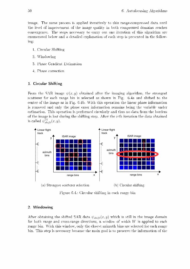
50 6. Autofocusing Algorithms
image. The same process is applied iteratively to this range-compressed data untilthe level of improvement of the image quality in both compressed domains reachesconvergence. The steps necessary to carry out one iteration of this algorithm areenumerated below and a detailed explanation of each step is presented in the follow-ing:
1. Circular Shifting
2. Windowing
3. Phase Gradient Estimation
4. Phase correction
1. Circular Shifting
From the SAR image ψ(x, y) obtained after the imaging algorithm, the strongestscatterer for each range bin is selected as shown in Fig. 6.4a and shifted to thecenter of the image as in Fig. 6.4b. With this operation the linear phase informationis removed and only the phase error information remains being the variable underestimation. This operation is performed circularly and thus no data from the bordersof the image is lost during the shifting step. After the i-th iteration the data obtainedis called ψ(i)
shift(x, y).
x
y
range bins
azimuth bins
ISAR image
Linear flight track
(a) Strongest scatterer selection
x
y
range bins
azimuth bins
ISAR image
Linear flight track
(b) Circular shifting
Figure 6.4.: Circular shifting in each range bin
2. Windowing
After obtaining the shifted SAR data ψshift(x, y) which is still in the image domainfor both range and cross-range directions, a window of width W is applied to eachrange bin. With this window, only the closest azimuth bins are selected for each rangebin. This step is necessary because the main goal is to preserve the information of the

6.3. Phase gradient Autofocus (PGA) 51
blur produced by the phase error sources which usually appears in the pixels closestto the strongest scatterers. The rest of the data does not contribute to the phase errorestimation but introduces a degradation in the SNR only [36].The diculty lies in choosing a proper window size W . This window is supposed todiscard as much useless data as possible but should also preserve the useful data ofthe blur which will be used for the estimation process. This is the point where themost important design decision of the algorithm is made. It has been observed inthe literature that this step allows a high level of customization [36]. The selectionof this window could be actually done manually by human intervention by observingand calculating the blur width W . In this way, each image case could be treated inde-pendently. However, this method is obviously tedious and inecient so an automaticwindow calculation is applied.There are of course many automatic methods that can work properly, but it is impor-tant to distinguish between the characteristics of the scene. If the target analysed isformed by some strong scatterers a cost function can be used.As it has been mentioned before the blur function is supposed to be identical in eachrange bin and therefore using this redundancy characteristic some cost function s(y)can be applied, which somehow calculates an average through an incoherent sum. Thefunction obtained will depend on the uncompressed azimuth x and will have its max-imum in s(y = 0) due to the shifting step performed [36]. Afterwards, the windowwidth W can be calculated by thresholding the function at some level which can befor example set to 25dB below the maximum peak s(0) [36]. Since the error is par-tially corrected in each iteration, it will be observed that the window width W getssmaller in each iteration until reaching convergence, where this width will practicallynot decrease anymore. In Fig. 6.5 there is an example of the s(x) function and thethresholding step.
Azimuth step (sample)
s(x)
W
Figure 6.5.: Windowing step
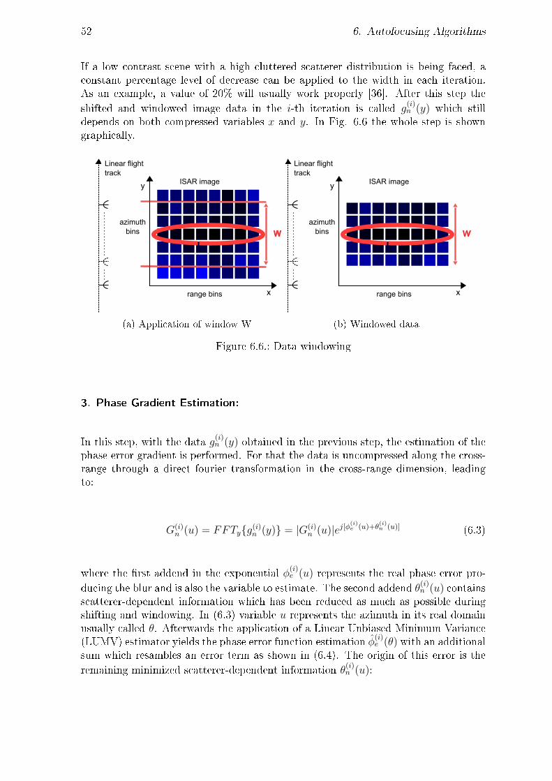
52 6. Autofocusing Algorithms
If a low contrast scene with a high cluttered scatterer distribution is being faced, aconstant percentage level of decrease can be applied to the width in each iteration.As an example, a value of 20% will usually work properly [36]. After this step theshifted and windowed image data in the i-th iteration is called g
(i)n (y) which still
depends on both compressed variables x and y. In Fig. 6.6 the whole step is showngraphically.
x
y
range bins
azimuth bins
ISAR image
Linear flight track
W
(a) Application of window W
x
y
range bins
azimuth bins
ISAR image
Linear flight track
W
(b) Windowed data
Figure 6.6.: Data windowing
3. Phase Gradient Estimation:
In this step, with the data g(i)n (y) obtained in the previous step, the estimation of the
phase error gradient is performed. For that the data is uncompressed along the cross-range through a direct fourier transformation in the cross-range dimension, leadingto:
G(i)n (u) = FFTyg(i)
n (y) = |G(i)n (u)|ej[φ
(i)e (u)+θ
(i)n (u)] (6.3)
where the rst addend in the exponential φ(i)e (u) represents the real phase error pro-
ducing the blur and is also the variable to estimate. The second addend θ(i)n (u) contains
scatterer-dependent information which has been reduced as much as possible duringshifting and windowing. In (6.3) variable u represents the azimuth in its real domainusually called θ. Afterwards the application of a Linear Unbiased Minimum Variance(LUMV) estimator yields the phase error function estimation φ(i)
e (θ) with an additionalsum which resambles an error term as shown in (6.4). The origin of this error is theremaining minimized scatterer-dependent information θ(i)
n (u):
6.3. Phase gradient Autofocus (PGA) 53
ˆφLUMV (θ) =
∑n ImG∗n(θ)Gn(θ)∑
n |Gn(θ)|2
= φe(θ) +
∑n |Gn(θ)|2θn(θ)∑
n |Gn(θ)|2
(6.4)
where the subindexes for the i-th iteration(i) have been removed to reduce notationcomplexity reasons.
4. Phase Correction:
In the last step, the estimated function ˆφ(i)LUMV (θ) is applied to the crossrange-uncompressed
image data of the ith-iteration, G(i)(x, θ) = FFTyψ(i)(x, y), in order to partlycompensate the phase error. The operation is performed by a complex multiplica-tion:
G(i)comp(x, θ) = G(i)(x, θ) · e−j
ˆφ(i)LUMV (θ) (6.5)
After this correction in azimuth fourier domain the data is azimut-compressed by aninverse FFT again. With this a better quality image ψ(i)
comp(x, y) is obtained, wherethe phase error has been partly compensated:
ψ(i)comp(x, y) = IFFTθG(i)
comp(x, θ) (6.6)
These 4 steps are repeated iteratively until the improvement in the image quality isnegligible. This point is reached when the reduction of the window width W reachesconvergence, as seen in the second step.
In Fig. 6.7 the owchart of this algorithm is presented.

54 6. Autofocusing Algorithms
Ψ(i)(x,y)
Ψshift(i)(x,y)
Windowing
gn(i)(y)
CircularShifting
FFTy
Gn(i)(θ)
GradientvPhasevEstimation
Φlumv(i)(θ)
Gcomp(i)(x,θ)
FFTy
G(i)(x,θ)
.
Integration
Φlumv(i)(θ)ˆ
Convergence?
Yes
No
END
i=i+1
Figure 6.7.: PGA Algorithm Flowchart
6.4. Pre-processing autofocus with coordinate descent optimization 55
6.4. Pre-processing autofocus with coordinate
descent optimization
6.4.1. Constraints
In the previous section the methodology of an estimation-based autofocus algorithmwith a post-processing basis was explained. However, despite the high level of ac-curacy of this algorithm, it has been mentioned its main shortcoming, its limitationto linear tracks. For the Mobile RCS Handheld it has been noticed that this is anunacceptable constraint. For such a device a geometrically unconstrained auto-focus solution that can work with any exotic geometry such as circular or arbitrarypaths is required. As explained in section 5.2, time-domain algorithms such as Back-Projection or its improvement FFBP work on a pulse-per-pulse basis. This meansthat only the range-compression is performed through inverse fourier transformation.Due to this independence between each collected pulse data any kind of along-trackgeometry conguration will work properly. Therefore an autofocus algorithm with thesame principle will also allow an unconstrained geometry. An a priori pulse-per-pulseautofocus approach will the most robust solution for this purpose. In this case wide-angle apertures within near-eld region and arbitrary ight paths will not representan insurmountable problem anymore as for all the time-domain imaging algorithms[37].
6.4.2. Fundamentals
As mentioned above this algorithm does not work by analysing the SAR image butapplying it in pre-processing. The autofocusing is therefore applied to the raw scat-tered degraded data on a pulse-per-pulse basis previous to image formation. It isimporant to emphasize that this algorithm can for this reason be integrated with anyimaging algorithm either in frequency domain or time domain. The autofocusing isapplied to the raw data Es(f, θ) and the corrected data Es(f, θ) is obtained. Then,any frequency-domain or time-domain imaging algorithm can be applied in order toobtain a compensated SAR image from the compensated raw scattered data. A greatadvantadge of this method is that the degraded raw data Es(f, θ) is range-compressedonly once and stored. This data is afterwards the input given to the autofocus algo-rithm. A coordinate descent estimation method uses this information to perform afast estimation. However, this autofocusing algorithm will work in the same way. Themain principle is to estimate the phase error function that maximizes some metriclike:
s(φ) =∑i
Ψ(vi(φ)) (6.7)
where a sum over a nonlinear point transformation of the pixel values of the image isperformed in order to maximize image sharpness. In (6.7) subindex i means i-th pixel

56 6. Autofocusing Algorithms
of the image. Only one index has been used to represent the pixels in both dimensions.vi(φ) is the image intensity of each pixel and Ψ(x) is a non-linear cost function. As hasbeen analysed in [38] several cost functions such as entropy minimisation or contrastmaximisation can be used. For the former a logarithmic sum is carried out with thecost function:
Ψentr(x) = −vi(x) · log vi(x) (6.8)
For the latter the norm of all pixel intensities is added up with a cost function lookinglike:
Ψcontr(x) = −vi(x)2 (6.9)
In the following, it is described how obtaining the estimated phase error functionworks in the ith iteration. This process is repeated until reaching convergence. Fornotation reasons the index of pixels of the image corresponding to coordinates [xi, yi]are denoted only in one direction with sub-index i:
qi = [xi, yi] (6.10)
Now, using the back-projection integral explained in section 5.2.1 the complex valueof the pixel i in the nal image after complete back-projection can be rewrittenlike:
zi =
∫ θmax
θmin
∫ wmax
wmin
pθ(w)ejwd(qi)|w|dwdθ (6.11)
where all range-proles from all aspect angles are obtained from the scattered raw datapθ(w) through an integration in both frequancy w and aspect angle θ directions. Factord(qi) denotes the distance from the ith pixel of the image to the antenna position,which in the near-eld region corresponds to the expression analysed in section 5.As it was explained previously this integral can be regarded as a discrete sum of therange-compressed function Qk(r) along all azimuth directions:
zi =K∑k=1
Qk(d(qi)) (6.12)
where
Qk(r) = F−1pθk(w)|w| (6.13)
(6.13) can be expressed in a more compact way like:

6.4. Pre-processing autofocus with coordinate descent optimization 57
bk = Qk(d(qi)) (6.14)
Now, proceeding with the sum stated in (6.12) the complete back-projected image canbe expressed in absence of phase errors like:
z =∑k
bk , SAR (x, y) (6.15)
The theory explained until this point is jsut a generalisation of the back-projectionprodecure. However, if at this step this back-projection integral is applied withoutconsidering the possible phase error sources, the image obtained in the nal stepcan present really bad quality levels with signicant blurring eects [17]. Thus, anautofocusing step prior to back-projection which works properly on the pulse-per-pulse basis is almost mandatory. It can be seen that when raw scattered data becomescorrupted the changes are transmitted in the fourier transformed domain as it is shownin
bk −→ bk = bk · ejφk (6.16)
With this eect it is clear that the summation in (6.15) will lead to a low-contrastunfocused image. This phenomenon is due to the fact that the peak values decreaseand the mainlobe and sidelobe widths increase [39]. Therefore the autofocus algorithmhas the goal of estimating the phase function φ = φ1...φK for which the blurrinesslevel of z in (6.17) is minimized over a given metric [37]:
z =∑k
bke−jφk (6.17)
As seen before, there exist a wide sort of proper metrics. In this section this algorithmis analysed for the case of contrast maximisation, in which a sum of all pixel inten-
sities s(φ) =∑
i vi(φ)2with vi = ziz
∗i is maximised. Thus the variable to estimate
is:
φ = arg maxφ
s(φ) (6.18)
As stated at the beginning the maximisation of (6.18) can be performed in severalways, eg. with a maximum likelihood estimator (ML) as in [40], a gradient descentoptimization as in [41], or a coordinate descent optimization as in [37]. The rstalternative would be optimal because it takes into account all combinations betweenall possible values from all coordinate samples to perform estimation. However, forthe amount of data collected from the Mobile RCS Handheld the number of angu-lar samples to estimate in the vector φ will be too high leading to an unacceptablecomputation load. For this reason this estimator has been discarded. Therefore the
58 6. Autofocusing Algorithms
coordinate descent optimization method will be introduced theorically and then itsintegration into the autofocusing process explained.This approach is based on the independent estimation of each coordinate of a vector,while holding the rest of coordinates xed. To estimate the k-th coordinate in the i-thiteration φik, two dierent blocks of variables are used:
1. The lower phase coordinates estimated in the same ith iteration (blue samplesin Fig. 6.8)
2. The higher coordinates estimated in the previous (i−1)th iteration (red samplesin Fig. 6.8)
When the coordinate φik is nally estimated it is the turn of the next coordinate φik+1
of the vector of variables φi. After reaching the last coordinate the whole estimationprocess will be iteratively repeated until reaching convergence. Thus for the coordinatedescent optimization the general maximisation performed in (6.18) in the i-th iterationand for a k-th coordinate can be expressed as following:
φik = arg maxφ
(φi1, ..., φik−1, φ, ..., φ
i−1k+1, ..., φ
i−1K ) (6.19)
In Fig. 6.8 this principle is illustrated for a unique iteration. In the following thisoptimization method is applied to the pulse-per-pulse autofocus algorithm. Firstly,the sum of each contribution of each pulse for the formation of the image in (6.17) isdivided into three addends:
z(φ) =k−1∑p=1
e−jφi+1p bp +
K∑p=k+1
e−jφipbp + e−jφkbk (6.20)
where the rst addend represents the data from the pulses already estimated in theprevious (i−1)-th iteration, the second addend represents the the data from the pulsesnot yet estimated in the actual ith iteration and the third represents the data fromthe kth phase coordinate φk under estimation. Next, equation (6.20) is expressed in amore compact way:
z(φ) =k−1∑p=1
e−jφi+1p bp +
K∑p=k+1
e−jφipbp + e−jφkbk
= m + e−jφkn
(6.21)
Thus the expression of the i-th pixel intensity will be written like:

6.4. Pre-processing autofocus with coordinate descent optimization 59
vi = ziz∗i = (mi + e−jφkni)(m
∗i + ejφkn∗i )
= |mi|2 + |ni|2 + 2<(n∗imiejφk)
= (vconst)i + (vφk)i
(6.22)
where the rst addend (vconst)i has no dependence on the kth phase coordinate estima-tion φk and the second addend (vφk)i depends on its value. Finally the sharpness metricstated in 6.9 is maximised for a specic value of φk as shown in:
s(φ) =∑i
v2i (φ) = ||v||2 (6.23)

60 6. Autofocusing Algorithms
0
2π
ϕi1 ϕi2 ϕi3 ϕi4 ϕi5 ϕiK^ ^ ^ ^ ^ ^
. . . . . . .
. . . . . . .
0
2π
ϕi+11
ϕi+12
ϕi3 ϕi4 ϕi5 ϕiK^
^
^ ^ ^ ^
. . . . . . .
. . . . . . .
0
2π
ϕi+11 ϕi3 ϕi4 ϕi5 ϕiK^ ^ ^ ^ ^
. . . . . . .
. . . . . . .
ϕi2^
ϕi+12
^
0
2π
ϕi+11 ϕi+13 ϕi+1
4 ϕi+1
5 ϕi+1K
^ ^ ^ ^ ^
. . . . . . .
. . . . . . .
Initial data
1st coordinate estimation
2nd coordinate estimation
last coordinate estimation
Figure 6.8.: Coordinate descent optimization

61
7. Implementation and Simulations
In this chapter a detailed analysis of the simulation results of all the implementedalgorithms is presented for both imaging an autofocusing purposes. The results areaccurately analysed in order to give a clue which could be the most suitable algo-rithms to use in the portable device and which advantages and drawbacks they of-fer.
The section is divided basically in two big sections, corresponding to both kinds ofalgorithms analysed:
• Simulations and comparison of imaging algorithms In section 7.1 thesimulation results of the solutions studied to obtain the SAR image of a targetare shown considering an ideal context in which no error sources have beenintroduced. In this case the position which would be provided from the RCSHandheld position estimator has been considered to be exact.
• Simulations and comparison of autofocusing algorithms In section 7.2several error sources explained previously in section 4 are introduced to thecalculation of the scattered eld. In this section two simulation results havebeen analysed:
Level of degradation of the image caused by phase errors
Autofocusing performance for the case of pre-processing with an autofocusalgorithm in order to improve image quality and recude the level of blur.
The raw scattered data used as input data by all the algorithms to produce SAR imageshas been generated in MATLAB by a discretization of frequency f and angle θ. In thisway a Stepped Frequency Continous Wave (SFCW) radar already explained in 2.3.2 isvirutually simulated. Considering the near-eld equation of the scattered eld Es(f, θ)shown in (5.1) and the distance d in (5.2) has been exactly calculated as the raw datais generated in MATLAB as presented in the apendix A.
7.1. Simulations of Imaging Algorithms
In this section, the simulations regarding the imaging algorithms are presented withthe following structure:First of all the common conguration of the whole system used for the simulations, aswell the modeled target characteristics, is in section 7.1.1 depicted.Secondly, in section 7.1.2 the metrics and evaluation methods used in general for the

62 7. Implementation and Simulations
comparison and analysis of the results provided by each of the imaging algorithms arepresented. It is important to mention that there is a wide sort of possible metrics touse. However, the decision which metric suits this project best has been inuenced byobserving the results.Thirdly, the simulations of the near-nield Fast Cyclical Convolution (FCC) algorithmin the frequency domain are analysed independently in order to show its theoreticallimitations and its geometrical requirements explained previously. It is demonstratedhow aliasing or virtual eects can ocurr in this context. A detailed analysis can befound in section 7.1.3.Fourthly, the near-nield Back-Projection (BP) algorithm in the time-domain is sim-ulated and the improvements of the results obtained by using techniques explainedin previous sections are shown in section 7.1.4. This is the case for zero-padding andwindowing. Also simulations with dierent track geometries have been carried out.Fifthly, a comparison between BP and FCC is performed in section 7.1.5.Finally the factorisation technique used in the Fast Factorized Back-Projection Algo-rithm (FFBP) is analysed and compared to the classical Back-Projection algorithmin section 7.1.6. As has been explained the factorisation performed in FFBP can becustomized. A compromise between factorisation and error introduced in the image isalso performed in this section.The FFBP algorithm is designed to work only with linear tracks. Nevertheless it isimportant to consider that actually any sort of track could be modeled by a combi-nation of smaller linear tracks [42]. This approximation would obviously introduce anerror to the calculation but it is worth to consider this possibility to make the FFBPalgorithm not only useful since it reduces computational complexity, but also providesthis solution with a higher robustness level.
7.1.1. System and target conguration
For all simulations of the imaging algorithms in this section the dimensions of thetarget analysed as well as the system conguration and the track path of the RCS-Handheld have been xed to the following values shown in Table 7.1. The values with(*) have been changed for some specic simulations. The selection of these valueshave been choosen in order to suit all constraints for all algorithms. Basically theFCC algorithm with its angular sampling limitation has inuenced this decision. Thegeneral system and target dimensions and distances used for the simulations are aswell graphically shown in Fig. 7.1.
7.1.2. Metrics of image quality
In order to measure the quality of the image obtained with any algorithm it is essentialto use some metric to compare the results between algorithms. To analyse each algo-rithm the Point Spread Function (PSF)is used. This impulse response of the imagingalgorithm to an ideal omnidirectional scatterer located in the middle of the target areais the main result used in all the imaging algorithm comparisons. In order to analyse

7.1. Simulations of Imaging Algorithms 63
y
x
Target
Circular flight track
R=1m
ρmax=0.2mideal scatterer
Figure 7.1.: General System and target dimensions (Circular track case)
Target dimensionsMaximum target radius ρi,max = 0.2m
System CongurationCenter Frequency fc = 23GHzBandwidth f = [4.25, 41.375]Center wavelength λc = 13mmFrequency samples Nf = 100Aperture Samples Nθ = 700Pixel number Npix = 600× 600Interpolation method Cubic spline Interpolator
Geometry Track(*)Track path(*) CircularAngular Bandwith(*) 360o
Distance to target center(*) R = 1m
Table 7.1.: General System and Target conguration for Imaging Algorithms simula-tions
each of the four studies carried out in this section the PSF has been analysed in eachstudy. In Fig. 7.2a this geometry can be seen. Two slices of the PSF are studied.Moreover the SAR image of a specic distribution of ideal scatterers shown in Fig.7.2b is used by covering the whole target area in order to be able to understand moreglobally the image quality achieved in each study. Thus, for each study the followinginformation has been extracted for the comparison of the results:
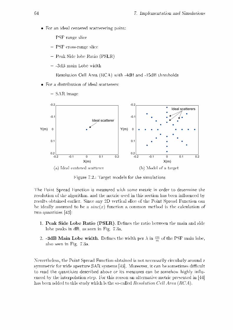
64 7. Implementation and Simulations
• For an ideal centered scatterering point:
PSF range slice
PSF cross-range slice
Peak Side lobe Ratio (PSLR)
-3dB main Lobe width
Resolution Cell Area (RCA) with -4dB and -15dB thresholds
• For a distribution of ideal scatterers:
SAR image
X(m)
Y(m)
-0.2 -0.1 0 0.1 0.2
-0.2
-0.1
0
0.1
0.2
Ideal scatterer
(a) Ideal centered scatterer
X(m)
Y(m)
-0.2 -0.1 0 0.1 0.2
-0.2
-0.1
0
0.1
0.2
Ideal scatterers
(b) Model of a target
Figure 7.2.: Target models for the simulations
The Point Spread Function is measured with some metric in order to determine theresolution of the algorithm, and the metric used in this section has been inuenced byresults obtained earlier. Since any 2D vertical slice of the Point Spread Function canbe ideally assumed to be a sinc(x) function a common method is the calculation oftwo quantities [43]:
1. Peak Side Lobe Ratio (PSLR). Denes the ratio between the main and sidelobe peaks in dB, as seen in Fig. 7.3a.
2. -3dB Main Lobe width. Denes the width per λ in cmm
of the PSF main lobe,also seen in Fig. 7.3a.
Nevertheless, the Point Spread Function obtained is not necessarily circularly around zsymmetric for wide aperture SAR systems [43]. Moreover, it can be sometimes dicultto read the quantities described above or its measures can be somehow highly inu-enced by the interpolation step. For this reason an alternative metric presented in [44]has been added to this study which is the so-calledResolution Cell Area (RCA).

7.1. Simulations of Imaging Algorithms 65
3. Resolution Cell Area (RCA). Denes the total area of the image exceedingan specic threshold value in dB, as shown in Fig. 7.3b.
This metric counts the number of pixels of the whole normalized PSF image exceedinga specic threshold in dB and then multiplicates this value with the pixel equiva-lent area. The main advantage of this metric is that it is completely independentfrom angle. Thus the quantity is globally valid which better suits the images ob-tained in this thesis. Two thresholds have been used for the simulations to denethe Resolution Cell Area, −4dB and −15dB, because with the former usually mainlobe information can be measured and with the latter rst side lobe levels can beincluded. As it can be seen these thresholds are set slightly below the common valuesfor sinc functions of −3dB and −13dB in order to obtain more information in eachcomparison.
−0.02 −0.01 0 0.01 0.02−60
−50
−40
−30
−20
−10
0
Range(m)
Res
pons
euF
unct
ion(
dB)
PSLR -3dBuwidth
(a) PSLR and -3dB width
Range(m)
Cro
ss−
Ran
ge(m
)
−6 −4 −2 0 2 4
x 10−3
−6
−4
−2
0
2
4
6
x 10−3
dB
−25
−20
−15
−10
−5
0
-4 dB
-15 dB
(b) Resolution Cell Area
Figure 7.3.: Resolution metrics used
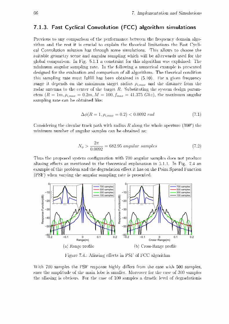
66 7. Implementation and Simulations
7.1.3. Fast Cyclical Convolution (FCC) algorithm simulations
Previous to any comparison of the performance between the frequency domain algo-rithm and the rest it is crucial to explain the theorical limitations the Fast Cycli-cal Convolution solution has through some simulations. This allows to choose thesuitable geometry scene and angular sampling which will be afterwards used for theglobal comparison. In Fig. 5.1.1 a constraint for this algorithm was explained: Theminimum angular sampling rate. In the following a numerical example is presenteddesigned for the evaluation and comparison of all algorithms. The theorical conditionthis sampling rate must fulll has been obtained in (5.10). For a given frequencyrange it depends on the maximum target radius ρi,max and the distance from theradar antenna to the center of the target R. Substituting the system design param-eters (R = 1m, ρi,max = 0.2m,M = 100, fmax = 41.375 Ghz), the maximum angularsampling rate can be obtained like:
∆φ(R = 1, ρi,max = 0.2) < 0.0092 rad (7.1)
Considering the circular track path with radius R along the whole aperture (360o) theminimum number of angular samples can be obtained as:
Nφ >2π
0.0092= 682.95 angular samples (7.2)
Thus the proposed system conguration with 700 angular samples does not producealiasing eects as mentioned in the theoretical explanation in 5.1.1. In Fig. 7.4 anexample of this problem and the degradation eect it has on the Point Spread Function(PSF) when varying the angular sampling rate is presented.
−0.2 −0.1 0 0.1 0.2−60
−50
−40
−30
−20
−10
0
Range(m)
Res
pons
e F
unct
ion(
dB)
700 samples500 samples300 samples100 samples
−0.015 −0.01 −0.005 0 0.005 0.01 0.015−40
−35
−30
−25
−20
−15
−10
−5
0
Range(m)
Res
pons
eF
unct
ion(
dB)
(a) Range prole
−0.2 −0.1 0 0.1 0.2−60
−50
−40
−30
−20
−10
0
Cross−Range(m)
Res
pons
e F
unct
ion(
dB)
700 samples500 samples300 samples100 samples
−0.015 −0.01 −0.005 0 0.005 0.01 0.015−40
−35
−30
−25
−20
−15
−10
−5
0
Range(m)
Res
pons
eF
unct
ion(
dB)
(b) Cross-Range prole
Figure 7.4.: Aliasing eects in PSF of FCC algorithm
With 700 samples the PSF response highly diers from the case with 500 samples,snce the amplitude of the main lobe is smaller. Moreover for the case of 300 samplesthe aliasing is obvious. For the case of 100 samples a drastic level of degradationis

7.1. Simulations of Imaging Algorithms 67
reached. The results in Fig. 7.4 have been obtained under a dynamic range of 60dB toshow a more global result. 13x zoom has been also applied to highlight these eects.Apart from the eects onto the PSF function, it will be investigated how the violationof this requirement in the present imaging algorithm can aect a SAR image. FollowingFig. 7.5 an example obtained after applying the FCC algorithm to a distribution ofideal scatterers within the target extent is shown.
Range(m)
Cro
ss−
Ra
ng
e(m
)
−0.2 −0.1 0 0.1
−0.2
−0.15
−0.1
−0.05
0
0.05
0.1
0.15
(a) 700 angular samples
Range(m)C
ross−
Ra
ng
e(m
)
−0.2 −0.1 0 0.1
−0.2
−0.15
−0.1
−0.05
0
0.05
0.1
0.15
(b) 500 angular samples
Range(m)
Cro
ss−
Ra
ng
e(m
)
−0.2 −0.1 0 0.1
−0.2
−0.15
−0.1
−0.05
0
0.05
0.1
0.15
(c) 300 angular samples
Range(m)
Cro
ss−
Ra
ng
e(m
)
−0.2 −0.1 0 0.1
−0.2
−0.15
−0.1
−0.05
0
0.05
0.1
0.15
(d) 100 angular samples
Figure 7.5.: Aliasing eects in SAR images varying angular sampling in FCC algorithm
For the case of 500 and 300 angular samples the overlapping of secondary lobes pro-duces slightly higher intensity levels in points of the image where no scatterer is lo-cated. For the case of 100 samples the degradation is more than obvious. Wherehigh secondary lobes appear, due to aliasing eects defocus the image gets defocused.Therefore for the following studies and comparisons of this frequency domain algorithmwith other solutions the sampling rate has been set to 700 samples which ensures agood SAR image quality.
7.1.4. Back-Projection (BP) algorithm simulations
In the same way the previous frequency domain algorithm has been independentlyanalysed the same analysis approach will be carried out for the second algorithm. Asexplained previously in section 5.2.1 the tomographic back-projection oers a highlevel of customization and it can be applied to many congurations. For this reason,
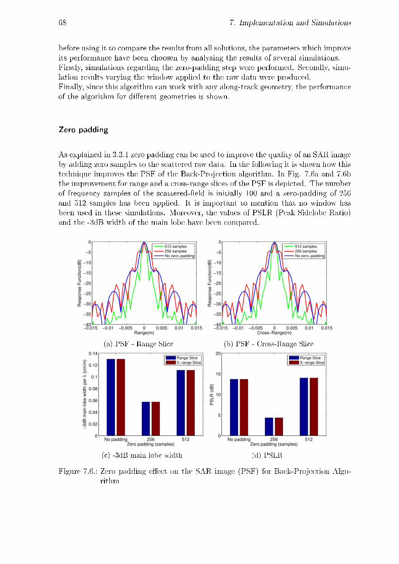
68 7. Implementation and Simulations
before using it to compare the results from all solutions, the parameters which improveits performance have been choosen by analysing the results of several simulations.Firstly, simulations regarding the zero-padding step were performed. Secondly, simu-lation results varying the window applied to the raw data were produced.Finally, since this algorithm can work with any along-track geometry, the performanceof the algorithm for dierent geometries is shown.
Zero padding
As explained in 3.3.1 zero padding can be used to improve the quality of an SAR imageby adding zero samples to the scattered raw data. In the following it is shown how thistechnique improves the PSF of the Back-Projection algorithm. In Fig. 7.6a and 7.6bthe improvement for range and a cross-range slices of the PSF is depicted. The numberof frequency samples of the scattered-eld is initially 100 and a zero-padding of 256and 512 samples has been applied. It is important to mention that no window hasbeen used in these simulations. Moreover, the values of PSLR (Peak Sidelobe Ratio)and the -3dB width of the main lobe have been compared.
−0.015 −0.01 −0.005 0 0.005 0.01 0.015−40
−35
−30
−25
−20
−15
−10
−5
0
Range(m)
Re
sp
on
se
Fu
nctio
n(d
B)
512 samples
256 samples
No zero−padding
(a) PSF - Range Slice
−0.015 −0.01 −0.005 0 0.005 0.01 0.015−40
−35
−30
−25
−20
−15
−10
−5
0
Cross−Range(m)
Re
sp
on
se
Fu
nctio
n(d
B)
512 samples
256 samples
No zero−padding
(b) PSF - Cross-Range Slice
No padding 256 5120
0.02
0.04
0.06
0.08
0.1
0.12
0.14
Zero padding (samples)
−3
dB
ma
in lo
be
wid
th p
er
λ (
cm
/m)
Range Slice
X−range Slice
(c) -3dB main lobe width
No padding 256 5120
5
10
15
20
Zero padding (samples)
PS
LR
(d
B)
Range Slice
X−range Slice
(d) PSLR
Figure 7.6.: Zero padding eect on the SAR image (PSF) for Back-Projection Algo-rithm

7.1. Simulations of Imaging Algorithms 69
As it can be seen in Fig. 7.6c the -3dB width of the main lobe by applying a zeropadding of 256 samples does not match the results expected since the main lobe widthexpands. This phenomenon happens because not enough pixels were used for theinterpolation process. The same phenomenon can be observed for the PSLR in Fig.7.6d. However, the improvement in the -15 dB main lobe width for the case of a zeropadding of 512 samples is obvious and will still to a more focused SAR image. A zeropadding with more samples could have been studied but it has been discarded becauseof high time computational burden.The eect has been as well shown in the SAR image results in Fig. 7.7, where it can beseen that a zero padding of 512 samples almost perfectly removes levels of higher inten-sity produced in zones of the image where no scatterer is present.
Range(m)
Cro
ss−
Ra
ng
e(m
)
−0.2 −0.1 0 0.1
−0.2
−0.15
−0.1
−0.05
0
0.05
0.1
0.15
(a) No zero padding
Range(m)
Cro
ss−
Ra
ng
e(m
)
−0.2 −0.1 0 0.1
−0.2
−0.15
−0.1
−0.05
0
0.05
0.1
0.15
(b) Zero padding with 256 samples
Range(m)
Cro
ss−
Ra
ng
e(m
)
−0.2 −0.1 0 0.1
−0.2
−0.15
−0.1
−0.05
0
0.05
0.1
0.15
(c) Zero padding with 512 samples
Figure 7.7.: Zero padding eect for Back-Projection Algorithm
Therefore, 512 zero-padding samples were choosen in the following analysis.
Windowing
Apart from applying zero padding to the data the application of a window can improvethe result of the PSF due to the shape characteristics of the functions. It will beshown how this technique together with a zero padding of 512 samples improves thePSF obtained with Back-Projection. Fig. 7.8a and 7.8b depict the eects of thewindowing for a range and a cross-range slice of the PSF. The windows analysed
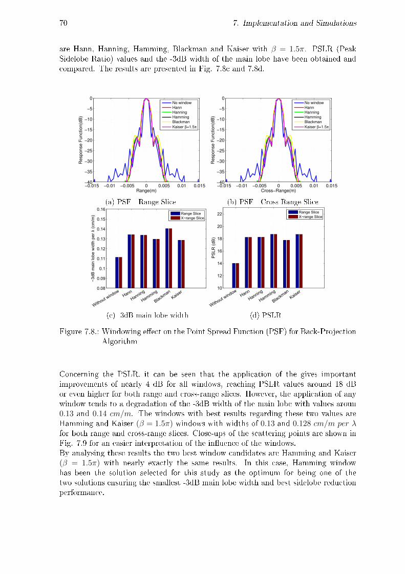
70 7. Implementation and Simulations
are Hann, Hanning, Hamming, Blackman and Kaiser with β = 1.5π. PSLR (PeakSidelobe Ratio) values and the -3dB width of the main lobe have been obtained andcompared. The results are presented in Fig. 7.8c and 7.8d.
−0.015 −0.01 −0.005 0 0.005 0.01 0.015−40
−35
−30
−25
−20
−15
−10
−5
0
Range(m)
Re
sp
on
se
Fu
nctio
n(d
B)
No window
Hann
Hanning
Hamming
Blackman
Kaiser β=1.5π
(a) PSF - Range Slice
−0.015 −0.01 −0.005 0 0.005 0.01 0.015−40
−35
−30
−25
−20
−15
−10
−5
0
Cross−Range(m)
Re
sp
on
se
Fu
nctio
n(d
B)
No window
Hann
Hanning
Hamming
Blackman
Kaiser β=1.5π
(b) PSF - Cross-Range Slice
0.08
0.09
0.1
0.11
0.12
0.13
0.14
0.15
0.16
−3d
B6m
ain6
lobe
6wid
th6p
erλ
Xcm
/m) Range6Slice
X−range6Slice
Without6window
Hann
Hanning
Hamming
Blackman
Kaiser
(c) -3dB main lobe width
10
12
14
16
18
20
22P
SLR
R(dB
)RangeRSliceX−rangeRSlice
WithoutRwindow
Hann
Hanning
Hamming
Blackman
Kaiser
(d) PSLR
Figure 7.8.: Windowing eect on the Point Spread Function (PSF) for Back-ProjectionAlgorithm
Concerning the PSLR, it can be seen that the application of the gives importantimprovements of nearly 4 dB for all windows, reaching PSLR values around 18 dBor even higher for both range and cross-range slices. However, the application of anywindow tends to a degradation of the -3dB width of the main lobe with values aroun0.13 and 0.14 cm/m. The windows with best results regarding these two values areHamming and Kaiser (β = 1.5π) windows with widths of 0.13 and 0.128 cm/m per λfor both range and cross-range slices. Close-ups of the scattering points are shown inFig. 7.9 for an easier interpretation of the inuence of the windows.By analysing these results the two best window candidates are Hamming and Kaiser(β = 1.5π) with nearly exactly the same results. In this case, Hamming windowhas been the solution selected for this study as the optimum for being one of thetwo solutions ensuring the smallest -3dB main lobe width and best sidelobe reductionperformance.

7.1. Simulations of Imaging Algorithms 71
Range(m)
Cro
ss−
Ran
ge(m
)
−6 −4 −2 0 2 4 6
x 10−3
−0.062
−0.06
−0.058
−0.056
−0.054
−0.052
(a) No window applied
Range(m)
Cro
ss−
Ran
ge(m
)
−6 −4 −2 0 2 4 6
x 10−3
−0.062
−0.06
−0.058
−0.056
−0.054
−0.052
(b) With Hamming window
Range(m)
Cro
ss−
Ran
ge(m
)
−6 −4 −2 0 2 4 6
x 10−3
−0.062
−0.06
−0.058
−0.056
−0.054
−0.052
(c) With Kaiser window
Figure 7.9.: Zoomed result of windowing eect on the SAR image for Back-ProjectionAlgorithm
Track geometry
As explained previously in the theory of section 5.2.1 the Back-Projection solution ishighly customizable and since the IFFT compression is performed pulse per pulse, thealgorithm can work with any along-track geometry.In order to demonstrate the performance of this algorithm under several tack geome-tries, 3 basic congurations have been designed. These should represent a wide rangeof possible track congurations.The rst one is the classical circular geometry which is used in almost all the rest ofthe simulations (see Fig. 7.10a).Secondly a linear track conguration was integrated which was already used in someother simulation (see Fig. 7.10b).Finally an exotic geometry has been designed similar to the circular case and cov-ering the whole possible anglular range [0o, 360o] but in which the radar approachesand moves away from the target repetitively within a range of [0.5m < R < 1m].A graphical explanation is given in Fig. 7.10c. The PSF function has been anal-ysed by its range and cross range slices in Fig. 7.11a and 7.11b, and the PSLR and-3dB main lobe width values have been obtained and discussed in Fig. 7.11c and
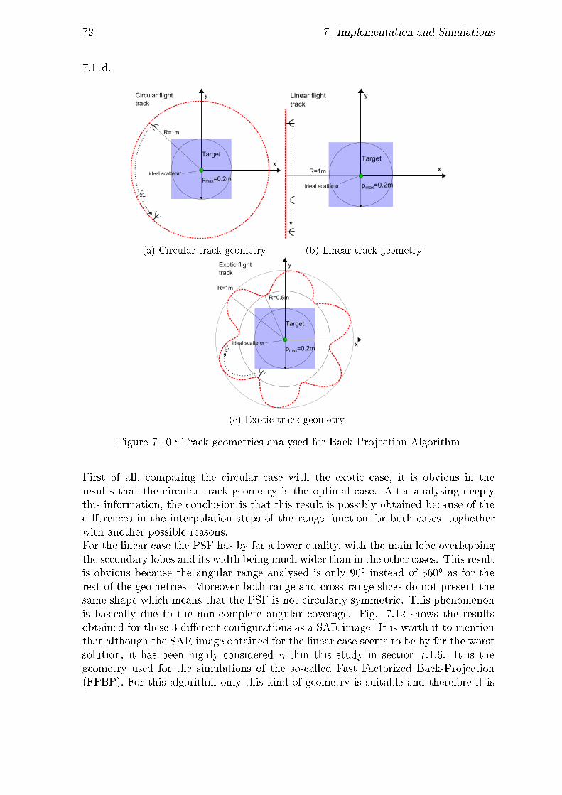
72 7. Implementation and Simulations
7.11d.
y
x
Target
Circular flight track
R=1m
ρmax=0.2mideal scatterer
(a) Circular track geometry
y
x
Target
Linear flight track
R=1m
ρmax=0.2mideal scatterer
(b) Linear track geometry
y
Target
Exotic flight track
R=1m
ρmax=0.2mideal scatterer
R=0.5m
x
(c) Exotic track geometry
Figure 7.10.: Track geometries analysed for Back-Projection Algorithm
First of all, comparing the circular case with the exotic case, it is obvious in theresults that the circular track geometry is the optimal case. After analysing deeplythis information, the conclusion is that this result is possibly obtained because of thedierences in the interpolation steps of the range function for both cases, toghetherwith another possible reasons.For the linear case the PSF has by far a lower quality, with the main lobe overlappingthe secondary lobes and its width being much wider than in the other cases. This resultis obvious because the angular range analysed is only 90o instead of 360o as for therest of the geometries. Moreover both range and cross-range slices do not present thesame shape which means that the PSF is not circularly symmetric. This phenomenonis basically due to the non-complete angular coverage. Fig. 7.12 shows the resultsobtained for these 3 dierent congurations as a SAR image. It is worth it to mentionthat although the SAR image obtained for the linear case seems to be by far the worstsolution, it has been highly considered within this study in section 7.1.6. It is thegeometry used for the simulations of the so-called Fast Factorized Back-Projection(FFBP). For this algorithm only this kind of geometry is suitable and therefore it is
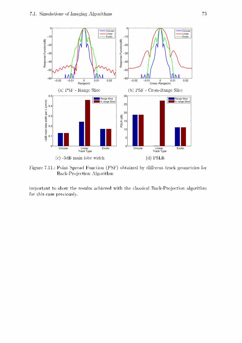
7.1. Simulations of Imaging Algorithms 73
−0.02 −0.01 0 0.01 0.02−60
−50
−40
−30
−20
−10
0
Range(m)
Re
sp
on
se
Fu
nctio
n(d
B)
Circular
Linear
Exotic
(a) PSF - Range Slice
−0.02 −0.01 0 0.01 0.02−60
−50
−40
−30
−20
−10
0
Cross−Range(m)
Re
sp
on
se
Fu
nctio
n(d
B)
Circular
Linear
Exotic
(b) PSF - Cross-Range Slice
Circular Linear Exotic0
0.1
0.2
0.3
0.4
0.5
Track Type
−3
dB
ma
in lo
be
wid
th p
er
λ (
cm
/m)
Range Slice
X−range Slice
(c) -3dB main lobe width
Circular Linear Exotic0
5
10
15
20
25
30
Track Type
PS
LR
(d
B)
Range Slice
X−range Slice
(d) PSLR
Figure 7.11.: Point Spread Function (PSF) obtained by dierent track geometries forBack-Projection Algorithm
important to show the results achieved with the classical Back-Projection algorithmfor this case previously.

74 7. Implementation and Simulations
Range(m)
Cro
ss−
Ra
ng
e(m
)
−0.2 −0.1 0 0.1
−0.2
−0.15
−0.1
−0.05
0
0.05
0.1
0.15
(a) Circular geometry
Range(m)
Cro
ss−
Ra
ng
e(m
)
−0.2 −0.1 0 0.1
−0.2
−0.15
−0.1
−0.05
0
0.05
0.1
0.15
(b) Exotic geometry
Range(m)
Cro
ss−
Ra
ng
e(m
)
−0.2 −0.1 0 0.1
−0.2
−0.15
−0.1
−0.05
0
0.05
0.1
0.15
(c) Linear geometry
Figure 7.12.: SAR image obtained by dierent track geometries for Back-ProjectionAlgorithm

7.1. Simulations of Imaging Algorithms 75
7.1.5. BP vs FCC simulations
After choosing the best conguration for the rst two imaging algorithms a com-parison has been carried out between the optimized result from the Back-ProjectionAlgorithm. The images and metrics used for the comparison have been obtained withthe same method as in the previous sections. In Fig. 7.13a and 7.13b both rangeand cross range slices of the PSF for both algorithms can be seen. Also the PSLRand -3dB main lobe width are compared in Fig. 7.13e and 7.13f. Since in this casethe comparison is performed between two dierent algorithms working with dierentmethods, it has been considered to be interesting to compare the Resolution Cell Area(RCA) provided for both solutions because it gives an easier and more global wayto understand the performance for each case. This result is presented in Fig. 7.13g.With the results obtained with these simulations there are many aspects to analyse.The -3dB main lobe width obtained with the focusing operator algorithm seems tobe slightly better with a value of 0.105 cm/m compared to the value of 0.13 cm/machieved by the time domain solution. This result gives advantage to the former so-lution. Moreover having a look at the PSLR values the frequency domain solutionprovides 7.5 dB more than the solution in the time domain.Nevertheless, and for this reason the RCA value has been presented in this comparison,the quantity of pixels exceeding the second threshold (-15dB), which reaches an areaof 0.2 (cm/m)2 in the FFC performance, is more than the half of the pixels for theBack-Projection case, corresponding to a value of 0.09 (cm/m)2. That means usingthe FFC solution the secondary lobes generate much more intensity in zones wherethere are no scatterers than for the case of Back-Projection algorithm. For both algo-rithms a SAR image has been generated as well. The conclusions extracted from thePSF function are corroborated in the image domain shown in Fig. 7.14a for the BPcase and in Fig. 7.14b for the FFC case.Looking at both results it is obvious that the image quality achieved by the back pro-jection algorithm is by far better than the solution in the frequency domain. Howeverthe computational load of both solutions should be as well compared because theor-ically with the expressions in the big O notation it is not clear which solution wouldbe faster.
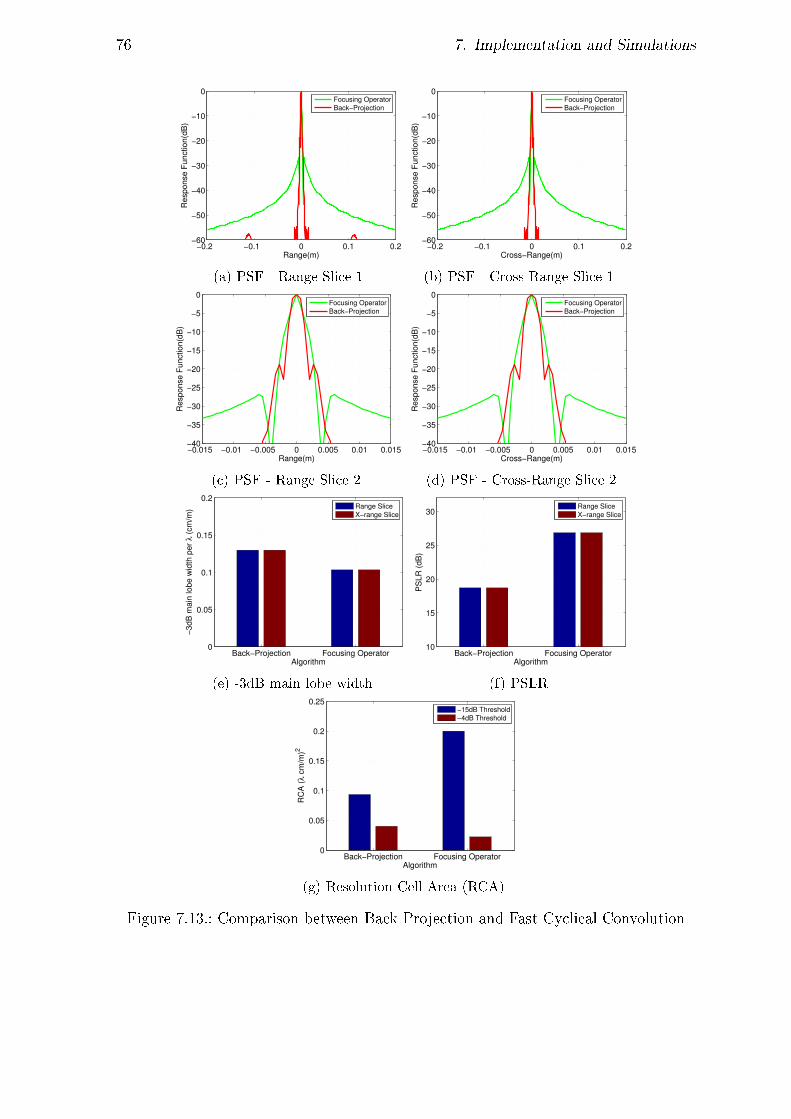
76 7. Implementation and Simulations
−0.2 −0.1 0 0.1 0.2−60
−50
−40
−30
−20
−10
0
Range(m)
Re
sp
on
se
Fu
nctio
n(d
B)
Focusing Operator
Back−Projection
(a) PSF - Range Slice 1
−0.2 −0.1 0 0.1 0.2−60
−50
−40
−30
−20
−10
0
Cross−Range(m)
Re
sp
on
se
Fu
nctio
n(d
B)
Focusing Operator
Back−Projection
(b) PSF - Cross-Range Slice 1
−0.015 −0.01 −0.005 0 0.005 0.01 0.015−40
−35
−30
−25
−20
−15
−10
−5
0
Range(m)
Re
sp
on
se
Fu
nctio
n(d
B)
Focusing Operator
Back−Projection
(c) PSF - Range Slice 2
−0.015 −0.01 −0.005 0 0.005 0.01 0.015−40
−35
−30
−25
−20
−15
−10
−5
0
Cross−Range(m)
Re
sp
on
se
Fu
nctio
n(d
B)
Focusing Operator
Back−Projection
(d) PSF - Cross-Range Slice 2
Back−Projection Focusing Operator0
0.05
0.1
0.15
0.2
Algorithm
−3
dB
ma
in lo
be
wid
th p
er
λ (
cm
/m)
Range Slice
X−range Slice
(e) -3dB main lobe width
Back−Projection Focusing Operator10
15
20
25
30
Algorithm
PS
LR
(d
B)
Range Slice
X−range Slice
(f) PSLR
Back−Projection Focusing Operator0
0.05
0.1
0.15
0.2
0.25
Algorithm
RC
A (
λ c
m/m
)2
−15dB Threshold
−4dB Threshold
(g) Resolution Cell Area (RCA)
Figure 7.13.: Comparison between Back-Projection and Fast Cyclical Convolution

7.1. Simulations of Imaging Algorithms 77
Range(m)
Cro
ss−
Range(m
)
−0.2 −0.1 0 0.1
−0.2
−0.15
−0.1
−0.05
0
0.05
0.1
0.15
(a) Back-Projection time domain algorithm
Range(m)
Cro
ss−
Range(m
)
−0.2 −0.1 0 0.1
−0.2
−0.15
−0.1
−0.05
0
0.05
0.1
0.15
(b) Fast Cyclical Convolution frequency domain algo-
rithm
Figure 7.14.: SAR image obtained by dierent track geometries for Back-ProjectionAlgorithm
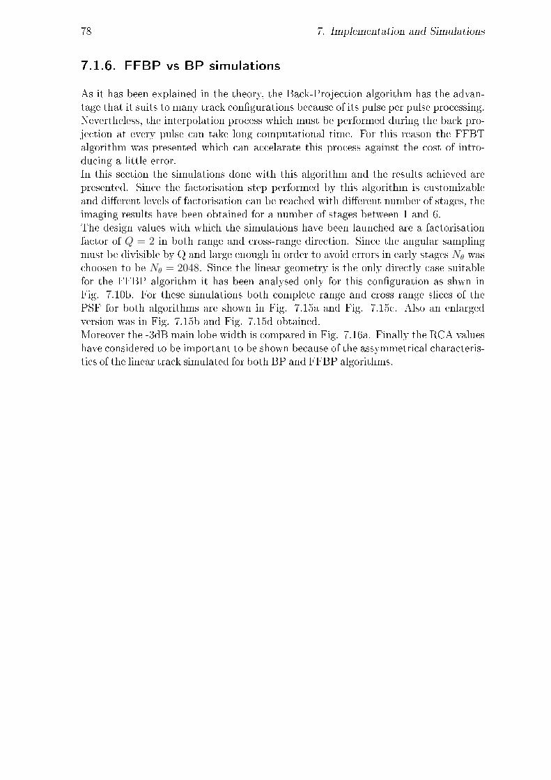
78 7. Implementation and Simulations
7.1.6. FFBP vs BP simulations
As it has been explained in the theory, the Back-Projection algorithm has the advan-tage that it suits to many track congurations because of its pulse per pulse processing.Nevertheless, the interpolation process which must be performed during the back pro-jection at every pulse can take long computational time. For this reason the FFBTalgorithm was presented which can accelarate this process against the cost of intro-ducing a little error.In this section the simulations done with this algorithm and the results achieved arepresented. Since the factorisation step performed by this algorithm is customizableand dierent levels of factorisation can be reached with dierent number of stages, theimaging results have been obtained for a number of stages between 1 and 6.The design values with which the simulations have been launched are a factorisationfactor of Q = 2 in both range and cross-range direction. Since the angular samplingmust be divisible by Q and large enough in order to avoid errors in early stages Nθ waschoosen to be Nθ = 2048. Since the linear geometry is the only directly case suitablefor the FFBP algorithm it has been analysed only for this conguration as shwn inFig. 7.10b. For these simulations both complete range and cross range slices of thePSF for both algorithms are shown in Fig. 7.15a and Fig. 7.15c. Also an enlargedversion was in Fig. 7.15b and Fig. 7.15d obtained.Moreover the -3dB main lobe width is compared in Fig. 7.16a. Finally the RCA valueshave considered to be important to be shown because of the assymmetrical characteris-tics of the linear track simulated for both BP and FFBP algorithms.

7.1. Simulations of Imaging Algorithms 79
−0.2 −0.15 −0.1 −0.05 0 0.05 0.1 0.15 0.2−60
−50
−40
−30
−20
−10
0
Range(m)
Response F
unction(d
B)
Back−Projection
FFBP 1 Stage
FFBP 2 Stages
FFBP 3 Stages
FFBP 4 Stages
FFBP 5 Stages
FFBP 6 Stages
(a) PSF - Range Slice
−0.02 −0.015 −0.01 −0.005 0 0.005 0.01 0.015 0.02−30
−25
−20
−15
−10
−5
0
Range(m)
Response F
unction(d
B)
Back−Projection
FFBP 1 Stage
FFBP 2 Stages
FFBP 3 Stages
FFBP 4 Stages
FFBP 5 Stages
FFBP 6 Stages
(b) PSF - Range Slice, enlarged
−0.2 −0.15 −0.1 −0.05 0 0.05 0.1 0.15 0.2−60
−50
−40
−30
−20
−10
0
Cross−Range(m)
Response F
unction(d
B)
Back−Projection
FFBP 1 Stage
FFBP 2 Stages
FFBP 3 Stages
FFBP 4 Stages
FFBP 5 Stages
FFBP 6 Stages
(c) PSF - Cross-Range Slice
−0.02 −0.015 −0.01 −0.005 0 0.005 0.01 0.015 0.02−30
−25
−20
−15
−10
−5
0
Cross−Range(m)
Response F
unction(d
B)
Back−Projection
FFBP 1 Stage
FFBP 2 Stages
FFBP 3 Stages
FFBP 4 Stages
FFBP 5 Stages
FFBP 6 Stages
(d) PSF - Cross-Range Slice, enlarged)
Figure 7.15.: Comparison between Back-Projection and Fast Factorized Back-Projection (Part 1)
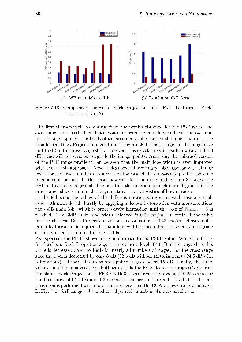
80 7. Implementation and Simulations
Back−Projectio
n
FFBPb1bStage
FFBPb2bStages
FFBPb3bStages
FFBPb4bStages
FFBPb5bStages
FFBPb6bStages0
0.1
0.2
0.3
0.4
0.5
0.6
0.7
0.8
0.9
1
−3d
Bbm
ainb
lobe
bwid
thb(
cm/λ
)
RangebSliceX−rangebSlice
(a) -3dB main lobe width
0
0.5
1
1.5
2
2.5
RC
Ad(λ
cm/m
)2
−15dBdThreshold−4dBdThreshold
Back−Projectio
n
FFBPd1dStage
FFBPd2dStages
FFBPd3dStages
FFBPd4dStages
FFBPd5dStages
(b) Resolution Cell Area
Figure 7.16.: Comparison between Back-Projection and Fast Factorized Back-Projection (Part 2)
The rst characteristic to analyse from the results obtained for the PSF range andcross-range slices is the fact that in zones far from the main lobe and even for low num-ber of stages applied, the levels of the secondary lobes are much higher than it is thecase for the Back-Projection algorithm. They are 20dB more larger in the range sliceand 15 dB in the cross-range slice. However, these levels are still really low (around -40dB), and will not seriously degrade the image quality. Analysing the enlarged versionof the PSF range prole it can be seen that the main lobe width is even improvedwith the FFBP approach. Nevertheless several secondary lobes appear with similarlevels for the lower number of stages. For the case of the cross-range prole, the samephenomenon occurs. In this case, however, for a number higher than 3 stages, thePSF is drastically degraded. The fact that the function is much more degraded in thecross-range slice is due to the assymmetrical characteristics of linear tracks.In the following the values of the dierent metrics achieved in each case are anal-ysed with more detail. Firstly by applying a deeper factorisation with more iterationsthe -3dB main lobe width is progressively increasing until the case of Nstages = 3 isreached. The -3dB main lobe width achieved is 0.29 cm/m. In contrast the valuefor the classical Back-Projection without factorisation is 0.43 cm/m. However if alarger factorisation is applied the main lobe width in both directions starts to degradeseriously as can be noticed in Fig. 7.16a.As expected, the FFBP shows a strong decrease to the PSLR value. While the PSLRfor the classic Back-Projection algorithm reaches a level of 43 dB in the range slice, thisvalue is decreased down to 13dB for nearly all numbers of stages. For the cross-rangeslice the level is decreased by only 8 dB (32.5 dB without factorisation to 24.5 dB with3 iterations). If more iterations are applied it goes below 15 dB. Finally, the RCAvalues should be analysed. For both thresholds the RCA decreases progressively fromthe classic Back-Projection to FFBP with 3 stages, reaching a value of 0.25 cm/m forthe rst threshold (-4dB) and 1.3 cm/m for the second threshold (-15dB). If the fac-torisation is performed with more than 3 stages then the RCA values strongly increase.In Fig. 7.17 SAR images obtained for all possible numbers of stages are shown.
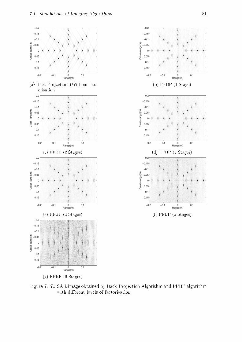
7.1. Simulations of Imaging Algorithms 81
Range(m)
Cro
ss−
ran
ge
(m)
−0.2 −0.1 0 0.1
−0.2
−0.15
−0.1
−0.05
0
0.05
0.1
0.15
(a) Back-Projection (Without fac-
torisation
Range(m)
Cro
ss−
ran
ge
(m)
−0.2 −0.1 0 0.1
−0.2
−0.15
−0.1
−0.05
0
0.05
0.1
0.15
(b) FFBP (1 Stage)
Range(m)
Cro
ss−
ran
ge
(m)
−0.2 −0.1 0 0.1
−0.2
−0.15
−0.1
−0.05
0
0.05
0.1
0.15
(c) FFBP (2 Stages)
Range(m)
Cro
ss−
ran
ge
(m)
−0.2 −0.1 0 0.1
−0.2
−0.15
−0.1
−0.05
0
0.05
0.1
0.15
(d) FFBP (3 Stages)
Range(m)
Cro
ss−
ran
ge
(m)
−0.2 −0.1 0 0.1
−0.2
−0.15
−0.1
−0.05
0
0.05
0.1
0.15
(e) FFBP (4 Stages)
Range(m)
Cro
ss−
ran
ge
(m)
−0.2 −0.1 0 0.1
−0.2
−0.15
−0.1
−0.05
0
0.05
0.1
0.15
(f) FFBP (5 Stages)
Range(m)
Cro
ss−
ran
ge
(m)
−0.2 −0.1 0 0.1
−0.2
−0.15
−0.1
−0.05
0
0.05
0.1
0.15
(g) FFBP (6 Stages)
Figure 7.17.: SAR image obtained by Back-Projection Algorithm and FFBP algorithmwith dierent levels of factorisation
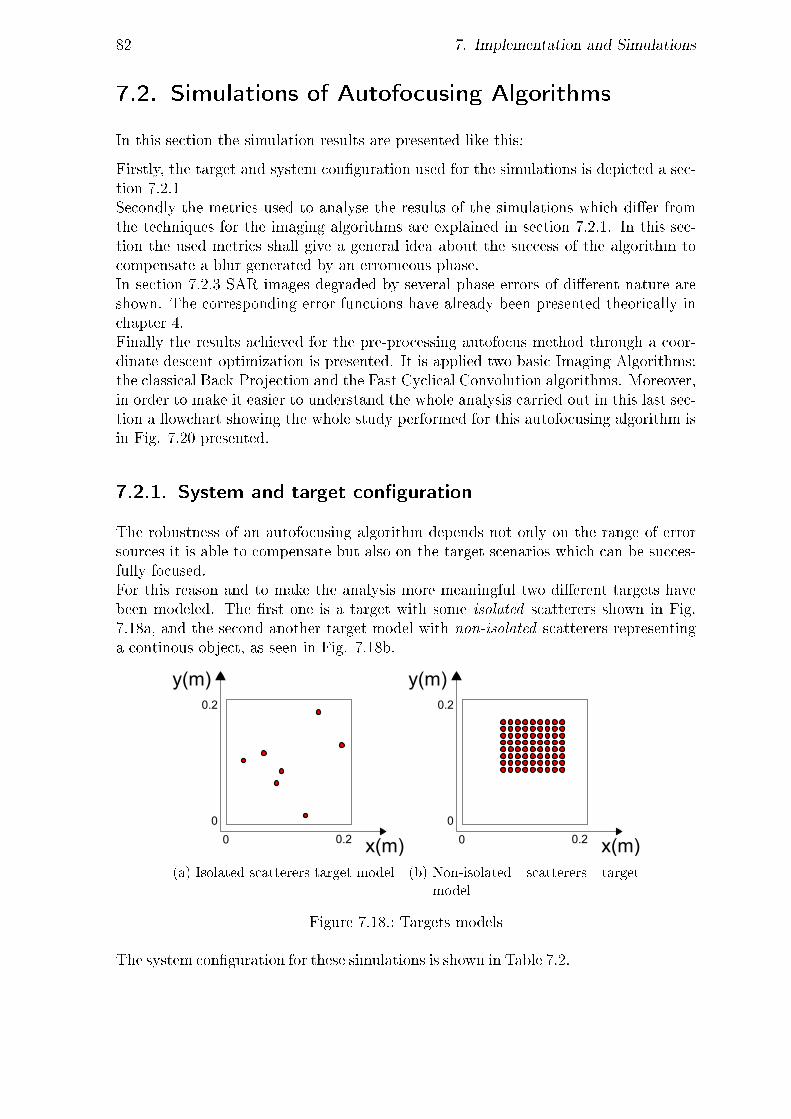
82 7. Implementation and Simulations
7.2. Simulations of Autofocusing Algorithms
In this section the simulation results are presented like this:
Firstly, the target and system conguration used for the simulations is depicted a sec-tion 7.2.1Secondly the metrics used to analyse the results of the simulations which dier fromthe techniques for the imaging algorithms are explained in section 7.2.1. In this sec-tion the used metrics shall give a general idea about the success of the algorithm tocompensate a blur generated by an errorneous phase.In section 7.2.3 SAR images degraded by several phase errors of dierent nature areshown. The corresponding error functions have already been presented theorically inchapter 4.Finally the results achieved for the pre-processing autofocus method through a coor-dinate descent optimization is presented. It is applied two basic Imaging Algorithms:the classical Back-Projection and the Fast Cyclical Convolution algorithms. Moreover,in order to make it easier to understand the whole analysis carried out in this last sec-tion a owchart showing the whole study performed for this autofocusing algorithm isin Fig. 7.20 presented.
7.2.1. System and target conguration
The robustness of an autofocusing algorithm depends not only on the range of errorsources it is able to compensate but also on the target scenarios which can be succes-fully focused.For this reason and to make the analysis more meaningful two dierent targets havebeen modeled. The rst one is a target with some isolated scatterers shown in Fig.7.18a, and the second another target model with non-isolated scatterers representinga continous object, as seen in Fig. 7.18b.
x(m)
y(m)
0 0.2
0
0.2
(a) Isolated scatterers target model
x(m)
y(m)
0 0.2
0
0.2
(b) Non-isolated scatterers target
model
Figure 7.18.: Targets models
The system conguration for these simulations is shown in Table 7.2.

7.2. Simulations of Autofocusing Algorithms 83
Target dimensionsMaximum target radius ρi,max = 0.2m
System CongurationCenter Frequency fc = 23GHzBandwidth f = [4.25, 41.375]Center wavelength λc = 13mmFrequency samples Nf = 100Aperture Samples Nθ = 300Pixel number Npix = 600× 600Interpolation method Cubic spline Interpolator
Geometry Track(*)Track path CircularAngular Bandwith 360o
Distance to target center R = 1m
Table 7.2.: General System and Target conguration for Autofocusing techniques sim-ulations
7.2.2. Focusing metrics
For the analysis of focusing techniques the method used in the previous chapter forthe case of imaging algorithms has been discarded in this section.The PSF function is degraded in many dierent ways depending on the kind of errorfunction applied and therefore it makes no sense to calculate the PSLR values or the-3dB width of the main lobe. To measure the level of success from an autofocus tech-nique metrics giving a more global analysis have been choosen which take informationfrom all the image into account.In both target models presented in Fig. 7.18 many ideal scatterers are located withinthe target extent, and thus, the defocusing is produced in each of the scatterers gen-erating a globally defocused image.For this reason, in every study of this section the following three results have beencompared:
• Image without error
• Image defocused by phase error
• Image compensated by autofocusing algorithm
The metrics used for the comparison of these results are:
• Mean Square Error (MSE)
MSE =1
Npix
Npix∑xi
[Im1(xi)− Im2(xi)]2 (7.3)
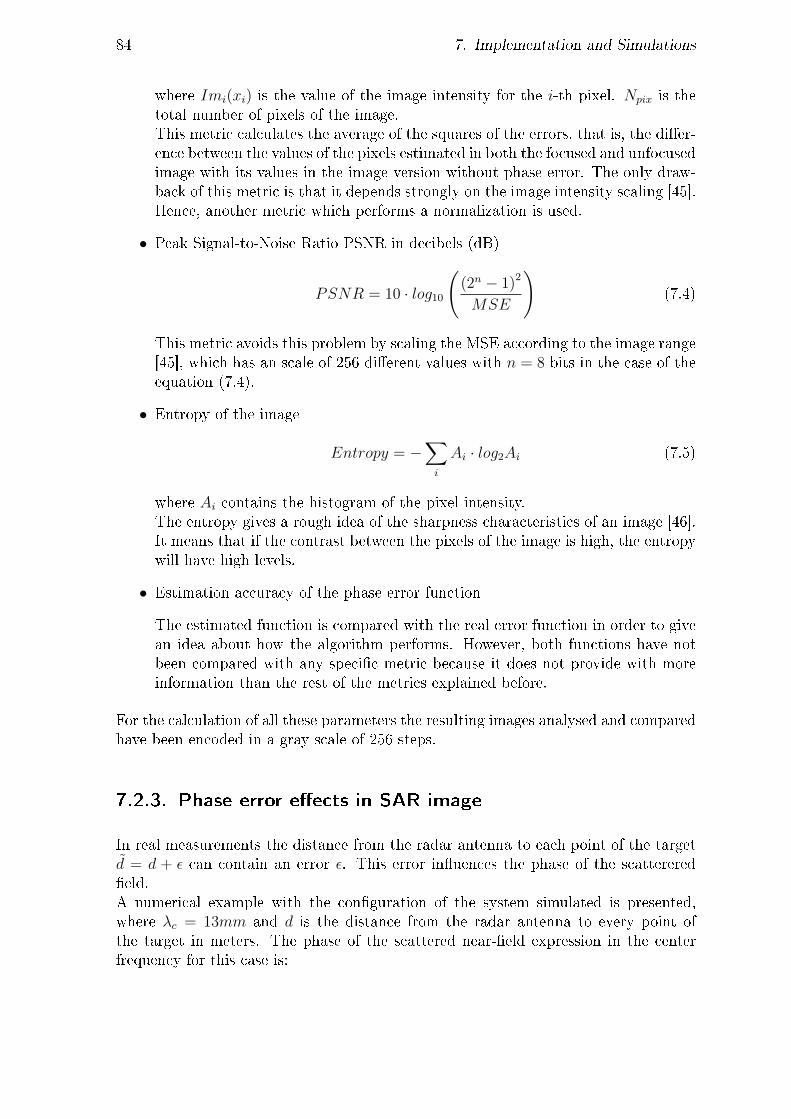
84 7. Implementation and Simulations
where Imi(xi) is the value of the image intensity for the i-th pixel. Npix is thetotal number of pixels of the image.This metric calculates the average of the squares of the errors, that is, the dier-ence between the values of the pixels estimated in both the focused and unfocusedimage with its values in the image version without phase error. The only draw-back of this metric is that it depends strongly on the image intensity scaling [45].Hence, another metric which performs a normalization is used.
• Peak Signal-to-Noise Ratio PSNR in decibels (dB)
PSNR = 10 · log10
((2n − 1)2
MSE
)(7.4)
This metric avoids this problem by scaling the MSE according to the image range[45], which has an scale of 256 dierent values with n = 8 bits in the case of theequation (7.4).
• Entropy of the image
Entropy = −∑i
Ai · log2Ai (7.5)
where Ai contains the histogram of the pixel intensity.The entropy gives a rough idea of the sharpness characteristics of an image [46].It means that if the contrast between the pixels of the image is high, the entropywill have high levels.
• Estimation accuracy of the phase error function
The estimated function is compared with the real error function in order to givean idea about how the algorithm performs. However, both functions have notbeen compared with any specic metric because it does not provide with moreinformation than the rest of the metrics explained before.
For the calculation of all these parameters the resulting images analysed and comparedhave been encoded in a gray scale of 256 steps.
7.2.3. Phase error eects in SAR image
In real measurements the distance from the radar antenna to each point of the targetd = d + ε can contain an error ε. This error inuences the phase of the scattereredeld.A numerical example with the conguration of the system simulated is presented,where λc = 13mm and d is the distance from the radar antenna to every point ofthe target in meters. The phase of the scattered near-eld expression in the centerfrequency for this case is:

7.2. Simulations of Autofocusing Algorithms 85
∠Es =2π
λc2d = 966.64 · d = 966.64 · d+ 966.64 · ε (7.6)
Thus, the smallest values of ε which produce a variation on the phase of [0, 2π] radiansin our simulation are:
ε = [0, 6.5] mm (7.7)
Moreover since the error phase is usually not constant during all the phase samples,the number of pixels shifted for each pulse is dierent. This phenomenon leads to adefocusing of the point even in more number of pixels.
As has been explained in chapter 4, the variety of phase errors that can ocurr dur-ing the image scanning period is too wide to do a complete analysis of each of theeects of these errors. For this reason the phase error functions have been mod-eled basically with 4 phase functions which should represent a wide sort of phaseerrors.
These functions are:
• Order 1 polynomial
• Order 2 polynomial
• High order polynomial (10th)
• Random
In Figs.7.19a, 7.19c, 7.19e, 7.19g these functions which are modeled in MATLAB canbe seen.
The error functions are integrated to the calculation of the scattered eld Es(f, θ)described in (5.1). Afterwards the raw data containing the errors is processed by theBack-Projection Algorithm in order to show the level of degradation and to demon-strate the eect each function introduces in the image. Once again an ideal scattererlocated at the center of the target has been used. The results of the images obtainedare shown in Figs.7.19b, 7.19d, 7.19f and 7.19h.The eects of each error in these results coincide with the theoretical eects explainedpreviosuly in section 4. For a rst order error the main lobe of the response functionis locally spread since the aperture is circular along 360o. In contrast for the secondorder error the image is defocused in a specic direction. For the case of the high ordererror the mainlobe is distorted in all directions with dierent intensities. Finally, fora random noise, the eect is similar to the one caused by the high order errors.This analysis leads to the conclusion that the low-order errors (order 1 and 2) degradethe response of a scatterer locally, that means, the response of an ideal scatterer inthe image is defocused within the closest pixels. The high order errors produce a moreintense distortion and the energy of the PSF function is spread along a wider range inthe image.
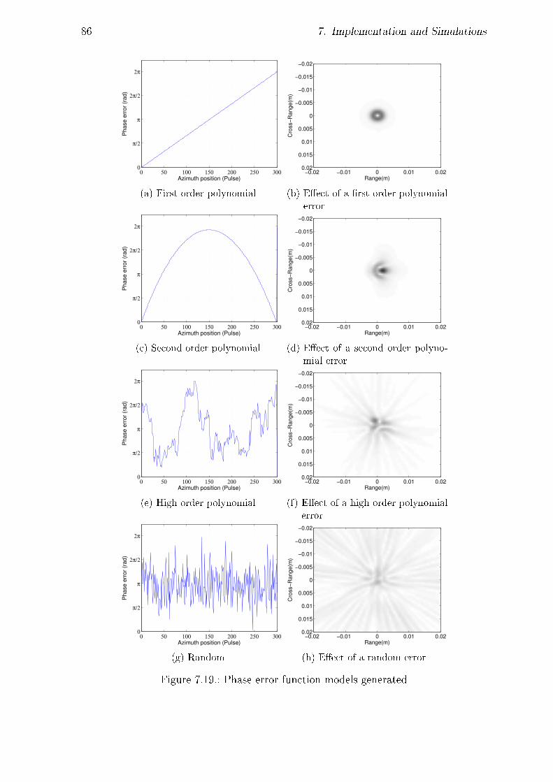
86 7. Implementation and Simulations
0 50 100 150 200 250 3000
π/2
π
2π/2
2π
Phase e
rror
(ra
d)
Azimuth position (Pulse)
(a) First order polynomial
Range(m)
Cro
ss−
Ra
ng
e(m
)
−0.02 −0.01 0 0.01 0.02
−0.02
−0.015
−0.01
−0.005
0
0.005
0.01
0.015
0.02
(b) Eect of a rst order polynomial
error
0 50 100 150 200 250 3000
π/2
π
2π/2
2π
Pha
se e
rro
r (r
ad)
Azimuth position (Pulse)
(c) Second order polynomial
Range(m)
Cro
ss−
Ra
ng
e(m
)
−0.02 −0.01 0 0.01 0.02
−0.02
−0.015
−0.01
−0.005
0
0.005
0.01
0.015
0.02
(d) Eect of a second order polyno-
mial error
0 50 100 150 200 250 3000
π/2
π
2π/2
2π
Ph
ase
err
or
(rad
)
Azimuth position (Pulse)
(e) High order polynomial
Range(m)
Cro
ss−
Ra
ng
e(m
)
−0.02 −0.01 0 0.01 0.02
−0.02
−0.015
−0.01
−0.005
0
0.005
0.01
0.015
0.02
(f) Eect of a high order polynomial
error
0 50 100 150 200 250 3000
π/2
π
2π/2
2π
Ph
ase
err
or
(ra
d)
Azimuth position (Pulse)
(g) Random
Range(m)
Cro
ss−
Ra
ng
e(m
)
−0.02 −0.01 0 0.01 0.02
−0.02
−0.015
−0.01
−0.005
0
0.005
0.01
0.015
0.02
(h) Eect of a random error
Figure 7.19.: Phase error function models generated

7.2. Simulations of Autofocusing Algorithms 87
Section 7.2.4 presents the results achieved by the compensation of all these errors usingthe pre-processing autofocusing technique previously explained.
7.2.4. Pre-processing Autofocusing simulations and results
For the simulations of the autofocusing technique 2 target models were analysed, 4dierent error functions were introduced and the autofocusing results were postpros-essed with 2 dierent imaging algorithms. An analysis of all combinations has beencarried out with a total of 2 ∗ 4 ∗ 2 = 16 results. The graphic explanation of thesestudies is shown in Fig. 7.20.
It is important to mention that the use of dierent imaging algorithms has no eectonto the coordinate descent error function estimation process since the autofocusingalgorithm is perfomed in a pre-processing basis. However it interesting to compare howblur is introduced and compensated in the image depending on the imaging algorithmused.Due to the numerous SAR images obtained during the complete analysis explained inFig.7.20, not all the results from all combinations have been shown in this document.Rather than that, a selection of the most representative results is shown and deeplyanalysed by the metrics explained in section 7.2.2.For each combination of the basic imaging algorithms (BP and FCC) with a targetmodel (isolated and non-isolated scatterer distributions) the results of the autofocusingtechinque is shown for 2 dierent error functions is shown in the following sections.This leads to a total of 8 analyses.

88 7. Implementation and Simulations
Es w
fuθD
232
122
132
622
632
y22
2
π6π
6π66π
PhaseJerrorJwradD
Azi
mut
hJpo
sitio
nJwP
ulse
D2
3212
213
262
263
2y2
22
π6π
6π66π
PhaseJerrorJwradD
Azi
mut
hJpo
sitio
nJwP
ulse
D2
3212
213
262
263
2y2
22
π6π
6π66π
PhaseJerrorJwradD
Azi
mut
hJpo
sitio
nJwP
ulse
D2
3212
213
262
263
2y2
22
π6π
6π66π
PhaseJerrorJwradD
Azi
mut
hJpo
sitio
nJwP
ulse
D
AU
TO
FO
CU
SIN
G
Coo
rdin
ate
desc
ent
wPre
pP
roce
ssin
gD
BA
CK
PR
OJE
CT
ION
ALG
OR
ITH
M
FA
ST
CY
CLI
CA
LC
ON
VO
LUT
ION
ALG
OR
ITH
M
Tar
get
mod
elat
ion
Raw
Dat
aP
hase
Jerr
orm
ultip
licai
onP
repP
roce
ssin
gA
utof
ocus
ingJ
Imag
ing
Pro
cess
Es w
fuθD
Es w
fuθD
Es w
fuθD
Es w
fuθD
Es w
fuθD
Es w
fuθD
Es w
fuθD
Es w
fuθD
Es w
fuθD
Es w
fuθD
Es w
fuθD
Es w
fuθD
Es w
fuθD
Es w
fuθD
Es w
fuθD
Es w
fuθD
Es w
fuθD
~ ~ ~ ~ ~ ~ ~ ~
^ ^ ^ ^ ^ ^ ^ ^
Isol
ated
scat
tere
rs
Non
pisol
ated
scat
tere
rs
Line
al6n
dor
der
Hig
hor
der
Ran
dom
Deg
rade
dD
ata
Com
pens
ated
Dat
a
Foc
used
SA
RJIm
age
s
14JIm
ages
Jto
Jana
lyse
J
1~JM
SE
6~JP
SN
Ry~
JEnt
ropy
.~JE
stim
atio
n
Met
rics/
Figure 7.20.: Complete study for Autofocusing

7.2. Simulations of Autofocusing Algorithms 89
Autofocusing integrated with BP
Range(m)
Cro
ss−
Range(m
)
−0.2 −0.1 0 0.1
−0.2
−0.15
−0.1
−0.05
0
0.05
0.1
0.15
(a) SAR image without error
Range(m)
Cro
ss−
Range(m
)
−0.2 −0.1 0 0.1
−0.2
−0.15
−0.1
−0.05
0
0.05
0.1
0.15
(b) SAR unfocused image with linear func-
tion error
Range(m)
Cro
ss−
Range(m
)
−0.2 −0.1 0 0.1
−0.2
−0.15
−0.1
−0.05
0
0.05
0.1
0.15
(c) SAR focused image with linear function
error
0 50 100 150 200 250 3000
π/2
π
2π/2
2π
Azimuth position (Pulse)
Ph
ase
err
or
(ra
d)
−π
−π/2
0
π/2
π
Real
Estimation
Difference
(d) Estimation performance of the phase error
function
Figure 7.21.: Autofocusing performance for BP imaging algorithm and isolated scat-terer distribution under presence of lineal phase error function
Metric Unfocused image Focused imageMSE 33.09 0.73PSNR 32.93 dB 49.50 dBEntropy 3.13 2.24
Table 7.3.: Metric results calculated from autofocused iamge obtained with BP imag-ing algorithm and isolated scatterer distribution under presence of linearphase error function

90 7. Implementation and Simulations
Range(m)
Cro
ss−
Range(m
)
−0.2 −0.1 0 0.1
−0.2
−0.15
−0.1
−0.05
0
0.05
0.1
0.15
(a) SAR image without error
Range(m)
Cro
ss−
Range(m
)
−0.2 −0.1 0 0.1
−0.2
−0.15
−0.1
−0.05
0
0.05
0.1
0.15
(b) SAR unfocused image with high order
error
Range(m)
Cro
ss−
Range(m
)
−0.2 −0.1 0 0.1
−0.2
−0.15
−0.1
−0.05
0
0.05
0.1
0.15
(c) SAR focused image with high order er-
ror
0 50 100 150 200 250 3000
π/2
π
2π/2
2π
Azimuth position (Pulse)
Ph
ase
err
or
(ra
d)
−π
−π/2
0
π/2
π
Real
Estimation
Difference
(d) Estimation performance of the phase error
function
Figure 7.22.: Autofocusing performance for BP imaging algorithm and isolated scat-terers distribution under presence of high order phase error function
Metric Unfocused image Focused imageMSE 46.37 11.36PSNR 31.47 dB 37.57 dBEntropy 3.61 2.37
Table 7.4.: Metric results calculated from autofocused image obtained with BP imag-ing algorithm and isolated scatterers distribution under presence of highorder phase error function

7.2. Simulations of Autofocusing Algorithms 91
Firstly Fig. 7.21 shows the autofocusing performance of an isolated scatterer distribu-tion imaged with the Back-Projection algorithm after applying a linear error function.As it can be seen the linear function is succesfully estimated with the coordinate de-scent optimization in Fig. 7.21d. Only a small ripple appears which does not degradethe focused image severely. In the image domain the improvement can be detectedeasily: In the unfocused image the scatterers are blurred locally. This is correctedsuccessfully in the focused image.For the metrics analysed in these results the values match the expectations for thiscase as shown in Table 7.3. The Mean Square Error (MSE) decreases from 33.09 to0.73. A notable increase of around 17 dB for the Peak Signal-to-Noise Ratio (PSNR)can be recognized. The image entropy is reduced from 3.13 to 2.24.In Fig. 7.22 the results of the same conguration but with the application of a highorder error function are presented. In this case the estimation of the function is notoutstanding as seen in Fig. 7.22d but the high frequency components of the errorfunction are compensated well. The error function remaining after the applicationof the autofocusing method contains a low frequency component and only some localhigh frequency variations. In the image domain a more obvious improvement than inthe previous case can be recognized. However it does not mean that the improvementis higher than in the previous case, but this perception is produced for a simply reason:While a low order error function degrades the Point Spread Function locally, a highorder error does it in locations farther from the scatterer. This behaviour seems todegrade the image much more.These results can be corroborated with the metrics values obtained in Table 7.4. TheMSE of the unfocused image has a value of 46.37, higher than for the unfocused imagedistorted by a linear error. The same is observed as expected for the PSNR: 31.47dB for the high order error in comparison to the 32.93 dB for the linear error case.However, for the focused image with a high order error the improvement is smallerthan compared to the rst case: The PSNR is improved in 6dB, which still is a notableimprovement. The entropy image value is reduced from 3.61 to 2.37.To sum up the performance of this autofocusing technique for isolated scatterersand a Back-Projection algorithm is optimal. Furthermore it is important to em-phasize that for a high order error function some low frequency components are stillpresent after autofocusing. The level of focusing is nonetheless for both cases su-cient.
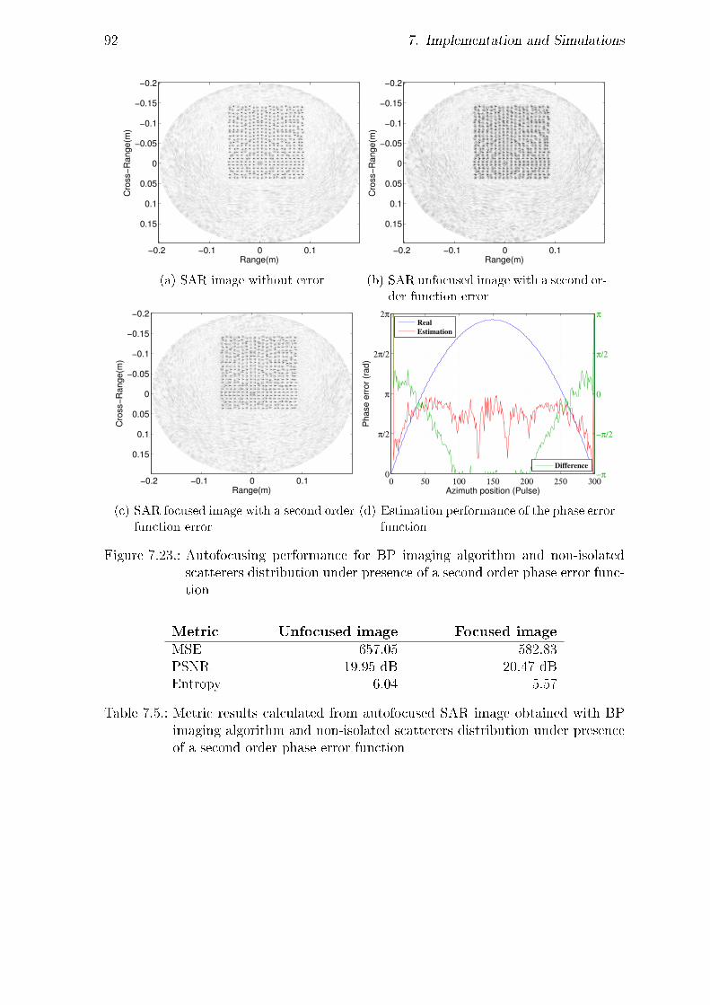
92 7. Implementation and Simulations
Range(m)
Cro
ss−
Range(m
)
−0.2 −0.1 0 0.1
−0.2
−0.15
−0.1
−0.05
0
0.05
0.1
0.15
(a) SAR image without error
Range(m)
Cro
ss−
Range(m
)
−0.2 −0.1 0 0.1
−0.2
−0.15
−0.1
−0.05
0
0.05
0.1
0.15
(b) SAR unfocused image with a second or-
der function error
Range(m)
Cro
ss−
Range(m
)
−0.2 −0.1 0 0.1
−0.2
−0.15
−0.1
−0.05
0
0.05
0.1
0.15
(c) SAR focused image with a second order
function error
0 50 100 150 200 250 3000
π/2
π
2π/2
2π
Azimuth position (Pulse)
Ph
ase
err
or
(ra
d)
−π
−π/2
0
π/2
π
Real
Estimation
Difference
(d) Estimation performance of the phase error
function
Figure 7.23.: Autofocusing performance for BP imaging algorithm and non-isolatedscatterers distribution under presence of a second order phase error func-tion
Metric Unfocused image Focused imageMSE 657.05 582.83PSNR 19.95 dB 20.47 dBEntropy 6.04 5.57
Table 7.5.: Metric results calculated from autofocused SAR image obtained with BPimaging algorithm and non-isolated scatterers distribution under presenceof a second order phase error function
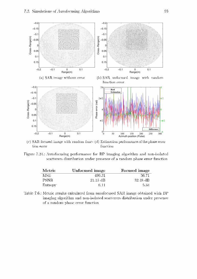
7.2. Simulations of Autofocusing Algorithms 93
Range(m)
Cro
ss−
Range(m
)
−0.2 −0.1 0 0.1
−0.2
−0.15
−0.1
−0.05
0
0.05
0.1
0.15
(a) SAR image without error
Range(m)
Cro
ss−
Range(m
)
−0.2 −0.1 0 0.1
−0.2
−0.15
−0.1
−0.05
0
0.05
0.1
0.15
(b) SAR unfocused image with random
function error
Range(m)
Cro
ss−
Range(m
)
−0.2 −0.1 0 0.1
−0.2
−0.15
−0.1
−0.05
0
0.05
0.1
0.15
(c) SAR focused image with random func-
tion error
0 50 100 150 200 250 3000
π/2
π
2π/2
2π
Azimuth position (Pulse)
Ph
ase
err
or
(ra
d)
−π
−π/2
0
π/2
π
Real
Estimation
Difference
(d) Estimation performance of the phase error
function
Figure 7.24.: Autofocusing performance for BP imaging algorithm and non-isolatedscatterers distribution under presence of a random phase error function
Metric Unfocused image Focused imageMSE 499.31 36.71PSNR 21.15 dB 32.48 dBEntropy 6.11 5.34
Table 7.6.: Metric results calculated from autofocused SAR image obtained with BPimaging algorithm and non-isolated scatterers distribution under presenceof a random phase error function

94 7. Implementation and Simulations
In Fig. 7.23 and Fig. 7.24 the results for the case of a non-isolated scatterer distri-bution are shown with the two remaining error functions. The results for the formergure are obtained after applying a second order error function and for the latter arandom error function is applied.For the second order error function it can be observed in Fig. 7.23d that the estimationperformance is good for the rst and last azimuth samples, but fails for the centralazimuth samples. This phenomenon leads to a partial compensation of the blur only.However altough the estimation is erroneous the blurring of the scatterers in the imagedomain is slightly reduced.This information can be again corroborated with the values of the metrics valuesshown in Table 7.5. The MSE value is reduced from 675.05 to 582.83. These valuesare in comparison with to the isolated scatterers distribution model much higher. Themain reason for that is that the amount of scatterers located to model the target wasincreased and hence the number of deviations is increased as well. The PSNR value isin this case only 0.5dB higher and the entropy decreased from a value of 6.04 to 5.57.On the contrary for the case of a random phase error function, the improvement levelreaches the best performance. It can be seen that the autofocusing estimation com-pensates the high frequency components of the random function and leaves only asmall ripple and a small oset.In the image domain it is easy to percieve the high level of degradation introduced bythe random error, and how it is xed in the focused image.For the metrics presented in Table 7.6 the high level of Mean Square Error (MSE) of499.31 present in the unfocused image is drastically reduced to 36.71, the PSNR isimproved by more than 11dB and the entropy level is reduced from 6.11 to 5.34.All these results lead to the conclusion that when the autofocsing is used together withthe BP imaging algorithm the compensation of low and random order error functionsis still satisfactory even for a non-isolated scatterers distribution. This result is mean-ingful in terms of robustness of this autofocusing algorithm. It has been shown thatseveral types of errors can be compensated with this technique independent from thetarget model.However, in the following the results obtained with the FCC imaging algorithm arepresented.
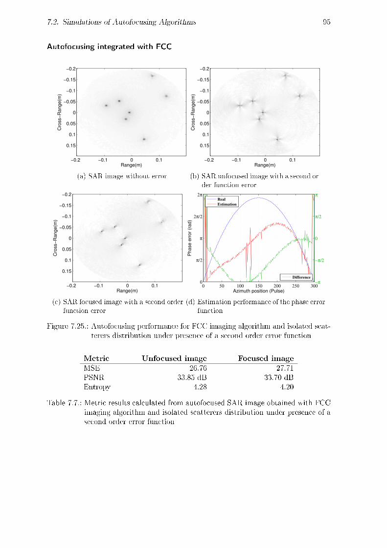
7.2. Simulations of Autofocusing Algorithms 95
Autofocusing integrated with FCC
Range(m)
Cro
ss−
Range(m
)
−0.2 −0.1 0 0.1
−0.2
−0.15
−0.1
−0.05
0
0.05
0.1
0.15
(a) SAR image without error
Range(m)
Cro
ss−
Range(m
)
−0.2 −0.1 0 0.1
−0.2
−0.15
−0.1
−0.05
0
0.05
0.1
0.15
(b) SAR unfocused image with a second or-
der function error
Range(m)
Cro
ss−
Range(m
)
−0.2 −0.1 0 0.1
−0.2
−0.15
−0.1
−0.05
0
0.05
0.1
0.15
(c) SAR focused image with a second order
function error
0 50 100 150 200 250 3000
π/2
π
2π/2
2π
Azimuth position (Pulse)
Ph
ase
err
or
(ra
d)
−π
−π/2
0
π/2
π
Real
Estimation
Difference
(d) Estimation performance of the phase error
function
Figure 7.25.: Autofocusing performance for FCC imaging algorithm and isolated scat-terers distribution under presence of a second order error function
Metric Unfocused image Focused imageMSE 26.76 27.71PSNR 33.85 dB 33.70 dBEntropy 4.28 4.20
Table 7.7.: Metric results calculated from autofocused SAR image obtained with FCCimaging algorithm and isolated scatterers distribution under presence of asecond order error function

96 7. Implementation and Simulations
Range(m)
Cro
ss−
Range(m
)
−0.2 −0.1 0 0.1
−0.2
−0.15
−0.1
−0.05
0
0.05
0.1
0.15
(a) SAR image without error
Range(m)
Cro
ss−
Range(m
)
−0.2 −0.1 0 0.1
−0.2
−0.15
−0.1
−0.05
0
0.05
0.1
0.15
(b) SAR unfocused image with random
function error
Range(m)
Cro
ss−
Range(m
)
−0.2 −0.1 0 0.1
−0.2
−0.15
−0.1
−0.05
0
0.05
0.1
0.15
(c) SAR focused image with random func-
tion error
0 50 100 150 200 250 3000
π/2
π
2π/2
2π
Azimuth position (Pulse)
Ph
ase
err
or
(ra
d)
−π
−π/2
0
π/2
π
Real
Estimation
Difference
(d) Estimation performance of the phase error
function
Figure 7.26.: Autofocusing performance for FCC imaging algorithm and isolated scat-terers distribution under presence of a random error function
Metric Unfocused image Focused imageMSE 542.41 1.63PSNR 20.78 dB 46.01 dBEntropy 5.89 4.16
Table 7.8.: Metric results calculated from autofocused SAR image obtained with FCCimaging algorithm and isolated scatterers distribution under presence of arandom error function
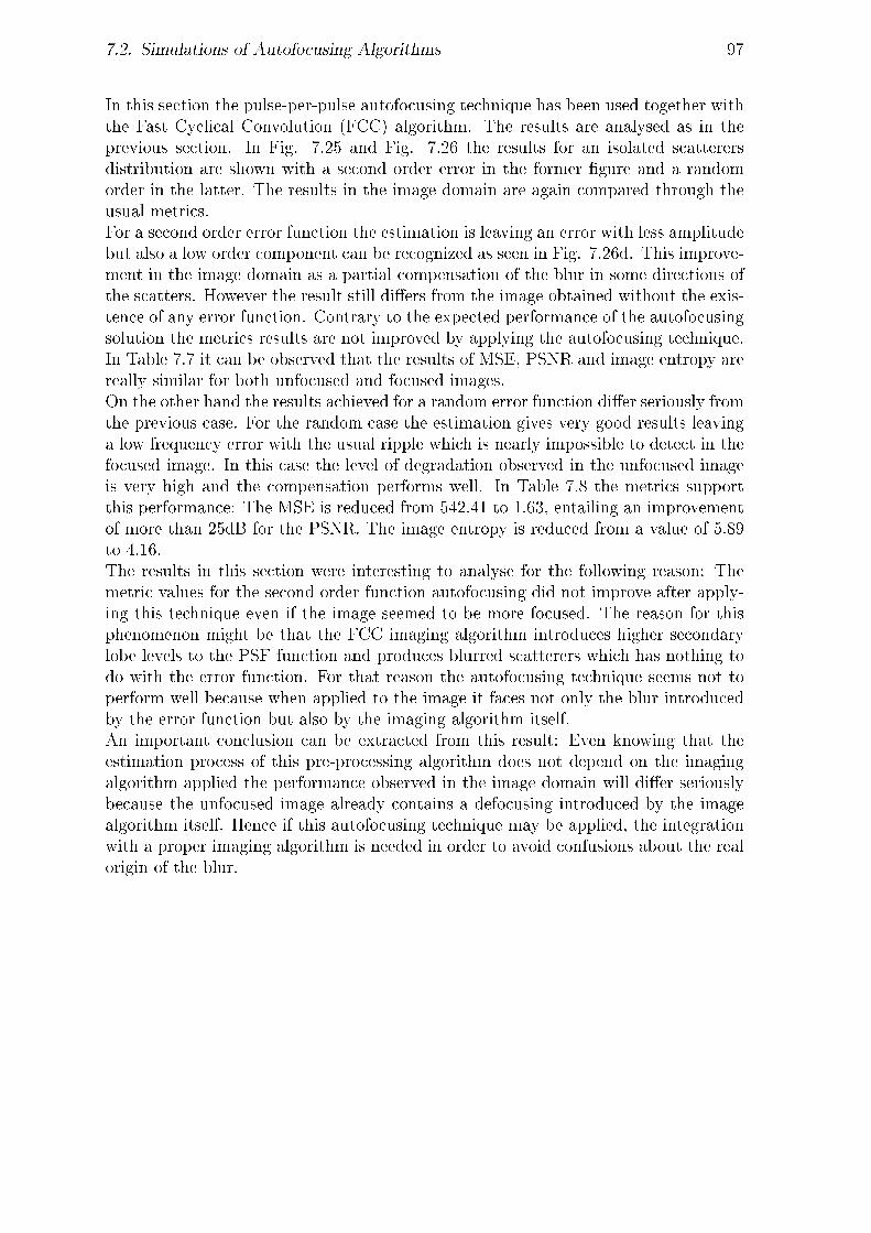
7.2. Simulations of Autofocusing Algorithms 97
In this section the pulse-per-pulse autofocusing technique has been used together withthe Fast Cyclical Convolution (FCC) algorithm. The results are analysed as in theprevious section. In Fig. 7.25 and Fig. 7.26 the results for an isolated scatterersdistribution are shown with a second order error in the former gure and a randomorder in the latter. The results in the image domain are again compared through theusual metrics.For a second order error function the estimation is leaving an error with less amplitudebut also a low order component can be recognized as seen in Fig. 7.26d. This improve-ment in the image domain as a partial compensation of the blur in some directions ofthe scatters. However the result still diers from the image obtained without the exis-tence of any error function. Contrary to the expected performance of the autofocusingsolution the metrics results are not improved by applying the autofocusing technique.In Table 7.7 it can be observed that the results of MSE, PSNR and image entropy arereally similar for both unfocused and focused images.On the other hand the results achieved for a random error function dier seriously fromthe previous case. For the random case the estimation gives very good results leavinga low frequency error with the usual ripple which is nearly impossible to detect in thefocused image. In this case the level of degradation observed in the unfocused imageis very high and the compensation performs well. In Table 7.8 the metrics supportthis performance: The MSE is reduced from 542.41 to 1.63, entailing an improvementof more than 25dB for the PSNR. The image entropy is reduced from a value of 5.89to 4.16.The results in this section were interesting to analyse for the following reason: Themetric values for the second order function autofocusing did not improve after apply-ing this technique even if the image seemed to be more focused. The reason for thisphenomenon might be that the FCC imaging algorithm introduces higher secondarylobe levels to the PSF function and produces blurred scatterers which has nothing todo with the error function. For that reason the autofocusing technique seems not toperform well because when applied to the image it faces not only the blur introducedby the error function but also by the imaging algorithm itself.An important conclusion can be extracted from this result: Even knowing that theestimation process of this pre-processing algorithm does not depend on the imagingalgorithm applied the performance observed in the image domain will dier seriouslybecause the unfocused image already contains a defocusing introduced by the imagealgorithm itself. Hence if this autofocusing technique may be applied, the integrationwith a proper imaging algorithm is needed in order to avoid confusions about the realorigin of the blur.

98 7. Implementation and Simulations
Range(m)
Cro
ss−
Range(m
)
−0.2 −0.1 0 0.1
−0.2
−0.15
−0.1
−0.05
0
0.05
0.1
0.15
(a) SAR image without error
Range(m)
Cro
ss−
Range(m
)
−0.2 −0.1 0 0.1
−0.2
−0.15
−0.1
−0.05
0
0.05
0.1
0.15
(b) SAR unfocused image with linear func-
tion error
Range(m)
Cro
ss−
Range(m
)
−0.2 −0.1 0 0.1
−0.2
−0.15
−0.1
−0.05
0
0.05
0.1
0.15
(c) SAR focused image with linear function
error
0 50 100 150 200 250 3000
π/2
π
2π/2
2π
Azimuth position (Pulse)
Ph
ase
err
or
(ra
d)
−π
−π/2
0
π/2
π
Real
Estimation
Difference
(d) Estimation performance of the phase error
function
Figure 7.27.: Autofocusing performance for FCC imaging algorithm and non-isolatedscatterers distribution under presence of a linear error function
Metric Unfocused image Focused imageMSE 5675.02 2.3707PSNR 10.59 dB 44.38 dBEntropy 6.68 7.44
Table 7.9.: Metric results calculated from autofocused SAR image obtained with FCCimaging algorithm and non-isolated scatterers distribution under presenceof a linear error function
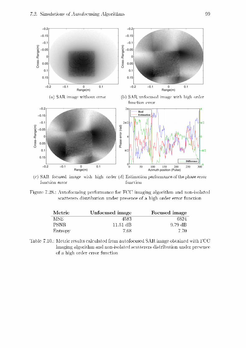
7.2. Simulations of Autofocusing Algorithms 99
Range(m)
Cro
ss−
Range(m
)
−0.2 −0.1 0 0.1
−0.2
−0.15
−0.1
−0.05
0
0.05
0.1
0.15
(a) SAR image without error
Range(m)
Cro
ss−
Range(m
)
−0.2 −0.1 0 0.1
−0.2
−0.15
−0.1
−0.05
0
0.05
0.1
0.15
(b) SAR unfocused image with high order
function error
Range(m)
Cro
ss−
Range(m
)
−0.2 −0.1 0 0.1
−0.2
−0.15
−0.1
−0.05
0
0.05
0.1
0.15
(c) SAR focused image with high order
function error
0 50 100 150 200 250 3000
π/2
π
2π/2
2π
Azimuth position (Pulse)
Ph
ase
err
or
(ra
d)
−π
−π/2
0
π/2
π
Real
Estimation
Difference
(d) Estimation performance of the phase error
function
Figure 7.28.: Autofocusing performance for FCC imaging algorithm and non-isolatedscatterers distribution under presence of a high order error function
Metric Unfocused image Focused imageMSE 4583 6824PSNR 11.51 dB 9.79 dBEntropy 7.68 7.70
Table 7.10.: Metric results calculated from autofocused SAR image obtained with FCCimaging algorithm and non-isolated scatterers distribution under presenceof a high order error function

100 7. Implementation and Simulations
In Fig. 7.27 and Fig. 7.28 the autofocusing together with the FCC imaging algorithmfor a non-isolated scatterers distribution is presented after applying two dierent errorfunctions. For the former gure a linear phase error is introduced and for the latter ahigh error function is added.For the lineal error case, a strange behaviour can be observed: The estimation ofthe function follows perfectly the linear component and has only the usual ripple. Inthe image domain it is easy to recognize the high similarity between the ideal imagewithout error and the focused version. Regarding the metric values shown in Table 7.9,the MSE value is reduced drastically from 5675.02 to 2.37. The PSNR level increasesabout 34 dB.However for the case of the image entropy a remarkable anomaly is noticed. It isnot reduced but increased by the autofocusing from 6.68 to 7.44. For this behaviourthe same reason holds as for studied previously: The defocus introduced by the FCCimaging algorithm itself.For the case of a high order error function the error function estimation performspoorly. In the image domain it can be seen that the error is not compensated. Themetrics listed in Table 7.10 show this non-proper performance. The MSE value isincreased while the PSNR is decreased for the focused image. The entropy of theimage remains nearly constant.For these results it can be noticed that the autofocusing technique does not performproperly in order to compensate the high order error function. The results rearmwhat was explained for the prior case: The autofocusing performance breaks downbecause of the non-isolated scatterer distribution and even more because of the innerblur introduced by the imaging algorithm.To sum up the use of this autofocusing algorithm should be discarded when usedtogether with the FCC algorithm in a non-isolated scatterer distribution since if a highorder phase error occurs it will not be compensated properly.
101
8. Conclusions and Future work
In this nal chapter an overview of the work conducted in the context of the currentthesis is presented. A synopsis of results obtained through the simulation of all algo-rithms is attempted and a global analysis of the performance of the imaging and aut-ofocusing solutions is presented. Finally, possible extensions of the current work takinginto account the available methods theorically studied are discussed.
8.1. Conclusions
The purpose of this thesis was to do a wide study of all available imaging algorithmswhich can be applied successfully in the Mobile RCS device under the following con-straints: Robustness, high resolution, a low computational time and a proper handlingof the Near-Field situation.Furthermore during the study performed within this thesis the existence of errorswhich can ocur during the collection of data previous to any processing step has beenas well taken into consideration. Hence the scope of this work was extended andanother block of algorithms has been studied apart from the imaging methods, theautofocusing algorithms. In the following the results for both types of algorithms arediscussed generally.The imaging algorithms considered and compared in this project are the Fast Cycli-cal Convolution algorithm, the classical Back-Projection algorithm and the Fast Fac-torized Back-Projection. All these solutions were studied independently in order toobtain an optimal performance and have also been compared with the goal of beingable to conrm which one can perform better for mentioned purpose or at least underwhich conditions they may be used. For the classical time domain solution calledBack-Projection it was observed that the implementation of a zero-padding processimproves the image quality. Also the windowing step with a Hamming window waschoosen being optimal to reduce the side-lobe levels of the PSF function even thoughthe main lobe is slightly widened. Moreover it was demonstrated that this solutioncan achieve good imaging results with any track-geometry discussed here. However,the circular track with a constant radius to the target center has been demonstratedto be the best conguration.On the contrary, the solution in the frequency domain called Fast Cyclical Convo-lution is not geometrically unconstrained so that only the circular track is available.Therefore, if a dierent geometric conguration should be used it must be discarded.For the FCC solution also the minimum angular sampling constraint was discussed. Itis important to emphasize that if the angular sampling cannot satisfy this limitation
102 8. Conclusions and Future work
because of external limitations this method can not be used.After the independent analysis for each of these two imaging algorithms together withtheir comparison an important conclusion is reached. Even if the solution in the fre-quency domain has a better performance of the main lobe the secondary lobes havehigher levels than it is for the case for Back-Projection. This can also be observed inthe SAR image. For this reason the Back-Projection is supposed to be more conve-nient in terms of image quality and resolution.Nevertheless an important consideration should be done: The Back-Projection solu-tion can require in some cases a higher computational time. If the desired SAR imagemust have a really high pixel resolution, the FCC solution might not be discardedbecause it can be for this case much less time demanding.As stated before a third alternative has been presented and simulated, the so-calledFFBP. The data factorisation performed previous to the back-projection step gener-ated satisfactory results. It has been demonstrated that if this solution is used, thelevel of factorisation must be controlled and should exceed a specic number of it-erations. The number of iterations strictly depends on the specic scenario and thesystem's conguration.During the explanation of this solution and its simulations the fact that it can usedfor a linear track geometry only has been emphasized. This is an important draw-back of this method, but in the following section it will be briey presented how thisdisadvantage can be overcome. The calculation of the computational burden for thissolution has not been shown in this thesis for the following reason: The code for theimplementation of the FFBP solution reaches a considerable complexity and it cannotbe ensured that it has been optimized. Therefore any computational time calculatedhas been considered to be not meaningful. Only the theoretical assymptotic calcula-tion through the Big O notation has been considered.Moreover interesting results have been obtained with autofocusing techniques. Sev-eral solutions have been briey introduced and the algorithm supposed to be moreunconstrained in terms of track geometry, target model, system conguration and in-tegration with imaging algorithms has been choosen, simulated and analysed. Thealgorithm chosen is the pulse-per-pulse autofocusing technique utilizing a coordinatedescent optimization estimation. The simulations of the proposed method have shownconvenient results regarding the focusing of an image degraded by dierent error mod-els. It was also demonstrated how this solution can deal with dierent target models.Moreovere the algorithm provides an outstanding robustness characteristic and can beintegrated with any imaging algorithm and used within the Mobile RCS device undernearly any condition. Even though the time computation for this solution has not beenshown in this document, the coordinate descent optimization ensures a much fastercalculation than the classical maximum likelihood estimation. Thus the robustnesslevel can be increased because a high number of azimuth samples or pulses can beused.

8.2. Future work suggestions 103
8.2. Future work suggestions
Proposed extensions to this work could include the following:
• Optimization of the code for the FFBP algorithm in order to perceive a signi-cant reduction of computational time.
• Implementation of the Fast Factorized Back Projection (FFBP) for circular trackgeometries or even for exotic track geometries. As explained previously it can beperformed by the approximation of track segments as linear subtracks. A studyin this direction may be interesting in order to suit the FFBP algorithm with ahigher robustness level.
• Other improvements of the Back-Projection algorithm can be studied apart fromthe FFBP. The Non-Uniform Fast Fourier Transformation (NUFFT) for exampleunites both range FFT computation and back-projection into one unique stepand it saves a high amount of time [47].
For the latter, the proposed extensions could include the following:
• Study of validity of post-processing techniques for this purpose. On the one handfor a model-based autofocusing the complexity of these models may be analysedto decide if it can suit the constraints. On the other hand estimation-basedautofocusing solutions such as the PGA algorithm may be studied deeply.
• For pre-processing techniques a considerable amount of alternatives have beenfound and it would be interesting to compare their performances with the so-lution proposed. For example the estimation process could be performed eitherwith the coordinate descent optimization or with a gradient descent estimationor other techniques which accelerate the estimation.
• Within the autofocusing solution proposed many metrics can be maximised orminimized such as image entropy or image contrast together with other sharpnessmetrics. Thus a study could be performed analysing each of these availablemetrics.

104

105
Appendices


107
A. Generation of the scattered
near-eld in MATLAB
1 f o r m=1:Mrho ;2 f o r n=1:Nphi ;3 d = sq r t (R^2+(RHO(m) ^2)−(2∗RHO(m)∗R∗ cos (PHI(n) ∗2∗
pi /360−THETA) ) ) ;4 Es = Es + r e f l e c t i v i t y (m, n)∗exp(−1 i ∗2∗ pi ∗K.∗d) . / ( d
.^2) ;5 end6 end
The polar coordinates reectivity function ψ(ρ, φ) has been as well generated by mod-elling the target under analysis with an ideal scatterers distribution described by re-ectivity(m,n).
All the algorithms analysed have been as well implemented in MATLAB and the evalu-ation of the results obtained has been done with the same tool.

108

109
List of Figures
1.1. Project overview . . . . . . . . . . . . . . . . . . . . . . . . . . . . . . 2
2.1. Bistatic and Monostatic congurations . . . . . . . . . . . . . . . . . . 72.2. Scattered energy in all directions . . . . . . . . . . . . . . . . . . . . . 82.3. Pulse Repetition Frequency (PRF) . . . . . . . . . . . . . . . . . . . . 112.4. Radar Waveforms . . . . . . . . . . . . . . . . . . . . . . . . . . . . . . 11
3.1. Synthetic Aperture Radar . . . . . . . . . . . . . . . . . . . . . . . . . 133.2. ISAR and SAR . . . . . . . . . . . . . . . . . . . . . . . . . . . . . . . 133.3. ISAR and SAR modes for many 2D track geometries . . . . . . . . . . 143.4. Range and Cross-Range proles . . . . . . . . . . . . . . . . . . . . . . 153.5. Geometry for monostatic SAR imaging within Far-Field region . . . . . 163.6. Scattered Field obtention and range and cross-Range Compression . . . 173.7. Polar Reformatting . . . . . . . . . . . . . . . . . . . . . . . . . . . . . 183.8. PSF physical meaning . . . . . . . . . . . . . . . . . . . . . . . . . . . 203.9. Zero padding eect . . . . . . . . . . . . . . . . . . . . . . . . . . . . . 21
4.1. Phase error eect during data collection . . . . . . . . . . . . . . . . . 244.2. Representative error modelation . . . . . . . . . . . . . . . . . . . . . . 25
5.1. Fast Cyclical Convolution Algorithm . . . . . . . . . . . . . . . . . . . 315.2. Radon Transform . . . . . . . . . . . . . . . . . . . . . . . . . . . . . . 335.3. Back Projection Algorithm . . . . . . . . . . . . . . . . . . . . . . . . . 355.4. Adjacent apertures Back-Projection . . . . . . . . . . . . . . . . . . . . 365.5. Range factorisation . . . . . . . . . . . . . . . . . . . . . . . . . . . . . 375.6. Focusing delay . . . . . . . . . . . . . . . . . . . . . . . . . . . . . . . . 385.7. Track samples factorisation . . . . . . . . . . . . . . . . . . . . . . . . . 395.8. Range error from Far-Field Assumption . . . . . . . . . . . . . . . . . . 405.9. Fast Factorised Back-Projection . . . . . . . . . . . . . . . . . . . . . . 41
6.1. Autofocus block performance . . . . . . . . . . . . . . . . . . . . . . . 446.2. Autofocus Algorithms classication . . . . . . . . . . . . . . . . . . . . 456.3. Linear track . . . . . . . . . . . . . . . . . . . . . . . . . . . . . . . . . 496.4. Circular shifting in each range bin . . . . . . . . . . . . . . . . . . . . . 506.5. Windowing step . . . . . . . . . . . . . . . . . . . . . . . . . . . . . . . 516.6. Data windowing . . . . . . . . . . . . . . . . . . . . . . . . . . . . . . . 526.7. PGA Algorithm Flowchart . . . . . . . . . . . . . . . . . . . . . . . . . 546.8. Coordinate descent optimization . . . . . . . . . . . . . . . . . . . . . . 60

110 List of Figures
7.1. General System and target dimensions (Circular track case) . . . . . . 637.2. Target models for the simulations . . . . . . . . . . . . . . . . . . . . . 647.3. Resolution metrics used . . . . . . . . . . . . . . . . . . . . . . . . . . 657.4. Aliasing eects in PSF of FCC algorithm . . . . . . . . . . . . . . . . . 667.5. Aliasing eects in SAR images varying angular sampling in FCC algorithm 677.6. Zero padding eect on the SAR image (PSF) for Back-Projection Al-
gorithm . . . . . . . . . . . . . . . . . . . . . . . . . . . . . . . . . . . 687.7. Zero padding eect for Back-Projection Algorithm . . . . . . . . . . . . 697.8. Windowing eect on the Point Spread Function (PSF) for Back-Projection
Algorithm . . . . . . . . . . . . . . . . . . . . . . . . . . . . . . . . . . 707.9. Zoomed result of windowing eect on the SAR image for Back-Projection
Algorithm . . . . . . . . . . . . . . . . . . . . . . . . . . . . . . . . . . 717.10. Track geometries analysed for Back-Projection Algorithm . . . . . . . . 727.11. Point Spread Function (PSF) obtained by dierent track geometries for
Back-Projection Algorithm . . . . . . . . . . . . . . . . . . . . . . . . . 737.12. SAR image obtained by dierent track geometries for Back-Projection
Algorithm . . . . . . . . . . . . . . . . . . . . . . . . . . . . . . . . . . 747.13. Comparison between Back-Projection and Fast Cyclical Convolution . . 767.14. SAR image obtained by dierent track geometries for Back-Projection
Algorithm . . . . . . . . . . . . . . . . . . . . . . . . . . . . . . . . . . 777.15. Comparison between Back-Projection and Fast Factorized Back-Projection
(Part 1) . . . . . . . . . . . . . . . . . . . . . . . . . . . . . . . . . . . 797.16. Comparison between Back-Projection and Fast Factorized Back-Projection
(Part 2) . . . . . . . . . . . . . . . . . . . . . . . . . . . . . . . . . . . 807.17. SAR image obtained by Back-Projection Algorithm and FFBP algo-
rithm with dierent levels of factorisation . . . . . . . . . . . . . . . . . 817.18. Targets models . . . . . . . . . . . . . . . . . . . . . . . . . . . . . . . 827.19. Phase error function models generated . . . . . . . . . . . . . . . . . . 867.20. Complete study for Autofocusing . . . . . . . . . . . . . . . . . . . . . 887.21. Autofocusing performance for BP imaging algorithm and isolated scat-
terer distribution under presence of lineal phase error function . . . . . 897.22. Autofocusing performance for BP imaging algorithm and isolated scat-
terers distribution under presence of high order phase error function . . 907.23. Autofocusing performance for BP imaging algorithm and non-isolated
scatterers distribution under presence of a second order phase errorfunction . . . . . . . . . . . . . . . . . . . . . . . . . . . . . . . . . . . 92
7.24. Autofocusing performance for BP imaging algorithm and non-isolatedscatterers distribution under presence of a random phase error function 93
7.25. Autofocusing performance for FCC imaging algorithm and isolated scat-terers distribution under presence of a second order error function . . . 95
7.26. Autofocusing performance for FCC imaging algorithm and isolated scat-terers distribution under presence of a random error function . . . . . . 96
7.27. Autofocusing performance for FCC imaging algorithm and non-isolatedscatterers distribution under presence of a linear error function . . . . . 98
7.28. Autofocusing performance for FCC imaging algorithm and non-isolatedscatterers distribution under presence of a high order error function . . 99

111
Bibliography
[1] C. Özdemir, Inverse Syntethic Aperture Radar Imaging with MATLAB Algo-rithms. New Jersey: Wiley, 2012.
[2] T. H. Chu and D. B. Lin., Microwave diversity imaging of perfectly conductingobjects in the near eld region, IEEE Trans Microwave Theory Tech, vol. 39,p. 480?487, 1991.
[3] D. L.Mensa, High Resolution Radar Cross-Section Imaging. Boston: ArtechHouse, 1991.
[4] D. J. M. Weiss, Continuous-wave stepped-frequency radar for target ranging andmotion detection, The Midwest Instruction and Computing Symposium (MICS),2009.
[5] L. Thourel, Initiation aux techniques modernes des radars. Toulouse:CEPADUES, 1982.
[6] J. P. Zwart, Aircraft Recognition from Features Extracted from Measured andSimulated Radar Range Proles. PhD thesis.
[7] T. S. L. V. C. Koo and H. T. Chuah, A comparison of autofocus algorithms forsar imagery, Progress In Electromagnetics Research Symposium 2005, Hangzhou,China, vol. 1, pp. 1619, 2005.
[8] E. C. A. S.Demirci, H.Centinkaya, A study on millimiter-wave imaging of con-cealed objects: Application using back-projection algorithm, Progress In Elec-tromagnetics Research, vol. 128, pp. 457 477, 2012.
[9] G. S. Lars M. H. Ulander, Hans Hellsten, Synthetic aperture radar processingusing fast factorized back-projection, Positioning, pp. 42 46, 2013, 4.
[10] L. J. A.Broquetas, Josep Palau and A. Cardama, Spherical wave near-eld imag-ing and radar cross-section measurement, IEEE Transactions on Antennas andPropagation, vol. 46, pp. 730 735, 1998.
[11] T. Vaupel and T. F.Eibert, Comparison and application of near-eld isar imagingtechniques for far-eld radar cross section determination, IEEE Transactions onAntennas and Propagation, vol. 54, pp. 144 151, 2006.
[12] R. M. Biao Zhang, Yiming Pi, A near-eld 3d circular sar imaging techniquebased on spherical wave decomposition, Progress In Electromagnetics Research,vol. 141, pp. 327 246, 2013.

112 Bibliography
[13] N. J.Redding and G. N.Newsam, Inverting the Circular Radon Transform. Edin-burgh, South Australia: DSTO Electronics and Surveillance Research Laboratory,2002.
[14] S. R. Deans, The Radon Transform and Some of Its Applications. Dover Publi-cations, 2007.
[15] R. D. Kriz, Parallel implementation of the ltered back projection algorithm fortomographic imaging, Virginia Tech, College of Engineering, 1995.
[16] R. Mersereau and A. Oppenheim, Digital reconstruction of multidimensionalsignals from their projections, Proc. IEEE, vol. 62, pp. 1319 1338, 1974.
[17] J. Munson, D.C. and W.K.Jenkins, A tomographic formnulation of spotlight-mode synthetic aperture radar, Proc. IEEE, vol. 71, No.8, pp. 917 925, 1983.
[18] J. Bauck and W.K.Jenkins, Tomographic processing of spotlight-mode syntheticaperture radar signals with compensation for wavefront curvature, Interna-tional Conference on Acoustics, Speech and Signal Processing, ICASSP-88, vol. 2,pp. 1192 1195, 1988.
[19] M. A. Hunter and P.Gough, A comparison of fast factorized back-projection andwavenumber algorithms for sas image reconstruction, Fifth World Congress onUltrasonics, Paris, pp. 527 530, 2003.
[20] D. G. Kyra Moon, A new factorized backprojection algorithm for stripmap syn-thetic aperture radar, Positioning, pp. 42 46, 2013, 4.
[21] Z. L. Miao Yu, Xiaoling Zhang, Acceleration of fast factorized back projection al-gorithm for bistatic sar, Geoscience and Remote Sensing Symposium (IGARSS),2013 IEEE International, pp. 2493 2496, 2013.
[22] C. Q. Haoyang Tang, Haoshan Shi, Study on improvement of phase gradientautofocus algorithm, ETCS, vol. 2, pp. 5861, 2009.
[23] G. I. V. D. Bezvesilniy, O.O., Estimation of phase errors in sar data by local-quadratic map-drift autofocus, Radar Symposium (IRS), pp. 376 381, 2012.
[24] K. Samczynski, P. ; Kulpa, Concept of the coherent autofocus map-drift tech-nique, Radar Symposium, 2006. IRS 2006. International, pp. 1 4, 2006.
[25] R. S. G. W. G. Carrara and R. M. Majewski, Spotlight synthetic aperture radar:Signal processing algorithms,
[26] T. M. Calloway and G. W. Donohoe, Subaperture autofocus for synthetic aper-ture radar, Trans. Aerosp. Electron. Syst., vol. 30, p. 617?621, 1994.
[27] X. L. Junfeng Wang, Sar minimum-entropy autofocus using an adaptive-orderpolynomial model, IEEE Geoscience and Remote Sensing Letters, 2006.
[28] N. J. Li Xi, Liu Guosui, Autofocusing of isar images based on entropy minimiza-tion, Aerospace and Electronic Systems, IEEE Transactions on, vol. 35, pp. 1240 1252, 1999.

Bibliography 113
[29] F. B. M. Martorella and B. Haywood, Contrast maximisation based technique for2-d isar autofocusing, Radar, Sonar and Navigation, IEE Proceedings, vol. 152,pp. 253 262, 2005.
[30] M. N. D. Robert L. Morrison and D. C. Munson, Sar image autofocus by sharp-ness optimization: A theoretical study, Image Processing, IEEE Transactionson, vol. 16, pp. 2309 2321, 2007.
[31] U. . B. P. Holzner, Juergen ; Fraunhofer Institute for High Frequency ; Gebhardt,Autofocus for high resolution isar imaging, Synthetic Aperture Radar (EUSAR),2010 8th European Conference on, pp. 1 4, 2010.
[32] L. W. . D. Z. . Z. Zhu, Improvements of rope in isar motion compensation,Synthetic Aperture Radar, 2007. APSAR 2007. 1st Asian and Pacic Conferenceon, 2007.
[33] C. Snarski, Rank one phase error estimation for range-doppler imaging,Aerospace and Electronic Systems, IEEE Transactions on, vol. 32, pp. 676 688,1996.
[34] L. L. . A. R. . M. Shiyi, Improvement of rank one phase estimation (rope) auto-focusing technique, Signal Processing Proceedings, 1998. ICSP '98. 1998 FourthInternational Conference on, 1998.
[35] D. C. P.H. Eichel and J. C.V. Jakowatz, Speckle processing method for synthetic-aperture-radar phase correction, OPTICS LETTERS, vol. 14, pp. 5861, 1989.
[36] D. C. D.E. Wahl, P.H. Eichel and C. Jakowatz, Phase gradient autofocus -a robust tool for high resolution sar phase correction, IEEE Transactions onAerospace and Electronic Systems, vol. 2, pp. 827835, 1994.
[37] J. N. Ash, An autofocus method for backprojection imagery in synthetic apertureradar, IEEE Geoscience and Remote Sensing Letters, vol. 9, NO.1, 2012.
[38] M. I. Duersch and D. G. Long, Backprojection autofocus for synthetic apertureradar, Department of Electrical and Computer Engineering, Brigham Young Uni-versity, 2013.
[39] J. M. J.R. Fienup, Aberration correction by maximazing generalized sharpnessmetrics, Optical Society of America, vol. 20, No. 4, pp. 609 620, 2003.
[40] D. C. M. Kuang-Hung Liu, Ami Wiesel, Synthetic aperture radar autofocusbased on a bilinear model, IEEE Transactions on image Processing, vol. 21, No.5, pp. 2735 2746, 2012.
[41] J. Fienup, Synthetic aperture radar autofocus by maximising sharpness, OpticLetters, vol. 25, No. 4, pp. 221 223, 2000.
[42] M. R. A. O.Ponce, P.Prats, Processing of circular sar trajectories with fast factor-ized back-projection, General Assembly and Scientic Symposium, 2011 XXXthURSI, pp. 14, 2011.

114 Bibliography
[43] J. E. Luminati, Wide-Angle Multistatic Synthetic Aperture Radar: Focused ImageFormation and Aliasing Artifact Mitigation. PhD thesis.
[44] T. . P. E. Cherniakov, M. ; Zeng, Ambiguity function for bistatic sar and itsapplication in ss-bsar performance analysis, Radar Conference, 2003. Proceedingsof the International, pp. 343 348, 2003.
[45] R. C. Gonzalez and R. E. Woods, Digital Image Processing. New York: Addison-Wesley, 1992.
[46] E. M. Du-Yih Tsai, Yongbum Lee, Information-entropy measure for evaluationof image quality, Journal of Digital Imaging. Department of Radiological Tech-nology, School of Health Sciences, Niigata University,, p. 338 ? 347, 2007.
[47] C. . L. A. . T. P. Capozzoli, A. Curcio, Nut-based sar backprojection on multiplegpus, Advances in Radar and Remote Sensing (TyWRRS), pp. 62 68, 2012.