econstor www.econstor.eu

Der Open-Access-Publikationsserver der ZBW – Leibniz-Informationszentrum WirtschaftThe Open Access Publication Server of the ZBW – Leibniz Information Centre for Economics

Standard-Nutzungsbedingungen:

Die Dokumente auf EconStor dürfen zu eigenen wissenschaftlichenZwecken und zum Privatgebrauch gespeichert und kopiert werden.

Sie dürfen die Dokumente nicht für öffentliche oder kommerzielleZwecke vervielfältigen, öffentlich ausstellen, öffentlich zugänglichmachen, vertreiben oder anderweitig nutzen.

Sofern die Verfasser die Dokumente unter Open-Content-Lizenzen(insbesondere CC-Lizenzen) zur Verfügung gestellt haben sollten,gelten abweichend von diesen Nutzungsbedingungen die in der dortgenannten Lizenz gewährten Nutzungsrechte.

Terms of use:

Documents in EconStor may be saved and copied for yourpersonal and scholarly purposes.

You are not to copy documents for public or commercialpurposes, to exhibit the documents publicly, to make thempublicly available on the internet, or to distribute or otherwiseuse the documents in public.

If the documents have been made available under an OpenContent Licence (especially Creative Commons Licences), youmay exercise further usage rights as specified in the indicatedlicence.

zbw Leibniz-Informationszentrum WirtschaftLeibniz Information Centre for Economics

Heckman, James J.; Raut, Lakshmi Kanta

Working Paper

Intergenerational Long Term Effects of Preschool:Structural Estimates from a Discrete DynamicProgramming Model

IZA Discussion Paper, No. 7415

Provided in Cooperation with:Institute for the Study of Labor (IZA)

Suggested Citation: Heckman, James J.; Raut, Lakshmi Kanta (2013) : Intergenerational LongTerm Effects of Preschool: Structural Estimates from a Discrete Dynamic Programming Model,IZA Discussion Paper, No. 7415

This Version is available at:http://hdl.handle.net/10419/80643

DI

SC

US

SI

ON

P

AP

ER

S

ER

IE

S

Forschungsinstitut zur Zukunft der ArbeitInstitute for the Study of Labor

Intergenerational Long Term Effects of Preschool: Structural Estimates from a Discrete DynamicProgramming Model

IZA DP No. 7415

May 2013

James J. HeckmanLakshmi K. Raut

Intergenerational Long Term Effects of Preschool: Structural Estimates from a Discrete Dynamic Programming Model

James J. Heckman University of Chicago

and IZA

Lakshmi K. Raut Social Security Administration

Discussion Paper No. 7415 May 2013

IZA

P.O. Box 7240 53072 Bonn

Germany

Phone: +49-228-3894-0 Fax: +49-228-3894-180

E-mail: iza@iza.org

Any opinions expressed here are those of the author(s) and not those of IZA. Research published in this series may include views on policy, but the institute itself takes no institutional policy positions. The IZA research network is committed to the IZA Guiding Principles of Research Integrity. The Institute for the Study of Labor (IZA) in Bonn is a local and virtual international research center and a place of communication between science, politics and business. IZA is an independent nonprofit organization supported by Deutsche Post Foundation. The center is associated with the University of Bonn and offers a stimulating research environment through its international network, workshops and conferences, data service, project support, research visits and doctoral program. IZA engages in (i) original and internationally competitive research in all fields of labor economics, (ii) development of policy concepts, and (iii) dissemination of research results and concepts to the interested public. IZA Discussion Papers often represent preliminary work and are circulated to encourage discussion. Citation of such a paper should account for its provisional character. A revised version may be available directly from the author.

IZA Discussion Paper No. 7415 May 2013

ABSTRACT

Intergenerational Long Term Effects of Preschool: Structural Estimates from a Discrete Dynamic

Programming Model* This paper formulates a structural dynamic programming model of preschool investment choices of altruistic parents and then empirically estimates the structural parameters of the model using the NLSY79 data. The paper finds that preschool investment significantly boosts cognitive and non-cognitive skills, which enhance earnings and school outcomes. It also finds that a standard Mincer earnings function, by omitting measures of non-cognitive skills on the right hand side, overestimates the rate of return to schooling. From the estimated equilibrium Markov process, the paper studies the nature of within generation earnings distribution and intergenerational earnings and schooling mobility. The paper finds that a tax financed free preschool program for the children of poor socioeconomic status generates positive net gains to the society in terms of average earnings and higher intergenerational earnings and schooling mobility. JEL Classification: J24, J62, O15, I21 Keywords: preschool investment, early childhood development, intergenerational social

mobility, structural dynamic programming Corresponding author: Lakshmi K. Raut† Social Security Administration 400 Virginia Avenue, SW, Suite 300 Washington, DC 20024 USA E-mail: Lakshmi.Raut@ssa.gov

* We would like to thank the anonymous Associate Editor and two referees of the Journal of Econometrics for many valuable comments. An earlier draft was presented at the Centre for Development Studies, Indian Statistical Institute, Indira Gandhi Institute of Development Research, Nanyang Technological University, Periyar University, Singapore National University, University of Nevada at Las Vegas, Tokyo University, University of Southern California, and the Western Economic Association Meeting, 2003. Comments of the participants of these workshops, especially of Juan Pantano as a discussant of the Western Economic Association conference and comments from Han A.T. Raut and T.N. Srinivasan are gratefully acknowledged. This research was supported in part by the American Bar Foundation, the Pritzker Children’s Initiative, the Buffett Early Childhood Fund, NICHD R37 HD065072, R01 HD054702, the Human Capital and Economic Opportunity Global Working Group – an initiative of the Becker Friedman Institute for Research in Economics – funded by the Institute for New Economic Thinking (INET), and an anonymous funder. The views expressed in this paper are those of the authors and not necessarily those of the funders or commentators mentioned here. † Raut is an Economist at the Social Security Administration (SSA). This paper was prepared prior to his joining SSA, and the analysis and conclusions expressed are those of the authors and not necessarily those of SSA.

1 Introduction

This paper formulates and estimates an altruistic model of parental preschool investment decisions.

In our model preschool investments affect the cognitive and non-cognitive skills of the children

and hence their lifetime permanent earnings and school outcomes. Optimal choices by parents

determine the equilibrium controlled Markov process, characterizing the equilibrium dynamics

of earnings distributions within each generation, and the schooling and earnings mobility across

generations. We also examine the effect of a social policy that provides free preschool to children of

low socioeconomic status (SES) financed by taxing all parents in the population, on the distribution

of earnings within generation and on intergenerational earnings and schooling mobility. We use

the NLSY79 (National Longitudinal Survey of Youth, 1979) and the NLSY79 Children and Young

Adults data containing information on a nationally representative sample of parent-child pairs of

the US population. This paper extends Raut (2003) by incorporating unobserved heterogeneity

and estimating the structural parameters. The paper utilizes the Rust (1987) nested fixed point

maximum likelihood estimation procedure.

Two important building blocks of our model are: (1) The stochastic production processes of

the cognitive and non-cognitive skills with early childhood investment as one of the inputs; (2) An

augmented Mincer earnings function that adds non-cognitive skills to the standard Mincer earnings

function. We estimate these relationships. We provide an estimate of the extent to which the rate

of return to schooling in the standard Mincer earnings function is inflated because the schooling

level in the standard Mincer earnings function embodies the effect of the omitted non-cognitive

4

skills variables.

In the past three decades, the income gap between the rich and the poor and the wage gap

between the college educated and the non-college educated workers in the US have been widening.

Equalizing education is advocated as the main policy in the US to reduce poverty and income

disparities. Many are, however, highly skeptical about a positive answer to the basic question:

“Can we conquer poverty through school?”

There are many reasons for this skepticism. In the US, education up to high school level

is virtually free. Yet many children of poor SES do not complete high school and many of them

perform poorly in schools. Gaps in test score between the rich and poor children are substantial and

unequal schooling does little to widen this gap (Carneiro and Heckman, 2003; Heckman, 2008).

In spite of its positive effects on test scores and earnings, the effects of improved school quality on

school drop out rates is marginal.

A growing consensus reached among educators, among media writers (see for instance Traub,

2000), among researchers in economics (see for instance Carneiro and Heckman, 2003; Cunha

et al., 2006; Heckman, 2000, 2008) find that children of poor SES are not prepared for college

because they were not prepared for school to begin with. The most effective intervention for the

children of poor SES should be directed at the preschool stage so that these children are prepared

for school and college. The question is then, does preschool experience have long-term positive

effects on school performance and labor market success? This is the main issue that we address

in this paper and corroborates the evidence in Cunha and Heckman (2007, 2009); Heckman et al.

(2010a,b) that early intervention is effective.

5

There are two types of quantitative studies on this issue. One set of studies use data on high

cost high quality pilot preschool programs such as the High Scope/Perry Preschool Program (see

Heckman et al., 2010a,b) and the North Carolina Abecedarian Study (Campbell et al., 2012). These

studies find a substantial lasting effect of these programs on school performance and labor market

outcomes. The participants in these programs are not representative of the US population.

The other set of studies use data on the Head Start preschool program which is funded by the

Federal government. It is available to the children whose parents earn incomes below poverty

line. Not all eligible children are, however, covered by the program. The quality of the program

is very poor compared to the enriched pilot programs or most private preschool programs. Some

studies find that the Head Start Preschool Program has no long-term effect on children’s cognitive

achievements and school performance, especially for black children. Currie and Thomas (1995)

carry out a careful econometric investigation and conclude that the benefits disappear for black

children because most of the Head Start black children attend low quality public schools. But after

controlling for the school quality, they find significant positive effects of Head Start Preschool

Program. See the recent study by Deming (2009).

These studies are not based on nationally representative samples of children. Most studies

examine only the effect on school performance such as grade retention and high school and college

graduation rates, and do not model parental choice of investing in their children’s preschool. In

this paper, we formulate a model of parental investment in preschool that is guided by economic

incentives. We show that the preschool experience benefits children in acquiring many useful

cognitive and non-cognitive skills, especially for the children of poor SES who live in poor HOME

6

environments—a measure of family investment. We also show the importance of non-cognitive

skills in improving school performance and life-time earnings of children, after controlling for

their education level, innate ability, and family background. Almlund et al. (2011); Heckman and

Kautz (2012) summarize the literature on the effects of noncognitive traits on earnings.

The rest of the paper is organized as follows. Section 2 describes the intergenerational altru-

ism model of parental preschool investment within a structural dynamic programming framework.

Section 3 describes the estimation algorithm that we use. Section 4 provides the empirical specifi-

cation of the production processes of cognitive and non-cognitive skills and reports the parameter

estimates. Section 5 conducts a policy analysis. Section 6 concludes.

2 The Basic Framework

In this section we formulate an econometrically implementable model of preschool investment of

altruistic parents in a structural dynamic programming framework. We describe how we compute

the long-run equilibrium distributions of earnings and schooling within generation. A transition

probability matrix of earnings or schooling levels provides information about the degree of in-

tergenerational earnings or schooling mobility or if there is intergenerational poverty cycle. We

explain how we compute the mobility index from a transition matrix and how we compute the

long-run equilibrium tax rate to finance the free preschool to the children of poor SES and its net-

gain or loss to the society in terms of welfare gains and loses of various groups, and in terms of

change in the per capita disposable (i.e., after tax) earnings in the long-run equilibrium.

7

We assume a parthenogenetic mode of biological reproduction in our model and with due

respect to both genders, all individuals are male gender. Parents of period t will be referred to as

generation t. Each parent has one child. After parents of generation t die at the end of period t,

their children become the parents of generation t + 1 and make decisions for their children and the

economy goes on in this recursive manner for ever.

In each period, parents are characterized by a vector of observed characteristics x, and a vector

of unobserved characteristics ε, which are described in detail below. We summarize these traits by

a vector z = (x, ε). When we need to be specific about his generation t or period t, we write him

as zt = (xt, εt). We assume that each component of x takes finite number of values, thus x will be

from a finite set X with m elements. We assume that the set X is ordered with elements x1, ...., xm

in it. For a parent-child pair, if v is a variable that refers to the parent, we use v′ to denote the

corresponding variable for his child.

An individual’s life time consists of several stages during which important life-cycle events

relevant to learning and earning occur. A parent invest in his child’s preschool activities during ages

[0-5), which help develop his child’s school readiness, and various cognitive and non-cognitive

skills. Denote by a the preschool investment choice of a parent. At the end of the preschool period,

the child acquires levels of innate ability or cognitive skill τ, social skill σ, motivational skill µ,

self-esteem skill η, and internal self-control skill φ.

During ages [5-17), the child goes to school. The school performance at this stage depends on

his level of τ, σ, µ, η, and φ that the child has acquired during the previous stage. It also depends

8

on the quality of the school that he attends1, the quality of the neighborhood, and the parental

home inputs such as how many hours of time the parent spend with the child to do his homework,

how many hours the child watches TV and the type of programs he watches, and how stable and

stimulating the relationships among the family members are. Many of these are choice variables

for the parent. We do not have adequate information about these factors in our dataset, so we do

not analyze them.2

During ages [17-26), the child decides the number of years of schooling to complete, which

depends on his parent’s family background, his own cognitive and non-cognitive abilities τ, σ, µ,

η, and φ, and some random shocks εs. We take this decision to be exogenously given, and denote

its dependence on these factors by the function s = s(τ, σ, µ, η, φ, s, εs).

During ages [26-], he works, forms his family, procreate one child and chooses a preschool

investment plan for his child. In section 4.1, we describe in detail the components of the observed

characteristics vector x = (τ, σ, µ, η, φ, s). In this section, we sequentially define below the com-

ponents of the vector of his unobservable characteristics ε.

The production sector of the economy uses a linear production function with labor in effi-

ciency unit as the only input. An individual with observed cognitive and non-cognitive skills

x = (τ, σ, µ, η, φ, s) is assumed to be equivalent to the unit of labor in efficiency unit w (x) + ε1,

where ε1 given x is a mean-zero random productivity shock or it can be interpreted as mean-zero

1Even differences in school qualities and parental choices of school quality in an altruistic dynamic programmingframework can limit social mobility and lead to the intergenerational poverty trap, see Nishimura and Raut (2007) forsuch a model.

2However, see the studies by Cunha et al. (2010) and Cunha and Heckman (2008), as well as Mohanty and Raut(2009) and Del Boca et al. (2013).

9

measurement error. The individual and the firm observe ε1 but it is unobserved by others. Let

π (x) be the probability density function on the set of observable characteristics X in that period

and g1 (dε1) be the probability density3 of the random shock ε1 given x. The aggregate output,

which turns out to be also the per capita income or the average income of the economy in any

period is

Y = ∑x∈X

[∫w (x) + ε1

]π (x) g1 (dε1) = ∑

x∈Xw (x)π (x) 4 (1)

An individual with skills x and productivity shock ε1 ends up with the marginal product w =

w (x) + ε1 in the labor market. This w is his annualized permanent earnings out of which he

chooses a preschool investment plan a for his child. The annual cost of his investment plan a is

θ (a) ≡ θ (a) + ε2 (a), where θ is a constant for all parents and ε2 is an unobserved parent specific

variation in the cost, assumed to have zero mean. The rest of his earnings makes up his annualized

permanent consumption c ≡ w− θ (a) = w (x)− θ (a) + ε (a), where ε (a) ≡ ε1 − ε2 (a) . We

assume that the parents with observed characteristics x have a finite number of feasible preschool

choices which is represented by the ordered set A (x) . The utility or reward of a parent (x , ε)

from a preschool investment choice a ∈ A (x) has the form u (x, ε, a) = u (x, a) + ε (a) where

u (x, a) ≡ w(x)− θ (a). In the rest of the exposition we assume general form for u (x, a).

Finally, we define the components of the unobserved heterogeneity vector ε of an individual of

3We use the convention of denoting the probability density g of a continuous random variable ε by the notationg (dε) and for a discrete random variable x by g (x) and for their joint density as g (x, dε) .

4In a similar theoretical model, Raut (1995) includes an external total factor productivity multiplier that increaseswith an increase in the number of skilled workers in the economy. The paper showed that policies that lead to highersocial mobility also leads to higher economic growth.

10

observed characteristics x as ε = (ε (a) , a ∈ A (x)), where ε (a) is defined above. Denote by E

the set of all possible ε.

In any period for a parent z = (x, ε) with a preschool investment choice a, his child’s vector

of cognitive and non-cognitive skills and unobserved heterogeneity shocks, i.e., the vector z′ =

(x′, ε′), is produced stochastically, which is characterized by the transition probability density

function p (x′, dε′|x, ε, a) .

The preschool investment choice problem of the parent (x ε) is given by the following Bellman

equation:

V (x, ε) = maxa∈A(x)

u (x, ε, a) + β ∑x′∈X

∫V(x′, ε′

)p(x′, dε′|x, ε, a

)(2)

where V (x, ε) is his maximized welfare, i.e. the value function, u(.) is the utility he derives from

his own consumption; the utility he derives from his child’s welfare is the expected maximized

welfare V (x′, ε′) of the child, discounted by β, the degree of parental altruism towards the child.

His influence over his child’s wellbeing is through his preschool investment choice a, which affects

his child’s cognitive and non-cognitive skill formations as reflected in the transition probability

density function p (x′, dε′|x, ε, a) . Under general regularity conditions on u(.), p (x′, dε′|x, ε, a)

and β, the measurable value function V (x, ε) and measurable optimal decision rule a (x, ε) exist

(see, for instance, Bhattacharya and Majumdar (1989), Theorem 3.2).

An equilibrium in our model is a controlled Markov process with a given initial distribution

of parent population µ0 (x, dε) on X × E in period t = 0, a family of optimal preschool invest-

ment decisions a (x, ε) , x ∈ X and ε ∈ E and the stationary transition probability density function

11

p (x′, dε′|x, ε, a (x, ε)) . These variables determine the equilibrium dynamics of the earnings dis-

tribution and the degree of intergenerational earnings and college mobilities, and how these are

affected by a public policy as described below.

This level of generality makes the estimation of the model computationally intractable. We are

more interested in studying the equilibrium dynamics over the observable states X . Since X is

finite the equilibrium dynamics over it is a Markov chain, determined by the initial distribution π0

of population over X , and the transition probability matrix Π = [Π (x, x′)]x,x′∈X . We derive π0,

and Π from the above equilibrium controlled Markov process, µ0, a, and p (.|.). A stationary or

long-run equilibrium in this reduced set-up is a probability density function π over the observable

states X such that π = πΠ, i.e., an invariant distribution π of the transition probability matrix Π.

Given π0 and Π, we can examine how the population distribution πt on X changes over time t.

The structure of Π can tell us if there exists a unique invariant distribution, and whether the equi-

librium population distribution πt over time t converges to the invariant distribution as t becomes

large. A sufficient condition for both is that Π (x, x′) > 0 for all x, x′ ∈ X . If the equilibrium

transition matrix of Π exhibits a block-diagonal structure (after reordering of the states in X if

necessary), then the economy would exhibit an intergenerational poverty cycle. However, our em-

pirical estimates of Π have all elements strictly positive. Hence we do not have intergenerational

poverty cycles. The unique invariant distribution is the long-run equilibrium distribution that the

economy will converge to starting at any initial distribution π0.

A number of mobility measures have been proposed in the literature for the Markov process

determined by a transition matrix. Sommers and Conlisk (1979) argues that 1− λmax is the most

12

appropriate measure of social mobility, where λmax is the second highest positive eigenvalue of the

transition probability matrix (it is well-known that the highest positive eigenvalue of a transition

probability matrix is always 1). We use this measure for earnings or college mobility, and use

the Gini coefficient of average earnings over the observable states (i.e., the Gini coefficients of

earnings distribution (w (x) , π (x) , x ∈ X ) to compare the effects of our public preschool policy.

Public preschool policy: We consider the effect of introducing a publicly provided free preschool

to children of poor SES financed by taxing all parents. In any period, we define parents of observ-

able state x to fall in the poor SES category if w (x) ≤ 0.7w where the average or per capita earn-

ings w = ∑ w (x)π (x) . Denote by Xp the set of observable characteristics of the parents of poor

SES. The equilibrium tax rate τ is then given by τ = θ ∑x∈Xp w (x)π (x) / ∑x∈X w (x)π (x) .

Once such a policy is introduced, a new set of optimal preschool investment decision rules and

a new transition matrix will emerge, affecting the invariant distribution, degree of earnings and

schooling inequalities within generation, and the degree of social and college mobilities between

generations. We estimate these effects empirically.

2.1 The Econometric Methodology

We follow the Rust (1987, 1994) approach to estimation of dynamic discrete choice model. He

introduced the following three assumptions to convert the choice problem in Equation (2) into a

random utility model.

Assumption 1 For u (x, ε, a) = u (x, a) + ε (a), the support of ε (a) is the real line for all a ∈

13

A (x) .

Assumption 2 The transition probability p (x′, dε′|x, ε, a) = f (x′|x, a) g (dε′|x′) for some

twice continuously differentiable density function g with finite first moment.

Assumption 3 The components of ε are independently and identically distributed as extreme

value distribution with location parameter 0 and scale parameter 1.

Let Ω (x, a) = ε|for individual (x, ε) , the choice a is optimal. The conditional choice prob-

abilities are defined as P (a|x) =∫

Ω(x,a) g (dε|x) . Denote the vector of conditional choice prob-

abilities by P = P (a|x) , a ∈ A (x) , x ∈ X. Let ∆ be the set of all possible vectors of condi-

tional probabilities. Under the above assumptions, it is easy to see that the transition probability

matrix Π and the average welfare of individuals in observable characteristics group can be com-

puted with the conditional choice probabilities only. Furthermore, the computation of the condi-

tional choice probabilities becomes a simpler iterative fixed point computation of a map Ψ on the

finite dimensional compact set ∆ as given below.

Π(x, x′

)= ∑

a∈A(x)f(x′|x, a

)P (a|x) . (3)

The average welfare of the group with observable state x has the form

v (x) ≡∫

V (x, ε) g (dε|x) = ∑a∈A(x)

P (a|x) [u (x, a) + e (x, a) + βF (x, a) · v] (4)

14

where v = [v (x1) , ..., v (xm)]′ is a column vector, e (x, a) =

∫Ω(x,a) εg (dε), and F (x, a) =

[ f (x1|x, a) , . . . , f (xm|x, a)], a m dimensional row vector.

Under Assumption 1 and 2, Rust (1987) showed that the problem in Equation (2) becomes a

random utility model. Using the McFadden result that a random utility model under Assumption 3

has a Logit representation, Rust showed that the conditional choice probabilities has the following

Logit representation,

P (a|x) =ev(x,a)

∑a′∈A(x) ev(x,a′), where (5)

v (x, a) = u (x, a) + βF (x, a) [Im − βF]−1[u + e]

where Im is a m × m identity matrix, F is an m × m matrix with the element in the (x, x′)

position is ∑a∈A(x) f (x′|x, a) P (a|x); u = [u (x1) , ..., u (xm)]′, and e = [e1 (x1) , ..., em (x)]′

are m dimensional column vectors with elements u (x) = ∑a∈A(x) u (x, a) P (a|x) and e (x) =

∑a∈A(x) e (x, a) P (a|x), x ∈ X .

The question is, given our data how do we estimate the structural parameters, and hence choose

a particular model to study all the policy issues? We explain this in the next section.

3 Econometric implementation

For each vector of structural parameters, we need compute the optimal choice probabilities P =

P (a|x) , a ∈ A (x) , x ∈ Xand use them to compute the likelihood of the sample and the maxi-

15

mum likelihood estimates of the structural parameters. To that end, Rust (1987) used a fixed point

algorithm on the set of functions to compute the value function, and used the value function to com-

pute the optimal choice probabilities. Hotz and Miller (1993) use the fixed point algorithm for the

choice probabilities and used these choice probabilities to compute the value function. For other

estimation procedures, see a recent survey of the literature by Aguirregabiria and Mira (2010). We

follow the Hotz and Miller approach to estimate the structural parameters as outlined below.

Based on what is known in the child-development literature, we specify the stochastic produc-

tion functions for cognitive and non-cognitive skills as follows:

fγ

(x′|x, a

)= qτ

(τ′|τ, s, a

)× qσ

(σ′|τ′, τ, σ, µ, η, φ, s, a

)×qµ

(µ′|τ′, τ, σ, µ, η, φ, s, a

)× qη

(η′|τ′, τ, σ, µ, η, φ, s, a

)×qϕ

(ϕ′|τ′, τ, σ, µ, η, φ, s, a

)× qs

(s′|τ′, σ′, µ′, η′, φ′, s, a

)(6)

where each component probability density function is further specified as a Logit model with the

regressors as the conditioning variables of the component. The details of the production process

are discussed in section 4.4. Denote by γ the vector of all of these regression parameters, which

together determine the transition probabilities fγ (x′|x, a). Denote the parameters of the reward

function, θ and the altruism parameter β by the vector ξ = (θ, β) .

We have data of the type(xi, ai, x′i

), i = 1, ..., n, on n parent-child pairs. The problem is to

estimate the structural parameters ζ = (ξ, γ) using this data.

Note that for fixed ζ, Equation (5), defines a map Ψ : ∆→∆ since the right hand side of the

16

equation is a function of conditional probabilities. The fixed point of which is the set of conditional

choice probabilities of the dynamic programming problem in Equation (2). It can be shown that

for each structural parameter ζ, the iterative process Pn = Ψ (Pn−1), starting from any initial P0,

always converges to a unique fixed point Pζ =(

Pζ (a|x) , a ∈ A (x) , x ∈ X). We use this Pζ to

calculate the log-likelihood of the sample in the following procedure.

First note that Pr (a, x′|x) = Pr (a|x) . Pr (x′|x, a) = Pζ (a|x) . fγ (x′|x, a). The log-likelihood

function for the sample is then given by L (ξ, γ) = L1 (ξ, γ) + L2 (γ), where L1 (ξ, γ) =

∑ni=1 ln Pζ (ai|xi) and L2 (γ) = ∑n

i=1 ln fγ

(x′i|xi, ai

). The full information maximum likelihood

estimation involves maximizing the full likelihood L (ξ, γ). The maximization of the full infor-

mation likelihood involves numerous parameters. The maximization algorithm does not always

converge and this turned out to be true in our case.

We follow a two-stage procedure instead. In the first stage we compute a consistent estimate γ

by maximizing the conditional likelihood L2 (γ), which given the recursive structure in Equation

(5), is equivalent to estimating the individual logit models constituting the parts of fγ (x′|x, a). We

then estimate ξ by maximizing L1 (ξ, γ) .

Denote this two stage estimate by(ξr, γr

)and the full information maximum likelihood esti-

mate by(ξ f , γ f

). How close is the estimate ξr to ξ f ? How precise is the estimate of the standard

error Σξξ·γ of ξr obtained from the restricted maximum likelihood procedure by fixing a value of

γ = γr?

17

Cox and Wermuth (1990) showed that up to a first order approximation, we have

ξr − ξ f ≈ I−1ξξ Iξγ

(γ f − γr

)(7)

Σξξ·γ = Σξξ − ΣξγΣ−1γγ Σγξ = I−1

ξξ

where the information matrix and the variance-covariance matrix are

I (ξ, γ)def= −E

∂2L(ξ,γ)

∂ξ2∂2L(ξ,γ)

∂ξ∂γ

∂2L(ξ,γ)∂γ∂ξ

∂2L(θ,γ)∂γ2

notation=

Iξξ Iξγ

Iγξ Iγγ

, (8)

I−1 (ξ, γ)notation=

Σξξ Σξγ

Σγξ Σγγ

Note that Σξξ would be the variance covariance matrix of the full information maximum likelihood

estimate ξ f .

Since our γr is a consistent estimator for γ, from the first line of Equation (7) we know that

we have zero asymptotic bias for our estimates. But from the second line of Equation (7) we see

that our standard errors are smaller, i.e., our t-statistics are larger than that of the full information

maximum likelihood estimators. We use the public domain Sun Java programming language to

implement the above estimation procedure and for all other computational tasks.

18

4 Empirical Findings

4.1 The Dataset and the Variables

We use the NLSY79 and the NLSY79 Children and Young Adults data. The NLSY79 dataset

contains a nationally representative sample of 12,686 young men and women who were 14-22

years old when they were first surveyed in 1979, i.e., these sampled individuals represent a pop-

ulation born in the 1950s and 1960s, and living in the United States in 1979. These individuals

are interviewed annually. The dataset has records of school and labor market experiences of these

individuals and also the information on their cognitive and non-cognitive traits. We, however, need

information on most of these variables for the parents of the respondents. This dataset does not

have much information on respondents’ parents. So we link this dataset with the NLSY79 Chil-

dren and Young Adults dataset. The child survey dataset includes longitudinal assessments of each

child’s cognitive, attitudinal and social, motivational, academic and labor market experiences. We

construct the variables of our study as follows:

Early childhood inputs and home environment: We take the father’s and mother’s education

levels to measure the child’s family background. The NLSY dataset has poor measures of respon-

dent’s early childhood inputs. It has only a binary variable containing information on whether

the respondent had preschool (which does not include Head Start) experience or not. We treat

individuals with Head Start as having no preschool in our analysis. Notice that this may lead to

underestimation of the effect of preschool investment. We use the revised AFQT score to measure

innate ability.

19

Socialization skill (σ): Each respondent was asked how social towards others he/she felt at age

6, expressed in the scale of 1 to 4, the highest number represents most social. We create a binary

sociability variable by assigning the value 1 if a respondent reported a value of 3 or 4 and assigning

0 otherwise.

Motivational skill (µ): We measure motivational skill as the job aspiration of the respondents

in the main NLSY79 sample. For the children sample, we have taken the average of the various

motivation measures at young ages of the child and assigned a value 1 if it the average is larger

than 3.75 and 0 otherwise.

Rosenberg measure of self-esteem skill (η): It measures the positiveness with which individ-

uals regard themselves in society, i.e., a positive sense of self. Six questions were taken from the

classic Rosenberg (1965) scale in the NLSY surveys. There is, however, no well accepted defini-

tion of adequate self-esteem. Based on the distribution, we divided the 25-point scale by treating

a score of 20 or greater to indicate a high self-esteem, assigning a value 1 to η and a value 0 to η

otherwise.

Pearlin mastery scale of internal self-concept (φ): This measures the extent to which an

individual believes that his life chances are under his own control (Pearlin et al., 1981). This is

similar to Rotter scale of self-control. The respondents were asked seven questions yielding scores

ranging from 0 to 28. We assign the value 1 representing a high sense of self-control to respondents

with a score between 23 and 28 inclusive, otherwise we assign a a value 0. For further discussion

of these measures see Almlund et al. (2011).

20

4.2 An Augmented Earnings Function - The Role of cognitive and non-

cognitive skills

Noncognitive traits are important determinants of both earnings and learning. For surveys of the

effect of noncognitive traits on earnings see Borghans et al. (2008) and Almlund et al. (2011).

We carry out a rudimentary analysis in this section to emphasize the importane of these traits

for earnings. We estimate an augmented Mincer earnings function by adding measures of non-

cognitive skills such as social, motivational, self-esteem and internal self-concept skills in the

standard Mincer earnings function that includes only cognitive skills such as innate ability and

the number of years of schooling. As a byproduct, we provide an estimate of how much of the

rate of returns to education in the standard Mincer earnings function is over estimated because

the schooling level which is correlated with the omitted non-cognitive skill variables captures the

effects of the non-cognitive skills.

Mincer (1958) showed that if foregone earnings is the only cost of schooling, and the effect

of an extra year of schooling on earnings is proportional and constant, then the log of earnings is

a linear function of the number of years of schooling. He later extended this model by allowing

experience (measured by the square of the age of the worker) to affect earnings over the life-cycle

as follows:

ln w = α0 + α1s + α2age + α3age2 + ε

This basic Mincer earnings function has been estimated using various datasets. It has been

given various interpretations by deriving it from various models of schooling choice, see for in-

21

stance Card (1999); Heckman et al. (2006, 2008); Weiss (1995). We estimate the basic model

taking w to be the annual earnings of the respondents in the NLSY79 dataset. The estimates for

this basic model are reported in the second column (with the heading ”Basic”) in Table 1. Our

estimate for α1 is 11.12 percent which is close to what is found in other studies, see for instance

the survey by Card (1999), and the analyses of Heckman et al. (2006, 2008)

What exactly is the role of education in the production of earnings? Does an extra year of

education have any intrinsic value in the production of output? Or is it a surrogate for other factors

such as innate ability and hence the estimated returns to education is higher than its actual worth

in production?5

We include the AFQT score variable as a regressor, which is a widely used measure of ability,

together with other standard variables used in the literature such as family background measured

by the parents’ education levels, and a dummy variable for the female gender. These are reported

in the third column (with the heading of ”Extended”) in Table 1. The estimate for the schooling

coefficient drops to 6.94 percent. This estimate is corrected for ability bias or gender bias in the

estimated returns to schooling and close to what is found in other studies, see Card (1999). We

now add to it our four measures of non-cognitive skills to see how much of the above estimate

of the returns to education is biased upward because it is capturing the effects of the omitted

non-cognitive skills. The estimates are shown in the fourth column of Table 1 (with the heading

”Augmented”). We see that all of the four non-cognitive skill variables have significant positive

effects on earnings and the rate of returns to education has dropped by about 1 percent point. By

5See Borghans et al. (2011); Heckman and Kautz (2012) for limitations of this measure.

22

looking at the R2 values, we see that about 1 percent variation in earnings is explained by the

inclusion of the non-cognitive skills in the standard Mincer earnings function.

4.3 Estimation of Schooling Function

We consider two specifications of the schooling function, s (τ′, σ′, µ′, η′, φ′, a, ε′). In the first spec-

ification, we assume that the schooling level is a continuous variable and the function s (τ′, σ′, µ′, η′, φ′, a, ε′)

is linear. We assume that the variable ε′ constitutes an additive error term and satisfies all the as-

sumptions of the OLS model.6 We included our measures of cognitive and non-cognitive skills

and the family background. The parameter estimates from this model are shown in table 2.

In our second specification, we consider only two levels of schooling: s = 1 for completed

college or more, and s = 0 otherwise. We assume that s (τ′, σ′, µ′, η′, φ′, a, ε′) is a Logit model.

The parameter estimates from this model are shown in table 2.

It is clear from the estimates that the most significant determinant of schooling is the innate

ability measured by AFQT score. Moreover, even after controlling for the family background, we

find that all non-cognitive skills have significant positive effects on schooling level.

4.4 Production of non-cognitive skills

As established in the cited literature, non-cognitive skills are important determinants of earnings

and learning. In this section we estimate the production process of these skills and estimate the

6More generally we could assume that E(

ε′s|τ′, σ′, µ′, h

)= 0 and use GLS method to correct for heteroskedas-

ticity.

23

Table 1: Determinants of earnings – role of cognitive and non-cognitive skills (from the parentsample)

Variables Basic Extended AugmentedIntercept 1.7137 2.3440 1.6978

(28.22) (36.36) 25.12Grade* 0.1112 0.0694 0.0595

(82.59) (37.93) (31.93)Age 0.3363 0.3277 0.3279

(82.66) (77.00) (76.77)Age Square -0.0040 -0.0039 -0.0039

(60.79) (56.45) (56.30)Mother’s grade -0.0022 -0.0050

(1.61) (3.59)Father’s Grade 0.0079 0.0065

(7.00) (5.67)Dummy variable for Female -0.5187 -0.5137

(81.19) (79.70)Dummy Variable for non-Black 0.0545 0.0794and non-Hispanic (7.21) (10.39)τ : Revised AFQT Score 0.0059 0.0048

(36.76) (28.90)s : Socialisation 0.0111

(1.68)µ : Motivation - Job Aspiration 0.0261

(3.57)η : Self-Esteem (Rosenberg Scale) 0.0193

(18.24)φ : Internal Self-Control (Pearlin Scale) 0.0251

(22.97)n 118,477 95,253 93,166R2 0.3083 0.3752 0.3839

Notes: Absolute values of t-statistics are in parentheses.

24

Table 2: Determinants of grade and College completion – role of cognitive and non-cognitive skills(from the parent sample)

Variables OLS model of years Logit model ofof completed schooling completing college

Intercept 9.1570 -7.9304(421.47) (117.45)

Mother’s grade 0.0817 0.1145(35.79) (23.76)

Father’s Grade 0.0430 0.0705(22.84) (19.59)

Preschool 0.4999 0.5800(35.89) (24.72)

τ : Revised AFQT Score 0.0384 0.0472(169.00) (104.15)

σ : Socialisation 0.0776 0.1332(7.00) (6.80)

µ : Motivation - Job Aspiration 0.4890 0.9446(40.69) (34.09)

η : Self-Esteem (Rosenberg Scale) 0.3551 0.3781(21.39) (14.66)

φ : Internal Self-Control (Pearlin scale) 0.4399 0.7299(31.32) (20.62)

n 108,565 108,636R2 * 0.4263 0.3436

* Notes: The R2 in the second column is the McFadden’s-R2.

25

effect of preschool experience on the production of these non-cognitive skills.

The literature in sociology, psychology, early childhood development and physiology suggest

that early childhood investment is the most crucial input for development of cognitive and non-

cognitive skills. (See Cunha and Heckman, 2007, 2009; Heckman et al., 2008)

We create the binary variable τ assigning the value 1 to denote an individual as highly talented

if the AFQT score of the individual is 70 or higher (in a scale of 0 to 100), and assigning the

value τ = 0 otherwise. Other binary skill variables are described earlier. We estimated the Logit

models for each of the cognitive and non-cognitive skills types on the children sample. These pa-

rameter estimates constitute the components of the parameter vector γ of the transition probability

function fγ (x′|x, a) . We report the parameter estimates in table 3 for the specifications of each

components of x and a. These are used in the two-step estimation procedure to estimate ξ = (θ, β)

given the parameters γ of the transition probability function fixed at these estimates. To compare

the sensitivity of our estimates and inference of the structural parameters, we estimated another

specification in which we included only those regressors that are significant.

From table 3, it is clear that after controlling for parents’ grade, preschool has significantly

positive effect on the socialization skill, and on the levels of talent and schooling. But it has no

effect on Pearlin measure of internal self-concept and the Rosenberg measure of self-esteem. The

estimates in the table also show that the level of talent has strong positive effects on the formation

of all skills.

26

Table 3: Logit model of cognitive and non-cognitive skills.

Variables τ′ σ′ µ′ η′ φ′ sIntercept -2.8005 -1.1219 -0.8990 -2.5222 -2.7063 -3.9698

(41.76) (20.80) (17.02) (32.42) (32.61) (33.60)τ 1.4300 0.1508 -0.0713 -0.5082 -0.4989 2.1359

(23.99) (2.47) (1.19) (6.99) (6.69) (26.38)τ′ 0.9459 1.2590 0.2423 0.1800

(16.78) (22.85) (4.18) (3.04)σ 0.2414 0.1940 0.1209 0.1044 0.3041

(5.64) (4.62) (2.54) (2.14) (3.92)µ 0.1005 -0.0211 -0.0449 -0.0312 0.7126

(2.26) (0.48) (0.89) (0.61) (6.78)η 0.2581 0.2577 0.2863 0.2542 0.5727

(5.82) (5.91) (5.90) (5.13) (7.31)φ -0.0177 -0.0466 0.1294 0.1333 0.6198

(0.41) (1.11) (2.66) (2.68) (7.72)s 0.8456 0.5096 0.4588 1.5443 1.6694 1.4013

(11.92) (10.64) (9.60) 21.21 (21.38) (15.49)a : Preschool 0.8766 0.7972 0.0496 -0.0731 -0.0647 0.6569

(16.75) (18.58) (1.16) (1.53) (1.33) (7.13)n 11,428 11,428 11,428 11,428 11,428 7,732McFadden’s-R2 0.109 0.0911 0.0623 0.0681 0.0705 0.2205

Notes: A variable x without a ′ refers to the parent and with a ′ refers to his child.

τ : Revised AFQT Scoreσ : Socialisationµ : Motivation - Job Aspirationη : Self-Esteem (Rosenberg Scale)φ : Internal Self-Control (Pearlin Scale)

While for other models the attributes Socialization, Motivation, Internal Self-concept (Pearlin) andSelf-esteem (Rosenberg) in the first column are parents’ attributes, for the schooling model s, theseattributes in column one are the individual’s own attributes, and this model is estimated using the1979 youth sample.

27

4.5 Optimal Parental Preschool Investment Decision

We assume that the state variables s, τ, σ, µ, η and φ are all binary, the components of the random

variable ε are continuous and the preschool investment choice a is a binary variable, taking value 1

if the parent decides to invest in preschool and taking value 0 otherwise. For many children in our

sample, we have two parents alive, but in our model we have assumed one parent family.

We use both parents’ information to create a synthetic parent as follows: We construct a par-

ent’s binary schooling variable s to take value 1 if either parent has 16 or more years of education,

otherwise s = 0.

We define a parent to fall in the poor SES if his earnings is less than 70 percent of the average

earnings in economy. We consider a public policy of providing preschool to children of poor

socioeconomic status (SES) in all periods. This will impose a tax burden on all parents, but such

policy may also improve the social mobility, reduce the earnings inequality and eventually lead

to a higher level of per capita earnings in the long-run. We examine if the gain from per capita

earnings can outpace the cost of providing such a social insurance program. We also look at its

within generation effects on earnings, and on the intergenerational effects on earnings and college

mobility.

The two-step maximum likelihood estimates of the structural parameters ξ = (θ, β) are shown

in table 4 for two sets of specifications of the transition probabilities fγ (x′|x, a) - the first column

contains the estimates from the specification in which only the significant conditioning variables

are included, and the second column contains the estimates of the parameters in which all the

28

conditioning variables are included. The table also reports the percent of parents falling into the

poor SES status in the long-run before and after the introduction of the public policy and the tax

rate τ that finances the public preschool policy in the long-run equilibrium. Furthermore, the table

also reports the long-run disposable (i.e., after tax) average yearly earnings of workers before and

after the introduction of the social contract policy.

An estimate of θ = 1.224 in the table means that the cost per year during the first five preschool

years is $6, 120. This comes from the fact we have annualized earnings over 25 years of life-cycle

and a total preschool cost of $30, 600 = $1, 224 × 25 is spread out uniformly over the first five

years of the child’s preschool age. Schweinhart et al. reported an estimate of the average yearly

preschool cost to be $6, 178 using the actual preschool cost. Our maximum likelihood estimate of

the cost is very close to their direct estimate of cost.

Table 4: Maximum likelihood parameter estimates of ξ = (θ, β) given two different estimates offγ (x′|x, a) ..

Given estimates of fγ (x′|x, a) withonly significant x all x

Cost (θ) of preschool (in ’000 dollars) 1.222 1.224t-stat (31.390) (31.29)

Degree of altruism: β 0.444 0.486t-stat (4.945) (5.56)

Long-run Equibrium Tax Rate: τ (in percent) 5.94 5.83Percent of population in poor SES:

Before the policy introduction (τ = 0) 36.22 35.71After the policy introduction 29.64 29.14

Per capita after tax annual earnings:Before the policy introduction (τ = 0) 5,621.85 5,640.08After the policy introduction 5,734.93 5,759.38

Log-likelihood -7424.97 -7429.575

Note: Absolute values of t-statistics are in parentheses.

29

5 Economic Benefits from Public Provision of Preschool

We have shown that investment in preschool enhances certain skills that are important for learn-

ing and earning. We have also seen that very few parents of poor SES invest in their children’s

preschool. If preschool is publicly provided for the children of poor SES, it will have many eco-

nomic benefits: It will increase social mobility, it will reduce income inequality, it will improve

college enrollment rate, it will improve the community or criminal behavior, and it will also bring

higher tax revenues because more workers will be earning higher wages. It is important to note

that the magnitude of the effect of publicly provided preschool will depend on if the social protec-

tion will be available to all future generations or it is just a one time policy. (See Heckman and

Masterov, 2004)

While looking at the magnitudes of the estimated economic benefits below, it is important to

keep in mind that the effects that we report in this paper are underestimates for many reasons: First,

we have treated the Head Start children same as children without preschool. Second, the preschool

programs that the respondents attended were the ones that existed during the sixties. The quality of

preschool programs since then has improved significantly and thus the effects of current preschool

programs will be much higher than the estimates that we have.

5.1 Intergenerational Earnings Mobility

To examine how the introduction of the public policy that provides free preschool to children of

poor SES, affect earnings mobility between generations, we computed the mobility index of the

30

stationary transition probability matrix of the equilibrium Markov process of earnings distributions

over time. Our estimate of the measure of earnings mobility before the introduction of the social

contract is 0.5945 and after the introduction of the public preschool program is 0.6468.

It is difficult to compare our estimate of the mobility index with previous studies because there

is no commonly agreed upon measure of earnings mobility. For a survey of various measures of

mobilities and their properties, see Geweke et al. (1986).

5.2 College Mobility

Denote by Qs =[qij]

, i, j = 1, 2, the intergenerational college mobility matrix in which state 1

represents no college and state 2 represents college or more. The element qij represents the proba-

bility that a child of a parent of college education status i will move to the college education status

j, for all i and j = 1, 2. We report below the estimated college mobility matrices, the corresponding

invariant distributions, and the estimates of the mobility measure before and after the introduction

of the social contract. These estimates indicate that the introduction of the social contract will

increase college enrollment from a 6.71 percent to a 9.45 percent, i.e. a 2.73 percentage point

increase for a child of non-college parent. And the percentage of college educated population will

increase in the long-run from the rate of 10.16 percent without social contract to a higher rate of

13.76 percent with the social contract. That is, there will be about a 3.6% increase in the college

enrollment in the long-run.

College mobility statistics before introduction of social contract:

31

Qsb =

0.93287 0.06713

0.59380 0.40620

, psb =

[0.8984 0.1016

], 1− λs

max,b = 0.6609

College mobility statistics after introduction of social contract:

Qsa =

0.90553 0.09447

0.59184 0.40816

, psa =

[0.8624 0.1376

], 1− λs

max,a = 0.6863

5.3 Lifetime Earnings Inequality

Preschool investment would increase the incomes of the children of poor SES families and thus it

will reduce the income gap between the rich and the poor. Using the Gini-coefficient to measure

income inequality, we would expect that over time income inequality will improve. The long-

run income distribution that one observes is the invariant distribution. We compute the Gini-

coefficient of income inequality for the invariant income distribution before the introduction of the

public policy and compare it with the Gini-coefficient for the invariant income distribution after

the introduction of the policy. The estimated Gini-coefficients are respectively 0.2363 without the

social contract, and 0.2335 with the social contract. The estimated Gini-coefficient of average

lifetime earnings is 0.2363. We note that the social contract of publicly providing preschool to

children of poor SES produces a reduction in the inequality of the long-term earnings.

32

To compare our estimates to the literature, it is important to know that earnings in our model

are averages over the life-cycle (it is 25 years in our data). Furthermore, we have earnings averaged

over 64 income groups, whereas most studies in the literature have many more groups. The Gini

coefficient decreases if it is applied to average earnings of groups. Keeping this in mind, our

estimates are comparable to estimates in the literature. For instance, Leigh (2009) estimates the

Gini coefficient of ten years average earnings over the life cycle to be little less than 0.3 in the

1990’s and around 0.35 for annual earnings in the 1990s.

5.4 The Tax Burden of the Social Policy

Suppose the government provides preschool to the children of poor SES perpetually. We know that

the size of the population of poor SES will become smaller over time. Thus the resource needs of

the program will become smaller, and the tax revenues will become higher over time. We can look

at the stream of these costs and benefits to the society and then compute the average per period costs

and benefits to calculate the tax-burdens of the social contract. Applying the Ergodic theorem, this

boils down to computing the costs and benefits of the invariant distribution that will result after the

introduction of the social contract. Our computations below are based on the long-run equilibrium.

Without the public policy, approximately 35.71 percent of the population in the long-run will

fall in the poor socioeconomic status, using our definition of poor SES. The introduction of the

public policy will reduce the population in the poor SES to 29.14 percent. From table 5, we see

that while the welfare of the income groups that get publicly provided preschool will be higher,

the welfare of the rest of the population will be lower. It is difficult to estimate the net effect of

33

the policy on social welfare since there is no universally agreed upon aggregation rule for social

welfare. We use the average yearly disposable earnings over the life-cycle to compare the net gain

or loss to the society. These estimates in table 4 show that the average yearly disposable earnings

of the society in the long-run is higher by $113 after the introduction of the policy. Based on this

we conclude that there is a net gain to the society of introducing such a publicly provided preschool

program for the children of poor SES.

Our benefit calculation does not take into account other public savings that will result due to

the policy such as savings from welfare assistance programs and savings to the criminal justice

system and potential victims of crimes. If we incorporate these, the returns will be much higher.

Using data from the High/Scope Perry Preschool Program, Heckman et al. (2010b) estimate a total

benefit of 7 percent from all these sources for each dollar spent on the preschool program even

counting for the social costs of taxation.

6 Conclusion

This paper formulates an altruistic model of preschool investment choices of parents in a structural

dynamic programming framework. It uses the NLSY79 and NLSY79 Children and Young Adult

data to estimate the structural parameters

The paper estimates the production processes of two types of cognitive skills - the IQ score and

the schooling level, and four types of non-cognitive skills - the socialization skill, the motivational

skill, the Rosenberg measure of self-esteem skill and the Pearlin mastery scale of internal self-

34

concept skill. The paper finds that the preschool boosts significantly both types of cognitive skills

and only the socialization skills among the four measures of non-cognitive skills. Moreover, all

these cognitive and non-cognitive skills have significant positive effects on the level of schooling

and the labor market earnings of individuals.

The paper estimates the structural parameters and then used those to carry out a Marschak

(1953)-Lucas (1976)-Critique free policy analysis to examine the effect of a publicly provided

preschool to economically disadvantaged children and financing it by taxing all parents. Taking

into account the within generation and between generations effects of such a policy, the paper finds

that introduction of such a public policy (a) improves the intergenerational earnings mobility from

0.5945 to 0.6468, measured in a scale of 0 to 1, (b) improves the college mobility from 0.6609

to 0.6863, measured in a scale of 0 to 1, (c) increases the college completion rate of the children

of non-college educated parents from 10.16 percent to 13.76 percent, i.e., a 3.6 percentage point

increase, (d) reduces the within generation earnings inequality measured by the Gini coefficient in

a scale of 0 to 1 from 0.2363 to 0.2335, and (e) there is a net gain (net of taxes) in the long-run per

capita earnings.

The positive effects of the public preschool policy will be even higher in reality because we

have used the estimated benefits from the lower quality preschool programs that existed in the

1970s.

35

References

Aguirregabiria, V. and P. Mira (2010). Dynamic discrete choice structural models: A survey.

Journal of Econometrics 156(1), 38–67. 3

Almlund, M., A. Duckworth, J. J. Heckman, and T. Kautz (2011). Personality psychology and

economics. In E. A. Hanushek, S. Machin, and L. Woßmann (Eds.), Handbook of the Economics

of Education, Volume 4, pp. 1–181. Amsterdam: Elsevier. 1, 4.1, 4.2

Bhattacharya, R. N. and M. Majumdar (1989). Controlled semi-markov models: The discounted

case. Journal of Statistical Planning and Inference 21(3), 365–381. 2

Borghans, L., A. L. Duckworth, J. J. Heckman, and B. ter Weel (2008, Fall). The economics and

psychology of personality traits. Journal of Human Resources 43(4), 972–1059. 4.2

Borghans, L., B. H. H. Golsteyn, J. J. Heckman, and J. E. Humphries (2011). Identification prob-

lems in personality psychology. Personality and Individual Differences 51(3: Special Issue on

Personality and Economics), 315–320. 5

Campbell, F., G. Conti, J. Heckman, S. Moon, and R. Pinto (2012). The long-term health effects

of early childhood interventions. Under review, Economic Journal. 1

Card, D. (1999). The causal effect of education on earnings. In O. Ashenfelter and D. Card (Eds.),

Handbook of Labor Economics, Volume 5, pp. 1801–1863. New York: North-Holland. 4.2

Carneiro, P. and J. J. Heckman (2003). Human capital policy. In J. J. Heckman, A. B. Krueger,

36

and B. M. Friedman (Eds.), Inequality in America: What Role for Human Capital Policies?, pp.

77–239. Cambridge, MA: MIT Press. 1

Cox, D. R. and N. Wermuth (1990). An approximation to maximum likelihood estimates in re-

duced models. Biometrika 77(4), 747–761. 3

Cunha, F. and J. J. Heckman (2007, May). The technology of skill formation. American Economic

Review 97(2), 31–47. 1, 4.4

Cunha, F. and J. J. Heckman (2008, Fall). Formulating, identifying and estimating the technology

of cognitive and noncognitive skill formation. Journal of Human Resources 43(4), 738–782. 2

Cunha, F. and J. J. Heckman (2009, April). The economics and psychology of inequality and

human development. Journal of the European Economic Association 7(2-3), 320–364. Presented

as the Marshall Lecture, European Economics Association, Milan, Italy, August 29, 2008. 1,

4.4

Cunha, F., J. J. Heckman, L. J. Lochner, and D. V. Masterov (2006). Interpreting the evidence on

life cycle skill formation. In E. A. Hanushek and F. Welch (Eds.), Handbook of the Economics

of Education, Chapter 12, pp. 697–812. Amsterdam: North-Holland. 1

Cunha, F., J. J. Heckman, and S. M. Schennach (2010, May). Estimating the technology of cogni-

tive and noncognitive skill formation. Econometrica 78(3), 883–931. 2

Currie, J. and D. Thomas (1995, June). Does Head Start make a difference? American Economic

Review 85(3), 341–364. 1

37

Del Boca, D., C. J. Flinn, and M. Wiswall (2013). Household choices and child development.

Unpublished manuscript, New York University. Forthcoming Review of Economic Studies. 2

Deming, D. (2009, July). Early childhood intervention and life-cycle skill development: Evidence

from Head Start. American Economic Journal: Applied Economics 1(3), 111–134. 1

Geweke, J., R. C. Marshall, and G. A. Zarkin (1986). Mobility indices in continuous time markov

chains. Econometrica 54(6), 1407–1423. 5.1

Heckman, J. J. (2000, March). Policies to foster human capital. Research in Economics 54(1),

3–56. 1

Heckman, J. J. (2008, July). Schools, skills and synapses. Economic Inquiry 46(3), 289–324. 1

Heckman, J. J., F. Flyer, and C. Loughlin (2008, January). An assessment of causal inference

in smoking initiation research and a framework for future research. Economic Inquiry 46(1),

37–44. 4.4

Heckman, J. J. and T. Kautz (2012, August). Hard evidence on soft skills. Labour Economics 19(4),

451–464. Adam Smith Lecture. 1, 5

Heckman, J. J., L. J. Lochner, and P. E. Todd (2006). Earnings equations and rates of return:

The Mincer equation and beyond. In E. A. Hanushek and F. Welch (Eds.), Handbook of the

Economics of Education, Volume 1, Chapter 7, pp. 307–458. Amsterdam: Elsevier. 4.2

Heckman, J. J., L. J. Lochner, and P. E. Todd (2008, Spring). Earnings functions and rates of

return. Journal of Human Capital 2(1), 1–31. 4.2

38

Heckman, J. J. and D. V. Masterov (2004, September). The productivity argument for investing in

young children. Technical Report Working Paper No. 5, Committee on Economic Development.

5

Heckman, J. J., S. H. Moon, R. Pinto, P. A. Savelyev, and A. Q. Yavitz (2010a, August). Analyzing

social experiments as implemented: A reexamination of the evidence from the HighScope Perry

Preschool Program. Quantitative Economics 1(1), 1–46. 1

Heckman, J. J., S. H. Moon, R. Pinto, P. A. Savelyev, and A. Q. Yavitz (2010b, February). The

rate of return to the HighScope Perry Preschool Program. Journal of Public Economics 94(1-2),

114–128. 1, 5.4

Hotz, V. J. and R. A. Miller (1993, July). Conditional choice probabilities and the estimation of

dynamic models. Review of Economic Studies 60(3), 497–529. 3

Leigh, A. (2009). Permanent income inequality: Australia, Britain, Germany, and the United

States. Discussion Paper DP628, The Australian National University Centre for Economic Pol-

icy Research. 5.3

Lucas, Jr., R. E. (1976). Econometric policy evaluation: A critique. In K. Brunner and A. H.

Meltzer (Eds.), The Phillips Curve and Labor Markets, Volume 1 of Carnegie-Rochester Con-

ference Series on Public Policy. New York: American Elsevier Publishing Company. 6

Marschak, J. (1953). Economic measurements for policy and prediction. In W. Hood and T. Koop-

mans (Eds.), Studies in Econometric Method, pp. 1–26. New York: Wiley. 6

39

Mincer, J. (1958, August). Investment in human capital and personal income distribution. Journal

of Political Economy 66(4), 281–302. 4.2

Mohanty, L. L. and L. K. Raut (2009). Home ownership and school outcomes of children: Ev-

idence from the PSID Child Development Supplement. American Journal of Economics and

Sociology 68(2), 465–489. 2

Nishimura, K. and L. K. Raut (2007). School choice and the intergenerational poverty trap. Review

of Development Economics 11(2), 412–420. 1

Pearlin, L. I., E. G. Menaghan, M. A. Lieberman, and J. T. Mullan (1981, December). The stress

process. Journal of Health and Social Behavior 22(4), 337–356. 4.1

Raut, L. K. (1995). Signalling equilibrium, intergenerational mobility and long-run growth. Tech-

nical Report 9603002, EconWPA. Presented at the Seventh World Congress of the Econometric

Society, Tokyo, Japan. 4

Raut, L. K. (2003). Long term effects of preschool investment on school performance and labor

market outcome. Technical Report 0307002, EconWPA. 1

Rosenberg, M. (1965). Society and the Adolescent Self-Image. Princeton, NJ: Princeton University

Press. 4.1

Rust, J. (1987, September). Optimal replacement of GMC bus engines: An empirical model of

Harold Zurcher. Econometrica 55(5), 999–1033. 1, 2.1, 2.1, 3

40

Rust, J. (1994). Structural estimation of Markov decision processes. In R. Engle and D. McFadden

(Eds.), Handbook of Econometrics, Volume, pp. 3081–3143. New York: North-Holland. 2.1

Schweinhart, L. J., H. V. Barnes, and D. Weikart (1993). Significant Benefits: The High-Scope

Perry Preschool Study Through Age 27. Ypsilanti, MI: High/Scope Press. 4.5

Sommers, P. M. and J. Conlisk (1979). Eigenvalue immobility measures for Markov chains. Jour-

nal of Mathematical Sociology 6(2), 253–276. 2

Traub, J. (2000). What no school can do. The New York Times Magazine January 16(Section 6),

52–57. 1

Weiss, A. (1995). Human capital vs. signalling explanations of wages. Journal of Economic

Perspectives 9(4), 133–154. 4.2

41

7 APPENDIX

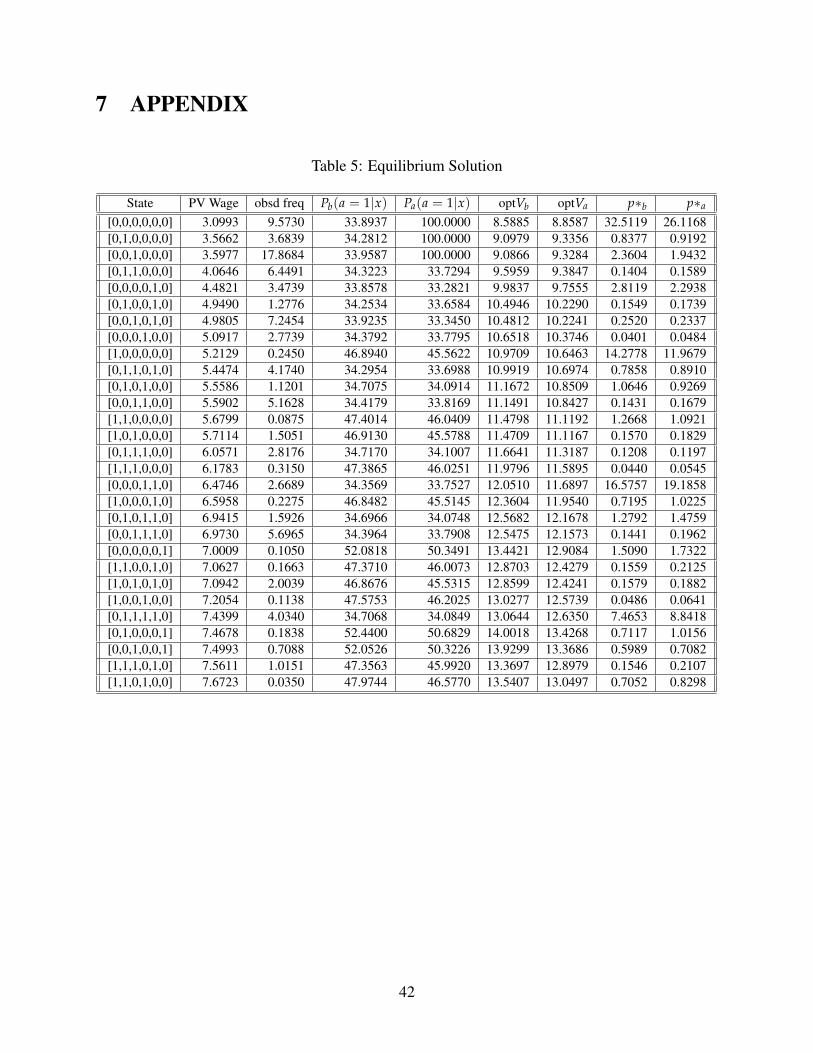
Table 5: Equilibrium Solution

State PV Wage obsd freq Pb(a = 1|x) Pa(a = 1|x) optVb optVa p∗b p∗a

[0,0,0,0,0,0] 3.0993 9.5730 33.8937 100.0000 8.5885 8.8587 32.5119 26.1168[0,1,0,0,0,0] 3.5662 3.6839 34.2812 100.0000 9.0979 9.3356 0.8377 0.9192[0,0,1,0,0,0] 3.5977 17.8684 33.9587 100.0000 9.0866 9.3284 2.3604 1.9432[0,1,1,0,0,0] 4.0646 6.4491 34.3223 33.7294 9.5959 9.3847 0.1404 0.1589[0,0,0,0,1,0] 4.4821 3.4739 33.8578 33.2821 9.9837 9.7555 2.8119 2.2938[0,1,0,0,1,0] 4.9490 1.2776 34.2534 33.6584 10.4946 10.2290 0.1549 0.1739[0,0,1,0,1,0] 4.9805 7.2454 33.9235 33.3450 10.4812 10.2241 0.2520 0.2337[0,0,0,1,0,0] 5.0917 2.7739 34.3792 33.7795 10.6518 10.3746 0.0401 0.0484[1,0,0,0,0,0] 5.2129 0.2450 46.8940 45.5622 10.9709 10.6463 14.2778 11.9679[0,1,1,0,1,0] 5.4474 4.1740 34.2954 33.6988 10.9919 10.6974 0.7858 0.8910[0,1,0,1,0,0] 5.5586 1.1201 34.7075 34.0914 11.1672 10.8509 1.0646 0.9269[0,0,1,1,0,0] 5.5902 5.1628 34.4179 33.8169 11.1491 10.8427 0.1431 0.1679[1,1,0,0,0,0] 5.6799 0.0875 47.4014 46.0409 11.4798 11.1192 1.2668 1.0921[1,0,1,0,0,0] 5.7114 1.5051 46.9130 45.5788 11.4709 11.1167 0.1570 0.1829[0,1,1,1,0,0] 6.0571 2.8176 34.7170 34.1007 11.6641 11.3187 0.1208 0.1197[1,1,1,0,0,0] 6.1783 0.3150 47.3865 46.0251 11.9796 11.5895 0.0440 0.0545[0,0,0,1,1,0] 6.4746 2.6689 34.3569 33.7527 12.0510 11.6897 16.5757 19.1858[1,0,0,0,1,0] 6.5958 0.2275 46.8482 45.5145 12.3604 11.9540 0.7195 1.0225[0,1,0,1,1,0] 6.9415 1.5926 34.6966 34.0748 12.5682 12.1678 1.2792 1.4759[0,0,1,1,1,0] 6.9730 5.6965 34.3964 33.7908 12.5475 12.1573 0.1441 0.1962[0,0,0,0,0,1] 7.0009 0.1050 52.0818 50.3491 13.4421 12.9084 1.5090 1.7322[1,1,0,0,1,0] 7.0627 0.1663 47.3710 46.0073 12.8703 12.4279 0.1559 0.2125[1,0,1,0,1,0] 7.0942 2.0039 46.8676 45.5315 12.8599 12.4241 0.1579 0.1882[1,0,0,1,0,0] 7.2054 0.1138 47.5753 46.2025 13.0277 12.5739 0.0486 0.0641[0,1,1,1,1,0] 7.4399 4.0340 34.7068 34.0849 13.0644 12.6350 7.4653 8.8418[0,1,0,0,0,1] 7.4678 0.1838 52.4400 50.6829 14.0018 13.4268 0.7117 1.0156[0,0,1,0,0,1] 7.4993 0.7088 52.0526 50.3226 13.9299 13.3686 0.5989 0.7082[1,1,1,0,1,0] 7.5611 1.0151 47.3563 45.9920 13.3697 12.8979 0.1546 0.2107[1,1,0,1,0,0] 7.6723 0.0350 47.9744 46.5770 13.5407 13.0497 0.7052 0.8298

42

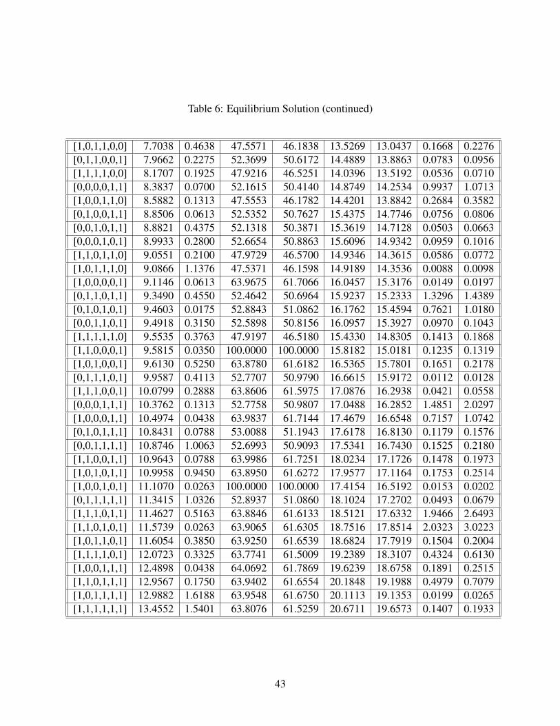
Table 6: Equilibrium Solution (continued)

[1,0,1,1,0,0] 7.7038 0.4638 47.5571 46.1838 13.5269 13.0437 0.1668 0.2276[0,1,1,0,0,1] 7.9662 0.2275 52.3699 50.6172 14.4889 13.8863 0.0783 0.0956[1,1,1,1,0,0] 8.1707 0.1925 47.9216 46.5251 14.0396 13.5192 0.0536 0.0710[0,0,0,0,1,1] 8.3837 0.0700 52.1615 50.4140 14.8749 14.2534 0.9937 1.0713[1,0,0,1,1,0] 8.5882 0.1313 47.5553 46.1782 14.4201 13.8842 0.2684 0.3582[0,1,0,0,1,1] 8.8506 0.0613 52.5352 50.7627 15.4375 14.7746 0.0756 0.0806[0,0,1,0,1,1] 8.8821 0.4375 52.1318 50.3871 15.3619 14.7128 0.0503 0.0663[0,0,0,1,0,1] 8.9933 0.2800 52.6654 50.8863 15.6096 14.9342 0.0959 0.1016[1,1,0,1,1,0] 9.0551 0.2100 47.9729 46.5700 14.9346 14.3615 0.0586 0.0772[1,0,1,1,1,0] 9.0866 1.1376 47.5371 46.1598 14.9189 14.3536 0.0088 0.0098[1,0,0,0,0,1] 9.1146 0.0613 63.9675 61.7066 16.0457 15.3176 0.0149 0.0197[0,1,1,0,1,1] 9.3490 0.4550 52.4642 50.6964 15.9237 15.2333 1.3296 1.4389[0,1,0,1,0,1] 9.4603 0.0175 52.8843 51.0862 16.1762 15.4594 0.7621 1.0180[0,0,1,1,0,1] 9.4918 0.3150 52.5898 50.8156 16.0957 15.3927 0.0970 0.1043[1,1,1,1,1,0] 9.5535 0.3763 47.9197 46.5180 15.4330 14.8305 0.1413 0.1868[1,1,0,0,0,1] 9.5815 0.0350 100.0000 100.0000 15.8182 15.0181 0.1235 0.1319[1,0,1,0,0,1] 9.6130 0.5250 63.8780 61.6182 16.5365 15.7801 0.1651 0.2178[0,1,1,1,0,1] 9.9587 0.4113 52.7707 50.9790 16.6615 15.9172 0.0112 0.0128[1,1,1,0,0,1] 10.0799 0.2888 63.8606 61.5975 17.0876 16.2938 0.0421 0.0558[0,0,0,1,1,1] 10.3762 0.1313 52.7758 50.9807 17.0488 16.2852 1.4851 2.0297[1,0,0,0,1,1] 10.4974 0.0438 63.9837 61.7144 17.4679 16.6548 0.7157 1.0742[0,1,0,1,1,1] 10.8431 0.0788 53.0088 51.1943 17.6178 16.8130 0.1179 0.1576[0,0,1,1,1,1] 10.8746 1.0063 52.6993 50.9093 17.5341 16.7430 0.1525 0.2180[1,1,0,0,1,1] 10.9643 0.0788 63.9986 61.7251 18.0234 17.1726 0.1478 0.1973[1,0,1,0,1,1] 10.9958 0.9450 63.8950 61.6272 17.9577 17.1164 0.1753 0.2514[1,0,0,1,0,1] 11.1070 0.0263 100.0000 100.0000 17.4154 16.5192 0.0153 0.0202[0,1,1,1,1,1] 11.3415 1.0326 52.8937 51.0860 18.1024 17.2702 0.0493 0.0679[1,1,1,0,1,1] 11.4627 0.5163 63.8846 61.6133 18.5121 17.6332 1.9466 2.6493[1,1,0,1,0,1] 11.5739 0.0263 63.9065 61.6305 18.7516 17.8514 2.0323 3.0223[1,0,1,1,0,1] 11.6054 0.3850 63.9250 61.6539 18.6824 17.7919 0.1504 0.2004[1,1,1,1,0,1] 12.0723 0.3325 63.7741 61.5009 19.2389 18.3107 0.4324 0.6130[1,0,0,1,1,1] 12.4898 0.0438 64.0692 61.7869 19.6239 18.6758 0.1891 0.2515[1,1,0,1,1,1] 12.9567 0.1750 63.9402 61.6554 20.1848 19.1988 0.4979 0.7079[1,0,1,1,1,1] 12.9882 1.6188 63.9548 61.6750 20.1113 19.1353 0.0199 0.0265[1,1,1,1,1,1] 13.4552 1.5401 63.8076 61.5259 20.6711 19.6573 0.1407 0.1933

43