Ecosystem Based Fisheries Management for the Western ...
80
Opitz & Froese, 2019 – EBFM for the WBS 1 Ecosystem Based Fisheries Management for the Western Baltic Sea Extended Report Silvia Opitz (1) and Rainer Froese (2) (1) e-mail: [email protected], (2) e-mail: [email protected] October 2019
Transcript of Ecosystem Based Fisheries Management for the Western ...
Opitz & Froese, 2019 – EBFM for the WBS
1
Ecosystem Based Fisheries Management for the Western Baltic Sea
Extended Report
Silvia Opitz (1) and Rainer Froese (2) (1)e-mail: [email protected], (2)e-mail: [email protected]
October 2019
Opitz & Froese, 2019 – EBFM for the WBS
2
Contents Page
Abstract……………………………………………………………………………………………………………………… 3 Keywords…………………………………………………………………………………………………………………… 4 Introduction……………………………………………………………………………………………………………….. 4
Objectives………….……………………….……………………………………………………………………………… 5
Project Description, Study Area (Map)………..………………………….……………………………... 5
Material & Methods…………………………………………………………………………………………………... 6
Trophic Groups in the Model of the WBS Ecosystem.………………………….…. 8 Data Sources………………………………………………………………………………………….... 10 Preparation of Basic Model Inputs for EwE……………….…………………………… 13
Biomass (B)……….…………………………………………………………………..... 13 Production / Biomass Ratio (P/B)………….…………………………………. 15 Consumption / Biomass Ratio (Q/B)…..……………………………………. 17 Non-assimilated Part of the Food (NA)…….…….………………………… 18 Diet Composition (DC)…………………………..….……………………………… 19 Fishery…………………………….…………………….….………………………………. 20
Pelagic Fleet Landings……………………………………………………. 21 Demersal Fleet Landings……………………………………………….. 21 Recreational Fishery Landings…………………………………...... 21 Bycatch / IUU Fishery Landings………………………………..….. 22 Pelagic Fleet Discards……………………………………………………. 23 Demersal Fleet Discards……………………………………………….. 23 Other Discards….……………………………………………………………. 24
Data Pedigree…………………………………………………………………………………………….. 26 Balancing Process………………………………………………………………………………………. 28 Dynamic Modelling of Different Fishery Management Scenarios…….……… 29
Results……………………………………………………………………………………………………………………… 31
Starting Situation in 1994 Represented by the Static Model………………….. 31 Trophic Flows within the Western Baltic Sea Food Web…….…………………….. 36 Relative Total Impact…………………………………………………………………………………..44 Mixed Trophic Impacts……………………..……………………………………………..………… 44 Dynamic Modelling of Different Fishery Management Scenarios……………….45 Exploring Ecosystem Development Until 2050 Under Different Scenarios. 50 Primary Production Required (PPR) in the WBS ecosystem……………………… 65
Discussion……………………………………………………………………………………….………………………… 67
Quality of the 1994 Model…………………….……………………………..…………………… 67 Quality of the EwE Fitting and Predictions…..….…....…………..….……………….. 68 Correction of Misconceptions………………….…….….……………...………………………. 71 EBFM for the WBS…………………………………...……....…….……………………………….. 73
Conclusions……………………………………………………………………….……………………………………. 74
Acknowledgements………………………………..…………….……………………………………………….. 74
References……………………………………………..……………….…………………………………………….. 75
Opitz & Froese, 2019 – EBFM for the WBS
3
Abstract Legal requirement in Europe asks for Ecosystem-Based Fisheries Management (EBFM) in
European seas, including considerations of trophic interactions and minimization of
negative impacts of fishing on food webs and ecosystem functioning.
Focusing on the interaction between fisheries and ecosystem components, the trophic
model presented here shows for the first time the “big picture” of the western Baltic Sea
(WBS) food web by quantifying structure and flows between all trophic elements and the
impact of fisheries that were and are active in the area, based on best available recent
data.
Model results show that fishing pressures exerted on the WBS since the early nineties of
the past century forces not only top predators such as harbour porpoises and seals but
also cod and other demersal fish to heavily compete for fish as food and to cover their
dietary needs by shifting to organisms lower in the trophic web, mainly to benthic
macrofauna and / or search for suitable prey in adjacent ecosystems such as Kattegat,
Skagerrak, central Baltic Sea and North Sea.
While common sense implementations of EBFM have been proposed, such as fishing all
stocks below Fmsy and reducing fishing pressure even further for forage fish such as
herring and sprat, few studies compared such fishing to alternative scenarios. Different
options for EBFM, with regards to recovery of depleted stocks and sustainable future
catches, are presented here based on the WBS ecosystem model, the legal framework
given by the new Common Fisheries Policy (CFP) and the Marine Strategy Framework
Directive (MSFD) of the European Union.
The model explores four legally valid future fishery scenarios: 1) business as usual, 2)
maximum sustainable fishing (F = Fmsy), 3) half of Fmsy, and 4) EBFM with F = 0.5 Fmsy for
forage fish and F = 0.8 Fmsy for other fish. In addition, a “No-fishing” scenario
demonstrates, that neither individual stocks nor the whole system would collapse when
all fishing activities from 2017 on would cease.
Simulations show that “Business as usual” would perpetuate low 2016 catches from
depleted stocks in an unstable ecosystem where endangered species may be lost. In
contrast, an “EBFM” scenario - with herring and sprat fished at 0.5 Fmsy level and cod and
other stocks fished at 0.8 Fmsy level - allows the recovery of all stocks with strongly
increased catches close to the maximum (at Fmsy) for cod and flatfish and catches similar
to the 2016 level for herring and sprat but with strongly reduced fishing effort.
Model and methodology presented here are considered suitable to assess MSFD Criterion
D4C2 in the WBS.
Opitz & Froese, 2019 – EBFM for the WBS
4
Keywords Ecosystem Based Fisheries Management (EBFM), food web, trophic model, western Baltic Sea, CFP, MSFD.
Introduction Fishing belongs to the strongest negative anthropogenic interventions on marine
ecosystems (Jones 1992, Hall et al. 2000, and Kaiser et al. 2006). In northern Europe,
this is particularly true for the North and Baltic Seas and consequently also for the
German Exclusive Economic Zone (EEZ) of both seas where all major species have been
heavily overfished for decades. The new Common Fisheries Policy (CFP, 2013) of the
European Union (EU) demands the end of overfishing latest in 2020. The Marine Strategy
Framework Directive (MSFD 2008, 2017a,b) of the EU demands furthermore - as criteria
of good environmental status - (1) biological diversity with species abundance or
demographic characteristics not affected by anthropogenic pressures, (2) a healthy size
and age structure of exploited stocks and (3) marine food webs with species composition,
diversity, balance, and productivity of the trophic guilds not affected by anthropogenic
pressures.
Ecosystem-Based Fisheries Management (EBFM) is a new direction for fishery
management, which essentially reverses the order of management priorities so that
management starts with the ecosystem considerations rather than the maximum
exploitation of several target species (Pikitch et al. 2004). EBFM aims to sustain healthy
marine ecosystems and the fisheries they support. Specifically, it aims to rebuild and
sustain populations of non-target and protected species.
The purpose of this study was thus the creation of a first ecosystem model for the WBS
ecosystem, using the best available recent data and focusing on the interaction between
fisheries and ecosystem components. Of special interest were the impacts of long-term
overfishing of important commercial stocks such as western Baltic cod (Gadus morhua)
and western Baltic spring spawning herring (Clupea harengus), the role of herring and
sprat (Sprattus sprattus) as low trophic level (LTL) key species in the food web, the level
of cannibalism of adult cod on juvenile cod, the competition between marine mammals
and fishers for fish, and the extraction of fish by seabirds.
Model results aim to offer suggestions for sustainable fisheries management measures
according to Article 2.3 of the new CFP of the EU which calls for the implementation of
“an ecosystem based approach for fisheries management by minimizing the negative
impacts of fishing activities”.
Opitz & Froese, 2019 – EBFM for the WBS
5
The WBS fishery model is furthermore viewed as a supporting tool for comparing model
results with stock assessments of the International Council for the Exploration of the Sea
(ICES). The model serves also as a prerequisite for estimating the impact of the recently
modified CFP on commercially exploited fish stocks and other elements of the WBS
ecosystem.
Objectives Based on the first ecosystem model for the WBS and the legal framework given by the
CFP and MSFD, the goal of this study was to present and compare different options for
EBFM with regard to recovery of depleted stocks and sustainable future catches.
A preliminary version of the WBS model was previously presented by Opitz & Garilao
(2014). The model presented here is viewed as a prototype that may be updated when
appropriate information / data becomes available and / or adapted to objectives of other
studies.
For the Baltic Sea a series of earlier models exist although to date there is no published
trophic network model of the WBS available. An overview of existing models may be
found further below in chapter “Data Sources”. All of them represent areas east of the
Arkona Basin, and of the German NATURA 2000 areas. Furthermore, with one exception
(Hansson et al. 2007), all models were prepared almost exclusively with data sets from
the last third of the 20th century. Except for Harvey et al. (2003) and Hansson et al.
(2007) the interaction between ecosystem components and fisheries was not the focus of
those models. The preparation of updated models is thus not only of importance for the
alignment of actions towards EBFM in the entire region and particularly in NATURA 2000
areas but also contribute to fill gaps of knowledge from a scientific point of view.
Project Description, Study Area (Map) In the scope of the project “Ecosystem Based Fisheries Management in the German EEZ”
implemented by the German Federal Agency for Environmental Protection (Bundesamt
für Naturschutz BfN) impacts of commercial fisheries on the marine ecosystem in the
German EEZ of the North and Baltic Seas, with special emphasis on NATURA 2000 areas
are being studied by the use of trophic network models.
The model area covers ICES subdivisions (SDs) 22 and 24. The reason to fit the model to
ICES management areas was that ICES has organized its fishery data by SDs which
makes it convenient for model construction because quantification of biomass and
catches of exploited fish stocks is (mostly) straightforward and more reliable. But our
Opitz & Froese, 2019 – EBFM for the WBS
6
model area also represents an ecologically more uniform area than the surrounding
regions. Salinity of SD 21 north of SD 22 is similar to conditions in the Kattegat and
Skagerak and considerably higher than in the southern areas. SD 23, representing the
sound that separates Sweden from Denmark has mostly rocky ground with ecological
qualities different from the sandy-muddy areas in SDs 22 and 24. The model area is
thus a compromise between data availability and ecological concerns.
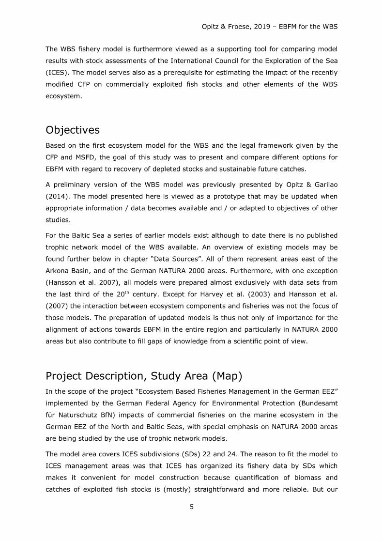
Geographical regions represented by the WBS model are: Great Belt, Little Belt, Kiel
Bay, Bay of Mecklenburg, Arkona Basin until West of Bornholm Basin (ICES subdivisions
22 and 24) and including all NATURA 2000 areas in the German EEZ (see Fig. 1).
NATURA 2000 areas in the German EEZ comprise Fehmarn Belt, Kadetrinne, Western
Rönnebank, Adlergrund and Pomeranian Bay with Oderbank, while Pomeranian Bay is
also a designated EU bird protection area (see Fig. 1).
Figure 1: Area represented by the WBS ecosystem model: WBS with German EEZ (green line), NATURA 2000 areas (white) and ICES subdivisions 22 and 24 (red line).
Material & Methods The basic trophic network model represents the WBS ecosystem in the year 1994
because this is the year when catch and stock size data were available online from ICES
for the majority of fish stocks included in the model, but particularly for cod, herring, and
sprat, the economically most important species in the WBS. Starting in 1994, it was
possible to subsequently model dynamically a time span of >20 years (see below).
The Ecopath with Ecosim software package (EwE, www.ecopath.org) was used for model
preparation. EwE is a software package suited for personal computers. The approach is
Opitz & Froese, 2019 – EBFM for the WBS
7
thoroughly documented in the scientific literature (see. e.g. Polovina 1984, Christensen
and Pauly 1992; Pauly et al. 2000). The EwE model software may be downloaded for
free from www.ecopath.org/downloads.
The basic trophic network model representing the WBS ecosystem in the year 1994 was
prepared using the Ecopath routine. Ecopath helps the user to create mass-balanced
snapshots of the resources in an ecosystem and their interactions, represented by
trophically linked biomass ‘pools’. These may consist of a single species, or species
groups representing ecological guilds. Pools may be further split into ontogenetically
linked groups called ‘multi-stanzas’ such as done here for adult (>35 cm) and juvenile
(<=35 cm) cod.
Ecopath bases the parameterization on an assumption of mass balance over an arbitrary
period, usually a year. In accordance with this feature the WBS model used annual
means as parameter inputs.
“The parameterization of an Ecopath model is based on satisfying two ‘master’
equations: The first equation describes how the production term for each group can be
divided:
(1) Production = catch + predation + net migration + biomass accumulation + other
mortality - import
The second ‘master’ equation is based on the principle of conservation of matter within a
group:
(2) Consumption = production + respiration + unassimilated food
A detritus compartment (D) receives flows originating from "other mortality (M)" and
"non-assimilated food (NA)", so that
(3) D = M + NA.
The model can accept accumulation and depletion of biomasses during the time period
modelled despite of the steady state assumption. Thus, biomass accumulation or
depletion rates can be quantified.
Input of three of the following four parameters is required for every functional group in a
model: biomass (B), production/biomass ratio (P/B) (or total mortality Z),
consumption/biomass ratio (Q/B), and ecotrophic efficiency (EE). Here, EE expresses the
proportion of the production that is used in the system, (i.e. it incorporates all production
terms apart from ‘other mortality’). If all four basic parameters are available for a group
the program can estimate either biomass accumulation or net migration. Ecopath sets up
a series of linear equations to solve for unknown values establishing mass-balance in the
same operation”.
Opitz & Froese, 2019 – EBFM for the WBS
8
A wide range of information on structure and matter flows within an ecosystem can be
obtained from Ecopath models. For more details see Christensen et al. (2000).
The Ecosim component of EwE provides a dynamic simulation capability at the ecosystem
level, with key initial parameters inherited from the base Ecopath model.
The basics of Ecosim consist of biomass dynamics expressed through a series of coupled
differential equations. The equations are derived from the Ecopath master equation and
take the form
(4) dBi / dt = gi ∑j Qji – ∑j Qij + Ii – (MOi + Fi + ei) Bi
where dBi / dt represents the growth rate during the time interval dt of group (i) in terms
of its biomass Bi; gi is the net growth efficiency (production/consumption ratio); ∑j Qji
total consumption by group i; ∑j Qij total predation by all predators on group i; MOi the
non-predation (‘other’) natural mortality rate; Fi is fishing mortality rate, ei is emigration
rate, Ii is immigration rate (Walters et al. 1997, 2000).
By doing repeated simulations Ecosim allows for the fitting of predicted biomasses to
time series data. “Sum of squares” (SS) in Ecosim is a measure for the goodness of fit
between input values and model outputs.
Ecosim was used for the purpose of fitting model outputs and time series data of
biomass, fishing mortality and catch.
Ecosim furthermore allows the dynamic forward projection of future biomass of trophic
groups based on the reported or assumed F exerted on the commercial groups (from
1994 until 2016).
This feature was used to evaluate the impact of different fishery scenarios on stock size
and catch into the future (from 2017 until 2050).
Trophic Groups in the Model of the WBS Ecosystem
The following 18 trophic groups - comprising the WBS ecosystem - are represented in our
model:
Harbour porpoises: Due to their dietary preferences, harbour porpoises (Phocoena
phocoena) act as top predators in the WBS ecosystem.
Seals: Due to their dietary preferences, seals also act as top predators in the WBS
ecosystem. The group represents two species: Mainly grey seal (Halichoerus grypus)
and harbour seal (Phoca vitulina) while the latter is much less common in the area than
Opitz & Froese, 2019 – EBFM for the WBS
9
the former. Theoretically, also the river otter (Lutra lutra) should be included here, but
no information on abundance was available to the authors.
(Sea-)birds: Theoretically, HELCOM (Helsinki Commission, see www.helcom.fi/) lists
around 50 bird species as occurring in the WBS ecosystem. However, biomass values
here are based only on the following 27 species occurring in different zones of the
German Baltic(?) EEZ (Schleswig-Holstein and Mecklenburg - Western Pomerania):
Gavia stellata, Gavia arctica, Podiceps cristatus, Podiceps grisegena, Podiceps auritus,
Fulmarus glacialis, Sula bassana, Phalacrocorax carbo, Aythya marila, Somateria
mollissima, Clangula hyemalis, Melanitta nigra, Melanitta fusca, Mergus serrator,
Hydrocoloeus minutus, Larus ridibundus, Larus canus, Larus fuscus, Larus argentatus,
Larus marinus, Rissa tridactyla, Sterna sandvicensis, Sterna hirundo, Sterna paradisaea,
Uria aalge, Alca torda, Cepphus grylle.
Adult cod: “Cod >35 cm” represents adults of the WBS cod (Gadus morhua) stock. The
cut-off length of 35 cm between adults and juveniles represents the official EU minimum
landing length of cod in the Baltic Sea after 2014.
Juvenile cod: “Cod<=35 cm" represents juveniles of the WBS cod stock.
The “Flat fish” box incorporates 1) flounder (Platichthys flesus), 2) dab (Limanda
limanda), 3) plaice (Pleuronectes platessa), 4) turbot (Scophthalmus maximus) and 5)
brill (Scophthalmus rhombus). The Baltic stocks of flounder, plaice, and turbot are fully
assessed by ICES, dab and brill stocks are not.
Other demersal fish represents > 130 species populating the lower parts of the water
column of the WBS (for a list of fish species in WBS see www.fishbase.org); only 53
species from this list were caught in the DATRAS BITS surveys from which a first
estimate of biomass for this group was calculated for 1994. It also includes 10 flatfish
species not fully assessed by ICES.
Herring represents a single species: Clupea harengus. The WBS herring stock (western
Baltic spring spawning herring (WBSS)) is fully assessed by ICES.
Sprat represents a single species: Sprattus sprattus. The Baltic Sea sprat stock is fully
assessed by ICES.
Other pelagic fish represents about 35 species populating the upper and midwater parts
of the water column of the WBS except for herring and sprat which are represented by
single species compartments. Only 10 species (Alosa fallax, Atherina presbyter, Belone
belone, Engraulis encrasicolus, Osmerus eperlanus, Salmo trutta, Sander lucioperca,
Sardina pilchardus, Scomber scombrus, Trachurus trachurus) from this list are recorded
in the DATRAS BITS surveys (designed for catching demersal fish) from which a
Opitz & Froese, 2019 – EBFM for the WBS
10
preliminary estimate of biomass was calculated for 1994. The “true” biomass for "Other
pelagic fish" though was assumed to be much higher.
Pelagic macrofauna comprises all animals >2 cm in size inhabiting the water column of
the WBS. This is mainly jellyfish such as moon jellyfish (Aurelia aurita) and lion´s mane
jellyfish (Cyanea capillata), other cnidarians such as hydrozoans, and several species of
polychaetes.
Benthic macrofauna represents a vast number (>500) of invertebrate species (Annelida,
Arthropoda, Bryozoa, Chordata, Cnidaria, Echinodermata, Mollusca, Nemertea,
Phoronida, Platyhelminthes, Porifera, Priapulida, Sipunculida) >1 mm in size and
associated with the benthic habitat of the WBS. A complete list of benthic macrofaunal
species is available from the lead author and / or from www.sealifebase.org.
Benthic meiofauna represents all animals <1 mm in length associated with the bottom
substrate in the WBS. These were not identified down to the species level.
Zooplankton merges micro-, meso-, and macrozooplankton into a single group.
Microzooplankton comprises planktonic animals from 0.02 to 0.2 mm in size (e.g.
phagotrophic protists such as flagellates, dinoflagellates, ciliates, acantharids,
radiolarians, foraminiferans, etc., and metazoans such as copepod nauplii, rotiferan and
meroplanktonic larvae); mesozooplankton comprises planktonic animals from 0.2 to 2
mm in size (in WBS mainly adult copepods and cladocerans); and macrozooplankton all
planktonic animals >2 mm in size (in WBS mainly mysids and amphipods).
Bacteria / microorganisms represents bacteria and other microorganisms <0.02-0.03
mm in size and associated with the bottom substrate and/or with the water column in the
WBS. Includes flagellates living in part autotrophically.
Phytoplankton comprises pelagic microalgae. Species composition in the WBS is unknown
to the authors.
Benthic producers represents benthic (macro- and micro-) algae and seaweeds. Phyla
occurring in WBS: Angiospermophyta, Charophyta, Chlorophyta, Ochrophyta,
Phaeophyta, Rhodophyta, Xanthophyta. A tentative species list is available from the lead
author and from www.sealifebase.org.
Detritus/DOM represents dead organic matter - particulate and dissolved.
Data Sources
Estimates of biomass (B), production (P/B year-1), consumption (Q/B year-1),
unassimilated consumption (NA), diet composition (DC), catch (C), and fishing mortality
Opitz & Froese, 2019 – EBFM for the WBS
11
(F) in 1994 were obtained from various sources. And so were time series for (B), (C),
and (F) for years 1994 to 2016.
Principal data sources were: FishBase (www.fishbase.org), SeaLifeBase
(www.sealifebase.org), ICES database, ICES Advice, ICES Working Group Reports, ICES
Stock Summaries, DATRAS, HELCOM, published ecosystem models of other areas in the
Baltic Sea (see Table 1 below), other relevant literature, and - last but not least -
personal communications by expert colleagues.
Opitz & Froese, 2019 – EBFM for the WBS
12
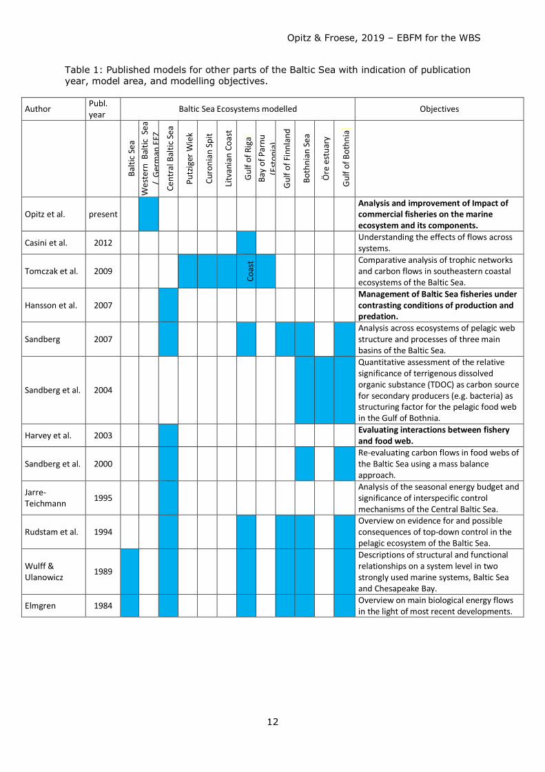
Table 1: Published models for other parts of the Baltic Sea with indication of publication year, model area, and modelling objectives.
Author Publ. year Baltic Sea Ecosystems modelled Objectives
Balti
c Se
a W
este
rn B
altic
Sea
/
Ger
man
EEZ
Ce
ntra
l Bal
tic S
ea
Putz
iger
Wie
k
Curo
nian
Spi
t
Litv
ania
n Co
ast
Gul
f of R
iga
Ba
y of
Par
nu
(Est
onia
) G
ulf o
f Fin
nlan
d
Both
nian
Sea
Öre
est
uary
Gul
f of B
othn
ia
Opitz et al. present
Analysis and improvement of Impact of commercial fisheries on the marine ecosystem and its components.
Casini et al. 2012 Understanding the effects of flows across systems.
Tomczak et al. 2009 Co
ast
Comparative analysis of trophic networks and carbon flows in southeastern coastal ecosystems of the Baltic Sea.
Hansson et al. 2007
Management of Baltic Sea fisheries under contrasting conditions of production and predation.
Sandberg 2007
Analysis across ecosystems of pelagic web structure and processes of three main basins of the Baltic Sea.
Sandberg et al. 2004
Quantitative assessment of the relative significance of terrigenous dissolved organic substance (TDOC) as carbon source for secondary producers (e.g. bacteria) as structuring factor for the pelagic food web in the Gulf of Bothnia.
Harvey et al. 2003 Evaluating interactions between fishery and food web.
Sandberg et al. 2000
Re-evaluating carbon flows in food webs of the Baltic Sea using a mass balance approach.
Jarre-Teichmann 1995
Analysis of the seasonal energy budget and significance of interspecific control mechanisms of the Central Baltic Sea.
Rudstam et al. 1994
Overview on evidence for and possible consequences of top-down control in the pelagic ecosystem of the Baltic Sea.
Wulff & Ulanowicz 1989
Descriptions of structural and functional relationships on a system level in two strongly used marine systems, Baltic Sea and Chesapeake Bay.
Elmgren 1984 Overview on main biological energy flows in the light of most recent developments.
Opitz & Froese, 2019 – EBFM for the WBS
13
Preparation of Basic Model Inputs for EwE
Biomass (B)
Because biomass of a trophic group is far more ecosystem specific than physiological
parameters like production and consumption, realistic biomass values are therefore of
paramount importance for any model aimed to closely represent matter flow in a specific
ecosystem. In the following it will be explained how biomass values for each trophic
group was calculated. Wet or fresh weight was transformed into carbon by applying a
factor of 10:1, if not otherwise stated. Values represent biomass in ICES subdivisions
22+24, if not otherwise stated.
Harbour porpoises: Value in wet weight (WW) was derived from biomass indications by
A. Gilles (pers. comm.) and from Viquerat et al. (2014) for German coastal waters of the
Baltic Sea.
Seals: Value in WW was derived from a trophic model by Harvey et al. (2003)
representing ICES SDs 25-29 + 32 and covering years 1974 - 2000.
(Sea-)birds: Value in WW was derived from indications on number of individuals of 27
bird species in different zones (EEZ, coastal and offshore zones of Schleswig-Holstein and
Mecklenburg - Western Pomerania) of the German part of the Baltic Sea (information
kindly made available by colleagues from ECOLAB, FTZ Büsum; www.ftz.uni-
kiel.de/de/forschungsabteilungen/ecolab-oekologie-mariner-tiere). Data are based on
counts from the 1st decade of the 21st century. Number of individuals was multiplied
with indications on mean WW of species - all values obtained through internet queries –
the majority of values were derived from Wikipedia (www.wikipedia.org). Total weight for
each species was then divided by the number of m2 of total area (information on km2
values per area kindly made available by colleagues from ECOLAB, FTZ Büsum).
Adult cod: B is based on data for western Baltic cod stock from Table 12 in ICES
(2017a). SSB for age 3-5 for year 1994 was divided by area size for SD 22, 23 and 24
(44 746 km2) to obtain gWWm-2. The biomass value of cod should be treated with some
caution as a recent comparison of cod otoliths readings from countries involved proved
to be uncertain (R. Froese pers. comm.)
Juvenile cod: Value was calculated by multi-stanza routine in Ecopath based on B for
adult cod. The stanza routine result was adapted to an external value of B for juvenile
cod. The external value was calculated to be the difference between total stock B (TSB,
obtained from Table 2.3.22 in ICES 2017b) and SSB (obtained from Table 12 in ICES
2017a), both for 1994. The difference was then divided by area size for SD 22, 23 and 24
(44,746 km2) to obtain gWWm-2.
Opitz & Froese, 2019 – EBFM for the WBS
14
Flatfish: dab, flounder, plaice, turbot, and brill: B for this group represents the summed
total of the five species for year 1994. TSB for plaice in ICES SDs 21-23 is based on
Table 5.2.7 in ICES (2016b). B for 1994 is back calculated based on mean exploitation
rate (ExplR) for years 1999-2001. B in WW for 1994 was calculated from DATRAS BITS
CPUE data separately for dab, flounder, turbot and brill as follows: number of individuals
per length class from CPUE was multiplied by weight per individual per length class
obtained from length - weight relationship (LWR) by species. Total B was then divided by
area size for SD 22 and 24 to obtain gWWm-2.
Other demersal fish: Original B for this group was calculated from DATRAS BITS CPUE
data for demersal fish but excluding cod and the five species in the flatfish box (B
proportion of flatfish on total group B was ca. 13.5 %). No. of individuals per length
class from CPUE was multiplied by weight per individual per length class obtained from
length - weight relationship by species. WW was converted into carbon weight. The B
value of 0.0436 gCm-2 obtained from DATRAS BITS in this way was much too low to
satisfy predator requirements (including fishery); the necessary minimum B was obtained
during the balancing process by setting EE for this group to 0.99.
Herring: Original input B was obtained by dividing SSB for 1994 in ICES SDs 20 - 24
(WBSS herring) from Table 11 in ICES (2017i) by area size (102,288 km2) to obtain
gWWm-2.
Sprat: Available SSB value for 1994 in ICES SDs 22-32 from Tables in ICES (2017j) was
adjusted to SDs 22-24 by calculating ExplR (B / landings) for SDs 22-32 (median = 3.24
%) and calculating B for SDs 22-24 by applying this percent relationship to sprat
landings for SDs 22-24 from tables in ICES (2017b).
Other pelagic fish: Original B was calculated from DATRAS BITS CPUE data for demersal
fish. For species in the DATRAS database identified to be pelagic the number of
individuals per length class from CPUE data was multiplied by weight per individual per
length class obtained from LWR by species. Resulting B (0.00349 gCm-2) was much too
low to satisfy predator requirements (including fishery). This value might have strongly
underestimated the real B of pelagic fish since DATRAS BITS surveys are made with
bottom trawls targeting demersal species. An estimate of the necessary minimum B was
obtained during the balancing process by setting EE to 0.99.
Pelagic macrofauna: Mainly medusae (several species); B is an average of B values in
Harvey et al. (2003, 0.133 gCm-2) and Jarre-Teichmann (1995, 0.27 gCm-2) for Baltic
Proper.
Benthic macrofauna: Fresh weight was read off an unpublished graph on benthic
macrofauna for ICES SDs 22 and 24, kindly provided by M. Zettler, IOW Warnemünde.
Opitz & Froese, 2019 – EBFM for the WBS
15
Benthic meiofauna: An estimate of fresh weight was provided by M. Zettler, IOW
Warnemünde (pers.comm.).
Zooplankton: B represents lumped B for macro (mainly mysids) -, meso-, and
microzooplankton. B values for each group correspond to the mean of a range for each
group from a series of published trophic models (see Table 1 for an overview). For
conversion of WW into carbon a factor of 1 gWW = 12.07 gC and 1 gC = 0.0828 gWW
was applied.
Bacteria/microorganisms: B represents the average of a range (0.21-0.42 gCm-2) from a
series of published trophic models (see Table 1 for an overview).
Phytoplankton: B represents the average of a range (1.01-3.312 gCm-2) from a series of
published models (see Table 1 for an overview). For conversion of WW into carbon a
factor of 1 gWW = 12.07 gC and 1 gC = 0.0828 gWW was applied.
Benthic producers: B represents a rough estimate between lower values (0.02 – 0.0214
gCm-2) from several published models (see Table 1 for an overview), mainly Sandberg et
al. (2000), Jarre-Teichmann (1995) for Baltic Proper, and Wulff & Ulanowicz (1989)
(adopted from Elmgren, 1984) for the whole Baltic Sea, and a very high value of 65.74
gCm-2 (based on estimates of macroalgae production for the whole Baltic Sea in
Bergström, 2012).
Detritus/DOM: Value represents the average of a range (680-885 gCm-2) from Sandberg
et al. (2000) for Baltic Proper and Wulff & Ulanowicz (1989) for the whole Baltic Sea.
Production / Biomass ratio (P/B)
Production refers to the building up of biomass by a group over the period considered,
entered as P/B per year and transformed into absolute flows (gCm-2y-1) by the Ecopath
software. Total mortality Z, under the condition assumed for the construction of mass-
balance models, is equal to production over biomass (Allen, 1971) and was used for
groups where no P/B value was available. Below, source of P/B model inputs are
described individually for each trophic group.
Harbour porpoises: Adopted from Table 3 - Z for harbour porpoises – in Araújo and
Bundy (2011).
Seals: P/B was adopted from Mackinson & Daskalov 2007 and Harvey et al. 2003
(Sea-)birds: Value represents mean of range (0.3 – 7.027 y-1) of production values in
Tomczak et al. (2009) for seabirds from five coastal ecosystems in the southern and
south-eastern Baltic Sea.
Opitz & Froese, 2019 – EBFM for the WBS
16
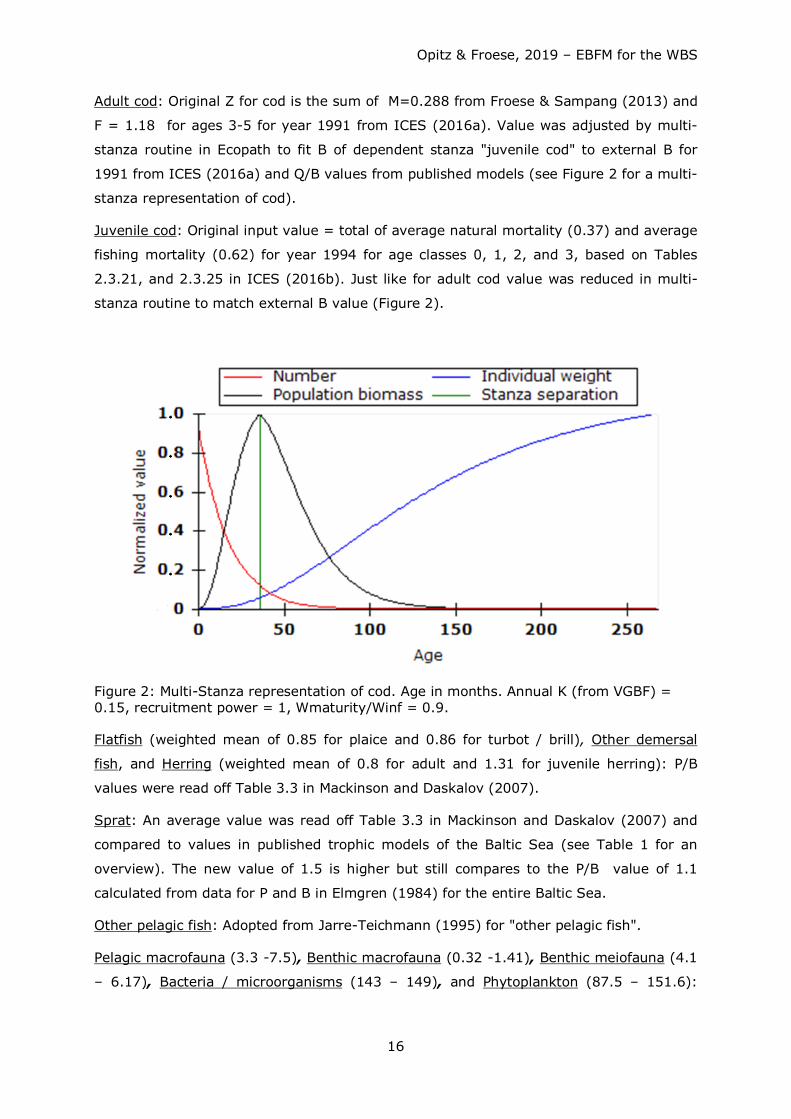
Adult cod: Original Z for cod is the sum of M=0.288 from Froese & Sampang (2013) and
F = 1.18 for ages 3-5 for year 1991 from ICES (2016a). Value was adjusted by multi-
stanza routine in Ecopath to fit B of dependent stanza "juvenile cod" to external B for
1991 from ICES (2016a) and Q/B values from published models (see Figure 2 for a multi-
stanza representation of cod).
Juvenile cod: Original input value = total of average natural mortality (0.37) and average
fishing mortality (0.62) for year 1994 for age classes 0, 1, 2, and 3, based on Tables
2.3.21, and 2.3.25 in ICES (2016b). Just like for adult cod value was reduced in multi-
stanza routine to match external B value (Figure 2).
Figure 2: Multi-Stanza representation of cod. Age in months. Annual K (from VGBF) = 0.15, recruitment power = 1, Wmaturity/Winf = 0.9.
Flatfish (weighted mean of 0.85 for plaice and 0.86 for turbot / brill), Other demersal
fish, and Herring (weighted mean of 0.8 for adult and 1.31 for juvenile herring): P/B
values were read off Table 3.3 in Mackinson and Daskalov (2007).
Sprat: An average value was read off Table 3.3 in Mackinson and Daskalov (2007) and
compared to values in published trophic models of the Baltic Sea (see Table 1 for an
overview). The new value of 1.5 is higher but still compares to the P/B value of 1.1
calculated from data for P and B in Elmgren (1984) for the entire Baltic Sea.
Other pelagic fish: Adopted from Jarre-Teichmann (1995) for "other pelagic fish".
Pelagic macrofauna (3.3 -7.5), Benthic macrofauna (0.32 -1.41), Benthic meiofauna (4.1
– 6.17), Bacteria / microorganisms (143 – 149), and Phytoplankton (87.5 – 151.6):
Opitz & Froese, 2019 – EBFM for the WBS
17
Value for each of these trophic groups represents the average from two published models
(Jarre-Teichmann 1995 and Harvey et al. 2003).
Zooplankton: Value represents average P/B value for macro-, meso-, and
microzooplankton (weighted for differing production). P/B values for each group
correspond to mean of range for each group from a series of published trophic models
(see Table 1 for an overview).
Benthic producers: Value adopted from two predecessor models (Wulff & Ulanowicz 1989
and Jarre-Teichmann 1995).
Consumption / Biomass ratio (Q/B)
Consumption is the intake of food by a group over the time period considered. In Ecopath
it is entered as the ratio of consumption over biomass (Q/B) per year. Absolute
consumption computed by Ecopath in our model is then a flow expressed in gCm-2y-1.
Below, source of Q/B model inputs are described individually for each trophic group.
Harbour porpoises: Value is based on information in Andreasen et al. (2017).
Seals: Value is the mean of Q/B y-1 for grey seal and harbour seal. Q/B y-1 for both
species were calculated based on information of individual weight and daily food intake
obtained from Stiftung deutsches Meeresmuseum (www.deutsches-
meeresmuseum.de/wissenschaft/infothek/artensteckbriefe) and from Wikipedia
(www.wikipedia.org). The Q/B y-1 value used here for seals is at the upper limit of food
intake since maximum weight and maximum food intake were used for the calculation.
(Sea-)birds: Value is the mean of a range (5 -14.41 / year) of consumption values in
Tomczak et al. (2009) for seabirds from five coastal ecosystems in the southern and
south-eastern Baltic Sea.
Q/B values for all fish groups except for Other pelagic fish were read off Table 3.3 in
Mackinson and Daskalov (2007). An updated Q/B value for Juvenile cod (<=35 cm) was
calculated by the multi-stanza routine of the EwE software based on P/B and Q/B values
for Adult cod and original Q/B for Juvenile cod. Q/B for Juvenile cod is thus a trade-off
between values from the literature and stanza routine logic. Q/B value for Flatfish is the
weighted (by consumption) mean of 3.68 for dab, 3.2 for flounder, 2.78 for plaice, and
2.2 for turbot. Q/B for Herring is the weighted (by consumption) mean of 4.34 for adult
and 5.63 for juvenile herring.
Other pelagic fish: Value was adopted from Jarre-Teichmann (1995) for "other pelagic
fish".
Opitz & Froese, 2019 – EBFM for the WBS
18
Values for Pelagic macrofauna (10.6 / 25), Benthic macrofauna (9.5 / 13), and Benthic
meiofauna (31.17 / 33.9) represent each the average of two values (in parentheses)
from two published models (Jarre-Teichmann 1995 and Harvey et al. 2003).
Zooplankton: Value represents the average Q/B value for macro-, meso-, and
microzooplankton (weighted for differing consumption). Q/B values for each group
correspond to the mean of a range for each group from a series of published trophic
models for the Baltic Sea (see Table 1 for details).
Bacteria/microorganisms: Value represents the average of two published models (248 in
Harvey et al. 2003 and 355 in Jarre-Teichmann 1995 for Baltic Proper).
Original input data for biomass, P/B ratio, Q/B ratio, for all groups (except fishery) are
shown in the input – output tables in the results section.
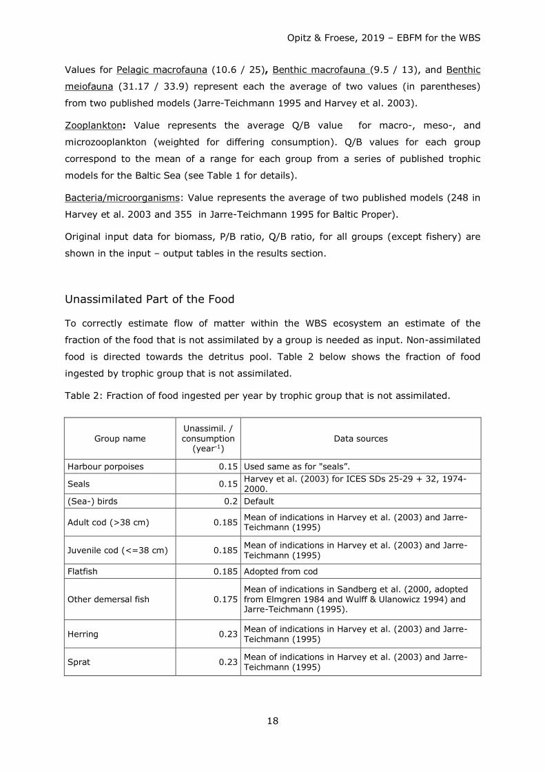
Unassimilated Part of the Food
To correctly estimate flow of matter within the WBS ecosystem an estimate of the
fraction of the food that is not assimilated by a group is needed as input. Non-assimilated
food is directed towards the detritus pool. Table 2 below shows the fraction of food
ingested by trophic group that is not assimilated.
Table 2: Fraction of food ingested per year by trophic group that is not assimilated.
Group name Unassimil. / consumption
(year-1) Data sources
Harbour porpoises 0.15 Used same as for "seals”.
Seals 0.15 Harvey et al. (2003) for ICES SDs 25-29 + 32, 1974-2000.
(Sea-) birds 0.2 Default
Adult cod (>38 cm) 0.185 Mean of indications in Harvey et al. (2003) and Jarre-Teichmann (1995)
Juvenile cod (<=38 cm) 0.185 Mean of indications in Harvey et al. (2003) and Jarre-Teichmann (1995)
Flatfish 0.185 Adopted from cod
Other demersal fish 0.175 Mean of indications in Sandberg et al. (2000, adopted from Elmgren 1984 and Wulff & Ulanowicz 1994) and Jarre-Teichmann (1995).
Herring 0.23 Mean of indications in Harvey et al. (2003) and Jarre-Teichmann (1995)
Sprat 0.23 Mean of indications in Harvey et al. (2003) and Jarre-Teichmann (1995)
Opitz & Froese, 2019 – EBFM for the WBS
19
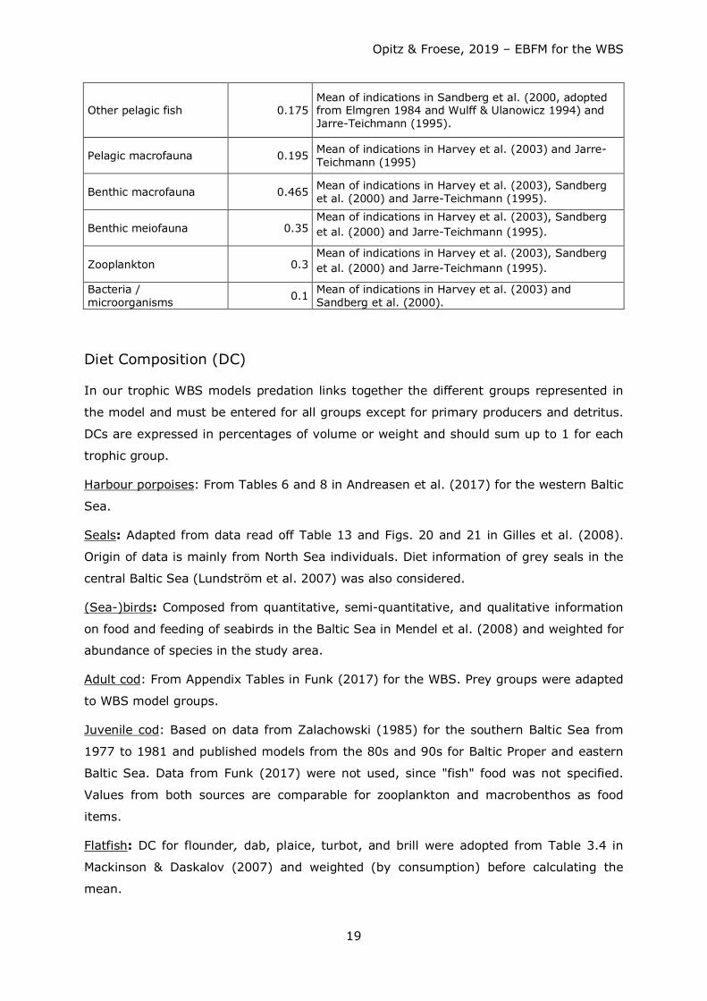
Other pelagic fish 0.175 Mean of indications in Sandberg et al. (2000, adopted from Elmgren 1984 and Wulff & Ulanowicz 1994) and Jarre-Teichmann (1995).
Pelagic macrofauna 0.195 Mean of indications in Harvey et al. (2003) and Jarre-Teichmann (1995)
Benthic macrofauna 0.465 Mean of indications in Harvey et al. (2003), Sandberg et al. (2000) and Jarre-Teichmann (1995).
Benthic meiofauna 0.35 Mean of indications in Harvey et al. (2003), Sandberg et al. (2000) and Jarre-Teichmann (1995).
Zooplankton 0.3 Mean of indications in Harvey et al. (2003), Sandberg et al. (2000) and Jarre-Teichmann (1995).
Bacteria / microorganisms 0.1 Mean of indications in Harvey et al. (2003) and
Sandberg et al. (2000).
Diet Composition (DC)
In our trophic WBS models predation links together the different groups represented in
the model and must be entered for all groups except for primary producers and detritus.
DCs are expressed in percentages of volume or weight and should sum up to 1 for each
trophic group.
Harbour porpoises: From Tables 6 and 8 in Andreasen et al. (2017) for the western Baltic
Sea.
Seals: Adapted from data read off Table 13 and Figs. 20 and 21 in Gilles et al. (2008).
Origin of data is mainly from North Sea individuals. Diet information of grey seals in the
central Baltic Sea (Lundström et al. 2007) was also considered.
(Sea-)birds: Composed from quantitative, semi-quantitative, and qualitative information
on food and feeding of seabirds in the Baltic Sea in Mendel et al. (2008) and weighted for
abundance of species in the study area.
Adult cod: From Appendix Tables in Funk (2017) for the WBS. Prey groups were adapted
to WBS model groups.
Juvenile cod: Based on data from Zalachowski (1985) for the southern Baltic Sea from
1977 to 1981 and published models from the 80s and 90s for Baltic Proper and eastern
Baltic Sea. Data from Funk (2017) were not used, since "fish" food was not specified.
Values from both sources are comparable for zooplankton and macrobenthos as food
items.
Flatfish: DC for flounder, dab, plaice, turbot, and brill were adopted from Table 3.4 in
Mackinson & Daskalov (2007) and weighted (by consumption) before calculating the
mean.
Opitz & Froese, 2019 – EBFM for the WBS
20
Other demersal fish: Composed of DC for (other) demersal fish from published models
(Sandberg 2007, Sandberg et al. 2000, Jarre-Teichmann 1995).
Herring: Composed of DC for adult and juvenile herring from published models
(Sandberg 2007, Harvey et al. 2003, Jarre-Teichmann 1995, Rudstam 1994, Elmgren
1984).
Sprat: Composed of DC for sprat from published models (Sandberg 2007, Harvey et al.
2003, Jarre-Teichmann 1995, Rudstam 1994, Elmgren 1984).
Other pelagic fish: Adapted from DC for other pelagic fish in Sandberg (2007) and
Sandberg et al. (2000).
Pelagic macrofauna: Composed from DC for pelagic macrofauna in Harvey et al. (2003)
and Jarre-Teichmann (1995). An assumed 5 % for cannibalism was included (based on
pers. observation by S. Opitz: e.g. Cyanea feeding on Aurelia aurita).
DC for Benthic macrofauna, Benthic meiofauna and Bacteria / microorganisms were
composed of DCs for these groups from published models (Sandberg 2007, Harvey et al.
2003, Sandberg et al. 2000, Jarre-Teichmann 1995).
Zooplankton: Composed of DC for macro-, meso-, and microzooplankton from published
models (Sandberg 2007, Harvey et al. 2003, Sandberg et al. 2000, Jarre-Teichmann
1995). DC of Zooplankton was weighted for consumption of components.
Original DC composition input data are shown in the input - output tables in the Results
section.
Fishery
The objectives of this study were to analyse the impact of commercial fisheries on the
WBS ecosystem and to explore improved fisheries management options. To assemble
reliable model inputs of fishery extractions was therefore of paramount importance.
The "fishery" in our WBS models is divided into pelagic and demersal fleets, a
recreational fishery, and a bycatch / IUU (illegal, unreported, unregulated) fishery. Origin
of inputs for landings, bycatch, and discards are described below (see also section Data
Sources above). If not stated otherwise, fishery data represent values for ICES SDs 22
and 24 in 1994. Original catch / landing / discard values were transformed into gWWm-
2year-1 by dividing weight (in tons) by area size (42.224 km2). All landings, bycatch, and
discard values in gWWm-2year-1 were then transformed into carbon by applying a
conversion factor of 10:1.
Opitz & Froese, 2019 – EBFM for the WBS
21
Pelagic Fleet Landings
Herring: Original value for commercial landings (in tons) of WBSS herring in 1994 in
subdivisions 20-24 is from Table 11 in ICES (2017i). This value was transformed into
gWWm-2y-1 by dividing total weight of catch by area size (102, 288 km2).
Sprat: Original value for commercial landings (in tons) in 1994 in WBS SDs 22 and 24
was extracted from Table 7.2 in ICES (2016b).
Other pelagic fish: Landings of "other fish" were read off appendix tables in Rossing et al.
(2010) for Germany and Denmark. Mean from both countries for years 2003 to 2007 was
used to calculate value. Total amount was divided into two equal parts for “Other pelagic
fish” and “Other demersal fish”.
Demersal Fleet Landings
Adult Cod (>35 cm): Original value for commercial landings in 1994 in WBS SDs 22-24
is from Table 6 in ICES (2017a). Original value was transformed into gWWm-2year-1 by
dividing total weight by area size (44,746 km2).
Flatfish:
- Dab landings extracted from Table 5.2 in ICES (2016b), (see also ICES 2017d).
- Flounder landings extracted from Table 4.2.2 in ICES (2016b), (see also ICES
2017 e,f).
- Plaice landings extracted from ICES (2017g,h) and Table 8.2.1 in ICES (2016b).
- Turbot landings extracted from Table 5.1 in ICES (2016b), (see also ICES 2017c).
- Brill landings extracted from Table 5.3 in ICES (2016b) for ICES SDs 22-24.
Landings were divided by area size (44,746 km2) to obtain gWWm-2year-1.
Other demersal fish: Landings of "other fish" were read off appendix tables in Rossing et
al. (2010) for Germany and Denmark. Mean from both countries for years 2003 to 2007
was used to calculate value. Total amount was divided into two equal parts for Other
pelagic fish and Other demersal fish. Landings of salmon were added to Other demersal
fish.
Recreational Fishery Landings
If not stated otherwise, catch values for recreational fishery used in the WBS models,
originate from appendix tables for Germany and Denmark in Rossing et al. (2010). The
mean from both countries for years 2003 to 2007 was used to obtain an estimate for the
amount of fish extracted by that type of fishery.
Opitz & Froese, 2019 – EBFM for the WBS
22
Adult cod (>35 cm): Original value in ICES SDs 22-24 was adopted from Table 6 in ICES
(2017a). This value was transformed into gWWm-2y-1 by dividing total weight by area size
(44,746 km2).
Flatfish: 5% of catch of flounder, dab, plaice, turbot, and brill in ICES SDs 22-24.
Other demersal fish: 5% of catch of "other demersal fish" in SDs 22 and 24. Value for
"salmon" (in Rossing et al. 2010) was added to "other demersal fish" in proportion to
catch.
Herring: 2% of catch of herring in SDs 22 and 24.
Sprat: Values from Rossing et al. (2010) for Germany and Denmark resulted in a very
low rate of 0.001 gCm-2y-1 for both recreational and IUU fishery. Extraction by
recreational fishery was therefore set to 0 in the model.
Other pelagic fish: 6% of catch of "other pelagic fish" in SDs 22 and 24.
Bycatch / IUU Fishery Landings
Since no official information on bycatch and IUU fishery landings was available to the
authors, values of bycatch and IUU fishery used in the WBS models, originate from
appendix tables for Germany and Denmark in Rossing et al. (2010). The mean from both
countries for years 2003 to 2007 was used to obtain an estimate for the amount of fish
extracted by that type of fishery.
Harbour porpoises, Seals, (Sea-)birds: Bycatch of fishery with fixed nets / traps:
To date, reliable quantitative information on bycatch numbers of marine mammals and
birds ranges from scarce to non-existent for the model area. Therefore, also information
from nearby regions was used to obtain preliminary bycatch estimates.
A recent estimate of 758 individuals of annual bycatch for the western Baltic harbour
porpoise population for ICES SDs 21,22, and 23 was published by the North Atlantic
Marine Mammal Commission and the Norwegian Institute for Marine Research (2019).
When transforming this number into gCm-2y-1 with an average weight of 50 kg per
individual the resulting value amounts roughly to 10% of the annual population
production.
The Finnish Game and Fisheries Research Institute (2013) estimated a by-catch rate of
7.7 – 8.4 % of grey seal population size for the eastern Baltic sea, while estimates of
annual population growth rates for grey and harbour seal ranged from 3.5 % to 9.4 %
for different periods and locations. A study by Vanhalato et al. (2014) suggests that
>2000 seals - by-caught in the Eastern Baltic - represented at least 90% of the total by-
catch in the whole Baltic Sea. Based on these informations we concluded that 10 % of
Opitz & Froese, 2019 – EBFM for the WBS
23
annual population production being by-caught would be a conservative figure for the
WBS model.
According to various authors (Zydelis et al. 2009, 2013, Bellebaum et al. 2012), a rough
estimate of 100,000-200,000 waterbirds are drowning annually in the North and Baltic
Seas, of which the great majority refers to the Baltic Sea. Derived from this information a
preliminary estimate of 0,25 % of annual production was entered into the model to
represent bycatch of seabirds.
Cod: 65 % of catch. This value was considered too high since both countries obtain the
bulk of their landings form the eastern cod stock around Bornholm (ICES SD 25).
Therefore, the same average estimate for all other fish groups (27% of landings) was
used to calculate IUU of cod in WBS. Total amount was divided into two equal parts for
adult and juvenile cod.
Flatfish, Other demersal fish, Herring, Sprat, and Other pelagic fish: 27% of catch in SDs
22 and 24 (corresponds to the average of all fish groups).
Benthic macrofauna: Bycatch of bottom trawling; an assumed 0.1% of annual production
of benthic macrofauna was used as model input.
Fishery data used in the WBS model are listed in Tables 3 and 4 below.
Pelagic Fleet discards
All values for pelagic fleet discards were read off appendix tables for Germany and
Denmark in Rossing et al. (2010). Mean % value from both countries for years 2003 to
2007 were used. Total amount for “other fish” in Rossing et al. (2010) was divided into
two equal parts for Other pelagic fish and Other demersal fish.
Herring and Sprat: Discards of the herring and sprat fishery are considered negligible by
ICES in contrast to estimates for Germany and Denmark in Rossing et al. (2010). Mean
% value from both countries in 1994 was used here to calculate Herring (10%) and Sprat
(11%) discard from catch data for both species in WBS.
Other pelagic fish: 12% of catch in WBS.
Demersal Fleet Discards
According to ICES (2017b) and Valentinsson et al. (2019) discards of the cod fishery in
the Baltic sea consist primarily of juvenile cod and therefore discards of the cod fishery
were set equal to catch of juvenile cod (discards for western Baltic cod in 1994 –
assumed to be mostly juvenile cod - are based on values from Table 6 in ICES (2017a) in
subdivisions 22-24) All other values for demersal fleet discards were read off appendix
Opitz & Froese, 2019 – EBFM for the WBS
24
tables for Germany and Denmark in Rossing et al. (2010). Mean % value from both
countries for years 2003 to 2007 were used to calculate discard rate for Flatfish (47 %)
and Other demersal fish (12 %). Total amount for Other fish in Rossing et al. (2010) was
divided here into two equal parts for Other pelagic fish and Other demersal fish.
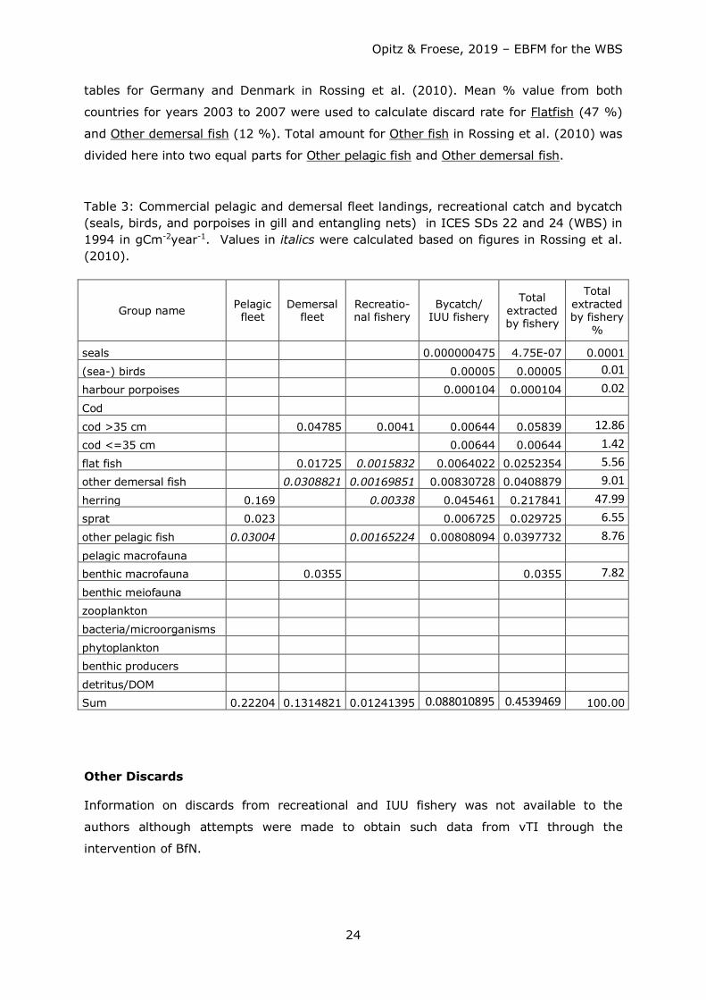
Table 3: Commercial pelagic and demersal fleet landings, recreational catch and bycatch (seals, birds, and porpoises in gill and entangling nets) in ICES SDs 22 and 24 (WBS) in 1994 in gCm-2year-1. Values in italics were calculated based on figures in Rossing et al. (2010).
Group name Pelagic fleet
Demersal fleet
Recreatio-nal fishery
Bycatch/ IUU fishery
Total extracted by fishery
Total extracted by fishery
%
seals 0.000000475 4.75E-07 0.0001
(sea-) birds 0.00005 0.00005 0.01 harbour porpoises 0.000104 0.000104 0.02 Cod
cod >35 cm 0.04785 0.0041 0.00644 0.05839 12.86 cod <=35 cm 0.00644 0.00644 1.42 flat fish 0.01725 0.0015832 0.0064022 0.0252354 5.56 other demersal fish 0.0308821 0.00169851 0.00830728 0.0408879 9.01 herring 0.169 0.00338 0.045461 0.217841 47.99 sprat 0.023
0.006725 0.029725 6.55
other pelagic fish 0.03004 0.00165224 0.00808094 0.0397732 8.76 pelagic macrofauna
benthic macrofauna 0.0355 0.0355 7.82 benthic meiofauna zooplankton
bacteria/microorganisms
phytoplankton benthic producers
detritus/DOM Sum 0.22204 0.1314821 0.01241395 0.088010895 0.4539469 100.00
Other Discards
Information on discards from recreational and IUU fishery was not available to the
authors although attempts were made to obtain such data from vTI through the
intervention of BfN.
Opitz & Froese, 2019 – EBFM for the WBS
25
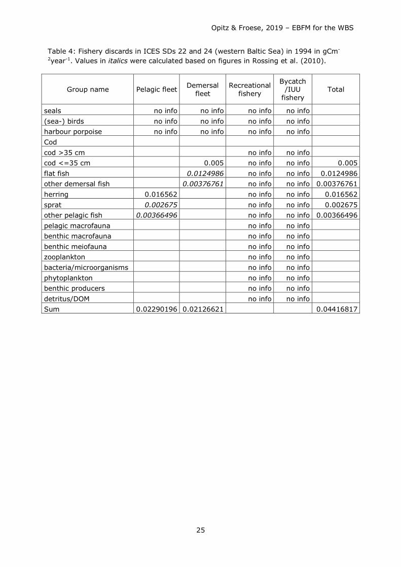
Table 4: Fishery discards in ICES SDs 22 and 24 (western Baltic Sea) in 1994 in gCm-
2year-1. Values in italics were calculated based on figures in Rossing et al. (2010).
Group name Pelagic fleet Demersal fleet
Recreational fishery
Bycatch /IUU
fishery Total
seals no info no info no info no info (sea-) birds no info no info no info no info harbour porpoise no info no info no info no info Cod cod >35 cm
no info no info
cod <=35 cm 0.005 no info no info 0.005 flat fish 0.0124986 no info no info 0.0124986 other demersal fish 0.00376761 no info no info 0.00376761 herring 0.016562 no info no info 0.016562 sprat 0.002675 no info no info 0.002675 other pelagic fish 0.00366496 no info no info 0.00366496 pelagic macrofauna no info no info benthic macrofauna no info no info benthic meiofauna no info no info zooplankton no info no info bacteria/microorganisms no info no info phytoplankton no info no info benthic producers no info no info detritus/DOM no info no info Sum 0.02290196 0.02126621 0.04416817
Opitz & Froese, 2019 – EBFM for the WBS
26
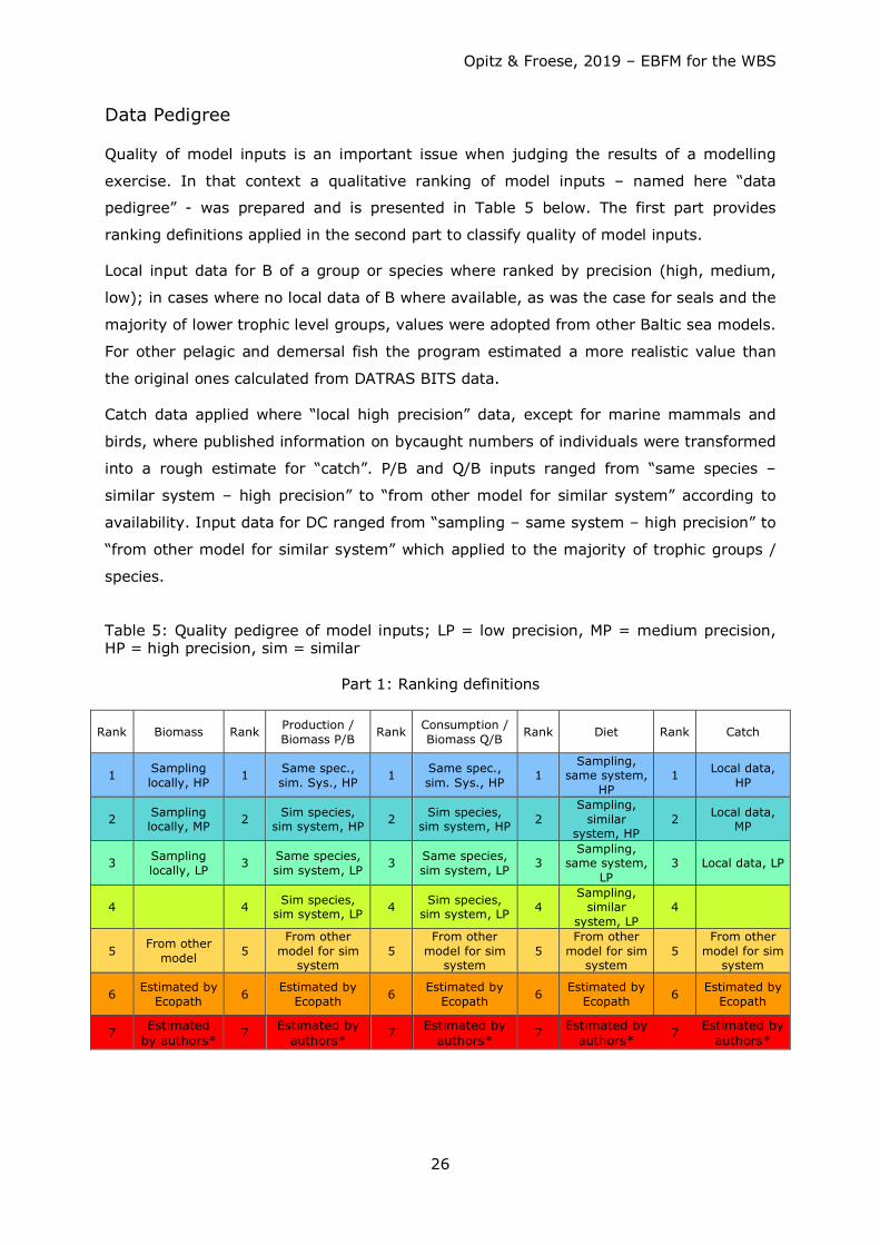
Data Pedigree
Quality of model inputs is an important issue when judging the results of a modelling
exercise. In that context a qualitative ranking of model inputs – named here “data
pedigree” - was prepared and is presented in Table 5 below. The first part provides
ranking definitions applied in the second part to classify quality of model inputs.
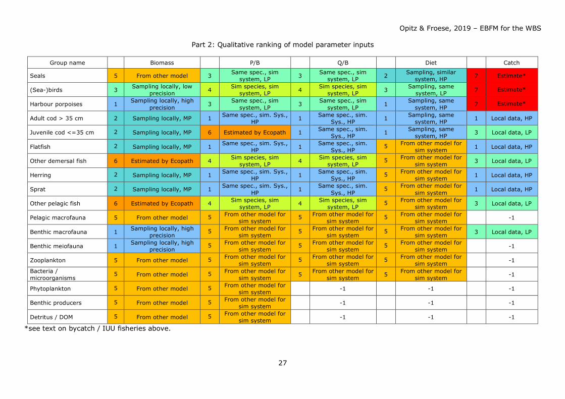
Local input data for B of a group or species where ranked by precision (high, medium,
low); in cases where no local data of B where available, as was the case for seals and the
majority of lower trophic level groups, values were adopted from other Baltic sea models.
For other pelagic and demersal fish the program estimated a more realistic value than
the original ones calculated from DATRAS BITS data.
Catch data applied where “local high precision” data, except for marine mammals and
birds, where published information on bycaught numbers of individuals were transformed
into a rough estimate for “catch”. P/B and Q/B inputs ranged from “same species –
similar system – high precision” to “from other model for similar system” according to
availability. Input data for DC ranged from “sampling – same system – high precision” to
“from other model for similar system” which applied to the majority of trophic groups /
species.
Table 5: Quality pedigree of model inputs; LP = low precision, MP = medium precision, HP = high precision, sim = similar
Part 1: Ranking definitions
Rank Biomass Rank Production / Biomass P/B Rank Consumption /
Biomass Q/B Rank Diet Rank Catch
1 Sampling locally, HP 1 Same spec.,
sim. Sys., HP 1 Same spec., sim. Sys., HP 1
Sampling, same system,
HP 1 Local data,
HP
2 Sampling locally, MP 2 Sim species,
sim system, HP 2 Sim species, sim system, HP 2
Sampling, similar
system, HP 2 Local data,
MP
3 Sampling locally, LP 3 Same species,
sim system, LP 3 Same species, sim system, LP 3
Sampling, same system,
LP 3 Local data, LP
4 4 Sim species, sim system, LP 4 Sim species,
sim system, LP 4 Sampling,
similar system, LP
4
5 From other model 5
From other model for sim
system 5
From other model for sim
system 5
From other model for sim
system 5
From other model for sim
system
6 Estimated by Ecopath 6 Estimated by
Ecopath 6 Estimated by Ecopath 6 Estimated by
Ecopath 6 Estimated by Ecopath
7 Estimated by authors*
7 Estimated by authors*
7 Estimated by authors*
7 Estimated by authors*
7 Estimated by authors*
Opitz & Froese, 2019 – EBFM for the WBS
27
Part 2: Qualitative ranking of model parameter inputs
Group name Biomass P/B Q/B Diet Catch
Seals 5 From other model 3 Same spec., sim system, LP 3 Same spec., sim
system, LP 2 Sampling, similar system, HP 7 Estimate*
(Sea-)birds 3 Sampling locally, low precision 4 Sim species, sim
system, LP 4 Sim species, sim system, LP 3 Sampling, same
system, LP 7 Estimate*
Harbour porpoises 1 Sampling locally, high precision 3 Same spec., sim
system, LP 3 Same spec., sim system, LP 1 Sampling, same
system, HP 7 Estimate*
Adult cod > 35 cm 2 Sampling locally, MP 1 Same spec., sim. Sys., HP 1 Same spec., sim.
Sys., HP 1 Sampling, same system, HP 1 Local data, HP
Juvenile cod <=35 cm 2 Sampling locally, MP 6 Estimated by Ecopath 1 Same spec., sim. Sys., HP 1 Sampling, same
system, HP 3 Local data, LP
Flatfish 2 Sampling locally, MP 1 Same spec., sim. Sys., HP 1 Same spec., sim.
Sys., HP 5 From other model for
sim system 1 Local data, HP
Other demersal fish 6 Estimated by Ecopath 4 Sim species, sim system, LP 4 Sim species, sim
system, LP 5 From other model for
sim system 3 Local data, LP
Herring 2 Sampling locally, MP 1 Same spec., sim. Sys., HP 1 Same spec., sim.
Sys., HP 5 From other model for
sim system 1 Local data, HP
Sprat 2 Sampling locally, MP 1 Same spec., sim. Sys., HP 1 Same spec., sim.
Sys., HP 5 From other model for
sim system 1 Local data, HP
Other pelagic fish 6 Estimated by Ecopath 4 Sim species, sim system, LP 4 Sim species, sim
system, LP 5 From other model for
sim system 3 Local data, LP
Pelagic macrofauna 5 From other model 5 From other model for sim system
5 From other model for sim system
5 From other model for sim system -1
Benthic macrofauna 1 Sampling locally, high precision
5 From other model for sim system
5 From other model for sim system
5 From other model for sim system 3 Local data, LP
Benthic meiofauna 1 Sampling locally, high precision
5 From other model for sim system
5 From other model for sim system
5 From other model for sim system -1
Zooplankton 5 From other model 5 From other model for sim system
5 From other model for sim system
5 From other model for sim system -1
Bacteria / microorganisms
5 From other model 5 From other model for sim system 5 From other model for
sim system 5 From other model for sim system -1
Phytoplankton 5 From other model 5 From other model for sim system -1 -1 -1
Benthic producers 5 From other model 5 From other model for sim system -1 -1 -1
Detritus / DOM 5 From other model 5 From other model for sim system -1 -1 -1
*see text on bycatch / IUU fisheries above.
Opitz & Froese, 2019 – EBFM for the WBS
28
Balancing Process
Flows based on original model inputs did not balance in every case, i.e. consumption by
certain system elements exceeded production of their prey - in some cases considerably.
Imbalances of model inputs, originating from prey groups with EEs >1 were then
balanced by applying the following strategies:
Raise the biomass (B) of a trophic group by a) immigration or b) letting the model
software estimate the minimum B needed to satisfy predator requirements (including
fisheries) by entering a limiting EE value of 0.99. In cases where a) and b) were not
applicable, “import” of the respective food item by the predator was assumed.
Furthermore, c) small shifts of diet between food items served to eliminate
“questionable” food requirements (derived from published models) or to smooth out
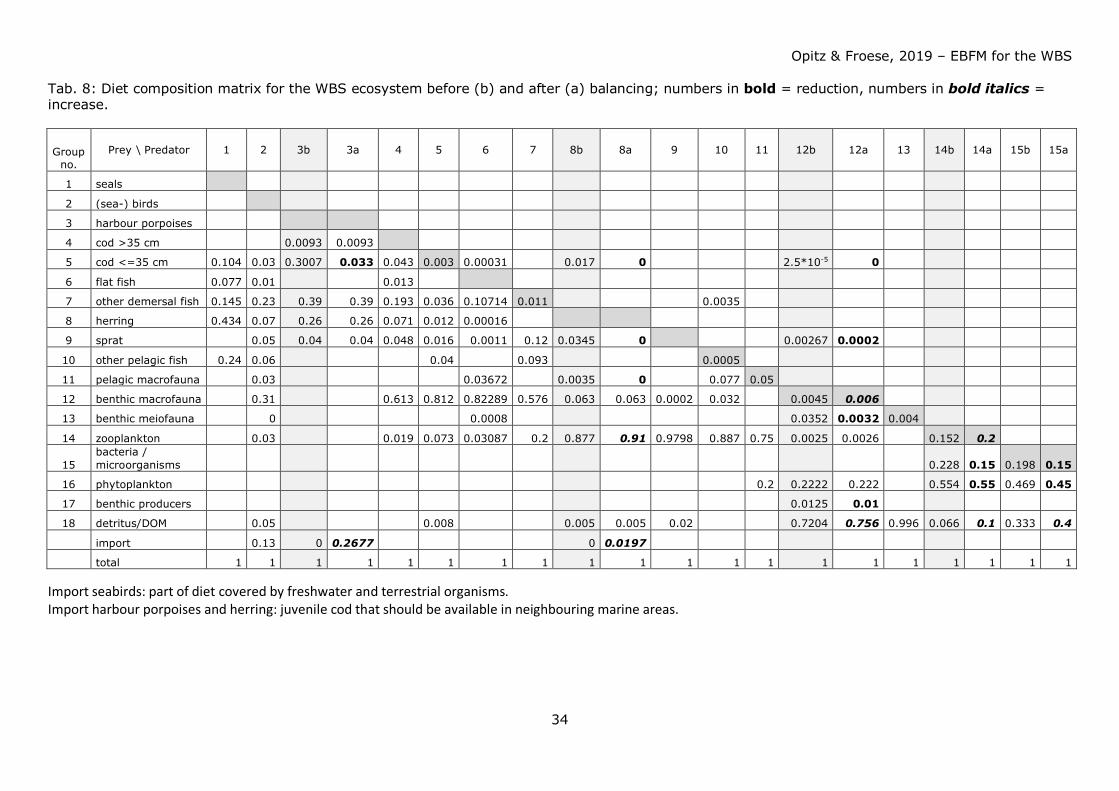
initial inputs. Hereafter, the balancing process is described in detail by trophic group.
Juvenile cod: Excess predation pressure by its main predator, the Harbour porpoises (30
% of its diet), was shifted to "import" hypothesizing that if not enough juvenile cod is
available within the system highly mobile harbour porpoises must obtain this food item
elsewhere in a neighbouring system (Kattegat, North Sea, etc.). Consumption by Herring
was viewed as “questionable”, therefore reduced from 1.7% to 0% and shifted to
"import". For the same reason the very small share (0.025%) of Juvenile cod in the diet
of Benthic macrofauna was set to 0 and shifted to Benthic macrofauna (cannibalism).
Other demersal fish: Strategy b) was applied since initial input value from DATRAS data
of 0.043 gCm-2 was way to low to satisfy food requirements of predators (including
fishery).
Other pelagic fish: For the same reason as Other demersal fish, strategy b) was also
applied to this group; start value from DATRAS was 0.003 gCm-2.
Sprat: Predation by Herring was considered questionable (eventually only larvae as part
of macrozooplankton), therefore reduced to 0 and shifted to Zooplankton. Predation by
Benthic macrofauna was reduced from 0.3 % to 0.02 % and shifted to Benthic
macrofauna (cannibalism).
Pelagic macrofauna: Predation by Herring was set to 0 since Mysis in our model forms
part of macrozooplankton instead of Pelagic macrofauna as in the published models –
source of information on herring diet.
Benthic meiofauna: A 90% reduction of this group in the diet of Benthic macrofauna
reduced EE of Benthic meiofauna to 0.824. The missing amount in the diet composition
of Benthic macrofauna was shifted to Detritus DOM.
Opitz & Froese, 2019 – EBFM for the WBS
29
Bacteria/Microorganisms: Consumption by Zooplankton was reduced from 0.228 to 0.15
and shifted to Zooplankton (cannibalism) and Detritus/DOM. Cannibalism within this
group was reduced from 18.8% to 15% and shifted to Detritus/DOM. Final EE of 0.926 is
<1 but still very high.
Phytoplankton: A slight reduction of grazing pressure by Benthic macrofauna,
Zooplankton, and Bacteria/microorganisms resulted in a modest reduction of EE from
0.974 to 0.964. This value is still very high and should be more in the range of 0.4 to
0.6. Standing stock B of 2.16 gCm-2 for phytoplankton was adopted from published
models for other parts of the Baltic Sea. More recent values for years 1990 to 1997, e.g.
in Thamm et al. (2005) for the WBS were even lower and in the range of 1.5 gCm-2 .
Benthic producers: Consumption by Benthic macrofauna was reduced from 1.25% to
0.1% and shifted to Detritus/DOM. The resulting EE of 0.952 is < 1 but still very high.
Start and end EEs for all trophic groups and shifts within the diet matrix are listed in the
input-output tables in the Results section below.
Dynamic Modelling of Different Fishery Management Scenarios This part of the study was performed in two steps.
Step 1: Using the mass-balanced Ecopath model for 1994 as a starting point, model runs
were executed with Ecosim after loading time series of B, catch and F / ExplR of
important commercial fish stocks such as cod, herring, sprat and several flatfish species
lumped into a “flatfish” box (see “Trophic Groups in the Model of the WBS Ecosystem”)
for years 1994 to 2016 into the model software. Purpose was to check whether the
model reflected realistic fishing scenarios of the past prior to applying it to fishing
scenarios reaching far into the future. F or ExplR was the driving parameter that would
eventually be modified for a better fit between modelled and external B and catch data
(thus the depending parameters).
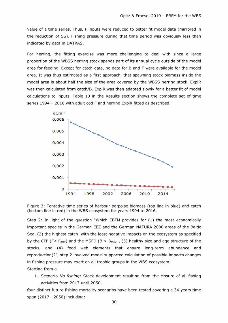
Since harbour porpoise data were not readily available to the authors, a time series for
this group was derived (see Figure 3) from rough quantitative information over the past
25 years (Hammond et al. 1995, Hammond et al. 2002, and SCANS II 2008). It was
then included into the modelling process with the objective to test the longstanding
fisherman’s view that this top predators is a serious competitor for fish.
Cod F and herring ExplR were fitted in such a way as to reduce sum of squares (SS) for
these stock parameters. For cod there was a considerable deviation of model outputs
from input data for the time period 1994 to 2003, i.e. for less than the first half of the
time series. Model algorithm and - consequently model output - is sensitive to the start
Opitz & Froese, 2019 – EBFM for the WBS
30
value of a time series. Thus, F inputs were reduced to better fit model data (mirrored in
the reduction of SS). Fishing pressure during that time period was obviously less than
indicated by data in DATRAS.
For herring, the fitting exercise was more challenging to deal with since a large
proportion of the WBSS herring stock spends part of its annual cycle outside of the model
area for feeding. Except for catch data, no data for B and F were available for the model
area. It was thus estimated as a first approach, that spawning stock biomass inside the
model area is about half the size of the area covered by the WBSS herring stock. ExplR
was then calculated from catch/B. ExplR was then adapted slowly for a better fit of model
calculations to inputs. Table 10 in the Results section shows the complete set of time
series 1994 – 2016 with adult cod F and herring ExplR fitted as described.
Figure 3: Tentative time series of harbour porpoise biomass (top line in blue) and catch (bottom line in red) in the WBS ecosystem for years 1994 to 2016.
Step 2: In light of the question “Which EBFM provides for (1) the most economically
important species in the German EEZ and the German NATURA 2000 areas of the Baltic
Sea, (2) the highest catch with the least negative impacts on the ecosystem as specified
by the CFP (F< Fmsy) and the MSFD (B > Bmsy) , (3) healthy size and age structure of the
stocks, and (4) food web elements that ensure long-term abundance and
reproduction)?”, step 2 involved model supported calculation of possible impacts changes
in fishing pressure may exert on all trophic groups in the WBS ecosystem.
Starting from a
1. Scenario No fishing: Stock development resulting from the closure of all fishing
activities from 2017 until 2050,
four distinct future fishing mortality scenarios have been tested covering a 34 years time
span (2017 - 2050) including:
Opitz & Froese, 2019 – EBFM for the WBS
31
2. Scenario Business as usual (BAU): Stock development from 2017 until 2050 under
the same fishing pressure as in 2016.
3. Scenario Fmsy: Stock development when fishing pressure F from 2017 until 2050
is reduced (if previously higher) or raised (if previously lower) to a value F, where
fishery yield / catch is sustainably at or slightly below a maximum level (if
available).
4. Scenario Half Fmsy: Stock development when fishing pressure F from 2017 until
2050 is reduced to (if previously higher) ½ Fmsy.
5. Scenario Ecosystem Based Fisheries Management (EBFM): Herring and sprat
fished at ½ Fmsy and other stocks at 80% Fmsy.
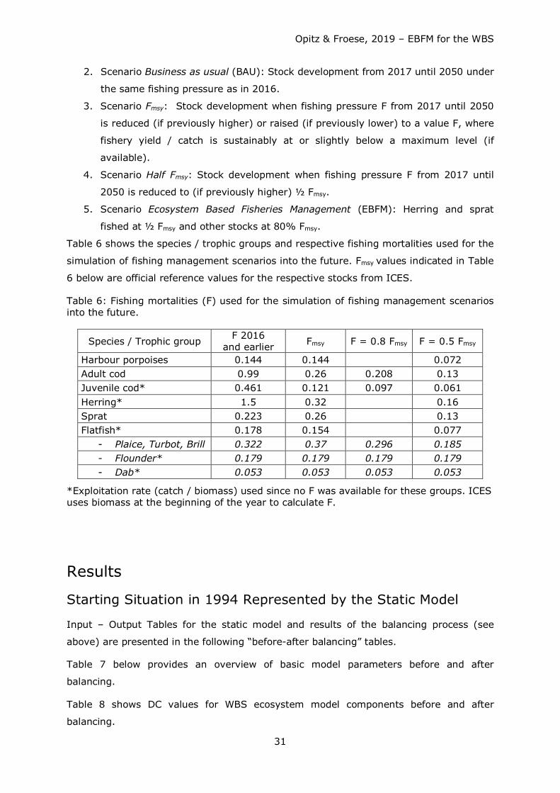
Table 6 shows the species / trophic groups and respective fishing mortalities used for the
simulation of fishing management scenarios into the future. Fmsy values indicated in Table
6 below are official reference values for the respective stocks from ICES.
Table 6: Fishing mortalities (F) used for the simulation of fishing management scenarios into the future.
Species / Trophic group F 2016 and earlier Fmsy F = 0.8 Fmsy F = 0.5 Fmsy
Harbour porpoises 0.144 0.144 0.072 Adult cod 0.99 0.26 0.208 0.13 Juvenile cod* 0.461 0.121 0.097 0.061 Herring* 1.5 0.32 0.16 Sprat 0.223 0.26 0.13 Flatfish* 0.178 0.154 0.077
- Plaice, Turbot, Brill 0.322 0.37 0.296 0.185 - Flounder* 0.179 0.179 0.179 0.179 - Dab* 0.053 0.053 0.053 0.053
*Exploitation rate (catch / biomass) used since no F was available for these groups. ICES uses biomass at the beginning of the year to calculate F.
Results
Starting Situation in 1994 Represented by the Static Model
Input – Output Tables for the static model and results of the balancing process (see
above) are presented in the following “before-after balancing” tables.
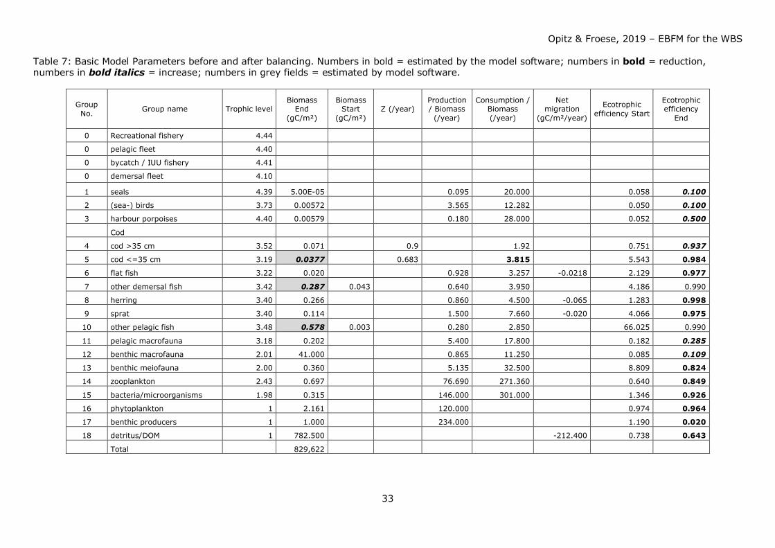
Table 7 below provides an overview of basic model parameters before and after
balancing.
Table 8 shows DC values for WBS ecosystem model components before and after
balancing.
Opitz & Froese, 2019 – EBFM for the WBS
32
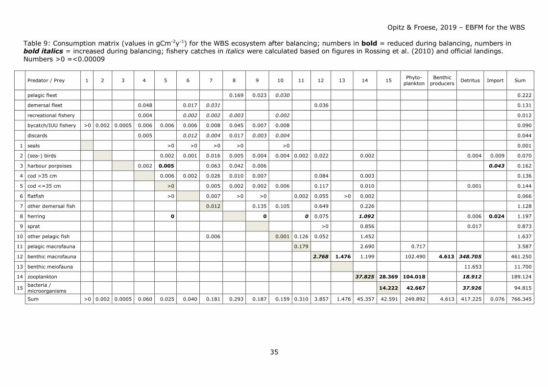
Table 9 shows consumption by ecosystem components after balancing and extraction by
fisheries.
Except for benthic producers and pelagic (mostly jellyfish) and benthic macrofauna all
system resources (trophic groups) were scarce; benthic macrofauna therefore exerted a
strong predation pressure on its prey organisms - usually low in the food web. On the
other hand, benthic macrofauna offered a rich source of food for organisms higher in the
food web, particularly for demersal fish species and seabirds.
Consumption of fish by fisheries and other predators exeeded the annual production of
fish. Competition for fish as food (mainly juvenile cod, herring and sprat) occurred
between the fisheries and other top predators such as harbour porpoises and seals, with
the fishery taking about 4-5 times more than harbour porpoises and seals combined (see
Figs. 38a – 41a). Strong competition for herring and sprat as food occurred between
fisheries, harbour porpoises, and (adult and juvenile) cod (see Table 9 for comparison of
predator impact including fisheries).
Biomass production of small pelagics (particularly herring and sprat) in the system was
hardly sufficient to satisfy food requirements by natural predators and at the same time
withdrawal by fisheries (to be demonstrated by the high EEs for these groups, see Table
7). Fisheries withdrew too many small pelagics which are an important food source
particularly for adult and juvenile cod. They were forced to shift their dietary needs to
other food sources such as benthic macrofauna. Particularly for herring the demand could
only be balanced assuming immigration of herring and to a small extent – sprat.
Such migrations are well known for the WBSS herring, which feed in summer off western
Sweden and bring biomass increased by somatic growth back into the WBS when they
return (e.g. van Deurs et al. 2016, Clausen et al. 2015, van Deurs & Ramkaer 2007,
Nielsen 2001).
Also, other species can enter the WBS e.g. as summer guests (known for mackerel
(Scomber scombrus) or mullets (Mugil cephalus)) and are preyed upon in the system.
These species form part of “other” pelagic and “other” demersal fish, respectively.
Predators like harbour porpoises had to look for other food sources as well, since there
was not enough fish – and particularly juvenile cod - in the system to satisfy their dietary
needs. As harbour porpoises do not feed on macrobenthos, they are forced or to go
hungry or to search for food elsewhere (Kattegat, Skagerrak, North Sea).
Opitz & Froese, 2019 – EBFM for the WBS
33
Table 7: Basic Model Parameters before and after balancing. Numbers in bold = estimated by the model software; numbers in bold = reduction, numbers in bold italics = increase; numbers in grey fields = estimated by model software.
Group No. Group name Trophic level
Biomass End
(gC/m²)
Biomass Start
(gC/m²) Z (/year)
Production / Biomass (/year)
Consumption / Biomass (/year)
Net migration
(gC/m²/year)
Ecotrophic efficiency Start
Ecotrophic efficiency
End
0 Recreational fishery 4.44
0 pelagic fleet 4.40
0 bycatch / IUU fishery 4.41
0 demersal fleet 4.10
1 seals 4.39 5.00E-05 0.095 20.000 0.058 0.100
2 (sea-) birds 3.73 0.00572 3.565 12.282 0.050 0.100
3 harbour porpoises 4.40 0.00579 0.180 28.000 0.052 0.500
Cod
4 cod >35 cm 3.52 0.071 0.9 1.92 0.751 0.937
5 cod <=35 cm 3.19 0.0377 0.683 3.815 5.543 0.984
6 flat fish 3.22 0.020 0.928 3.257 -0.0218 2.129 0.977
7 other demersal fish 3.42 0.287 0.043 0.640 3.950
4.186 0.990
8 herring 3.40 0.266 0.860 4.500 -0.065 1.283 0.998
9 sprat 3.40 0.114 1.500 7.660 -0.020 4.066 0.975
10 other pelagic fish 3.48 0.578 0.003 0.280 2.850 66.025 0.990
11 pelagic macrofauna 3.18 0.202 5.400 17.800 0.182 0.285
12 benthic macrofauna 2.01 41.000 0.865 11.250 0.085 0.109
13 benthic meiofauna 2.00 0.360 5.135 32.500 8.809 0.824
14 zooplankton 2.43 0.697 76.690 271.360 0.640 0.849
15 bacteria/microorganisms 1.98 0.315 146.000 301.000 1.346 0.926
16 phytoplankton 1 2.161 120.000 0.974 0.964
17 benthic producers 1 1.000 234.000 1.190 0.020
18 detritus/DOM 1 782.500 -212.400 0.738 0.643
Total 829,622
Opitz & Froese, 2019 – EBFM for the WBS
34
Tab. 8: Diet composition matrix for the WBS ecosystem before (b) and after (a) balancing; numbers in bold = reduction, numbers in bold italics = increase.
Group
no. Prey \ Predator 1 2 3b 3a 4 5 6 7 8b 8a 9 10 11 12b 12a 13 14b 14a 15b 15a
1 seals
2 (sea-) birds
3 harbour porpoises
4 cod >35 cm 0.0093 0.0093
5 cod <=35 cm 0.104 0.03 0.3007 0.033 0.043 0.003 0.00031 0.017 0 2.5*10-5 0
6 flat fish 0.077 0.01 0.013
7 other demersal fish 0.145 0.23 0.39 0.39 0.193 0.036 0.10714 0.011 0.0035
8 herring 0.434 0.07 0.26 0.26 0.071 0.012 0.00016
9 sprat
0.05 0.04 0.04 0.048 0.016 0.0011 0.12 0.0345 0 0.00267 0.0002
10 other pelagic fish 0.24 0.06 0.04
0.093 0.0005
11 pelagic macrofauna 0.03
0.03672
0.0035 0 0.077 0.05
12 benthic macrofauna 0.31 0.613 0.812 0.82289 0.576 0.063 0.063 0.0002 0.032 0.0045 0.006
13 benthic meiofauna 0
0.0008
0.0352 0.0032 0.004
14 zooplankton 0.03 0.019 0.073 0.03087 0.2 0.877 0.91 0.9798 0.887 0.75 0.0025 0.0026 0.152 0.2
15 bacteria / microorganisms
0.228 0.15 0.198 0.15
16 phytoplankton 0.2 0.2222 0.222 0.554 0.55 0.469 0.45
17 benthic producers 0.0125 0.01
18 detritus/DOM 0.05 0.008 0.005 0.005 0.02 0.7204 0.756 0.996 0.066 0.1 0.333 0.4
import 0.13 0 0.2677
0 0.0197
total 1 1 1 1 1 1 1 1 1 1 1 1 1 1 1 1 1 1 1 1
Import seabirds: part of diet covered by freshwater and terrestrial organisms. Import harbour porpoises and herring: juvenile cod that should be available in neighbouring marine areas.
Opitz & Froese, 2019 – EBFM for the WBS
35
Table 9: Consumption matrix (values in gCm-2y-1) for the WBS ecosystem after balancing; numbers in bold = reduced during balancing, numbers in bold italics = increased during balancing; fishery catches in italics were calculated based on figures in Rossing et al. (2010) and official landings. Numbers >0 =<0.00009
Predator / Prey 1 2 3 4 5 6 7 8 9 10 11 12 13 14 15 Phyto-plankton
Benthic producers Detritus Import Sum
pelagic fleet 0.169 0.023 0.030 0.222
demersal fleet 0.048 0.017 0.031 0.036 0.131
recreational fishery 0.004 0.002 0.002 0.003 0.002 0.012
bycatch/IUU fishery >0 0.002 0.0005 0.006 0.006 0.006 0.008 0.045 0.007 0.008 0.090
discards 0.005 0.012 0.004 0.017 0.003 0.004 0.044
1 seals >0 >0 >0 >0 >0 0.001
2 (sea-) birds 0.002 0.001 0.016 0.005 0.004 0.004 0.002 0.022 0.002 0.004 0.009 0.070
3 harbour porpoises 0.002 0.005 0.063 0.042 0.006 0.043 0.162
4 cod >35 cm 0.006 0.002 0.026 0.010 0.007 0.084 0.003 0.136
5 cod <=35 cm >0 0.005 0.002 0.002 0.006 0.117 0.010 0.001 0.144
6 flatfish >0 0.007 >0 >0 0.002 0.055 >0 0.002 0.066
7 other demersal fish 0.012 0.135 0.105 0.649 0.226 1.128
8 herring 0 0 0 0.075 1.092 0.006 0.024 1.197
9 sprat >0 0.856 0.017 0.873
10 other pelagic fish 0.006 0.001 0.126 0.052 1.452 1.637
11 pelagic macrofauna 0.179 2.690 0.717 3.587
12 benthic macrofauna 2.768 1.476 1.199 102.490 4.613 348.705 461.250
13 benthic meiofauna 11.653 11.700
14 zooplankton 37.825 28.369 104.018 18.912 189.124
15 bacteria / microorganisms 14.222 42.667 37.926 94.815
Sum >0 0.002 0.0005 0.060 0.025 0.040 0.181 0.293 0.187 0.159 0.310 3.857 1.476 45.357 42.591 249.892 4.613 417.225 0.076 766.345
Opitz & Froese, 2019 – EBFM for the WBS
36
Even when excluding fishery from the model there is not sufficient juvenile cod in the
system to satisfy feeding requirements of its natural predators such as harbour
porpoises, birds, and adult cod. Lack of juvenile cod must be balanced through
“imports”, i.e. predators find this type of food partly in adjacent ecosystems (Kattegat,
Skagerrak, Central Baltic Sea), or by immigration of juveniles.
According to model results cannibalism occurs within the cod population, with 4.3 % of
the diet of adult cod consisting of juvenile cod, and 0.3 % of the diet of juvenile cod
consisting of other juvenile cod. These percentages are low and have only a marginal
effect on the population.
Trophic Flows within the Western Baltic Sea Food Web
Figure 4 provides a schematic representation of trophic groups and flows within the WBS
food web.
In this and the subsequent graphs, trophic groups are represented by squares. The area
of the squares is proportional (on a square-root scale) to the biomass of the group. The
colour of the squares is related to the type of group, with dark grey = detritus, green =
primary producers, yellow = secondary non-fish producers, blue = fish, red = fishing
fleets). Trophic flows are indicated by grey lines. In Figures 4 to 15 with individual groups
highlighted, inflows to a compartment from other groups are green, outflows to other
system elements (predators) are bright red. Flow size is relative and scaled individually
by group and cannot be compared directly to flows of another group. Also, size of in- and
outflows to and from a group cannot be compared directly. The true magnitude of the
flows between groups (including fisheries) is presented in Table 9 above. A dark blue
arrow indicates import of food from adjacent ecosystems by a certain group. A red arrow
indicates that biomass of a certain group was raised by immigration from adjacent
ecosystems. A curved green arrow indicates cannibalism within a group. Note: Size of
arrows is not in proportion to the size of import / immigration / cannibalism.
Harbour porpoises and seals are the top predators (trophic level > 4) in the system (see
Figs. 4, 5, and 6), but have only a small biomass and hence a small consumption
compared to the fisheries operating at the same trophic level, i.e. pelagic fleet,
recreational fleet and bycatch/IUU fishery (Figs. 4, 8, 9, 15, see also Table 9 for a
comparison of consumption / extraction). The demersal fleet operates at a slightly lower
trophic level (Fig. 12). Adult and juvenile cod (Figs. 10 and 11), flatfish and other
demersal and pelagic fish are the main predators on herring, sprat and benthic
macrofauna.
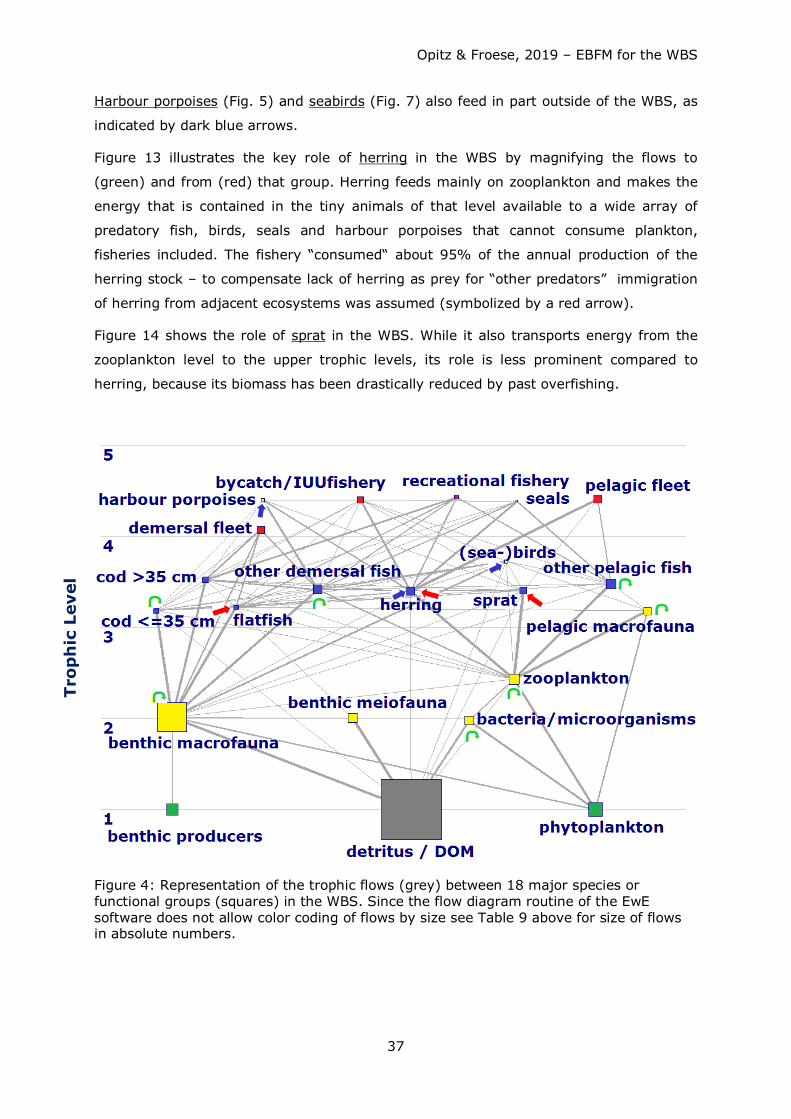
Opitz & Froese, 2019 – EBFM for the WBS
37
Harbour porpoises (Fig. 5) and seabirds (Fig. 7) also feed in part outside of the WBS, as
indicated by dark blue arrows.
Figure 13 illustrates the key role of herring in the WBS by magnifying the flows to
(green) and from (red) that group. Herring feeds mainly on zooplankton and makes the
energy that is contained in the tiny animals of that level available to a wide array of
predatory fish, birds, seals and harbour porpoises that cannot consume plankton,
fisheries included. The fishery “consumed“ about 95% of the annual production of the
herring stock – to compensate lack of herring as prey for “other predators” immigration
of herring from adjacent ecosystems was assumed (symbolized by a red arrow).
Figure 14 shows the role of sprat in the WBS. While it also transports energy from the
zooplankton level to the upper trophic levels, its role is less prominent compared to
herring, because its biomass has been drastically reduced by past overfishing.
Figure 4: Representation of the trophic flows (grey) between 18 major species or functional groups (squares) in the WBS. Since the flow diagram routine of the EwE software does not allow color coding of flows by size see Table 9 above for size of flows in absolute numbers.
Trop
hic
Lev
el
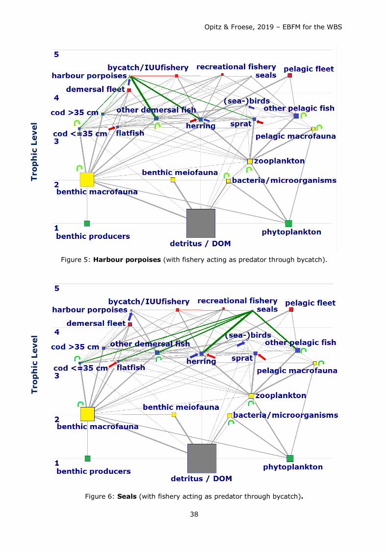
Opitz & Froese, 2019 – EBFM for the WBS
38
Figure 5: Harbour porpoises (with fishery acting as predator through bycatch).
Figure 6: Seals (with fishery acting as predator through bycatch).
Trop
hic
Lev
el
Trop
hic
Lev
el
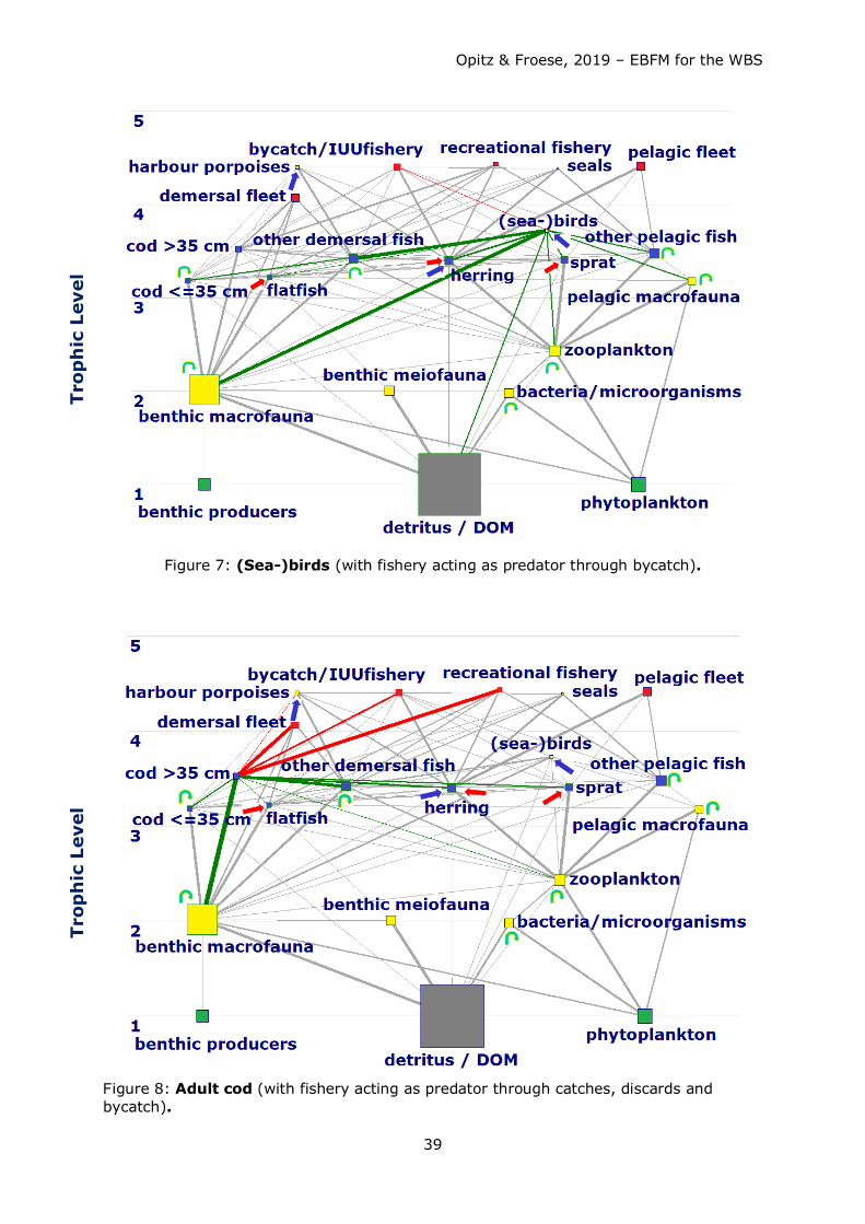
Opitz & Froese, 2019 – EBFM for the WBS
39
Figure 7: (Sea-)birds (with fishery acting as predator through bycatch).
Figure 8: Adult cod (with fishery acting as predator through catches, discards and bycatch).
Trop
hic
Lev
el
Trop
hic
Lev
el
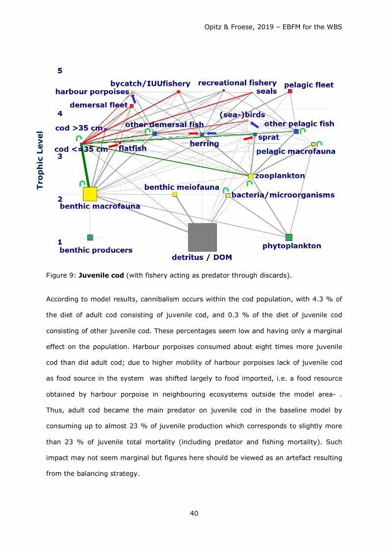
Opitz & Froese, 2019 – EBFM for the WBS
40
Figure 9: Juvenile cod (with fishery acting as predator through discards).
According to model results, cannibalism occurs within the cod population, with 4.3 % of
the diet of adult cod consisting of juvenile cod, and 0.3 % of the diet of juvenile cod
consisting of other juvenile cod. These percentages seem low and having only a marginal
effect on the population. Harbour porpoises consumed about eight times more juvenile
cod than did adult cod; due to higher mobility of harbour porpoises lack of juvenile cod
as food source in the system was shifted largely to food imported, i.e. a food resource
obtained by harbour porpoise in neighbouring ecosystems outside the model area- .
Thus, adult cod became the main predator on juvenile cod in the baseline model by
consuming up to almost 23 % of juvenile production which corresponds to slightly more
than 23 % of juvenile total mortality (including predator and fishing mortality). Such
impact may not seem marginal but figures here should be viewed as an artefact resulting
from the balancing strategy.
Trop
hic
Lev
el
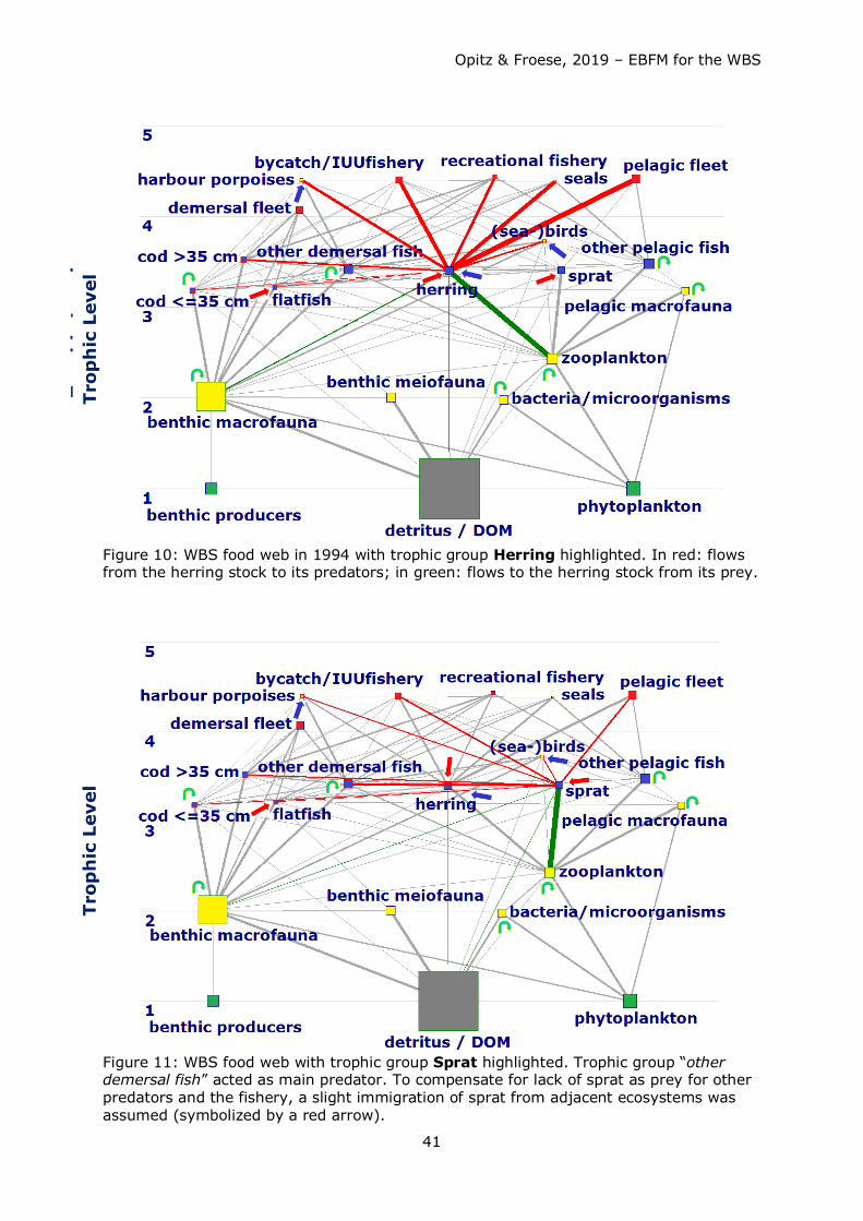
Opitz & Froese, 2019 – EBFM for the WBS
41
Figure 10: WBS food web in 1994 with trophic group Herring highlighted. In red: flows from the herring stock to its predators; in green: flows to the herring stock from its prey.
Figure 11: WBS food web with trophic group Sprat highlighted. Trophic group “other demersal fish” acted as main predator. To compensate for lack of sprat as prey for other predators and the fishery, a slight immigration of sprat from adjacent ecosystems was assumed (symbolized by a red arrow).
Trop
hic
Lev
el
Trop
hic
Lev
el
Trop
hic
Lev
el
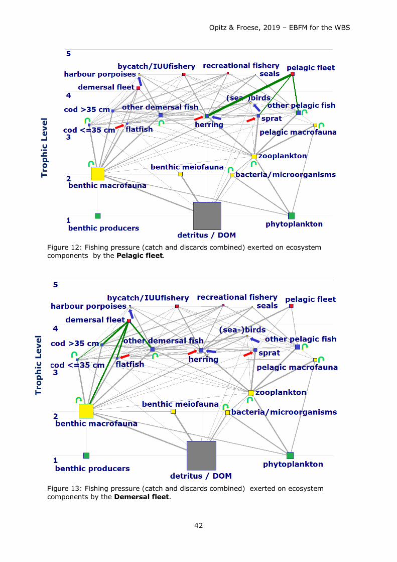
Opitz & Froese, 2019 – EBFM for the WBS
42
Figure 12: Fishing pressure (catch and discards combined) exerted on ecosystem components by the Pelagic fleet.
Figure 13: Fishing pressure (catch and discards combined) exerted on ecosystem components by the Demersal fleet.
Trop
hic
Lev
el
Trop
hic
Lev
el
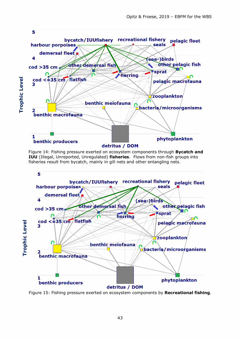
Opitz & Froese, 2019 – EBFM for the WBS
43
Figure 14: Fishing pressure exerted on ecosystem components through Bycatch and IUU (Illegal, Unreported, Unregulated) fisheries. Flows from non-fish groups into fisheries result from bycatch, mainly in gill nets and other entangling nets.
Figure 15: Fishing pressure exerted on ecosystem components by Recreational fishing.
Trop
hic
Lev
el
Trop
hic
Lev
el
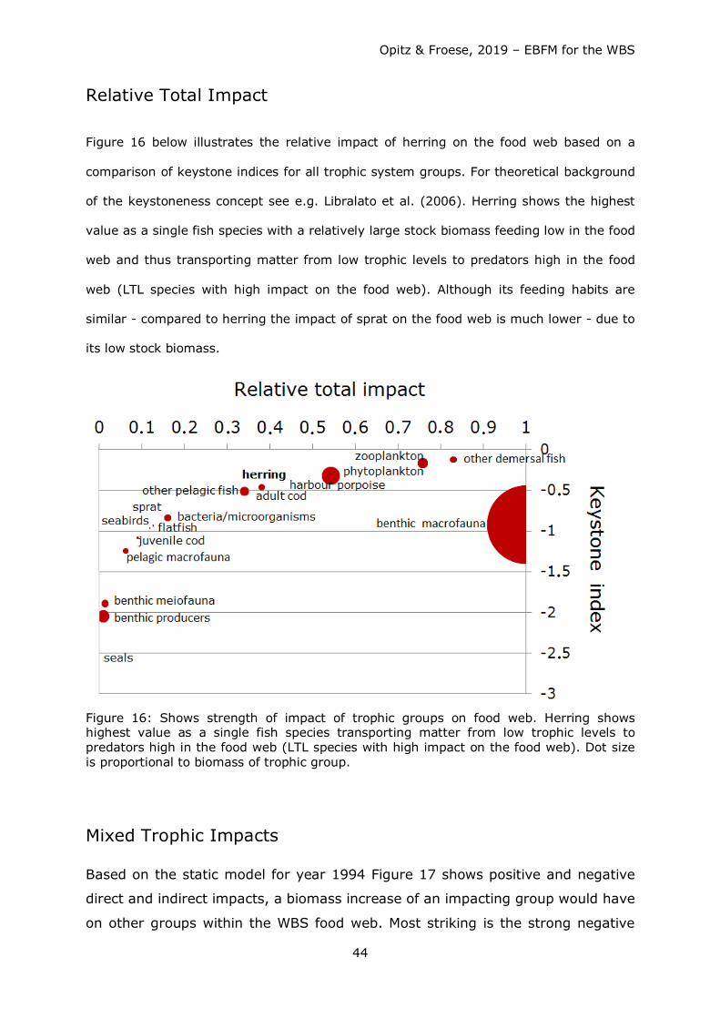
Opitz & Froese, 2019 – EBFM for the WBS
44
Relative Total Impact
Figure 16 below illustrates the relative impact of herring on the food web based on a
comparison of keystone indices for all trophic system groups. For theoretical background
of the keystoneness concept see e.g. Libralato et al. (2006). Herring shows the highest
value as a single fish species with a relatively large stock biomass feeding low in the food
web and thus transporting matter from low trophic levels to predators high in the food
web (LTL species with high impact on the food web). Although its feeding habits are
similar - compared to herring the impact of sprat on the food web is much lower - due to
its low stock biomass.
Figure 16: Shows strength of impact of trophic groups on food web. Herring shows highest value as a single fish species transporting matter from low trophic levels to predators high in the food web (LTL species with high impact on the food web). Dot size is proportional to biomass of trophic group.
Mixed Trophic Impacts Based on the static model for year 1994 Figure 17 shows positive and negative
direct and indirect impacts, a biomass increase of an impacting group would have
on other groups within the WBS food web. Most striking is the strong negative
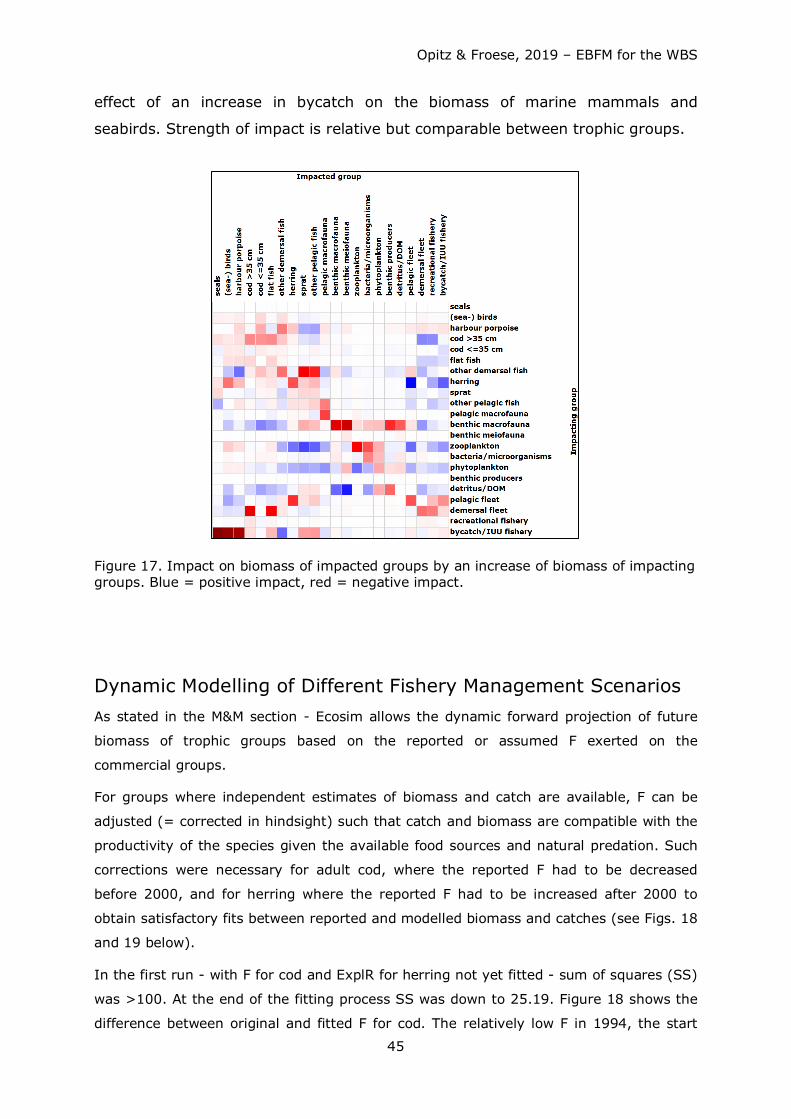
Opitz & Froese, 2019 – EBFM for the WBS
45
effect of an increase in bycatch on the biomass of marine mammals and
seabirds. Strength of impact is relative but comparable between trophic groups.
Figure 17. Impact on biomass of impacted groups by an increase of biomass of impacting groups. Blue = positive impact, red = negative impact.
Dynamic Modelling of Different Fishery Management Scenarios As stated in the M&M section - Ecosim allows the dynamic forward projection of future
biomass of trophic groups based on the reported or assumed F exerted on the
commercial groups.
For groups where independent estimates of biomass and catch are available, F can be
adjusted (= corrected in hindsight) such that catch and biomass are compatible with the
productivity of the species given the available food sources and natural predation. Such
corrections were necessary for adult cod, where the reported F had to be decreased
before 2000, and for herring where the reported F had to be increased after 2000 to
obtain satisfactory fits between reported and modelled biomass and catches (see Figs. 18
and 19 below).
In the first run - with F for cod and ExplR for herring not yet fitted - sum of squares (SS)
was >100. At the end of the fitting process SS was down to 25.19. Figure 18 shows the
difference between original and fitted F for cod. The relatively low F in 1994, the start
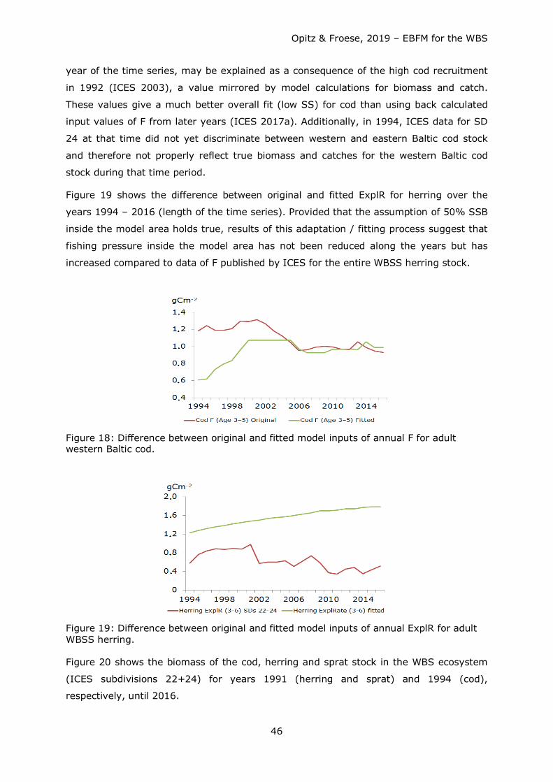
Opitz & Froese, 2019 – EBFM for the WBS
46
year of the time series, may be explained as a consequence of the high cod recruitment
in 1992 (ICES 2003), a value mirrored by model calculations for biomass and catch.
These values give a much better overall fit (low SS) for cod than using back calculated
input values of F from later years (ICES 2017a). Additionally, in 1994, ICES data for SD
24 at that time did not yet discriminate between western and eastern Baltic cod stock
and therefore not properly reflect true biomass and catches for the western Baltic cod
stock during that time period.
Figure 19 shows the difference between original and fitted ExplR for herring over the
years 1994 – 2016 (length of the time series). Provided that the assumption of 50% SSB
inside the model area holds true, results of this adaptation / fitting process suggest that
fishing pressure inside the model area has not been reduced along the years but has
increased compared to data of F published by ICES for the entire WBSS herring stock.
Figure 18: Difference between original and fitted model inputs of annual F for adult western Baltic cod.
Figure 19: Difference between original and fitted model inputs of annual ExplR for adult WBSS herring.
Figure 20 shows the biomass of the cod, herring and sprat stock in the WBS ecosystem
(ICES subdivisions 22+24) for years 1991 (herring and sprat) and 1994 (cod),
respectively, until 2016.
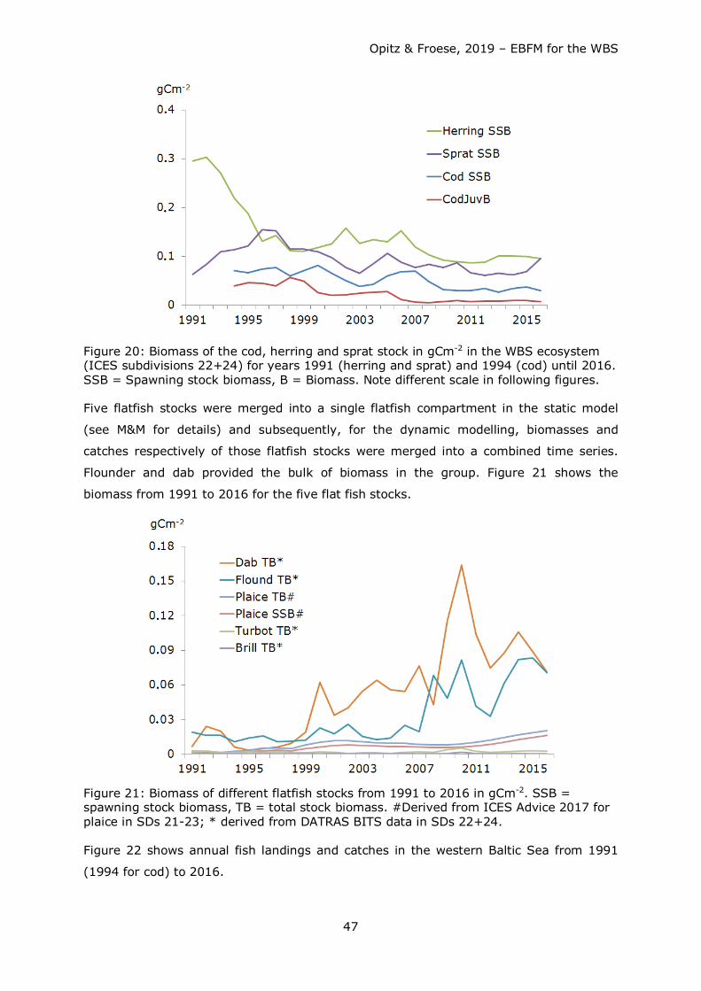
Opitz & Froese, 2019 – EBFM for the WBS
47
Figure 20: Biomass of the cod, herring and sprat stock in gCm-2 in the WBS ecosystem (ICES subdivisions 22+24) for years 1991 (herring and sprat) and 1994 (cod) until 2016. SSB = Spawning stock biomass, B = Biomass. Note different scale in following figures.
Five flatfish stocks were merged into a single flatfish compartment in the static model
(see M&M for details) and subsequently, for the dynamic modelling, biomasses and
catches respectively of those flatfish stocks were merged into a combined time series.
Flounder and dab provided the bulk of biomass in the group. Figure 21 shows the
biomass from 1991 to 2016 for the five flat fish stocks.
Figure 21: Biomass of different flatfish stocks from 1991 to 2016 in gCm-2. SSB = spawning stock biomass, TB = total stock biomass. #Derived from ICES Advice 2017 for plaice in SDs 21-23; * derived from DATRAS BITS data in SDs 22+24.
Figure 22 shows annual fish landings and catches in the western Baltic Sea from 1991
(1994 for cod) to 2016.
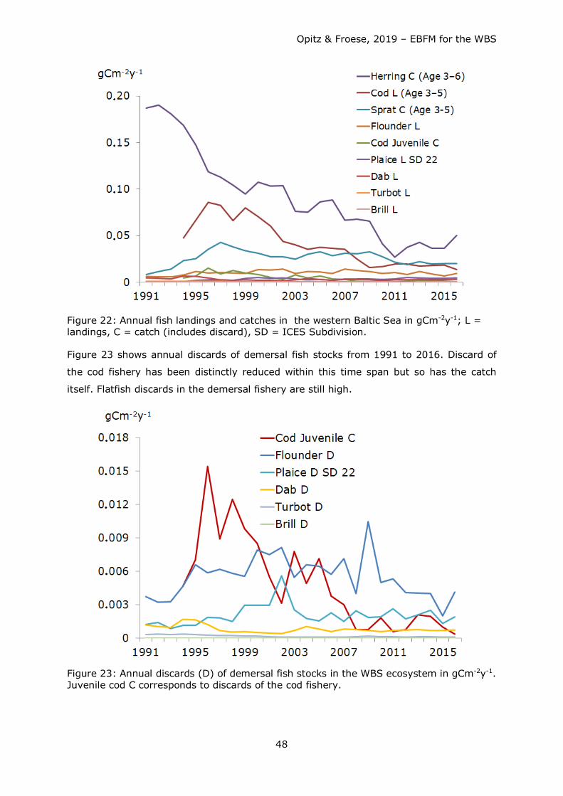
Opitz & Froese, 2019 – EBFM for the WBS
48
Figure 22: Annual fish landings and catches in the western Baltic Sea in gCm-2y-1; L = landings, C = catch (includes discard), SD = ICES Subdivision.
Figure 23 shows annual discards of demersal fish stocks from 1991 to 2016. Discard of
the cod fishery has been distinctly reduced within this time span but so has the catch
itself. Flatfish discards in the demersal fishery are still high.
Figure 23: Annual discards (D) of demersal fish stocks in the WBS ecosystem in gCm-2y-1. Juvenile cod C corresponds to discards of the cod fishery.
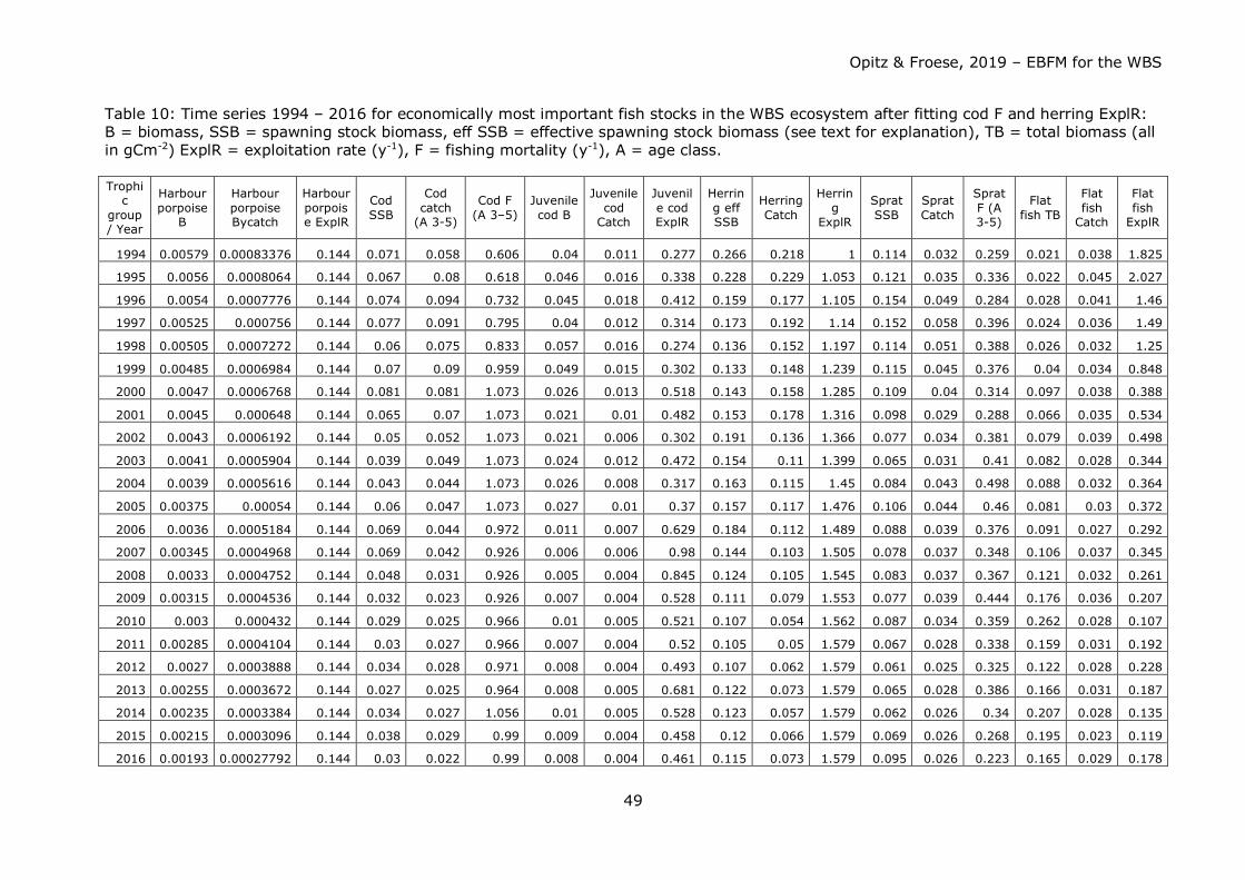
Opitz & Froese, 2019 – EBFM for the WBS
49
Table 10: Time series 1994 – 2016 for economically most important fish stocks in the WBS ecosystem after fitting cod F and herring ExplR: B = biomass, SSB = spawning stock biomass, eff SSB = effective spawning stock biomass (see text for explanation), TB = total biomass (all in gCm-2) ExplR = exploitation rate (y-1), F = fishing mortality (y-1), A = age class.
Trophic
group / Year
Harbour porpoise
B
Harbour porpoise Bycatch
Harbour porpoise ExplR
Cod SSB
Cod catch
(A 3-5)
Cod F (A 3–5)
Juvenile cod B
Juvenile cod
Catch
Juvenile cod ExplR
Herring eff SSB
Herring Catch
Herring
ExplR
Sprat SSB
Sprat Catch
Sprat F (A 3-5)
Flat fish TB
Flat fish
Catch
Flat fish
ExplR
1994 0.00579 0.00083376 0.144 0.071 0.058 0.606 0.04 0.011 0.277 0.266 0.218 1 0.114 0.032 0.259 0.021 0.038 1.825
1995 0.0056 0.0008064 0.144 0.067 0.08 0.618 0.046 0.016 0.338 0.228 0.229 1.053 0.121 0.035 0.336 0.022 0.045 2.027
1996 0.0054 0.0007776 0.144 0.074 0.094 0.732 0.045 0.018 0.412 0.159 0.177 1.105 0.154 0.049 0.284 0.028 0.041 1.46
1997 0.00525 0.000756 0.144 0.077 0.091 0.795 0.04 0.012 0.314 0.173 0.192 1.14 0.152 0.058 0.396 0.024 0.036 1.49
1998 0.00505 0.0007272 0.144 0.06 0.075 0.833 0.057 0.016 0.274 0.136 0.152 1.197 0.114 0.051 0.388 0.026 0.032 1.25
1999 0.00485 0.0006984 0.144 0.07 0.09 0.959 0.049 0.015 0.302 0.133 0.148 1.239 0.115 0.045 0.376 0.04 0.034 0.848
2000 0.0047 0.0006768 0.144 0.081 0.081 1.073 0.026 0.013 0.518 0.143 0.158 1.285 0.109 0.04 0.314 0.097 0.038 0.388
2001 0.0045 0.000648 0.144 0.065 0.07 1.073 0.021 0.01 0.482 0.153 0.178 1.316 0.098 0.029 0.288 0.066 0.035 0.534
2002 0.0043 0.0006192 0.144 0.05 0.052 1.073 0.021 0.006 0.302 0.191 0.136 1.366 0.077 0.034 0.381 0.079 0.039 0.498
2003 0.0041 0.0005904 0.144 0.039 0.049 1.073 0.024 0.012 0.472 0.154 0.11 1.399 0.065 0.031 0.41 0.082 0.028 0.344
2004 0.0039 0.0005616 0.144 0.043 0.044 1.073 0.026 0.008 0.317 0.163 0.115 1.45 0.084 0.043 0.498 0.088 0.032 0.364
2005 0.00375 0.00054 0.144 0.06 0.047 1.073 0.027 0.01 0.37 0.157 0.117 1.476 0.106 0.044 0.46 0.081 0.03 0.372
2006 0.0036 0.0005184 0.144 0.069 0.044 0.972 0.011 0.007 0.629 0.184 0.112 1.489 0.088 0.039 0.376 0.091 0.027 0.292
2007 0.00345 0.0004968 0.144 0.069 0.042 0.926 0.006 0.006 0.98 0.144 0.103 1.505 0.078 0.037 0.348 0.106 0.037 0.345
2008 0.0033 0.0004752 0.144 0.048 0.031 0.926 0.005 0.004 0.845 0.124 0.105 1.545 0.083 0.037 0.367 0.121 0.032 0.261
2009 0.00315 0.0004536 0.144 0.032 0.023 0.926 0.007 0.004 0.528 0.111 0.079 1.553 0.077 0.039 0.444 0.176 0.036 0.207
2010 0.003 0.000432 0.144 0.029 0.025 0.966 0.01 0.005 0.521 0.107 0.054 1.562 0.087 0.034 0.359 0.262 0.028 0.107
2011 0.00285 0.0004104 0.144 0.03 0.027 0.966 0.007 0.004 0.52 0.105 0.05 1.579 0.067 0.028 0.338 0.159 0.031 0.192
2012 0.0027 0.0003888 0.144 0.034 0.028 0.971 0.008 0.004 0.493 0.107 0.062 1.579 0.061 0.025 0.325 0.122 0.028 0.228
2013 0.00255 0.0003672 0.144 0.027 0.025 0.964 0.008 0.005 0.681 0.122 0.073 1.579 0.065 0.028 0.386 0.166 0.031 0.187
2014 0.00235 0.0003384 0.144 0.034 0.027 1.056 0.01 0.005 0.528 0.123 0.057 1.579 0.062 0.026 0.34 0.207 0.028 0.135
2015 0.00215 0.0003096 0.144 0.038 0.029 0.99 0.009 0.004 0.458 0.12 0.066 1.579 0.069 0.026 0.268 0.195 0.023 0.119
2016 0.00193 0.00027792 0.144 0.03 0.022 0.99 0.008 0.004 0.461 0.115 0.073 1.579 0.095 0.026 0.223 0.165 0.029 0.178
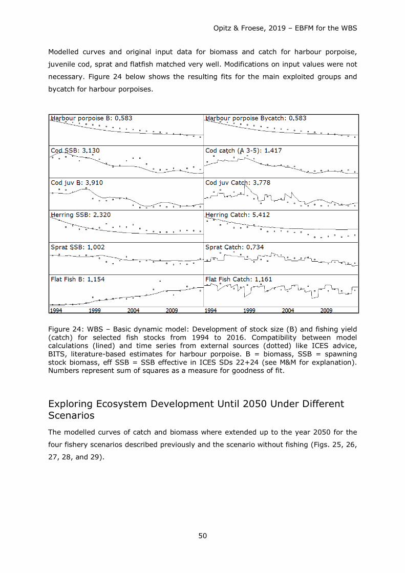
Opitz & Froese, 2019 – EBFM for the WBS
50
Modelled curves and original input data for biomass and catch for harbour porpoise,
juvenile cod, sprat and flatfish matched very well. Modifications on input values were not
necessary. Figure 24 below shows the resulting fits for the main exploited groups and
bycatch for harbour porpoises.
Figure 24: WBS – Basic dynamic model: Development of stock size (B) and fishing yield (catch) for selected fish stocks from 1994 to 2016. Compatibility between model calculations (lined) and time series from external sources (dotted) like ICES advice, BITS, literature-based estimates for harbour porpoise. B = biomass, SSB = spawning stock biomass, eff SSB = SSB effective in ICES SDs 22+24 (see M&M for explanation). Numbers represent sum of squares as a measure for goodness of fit.
Exploring Ecosystem Development Until 2050 Under Different Scenarios The modelled curves of catch and biomass where extended up to the year 2050 for the
four fishery scenarios described previously and the scenario without fishing (Figs. 25, 26,
27, 28, and 29).
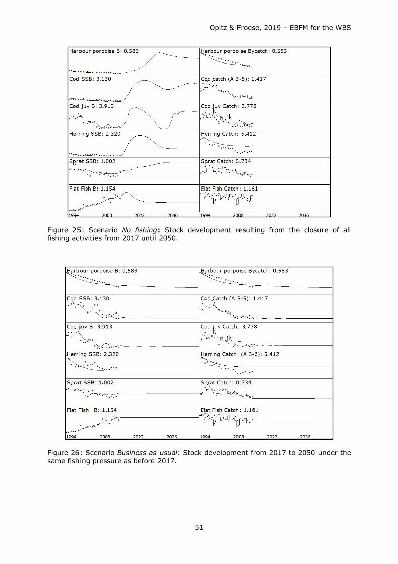
Opitz & Froese, 2019 – EBFM for the WBS
51
Figure 25: Scenario No fishing: Stock development resulting from the closure of all fishing activities from 2017 until 2050.
Figure 26: Scenario Business as usual: Stock development from 2017 to 2050 under the same fishing pressure as before 2017.
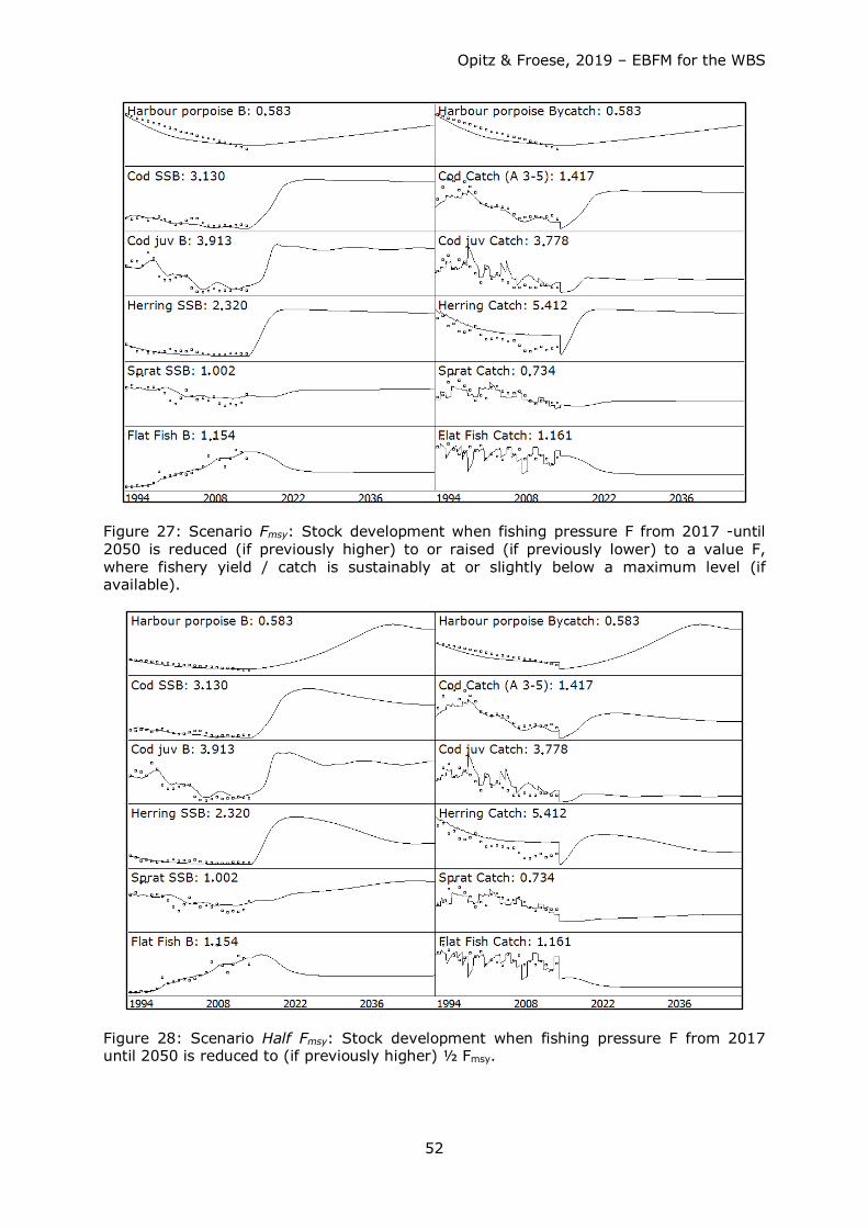
Opitz & Froese, 2019 – EBFM for the WBS
52
Figure 27: Scenario Fmsy: Stock development when fishing pressure F from 2017 -until 2050 is reduced (if previously higher) to or raised (if previously lower) to a value F, where fishery yield / catch is sustainably at or slightly below a maximum level (if available).
Figure 28: Scenario Half Fmsy: Stock development when fishing pressure F from 2017 until 2050 is reduced to (if previously higher) ½ Fmsy.
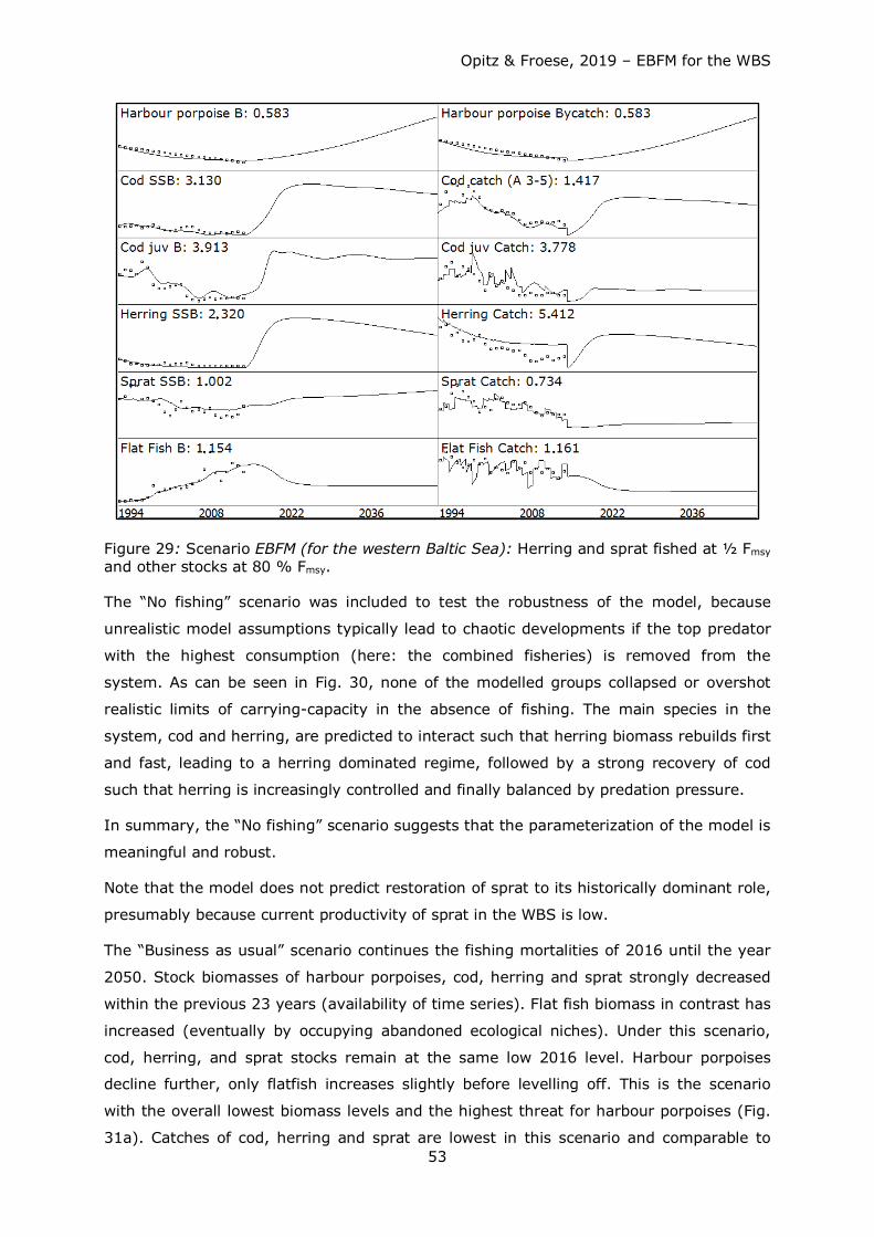
Opitz & Froese, 2019 – EBFM for the WBS
53
Figure 29: Scenario EBFM (for the western Baltic Sea): Herring and sprat fished at ½ Fmsy and other stocks at 80 % Fmsy.
The “No fishing” scenario was included to test the robustness of the model, because
unrealistic model assumptions typically lead to chaotic developments if the top predator
with the highest consumption (here: the combined fisheries) is removed from the
system. As can be seen in Fig. 30, none of the modelled groups collapsed or overshot
realistic limits of carrying-capacity in the absence of fishing. The main species in the
system, cod and herring, are predicted to interact such that herring biomass rebuilds first
and fast, leading to a herring dominated regime, followed by a strong recovery of cod
such that herring is increasingly controlled and finally balanced by predation pressure.
In summary, the “No fishing” scenario suggests that the parameterization of the model is
meaningful and robust.
Note that the model does not predict restoration of sprat to its historically dominant role,
presumably because current productivity of sprat in the WBS is low.
The “Business as usual” scenario continues the fishing mortalities of 2016 until the year
2050. Stock biomasses of harbour porpoises, cod, herring and sprat strongly decreased
within the previous 23 years (availability of time series). Flat fish biomass in contrast has
increased (eventually by occupying abandoned ecological niches). Under this scenario,
cod, herring, and sprat stocks remain at the same low 2016 level. Harbour porpoises
decline further, only flatfish increases slightly before levelling off. This is the scenario
with the overall lowest biomass levels and the highest threat for harbour porpoises (Fig.
31a). Catches of cod, herring and sprat are lowest in this scenario and comparable to
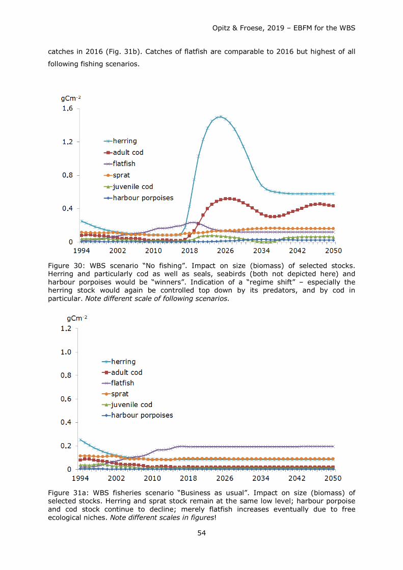
Opitz & Froese, 2019 – EBFM for the WBS
54
catches in 2016 (Fig. 31b). Catches of flatfish are comparable to 2016 but highest of all
following fishing scenarios.
Figure 30: WBS scenario “No fishing”. Impact on size (biomass) of selected stocks. Herring and particularly cod as well as seals, seabirds (both not depicted here) and harbour porpoises would be “winners”. Indication of a “regime shift” – especially the herring stock would again be controlled top down by its predators, and by cod in particular. Note different scale of following scenarios.
Figure 31a: WBS fisheries scenario “Business as usual”. Impact on size (biomass) of selected stocks. Herring and sprat stock remain at the same low level; harbour porpoise and cod stock continue to decline; merely flatfish increases eventually due to free ecological niches. Note different scales in figures!
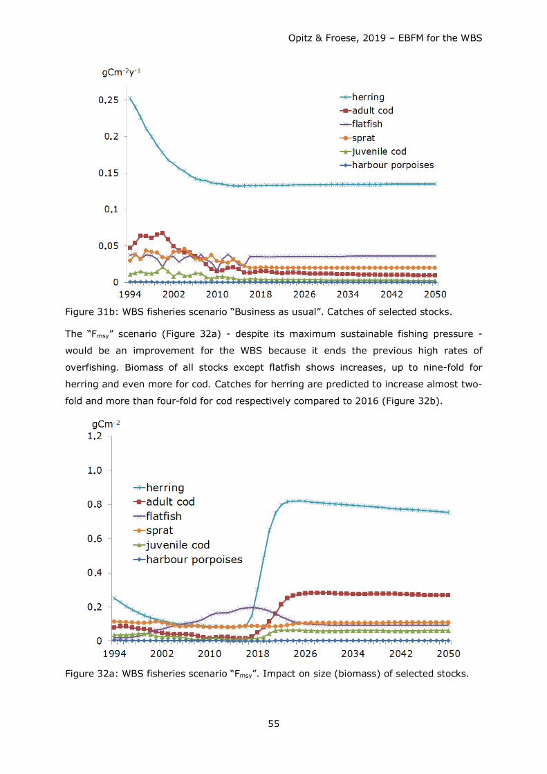
Opitz & Froese, 2019 – EBFM for the WBS
55
Figure 31b: WBS fisheries scenario “Business as usual”. Catches of selected stocks.
The “Fmsy” scenario (Figure 32a) - despite its maximum sustainable fishing pressure -
would be an improvement for the WBS because it ends the previous high rates of
overfishing. Biomass of all stocks except flatfish shows increases, up to nine-fold for
herring and even more for cod. Catches for herring are predicted to increase almost two-
fold and more than four-fold for cod respectively compared to 2016 (Figure 32b).
Figure 32a: WBS fisheries scenario “Fmsy”. Impact on size (biomass) of selected stocks.
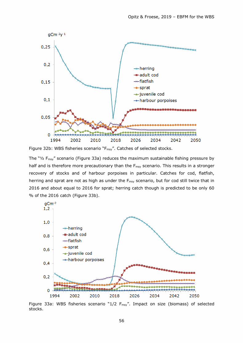
Opitz & Froese, 2019 – EBFM for the WBS
56
Figure 32b: WBS fisheries scenario “Fmsy”. Catches of selected stocks.
The “½ Fmsy” scenario (Figure 33a) reduces the maximum sustainable fishing pressure by
half and is therefore more precautionary than the Fmsy scenario. This results in a stronger
recovery of stocks and of harbour porpoises in particular. Catches for cod, flatfish,
herring and sprat are not as high as under the Fmsy scenario, but for cod still twice that in
2016 and about equal to 2016 for sprat; herring catch though is predicted to be only 60
% of the 2016 catch (Figure 33b).
Figure 33a: WBS fisheries scenario “1/2 Fmsy”. Impact on size (biomass) of selected stocks.
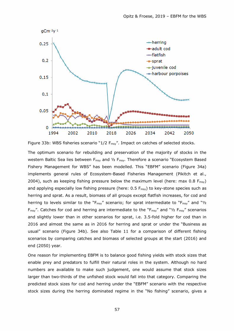
Opitz & Froese, 2019 – EBFM for the WBS
57
Figure 33b: WBS fisheries scenario “1/2 Fmsy”. Impact on catches of selected stocks.
The optimum scenario for rebuilding and preservation of the majority of stocks in the
western Baltic Sea lies between Fmsy and ½ Fmsy. Therefore a scenario “Ecosystem Based
Fishery Management for WBS” has been modelled. This “EBFM” scenario (Figure 34a)
implements general rules of Ecosystem-Based Fisheries Management (Pikitch et al.,
2004), such as keeping fishing pressure below the maximum level (here: max 0.8 Fmsy)
and applying especially low fishing pressure (here: 0.5 Fmsy) to key-stone species such as
herring and sprat. As a result, biomass of all groups except flatfish increases, for cod and
herring to levels similar to the “Fmsy” scenario; for sprat intermediate to “Fmsy” and “½
Fmsy”. Catches for cod and herring are intermediate to the “Fmsy” and “½ Fmsy” scenarios
and slightly lower than in other scenarios for sprat, i.e. 3.5-fold higher for cod than in
2016 and almost the same as in 2016 for herring and sprat or under the “Business as
usual” scenario (Figure 34b). See also Table 11 for a comparison of different fishing
scenarios by comparing catches and biomass of selected groups at the start (2016) and
end (2050) year.
One reason for implementing EBFM is to balance good fishing yields with stock sizes that
enable prey and predators to fulfill their natural roles in the system. Although no hard
numbers are available to make such judgement, one would assume that stock sizes
larger than two-thirds of the unfished stock would fall into that category. Comparing the
predicted stock sizes for cod and herring under the “EBFM” scenario with the respective
stock sizes during the herring dominated regime in the “No fishing” scenario, gives a
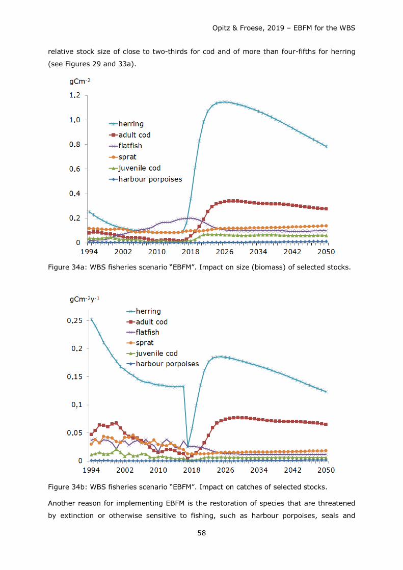
Opitz & Froese, 2019 – EBFM for the WBS
58
relative stock size of close to two-thirds for cod and of more than four-fifths for herring
(see Figures 29 and 33a).
Figure 34a: WBS fisheries scenario “EBFM”. Impact on size (biomass) of selected stocks.
Figure 34b: WBS fisheries scenario “EBFM”. Impact on catches of selected stocks.
Another reason for implementing EBFM is the restoration of species that are threatened
by extinction or otherwise sensitive to fishing, such as harbour porpoises, seals and
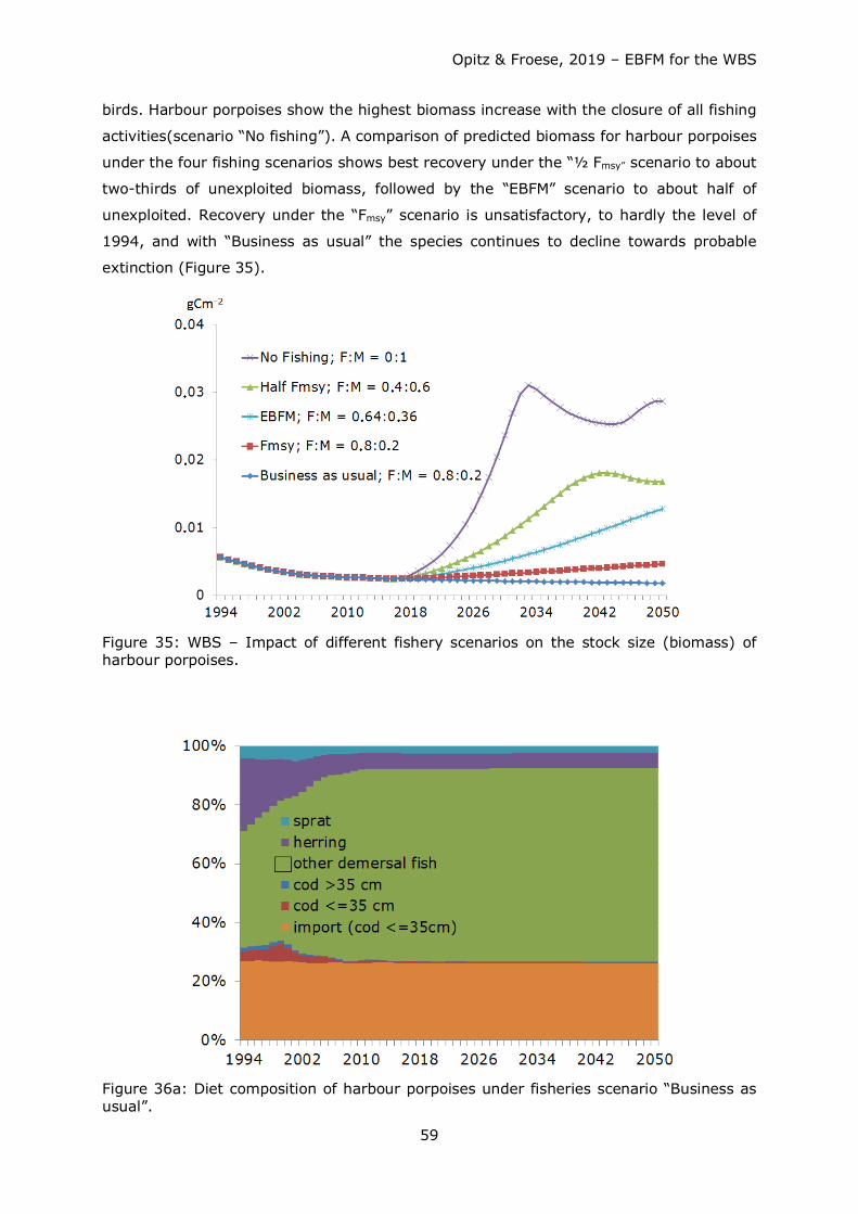
Opitz & Froese, 2019 – EBFM for the WBS
59
birds. Harbour porpoises show the highest biomass increase with the closure of all fishing
activities(scenario “No fishing”). A comparison of predicted biomass for harbour porpoises
under the four fishing scenarios shows best recovery under the “½ Fmsy” scenario to about
two-thirds of unexploited biomass, followed by the “EBFM” scenario to about half of
unexploited. Recovery under the “Fmsy” scenario is unsatisfactory, to hardly the level of
1994, and with “Business as usual” the species continues to decline towards probable
extinction (Figure 35).
Figure 35: WBS – Impact of different fishery scenarios on the stock size (biomass) of harbour porpoises.
Figure 36a: Diet composition of harbour porpoises under fisheries scenario “Business as usual”.
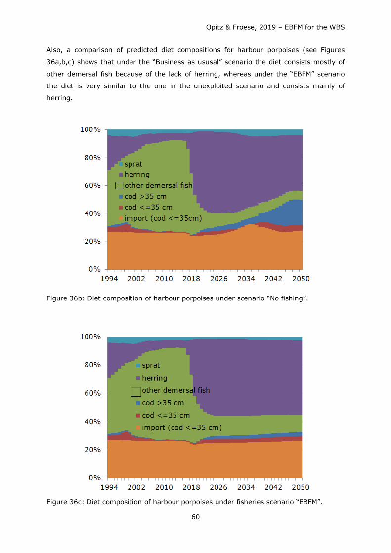
Opitz & Froese, 2019 – EBFM for the WBS
60
Also, a comparison of predicted diet compositions for harbour porpoises (see Figures
36a,b,c) shows that under the “Business as ususal” scenario the diet consists mostly of
other demersal fish because of the lack of herring, whereas under the “EBFM” scenario
the diet is very similar to the one in the unexploited scenario and consists mainly of
herring.
Figure 36b: Diet composition of harbour porpoises under scenario “No fishing”.
Figure 36c: Diet composition of harbour porpoises under fisheries scenario “EBFM”.
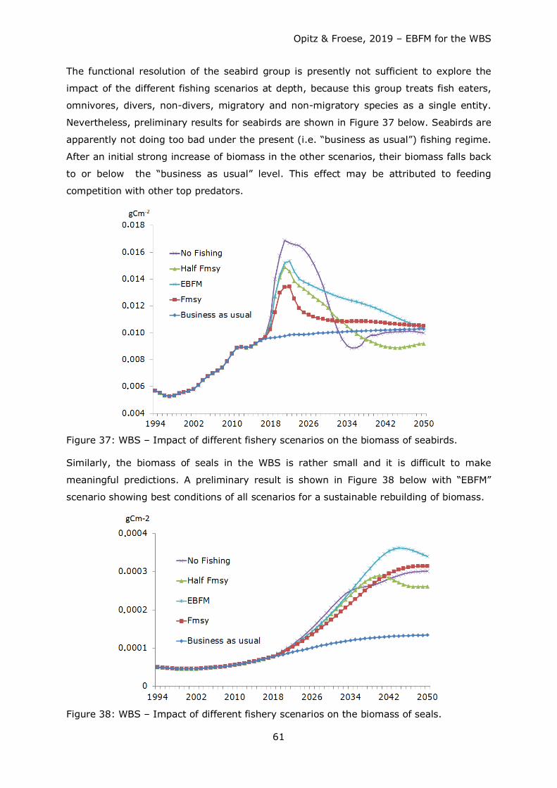
Opitz & Froese, 2019 – EBFM for the WBS
61
The functional resolution of the seabird group is presently not sufficient to explore the
impact of the different fishing scenarios at depth, because this group treats fish eaters,
omnivores, divers, non-divers, migratory and non-migratory species as a single entity.
Nevertheless, preliminary results for seabirds are shown in Figure 37 below. Seabirds are
apparently not doing too bad under the present (i.e. “business as usual”) fishing regime.
After an initial strong increase of biomass in the other scenarios, their biomass falls back
to or below the “business as usual” level. This effect may be attributed to feeding
competition with other top predators.
Figure 37: WBS – Impact of different fishery scenarios on the biomass of seabirds.
Similarly, the biomass of seals in the WBS is rather small and it is difficult to make
meaningful predictions. A preliminary result is shown in Figure 38 below with “EBFM”
scenario showing best conditions of all scenarios for a sustainable rebuilding of biomass.
Figure 38: WBS – Impact of different fishery scenarios on the biomass of seals.
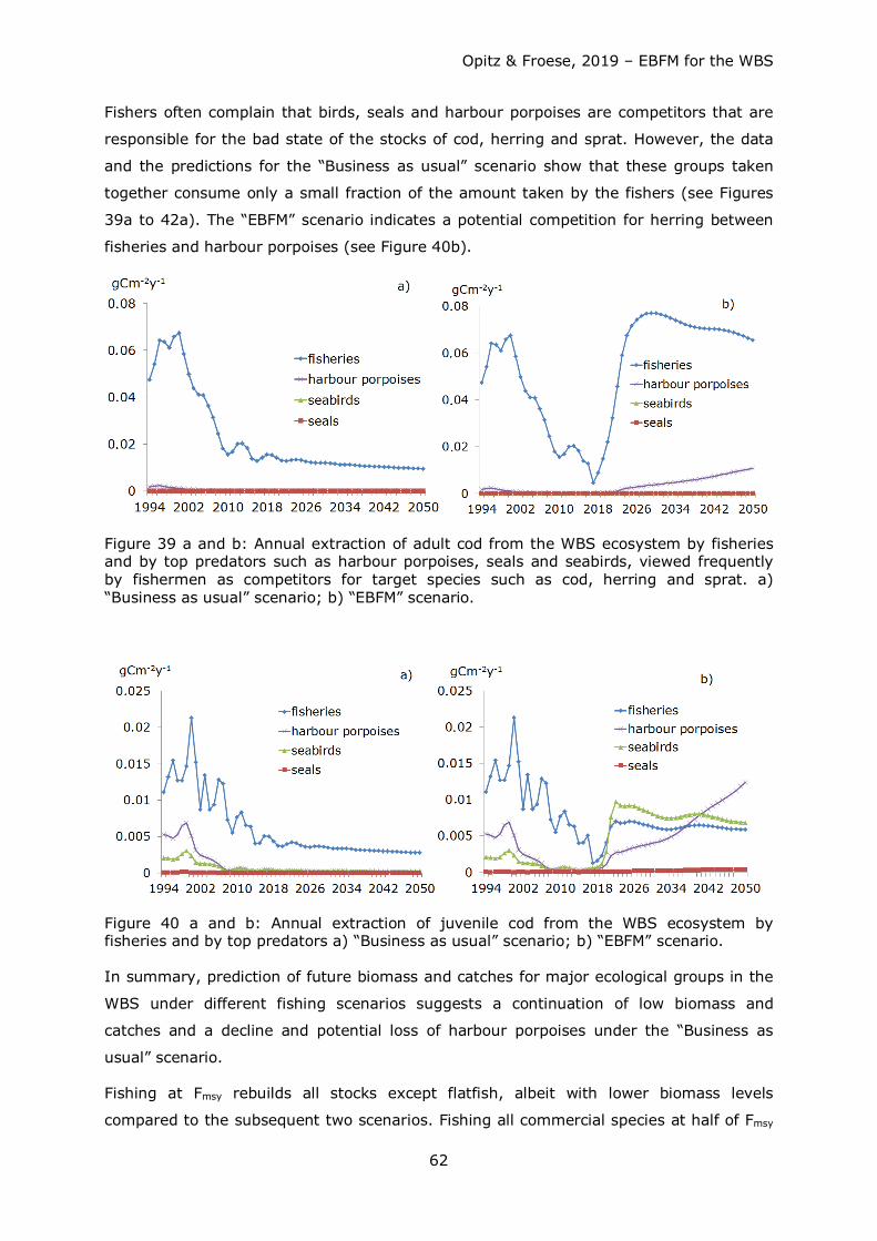
Opitz & Froese, 2019 – EBFM for the WBS
62
Fishers often complain that birds, seals and harbour porpoises are competitors that are
responsible for the bad state of the stocks of cod, herring and sprat. However, the data
and the predictions for the “Business as usual” scenario show that these groups taken
together consume only a small fraction of the amount taken by the fishers (see Figures
39a to 42a). The “EBFM” scenario indicates a potential competition for herring between
fisheries and harbour porpoises (see Figure 40b).
Figure 39 a and b: Annual extraction of adult cod from the WBS ecosystem by fisheries and by top predators such as harbour porpoises, seals and seabirds, viewed frequently by fishermen as competitors for target species such as cod, herring and sprat. a) “Business as usual” scenario; b) “EBFM” scenario.
Figure 40 a and b: Annual extraction of juvenile cod from the WBS ecosystem by fisheries and by top predators a) “Business as usual” scenario; b) “EBFM” scenario.
In summary, prediction of future biomass and catches for major ecological groups in the
WBS under different fishing scenarios suggests a continuation of low biomass and
catches and a decline and potential loss of harbour porpoises under the “Business as
usual” scenario.
Fishing at Fmsy rebuilds all stocks except flatfish, albeit with lower biomass levels
compared to the subsequent two scenarios. Fishing all commercial species at half of Fmsy
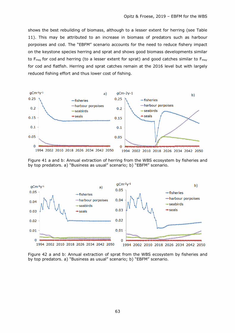
Opitz & Froese, 2019 – EBFM for the WBS
63
shows the best rebuilding of biomass, although to a lesser extent for herring (see Table
11). This may be attributed to an increase in biomass of predators such as harbour
porpoises and cod. The “EBFM” scenario accounts for the need to reduce fishery impact
on the keystone species herring and sprat and shows good biomass developments similar
to Fmsy for cod and herring (to a lesser extent for sprat) and good catches similar to Fmsy
for cod and flatfish. Herring and sprat catches remain at the 2016 level but with largely
reduced fishing effort and thus lower cost of fishing.
Figure 41 a and b: Annual extraction of herring from the WBS ecosystem by fisheries and by top predators. a) “Business as usual” scenario; b) “EBFM” scenario.
Figure 42 a and b: Annual extraction of sprat from the WBS ecosystem by fisheries and by top predators. a) “Business as usual” scenario; b) “EBFM” scenario.
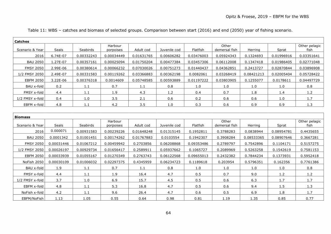
Opitz & Froese, 2019 – EBFM for the WBS
64
Table 11: WBS – catches and biomass of selected groups. Comparison between start (2016) and end (2050) year of fishing scenario.
Catches
Scenario & Year Seals Seabirds Harbour
porpoises Adult cod Juvenile cod Flatfish Other
demersal fish Herring Sprat Other pelagic
fish
2016 6.74E-07 0.00332243 0.00034449 0.01631765 0.00606282 0.03476003 0.05924343 0.1324693 0.01996916 0.03351641
BAU 2050 1.27E-07 0.00357161 0.00025094 0.01750204 0.00477384 0.03457306 0.06112008 0.1347418 0.01986405 0.02771048
FMSY 2050 2.99E-06 0.00380614 0.00066232 0.07030026 0.00751273 0.01440437 0.04362851 0.2413727 0.02870844 0.03896908
1/2 FMSY 2050 2.49E-07 0.00331583 0.00119262 0.03366883 0.00362198 0.0082061 0.03268419 0.08421213 0.02005404 0.05728422
EBFM 2050 3.22E-06 0.00376318 0.0014609 0.05748585 0.00593889 0.01197222 0.03803905 0.1255077 0.0178611 0.04497729
BAU x-fold 0.2 1.1 0.7 1.1 0.8 1.0 1.0 1.0 1.0 0.8
FMSY x-fold 4.4 1.1 1.9 4.3 1.2 0.4 0.7 1.8 1.4 1.2
1/2 FMSY x-fold 0.4 1.0 3.5 2.1 0.6 0.2 0.6 0.6 1.0 1.7
EBFM x-fold 4.8 1.1 4.2 3.5 1.0 0.3 0.6 0.9 0.9 1.3
Biomass
Scenario & Year Seals Seabirds Harbour
porpoises Adult cod Juvenile cod Flatfish Other
demersal fish Herring Sprat Other pelagic
fish
2016 0.000071 0.00931583 0.00239226 0.01648248 0.01315145 0.1952811 0.3788283 0.0838944 0.08954781 0.4435655
BAU 2050 0.0001342 0.01001451 0.00174262 0.01767883 0.0103554 0.1942307 0.3908284 0.08533365 0.08907646 0.3667281
FMSY 2050 0.00031446 0.01067212 0.00459942 0.2703856 0.06208868 0.09353486 0.2789797 0.7542896 0.1104171 0.5157275
1/2 FMSY 2050 0.00026197 0.00929734 0.01656417 0.2589911 0.05937662 0.1065727 0.2089969 0.5263258 0.1542619 0.7581153
EBFM 2050 0.00033939 0.01055167 0.01270349 0.2763743 0.06122568 0.09655013 0.2432382 0.7844234 0.1373931 0.5952418
NoFish 2050 0.00030109 0.01006032 0.02297375 0.4345959 0.06234723 0.1189618 0.203954 0.5796351 0.162356 0.7761386
BAU x-fold 1.9 1.1 0.7 1.1 0.8 1.0 1.0 1.0 1.0 0.8
FMSY x-fold 4.4 1.1 1.9 16.4 4.7 0.5 0.7 9.0 1.2 1.2
1/2 FMSY x-fold 3.7 1.0 6.9 15.7 4.5 0.5 0.6 6.3 1.7 1.7
EBFM x-fold 4.8 1.1 5.3 16.8 4.7 0.5 0.6 9.4 1.5 1.3
NoFish x-fold 4.2 1.1 9.6 26.4 4.7 0.6 0.5 6.9 1.8 1.7
EBFM/NoFish 1.13 1.05 0.55 0.64 0.98 0.81 1.19 1.35 0.85 0.77
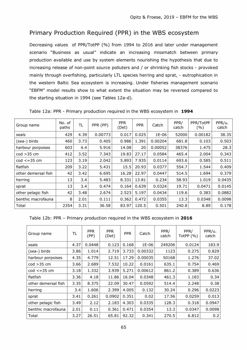
Opitz & Froese, 2019 – EBFM for the WBS
65
Primary Production Required (PPR) in the WBS ecosystem
Decreasing values of PPR/TotPP (%) from 1994 to 2016 and later under management
scenario “Business as usual” indicate an increasing missmatch between primary
production available and use by system elements nourishing the hypothesis that due to
increasing release of non-point source polluters and / or shrinking fish stocks - provoked
mainly through overfishing, particularly LTL species herring and sprat, - eutrophication in
the western Baltic Sea ecosystem is increasing. Under fisheries management scenario
“EBFM” model results show to what extent the situation may be reversed compared to
the starting situation in 1994 (see Tables 12a-d).
Table 12a: PPR - Primary production required in the WBS ecosystem in 1994
Group name No. of paths TL PPR (PP) PPR
(Det) PPR Catch PPR/ catch
PPR/TotPP (%)
PPR/u. catch
seals 429 4.39 0.00773 0.017 0.025 1E-06 52000 0.00182 38.35
(sea-) birds 460 3.73 0.405 0.986 1.391 0.00204 681.8 0.103 0.503 harbour porpoises 603 4.4 5.916 14.08 20 0.00052 38376 1.475 28.3
cod >35 cm 412 3.52 7.343 19.83 27.17 0.0584 465.4 2.004 0.343 cod <=35 cm 123 3.19 2.042 5.893 7.935 0.0114 693.6 0.585 0.511
flatfish 209 3.22 5.431 15.5 20.93 0.0377 554.7 1.544 0.409 other demersal fish 42 3.42 6.695 16.28 22.97 0.0447 514.5 1.694 0.379
herring 13 3.4 5.483 8.331 13.81 0.234 58.93 1.019 0.0435
sprat 13 3.4 0.474 0.164 0.639 0.0324 19.71 0.0471 0.0145 other pelagic fish 42 3.48 2.674 2.523 5.197 0.0434 119.6 0.383 0.0882
benthic macrofauna 8 2.01 0.111 0.362 0.472 0.0355 13.3 0.0348 0.0098 Total 2354 3.31 36.58 83.97 120.5 0.501 240.8 8.89 0.178
Table 12b: PPR – Primary production required in the WBS ecosystem in 2016
Group name TL PPR (PP)
PPR (Det) PPR Catch PPR/
catch PPR/
TotPP (%) PPR/u. catch
seals 4.37 0.0448 0.123 0.168 1E-06 249206 0.0124 183.9 (sea-) birds 3.86 1.014 2.719 3.733 0.00332 1123 0.275 0.829
harbour porpoises 4.35 4.779 12.51 17.29 0.00035 50168 1.276 37.02
cod >35 cm 3.66 2.689 7.532 10.22 0.0161 635.1 0.754 0.469 cod <=35 cm 3.18 1.332 3.939 5.271 0.00612 861.2 0.389 0.636
flatfish 3.36 4.18 11.86 16.04 0.0348 461.3 1.183 0.34 other demersal fish 3.35 8.375 22.09 30.47 0.0592 514.4 2.248 0.38
herring 3.4 1.606 2.399 4.005 0.132 30.24 0.296 0.0223 sprat 3.41 0.261 0.0902 0.351 0.02 17.56 0.0259 0.013
other pelagic fish 3.49 2.12 2.183 4.303 0.0335 128.3 0.318 0.0947
benthic macrofauna 2.01 0.11 0.361 0.471 0.0354 13.3 0.0347 0.0098 Total 3.27 26.51 65.81 92.32 0.341 270.5 6.812 0.2
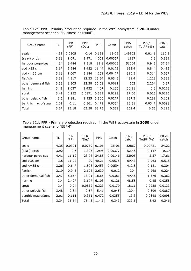
Opitz & Froese, 2019 – EBFM for the WBS
66
Table 12c: PPR - Primary production required in the WBS ecosystem in 2050 under management scenario “Business as usual”.
Group name TL PPR (PP)
PPR (Det) PPR Catch PPR/
catch PPR/
TotPP (%) PPR/u. catch
seals 4.38 0.0505 0.14 0.191 1E-06 149802 0.0141 110.5 (sea-) birds 3.88 1.091 2.971 4.062 0.00357 1137 0.3 0.839
harbour porpoises 4.34 3.484 9.318 12.8 0.00025 51004 0.945 37.64
cod >35 cm 3.67 2.984 8.452 11.44 0.0175 653.4 0.844 0.482 cod <=35 cm 3.18 1.067 3.184 4.251 0.00477 890.5 0.314 0.657
flatfish 3.39 4.317 12.33 16.64 0.0346 481.4 1.228 0.355 other demersal fish 3.33 8.303 22.38 30.68 0.0611 502 2.264 0.37
herring 3.41 1.637 2.432 4.07 0.135 30.21 0.3 0.0223 sprat 3.41 0.252 0.0871 0.339 0.0199 17.06 0.025 0.0126
other pelagic fish 3.5 1.881 1.925 3.806 0.0277 137.3 0.281 0.101
benthic macrofauna 2.01 0.11 0.361 0.471 0.0354 13.31 0.0347 0.0098 Total 3.27 25.18 63.58 88.75 0.339 261.4 6.55 0.193 Table 12d: PPR - Primary production required in the WBS ecosystem in 2050 under management scenario “EBFM”.
Group name TL PPR (PP)
PPR (Det) PPR Catch PPR /
catch PPR /
TotPP (%) PPR /u. catch
seals 4.35 0.0321 0.0739 0.106 3E-06 32867 0.00781 24.22
(sea-) birds 3.92 0.6 1.395 1.995 0.00377 529.8 0.147 0.39 harbour porpoises 4.41 11.12 23.76 34.88 0.00146 23905 2.57 17.61
cod >35 cm 3.8 11.22 29 40.21 0.0575 699.3 2.963 0.515 cod <=35 cm 3.26 0.647 1.806 2.453 0.00594 412.8 0.181 0.304
flatfish 3.19 0.943 2.696 3.639 0.012 304 0.268 0.224
other demersal fish 3.47 5.667 13.01 18.68 0.0381 490.8 1.376 0.362 herring 3.4 2.427 3.677 6.103 0.126 48.58 0.45 0.0358
sprat 3.4 0.24 0.0832 0.323 0.0179 18.11 0.0238 0.0133 other pelagic fish 3.48 2.84 2.57 5.41 0.045 120.4 0.399 0.0887
benthic macrofauna 2.01 0.111 0.361 0.472 0.0355 13.3 0.0348 0.0098 Total 3.34 35.84 78.43 114.3 0.343 333.5 8.42 0.246
Opitz & Froese, 2019 – EBFM for the WBS
67
Discussion Quality of the 1994 Model
The Ecopath model for 1994 is the first model that combines all living components of the
WBS ecosystem and quantitatively connects them via their diet.
In summary, the WBS food web in 1994 may be characterized as a system under stress.
Ecotrophic efficiency values >1 or near 1 for all fish species / groups indicated that these
groups were “overused”, i.e. annual consumption (to a larger extent by fisheries and to a
lesser one by natural predators) exceeded annual production. In some cases, e.g. for
flatfish, this result may be aggravated by reporting biases. Important commercial stocks
such as western Baltic cod and western Baltic spring spawning herring were suffering
from overfishing. Particularly for herring and juvenile cod the demand could only be
balanced assuming immigration from and coverage of dietary needs of predators in
neighbouring areas.
One may argue “why should one have confidence in a model where more is used than is
available”?
The western Baltic sea is not a closed system; instead there is inflow and outflow of
waters and organisms swimming and floating therein. And there are organisms that can
actively search for food, shelter, and suitable mating and hatching sites in nearby
ecosystems. Thus, there is considerable exchange of energy and matter with those
neighbouring ecosystems.
In the Ecopath base model year 1994 important fish stocks such as herring, and sprat
were already overfished and in the decent and stocks did not produce “sufficient”
biomass to satisfy extraction by predators and fishery on a balanced level. Thus, the lack
of a certain food item may be balanced by shifting to more abundant food items within
the model area or by assuming import or immigration of the scarce food item. We opted
for the latter approach because the first one makes single contributions from different
scarce food items indiscernible. Conclusion is that system resources – are being or
“overused” or “predation pressure shifted down to lower trophic levels”.
One of the rules in Ecopath is that the exchange of matter with neighbouring systems per
unit of time should not exceed the production of matter within the model system.
Summary statistics for the model area show, that total system production was 632 gCm-
2y-1. In comparison only 0,4 gCm-2y-1 (excluding detritus) or 232 gCm-2y-1 (including
detritus) were exported out of the model system, and 0,18 gCm-2y-1 (excluding detritus)
or 213 gCm-2y-1 (including detritus) entered the system by import of food through mobile
organisms (e.g. harbour porpoises, birds) or by immigration (herring, sprat, flatfish). It
Opitz & Froese, 2019 – EBFM for the WBS
68
should be noted in this context that detritus is not a producer but more a source / sink of
matter.
Prior qualitative knowledge about the WBS suggested that herring was a LTL (Low
Trophic Level) keystone species (Essington & Plagányi, 2013) and of more importance to
higher trophic levels than sprat. This may be attributable quantitatively to the size of the
herring stock and related flows. Herring had the highest stock biomass in the WBS
system (the sprat stock – although being more productive per unit of biomass - was only
half the size of the herring stock) and transported the highest amount of matter from
lower trophic levels (mostly zooplankton) to a large number of predators at higher and
highest trophic levels. The model showed that herring served more predators and more
herring was consumed by predators than sprat. Figure 42 shows the strength of impact
of trophic groups on the food web using a measure named Keystone Index no. 1
(Libralato et al. 2006). Herring shows the highest value as a single fish species
transporting matter from low trophic levels to predators high in the food web.
With reference to the quality of input data (for a quality ranking of input data see Table 5
above) there is a strong need for better inputs particularly for top predators such as
harbour porpoises (B, P/B), seals (all inputs), and seabirds (all inputs).
Quality of the EwE Fitting and Predictions
For the 1994 Ecopath model, the biomass of seals was actually too low to properly
qualify for a group of their own and would normally have been lumped with harbour
porpoises into one marine mammals group. Nevertheless, this species was treated as a
group of its own because harbour porpoises in the WBS are threatened by extinction and
thus of special concern in the context of EBFM. Furthermore, harbour porpoises and
seals have different dietary needs. Porpoises are particularly dependent on energy-rich
food and must eat constantly to meet their high metabolic energy demands (Read &
Hohn, 1995, Wisniewska et al. 2018). Similarly, seabirds are a group that spans several
trophic levels (from benthic macrofauna eaters such as ducks to fish eaters such as sea
gulls and cormorants (Phalacrocorax carbo)) and includes migratory and non-migratory
birds (ICES JWGBIRD, 2016c). For these reasons, the EwE for seals and seabirds are
considered to be only partially representative and are not discussed further.
Traditionally, the quality of a model is validated by comparing model results with
independent (sets of) data, i.e. with external data not used during the modelling
procedure (Joergensen & Bendoricchio, 2001). In this study, model predictions of catch
and biomass for years 1994-2016 matched input values for catch and biomass
remarkably well and only some adjustments to the fishing mortality before 2000 were
Opitz & Froese, 2019 – EBFM for the WBS
69
needed for adult cod to improve fits in these early years. There are indications in nature
– particularly for cod – for immigration and mixing of adjacent populations. Hüssy et al.
(2015) noted eastern Baltic cod invasions into the western Baltic since 2008, i.e. the
area west of Bornholm comprising a mixture of both stocks. While SD 22 is utilized
soley by the western cod stock and SD 25 utilized soley by the eastern cod stock, SD
24 north of Rügen is the main mixing zone, with 9 to 90 % eastern stock occurring in the
said area. According to Hüssy et al. (2015) invading cod from the eastern Baltic do not
spawn in the western part. Only occasionally do eastern juvenile cod invade the western
part.
ExplR for WBSS in ICES SDs 22+24 was fitted to estimated SSB time series of 50 % of
total stock area since biomass and F data were only available for the entire area covered
by the herring stock throughout the year (ICES SDs 20-24). The approximation of the
best fit for ExplR obtained during the fitting process suggested an increase of fishing
pressure within the model area along the time axis in contrast to a decrease of F for the
entire stock area (ICES SDs 20-24). The cause for this phenomenon is not quite clear but
it would explain to some extent why the herring stock is not rebuilding properly despite
of reducing quotas and thus fishing pressure lately. Provided that the assumption of 50%
SSB inside the model area holds true, results suggest that fishing pressure on herring
inside the model area has not been reduced along the years but has increased compared
to data of F published by ICES for the entire WBSS herring stock.
Plaganyi & Butterworth (2004) published a thorough analysis of advantages and
shortcomings of the EwE software packages II to VI. They state that “ECOPATH
constraints act as a rigorous analytical framework (in contrast to an ad hoc type model)”,
as well as “given good input data, EwE has utility to provide a first-order perturbation
analysis.” Plaganyi & Butterworth (2004) explicitly welcomed the introduction of the
foraging arena concept into EwE expressed through a vulnerability parameter (V) of prey
towards its predators. This has the effect of “dampening the unrealistically large
population fluctuations usually predicted by the Lotka-Volterra formulation”. Because
they state that vulnerability parameters are difficult to estimate, we used the default V =
2 for all predator-prey combinations.
The foraging arena concept in EwE expressed through a vulnerability parameter (V) of
prey towards its predators has the effect of “dampening the unrealistically large
population fluctuations usually predicted by the Lotka-Volterra formulation” (Plaganyi &
Butterworth, 2004). These vulnerability parameters are usually difficult to estimate. Trial
runs using the vulnerability routine during the fitting process yielded unrealistically high
values for a great part of predator / prey combinations. Therefore the default V = 2 for
all predator-prey combinations was used.
Opitz & Froese, 2019 – EBFM for the WBS
70
Another routine in EwE (see e.g. Heymans et al., 2016, for a thorough compilation of
model result evaluation routines in EwE) for addressing uncertainty of inputs is by
running input parameters through Monte Carlo simulations. This showed only a negligible
difference of SS before (25.19) and after (24.68) applying the routine to the calibrated
WBS model (start value before calibration >100).
These good fits increased confidence in the model predictions of future biomass and
catch for 2017 until 2050.
Another routine in EwE (see e.g. Heymans et al., 2016, for a thorough compilation of
model result evaluation routines in EwE) for addressing uncertainty of inputs is by
running input parameters through Monte Carlo simulations. Doing this showed only a
negligible difference of SS before (25.19) and after (24.68) applying the routine to the
calibrated WBS model (start value before calibration >100).
(1) The groups of juvenile and adult cod are treated as development “stanzas” (life
history stages) in EwE and are interdependent in the model. Figure 43 shows the
relationship between juvenile and adult cod biomass, which resembles a hockey-stick
stock-recruitment relationship (SR), as expected for cod. This SR is not an input to but
an output of the modelling process, and thus confirms the ability of the model to produce
reasonable results.
(2) Most ecosystem models enter states where groups crash or explode in size when left
unchecked for an extended period of time. This is, however, not the case for this WBS
model, where no group crashed or increased indefinitely, but rather, when modelled
without fishing, all groups reached and fluctuated around levels that seem to be
reasonable representations of carrying capacity, suggesting that biomass in 2016
represented about 4% of carrying capacity for cod and about 15% for herring.
(3) Köster & Möllmann (2000) postulate two stable states for the Baltic ecosystem, one
that is herring-dominated and the other, cod-dominated. The model predictions without
fishing indeed show two such stable states and suggest that, under such conditions, a
herring-dominated state would establish first (because increase in herring biomass is
faster), followed later by a cod-dominated state (because other herring-eating groups
increase even slower than cod but help switch the system once the joined consumption
equals or exceeds annual production of herring).
(4) Based on an earlier published ecosystem model by Harvey et al. (2003), Hansson et
al. (2007) explored possible effects of different management scenarios for the central
and eastern Baltic Sea. Scenarios included a strong increase of seals (marine mammals),
oligotrophication of the system, and impact of different fishing intensities on stock size
and catches of cod, herring, and sprat. They simulated a large number of scenario
combinations for the period 2001 to 2100 (we simulated scenarios for years 2017 to
Opitz & Froese, 2019 – EBFM for the WBS
71
2050). They ran simulations with three different fishing intensities named SQ (status quo
conditions), PA (precautionary approach as defined by ICES), and ½ PA. SQ resembles
“Business as usual” in our modelling and ½ PA would roughly correspond to Fmsy.
Similarly to our model (numbers in parentheses), both herring and cod biomass dropped
by 80% (77%) and 85% (80%) respectively during the “calibration” period 1974 to 2000
(1994 to 2016). In contrast to Hansson et al.´s (2007) findings of 80% sprat biomass in
WBS dropped only by slightly over 20%. This may be attributed to the fact that the Baltic
sprat stock is concentrated in the eastern part of the Baltic Sea and in WBS stock
biomass is only half the size of the herring stock. Thus, the ecological role (e.g. main LTL
species) and pattern of interaction differs from the eastern Baltic situation. Hansson et
al.´s (2007) simulations for years 2001 to 2100 predicted a continued and drastic
decrease of the herring and cod populations and an increase of the sprat stock for
continued SQ fishing intensities. For PA levels herring and cod stocks would thrive but
the sprat stock would be drastically reduced (PA level for sprat was higher than SQ
level). Despite decreased fishing intensities for cod and herring, catches would be
substantially higher than during the SQ fishing regime and similar to average catches for
the calibration period. Sprat catches, however, would decrease drastically due to
increased predation by cod. The highest catches were obtained when sprat was fished at
½ PA and cod and herring where fished at PA level. This combination and the resulting
catches compare to some extent to our “EBFM” scenario with herring and sprat fished at
½ Fmsy and other fish (including cod) at 80% Fmsy. Simulations of increased selection and
without catches of juveniles had only a very marginal impact on stock size.
Correction of Misconceptions
A number of misconceptions exist about the trophic relations in the WBS. One of these
predicts that an increase in adult cod would increase the rate of cannibalism on juvenile
cod (ICES, 2013). However, our model shows that if fishing pressure on herring is
reduced and thus herring biomass is allowed to increase, then cannibalism on juvenile
cod plays a minor, not increasing role. This is evident in the stock-recruitment
relationship (Figure 43) where, after an early peak, the number of juvenile cod should
continuously decline with increase in biomass of cannibalistic adults, which is clearly not
the case.
Another misconception is that birds (especially cormorants) consume a large fraction of
the biomass of cod and herring. The model shows that the combined consumption by
birds, seals and harbour porpoises on cod, herring, and sprat is negligible compared to
extraction by current fisheries (Figures 38a to 41a). But the model shows also that a big
increase of fish-eating marine mammals may create competition with fisheries
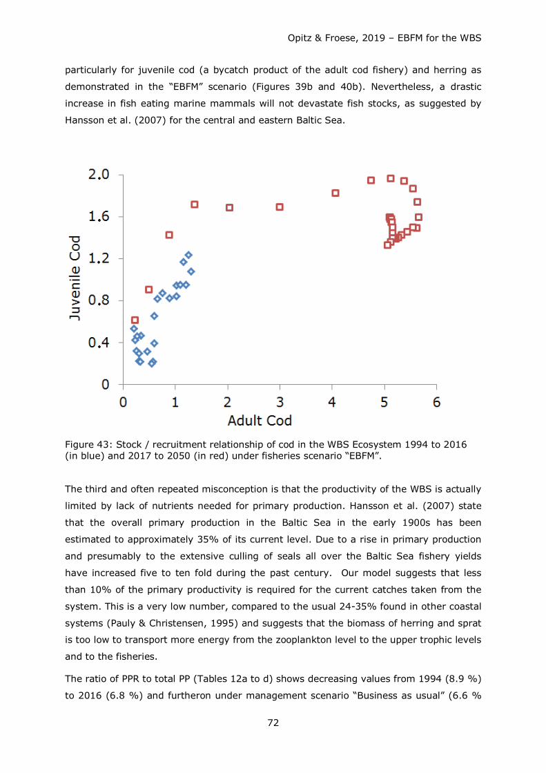
Opitz & Froese, 2019 – EBFM for the WBS
72
particularly for juvenile cod (a bycatch product of the adult cod fishery) and herring as
demonstrated in the “EBFM” scenario (Figures 39b and 40b). Nevertheless, a drastic
increase in fish eating marine mammals will not devastate fish stocks, as suggested by
Hansson et al. (2007) for the central and eastern Baltic Sea.
Figure 43: Stock / recruitment relationship of cod in the WBS Ecosystem 1994 to 2016 (in blue) and 2017 to 2050 (in red) under fisheries scenario “EBFM”.
The third and often repeated misconception is that the productivity of the WBS is actually
limited by lack of nutrients needed for primary production. Hansson et al. (2007) state
that the overall primary production in the Baltic Sea in the early 1900s has been
estimated to approximately 35% of its current level. Due to a rise in primary production
and presumably to the extensive culling of seals all over the Baltic Sea fishery yields
have increased five to ten fold during the past century. Our model suggests that less
than 10% of the primary productivity is required for the current catches taken from the
system. This is a very low number, compared to the usual 24-35% found in other coastal
systems (Pauly & Christensen, 1995) and suggests that the biomass of herring and sprat
is too low to transport more energy from the zooplankton level to the upper trophic levels
and to the fisheries.
The ratio of PPR to total PP (Tables 12a to d) shows decreasing values from 1994 (8.9 %)
to 2016 (6.8 %) and furtheron under management scenario “Business as usual” (6.6 %
Opitz & Froese, 2019 – EBFM for the WBS
73
in 2050). This indicates an increasing missmatch between PP available and use by
system elements nourishing the hypothesis that due to increasing release of non-point
source polluters and / or shrinking fish stocks - provoked mainly through overfishing,
particularly LTL species herring and sprat, - eutrophication in the western Baltic Sea
ecosystem is increasing. Under fisheries management scenario “EBFM” model results
show (8.4 % in 2050) to what extent the situation may be reversed compared to the
starting situation in 1994. It should be noted though, that for the 2050 “EBFM” scenario,
the model predicts a considerable lack of juvenile cod – possibly due to strongly
increased feeding pressure by strongly increased biomass of harbour porpoises and adult
cod.
EBFM for the WBS
The CFP (2013) and the MSFD (2008, 2017a,b) of the EU call for Ecosystem-Based
Fisheries Management in European seas where negative impacts of fishing are minimized
and the biological wealth and the natural functioning of the ecosystem are safeguarded,
and where multiannual management plans shall take into account knowledge about the
interactions between fish stocks, fisheries and marine ecosystems. While enabling a
sustainable use of marine goods and services, priority should be given to achieving and
maintaining good environmental status in European seas. With these obligations from the
MSFD, the entire spectrum of species and habitats in Europe's seas must be included in
management decisions (Kreutle et al. 2016). The WBS model addresses most of these
legal requirements and allows, for the first time, a comprehensive assessment of MSFD
criteria D4C, referring to the undisturbed diversity, abundance and balance of trophic
guilds.
While common sense implementations of EBFM have been proposed (Pikitch et al., 2004,
Froese et al., 2016), such as fishing all stocks below Fmsy and reducing fishing pressure
even further for forage fish such as herring and sprat (Pikitch et al., 2012), few studies
compared such fishing to alternative scenarios. This model shows for the first time for
the WBS, that without changes to the present fishing regime low biomass and catches
and a decline and potential loss of harbour porpoises will continue as demonstrated by
the “Business as usual” scenario. Fishing at Fmsy would rebuild all stocks except flatfish,
albeit with lower biomass levels compared to the subsequent two scenarios. Fishing all
commercial species at half of Fmsy shows the best rebuilding of biomass for most groups
(to a lesser extent for herring) due to increased predation pressure by enlarged stocks of
harbour porpoise and cod. The “EBFM” scenario accounts for the need to reduce fishery
impact on herring and sprat and shows good biomass developments similar to Fmsy for
cod and herring (to a lesser extent for sprat) and good catches similar to Fmsy for cod and
Opitz & Froese, 2019 – EBFM for the WBS
74
flatfish. Herring and sprat catches remain at the 2016 level but with largely reduced
fishing effort and thus lower cost of fishing.
Conclusions The trophic model presented here shows for the first time the “big picture” of the WBS
food web by quantifying structure and flows between all trophic elements. The model
may be viewed as a preliminary but thermodynamically viable hypothesis of the WBS
food web subject to more refined results along with the availability of more up-to-date
data particularly for top predators such as marine mammals and seabirds.
Results from our model show that the fishing pressure presently exerted on the WBS
forces not only top predators such as harbour porpoises and seals, but also cod and other
demersal fish to heavily compete for fish as food and to cover their dietary needs by
shifting to organisms lower in the trophic web, mainly to benthic macrofauna and / or
search for suitable prey in adjacent ecosystems such as Kattegat, Skagerrak, central
Baltic Sea and North Sea.
Simulations show that a “Business as usual” scenario would perpetuate low catches from
depleted stocks in an unstable ecosystem where endangered species may be lost. In
contrast, the “EBFM” scenario allows the recovery of all stocks (to a lesser extent for
sprat) with strongly increased catches close to the maximum for cod and flatfish and
catches similar to the 2016 level for herring and sprat.
Acknowledgements
The German Federal Agency for Environmental Protection (Bundesamt für Naturschutz
BfN) provided financial support. ECOLAB (FTZ Büsum, DE) provided information on
marine mammals and sea birds in WBS, and M. Zettler (IOW, Warnemünde, DE) helped
with quantitative information on benthic macro- and meiofauna in the WBS ecosystem.
C. Garilao provided valuable technical support and a thorough final review of the
manuscript.
Opitz & Froese, 2019 – EBFM for the WBS
75
References
Allen, K. R. (1971). Relation between production and biomass. Journal of the Fisheries Research Board of Canada, 28, 1573-1581. doi:10.1139/f71-236
Andreasen, H., Ross, S. D., Siebert, U., Andersen, N. G., Ronnenberg, K., & Gilles, A. (2017). Diet composition and food consumption rate of harbour porpoises (Phocoena phocoena) in the western Baltic Sea. Marine Mammal Science, 33, 1059-1073. doi:10.1111/mms.12421
Araújo, J. N., & Bundy, A. (2011). Description of three Ecopath with Ecosim ecosystem models developed for the Bay of Fundy, Western Scotian Shelf and NAFO Division 4X. Canadian Technical Report of Fisheries and Aquatic Sciences, 2952, xii+189 p.
Bellebaum, J., Schirmeister, B., Sonntag, N., Garthe, S. (2012). Decreasing but still high: bycatch of seabirds in gillnet fisheries along the German Baltic coast. Aquatic Conservation: marine and Freshwater Ecosystems. DOI: 10.1002/aqc.2285.
Bergström, K. (2012). Impact of using macroalgae from the Baltic Sea in biogas production: A review with special emphasis on heavy metals (Master’s Thesis). Retrieved from http://urn.kb.se/resolve?urn=urn:nbn:se:lnu:diva-20843
Casini, M., Blenckner, Th., Möllmann, Ch., Gardmark, A., Lindegren, M., Llope, M., Kornilovs, G., Plikshs, M., & Stenseth, N. Ch. (2012). Predatory transitory spillover induces trophic cascades in ecological sinks. Proceedings of the National Academy of Sciences of the United States of America, 109, 8185-8189. doi:10.1073/pnas.1113286109
Christensen, V., & Pauly, D. (1992). Ecopath II—a software for balancing steady-state ecosystem models and calculating network characteristics. Ecological Modelling, 61, 169-185. doi:10.1016/0304-3800(92)90016-8
Christensen, V., Walters, C., & Pauly, D. (2000). Ecopath and Ecosim: A user’s guide (October 2000 ed.). Vancouver, Canada: Fisheries Centre, University of British Columbia and Penang, Malaysia: ICLARM.
CFP (2013). Regulation EU No. 1380/2013 OF THE EUROPEAN PARLIAMENT AND OF THE COUNCIL of 11 December 2013 on the Common Fisheries Policy, amending Council Regulations (EC) No 1954/2003 and (EC) No 1224/2009 and repealing Council Regulations (EC) No 2371/2002 and (EC) No 639/2004 and Council Decision 2004/585/EC. Official Journal of the European Union L354/22. Retrieved from https://eur-lex.europa.eu/legal-content/EN/TXT/?uri=celex%3A32013R1380
Clausen, L. A. W., Stæhr, K. J., Rindorf, A., & Mosegaard, H. (2015). Effect of spatial differences in growth on distribution of seasonally co‐occurring herring Clupea harengus stocks. Journal of Fish Biology, 86, 228-247. doi:10.1111/jfb.12571
van Deurs, M., Persson, A., Lindegren, M., Jacobsen, C., Neuenfeldt, S., Joergensen, C., & Nilsson, P. A. (2016). Marine ecosystem connectivity mediated by migrant–resident interactions and the concomitant cross‐system flux of lipids. Ecology and Evolution, 6, 4076-4087. doi:10.1002/ece3.2167
van Deurs, M., & Ramkær, K. (2007). Application of a tag parasite, Anisakis sp., indicates a common feeding migration for some genetically distinct neighbouring populations of herring, Clupea harengus. Acta Ichthyologica et Piscatoria, 37, 73-79.
Elmgren, R. (1984). Trophic dynamics in the enclosed, brackish Baltic Sea. Rapports et Proces-verbaux des Réunions. Conseil International pour l’Éxploration de la Mer, 183, 152-169.
Essington, T. & Pláganyi, E. E. (2013). Model and data adequacy for Marine Stewardship Council key low trophic level species designation and criteria and a proposed new assessment index. Marine Stewardship Council Science Series, 1, 171-191.
Opitz & Froese, 2019 – EBFM for the WBS
76
Finnish Game and Fisheries Research Institute (2013). Up to 28,000 grey seals in the Baltic. 10.1.2013. Available at: https://yle.fi/uutiset/osasto/news/up_to_28000_grey_seals_in_the_baltic/6444137.
Froese, R., Winker, H., Gascuel, D., Sumaila, U. R., & Pauly, D. (2016). Minimizing the impact of fishing. Fish and Fisheries, 17, 785-802. doi:10.1111/faf.12146
Froese, R., & Sampang, A. (2013). Potential Indicators and Reference Points for Good Environmental Status of Commercially Exploited Marine Fishes and Invertebrates in the German EEZ. Retrieved from http://oceanrep.geomar.de/22079/.
Funk, S. (2017). Depth-specific patterns in distribution and food intake of cod (Gadus morhua) in the western Baltic Sea (Unpublished master’s thesis). Institute for Hydrobiology and Fisheries Science, University of Hamburg, Germany.
Gilles, A., Andreasen, H., Müller, S., & Siebert, U. (2008). Nahrungsökologie von marinen Säugetieren und Seevögeln für das Management von NATURA 2000 Gebieten. Teil: Marine Säugetiere (Endbericht für das Bundesamt für Naturschutz, F + E Vorhaben FKZ: 805 85 018). Retrieved from https://www.bfn.de/fileadmin/MDB/documents/themen/meeresundkuestenschutz/downloads/Forschungsberichte/NAHRUNG_Meeressaegetiere_Endbericht_2008.pdf
Hall, M. A., Alverson, D. L., & Metuzals, K. I. (2000). By-Catch: problems and solutions. Marine Pollution Bulletin, 41, 204-219. doi:10.1016/S0025-326X(00)00111-9
Hammond P. S., Berggren, P., Benke, H., Borchers, D. L., Collet, A., Heide-Jørgensen, M. P., Heimlich-Boran, S., Hiby, A. R., Leopold, M. F., & Øien, N. (2002). Abundance of harbour porpoise and other cetaceans in the North Sea and adjacent waters. Journal of Applied Ecology, 39, 361-376. doi:10.1046/j.1365-2664.2002.00713.x
Hammond, P. S., Benke, H., Berggren, P., Borchers, D. L., Buckland, S. T., Collet, A., Heide-Jørgensen, M. P., Heimlich-Boran, S., Hiby, A. R., Leopold, M. P., & Øien, N. (1995). Distribution and abundance of the harbour porpoise and other small cetaceans in the North Sea and adjacent waters. Final Report, LIFE 92-2/UK/027, 242 p.
Hansson, S., Hjerne, O., Harvey, C., Kitchell, J. F. , Cox, S. P., & Essington, T. E. (2007). Managing Baltic Sea fisheries under contrasting production and predation regimes: ecosystem model analyses. Ambio, 36, 265-271.
Harvey, C. J., Cox, S. P., Essington, T. E., Hansson, S., & Kitchell, J. F. (2003). An ecosystem model of food web and fisheries interactions in the Baltic Sea. ICES Journal of Marine Sciences, 60, 939-950. doi:10.1016/s1054-3139(03)00098-5
Heymans, J. J. , Coll, M., Link, J. S., Mackinson, S., Steenbeek, J., Walters, C., & Christensen, V. (2016). Best practice in Ecopath with Ecosim food-web models for ecosystem-based management. Ecological Modelling, 331, 173-184. doi:10.1016/j.ecolmodel.2015.12.007
Hüssy, K., Hinrichsen, H.-H., Eero, M., Mosegaard, H., Hemmer-Hansen, J., Lehmann, A., & Lundgaard, L. S. (2015). Spatio-temporal trends in stock mixing of eastern and western Baltic cod in the Arkona Basin and the implications for recruitment. ICES Journal of Marine Science, 73, 293-303. doi:10.1093/icesjms/fsv227
ICES (2017a). Advice on fishing opportunities, catch, and effort. cod.27.22-24. Version 2, 8 June 2017. Cod (Gadus morhua) in subdivisions 22-24, western Baltic stock (western Baltic Sea). Retrieved from http://ices.dk/sites/pub/Publication%20Reports/Advice/2017/2017/cod.27.22-24.pdf. doi:10.17895/ices.pub.3095
ICES (2017b). Report of the Baltic Fisheries Assessment Working Group (WGBFAS), 19-26 April 2017, Copenhagen, Denmark (ICES CM 2017/ACOM:11). Retrieved from http://www.ices.dk/sites/pub/Publication%20Reports/Expert%20Group%20Report/acom/2017/WGBFAS/01%20WGBFAS%20Report%202017.pdf
ICES (2017c). Advice on fishing opportunities, catch, and effort. Baltic Sea ecoregion. bll.27.22-32. Brill (Scophthalmus rhombus) in subdivisions 22-32 (Baltic Sea). Retrieved
Opitz & Froese, 2019 – EBFM for the WBS
77
from http://ices.dk/sites/pub/Publication%20Reports/Advice/2017/2017/bll.27.22-32.pdf. doi:10.17895/ices.pub.3057
ICES (2017d). Advice on fishing opportunities, catch, and effort. Baltic Sea and Greater North Sea ecoregions. dab.27.22-32. Dab (Limanda limanda) in subdivisions 22-32 (Baltic Sea). Retrieved from http://ices.dk/sites/pub/Publication%20Reports/Advice/2017/2017/dab.27.22-32.pdf. doi:10.17895/ices.pub.3105
ICES (2017e). Advice on fishing opportunities, catch, and effort. Baltic Sea ecoregion. fle.27.2223. Flounder (Platichthys flesus) in subdivisions 22 and 23 (Belt Seas and the Sound). Retrieved from http://ices.dk/sites/pub/Publication%20Reports/Advice/2017/2017/fle.27.2223.pdf. doi: 10.17895/ices.pub.3109
ICES (2017f). Advice on fishing opportunities, catch, and effort. Baltic Sea ecoregion. fle.27.2425. Flounder (Platichthys flesus) in subdivisions 24 and 25 (west of Bornholm and southwestern central Baltic). Retrieved from http://ices.dk/sites/pub/Publication%20Reports/Advice/2017/2017/fle.27.2425.pdf. doi: 10.17895/ices.pub.3110
ICES (2017g). Advice on fishing opportunities, catch, and effort. Baltic Sea and Greater North Sea ecoregions. ple.27.21-23. Plaice (Pleuronectes platessa) in subdivisions 21-23 (Kattegat, Belt Seas, and the Sound). Retrieved from http://ices.dk/sites/pub/Publication%20Reports/Advice/2017/2017/ple.27.21-23.pdf. doi:10.17895/ices.pub.3049
ICES (2017h). Advice on fishing opportunities, catch, and effort. Baltic Sea ecoregion. ple.27.24-32. Plaice (Pleuronectes platessa) in subdivisions 24-32 (Baltic Sea, excluding the Sound and Belt Seas). Retrieved from http://ices.dk/sites/pub/Publication%20Reports/Advice/2017/2017/ple.27.24-32.pdf. doi:10.17895/ices.pub.3196
ICES (2017i). Advice on fishing opportunities, catch, and effort. Baltic Sea and Greater North Sea ecoregions. her.27.20-24. Herring (Clupea harengus) in subdivisions 20-24, spring spawners (Skagerrak, Kattegat, and western Baltic). Retrieved from http://ices.dk/sites/pub/Publication%20Reports/Advice/2017/2017/her.27.20-24.pdf. doi:10.17895/ices.pub.3126
ICES (2017j). Advice on fishing opportunities, catch, and effort. Baltic Sea ecoregion. spr.27.22-32. Sprat (Sprattus sprattus) in subdivisions 22-32 (Baltic Sea). Retrieved from http://ices.dk/sites/pub/Publication%20Reports/Advice/2017/2017/spr.27.22-32.pdf. doi:10.17895/ices.pub.3255
ICES (2016a). Advice on fishing opportunities, catch, and effort. Baltic Sea ecoregion. cod.22-24. Version 3, 6 October 2016. Cod (Gadus morhua) in subdivisions 22-24, western Baltic stock (western Baltic Sea). Retrieved from http://www.ices.dk/sites/pub/Publication%20Reports/Advice/2016/2016/cod-2224.pdf
ICES (2016b). Report of the Baltic Fisheries Assessment Working Group (WGBFAS), 12-19 April 2016, ICES HQ, Copenhagen, Denmark (ICES CM 2016/ACOM:11). Retrieved from http://www.ices.dk/sites/pub/Publication%20Reports/Expert%20Group%20Report/acom/2016/WGBFAS/01%20WGBFAS%20Report%202016.pdf
ICES (2003). Report of the ICES Advisory Committee on Fishery Management. 975 pp. ICES Cooperative Research Report, No. 261. Retrieved from http://ices.dk/sites/pub/Publication%20Reports/Forms/defaultone.aspx?RootFolder=%2Fsites%2Fpub%2FPublication%20Reports%2FCooperative%20Research%20Report%20%28CRR%29%2FCRR261&FolderCTID=0x0120005DAF18EB10DAA049BBB066544D790785&View=%7B24A83160-91CE-481D-9F57-7E1A03F87B79%7D.
Jarre-Teichmann, A. (1995). Seasonal mass-balance models of carbon flow in the central Baltic Sea with emphasis on the upper trophic levels. ICES CM 1995/T:6.
Opitz & Froese, 2019 – EBFM for the WBS
78
Joergensen, S. E., & Bendoricchio, G. (2001). Fundamentals of Ecological Modelling, Volume 21 (3rd ed.). Elsevier Science.
Jones, J. B. (1992). Environmental impact of trawling on the seabed: a review. New Zealand Journal of Marine and Freshwater Research 26, 59-67.
Kaiser, M. J., Clarke, K. R., Hinz, H., Austen, M. C. V., Somerfield, P. J., & Karakassis, I. (2006). Global analysis of response and recovery of benthic biota to fishing. Marine Ecology Progress Series, 311, 1-14.
Köster, F. W., & Möllmann, C. (2000). Trophodynamic control by clupeid predators on recruitment success in Baltic cod? ICES Journal of Marine Science, 57, 310-323. doi:10.1006/jmsc.1999.0528
Kreutle, A., Schröder, N., Krause, J. C. & von Nordheim, H. (2016). Das erste MSRL-Maßnahmenprogramm und sein Beitrag zum Erhalt der Biodiversität der deutschen Meeresgebiete. Natur und Landschaft, 91 (11/16), 520-521.
Libralato, S., Christensen, V., & Pauly, D. (2006). A method for identifying keystone species in food web models. Ecological Modelling, 195, 153–171.
Lundström, K., Hjerne, O., Alexandersson, K. & Karlsson, O. (2007). Estimation of grey seal (Halichoerus grypus) diet composition in the Baltic Sea. NAMMCO Scientific Publications, Volume 6, p. 177-196.
Mackinson, S., & Daskalov, G. (2007). An ecosystem model of the North Sea to support an ecosystem approach to fisheries management: description and parameterisation. Science Series Technical Report, Cefas Lowestoft, 142: 196 p.
Mendel, B., Sonntag, N., Wahl, J., Schwemmer, Ph., Dries, H., Guse, N., Müller, S., & Garthe, S. (2008). Artensteckbriefe von See- und Wasservögeln der deutschen Nord- und Ostsee: Verbreitung, Ökologie und Empfindlichkeiten gegenüber Eingriffen in ihren marinen Lebensraum (Naturschutz und biologische Vielfalt. Heft 59). Bonn: Bundesamt für Naturschutz.
MSFD (2017a). COMMISSION DECISION (EU) 2017/848 of 17 May 2017 laying down criteria and methodological standards on good environmental status of marine waters and specifications and standardised methods for monitoring and assessment, and repealing Decision 2010/477/EU. Official Journal of the European Union L 125/43. Retrieved from https://eur-lex.europa.eu/legal-content/EN/TXT/?qid=1495097018132&uri=CELEX:32017D0848
MSFD (2017b). COMMISSION DIRECTIVE (EU) 2017/845 of 17 May 2017 amending Directive 2008/56/EC of the European Parliament and of the Council as regards the indicative lists of elements to be taken into account for the preparation of marine strategies. Official Journal of the European Union L 125/27. Retrieved from https://eur-lex.europa.eu/legal-content/EN/TXT/?qid=1495097018132&uri=CELEX:32017L0845
MSFD (2008). DIRECTIVE 2008/56/EC OF THE EUROPEAN PARLIAMENT AND OF THE COUNCIL of 17 June 2008 establishing a framework for community action in the field of marine environmental policy (Marine Strategy Framework Directive). Official Journal of the European Union L 164/19. Retrieved from https://eur-lex.europa.eu/legal-content/EN/TXT/?uri=CELEX:32008L0056
Nielsen, J. R., Lundgren, B., Jensen, T. F., & Stæhr, K. J. (2001). Distribution, density and abundance of the western Baltic herring (Clupea harengus) in the Sound (ICES Subdivision 23) in relation to hydrographical features. Fisheries Research, 50, 235-258. doi:10.1016/S0165-7836(00)00220-4
North Atlantic Marine Mammal Commission and the Norwegian Institute for Marine Research (2019). Report of the Status of Harbour Porpoise in the North Atlantic Workshop. Tromsö, Norway. 185 p.
Pauly, D., & Christensen, V. (1995). Primary production required to sustain global fisheries. Nature, 374, 255-257.
Opitz & Froese, 2019 – EBFM for the WBS
79
Pikitch, E., Boersma, P. D., Boyd, I. L., Conover, D. O., Cury, P., Essington, T., Heppell, S. S., Houde, E. D., Mangel, M., Pauly, D., Plagányi, É., Sainsbury, K., & Steneck, R. S. (2012). Little fish, big impact: Managing a crucial link in ocean food webs. Washington DC: Lenfest Ocean Program.
Pikitch, E. K., Santora, C., Babcock, E. A., Bakun, A., Bonfil, R., Conover, D. O., Dayton, P., Doukakis, P., Fluharty, D., Heneman, B., Houde, E. D., Link, J., Livingston, P. A., Mangel, M., McAllister, M. K., Pope, J., & Sainsbury, K. J. (2004). Ecosystem-Based Fishery Management. Science, 305, 346-347. doi:10.1126/science.1098222
Plagányi, É. E., & Butterworth, D. S. (2004). A critical look at the potential of Ecopath with ecosim to assist in practical fisheries management. African Journal of Marine Science, 26, 261-287. doi:10.2989/18142320409504061
Polovina, J. J. (1984). Model of a coral reef ecosystem I. The ECOPATH model and its application to French Frigate Shoals. Coral Reefs, 3, 1-11.
Read, A. J. & Hohn, A. A. (1995). Life in the fast lane: the life history of harbor porpoises from the Gulf of Maine. Marine Mammal Science, 11, 423-440.
Rossing, P., Booth, S., & Zeller, D. (Eds.) (2010). Total marine fisheries extractions by country in the Baltic Sea: 1950–present. Fisheries Centre Research Reports, 18(1): 263 p.
Rudstam, L. G., Aneer, G., & Hildén, M. (1994). Top-down control in the pelagic Baltic ecosystem. Dana, 10, 105-129.
Sandberg, J. (2007). Cross-ecosystem analyses of pelagic food web structure and processes in the Baltic Sea. Ecological Modelling, 201, 243-261. doi:10.1016/j.ecolmodel.2006.09.023
Sandberg, J., Andersson, A., Johansson, S., & Wikner, J. (2004). Pelagic food web structure and carbon budget in the northern Baltic Sea: potential importance of terrigenous carbon. Marine Ecology Progress Series, 268, 13-29.
Sandberg, J., Elmgren, R., & Wulff, F. (2000). Carbon flows in Baltic Sea food webs – a re-evaluation using a mass balance approach. Journal of Marine Systems, 25, 249-260. doi:10.1016/S0924-7963(00)00019-1
SCANS-II (2008). Final Report: Small cetaceans in the European Atlantic and North Sea (SCANS-II). Document AC15/Doc.21 (S), Dist. 18 March 2008, 54 p.
Thamm, R., G. Schernewski, N. Wasmund & T. Neumann (2005). Spatial phytoplankton pattern in the Baltic Sea. P. 85-109 in G. Schernewski & M. Wielgat (eds.): Baltic Sea Typology. Coastline Reports 4 (2004).
Tomczak, M. T., Muller-Karulis, B., Jarv, L., Kotta, J., Martin, G., Winde, A., Pollumae, A., Razinkovas, A., Strake, S., Bucas, M., & Blenckner, Th. (2009). Analysis of trophic networks and carbon flows in south-eastern Baltic coastal ecosystems. Progress in Oceanography, 81, 111-131.
Valentinsson D., Ringdahl K., Storr-Paulsen M., Madsen N. (2019) The Baltic Cod Trawl Fishery: The Perfect Fishery for a Successful Implementation of the Landing Obligation?. In: Uhlmann S.S., Ulrich C., Kennelly S.J. (eds) The European Landing Obligation. Springer, Cham. doi: https://doi.org/10.1007/978-3-030-03308-8_10
Vanhatalo J, Vetemaa M, Herrero A, Aho T, Tiilikainen R (2014) By-Catch of Grey Seals (Halichoerus grypus) in Baltic Fisheries—A Bayesian Analysis of Interview Survey. PLoS ONE 9(11): e113836. https://doi.org/10.1371/
Viquerat, S., Herr, H., Gilles, A., Peschko, V., Siebert, U., Sveegaard, S., & Teilmann, J. (2014). Abundance of harbour porpoises (Phocoena phocoena) in the western Baltic, Belt Seas and Kattegat. Marine Biology, 161, 745-754.
Opitz & Froese, 2019 – EBFM for the WBS
80
Walters, C., Pauly, D., Christensen, V., and Kitchell, J.F. (2000). Representing density dependent consequences of life history strategies in aquatic ecosystems: EcoSim II. Ecosystems, 3(1): 70-83.
Walters, C., Christensen, V., and Pauly, D. (1997). Structuring dynamic models of exploited ecosystems from trhophic mass-balance assessments. Reviews in Fish Biology And Fisheries, 7(2): 139-172.
Wisniewska, D. M., Johnson, M., Teilmann, J., Siebert, U., Galatius, A., Dietz, R., & Madsen, P. T. (2018). High rates of vessel noise disrupt foraging in wild harbour porpoises (Phocoena phocoena). Proceedings of the Royal Society B: Biological Sciences, 285:20172314. doi:10.1098/rspb.2017.2314
Wulff, F., & Ulanowicz, R. E. (1989). A comparative anatomy of the Baltic Sea and Chesapeake Bay. In F. Wulff, J. G. Field, & K. H. Mann (Eds.), Network analysis in marine ecology (pp. 232-256). Berlin: Springer-Verlag.
Zalachowski, W. (1985). Amount and composition of food of cod (Gadus morhua) in the southern Baltic in 1977-1982. Acta Ichthyologica et Piscatoria, 15, 96-118. doi:10.3750/AIP1985.15.2.04.
Zydelis, R., Small, C., French, G. (2013). The incidental catch of seabirds in gillnet fisheries: A global review. Biological Conservation 162: 76-88.
Zydelis, R., Bellebaum, J., Österblom, H., Vetemaa, M., Schirmeister, B., Stipniece, A., Dagys, M., van Eerden, M., Garthe, S. (2009). Bycatch in gillnet fisheries – An overlooked threat to waterbirds populations. Biological Conservation 142: 1269-1281.