Einkommensungleichheit als Krisenursache
73
Einkommensungleichheit als Krisenursache Makro¨ okonomische Ungleichgewichte, DSGE Kritik, (Empirie) Thomas Theobald Ringvorlesung Plurale ¨ Okonomik November 2015 1 / 71
Transcript of Einkommensungleichheit als Krisenursache

Einkommensungleichheit als Krisenursache
Makrookonomische Ungleichgewichte, DSGE Kritik, (Empirie)
Thomas Theobald
Ringvorlesung Plurale Okonomik November 2015 1 / 71

Outline - Block I:
Einkommensungleichheit als Krisenursache (Credit)
1 Theoretische Wirkungsweisen moglicher Krisenursachen
2 Stylized Facts - USA pre-crisis time
3 Das Kumhof et al. (2012) DSGE zur Erklarung der US Dynamik
4 Simulation und Politikempfehlung
5 Ein alternativer Erklarungsansatz uber die Relative Einkommenshypothese
Ringvorlesung Plurale Okonomik November 2015 1 / 71

Outline - Block II:
Einkommensungleichheit als Krisenursache (Current Account)
1 Was ist der Unternehmensschleier (Corporate Veil) ?
2 Stylized Facts - GER pre-crisis time
3 Das Gruning et al. (2012) DSGE zur Berucksichtigung der deutschen Dynamik
4 Simulation und Politikempfehlung
5 Stilisierte Zusammenfassung unterschiedlicher Schocks auf die Einkommensverteilung
Ringvorlesung Plurale Okonomik November 2015 2 / 71

Outline - Block III:
DSGE Kritik und Robustifizierung
1 Pros and Cons of (2nd generation) DSGE models used
2 Should you never use rational expectations ?Ricardian equivalence and its consequences for expansionary fiscal policy
3 Should you never use rational expectations ?A Dynamic Stochastic Labor-Market Disequilibrium and effective demand
4 Macroeconomic factors behind financial instability -Evidence from Granger causality tests including both panel and time series econometrics
Ringvorlesung Plurale Okonomik November 2015 3 / 71
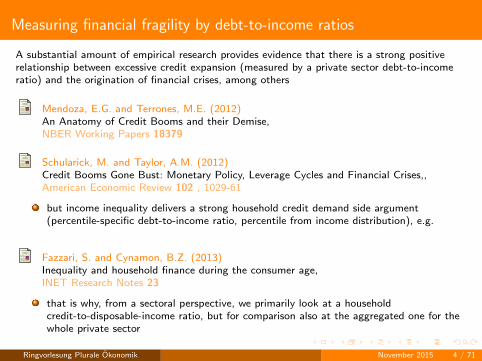
Measuring financial fragility by debt-to-income ratios
A substantial amount of empirical research provides evidence that there is a strong positiverelationship between excessive credit expansion (measured by a private sector debt-to-incomeratio) and the origination of financial crises, among others
Mendoza, E.G. and Terrones, M.E. (2012)An Anatomy of Credit Booms and their Demise,NBER Working Papers 18379
Schularick, M. and Taylor, A.M. (2012)Credit Booms Gone Bust: Monetary Policy, Leverage Cycles and Financial Crises,,American Economic Review 102 , 1029-61
but income inequality delivers a strong household credit demand side argument(percentile-specific debt-to-income ratio, percentile from income distribution), e.g.
Fazzari, S. and Cynamon, B.Z. (2013)Inequality and household finance during the consumer age,INET Research Notes 23
that is why, from a sectoral perspective, we primarily look at a householdcredit-to-disposable-income ratio, but for comparison also at the aggregated one for thewhole private sector
Ringvorlesung Plurale Okonomik November 2015 4 / 71
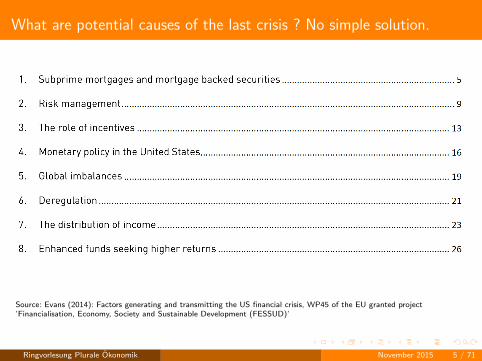
What are potential causes of the last crisis ? No simple solution.
Source: Evans (2014): Factors generating and transmitting the US financial crisis, WP45 of the EU granted project’Financialisation, Economy, Society and Sustainable Development (FESSUD)’
Ringvorlesung Plurale Okonomik November 2015 5 / 71
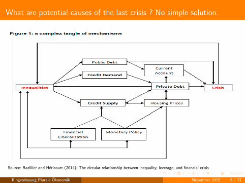
What are potential causes of the last crisis ? No simple solution.
Source: Bazillier and Hericourt (2014): The circular relationship between inequality, leverage, and financial crisis
Ringvorlesung Plurale Okonomik November 2015 6 / 71

Potential causes of the crisis - Transmission mechanism
Think about a state where credit demand and supply clear
There is a bunch of explanations starting from the credit supply side
asset prices ↑ => collateral value ↑ => (bank) lending ↑ (Kiyotaki and Moore, 1997)
financial deregulation (e.g. allowing for securitization) ↑ => off-balance sheettransactions ↑ => (bank) lending ↑ (Hein, 2009)
expansionary monetary policy ↑ => cheap refinancing ↑ => lending ↑ (Taylor, 2010)
excess saving (from abroad) ↑ => deposits ↑ => (bank) lending ↑ (Bernanke, 2005)
But there is not much on the credit demand side
income inequality ↑ => people trying to compensate permanent income loss by debt(while the rich search for return) ↑ => lending ↑ (Post Keynesians; Rajan, 2010)
asst prices ↑ => herding and irrational expectations make people to demand for theextra house to benefit from future prices (Campbell, 1998)
Ringvorlesung Plurale Okonomik November 2015 7 / 71

Outline
Block I - Einkommensungleichheit als Krisenursache (Credit)
1 Theoretische Wirkungsweisen moglicher Krisenursachen
2 Stylized Facts - USA pre-crises time
3 Das Kumhof (2012) DSGE zur Erklarung der US Dynamik
4 Simulation und Politikempfehlung
5 Ein alternativer Erklarungsansatz uber die Relative Einkommenshypothese
Ringvorlesung Plurale Okonomik November 2015 8 / 71
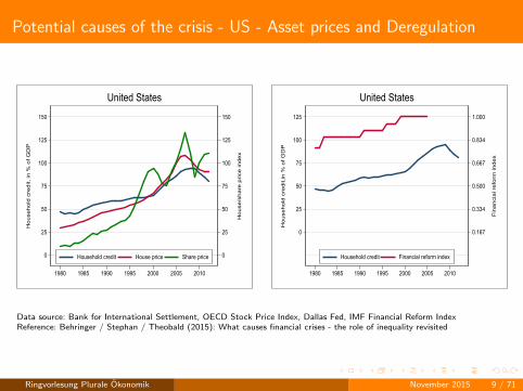
Potential causes of the crisis - US - Asset prices and Deregulation
0
25
50
75
100
125
150
Ho
use
/sh
are
Sprice
Sin
de
x
0
25
50
75
100
125
150
Ho
use
ho
ldSc
red
it,Sin
S%So
fSG
DP
1980 1985 1990 1995 2000 2005 2010
HouseholdScredit HouseSprice ShareSprice
UnitedSStates
0.167
0.334
0.500
0.667
0.834
1.000
Fin
an
cia
lGre
form
Gin
de
x
0
25
50
75
100
125
Ho
use
ho
ldGc
red
it,in
GSGo
fGG
DP
1980 1985 1990 1995 2000 2005 2010
HouseholdGcredit FinancialGreformGindex
UnitedGStates
Data source: Bank for International Settlement, OECD Stock Price Index, Dallas Fed, IMF Financial Reform IndexReference: Behringer / Stephan / Theobald (2015): What causes financial crises - the role of inequality revisited
Ringvorlesung Plurale Okonomik November 2015 9 / 71
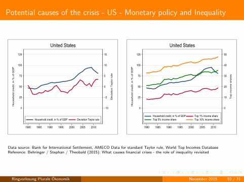
Potential causes of the crisis - US - Monetary policy and Inequality
−10
−5
0
5
10
15
De
via
tio
nUT
aylo
rUru
le0
25
50
75
100
125
Ho
use
ho
ldUc
red
it,Uin
U%Uo
fUG
DP
1980 1985 1990 1995 2000 2005 2010
HouseholdUcredit,UinU%UofUGDP DeviationUTaylorUrule
UnitedUStates
0
10
20
30
40
50
To
p9in
co
me
9sh
are
s
0
25
50
75
100
125
Ho
use
ho
ld9c
red
it,9in
9%9o
f9G
DP
1980 1985 1990 1995 2000 2005 2010
Household9credit,9in9%9of9GDP Top91%9income9shareTop95%9income9share Top910%9income9share
United9States
Data source: Bank for International Settlement, AMECO Data for standard Taylor rule, World Top Incomes DatabaseReference: Behringer / Stephan / Theobald (2015): What causes financial crises - the role of inequality revisited
Ringvorlesung Plurale Okonomik November 2015 10 / 71
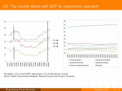
US: Top income shares and GDP by expenditure approach
-10
0
10
20
30
40
50
60
70
80
19
80
19
81
19
82
19
83
19
84
19
85
19
86
19
87
19
88
19
89
19
90
19
91
19
92
19
93
19
94
19
95
19
96
19
97
19
98
19
99
20
00
20
01
20
02
20
03
20
04
20
05
20
06
20
07
Privatexconsumption Governmentxconsumption
Governmentxinvestment Residentialxinvestment
Privatexnon-residentialxinvestment Netxexports
left graph: in % of total GDP, right graph: in % of total pre-tax incomeSource: World Top Incomes Database, National Income and Product Accounts
Ringvorlesung Plurale Okonomik November 2015 11 / 71
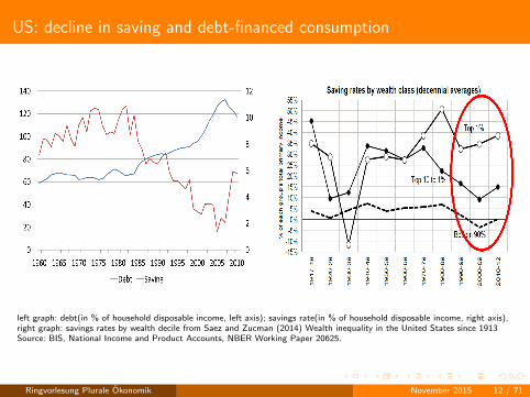
US: decline in saving and debt-financed consumption
left graph: debt(in % of household disposable income, left axis); savings rate(in % of household disposable income, right axis),right graph: savings rates by wealth decile from Saez and Zucman (2014) Wealth inequality in the United States since 1913Source: BIS, National Income and Product Accounts, NBER Working Paper 20625.
Ringvorlesung Plurale Okonomik November 2015 12 / 71
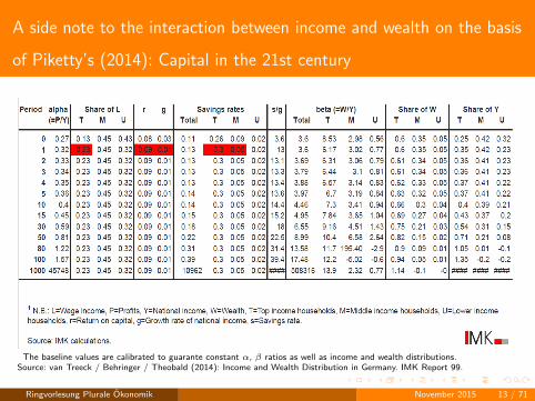
A side note to the interaction between income and wealth on the basis
of Piketty’s (2014): Capital in the 21st century
The baseline values are calibrated to guarante constant α, β ratios as well as income and wealth distributions.Source: van Treeck / Behringer / Theobald (2014): Income and Wealth Distribution in Germany. IMK Report 99.
Ringvorlesung Plurale Okonomik November 2015 13 / 71
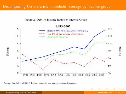
Decomposing US pre-crisis household leverage by income group
Source: Kumhof et al.(2012) Income inequality and current account imbalances
Ringvorlesung Plurale Okonomik November 2015 14 / 71

Outline - Block I:
Einkommensungleichheit als Krisenursache (Credit)
1 Theoretische Wirkungsweisen moglicher Krisenursachen
2 Stylized Facts - USA pre-crisis time
3 Das Kumhof et al. (2012) DSGE zur Erklarung der US Dynamik
4 Simulation und Politikempfehlung
5 Ein alternativer Erklarungsansatz uber die Relative Einkommenshypothese
Ringvorlesung Plurale Okonomik November 2015 15 / 71
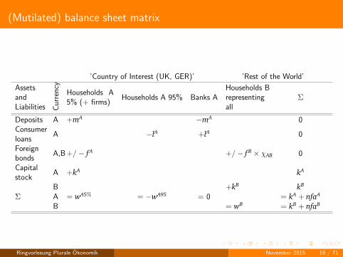
(Mutilated) balance sheet matrix
’Country of Interest (UK, GER)’ ’Rest of the World’
AssetsandLiabilities C
urre
ncy
Households A5% (+ firms)
Households A 95% Banks AHouseholds Brepresentingall
Σ
Deposits A +mA −mA 0Consumerloans
A −lA +lA 0
Foreignbonds
A,B +/− fA +/− fB × χAB 0
Capitalstock
A +kA kA
B +kB kB
Σ A = wA5% = −wA95 = 0 = kA + nfaA
B = wB = kB + nfaB
Ringvorlesung Plurale Okonomik November 2015 16 / 71
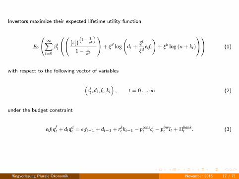
Investors maximize their expected lifetime utility function
E0
∞∑t=0
βit
(cit)(1− 1
σi
)1− 1
σi
+ ξd log
(dt +
ξf
ξdetft
)+ ξk log (κ+ kt)
(1)
with respect to the following vector of variables
(cit, dt, ft, kt
), t = 0 . . .∞ (2)
under the budget constraint
etftqft + dtqd
t = etft−1 + dt−1 + rkt kt−1 − pcons
t cit − pinv
t It + Πbankt . (3)
Ringvorlesung Plurale Okonomik November 2015 17 / 71
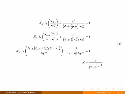
βit+1Et
(λt+1
λtqdt
)+
ξd(dt + ξf
ξd etft)λtqd
t
= 1
βit+1Et
(λt+1
λt
et+1et
qft
)+
ξf(dt + ξf
ξd etft)λtq
ft
= 1
βit+1Et
λt+1
(rkt+1 + pinv
t+1 (1− δ))
λtpinvt
+ξk
(κ+ kt)λtpinvt
= 1
λit =
1
pconst c
i(
1σi
)t
(4)
Ringvorlesung Plurale Okonomik November 2015 18 / 71
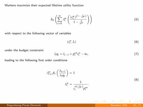
Workers maximize their expected lifetime utility function
E0
( ∞∑t=0
βwt
((cw
t )(1− 1σw )
1− 1σw
))(5)
with respect to the following vector of variables
(cwt , lt) (6)
under the budget constraintltqt = lt−1 + pcw
t cwt − wt. (7)
leading to the following first order conditions
βwt+1Et
(λt+1
λtqt
)= 1
λwt =
1
cw( 1σw )
t pcwt
.
(8)
Ringvorlesung Plurale Okonomik November 2015 19 / 71
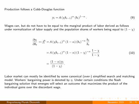
Production follows a Cobb-Douglas function
yt = A (χkt−1)α (ht)1−α . (9)
Wages can, but do not have to be equal to the marginal product of labor derived as followsunder normalization of labor supply and the population shares of workers being equal to (1− χ)
∂yt
∂ht=: fh
t = A (χkt−1)α (1− α) (ht)−α ht
ht
= A (χkt−1)α (1− α) (1− χ)−α1− χ1− χ
=(1− α) yt
(1− χ).
(10)
Labor market can mostly be identified by some canonical (over-) simplified search and matchingmodel. Workers’ bargaining power is denoted by η. Under certain conditions the Nashbargaining solution that emerges will select an outcome that maximizes the product of theindividual gains over the discordant wage.
Ringvorlesung Plurale Okonomik November 2015 20 / 71
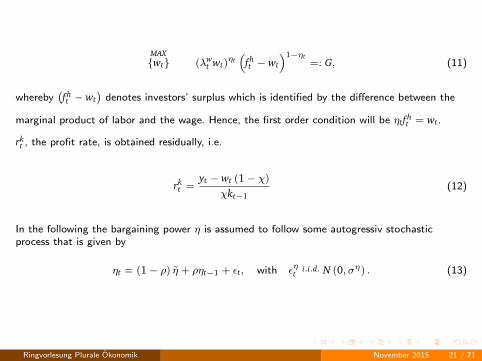
MAX{wt} (λw
t wt)ηt(
fht − wt
)1−ηt=: G, (11)
whereby(fht − wt
)denotes investors’ surplus which is identified by the difference between the
marginal product of labor and the wage. Hence, the first order condition will be ηtfht = wt.
rkt , the profit rate, is obtained residually, i.e.
rkt =
yt − wt (1− χ)
χkt−1(12)
In the following the bargaining power η is assumed to follow some autogressiv stochasticprocess that is given by
ηt = (1− ρ) η + ρηt−1 + εt, with εηt i.i.d. N (0, ση) . (13)
Ringvorlesung Plurale Okonomik November 2015 21 / 71
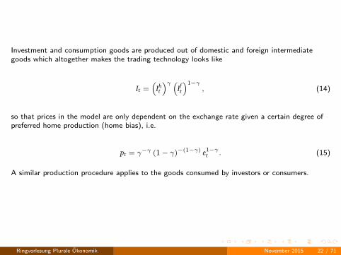
Investment and consumption goods are produced out of domestic and foreign intermediategoods which altogether makes the trading technology looks like
It =(
Iht
)γ (Ift
)1−γ, (14)
so that prices in the model are only dependent on the exchange rate given a certain degree ofpreferred home production (home bias), i.e.
pt = γ−γ (1− γ)−(1−γ) e1−γt . (15)
A similar production procedure applies to the goods consumed by investors or consumers.
Ringvorlesung Plurale Okonomik November 2015 22 / 71
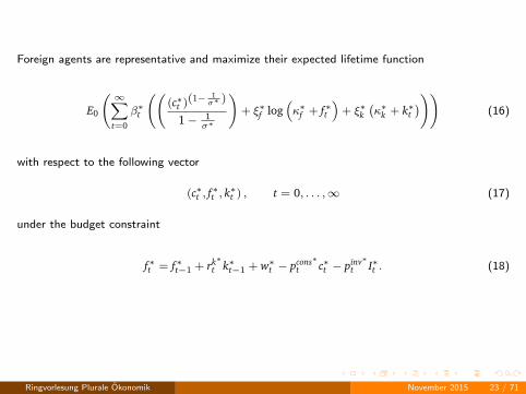
Foreign agents are representative and maximize their expected lifetime function
E0
( ∞∑t=0
β∗t
(((c∗t )(1− 1
σ∗ )
1− 1σ∗
)+ ξ∗f log
(κ∗f + f∗t
)+ ξ∗k
(κ∗k + k∗t
)))(16)
with respect to the following vector
(c∗t , f∗t , k∗t ) , t = 0, . . . ,∞ (17)
under the budget constraint
f∗t = f∗t−1 + rk∗t k∗t−1 + w∗t − pcons∗
t c∗t − pinv∗t I∗t . (18)
Ringvorlesung Plurale Okonomik November 2015 23 / 71
Banks are monopolistically competitive in the loans market, where each bank makes loans in theamount of lt (z) at (theoretically different) gross interest rates 1/qt (z). The aggregate creditbundle, demanded by borrowers, follows a Dixit-Stiglitz form:
lt =
(∫ 1
0lt (z)
1θ+1 dz
)θ+1
, (19)
Rewritting leads to the following constraint
lt (z) =
(qt (z)
qt
)θ+1
lt (20)
under which banks maximize their profit
Π =1
qt (z)lt (z)−
1
qdt
lt (z) (21)
with respect to qt (z) which in turn delivers for profits
Π = qt (z)θ q(−θ−1)t lt − qt (z)(θ+1) q(−θ−1)
t lt1
qdt. (22)
Ringvorlesung Plurale Okonomik November 2015 24 / 71
Optimization of profits delivers
∂Πsingle
∂qt (z)=
qt (z)θ θq(−θ−1)t lt
qt (z)−
qt (z)(θ+1) (θ + 1) q(−θ−1)t lt
qdt qt (z)
!= 0
⇔1qt
=θ + 1θ
1
qdt
=1
qdt
s.
(23)
Also the spread s is assumed to follow some autogressiv stochastic process that is given by
st = (1− ρ) s + ρst−1 + εt, with εt i.i.d. N (0, σ) . (24)
Bank profits (here as a fraction of deposits) are given by
Πbankt = dt
(qd
t − qt
). (25)
With respect to financial markets clearing condition, credit amounts lent by domestic investorsto domestic workers must be equal to the bank deposits (national bank balances check)
χdt = (1− χ) lt. (26)
International credit amounts must find their offsetting item, while all credit transactions areintermediated by domestic investors
wχft = − (1− w) f∗t . (27)
Ringvorlesung Plurale Okonomik November 2015 25 / 71
A,A∗ set national output to a certain level, e.g. equal to 1. Hence, to reproduce the world’soutput (or income) shares, one multiplies domestic variables by the factor w and foreignvariables by 1− w for a rest of the world perspective. The following identities decompose homeand foreign output into consumption, investment and gross exports:
wyt = wχ(
ciht + Ih
t
)+ w (1− χ) cwh
t + (1− w)(
ch∗t + Ih∗
t
)(28)
(1− w) y∗t = (1− w)(
cf∗t + If∗
t
)+ wχ
(cift + Iif
t
)+ w (1− χ) cwf
t (29)
Net exports from home perspective are equal to domestic export minus foreign exports
(1− w)(
ch∗t + Ih∗
t
)− w
(χ(
cift + If
t
)+ (1− χ) cwf
t
)et (30)
Considering gross interest payments on foreign bonds one obtaines for the identity betweeninternational financial and trading flows
wχ(
etftqft − etft−1
)= (1− w)
(ch∗t + Ih∗
t
)− w
(χ(
cift + If
t
)+ (1− χ) cwf
t
)et
⇔ χetftqft = χetft−1 +
(1− w)
w
(ch∗t + Ih∗
t
)− etw
(χ(
cift + If
t
)+ (1− χ) cwf
t
) (31)
Ringvorlesung Plurale Okonomik November 2015 26 / 71

Outline - Block I:
Einkommensungleichheit als Krisenursache (Credit)
1 Theoretische Wirkungsweisen moglicher Krisenursachen
2 Stylized Facts - USA pre-crisis time
3 Das Kumhof et al. (2012) DSGE zur Erklarung der US Dynamik
4 Simulation und Politikempfehlung
5 Ein alternativer Erklarungsansatz uber die Relative Einkommenshypothese
Ringvorlesung Plurale Okonomik November 2015 27 / 71
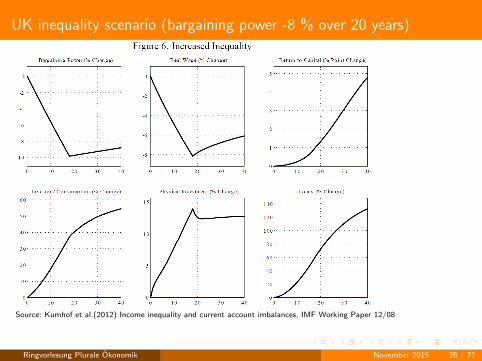
UK inequality scenario (bargaining power -8 % over 20 years)
Source: Kumhof et al.(2012) Income inequality and current account imbalances, IMF Working Paper 12/08
Ringvorlesung Plurale Okonomik November 2015 28 / 71
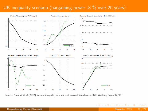
UK inequality scenario (bargaining power -8 % over 20 years)
Source: Kumhof et al.(2012) Income inequality and current account imbalances, IMF Working Paper 12/08
Ringvorlesung Plurale Okonomik November 2015 29 / 71
Policy Implications
‘There is no way around addressing the income inequality directly’ (Kumhof et al., 2012)
not only from a social fairness and fairness of opportunities perspective, but also from amacroeconomic stability perspective. Possible instruments are
strengthening workers bargaining power over wages via labour unions
taxing income more progressively
(re-)introducing progressive wealth taxes (Piketty, 2014)
Ringvorlesung Plurale Okonomik November 2015 30 / 71

Outline - Block I:
Einkommensungleichheit als Krisenursache (Credit)
1 Theoretische Wirkungsweisen moglicher Krisenursachen
2 Stylized Facts - USA pre-crisis time
3 Das Kumhof et al. (2012) DSGE zur Erklarung der US Dynamik
4 Simulation und Politikempfehlung
5 Ein alternativer Erklarungsansatz uber die Relative Einkommenshypothese
Ringvorlesung Plurale Okonomik November 2015 31 / 71
An alternative explanation by expenditure cascades
Milton Friedman’s permanent income hypothesis can only explain the fact that USconsumption of low and middle income class households did not decline before crisis, ifthose income changes were purely transitory
Keynesians would traditionally expect the aggregate household saving rate to rise, asinequality increases
However, models with upward-looking status comparisons (as a specific type of therelative income hypothesis by James Duesenberry) predict a negative link betweeninequality and the aggregate saving rate
This is not about eccentric luxury consumption, but basic middle class needs (privatefinancing of important positional goods such as education, housing, health care, etc. inthe U.S.)
Source: Sturn / van Treeck (2012) Income inequality as a cause of the Great Recession
Ringvorlesung Plurale Okonomik November 2015 32 / 71
An alternative explanation by expenditure cascades
The impact of expenditure cascades depends on country-specific institutions. Forinstance, in countries with relatively strong public infrastructure such effects will belimited
The alternative is modelled in the tradition of the stock-flow consistent (SFC) approachby W. Godley / M. Lavoi (2007), which ‘studies how flows of income, expenditure andproduction are intertwined with stocks of assets and liabilities determining how wholeeconomies evolve through time’
Unfortunately sofar, no explicit consideration of forward-looking behaviour(expectations), but fully calibrated / partly estimated to US, German, and Chinese data
Source: Belabed / Theobald / van Treeck (2013) Income distribution and current account imbalances
Ringvorlesung Plurale Okonomik November 2015 33 / 71
Modeling the relative income hypothesis in a SFC
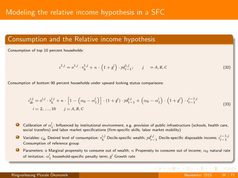
Consumption and the Relative income hypothesis
Consumption of top 10 percent households:
c1,j= o1,j · v1,j
h + κ ·(
1 + gj)· yd1,j
t−1; j = A, B, C (32)
Consumption of bottom 90 percent households under upward looking status comparisons:
ci,jde = oi,j · vi,j
h + κ ·[1−
(α0 − α
j1
)]· (1 + gj
) · ydi,jt−1 +
(α0 − α
j1
)·(
1 + gj)· ci−1,j
t−1
i = 2, ..., 10 j = A, B, C(33)
Calibration of αj1: Influenced by institutional environment, e.g. provision of public infrastructure (schools, health care,
social transfers) and labor market specifications (firm-specific skills, labor market mobility)
Variables: cde Desired level of consumption; vi,jh Decile-specific wealth; ydi,j
t−1 Decile-specific disposable income; ci−1,jt−1
Consumption of reference group
Parameters: o Marginal propensity to consume out of wealth; κ Propensity to consume out of income; α0 natural rate
of imitation; αj1 household-specific penalty term; gj Growth rate
Ringvorlesung Plurale Okonomik November 2015 34 / 71
Modeling the relative income hypothesis in a SFC
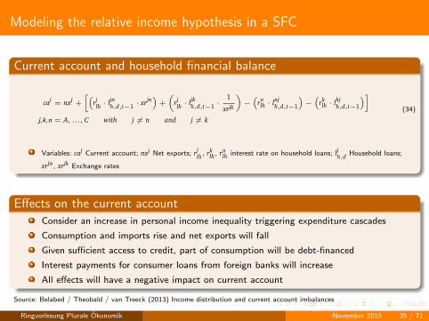
Current account and household financial balance
caj= nxj
+
[(rjlh · ljnh,d,t−1 · xrjn
)+
(rjlh · ljkh,d,t−1 ·
1
xrjk
)−(
rnlh · lnj
h,d,t−1
)−(
rklh · lkj
h,d,t−1
)]j,k,n = A, ..., C with j 6= n and j 6= k
(34)
Variables: caj Current account; nxj Net exports; rjlh, rk
lh, rnlh interest rate on household loans; ljh,d Household loans;
xrjn, xrjk Exchange rates
Effects on the current account
Consider an increase in personal income inequality triggering expenditure cascades
Consumption and imports rise and net exports will fall
Given sufficient access to credit, part of consumption will be debt-financed
Interest payments for consumer loans from foreign banks will increase
All effects will have a negative impact on current account
Source: Belabed / Theobald / van Treeck (2013) Income distribution and current account imbalances
Ringvorlesung Plurale Okonomik November 2015 35 / 71

Outline - Block II:
Einkommensungleichheit als Krisenursache (Current Account)
1 Was ist der Unternehmensschleier (Corporate Veil) ?
2 Stylized Facts - GER pre-crisis time
3 Das Gruning et al. (2012) DSGE zur Berucksichtigung der deutschen Dynamik
4 Simulation und Politikempfehlung
5 Stilisierte Zusammenfassung unterschiedlicher Schocks auf die Einkommensverteilung
Ringvorlesung Plurale Okonomik November 2015 36 / 71
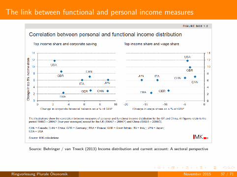
The link between functional and personal income measures
Source: Behringer / van Treeck (2013) Income distribution and current account: A sectoral perspective
Ringvorlesung Plurale Okonomik November 2015 37 / 71
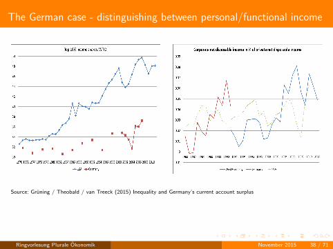
The German case - distinguishing between personal/functional income
Source: Gruning / Theobald / van Treeck (2015) Inequality and Germany’s current account surplus
Ringvorlesung Plurale Okonomik November 2015 38 / 71
The macroeconomic implications of the corporate veil
The ‘corporate veil’
hides the rise in inequality between households
restraints domestic demand (rising retained profits are not spent)
limits the pressure put on the middle class to engage in debt-financed consumption
enlarges the current account surplus
increases global financial fragility(World Current Account Balance = 0 !!!)
Source: Sturn / van Treeck (2012) Income inequality as a cause of the Great Recession
Ringvorlesung Plurale Okonomik November 2015 39 / 71

Outline - Block II:
Einkommensungleichheit als Krisenursache (Current Account)
1 Was ist der Unternehmensschleier (Corporate Veil) ?
2 Stylized Facts - GER pre-crisis time
3 Das Gruning et al. (2012) DSGE zur Berucksichtigung der deutschen Dynamik
4 Simulation und Politikempfehlung
5 Stilisierte Zusammenfassung unterschiedlicher Schocks auf die Einkommensverteilung
Ringvorlesung Plurale Okonomik November 2015 40 / 71
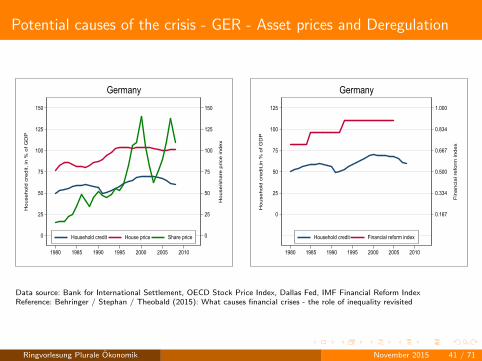
Potential causes of the crisis - GER - Asset prices and Deregulation
0
25
50
75
100
125
150
Ho
use
/sh
are
Sprice
Sin
de
x
0
25
50
75
100
125
150
Ho
use
ho
ldSc
red
it,Sin
S%So
fSG
DP
1980 1985 1990 1995 2000 2005 2010
HouseholdScredit HouseSprice ShareSprice
Germany
0.167
0.334
0.500
0.667
0.834
1.000
Fin
an
cia
lGre
form
Gin
de
x
0
25
50
75
100
125
Ho
use
ho
ldGc
red
it,in
G%Go
fGG
DP
1980 1985 1990 1995 2000 2005 2010
HouseholdGcredit FinancialGreformGindex
Germany
Data source: Bank for International Settlement, OECD Stock Price Index, Dallas Fed, IMF Financial Reform IndexReference: Behringer / Stephan / Theobald (2015): What causes financial crises - the role of inequality revisited
Ringvorlesung Plurale Okonomik November 2015 41 / 71
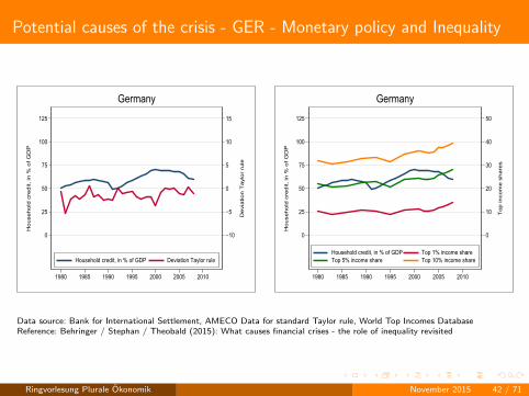
Potential causes of the crisis - GER - Monetary policy and Inequality
−10
−5
0
5
10
15
De
via
tio
nmT
aylo
rmru
le0
25
50
75
100
125
Ho
use
ho
ldmc
red
it,min
m%mo
fmG
DP
1980 1985 1990 1995 2000 2005 2010
Householdmcredit,minm%mofmGDP DeviationmTaylormrule
Germany
0
10
20
30
40
50
To
p9in
co
me
9sh
are
s
0
25
50
75
100
125
Ho
use
ho
ld9c
red
it,9in
9%9o
f9G
DP
1980 1985 1990 1995 2000 2005 2010
Household9credit,9in9%9of9GDP Top91%9income9shareTop95%9income9share Top910%9income9share
Germany
Data source: Bank for International Settlement, AMECO Data for standard Taylor rule, World Top Incomes DatabaseReference: Behringer / Stephan / Theobald (2015): What causes financial crises - the role of inequality revisited
Ringvorlesung Plurale Okonomik November 2015 42 / 71
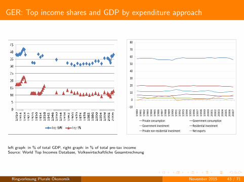
GER: Top income shares and GDP by expenditure approach
-10
0
10
20
30
40
50
60
70
80
19
80
19
81
19
82
19
83
19
84
19
85
19
86
19
87
19
88
19
89
19
90
19
91
19
92
19
93
19
94
19
95
19
96
19
97
19
98
19
99
20
00
20
01
20
02
20
03
20
04
20
05
20
06
20
07
Privatexconsumption Governmentxconsumption
Governmentxinvestment Residentialxinvestment
Privatexnon-residentialxinvestment Netxexports
left graph: in % of total GDP, right graph: in % of total pre-tax incomeSource: World Top Incomes Database, Volkswirtschaftliche Gesamtrechnung
Ringvorlesung Plurale Okonomik November 2015 43 / 71
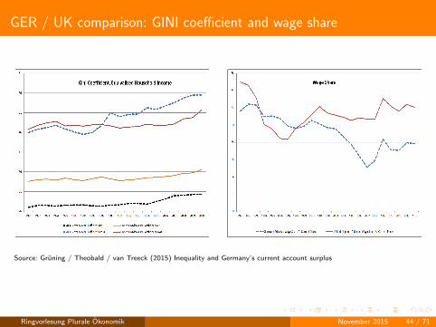
GER / UK comparison: GINI coefficient and wage share
Source: Gruning / Theobald / van Treeck (2015) Inequality and Germany’s current account surplus
Ringvorlesung Plurale Okonomik November 2015 44 / 71
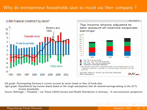
Why do entrepreneur households save so much via their company ?
left graph: Decomposing Germany’s current account by sector based on flow of funds data.right graph: Hypothetical top income shares based on the rough assumptions that all retained earnings belong to the 10 %
income households.Source: Behringer / Theobald / van Treeck (2014) Income and Wealth Distribution in Germany - A macroeconomic perspective
Ringvorlesung Plurale Okonomik November 2015 45 / 71

Outline - Block II:
Einkommensungleichheit als Krisenursache (Current Account)
1 Was ist der Unternehmensschleier (Corporate Veil) ?
2 Stylized Facts - GER pre-crisis time
3 Das Gruning et al. (2012) DSGE zur Berucksichtigung der deutschen Dynamik
4 Simulation und Politikempfehlung
5 Stilisierte Zusammenfassung unterschiedlicher Schocks auf die Einkommensverteilung
Ringvorlesung Plurale Okonomik November 2015 46 / 71
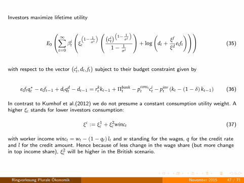
Investors maximize lifetime utility
E0
∞∑t=0
βit
ξ(1− 1σi
)c
(cit)(1− 1
σi
)1− 1
σi
+ log
(dt +
ξf
ξdetft
) (35)
with respect to the vector(cit, dt, ft
)subject to their budget constraint given by
etftq∗t − etft−1 + dtqdt − dt−1 = rk
t kt−1 + Πbankt − pconsi
t cit − pinv
t (kt − (1− δ) kt−1) (36)
In contrast to Kumhof et al.(2012) we do not presume a constant consumption utility weight. Ahigher ξc stands for lower investors consumption:
ξc := ξ1c + ξ2
c winct (37)
with worker income winct = wt − (1− qt) lt and w standing for the wages, q for the credit rateand l for the credit amount. Hence because of less change in the wage share (but more changein top income share), ξ2
c will be higher in the British scenario.
Ringvorlesung Plurale Okonomik November 2015 47 / 71

Straightforward Lagrangian optimization delivers first order conditions for domestic deposits,foreign bonds, and investor consumption:
(βi)t+1
Et
(λt+1
λtqdt
)+
ξd(dt + ξf
ξd etft)λtqd
t
= 1
(βi)t+1
Et
(λt+1
λt
et+1et
qft
)+
ξf(dt + ξf
ξd etft)λtq
ft
= 1
cit =
(1
λitp
const
)σi
(ξct )σi−1 , σi < 1.
(38)
Workers maximize lifetime utility
E0
( ∞∑t=0
(βw)t
((cw
t )(1− 1σw )
1− 1σw
))(39)
with respect to the vector (cwt , lt) subject to their budget constraint
ltqt = lt−1 + pcwt cw
t − wt. (40)
l denotes the amount of credit supplied by banks.
Ringvorlesung Plurale Okonomik November 2015 48 / 71
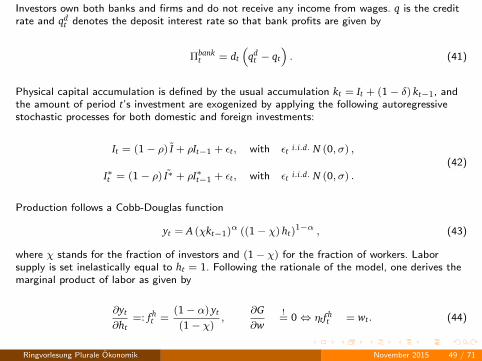
Investors own both banks and firms and do not receive any income from wages. q is the creditrate and qd
t denotes the deposit interest rate so that bank profits are given by
Πbankt = dt
(qd
t − qt
). (41)
Physical capital accumulation is defined by the usual accumulation kt = It + (1− δ) kt−1, andthe amount of period t’s investment are exogenized by applying the following autoregressivestochastic processes for both domestic and foreign investments:
It = (1− ρ) I + ρIt−1 + εt, with εt i.i.d. N (0, σ) ,
I∗t = (1− ρ) I∗ + ρI∗t−1 + εt, with εt i.i.d. N (0, σ) .
(42)
Production follows a Cobb-Douglas function
yt = A (χkt−1)α ((1− χ) ht)1−α , (43)
where χ stands for the fraction of investors and (1− χ) for the fraction of workers. Laborsupply is set inelastically equal to ht = 1. Following the rationale of the model, one derives themarginal product of labor as given by
∂yt
∂ht=: fh
t =(1− α) yt
(1− χ),
∂G∂w
!= 0⇔ ηtfh
t = wt. (44)
Ringvorlesung Plurale Okonomik November 2015 49 / 71

Outline - Block II:
Einkommensungleichheit als Krisenursache (Current Account)
1 Was ist der Unternehmensschleier (Corporate Veil) ?
2 Stylized Facts - GER pre-crisis time
3 Das Gruning et al. (2012) DSGE zur Berucksichtigung der deutschen Dynamik
4 Simulation und Politikempfehlung
5 Stilisierte Zusammenfassung unterschiedlicher Schocks auf die Einkommensverteilung
Ringvorlesung Plurale Okonomik November 2015 50 / 71

UK inequality scenario (bargaining power -8 % over 20 years)
0 10 20 30 40-10
-5
0
5Bargaining Power,Banking Spread (abs)
0 10 20 30 40-8
-6
-4
-2
0Real Wage (%)
0 10 20 30 400
5
10
15
20Rental Rate of Capital (%)
0 10 20 30 400
10
20
30Investors' Consumption (%)
0 10 20 30 40-1
-0.5
0
0.5
1Domestic Investment (%)
0 10 20 30 40-1
-0.5
0
0.5
1Foreign Investment (%)
0 10 20 30 40-8
-6
-4
-2
0Workers' Consumption (%)
0 10 20 30 400
50
100
150
200Workers' Leverage (abs)
0 10 20 30 401
2
3
4
5Deposit and Loan Rates (level)
0 10 20 30 40-1.5
-1
-0.5
0Current Account/GDP (abs)
0 10 20 30 40-1.5
-1
-0.5
0
0.5NFA/GDP (abs)
0 10 20 30 400
2
4
6
8Top 5% Income Share (abs)
Ringvorlesung Plurale Okonomik November 2015 51 / 71

GER inequality scenario (bargaining power -7 % over 20 years)
0 10 20 30 40-10
-5
0
5Bargaining Power,Banking Spread (abs)
0 10 20 30 40-8
-6
-4
-2
0Real Wage (%)
0 10 20 30 400
5
10
15
20Rental Rate of Capital (%)
0 10 20 30 400
20
40
60Investors' Consumption (%)
0 10 20 30 40-1
-0.5
0
0.5
1Domestic Investment (%)
0 10 20 30 40-1
-0.5
0
0.5
1Foreign Investment (%)
0 10 20 30 40-8
-6
-4
-2
0Workers' Consumption (%)
0 10 20 30 400
50
100
150Workers' Leverage (abs)
0 10 20 30 401
2
3
4
5Deposit and Loan Rates (level)
0 10 20 30 400
0.1
0.2
0.3
0.4Current Account/GDP (abs)
0 10 20 30 400
0.2
0.4
0.6
0.8NFA/GDP (abs)
0 10 20 30 400
2
4
6
8Top 5% Income Share (abs)
Ringvorlesung Plurale Okonomik November 2015 52 / 71
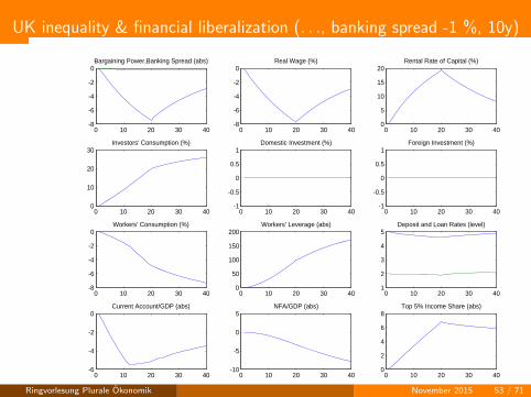
UK inequality & financial liberalization (. . ., banking spread -1 %, 10y)
0 10 20 30 40-8
-6
-4
-2
0Bargaining Power,Banking Spread (abs)
0 10 20 30 40-8
-6
-4
-2
0Real Wage (%)
0 10 20 30 400
5
10
15
20Rental Rate of Capital (%)
0 10 20 30 400
10
20
30Investors' Consumption (%)
0 10 20 30 40-1
-0.5
0
0.5
1Domestic Investment (%)
0 10 20 30 40-1
-0.5
0
0.5
1Foreign Investment (%)
0 10 20 30 40-8
-6
-4
-2
0Workers' Consumption (%)
0 10 20 30 400
50
100
150
200Workers' Leverage (abs)
0 10 20 30 401
2
3
4
5Deposit and Loan Rates (level)
0 10 20 30 40-6
-4
-2
0Current Account/GDP (abs)
0 10 20 30 40-10
-5
0
5NFA/GDP (abs)
0 10 20 30 400
2
4
6
8Top 5% Income Share (abs)
Ringvorlesung Plurale Okonomik November 2015 53 / 71
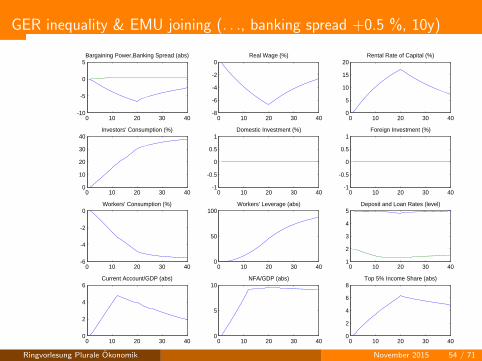
GER inequality & EMU joining (. . ., banking spread +0.5 %, 10y)
0 10 20 30 40-10
-5
0
5Bargaining Power,Banking Spread (abs)
0 10 20 30 40-8
-6
-4
-2
0Real Wage (%)
0 10 20 30 400
5
10
15
20Rental Rate of Capital (%)
0 10 20 30 400
10
20
30
40Investors' Consumption (%)
0 10 20 30 40-1
-0.5
0
0.5
1Domestic Investment (%)
0 10 20 30 40-1
-0.5
0
0.5
1Foreign Investment (%)
0 10 20 30 40-6
-4
-2
0Workers' Consumption (%)
0 10 20 30 400
50
100Workers' Leverage (abs)
0 10 20 30 401
2
3
4
5Deposit and Loan Rates (level)
0 10 20 30 400
2
4
6Current Account/GDP (abs)
0 10 20 30 400
5
10NFA/GDP (abs)
0 10 20 30 400
2
4
6
8Top 5% Income Share (abs)
Ringvorlesung Plurale Okonomik November 2015 54 / 71
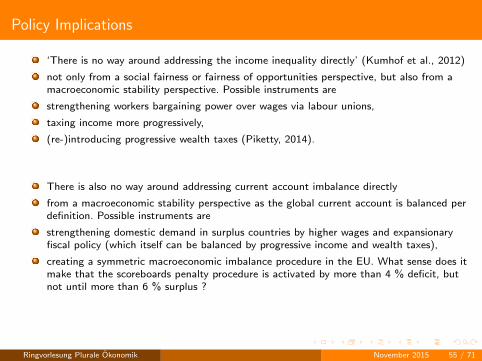
Policy Implications
‘There is no way around addressing the income inequality directly’ (Kumhof et al., 2012)
not only from a social fairness or fairness of opportunities perspective, but also from amacroeconomic stability perspective. Possible instruments are
strengthening workers bargaining power over wages via labour unions,
taxing income more progressively,
(re-)introducing progressive wealth taxes (Piketty, 2014).
There is also no way around addressing current account imbalance directly
from a macroeconomic stability perspective as the global current account is balanced perdefinition. Possible instruments are
strengthening domestic demand in surplus countries by higher wages and expansionaryfiscal policy (which itself can be balanced by progressive income and wealth taxes),
creating a symmetric macroeconomic imbalance procedure in the EU. What sense does itmake that the scoreboards penalty procedure is activated by more than 4 % deficit, butnot until more than 6 % surplus ?
Ringvorlesung Plurale Okonomik November 2015 55 / 71

Outline - Block II:
Einkommensungleichheit als Krisenursache (Current Account)
1 Was ist der Unternehmensschleier (Corporate Veil) ?
2 Stylized Facts - GER pre-crisis time
3 Das Gruning et al. (2012) DSGE zur Berucksichtigung der deutschen Dynamik
4 Simulation und Politikempfehlung
5 Stilisierte Zusammenfassung unterschiedlicher Schocks auf die Einkommensverteilung
Ringvorlesung Plurale Okonomik November 2015 56 / 71
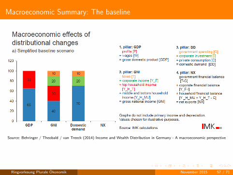
Macroeconomic Summary: The baseline
Source: Behringer / Theobald / van Treeck (2014) Income and Wealth Distribution in Germany - A macroeconomic perspective
Ringvorlesung Plurale Okonomik November 2015 57 / 71
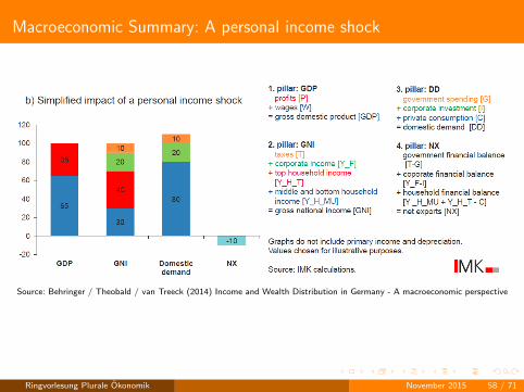
Macroeconomic Summary: A personal income shock
Source: Behringer / Theobald / van Treeck (2014) Income and Wealth Distribution in Germany - A macroeconomic perspective
Ringvorlesung Plurale Okonomik November 2015 58 / 71
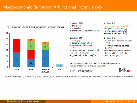
Macroeconomic Summary: A functional income shock
Source: Behringer / Theobald / van Treeck (2014) Income and Wealth Distribution in Germany - A macroeconomic perspective
Ringvorlesung Plurale Okonomik November 2015 59 / 71

Outline
Block III - DSGE Kritik und Robustifizierung
1 Pros and Cons of the DSGE models used
2 Should you never use rational expectations ?Ricardian equivalence and its consequences for expansionary fiscal policy
3 Should you never use rational expectations ?A Dynamic Stochastic Labor-Market Disequilibrium and effective demand
4 Macroeconomic factors behind financial instability -Evidence from Granger causality tests including both panel and time series econometrics
Ringvorlesung Plurale Okonomik November 2015 60 / 71

2nd generation DSGE models: Kritische Wurdigung
What is the pro of the model presented ?
heterogeneity among forward looking agents: i. capitalists (top 5%) own firms andbanks and obtain only capital income from physical and financial capital. ii. workers(bottom 95%) obtain only labor income, in contrast to a standard DSGE the modelallows to analyze distributional shocks via a deline in bargaining power so that wages areno longer equal to the marginal product of labor (derived from a CD production)
The investor class strongly drives the results. Those agents maximizing
E0
∞∑t=0
βit
ξ(1− 1σi
)c
(cit)(1− 1
σi
)1− 1
σi
+ log
(dt +
ξf
ξdetft
) (45)
with respect to the vector(cit, dt, ft
)subject to their budget constraint given by
etftq∗t − etft−1 + dtqdt − dt−1 = rk
t kt−1 + Πbankt − pconsi
t cit − pinv
t (kt − (1− δ) kt−1) (46)
set credit supply which is always cleared through workers’ budget constraint.
Source: Gruning / Theobald / van Treeck (2015) Inequality and Germany’s current account surplusRingvorlesung Plurale Okonomik November 2015 61 / 71
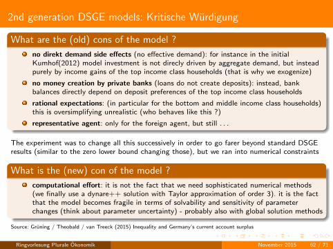
2nd generation DSGE models: Kritische Wurdigung
What are the (old) cons of the model ?
no direkt demand side effects (no effective demand): for instance in the initialKumhof(2012) model investment is not direcly driven by aggregate demand, but insteadpurely by income gains of the top income class households (that is why we exogenize)
no money creation by private banks (loans do not create deposits): instead, bankbalances directly depend on deposit preferences of the top income class households
rational expectations: (in particular for the bottom and middle income class households)this is oversimplifying unrealistic (who behaves like this ?)
representative agent: only for the foreign agent, but still . . .
The experiment was to change all this successively in order to go farer beyond standard DSGEresults (similar to the zero lower bound changing those), but we ran into numerical constraints
What is the (new) con of the model ?
computational effort: it is not the fact that we need sophisticated numerical methods(we finally use a dynare++ solution with Taylor approximation of order 3). it is the factthat the model becomes fragile in terms of solvability and sensitivity of parameterchanges (think about parameter uncertainty) - probably also with global solution methods
Source: Gruning / Theobald / van Treeck (2015) Inequality and Germany’s current account surplus
Ringvorlesung Plurale Okonomik November 2015 62 / 71

Outline
Block III - DSGE Kritik und Robustifizierung
1 Pros and Cons of the DSGE models used
2 Should you never use rational expectations ?Ricardian equivalence and its consequences for expansionary fiscal policy
3 Should you never use rational expectations ?A Dynamic Stochastic Labor-Market Disequilibrium and effective demand
4 Macroeconomic factors behind financial instability -Evidence from Granger causality tests including both panel and time series econometrics
Ringvorlesung Plurale Okonomik November 2015 63 / 71
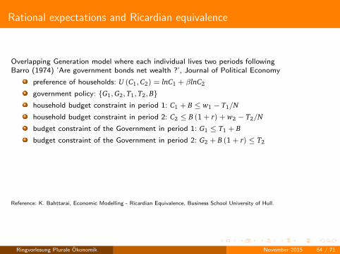
Rational expectations and Ricardian equivalence
Overlapping Generation model where each individual lives two periods followingBarro (1974) ’Are government bonds net wealth ?’, Journal of Political Economy
preference of households: U (C1,C2) = lnC1 + βlnC2
government policy: {G1,G2, T1, T2, B}household budget constraint in period 1: C1 + B ≤ w1 − T1/N
household budget constraint in period 2: C2 ≤ B (1 + r) + w2 − T2/N
budget constraint of the Government in period 1: G1 ≤ T1 + B
budget constraint of the Government in period 2: G2 + B (1 + r) ≤ T2
Reference: K. Bahttarai, Economic Modelling - Ricardian Equivalence, Business School University of Hull.
Ringvorlesung Plurale Okonomik November 2015 64 / 71

Rational expectations and Ricardian equivalence
Inter temporal budget constraints for government and households:
G1 +G2
1 + r= T1 +
T2
1 + r
C1 +C2
1 + r= (w1 − T1) +
(w2
1 + r−
T2
1 + r
)
Market clearing conditions in this economy without money are
NC1 + G1 = Nw1 NC2 + G2 = Nw2
Optimization delivers C2 = β (1 + r) C1 so that we obtain for two different government policies
T1 6= 0, T2 6= 0, B = 0
T1 = 0, T2 6= 0, B 6= 0
Ringvorlesung Plurale Okonomik November 2015 65 / 71
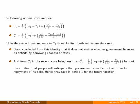
the following optimal consumption
C1 = 1β
((w1 − T1) +
(w2
1+r −T2
1+r
))C1 = 1
β
((w1) +
(w2
1+r −T2+B(1+r)
1+r
))If B in the second case amounts to T1 from the first, both results are the same.
Barro concluded from this identity that it does not matter whether government financesits deficits by borrowing (bonds) or taxes.
And from C1 in the second case being less than C1 = 1β
((w1) +
(w2
1+r −T2
1+r
))he took
the intuition that people will anticipate that government raises tax in the future forrepayment of its debt. Hence they save in period 1 for the future taxation.
Ringvorlesung Plurale Okonomik November 2015 66 / 71
Rational expectations and Ricardian equivalence
The problem is not that there is anything wrong with the computation, but
that there is everything wrong with the economy modelled.
It is just too simplistic. What if people make (ex-ante) systematic mistakes when theyform their expectations ?
Or do you think about next year’s government budget before making your supermarketchoice between Spanish Rioja and red wine from the Mosel ?
Ringvorlesung Plurale Okonomik November 2015 67 / 71
Rational expectations and Ricardian equivalence
Further drawbacks
No private wealth accumulation, no bequest motive, no heterogeneity, no distributionalchange, no money . . .
This result is against all the modern empirical findings about the regime-dependence ofthe fiscal multiplier (it matters if you consolidate via revenues or expenditures ! as itmatters if you consolidate in a recession or in an expansion !)
Already in 1976, James Buchanan wrote a comment in the same journal:‘. . . From this Barro infers that the substitution of debt for tax finance will exert noexpansionary effect on total spending. There are two questions here. Are the future taxliabilities fully capitalized ? And, even if they are, does this necessarily imply that thefiscal policy shift exerts no effect on total spending ? To establish the second result, it isnecessary to examine the differential impacts of taxation and debt issue, quite apart fromthe question of capitalization of future taxes. Barro wholly neglects this necessary part ofany comparative analysis of the two fiscal instruments, and, because of this neglect, hisconclusion is not nearly so relevant for policy as it seems to be . . . ’
Unfortunately, it was and is still very relevant for the role of fiscal policy in many DSGEs(apart from those including the Zero Lower Bound problem)
Ringvorlesung Plurale Okonomik November 2015 68 / 71

Outline
Block III - DSGE Kritik und Robustifizierung
1 Pros and Cons of the DSGE models used
2 Should you never use rational expectations ?Ricardian equivalence and its consequences for expansionary fiscal policy
3 Should you never use rational expectations ?A Dynamic Stochastic Labor-Market Disequilibrium and effective demand
4 Macroeconomic factors behind financial instability -Evidence from Granger causality tests including both panel and time series econometrics
Ringvorlesung Plurale Okonomik November 2015 69 / 71

DSLMD: Typical micro-foundations but effective demand
Schoder (2015) proposes a ‘Dynamic Stochastic Labor Market Disequilibrium model’ which usesrational expectations but
unemployment arises from job rationing due to insufficient aggregate spending ratherthan search and matching frictions
the state of the labor market affects the relative bargaining power in a collective Nashbargaining process
a consumption function is implied by a precautionary saving motive arising from anuninsurable risk of permanent income loss
=> The variation of unemployment (and the one of the business cycle) is mainly driven bydemand shocks in the DSLMD model and by (labor) supply shocks in the DSGE=> The persistence of standard shocks seems to deliver a better fit with observable data.
Ringvorlesung Plurale Okonomik November 2015 70 / 71

Conclusion about DSGE
each model has its strengths and weaknesses
DSGE models get better over the years
still, the whole framework usually allows only to make one feature more realistic
I personally prefer something else for the future of macroeconomic modelling
Ringvorlesung Plurale Okonomik November 2015 71 / 71

Thank you very much !
An overview of current research
Thomas Theobald
Ringvorlesung Plurale Okonomik Hamburg November 2015 71 / 71