Enhanced heat transfer - tfd.mw.tum.de · brennung mit pulsierender Str¨omung wird, neben der...
194
Technische Universit¨ at M¨ unchen Institut f¨ ur Energietechnik Lehrstuhl f¨ ur Thermodynamik Influence of Enhanced Heat Transfer in Pulsating Flow on the Damping Characteristics of Resonator Rings Alejandro C´ ardenas Miranda Vollst¨andiger Abdruck der von der Fakult¨ at f¨ ur Maschinenwesen der Technischen Universit¨ at M¨ unchen zur Erlangung des akademischen Grades eines Doktor – Ingenieurs genehmigten Dissertation. Vorsitzender: Univ.-Prof. Dr.-Ing. Nikolaus A. Adams Pr¨ ufer der Dissertation: 1. Univ.-Prof. Wolfgang Polifke, Ph.D 2. Univ.-Prof. Dr. Michael Oschwald RWTH Aachen Die Dissertation wurde am 12.06.2014 bei der Technischen Universit¨ at M¨ unchen eingereicht und durch die Fakult¨ at f¨ ur Maschinenwesen am 29.09.2014 angenommen.
Transcript of Enhanced heat transfer - tfd.mw.tum.de · brennung mit pulsierender Str¨omung wird, neben der...
Technische Universitat MunchenInstitut fur Energietechnik
Lehrstuhl fur Thermodynamik
Influence of Enhanced Heat Transfer in PulsatingFlow on the Damping Characteristics of Resonator
Rings
Alejandro Cardenas Miranda
Vollstandiger Abdruck der von der Fakultat fur Maschinenwesen der TechnischenUniversitat Munchen zur Erlangung des akademischen Grades eines
Doktor – Ingenieursgenehmigten Dissertation.
Vorsitzender:Univ.-Prof. Dr.-Ing. Nikolaus A. Adams
Prufer der Dissertation:1. Univ.-Prof. Wolfgang Polifke, Ph.D2. Univ.-Prof. Dr. Michael Oschwald
RWTH Aachen
Die Dissertation wurde am 12.06.2014 bei der Technischen Universitat Munchen eingereichtund durch die Fakultat fur Maschinenwesen am 29.09.2014 angenommen.

Vorwort
Die vorliegende Arbeit entstand am Lehrstuhl fur Thermodynamik der TechnischenUniversitat Munchen wahrend meiner Tatigkeit als wissenschaftlicher Mitarbeiter.Diese wurde durch die Deutsche Forschungsgemeinschaft (DFG) im Rahmen des Son-derforschungsbereichs Transregio 40 gefordert.Mein erster und aufrichtiger Dank gilt meinen Doktorvater, Prof. Wolfgang Polifke,PhD., fur seine fachliche Orientierung und fur seine stets konstruktiven Anregungen.Vor allem danke ich Ihm dafur, dass er mir wissenschaftlichen Freiraum gab, mich abergleichzeitig durch seine menschliche Art motivierte und Vertrauen schenkte. Prof. Dr.Michael Oschwald danke ich fur die freundliche Ubernahme des Koreferats sowie Prof.Dr.-Ing. Nikolaus A. Adams fur die Ubernahme des Vorsitzes bei meiner mundlichenPrufung.Fur die hilfsbereite Athmosphare am Lehrstuhl will ich mich bei allen Kolleginnenund Kollegen bedanken. Es ist keine Selbstverstandlichkeit so viel Offenheit und Fre-undschaft in ein Kollegium zu finden. Dazu gehort mein langjahriger Burokollege Dr.Christoph Hirsch, mit dem ich das Gluck hatte, schon als Student das Buro teilen zudurfen. Wahrend dieser ganzen Zeit stand er mir mit wertvollem Rat zur Seite, wofurich Ihm herzlich danke.Mehrere Kollegen trugen mit wertvollen fachlichen Diskussionen und Unterstutzungzur Besserung dieser Arbeit bei. Besonders will ich hier Kilian Forner danken, der dasForschungsprojekt fur die zweite Phase mit Interesse ubernahm und diese Arbeit akku-rat Korrektur las. Frederik Collonval danke ich fur seine Hilfe bei der Programmierungin openFoam und Tobias Holzinger fur die grundlichen Diskussionen zu akustischenWellen. Die Raketen-Gruppe am Lehrstuhl, vor allem Daniel Morgenweck und MoritzSchulze danke ich fur die gute Zusammenarbeit.Fur die sehr gute Zusammenarbeit wahrend meiner Zeit in der Systemadministra-tion des Lehrstuhls danke ich dem IT-Team, insbesondere meinem Admin-KollegenChristoph Jorg.Zu Dank verpflichtet bin ich auch dem Sekretariat-Team, das mir bei organisatorischenund vor allem finanziellen Projekt-Angelegenheiten half.Die Studenten, die im Rahmen von Studienarbeiten oder Hiwi-Tatigkeiten diese Arbeitunterstutzten verdienen auch meine Anerkennung. Besonders der Einsatz von ThomasEmmert und Christoph Kunzer will ich hier hervorheben.Ganz besonders will ich auch meiner Gastfamilie in Deutschland, Familie v. Kruedener,fur all die Fursorge wahrend meines Studiums und die vielen Jahren die ich schon inDeutschland lebe, danken.Diese Arbeit steht als Abschluss eines langen Ausbildungsweges. Mein innigster Dankgilt meiner Familie in Mexiko, vor allem meinen Eltern, die mir diesen Weg erstermoglichten. El mayor merito de este trabajo les pertenece a mis padres. Es im-posible plasmar en unas cuantas palabras todo el apoyo, orientacion y carino que herecibido de parte de ellos. Les agradesco de corazon a mis padres Fernando y Bety, ya mis hermanos Gabi y Fer su apoyo incondicional.
iii
Vom Herzen will ich meiner Freundin Nelli Born fur all Ihr Verstandnis und Ihre Hilfedanken. Insbesondere danke ich Ihr dafur, dass Sie mir selbst in den schwierigen Phasenso einer Arbeit die Ruhe und die Freude im Leben schenkt. Ohne Ihre Hilfe hatte ichdiese Arbeit nicht in dieser Form zum Abschluss gebracht.
Munchen, im Juni 2014 Alejandro Cardenas Miranda
Teile dieser Dissertation wurden vom Autor bereits vorab als Konferenz- undZeitschriftenbeitrage veroffentlicht [12–18, 32, 35]. Alle Vorveroffentlichungen sindentsprechend der gultigen Promotionsordnung ordnungsgemaß gemeldet. Sie sind de-shalb nicht zwangslaufig im Detail einzeln referenziert. Vielmehr wurde bei der Ref-erenzierung eigener Vorveroffentlichungen Wert auf Verstandlichkeit und inhaltlichenBezug gelegt.Parts of this Ph.D. thesis were published by the author beforehand in conference pro-ceedings and journal papers [12–18, 32, 35]. All of these prior printed publicationsare registered according to the valid doctoral regulations. For this reason, they arenot quoted explicitly at all places. Whether these personal prior printed publicationswere referenced, depended on maintaining comprehensibility and providing all neces-sary context.
iv
Abstract
Rocket thrust chambers are prone to thermoacoustic instabilities. Apart of the struc-tural loads induced by pressure fluctuations, considerably enhanced heat transfer hasbeen repeatedly observed under pulsating flow driven by unstable combustion. Toincrease stability and extend the operation margin of the engine, the application ofresonator rings is common practice. This thesis aims at providing a more fundamentalunderstanding of the functionality of resonator rings and their sensitivity to gas temper-ature inhomogeneities possibly caused by the aforementioned enhanced heat transfer.To truly evaluate the functionality of the resonators and provide a complete pictureof their stabilizing influence, a linear thermoacoustic stability prediction method ispresented. This low-order acoustic network approach is capable not only of handlingthree-dimensional acoustic modes, but also of accounting for the essential driving anddamping mechanisms, giving special attention to the resonator ring, and allowing para-metric studies. It is shown that the inhomogeneity in the gas temperature can indeedreduce the performance of the resonators and might lead to the destabilization of theengine. Furthermore, the mechanisms that lead to enhanced heat transfer in pulsatingflow induced by acoustic waves are also investigated through a series of configura-tions of increasing complexity. Firstly, a low-order analytical model for the convectiveheat flux through a wall of finite thickness is given, that accounts for heat transfercoefficient and bulk flow temperature imposed pulsations. In subsequent steps, compu-tational fluid dynamic approaches are employed to study the response of the laminarand turbulent boundary layers, and resulting heat transfer, to bulk flow velocity pul-sations. An acoustically compact LES approach is followed, allowing for managementof the turbulent case with an incompressible solver under admissible computationalcosts. The method is extended into a weakly-compressible formalism to account fortemperature-dependent properties and imposed acoustic pressure fluctuations. Theseinvestigations give a qualitative order of the magnitude of the enhancement for a widerange of pulsation parameters.
v

Kurzfassung
Raketentriebwerke sind anfallig fur thermoakustische Instabilitaten. Bei instabiler Ver-brennung mit pulsierender Stromung wird, neben der durch die Druckschwankungeninduzierten Strukturlasten, auch von einer deutlich erhohten Warmeubertragung in derLiteratur berichtet. Die Anwendung von Resonator-Ringen ist dabei gangige Praxis,um die Stabilitat bzw. den Betriebsbereich des Motors zu vergroßern. Diese Ar-beit zielt darauf ab, ein tieferes Verstandnis der Wirksamkeit von Resonator-Ringenzu schaffen, sowie deren Empfindlichkeit gegenuber Gastemperatur-Inhomogenitatenabzuschatzen. Letzteres wird als Konsequenz von der oben erwahnten erhohtenWarmeubertragung angenommen. Eine Methode zur thermoakustischen Stabilitats-analyse wird vorgestellt, um ein vollstandiges Bild der stabilisierenden Wirkung vonResonatoren zu bekommen. Dieser niedrig-dimensionale, akustische Netzwerkansatzberucksichtigt nicht nur die wesentlichen antreibenden und dampfenden Mechanis-men, sondern auch drei-dimensionale Moden. Besonderes Augenmerk wird hierbei aufden Resonator-Ring gelegt. Außerdem ermoglicht die Methode Parameterstudien. Eswird gezeigt, dass eine Inhomogenitat der Gastemperatur tatsachlich die Wirksamkeitder Resonatoren reduziert, was zur einer Destabilisierung des Motors fuhrt. Daruberhinaus werden die Mechanismen in einer durch Schallwellen induzierten pulsierendenStromung, die zur erhohten Warmeubertragung fuhren, durch eine Reihe von Kon-figurationen von zunehmender Komplexitat untersucht. Als Erstes wird ein analytis-ches niedrig-dimensionales Modell fur den konvektiven Warmefluss durch eine Wandendlicher Dicke vorgestellt. Anstromtemperatur und Warmeubergangskoeffizient wer-den dabei pulsierend vorgegeben. Anschließend wird die Antwort der Warmeubertra-gung auf pulsierende Stromung fur laminare und turbulente Falle mittels numerischerStromungssimulation untersucht. Ein akustisch kompakter LES-Ansatz erlaubt dieBehandlung der turbulenten Falle mit einem inkompressiblen Solver unter vertret-baren Rechenaufwand. Die Methode wird auf einem schwach-kompressiblen Formalis-mus erweitert, um temperaturabhangige Stoffeigenschaften und vorgegebene akustischeDruckpulsationen zu berucksichtigen. Diese Untersuchungen geben eine qualitative Ab-schatzung der Erhohung des Warmeubergangs fur eine breite Parameterauswahl.
vii

Contents
Nomenclature xii
1 Introduction 11.1 Motivation . . . . . . . . . . . . . . . . . . . . . . . . . . . . . . . . . . 11.2 Scope of the Work . . . . . . . . . . . . . . . . . . . . . . . . . . . . . 31.3 Strategy and Thesis Outline . . . . . . . . . . . . . . . . . . . . . . . . 4
2 Theoretical Background and Simulation Approaches 72.1 Conservation Equations . . . . . . . . . . . . . . . . . . . . . . . . . . 7
2.1.1 Constitutive Laws . . . . . . . . . . . . . . . . . . . . . . . . . . 82.1.2 Navier-Stokes Equations . . . . . . . . . . . . . . . . . . . . . . 102.1.3 Numerical Challenges Arising from Compressibility . . . . . . . 10
2.2 Linearized Analysis for Acoustics . . . . . . . . . . . . . . . . . . . . . 112.2.1 Propagation of Acoustic Waves in Cylindrical Ducts with Mean
Flow . . . . . . . . . . . . . . . . . . . . . . . . . . . . . . . . . 122.2.2 Plane Wave Approximation . . . . . . . . . . . . . . . . . . . . 16
2.2.2.1 Acoustic Impedance . . . . . . . . . . . . . . . . . . . 172.2.2.2 Reflection Coefficient . . . . . . . . . . . . . . . . . . . 182.2.2.3 Standing Acoustic Waves . . . . . . . . . . . . . . . . 18
2.2.3 Networks of Low Oder Acoustic Elements . . . . . . . . . . . . 192.2.4 Linear Stability Analysis . . . . . . . . . . . . . . . . . . . . . . 222.2.5 Generalized Nyquist Criterion . . . . . . . . . . . . . . . . . . . 23
2.3 Low Mach Number Approximations . . . . . . . . . . . . . . . . . . . . 252.3.1 Dimensional Analysis . . . . . . . . . . . . . . . . . . . . . . . . 25
2.3.1.1 Weakly Compressible Flows . . . . . . . . . . . . . . . 262.3.1.2 Fully Incompressible Flows . . . . . . . . . . . . . . . 26
2.3.2 Simplified Characterization of Turbulence . . . . . . . . . . . . 272.3.3 Turbulent Boundary Layer: Law of the Wall . . . . . . . . . . . 27
2.4 Computational Fluid Dynamics . . . . . . . . . . . . . . . . . . . . . . 292.4.1 Simulation Approaches . . . . . . . . . . . . . . . . . . . . . . . 292.4.2 Large Eddy Simulation Approach . . . . . . . . . . . . . . . . . 30
2.4.2.1 Subgrid Scale Models Based on Eddy Viscosity . . . . 302.4.3 Simulation Tool . . . . . . . . . . . . . . . . . . . . . . . . . . . 32
2.4.3.1 Iterative Solution of the NS-Equations . . . . . . . . . 322.5 Pulsating Flows . . . . . . . . . . . . . . . . . . . . . . . . . . . . . . . 33
2.5.1 Oscillating flow . . . . . . . . . . . . . . . . . . . . . . . . . . . 342.5.2 Pulsating Flow . . . . . . . . . . . . . . . . . . . . . . . . . . . 35
ix
CONTENTS
3 Characterization of Resonator Rings 373.1 Application of Acoustic Cavities in Rocket Chambers . . . . . . . . . . 373.2 State of the Art Impedance Models for Single Cavities . . . . . . . . . 38
3.2.1 Helmholtz Resonators . . . . . . . . . . . . . . . . . . . . . . . 383.2.2 Quarter-Wave Tubes . . . . . . . . . . . . . . . . . . . . . . . . 413.2.3 Cavities of Mixed Type . . . . . . . . . . . . . . . . . . . . . . . 43
3.3 Equivalent Shell Impedance of a Resonator Ring . . . . . . . . . . . . . 443.4 Absorption Coefficient as an Evaluation Parameter . . . . . . . . . . . 45
3.4.1 Simplified Comparison Between Cavity Types . . . . . . . . . . 463.5 Accounting for Gas Temperature Inhomogeneity . . . . . . . . . . . . . 47
3.5.1 Resistance . . . . . . . . . . . . . . . . . . . . . . . . . . . . . . 483.5.2 Reactance . . . . . . . . . . . . . . . . . . . . . . . . . . . . . . 48
3.6 Decoupled Analysis . . . . . . . . . . . . . . . . . . . . . . . . . . . . . 503.6.1 Preliminary Estimation of Sensitivity to Temperature Inhomo-
geneity . . . . . . . . . . . . . . . . . . . . . . . . . . . . . . . . 513.6.2 Uncertainty Analysis Concerning the Non-Linear Resistance Factor 55
4 Method to Account for The Stabilizing Influence of Resonator Ringson Rocket Thrust Chambers 574.1 Overview of Available Thermoacoustic Stability Prediction Methods . . 574.2 Proposed Method Based on Network Models and Nyquist Plot . . . . . 594.3 Considerations and Necessary Extensions for Proposed Method . . . . . 61
4.3.1 Propagation of Acoustic Waves in Cylindrical Ducts with Arbi-trarily Shell B.C. . . . . . . . . . . . . . . . . . . . . . . . . . . 61
4.3.2 Integral Mode Matching at Discontinuities . . . . . . . . . . . . 634.3.3 Acoustic Network Approach Above Cut-on and Mode Coupling 694.3.4 Generalized Nyquist Criterion for Systems Above Cut-on and
Mode Coupling . . . . . . . . . . . . . . . . . . . . . . . . . . . 704.4 Resonator Ring Element . . . . . . . . . . . . . . . . . . . . . . . . . . 704.5 Model of Representative Thrust Chamber . . . . . . . . . . . . . . . . 72
4.5.1 Network Model of Representative Thrust Chamber . . . . . . . 734.5.2 Test Case Configurations . . . . . . . . . . . . . . . . . . . . . . 75
4.6 Validation: Linear Stability Without Resonator Ring . . . . . . . . . . 764.7 Stabilizing Influence of a Resonator Ring . . . . . . . . . . . . . . . . . 80
4.7.1 Influence of Cavity Length . . . . . . . . . . . . . . . . . . . . . 844.7.2 Influence of Non-Linear Dissipation at the Cavity . . . . . . . . 884.7.3 Influence of Inhomogeneous Temperature Distribution Inside the
Cavities . . . . . . . . . . . . . . . . . . . . . . . . . . . . . . . 904.8 Consequences of EHT on the Damping Behavior of Resonator Rings . . 91
5 Enhanced Heat Transfer in Pulsating Flows 955.1 Literature Review Concerning Enhanced Heat Transfer in Pulsating Flows 955.2 Identification of Relevant Mechanisms for EHT in Rocket Chambers . . 98
5.2.1 Definition of a Representative Domain . . . . . . . . . . . . . . 995.2.2 Strategy . . . . . . . . . . . . . . . . . . . . . . . . . . . . . . . 101
5.3 Low Order Model for the Heat Flux . . . . . . . . . . . . . . . . . . . . 1025.4 Laminar Pulsating Flow Past a Flat Plate . . . . . . . . . . . . . . . . 107
5.4.1 Test Case Set-up and Simulation Approach . . . . . . . . . . . . 1085.4.2 Low amplitudes . . . . . . . . . . . . . . . . . . . . . . . . . . . 110
x
CONTENTS
5.4.3 High amplitudes . . . . . . . . . . . . . . . . . . . . . . . . . . 1115.5 Conclusions Concerning Preliminary Studies . . . . . . . . . . . . . . . 113
6 Turbulent Pulsating Channel Flow with Heat Transfer 1156.1 Acoustic Field as Driving Mechanism . . . . . . . . . . . . . . . . . . . 1166.2 Incompressible Case with Constant Properties . . . . . . . . . . . . . . 117
6.2.1 Problem Formulation and Test Case Set-up . . . . . . . . . . . 1176.2.2 Characterization of Turbulent Pulsating Flows . . . . . . . . . . 1196.2.3 Governing Equations and Numerical Method . . . . . . . . . . . 1206.2.4 Data Reduction Through Averaging Operators . . . . . . . . . . 1216.2.5 Stationary Validation and Reference Case . . . . . . . . . . . . 1226.2.6 Pulsating Case Validation . . . . . . . . . . . . . . . . . . . . . 1236.2.7 Results of Simulation Campaign . . . . . . . . . . . . . . . . . . 129
6.3 Extension of the Solver to Handle Pulsating Pressure and Stratification 1336.3.1 Generalized Acoustically Compact Approach . . . . . . . . . . . 1336.3.2 Demonstration of Applicability . . . . . . . . . . . . . . . . . . 1346.3.3 Weakly Compressible Turbulent Channel Flow: Reference Case 1366.3.4 Influence of Stratification Close to a Pressure Node . . . . . . . 1386.3.5 Influence of Pressure Fluctuations . . . . . . . . . . . . . . . . . 139
7 Summary and Conclusions 141
A Linear Acoustics 145A.1 Derivation of Wave Equation . . . . . . . . . . . . . . . . . . . . . . . . 145A.2 Implications of Sign Convention for Time Dependency . . . . . . . . . 146A.3 Relation for the mean properties across a temperature jump . . . . . . 147
B Analytical Expression for Laminar Pulsating Flows 149B.1 Flow Induced by the Oscillation of an Infinite plate . . . . . . . . . . . 149B.2 Pulsating flow, Lighthill approximation . . . . . . . . . . . . . . . . . . 150
C Computational Fluid Dynamics 153C.1 Incompressible turbulent channel flow with heat transfer and constant
properties . . . . . . . . . . . . . . . . . . . . . . . . . . . . . . . . . . 153C.1.1 Very low Reynolds number . . . . . . . . . . . . . . . . . . . . . 153C.1.2 Moderate Reynolds number . . . . . . . . . . . . . . . . . . . . 155
C.2 Weakly Compressible Turbulent Channel Flow . . . . . . . . . . . . . . 156
List of Figures 163
List of Tables 166
Supervised Theses 167
References 169
xi
Nomenclature
Latin Characters
A Acoustic network system matrix [-]a Thermal diffusivity [m2 s−1]auc Axial velocity center-line amplitude [m s−1]c Speed of sound [m s−1]cp Specific heat at constant pressure [J kg−1 K−1]Cs Sutherland constant [-]cs, ck, cε Smagorinsky, kinetic energy and dissipation subgrid
model constants[-]
cv Specific heat at constant volume [J kg−1 K−1]d Resonator cavity mouth diameter [m]Dji Shear strain tensor [s−1]E Identity matrix [-]e Specific internal energy [J kg−1]EHT Ratio of heat transfer enhancement [-]Fmn, Gmn Down- and upstream traveling wave amplitudes [m s−1]fmn, gmn Down- and upstream traveling waves [m s−1]h Specific enthalpy [J kg−1]i Imaginary unit
√−1 [-]
Jm Bessel function of the first kind of order m [-]k±mn Axial wave numbers of order m and n [m−1]ksgs Subgrid turbulent kinetic energy [m2 s−2]la, le, lr Geometrical, effective and equivalent mass length of
quarter wave cavity[m]
Lc Thrust chamber effective length [m]l+s Stokes’ length in wall units [-]M Molar mass [kg mol−1]m Tangential wave number [rad−1]nr Number of cavities in a resonator ring [-]p Pressure [Pa]Q Volumetric heat release rate [W m−3]q Specific heat flux [W m−2]qw Specific wall heat flux [W m−2]R Universal gas constant [J mol−1 K−1]r Reflection coefficient [-]Rc Thrust chamber radius [m]Rs Specific ideal gas constant [J kg−1 K−1]
xii
Nomenclature
r, ϕ, x Cylindrical coordinate system [m, rad, m]S Scattering matrix [-]T Transfer matrix [-]T Temperature [K]t Time [s]Tτ Friction temperature [K]u, v, w Three dimensional components of velocity [m s−1]Ub Bulk flow velocity [m s−1]uτ Friction velocity [m s−1]x, y, z Cartesian coordinate system [m]Ym Bessel function of the second kind of order m [-]Z Acoustic impedance [N s m−3]
Greek Characters
α Heat transfer coefficient (in the context of heattransfer)
[W m−2 K−1]
α Absorption coefficient (in the context of acoustics) [-]α±mn Radial wave numbers [m−1]Γ Cycle increment [-]γ Ratio of heat capacities [-]Γvt Visco-thermal propagation constant [m−1]δ Boundary layer thickness [m]δij Kronecker symbol [-]δs Stokes’ length [m]ε Small quantity [-]εnl Non-linear resistance factor [-]ηmn Roots of the derivative of the Bessel function of first
kind[-]
κK Von Karman constant [-]λ Thermal conductivity [W m−1 K−1]µ Dynamic Viscosity [kg m−1 s−1]ν Kinematic viscosity [m2 s−1]νsgs Subgrid viscosity [m2 s−1]Ξ Excess temperature [-]ξ Ratio of specific impedance [-]ρ Density [kg m−3]σji Stress tensor [N m−2]τ Combustion time lag [s]τji Shear stress tensor [N m−2]τw Skin friction [N m−2]Θ Resistance [N s m−3]φdiss Viscous dissipation [N m−2 s]χ Temperature inhomogeneity ratio [-]Ψ Reactance [N s m−3]Ω = ω + iϑ Complex valued frequency [rad s−1]ωcmn Cut-on frequency [rad s−1]M Grid size [m]
xiii
Nomenclature
N Test filter size [m]
Subscripts
(.)C Cold state(.)eig Resonance(.)H Hot state(.)mnl Tangential, radial and longitudinal mode order(.)o Reference state
Superscripts
~(.) Vector(.)∗ Non-dimensionalized quantity(.) Complex valued amplitude of harmonic oscillation(.)+ Wall units(.)′ Acoustic fluctuation(.) Mean value(.)8 Turbulent fluctuation(.) Resolved or grid scale(.)’ Unresolved or subgrid scale
Operators
〈. . .〉 Temporal and spatial averaging〈. . .〉p Ensemble and spatial averagingdet. . . DeterminantRe. . . Real partIm. . . Imaginary part∆ Change~∇ Spatial differentiation~∇2 Laplace operatorDDt
= ∂∂t
+ ~u · ~∇ Total derivative
Dimensionless Numbers
Bi Biot numberFo Fourier numberHe Helmholtz numberM Mach numberNu Nusselt numberPr Prandtl numberRe Reynolds numberReτ Turbulent Reynolds number
xiv

Nomenclature
Abbreviations
BC Boundary ConditionCFD Computational Fluid DynamicsDNS Direct Numerical SimulationEHT Enhanced Heat TransferLES Large Eddy SimulationOLTF Open Loop Transfer FunctionPISO Pressure Implicit with Splitting of OperatorsRANS Reynolds Averaged Navier-Stokes SimulationSPL Sound Pressure LevelTKE Turbulent Kinetic Energy
xv

1 Introduction
1.1 Motivation
Space transportation systems have become indispensable for the global society of ourdays. The applications that directly benefit from the access to space are wide, includ-ing telecommunication, earth observation, weather forecast and navigation, to namesome of them. Furthermore, the opportunities that the access to space offers to thebasic research areas like astronomy, natural sciences and medicine have considerablycontributed to fundamental advances. These space systems demand key technologicalexpertise, which drives innovation and translates indirectly into enormous benefits forthe society when transferred to other more common areas.
To assure the access to space, efficient and reliable rocket propulsion systems are re-quired, which in the civil sector are predominately feed by liquid propellants. Liquidpropellants offer the best trade-off between performance, costs and efficiency for thepresent and near future propulsion systems. Modern rocket engines exhibit a noticeablycomplexity due to the extreme conditions they are operated under. A look at some keyperformance parameters of the Ariane 5 launcher and its primary engine, the Vulcain 2,gives a representative example. The core of the primary engine is the thrust chamber.In this relatively small device of approximately 900 kg weight, fuel and oxidizer arepumped through the injector plate at a rate of more than 300 kg/s and subsequentlyburned releasing about 3 GW power. Acceleration and expansion of the exhaust gasesthrough the nozzle deliver the desired thrust of 1400 kN [1]. There is no other machinewith a higher energy conversion density.
Despite the impressive achievements in rocket propulsion performance during the lastspace programs, further improvement is still needed. One of the more critical issuespresent in these propulsion devices is the emergence of thermoacoustic instabilities,which may occur due to a feedback between the unsteady combustion heat release andthe acoustic field of the chamber. This phenomenon is not exclusive of rocket chambers,also modern, lean premixed gas turbines [63] or even heating units [90] are prone tothis kind of instabilities.
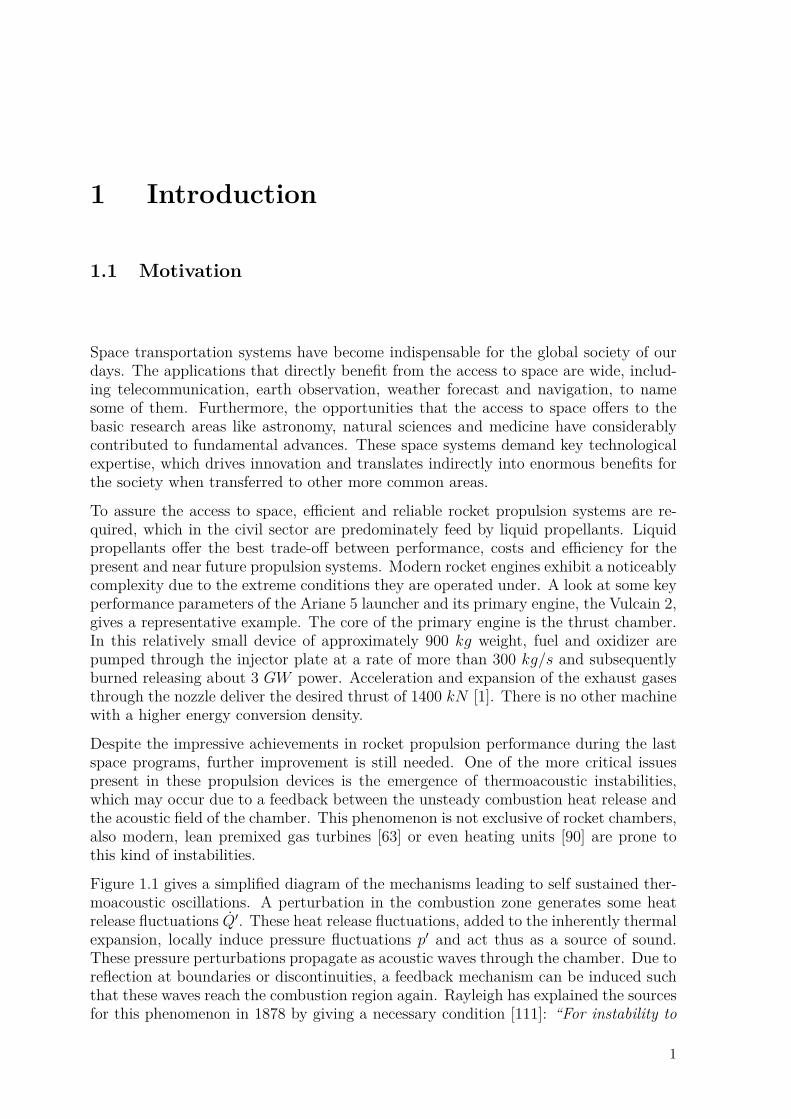
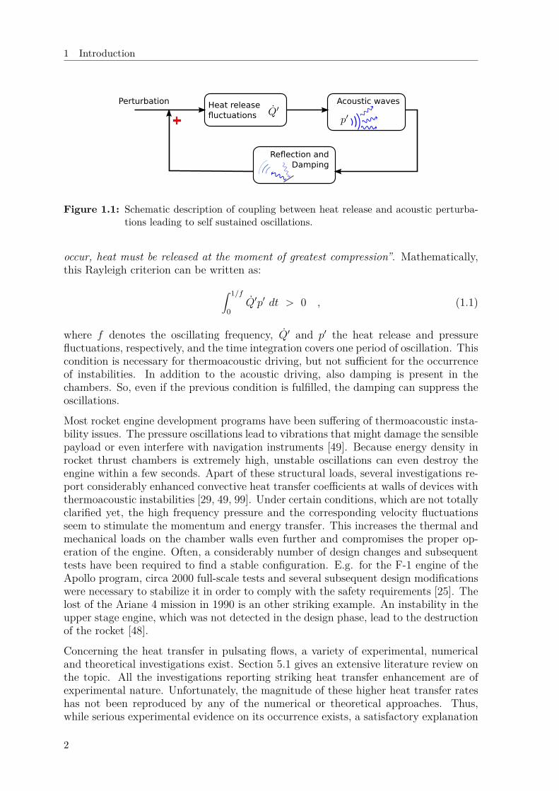
Figure 1.1 gives a simplified diagram of the mechanisms leading to self sustained ther-moacoustic oscillations. A perturbation in the combustion zone generates some heatrelease fluctuations Q′. These heat release fluctuations, added to the inherently thermalexpansion, locally induce pressure fluctuations p′ and act thus as a source of sound.These pressure perturbations propagate as acoustic waves through the chamber. Due toreflection at boundaries or discontinuities, a feedback mechanism can be induced suchthat these waves reach the combustion region again. Rayleigh has explained the sourcesfor this phenomenon in 1878 by giving a necessary condition [111]: “For instability to
1
1 Introduction
Acoustic wavesHeat release fluctuations
Reflection andDamping
+
Perturbation
Figure 1.1: Schematic description of coupling between heat release and acoustic perturba-tions leading to self sustained oscillations.
occur, heat must be released at the moment of greatest compression”. Mathematically,this Rayleigh criterion can be written as:
∫ 1/f
0Q′p′ dt > 0 , (1.1)
where f denotes the oscillating frequency, Q′ and p′ the heat release and pressurefluctuations, respectively, and the time integration covers one period of oscillation. Thiscondition is necessary for thermoacoustic driving, but not sufficient for the occurrenceof instabilities. In addition to the acoustic driving, also damping is present in thechambers. So, even if the previous condition is fulfilled, the damping can suppress theoscillations.
Most rocket engine development programs have been suffering of thermoacoustic insta-bility issues. The pressure oscillations lead to vibrations that might damage the sensiblepayload or even interfere with navigation instruments [49]. Because energy density inrocket thrust chambers is extremely high, unstable oscillations can even destroy theengine within a few seconds. Apart of these structural loads, several investigations re-port considerably enhanced convective heat transfer coefficients at walls of devices withthermoacoustic instabilities [29, 49, 99]. Under certain conditions, which are not totallyclarified yet, the high frequency pressure and the corresponding velocity fluctuationsseem to stimulate the momentum and energy transfer. This increases the thermal andmechanical loads on the chamber walls even further and compromises the proper op-eration of the engine. Often, a considerably number of design changes and subsequenttests have been required to find a stable configuration. E.g. for the F-1 engine of theApollo program, circa 2000 full-scale tests and several subsequent design modificationswere necessary to stabilize it in order to comply with the safety requirements [25]. Thelost of the Ariane 4 mission in 1990 is an other striking example. An instability in theupper stage engine, which was not detected in the design phase, lead to the destructionof the rocket [48].
Concerning the heat transfer in pulsating flows, a variety of experimental, numericaland theoretical investigations exist. Section 5.1 gives an extensive literature review onthe topic. All the investigations reporting striking heat transfer enhancement are ofexperimental nature. Unfortunately, the magnitude of these higher heat transfer rateshas not been reproduced by any of the numerical or theoretical approaches. Thus,while serious experimental evidence on its occurrence exists, a satisfactory explanation
2
1.2 Scope of the Work
of the responsible mechanisms has not yet been given. Fundamental research in thisarea is still necessary.
According to the feedback analysis, the balance between the driving and damping mech-anisms present in the chamber determine whether the oscillations are stable or not. Inrocket thrust chambers, the main components relevant for this balance are the injectorplate, the nozzle, the chamber volume, and the combustion front. To increase stabilityand extend the operation margin of the engine, the application of small passive acousticcavities, so-called resonators, has been demonstrated repeatedly [93]. Other possibili-ties to stabilize the chamber are an adapted injector design and baffles, which both havethe drawback that they can affect the performance of the thrust chamber. Two mech-anisms are believed to be responsible for the stabilizing influence of resonators: First,the attached cavities shift the eigenfrequencies of the overall system, thus disturbingthe feedback mechanism between heat release and acoustic field. Second, dissipationof acoustic energy through viscous and turbulent losses at the cavities mouth. Thisdissipation is maximum within small frequency ranges around the eigenfrequency ofthe cavities. Thus, resonators have to be tuned according to the oscillations modes ofthe overall system. However, the optimal cavity design that leads to maximum stabi-lization is still challenging. Since the resonators themselves influence those eigenmodessignificantly, this is not a simple task. The eigenfrequency of a cavity depends primarilyon its geometrical dimensions and on the speed of sound of the gas inside it.
Under operation, the superimposed acoustic velocity perturbations may also flush hotexhaust gases into the cavity. Furthermore, the possibly enhanced heat transfer bothin axial as well as in wall normal direction in acoustic pulsating flows can compromiseunder certain conditions the thermal integrity of the cavities and the chamber walls.These two mechanisms might change the temperature distribution inside the cavities.Due to the temperature dependency of the speed of sound, the propagation of theacoustic waves would also change, bringing the resonators out of their design point.For instance, the cavities might fail in stabilizing the engine.
Due to the aggressive conditions at operation with temperatures of up to 3600 K andpressure of about 100 bar, measurements and experimental verification of functionalityare difficult and expensive. Theoretical and numerical approaches are thus desirablein all phases of the design process. An accurate prediction of the stabilizing influenceof resonators under real operation conditions taking the previous effects into accountwould be of great interest for the development of more reliable space transportationsystems.
1.2 Scope of the Work
The work presented in this thesis is funded by the German Research Foundation (DFG)in the framework of the “Sonderforschungsbereich SFB-TRR40” [3], which focuses onthe technological foundations for the design of thermally and mechanically highly loadedcomponents of future space transportations systems. Several German institutions areinvolved in a long-term cooperation initiative planed to last approximately 12 years. Itis divided into three subsequent phases that should gradually evolve from fundamentalresearch towards development of new technologies and demonstration of applicability.
3
1 Introduction
This work belongs to the project A3 and covers the investigations of the first funda-mental phase.
The long-term objective of this project is the development of reliable engineering toolsto characterize the damping behavior of resonator rings in rocket thrust chambers underreal operation conditions. Hereby, the influence of enhanced heat transfer presumablydriven by the acoustic fluctuations should be considered in the analysis. The overallintention of the project is to clarify the following questions:
1. Is enhanced heat transfer present in resonators or in the vicinity of the cavitymouths?
2. Does this enhanced heat transfer have any consequences on the stabilizing influ-ence of resonators?
Two top level topics and the interaction between them are covered by the foregoingquestions, namely: heat transfer in pulsating flow and damping characteristics of res-onator rings.
The long-term objective is indeed quite ambitious. In order to provide satisfactory an-swers to the two mentioned questions, firstly, a variety of preliminary issues have to besolved. As mentioned in the motivation of this thesis, yet, the mechanisms leading toenhanced heat transfer in pulsating flows are not totally clarified. This is indicated bythe lack of models that are able to reproduce the large heat transfer rates observed insome experiments and the partially contradictory results that can be found in the liter-ature. Furthermore, the initial investigations during the course of this project showedthat the mere description of the damping characteristics of resonators does not neces-sarily provide a complete picture of their stabilizing influence. The balance betweenthe driving and damping mechanisms present in the thrust chamber decides whetherits operation is stable or not. Thus, extended models that are able to incorporate theinfluence of enhanced heat transfer on the damping characteristics of resonator ringsare not sufficient. Additionally, in order to truly estimate the consequences of enhancedheat transfer, a method that is able to evaluate the stability of a representative thrustchamber coupled to the extended resonator ring model is necessary.
1.3 Strategy and Thesis Outline
Both the enhanced heat transfer in pulsating flows driven by acoustic fields and thestabilizing influence of resonators are not totally clarified yet. Wide ranges of time andlength scales are present in both problems, as will be explained in Sec. 2.1.3. Thus, acoupled analysis considering all these scales would not be efficient or even possible atthis stage. Instead, a decoupled analysis of these two main topics, stabilizing influenceof resonators on the one hand and heat transfer in pulsating flows on the other, appearsas an appropriate strategy to bring more fundamental understanding. For this purpose,adequate simulation approaches have to be defined and extended.
Following this strategy, the first task is the development of resonator ring models thatare able to account for some influence of enhanced heat transfer. As a first attempt, it
4
1.3 Strategy and Thesis Outline
will be assumed that, if present, enhanced heat transfer will primarily modify the gastemperature profile inside the cavities. A milestone is the estimation of the sensitivityof the resonator rings to an imposed inhomogeneous temperature profile. Furthermore,an appropriate method for the stability analysis of rocket thrust chambers that incor-porates the extended resonator ring model has to be developed. Using this method, thestabilizing influence of the resonator rings should be investigated for various operationconditions. Thus, the method should be able to reproduce the essential driving anddamping mechanisms present in the chamber, give especial attention to the resonatorring, and afford parametric studies.
In the second part of this thesis, the mechanisms leading to enhanced heat transfer inpulsating flows are studied. These investigations should clarify whether an enhancementof energy transfer is expected to occur under periodic transient conditions. Rather thana quantitative estimate, it should give a qualitative order of magnitude and highlight thekey parameters controlling the presumably heat transfer enhancement. The first taskinvolves the identification and definition of the periodic transient conditions presentin the rocket thrust chamber. A divide and conquer strategy is followed, that studiesproblems of increasing complexity. Each of this problems aim to estimate the influenceof some precise transients on the heat transfer. In this way, mechanisms leading toenhanced heat transfer in rocket chambers can be identified.
The thesis is organized as follows: Chapter 2 presents the necessary theoretical back-ground on fluid mechanics and thermodynamics. Based on a first estimation of lengthand time scales, simulation approaches that focus on certain scales are introduced.Chapter 3 presents relevant models describing the acoustic damping of resonator ringsand an extension of these models to account for inhomogeneous temperature profiles isderived. A preliminary investigation of the cavities’ sensitivity to temperature inhomo-geneities is also given in this chapter. In Ch. 4, a methodology for the stability analysisof representative rocket thrust chambers is proposed. The method is validated andthe stabilizing influence of resonator rings in rocket trust chambers is discussed. Theresults of a sensitivity analysis for a representative thrust chamber configuration overa range of operation conditions and resonator ring geometries concludes this chapter.Chapter 5 introduces the heat transfer in pulsating flows, defines the environment to bestudied and presents an appropriate strategy. A preliminary investigation using a loworder model of conjugate heat transfer and a laminar pulsating flow past a flat plate ispresented in the same chapter. The third and most challenging configuration studiesthe heat transfer in turbulent pulsating channel and is given in Ch. 6. An extendedCFD simulation technique that accounts for the influence of acoustic fields on turbu-lent heat transfer is presented. After validation, the results of an extensive simulationcampaign are presented, that estimate the heat transfer enhancement for a variety ofpulsation parameters. Finally, Ch. 7 summarizes this thesis and gives the conclusionsof the investigations.
5

2 Theoretical Background andSimulation Approaches
2.1 Conservation Equations
In the context of continuum mechanics, gases and liquids can be treated as a fluidcomposed of infinitesimal elements assumed to be small compared to all length scalesof the problem, but large compared to the molecular scales. The conservation equationsof mass, momentum and energy provide a framework for the mathematical descriptionof fluid dynamics. These conservation laws are derived in an integral sense over acontrol volume using the density ρ, pressure p, velocity vector ~u and internal energy eas primitive variables. Application of Gauß’ integral theorem allows to express them indifferential form, too. Several textbooks devote detailed chapters to the derivation andformulation of these laws [8, 97]. This section presents only the essential informationnecessary in the appreciation of the topics handled in this thesis.
The convective or total derivative operator
D
Dt= ∂
∂t+ ui
∂
∂xi, (2.1)
accounts for the total change of a property. Using this operator, three dimensionalCartesian coordinates and Einsteins index notation, the conservation equations can bewritten as [8]:
Dρ
Dt= −ρ∂ui
∂xi+ km , (2.2)
ρDujDt
= ∂σji∂xi
+ kf,j , (2.3)
ρDe
Dt= − ∂qi
∂xi+ σji
∂ui∂xj
+ ke . (2.4)
Equation (2.2) represents the continuity equation considering mass sources km. Themomentum conservation is expressed by Eq. (2.3) and states that the change in overallmomentum can be induced by surface forces given by the stress tensor σji and bodyforces given by the source term kf,j. Finally, based on the first law of thermodynamics,the conservation of energy Eq. (2.4) relates the total change in internal energy e tosurface heat fluxes qi, mechanical power σji(∂ui/∂xj) and energy sources ke. Theseequations are valid for any single species fluid. In cases with several fluid species,diffusion fluxes have to be additionally considered [103]. All quantities different thanthe primitive variables present in this conservation equations depend on the specificfluid and problem properties.
7
2 Theoretical Background and Simulation Approaches
2.1.1 Constitutive Laws
Constitutive laws are necessary to express the fluid properties in the just given set ofequations as functions of the primitive variables.
The stress tensor is commonly decomposed into the shear or viscous stress tensor τjiand the normal stress tensor −δjip:
σji = τji − δjip+ ζ∂uk∂xk
δji . (2.5)
The third term in this expression accounts for a possible non-equilibrium betweennormal stresses and thermodynamic pressure. The proportionality factor, the so-calledvolume viscosity ζ, is very small for most fluids and is only relevant for very fastdeformations. All problems studied in this thesis are assumed to obey thermodynamicequilibrium at all instants and the volume viscosity is neglected. It is mentioned herefor completeness.
Concerning the shear stresses and contrary to solids, it is the rate of shear deformationand not the deformation itself that matters. The rate of shear deformation is given bythe shear strain tensor:
Dji = 12
[(∂uj∂xi
+ ∂ui∂xj
)− 2
3δji∂uk∂xk
]. (2.6)
In general, the shear stress tensor is a function of the shear strain tensor τji = f(Dji).For Newtonian fluids, the relation between shear stresses and shear strain is assumedas linear τji = 2µDji, with the dynamic viscosity µ as proportionality factor [8]:
τji = µ
[(∂uj∂xi
+ ∂ui∂xj
)− 2
3δji∂uk∂xk
]. (2.7)
In the energy equation, the mechanical power can be expressed as:
σji∂ui∂xj
= −p∂ui∂xi
+ τji∂ui∂xj
. (2.8)
The second term on the right-hand side accounts for the mechanical dissipation throughviscous forces.
In addition to the stress tensor, a relation for the heat fluxes is also necessary. Fourier’slaw correlates the heat flux as a function of the temperature gradient:
qi = −λ ∂T∂xi
, (2.9)
with the fluid thermal conductivity λ as proportionality factor.
Still, the number of unknowns (p, ρ, ui, T and e) is larger than the number of equations(1×continuity, 3×momentum and 1×energy) and two additional laws are necessary toclose the problem.
8
2.1 Conservation Equations
For moderate pressures and temperatures, the ideal gas law relates the density, pressureand temperature of a fluid through the following equation of state:
p
ρ= RsT , (2.10)
where the specific ideal gas constant Rs is a property of the fluid and can be expressedusing the universal gas constant R and the molecular weight of the fluid M as:
Rs = RM . (2.11)
Often, the ideal gas law written in differential form is useful:
dρ
ρ= dp
p− dT
T. (2.12)
A variety of state equations derived from the basic laws of thermodynamics exist thatexpress the internal energy as a function of other two primitive variables, e.g. densityand temperature. Combination with the ideal gas law gives:
e =∫cv dT = h− p
ρ=∫cp dT −
p
ρ, (2.13)
where cv denotes the heat capacity at constant specific volume, h the specific enthalpyand cp the heat capacity at constant pressure. For ideal gases, the following relationshold:
Rs = cp − cv = cv(γ − 1) , (2.14)
c2 = ∂p
∂ρ
∣∣∣∣∣s
= γRsT , (2.15)
where γ = cp/cv denotes the ratio of heat capacities. For perfect gases, the heatcapacities are assumed to be constant and the specific internal energy can be given by:
e = cvT + eref = cpT −p
ρ+ href . (2.16)
The proportionality factors for the viscous µ and thermal diffusion λ are also functionsof the thermodynamic state, principally from temperature if ideal gas behavior is as-sumed. A well known approximate expression for the dynamic viscosity is given by theSutherland law [131]:
µ(T ) = µref
(Tref + CsT + Cs
)(T
Tref
)3/2
, (2.17)
with reference Temperature Tref and viscosity µref , and Sutherland constant Cs, re-spectively. Similar expressions exist for the thermal conductivity. Another possibilityis to express it in terms of the Prandtl number, which gives the ratio of momentum tothermal diffusivity:
Pr = ν
a= µcp
λ, (2.18)
9
2 Theoretical Background and Simulation Approaches
and can be approximately taken as constant for most fluids. For perfect gases thethermal conductivity can be expressed as:
λ(T ) = µ(T )cpPr . (2.19)
The constitutive equations presented in this section are valid for moderate pressureslower than the critical pressure and temperature higher than the critical temperature.These expressions provide a good approximation for single species mixtures. Undermore critical conditions, so-called real gas expressions should be used [109]. Anotherpossibility is the use of polynomial expressions fitted from very accurate tabulatedvalues [73, 128].
2.1.2 Navier-Stokes Equations
Assuming Newtonian fluids, neglecting the volume viscosity and dropping the sourceterms, the general conservation Eqs. (2.2) to (2.4) can be expressed as:
Dρ
Dt= −ρ∂ui
∂xi(2.20)
ρDujDt
= − ∂p
∂xi+ ∂
∂xiµ
[(∂uj∂xi
+ ∂ui∂xj
)− 2
3δji∂uk∂xk
](2.21)
ρDe
Dt= − ∂qi
∂xi− p∂ui
∂xi+ φdiss , (2.22)
where the viscous dissipation is denoted by φdiss = τji∂uj∂xi
. This set of equations will bedenoted from now on as Navier-Stokes equations (NS-equations), even though strictlyspeaking this term refers solely to the momentum equation.
For some problems, it is more convenient to express the energy equation as a functionof a different primitive variable. The enthalpy form is given by:
ρDh
Dt= − ∂qi
∂xi+ Dp
Dt+ φdiss . (2.23)
Another practical form for perfect gases uses the temperature as independent variable:
ρcpDT
Dt= ∂
∂xi
(λ∂T
∂xi
)+ Dp
Dt+ φdiss . (2.24)
These set of equations provide a complete framework for the mathematical descriptionof fluid dynamical problems. All problems treated in this thesis can be described bythese set of equations. However, closed form solutions are only known for cases allowingconsiderable simplifications.
2.1.3 Numerical Challenges Arising from Compressibility
Any attempt to solve the full set of compressible Navier-Stokes equations in problemsin which only some scales dominate would be very complicated and inefficient. This is
10

2.2 Linearized Analysis for Acoustics
especially true for fluid problems accounting only small compressibility, that is to sayonly small density changes due to changes in pressure. Note that changes in densitymay also be caused by changes in temperature or fluid mixture, which in this studywill be denoted as stratification. The main criterion for the compressibility of a flow isthe Mach number:
M = uref
c, (2.25)
defined as the ratio of the fluid characteristic velocity to the speed of sound in themedium. In the context of compressibility, the speed of sound is not only a measureof the wave propagation velocity, but also an indication of the density changes in theflow, as stated by Panton [97]. The kinetic energy of the flow gives an estimate forthe pressure changes present in the flow ∆p ≈ ρrefu
2ref/2 or u2
ref ≈ 2∆p/ρref . Using thisestimate in the definition of the Mach number and Eq. (2.15) gives:
M2 = u2refc2 ≈
2∆pρref
∆ρ∆p
∣∣∣∣∣s
∼ ∆ρρref
. (2.26)
For low Mach number flows M2 1, the fluid dynamics display two types of motions ofconsiderably different magnitude and time scale. Acoustic motions of small magnitudetravel much faster than the hydrodynamic motions. This makes the consideration ofboth acoustic and hydrodynamic flow fields in a single analysis extremely difficult,especially in numerical solution approaches. To overcome this issue, the two fluidmotions can be handled separately, as will be presented in the following sections.
2.2 Linearized Analysis for Acoustics
In acoustics, sound is defined as a small pressure perturbation p′ that moves as awave through a medium at the speed of sound c. This pressure perturbation inducesalso small velocity u′ and density ρ′ perturbations. As shown by Rienstra and Hir-shberg [115], in free space, these perturbations are almost insensitive to viscous andthermal dissipation. Thus, the small perturbations can be treated as isentropic suchthat:
c2 = p′
ρ′. (2.27)
Since the perturbations are small, the fluid motion can be described by a linearizedanalysis in which the variables are decomposed into a mean quantity denoted by anover-bar and a small perturbation denoted by a prime:
p = p+ p′ , (2.28)ρ = ρ+ ρ′ , (2.29)~u = ~u+ ~u′ . (2.30)
Substitution into the conservation equations for perfect, inviscid and non heat conduct-ing fluids leads to a set of linearized perturbation equations. Depending on the spatialdependency of the mean quantities, the resulting linearized perturbation equations canstill be to complex for an analytical treatment. Numerical solvers have emerged thatare able to treat also complex geometries [42, 86, 103].
11
2 Theoretical Background and Simulation Approaches
If the mean field allows the introduction of some spatial simplifications, a wave equationfor the pressure p′ might be deduced from the perturbation equations. In this thesis, twocases are considered for which this condition holds. For completeness, their derivationis shown in App. A.1.
• Homogeneous mean flow with constant properties and no sources:(∂
∂t+ ~u · ~∇
)2
p′ − c2~∇2p′ = 0 . (2.31)
• Stagnant fluid with non-uniform properties:∂2p′
∂t2− ~∇
(c2~∇p′
)= 0 . (2.32)
Due to linearity of the wave equation, the general solution can also be determined inthe frequency domain assuming harmonic dependency:
p′ ∼ Rep eiΩt , (2.33)
where the amplitude of the perturbation p and the angular frequency Ω are complexvalued. The complex notation brings several advantages in the mathematical treatment.Of course, only the real part is physical. Substitution of this approach in the waveequation leads to the Helmholtz equation. For several geometries, analytical solutionsare possible that express the solution of the Helmholtz equation in a very descriptivemanner in terms of up- and downstream traveling waves [33, 104].
2.2.1 Propagation of Acoustic Waves in Cylindrical Ducts with Mean Flow
Throughout this thesis, the propagation of acoustic waves in cylindrical geometrieswill be widely studied, because rocket thrust chambers can be effectively simplifiedas cylindrical ducts. In the presence of a uniform mean flow ~u = [U, 0, 0]T in axialdirection x and homogeneous speed of sound c, Eq. (2.31) can be written as [115]:
1c2
(∂
∂t+ U
∂
∂x
)2
p′ = ~∇2p′ . (2.34)
Using cylindrical coordinates (x, r and θ) and Mach number M = U/c gives:1c2∂2p′
∂t2+ 2M
c
∂2p′
∂t∂x+M2∂
2p′
∂x2 = ∂2p′
∂r2 + 1r
∂p′
∂r+ 1r2∂2p′
∂θ2 + ∂2p′
∂x2 . (2.35)
Following the method of separation of variables, substitution of an harmonic approachfor the pressure fluctuations p′ = R(r) exp(iΩt− ikx+ imθ) leads after some rearrange-ment to:
r2d2Rdr2 + r
dRdr
+[r2((Ω/c−Mk)2 − k2
)−m2
]R = 0 . (2.36)
Please note that throughout this thesis, the acoustic notation e+iΩt is used for the timedependency. The motivation for this decision and the resulting implications are givenin App. A.2. Introducing the dispersion relation
α2 = (Ω/c−Mk)2 − k2 (2.37)
12
2.2 Linearized Analysis for Acoustics
and using the substitution r = αr, the wave equation can be written as:
r2d2Rdr2 + r
dRdr
+[r2 −m2
]R = 0 , (2.38)
which is a Bessel differential equation of order m. The general solution for such anequation is [80]:
R = CJm(r) +DYm(r) , (2.39)
where Jm and Ym are Bessel functions of the first and second type, respectively. Ymis divergent at r = 0 and thus, the coefficient D has to be zero to keep the pressurep′ physical in the absence of sources at this position. Back transformation into ther-space and substitution in the harmonic approach gives:
p′ = CJm(αr) exp(iΩt− ikx+ imθ) , m ∈ Z (2.40)
where C is a constant defining the magnitude of the pressure amplitude, α, m andk are the radial, tangential and axial wave numbers, respectively, that describe thespatial dependency. To close the problem, radial and tangential boundary conditionsare needed to determine these wave numbers. For cylindrical ducts, axial symmetryenforces periodicity in the tangential direction such that eimθ = eim(θ+2π). Thus thetangential wave numbers can only take integer values m ∈ Z. Furthermore, the ra-dial and axial wave numbers are related to each other trough the dispersion relationEq. (2.37).
Due to its quadratic dependency, the dispersion relation has two solutions, one for thepositive root (α+) and another for the negative one (α−). The general solution of thelinearized convective wave equation Eq. (2.34) is thus a superposition of four linearlyindependent terms. In the most general case, they represent helical waves with pos-itive and negative sense of rotation (∼ exp(±imθ)) that travel the duct in up- anddownstream direction (∼ exp(−ik±mnx)) [104]. Depending on the magnitude of the am-plitudes of the helical waves relative to each other, so-called spinning tangential modesare physically possible [33]. However, this thesis is restricted to the case where thehelical waves have equal amplitudes, leading to standing tangential modes ∼ cos(mθ)with positive tangential wave number m ∈ N0.
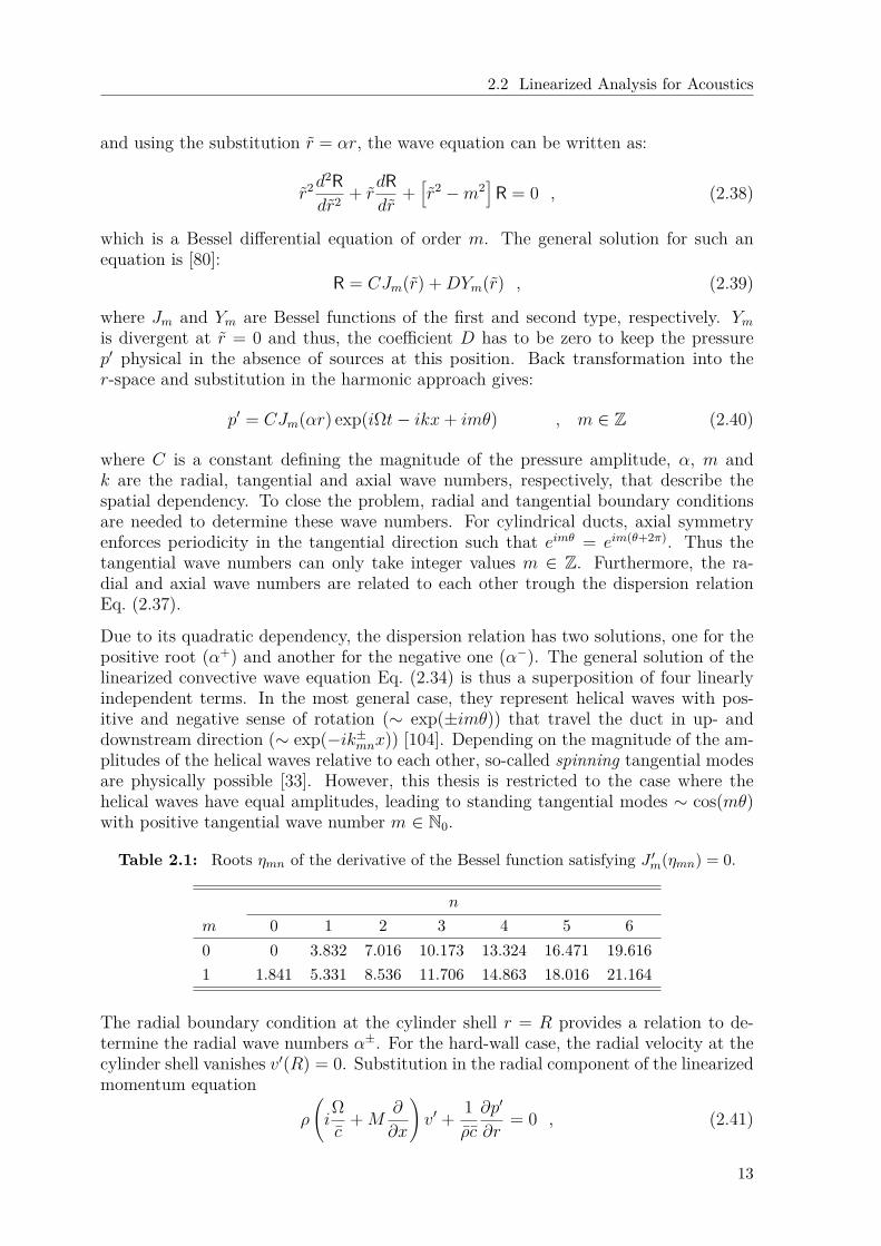
Table 2.1: Roots ηmn of the derivative of the Bessel function satisfying J ′m(ηmn) = 0.
n
m 0 1 2 3 4 5 60 0 3.832 7.016 10.173 13.324 16.471 19.6161 1.841 5.331 8.536 11.706 14.863 18.016 21.164
The radial boundary condition at the cylinder shell r = R provides a relation to de-termine the radial wave numbers α±. For the hard-wall case, the radial velocity at thecylinder shell vanishes v′(R) = 0. Substitution in the radial component of the linearizedmomentum equation
ρ
(iΩc
+M∂
∂x
)v′ + 1
ρc
∂p′
∂r= 0 , (2.41)
13
2 Theoretical Background and Simulation Approaches
leads to:d
drJm(αr)
∣∣∣∣∣r=R
= 0 . (2.42)
For each tangential order m, the solutions of this transcendental equation are given byαmnR = ±ηmn, where ηmn corresponds to the n’th root of the Bessel function derivative.Some roots of the Bessel function derivative are given in Tab. (2.1). They are purelyreal valued and frequency independent. Furthermore, the up- and downstream travelingwaves have equal mode shape even in the presence of mean flow:
α+mn = α−mn = ηmn
R= const. ∈ R . (2.43)
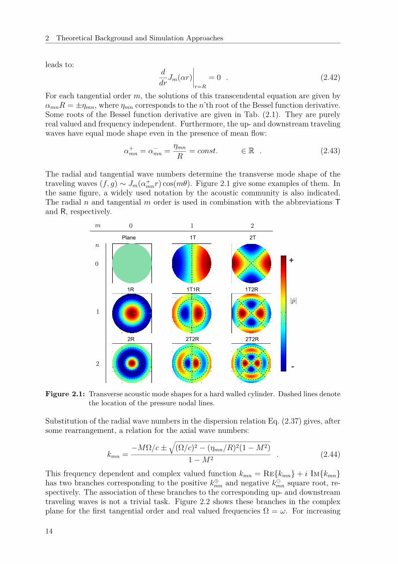
The radial and tangential wave numbers determine the transverse mode shape of thetraveling waves (f, g) ∼ Jm(α+
mnr) cos(mθ). Figure 2.1 give some examples of them. Inthe same figure, a widely used notation by the acoustic community is also indicated.The radial n and tangential m order is used in combination with the abbreviations Tand R, respectively.
+
-
1T1R1R
2T2R
Plane
2T2R
1T 2T
1T2R
2R
Figure 2.1: Transverse acoustic mode shapes for a hard walled cylinder. Dashed lines denotethe location of the pressure nodal lines.
Substitution of the radial wave numbers in the dispersion relation Eq. (2.37) gives, aftersome rearrangement, a relation for the axial wave numbers:
kmn =−MΩ/c±
√(Ω/c)2 − (ηmn/R)2(1−M2)
1−M2 . (2.44)
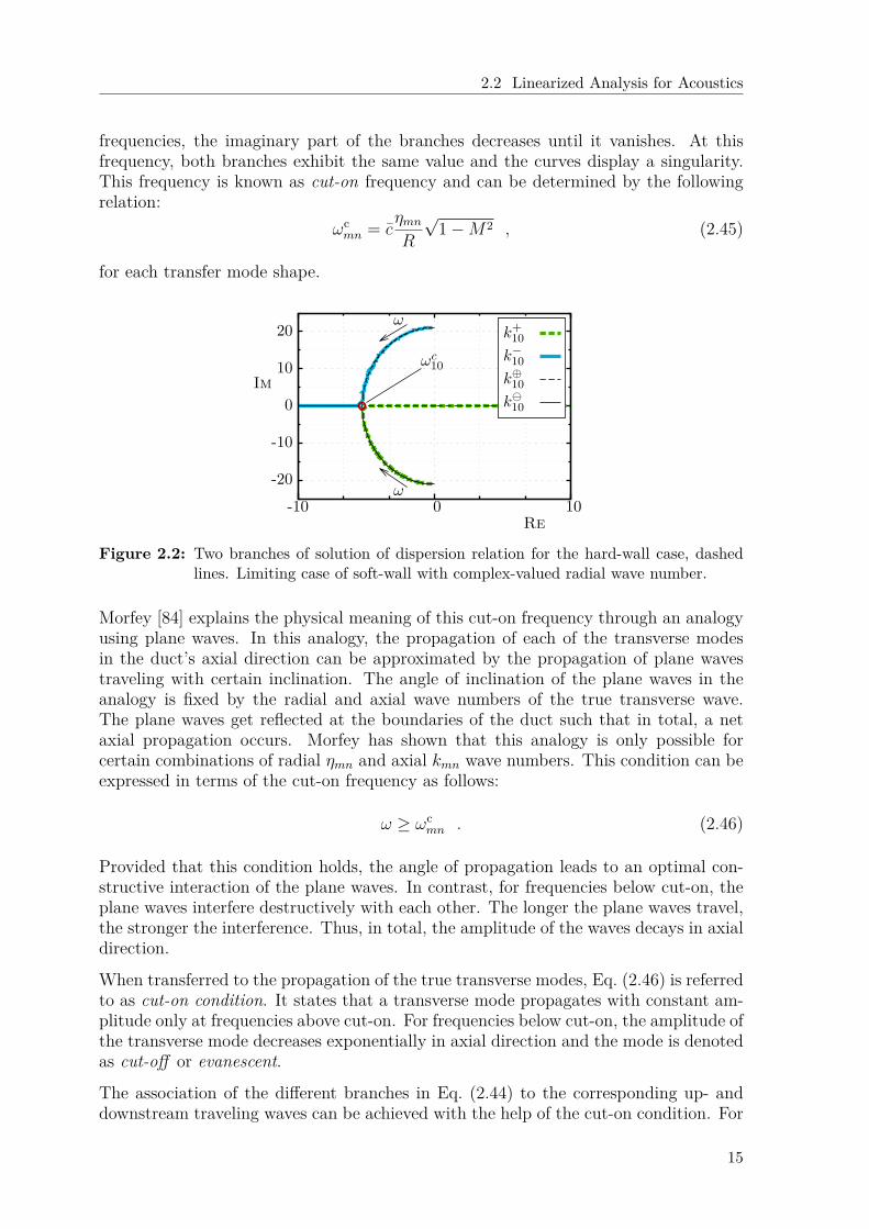
This frequency dependent and complex valued function kmn = Rekmn + i Imkmnhas two branches corresponding to the positive k⊕mn and negative kmn square root, re-spectively. The association of these branches to the corresponding up- and downstreamtraveling waves is not a trivial task. Figure 2.2 shows these branches in the complexplane for the first tangential order and real valued frequencies Ω = ω. For increasing
14
2.2 Linearized Analysis for Acoustics
frequencies, the imaginary part of the branches decreases until it vanishes. At thisfrequency, both branches exhibit the same value and the curves display a singularity.This frequency is known as cut-on frequency and can be determined by the followingrelation:
ωcmn = c
ηmnR
√1−M2 , (2.45)
for each transfer mode shape.
-20
-10
0
10
20
-10 0 10
Im
Re
ω
ω
ωc10
k+10k−10k⊕10k10
Figure 2.2: Two branches of solution of dispersion relation for the hard-wall case, dashedlines. Limiting case of soft-wall with complex-valued radial wave number.
Morfey [84] explains the physical meaning of this cut-on frequency through an analogyusing plane waves. In this analogy, the propagation of each of the transverse modesin the duct’s axial direction can be approximated by the propagation of plane wavestraveling with certain inclination. The angle of inclination of the plane waves in theanalogy is fixed by the radial and axial wave numbers of the true transverse wave.The plane waves get reflected at the boundaries of the duct such that in total, a netaxial propagation occurs. Morfey has shown that this analogy is only possible forcertain combinations of radial ηmn and axial kmn wave numbers. This condition can beexpressed in terms of the cut-on frequency as follows:
ω ≥ ωcmn . (2.46)
Provided that this condition holds, the angle of propagation leads to an optimal con-structive interaction of the plane waves. In contrast, for frequencies below cut-on, theplane waves interfere destructively with each other. The longer the plane waves travel,the stronger the interference. Thus, in total, the amplitude of the waves decays in axialdirection.
When transferred to the propagation of the true transverse modes, Eq. (2.46) is referredto as cut-on condition. It states that a transverse mode propagates with constant am-plitude only at frequencies above cut-on. For frequencies below cut-on, the amplitude ofthe transverse mode decreases exponentially in axial direction and the mode is denotedas cut-off or evanescent.
The association of the different branches in Eq. (2.44) to the corresponding up- anddownstream traveling waves can be achieved with the help of the cut-on condition. For
15
2 Theoretical Background and Simulation Approaches
the chosen acoustic notation e+iωt, for real valued frequencies, an alternation of the twobranches is necessary to satisfy the cut-on condition:
k+mn =
kmn if ω < ωc ,
k⊕mn if ω ≥ ωc .and k−mn =
k⊕mn if ω < ωc ,
kmn if ω ≥ ωc .(2.47)
Mathematically, this alternation can be expressed in a single formula as:
k±mn =−Mω/c± sign(ω − ωc
mn)√
(ω/c)2 − (ηmn/R)2(1−M2)1−M2 . (2.48)
Note that the alternation is only necessary for hard walled ducts in the limiting caseof real valued frequencies. For a detailed explanation and validation of this neces-sity please refer to App. A.2. Figure 2.2 shows the axial wave numbers associated tothe corresponding up- and downstream direction of propagation using the previouslyintroduced notation k−mn and k+
mn, respectively.
After determination of all wave numbers, the general solution in cylindrical coordinatescan finally be written as:
p′
cρ=∑m,n
[Jm(α+
mnr)Fmne−ik+mnx + Jm(α−mnr)Gmne
−ik−mnx]
cos(mθ)eiΩt =∑m,n
(fmn + gmn) , (2.49)
which can be interpreted as three dimensional waves or “modes” of tangential and radialorder m and n traveling in the down- “f” and upstream “g” direction, respectively. Theamplitudes Fmn and Gmn give information about the relative local sound pressure level.
Due to the linearity of the linearized momentum equation, the same holds for thevelocity fluctuations. Introducing the abbreviations
κ±mn = k±mnΩ/c−Mk±mn
, and β±mn = 1Ω/c−Mk±mn
, (2.50)
these fluctuations can be written in terms of the characteristic amplitudes fmn and gmnas:
u′ =∑m,n
(κ+mnfmn + κ−mngmn
), (2.51)
v′ = i∑m,n
(β+mn
∂fmn∂r
+ β−mn∂gmn∂r
), (2.52)
w′ = −mr
∑m,n
(β+mnfmn + β−mngmn
). (2.53)
2.2.2 Plane Wave Approximation
For systems in which the frequency range of interest lies well below the cut-on frequencyof the first transverse mode, a plane wave approximation is applicable. This is based
16
2.2 Linearized Analysis for Acoustics
on the assumption that any transverse mode will rapidly decay in axial direction. Thegeneral solution given by Eqs. (2.49) and (2.51) to (2.53) simplifies considerably forplane waves (m = n = 0):
p′
ρc=[F e−ik
+x + Ge−ik−x]eiΩt , (2.54)
u′ =[F e−ik
+x − Ge−ik−x]eiΩt , (2.55)
v′ = w′ = 0 , (2.56)
where the solution is expressed solely as a superposition of one up- and one downstreamtraveling wave of amplitude F and G, respectively. For simplicity, the mode order 00 isomitted in this representation. The axial wave numbers simplify to:
k± = ±Ω/c1±M . (2.57)
It is also useful to express the characteristics acoustic amplitudes in terms of the prim-itives variables:
f = F e−ik+xeiΩt = p′
ρc+ u′ , (2.58)
g = Ge−ik−xeiΩt = p′
ρc− u′ . (2.59)
For vanishing Mach number, the axial wave numbers simplify further into k+ = −k− =k = Ω/c and the general solution can be written as:
p′
ρc=[F e−ikx + Geikx
]eiΩt , (2.60)
u′ =[F e−ikx − Geikx
]eiΩt . (2.61)
The relative magnitude of the amplitudes F and G to each other depends on theboundary conditions. General expressions suitable for the description of such boundaryconditions are given in the next sections.
2.2.2.1 Acoustic Impedance
The acoustic impedance is defined on a surface as the Fourier transform of the ratioof acoustic pressure perturbation to acoustic velocity perturbation and is in generalcomplex valued. Only the surface normal velocity component is considered for thisratio. Thus, for plane waves it can simply be expressed as:
Z(Ω) = p′
u′= Θ + i Ψ . (2.62)
The real part Θ is named resistance, while the imaginary part Ψ reactance. The specificimpedance of a fluid is given by ρc. This factor is commonly used as a reference tonon-dimensionalize the acoustic impedance:
z = Z
ρc= θ + i ψ . (2.63)
17
2 Theoretical Background and Simulation Approaches
As explained by Rienstra and Hirschberg [115], the acoustic impedance can be used todescribe the coupling between two adjacent regions in an acoustic system. Any kindof boundary condition can be expressed as an effective impedance. Furthermore, theacoustic impedance allows to use well established electric network rules to calculate theequivalent impedance of a system [88].
2.2.2.2 Reflection Coefficient
A more descriptive quantity considering the influence of a boundary on traveling wavesis the reflection coefficient. It is defined as the ratio of reflected to incident waveamplitude:
r = G
F= p′/(ρc)− u′p′/(ρc) + u′
= z − 1z + 1 . (2.64)
Alternatively, the specific impedance can be given in terms of the reflection coefficientby:
z = 1 + r
1− r . (2.65)
Table 2.2 gives an overview of idealized boundary conditions with their correspondingimpedance and reflection factors.
Table 2.2: Relation between specific impedance and reflection coefficient for ideal boundaryconditions.
closed end open end non- partially reactive generalu′ = 0 p′ = 0 reflective reflective
z ∞ 0 1 θ ψi θ + i ψ
r 1 −1 0 θ−1θ+1
1−ψ2
1+ψ2 − i 2ψ1+ψ2
(θ2+1+ψ2)+2ψ i(θ+1)2+ψ2
2.2.2.3 Standing Acoustic Waves
Depending on the boundary conditions, traveling waves can form standing waves. Thisis the case for the majority of self sustained oscillations, as encountered in rocketchambers. This thesis focuses on this kind of acoustic waves.
As an example, consider the acoustic field in a channel of length L and uniform flowwith two acoustically closed ends, i.e. u′(x = 0) = u′(x = L) = 0. Substitutionin the general solution, Eqs. (2.54) and (2.55) delivers the conditions F = G andF (e−ik+L − e−ik−L) = 0. For finite amplitudes, the relation e−ik
+L − e−ik−L = 0 has tobe fulfilled. With some mathematical manipulation, this relation can be recast into:
e−i(k+−k−)L − 1 = e
2Ω/cL1−M2 i − 1 = 0 . (2.66)
The roots of Eq. (2.66) correspond to the eigenfrequencies of the acoustic system andare given by the following expression:
ωl = lπc(1−M2)
L, l = 1, 2, 3, ... . (2.67)
18
2.2 Linearized Analysis for Acoustics
For this simplified system, they are all real valued, ωl ∈ R. The interpretation of acomplex valued eigenfrequency will be given in Sec. 2.2.4.
-1
0
1
0 0.25 0.5 0.75 1x/L
l = 1
-1
0
1l = 2
-1
0
1l = 3
P /A U/A
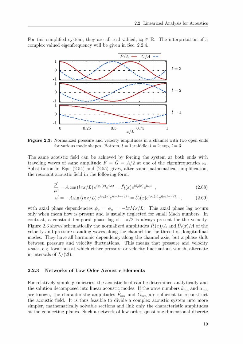
Figure 2.3: Normalized pressure and velocity amplitudes in a channel with two open endsfor various mode shapes. Bottom, l = 1; middle, l = 2; top, l = 3.
The same acoustic field can be achieved by forcing the system at both ends withtraveling waves of same amplitude F = G = A/2 at one of the eigenfrequencies ωl.Substitution in Eqs. (2.54) and (2.55) gives, after some mathematical simplification,the resonant acoustic field in the following form:
p′
ρc= A cos (lπx/L) eiφp(x)eiωlt = Pl(x)eiφp(x)eiωlt , (2.68)
u′ = −A sin (lπx/L) eiφu(x)ei(ωlt−π/2) = Ul(x)eiφu(x)ei(ωlt−π/2) , (2.69)
with axial phase dependencies φp = φu = −lπMx/L. This axial phase lag occursonly when mean flow is present and is usually neglected for small Mach numbers. Incontrast, a constant temporal phase lag of −π/2 is always present for the velocity.Figure 2.3 shows schematically the normalized amplitudes Pl(x)/A and Ul(x)/A of thevelocity and pressure standing waves along the channel for the three first longitudinalmodes. They have all harmonic dependency along the channel axis, but a phase shiftbetween pressure and velocity fluctuations. This means that pressure and velocitynodes, e.g. locations at which either pressure or velocity fluctuations vanish, alternatein intervals of L/(2l).
2.2.3 Networks of Low Oder Acoustic Elements
For relatively simple geometries, the acoustic field can be determined analytically andthe solution decomposed into linear acoustic modes. If the wave numbers k±mn and α±mnare known, the characteristic amplitudes Fmn and Gmn are sufficient to reconstructthe acoustic field. It is thus feasible to divide a complex acoustic system into moresimpler, mathematically solvable sections and link only the characteristic amplitudesat the connecting planes. Such a network of low order, quasi one-dimensional discrete
19
2 Theoretical Background and Simulation Approaches
elements allows to study acoustic systems in a very flexible and descriptive manner[88, 103, 104]. Each element in the network is mathematically described by expressionslinking the characteristic amplitudes of the downstream and upstream traveling wavesat the connecting planes, in the following referred to as ports. This method has beenextensively applied to estimate the response of acoustic systems especially at frequenciesbelow the cut-on, where only plane-waves propagate [7, 59, 66, 67, 90]. In this case,the connecting ports in the network have only two pins, one for the plane f00 andone for the plane g00 wave. Networks treating higher order modes are also possible[33, 107, 120], but their application is not common. Especially the handling of theconnecting planes becomes in this case challenging, where additional assumptions arenecessary. This section gives only an introduction to conventional plane wave acousticnetworks. Because of this, the mode indices mn are omitted in the rest of this sectionto improve readability. The necessary extensions and considerations for network abovecut-on will be given in Sec. 4.3.
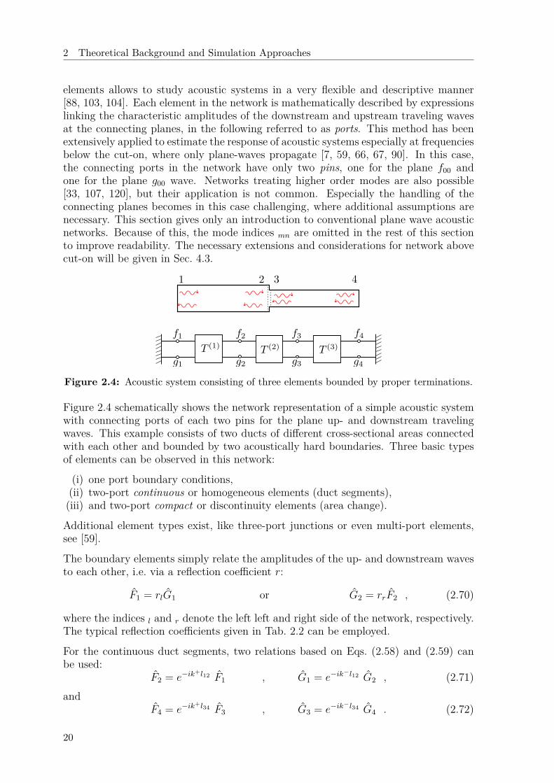
Figure 2.4: Acoustic system consisting of three elements bounded by proper terminations.
Figure 2.4 schematically shows the network representation of a simple acoustic systemwith connecting ports of each two pins for the plane up- and downstream travelingwaves. This example consists of two ducts of different cross-sectional areas connectedwith each other and bounded by two acoustically hard boundaries. Three basic typesof elements can be observed in this network:
(i) one port boundary conditions,(ii) two-port continuous or homogeneous elements (duct segments),(iii) and two-port compact or discontinuity elements (area change).
Additional element types exist, like three-port junctions or even multi-port elements,see [59].
The boundary elements simply relate the amplitudes of the up- and downstream wavesto each other, i.e. via a reflection coefficient r:
F1 = rlG1 or G2 = rrF2 , (2.70)
where the indices l and r denote the left left and right side of the network, respectively.The typical reflection coefficients given in Tab. 2.2 can be employed.
For the continuous duct segments, two relations based on Eqs. (2.58) and (2.59) canbe used:
F2 = e−ik+l12 F1 , G1 = e−ik
−l12 G2 , (2.71)and
F4 = e−ik+l34 F3 , G3 = e−ik
−l34 G4 . (2.72)
20
2.2 Linearized Analysis for Acoustics
Finally, the compact element relates the amplitudes of the up- and downstream trav-eling waves across the sudden area change. Actually, any discontinuity in an acousticsystem like area changes, jumps in fluid properties induced for example by flames, sud-den changes in shell boundary conditions and so on, can be modeled in the networkas compact elements. The derivation of the relations for compact elements stronglydepends on the type of discontinuity. Often, the relations are derived based on con-servation equations in the limiting case of a domain of zero thickness enclosing thediscontinuity plane. In a pure plane wave approximation, some simplified formulationsexist, that can be expressed in form of transmission and reflection coefficients. However,it is important to remark that in the general case, such a discontinuity can also inducescattering into higher order modes, even for frequencies below cut-on. This behaviorin usually referred to as mode coupling and plays an important role in the derivationof low order acoustic elements for resonator rings. The derivation and the necessaryconsiderations for the discontinuity types treated in this study will be given in detailin Sec. 4.3.2.
The basic example shown in Fig. 2.4 should serve only as a reference to explain theformalism of acoustic low order networks. Of course, the number of possible elementsis large, see for example [59, 88]. The relations for the elements used in this thesis aregiven in Sec. 4.5.1.
In a pure plane wave simplification, the two relations between the characteristic am-plitudes of the acoustic waves at the connecting ports left and right from an element(continuous or compact) can be arranged in matrix form as:Fr
Gr
=T11 T12
T21 T22
FlGl
. (2.73)
One advantage of this so-called transfer matrix notation is that the relation betweennon-adjacent ports can be simply determined by matrix multiplication. E.g., a transfermatrix between ports 1 and 3 can be expressed as matrix multiplication using thetransfer matrices between the adjacent ports: T(3) = T(1)T(2).
Physically, the scattering matrix notation offers a more descriptive representation ofthe elements that preserves causality. In this case, the relations are arranged such thatthe resulting matrix relates the amplitudes of the outgoing to the incoming waves:Fr
Gl
=S11 S12
S21 S22
FlGr
. (2.74)
The diagonal entries of the scattering matrix represent transmission and the off-diagonalentries reflection coefficients for the up- and downstream traveling waves.
Combined with proper boundary conditions at the terminations the whole network canbe described by a system of linear equations:
A~x = ~b , (2.75)
with system matrix A, state vector ~x containing the characteristic amplitudes of allpins at the connecting ports and, depending on the boundary conditions or the presenceof sources within the system, excitation vector ~b.
21
2 Theoretical Background and Simulation Approaches
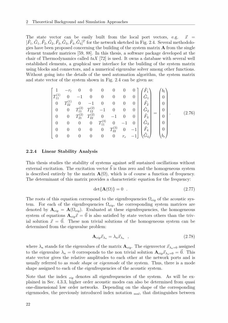
The state vector can be easily built from the local port vectors, e.g. ~x =[F1, G1, F2, G2, F3, G3, F4, G4]T for the network sketched in Fig. 2.4. Several methodolo-gies have been proposed concerning the building of the system matrix A from the singleelement transfer matrices [59, 88]. In this thesis, a software package developed at thechair of Thermodynamics called taX [72] is used. It owns a database with several wellestablished elements, a graphical user interface for the building of the system matrixusing blocks and connectors, and a numerical eigenvalue solver among other functions.Without going into the details of the used automation algorithm, the system matrixand state vector of the system shown in Fig. 2.4 can be given as:
1 −rl 0 0 0 0 0 0T
(1)11 0 −1 0 0 0 0 00 T
(1)22 0 −1 0 0 0 0
0 0 T(2)11 T
(2)12 −1 0 0 0
0 0 T(2)21 T
(2)22 0 −1 0 0
0 0 0 0 T(3)11 0 −1 0
0 0 0 0 0 T(3)22 0 −1
0 0 0 0 0 0 rr −1
F1
G1
F2
G2
F3
G3
F4
G4
=
bl000000br
. (2.76)
2.2.4 Linear Stability Analysis
This thesis studies the stability of systems against self sustained oscillations withoutexternal excitation. The excitation vector ~b is thus zero and the homogeneous systemis described entirely by the matrix A(Ω), which is of course a function of frequency.The determinant of this matrix provides a characteristic equation for the frequency:
detA(Ω) = 0 . (2.77)
The roots of this equation correspond to the eigenfrequencies Ωeig of the acoustic sys-tem. For each of the eigenfrequencies Ωeig, the corresponding system matrices aredenoted by Aeig = A(Ωeig). Evaluated at these eigenfrequencies, the homogeneoussystem of equations Aeig~x = ~0 is also satisfied by state vectors others than the triv-ial solution ~x = ~0. These non trivial solutions of the homogeneous system can bedetermined from the eigenvalue problem:
Aeig~xλn = λn~xλn , (2.78)
where λn stands for the eigenvalues of the matrix Aeig. The eigenvector ~xλn=0 assignedto the eigenvalue λn = 0 corresponds to the non trivial solution Aeig~xλn=0 = ~0. Thisstate vector gives the relative amplitudes to each other at the network ports and isusually referred to as mode shape or eigenmode of the system. Thus, there is a modeshape assigned to each of the eigenfrequencies of the acoustic system.
Note that the index eig denotes all eigenfrequencies of the system. As will be ex-plained in Sec. 4.3.3, higher order acoustic modes can also be determined from quasione-dimensional low order networks. Depending on the shape of the correspondingeigenmodes, the previously introduced index notation mnl, that distinguishes between
22
2.2 Linearized Analysis for Acoustics
tangential, radial and longitudinal order, respectively, can be also employed. In thisthesis, the latter notation will be used, when a specific eigenfrequency of a given geomet-rical problem is meant. Instead, the former notation is used when all eigenfrequenciesof a general undefined problem are meant.
With the time dependency convention ∼ eiΩt = eiωte−ϑt, the imaginary part ϑeig ofthe eigenfrequencies Ωeig decides whether the system is stable or not. An eigenmodeis linearly stable if ϑeig > 0, metastable if ϑeig = 0 and unstable otherwise. A moreconvenient quantity for the stability behavior is the cycle increment [66]
Γeig = e−2π
ϑeigωeig − 1 , (2.79)
that represents the percentage by which the amplitude of a perturbation grows or decaysduring one cycle.
2.2.5 Generalized Nyquist Criterion
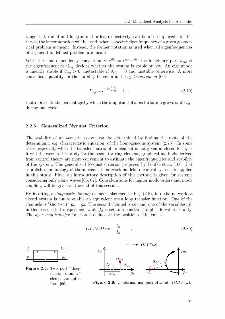
The stability of an acoustic system can be determined by finding the roots of thedeterminant, e.g. characteristic equation, of the homogeneous system (2.75). In somecases, especially when the transfer matrix of an element is not given in closed form, asit will the case in this study for the resonator ring element, graphical methods derivedfrom control theory are more convenient to estimate the eigenfrequencies and stabilityof the system. The generalized Nyquist criterion proposed by Polifke et al. [106] thatestablishes an analogy of thermoacoustic network models to control systems is appliedin this study. First, an introductory description of this method is given for systemsconsidering only plane waves [66, 67]. Considerations for higher mode orders and modecoupling will be given at the end of this section.
By inserting a diagnostic dummy element, sketched in Fig. (2.5), into the network, aclosed system is cut to enable an equivalent open loop transfer function. One of thechannels is ”short-cut“ gu = gd. The second channel is cut and one of the variables, fuin this case, is left unspecified, while fd is set to a constant amplitude value of unity.The open loop transfer function is defined at the position of the cut as
OLTF (Ω) = −fufd
, (2.80)
Figure 2.5: Two port “diag-nostic dummy”element, adaptedfrom [66]. Figure 2.6: Conformal mapping of ω into OLTF (ω).
23
2 Theoretical Background and Simulation Approaches
which may be interpreted as the response of the system to a constant amplitude forcing.Thus, the system is changed into an inhomogeneous one:
ANyq~xNyq = ~bNyq = [0, . . . , 1, . . . , 0]T . (2.81)
Hereby, the index Nyq refers to the extended acoustic network with the Nyquist dummy.The solution of the now inhomogeneous forced system will coincide with the unper-turbed homogeneous one only at the eigenfrequencies Ωeig, where fu/fd = 1. Thus theOLTF can be interpreted as a conformal mapping Ω → OLTF (Ω) that maps all theeigenfrequencies of the unforced system Ωeig to the critical point −1 + 0i in the imagespace.
Applying the generalized Nyquist criterion and keeping in mind that some elements areeventually only available for real frequencies, the OLTF is evaluated for real valuedfrequencies only. The Nyquist curve represents thus the mapping of the positive real axisinto the image plane, see Fig. (2.6). The OLTF (ω) curve will orbit the origin withoutnecessary crossing the critical point. Following the curve towards higher frequencies,its position with respect to the critical point −1 + 0i determines stability. For stableeigenmodes with ϑeig > 0 the critical point will be on the left side of the curve, assketched in Fig. (2.6).
As shown in [118], exploiting the properties of conformal mappings that locally pre-serve orientation or handedness, the frequencies at which the OLTF curve passes thecritical point with minimal distance identify the real part of the eigenfrequencies. Atthese locations denoted by OLTF (ω⊥), the connecting line to the critical point willbe perpendicular to the OLTF curve. The imaginary part of the eigenfrequencies canbe estimated from the minimal distance using a proper scaling factor. The factor bywhich the critical distance Smin in the image plane has to be scaled ϑeig = Smin/σ canbe determined from geometrical considerations as:
σ = lim∆ω → 0
∣∣∣∣∣OLTF (ω⊥ + ∆ω)−OLTF (ω⊥ −∆ω)∆ω
∣∣∣∣∣ . (2.82)
For a discrete OLTF , Sattelmayer and Polifke [118] proposed a polynomial fit of theOLTF curve to increase the accuracy when only low frequency resolution is feasible.As shown by Kopitz et al. [66], for small frequency increments, the linear approxi-mation of the scaling factor provides adequate accuracy. The imaginary part of theeigenfrequencies can then be estimated as:
Ωn ≈ ω⊥ + sign(RHR)i 2|Smin|∆ω|OLTF (ω⊥ + ∆ω)−OLTF (ω⊥ −∆ω)| , (2.83)
where the sign of the imaginary part is determined through the right-hand rule (RHR).With the eigenfrequencies estimated in this way, the cycle increment can be deducedfrom the Nyquist plot using Eq. (2.79). The method is well tested and validated forsystems of frequency range below the first cut-on frequency incorporating only planewaves. Advantages and disadvantages are also mentioned in the literature [59, 66].
24
2.3 Low Mach Number Approximations
2.3 Low Mach Number Approximations
To overcome the compressibility issues discussed in Sec. 2.1.3, a series of simplificationscan be applied to the fully compressible governing equations. The derivation is basedon the dimensional analysis presented by Panton [97] and assuming ideal gas behavior.
2.3.1 Dimensional Analysis
To estimate the order of magnitude of the different terms present in the fully compress-ible NS-equations, a proper non-dimensionalization is necessary. Most of the variablescan be non-dimensionalized in a straightforward manner by the boundary conditionsof the problem:
x∗i = xiL
, t∗ = tuoL
, u∗i = uiuo
, ρ∗ = ρ
ρo, λ∗ = λ
λo,
p∗ = p
ρou2o
, T ∗ = T − TCTH − TC
, (2.84)
where L is the characteristic length of the geometry, the temperature field is bounded bythe limits TH and TC , and the index o denotes a reference state at the cold temperature,respectively. Substitution in the ideal gas law in differential form (Eq. (2.12)) gives aftersome thermodynamic development:
Dρ∗
Dt∗= γM2Dp
∗
Dt∗− ∆T
TC
ρ∗
T ∗∆TTC
+ 1
DT ∗Dt∗
, (2.85)
where ∆T = TH−TC stands for the maximum temperature difference. Put in this form,the ideal gas law states that the total change in density depends on two parameters:γM2 and the relative temperature difference ∆T/Tc. Similarly, substitution in the fullycompressible NS-equations gives:
1ρ∗Dρ∗
Dt∗= −∂u
∗i
∂x∗i, (2.86)
ρ∗Du∗iDt∗
= −∂p∗
∂x∗i+ 1
Re∂
∂x∗i
[µ∗(∂u∗i∂xj
+∂u∗j∂xi− 2
3∂u∗j∂xj
)], (2.87)
ρ∗DT ∗
Dt∗= 1
Re Pr∂
∂x∗i
(λ∗∂T ∗
∂x∗i
)+M2(γ − 1) Tc∆T
[Dp∗
Dt∗+ φ∗
]. (2.88)
25
2 Theoretical Background and Simulation Approaches
2.3.1.1 Weakly Compressible Flows
For low Mach flows γM2 → 0 and neglecting dissipation φ∗diss 1, the set of equationscan be simplified into the so-called weakly compressible form:
Dρ∗
Dt∗= −∆T
TC
ρ∗
T ∗∆TTC
+ 1
DT ∗Dt∗
, (2.89)
1ρ∗Dρ∗
Dt∗= −∂u
∗i
∂x∗i, (2.90)
ρ∗Du∗iDt∗
= −∂p∗
∂x∗i+ 1
Re∂
∂x∗i
[µ∗(∂u∗i∂xj
+∂u∗j∂xi− 2
3∂u∗j∂xj
)], (2.91)
ρ∗DT ∗
Dt∗= 1
Re Pr∂
∂x∗i
(λ∗∂T ∗
∂x∗i
). (2.92)
From the ideal gas law, the density is solely a function of temperature uncoupled fromthe pressure perturbations. The same holds for the transport coefficients µ and λ. Amore rigorous approach expanding the primitive variables as a power series in ε = γM2
can also be applied [92]. The resulting first order approximation with constant referenceatmospheric pressure is equivalent to the approach presented above.
2.3.1.2 Fully Incompressible Flows
In the double limiting case of low Mach number γM2 → 0 and negligible temperaturedifferences ∆T/TC → 0, the Navier-Stokes equations simplify into their fully incom-pressible form. From the differential ideal gas law, the total change of density vanishes.Furthermore, it can be easily shown that the transport properties become constant:
µ = µo , λ = λo . (2.93)
The non-dimensionalized equations of motion simplify to:
∂u∗i∂x∗i
= 0 , (2.94)
Du∗iDt∗
= −∂p∗
∂x∗i+ 1
Re∂2u∗i∂x∗2j
, (2.95)
DT ∗
Dt∗= 1
Re Pr∂2T ∗
∂x∗2i. (2.96)
Again, the viscous dissipation is neglected. In this case, the momentum equationuncouples from the energy equation. The momentum transfer is solely characterizedby the Reynolds number and the energy equation takes the form of a transport equationfor a passive scalar.
Even in the fully incompressible case, an analytical solution of the Navier-Stokes equa-tions is only possible for strongly simplified configurations. Especially the non-linearterm on the momentum equation impedes the solution of the system.
26
2.3 Low Mach Number Approximations
2.3.2 Simplified Characterization of Turbulence
Based on the non-dimensional representation of the governing equations, the magnitudeof the individual terms can be estimated. Concerning the momentum equation, themost important parameter is the well known non-dimensional Reynolds number:
Re = uoL
ν∼ ρu2
o/L
µuo/L2 . (2.97)
It can be interpreted as the ratio of inertial (∼ ρu2o/L) to viscous forces (∼ µuo/L
2) inthe flow. For low Reynolds numbers, a perturbation will decay fast because the fluidparticles can be stabilized by the viscous forces. The fluid particles follow well definedstream lines in this so-called laminar regime. For large Reynolds numbers, the inertia ofthe fluid is too high to be stabilized by the small viscous forces. The flow field becomesturbulent displaying transient, three-dimensional and chaotic velocity perturbations.
A useful manner to characterize turbulence is via the Reynolds decomposition. Allprimitive variables in the flow are split into a mean and a turbulent fluctuating quantity:
f = f + f 8 , (2.98)where the mean component f corresponds to a time average over a sufficiently largeperiod of time. By definition, the time average of the chaotic fluctuations vanishesf 8 = 0.
The spectrum of turbulent scales present in a turbulent flow is large. The size of thelargest structures is constrained by the domain geometry. Furthermore, these large ed-dies behave anisotropic being affected by the boundary conditions of the flow. Withinthe concept of energy cascade presented by Richardson and demonstrated by Kol-mogorov [108], the large eddies are unstable and transfer their kinetic energy by inviscidprocesses to smaller and smaller eddies when breaking up. This energy transfer endswhen the turbulent motions are small enough, such that the viscous forces can stabilizethe eddies. This size of eddies is denoted by the Kolmogorov length scale ηk. The kineticenergy is dissipated trough viscous effects and converted to heat. In contrast to thelarger scales, the small eddies can be statistically treated as isotropic.
The turbulent kinetic energy associated to each eddy size r can be also described inspectral space. The well known Kolmogorov decay law is derived from the assump-tion that the rate of production and dissipation of turbulent kinetic energy are inbalance [108]:
E(kturb) ∼ k−5/3turb ε
2/3turb , (2.99)
where kturb = π/r is the wave number and εturb the dissipation rate.
2.3.3 Turbulent Boundary Layer: Law of the Wall
For fully developed turbulent flows, the region close to a wall or turbulent boundarylayer exhibits a universal behavior. Using the Reynolds decomposition, the wall normalmomentum transfer is characterized by the shear stresses:
τxyρ
= ν∂u
∂y− u8v8 . (2.100)
27
2 Theoretical Background and Simulation Approaches
At the location of the wall, the wall normal velocity fluctuations vanish and the wallshear stresses or skin friction τxy(0) = τw is simply given by the gradient of the meanvelocity component. Based on this quantity, a so-called friction velocity
uτ =√τwρ
(2.101)
is defined. Together with the dynamic viscosity, non-dimensional wall units can beintroduced:
u+ = u
uτand y+ = y
uτν
. (2.102)
The Prandtl mixing-length theory provides an estimation for the shear stress distribu-tion u′v′ at various wall normal locations given in non-dimensional wall units as [62]:
1 = du+
dy+ + κ2vy
+2(du+
dy+
)2
, (2.103)
with the v. Karman constant κv. Building the limit of this equation for regions closey+ → 0 and far away from the wall y+ → 0 allows an asymptotic solution denoted aslaw of the wall:
u+ =
y+ in the viscous sublayer y+ . 5,
1κv
ln(y+) + C in the logarithmic region y+ & 60.(2.104)
For fully turbulent flows, this law of the wall reflects the universal behavior of the flow.The transition between the two regions occurs smoothly within the region 5 & y+ . 60.The constants κv ≈ 0.4 and C ≈ 5.5 [62] are determined experimentally.
A similar analysis is also possible for the fully developed turbulent thermal boundarylayer. In an analogy to the friction velocity, a so-called friction temperature Tτ derivedfrom the wall heat flux qw is used to characterize the heat transfer problem:
Tτ = qwρcpuτ
= ν
Pruτ∂T
∂y
∣∣∣∣∣y=0
. (2.105)
Within the thermal boundary layer, this quantity is also used to non-dimensionalizethe temperature:
T+ = T − TwTτ
, (2.106)
where the wall surface temperature is denoted by Tw. Expressed in non-dimensionalform, the temperature profile can also be divided into a diffusion layer close to the walland a logarithmic bulk region. Based on the Reynolds analogy, the temperature profilecan be expressed as:
T+ =
Pr y+ in the diffusion sublayer y+ . 5,
1α
ln(y+) + β(Pr) in the logarithmic region y+ & 40.(2.107)
28
2.4 Computational Fluid Dynamics
where the coefficients α and β are functions of the Prandtl number. Kays and Crow-ford [62] give the following expression for the logarithmic thermal layer:
T+ = Prtκv
ln(y+) + 13.2 Pr−Prtκv
ln(13.2) , (2.108)
where the turbulent Prandtl number can be approximately taken as constant Prt ≈ 0.9.Kader [58] proposed a closed form expression that matches both asymptotic solutionsof the thermal law of the wall.
2.4 Computational Fluid Dynamics
The increasing growth of computational resources makes the numerical treatment offluid dynamic problems a promising strategy. While several discretization approachesexist for the numerical solution of differential equations, within Computational FluidDynamics (CFD) the finite volume discretization dominates [34].
2.4.1 Simulation Approaches
Despite the tremendous advances concerning computational power, the simulation ofturbulent flows is still challenging. Over the years, three main simulation approachesfor the treatment of turbulent flows have emerged, that differ from each other in thelevel of resolution of the flow structures.
The Direct Numerical Simulation approach (DNS) resolves the whole turbulence spec-trum by solving the full Navier-Stokes equations. This brings considerable requirementson the grid and time step to be used. Furthermore, accurate numerical schemes are nec-essary. Consequently, this approach is restricted to academic cases of small Reynoldsnumbers and simple geometries. The advantage of this approach is that no turbulencemodels are needed, providing a high level of validity.
The opposite level of resolution is achieved by the Reynolds Averaged Navier-Stokes(RANS) approach. It uses the Reynolds decomposition and solves the equations onlyfor the time averaged quantities. Due to the non-linearities in the set of equations,additional terms have to be modeled to account for the contributions of the turbulentfluctuations. Coarser grids designed to resolve only the global fluid motions in thegeometry afford the simulation of engineering problems.
The Large Eddy Simulation approach (LES) lies between the two just mentioned ap-proaches concerning the resolution of the flow motions. The approach is intended toresolve the large energy containing turbulent scales, which are difficult to model, sincethey depend on the specific domain. Models to account for the influence of unresolvedsmall turbulent scales have a universal validity assuming isotropy. As will be explainedin Ch. 6, the LES approach has proven to be very suitable for the numerical simulationof turbulent pulsating flows.
29

2 Theoretical Background and Simulation Approaches
2.4.2 Large Eddy Simulation Approach
In the context of the LES approach, only the large scales of the flow have to be resolvedby the grid. The grid acts as a low pass filter for the primitive variables. This spatialfiltering operation can be expressed by the convolution of the primitive variable f witha grid dependent filter function G(~x):
f =∫ +∞
−∞G(~x− ~x′)f(~x) d~x′ . (2.109)
Several filter or kernel functions G in both spectral or physical space exist [103], thatdepend on the local grid size M. Using this filter, the primitive variables are decomposedinto a resolved or grid scale, and an unresolved or subgrid scale:
f = f + f ’ . (2.110)
The governing equations for the LES approach are obtained by filtering the instanta-neous balance equations for mass, momentum and energy. For the fully incompressiblecase, the filtered set of equations can be written as:
∂ui∂xi
= 0 , (2.111)
∂ui∂t
+ ∂
∂xj(uiuj) = −1
ρ
∂p
∂xi+ ∂
∂xj
(ν∂ui∂xj
), (2.112)
∂T
∂t+ ∂
∂xi(T ui) = − ∂
∂xi
(ν
Pr∂T
∂xi
), (2.113)
for which the commutability of derivative and filtering operations is assumed [103].Neglecting the Leonard and Cross terms [53], the non-linearities in the NS-equationscan be written as:
uiuj = uiuj + u’iu’j , (2.114)T ui = T ui + T ’u’i , (2.115)
where the contributions of the subgrid components have to be modeled in terms offiltered variables to close the problem. Several so-called subgrid scale models exist, seee.g. [37, 103], to model the unresolved Reynolds stresses and heat fluxes.
2.4.2.1 Subgrid Scale Models Based on Eddy Viscosity
In the incompressible case, subgrid scale models of the eddy viscosity type assume thatthe unresolved Reynolds stresses are locally aligned with the resolved strain tensor [37]:
u’iu’j = ∂
∂xj
(νsgsDij
), (2.116)
andDij = 1
2
(∂ui∂xj
+ ∂uj∂xi
). (2.117)
30
2.4 Computational Fluid Dynamics
The physical interpretation is that the effects of the unresolved scales can be correlatedto the resolved strain tensor by means of a subgrid viscosity νsgs. This fictive viscositydepends on the kinetic energy of the unresolved scales ksgs [37]:
νsgs = ck M√ksgs . (2.118)
Based on statistical theory, estimates for the subgrid kinetic energy can be used togive a closed form expression for the subgrid viscosity. The subgrid kinetic energy ismodeled primarily as a function of the grid size M, resolved strain Dij and eventuallysome model constants, see e.g. Eq. (2.121). A more general approach proposed byYoshizawa and Horiuti [53] starts from a conservation equation for ksgs:
∂ksgs
∂t= −ui
∂ksgs
∂xi+ 1
2νsgs|Dij|2 + ∂
∂xi
[(ν + νsgs)
∂ksgs
∂xi
]− cε
Mk3/2
sgs . (2.119)
The terms on the right-hand side of Eq. (2.119) represent convection, production, diffu-sion and dissipation, respectively. The production term is correlated to the magnitudeof the resolved strain |Dij| = (2DijDij)1/2. The diffusion term accounts for the contri-bution of both molecular and subgrid viscosity. Finally, the dissipation term dependson the cut-off grid scale and a model constant. The model constants take approximatelythe values ck = 0.05 and cε = 1 [37].
As showed by Horiuti [53], the most commonly and popular SGS model developedby Smagorinsky [123] can be derived from Eq. (2.119) assuming equilibrium betweenenergy production and dissipation:
12νsgs|Dij|2 = cε
Mk3/2
sgs . (2.120)
Substitution of Eq. (2.118) gives after some rearrangement
νsgs = c3/2k√2cε
M2 |Dij|2 = (cs M)2|Dij|2 , (2.121)
that clearly displays the Smagorinsky formalism. The value cs = 0.09 lies close to thewell established optimal value of cs ≈ 0.1.
Concerning the unresolved heat fluxes, a gradient approach also based on SGS eddydiffusivity proposed by Moin et al. [83] is well established:
T ’u’j = − ∂
∂xj
(νsgs
Prsgs
∂T
∂xj
). (2.122)
The subgrid scale viscosity models depend on the proper choice of several model pa-rameters. As argued by Germano et al. [41], it is not possible to effectively model allkinds of turbulent flows treating these parameters as global constants. Several investi-gations have shown that the optimal values for the parameters depend on the boundaryconditions, local flow regime and local grid resolution. To overcome this deficiencies,Germano et al. [41] proposed a dynamic procedure to estimate the model coefficientsas part of the simulation. The approach samples information from the resolved scalesvia a coarser test filter of size N and assumes similarity between the test-grid and sub-grid scales. This leads to a tensor relation for the model coefficients, which depends
31
2 Theoretical Background and Simulation Approaches
solely on the resolved variables. Lilly extended the method by expressing the Germanoidentity as a least square optimization problem [76].
To increase numerical stability, two additional actions suggested by Fureby [36] can beapplied: firstly, the amount of backscatter denoted by negative values of the sub-gridtransport coefficients, is limited by the entropy conditions µ+µsgs ≥ 0 and a+asgs ≥ 0and secondly, in the least squares optimization, the local cell values are computed asthe average over the neighboring cells.
2.4.3 Simulation Tool
In this thesis, the open-source package openFOAM is used for the numerical inves-tigation of heat transfer in pulsating flows. OpenFOAM (Open Field Operation andManipulation) is an open-source simulation package for the solution of continuum me-chanics problems, including computational fluid dynamics. It consists of a large numberof libraries written in C++ and build up using common object-orientation techniqueslike encapsulation, inheritance and polymorphism. The code has been initially devel-oped by Jasak [57] and formally presented by Weller et al. [130]. The intention ofthe package is to provide a general code that uses a top-level syntax very close to con-ventional mathematical notation for tensors and partial differential equations in orderto facilitate the programming and extension of solvers [130]. Currently, the softwarepackage is a registered trademark owned by the ESI Group, but is distributed by theOpenFoam Foundation [2] under the General Public License and provides a variety ofsolvers and utilities applicable to a wide range of problems. Furthermore, a growingcommunity of developers all over the world contribute, permanently extending andimproving its functionality.
The package has been chosen because of its flexibility to create or modify solvers andpost-processing utilities. Through the course of this thesis, several solvers and utilitieshave been extended.
Detailed information concerning the numerical schemes used in openFoam can be takenfrom the official documentation [2] or the extensive literature on the topic, e.g. [34].In the framework of this thesis, some properties of the principal schemes have beendescribed and evaluated by Kunzer [69]. Based on this study, the optimal combinationof numerical schemes used in most simulations presented in this work was chosen.
2.4.3.1 Iterative Solution of the NS-Equations
There exist several algorithms for the numerical solution of the resulting system of dis-cretized Navier-Stokes equations within the finite volume approach. The PISO (Pres-sure Implicit with Splitting of Operators) algorithm is an iterative approach proposedby Issa [56] that has become very popular in the majority of commercial CFD codesbecause of its robustness and numerical efficiency. The basic principle of the methodis to solve the linear system approximately in a series of steps, in which the pressureand velocity are uncoupled. The approximate solutions are subsequently improvediteratively.
32
2.5 Pulsating Flows
The steps in this methodology will be presented in this section in its most essentialform. Details can be found in [34, 56, 102]. To keep a general formalism independentof the discretization scheme, a matrix notation will be employed. The momentumequation can be written in its discretized form using the vectors of cell values ~u and ~pas:
A~u∗ + H′~u∗ = ~r −∇~pn , (2.123)where the matrix A accounts the diagonal and H′ the off diagonal entries of the dis-cretization matrix. The vector ~r accounts all explicit terms: either values from theprevious time iteration, imposed values at boundaries or source terms. This equationcan be solved for the velocity using the previous values for the pressure ~pn in the so-called predictor step denoted by a ∗. The resulting velocity field does not satisfy massconservation and has to be corrected.
In a subsequent step, Eq. (2.123) is recast using the predicted velocity values for thecell fluxes H′~u∗, a new set of corrected values ~u∗∗ and ~p∗, and matrix inversion:
~u∗∗ = A−1 [~r −H′~u∗]−A−1∇~p∗ . (2.124)
The unknown corrected velocity can be substituted from the mass conservation∇( ~ρu∗∗) = −∂ρ
∂tby application of the divergence operator to Eq. (2.124):
−∂ρ∂t
= ∇(ρA−1 [~r −H′~u∗]
)−∇
(ρA−1∇~p∗
). (2.125)
This pressure equation is uncoupled from the velocity, because the density can becomputed from the constitutive laws. For constant density flows, the transient termvanishes. For compressible or weakly compressible flows, the energy equation has to beincorporated in the analysis to estimate the temperature and the density via ideal gaslaw. A similar predictor-corrector scheme can be derived in this case, see [56]. Solutionof Eq. (2.125) gives the corrected values for the pressure ~p∗. Using Eq. (2.124), thecorrected velocity ~u∗∗ can also be computed. In this manner, a series of corrector stepscan be performed until the solution converges. For constant density flows, Issa [56] hasshown that two corrector steps in the PISO-loop are sufficient when using second ordernumerical schemes. Compressible flows need additional corrections due to the couplingwith the energy equation.
2.5 Pulsating Flows
A variety of both engineering and natural flows are accompanied by an inherent periodicunsteadiness. Examples belonging to the latter group are ocean flows or blood flowin large arteries. The former group comprises for example flows in the exhaust ofreciprocating engines, turbo-machinery or, as is the case concerning the present study,combustor chambers suffering from thermoacoustic instabilities. The characteristicfeature of all mentioned flows is that they are composed of a temporal mean and a timeoscillating component. The terms used in the literature to describe such kind of flowsare sometimes misleading. This study uses the definition adopted in [19], in which apulsating flow denotes the more general case of a steady state component superimposedwith a time oscillating component. If the mean part vanishes, the flow is denoted asoscillating flow and is strictly speaking a sub-branch of pulsating flow.
33
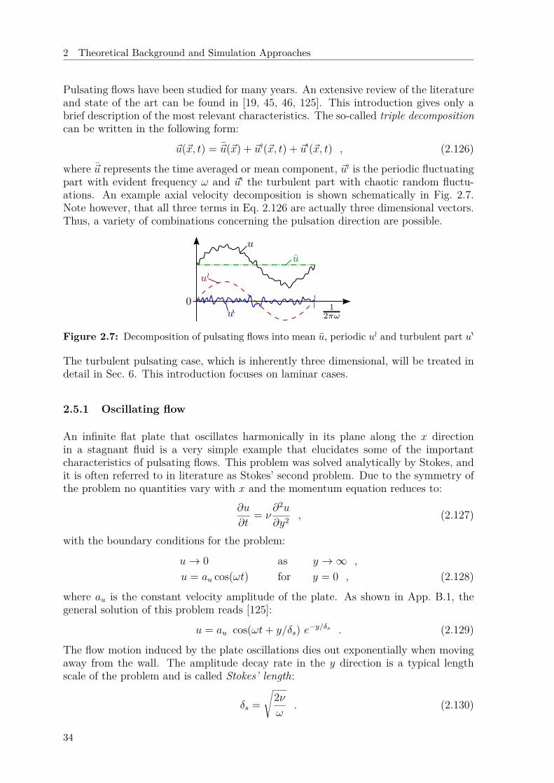
2 Theoretical Background and Simulation Approaches
Pulsating flows have been studied for many years. An extensive review of the literatureand state of the art can be found in [19, 45, 46, 125]. This introduction gives only abrief description of the most relevant characteristics. The so-called triple decompositioncan be written in the following form:
~u(~x, t) = ~u(~x) + ~uo(~x, t) + ~u8(~x, t) , (2.126)
where ~u represents the time averaged or mean component, ~uo is the periodic fluctuatingpart with evident frequency ω and ~u8 the turbulent part with chaotic random fluctu-ations. An example axial velocity decomposition is shown schematically in Fig. 2.7.Note however, that all three terms in Eq. 2.126 are actually three dimensional vectors.Thus, a variety of combinations concerning the pulsation direction are possible.
Figure 2.7: Decomposition of pulsating flows into mean u, periodic uo and turbulent part u8
The turbulent pulsating case, which is inherently three dimensional, will be treated indetail in Sec. 6. This introduction focuses on laminar cases.
2.5.1 Oscillating flow
An infinite flat plate that oscillates harmonically in its plane along the x directionin a stagnant fluid is a very simple example that elucidates some of the importantcharacteristics of pulsating flows. This problem was solved analytically by Stokes, andit is often referred to in literature as Stokes’ second problem. Due to the symmetry ofthe problem no quantities vary with x and the momentum equation reduces to:
∂u
∂t= ν
∂2u
∂y2 , (2.127)
with the boundary conditions for the problem:
u→ 0 as y →∞ ,u = au cos(ωt) for y = 0 , (2.128)
where au is the constant velocity amplitude of the plate. As shown in App. B.1, thegeneral solution of this problem reads [125]:
u = au cos(ωt+ y/δs) e−y/δs . (2.129)
The flow motion induced by the plate oscillations dies out exponentially when movingaway from the wall. The amplitude decay rate in the y direction is a typical lengthscale of the problem and is called Stokes’ length:
δs =√
2νω
. (2.130)
34
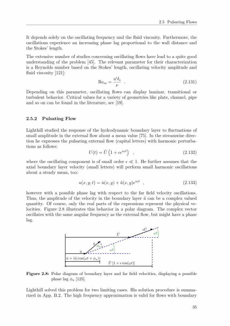
2.5 Pulsating Flows
It depends solely on the oscillating frequency and the fluid viscosity. Furthermore, theoscillations experience an increasing phase lag proportional to the wall distance andthe Stokes’ length.
The extensive number of studies concerning oscillating flows have lead to a quite goodunderstanding of the problem [45]. The relevant parameter for their characterizationis a Reynolds number based on the Stokes’ length, oscillating velocity amplitude andfluid viscosity [121]:
Reos = uoδsν
. (2.131)
Depending on this parameter, oscillating flows can display laminar, transitional orturbulent behavior. Critical values for a variety of geometries like plate, channel, pipeand so on can be found in the literature, see [19].
2.5.2 Pulsating Flow
Lighthill studied the response of the hydrodynamic boundary layer to fluctuations ofsmall amplitude in the external flow about a mean value [75]. In the streamwise direc-tion he expresses the pulsating external flow (capital letters) with harmonic perturba-tions as follows:
U(t) = U(1 + εeiωt
), (2.132)
where the oscillating component is of small order ε 1. He further assumes that theaxial boundary layer velocity (small letters) will perform small harmonic oscillationsabout a steady mean, too:
u(x, y, t) = u(x, y) + u(x, y)eiωt , (2.133)
however with a possible phase lag with respect to the far field velocity oscillations.Thus, the amplitude of the velocity in the boundary layer u can be a complex valuedquantity. Of course, only the real parts of the expressions represent the physical ve-locities. Figure 2.8 illustrates this behavior in a polar diagram. The complex vectoroscillates with the same angular frequency as the external flow, but might have a phaselag.
Figure 2.8: Polar diagram of boundary layer and far field velocities, displaying a possiblephase lag φu [125].
Lighthill solved this problem for two limiting cases. His solution procedure is summa-rized in App. B.2. The high frequency approximation is valid for flows with boundary
35
2 Theoretical Background and Simulation Approaches
layer thickness much larger than the Stokes’ length, δ δs. In this case, the generalsolution for the oscillating velocity component in the boundary layer reads:
u = εU[1− e−y/δse−iy/δs
]. (2.134)
The stationary component u can be determined from a Karman-Pohlhausen treatment[44], see App. B.2. From Eq. (2.134), the wall normal dependency of the phase lag φucan be expressed as:
tan(φu) = sin(y)eδ2s/δs − cos(y) . (2.135)
At distances far away from the wall, y → ∞, the phase lag vanishes φu → 0 and thevelocity amplitude tends to the far field value u → U . Towards the wall, y → 0, thephase lag tends to the limit φu → π/4 and the velocity amplitude vanishes u → 0.This means that the velocity fluctuations in the boundary layer advance always thefluctuations of the external flow. This is a very important feature of pulsating flows.Due to the viscous forces in the boundary layer, the magnitude of the velocity is smaller.Thus, the inertia of the fluid in this region is lower and it can respond faster to externalperturbations.
The small frequency approximation given by Lighthill is valid for flows with bound-ary layer thickness much smaller than the Stokes’ length δ δs. The details of hisderivation and the solution for this case are given in App. B.2.
36
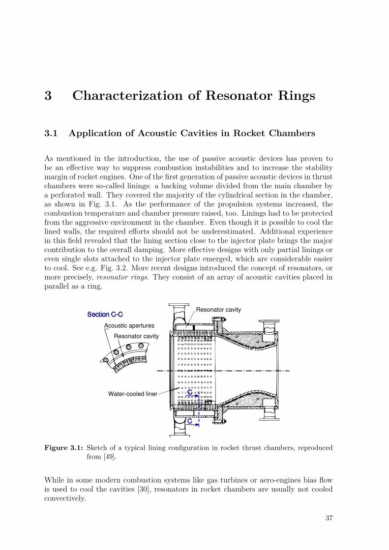
3 Characterization of Resonator Rings
3.1 Application of Acoustic Cavities in Rocket Chambers
As mentioned in the introduction, the use of passive acoustic devices has proven tobe an effective way to suppress combustion instabilities and to increase the stabilitymargin of rocket engines. One of the first generation of passive acoustic devices in thrustchambers were so-called linings: a backing volume divided from the main chamber bya perforated wall. They covered the majority of the cylindrical section in the chamber,as shown in Fig. 3.1. As the performance of the propulsion systems increased, thecombustion temperature and chamber pressure raised, too. Linings had to be protectedfrom the aggressive environment in the chamber. Even though it is possible to cool thelined walls, the required efforts should not be underestimated. Additional experiencein this field revealed that the lining section close to the injector plate brings the majorcontribution to the overall damping. More effective designs with only partial linings oreven single slots attached to the injector plate emerged, which are considerable easierto cool. See e.g. Fig. 3.2. More recent designs introduced the concept of resonators, ormore precisely, resonator rings. They consist of an array of acoustic cavities placed inparallel as a ring.
Figure 3.1: Sketch of a typical lining configuration in rocket thrust chambers, reproducedfrom [49].
While in some modern combustion systems like gas turbines or aero-engines bias flowis used to cool the cavities [30], resonators in rocket chambers are usually not cooledconvectively.
37
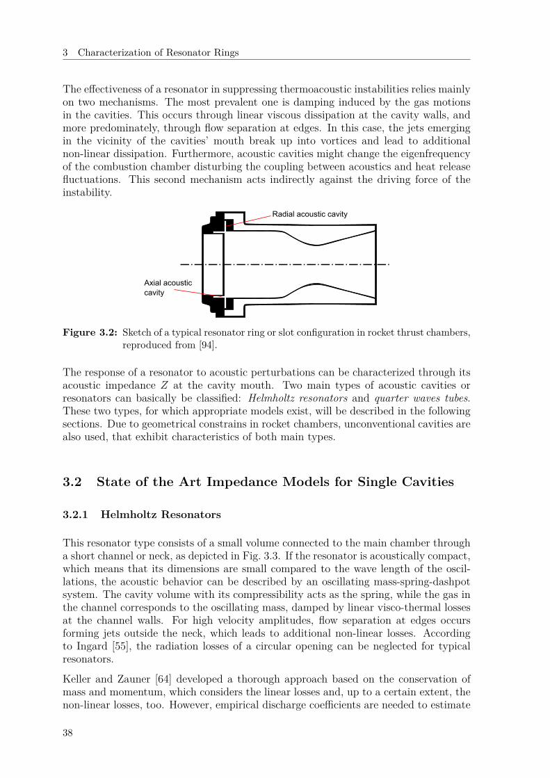
3 Characterization of Resonator Rings
The effectiveness of a resonator in suppressing thermoacoustic instabilities relies mainlyon two mechanisms. The most prevalent one is damping induced by the gas motionsin the cavities. This occurs through linear viscous dissipation at the cavity walls, andmore predominately, through flow separation at edges. In this case, the jets emergingin the vicinity of the cavities’ mouth break up into vortices and lead to additionalnon-linear dissipation. Furthermore, acoustic cavities might change the eigenfrequencyof the combustion chamber disturbing the coupling between acoustics and heat releasefluctuations. This second mechanism acts indirectly against the driving force of theinstability.
Axial acoustic cavity
Radial acoustic cavity
Figure 3.2: Sketch of a typical resonator ring or slot configuration in rocket thrust chambers,reproduced from [94].
The response of a resonator to acoustic perturbations can be characterized through itsacoustic impedance Z at the cavity mouth. Two main types of acoustic cavities orresonators can basically be classified: Helmholtz resonators and quarter waves tubes.These two types, for which appropriate models exist, will be described in the followingsections. Due to geometrical constrains in rocket chambers, unconventional cavities arealso used, that exhibit characteristics of both main types.
3.2 State of the Art Impedance Models for Single Cavities
3.2.1 Helmholtz Resonators
This resonator type consists of a small volume connected to the main chamber througha short channel or neck, as depicted in Fig. 3.3. If the resonator is acoustically compact,which means that its dimensions are small compared to the wave length of the oscil-lations, the acoustic behavior can be described by an oscillating mass-spring-dashpotsystem. The cavity volume with its compressibility acts as the spring, while the gas inthe channel corresponds to the oscillating mass, damped by linear visco-thermal lossesat the channel walls. For high velocity amplitudes, flow separation at edges occursforming jets outside the neck, which leads to additional non-linear losses. Accordingto Ingard [55], the radiation losses of a circular opening can be neglected for typicalresonators.
Keller and Zauner [64] developed a thorough approach based on the conservation ofmass and momentum, which considers the linear losses and, up to a certain extent, thenon-linear losses, too. However, empirical discharge coefficients are needed to estimate
38

3.2 State of the Art Impedance Models for Single Cavities
Figure 3.3: Sketch of a resonator cavity ofthe Helmholtz type.
Figure 3.4: Analogy of Helmholtz res-onator as mass-spring-dashpotsystem.
these non-linear losses. They derived the following equation of motion for the gas insidethe neck assuming compactness:
(1 + s)leρnd2u′
dt2−[sρn(l + lf )ω + ζρn|u′|
] du′dt
+ Anρv c2v
Vu′ = dp′
dt, (3.1)
where u′ represents the axial acoustic velocity in the neck, p′ the acoustic pressure actingon the left side of the neck, An = πd2/4 denotes the neck transverse area, and the indicesn and v stand for average values at the neck and backing volume locations, respectively(see Fig. 3.3). A so-called boundary layer parameter s accounts for the thermal andviscous dissipation. For cylindrical ducts and small Stokes’ numbers d/δs 1, it canbe given by the following expression [64, 117]:
s = 1d
(1 + γ − 1√
Pr
)δs . (3.2)
Equation (3.1) corresponds to the time derivative of a mass-spring-dashpot differentialequation, as sketched in Fig. 3.4. The first term on the left-hand side corresponds tothe inertia of the gaseous mass in the neck with some correction due to boundary layereffects. An effective length le accounting the mass of gas surrounding the neck thattakes part in the oscillation is also applied:
le = l + δli + δlo . (3.3)
For the outside correction δlo on the chamber side the well known model of a pistonradiating into half space can be used [88]:
δlo ≈4
3πd . (3.4)
Ingard [55] proposed to model the inside correction δli on the backing volume side asa piston radiating into a volume of equivalent diameter De ≈ 3
√V :
δli = 43πd
(1− 1.24 d
De
)for d
De
< 0.4 . (3.5)
For high aspect ratios d/De 1, Eq. (3.5) converges to Eq. (3.4) and the effectivelength can be approximated as
le ≈ l + 2δo . (3.6)
39
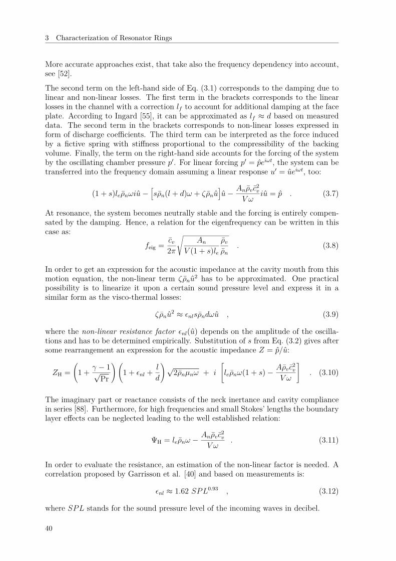
3 Characterization of Resonator Rings
More accurate approaches exist, that take also the frequency dependency into account,see [52].
The second term on the left-hand side of Eq. (3.1) corresponds to the damping due tolinear and non-linear losses. The first term in the brackets corresponds to the linearlosses in the channel with a correction lf to account for additional damping at the faceplate. According to Ingard [55], it can be approximated as lf ≈ d based on measureddata. The second term in the brackets corresponds to non-linear losses expressed inform of discharge coefficients. The third term can be interpreted as the force inducedby a fictive spring with stiffness proportional to the compressibility of the backingvolume. Finally, the term on the right-hand side accounts for the forcing of the systemby the oscillating chamber pressure p′. For linear forcing p′ = peiωt, the system can betransferred into the frequency domain assuming a linear response u′ = ueiωt, too:
(1 + s)leρnωiu−[sρn(l + d)ω + ζρnu
]u− Anρv c
2v
V ωiu = p . (3.7)
At resonance, the system becomes neutrally stable and the forcing is entirely compen-sated by the damping. Hence, a relation for the eigenfrequency can be written in thiscase as:
feig = cv2π
√An
V (1 + s)leρvρn
. (3.8)
In order to get an expression for the acoustic impedance at the cavity mouth from thismotion equation, the non-linear term ζρnu
2 has to be approximated. One practicalpossibility is to linearize it upon a certain sound pressure level and express it in asimilar form as the visco-thermal losses:
ζρnu2 ≈ εnlsρndωu , (3.9)
where the non-linear resistance factor εnl(u) depends on the amplitude of the oscilla-tions and has to be determined empirically. Substitution of s from Eq. (3.2) gives aftersome rearrangement an expression for the acoustic impedance Z = p/u:
ZH =(
1 + γ − 1√Pr
)(1 + εnl + l
d
)√
2ρnµnω + i
[leρnω(1 + s)− Aρv c
2v
V ω
]. (3.10)
The imaginary part or reactance consists of the neck inertance and cavity compliancein series [88]. Furthermore, for high frequencies and small Stokes’ lengths the boundarylayer effects can be neglected leading to the well established relation:
ΨH = leρnω −Anρv c
2v
V ω. (3.11)
In order to evaluate the resistance, an estimation of the non-linear factor is needed. Acorrelation proposed by Garrisson et al. [40] and based on measurements is:
εnl ≈ 1.62 SPL0.93 , (3.12)
where SPL stands for the sound pressure level of the incoming waves in decibel.
40
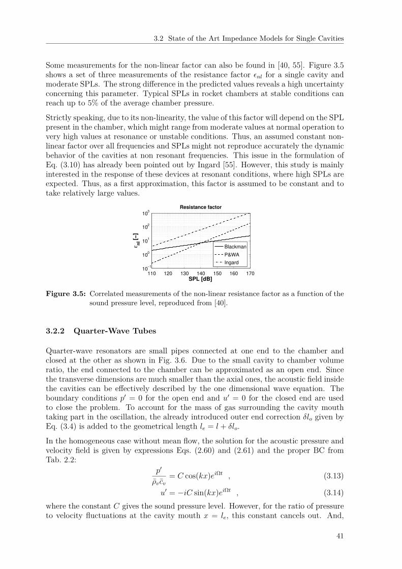
3.2 State of the Art Impedance Models for Single Cavities
Some measurements for the non-linear factor can also be found in [40, 55]. Figure 3.5shows a set of three measurements of the resistance factor εnl for a single cavity andmoderate SPLs. The strong difference in the predicted values reveals a high uncertaintyconcerning this parameter. Typical SPLs in rocket chambers at stable conditions canreach up to 5% of the average chamber pressure.
Strictly speaking, due to its non-linearity, the value of this factor will depend on the SPLpresent in the chamber, which might range from moderate values at normal operation tovery high values at resonance or unstable conditions. Thus, an assumed constant non-linear factor over all frequencies and SPLs might not reproduce accurately the dynamicbehavior of the cavities at non resonant frequencies. This issue in the formulation ofEq. (3.10) has already been pointed out by Ingard [55]. However, this study is mainlyinterested in the response of these devices at resonant conditions, where high SPLs areexpected. Thus, as a first approximation, this factor is assumed to be constant and totake relatively large values.
110 120 130 140 150 160 17010
−1
100
101
102
103
SPL [dB]
εn
l [−
]
Resistance factor
Blackman
P&WA
Ingard
Figure 3.5: Correlated measurements of the non-linear resistance factor as a function of thesound pressure level, reproduced from [40].
3.2.2 Quarter-Wave Tubes
Quarter-wave resonators are small pipes connected at one end to the chamber andclosed at the other as shown in Fig. 3.6. Due to the small cavity to chamber volumeratio, the end connected to the chamber can be approximated as an open end. Sincethe transverse dimensions are much smaller than the axial ones, the acoustic field insidethe cavities can be effectively described by the one dimensional wave equation. Theboundary conditions p′ = 0 for the open end and u′ = 0 for the closed end are usedto close the problem. To account for the mass of gas surrounding the cavity mouthtaking part in the oscillation, the already introduced outer end correction δlo given byEq. (3.4) is added to the geometrical length le = l + δlo.
In the homogeneous case without mean flow, the solution for the acoustic pressure andvelocity field is given by expressions Eqs. (2.60) and (2.61) and the proper BC fromTab. 2.2:
p′
ρv cv= C cos(kx)eiΩt , (3.13)
u′ = −iC sin(kx)eiΩt , (3.14)where the constant C gives the sound pressure level. However, for the ratio of pressureto velocity fluctuations at the cavity mouth x = le, this constant cancels out. And,
41
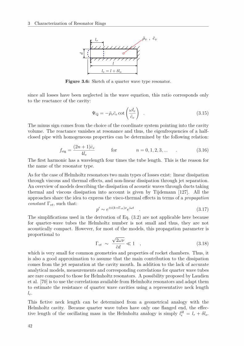
3 Characterization of Resonator Rings
Figure 3.6: Sketch of a quarter wave type resonator.
since all losses have been neglected in the wave equation, this ratio corresponds onlyto the reactance of the cavity:
ΨQ = −ρv cv cot(ωlecv
). (3.15)
The minus sign comes from the choice of the coordinate system pointing into the cavityvolume. The reactance vanishes at resonance and thus, the eigenfrequencies of a half-closed pipe with homogeneous properties can be determined by the following relation:
feig = (2n+ 1)cv4le
for n = 0, 1, 2, 3, ... . (3.16)
The first harmonic has a wavelength four times the tube length. This is the reason forthe name of the resonator type.
As for the case of Helmholtz resonators two main types of losses exist: linear dissipationthrough viscous and thermal effects, and non-linear dissipation through jet separation.An overview of models describing the dissipation of acoustic waves through ducts takingthermal and viscous dissipation into account is given by Tijdemann [127]. All theapproaches share the idea to express the visco-thermal effects in terms of a propagationconstant Γvt, such that:
p′ ∼ e±i(k+Γvt)xeiωt . (3.17)The simplifications used in the derivation of Eq. (3.2) are not applicable here becausefor quarter-wave tubes the Helmholtz number is not small and thus, they are notacoustically compact. However, for most of the models, this propagation parameter isproportional to
Γvt ∼√
2ωνcd
1 , (3.18)
which is very small for common geometries and properties of rocket chambers. Thus, itis also a good approximation to assume that the main contribution to the dissipationcomes from the jet separation at the cavity mouth. In addition to the lack of accurateanalytical models, measurements and corresponding correlations for quarter wave tubesare rare compared to those for Helmholtz resonators. A possibility proposed by Laudienet al. [70] is to use the correlations available from Helmholtz resonators and adapt themto estimate the resistance of quarter wave cavities using a representative neck lengthlr.
This fictive neck length can be determined from a geometrical analogy with theHelmholtz cavity. Because quarter wave tubes have only one flanged end, the effec-tive length of the oscillating mass in the Helmholtz analogy is simply lHe = lr + δlo.
42
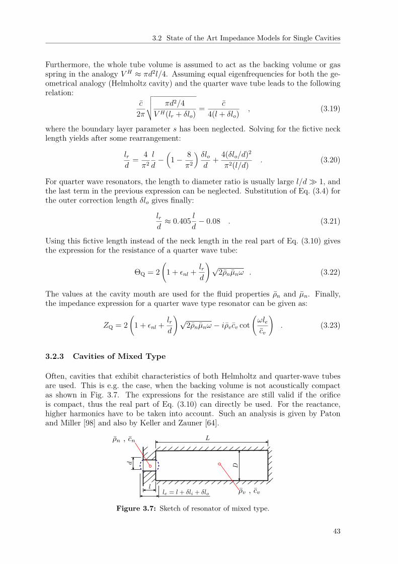
3.2 State of the Art Impedance Models for Single Cavities
Furthermore, the whole tube volume is assumed to act as the backing volume or gasspring in the analogy V H ≈ πd2l/4. Assuming equal eigenfrequencies for both the ge-ometrical analogy (Helmholtz cavity) and the quarter wave tube leads to the followingrelation:
c
2π
√√√√ πd2/4V H(lr + δlo)
= c
4(l + δlo), (3.19)
where the boundary layer parameter s has been neglected. Solving for the fictive necklength yields after some rearrangement:
lrd
= 4π2
l
d−(
1− 8π2
)δlod
+ 4(δlo/d)2
π2(l/d) . (3.20)
For quarter wave resonators, the length to diameter ratio is usually large l/d 1, andthe last term in the previous expression can be neglected. Substitution of Eq. (3.4) forthe outer correction length δlo gives finally:
lrd≈ 0.405 l
d− 0.08 . (3.21)
Using this fictive length instead of the neck length in the real part of Eq. (3.10) givesthe expression for the resistance of a quarter wave tube:
ΘQ = 2(
1 + εnl + lrd
)√
2ρnµnω . (3.22)
The values at the cavity mouth are used for the fluid properties ρn and µn. Finally,the impedance expression for a quarter wave type resonator can be given as:
ZQ = 2(
1 + εnl + lrd
)√
2ρnµnω − iρv cv cot(ωlecv
). (3.23)
3.2.3 Cavities of Mixed Type
Often, cavities that exhibit characteristics of both Helmholtz and quarter-wave tubesare used. This is e.g. the case, when the backing volume is not acoustically compactas shown in Fig. 3.7. The expressions for the resistance are still valid if the orificeis compact, thus the real part of Eq. (3.10) can directly be used. For the reactance,higher harmonics have to be taken into account. Such an analysis is given by Patonand Miller [98] and also by Keller and Zauner [64].
Figure 3.7: Sketch of resonator of mixed type.
43
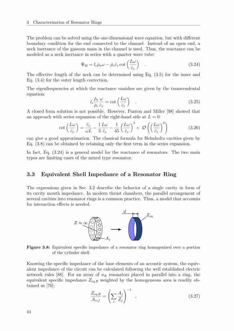
3 Characterization of Resonator Rings
The problem can be solved using the one-dimensional wave equation, but with differentboundary condition for the end connected to the channel. Instead of an open end, aneck inertance of the gaseous mass in the channel is used. Thus, the reactance can bemodeled as a neck inertance in series with a quarter wave tube:
ΨM = leρnω − ρv cv cot(Lω
cv
). (3.24)
The effective length of the neck can be determined using Eq. (3.5) for the inner andEq. (3.4) for the outer length correction.
The eigenfrequencies at which the reactance vanishes are given by the transcendentalequation:
leρnρv
ω
cv= cot
(Lω
cv
). (3.25)
A closed form solution is not possible. However, Panton and Miller [98] showed thatan approach with series expansion of the right-hand side at L = 0:
cot(Lω
cv
)= cvωL− 1
3Lω
cv− 1
45
(Lω
cv
)3+ O
((Lω
cv
)5)(3.26)
can give a good approximation. The classical formula for Helmholtz cavities given byEq. (3.8) can be obtained by retaining only the first term in the series expansion.
In fact, Eq. (3.24) is a general model for the reactance of resonators. The two maintypes are limiting cases of the mixed type resonator.
3.3 Equivalent Shell Impedance of a Resonator Ring
The expressions given in Sec. 3.2 describe the behavior of a single cavity in form ofits cavity mouth impedance. In modern thrust chambers, the parallel arrangement ofseveral cavities into resonator rings is a common practice. Thus, a model that accountsfor interaction effects is needed.
Figure 3.8: Equivalent specific impedance of a resonator ring homogenized over a portionof the cylinder shell.
Knowing the specific impedance of the base elements of an acoustic system, the equiv-alent impedance of the circuit can be calculated following the well established electricnetwork rules [88]. For an array of nR resonators placed in parallel into a ring, theequivalent specific impedance Zeq,R weighted by the homogeneous area is readily ob-tained as [70]:
Zeq,RAref
=∑
j
AjZj
−1
, (3.27)
44
3.4 Absorption Coefficient as an Evaluation Parameter
where the equivalent impedance is weighted by the total area Aref = ∑Aj = 2πRcd and
the individual local impedances Zj by their local reaction area Aj. The portion of theshell with hard boundaries has an infinite impedance, because the wall-normal velocityfluctuations have to be zero there. Thus, their effect is taken inherently into accountby the weighting area since Aref = ∑
Aj in Eq. (3.27). This procedure correspondsto averaging the impedance over the cylinder shell area as illustrated in Fig. 3.8. Inrocket chambers, resonator rings with cavities of different size are sometimes employedto provide damping over a broader range of frequencies. In principle, a ring with aset of cavities of different type or geometry can be modeled through this approach,too. However, the different sets of cavities should have a minimum number of cavitiesand be homogeneously distributed in the azimuthal direction to assure symmetry andjustify the homogenization.
In this study, the resonator ring has identical cavities of reaction area An = πd2/4 andacoustic impedance ZR. Equation (3.27) can be then simplified to:
Zeq,R = 8Rc
nRdZR . (3.28)
This model is denoted, from now on, as soft-wall shell. Here the cavities are placedperpendicularly to the chamber wall where a three dimensional acoustic field is present.The impedance expression for the cavity mouth takes only the surface normal velocitycomponent into account. In this case, this corresponds to the radial component of thevelocity fluctuations:
Z = p′
~n · ~u′= p
v. (3.29)
3.4 Absorption Coefficient as an Evaluation Parameter
In general terms, the efficiency of a resonator can be evaluated by its absorption coef-ficient α. It is defined as the ratio of the power absorbed by a surface to the power ofthe incident traveling acoustic waves. The absorbed power per unit area is the productof acoustic velocity at the surface times the force needed for this motion. In acoustics,this force is in general the component of the pressure fluctuation p′ in phase with thevelocity fluctuation at the cavity mouth. However, the acoustic pressure and velocityfluctuations depend on the reflection factor r of the corresponding surface. Assumingnegligible chamber flow effects (no mean flow and bias flow), the reflection factor canbe expressed via Eq. (2.65) as a function of the surface impedance. For incident planewaves normal to the boundary, the absorption coefficient can be written after somerearrangement as [87]:
α = 1− |r|2 = 4θ(θ + 1)2 + ψ2 , (3.30)
where |r| stands for the modulus of the reflection factor. Figure 3.9 shows this depen-dency for a series of parameters.
By definition, the optimum value of the absorption coefficient is unity, which meansthat 100% of the incident wave energy is absorbed. At resonance, the reactance of the
45
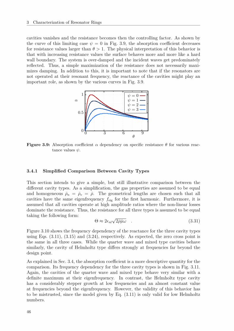
3 Characterization of Resonator Rings
cavities vanishes and the resistance becomes then the controlling factor. As shown bythe curve of this limiting case ψ = 0 in Fig. 3.9, the absorption coefficient decreasesfor resistance values larger than θ > 1. The physical interpretation of this behavior isthat with increasing resistance values the surface behaves more and more like a hardwall boundary. The system is over-damped and the incident waves get predominatelyreflected. Thus, a simple maximization of the resistance does not necessarily maxi-mizes damping. In addition to this, it is important to note that if the resonators arenot operated at their resonant frequency, the reactance of the cavities might play animportant role, as shown by the various curves in Fig. 3.9.
0
0.5
1
0 3 6 9
α
θ
ψ = 0ψ = 1ψ = 2ψ = 3
Figure 3.9: Absorption coefficient α dependency on specific resistance θ for various reac-tance values ψ.
3.4.1 Simplified Comparison Between Cavity Types
This section intends to give a simple, but still illustrative comparison between thedifferent cavity types. As a simplification, the gas properties are assumed to be equaland homogeneous ρn = ρv = ρ. The geometrical lengths are chosen such that allcavities have the same eigenfrequency feig for the first harmonic. Furthermore, it isassumed that all cavities operate at high amplitude ratios where the non-linear lossesdominate the resistance. Thus, the resistance for all three types is assumed to be equaltaking the following form:
Θ ≈ 2εnl√
2ρµω . (3.31)
Figure 3.10 shows the frequency dependency of the reactance for the three cavity typesusing Eqs. (3.11), (3.15) and (3.24), respectively. As expected, the zero cross point isthe same in all three cases. While the quarter wave and mixed type cavities behavesimilarly, the cavity of Helmholtz type differs strongly at frequencies far beyond thedesign point.
As explained in Sec. 3.4, the absorption coefficient is a more descriptive quantity for thecomparison. Its frequency dependency for the three cavity types is shown in Fig. 3.11.Again, the cavities of the quarter wave and mixed type behave very similar with adefinite maximum at their eigenfrequency. In contrast, the Helmholtz type cavityhas a considerably stepper growth at low frequencies and an almost constant valueat frequencies beyond the eigenfrequency. However, the validity of this behavior hasto be mistrusted, since the model given by Eq. (3.11) is only valid for low Helmholtznumbers.
46
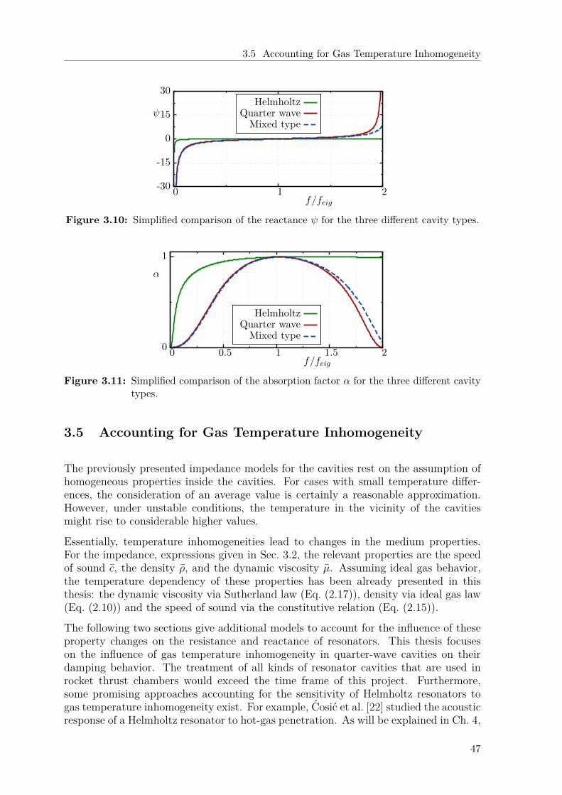
3.5 Accounting for Gas Temperature Inhomogeneity
-30
-15
0
15
30
0 1 2
ψ
f/feig
HelmholtzQuarter wave
Mixed type
Figure 3.10: Simplified comparison of the reactance ψ for the three different cavity types.
0
1
0 0.5 1 1.5 2
α
f/feig
HelmholtzQuarter wave
Mixed type
Figure 3.11: Simplified comparison of the absorption factor α for the three different cavitytypes.
3.5 Accounting for Gas Temperature Inhomogeneity
The previously presented impedance models for the cavities rest on the assumption ofhomogeneous properties inside the cavities. For cases with small temperature differ-ences, the consideration of an average value is certainly a reasonable approximation.However, under unstable conditions, the temperature in the vicinity of the cavitiesmight rise to considerable higher values.
Essentially, temperature inhomogeneities lead to changes in the medium properties.For the impedance, expressions given in Sec. 3.2, the relevant properties are the speedof sound c, the density ρ, and the dynamic viscosity µ. Assuming ideal gas behavior,the temperature dependency of these properties has been already presented in thisthesis: the dynamic viscosity via Sutherland law (Eq. (2.17)), density via ideal gas law(Eq. (2.10)) and the speed of sound via the constitutive relation (Eq. (2.15)).
The following two sections give additional models to account for the influence of theseproperty changes on the resistance and reactance of resonators. This thesis focuseson the influence of gas temperature inhomogeneity in quarter-wave cavities on theirdamping behavior. The treatment of all kinds of resonator cavities that are used inrocket thrust chambers would exceed the time frame of this project. Furthermore,some promising approaches accounting for the sensitivity of Helmholtz resonators togas temperature inhomogeneity exist. For example, Cosic et al. [22] studied the acousticresponse of a Helmholtz resonator to hot-gas penetration. As will be explained in Ch. 4,
47
3 Characterization of Resonator Rings
the inclusion of additional cavity impedance models in the methodology presented inthis thesis is straightforward.
3.5.1 Resistance
The major contribution to the resistance comes from a small portion of the cavity closeto the mouth. Thus, a cavity mouth temperature Tm can be used to estimate the gasproperties in this region. Using Eqs. (2.17) to (2.15), the expression for the cavityresistance given by Eq. (3.22) can be evaluated for various temperature ratios.
The non-linear factor εnl inherits again a high degree of uncertainty. Physically, itis comprehensible to expect also a temperature dependency of it, simply because theReynolds and Strouhal numbers change with temperature, leading to perhaps com-pletely different flow regimes. The jet separation responsible for the non-linear dissi-pation will thus be influenced by the rise in temperature. However, due to the lack ofan accurate analytical model, a constant non-linear factor is assumed in this work.
3.5.2 Reactance
The response of the reactance to temperature inhomogeneities demands a more de-tailed analysis. In contrast to the resistance, the reactance of a backing cavity is notnecessarily acoustically compact.
In this thesis, a quarter-wave resonator impedance is derived from a general ap-proach presented by Kumar & Sujith [68]. They give closed form expressions for one-dimensional sound propagation in ducts with axial temperature profiles of polynomialform:
T (x) =∫ 2π
0
∫ d/2
0T (x, r, ϕ) dr dϕ ≡ (apx+ bp)np , (3.32)
where at each axial location the transverse averaged value is used. The one dimensionalwave equation (Eq. (2.32)) for a quiescent fluid with an axial temperature gradient, butnegligible thermal and viscous dissipation, is the starting point of their derivation. Fora perfect gas and using c2 = γRsT , the wave equation can be written as:
∂2p′
∂x2 + 1T
dT
dx
∂p′
∂x− 1γRsT
∂2p′
∂t2= 0 . (3.33)
In the linear case, a solution of the form p′ = peiωt can be assumed. Substitution givesa Helmholtz equation
d2p
dx2 + 1T
dT
dx
dp
dx+ ω2
γRsTp = 0 , (3.34)
which Kumar and Sujith were able to solve using a special transformation, see [68].They determined the following solution for the pressure field
p = Tαp[c1Jνp(βpT
σp) + c2J−νp(βpTσp)]
, (3.35)
where
αp = 12
(1np− 1
), βp = ω
anp√γRsσp
, σp =(
1np− 1
2
), νp = 1− np
2− np, (3.36)
48
3.5 Accounting for Gas Temperature Inhomogeneity
and Jνp are Bessel functions of order νp. The solution presented here is only valid fornon integer valued νp and np 6= 2. For integer valued νp Neumann functions have tobe taken additionally into account, see [68]. Using the linearized momentum equation,the acoustic velocity can be expressed as:
u = −apnpTαp−1/np
iωρ
αpc1Jνp (βpTσp) + c2J−νp (βpT
σp) +
βpσTσp
2[c1Jνp−1(βpT
σp)− Jνp+1(βpTσp)+ c2J−νp−1(βpT
σp)− J−νp+1(βpTσp)
] .(3.37)
The constants c1 and c2 can be determined from the boundary conditions at the leftand right duct ends. Using the general solution, the primitive variables on the left,(index “l”), and on the right side of the duct, (index “r”), can be expressed in matrixform as: p
ρc
u
l
=A11 A12
A21 A22
c1
c2
,
pρc
u
r
=B11 B12
B21 B22
c1
c2
, (3.38)
where the pressure has been weighted by ρc for dimensional consistency and the matrixcoefficients Aij and Bij are functions of f(αp, σp, βp, νp, np). By substituting the vectorof constants in the previous expressions, the acoustic quantities on the right-hand sideare related to the ones on the left-hand side by:p/(ρc)
u
r
=B11 B12
B21 B22
A11 A12
A21 A22
−1p/(ρc)u
l
. (3.39)
As an analogy to Eq. (2.73), the matrix T = BA−1 is sometimes regarded as a transfermatrix, too. The linear system can be rearranged into:pl/(ρc)
ur
= S
pr/(ρc)ul
. (3.40)
For quarter wave cavities the boundaries can be assumed as ideal, with pr = 0 at theleft opened end and ul = 0 at the right closed end. In this case, the system given byEq. (3.40) becomes homogeneous:
S
pr/(ρc)ul
= ~0 . (3.41)
To allow also non-trivial solutions, the determinant of such systems has to be zero.This condition detS = 0 is given in closed form as:
Jνp(βpTσp2 )
[αpJ−νp(βpT
σp1 ) + σpβpT
σp1
2 J−νp−1(βpTσp1 )− J−νp+1(βpT
σp1 )
]
− J−νp(βpTσp2 )
[αpJνp(βpT
σp1 ) + σpβpT
σp1
2 Jνp−1(βpTσp1 )− Jνp+1(βpT
σp1 )
]= 0 .(3.42)
For given temperature profile and fluid properties, the determinant is only a functionof the frequency ω (via the parameter βp). The roots of this transcendental equation
49
3 Characterization of Resonator Rings
can be determined numerically and correspond to the eigenfrequencies of the cavitydetS(ωeig) = 0.
The acoustic impedance at the cavity mouth is used for the characterization of thecavities with polynomial temperature inhomogeneity. Applying the matrix notationgiven in Eq. (3.39), the ratio between pressure and velocity perturbations can be writtenas:
1ρc
prur
= T11pl + T12ulT21pl + T22ul
. (3.43)
This ratio corresponds to the reactance of the cavity. It is purely complex-valued,because the underlying wave equation does not account for any dissipation effects.Because the velocity fluctuation has to be zero at the closed left end, the expressionfor the reactance at the resonator mouth is given as:
ΨQ∗ = ρcT11
T21=
−[(iρω((αp + νpσp)J−νp(βpT
σp1 )Jνp(βpT
σp2 ) + βpσpJ−1−νp(βpT
σp1 )Jνp(βpT
σp2 )T σp
1
−J−νp(βpTσp2 )
((αp − νpσp)Jνp(βpT
σp1 ) + βpσpJ−1+νp(βpT
σp1 )T σp
1
))T 1/np
2
]/[apnp
( ((αp − νpσp) Jνp(βpT
σp1 ) + βpσpJ−1+νp(βpT
σp1 )T σp
1
)((αp + νpσp)J−νp(βpT
σp2 ) + βpσpJ−1−νp(βpT
σp2 )T σp
2
)−
((αp + νpσp)J−νp(βpT
σp1 ) + βpσpJ−1−νp(βpT
σp1 )T σp
1 ))
((αp − νpσp) Jνp(βpT
σp2 ) + βpσpJ−1+νp(βpT
σp2 )T σp
2 )) )]
. (3.44)
For given temperature profile and fluid properties, it is again only a function of fre-quency ω.
3.6 Decoupled Analysis
In a general sense, the behavior of a given system depends on its own system dynamicssubjected to certain boundary conditions. However, from a practical point of view,a study restricted to the boundary conditions can also provide valuable preliminaryconclusions. Thus, as a starting point, the stabilizing influence of resonators mightbe assessed by a decoupled analysis that considers only the impedance expressions bywhich they are described. In the same way, the sensitivity of the cavities to changes intheir local environment can be estimated as a first approximation, too. Note that this isa preliminary study that should serve as a reference. In the next Ch. 4, the stabilizinginfluence of the cavities attached to a rocket thrust chamber will be studied. It will beshown that a fully coupled analysis provides a much more accurate description of thedamping behavior of resonators.
50
3.6 Decoupled Analysis
3.6.1 Preliminary Estimation of Sensitivity to Temperature Inhomogeneity
As stated by Acker and Mitchell [4], the gas filling the resonator cavities can locallyexhibit strong temperature differences because the cavities are placed on cooled cham-ber walls. From the few documented cases in the literature, a sudden rise in the wallsurface temperature of the chamber can be expected upon the occurrence of combus-tion instability. This will in turn lead to an increase in the cavity mouth temperatureincreasing the temperature inhomogeneity ratio in the cavities. Indeed, such strongtemperature spatial variations have been measured by Oberg [93] during full-scale testprograms.
Homogeneous
PolynomialEHT
Chamber Resonator
Figure 3.12: Temperature levels present in the rocket thrust chamber
Without going into the detailed mechanisms leading to this rise in temperature or heatload, this first approximated analysis simply assumes a higher neck temperature. Thesituation is sketched in Fig. 3.12, where the radial temperature dependency in thechamber and cavities is given at the axial location where the resonator ring is placed.The chamber radius is denoted by Rc. The temperature range is bounded by thecooling temperature Tcool and the combustion temperature Tcomb, which are assumedto be constant even in the case of an instability. At the radial position r = Rc− δlo thecavity neck temperature Tn is measured. Due to the mean flow in the chamber section,the thermal boundary layer on this side is small and a steep temperature gradientis expected. On the cavity side, no mean flow is present and the cavity temperaturedecreases smoother towards the cooling temperature. If enhanced heat transfer appearsdue to an instability, the neck temperature Tn will rise, leading also to a change in thecavity temperature distribution. For simplicity, a second reference coordinate systemx, r and ϕ is defined with origin at the cavity’s closed end. As a first approximation, thegas temperature in the cavity Tr is assumed to be homogeneous in the transverse planebut to vary along the cavity axial direction. This cavity temperature distribution canbe given by Eq. (3.32) in form of a polynomial function. Introducing the inhomogeneityratio
χ = Tn
Tcool, (3.45)
51
3 Characterization of Resonator Rings
and imposing the previously described boundary conditions to Eq. 3.32, the non-dimensional temperature profile can be written as:
Tr(x)Tcool
=[(χ1/np − 1
) xle
+ 1]np
. (3.46)
Figure 3.13 shows three exemplary profiles with increasing temperature inhomogeneity.A polynomial of the order np = 8 is used. The corresponding average values can bedetermined from the axial integration of Eq. (3.46):
〈Tr〉xTcool
= 1leTcool
∫ le
0Tr dx = χ
np+1np − 1
(np + 1) (χ1/np − 1) . (3.47)
These homogeneous profiles are also shown in Fig. 3.13 by dashed lines.
0
5
10
15
0 0.5 1
Tr(x)Tcool
x/le
χ = 1.8χ = 6.2χ = 12.6
Figure 3.13: Assumed temperature profiles along the cavities for three different inhomo-geneity ratios. Dashed lines denote the corresponding average value.
The first goal of this section is to estimate the influence of the inhomogeneity bycomparing the two previously described approaches: state of the art with averagehomogeneous temperature versus the extended approach taking the inhomogeneity intoaccount. For this purpose, a resonator ring configuration described by Tab. 3.1 is used.
Table 3.1: Geometrical and thermodynamical parameters of resonator ring for the decou-pled analysis.
l/Rc d/Rc nr εnl np γ Pc/(ρcoolγRsTcool)0.089 0.467 22 50 8 1.8 32.6
Figure 3.14 shows the absorption coefficient against frequency for the three differentinhomogeneity ratios. The eigenfrequency of a cavity kept at a homogeneous cool-ing temperature ωo = 2π
√γRsTcool/(4le) is used to normalize the frequency. Due to
the increment in average temperature, for increasing inhomogeneity ratio the eigen-frequencies of the cavities and thus the absorption maxima are shifted towards higherfrequencies. Furthermore, the higher viscosity at the cavity mouth increases the resis-tance. The chosen configuration is underdamped, and thus, this increment of resistancehas a positive impact, because the absorption approaches its optimum value of unity.However, for overdamped systems, this would cause exactly the opposite effect. Finally,this figure clearly shows that the bandwidth of operation predicted by the approach
52
3.6 Decoupled Analysis
0
0.5
1
1 2 3
α
ω/ωo
χ = 1.8χ = 6.2χ = 12.6
Figure 3.14: Absorption coefficient α as a function of the normalized frequency for thethree assumed temperature profiles. Continuous lines give the real dependencytaking the inhomogeneity into account, dashed lines denote the approximatedapproach using the homogeneous average value.
accounting the inhomogeneity is considerably thinner than the one predicted by thehomogeneous approach. In contrast to the other two just mentioned effects (shift ofeigenfrequencies to higher values and increased resistance), the third effect (narrowingof the high absorption frequency range) was rather unexpected.
1
2
0 10 20
ωeig/ωo
χ
HomogeneousPolynomial
Figure 3.15: Dependency of the first eigen-frequency on the inhomogene-ity ratio χ.
0.5
1
0 10 20
αeig
χ
HomogeneousPolynomial
Figure 3.16: Absorption coefficient αeig atresonance versus the inhomo-geneity ratio χ.
At resonance, predictions of eigenfrequencies with both approaches differ only slightlyfrom each other. This can be seen in Fig. 3.15 where the first eigenfrequency of thecavity is plotted against the inhomogeneity ratio for both impedance models. Similarly,the maxima in absorption for the different temperature inhomogeneity ratios predictedby the two approaches is very similar, as can be seen in Fig. 3.16. Thus, consideringonly this optimal design point given by the eigenfrequency of the cavities, the accuracyof the lumped temperature approach is very good.
However, the higher the inhomogeneity ratio, the stronger the differences between thetwo approaches at off-design frequencies. This can be seen in Fig. 3.17, where theabsorption coefficient is plotted against the inhomogeneity ratio at an off-design fre-quency ωoff = 1.1ωeig. While the homogeneous approach predicts a continuously grow-ing absorption coefficient within the investigated temperature ranges, the polynomialapproach predicts a maximum in absorption at approximately χ ≈ 6.5. For higherinhomogeneity ratios the absorption decreases towards values lower than 50%. This
53
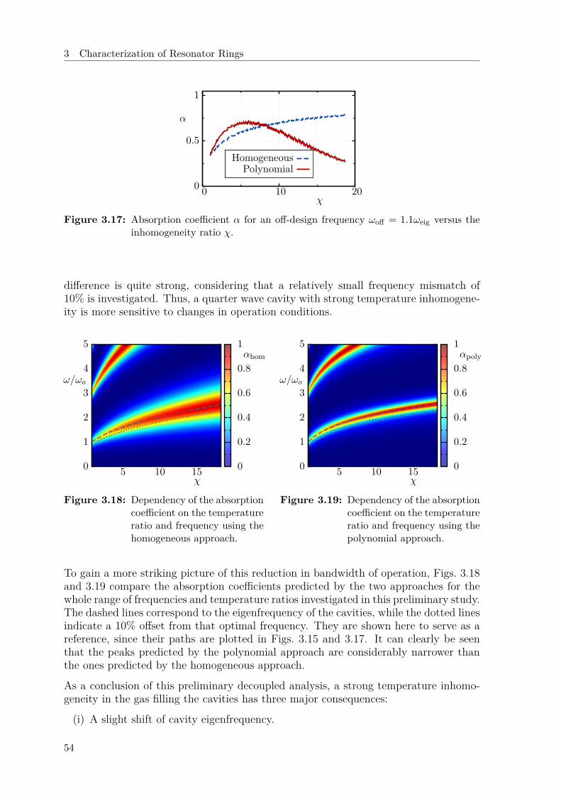
3 Characterization of Resonator Rings
0
0.5
1
0 10 20
α
χ
HomogeneousPolynomial
Figure 3.17: Absorption coefficient α for an off-design frequency ωoff = 1.1ωeig versus theinhomogeneity ratio χ.
difference is quite strong, considering that a relatively small frequency mismatch of10% is investigated. Thus, a quarter wave cavity with strong temperature inhomogene-ity is more sensitive to changes in operation conditions.
0
1
2
3
4
5
5 10 15
ω/ωo
χ
0
0.2
0.4
0.6
0.8
1αhom
Figure 3.18: Dependency of the absorptioncoefficient on the temperatureratio and frequency using thehomogeneous approach.
0
1
2
3
4
5
5 10 15
ω/ωo
χ
0
0.2
0.4
0.6
0.8
1αpoly
Figure 3.19: Dependency of the absorptioncoefficient on the temperatureratio and frequency using thepolynomial approach.
To gain a more striking picture of this reduction in bandwidth of operation, Figs. 3.18and 3.19 compare the absorption coefficients predicted by the two approaches for thewhole range of frequencies and temperature ratios investigated in this preliminary study.The dashed lines correspond to the eigenfrequency of the cavities, while the dotted linesindicate a 10% offset from that optimal frequency. They are shown here to serve as areference, since their paths are plotted in Figs. 3.15 and 3.17. It can clearly be seenthat the peaks predicted by the polynomial approach are considerably narrower thanthe ones predicted by the homogeneous approach.
As a conclusion of this preliminary decoupled analysis, a strong temperature inhomo-geneity in the gas filling the cavities has three major consequences:
(i) A slight shift of cavity eigenfrequency.
54
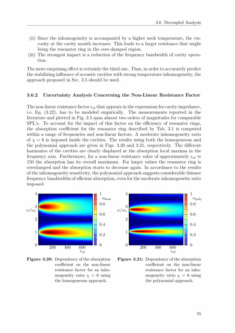
3.6 Decoupled Analysis
(ii) Since the inhomogeneity is accompanied by a higher neck temperature, the vis-cosity at the cavity mouth increases. This leads to a larger resistance that mightbring the resonator ring in the over-damped region.
(iii) The strongest impact is a reduction of the frequency bandwidth of cavity opera-tion.
The more surprising effect is certainly the third one. Thus, in order to accurately predictthe stabilizing influence of acoustic cavities with strong temperature inhomogeneity, theapproach proposed in Sec. 3.5 should be used.
3.6.2 Uncertainty Analysis Concerning the Non-Linear Resistance Factor
The non-linear resistance factor εnl that appears in the expressions for cavity impedance,i.e. Eq. (3.22), has to be modeled empirically. The measurements reported in theliterature and plotted in Fig. 3.5 span almost two orders of magnitudes for comparableSPL’s. To account for the impact of this factor on the efficiency of resonator rings,the absorption coefficient for the resonator ring described by Tab. 3.1 is computedwithin a range of frequencies and non-linear factors. A moderate inhomogeneity ratioof χ = 6 is imposed inside the cavities. The results using both the homogeneous andthe polynomial approach are given in Figs. 3.20 and 3.21, respectively. The differentharmonics of the cavities are clearly displayed at the absorption local maxima in thefrequency axis. Furthermore, for a non-linear resistance value of approximately εnl ≈150 the absorption has its overall maximum. For larger values the resonator ring isoverdamped and the absorption starts to decrease again. In accordance to the resultsof the inhomogeneity sensitivity, the polynomial approach suggests considerable thinnerfrequency bandwidths of efficient absorption, even for the moderate inhomogeneity ratioimposed.
0
1
2
3
4
200 400 600
ω/ωo
εnl
0
0.2
0.4
0.6
0.8
1αhom
Figure 3.20: Dependency of the absorptioncoefficient on the non-linearresistance factor for an inho-mogeneity ratio χ = 6 usingthe homogeneous approach.
0
1
2
3
4
200 400 600
ω/ωo
εnl
0
0.2
0.4
0.6
0.8
1αpoly
Figure 3.21: Dependency of the absorptioncoefficient on the non-linearresistance factor for an inho-mogeneity ratio χ = 6 usingthe polynomial approach.
55

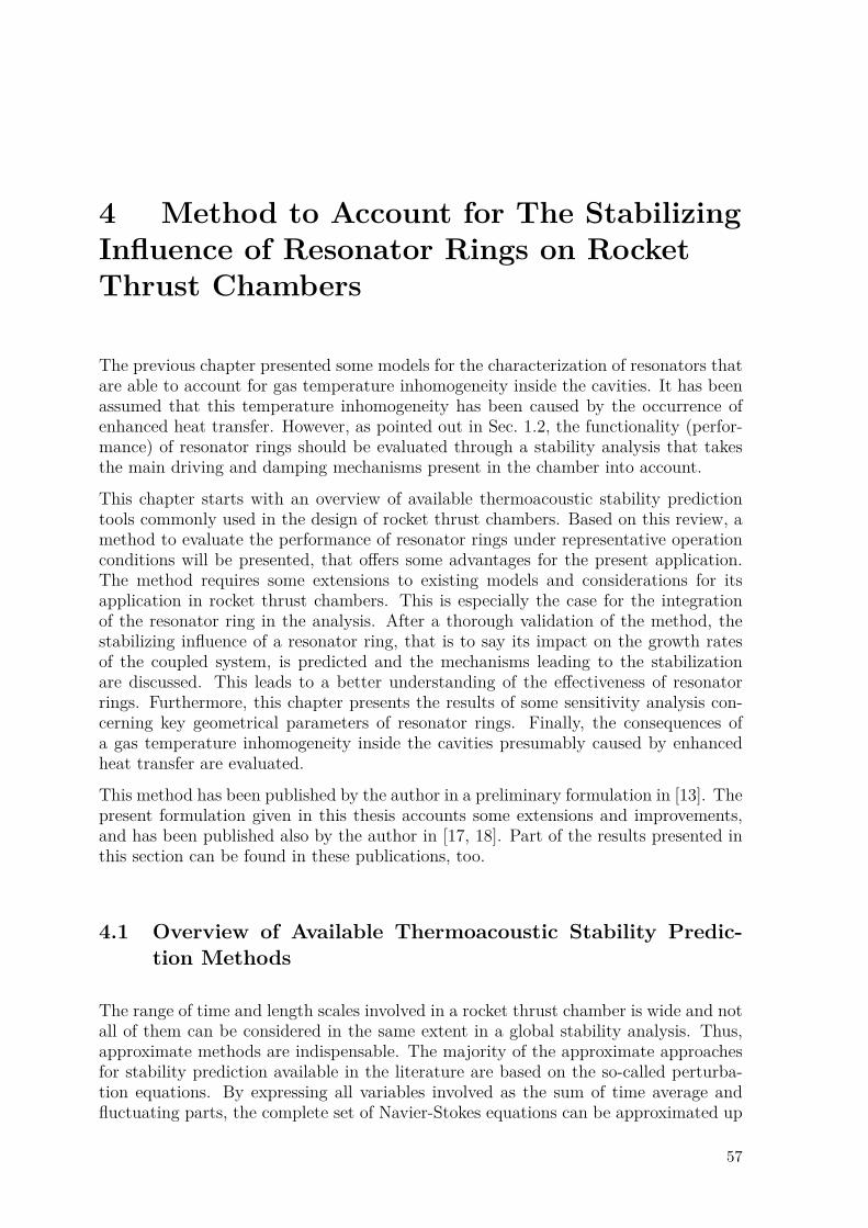
4 Method to Account for The StabilizingInfluence of Resonator Rings on RocketThrust Chambers
The previous chapter presented some models for the characterization of resonators thatare able to account for gas temperature inhomogeneity inside the cavities. It has beenassumed that this temperature inhomogeneity has been caused by the occurrence ofenhanced heat transfer. However, as pointed out in Sec. 1.2, the functionality (perfor-mance) of resonator rings should be evaluated through a stability analysis that takesthe main driving and damping mechanisms present in the chamber into account.
This chapter starts with an overview of available thermoacoustic stability predictiontools commonly used in the design of rocket thrust chambers. Based on this review, amethod to evaluate the performance of resonator rings under representative operationconditions will be presented, that offers some advantages for the present application.The method requires some extensions to existing models and considerations for itsapplication in rocket thrust chambers. This is especially the case for the integrationof the resonator ring in the analysis. After a thorough validation of the method, thestabilizing influence of a resonator ring, that is to say its impact on the growth ratesof the coupled system, is predicted and the mechanisms leading to the stabilizationare discussed. This leads to a better understanding of the effectiveness of resonatorrings. Furthermore, this chapter presents the results of some sensitivity analysis con-cerning key geometrical parameters of resonator rings. Finally, the consequences ofa gas temperature inhomogeneity inside the cavities presumably caused by enhancedheat transfer are evaluated.
This method has been published by the author in a preliminary formulation in [13]. Thepresent formulation given in this thesis accounts some extensions and improvements,and has been published also by the author in [17, 18]. Part of the results presented inthis section can be found in these publications, too.
4.1 Overview of Available Thermoacoustic Stability Predic-tion Methods
The range of time and length scales involved in a rocket thrust chamber is wide and notall of them can be considered in the same extent in a global stability analysis. Thus,approximate methods are indispensable. The majority of the approximate approachesfor stability prediction available in the literature are based on the so-called perturba-tion equations. By expressing all variables involved as the sum of time average andfluctuating parts, the complete set of Navier-Stokes equations can be approximated up
57
4 Method to Account for The Stabilizing Influence of Resonator Rings on Rocket ThrustChambers
to certain order. An overview of the derivation of these methods has been given byCulick [24]. In recent years, advances in computational resources have made the nu-merical solution of these equations by means of FDM feasible, see for example [86, 101].Even if detailed geometries can be studied in this way, important issues like computa-tional cost, code stability and application of boundary conditions are not totally solvedyet.
As stated by Culick [24], the primary source of information concerning combustion in-stabilities is given by the oscillations of pressure p′. Thus, in the approximate methodsproposed by Culick and co-workers, an inhomogeneous wave equation for the fluctuat-ing pressure p′ is derived from the perturbation equations, see Sec. 2.2 and App. A.1.Using a transformation into a velocity potential, an alternative wave equation is usedin a similar way by Zinn et al. [132]. The wave equation is inhomogeneous due tomean flow and various source terms present in the perturbation equations. A modifiedGalerkin approach based on the application of the method of weighted residuals pro-posed by Zinn and Powell [133] can be used to solve the inhomogeneous wave equationfor simplified cylindrical geometries and various boundary conditions. The essence ofthis semi-analytical approach is to express the unsteady pressure field as a superpositionof the basic acoustic modes with time varying modal amplitudes. These basic acousticmodes correspond to solutions of the homogeneous wave equation with hard bound-aries and form an orthogonal basis. Multiplication of the wave equation by a series oftest functions - normalized basic acoustic modes - and integration over the chamberdomain leads to a system of equations for the amplitudes of the perturbed solution,which can be solved by means of least residuals. In its general form, the method iscapable of handling non-linear behavior with mode coupling [24]. Culick also proposeda linear stability analysis transforming the previously described approach from the timeinto the frequency domain [24]. Assuming linearity, all variables involved can be ex-pressed with harmonic time dependence. One advantage of treating the problem in thefrequency domain is that non-trivial acoustic boundary conditions are quite easy to ap-ply. Non-trivial acoustic boundary conditions include frequency dependent impedanceexpressions, as is for example the case for the models describing the behavior of res-onator cavities and given in Ch. 3. The transformation of such an expression into thetime domain via inverse Fourier transformation requires the evaluation of a convolutionintegral [100]. This cumbersome procedure is avoided in a complete frequency domainformulation of the problem. Substitution of the linear harmonic approach into the sys-tem of equations for the amplitudes delivers a set of expressions for the eigenfrequenciesof the system, from which stability can be deduced.
A similar linear approach has been developed by Mitchell and co-workers [4, 82]. Hetransformed the linearized inhomogeneous Helmholtz equation (frequency domain) intoa surface integral following the Green’s function approach and integrating over thechamber surface. The resulting frequency dependent integral equation holds only atthe eigenfrequencies of the system. Thus, for given parameters, the solutions of thisequation delivers the eigenfrequencies of the system, from which the linear stability canbe deduced. Mitchell solved the integral equation iteratively expressing the Green’sfunction also as a superposition of the classical acoustic modes with hard boundaries.Up to second order, the methods of Culick and Mitchell are equivalent [24].
The solution of the Helmholtz equation can also be achieved numerically using threedimensional Helmholtz tools. This has the advantage that several additional effects like
58
4.2 Proposed Method Based on Network Models and Nyquist Plot
stratification, complex geometries, source terms, etc. can be considered in the linearizedHelmholtz equation. The resulting Helmholtz equation can be solved by techniquesbased on the FEM [43, 91, 103].
Despite the simplistic assumptions of linearity, uniform flow, constant properties andso on, the semi-analytical approaches based on modes give insight in global trendsand help in the fundamental understanding of the problem [113]. Furthermore, theyare fast and thus afford parameter studies for optimization at early design stages.On the other hand, the resulting complex-valued equations for the eigenfrequencieshave several solutions. In addition to the numerical complexity of solving them, itis not always simple to assure that all possible solutions in the parameter range ofinterest have actually been found. Furthermore, the expressions describing the differentboundary conditions present in the system have to be known also for complex-valuedfrequencies, simply because a non-zero growth rate of an eigenmode implies a non-zero imaginary part of the corresponding eigenfrequency. If the expressions are givenin closed form this is not a serious issue, while for expressions based on tabulatedvalues from semi-analytical approaches – as it will be the case for the resonator rings inthe present study – it brings considerably more computational effort. For data basedon forced experiments, this might not be possible because only real frequencies canbe excited. Another issue present in the two previously described methods is that,since the acoustic field is expressed as superposition of classical acoustic modes withhard boundaries, the solutions do not accurately reproduce the field near reactive anddissipative boundaries. Culick acknowledged this issue [24] and argued that the errorsare small if the perturbation order is also small.
4.2 Proposed Method Based on Network Models and NyquistPlot
As stated by Mitchell [82], in order to accurately predict the stabilizing influence ofresonators in rocket thrust chambers, the main driving and damping mechanisms haveto be taken into account. Attached to the shell of the thrust chamber, the resonatorswill interact with a three-dimensional acoustic pressure field. This acoustic field in turnis influenced by the mean flow, the combustion flame front, the injector plate and thechoked nozzle. Thus, the resonator ring interacts through the acoustic field indirectlywith the just mentioned effects. Thus, an appropriate method that accounts for thelinear stability of the coupled system, chamber and resonator ring, is necessary to eval-uate the performance of resonator rings. The method should fulfill some requirements:firstly, account for the just mentioned main driving and damping mechanisms presentin the chamber, secondly, allow the incorporation of the resonator models presented inCh. 3, and thirdly, afford parametric studies on critical resonator features.
The three-dimensional computational tools that solve linearized perturbation equa-tions either in time or frequency domain can certainly reproduce the main driving anddamping mechanisms present in the thrust chamber, as shown by [42, 86, 101]. Theyalso allow the incorporation of resonator ring models as boundary conditions, althoughthis is accompanied by some non-trivial difficulties concerning the code stability. Fur-thermore, the necessary computational efforts are not be underestimated, making the
59
4 Method to Account for The Stabilizing Influence of Resonator Rings on Rocket ThrustChambers
parametric studies intended in this thesis not really feasible. Note that this decisionconcerns only the studies intended in the present investigation, where the focus lies onthe resonator rings. Actually, such codes provide quite promising capabilities for thestability prediction of rocket thrust chambers. This is the scope of a parallel projectwithin the SFB-TRR40 (project C3).
The linear stability analysis of Culick [24] and Mitchel et al. [82] fulfill the three re-quirements mentioned at the beginning of this section. However, their numerical im-plementation is not trivial, because the whole method is encapsulated into a singleintegral equation over the chamber boundaries and the solution procedure is iterative.Thus, convergence might play an important role. Furthermore, three issues related tosuch methods have been mentioned in Sec. 4.1: (i) complex root finding, (ii) necessityof boundary expressions over the whole complex-valued frequency range and (iii) inac-curate pressure field close to reactive and dissipative boundaries. The third issue is ofminor importance, since the errors are small provided that the perturbation order isalso small. In contrast, the former two can indeed lead to serious difficulties.
In this thesis, a different method for linear stability analysis of rocket thrust chambersis proposed, that fulfills the necessary requirements and overcomes the three issuesmentioned above. Instead of solving the Helmholtz equation iteratively over the wholechamber domain, the acoustic field is constructed piecewise using cylindrical segmentsfollowing the acoustic network approach introduced in Sec. 2.2.3. The acoustic fieldin the segments is described analytically in terms of up- and downstream travelingwaves, i.e. Eq. (2.49) for a simple duct segment with hard shell. Exact solutions foradditional segments or boundary types necessary for the description of rocket thrustchambers, like resonator rings, flame, nozzle and so on, will be presented later on in thischapter. Decisive is that the expressions describing the segments are exact solutions ofthe Helmholtz equation that fully satisfy the corresponding boundary conditions, thusresolving issue (iii). At connecting planes between two different segments, the compactelements introduced also in Sec. 2.2.3 are employed. As will be shown in Sec. 4.3.2,mode matching techniques based on the Galerkin approach can be applied for thispurpose. They are similar to those used in ducts with discontinuous shell impedanceswidely studied in the field of aero engines with regard to suppression of noise. Finally,the linear stability of the acoustic network can be determined with the Nyquist-plotmethod introduced in Sec. 2.2.5 if some considerations for its application above cut-onare taken. The number and location of the eigenfrequencies present in the frequencyrange of interest are inferred graphically from the Nyquist-plot. The complex rootfinding procedure is avoided in this way, overcoming issue (i). Furthermore, since onlytransfer matrix coefficients at purely real valued frequencies are needed for the stabil-ity prediction, tabulated data used either by boundary conditions or semi-analyticalsolutions of the different segments reduces considerably. Thus, the application of theNyquist-plot method overcomes issue (ii), too.
In addition to the advantages just mentioned, the acoustic network approach allowsa strong flexibility, because the different mechanisms can be separated into elementsthat can be handled more easily. In this way, the network representation of the thrustchamber can be easily adapted, extended or improved by simply changing some ofthe elements without changing the solution procedure. Even elements derived fromempirical approaches based on tabulated data can be incorporated via the Nyquist-plot technique. In the present case, the focus lies on the element representing the
60
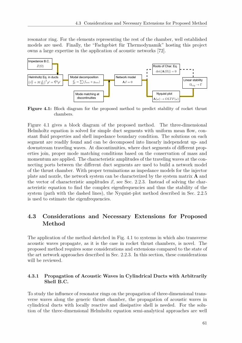
4.3 Considerations and Necessary Extensions for Proposed Method
resonator ring. For the elements representing the rest of the chamber, well establishedmodels are used. Finally, the “Fachgebiet fur Thermodynamik” hosting this projectowns a large expertise in the application of acoustic networks [72].
Figure 4.1: Block diagram for the proposed method to predict stability of rocket thrustchambers.
Figure 4.1 gives a block diagram of the proposed method. The three-dimensionalHelmholtz equation is solved for simple duct segments with uniform mean flow, con-stant fluid properties and shell impedance boundary condition. The solutions on eachsegment are readily found and can be decomposed into linearly independent up- anddownstream traveling waves. At discontinuities, where duct segments of different prop-erties join, proper mode matching conditions based on the conservation of mass andmomentum are applied. The characteristic amplitudes of the traveling waves at the con-necting ports between the different duct segments are used to build a network modelof the thrust chamber. With proper terminations as impedance models for the injectorplate and nozzle, the network system can be characterized by the system matrix A andthe vector of characteristic amplitudes ~x, see Sec. 2.2.3. Instead of solving the char-acteristic equation to find the complex eigenfrequencies and thus the stability of thesystem (path with the dashed lines), the Nyquist-plot method described in Sec. 2.2.5is used to estimate the eigenfrequencies.
4.3 Considerations and Necessary Extensions for ProposedMethod
The application of the method sketched in Fig. 4.1 to systems in which also transverseacoustic waves propagate, as it is the case in rocket thrust chambers, is novel. Theproposed method requires some considerations and extensions compared to the state ofthe art network approaches described in Sec. 2.2.3. In this section, these considerationswill be reviewed.
4.3.1 Propagation of Acoustic Waves in Cylindrical Ducts with ArbitrarilyShell B.C.
To study the influence of resonator rings on the propagation of three-dimensional trans-verse waves along the generic thrust chamber, the propagation of acoustic waves incylindrical ducts with locally reactive and dissipative shell is needed. For the solu-tion of the three-dimensional Helmholtz equation semi-analytical approaches are well
61
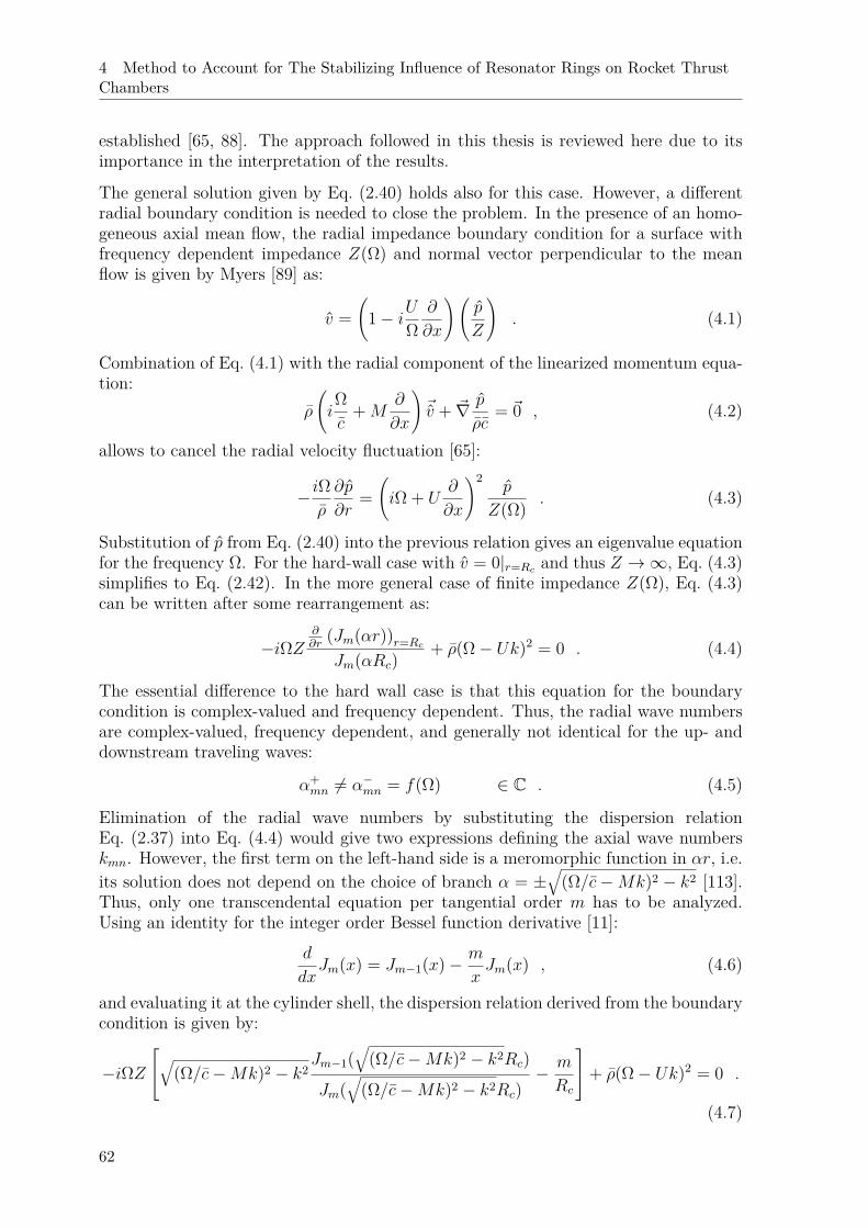
4 Method to Account for The Stabilizing Influence of Resonator Rings on Rocket ThrustChambers
established [65, 88]. The approach followed in this thesis is reviewed here due to itsimportance in the interpretation of the results.
The general solution given by Eq. (2.40) holds also for this case. However, a differentradial boundary condition is needed to close the problem. In the presence of an homo-geneous axial mean flow, the radial impedance boundary condition for a surface withfrequency dependent impedance Z(Ω) and normal vector perpendicular to the meanflow is given by Myers [89] as:
v =(
1− iUΩ∂
∂x
)(p
Z
). (4.1)
Combination of Eq. (4.1) with the radial component of the linearized momentum equa-tion:
ρ
(iΩc
+M∂
∂x
)~v + ~∇ p
ρc= ~0 , (4.2)
allows to cancel the radial velocity fluctuation [65]:
−iΩρ
∂p
∂r=(iΩ + U
∂
∂x
)2p
Z(Ω) . (4.3)
Substitution of p from Eq. (2.40) into the previous relation gives an eigenvalue equationfor the frequency Ω. For the hard-wall case with v = 0|r=Rc and thus Z →∞, Eq. (4.3)simplifies to Eq. (2.42). In the more general case of finite impedance Z(Ω), Eq. (4.3)can be written after some rearrangement as:
−iΩZ∂∂r
(Jm(αr))r=RcJm(αRc)
+ ρ(Ω− Uk)2 = 0 . (4.4)
The essential difference to the hard wall case is that this equation for the boundarycondition is complex-valued and frequency dependent. Thus, the radial wave numbersare complex-valued, frequency dependent, and generally not identical for the up- anddownstream traveling waves:
α+mn 6= α−mn = f(Ω) ∈ C . (4.5)
Elimination of the radial wave numbers by substituting the dispersion relationEq. (2.37) into Eq. (4.4) would give two expressions defining the axial wave numberskmn. However, the first term on the left-hand side is a meromorphic function in αr, i.e.its solution does not depend on the choice of branch α = ±
√(Ω/c−Mk)2 − k2 [113].
Thus, only one transcendental equation per tangential order m has to be analyzed.Using an identity for the integer order Bessel function derivative [11]:
d
dxJm(x) = Jm−1(x)− m
xJm(x) , (4.6)
and evaluating it at the cylinder shell, the dispersion relation derived from the boundarycondition is given by:
−iΩZ√(Ω/c−Mk)2 − k2
Jm−1(√
(Ω/c−Mk)2 − k2Rc)
Jm(√
(Ω/c−Mk)2 − k2Rc)− m
Rc
+ ρ(Ω− Uk)2 = 0 .
(4.7)
62
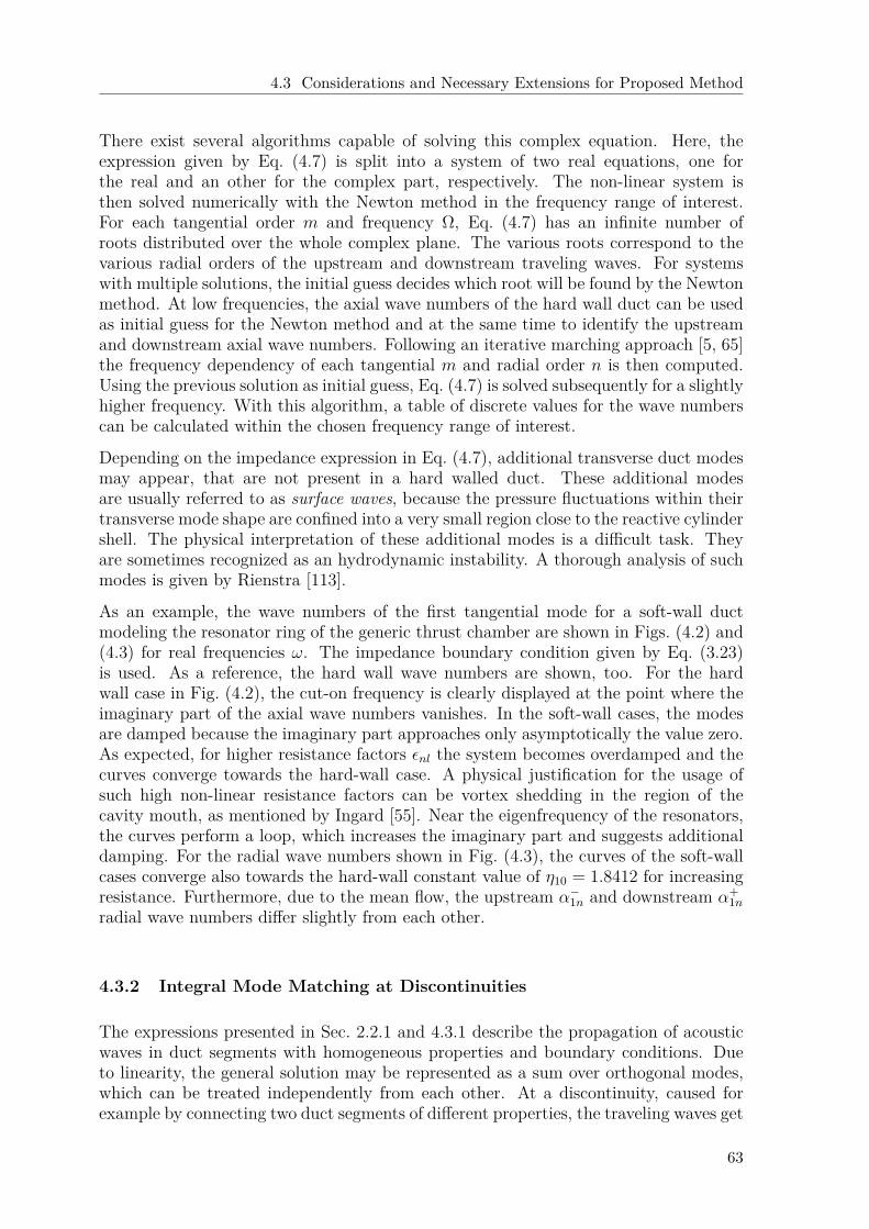
4.3 Considerations and Necessary Extensions for Proposed Method
There exist several algorithms capable of solving this complex equation. Here, theexpression given by Eq. (4.7) is split into a system of two real equations, one forthe real and an other for the complex part, respectively. The non-linear system isthen solved numerically with the Newton method in the frequency range of interest.For each tangential order m and frequency Ω, Eq. (4.7) has an infinite number ofroots distributed over the whole complex plane. The various roots correspond to thevarious radial orders of the upstream and downstream traveling waves. For systemswith multiple solutions, the initial guess decides which root will be found by the Newtonmethod. At low frequencies, the axial wave numbers of the hard wall duct can be usedas initial guess for the Newton method and at the same time to identify the upstreamand downstream axial wave numbers. Following an iterative marching approach [5, 65]the frequency dependency of each tangential m and radial order n is then computed.Using the previous solution as initial guess, Eq. (4.7) is solved subsequently for a slightlyhigher frequency. With this algorithm, a table of discrete values for the wave numberscan be calculated within the chosen frequency range of interest.
Depending on the impedance expression in Eq. (4.7), additional transverse duct modesmay appear, that are not present in a hard walled duct. These additional modesare usually referred to as surface waves, because the pressure fluctuations within theirtransverse mode shape are confined into a very small region close to the reactive cylindershell. The physical interpretation of these additional modes is a difficult task. Theyare sometimes recognized as an hydrodynamic instability. A thorough analysis of suchmodes is given by Rienstra [113].
As an example, the wave numbers of the first tangential mode for a soft-wall ductmodeling the resonator ring of the generic thrust chamber are shown in Figs. (4.2) and(4.3) for real frequencies ω. The impedance boundary condition given by Eq. (3.23)is used. As a reference, the hard wall wave numbers are shown, too. For the hardwall case in Fig. (4.2), the cut-on frequency is clearly displayed at the point where theimaginary part of the axial wave numbers vanishes. In the soft-wall cases, the modesare damped because the imaginary part approaches only asymptotically the value zero.As expected, for higher resistance factors εnl the system becomes overdamped and thecurves converge towards the hard-wall case. A physical justification for the usage ofsuch high non-linear resistance factors can be vortex shedding in the region of thecavity mouth, as mentioned by Ingard [55]. Near the eigenfrequency of the resonators,the curves perform a loop, which increases the imaginary part and suggests additionaldamping. For the radial wave numbers shown in Fig. (4.3), the curves of the soft-wallcases converge also towards the hard-wall constant value of η10 = 1.8412 for increasingresistance. Furthermore, due to the mean flow, the upstream α−1n and downstream α+
1nradial wave numbers differ slightly from each other.
4.3.2 Integral Mode Matching at Discontinuities
The expressions presented in Sec. 2.2.1 and 4.3.1 describe the propagation of acousticwaves in duct segments with homogeneous properties and boundary conditions. Dueto linearity, the general solution may be represented as a sum over orthogonal modes,which can be treated independently from each other. At a discontinuity, caused forexample by connecting two duct segments of different properties, the traveling waves get
63
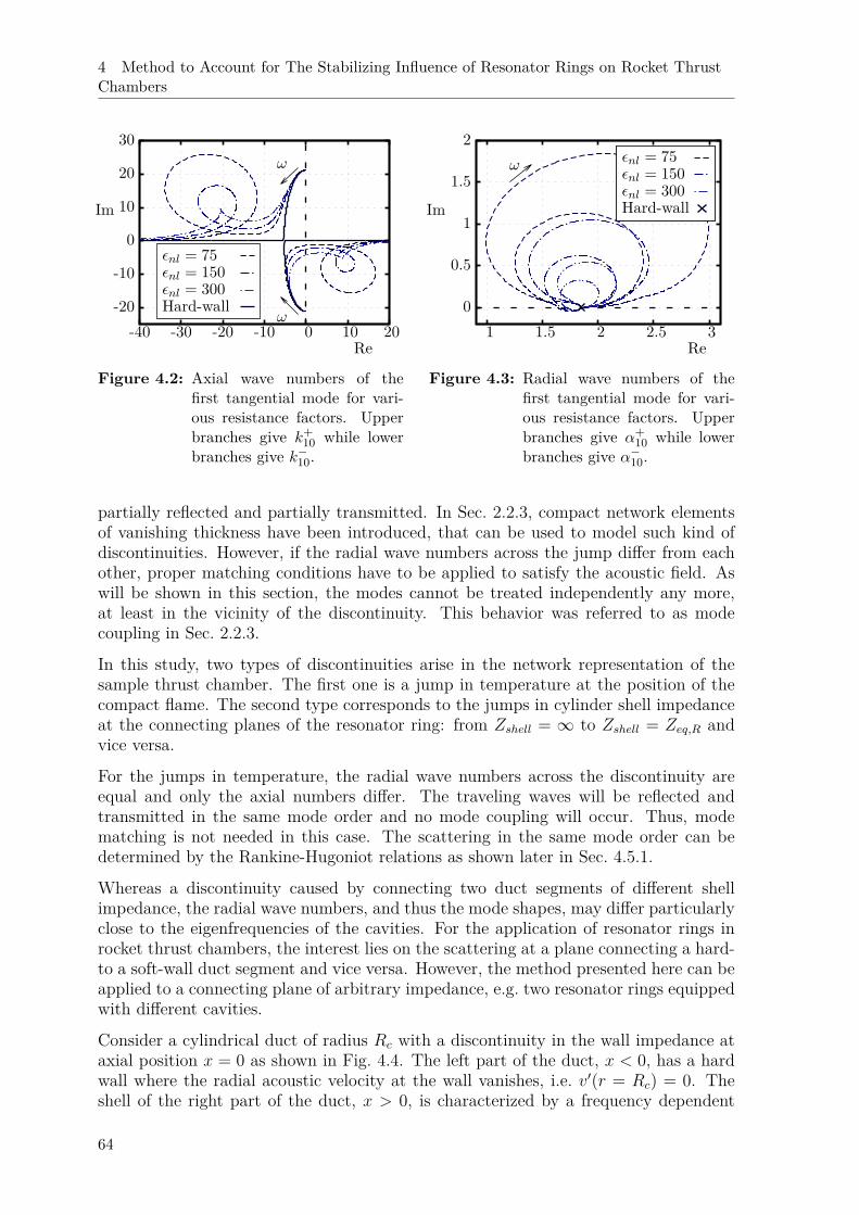
4 Method to Account for The Stabilizing Influence of Resonator Rings on Rocket ThrustChambers
-20
-10
0
10
20
30
-40 -30 -20 -10 0 10 20
Im
Re
ω
ω
εnl = 75εnl = 150εnl = 300Hard-wall
Figure 4.2: Axial wave numbers of thefirst tangential mode for vari-ous resistance factors. Upperbranches give k+
10 while lowerbranches give k−10.
0
0.5
1
1.5
2
1 1.5 2 2.5 3
Im
Re
ωεnl = 75εnl = 150εnl = 300Hard-wall
Figure 4.3: Radial wave numbers of thefirst tangential mode for vari-ous resistance factors. Upperbranches give α+
10 while lowerbranches give α−10.
partially reflected and partially transmitted. In Sec. 2.2.3, compact network elementsof vanishing thickness have been introduced, that can be used to model such kind ofdiscontinuities. However, if the radial wave numbers across the jump differ from eachother, proper matching conditions have to be applied to satisfy the acoustic field. Aswill be shown in this section, the modes cannot be treated independently any more,at least in the vicinity of the discontinuity. This behavior was referred to as modecoupling in Sec. 2.2.3.
In this study, two types of discontinuities arise in the network representation of thesample thrust chamber. The first one is a jump in temperature at the position of thecompact flame. The second type corresponds to the jumps in cylinder shell impedanceat the connecting planes of the resonator ring: from Zshell = ∞ to Zshell = Zeq,R andvice versa.
For the jumps in temperature, the radial wave numbers across the discontinuity areequal and only the axial numbers differ. The traveling waves will be reflected andtransmitted in the same mode order and no mode coupling will occur. Thus, modematching is not needed in this case. The scattering in the same mode order can bedetermined by the Rankine-Hugoniot relations as shown later in Sec. 4.5.1.
Whereas a discontinuity caused by connecting two duct segments of different shellimpedance, the radial wave numbers, and thus the mode shapes, may differ particularlyclose to the eigenfrequencies of the cavities. For the application of resonator rings inrocket thrust chambers, the interest lies on the scattering at a plane connecting a hard-to a soft-wall duct segment and vice versa. However, the method presented here can beapplied to a connecting plane of arbitrary impedance, e.g. two resonator rings equippedwith different cavities.
Consider a cylindrical duct of radius Rc with a discontinuity in the wall impedance ataxial position x = 0 as shown in Fig. 4.4. The left part of the duct, x < 0, has a hardwall where the radial acoustic velocity at the wall vanishes, i.e. v′(r = Rc) = 0. Theshell of the right part of the duct, x > 0, is characterized by a frequency dependent
64
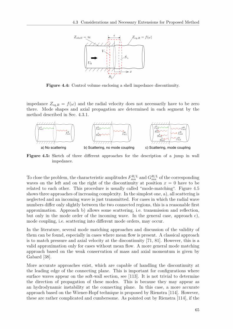
4.3 Considerations and Necessary Extensions for Proposed Method
Figure 4.4: Control volume enclosing a shell impedance discontinuity.
impedance Zeq,R = f(ω) and the radial velocity does not necessarily have to be zerothere. Mode shapes and axial propagation are determined in each segment by themethod described in Sec. 4.3.1.
a) No scattering b) Scattering, no mode coupling c) Scattering, mode coupling
Figure 4.5: Sketch of three different approaches for the description of a jump in wallimpedance.
To close the problem, the characteristic amplitudes FR/Lmn and GR/L
mn of the correspondingwaves on the left and on the right of the discontinuity at position x = 0 have to berelated to each other. This procedure is usually called “mode-matching“. Figure 4.5shows three approaches of increasing complexity. In the simplest one, a), all scattering isneglected and an incoming wave is just transmitted. For cases in which the radial wavenumbers differ only slightly between the two connected regions, this is a reasonable firstapproximation. Approach b) allows some scattering, i.e. transmission and reflection,but only in the mode order of the incoming wave. In the general case, approach c),mode coupling, i.e. scattering into different mode orders, may occur.
In the literature, several mode matching approaches and discussion of the validity ofthem can be found, especially in cases where mean flow is present. A classical approachis to match pressure and axial velocity at the discontinuity [71, 81]. However, this is avalid approximation only for cases without mean flow. A more general mode matchingapproach based on the weak conservation of mass and axial momentum is given byGabard [38].
More accurate approaches exist, which are capable of handling the discontinuity atthe leading edge of the connecting plane. This is important for configurations wheresurface waves appear on the soft-wall section, see [113]. It is not trivial to determinethe direction of propagation of these modes. This is because they may appear asan hydrodynamic instability at the connecting plane. In this case, a more accurateapproach based on the Wiener-Hopf technique is proposed by Rienstra [114]. However,these are rather complicated and cumbersome. As pointed out by Rienstra [114], if the
65
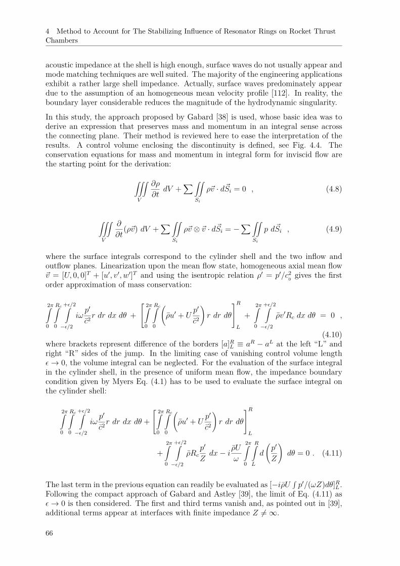
4 Method to Account for The Stabilizing Influence of Resonator Rings on Rocket ThrustChambers
acoustic impedance at the shell is high enough, surface waves do not usually appear andmode matching techniques are well suited. The majority of the engineering applicationsexhibit a rather large shell impedance. Actually, surface waves predominately appeardue to the assumption of an homogeneous mean velocity profile [112]. In reality, theboundary layer considerable reduces the magnitude of the hydrodynamic singularity.
In this study, the approach proposed by Gabard [38] is used, whose basic idea was toderive an expression that preserves mass and momentum in an integral sense acrossthe connecting plane. Their method is reviewed here to ease the interpretation of theresults. A control volume enclosing the discontinuity is defined, see Fig. 4.4. Theconservation equations for mass and momentum in integral form for inviscid flow arethe starting point for the derivation:
∫∫∫V
∂ρ
∂tdV +
∑∫∫Si
ρ~v · d~Si = 0 , (4.8)
∫∫∫V
∂
∂t(ρ~v) dV +
∑∫∫Si
ρ~v ⊗ ~v · d~Si = −∑∫∫
Si
p d~Si , (4.9)
where the surface integrals correspond to the cylinder shell and the two inflow andoutflow planes. Linearization upon the mean flow state, homogeneous axial mean flow~v = [U, 0, 0]T + [u′, v′, w′]T and using the isentropic relation ρ′ = p′/c2
0 gives the firstorder approximation of mass conservation:
2π∫0
Rc∫0
+ε/2∫−ε/2
iωp′
c2 r dr dx dθ + 2π∫
0
Rc∫0
(ρu′ + U
p′
c2
)r dr dθ
RL
+2π∫0
+ε/2∫−ε/2
ρv′Rc dx dθ = 0 ,
(4.10)where brackets represent difference of the borders [a]RL ≡ aR − aL at the left “L” andright “R” sides of the jump. In the limiting case of vanishing control volume lengthε→ 0, the volume integral can be neglected. For the evaluation of the surface integralin the cylinder shell, in the presence of uniform mean flow, the impedance boundarycondition given by Myers Eq. (4.1) has to be used to evaluate the surface integral onthe cylinder shell:
2π∫0
Rc∫0
+ε/2∫−ε/2
iωp′
c2 r dr dx dθ + 2π∫
0
Rc∫0
(ρu′ + U
p′
c2
)r dr dθ
RL
+2π∫0
+ε/2∫−ε/2
ρRcp′
Zdx− i ρU
ω
2π∫0
R∫L
d
(p′
Z
)dθ = 0 . (4.11)
The last term in the previous equation can readily be evaluated as [−iρU∫p′/(ωZ)dθ]RL .
Following the compact approach of Gabard and Astley [39], the limit of Eq. (4.11) asε→ 0 is then considered. The first and third terms vanish and, as pointed out in [39],additional terms appear at interfaces with finite impedance Z 6=∞.
66
4.3 Considerations and Necessary Extensions for Proposed Method
Applying the same series of principles, linearization and limit to ε→ 0, to the conser-vation of momentum yields after some rearrangement to:
2π∫0
Rc∫0
Ψ(Mu′~ex +M~v′ + (M2 + 1) p
′
ρc~ex
)r dr dθ − iΨM
2cRc
ω
2π∫0
p′
Zdθ ~ex
RL
= 0 .
(4.12)Again, additional terms at interfaces with finite impedance arise. However, these canbe replaced by substitution of the mass conservation Eq. (4.11) into Eq. (4.12):
Due to the different mode shapes across the jump, a discontinuity in the rθ-planeoccurs and the conservation equations can only be weakly fulfilled. Following theGalerkin approach, the rearranged integral equations are weighted by a continuousfunction Ψ(r, θ):
2π∫0
Rc∫0
Ψ(u′ +M
p′
ρc
)r dr dθ − i ΨMcRc
Ω
2π∫0
p′
Zdθ
RL
= 0 , (4.13)
2π∫0
Rc∫0
Ψ(M~v′ + p′
ρc~ex
)r dr dθ
RL
= 0 , (4.14)
where pure mean quantities vanish since they are continuous across the jump. Forthe general case with mean flow and constraining the system only by the conservationof mass and momentum, the problem is overdetermined. To overcome this issue onlythe axial component of the momentum conservation is considered. The resulting setof equations correspond to those given by Gabard and Astley [39]. In the absence ofmean flow, the conservation equations for the jump reduce to the classical matching ofpressure and velocity.
Substitution of the general solution Eq. (2.40) in the chosen set of equations deliversrelations between the characteristic amplitudes on both sides of the jump. Since allquantities obey the same harmonic time dependency, the term eiΩt cancels out. Throughthe course of this study, all geometries to be treated are axisymmetric and thus nodiscontinuities in the θ coordinate are considered. Due to linearity, the tangential modescan be treated independently. This means that no scattering into different tangentialmode orders occurs. Furthermore, without loss of generality, the axial position x = 0is used. In practice, only a finite number of nr radial modes can be taken into account.The problem has thus 2× nr unknowns: the characteristic amplitudes on both sides ofthe discontinuity. The Galerkin approach with an orthogonal set of weighting functionsΨmν with ν = 0, 1, . . . , nr is used to close the problem. Note that the radial and axialwave numbers have different values on the left and on the right side of the connectingplane. To distinguish them, the soft-wall case will be denoted by a ∗ superscript.The radial mode shapes of the hard-wall case build an orthogonal set and are used as
67
4 Method to Account for The Stabilizing Influence of Resonator Rings on Rocket ThrustChambers
weighting functions Ψmν = Jm(ηmνr/Rc). This leads to the following linear system ofequations:nr∑n=0
ζνn[(κ+
mnM + 1)Fmn + (κ−mnM + 1)Gmn
]=
nr∑n=0
[ζ∗+νn (κ∗+mnM + 1)F ∗mn + ζ∗−νn (κ∗−mnM + 1)G∗mn
]− i
Mc0Rc
ΩJm(ηmν)
Z
nr∑n=0
[Jm(α∗+mnRc)F ∗mn + Jm(α∗−mnRc)G∗mn
](4.15)
nr∑n=0
ζνn[(κ+
mn +M)Fmn + (κ−mn +M)Gmn
]=
nr∑n=0
ζ∗+νn (κ∗+mn +M)F ∗mn +nr∑n=0
ζ∗−νn (κ∗−mn +M)G∗mn (4.16)
with integral terms that can be evaluated analytically [81]:
ζνn =Rc∫0
Jm
(ηmνr
Rc
)Jm(ηmnr
Rc
)r dr =
R2c
2
[1−
(mηmn
)2]J2m(ηmn) if ν = n;
0 if ν 6= n.(4.17)
ζ∗±νn =Rc∫0
Jm(ηmνrRc
)Jm(α∗±mnr)rdr = R2c
η2mν −R2
cα∗±2mn[
ηmνJm+1(ηmν)Jm(α∗±mnRc)−Rcα∗±mνJm+1(α∗±mνRc)Jm(ηmν)
]. (4.18)
In matrix vector notation and using the vectors ~q =[Fm0, Gm0, Fm1, Gm1, . . . , Fmnr , Gmnr ]T and ~q∗ = [F ∗m0, G
∗m0, F
∗m1, G
∗m1, . . . , F
∗mnr , G
∗mnr ]T
they can be written as:Q~q = Q∗~q∗ , (4.19)
with matrices Q and Q∗ of size 2nr × 2nr and entries:
Q(2ν − 1, 2n− 1) = ζνn(κ+mnM + 1) , Q(2ν − 1, 2n) = ζνn(κ−mnM + 1) , (4.20)
Q(2ν , 2n− 1) = ζνn(κ+mn +M) , Q(2ν, 2n) = ζνn(κ+
mn +M) , (4.21)
and:
Q∗(2ν − 1, 2n− 1) = ζ∗+νn (κ∗+mnM + 1) − iMcRc
ωZJm(ηmνRc)Jm(α∗+mnRc) , (4.22)
Q∗(2ν − 1, 2n ) = ζ∗−νn (κ∗−mnM + 1) − iMcRc
ωZJm(ηmνRc)Jm(α∗−mnRc) , (4.23)
Q∗(2ν , 2n− 1) = ζ∗+νn (κ∗+mnM + 1) , (4.24)Q∗(2ν , 2n ) = ζ∗−νn (κ∗−mnM + 1) . (4.25)
Due to the orthogonality of the weighting functions, Q is a block diagonal matrix.Using this notation, the transfer matrix of a jump in shell impedance can finally beexpressed in terms of these two matrices. For the jump from the hard-wall into the
68
4.3 Considerations and Necessary Extensions for Proposed Method
soft-wall, the transfer matrix is Ths = Q−1Q∗. For the jump in the opposite direction,the transfer matrix is Tsh = T−1
hs = (Q∗)−1Q.
Since matrix inversion is needed, the condition number of the involved matrices isimportant. As pointed out in [39], in some cases, the choice of the hard-wall modes asweighting functions might lead to ill conditioned matrices. Gabard et al. suggest touse then a different set of weighting functions to improve the accuracy.
Physically, the scattering matrix notation introduced in Sec. 2.2.3 offers a more descrip-tive characterization of the problem that preserves causality. In this case, the system isdescribed by a matrix Ssh that relates the incoming to the outgoing waves at the jumpposition:
f ∗m0
gm0...
f ∗mngmn
out
= Ssh
fm0
g∗m0...
fmng∗mn
in
=
[2× 2]0→0 · · · [2× 2]n→0
[2× 2]0→1...
... . . .[2× 2]0→n [2× 2]n→n
fm0
g∗m0...
fmng∗mn
in
. (4.26)
The scattering matrix can be divided into [2×2] sub-block matrices that allow a physicalrepresentation of the different entries as explained in Sec. 2.2.3. Each sub-block matrixrepresents the coupling between two radial mode orders as shown by the arrows inthe indices of Eq. (4.26). Thus, within each sub-block, the diagonal entries representtransmission, while the off-diagonal elements reflection of the corresponding travelingwaves into a different mode order. As an example consider the coupling of the radialorder n = 0 into order n = 1:
[2× 2]0→1 =T+
0→1 R+0→1
R−0→1 T−0→1
. (4.27)
4.3.3 Acoustic Network Approach Above Cut-on and Mode Coupling
The low order acoustic network approach introduced in Sec. 2.2.3 has been extensivelyapplied for systems in which mainly plane waves propagate. For higher frequenciesabove the cut-on, ω > ωc, transverse modes have to be taken into account, too. This isthe case in rocket thrust chambers, where the strongest and most dangerous instabilitiesoccur at high frequencies. Due to linearity of the solution and assuming no interactionbetween the different mode orders at discontinuities, each mode can be treated inde-pendently. As pointed out in [107], for each transverse mode order the network can stillbe built by single mode elements using the corresponding wave numbers k±mn and α±mnconnected by two pins. Thus, each transverse mode order mn is treated independentlywith a system of linear equations:
Amn~xmn = ~bmn . (4.28)
Even if the modes behave independently along the element segments, this does notnecessarily have to always be valid at connecting planes. At discontinuities like areachanges or shell impedance jumps, the matching conditions may lead to mode coupling.
69
4 Method to Account for The Stabilizing Influence of Resonator Rings on Rocket ThrustChambers
In this more general case, several mode orders have to be taken into account. So-calledmulti-mode elements in the network can thus have several pairs of connecting pins perport. The low order network can still be described by a system of linear equations:
Acoupl~xcoupl = ~bcoupl , (4.29)
where the system matrix Acoupl, state ~xcoupl, and excitation vector ~bcoupl are concate-nations of their single mode counterparts Amn, ~xmn, and ~bmn, respectively. The size ofthe linear system depends on the number of modes considered in the coupling.
4.3.4 Generalized Nyquist Criterion for Systems Above Cut-on and ModeCoupling
The application of the Nyquist method presented in Sec. 2.2.5 for linearly independenthigher order modes is quite straightforward. The diagnostic dummy and the acousticelements are evaluated with the wave numbers α±mn, m and k±mn of the mode order ofinterest. An OLTF curve can then be evaluated for each mode OLTFmn and the linearstability predicted. However, it has not yet been validated for transverse modes.
When radial mode coupling has to be taken into account, due to interactions at dis-continuities combined with frequencies beyond the radial cut-on, the method has to beextended. In fact, due to the coupling, a multiple input and multiple output analysishas to be considered [120]. As mentioned before, in this study the coupling is restrictedto the vicinity of the resonator ring and the modes are treated independently whenperforming the global stability analysis. This procedure will be explained in the nextsection where the resonator ring element is described.
4.4 Resonator Ring Element
The methodologies presented in Sec. 4.3 allow to model a resonator ring in a low orderelement sense. With integral mode matching, the resonator ring element that accountsfor scattering and mode coupling can be modeled as a combination of two jumps witha soft-wall duct segment of homogeneous shell impedance of length d in-between, seeFig. 4.6. The impedance jumps are characterized by the transfer matrices Ths andTsh. The soft-wall duct segment can be characterized by a diagonal matrix, whoseexponential entries describe the axial propagation of the up- f ∗mn and downstreamtraveling waves g∗mn in terms of the axial wave numbers k∗±mn of the different modes:
Ts =
e−ik∗+m0L 0 · · · 0
0 e−ik∗−m0L
...... . . . . . .
e−ik∗+mnrL 0
0 · · · 0 e−ik∗−mnrL
(4.30)
Taking advantage of the transfer matrix notation the resonator ring element can simplybe described by:
Tring = TshTsThs . (4.31)
70
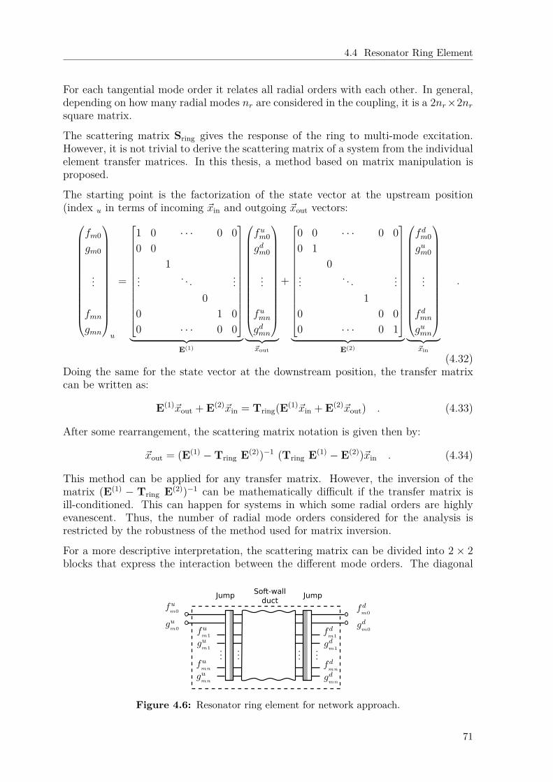
4.4 Resonator Ring Element
For each tangential mode order it relates all radial orders with each other. In general,depending on how many radial modes nr are considered in the coupling, it is a 2nr×2nrsquare matrix.
The scattering matrix Sring gives the response of the ring to multi-mode excitation.However, it is not trivial to derive the scattering matrix of a system from the individualelement transfer matrices. In this thesis, a method based on matrix manipulation isproposed.
The starting point is the factorization of the state vector at the upstream position(index u in terms of incoming ~xin and outgoing ~xout vectors:
fm0
gm0
...
fmngmn
u
=
1 0 · · · 0 00 0
1... . . . ...
00 1 00 · · · 0 0
︸ ︷︷ ︸
E(1)
fum0
gdm0
...
fumngdmn
︸ ︷︷ ︸~xout
+
0 0 · · · 0 00 1
0... . . . ...
10 0 00 · · · 0 1
︸ ︷︷ ︸
E(2)
fdm0
gum0
...
fdmngumn
︸ ︷︷ ︸
~xin
.
(4.32)Doing the same for the state vector at the downstream position, the transfer matrixcan be written as:
E(1)~xout + E(2)~xin = Tring(E(1)~xin + E(2)~xout) . (4.33)
After some rearrangement, the scattering matrix notation is given then by:
~xout = (E(1) −Tring E(2))−1 (Tring E(1) − E(2))~xin . (4.34)
This method can be applied for any transfer matrix. However, the inversion of thematrix (E(1) − Tring E(2))−1 can be mathematically difficult if the transfer matrix isill-conditioned. This can happen for systems in which some radial orders are highlyevanescent. Thus, the number of radial mode orders considered for the analysis isrestricted by the robustness of the method used for matrix inversion.
For a more descriptive interpretation, the scattering matrix can be divided into 2 × 2blocks that express the interaction between the different mode orders. The diagonal
JumpSoft-wall
ductJump
Figure 4.6: Resonator ring element for network approach.
71
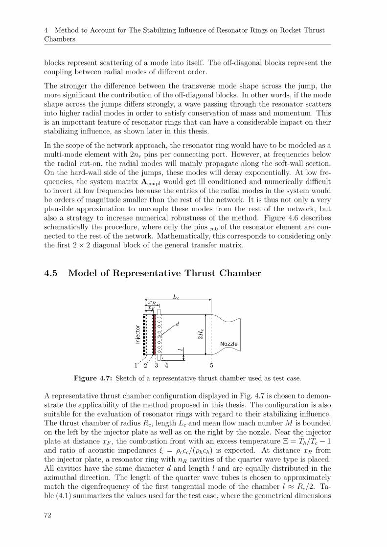
4 Method to Account for The Stabilizing Influence of Resonator Rings on Rocket ThrustChambers
blocks represent scattering of a mode into itself. The off-diagonal blocks represent thecoupling between radial modes of different order.
The stronger the difference between the transverse mode shape across the jump, themore significant the contribution of the off-diagonal blocks. In other words, if the modeshape across the jumps differs strongly, a wave passing through the resonator scattersinto higher radial modes in order to satisfy conservation of mass and momentum. Thisis an important feature of resonator rings that can have a considerable impact on theirstabilizing influence, as shown later in this thesis.
In the scope of the network approach, the resonator ring would have to be modeled as amulti-mode element with 2nr pins per connecting port. However, at frequencies belowthe radial cut-on, the radial modes will mainly propagate along the soft-wall section.On the hard-wall side of the jumps, these modes will decay exponentially. At low fre-quencies, the system matrix Acoupl would get ill conditioned and numerically difficultto invert at low frequencies because the entries of the radial modes in the system wouldbe orders of magnitude smaller than the rest of the network. It is thus not only a veryplausible approximation to uncouple these modes from the rest of the network, butalso a strategy to increase numerical robustness of the method. Figure 4.6 describesschematically the procedure, where only the pins m0 of the resonator element are con-nected to the rest of the network. Mathematically, this corresponds to considering onlythe first 2× 2 diagonal block of the general transfer matrix.
4.5 Model of Representative Thrust Chamber
Injector
Nozzle
Figure 4.7: Sketch of a representative thrust chamber used as test case.
A representative thrust chamber configuration displayed in Fig. 4.7 is chosen to demon-strate the applicability of the method proposed in this thesis. The configuration is alsosuitable for the evaluation of resonator rings with regard to their stabilizing influence.The thrust chamber of radius Rc, length Lc and mean flow mach number M is boundedon the left by the injector plate as well as on the right by the nozzle. Near the injectorplate at distance xF , the combustion front with an excess temperature Ξ = Th/Tc − 1and ratio of acoustic impedances ξ = ρccc/(ρhch) is expected. At distance xR fromthe injector plate, a resonator ring with nR cavities of the quarter wave type is placed.All cavities have the same diameter d and length l and are equally distributed in theazimuthal direction. The length of the quarter wave tubes is chosen to approximatelymatch the eigenfrequency of the first tangential mode of the chamber l ≈ Rc/2. Ta-ble (4.1) summarizes the values used for the test case, where the geometrical dimensions
72
4.5 Model of Representative Thrust Chamber
are non-dimensionalized by the chamber radius. The eigenfrequency of the first tan-gential mode without mean flow and closed boundaries fo = cη10/(2πRc) is used tonon-dimensionalize all frequencies and time scales throughout this study. All thermo-dynamic properties are assumed homogeneous over the transverse chamber plane andthe spatial average operator is omitted for clarity.
Table 4.1: Geometrical and thermodynamical parameters of the test case in non-dimensional form.
RcRc
LRc
xFRc
xrRc
dRc
lRc
lrRc
Ξ ξ γ nr n τfo Mh
1 2.86 0.11 0.16 0.089 0.466 0.179 12 3.85 1.13 22 1.1 0.55 0.25
4.5.1 Network Model of Representative Thrust Chamber
The generic thrust chamber presented in Sec. 4.5 is modeled here as a network of loworder elements. Using the notation shown in Fig. 4.7, the mathematical description ofthe particular elements is given here, from which the transfer matrices can easily bedetermined. The numbered indices denote the axial position in the chamber accordingto Fig. 4.7. For better readability, the mode indices mn are omitted in this part,however the expressions are valid for any mode order.
• For the injector plate at position 1, the acoustic mass flow fluctuations areset to zero (ρ1u1)′ = 0. This follows from the assumption of critical mass flow ratethrough the injectors. Written in terms of Riemann-Invariants, the boundary conditionis given by [67]:
(κ+1 +M1)f1 + (κ−1 +M1)g1 = 0 . (4.35)
• For a short duct with hard walls of length L12 = xF with wave numbers given byEq. (2.37), it follows:
f2 = f1e−ik+
1 L12 , (4.36)g2 = g1e
−ik−1 L12 . (4.37)
• The combustion process is modeled as a compact heat source of zero thicknessL23 ≈ 0. Matching conditions are not needed, because the radial wave numbers do notchange across the jump. The linearized Rankine-Hugoniot equations [107] relate theacoustic primitive variables across the flame front:
p′3 = p′2 − ρ2u22Ξu′2u2
+ Q′
¯Q
, (4.38)
u′3 = u′2 + u2ΞQ′
¯Q− p′2p2
, (4.39)
where Ξ = (T3/T2 − 1) is the excess temperature. Only for vanishing Mach numbers,
73
4 Method to Account for The Stabilizing Influence of Resonator Rings on Rocket ThrustChambers
the pressure fluctuations at both sides are approximately equal p′3 ≈ p′2. Entropyinhomogeneities are neglected upstream of the flame front. To close the expressions, thevariation of heat release rate Q′ has to be given in terms of the acoustic quantities. Usingthe n-τ sensitive time lag model proposed by Crocco [23], the heat release fluctuationsare linked to the pressure fluctuations on the cold side and can be given by [101]:
Q′
¯Q= n
(1− eiΩτ
) p′2p2
. (4.40)
This assumes that in the chain of processes taking part in the combustion, the most sen-sitive one responds to pressure excitation [100]. Using the ratio of specific impedancesξ and the isentropic exponent γ, substitution of Eq. (4.40), and the general solutionEq. (2.49) and Eq. (2.51) in the Rankine-Hugoniot equations leads to:
f3 + g3 = ξ[1−M2Θ
(γM2n(1− eiΩτ ) + κ+
2
)]f2
+ ξ[1−M2Θ
(γM2n(1− eiΩτ ) + κ−2
)]g2 , (4.41)
κ+3 f3 + κ−3 g3 =
[κ+
2 +M2γΘ(n(1− eiΩτ )− 1
)]f2
+[κ−2 +M2γΘ
(n(1− eiΩτ )− 1
)]g2 . (4.42)
Note that from the conservation equations across the flame, a relation for the meanproperties exists between the excess temperature Ξ, the ratio of specific impedancesξ and the Mach number on the hot side M2, see App. A.3. Thus, only two of thesethree parameters can be chosen independently. The fourth and fifth parameters givenby the interaction index n and the time lag τ are assumed to be independent and canbe arbitrarily chosen. In practice, they depend on the propellant and feed system.
• For the resonator ring element of length L34 = d, the first 2 × 2 diagonal blockof the discrete transfer matrix Tring is taken, see Sec. 4.4. Depending on the testcase, the impedance expression for a quarter wave cavity is applied as shell boundarycondition using either Eq. (3.23) for the homogeneous approach or Eqs. (3.22) and(3.44) for the polynomial approach. The tabulated values for real valued frequenciesω ∈ [0.027 : 2.194] with frequency increment ∆ω = 0.0017 is used to estimate theradial α±mn and axial k±mn wave numbers:f4
g4
=Tring(1, 1) Tring(1, 2)Tring(2, 1) Tring(2, 2)
f3
g3
. (4.43)
• A second duct of length L45 = Lc − xR − d/2 with hard walls and wave numbersgiven by Eq. (2.37) follows:
f5 = f4e−ik+
x L45 , (4.44)g5 = g4e
−ik−x L45 . (4.45)
• For the application of the Nyquist method, the diagnostic element is placed at
74
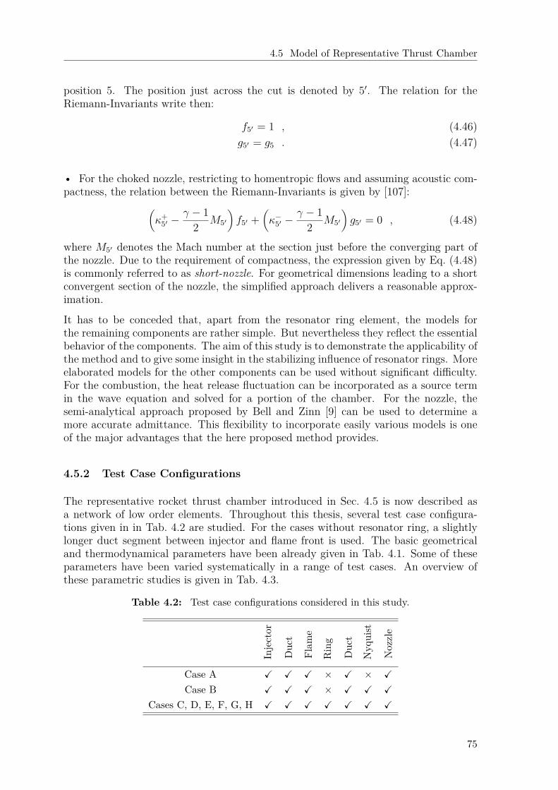
4.5 Model of Representative Thrust Chamber
position 5. The position just across the cut is denoted by 5′. The relation for theRiemann-Invariants write then:
f5′ = 1 , (4.46)g5′ = g5 . (4.47)
• For the choked nozzle, restricting to homentropic flows and assuming acoustic com-pactness, the relation between the Riemann-Invariants is given by [107]:(
κ+5′ −
γ − 12 M5′
)f5′ +
(κ−5′ −
γ − 12 M5′
)g5′ = 0 , (4.48)
where M5′ denotes the Mach number at the section just before the converging part ofthe nozzle. Due to the requirement of compactness, the expression given by Eq. (4.48)is commonly referred to as short-nozzle. For geometrical dimensions leading to a shortconvergent section of the nozzle, the simplified approach delivers a reasonable approx-imation.
It has to be conceded that, apart from the resonator ring element, the models forthe remaining components are rather simple. But nevertheless they reflect the essentialbehavior of the components. The aim of this study is to demonstrate the applicability ofthe method and to give some insight in the stabilizing influence of resonator rings. Moreelaborated models for the other components can be used without significant difficulty.For the combustion, the heat release fluctuation can be incorporated as a source termin the wave equation and solved for a portion of the chamber. For the nozzle, thesemi-analytical approach proposed by Bell and Zinn [9] can be used to determine amore accurate admittance. This flexibility to incorporate easily various models is oneof the major advantages that the here proposed method provides.
4.5.2 Test Case Configurations
The representative rocket thrust chamber introduced in Sec. 4.5 is now described asa network of low order elements. Throughout this thesis, several test case configura-tions given in in Tab. 4.2 are studied. For the cases without resonator ring, a slightlylonger duct segment between injector and flame front is used. The basic geometricaland thermodynamical parameters have been already given in Tab. 4.1. Some of theseparameters have been varied systematically in a range of test cases. An overview ofthese parametric studies is given in Tab. 4.3.
Table 4.2: Test case configurations considered in this study.
Inje
ctor
Duc
t
Flam
e
Rin
g
Duc
t
Nyq
uist
Noz
zle
Case A X X X × X × X
Case B X X X × X X X
Cases C, D, E, F, G, H X X X X X X X
75
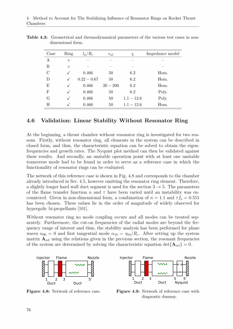
4 Method to Account for The Stabilizing Influence of Resonator Rings on Rocket ThrustChambers
Table 4.3: Geometrical and thermodynamical parameters of the various test cases in non-dimensional form.
Case Ring la/Rc εnl χ Impedance modelA × – – – –B × – – – –C X 0.466 50 6.2 Hom.D X 0.22− 0.67 50 6.2 Hom.E X 0.466 20− 200 6.2 Hom.F X 0.466 50 6.2 Poly.G X 0.466 50 1.1− 12.6 Poly.H X 0.466 50 1.1− 12.6 Hom.
4.6 Validation: Linear Stability Without Resonator Ring
At the beginning, a thrust chamber without resonator ring is investigated for two rea-sons. Firstly, without resonator ring, all elements in the system can be described inclosed form, and thus, the characteristic equation can be solved to obtain the eigen-frequencies and growth rates. The Nyquist plot method can then be validated againstthese results. And secondly, an unstable operation point with at least one unstabletransverse mode had to be found in order to serve as a reference case in which thefunctionality of resonator rings can be evaluated.
The network of this reference case is shown in Fig. 4.8 and corresponds to the chamberalready introduced in Sec. 4.5, however omitting the resonator ring element. Therefore,a slightly longer hard wall duct segment is used for the section 3→ 5. The parametersof the flame transfer function n and τ have been varied until an instability was en-countered. Given in non-dimensional form, a combination of n = 1.1 and τfo = 0.551has been chosen. These values lie in the order of magnitude of widely observed forhypergolic bi-propellants [101].
Without resonator ring no mode coupling occurs and all modes can be treated sep-arately. Furthermore, the cut-on frequencies of the radial modes are beyond the fre-quency range of interest and thus, the stability analysis has been performed for planewaves α00 = 0 and first tangential mode α10 = η10/Rc. After setting up the systemmatrix Aref using the relations given in the previous section, the resonant frequenciesof the system are determined by solving the characteristic equation detAref = 0.
NozzleInjector Flame
Duct Duct21 3 5'
Figure 4.8: Network of reference case.
NozzleInjector Flame
Duct Duct Nyquist21 3 5 5'
Figure 4.9: Network of reference case withdiagnostic dummy.
76
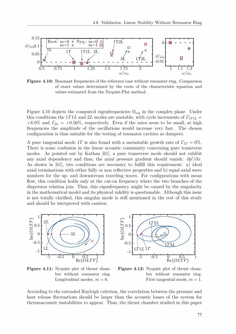
4.6 Validation: Linear Stability Without Resonator Ring
0
0.05
0.1
0.15
0.5 0.75 1 1.25 1.5 1.75 2
ϑ/ωo
ω/ωo
1L 1T 1T1L 2L
1T2L
3L 1T3L -0.01
0
1 1.1 1.2
ϑ/ωo
ω/ωo
1L
1T 1T1L 2L
1T2L
3L 1T3L
Root: m=0m=1
Nyq.: m=0m=1
Figure 4.10: Resonant frequencies of the reference case without resonator ring. Comparisonof exact values determined by the roots of the characteristic equation andvalues estimated from the Nyquist-Plot method.
Figure 4.10 depicts the computed eigenfrequencies Ωeig in the complex plane. Underthis conditions the 1T1L and 2L modes are unstable, with cycle increments of Γ1T1L =+8.0% and Γ2L = +0.56%, respectively. Even if the rates seem to be small, at highfrequencies the amplitude of the oscillations would increase very fast. The chosenconfiguration is thus suitable for the testing of resonator cavities as dampers.
A pure tangential mode 1T is also found with a metastable growth rate of Γ1T = 0%.There is some confusion in the linear acoustic community concerning pure transversemodes. As pointed out by Kathan [61], a pure transverse mode should not exhibitany axial dependency and thus, the axial pressure gradient should vanish: ∂p′/∂x.As shown in [61], two conditions are necessary to fulfill this requirement: a) idealaxial terminations with either fully or non reflective properties and b) equal axial wavenumbers for the up- and downstream traveling waves. For configurations with meanflow, this condition holds only at the cut-on frequency where the two branches of thedispersion relation join. Thus, this eigenfrequency might be caused by the singularityin the mathematical model and its physical validity is questionable. Although this issueis not totally clarified, this singular mode is still mentioned in the rest of this studyand should be interpreted with caution.
-1
-0.5
0
0.5
1
-1 -0.5 0 0.5 1
ImOLTF
ReOLTF
ω
1L
3L
2L
Figure 4.11: Nyquist plot of thrust cham-ber without resonator ring.Longitudinal modes, m = 0.
-1
-0.5
0
0.5
1
-1 -0.5 0 0.5 1
ImOLTF
ReOLTF
ω
1T1T1L
1T2L
1T3L
Figure 4.12: Nyquist plot of thrust cham-ber without resonator ring.First tangential mode, m = 1.
According to the extended Rayleigh criterion, the correlation between the pressure andheat release fluctuations should be larger than the acoustic losses of the system forthermoacoustic instabilities to appear. Thus, the thrust chamber studied in this paper
77
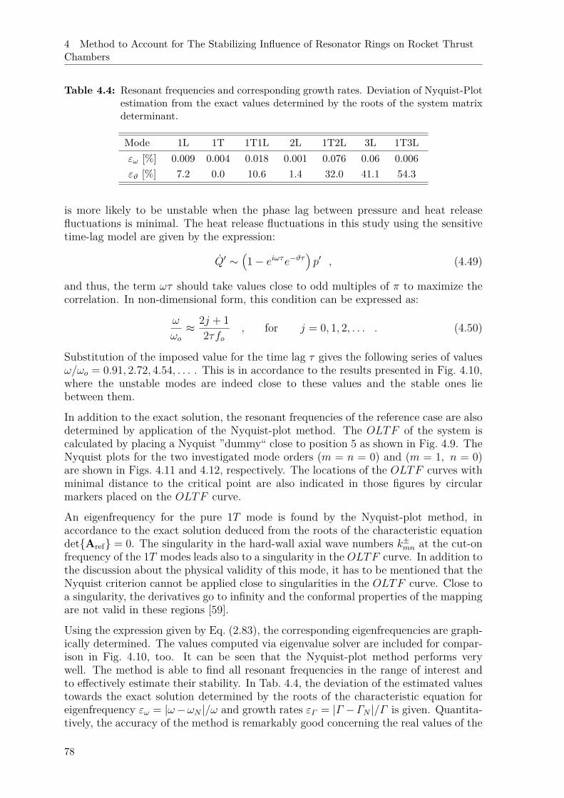
4 Method to Account for The Stabilizing Influence of Resonator Rings on Rocket ThrustChambers
Table 4.4: Resonant frequencies and corresponding growth rates. Deviation of Nyquist-Plotestimation from the exact values determined by the roots of the system matrixdeterminant.
Mode 1L 1T 1T1L 2L 1T2L 3L 1T3Lεω [%] 0.009 0.004 0.018 0.001 0.076 0.06 0.006εϑ [%] 7.2 0.0 10.6 1.4 32.0 41.1 54.3
is more likely to be unstable when the phase lag between pressure and heat releasefluctuations is minimal. The heat release fluctuations in this study using the sensitivetime-lag model are given by the expression:
Q′ ∼(1− eiωτe−ϑτ
)p′ , (4.49)
and thus, the term ωτ should take values close to odd multiples of π to maximize thecorrelation. In non-dimensional form, this condition can be expressed as:
ω
ωo≈ 2j + 1
2τfo, for j = 0, 1, 2, . . . . (4.50)
Substitution of the imposed value for the time lag τ gives the following series of valuesω/ωo = 0.91, 2.72, 4.54, . . . . This is in accordance to the results presented in Fig. 4.10,where the unstable modes are indeed close to these values and the stable ones liebetween them.
In addition to the exact solution, the resonant frequencies of the reference case are alsodetermined by application of the Nyquist-plot method. The OLTF of the system iscalculated by placing a Nyquist ”dummy“ close to position 5 as shown in Fig. 4.9. TheNyquist plots for the two investigated mode orders (m = n = 0) and (m = 1, n = 0)are shown in Figs. 4.11 and 4.12, respectively. The locations of the OLTF curves withminimal distance to the critical point are also indicated in those figures by circularmarkers placed on the OLTF curve.
An eigenfrequency for the pure 1T mode is found by the Nyquist-plot method, inaccordance to the exact solution deduced from the roots of the characteristic equationdetAref = 0. The singularity in the hard-wall axial wave numbers k±mn at the cut-onfrequency of the 1T modes leads also to a singularity in the OLTF curve. In addition tothe discussion about the physical validity of this mode, it has to be mentioned that theNyquist criterion cannot be applied close to singularities in the OLTF curve. Close toa singularity, the derivatives go to infinity and the conformal properties of the mappingare not valid in these regions [59].
Using the expression given by Eq. (2.83), the corresponding eigenfrequencies are graph-ically determined. The values computed via eigenvalue solver are included for compar-ison in Fig. 4.10, too. It can be seen that the Nyquist-plot method performs verywell. The method is able to find all resonant frequencies in the range of interest andto effectively estimate their stability. In Tab. 4.4, the deviation of the estimated valuestowards the exact solution determined by the roots of the characteristic equation foreigenfrequency εω = |ω−ωN |/ω and growth rates εΓ = |Γ −ΓN |/Γ is given. Quantita-tively, the accuracy of the method is remarkably good concerning the real values of the
78
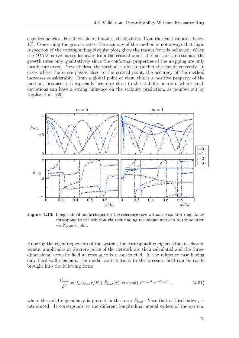
4.6 Validation: Linear Stability Without Resonator Ring
eigenfrequencies. For all considered modes, the deviation from the exact values is below1%. Concerning the growth rates, the accuracy of the method is not always that high.Inspection of the corresponding Nyquist plots gives the reason for this behavior. Whenthe OLTF curve passes far away from the critical point, the method can estimate thegrowth rates only qualitatively since the conformal properties of the mapping are onlylocally preserved. Nevertheless, the method is able to predict the trends correctly. Incases where the curve passes close to the critical point, the accuracy of the methodincreases considerably. From a global point of view, this is a positive property of themethod, because it is especially accurate close to the stability margin, where smalldeviations can have a strong influence on the stability prediction, as pointed out byKopitz et al. [66].
0
0.5
1
Pm0l
m = 0 m = 1
−π
0
π
0 0.2 0.4 0.6 0.8 1
φm0l
x/Lc0 0.2 0.4 0.6 0.8 1
x/Lc
l=0l=1l=2l=3
Figure 4.13: Longitudinal mode shapes for the reference case without resonator ring. Linescorrespond to the solution via root finding technique; markers to the solutionvia Nyquist plot.
Knowing the eigenfrequencies of the system, the corresponding eigenvectors or charac-teristic amplitudes at discrete ports of the network are then calculated and the three-dimensional acoustic field at resonance is reconstructed. In the reference case havingonly hard-wall elements, the modal contributions to the pressure field can be easilybrought into the following form:
p′mnlρc
= Jm(ηmnr/Rc) Pmnl(x) cos(mθ) eiωmnlt e−ϑmnlt , (4.51)
where the axial dependency is present in the term Pmnl. Note that a third index l isintroduced. It corresponds to the different longitudinal modal orders of the system.
79
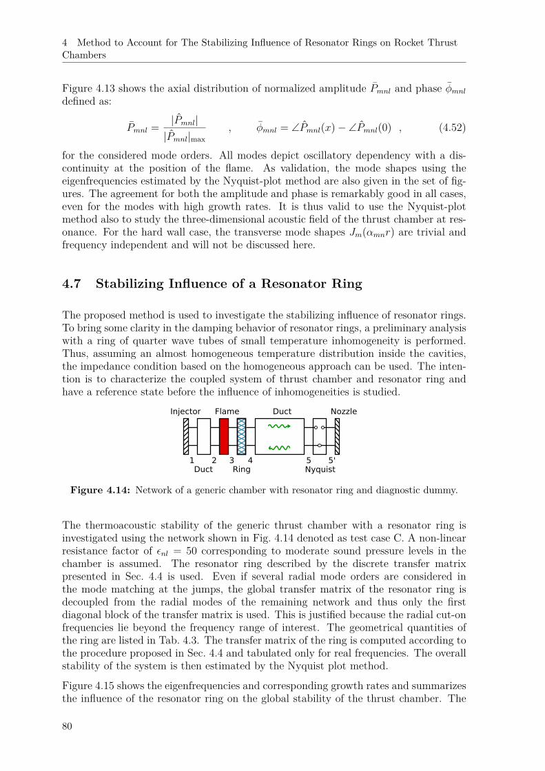
4 Method to Account for The Stabilizing Influence of Resonator Rings on Rocket ThrustChambers
Figure 4.13 shows the axial distribution of normalized amplitude Pmnl and phase φmnldefined as:
Pmnl = |Pmnl||Pmnl|max
, φmnl = ∠Pmnl(x)− ∠Pmnl(0) , (4.52)
for the considered mode orders. All modes depict oscillatory dependency with a dis-continuity at the position of the flame. As validation, the mode shapes using theeigenfrequencies estimated by the Nyquist-plot method are also given in the set of fig-ures. The agreement for both the amplitude and phase is remarkably good in all cases,even for the modes with high growth rates. It is thus valid to use the Nyquist-plotmethod also to study the three-dimensional acoustic field of the thrust chamber at res-onance. For the hard wall case, the transverse mode shapes Jm(αmnr) are trivial andfrequency independent and will not be discussed here.
4.7 Stabilizing Influence of a Resonator Ring
The proposed method is used to investigate the stabilizing influence of resonator rings.To bring some clarity in the damping behavior of resonator rings, a preliminary analysiswith a ring of quarter wave tubes of small temperature inhomogeneity is performed.Thus, assuming an almost homogeneous temperature distribution inside the cavities,the impedance condition based on the homogeneous approach can be used. The inten-tion is to characterize the coupled system of thrust chamber and resonator ring andhave a reference state before the influence of inhomogeneities is studied.
NozzleInjector
Ring
Flame Duct
Duct Nyquist21 3 5 5'4
Figure 4.14: Network of a generic chamber with resonator ring and diagnostic dummy.
The thermoacoustic stability of the generic thrust chamber with a resonator ring isinvestigated using the network shown in Fig. 4.14 denoted as test case C. A non-linearresistance factor of εnl = 50 corresponding to moderate sound pressure levels in thechamber is assumed. The resonator ring described by the discrete transfer matrixpresented in Sec. 4.4 is used. Even if several radial mode orders are considered inthe mode matching at the jumps, the global transfer matrix of the resonator ring isdecoupled from the radial modes of the remaining network and thus only the firstdiagonal block of the transfer matrix is used. This is justified because the radial cut-onfrequencies lie beyond the frequency range of interest. The geometrical quantities ofthe ring are listed in Tab. 4.3. The transfer matrix of the ring is computed according tothe procedure proposed in Sec. 4.4 and tabulated only for real frequencies. The overallstability of the system is then estimated by the Nyquist plot method.
Figure 4.15 shows the eigenfrequencies and corresponding growth rates and summarizesthe influence of the resonator ring on the global stability of the thrust chamber. The
80
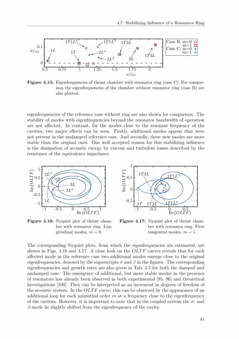
4.7 Stabilizing Influence of a Resonator Ring
0
0.1
0.5 0.75 1 1.25 1.5 1.75 2
ϑ/ωo
ω/ωo
1L 1T
1T1Lβ
2Lβ
1T2L
3L1T3L
1T1Lσ
2Lσ
Case B: m=0m=1
Case C: m=0m=1
Figure 4.15: Eigenfrequencies of thrust chamber with resonator ring (case C). For compar-ison the eigenfrequencies of the chamber without resonator ring (case B) arealso plotted.
eigenfrequencies of the reference case without ring are also shown for comparison. Thestability of modes with eigenfrequencies beyond the resonator bandwidth of operationare not affected. In contrast, for the modes close to the resonant frequency of thecavities, two major effects can be seen. Firstly, additional modes appear that werenot present in the undamped reference case. And secondly, these new modes are morestable than the original ones. One well accepted reason for this stabilizing influenceis the dissipation of acoustic energy by viscous and turbulent losses described by theresistance of the equivalence impedance.
-1
-0.5
0
0.5
1
-1 -0.5 0 0.5 1
ImOLTF
ReOLTF
ω
1L
3L
2Lβ
2Lσ
Figure 4.16: Nyquist plot of thrust cham-ber with resonator ring. Lon-gitudinal modes, m = 0.
-0.5
0
0.5
1
-1 -0.5 0 0.5
ImOLTF
ReOLTF
ω
1T
1T1Lβ1T2L
1T1Lσ1T3L
Figure 4.17: Nyquist plot of thrust cham-ber with resonator ring. Firsttangential modes, m = 1.
The corresponding Nyquist plots, from which the eigenfrequencies are estimated, areshown in Figs. 4.16 and 4.17. A close look on the OLTF curves reveals that for eachaffected mode in the reference case two additional modes emerge close to the originaleigenfrequencies, denoted by the superscripts σ and β in the figures. The correspondingeigenfrequencies and growth rates are also given in Tab. 4.5 for both the damped andundamped case. The emergence of additional, but more stable modes in the presenceof resonators has already been observed in both experimental [95, 96] and theoreticalinvestigations [100]. They can be interpreted as an increment in degrees of freedom ofthe acoustic system. In the OLTF curve, this can be observed by the appearance of anadditional loop for each azimuthal order m at a frequency close to the eigenfrequencyof the cavities. However, it is important to note that in the coupled system the σ- andβ-mode lie slightly shifted from the eigenfrequency of the cavity.
81
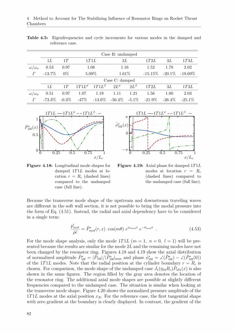
4 Method to Account for The Stabilizing Influence of Resonator Rings on Rocket ThrustChambers
Table 4.5: Eigenfrequencies and cycle increments for various modes in the damped andreference case.
Case B: undamped1L 1T 1T1L 2L 1T2L 3L 1T3L
ω/ωo 0.53 0.97 1.08 1.16 1.52 1.78 2.02Γ -13.7% 0% 5.09% 1.61% -15.15% -20.1% -19.69%
Case C: damped1L 1T 1T1Lσ 1T1Lβ 2Lσ 2Lβ 1T2L 3L 1T3L
ω/ωo 0.51 0.97 1.07 1.19 1.11 1.21 1.56 1.80 2.03Γ -73.3% -0.3% -47% -13.6% -56.4% -5.1% -21.9% -26.4% -25.1%
0
0.5
1
0 0.25 0.5 0.75 1
P ∗10l(x)
x/Lc
1T1L 1T1Lσ 1T1Lβ
Figure 4.18: Longitudinal mode shapes fordamped 1T1L modes at lo-cation r = Rc (dashed lines)compared to the undampedcase (full line).
−π
0
π
0 0.25 0.5 0.75 1
φ∗10l(x)
x/Lc
1T1L 1T1Lσ 1T1Lβ
Figure 4.19: Axial phase for damped 1T1Lmodes at location r = Rc(dashed lines) compared tothe undamped case (full line).
Because the transverse mode shape of the upstream and downstream traveling wavesare different in the soft wall section, it is not possible to bring the modal pressure intothe form of Eq. (4.51). Instead, the radial and axial dependency have to be consideredin a single term:
p′mnlρc
= P ∗mnl(r, x) cos(mθ) eiωmnlt e−ϑmnlt . (4.53)
For the mode shape analysis, only the mode 1T1L (m = 1, n = 0, l = 1) will be pre-sented because the results are similar for the mode 2L and the remaining modes have notbeen changed by the resonator ring. Figures 4.18 and 4.19 show the axial distributionof normalized amplitude P ∗10l = |P10l|/|P ∗10l|max and phase φ∗10l = ∠(P ∗10l) − ∠(P ∗10l(0))of the 1T1L modes. Note that the radial position at the cylinder boundary r = Rc ischosen. For comparison, the mode shape of the undamped case J1(η10Rc)P101(x) is alsoshown in the same figures. The region filled by the gray area denotes the location ofthe resonator ring. The additional axial mode shapes are possible at slightly differentfrequencies compared to the undamped case. The situation is similar when looking atthe transverse mode shape. Figure 4.20 shows the normalized pressure amplitude of the1T1L modes at the axial position xR. For the reference case, the first tangential shapewith zero gradient at the boundary is clearly displayed. In contrast, the gradient of the
82

4.7 Stabilizing Influence of a Resonator Ring
σ and β modes is not zero. At the corresponding slightly lower and higher frequencies,the magnitude of the gradient is equal, once with positive and once with negative step.
To prove the validity of the mode matching conditions, the normalized pressure dis-tribution at one of the jumps is given in Figs. 4.22 and Fig. 4.23. At one of theeigenfrequencies, they show the pressure and radial velocity amplitudes on both sidesof the first jump. The matching condition proposed in this study is capable of handlingthis discontinuity in shell impedance remarkably good. From the figures, it is also clearthat this is only possible if higher radial mode orders are present, even at frequenciesbelow their cut-on. This scattering into higher mode orders can also have an stabilizinginfluence, as shown recently by McAlpine et. al [81], who exploited this mechanism inthe optimization of acoustic liners for noise reduction in aero engines. A detailed anal-ysis of the transport of acoustic energy for both propagating and evanescent modes isgiven by Morfey [85]. He shows that, even though a single evanescent wave is not ableto transport acoustic energy, the interaction between up- and downstream evanescentwaves does actually lead to a non zero transport. This holds even for ducts withoutmean flow. In the literature of resonator rings for rocket thrust chambers, this mech-anism is not mentioned at all yet. The low-order model is capable to handle these3D-effects remarkably good.
Three major stabilizing effects of the resonator rings have been identified:
(i) The eigenfrequencies of the system close to the design point of the cavities areshifted to slightly different frequencies. The coupling between driving mechanismsand acoustic might be weakened in this way.
(ii) Dissipation of acoustic energy by viscous effects described by the real part of theshell impedance stabilizes the system.
(iii) At connecting planes of the resonator ring, the traveling waves are scattered intohigher order, evanescent modes reducing the acoustic energy present in the reso-nant mode.
To further clarify these three mechanisms, a series of parametric studies have beenperformed and the results will be presented in the next subsections. The informationobtained from these parametric studies should serve as a basis for the interpretation offurther results concerning the sensitivity to cavity temperature inhomogeneities causedby EHT.
0
0.5
1
-1 -0.5 0 0.5 1
P10l(r)
r/Rc
1T1L 1T1Lσ 1T1Lβ
Figure 4.20: Normalized Pressure ampli-tude of 1T1L modes at axialposition xR.
−π
0
π
-1 -0.5 0 0.5 1
φ∗10l(r)
r/Rc
1T1L 1T1Lσ 1T1Lβ
Figure 4.21: Phase of 1T1L modes at axialposition xR.
83
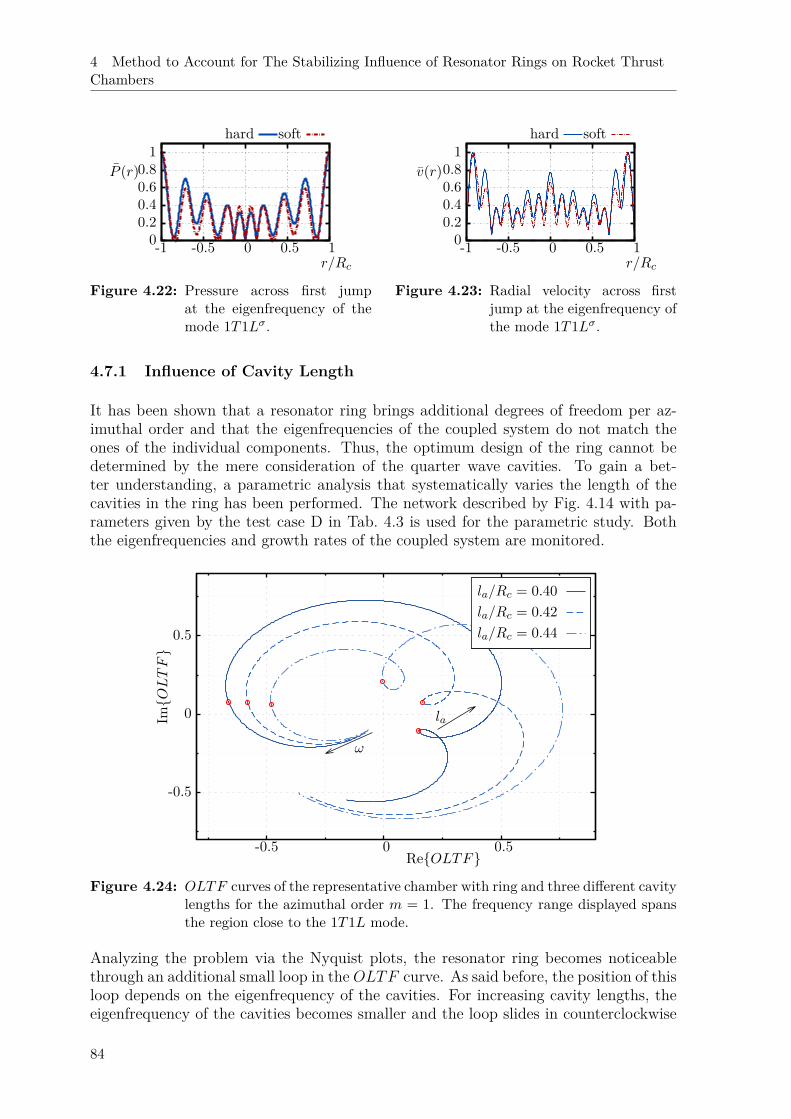
4 Method to Account for The Stabilizing Influence of Resonator Rings on Rocket ThrustChambers
00.20.40.60.8
1
-1 -0.5 0 0.5 1
P (r)
r/Rc
hard soft
Figure 4.22: Pressure across first jumpat the eigenfrequency of themode 1T1Lσ.
00.20.40.60.8
1
-1 -0.5 0 0.5 1
v(r)
r/Rc
hard soft
Figure 4.23: Radial velocity across firstjump at the eigenfrequency ofthe mode 1T1Lσ.
4.7.1 Influence of Cavity Length
It has been shown that a resonator ring brings additional degrees of freedom per az-imuthal order and that the eigenfrequencies of the coupled system do not match theones of the individual components. Thus, the optimum design of the ring cannot bedetermined by the mere consideration of the quarter wave cavities. To gain a bet-ter understanding, a parametric analysis that systematically varies the length of thecavities in the ring has been performed. The network described by Fig. 4.14 with pa-rameters given by the test case D in Tab. 4.3 is used for the parametric study. Boththe eigenfrequencies and growth rates of the coupled system are monitored.
-0.5
0
0.5
-0.5 0 0.5
ImOLTF
ReOLTF
ω
la
la/Rc = 0.40la/Rc = 0.42la/Rc = 0.44
Figure 4.24: OLTF curves of the representative chamber with ring and three different cavitylengths for the azimuthal order m = 1. The frequency range displayed spansthe region close to the 1T1L mode.
Analyzing the problem via the Nyquist plots, the resonator ring becomes noticeablethrough an additional small loop in the OLTF curve. As said before, the position of thisloop depends on the eigenfrequency of the cavities. For increasing cavity lengths, theeigenfrequency of the cavities becomes smaller and the loop slides in counterclockwise
84
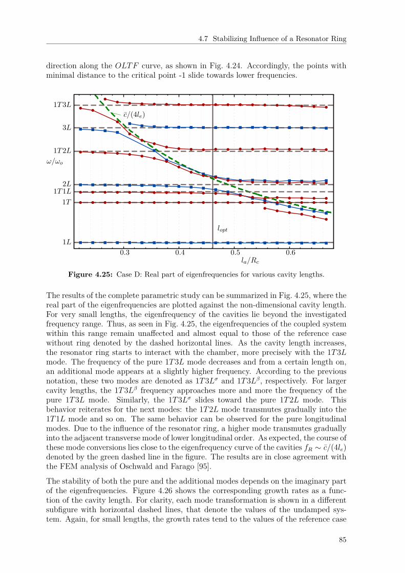
4.7 Stabilizing Influence of a Resonator Ring
direction along the OLTF curve, as shown in Fig. 4.24. Accordingly, the points withminimal distance to the critical point -1 slide towards lower frequencies.
1L
1T1T1L
2L
1T2L
3L
1T3L
0.3 0.4 0.5 0.6
ω/ωo
la/Rc
c/(4le)
lopt
Figure 4.25: Case D: Real part of eigenfrequencies for various cavity lengths.
The results of the complete parametric study can be summarized in Fig. 4.25, where thereal part of the eigenfrequencies are plotted against the non-dimensional cavity length.For very small lengths, the eigenfrequency of the cavities lie beyond the investigatedfrequency range. Thus, as seen in Fig. 4.25, the eigenfrequencies of the coupled systemwithin this range remain unaffected and almost equal to those of the reference casewithout ring denoted by the dashed horizontal lines. As the cavity length increases,the resonator ring starts to interact with the chamber, more precisely with the 1T3Lmode. The frequency of the pure 1T3L mode decreases and from a certain length on,an additional mode appears at a slightly higher frequency. According to the previousnotation, these two modes are denoted as 1T3Lσ and 1T3Lβ, respectively. For largercavity lengths, the 1T3Lβ frequency approaches more and more the frequency of thepure 1T3L mode. Similarly, the 1T3Lσ slides toward the pure 1T2L mode. Thisbehavior reiterates for the next modes: the 1T2L mode transmutes gradually into the1T1L mode and so on. The same behavior can be observed for the pure longitudinalmodes. Due to the influence of the resonator ring, a higher mode transmutes graduallyinto the adjacent transverse mode of lower longitudinal order. As expected, the course ofthese mode conversions lies close to the eigenfrequency curve of the cavities fR ∼ c/(4le)denoted by the green dashed line in the figure. The results are in close agreement withthe FEM analysis of Oschwald and Farago [95].
The stability of both the pure and the additional modes depends on the imaginary partof the eigenfrequencies. Figure 4.26 shows the corresponding growth rates as a func-tion of the cavity length. For clarity, each mode transformation is shown in a differentsubfigure with horizontal dashed lines, that denote the values of the undamped sys-tem. Again, for small lengths, the growth rates tend to the values of the reference case
85
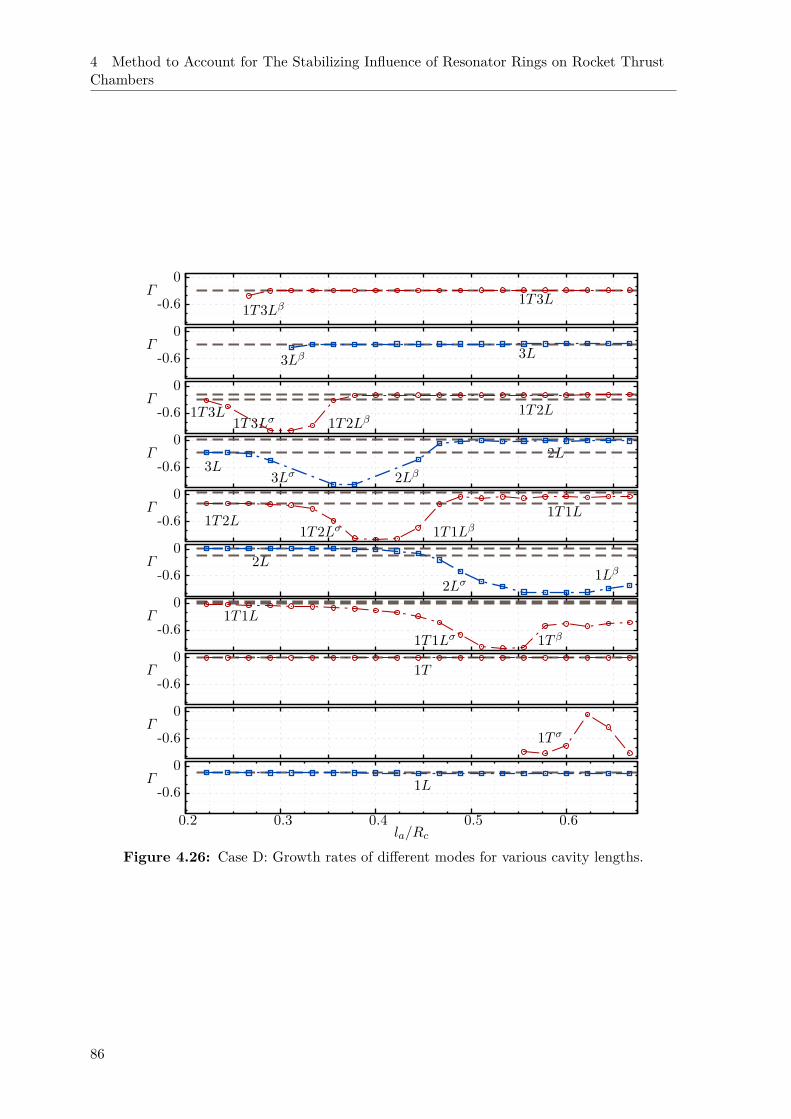
4 Method to Account for The Stabilizing Influence of Resonator Rings on Rocket ThrustChambers
-0.6
0Γ
1T3Lβ1T3L
-0.6
0Γ
3Lβ 3L
-0.6
0Γ
1T3L1T3Lσ 1T2Lβ
1T2L
-0.6
0Γ
3L3Lσ 2Lβ
2L
-0.6
0Γ
1T2L1T2Lσ 1T1Lβ
1T1L
-0.6
0Γ 2L
2Lσ1Lβ
-0.6
0Γ 1T1L
1T1Lσ 1T β
-0.6
0Γ 1T
-0.6
0Γ
1T σ
-0.6
0
0.2 0.3 0.4 0.5 0.6
Γ
la/Rc
1L
Figure 4.26: Case D: Growth rates of different modes for various cavity lengths.
86
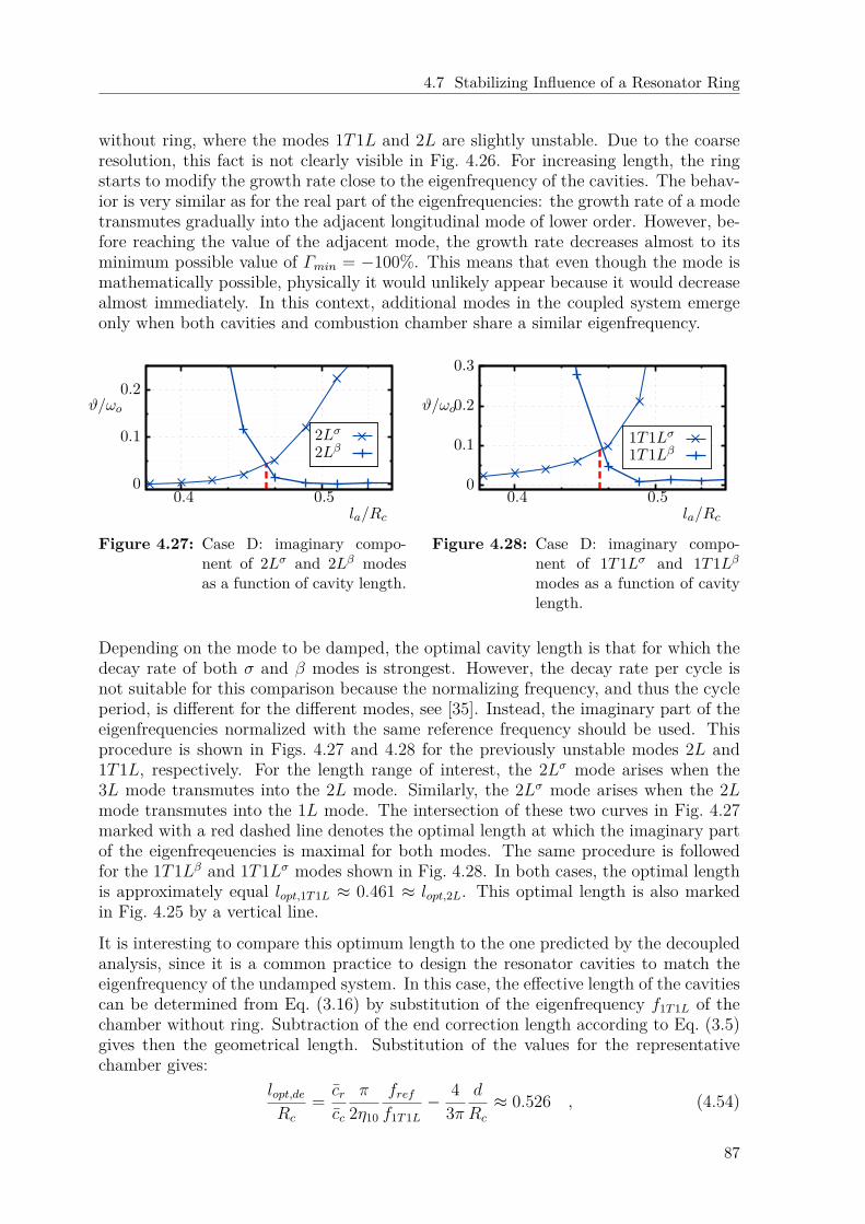
4.7 Stabilizing Influence of a Resonator Ring
without ring, where the modes 1T1L and 2L are slightly unstable. Due to the coarseresolution, this fact is not clearly visible in Fig. 4.26. For increasing length, the ringstarts to modify the growth rate close to the eigenfrequency of the cavities. The behav-ior is very similar as for the real part of the eigenfrequencies: the growth rate of a modetransmutes gradually into the adjacent longitudinal mode of lower order. However, be-fore reaching the value of the adjacent mode, the growth rate decreases almost to itsminimum possible value of Γmin = −100%. This means that even though the mode ismathematically possible, physically it would unlikely appear because it would decreasealmost immediately. In this context, additional modes in the coupled system emergeonly when both cavities and combustion chamber share a similar eigenfrequency.
0
0.1
0.2
0.4 0.5
ϑ/ωo
la/Rc
2Lσ2Lβ
Figure 4.27: Case D: imaginary compo-nent of 2Lσ and 2Lβ modesas a function of cavity length.
0
0.1
0.2
0.3
0.4 0.5
ϑ/ωo
la/Rc
1T1Lσ1T1Lβ
Figure 4.28: Case D: imaginary compo-nent of 1T1Lσ and 1T1Lβmodes as a function of cavitylength.
Depending on the mode to be damped, the optimal cavity length is that for which thedecay rate of both σ and β modes is strongest. However, the decay rate per cycle isnot suitable for this comparison because the normalizing frequency, and thus the cycleperiod, is different for the different modes, see [35]. Instead, the imaginary part of theeigenfrequencies normalized with the same reference frequency should be used. Thisprocedure is shown in Figs. 4.27 and 4.28 for the previously unstable modes 2L and1T1L, respectively. For the length range of interest, the 2Lσ mode arises when the3L mode transmutes into the 2L mode. Similarly, the 2Lσ mode arises when the 2Lmode transmutes into the 1L mode. The intersection of these two curves in Fig. 4.27marked with a red dashed line denotes the optimal length at which the imaginary partof the eigenfreqeuencies is maximal for both modes. The same procedure is followedfor the 1T1Lβ and 1T1Lσ modes shown in Fig. 4.28. In both cases, the optimal lengthis approximately equal lopt,1T1L ≈ 0.461 ≈ lopt,2L. This optimal length is also markedin Fig. 4.25 by a vertical line.
It is interesting to compare this optimum length to the one predicted by the decoupledanalysis, since it is a common practice to design the resonator cavities to match theeigenfrequency of the undamped system. In this case, the effective length of the cavitiescan be determined from Eq. (3.16) by substitution of the eigenfrequency f1T1L of thechamber without ring. Subtraction of the end correction length according to Eq. (3.5)gives then the geometrical length. Substitution of the values for the representativechamber gives:
lopt,deRc
= crcc
π
2η10
freff1T1L
− 43π
d
Rc
≈ 0.526 , (4.54)
87
4 Method to Account for The Stabilizing Influence of Resonator Rings on Rocket ThrustChambers
which is considerably larger than the one determined from the stability of the coupledsystem. From this example it is clear that the coupled system of combustion chamberand damping devices has to be considered in order to optimize resonator cavities.
4.7.2 Influence of Non-Linear Dissipation at the Cavity
In the decoupled analysis, the absorption coefficient has been used to evaluate the effi-ciency of resonator rings. The maximum in absorption occurs at the cavity resonancesand the equivalent resistance plays a decisive role for its magnitude. However, it hasbeen suggested that sound absorption through dissipation is not the only stabilizingmechanism of resonator rings when coupled to the chamber. To bring some insight intothe influence of acoustic dissipation on the efficiency of resonator rings, a parametricstudy that varies the non-linear resistance factor in the impedance expression of thequarter wave cavities has been performed. Test case E in Tab. 4.3 gives the geometricalparameters used in this analysis.
1L
1T1T1L
2L
1T2L
3L
1T3L
50 100 150 200
ω/ωo
εnl
Figure 4.29: Real part of eigenfrequencies for various non-linear resistance factors calculatedfrom test case E.
Figure 4.29 shows the eigenfrequencies of the coupled system as a function of the non-linear resistance factor. Again, the dashed horizontal lines denote the frequencies of theundamped case without ring and serve as reference. For non-linear resistance factorslarger than εnl & 100, the eigenfrequencies of the coupled system are almost equal tothe ones of the undamped case and no additional DOF’s appear. For such high non-linear factors, the resonator ring’s equivalent resistance is large and the cavities areoverdamped. Thus, the soft shell modeling the resonator ring behaves actually morelike a hard boundary. The additional DOF’s appear only for lower resistance valuesof about εnl . 80. Since the cavities’ length for this test case are chosen to mainlyinteract with the 2L and 1T1L modes, these modes are split into β and σ modes ata slightly higher and lower frequencies, respectively. The stability dependency of thecoupled system is given in Fig. 4.30, where the growth rates of the modes are plotted
88
4.7 Stabilizing Influence of a Resonator Ring
against the non-linear factor. As expected, only the growth rates of the 2L and 1T1Lmodes are influenced by the ring.
-0.60
Γ
-0.60
Γ
-0.60
Γ
-0.60
Γ
-0.60
Γ
-0.60
Γ
-0.60
Γ
-0.60
Γ
-0.60
50 100 150 200
Γ
εnl
1T3L
3L
1T2L
2Lβ
1T1Lβ
1T1Lσ
2Lσ
1T
1L
Figure 4.30: Growth rates for various non-linear resistance factors computed from test caseE. Markers denote the damped case, dashed lines the reference values from theundamped case A.
Again, rather than the growth rates, the imaginary part of the eigenfrequencies shouldbe used to estimate the optimal non-linear factor that leads to maximum stabilization.For this purpose, dissipation is given in Figs. 4.31 and 4.32. For large non-linearfactors the system is only barely damped. For lower values, the system stabilizes andthe damping increases, while the additional DOF’s also appear. This trend continuesuntil a maximum is reached in the 2Lσ and 1T1Lσ modes and the imaginary partstarts to decrease again. Thus, at this points the coupled system is optimally dampedfor the given configuration. The optimal values of the non-linear resistance factor areapproximately equal for both modes εnl,opt,2L ≈ εnl,opt,1T1L ≈ 80.
Again, it is interesting to compare this optimal value against the one predicted by thedecoupled analysis. According to Fig. 3.20, the absorption coefficient of the equivalentresonator ring has its maximum of αmax = 1 at a non-linear factor of εnl,opt,de ≈ 140.The value considerably differs from the one determined by the parametric study ofthe coupled system. One major conclusion of this result is that, when consideringthe coupled system of chamber and resonator ring, the strongest stabilization doesnot necessarily occurs when the absorption of the ring is maximum. This means thatthe dissipation of acoustic energy is not the solely stabilization mechanism of resonatorrings. As suggested at the end of Sec. 4.7, the additional stabilization comes from weak-
89

4 Method to Account for The Stabilizing Influence of Resonator Rings on Rocket ThrustChambers
ening the coupling between combustion dynamics and acoustics and from the scatteringof acoustic waves at connecting planes of the resonator ring. These two mechanism arestronger when additional DOF’s appear in the coupled system because then, the eigen-freqeuencies of the additional modes are shifted and their transverse mode shapes differfrom the hard walled modes.
0
0.05
0.1
50 100 150 200
ϑ/fref
εnl
2Lσ2Lβ
Figure 4.31: Imaginary component of 2Lσand 2Lβ modes as a functionof non-linear resistance factorcomputed from test case E.
0
0.1
0.2
0.3
50 100 150 200
ϑ/fref
εnl
1T1Lσ1T1Lβ
Figure 4.32: Imaginary component of1T1Lσ and 1T1Lβ modesas a function of non-linearresistance factor computedfrom test case E.
4.7.3 Influence of Inhomogeneous Temperature Distribution Inside theCavities
In this section, the influence of a moderate cavity temperature inhomogeneity is eval-uated. A simple polynomial temperature profile is assumed along the cavity axis. Forthis purpose, the stability of the coupled system defined by the test case F in Tab. 4.3is estimated using the polynomial approach and the results compared against the onesof test case C using the homogeneous approach.
0
0.1
0.2
0.5 0.75 1 1.25 1.5 1.75 2
ϑ/ωo
ω/ωo
1L 1T
1T1Lβ
2Lβ1T2L
3L1T3L
1T1Lσ
2Lσ
2L1T1L
Case B: m=0m=1
Case C: m=0m=1
Case F: m=0m=1
Figure 4.33: Eigenfrequencies of representative thrust chamber with resonator ring. Com-parison between homogeneous and polynomial approach. Case B, undamped.Case C, damped with homogeneous approach; Case F, damped with polyno-mial approach.
90
4.8 Consequences of EHT on the Damping Behavior of Resonator Rings
The results of this comparison are given in Fig. 4.33, where the normalized eigenfre-quencies of the coupled system are plotted in the complex plane. As a reference, theeigenfrequencies of the undamped case are also given. It can be seen that only theeigenfrequencies close to the resonant frequency of the cavities are affected by the ringin accordance to all previous observations. Furthermore, the appearance of additionalDOF’s is predicted by the two modeling approaches. However, even for this moderateinhomogeneity ratio of χ = 6.2, the eigenfrequencies and growth rates of the systemmodes differ slightly depending on the approach used. Since the same resistance de-pendency is used for the two approaches, the discrepancy can only come from thereactance.
4.8 Consequences of EHT on the Damping Behavior of Res-onator Rings
The previous Sec. 4.7 has validated the low-order method and has demonstrated itsapplicability to qualitatively predict the stability of rocket thrust chambers. For anidealized representative chamber, the stabilizing influence of a resonator ring of thequarter wave type has been described. The influence of some design parameters on thestability of the coupled system has been also estimated. Furthermore, the necessityto account for temperature inhomogeneities inside the cavities has been demonstrated.Based on these findings, the impact of stronger thermal loads in the vicinity of theresonator rings during transient operation (EHT) on their damping behavior and thestability of the coupled system can be now qualitatively predicted.
In Sec. 3.6, an idealized radial temperature distribution has been defined. In this sim-plified temperature distribution, the influence of EHT is qualitatively modeled by anincrease of the chamber wall temperature. This assumed radial temperature distri-bution shown in Fig. 3.12 is used again to estimate the consequences of EHT on thestabilizing influence of resonator rings for the coupled system. Again, the cooling Tcooland combustion temperatures Tcomb are assumed to be constant. Upon the occurrenceof EHT, the cavity mouth temperature Tn is expected to rise to higher values changingboth the cavity’s average temperature Tr and inhomogeneity ratio χ = Tn/Tcool. Onthe chamber side, the change in average chamber temperature due to the higher walltemperature is assumed to be small Tc ≈ const. Table 4.3 gives the geometrical andthermodynamical values used in this test case G.
The stability of the coupled system is monitored within the frequency range of inter-est. The real part of the eigenfrequencies for various inhomogeneity ratios is given inFig. 4.34. For increasing cavity mouth temperature both the inhomogeneity ratio andaverage temperature inside the cavities rise. Thus, the eigenfrequency of the resonatorcavities also increases. According to Fig. 3.15, the eigenfrequency of the cavities canbe approximated by the simple homogeneous approach using the average temperatureinside the cavities given by Eq. (3.16). This approximated dependency fr ≈ cr/(4le) isalso plotted in the figure. The behavior is very similar to the previous observations: ad-ditional DOF’s appear and, as the eigenfrequency of the cavities changes, the modes ofthe coupled system gradually transmute into the adjacent modes of longitudinal order.These transmutations take place close to the approximated cavity resonant curve.
91
4 Method to Account for The Stabilizing Influence of Resonator Rings on Rocket ThrustChambers
1L
1T1T1L
2L
1T2L
3L
1T3L
5 10
ω/ωo
χ
cr/(4le)
Figure 4.34: Real part of eigenfrequencies against the temperature inhomogeneity ratio inthe cavities. Computed using case G.
Accordingly, the growth rates of the coupled system modes shown in Fig. 4.35 decreaseto their minimum value of Γmin = −1 before reaching the value of the adjacent longitu-dinal mode. The conclusions addressed in Sec. 4.7.1 can also be applied here, with thedifference that upon the occurrence of EHT, the equivalent resistance of the resonatorring increases.
To determine how important it is to account for the temperature inhomogeneity in theglobal stability analysis of the representative chamber, the results using the polynomialapproach are compared against those from the simplified homogeneous approach (CaseH). The analysis focus on the previously unstable modes 2L and 1T1L. Again, theimaginary part of the eigenfrequencies is used for the comparison. Figure 4.36 showsthe results of this comparison. For small inhomogeneity ratios, both approaches predictapproximately the same stability margin. The wiggles in the curves at regions of smallinhomogeneity ratio are caused by a singularity in the Nyquist-curve close to the pointsof minimal distance. As explained by Kaess [59], such discontinuities may appear whenportions of the network uncouple from the rest of the system. The discontinuity re-duces the accuracy of the Nyquist-plot method leading for example to such oscillations.Fortunately, the method is still able to predict the trends of the system. For increasinginhomogeneity ratio, the homogeneous approach predicts a larger imaginary part forthe eigenfrequencies. This is especially critical for modes close to neutral stability, asis the case of the 2Lβ and 1T1Lβ. Thus, from the homogeneous approach, the stabilityof the coupled system appears to have a larger stability margin and to be less sensitiveto EHT, while in reality the system is closer to neutral stability. This is in accordanceto the results predicted by the decoupled analysis performed in Sec. 3.6.
92
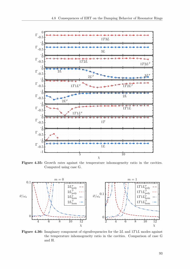
4.8 Consequences of EHT on the Damping Behavior of Resonator Rings
-1-0.5
0Γ
1T3L
-1-0.5
0Γ
3L
-1-0.5
0Γ 1T2L
1T2Lβ
-1-0.5
0Γ 2L
2Lβ 3Lσ
-1-0.5
0Γ 1T1Lσ 1T2Lβ
-1-0.5
0Γ
2Lσ2L
-1-0.5
0Γ
1T1Lσ1T1L
-1-0.5
0Γ 1T
-1-0.5
0Γ
-1-0.5
0
5 10
Γ
χ
1L
Figure 4.35: Growth rates against the temperature inhomogeneity ratio in the cavities.Computed using case G.
0
0.1
4 6 8 10 12
ϑ/ωo
χ
m = 0
2Lσpoly2Lβpoly2Lσhom2Lβhom
0
0.1
2 4 6 8 10 12
ϑ/ωo
χ
m = 1
1T1Lσpoly1T1Lβpoly1T1Lσhom1T1Lβhom
Figure 4.36: Imaginary component of eigenfrequencies for the 2L and 1T1L modes againstthe temperature inhomogeneity ratio in the cavities. Comparison of case Gand H.
93

5 Enhanced Heat Transfer in PulsatingFlows
In devices suffering from self-sustained combustion oscillations, the resulting acous-tic field with periodic pressure and velocity fluctuations has been reported to lead toconsiderably enhanced heat transfer coefficients [29, 49, 99]. In the literature, thesephenomena have been repeatedly reported not only in rocket thrust chambers, but alsoin tail pipe pulse combustors. While the enhancement can be considered as beneficialin the later devices due to the possible reduction of required heat transfer area, theenhancement can actually decrease the performance and reliability of the engine inrocket motors. The higher thermal loads can change the temperature distribution inthe chamber, including the gas inside the resonators used as damping devices. Thedamping behavior of these cavities can degrade due to the different temperature dis-tribution. As demonstrated in Ch. 4, even moderate temperature changes of the gasinside the cavities can lead to the destabilization of the engine. In extreme cases, thereported enhancement has reached such intense values that the thermal integrity ofthe chamber is compromised. It is thus very important to understand the mechanismsleading to this heat transfer enhancement in order to accurately predict the thermalloads under real operating conditions. The literature review given in Sec. 5.1 illustratesthe necessity of additional fundamental research in this area. Yet, it has not been pos-sible to reproduce in theoretical or numerical approaches the higher heat transfer ratesobserved in some striking experiments. Even contradictory results can be found in theliterature, which report enhanced as well as decreased heat transfer.
Of particular interest for the present study is hereby, how far can the periodic transientconditions present in rocket thrust chambers lead to heat transfer enhancement andup to what extent can this modify the temperature distribution in the chamber andthe resonator cavities. The former concerns the thermal integrity of the chamber walls,while the latter the proper design of damping cavities. In the second part of this thesis,a detailed analysis of the problem is given, which tries to clarify these questions. Dueto the complexity of the problem, a divide and conquer strategy presented in Sec. 5.2 isfollowed. Part of the results presented in this chapter have been published previouslyby the author in [15, 32] or are based on the results of supervised student thesis [31].
5.1 Literature Review Concerning Enhanced Heat Transfer inPulsating Flows
In the literature, the phenomenon of enhanced heat transfer in pulsating flows hasbeen reported repeatedly. For the case of rocket motors, Harrje [49] gives an overviewof early observed incidents and argues that, due to the aggressive conditions in thechambers, most of the experimental information is limited and of rather qualitative
95
5 Enhanced Heat Transfer in Pulsating Flows
nature. Under representative conditions, unstable operation does not permit reliablemeasurements and often only a severe hardware damage can be attested. Nevertheless,he listed a few references where some measurements could be achieved leading to arelative heat transfer enhancement ranging from 170% to even 400%. From these earlyqualitative observations, he summarizes that
a) both transverse and longitudinal instabilities of significant amplitude can lead toheat transfer enhancement,
b) the enhancement for transverse modes tends to be stronger, andc) devices operated at lower pressure are more susceptible to higher normalized en-
hancement.
At Princeton University, the heat transfer in oscillating flows driven by acoustic waveshas been studied primarily experimentally by the group of Harrje et al. under idealizedacademic conditions. In a final report [50], Harrje concludes that the heat transferunder periodic unsteady conditions can indeed be considerably higher than in steadystate by more than 100%. The enhancement seems to be maximal close to the velocityantinode of the oscillating modes. Furthermore, the degree of flow reversal plays adecisive role for the enhancement. Viscous dissipation and acoustic streaming appearto be of secondary order for the cases representative of thrust chambers. Harrje suggeststhat an interaction between the oscillations and the turbulent exchange properties offersthe more plausible mechanism that controls the heat transfer enhancement in the flow.
In a laboratory scale, Perry and Culick [99] also studied the overall heat transfer in asolid propellant T-burner triggered to display combustion instabilities. In the presenceof the oscillations, they found a definite heat transfer enhancement proportional to thesquare root of the oscillation amplitudes and the fourth root of the frequency.
Later on, the group of Dec et al. studied the problem experimentally with the help of apulse combustor, which they managed to systematically trigger at various amplitudesand frequencies. The amplitude range was high enough to allow for flow reversal. Ina series of papers [6, 27–29] they measured heat transfer enhancement that locallyincreased by 300%. The novelty compared to the investigations listed before was thatthey were able to perform detailed measurements of velocity, temperature and heat fluxrates. They also share the hypothesis that a combination of increased turbulence at theshear layer and strong convection, driven by transverse flows at times of flow reversal,provide the most plausible explanation for the phenomenon. However, they were notable to explain the mechanism leading to these transverse flows during flow reversal.
While heat transfer enhancement has been experimentally reported several times, theresponsible mechanisms have not been totally clarified yet. Neither in analytical nor innumerical approaches was it possible to reproduce those high enhancement ratios. Def-initely, the large number of effects involved in the process of heat transfer in pulsatingflows makes an accurate simulation difficult, especially in the case of turbulent pulsatingflows. Due to the wide range of perturbation frequencies and the mean flow Reynoldsnumbers used in the different investigations, apparently contradictory arguments canbe found in the literature, with both enhancement and decrease of heat transfer beingreported.
Hemida et al. [51] attempted to clarify these issues with a theoretical analysis of heattransfer in laminar pulsating flow in a tube with constant wall heat flux. They found
96
5.1 Literature Review Concerning Enhanced Heat Transfer in Pulsating Flows
that the local Nusselt number exhibits a spatial modulation along the tube with bothhigher and lower values compared to the stationary case. The perturbations are mostlypresent in the thermally developing region and are damped out further downstream.However, their studies are restricted to pulsating flow without center-line flow reversal.In an experimental study of laminar pulsating pipe flow, Habib et al. [47] studiedthe heat transfer characteristics at various pulsation frequencies. They again foundcases with higher as well as lower Nusselt numbers and confirmed that the effects areprimarily present in the thermally developing region.
In an analytical approach, Lundgren et al. [78] were able to resolve the flow field andheat transfer in pulsating flows in channel configurations including pipe flow. Theytreated the flow field as fully developed and imposed pressure, and velocity gradientsin the axial direction that oscillated harmonically in time. Due to the symmetry oftheir formulation, they solved the governing equations of motions and energy in thetransverse direction. While their study is restricted to laminar flows, they consideredlarge amplitudes with center-line flow reversal. The consideration of an oscillatingaxial temperature gradient is the most important novelty of their study. Qualitatively,their results match the behavior of the experiments performed by Dec et al. very well,displaying second harmonics in the channel bulk temperature modulation. However,the results cannot be compared quantitatively because of the absence of turbulentscales. Nevertheless, the study also demonstrates the possibility of both enhancedand decreased heat transfer depending on the phase between the temperature and thevelocity fluctuations.
One of the strongest limitations faced by CFD based simulations of turbulent pulsatingflows is the required number of cells to properly resolve the turbulent scales. In additionto this, depending on the frequency of the organized motions, large integration timesof several periods are necessary to achieve statistical convergence. For this reasons,DNS investigations are only feasible for academic conditions at low Reynolds numbers.On the other hand, computationally more efficient approaches like URANS generateunclosed terms that have to be modeled. For stationary turbulent flows accurate modelsexist. However, these conventional models fail to properly predict the flow dynamicsin unsteady flows, as shown by Scotti and Piomelli [122]. Thyageswaran intended tosimulate the turbulent flow in a pulse combustor tail pipe [126] and reproduce the highheat transfer rates reported by Dec et al. In order to resolve the whole tail pipe domain,his simulations were based on the use of wall models and URANS. They tested wellestablished wall models, which however failed to reproduce the transient behavior of theheat transfer. They proposed an improved model which was only capable to reproducethe higher heat transfer rates qualitatively. Thus, while the investigation is able toapproximately describe the heat transfer, it does not give insight into the mechanismsleading to the enhancement.
In this context, the trade-off between resolution and computational costs offered by theLES approach can be exploited in the study of turbulent pulsating flows. The validityand advantages of the LES approach to study unsteady problems as turbulent pulsatingflows has been demonstrated by Scotti and Piomelli [121] for a wide range of frequencies.They showed that dynamic sub-grid scale models, which can be seen as state of theart, are capable of modeling accurately the unclosed terms in transient cases, too. Thisis not valid if conventional wall models are used. The near wall region has to be fullyresolved, making the necessity of dynamically adapted coefficients evident. The study
97
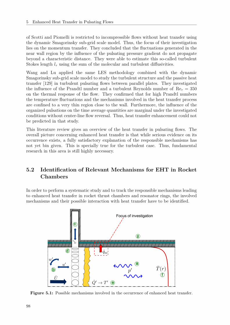
5 Enhanced Heat Transfer in Pulsating Flows
of Scotti and Piomelli is restricted to incompressible flows without heat transfer usingthe dynamic Smagorinsky sub-grid scale model. Thus, the focus of their investigationlies on the momentum transfer. They concluded that the fluctuations generated in thenear wall region by the influence of the pulsating pressure gradient do not propagatebeyond a characteristic distance. They were able to estimate this so-called turbulentStokes length lτ using the sum of the molecular and turbulent diffusivities.
Wang and Lu applied the same LES methodology combined with the dynamicSmagorinsky sub-grid scale model to study the turbulent structure and the passive heattransfer [129] in turbulent pulsating flows between parallel plates. They investigatedthe influence of the Prandtl number and a turbulent Reynolds number of Reτ = 350on the thermal response of the flow. They confirmed that for high Prandtl numbersthe temperature fluctuations and the mechanisms involved in the heat transfer processare confined to a very thin region close to the wall. Furthermore, the influence of theorganized pulsations on the time average quantities are marginal under the investigatedconditions without center-line flow reversal. Thus, heat transfer enhancement could notbe predicted in that study.
This literature review gives an overview of the heat transfer in pulsating flows. Theoverall picture concerning enhanced heat transfer is that while serious evidence on itsoccurrence exists, a fully satisfactory explanation of the responsible mechanisms hasnot yet bin given. This is specially true for the turbulent case. Thus, fundamentalresearch in this area is still highly necessary.
5.2 Identification of Relevant Mechanisms for EHT in RocketChambers
In order to perform a systematic study and to track the responsible mechanisms leadingto enhanced heat transfer in rocket thrust chambers and resonator rings, the involvedmechanisms and their possible interaction with heat transfer have to be identified.
Figure 5.1: Possible mechanisms involved in the occurrence of enhanced heat transfer.
98
5.2 Identification of Relevant Mechanisms for EHT in Rocket Chambers
The situation in the vicinity of the resonator cavities is sketched in Fig. 5.1. A seriesof effects that could interact directly or indirectly with the heat transfer are marked inthis figure with small letters and their description is given in the following list:
a) Acoustic waves: First of all, in rocket chambers, as in the majority of the deviceswhere enhanced heat transfer has been observed, the driving force (mechanism)leading to the periodic oscillations are standing acoustic waves. These waves canhave both longitudinal and transverse mode shapes, and their frequency is given bythe chamber geometry.
b) Pulsating flow: Due to the axial mean flow U , the velocity fluctuations induced bythe acoustic waves present in the thrust chamber lead to a pulsating flow. Dependingon the mode shape of the waves, the pulsating component can be in axial, tangentialand radial direction.
c) Oscillating flow: In contrast, inside the cavities, the velocity fluctuates primarilyin the chamber radial direction (or cavity local axial direction) due to the smalltransverse dimensions of the resonators. Furthermore, a pure oscillating flow isexpected inside the cavities since no purge flow is used in rocket chambers. Asexplained in Sec. 2.5, oscillating flows are quite well understood, see [45, 121].
d) Turbulence: The flow field in the chamber is highly turbulent. At high oscillat-ing amplitudes, jets emerge from the cavity mouths creating a very complex threedimensional flow field at this location.
e) Temperature fluctuations: Due to the coupling between the acoustic field andthe local heat release of the combustion front, it can be expected that temperaturefluctuations also occur.
f) Stratification: The high combustion temperatures coupled with the wall coolinglead to strong temperature gradients especially at the boundary layer. Thus, theflow field is expected to be stratified.
g) Conjugate heat transfer: The thermal inertia of the wall leads to a conjugateheat transfer problem.
This list of effects might be incomplete, but it gives a picture of the complexity exhibitedby an environment representative of rocket thrust chambers. In the second part of thisthesis, the intention is to evaluate the relevance of these effects concerning enhancedheat transfer and to characterize the conditions leading to its occurrence. However,not all effects listed will be handled in the same extent. Emphasis has been put on themost promising ones.
5.2.1 Definition of a Representative Domain
Going directly to the study of heat transfer under real rocket chamber operation con-ditions is not convenient or even feasible. The large number of involved effects andthe complexity exhibited by each one of them would make the characterization un-clear and confusing. The same holds for the different flow regimes at certain locationsin the geometry. Certainly, the flow field close to the resonator cavity mouths is themost complex one due to the jets emerging at high amplitudes. The study of the heattransfer in this region would extend far beyond the goals of the first stage of the tran-sregio TRR40. In contrast, the oscillating flow field inside the cavities is already wellunderstood [45, 46, 121].
99
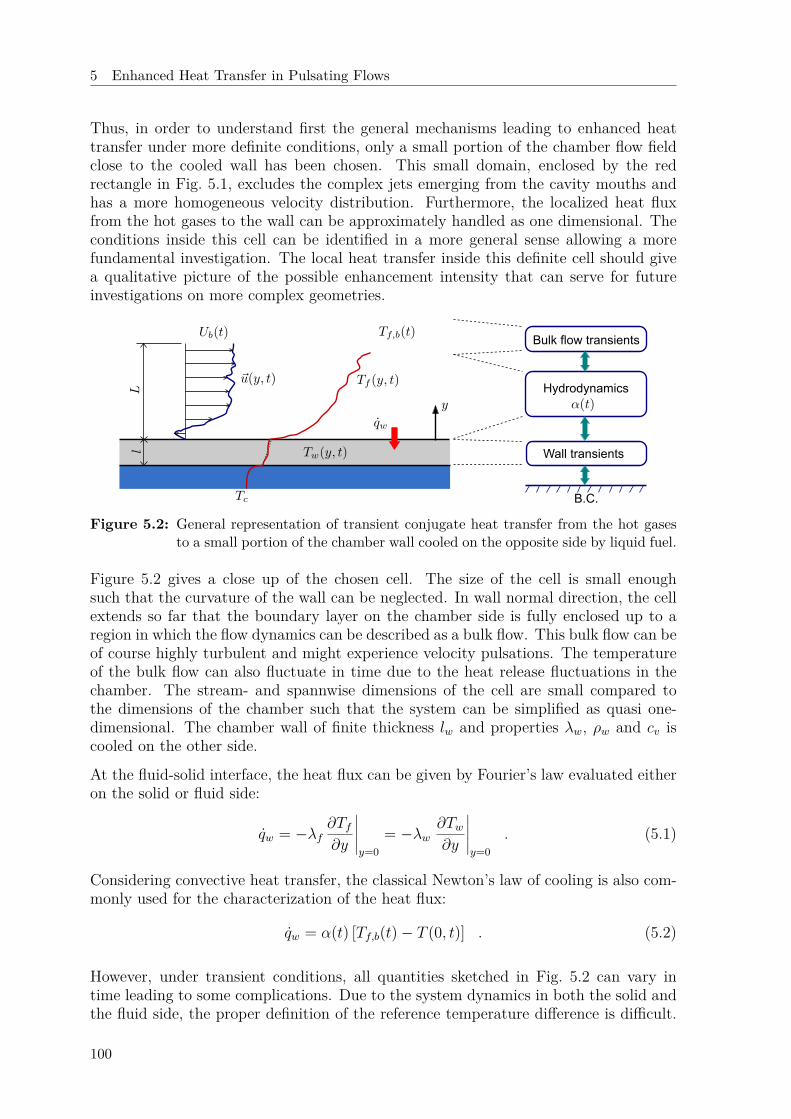
5 Enhanced Heat Transfer in Pulsating Flows
Thus, in order to understand first the general mechanisms leading to enhanced heattransfer under more definite conditions, only a small portion of the chamber flow fieldclose to the cooled wall has been chosen. This small domain, enclosed by the redrectangle in Fig. 5.1, excludes the complex jets emerging from the cavity mouths andhas a more homogeneous velocity distribution. Furthermore, the localized heat fluxfrom the hot gases to the wall can be approximately handled as one dimensional. Theconditions inside this cell can be identified in a more general sense allowing a morefundamental investigation. The local heat transfer inside this definite cell should givea qualitative picture of the possible enhancement intensity that can serve for futureinvestigations on more complex geometries.
Wall transients
Bulk flow transients
Hydrodynamics
B.C.
Figure 5.2: General representation of transient conjugate heat transfer from the hot gasesto a small portion of the chamber wall cooled on the opposite side by liquid fuel.
Figure 5.2 gives a close up of the chosen cell. The size of the cell is small enoughsuch that the curvature of the wall can be neglected. In wall normal direction, the cellextends so far that the boundary layer on the chamber side is fully enclosed up to aregion in which the flow dynamics can be described as a bulk flow. This bulk flow can beof course highly turbulent and might experience velocity pulsations. The temperatureof the bulk flow can also fluctuate in time due to the heat release fluctuations in thechamber. The stream- and spannwise dimensions of the cell are small compared tothe dimensions of the chamber such that the system can be simplified as quasi one-dimensional. The chamber wall of finite thickness lw and properties λw, ρw and cv iscooled on the other side.
At the fluid-solid interface, the heat flux can be given by Fourier’s law evaluated eitheron the solid or fluid side:
qw = −λf∂Tf∂y
∣∣∣∣∣y=0
= −λw∂Tw∂y
∣∣∣∣∣y=0
. (5.1)
Considering convective heat transfer, the classical Newton’s law of cooling is also com-monly used for the characterization of the heat flux:
qw = α(t) [Tf,b(t)− T (0, t)] . (5.2)
However, under transient conditions, all quantities sketched in Fig. 5.2 can vary intime leading to some complications. Due to the system dynamics in both the solid andthe fluid side, the proper definition of the reference temperature difference is difficult.
100
5.2 Identification of Relevant Mechanisms for EHT in Rocket Chambers
From Eq. (5.2), a change in the temperature difference leads also to a change in heattransfer coefficient, even if the net heat flux remains constant. A more striking difficultyarises if the local heat flux at the wall temporarily changes direction due to the systemdynamics. This can lead to temporarily negative heat transfer coefficients, and alsoNusselt numbers [77, 79], which is of course non-physical.
To avoid these complications, the present study follows numerical approaches thatallow the direct computation of the flux via Fourier’s law. Taking these considerationsinto account, the Nusselt number can be subsequently evaluated and used for thequantification of the heat transfer if the following condition is valid at all times:
α = qwL
λf (Tf,b − Tw(0, t)) ≥ 0 . (5.3)
Even if the condition given by Eq. (5.3) holds, care has to be taken when applying anykind of averaging operator for the characterization [134]. Zudin explain this introducinga true heat transfer coefficient:
αtrue =(
qw(t)Tb(t)− Tw(t)
), (5.4)
that can only be determined if all quantities are known at all instants. In contrast, henames the more practicable definition:
αexp =¯qw
(Tb − Tw), (5.5)
as experimental heat transfer coefficient. Depending on the boundary conditions, theratio αtrue/αexp, denoted by Zudin [134] as the factor of conjugation, can take valuesdifferent from unity. This fact is mentioned in this section for completeness since theboundary conditions are left as general as possible. Later on, they will be of courserestricted to specific cases. For simplicity, the true averaging procedure is meant if notspecified.
Concerning the possible rise in heat transfer, a ratio of enhancement is defined com-paring the average heat flux under pulsating conditions and a reference value withoutorganized fluctuations:
EHT =¯qw − qw,ref
qw,ref. (5.6)
Within this convention, positive values denote enhancement while negative values di-minishment.
5.2.2 Strategy
As sketched in Fig. 5.2, the system dynamics have been divided into three major groups:the wall transients due to the thermal inertia, the hydrodynamics of the flow close to thehot side of the wall eventually abstracted into a heat transfer coefficient and finally, thebulk flow transients. On the cold side of the wall, the cold flow is assumed as a constantboundary condition due to the high mass flow rate of the cooling fluid in liquid state.
101
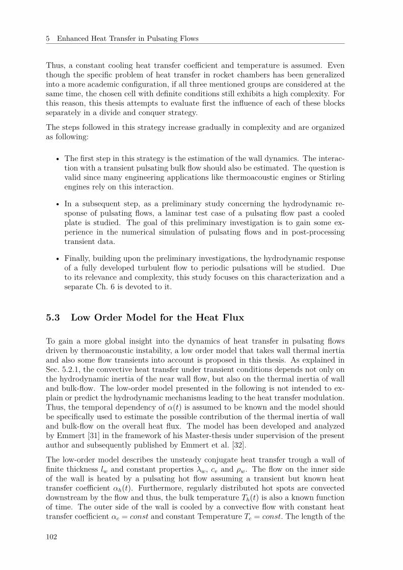
5 Enhanced Heat Transfer in Pulsating Flows
Thus, a constant cooling heat transfer coefficient and temperature is assumed. Eventhough the specific problem of heat transfer in rocket chambers has been generalizedinto a more academic configuration, if all three mentioned groups are considered at thesame time, the chosen cell with definite conditions still exhibits a high complexity. Forthis reason, this thesis attempts to evaluate first the influence of each of these blocksseparately in a divide and conquer strategy.
The steps followed in this strategy increase gradually in complexity and are organizedas following:
• The first step in this strategy is the estimation of the wall dynamics. The interac-tion with a transient pulsating bulk flow should also be estimated. The question isvalid since many engineering applications like thermoacoustic engines or Stirlingengines rely on this interaction.
• In a subsequent step, as a preliminary study concerning the hydrodynamic re-sponse of pulsating flows, a laminar test case of a pulsating flow past a cooledplate is studied. The goal of this preliminary investigation is to gain some ex-perience in the numerical simulation of pulsating flows and in post-processingtransient data.
• Finally, building upon the preliminary investigations, the hydrodynamic responseof a fully developed turbulent flow to periodic pulsations will be studied. Dueto its relevance and complexity, this study focuses on this characterization and aseparate Ch. 6 is devoted to it.
5.3 Low Order Model for the Heat Flux
To gain a more global insight into the dynamics of heat transfer in pulsating flowsdriven by thermoacoustic instability, a low order model that takes wall thermal inertiaand also some flow transients into account is proposed in this thesis. As explained inSec. 5.2.1, the convective heat transfer under transient conditions depends not only onthe hydrodynamic inertia of the near wall flow, but also on the thermal inertia of walland bulk-flow. The low-order model presented in the following is not intended to ex-plain or predict the hydrodynamic mechanisms leading to the heat transfer modulation.Thus, the temporal dependency of α(t) is assumed to be known and the model shouldbe specifically used to estimate the possible contribution of the thermal inertia of walland bulk-flow on the overall heat flux. The model has been developed and analyzedby Emmert [31] in the framework of his Master-thesis under supervision of the presentauthor and subsequently published by Emmert et al. [32].
The low-order model describes the unsteady conjugate heat transfer trough a wall offinite thickness lw and constant properties λw, cv and ρw. The flow on the inner sideof the wall is heated by a pulsating hot flow assuming a transient but known heattransfer coefficient αh(t). Furthermore, regularly distributed hot spots are convecteddownstream by the flow and thus, the bulk temperature Th(t) is also a known functionof time. The outer side of the wall is cooled by a convective flow with constant heattransfer coefficient αc = const and constant Temperature Tc = const. The length of the
102
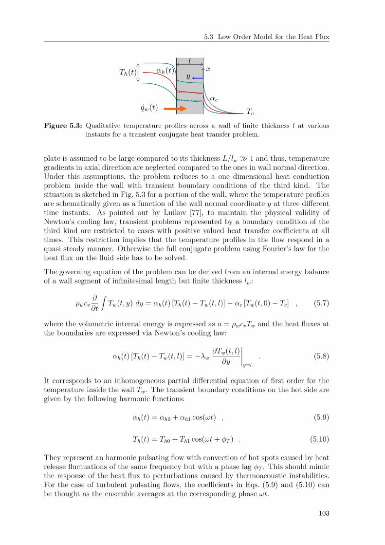
5.3 Low Order Model for the Heat Flux
Figure 5.3: Qualitative temperature profiles across a wall of finite thickness l at variousinstants for a transient conjugate heat transfer problem.
plate is assumed to be large compared to its thickness L/lw 1 and thus, temperaturegradients in axial direction are neglected compared to the ones in wall normal direction.Under this assumptions, the problem reduces to a one dimensional heat conductionproblem inside the wall with transient boundary conditions of the third kind. Thesituation is sketched in Fig. 5.3 for a portion of the wall, where the temperature profilesare schematically given as a function of the wall normal coordinate y at three differenttime instants. As pointed out by Luikov [77], to maintain the physical validity ofNewton’s cooling law, transient problems represented by a boundary condition of thethird kind are restricted to cases with positive valued heat transfer coefficients at alltimes. This restriction implies that the temperature profiles in the flow respond in aquasi steady manner. Otherwise the full conjugate problem using Fourier’s law for theheat flux on the fluid side has to be solved.
The governing equation of the problem can be derived from an internal energy balanceof a wall segment of infinitesimal length but finite thickness lw:
ρwcv∂
∂t
∫Tw(t, y) dy = αh(t) [Th(t)− Tw(t, l)]− αc [Tw(t, 0)− Tc] , (5.7)
where the volumetric internal energy is expressed as u = ρwcvTw and the heat fluxes atthe boundaries are expressed via Newton’s cooling law:
αh(t) [Th(t)− Tw(t, l)] = −λw∂Tw(t, l)∂y
∣∣∣∣∣y=l
. (5.8)
It corresponds to an inhomogeneous partial differential equation of first order for thetemperature inside the wall Tw. The transient boundary conditions on the hot side aregiven by the following harmonic functions:
αh(t) = αh0 + αh1 cos(ωt) , (5.9)
Th(t) = Th0 + Th1 cos(ωt+ φT ) . (5.10)
They represent an harmonic pulsating flow with convection of hot spots caused by heatrelease fluctuations of the same frequency but with a phase lag φT . This should mimicthe response of the heat flux to perturbations caused by thermoacoustic instabilities.For the case of turbulent pulsating flows, the coefficients in Eqs. (5.9) and (5.10) canbe thought as the ensemble averages at the corresponding phase ωt.
103
5 Enhanced Heat Transfer in Pulsating Flows
For generality, after substitution of the time dependent boundary conditions, and usingthe following set of non-dimensional parameters:
ξ = y
l, ϑ = T − Tc
Th0 − Tc, θ = Th0
Th0 − Tc, εα = αh1
αh0, εT = Th1
Th0,
αh = αh0
αh0 + αc, αc = αc
αh0 + αc, τ = αh0(1 + εα)
ρwcvlwt , (5.11)
Eq. (5.7) can be non-dimensionalized as:
[1 + εα] ∂∂t
∫ϑ(τ, ξ) dξ = αh [1 + εα cos(ωτ)] [εT θ cos(ωτ + φT )− ϑ(τ, 1) + 1]
−αcϑ(τ, 0) .(5.12)
Note that θ is a non-dimensional parameter fixed by a given problem, while ϑ corre-sponds to the time and location dependent variable. The resulting non-dimensionalfrequency:
ω = ρwcvlwαh0 [1 + εα]ω ∼
1Fo Bih [1 + εα] (5.13)
corresponds to the ratio of oscillation period to a characteristic time of the unit im-pulse response of the temperature distribution [105]. This choice is important becauseit makes clear whether the oscillation frequency is large or small compared to the tran-sients in the wall. To clarify this, consider first the steady state problem. In thiscase, the wall temperature profile is linear and the relation between the left and righttemperatures is given by:
ϑ(1) = Bih + ϑ(0)1 + Bih
, (5.14)
where the Biot number on the hot side Bih = αh0lw/λw is taken as the controlling pa-rameter. The simplification into a lumped capacity, in which the temperature gradientsinside the wall are assumed to be negligible, is valid for small Biot numbers Bih . 0.2[105]. In addition, if the ratio of heat transfer coefficients is small Γα = αh/αc 1,then the wall temperature can be assumed as constant ϑ ≈ 0. The wall transientscan be completely neglected and an ideal BC of the first kind can be used for thehydrodynamic problem.
For transient periodic cases, the two just mentioned conditions are necessary but notsufficient for the same simplification. It has to be additionally ensured that the periodof oscillation is large enough so the whole wall can respond to the new boundarycondition as sketched in Fig. 5.3 by the horizontal dashed lines. Emmert et al. decidedto approximate the sinusoidal excitation by a square wave signal and compare thecharacteristic time of the step response to one fourth of the excitation period tcrit ≈1/(8πω). The step response of a plate under the lumped capacity approximation to asudden change in temperature ϑstep can be given by the following relation:
ϑ(t)− ϑrefϑstep − ϑref
= e−αh0(1+εα)ρwcvlw
t = e−τ . (5.15)
Here, a conservative simplification using the maximum heat transfer coefficient αh0(1+εα) has been applied. To find the threshold value, the specification of a 90% responseis used as the critical time scale under pulsating conditions:
0.1 = e−τcrit → τcrit = − ln(0.1) . (5.16)
104
5.3 Low Order Model for the Heat Flux
This leads to the following threshold value for the non-dimensional frequency:
ωcrit = 2π− ln(0.1) ≈ 0.87π . (5.17)
Thus, in order to estimate the importance of the wall transients in the overall dynamicsystem these three parameters can be used. If the following three conditions:
Bih 1 & Γα 1 & ω . 0.87π , (5.18)
hold, the wall transients are negligible and an ideal BC of the first kind can also beapplied for transient problems. For rocket chambers, these three conditions are mostlyvalid.
In addition, Emmert studied two cases of increasing complexity in which wall transientsdo occur [31]. The first one allows wall transients assuming a finite ratio Γα 0,but treating the wall as a lumped capacity ω < 0.87π and Bih 1. Under theseassumptions, Eq. (5.12) reduces to a simple inhomogeneous differential equation offirst order:
[1 + εα] dϑwdτ
+ [1 + εααh cos(ωτ)]ϑw =
αh [1 + εα cos(ωτ) + εT θ cos(ωτ + φT )] + αhεαεT θ
2 [cos(2ωτ + φT ) + cos(φT )] ,(5.19)
where the trigonometric functions have been expanded using the identity:
cos(ωτ) cos(ωτ + φT ) = 12 [cos(2ωτ + φT ) + cos(φT )] . (5.20)
Note also that αh +αc = 1. Three important features concerning the system dynamicscan already be identified: Firstly, due to the oscillations of heat transfer coefficient onthe hot side, the differential equation is non-linear with time dependent coefficients.Secondly, the response of the system will also display higher harmonics due to the termoscillating with the frequency 2ω in the inhomogeneous part. And thirdly, the averagewall value will be offset by the time independent term ∼ εαεT cos(φT ). Concerningenhanced heat transfer, the third conclusion is definitely the most important one. Itimplies that the unsteadiness will induce a permanent, time independent change onlywhen both the temperature and the heat transfer coefficient fluctuate. Furthermore,this permanent change can be positive or negative, depending on the relative phasebetween these oscillations leading either to heat transfer enhancement or diminishment.The concordance between these observations and the results of Lundgren et al. [78] forthe heat transfer in pulsating pipe flow are remarkably good.
Before analyzing the temporal evolution of the heat transfer, important conclusionscan be developed concerning the long time average solution. The permanent changesin overall heat transfer, can be estimated by averaging Eq. (5.19) over an oscillatingperiod after the homogeneous solution vanishes. As shown by Emmert et al. [32] thetransient term on the left-hand side vanishes due to the periodicity of the solution. Thesame holds for all harmonic terms of the inhomogeneous part and only the time inde-pendent terms are retained. Denoting this long time average operator by an overbar,the averaged equation can be written as:
(1 + εα)ϑw + αhεαcos(ωτ)ϑw = αh + αhεαεT θ
2 cos(φ) . (5.21)
105
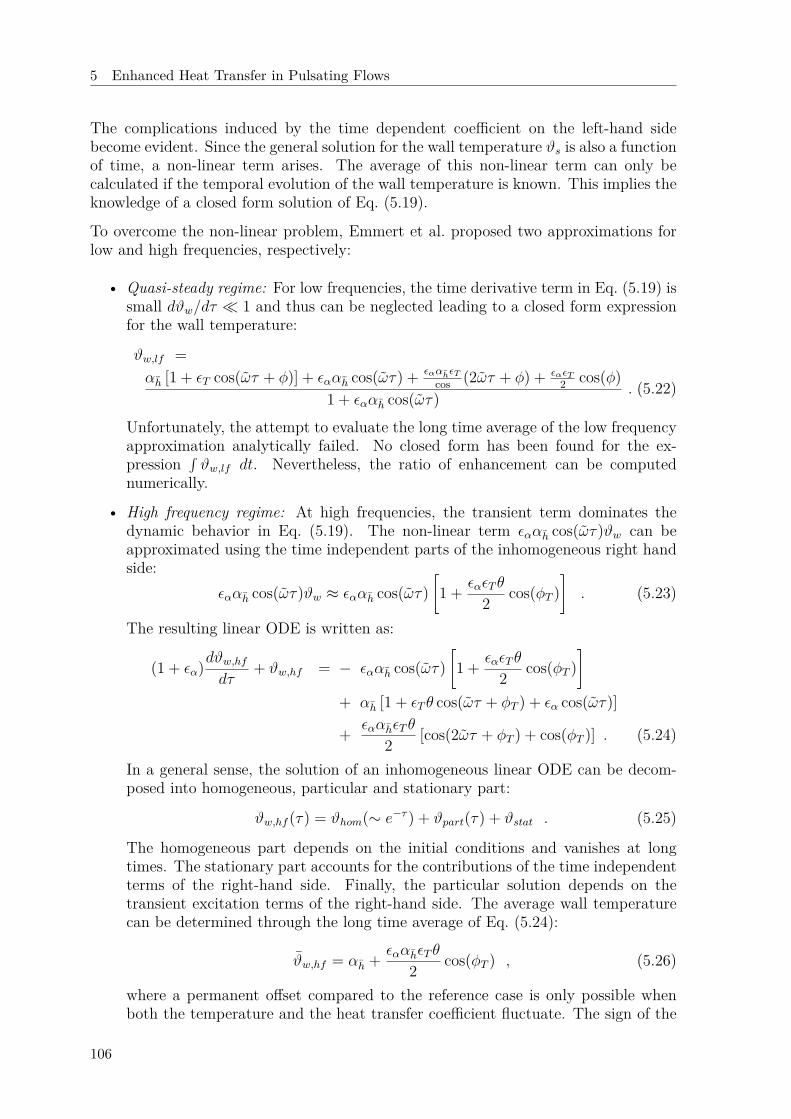
5 Enhanced Heat Transfer in Pulsating Flows
The complications induced by the time dependent coefficient on the left-hand sidebecome evident. Since the general solution for the wall temperature ϑs is also a functionof time, a non-linear term arises. The average of this non-linear term can only becalculated if the temporal evolution of the wall temperature is known. This implies theknowledge of a closed form solution of Eq. (5.19).
To overcome the non-linear problem, Emmert et al. proposed two approximations forlow and high frequencies, respectively:
• Quasi-steady regime: For low frequencies, the time derivative term in Eq. (5.19) issmall dϑw/dτ 1 and thus can be neglected leading to a closed form expressionfor the wall temperature:
ϑw,lf =αh [1 + εT cos(ωτ + φ)] + εααh cos(ωτ) + εααhεT
cos (2ωτ + φ) + εαεT2 cos(φ)
1 + εααh cos(ωτ) . (5.22)
Unfortunately, the attempt to evaluate the long time average of the low frequencyapproximation analytically failed. No closed form has been found for the ex-pression
∫ϑw,lf dt. Nevertheless, the ratio of enhancement can be computed
numerically.
• High frequency regime: At high frequencies, the transient term dominates thedynamic behavior in Eq. (5.19). The non-linear term εααh cos(ωτ)ϑw can beapproximated using the time independent parts of the inhomogeneous right handside:
εααh cos(ωτ)ϑw ≈ εααh cos(ωτ)[1 + εαεT θ
2 cos(φT )]
. (5.23)
The resulting linear ODE is written as:
(1 + εα)dϑw,hfdτ
+ ϑw,hf = − εααh cos(ωτ)[1 + εαεT θ
2 cos(φT )]
+ αh [1 + εT θ cos(ωτ + φT ) + εα cos(ωτ)]
+ εααhεT θ
2 [cos(2ωτ + φT ) + cos(φT )] . (5.24)
In a general sense, the solution of an inhomogeneous linear ODE can be decom-posed into homogeneous, particular and stationary part:
ϑw,hf (τ) = ϑhom(∼ e−τ ) + ϑpart(τ) + ϑstat . (5.25)
The homogeneous part depends on the initial conditions and vanishes at longtimes. The stationary part accounts for the contributions of the time independentterms of the right-hand side. Finally, the particular solution depends on thetransient excitation terms of the right-hand side. The average wall temperaturecan be determined through the long time average of Eq. (5.24):
ϑw,hf = αh + εααhεT θ
2 cos(φT ) , (5.26)
where a permanent offset compared to the reference case is only possible whenboth the temperature and the heat transfer coefficient fluctuate. The sign of the
106
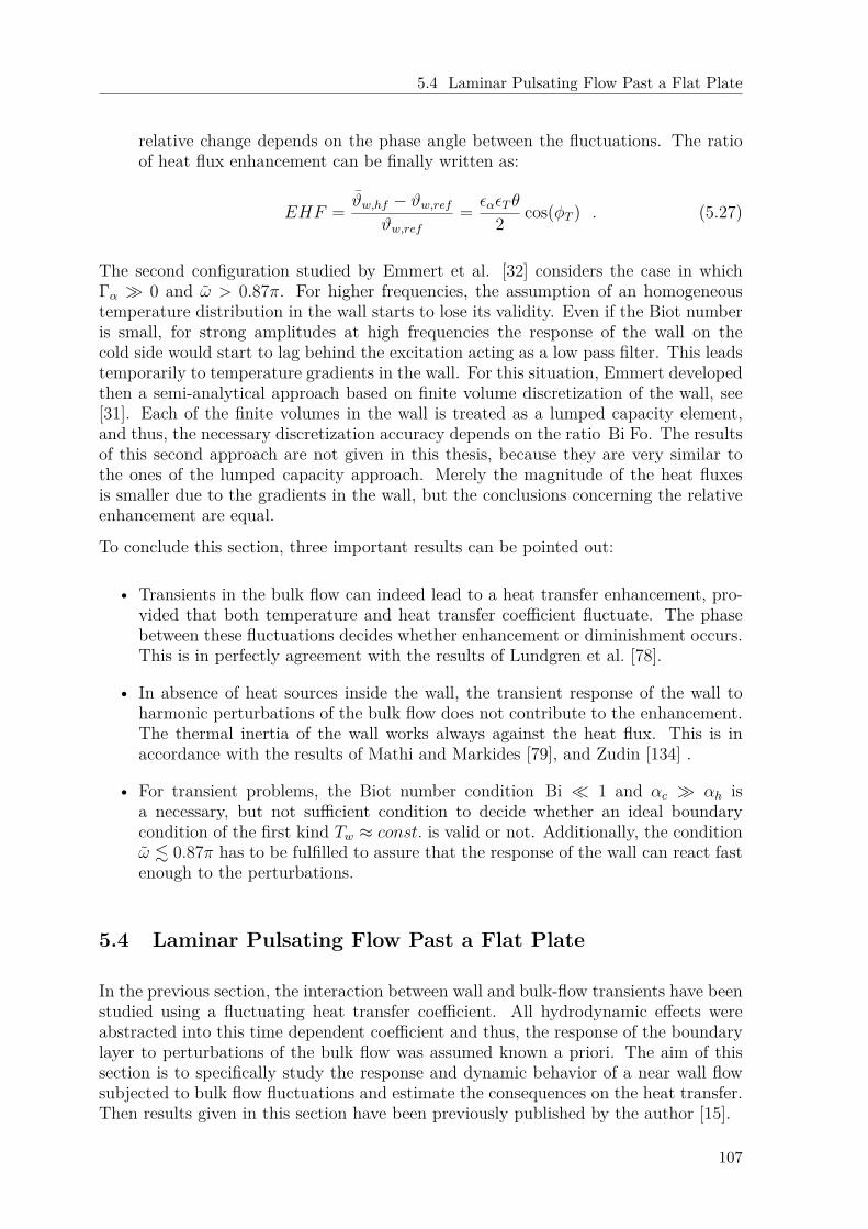
5.4 Laminar Pulsating Flow Past a Flat Plate
relative change depends on the phase angle between the fluctuations. The ratioof heat flux enhancement can be finally written as:
EHF = ϑw,hf − ϑw,refϑw,ref
= εαεT θ
2 cos(φT ) . (5.27)
The second configuration studied by Emmert et al. [32] considers the case in whichΓα 0 and ω > 0.87π. For higher frequencies, the assumption of an homogeneoustemperature distribution in the wall starts to lose its validity. Even if the Biot numberis small, for strong amplitudes at high frequencies the response of the wall on thecold side would start to lag behind the excitation acting as a low pass filter. This leadstemporarily to temperature gradients in the wall. For this situation, Emmert developedthen a semi-analytical approach based on finite volume discretization of the wall, see[31]. Each of the finite volumes in the wall is treated as a lumped capacity element,and thus, the necessary discretization accuracy depends on the ratio Bi Fo. The resultsof this second approach are not given in this thesis, because they are very similar tothe ones of the lumped capacity approach. Merely the magnitude of the heat fluxesis smaller due to the gradients in the wall, but the conclusions concerning the relativeenhancement are equal.
To conclude this section, three important results can be pointed out:
• Transients in the bulk flow can indeed lead to a heat transfer enhancement, pro-vided that both temperature and heat transfer coefficient fluctuate. The phasebetween these fluctuations decides whether enhancement or diminishment occurs.This is in perfectly agreement with the results of Lundgren et al. [78].
• In absence of heat sources inside the wall, the transient response of the wall toharmonic perturbations of the bulk flow does not contribute to the enhancement.The thermal inertia of the wall works always against the heat flux. This is inaccordance with the results of Mathi and Markides [79], and Zudin [134] .
• For transient problems, the Biot number condition Bi 1 and αc αh isa necessary, but not sufficient condition to decide whether an ideal boundarycondition of the first kind Tw ≈ const. is valid or not. Additionally, the conditionω . 0.87π has to be fulfilled to assure that the response of the wall can react fastenough to the perturbations.
5.4 Laminar Pulsating Flow Past a Flat Plate
In the previous section, the interaction between wall and bulk-flow transients have beenstudied using a fluctuating heat transfer coefficient. All hydrodynamic effects wereabstracted into this time dependent coefficient and thus, the response of the boundarylayer to perturbations of the bulk flow was assumed known a priori. The aim of thissection is to specifically study the response and dynamic behavior of a near wall flowsubjected to bulk flow fluctuations and estimate the consequences on the heat transfer.Then results given in this section have been previously published by the author [15].
107
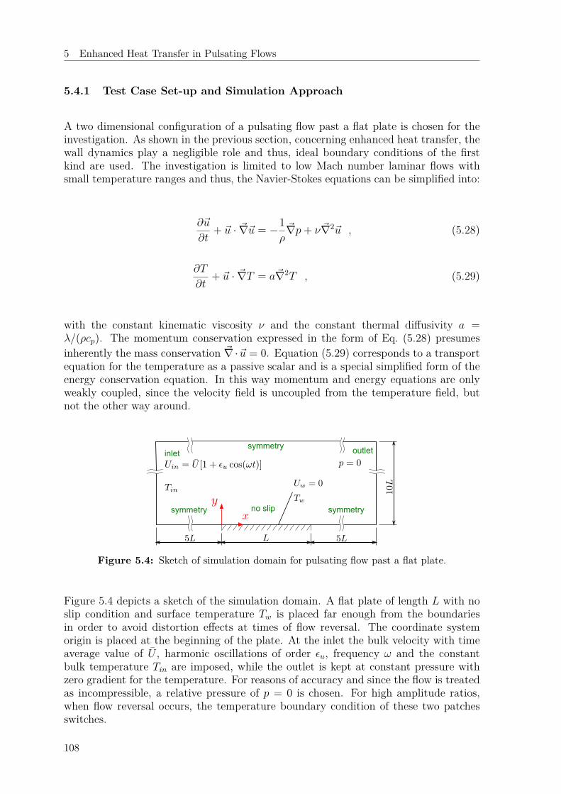
5 Enhanced Heat Transfer in Pulsating Flows
5.4.1 Test Case Set-up and Simulation Approach
A two dimensional configuration of a pulsating flow past a flat plate is chosen for theinvestigation. As shown in the previous section, concerning enhanced heat transfer, thewall dynamics play a negligible role and thus, ideal boundary conditions of the firstkind are used. The investigation is limited to low Mach number laminar flows withsmall temperature ranges and thus, the Navier-Stokes equations can be simplified into:
∂~u
∂t+ ~u · ~∇~u = −1
ρ~∇p+ ν ~∇2~u , (5.28)
∂T
∂t+ ~u · ~∇T = a~∇2T , (5.29)
with the constant kinematic viscosity ν and the constant thermal diffusivity a =λ/(ρcp). The momentum conservation expressed in the form of Eq. (5.28) presumesinherently the mass conservation ~∇·~u = 0. Equation (5.29) corresponds to a transportequation for the temperature as a passive scalar and is a special simplified form of theenergy conservation equation. In this way momentum and energy equations are onlyweakly coupled, since the velocity field is uncoupled from the temperature field, butnot the other way around.
symmetry no slip
inlet outlet
symmetry
symmetry
Figure 5.4: Sketch of simulation domain for pulsating flow past a flat plate.
Figure 5.4 depicts a sketch of the simulation domain. A flat plate of length L with noslip condition and surface temperature Tw is placed far enough from the boundariesin order to avoid distortion effects at times of flow reversal. The coordinate systemorigin is placed at the beginning of the plate. At the inlet the bulk velocity with timeaverage value of U , harmonic oscillations of order εu, frequency ω and the constantbulk temperature Tin are imposed, while the outlet is kept at constant pressure withzero gradient for the temperature. For reasons of accuracy and since the flow is treatedas incompressible, a relative pressure of p = 0 is chosen. For high amplitude ratios,when flow reversal occurs, the temperature boundary condition of these two patchesswitches.
108
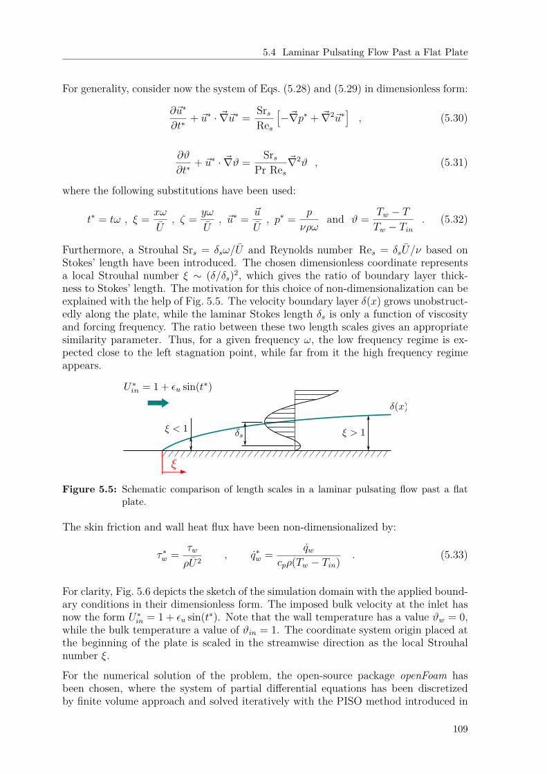
5.4 Laminar Pulsating Flow Past a Flat Plate
For generality, consider now the system of Eqs. (5.28) and (5.29) in dimensionless form:
∂~u∗
∂t∗+ ~u∗ · ~∇~u∗ = Srs
Res
[−~∇p∗ + ~∇2~u∗
], (5.30)
∂ϑ
∂t∗+ ~u∗ · ~∇ϑ = Srs
Pr Res~∇2ϑ , (5.31)
where the following substitutions have been used:
t∗ = tω , ξ = xω
U, ζ = yω
U, ~u∗ = ~u
U, p∗ = p
νρωand ϑ = Tw − T
Tw − Tin. (5.32)
Furthermore, a Strouhal Srs = δsω/U and Reynolds number Res = δsU/ν based onStokes’ length have been introduced. The chosen dimensionless coordinate representsa local Strouhal number ξ ∼ (δ/δs)2, which gives the ratio of boundary layer thick-ness to Stokes’ length. The motivation for this choice of non-dimensionalization can beexplained with the help of Fig. 5.5. The velocity boundary layer δ(x) grows unobstruct-edly along the plate, while the laminar Stokes length δs is only a function of viscosityand forcing frequency. The ratio between these two length scales gives an appropriatesimilarity parameter. Thus, for a given frequency ω, the low frequency regime is ex-pected close to the left stagnation point, while far from it the high frequency regimeappears.
Figure 5.5: Schematic comparison of length scales in a laminar pulsating flow past a flatplate.
The skin friction and wall heat flux have been non-dimensionalized by:
τ ∗w = τw
ρU2, q∗w = qw
cpρ(Tw − Tin) . (5.33)
For clarity, Fig. 5.6 depicts the sketch of the simulation domain with the applied bound-ary conditions in their dimensionless form. The imposed bulk velocity at the inlet hasnow the form U∗in = 1 + εu sin(t∗). Note that the wall temperature has a value ϑw = 0,while the bulk temperature a value of ϑin = 1. The coordinate system origin placed atthe beginning of the plate is scaled in the streamwise direction as the local Strouhalnumber ξ.
For the numerical solution of the problem, the open-source package openFoam hasbeen chosen, where the system of partial differential equations has been discretizedby finite volume approach and solved iteratively with the PISO method introduced in
109
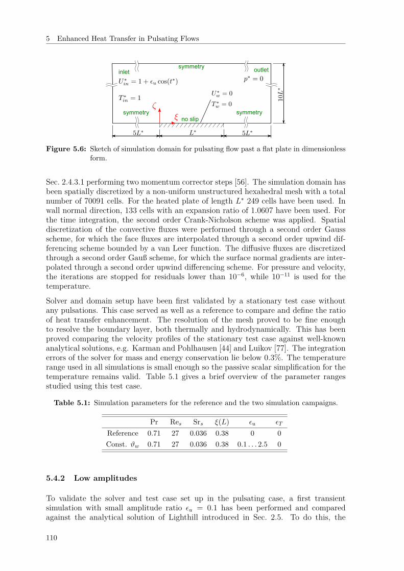
5 Enhanced Heat Transfer in Pulsating Flows
symmetryno slip
inlet outlet
symmetry
symmetry
Figure 5.6: Sketch of simulation domain for pulsating flow past a flat plate in dimensionlessform.
Sec. 2.4.3.1 performing two momentum corrector steps [56]. The simulation domain hasbeen spatially discretized by a non-uniform unstructured hexahedral mesh with a totalnumber of 70091 cells. For the heated plate of length L∗ 249 cells have been used. Inwall normal direction, 133 cells with an expansion ratio of 1.0607 have been used. Forthe time integration, the second order Crank-Nicholson scheme was applied. Spatialdiscretization of the convective fluxes were performed through a second order Gaussscheme, for which the face fluxes are interpolated through a second order upwind dif-ferencing scheme bounded by a van Leer function. The diffusive fluxes are discretizedthrough a second order Gauß scheme, for which the surface normal gradients are inter-polated through a second order upwind differencing scheme. For pressure and velocity,the iterations are stopped for residuals lower than 10−6, while 10−11 is used for thetemperature.
Solver and domain setup have been first validated by a stationary test case withoutany pulsations. This case served as well as a reference to compare and define the ratioof heat transfer enhancement. The resolution of the mesh proved to be fine enoughto resolve the boundary layer, both thermally and hydrodynamically. This has beenproved comparing the velocity profiles of the stationary test case against well-knownanalytical solutions, e.g. Karman and Pohlhausen [44] and Luikov [77]. The integrationerrors of the solver for mass and energy conservation lie below 0.3%. The temperaturerange used in all simulations is small enough so the passive scalar simplification for thetemperature remains valid. Table 5.1 gives a brief overview of the parameter rangesstudied using this test case.
Table 5.1: Simulation parameters for the reference and the two simulation campaigns.
Pr Res Srs ξ(L) εu εT
Reference 0.71 27 0.036 0.38 0 0Const. ϑw 0.71 27 0.036 0.38 0.1 . . . 2.5 0
5.4.2 Low amplitudes
To validate the solver and test case set up in the pulsating case, a first transientsimulation with small amplitude ratio εu = 0.1 has been performed and comparedagainst the analytical solution of Lighthill introduced in Sec. 2.5. To do this, the
110
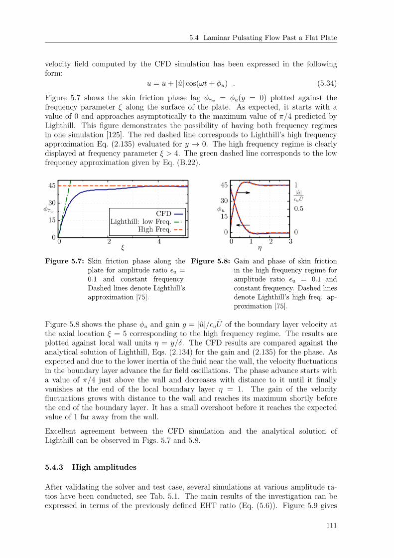
5.4 Laminar Pulsating Flow Past a Flat Plate
velocity field computed by the CFD simulation has been expressed in the followingform:
u = u+ |u| cos(ωt+ φu) . (5.34)
Figure 5.7 shows the skin friction phase lag φτw = φu(y = 0) plotted against thefrequency parameter ξ along the surface of the plate. As expected, it starts with avalue of 0 and approaches asymptotically to the maximum value of π/4 predicted byLighthill. This figure demonstrates the possibility of having both frequency regimesin one simulation [125]. The red dashed line corresponds to Lighthill’s high frequencyapproximation Eq. (2.135) evaluated for y → 0. The high frequency regime is clearlydisplayed at frequency parameter ξ > 4. The green dashed line corresponds to the lowfrequency approximation given by Eq. (B.22).
0
15
30
45
0 2 4
φτw
ξ
CFDLighthill: low Freq.
High Freq.
Figure 5.7: Skin friction phase along theplate for amplitude ratio εu =0.1 and constant frequency.Dashed lines denote Lighthill’sapproximation [75].
0
15
30
45
0 1 2 30
0.5
1
φu
|u|εuU
η
Figure 5.8: Gain and phase of skin frictionin the high frequency regime foramplitude ratio εu = 0.1 andconstant frequency. Dashed linesdenote Lighthill’s high freq. ap-proximation [75].
Figure 5.8 shows the phase φu and gain g = |u|/εuU of the boundary layer velocity atthe axial location ξ = 5 corresponding to the high frequency regime. The results areplotted against local wall units η = y/δ. The CFD results are compared against theanalytical solution of Lighthill, Eqs. (2.134) for the gain and (2.135) for the phase. Asexpected and due to the lower inertia of the fluid near the wall, the velocity fluctuationsin the boundary layer advance the far field oscillations. The phase advance starts witha value of π/4 just above the wall and decreases with distance to it until it finallyvanishes at the end of the local boundary layer η = 1. The gain of the velocityfluctuations grows with distance to the wall and reaches its maximum shortly beforethe end of the boundary layer. It has a small overshoot before it reaches the expectedvalue of 1 far away from the wall.
Excellent agreement between the CFD simulation and the analytical solution ofLighthill can be observed in Figs. 5.7 and 5.8.
5.4.3 High amplitudes
After validating the solver and test case, several simulations at various amplitude ra-tios have been conducted, see Tab. 5.1. The main results of the investigation can beexpressed in terms of the previously defined EHT ratio (Eq. (5.6)). Figure 5.9 gives
111
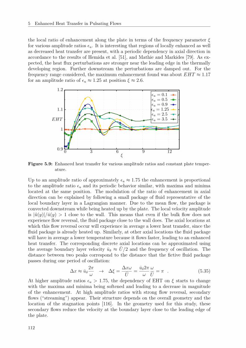
5 Enhanced Heat Transfer in Pulsating Flows
the local ratio of enhancement along the plate in terms of the frequency parameter ξfor various amplitude ratios εu. It is interesting that regions of locally enhanced as wellas decreased heat transfer are present, with a periodic dependency in axial direction inaccordance to the results of Hemida et al. [51], and Mathie and Markides [79]. As ex-pected, the heat flux perturbations are stronger near the leading edge in the thermallydeveloping region. Further downstream the perturbations are damped out. For thefrequency range considered, the maximum enhancement found was about EHT ≈ 1.17for an amplitude ratio of εu ≈ 1.25 at position ξ ≈ 2.6.
0.9
1
1.1
1.2
0 3 6 9 12
EHT
ξ
εu = 0.1εu = 0.5εu = 0.9εu = 1.25εu = 2.5εu = 3.5
Figure 5.9: Enhanced heat transfer for various amplitude ratios and constant plate temper-ature.
Up to an amplitude ratio of approximately εu ≈ 1.75 the enhancement is proportionalto the amplitude ratio εu and its periodic behavior similar, with maxima and minimalocated at the same position. The modulation of the ratio of enhancement in axialdirection can be explained by following a small package of fluid representative of thelocal boundary layer in a Lagrangian manner. Due to the mean flow, the package isconvected downstream while being heated up by the plate. The local velocity amplitudeis |u(y)|/u(y) > 1 close to the wall. This means that even if the bulk flow does notexperience flow reversal, the fluid package close to the wall does. The axial locations atwhich this flow reversal occur will experience in average a lower heat transfer, since thefluid package is already heated up. Similarly, at other axial locations the fluid packagewill have in average a lower temperature because it flows faster, leading to an enhancedheat transfer. The corresponding discrete axial locations can be approximated usingthe average boundary layer velocity uδ ≈ U/2 and the frequency of oscillation. Thedistance between two peaks correspond to the distance that the fictive fluid packagepasses during one period of oscillation:
∆x ≈ uδ2πω→ ∆ξ = ∆xω
U= uδ2π
ω
ω
U= π . (5.35)
At higher amplitude ratios εu > 1.75, the dependency of EHT on ξ starts to changewith the maxima and minima being softened and leading to a decrease in magnitudeof the enhancement. At high amplitude ratios with strong flow reversal, secondaryflows (“streaming”) appear. Their structure depends on the overall geometry and thelocation of the stagnation points [116]. In the geometry used for this study, thesesecondary flows reduce the velocity at the boundary layer close to the leading edge ofthe plate.
112
5.5 Conclusions Concerning Preliminary Studies
5.5 Conclusions Concerning Preliminary Studies
After giving some introduction to heat transfer in pulsating flows, with special attentionto the conditions present in rocket thrust chambers, this chapter presented the strategyto study these phenomena, that has been followed in this thesis. The steps in thisstrategy increase gradually in complexity.
The first preliminary investigation included a low order model for heat flux througha wall of finite thickness subjected to transient boundary conditions similar to thoseexpected in devices suffering from thermoacoustic instabilities. Two major results canbe formulated from this investigation: Firstly, for most combinations of parameters, thewall thermal inertia plays a minor role in the heat transfer under transient conditionsand leads always to a reduction of the heat flux through the wall. These results arein accordance to similar investigations available in the literature [51, 79, 134]. Andsecondly, the bulk flow transients can indeed lead to a permanent time averaged heattransfer change, provided that both the temperature and the heat transfer coefficientfluctuate in time. As predicted by Lundgren et al. [78], the phase between the oscil-lations plays the decisive role concerning the sign of the offset. The magnitude of theoffset is proportional to the amplitudes of the heat transfer coefficient and temperatureoscillations.
The second step performed in the strategy treated the heat transfer in pulsating flowpast a flat plate. A numerical CFD approach was used in the investigation. Based onthe results gained from the low order model, an ideal temperature boundary conditionfor the wall has been used, because no major contributions are expected from its ther-mal inertia. Apart from serving as a validation for some numerical simulation toolsand post-processing utilities, this test case produced some interesting results concern-ing the thermally developing region. Indeed, pulsating flow can lead locally to bothenhancement and diminishment of time averaged heat transfer. The changes are morepredominant in the thermally developing region and are damped out downstream, ingood agreement with results available from the literature [51, 79].
The results of these preliminary investigations are in good agreement, both qualita-tively and quantitatively, with other theoretical and numerical investigations availablefrom the literature. Quantitatively, the possible heat transfer enhancement accountsmerely few percent. Thus, the mechanisms found in this preliminary investigation can-not explain the large heat transfer enhancement rates observed in some experimentalinvestigations [29, 49]. However, turbulence phenomena have been left aside in thesepreliminary investigations. Chapter 6 will deal precisely with these phenomena.
113

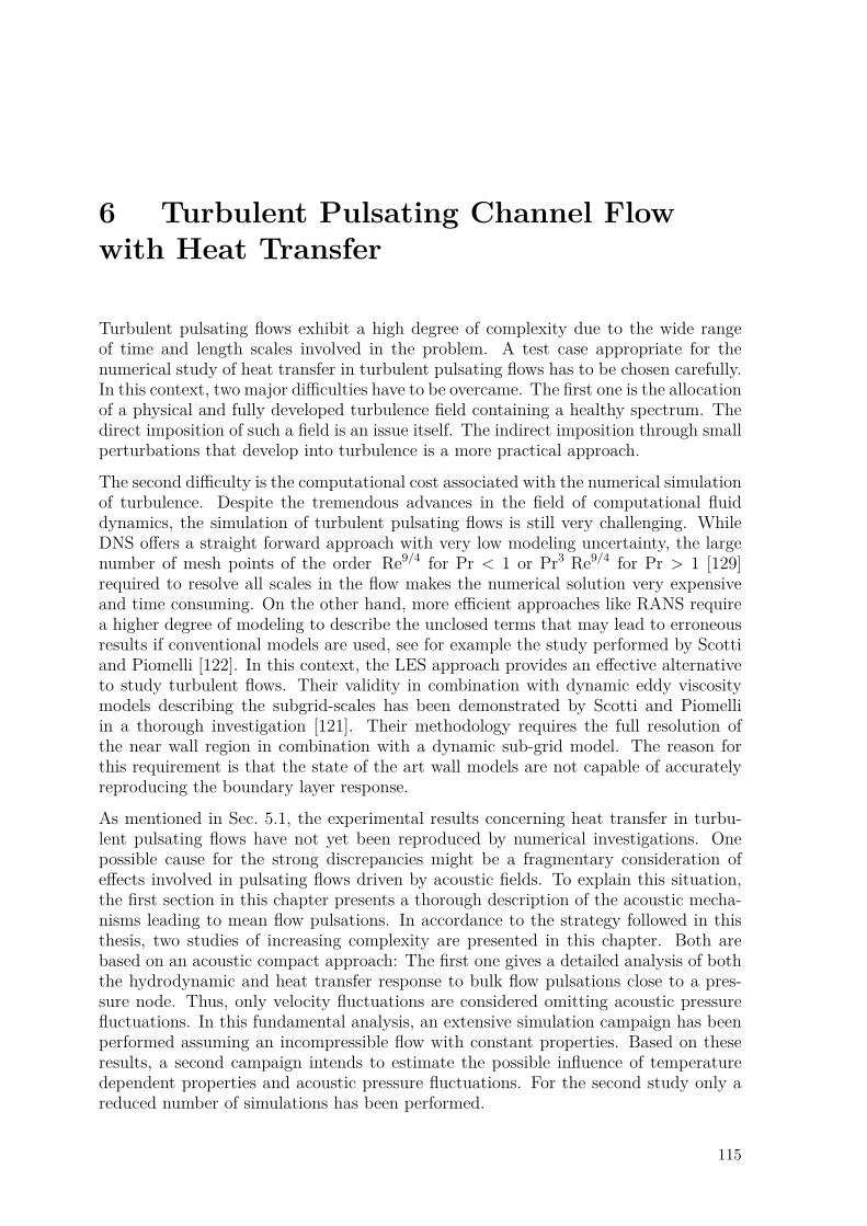
6 Turbulent Pulsating Channel Flowwith Heat Transfer
Turbulent pulsating flows exhibit a high degree of complexity due to the wide rangeof time and length scales involved in the problem. A test case appropriate for thenumerical study of heat transfer in turbulent pulsating flows has to be chosen carefully.In this context, two major difficulties have to be overcame. The first one is the allocationof a physical and fully developed turbulence field containing a healthy spectrum. Thedirect imposition of such a field is an issue itself. The indirect imposition through smallperturbations that develop into turbulence is a more practical approach.
The second difficulty is the computational cost associated with the numerical simulationof turbulence. Despite the tremendous advances in the field of computational fluiddynamics, the simulation of turbulent pulsating flows is still very challenging. WhileDNS offers a straight forward approach with very low modeling uncertainty, the largenumber of mesh points of the order Re9/4 for Pr < 1 or Pr3 Re9/4 for Pr > 1 [129]required to resolve all scales in the flow makes the numerical solution very expensiveand time consuming. On the other hand, more efficient approaches like RANS requirea higher degree of modeling to describe the unclosed terms that may lead to erroneousresults if conventional models are used, see for example the study performed by Scottiand Piomelli [122]. In this context, the LES approach provides an effective alternativeto study turbulent flows. Their validity in combination with dynamic eddy viscositymodels describing the subgrid-scales has been demonstrated by Scotti and Piomelliin a thorough investigation [121]. Their methodology requires the full resolution ofthe near wall region in combination with a dynamic sub-grid model. The reason forthis requirement is that the state of the art wall models are not capable of accuratelyreproducing the boundary layer response.
As mentioned in Sec. 5.1, the experimental results concerning heat transfer in turbu-lent pulsating flows have not yet been reproduced by numerical investigations. Onepossible cause for the strong discrepancies might be a fragmentary consideration ofeffects involved in pulsating flows driven by acoustic fields. To explain this situation,the first section in this chapter presents a thorough description of the acoustic mecha-nisms leading to mean flow pulsations. In accordance to the strategy followed in thisthesis, two studies of increasing complexity are presented in this chapter. Both arebased on an acoustic compact approach: The first one gives a detailed analysis of boththe hydrodynamic and heat transfer response to bulk flow pulsations close to a pres-sure node. Thus, only velocity fluctuations are considered omitting acoustic pressurefluctuations. In this fundamental analysis, an extensive simulation campaign has beenperformed assuming an incompressible flow with constant properties. Based on theseresults, a second campaign intends to estimate the possible influence of temperaturedependent properties and acoustic pressure fluctuations. For the second study only areduced number of simulations has been performed.
115
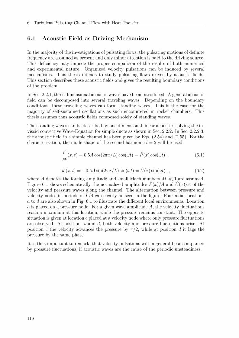
6 Turbulent Pulsating Channel Flow with Heat Transfer
6.1 Acoustic Field as Driving Mechanism
In the majority of the investigations of pulsating flows, the pulsating motions of definitefrequency are assumed as present and only minor attention is paid to the driving source.This deficiency may impede the proper comparison of the results of both numericaland experimental nature. Organized velocity pulsations can be induced by severalmechanisms. This thesis intends to study pulsating flows driven by acoustic fields.This section describes these acoustic fields and gives the resulting boundary conditionsof the problem.
In Sec. 2.2.1, three dimensional acoustic waves have been introduced. A general acousticfield can be decomposed into several traveling waves. Depending on the boundaryconditions, these traveling waves can form standing waves. This is the case for themajority of self-sustained oscillations as such encountered in rocket chambers. Thisthesis assumes thus acoustic fields composed solely of standing waves.
The standing waves can be described by one dimensional linear acoustics solving the in-viscid convective Wave-Equation for simple ducts as shown in Sec. 2.2.2. In Sec. 2.2.2.3,the acoustic field in a simple channel has been given by Eqs. (2.54) and (2.55). For thecharacterization, the mode shape of the second harmonic l = 2 will be used:
p′
ρc(x, t) = 0.5A cos(2πx/L) cos(ωt) = P (x) cos(ωt) , (6.1)
u′(x, t) = −0.5A sin(2πx/L) sin(ωt) = U(x) sin(ωt) , (6.2)where A denotes the forcing amplitude and small Mach numbers M 1 are assumed.Figure 6.1 shows schematically the normalized amplitudes P (x)/A and U(x)/A of thevelocity and pressure waves along the channel. The alternation between pressure andvelocity nodes in periods of L/4 can clearly be seen in the figure. Four axial locationsa to d are also shown in Fig. 6.1 to illustrate the different local environments. Locationa is placed on a pressure node. For a given wave amplitude A, the velocity fluctuationsreach a maximum at this location, while the pressure remains constant. The oppositesituation is given at location c placed at a velocity node where only pressure fluctuationsare observed. At positions b and d, both velocity and pressure fluctuations arise. Atposition c the velocity advances the pressure by π/2, while at position d it lags thepressure by the same phase.
It is thus important to remark, that velocity pulsations will in general be accompaniedby pressure fluctuations, if acoustic waves are the cause of the periodic unsteadiness.
116
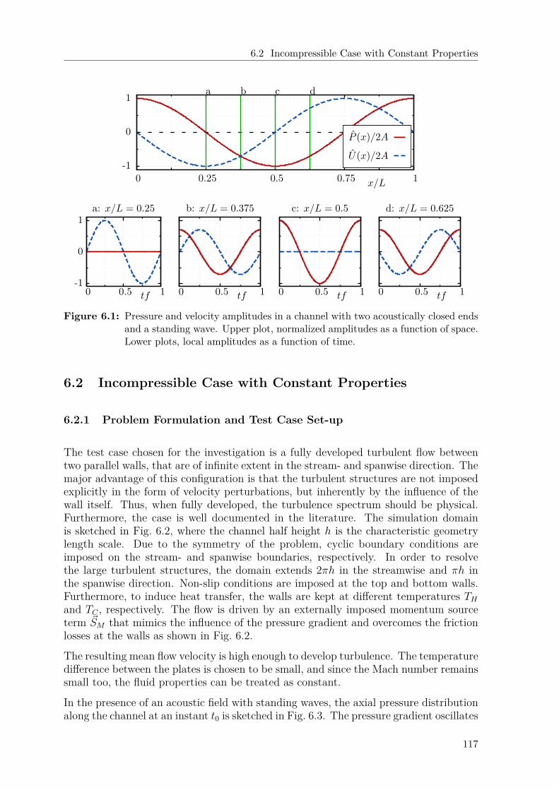
6.2 Incompressible Case with Constant Properties
-1
0
1
0 0.25 0.5 0.75 1x/L
a b c d
P (x)/2A
U(x)/2A
-1
0
1
0 0.5 1tf
a: x/L = 0.25
0 0.5 1tf
b: x/L = 0.375
0 0.5 1tf
c: x/L = 0.5
0 0.5 1tf
d: x/L = 0.625
Figure 6.1: Pressure and velocity amplitudes in a channel with two acoustically closed endsand a standing wave. Upper plot, normalized amplitudes as a function of space.Lower plots, local amplitudes as a function of time.
6.2 Incompressible Case with Constant Properties
6.2.1 Problem Formulation and Test Case Set-up
The test case chosen for the investigation is a fully developed turbulent flow betweentwo parallel walls, that are of infinite extent in the stream- and spanwise direction. Themajor advantage of this configuration is that the turbulent structures are not imposedexplicitly in the form of velocity perturbations, but inherently by the influence of thewall itself. Thus, when fully developed, the turbulence spectrum should be physical.Furthermore, the case is well documented in the literature. The simulation domainis sketched in Fig. 6.2, where the channel half height h is the characteristic geometrylength scale. Due to the symmetry of the problem, cyclic boundary conditions areimposed on the stream- and spanwise boundaries, respectively. In order to resolvethe large turbulent structures, the domain extends 2πh in the streamwise and πh inthe spanwise direction. Non-slip conditions are imposed at the top and bottom walls.Furthermore, to induce heat transfer, the walls are kept at different temperatures THand TC , respectively. The flow is driven by an externally imposed momentum sourceterm ~SM that mimics the influence of the pressure gradient and overcomes the frictionlosses at the walls as shown in Fig. 6.2.
The resulting mean flow velocity is high enough to develop turbulence. The temperaturedifference between the plates is chosen to be small, and since the Mach number remainssmall too, the fluid properties can be treated as constant.
In the presence of an acoustic field with standing waves, the axial pressure distributionalong the channel at an instant t0 is sketched in Fig. 6.3. The pressure gradient oscillates
117
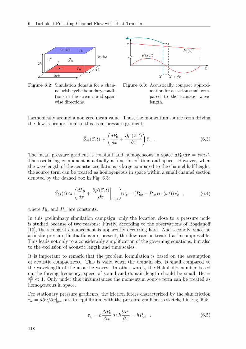
6 Turbulent Pulsating Channel Flow with Heat Transfer
Figure 6.2: Simulation domain for a chan-nel with cyclic boundary condi-tions in the stream- and span-wise directions.
Figure 6.3: Acoustically compact approxi-mation for a section small com-pared to the acoustic wave-length.
harmonically around a non zero mean value. Thus, the momentum source term drivingthe flow is proportional to this axial pressure gradient:
~SM(~x, t) ∼(dP0
dx+ ∂p′(~x, t)
∂x
)~ex . (6.3)
The mean pressure gradient is constant and homogeneous in space dP0/dx = const.The oscillating component is actually a function of time and space. However, whenthe wavelength of the acoustic oscillations is large compared to the channel half height,the source term can be treated as homogeneous in space within a small channel sectiondenoted by the dashed box in Fig. 6.3:
~SM(t) ≈(dP0
dx+ ∂p′(~x, t)
∂x
∣∣∣∣∣x=X
)~ex = (P0x + P1x cos(ωt))~ex , (6.4)
where P0x and P1x are constants.
In this preliminary simulation campaign, only the location close to a pressure nodeis studied because of two reasons: Firstly, according to the observations of Bogdanoff[10], the strongest enhancement is apparently occurring here. And secondly, since noacoustic pressure fluctuations are present, the flow can be treated as incompressible.This leads not only to a considerably simplification of the governing equations, but alsoto the exclusion of acoustic length and time scales.
It is important to remark that the problem formulation is based on the assumptionof acoustic compactness. This is valid when the domain size is small compared tothe wavelength of the acoustic waves. In other words, the Helmholtz number basedon the forcing frequency, speed of sound and domain length should be small, He =ωhc 1. Only under this circumstances the momentum source term can be treated as
homogeneous in space.
For stationary pressure gradients, the friction forces characterized by the skin frictionτw = µ∂u/∂y|y=0 are in equilibrium with the pressure gradient as sketched in Fig. 6.4:
τw = h∆P0
∆x ≈ h∂P0
∂x= hP0x . (6.5)
118
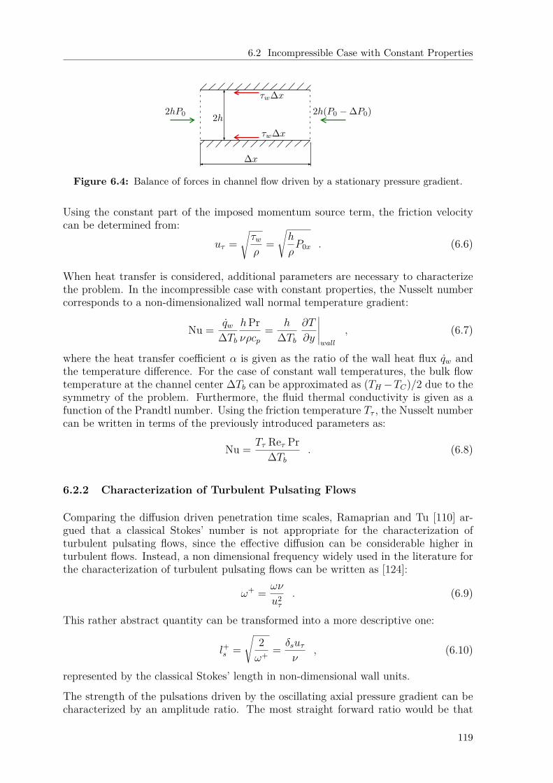
6.2 Incompressible Case with Constant Properties
Figure 6.4: Balance of forces in channel flow driven by a stationary pressure gradient.
Using the constant part of the imposed momentum source term, the friction velocitycan be determined from:
uτ =√τwρ
=√h
ρP0x . (6.6)
When heat transfer is considered, additional parameters are necessary to characterizethe problem. In the incompressible case with constant properties, the Nusselt numbercorresponds to a non-dimensionalized wall normal temperature gradient:
Nu = qw∆Tb
hPrνρcp
= h
∆Tb∂T
∂y
∣∣∣∣∣wall
, (6.7)
where the heat transfer coefficient α is given as the ratio of the wall heat flux qw andthe temperature difference. For the case of constant wall temperatures, the bulk flowtemperature at the channel center ∆Tb can be approximated as (TH−TC)/2 due to thesymmetry of the problem. Furthermore, the fluid thermal conductivity is given as afunction of the Prandtl number. Using the friction temperature Tτ , the Nusselt numbercan be written in terms of the previously introduced parameters as:
Nu = Tτ Reτ Pr∆Tb
. (6.8)
6.2.2 Characterization of Turbulent Pulsating Flows
Comparing the diffusion driven penetration time scales, Ramaprian and Tu [110] ar-gued that a classical Stokes’ number is not appropriate for the characterization ofturbulent pulsating flows, since the effective diffusion can be considerable higher inturbulent flows. Instead, a non dimensional frequency widely used in the literature forthe characterization of turbulent pulsating flows can be written as [124]:
ω+ = ων
u2τ
. (6.9)
This rather abstract quantity can be transformed into a more descriptive one:
l+s =√
2ω+ = δsuτ
ν, (6.10)
represented by the classical Stokes’ length in non-dimensional wall units.
The strength of the pulsations driven by the oscillating axial pressure gradient can becharacterized by an amplitude ratio. The most straight forward ratio would be that
119
6 Turbulent Pulsating Channel Flow with Heat Transfer
of the center-line velocity εuc. In the current dominated flow (εuc < 1), the flow isapparently controlled by the forcing frequency ω+ [121, 124]. Scotti and Piomelli gofurther and propose a turbulent Stokes length lτ in order to estimate the thickness ofthe layer to which the influence of the oscillations is confined. In an analogy to thelaminar Stokes problem, they obtain this turbulent length scale by adding molecularand turbulent diffusivities:
lt =√
2(ν + ντ )ω
. (6.11)
Modeling qualitatively the influence of turbulence by an eddy viscosity model:
ντ = κKuτ lτ , (6.12)
where κK is the von Karman constant, they derived to the following expression innon-dimensional wall units:
l+t = l+s
(κKl+s
2
)+
√√√√1 +(κKl+s
2
)2 . (6.13)
Based on this expression, they characterize the different frequency regimes describedby Gundogdu and Carpinlioglu [46] in the current dominated case:
• quasisteady regime
• low-frequency regime
• intermediate frequency regime
• high frequency regime
• very high frequency regime (bursting frequency)
6.2.3 Governing Equations and Numerical Method
For low Mach numbers and small temperature gradients, the incompressible Navier-Stokes-Equations with constant properties can be used to describe the flow. In theLES context, they filtered counterparts can be written as:
∂~u
∂t+ (~u · ~∇)~u = −1
ρ~∇p+ ~∇
[(ν + νsgs)~∇~u
]+ 1ρ~SM , (6.14)
∂T
∂t+ (~u · ~∇)T = ~∇
[(a+ asgs)~∇T
]. (6.15)
For simplicity, the tilde denoting filtered variables is omitted. The effects of the subgridscales are captured by a simple eddy viscosity νsgs. The momentum equation Eq. (4.2)satisfies inherently the mass conservation ~∇ · ~u = 0. The effects of the subgrid scaleson the thermal diffusivity are approximated through a turbulent Prandtl number:
Prt = νsgsasgs≈ Pr , (6.16)
120
6.2 Incompressible Case with Constant Properties
assumed to be constant. For the subgrid scales, a one equation eddy viscosity modelbased on the conservation of SGS turbulent kinetic energy is used, see Sec. 2.4.2.1. Themodel constants are dynamically adapted through the Germano identity [41] and theextension of Lilly [76]. Scotti and Piomelly [121] and later Wong and Lu [129] used thedynamic Smagorinsky model, which is based on the assumption of local equilibrium. Inthis study, the less restrictive one equation TKE model is consciously chosen becausethe unsteadiness might partially break the equilibrium assumed by the Smagorinskymodel.
The simulations are run within the openFoam environment. The standard incompress-ible solver pisoFoam that solves Eq. (6.14) has been extended to solve also the transportequation for the temperature given by Eq. (6.15). Furthermore, the momentum sourceterm with harmonic dependency given by Eq. (6.4) has been included in the solverwhere the parameters P0x, P1x and ω can be freely chosen. The system of partialdifferential equations is solved iteratively by the PISO algorithm [56] using two mo-mentum correction steps. Time discretization is performed through a second orderCrank-Nicholson scheme. Spatial discretization of the convective fluxes is performedthrough a second order Gauß scheme, for which the face fluxes are interpolated througha second order upwind differencing scheme bounded by a van Leer function. The diffu-sive fluxes are discretized through a second order Gauß scheme, for which the surfacenormal gradients are interpolated trough a second order upwind differencing scheme.Details concerning the discretization schemes and the chosen parameters can be foundin [34, 69]. The mesh used for the spatial discretization is orthogonal with a stretchingfunction in the wall normal direction and homogeneous distribution in the span- andstreamwise directions, see App. C.1.
6.2.4 Data Reduction Through Averaging Operators
For the characterization of turbulent pulsating flows different averaging procedures ofa quantity ψ(~x, t) can be defined including spatial, temporal and combination of both.
Temporal averaging of a quantity will be denoted by an overbar and is defined as:
ψ(~x) = 1ttot
∫ ttot
0ψ(~x, t)dt , (6.17)
where ttot denotes the total integration time. To increase the statistical validity of themean quantities, spatial averaging in the directions of homogeneity can also be per-formed. This combination of temporal and spatial average operations will be denotedby angle brackets:
〈ψ〉(y) = 1ttotLxLz
∫ Lz
0
∫ Lx
0
∫ ttot
0ψ(~x, t) dt dz dx , (6.18)
where Lx and Lz denote the domain size in stream- and spanwise direction, respectively.
When dealing with pulsating flows driven at one given frequency f = 2πω, phase orensemble averaging can help in the identification of coherent structures. As arguedby Scotti and Piomelli [121], this assumes that the major contribution of the system
121

6 Turbulent Pulsating Channel Flow with Heat Transfer
response occurs at the forcing frequency. This kind of operation will be denoted bysubscripted angle brackets 〈 〉p and is defined as:
〈ψ〉p(y, ϕ) = 1NtLxLz
Nt∑j=1
∫ Lz
0
∫ Lx
0ψ
(~x,ϕ
ω+ 2π (j − 1)
ω
)dz dx , (6.19)
where Nt is the number of cycles considered in the ensemble averaging and 0 < ϕ ≤ 2πrepresents the phase angle. The phase averaged quantities can be further decomposedinto a mean, an harmonic and a non-linear component as proposed in [121]:
〈ψ〉p(y, ϕ) = 〈ψ〉(y) + aψ(y) cos(ϕ+ φψ(y)) + ψha(y, ϕ) . (6.20)
Of course, the stationary component corresponds to the temporal and spatial average ofthe original quantity. The harmonic component can be seen as a real valued amplitude,and thus, a phase lag φψ towards a reference value is necessary. Note that both theamplitude and the phase lag are functions of the wall distance. Usually, the phase lagis defined using the axial velocity oscillations at the channel center-line as reference.From the phase averaging definition, the oscillating component accounts only for thecontribution of the forcing frequency. The contributions at higher harmonics are alladded up in the term ψha which is of course a function of the phase ϕ and the wallnormal location y.
For the pulsating channel flow, the triple decomposition introduced in Sec. 2.5 andwidely used in the literature can be written in terms of these average operators as:
ψ(~x, t) = 〈ψ〉+ aψ(y) cos(ωt+ φψ(y)) + ψ8(~x, t) . (6.21)
where 8 denotes the chaotic turbulent fluctuations.
6.2.5 Stationary Validation and Reference Case
The first step in this study was the validation of the numerical solver used in themethodology for both stationary and pulsating case. Unfortunately, if heat transfer isconsidered, the available data in the literature is very sparse and a test case with thecombination of parameters as those used in this study has not been found.
For the stationary case without pulsating forcing, App. C.1 gives a thorough validationfor two different cases of turbulent Reynolds numbers Reτ = 150 and Reτ = 180against DNS data available from the literature. The combination of solver, turbulencemodel and mesh performs very well and the agreement with the DNS data is very good.The details of the validation are given in the appendix.
Table 6.1: Reference case for turbulent channel flow with heat transfer.
Reτ Pr Nuref Logarithmic sublayer179.9 0.71 6.26 u+ = 2.5 ln(y+) + 5.5
T+ = 3.6 ln(y+) + 0.3
After the validation, a turbulent test case without acoustic pulsations has to be definedto serve as a reference for the evaluation of heat transfer enhancement. The test case
122
6.2 Incompressible Case with Constant Properties
of Reynolds number Reτ = 180 and Prandtl number Pr = 0.71 already used for thestationary validation is chosen to serve as the reference case. Table 6.1 gives the keyparameters of this simulation. This Reynolds number is lower than the one used in thetwo major publications cited in this thesis [121, 129], which was Reτ = 350. However,in these studies, only the current dominated flow with velocity amplitudes at the center-line εuc = auc/〈u(h)〉 of εuc . 0.7 and various frequencies was studied. In the researchpresented in this thesis, a wider range of amplitudes covering also at least partially thewave dominated flow εuc > 1 are studied. Thus, a lower turbulent Reynolds numberof Reτ = 180 is chosen in order to save some computational resources. Nevertheless,as it will be shown later, the effective non-dimensional frequency ω+ still allows thecomparison against the data of these studies.
6.2.6 Pulsating Case Validation
As a starting point, three exemplary operation points are described and compared tosome of the data available from the literature. This should serve as a validation forthe turbulent pulsating case and help to elucidate the main hydrodynamic behaviorof turbulent pulsating flows already observed in previous investigations. The casescorrespond to the ones studied experimentally by Tardu et al. [124], which were subse-quently also used in the numerical studies of Scotti and Piomelli [122] and Wang andLu [129]. Table 6.2 lists the key parameters of the three different computed cases inthe present study compared against the ones used by the mentioned investigations. Allcases lie in the current dominated regime with velocity center-line amplitude of approx-imately εuc ≈ 0.7. It is important to remark that the turbulent Reynolds numbers ofthe different investigations are not always equal, ranging from Reτ = 432 in the ex-perimental study to Reτ = 180 in the present study. The other two numerical studiesuse Reτ = 350. However, the forcing frequencies are chosen in such a way that theresulting turbulent Stokes numbers l+s are comparable, depicting the low, medium andhigh frequency regimes, respectively.
For the present study, the different cases are simulated using the solver and methodologypresented in Sec. 6.2.3 and run for several periods to get accurate temporal and phaseaverage statistics. Figure 6.5 shows the axial velocity components after performingthe triple decomposition given by Eq. (6.20) and plotted in wall units. The profilesof the present LES simulations are compared against the results of the investigationslisted in Tab. 6.2. The first row in the figure shows the time independent part ofthe axial velocity, which clearly follows the classical law of the wall. In the low andthe high frequency regimes, the profiles collapse to the classical law of the wall 〈u+〉 =2.5 ln(y+)+5 and 〈u+〉 = y+ denoted by the dashed lines and the agreement between thedifferent investigations is very good. In the medium frequency regime, the present LESsimulations match the experimental results somewhat better than the LES of Scottiand Piomelli. In this regime, it seems that the logarithmic region is shifted slightly to alower wall normal coordinate. For the other frequencies, the average profiles lie close tothe ones of the stationary case without pulsations. The middle row shows the ensembleaveraged velocity amplitude a+
u normalized by its center-line value a+uc. As expected,
the thickness of the turbulent Stokes’ layer is inversely proportional to the forcingfrequency ranging from 10 in the high to 500 in the low frequency regime. Again, theconcordance between the three investigations is remarkably good. Finally, the third
123
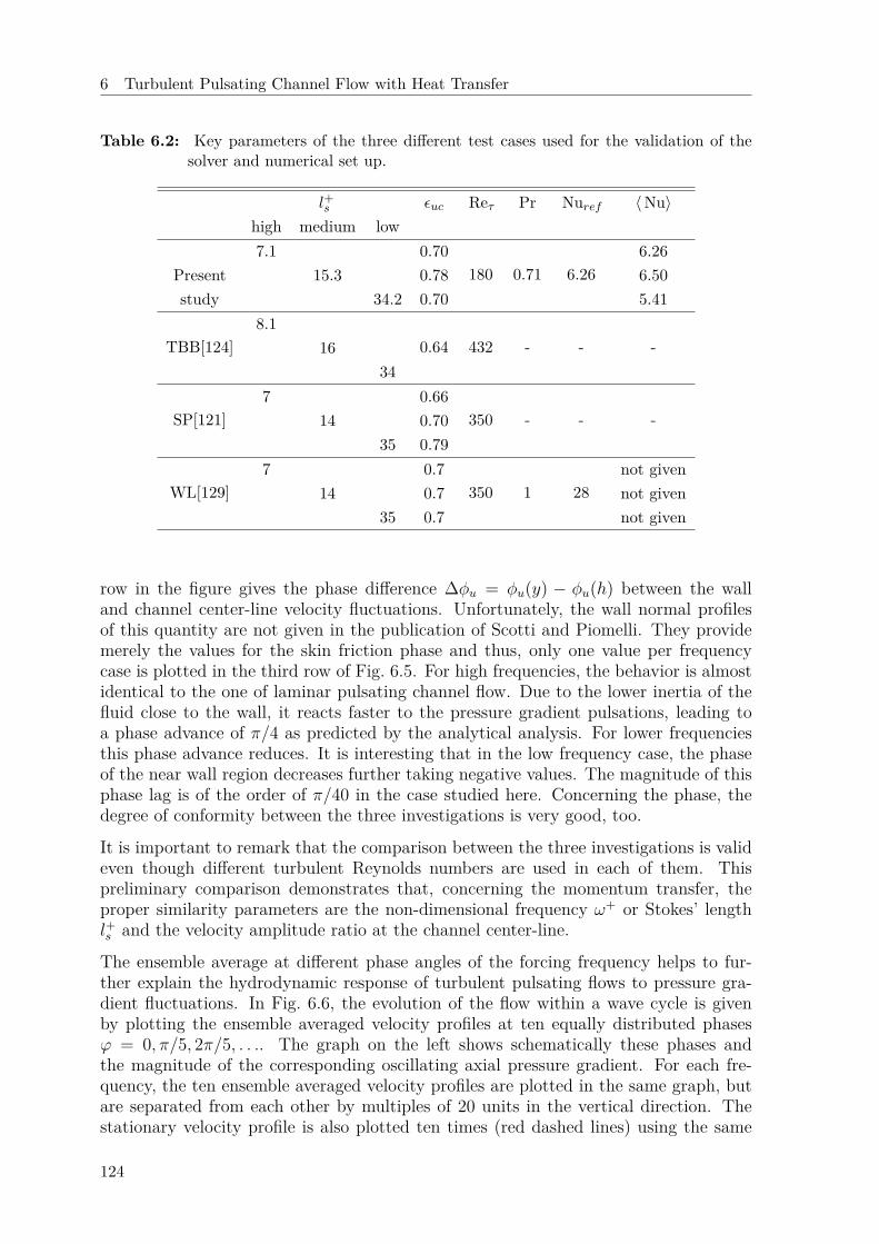
6 Turbulent Pulsating Channel Flow with Heat Transfer
Table 6.2: Key parameters of the three different test cases used for the validation of thesolver and numerical set up.
l+s εuc Reτ Pr Nuref 〈Nu〉high medium low7.1 0.70
180 0.71 6.266.26
Present 15.3 0.78 6.50study 34.2 0.70 5.41
TBB[124]8.1
0.64 432 - - -1634
SP[121]7 0.66
350 - - -14 0.7035 0.79
WL[129]7 0.7
350 1 28not given
14 0.7 not given35 0.7 not given
row in the figure gives the phase difference ∆φu = φu(y) − φu(h) between the walland channel center-line velocity fluctuations. Unfortunately, the wall normal profilesof this quantity are not given in the publication of Scotti and Piomelli. They providemerely the values for the skin friction phase and thus, only one value per frequencycase is plotted in the third row of Fig. 6.5. For high frequencies, the behavior is almostidentical to the one of laminar pulsating channel flow. Due to the lower inertia of thefluid close to the wall, it reacts faster to the pressure gradient pulsations, leading toa phase advance of π/4 as predicted by the analytical analysis. For lower frequenciesthis phase advance reduces. It is interesting that in the low frequency case, the phaseof the near wall region decreases further taking negative values. The magnitude of thisphase lag is of the order of π/40 in the case studied here. Concerning the phase, thedegree of conformity between the three investigations is very good, too.
It is important to remark that the comparison between the three investigations is valideven though different turbulent Reynolds numbers are used in each of them. Thispreliminary comparison demonstrates that, concerning the momentum transfer, theproper similarity parameters are the non-dimensional frequency ω+ or Stokes’ lengthl+s and the velocity amplitude ratio at the channel center-line.
The ensemble average at different phase angles of the forcing frequency helps to fur-ther explain the hydrodynamic response of turbulent pulsating flows to pressure gra-dient fluctuations. In Fig. 6.6, the evolution of the flow within a wave cycle is givenby plotting the ensemble averaged velocity profiles at ten equally distributed phasesϕ = 0, π/5, 2π/5, . . .. The graph on the left shows schematically these phases andthe magnitude of the corresponding oscillating axial pressure gradient. For each fre-quency, the ten ensemble averaged velocity profiles are plotted in the same graph, butare separated from each other by multiples of 20 units in the vertical direction. Thestationary velocity profile is also plotted ten times (red dashed lines) using the same
124
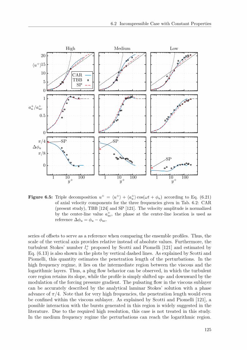
6.2 Incompressible Case with Constant Properties
0
5
10
15
20
〈u+〉
High Medium Low
0
0.5
1
a+u /a
+uc
0
π/8
π/4
1 10 100
∆φu
y+
SP
1 10 100y+
SP
1 10 100y+
SP
CARTBB
SP
Figure 6.5: Triple decomposition u+ = 〈u+〉 + 〈a+u 〉 cos(ωt + φu) according to Eq. (6.21)
of axial velocity components for the three frequencies given in Tab. 6.2: CAR(present study), TBB [124] and SP [121]. The velocity amplitude is normalizedby the center-line value a+
uc, the phase at the center-line location is used asreference ∆φu = φu − φuc.
series of offsets to serve as a reference when comparing the ensemble profiles. Thus, thescale of the vertical axis provides relative instead of absolute values. Furthermore, theturbulent Stokes’ number l+τ proposed by Scotti and Piomelli [121] and estimated byEq. (6.13) is also shown in the plots by vertical dashed lines. As explained by Scotti andPiomelli, this quantity estimates the penetration length of the perturbations. In thehigh frequency regime, it lies on the intermediate region between the viscous and thelogarithmic layers. Thus, a plug flow behavior can be observed, in which the turbulentcore region retains its slope, while the profile is simply shifted up- and downward by themodulation of the forcing pressure gradient. The pulsating flow in the viscous sublayercan be accurately described by the analytical laminar Stokes’ solution with a phaseadvance of π/4. Note that for very high frequencies, the penetration length would evenbe confined within the viscous sublayer. As explained by Scotti and Piomelli [121], apossible interaction with the bursts generated in this region is widely suggested in theliterature. Due to the required high resolution, this case is not treated in this study.In the medium frequency regime the perturbations can reach the logarithmic region.
125
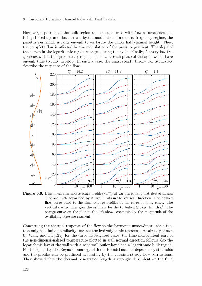
6 Turbulent Pulsating Channel Flow with Heat Transfer
However, a portion of the bulk region remains unaltered with frozen turbulence andbeing shifted up- and downstream by the modulation. In the low frequency regime, thepenetration length is large enough to enclosure the whole half channel height. Thus,the complete flow is affected by the modulation of the pressure gradient. The slope ofthe curves in the logarithmic region changes during the cycle. Finally, for very low fre-quencies within the quasi steady regime, the flow at each phase of the cycle would haveenough time to fully develop. In such a case, the quasi steady theory can accuratelydescribe the response of the flow.
0
20
40
60
80
100
120
140
160
180
200
220
1 10 100
〈u+〉p
y+
l+s = 34.2
2l+t = 9401 10 100
y+
l+s = 11.8
2l+t = 1161 10 100
y+
l+s = 7.1
2l+t = 450π 5
2π 53π 5
4π 5π
6π 57π 5
8π 59π 5
ϕ∂p′
∂x
Figure 6.6: Blue lines, ensemble average profiles 〈u+〉p at various equally distributed phasesϕ of one cycle separated by 20 wall units in the vertical direction. Red dashedlines correspond to the time average profiles at the corresponding cases. Thevertical dashed lines give the estimate for the turbulent Stokes’ length l+t . Theorange curve on the plot in the left show schematically the magnitude of theoscillating pressure gradient.
Concerning the thermal response of the flow to the harmonic unsteadiness, the situa-tion only has limited similarity towards the hydrodynamic response. As already shownby Wang and Lu [129], for the three investigated cases, the time independent part ofthe non-dimensionalized temperature plotted in wall normal direction follows also thelogarithmic law of the wall with a near wall buffer layer and a logarithmic bulk region.For this quantity, the Reynolds analogy with the Prandtl number dependency still holdsand the profiles can be predicted accurately by the classical steady flow correlations.They showed that the thermal penetration length is strongly dependent on the fluid
126
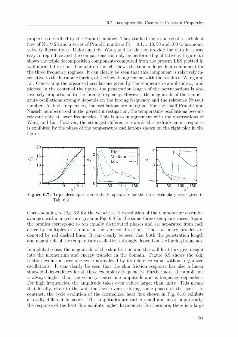
6.2 Incompressible Case with Constant Properties
properties described by the Prandtl number. They studied the response of a turbulentflow of Nu ≈ 28 and a series of Prandtl numbers Pr = 0.1, 1, 10, 50 and 100 to harmonicvelocity fluctuations. Unfortunately, Wang and Lu do not provide the data in a wayeasy to reproduce and the comparisons can only be performed qualitatively. Figure 6.7shows the triple decomposition components computed from the present LES plotted inwall normal direction. The plot on the left shows the time independent component forthe three frequency regimes. It can clearly be seen that this component is relatively in-sensitive to the harmonic forcing of the flow, in agreement with the results of Wang andLu. Concerning the organized oscillations given by the temperature amplitude a+
T andplotted in the center of the figure, the penetration length of the perturbations is alsoinversely proportional to the forcing frequency. However, the magnitude of the temper-ature oscillations strongly depends on the forcing frequency and the reference Nusseltnumber. At high frequencies, the oscillations are marginal. For the small Prandtl andNusselt numbers used in the present investigation, the temperature oscillations becomerelevant only at lower frequencies. This is also in agreement with the observations ofWang and Lu. However, the strongest difference towards the hydrodynamic responseis exhibited by the phase of the temperature oscillations shown on the right plot in thefigure.
0
5
10
15
20
1 10 100
〈T+〉
y+0
1
2
0 50 100 150
a+T
y+
−π
0
π
0 50 100 150
φT
y+
HighMediumLow
Figure 6.7: Triple decomposition of the temperature for the three exemplary cases given inTab. 6.2.
Corresponding to Fig. 6.5 for the velocities, the evolution of the temperature ensembleaverages within a cycle are given in Fig. 6.8 for the same three exemplary cases. Again,the profiles correspond to ten equally distributed phases and are separated from eachother by multiples of 5 units in the vertical direction. The stationary profiles aredenoted by red dashed lines. It can clearly be seen that both the penetration lengthand magnitude of the temperature oscillations strongly depend on the forcing frequency.
In a global sense, the magnitude of the skin friction and the wall heat flux give insightinto the momentum and energy transfer in the domain. Figure 6.9 shows the skinfriction evolution over one cycle normalized by its reference value without organizedoscillations. It can clearly be seen that the skin friction response has also a linearsinusoidal dependency for all three exemplary frequencies. Furthermore, the amplitudeis always higher than the velocity center-line amplitude and is frequency dependent.For high frequencies, the amplitude takes even values larger than unity. This meansthat locally, close to the wall the flow reverses during some phases of the cycle. Incontrast, the cycle evolution of the normalized heat flux shown in Fig. 6.10 exhibitsa totally different behavior. The amplitudes are rather small and most importantly,the response of the heat flux exhibits higher harmonics. Furthermore, there is a large
127
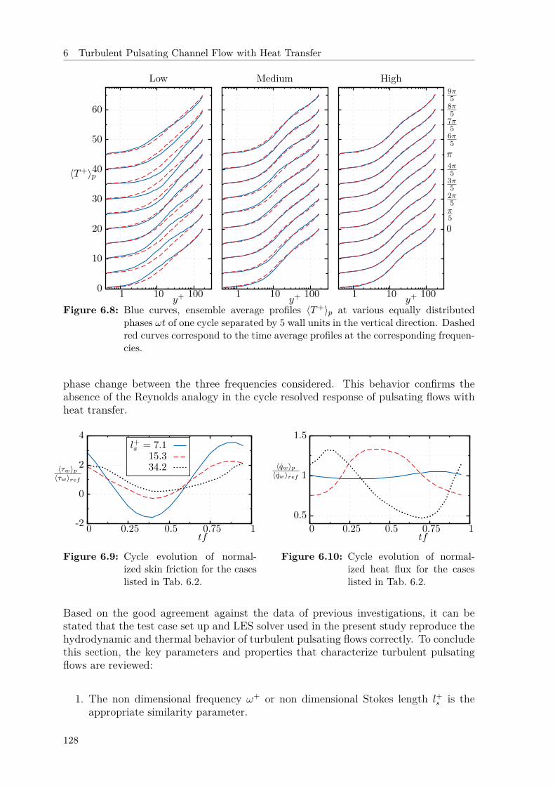
6 Turbulent Pulsating Channel Flow with Heat Transfer
0
10
20
30
40
50
60
1 10 100
〈T+〉p
y+
Low
1 10 100y+
Medium
1 10 100y+
High
0
π5
2π5
3π5
4π5
π
6π5
7π5
8π5
9π5
Figure 6.8: Blue curves, ensemble average profiles 〈T+〉p at various equally distributedphases ωt of one cycle separated by 5 wall units in the vertical direction. Dashedred curves correspond to the time average profiles at the corresponding frequen-cies.
phase change between the three frequencies considered. This behavior confirms theabsence of the Reynolds analogy in the cycle resolved response of pulsating flows withheat transfer.
-2
0
2
4
0 0.25 0.5 0.75 1
〈τw〉p〈τw〉ref
tf
l+s = 7.115.334.2
Figure 6.9: Cycle evolution of normal-ized skin friction for the caseslisted in Tab. 6.2.
0.5
1
1.5
0 0.25 0.5 0.75 1
〈qw〉p〈qw〉ref
tf
Figure 6.10: Cycle evolution of normal-ized heat flux for the caseslisted in Tab. 6.2.
Based on the good agreement against the data of previous investigations, it can bestated that the test case set up and LES solver used in the present study reproduce thehydrodynamic and thermal behavior of turbulent pulsating flows correctly. To concludethis section, the key parameters and properties that characterize turbulent pulsatingflows are reviewed:
1. The non dimensional frequency ω+ or non dimensional Stokes length l+s is theappropriate similarity parameter.
128
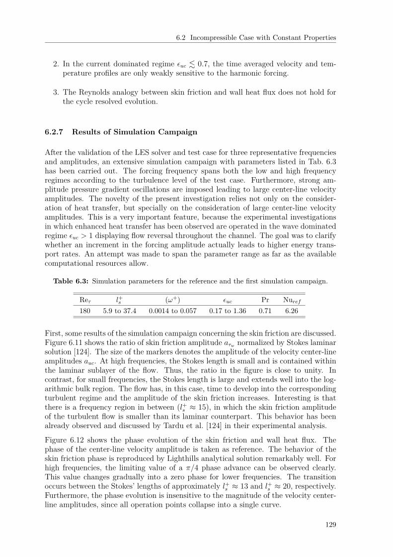
6.2 Incompressible Case with Constant Properties
2. In the current dominated regime εuc . 0.7, the time averaged velocity and tem-perature profiles are only weakly sensitive to the harmonic forcing.
3. The Reynolds analogy between skin friction and wall heat flux does not hold forthe cycle resolved evolution.
6.2.7 Results of Simulation Campaign
After the validation of the LES solver and test case for three representative frequenciesand amplitudes, an extensive simulation campaign with parameters listed in Tab. 6.3has been carried out. The forcing frequency spans both the low and high frequencyregimes according to the turbulence level of the test case. Furthermore, strong am-plitude pressure gradient oscillations are imposed leading to large center-line velocityamplitudes. The novelty of the present investigation relies not only on the consider-ation of heat transfer, but specially on the consideration of large center-line velocityamplitudes. This is a very important feature, because the experimental investigationsin which enhanced heat transfer has been observed are operated in the wave dominatedregime εuc > 1 displaying flow reversal throughout the channel. The goal was to clarifywhether an increment in the forcing amplitude actually leads to higher energy trans-port rates. An attempt was made to span the parameter range as far as the availablecomputational resources allow.
Table 6.3: Simulation parameters for the reference and the first simulation campaign.
Reτ l+s (ω+) εuc Pr Nuref180 5.9 to 37.4 0.0014 to 0.057 0.17 to 1.36 0.71 6.26
First, some results of the simulation campaign concerning the skin friction are discussed.Figure 6.11 shows the ratio of skin friction amplitude aτw normalized by Stokes laminarsolution [124]. The size of the markers denotes the amplitude of the velocity center-lineamplitudes auc. At high frequencies, the Stokes length is small and is contained withinthe laminar sublayer of the flow. Thus, the ratio in the figure is close to unity. Incontrast, for small frequencies, the Stokes length is large and extends well into the log-arithmic bulk region. The flow has, in this case, time to develop into the correspondingturbulent regime and the amplitude of the skin friction increases. Interesting is thatthere is a frequency region in between (l+s ≈ 15), in which the skin friction amplitudeof the turbulent flow is smaller than its laminar counterpart. This behavior has beenalready observed and discussed by Tardu et al. [124] in their experimental analysis.
Figure 6.12 shows the phase evolution of the skin friction and wall heat flux. Thephase of the center-line velocity amplitude is taken as reference. The behavior of theskin friction phase is reproduced by Lighthills analytical solution remarkably well. Forhigh frequencies, the limiting value of a π/4 phase advance can be observed clearly.This value changes gradually into a zero phase for lower frequencies. The transitionoccurs between the Stokes’ lengths of approximately l+s ≈ 13 and l+s ≈ 20, respectively.Furthermore, the phase evolution is insensitive to the magnitude of the velocity center-line amplitudes, since all operation points collapse into a single curve.
129
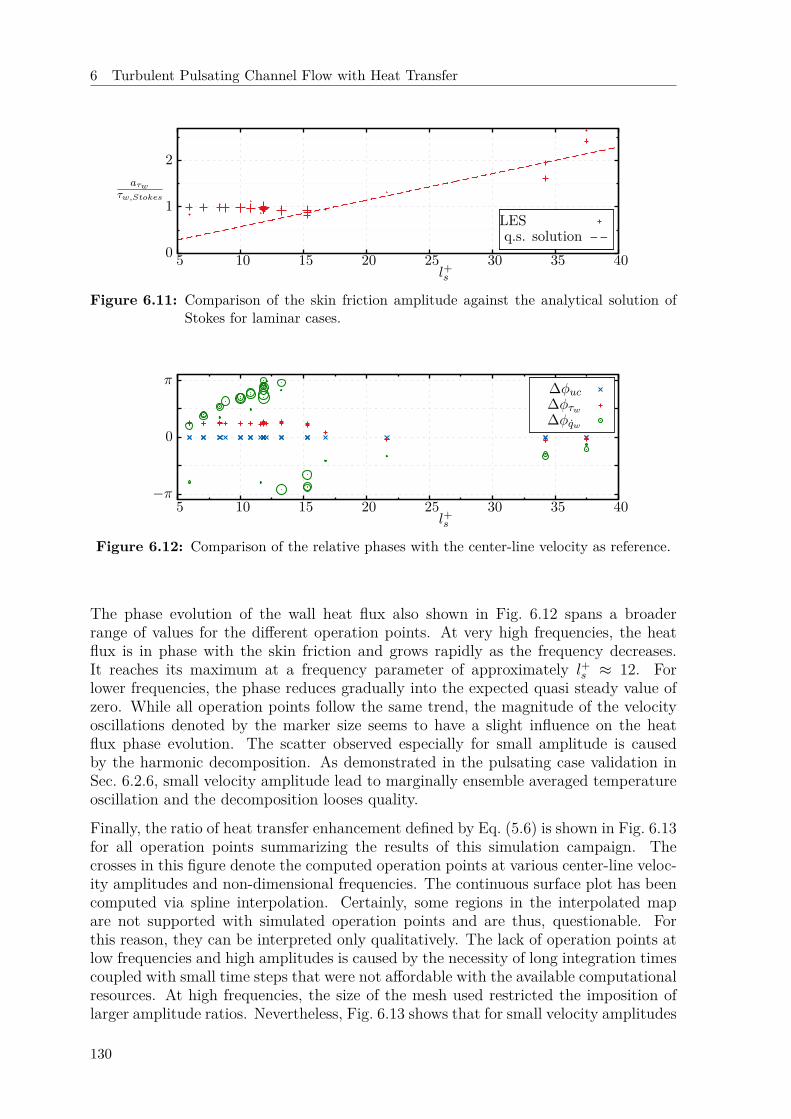
6 Turbulent Pulsating Channel Flow with Heat Transfer
0
1
2
5 10 15 20 25 30 35 40
aτwτw,Stokes
l+s
LESq.s. solution
Figure 6.11: Comparison of the skin friction amplitude against the analytical solution ofStokes for laminar cases.
−π
0
π
5 10 15 20 25 30 35 40l+s
∆φuc∆φτw∆φqw
Figure 6.12: Comparison of the relative phases with the center-line velocity as reference.
The phase evolution of the wall heat flux also shown in Fig. 6.12 spans a broaderrange of values for the different operation points. At very high frequencies, the heatflux is in phase with the skin friction and grows rapidly as the frequency decreases.It reaches its maximum at a frequency parameter of approximately l+s ≈ 12. Forlower frequencies, the phase reduces gradually into the expected quasi steady value ofzero. While all operation points follow the same trend, the magnitude of the velocityoscillations denoted by the marker size seems to have a slight influence on the heatflux phase evolution. The scatter observed especially for small amplitude is causedby the harmonic decomposition. As demonstrated in the pulsating case validation inSec. 6.2.6, small velocity amplitude lead to marginally ensemble averaged temperatureoscillation and the decomposition looses quality.
Finally, the ratio of heat transfer enhancement defined by Eq. (5.6) is shown in Fig. 6.13for all operation points summarizing the results of this simulation campaign. Thecrosses in this figure denote the computed operation points at various center-line veloc-ity amplitudes and non-dimensional frequencies. The continuous surface plot has beencomputed via spline interpolation. Certainly, some regions in the interpolated mapare not supported with simulated operation points and are thus, questionable. Forthis reason, they can be interpreted only qualitatively. The lack of operation points atlow frequencies and high amplitudes is caused by the necessity of long integration timescoupled with small time steps that were not affordable with the available computationalresources. At high frequencies, the size of the mesh used restricted the imposition oflarger amplitude ratios. Nevertheless, Fig. 6.13 shows that for small velocity amplitudes
130
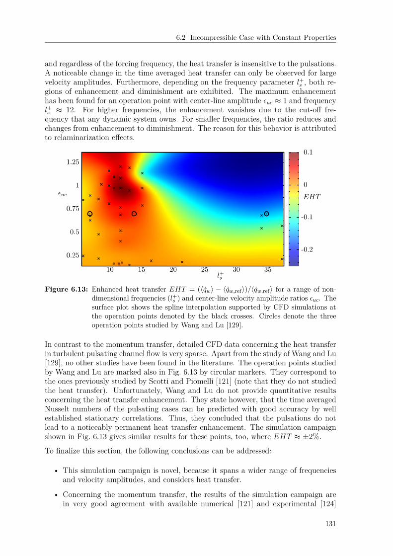
6.2 Incompressible Case with Constant Properties
and regardless of the forcing frequency, the heat transfer is insensitive to the pulsations.A noticeable change in the time averaged heat transfer can only be observed for largevelocity amplitudes. Furthermore, depending on the frequency parameter l+s , both re-gions of enhancement and diminishment are exhibited. The maximum enhancementhas been found for an operation point with center-line amplitude εuc ≈ 1 and frequencyl+s ≈ 12. For higher frequencies, the enhancement vanishes due to the cut-off fre-quency that any dynamic system owns. For smaller frequencies, the ratio reduces andchanges from enhancement to diminishment. The reason for this behavior is attributedto relaminarization effects.
0.25
0.5
0.75
1
1.25
10 15 20 25 30 35
εuc
l+s
-0.2
-0.1
0
0.1
EHT
Figure 6.13: Enhanced heat transfer EHT = (〈qw〉 − 〈qw,ref〉)/〈qw,ref〉 for a range of non-dimensional frequencies (l+s ) and center-line velocity amplitude ratios εuc. Thesurface plot shows the spline interpolation supported by CFD simulations atthe operation points denoted by the black crosses. Circles denote the threeoperation points studied by Wang and Lu [129].
In contrast to the momentum transfer, detailed CFD data concerning the heat transferin turbulent pulsating channel flow is very sparse. Apart from the study of Wang and Lu[129], no other studies have been found in the literature. The operation points studiedby Wang and Lu are marked also in Fig. 6.13 by circular markers. They correspond tothe ones previously studied by Scotti and Piomelli [121] (note that they do not studiedthe heat transfer). Unfortunately, Wang and Lu do not provide quantitative resultsconcerning the heat transfer enhancement. They state however, that the time averagedNusselt numbers of the pulsating cases can be predicted with good accuracy by wellestablished stationary correlations. Thus, they concluded that the pulsations do notlead to a noticeably permanent heat transfer enhancement. The simulation campaignshown in Fig. 6.13 gives similar results for these points, too, where EHT ≈ ±2%.
To finalize this section, the following conclusions can be addressed:
• This simulation campaign is novel, because it spans a wider range of frequenciesand velocity amplitudes, and considers heat transfer.
• Concerning the momentum transfer, the results of the simulation campaign arein very good agreement with available numerical [121] and experimental [124]
131
6 Turbulent Pulsating Channel Flow with Heat Transfer
data. It has been confirmed that the relevant similarity parameter is the non-dimensional frequency ω+ or l+s .
• A noticeable permanent change in time averaged heat transfer is only observedat velocity amplitudes with considerable flow reversal, in accordance with someexperimental observations. Depending on the non-dimensional frequency, both re-gions of enhancement and diminishment are possible. This may lead to contradic-tory results, if investigations of different non-dimensional frequency are comparedwith each other.
• However, the magnitude of the possible enhancement is much lower than theone predicted in some experimental investigations, e.g. [29], even if the non-dimensional frequency is similar. While the maximum enhancement found in thepresent investigation is of the order of magnitude of a few percent EHTmax ≈ 8%,the aforementioned publications report ratios larger than 200%.
One possible reason for the discrepancies mentioned in the last point is that the ex-perimental investigations reporting striking enhancement ratios exhibit large velocityamplitudes εuc 1. Furthermore, as explained in the introduction of this chapter,pressure fluctuations inherent of acoustic waves that have been neglected in this firstcampaign might also play a role. Finally, stratification caused by temperature depen-dent properties can lead to a destabilization of the turbulent pulsating flow, which wasnot considered in the present simulation campaign. Thus, further investigations arenecessary to evaluate the influence of these effects. These additional investigations willbe presented in the next section. However, the computational resources available inthe present work are restricted, and it will not be possible to study the large velocityamplitudes.
132
6.3 Extension of the Solver to Handle Pulsating Pressure and Stratification
6.3 Extension of the Solver to Handle Pulsating Pressure andStratification
The NS-equations presented in Sec. 2.1.2 provide a general framework for the descrip-tion of flows with strong temperature differences leading to stratification, and acousticwaves. However, the numerical treatment of such a set of equations is very challeng-ing. In addition to the high resolution requirements, difficulties concerning the wavepropagation arise. As explained in [103], the numerical schemes influence the wavepropagation velocity and induce dispersion errors. Furthermore, spatial discretizationinduces also numerical errors at regions with step gradients. The consequence of thesetwo issues are spurious non-physical waves of short wavelength and high propagationspeed that are very sensitive to boundary conditions. The stabilization of the codeagainst such numerical waves is a difficult task.
Certainly, the low Mach number simplification presented in Sec. 2.3 provides a robustsolution to the issues just mentioned. Actually, the influence of stratification can beinvestigated directly by this approach in combination with the acoustically compactmethod presented in Sec. 6.2.1. However, this method completely suppress the acousticwaves in the system making only the simulation close to a pressure node feasible.
6.3.1 Generalized Acoustically Compact Approach
To account for acoustic pressure fluctuations, a generalized acoustic compact approachhas been developed in the present study. This method avoids also the numerical issuesleading to spurious waves by solving the low Mach number approximation of the NS-equations (Eqs. (2.90) to (2.92)), but introducing momentum and mass source termsthat mimic the effects of acoustic standing waves.
The first step in the derivation splits the pressure into a thermodynamic and a hydro-dynamic component:
p = pth(~x, t) + phy(~x, t) . (6.22)As explained in Sec. 2.1.3, each of this terms accounts the contributions of two scalesof considerably different magnitude. Perturbations of the hydrodynamic componenttravel through the domain at velocities similar to the reference flow velocity and theirmagnitude is similar to the kinetic energy of the flow. In contrast, the isentroppicthermodynamic perturbations display small amplitudes and travel through the domainat the speed of sound. They can be linearized into a mean and a fluctuating componentpth = pth + p′. The mean component corresponds to the atmospheric pressure, whichis constant for open configurations. As explained in Sec. 6.1, the spatio-temporaldependency of the acoustic perturbations can be predicted by linear theory. In thepresent study, the investigations focus on the channel flow test case with acousticstanding waves already introduced in Sec. 6.2.1, such that:
p = Po + p′(x, t) + phy(~x, t) , (6.23)
where Po denotes the constant atmospheric pressure. Following the same principlesof acoustic compactness described in Sec. 6.2.1, only the hydrodynamic component isused as primitive variable in the momentum equation. The gradient of the acoustic
133
6 Turbulent Pulsating Channel Flow with Heat Transfer
perturbation is incorporated as a homogeneous source term that fluctuates in time. Upto here, the approach is equivalent to the one used for pressure nodes.
Within the low Mach number approximation, only the atmospheric pressure is consid-ered in the ideal gas law. However, small prescribed perturbations are also introducedto account for the pressure fluctuations:
ρ = PoRsT (~x, t) + ρ′(t) . (6.24)
Neglecting the acoustic perturbations in Eq. (6.24) leads to the classical weakly com-pressible set of equations widely used in the literature [92, 97].
Numerically, the density oscillations can be incorporated effectively in the PISO loopvia pressure equation. Substitution in Eq. (2.125) gives a new Poisson equation in theiterative PISO algorithm:
−∂ρo∂t− ∂ρ′
∂t= ∇
(ρA−1 [~r −H′~u∗]
)−∇
(ρA−1∇ ~phy
∗)
, (6.25)
where ρo = Po/(RsT ) denotes the density at atmospheric pressure. Some assumptionsare necessary to couple the density fluctuations to the prescribed pressure fluctuations.Restricting to small isentropic acoustic perturbations, the constitutive equation ρ′ =p′/c2 can be used. The transient term for the fluctuations can be approximated as:
∂ρ′
∂t= ∂ρ′
∂p′∂p′
∂t≈ 1c2∂p′
∂t= 1γRsTo
∂p′(x, t)∂t
. (6.26)
Furthermore, within an acoustically compact region at location X, the pressure fluctu-ations are
p′ ≈ ap(X) cos(ωt) , (6.27)with pressure amplitude ap ∼ cos(lπx/λa). Substitution in Eq. (6.25) gives after somerearrangement the following modified iterative pressure equation:
−∂ρo∂t
= ∇(ρA−1 [~r −H′~u∗]
)−∇
(ρA−1∇~p∗hy
)− ρoγPo
ωap(X) sin(ωt) , (6.28)
where the third term on the right-hand side corresponds to an explicit source term. Thismethod introduces source terms in the momentum and pressure equations to accountfor the influence of acoustic standing waves in a compact region. A similar approachhas been proposed by Schmid et al. [119] by pumping mass through the boundariesinstead of using source terms.
However, a conflict arises since the flow transfers heat with the boundaries and theassumption of isotropy is breach. Thus, it has to be noted that this method is only anapproximation.
6.3.2 Demonstration of Applicability
To prove the applicability of the generalized acoustically compact approach, an aca-demic case shown in Fig. 6.14 is computed. It corresponds to a two dimensional channel
134
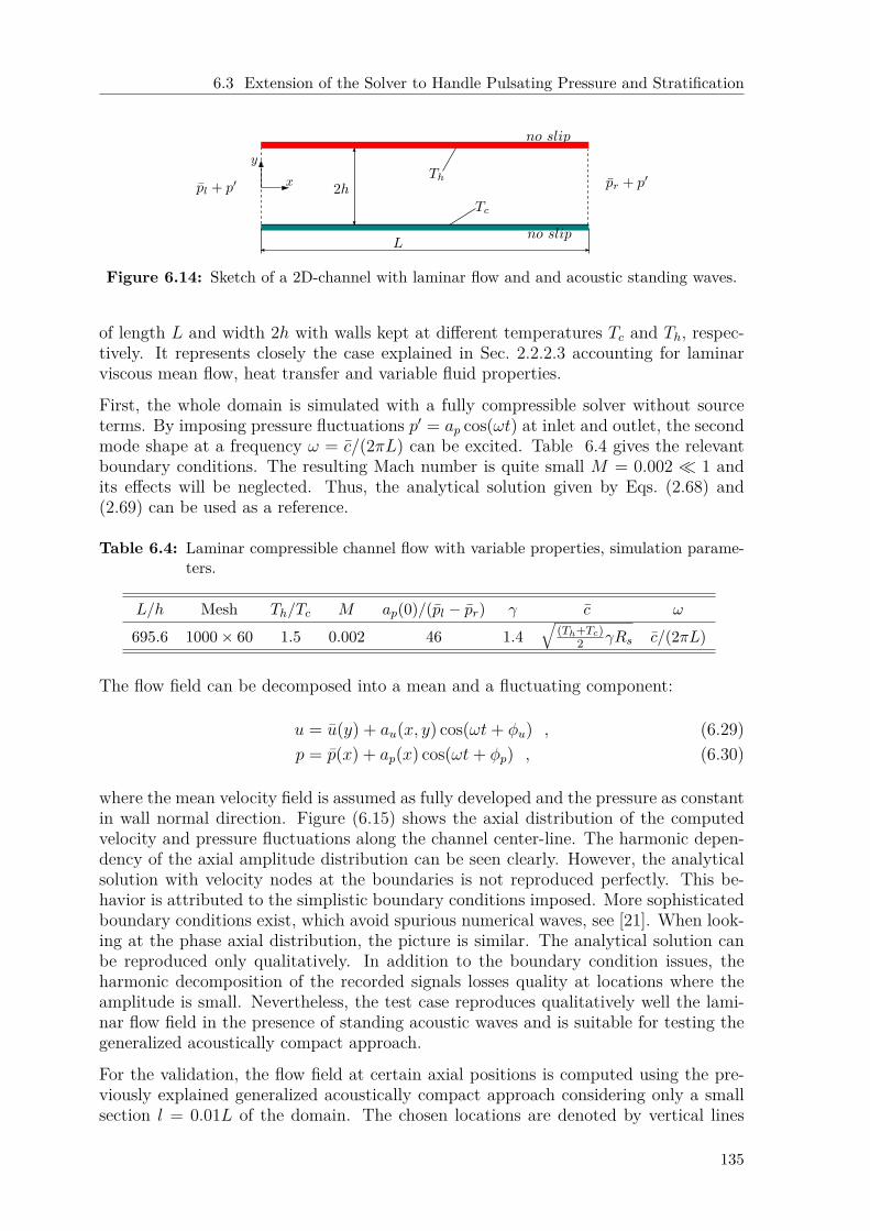
6.3 Extension of the Solver to Handle Pulsating Pressure and Stratification
Figure 6.14: Sketch of a 2D-channel with laminar flow and and acoustic standing waves.
of length L and width 2h with walls kept at different temperatures Tc and Th, respec-tively. It represents closely the case explained in Sec. 2.2.2.3 accounting for laminarviscous mean flow, heat transfer and variable fluid properties.
First, the whole domain is simulated with a fully compressible solver without sourceterms. By imposing pressure fluctuations p′ = ap cos(ωt) at inlet and outlet, the secondmode shape at a frequency ω = c/(2πL) can be excited. Table 6.4 gives the relevantboundary conditions. The resulting Mach number is quite small M = 0.002 1 andits effects will be neglected. Thus, the analytical solution given by Eqs. (2.68) and(2.69) can be used as a reference.
Table 6.4: Laminar compressible channel flow with variable properties, simulation parame-ters.
L/h Mesh Th/Tc M ap(0)/(pl − pr) γ c ω
695.6 1000× 60 1.5 0.002 46 1.4√
(Th+Tc)2 γRs c/(2πL)
The flow field can be decomposed into a mean and a fluctuating component:
u = u(y) + au(x, y) cos(ωt+ φu) , (6.29)p = p(x) + ap(x) cos(ωt+ φp) , (6.30)
where the mean velocity field is assumed as fully developed and the pressure as constantin wall normal direction. Figure (6.15) shows the axial distribution of the computedvelocity and pressure fluctuations along the channel center-line. The harmonic depen-dency of the axial amplitude distribution can be seen clearly. However, the analyticalsolution with velocity nodes at the boundaries is not reproduced perfectly. This be-havior is attributed to the simplistic boundary conditions imposed. More sophisticatedboundary conditions exist, which avoid spurious numerical waves, see [21]. When look-ing at the phase axial distribution, the picture is similar. The analytical solution canbe reproduced only qualitatively. In addition to the boundary condition issues, theharmonic decomposition of the recorded signals losses quality at locations where theamplitude is small. Nevertheless, the test case reproduces qualitatively well the lami-nar flow field in the presence of standing acoustic waves and is suitable for testing thegeneralized acoustically compact approach.
For the validation, the flow field at certain axial positions is computed using the pre-viously explained generalized acoustically compact approach considering only a smallsection l = 0.01L of the domain. The chosen locations are denoted by vertical lines
135
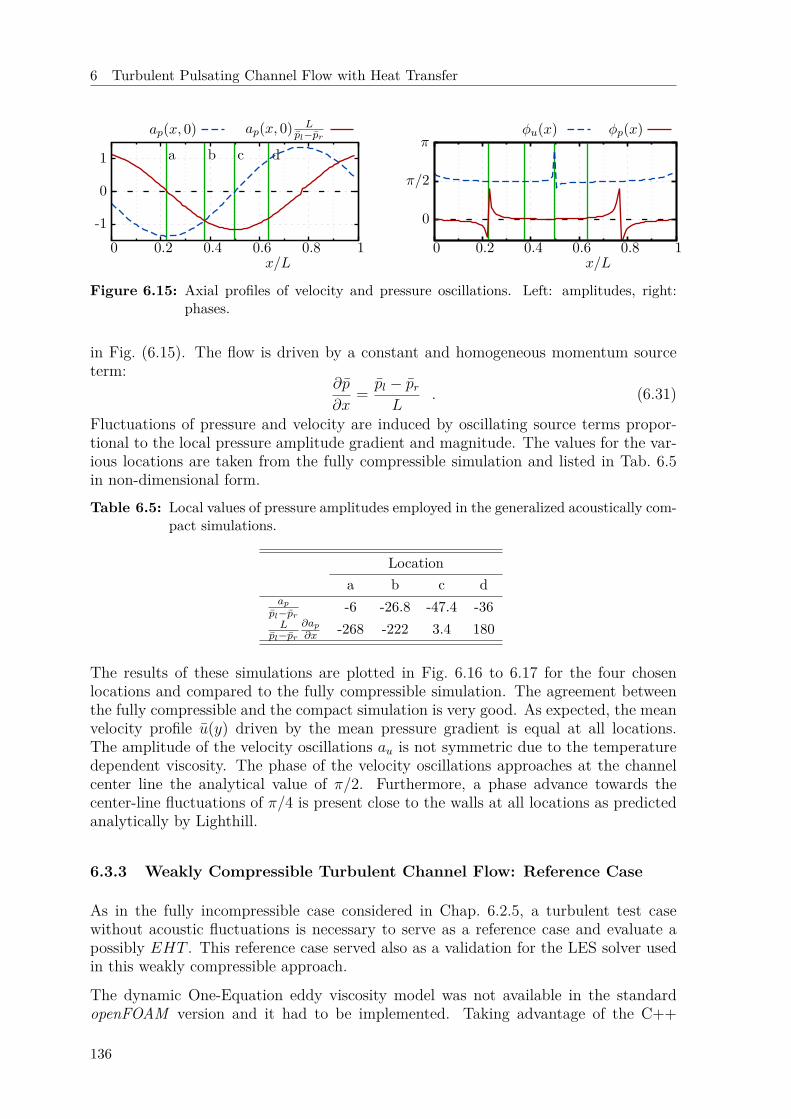
6 Turbulent Pulsating Channel Flow with Heat Transfer
-1
0
1
0 0.2 0.4 0.6 0.8 1x/L
a b c d
ap(x, 0) ap(x, 0) Lpl−pr
0
π/2
π
0 0.2 0.4 0.6 0.8 1x/L
φu(x) φp(x)
Figure 6.15: Axial profiles of velocity and pressure oscillations. Left: amplitudes, right:phases.
in Fig. (6.15). The flow is driven by a constant and homogeneous momentum sourceterm:
∂p
∂x= pl − pr
L. (6.31)
Fluctuations of pressure and velocity are induced by oscillating source terms propor-tional to the local pressure amplitude gradient and magnitude. The values for the var-ious locations are taken from the fully compressible simulation and listed in Tab. 6.5in non-dimensional form.Table 6.5: Local values of pressure amplitudes employed in the generalized acoustically com-
pact simulations.
Locationa b c d
appl−pr -6 -26.8 -47.4 -36L
pl−pr∂ap∂x -268 -222 3.4 180
The results of these simulations are plotted in Fig. 6.16 to 6.17 for the four chosenlocations and compared to the fully compressible simulation. The agreement betweenthe fully compressible and the compact simulation is very good. As expected, the meanvelocity profile u(y) driven by the mean pressure gradient is equal at all locations.The amplitude of the velocity oscillations au is not symmetric due to the temperaturedependent viscosity. The phase of the velocity oscillations approaches at the channelcenter line the analytical value of π/2. Furthermore, a phase advance towards thecenter-line fluctuations of π/4 is present close to the walls at all locations as predictedanalytically by Lighthill.
6.3.3 Weakly Compressible Turbulent Channel Flow: Reference Case
As in the fully incompressible case considered in Chap. 6.2.5, a turbulent test casewithout acoustic fluctuations is necessary to serve as a reference case and evaluate apossibly EHT . This reference case served also as a validation for the LES solver usedin this weakly compressible approach.
The dynamic One-Equation eddy viscosity model was not available in the standardopenFOAM version and it had to be implemented. Taking advantage of the C++
136
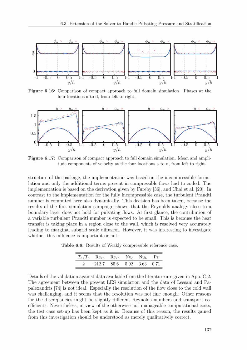
6.3 Extension of the Solver to Handle Pulsating Pressure and Stratification
0
π2
-1 -0.5 0 0.5 1y/h
φu φp
-1 -0.5 0 0.5 1y/h
φu φp
-1 -0.5 0 0.5 1y/h
φu φp
-1 -0.5 0 0.5 1y/h
φu φp
Figure 6.16: Comparison of compact approach to full domain simulation. Phases at thefour locations a to d, from left to right.
0
0.5
1
1.5
-1 -0.5 0 0.5 1y/h
u up
-1 -0.5 0 0.5 1y/h
u au
-1 -0.5 0 0.5 1y/h
u au
-1 -0.5 0 0.5 1y/h
u au
Figure 6.17: Comparison of compact approach to full domain simulation. Mean and ampli-tude components of velocity at the four locations a to d, from left to right.
structure of the package, the implementation was based on the incompressible formu-lation and only the additional terms present in compressible flows had to coded. Theimplementation is based on the derivation given by Fureby [36], and Chai et al. [20]. Incontrast to the implementation for the fully incompressible case, the turbulent Prandtlnumber is computed here also dynamically. This decision has been taken, because theresults of the first simulation campaign shown that the Reynolds analogy close to aboundary layer does not hold for pulsating flows. At first glance, the contribution ofa variable turbulent Prandtl number is expected to be small. This is because the heattransfer is taking place in a region close to the wall, which is resolved very accuratelyleading to marginal subgrid scale diffusion. However, it was interesting to investigatewhether this influence is important or not.
Table 6.6: Results of Weakly compressible reference case.
Th/Tc Reτc Reτh Nuc Nuh Pr2 212.7 85.6 5.92 3.63 0.71
Details of the validation against data available from the literature are given in App. C.2.The agreement between the present LES simulation and the data of Lessani and Pa-palexandris [74] is not ideal. Especially the resolution of the flow close to the cold wallwas challenging, and it seems that the resolution was not fine enough. Other reasonsfor the discrepancies might be slightly different Reynolds numbers and transport co-efficients. Nevertheless, in view of the otherwise not manageable computational costs,the test case set-up has been kept as it is. Because of this reason, the results gainedfrom this investigation should be understood as merely qualitatively correct.
137
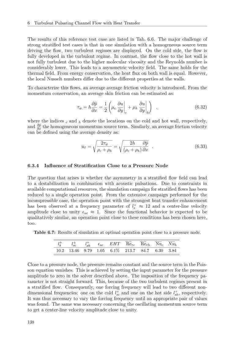
6 Turbulent Pulsating Channel Flow with Heat Transfer
The results of this reference test case are listed in Tab. 6.6. The major challenge ofstrong stratified test cases is that in one simulation with a homogeneous source termdriving the flow, two turbulent regimes are displayed. On the cold side, the flow isfully developed in the turbulent regime. In contrast, the flow close to the hot wall isnot fully turbulent due to the higher molecular viscosity and the Reynolds number isconsiderably lower. This leads to a asymmetric velocity field. The same holds for thethermal field. From energy conservation, the heat flux on both wall is equal. However,the local Nusselt numbers differ due to the different properties at the walls.
To characterize this flows, an average average friction velocity is introduced. From themomentum conservation, an average skin friction can be estimated as:
τw = h∂p
∂x= 1
2
(µc
∂u
∂y
∣∣∣∣∣c
+ µh∂u
∂y
∣∣∣∣∣h
), (6.32)
where the indices c and h denote the locations on the cold and hot wall, respectively,and ∂p
∂xthe homogeneous momentum source term. Similarly, an average friction velocity
can be defined using the average density as:
uτ =√
2τwρc + ρh
=√
2h(ρc + ρh)
∂p
∂x. (6.33)
6.3.4 Influence of Stratification Close to a Pressure Node
The question that arises is whether the asymmetry in a stratified flow field can leadto a destabilization in combination with acoustic pulsations. Due to constraints inavailable computational resources, the simulation campaign for stratified flows has beenreduced to a single operation point. From the extensive campaign performed for theincompressible case, the operation point with the strongest heat transfer enhancementhas been observed at a frequency parameter of l+s ≈ 12 and a center-line velocityamplitude close to unity εuc ≈ 1. Since the functional behavior is expected to bequalitatively similar, an operation point close to these conditions has been chosen here,too.
Table 6.7: Results of simulation at optimal operation point close to a pressure node.
l+s l+sc l+sh εuc EHT Reτc Reτh Nuc Nuh
10.2 13.46 9.79 1.05 6.1% 213.7 84.7 6.30 3.84
Close to a pressure node, the pressure remains constant and the source term in the Pois-son equation vanishes. This is achieved by setting the input parameter for the pressureamplitude to zero in the solver described above. The imposition of the frequency pa-rameter is not straight forward. This, because of the two turbulent regimes present ina stratified flow. Consequently, one forcing frequency will lead to two different non-dimensional frequencies: one on the cold l+sc and one on the hot side l+sh, respectively.It was thus necessary to vary the forcing frequency until an appropriate pair of valueswas found. The same was necessary concerning the oscillating momentum source termto get a center-line velocity amplitude close to unity.
138
6.3 Extension of the Solver to Handle Pulsating Pressure and Stratification
Table 6.7 gives the results of the simulation closest to the desired operation conditions.The essential parameter concerning heat transfer is again the ratio of enhancement. Un-der the given operation conditions, an enhancement of approximately 6.1% has beenfound. Compared to the value of 6.6% that the map of the fully incompressible cam-paign predicts for the operation point l+s = 10.2 and εuc = 1.05, no appreciable changecan be observed. This means that the stratification does not change essentially therelative average heat transfer in pulsating flows.
6.3.5 Influence of Pressure Fluctuations
To get the general picture of heat transfer in pulsating flows driven by standing acousticwaves, three additional operation points have been computed. They corresponds tolocations in an acoustic field others than the pressure node. To explain this simulationcampaign, consider the acoustic field shown schematically in Fig. 6.18 by the dashedlines. It corresponds to standing acoustic waves of wavelength λa. The locations to beinvestigated are denoted by small dashed rectangles at positions x = X1 to x = X4.According to the linear theory presented in Sec. 2.2.2, the pressure field can be describedby:
p′ = P1 cos(2πx/λa) cos(ωt) = ap(x) cos(ωt) , (6.34)with pressure amplitude P1. According to the compact approach presented above, themomentum source term is:
~SM = ∂
∂x[p+ P1 cos(2πx/λa) cos(ωt)] = P0x − P1x(x) cos(ωt) , (6.35)
where stationary and oscillating components are assumed homogeneous over a smallportion of the channel for a given location x = X. To be consistent with the operationpoint presented in Sec. 6.3.4, the parameters used in that simulation are adopted herefor position X3. The normalized parameters for all positions are listed in the first threecolumns of Tab. 6.8.Table 6.8: Parameters used in the simulation campaign for various compact axial locations
and corresponding results.
Location P0x|P0x(X1)|
P1x|P1x(X3)| EHT l+sc l+sh εuc Reτc Reτh Nuc Nuh
X1 1 0 −0.9% 13.69 9.66 1.05 216.3 84.4 5.89 3.58X2
√2 −
√2 5.6% 13.43 9.94 1.05 212.2 86.9 6.27 3.84
X3 0 −1 6.1% 13.46 9.79 1.05 213.7 84.7 6.30 3.84X4 −
√2 −
√2 5.6% 13.39 9.53 1.05 211.6 83.3 6.29 3.84
Again, the results concerning heat transfer are evaluated primarily through the ratioof enhancement, which is also listed in Tab. 6.8. For a better overview, the ratioof enhancement is also plotted in Fig. 6.18, where the profiles of acoustic pressureand velocity fluctuations are also sketched. The ratio of enhancement at locations X2and X4 is almost identical to the ratio at the reference position X3. In contrast, atposition X1 where only pressure fluctuations occur, the ratio of enhancement vanishes.The results of this simulation campaign show that the heat transfer enhancement iscontrolled solely by velocity fluctuations. The amplitude of the small acoustic pressurefluctuation does not influence the heat transfer.
139
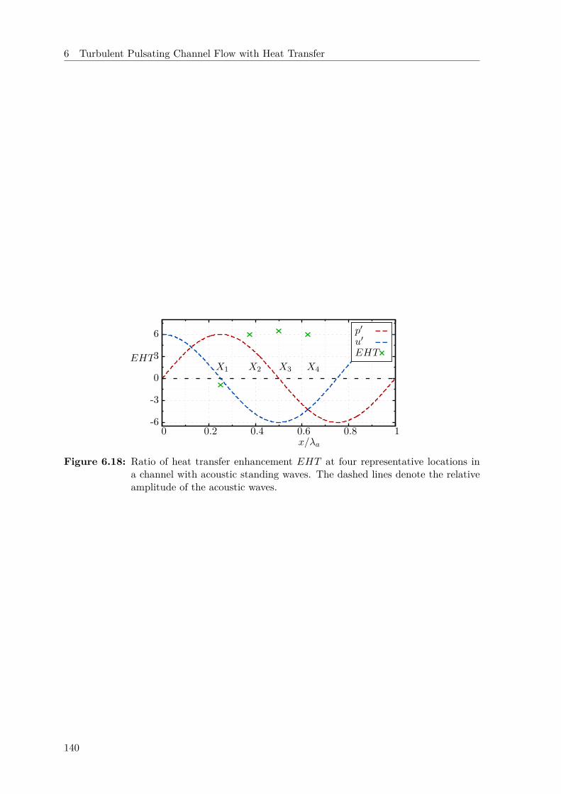
6 Turbulent Pulsating Channel Flow with Heat Transfer
-6
-3
0
3
6
0 0.2 0.4 0.6 0.8 1
EHT
x/λa
X1 X2 X3 X4
p′
u′
EHT
Figure 6.18: Ratio of heat transfer enhancement EHT at four representative locations ina channel with acoustic standing waves. The dashed lines denote the relativeamplitude of the acoustic waves.
140
7 Summary and Conclusions
The long term objective of the project hosting this work is the development of reliableengineering tools to characterize the damping behavior of resonator rings in rocketthrust chambers under real operation conditions. Hereby, the influence of enhancedheat transfer presumably driven by the acoustic fluctuations should be considered inthe analysis. The overall intention of the project is to clarify the following questions:
1. Should we expect significantly enhanced heat transfer in resonators or in thevicinity of the cavity mouths?
2. Does this enhanced heat transfer has any consequences on the damping behaviorof resonators?
In order to provide satisfactory answers to these questions, fundamental research con-cerning two top level topics is necessary, namely: damping characteristics of resonatorrings and heat transfer in pulsating flow. This fundamental research, and a preliminaryestimation of possible consequences was the goal of this thesis.
The first part of this thesis dealt with the accurate description of the damping be-havior of resonator rings under representative rocket chamber operation conditions.The characterization of the resonator rings is based on impedance expressions treatedas boundary conditions. After giving some state of the art models for resonators, anextension to account for temperature inhomogeneities inside the cavities is proposed.Based on these equivalent impedance expressions, a preliminary decoupled analysis ispresented that describes the dependency of the cavities to some design parameters andchamber conditions. Especial attention is given to the influence of an inhomogeneoustemperature profile possibly caused by heat transfer enhancement. The results of thispreliminary investigation show that the cavities frequency bandwidth of operation isconsiderably reduced by a temperature inhomogeneity. Furthermore, it has been shownthat the models describing the non-linear losses exhibit a strong uncertainty.
To accurately predict the stabilizing influence of resonator rings, the main driving anddamping mechanisms present in the thrust chambers have to be considered. For thispurpose, a low-order method to predict linear stability is proposed, which is able toreproduce the essential driving and damping mechanisms present in the chamber, giveespecial attention to the resonator ring, and afford parametric studies. The methodis based on a network representation of the chamber combined with a Nyquist-plottechnique for the determination of the system eigenfrequencies. This method widelyapplied for configurations propagating only plane waves, has been extended to accountfor non-plane transverse acoustic modes of major importance in rocket chambers. Thenecessary modifications to the method have been discussed. The incorporation of theresonator ring element has been carefully accomplished, taking an accurate acousticpressure field close to reactive and dissipative boundaries. This causes higher order
141
7 Summary and Conclusions
mode coupling at connections to the rest of the network. Studying a representativerocket thrust chamber configuration, three major stabilizing effects of resonator ringshave been identified:
(i) The eigenfrequencies of the system close to the design point of the cavities areshifted to slightly different frequencies. The coupling between driving mechanismsand acoustic might be weakened in this way.
(ii) Dissipation of acoustic energy by viscous effects described by the real part of theshell impedance stabilizes the system.
(iii) At connecting planes of the resonator ring, the traveling waves are scattered intohigher order, evanescent modes reducing the acoustic energy present in the reso-nant mode.
Furthermore, it has been demonstrated that the optimal design of resonator rings pre-dicted by a decoupled analysis differs from the one predicted by the coupled analysis.The reason for this behavior is the emergence of additional modes in the coupled sys-tem, which can not be described by a mere analysis of the boundary conditions. Thisis in accordance to experimental and numerical investigations [96].
This framework allowed finally to study the sensitivity of resonator rings to changesin the chamber operation conditions. The occurrence of enhanced heat transfer hasbeen modeled as a sudden increase of chamber wall temperature leading to a gas tem-perature inhomogeneity in the cavities. It has been shown that such a inhomogeneitycan indeed lead to a destabilization of the engine that was no predicted by state of theart models. This highlights the necessity for an accurate knowledge of the temperatureprofiles in rocket chambers, especially in the resonator cavities and under real operationconditions.
Thus, a major long term goal of the project hosting this work is the prediction of reliabletemperature profiles inside and in the vicinity of the cavities under pulsating conditions.However, to achieve this goal, a more concise understanding of the fundamental heattransfer phenomena under pulsating conditions as those induced by acoustic waves isnecessary. This was the intention of the second part of this thesis. Because the systemdynamics in representative rocket chambers are very complex, displaying bulk flow, nearwall turbulent hydrodynamic and wall thermal transients, the problem has been dividedinto more definite work packages of increasing complexity. In a divide and conquerstrategy, the influence of the different transients has been studied separately. The firstpreliminary investigation included a low order model for heat flux through a wall offinite thickness subjected to transient boundary conditions similar to those expectedin devices suffering from thermoacoustic instabilities. The second step performed inthe strategy treated the heat transfer in laminar pulsating flow past a heated flatplate using a numerical CFD approach. Based on these two preliminary investigations,various mechanisms leading to enhanced heat transfer have been identified and thefollowing conclusions can be addressed:
• Bulk flow transients can indeed lead to a permanent time averaged heat trans-fer change, provided that both the temperature and the heat transfer coefficientfluctuate in time. The phase between the two pulsations decides whether enhance-ment or diminishment occurs. The magnitude of the offset is proportional to the
142

amplitudes of the heat transfer coefficient and temperature oscillations. A similardependency has been predicted by Lundgren et al. [78].
• Two dimensional laminar hydrodynamic effects like flow reversal in a thermallydeveloping flow can also lead to permanent time averaged heat transfer changes.Both enhancement and diminishment of time averaged heat transfer is locallypossible, in agreement with theoretical and experimental observations [51, 79].
• For most combinations of parameters, the wall thermal inertia plays a minor rolein the heat transfer under transient conditions caused by pulsations of the bulkflow. The thermal inertia does not contribute to any permanent enhancement andworks always against the heat flux. These observations agree with the results ofsimilar investigations available in the literature [51, 79, 134].
The magnitude of the enhancement induced by the mechanisms mentioned in the pre-vious list is small. However, the interaction of turbulent scales with the organizedpulsations was omitted in those preliminary analysis. To account for the influence ofthis interaction, the third step in the strategy focused on the more challenging studyof heat transfer in turbulent pulsating flow.
First, a proper test case set-up has been defined, that makes the numerical treatmentof turbulent flows feasible based on the large eddy simulation approach. The organizedpulsations are imposed via an acoustically compact approach driven by source termsthat allow the treatment of the problem within an incompressible formalism. Thisovercomes several numerical issues concerning spurious numerical waves. Periodicityboundary conditions in stream- and spanwise direction allowed the flow to developturbulent fluctuations inherently. This leads to a physical turbulent spectrum and toa reduction of computational cost, because only a compact region of the channel hasto be simulated. The novelty of this extensive simulation campaign is that it coversa wider range of frequencies and center-line velocity amplitudes, and considers heattransfer. The principal results of this study are:
• The momentum transfer exhibited by the simulation campaign is in very goodagreement with available numerical [121] and experimental [124] data. It has beenconfirmed that the relevant similarity parameter is a non-dimensional frequencyscaled by appropriate turbulent time scales.
• A noticeable permanent change in time averaged heat transfer is only observedat large velocity amplitudes, in accordance with some experimental observations.Depending on the non-dimensional frequency, both heat transfer enhancement anddiminishment is possible. This may lead to contradictory results, if investigationsof different non-dimensional frequency are compared with each other.
• However, the magnitude of the possible enhancement is only a few percent and isorder of magnitudes lower than the one predicted in some experimental investi-gations, e.g. [29, 49], even if the non-dimensional frequency is similar.
In the first turbulent simulation campaign, stratification and acoustic pressure fluctu-ations have been neglected. In a subsequent final analysis, the method has been ex-tended to account for temperature dependent properties and local pressure fluctuations
143

7 Summary and Conclusions
in a weakly compressible formalism. Again, the assumption of acoustic compactness al-lowed the incorporation of these effects via source terms in the momentum and iterativepressure equation. After validation of the extended method, the operation point thatexhibited the maximum enhancement in the previous campaign has been investigatedtaking stratification and pressure fluctuations into account. However, these effects seemto play a negligible role concerning heat transfer enhancement.
144
A Linear Acoustics
A.1 Derivation of Wave Equation
This section reviews the derivation of a general inhomogeneous wave equation for thepressure fluctuations p′ and is based on the analysis given by Culick [24].
The starting point of the derivation are the Navier-Stokes equations given in Sec. 2.1.2.However, it is more convenient to express the equation of energy in terms of the pressure.This can be done assuming ideal gas behavior with homogeneous and constant heatcapacities (perfect gas). The set of equations in tensorial notation are:
∂ρ
∂t+ ~u · ~∇ρ = −ρ~∇ · ~u , (A.1)
ρ∂~u
∂t+ ρ~u · ~∇~u = −~∇p+ ~∇ · τ , (A.2)
∂p
∂t+ γp~∇ · ~u = −~u · ~∇p+ Rs
cv
[−~∇ · ~q + Q
], (A.3)
where τ corresponds to the stress tensor, mass and momentum source terms are ne-glected, and Q represents a volumetric heat release rate. This heat release rate can becaused for example by combustion.
In a perturbation analysis, all variables are decomposed into time averaged (mean) andfluctuating parts. Apart from the mean pressure, all mean quantities might vary inspace. A homogeneous averaged pressure assumption is valid for low Mach numbers.Under these assumptions, the set of perturbed equations can be written as:
∂ρ′
∂t+ ~u · ~∇ρ′ = −~u′ · ~∇ρ+O2 , (A.4)
∂~u′
∂t+ 1ρ~∇p′ = −
[~u · ~∇~u′ + ~u′ · ~∇~u
]+ 1ρ~∇ · τ ′ +O2 , (A.5)
∂p′
∂t+ γp~∇ · ~u′ = −~u · ~∇p′ − γp′~∇ · ~u+ Rs
cv
[−~∇ · ~q′ + Q′
]+O2 . (A.6)
The perturbed form of the equation of state reads:p′ = Rs(ρ′T + ρT ′) +O2 . (A.7)
Culick derived this equations up to second order in the fluctuations [24]. Here, theseterms are not shown explicitly, but are denoted by O2 in the corresponding equations.
A general perturbed wave equation can be derived by differentiating Eq. (A.6) withrespect to time and substracting the divergence of Eq. (A.5), such that the term ~∇· ∂~u′
∂tvanishes. This operation can be written, after some rearrangement as:
∂2p′
∂t2− ~∇ ·
(c2~∇p′
)= ℘ , (A.8)
145
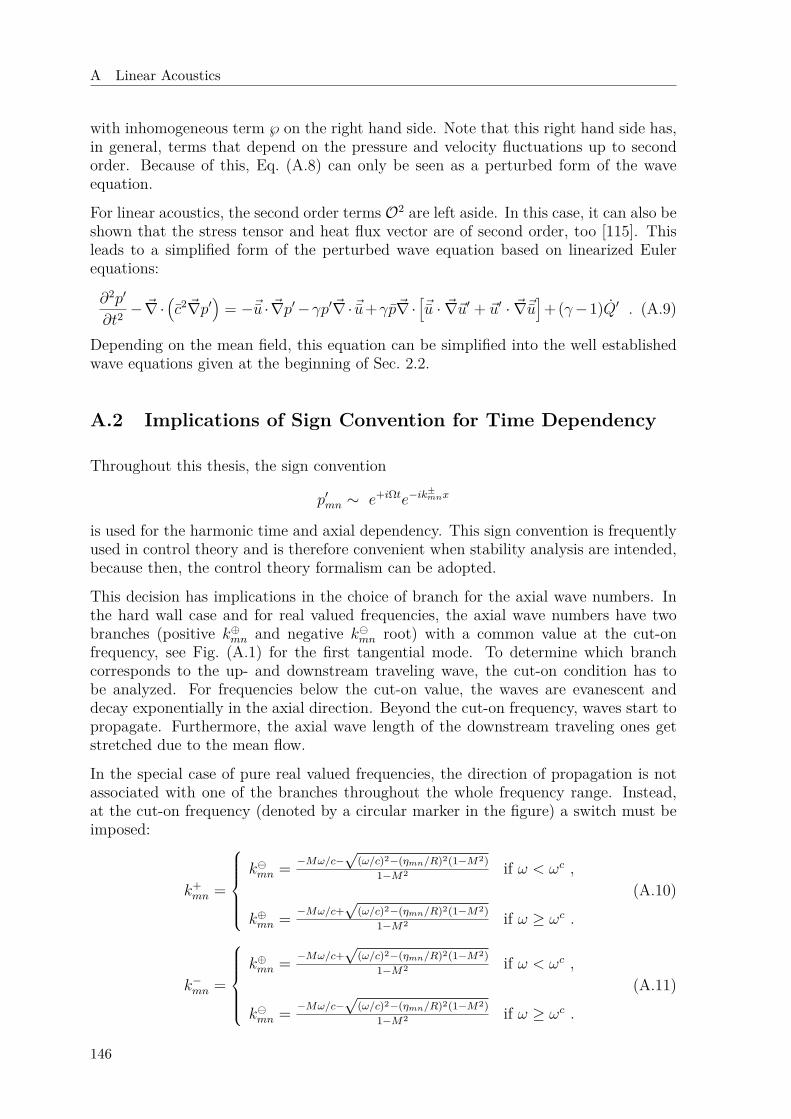
A Linear Acoustics
with inhomogeneous term ℘ on the right hand side. Note that this right hand side has,in general, terms that depend on the pressure and velocity fluctuations up to secondorder. Because of this, Eq. (A.8) can only be seen as a perturbed form of the waveequation.
For linear acoustics, the second order terms O2 are left aside. In this case, it can also beshown that the stress tensor and heat flux vector are of second order, too [115]. Thisleads to a simplified form of the perturbed wave equation based on linearized Eulerequations:
∂2p′
∂t2− ~∇·
(c2~∇p′
)= −~u · ~∇p′−γp′~∇· ~u+γp~∇·
[~u · ~∇~u′ + ~u′ · ~∇~u
]+(γ−1)Q′ . (A.9)
Depending on the mean field, this equation can be simplified into the well establishedwave equations given at the beginning of Sec. 2.2.
A.2 Implications of Sign Convention for Time Dependency
Throughout this thesis, the sign convention
p′mn ∼ e+iΩte−ik±mnx
is used for the harmonic time and axial dependency. This sign convention is frequentlyused in control theory and is therefore convenient when stability analysis are intended,because then, the control theory formalism can be adopted.
This decision has implications in the choice of branch for the axial wave numbers. Inthe hard wall case and for real valued frequencies, the axial wave numbers have twobranches (positive k⊕mn and negative kmn root) with a common value at the cut-onfrequency, see Fig. (A.1) for the first tangential mode. To determine which branchcorresponds to the up- and downstream traveling wave, the cut-on condition has tobe analyzed. For frequencies below the cut-on value, the waves are evanescent anddecay exponentially in the axial direction. Beyond the cut-on frequency, waves start topropagate. Furthermore, the axial wave length of the downstream traveling ones getstretched due to the mean flow.
In the special case of pure real valued frequencies, the direction of propagation is notassociated with one of the branches throughout the whole frequency range. Instead,at the cut-on frequency (denoted by a circular marker in the figure) a switch must beimposed:
k+mn =
kmn = −Mω/c−
√(ω/c)2−(ηmn/R)2(1−M2)
1−M2 if ω < ωc ,
k⊕mn = −Mω/c+√
(ω/c)2−(ηmn/R)2(1−M2)1−M2 if ω ≥ ωc .
(A.10)
k−mn =
k⊕mn = −Mω/c+
√(ω/c)2−(ηmn/R)2(1−M2)
1−M2 if ω < ωc ,
kmn = −Mω/c−√
(ω/c)2−(ηmn/R)2(1−M2)1−M2 if ω ≥ ωc .
(A.11)
146
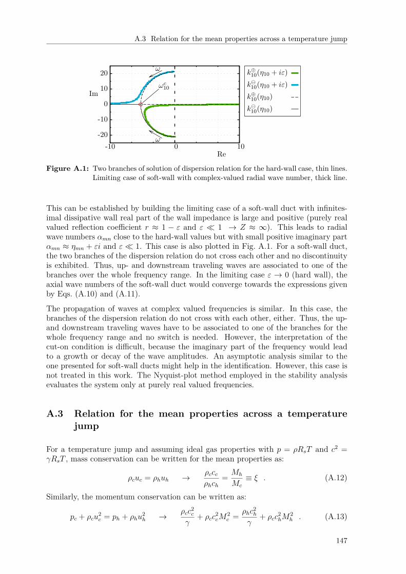
A.3 Relation for the mean properties across a temperature jump
-20
-10
0
10
20
-10 0 10
Im
Re
ω
ω
ωc10
k⊕10(η10 + iε)k10(η10 + iε)k⊕10(η10)k10(η10)
Figure A.1: Two branches of solution of dispersion relation for the hard-wall case, thin lines.Limiting case of soft-wall with complex-valued radial wave number, thick line.
This can be established by building the limiting case of a soft-wall duct with infinites-imal dissipative wall real part of the wall impedance is large and positive (purely realvalued reflection coefficient r ≈ 1 − ε and ε 1 → Z ≈ ∞). This leads to radialwave numbers αmn close to the hard-wall values but with small positive imaginary partαmn ≈ ηmn + εi and ε 1. This case is also plotted in Fig. A.1. For a soft-wall duct,the two branches of the dispersion relation do not cross each other and no discontinuityis exhibited. Thus, up- and downstream traveling waves are associated to one of thebranches over the whole frequency range. In the limiting case ε → 0 (hard wall), theaxial wave numbers of the soft-wall duct would converge towards the expressions givenby Eqs. (A.10) and (A.11).
The propagation of waves at complex valued frequencies is similar. In this case, thebranches of the dispersion relation do not cross with each other, either. Thus, the up-and downstream traveling waves have to be associated to one of the branches for thewhole frequency range and no switch is needed. However, the interpretation of thecut-on condition is difficult, because the imaginary part of the frequency would leadto a growth or decay of the wave amplitudes. An asymptotic analysis similar to theone presented for soft-wall ducts might help in the identification. However, this case isnot treated in this work. The Nyquist-plot method employed in the stability analysisevaluates the system only at purely real valued frequencies.
A.3 Relation for the mean properties across a temperaturejump
For a temperature jump and assuming ideal gas properties with p = ρRsT and c2 =γRsT , mass conservation can be written for the mean properties as:
ρcuc = ρhuh → ρcccρhch
= Mh
Mc
≡ ξ . (A.12)
Similarly, the momentum conservation can be written as:
pc + ρcu2c = ph + ρhu
2h → ρcc
2c
γ+ ρcc
2cM
2c = ρhc
2h
γ+ ρcc
2hM
2h . (A.13)
147
A Linear Acoustics
Substitution of the excess temperature Ξ = (ch/cc)2 − 1 = Th/Tc − 1 and the massconservation into the momentum conservation leads after some rearrangement to thefollowing relation:
Ξ =[ξ2 + γM2
h
(1 + γM2h) ξ
]2
− 1 . (A.14)
Thus, for an excess temperature of Ξ = 12, and a Mach number on the hot side ofMh = 0.25 the ratio of acoustic impedances should be ξ ≈ 3.84.
For vanishing mach numbers Mh 1, the relation can be approximated as:
Ξ ≈ ξ2 − 1 or ξ ≈√
Ξ + 1 . (A.15)
148
B Analytical Expression for LaminarPulsating Flows
B.1 Flow Induced by the Oscillation of an Infinite plate
The flow over an infinite flat plate that oscillates harmonically in its plane along the xdirection is a very simple example that indicates some of the important characteristics ofpulsating flows. This problem was solved analytically by Stokes, and it is often referredto in literature as Stokes’ second problem. Due to the symmetry of the problem noquantities vary with x and the incompressible momentum equation reduces to:
∂u
∂t= ν
∂2u
∂y2 , (B.1)
with the boundary conditions for the problem:
u→ 0 as y →∞ ,u = au cos(ωt) for y = 0 , (B.2)
where au is the velocity amplitude the plate and ω the oscillating frequency. Thesolution is based on an harmonic approach for the fluid velocity:
u = ueiωt , (B.3)
where a complex notation is used with a complex valued amplitude u. Substitution ofthis approach into Eq. (B.1) gives after some rearrangement:
ν∂2u
∂y2 = iω
ν. (B.4)
The solution of this equation satisfying the boundary conditions of the problem is givenby [125]:
u = aue√
iωνy = aue
√ω2ν yei√
ω2ν y , (B.5)
where the following identity has been used:
√i =
(eiπ2)0.5
= 1√2
+ i√2. (B.6)
Using the Stokes’ length δs to express the amplitude decay in the y direction, thegeneral solution can be finally written as:
u = aue− yδs ei
yδs eiωt . (B.7)
149
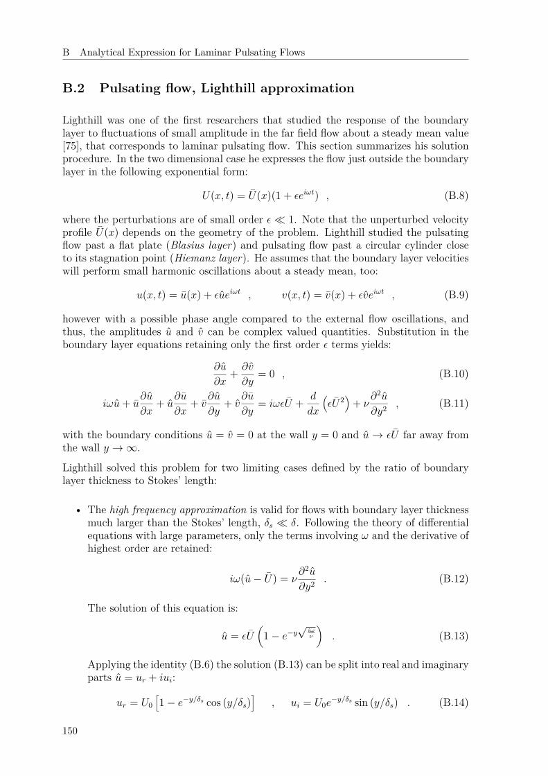
B Analytical Expression for Laminar Pulsating Flows
B.2 Pulsating flow, Lighthill approximation
Lighthill was one of the first researchers that studied the response of the boundarylayer to fluctuations of small amplitude in the far field flow about a steady mean value[75], that corresponds to laminar pulsating flow. This section summarizes his solutionprocedure. In the two dimensional case he expresses the flow just outside the boundarylayer in the following exponential form:
U(x, t) = U(x)(1 + εeiωt) , (B.8)
where the perturbations are of small order ε 1. Note that the unperturbed velocityprofile U(x) depends on the geometry of the problem. Lighthill studied the pulsatingflow past a flat plate (Blasius layer) and pulsating flow past a circular cylinder closeto its stagnation point (Hiemanz layer). He assumes that the boundary layer velocitieswill perform small harmonic oscillations about a steady mean, too:
u(x, t) = u(x) + εueiωt , v(x, t) = v(x) + εveiωt , (B.9)
however with a possible phase angle compared to the external flow oscillations, andthus, the amplitudes u and v can be complex valued quantities. Substitution in theboundary layer equations retaining only the first order ε terms yields:
∂u
∂x+ ∂v
∂y= 0 , (B.10)
iωu+ u∂u
∂x+ u
∂u
∂x+ v
∂u
∂y+ v
∂u
∂y= iωεU + d
dx
(εU2
)+ ν
∂2u
∂y2 , (B.11)
with the boundary conditions u = v = 0 at the wall y = 0 and u → εU far away fromthe wall y →∞.
Lighthill solved this problem for two limiting cases defined by the ratio of boundarylayer thickness to Stokes’ length:
• The high frequency approximation is valid for flows with boundary layer thicknessmuch larger than the Stokes’ length, δs δ. Following the theory of differentialequations with large parameters, only the terms involving ω and the derivative ofhighest order are retained:
iω(u− U) = ν∂2u
∂y2 . (B.12)
The solution of this equation is:
u = εU(
1− e−y√
iων
). (B.13)
Applying the identity (B.6) the solution (B.13) can be split into real and imaginaryparts u = ur + iui:
ur = U0[1− e−y/δs cos (y/δs)
], ui = U0e
−y/δs sin (y/δs) . (B.14)
150

B.2 Pulsating flow, Lighthill approximation
The phase lag between the boundary layer velocity and the far field velocityoscillations can be determined from the following expression:
tan(φu) = sin(y)eδ2s/δs − cos(y) . (B.15)
The bounds of the phase lag are π/4 at the wall y → 0 and 0 for y → ∞. Thismeans that in the high frequency regime, the velocity fluctuations in the boundarylayer advance always the fluctuations of the external flow.
• The low frequency approximation is valid for flows with boundary layer thicknessmuch smaller than the Stokes’ length, δs δ. Lighthill splits the solution into aquasi steady contribution uqs, which is in phase with the external perturbation,and an out of phase contribution uop:
u = uqs + iωuop . (B.16)
The quasi steady contribution represents the functional dependency of u to U ,which for small perturbations reads:
uqs = εU∂u
∂U. (B.17)
For several geometries like the Blasius layer (flat plate) or the Hiemanz-layer(circular cylinder), this dependency can be approximated with good accuracy withpolynomial expressions on η = y/δ according to a Karman-Pohlhausen treatment[44]. For the flow past a flat plate, U = const. and evolution of the boundarylayer flow along the plate is given by the following expressions [75]:
Uδ2
ν= 34x , (B.18)
u(x)U
= 1− (1− η)3 (1 + η) . (B.19)
Substitution of the previous relations into equation (B.11) yields again a partialdifferential equation for the out of phase contribution uop. The resulting equa-tion can be solved integrating it over the boundary layer thickness using also apolynomial approximation for uop (not shown here).The low frequency approximation for the pulsating flow past a flat plate, splitagain in real and imaginary parts, can be finally written as:
ur = uqs = U[1− (1− η)2(1− η − 3η2)
],
ui = ωuop = 34ωx(1− η)2η
5
(34 − η
). (B.20)
The components of the skin friction can be determined from the wall normalderivative of the velocity components:
τw,qs ∼∂uqs∂y
∣∣∣∣∣y=0
= 3U ,
τw,op ∼ ω∂uop∂y
∣∣∣∣∣y=0
= 5110ωx . (B.21)
151

B Analytical Expression for Laminar Pulsating Flows
The phase lag of the skin friction in this low frequency approximation can bedetermined from the following expression:
tan(φτw) = τw,opτw,qs
= 1710ωx
U. (B.22)
152
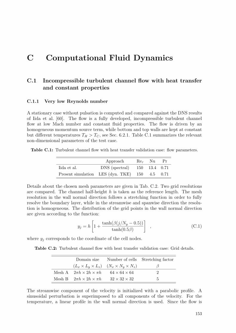
C Computational Fluid Dynamics
C.1 Incompressible turbulent channel flow with heat transferand constant properties
C.1.1 Very low Reynolds number
A stationary case without pulsation is computed and compared against the DNS resultsof Iida et al. [60]. The flow is a fully developed, incompressible turbulent channelflow at low Mach number and constant fluid properties. The flow is driven by anhomogeneous momentum source term, while bottom and top walls are kept at constantbut different temperatures TH > TC , see Sec. 6.2.1. Table C.1 summarizes the relevantnon-dimensional parameters of the test case.
Table C.1: Turbulent channel flow with heat transfer validation case: flow parameters.
Approach Reτ Nu PrIida et al. DNS (spectral) 150 13.4 0.71Present simulation LES (dyn. TKE) 150 4.5 0.71
Details about the chosen mesh parameters are given in Tab. C.2. Two grid resolutionsare compared. The channel half-height h is taken as the reference length. The meshresolution in the wall normal direction follows a stretching function in order to fullyresolve the boundary layer, while in the streamwise and spanwise direction the resolu-tion is homogeneous. The distribution of the grid points in the wall normal directionare given according to the function:
yj = h
[1 + tanh(β(j/Ny − 0.5))
tanh(0.5β)
], (C.1)
where yj corresponds to the coordinate of the cell nodes.
Table C.2: Turbulent channel flow with heat transfer validation case: Grid details.
Domain size Number of cells Stretching factor(Lx × Ly × Lz) (Nx ×Ny ×Nz) β
Mesh A 2πh× 2h× πh 64× 64× 64 2Mesh B 2πh× 2h× πh 32× 32× 32 5
The streamwise component of the velocity is initialized with a parabolic profile. Asinusoidal perturbation is superimposed to all components of the velocity. For thetemperature, a linear profile in the wall normal direction is used. Since the flow is
153
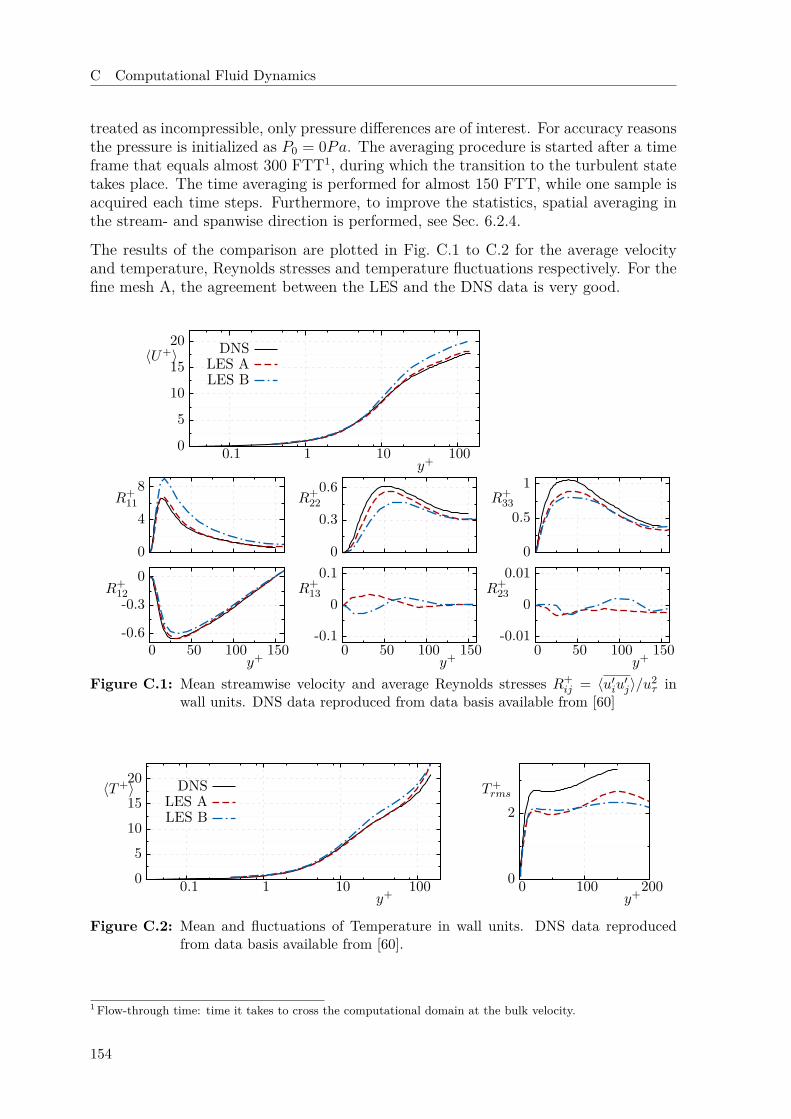
C Computational Fluid Dynamics
treated as incompressible, only pressure differences are of interest. For accuracy reasonsthe pressure is initialized as P0 = 0Pa. The averaging procedure is started after a timeframe that equals almost 300 FTT1, during which the transition to the turbulent statetakes place. The time averaging is performed for almost 150 FTT, while one sample isacquired each time steps. Furthermore, to improve the statistics, spatial averaging inthe stream- and spanwise direction is performed, see Sec. 6.2.4.
The results of the comparison are plotted in Fig. C.1 to C.2 for the average velocityand temperature, Reynolds stresses and temperature fluctuations respectively. For thefine mesh A, the agreement between the LES and the DNS data is very good.
0
5
10
15
20
0.1 1 10 100
〈U+〉
y+
DNSLES ALES B
0
4
8R+
11
0
0.3
0.6R+
22
0
0.5
1R+
33
-0.6
-0.3
0
0 50 100 150
R+12
y+
-0.1
0
0.1
0 50 100 150
R+13
y+
-0.01
0
0.01
0 50 100 150
R+23
y+
Figure C.1: Mean streamwise velocity and average Reynolds stresses R+ij = 〈u′iu′j〉/u2
τ inwall units. DNS data reproduced from data basis available from [60]
05
101520
0.1 1 10 100
〈T+〉
y+0
2
0 100 200
T+rms
y+
DNSLES ALES B
Figure C.2: Mean and fluctuations of Temperature in wall units. DNS data reproducedfrom data basis available from [60].
1 Flow-through time: time it takes to cross the computational domain at the bulk velocity.
154
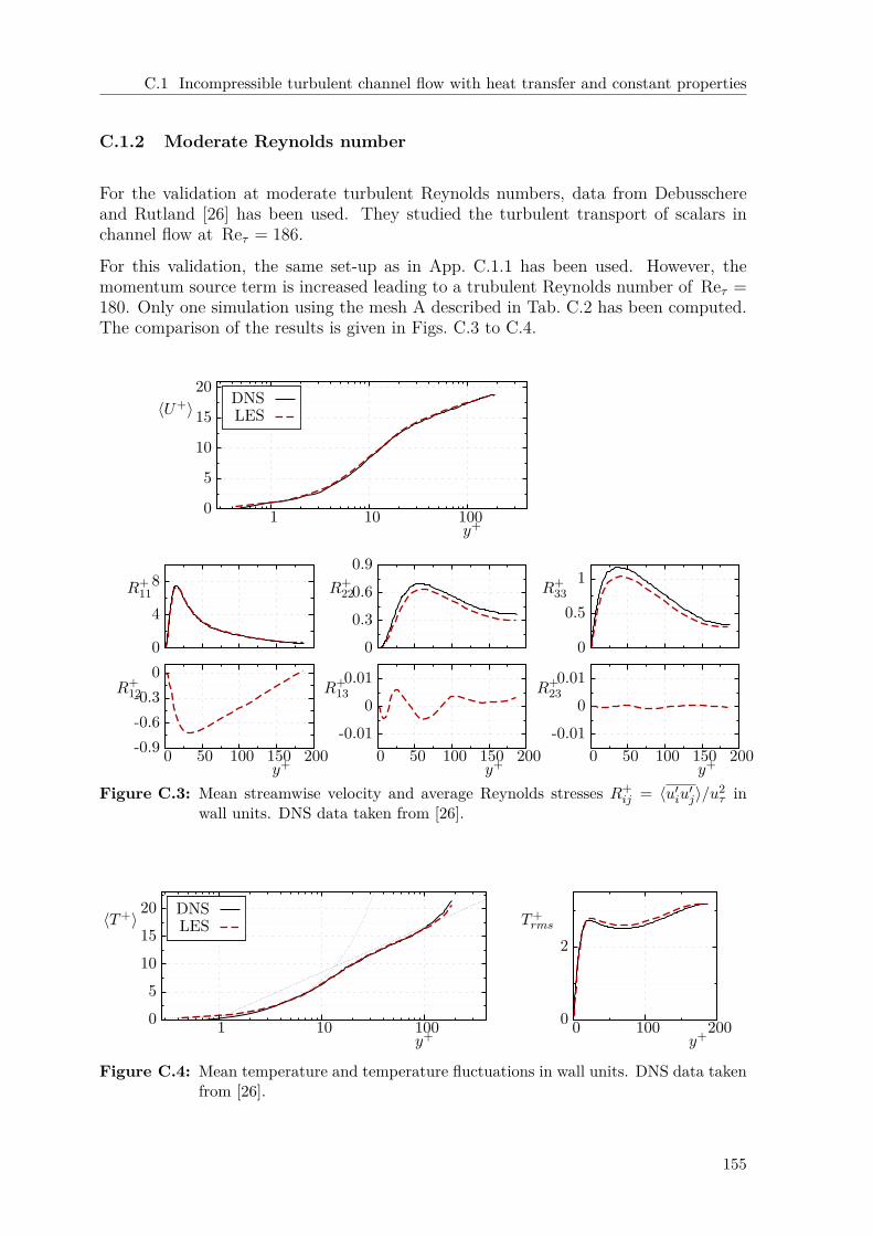
C.1 Incompressible turbulent channel flow with heat transfer and constant properties
C.1.2 Moderate Reynolds number
For the validation at moderate turbulent Reynolds numbers, data from Debusschereand Rutland [26] has been used. They studied the turbulent transport of scalars inchannel flow at Reτ = 186.
For this validation, the same set-up as in App. C.1.1 has been used. However, themomentum source term is increased leading to a trubulent Reynolds number of Reτ =180. Only one simulation using the mesh A described in Tab. C.2 has been computed.The comparison of the results is given in Figs. C.3 to C.4.
0
5
10
15
20
1 10 100
〈U+〉
y+
DNSLES
0
4
8R+11
00.30.60.9
R+22
0
0.5
1R+
33
-0.9-0.6-0.3
0
0 50 100 150 200
R+12
y+
-0.010
0.01
0 50 100 150 200
R+13
y+
-0.010
0.01
0 50 100 150 200
R+23
y+
Figure C.3: Mean streamwise velocity and average Reynolds stresses R+ij = 〈u′iu′j〉/u2
τ inwall units. DNS data taken from [26].
05
101520
1 10 100
〈T+〉
y+0
2
0 100 200
T+rms
y+
DNSLES
Figure C.4: Mean temperature and temperature fluctuations in wall units. DNS data takenfrom [26].
155
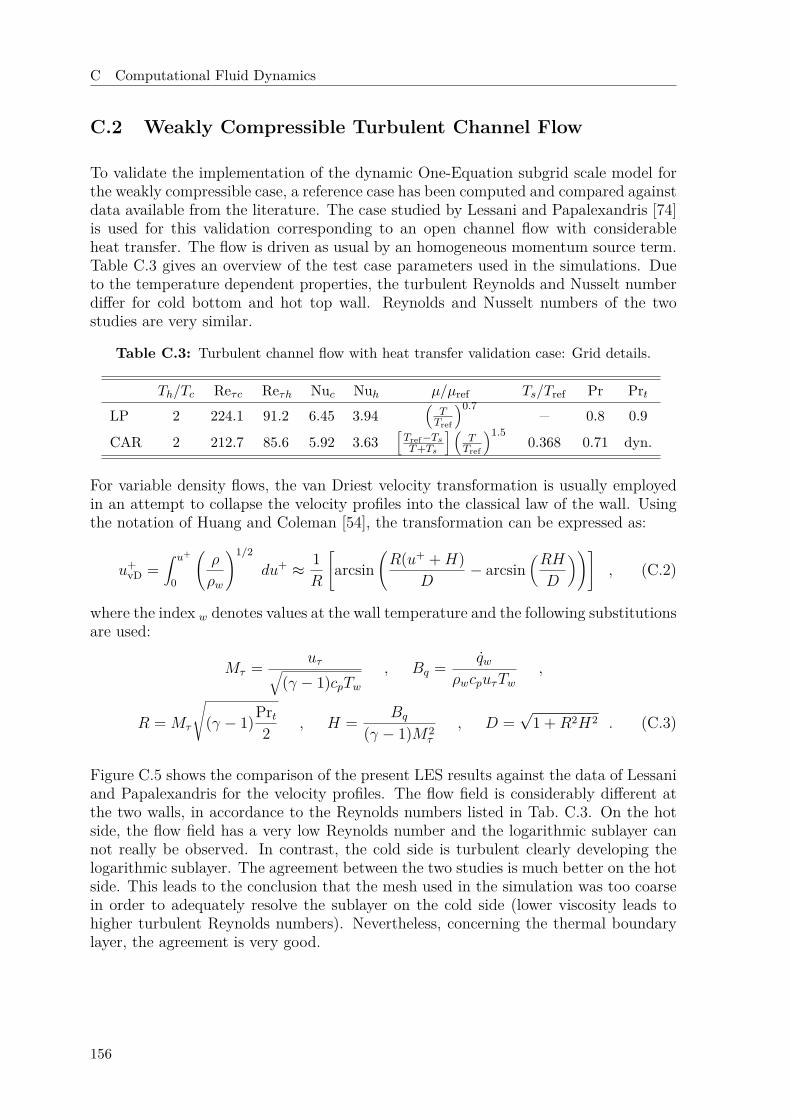
C Computational Fluid Dynamics
C.2 Weakly Compressible Turbulent Channel Flow
To validate the implementation of the dynamic One-Equation subgrid scale model forthe weakly compressible case, a reference case has been computed and compared againstdata available from the literature. The case studied by Lessani and Papalexandris [74]is used for this validation corresponding to an open channel flow with considerableheat transfer. The flow is driven as usual by an homogeneous momentum source term.Table C.3 gives an overview of the test case parameters used in the simulations. Dueto the temperature dependent properties, the turbulent Reynolds and Nusselt numberdiffer for cold bottom and hot top wall. Reynolds and Nusselt numbers of the twostudies are very similar.
Table C.3: Turbulent channel flow with heat transfer validation case: Grid details.
Th/Tc Reτc Reτh Nuc Nuh µ/µref Ts/Tref Pr PrtLP 2 224.1 91.2 6.45 3.94
(TTref
)0.7 0.8 0.9
CAR 2 212.7 85.6 5.92 3.63[Tref−TsT+Ts
] (TTref
)1.50.368 0.71 dyn.
For variable density flows, the van Driest velocity transformation is usually employedin an attempt to collapse the velocity profiles into the classical law of the wall. Usingthe notation of Huang and Coleman [54], the transformation can be expressed as:
u+vD =
∫ u+
0
(ρ
ρw
)1/2
du+ ≈ 1R
[arcsin
(R(u+ +H)
D− arcsin
(RH
D
))], (C.2)
where the index w denotes values at the wall temperature and the following substitutionsare used:
Mτ = uτ√(γ − 1)cpTw
, Bq = qwρwcpuτTw
,
R = Mτ
√(γ − 1)Prt
2 , H = Bq
(γ − 1)M2τ
, D =√
1 +R2H2 . (C.3)
Figure C.5 shows the comparison of the present LES results against the data of Lessaniand Papalexandris for the velocity profiles. The flow field is considerably different atthe two walls, in accordance to the Reynolds numbers listed in Tab. C.3. On the hotside, the flow field has a very low Reynolds number and the logarithmic sublayer cannot really be observed. In contrast, the cold side is turbulent clearly developing thelogarithmic sublayer. The agreement between the two studies is much better on the hotside. This leads to the conclusion that the mesh used in the simulation was too coarsein order to adequately resolve the sublayer on the cold side (lower viscosity leads tohigher turbulent Reynolds numbers). Nevertheless, concerning the thermal boundarylayer, the agreement is very good.
156
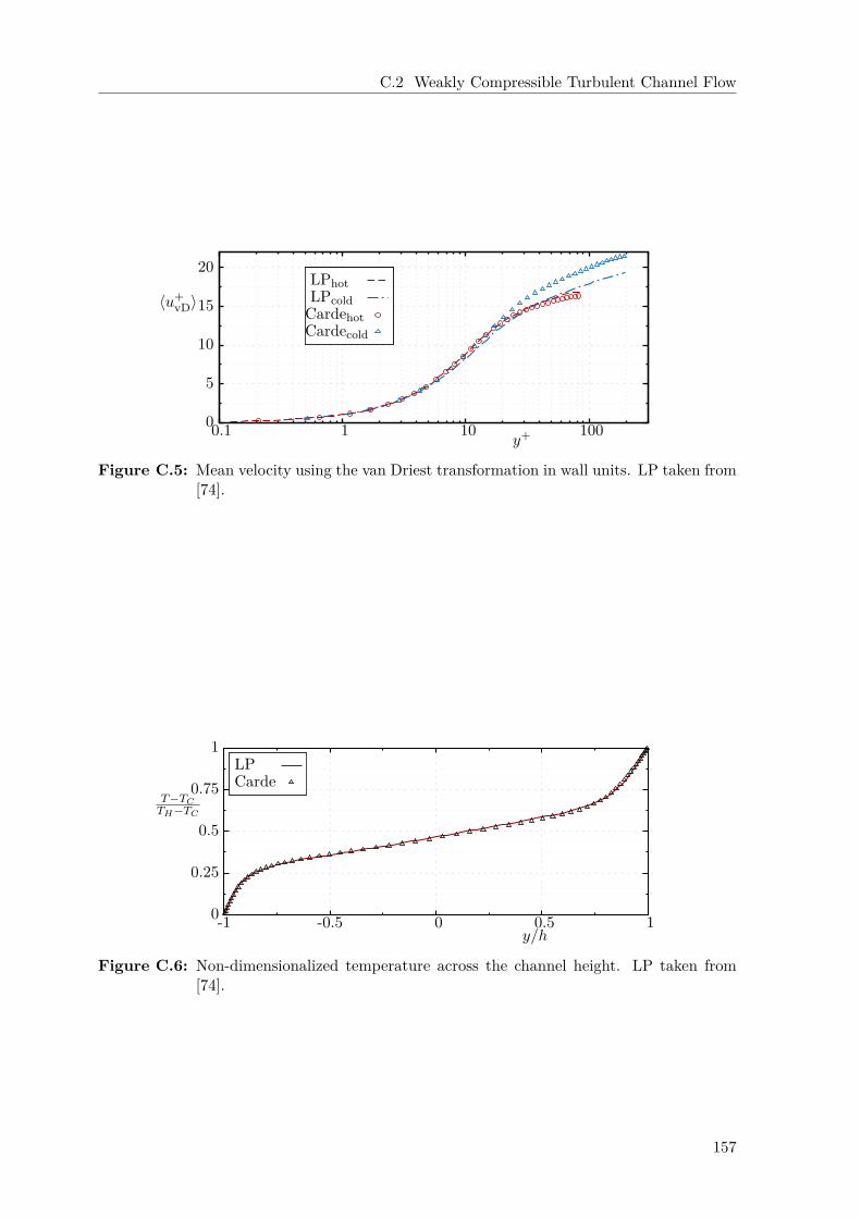
C.2 Weakly Compressible Turbulent Channel Flow
0
5
10
15
20
0.1 1 10 100
〈u+vD〉
y+
LPhotLPcold
CardehotCardecold
Figure C.5: Mean velocity using the van Driest transformation in wall units. LP taken from[74].
0
0.25
0.5
0.75
1
-1 -0.5 0 0.5 1
T−TCTH−TC
y/h
LPCarde
Figure C.6: Non-dimensionalized temperature across the channel height. LP taken from[74].
157
List of Figures
1.1 Schematic description of coupling between heat release and acoustic per-turbations leading to self sustained oscillations. . . . . . . . . . . . . . 2
2.1 Transverse acoustic mode shapes for a hard walled cylinder. Dashedlines denote the location of the pressure nodal lines. . . . . . . . . . . . 14
2.2 Two branches of solution of dispersion relation for the hard-wall case,dashed lines. Limiting case of soft-wall with complex-valued radial wavenumber. . . . . . . . . . . . . . . . . . . . . . . . . . . . . . . . . . . . 15
2.3 Normalized pressure and velocity amplitudes in a channel with two openends for various mode shapes. Bottom, l = 1; middle, l = 2; top, l = 3. 19
2.4 Acoustic system consisting of three elements bounded by proper termi-nations. . . . . . . . . . . . . . . . . . . . . . . . . . . . . . . . . . . . 20
2.5 Two port “diagnostic dummy” element, adapted from [66]. . . . . . . . 23
2.6 Conformal mapping of ω into OLTF (ω).. . . . . . . . . . . . . . . . . . . . . . . . . . . . . . . . . . . . . . . . 23
2.7 Decomposition of pulsating flows into mean u, periodic uo and turbulentpart u8 . . . . . . . . . . . . . . . . . . . . . . . . . . . . . . . . . . . . 34
2.8 Polar diagram of boundary layer and far field velocities, displaying apossible phase lag φu [125]. . . . . . . . . . . . . . . . . . . . . . . . . . 35
3.1 Sketch of a typical lining configuration in rocket thrust chambers, repro-duced from [49]. . . . . . . . . . . . . . . . . . . . . . . . . . . . . . . . 37
3.2 Sketch of a typical resonator ring or slot configuration in rocket thrustchambers, reproduced from [94]. . . . . . . . . . . . . . . . . . . . . . . 38
3.3 Sketch of a resonator cavity of the Helmholtz type. . . . . . . . . . . . 39
3.4 Analogy of Helmholtz resonator as mass-spring-dashpot system. . . . . 39
3.5 Correlated measurements of the non-linear resistance factor as a functionof the sound pressure level, reproduced from [40]. . . . . . . . . . . . . 41
3.6 Sketch of a quarter wave type resonator. . . . . . . . . . . . . . . . . . 42
158
LIST OF FIGURES
3.7 Sketch of resonator of mixed type. . . . . . . . . . . . . . . . . . . . . . 43
3.8 Equivalent specific impedance of a resonator ring homogenized over aportion of the cylinder shell. . . . . . . . . . . . . . . . . . . . . . . . . 44
3.9 Absorption coefficient α dependency on specific resistance θ for variousreactance values ψ. . . . . . . . . . . . . . . . . . . . . . . . . . . . . . 46
3.10 Simplified comparison of the reactance ψ for the three different cavitytypes. . . . . . . . . . . . . . . . . . . . . . . . . . . . . . . . . . . . . 47
3.11 Simplified comparison of the absorption factor α for the three differentcavity types. . . . . . . . . . . . . . . . . . . . . . . . . . . . . . . . . . 47
3.12 Algo . . . . . . . . . . . . . . . . . . . . . . . . . . . . . . . . . . . . . 51
3.13 Assumed temperature profiles along the cavities for three different inho-mogeneity ratios. Dashed lines denote the corresponding average value. 52
3.14 Absorption coefficient α as a function of the normalized frequency forthe three assumed temperature profiles. Continuous lines give the realdependency taking the inhomogeneity into account, dashed lines denotethe approximated approach using the homogeneous average value. . . . 53
3.15 Dependency of the first eigenfrequency on the inhomogeneity ratio χ. . 53
3.16 Absorption coefficient αeig at resonance versus the inhomogeneity ratio χ. 53
3.17 Absorption coefficient α for an off-design frequency ωoff = 1.1ωeig versusthe inhomogeneity ratio χ. . . . . . . . . . . . . . . . . . . . . . . . . . 54
3.18 Dependency of the absorption coefficient on the temperature ratio andfrequency using the homogeneous approach. . . . . . . . . . . . . . . . 54
3.19 Dependency of the absorption coefficient on the temperature ratio andfrequency using the polynomial approach. . . . . . . . . . . . . . . . . 54
3.20 Dependency of the absorption coefficient on the non-linear resistancefactor for an inhomogeneity ratio χ = 6 using the homogeneous approach. 55
3.21 Dependency of the absorption coefficient on the non-linear resistancefactor for an inhomogeneity ratio χ = 6 using the polynomial approach. 55
4.1 Block diagram for the proposed method to predict stability of rocketthrust chambers. . . . . . . . . . . . . . . . . . . . . . . . . . . . . . . 61
4.2 Axial wave numbers of the first tangential mode for various resistancefactors. Upper branches give k+
10 while lower branches give k−10. . . . . . 64
4.3 Radial wave numbers of the first tangential mode for various resistancefactors. Upper branches give α+
10 while lower branches give α−10. . . . . 64
4.4 Control volume enclosing a shell impedance discontinuity. . . . . . . . . 65
4.5 Sketch of three different approaches for the description of a jump in wallimpedance. . . . . . . . . . . . . . . . . . . . . . . . . . . . . . . . . . 65
159
LIST OF FIGURES
4.6 Resonator ring element for network approach. . . . . . . . . . . . . . . 71
4.7 Sketch of a representative thrust chamber used as test case. . . . . . . . 72
4.8 Network of reference case.. . . . . . . . . . . . . . . . . . . . . . . . . . . . . . . . . . . . . . . . 76
4.9 Network of reference case with diagnostic dummy. . . . . . . . . . . . . 76
4.10 Resonant frequencies of the reference case without resonator ring. Com-parison of exact values determined by the roots of the characteristicequation and values estimated from the Nyquist-Plot method. . . . . . 77
4.11 Nyquist plot of thrust chamber without resonator ring. Longitudinalmodes, m = 0. . . . . . . . . . . . . . . . . . . . . . . . . . . . . . . . . 77
4.12 Nyquist plot of thrust chamber without resonator ring. First tangentialmode, m = 1. . . . . . . . . . . . . . . . . . . . . . . . . . . . . . . . . 77
4.13 Longitudinal mode shapes for the reference case without resonator ring.Lines correspond to the solution via root finding technique; markers tothe solution via Nyquist plot. . . . . . . . . . . . . . . . . . . . . . . . 79
4.14 Network of a generic chamber with resonator ring and diagnostic dummy. 80
4.15 Eigenfrequencies of thrust chamber with resonator ring (case C). Forcomparison the eigenfrequencies of the chamber without resonator ring(case B) are also plotted. . . . . . . . . . . . . . . . . . . . . . . . . . . 81
4.16 Nyquist plot of thrust chamber with resonator ring. Longitudinal modes,m = 0. . . . . . . . . . . . . . . . . . . . . . . . . . . . . . . . . . . . . 81
4.17 Nyquist plot of thrust chamber with resonator ring. First tangentialmodes, m = 1. . . . . . . . . . . . . . . . . . . . . . . . . . . . . . . . . 81
4.18 Longitudinal mode shapes for damped 1T1L modes at location r = Rc
(dashed lines) compared to the undamped case (full line). . . . . . . . . 82
4.19 Axial phase for damped 1T1L modes at location r = Rc (dashed lines)compared to the undamped case (full line). . . . . . . . . . . . . . . . . 82
4.20 Normalized Pressure amplitude of 1T1L modes at axial position xR. . . 83
4.21 Phase of 1T1L modes at axial position xR. . . . . . . . . . . . . . . . . 83
4.22 Pressure across first jump at the eigenfrequency of the mode 1T1Lσ. . . 84
4.23 Radial velocity across first jump at the eigenfrequency of the mode 1T1Lσ. 84
4.24 OLTF curves of the representative chamber with ring and three differentcavity lengths for the azimuthal order m = 1. The frequency rangedisplayed spans the region close to the 1T1L mode. . . . . . . . . . . . 84
4.25 Case D: Real part of eigenfrequencies for various cavity lengths. . . . . 85
4.26 Case D: Growth rates of different modes for various cavity lengths. . . 86
160

LIST OF FIGURES
4.27 Case D: imaginary component of 2Lσ and 2Lβ modes as a function ofcavity length. . . . . . . . . . . . . . . . . . . . . . . . . . . . . . . . . 87
4.28 Case D: imaginary component of 1T1Lσ and 1T1Lβ modes as a functionof cavity length. . . . . . . . . . . . . . . . . . . . . . . . . . . . . . . . 87
4.29 Real part of eigenfrequencies for various non-linear resistance factorscalculated from test case E. . . . . . . . . . . . . . . . . . . . . . . . . 88
4.30 Growth rates for various non-linear resistance factors computed fromtest case E. Markers denote the damped case, dashed lines the referencevalues from the undamped case A. . . . . . . . . . . . . . . . . . . . . . 89
4.31 Imaginary component of 2Lσ and 2Lβ modes as a function of non-linearresistance factor computed from test case E. . . . . . . . . . . . . . . . 90
4.32 Imaginary component of 1T1Lσ and 1T1Lβ modes as a function of non-linear resistance factor computed from test case E. . . . . . . . . . . . . 90
4.33 Eigenfrequencies of representative thrust chamber with resonator ring.Comparison between homogeneous and polynomial approach. Case B,undamped. Case C, damped with homogeneous approach; Case F,damped with polynomial approach. . . . . . . . . . . . . . . . . . . . . 90
4.34 Real part of eigenfrequencies against the temperature inhomogeneity ra-tio in the cavities. Computed using case G. . . . . . . . . . . . . . . . . 92
4.35 Growth rates against the temperature inhomogeneity ratio in the cavi-ties. Computed using case G. . . . . . . . . . . . . . . . . . . . . . . . 93
4.36 Imaginary component of eigenfrequencies for the 2L and 1T1L modesagainst the temperature inhomogeneity ratio in the cavities. Comparisonof case G and H. . . . . . . . . . . . . . . . . . . . . . . . . . . . . . . 93
5.1 Possible mechanisms involved in the occurrence of enhanced heat transfer. 98
5.2 General representation of transient conjugate heat transfer from the hotgases to a small portion of the chamber wall cooled on the opposite sideby liquid fuel. . . . . . . . . . . . . . . . . . . . . . . . . . . . . . . . . 100
5.3 Qualitative temperature profiles across a wall of finite thickness l atvarious instants for a transient conjugate heat transfer problem. . . . . 103
5.4 Sketch of simulation domain for pulsating flow past a flat plate. . . . . 108
5.5 Schematic comparison of length scales in a laminar pulsating flow pasta flat plate. . . . . . . . . . . . . . . . . . . . . . . . . . . . . . . . . . 109
5.6 Sketch of simulation domain for pulsating flow past a flat plate in di-mensionless form. . . . . . . . . . . . . . . . . . . . . . . . . . . . . . . 110
5.7 Skin friction phase along the plate for amplitude ratio εu = 0.1 andconstant frequency. Dashed lines denote Lighthill’s approximation [75]. 111
161
LIST OF FIGURES
5.8 Gain and phase of skin friction in the high frequency regime for am-plitude ratio εu = 0.1 and constant frequency. Dashed lines denoteLighthill’s high freq. approximation [75]. . . . . . . . . . . . . . . . . . 111
5.9 Enhanced heat transfer for various amplitude ratios and constant platetemperature. . . . . . . . . . . . . . . . . . . . . . . . . . . . . . . . . . 112
6.1 Pressure and velocity amplitudes in a channel with two acousticallyclosed ends and a standing wave. Upper plot, normalized amplitudesas a function of space. Lower plots, local amplitudes as a function of time.117
6.2 Simulation domain for a channel with cyclic boundary conditions in thestream- and spanwise directions. . . . . . . . . . . . . . . . . . . . . . . 118
6.3 Acoustically compact approximation for a section small compared to theacoustic wavelength. . . . . . . . . . . . . . . . . . . . . . . . . . . . . 118
6.4 Balance of forces in channel flow driven by a stationary pressure gradient.119
6.5 Triple decomposition u+ = 〈u+〉 + 〈a+u 〉 cos(ωt + φu) according to
Eq. (6.21) of axial velocity components for the three frequencies given inTab. 6.2: CAR (present study), TBB [124] and SP [121]. The velocityamplitude is normalized by the center-line value a+
uc, the phase at thecenter-line location is used as reference ∆φu = φu − φuc. . . . . . . . . 125
6.6 Blue lines, ensemble average profiles 〈u+〉p at various equally distributedphases ϕ of one cycle separated by 20 wall units in the vertical direc-tion. Red dashed lines correspond to the time average profiles at thecorresponding cases. The vertical dashed lines give the estimate for theturbulent Stokes’ length l+t . The orange curve on the plot in the leftshow schematically the magnitude of the oscillating pressure gradient. . 126
6.7 Triple decomposition of the temperature for the three exemplary casesgiven in Tab. 6.2. . . . . . . . . . . . . . . . . . . . . . . . . . . . . . . 127
6.8 Blue curves, ensemble average profiles 〈T+〉p at various equally dis-tributed phases ωt of one cycle separated by 5 wall units in the verticaldirection. Dashed red curves correspond to the time average profiles atthe corresponding frequencies. . . . . . . . . . . . . . . . . . . . . . . . 128
6.9 Cycle evolution of normalized skin friction for the cases listed in Tab. 6.2.128
6.10 Cycle evolution of normalized heat flux for the cases listed in Tab. 6.2. 128
6.11 Comparison of the skin friction amplitude against the analytical solutionof Stokes for laminar cases. . . . . . . . . . . . . . . . . . . . . . . . . . 130
6.12 Comparison of the relative phases with the center-line velocity as reference.130
6.13 Enhanced heat transfer EHT = (〈qw〉 − 〈qw,ref〉)/〈qw,ref〉 for a rangeof non-dimensional frequencies (l+s ) and center-line velocity amplituderatios εuc. The surface plot shows the spline interpolation supported byCFD simulations at the operation points denoted by the black crosses.Circles denote the three operation points studied by Wang and Lu [129]. 131
162
LIST OF FIGURES
6.14 Sketch of a 2D-channel with laminar flow and and acoustic standing waves.135
6.15 Axial profiles of velocity and pressure oscillations. Left: amplitudes,right: phases. . . . . . . . . . . . . . . . . . . . . . . . . . . . . . . . . 136
6.16 Comparison of compact approach to full domain simulation. Phases atthe four locations a to d, from left to right. . . . . . . . . . . . . . . . . 137
6.17 Comparison of compact approach to full domain simulation. Mean andamplitude components of velocity at the four locations a to d, from leftto right. . . . . . . . . . . . . . . . . . . . . . . . . . . . . . . . . . . . 137
6.18 Ratio of heat transfer enhancement EHT at four representative locationsin a channel with acoustic standing waves. The dashed lines denote therelative amplitude of the acoustic waves. . . . . . . . . . . . . . . . . . 140
A.1 Two branches of solution of dispersion relation for the hard-wall case,thin lines. Limiting case of soft-wall with complex-valued radial wavenumber, thick line. . . . . . . . . . . . . . . . . . . . . . . . . . . . . . 147
C.1 Mean streamwise velocity and average Reynolds stresses R+ij = 〈u′iu′j〉/u2
τ
in wall units. DNS data reproduced from data basis available from [60] 154
C.2 Mean and fluctuations of Temperature in wall units. DNS data repro-duced from data basis available from [60]. . . . . . . . . . . . . . . . . 154
C.3 Mean streamwise velocity and average Reynolds stresses R+ij = 〈u′iu′j〉/u2
τ
in wall units. DNS data taken from [26]. . . . . . . . . . . . . . . . . . 155
C.4 Mean temperature and temperature fluctuations in wall units. DNS datataken from [26]. . . . . . . . . . . . . . . . . . . . . . . . . . . . . . . . 155
C.5 Mean velocity using the van Driest transformation in wall units. LPtaken from [74]. . . . . . . . . . . . . . . . . . . . . . . . . . . . . . . . 157
C.6 Non-dimensionalized temperature across the channel height. LP takenfrom [74]. . . . . . . . . . . . . . . . . . . . . . . . . . . . . . . . . . . 157
163

List of Tables
2.1 Roots ηmn of the derivative of the Bessel function satisfying J ′m(ηmn) = 0. 13
2.2 Relation between specific impedance and reflection coefficient for idealboundary conditions. . . . . . . . . . . . . . . . . . . . . . . . . . . . . 18
3.1 Geometrical and thermodynamical parameters of resonator ring for thedecoupled analysis. . . . . . . . . . . . . . . . . . . . . . . . . . . . . . 52
4.1 Geometrical and thermodynamical parameters of the test case in non-dimensional form. . . . . . . . . . . . . . . . . . . . . . . . . . . . . . . 73
4.2 Test case configurations considered in this study. . . . . . . . . . . . . . 75
4.3 Geometrical and thermodynamical parameters of the various test casesin non-dimensional form. . . . . . . . . . . . . . . . . . . . . . . . . . . 76
4.4 Resonant frequencies and corresponding growth rates. Deviation ofNyquist-Plot estimation from the exact values determined by the rootsof the system matrix determinant. . . . . . . . . . . . . . . . . . . . . . 78
4.5 Eigenfrequencies and cycle increments for various modes in the dampedand reference case. . . . . . . . . . . . . . . . . . . . . . . . . . . . . . 82
5.1 Simulation parameters for the reference and the two simulation campaigns.110
6.1 Reference case for turbulent channel flow with heat transfer. . . . . . . 122
6.2 Key parameters of the three different test cases used for the validationof the solver and numerical set up. . . . . . . . . . . . . . . . . . . . . 124
6.3 Simulation parameters for the reference and the first simulation campaign.129
6.4 Laminar compressible channel flow with variable properties, simulationparameters. . . . . . . . . . . . . . . . . . . . . . . . . . . . . . . . . . 135
6.5 Local values of pressure amplitudes employed in the generalized acous-tically compact simulations. . . . . . . . . . . . . . . . . . . . . . . . . 136
6.6 Results of Weakly compressible reference case. . . . . . . . . . . . . . . 137
6.7 Results of simulation at optimal operation point close to a pressure node. 138
165

LIST OF TABLES
6.8 Parameters used in the simulation campaign for various compact axiallocations and corresponding results. . . . . . . . . . . . . . . . . . . . . 139
C.1 Turbulent channel flow with heat transfer validation case: flow parameters.153
C.2 Turbulent channel flow with heat transfer validation case: Grid details. 153
C.3 Turbulent channel flow with heat transfer validation case: Grid details. 156
166
Supervised Theses
Im Rahmen dieser Dissertation entstanden am Lehrstuhl fur Thermodynamik in denJahren 2009 bis 2012 unter wesentlicher wissenschaftlicher, fachlicher und inhaltlicherAnleitung des Autors die im Folgenden aufgefuhrten studentischen Arbeiten. Ergeb-nisse aus diesen Arbeiten konnen in Teilen in das vorliegende Dokument eingeflossensein. Der Autor dankt hiermit nochmals explizit allen ehemals betreuten Studenten furihr Engagement bei der Unterstutzung dieser wissenschaftlichen Arbeit.
Associated with this Ph.D. thesis are a number of student theses (Semesterarbeiten,Diplomarbeiten, Bachelor theses, or Master theses) that were supervised by the authorof the present work. These theses were prepared at the Lehrstuhl fur Thermodynamikin the years 2009 through 2012 under the close supervision of the present author in itsfull academical and professional breadth. Under certain circumstances, parts of thosesupervised theses may have been incorporated into the present thesis. Finally, theauthor would like to express his sincere gratitude to all formerly supervised studentsfor their commitment supporting this research project.
Student Thesis
Matthias Plank Implementierung eines CFD Codes fur inkompressible Stromungenmit veranderlichen Stoffparametern in OpenFoam, (in German), Se-mesterarbeit, filed in December 6th, 2010.
Thomas Emmert Untersuchung der Fluid-Struktur-Interaktion periodisch insta-tionnarer Stromungen in Bezug auf Warmeubergang (in German),Diplomarbeit, filed in Mai 26th, 2011.
Christoph Kunzer Untersuchung der numerischen Eigenschaften unterschiedlichenDiskretisierungsschemata in OpenFoam (in German), Semesterar-beit, filed in December 9th, 2011.
167

References
[1] Astrium. URL cs.astrium.eads.net. Stand 2014.
[2] The OpenFOAM Foundation. URL www.openfoam.org. Stand 2014.
[3] Sonderforschungsbereich Transregio 40, SFBTRR40. URL www.sfbtr40.de.Stand 2014.
[4] T. Acker and C.E. Mitchell. Combustion Zone-Acoustic Cavity Interactions inRocket Combustors. Journal of Propulsion and Power, 10(2):235–243, 1994.
[5] J.S. Alonso and R.A. Burdisso. Eigenvalue Solution of the Convected Wave Equa-tion in a Circular Soft Wall Duct. Journal of Sound and Vibration, 315:1003–1015,2008. doi: 10.1016/j.jsv.2008.02.006.
[6] V.S. Arpaci, J.E. Dec, and J.O. Keller. Heat Transfer in Pulse CombustorTailpipes. Combustion Science and Technology, 94(1-6):131–146, 1993. doi:10.1080/00102209308935307.
[7] S. Bade, M. Wagner, C. Hirsch, T. Sattelmayer, and B. Schuermans. Design forThermo-Acoustic Stability: Modeling of Burner And Flame Dynamics. Journal ofEngineering Gas Turbines and Power, 135(11):111502–1–7, 2013. doi: 10.1115/GT2013-95058.
[8] H.D. Baehr and K. Stephan. Heat and Mass Transfer. Springer-Verlag BerlinHeidelberg, second edition, 2006. doi: ISBN-103-540-29526-7.
[9] W.A. Bell and B.T. Zinn. The Prediction of Three-Dimensional Liquid-PropellantRocket Nozzle Admittances. Technical Report NASA CR-121129, Georgia Insti-tute of Technology, 1973.
[10] D.W. Bogdanoff. A Study of the Mechanisms of Heat Transfer in OscillatingFlows. PhD thesis, Princeton University, Department of Aerospace and Mechan-ical Sciences, Princeton, New Jersey, October 1967.
[11] I.N. Bronstein and K.A. Semendjajew. Taschenbuch der Mathematik. VerlagHarry Deutsch Thun, Frankfurt am Main, 1989.
[12] A. Cardenas Miranda and W. Polifke. Effects of Temperature Inhomogeneityon the Damping Characteristics of Quarter Wave Resonator Rings. Technicalreport, SFB/TRR 40, Annual Report, pages 41–54, November 2010. URL http://www.sfbtr40.de/images/stories/annualreport2010/a3-effects.pdf.
169
REFERENCES
[13] A. Cardenas Miranda and W. Polifke. Damping Characteristics of ResonatorRings with Application to Low Order Stability Prediction of Rocket ThrustChambers. In 4th European Conference for Aerospace Sciences, St. Petersburg,Russia, Juli 2011.
[14] A. Cardenas Miranda and W. Polifke. Study of Enhanced Heat Transfer inGeneric Configurations of Pulsating Flow. Technical report, SFB/TRR 40,Annual Report, pages 31–42, 2011. URL http://www.sfbtr40.de/images/stories/annualreport2011/a3-study.pdf.
[15] A. Cardenas Miranda and W. Polifke. Enhanced Heat Transfer in Laminar Pul-sating Flow Past a Flat Plate. In 9th International Conference on Heat Transfer,Fluid Mechanics and Thermodynamics HEFAT 2012, pages 1112–1119. HEFAT,Juli 2012.
[16] A. Cardenas Miranda and W. Polifke. On the Reflection, Transmission, Couplingand Damping of Non-Plane Acoustic Modes by Resonator Rings. Technical report,SFB-TRR 40, Annual Report, pages 29–40, November 2012. URL http://www.sfbtr40.de/images/stories/annualreport2012/a3.pdf.
[17] A. Cardenas Miranda and W. Polifke. On the Reflection, Transmission, Couplingand Damping of Non-Plane Acoustic Modes by Resonator Rings. In Proc. 5thEuropean Conference for Aeronautics and Space Sciences, Munich, Germany,2013.
[18] A. Cardenas Miranda and W. Polifke. Combustion Stability Analysis of RocketEngines with Resonators Based on Nyquist Plots. Journal of Propulsion andPower, 30(4):962–977, July 2014. doi: 10.2514/1.B35149.
[19] M.O. Carpinlioglu and M.Y. Gundogdu. A Critical Review on Pulsatile PipeFlow Studies Directing Towards Future Research Topics. Flow Measurement andInstrumentation, 12(3):163–174, 2001. doi: 10.1016/S0955-5986(01)00020-6.
[20] X. Chai and K. Mahesh. Dynamic k-Equation Model for Large-Eddy Simulationof Compressible Flows. Journal of Fluid Mechanics, 699:385–413, 2012. doi:10.1017/jfm.2012.115.
[21] T. Colonius and S.K. Lele. Computational Aeroacoustics: Progress on NonlinearProblems of Sound Generation. Progress in Aerospace Sciences, 40(6):345–416,2004. doi: 10.1016/j.paerosci.2004.09.001.
[22] B. Cosic, T.G. Reichel, and C.O. Paschereit. Acoustic Response of a HelmholtzResonator Exposed to Hot-Gas Penetration and High Amplitudes Oscillations.Journal of Engineering Gas Turbines and Power, 134(10):1–9, 2012. doi: 10.1115/1.4007024.
[23] L. Crocco. Aspects of Combustion Instability in Liquid Propellant Rocket MotorsPart2: High Frequency Instabillity. Journal of American Rocket Society, 1:7–16,1952.
[24] F.E.C. Culick. Combustion Instabilities in Liquid-Fueled Propulsion Systems- An Overview. In Proc. of the 72B Specialists’ Meeting of the Propulsion and
170
REFERENCES
Energetics Panel, number 450, pages 1–74, 7 Rue Ancelle 92200 Neuilly Sur SeineFrance, 1988. AGARD.
[25] F.E.C. Culick and . Yang. Overview of Combustion Instabilities in Liquid-Propellant Rocket Engines. Technical report, AIAA, 1995.
[26] B. Debusschere and C.J. Rutland. Turbulent Scalar Transport Mechanisms inPlane Channel and Couette Flows. International Journal of Heat and Mass Trans-fer, 47(8–9):1771–1781, 2004. doi: 10.1016/j.ijheatmasstransfer.2003.10.031.
[27] J.E. Dec and J.O. Keller. Pulse Combustor Tail-Pipe Heat-Transfer Dependenceon Frequency, Amplitude, and Mean Flow Rate. Combustion and Flame, 77(3–4):359–374, 1989. doi: 10.1016/0010-2180(89)90141-7.
[28] J.E. Dec and J.O. Keller. Time-Resolved Gas Temperatures in the OscillatingTurbulent Flow of a Pulse Combustor Tail Pipe. Combustion and Flame, 80(3-4):358–370, 1990. doi: 10.1016/0010-2180(90)90112-5.
[29] J.E. Dec, J.O. Keller, and V.S. Arpaci. Heat transfer enhancement in the os-cillating turbulent flow of a pulse combustor tail pipe. International Journal ofHeat and Mass Transfer, 35(9):2311–2325, 1992. doi: http://dx.doi.org/10.1016/0017-9310(92)90074-3.
[30] J.D. Eldredge. On the Interaction of Higher Duct Modes with a Perforated LinerSystem with Bias Flow. Journal of Fluid Mechanics, 510:303–331, 2004. doi:10.1017/S0022112004009504.
[31] T. Emmert. Untersuchung der Fluid-Struktur-Interaktion periodisch insta-tionnarer Stromungen in Bezug auf Warmeubergang. Diplomarbeit, Lehrstuhlfur Thermodynamik der Technischen Universitat Munchen, Mai 2011.
[32] T. Emmert, A. Cardenas, and W. Polifke. Low-Order Analysis of Conjugate HeatTransfer in Pulsating Flow with Fluctuating Temperature. Journal of Physics:Conference Series, 395(1):012040, 2012. doi: 10.1088/1742-6596/395/1/012040.
[33] S. Evesque and W. Polifke. Low-Order Acoustic Modeling for Annular Combus-tors: Validation and Inclusion of Modal Coupling. In Proc. ASME Turbo Expo2002, number GT-2002-30064, page 11, Amsterdam, NL, June 2002. ASME.
[34] J.H. Ferziger and M. Peric. Computational Methods for Fluid Dynamics. BerlinSpringer, third edition, 1996.
[35] K. Forner, A. Cardenas Miranda, and W. Polifke. Mapping the Influence ofAAcoustic Resonators on Rocket Engine Combustion Stability. Technical report,SFB-TRR 40, Annual Report, pages 33–45, 2013.
[36] C. Fureby. On Subgrid Scale Modeling in Large Eddy Simulations of CompressibleFluid Flow. Physics of Fluids, 8(5):1301–1311, 1996. doi: 10.1063/1.868900.
[37] C. Fureby, G. Tabor, H.G. Weller, and A.D. Gosman. A Comparative Study ofSubgrid Scale Models in Homogeneous Isotropic Turbulence. Physics of Fluids,9(5):1416–1429, May 1997. doi: 10.1063/1.869254.
171
REFERENCES
[38] G. Gabard. Mode-Matching Techniques for Sound Propagation in Lined Ductswith Flow. In Proc. 16th AIAA/CEAS Aeroacoustic Conference, number AIAA2010-3940, pages 1–12. AIAA, 2010.
[39] G. Gabard and R.J. Astley. A Computational Mode-Matching Approach forSound Propagation in Three-Dimensional Ducts with Flow. Journal of Soundand Vibration, 315(4):1103–1124, Feb 2008. doi: http://dx.doi.org/10.1016/j.bbr.2011.03.031.
[40] G.D. Garrison, A.C. Schnell, C.D. Baldwin, and P.R. Russell. Suppression ofCombustion Oscillations with Mechanical Damping Devices. Interim Report PWAFR-3299, Pratt & Whitney Aircraft, Box 2691, West Palm Beach, Florida 33402,1969.
[41] M. Germano, U. Piomelli, P. Moin, and W.H. Cabot. A Dynamic Subgrid ScaleEddy Viscosity Model. Physics of Fluids A Fluid Dynamics, 3(7):1760–1765,1991. doi: 10.1063/1.857955.
[42] J. Gikadi, T. Sattelmayer, and A. Peschiulli. Effects of the Mean Flow Field onthe Thermo-Acoustic Stability of Aero-Engine Combustion Chambers. In ASMETurbo Expo 2012, number No. GT2012-69612, Copenhagen, DK, 2012.
[43] J. Gikadi, M. Schulze, S. Foller, J. Schwing, and T. Sattelmayer. LinearizedNavier-Stokes and Euler Equations for the Determination of the Acoustic Scat-tering Behaviour of an Area Expansion. In 18th AIAA/CEAS Conference, numberAIAA2012-2292, Colorado Springs, June 4-6 2012.
[44] S. Goldstein. Modern developments in fluid mechanics, Vol. I. Oxford at theClaredon Press, 1950.
[45] M.Y. Gundogdu and M.O. Carpinlioglu. Present State of Art on Pulsatile FlowTheory (Part 1: Laminar and Transitional Flow Regimes). JSME InternationalJournal. Series B, Fluids and Thermal Engineering, 42(3):384–397, 1999.
[46] M.Y. Gundogdu and M.O. Carpinlioglu. Present State of Art on Pulsatile FlowTheory (Part 2: Turbulent Flow Regime). JSME Iinternational Journal. SeriesB, Fluids and Thermal Engineering, 42(3):398–410, 1999.
[47] M.A. Habib, A.M. Attya, A.I. Eid, and A.Z. Aly. Convective Heat TransferCharacteristics of Laminar Pulsating Pipe Air Flow. Heat and Mass Transfer, 38(3):221–232, 2002. doi: 10.1007/s002310100206.
[48] M. Habiballah, D. Lourme, and F. Pit. PHEDRE - Numerical Model for Combus-tion Stability Studies Applied to the Ariane Viking Engine. Journal of Propulsionand Power, 7(3):332–329, 1991. doi: 10.2514/3.23330.
[49] D.T. Harrje. Liquid Propellant Rocket Combustion Instability. NASA. SP-194.
[50] D.T. Harrje. Heat Transfer in oscillating Flow, Final Report. Technical Report483-g, Princeton University, Department of Aerospace and Mechanical Sciences,Oct 1967.
172
REFERENCES
[51] H.M. Hemida, M.N. Sabry, A. Abdel-Rahim, and H. Mansour. Theoretical anal-ysis of heat transfer in laminar pulsating flow. International Journal of Heat andMass Transfer, 45(8):1767 – 1780, 2002. doi: 10.1016/S0017-9310(01)00274-5.
[52] A.S. Hersh, B.E. Walker, and J.W. Celano. Helmholtz Resonator ImpedanceModel, Part 1: Nonlinear Behavior. AIAA Journal, 41(5):795–808, May 2003.doi: 10.2514/2.2041.
[53] K. Horiuti. Large Eddy Simulation of Turbulent Channel Flow by One-EquationModeling. Journal of the Physical Society of Japan, 54(8):2855–2865, 1985. doi:10.1143/JPSJ.54.2855.
[54] P.G. Huang and G.N. Coleman. Van Driest Transformation and CompressibleWall-Bounded Flows. AIAA Journal, 32(10):2110–2113, 1994. doi: 10.2514/3.12259.
[55] U. Ingard. On the Theory and Design of Acoustic Resonators. Journal of Acous-tical Society of America, 25:10–37, 1953. doi: 10.1121/1.1907235.
[56] R.I. Issa. Solution of the Implicitly Discretised Fluid Flow Equations by Operator-Splitting. Journal of Computational Physics, 62(1):40–65, 1986. doi: 10.1016/0021-9991(86)90099-9.
[57] H. Jasak. Error Analysis and Estimation for the Finite Volume Method withApplications to Fluid Flows. PhD thesis, University of London, 1996.
[58] B.A. Kader. Temperature and Concentration Profiles in Fully Turbulent Bound-ary Layers. International Journal of Heat and Mass Transfer, 24(9):1541–1544,1981.
[59] R. Kaess. Thermoacoustic Stability Analysis from Open Loop Transfer FunctionsBased on LES. PhD thesis, Technische Universitat Munchen, Lehrstuhl fur Ther-modynamik, 2010.
[60] N. Kasagi and O. Iida. Progress in Direct Numerical Simulation of TurbulentHeat Transfer. In 5th ASME/JSME Joint Thermal Engineering Conference, SanDiego, California, March 15-19 1999.
[61] R. Kathan. Verlustmechanismen in Raketenbrennkammern. PhD thesis, Tech-nische Universitat Munchen, Lehrstuhl fur Thermodynamik, 2013. ISBN 978-3-8439-1140-5.
[62] W.M. Kays and M.E. Crawford. Convective Heat and Mass Transfer. NumberISBN 0-07-033457-9 in Series in Mechanical Engineering. McGraw-Hill, secondedition, 1980.
[63] J.J. Keller. Thermoacoustic Oscillations in Combustion Chambers of Gas Tur-bines. AIA Journal, 33(12):2280–2287, Dec 1995. doi: 10.2514/3.12980.
[64] J.J. Keller and E. Zauner. On the Use of Helmholtz Resonators as Sound Attenu-ators. Zeitschrift fur angewandte Mathematik und Physik ZAMP, 46(3):297–327,1995. doi: 10.1007/BF01003552.
173
REFERENCES
[65] S.H. Ko. Sound Attenuation in Acoustic Lined Circular Ducts in the Presence ofUniform Flow and Shear Flow. Journal of Sound and Vibration, 22(2):193–210,1972.
[66] J. Kopitz and W. Polifke. CFD-Based Application of the Nyquist Criterion toThermo-Acoustic Instabilities. Journal of Computational Physics, 227(14):6754–6778, July 2008. ISSN 0021-9991. doi: 10.1016/j.jcp.2008.03.022.
[67] J. Kopitz, A. Huber, T. Sattelmayer, and W. Polifke. Thermoacoustic StabilityAnalysis of an Annular Combustion Chamber with Acoustic Low Order Modelingand Validation Against Experiment. In Proc. of ASME Turbo Expo 2005 Powerfor Land, Sea and Air, number GT2005-68797, page 11, Reno-Tahoe, Nevada,USA, June 6-9 2005. ASME.
[68] B.M. Kumar and R.I. Sijith. Exact Solution for One-Dimensional Acoustic Fieldsin Ducts with Polynomial Mean Temperature Profiles. Journal of Vibration andAcoustics, 120(4):965–969, 1998. doi: 10.1115/1.2893927.
[69] C. Kunzer. Untersuchung der Numerischen Eigenschaften UnnterschiedlichenDiskretisierungsschemata in OpenFOAM. Semesterarbeit, Lehrstuhl fur Ther-modynamik der Technischen Universitat Munchen, Dez 2011.
[70] E. Laudien, R. Pongratz, R. Pierro, and D. Preclik. Experimental ProceduresAiding the Design of Acoustic Cavities. Progress in Astronautics and Aeronautics,96:377–399, 1995. doi: 10.2514/5.9781600866371.0377.0399.
[71] T.R. Law, A.P. Dowling, and R. Corral. Optimisation of Axially SegmentedLiners for Aeroengine Broadband Noise. Journal of Sound and Vibration, 329(21):4367–4379, 2010. doi: 10.1016/j.jsv.2010.04.029.
[72] R. Leandro, A. Huber, and W. Polifke. taX - a Low-Order Modeling Tool forThermo- and Aero-Acoustic Instabilities. Technical report, Lehrstuhl fur Ther-modynamik, TU-Munchen, 2010. URL http://www.td.mw.tum.de/tum-td/de/forschung/infrastruktur/scientific_comp.
[73] E.W. Lemmon, M.O. McLinden, and D.G. Friend. Thermophysical Properties ofFluid Systems. NIST Chemistry WebBook. Technical report, National Instituteof Standards and Technology, 2005. URL http://webbook.nist.gov.
[74] B. Lessani and M.V. Papalexandris. Time-Accurate Calculation of Variable Den-sity Flows with StrongTemperature Gradients and Combustion. Journal of Com-putational Physics, 212(1):218–246, 2006. doi: 10.1016/j.jcp.2005.07.001.
[75] M. J. Lighthill. The Response of Laminar Skin Friction and Heat Transfer toFluctuations in the Stream Velocity. Proceedings of the Royal Society of London.Series A. Mathematical and Physical Sciences, 224(1156):1–23, 1954. doi: 10.1098/rspa.1954.0137.
[76] D.K. Lilly. A Proposed Modification of the Germano Subgrid Scale Clo-sure Method. Physics of Fluids A: Fluid Dynamics, 4(3):633–635, 1992. doi:10.1063/1.858280.
174
REFERENCES
[77] A.V Luikov. Conjugate Convective Heat Transfer Problems. International Jour-nal of Heat and Mass Transfer, 17(2):257–265, 1974. doi: 10.1016/0017-9310(74)90087-8.
[78] B. Lundgren, U. Marksten, and A. Holst. Enhanced Heat Transfer in an Oscil-lating Pipe Flow. In 6th ASME-JSME Themal Engineering Joint Conference,March 16-20 2003.
[79] R. Mathie and C.N. Markides. Heat transfer Augmentation in Unsteady Con-jugate Thermal Systems – Part I: Semi-Analytical 1-D Framework. Inter-national Journal of Heat and Mass Transfer, 56(1–2):802 –818, 2013. doi:10.1016/j.ijheatmasstransfer.2012.08.023.
[80] J. Matthews and R.L. Walker. Mathematical Methods of Physics. WA Benjamin,2nd edition, 1970.
[81] A. McAlpine, R.J. Astley, V.J.T. Hii, N.J. Baker, and A.J. Kempton. AcosuticScattering by an Axially-Segmented Turbofan Inlet Duct Liner at Supersonic FanSpeeds. Journal of Sound and Vibration, 294:780–806, 2006. doi: 10.1016/j.jsv.2005.12.039.
[82] C.E. Mitchell. Stability of Combustors with Partial Length Acoustic Lin-ers. Combustion Science and Technology, 6(1):61–70, 1972. doi: 10.1080/00102207208952305.
[83] P. Moin, K. Squires, W. Cabot, and S. Lee. A Dynamic Subgrid-Scale Modelfor Compressible Turbulence and Scalar Transport. Physics of Fluids A, 3(11):2746–2757, 1991. doi: 10.1063/1.858164.
[84] C.L. Morfey. Rotating Pressure Patterns in Ducts: Their Generation and Trans-mission. Journal of Sound and Vibration, 1:60–87, 1964.
[85] C.L. Morfey. Sound Transmission and Generation in Ducts with Flow. Journalof Sound and Vibration, 14(1):37–55, 1971.
[86] D. Morgenweck, T. Sattelmayer, F. Fassl, and R. Kaess. Influence of ScalingRules on the Loss of Acoustic Energy. Journal of Spacecraft and Rockets, 48(3):498–506, 2011.
[87] M. Moser. Engineering Acoustics an Introduction to Noise Control. Springer-Verlag, 2004.
[88] M.L. Munjal. Acoustics of Ducts and Mufflers. John Wiley & Sons, 1987.
[89] M.K. Myers. On the Acoustic Boundary Condition in the Presence of Flow.Journal of Sound and Vibration, 71(3):429–434, 1980.
[90] U. Neunert. Thermoakustische Stabilitat einer Reisemobilheizung. PhD thesis,Technische Universitat Munchen, Lehrstuhl fur Thermodynamik, 2009.
[91] F. Nicoud, L. Benoit, C. Sensiau, and T. Poinsot. Acoustic Modes in Combustorswith Complex Impedances and Multidimensional Active Flames. AIAA Journal,45(2):426–441, Feb. 2007. doi: 10.2514/1.24933.
175
REFERENCES
[92] F.C. Nicoud. Numerical Study of a Channel Flow with Variable Properties.Technical report, Center of Turbulent Research, 1998.
[93] C.L. Oberg. Combustion Stabilization with Acoustic Cavities. Journal of Space-craft and Rockets, 8(12):1220–1225, 1971.
[94] C.L. Oberg, T.L. Wong, and W.M. Ford. Evaluation of Acoustic Cavities forCombustion Stabilization. Final Report CR-115087, NASA, July 1971.
[95] M. Oschwald and Z. Farago. Acoustics of Rocket Combustors Equipped withAbsorber Rings. In Proc. 44th Joint Propulsion Conference, number AIAA 2008-5112, page 10, Hartford, CT, July 2008. AIAA.
[96] M. Oschwald, Z. Farago, G. Searby, and F. Cheuret. Resonance Frequenciesand Damping of a Combustor Acoustically Coupled to an Absorber. Journal ofPropulsion and Power, 24(3):524–533, 2008. doi: 10.2514/1.32313.
[97] R.L. Panton. Incompressible Flow. Number ISBN 0-471-89765-5. John Wiley &Sons, 1984.
[98] R.L. Paton and J.M. Miller. Resonant Frequencies of Cylindrical Helmholtz Res-onators. Journal Acoustical Society of America, 57(6):1533–1535, Jnue 1975.
[99] E.H. Perry and F.E.C. Culick. Measurements of Wall Heat Transfer in the Pres-ence of Large-Amplitude Combustion-Driven Oscillations. Combustion Scienceand Technology, 9(1-2):49–53, 1974. doi: 10.1080/00102207408960336.
[100] J. Pieringer. Simulation selbsterregter Verbrennungsschwingungen in Raketen-schubkammern in Zeitbereich. PhD thesis, Technische Universitat Munchen,Lehrstuhl fur Thermodynamik, 2008.
[101] J. Pieringer, T. Sattelmayer, and F. Fassl. Simulatioon of Combustion Insta-bilities in Liquid Rocket Engines with Acoustic Perturbation Equations. Jour-nal of Propulsion and Power, 25(5):1020–1031, September-October 2009. doi:10.2514/1.38782.
[102] M. Plank. Implementierung eines CFD Codes fur Inkompressible Stromungenmit Veranderlichen Stoffparametern in OpenFOAM. Semesterarbeit, Lehrstuhlfur Thermodynamik der Technischen Universitat Munchen, Dez 2010.
[103] T. Poinsot and D. Veynante. Theoretical and Numerical Combustion. Aquaprint,third edition. doi: ISBN978-2-7466-3990-4.
[104] W. Polifke. Low-Order Analysis Tools for Aero- and Thermo-Acoustic Instabil-ities. In C. Schram, editor, Advances in Aero-Acoustics and Thermo-Acoustics,number ISBN-13 978-2-87516-012-6 in VKI LS 2011-01. Von Karman Institute,Rhode-St-Genese, BE, 2011.
[105] W. Polifke and J. Kopitz. Warmeubertragung: Grundlagen, analytische und nu-merische Methoden. Pearson Deutschland GmbH, 2009.
[106] W. Polifke, C.O. Paschereit, and T. Sattelmayer. A Universally Applicable Sta-bility Criterion for Complex Thermo-Acoustic Systems, August 1997.
176
REFERENCES
[107] W. Polifke, C.O. Paschereit, and K. Dobbeling. Constructive and DestructiveInterference of Acoustic and Entropy Waves in a Premixed Combustor with achocked Exit. International Journal of Acoustics and Vibration, 6(3):135–146,2001.
[108] S.B. Pope. Turbulent Flows. Number ISBN 0-521-591-25-2. Cambridge UniversityPress, 2000.
[109] M. Poschner and M. Pfitzner. Realgas Modelling of Injection Mixing and Com-bustion Processes in Rocket Combustion Engines. Technical report, SFB/TRR40, Annual Report 2009, pages 149–164, November 2009. URL http://www.sfbtr40.de/images/stories/annualreport2009.
[110] B.R. Ramaprian and S.W. Tu. Fully Developed Periodic Turbulent Pipe Flow.Part 2. The Detailed Structure of the Flow. Journal of Fluid Mechanics, 137:59–81, 1983.
[111] F.R.S. Rayleigh. The Explanation of Certain Acoustical Phenomena. Nature, 18:319–323, 1878.
[112] S.W. Rienstra. Private Communication, 2013.
[113] S.W. Rienstra. A Classification of Duct Modes Based on Surface Waves. WaveMotion, 37:119–135, 2003.
[114] S.W. Rienstra. Acoustic Scattering at a Hard-Soft Lining Transition in aFlow Duct. Journal of Engineering Math, 59:451–475, 2007. doi: 10.1007/s10665-007-9193-z.
[115] S.W. Rienstra and A. Hirschberg. An Introduction to Acoustics. Technical report,Eindhoven University of Technology, 2012.
[116] N. Riley. Steady Streaming. Annual Review of Fluid Mechanics, 33:43–65, Jan2001. doi: 10.1146/annurev.fluid.33.1.43.
[117] N. Rott and R. Hartunian. On the Heat Transfer to the Walls of a Shock Tue.Graduate School of Aeronautical Engineering, 1955. Cornell University Report.
[118] T. Sattelmayer and W. Polifke. A Novel Method for the Computation of theLinear Stability of Combustors. Combustion Science and Technology, 175(3):477–497, 2003.
[119] M. Schmid and T. Sattelmayer. Interaction of Acoustic Pressure Fluctuationswith Supercritical Nitrogen Jets. In AIAA/ASME/SAE/ASEE Joint PropulsionConference & Exhibit, Atlanta, Georgia, 2012. AIAA.
[120] B. Schuermans. Modeling and Control of Thermoacoustic Instabilities. PhD thesis,Ecole Polythechnique Federale de Lausanne, 2003.
[121] A. Scotti and U. Piomelli. Numerical Simulation of Pulsating Turbulent ChannelFlow. Physics of Fluids, 13(5):1367–1384, May 2001. doi: 10.1063/1.1359766.
[122] A. Scotti and U. Piomelli. TurbulenceModels in Pulsating Flows. AIAA Journal,40(3):537–544, March 2002. doi: 10.2514/2.1679.
177
REFERENCES
[123] J. Smagorinsky. General circulation experiments with the primitive equations:I. the basic experiment*. Monthly Weather Review, 91(3):99–164, 1963. doi:10.1175/1520-0493.
[124] S.F. Tardu, G. Binder, and R.F.ls Blackwelder. Turbulent channel flow withlarge-amplitude velocity oscillations. Journal of Fluid Mechanics, 267:109–151, 51994. doi: 10.1017/S0022112094001138.
[125] D.P. Telionis. Unsteady Viscous Flows. Springer Series in Computational Physics.Springer Berlin Heidelberg, 1981. doi: 10.1007/978-3-642-88567-9.
[126] S. Thyageswaran. Numerical Modeling of Pulse Combustor Tail Pipe Heat Trans-fer. International Journal of Heat and Mass Transfer, 47(12-13):2637–2651, 2004.doi: 10.1016/j.ijheatmasstransfer.2003.12.020.
[127] H. Tijdeman. On the Propagation of Sound Waves in Cylindrical Tubes. Journalof Sound and Vibration, 39(1):1–33, 1975. doi: 10.1016/S0022-460X(75)80206-9.
[128] VDI Verlag. VDI Warmeatlas. Springer, 2006.
[129] L. Wang and X.-Y. Lu. An Investigation of Turbulent Oscillatory Heat Transfer inChannel Fows by Large Eddy Simulation. International Journal of Heat and MassTransfer, 47:2161–2172, 2004. doi: 10.1016/j.ijheatmasstransfer.2003.11.010.
[130] H.G. Weller, G. Tabor, H. Jasak, and C. Fureby. A Tensorial Approach to Com-putational Continuum Mechanics Using Object-Oriented Techniques. Computersin Physics, 12(6):620–631, Dec 1998. doi: 10.1063/1.168744.
[131] F.M. White. Viscous Fluid Flow. Number 0072402318 / 9780072402315. McGraw-Hill, 3 edition, 2006.
[132] B.T. Zinn and M.E. Lores. Application of the Galerkin Method in the Solutionof Non-Linear Axial Combustion Instability Problems in Liquid Rockets. Com-bustion Science and Technology, 4(1):269–278, 1972.
[133] B.T. Zinn and E.A. Powell. Application of the Galerkin Method in the Solutionof Combustion Instability Problems. In Proceedings of the 19th InternationalAstronautical Congress, volume 3, pages 59–73, 1970.
[134] Y.B. Zudin. Theory of Periodic Conjugate Heat Transfer, volume 5. Springer,2011.
178